everytime routing for offset pipelined coarse grain

ACM Transactions on xxxxxxxx, Vol. xx, No. x, Article xx, Publication date: Month YYYY

EveryTime Routing for Offset Pipelined Coarse Grain Reconfigurable Architectures

AARON WOOD, University of Washington SCOTT HAUCK, University of Washington

Coarse Grain Reconfigurable Arrays (CGRAs) offer improved energy efficiency and performance over conventional architectures. Offset Pipelining presents an improved execution model that broadens the useful range of CGRA applications. This paper introduces placement and routing for Offset Pipelined systems. The EveryTime router provides a mechanism to handle the unique run time behavior without impacting channel width requirements. Evaluated in contrast to a modulo scheduled CGRA, the complete tool chain reduces resource utilization 0.58x for the same throughput or improves performance by 1.72x for resource limited applications. These comparisons showcase the viability and benefits of the EveryTime routing approach and the Offset Pipelining execution model.

• Computer systems organization ➝ Other architectures ➝ Reconfigurable computing • Computer systems organization ➝ Other architectures ➝ Data flow architectures • Hardware ➝ Integrated Circuits ➝

Reconfigurable logic and FPGAs • Hardware ➝ Electronic design automation ➝ Physical design (EDA) ➝

Placement • Hardware ➝ Electronic design automation ➝ Physical design (EDA) ➝ Wire routing

Additional Key Words and Phrases: CGRAs, Placement, Routing

INTRODUCTION

In our companion paper [Wood-Scheduling] we introduce the concept of Offset Pipelining, an execution model for CGRAs to significantly improve computational capabilities for applications that exhibit modal behavior, yet still match the efficiency of standard CGRAs for simpler code. We also present a scheduling algorithm to efficiently map multi-mode applications to these architectures. In this paper we complete the toolchain by presenting placement and routing algorithms for these systems.

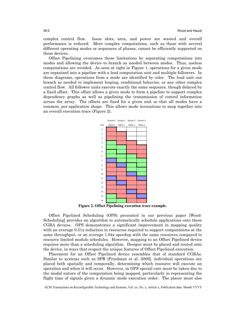
Figure 1. Example modulo schedule (left) and Offset Pipelined schedule (right) for multi-

mode execution.

Offset Pipelining improves the efficiency of CGRA architectures by effectively introducing conditional branching, which is the basis of complex control flow supported by standard microprocessors. Traditional CGRA architectures are generally restricted to implementing an entire computation as a single repeated loop as shown on the left in Figure 1. The architecture time-multiplexes the resources in the device in a fixed schedule, executing a repeating sequence of operations. While arbitrary computations can be supported in this paradigm, it is inefficient for

Time Domain 0 Domain 1 Domain 2 Domain 3

0

1

2

3

4

5

Domain 0 Domain 1 Domain 2 Domain 3

Time Offset 0 Offset 1 Offset 3 Offset 4

0

1

2

0

1

0

?

39:2 Wood and Hauck

ACM Transactions on Reconfigurable Technology and Systems, Vol. xx, No. x, Article x, Publication date: Month YYYY

complex control flow. Issue slots, area, and power are wasted and overall performance is reduced. More complex computations, such as those with several different operating modes or sequences of phases, cannot be efficiently supported on these devices.

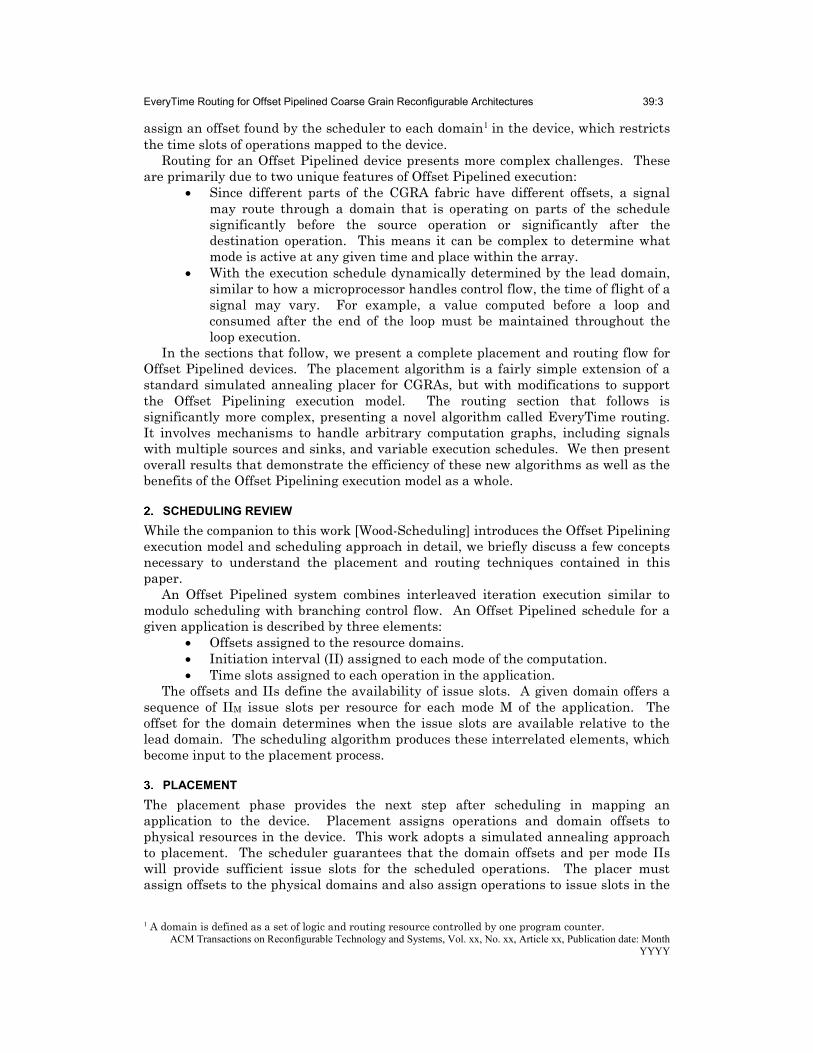
Offset Pipelining overcomes these limitations by separating computations into modes and allowing the device to branch as needed between modes. Thus, useless computations are avoided. As seen at right in Figure 1, operations for a given mode are organized into a pipeline with a lead computation unit and multiple followers. In these diagrams, operations from a mode are identified by color. The lead unit can branch as needed to implement looping, conditional behavior, or any other complex control flow. All follower units execute exactly the same sequence, though delayed by a fixed offset. This offset allows a given mode to form a pipeline to support complex dependency graphs as well as pipelining the transmission of control information across the array. The offsets are fixed for a given unit so that all modes have a common, per-application shape. This allows mode invocations to snap together into an overall execution trace (Figure 2).

Figure 2. Offset Pipelining execution trace example.

Offset Pipelined Scheduling (OPS) presented in our previous paper [Wood-

Scheduling] provides an algorithm to automatically schedule applications onto these CGRA devices. OPS demonstrates a significant improvement in mapping quality with an average 0.51x reduction in resources required to support computations at the same throughput, or an average 1.94x speedup with the same resources compared to resource limited modulo schedules. However, mapping to an Offset Pipelined device requires more than a scheduling algorithm. Designs must be placed and routed onto the device, in ways that respect the unique features of Offset Pipelined execution.

Placement for an Offset Pipelined device resembles that of standard CGRAs. Similar to systems such as SPR [Friedman et al. 2009], individual operations are placed both spatially and temporally, determining which resource will execute an operation and when it will occur. However, in OPS special care must be taken due to the modal nature of the computation being mapped, particularly in representing the flight time of signals given a dynamic mode execution order. The placer must also


Time Offset 0 Offset 1 Offset 3 Offset 4

0

1

2

3

4

5

6

7

8

9

10

11

12

13

14

15

16

EveryTime Routing for Offset Pipelined Coarse Grain Reconfigurable Architectures 39:3

ACM Transactions on Reconfigurable Technology and Systems, Vol. xx, No. xx, Article xx, Publication date: Month YYYY

assign an offset found by the scheduler to each domain1 in the device, which restricts the time slots of operations mapped to the device.

Routing for an Offset Pipelined device presents more complex challenges. These are primarily due to two unique features of Offset Pipelined execution:

Since different parts of the CGRA fabric have different offsets, a signal may route through a domain that is operating on parts of the schedule significantly before the source operation or significantly after the destination operation. This means it can be complex to determine what mode is active at any given time and place within the array.

With the execution schedule dynamically determined by the lead domain, similar to how a microprocessor handles control flow, the time of flight of a signal may vary. For example, a value computed before a loop and consumed after the end of the loop must be maintained throughout the loop execution.

In the sections that follow, we present a complete placement and routing flow for Offset Pipelined devices. The placement algorithm is a fairly simple extension of a standard simulated annealing placer for CGRAs, but with modifications to support the Offset Pipelining execution model. The routing section that follows is significantly more complex, presenting a novel algorithm called EveryTime routing. It involves mechanisms to handle arbitrary computation graphs, including signals with multiple sources and sinks, and variable execution schedules. We then present overall results that demonstrate the efficiency of these new algorithms as well as the benefits of the Offset Pipelining execution model as a whole.

SCHEDULING REVIEW

While the companion to this work [Wood-Scheduling] introduces the Offset Pipelining execution model and scheduling approach in detail, we briefly discuss a few concepts necessary to understand the placement and routing techniques contained in this paper.

An Offset Pipelined system combines interleaved iteration execution similar to modulo scheduling with branching control flow. An Offset Pipelined schedule for a given application is described by three elements:

Offsets assigned to the resource domains. Initiation interval (II) assigned to each mode of the computation. Time slots assigned to each operation in the application.

The offsets and IIs define the availability of issue slots. A given domain offers a sequence of IIM issue slots per resource for each mode M of the application. The offset for the domain determines when the issue slots are available relative to the lead domain. The scheduling algorithm produces these interrelated elements, which become input to the placement process.

PLACEMENT

The placement phase provides the next step after scheduling in mapping an application to the device. Placement assigns operations and domain offsets to physical resources in the device. This work adopts a simulated annealing approach to placement. The scheduler guarantees that the domain offsets and per mode IIs will provide sufficient issue slots for the scheduled operations. The placer must assign offsets to the physical domains and also assign operations to issue slots in the

1 A domain is defined as a set of logic and routing resource controlled by one program counter.

39:4 Wood and Hauck


domains. An initial placement assigns domains and operations randomly while respecting the scheduled time slots. The placer follows the VPR [Betz and Rose 1997] cooling schedule. Different move types and the cost function formulation are the major features of the placement phase unique to Offset Pipelining.

Move Types

The move function is responsible for making changes to the placed design in order to explore the space of possible placements during the annealing process. There are two types of moves made for placement: an operation move and an offset move. The move type is selected proportionally based on the number of movable items in the design. Both of these move types preserve the schedule constraints while exploring possible placements for the scheduled netlist.

3.1.1 Operation Move

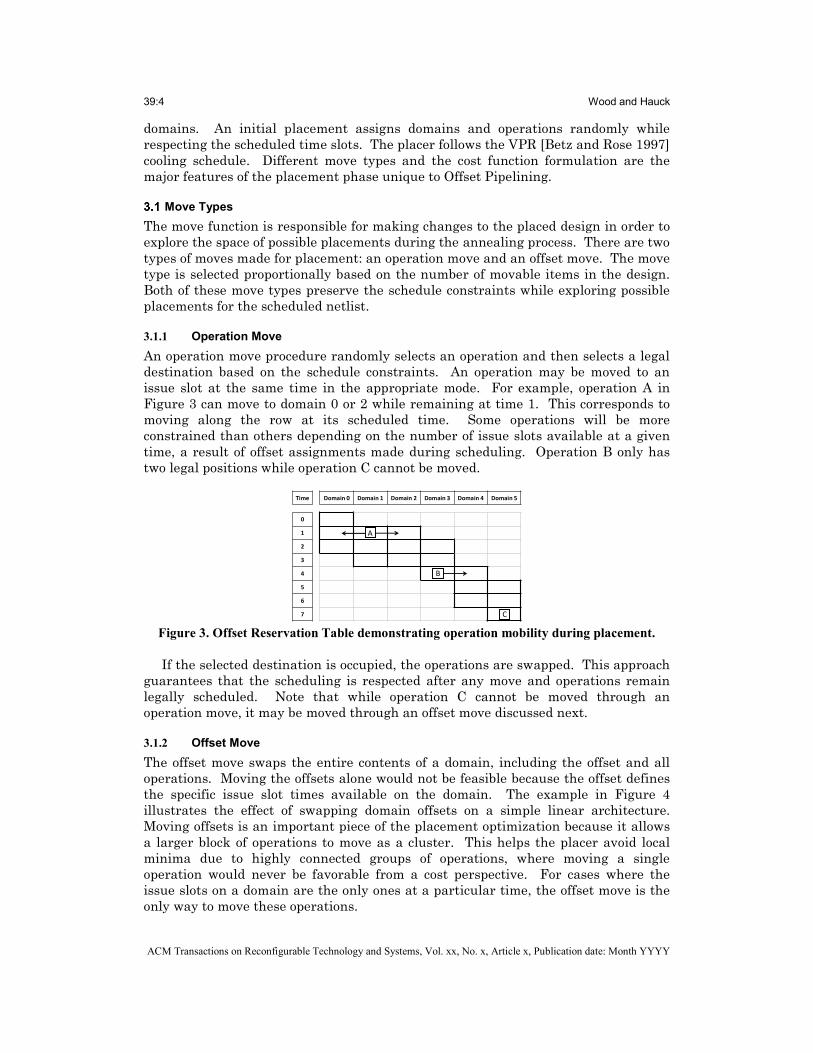
An operation move procedure randomly selects an operation and then selects a legal destination based on the schedule constraints. An operation may be moved to an issue slot at the same time in the appropriate mode. For example, operation A in Figure 3 can move to domain 0 or 2 while remaining at time 1. This corresponds to moving along the row at its scheduled time. Some operations will be more constrained than others depending on the number of issue slots available at a given time, a result of offset assignments made during scheduling. Operation B only has two legal positions while operation C cannot be moved.

Figure 3. Offset Reservation Table demonstrating operation mobility during placement.

If the selected destination is occupied, the operations are swapped. This approach

guarantees that the scheduling is respected after any move and operations remain legally scheduled. Note that while operation C cannot be moved through an operation move, it may be moved through an offset move discussed next.

3.1.2 Offset Move

The offset move swaps the entire contents of a domain, including the offset and all operations. Moving the offsets alone would not be feasible because the offset defines the specific issue slot times available on the domain. The example in Figure 4 illustrates the effect of swapping domain offsets on a simple linear architecture. Moving offsets is an important piece of the placement optimization because it allows a larger block of operations to move as a cluster. This helps the placer avoid local minima due to highly connected groups of operations, where moving a single operation would never be favorable from a cost perspective. For cases where the issue slots on a domain are the only ones at a particular time, the offset move is the only way to move these operations.

Time Domain 0 Domain 1 Domain 2 Domain 3 Domain 4 Domain 5

0

1

2

3

4

5

6

7

B

A

C



Figure 4. Illustration of a domain swap.

Cost Function

The cost function distills the quality of the placement to a value for evaluating the progress of the algorithm. In order for the placement to be viable for routing, it must be possible to route each signal in the application. Dealing with congestion is left to the router, but the placer will not complete successfully until all signals can individually be routed. The cost function aggregates over each source/sink pair the difference between the best case route latency and the required schedule latency, illustrated in Figure 5. When the slack term is positive, the pair of terminals cannot be routed within the required latency, so the cost is multiplied by ten to encourage further annealing improvement. A successful placement minimizes the cost function with no net violating its required latency such that each source and sink pair in the design can be routed. Negative slack terms minimize wire length as a secondary goal, favoring nets shorter than the latency requires.

cost = 0; foreach (source:sink pair) { slack = MinPlacedLatency(source, sink) - ScheduleLatency(source, sink); if (slack > 0) slack *= 10; cost += slack; }

Figure 5. Placement cost function applied to each source/sink pair.

ROUTING FOR OFFSET PIPELINED DEVICES

In the previous section we developed a complete placement approach for Offset Pipelined devices. We now turn to the challenge of routing in these devices. As done for an FPGA, routing must be precomputed with only one signal allowed to use a given resource at a time. However, the new requirements of an Offset Pipelined system introduce complexities that require special handling in the routing algorithm.

To aid in this discussion, we first present two styles of diagrams that will be used to illustrate the challenges of these systems and the algorithmic innovations we have developed to solve them. We then provide an overview of the EveryTime router before going into the full details of the algorithm.

Routing Abstractions

During the placement discussion, we presented tables such as Figure 3 with domains given as columns and timeslots as rows. For routing, we will extend these with a simplified routing structure used to help illustrate points throughout our routing discussion. As shown in Figure 6, we consider a simple one dimensional architecture with single cycle routing available between adjacent domains. Signals that travel longer distances must do so over multiple clock cycles. The real architectures we

Time Domain 0 Domain 1 Domain 2 Domain 3 Domain 4 Domain 5

0

1

2

3

4

5

6

7

39:6 Wood and Hauck


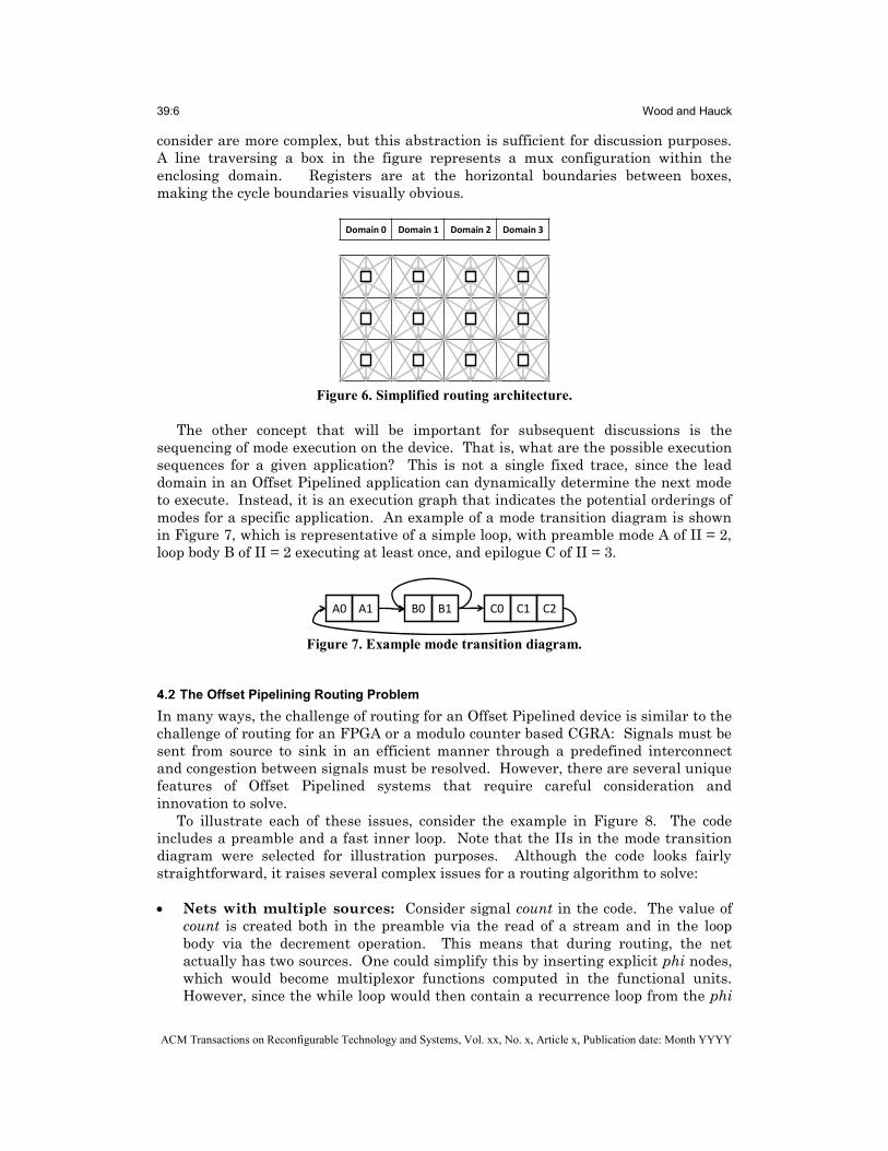
consider are more complex, but this abstraction is sufficient for discussion purposes. A line traversing a box in the figure represents a mux configuration within the enclosing domain. Registers are at the horizontal boundaries between boxes, making the cycle boundaries visually obvious.

Figure 6. Simplified routing architecture.

The other concept that will be important for subsequent discussions is the

sequencing of mode execution on the device. That is, what are the possible execution sequences for a given application? This is not a single fixed trace, since the lead domain in an Offset Pipelined application can dynamically determine the next mode to execute. Instead, it is an execution graph that indicates the potential orderings of modes for a specific application. An example of a mode transition diagram is shown in Figure 7, which is representative of a simple loop, with preamble mode A of II = 2, loop body B of II = 2 executing at least once, and epilogue C of II = 3.

Figure 7. Example mode transition diagram.

The Offset Pipelining Routing Problem

In many ways, the challenge of routing for an Offset Pipelined device is similar to the challenge of routing for an FPGA or a modulo counter based CGRA: Signals must be sent from source to sink in an efficient manner through a predefined interconnect and congestion between signals must be resolved. However, there are several unique features of Offset Pipelined systems that require careful consideration and innovation to solve.

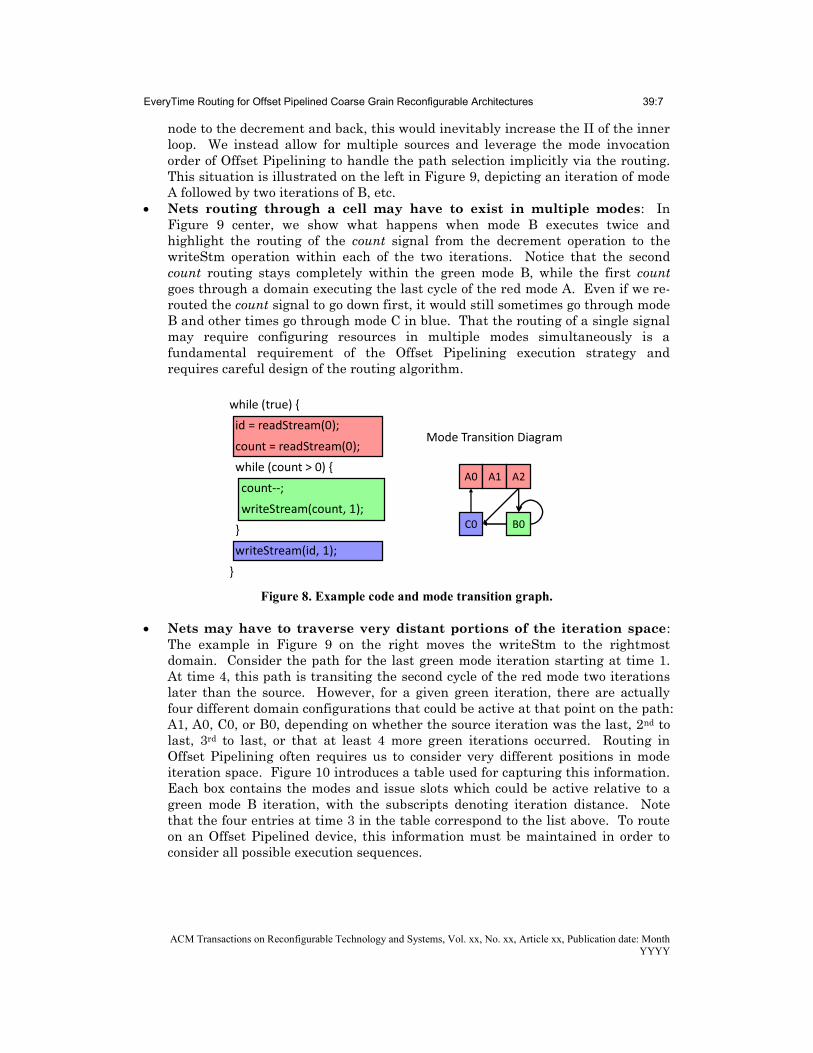
To illustrate each of these issues, consider the example in Figure 8. The code includes a preamble and a fast inner loop. Note that the IIs in the mode transition diagram were selected for illustration purposes. Although the code looks fairly straightforward, it raises several complex issues for a routing algorithm to solve: Nets with multiple sources: Consider signal count in the code. The value of

count is created both in the preamble via the read of a stream and in the loop body via the decrement operation. This means that during routing, the net actually has two sources. One could simplify this by inserting explicit phi nodes, which would become multiplexor functions computed in the functional units. However, since the while loop would then contain a recurrence loop from the phi


A0 B0 C0A1 B1 C1 C2



node to the decrement and back, this would inevitably increase the II of the inner loop. We instead allow for multiple sources and leverage the mode invocation order of Offset Pipelining to handle the path selection implicitly via the routing. This situation is illustrated on the left in Figure 9, depicting an iteration of mode A followed by two iterations of B, etc.

Nets routing through a cell may have to exist in multiple modes: In Figure 9 center, we show what happens when mode B executes twice and highlight the routing of the count signal from the decrement operation to the writeStm operation within each of the two iterations. Notice that the second count routing stays completely within the green mode B, while the first count goes through a domain executing the last cycle of the red mode A. Even if we re-routed the count signal to go down first, it would still sometimes go through mode B and other times go through mode C in blue. That the routing of a single signal may require configuring resources in multiple modes simultaneously is a fundamental requirement of the Offset Pipelining execution strategy and requires careful design of the routing algorithm.

Figure 8. Example code and mode transition graph.

Nets may have to traverse very distant portions of the iteration space:

The example in Figure 9 on the right moves the writeStm to the rightmost domain. Consider the path for the last green mode iteration starting at time 1. At time 4, this path is transiting the second cycle of the red mode two iterations later than the source. However, for a given green iteration, there are actually four different domain configurations that could be active at that point on the path: A1, A0, C0, or B0, depending on whether the source iteration was the last, 2nd to last, 3rd to last, or that at least 4 more green iterations occurred. Routing in Offset Pipelining often requires us to consider very different positions in mode iteration space. Figure 10 introduces a table used for capturing this information. Each box contains the modes and issue slots which could be active relative to a green mode B iteration, with the subscripts denoting iteration distance. Note that the four entries at time 3 in the table correspond to the list above. To route on an Offset Pipelined device, this information must be maintained in order to consider all possible execution sequences.

while (true) {

id = readStream(0);

count = readStream(0);

while (count > 0) {

count--;

writeStream(count, 1);

}

writeStream(id, 1);

}

Mode Transition Diagram

A0

C0

A1

B0

A2

39:8 Wood and Hauck


Figure 9. Execution traces. Net with multiple sources (left). Net traversing resources in

multiple modes (center). Net moving through resources several iterations away from source and sink (right).

Figure 10. Possible active cycles relative to a known mode iteration.

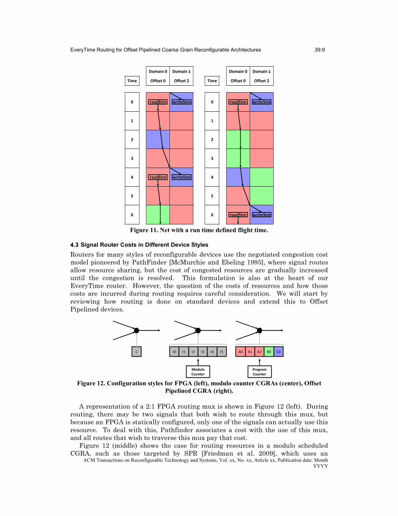
Unknown time of flight: Consider signal id, whose value is read during mode

A and is written in mode C, meaning this signal must be “live” during all, if any, intervening iterations of mode B. However, we would only know the number of B iterations at runtime. Thus, the signal must travel fast enough to get from the read to the write in the case where count is zero and mode B never executes, but must maintain the value during any intervening iterations of B. This situation is illustrated in Figure 11, with count equal to 0 on the left and 2 on the right.

Given these complexities, it is clear that Offset Pipelined routing must manage

constraints which have not been studied previously. By careful application of existing techniques and the introduction of new approaches, we have developed a novel, efficient routing algorithm for these systems which is presented in the following sections.

Domain 0 Domain 1 Domain 2

Time Offset 0 Offset 2 Offset 5

0 count--

1 count--

2 writeStm

3 writeStm

4

5

6 count--



0 count-- writeStm

1 count--

2

3

4

5 writeStm

6 count-- writeStm

Domain 0

Time Offset 0

0

1 readStm

2

3 count--

4 count--

5

6

Time

-3 A0-1 A1-2 A2-3 B0-3

-2 A1-1 A2-2 B0-2

-1 A2-1 B0-1

0 B00

1 B01 C01

2 A02 B02 C02

3 A12 A03 B03 C03

A0

C0

A1

B0

A2



Figure 11. Net with a run time defined flight time.

Signal Router Costs in Different Device Styles

Routers for many styles of reconfigurable devices use the negotiated congestion cost model pioneered by PathFinder [McMurchie and Ebeling 1995], where signal routes allow resource sharing, but the cost of congested resources are gradually increased until the congestion is resolved. This formulation is also at the heart of our EveryTime router. However, the question of the costs of resources and how those costs are incurred during routing requires careful consideration. We will start by reviewing how routing is done on standard devices and extend this to Offset Pipelined devices.

Figure 12. Configuration styles for FPGA (left), modulo counter CGRAs (center), Offset

Pipelined CGRA (right).

A representation of a 2:1 FPGA routing mux is shown in Figure 12 (left). During routing, there may be two signals that both wish to route through this mux, but because an FPGA is statically configured, only one of the signals can actually use this resource. To deal with this, Pathfinder associates a cost with the use of this mux, and all routes that wish to traverse this mux pay that cost.

Figure 12 (middle) shows the case for routing resources in a modulo scheduled CGRA, such as those targeted by SPR [Friedman et al. 2009], which uses an

Domain 0 Domain 1

Time Offset 0 Offset 2

0 readStm writeStm

1

2

3

4 readStm writeStm

5

6

Domain 0 Domain 1


0 readStm writeStm

1

2

3

4

5

6 readStm writeStm

C I0 I1 I2 I3 A0 A1 A2 B0I4 I5 C0

Modulo Counter

Program Counter

39:10 Wood and Hauck


extension of PathFinder. The programming of the mux in this case is actually handled by II different programming bits, each at a different issue slot of the modulo schedule. Now, multiple signals can share the same mux, as long as they do so during different time slots. Thus, if we are attempting to route signals S0, S1, and S2 through this mux and S0 wants to use it at time 0, and S1 and S2 at time 1, only S1 and S2 are conflicting and see an added congestion cost. Consider the routes contending for the programming bits of the mux, rather than for the mux itself. As such, the routing costs are maintained for each issue slot of a mux and signal routes only see the costs for time slots on a mux that they are actually using. This method for negotiation is how SPR handles modulo counter pipelined routing.

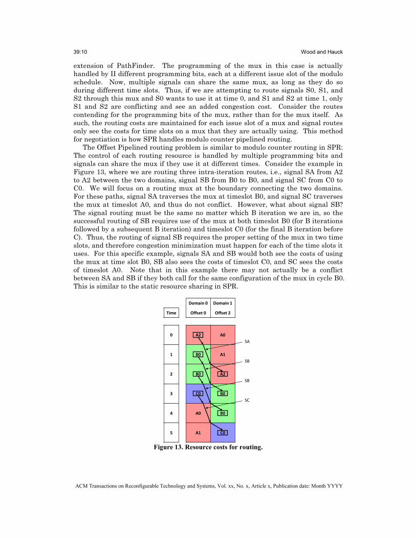
The Offset Pipelined routing problem is similar to modulo counter routing in SPR: The control of each routing resource is handled by multiple programming bits and signals can share the mux if they use it at different times. Consider the example in Figure 13, where we are routing three intra-iteration routes, i.e., signal SA from A2 to A2 between the two domains, signal SB from B0 to B0, and signal SC from C0 to C0. We will focus on a routing mux at the boundary connecting the two domains. For these paths, signal SA traverses the mux at timeslot B0, and signal SC traverses the mux at timeslot A0, and thus do not conflict. However, what about signal SB? The signal routing must be the same no matter which B iteration we are in, so the successful routing of SB requires use of the mux at both timeslot B0 (for B iterations followed by a subsequent B iteration) and timeslot C0 (for the final B iteration before C). Thus, the routing of signal SB requires the proper setting of the mux in two time slots, and therefore congestion minimization must happen for each of the time slots it uses. For this specific example, signals SA and SB would both see the costs of using the mux at time slot B0, SB also sees the costs of timeslot C0, and SC sees the costs of timeslot A0. Note that in this example there may not actually be a conflict between SA and SB if they both call for the same configuration of the mux in cycle B0. This is similar to the static resource sharing in SPR.

Figure 13. Resource costs for routing.

Domain 0 Domain 1


0 A2 A0

1 B0 A1

2 B0 A2

3 C0 B0

4 A0 B0

5 A1 C0

SA

SB

SB

SC



EVERYTIME ROUTER OVERVIEW

The EveryTime approach provides solutions to the aforementioned challenges faced in routing multi-mode Offset Pipelined systems. At a high level, routing a net using the EveryTime concept creates a single path that consumes all resources across every iteration that could be active at each node along the path. This guarantees that the path is complete for all possible run time mode sequences. The single path concept implicitly encapsulates any run time behavior.

The proposed solution is based on two observations. The first is that, even with the multi-mode execution style, each signal is generated at a particular time and location and must arrive at the destination time and location regardless of what may happen along the way. The routing cost for a resource is based on the use at a given issue slot. The cost of a route using a resource is the sum of the costs of all issue slots that could be active at that point on the path.

The second observation is that not all nets have a fixed flight time. The router must be able to reconcile different paths among possible execution sequences. EveryTime routing takes advantage of register file resources to synchronize these paths. By breaking these signals into fixed delay paths from source to a register file and from the register file to the sink, the variable delay portion of the path is confined to the register file.

There are several advantages of the EveryTime approach. The core routing is straightforward with no complex multi-path handling. It can handle arbitrary mode transition diagrams and uses negotiated congestion to resolve resource contention. The use of register files to handle variable signal flight time maintains the single path nature of the routing.

By limiting the router to a single physical path, possibly better solutions may be overlooked that involve merging different, independent paths rather than the unified EveryTime path. There may then be a channel width penalty for the EveryTime approach; however, the benefit of avoiding merge and synchronization issues favors a simplified routing approach to multi-mode routing. In the evaluation we will also demonstrate that any such overhead is small in practice.

EVERYTIME TABLES

The central issue in routing in an Offset Pipelined system is tracking the active mode and iteration at a given time and place. This section introduces the concept of the EveryTime table that is used to determine which modes and times are active at a given distance from the source and/or sink while routing. These tables are calculated based on the scheduled and placed application, since they are dependent on the mode IIs and domain offset assignments. During routing, these tables are constant and provide reference for the active set of modes and times. EveryTime tables represent the iteration space relative to a particular mode iteration, allowing the router to track the set of possible active resources anywhere and anytime on the device relative to an anchor point. An anchor point is usually the mode containing the source of the net, though in cases where the signal flight time is not fixed, the sink serves as a second anchor.

Dealing with Iteration Space

Routing on a modulo scheduled architecture requires tracking use of physical resources for each time slot in the schedule, effectively unrolling the architecture graph in time to represent the available resources. Adding the dimension of independent modes means that physical resources must be tracked by mode as well



as time within each mode. The router must understand how to traverse the possible mode transitions and track the utilization of a resource in multiple modes and times simultaneously.

For modulo scheduling, the next cycle is always known through an increment and modulo operation. In an Offset Pipelined system, moving forward or backward in time relative to a known point can lead to one of multiple possible modes and times in different iterations as illustrated in Figure 10. In the most basic case, within a domain, moving forward in time one cycle has two possibilities: either the next cycle is still within the II cycles of the current iteration or the next cycle is in a new iteration. The new iteration can be found through traversal of the mode transition diagram. Consider an iteration of mode B in the example shown in Figure 14 on the left. We place the iteration of mode B at time 0 and then construct new entries by examining the mode transition diagram. At time 2, a new iteration of either mode B or mode C begins, as shown in the table. By time 4, there are three possibilities: a second iteration of mode B, an iteration of C following the iteration of B, or the last cycle of an iteration of C that immediately followed the initial mode B iteration that anchors the table. When we move between domains (Figure 14 right) we must shift the entries in the table by the difference in offsets between the two domains.

Entries in the table represent possible mode/times that would be active at run time. A letter denotes the mode and a number the cycle of the associated mode iteration from the mode transition diagram. This table captures all possible run time mode execution sequences and provides some intuition about the cost of using a resource for routing a net. Subscripts track the iteration offset relative to the anchor iteration with subscript 0.

Figure 14. EveryTime table for mode B (left). EveryTime tables set to different offsets

(right). Mode transition diagram for the EveryTime tables (bottom). We can see that moving further away from the anchor increases the uncertainty of

determining which mode and iteration is executing. From a routing cost perspective, moving away from the anchor generally becomes increasingly costly corresponding to



-3 A1-2 B1-2 C2-2 A0-2 B0-2 C1-2 A0-3 B0-3 B1-3 C1-3

-2 A0-1 B0-1 A1-2 B1-2 C2-2 A1-3 B1-3 C0-2 C2-3

-1 A1-1 B1-1 A0-1 B0-1 A0-2 B0-2 C1-2

0 B00 A1-1 B1-1 A1-2 B1-2 C2-2

1 B10 B00 A0-1 B0-1

2 B01 C01 B10 A1-1 B1-1

3 B11 C11 B01 C01 B00

4 B02 C02 C21 B11 C11 B10

5 A02 B12 C12 B02 C02 C21 B01 C01

6 A12 B03 C03 C22 A02 B12 C12 B11 C11

A0 B0 C0A1 B1 C1 C2

Time

-3 A1-2 B1-2 C2-2

-2 A0-1 B0-1

-1 A1-1 B1-1

0 B00

1 B10

2 B01 C01

3 B11 C11

4 B02 C02 C21

5 A02 B12 C12

6 A12 B03 C03 C22



this run time uncertainty. The router will try to avoid large sets of active modes and times, but can handle it when needed.

Fused Source and Destination Relative Timing

While many nets in a design will remain within a single iteration, nets also connect different iterations and modes in order to move data. In this case, two EveryTime tables, one associated with the source and the other with the sink can be combined to prune the space of active mode/time combinations required to connect source and sink. This will be explored further in later sections, but the high level idea is to intersect a source relative table and a sink relative table with the appropriate shift in time to provide the set of mode/times that will complete the path under any runtime scenario. Note that for an intra-iteration net, the EveryTime table for the source and sink is the same, so no further pruning would be possible.

Reachability

The EveryTime tables can also be pruned through analysis of modes that can be legally reached from the source enroute to the sink. The basic idea is that the router should not visit resources that cannot be active with the given source and sink pair. This is a more detailed analysis compared to simply applying an EveryTime table to determine the active set.

An example of this situation concerns a variable that is updated in a loop (such as in mode B in Figure 14) and the last version of the value is required for an operation in mode C. It is important that the correct value be passed to C, which can be handled during routing by not allowing the path to traverse resources in a subsequent iteration of B. A second example can be found in Figure 15. A net with a source in A1 and a sink in the immediately following iteration at B0 would never traverse the alternate iteration of mode C following A. These entries would be pruned from the EveryTime table when routing this net.

Figure 15. Mode transition graph with variable distance between modes A and D.

LOCKED NETS

We consider nets with a constant flight time to be “time locked,” having a flight time independent of the run time mode execution sequence. The following examples demonstrate EveryTime routing using EveryTime tables to account for the possible execution sequences that may arise at run time.

Nets With No Iteration Delay

A net whose source and sink are contained within one iteration is the most basic case. Imagine a net in Figure 14 (right) has a source in B00 of the left domain and a sink in B10 on the right domain. As the router explores the available resources at a given distance from the source, the modes and times these resources will be active can be found in the table. Ignoring congestion for the moment, in order to use the minimum number of resources to route this net, it is clearly desirable to remain within the active iteration if possible, otherwise the net will exist in other iterations

A0B1

D0C1

A1B0

C0D1

C2



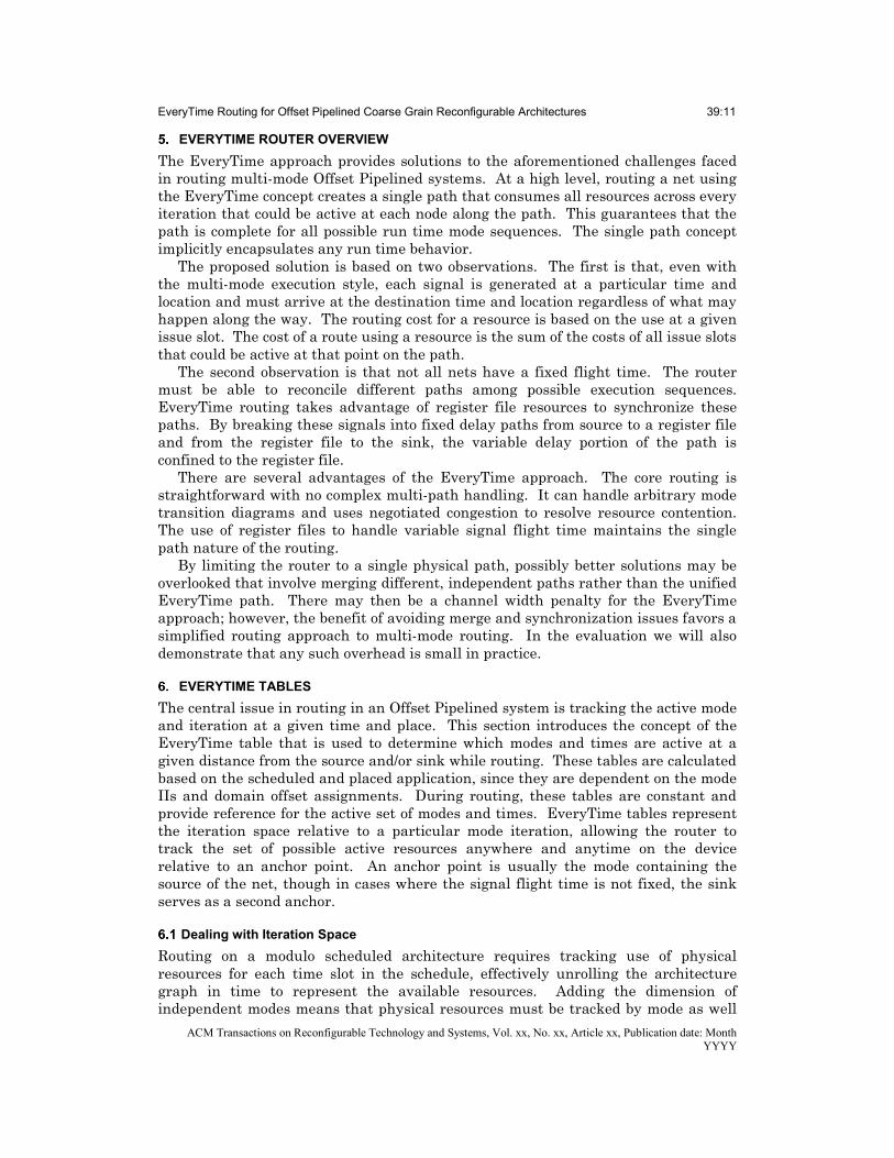
at some point along the path. However, this isn’t always possible for two reasons. An intervening offset, such as domain 1 in the example, may have a much larger or smaller offset. This would lead to the table for the domain being shifted up or down such that, in order to traverse that domain, there would necessarily be several active modes and times. The second issue faced in routing is simply congestion; the net may have to find an alternate route, possibly through less desirable resources that have additional mode/times active.

Figure 16. Source and sink relative routing tables for a net from mode B to mode C.

Iteration Delayed Net

An iteration delayed net differs from the intra-iteration net in that the source and sink use different tables anchored by their respective modes. Figure 16 shows an example of the source relative table on the left for B10 on domain 1 and the sink relative table on the right for mode C01 on domain 2. Note that the sink has a subscript of 1 representing the iteration delay relative to the source. What is unique about an iteration delayed net is that these two tables can be intersected to prune some of the active mode/times for routing. This helps to ignore resources that are not necessary for a given scenario, thereby avoiding overpaying for the path and without repeated calculation of the active set of mode/times.

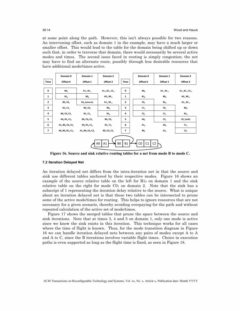
Figure 17 shows the merged tables that prune the space between the source and sink iterations. Note that at times 3, 4 and 5 on domain 1, only one mode is active since we know the sink exists in this iteration. This technique works for all cases where the time of flight is known. Thus, for the mode transition diagram in Figure 16 we can handle iteration delayed nets between any pairs of modes except A to A and A to C, since the B iterations involves variable flight times. Choice in execution paths is even supported as long as the flight time is fixed, as seen in Figure 18.



0 B00 A1-1 B1-1 A1-2 B1-2 C2-2

1 B10 B00 A0-1 B0-1

2 B01 C01 B10 (source) A1-1 B1-1

3 B11 C11 B01 C01 B00

4 B02 C02 C21 B11 C11 B10

5 A02 B12 C12 B02 C02 C21 B01 C01

6 A12 B03 C03 C22 A02 B12 C12 B11 C11

7 A03 B03 B13 C13 A12 B03 C03 C22 B02 C02 C21



0 B00 A1-1 B1-1 A1-2 B1-2 C2-2

1 B10 B00 A0-1 B0-1

2 C01 B10 A1-1 B1-1

3 C11 C01 B00

4 C21 C11 B10

5 A02 C21 C01 (sink)

6 A12 A02 C11

7 B03 A12 C21

A0 B0 C0A1 B1 C1 C2



Figure 17. Merged routing table.

UNLOCKED NETS

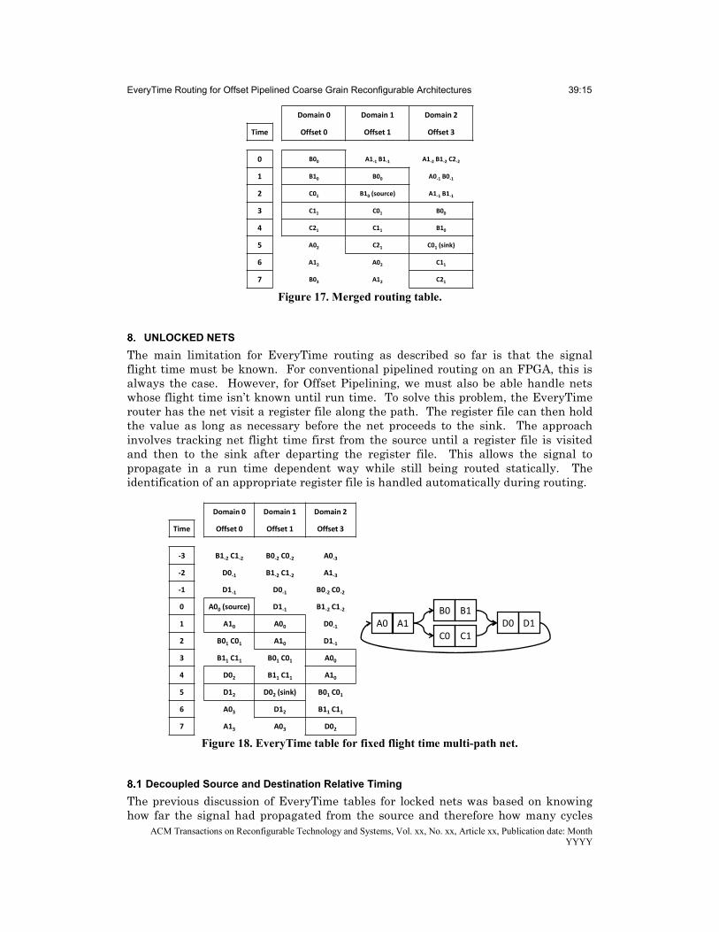
The main limitation for EveryTime routing as described so far is that the signal flight time must be known. For conventional pipelined routing on an FPGA, this is always the case. However, for Offset Pipelining, we must also be able handle nets whose flight time isn’t known until run time. To solve this problem, the EveryTime router has the net visit a register file along the path. The register file can then hold the value as long as necessary before the net proceeds to the sink. The approach involves tracking net flight time first from the source until a register file is visited and then to the sink after departing the register file. This allows the signal to propagate in a run time dependent way while still being routed statically. The identification of an appropriate register file is handled automatically during routing.

Figure 18. EveryTime table for fixed flight time multi-path net.

Decoupled Source and Destination Relative Timing

The previous discussion of EveryTime tables for locked nets was based on knowing how far the signal had propagated from the source and therefore how many cycles



0 B00 A1-1 B1-1 A1-2 B1-2 C2-2

1 B10 B00 A0-1 B0-1

2 C01 B10 (source) A1-1 B1-1

3 C11 C01 B00

4 C21 C11 B10

5 A02 C21 C01 (sink)

6 A12 A02 C11

7 B03 A12 C21



-3 B1-2 C1-2 B0-2 C0-2 A0-3

-2 D0-1 B1-2 C1-2 A1-3

-1 D1-1 D0-1 B0-2 C0-2

0 A00 (source) D1-1 B1-2 C1-2

1 A10 A00 D0-1

2 B01 C01 A10 D1-1

3 B11 C11 B01 C01 A00

4 D02 B11 C11 A10

5 D12 D02 (sink) B01 C01

6 A03 D12 B11 C11

7 A13 A03 D02

A0B1

D0C1

A1B0

C0D1



were left before it would reach the sink. For a net that does not have a fixed flight time, this is not possible. The problem of guaranteeing a register file along the path that can hold the unlocked net value is solved using a series of steps. All routing from the source to the register file is source-relative, meaning that the set of possible executing modes and times is computed relative to the source mode. All routing from the register file to the sink is sink-relative, where we compute the set of possible executing modes and times with an EveryTime table anchored to the sink mode. In this way we essentially convert the time unlocked route into two time locked signals stitched together via a register file. Note that the register file used is dynamically determined via a phased search concept adapted from PipeRoute [Sharma et al. 2003].

Although the exact time allowed to send the signal from source to sink is unknown, since there are many possible run time execution sequences, we can use the mode transition diagram to find the minimum such delay. Thus, the path must travel from source to register file and register file to sink within the minimum delay. In this way, the communication will complete no matter which mode sequence executes at run time.

Figure 19 illustrates the scenario for an unlocked net routing from A10 in domain 0 to C02 in domain 1. The left table is anchored to the source while the right is anchored to the sink. In the diagram, the tables are placed relative to each other based upon the shortest flight time (a single B iteration), but a route must support a dynamically determined number of B mode iterations.

Figure 19. Unlocked net routed with a register file.

The PipeRoute phased search is adapted in the EveryTime router to guarantee a

register file waypoint for unlocked nets. Routing begins in the first phase using a source relative EveryTime table. Upon visiting a register file, the search begins a second phase switching to a sink relative EveryTime table to find the destination.



-1 C2-1 C1-1 B1-2

0 A00 C2-1 C0-1

1 A10 (source) A00 C1-1

2 B01 A10 C2-1

3 B11 B01 A00

4 B02 C02 B11 A10

5 B12 C12 B02 C02 B01

6 B03 C03 C22 B12 C12 B11

7 A03 B13 C13 B03 C03 C22 B02 C02

8 A13 B04 C04 C23 A03 B13 C13 B12 C12

9 A04 B04 B14 C14 A13 B04 C04 C23 B03 C03 C22



-5 A1-3 B1-3 C2-3 A0-3 B0-3 C1-3 A0-4 B0-4 B1-4 C1-4

-4 A0-2 B0-2 A1-3 B1-3 C2-3 A1-4 B1-4 C0-3 C2-4

-3 A1-2 B1-2 A0-2 B0-2 A0-3 B0-3 C1-3

-2 B0-1 A1-2 B1-2 A1-3 B1-3 C2-3

-1 B1-1 B0-1 A0-2 B0-2

0 C02 B1-1 A1-2 B1-2

1 C12 C02 (sink) B0-1

2 C22 C12 B1-1

3 A03 C22 C02

4 A13 A03 C12

5 B04 A13 C22

A0 B0 C0A1 B1 C1 C2



The lowest cost route to the destination implicitly selects a register file along the way by requiring the second phase search to discover the sink.

Architecture Considerations

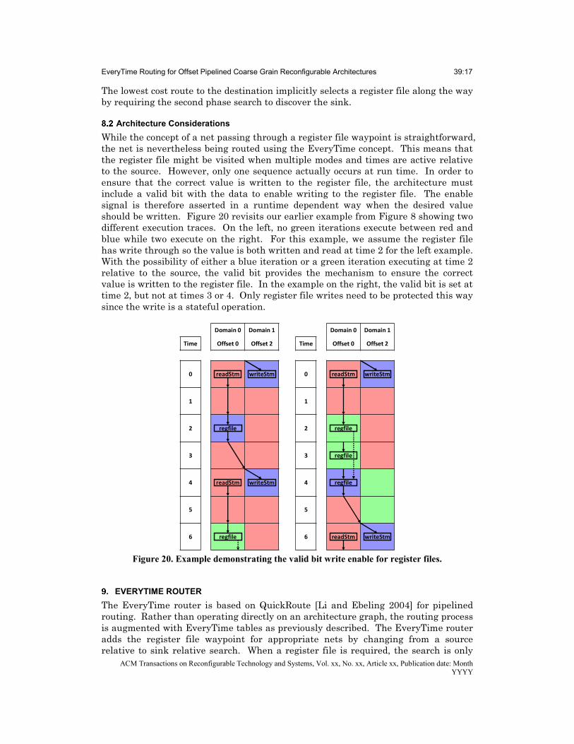
While the concept of a net passing through a register file waypoint is straightforward, the net is nevertheless being routed using the EveryTime concept. This means that the register file might be visited when multiple modes and times are active relative to the source. However, only one sequence actually occurs at run time. In order to ensure that the correct value is written to the register file, the architecture must include a valid bit with the data to enable writing to the register file. The enable signal is therefore asserted in a runtime dependent way when the desired value should be written. Figure 20 revisits our earlier example from Figure 8 showing two different execution traces. On the left, no green iterations execute between red and blue while two execute on the right. For this example, we assume the register file has write through so the value is both written and read at time 2 for the left example. With the possibility of either a blue iteration or a green iteration executing at time 2 relative to the source, the valid bit provides the mechanism to ensure the correct value is written to the register file. In the example on the right, the valid bit is set at time 2, but not at times 3 or 4. Only register file writes need to be protected this way since the write is a stateful operation.

Figure 20. Example demonstrating the valid bit write enable for register files.

EVERYTIME ROUTER

The EveryTime router is based on QuickRoute [Li and Ebeling 2004] for pipelined routing. Rather than operating directly on an architecture graph, the routing process is augmented with EveryTime tables as previously described. The EveryTime router adds the register file waypoint for appropriate nets by changing from a source relative to sink relative search. When a register file is required, the search is only

Domain 0 Domain 1


0 readStm writeStm

1

2 regfile

3

4 readStm writeStm

5

6 regfile

Domain 0 Domain 1


0 readStm writeStm

1

2 regfile

3 regfile

4 regfile

5

6 readStm writeStm



allowed to successfully reach the sink during the sink relative phase, ensuring a register file is visited.

The PathFinder cost metrics rely purely on the available time slots provided by each mode. This is akin to the SPR unrolled datapath graph that represents the time slots available for each physical resource in the device. These data structures provide convenient accounting of the PathFinder metrics, but are not used directly for routing. They are instead populated based on the EveryTime table data for a given path. From a cost perspective, a path must pay for the use of all the mode/times that are active along the path. For example, if a resource is used where six different mode/times are possible, the cost of this resource is the sum of the costs of each of the six mode/time possibilities. This will encourage routes to use paths that are less uncertain, but allow paths to use whatever resources are necessary to achieve the required signal connectivity.

EveryTime Expansion

The EveryTime tables are pre-calculated based on mode IIs and assigned offsets. Preparing to route a given net involves aligning and merging tables if the net is locked. In order to expand a node in the architecture during routing, the domains of the wires in question are used to index into the EveryTime table to determine the active mode/times at the given distance from the source or sink. The tables allow movement among domains and through time relative to the source and/or sink. There is no need to traverse the mode transition diagram to calculate when the signal exists.

RESOLVING CONGESTION

PathFinder [McMurchie and Ebeling 1995] provides the mechanism to resolve congestion. A given net consumes whatever mode/times are part of the active set for each node in the path. PathFinder evaluates the mode/time occupancy information to address present and history sharing costs.

While conventional routing algorithms support nets with a single source but multiple sinks, offset pipelined netlists also involve nets with multiple sources in certain situations. For example, in Figure 9 left, the signal is initialized in one mode and updated in another, and therefore has two possible sources. This is reasonable since the dynamic execution pattern will determine which source actually generated a given signal at run time.

Our EveryTime router handles this by decomposing all nets into two-terminal source-sink pairs, which are routed independently. However, we must now resolve the merging of the two sources: Once an iteration of a loop begins, the two sources of the loop index must enter this loop body mapping at the same point. We use PathFinder to negotiate this shared join point by tracking the configuration of muxes in the architecture. The separate source-sink routes of the signal are routed independently and can share resources between the paths freely since they represent the same signal, but an incompatible mux configuration between the two paths is penalized. Thus, if the two routes join at the entrance point to the loop body, there is no penalty, but any other join is penalized and negotiated by PathFinder. Our EveryTime router creates an implicit phi node to join the paths, created as a side-effect of which mode precedes the loop body iteration in the run time execution.



ROUTING CONSTANTS

Routing constants calls for another type of router. In this case, a sink is known but no source is assigned. Here we perform a reverse best first search from the sink using EveryTime expansion following the same cost metrics as QuickRoute to find an available register file read port. PathFinder’s present and history sharing values also apply to these paths and ensure they are negotiated on the same footing as all other nets.

FEEDBACK TO SCHEDULING OR PLACEMENT

The prototype tool chain does not include feedback to scheduling and placement from the router. In order to evaluate routing performance, the architecture channel width is swept to determine the minimum channel width necessary to route designs. This stresses the performance of the router in order to focus on evaluation rather than meeting constraints of a specific target architecture.

For use with a fixed architecture, a practical tool chain would include feedback to the scheduler and placer to loosen constraints in these phases to provide enough flexibility to complete routing. One possibility would be to annotate nets that remain in a conflicted state after a certain number of PathFinder iterations. These nets could be assigned additional slack in scheduling to stretch out the overall schedule to make it easier for placement and routing to find a solution.

A second alternative would include analysis of channel utilization which the placer could use to search for a better resource arrangement in advance of routing. These metrics might be used in a more sophisticated manner for partitioning to further guide scheduling and placement in order to map applications to specific architectures with fixed routing resources.

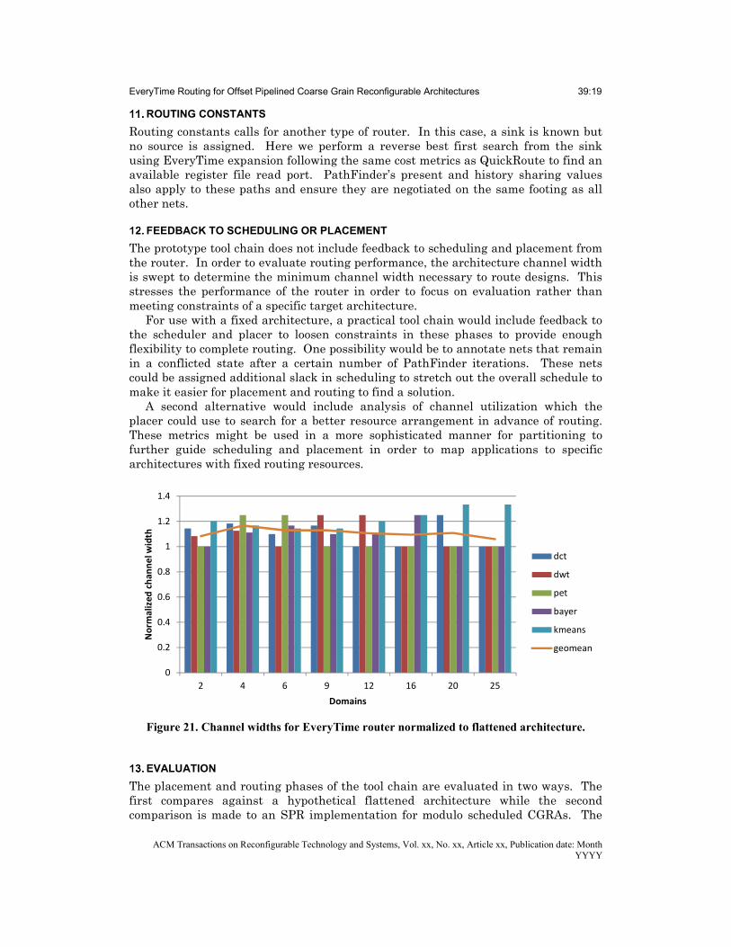
Figure 21. Channel widths for EveryTime router normalized to flattened architecture.

EVALUATION

The placement and routing phases of the tool chain are evaluated in two ways. The first compares against a hypothetical flattened architecture while the second comparison is made to an SPR implementation for modulo scheduled CGRAs. The

0

0.2

0.4

0.6

0.8

1

1.2

1.4

2 4 6 9 12 16 20 25

Nor

mal

ized

cha

nnel

wid

th

Domains

dct

dwt

pet

bayer

kmeans

geomean



target architecture is based on work that explored resource composition for modulo scheduled CGRAs [Van Essen 2010].

The first architecture is “flattened” to provide a likely unachievable theoretical lower bound modeling the best possible implementation that might be attained by the Offset Pipelined placer and router. Our goal is to apply existing techniques to this flattened architecture and measure the relative algorithm efficiency via the resulting channel widths. We transform the Offset Pipelined placement and routing problem into a more standard pipelined FPGA routing problem that will have similar or relaxed constraints. We remove mode transitions and instead have only a single configuration where every domain has logic resources equal to the Offset Pipelined resources multiplied by the total schedule length. Thus, if in the Offset Pipelined case we have two modes with IIs of 2 and 3, the flattened architecture has 5 times as many logic resources per domain than the Offset Pipelined device. Signals are pipelined so that if the minimum flight time in the schedule is N, the signal must go through exactly N registers in the flattened architecture. In this way, the two architectures have the same scheduling, placement and essentially the same routing constraints, but the additional complexity of mode transitions and issue slot windows have been eliminated. The router for the flattened architecture is a QuickRoute [Li and Ebeling 2004] implementation for pipelined routing.

The flattened architecture comparison normalizes channel width to the best result we could expect if signals were evenly distributed among the cycles of the Offset Pipelined version. The channel width attained by a flattened implementation is divided by the total schedule length of the corresponding Offset Pipelined implementation and rounded up to produce this lower bound.

The channel width results in Figure 21 show that the Offset Pipelined tool chain achieves mappings with channel widths with approximately a 10% overhead compared to a flattened architecture using QuickRoute, demonstrating that our algorithm is quite close in efficiency to the existing router even though it must deal with a more complex problem. Note that this overhead corresponds to an average of 0.63 of a channel across our benchmark suite for the Offset Pipelined device, which is a minor penalty.

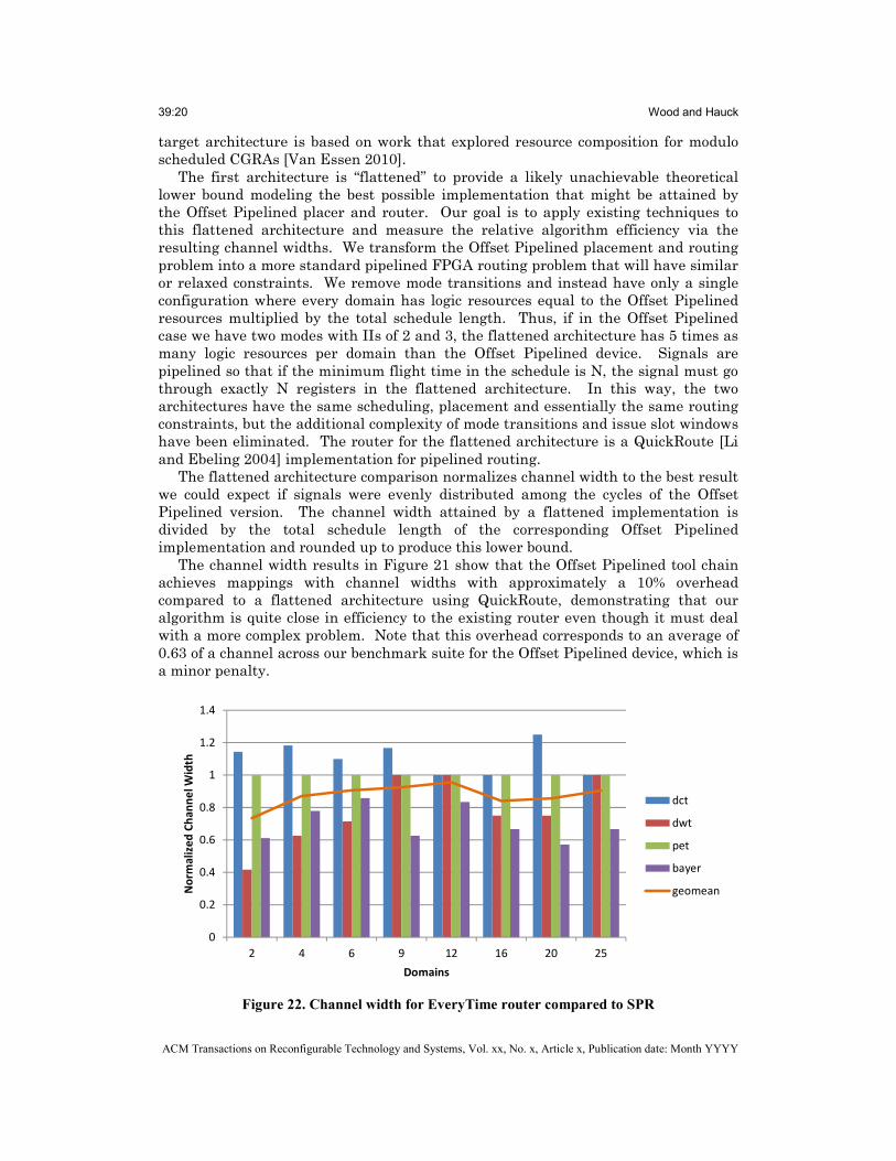
Figure 22. Channel width for EveryTime router compared to SPR

0

0.2

0.4

0.6

0.8

1

1.2

1.4

2 4 6 9 12 16 20 25

Nor

mal

ized

Cha

nnel

Wid

th

Domains

dct

dwt

pet

bayer

geomean



Our second comparison is to an SPR implementation. While the FPGA-like

baseline is a useful tool to evaluate the channel width requirements of the EveryTime router, SPR is a more closely related CGRA tool taking advantage of modulo scheduling and time multiplexed resources. Results for this second comparison are shown in Figure 22 comparing Offset Pipelining to SPR. In SPR we are restricted to the single modulo counter based implementation of existing systems, while the EveryTime router makes use the Offset Pipelining execution style.

As seen in the graph, the channel width requirements are heavily influenced by the application. For applications like the discrete wavelet transform with many modes, the EveryTime router requires fewer channels by allowing resources to be more effectively shared in time. The DCT on the other hand with only two modes uses slightly more channels. Overall, EveryTime routing of the Offset Pipelined implementations uses 0.87x the channels of SPR.

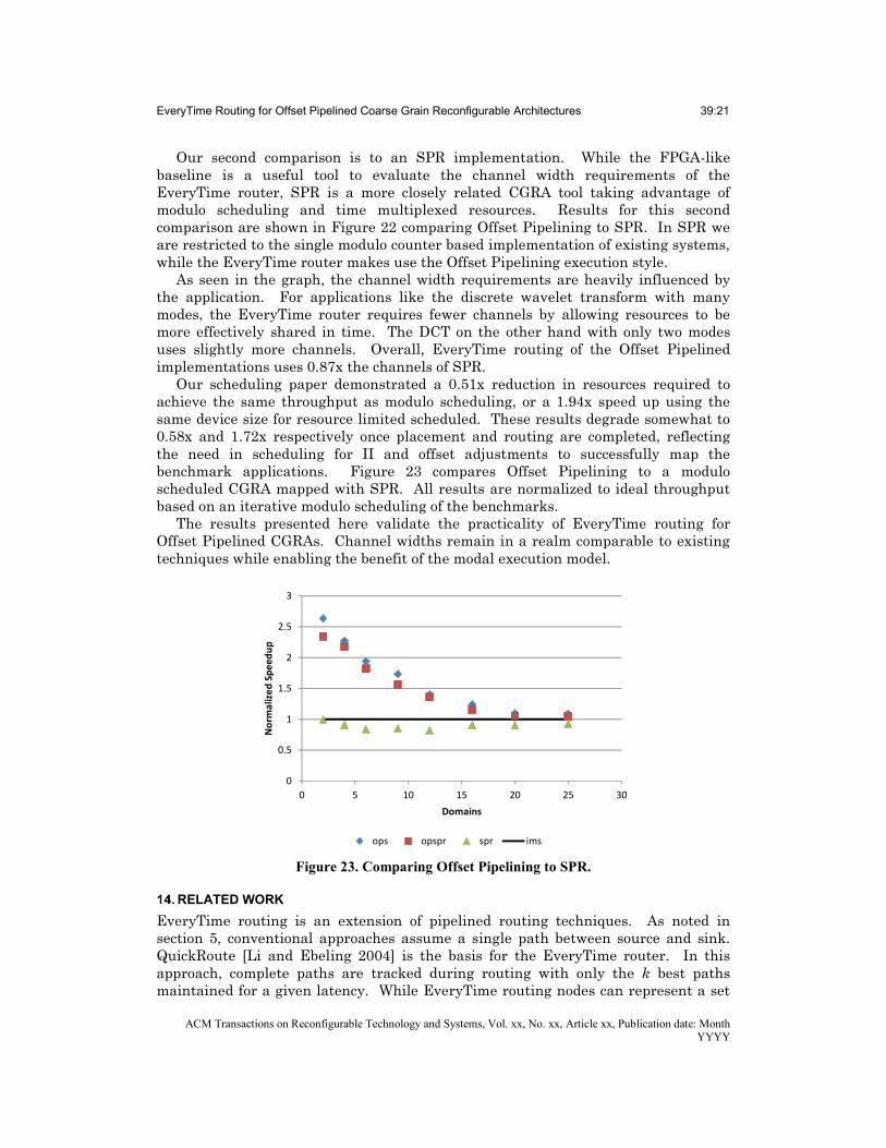
Our scheduling paper demonstrated a 0.51x reduction in resources required to achieve the same throughput as modulo scheduling, or a 1.94x speed up using the same device size for resource limited scheduled. These results degrade somewhat to 0.58x and 1.72x respectively once placement and routing are completed, reflecting the need in scheduling for II and offset adjustments to successfully map the benchmark applications. Figure 23 compares Offset Pipelining to a modulo scheduled CGRA mapped with SPR. All results are normalized to ideal throughput based on an iterative modulo scheduling of the benchmarks.

The results presented here validate the practicality of EveryTime routing for Offset Pipelined CGRAs. Channel widths remain in a realm comparable to existing techniques while enabling the benefit of the modal execution model.

Figure 23. Comparing Offset Pipelining to SPR.

RELATED WORK

EveryTime routing is an extension of pipelined routing techniques. As noted in section 5, conventional approaches assume a single path between source and sink. QuickRoute [Li and Ebeling 2004] is the basis for the EveryTime router. In this approach, complete paths are tracked during routing with only the k best paths maintained for a given latency. While EveryTime routing nodes can represent a set

0

0.5

1

1.5

2

2.5

3

0 5 10 15 20 25 30

Nor

mal

ized

Spe

edup

Domains

ops opspr spr ims



of modes and times while traversing an EveryTime table, a single mode application reduces the scope of the routing problem to a normal QuickRoute implementation.

The PathFinder [McMurchie and Ebeling 1995] router introduced the negotiated congestion concept for global routing. EveryTime routing adapts this approach by negotiating occupancy of resource mode/time tuples. This approach decouples the EveryTime table information used to route a signal from the individual mode/time tuples consumed by a path providing a clean mechanism for negotiation.

CONCLUSIONS

We have presented placement and routing methods to develop a viable tool chain for Offset Pipelined systems. The EveryTime router provides a means to support the multi-mode execution style presented in [Wood-Scheduling]. An evaluation of the router channel width performance indicates that it does not require more than 10% more resources than the expected lower bound and is likewise competitive with a comparable tool chain for CGRA mapping. The overall tool chain provides an average 0.58x reduction in resources required to support computations at the same throughput, or an average 1.72x speed up with the same resources compared to resource limited modulo schedules mapped with SPR.

This paper demonstrates that a practical tool chain can support Offset Pipelining on CGRA devices yielding improved throughput or reduced resource utilization over modulo scheduled architectures. The increased flexibility for CGRA devices through Offset Pipelining strikes a balance between the flexibility of general purpose processors and the parallelism of conventional CGRA and FPGA architectures.

REFERENCES

Vaughn Betz and Jonathan Rose. 1997. VPR: A New Packing, Placement and Routing Tool for FPGA Research. In International Workshop on Field-Programmable Logic and Applications, Springer Berlin Heidelberg, 213-222.

Stephen Friedman, Allan Carroll, Brian Van Essen, Benjamin Ylvisaker, Carl Ebeling, and Scott Hauck. 2009. SPR: An Architecture-Adaptive CGRA Mapping Tool. In Proceedings of the ACM/SIGDA International Symposium on Field Programmable Gate Arrays, ACM, 191-200.

Song Li and Carl Ebeling. 2004. QuickRoute: A Fast Routing Algorithm for Pipelined Architectures. In IEEE International Conference on Field-Programmable Technology, IEEE, 73-80.

Larry McMurchie and Carl Ebeling. 1995. PathFinder: A Negotiation-Based Performance-Driven Router for FPGAs. In Proceedings of the 1995 ACM third international symposium on Field-programmable gate arrays, ACM, 111–117.

Akshay Sharma, Carl Ebeling, and Scott Hauck. 2003. PipeRoute: A Pipelining-Aware Router for FPGAs. In Proceedings of the 2003 ACM/SIGDA eleventh international symposium on Field programmable gate arrays, ACM, 68-77.

Brian Van Essen. 2010. Improving the Energy Efficiency of Coarse-Grained Reconfigurable Arrays. Ph.D. Thesis, University of Washington, Dept. of CSE.

Aaron Wood and Scott Hauck. Offset Pipelined Scheduling for Coarse Grain Reconfigurable Architectures. Submitted to ACM Transactions on Reconfigurable Technology and Systems.

everytime routing for offset pipelined coarse grain

Documents