THÈSEPour obtenir le grade de

DOCTEUR DE LA COMMUNAUTÉUNIVERSITÉ GRENOBLE ALPESSpécialité : Informatique

Arrêté ministériel : 25 mai 2016

Présentée par

Camille Bernard

Thèse dirigée par M. Jérôme Genselcodirigée par M. Hy Daoet co-encadrée par Mme Marlène Villanova-Oliver

préparée au sein du Laboratoire d’Informatique de Grenobleet de l’École Doctorale Mathématiques, Sciences et Technologies del’Information, Informatique

Immersing evolving geographic divisionsin the semantic WebTowards spatiotemporal knowledge graphsto reflect territorial dynamics over time

Thèse soutenue publiquement le 27 novembre 2019,devant le jury composé de :

Mme Sihem Amer-YahiaDirectrice de recherche CNRS Délégation Alpes, LIG, Université Grenoble Alpes,PrésidenteMme Nathalie Aussenac-GillesDirectrice de Recherche CNRS Délégation Occitanie Ouest, IRIT, Université deToulouse, RapporteurM. Christophe ClaramuntProfesseur des Universités, Institut de Recherche de l’Ecole navale, RapporteurMme Thérèse LibourelProfesseur émérite, Université de Montpellier, ExaminatriceM. Christophe CruzMaître de Conférences HDR, Université Bourgogne Franche-Comté,ExaminateurMme Marlène Villanova-OliverMaître de Conférences HDR, Université Grenoble Alpes, Co-Encadrante de thèseM. Jérôme GenselProfesseur des Universités, Université Grenoble Alpes, Directeur de thèseM. Hy DaoProfesseur titulaire, Université de Genève, Co-Directeur de thèse

ii

La Géographie n’est autre chose que l’Histoire dans l’Espace, demême que l’Histoire est la Géographie dans le Temps.

L’Homme et la Terre – Élisée Reclus

Remerciements

Au cours de cette thèse, il y a eu bien des événements et des changements,comme certainement au cours de toutes les thèses d’ailleurs. Une période courteoù tant de choses se bousculent, où les doctorants eux-mêmes sont amenés à tantchanger, à voyager, faire des rencontres, franchir des obstacles tout en ne perdantpas de vue l’objectif "majeur", rendre un manuscrit et avoir par celui-ci contribué(au moins un tout petit peu) à sa discipline. Ce parcours se clôt par des échangesavec des chercheurs dont bien souvent nous lisons avec admiration les travaux depuislongtemps, c’est combien vous assurer l’honneur que me font l’ensemble des membresde mon jury par leur présence lors de cette soutenance.

Je souhaite exprimer ici en premier lieu mes plus sincères remerciements àMadame Aussenac-Gilles et à Monsieur Claramunt, tous deux rapporteurs de cestravaux. Merci à vous pour le temps consacré à l’évaluation de ces travaux, pourvos remarques et propositions, qui alimentent depuis de nouvelles réflexions. Messincères remerciements vont également à Madame Amer-Yahia, Madame Libourel etMonsieur Cruz examinateurs de ces travaux. Un petit mot particulier pour MadameLibourel, qui lors d’une courte discussion au cours de ma thèse, a su donner un nou-vel éclairage à ma problématique.

Je remercie ensuite très chaleureusement mes trois encadrants Madame MarlèneVillanova-Oliver, Monsieur Jérôme Gensel et Monsieur Hy Dao, pour leur confi-ance et leur soutien tout au long de ces années. Merci Jérôme pour tes lectures etrelectures multiples, un peu partout dans le monde. Merci pour ton humour quipermet à tous de décompresser en réunion. Merci Hy pour tes conseils et ton ent-housiasme pour ces travaux. Merci d’avoir fait le pas vers ces problématiques trèsinformatiques. Merci beaucoup Marlène pour tous ces moments de discussion, et deco-construction de ces travaux de recherche, pour tout ce que tu m’as appris, pasuniquement en recherche. Merci pour ta rigueur scientifique, ton sens du détail maissurtout merci pour ta générosité et ton soutien que tu offres à tous les membres del’équipe STeamer. J’ai pris beaucoup de plaisir à travailler avec vous trois et j’estimeavoir eu beaucoup de chance d’être encadrée par trois chercheurs très différents maisaussi très complémentaires.

Si je remonte maintenant le temps pour en revenir au début de ce parcoursuniversitaire, je souhaite en premier lieu remercier chaleureusement mes professeursdu DCISS (en particulier Monsieur Jean-Michel Adam, Monsieur Daniel Bardou etMonsieur Jérôme Gensel) qui, par leur démarche pédagogique, savent accompagnerdes étudiants en reconversion (avant l’informatique, j’ai étudié la linguistique, passans lien d’ailleurs avec ces travaux de thèse, car les cours qui me passionnaient àl’époque étaient alors des cours de sémantique et sémiologie).

Viennent ensuite des années en tant qu’ingénieur auprès de Madame IsabelleSalmon, Monsieur Ronan Ysebaert et Benoit Le Rubrus. Merci à vous trois pourtout ce que vous m’avez appris, j’ai maintenant quelques tic et tocs (de travail)

vi

certainement suite à ces années, parce que vous vous engagez tellement dans ce quevous faites qu’il est difficile ensuite de ne pas en faire autant. Merci beaucoup Benoitpour toutes nos discussions et pour tes encouragements à poursuivre en thèse.

Au commencement de cette thèse, je prends conscience du travail de rechercheremarquable accompli par Madame Christine Plumejeaud, au cours de sa thèsequelques années auparavant au LIG, STeamer. Je remercie alors Marlène et Jérômepour m’avoir fait rencontrer Christine. S’ensuivent des échanges et des collabora-tions pour des articles et je te remercie Christine pour tes conseils et ta formidableénergie partagés à cette occasion. Ces travaux n’auraient pas pu autant aboutirsans ton implication et tes connaissances.

Je remercie également tous les enseignants-chercheurs de l’équipe STeamer :Paul-Annick Davoine, Danielle Ziebelin (merci Danielle pour toutes nos discussionsscientifiques ou non, et pour m’avoir impliquée dans tes projets de recherche), Mar-lène Villanova-Oliver, Philippe Genoud, Sylvain Bouveret, Jérôme Gensel et toutesles personnes rencontrées au labo depuis le début de cette thèse. Merci aux in-génieurs, aux doctorants, aux stagiaires et mes remerciements tous particuliers àYagmur Cinar, Lina Toro, Mahdieh Khosravi, Raffaella Balzarini, Aline Menin,Camille Cavalière, Karine Aubry, Maeva Seffar, Fatima Danash, Anna Mannai,Jacques Gautier, David Noël, Anthony Hombiat, Gabriel Lopez, Thibaut Thonet,Lies Hadjadj, Matthieu Viry, Clément Chagnaud, Adrien Dulac, Matthew Sreeves,Georgios Balikas. Un grand merci également pour leur chaleureux accueil à tous mesnouveaux collègues de l’IUT2 Grenoble départements Tech. de Co. et Info-com, eten particulier, merci pour la confiance qu’ont su me faire Didier Schwab et BenjaminLecouteux. Un grand merci aussi à toutes les personnels techniques et administratifsdu laboratoire LIG qui, par leur accompagnement, nous permettent de réaliser nosrecherches sereinement. MERCI en particulier à Pascale Poulet, Michèle Hamm,Sylvianne Flammier, Francoise Jeewooth, Zilora Zouaoui, Christiane Plumere etenfin un grand merci à Christian Seguy pour m’avoir dépannée et aidée dans desinstallations serveur à de nombreuses reprises.

Une thèse sur la filiation me permet de placer facilement mes plus tendres remer-ciements à ma famille et en particulier à mes chers parents, mon grand frère, et mapetite soeur. Vous êtes là au quotidien pour moi, alors pour vous les changementsse font plus continus que discrets, et c’est en ça que je souhaite vous remercier, pourtoutes ces petites choses que vous faites et m’apportez depuis toujours. Je voudraisaussi remercier mes ami(e)s Julia (et p’tite patate Lucas), Cécile (et sa petite Lise),Ambre & Laura, Cynthia (et ma belle Alex, mon p’tit Darel), Miléna, Marine, An-dré, Mihary, Anja, Ivan, Kevin. A ma belle-famille et tout particulièrement dadabeClaude et bebe Honorine, Masy, Rindra, Maeva, Josoa. Enfin, je remercie du plusprofond de mon coeur Aronarivo le premier a m’avoir parlé de SIG, présent au quo-tidien pour me faire rire et m’aider à avancer dans mes études -tiako ianao-. A notrefille Clara Line-Tsoa, le plus Grand changement et le plus bel événement survenuau cours de cette thèse.

vii

Résumé

Dans le Web des données ouvertes, on observe de nos jours une augmentation du volumede données provenant du secteur public, d’organismes gouvernementaux et notamment d’institutsofficiels de statistique et de cartographie. Ces institutions publient des statistiques géo-codées àtravers des découpages géographiques permettant aux responsables politiques de disposer d’ana-lyses fines du territoire dont ils ont la charge. Ces découpages, construits pour les besoins de lastatistique mais dérivant généralement de structures électorales ou administratives, sont nommésNomenclatures Statistiques Territoriales (acronyme TSN en anglais). Les TSN codifient les unitésgéographiques qui, sur plusieurs niveaux d’imbrication (par exemple, en France les niveaux ré-gional, départemental, communal, etc.), composent ces territoires. Or, partout dans le monde, lesdécoupages dont ces territoires font l’objet sont fréquemment soumis à des modifications : de nom,d’affiliation, de frontières, etc. Ces changements sont un obstacle patent à la comparabilité des don-nées socio-économiques au cours du temps, celle-ci n’étant possible qu’à la condition d’estimer lesdonnées dans un même découpage géographique, un processus compliqué qui finit par masquer leschangements territoriaux. Dès lors, des solutions conceptuelles et opérationnelles sont nécessairespour être en mesure de représenter et de gérer différentes versions de TSNs, ainsi que leur évolu-tion dans le temps, dans le contexte du Web des Données Ouvertes. De tels outils permettraient eneffet d’améliorer la compréhension des dynamiques territoriales, de documenter les changementsterritoriaux à l’origine de ruptures dans les séries statistiques et d’éviter des interprétations etmanipulations erronées des données statistiques disponibles.

Dans cette thèse, nous présentons un framework nommé Theseus qui s’appuie sur les techno-logies du Web sémantique pour représenter les découpages géographiques et leurs évolutions aucours du temps sous forme de données ouvertes et liées (Linked Open Data (LOD) en anglais).Ces technologies garantissent notamment l’interopérabilité syntaxique et sémantique entre des sys-tèmes échangeant des TSNs. Theseus est composé d’un ensemble de modules permettant la gestiondu cycle de vie des TSNs dans le Web des LOD : de la modélisation des zones géographiques etde leurs changements au cours du temps, à la détection automatique des changements, jusqu’àl’exploitation de ces descriptions dans le LOD Cloud. L’ensemble des modules logiciels est arti-culé autour de deux ontologies nommées TSN Ontology et TSN-Change Ontology, que nous avonsconçues pour une description spatiale et temporelle non ambiguë des structures géographiques etde de leurs modifications au cours du temps.

Theseus s’adresse tout d’abord aux agences statistiques, car il facilite considérablement la miseen conformité de leurs données géographiques avec les directives Open Data. De plus, les graphesde connaissances générés améliorent la compréhension des dynamiques territoriales, en fournissantaux décideurs politiques, aux techniciens, aux chercheurs et au grand public des descriptions sé-mantiques fines des changements territoriaux, exploitables pour des analyses fiables et traçables.L’applicabilité et la généricité de notre approche sont illustrées par des tests du framework Theseusmenés sur trois TSN officielles : la Nomenclature européenne des unités territoriales statistiques(versions 1999, 2003, 2006 et 2010) de l’Institut statistique européen Eurostat ; les unités adminis-tratives de la Suisse de l’Office fédéral suisse de la statistique, décrivant les cantons, districts etcommunes de la Suisse en 2017 et 2018 ; l’Australian Statistical Geography Standard, construit parle Bureau australien de la statistique, composé de sept divisions imbriquées du territoire australien,dans les versions 2011 et 2016.

Abstract

On the Open Data Web, there is an increase of the amount of data coming from thepublic sector. Most of these data are created by government agencies, including Statisticaland Mapping Agencies. These institutions publish geo-coded statistics through geographicdivisions. These statistics are of utmost importance for policy-makers to conduce variousanalyzes upon the territory they are responsible for. The geographic divisions built byStatistical Agencies for purposes of data collection and restitution are called TerritorialStatistical Nomenclatures (TSNs). They are sets of artifact areas although they usuallycorrespond to political or administrative structures. TSNs codify the geographic areaswhich, on several nested levels (for instance, in the United Kingdom, the regions, districts,sub-districts levels, etc.), compose these territories. However, all around the world, thesegeographic divisions often change: their names, belonging or boundaries change for politicalor administrative reasons. Consequently, these changes are a clear obstacle to the compa-rability of socio-economic data over time, as this is only possible if data are estimated inthe same geographical divisions, a complicated process that, in the end, hide territorialchanges. Conceptual and operational solutions are needed to be able to represent and man-age different versions of TSNs, as well as their evolution over time, in the Open Data Webcontext. By extension, these tools should improve the understanding of territorial dynam-ics, document the territorial changes causing breaks in the statistical series and avoid wronginterpretations and manipulations of the available statistical data.

In this thesis, we present the Theseus Framework. Theseus adopts Semantic Web tech-nologies and Linked Open Data (LOD) representation for the description of the TSNs’areas, and of their changes: this guaranties among others the syntactic and semantic in-teroperability between systems exchanging TSN information. Theseus is composed of a setof modules to handle the whole TSN data life cycle on the LOD Web: from the model-ing of geographic areas and of their changes, to the automatic detection of changes andexploitation of these descriptions on the LOD Web. All the software modules rely on twoontologies, TSN Ontology and TSN-Change Ontology, we have designed for an unambiguousdescription of the areas and of their changes in time and space.

This framework is intended first for the Statistical Agencies, since it considerably helpsthem to comply with Open Data directives, by automating the publication of Open Datarepresentation of their geographic divisions that change over time. Second, the gener-ated knowledge graphs enhance the understanding of territorial dynamics, providing policy-makers, technicians, researchers, general public with fine-grained semantic descriptions ofterritorial changes to conduct various accurate and traceable analyses. The applicabilityand genericity of our approach is illustrated by testing Theseus on three very different officialTSNs: The European Nomenclature of Territorial Units for Statistics (NUTS) (versions1999, 2003, 2006, and 2010) from the European Eurostat Statistical Institute; The Switzer-land Administrative Units (SAU), from The Swiss Federal Statistical Office, that describesthe cantons, districts and municipalities of Switzerland in 2017 and 2018; The AustralianStatistical Geography Standard (ASGS), built by the Australian Bureau of Statistics, com-posed of seven nested divisions of the Australian territory, in versions 2011 and 2016.

Contents

Contents . . . . . . . . . . . . . . . . . . . . . . . . . . . . . . . . . . . . . . . xvAcronyms . . . . . . . . . . . . . . . . . . . . . . . . . . . . . . . . . . . . . . xixList of Figures . . . . . . . . . . . . . . . . . . . . . . . . . . . . . . . . . . . xxivList of Tables . . . . . . . . . . . . . . . . . . . . . . . . . . . . . . . . . . . . xxvList of Listing Codes . . . . . . . . . . . . . . . . . . . . . . . . . . . . . . . . xxviii1 Introduction . . . . . . . . . . . . . . . . . . . . . . . . . . . . . . . . . . . 1

1.1 Context . . . . . . . . . . . . . . . . . . . . . . . . . . . . . . . . . . 11.2 Problematic . . . . . . . . . . . . . . . . . . . . . . . . . . . . . . . . 71.3 Contributions . . . . . . . . . . . . . . . . . . . . . . . . . . . . . . . 81.4 Thesis Outline . . . . . . . . . . . . . . . . . . . . . . . . . . . . . . 10

A State of the Art . . . . . . . . . . . . . . . . . . . . . . . . . . . . . . . . 132 Territorial Statistical Information . . . . . . . . . . . . . . . . . . . . . . . 15

2.1 Current states of Territorial Statistical Information . . . . . . . . . . 152.1.1 Not fully interconnected data . . . . . . . . . . . . . . . . . . 152.1.2 Broken time-series . . . . . . . . . . . . . . . . . . . . . . . . 202.1.3 Removal of territorial changes . . . . . . . . . . . . . . . . . . 21

2.2 Territorial Statistical Nomenclature Structures . . . . . . . . . . . . 222.3 Territorial Statistical Nomenclature that change over time . . . . . . 30

Preliminary Remarks – Data management process in the Semantic Web . . . 403 Specifying and Modeling spatiotemporal entities . . . . . . . . . . . . . . 41

3.1 Specifying . . . . . . . . . . . . . . . . . . . . . . . . . . . . . . . . . 413.1.1 Spatiotemporal entities . . . . . . . . . . . . . . . . . . . . . . 413.1.2 Identity concept . . . . . . . . . . . . . . . . . . . . . . . . . . 423.1.3 Versioning in computer science . . . . . . . . . . . . . . . . . 42

3.2 Modeling . . . . . . . . . . . . . . . . . . . . . . . . . . . . . . . . . 443.2.1 Standard space and time ontologies . . . . . . . . . . . . . . . 443.2.2 Fundamentals for the modeling of spatiotemporal entities . . . 47

4 Modeling evolving geographic divisions and TSNs . . . . . . . . . . . . . . 594.1 Modeling evolving geographic divisions . . . . . . . . . . . . . . . . . 59

4.1.1 Land-cover context - The Continuum Model . . . . . . . . . . 594.1.2 Historical Context - The Finnish Spatiotemporal Ontology . . 634.1.3 Political context - The Jurisdictional Domain Ontology . . . . 664.1.4 Administrative Context - The SONADUS Ontology . . . . . . 70

4.2 Modeling evolving TSNs and their changes . . . . . . . . . . . . . . . 724.2.1 Ontologies for TSN representation . . . . . . . . . . . . . . . . 744.2.2 TSN data sets as Linked Data . . . . . . . . . . . . . . . . . . 764.2.3 A spatiotemporal model for TSN . . . . . . . . . . . . . . . . 77

5 Generating and Exploiting descriptions of evolving TSN . . . . . . . . . . 815.1 Generating . . . . . . . . . . . . . . . . . . . . . . . . . . . . . . . . 81

5.1.1 Conflation Algorithms . . . . . . . . . . . . . . . . . . . . . . 825.1.2 Algorithm for the automatic matching of two TSN versions . 835.1.3 Methodology for constructing filiation links in CLC data sets 845.1.4 Version Control System . . . . . . . . . . . . . . . . . . . . . 86

xiv Contents

5.2 Exploiting . . . . . . . . . . . . . . . . . . . . . . . . . . . . . . . . . 885.2.1 Linked Open statistical data sets . . . . . . . . . . . . . . . . 895.2.2 Contextual information about territorial changes . . . . . . . 91

6 Synthesis . . . . . . . . . . . . . . . . . . . . . . . . . . . . . . . . . . . . 93B Contributions . . . . . . . . . . . . . . . . . . . . . . . . . . . . . . . . . . 997 The Theseus Framework . . . . . . . . . . . . . . . . . . . . . . . . . . . . 101

7.1 Introduction . . . . . . . . . . . . . . . . . . . . . . . . . . . . . . . . 1017.2 Motivations and requirements . . . . . . . . . . . . . . . . . . . . . . 1027.3 Use Cases . . . . . . . . . . . . . . . . . . . . . . . . . . . . . . . . . 1037.4 Prerequisites . . . . . . . . . . . . . . . . . . . . . . . . . . . . . . . 1047.5 Overall Architecture . . . . . . . . . . . . . . . . . . . . . . . . . . . 1057.6 Conclusion . . . . . . . . . . . . . . . . . . . . . . . . . . . . . . . . . 106

8 The TSN ontological model . . . . . . . . . . . . . . . . . . . . . . . . . . 1098.1 Introduction . . . . . . . . . . . . . . . . . . . . . . . . . . . . . . . . 1098.2 Specifications . . . . . . . . . . . . . . . . . . . . . . . . . . . . . . . 1098.3 The TSN Ontology . . . . . . . . . . . . . . . . . . . . . . . . . . . . 1128.4 The TSN-Change Ontology . . . . . . . . . . . . . . . . . . . . . . . 1158.5 Conclusion . . . . . . . . . . . . . . . . . . . . . . . . . . . . . . . . . 120

9 Populating the TSN ontological model . . . . . . . . . . . . . . . . . . . . 1219.1 Introduction . . . . . . . . . . . . . . . . . . . . . . . . . . . . . . . . 1219.2 Workflows . . . . . . . . . . . . . . . . . . . . . . . . . . . . . . . . . 1219.3 Populating the TSN Ontology . . . . . . . . . . . . . . . . . . . . . . 1229.4 Populating the TSN-Change Ontology . . . . . . . . . . . . . . . . . 124

9.4.1 Methodology . . . . . . . . . . . . . . . . . . . . . . . . . . . 1249.4.2 The TSN Semantic Matching Algorithm . . . . . . . . . . . . 1269.4.3 The Workflow . . . . . . . . . . . . . . . . . . . . . . . . . . . 138

9.5 Conclusion . . . . . . . . . . . . . . . . . . . . . . . . . . . . . . . . . 13910 Case studies and discussion . . . . . . . . . . . . . . . . . . . . . . . . . . 141

10.1 Introduction . . . . . . . . . . . . . . . . . . . . . . . . . . . . . . . . 14110.2 Case Studies . . . . . . . . . . . . . . . . . . . . . . . . . . . . . . . . 141

10.2.1 Main characteristics of the three TSNs . . . . . . . . . . . . . 14210.2.2 The NUTS Eurostat Nomenclature . . . . . . . . . . . . . . . 14310.2.3 The Swiss Administrative Units . . . . . . . . . . . . . . . . . 14810.2.4 The Australian Statistical Geography Standard . . . . . . . . 153

10.3 Discussion . . . . . . . . . . . . . . . . . . . . . . . . . . . . . . . . . 16010.3.1 Algorithm Complexity . . . . . . . . . . . . . . . . . . . . . . 16010.3.2 Geometries Generalization Problem . . . . . . . . . . . . . . . 16210.3.3 Genericity of the approach . . . . . . . . . . . . . . . . . . . . 166

10.4 Conclusion . . . . . . . . . . . . . . . . . . . . . . . . . . . . . . . . . 16911 Exploring and Exploiting the TSN model and data . . . . . . . . . . . . . 171

11.1 Introduction . . . . . . . . . . . . . . . . . . . . . . . . . . . . . . . . 17111.2 Knowledge extraction from TSN history graphs . . . . . . . . . . . . 171

11.2.1 Vertical reading of the change graphs . . . . . . . . . . . . . . 17111.2.2 Horizontal reading of the change graphs . . . . . . . . . . . . 17611.2.3 Towards a user interface to geo-visualize changes . . . . . . . 176

11.3 Automatic contextualization of territorial changes . . . . . . . . . . . 17911.4 Exploitation of TSN history graphs with Linked Open statistical Data 182

Contents xv

11.5 The TSN catalogs of areas for statistics . . . . . . . . . . . . . . . . 18511.6 Conclusion . . . . . . . . . . . . . . . . . . . . . . . . . . . . . . . . . 187

12 Conclusion . . . . . . . . . . . . . . . . . . . . . . . . . . . . . . . . . . . 18912.1 Summary of the contributions . . . . . . . . . . . . . . . . . . . . . . 19012.2 Future research and development directions . . . . . . . . . . . . . . 192

12.2.1 Automatic contextualization of changes . . . . . . . . . . . . . 19212.2.2 Managing other kinds of geographic divisions . . . . . . . . . 19312.2.3 Create bridges between TSNs . . . . . . . . . . . . . . . . . . 19712.2.4 Describe other kinds of changes . . . . . . . . . . . . . . . . . 19712.2.5 GUI for territorial changes visualization . . . . . . . . . . . . 199

References . . . . . . . . . . . . . . . . . . . . . . . . . . . . . . . . . . . . . . 201

A The Theseus data life cycle . . . . . . . . . . . . . . . . . . . . . . . . . . 219B The TSN R2RML Mapping File example . . . . . . . . . . . . . . . . . . 221

List of Publications

The following papers were published as part of this thesis:

— Bernard, C., Villanova-Oliver, M., Gensel, J., and Le Rubrus, B. (2017a)Spatio-Temporal evolutive Data Infrastructure: a Spatial Data Infrastructure formanaging data flows of Territorial Statistical Information, International Journal ofDigital Earth, 10(3):257–283,. ISSN: 1753-8947, 1753-8955. DOI-URL https://www.tandfonline.com/doi/full/10.1080/17538947.2016.122200.

— Bernard, C., Villanova-Oliver, M., Gensel, J., and Dao, H. (2017b) TSNet TSN-change : ontologies pour représenter l’évolution des découpages territoriauxstatistiques. Conférence internationale de géomatique Sageo, Novembre 2017, Rouen,France.

— Bernard, C., Villanova-Oliver, M., Gensel, J., and Dao, H. (2018a) Modelingchanges in territorial partitions over time: Ontologies tsn and tsn-change. ISBN:978-1-4503-5191-1. In Proceedings of the 33rd Annual ACM Symposium on AppliedComputing, SAC’18, pages 866–875. ACM. DOI-URL http://doi.acm.org/10.1145/3167132.3167227.

— Bernard, C., Villanova-Oliver, M., Gensel, J., and Dao, H. (2018b) On-tologies pour représenter l’évolution des découpages territoriaux statistiques. RevueInternationale de Géomatique, 28 4 (2018) 409-437. DOI-URL: https://doi.org/10.3166/rig.2019.00069.

— Bernard, C., Plumejeaud-Perreau, C., Villanova-Oliver, M., Gensel, J.,and Dao, H. (2018c) An ontology-based algorithm for managing the evolution ofmulti-level territorial partitions. ISBN: 978-1-4503-5889-7. In Proceedings of the 26thACM SIGSPATIAL International Conference on Advances in Geographic InformationSystems, SIGSPATIAL’18, pages 456–459, New York, NY, USA. ACM. DOI-URLhttp://doi.acm.org/10.1145/3274895.3274944.

— Bernard, C., Plumejeaud-Perreau, C., Villanova-Oliver, M., Gensel, J.,and Dao, H. (will be published in 2020) Semantic graphs to reflect the evolution ofgeographic subdivisions. Handbook of Big Geospatial Data edited by Martin Wernerand Yao-Yi Chiang, Springer.

Acronyms

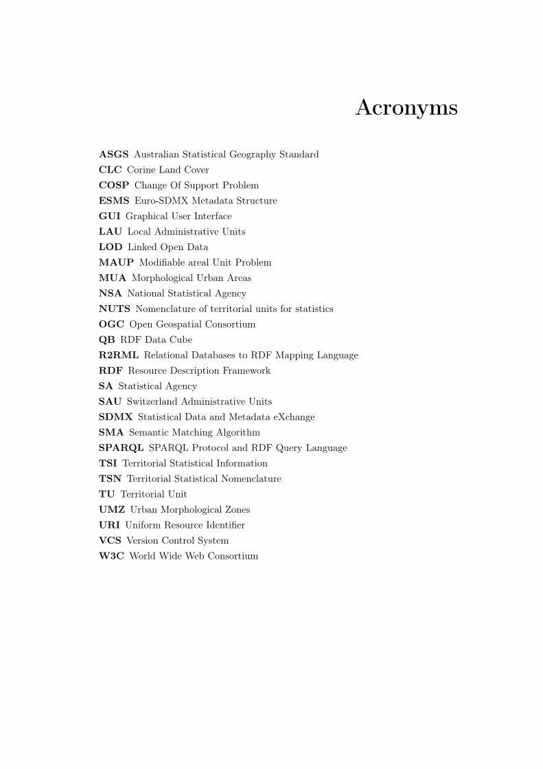
ASGS Australian Statistical Geography StandardCLC Corine Land CoverCOSP Change Of Support ProblemESMS Euro-SDMX Metadata StructureGUI Graphical User InterfaceLAU Local Administrative UnitsLOD Linked Open DataMAUP Modifiable areal Unit ProblemMUA Morphological Urban AreasNSA National Statistical AgencyNUTS Nomenclature of territorial units for statisticsOGC Open Geospatial ConsortiumQB RDF Data CubeR2RML Relational Databases to RDF Mapping LanguageRDF Resource Description FrameworkSA Statistical AgencySAU Switzerland Administrative UnitsSDMX Statistical Data and Metadata eXchangeSMA Semantic Matching AlgorithmSPARQL SPARQL Protocol and RDF Query LanguageTSI Territorial Statistical InformationTSN Territorial Statistical NomenclatureTU Territorial UnitUMZ Urban Morphological ZonesURI Uniform Resource IdentifierVCS Version Control SystemW3C World Wide Web Consortium

List of Figures

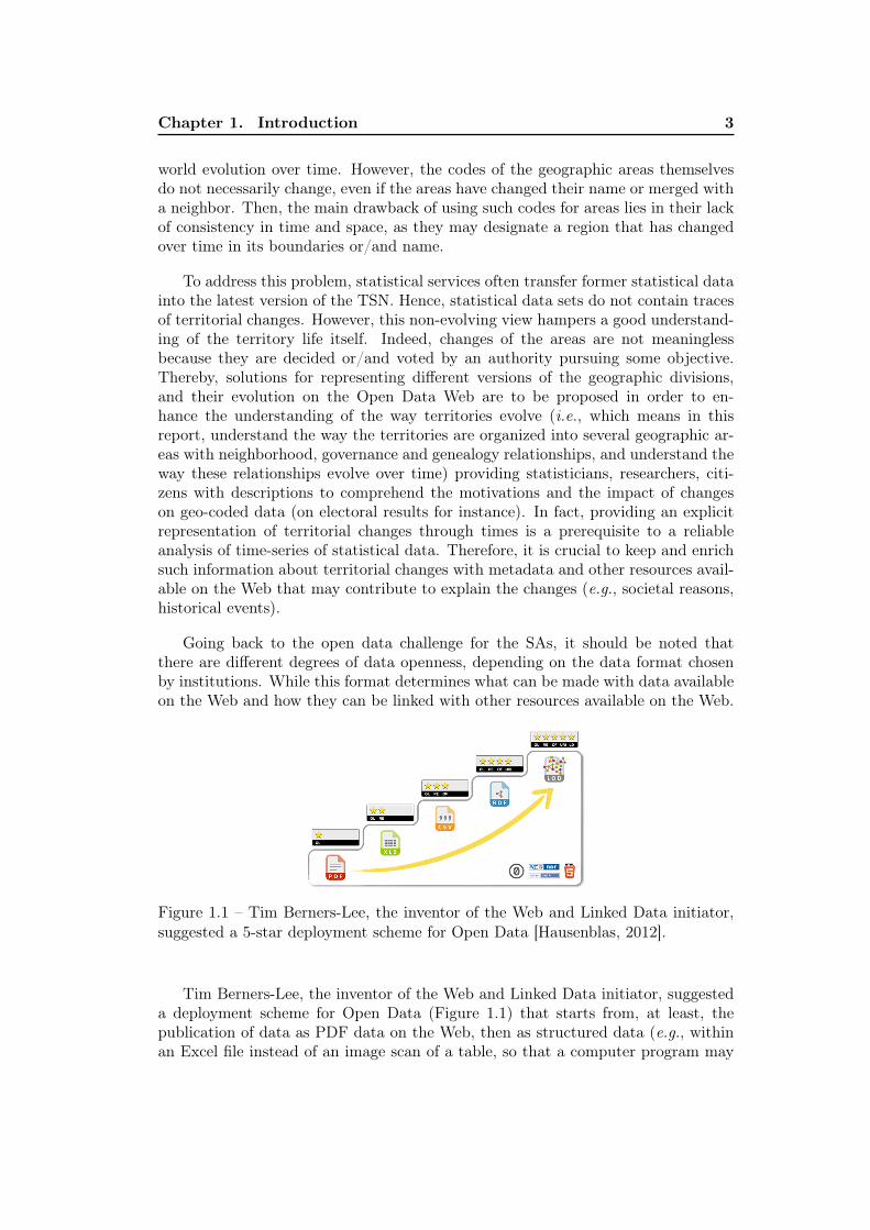
1.1 Tim Berners-Lee, the inventor of the Web and Linked Data initiator,suggested a 5-star deployment scheme for Open Data [Hausenblas,2012]. . . . . . . . . . . . . . . . . . . . . . . . . . . . . . . . . . . . 3

1.2 Example of Linked Resources on the Web using URI and the RDFsyntax for their identification and representation. . . . . . . . . . . . 4

1.3 Simplified illustration of the RDF Graph representing territorial changeswe want to achieve. . . . . . . . . . . . . . . . . . . . . . . . . . . . . 9

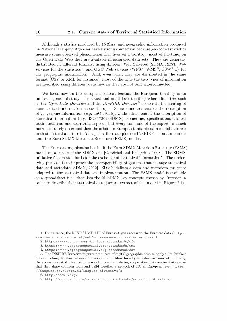
2.1 Extract of the ESMS model (based on the Eurostat Metadata Struc-ture, source: http://ec.europa.eu/eurostat/data/metadata/metadata-structure . . . . . . . . . . . . . . . . . . . . . . 17

2.2 INSPIRE data model extract (Based on: INSPIRE ConsolidatedUML Model http://inspire.ec.europa.eu/data-model/approved/r4618-ir/html/) . . . . . . . . . . . . . . . . . . . . . 18

2.3 Eurostat Unemployment rates by sex, age and NUTS regions data setextract (source https://ec.europa.eu/eurostat/web/products-datasets/-/LFST_R_LFU3RT) . . . . . . . . . . . . . . . . 19

2.4 Eurostat NUTS 2016 Level 2 ESRI shapefile. Data was rendered usingthe QuantumGIS software (source https://ec.europa.eu/eurostat/cache/GISCO/distribution/v2/nuts/download/ref-nuts-2016-01m.shp.zip) . . . . . . . . . . . . . . . . . . . . 19

2.5 Schema of a Territorial Statistical Nomenclature Structure. . . . . . 222.6 Four TSNs Structures from four agencies producing, managing and

delivering official statistics (Eurostat, the U.S. Census Bureau, theAustralian Bureau of Statistics and the Swiss Federal Statistical Office). 25

2.7 The NUTS divisions of the French territory into four levels. . . . . . 262.8 Territorial nomenclatures heterogeneity: example of the NUTS and

UMZ nomenclatures. . . . . . . . . . . . . . . . . . . . . . . . . . . . 272.9 Example of two versions of a TSN represented as tree data structures. 282.10 Example of covering and non-covering hierarchies. . . . . . . . . . . . 282.11 Example of strict and non-strict hierarchies. . . . . . . . . . . . . . . 292.12 Example of onto and non-onto hierarchies. . . . . . . . . . . . . . . . 292.13 Intercommunalities: a non-covering, non-strict, and non-onto nomen-

clature. Source: [Plumejeaud et al., 2011]. . . . . . . . . . . . . . . . 302.14 Example of territorial change - Split of the territorial unit ES63 from

NUTS Version 1999 to NUTS Version 2003, at Level 2. . . . . . . . . 322.15 Different Problems related to spatial sampling (Figure inspired from

[Louvet et al., 2015]) . . . . . . . . . . . . . . . . . . . . . . . . . . . 342.16 Modifiable areal Unit Problem (MAUP) – scale effect and zoning

effect (Figure inspired from [Loidl et al., 2016]) . . . . . . . . . . . . 352.17 State of Utah Census Tracts – Source [Census Tracts Geographic

Products Branch, 2013] . . . . . . . . . . . . . . . . . . . . . . . . . 352.18 United States census geographic units [ESRI, 2017] . . . . . . . . . . 36

xxii List of Figures

2.19 Modifiable areal Unit Problem (MAUP) over time – zoning effect attime t and zoning effect over time (evolving zoning problem) . . . . . 37

2.20 Linked Government Data information management process, proposedin [Villazón-Terrazas et al., 2011]. . . . . . . . . . . . . . . . . . . . . 39

3.1 Ship of Theseus illustration from [Vazirani, 2014]. . . . . . . . . . . . 423.2 GeoSPARQL main classes [Perry and Herring, 2012]. . . . . . . . . . 453.3 GeoSPARQL main topological relations between geo:SpatialObject A

and B [Perry and Herring, 2012]. . . . . . . . . . . . . . . . . . . . . 453.4 The GeoSPARQL main classes [Cox and Little, 2017]. . . . . . . . . 463.5 Thirteen elementary possible relations between time periods [Cox and

Little, 2017; Allen and Ferguson, 1997]. . . . . . . . . . . . . . . . . . 473.6 Generic behaviour of spatiotemporal objects using the Statechart no-

tation, from [Renolen, 1997]. . . . . . . . . . . . . . . . . . . . . . . . 483.7 Typology of spatiotemporal processes from [Claramunt and Théri-

ault, 1995]. . . . . . . . . . . . . . . . . . . . . . . . . . . . . . . . . 493.8 The story of a land area (above) shown in the history graph notation

(below), from [Renolen, 1997]. . . . . . . . . . . . . . . . . . . . . . . 503.9 The main concepts of the BFO ontology. . . . . . . . . . . . . . . . . 543.10 Schematic representation of the concept of time-determined ontol-

ogy[Baratis et al., 2009]. On the left: a series of snapshot ontologies.On the right: a 4D-Fluents (perdurantist) ontology. . . . . . . . . . . 55

3.11 Example of N-ary Relations from [Batsakis et al., 2017]. . . . . . . . 563.12 Example of 4D-Fluents from [Batsakis et al., 2017]. . . . . . . . . . . 56

4.1 Continuum Main concepts [Harbelot et al., 2013]. . . . . . . . . . . . 604.2 Timeslice in the LC3 Model [Harbelot et al., 2015]. . . . . . . . . . . 604.3 The Continuum Model with different levels of filiation relationship

[Harbelot et al., 2013]. . . . . . . . . . . . . . . . . . . . . . . . . . . 614.4 Filiation Graphs of evolving land-parcels example [Harbelot et al.,

2015]. . . . . . . . . . . . . . . . . . . . . . . . . . . . . . . . . . . . 624.5 A Change bridge example from [Kauppinen and Hyvönen, 2007]. . . 644.6 The Jurisdictional domain ontology (upper, domain and application

ontologies) from [Lopez-Pellicer et al., 2012]. . . . . . . . . . . . . . . 674.7 Meaning of the different succession relations in the model of [Lopez-

Pellicer et al., 2012]. . . . . . . . . . . . . . . . . . . . . . . . . . . . 674.8 Change types of SONADUS [Gantner, 2011]. . . . . . . . . . . . . . 714.9 A model for identifying geographic units into various nomenclatures,

from [Plumejeaud et al., 2011]. . . . . . . . . . . . . . . . . . . . . . 784.10 Typology of territorial events in TSN, from [Plumejeaud et al., 2011]. 794.11 The geographical units of a TSN represented in relation to the terri-

torial events they are involved in and that lead to their change overtime (LifeEvent), from [Plumejeaud et al., 2011]. . . . . . . . . . . . 80

5.1 List of patterns detected in the LC3 Model [Harbelot et al., 2015]. . 85

List of Figures xxiii

5.2 Excerpt of a statistical data set measuring the Life Expectancy (inyears), in France (the codes FR02, FR03, FR04 are the codes forfrench areas in the NUTS TSN). . . . . . . . . . . . . . . . . . . . . 89

7.1 The Theseus Semantic Framework Use Cases. . . . . . . . . . . . . . 1037.2 The Theseus Framework Modules. . . . . . . . . . . . . . . . . . . . 105

8.1 TSN Ontological Model main concepts inherited from the BFO on-tology (Occurrent and Continuant concepts from [Grenon and Smith,2004]). . . . . . . . . . . . . . . . . . . . . . . . . . . . . . . . . . . . 110

8.2 Combining approaches for the TSN/TSN-Change Ontological Model. 1118.3 TSN Ontology - Example of three TSN declared using the TSN

Nomenclature main concept. . . . . . . . . . . . . . . . . . . . . . . . 1128.4 TSN Ontology main concepts. . . . . . . . . . . . . . . . . . . . . . . 1148.5 TSN-Change Ontology main elements. . . . . . . . . . . . . . . . . . 1168.6 TSN-Change Ontology X-ChangeBridge Model. . . . . . . . . . . . . 1178.7 Split of a TU - Scission and Extraction. . . . . . . . . . . . . . . . . 1188.8 TSN-Change Ontology TU Life line. . . . . . . . . . . . . . . . . . . 119

9.1 The workflows of the Theseus Framework to populate semi-automaticallythe TSN ontological model. . . . . . . . . . . . . . . . . . . . . . . . 122

9.2 Ceuta and Melilla TUs in the NUTS TSN. . . . . . . . . . . . . . . . 1279.3 NUTS Hierarchy of levels linked to the example of Figure 9.2. . . . . 1279.4 Iterations of the SMA Algorithm in order to find a set of TUs involved

in a same StructureChange. . . . . . . . . . . . . . . . . . . . . . . . 1339.5 Example of a multi-level change graph created with Theseus, linked

to the example Figure 9.2. . . . . . . . . . . . . . . . . . . . . . . . . 137

10.1 Example of three TSNs’ structures declared using the TSN Ontology. 14310.2 SAU Districts Neuchâtel changes. . . . . . . . . . . . . . . . . . . . . 15010.3 The ASGS Structures (source: https://www.abs.gov.au/web

sitedbs/D3310114.nsf/home/Australian+Statistical+Geography+Standard+(ASGS)). . . . . . . . . . . . . . . . . . . . 153

10.4 The ASGS map representation of the Split of the TU 508 at level 4and representation of the sub-changes on the sub-TUs of TU 508. . . 156

10.5 Visualization of the TUs listed in Listing 10.6 that change their codein the NUTS from V1999 to V2003. . . . . . . . . . . . . . . . . . . . 159

10.6 A solution to reduce the calculation time of ST_Intersects() on com-plex polygons (more than 100 vertices) by reducing somewhat thenumber of vertices required to represent elementary polygons [Furi-eri, 2011]. . . . . . . . . . . . . . . . . . . . . . . . . . . . . . . . . . 163

10.7 A Map of Australia highlighting the Western Australia TU (source:https://commons.wikimedia.org/wiki/File:Western_Australia_locator-MJC.png. . . . . . . . . . . . . . . . . . . . . 165

10.8 Western Australia TU (ASGS version 2011) – The offset between theoriginal geometry (in green) and the simplified one (in red). . . . . . 166

xxiv List of Figures

10.9 The two TUs named Salisbury (id 40204) of the ASGS TSN in version2011 and 2016 (the TU version 2016 is displayed in yellow, under theTU in the version 2011 to observe the boundaries differences). . . . . 168

11.1 The Multi-levels change graph of the NUTS 1999 TU ES6 (result ofthe query in Listing 11.2, also online at http://purl.org/steamer/nuts_V1999_ES6_change_graph). . . . . . . . . . . . . . . . 173

11.2 The life line of the NUTS TU ES63 (result of the query in Listing11.6, also online at http://purl.org/steamer/nuts_ES63_lifeline). . . . . . . . . . . . . . . . . . . . . . . . . . . . . . . . . 176

11.3 Visualization of evolving geospatial data with GitHub [Balter, 2014]. 17711.4 The Theseus Framework Web Mapping GUI using request to the

Geoserver WMS (available at http://lig-tdcge.imag.fr/tsn-catalog/). . . . . . . . . . . . . . . . . . . . . . . . . . . . . . . . 187

12.1 Boundaries for Illinois’s 4th United States Federal Congressional Dis-trict, since 2013 (source: GIS (congressional districts, 2013) shapefiledata was created by the United States Department of the Interior.Data was rendered using ArcGIS software by Esri. File developed foruse on Wikipedia (Public domain)). . . . . . . . . . . . . . . . . . . . 193

12.2 Corine Land Cover Classes (source: Copernicus Project https://land.copernicus.eu/Corinelandcoverclasses.eps.75dpi.png/). . . . . . . . . . . . . . . . . . . . . . . . . . . . . . . . . . 195

12.3 An example of three kinds of derivation in the CLC data set: weak,medium and strong derivation [Harbelot et al., 2015]. . . . . . . . . . 196

12.4 GUI proposition – Geo-visualization of the change of the district 4thin Illinois: two maps are shown (on the left the congressional districtsin 1983, and on the right the congressional districts in 1993). (Source:Jeffrey B. Lewis, Brandon DeVine, Lincoln Pitcher, and Kenneth C.Martis. (2013) Digital Boundary Definitions of United States Con-gressional Districts, 1789-2012. Retrieved from http://cdmaps.polisci.ucla.eduon 2019-11-06.) . . . . . . . . . . . . . . . . . . . . . . . . . . . . . 200

1.1 The Theseus Framework data life cycle . . . . . . . . . . . . . . . . . 220

List of Tables

9.1 Extract of the list of TUs of the NUTS version 1999 (V ′) (Algorithm1 input). . . . . . . . . . . . . . . . . . . . . . . . . . . . . . . . . . 126

9.2 Extract of the list of TUs of the NUTS version 2003 (V ′′) (Algorithm1 input). . . . . . . . . . . . . . . . . . . . . . . . . . . . . . . . . . 126

9.3 TSN Semantic Matching Algorithm Constants. . . . . . . . . . . . . 127

10.1 TSN triplestore numbers of triples . . . . . . . . . . . . . . . . . . . 14210.2 Configurations for test of the Theseus Framework on the NUTS TSN.14410.3 The NUTS TSN Change Graph – number of change nodes. . . . . . 14510.4 The NUTS TSN Change Graph – main change types distribution

from version 2006 to 2010. . . . . . . . . . . . . . . . . . . . . . . . 14610.5 Configurations for test of the Theseus Framework on the SAU TSN. 14810.6 The SAU TSN Change Graph – main change types distribution from

version 2017 to 2018. . . . . . . . . . . . . . . . . . . . . . . . . . . 14910.7 The TSN SMA Algorithm 1 implementation – configurations for

tests on the SAU TSN. . . . . . . . . . . . . . . . . . . . . . . . . . 15410.8 The ASGS TSN Change Graph – main change types distribution

from version 2011 to 2016. . . . . . . . . . . . . . . . . . . . . . . . 15510.9 The result of the query 10.5 that returns a chain of StructureChange

nodes, starting from the change that affects the TU asgs:V2011_-L4_508 . . . . . . . . . . . . . . . . . . . . . . . . . . . . . . . . . . 157

10.10 Key Figures on several TSNs data sets, processed by the TSN SMAAlgorithm 1. . . . . . . . . . . . . . . . . . . . . . . . . . . . . . . . 161

10.11 Variability of the TSN matching Algorithm outputs after modifyingthe Spatial Thresholds. . . . . . . . . . . . . . . . . . . . . . . . . . 169

11.1 Excerpt of the list of TUs that change at NUTS Level 1, from version1999 to 2003, result of the query 11.1. . . . . . . . . . . . . . . . . . 172

11.2 Part of the result of the SPARQL query 11.10. . . . . . . . . . . . . 180

List of Listing Codes

4.1 Example of the use of the Change Vocabulary to model the mergeof East Germany and West Germany in 1990. . . . . . . . . . . . . 64

4.2 Nested Spatial Reference Features using QB4ST [Atkinson, 2017] . 735.1 RDF Data Cube Observation example in turtle [Atkinson, 2017] . . 908.1 Description of the NUTS and ASGS nomenclatures using the TSN

Ontology vocabulary (RDF-Turtle syntax) . . . . . . . . . . . . . . 1139.1 URIs’ Patterns for the elements of a TSN. . . . . . . . . . . . . . . 1239.2 An implementation of the Levenshtein distance algorithm that al-

lows to make an approximate comparison of the matching betweentwo given strings (Author: Christine Plumejeaud). . . . . . . . . . . 130

10.1 The NUTS 1999 ES63 TU description using concepts from the TSNand GeoSPARQL Ontologies. . . . . . . . . . . . . . . . . . . . . . . 144

10.2 The RDF change description of TU ES63 from NUTS version 1999to 2003 – please note that the Figure 9.2 is a map representation ofthis event. . . . . . . . . . . . . . . . . . . . . . . . . . . . . . . . . 146

10.3 The RDF change description of the Canton of Neuchâtel from SAUversion 2017 to 2018. . . . . . . . . . . . . . . . . . . . . . . . . . . 151

10.4 A SPARQL query that returns all the change nodes of type "Split"in the ASGS change graph version 2011 to 2016 at the highest levelSA4. . . . . . . . . . . . . . . . . . . . . . . . . . . . . . . . . . . . 155

10.5 A SPARQL query that returns the whole chain of changes that oc-curred on the sub-TUs to the TU with code 508 that split in ASGSversion 2006. . . . . . . . . . . . . . . . . . . . . . . . . . . . . . . . 157

10.6 One result of the implementation of IdentificationRetructurationsearch by spatial proximity (in the NUTS V1999 to 2003). . . . . . 158

10.7 The Areal Distance Test implementation – The PostGIS DBMS SQLrequest executed during the SpatialMatchTest (see Algorithm 1 line4) ("geom1" and "geom2" are input parameters – multi-polygongeometries of the two processed TUs in V ′ and V ′′). . . . . . . . . . 161

10.8 The SQL script that recalculates the topological network of a TSNand simplifies each TU geometry (polygon) while maintaining a net-work where simplified units are adjacent. . . . . . . . . . . . . . . . 164

11.1 A SPARQL query that returns all the TUs that change between twoTSNs versions at a specified territorial level. . . . . . . . . . . . . . 172

11.2 A SPARQL query that returns the multi-levels change graph of a TU.17211.3 Pathfinder syntax of path queries, source Sirin [2017]. . . . . . . . . 17411.4 A SPARQL query that searches for the sub-graph of changes of a

super-TU. . . . . . . . . . . . . . . . . . . . . . . . . . . . . . . . . 17411.5 A SPARQL query that, from a TU in the lowest level, goes up the

chain of changes until a super-TU. . . . . . . . . . . . . . . . . . . . 17511.6 A SPARQL query that returns the life line of a TU. . . . . . . . . . 17611.7 Query the TUs that do not change from one version to another at a

specific territorial level. . . . . . . . . . . . . . . . . . . . . . . . . . 177

xxviii List of Listing Codes

11.8 Query the TUs that change from one version to another at a specificterritorial level. . . . . . . . . . . . . . . . . . . . . . . . . . . . . . 178

11.9 Query the TUs that disappear from one version to another at aspecific territorial level. . . . . . . . . . . . . . . . . . . . . . . . . . 178

11.10 A SPARQL request to the DBPedia Service in order to find contex-tual information about a territorial change. . . . . . . . . . . . . . . 179

11.11 A description of two versions of the TUs ES63 in NUTS 1999 and2003 using the TSN and the GeoSPARQL ontologies (RDF-Turtlesyntax). . . . . . . . . . . . . . . . . . . . . . . . . . . . . . . . . . 183

11.12 A description of the Total population Eurostat indicator - Two ob-servations of the same indicator in different NUTS versions for theES63 TU (RDF-Turtle syntax). . . . . . . . . . . . . . . . . . . . . 184

11.13 A WFS GetFeature Request on the OGC Web Services of the The-seus Framework. . . . . . . . . . . . . . . . . . . . . . . . . . . . . . 185

11.14 A WFS GetFeature Response on the OGC Web Services of the The-seus Framework. . . . . . . . . . . . . . . . . . . . . . . . . . . . . . 186

B.1 The Theseus R2RML Mapping File between an input TSN shapefileand the TSN Ontology Concepts . . . . . . . . . . . . . . . . . . . . 221

Chapter 1

Introduction

1.1 Context

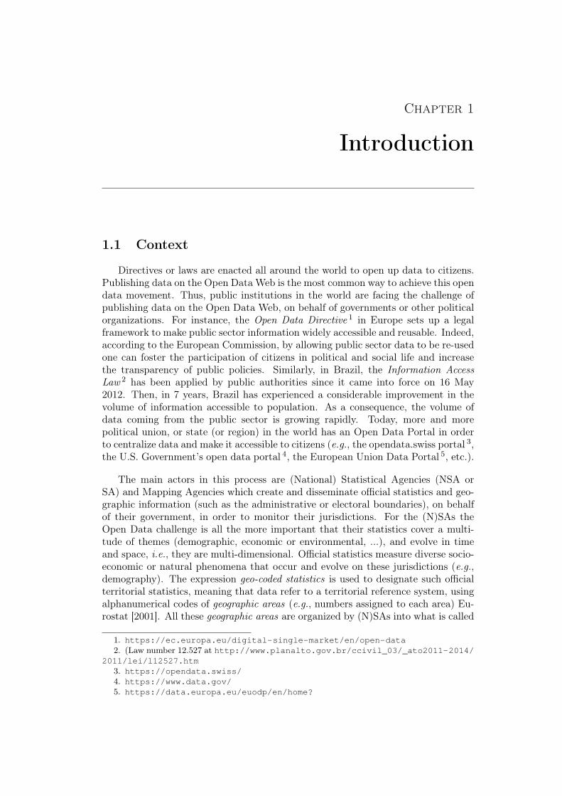
Directives or laws are enacted all around the world to open up data to citizens.Publishing data on the Open Data Web is the most common way to achieve this opendata movement. Thus, public institutions in the world are facing the challenge ofpublishing data on the Open Data Web, on behalf of governments or other politicalorganizations. For instance, the Open Data Directive 1 in Europe sets up a legalframework to make public sector information widely accessible and reusable. Indeed,according to the European Commission, by allowing public sector data to be re-usedone can foster the participation of citizens in political and social life and increasethe transparency of public policies. Similarly, in Brazil, the Information AccessLaw 2 has been applied by public authorities since it came into force on 16 May2012. Then, in 7 years, Brazil has experienced a considerable improvement in thevolume of information accessible to population. As a consequence, the volume ofdata coming from the public sector is growing rapidly. Today, more and morepolitical union, or state (or region) in the world has an Open Data Portal in orderto centralize data and make it accessible to citizens (e.g., the opendata.swiss portal 3,the U.S. Government’s open data portal 4, the European Union Data Portal 5, etc.).

The main actors in this process are (National) Statistical Agencies (NSA orSA) and Mapping Agencies which create and disseminate official statistics and geo-graphic information (such as the administrative or electoral boundaries), on behalfof their government, in order to monitor their jurisdictions. For the (N)SAs theOpen Data challenge is all the more important that their statistics cover a multi-tude of themes (demographic, economic or environmental, ...), and evolve in timeand space, i.e., they are multi-dimensional. Official statistics measure diverse socio-economic or natural phenomena that occur and evolve on these jurisdictions (e.g.,demography). The expression geo-coded statistics is used to designate such officialterritorial statistics, meaning that data refer to a territorial reference system, usingalphanumerical codes of geographic areas (e.g., numbers assigned to each area) Eu-rostat [2001]. All these geographic areas are organized by (N)SAs into what is called

1. https://ec.europa.eu/digital-single-market/en/open-data2. (Law number 12.527 at http://www.planalto.gov.br/ccivil_03/_ato2011-2014/

2011/lei/l12527.htm3. https://opendata.swiss/4. https://www.data.gov/5. https://data.europa.eu/euodp/en/home?

2 1.1. Context

a Territorial Statistical Nomenclature (TSN). A Territorial Statistical Nomencla-ture is a set of artifact geographic areas (also called Territorial Units (TU)) builtby (N)SAs to observe a given territory at several geographic subdivision levels (e.g.,regions, districts, sub-districts levels). Numerous TSNs exist throughout the world.A Territory, in this thesis report, refers to the largest geographic area of the TSN,(that bounds all the others subdivisions), a portion of space (on Earth) well delim-ited. One example of TSN is the Eurostat 6 nomenclature, called the Nomenclatureof Territorial Units for Statistics (NUTS) 7, that provides four nested divisions ofthe European Union (EU) territory, for the collection of EU regional statistics: Level0 corresponds to the division of the European territory into its State members, Level1 splits each of the States obtained at Level 0 into major Regions, Level 2 divideseach major Region of the Level 1 into basic Regions, and Level 3 into small Regions.The concept of TSN is a central topic in this thesis.

Geo-coded statistics are of utmost importance for policy-makers to conduct var-ious analyses, in time and within the space of their jurisdiction. For instance, usingdata available at two or more periods of time, they can observe the evolution of theunemployment rate in a given administrative region. As a matter of fact, the analysisof territories through the evolution of statistical series over time allows stakehold-ers to be aware of the impact of past policies, to understand territory at presenttime, and to better grasp the future [Bernard et al., 2017]. Thus, there is a strongdemand from governments, organizations and researchers regarding time-series ofofficial territorial statistics.

However, even if statistical data are available for several points in time, they areoften not comparable through time due to changes in concepts (e.g., definition ofunemployment), in acquisition methods or in territorial units. This latter aspect isthe focus of the thesis. Past geo-coded data cannot be compared to more recent dataif the geographic areas observed have changed in the meantime i.e., data collectedin different versions of a TSN are not directly comparable because the observedgeographic areas are potentially not the same areas anymore. Then, territorialchanges lead to broken time-series and are source of misinterpretations of statistics,and statistical biases when not properly documented. Territorial changes are veryfrequent in Europe (for instance in France, in 2016, administrative regions have beenmerged into greater regions) or in the U.S.A., as a result of a well-known processcalled gerrymandering or, more broadly redistricting. They lead to broken statisticaltime-series because data are collected for and from areas that have changed. Thisproblem, well known as the Change of Support Problem (COSP) [Openshaw andTaylor, 1979; Gotway Crawford and Young, 2005; Howenstine, 1993], describes thephenomenon where data collected in different zonings or versions of a zoning arenot comparable due to potential differences between the geographic areas used assupports for the collected data.

As a result of territorial changes, TSNs also change over time: statistical agenciesusually update their geographic areas every 1 to 10 years in order to reflect the real

6. The European Statistical Agency that provides official statistics to the NSAs of the EuropeanUnion member states

7. http://ec.europa.eu/eurostat/web/nuts/overview

Chapter 1. Introduction 3

world evolution over time. However, the codes of the geographic areas themselvesdo not necessarily change, even if the areas have changed their name or merged witha neighbor. Then, the main drawback of using such codes for areas lies in their lackof consistency in time and space, as they may designate a region that has changedover time in its boundaries or/and name.

To address this problem, statistical services often transfer former statistical datainto the latest version of the TSN. Hence, statistical data sets do not contain tracesof territorial changes. However, this non-evolving view hampers a good understand-ing of the territory life itself. Indeed, changes of the areas are not meaninglessbecause they are decided or/and voted by an authority pursuing some objective.Thereby, solutions for representing different versions of the geographic divisions,and their evolution on the Open Data Web are to be proposed in order to en-hance the understanding of the way territories evolve (i.e., which means in thisreport, understand the way the territories are organized into several geographic ar-eas with neighborhood, governance and genealogy relationships, and understand theway these relationships evolve over time) providing statisticians, researchers, citi-zens with descriptions to comprehend the motivations and the impact of changeson geo-coded data (on electoral results for instance). In fact, providing an explicitrepresentation of territorial changes through times is a prerequisite to a reliableanalysis of time-series of statistical data. Therefore, it is crucial to keep and enrichsuch information about territorial changes with metadata and other resources avail-able on the Web that may contribute to explain the changes (e.g., societal reasons,historical events).

Going back to the open data challenge for the SAs, it should be noted thatthere are different degrees of data openness, depending on the data format chosenby institutions. While this format determines what can be made with data availableon the Web and how they can be linked with other resources available on the Web.

Figure 1.1 – Tim Berners-Lee, the inventor of the Web and Linked Data initiator,suggested a 5-star deployment scheme for Open Data [Hausenblas, 2012].

Tim Berners-Lee, the inventor of the Web and Linked Data initiator, suggesteda deployment scheme for Open Data (Figure 1.1) that starts from, at least, thepublication of data as PDF data on the Web, then as structured data (e.g., withinan Excel file instead of an image scan of a table, so that a computer program may

4 1.1. Context

extract the value of each cell). The next step is to make data available but in a non-proprietary format (e.g., comma-separated values instead of Excel). Data reach4 stars when each of them (e.g., each cell of a table) may be identified uniquelyusing a Unique Resource Identifier (URI), so that people can point at data usingtheir URI. The Open data process ends when linking each URI with each other i.e.,each cell data being identified uniquely by a URI is connected to other data on theWeb using a link (also identified by a URI). Indeed, the more data are linked, themore users can discover new facts, by going from one node of the distributed Webgraph database to another. Such a linking of two resources on the Web is calleda triple (subject-predicate-object) (Figure 1.2). Most of the time, the ResourceDescription Framework (RDF) standard syntax is used to write these triples, calledRDF triples. For instance, from the data resource "Helsinki" identified by the URIhttp://dbpedia.org/resource/Helsinki on the LOD Web, users discoverpeople born in Helsinki by visiting linked nodes.

GrandDuchyofFinland

iscapitalof

http://dbpedia.org/ontology/capital

http://dbpedia.org/ontology/birthPlace

isbirthPlaceof

http://dbpedia.org/resource/Helsinki

http://dbpedia.org/resource/Grand_Duchy_of_Finland

http://dbpedia.org/resource/Tarja_Halonen

Helsinki

Resource1(Subject) Link(PropertyorPredicate)

Tarja Halonen …

Resource2(Object)

Resourcehttp://dbpedia… URI

Figure 1.2 – Example of Linked Resources on the Web using URI and the RDFsyntax for their identification and representation.

For the (N)SAs, the stakes behind adopting the LOD approach and technologiesare crucial because the more contextualized data are (linked to historical, environ-mental information, etc.), and linked to each other, in time and space, the moreanalyzes carried out on the territories using these data will be multi-criteria, rel-evant and reusable by the policies and researchers. As a matter of fact, the morestatistical data are linked together (two statistical indicators 8 that describe thesame geographic area could be linked together for instance on the spatial dimensionof data), the more analysts may explore correlations, causalities and understand theterritory under analysis. So far, (N)SAs share their statistics at the data set level.Then, users have to download the whole data set in order to perform their analysis,

8. According to Eurostat (Source: https://ec.europa.eu/eurostat/statistics-explained/index.php/Glossary:Statistical_indicator) "A statistical indicator is the rep-resentation of statistical data for a specified time, place or any other relevant characteristic [...]. Itis a summary measure related to a key issue or phenomenon and derived from a series of observedfacts. Indicators can be used to reveal relative positions or show positive or negative change..

Chapter 1. Introduction 5

even if they are interested in only one indicator or one value of the file. Then,(N)SAs are far from disseminating atomic data from which one may automate theprocess, re-used, or infer new fact from it. Similarly, to address a specific problem,analysts have to download multiple isolated data sets, each of them resolving onlya part of the problem.

Using the LOD paradigm, each statistical data set available on the Web maybe identified by a URI representing a resource, while each indicator, each data andmetadata composing the data set as well: everything being a resource node in thedistributed Web graph database. Thus, data sets as LOD are no longer isolated in-stances, they are immersed in the Web as graph(s). They are all interconnected, andat a finer granularity, the indicators and the statistical values can be interconnectedas well. Furthermore, LOD technologies foster syntactic interoperability, and mostof all semantic interoperability between systems. Indeed, for each data publishedon the LOD Web, it is necessary to define which set of things – real-world objects,events, situations or abstract notion – it belongs to, by linking it to a concept defin-ing this set. As part of LOD, ontologies are documents that formally define theseconcepts and their relations [Berners-Lee et al., 2001]. They help both people andmachines to communicate, supporting the share of semantics and not only syntax[Maedche and Staab, 2001]. Hence, using RDF triples, the syntax of data is ho-mogenized, data can be transferred from one system to another, and because of theexplicit semantic, systems "understand" data they receive and can determine theappropriate process to be applied (e.g., data tagged as geospatial data may auto-matically be displayed on a map). Thus, the term Semantic Web is also used todenote data sets, ontologies and technologies on the LOD Web. More recently theterm knowledge graphs emerges to denote graph on the LODWeb containing bothdata sets and ontologies, bearing formal semantics, which can be used to interpretdata and infer new facts [Ontotext, 2018]. A kowledge graph can be envisaged as anetwork of several data sets and ontologies which are relevant to a specific domain,and on which one can apply a reasoner in order to derive new knowledge [Ehrlingerand Wöß, 2016]. Even if the term is borrowed from a commercial data graph, theGoogle Knowledge Graph, it is now used to denote also available open graphs, suchas DBpedia, YAGO, and Freebase [Paulheim, 2017].

Thus, there are many benefits for (N)SAs in using LOD technologies for theirstatistics:– users may navigate from one data set to another;– data and metadata are interlinked;– systems "understand" the data they receive and can determine the appropriateprocess to apply to data;– data are put in context, as they are linked to other resources on the LOD Web;– each statistical indicators and value become addressable;– using a network of ontologies and data sets, a knowledge graph representing thedynamics of the territories over time may be constructed, combining several statis-tical data sets from various disciplines (e.g., environment, socio-economy, ethology,transports), at different instants in time, observed in different meshes and versionsof these meshes. Also historical and political information could be mobilized inorder to explain the changes over time, such as the changes in boundaries over time.

6 1.1. Context

From this knowledge graph one can build intelligent tools for the restitution ofthese very disparate data which, taken as a whole, may help in understanding thecomplexity of the change phenomenon, and the cascading effect of changes throughall levels of the European territory, for instance. These tools might also be able toinfer new data (such as the estimation of unemployment values after a redistricting),using a cross-sectoral approach for accurate estimation.

(N)SAs have just started publishing their data on the LOD Web to benefitfrom all the technologies and ontologies around this new data format. Variousinitiatives to disseminate Linked Statistical Data emerge throughout the world. Forinstance, the Aragón Statistical Office Open Data Portal provides LOD statisticson municipalities of the Aragon region of Spain 9; the Italian Istat Linked OpenData Portal 10 and the e-Stat Japanese Portal 11 disseminate statistical LOD for theNational SAs of Italia and Japan; the European Union (EU) Open Data Portal 12

gives access to (L)OD published by EU institutions such as Eurostat that providesofficial statistics on the European Union territory.

The W3C RDF Data Cube ontology (QB) is widely used to describe these LODstatistics in a way that is compatible with the Statistical Data and Metadata eX-change (SDMX), an ISO standard for exchanging and sharing statistical data andmetadata among organizations [Cyganiak and Reynolds, 2014]. Using the QB vo-cabulary, one can publish statistical observations and a set of dimensions that definewhat the observation applies to: time, gender and geographic areas, for instance.However, the QB ontology does not provide the necessary vocabulary to achievethe description of the geographic areas and of the TSN these areas belong to. TSNlevels and TUs have to be described elsewhere, using other ontologies than QB.

The (N)SAs, for their part, often create their own ontology for the descriptionof statistical areas (e.g., the Territorio Ontology 13 of the Italian National Institutefor Statistics, the Geography Ontology 14 of the Scottish Government), which resultsinto a counterproductive proliferation of non-aligned vocabularies. Consequently,there is no semantic interoperability between TSN data set nowadays.

The spatiotemporal model of Plumejeaud et al. [2011] (created few years agoby researchers of our STeamer LIG group) offers a way to represent hierarchies ofgeographic divisions used for statistical purposes. The geographic areas that com-pose the TSN are described over time, in relation to their ancestors or descendants.The constructed lineages of areas provide policy-makers with information about thechanges of the territory observed over time. However, this conceptual model stillneeds to be immersed in the LOD world if ones want to address the NSAs today’schallenge with regard to dissemination of data. This still requires, as noticed by theSpatial Data on the Web Working Group 15(a group that gathers members from the

9. http://opendata.aragon.es/10. http://datiopen.istat.it/index.php?language=eng11. http://data.e-stat.go.jp/lodw/en12. http://data.europa.eu/euodp/home13. http://datiopen.istat.it/odi/ontologia/territorio/14. http://statistics.gov.scot/vocabularies/15. https://www.w3.org/2015/spatial/wiki/Main_Page

Chapter 1. Introduction 7

World Wide Web Consortium (W3C) and the Open Geospatial Consortium (OGC),"a significant change of emphasis from traditional Spatial Data Infrastructures (SDI)by adopting a Linked Data approach. " [Tandy et al., 2017].

Regarding TSN spatial data, even if some agencies published their TSN asLOD (i.e., using the RDF syntax), in most cases, TSNs data are availableonline as ESRI ®shapefiles i.e., an open format for geospatial data. If werefer to the Tim Berner-Lee deployment scheme for Open Data (see Figure1.1), in the field of TSNs, such a deployment reaches level 3. TSN data are,most of the time, not yet available as Linked (Open) Data.

1.2 Problematic

We focus through this thesis report on the spatial dimension of geo-coded statis-tics, and we try to immerse TSNs on the LOD Web by taking into account theheterogeneity of existing TSNs and their evolving nature. Our work is a continua-tion of the previous work from Plumejeaud [2011] and extend the proposed modeland algorithm for TSNs.

Since no ontology in the LOD Web is generic enough to enable the description ofany TSN in the world, semantic interoperability of TSNs is not yet achieved thoughit would foster the exchange of information among SAs in the world, the compar-ison of these statistical areas in the world and the processing of these geo-codedstatistics. Similarly, no ontology on the LOD Web enables the description of TSNevolution and changes over time while, by describing TSN changes, one can meetstakeholders’ needs for tools to:a) geo-visualize changes in boundaries over time and understand the way territo-ries evolve through neighborhood, governance and genealogy relationships [Plume-jeaud et al., 2011], and also through information on the historical, societal or legalcontexts when the change occurred;b) automatically estimate the values of socio-economic indicators in a newgeographic division, using a program able to determine the operation (e.g., aggre-gation, disaggregation) to be performed on data according to the nature of theterritorial change [Goodchild et al., 1980; Flowerdew, 1991];c) simulate the evolution of the territory to observe the effect of a redistrict-ing. For instance, the fusion of two municipalities into one may change the averageincome per capita, then may impact the budget subventions but, in turn, shouldreduce the cost of waste collection and treatment;d) compare two territories each other, especially their evolution over time, inorder to examine the relevance of following a similar trajectory (in terms of re-composition, extension, etc.) or not.

8 1.3. Contributions

The fundamental question we address in this thesis report is: How to im-merse in the LOD Web any evolving hierarchy of geographic divisions, usedfor statistical purpose? How to provide statisticians and researchers with se-mantic descriptions of changes and life lines of evolving hierarchies and geo-spatial entities, paying attention to report on these changes on each of theelement composing the hierarchy and on the cascading effects of changes?Secondly, how to interlink these TSNs as LOD and their change descriptionswith other data on the LODWeb, towards spatiotemporal knowledge graphscomposed of geo-spatial, statistical and historical data, so that experts, butalso citizens can explore and exploit these knowledge graphs, cross mul-tiple data to conduct various analyses on many countries, or regions andunderstand, compare and predict the evolution of these regions?

Building such a knowledge graph implies to overcome four main challenges:

(1) to reduce the lack of semantic interoperability between systemsfor TSNs exchange.

(2) to provide a description of TSNs evolution over time in a way thatit helps understanding the reason for the changes, and assists statisticiansin the operation of transferring statistical data from one TSN version toanother.

(3) to take into account the vertical/hierarchical dimension of TSNs(i.e., made of several embedded geographic divisions) in their evolutions.

(4) to populate automatically such a descriptive model of TSNs andof their evolution over time, by preserving its genericity, handling thefact that the characteristics of the TUs identity may vary depending oncountries and on the quality of the input TSN data sets.

1.3 Contributions

To meet these challenges, we adopt a descriptive approach for the dynamics ofthe territories, strongly defended within the community of geo information science[Claramunt and Thériault, 1995; Wachowicz, 2003; Del Mondo et al., 2013; Harbelotet al., 2015]. As far as we know, this is the first time that this approach is used inthe context of statistics in order to describe the processes that rule the evolution ofareas and of the structures these areas belong to. Thus, we extend these descriptiveapproaches for the dynamics of the territories by applying them to complex, andmulti-level territorial structures. We try to describe the evolution of hierarchicallinks in the structure over time. Our model is multiscalar and allows to zoom in,zoom out to visualize in a global way the main changes of the structure from oneversion to another, but also all the sub-changes, including the change of name of thesmallest unit of the structure, all elements being interconnected in time and space.We focus on the links between the elements of a TSN (hierarchical links, spatiotem-poral links, filiation links) and the automatic publication of their description on theLOD Web.

Chapter 1. Introduction 9

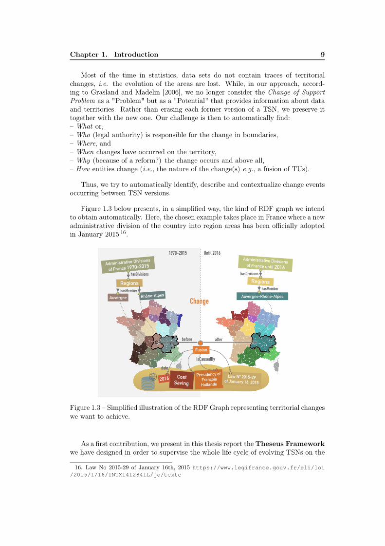
Most of the time in statistics, data sets do not contain traces of territorialchanges, i.e. the evolution of the areas are lost. While, in our approach, accord-ing to Grasland and Madelin [2006], we no longer consider the Change of SupportProblem as a "Problem" but as a "Potential" that provides information about dataand territories. Rather than erasing each former version of a TSN, we preserve ittogether with the new one. Our challenge is then to automatically find:– What or,– Who (legal authority) is responsible for the change in boundaries,– Where, and– When changes have occurred on the territory,– Why (because of a reform?) the change occurs and above all,– How entities change (i.e., the nature of the change(s) e.g., a fusion of TUs).

Thus, we try to automatically identify, describe and contextualize change eventsoccurring between TSN versions.

Figure 1.3 below presents, in a simplified way, the kind of RDF graph we intendto obtain automatically. Here, the chosen example takes place in France where a newadministrative division of the country into region areas has been officially adoptedin January 2015 16.

Fusion

Presidency of François Hollande

Cost Saving

Change

Law Nº 2015-29 of January 16, 2015

2016

before after

Administrative Divisions of France until 2016hasDivisions

Regions

Administrative Divisions

of France 1970-2015 hasDivisions

date

Auvergne Rhône-AlpeshasMember

RegionshasMember

Auvergne-Rhône-Alpes

isCausedBy

1970-2015 Until 2016

Figure 1.3 – Simplified illustration of the RDF Graph representing territorial changeswe want to achieve.

As a first contribution, we present in this thesis report theTheseus Frameworkwe have designed in order to supervise the whole life cycle of evolving TSNs on the

16. Law No 2015-29 of January 16th, 2015 https://www.legifrance.gouv.fr/eli/loi/2015/1/16/INTX1412841L/jo/texte

10 1.4. Thesis Outline

LOD Web: from the modeling of geographic areas to the exploitation of TSNs(and their successive versions) on the LOD Web. This framework is intended forStatistical Agencies, statisticians, or researchers who wish to publish on the LODWeb successive version of their TSN, as well as change and similarity descriptionsbetween the versions i.e., filiation links between the features throughout the versions.Its main objective is to automate the detection and semantic description of a setof well identified processes (merge, split etc.) that characterize the evolution ofTSNs and of all their features (levels, TUs), adopting a multi-level approach for thedescription of the territorial structure, as well as for the description of the changesthat impact the embedded features of TSNs.

As a second contribution, this Theseus framework encapsulates two ontologies wehave designed, called TSN-Ontology and TSN-Change Ontology. Their goal istwofold: unambiguous identification of the statistical areas in time and space, andthe description of their filiation links (comprising similarity and change descriptions)over time on the Linked Open Data (LOD) Web.

Theseus also embeds an implementation of an extended version of the Algorithmfor Automatic Matching of Two TSN Versions of [Plumejeaud, 2011]. This adapta-tion, called the TSN Semantic Matching Algorithm, is our third contribution.It has been designed to automate both the detection and the description on theLOD Web of territorial similarities and changes among various TSNs. Together,all the software modules of the Theseus framework contribute to the publicationon the LOD Web of TSNs semantic history graphs. Those latter constitutecatalogs of evolving statistical areas that enhance the understanding of dynamicsof the territories, providing statisticians, researchers, citizens with descriptions tocomprehend the motivations and the impact of changes.

Theseus is then a step towards the generation of knowledge graphs of evolvinggeo-coded statistics that link several ontologies and data sets: RDF Data Cubedata sets, geospatial TSN data sets, (historical) event data sets, law data sets...from which one could build intelligent tools for the analysis of the territorial dy-namics (e.g., analysis the territorial evolution together with demographic, economic,environmental indicators, information on the history of the territories...) . Thesetools could be capable of inferring new data (such as estimating statistical values ina new TSN version).

1.4 Thesis Outline

In Chapter II, we present in more details the topic of this thesis. We describethe current states of Territorial Statistical Information (TSI), an information madeof two peaces: the statistical information (geo-coded statistics), and the geographicareas, organized into Territorial Statistical Nomenclature, used for the collectionand dissemination of official territorial statistics. We present the problems causedby the evolution of TSN over time.In Chapter III, we introduce the main spatiotemporal concepts involved in the mod-eling of evolving spatial entities, the fundamentals for the modeling of these entities,

Chapter 1. Introduction 11

and the existing approaches in the semantic Web.In Chapter IV, we present the fundamentals for the spatiotemporal modeling ofevolving TUs and TSNs, that are specific spatial entities, with a focus on the ap-proaches implemented in the semantic Web.In Chapter V, we evaluate the existing methods for automatically generating, thenexploiting in the semantic Web, descriptions of evolving TUs (descriptions of theirlife, filiation and changes over time).In Chapter VI, we make a synthesis of the state of the art, and we list the require-ments that a system managing the whole life cycle of evolving TSNs in the SemanticWeb should meet.In Chapter VII, we introduce Theseus, a configurable framework designed for man-aging evolving TSNs in the semantic Web, according to a management process thatconsists of the following activities: Specify, Model, Generate, Publish, and Exploit.In Chapter VIII, we present the main component of Theseus, a ontological model,made of two ontologies, called TSN Ontology and TSN-Change Ontology, designedin order to describe in the semantic Web any TSN hierarchical structure and itschanges over time.In Chapter IX, we describe the two workflows created in order to populate our TSNontological model. We present, in particular, the TSN Semantic Matching Algo-rithm designed in order to automatically detect and describe, on the LOD Web,similarities and changes of TSN structures throughout their versions.In Chapter X, we present experiments performed on three very different TSNs inorder to evaluate our Theseus Framework and the performances of the TSN Seman-tic Matching Algorithm.In Chapter XI, we show how to explore and exploit data created by Theseus, inparticular how to explore territorial change descriptions and how to exploit themwith other data on the LOD Web, such as Linked Open statistical Data.In the concluding Chapter, we list the main contributions of the thesis. We discussthe limitations of our work that focuses on a specif type of geographic divisions. Wepresent how one could extend our approach, and some perspectives for future workin this respect.

Part A

State of the Art

Chapter 2

Territorial Statistical Information

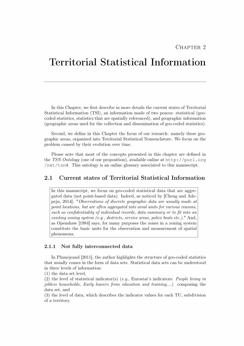
In this Chapter, we first describe in more details the current states of TerritorialStatistical Information (TSI), an information made of two peaces: statistical (geo-coded statistics, statistics that are spatially referenced), and geographic information(geographic areas used for the collection and dissemination of geo-coded statistics).

Second, we define in this Chapter the focus of our research: namely these geo-graphic areas, organized into Territorial Statistical Nomenclature. We focus on theproblem caused by their evolution over time.

Please note that most of the concepts presented in this chapter are defined inthe TSN Ontology (one of our proposition), available online at http://purl.org/net/tsn#. This ontology is an online glossary associated to this manuscript.

2.1 Current states of Territorial Statistical Information

In this manuscript, we focus on geo-coded statistical data that are aggre-gated data (not point-based data). Indeed, as noticed by [Cheng and Ade-peju, 2014]: "Observations of discrete geographic data are usually made atpoint locations, but are often aggregated into areal units for various reasons,such as confidentiality of individual records, data summary or to fit into anexisting zoning system (e.g., districts, service areas, police beats etc.)." And,as Openshaw [1984] says, for many purposes the zones in a zoning systemconstitute the basic units for the observation and measurement of spatialphenomena.

2.1.1 Not fully interconnected data

In Plumejeaud [2011], the author highlights the structure of geo-coded statisticsthat usually comes in the form of data sets. Statistical data sets can be understoodin three levels of information:(1) the data set level,(2) the level of statistical indicator(s) (e.g., Eurostat’s indicators: People living injobless households, Early leavers from education and training,...) composing thedata set, and(3) the level of data, which describes the indicator values for each TU, subdivisionof a territory.

16 2.1. Current states of Territorial Statistical Information

Although statistics produced by (N)SAs, and geographic information producedby National Mapping Agencies have a strong connection because geo-coded statisticsmeasure some observed phenomenon that lives on a territory, most of the time, onthe Open Data Web they are available in separated data sets. They are generallydistributed in different formats, using different Web Services (SDMX REST Webservices for the statistics 1, and OGC Web services (WFS 2, WMS 3, CSW 4...) forthe geographic information). And, even when they are distributed in the sameformat (CSV or XML for instance), most of the time the two types of informationare described using different data models that are not fully interconnected.

We focus now on the European context because the European territory is aninteresting case of study: it is a vast and multi-level territory where directives suchas the Open Data Directive and the INSPIRE Directive 5 accelerate the sharing ofstandardized information across Europe. Some standards enable the descriptionof geographic information (e.g. ISO-19115), while others enable the description ofstatistical information (e.g. ISO-17369/SDMX). Sometime, specifications addressboth statistical and territorial aspects, but every time one of the aspects is muchmore accurately described then the other. In Europe, standards data models addressboth statistical and territorial aspects, for example: the INSPIRE metadata modelsand, the Euro-SDMX Metadata Structure (ESMS) model.

The Eurostat organization has built the Euro-SDMXMetadata Structure (ESMS)model on a subset of the SDMX one [Gotzfried and Pellegrino, 2008]. The SDMXinitiative fosters standards for the exchange of statistical information 6. The under-lying purpose is to improve the interoperability of systems that manage statisticaldata and metadata [SDMX, 2012]. SDMX defines a data and metadata structureadapted to the statistical datasets implementation. The ESMS model is availableas a spreadsheet file 7 that lists the 21 SDMX key concepts chosen by Eurostat inorder to describe their statistical data (see an extract of this model in Figure 2.1).

1. For instance, the REST SDMX API of Eurostat gives access to the Eurostat data (https://ec.europa.eu/eurostat/web/sdmx-web-services/rest-sdmx-2.1

2. https://www.opengeospatial.org/standards/wfs3. https://www.opengeospatial.org/standards/wms4. https://www.opengeospatial.org/standards/cat5. The INSPIRE Directive requires producers of digital geographic data to apply rules for their

harmonization, standardization and dissemination. More broadly, this directive aims at improvingthe access to spatial information across Europe by fostering cooperation between institutions, sothat they share common tools and build together a network of SDI at European level. https://inspire.ec.europa.eu/inspire-directive/2

6. http://sdmx.org/7. http://ec.europa.eu/eurostat/data/metadata/metadata-structure

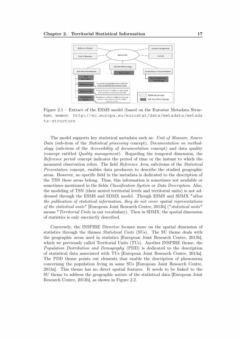
Chapter 2. Territorial Statistical Information 17

Figure 2.1 – Extract of the ESMS model (based on the Eurostat Metadata Struc-ture, source: http://ec.europa.eu/eurostat/data/metadata/metadata-structure

The model supports key statistical metadata such as: Unit of Measure, SourceData (sub-item of the Statistical processing concept), Documentation on method-ology (sub-item of the Accessibility of documentation concept) and data quality(concept entitled Quality management). Regarding the temporal dimension, theReference period concept indicates the period of time or the instant to which themeasured observation refers. The field Reference Area, sub-items of the StatisticalPresentation concept, enables data producers to describe the studied geographicareas. However, no specific field in the metadata is dedicated to the description ofthe TSN these areas belong. Thus, this information is sometimes not available orsometimes mentioned in the fields Classification System or Data Description. Also,the modeling of TSN (their nested territorial levels and territorial units) is not ad-dressed through the ESMS and SDMX model. Though ESMS and SDMX "allowthe publication of statistical information, they do not cover spatial representationsof the statistical units" [European Joint Research Centre, 2013b] ("statistical units"means "Territorial Units in our vocabulary). Then in SDMX, the spatial dimensionof statistics is only succinctly described.

Conversely, the INSPIRE Directive focuses more on the spatial dimension ofstatistics through the themes Statistical Units (SUs). The SU theme deals withthe geographic areas used in statistics [European Joint Research Centre, 2013b],which we previously called Territorial Units (TUs). Another INSPIRE theme, thePopulation Distribution and Demography (PDD) is dedicated to the descriptionof statistical data associated with TUs [European Joint Research Centre, 2013a].The PDD theme points out elements that enable the description of phenomenaconcerning the population living in some SUs [European Joint Research Centre,2013a]. This theme has no direct spatial features. It needs to be linked to theSU theme to address the geographic nature of the statistical data [European JointResearch Centre, 2013b], as shown in Figure 2.2.

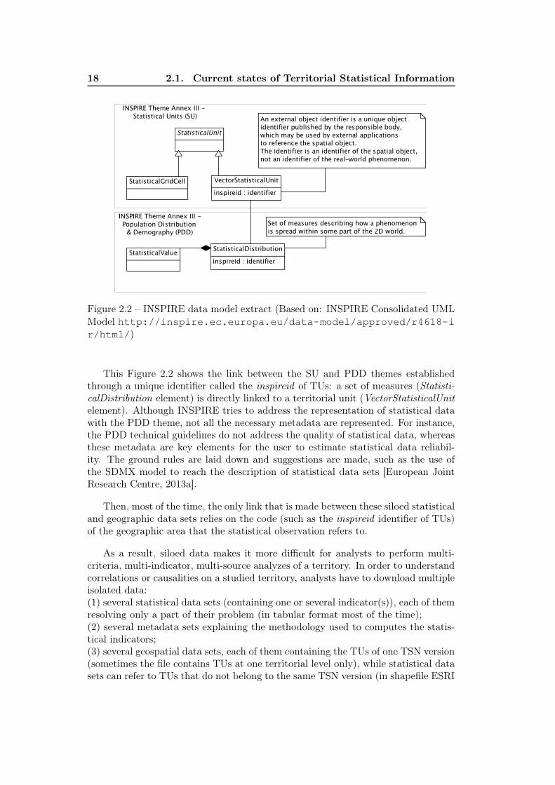
18 2.1. Current states of Territorial Statistical Information

StatisticalUnit

StatisticalGridCell

An external object identifier is a unique object identifier published by the responsible body, which may be used by external applications to reference the spatial object. The identifier is an identifier of the spatial object, not an identifier of the real-world phenomenon.

VectorStatisticalUnit

inspireid : identifier

INSPIRE Theme Annex III - Statistical Units (SU)

StatisticalDistribution

inspireid : identifierStatisticalValue

Set of measures describing how a phenomenon is spread within some part of the 2D world.

INSPIRE Theme Annex III -Population Distribution

& Demography (PDD)

Figure 2.2 – INSPIRE data model extract (Based on: INSPIRE Consolidated UMLModel http://inspire.ec.europa.eu/data-model/approved/r4618-ir/html/)

This Figure 2.2 shows the link between the SU and PDD themes establishedthrough a unique identifier called the inspireid of TUs: a set of measures (Statisti-calDistribution element) is directly linked to a territorial unit (VectorStatisticalUnitelement). Although INSPIRE tries to address the representation of statistical datawith the PDD theme, not all the necessary metadata are represented. For instance,the PDD technical guidelines do not address the quality of statistical data, whereasthese metadata are key elements for the user to estimate statistical data reliabil-ity. The ground rules are laid down and suggestions are made, such as the use ofthe SDMX model to reach the description of statistical data sets [European JointResearch Centre, 2013a].

Then, most of the time, the only link that is made between these siloed statisticaland geographic data sets relies on the code (such as the inspireid identifier of TUs)of the geographic area that the statistical observation refers to.

As a result, siloed data makes it more difficult for analysts to perform multi-criteria, multi-indicator, multi-source analyzes of a territory. In order to understandcorrelations or causalities on a studied territory, analysts have to download multipleisolated data:(1) several statistical data sets (containing one or several indicator(s)), each of themresolving only a part of their problem (in tabular format most of the time);(2) several metadata sets explaining the methodology used to computes the statis-tical indicators;(3) several geospatial data sets, each of them containing the TUs of one TSN version(sometimes the file contains TUs at one territorial level only), while statistical datasets can refer to TUs that do not belong to the same TSN version (in shapefile ESRI

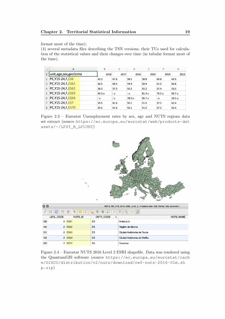
Chapter 2. Territorial Statistical Information 19

format most of the time);(4) several metadata files describing the TSN versions, their TUs used for calcula-tion of the statistical values and their changes over time (in tabular format most ofthe time).

Figure 2.3 – Eurostat Unemployment rates by sex, age and NUTS regions dataset extract (source https://ec.europa.eu/eurostat/web/products-datasets/-/LFST_R_LFU3RT)

Figure 2.4 – Eurostat NUTS 2016 Level 2 ESRI shapefile. Data was rendered usingthe QuantumGIS software (source https://ec.europa.eu/eurostat/cache/GISCO/distribution/v2/nuts/download/ref-nuts-2016-01m.shp.zip)

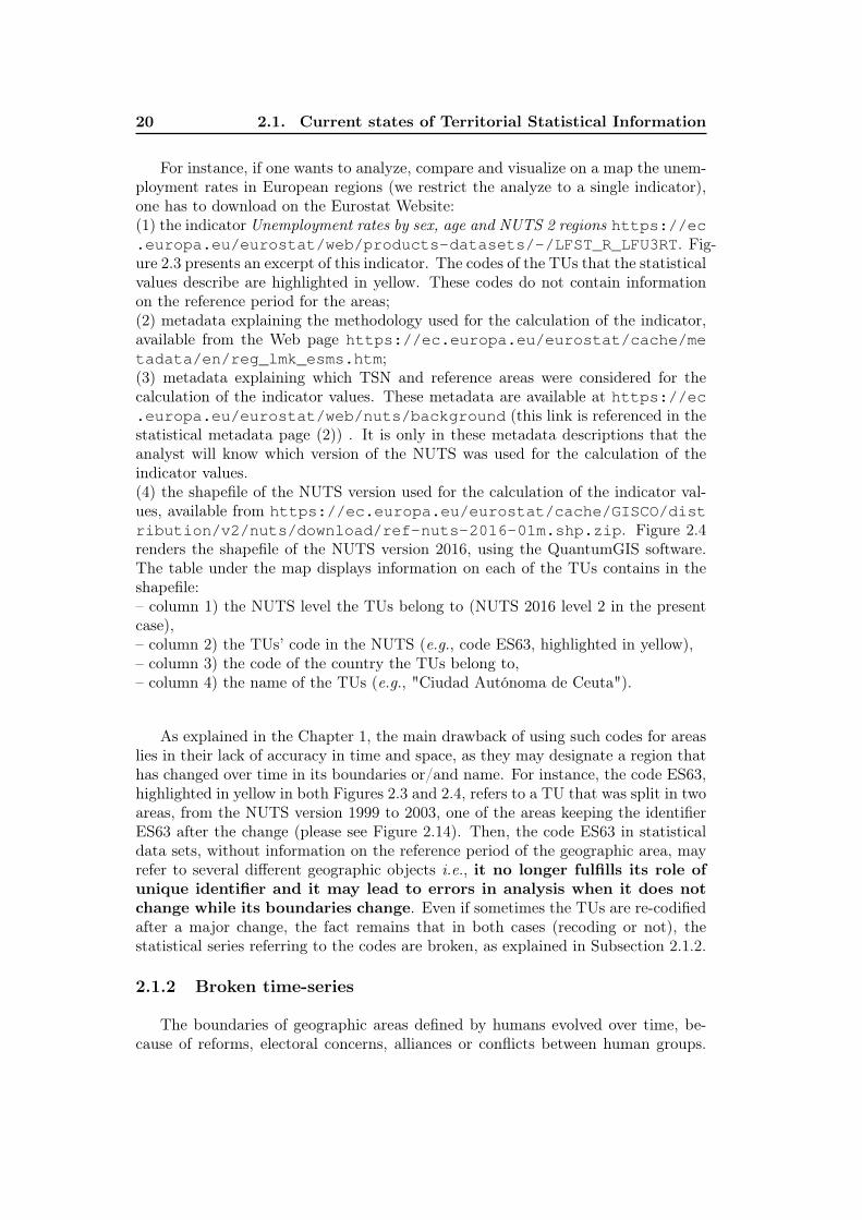
20 2.1. Current states of Territorial Statistical Information

For instance, if one wants to analyze, compare and visualize on a map the unem-ployment rates in European regions (we restrict the analyze to a single indicator),one has to download on the Eurostat Website:(1) the indicator Unemployment rates by sex, age and NUTS 2 regions https://ec.europa.eu/eurostat/web/products-datasets/-/LFST_R_LFU3RT. Fig-ure 2.3 presents an excerpt of this indicator. The codes of the TUs that the statisticalvalues describe are highlighted in yellow. These codes do not contain informationon the reference period for the areas;(2) metadata explaining the methodology used for the calculation of the indicator,available from the Web page https://ec.europa.eu/eurostat/cache/metadata/en/reg_lmk_esms.htm;(3) metadata explaining which TSN and reference areas were considered for thecalculation of the indicator values. These metadata are available at https://ec.europa.eu/eurostat/web/nuts/background (this link is referenced in thestatistical metadata page (2)) . It is only in these metadata descriptions that theanalyst will know which version of the NUTS was used for the calculation of theindicator values.(4) the shapefile of the NUTS version used for the calculation of the indicator val-ues, available from https://ec.europa.eu/eurostat/cache/GISCO/distribution/v2/nuts/download/ref-nuts-2016-01m.shp.zip. Figure 2.4renders the shapefile of the NUTS version 2016, using the QuantumGIS software.The table under the map displays information on each of the TUs contains in theshapefile:– column 1) the NUTS level the TUs belong to (NUTS 2016 level 2 in the presentcase),– column 2) the TUs’ code in the NUTS (e.g., code ES63, highlighted in yellow),– column 3) the code of the country the TUs belong to,– column 4) the name of the TUs (e.g., "Ciudad Autónoma de Ceuta").

As explained in the Chapter 1, the main drawback of using such codes for areaslies in their lack of accuracy in time and space, as they may designate a region thathas changed over time in its boundaries or/and name. For instance, the code ES63,highlighted in yellow in both Figures 2.3 and 2.4, refers to a TU that was split in twoareas, from the NUTS version 1999 to 2003, one of the areas keeping the identifierES63 after the change (please see Figure 2.14). Then, the code ES63 in statisticaldata sets, without information on the reference period of the geographic area, mayrefer to several different geographic objects i.e., it no longer fulfills its role ofunique identifier and it may lead to errors in analysis when it does notchange while its boundaries change. Even if sometimes the TUs are re-codifiedafter a major change, the fact remains that in both cases (recoding or not), thestatistical series referring to the codes are broken, as explained in Subsection 2.1.2.

2.1.2 Broken time-series

The boundaries of geographic areas defined by humans evolved over time, be-cause of reforms, electoral concerns, alliances or conflicts between human groups.

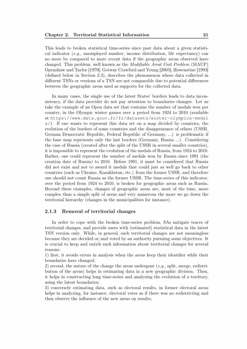
Chapter 2. Territorial Statistical Information 21

This leads to broken statistical time-series since past data about a given statisti-cal indicator (e.g., unemployed number, income distribution, life expectancy) canno more be compared to more recent data if the geographic areas observed havechanged. This problem, well known as the Modifiable Areal Unit Problem (MAUP)Openshaw and Taylor [1979]; Gotway Crawford and Young [2005]; Howenstine [1993](defined below in Section 2.3), describes the phenomenon where data collected indifferent TSNs or versions of a TSN are not comparable due to potential differencesbetween the geographic areas used as supports for the collected data.

In many cases, the single use of the latest States’ borders leads to data incon-sistency, if the data provider do not pay attention to boundaries changes. Let ustake the example of an Open data set that contains the number of medals won percountry, in the Olympic winter games over a period from 1924 to 2010 (availableat https://www.data.gouv.fr/fr/datasets/winter-olympics-medals/). If one wants to represent this data set on a map divided by countries, theevolution of the borders of some countries and the disappearance of others (USSR,German Democratic Republic, Federal Republic of Germany, ...) is problematic ifthe base map represents only the last borders (Germany, Russia ...). Consideringthe case of Russia (created after the split of the USSR in several smaller countries),it is impossible to represent the evolution of the medals of Russia, from 1924 to 2010.Rather, one could represent the number of medals won by Russia since 1991 (thecreation date of Russia) to 2010. Before 1991, it must be considered that Russiadid not exist and not to award it medals that could just as well go back to othercountries (such as Ukraine, Kazakhstan, etc.) from the former USSR, and thereforeone should not count Russia as the former USSR. The time-series of this indicator,over the period from 1924 to 2010, is broken for geographic areas such as Russia.Beyond these examples, changes of geographic areas are, most of the time, morecomplex than a simple split of areas and very numerous the more we go down theterritorial hierarchy (changes in the municipalities for instance).

2.1.3 Removal of territorial changes

In order to cope with the broken time-series problem, SAs mitigate traces ofterritorial changes, and provide users with (estimated) statistical data in the latestTSN version only. While, in general, such territorial changes are not meaninglessbecause they are decided or/and voted by an authority pursuing some objectives. Itis crucial to keep and enrich such information about territorial changes for severalreasons:1) first, it avoids errors in analysis when the areas keep their identifier while theirboundaries have changed;2) second, the nature of the change the areas undergone (e.g., split, merge, redistri-bution of the areas) helps in estimating data in a new geographic division. Then,it helps in constructing long time-series and analyzing the evolution of a territory,using the latest boundaries;3) conversely estimating data, such as electoral results, in former electoral areashelps in analyzing, for instance, electoral votes as if there was no redistricting andthen observe the influence of the new areas on results;

22 2.2. Territorial Statistical Nomenclature Structures

4) and finally, knowing which area has changed, because of which event or law helpsin understanding the reason for the change. For instance, the fusion of the French re-gions in 2016 was acted by a law that aims at reducing the number of administrativelevels for cost saving purposes.

In this Section, we have identified three issues (not fully interconnected data,broken time-series, removal of territorial changes) related to the TSI. In the nextSection, we describe in more details the geographic part of the TSI i.e., the Terri-torial Statistical Nomenclatures.

2.2 Territorial Statistical Nomenclature Structures

GEOGRAPHIC DIVISIONS TERRITORIAL STATISTICAL NOMENCLATURE

TERRITORIAL UNIT

Figure 2.5 – Schema ofa Territorial StatisticalNomenclature Structure.

Although Geographic Divisions vary in nature (e.g.,regular/irregular shapes, contiguous/non contiguous ar-eas, etc.) or in the territories they cover (States,metropolises, etc.), they have in common to draw fron-tiers dividing the geographical space into TerritorialUnits (TUs).A Territorial Unit, in this thesis manuscript, refers toa bounded geographic area (a portion of space on Earthe.g., a Region in Europe) delimited by and under the con-trol of a human group (in general a political or admin-istrative authority) [Sack, 1983]. Territorial StatisticalNomenclatures (TSNs) are composed of one or severalstandard geographic divisions, built by (N)SAs to ob-serve a territory at several geographic levels (e.g., coun-tries, regions, districts, municipalities, ...). They are setsof artifact (embedded) areas designed for statistical pur-pose, although they usually derived from a political oradministrative structure. Together, the embedded geo-graphic divisions of a TSN form a territorial hierarchy.

In the literature, the following terms may refer to geographic divisions: zoning,partition, mesh. In this manuscript, we will use these terms interchangeably.

In the literature, the following terms may refer to a TSN: Hierarchy of Census Ge-ographic Entities 8 ; Hierarchy of standard geographic units/Hierarchy of geographicareas used for disseminating data 9 ; Statistical Geography Standard/Standard Ge-ographical Classification 10 ; Nomenclature of territorial units for statistics 11. In

8. Source: United States of America Census Bureau, the principal agency of the U.S. FederalStatistical Systemhttps://www.census.gov/geo/reference/hierarchy.html

9. Source: Statistics Canada, the national statistical office of Canada https://www12.statcan.gc.ca/census-recensement/2016/ref/98-304/chap12-eng.cfm10. Source: Australian Bureau of Statistics https://www.abs.gov.au/websitedbs/d331

0114.nsf/home/geography11. Source: Eurostat, the European Statistical Office https://ec.europa.eu/eurostat/

web/nuts/background

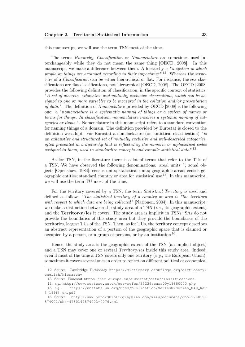
Chapter 2. Territorial Statistical Information 23

this manuscript, we will use the term TSN most of the time.

The terms Hierarchy, Classification or Nomenclature are sometimes used in-terchangeably while they do not mean the same thing [OECD, 2008]. In thismanuscript, we make a difference between them. A hierarchy is "a system in whichpeople or things are arranged according to their importance" 12. Whereas the struc-ture of a Classification can be either hierarchical or flat. For instance, the sex clas-sifications are flat classifications, not hierarchical [OECD, 2008]. The OECD [2008]provides the following definition of classification, in the specific context of statistics:"A set of discrete, exhaustive and mutually exclusive observations, which can be as-signed to one or more variables to be measured in the collation and/or presentationof data.". The definition of Nomenclature provided by OECD [2008] is the followingone: a "nomenclature is a systematic naming of things or a system of names orterms for things. In classification, nomenclature involves a systemic naming of cat-egories or items.". Nomenclature in this manuscript refers to a standard conventionfor naming things of a domain. The definition provided by Eurostat is closed to thedefinition we adopt. For Eurostat a nomenclature (or statistical classification) "isan exhaustive and structured set of mutually exclusive and well-described categories,often presented in a hierarchy that is reflected by the numeric or alphabetical codesassigned to them, used to standardize concepts and compile statistical data" 13.

As for TSN, in the literature there is a lot of terms that refer to the TUs ofa TSN. We have observed the following denominations: areal units 14; zonal ob-jects [Openshaw, 1984]; census units; statistical units; geographic areas; census ge-ographic entities; standard country or area for statistical use 15. In this manuscript,we will use the term TU most of the time.

For the territory covered by a TSN, the term Statistical Territory is used anddefined as follows "The statistical territory of a country or area is "the territorywith respect to which data are being collected" [Nationen, 2004]. In this manuscript,we make a distinction between the study area of a TSN (i.e., its geographic extent)and the Territor-y/ies it covers. The study area is implicit in TSNs: SAs do notprovide the boundaries of this study area but they provide the boundaries of theterritories, largest TUs of the TSN. Then, as for TUs, the territory concept describesan abstract representation of a portion of the geographic space that is claimed oroccupied by a person, or a group of persons, or by an institution 16.

Hence, the study area is the geographic extent of the TSN (an implicit object)and a TSN may cover one or several Territory/ies inside this study area. Indeed,even if most of the time a TSN covers only one territory (e.g., the European Union),sometimes it covers several ones in order to reflect on different political or economical

12. Source: Cambridge Dictionary https://dictionary.cambridge.org/dictionary/english/hierarchy13. Source: Eurostat https://ec.europa.eu/eurostat/data/classifications14. e.g., http://www.restore.ac.uk/geo-refer/35236ceurs00y19880000.php15. e.g., https://unstats.un.org/unsd/publication/SeriesM/Series_M49_Rev

3(1996)_en.pdf16. Source: http://www.oxfordbibliographies.com/view/document/obo-9780199

874002/obo-9780199874002-0076.xml

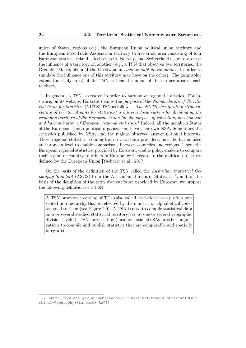
24 2.2. Territorial Statistical Nomenclature Structures

union of States, regions (e.g., the European Union political union territory andthe European Free Trade Association territory (a free trade area consisting of fourEuropean states: Iceland, Liechtenstein, Norway, and Switzerland)), or to observethe influence of a territory on another (e.g., a TSN that observes two territories, theGrenoble Metropolis and the Gresivaudan communauté de communes, in order tosimulate the influence one of this territory may have on the other). The geographicextent (or study area) of the TSN is then the union of the surface area of eachterritory.

In general, a TSN is created in order to harmonize regional statistics. For in-stance, on its website, Eurostat defines the purpose of the Nomenclature of Territo-rial Units for Statistics (NUTS) TSN as follows: "The NUTS classification (Nomen-clature of territorial units for statistics) is a hierarchical system for dividing up theeconomic territory of the European Union for the purpose of collection, developmentand harmonization of European regional statistics." Indeed, all the members Statesof the European Union political organization, have their own NSA. Sometimes thestatistics published by NSAs and the regions observed answer national interests.Those regional statistics, coming from several data providers, must be harmonizedat European level to enable comparisons between countries and regions. Then, theEuropean regional statistics, provided by Eurostat, enable policy-makers to comparetheir region or country to others in Europe, with regard to the political objectivesdefined by the European Union [Ysebaert et al., 2017].

On the basis of the definition of the TSN called the Australian Statistical Ge-ography Standard (ASGS) from the Australian Bureau of Statistics 17, and on thebasis of the definition of the term Nomenclature provided by Eurostat, we proposethe following definition of a TSN:

A TSN provides a catalog of TUs (also called statistical areas), often pre-sented in a hierarchy that is reflected by the numeric or alphabetical codesassigned to them (see Figure 2.9). A TSN is used to compile statistical dataon a or several studied statistical territory/ies, at one or several geographicdivision level(s). TSNs are used by (local or national) SAs or other organi-zations to compile and publish statistics that are comparable and spatiallyintegrated.

17. http://www.abs.gov.au/websitedbs/D3310114.nsf/home/Australian+Statistical+Geography+Standard+(ASGS)

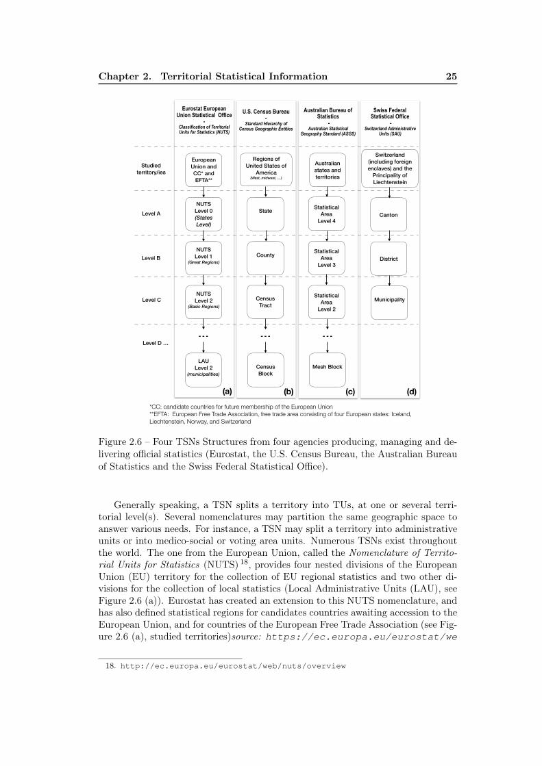
Chapter 2. Territorial Statistical Information 25

Eurostat European Union Statistical Office

- Classification of Territorial Units for Statistics (NUTS)

European Union and CC* and EFTA**

NUTS Level 0 (States Level)

NUTS Level 1

(Great Regions)

NUTS Level 2

(Basic Regions)

LAU Level 2

(municipalities)

…

(a)

U.S. Census Bureau -

Standard Hierarchy of Census Geographic Entities

State

County

Census Block

Regions of United States of

America (West, midwest, …)

Census Tract

(b)

Australian Bureau of Statistics

- Australian Statistical

Geography Standard (ASGS)

Australian states and territories

Statistical Area

Level 4

Statistical Area

Level 3

Mesh Block

…

(c)

Swiss Federal Statistical Office

- Switzerland Administrative

Units (SAU)

Switzerland (including foreign enclaves) and the

Principality of Liechtenstein

Canton

District

Municipality

(d)

Studied territory/ies

Level A

Level B

Level C

Level D …

Statistical Area

Level 2

*CC: candidate countries for future membership of the European Union **EFTA: European Free Trade Association, free trade area consisting of four European states: Iceland, Liechtenstein, Norway, and Switzerland

…

Figure 2.6 – Four TSNs Structures from four agencies producing, managing and de-livering official statistics (Eurostat, the U.S. Census Bureau, the Australian Bureauof Statistics and the Swiss Federal Statistical Office).

Generally speaking, a TSN splits a territory into TUs, at one or several terri-torial level(s). Several nomenclatures may partition the same geographic space toanswer various needs. For instance, a TSN may split a territory into administrativeunits or into medico-social or voting area units. Numerous TSNs exist throughoutthe world. The one from the European Union, called the Nomenclature of Territo-rial Units for Statistics (NUTS) 18, provides four nested divisions of the EuropeanUnion (EU) territory for the collection of EU regional statistics and two other di-visions for the collection of local statistics (Local Administrative Units (LAU), seeFigure 2.6 (a)). Eurostat has created an extension to this NUTS nomenclature, andhas also defined statistical regions for candidates countries awaiting accession to theEuropean Union, and for countries of the European Free Trade Association (see Fig-ure 2.6 (a), studied territories)source: https://ec.europa.eu/eurostat/we

18. http://ec.europa.eu/eurostat/web/nuts/overview

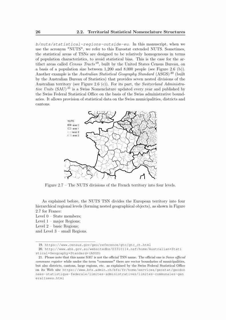
26 2.2. Territorial Statistical Nomenclature Structures

b/nuts/statistical-regions-outside-eu. In this manuscript, when weuse the acronym "NUTS", we refer to this Eurostat extended NUTS. Sometimes,the statistical areas of TSNs are designed to be relatively homogeneous in termsof population characteristics, to avoid statistical bias. This is the case for the ar-tifact areas called Census Tracts 19, built by the United States Census Bureau, ona basis of a population size between 1,200 and 8,000 people (see Figure 2.6 (b)).Another example is the Australian Statistical Geography Standard (ASGS) 20 (builtby the Australian Bureau of Statistics) that provides seven nested divisions of theAustralian territory (see Figure 2.6 (c)). For its part, the Switzerland Administra-tive Units (SAU) 21 is a Swiss Nomenclature updated every year and published bythe Swiss Federal Statistical Office on the basis of the Swiss administrative bound-aries. It allows provision of statistical data on the Swiss municipalities, districts andcantons.

Figure 2.7 – The NUTS divisions of the French territory into four levels.

As explained before, the NUTS TSN divides the European territory into fourhierarchical regional levels (forming nested geographical objects), as shown in Figure2.7 for France:Level 0 – State members;Level 1 – major Regions;Level 2 – basic Regions;and Level 3 – small Regions.

19. https://www.census.gov/geo/reference/gtc/gtc_ct.html20. http://www.abs.gov.au/websitedbs/D3310114.nsf/home/Australian+Stati

stical+Geography+Standard+(ASGS)21. Please note that this name SAU is not the official TSN name. The official one is Swiss official

commune register while under the term "commune" there are vector boundaries of municipalities,but also districts, cantons, large regions, etc. as explained by the Swiss Federal Statistical Officeon its Web site https://www.bfs.admin.ch/bfs/fr/home/services/geostat/geodonnees-statistique-federale/limites-administratives/limites-communales-generalisees.html

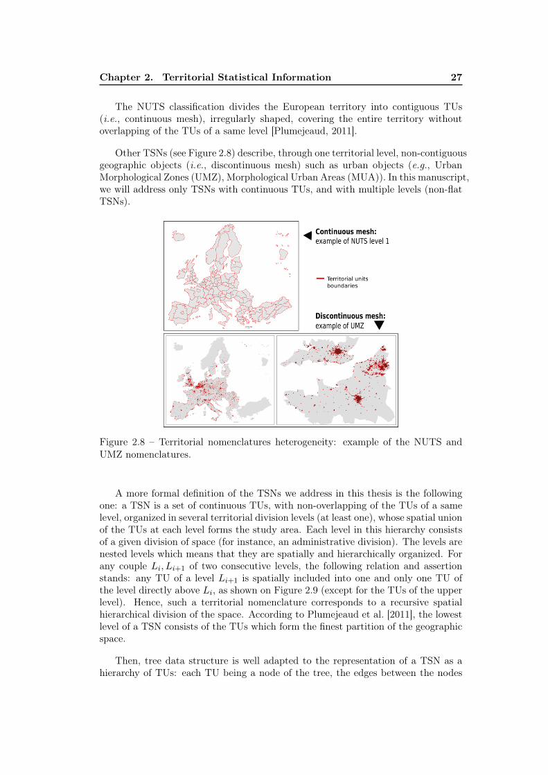
Chapter 2. Territorial Statistical Information 27

The NUTS classification divides the European territory into contiguous TUs(i.e., continuous mesh), irregularly shaped, covering the entire territory withoutoverlapping of the TUs of a same level [Plumejeaud, 2011].

Other TSNs (see Figure 2.8) describe, through one territorial level, non-contiguousgeographic objects (i.e., discontinuous mesh) such as urban objects (e.g., UrbanMorphological Zones (UMZ), Morphological Urban Areas (MUA)). In this manuscript,we will address only TSNs with continuous TUs, and with multiple levels (non-flatTSNs).

Figure 2.8 – Territorial nomenclatures heterogeneity: example of the NUTS andUMZ nomenclatures.

A more formal definition of the TSNs we address in this thesis is the followingone: a TSN is a set of continuous TUs, with non-overlapping of the TUs of a samelevel, organized in several territorial division levels (at least one), whose spatial unionof the TUs at each level forms the study area. Each level in this hierarchy consistsof a given division of space (for instance, an administrative division). The levels arenested levels which means that they are spatially and hierarchically organized. Forany couple Li, Li+1 of two consecutive levels, the following relation and assertionstands: any TU of a level Li+1 is spatially included into one and only one TU ofthe level directly above Li, as shown on Figure 2.9 (except for the TUs of the upperlevel). Hence, such a territorial nomenclature corresponds to a recursive spatialhierarchical division of the space. According to Plumejeaud et al. [2011], the lowestlevel of a TSN consists of the TUs which form the finest partition of the geographicspace.

Then, tree data structure is well adapted to the representation of a TSN as ahierarchy of TUs: each TU being a node of the tree, the edges between the nodes

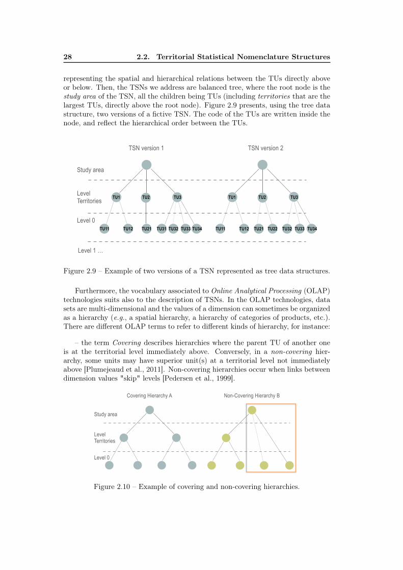
28 2.2. Territorial Statistical Nomenclature Structures

representing the spatial and hierarchical relations between the TUs directly aboveor below. Then, the TSNs we address are balanced tree, where the root node is thestudy area of the TSN, all the children being TUs (including territories that are thelargest TUs, directly above the root node). Figure 2.9 presents, using the tree datastructure, two versions of a fictive TSN. The code of the TUs are written inside thenode, and reflect the hierarchical order between the TUs.

Study area

Level Territories

Level 0

TSN version 1 TSN version 2

Level 1 …

TU1 TU2 TU3

TU11 TU12 TU21 TU31 TU32 TU33 TU34

TU1 TU2 TU3

TU11 TU12 TU21 TU22 TU32 TU33 TU34

Figure 2.9 – Example of two versions of a TSN represented as tree data structures.

Furthermore, the vocabulary associated to Online Analytical Processing (OLAP)technologies suits also to the description of TSNs. In the OLAP technologies, datasets are multi-dimensional and the values of a dimension can sometimes be organizedas a hierarchy (e.g., a spatial hierarchy, a hierarchy of categories of products, etc.).There are different OLAP terms to refer to different kinds of hierarchy, for instance:

– the term Covering describes hierarchies where the parent TU of another oneis at the territorial level immediately above. Conversely, in a non-covering hier-archy, some units may have superior unit(s) at a territorial level not immediatelyabove [Plumejeaud et al., 2011]. Non-covering hierarchies occur when links betweendimension values "skip" levels [Pedersen et al., 1999].

Covering Hierarchy A Non-Covering Hierarchy B

Study area

Level Territories

Level 0

Figure 2.10 – Example of covering and non-covering hierarchies.

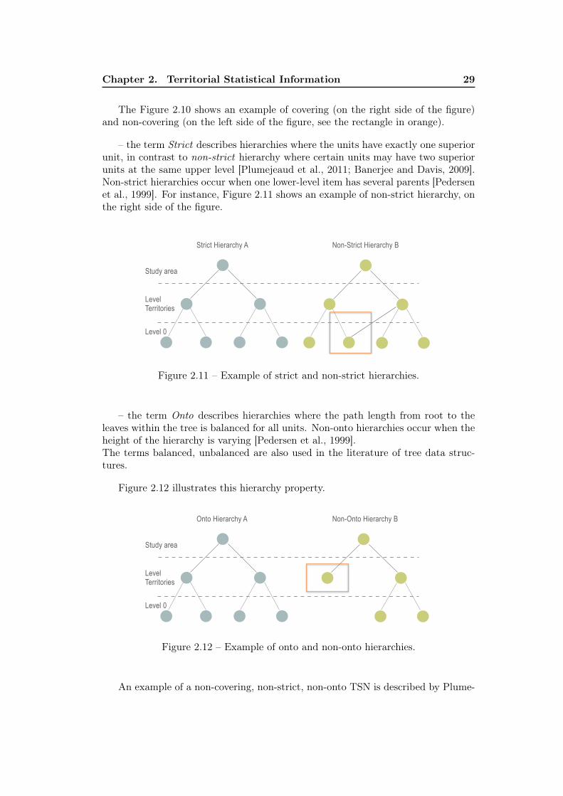
Chapter 2. Territorial Statistical Information 29

The Figure 2.10 shows an example of covering (on the right side of the figure)and non-covering (on the left side of the figure, see the rectangle in orange).

– the term Strict describes hierarchies where the units have exactly one superiorunit, in contrast to non-strict hierarchy where certain units may have two superiorunits at the same upper level [Plumejeaud et al., 2011; Banerjee and Davis, 2009].Non-strict hierarchies occur when one lower-level item has several parents [Pedersenet al., 1999]. For instance, Figure 2.11 shows an example of non-strict hierarchy, onthe right side of the figure.

Strict Hierarchy A Non-Strict Hierarchy B

Study area

Level Territories

Level 0

Figure 2.11 – Example of strict and non-strict hierarchies.

– the term Onto describes hierarchies where the path length from root to theleaves within the tree is balanced for all units. Non-onto hierarchies occur when theheight of the hierarchy is varying [Pedersen et al., 1999].The terms balanced, unbalanced are also used in the literature of tree data struc-tures.

Figure 2.12 illustrates this hierarchy property.

Onto Hierarchy A Non-Onto Hierarchy B

Study area

Level Territories

Level 0

Figure 2.12 – Example of onto and non-onto hierarchies.

An example of a non-covering, non-strict, non-onto TSN is described by Plume-

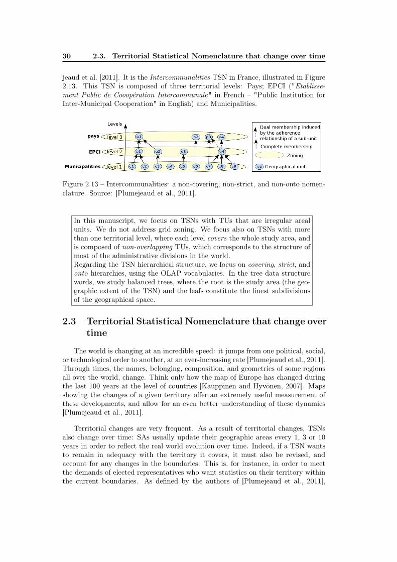
30 2.3. Territorial Statistical Nomenclature that change over time

jeaud et al. [2011]. It is the Intercommunalities TSN in France, illustrated in Figure2.13. This TSN is composed of three territorial levels: Pays; EPCI ("Etablisse-ment Public de Cooopération Intercommunale" in French – "Public Institution forInter-Municipal Cooperation" in English) and Municipalities.

Figure 2.13 – Intercommunalities: a non-covering, non-strict, and non-onto nomen-clature. Source: [Plumejeaud et al., 2011].

In this manuscript, we focus on TSNs with TUs that are irregular arealunits. We do not address grid zoning. We focus also on TSNs with morethan one territorial level, where each level covers the whole study area, andis composed of non-overlapping TUs, which corresponds to the structure ofmost of the administrative divisions in the world.Regarding the TSN hierarchical structure, we focus on covering, strict, andonto hierarchies, using the OLAP vocabularies. In the tree data structurewords, we study balanced trees, where the root is the study area (the geo-graphic extent of the TSN) and the leafs constitute the finest subdivisionsof the geographical space.

2.3 Territorial Statistical Nomenclature that change overtime

The world is changing at an incredible speed: it jumps from one political, social,or technological order to another, at an ever-increasing rate [Plumejeaud et al., 2011].Through times, the names, belonging, composition, and geometries of some regionsall over the world, change. Think only how the map of Europe has changed duringthe last 100 years at the level of countries [Kauppinen and Hyvönen, 2007]. Mapsshowing the changes of a given territory offer an extremely useful measurement ofthese developments, and allow for an even better understanding of these dynamics[Plumejeaud et al., 2011].

Territorial changes are very frequent. As a result of territorial changes, TSNsalso change over time: SAs usually update their geographic areas every 1, 3 or 10years in order to reflect the real world evolution over time. Indeed, if a TSN wantsto remain in adequacy with the territory it covers, it must also be revised, andaccount for any changes in the boundaries. This is, for instance, in order to meetthe demands of elected representatives who want statistics on their territory withinthe current boundaries. As defined by the authors of [Plumejeaud et al., 2011],

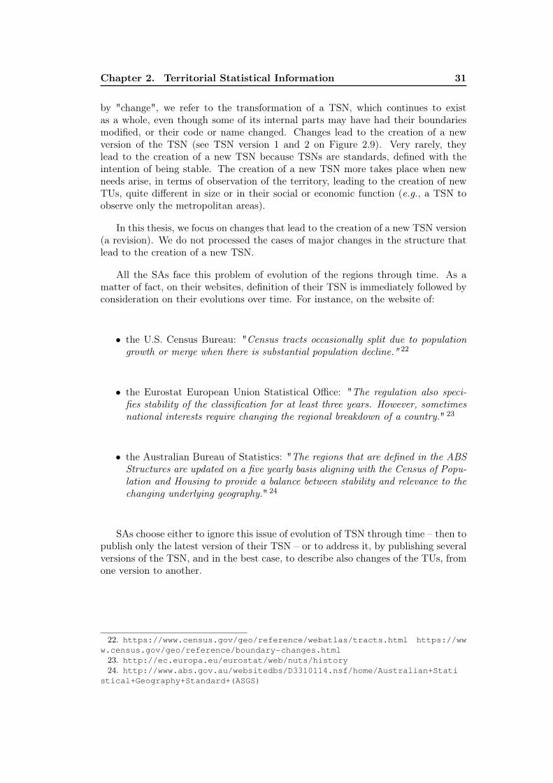
Chapter 2. Territorial Statistical Information 31

by "change", we refer to the transformation of a TSN, which continues to existas a whole, even though some of its internal parts may have had their boundariesmodified, or their code or name changed. Changes lead to the creation of a newversion of the TSN (see TSN version 1 and 2 on Figure 2.9). Very rarely, theylead to the creation of a new TSN because TSNs are standards, defined with theintention of being stable. The creation of a new TSN more takes place when newneeds arise, in terms of observation of the territory, leading to the creation of newTUs, quite different in size or in their social or economic function (e.g., a TSN toobserve only the metropolitan areas).

In this thesis, we focus on changes that lead to the creation of a new TSN version(a revision). We do not processed the cases of major changes in the structure thatlead to the creation of a new TSN.

All the SAs face this problem of evolution of the regions through time. As amatter of fact, on their websites, definition of their TSN is immediately followed byconsideration on their evolutions over time. For instance, on the website of:

• the U.S. Census Bureau: "Census tracts occasionally split due to populationgrowth or merge when there is substantial population decline." 22

• the Eurostat European Union Statistical Office: "The regulation also speci-fies stability of the classification for at least three years. However, sometimesnational interests require changing the regional breakdown of a country." 23

• the Australian Bureau of Statistics: "The regions that are defined in the ABSStructures are updated on a five yearly basis aligning with the Census of Popu-lation and Housing to provide a balance between stability and relevance to thechanging underlying geography." 24

SAs choose either to ignore this issue of evolution of TSN through time – then topublish only the latest version of their TSN – or to address it, by publishing severalversions of the TSN, and in the best case, to describe also changes of the TUs, fromone version to another.

22. https://www.census.gov/geo/reference/webatlas/tracts.html https://www.census.gov/geo/reference/boundary-changes.html23. http://ec.europa.eu/eurostat/web/nuts/history24. http://www.abs.gov.au/websitedbs/D3310114.nsf/home/Australian+Stati

stical+Geography+Standard+(ASGS)

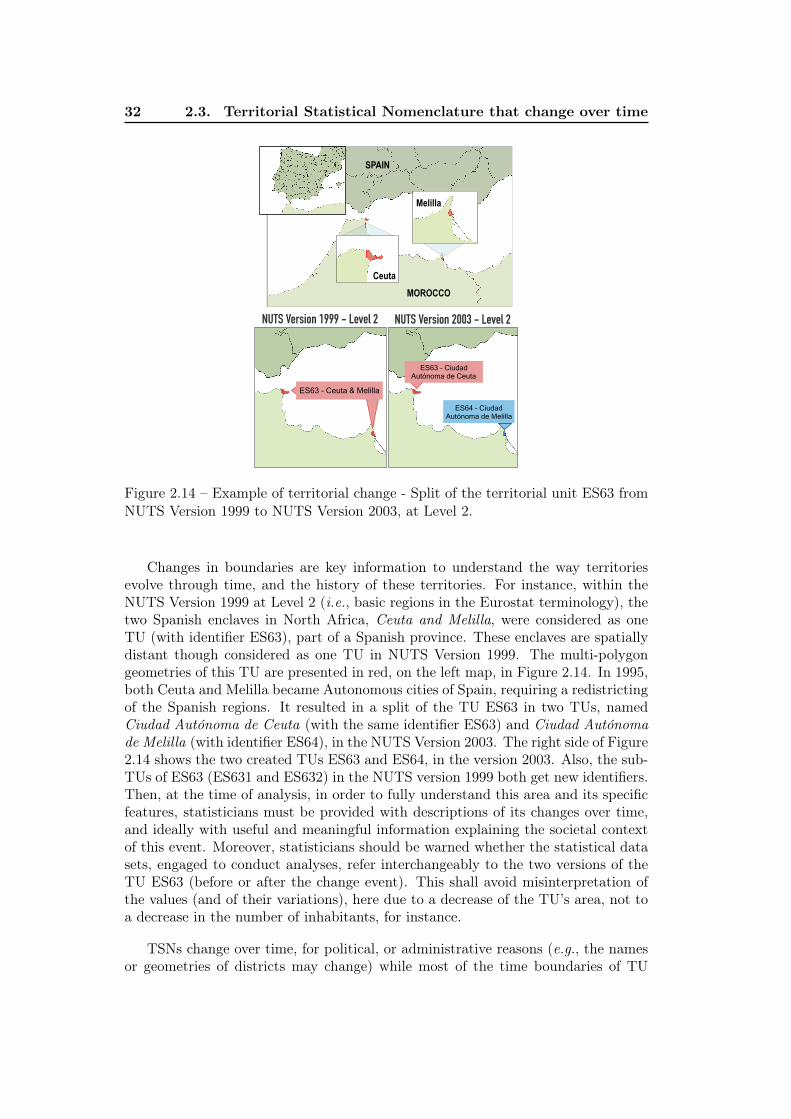
32 2.3. Territorial Statistical Nomenclature that change over time

NUTS Version 1999 - Level 2 NUTS Version 2003 - Level 2

ES63 - Ciudad Autónoma de Ceuta

ES64 - Ciudad Autónoma de Melilla

Ceuta

Melilla

SPAIN

MOROCCO

ES63 - Ceuta & Melilla

Figure 2.14 – Example of territorial change - Split of the territorial unit ES63 fromNUTS Version 1999 to NUTS Version 2003, at Level 2.

Changes in boundaries are key information to understand the way territoriesevolve through time, and the history of these territories. For instance, within theNUTS Version 1999 at Level 2 (i.e., basic regions in the Eurostat terminology), thetwo Spanish enclaves in North Africa, Ceuta and Melilla, were considered as oneTU (with identifier ES63), part of a Spanish province. These enclaves are spatiallydistant though considered as one TU in NUTS Version 1999. The multi-polygongeometries of this TU are presented in red, on the left map, in Figure 2.14. In 1995,both Ceuta and Melilla became Autonomous cities of Spain, requiring a redistrictingof the Spanish regions. It resulted in a split of the TU ES63 in two TUs, namedCiudad Autónoma de Ceuta (with the same identifier ES63) and Ciudad Autónomade Melilla (with identifier ES64), in the NUTS Version 2003. The right side of Figure2.14 shows the two created TUs ES63 and ES64, in the version 2003. Also, the sub-TUs of ES63 (ES631 and ES632) in the NUTS version 1999 both get new identifiers.Then, at the time of analysis, in order to fully understand this area and its specificfeatures, statisticians must be provided with descriptions of its changes over time,and ideally with useful and meaningful information explaining the societal contextof this event. Moreover, statisticians should be warned whether the statistical datasets, engaged to conduct analyses, refer interchangeably to the two versions of theTU ES63 (before or after the change event). This shall avoid misinterpretation ofthe values (and of their variations), here due to a decrease of the TU’s area, not toa decrease in the number of inhabitants, for instance.

TSNs change over time, for political, or administrative reasons (e.g., the namesor geometries of districts may change) while most of the time boundaries of TU

Chapter 2. Territorial Statistical Information 33

are delineated with the intention of being maintained over a long time to ensurecomparability of statistical observations. On the one hand, with regard to theproblematic of evolution through time, if a TSN wants to remain in line with theterritory it covers, then it has to change at the same time as the territorial partitionevolves. On the other hand, statisticians need stability in the partition to make surethat data are comparable over the years (as they refer to the same TU). Stabilityallows them to construct long time-series (i.e., series composed of several statisticalobservations of an indicator, indexed in time order, to observe the variations of theindicator values measured on a TU that does not change over the series) that areof huge importance for stakeholders to be aware of the impact of past policies, tounderstand territory at present time, and then, to better build the future. Thus,the alternative chosen in general by statisticians is to create a "snapshot" of theterritorial divisions at one time and to amend this version at the end of a specifiedperiod of stability (e.g., three years at least for the NUTS, 10 years for the CensusTract) to reflect changes in the regional breakdown of a territory.

By doing this, statisticians freeze territory boundaries for a period of time andmake effective the changes undergone by the territory, in a new TSN version. Sucha versioning approach solves data collection problems but, considering a long timeperiod, leads to broken statistical series because data are collected for and storedin different versions of the same TSN. Then, territorial changes lead to new TSNversions causing ruptures in statistical time-series. Here, time-series refers to sets ofobservations of a statistical variable, measured at regular time intervals (e.g., year,month, day) 25.

Let us assume that the version V 1 of the NUTS N (i.e., NV 1) is used, in 2014,to measure the indicator "Employment rate in Europe" and the version V 2 of theNUTS N (i.e., NV 2) is used to measure the indicator, in 2015. In this case, the twosets of measurement do not belong to the same time-series, since the territory mayhave changed between NV 1 and NV 2. The time-series of the indicator is broken,in 2014, unless all data measured before 2015 are migrated from NV 1 to NV 2, orvice-versa. Such a process implies that statisticians check, value-by-value, whetherthe described TUs are the same from one TSN version to another and if not, theycompute estimates of values, considering the new TU boundaries. For instance, theestimation of values may be computed using the ratio established between the formerand the new surface area of the TU, provided that there is a correlation betweenthe surface area and the value. Thus, geographic information (among other data,such as the number of inhabitants) is crucial in territorial statistics [Gallego, 2010]as it enables statisticians to reconstruct broken time-series of indicators describinga territory.

The estimation of data in a new geographic support raises issues well known inthe literature under the term Change of Support Problem (COSP) [Openshaw andTaylor, 1979; Howenstine, 1993; Gelfand, 2001; Gotway Crawford and Young, 2005].In spatial statistics, this term relates to several types of change of data support,such as:

25. https://www.insee.fr/en/metadonnees/definition/c2068

34 2.3. Territorial Statistical Nomenclature that change over time

– the change of data support from points to surfaces i.e., aggregation/upscaling;– and conversely, the change of data support, from surfaces to points i.e., disaggre-gation/downscaling).In [Gelfand, 2001] the Change of Support Problem is introduced as follows:"In prac-tice, spatial data are sometimes collected at points (i.e., point-referenced data) and atother times are associated with areal units (i.e., block data). The change of supportproblem is concerned with inference about the values of a variable at points or blocksdifferent from those at which it has been observed." The data we are interested in

Chan

ge Of

Supp

ort P

roblem

(C

OSP)

Modifiable Areal Unit Problem (MAUP)

Ecological Fallacy Problem

upscaling

downscaling

Figure 2.15 – Different Problems related to spatial sampling (Figure inspired from[Louvet et al., 2015])

are collected exclusively at blocks and inference is sought exclusively at new blocksversions [Gelfand, 2001]: this specific issue is known under the Modifiable Areal UnitProblem (MAUP). The COSP covers all the problems due to spatial aggregation ordisaggregation whereas the MAUP is only an upscaling problem, since spatial infor-mation is aggregated by changing the geographic divisions or changing the scale ofthe zoning [Louvet et al., 2015]. Figure 2.15 illustrated the links between the threespatial data analysis problems. The ecological fallacy occurs when, at the opposite,it is inferred that results based on aggregate zonal (or grouped) data can be appliedto the individuals who form the zones or groups being studied [Openshaw, 1984].The MAUP describes the fact that spatially aggregated data are sources of statis-tical bias. It describes the influence of the zoning on data. Indeed, the aggregatedpoint-based data vary according to how one draws the boundaries. The MAUP iscomposed of two separate but closely related problems, illustrated in Figure 2.16:– the scale effect "which is the variation in results that can often be obtained whendata for one set of areal units are progressively aggregated into fewer and largerunits for analysis. For example, when census enumeration districts are aggregatedinto wards, Districts, and Counties the results change with increasing scale." [Open-shaw, 1984]– the zoning effect (or aggregation problem) defined as "the problem of alternativecombinations of areal units at equal or similar scales. Any variation in results dueto the use of alternative units of analysis when the number of units is held constantis termed the aggregation problem." [Openshaw, 1984]

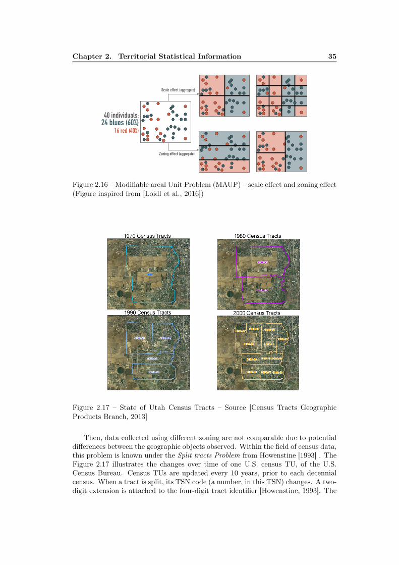
Chapter 2. Territorial Statistical Information 35

40 individuals: 24 blues (60%)

16 red (40%)

Scale effect (aggregate)

Zoning effect (aggregate)

Figure 2.16 – Modifiable areal Unit Problem (MAUP) – scale effect and zoning effect(Figure inspired from [Loidl et al., 2016])

Figure 2.17 – State of Utah Census Tracts – Source [Census Tracts GeographicProducts Branch, 2013]

Then, data collected using different zoning are not comparable due to potentialdifferences between the geographic objects observed. Within the field of census data,this problem is known under the Split tracts Problem from Howenstine [1993] . TheFigure 2.17 illustrates the changes over time of one U.S. census TU, of the U.S.Census Bureau. Census TUs are updated every 10 years, prior to each decennialcensus. When a tract is split, its TSN code (a number, in this TSN) changes. A two-digit extension is attached to the four-digit tract identifier [Howenstine, 1993]. The

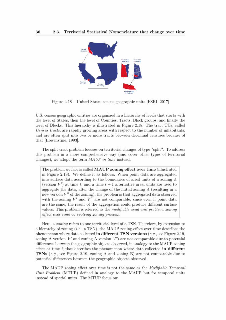
36 2.3. Territorial Statistical Nomenclature that change over time

Figure 2.18 – United States census geographic units [ESRI, 2017]

U.S. census geographic entities are organized in a hierarchy of levels that starts withthe level of States, then the level of Counties, Tracts, Block groups, and finally thelevel of Blocks. This hierarchy is illustrated in Figure 2.18. The tract TUs, calledCensus tracts, are rapidly growing areas with respect to the number of inhabitants,and are often split into two or more tracts between decennial censuses because ofthat [Howenstine, 1993].

The split tract problem focuses on territorial changes of type "split". To addressthis problem in a more comprehensive way (and cover other types of territorialchanges), we adopt the term MAUP in time instead.

The problem we face is calledMAUP zoning effect over time (illustratedin Figure 2.19). We define it as follows: When point data are aggregatedinto surface data according to the boundaries of areal units of a zoning A(version V ′) at time t, and a time t + 1 alternative areal units are used toaggregate the data, after the change of the initial zoning A (resulting in anew version V ′′ of the zoning), the problem is that aggregated data observedwith the zoning V ′ and V ′′ are not comparable, since even if point dataare the same, the result of the aggregation could produce different surfacevalues. This problem is referred as the modifiable areal unit problem, zoningeffect over time or evolving zoning problem.

Here, a zoning refers to one territorial level of a TSN. Therefore, by extension toa hierarchy of zoning (i.e., a TSN), the MAUP zoning effect over time describes thephenomenon where data collected in different TSN versions (e.g., see Figure 2.19,zoning A version V’ and zoning A version V”) are not comparable due to potentialdifferences between the geographic objects observed, in analogy to the MAUP zoningeffect at time t, that describes the phenomenon where data collected in differentTSNs (e.g., see Figure 2.19, zoning A and zoning B) are not comparable due topotential differences between the geographic objects observed.

The MAUP zoning effect over time is not the same as the Modifiable TemporalUnit Problem (MTUP) defined in analogy to the MAUP but for temporal unitsinstead of spatial units. The MTUP focus on:

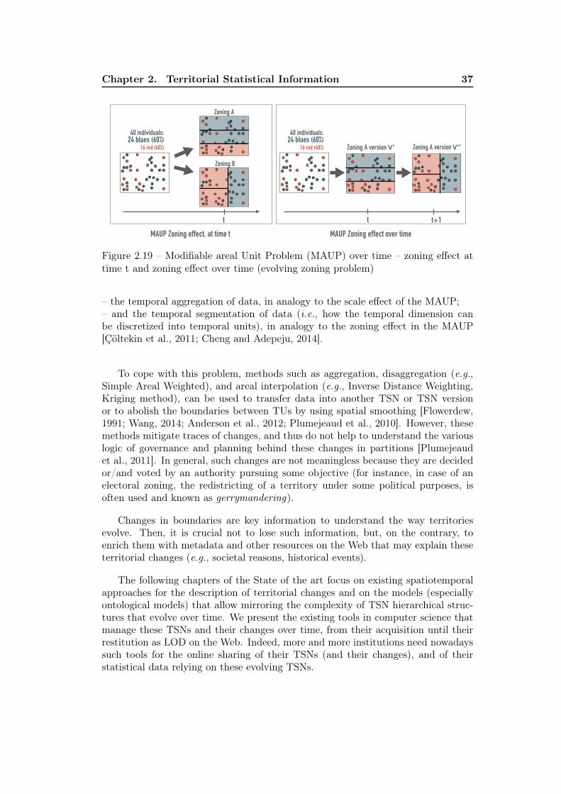
Chapter 2. Territorial Statistical Information 37

MAUP Zoning effect over time t+1t

MAUP Zoning effect, at time t

Zoning A version V’’Zoning A version V’

40 individuals: 24 blues (60%)

16 red (40%)

40 individuals: 24 blues (60%)

16 red (40%)

Zoning A

Zoning B

t

Figure 2.19 – Modifiable areal Unit Problem (MAUP) over time – zoning effect attime t and zoning effect over time (evolving zoning problem)

– the temporal aggregation of data, in analogy to the scale effect of the MAUP;– and the temporal segmentation of data (i.e., how the temporal dimension canbe discretized into temporal units), in analogy to the zoning effect in the MAUP[Çöltekin et al., 2011; Cheng and Adepeju, 2014].

To cope with this problem, methods such as aggregation, disaggregation (e.g.,Simple Areal Weighted), and areal interpolation (e.g., Inverse Distance Weighting,Kriging method), can be used to transfer data into another TSN or TSN versionor to abolish the boundaries between TUs by using spatial smoothing [Flowerdew,1991; Wang, 2014; Anderson et al., 2012; Plumejeaud et al., 2010]. However, thesemethods mitigate traces of changes, and thus do not help to understand the variouslogic of governance and planning behind these changes in partitions [Plumejeaudet al., 2011]. In general, such changes are not meaningless because they are decidedor/and voted by an authority pursuing some objective (for instance, in case of anelectoral zoning, the redistricting of a territory under some political purposes, isoften used and known as gerrymandering).

Changes in boundaries are key information to understand the way territoriesevolve. Then, it is crucial not to lose such information, but, on the contrary, toenrich them with metadata and other resources on the Web that may explain theseterritorial changes (e.g., societal reasons, historical events).

The following chapters of the State of the art focus on existing spatiotemporalapproaches for the description of territorial changes and on the models (especiallyontological models) that allow mirroring the complexity of TSN hierarchical struc-tures that evolve over time. We present the existing tools in computer science thatmanage these TSNs and their changes over time, from their acquisition until theirrestitution as LOD on the Web. Indeed, more and more institutions need nowadayssuch tools for the online sharing of their TSNs (and their changes), and of theirstatistical data relying on these evolving TSNs.

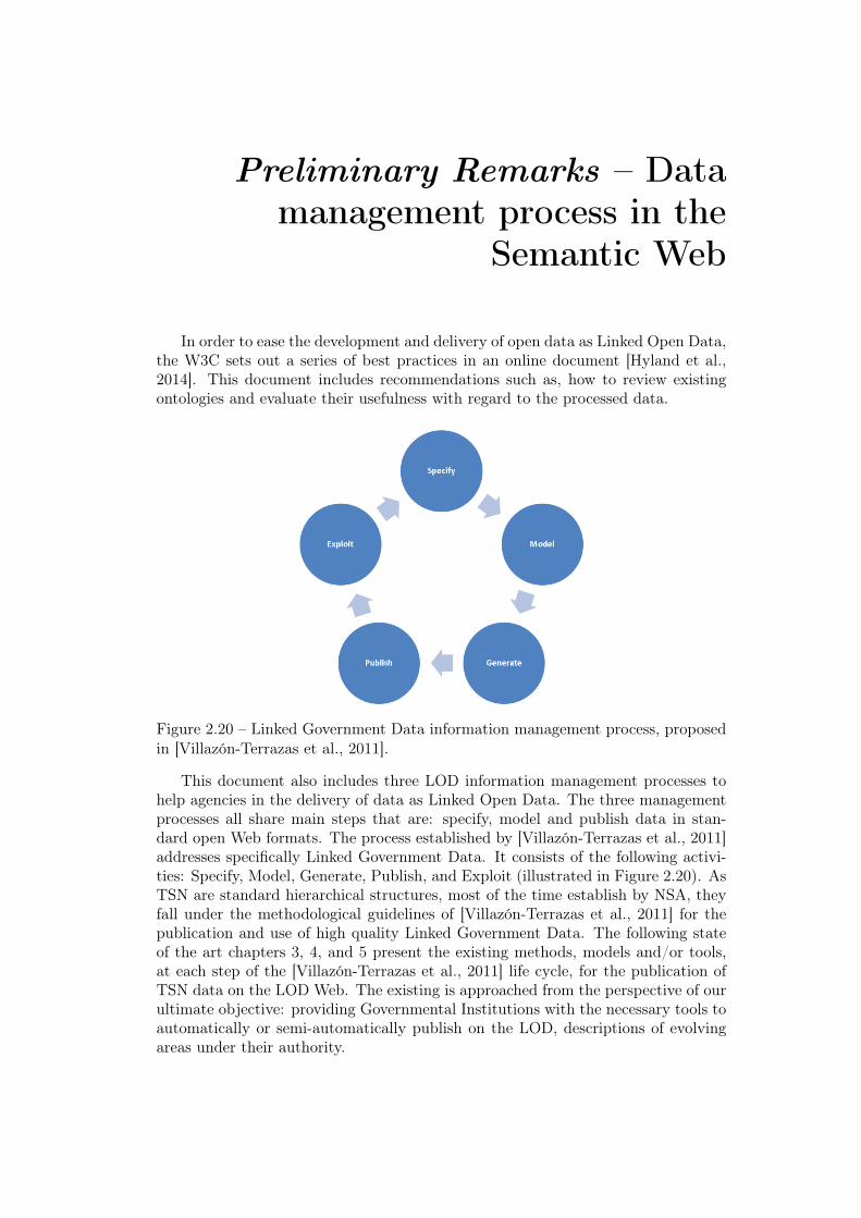
Preliminary Remarks – Datamanagement process in the

Semantic Web

In order to ease the development and delivery of open data as Linked Open Data,the W3C sets out a series of best practices in an online document [Hyland et al.,2014]. This document includes recommendations such as, how to review existingontologies and evaluate their usefulness with regard to the processed data.

Figure 2.20 – Linked Government Data information management process, proposedin [Villazón-Terrazas et al., 2011].

This document also includes three LOD information management processes tohelp agencies in the delivery of data as Linked Open Data. The three managementprocesses all share main steps that are: specify, model and publish data in stan-dard open Web formats. The process established by [Villazón-Terrazas et al., 2011]addresses specifically Linked Government Data. It consists of the following activi-ties: Specify, Model, Generate, Publish, and Exploit (illustrated in Figure 2.20). AsTSN are standard hierarchical structures, most of the time establish by NSA, theyfall under the methodological guidelines of [Villazón-Terrazas et al., 2011] for thepublication and use of high quality Linked Government Data. The following stateof the art chapters 3, 4, and 5 present the existing methods, models and/or tools,at each step of the [Villazón-Terrazas et al., 2011] life cycle, for the publication ofTSN data on the LOD Web. The existing is approached from the perspective of ourultimate objective: providing Governmental Institutions with the necessary tools toautomatically or semi-automatically publish on the LOD, descriptions of evolvingareas under their authority.

Chapter 3

Specifying and Modelingspatiotemporal entities

In this Chapter, we focus on the two first steps of the [Villazón-Terrazas et al.,2011] life cycle: Specifying and Modeling. We first present the main spatiotemporalconcepts involved in the modeling of evolving spatial entities. Second, we presentthe fundamentals for the modeling of these evolving spatial entities, and the existingapproaches in the Semantic Web.

3.1 Specifying

The first step of the [Villazón-Terrazas et al., 2011] life cycle consist in Specifyingthe data i.e., which data one wishes to publish on the LOD Web (see Subsection3.1.1), which modeling problem one faced (see Subsection 3.1.2), from which disci-pline we can learn from (see Subsection 3.1.3).

3.1.1 Spatiotemporal entities

As explain in the main introduction, Chapter 1, the descriptions of territorialchanges over time are critical for the interpretation of statistical data produced overseveral versions of a TSN. Description of the way territories evolve should help inunderstanding the events behind changes and the motivations for partitioning aterritory. In [Beller, 1991; Claramunt and Thériault, 1995], it is stated that repro-ducing the dynamics of spatiotemporal processes consists in describing changes andrelationships between entities, and in considering the events behind changes and thefacts which enable observation of these changes. On these fundamentals, [Del Mondoet al., 2010] notice that modeling these dynamics of the world requires modeling theentities themselves but must of all, the spatial, spatiotemporal and filiationrelations between them (e.g., topological relation, topological relationconsidered in time, ancestor/descendant relation). The entities we addressparticularly are TUs spatiotemporal entities (composing a TSN), and the relationsbetween them, over time and space. [Del Mondo et al., 2013] provide the followingdefinition for Spatiotemporal entities:

Spatiotemporal entity A spatiotemporal entity (also denoted en-tity) represents an abstraction of the real world. An entity has a fixedidentity and a type that describes its semantics; for example, types of

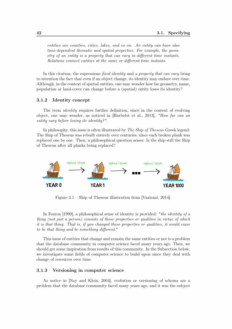
42 3.1. Specifying

entities are counties, cities, lakes, and so on. An entity can have alsotime-dependent thematic and spatial properties. For example, the geom-etry of an entity is a property that can vary in different time instants.Relations connect entities at the same or different time instants.

In this citation, the expressions fixed identity and a property that can vary bringto attention the fact that even if an object change, its identity may endure over time.Although, in the context of spatial entities, one may wonder how far geometry, name,population or land-cover can change before a (spatial) entity loses its identity?

3.1.2 Identity concept

The term identity requires further definition, since in the context of evolvingobject, one may wonder, as noticed in [Harbelot et al., 2013], "How far can anentity vary before losing its identity?".

In philosophy, this issue is often illustrated by The Ship of Theseus Greek legend:The Ship of Theseus was rebuilt entirely over centuries, since each broken plank wasreplaced one by one. Then, a philosophical question arises: Is the ship still the Shipof Theseus after all planks being replaced?

Figure 3.1 – Ship of Theseus illustration from [Vazirani, 2014].

In Fearon [1999], a philosophical sense of identity is provided: "the identity of athing (not just a person) consists of those properties or qualities in virtue of whichit is that thing. That is, if you changed these properties or qualities, it would ceaseto be that thing and be something different."

This issue of entities that change and remain the same entities or not is a problemthat the database community in computer science faced many years ago. Then, weshould get some inspiration from results of this community. In the Subsection below,we investigate some fields of computer science to build upon since they deal withchange of resources over time.

3.1.3 Versioning in computer science

As notice in [Noy and Klein, 2004], evolution or versioning of schema are aproblem that the database community faced many years ago, and it was the subject

Chapter 3. Specifying and Modeling spatiotemporal entities 43

of schema-evolution research mainly. Schema-evolution research tries to preserve theintegrity of data through the schema versions and to answer the following questions,for each processed database: "How does the new schema affect the view of the olddata? Will queries based on the old schema work with the new data? Can old data beviewed using the new schema?" [Noy and Klein, 2004]. Database schema-evolution is"a centralized process: Developers of the original schema usually make the changesand maintain the schema." While ontology development is a more decentralizedprocess than database schema development since a change in one ontology mayaffect the other ontologies that use it. In [Noy and Klein, 2004], it is stated furtherthat in the context of ontologies, one has to distinguish between "changes in thedomain or changes in the real world" and "changes in conceptualization". Changesin subdivisions of a territory fall under the first type, as noticed by [Kauppinen andHyvönen, 2007], with respect to geospatial changes over time. Then, clearly thiskind of change should not be confused with ontology versioning, database schema-evolution or ontology evolution that deal with changes in the conceptualization.

Attention should be paid to the way semantic Web technologies deal with changeover time. The RDF Specification [Cyganiak et al., 2014] states that the RDF datamodel is atemporal since RDF graphs are static snapshots of information. However,RDF graphs can express information about events and temporal aspects, given ap-propriate vocabulary terms (i.e., ontological concepts). Whenever possible, it isrecommended to use existing vocabularies (such as OWL-Time 1) to achieve seman-tic interoperability. Another concern addressed by the W3C [Cyganiak et al., 2014]is the possibility to express different states of a resource over time through differ-ent RDF graphs enclosed in one resource. However, [Stefanidis et al., 2014] warnsabout possible duplications of data from one version to another. Then, this approachcan rapidly increase the space memory requirements. An alternative solution is tostore only one version (e.g., the first one) and deltas (the differences between twoconsecutive versions).

Another field we have to explore is the field of Software configuration manage-ment (SCM) for managing the evolution of large software systems [Tichy, 1988].Within this field, a version is defined as a state of an evolving item and differenttypes of version are identified [Conradi and Westfechtel, 1998] such as: revisionsthat are versions intended to supersede their predecessor; variants that are versionsintended to coexist. Versions of TSN are of this second type, they are variants thatmust coexist in order to observe the influence of the territorial divisions on statis-tical data. Another core concept of SCM is the version model. A version modeldefines the items to be versioned and the delta, which is the differences between twoconsecutive versions [Conradi and Westfechtel, 1998].

1. https://www.w3.org/TR/owl-time/

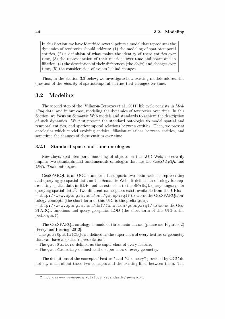
44 3.2. Modeling

In this Section, we have identified several points a model that reproduces thedynamics of territories should address: (1) the modeling of spatiotemporalentities, (2) a definition of what makes the identity of these entities overtime, (3) the representation of their relations over time and space and infiliation, (4) the description of their differences (the delta) and changes overtime, (5) the consideration of events behind changes.

Thus, in the Section 3.2 below, we investigate how existing models address thequestion of the identity of spatiotemporal entities that change over time.

3.2 Modeling

The second step of the [Villazón-Terrazas et al., 2011] life cycle consists in Mod-eling data, and in our case, modeling the dynamics of territories over time. In thisSection, we focus on Semantic Web models and standards to achieve the descriptionof such dynamics. We first present the standard ontologies to model spatial andtemporal entities, and spatiotemporal relations between entities. Then, we presentontologies which model evolving entities, filiation relations between entities, andsometime the changes of these entities over time.

3.2.1 Standard space and time ontologies

Nowadays, spatiotemporal modeling of objects on the LOD Web, necessarilyimplies two standards and fundamentals ontologies that are the GeoSPARQL andOWL-Time ontologies.

GeoSPARQL is an OGC standard. It supports two main actions: representingand querying geospatial data on the Semantic Web. It defines an ontology for rep-resenting spatial data in RDF, and an extension to the SPARQL query language forquerying spatial data 2. Two different namespaces exist, available from the URIs:– http://www.opengis.net/ont/geosparql# to access the GeoSPARQL on-tology concepts (the short form of this URI is the prefix geo);– http://www.opengis.net/def/function/geosparql/ to access the Geo-SPARQL functions and query geospatial LOD (the short form of this URI is theprefix geof).

The GeoSPARQL ontology is made of three main classes (please see Figure 3.2)[Perry and Herring, 2012]:– The geo:SpatialObject defined as the super class of every feature or geometrythat can have a spatial representation;– The geo:Feature defined as the super class of every feature;– The geo:Geometry defined as the super class of every geometry.

The definitions of the concepts "Feature" and "Geometry" provided by OGC donot say much about these two concepts and the existing links between them. The

2. http://www.opengeospatial.org/standards/geosparql

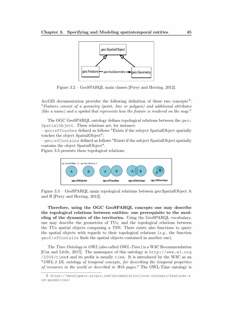
Chapter 3. Specifying and Modeling spatiotemporal entities 45

Figure 3.2 – GeoSPARQL main classes [Perry and Herring, 2012].

ArcGIS documentation provides the following definition of these two concepts 3:"Features consist of a geometry (point, line or polygon) and additional attributes(like a name) and a symbol that represents how the feature is rendered on the map."

The OGC GeoSPARQL ontology defines topological relations between the geo:SpatialObject. These relations are, for instance:– geo:sfTouches defined as follows "Exists if the subject SpatialObject spatiallytouches the object SpatialObject";– geo:sfContains defined as follows "Exists if the subject SpatialObject spatiallycontains the object SpatialObject".Figure 3.3 presents these topological relations.

Figure 3.3 – GeoSPARQL main topological relations between geo:SpatialObject Aand B [Perry and Herring, 2012].

Therefore, using the OGC GeoSPARQL concepts one may describethe topological relations between entities: one prerequisite to the mod-eling of the dynamics of the territories. Using the GeoSPARQL vocabulary,one may describe the geometries of TUs, and the topological relations betweenthe TUs spatial objects composing a TSN. There exists also functions to querythe spatial objects with regards to their topological relations (e.g., the functiongeof:sfContains finds the spatial objects contained in another one).

The Time Ontology in OWL (also called OWL-Time) is a W3C Recommendation[Cox and Little, 2017]. The namespace of this ontology is http://www.w3.org/2006/time# and its prefix is usually time. It is introduced by the W3C as an"OWL-2 DL ontology of temporal concepts, for describing the temporal propertiesof resources in the world or described in Web pages." The OWL-Time ontology is

3. https://developers.arcgis.com/documentation/core-concepts/features-and-geometries/

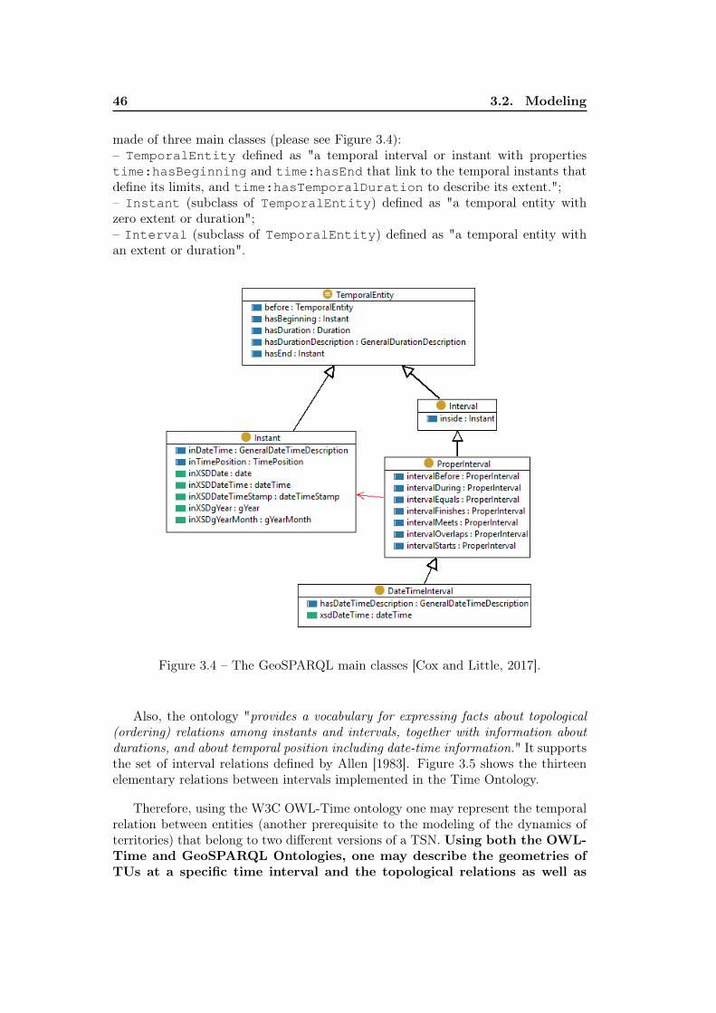
46 3.2. Modeling

made of three main classes (please see Figure 3.4):– TemporalEntity defined as "a temporal interval or instant with propertiestime:hasBeginning and time:hasEnd that link to the temporal instants thatdefine its limits, and time:hasTemporalDuration to describe its extent.";– Instant (subclass of TemporalEntity) defined as "a temporal entity withzero extent or duration";– Interval (subclass of TemporalEntity) defined as "a temporal entity withan extent or duration".

Figure 3.4 – The GeoSPARQL main classes [Cox and Little, 2017].

Also, the ontology "provides a vocabulary for expressing facts about topological(ordering) relations among instants and intervals, together with information aboutdurations, and about temporal position including date-time information." It supportsthe set of interval relations defined by Allen [1983]. Figure 3.5 shows the thirteenelementary relations between intervals implemented in the Time Ontology.

Therefore, using the W3C OWL-Time ontology one may represent the temporalrelation between entities (another prerequisite to the modeling of the dynamics ofterritories) that belong to two different versions of a TSN. Using both the OWL-Time and GeoSPARQL Ontologies, one may describe the geometries ofTUs at a specific time interval and the topological relations as well as

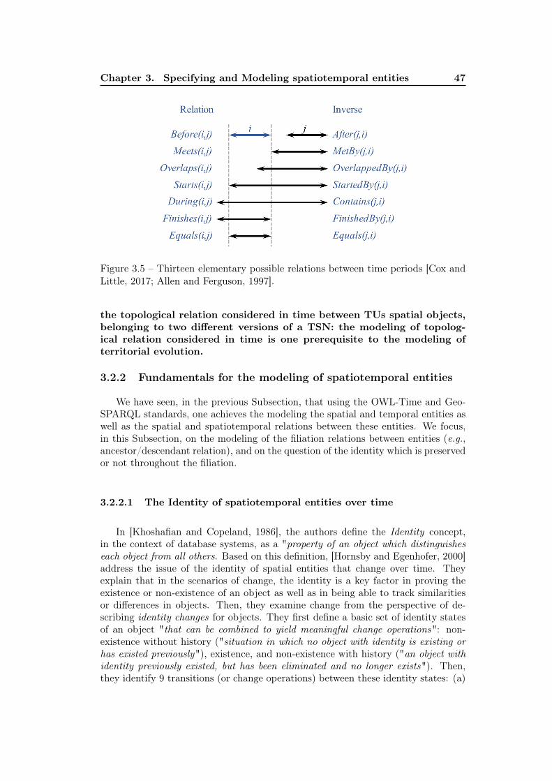
Chapter 3. Specifying and Modeling spatiotemporal entities 47

Figure 3.5 – Thirteen elementary possible relations between time periods [Cox andLittle, 2017; Allen and Ferguson, 1997].

the topological relation considered in time between TUs spatial objects,belonging to two different versions of a TSN: the modeling of topolog-ical relation considered in time is one prerequisite to the modeling ofterritorial evolution.

3.2.2 Fundamentals for the modeling of spatiotemporal entities

We have seen, in the previous Subsection, that using the OWL-Time and Geo-SPARQL standards, one achieves the modeling the spatial and temporal entities aswell as the spatial and spatiotemporal relations between these entities. We focus,in this Subsection, on the modeling of the filiation relations between entities (e.g.,ancestor/descendant relation), and on the question of the identity which is preservedor not throughout the filiation.

3.2.2.1 The Identity of spatiotemporal entities over time

In [Khoshafian and Copeland, 1986], the authors define the Identity concept,in the context of database systems, as a "property of an object which distinguisheseach object from all others. Based on this definition, [Hornsby and Egenhofer, 2000]address the issue of the identity of spatial entities that change over time. Theyexplain that in the scenarios of change, the identity is a key factor in proving theexistence or non-existence of an object as well as in being able to track similaritiesor differences in objects. Then, they examine change from the perspective of de-scribing identity changes for objects. They first define a basic set of identity statesof an object "that can be combined to yield meaningful change operations": non-existence without history ("situation in which no object with identity is existing orhas existed previously"), existence, and non-existence with history ("an object withidentity previously existed, but has been eliminated and no longer exists"). Then,they identify 9 transitions (or change operations) between these identity states: (a)

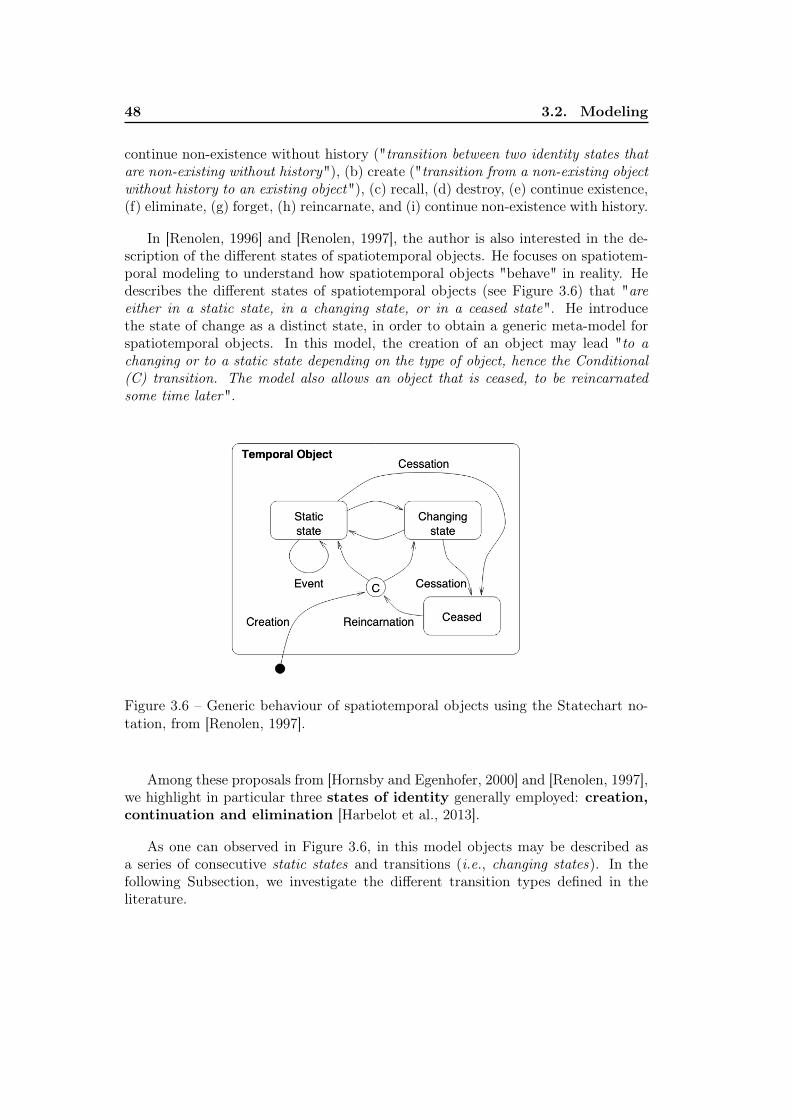
48 3.2. Modeling

continue non-existence without history ("transition between two identity states thatare non-existing without history"), (b) create ("transition from a non-existing objectwithout history to an existing object"), (c) recall, (d) destroy, (e) continue existence,(f) eliminate, (g) forget, (h) reincarnate, and (i) continue non-existence with history.

In [Renolen, 1996] and [Renolen, 1997], the author is also interested in the de-scription of the different states of spatiotemporal objects. He focuses on spatiotem-poral modeling to understand how spatiotemporal objects "behave" in reality. Hedescribes the different states of spatiotemporal objects (see Figure 3.6) that "areeither in a static state, in a changing state, or in a ceased state". He introducethe state of change as a distinct state, in order to obtain a generic meta-model forspatiotemporal objects. In this model, the creation of an object may lead "to achanging or to a static state depending on the type of object, hence the Conditional(C) transition. The model also allows an object that is ceased, to be reincarnatedsome time later".

Figure 3.6 – Generic behaviour of spatiotemporal objects using the Statechart no-tation, from [Renolen, 1997].

Among these proposals from [Hornsby and Egenhofer, 2000] and [Renolen, 1997],we highlight in particular three states of identity generally employed: creation,continuation and elimination [Harbelot et al., 2013].

As one can observed in Figure 3.6, in this model objects may be described asa series of consecutive static states and transitions (i.e., changing states). In thefollowing Subsection, we investigate the different transition types defined in theliterature.

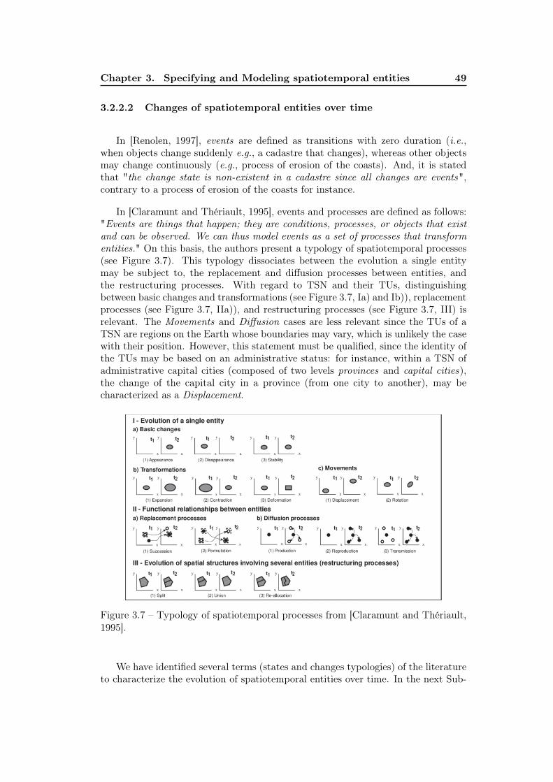
Chapter 3. Specifying and Modeling spatiotemporal entities 49

3.2.2.2 Changes of spatiotemporal entities over time

In [Renolen, 1997], events are defined as transitions with zero duration (i.e.,when objects change suddenly e.g., a cadastre that changes), whereas other objectsmay change continuously (e.g., process of erosion of the coasts). And, it is statedthat "the change state is non-existent in a cadastre since all changes are events",contrary to a process of erosion of the coasts for instance.

In [Claramunt and Thériault, 1995], events and processes are defined as follows:"Events are things that happen; they are conditions, processes, or objects that existand can be observed. We can thus model events as a set of processes that transformentities." On this basis, the authors present a typology of spatiotemporal processes(see Figure 3.7). This typology dissociates between the evolution a single entitymay be subject to, the replacement and diffusion processes between entities, andthe restructuring processes. With regard to TSN and their TUs, distinguishingbetween basic changes and transformations (see Figure 3.7, Ia) and Ib)), replacementprocesses (see Figure 3.7, IIa)), and restructuring processes (see Figure 3.7, III) isrelevant. The Movements and Diffusion cases are less relevant since the TUs of aTSN are regions on the Earth whose boundaries may vary, which is unlikely the casewith their position. However, this statement must be qualified, since the identity ofthe TUs may be based on an administrative status: for instance, within a TSN ofadministrative capital cities (composed of two levels provinces and capital cities),the change of the capital city in a province (from one city to another), may becharacterized as a Displacement.

Figure 3.7 – Typology of spatiotemporal processes from [Claramunt and Thériault,1995].

We have identified several terms (states and changes typologies) of the literatureto characterize the evolution of spatiotemporal entities over time. In the next Sub-

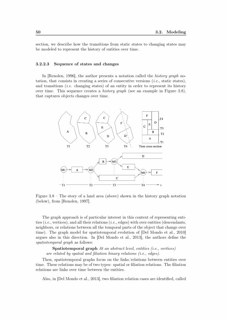
50 3.2. Modeling

section, we describe how the transitions from static states to changing states maybe modeled to represent the history of entities over time.

3.2.2.3 Sequence of states and changes

In [Renolen, 1996], the author presents a notation called the history graph no-tation, that consists in creating a series of consecutive versions (i.e., static states),and transitions (i.e. changing states) of an entity in order to represent its historyover time. This sequence creates a history graph (see an example in Figure 3.8),that captures objects changes over time.

Figure 3.8 – The story of a land area (above) shown in the history graph notation(below), from [Renolen, 1997].

The graph approach is of particular interest in this context of representing enti-ties (i.e., vertices), and all their relations (i.e., edges) with over entities (descendants,neighbors, or relations between all the temporal parts of the object that change overtime). The graph model for spatiotemporal evolution of [Del Mondo et al., 2010]argues also in this direction. In [Del Mondo et al., 2013], the authors define thespatiotemporal graph as follows:

Spatiotemporal graph At an abstract level, entities (i.e., vertices)are related by spatial and filiation binary relations (i.e., edges).

Then, spatiotemporal graphs focus on the links/relations between entities overtime. These relations may be of two types: spatial or filiation relations. The filiationrelations are links over time between the entities.

Also, in [Del Mondo et al., 2013], two filiation relation cases are identified, called

Chapter 3. Specifying and Modeling spatiotemporal entities 51

Continuation and Derivation relations defined as follows:Continuation relation the first entity is the same as the second

entity (e.g., one person at two times).Derivation relation the first entity creates (possibly with others)

the second entity (e.g., a parent of a child)In the case of the Continuation relation, entities maintained their identity after

change whereas, on the contrary, in case of the Derivation relation, the identity ofthe first element is not maintained after change, the two entities have not the sameidentity.

Let us consider once again the example of the ship of Theseus:

– Does the ship of Theseus at time 0 has a relation of type Continuation withthe ship of Theseus at time 1?– What if we consider the relation between the ship at time 0 and time 1000, all theplanks having being replaced? (see Figure 3.1.2) In other word, it it still the sameship or a different one?

In the literature, there is no unique answer to this question, the response variesfrom one chosen definition of what makes the identity of the ship to another, and,more broadly, it depends on modeling choices. In the Subsections 3.2.2.4, 3.2.2.5,3.2.2.6 different models and ontologies are presented. They all address the issue ofthe identity of evolving entities, but in different ways.

3.2.2.4 Versioning approach

The terms Versioning and Version Control are most of the time used in thecontext of computer science and more broadly for the management of modificationsto text document. Rouse [2007] provides the following definition of these two terms:

Versioning is the creation and management of multiple releases of aproduct, all of which have the same general function but are improved,upgraded or customized. The term applies specially to operating systems(OSs), software and Web services.Version control is the practice of ensuring collaborative data sharing andediting among users of systems that employ different versions of a prod-uct. The terms "versioning" and "version control" are sometimes usedinterchangeably even though their technical meanings are different.

As previously explained in Subsection 3.1.3, in the field of Software configurationmanagement (SCM) (for managing the evolution of large software systems [Tichy,1988]), a version is defined as a state of an evolving item. Another core concept ofSCM is the version model. A version model defines the items to be versioned andthe delta, which is the differences between two consecutive versions [Conradi andWestfechtel, 1998].

52 3.2. Modeling

Version-Difference Spatiotemporal model Adopting the approach of Soft-ware configuration management (SCM), Huibing et al. [2005] introduce the Version-Difference Spatiotemporal model developed with the requirement of using historicalinformation in order to analyze changes of spatial objects over time.

Information systems based on this model store "the current state of an object(called the default version) and all historic changes (called version difference)."Then, using reconstruction operator and change descriptions, all the states of anentity over time can be obtained.

PAV and DC-terms Ontologies The Provenance, Authoring and VersioningOntology (PAV) (URI: http://purl.org/pav/), and the Dublin Core MetadataInitiative Terms (DC-terms) (URI: http://purl.org/dc/terms/) also adoptthe term Version. They focus on entities that are published on the Web: DC-termsprovides terms to describe resources with metadata, whereas the PAV ontology ismore devoted to the agents contributing in Web resources: contributors, authors,curators and digital artifact creators. Also, PAV provides terms for tracking theprovenance of digital entities that are published on the Web [Ciccarese et al., 2013].Both PAV and DC-terms use the predicate hasVersion to point towards a re-source that is a version, edition, or adaptation of the described resource. The PAVontology provides the following definition of the property hasVersion: "This prop-erty is intended for relating a non-versioned or abstract resource to several versionedresources, e.g. snapshots.

The term Snapshot is found in several models:– in [Renolen, 1997], the following fundamental definition is given: Objects thatchange suddenly would then be described by transitions with zero duration (i.e.events), while objects that change continuously would be described by version withzero duration (i.e. snapshots) describing intermediate states.– in the Basic Formal Ontology [Grenon and Smith, 2004], it is proposed to makea distinction between static SNAP (Snapshots) entities that change over time anddynamic SPAN entities. This model goes a step further than the models for version-ing of entities, since it proposes to represent static Snapshots that change over time(e.g., a person) but also the process behind these changes (e.g., the aging process),i.e. the SPAN entities. This approach is presented below.

3.2.2.5 The SNAP and SPAN approach

The Basic Formal Ontology (BFO) is an upper ontology based on the approach ofGrenon and Smith [2004] that accounts for both the static SNAP and the dynamicSPAN entities, while most of the existing models account only for one type ata time. Ontologies for continuants are called SNAP. The terms ’continuant’and ’endurant’ are used interchangeably for those entities that have continuousexistence and a capacity to endure (persist self-identically) through time even whileundergoing different sorts of changes (e.g., a person, the planet Earth) Grenon and

Chapter 3. Specifying and Modeling spatiotemporal entities 53

Smith [2004].

Ontologies for occurrents are called SPAN. Two different terms are used torefer to occurrent entities (e.g., a smile, the passage of a rainstorm over a forest)Grenon and Smith [2004]:– processes that are occurrent entities which persist (perdure) in time i.e., there arenot instantaneous. The term perdurant is used for these occurrents;– events that are occurrent entities which exhaust themselves in single instants oftime.

The BFO framework addresses both the continuant and occurrent entities: it isa SNAP-SPAN framework. Indeed, while these two alternative views have tradition-ally been considered as incompatible, the authors argue that, as reality is essentiallydynamic, an ontology must be capable of accounting for spatial reality both syn-chronically (entities that exist at a time) and diachronically (how the things unfoldthrough time).

They introduce the notion of Trans-Ontological relation. A trans-Ontologicalrelation is a "relation between entities that are constituents of distinct ontologies."

The SNAP-SNAP Trans-Ontologies are ontologies that depict the world overtime as a succession of temporally separated snapshots. Changes from one SNAPto another are described and may belong to one of the three main types that are:– qualitative change: for instance, the color of a table becomes tarnished over time,yet there is still something which remains the same;– locational change: for instance, "in one SNAP ontology the cup is on the table,in a later SNAP ontology it is on the floor. The cup underwent location change";– substantial change: for instance, it is when a substance is divided up so as toproduce a plurality of substances.The SNAP-SPAN Trans-Ontologies are ontologies that depict the life or history ofentities over time. The life line of an entity is a SPAN object, and the entity itself isa SNAP object. "Histories might best be understood as four-dimensional settings."

The two approach SNAP-SNAP and SNAP-SPAN may also be combined in orderto depict both the changes of a SNAP entity between two periods of time and itsevolution process over time (i.e., its life).

Then, [Grenon and Smith, 2004] address in particular the case of Geographicalobjects, and dissociate between the:

– SNAP Geographical Object Ontology from which the subcategory "Boundariesand Geographical Regions" is one of the 5 major subcategories to geographical SNAPentities. The authors explain that administrative boundaries are SNAP fiat objects,that is to say, they are constructed objects that exist according to an administra-tive, social or political convention (in opposition to bona fide object that correspondto "natural" objects, such as natural boundaries like mountains) [Smith and Varzi,2000; Mathian and Sanders, 2014].

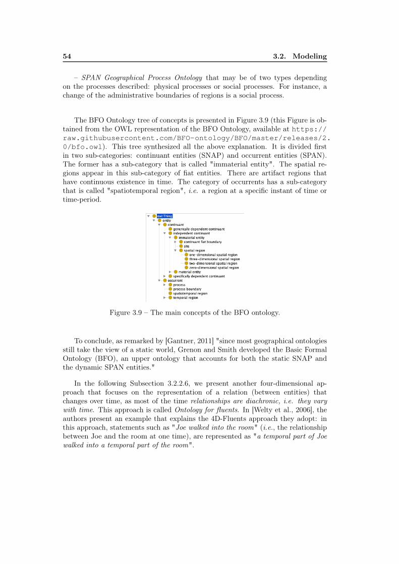
54 3.2. Modeling

– SPAN Geographical Process Ontology that may be of two types dependingon the processes described: physical processes or social processes. For instance, achange of the administrative boundaries of regions is a social process.

The BFO Ontology tree of concepts is presented in Figure 3.9 (this Figure is ob-tained from the OWL representation of the BFO Ontology, available at https://raw.githubusercontent.com/BFO-ontology/BFO/master/releases/2.0/bfo.owl). This tree synthesized all the above explanation. It is divided firstin two sub-categories: continuant entities (SNAP) and occurrent entities (SPAN).The former has a sub-category that is called "immaterial entity". The spatial re-gions appear in this sub-category of fiat entities. There are artifact regions thathave continuous existence in time. The category of occurrents has a sub-categorythat is called "spatiotemporal region", i.e. a region at a specific instant of time ortime-period.

Figure 3.9 – The main concepts of the BFO ontology.

To conclude, as remarked by [Gantner, 2011] "since most geographical ontologiesstill take the view of a static world, Grenon and Smith developed the Basic FormalOntology (BFO), an upper ontology that accounts for both the static SNAP andthe dynamic SPAN entities."

In the following Subsection 3.2.2.6, we present another four-dimensional ap-proach that focuses on the representation of a relation (between entities) thatchanges over time, as most of the time relationships are diachronic, i.e. they varywith time. This approach is called Ontology for fluents. In [Welty et al., 2006], theauthors present an example that explains the 4D-Fluents approach they adopt: inthis approach, statements such as "Joe walked into the room" (i.e., the relationshipbetween Joe and the room at one time), are represented as "a temporal part of Joewalked into a temporal part of the room".

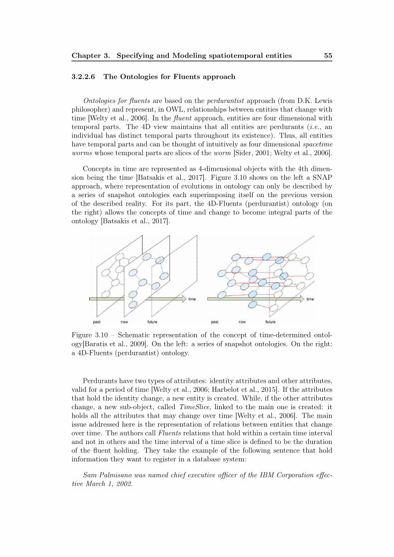
Chapter 3. Specifying and Modeling spatiotemporal entities 55

3.2.2.6 The Ontologies for Fluents approach

Ontologies for fluents are based on the perdurantist approach (from D.K. Lewisphilosopher) and represent, in OWL, relationships between entities that change withtime [Welty et al., 2006]. In the fluent approach, entities are four dimensional withtemporal parts. The 4D view maintains that all entities are perdurants (i.e., anindividual has distinct temporal parts throughout its existence). Thus, all entitieshave temporal parts and can be thought of intuitively as four dimensional spacetimeworms whose temporal parts are slices of the worm [Sider, 2001; Welty et al., 2006].

Concepts in time are represented as 4-dimensional objects with the 4th dimen-sion being the time [Batsakis et al., 2017]. Figure 3.10 shows on the left a SNAPapproach, where representation of evolutions in ontology can only be described bya series of snapshot ontologies each superimposing itself on the previous versionof the described reality. For its part, the 4D-Fluents (perdurantist) ontology (onthe right) allows the concepts of time and change to become integral parts of theontology [Batsakis et al., 2017].

Figure 3.10 – Schematic representation of the concept of time-determined ontol-ogy[Baratis et al., 2009]. On the left: a series of snapshot ontologies. On the right:a 4D-Fluents (perdurantist) ontology.

Perdurants have two types of attributes: identity attributes and other attributes,valid for a period of time [Welty et al., 2006; Harbelot et al., 2015]. If the attributesthat hold the identity change, a new entity is created. While, if the other attributeschange, a new sub-object, called TimeSlice, linked to the main one is created: itholds all the attributes that may change over time [Welty et al., 2006]. The mainissue addressed here is the representation of relations between entities that changeover time. The authors call Fluents relations that hold within a certain time intervaland not in others and the time interval of a time slice is defined to be the durationof the fluent holding. They take the example of the following sentence that holdinformation they want to register in a database system:

Sam Palmisano was named chief executive officer of the IBM Corporation effec-tive March 1, 2002.

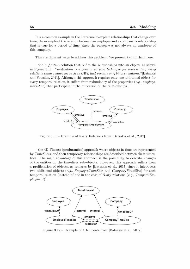
56 3.2. Modeling

It is a common example in the literature to explain relationships that change overtime, the example of the relation between an employee and a company, a relationshipthat is true for a period of time, since the person was not always an employee ofthis company.

There is different ways to address this problem. We present two of them here:

– the reification solution that reifies the relationships into an object, as shownin Figure 3.11. "Reification is a general purpose technique for representing n-aryrelations using a language such as OWL that permits only binary relations."[Batsakisand Petrakis, 2011]. Although this approach requires only one additional object forevery temporal relation, it suffers from redundancy of the properties (e.g., employs,worksFor) that participate in the reification of the relationships.

Figure 3.11 – Example of N-ary Relations from [Batsakis et al., 2017].

– the 4D-Fluents (perdurantist) approach where objects in time are representedby TimeSlices, and their temporary relationships are described between these times-lices. The main advantage of this approach is the possibility to describe changesof the entities on the timeslices sub-objects. However, this approach suffers froma proliferation of objects, as remarks by [Batsakis et al., 2017] since it introducestwo additional objects (e.g., EmployeeTimeSlice and CompanyTimeSlice) for eachtemporal relation (instead of one in the case of N-ary relations (e.g., TemporalEm-ployment)).

Figure 3.12 – Example of 4D-Fluents from [Batsakis et al., 2017].

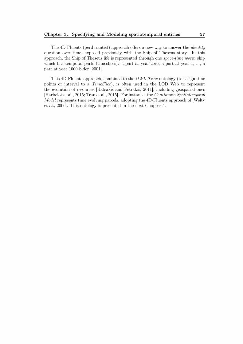
Chapter 3. Specifying and Modeling spatiotemporal entities 57

The 4D-Fluents (perdurantist) approach offers a new way to answer the identityquestion over time, exposed previously with the Ship of Theseus story. In thisapproach, the Ship of Theseus life is represented through one space-time worm shipwhich has temporal parts (timeslices): a part at year zero, a part at year 1, ..., apart at year 1000 Sider [2001].

This 4D-Fluents approach, combined to the OWL-Time ontology (to assign timepoints or interval to a TimeSlice), is often used in the LOD Web to representthe evolution of resources [Batsakis and Petrakis, 2011], including geospatial ones[Harbelot et al., 2015; Tran et al., 2015]. For instance, the Continuum SpatiotemporalModel represents time evolving parcels, adopting the 4D-Fluents approach of [Weltyet al., 2006]. This ontology is presented in the next Chapter 4.

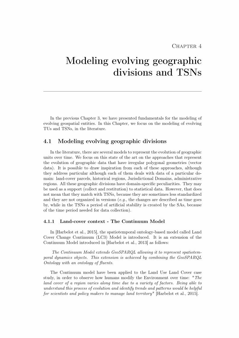
Chapter 4

Modeling evolving geographicdivisions and TSNs

In the previous Chapter 3, we have presented fundamentals for the modeling ofevolving geospatial entities. In this Chapter, we focus on the modeling of evolvingTUs and TSNs, in the literature.

4.1 Modeling evolving geographic divisions

In the literature, there are several models to represent the evolution of geographicunits over time. We focus on this state of the art on the approaches that representthe evolution of geographic data that have irregular polygonal geometries (vectordata). It is possible to draw inspiration from each of these approaches, althoughthey address particular although each of them deals with data of a particular do-main: land-cover parcels, historical regions, Jurisdictional Domains, administrativeregions. All these geographic divisions have domain-specific peculiarities. They maybe used as a support (collect and restitution) to statistical data. However, that doesnot mean that they match with TSNs, because they are sometimes less standardizedand they are not organized in versions (e.g., the changes are described as time goesby, while in the TSNs a period of artificial stability is created by the SAs, becauseof the time period needed for data collection).

4.1.1 Land-cover context - The Continuum Model

In [Harbelot et al., 2015], the spatiotemporal ontology-based model called LandCover Change Continuum (LC3) Model is introduced. It is an extension of theContinuum Model introduced in [Harbelot et al., 2013] as follows:

The Continuum Model extends GeoSPARQL allowing it to represent spatiotem-poral dynamics objects. This extension is achieved by combining the GeoSPARQLOntology with an ontology of fluents.

The Continuum model have been applied to the Land Use Land Cover casestudy, in order to observe how humans modify the Environment over time: "Theland cover of a region varies along time due to a variety of factors. Being able tounderstand this process of evolution and identify trends and patterns would be helpfulfor scientists and policy makers to manage land territory" [Harbelot et al., 2015].

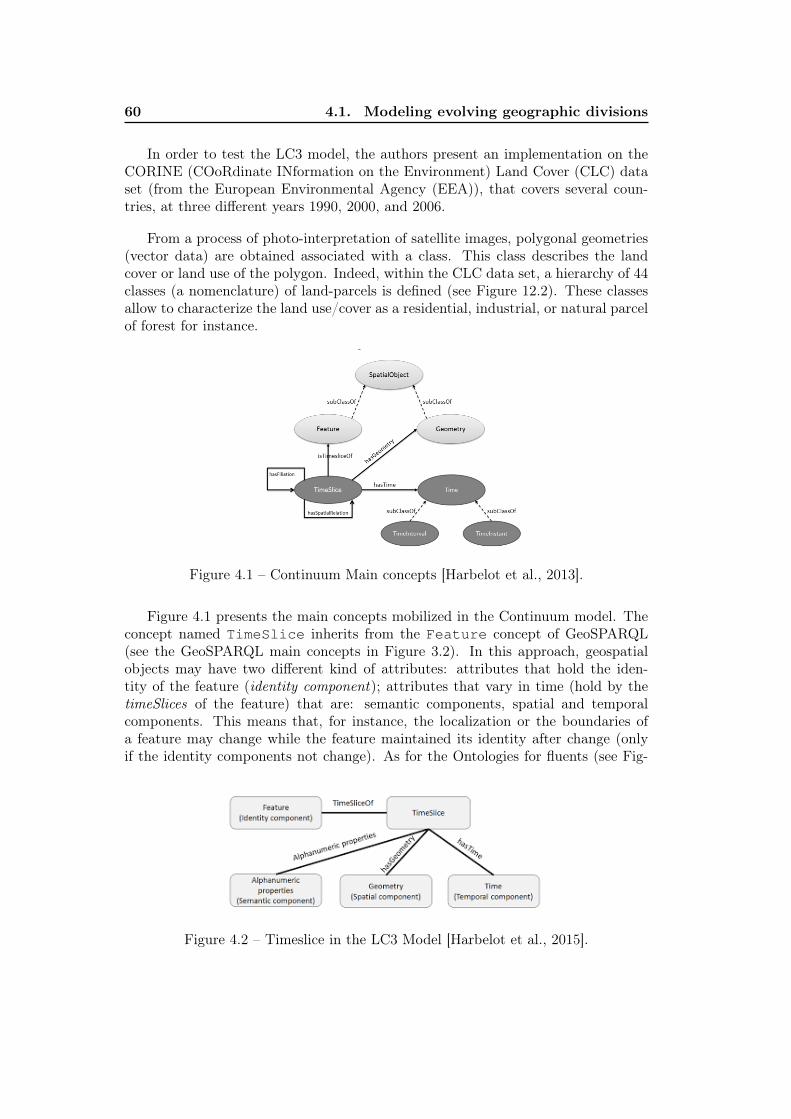
60 4.1. Modeling evolving geographic divisions

In order to test the LC3 model, the authors present an implementation on theCORINE (COoRdinate INformation on the Environment) Land Cover (CLC) dataset (from the European Environmental Agency (EEA)), that covers several coun-tries, at three different years 1990, 2000, and 2006.

From a process of photo-interpretation of satellite images, polygonal geometries(vector data) are obtained associated with a class. This class describes the landcover or land use of the polygon. Indeed, within the CLC data set, a hierarchy of 44classes (a nomenclature) of land-parcels is defined (see Figure 12.2). These classesallow to characterize the land use/cover as a residential, industrial, or natural parcelof forest for instance.

Figure 4.1 – Continuum Main concepts [Harbelot et al., 2013].

Figure 4.1 presents the main concepts mobilized in the Continuum model. Theconcept named TimeSlice inherits from the Feature concept of GeoSPARQL(see the GeoSPARQL main concepts in Figure 3.2). In this approach, geospatialobjects may have two different kind of attributes: attributes that hold the iden-tity of the feature (identity component); attributes that vary in time (hold by thetimeSlices of the feature) that are: semantic components, spatial and temporalcomponents. This means that, for instance, the localization or the boundaries ofa feature may change while the feature maintained its identity after change (onlyif the identity components not change). As for the Ontologies for fluents (see Fig-

Figure 4.2 – Timeslice in the LC3 Model [Harbelot et al., 2015].

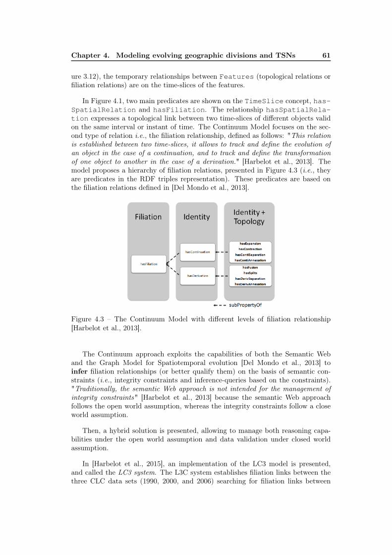
Chapter 4. Modeling evolving geographic divisions and TSNs 61

ure 3.12), the temporary relationships between Features (topological relations orfiliation relations) are on the time-slices of the features.

In Figure 4.1, two main predicates are shown on the TimeSlice concept, has-SpatialRelation and hasFiliation. The relationship hasSpatialRela-tion expresses a topological link between two time-slices of different objects validon the same interval or instant of time. The Continuum Model focuses on the sec-ond type of relation i.e., the filiation relationship, defined as follows: "This relationis established between two time-slices, it allows to track and define the evolution ofan object in the case of a continuation, and to track and define the transformationof one object to another in the case of a derivation." [Harbelot et al., 2013]. Themodel proposes a hierarchy of filiation relations, presented in Figure 4.3 (i.e., theyare predicates in the RDF triples representation). These predicates are based onthe filiation relations defined in [Del Mondo et al., 2013].

Figure 4.3 – The Continuum Model with different levels of filiation relationship[Harbelot et al., 2013].

The Continuum approach exploits the capabilities of both the Semantic Weband the Graph Model for Spatiotemporal evolution [Del Mondo et al., 2013] toinfer filiation relationships (or better qualify them) on the basis of semantic con-straints (i.e., integrity constraints and inference-queries based on the constraints)."Traditionally, the semantic Web approach is not intended for the management ofintegrity constraints" [Harbelot et al., 2013] because the semantic Web approachfollows the open world assumption, whereas the integrity constraints follow a closeworld assumption.

Then, a hybrid solution is presented, allowing to manage both reasoning capa-bilities under the open world assumption and data validation under closed worldassumption.

In [Harbelot et al., 2015], an implementation of the LC3 model is presented,and called the LC3 system. The L3C system establishes filiation links between thethree CLC data sets (1990, 2000, and 2006) searching for filiation links between

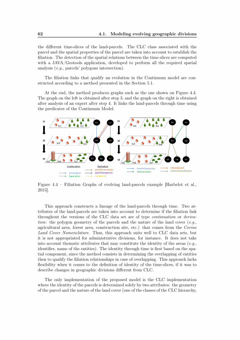
62 4.1. Modeling evolving geographic divisions

the different time-slices of the land-parcels. The CLC class associated with theparcel and the spatial properties of the parcel are taken into account to establish thefiliation. The detection of the spatial relations between the time-slices are computedwith a JAVA/Geotools application, developed to perform all the required spatialanalysis (e.g., parcels’ polygons intersection).

The filiation links that qualify an evolution in the Continuum model are con-structed according to a method presented in the Section 5.1.

At the end, the method produces graphs such as the one shown on Figure 4.4.The graph on the left is obtained after step 3, and the graph on the right is obtainedafter analysis of an expert after step 4. It links the land-parcels through time usingthe predicates of the Continuum Model.

Figure 4.4 – Filiation Graphs of evolving land-parcels example [Harbelot et al.,2015].

This approach constructs a lineage of the land-parcels through time. Two at-tributes of the land-parcels are taken into account to determine if the filiation linkthroughout the versions of the CLC data set are of type continuation or deriva-tion: the polygon geometry of the parcels and the nature of the land cover (e.g.,agricultural area, forest area, construction site, etc.) that comes from the CorineLand Cover Nomenclature. Thus, this approach suits well to CLC data sets, butit is not appropriated for administrative divisions, for instance. It does not takeinto account thematic attributes that may constitute the identity of the areas (e.g.,identifier, name of the entities). The identity through time is first based on the spa-tial component, since the method consists in determining the overlapping of entitiesthen to qualify the filiation relationships in case of overlapping. This approach lacksflexibility when it comes to the definition of identity of the time-slices, if it was todescribe changes in geographic divisions different from CLC.

The only implementation of the proposed model is the CLC implementationwhere the identity of the parcels is determined solely by two attributes: the geometryof the parcel and the nature of the land cover (one of the classes of the CLC hierarchy,

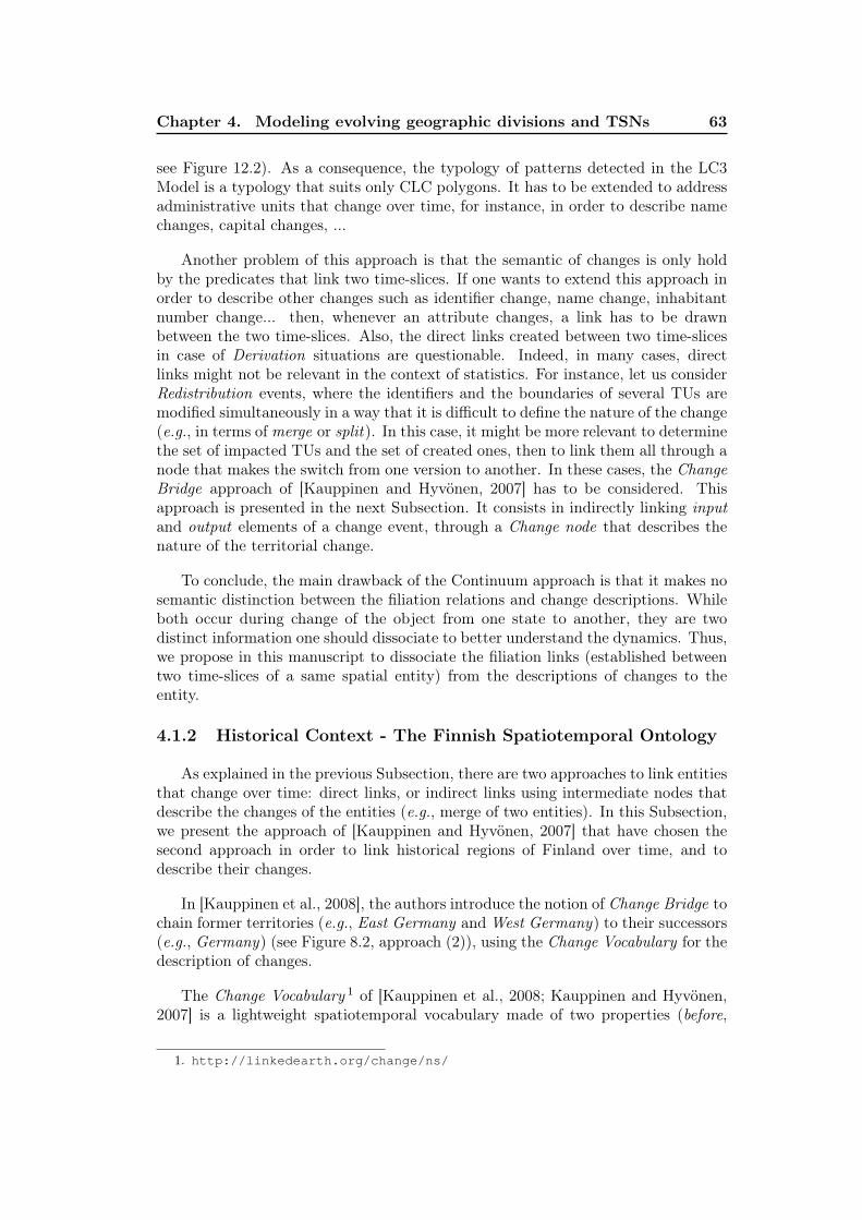
Chapter 4. Modeling evolving geographic divisions and TSNs 63

see Figure 12.2). As a consequence, the typology of patterns detected in the LC3Model is a typology that suits only CLC polygons. It has to be extended to addressadministrative units that change over time, for instance, in order to describe namechanges, capital changes, ...

Another problem of this approach is that the semantic of changes is only holdby the predicates that link two time-slices. If one wants to extend this approach inorder to describe other changes such as identifier change, name change, inhabitantnumber change... then, whenever an attribute changes, a link has to be drawnbetween the two time-slices. Also, the direct links created between two time-slicesin case of Derivation situations are questionable. Indeed, in many cases, directlinks might not be relevant in the context of statistics. For instance, let us considerRedistribution events, where the identifiers and the boundaries of several TUs aremodified simultaneously in a way that it is difficult to define the nature of the change(e.g., in terms of merge or split). In this case, it might be more relevant to determinethe set of impacted TUs and the set of created ones, then to link them all through anode that makes the switch from one version to another. In these cases, the ChangeBridge approach of [Kauppinen and Hyvönen, 2007] has to be considered. Thisapproach is presented in the next Subsection. It consists in indirectly linking inputand output elements of a change event, through a Change node that describes thenature of the territorial change.

To conclude, the main drawback of the Continuum approach is that it makes nosemantic distinction between the filiation relations and change descriptions. Whileboth occur during change of the object from one state to another, they are twodistinct information one should dissociate to better understand the dynamics. Thus,we propose in this manuscript to dissociate the filiation links (established betweentwo time-slices of a same spatial entity) from the descriptions of changes to theentity.

4.1.2 Historical Context - The Finnish Spatiotemporal Ontology

As explained in the previous Subsection, there are two approaches to link entitiesthat change over time: direct links, or indirect links using intermediate nodes thatdescribe the changes of the entities (e.g., merge of two entities). In this Subsection,we present the approach of [Kauppinen and Hyvönen, 2007] that have chosen thesecond approach in order to link historical regions of Finland over time, and todescribe their changes.

In [Kauppinen et al., 2008], the authors introduce the notion of Change Bridge tochain former territories (e.g., East Germany and West Germany) to their successors(e.g., Germany) (see Figure 8.2, approach (2)), using the Change Vocabulary for thedescription of changes.

The Change Vocabulary 1 of [Kauppinen et al., 2008; Kauppinen and Hyvönen,2007] is a lightweight spatiotemporal vocabulary made of two properties (before,

1. http://linkedearth.org/change/ns/

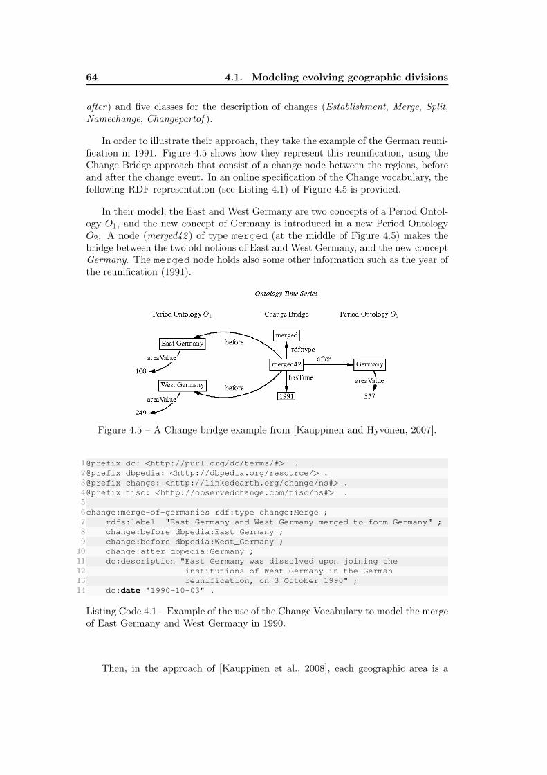
64 4.1. Modeling evolving geographic divisions

after) and five classes for the description of changes (Establishment, Merge, Split,Namechange, Changepartof ).

In order to illustrate their approach, they take the example of the German reuni-fication in 1991. Figure 4.5 shows how they represent this reunification, using theChange Bridge approach that consist of a change node between the regions, beforeand after the change event. In an online specification of the Change vocabulary, thefollowing RDF representation (see Listing 4.1) of Figure 4.5 is provided.

In their model, the East and West Germany are two concepts of a Period Ontol-ogy O1, and the new concept of Germany is introduced in a new Period OntologyO2. A node (merged42 ) of type merged (at the middle of Figure 4.5) makes thebridge between the two old notions of East and West Germany, and the new conceptGermany. The merged node holds also some other information such as the year ofthe reunification (1991).

Figure 4.5 – A Change bridge example from [Kauppinen and Hyvönen, 2007].

1@prefix dc: <http://purl.org/dc/terms/#> .2@prefix dbpedia: <http://dbpedia.org/resource/> .3@prefix change: <http://linkedearth.org/change/ns#> .4@prefix tisc: <http://observedchange.com/tisc/ns#> .56change:merge-of-germanies rdf:type change:Merge ;7 rdfs:label "East Germany and West Germany merged to form Germany" ;8 change:before dbpedia:East_Germany ;9 change:before dbpedia:West_Germany ;10 change:after dbpedia:Germany ;11 dc:description "East Germany was dissolved upon joining the12 institutions of West Germany in the German13 reunification, on 3 October 1990" ;14 dc:date "1990-10-03" .

Listing Code 4.1 – Example of the use of the Change Vocabulary to model the mergeof East Germany and West Germany in 1990.

Then, in the approach of [Kauppinen et al., 2008], each geographic area is a

Chapter 4. Modeling evolving geographic divisions and TSNs 65

concept that belongs to an ontology time-series, made of several Period Ontologies(e.g., O1, O2). In [Kauppinen and Hyvönen, 2007], an ontology time series is definedas follows: "Ontologies evolve when the underlying domain world changes at differentpoints of time. The result then is a series of ontologies whose concepts are relatedwith each other not only within one ontology valid at a moment but through the time."[Kauppinen et al., 2008] focus on the modeling of relations between geographic areaconcepts that evolved over long periods of time. The domain of application of theirmethod is the historical geospatial reasoning. Thus, their Change Bridge approachhas been implemented in order to create the Finnish Spatiotemporal Ontology, anontology time series of the Finnish municipalities over the time interval 1865–2007[Kauppinen et al., 2008].

In [Kauppinen and Hyvönen, 2007], the authors explain that they adopt a three-dimensional approach. They represent geospatial entities that change over time us-ing a "combination of a three-dimensional SNAP-ontology". They do not have thefour-dimensional notion of the same concept, for instance "Finland" or "Lappeen-ranta" (a city in Finland) that changes over time. Instead, they define different ar-eas, each one having one temporal part (e.g., location:Lappeenranta(1967-1989), location:Lappeenranta(1989-)). Each time a change of boundariesor name occur, new area(s) (with a new temporal part) is/are created. This repre-sentation of changes over time suits well to the domain (historical data), and to theaim of their works, i.e., enabling semantic search and browsing of historical regions(using the historical names of the regions for instance).

In order to create the ontology time series that represents the evolution over timeof a country such as Finland, they propose a methodology in 3 steps [Kauppinenet al., 2008]:– (1) modeling geospatial changes. They analyze the change types and construct aMetadata Schema of Current Places, one for Historical Places and another one forChanges. The Metadata Schema of Changes is composed of the following main fields:identifier for the change, date of the change, change type (either establishment,merge, split, namechange, or changepart).– (2) populating the metadata schema. The metadata schemas were implemented asa spreadsheet table, edited by hand. This means that the authors do not automatethe process of detecting and describing changes.– (3) creating the ontology time series from the data spreadsheet table created afterstep (2). They create a JAVA program in order to transform the spreadsheet inputinto an RDF graph (output).

The created RDF graphs are available online from the Finnish Ontology Serviceof Historical Places and Maps 2 at http://dev.hipla.fi/ and the HTML pagesof the resources are accessible online e.g., http://www.yso.fi/onto/sapo/Heinavesi(1920-).

The modeling approach presented in [Kauppinen and Hyvönen, 2007; Kauppinenet al., 2008] is criticized by [Lacasta et al., 2014] as it may lead to a proliferation

2. description of the service at https://seco.cs.aalto.fi/projects/histoplaces/en/

66 4.1. Modeling evolving geographic divisions

of instances. Indeed, the complete status of a TU is described before and afterthe associated change event. We present in the next Subsection the approach from[Lacasta et al., 2014], deriving from [López-Pellicer et al., 2008].

4.1.3 Political context - The Jurisdictional Domain Ontology

[López-Pellicer et al., 2008] propose description of changes in political divisions,called Jurisdictional Domains, that change quite frequently. They approach is tominimize the description and to avoid duplication of data.

"Jurisdictional Domains (JDs) are generally accepted political divisions of theearth surface that cover specific territorial and functional scopes over time. Theyare units of administration for local, regional, national, or international governancewith specific roles separated by administrative boundaries." In [López-Pellicer et al.,2008; Lopez-Pellicer et al., 2012], the authors address two issues: the heterogeneityof political divisions and their evolving nature. They propose an ontology schemathat combines, in a single model, the political structure, the spatial components, andthe temporal evolution of units. Focusing on existing ISO standards, the authorsconclude that no model has an appropriate semantic representation of the differenttypes of administrative units, and of their spatial and temporal relations. Theyfocus on JDs for local, regional, national or international governance.

They propose to connect to a higher ontology (the Descriptive Ontology for Lin-guistic and Cognitive Engineering (DOLCE)), and to allow others to create theirown application ontology, by country, for the representation of their own adminis-trative units.

" This scheme has three layers as shown in Figure 4.6:(1) A high-level ontology that defines data types and general relationswhich are independent of context.(2) A domain ontology which defines concepts and relations that can bereused in the context of the administrative models of different countries.(3) And an application ontology per country, which represents the specifictypes of administrative units of each country, along with specific instancesof existing units."

In the Jurisdictional domain ontology, the jurisdictional-domain concept is spe-cialized in states and administrative-divisions among others. "States are territoriesunder effective and civil government; administrative-divisions represent any divisionin a jurisdictional-domain (administrative-divisions hold a relation with their parentjurisdiction). The spatial information is modeled by the jurisdictional-geographic-object concept, which is defined as a kind of DOLCE politic-geographic-object."

In [Lopez-Pellicer et al., 2012], the authors identify different types of changesthat a JD can undergone: creation, dissolution, change in its properties, and changein its relations. The latter has sub-types presented in Figure 4.7

The model supports the representation of JDs hierarchies using the predicate

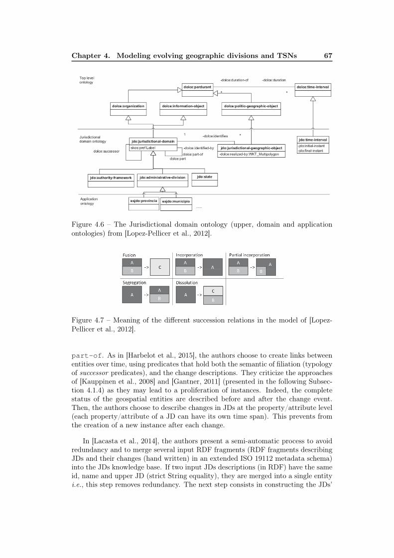
Chapter 4. Modeling evolving geographic divisions and TSNs 67

Figure 4.6 – The Jurisdictional domain ontology (upper, domain and applicationontologies) from [Lopez-Pellicer et al., 2012].

Figure 4.7 – Meaning of the different succession relations in the model of [Lopez-Pellicer et al., 2012].

part-of. As in [Harbelot et al., 2015], the authors choose to create links betweenentities over time, using predicates that hold both the semantic of filiation (typologyof successor predicates), and the change descriptions. They criticize the approachesof [Kauppinen et al., 2008] and [Gantner, 2011] (presented in the following Subsec-tion 4.1.4) as they may lead to a proliferation of instances. Indeed, the completestatus of the geospatial entities are described before and after the change event.Then, the authors choose to describe changes in JDs at the property/attribute level(each property/attribute of a JD can have its own time span). This prevents fromthe creation of a new instance after each change.

In [Lacasta et al., 2014], the authors present a semi-automatic process to avoidredundancy and to merge several input RDF fragments (RDF fragments describingJDs and their changes (hand written) in an extended ISO 19112 metadata schema)into the JDs knowledge base. If two input JDs descriptions (in RDF) have the sameid, name and upper JD (strict String equality), they are merged into a single entityi.e., this step removes redundancy. The next step consists in constructing the JDs’

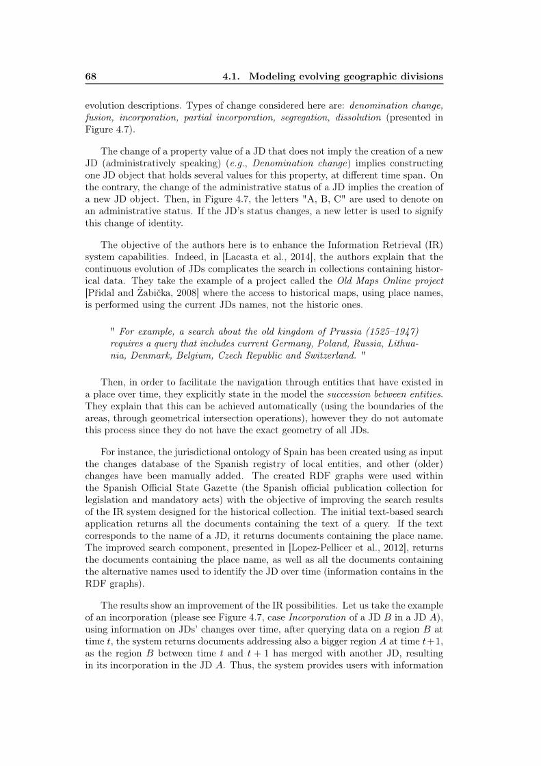
68 4.1. Modeling evolving geographic divisions

evolution descriptions. Types of change considered here are: denomination change,fusion, incorporation, partial incorporation, segregation, dissolution (presented inFigure 4.7).

The change of a property value of a JD that does not imply the creation of a newJD (administratively speaking) (e.g., Denomination change) implies constructingone JD object that holds several values for this property, at different time span. Onthe contrary, the change of the administrative status of a JD implies the creation ofa new JD object. Then, in Figure 4.7, the letters "A, B, C" are used to denote onan administrative status. If the JD’s status changes, a new letter is used to signifythis change of identity.

The objective of the authors here is to enhance the Information Retrieval (IR)system capabilities. Indeed, in [Lacasta et al., 2014], the authors explain that thecontinuous evolution of JDs complicates the search in collections containing histor-ical data. They take the example of a project called the Old Maps Online project[Přidal and Žabička, 2008] where the access to historical maps, using place names,is performed using the current JDs names, not the historic ones.

" For example, a search about the old kingdom of Prussia (1525–1947)requires a query that includes current Germany, Poland, Russia, Lithua-nia, Denmark, Belgium, Czech Republic and Switzerland. "

Then, in order to facilitate the navigation through entities that have existed ina place over time, they explicitly state in the model the succession between entities.They explain that this can be achieved automatically (using the boundaries of theareas, through geometrical intersection operations), however they do not automatethis process since they do not have the exact geometry of all JDs.

For instance, the jurisdictional ontology of Spain has been created using as inputthe changes database of the Spanish registry of local entities, and other (older)changes have been manually added. The created RDF graphs were used withinthe Spanish Official State Gazette (the Spanish official publication collection forlegislation and mandatory acts) with the objective of improving the search resultsof the IR system designed for the historical collection. The initial text-based searchapplication returns all the documents containing the text of a query. If the textcorresponds to the name of a JD, it returns documents containing the place name.The improved search component, presented in [Lopez-Pellicer et al., 2012], returnsthe documents containing the place name, as well as all the documents containingthe alternative names used to identify the JD over time (information contains in theRDF graphs).

The results show an improvement of the IR possibilities. Let us take the exampleof an incorporation (please see Figure 4.7, case Incorporation of a JD B in a JD A),using information on JDs’ changes over time, after querying data on a region B attime t, the system returns documents addressing also a bigger region A at time t+1,as the region B between time t and t + 1 has merged with another JD, resultingin its incorporation in the JD A. Thus, the system provides users with information

Chapter 4. Modeling evolving geographic divisions and TSNs 69

about the evolution of the JDs (fusions, segregation, etc.). The main issue identifiedby the authors is the lack of available spatial historical information.

Then, the Jurisdictional Domain Ontology (JDO) [Lopez-Pellicer et al., 2012]describes changes in Jurisdictional Domains (JDs) at the property level (each prop-erty can have its own time span). This prevents from the creation of new instanceafter each change. However, the modeling of JDs changes over time is still a dif-ferent issue than the modeling of TSN changes over time. Indeed, the objective isto report on JDs changes as soon as they occurred (quite frequently) whereas, instatistics, several versions of the whole TSN (geographic divisions) are created toreport on TSNs changes all at the same time, that is to say not at the time wherethey occur but after a period of stability (see Chapter 2, Section 2.3). Our model,described in the Chapter 8, is trans-temporal (the time of the statistical data isdissociated from the time of the territorial partition) and adopts a versioning ap-proach. In [Lacasta et al., 2014], the authors propose a semi-automatic process forcreating and populating the evolution model of any country, with an approach thatis also quite generic since the characteristics of the heterogeneous sources can beset dynamically. However, it does not produce any description of the impacts ofchanges on hierarchies of TUs. Furthermore, this approach requires the use of awritten dictionary of changes to populate the ontology. This dictionary listsall of the individual changes as textual data described in the ISO-19112 standard,extended with elements to represent changes. This requirement may be seen as adrawback for current statistical information systems because the manual listing ofchanges takes times. Automating the change detection and annotation allows forprocessing many geographic divisions in the world (using the same semantics for thedescription of changes), whether or not there exists a catalog of changes. However, itshould be noted that in the case of crowd-sourcing platform, this approach is a veryinteresting one, as each participant may edit the geometries of the JDs they know,the changes on the JDs’ attributes, using the appropriate administrative terms ofthe JDs described.

Moreover, the main drawback of this approach is the lack of definition of whatcould make the identity of the JDs (over time). Thus, we assume that what istaken into account (when describing changes manually) for the distinction betweena change of type continuation or derivation (i.e., a change of the identity of the JDsor not, e.g., Fusion versus Incorporation, see Figure 4.7) is a new act of law (ornot), that indicates a change of the political identity of the JD.

The next Subsection presents an ontological approach for the representation ofthe evolutions of the Switzerland administrative regions. The model also deals withadministrative divisions, with a much less important place to the political dimension.Conversely, in this approach it was decided to define clearly what makes the identityof the administrative regions over time.

70 4.1. Modeling evolving geographic divisions

4.1.4 Administrative Context - The SONADUS Ontology

In [Gantner, 2011], an ontology called Spatiotemporal Ontology for the Admin-istrative Units of Switzerland (SONADUS) 3 is proposed in order to observe theevolution of the Swiss administrative units, between 1960 and 2010. The Ontologyis written in German: "Since potential users are mostly Swiss, the concepts in theontology were given German names." It focuses on the specificity of the Swiss terri-tory without adopting abstract terms so that other geographic divisions in the worldcould be described using the ontology. The author points out that the administra-tive units (AUs) of Switzerland evolve rapidly and can become unrecognizable overtime because neither the Historicized Municipality Register nor the geometric datasets define what makes the identity of these AUs. This was the main motivation forcreating the SONADUS ontology and the data sets based on it.

The SONADUS ontology and data set were created according to the followingsteps:

(1) The ontology was first created by transferring in OWL the conceptual datamodel of the Historicized Municipality Register (HMR) 4. At this step, both conceptsdescribing the Swiss administrative structure (cantons, districts, ...) and conceptsdescribing changes were created based on the change types defined by the SwissFederal Statistical Office in HMR publication [statistique, 2017]. The SONADUStypology of changes is presented in the Figure 4.8 (please, see the second columnthat is an English translation of the concepts of the SONADUS ontology.

Regarding these change types: "SONADUS differentiates between 24 types ofchange, an increase of 11 types in comparison to the HMR+. This also contrastssharply with the classification of [Kauppinen et al., 2008] that includes seven changetypes of the AUs of Finland. SONADUS, more precisely, makes a distinction betweenthe hierarchical levels, expands the set of change types to the level of cantons, opensand ends the change history, corrects errors in the source data, and finally containspurely administrative change types such as formal renumbering." [Gantner, 2011].

The main issue regarding this typology is that in one concept sev-eral different kind of change, and several different semantic informationare expressed. For instance, the concept "Change of membership of a canton onthe municipality level" expresses to which Swiss administrative level the AUs thatchange belong to, as well as the Swiss administrative level of their super AUs, andfinally the nature of the change (that in a more abstract way may be describedas a change of super TU). Also, all the concepts depend on the Swiss ad-ministrative context, and are written in German which may hinder theirre-use. In this respect, the author wonders: "To what extent is SAPO [Kauppinenet al., 2008] applicable to the situation in Switzerland? In what way does the evolu-tion of administrative units differ between Finland and Switzerland?". Even if the

3. URI of the SONADUS ontology: https://www.wsl.ch/sonadus#4. https://www.bfs.admin.ch/bfs/fr/home/bases-statistiques/repertoi

re-officiel-communes-suisse/liste-historisee-communes.html ; https://opendata.swiss/en/dataset/historicized-municipalities-register

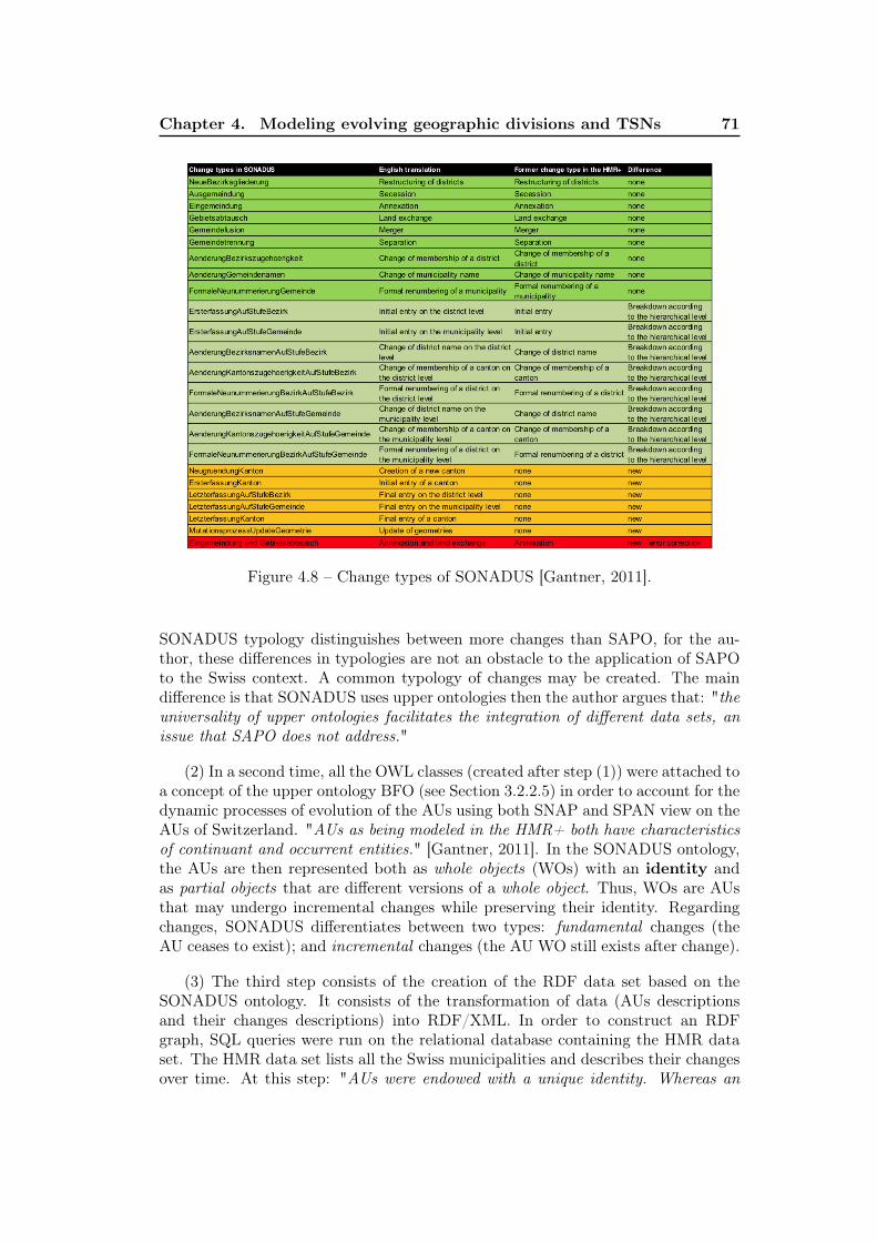
Chapter 4. Modeling evolving geographic divisions and TSNs 71

Figure 4.8 – Change types of SONADUS [Gantner, 2011].

SONADUS typology distinguishes between more changes than SAPO, for the au-thor, these differences in typologies are not an obstacle to the application of SAPOto the Swiss context. A common typology of changes may be created. The maindifference is that SONADUS uses upper ontologies then the author argues that: "theuniversality of upper ontologies facilitates the integration of different data sets, anissue that SAPO does not address."

(2) In a second time, all the OWL classes (created after step (1)) were attached toa concept of the upper ontology BFO (see Section 3.2.2.5) in order to account for thedynamic processes of evolution of the AUs using both SNAP and SPAN view on theAUs of Switzerland. "AUs as being modeled in the HMR+ both have characteristicsof continuant and occurrent entities." [Gantner, 2011]. In the SONADUS ontology,the AUs are then represented both as whole objects (WOs) with an identity andas partial objects that are different versions of a whole object. Thus, WOs are AUsthat may undergo incremental changes while preserving their identity. Regardingchanges, SONADUS differentiates between two types: fundamental changes (theAU ceases to exist); and incremental changes (the AU WO still exists after change).

(3) The third step consists of the creation of the RDF data set based on theSONADUS ontology. It consists of the transformation of data (AUs descriptionsand their changes descriptions) into RDF/XML. In order to construct an RDFgraph, SQL queries were run on the relational database containing the HMR dataset. The HMR data set lists all the Swiss municipalities and describes their changesover time. At this step: "AUs were endowed with a unique identity. Whereas an

72 4.2. Modeling evolving TSNs and their changes

AU maintains its identity in the case of incremental change, fundamental changecauses either the creation or the loss of an identity."

To conclude on the SONADUS approach, we want to emphasize here the qualityof the design of this ontology, which takes into account both the SNAP and SPANrepresentations of the AUs, connects concepts dependent from the Swiss context tomore abstract concepts of the BFO framework, and transfers a relational databaseto a representation in triplets, using a data-model that suits with the triple repre-sentation.

Since the work from [Gantner, 2011], the Governmental Ontology Switzerland(curated by Zazuko.com) has been created, and is available at https://gont.ch/ 5. This ontology is written in English, and aims at describing the HMRdata set, as the SONADUS ontology. The data sets created using this ontologyare available from http://classifications.data.admin.ch/datasets/.The different versions of the municipalities, cantons, and districts of Switzerlandare represented. For instance, the predicate districtVersion is used to saythat a DistrictEntity has a district version DistrictEntityVersion (e.g.,representation of a district and of its version under the number 10107 http://classifications.data.admin.ch/district/1001).

The concept ChangeEvent is defined as a subclass of the Event class de-fined in the The Simple Event Model Ontology 6. Then, several ChangeEventsub-concepts are defined: InitialCompilation, NameChange, NewDistrictOrCanton,TerritorialChange, Renumbering, Dissolution, AbrogationOfMutation.

One of the issues behind these graphs is that numbers are used in the graphs torefer to the type of change that has occurred on a canton, district, or municipality.This makes it difficult for humans to read graphs, because we have to refer to acorrespondence table (number/change type). This suggests that the design of thisontology is not really based on a triplet approach but on a direct translation of arelational model into a triplet one. Another problem is that the concepts are, as inthe case of SONADUS, very dependent from the Swiss administrative context, andthe changes are not represented in a multilevel approach (e.g., the impact of thechanges of a canton on its sub-districts is not represented).

4.2 Modeling evolving TSNs and their changes

Various initiatives to disseminate Linked Statistical Data have emerged through-out the world, for instance: the Aragón Statistical Office Open Data Portal providesLOD statistics on municipalities of the Aragon region of Spain 7; the Italian IstatLinked Open Data Portal 8 and the e-Stat Japanese Portal 9 disseminate statistical

5. The turtle of the ontology is on github https://github.com/gontch/gont.ch/blob/master/gont.ttl

6. URI of the ontology: http://semanticweb.cs.vu.nl/2009/11/sem/7. http://opendata.aragon.es/8. http://datiopen.istat.it/index.php?language=eng9. http://data.e-stat.go.jp/lodw/en

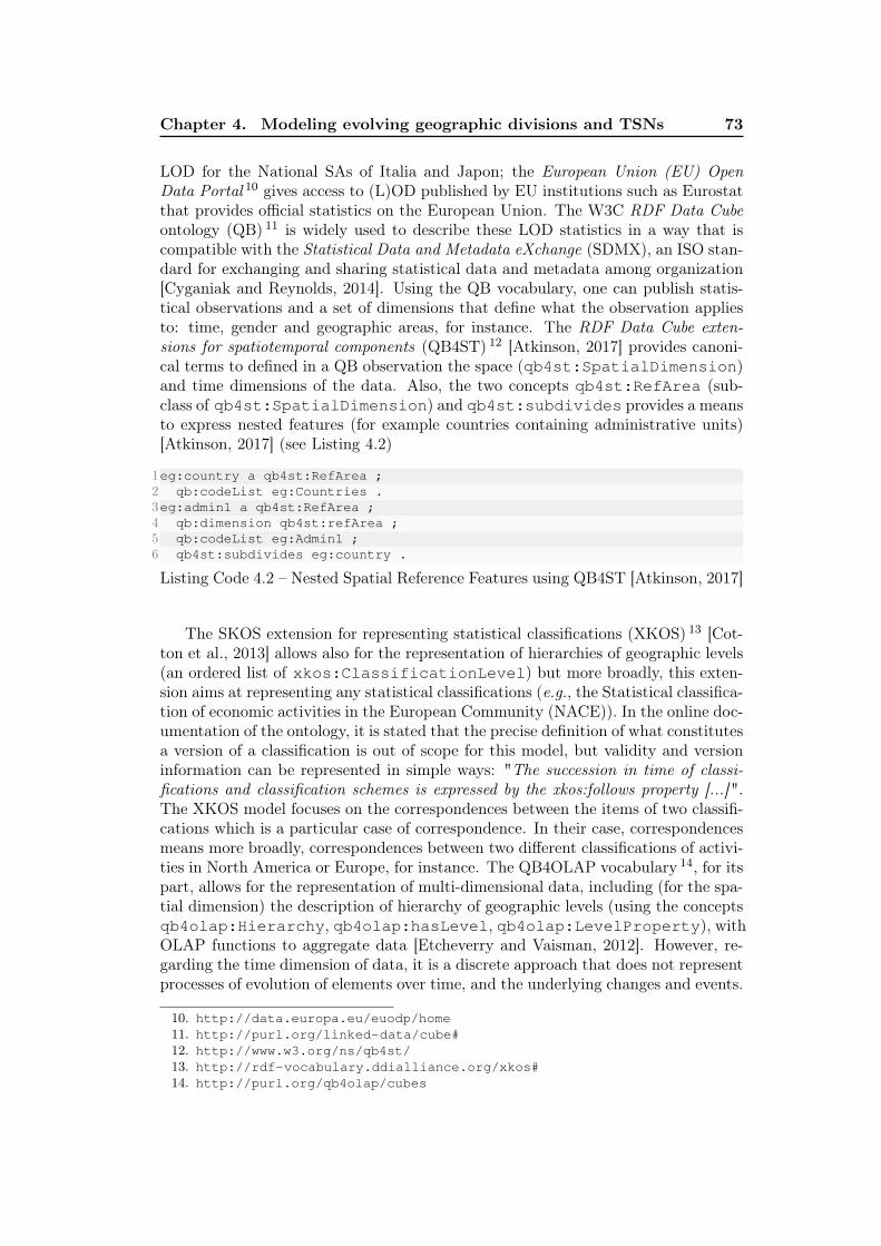
Chapter 4. Modeling evolving geographic divisions and TSNs 73

LOD for the National SAs of Italia and Japon; the European Union (EU) OpenData Portal 10 gives access to (L)OD published by EU institutions such as Eurostatthat provides official statistics on the European Union. The W3C RDF Data Cubeontology (QB) 11 is widely used to describe these LOD statistics in a way that iscompatible with the Statistical Data and Metadata eXchange (SDMX), an ISO stan-dard for exchanging and sharing statistical data and metadata among organization[Cyganiak and Reynolds, 2014]. Using the QB vocabulary, one can publish statis-tical observations and a set of dimensions that define what the observation appliesto: time, gender and geographic areas, for instance. The RDF Data Cube exten-sions for spatiotemporal components (QB4ST) 12 [Atkinson, 2017] provides canoni-cal terms to defined in a QB observation the space (qb4st:SpatialDimension)and time dimensions of the data. Also, the two concepts qb4st:RefArea (sub-class of qb4st:SpatialDimension) and qb4st:subdivides provides a meansto express nested features (for example countries containing administrative units)[Atkinson, 2017] (see Listing 4.2)

1eg:country a qb4st:RefArea ;2 qb:codeList eg:Countries .3eg:admin1 a qb4st:RefArea ;4 qb:dimension qb4st:refArea ;5 qb:codeList eg:Admin1 ;6 qb4st:subdivides eg:country .

Listing Code 4.2 – Nested Spatial Reference Features using QB4ST [Atkinson, 2017]

The SKOS extension for representing statistical classifications (XKOS) 13 [Cot-ton et al., 2013] allows also for the representation of hierarchies of geographic levels(an ordered list of xkos:ClassificationLevel) but more broadly, this exten-sion aims at representing any statistical classifications (e.g., the Statistical classifica-tion of economic activities in the European Community (NACE)). In the online doc-umentation of the ontology, it is stated that the precise definition of what constitutesa version of a classification is out of scope for this model, but validity and versioninformation can be represented in simple ways: "The succession in time of classi-fications and classification schemes is expressed by the xkos:follows property [...]".The XKOS model focuses on the correspondences between the items of two classifi-cations which is a particular case of correspondence. In their case, correspondencesmeans more broadly, correspondences between two different classifications of activi-ties in North America or Europe, for instance. The QB4OLAP vocabulary 14, for itspart, allows for the representation of multi-dimensional data, including (for the spa-tial dimension) the description of hierarchy of geographic levels (using the conceptsqb4olap:Hierarchy, qb4olap:hasLevel, qb4olap:LevelProperty), withOLAP functions to aggregate data [Etcheverry and Vaisman, 2012]. However, re-garding the time dimension of data, it is a discrete approach that does not representprocesses of evolution of elements over time, and the underlying changes and events.

10. http://data.europa.eu/euodp/home11. http://purl.org/linked-data/cube#12. http://www.w3.org/ns/qb4st/13. http://rdf-vocabulary.ddialliance.org/xkos#14. http://purl.org/qb4olap/cubes

74 4.2. Modeling evolving TSNs and their changes

With regard to the evolving nature of the geographic areas the observations coverand the TSN these evolving areas belong to, none of the ontologies described aboveprovide the vocabulary required to achieve the description of the way these TSNs,their levels, and TUs evolved over time. The (N)SAs or National Mapping Agen-cies, for their part, often create their own ontology for the description of their areas(e.g., the Territorio Ontology 15 of the Italian National Institute for Statistics, theGeography Ontology 16 of the Scottish Government, the Ordnance Survey Ireland’sOntologies 17 [Debruyne et al., 2017]), which results in a counterproductive prolifer-ation of non-aligned vocabularies. Among these initiatives, we highlight here someof them. Then, we present the generic approach of [Plumejeaud et al., 2011; Plume-jeaud, 2011] that addresses the TSNs specificities, and describes their evolution andchanges over time.

4.2.1 Ontologies for TSN representation

4.2.1.1 INSEE - INSEE Ontologie geographique

The INSEE French National Institute of Statistics and Economic Studies pub-lishes the INSEE Geographic Ontology 18. However, this ontology is written in Frenchand the concepts are strongly dependent from the French context.

4.2.1.2 Eurostat - Reference And Management Of Nomenclatures On-tology

The Eurostat Directorate-General of the European Commission publishes theReference And Management Of Nomenclatures Ontology (RAMON) 19. This ontol-ogy allows for the description of Local Administrative Units 20 and NUTS TSN.However, if one wants to describe TU coming from another TSN than NUTS andLAU, the ontology needs to be modified by adding new sub-concepts, subsumed bythe "Geographical Region" concept.

15. http://datiopen.istat.it/odi/ontologia/territorio/16. http://statistics.gov.scot/vocabularies/17. Ireland’s Administrative boundaries ontology:http://ontologies.geohive.ie/osi#;

Ontology to describe the evolution of Ireland’s boundaries: http://ontologies.geohive.ie/osiprov#18. http://rdf.insee.fr/def/geo/insee-geo-onto.ttl19. http://ec.europa.eu/eurostat/ramon/ontologies/geographic.rdf20. http://ec.europa.eu/eurostat/web/nuts/local-administrative-units

Chapter 4. Modeling evolving geographic divisions and TSNs 75

4.2.1.3 Ordnance Survey - Administrative geography and civil votingarea Ontology for UK

The Ordnance Survey national mapping agency in Great Britain publishes theAdministrative geography and civil voting area ontology for UK 21. As stated in [Cor-rendo et al., 2010], the hierarchical nature of NUTS can be described with the Ord-nance Survey ontology, but the temporal extent of a given geographical subdivisioncannot. Furthermore, as for INSEE the concepts are strongly dependent from theUK context.

4.2.1.4 ONS - ONS Boundary Change Ontology

The UK Office for National Statistics proposes vocabularies 22 to represent theevolution of geographic areas in the context of statistical data publication. Even if wecan notice a certain level of abstraction on the terms used to describe TUs 23, whichmakes it possible to describe other TUs than UK’s ones, none of these vocabulariesallows to describe any TSN structure and its levels. New concepts need to be addedto the ontology Geographical hierarchy ontology 24 in order to describe new territoriesand new territorial meshes than those listed. Furthermore, none of the concepts ofthe ONS Boundary Change Ontology 25 provides naming for changes that impactseveral TUs at the same time. Finally, the concepts describing change events arefew and limited to Recoding change, Boundary change.

4.2.1.5 Statistics Bureau of Japan - SAC Ontology

The Statistics Bureau of Japan proposes vocabularies 26 to represent geographicareas and their evolution, including the description of change events in the context ofstatistical data publication. In [Yamamoto et al., 2017], the authors propose a solu-tion to describe changes, with the reason for the change. Nevertheless, they limit todescription of changes in municipalities, using the following change event concepts:absorption, abolishment, separation, establishment, division, name change, bound-ary change, and shiftToAnotherKindOfCity. Also, the description of the reason forthe change is limited to one literal.

21. http://data.ordnancesurvey.co.uk/ontology/admingeo/22. http://statistics.data.gov.uk/vocabularies23. http://statistics.data.gov.uk/def/statistical-entity24. http://statistics.data.gov.uk/def/hierarchy/best-fit25. http://statistics.data.gov.uk/def/boundary-change26. e.g., http://data.e-stat.go.jp/lod/sac/, http://data.e-stat.go.jp/lod/te

rms/sacs#, http://data.e-stat.go.jp/lod/sace/

76 4.2. Modeling evolving TSNs and their changes

4.2.1.6 Food and Agriculture Organization of the United Nations - FAOGeopolitical Ontology

The Food and Agriculture Organization of the United Nations (FAO) publishesthe FAO Geopolitical Ontology 27. FAO produces also a data set composed of a list ofcountries in the world. This data set is semantically annotated thanks to geopoliticalconcepts of the ontology (e.g., self-governing, non-self-governing, disputed). TheFAO Geopolitical Ontology identifies successive versions of a TU (i.e., predicatespredecessor, successor, valid since, valid until). However, the changes undergone byTUs are not described (e.g., spatial area changes).

4.2.2 TSN data sets as Linked Data

When publishing a TSN on the Web of data, we have to distinguish between theontology used to describe the structure of a TSN and the data sets described viathis ontology. With regard to the TSN data sets published on the LOD Web, wefocus in this manuscript on the NUTS TSN data sets:

4.2.2.1 NUTS-RDF Geovocab

NUTS-RDF Geovocab 28 are published as part of the Planet Data EU Networkof Excellence 29. Nevertheless, only one version of the NUTS is published online.

4.2.2.2 Eionet - NUTS Data set

Eionet publishes NUTS versions in RDF format 30 and uses the Eionet RAMONOntology for the description of NUTS. There are two types of links (owl:sameAs,rdfs:seeAlso) to connect TU from the NUTS version 2006 to TU from the 2003version. Nevertheless, changes undergone by TU from one version to another arenot described.

4.2.2.3 EnAKTing - Linked NUTS

The EnAKTing project 31 (funded by the Engineering and Physical SciencesResearch Council) publishes NUTS versions in RDF format, under the Linked NUTS

27. http://www.fao.org/countryprofiles/geoinfo/en/28. http://nuts.geovocab.org/29. http://www.planet-data.eu/30. http://rdfdata.eionet.europa.eu/ramon/nuts.rdfhttp://rdfdata.eionet

.europa.eu/ramon/nuts2008.rdf http://rdfdata.eionet.europa.eu/ramon/nuts2003.rdf31. http://gow.epsrc.ac.uk/NGBOViewGrant.aspx?GrantRef=EP/G008493/1

Chapter 4. Modeling evolving geographic divisions and TSNs 77

name [Correndo and Shadbolt, 2013]. The Linked NUTS represents the modificationof NUTS TU over time. However, the description of the changes undergone by TUfrom one NUTS version to another is brief and restricted to code change, regionsplitting, and regions merging, while, as will be seen later, other changes that affectthe TSN components should be taken into account to avoid misinterpretation ofstatistical data.

The Subsections 4.2.1 and 4.2.2 have shown that, despite the multiple initiativesto represent TSNs on the LOD Web, none of them is abstract enough to enable thedescription of any TSN (with a structure such as the one we address in this thesis,defined in Chapter 2, Section 2.2) and of its changes over time, on the LOD Web.The next Subsection presents an approach that is generic. Our work is a continuationof these works from [Plumejeaud, 2011], achieved in our STeamer research group. Wepropose an immersion of the models and algorithm in the semantic Web since theywere originally designed specifically for relational databases, and not for triplets’representation and graphs.

4.2.3 A spatiotemporal model for TSN

The generic approach of [Plumejeaud et al., 2011; Plumejeaud, 2011] addressesTSNs specificities, and describes their evolutions and changes over time. In previouswork of our research group [Plumejeaud et al., 2011], the model is presented asfollows: "A model based on the identity of geographic units which enables one tostudy the genealogy of units, and to observe a unit inside different kinds of territorialorganizations, possibly changing over time."

The model is introduced in this manuscript as in the paper [Plumejeaud et al.,2011], in two steps: first we present how the identity concept of TUs inside territorialhierarchies is modeled; second, we present how is modeled the evolution of the TUsover time, from the concept of identity to the concept of genealogy.

4.2.3.1 Identity and Hierarchy

The first part of the model, presented in Figure 4.9 enables the description ofa TSN hierarchical organization: the concept Nomenclature represents the TSNused by statistical agencies, composed of Geographic Units.

The Zoning object refers to a set of Geographic Units which have the same scale,that is to say the same level, inside a given Nomenclature. Each Geographic Unitis linked to a nomenclature by an association class IdentityAttributes thatholds the list of attributes that usually describe a Geographic Unit in a nomencla-ture:– Designation: refers to the official name of the unit in a given language.– Code: specifies the code of the unit inside the Nomenclature.– Center: represents the position of the center of the unit (a point or another Geo-graphicUnit included inside the considered unit). The center can also have an official

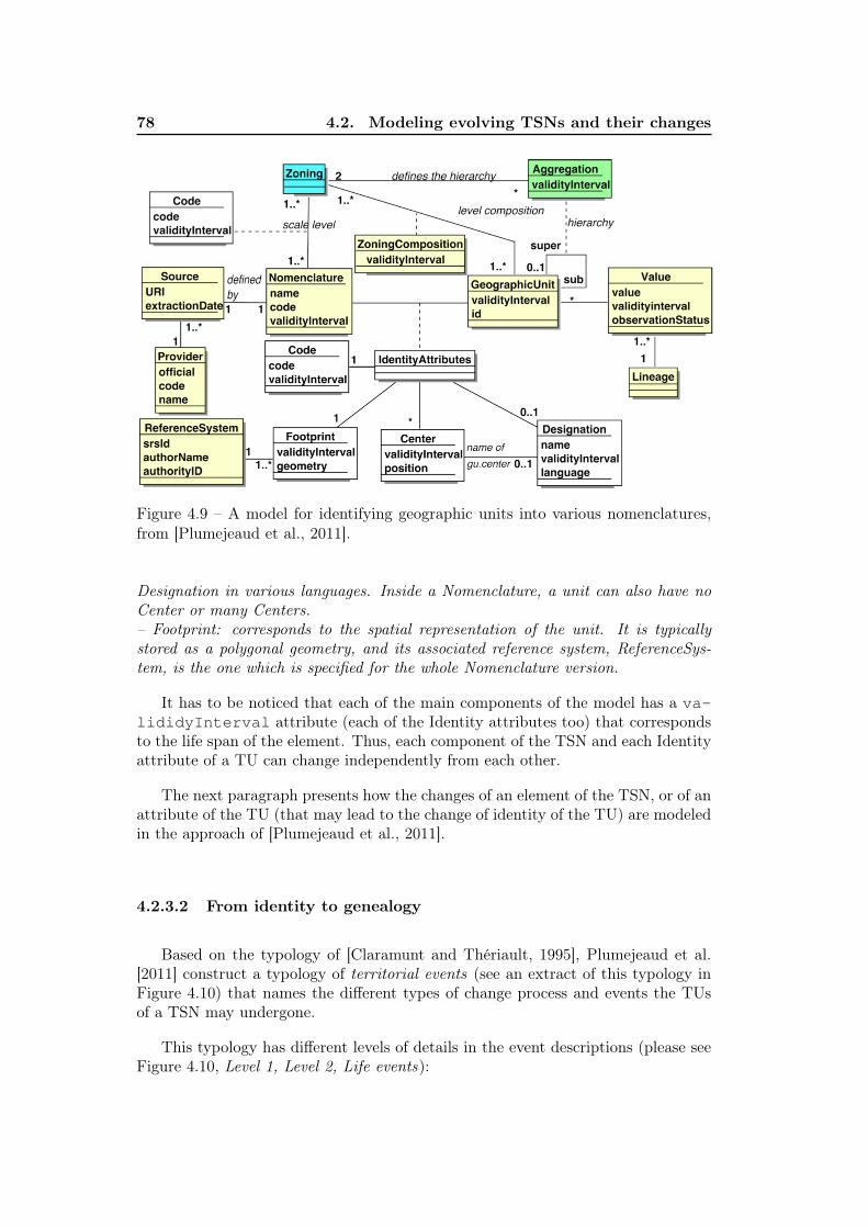
78 4.2. Modeling evolving TSNs and their changes

Figure 4.9 – A model for identifying geographic units into various nomenclatures,from [Plumejeaud et al., 2011].

Designation in various languages. Inside a Nomenclature, a unit can also have noCenter or many Centers.– Footprint: corresponds to the spatial representation of the unit. It is typicallystored as a polygonal geometry, and its associated reference system, ReferenceSys-tem, is the one which is specified for the whole Nomenclature version.

It has to be noticed that each of the main components of the model has a va-lididyInterval attribute (each of the Identity attributes too) that correspondsto the life span of the element. Thus, each component of the TSN and each Identityattribute of a TU can change independently from each other.

The next paragraph presents how the changes of an element of the TSN, or of anattribute of the TU (that may lead to the change of identity of the TU) are modeledin the approach of [Plumejeaud et al., 2011].

4.2.3.2 From identity to genealogy

Based on the typology of [Claramunt and Thériault, 1995], Plumejeaud et al.[2011] construct a typology of territorial events (see an extract of this typology inFigure 4.10) that names the different types of change process and events the TUsof a TSN may undergone.

This typology has different levels of details in the event descriptions (please seeFigure 4.10, Level 1, Level 2, Life events):

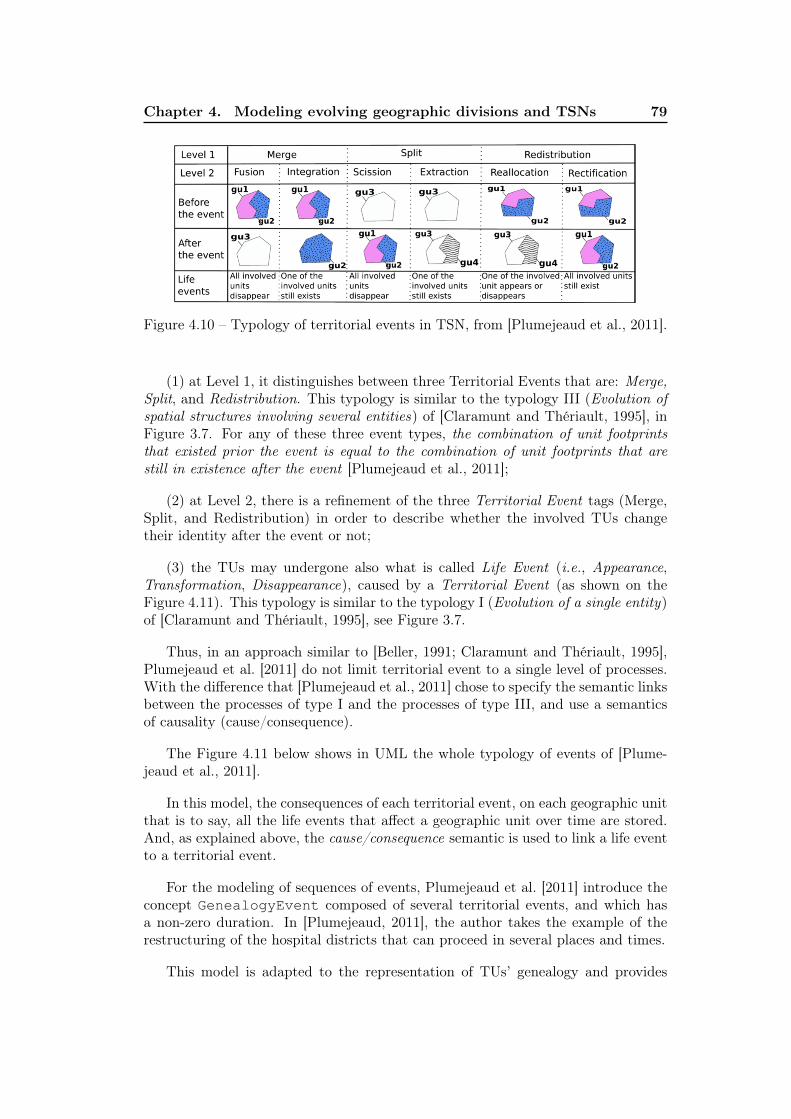
Chapter 4. Modeling evolving geographic divisions and TSNs 79

Figure 4.10 – Typology of territorial events in TSN, from [Plumejeaud et al., 2011].

(1) at Level 1, it distinguishes between three Territorial Events that are: Merge,Split, and Redistribution. This typology is similar to the typology III (Evolution ofspatial structures involving several entities) of [Claramunt and Thériault, 1995], inFigure 3.7. For any of these three event types, the combination of unit footprintsthat existed prior the event is equal to the combination of unit footprints that arestill in existence after the event [Plumejeaud et al., 2011];

(2) at Level 2, there is a refinement of the three Territorial Event tags (Merge,Split, and Redistribution) in order to describe whether the involved TUs changetheir identity after the event or not;

(3) the TUs may undergone also what is called Life Event (i.e., Appearance,Transformation, Disappearance), caused by a Territorial Event (as shown on theFigure 4.11). This typology is similar to the typology I (Evolution of a single entity)of [Claramunt and Thériault, 1995], see Figure 3.7.

Thus, in an approach similar to [Beller, 1991; Claramunt and Thériault, 1995],Plumejeaud et al. [2011] do not limit territorial event to a single level of processes.With the difference that [Plumejeaud et al., 2011] chose to specify the semantic linksbetween the processes of type I and the processes of type III, and use a semanticsof causality (cause/consequence).

The Figure 4.11 below shows in UML the whole typology of events of [Plume-jeaud et al., 2011].

In this model, the consequences of each territorial event, on each geographic unitthat is to say, all the life events that affect a geographic unit over time are stored.And, as explained above, the cause/consequence semantic is used to link a life eventto a territorial event.

For the modeling of sequences of events, Plumejeaud et al. [2011] introduce theconcept GenealogyEvent composed of several territorial events, and which hasa non-zero duration. In [Plumejeaud, 2011], the author takes the example of therestructuring of the hospital districts that can proceed in several places and times.

This model is adapted to the representation of TUs’ genealogy and provides

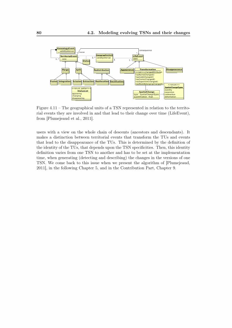
80 4.2. Modeling evolving TSNs and their changes

Figure 4.11 – The geographical units of a TSN represented in relation to the territo-rial events they are involved in and that lead to their change over time (LifeEvent),from [Plumejeaud et al., 2011].

users with a view on the whole chain of descents (ancestors and descendants). Itmakes a distinction between territorial events that transform the TUs and eventsthat lead to the disappearance of the TUs. This is determined by the definition ofthe identity of the TUs, that depends upon the TSN specificities. Then, this identitydefinition varies from one TSN to another and has to be set at the implementationtime, when generating (detecting and describing) the changes in the versions of oneTSN. We come back to this issue when we present the algorithm of [Plumejeaud,2011], in the following Chapter 5, and in the Contribution Part, Chapter 9.

Chapter 5

Generating and Exploitingdescriptions of evolving TSN

In this Chapter, we evaluate the existing methods for automatically generatingthen exploiting, in the semantic Web, descriptions of evolving geographic areas(descriptions of their life, filiation and changes over time).

5.1 Generating

We focus in this Section on the process of generating information on the dynamicsof the world (mainly generating similarities and changes description of geospatialobjects that evolved over time). Generating LOD descriptions of geospatial objectsat one time period is a trivial task if one has, for instance, a shapefile containingthe geospatial features. Indeed, tools such as GeoTriples 1 exist, taking as inputa shapefile and generating the RDF representation of the features inside the inputshapefile. In the Chapter 9, we explain how to do this, using the GeoTriples programand a mapping file that associate the shapefile columns with ontological concepts.

We have seen in Chapter 3, Section 3.2 that in order to populatetheir ontological model, [Lopez-Pellicer et al., 2012], [Kauppinen et al.,2008], and [Gantner, 2011] use a written dictionary of changes, otherssuch as [Plumejeaud, 2011], and [Harbelot et al., 2015] develop computerprograms in order to detect the changes. In this Section, we focus on thesecond approach that automate the change descriptions in geospatial data. In theliterature, the approaches consist mainly in computing similarity scores betweeneach pair of geospatial objects (e.g., a pair composed of a TU that belongs to aTSN version V ′ and of a TU that belongs to the next version V ′′ of the same TSN).However, the approaches differ in the similarity threshold calculation: sometimes itis based only on the spatial footprint (by calculating the intersection of geometries inthe case of polygons), or, sometimes, it takes into account other information (such asthe name of the TU, its capital, etc.). A further difference is that some approachesdescribe changes that affect only isolated features, while others try to detect andput a semantic label on changes that simultaneously affect several features (e.g.,merge of two TUs). In the following Subsection, we present conflation approachesthat calculate similarities between data in order to combine information from twoor more related data sets.

1. https://github.com/LinkedEOData/GeoTriples/wiki

82 5.1. Generating

5.1.1 Conflation Algorithms

As noted in [Li and Goodchild, 2011], many GIS require data from more thanone source. However, in this case the establishment of a coherent GIS can be difficultsince data may differ greatly: geographic data may initially be created by variousactors, for a variety of purposes, in different formats, or at different scales...

Depending on the final objective of mobilizing various data sources, the processesto be apply on data that enter the GIS are different. Let us assume that the differentdata sources describe the same geographic objects:– if there is a need to preserve all the information from these different data sources:then, there is a need for tools that detect and describe the differences and similaritiesbetween the data sources;– if there is a need to create, using different data sources, one data set that mergedata from different sources (because one data set may contain information the othersdon’t have and conversely): then, in this case, there is a need for tools that resolveconflict between duplicated data for instance, and remove the duplicates.

Yet, both cases face first the same problem of feature matching as in con-flation approaches: in the second case, only one of the features that match willbe kept; in the first case, both of them will be kept, and similarities measure will betranslated into semantic information for instance.

Based on the Conflation definition of [Longley et al., 2005], Shekhar and Xiong[2007] provide the following definition of the term Conflation of Features:

"In GIS, conflation is defined as the process of combining geographic informationfrom overlapping sources so as to retain accurate data, minimize redundancy, andreconcile data conflicts".

One of the conflation steps consists in feature matching : "Feature matchinginvolves the identification of features in multiple data sets that represent the sameentity in reality" [Li and Goodchild, 2011]. The main problem of feature matchingis "due to different data quality, different scales, different schemata and differentpurposes, the same entity may be represented differently in terms of position, shapeand level of detail." [Li and Goodchild, 2011].

"There are generally two major steps in feature matching: First, we choose asimilarity measurement to be used as a criterion for matching; second, we identifyall matched pairs of features using this selected similarity criterion [...] similaritymeasures commonly used in feature matching can be classified into three types accord-ing to whether they are based on similarities of geometry, attribute or topology, orcombinations of these." [Li and Goodchild, 2011]. Conflation algorithms, like thoseproposed by [Hastings, 2008] and [McKenzie et al., 2014], but also [Ruiz et al., 2011]take in consideration the spatial dimension. [Hastings, 2008] takes a multi-attributeapproach to conflating digital gazetteers. [McKenzie et al., 2014] use also the multi-attribute approach from [Hastings, 2008] to perform Points of Interest conflation,namely identifying whether two information entities refer to the same place in the

Chapter 5. Generating and Exploiting descriptions of evolving TSN 83

physical world. They demonstrated a weighted multi-attribute matching strategythat can successfully match 97% of randomly selected POI from two different datasets. Metric results are then used for conflict resolution for gazetteers or POI (e.g.,choose the canonical form of a place name between multiple possibilities).

[Plumejeaud, 2011] also uses similarity measures on a list of TU’s attributes,identified as relevant for comparison between two versions of a TSN. She designs anAlgorithm presented in the following Subsection.

5.1.2 Algorithm for the automatic matching of two TSN versions

Please note that this algorithm and its main functions are more detailed in theChapter 9 as our work enriches this algorithm to output semantic RDF descriptionsof the territorial changes in TSNs. In this Section, we provide the reader with themain ideas of how the algorithm works.

The algorithm looks for TUs that are equal between two versions of a TSN.Knowing that two units are considered equal if a combination of criteria (relating tothe attributes of the TUs) are satisfied. These criteria consist of similarity measureson a list of TU’s attributes, identified as relevant (by an expert of the TSN) forcomparison between two TSN’s versions. Some similarity tests are more complexthan others.

For instance, the distance test on the geometry of the TUs, implies first thatthe geometries are in the same coordinate system or, if not, it implies convertinggeometries into the same representation system. Second, the geometries may nothave the same level of detail, i.e., they are not exactly the same although the unithas not changed between the two versions. There are several solutions to com-pute a similarity score between two geometries, depending on the nature of thegeometries i.e., point, line or polygon. The score corresponds most of the time to acomputed distance, usually determined by a Euclidean distance for the point geome-tries, or Hausdorff distance for the poly-lines geometries. In addition to Euclidean orHausdorff distances, other distances are used in order to compute similarity scores.[Devogele, 2002] uses the maximal distance between two lines, called the discreteFrechet distance, that considers the locations and the ordering of the constituentpoints of poly-lines when calculating proximity. [Bel Adj Ali and Vauglin, 1999]propose an areal distance test for polygonal geometries. It computes for two ge-ometries that intersect, the ratio of the shared area by the union of their areas. In[Plumejeaud, 2011], the proposed solution is to use the areal distance of [Bel Adj Aliand Vauglin, 1999] for the similarity test between two TUs’ geometries, in two dif-ferent versions of a TSN. If the ratio obtained after the [Bel Adj Ali and Vauglin,1999] test, multiplied by 100 is smaller than a small value, denoted epsilon ε, itmeans that the spatial footprint has changed very little. It is therefore consideredunchanged. This surface distance test has the advantage of being customizable, byvarying the ε value. All the results of the areal distance test between each pair ofTUs are registered into a SpatialMatch matrix.

In a second step, in case of a geometry change identified by the areal distance test,

84 5.1. Generating

the algorithm tries to determine precisely if only one TU’s geometry has changedor more neighboring TUs with it. For instance, if a TU u′1 is split in two TUs (u′′2and u′′3), the SpatialMatch matrix will have registered two intersections for theTU u′1 and will conclude to a territorial change of type Split (see the [Plumejeaudet al., 2011] typology of changes in Figure 4.11). An equality test is performed onthe external geometries of the two sets of TUs before and after change (e.g., equalitytest between the external geometry of u′1 and external geometry of the union of u′′2and u′′3) in order to validate the aggregation of several TUs changes under oneterritorial change tag (e.g., split, merge, redistribution), with a tolerance threshold.

For each pair of TUs that intersects, other distance tests, on the others TUsattributes are performed and summed at the end, in order to determine if the TUsof the two versions match or not. Please note that all these tests are described inmore details in the Chapter 9.

The algorithm always proceeds from top to bottom, it first matches higher-levelunits before attempting to match the units at the next lower level. This algorithmhas been implemented and tested on the NUTS TSN versions. The program retrievesall the territorial and life event changes in the NUTS TSN, in half an hour orless. The author concludes that the program is very beneficial to agencies such asEurostat, as the manual listing of changes is time consuming for them.

The areal distance test proposed in [Plumejeaud, 2011] needs to test first theintersection between two geometries then to compute a percentage of intersection.This percentage is computed using the spatial functions of the PostGIS DBMS. In[Harbelot et al., 2015], the authors adopt the same methodology. They first computea similarity score between the parcels of the CLC data set (in different versions),then depending on the score values, they attach semantic tags that describe filiationlinks between the parcels, or changes.

5.1.3 Methodology for constructing filiation links in CLC data sets

As noticed in [Harbelot et al., 2015], the Corine Land Cover data set does notprovide any knowledge about filiation relationships and requires a new methodologyin order to identify the relationships between the different parcels versions.

Then, the authors propose the following solution to semi-automate such descrip-tion of the filiation links in the CLC data sets, using the Continuum models:– (1) find filiation and link entities using hasFiliation Continuum predicates.It consists in finding all pairs of entities having an overlap (i.e., intersection testbetween two geometries). At this step, an overlapping score is computed betweeneach pair of features and stored. However, some of these intersections represent afiliation relationship while others should be considered as noise due to inaccuraciesor negligible changes. A threshold is defined in order to filter spatial filiation andaccept a correct filiation relationships only when the parent and child overlap ex-ceeds a certain threshold.– (2) find continuation links that may be of three different kinds referring to growth,reduction or equality of the geometries. In order to distinguish each case, the pro-

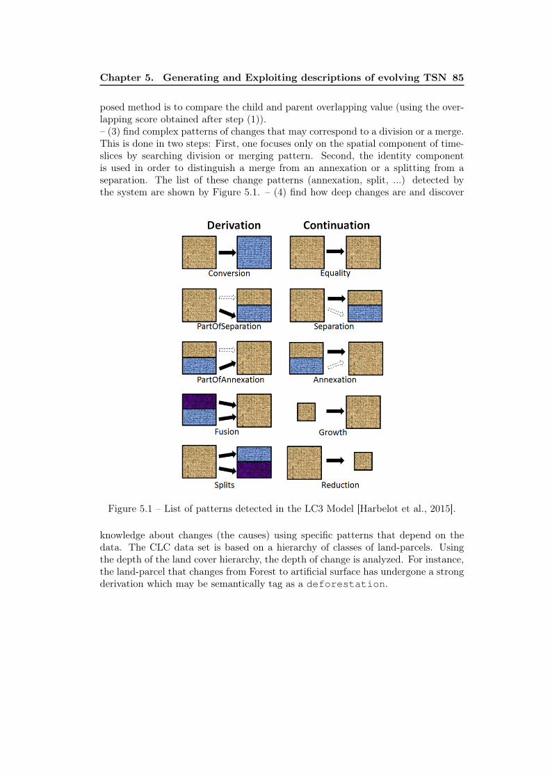
Chapter 5. Generating and Exploiting descriptions of evolving TSN 85

posed method is to compare the child and parent overlapping value (using the over-lapping score obtained after step (1)).– (3) find complex patterns of changes that may correspond to a division or a merge.This is done in two steps: First, one focuses only on the spatial component of time-slices by searching division or merging pattern. Second, the identity componentis used in order to distinguish a merge from an annexation or a splitting from aseparation. The list of these change patterns (annexation, split, ...) detected bythe system are shown by Figure 5.1. – (4) find how deep changes are and discover

Figure 5.1 – List of patterns detected in the LC3 Model [Harbelot et al., 2015].

knowledge about changes (the causes) using specific patterns that depend on thedata. The CLC data set is based on a hierarchy of classes of land-parcels. Usingthe depth of the land cover hierarchy, the depth of change is analyzed. For instance,the land-parcel that changes from Forest to artificial surface has undergone a strongderivation which may be semantically tag as a deforestation.

86 5.1. Generating

As explain in the Subsection 4.1.1, this approach suits well to CLC data sets,but it is not appropriated to administrative divisions, for instance, becauseit only takes into account the geometry of the parcel and the nature of theland cover when detecting changes. It does not take into account otherattributes that may constitute the identity of the geospatial entities, suchas the identifier or name of the entity. This approach lacks flexibility whenit comes to the definition of identity of the time-slices, if it was to describechanges in geographic divisions different from CLC.The approach of [Plumejeaud, 2011] is more flexible (the definition of whatmakes the identity of the TUs (a list of TUs’ attributes) and in whichproportion those attributes can vary are configurable). However, it is notimmersed in the Semantic Web, contrary to the L3C method from Harbelotet al. [2015].

Here, we have reviewed the solution for conflation of geospatial data sets andthe different measures of similarities between the geometries of geospatial data sets.Version Control Systems (VCS) propose another approach that intends to solve theproblem of data conflict that occurs when several persons simultaneously edit thesame source code text, for instance. As in the conflation approach, the VCS toolsneed first to identify the changes between two texts, then to resolve the conflictbetween different versions.

5.1.4 Version Control System

We focus in this Subsection on the existing Version Control System Tools forthe versioning of Geospatial Data. With regard to software tools specialized in ver-sion control, semantic descriptions of changes in ontologies emerge [Redmond et al.,2008], [Völkel and Groza, 2012] in order to ease collaborative ontology editing and re-solve conflicts. These ontology versioning systems describe the set of edit operationsmade on ontology versions. For instance, the SemVersion, plug-in to Protégé soft-ware "provides structural and semantic diffs visualization of the added and removedstatements" [Völkel and Groza, 2012]. And, they plan for "future developments, tocreate an intuitive format, for example, by displaying the two ontologies in paralleland create graphic connections to indicate the added and removed statements."

Conflict resolution in VCS, is most of the time a problem of collaborative con-struction of data set or software source code. With regards to Geospatial Data, forinstance the software Ethermap [Fechner et al., 2015] is a real-time synchronizedcollaborative map editor, with multiple concurrent users. It allows users to reviewchanges made to the map, using an "History" tool that tracks the edit (e.g., descrip-tions such as "edited properties", "edited geometry", "created feature") or removeactions, and tracks which user is responsible for those actions on the map.

Other VCS tools, such as GeoGIG 2 or the GitHub Inc. project 3, focus on geospa-tial data with the very purpose of conflict detection, conflict resolution and merge

2. http://geogig.org/3. https://blog.github.com/2014-02-05-diffable-more-customizable-maps/

Chapter 5. Generating and Exploiting descriptions of evolving TSN 87

in data when multiple contributors edit the data. Hereafter is the description ofthe GeoGIG tool on its official Website: "Users are able to import raw geospatialdata (currently from Shapefiles, PostGIS or SpatiaLite) into a repository where everychange to the data is tracked. These changes can be viewed in a history, reverted toolder versions, branched in to sandboxed areas, merged back in, and pushed to remoterepositories." GeoGIG or Google limit their comparison to attributes independently.

Although tools such as Ethermap, GeoGIG 4 or the GitHub Inc. project 5 [Ne-gretti, 2015; LocationTech, 2018; Boundless, 2014a; ?,b] handle versioning of geospa-tial data and provide a way to visualize differences in geometries, feature by feature,they are unable to group changes that affect several geographic objects at the sametime (e.g., a merge of two TUs), or to attach semantics describing the context andnature of these territorial changes. Indeed, the very purpose of these tools is conflictdetection and resolution, as explained before. Such software do not focus on thesemantic of changes that help in understanding the reason for the change.

Several works try also to reconcile data conflicts and focus on the measurementof similarities between GeoSpatial Data [Angela, 2008], in order to improve thequality of volunteered geographic data for instance [Vandecasteele and Devillers,2013], by avoiding duplication of data, among others [Zhang et al., 2007]. In [Van-decasteele and Devillers, 2013], the authors explain that, during the editing process,by automatically notifying contributors when two attributes are too similar or toodissimilar using similarity measures, their system reduces semantic heterogeneity ofthe edited data. They address the issue of semantic similarities between conceptssuch as ’road’, ’highway’ or ’river’: "Semantic similarity quantifies how similar, ordissimilar, concepts are, based on their meanings." Several methods for measuringsemantic similarities exists such as the Network model where concepts are in a se-mantic networks. "In such networks, concepts are represented as nodes and relationsbetween concepts are represented by edges. The similarity between two concepts ismeasured using a distance function. This distance function is based on graph theoryalgorithms, such as the shortest path model." [Vandecasteele and Devillers, 2013].These approaches based on similarity measures are another way of resolving conflictsin order to avoid unnecessary changes (to avoid the addition of similar data).

Other works propose solution (using relational database system) to keep trackof multi-scale data evolution. Multi-scale means multi-representation of a geospa-tial object, at different levels of detail: "in different scales the objects are usuallyrepresented in different ways, because each scale can have a convention of repre-sentation". However, we haven’t find software that keep track of multi-levels (e.g.,States, regions, districts) data evolution.

As a conclusion, none of the works presented in this section addresses the seman-tic description of changes (changes in feature attributes and more complex changessuch as merge of two polygons) in multi-levels geospatial data. Nevertheless, theyall investigate interesting options to deal with geospatial evolution over time, in real-time context different from the one of official TSNs data published every 3 (NUTS)

4. http://geogig.org/5. https://blog.github.com/2014-02-05-diffable-more-customizable-maps/

88 5.2. Exploiting

or ten years (U.S. Census tract) for instance.

We have investigated in this section the algorithms and tools for conflation anddescription of changes in geospatial datatasets. In the next Section, we investigatethe existing tools that exploit description of changes in geospatial data.

5.2 Exploiting

After generating and publishing LOD data on a triple store (using software toolssuch as Strabon, Stardog, GraphDB), the SPARQL language allows to query andexplore data. Also, for the Geospatial data, the GeoSPARQL extension to SPARQLmay be used to query data and discover their spatial relations according to the RCC-8 typology, for instance. Some visualization tools to explore the LOD on the Weboffer view on nodes and edges of an RDF graph. For instance, the GraphDB triplestore has a visualization module that draws the RDF graph, result of a ConstructSPARQL query. This tool helps checking the content returned after a SPARQLquery. Another more specific tool called Sextant http://sextant.di.uoa.gr/allows visualizing time-evolving linked geospatial data that are described with thestSPARQL ontological concepts (i.e., not with the standard space and time ontolo-gies OWL Time and GeoSPARQL, which limits its usability). The research projectGeoPeuple http://geopeuple.ign.fr/ provides a demo available at http://www.rotefabrik.free.fr/geopeuple/en/onglets-33038.html to visu-alize the evolution of administrative regions in France over time.

Exploration of isolated data restricts users to a closed world. Thus, more thanproviding tools to visualized data, one of the most important steps to benefit fromthe distributed Web database is to integrate first the published LOD with other dataon the LOD Web. This adds more values for the end-users, because combining datamay reveal relationships between data and provide context for their interpretation[Fahd and Yousuf, 2017].

The final goal of our work is to construct and publish on the LOD Web, RDFgraphs that describe the evolution and changes of TUs over time. In order to findautomatically the (historical) reason for the changes over time, we have to identifyand link TSN data with other Link Open data sets. This information may providecontext to territorial change descriptions, and help the users to understand theevents at the origin of a territorial reform. Several tools help in interlinking data,such as SILK, LIMES, KnoFuss, RDF-AI, SERIMI, OKKAM [Fahd and Yousuf,2017], but how to make links is not really the topic of the present study. Ourissue is more: what to connect to, which are the existing source of information(encyclopedia, media, etc.) on the LOD Web, where and how the historical orsocietal information explaining the cause of change are available on the LOD Web(if they are)? Also, in the context of geographic divisions for statistics, a sourceof information to which we seek to relate is of course geo-coded statistics (LinkedOpen statistical data sets), which make it possible to characterize a territory, andits TUs in terms of number of inhabitants, for instance.

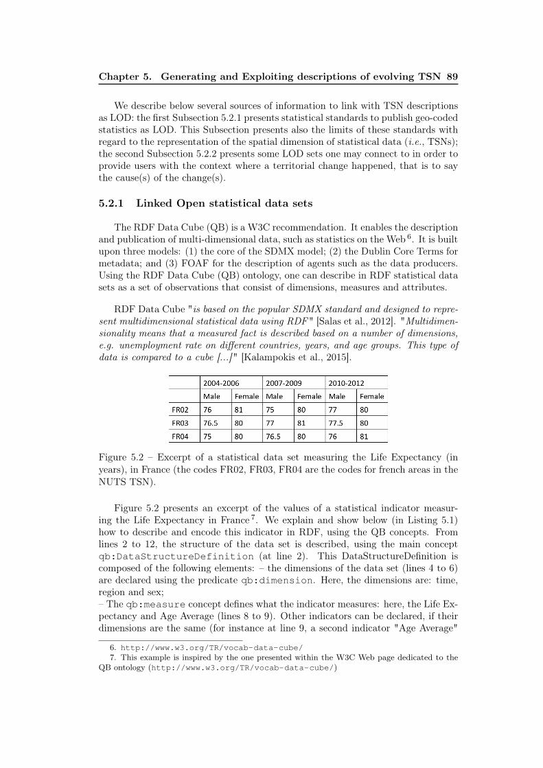
Chapter 5. Generating and Exploiting descriptions of evolving TSN 89

We describe below several sources of information to link with TSN descriptionsas LOD: the first Subsection 5.2.1 presents statistical standards to publish geo-codedstatistics as LOD. This Subsection presents also the limits of these standards withregard to the representation of the spatial dimension of statistical data (i.e., TSNs);the second Subsection 5.2.2 presents some LOD sets one may connect to in order toprovide users with the context where a territorial change happened, that is to saythe cause(s) of the change(s).

5.2.1 Linked Open statistical data sets

The RDF Data Cube (QB) is a W3C recommendation. It enables the descriptionand publication of multi-dimensional data, such as statistics on the Web 6. It is builtupon three models: (1) the core of the SDMX model; (2) the Dublin Core Terms formetadata; and (3) FOAF for the description of agents such as the data producers.Using the RDF Data Cube (QB) ontology, one can describe in RDF statistical datasets as a set of observations that consist of dimensions, measures and attributes.

RDF Data Cube "is based on the popular SDMX standard and designed to repre-sent multidimensional statistical data using RDF" [Salas et al., 2012]. "Multidimen-sionality means that a measured fact is described based on a number of dimensions,e.g. unemployment rate on different countries, years, and age groups. This type ofdata is compared to a cube [...]" [Kalampokis et al., 2015].

Figure 5.2 – Excerpt of a statistical data set measuring the Life Expectancy (inyears), in France (the codes FR02, FR03, FR04 are the codes for french areas in theNUTS TSN).

Figure 5.2 presents an excerpt of the values of a statistical indicator measur-ing the Life Expectancy in France 7. We explain and show below (in Listing 5.1)how to describe and encode this indicator in RDF, using the QB concepts. Fromlines 2 to 12, the structure of the data set is described, using the main conceptqb:DataStructureDefinition (at line 2). This DataStructureDefinition iscomposed of the following elements: – the dimensions of the data set (lines 4 to 6)are declared using the predicate qb:dimension. Here, the dimensions are: time,region and sex;– The qb:measure concept defines what the indicator measures: here, the Life Ex-pectancy and Age Average (lines 8 to 9). Other indicators can be declared, if theirdimensions are the same (for instance at line 9, a second indicator "Age Average"

6. http://www.w3.org/TR/vocab-data-cube/7. This example is inspired by the one presented within the W3C Web page dedicated to the

QB ontology (http://www.w3.org/TR/vocab-data-cube/)

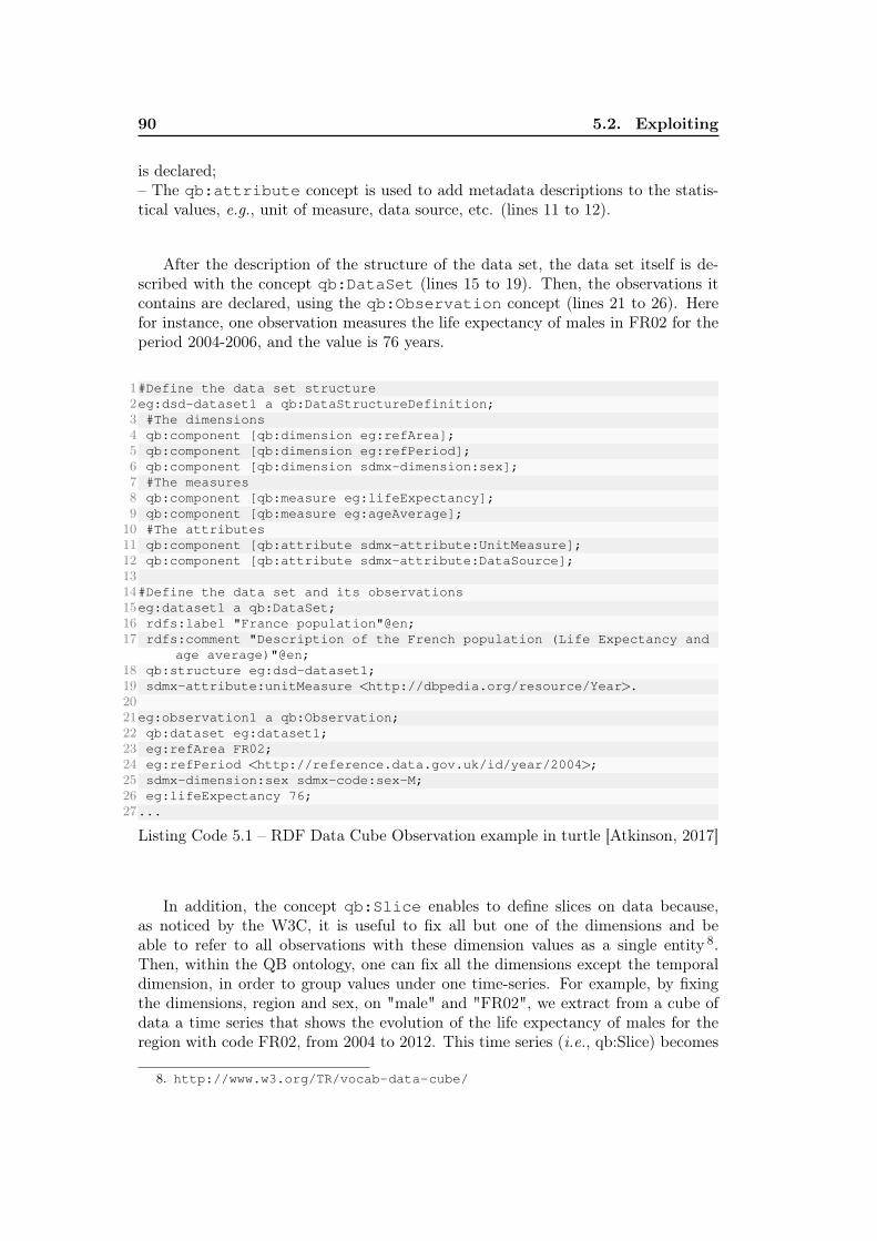
90 5.2. Exploiting

is declared;– The qb:attribute concept is used to add metadata descriptions to the statis-tical values, e.g., unit of measure, data source, etc. (lines 11 to 12).

After the description of the structure of the data set, the data set itself is de-scribed with the concept qb:DataSet (lines 15 to 19). Then, the observations itcontains are declared, using the qb:Observation concept (lines 21 to 26). Herefor instance, one observation measures the life expectancy of males in FR02 for theperiod 2004-2006, and the value is 76 years.

1#Define the data set structure2eg:dsd-dataset1 a qb:DataStructureDefinition;3 #The dimensions4 qb:component [qb:dimension eg:refArea];5 qb:component [qb:dimension eg:refPeriod];6 qb:component [qb:dimension sdmx-dimension:sex];7 #The measures8 qb:component [qb:measure eg:lifeExpectancy];9 qb:component [qb:measure eg:ageAverage];10 #The attributes11 qb:component [qb:attribute sdmx-attribute:UnitMeasure];12 qb:component [qb:attribute sdmx-attribute:DataSource];1314#Define the data set and its observations15eg:dataset1 a qb:DataSet;16 rdfs:label "France population"@en;17 rdfs:comment "Description of the French population (Life Expectancy and

age average)"@en;18 qb:structure eg:dsd-dataset1;19 sdmx-attribute:unitMeasure <http://dbpedia.org/resource/Year>.2021eg:observation1 a qb:Observation;22 qb:dataset eg:dataset1;23 eg:refArea FR02;24 eg:refPeriod <http://reference.data.gov.uk/id/year/2004>;25 sdmx-dimension:sex sdmx-code:sex-M;26 eg:lifeExpectancy 76;27...

Listing Code 5.1 – RDF Data Cube Observation example in turtle [Atkinson, 2017]

In addition, the concept qb:Slice enables to define slices on data because,as noticed by the W3C, it is useful to fix all but one of the dimensions and beable to refer to all observations with these dimension values as a single entity 8.Then, within the QB ontology, one can fix all the dimensions except the temporaldimension, in order to group values under one time-series. For example, by fixingthe dimensions, region and sex, on "male" and "FR02", we extract from a cube ofdata a time series that shows the evolution of the life expectancy of males for theregion with code FR02, from 2004 to 2012. This time series (i.e., qb:Slice) becomes

8. http://www.w3.org/TR/vocab-data-cube/

Chapter 5. Generating and Exploiting descriptions of evolving TSN 91

addressable through an URI. To conclude, the QB ontology is well adapted to thedescription of statistical data sets and time-series. Several organizations use the QBOntology (e.g., Eurostat, European Environment Agency, OECD, INSEE, etc.).

The QB4ST extension 9 [Atkinson, 2017] provides canonical terms to defined ina QB observation the space (qb4st:SpatialDimension) and time dimensions of thedata (as explained in 4.2). However, as explained in 4.2, with regard to the evolvingnature of the geographic areas the observations cover, none of the QB, QB4ST,XKOS, and QB4OLAP ontologies provide the vocabulary required to achieve thedescription of the way the TSNs, their levels, and TUs evolved over time.

To conclude, with regard to the spatial dimension of the statistical QBobservations, other ontologies than QB must be used in order to describethe geospatial areas the observations apply to (i.e., the spatial dimensionof statistical data). The issue with the existing vocabularies is that they donot represent hierarchies of TUs and/or they do not represent the evolutionof the TUs over time. Then, most of the time, QB observations are declaredfor regions, with boundaries for which it is not said at which period of timethey correspond, and if they were the boundaries of the TUs at the time ofthe data collection, and to which geographic division the TUs belong to. Asa result, there is a limited trust in the statistical data published on the LODbecause it is difficult to know which geographic object the observed valuesrefer to. A model is still lacking that allows SAs to mention precisely foreach statistical observation: what is the observed TU (time and space) andto which geographic division (hierarchy) it belongs. Is also lacking a modelthat can help to know how this area has evolved over time, and therefore tosee how the statistical values measured on this evolving area have evolvedtoo.

5.2.2 Contextual information about territorial changes

Various models have been proposed for representing events on the Semantic Web,such as the Simple Event Model [Hage et al., 2011], the Event Ontology [Raimondet al., 2007], the Linking Open Descriptions of Events Ontology (LODE) [Shawet al., 2009], the F-Model (F) [Scherp et al., 2009], the Event Ontology used in Cul-tureSampo [Ruotsalo and Hyvönen, 2007] and the CIDOC Conceptual ReferenceModel Ontology (www.cidoc-crm.org), an event centric model, designed for therepresentation of historic events [Doerr, 2003]. The CIDOC ontology mediates be-tween different sources of cultural heritage information (from museum for instance).For a comparison of these models the reader should refer to [Hage et al., 2011].

The DBPedia Ontology define a class named Event 10 but, as noticed by [Hienertand Luciano, 2015], existing events in the DBPedia data set are distributed over onlya few categories: military battles and sport events...

9. http://www.w3.org/ns/qb4st/10. http://dbpedia.org/ontology/Event

92 5.2. Exploiting

Because the historical events in Wikipedia are listed in the article body, theyare not yet included in DBPedia and cannot be queried in a structured way. Then,to automate the contextualization of territorial changes, using the LOD Web, onemay encounter some problems using the DBPedia service. The work by [Hienertand Luciano, 2015] offers a solution to this issue. They automate the extraction ofhistorical events from articles in Wikipedia, using language-dependent patterns toidentify the text section with events. For instance, to extract events, their systemextracts sentences containing a date.

In Europe, the European Legislation Identifier (ELI) 11 provides Web identi-fiers (URIs) for legal information. For instance, in France the Law No 2015-29 ofJanuary 16th, 2015, redefining the regional administrative areas for France, hasan ELI URI that is https://www.legifrance.gouv.fr/eli/loi/2015/1/16/INTX1412841L/jo/texte. The implementation of ELI is still a work inprogress in Spain, as the Spanish legal system is complex and diverse, comprisingrules corresponding to different territorial levels (national, Autonomous Communityand local) 12.

We have reviewed the existing works for the management of TSNs on the LOD:from the existing modeling approaches and ontological models to the exploitationof the TSNs as LOD, interlinked with other information that give sense to theterritorial redistribution. In the following Chapter 6, we make a synthesis of thestate of the art and try to answer how this existing solves or not the issues identifiedin the main introduction, Chapter 1.

11. https://eur-lex.europa.eu/eli-register/about.html12. https://eur-lex.europa.eu/eli-register/spain.html

Chapter 6

Synthesis

The state of the art has presented the existing spatiotemporal approaches, mod-els, tools and algorithms, at each step of the [Villazón-Terrazas et al., 2011] lifecycle, in view of our fundamental objective: the publication of evolving TSNs onthe LOD Web, with semantic representations of their changes over time.

As explained in the Chapter 1, such an objective raise four research challenges.Below, we summarize the main elements of the existing approaches to meet thesechallenges, we list shortcomings and requirements for a system managing the wholelife cycle of evolving TSNs in the Semantic Web. We briefly describe our proposalsto meet these challenges.

– Challenge (1): To overcome the lack of interoperability betweensystems for TSNs exchange in the semantic Web.

Many Statistical Institutes (SAs) through the world now publish their statisticsas LOD (e.g., Italian statistical data 1, Scottish statistical data 2, UK Department forCommunities and Local Government statistical data 3, Aragonese statistical data 4

or Japanese statistical data 5). However, for the description of the geographic re-gions they administrate, they often create their own ontology (e.g., the TerritorioOntology 6 of the Italian National Institute for Statistics, the Geography Ontology 7

of the Scottish Government), which results in a counterproductive proliferation ofnon-aligned vocabularies. The most thoroughgoing initiative is the one from UKOffice for National Statistics (ONS) that proposes vocabularies 8 to represent geo-graphic areas in the context of statistical data publication. Even if we can noticea certain level of abstraction on the terms used to describe TUs 9, which makes itpossible to describe other TUs than UK’s ones, none of these vocabularies allows oneto describe any TSN structure and its levels. One needs to add new concepts to theontology Geographical hierarchy ontology 10 if one wants to describe new territoriesand new territorial hierarchies than those listed. Similarly, in the Subsection 4.2.1,

1. http://datiopen.istat.it/2. http://statistics.gov.scot/3. http://opendatacommunities.org/data4. http://opendata.aragon.es/sparql/5. http://data.e-stat.go.jp/lodw/6. http://datiopen.istat.it/odi/ontologia/territorio/7. http://statistics.gov.scot/vocabularies/8. http://statistics.data.gov.uk/vocabularies9. http://statistics.data.gov.uk/def/statistical-entity

10. http://statistics.data.gov.uk/def/hierarchy/best-fit

94

we have shown that none of the existing ontologies of SAs or Mapping Agencies,has a sufficient level of abstraction to semantically describe any TSN hierarchicalstructure. The model created by [Plumejeaud et al., 2011] (a relational databasemodel), previous work of our research group, has, for its part, a sufficient level ofabstraction to semantically describe any TSN (with a structure such as the one weaddress in this thesis, defined in Chapter 2, Section 2.2).

I Hence, one first requirement to meet the first challenge is to immerse themodel of [Plumejeaud et al., 2011] in the semantic Web.

With regard to TSN data sets published on the LOD Web, the RDF NUTS datasets (see Subsection 4.2.2) provide only one representation (i.e., one resource withone URI) for TU such as ES63 Version 1999 and Version 2003 where two distinctresources are preferable, to refer to them in a statistical data set by their respectiveURI. Indeed, statisticians need to easily dissociate observations measured on thesetwo distinct geographic objects since the surface is reduced by almost half from oneversion to another. More broadly, they need to easily distinguish each geographicarea, in time and space, especially distinguish between different versions of a TUthat changes while it maintains its name, or code.

I The second requirement identified is to create unique identifiers (URI on theLOD web) for each element of a TSN version.

We propose and present in a next Chapter 8, the TSN Ontology that enablesthe representation of any TSN hierarchical structure (structure defined inSection 2.2) on the LOD Web. This ontology immerses the generic modelof [Plumejeaud et al., 2011] in the semantic Web.We make the following design choices according to the [Grenon and Smith,2004] approach, we decide to create a SNAP-SPAN Trans-Ontologies thatdepict the life (or history) of entities (TUs, Territories, Levels, TSNs) overtime. Our model distinguishes between SNAP (continuant) entities (TUs,Territories, Levels, TSNs), and SPAN (occurrent) entities (TU versions,Territory versions, Level versions, TSN versions). The SNAP entities rep-resent the TUs, Territories, Levels and TSNs as one would have representeda person that "endures, or continues to exist through time while maintain-ing its identity". The SPAN entities, along the versions, draw the life ofthese elements (a process): they are 4D representation of them (space timeworm), that depict their history over time (using the 4D-fluents approach).We demonstrate, in the Implementation Chapter 10 that our vocabulary isabstract and generic enough to cover any TSN hierarchical structure cases.It allows (N)SAs to describe their own territorial hierarchical structure, aswell as their TUs, for each version of the TSN. We propose patterns for thecreation of unique URIs for each element of a TSN version. Using our vo-cabulary, SAs may create LOD dictionaries of spatial units for statistics, allTSNs being described using the same terms, for the sake of interoperability.

– Challenge (2): To provide a description of TSNs evolution overtime in a way that it helps understanding the reason for the changes,

Chapter 6. Synthesis 95

and assists statisticians in the operation of transferring statistical datafrom one TSN version to another.

Most of the agencies contributions limit their description to isolated attributechange and do not propose any vocabulary to describe and group together changesthat are involved in the same territorial event. Among these initiatives, we havehighlighted several of them (please see Subsection 4.2.1). Here we come back to twoof them that address the problem of evolution through time:– the UK (ONS) proposes a vocabulary 11 to represent evolution of geographic areasin the context of statistical data publication. Nevertheless, none of the concepts ofthe ONS Boundary Change Ontology makes it possible to name changes that impactseveral TUs at the same time. The concepts describing change events are few andlimited to Recoding change and Boundary change.– vocabularies of the Statistics Bureau of Japan 12 represent geographic areas andtheir evolution, including description of area changes, in the context of statisticaldata publication. Their proposal is limited to description of changes in municipal-ities. Also, the description of the reason for the change is limited to a literal whilewe propose to provide URI links to discover new things in other data sets on theLOD, such as DBpedia.

With regard to software tools specialized in version control, although tools suchas GeoGIG or the GitHub Inc. project handle versioning of geospatial data andprovide a way to visualize differences in geometries, feature by feature [Negretti,2015; LocationTech, 2018; Boundless, 2014a; ?,b], they are unable to group changesthat affect several geographic objects at the same time (e.g., a merge of two TUs),or to attach semantics describing the context and nature of this territorial change.

Hence, changes occurring in TSN structures are rarely described and wheneverthey are, the descriptions are made TU by TU, with no link between changes. Thismakes it difficult to identify each of the TSN’s features (territories, levels and TUs)that changes because of a same event. The model created by [Plumejeaud et al.,2011] includes a Typology of Territorial Changes in order to characterize changes inTSNs over time, whether they are isolated changes (e.g., a name change) or changesthat impact multiple TUs at the same time (e.g., merge of two TUs). Regard-ing the description of changes, in [Plumejeaud et al., 2011], the authors dissociateDerivation cases (e.g., Figure 8.7, (a)) from Continuation cases (e.g., Figure 8.7,(b)), depending on whether the identity of the object is impacted during the changeevent or not. This approach is also the one adopted by ontologies for fluents (basedon the perdurantist approach) which represent, in OWL, relationships between enti-ties that change with time [Welty et al., 2006]. The Typology of Territorial Changesof [Plumejeaud et al., 2011] is not published on the LOD Web, contrary to theChange Vocabulary 13 of [Kauppinen et al., 2008; Kauppinen and Hyvönen, 2007],a lightweight spatiotemporal vocabulary made of two properties (before, after) andfive classes for the description of changes (Establishment, Merge, Split, Namechange,

11. http://statistics.data.gov.uk/def/boundary-change12. e.g., http://data.e-stat.go.jp/lod/sac/, http://data.e-stat.go.jp/lod/te

rms/sacs#, http://data.e-stat.go.jp/lod/sace/13. http://linkedearth.org/change/ns/

96

Changepartof ). In [Kauppinen et al., 2008], the authors introduce the notion ofChange Bridge to chain old territories (e.g., East Germany and West Germany) tothe following ones (e.g., Germany), using the Change Vocabulary for the descriptionof changes.

I The third requirement identified is to immerse in the semantic Web the Typol-ogy of Territorial Changes of [Plumejeaud et al., 2011], adopting the Change Bridgeapproach of [Kauppinen et al., 2008] to chain former territories to the followingones, and the 4D-fluent perdurantist approach in order to describe the life processof spatiotemporal entities.

Using typologies of spatiotemporal processes from [Claramunt and Théri-ault, 1995; Del Mondo et al., 2010; Plumejeaud et al., 2011], we proposethe TSN-Change Ontology that defines a set of tags to describe territo-rial changes whether they modify the identity of the geographic objects ornot. Contrary to [Harbelot et al., 2013], our model dissociates the filiationlinks (established between two time-slices of a same spatial entity) fromthe descriptions of changes to the entity, and it adopts the Change Bridgeapproach of [Kauppinen et al., 2008]. The change descriptions are SPANobjects that may be link with other resources on the LOD Web (LOD setsdescribing historical events for instance), in order to contextualize the ter-ritorial changes. We believe that our model, by offering a more detaileddescription of territorial changes in TSN, contributes to a better under-standing of territorial evolution over time.

– Challenge (3): To take into account the vertical/hierarchical dimen-sion of TSNs in their evolution.

Works from [Kauppinen et al., 2008] and [Lacasta et al., 2014] adopt an onto-logical approach for the description of changes of geographic features over time, butthese approaches lack a description of changes that propagates level-to-level (e.g.,change of the boundaries of a TU may impact also the boundaries of its nested TUs)considering the nested nature of the geographic elements of a TSN.

I The fourth requirement identified is to construct chains of changes that is tosay, create links between change descriptions when the changes impact embeddedfeatures of the TSN.

We propose to describe changes that affect several levels of the TSNs. Inorder to automate the detection and semantic description of territorialchanges, we decide to adapt and immerse the algorithm of [Plumejeaud,2011] in the semantic Web. Our algorithm, called the TSN Semantic Match-ing Algorithm, detects TUs changes and chains together changes throughthe TSN levels to offer a view on embedded changes, probably caused bythe same initial event (societal, historical or political event). Then, ourautomatically generated descriptions of territorial changes are by far moreaccurate and complete than the one presented in the cultural heritage portalof [Kauppinen et al., 2008].

Chapter 6. Synthesis 97

– Challenge (4): To populate automatically such an ontological model,by preserving its genericity, since the characteristics which make up theidentity of geographic areas may vary form one country to another.

In [Lacasta et al., 2014], the authors propose a semi-automatic process for cre-ating and populating the evolution model of any country, with an approach that isalso quite generic since the characteristics of the heterogeneous sources can be setdynamically. However, this process does not produce any description of the impactsof changes on the hierarchy of TUs. Furthermore, this approach requires the useof a written dictionary of changes as input, listing all of the individual changes.This requirement may be seen as a drawback for current statistical information sys-tems because the manual listing of changes is time consuming. Then, we decide toautomate the detection and description of such a dictionary.

I The fifth requirement identified is to create a configurable system the userscan set up according to the characteristics of the TUs identity.

To meet this challenge, we get inspiration from conflation approaches [Hast-ings, 2008; McKenzie et al., 2014; Ruiz et al., 2011]. We create a config-urable framework, called the Theseus Framework, that computes similaritymeasures on TUs attributes. The Theseus framework uses the concept ofIdentity attached to each TU, in an approach similar to the one of Huibinget al. [2005]. A weighting function is created in order to determine if theidentity of a TU is preserved in the following version of the TSN. Whilemetrics results are used for conflict resolution for gazetteers or POI (e.g.,choose the canonical form of a place name between multiple possibilities),we chose to transform metrics in semantics. Each result of the distancetests on each attribute is transposed into semantic descriptions using theTSN-Change Ontology. Then, the strength of our approach stands not onlyin the computation of similarities, but also, and mostly, in the underly-ing semantic model for changes representation and spatial objects lineagedescriptions.

As a conclusion, we have identified in this state of the art that no ontologi-cal model enables the representation of any TSN hierarchical structure and of itsevolution over time on the LOD Web. However, we have identified modeling ap-proaches (SPAN, perdurantist and 4D-Fluent approaches) and upper ontologies tobuild upon (PAV, BFO, GeoSPARQL, OWL Time), as well as algorithm [Plume-jeaud, 2011] that proves the feasibility of detecting and describing automaticallycomplex changes in TSNs.

We present in the following Chapter 7 our contributions for the publication andexploitation on the LOD Web of TSNs in such a way that it gives access to the lifeof the TSNs over time, as well as the life of each of the features that compose it,considering their belonging to a territorial hierarchy.

Part B

Contributions

Chapter 7

The Theseus Framework

7.1 Introduction

In this manuscript, we present Theseus, a framework designed for managingTSNs in the semantic Web, according to a management process that consists ofthe following activities: Specify, Model, Generate, Publish, and Exploit. It is calledTheseus with reference to the identity philosophic issue raised by the Ship of Theseusthat changes over time and was rebuilt entirely over the years, every plank beingbroken one by one. This framework automates the publication on the LOD Web ofany TSN (structure defined in Section 2.2), the detection of their changes over time,and the publication of such changes on the LOD Web. It encapsulates two ontolo-gies we have designed in order to describe TSNs and their changes over time: theontologies are called TSN-Ontology and TSN-Change Ontology. It also encapsulatesan implementation of the algorithm of [Plumejeaud, 2011] that detects and describessimilarities and changes between two consecutive versions of a TSN. However, the[Plumejeaud, 2011] algorithm has been modified to output RDF descriptions of aTSN and of its changes over time, based on the concepts defined in the TSN-Changeontology. This adaptation of the algorithm of [Plumejeaud, 2011] is called the TSNSemantic Matching Algorithm. The major challenge we face when automating thedetection and semantic description of TSN changes is the implementation of ourconcepts and algorithm with regard to the heterogeneity of the input data. Indeed,the definition of the identity of TUs varies from one TSN to another TSN. Does aTU, its name or geometries or both are changed, remain the same TU, or no longerexist? There is no unique answer to this question, again the response varies fromone TSN to another. Thus, the Theseus Framework is made of several configurablesoftware modules that implement the TSN Semantic Matching Algorithm, allowingto define the list of attributes that compose the identity of a TU in a processedTSN, and in which proportion each of these attributes can vary before a TU losesits identity and is therefore considered as a new one. This semantic framework is,as far as we know, the first one that handle TSNs’ structure versioning. But, farmore than just linking the TSN elements throughout the versions, this frameworkprovides users with semantic descriptions of TUs filiation links over time (includingsimilarities and changes description).

102 7.2. Motivations and requirements

7.2 Motivations and requirements

Below, we present the issues behind the four challenges we have identified inChapter 1, and the requirements 1 our system must meet to address these issues:

Issue 1: Lack of semantic interoperability between systems for TSNs exchange.Requirement 1.1: Adopting Semantic Web technologies.Requirement 1.2: A pivot semantic model to describe any TSN hierarchical struc-ture.

Issue 2: Lack of semantic interoperability between systems for TSNs changedescriptions exchange in a way that it assists statisticians in the operation of trans-ferring statistical data from one TSN version to another.Requirement 2.1: A semantic model to describe any TSN change over time.Requirement 2.2: A "Gateway" modeling approach that may bridge data fromdifferent versions.

Issue 3: Lack of semantic interoperability between systems for TSNs changedescriptions exchange in a way that it helps understanding the impact of a territorialchange on all the levels of the territorial structure.Requirement 3: A modeling approach to construct chains of changes, that is tosay, create links between change descriptions when the changes impact embeddedfeatures of the TSN.

Issue 4: Lack of semantic interoperability between systems for TSNs change de-scriptions exchange in a way that it helps understanding the reason for the changes.Requirement 4: A modeling approach that connects territorial changes to theevents that have caused these changes.

Issue 5: Lack of tools to populate automatically such a descriptive model ofTSNs and of their evolution over time, by preserving its genericity, since the identitycharacteristics may vary depending on countries and on the quality of the input TSNdata sets.Requirement 5: A configurable system the users can set up according to thecharacteristics of TUs.

To meet these requirements, we adopt the semantic Web technologies for thedescription of the TSN’s areas and of their changes. These technologies guarantythe syntactic interoperability and, most of all, the semantic interoperability betweensystems exchanging TSN information. Thus, we make sure that the semantics ofchanges are shared and understood in the same way, by humans and software agents,that share the same concepts and definitions. Another benefit is the LOD Web,which allows us to connect and contextualize data from our system to other data onthe LOD Web. As a matter of fact, the OGC and W3C recommend for spatial datato be on the Web, to be connected or linked, to other resources. They suggest linkingspatial data with URIs (using a Linked Data approach) from popular repositories

1. The requirements presented here are more precises then the ones presented in the previousChapter 6

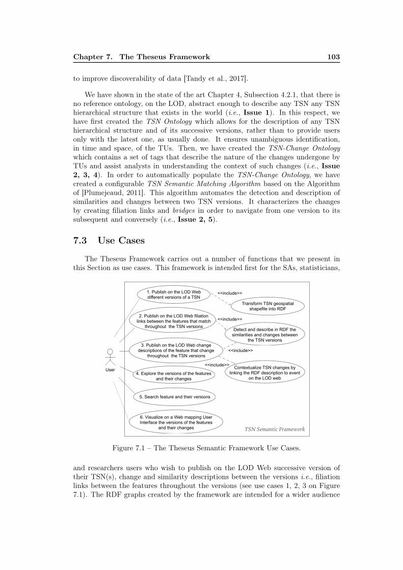
Chapter 7. The Theseus Framework 103

to improve discoverability of data [Tandy et al., 2017].

We have shown in the state of the art Chapter 4, Subsection 4.2.1, that there isno reference ontology, on the LOD, abstract enough to describe any TSN any TSNhierarchical structure that exists in the world (i.e., Issue 1). In this respect, wehave first created the TSN Ontology which allows for the description of any TSNhierarchical structure and of its successive versions, rather than to provide usersonly with the latest one, as usually done. It ensures unambiguous identification,in time and space, of the TUs. Then, we have created the TSN-Change Ontologywhich contains a set of tags that describe the nature of the changes undergone byTUs and assist analysts in understanding the context of such changes (i.e., Issue2, 3, 4). In order to automatically populate the TSN-Change Ontology, we havecreated a configurable TSN Semantic Matching Algorithm based on the Algorithmof [Plumejeaud, 2011]. This algorithm automates the detection and description ofsimilarities and changes between two TSN versions. It characterizes the changesby creating filiation links and bridges in order to navigate from one version to itssubsequent and conversely (i.e., Issue 2, 5).

7.3 Use Cases

The Theseus Framework carries out a number of functions that we present inthis Section as use cases. This framework is intended first for the SAs, statisticians,

1. Publish on the LOD Web different versions of a TSN

2. Publish on the LOD Web filiation links between the features that match

throughout the TSN versions

3. Publish on the LOD Web change descriptions of the feature that change

throughout the TSN versions

Transform TSN geospatial shapefile into RDF

Detect and describe in RDF the similarities and changes between

the TSN versions

<<include>>

<<include>>

<<include>>

6. Visualize on a Web mapping User Interface the versions of the features

and their changes

4. Explore the versions of the features and their changes

5. Search feature and their versions

Contextualize TSN changes by linking the RDF description to event

on the LOD web

<<include>>User

TSN Semantic Framework

Figure 7.1 – The Theseus Semantic Framework Use Cases.

and researchers users who wish to publish on the LOD Web successive version oftheir TSN(s), change and similarity descriptions between the versions i.e., filiationlinks between the features throughout the versions (see use cases 1, 2, 3 on Figure7.1). The RDF graphs created by the framework are intended for a wider audience

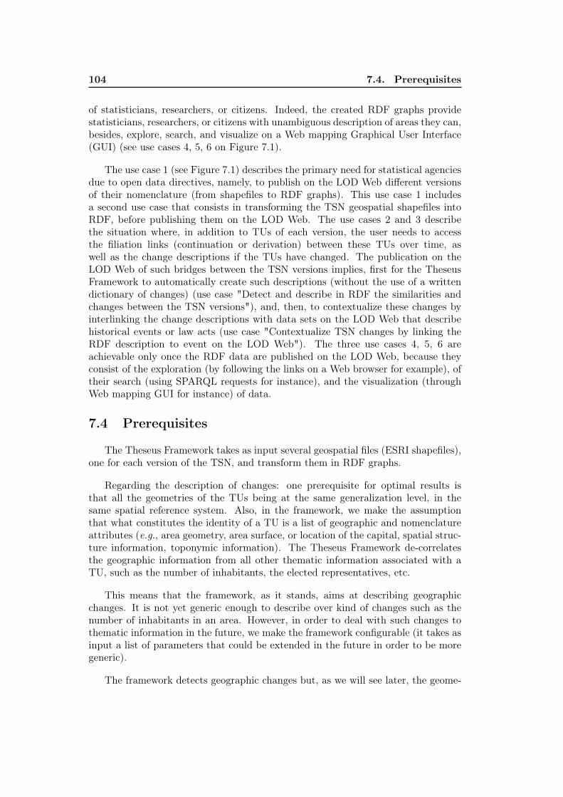
104 7.4. Prerequisites

of statisticians, researchers, or citizens. Indeed, the created RDF graphs providestatisticians, researchers, or citizens with unambiguous description of areas they can,besides, explore, search, and visualize on a Web mapping Graphical User Interface(GUI) (see use cases 4, 5, 6 on Figure 7.1).

The use case 1 (see Figure 7.1) describes the primary need for statistical agenciesdue to open data directives, namely, to publish on the LOD Web different versionsof their nomenclature (from shapefiles to RDF graphs). This use case 1 includesa second use case that consists in transforming the TSN geospatial shapefiles intoRDF, before publishing them on the LOD Web. The use cases 2 and 3 describethe situation where, in addition to TUs of each version, the user needs to accessthe filiation links (continuation or derivation) between these TUs over time, aswell as the change descriptions if the TUs have changed. The publication on theLOD Web of such bridges between the TSN versions implies, first for the TheseusFramework to automatically create such descriptions (without the use of a writtendictionary of changes) (use case "Detect and describe in RDF the similarities andchanges between the TSN versions"), and, then, to contextualize these changes byinterlinking the change descriptions with data sets on the LOD Web that describehistorical events or law acts (use case "Contextualize TSN changes by linking theRDF description to event on the LOD Web"). The three use cases 4, 5, 6 areachievable only once the RDF data are published on the LOD Web, because theyconsist of the exploration (by following the links on a Web browser for example), oftheir search (using SPARQL requests for instance), and the visualization (throughWeb mapping GUI for instance) of data.

7.4 Prerequisites

The Theseus Framework takes as input several geospatial files (ESRI shapefiles),one for each version of the TSN, and transform them in RDF graphs.

Regarding the description of changes: one prerequisite for optimal results isthat all the geometries of the TUs being at the same generalization level, in thesame spatial reference system. Also, in the framework, we make the assumptionthat what constitutes the identity of a TU is a list of geographic and nomenclatureattributes (e.g., area geometry, area surface, or location of the capital, spatial struc-ture information, toponymic information). The Theseus Framework de-correlatesthe geographic information from all other thematic information associated with aTU, such as the number of inhabitants, the elected representatives, etc.

This means that the framework, as it stands, aims at describing geographicchanges. It is not yet generic enough to describe over kind of changes such as thenumber of inhabitants in an area. However, in order to deal with such changes tothematic information in the future, we make the framework configurable (it takes asinput a list of parameters that could be extended in the future in order to be moregeneric).

The framework detects geographic changes but, as we will see later, the geome-

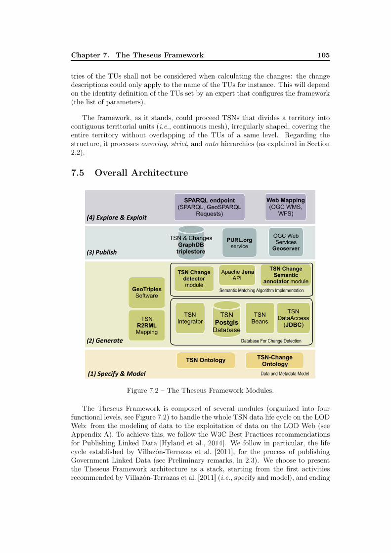
Chapter 7. The Theseus Framework 105

tries of the TUs shall not be considered when calculating the changes: the changedescriptions could only apply to the name of the TUs for instance. This will dependon the identity definition of the TUs set by an expert that configures the framework(the list of parameters).

The framework, as it stands, could proceed TSNs that divides a territory intocontiguous territorial units (i.e., continuous mesh), irregularly shaped, covering theentire territory without overlapping of the TUs of a same level. Regarding thestructure, it processes covering, strict, and onto hierarchies (as explained in Section2.2).

7.5 Overall Architecture

(1)Specify&Model

TSN Ontology TSN-Change Ontology

Data and Metadata Model

(3)Publish

PURL.org service

TSN & Changes GraphDB triplestore

OGC Web Services

Geoserver

(4)Explore&Exploit

SPARQL endpoint (SPARQL, GeoSPARQL

Requests)

Web Mapping (OGC WMS,

WFS)

GeoTriples Software

Semantic Matching Algorithm Implementation

TSN Change Semantic

annotator moduleTSN Change

detector module

TSN Postgis

Database

TSN Integrator

Database For Change Detection

TSN DataAccess

(JDBC)

(2)Generate

Apache Jena API

TSN BeansTSN

R2RML Mapping

Figure 7.2 – The Theseus Framework Modules.

The Theseus Framework is composed of several modules (organized into fourfunctional levels, see Figure 7.2) to handle the whole TSN data life cycle on the LODWeb: from the modeling of data to the exploitation of data on the LOD Web (seeAppendix A). To achieve this, we follow the W3C Best Practices recommendationsfor Publishing Linked Data [Hyland et al., 2014]. We follow in particular, the lifecycle established by Villazón-Terrazas et al. [2011], for the process of publishingGovernment Linked Data (see Preliminary remarks, in 2.3). We choose to presentthe Theseus Framework architecture as a stack, starting from the first activitiesrecommended by Villazón-Terrazas et al. [2011] (i.e., specify and model), and ending

106 7.6. Conclusion

by the Exploit activity. The Figure 7.2 presents, the modules of the framework, ateach steps of the life cycle process:

– (1) Specify and Model : at the very heart of the Theseus Framework lies itsdata model (composed of the TSN and TSN-Change ontologies). We have speci-fied this model according to the methodology for designing ontologies proposed in[Bachimont et al., 2002]: a corpus of TSNs and existing ontologies (based on thecorpus presented in Section 4.2) helped us to determine the vocabulary to be usedto be close to the designations used by the SAs, and thus to facilitate the use of themodel. The TSN ontological model provides the modules of the framework with aformal representation of TSNs and how they change over time.

– (2) Generate: during the activity of generating RDF data that apply to theTSN and TSN-Change ontologies, several software modules are used, such as: theGeotriples Software 2 that aims at transforming the TSN Geospatial files (also calledshapefile) into RDF triples, using the TSN ontology concepts for the descriptionsof the TSN elements; the TSN Change Detector and the TSN Change annotatormodules, we have developed in order to detect changes in TSN’s Geospatial shapes,and describe these changes using the RDF model and the TSN-Change ontologyconcepts.

– (3) Publish: at this step, three existing software are used: the purl.org service(to provide persistent URI to data); the GraphDB triplestore (to publish the RDFdata created); the GeoServer software (to publish the TUs’ geometries linked to theirLOD representation). We will come back to the usefulness of these three softwarein the Section 9.2 dedicated to the description of the workflows implemented withinthe Theseus Framework.

– (4) Explore and Exploit : in order to provide users with tools to explore andexploit the published data, we set up various search engines, using standard Webmechanisms: a SPARQL enpoint for performing RDF data manipulations throughSPARQL and GeoSPARQL requests; a Web Graphical User Interface (GUI) to vi-sualize and query the geospatial data, using standard OGC requests to the WebMap Service (WMS) and Web Feature Service (WFS) published by our GeoServerthat connects to the TSN PostGIS database of our framework.

7.6 Conclusion

In this Chapter, we have introduced the Theseus Framework, the requirements itanswers, its main use cases, and its overall architecture. The main component of theframework is its model, composed of two ontologies, in order to dissociate betweenthe TSN elements in each version and the filiation links between these elements overtime. The TSN Ontology aims at describing the TSN elements and TSN’s versionselements. The TSN-Change Ontology aims at describing the filiation links betweenthe TSN versions elements over time.

2. http://geotriples.di.uoa.gr/

Chapter 7. The Theseus Framework 107

In order to populate this model, two different workflows have been set up withinthe framework: the first workflow creates the RDF catalogs of TUs’ versions (pleasesee Workflow A, Figure 9.1); the second workflow detects and describes the filiationlinks between the TSN elements throughout the versions (please see Workflow B,Figure 9.1). These two workflows of the Theseus Framework are presented in theChapter 9.

Prior to this, the following Chapter 8, present the two ontologies core componentsof the Theseus Framework.

Chapter 8

The TSN ontological model

8.1 Introduction

We present, in this chapter, the TSN ontological model we have created. It ismade of two ontologies: the TSN Ontology and the TSN-Change Ontology. Both theTSN and TSN-Change ontologies are geographic ontologies that define geographicconcepts (e.g., a town, TU) and not geometric concepts [Klien and Probst, 2005],contrary to the NeoGeo Geometry Ontology 1, for instance.

In order to be generic, the ontologies described the main attributes (and theirchanges) of the areas for statistics observed in TSNs in the world, that is to say: theTU’s identifier in the TSN (also called its code), name, geometry, level of belonging(e.g., district level), and a free text description. The two ontologies are domainontologies, that are built on upper ontologies.

We first present in Section Specify 8.2 our design choices, based on the review ofthe existing works (please see Chapters 3, 4). Second, in the Sections 8.3 and 8.4, wepresent the two ontologies that together constitute a SNAP-SPAN trans-ontology,according to the approach of [Grenon and Smith, 2004].

8.2 Specifications

We have specified the TSN ontological model according to the methodologyfor designing ontologies proposed in [Bachimont et al., 2002]: a corpus of TSNsand existing ontologies (based on the corpus presented in Section 3.2) helped us toevaluate the most relevant vocabulary to be close to the designations used by theSAs, and thus to facilitate the adoption of the model. The result of this Specify stepcorresponds to the state of the art part of this manuscript (Chapters 3, 4).

We get inspired by Version Control Systems and the way they manage changesthroughout the versions (see Subsection 5.1.4). We also get inspired by the BFOframework, and have decided to represent the life of TUs over time, that is tosay four-dimensional entities also called occurrent entities (SPAN is the ontologicaltheory of those entities in the approach of [Grenon and Smith, 2004]) (see Subsection3.2.2.5). More precisely, we adopt the Ontology for fluents [Welty et al., 2006]approach that is a perdurantist approach. In the BFO framework, perdurants areprocesses, occurrent entities which persist through time. Our choice is to detect and

1. http://geovocab.org/geometry

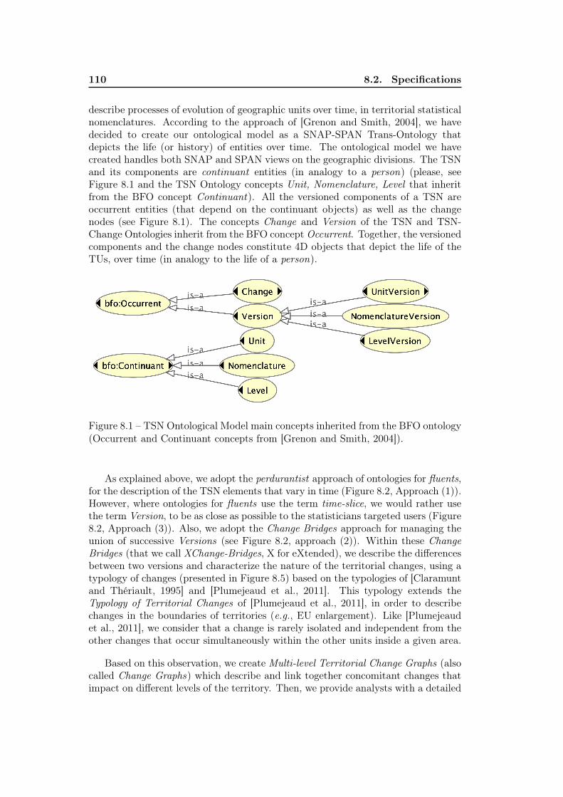
110 8.2. Specifications

describe processes of evolution of geographic units over time, in territorial statisticalnomenclatures. According to the approach of [Grenon and Smith, 2004], we havedecided to create our ontological model as a SNAP-SPAN Trans-Ontology thatdepicts the life (or history) of entities over time. The ontological model we havecreated handles both SNAP and SPAN views on the geographic divisions. The TSNand its components are continuant entities (in analogy to a person) (please, seeFigure 8.1 and the TSN Ontology concepts Unit, Nomenclature, Level that inheritfrom the BFO concept Continuant). All the versioned components of a TSN areoccurrent entities (that depend on the continuant objects) as well as the changenodes (see Figure 8.1). The concepts Change and Version of the TSN and TSN-Change Ontologies inherit from the BFO concept Occurrent. Together, the versionedcomponents and the change nodes constitute 4D objects that depict the life of theTUs, over time (in analogy to the life of a person).

Figure 8.1 – TSN Ontological Model main concepts inherited from the BFO ontology(Occurrent and Continuant concepts from [Grenon and Smith, 2004]).

As explained above, we adopt the perdurantist approach of ontologies for fluents,for the description of the TSN elements that vary in time (Figure 8.2, Approach (1)).However, where ontologies for fluents use the term time-slice, we would rather usethe term Version, to be as close as possible to the statisticians targeted users (Figure8.2, Approach (3)). Also, we adopt the Change Bridges approach for managing theunion of successive Versions (see Figure 8.2, approach (2)). Within these ChangeBridges (that we call XChange-Bridges, X for eXtended), we describe the differencesbetween two versions and characterize the nature of the territorial changes, using atypology of changes (presented in Figure 8.5) based on the typologies of [Claramuntand Thériault, 1995] and [Plumejeaud et al., 2011]. This typology extends theTypology of Territorial Changes of [Plumejeaud et al., 2011], in order to describechanges in the boundaries of territories (e.g., EU enlargement). Like [Plumejeaudet al., 2011], we consider that a change is rarely isolated and independent from theother changes that occur simultaneously within the other units inside a given area.

Based on this observation, we create Multi-level Territorial Change Graphs (alsocalled Change Graphs) which describe and link together concomitant changes thatimpact on different levels of the territory. Then, we provide analysts with a detailed

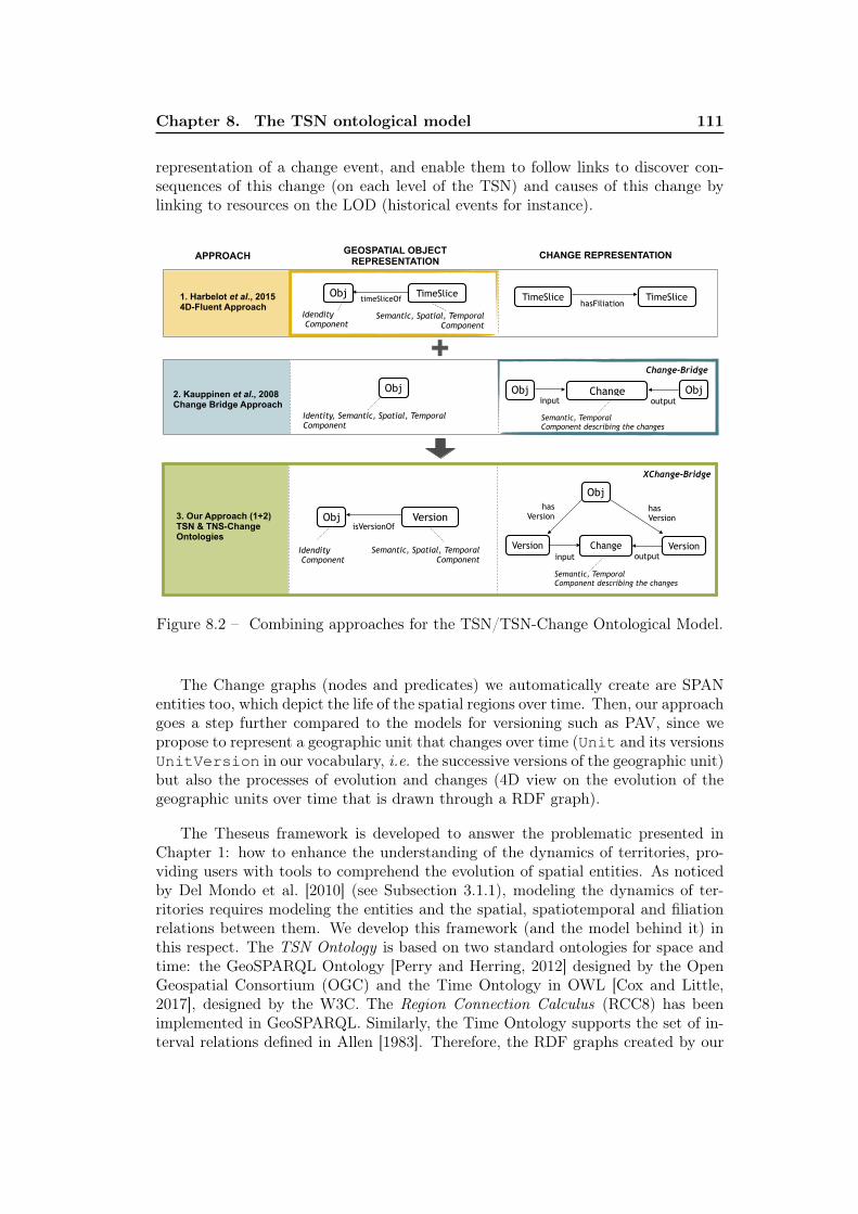
Chapter 8. The TSN ontological model 111

representation of a change event, and enable them to follow links to discover con-sequences of this change (on each level of the TSN) and causes of this change bylinking to resources on the LOD (historical events for instance).

Obj Obj ObjChange

Identity, Semantic, Spatial, Temporal Component

input output2. Kauppinen et al., 2008 Change Bridge Approach

Semantic, Temporal Component describing the changes

+Change-Bridge

TimeSlice TimeSlicehasFiliation

GEOSPATIAL OBJECT REPRESENTATION CHANGE REPRESENTATION

1. Harbelot et al., 2015 4D-Fluent Approach

APPROACH

Obj TimeSlicetimeSliceOf

Idendity Component

Semantic, Spatial, Temporal Component

ChangeVersion Versioninput output

Obj VersionisVersionOf

Idendity Component

Semantic, Spatial, Temporal Component

3. Our Approach (1+2) TSN & TNS-Change Ontologies

Semantic, Temporal Component describing the changes

Objhas

Version

XChange-Bridge

has Version

Figure 8.2 – Combining approaches for the TSN/TSN-Change Ontological Model.

The Change graphs (nodes and predicates) we automatically create are SPANentities too, which depict the life of the spatial regions over time. Then, our approachgoes a step further compared to the models for versioning such as PAV, since wepropose to represent a geographic unit that changes over time (Unit and its versionsUnitVersion in our vocabulary, i.e. the successive versions of the geographic unit)but also the processes of evolution and changes (4D view on the evolution of thegeographic units over time that is drawn through a RDF graph).

The Theseus framework is developed to answer the problematic presented inChapter 1: how to enhance the understanding of the dynamics of territories, pro-viding users with tools to comprehend the evolution of spatial entities. As noticedby Del Mondo et al. [2010] (see Subsection 3.1.1), modeling the dynamics of ter-ritories requires modeling the entities and the spatial, spatiotemporal and filiationrelations between them. We develop this framework (and the model behind it) inthis respect. The TSN Ontology is based on two standard ontologies for space andtime: the GeoSPARQL Ontology [Perry and Herring, 2012] designed by the OpenGeospatial Consortium (OGC) and the Time Ontology in OWL [Cox and Little,2017], designed by the W3C. The Region Connection Calculus (RCC8) has beenimplemented in GeoSPARQL. Similarly, the Time Ontology supports the set of in-terval relations defined in Allen [1983]. Therefore, the RDF graphs created by our

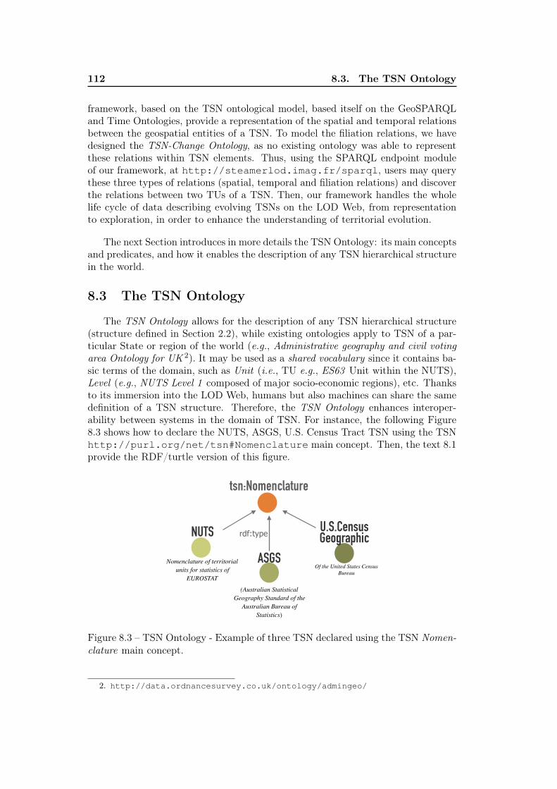
112 8.3. The TSN Ontology

framework, based on the TSN ontological model, based itself on the GeoSPARQLand Time Ontologies, provide a representation of the spatial and temporal relationsbetween the geospatial entities of a TSN. To model the filiation relations, we havedesigned the TSN-Change Ontology, as no existing ontology was able to representthese relations within TSN elements. Thus, using the SPARQL endpoint moduleof our framework, at http://steamerlod.imag.fr/sparql, users may querythese three types of relations (spatial, temporal and filiation relations) and discoverthe relations between two TUs of a TSN. Then, our framework handles the wholelife cycle of data describing evolving TSNs on the LOD Web, from representationto exploration, in order to enhance the understanding of territorial evolution.

The next Section introduces in more details the TSN Ontology: its main conceptsand predicates, and how it enables the description of any TSN hierarchical structurein the world.

8.3 The TSN Ontology

The TSN Ontology allows for the description of any TSN hierarchical structure(structure defined in Section 2.2), while existing ontologies apply to TSN of a par-ticular State or region of the world (e.g., Administrative geography and civil votingarea Ontology for UK 2). It may be used as a shared vocabulary since it contains ba-sic terms of the domain, such as Unit (i.e., TU e.g., ES63 Unit within the NUTS),Level (e.g., NUTS Level 1 composed of major socio-economic regions), etc. Thanksto its immersion into the LOD Web, humans but also machines can share the samedefinition of a TSN structure. Therefore, the TSN Ontology enhances interoper-ability between systems in the domain of TSN. For instance, the following Figure8.3 shows how to declare the NUTS, ASGS, U.S. Census Tract TSN using the TSNhttp://purl.org/net/tsn#Nomenclature main concept. Then, the text 8.1provide the RDF/turtle version of this figure.

tsn:Nomenclature

NUTS

ASGS

U.S.Census Geographicrdf:type

Nomenclature of territorialunits for statistics of

EUROSTAT

(Australian Statistical Geography Standard of the

Australian Bureau of Statistics)

Of the United States Census Bureau

Figure 8.3 – TSN Ontology - Example of three TSN declared using the TSN Nomen-clature main concept.

2. http://data.ordnancesurvey.co.uk/ontology/admingeo/

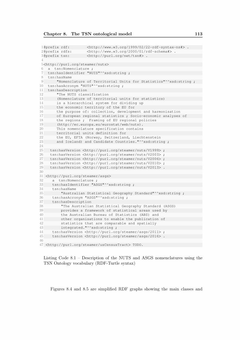
Chapter 8. The TSN ontological model 113

1@prefix rdf: <http://www.w3.org/1999/02/22-rdf-syntax-ns#> .2@prefix rdfs: <http://www.w3.org/2000/01/rdf-schema#> .3@prefix tsn: <http://purl.org/net/tsn#> .45<http://purl.org/steamer/nuts>6 a tsn:Nomenclature ;7 tsn:hasIdentifier "NUTS"^^xsd:string ;8 tsn:hasName9 "Nomenclature of Territorial Units for Statistics"^^xsd:string ;10 tsn:hasAcronym "NUTS"^^xsd:string ;11 tsn:hasDescription12 "The NUTS classification13 (Nomenclature of territorial units for statistics)14 is a hierarchical system for dividing up15 the economic territory of the EU for16 the purpose of: collection, development and harmonisation17 of European regional statistics ; Socio-economic analyses of18 the regions ; Framing of EU regional policies19 (http://ec.europa.eu/eurostat/web/nuts).20 This nomenclature specification contains21 territorial units definition for22 the EU, EFTA (Norway, Switzerland, Liechtenstein23 and Iceland) and Candidate Countries."^^xsd:string ;2425 tsn:hasVersion <http://purl.org/steamer/nuts/V1999> ;26 tsn:hasVersion <http://purl.org/steamer/nuts/V2003> ;27 tsn:hasVersion <http://purl.org/steamer/nuts/V2006> ;28 tsn:hasVersion <http://purl.org/steamer/nuts/V2010> ;29 tsn:hasVersion <http://purl.org/steamer/nuts/V2013> .3031 <http://purl.org/steamer/asgs>32 a tsn:Nomenclature ;33 tsn:hasIdentifier "ASGS"^^xsd:string ;34 tsn:hasName35 "Australian Statistical Geography Standard"^^xsd:string ;36 tsn:hasAcronym "ASGS"^^xsd:string ;37 tsn:hasDescription38 "The Australian Statistical Geography Standard (ASGS)39 provides a framework of statistical areas used by40 the Australian Bureau of Statistics (ABS) and41 other organisations to enable the publication of42 statistics that are comparable and spatially43 integrated."^^xsd:string ;44 tsn:hasVersion <http://purl.org/steamer/asgs/2011> ;45 tsn:hasVersion <http://purl.org/steamer/asgs/2016> .4647 <http://purl.org/steamer/usCensusTract> TODO.

Listing Code 8.1 – Description of the NUTS and ASGS nomenclatures using theTSN Ontology vocabulary (RDF-Turtle syntax)

Figures 8.4 and 8.5 are simplified RDF graphs showing the main classes and

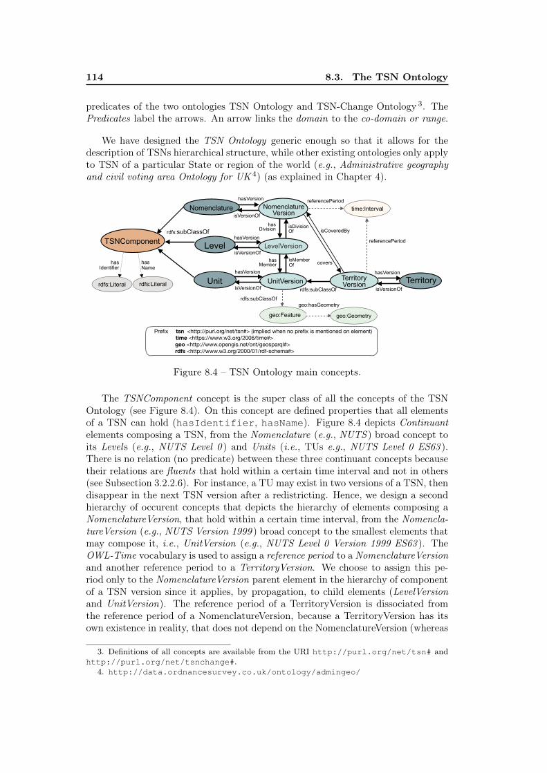
114 8.3. The TSN Ontology

predicates of the two ontologies TSN Ontology and TSN-Change Ontology 3. ThePredicates label the arrows. An arrow links the domain to the co-domain or range.

We have designed the TSN Ontology generic enough so that it allows for thedescription of TSNs hierarchical structure, while other existing ontologies only applyto TSN of a particular State or region of the world (e.g., Administrative geographyand civil voting area Ontology for UK 4) (as explained in Chapter 4).

isVersionOfNomenclature

Version

LevelVersion

has Division isDivision

Of

Nomenclature

has Member

isMember Of

UnitVersion

Level

Unit

hasVersion

isVersionOf

isVersionOf

time:IntervalreferencePeriod

geo:Feature

geo:hasGeometry

geo:Geometry

rdfs:subClassOf

TSNComponentrdfs:subClassOf

hasVersion

hasVersion

Prefix tsn <http://purl.org/net/tsn#> (implied when no prefix is mentioned on element) time <https://www.w3.org/2006/time#>

geo <http://www.opengis.net/ont/geosparql#> rdfs <http://www.w3.org/2000/01/rdf-schema#>

covers

Territory Version

hasVersion

isVersionOfTerritory

rdfs:subClassOf

isCoveredBy

referencePeriod

has Name

has Identifier

rdfs:Literal rdfs:Literal

Figure 8.4 – TSN Ontology main concepts.

The TSNComponent concept is the super class of all the concepts of the TSNOntology (see Figure 8.4). On this concept are defined properties that all elementsof a TSN can hold (hasIdentifier, hasName). Figure 8.4 depicts Continuantelements composing a TSN, from the Nomenclature (e.g., NUTS ) broad concept toits Levels (e.g., NUTS Level 0 ) and Units (i.e., TUs e.g., NUTS Level 0 ES63 ).There is no relation (no predicate) between these three continuant concepts becausetheir relations are fluents that hold within a certain time interval and not in others(see Subsection 3.2.2.6). For instance, a TU may exist in two versions of a TSN, thendisappear in the next TSN version after a redistricting. Hence, we design a secondhierarchy of occurent concepts that depicts the hierarchy of elements composing aNomenclatureVersion, that hold within a certain time interval, from the Nomencla-tureVersion (e.g., NUTS Version 1999 ) broad concept to the smallest elements thatmay compose it, i.e., UnitVersion (e.g., NUTS Level 0 Version 1999 ES63 ). TheOWL-Time vocabulary is used to assign a reference period to a NomenclatureVersionand another reference period to a TerritoryVersion. We choose to assign this pe-riod only to the NomenclatureVersion parent element in the hierarchy of componentof a TSN version since it applies, by propagation, to child elements (LevelVersionand UnitVersion). The reference period of a TerritoryVersion is dissociated fromthe reference period of a NomenclatureVersion, because a TerritoryVersion has itsown existence in reality, that does not depend on the NomenclatureVersion (whereas

3. Definitions of all concepts are available from the URI http://purl.org/net/tsn# andhttp://purl.org/net/tsnchange#.

4. http://data.ordnancesurvey.co.uk/ontology/admingeo/

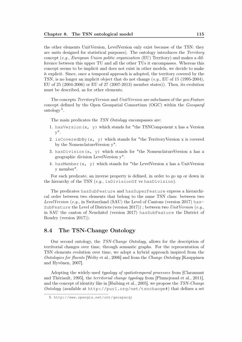
Chapter 8. The TSN ontological model 115

the other elements UnitVersion, LevelVersion only exist because of the TSN: theyare units designed for statistical purposes). The ontology introduces the Territoryconcept (e.g., European Union politic organization (EU) Territory) and makes a dif-ference between this upper TU and all the other TUs it encompasses. Whereas thisconcept seems to be implicit and does not exist in other models, we decide to makeit explicit. Since, once a temporal approach is adopted, the territory covered by theTSN, is no longer an implicit object that do not change (e.g., EU of 15 (1995-2004),EU of 25 (2004-2006) or EU of 27 (2007-2013) member states)). Then, its evolutionmust be described, as for other elements.

The concepts TerritoryVersion and UnitVersion are subclasses of the geo:Featureconcept defined by the Open Geospatial Consortium (OGC) within the Geosparqlontology 5.

The main predicates the TSN Ontology encompasses are:1. hasVersion(x, y) which stands for "the TSNComponent x has a Version

y".2. isCoveredbBy(x, y) which stands for "the TerritoryVersion x is covered

by the NomenclatureVersion y".3. hasDivision(x, y) which stands for "the NomenclatureVersion x has a

geographic division LevelVersion y".4. hasMember(x, y) which stands for "the LevelVersion x has a UnitVersion

y member".For each predicate, an inverse property is defined, in order to go up or down in

the hierarchy of the TSN (e.g., isDivisionOf vs hasDivision).

The predicates hasSubFeature and hasSuperFeature express a hierarchi-cal order between two elements that belong to the same TSN class: between twoLevelVersion (e.g., in Switzerland (SAU) the Level of Cantons (version 2017) has-SubFeature the Level of Districts (version 2017)) ; between two UnitVersion (e.g.,in SAU the canton of Neuchâtel (version 2017) hasSubFeature the District ofBoudry (version 2017)).

8.4 The TSN-Change Ontology

Our second ontology, the TSN-Change Ontology, allows for the description ofterritorial changes over time, through semantic graphs. For the representation ofTSN elements evolution over time, we adopt a hybrid approach inspired from theOntologies for fluents [Welty et al., 2006] and from the Change Ontology [Kauppinenand Hyvönen, 2007].

Adopting the widely-used typology of spatiotemporal processes from [Claramuntand Thériault, 1995], the territorial change typology from [Plumejeaud et al., 2011],and the concept of identity like in [Huibing et al., 2005], we propose the TSN-ChangeOntology (available at http://purl.org/net/tsnchange#) that defines a set

5. http://www.opengis.net/ont/geosparql

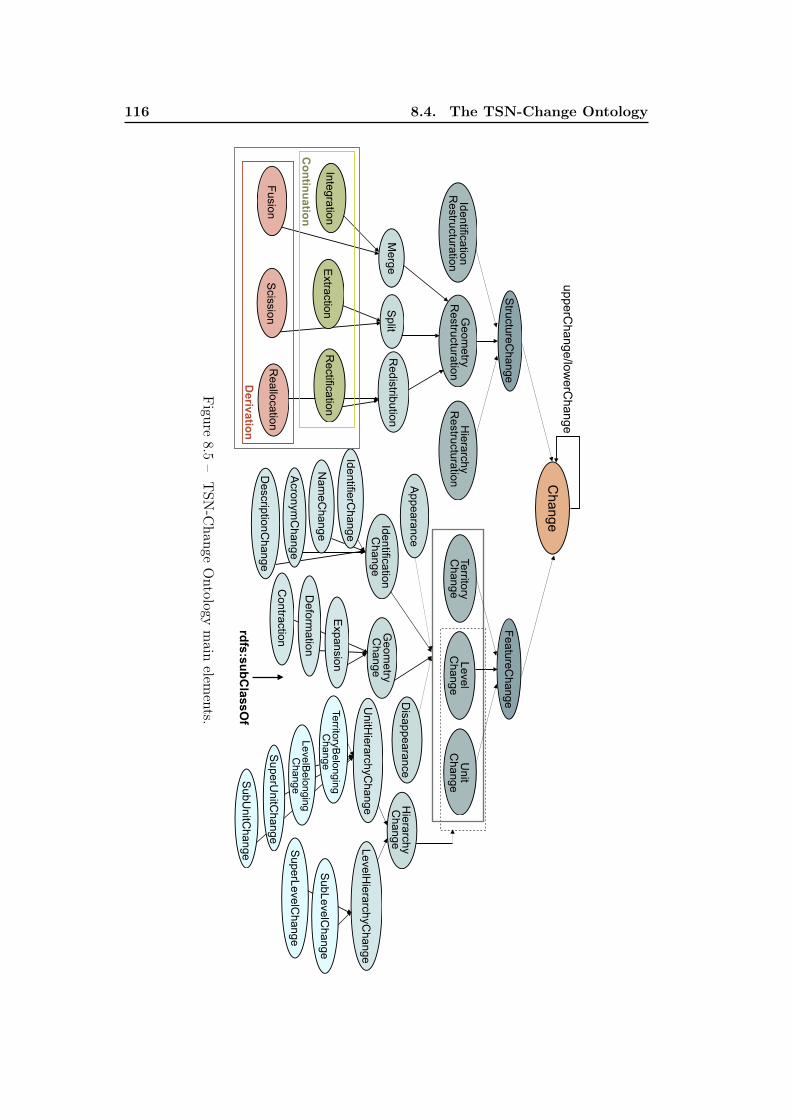
116 8.4. The TSN-Change Ontology

Change

StructureC

hangeFeatureC

hange

Hierarchy

Restructuration

Geom

etry R

estructurationIdentification

Restructuration

Merge

Split

Redistribution

IntegrationE

xtractionR

ectification

Scission

Reallocation

Unit

Change

Level C

hangeTerritory C

hange

Appearance

Identification C

hangeG

eometry

Change

Disappearance

Hierarchy

Change

IdentifierChange

Nam

eChange

Acronym

Change

DescriptionC

hange

Expansion

Deform

ation

Contraction

UnitH

ierarchyChange

LevelHierarchyC

hange

TerritoryBelonging

Change

LevelBelonging

Change

SuperU

nitChange

SubU

nitChange S

uperLevelChange

SubLevelC

hangeContinuation

Derivation

Fusion

upperChange/low

erChange

rdfs:subClassO

f

Figure

8.5–

TSN

-Change

Ontology

main

elements.

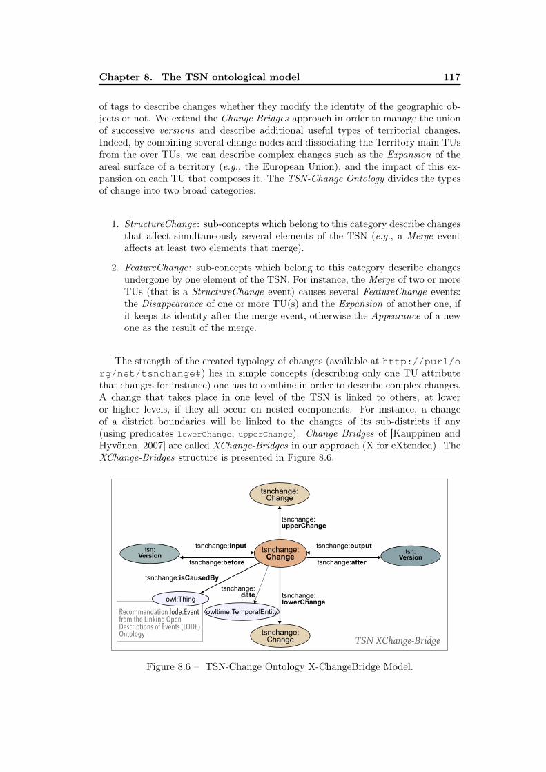
Chapter 8. The TSN ontological model 117

of tags to describe changes whether they modify the identity of the geographic ob-jects or not. We extend the Change Bridges approach in order to manage the unionof successive versions and describe additional useful types of territorial changes.Indeed, by combining several change nodes and dissociating the Territory main TUsfrom the over TUs, we can describe complex changes such as the Expansion of theareal surface of a territory (e.g., the European Union), and the impact of this ex-pansion on each TU that composes it. The TSN-Change Ontology divides the typesof change into two broad categories:

1. StructureChange: sub-concepts which belong to this category describe changesthat affect simultaneously several elements of the TSN (e.g., a Merge eventaffects at least two elements that merge).

2. FeatureChange: sub-concepts which belong to this category describe changesundergone by one element of the TSN. For instance, the Merge of two or moreTUs (that is a StructureChange event) causes several FeatureChange events:the Disappearance of one or more TU(s) and the Expansion of another one, ifit keeps its identity after the merge event, otherwise the Appearance of a newone as the result of the merge.

The strength of the created typology of changes (available at http://purl/org/net/tsnchange#) lies in simple concepts (describing only one TU attributethat changes for instance) one has to combine in order to describe complex changes.A change that takes place in one level of the TSN is linked to others, at loweror higher levels, if they all occur on nested components. For instance, a changeof a district boundaries will be linked to the changes of its sub-districts if any(using predicates lowerChange, upperChange). Change Bridges of [Kauppinen andHyvönen, 2007] are called XChange-Bridges in our approach (X for eXtended). TheXChange-Bridges structure is presented in Figure 8.6.

tsn: Version

tsnchange: upperChange

tsn: Version

tsnchange:input tsnchange:output

tsnchange:before tsnchange:after

tsnchange:Change

tsnchange:Change

tsnchange: lowerChange

TSN XChange-Bridge

tsnchange:isCausedBy

owl:Thingtsnchange:

date

tsnchange: Change

Recommandation lode:Event from the Linking Open Descriptions of Events (LODE) Ontology

owltime:TemporalEntity

Figure 8.6 – TSN-Change Ontology X-ChangeBridge Model.

118 8.4. The TSN-Change Ontology

The predicate tsnchange:input (inverse property tsnchange:before)points to a TSNComponent (LevelVersion and/or UnitVersion) that changes; tsn-change:output points to a TSNComponent created or modified after the changeevent; the predicate tsnchange:lowerChange (inverse property tsnchange:upper-

Change) indicates another change event on a sub-element of the current describedelement that changes; and isCausedBy indicates the contextual reasons for thechange (provided that the information is available on the LOD, on DBpedia forinstance). We recommend the use of the Linking Open Descriptions of Events Ontol-ogy (LODE) 6 [Shaw et al., 2009] for the representation of (historical) events behindareas changes, because it is a domain-independent and a light weighted structure asremarked by [Hienert and Luciano, 2015].

A XChange-Bridge is defined by the tuple:

< t, input, output, lowerChange, upperChange, isCausedBy > (8.1)

where t is the time instant when the change happens; input is the set of TSNCom-ponents (Territories, Level and/or TUs) that are subject to change; output is the setof TSNComponents created or modified after the change event, lowerChange is a setof Change caused by the current described Change; upperChange indicates a set ofupper Change that causes the current described Change; and isCausedBy indicatesthe contextual reasons for the change (provided that the information is available onthe LOD). Using this tuple, any Territorial Change can be described. We show herehow it allows us to dissociate the two Split subtypes: Scission (Split of aTU that causes its disapearance, i.e., Derivation case) and Extraction changes(Split of a TU that still exists after the change, i.e., Continuation case). TheFigure 8.7 presents schematically the difference between these two change tags.

Split – Scission (Derivation)Split – Scission (Derivation)

TU1

(a)

TU2

TU3

Split – Extraction (Continuation)Split – Extraction (Continuation)

TU1TU1

TU3

(b)

Figure 8.7 – Split of a TU - Scission and Extraction.

The Scission of the TU with identifier TU1, on the left side (a) of the Figure8.7, is defined by the tuple:

Scission(TU1) ≡ < t, {TU1}, {TU2, TU3}, {Disappearance(TU1),Appearance(TU2), Appearance(TU3)}, ∗, ∗∗ > (8.2)

where ∗ represents the set of upperChange (not described here)and ∗∗ represents a resource (not described here) that explain why the current

6. http://linkedevents.org/ontology/

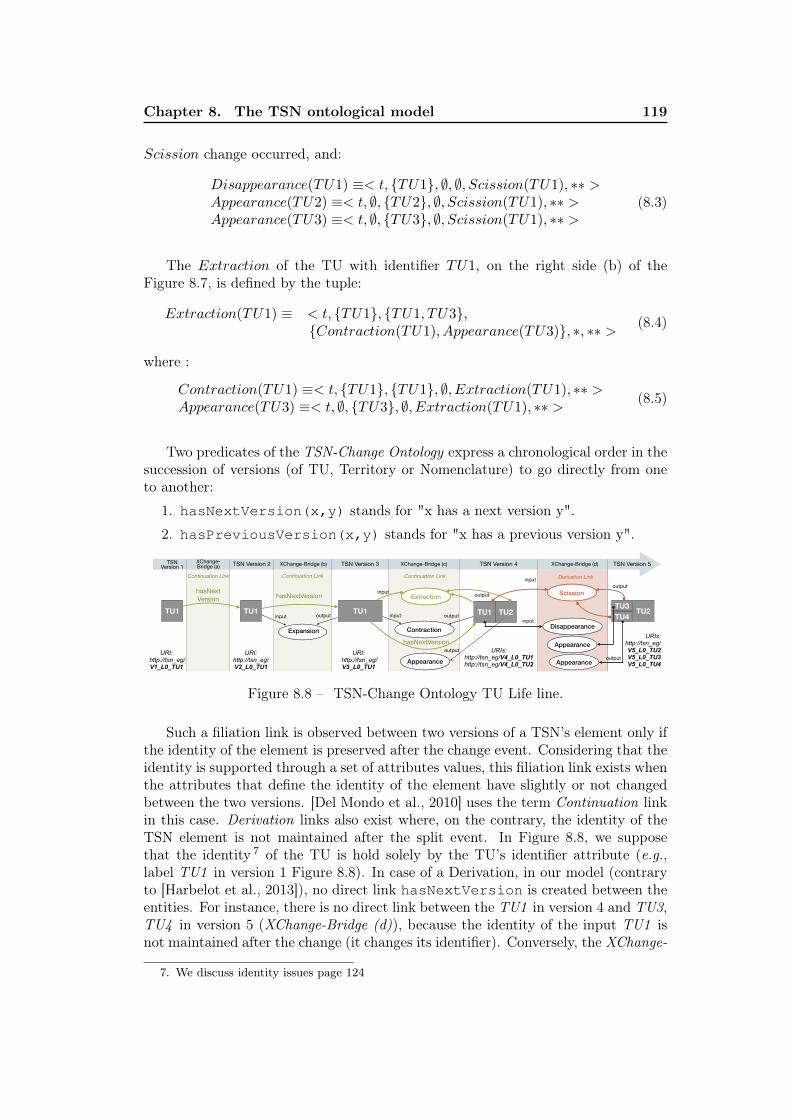
Chapter 8. The TSN ontological model 119

Scission change occurred, and:

Disappearance(TU1) ≡< t, {TU1}, ∅, ∅, Scission(TU1), ∗∗ >Appearance(TU2) ≡< t, ∅, {TU2}, ∅, Scission(TU1), ∗∗ >Appearance(TU3) ≡< t, ∅, {TU3}, ∅, Scission(TU1), ∗∗ >

(8.3)

The Extraction of the TU with identifier TU1, on the right side (b) of theFigure 8.7, is defined by the tuple:

Extraction(TU1) ≡ < t, {TU1}, {TU1, TU3},{Contraction(TU1), Appearance(TU3)}, ∗, ∗∗ > (8.4)

where :

Contraction(TU1) ≡< t, {TU1}, {TU1}, ∅, Extraction(TU1), ∗∗ >Appearance(TU3) ≡< t, ∅, {TU3}, ∅, Extraction(TU1), ∗∗ > (8.5)

Two predicates of the TSN-Change Ontology express a chronological order in thesuccession of versions (of TU, Territory or Nomenclature) to go directly from oneto another:

1. hasNextVersion(x,y) stands for "x has a next version y".

2. hasPreviousVersion(x,y) stands for "x has a previous version y".

Appearance

TSN Version 1 TSN Version 2 TSN Version 3 TSN Version 4XChange-

Bridge (a) XChange-Bridge (b) XChange-Bridge (c)

Continuation Link Continuation Link Continuation Link

TU1

hasNextVersion hasNextVersion

Expansion Contraction

TU2

Extraction

TU1 TU1

URI: http://tsn_eg/ V1_L0_TU1

URI: http://tsn_eg/ V2_L0_TU1

input output input output

input output

outputAppearance

Appearance

TSN Version 5XChange-Bridge (d)

Derivation Link

Disappearance

TU2

Scissionoutput

hasNextVersionURI:

http://tsn_eg/ V3_L0_TU1

URIs: http://tsn_eg/V4_L0_TU1 http://tsn_eg/V4_L0_TU2

input

TU4TU3

input

output

URIs: http://tsn_eg/ V5_L0_TU2 V5_L0_TU3 V5_L0_TU4

TU1

Figure 8.8 – TSN-Change Ontology TU Life line.

Such a filiation link is observed between two versions of a TSN’s element only ifthe identity of the element is preserved after the change event. Considering that theidentity is supported through a set of attributes values, this filiation link exists whenthe attributes that define the identity of the element have slightly or not changedbetween the two versions. [Del Mondo et al., 2010] uses the term Continuation linkin this case. Derivation links also exist where, on the contrary, the identity of theTSN element is not maintained after the split event. In Figure 8.8, we supposethat the identity 7 of the TU is hold solely by the TU’s identifier attribute (e.g.,label TU1 in version 1 Figure 8.8). In case of a Derivation, in our model (contraryto [Harbelot et al., 2013]), no direct link hasNextVersion is created between theentities. For instance, there is no direct link between the TU1 in version 4 and TU3,TU4 in version 5 (XChange-Bridge (d)), because the identity of the input TU1 isnot maintained after the change (it changes its identifier). Conversely, the XChange-

7. We discuss identity issues page 124

120 8.5. Conclusion

Bridge (c) describes a split event as a structure change of type Continuation wherethe identity of the input TU1 is maintained after the change, although the TU splitsin two.

This figure shows, within the graph of versions of a TSN, nodes and links thatdraw the life line of one TU, and provides a view of the three main states (creation,continuation, elimination) as expected in such a model that addresses identity evo-lution issues [Harbelot et al., 2013].

8.5 Conclusion

We have presented, in this Chapter, the TSN Ontology for the description andpublication on the LOD Web of any TSN hierarchical structure. We have underlinedthe importance of adopting a spatiotemporal approach when analyzing territoriesand have proposed to publish all the versions of a TSN rather than to provide usersonly with the latest one. Then, we have introduced the TSN-Change Ontologyfor the description of (boundaries) changes from one TSN version to it subsequent.Together, the TSN and TSN-Change ontologies constitute an innovative approach(combining the Change Bridge approach with the fluents one) for the modeling ofterritorial changes on the LOD Web through graphs we call Multi-level TerritorialChange Graphs.

Chapter 9

Populating the TSN ontologicalmodel

9.1 Introduction

In this Chapter, we present our approach to populate our two ontologies, TSNand TSN-Change. We present the workflows and our methodology to populateautomatically the TSN-Change ontology by taking into account the heterogeneityof the existing TSNs.

9.2 Workflows

There exists two different workflows within the Theseus Framework (see Figure9.1): Workflow A creates the RDF catalog of all the TUs of the proceeded TSNversions; Workflow B creates RDF descriptions of the filiation links between theTSN versions. We present in this Chapter, the TSN Semantic Matching Algorithm,an adaptation of the Algorithm of [Plumejeaud, 2011] created to detect and seman-tically describe these filiation links, using the TSN-Change Ontology. At the end ofthe two workflows, while there are two distinct RDF outputs (TUs, levels descrip-tions and changes, filiation descriptions), all the created data are available from asingle triplestore and are linked together because of the HTTP URIs assigned toeach TSN’s elements, URIs which are also referenced when describing the changesof these elements.

Both Workflows A and B take input files (Figure 9.1, Input box) that are:– a tabular metadata file containing (e.g., CSV, Excel©): metadata information onthe TSN versions to publish as RDF i.e., the names, acronym and description of theTSN and of its versions, the periods covered by the versions, the name and period ofreference of the territories covered by the TSN versions; the list of TUs’ attributesfor which the algorithm will perform a comparison of the values from one versionto another, as well as the weights assigned to each of these attributes; the valueassigned to the three thresholds, run parameters of the algorithm. This tabular fileis filled up by the expert of the TSN. (In the future, we have planned to design aGUI where the expert will be able to enter this information).– a data shapefile for each version of the TSN containing the list of the TUs withtheir identifier in the version, their name, the language used for this name, theirsuper-TU, and the level they belong to. For both the metadata and data inputfiles, information comes from the TSN responsible authority. The shapefiles of the

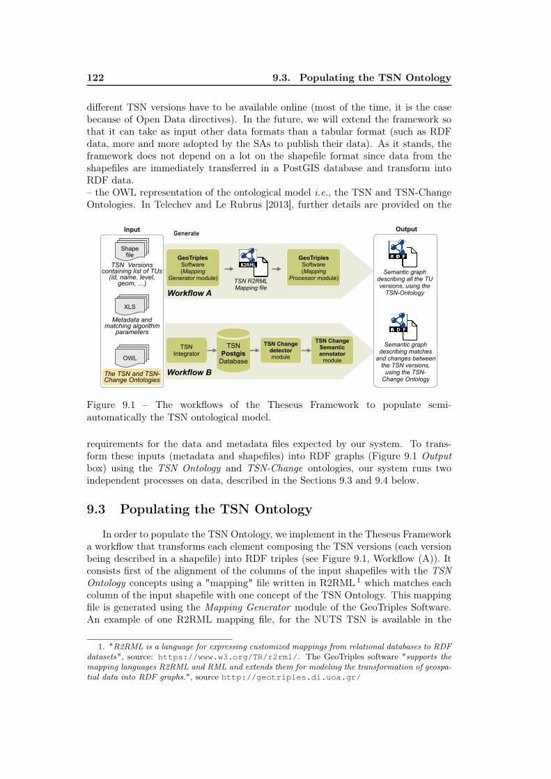
122 9.3. Populating the TSN Ontology

different TSN versions have to be available online (most of the time, it is the casebecause of Open Data directives). In the future, we will extend the framework sothat it can take as input other data formats than a tabular format (such as RDFdata, more and more adopted by the SAs to publish their data). As it stands, theframework does not depend on a lot on the shapefile format since data from theshapefiles are immediately transferred in a PostGIS database and transform intoRDF data.– the OWL representation of the ontological model i.e., the TSN and TSN-ChangeOntologies. In Telechev and Le Rubrus [2013], further details are provided on the

Metadata and matching algorithm

parameters

Semantic graph describing all the TU versions, using the

TSN-Ontology

Semantic graph describing matches

and changes between the TSN versions,

using the TSN-Change Ontology

Input

Shape file

XLS

OWL

GeoTriples Software (Mapping

Generator module) TSN R2RML Mapping file

TSN Integrator

TSN Postgis

Database

TSN Change detector module

OutputGenerate

TSN Versions containing list of TUs

(id, name, level, geom, …)

The TSN and TSN-Change Ontologies

Workflow A

Workflow B

TSN Change Semantic annotator

module

GeoTriples Software (Mapping

Processor module)

Figure 9.1 – The workflows of the Theseus Framework to populate semi-automatically the TSN ontological model.

requirements for the data and metadata files expected by our system. To trans-form these inputs (metadata and shapefiles) into RDF graphs (Figure 9.1 Outputbox) using the TSN Ontology and TSN-Change ontologies, our system runs twoindependent processes on data, described in the Sections 9.3 and 9.4 below.

9.3 Populating the TSN Ontology

In order to populate the TSN Ontology, we implement in the Theseus Frameworka workflow that transforms each element composing the TSN versions (each versionbeing described in a shapefile) into RDF triples (see Figure 9.1, Workflow (A)). Itconsists first of the alignment of the columns of the input shapefiles with the TSNOntology concepts using a "mapping" file written in R2RML 1 which matches eachcolumn of the input shapefile with one concept of the TSN Ontology. This mappingfile is generated using the Mapping Generator module of the GeoTriples Software.An example of one R2RML mapping file, for the NUTS TSN is available in the

1. "R2RML is a language for expressing customized mappings from relational databases to RDFdatasets", source: https://www.w3.org/TR/r2rml/. The GeoTriples software "supports themapping languages R2RML and RML and extends them for modeling the transformation of geospa-tial data into RDF graphs.", source http://geotriples.di.uoa.gr/

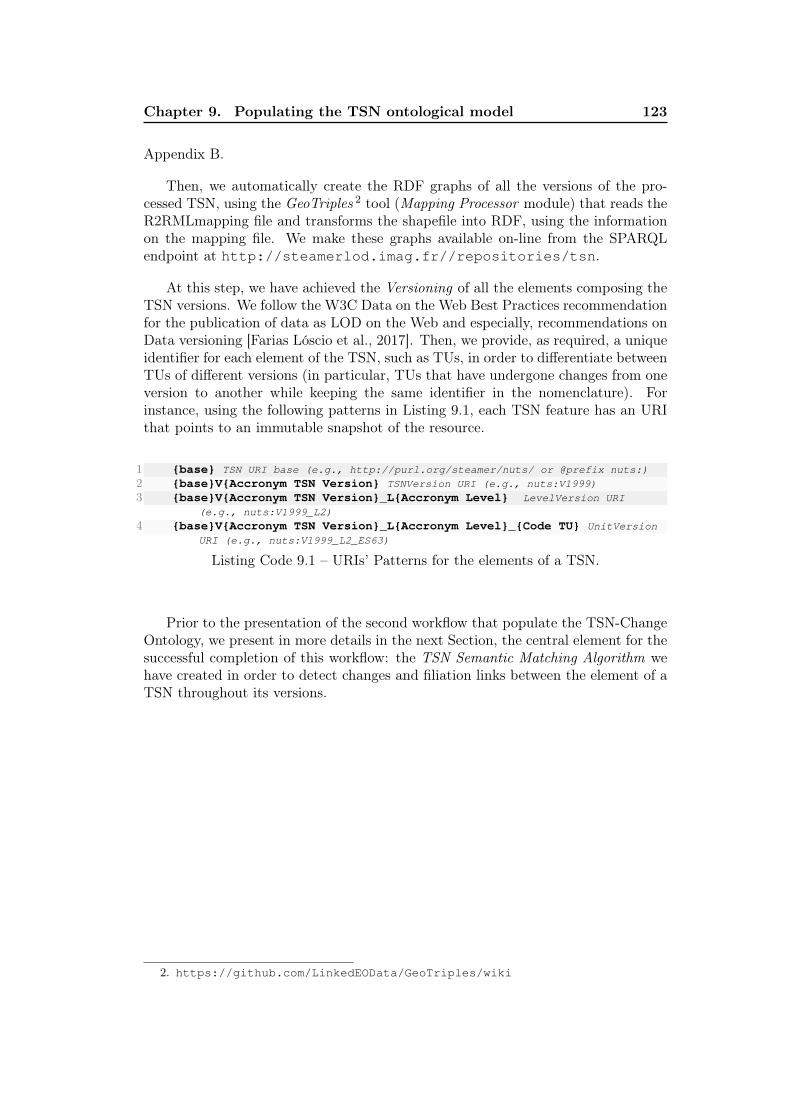
Chapter 9. Populating the TSN ontological model 123

Appendix B.

Then, we automatically create the RDF graphs of all the versions of the pro-cessed TSN, using the GeoTriples 2 tool (Mapping Processor module) that reads theR2RMLmapping file and transforms the shapefile into RDF, using the informationon the mapping file. We make these graphs available on-line from the SPARQLendpoint at http://steamerlod.imag.fr//repositories/tsn.

At this step, we have achieved the Versioning of all the elements composing theTSN versions. We follow the W3C Data on the Web Best Practices recommendationfor the publication of data as LOD on the Web and especially, recommendations onData versioning [Farias Lóscio et al., 2017]. Then, we provide, as required, a uniqueidentifier for each element of the TSN, such as TUs, in order to differentiate betweenTUs of different versions (in particular, TUs that have undergone changes from oneversion to another while keeping the same identifier in the nomenclature). Forinstance, using the following patterns in Listing 9.1, each TSN feature has an URIthat points to an immutable snapshot of the resource.

1 {base} TSN URI base (e.g., http://purl.org/steamer/nuts/ or @prefix nuts:)

2 {base}V{Accronym TSN Version} TSNVersion URI (e.g., nuts:V1999)

3 {base}V{Accronym TSN Version}_L{Accronym Level} LevelVersion URI

(e.g., nuts:V1999_L2)

4 {base}V{Accronym TSN Version}_L{Accronym Level}_{Code TU} UnitVersion

URI (e.g., nuts:V1999_L2_ES63)

Listing Code 9.1 – URIs’ Patterns for the elements of a TSN.

Prior to the presentation of the second workflow that populate the TSN-ChangeOntology, we present in more details in the next Section, the central element for thesuccessful completion of this workflow: the TSN Semantic Matching Algorithm wehave created in order to detect changes and filiation links between the element of aTSN throughout its versions.

2. https://github.com/LinkedEOData/GeoTriples/wiki

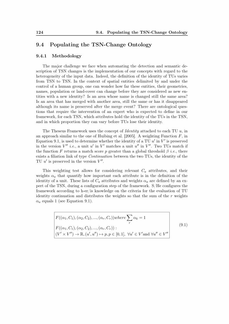
124 9.4. Populating the TSN-Change Ontology

9.4 Populating the TSN-Change Ontology

9.4.1 Methodology

The major challenge we face when automating the detection and semantic de-scription of TSN changes is the implementation of our concepts with regard to theheterogeneity of the input data. Indeed, the definition of the identity of TUs variesfrom TSN to TSN. In the context of spatial entities delimited by and under thecontrol of a human group, one can wonder how far these entities, their geometries,names, population or land-cover can change before they are considered as new en-tities with a new identity? Is an area whose name is changed still the same area?Is an area that has merged with another area, still the same or has it disappearedalthough its name is preserved after the merge event? There are ontological ques-tions that require the intervention of an expert who is expected to define in ourframework, for each TSN, which attributes hold the identity of the TUs in the TSN,and in which proportion they can vary before TUs lose their identity.

The Theseus Framework uses the concept of Identity attached to each TU u, inan approach similar to the one of Huibing et al. [2005]. A weighting Function F , inEquation 9.1, is used to determine whether the identity of a TU u′ in V ′ is preservedin the version V ′′ i.e., a unit u′ in V ′ matches a unit u′′ in V ′′. Two TUs match ifthe function F returns a match score p greater than a global threshold β i.e., thereexists a filiation link of type Continuation between the two TUs, the identity of theTU u′ is preserved in the version V ′′.

This weighting test allows for considering relevant Ca attributes, and theirweights αa that quantify how important each attribute is in the definition of theidentity of a unit. These lists of Ca attributes and weights αa are defined by an ex-pert of the TSN, during a configuration step of the framework. S/He configures theframework according to h-er/is knowledge on the criteria for the evaluation of TUidentity continuation and distributes the weights so that the sum of the r weightsαa equals 1 (see Equation 9.1).

F ((α1, C1), (α2, C2), ..., (αr, Cr))where∑r

αk = 1

F ((α1, C1), (α2, C2), ..., (αr, Cr)) :

(V ′ × V ′′)→ R, (u′, u′′) 7→ p, p ∈ [0, 1], ∀u′ ∈ V ′and ∀u′′ ∈ V ′′

(9.1)

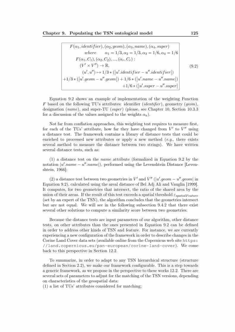
Chapter 9. Populating the TSN ontological model 125

F (α1, identifier), (α2, geom), (α3, name), (α4, super)

where α1 = 1/3, α2 = 1/3, α3 = 1/6, α4 = 1/6

F (α1, C1), (α2, C2), ..., (αr, Cr) :

(V ′ × V ′′)→ R,(u′, u′′) 7→ 1/3 ∗ (

∣∣u′.identifier − u′′.identifier∣∣)+1/3 ∗ (

∣∣u′.geom− u′′.geom∣∣) + 1/6 ∗ (∣∣u′.name− u′′.name∣∣)

+1/6 ∗ (∣∣u′.super − u′′.super∣∣

(9.2)

Equation 9.2 shows an example of implementation of the weighting FunctionF based on the following TU’s attributes: identifier (identifier), geometry (geom),designation (name), and super-TU (super) (please, see Chapter 10, Section 10.3.3for a discussion of the values assigned to the weights αa).

Not far from conflation approaches, this weighting test requires to measure first,for each of the TUs’ attribute, how far they have changed from V ′ to V ′′ usinga distance test. The framework contains a library of distance tests that could beenriched to processed new attributes or apply a new method (e.g., there existsseveral method to measure the distance between two strings). We have writtenseveral distance tests, such as:

(1) a distance test on the name attribute (formalized in Equation 9.2 by thenotation |u′.name− u′′.name|), performed using the Levenshtein Distance [Leven-shtein, 1966];

(2) a distance test between two geometries in V ′ and V ′′ (|u′.geom− u′′.geom| inEquation 9.2), calculated using the areal distance of Bel Adj Ali and Vauglin [1999].It computes, for two geometries that intersect, the ratio of the shared area by theunion of their areas. If the result of this test exceeds a spatial threshold εspatialFeature

(set by an expert of the TSN), the algorithm concludes that the geometries intersectbut are not equal. We will see in the following subsection 9.4.2 that there existseveral other solutions to compute a similarity score between two geometries.

Because the distance tests are input parameters of our algorithm, other distancetests, on other attributes than the ones presented in Equation 9.2 can be definedin order to address other kinds of TSN and feature. For instance, we are currentlyexperiencing a new configuration of the framework in order to describe changes in theCorine Land Cover data sets (available online from the Copernicus web site https://land.copernicus.eu/pan-european/corine-land-cover). We comeback to this perspective in Section 12.2.

To summarize, in order to adapt to any TSN hierarchical structure (structuredefined in Section 2.2), we make our framework configurable. This is a step towardsa generic framework, as we propose in the perspective to these works 12.2. There areseveral sets of parameters to adjust for the matching of the TSN versions, dependingon characteristics of the geospatial data:(1) a list of TUs’ attributes considered for matching;

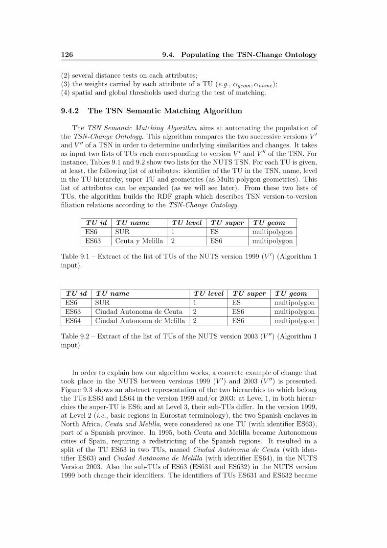
126 9.4. Populating the TSN-Change Ontology

(2) several distance tests on each attributes;(3) the weights carried by each attribute of a TU (e.g., αgeom, αname);(4) spatial and global thresholds used during the test of matching.

9.4.2 The TSN Semantic Matching Algorithm

The TSN Semantic Matching Algorithm aims at automating the population ofthe TSN-Change Ontology. This algorithm compares the two successive versions V ′and V ′′ of a TSN in order to determine underlying similarities and changes. It takesas input two lists of TUs each corresponding to version V ′ and V ′′ of the TSN. Forinstance, Tables 9.1 and 9.2 show two lists for the NUTS TSN. For each TU is given,at least, the following list of attributes: identifier of the TU in the TSN, name, levelin the TU hierarchy, super-TU and geometries (as Multi-polygon geometries). Thislist of attributes can be expanded (as we will see later). From these two lists ofTUs, the algorithm builds the RDF graph which describes TSN version-to-versionfiliation relations according to the TSN-Change Ontology.

TU id TU name TU level TU super TU geomES6 SUR 1 ES multipolygonES63 Ceuta y Melilla 2 ES6 multipolygon

Table 9.1 – Extract of the list of TUs of the NUTS version 1999 (V ′) (Algorithm 1input).

TU id TU name TU level TU super TU geomES6 SUR 1 ES multipolygonES63 Ciudad Autonoma de Ceuta 2 ES6 multipolygonES64 Ciudad Autonoma de Melilla 2 ES6 multipolygon

Table 9.2 – Extract of the list of TUs of the NUTS version 2003 (V ′′) (Algorithm 1input).

In order to explain how our algorithm works, a concrete example of change thattook place in the NUTS between versions 1999 (V ′) and 2003 (V ′′) is presented.Figure 9.3 shows an abstract representation of the two hierarchies to which belongthe TUs ES63 and ES64 in the version 1999 and/or 2003: at Level 1, in both hierar-chies the super-TU is ES6; and at Level 3, their sub-TUs differ. In the version 1999,at Level 2 (i.e., basic regions in Eurostat terminology), the two Spanish enclaves inNorth Africa, Ceuta and Melilla, were considered as one TU (with identifier ES63),part of a Spanish province. In 1995, both Ceuta and Melilla became Autonomouscities of Spain, requiring a redistricting of the Spanish regions. It resulted in asplit of the TU ES63 in two TUs, named Ciudad Autónoma de Ceuta (with iden-tifier ES63) and Ciudad Autónoma de Melilla (with identifier ES64), in the NUTSVersion 2003. Also the sub-TUs of ES63 (ES631 and ES632) in the NUTS version1999 both change their identifiers. The identifiers of TUs ES631 and ES632 became

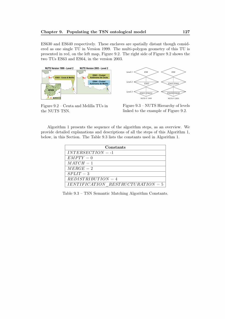
Chapter 9. Populating the TSN ontological model 127

ES630 and ES640 respectively. These enclaves are spatially distant though consid-ered as one single TU in Version 1999. The multi-polygon geometry of this TU ispresented in red, on the left map, Figure 9.2. The right side of Figure 9.2 shows thetwo TUs ES63 and ES64, in the version 2003.

NUTS Version 1999 - Level 2

ES63 - Ceuta & MelillaMelilla

NUTS Version 2003 - Level 2

ES64 - Ciudad Autónoma de Melilla

ES63 - Ciudad Autónoma de Ceuta

SPAIN

MOROCCO

Figure 9.2 – Ceuta and Melilla TUs inthe NUTS TSN.

ES6 ES6

ES63 ES63 ES64

ES631 ES632 ES630 ES640

Level 1

Level 2

Level 3

NUTS V 1999 NUTS V 2003

Figure 9.3 – NUTS Hierarchy of levelslinked to the example of Figure 9.2.

Algorithm 1 presents the sequence of the algorithm steps, as an overview. Weprovide detailed explanations and descriptions of all the steps of this Algorithm 1,below, in this Section. The Table 9.3 lists the constants used in Algorithm 1.

ConstantsINTERSECTION = -1EMPTY = 0MATCH = 1MERGE = 2SPLIT = 3REDISTRIBUTION = 4IENTIFICATION_RESTRUCTURATION = 5

Table 9.3 – TSN Semantic Matching Algorithm Constants.

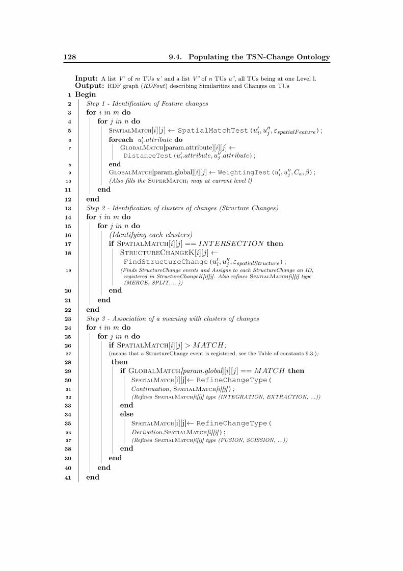
128 9.4. Populating the TSN-Change Ontology

Input: A list V’ of m TUs u’ and a list V” of n TUs u”, all TUs being at one Level l.Output: RDF graph (RDFout) describing Similarities and Changes on TUs

1 Begin2 Step 1 - Identification of Feature changes3 for i in m do4 for j in n do5 SpatialMatch[i][j]← SpatialMatchTest(u′i, u

′′j , εspatialFeature);

6 foreach u′i.attribute do7 GlobalMatch[param.attribute][i][j]←

DistanceTest(u′i.attribute, u′′j .attribute);

8 end9 GlobalMatch[param.global][i][j]← WeightingTest(u′i, u

′′j , Ca, β);

10 (Also fills the SuperMatchl map at current level l)11 end12 end13 Step 2 - Identification of clusters of changes (Structure Changes)14 for i in m do15 for j in n do16 (Identifying each clusters)17 if SpatialMatch[i][j] == INTERSECTION then18 StructureChangeK[i][j]←

FindStructureChange(u′i, u′′j , εspatialStructure);

19 (Finds StructureChange events and Assigns to each StructureChange an ID,registered in StructureChangeK[i][j]. Also refines SpatialMatch[i][j] type(MERGE, SPLIT, ...))

20 end21 end22 end23 Step 3 - Association of a meaning with clusters of changes24 for i in m do25 for j in n do26 if SpatialMatch[i][j] > MATCH;27 (means that a StructureChange event is registered, see the Table of constants 9.3.);

28 then29 if GlobalMatch[param.global][i][j] == MATCH then30 SpatialMatch[i][j]← RefineChangeType(31 Continuation, SpatialMatch[i][j]);32 (Refines SpatialMatch[i][j] type (INTEGRATION, EXTRACTION, ...))

33 end34 else35 SpatialMatch[i][j]← RefineChangeType(36 Derivation,SpatialMatch[i][j]);37 (Refines SpatialMatch[i][j] type (FUSION, SCISSION, ...))

38 end39 end40 end41 end

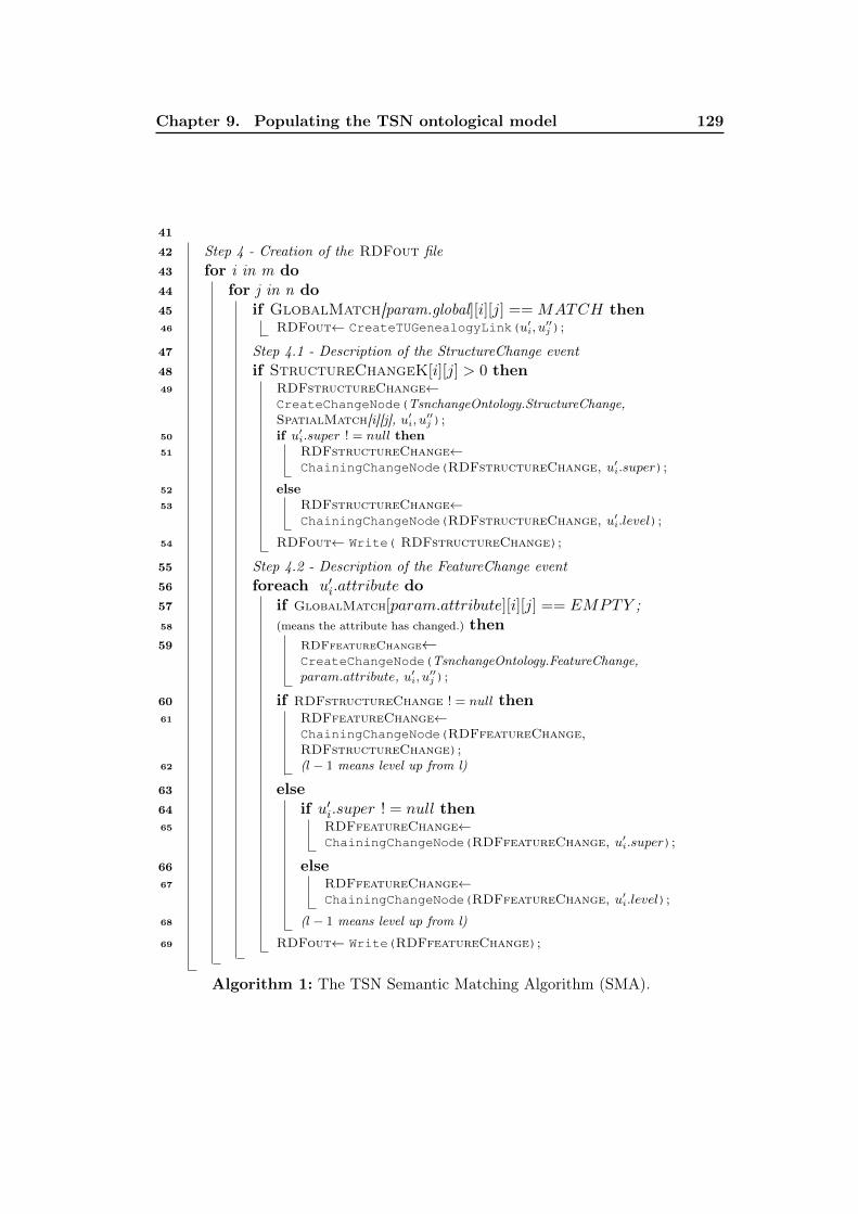
Chapter 9. Populating the TSN ontological model 129

41

42 Step 4 - Creation of the RDFout file43 for i in m do44 for j in n do45 if GlobalMatch[param.global][i][j] == MATCH then46 RDFout← CreateTUGenealogyLink(u′

i, u′′j );

47 Step 4.1 - Description of the StructureChange event48 if StructureChangeK[i][j] > 0 then49 RDFstructureChange←

CreateChangeNode(TsnchangeOntology.StructureChange,SpatialMatch[i][j], u′

i, u′′j );

50 if u′i.super ! = null then

51 RDFstructureChange←ChainingChangeNode(RDFstructureChange, u′

i.super);

52 else53 RDFstructureChange←

ChainingChangeNode(RDFstructureChange, u′i.level);

54 RDFout← Write( RDFstructureChange);

55 Step 4.2 - Description of the FeatureChange event56 foreach u′i.attribute do57 if GlobalMatch[param.attribute][i][j] == EMPTY ;58 (means the attribute has changed.) then59 RDFfeatureChange←

CreateChangeNode(TsnchangeOntology.FeatureChange,param.attribute, u′

i, u′′j );

60 if RDFstructureChange ! = null then61 RDFfeatureChange←

ChainingChangeNode(RDFfeatureChange,RDFstructureChange);

62 (l − 1 means level up from l)

63 else64 if u′i.super ! = null then65 RDFfeatureChange←

ChainingChangeNode(RDFfeatureChange, u′i.super);

66 else67 RDFfeatureChange←

ChainingChangeNode(RDFfeatureChange, u′i.level);

68 (l − 1 means level up from l)

69 RDFout← Write(RDFfeatureChange);

Algorithm 1: The TSN Semantic Matching Algorithm (SMA).

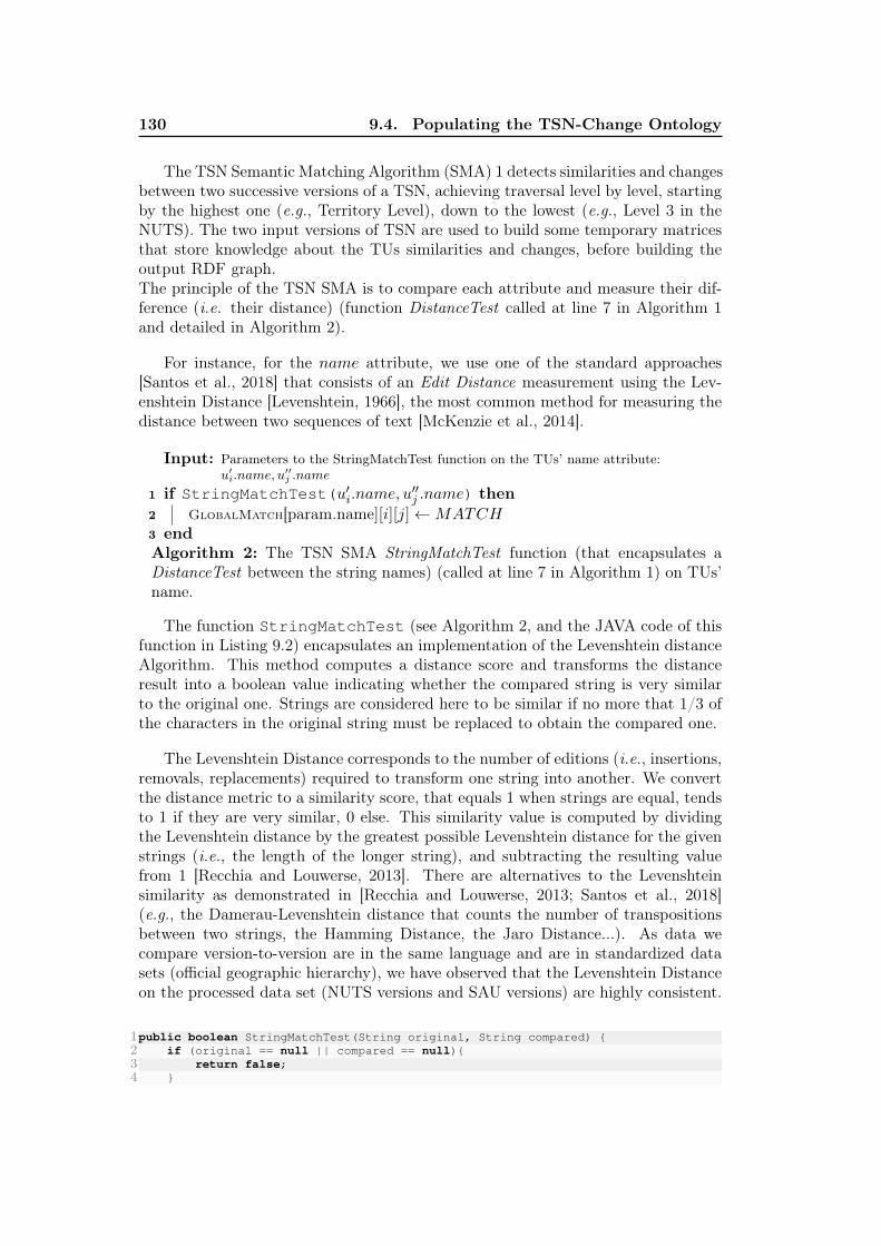
130 9.4. Populating the TSN-Change Ontology

The TSN Semantic Matching Algorithm (SMA) 1 detects similarities and changesbetween two successive versions of a TSN, achieving traversal level by level, startingby the highest one (e.g., Territory Level), down to the lowest (e.g., Level 3 in theNUTS). The two input versions of TSN are used to build some temporary matricesthat store knowledge about the TUs similarities and changes, before building theoutput RDF graph.The principle of the TSN SMA is to compare each attribute and measure their dif-ference (i.e. their distance) (function DistanceTest called at line 7 in Algorithm 1and detailed in Algorithm 2).

For instance, for the name attribute, we use one of the standard approaches[Santos et al., 2018] that consists of an Edit Distance measurement using the Lev-enshtein Distance [Levenshtein, 1966], the most common method for measuring thedistance between two sequences of text [McKenzie et al., 2014].

Input: Parameters to the StringMatchTest function on the TUs’ name attribute:u′i.name, u

′′j .name

1 if StringMatchTest(u′i.name, u′′j .name) then

2 GlobalMatch[param.name][i][j]←MATCH3 endAlgorithm 2: The TSN SMA StringMatchTest function (that encapsulates aDistanceTest between the string names) (called at line 7 in Algorithm 1) on TUs’name.

The function StringMatchTest (see Algorithm 2, and the JAVA code of thisfunction in Listing 9.2) encapsulates an implementation of the Levenshtein distanceAlgorithm. This method computes a distance score and transforms the distanceresult into a boolean value indicating whether the compared string is very similarto the original one. Strings are considered here to be similar if no more that 1/3 ofthe characters in the original string must be replaced to obtain the compared one.

The Levenshtein Distance corresponds to the number of editions (i.e., insertions,removals, replacements) required to transform one string into another. We convertthe distance metric to a similarity score, that equals 1 when strings are equal, tendsto 1 if they are very similar, 0 else. This similarity value is computed by dividingthe Levenshtein distance by the greatest possible Levenshtein distance for the givenstrings (i.e., the length of the longer string), and subtracting the resulting valuefrom 1 [Recchia and Louwerse, 2013]. There are alternatives to the Levenshteinsimilarity as demonstrated in [Recchia and Louwerse, 2013; Santos et al., 2018](e.g., the Damerau-Levenshtein distance that counts the number of transpositionsbetween two strings, the Hamming Distance, the Jaro Distance...). As data wecompare version-to-version are in the same language and are in standardized datasets (official geographic hierarchy), we have observed that the Levenshtein Distanceon the processed data set (NUTS versions and SAU versions) are highly consistent.

1public boolean StringMatchTest(String original, String compared) {2 if (original == null || compared == null){3 return false;4 }

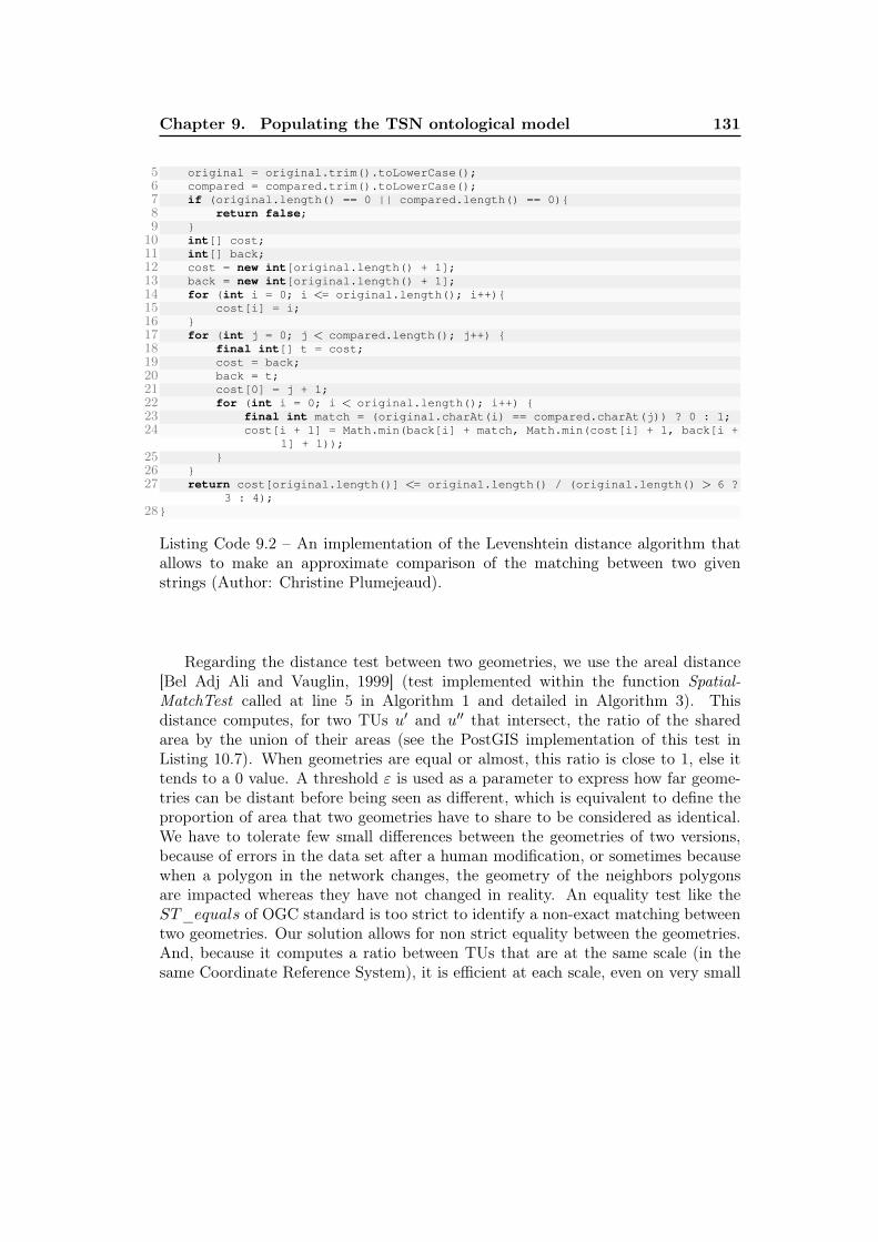
Chapter 9. Populating the TSN ontological model 131

5 original = original.trim().toLowerCase();6 compared = compared.trim().toLowerCase();7 if (original.length() == 0 || compared.length() == 0){8 return false;9 }10 int[] cost;11 int[] back;12 cost = new int[original.length() + 1];13 back = new int[original.length() + 1];14 for (int i = 0; i <= original.length(); i++){15 cost[i] = i;16 }17 for (int j = 0; j < compared.length(); j++) {18 final int[] t = cost;19 cost = back;20 back = t;21 cost[0] = j + 1;22 for (int i = 0; i < original.length(); i++) {23 final int match = (original.charAt(i) == compared.charAt(j)) ? 0 : 1;24 cost[i + 1] = Math.min(back[i] + match, Math.min(cost[i] + 1, back[i +

1] + 1));25 }26 }27 return cost[original.length()] <= original.length() / (original.length() > 6 ?

3 : 4);28}

Listing Code 9.2 – An implementation of the Levenshtein distance algorithm thatallows to make an approximate comparison of the matching between two givenstrings (Author: Christine Plumejeaud).

Regarding the distance test between two geometries, we use the areal distance[Bel Adj Ali and Vauglin, 1999] (test implemented within the function Spatial-MatchTest called at line 5 in Algorithm 1 and detailed in Algorithm 3). Thisdistance computes, for two TUs u′ and u′′ that intersect, the ratio of the sharedarea by the union of their areas (see the PostGIS implementation of this test inListing 10.7). When geometries are equal or almost, this ratio is close to 1, else ittends to a 0 value. A threshold ε is used as a parameter to express how far geome-tries can be distant before being seen as different, which is equivalent to define theproportion of area that two geometries have to share to be considered as identical.We have to tolerate few small differences between the geometries of two versions,because of errors in the data set after a human modification, or sometimes becausewhen a polygon in the network changes, the geometry of the neighbors polygonsare impacted whereas they have not changed in reality. An equality test like theST_equals of OGC standard is too strict to identify a non-exact matching betweentwo geometries. Our solution allows for non strict equality between the geometries.And, because it computes a ratio between TUs that are at the same scale (in thesame Coordinate Reference System), it is efficient at each scale, even on very small

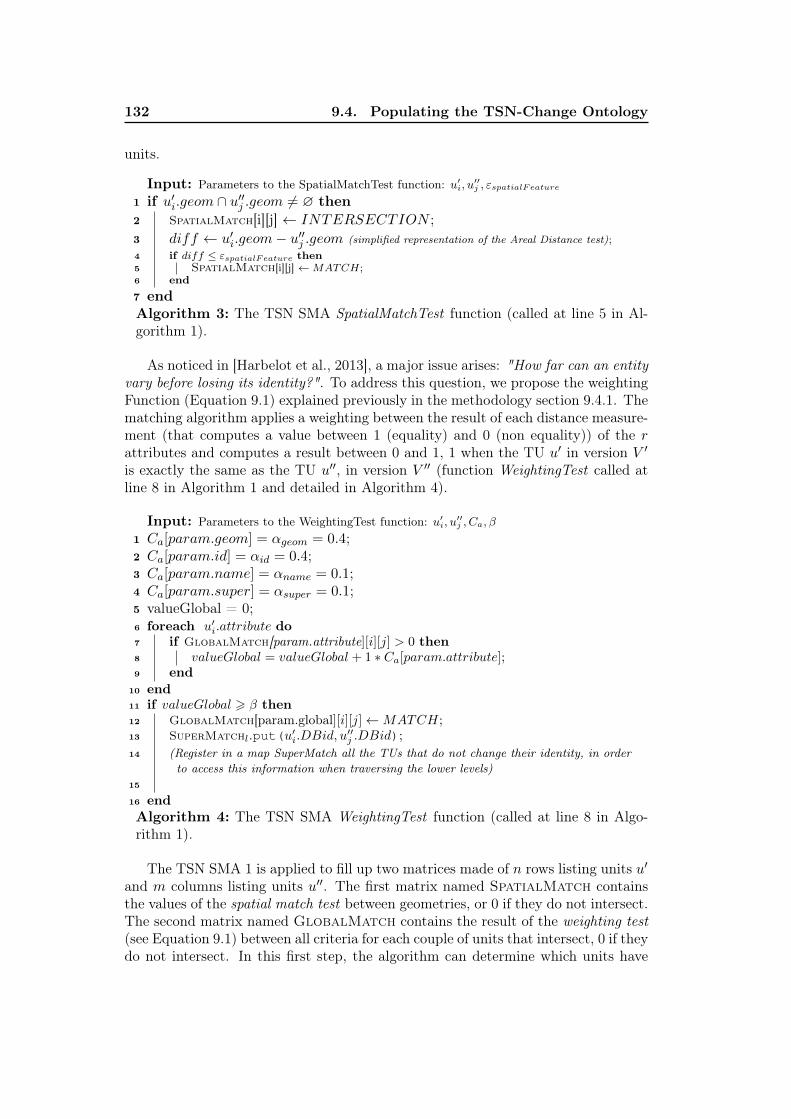
132 9.4. Populating the TSN-Change Ontology

units.

Input: Parameters to the SpatialMatchTest function: u′i, u

′′j , εspatialFeature

1 if u′i.geom ∩ u′′j .geom 6= ∅ then2 SpatialMatch[i][j] ← INTERSECTION ;3 diff ← u′i.geom− u′′j .geom (simplified representation of the Areal Distance test);4 if diff ≤ εspatialFeature then5 SpatialMatch[i][j] ←MATCH;6 end7 endAlgorithm 3: The TSN SMA SpatialMatchTest function (called at line 5 in Al-gorithm 1).

As noticed in [Harbelot et al., 2013], a major issue arises: "How far can an entityvary before losing its identity?". To address this question, we propose the weightingFunction (Equation 9.1) explained previously in the methodology section 9.4.1. Thematching algorithm applies a weighting between the result of each distance measure-ment (that computes a value between 1 (equality) and 0 (non equality)) of the rattributes and computes a result between 0 and 1, 1 when the TU u′ in version V ′is exactly the same as the TU u′′, in version V ′′ (function WeightingTest called atline 8 in Algorithm 1 and detailed in Algorithm 4).

Input: Parameters to the WeightingTest function: u′i, u

′′j , Ca, β

1 Ca[param.geom] = αgeom = 0.4;2 Ca[param.id] = αid = 0.4;3 Ca[param.name] = αname = 0.1;4 Ca[param.super] = αsuper = 0.1;5 valueGlobal = 0;6 foreach u′i.attribute do7 if GlobalMatch[param.attribute][i][j] > 0 then8 valueGlobal = valueGlobal + 1 ∗ Ca[param.attribute];9 end

10 end11 if valueGlobal > β then12 GlobalMatch[param.global][i][j]←MATCH;13 SuperMatchl.put(u′i.DBid, u

′′j .DBid);

14 (Register in a map SuperMatch all the TUs that do not change their identity, in orderto access this information when traversing the lower levels)

15

16 endAlgorithm 4: The TSN SMA WeightingTest function (called at line 8 in Algo-rithm 1).

The TSN SMA 1 is applied to fill up two matrices made of n rows listing units u′and m columns listing units u′′. The first matrix named SpatialMatch containsthe values of the spatial match test between geometries, or 0 if they do not intersect.The second matrix named GlobalMatch contains the result of the weighting test(see Equation 9.1) between all criteria for each couple of units that intersect, 0 if theydo not intersect. In this first step, the algorithm can determine which units have

Chapter 9. Populating the TSN ontological model 133

not changed by comparing the computed values with the global threshold β givenin the configuration. Conversely, units that have changed can be identified, andare associated with the corresponding FeatureChange tag from the TSN-ChangeOntology. When applied to our case study in Spain, at the end of this step, ithas been detected that the TU ES63′ intersects the TU ES63′′, but that theirgeometries are not equal. Also, the appearance of the TU ES64′′ is detected. Still,the set of changes have to be grouped together under StructureChange tags (fromthe TSN-Change Ontology) such as Split.

The second traversal of SpatialMatch aims at building k sets of TUs involvedin the same StructureChange (each one being denoted as StructureChangeK, i.e.,"K" stands for "Knowledge") (function FindStructureChange, Algorithm 1,moredetails about this function can be found in [Plumejeaud, 2011]). By reading theSpatialMatch matrix, the function FindStructureChange (Algorithm 1, line 14)tries to determine precisely if only one TU’s geometry has changed or more neigh-boring TUs with it. For each StructureChangeK event, the algorithm builds throughiterations two sets: the beforeK set of TUs preceding the event, and the afterKset of TUs succeeding the event. For instance, if a TU u′1 splits in two TUs (u′′2and u′′3) from version V ′ to V ′′, the SpatialMatch matrix will have registeredtwo intersections for the TU u′1 and will conclude that a StructureChange of typeSplit. If two TUs u′1 and u′2 merge into one TU u′′3 from version V ′ to V ′′, theSpatialMatch matrix will have registered two intersections for the TU u′′3 andwill conclude that a StructureChange of type Merge. Figure 9.4 presents schemat-ically an example of the iterations of the algorithm, in case of a Split event. Anequality test is performed on the external geometries of the two sets of TUs beforeand after change (e.g., equality test between the external geometry of u′1 and ex-ternal geometry of the union of u′′2 and u′′3) in order to validate the aggregationof several TUs changes under one semantic tag (e.g., split, merge, redistribution),with a tolerance threshold εspatialStructure.

ES63’ES63’’

ES64’’

Iterations of the algorithmBeforeK

1. (ES63) 2. 3. (ES63)

AfterK

(ES63’’, ES64’’)

NUTS V 1999 NUTS V 2003

Figure 9.4 – Iterations of the SMA Algorithm in order to find a set of TUs involvedin a same StructureChange.

The first iteration starts with the first TUs that have an areal distance differentfrom 0 in SpatialMatch. For instance, on the TUs ES63′ and ES63′′ the scorein SpatialMatch is of 0.5. Thus, a set named beforeK is initialized with theTU ES63′ identified as a TU that intersects another one, here the TU ES63′′.Starting from this seed, here ES63′, the second iteration adds to the set namedafterK the whole set of TUs that intersects ES63′ in V ′′ (ES63′′, ES64′′ here)(an information stored in the SpatialMatch matrix). Conversely, starting fromafterK, the third iteration checks if any TU of afterK intersects others in V ′.

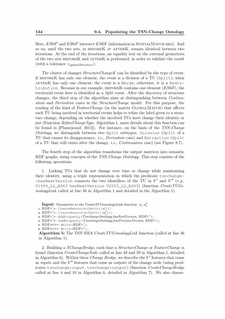
134 9.4. Populating the TSN-Change Ontology

Here, ES63′′ and ES64′′ intersect ES63′ (information in SpatialMatch also). Andso on, until the two sets, in beforeK or afterK, remain identical between twoiterations. At the end of the iterations, an equality test on the external geometriesof the two sets beforeK and afterK is performed, in order to validate the result(with a tolerance εspatialStructure).

The cluster of changes StructureChangeK can be identified by the type of event:if beforeK has only one element, the event is a division of a TU (Split); whenafterK has only one element, the event is a Merge; otherwise, it is a Redis-tribution. Because in our example, beforeK contains one element (ES63′), theterritorial event here is identified as a Split event. After the discovery of structurechanges, the third step of the algorithm aims at distinguishing between Continu-ation and Derivation cases in the StructureChange model. For this purpose, thereading of the kind of FeatureChange (in the matrix GlobalMatch) that affectseach TU being involved in territorial events helps to refine the label given to a struc-ture change, depending on whether the involved TUs have change their identity ornot (Function RefineChangeType, Algorithm 1, more details about this function canbe found in [Plumejeaud, 2011]). For instance, on the basis of the TSN-ChangeOntology, we distinguish between two Split subtypes: Scission (Split of aTU that causes its disappearance, i.e., Derivation case) and Extraction (Splitof a TU that still exists after the change, i.e., Continuation case) (see Figure 8.7).

The fourth step of the algorithm transforms the output matrices into semanticRDF graphs, using concepts of the TSN-Change Ontology. This step consists of thefollowing operations:

1. Linking TUs that do not change over time or change while maintainingtheir identity, using a triple representation in which the predicate tsnchange-:hasNextVersion connects the two identifiers of the TU in V ′ and V ′′ (e.g.,V1999_L2_ES63 hasNextVersion V2003_L2_ES63) (function CreateTUGe-nealogyLink called at line 46 in Algorithm 1 and detailed in the Algorithm 5).

Input: Parameters to the CreateTUGenealogyLink function: u′i, u

′′j

1 RDFu’← CreateResource(GetUri(u′i));

2 RDFu”← CreateResource(GetUri(u′′j ));

3 RDFu’← AddProperty(TsnchangeOntology.hasNextVersion, RDFu”);4 RDFu”← AddProperty(TsnchangeOntology.hasPreviousVersion, RDFu’);5 RDFout← Write(RDFu’);6 RDFout← Write(RDFu”);Algorithm 5: The TSN SMA CreateTUGenealogyLink function (called at line 46in Algorithm 1).

2. Building a XChangeBridge, each time a StructureChange or FeatureChange isfound (function CreateChangeNode called at line 49 and 59 in Algorithm 1, detailedin Algorithm 6). Within these Change Bridge, we describe the V ′ features that comeas inputs and the V ′′ features that come as outputs of the change node (using pred-icates tsnchange:input, tsnchange:output) (function CreateChangeBridgecalled at line 4 and 10 in Algorithm 6, detailed in Algorithm 7). We also charac-

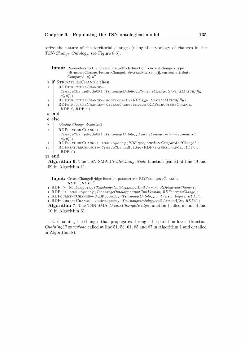
Chapter 9. Populating the TSN ontological model 135

terize the nature of the territorial changes (using the typology of changes in theTSN-Change Ontology, see Figure 8.5).

Input: Parameters to the CreateChangeNode function: current change’s type(StructureChange/FeatureChange), SpatialMatch[i][j], current attributeCompared, u′

i, u′′j

1 if StructureChange then2 RDFstructureChange←

CreateChangeNodeURI(TsnchangeOntology.StructureChange, SpatialMatch[i][j],u′i, u

′′j );

3 RDFstructureChange← AddProperty(RDF.type, SpatialMatch[i][j]);4 RDFstructureChange← CreateChangeBridge(RDFstructureChange,

RDFu’, RDFu”)5 end6 else7 (FeatureChange described)8 RDFfeatureChange←

CreateChangeNodeURI(TsnchangeOntology.FeatureChange, attributeCompared,u′i, u

′′j );

9 RDFfeatureChange← AddProperty(RDF.type, attributeCompared+"Change");10 RDFfeatureChange← CreateChangeBridge(RDFfeatureChange, RDFu’,

RDFu”)11 endAlgorithm 6: The TSN SMA CreateChangeNode function (called at line 49 and59 in Algorithm 1).

Input: CreateChangeBridge function parameters: RDFcurrentChange,RDFu′, RDFu′′

1 RDFu’← AddProperty(TsnchangeOntology.inputUnitVersion, RDFcurrentChange);2 RDFu”← AddProperty(TsnchangeOntology.outputUnitVersion, RDFcurrentChange);3 RDFcurrentChange← AddProperty(TsnchangeOntology.unitVersionBefore, RDFu’);4 RDFcurrentChange← AddProperty(TsnchangeOntology.unitVersionAfter, RDFu”);Algorithm 7: The TSN SMA CreateChangeBridge function (called at line 4 and10 in Algorithm 6).

3. Chaining the changes that propagates through the partition levels (functionChainingChangeNode called at line 51, 53, 61, 65 and 67 in Algorithm 1 and detailedin Algorithm 8).

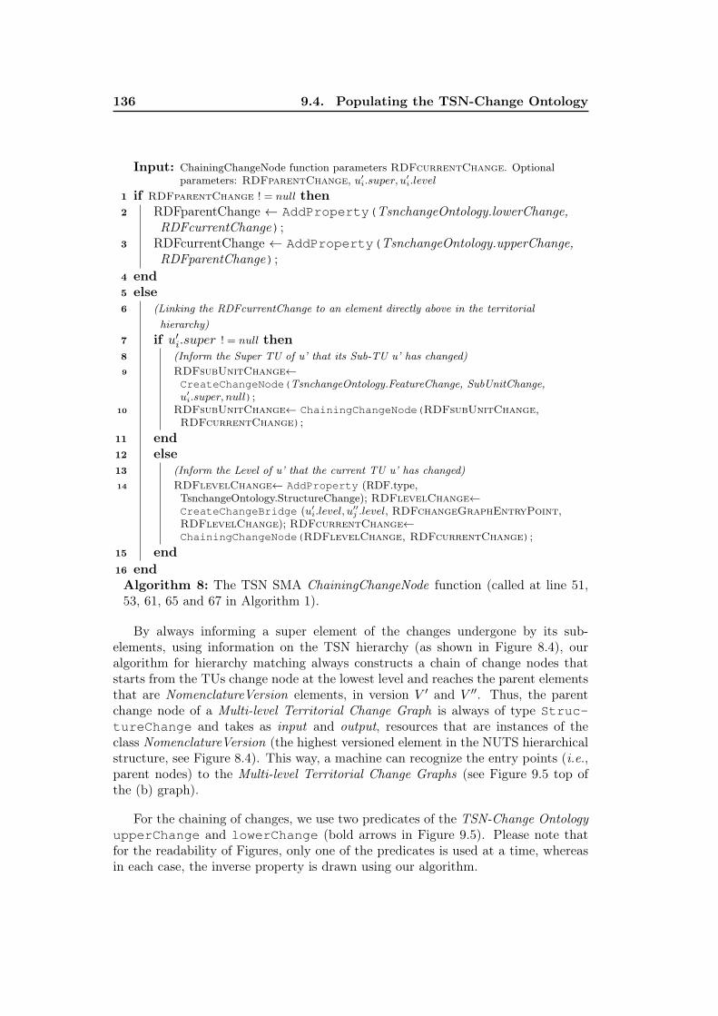
136 9.4. Populating the TSN-Change Ontology

Input: ChainingChangeNode function parameters RDFcurrentChange. Optionalparameters: RDFparentChange, u′

i.super, u′i.level

1 if RDFparentChange ! = null then2 RDFparentChange ← AddProperty(TsnchangeOntology.lowerChange,

RDFcurrentChange);3 RDFcurrentChange ← AddProperty(TsnchangeOntology.upperChange,

RDFparentChange);4 end5 else6 (Linking the RDFcurrentChange to an element directly above in the territorial

hierarchy)7 if u′i.super ! = null then8 (Inform the Super TU of u’ that its Sub-TU u’ has changed)9 RDFsubUnitChange←

CreateChangeNode(TsnchangeOntology.FeatureChange, SubUnitChange,u′i.super, null);

10 RDFsubUnitChange← ChainingChangeNode(RDFsubUnitChange,RDFcurrentChange);

11 end12 else13 (Inform the Level of u’ that the current TU u’ has changed)14 RDFlevelChange← AddProperty (RDF.type,

TsnchangeOntology.StructureChange); RDFlevelChange←CreateChangeBridge (u′

i.level, u′′j .level, RDFchangeGraphEntryPoint,

RDFlevelChange); RDFcurrentChange←ChainingChangeNode(RDFlevelChange, RDFcurrentChange);

15 end16 endAlgorithm 8: The TSN SMA ChainingChangeNode function (called at line 51,53, 61, 65 and 67 in Algorithm 1).

By always informing a super element of the changes undergone by its sub-elements, using information on the TSN hierarchy (as shown in Figure 8.4), ouralgorithm for hierarchy matching always constructs a chain of change nodes thatstarts from the TUs change node at the lowest level and reaches the parent elementsthat are NomenclatureVersion elements, in version V ′ and V ′′. Thus, the parentchange node of a Multi-level Territorial Change Graph is always of type Struc-tureChange and takes as input and output, resources that are instances of theclass NomenclatureVersion (the highest versioned element in the NUTS hierarchicalstructure, see Figure 8.4). This way, a machine can recognize the entry points (i.e.,parent nodes) to the Multi-level Territorial Change Graphs (see Figure 9.5 top ofthe (b) graph).

For the chaining of changes, we use two predicates of the TSN-Change OntologyupperChange and lowerChange (bold arrows in Figure 9.5). Please note thatfor the readability of Figures, only one of the predicates is used at a time, whereasin each case, the inverse property is drawn using our algorithm.

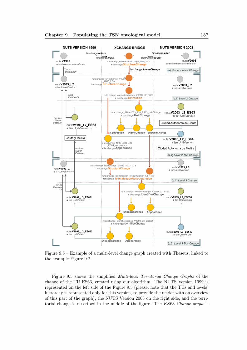
Chapter 9. Populating the TSN ontological model 137

nuts:change_extractionchange_V1999_L2_ES63 a tsnchange:Extraction

nuts:change_1999-2003_730_ES64_appearance

a tsnchange:Appearance

nuts:V2003_L2_ES64 a tsn:UnitVersion

nuts:V1999_L2_ES63 a tsn:UnitVersion

nuts:change_1999-2003_730_ES63_unitChange a tsnchange:UnitChange

:Contraction

nuts:V2003_L2_ES63 a tsn:UnitVersion

:NameChange

nuts:change_levelchange_V1999_2003_L2 a

tsnchange:StructureChangenuts:V1999_L2 a tsn:LevelVersion

Ceuta y Mellila

Ciudad Autonoma de Ceuta

Ciudad Autonoma de Mellila

NUTS VERSION 1999

nuts:change_nomenclaturechange_1999_2003a tsnchange:StructureChange

NUTS VERSION 2003XCHANGE-BRIDGE

(a) Nomenclature Change

tsnchange:input

tsnchange:before

nuts:V2003 a tsn:NomenclatureVersion

:Disappearance

nuts:V1999_L3_ES631 a tsn:UnitVersion

nuts:V2003_L3_ES640 a tsn:UnitVersion

nuts:change_identifierchange_V1999_L3_ES632 a tsnchange:IdentifierChange

:Appearance

nuts:change_identification_restructuration_L3_14 a tsnchange: IdentificationRestructuration

nuts:V1999_L3 a tsn:LevelVersion

:Appearance

nuts:V2003_L3_ES630 a tsn:UnitVersion

nuts:V1999_L3_ES632 a tsn:UnitVersion

:Disappearance

nuts:change_identifierchange_V1999_L3_ES631 a tsnchange:IdentifierChange

tsnchange:lowerChange

tsnchange:output

tsnchange:after

nuts:V1999 a tsn:NomenclatureVersion

(b.1) Level 2 Change

(b.2) Level 2 TUs Change

(c.1) Level 3 Change

(c.2) Level 3 TUs Change

nuts:V2003_L2 a tsn:LevelVersion

nuts:V2003_L3 a tsn:LevelVersion

:SubUnitChange

nuts:change_levelchange_V1999_2003_L2 a tsnchange:StructureChange

tsn:is Member

Of

tsn:is MemberOf

tsn:has Super

Feature

tsn:is DivisionOf

tsn:has Super Feature

Figure 9.5 – Example of a multi-level change graph created with Theseus, linked tothe example Figure 9.2.

Figure 9.5 shows the simplified Multi-level Territorial Change Graphs of thechange of the TU ES63, created using our algorithm. The NUTS Version 1999 isrepresented on the left side of the Figure 9.5 (please, note that the TUs and levels’hierarchy is represented only for this version, to provide the reader with an overviewof this part of the graph); the NUTS Version 2003 on the right side; and the terri-torial change is described in the middle of the figure. The ES63 Change graph is

138 9.4. Populating the TSN-Change Ontology

designed as follows:(a) at the top of the graph, the parent change node is of type StructureChange(because this Split event impacts several TSN features). The NomenclatureVersionresource NUTS Version 1999 comes as an input resource to this change node, andthe NUTS Version 2003 comes as an output resource, as the TSN versions them-selves change after this event on ES63.(b.1) this parent change node has a lower change at Level 2 (linked to it using thepredicate tsnchange:lowerChange) labeled Extraction (i.e., Split change where Con-tinuation of the input TU is observed after the change, see Figure 8.7).(b.2) each modification on each impacted feature, caused by this Extraction event isthen represented, thanks to FeatureChange nodes (see the FeatureChange sub-typesin Figure 8.5). Here, the split of the TU ES63 results in: the Appearance of the TUES64 (Ciudad Autónoma de Melilla) ; several changes on the TU ES63 (all thesechanges are grouped under one UnitChange node): its Contraction, NameChange,and also the change of its sub-units. This node SubUnitChange is essential: it chainsthe change nodes through the levels.(c.1) then, by visiting the ES63′ node, one may directly know the changes its sub-TUs have undergone, without having to go through all the list of its sub-TUs tocheck if they have changed or not. By following this SubUnitChange node, onediscovers that the sub-TUs of ES63′ change their identifier (IdentificationRestruc-turation) after the Extraction event.(c.2) each modification on each impacted feature, caused by this IdentificationRe-structuration event is then represented. Here, it consists of several IdentifierChangedescriptions, for each of the sub-TUs of ES63 that changes its nomenclature iden-tifier (also called code).

The following Subsection presents the workflow implemented in the TheseusFramework to populate the TSN-Change ontology, using the TSN SMA.

9.4.3 The Workflow

The second workflow implemented in the Theseus Framework consists in per-forming the matching of all the TSN elements, version-to-version, and describingtheir changes by means of RDF triples using the concepts of the TSN-Change On-tology (see Figure 9.1, Workflow (B)), and an implementation of the TSN SMA.

The TSN SMA has been implemented in two Java modules (see modules TSNChange Detector and TSN Change Semantic Annotator, Workflow (B), Figure 9.1).

The TSN Change Detector module takes as input a tabular metadata file, setup by an expert of the TSN with the list of the parameters of the TSN SMAAlgorithm, as defined in the Methodology Section 9.4.1. This file contains: the listof TU’s attributes to be considered during the matching tests on TUs, the weightassigned to each attribute, the value of the three thresholds. In order to computethe changes between two versions of a TSN, a PostGIS spatial database is built.

Using the TSN Integrator module we have developed, we insert in the PostGIS

Chapter 9. Populating the TSN ontological model 139

spatial database of the framework, the shapefiles of the TSN, the metadata descrip-tion of the TSN (contained in an tabular file) and the algorithm parameters values,set by the expert (in an tabular file also). Using the Jena Plugin Schemagen 3, wegenerate a Java representation of the TSN ontological model (all the concepts aretranslate into Java constants to be used in our Java programs).

Then, the TSN change Detector module accesses the PostGIS spatial database ofthe framework, and according to the values of the weights and thresholds set by theexpert in the CSV file, it computes similarities measures (registered in temporarymatrices).

The TSN Change Semantic Annotator reads the matrices and according to thevalues, assigns a TSN-Change tag to each change detected, and constructs the RDFchange bridges between all the elements of the two TSN’s versions processed, usingthe Apache-Jena RDF API 4 and the Java representation of the TSN and TSN-Change ontologies.

At the end of Workflow B, the TSN RDF history graph is created. This graphis available online from the SPARQL endpoint at http://steamerlod.imag.fr//repositories/tsn (please note that the SPARQL Query GUI provided byour GraphDB triplestore, at http://steamerlod.imag.fr/sparql, may bemore convenient to human tests).

9.5 Conclusion

In [Wiemann and Bernard, 2016], the authors describe their approach for spa-tial data fusion and/or versioning management of network data in Open Street Map(OSM) data sets. In an approach very similar to ours, they sum several weightedsimilarity measurements (the Damerau–Levenshtein distance to calculate the dis-tance between road names, the Hausdorff distance, the angle difference and thelength difference between poly-line geometries of the network) and construct RDFgraphs describing changes over time, in OSM data sets. They use the ChangeSetvocabulary 5 to describe the delta between two versions of a resource, in terms ofadditions and removals only. Consequently, the description of changes are very lim-ited, as the aim is more to track, feature by feature, who has modified a featureand how (e.g.,the change of the type of a road from "footway" to "path" will bedescribed as a removal of the "footway" type and addition of the new type "path").This vocabulary does not fit our objective of precisely describe changes in TSN thatmay impact several features at the same time (e.g., merge of two features in one).Our TSN-Change Ontology inherits from the Provenance, Authoring and VersioningOntology 6, and contains more tags resulting in an accurate description of featureand spatial structure changes.

Because the distance tests are input parameters to our algorithm, other distance

3. https://jena.apache.org/documentation/tools/schemagen-maven.html4. https://jena.apache.org/5. http://purl.org/vocab/changeset/schema#6. http://purl.org/pav/

140 9.5. Conclusion

tests, on other attributes than the ones presented in Equation 9.2 can be definedin order to address other kinds of TSN and feature. For instance, we are currentlyexperiencing a new configuration of the framework in order to describe changes in theCorine Land Cover data sets (available online from the Copernicus web site https://land.copernicus.eu/pan-european/corine-land-cover). We comeback to this perspective in the Chapter 12.

In order to adapt in the future to any TSN hierarchical structure in the world,we make our framework configurable and expandable. We propose, in Section 12.2,a solution to make our framework more generic.

So far, the Theseus Framework has been used on 3 different TSNs i.e., 3 TSNRDF history graph have been created:– the NUTS TSN (from Eurostat) versions 1999, 2003, 2006, 2010. The out-put graph (containing all the TUs and changes descriptions) is available onlineat http://purl.org/steamer/nuts (entry points of the change graphs areavailable at http://purl.org/steamer/nuts/change_nomenclaturechange_1999_2003; http://purl.org/steamer/nuts/change_nomenclaturechange_2003_2006; http://purl.org/steamer/nuts/change_nomenclaturechange_2006_2010);– the SAU TSN (from the Swiss Federal Statistical Office) versions 2017 and 2018.The output graph (containing all the TUs and changes descriptions) is available on-line at http://purl.org/steamer/sau (the entry point of the change graph isavailable at http://purl.org/steamer/sau/change_nomenclaturechange_2017_2018);– the ASGS TSN (from the Australian Bureau of Statistics) versions 2011 and 2016.The output graph (containing all the TUs and changes descriptions) is available on-line at http://purl.org/steamer/asgs (the entry point of the change graphis available at http://purl.org/steamer/asgs/change_nomenclaturechange_2011_2016).

In the next Chapter of this manuscript, we present first the two tests on theNUTS and SAU TSNs. Then, we present the ASGS case study as it covers thehuge territory of Australia. It brings new challenges, such as big data processingby our software tools, and questions on the generalization of the geometries versionto version. Finally, these three case studies allow us to assess the complexity of ouralgorithm.

Chapter 10

Case studies and discussion

10.1 Introduction

In this chapter, we present first three tests of our Theseus Framework developedto describe and publish on the LOD Web the elements of a TSN and its changesover time. We focus on the description of changes created by our program thatimplements our TSN Semantic Matching Algorithm. As described in the previousChapter 9, the program consists of two Java modules (the TSN Change Detector andTSN Change Semantic Annotator) of the Theseus Framework. We ran three testson three very different TSNs: the NUTS, ASGS, and SAU TSNs. Regarding thetwo data sets NUTS and SAU, although they both focus on Europe, they are quitedifferent because of the size of the TUs they contain. The NUTS biggest TUs are theEU member states whereas the biggest TUs of the SAU are cantons, equivalent to theNUTS smallest regions (Level 3). The smallest units in the SAU are municipalities,much smaller units and more numerous than in the NUTS. Thus, these two datasets allow us to open up on interesting perspectives, such as the matching of twodifferent TSNs, using the TSN-Ontology and TSN-Change Ontology to create bridgesbetween the Level 3 of the NUTS and the Level 0 of the SAU. The third Australiandata set ASGS was chose for experiment as it covers a very different region of theworld, a vast territory whose TUs’ geometries are composed of 4,000 vertices onaverage (compared to an average of 28 vertices in the NUTS). This was a challengefor our software program, allowing us to assess its ability to generate similaritiesand changes descriptions even on large data set.

In a second time, we assess the complexity of the TSN Semantic Matching Al-gorithm. We report about the problems we have encountered when testing ourprogram on these three data sets, and we discuss the genericity of our approach,meaning its capability to handle various TSNs or not.

10.2 Case Studies

Please, note that the value of the input parameters (i.e., weights on TUs at-tributes, tolerance thresholds for variation) of our program that implements theTSN Semantic Matching Algorithm are not discussed in this Section, but in theSection 10.3. These parameters and the definition of what makes the identity of theprocessed TUs have been fixed by experts of the TSNs.

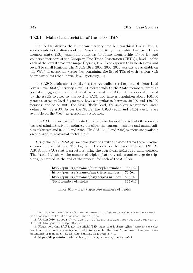
142 10.2. Case Studies

10.2.1 Main characteristics of the three TSNs

The NUTS divides the European territory into 5 hierarchical levels: level 0corresponds to the division of the European territory into States (European Unionmember states (EU), candidate countries for future membership of the EU andcountries members of the European Free Trade Association (EFTA)), level 1 splitseach of the level 0 areas into major Regions, level 2 corresponds to basic Regions, andlevel 3 to small Regions. The NUTS 1999, 2003, 2006, 2010 versions are available onthe Web 1 as geospatial vector files containing the list of TUs of each version withtheir attributes (code, name, level, geometry, ...).

The ASGS main structure divides the Australian territory into 6 hierarchicallevels: level State/Territory (level 5) corresponds to the State members, areas atlevel 4 are aggregations of the Statistical Areas at level 3 (i.e., the abbreviation usedby the ASGS to refer to this level is SA3), and have a population above 100,000persons, areas at level 3 generally have a population between 30,000 and 130,000persons, and so on until the Mesh Blocks level, the smallest geographical areasdefined by the ABS. As for the NUTS, the ASGS (2011 and 2016) versions areavailable on the Web 2 as geospatial vector files.

The SAU nomenclature 3 created by the Swiss Federal Statistical Office on thebasis of administrative boundaries, describes the cantons, districts and municipali-ties of Switzerland in 2017 and 2018. The SAU (2017 and 2018) versions are availableon the Web as geospatial vector files 4.

Using the TSN Ontology, we have described with the same terms these 3 ratherdifferent nomenclatures. The Figure 10.1 shows how to describe these 3 (NUTS,ASGS, and SAU) spatial structures, using the tsn:Nomenclature main concept.The Table 10.1 shows the number of triples (feature versions and change descrip-tions) generated at the end of the process, for each of the 3 TSNs.

http://purl.org/steamer/nuts triples number 156,162http://purl.org/steamer/sau triples number 76,504http://purl.org/steamer/asgs triples number 89,974Total number of triples 322,640

Table 10.1 – TSN triplestore numbers of triples

1. https://ec.europa.eu/eurostat/web/gisco/geodata/reference-data/administrative-units-statistical-units/nuts

2. Version 2016: https://www.abs.gov.au/AUSSTATS/abs@.nsf/DetailsPage/1270.0.55.001July%202016?OpenDocument

3. Please note that SAU is not the official TSN name that is Swiss official commune register.We found this name misleading and reductive as under the term "commune" there are vectorboundaries of municipalities, districts, cantons, large regions, etc.

4. https://shop.swisstopo.admin.ch/en/products/landscape/boundaries3D

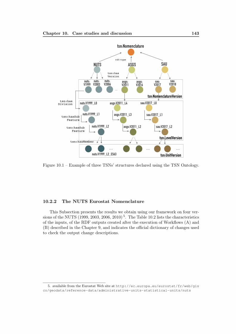
Chapter 10. Case studies and discussion 143

tsn:Nomenclature

NUTS ASGS SAUrdf:type

nuts: V1999

nuts: V2003

asgs: V2011

sau: V2018

asgs: V2016

sau: V2017

tsn:hasVersion

…

nuts: V2006

nuts:V1999_L0

nuts:V1999_L1

nuts:V1999_L2

asgs:V2011_L4

asgs:V2011_L3

asgs:V2011_L2

sau:V2017_L0

sau:V2017_L1

sau:V2017_L2

tsn:hasSubFeature

tsn:hasDivision

tsn:LevelVersiontsn:hasMember

nuts:V1999_L2_ES63 …

tsn:UnitVersion … …

tsn:NomenclatureVersion

tsn:hasSubFeature

Figure 10.1 – Example of three TSNs’ structures declared using the TSN Ontology.

10.2.2 The NUTS Eurostat Nomenclature

This Subsection presents the results we obtain using our framework on four ver-sions of the NUTS (1999, 2003, 2006, 2010) 5. The Table 10.2 lists the characteristicsof the inputs, of the RDF outputs created after the execution of Workflows (A) and(B) described in the Chapter 9, and indicates the official dictionary of changes usedto check the output change descriptions.

5. available from the Eurostat Web site at http://ec.europa.eu/eurostat/fr/web/gisco/geodata/reference-data/administrative-units-statistical-units/nuts

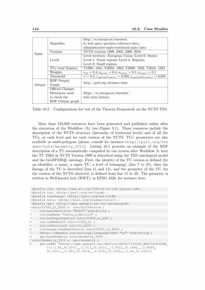
144 10.2. Case Studies

Input

Shapefileshttp://ec.europa.eu/eurostat/fr/web/gisco/geodata/reference-data/administrative-units-statistical-units/nuts

Versions NUTS versions 1999, 2003, 2006, 2010

LevelsLevel territory: European Union; Level 0: States;Level 1: Great regions; Level 2: Regions;Level 3: Small regions

TUs total Number V1999: 1861; V2003: 1902; V2006: 1933; V2010: 1923Weights αid = 0.4, αgeom = 0.4, αname = 0.1, αsuper = 0.1Threshold β = 0.5, εspatialFeature = 0.005, εspatialStructure = 0.005

OutputRDF OutputGraph http://purl.org/steamer/nuts

Official ChangesDictionary usedto check theRDF Output graph

https://ec.europa.eu/eurostat/web/nuts/history

Table 10.2 – Configurations for test of the Theseus Framework on the NUTS TSN.

More than 122,000 resources have been generated and published online afterthe execution of the Workflow (A) (see Figure 9.1). These resources include thedescription of the NUTS structure (hierarchy of territorial levels) and of all theTUs, at each level and for each version of the NUTS. TUs’ geometries are alsoavailable as multi-polygons (please, consult for instance http://purl.org/steamer/nuts/Geometry_3512). Listing 10.1 presents an example of the RDFdescription of a TU automatically computed by our system after Workflow A: herethe TU ES63 in NUTS Version 1999 is described using the TSN ontological modeland the GeoSPARQL ontology. First, the identity of the TU version is defined (byan identifier, a name, a super TU, a level of belonging) (line 7 to 10), then thelineage of the TU is described (line 11 and 12), and the geometry of the TU, forthe version of the NUTS observed, is defined from line 15 to 20. The geometry iswritten in Well-known text (WKT), in EPSG 4326, for instance here.

1@prefix rdf: <http://www.w3.org/1999/02/22-rdf-syntax-ns#> .2@prefix tsn: <http://purl.org/net/tsn#> .3@prefix tsnchange: <http://purl.org/net/tsn#> .4@prefix nuts: <http://purl.org/steamer/nuts/> .5@prefix geo: <http://www.opengis.net/ont/geosparql#>6nuts:V1999_L2_ES63 a tsn:UnitVersion ;7 tsn:hasIdentifier "ES63"^^xsd:string ;8 tsn:hasName "Ceuta y Melilla" ;9 tsn:hasSuperFeature nuts:V1999_L1_ES6 ;10 tsn:isMemberOf nuts:V1999_L2 ;11 tsn:isVersionOf nuts:L2_ES63 ;12 tsnchange:hasNextVersion nuts:V2003_L2_ES63 ;13 <http://dbpedia.org/ontology/languageCode> "es"^^xsd:string ;14 geo:hasGeometry nuts:Geometry_3245 .15nuts:Geometry_3512 a geo:Geometry ;16 geo:asWKT "<http://www.opengis.net/def/crs/EPSG/0/4326> MULTIPOLYGON

(((-2.84 35.2937, -2.913 35.2633, -2.9522 35.3492, -2.895935.3657, -2.893 35.3619, -2.8593 35.3185, -2.84 35.2937))

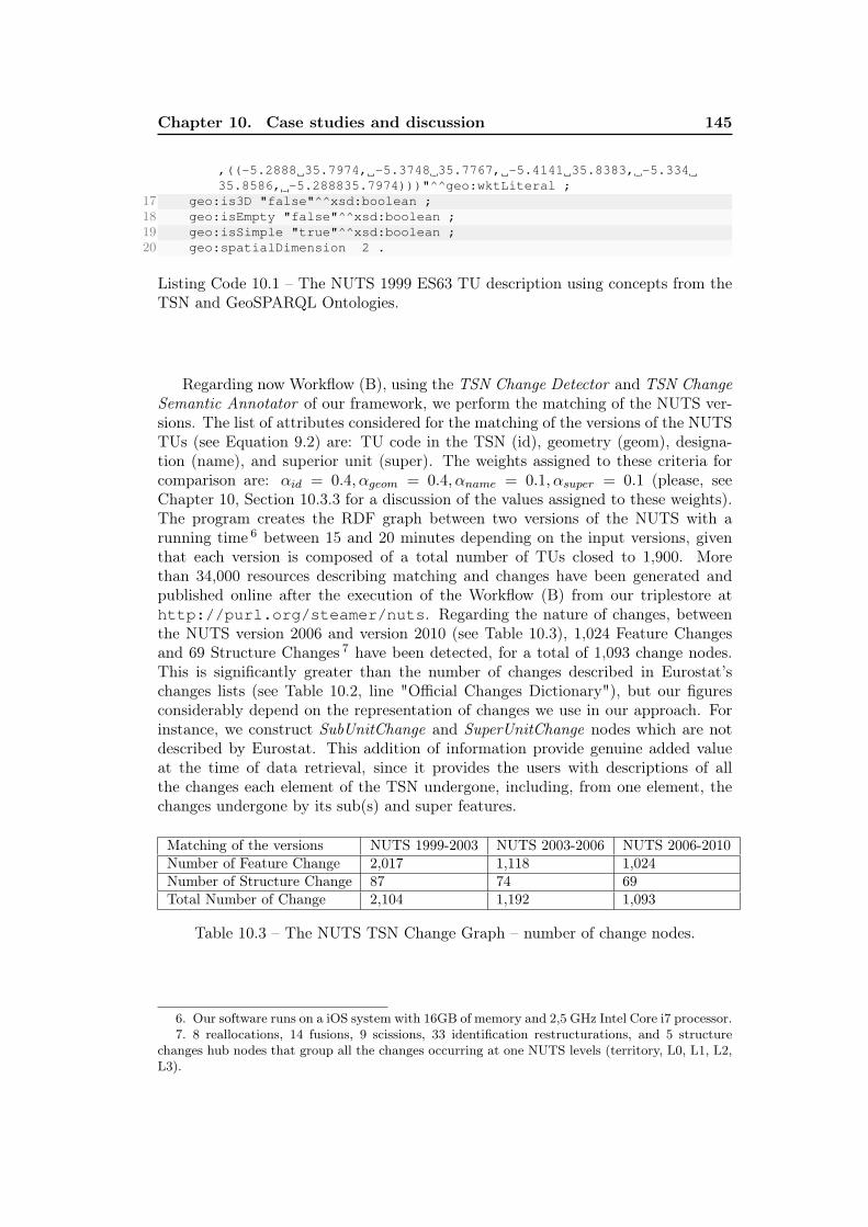
Chapter 10. Case studies and discussion 145

,((-5.2888 35.7974, -5.3748 35.7767, -5.4141 35.8383, -5.33435.8586, -5.288835.7974)))"^^geo:wktLiteral ;

17 geo:is3D "false"^^xsd:boolean ;18 geo:isEmpty "false"^^xsd:boolean ;19 geo:isSimple "true"^^xsd:boolean ;20 geo:spatialDimension 2 .

Listing Code 10.1 – The NUTS 1999 ES63 TU description using concepts from theTSN and GeoSPARQL Ontologies.

Regarding now Workflow (B), using the TSN Change Detector and TSN ChangeSemantic Annotator of our framework, we perform the matching of the NUTS ver-sions. The list of attributes considered for the matching of the versions of the NUTSTUs (see Equation 9.2) are: TU code in the TSN (id), geometry (geom), designa-tion (name), and superior unit (super). The weights assigned to these criteria forcomparison are: αid = 0.4, αgeom = 0.4, αname = 0.1, αsuper = 0.1 (please, seeChapter 10, Section 10.3.3 for a discussion of the values assigned to these weights).The program creates the RDF graph between two versions of the NUTS with arunning time 6 between 15 and 20 minutes depending on the input versions, giventhat each version is composed of a total number of TUs closed to 1,900. Morethan 34,000 resources describing matching and changes have been generated andpublished online after the execution of the Workflow (B) from our triplestore athttp://purl.org/steamer/nuts. Regarding the nature of changes, betweenthe NUTS version 2006 and version 2010 (see Table 10.3), 1,024 Feature Changesand 69 Structure Changes 7 have been detected, for a total of 1,093 change nodes.This is significantly greater than the number of changes described in Eurostat’schanges lists (see Table 10.2, line "Official Changes Dictionary"), but our figuresconsiderably depend on the representation of changes we use in our approach. Forinstance, we construct SubUnitChange and SuperUnitChange nodes which are notdescribed by Eurostat. This addition of information provide genuine added valueat the time of data retrieval, since it provides the users with descriptions of allthe changes each element of the TSN undergone, including, from one element, thechanges undergone by its sub(s) and super features.

Matching of the versions NUTS 1999-2003 NUTS 2003-2006 NUTS 2006-2010Number of Feature Change 2,017 1,118 1,024Number of Structure Change 87 74 69Total Number of Change 2,104 1,192 1,093

Table 10.3 – The NUTS TSN Change Graph – number of change nodes.

6. Our software runs on a iOS system with 16GB of memory and 2,5 GHz Intel Core i7 processor.7. 8 reallocations, 14 fusions, 9 scissions, 33 identification restructurations, and 5 structure

changes hub nodes that group all the changes occurring at one NUTS levels (territory, L0, L1, L2,L3).

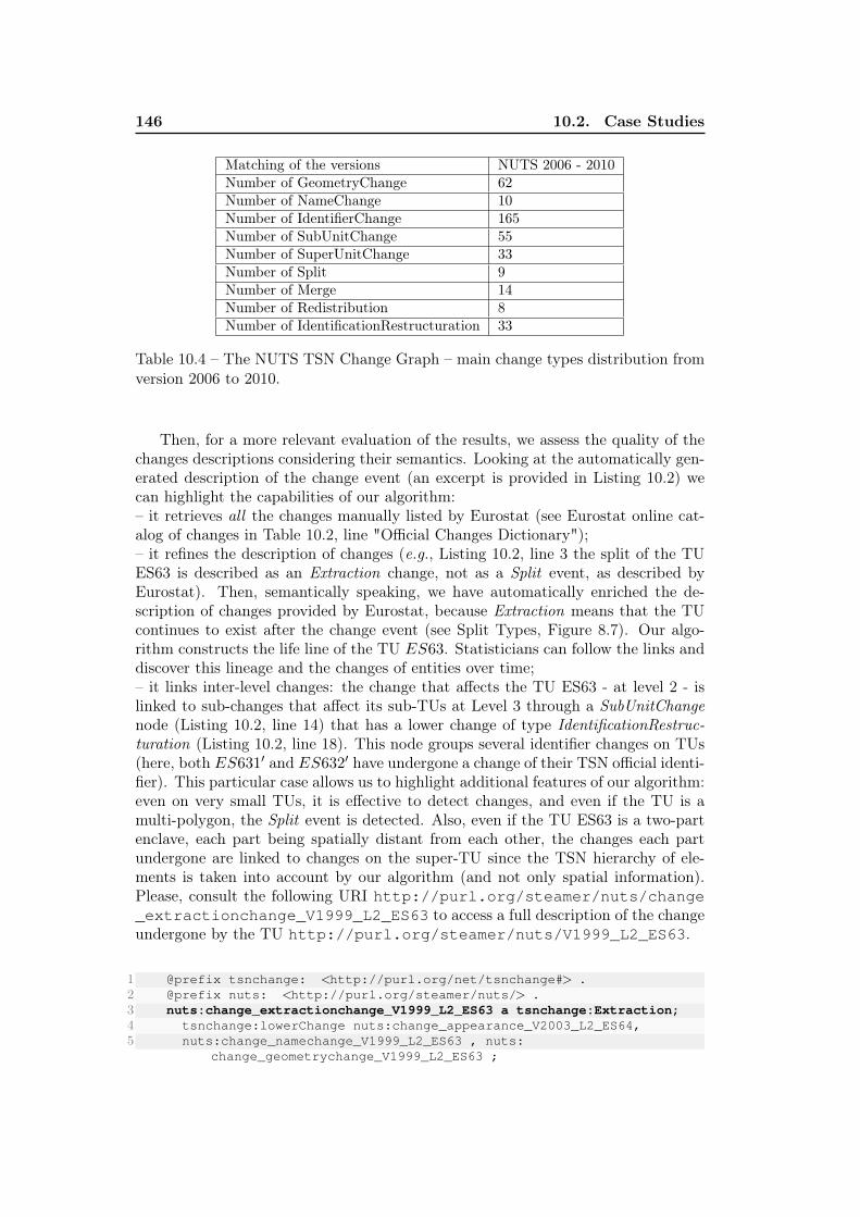
146 10.2. Case Studies

Matching of the versions NUTS 2006 - 2010Number of GeometryChange 62Number of NameChange 10Number of IdentifierChange 165Number of SubUnitChange 55Number of SuperUnitChange 33Number of Split 9Number of Merge 14Number of Redistribution 8Number of IdentificationRestructuration 33

Table 10.4 – The NUTS TSN Change Graph – main change types distribution fromversion 2006 to 2010.

Then, for a more relevant evaluation of the results, we assess the quality of thechanges descriptions considering their semantics. Looking at the automatically gen-erated description of the change event (an excerpt is provided in Listing 10.2) wecan highlight the capabilities of our algorithm:– it retrieves all the changes manually listed by Eurostat (see Eurostat online cat-alog of changes in Table 10.2, line "Official Changes Dictionary");– it refines the description of changes (e.g., Listing 10.2, line 3 the split of the TUES63 is described as an Extraction change, not as a Split event, as described byEurostat). Then, semantically speaking, we have automatically enriched the de-scription of changes provided by Eurostat, because Extraction means that the TUcontinues to exist after the change event (see Split Types, Figure 8.7). Our algo-rithm constructs the life line of the TU ES63. Statisticians can follow the links anddiscover this lineage and the changes of entities over time;– it links inter-level changes: the change that affects the TU ES63 - at level 2 - islinked to sub-changes that affect its sub-TUs at Level 3 through a SubUnitChangenode (Listing 10.2, line 14) that has a lower change of type IdentificationRestruc-turation (Listing 10.2, line 18). This node groups several identifier changes on TUs(here, both ES631′ and ES632′ have undergone a change of their TSN official identi-fier). This particular case allows us to highlight additional features of our algorithm:even on very small TUs, it is effective to detect changes, and even if the TU is amulti-polygon, the Split event is detected. Also, even if the TU ES63 is a two-partenclave, each part being spatially distant from each other, the changes each partundergone are linked to changes on the super-TU since the TSN hierarchy of ele-ments is taken into account by our algorithm (and not only spatial information).Please, consult the following URI http://purl.org/steamer/nuts/change_extractionchange_V1999_L2_ES63 to access a full description of the changeundergone by the TU http://purl.org/steamer/nuts/V1999_L2_ES63.

1 @prefix tsnchange: <http://purl.org/net/tsnchange#> .2 @prefix nuts: <http://purl.org/steamer/nuts/> .3 nuts:change_extractionchange_V1999_L2_ES63 a tsnchange:Extraction;4 tsnchange:lowerChange nuts:change_appearance_V2003_L2_ES64,5 nuts:change_namechange_V1999_L2_ES63 , nuts:

change_geometrychange_V1999_L2_ES63 ;

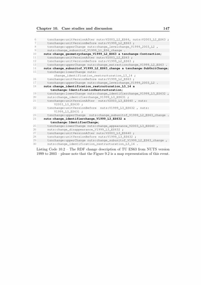
Chapter 10. Case studies and discussion 147

6 tsnchange:unitVersionAfter nuts:V2003_L2_ES64, nuts:V2003_L2_ES63 ;7 tsnchange:unitVersionBefore nuts:V1999_L2_ES63 ;8 tsnchange:upperChange nuts:change_levelchange_V1999_2003_L2 ,9 nuts:change_subunitof_V1999_L1_ES6_change .10 nuts:change_geometrychange_V1999_L2_ES63 a tsnchange:Contraction;11 tsnchange:unitVersionAfter nuts:V2003_L2_ES63 ;12 tsnchange:unitVersionBefore nuts:V1999_L2_ES63 ;13 tsnchange:upperChange nuts:change_extractionchange_V1999_L2_ES63 .14 nuts:change_subunitof_V1999_L2_ES63_change a tsnchange:SubUnitChange;15 tsnchange:lowerChange nuts:

change_identification_restructuration_L3_14 ;16 tsnchange:unitVersionBefore nuts:V1999_L2_ES63 ;17 tsnchange:upperChange nuts:change_levelchange_V1999_2003_L2 .18 nuts:change_identification_restructuration_L3_14 a

tsnchange:IdentificationRestructuration;19 tsnchange:lowerChange nuts:change_identifierchange_V1999_L3_ES632 ,20 nuts:change_identifierchange_V1999_L3_ES631 ;21 tsnchange:unitVersionAfter nuts:V2003_L3_ES640 , nuts:

V2003_L3_ES630 ;22 tsnchange:unitVersionBefore nuts:V1999_L3_ES632 , nuts:

V1999_L3_ES631 ;23 tsnchange:upperChange nuts:change_subunitof_V1999_L2_ES63_change .24 nuts:change_identifierchange_V1999_L3_ES632 a

tsnchange:IdentifierChange;25 tsnchange:lowerChange nuts:change_appearance_V2003_L3_ES640 ,26 nuts:change_disappearance_V1999_L3_ES632 ;27 tsnchange:unitVersionAfter nuts:V2003_L3_ES640 ;28 tsnchange:unitVersionBefore nuts:V1999_L3_ES632 ;29 tsnchange:upperChange nuts:change_subunitof_V1999_L2_ES63_change ,30 nuts:change_identification_restructuration_L3_14 .

Listing Code 10.2 – The RDF change description of TU ES63 from NUTS version1999 to 2003 – please note that the Figure 9.2 is a map representation of this event.

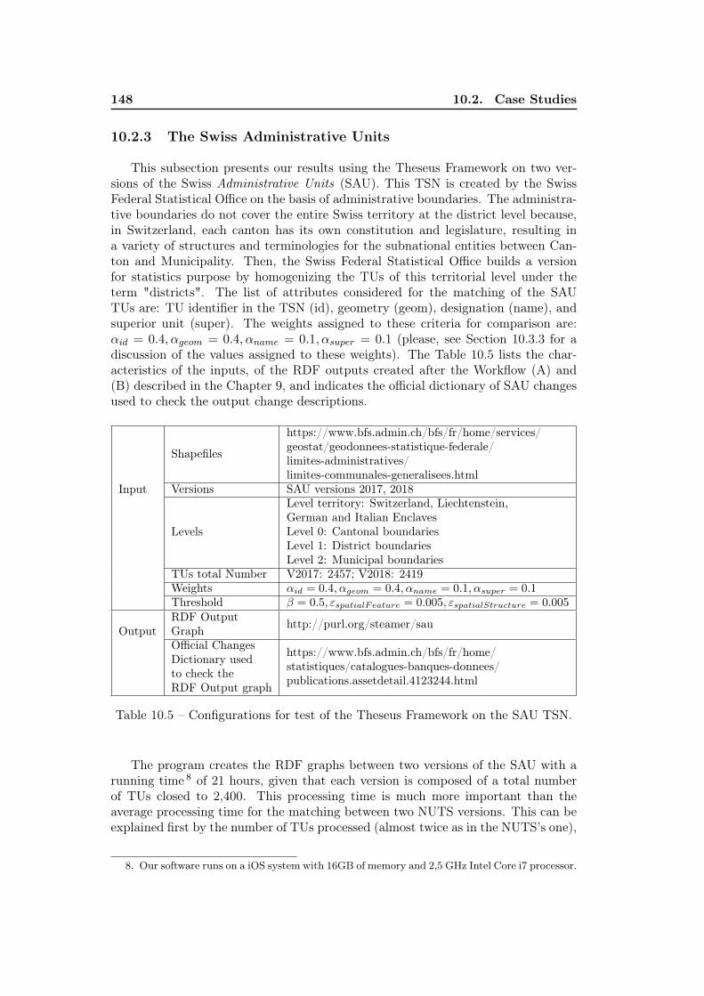
148 10.2. Case Studies

10.2.3 The Swiss Administrative Units

This subsection presents our results using the Theseus Framework on two ver-sions of the Swiss Administrative Units (SAU). This TSN is created by the SwissFederal Statistical Office on the basis of administrative boundaries. The administra-tive boundaries do not cover the entire Swiss territory at the district level because,in Switzerland, each canton has its own constitution and legislature, resulting ina variety of structures and terminologies for the subnational entities between Can-ton and Municipality. Then, the Swiss Federal Statistical Office builds a versionfor statistics purpose by homogenizing the TUs of this territorial level under theterm "districts". The list of attributes considered for the matching of the SAUTUs are: TU identifier in the TSN (id), geometry (geom), designation (name), andsuperior unit (super). The weights assigned to these criteria for comparison are:αid = 0.4, αgeom = 0.4, αname = 0.1, αsuper = 0.1 (please, see Section 10.3.3 for adiscussion of the values assigned to these weights). The Table 10.5 lists the char-acteristics of the inputs, of the RDF outputs created after the Workflow (A) and(B) described in the Chapter 9, and indicates the official dictionary of SAU changesused to check the output change descriptions.

Input

Shapefiles

https://www.bfs.admin.ch/bfs/fr/home/services/geostat/geodonnees-statistique-federale/limites-administratives/limites-communales-generalisees.html

Versions SAU versions 2017, 2018

Levels

Level territory: Switzerland, Liechtenstein,German and Italian EnclavesLevel 0: Cantonal boundariesLevel 1: District boundariesLevel 2: Municipal boundaries

TUs total Number V2017: 2457; V2018: 2419Weights αid = 0.4, αgeom = 0.4, αname = 0.1, αsuper = 0.1Threshold β = 0.5, εspatialFeature = 0.005, εspatialStructure = 0.005

OutputRDF OutputGraph http://purl.org/steamer/sau

Official ChangesDictionary usedto check theRDF Output graph

https://www.bfs.admin.ch/bfs/fr/home/statistiques/catalogues-banques-donnees/publications.assetdetail.4123244.html

Table 10.5 – Configurations for test of the Theseus Framework on the SAU TSN.

The program creates the RDF graphs between two versions of the SAU with arunning time 8 of 21 hours, given that each version is composed of a total numberof TUs closed to 2,400. This processing time is much more important than theaverage processing time for the matching between two NUTS versions. This can beexplained first by the number of TUs processed (almost twice as in the NUTS’s one),

8. Our software runs on a iOS system with 16GB of memory and 2,5 GHz Intel Core i7 processor.

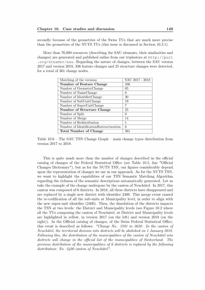
Chapter 10. Case studies and discussion 149

secondly because of the geometries of the Swiss TUs that are much more precisethan the geometries of the NUTS TUs (this issue is discussed in Section 10.3.1).

More than 76,000 resources (describing the SAU elements, their similarities andchanges) are generated and published online from our triplestore at http://purl.org/steamer/sau. Regarding the nature of changes, between the SAU version2017 and version 2018, 336 feature changes and 25 structure changes were detected,for a total of 361 change nodes.

Matching of the versions SAU 2017 - 2018Number of Feature Change 336Number of GeometryChange 65Number of NameChange 0Number of IdentifierChange 30Number of SubUnitChange 19Number of SuperUnitChange 7Number of Structure Change 25Number of Split 0Number of Merge 14Number of Redistribution 1Number of IdentificationRestructuration 6Total Number of Change 361

Table 10.6 – The SAU TSN Change Graph – main change types distribution fromversion 2017 to 2018.

This is quite mush more than the number of changes described in the officialcatalog of changes of the Federal Statistical Office (see Table 10.5, line "OfficialChanges Dictionary"), but as for the NUTS TSN, our figures considerably dependupon the representation of changes we use in our approach. As for the NUTS TSN,we want to highlight the capabilities of our TSN Semantic Matching Algorithmregarding the richness of the semantic descriptions automatically generated. Let ustake the example of the change undergone by the canton of Neuchâtel. In 2017, thiscanton was composed of 6 districts. In 2018, all these districts have disappeared andare replaced by a single new district with identifier 2400. This merge event causedthe re-codification of all the sub-units at Municipality level, in order to align withthe new super-unit identifier (2400). Then, the dissolution of the districts impactsthe TSN at two levels: the District and Municipality levels (see Figure 10.2 whereall the TUs composing the canton of Neuchâtel, at District and Municipality levelsare highlighted in yellow, in version 2017 (on the left) and version 2018 (on theright)). In the Official catalog of changes, of the Swiss Federal Statistical Office,this event is described as follows: "Change No. 3591 to 3620 : In the canton ofNeuchâtel, the territorial division into districts will be abolished on 1 January 2018.Following this, the distribution of the municipalities of the canton of Neuchâtel intodistricts will change in the official list of the municipalities of Switzerland. Theprevious distribution of the municipalities of 6 districts is replaced by the followingdistribution: No. 2400 canton of Neuchâtel".

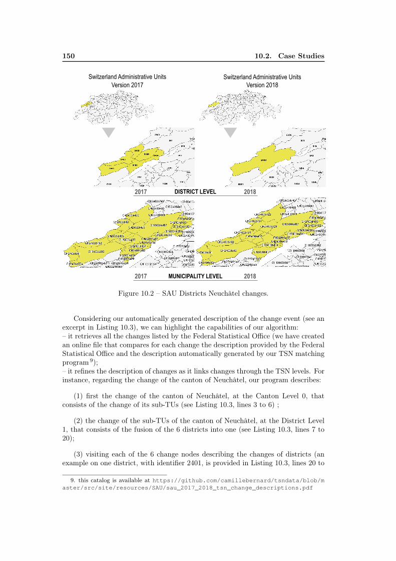
150 10.2. Case Studies

Switzerland Administrative Units Version 2017

MUNICIPALITY LEVEL

Switzerland Administrative Units Version 2018

DISTRICT LEVEL2017

2017

2018

2018

Figure 10.2 – SAU Districts Neuchâtel changes.

Considering our automatically generated description of the change event (see anexcerpt in Listing 10.3), we can highlight the capabilities of our algorithm:– it retrieves all the changes listed by the Federal Statistical Office (we have createdan online file that compares for each change the description provided by the FederalStatistical Office and the description automatically generated by our TSN matchingprogram 9);– it refines the description of changes as it links changes through the TSN levels. Forinstance, regarding the change of the canton of Neuchâtel, our program describes:

(1) first the change of the canton of Neuchâtel, at the Canton Level 0, thatconsists of the change of its sub-TUs (see Listing 10.3, lines 3 to 6) ;

(2) the change of the sub-TUs of the canton of Neuchâtel, at the District Level1, that consists of the fusion of the 6 districts into one (see Listing 10.3, lines 7 to20);

(3) visiting each of the 6 change nodes describing the changes of districts (anexample on one district, with identifier 2401, is provided in Listing 10.3, lines 20 to

9. this catalog is available at https://github.com/camillebernard/tsndata/blob/master/src/site/resources/SAU/sau_2017_2018_tsn_change_descriptions.pdf

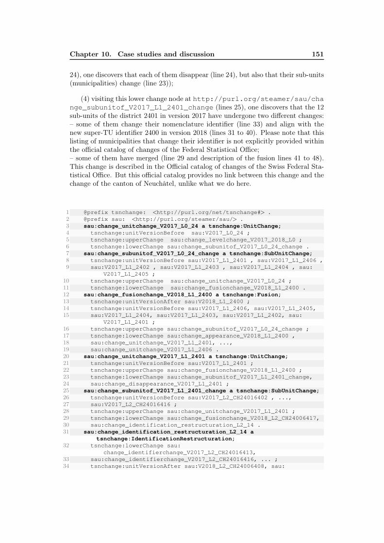
Chapter 10. Case studies and discussion 151

24), one discovers that each of them disappear (line 24), but also that their sub-units(municipalities) change (line 23));

(4) visiting this lower change node at http://purl.org/steamer/sau/change_subunitof_V2017_L1_2401_change (lines 25), one discovers that the 12sub-units of the district 2401 in version 2017 have undergone two different changes:– some of them change their nomenclature identifier (line 33) and align with thenew super-TU identifier 2400 in version 2018 (lines 31 to 40). Please note that thislisting of municipalities that change their identifier is not explicitly provided withinthe official catalog of changes of the Federal Statistical Office;– some of them have merged (line 29 and description of the fusion lines 41 to 48).This change is described in the Official catalog of changes of the Swiss Federal Sta-tistical Office. But this official catalog provides no link between this change and thechange of the canton of Neuchâtel, unlike what we do here.

1 @prefix tsnchange: <http://purl.org/net/tsnchange#> .2 @prefix sau: <http://purl.org/steamer/sau/> .3 sau:change_unitchange_V2017_L0_24 a tsnchange:UnitChange;4 tsnchange:unitVersionBefore sau:V2017_L0_24 ;5 tsnchange:upperChange sau:change_levelchange_V2017_2018_L0 ;6 tsnchange:lowerChange sau:change_subunitof_V2017_L0_24_change .7 sau:change_subunitof_V2017_L0_24_change a tsnchange:SubUnitChange;8 tsnchange:unitVersionBefore sau:V2017_L1_2401 , sau:V2017_L1_2406 ,9 sau:V2017_L1_2402 , sau:V2017_L1_2403 , sau:V2017_L1_2404 , sau:

V2017_L1_2405 ;10 tsnchange:upperChange sau:change_unitchange_V2017_L0_24 ;11 tsnchange:lowerChange sau:change_fusionchange_V2018_L1_2400 .12 sau:change_fusionchange_V2018_L1_2400 a tsnchange:Fusion;13 tsnchange:unitVersionAfter sau:V2018_L1_2400 ;14 tsnchange:unitVersionBefore sau:V2017_L1_2406, sau:V2017_L1_2405,15 sau:V2017_L1_2404, sau:V2017_L1_2403, sau:V2017_L1_2402, sau:

V2017_L1_2401 ;16 tsnchange:upperChange sau:change_subunitof_V2017_L0_24_change ;17 tsnchange:lowerChange sau:change_appearance_V2018_L1_2400 ,18 sau:change_unitchange_V2017_L1_2401, ...,19 sau:change_unitchange_V2017_L1_2406 .20 sau:change_unitchange_V2017_L1_2401 a tsnchange:UnitChange;21 tsnchange:unitVersionBefore sau:V2017_L1_2401 ;22 tsnchange:upperChange sau:change_fusionchange_V2018_L1_2400 ;23 tsnchange:lowerChange sau:change_subunitof_V2017_L1_2401_change,24 sau:change_disappearance_V2017_L1_2401 ;25 sau:change_subunitof_V2017_L1_2401_change a tsnchange:SubUnitChange;26 tsnchange:unitVersionBefore sau:V2017_L2_CH24016402 , ...,27 sau:V2017_L2_CH24016416 ;28 tsnchange:upperChange sau:change_unitchange_V2017_L1_2401 ;29 tsnchange:lowerChange sau:change_fusionchange_V2018_L2_CH24006417,30 sau:change_identification_restructuration_L2_14 .31 sau:change_identification_restructuration_L2_14 a

tsnchange:IdentificationRestructuration;32 tsnchange:lowerChange sau:

change_identifierchange_V2017_L2_CH24016413,33 sau:change_identifierchange_V2017_L2_CH24016416, ... ;34 tsnchange:unitVersionAfter sau:V2018_L2_CH24006408, sau:

152 10.2. Case Studies

V2018_L2_CH24006412 ,35 sau:V2018_L2_CH24006413 , sau:V2018_L2_CH24006404 ,36 sau:V2018_L2_CH24006407 , sau:V2018_L2_CH24006416 ;37 tsnchange:unitVersionBefore sau:V2017_L2_CH24016412 , sau:

V2017_L2_CH24016416 ,38 sau:V2017_L2_CH24016408 , sau:V2017_L2_CH24016413 ,39 sau:V2017_L2_CH24016404 , sau:V2017_L2_CH24016407 ;40 tsnchange:upperChange sau:change_superunit_V2017_L1_2401_change .41 sau:change_fusionchange_V2018_L2_CH24006417 a tsnchange:Fusion;42 tsnchange:lowerChange sau:change_appearance_V2018_L2_CH24006417 ,43 sau:change_disappearance_V2017_L2_CH24016409 , ... ;44 tsnchange:unitVersionAfter sau:V2018_L2_CH24006417 ;45 tsnchange:unitVersionBefore sau:V2017_L2_CH24016414, sau:

V2017_L2_CH24016402,46 sau:V2017_L2_CH24016410, sau:V2017_L2_CH24016411, sau:

V2017_L2_CH24016415,47 sau:V2017_L2_CH24016409 ;48 tsnchange:upperChange sau:change_subunitof_V2017_L1_2401_change .

Listing Code 10.3 – The RDF change description of the Canton of Neuchâtel fromSAU version 2017 to 2018.

Here, we have shown that our algorithm automatically creates linked descriptionof changes that help analysts in understanding the territorial changes and theirimpacts on each sub-element, starting from the main element that changes, thecanton of Neuchâtel, and zooming in to visualize changes on each sub-elements(districts and municipalities). Please note that the links we have created betweenchanges are not causal ones. The semantics they hold is a hierarchical informationabout the changes. Nevertheless, the TSN-Change Ontology defines a predicate tolink a change node to some causal information (tsnchange:isCausedBy). Thesubsection 11.3 shows how we use the LODWeb to search for this causal information:historical, societal information that may explain the change event.

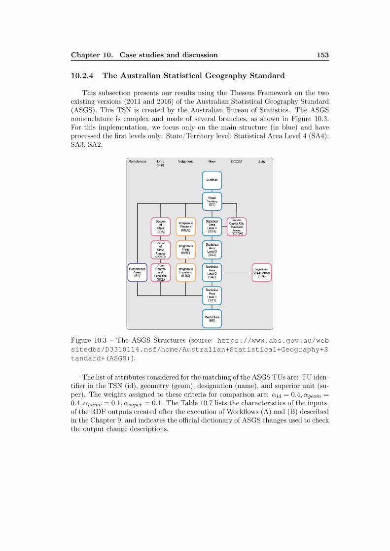
Chapter 10. Case studies and discussion 153

10.2.4 The Australian Statistical Geography Standard

This subsection presents our results using the Theseus Framework on the twoexisting versions (2011 and 2016) of the Australian Statistical Geography Standard(ASGS). This TSN is created by the Australian Bureau of Statistics. The ASGSnomenclature is complex and made of several branches, as shown in Figure 10.3.For this implementation, we focus only on the main structure (in blue) and haveprocessed the first levels only: State/Territory level; Statistical Area Level 4 (SA4);SA3; SA2.

Figure 10.3 – The ASGS Structures (source: https://www.abs.gov.au/websitedbs/D3310114.nsf/home/Australian+Statistical+Geography+Standard+(ASGS)).

The list of attributes considered for the matching of the ASGS TUs are: TU iden-tifier in the TSN (id), geometry (geom), designation (name), and superior unit (su-per). The weights assigned to these criteria for comparison are: αid = 0.4, αgeom =0.4, αname = 0.1, αsuper = 0.1. The Table 10.7 lists the characteristics of the inputs,of the RDF outputs created after the execution of Workflows (A) and (B) describedin the Chapter 9, and indicates the official dictionary of ASGS changes used to checkthe output change descriptions.

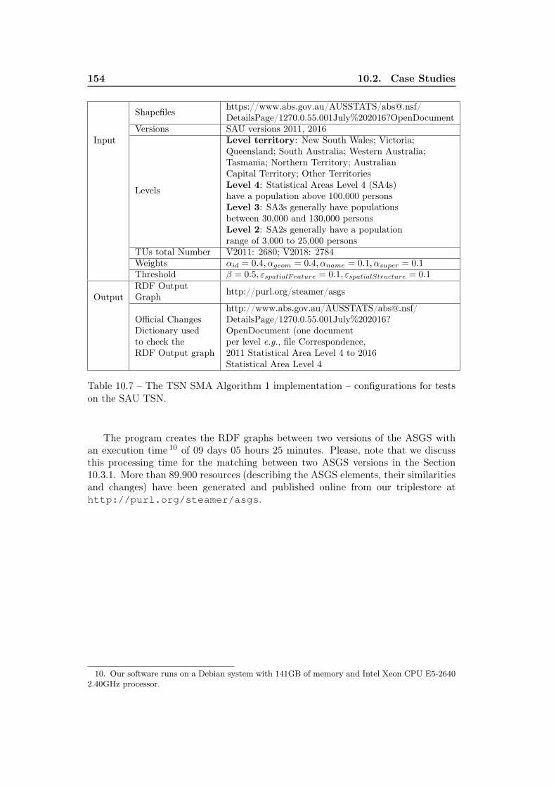
154 10.2. Case Studies

Input

Shapefiles https://www.abs.gov.au/AUSSTATS/abs@.nsf/DetailsPage/1270.0.55.001July%202016?OpenDocument

Versions SAU versions 2011, 2016

Levels

Level territory: New South Wales; Victoria;Queensland; South Australia; Western Australia;Tasmania; Northern Territory; AustralianCapital Territory; Other TerritoriesLevel 4: Statistical Areas Level 4 (SA4s)have a population above 100,000 personsLevel 3: SA3s generally have populationsbetween 30,000 and 130,000 personsLevel 2: SA2s generally have a populationrange of 3,000 to 25,000 persons

TUs total Number V2011: 2680; V2018: 2784Weights αid = 0.4, αgeom = 0.4, αname = 0.1, αsuper = 0.1Threshold β = 0.5, εspatialFeature = 0.1, εspatialStructure = 0.1

OutputRDF OutputGraph http://purl.org/steamer/asgs

Official ChangesDictionary usedto check theRDF Output graph

http://www.abs.gov.au/AUSSTATS/abs@.nsf/DetailsPage/1270.0.55.001July%202016?OpenDocument (one documentper level e.g., file Correspondence,2011 Statistical Area Level 4 to 2016Statistical Area Level 4

Table 10.7 – The TSN SMA Algorithm 1 implementation – configurations for testson the SAU TSN.

The program creates the RDF graphs between two versions of the ASGS withan execution time 10 of 09 days 05 hours 25 minutes. Please, note that we discussthis processing time for the matching between two ASGS versions in the Section10.3.1. More than 89,900 resources (describing the ASGS elements, their similaritiesand changes) have been generated and published online from our triplestore athttp://purl.org/steamer/asgs.

10. Our software runs on a Debian system with 141GB of memory and Intel Xeon CPU E5-26402.40GHz processor.

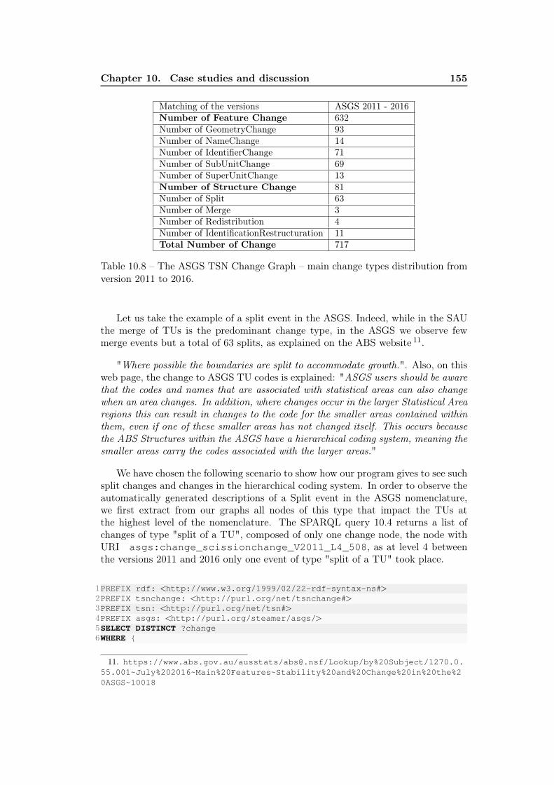
Chapter 10. Case studies and discussion 155

Matching of the versions ASGS 2011 - 2016Number of Feature Change 632Number of GeometryChange 93Number of NameChange 14Number of IdentifierChange 71Number of SubUnitChange 69Number of SuperUnitChange 13Number of Structure Change 81Number of Split 63Number of Merge 3Number of Redistribution 4Number of IdentificationRestructuration 11Total Number of Change 717

Table 10.8 – The ASGS TSN Change Graph – main change types distribution fromversion 2011 to 2016.

Let us take the example of a split event in the ASGS. Indeed, while in the SAUthe merge of TUs is the predominant change type, in the ASGS we observe fewmerge events but a total of 63 splits, as explained on the ABS website 11.

"Where possible the boundaries are split to accommodate growth.". Also, on thisweb page, the change to ASGS TU codes is explained: "ASGS users should be awarethat the codes and names that are associated with statistical areas can also changewhen an area changes. In addition, where changes occur in the larger Statistical Arearegions this can result in changes to the code for the smaller areas contained withinthem, even if one of these smaller areas has not changed itself. This occurs becausethe ABS Structures within the ASGS have a hierarchical coding system, meaning thesmaller areas carry the codes associated with the larger areas."

We have chosen the following scenario to show how our program gives to see suchsplit changes and changes in the hierarchical coding system. In order to observe theautomatically generated descriptions of a Split event in the ASGS nomenclature,we first extract from our graphs all nodes of this type that impact the TUs atthe highest level of the nomenclature. The SPARQL query 10.4 returns a list ofchanges of type "split of a TU", composed of only one change node, the node withURI asgs:change_scissionchange_V2011_L4_508, as at level 4 betweenthe versions 2011 and 2016 only one event of type "split of a TU" took place.

1PREFIX rdf: <http://www.w3.org/1999/02/22-rdf-syntax-ns#>2PREFIX tsnchange: <http://purl.org/net/tsnchange#>3PREFIX tsn: <http://purl.org/net/tsn#>4PREFIX asgs: <http://purl.org/steamer/asgs/>5SELECT DISTINCT ?change6WHERE {

11. https://www.abs.gov.au/ausstats/abs@.nsf/Lookup/by%20Subject/1270.0.55.001~July%202016~Main%20Features~Stability%20and%20Change%20in%20the%20ASGS~10018

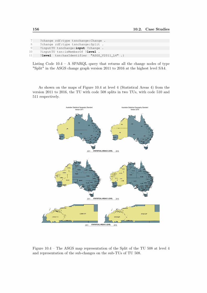
156 10.2. Case Studies

7 ?change rdf:type tsnchange:Change .8 ?change rdf:type tsnchange:Split .9 ?inputTU tsnchange:input ?change .10 ?inputTU tsn:isMemberOf ?level .11 ?level tsn:hasIdentifier "ASGS_V2011_L4" .}

Listing Code 10.4 – A SPARQL query that returns all the change nodes of type"Split" in the ASGS change graph version 2011 to 2016 at the highest level SA4.

As shown on the maps of Figure 10.4 at level 4 (Statistical Areas 4) from theversion 2011 to 2016, the TU with code 508 splits in two TUs, with code 510 and511 respectively.

Australian Statistical Geography Standard Version 2011

Australian Statistical Geography Standard Version 2016

STATISTICAL AREAS 4 LEVEL2011 2016

2011 2016STATISTICAL AREAS 2 LEVEL

2011 2016STATISTICAL AREAS 3 LEVEL

Figure 10.4 – The ASGS map representation of the Split of the TU 508 at level 4and representation of the sub-changes on the sub-TUs of TU 508.

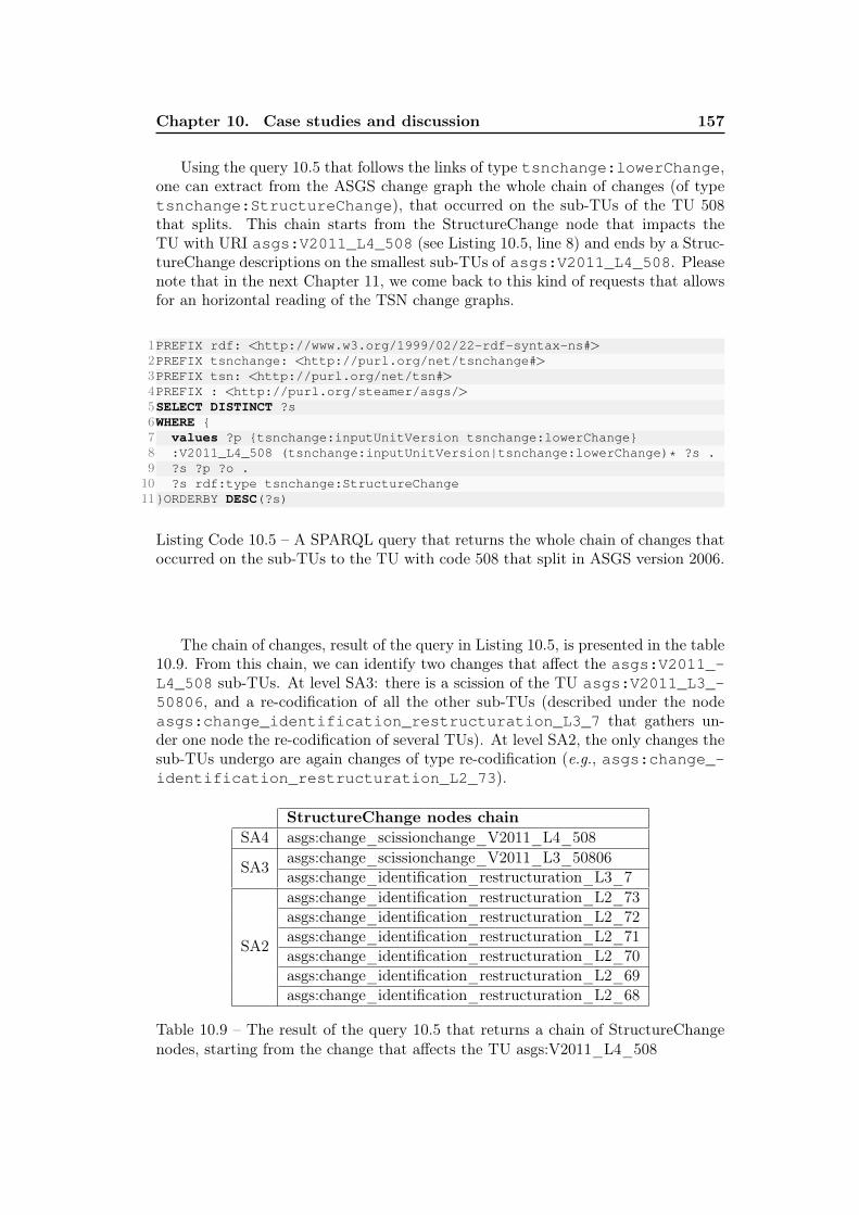
Chapter 10. Case studies and discussion 157

Using the query 10.5 that follows the links of type tsnchange:lowerChange,one can extract from the ASGS change graph the whole chain of changes (of typetsnchange:StructureChange), that occurred on the sub-TUs of the TU 508that splits. This chain starts from the StructureChange node that impacts theTU with URI asgs:V2011_L4_508 (see Listing 10.5, line 8) and ends by a Struc-tureChange descriptions on the smallest sub-TUs of asgs:V2011_L4_508. Pleasenote that in the next Chapter 11, we come back to this kind of requests that allowsfor an horizontal reading of the TSN change graphs.

1PREFIX rdf: <http://www.w3.org/1999/02/22-rdf-syntax-ns#>2PREFIX tsnchange: <http://purl.org/net/tsnchange#>3PREFIX tsn: <http://purl.org/net/tsn#>4PREFIX : <http://purl.org/steamer/asgs/>5SELECT DISTINCT ?s6WHERE {7 values ?p {tsnchange:inputUnitVersion tsnchange:lowerChange}8 :V2011_L4_508 (tsnchange:inputUnitVersion|tsnchange:lowerChange)* ?s .9 ?s ?p ?o .10 ?s rdf:type tsnchange:StructureChange11}ORDERBY DESC(?s)

Listing Code 10.5 – A SPARQL query that returns the whole chain of changes thatoccurred on the sub-TUs to the TU with code 508 that split in ASGS version 2006.

The chain of changes, result of the query in Listing 10.5, is presented in the table10.9. From this chain, we can identify two changes that affect the asgs:V2011_-L4_508 sub-TUs. At level SA3: there is a scission of the TU asgs:V2011_L3_-50806, and a re-codification of all the other sub-TUs (described under the nodeasgs:change_identification_restructuration_L3_7 that gathers un-der one node the re-codification of several TUs). At level SA2, the only changes thesub-TUs undergo are again changes of type re-codification (e.g., asgs:change_-identification_restructuration_L2_73).

StructureChange nodes chainSA4 asgs:change_scissionchange_V2011_L4_508

SA3 asgs:change_scissionchange_V2011_L3_50806asgs:change_identification_restructuration_L3_7

SA2

asgs:change_identification_restructuration_L2_73asgs:change_identification_restructuration_L2_72asgs:change_identification_restructuration_L2_71asgs:change_identification_restructuration_L2_70asgs:change_identification_restructuration_L2_69asgs:change_identification_restructuration_L2_68

Table 10.9 – The result of the query 10.5 that returns a chain of StructureChangenodes, starting from the change that affects the TU asgs:V2011_L4_508

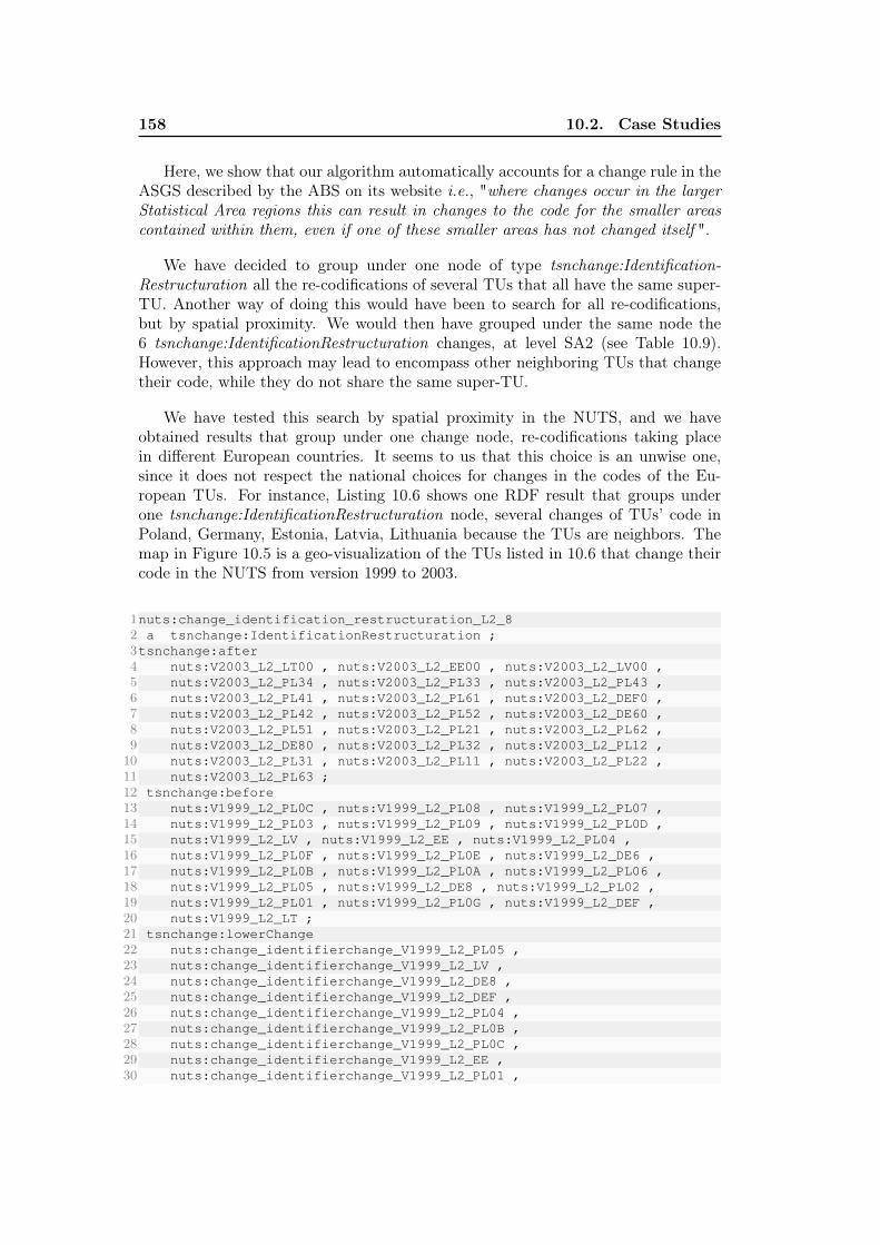
158 10.2. Case Studies

Here, we show that our algorithm automatically accounts for a change rule in theASGS described by the ABS on its website i.e., "where changes occur in the largerStatistical Area regions this can result in changes to the code for the smaller areascontained within them, even if one of these smaller areas has not changed itself ".

We have decided to group under one node of type tsnchange:Identification-Restructuration all the re-codifications of several TUs that all have the same super-TU. Another way of doing this would have been to search for all re-codifications,but by spatial proximity. We would then have grouped under the same node the6 tsnchange:IdentificationRestructuration changes, at level SA2 (see Table 10.9).However, this approach may lead to encompass other neighboring TUs that changetheir code, while they do not share the same super-TU.

We have tested this search by spatial proximity in the NUTS, and we haveobtained results that group under one change node, re-codifications taking placein different European countries. It seems to us that this choice is an unwise one,since it does not respect the national choices for changes in the codes of the Eu-ropean TUs. For instance, Listing 10.6 shows one RDF result that groups underone tsnchange:IdentificationRestructuration node, several changes of TUs’ code inPoland, Germany, Estonia, Latvia, Lithuania because the TUs are neighbors. Themap in Figure 10.5 is a geo-visualization of the TUs listed in 10.6 that change theircode in the NUTS from version 1999 to 2003.

1nuts:change_identification_restructuration_L2_82 a tsnchange:IdentificationRestructuration ;3tsnchange:after4 nuts:V2003_L2_LT00 , nuts:V2003_L2_EE00 , nuts:V2003_L2_LV00 ,5 nuts:V2003_L2_PL34 , nuts:V2003_L2_PL33 , nuts:V2003_L2_PL43 ,6 nuts:V2003_L2_PL41 , nuts:V2003_L2_PL61 , nuts:V2003_L2_DEF0 ,7 nuts:V2003_L2_PL42 , nuts:V2003_L2_PL52 , nuts:V2003_L2_DE60 ,8 nuts:V2003_L2_PL51 , nuts:V2003_L2_PL21 , nuts:V2003_L2_PL62 ,9 nuts:V2003_L2_DE80 , nuts:V2003_L2_PL32 , nuts:V2003_L2_PL12 ,10 nuts:V2003_L2_PL31 , nuts:V2003_L2_PL11 , nuts:V2003_L2_PL22 ,11 nuts:V2003_L2_PL63 ;12 tsnchange:before13 nuts:V1999_L2_PL0C , nuts:V1999_L2_PL08 , nuts:V1999_L2_PL07 ,14 nuts:V1999_L2_PL03 , nuts:V1999_L2_PL09 , nuts:V1999_L2_PL0D ,15 nuts:V1999_L2_LV , nuts:V1999_L2_EE , nuts:V1999_L2_PL04 ,16 nuts:V1999_L2_PL0F , nuts:V1999_L2_PL0E , nuts:V1999_L2_DE6 ,17 nuts:V1999_L2_PL0B , nuts:V1999_L2_PL0A , nuts:V1999_L2_PL06 ,18 nuts:V1999_L2_PL05 , nuts:V1999_L2_DE8 , nuts:V1999_L2_PL02 ,19 nuts:V1999_L2_PL01 , nuts:V1999_L2_PL0G , nuts:V1999_L2_DEF ,20 nuts:V1999_L2_LT ;21 tsnchange:lowerChange22 nuts:change_identifierchange_V1999_L2_PL05 ,23 nuts:change_identifierchange_V1999_L2_LV ,24 nuts:change_identifierchange_V1999_L2_DE8 ,25 nuts:change_identifierchange_V1999_L2_DEF ,26 nuts:change_identifierchange_V1999_L2_PL04 ,27 nuts:change_identifierchange_V1999_L2_PL0B ,28 nuts:change_identifierchange_V1999_L2_PL0C ,29 nuts:change_identifierchange_V1999_L2_EE ,30 nuts:change_identifierchange_V1999_L2_PL01 ,

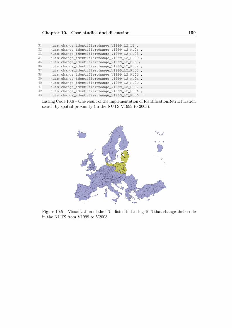
Chapter 10. Case studies and discussion 159

31 nuts:change_identifierchange_V1999_L2_LT ,32 nuts:change_identifierchange_V1999_L2_PL0F ,33 nuts:change_identifierchange_V1999_L2_PL03 ,34 nuts:change_identifierchange_V1999_L2_PL09 ,35 nuts:change_identifierchange_V1999_L2_DE6 ,36 nuts:change_identifierchange_V1999_L2_PL02 ,37 nuts:change_identifierchange_V1999_L2_PL08 ,38 nuts:change_identifierchange_V1999_L2_PL0G ,39 nuts:change_identifierchange_V1999_L2_PL0E ,40 nuts:change_identifierchange_V1999_L2_PL0D ,41 nuts:change_identifierchange_V1999_L2_PL07 ,42 nuts:change_identifierchange_V1999_L2_PL0A ,43 nuts:change_identifierchange_V1999_L2_PL06 .

Listing Code 10.6 – One result of the implementation of IdentificationRetructurationsearch by spatial proximity (in the NUTS V1999 to 2003).

Figure 10.5 – Visualization of the TUs listed in Listing 10.6 that change their codein the NUTS from V1999 to V2003.

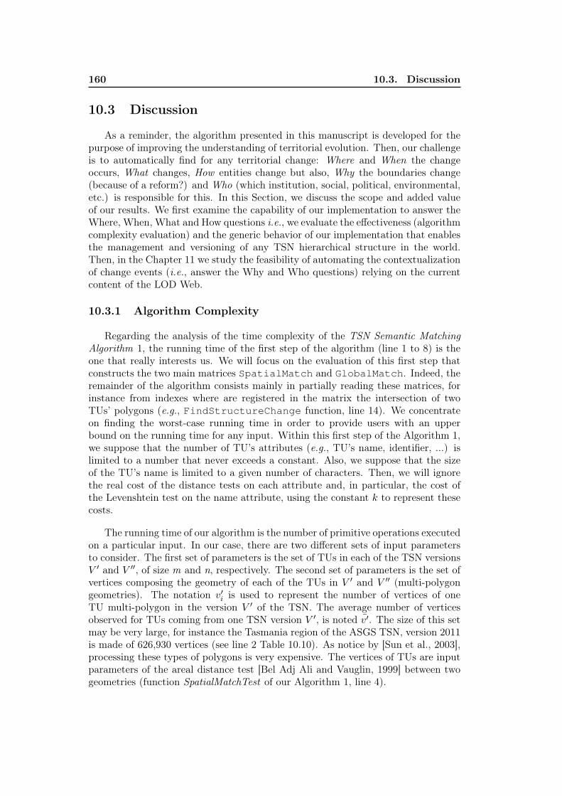
160 10.3. Discussion

10.3 Discussion

As a reminder, the algorithm presented in this manuscript is developed for thepurpose of improving the understanding of territorial evolution. Then, our challengeis to automatically find for any territorial change: Where and When the changeoccurs, What changes, How entities change but also, Why the boundaries change(because of a reform?) and Who (which institution, social, political, environmental,etc.) is responsible for this. In this Section, we discuss the scope and added valueof our results. We first examine the capability of our implementation to answer theWhere, When, What and How questions i.e., we evaluate the effectiveness (algorithmcomplexity evaluation) and the generic behavior of our implementation that enablesthe management and versioning of any TSN hierarchical structure in the world.Then, in the Chapter 11 we study the feasibility of automating the contextualizationof change events (i.e., answer the Why and Who questions) relying on the currentcontent of the LOD Web.

10.3.1 Algorithm Complexity

Regarding the analysis of the time complexity of the TSN Semantic MatchingAlgorithm 1, the running time of the first step of the algorithm (line 1 to 8) is theone that really interests us. We will focus on the evaluation of this first step thatconstructs the two main matrices SpatialMatch and GlobalMatch. Indeed, theremainder of the algorithm consists mainly in partially reading these matrices, forinstance from indexes where are registered in the matrix the intersection of twoTUs’ polygons (e.g., FindStructureChange function, line 14). We concentrateon finding the worst-case running time in order to provide users with an upperbound on the running time for any input. Within this first step of the Algorithm 1,we suppose that the number of TU’s attributes (e.g., TU’s name, identifier, ...) islimited to a number that never exceeds a constant. Also, we suppose that the sizeof the TU’s name is limited to a given number of characters. Then, we will ignorethe real cost of the distance tests on each attribute and, in particular, the cost ofthe Levenshtein test on the name attribute, using the constant k to represent thesecosts.

The running time of our algorithm is the number of primitive operations executedon a particular input. In our case, there are two different sets of input parametersto consider. The first set of parameters is the set of TUs in each of the TSN versionsV ′ and V ′′, of size m and n, respectively. The second set of parameters is the set ofvertices composing the geometry of each of the TUs in V ′ and V ′′ (multi-polygongeometries). The notation v′i is used to represent the number of vertices of oneTU multi-polygon in the version V ′ of the TSN. The average number of verticesobserved for TUs coming from one TSN version V ′, is noted v̄′. The size of this setmay be very large, for instance the Tasmania region of the ASGS TSN, version 2011is made of 626,930 vertices (see line 2 Table 10.10). As notice by [Sun et al., 2003],processing these types of polygons is very expensive. The vertices of TUs are inputparameters of the areal distance test [Bel Adj Ali and Vauglin, 1999] between twogeometries (function SpatialMatchTest of our Algorithm 1, line 4).

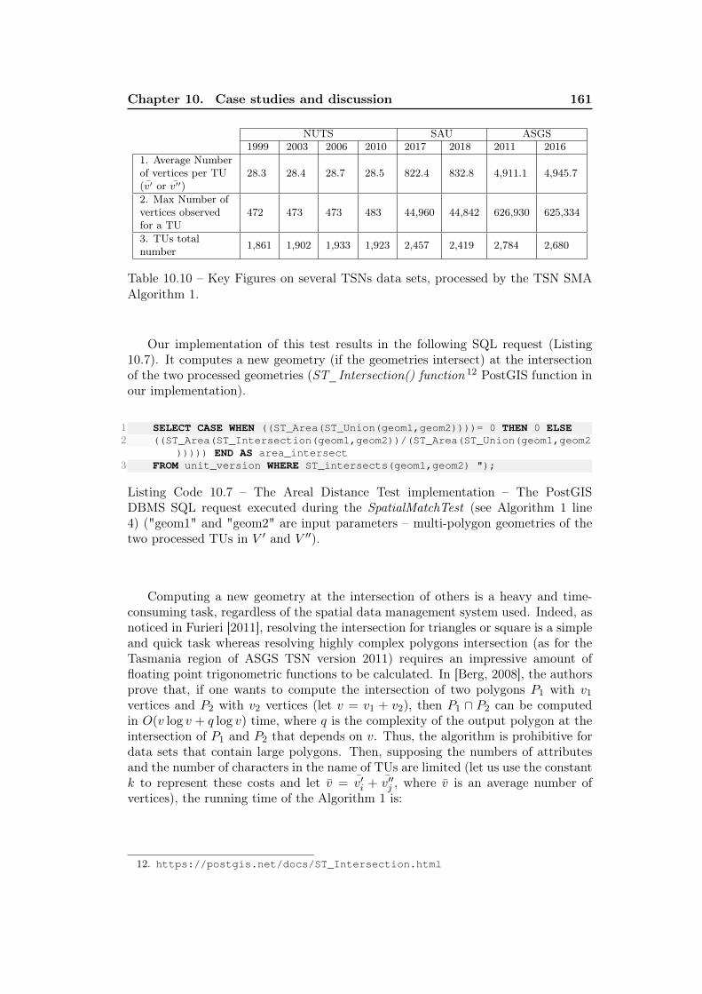
Chapter 10. Case studies and discussion 161

NUTS SAU ASGS1999 2003 2006 2010 2017 2018 2011 2016

1. Average Numberof vertices per TU(v̄′ or v̄′′)

28.3 28.4 28.7 28.5 822.4 832.8 4,911.1 4,945.7

2. Max Number ofvertices observedfor a TU

472 473 473 483 44,960 44,842 626,930 625,334

3. TUs totalnumber 1,861 1,902 1,933 1,923 2,457 2,419 2,784 2,680

Table 10.10 – Key Figures on several TSNs data sets, processed by the TSN SMAAlgorithm 1.

Our implementation of this test results in the following SQL request (Listing10.7). It computes a new geometry (if the geometries intersect) at the intersectionof the two processed geometries (ST_Intersection() function 12 PostGIS function inour implementation).

1 SELECT CASE WHEN ((ST_Area(ST_Union(geom1,geom2))))= 0 THEN 0 ELSE2 ((ST_Area(ST_Intersection(geom1,geom2))/(ST_Area(ST_Union(geom1,geom2

))))) END AS area_intersect3 FROM unit_version WHERE ST_intersects(geom1,geom2) ");

Listing Code 10.7 – The Areal Distance Test implementation – The PostGISDBMS SQL request executed during the SpatialMatchTest (see Algorithm 1 line4) ("geom1" and "geom2" are input parameters – multi-polygon geometries of thetwo processed TUs in V ′ and V ′′).

Computing a new geometry at the intersection of others is a heavy and time-consuming task, regardless of the spatial data management system used. Indeed, asnoticed in Furieri [2011], resolving the intersection for triangles or square is a simpleand quick task whereas resolving highly complex polygons intersection (as for theTasmania region of ASGS TSN version 2011) requires an impressive amount offloating point trigonometric functions to be calculated. In [Berg, 2008], the authorsprove that, if one wants to compute the intersection of two polygons P1 with v1vertices and P2 with v2 vertices (let v = v1 + v2), then P1 ∩ P2 can be computedin O(v log v + q log v) time, where q is the complexity of the output polygon at theintersection of P1 and P2 that depends on v. Thus, the algorithm is prohibitive fordata sets that contain large polygons. Then, supposing the numbers of attributesand the number of characters in the name of TUs are limited (let us use the constantk to represent these costs and let v̄ = v̄′i + v̄′′j , where v̄ is an average number ofvertices), the running time of the Algorithm 1 is:

12. https://postgis.net/docs/ST_Intersection.html

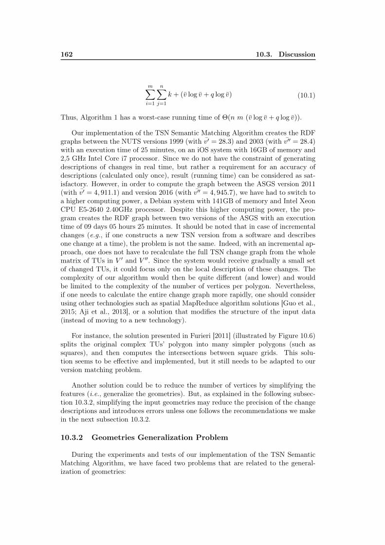
162 10.3. Discussion

m∑i=1

n∑j=1

k + (v̄ log v̄ + q log v̄) (10.1)

Thus, Algorithm 1 has a worst-case running time of Θ(n m (v̄ log v̄ + q log v̄)).

Our implementation of the TSN Semantic Matching Algorithm creates the RDFgraphs between the NUTS versions 1999 (with v̄′ = 28.3) and 2003 (with v̄′′ = 28.4)with an execution time of 25 minutes, on an iOS system with 16GB of memory and2,5 GHz Intel Core i7 processor. Since we do not have the constraint of generatingdescriptions of changes in real time, but rather a requirement for an accuracy ofdescriptions (calculated only once), result (running time) can be considered as sat-isfactory. However, in order to compute the graph between the ASGS version 2011(with v̄′ = 4, 911.1) and version 2016 (with v̄′′ = 4, 945.7), we have had to switch toa higher computing power, a Debian system with 141GB of memory and Intel XeonCPU E5-2640 2.40GHz processor. Despite this higher computing power, the pro-gram creates the RDF graph between two versions of the ASGS with an executiontime of 09 days 05 hours 25 minutes. It should be noted that in case of incrementalchanges (e.g., if one constructs a new TSN version from a software and describesone change at a time), the problem is not the same. Indeed, with an incremental ap-proach, one does not have to recalculate the full TSN change graph from the wholematrix of TUs in V ′ and V ′′. Since the system would receive gradually a small setof changed TUs, it could focus only on the local description of these changes. Thecomplexity of our algorithm would then be quite different (and lower) and wouldbe limited to the complexity of the number of vertices per polygon. Nevertheless,if one needs to calculate the entire change graph more rapidly, one should considerusing other technologies such as spatial MapReduce algorithm solutions [Guo et al.,2015; Aji et al., 2013], or a solution that modifies the structure of the input data(instead of moving to a new technology).

For instance, the solution presented in Furieri [2011] (illustrated by Figure 10.6)splits the original complex TUs’ polygon into many simpler polygons (such assquares), and then computes the intersections between square grids. This solu-tion seems to be effective and implemented, but it still needs to be adapted to ourversion matching problem.

Another solution could be to reduce the number of vertices by simplifying thefeatures (i.e., generalize the geometries). But, as explained in the following subsec-tion 10.3.2, simplifying the input geometries may reduce the precision of the changedescriptions and introduces errors unless one follows the recommendations we makein the next subsection 10.3.2.

10.3.2 Geometries Generalization Problem

During the experiments and tests of our implementation of the TSN SemanticMatching Algorithm, we have faced two problems that are related to the general-ization of geometries:

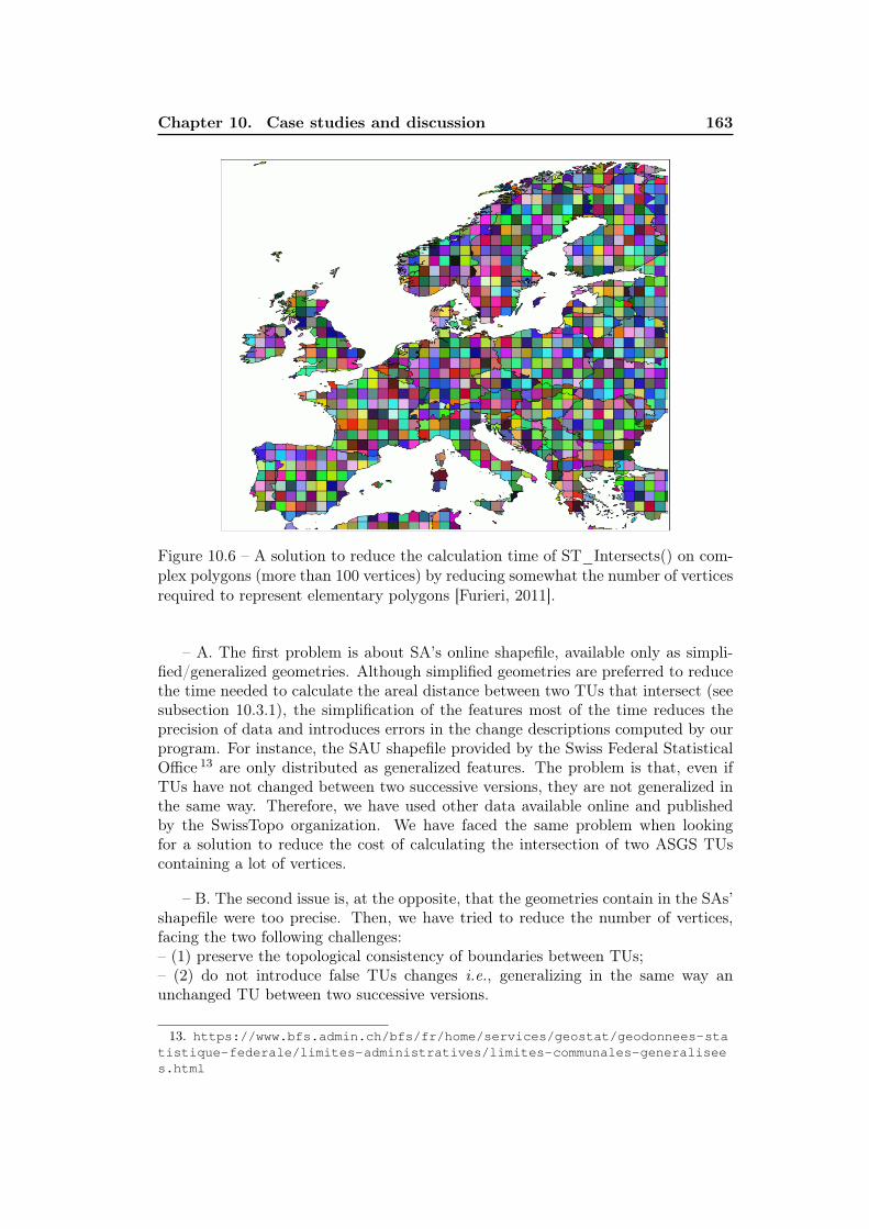
Chapter 10. Case studies and discussion 163

Figure 10.6 – A solution to reduce the calculation time of ST_Intersects() on com-plex polygons (more than 100 vertices) by reducing somewhat the number of verticesrequired to represent elementary polygons [Furieri, 2011].

– A. The first problem is about SA’s online shapefile, available only as simpli-fied/generalized geometries. Although simplified geometries are preferred to reducethe time needed to calculate the areal distance between two TUs that intersect (seesubsection 10.3.1), the simplification of the features most of the time reduces theprecision of data and introduces errors in the change descriptions computed by ourprogram. For instance, the SAU shapefile provided by the Swiss Federal StatisticalOffice 13 are only distributed as generalized features. The problem is that, even ifTUs have not changed between two successive versions, they are not generalized inthe same way. Therefore, we have used other data available online and publishedby the SwissTopo organization. We have faced the same problem when lookingfor a solution to reduce the cost of calculating the intersection of two ASGS TUscontaining a lot of vertices.

– B. The second issue is, at the opposite, that the geometries contain in the SAs’shapefile were too precise. Then, we have tried to reduce the number of vertices,facing the two following challenges:– (1) preserve the topological consistency of boundaries between TUs;– (2) do not introduce false TUs changes i.e., generalizing in the same way anunchanged TU between two successive versions.

13. https://www.bfs.admin.ch/bfs/fr/home/services/geostat/geodonnees-statistique-federale/limites-administratives/limites-communales-generalisees.html

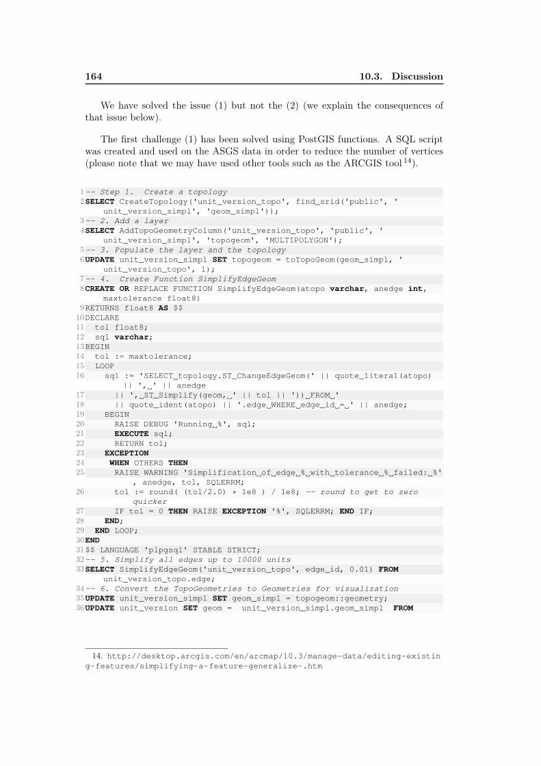
164 10.3. Discussion

We have solved the issue (1) but not the (2) (we explain the consequences ofthat issue below).

The first challenge (1) has been solved using PostGIS functions. A SQL scriptwas created and used on the ASGS data in order to reduce the number of vertices(please note that we may have used other tools such as the ARCGIS tool 14).

1-- Step 1. Create a topology2SELECT CreateTopology('unit_version_topo', find_srid('public', '

unit_version_simpl', 'geom_simpl'));3-- 2. Add a layer4SELECT AddTopoGeometryColumn('unit_version_topo', 'public', '

unit_version_simpl', 'topogeom', 'MULTIPOLYGON');5-- 3. Populate the layer and the topology6UPDATE unit_version_simpl SET topogeom = toTopoGeom(geom_simpl, '

unit_version_topo', 1);7-- 4. Create Function SimplifyEdgeGeom8CREATE OR REPLACE FUNCTION SimplifyEdgeGeom(atopo varchar, anedge int,

maxtolerance float8)9RETURNS float8 AS $$10DECLARE11 tol float8;12 sql varchar;13BEGIN14 tol := maxtolerance;15 LOOP16 sql := 'SELECT topology.ST_ChangeEdgeGeom(' || quote_literal(atopo)

|| ', ' || anedge17 || ', ST_Simplify(geom, ' || tol || ')) FROM '18 || quote_ident(atopo) || '.edge WHERE edge_id = ' || anedge;19 BEGIN20 RAISE DEBUG 'Running %', sql;21 EXECUTE sql;22 RETURN tol;23 EXCEPTION24 WHEN OTHERS THEN25 RAISE WARNING 'Simplification of edge % with tolerance % failed: %'

, anedge, tol, SQLERRM;26 tol := round( (tol/2.0) * 1e8 ) / 1e8; -- round to get to zero

quicker27 IF tol = 0 THEN RAISE EXCEPTION '%', SQLERRM; END IF;28 END;29 END LOOP;30END31$$ LANGUAGE 'plpgsql' STABLE STRICT;32-- 5. Simplify all edges up to 10000 units33SELECT SimplifyEdgeGeom('unit_version_topo', edge_id, 0.01) FROM

unit_version_topo.edge;34-- 6. Convert the TopoGeometries to Geometries for visualization35UPDATE unit_version_simpl SET geom_simpl = topogeom::geometry;36UPDATE unit_version SET geom = unit_version_simpl.geom_simpl FROM

14. http://desktop.arcgis.com/en/arcmap/10.3/manage-data/editing-existing-features/simplifying-a-feature-generalize-.htm

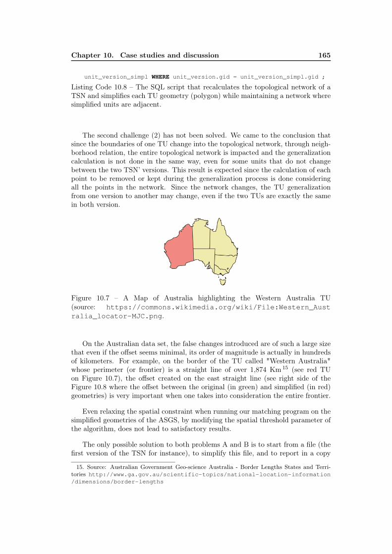
Chapter 10. Case studies and discussion 165

unit_version_simpl WHERE unit_version.gid = unit_version_simpl.gid ;

Listing Code 10.8 – The SQL script that recalculates the topological network of aTSN and simplifies each TU geometry (polygon) while maintaining a network wheresimplified units are adjacent.

The second challenge (2) has not been solved. We came to the conclusion thatsince the boundaries of one TU change into the topological network, through neigh-borhood relation, the entire topological network is impacted and the generalizationcalculation is not done in the same way, even for some units that do not changebetween the two TSN’ versions. This result is expected since the calculation of eachpoint to be removed or kept during the generalization process is done consideringall the points in the network. Since the network changes, the TU generalizationfrom one version to another may change, even if the two TUs are exactly the samein both version.

Figure 10.7 – A Map of Australia highlighting the Western Australia TU(source: https://commons.wikimedia.org/wiki/File:Western_Australia_locator-MJC.png.

On the Australian data set, the false changes introduced are of such a large sizethat even if the offset seems minimal, its order of magnitude is actually in hundredsof kilometers. For example, on the border of the TU called "Western Australia"whose perimeter (or frontier) is a straight line of over 1,874 Km 15 (see red TUon Figure 10.7), the offset created on the east straight line (see right side of theFigure 10.8 where the offset between the original (in green) and simplified (in red)geometries) is very important when one takes into consideration the entire frontier.

Even relaxing the spatial constraint when running our matching program on thesimplified geometries of the ASGS, by modifying the spatial threshold parameter ofthe algorithm, does not lead to satisfactory results.

The only possible solution to both problems A and B is to start from a file (thefirst version of the TSN for instance), to simplify this file, and to report in a copy

15. Source: Australian Government Geo-science Australia - Border Lengths States and Terri-tories http://www.ga.gov.au/scientific-topics/national-location-information/dimensions/border-lengths

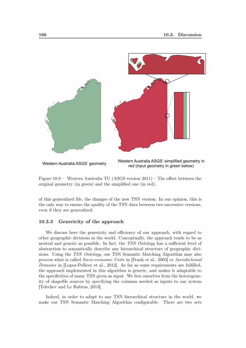
166 10.3. Discussion

Western Australia ASGS’ geometry Western Australia ASGS’ simplified geometry in red (input geometry in green below)

Figure 10.8 – Western Australia TU (ASGS version 2011) – The offset between theoriginal geometry (in green) and the simplified one (in red).

of this generalized file, the changes of the new TSN version. In our opinion, this isthe only way to ensure the quality of the TSN data between two successive versions,even if they are generalized.

10.3.3 Genericity of the approach

We discuss here the genericity and efficiency of our approach, with regard toother geographic divisions in the world. Conceptually, the approach tends to be asneutral and generic as possible. In fact, the TSN Ontology has a sufficient level ofabstraction to semantically describe any hierarchical structure of geographic divi-sions. Using the TSN Ontology, our TSN Semantic Matching Algorithm may alsoprocess what is called Socio-economic Units in [Frank et al., 2003] or JurisdictionalDomains in [Lopez-Pellicer et al., 2012]. As far as some requirements are fulfilled,the approach implemented in this algorithm is generic, and makes it adaptable tothe specificities of many TSN given as input. We free ourselves from the heterogene-ity of shapefile sources by specifying the columns needed as inputs to our system[Telechev and Le Rubrus, 2013].

Indeed, in order to adapt to any TSN hierarchical structure in the world, wemake our TSN Semantic Matching Algorithm configurable. There are two sets

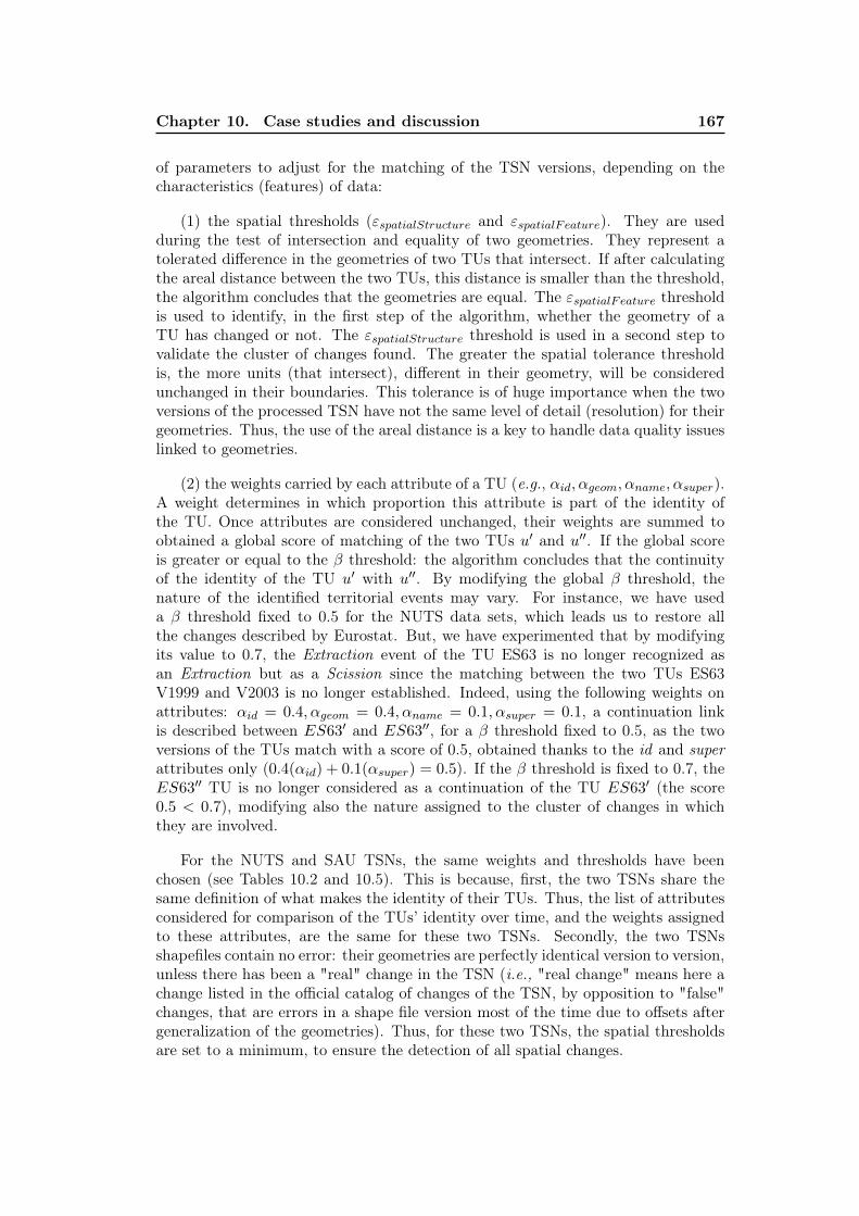
Chapter 10. Case studies and discussion 167

of parameters to adjust for the matching of the TSN versions, depending on thecharacteristics (features) of data:

(1) the spatial thresholds (εspatialStructure and εspatialFeature). They are usedduring the test of intersection and equality of two geometries. They represent atolerated difference in the geometries of two TUs that intersect. If after calculatingthe areal distance between the two TUs, this distance is smaller than the threshold,the algorithm concludes that the geometries are equal. The εspatialFeature thresholdis used to identify, in the first step of the algorithm, whether the geometry of aTU has changed or not. The εspatialStructure threshold is used in a second step tovalidate the cluster of changes found. The greater the spatial tolerance thresholdis, the more units (that intersect), different in their geometry, will be consideredunchanged in their boundaries. This tolerance is of huge importance when the twoversions of the processed TSN have not the same level of detail (resolution) for theirgeometries. Thus, the use of the areal distance is a key to handle data quality issueslinked to geometries.

(2) the weights carried by each attribute of a TU (e.g., αid, αgeom, αname, αsuper).A weight determines in which proportion this attribute is part of the identity ofthe TU. Once attributes are considered unchanged, their weights are summed toobtained a global score of matching of the two TUs u′ and u′′. If the global scoreis greater or equal to the β threshold: the algorithm concludes that the continuityof the identity of the TU u′ with u′′. By modifying the global β threshold, thenature of the identified territorial events may vary. For instance, we have useda β threshold fixed to 0.5 for the NUTS data sets, which leads us to restore allthe changes described by Eurostat. But, we have experimented that by modifyingits value to 0.7, the Extraction event of the TU ES63 is no longer recognized asan Extraction but as a Scission since the matching between the two TUs ES63V1999 and V2003 is no longer established. Indeed, using the following weights onattributes: αid = 0.4, αgeom = 0.4, αname = 0.1, αsuper = 0.1, a continuation linkis described between ES63′ and ES63′′, for a β threshold fixed to 0.5, as the twoversions of the TUs match with a score of 0.5, obtained thanks to the id and superattributes only (0.4(αid) + 0.1(αsuper) = 0.5). If the β threshold is fixed to 0.7, theES63′′ TU is no longer considered as a continuation of the TU ES63′ (the score0.5 < 0.7), modifying also the nature assigned to the cluster of changes in whichthey are involved.

For the NUTS and SAU TSNs, the same weights and thresholds have beenchosen (see Tables 10.2 and 10.5). This is because, first, the two TSNs share thesame definition of what makes the identity of their TUs. Thus, the list of attributesconsidered for comparison of the TUs’ identity over time, and the weights assignedto these attributes, are the same for these two TSNs. Secondly, the two TSNsshapefiles contain no error: their geometries are perfectly identical version to version,unless there has been a "real" change in the TSN (i.e., "real change" means here achange listed in the official catalog of changes of the TSN, by opposition to "false"changes, that are errors in a shape file version most of the time due to offsets aftergeneralization of the geometries). Thus, for these two TSNs, the spatial thresholdsare set to a minimum, to ensure the detection of all spatial changes.

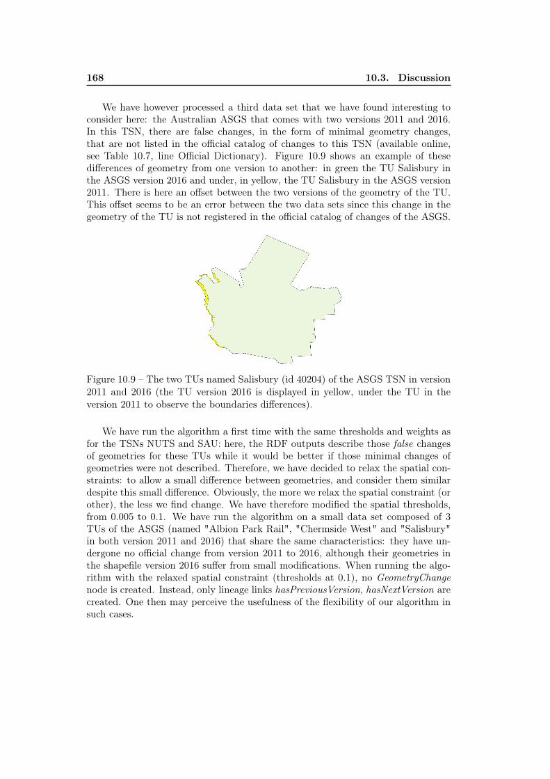
168 10.3. Discussion

We have however processed a third data set that we have found interesting toconsider here: the Australian ASGS that comes with two versions 2011 and 2016.In this TSN, there are false changes, in the form of minimal geometry changes,that are not listed in the official catalog of changes to this TSN (available online,see Table 10.7, line Official Dictionary). Figure 10.9 shows an example of thesedifferences of geometry from one version to another: in green the TU Salisbury inthe ASGS version 2016 and under, in yellow, the TU Salisbury in the ASGS version2011. There is here an offset between the two versions of the geometry of the TU.This offset seems to be an error between the two data sets since this change in thegeometry of the TU is not registered in the official catalog of changes of the ASGS.

Figure 10.9 – The two TUs named Salisbury (id 40204) of the ASGS TSN in version2011 and 2016 (the TU version 2016 is displayed in yellow, under the TU in theversion 2011 to observe the boundaries differences).

We have run the algorithm a first time with the same thresholds and weights asfor the TSNs NUTS and SAU: here, the RDF outputs describe those false changesof geometries for these TUs while it would be better if those minimal changes ofgeometries were not described. Therefore, we have decided to relax the spatial con-straints: to allow a small difference between geometries, and consider them similardespite this small difference. Obviously, the more we relax the spatial constraint (orother), the less we find change. We have therefore modified the spatial thresholds,from 0.005 to 0.1. We have run the algorithm on a small data set composed of 3TUs of the ASGS (named "Albion Park Rail", "Chermside West" and "Salisbury"in both version 2011 and 2016) that share the same characteristics: they have un-dergone no official change from version 2011 to 2016, although their geometries inthe shapefile version 2016 suffer from small modifications. When running the algo-rithm with the relaxed spatial constraint (thresholds at 0.1), no GeometryChangenode is created. Instead, only lineage links hasPreviousVersion, hasNextVersion arecreated. One then may perceive the usefulness of the flexibility of our algorithm insuch cases.

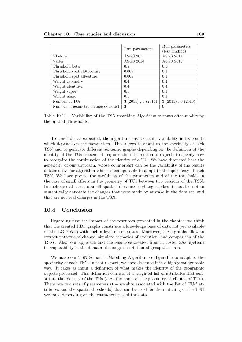
Chapter 10. Case studies and discussion 169

Run parameters Run parameters(less binding)

Vbefore ASGS 2011 ASGS 2011Vafter ASGS 2016 ASGS 2016Threshold beta 0.5 0.5Threshold spatialStructure 0.005 0.1Threshold spatialFeature 0.005 0.1Weight geometry 0.4 0.4Weight identifier 0.4 0.4Weight super 0.1 0.1Weight name 0.1 0.1Number of TUs 3 (2011) ; 3 (2016) 3 (2011) ; 3 (2016)Number of geometry change detected 3 0

Table 10.11 – Variability of the TSN matching Algorithm outputs after modifyingthe Spatial Thresholds.

To conclude, as expected, the algorithm has a certain variability in its resultswhich depends on the parameters. This allows to adapt to the specificity of eachTSN and to generate different semantic graphs depending on the definition of theidentity of the TUs chosen. It requires the intervention of experts to specify howto recognize the continuation of the identity of a TU. We have discussed here thegenericity of our approach, whose counterpart can be the variability of the resultsobtained by our algorithm which is configurable to adapt to the specificity of eachTSN. We have proved the usefulness of the parameters and of the thresholds inthe case of small offsets in the geometry of TUs between two versions of the TSN.In such special cases, a small spatial tolerance to change makes it possible not tosemantically annotate the changes that were made by mistake in the data set, andthat are not real changes in the TSN.

10.4 Conclusion

Regarding first the impact of the resources presented in the chapter, we thinkthat the created RDF graphs constitute a knowledge base of data not yet availableon the LOD Web with such a level of semantics. Moreover, these graphs allow toextract patterns of change, simulate scenarios of evolution, and comparison of theTSNs. Also, our approach and the resources created from it, foster SAs’ systemsinteroperability in the domain of change description of geospatial data.

We make our TSN Semantic Matching Algorithm configurable to adapt to thespecificity of each TSN. In that respect, we have designed it in a highly configurableway. It takes as input a definition of what makes the identity of the geographicobjects processed. This definition consists of a weighted list of attributes that con-stitute the identity of the TUs (e.g., the name or the geometry attributes of TUs).There are two sets of parameters (the weights associated with the list of TUs’ at-tributes and the spatial thresholds) that can be used for the matching of the TSNversions, depending on the characteristics of the data.

170 10.4. Conclusion

There is also a potential for extensibility to meet future requirements. Forinstance, currently we are working on several versions of the Corine Land CoverData set and we are experimenting the expansion of the TSN-Change Ontology andTSN Semantic Matching Algorithm in order to take into account another attributein the definition of the identity of the TUs: the nature of the land surface Harbelotet al. [2015].

Regarding the design quality, as explained previously, we follow the W3C Dataon the Web Best Practices recommendations Farias Lóscio et al. [2017], the W3Cseries of best practices for publishing Linked Data Hyland et al. [2014], and themethodological guidelines of Villazón-Terrazas et al. [2011] for the publication anduse of high quality Linked Government Data. For each concept defined, we use (whenrelevant) vocabularies such as Dublin Core Metadata Initiative terms 16 (for meta-data such as the source of data) or PAV - Provenance, Authoring and VersioningOntology 17. For instance, we refine the property pav:hasVersion, by specifying thedomain and range of this property using the TSN Ontology concepts. The conceptsTerritoryVersion (e.g., EU of 15 ) and UnitVersion are subclasses of the geo:Featureconcept defined within the OGC Geosparql ontology. The OWL-Time vocabularyis used to assign a reference period to a NomenclatureVersion and TerritoryVersionresources.

In the following Chapter 11, we show how to query these graphs and exploitthem with other data available on the LOD Web.

16. http://purl.org/dc/terms/17. http://purl.org/pav/

Chapter 11

Exploring and Exploiting the TSNmodel and data

11.1 Introduction

The created RDF graphs from the NUTS, ASGS and SAU data sets (presentedin the previous Chapter 10) constitute catalogs of TUs versions. Most of all, theydraw the lineage of each TU over time (horizontal reading of the graphs) and providea representation of the propagation of a change event through the divisions levels(vertical reading).

In order to highlight the potential of the created graphs, we come back hereto the change example of Ceuta and Melilla (already presented in Chapter 9) thathappened in the NUTS. We show here how, by querying our graphs, users are givenaccess to rich descriptions of this change. In the NUTS version 1999, at Level 2,the two Spanish enclaves in North Africa, Ceuta and Melilla, were considered asone TU (with identifier ES63) part of a Spanish province (please see Figure 9.2).In 1995, both Ceuta and Melilla became Autonomous cities of Spain, requiring aredistricting of the Spanish regions. It resulted in a split of the TU ES63 in two TUsnamed Ciudad Autònoma de Ceuta (with identifier ES63) and Ciudad Autònomade Melilla (with identifier ES64), in the NUTS Version 2003. Also, the sub-TUs ofES63 (ES631 and ES632) in the NUTS version 1999 both change identifiers. Wetry to find in our graph how this territorial change is described, first by a verticalreading of the graph, second by a horizontal reading.

Please note that an online data set at http://purl.org//steamer/tsndoc/resources/tsn_sparql_requests.pdf lists several SPARQL queries onthe 3 TSN change graphs ASGS, SAU and NUTS.

11.2 Knowledge extraction from TSN history graphs

11.2.1 Vertical reading of the change graphs

The following query, in Listing 11.1, addressed to our SPARQL endpoint http://steamerlod.imag.fr/sparql?&query=, shows how a program may auto-matically extract from the http://purl.org/steamer/nuts graph all the TUsthat have changed between two versions, at a specific level. Here, we ask for the listof all the NUTS 1999 major regions that change from 1999 to 2003. This request

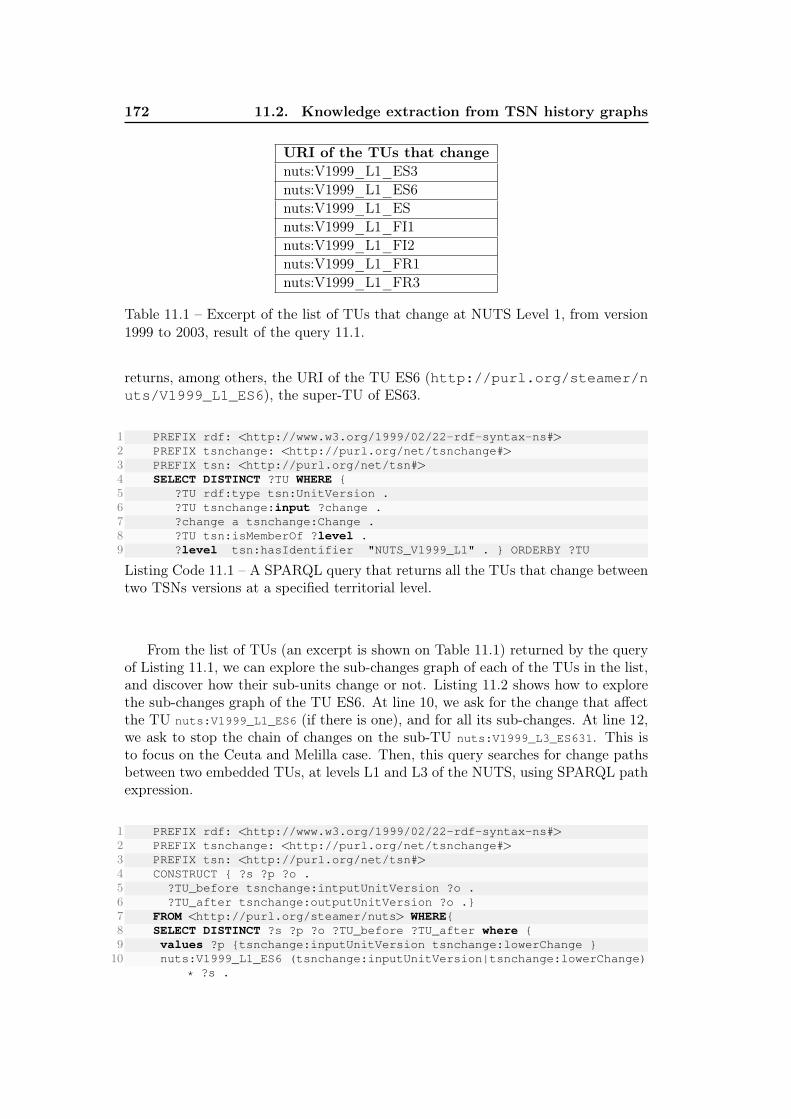
172 11.2. Knowledge extraction from TSN history graphs

URI of the TUs that changenuts:V1999_L1_ES3nuts:V1999_L1_ES6nuts:V1999_L1_ESnuts:V1999_L1_FI1nuts:V1999_L1_FI2nuts:V1999_L1_FR1nuts:V1999_L1_FR3

Table 11.1 – Excerpt of the list of TUs that change at NUTS Level 1, from version1999 to 2003, result of the query 11.1.

returns, among others, the URI of the TU ES6 (http://purl.org/steamer/nuts/V1999_L1_ES6), the super-TU of ES63.

1 PREFIX rdf: <http://www.w3.org/1999/02/22-rdf-syntax-ns#>2 PREFIX tsnchange: <http://purl.org/net/tsnchange#>3 PREFIX tsn: <http://purl.org/net/tsn#>4 SELECT DISTINCT ?TU WHERE {5 ?TU rdf:type tsn:UnitVersion .6 ?TU tsnchange:input ?change .7 ?change a tsnchange:Change .8 ?TU tsn:isMemberOf ?level .9 ?level tsn:hasIdentifier "NUTS_V1999_L1" . } ORDERBY ?TU

Listing Code 11.1 – A SPARQL query that returns all the TUs that change betweentwo TSNs versions at a specified territorial level.

From the list of TUs (an excerpt is shown on Table 11.1) returned by the queryof Listing 11.1, we can explore the sub-changes graph of each of the TUs in the list,and discover how their sub-units change or not. Listing 11.2 shows how to explorethe sub-changes graph of the TU ES6. At line 10, we ask for the change that affectthe TU nuts:V1999_L1_ES6 (if there is one), and for all its sub-changes. At line 12,we ask to stop the chain of changes on the sub-TU nuts:V1999_L3_ES631. This isto focus on the Ceuta and Melilla case. Then, this query searches for change pathsbetween two embedded TUs, at levels L1 and L3 of the NUTS, using SPARQL pathexpression.

1 PREFIX rdf: <http://www.w3.org/1999/02/22-rdf-syntax-ns#>2 PREFIX tsnchange: <http://purl.org/net/tsnchange#>3 PREFIX tsn: <http://purl.org/net/tsn#>4 CONSTRUCT { ?s ?p ?o .5 ?TU_before tsnchange:intputUnitVersion ?o .6 ?TU_after tsnchange:outputUnitVersion ?o .}7 FROM <http://purl.org/steamer/nuts> WHERE{8 SELECT DISTINCT ?s ?p ?o ?TU_before ?TU_after where {9 values ?p {tsnchange:inputUnitVersion tsnchange:lowerChange }10 nuts:V1999_L1_ES6 (tsnchange:inputUnitVersion|tsnchange:lowerChange)

* ?s .

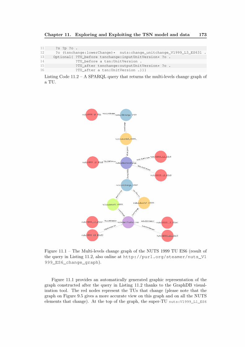
Chapter 11. Exploring and Exploiting the TSN model and data 173

11 ?s ?p ?o .12 ?o (tsnchange:lowerChange)* nuts:change_unitchange_V1999_L3_ES631 .13 Optional{ ?TU_before tsnchange:inputUnitVersion* ?o .14 ?TU_before a tsn:UnitVersion .15 ?TU_after tsnchange:outputUnitVersion* ?o .16 ?TU_after a tsn:UnitVersion .}}}

Listing Code 11.2 – A SPARQL query that returns the multi-levels change graph ofa TU.

Figure 11.1 – The Multi-levels change graph of the NUTS 1999 TU ES6 (result ofthe query in Listing 11.2, also online at http://purl.org/steamer/nuts_V1999_ES6_change_graph).

Figure 11.1 provides an automatically generated graphic representation of thegraph constructed after the query in Listing 11.2 thanks to the GraphDB visual-ization tool. The red nodes represent the TUs that change (please note that thegraph on Figure 9.5 gives a more accurate view on this graph and on all the NUTSelements that change). At the top of the graph, the super-TU nuts:V1999_L1_ES6

174 11.2. Knowledge extraction from TSN history graphs

is linked to a change node of type tsnchange:SubUnitChange. This node informsES6 that its sub-TU changes and it is linked to a sub-change that describes thesplit of the sub-TU nuts:V1999_L2_ES63. The term used to describe this change istsnchange:Extraction that is a sub-class of the tsnchange:Split concept, but moreprecise as it means that the initial TU that splits still exists after change. Finally,the graph describes the Identification restructuration of all the sub-TUs to ES63(purple node).

For path search between two TUs (e.g., a chain of change nodes between a super-TU and one of its sub-TUs), we ran into SAPRQL language limitations, includingits weakness in terms of finding paths and especially shortest paths. The SPARQLquery 11.2 uses property path expressions to search for a path between two re-sources. Property paths give a way to write parts of basic graph patterns [Harrisand Seaborne, 2013]. And, as explained in [Sirin, 2017], these property paths "can beused for queries that recursively traverse the RDF graph and find two nodes connectedvia a complex path of edges. But the result of a property path query is only the startand end nodes of the path and does not include the intermediate nodes. To find theintermediate nodes additional or more complex queries are needed." The query 11.2illustrates such complex queries that return intermediate nodes of changes betweentwo TUs (a super-TU and one of its sub-TU). Then, in an online documentation[Sirin, 2017], the author introduces an extension to the Stardog triplestore software,called Pathfinder, with the goal of providing an elegant, concise syntax for pathqueries in SPARQL. This extension allows, among others, to search for the shortestpath between two resources, using the following concise syntax shown in Listing11.3:

1PATH ?p FROM ([startNode AS] ?s) TO ([endNode AS] ?e) {2 GRAPH PATTERN3}4[ORDER BY condition]5[LIMIT int]

Listing Code 11.3 – Pathfinder syntax of path queries, source Sirin [2017].

Such extension would be particularly useful in the case of TSN change graphsand facilitate the search for chains of changes.

Please, note that one can also search for a sub-graph of changes without spec-ifying an end node, and, conversely, by specifying the type of changes one wantsto follow, as shown in the following query in Listing 11.5. This query returns thesub-graph of StructureChange (see filter on the type of changes at line 15) from theAustralian super-TU asgs:V2011_L4_508.

1PREFIX rdf: <http://www.w3.org/1999/02/22-rdf-syntax-ns#>2PREFIX tsnchange: <http://purl.org/net/tsnchange#>3PREFIX tsn: <http://purl.org/net/tsn#>4PREFIX : <http://purl.org/steamer/asgs/>5CONSTRUCT {

Chapter 11. Exploring and Exploiting the TSN model and data 175

6 ?s ?p ?o . ?TU_before tsnchange:intputUnitVersion ?o .7 ?TU_after tsnchange:outputUnitVersion ?o .}8FROM <http://purl.org/steamer/asgs>9WHERE{10 select distinct ?s ?p ?o ?TU_before ?TU_after11 where {12 values ?p {tsnchange:inputUnitVersion tsnchange:lowerChange}13 :V2011_L4_508 (tsnchange:inputUnitVersion|tsnchange:lowerChange)*

?s .14 ?s ?p ?o .15 ?o rdf:type tsnchange:StructureChange .16 Optional{17 ?TU_before tsnchange:inputUnitVersion* ?o .18 ?TU_before a tsn:UnitVersion .19 ?TU_after tsnchange:outputUnitVersion* ?o .20 ?TU_after a tsn:UnitVersion . }21 }22}

Listing Code 11.4 – A SPARQL query that searches for the sub-graph of changes ofa super-TU.

Also, the following query in Listing 11.5 shows how to traverse the graph but inthe ascending direction this time:

1PREFIX rdf: <http://www.w3.org/1999/02/22-rdf-syntax-ns#>2PREFIX tsnchange: <http://purl.org/net/tsnchange#>3PREFIX tsn: <http://purl.org/net/tsn#>4PREFIX : <http://purl.org/steamer/asgs/>5CONSTRUCT {6 ?s ?p ?o .7 ?uBefore tsnchange:intputUnitVersion ?o .8 ?uAfter tsnchange:outputUnitVersion ?o .}9FROM <http://purl.org/steamer/asgs> WHERE{10select distinct ?s ?p ?o ?uBefore ?uAfter where {11 values ?p {tsnchange:inputUnitVersion tsnchange:upperChange }12 :V2011_L2_508011194 (tsnchange:inputUnitVersion|tsnchange:upperChange)*

?s .13 ?s ?p ?o .14 ?o (tsnchange:upperChange)* :change_unitchange_V2011_L4_508.15 Optional{16 ?uBefore tsnchange:inputUnitVersion* ?o .17 ?uBefore a tsn:UnitVersion .18 ?uAfter tsnchange:outputUnitVersion* ?o .19 ?uAfter a tsn:UnitVersion .20 }21 }}

Listing Code 11.5 – A SPARQL query that, from a TU in the lowest level, goes upthe chain of changes until a super-TU.

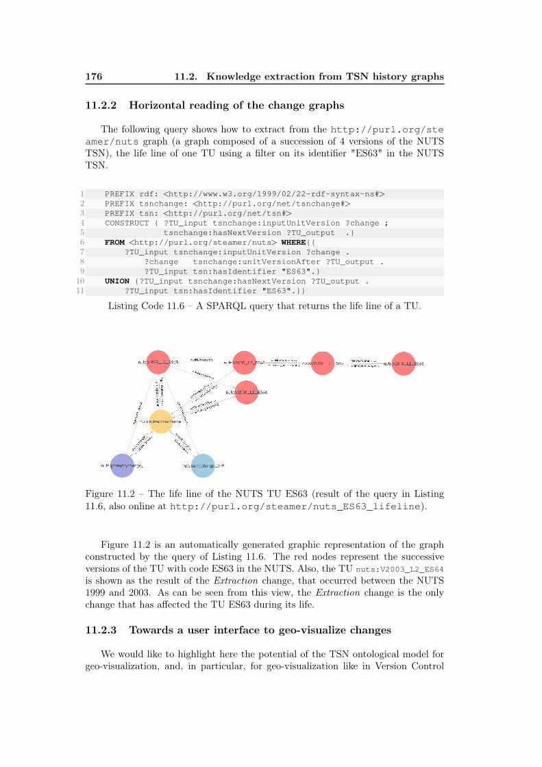
176 11.2. Knowledge extraction from TSN history graphs

11.2.2 Horizontal reading of the change graphs

The following query shows how to extract from the http://purl.org/steamer/nuts graph (a graph composed of a succession of 4 versions of the NUTSTSN), the life line of one TU using a filter on its identifier "ES63" in the NUTSTSN.

1 PREFIX rdf: <http://www.w3.org/1999/02/22-rdf-syntax-ns#>2 PREFIX tsnchange: <http://purl.org/net/tsnchange#>3 PREFIX tsn: <http://purl.org/net/tsn#>4 CONSTRUCT { ?TU_input tsnchange:inputUnitVersion ?change ;5 tsnchange:hasNextVersion ?TU_output .}6 FROM <http://purl.org/steamer/nuts> WHERE{{7 ?TU_input tsnchange:inputUnitVersion ?change .8 ?change tsnchange:unitVersionAfter ?TU_output .9 ?TU_input tsn:hasIdentifier "ES63".}10 UNION {?TU_input tsnchange:hasNextVersion ?TU_output .11 ?TU_input tsn:hasIdentifier "ES63".}}

Listing Code 11.6 – A SPARQL query that returns the life line of a TU.

Figure 11.2 – The life line of the NUTS TU ES63 (result of the query in Listing11.6, also online at http://purl.org/steamer/nuts_ES63_lifeline).

Figure 11.2 is an automatically generated graphic representation of the graphconstructed by the query of Listing 11.6. The red nodes represent the successiveversions of the TU with code ES63 in the NUTS. Also, the TU nuts:V2003_L2_ES64

is shown as the result of the Extraction change, that occurred between the NUTS1999 and 2003. As can be seen from this view, the Extraction change is the onlychange that has affected the TU ES63 during its life.

11.2.3 Towards a user interface to geo-visualize changes

We would like to highlight here the potential of the TSN ontological model forgeo-visualization, and, in particular, for geo-visualization like in Version Control

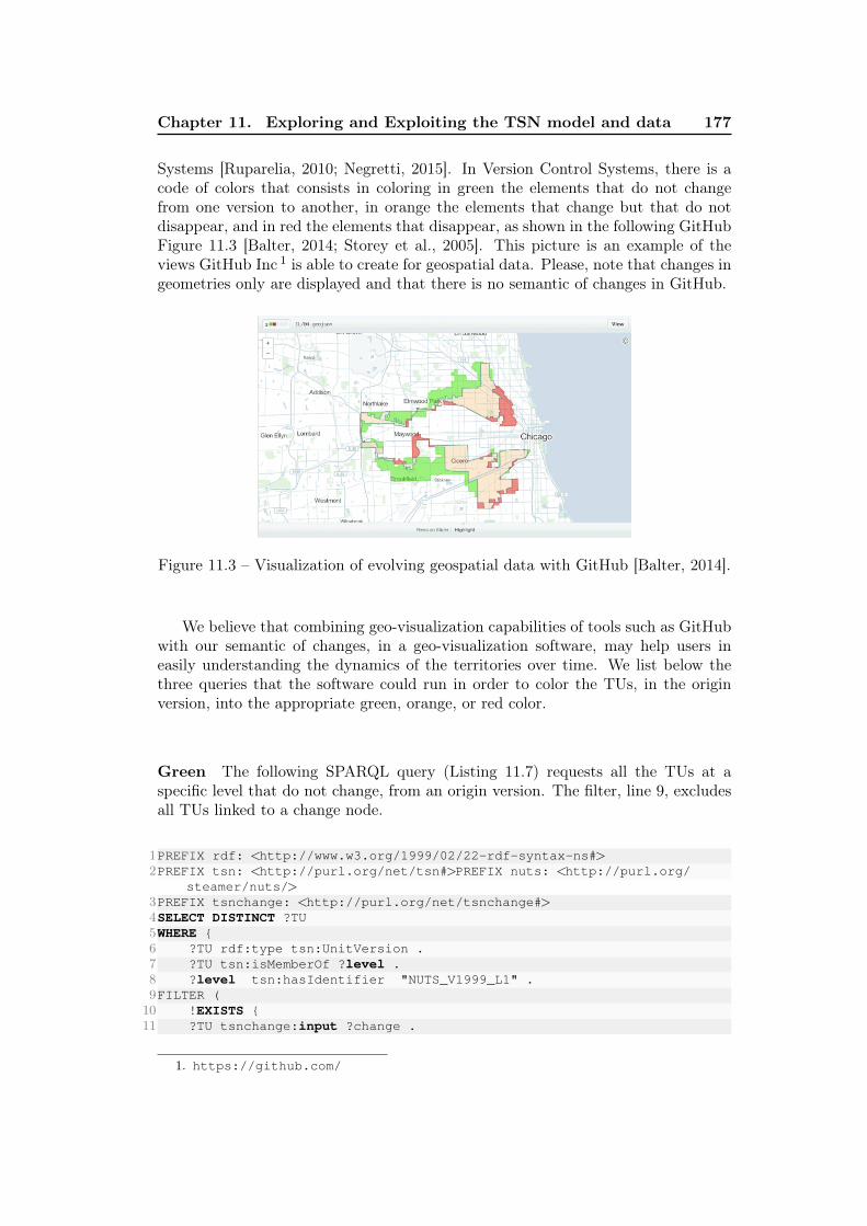
Chapter 11. Exploring and Exploiting the TSN model and data 177

Systems [Ruparelia, 2010; Negretti, 2015]. In Version Control Systems, there is acode of colors that consists in coloring in green the elements that do not changefrom one version to another, in orange the elements that change but that do notdisappear, and in red the elements that disappear, as shown in the following GitHubFigure 11.3 [Balter, 2014; Storey et al., 2005]. This picture is an example of theviews GitHub Inc 1 is able to create for geospatial data. Please, note that changes ingeometries only are displayed and that there is no semantic of changes in GitHub.

Figure 11.3 – Visualization of evolving geospatial data with GitHub [Balter, 2014].

We believe that combining geo-visualization capabilities of tools such as GitHubwith our semantic of changes, in a geo-visualization software, may help users ineasily understanding the dynamics of the territories over time. We list below thethree queries that the software could run in order to color the TUs, in the originversion, into the appropriate green, orange, or red color.

Green The following SPARQL query (Listing 11.7) requests all the TUs at aspecific level that do not change, from an origin version. The filter, line 9, excludesall TUs linked to a change node.

1PREFIX rdf: <http://www.w3.org/1999/02/22-rdf-syntax-ns#>2PREFIX tsn: <http://purl.org/net/tsn#>PREFIX nuts: <http://purl.org/

steamer/nuts/>3PREFIX tsnchange: <http://purl.org/net/tsnchange#>4SELECT DISTINCT ?TU5WHERE {6 ?TU rdf:type tsn:UnitVersion .7 ?TU tsn:isMemberOf ?level .8 ?level tsn:hasIdentifier "NUTS_V1999_L1" .9FILTER (10 !EXISTS {11 ?TU tsnchange:input ?change .

1. https://github.com/

178 11.2. Knowledge extraction from TSN history graphs

12})}

Listing Code 11.7 – Query the TUs that do not change from one version to anotherat a specific territorial level.

Orange The following SPARQL query (Listing 11.8) requests all the TUs at aspecific level that change, from an origin version. Line 8, the query asks for allTUs linked to a change node, whatever its type. However, line 11, the "MINUS"SPARQL keyword excludes all TUs linked to a change node of type Disappearance.This is because, this change type, means that the TUs has disappeared after thechange event.

At line 8, one can further specify the type of changes s/he wants to see, andcolor in orange, for example, TUs having changed their name (?change a tsn-change:NameChange).

1PREFIX rdf: <http://www.w3.org/1999/02/22-rdf-syntax-ns#>2PREFIX tsnchange: <http://purl.org/net/tsnchange#>3PREFIX tsn: <http://purl.org/net/tsn#>4PREFIX nuts: <http://purl.org/steamer/nuts/>5SELECT DISTINCT ?TU WHERE {6 ?TU rdf:type tsn:UnitVersion .7 ?TU tsnchange:input ?change .8 ?change a tsnchange:Change .9 ?TU tsn:isMemberOf ?level .10 ?level tsn:hasIdentifier "NUTS_V1999_L1" .11 MINUS12 {?change a tsnchange:Disappearance . }13 }

Listing Code 11.8 – Query the TUs that change from one version to another at aspecific territorial level.

Red The following SPARQL query (Listing 11.9) requests all the TUs at a specificlevel that disappear, from an origin version to a destination version:

1PREFIX rdf: <http://www.w3.org/1999/02/22-rdf-syntax-ns#>2PREFIX tsnchange: <http://purl.org/net/tsnchange#>3PREFIX tsn: <http://purl.org/net/tsn#>4PREFIX nuts: <http://purl.org/steamer/nuts/>5SELECT DISTINCT ?TU6WHERE {7 ?TU rdf:type tsn:UnitVersion .8 ?TU tsn:isMemberOf ?level .9 ?level tsn:hasIdentifier "NUTS_V1999_L1" .10 ?TU tsnchange:input ?change .

Chapter 11. Exploring and Exploiting the TSN model and data 179

11 ?change rdf:type tsnchange:Disappearance .}

Listing Code 11.9 – Query the TUs that disappear from one version to another ata specific territorial level.

11.3 Automatic contextualization of territorial changes

By exploiting the distributed LOD Web, we can enrich our descriptions of TSNand of their changes, by looking for other resources and understand more deeply theevolution of the territory. Different data sets exist on the LOD cloud, but the oneswe found the most relevant in our context are those from DBPedia 2 and WikiData 3.Indeed, they are generalists and provide encyclopedia-style information, such as his-torical data. Then, it may be possible to find the historical cause of a territorialchange in these data sets. A trivial example, addressing the DBPedia service within aSPARQL request allows to discover that the Ceuta TU of the NUTS TSN (using onlythe information on the TU identifier within the NUTS version 2003, i.e., ES630) is anAutonomous city of Spain (dbo:type dbr:Autonomous_cities_of_Spain),since 1995 (dbo:foundingDate 1995-03-14^^xsd:date).We also get, among other information, the total population of this TU (dbo:-populationTotal 823768sd:integer), information that may help statisti-cians at the time of comparing this TU with others in Europe. In particular, the lownumber of inhabitants of this TU, compared to the average number of inhabitants ofTUs at NUTS Level 3, should lead analysts to be careful in their comparative stud-ies of the European regions. Indeed, as stated on the Eurostat’s Website, "despitethe aim of ensuring that regions of comparable size all appear at the same NUTSlevel, each level still contains regions which differ greatly in terms of population",such as Luxembourg that is a small country in Europe, which appears at NUTSlevel 0, despite its low number of inhabitants.

1 PREFIX rdf: <http://www.w3.org/1999/02/22-rdf-syntax-ns#>2 PREFIX rdfs: <http://www.w3.org/2000/01/rdf-schema#>3 PREFIX geosparql: <http://www.opengis.net/ont/geosparql#>4 PREFIX tsn: <http://purl.org/net/tsn#>5 PREFIX dbo: <http://dbpedia.org/ontology/>6 PREFIX xsd: <http://www.w3.org/2001/XMLSchema#>7 SELECT *8 WHERE {9 ?tu a tsn:UnitVersion;10 tsn:hasIdentifier "ES630";11 tsn:hasName ?name;12 tsn:isMemberOf ?level;13 geosparql:hasGeometry [14 geosparql:asWKT ?geom; ].15 ?level tsn:hasIdentifier ?id_level ;16 tsn:isDivisionOf ?tsn_version .

2. https://wiki.dbpedia.org/3. https://www.wikidata.org/wiki/Wikidata:Main_Page

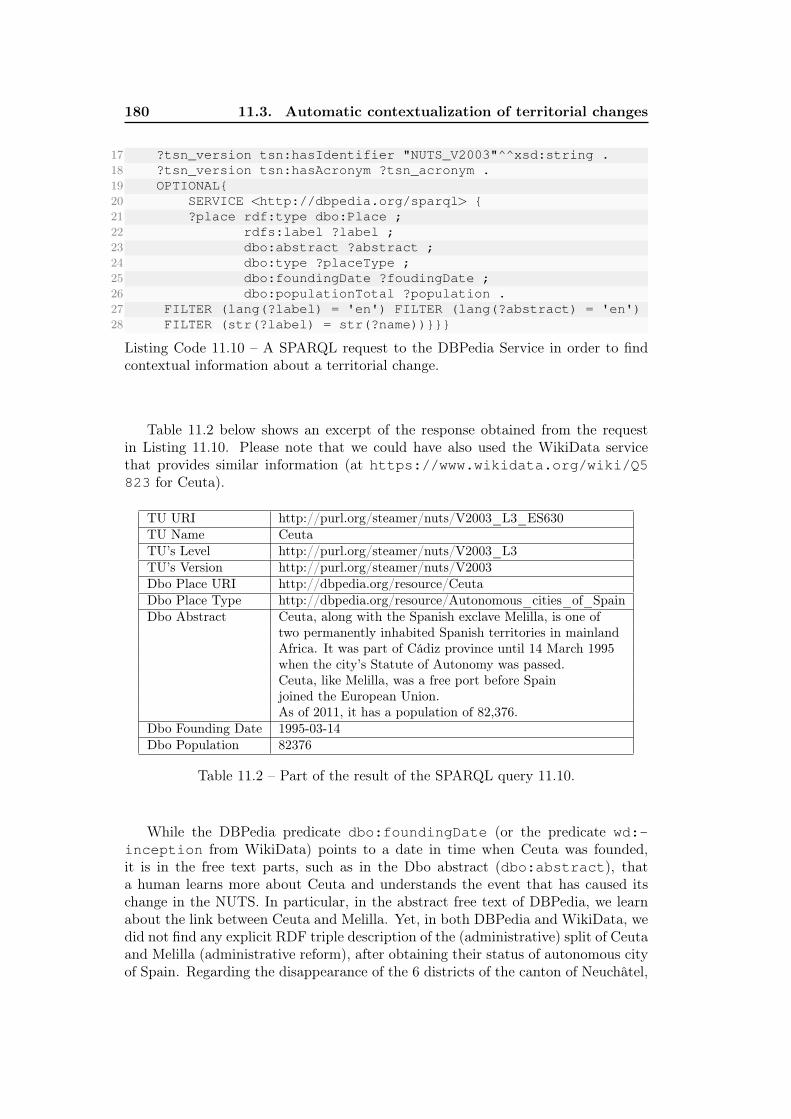
180 11.3. Automatic contextualization of territorial changes

17 ?tsn_version tsn:hasIdentifier "NUTS_V2003"^^xsd:string .18 ?tsn_version tsn:hasAcronym ?tsn_acronym .19 OPTIONAL{20 SERVICE <http://dbpedia.org/sparql> {21 ?place rdf:type dbo:Place ;22 rdfs:label ?label ;23 dbo:abstract ?abstract ;24 dbo:type ?placeType ;25 dbo:foundingDate ?foudingDate ;26 dbo:populationTotal ?population .27 FILTER (lang(?label) = 'en') FILTER (lang(?abstract) = 'en')28 FILTER (str(?label) = str(?name))}}}

Listing Code 11.10 – A SPARQL request to the DBPedia Service in order to findcontextual information about a territorial change.

Table 11.2 below shows an excerpt of the response obtained from the requestin Listing 11.10. Please note that we could have also used the WikiData servicethat provides similar information (at https://www.wikidata.org/wiki/Q5823 for Ceuta).

TU URI http://purl.org/steamer/nuts/V2003_L3_ES630TU Name CeutaTU’s Level http://purl.org/steamer/nuts/V2003_L3TU’s Version http://purl.org/steamer/nuts/V2003Dbo Place URI http://dbpedia.org/resource/CeutaDbo Place Type http://dbpedia.org/resource/Autonomous_cities_of_SpainDbo Abstract Ceuta, along with the Spanish exclave Melilla, is one of

two permanently inhabited Spanish territories in mainlandAfrica. It was part of Cádiz province until 14 March 1995when the city’s Statute of Autonomy was passed.Ceuta, like Melilla, was a free port before Spainjoined the European Union.As of 2011, it has a population of 82,376.

Dbo Founding Date 1995-03-14Dbo Population 82376

Table 11.2 – Part of the result of the SPARQL query 11.10.

While the DBPedia predicate dbo:foundingDate (or the predicate wd:-inception from WikiData) points to a date in time when Ceuta was founded,it is in the free text parts, such as in the Dbo abstract (dbo:abstract), thata human learns more about Ceuta and understands the event that has caused itschange in the NUTS. In particular, in the abstract free text of DBPedia, we learnabout the link between Ceuta and Melilla. Yet, in both DBPedia and WikiData, wedid not find any explicit RDF triple description of the (administrative) split of Ceutaand Melilla (administrative reform), after obtaining their status of autonomous cityof Spain. Regarding the disappearance of the 6 districts of the canton of Neuchâtel,

Chapter 11. Exploring and Exploiting the TSN model and data 181

in the SAU, neither DBPedia nor WikiData have information about this territorialchange. We presume this is because the event occurs quite recently on 1 January2018.

Various models have been proposed for representing events, as explained in theState of the Art part, Subsection 5.2.2. In order to automate the contextualiza-tion of territorial changes, using the DBPedia service we encounter problems be-cause listed events in DBPedia are few and limited to military battles and sportevents. They cannot be queried in a structured way. In [Hienert and Luciano,2015], the authors present a solution that automates the extraction of historicalevents from articles in Wikipedia, using language-dependent patterns to identifysentences containing a date. For the representation of these events, they have cho-sen the LODE ontology from [Shaw et al., 2009] because it is a domain-independentand a light weighted structure. Nevertheless, it seems that the created SPARQLendpoint does no longer exist 4. They have also created a GUI and a Web APIto visualize and query the historical events extracted from Wikipedia articles. Forinstance, the following query http://www.vizgr.org/historical-events/search.php?query=Ceuta returns in XML a list of historical events that takeplace in Ceuta. Yet, the autonomy of Ceuta in 1995 is not in this list.

The autonomous status of Ceuta and Melilla was introduced by the Law 1/1995and 2/1995, March 13, of the Statutes of Autonomy of Ceuta and Melilla 5. In Eu-rope, the European Legislation Identifier (ELI) 6 provides Web identifiers (URIs)for legal information. For instance, in France the Law No 2015-29 of January2015, the 16th, redefining the regional administrative areas for France, has anELI URI that is https://www.legifrance.gouv.fr/eli/loi/2015/1/16/INTX1412841L/jo/texte. The implementation of ELI is still a work in progressin Spain, since the Spanish legal system is complex and diverse, comprising rulescorresponding to different territorial levels (national, Autonomous Community andlocal) 7. Thus, the URI of the Laws 1/1995 and 2/1995, March 13, may be soonavailable. Everyone will then be able to automatically link to these URIs, usingthe ELI patterns for URIs construction, and therefore provide users with the legalcontext for the territorial change. In Wikidata, though there is the predicate sig-nificant event 8 to express a significant or notable event associated with the subject,we notice that it is not used for Ceuta for instance, and no description is returnedon the element history of Ceuta 9. Yet, in both DBPedia and WikiData, we havenot found any explicit triple description of the administrative division of Ceuta andMelilla, after obtaining their status of autonomous city of Spain. Then, our proposalfor future work is to:

(1) reuse the automatic extraction method of [Hienert and Luciano, 2015] to

4. The URL provided in the paper http://lod.gesis.org/historicalevents/sparqlreturn a 404 error code.

5. http://noticias.juridicas.com/base_datos/Admin/lo1-1995.html http://noticias.juridicas.com/base_datos/Admin/lo2-1995.html

6. https://eur-lex.europa.eu/eli-register/about.html7. https://eur-lex.europa.eu/eli-register/spain.html8. https://www.wikidata.org/wiki/Property:P7939. https://www.wikidata.org/wiki/Q19632088

18211.4. Exploitation of TSN history graphs with Linked Open statistical

Data

extract historical event from Wikipedia;

(2) create a triple representation of these historical events using the LODE Ontol-ogy [Shaw et al., 2009] for their description or the CIDOC CRM Ontology, designedfor the representation of historic events [Doerr, 2003];

(3) link TSN change nodes with event nodes created after step (2), using thepredicate tsnchange:isCausedBy in order to express in RDF that a territorialchange is caused by this historical event.

Regarding the disappearance of the districts of the canton of Neuchâtel, as no-ticed previously, no information was available in January 2019 neither in WikiDatanor in DBPedia (e.g., http://dbpedia.org/resource/Canton_of_Neuchatel). However, this event is described in Wikipedia as follows: "Until 2018 theCanton was divided into 6 districts. On 1 January 2018, the districts were dissolvedand all municipalities were placed directly under the canton". Since this descrip-tion contains a date, we think that the method from [Hienert and Luciano, 2015] isrelevant in this case to extract automatically a description of this event. Thus, bylinking this event to SAU TUs representations before and after the event, describedusing the TSN Ontology and TSN-Change Ontology, we should obtain accurate (intime and space) and semantic representation of the territory and of its evolutionover time.

11.4 Exploitation of TSN history graphs with LinkedOpen statistical Data

The W3C QB vocabulary is widely used to describe LOD statistics in a way thatis compatible with the Statistical Data and Metadata eXchange (SDMX), an ISOstandard for exchanging and sharing statistical data and metadata among organi-zation Cyganiak and Reynolds [2014]. Using the QB vocabulary, one can publishstatistical observations and a set of dimensions that define what the observation ap-plies to: time, gender and geographic areas, for instance. The QB4ST extension 10

Atkinson [2017] provides canonical terms to defined in a QB observation the space(qb4st:SpatialDimension) and time dimensions of the data.

As explained in the Subsection 5.2.1, regarding the spatial dimension of data,the QB and QB4ST approaches do not deal with the representation of the evolutionof the features over time, the underlying changes and events, as well.

Thus, we suggest, for the statistical observations described with the RDF DataCube (QB) 11 vocabulary, to declare the spatial dimension of data using both theRDF Data Cube extensions for spatiotemporal components (QB4ST) 12 (for a canon-ical declaration of the spatial dimension of data), and our TSN ontology to describethe TUs spatial dimension of data, i.e., the TU versions on which observations are

10. http://www.w3.org/ns/qb4st/11. http://purl.org/linked-data/cube#12. http://www.w3.org/ns/qb4st/

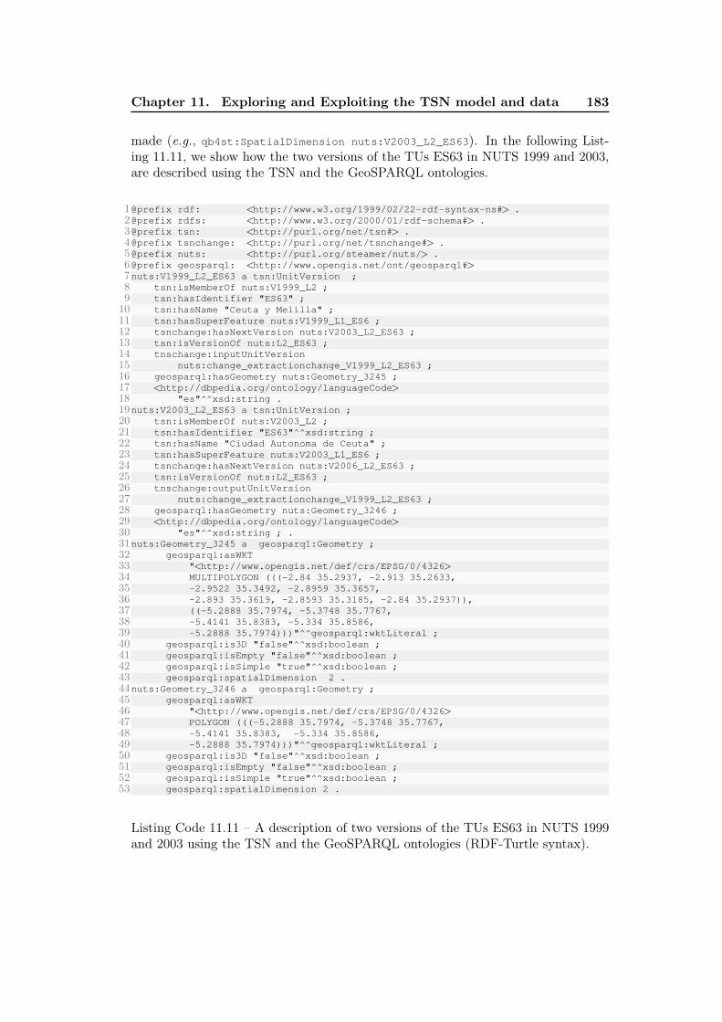
Chapter 11. Exploring and Exploiting the TSN model and data 183

made (e.g., qb4st:SpatialDimension nuts:V2003_L2_ES63). In the following List-ing 11.11, we show how the two versions of the TUs ES63 in NUTS 1999 and 2003,are described using the TSN and the GeoSPARQL ontologies.

1@prefix rdf: <http://www.w3.org/1999/02/22-rdf-syntax-ns#> .2@prefix rdfs: <http://www.w3.org/2000/01/rdf-schema#> .3@prefix tsn: <http://purl.org/net/tsn#> .4@prefix tsnchange: <http://purl.org/net/tsnchange#> .5@prefix nuts: <http://purl.org/steamer/nuts/> .6@prefix geosparql: <http://www.opengis.net/ont/geosparql#>7nuts:V1999_L2_ES63 a tsn:UnitVersion ;8 tsn:isMemberOf nuts:V1999_L2 ;9 tsn:hasIdentifier "ES63" ;10 tsn:hasName "Ceuta y Melilla" ;11 tsn:hasSuperFeature nuts:V1999_L1_ES6 ;12 tsnchange:hasNextVersion nuts:V2003_L2_ES63 ;13 tsn:isVersionOf nuts:L2_ES63 ;14 tnschange:inputUnitVersion15 nuts:change_extractionchange_V1999_L2_ES63 ;16 geosparql:hasGeometry nuts:Geometry_3245 ;17 <http://dbpedia.org/ontology/languageCode>18 "es"^^xsd:string .19nuts:V2003_L2_ES63 a tsn:UnitVersion ;20 tsn:isMemberOf nuts:V2003_L2 ;21 tsn:hasIdentifier "ES63"^^xsd:string ;22 tsn:hasName "Ciudad Autonoma de Ceuta" ;23 tsn:hasSuperFeature nuts:V2003_L1_ES6 ;24 tsnchange:hasNextVersion nuts:V2006_L2_ES63 ;25 tsn:isVersionOf nuts:L2_ES63 ;26 tnschange:outputUnitVersion27 nuts:change_extractionchange_V1999_L2_ES63 ;28 geosparql:hasGeometry nuts:Geometry_3246 ;29 <http://dbpedia.org/ontology/languageCode>30 "es"^^xsd:string ; .31nuts:Geometry_3245 a geosparql:Geometry ;32 geosparql:asWKT33 "<http://www.opengis.net/def/crs/EPSG/0/4326>34 MULTIPOLYGON (((-2.84 35.2937, -2.913 35.2633,35 -2.9522 35.3492, -2.8959 35.3657,36 -2.893 35.3619, -2.8593 35.3185, -2.84 35.2937)),37 ((-5.2888 35.7974, -5.3748 35.7767,38 -5.4141 35.8383, -5.334 35.8586,39 -5.2888 35.7974)))"^^geosparql:wktLiteral ;40 geosparql:is3D "false"^^xsd:boolean ;41 geosparql:isEmpty "false"^^xsd:boolean ;42 geosparql:isSimple "true"^^xsd:boolean ;43 geosparql:spatialDimension 2 .44nuts:Geometry_3246 a geosparql:Geometry ;45 geosparql:asWKT46 "<http://www.opengis.net/def/crs/EPSG/0/4326>47 POLYGON (((-5.2888 35.7974, -5.3748 35.7767,48 -5.4141 35.8383, -5.334 35.8586,49 -5.2888 35.7974)))"^^geosparql:wktLiteral ;50 geosparql:is3D "false"^^xsd:boolean ;51 geosparql:isEmpty "false"^^xsd:boolean ;52 geosparql:isSimple "true"^^xsd:boolean ;53 geosparql:spatialDimension 2 .

Listing Code 11.11 – A description of two versions of the TUs ES63 in NUTS 1999and 2003 using the TSN and the GeoSPARQL ontologies (RDF-Turtle syntax).

18411.4. Exploitation of TSN history graphs with Linked Open statistical

Data

Listing 11.12 shows how to define observations on the two versions of the TUES63 described in Listing 11.11. Here, we describe three observations of the Eurostatindicator called Total population. The first observation measures the total popula-tion of the TU nuts:V1999_L2_ES63, in 2001. The second observation measuresthe total population of the TU nuts:V2003_L2_ES63, in 2001. The third obser-vation measures the total population of the TU nuts:V2003_L2_ES64, in 2001.From line 9 to 12, we declare a predicate st-stat:refArea as a sub-property ofthe predicate qb4st:refArea, that is the canonical predicate of QB4ST to declare thereference area of a QB observation. This new sub-property allows us to specializethe range that has to be of the type tsn:UnitVersion i.e., the reference area ofthe observation have to be a tsn:UnitVersion.

Line 14 to 18, we declare the Eurostat indicator called Total population andthe structure of this indicator (its space and time dimensions, its source, unit ofmeasure...) is described from line 20 to 28. Then, the 3 observations are describedaccording to this data structure (lines 30-34; 36-40; 42-46). The 3 observationsdescribe the same indicator, in 2001, but the reference area is not the same. The firstobservation measures a total population in 2001 for Ceuta and Melilla, of 142,000people (TU version nuts:V1999_L2_ES63). The second observation measures atotal population in 2001 for Ceuta, of 74,000 people (TU version nuts:V2003_-L2_ES63). The third observation measures a total population in 2001 for Melilla of68,000 people (TU version nuts:V2003_L2_ES64). We show with this examplethat one may declare on the LOD Web the observations of an indicator on differentTSN versions that is to say, different versions of the geographic divisions can coexistto say different things about the territory (because they actually are different).

1@prefix st-stat: <http://purl.org/steamer/statistics/> .2@prefix rdf: <http://www.w3.org/1999/02/22-rdf-syntax-ns#> .3@prefix rdfs: <http://www.w3.org/2000/01/rdf-schema#> .4@prefix sdmx-dimension: <http://purl.org/linked-data/sdmx/2009/dimension#> .5@prefix sdmx-attribute: <http://purl.org/linked-data/sdmx/2009/attribute#> .6@prefix qb: <http://purl.org/linked-data/cube#> .7@prefix qb4st: <http://www.w3.org/ns/qb4st/>89st-stat:refArea a rdf:Property, qb:DimensionProperty;10 rdfs:label "reference area"@en;11 rdfs:subPropertyOf qb4st:refArea;12 rdfs:range tsn:UnitVersion.1314st-stat:dataset-poptot-eurostat a qb:DataSet;15 rdfs:label "Population, total"@en;16 rdfs:comment "Total population, both sexes."@en;17 qb:structure st-stat:dsd-dataset-poptot-eurostat;18 sdmx-attribute:unitMeasure <http://dbpedia.org/resource/Year>.1920st-stat:dsd-dataset-poptot-eurostat a qb:DataStructureDefinition;21 #The dimensions22 qb:component [qb:dimension st-stat:refArea];23 qb:component [qb:dimension sdmx-dimension:refPeriod];24 #The measures25 qb:component [qb:measure st-stat:totalPopulation];26 #The attributes27 qb:component [qb:attribute sdmx-attribute:UnitMeasure];28 qb:component [qb:attribute sdmx-attribute:DataSource].2930st-stat:observation-ES63-2001-nuts1999 a qb:Observation;

Chapter 11. Exploring and Exploiting the TSN model and data 185

31 qb:dataset st-stat:dataset-poptot-eurostat;32 st-stat:refArea nuts:V1999_L2_ES63;33 sdmx-dimension:refPeriod [time:year "2001"^^xsd:gYear] ;34 st-stat:totalPopulation 142000 .3536st-stat:observation-ES63-2001-nuts2003 a qb:Observation;37 qb:dataset st-stat:dataset-poptot-eurostat;38 st-stat:refArea nuts:V2003_L2_ES63;39 sdmx-dimension:refPeriod [time:year "2001"^^xsd:gYear] ;40 st-stat:totalPopulation 74000 .4142st-stat:observation-ES64-2001-nuts2003 a qb:Observation;43 qb:dataset st-stat:dataset-poptot-eurostat;44 st-stat:refArea nuts:V2003_L2_ES64;45 sdmx-dimension:refPeriod [time:year "2001"^^xsd:gYear] ;46 st-stat:totalPopulation 68000 .

Listing Code 11.12 – A description of the Total population Eurostat indicator -Two observations of the same indicator in different NUTS versions for the ES63 TU(RDF-Turtle syntax).

11.5 The TSN catalogs of areas for statistics

In addition to the triplestore, a second store is available online, and enablesusers to query data according to OGC standards. Indeed, we publish three OGCservices (recognized as GIS standards), using the GeoServer 13 software (at http://lig-tdcge.imag.fr/geoserver/web/): using our Catalog Service for theWeb (CSW), users discover the list of TUs through their metadata; from our WebFeature Service (WFS), users may download TUs representations (geometry, iden-tifier, name, level...), in XML format for instance; the Web Map Service (WMS)enables the visualization of TUs, in PNG for instance. Thus, the Web services dis-seminate data and metadata in various forms (image or text file) and formats (e.g.PNG, PDF, JPEG, GeoJSON, CSV, Shapefile). Then, TUs information (name,geometry, etc.) may be downloaded from the WFS layer and loaded from any clientsoftware (e.g. ArcGIS, QGIS or web-mapping clients Open Layers, Leaflet) that canread data in standard formats such as GML, CSV, GeoJSON, KML or Shapefile. Byconnecting to the PostGIS spatial database of the framework, the Geoserver softwareautomatically generate these OGC services. We register in the PostGIS database,for each TU Versions, its URI in the triplestore. Thus, we build the bridge betweenthe geomatics and the semantic worlds. For instance, searching for the ES63 TU, inversion 1999, using the WFS OGC standard request getFeature, in Listing 11.13, weobtain the response in JSON displayed in Listing 11.14. By clicking, in the JSONfile, line 4, one connects to the triplestore of the framework and obtains a HTMLrepresentation of the semantic resource.

13. geoserver.org/ free and open source software

186 11.5. The TSN catalogs of areas for statistics

1 http://lig-tdcge.imag.fr/geoserver/nuts/ows?service=WFS&version=1.0.0&request=GetFeature&typeName=nuts:unit_version&featureID=V1999_L2_ES63&outputFormat=application%2Fjson

Listing Code 11.13 – A WFS GetFeature Request on the OGC Web Services of theTheseus Framework.

1 {"type":"FeatureCollection","totalFeatures":1,"features":2 [{"type":"Feature","id":"unit_version.V1999_L2_ES63","geometry":{"

type":"MultiPolygon","coordinates":[[[[-2.84,35.2937],[-2.913,35.2633],

3 [-2.9522,35.3492],...]]]},"geometry_name":"geom", "properties":{4 "uri":"http://purl.org/steamer/nuts/V1999_L2_ES63",5 "id_unit_nomenclature":"ES63",6 "unit_name":"Ceuta y Melilla",7 "idnomenclature_version":"1999",8 "valid_from":"1999-12-31Z",9 "valid_until":"2003-06-29Z",10 "level":"2",11 "supunit":"ES6"}}],12 "crs":{"type":"name","properties":{"name":"urn:ogc:def:crs:EPSG

::4326"}}}

Listing Code 11.14 – A WFS GetFeature Response on the OGC Web Services of theTheseus Framework.

A GUI has been developed (available online at http://lig-tdcge.imag.fr/tsn-catalog/) using the OpenLayers 3 Web Mapping library 14 and standardrequests addressed to the WMS of the framework (see Figure 11.4). In this Webmapping GUI, we implement WMS Filter requests (see on top of Figure 11.4) sothat the user may filter the version and level of the TSN, s/he wants to visualize.By clicking one TU on the map (here, for instance, the UK TU has been selected)the user accesses a description of the TU on a table (see the right side of Figure11.4). S/He also visualizes below the table the HTTP request (GetFeatureInfo WMSrequest) run on the Geoserver to get such information. This GUI provides statis-ticians with a catalog of TU versions that they can visualize on a map. Also, ithelps Spatial Data Infrastructure developers accessing our system: they may copythe HTTP request text and provide a link to our semantic catalog of TUs from theirsystem.

14. http://openlayers.org/

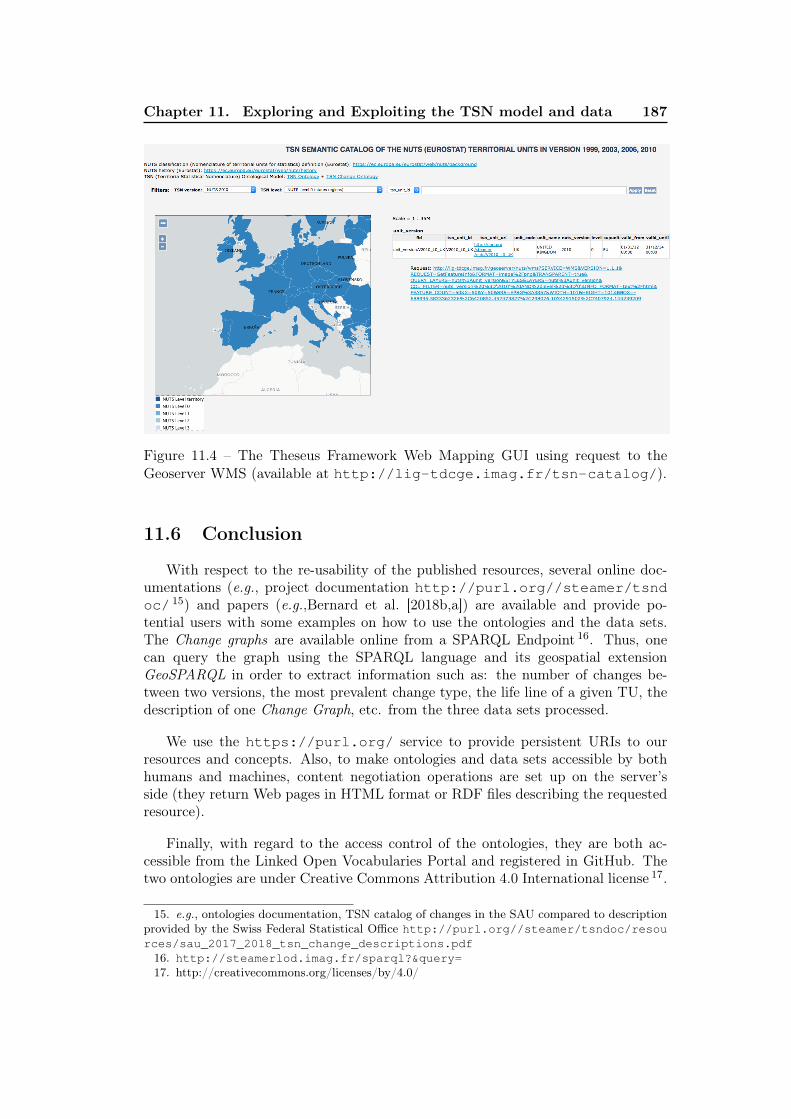
Chapter 11. Exploring and Exploiting the TSN model and data 187

Figure 11.4 – The Theseus Framework Web Mapping GUI using request to theGeoserver WMS (available at http://lig-tdcge.imag.fr/tsn-catalog/).

11.6 Conclusion

With respect to the re-usability of the published resources, several online doc-umentations (e.g., project documentation http://purl.org//steamer/tsndoc/ 15) and papers (e.g.,Bernard et al. [2018b,a]) are available and provide po-tential users with some examples on how to use the ontologies and the data sets.The Change graphs are available online from a SPARQL Endpoint 16. Thus, onecan query the graph using the SPARQL language and its geospatial extensionGeoSPARQL in order to extract information such as: the number of changes be-tween two versions, the most prevalent change type, the life line of a given TU, thedescription of one Change Graph, etc. from the three data sets processed.

We use the https://purl.org/ service to provide persistent URIs to ourresources and concepts. Also, to make ontologies and data sets accessible by bothhumans and machines, content negotiation operations are set up on the server’sside (they return Web pages in HTML format or RDF files describing the requestedresource).

Finally, with regard to the access control of the ontologies, they are both ac-cessible from the Linked Open Vocabularies Portal and registered in GitHub. Thetwo ontologies are under Creative Commons Attribution 4.0 International license 17.

15. e.g., ontologies documentation, TSN catalog of changes in the SAU compared to descriptionprovided by the Swiss Federal Statistical Office http://purl.org//steamer/tsndoc/resources/sau_2017_2018_tsn_change_descriptions.pdf16. http://steamerlod.imag.fr/sparql?&query=17. http://creativecommons.org/licenses/by/4.0/

188 11.6. Conclusion

Regarding the three data sets we have transformed in RDF, and the change descrip-tions we have created, with respect to:– the Eurostat NUTS data sets (versions 1999, 2003, 2006, 2010): the permission touse the data is granted on condition that: the data will not be used for commercialpurposes; the source will be acknowledged (copyright notice, ©European Union,1995-2019 and ©EuroGeographics for the administrative boundaries). This infor-mation is mentioned for each of the NUTS version e.g., http://purl.org/steamer/nuts/V2003.– the SAU data sets: the boundaries are provided by the Federal Office of Topog-raphy swisstopo, under the data set named swissBoundaries3D. The terms of use ofthis data set are: Open use. Must provide the source. Use for commercial purposesrequires permission of the data owner.– the ASGS data sets: they are under ©Commonwealth of Australia and CreativeCommons Attribution 4.0 International license.With regard to our RDF description of changes, e.g., based on Australian Bureauof Statistics data, they fall under the license of the geospatial files from which wecompute the changes description.

In the following Chapter, we conclude this manuscript by recalling the contri-butions of this work and listing some of the research and development perspectivesit opens up.

Chapter 12

Conclusion

The way the geographic divisions evolve over time is often ignored, and notrepresented. Most of the time, only the latest revisions of the geographic divisionsare shown and are queryable on a map. For instance, Web mapping services suchas Google Maps, or Open Street Map show only one border, the very last, andonly one toponym for a city, the last one(s) (sometimes two names are shown incontested cases). However, in many cases, it may be useful to access the previousboundaries, the old names of municipalities, and also to search them and locatethem on a map. Keeping each version of the geographical divisions and all theinformation on geographical units and their changes on the open data Web wouldtherefore greatly improve the search engines of geographic features over time. Thiswould allow, for instance, historians to find on a map the location of the Duché deSavoie in 1477. In this thesis report, we have studied in particular the evolution ofTerritorial Statistical Nomenclatures that are sets of artifact geographic areas builtby Statistical Agencies to observe a given territory at several geographic divisionlevels (e.g., regions, districts, sub-districts levels).

Nowadays, the challenge for SAs is to publish their geo-coded statistics andassociated TSNs on the Linked Open Data Web since the more contextualized dataare (linked to historical, environmental information, etc.), and linked to each other,in time and space, the more analyzes carried out on the territories using these datawill be multi-criteria, relevant and reusable by policies and researchers. This impliesa significant change of emphasis from traditional Spatial Data Infrastructures (SDI)by adopting an approach based on general Web standards [Tandy et al., 2017] i.e.,adopting the more general and domain independent Linked Open Data approach.

No ontology on the LOD Web is generic enough to enable the description of anyTSN in the world though it would foster the exchange of information among SAs.Similarly, no generic ontology on the LOD Web enables the description of the wayTSNs change over time, while description of such changes may avoid misinterpre-tations of statistics, statistical biases and enhance the understanding of territorialevolution, providing statisticians, and general public with descriptions to compre-hend the motivations and the impact of changes on geo-coded data (on electoralresults for instance).

The fundamental question we have addressed in this manuscript is how to en-hance the understanding of territorial dynamics, providing geographers and statis-ticians with tools to comprehend the impact of territorial changes by means ofsemantic representations of evolving territorial entities.

190 12.1. Summary of the contributions

12.1 Summary of the contributions

We have presented in this manuscript the Theseus Framework, a frameworkdesigned for managing TSNs and their evolution in the semantic Web, accordingto a management process that consists of the following activities: Specify, Model,Generate, Publish, and Exploit. It embeds our contributions, summarized below.

First, an ontological model have been proposed in order to describe anyTSN hierarchical structure in the world (i.e., structures with more than one ter-ritorial level, where each level covers the whole study area, and is composed ofnon-overlapping TUs, which corresponds to the structure of most of the administra-tive divisions in the world), their geographic areas (unambiguously defined in timeand space), and their changes over time. This model is composed of two ontologies:the TSN Ontology and TSN-Change Ontology that are published on the LOD Web.Through this model, we have proposed an innovative approach for detaileddescription of the evolution of TSNs over time taking into account thenested nature of such geographic divisions, at the time of describing theirchanges also. We decide to describe each change impacting each element of theterritorial structure, then to link together the changes when they occur on nestedareas. This new approach is based on the combination of two existing approaches:the 4D-fluent approach of [Welty et al., 2006] and the Change Bridge approachof [Kauppinen and Hyvönen, 2007]. Thus, using our approach, one may representboth the life line of the areas (4D object, space-time worm) and the way these areaschange from one time-slice (of the space-time worm) to another. The semantics ofchanges we have proposed, based on [Claramunt and Thériault, 1995; Plumejeaudet al., 2011] works, acts as a preliminary analysis of the territory and helps, amongother users, statisticians in estimating rapidly the areas that change and how theychange. Indeed, it must be noted that these changes are often much more complexthan a simple fusion of regions (because they impact several levels), and are verynumerous the more we go down the territorial divisions (municipalities in Switzer-land for example). Therefore, these changes are more difficult to see without anassisted visual detection or semantic descriptions, as the ones we propose.

Second, we have proposed the TSN Semantic Matching Algorithm inorder to automate the detection and semantic description of similaritiesand changes between two consecutive versions of a TSN. This algorithm extendsprevious works from [Plumejeaud et al., 2011; Plumejeaud, 2011]. It is configurableand expandable in order to adapt to the specifics of each TSN. In that respect, wehave designed it in a highly configurable way. The principle of the algorithm is tocompare TUs of two successive versions of a TSN and to measure their difference,taking into account a list of their attributes (e.g., name, geometry). An expertof the TSN configures the algorithm, according to h-er/is knowledge on the TSN:s/he constructs a definition of what makes the identity of the geographic objectsprocessed. S/He defines which attributes hold the identity of the TUs in the TSN,and in which proportion they can vary before TUs lose their identity.

Third, we have tested our whole approach and the Theseus Frameworkon different data sets in order to prove the ability of our framework to

Chapter 12. Conclusion 191

manage several TSNs, and automate the detection and description oftheir changes on the LOD Web. The created RDF graphs constitute catalogsof evolving geographic areas that enhance the understanding of territorial dynamics,providing statisticians with descriptions to comprehend the motivations and impactof redistricting. We now plan to use our method on other TSNs such as the CorineLand Cover data set and the Census Tracks of United States. We believe our ap-proach constitutes a step towards knowledge graphs of evolving geo-coded statisticsmade up of RDF Data Cube data sets, geospatial TSN data sets, event data sets,law data sets, etc., from which one could build intelligent tools for the analysis ofthe territory dynamics over time.

Let us come back to the representation of the evolution of the number of medalswon per country for the Olympic winter games, over a period from 1924 to 2010(see Subsection 2.1.2). If one wants to show on a map the medals won by countryfrom 1924 to 2010, it is necessary to have a representation of the borders of thecountries that varies over time. Therefore, one has to create a data set containingthe list of countries with their validity period and their geometry valid for the periodof existence of the country (referring to the International Olympic Committee’sCountry Code Data set 1). Under these conditions, it would be possible to displayon a map the countries according to their period of existence and the number ofmedals over this period. The user should also be informed that the count of medalsis only done over the period of the country’s existence, which does not necessarilycover the period 1924-2010. Then, using our approach that could be used in orderto draw Change Bridges between former States and current one, we offer a solutionto navigate through the data set of medal over time and space.

Many other data sets like the medals data set, require that the history of theregions (their name, borders, ...) is preserved. This is particularly the case forcultural heritage data. However, a major obstacle is that geographic informationdescribing these spatial units is often not available 2. One could imagine a crowd-sourcing platform in order to collect this information (past geometries, names ofunits ...), following the example of the collaborative project Open Historical Map 3,for instance. The contributors would be asked to provide information to characterizethe historical regions as in the TSN model. Then, our program would automati-cally computes the life line of the geographic areas. Finally, all these descriptionscould be published in the semantic Web and could therefore be linked to DBpediaor Wikidata resources describing the events related to the change of the regions overtime.

Thus, the approach we propose in this manuscript may be useful in many areas(socio-economic, archaeological, cultural, linguistic, ...) in order to correctly locatethe data in time and space. Indeed, our approach consists in describing very precisely

1. https://raw.githubusercontent.com/askmedia/datalogue/master/olympics/code_ioc.csv

2. However, in France, we notice the Geo-LARHRA initiative from a Research Group of his-torian that have redraw the boundaries of the french cantons from 1884 to 1966, available athttp://geo-larhra.ish-lyon.cnrs.fr/?q=atlas-historique

3. https://wiki.openstreetmap.org/wiki/Open_Historical_Map

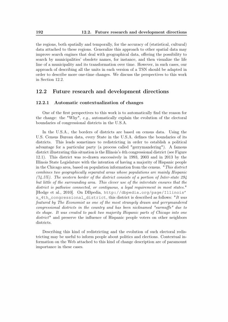
192 12.2. Future research and development directions

the regions, both spatially and temporally, for the accuracy of (statistical, cultural)data attached to these regions. Generalize this approach to other spatial data mayimprove search engines that deal with geographical data, offering the possibility tosearch by municipalities’ obsolete names, for instance, and then visualize the lifeline of a municipality and its transformation over time. However, in such cases, ourapproach of describing all the units in each version of a TSN should be adapted inorder to describe more one-time changes. We discuss the perspectives to this workin Section 12.2.

12.2 Future research and development directions

12.2.1 Automatic contextualization of changes

One of the first perspectives to this work is to automatically find the reason forthe change: the "Why", e.g., automatically explain the evolution of the electoralboundaries of congressional districts in the U.S.A.

In the U.S.A., the borders of districts are based on census data. Using theU.S. Census Bureau data, every State in the U.S.A. defines the boundaries of itsdistricts. This leads sometimes to redistricting in order to establish a politicaladvantage for a particular party (a process called "gerrymandering"). A famousdistrict illustrating this situation is the Illinois’s 4th congressional district (see Figure12.1). This district was re-drawn successively in 1993, 2003 and in 2013 by theIllinois State Legislature with the intention of having a majority of Hispanic peoplein the Chicago area, based on population information from the census. "This districtcombines two geographically separated areas whose populations are mainly Hispanic(74.5%). The western border of the district consists of a portion of Inter-state 294but little of the surrounding area. This clever use of the interstate ensures that thedistrict is pathwise connected, or contiguous, a legal requirement in most states."[Hodge et al., 2010]. On DBpedia, http://dbpedia.org/page/Illinois’s_4th_congressional_district, this district is described as follows: "It wasfeatured by The Economist as one of the most strangely drawn and gerrymanderedcongressional districts in the country and has been nicknamed "earmuffs" due toits shape. It was created to pack two majority Hispanic parts of Chicago into onedistrict" and preserve the influence of Hispanic people voters on other neighborsdistricts.

Describing this kind of redistricting and the evolution of such electoral redis-tricting may be useful to inform people about politics and elections. Contextual in-formation on the Web attached to this kind of change description are of paramountimportance in these cases.

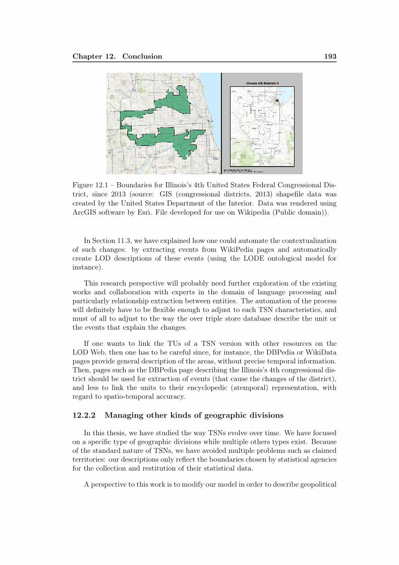
Chapter 12. Conclusion 193

Figure 12.1 – Boundaries for Illinois’s 4th United States Federal Congressional Dis-trict, since 2013 (source: GIS (congressional districts, 2013) shapefile data wascreated by the United States Department of the Interior. Data was rendered usingArcGIS software by Esri. File developed for use on Wikipedia (Public domain)).

In Section 11.3, we have explained how one could automate the contextualizationof such changes: by extracting events from WikiPedia pages and automaticallycreate LOD descriptions of these events (using the LODE ontological model forinstance).

This research perspective will probably need further exploration of the existingworks and collaboration with experts in the domain of language processing andparticularly relationship extraction between entities. The automation of the processwill definitely have to be flexible enough to adjust to each TSN characteristics, andmust of all to adjust to the way the over triple store database describe the unit orthe events that explain the changes.

If one wants to link the TUs of a TSN version with other resources on theLOD Web, then one has to be careful since, for instance, the DBPedia or WikiDatapages provide general description of the areas, without precise temporal information.Then, pages such as the DBPedia page describing the Illinois’s 4th congressional dis-trict should be used for extraction of events (that cause the changes of the district),and less to link the units to their encyclopedic (atemporal) representation, withregard to spatio-temporal accuracy.

12.2.2 Managing other kinds of geographic divisions

In this thesis, we have studied the way TSNs evolve over time. We have focusedon a specific type of geographic divisions while multiple others types exist. Becauseof the standard nature of TSNs, we have avoided multiple problems such as claimedterritories: our descriptions only reflect the boundaries chosen by statistical agenciesfor the collection and restitution of their statistical data.

A perspective to this work is to modify our model in order to describe geopolitical

194 12.2. Future research and development directions

divisions and report on territorial changes in real time.

Another perspective is to manage the evolution of other kinds of TSN (medico-social areas, cross-border areas, employment areas, cities ...) such as:– 1) non-covering hierarchies, where some units may have superior unit(s) at a ter-ritorial level not immediately above;– 2) non-strict hierarchies, where a TU may have several super features;– 3) non-onto hierarchies where the height of the hierarchy is varying;– 4) nomenclatures where TUs at one level (or at several levels) do not cover thewhole study area, such as the UMZ urban nomenclature, or other nomenclatures ofcities;– 5) nomenclatures composed of only one territorial level, such as the UMZ urbannomenclature.

1) Regarding TSNs with several levels, processing non-covering TSNs (wheresome units may have superior unit(s) at a territorial level not immediately above)requires no further development and modifications of the Theseus Framework, sinceeach TU is stored in the system with information on its super TU and the level thissuper TU belongs. At the time of chaining the changes that propagate through theTSN levels, the software program uses this information in order to link the changesof the current processed TU, to the changes of its super TU. Whether this TU isdirectly above, or not, does not matter.

2) In the same way, for non-strict hierarchies, instead of connecting to thechanges of a single super TU, the program will connect to several ones.

3) In TSNs where the height of the hierarchy is varying, some units may haveno super TU, or no sub TU(s) while others have both. Our TSN Ontology requiresa unit to be always connected to a super unit or to a territory (a specific type ofunit which may correspond to the study area of the nomenclature). Then, regardingnon-onto TSNs where the height is varying because some TUs don’t have super TU,data preprocessing is required before the TUs enters the system. Each TU has tobe linked to a super TU that could be the territory it belongs. Regarding non-ontoTSNs where the height is varying because some units don’t have sub TUs, there isno major obstacle since the program already manages this case, when traversing thelowest level in the hierarchy, composed of units that do not have sub units.

4) Regarding TSNs where TUs at one level (or at several levels) do not cover thewhole study area, there is no major obstacles. Indeed, for instance, the program isable to detect merge of TUs (merge of two cities for instance) that are not spatiallyclose, but that adopt a common identity after the change event, under a sharedmulti-polygon geometry, which covers the two initial polygons.

5) With regard to flat TSNs, composed of only one territorial level, we do notforesee any major obstacles to the processing of such TSNs. The TSN Ontology canbe used for the description of such TSNs on the LOD Web. A parameter should beadded to the SMA algorithm in order to disable or activate everything related to

Chapter 12. Conclusion 195

the chaining of changes over the hierarchy of territorial levels.

Regarding spatial nomenclatures with only one level, our methodology is ap-plicable to divisions of a territory on the physical characteristics of the landscapeelements. For instance, we could extend our framework in order to manage thechange of land cover in the Corine Land Cover data sets. Because our framework isconfigurable, we could add to the list of identity attributes the nature of the landcover. In order to perform the management of data sets such as the different versionsof the CLC data set (available online from the Copernicus Web site https://land.copernicus.eu/pan-european/corine-land-cover), we propose to:

Figure 12.2 – Corine Land Cover Classes (source: Copernicus Project https://land.copernicus.eu/Corinelandcoverclasses.eps.75dpi.png/).

– add a new attribute to the list of TUs attributes: a CLC class describing theland cover (one of the classes of the CLC hierarchy of land cover classes, see Figure12.2).Using the SmOD Land Cover Vocabulary and its predicate lc:corineLandCover,

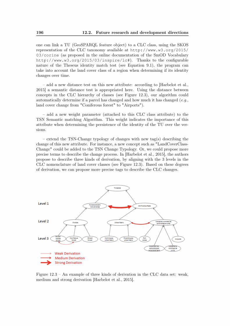
196 12.2. Future research and development directions

one can link a TU (GeoSPARQL feature object) to a CLC class, using the SKOSrepresentation of the CLC taxonomy available at http://www.w3.org/2015/03/corine (as proposed in the online documentation of the SmOD Vocabularyhttp://www.w3.org/2015/03/inspire/lc#). Thanks to the configurablenature of the Theseus identity match test (see Equation 9.1), the program cantake into account the land cover class of a region when determining if its identitychanges over time.

– add a new distance test on this new attribute: according to [Harbelot et al.,2015] a semantic distance test is appropriated here. Using the distance betweenconcepts in the CLC hierarchy of classes (see Figure 12.3), our algorithm couldautomatically determine if a parcel has changed and how much it has changed (e.g.,land cover change from "Coniferous forest" to "Airports").

– add a new weight parameter (attached to this CLC class attribute) to theTSN Semantic matching Algorithm. This weight indicates the importance of thisattribute when determining the persistence of the identity of the TU over the ver-sions.

– extend the TSN-Change typology of changes with new tag(s) describing thechange of this new attribute. For instance, a new concept such as "LandCoverClass-Change" could be added to the TSN Change Typology. Or, we could propose moreprecise terms to describe the change process. In [Harbelot et al., 2015], the authorspropose to describe three kinds of derivation, by aligning with the 3 levels in theCLC nomenclature of land cover classes (see Figure 12.3). Based on these degreesof derivation, we can propose more precise tags to describe the CLC changes.

Figure 12.3 – An example of three kinds of derivation in the CLC data set: weak,medium and strong derivation [Harbelot et al., 2015].

Chapter 12. Conclusion 197

To conclude, regarding the CLC data sets, one could set the identity matchtest with two parameters (as shown on the Equation 12.1): the geometry of theparcel (TU), and its CLC class. Thus, our algorithm could automatically constructthe lineage of the land-parcels through time, describing both the change of thegeometries of the TUs and the change of the land cover.

F (α1, geom), (α2, class) where α1 = 0.5, α2 = 0.5

(u′, u′′) 7→ 0.5 ∗ (∣∣u′.geom− u′′.geom∣∣)

+0.5 ∗ (∣∣u′.class− u′′.class∣∣) (12.1)

12.2.3 Create bridges between TSNs

The matching of TUs of different TSN versions is of paramount importance whenstatisticians have various geo-coded statistical data sets that use different versions ofa geographic support for the collection of data. In the same way, matching betweenTUs that belong to different TSNs is of paramount importance when statisticianshave various geo-coded statistical data sets that are based on different TSN supports.Indeed, the correspondences between units of different nomenclatures would allowstatisticians to transfer data from one TSN to another and this would make it easierto compare statistical data collected using different TSNs.

The Change Bridge approach we have used in order to chain former TSN versionto new ones could also be used in order to link different TSNs together. The corre-spondence between TUs of different TSNs could be made only if the two TSNs coverthe same territory/ies and if such correspondence between TUs seems feasible (e.g.,the TUs have almost the same surface area size or the correspondence is officiallydeclared by the SAs, as for the NUTS TUs at level 3 that correspond to the SAUTUs at level 0 (see Section 10.1).

12.2.4 Describe other kinds of changes

In this manuscript, we have started from the assumption that what constitutesthe identity of a TU is a list of attributes, with different weights. This list ofattributes contains only attributes that describe the TUs adopting a geographicnomenclature point of view: this list contains geometric information (e.g., areageometry, area surface, or location of the capital), spatial structure information,toponymic information. The Theseus Framework de-correlates the geographic in-formation from all other thematic information associated with a TU, such as: thenumber of inhabitants, the elected representatives, etc. This kind of thematic in-formation is considered so far as information that has to be described elsewhere,using another ontology than the TSN Ontology. For instance, the number of inhab-itants should be described using the RDF Data Cube ontology and linked to theUnitVersion resource it describes by specifying that this TU is the spatial dimensionof the observation (as described in Section 11.4). However, in order to describe howthe values of these observations evolved over time, we have identified two different

198 12.2. Future research and development directions

approaches:

– (1) Consider that the observation takes part in the identity of the TU.

– (2) De-correlate the observation from the TU and describe its changes elsewherethan in the TSN.

Adopting the approach (1) or (2) depends on the identity criteria defined by theexpert of the TSN. Thus, the two approaches are both perspectives to this work.

12.2.4.1 Approach 1 – Consider that the observation takes part in theidentity of the TU

In the first approach, the expert of the TSN adds new attribute(s) (such as the"number of inhabitants") to the list of attributes that take part in the identity of theTUs. Thus, the first approach implies to extend the TSN and TSN-Change Ontolo-gies and to make the Theseus Framework more configurable. Indeed, in order to con-sider new attributes in the identity definition and to describe their changes with spe-cific tags, we propose to build more domain specific ontologies that extend the TSNontological model. This consists in extending the TSN ontological model by: (1)adding new attribute(s) to the list of characteristics of a TU, that is to say defininga new predicate that apply to a UnitVersion (e.g., tsn:numberOfInhabitantswhere tsn:UnitVersion is the domain of this predicate). (2) adding new changesub-concepts to the tsnchange:Change concept, in order to characterize thechanges of the new attribute(s) (e.g., tsnchange:increase, tsnchange:de-crease).

For future work, we propose to make more generic the Theseus Framework byapplying the following methodology’s steps:– (a) the expert of the TSN sets the list of TUs’ attributes considered for matching,including variables such as the "number of inhabitants".– (b) the expert defines the TSN and TSN-Change terms in order to describe thenew attributes and their changes.– (c) according to the change terms defined in (b) for the new attribute(s), theexpert and the Theseus developers define and write the code of new distance test(s)on the new attribute(s). This new distance test forms part of the distance testslibrary of the Theseus Framework.– (d) the expert sets the thresholds and weights.

In this perspective to further develop the framework, we would like to make iteasier to use by experts, by creating several GUIs to:– select the list of attributes (in the existing list of attributes already processedby the framework) or record a new attribute (and the change vocabulary associ-ated with this new attribute). The recording of a new attribute will generate newdomain sub-ontologies to the TSN Ontology (a new property is associated to theUnitVersion concept, defining that a UnitVersion has a new attribute, for instance

Chapter 12. Conclusion 199

tsn:hasLandCoverType a rdf:Property ; tsn:hasLandCover rdfs:domaintsn:UnitVersion.) and TSN-Change (new change types are added such astsn:LandCoverTypeChange a owl:Class.) ;– select the distance tests to apply to each attribute, in the existing list of distancetests of the framework library, or create a new distance test that will be added tothe library of tests of the framework;– select the weight of each attribute;– draw a small bounding box on a map that displays one version of the TSN: onlythe TUs in this bounding box should be used for tests. Thus, the program could berun several times, in few minutes, in order to well adjust manually the weights andthresholds to the TSN characteristics;– visualize the changes descriptions created by the program (see Subsection 12.2.5).

12.2.4.2 Approach 2 – De-correlate the observation from the TU anddescribe its changes elsewhere than in the TSN

This second approach consists in describing the variation of the observationusing an appropriate vocabulary of changes. This could be done by extending thevocabularies for observation descriptions on the LOD (e.g., RDF Data Cube, O&M,SSN).

We believe that the work presented in this manuscript may help people in betterunderstanding the way their territory evolves and in quickly identifying which areaand how the areas change over time. In the same way, one of the perspectivesfor future work is to help people in quickly identify which and how the values ofobservations made on these areas change over time. By creating a vocabulary ofChange terms for observations, made of few tags such as increase, decrease, one coulddescribe with semantics the evolution of the values of an indicator over time. Thissemantic information may be useful for analysts, it may act as a pre-reading of theindicator values, a pre-analysis of its trends. This is particularly important whenone wants to analyze many indicators, measuring different environmental, social,economical variables, etc. on a territory. For instance, this may help analystsin rapidly identifying influence of the human action on the local flora and fauna,whenever such environmental indicators are available.

12.2.5 GUI for territorial changes visualization

Another perspective work is to give to see the TSN changes on a map. Indeed,the RDF graphs are difficult to read (even if we provide HTML representation ofthe graphs). A Graphical User Interface may considerably help the users in theiranalyses of the territory’s dynamics over time. Such Web mapping GUI may usethe color codes proposed by GitHub in order to color the TUs whether they havechange (orange), or not (green), or disappear (red) (see Figure 11.3) and, in thebackground, the SPARQL requests proposed in Section 11.2.3 in order to selectthe TUs to show on the map. The GUI may also focuses on one specific TU thathas changed. For instance, Figure 12.4 is a first proposal of geo-visualization of

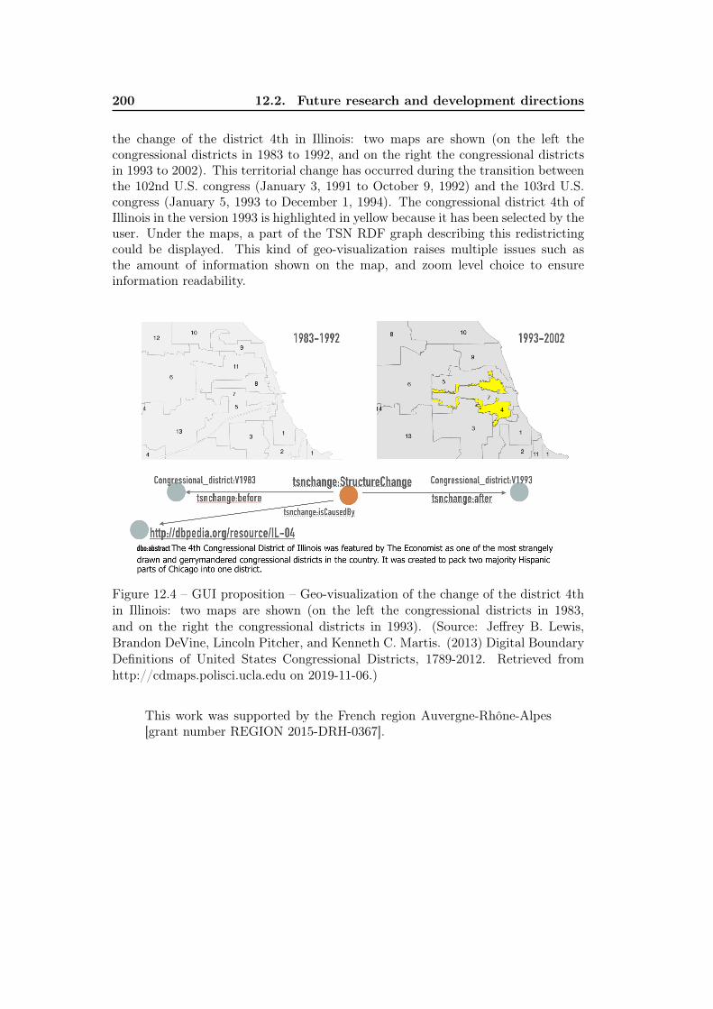
200 12.2. Future research and development directions

the change of the district 4th in Illinois: two maps are shown (on the left thecongressional districts in 1983 to 1992, and on the right the congressional districtsin 1993 to 2002). This territorial change has occurred during the transition betweenthe 102nd U.S. congress (January 3, 1991 to October 9, 1992) and the 103rd U.S.congress (January 5, 1993 to December 1, 1994). The congressional district 4th ofIllinois in the version 1993 is highlighted in yellow because it has been selected by theuser. Under the maps, a part of the TSN RDF graph describing this redistrictingcould be displayed. This kind of geo-visualization raises multiple issues such asthe amount of information shown on the map, and zoom level choice to ensureinformation readability.

Figure 12.4 – GUI proposition – Geo-visualization of the change of the district 4thin Illinois: two maps are shown (on the left the congressional districts in 1983,and on the right the congressional districts in 1993). (Source: Jeffrey B. Lewis,Brandon DeVine, Lincoln Pitcher, and Kenneth C. Martis. (2013) Digital BoundaryDefinitions of United States Congressional Districts, 1789-2012. Retrieved fromhttp://cdmaps.polisci.ucla.edu on 2019-11-06.)

This work was supported by the French region Auvergne-Rhône-Alpes[grant number REGION 2015-DRH-0367].

References

Ablimit Aji, Fusheng Wang, Hoang Vo, Rubao Lee, Qiaoling Liu, Xiaodong Zhang,and Joel Saltz. Hadoop gis: a high performance spatial data warehousing systemover mapreduce. Proceedings of the VLDB Endowment, 6(11):1009–1020, 2013.

James F. Allen. Maintaining knowledge about temporal intervals. Communicationsof the ACM, 26(11):832–843, 1983. URL http://dl.acm.org/citation.cfm?id=358434.

James F. Allen and George Ferguson. Actions and Events in Interval Temporal Logic,pages 205–245. Springer Netherlands, Dordrecht, 1997. ISBN 978-0-585-28322-7.doi: 10.1007/978-0-585-28322-7_7. URL https://doi.org/10.1007/978-0-585-28322-7_7.

Clive W Anderson, Vic Barnett, Philip C Chatwin, and Abdel H El-Shaarawi. Quan-titative Methods for Current Environmental Issues. Springer Science & BusinessMedia, 2012.

Schwering Angela. Approaches to semantic similarity measurement for geospatialdata: A survey. Transactions in GIS, 12(1):5–29, 2008. doi: 10.1111/j.1467-9671.2008.01084.x. URL https://onlinelibrary.wiley.com/doi/abs/10.1111/j.1467-9671.2008.01084.x.

Rob Atkinson. QB4ST: RDF Data Cube extensions for spatio-temporal components,2017. URL https://www.w3.org/TR/qb4st/.

Bruno Bachimont, Antoine Isaac, and Raphaël Troncy. Semantic commitment fordesigning ontologies: a proposal. In International Conference on Knowledge En-gineering and Knowledge Management, pages 114–121. Springer, 2002. URLhttp://link.springer.com/chapter/10.1007/3-540-45810-7_14.

Ben Balter. Diffable, more customizable maps, 2014. URL https://blog.github.com/2014-02-05-diffable-more-customizable-maps/.

Sandipto Banerjee and Karen C Davis. Modeling data warehouse schema evolutionover extended hierarchy semantics. In Journal on Data Semantics XIII, pages72–96. Springer, 2009.

Evdoxios Baratis, Euripides GM Petrakis, Sotiris Batsakis, Nikolaos Maris, andNikolaos Papadakis. TOQL: Temporal ontology querying language. In Interna-tional Symposium on Spatial and Temporal Databases, pages 338–354. Springer,2009. URL http://link.springer.com/chapter/10.1007/978-3-642-02982-0_22.

Sotiris Batsakis and Euripides GM Petrakis. SOWL: a framework for handlingspatio-temporal information in OWL 2.0. In International Workshop on Rulesand Rule Markup Languages for the Semantic Web, pages 242–249. Springer, 2011.

202 References

URL http://link.springer.com/10.1007%2F978-3-642-22546-8_19.

Sotiris Batsakis, Euripides G.M. Petrakis, Ilias Tachmazidis, and Grigoris Antoniou.Temporal representation and reasoning in OWL 2. Semantic Web, 8(6):981–1000,2017. doi: 10.3233/SW-160248. URL http://www.medra.org/servlet/aliasResolver?alias=iospress&doi=10.3233/SW-160248.

Atef Bel Adj Ali and François Vauglin. Geometric Matching of Polygons in GISsand assessment of Geometrical Quality of Polygons. In Michael Goodchild Wen-zhong Shi and Peter Fisher, editors, International Symposium on Spatial DataQuality’99, pages 33–43, Hong Kong Polytechnic University, 1999.

Aaron Beller. Spatial/temporal events in a GIS. In Proceedings of GIS/LIS, vol-ume 91, page 4, 1991.

Mark de Berg, editor. Computational geometry: algorithms and applications.Springer, Berlin, 3rd ed edition, 2008. ISBN 978-3-540-77973-5.

Camille Bernard, Marlène Villanova-Oliver, Jérôme Gensel, and Benoit Le Rubrus.Spatio-Temporal evolutive Data Infrastructure: a Spatial Data Infrastructurefor managing data flows of Territorial Statistical Information. InternationalJournal of Digital Earth, 10(3):257–283, March 2017. ISSN 1753-8947, 1753-8955. URL https://www.tandfonline.com/doi/full/10.1080/17538947.2016.1222003.

Camille Bernard, Christine Plumejeaud-Perreau, Marlène Villanova-Oliver, JérômeGensel, and Hy Dao. An ontology-based algorithm for managing the evolutionof multi-level territorial partitions. In Proceedings of the 26th ACM SIGSPA-TIAL International Conference on Advances in Geographic Information Systems,SIGSPATIAL ’18, pages 456–459, New York, NY, USA, 2018a. ACM. ISBN 978-1-4503-5889-7. doi: 10.1145/3274895.3274944. URL http://doi.acm.org/10.1145/3274895.3274944.

Camille Bernard, Marlène Villanova-Oliver, Jérôme Gensel, and Hy Dao. Modelingchanges in territorial partitions over time: Ontologies tsn and tsn-change. InProceedings of the 33rd Annual ACM Symposium on Applied Computing, SAC’18, pages 866–875. ACM, 2018b. ISBN 978-1-4503-5191-1. doi: 10.1145/3167132.3167227. URL http://doi.acm.org/10.1145/3167132.3167227.

Tim Berners-Lee, James Hendler, Ora Lassila, and others. The semantic web. Sci-entific american, 284(5):28–37, 2001.

Boundless. GeoGit in Action: Distributed Versioning Geospatial Data - Boundless,March 2014a. URL https://boundlessgeo.com/2014/03/geogit-distributed-versioning/.

Boundless. Introducing Versio: Version Control for Spatial Data - Boundless, Octo-ber 2014b. URL https://boundlessgeo.com/2014/10/introducing-versio/.

References 203

U.S. Census Bureau Census Tracts Geographic Products Branch. Census Tracts,2013. URL https://www2.census.gov/geo/pdfs/education/CensusTracts.pdf.

Tao Cheng and Monsuru Adepeju. Modifiable Temporal Unit Problem (MTUP)and Its Effect on Space-Time Cluster Detection. PLoS ONE, 9(6):e100465, June2014. ISSN 1932-6203. doi: 10.1371/journal.pone.0100465. URL https://dx.plos.org/10.1371/journal.pone.0100465.

Paolo Ciccarese, Stian Soiland-Reyes, Khalid Belhajjame, Alasdair JG Gray, CaroleGoble, and Tim Clark. Pav ontology: provenance, authoring and versioning.Journal of biomedical semantics, 4(1):37, 2013.

Christophe Claramunt and Marius Thériault. Managing Time in GIS An Event-Oriented Approach. In C. J. van Rijsbergen, James Clifford, and Alexan-der Tuzhilin, editors, Recent Advances in Temporal Databases, pages 23–42.Springer London, London, 1995. ISBN 978-3-540-19945-8 978-1-4471-3033-8. URLhttp://link.springer.com/10.1007/978-1-4471-3033-8_2. DOI:10.1007/978-1-4471-3033-8_2.

Arzu Çöltekin, Stefano De Sabbata, Corina Willi, Irene Vontobel, Sebastian Pfister,Matthias Kuhn, and Martin Lacayo. Modifiable temporal unit problem. In IS-PRS/ICA workshop. Persistent problems in geographic visualization (ICC2011),Paris, France, volume 2, 2011.

Reidar Conradi and Bernhard Westfechtel. Version models for software configurationmanagement. ACM Computing Surveys (CSUR), 30(2):232–282, 1998. URL http://dl.acm.org/citation.cfm?id=280280.

Gianluca Correndo and Nigel Shadbolt. Linked nomenclature of territorial units forstatistics. Semantic Web, 4(3):251–256, 2013. URL http://content.iospress.com/articles/semantic-web/sw079.

Gianluca Correndo, Alberto Granzotto, Manuel Salvadores, Wendy Hall, and NigelShadbolt. A linked data representation of the nomenclature of territorial unitsfor statistics. 2010. URL http://eprints.soton.ac.uk/271876/.

Franck Cotton, Richard Cyganiak, RTAM Grim, Daniel W Gillman, Yves Jaques,and Wendy Thomas. Xkos: An skos extension for statistical classifications. InProceedings of the 59th World Statistics Congress of the International StatisticalInstitute The Hague, The Netherlands. Citeseer, 2013. URL http://2013.isiproceedings.org/Files/CPS203-P32-S.pdf.

Simon Cox and Chris Little. Time Ontology in OWL - W3C Recommendation 19October 2017, 2017. URL https://www.w3.org/TR/owl-time/.

Richard Cyganiak and Dave Reynolds. The RDF Data Cube Vocabulary, 2014.URL https://www.w3.org/TR/vocab-data-cube/.

Richard Cyganiak, David Wood, and Markus Lanthaler. RDF 1.1 Concepts andAbstract Syntax, 2014. URL https://www.w3.org/TR/rdf11-concepts/.

204 References

Christophe Debruyne, Alan Meehan, Éamonn Clinton, Lorraine McNerney, AtulNautiyal, Peter Lavin, and Declan O’Sullivan. Ireland’s authoritative geospatiallinked data. In International Semantic Web Conference, pages 66–74. Springer,2017.

Géraldine Del Mondo, John G Stell, Christophe Claramunt, and Rémy Thibaud. Agraph model for spatio-temporal evolution. J. UCS, 16(11):1452–1477, 2010.

Géraldine Del Mondo, M.A. Rodríguez, C. Claramunt, L. Bravo, and R. Thibaud.Modeling consistency of spatio-temporal graphs. Data & Knowledge Engineer-ing, 84:59–80, March 2013. ISSN 0169023X. doi: 10.1016/j.datak.2012.12.007. URL http://linkinghub.elsevier.com/retrieve/pii/S0169023X12001188.

Thomas Devogele. A new merging process for data integration based on the discretefréchet distance. In Advances in spatial data handling, pages 167–181. Springer,2002.

Martin Doerr. The CIDOC conceptual reference module: an ontological approachto semantic interoperability of metadata. AI magazine, 24(3):75–75, 2003.

Lisa Ehrlinger and Wolfram Wöß. Towards a definition of knowledge graphs. SE-MANTiCS (Posters, Demos, SuCCESS), 48, 2016.

ESRI. United States census geography—Related Concepts | ArcGIS,2017. URL https://learn.arcgis.com/en/related-concepts/united-states-census-geography.htm.

Lorena Etcheverry and Alejandro A Vaisman. QB4OLAP: a new vocabulary forOLAP cubes on the semantic web. Proceedings of COLD, 2012.

European Joint Research Centre. D2.8.III.10 INSPIRE Data Specification on Pop-ulation Distribution - Technical Guidelines, 2013a. URL https://inspire.ec.europa.eu/id/document/tg/pd.

European Joint Research Centre. D2.8.III.1 INSPIRE Data Specification on Statis-tical Units - Technical Guidelines, 2013b. URL https://inspire.ec.europa.eu/id/document/tg/su.

Eurostat. Manual of concepts on land cover and land use information systems. Officefor Official Publications of the European Communities, Luxembourg, 2001. ISBN978-92-894-0432-7. OCLC: 464871883.

Rihab Fahd and Arwa Yousuf. Linked Open Data Life Cycle. International Journalof Computer Applications, 175(3):34–39, October 2017. ISSN 09758887. doi: 10.5120/ijca2017915489. URL http://www.ijcaonline.org/archives/volume175/number3/almutawa-2017-ijca-915489.pdf.

Bernadette Farias Lóscio, Caroline Burle, and Newton Calegari. Data on the WebBest Practices - W3C Recommendation, January 2017. URL https://www.w3.org/TR/dwbp/.

References 205

James D Fearon. What is identity (as we now use the word)? Unpublishedmanuscript, Stanford University, Stanford, Calif, 1999.

Thore Fechner, Dennis Wilhelm, and Christian Kray. Ethermap: Real-time col-laborative map editing. In Proceedings of the 33rd Annual ACM Conference onHuman Factors in Computing Systems, CHI ’15, pages 3583–3592, New York,NY, USA, 2015. ACM. ISBN 978-1-4503-3145-6. doi: 10.1145/2702123.2702536.URL http://doi.acm.org/10.1145/2702123.2702536.

Robin Flowerdew. Data integration: statistical methods for transferring data be-tween zonal systems. In Handling geographical information: methodology andpotential applications, pages 39–54, 1991.

Andrew Frank, Jonathan Raper, and Jean-Paul Cheylan. Life and Motion of Socio-Economic Units: GISDATA, volume 8. CRC Press, 2003.

Alessandro Furieri. Optimizing SQL access to really complex polygons,2011. URL http://www.gaia-gis.it/spatialite-3.0.0-BETA1/WorldBorders.pdf.

Francisco Javier Gallego. A population density grid of the European Union. Popula-tion and Environment, 31(6):460–473, July 2010. ISSN 0199-0039, 1573-7810. doi:10.1007/s11111-010-0108-y. URL http://link.springer.com/10.1007/s11111-010-0108-y.

Felix Gantner. A Spatiotemporal Ontology for the Administrative Units of Switzer-land. Theses, University of Zurich - Switzerland , April 2011.

A. E. Gelfand. On the change of support problem for spatio-temporal data. Bio-statistics, 2(1):31–45, March 2001. ISSN 14654644, 14684357. doi: 10.1093/biostatistics/2.1.31. URL https://academic.oup.com/biostatistics/article-lookup/doi/10.1093/biostatistics/2.1.31.

Michael F Goodchild, Nina Siu Ngan Lam, and University of Western Ontario.Dept. of Geography. Areal interpolation: a variant of the traditional spatial prob-lem. London, Ont.: Department of Geography, University of Western Ontario,1980.

Carol A Gotway Crawford and LJ Young. Change of support: an inter-disciplinarychallenge. Geostatistics for environmental applications, pages 1–13, 2005.

August Gotzfried and Marco Pellegrino. The Euro-SDMX Metadata structure andquality indicators, 2008. URL https://unstats.un.org/unsd/ccsa/cdqio-2008/Ses1-Pap4.pdf.

Claude Grasland and Malika Madelin. Modifiable Area Unit Problem. ESPON, 2006.URL https://halshs.archives-ouvertes.fr/halshs-00174241.

Pierre Grenon and Barry Smith. SNAP and SPAN: Towards Dynamic Spatial Ontol-ogy. Spatial Cognition & Computation, 4(1):69–104, March 2004. ISSN 1387-5868,1542-7633. doi: 10.1207/s15427633scc0401_5. URL http://www.tandfonline.com/doi/abs/10.1207/s15427633scc0401_5.

206 References

Q. Guo, B. Palanisamy, and H. A. Karimi. A mapreduce algorithm for polygonretrieval in geospatial analysis. In 2015 IEEE 8th International Conference onCloud Computing, pages 901–908, June 2015. doi: 10.1109/CLOUD.2015.123.

Willem Robert van Hage, Véronique Malaisé, Roxane H. Segers, Laura Hollink,and Guus Schreiber. Design and use of the Simple Event Model (SEM). WebSemantics: Science, Services and Agents on the World Wide Web, 9(2), 2011.ISSN 1570-8268. URL http://www.websemanticsjournal.org/index.php/ps/article/view/190.

Benjamin Harbelot, Helbert Arenas, and Christophe Cruz. Continuum: A spa-tiotemporal data model to represent and qualify filiation relationships. In Pro-ceedings of the 4th ACM SIGSPATIAL International Workshop on GeoStreaming,pages 76–85. ACM, 2013. URL http://dl.acm.org/citation.cfm?id=2534312.

Benjamin Harbelot, Helbert Arenas, and Christophe Cruz. LC3: A spatio-temporaland semantic model for knowledge discovery from geospatial datasets. WebSemantics: Science, Services and Agents on the World Wide Web, 35:3–24,2015. URL http://www.sciencedirect.com/science/article/pii/S1570826815000840.

Steve Harris and Andy Seaborne. SPARQL 1.1 Query Language, 2013. URL https://www.w3.org/TR/sparql11-query.

J. T. Hastings. Automated conflation of digital gazetteer data. International Journalof Geographical Information Science, 22(10):1109–1127, October 2008. ISSN 1365-8816. doi: 10.1080/13658810701851453. URL https://doi.org/10.1080/13658810701851453.

Michael Hausenblas. 5-star Open Data, January 2012. URL https://5stardata.info/en/.

Daniel Hienert and Francesco Luciano. Extraction of Historical Events fromWikipedia. In Elena Simperl, Barry Norton, Dunja Mladenic, EmanueleDella Valle, Irini Fundulaki, Alexandre Passant, and Raphaël Troncy, editors,The Semantic Web: ESWC 2012 Satellite Events, volume 7540, pages 16–28.Springer Berlin Heidelberg, Berlin, Heidelberg, 2015. ISBN 978-3-662-46640-7978-3-662-46641-4. doi: 10.1007/978-3-662-46641-4_2. URL http://link.springer.com/10.1007/978-3-662-46641-4_2.

Jonathan K Hodge, Emily Marshall, and Geoff Patterson. Gerrymandering andconvexity. The College Mathematics Journal, 41(4):312–324, 2010.

Kathleen Hornsby and Max J. Egenhofer. Identity-based change: a foundation forspatio-temporal knowledge representation. International Journal of GeographicalInformation Science, 14(3):207–224, April 2000. ISSN 1365-8816, 1362-3087. doi:10.1080/136588100240813. URL http://www.tandfonline.com/doi/abs/10.1080/136588100240813.

References 207

Erick Howenstine. Measuring demographic change: The split tract problem. Pro-fessional Geographer, 45(4):425, November 1993. ISSN 00330124.

Wang Huibing, Tang Xinming, Lei Bing, Yang Ping, and Chu Haifeng. Modelingspatial-temporal data in version-difference model. page 4, 2005.

Bernadette Hyland, Ghislain Auguste Atemezing, and Boris Villazón-Terrazas. BestPractices for Publishing Linked Data, January 2014. URL https://www.w3.org/TR/ld-bp/.

Evangelos Kalampokis, Bill Roberts, Areti Karamanou, Efthimios Tambouris, andKonstantinos A Tarabanis. Challenges on Developing Tools for Exploiting LinkedOpen Data Cubes. In SemStats@ ISWC, 2015.

Tomi Kauppinen and Eero Hyvönen. Modeling and reasoning about changes inontology time series. In Ontologies, pages 319–338. Springer, 2007. URL http://link.springer.com/chapter/10.1007/978-0-387-37022-4_11.

Tomi Kauppinen, Jari Väätäinen, and Eero Hyvönen. Creating and using geospa-tial ontology time series in a semantic cultural heritage portal. Springer, 2008.URL http://link.springer.com/chapter/10.1007/978-3-540-68234-9_11.

Setrag N Khoshafian and George P Copeland. Object identity, volume 21. ACM,1986.

Eva Klien and Florian Probst. Requirements for geospatial ontology engineering. In8th conference on geographic information science (AGILE 2005), pages 251–260,2005. URL http://www.agile-online.org/Conference_Paper/CDs/agile_2005/papers/79_Eva%20Klien.pdf.

Javier Lacasta, Francisco Javier Lopez-Pellicer, Aneta Florczyk, Francisco JavierZarazaga-Soria, and Javier Nogueras-Iso. Population of a spatio-temporal knowl-edge base for jurisdictional domains. International Journal of Geographical In-formation Science, 28(9):1964–1987, September 2014. ISSN 1365-8816, 1362-3087. URL http://www.tandfonline.com/doi/abs/10.1080/13658816.2014.911412.

Vladimir Iosifovich Levenshtein. Binary codes capable of correcting deletions, in-sertions and reversals. Soviet Physics Doklady, 10(8):707–710, 1966. DokladyAkademii Nauk SSSR, V163 No4 845-848 1965.

Linna Li and Michael F. Goodchild. An optimisation model for linear featurematching in geographical data conflation. International Journal of Image andData Fusion, 2(4):309–328, December 2011. ISSN 1947-9832, 1947-9824. doi:10.1080/19479832.2011.577458. URL http://www.tandfonline.com/doi/abs/10.1080/19479832.2011.577458.

LocationTech. GeoGig, April 2018. URL http://geogig.org/.

208 References

Martin Loidl, Gudrun Wallentin, Robin Wendel, and Bernhard Zagel. Mappingbicycle crash risk patterns on the local scale. Safety, 2(3), 2016. ISSN 2313-576X. doi: 10.3390/safety2030017. URL http://www.mdpi.com/2313-576X/2/3/17.

Paul A Longley, Michael F Goodchild, David J Maguire, and David W Rhind.Geographic information systems and science. John Wiley & Sons, 2005.

Francisco J. López-Pellicer, Aneta J. Florczyk, Javier Lacasta, Francisco JavierZarazaga-Soria, and Pedro R. Muro-Medrano. Administrative units, an ontologi-cal perspective. In Advances in Conceptual Modeling–Challenges and Opportuni-ties, pages 354–363. Springer, 2008. URL http://link.springer.com/chapter/10.1007/978-3-540-87991-6_42.

Francisco J. Lopez-Pellicer, Javier Lacasta, Aneta Florczyk, Javier Nogueras-Iso,and F. Javier Zarazaga-Soria. An ontology for the representation of spatiotempo-ral jurisdictional domains in information retrieval systems. International Journalof Geographical Information Science, 26(4):579–597, April 2012. ISSN 1365-8816,1362-3087. URL http://www.tandfonline.com/doi/abs/10.1080/13658816.2011.599811.

Romain Louvet, Didier Josselin, Jagannath Aryal, and Cyrille Genre-Grandpierre.R as a GIS: Illustrating Scale and Aggregation Problems with Forest FireData. In Proceedings of Spatial Statistics 2015 - Procedia Environmental Sci-ences, volume 27, pages 66–69. Elsevier - Science Direct , June 2015. URLhttps://hal.archives-ouvertes.fr/hal-01251316.

Alexander Maedche and Steffen Staab. Learning ontologies for the semantic web.In Proceedings of the Second International Conference on Semantic Web-Volume40, pages 51–60. CEUR-WS. org, 2001. URL http://dl.acm.org/citation.cfm?id=2889973.

Hélène Mathian and Lena Sanders. Spatio-temporal approaches: Geographic objectsand change process. John Wiley & Sons, 2014.

Grant McKenzie, Krzysztof Janowicz, and Benjamin Adams. A weighted multi-attribute method for matching user-generated Points of Interest. Cartographyand Geographic Information Science, 41(2), March 2014. ISSN 1523-0406, 1545-0465. doi: 10.1080/15230406.2014.880327. URL http://www.tandfonline.com/doi/abs/10.1080/15230406.2014.880327.

Vereinte Nationen, editor. International merchandise trade statistics: compilersmanual. Number 87 in [Studies in methods] / United Nations, Department ofEconomic and Social Affairs, Statistics Division Ser. F. United Nations, NewYork, 2004. ISBN 978-92-1-161454-1. OCLC: 250039369.

Marco Negretti. Operation-based revision control for geospatial data sets. page 15,2015.

Natalya F. Noy and Michel Klein. Ontology Evolution: Not the Same as SchemaEvolution. Knowledge and Information Systems, 6(4):428–440, July 2004. ISSN

References 209

0219-1377, 0219-3116. doi: 10.1007/s10115-003-0137-2. URL http://link.springer.com/10.1007/s10115-003-0137-2.

OECD. OECD glossary of statistical terms. 2008. URL https://ec.europa.eu/eurostat/ramon/coded_files/OECD_glossary_stat_terms.pdf.

Ontotext. What is a Knowledge Graph?, 2018. URL https://www.ontotext.com/knowledgehub/fundamentals/what-is-a-knowledge-graph/.

Stan Openshaw. The modifiable areal unit problem. Concepts and Techniques inModern Geography, 38, 1984. ISSN 0 86094 134 5. URL https://ci.nii.ac.jp/naid/10024464407/en/.

Stan Openshaw and Peter J Taylor. A million or so correlation coefficients: threeexperiments on the modifiable areal unit problem. Statistical applications in thespatial sciences, 21:127–144, 1979.

Heiko Paulheim. Knowledge graph refinement: A survey of approaches and evalua-tion methods. Semantic web, 8(3):489–508, 2017.

Torben Bach Pedersen, Christian S Jensen, and Curtis E Dyreson. Extending practi-cal pre-aggregation in on-line analytical processing. In Proceedings of the 25th In-ternational Conference on Very Large Data Bases, pages 663–674. Morgan Kauf-mann Publishers Inc., 1999.

Matthew Perry and John Herring. OGC GeoSPARQL - A Geographic Query Lan-guage for RDF Data. page 75, 2012.

Christine Plumejeaud. Modèles et méthodes pour l’information spatio-temporelleévolutive. PhD thesis, Université de Grenoble, 2011.

Christine Plumejeaud, Julie Prud’homme, Paule-Annick Davoine, and JérômeGensel. Transferring Indicators into Different Partitions of Geographic Space.In David Taniar, Osvaldo Gervasi, Beniamino Murgante, Eric Pardede, andBernady O. Apduhan, editors, Computational Science and Its ApplicationsICCSA 2010, volume 6016 of Lecture Notes in Computer Science, pages 445–460,Heidelberg, 2010. Springer. ISBN 978-3-642-12155-5.

Christine Plumejeaud, Hélène Mathian, Jérôme Gensel, and Claude Grasland.Spatio-temporal analysis of territorial changes from a multi-scale perspective.International Journal of Geographical Information Science, 25(10):1597–1612,2011. URL http://www.tandfonline.com/doi/abs/10.1080/13658816.2010.534658.

Mgr Petr Přidal and Petr Žabička. Tiles as an approach to on-line publishing ofscanned old maps, vedute and other historical documents. e-Perimetron, 3(1):10–21, 2008.

Yves Raimond, Samer A Abdallah, Mark B Sandler, and Frederick Giasson. Themusic ontology, 2007.

210 References

Gabriel Recchia and Max Louwerse. A Comparison of String Similarity Measures forToponymMatching. In Proceedings of The First ACM SIGSPATIAL InternationalWorkshop on Computational Models of Place - COMP ’13, pages 54–61, OrlandoFL, USA, 2013. ACM Press. ISBN 978-1-4503-2535-6. doi: 10.1145/2534848.2534850. URL http://dl.acm.org/citation.cfm?doid=2534848.2534850.

Timothy Redmond, Michael Smith, Nick Drummond, and Tania Tudorache. Man-aging Change: An Ontology Version Control System. page 10, 2008.

Agnar Renolen. History graphs: Conceptual modeling of spatio-temporal data. Gisfrontiers in business and science, 2:46, 1996.

Agnar Renolen. Conceptual modelling and spatiotemporal information systems:how to model the real world. In ScanGIS, volume 97, pages 1–22, 1997.

Margaret Rouse. What is versioning?, 2007. URL https://searchsoftwarequality.techtarget.com/definition/versioning.

Juan J. Ruiz, F. Javier Ariza, Manuel A. Ureña, and Elidia B. Blázquez. Digital mapconflation: a review of the process and a proposal for classification. InternationalJournal of Geographical Information Science, 25(9):1439–1466, September 2011.ISSN 1365-8816. doi: 10.1080/13658816.2010.519707. URL https://doi.org/10.1080/13658816.2010.519707.

Tuukka Ruotsalo and Eero Hyvönen. An event-based approach for semantic meta-data interoperability. In The Semantic Web, pages 409–422. Springer, 2007.

Nayan B Ruparelia. The history of version control. ACM SIGSOFT Software En-gineering Notes, 35(1):5–9, 2010.

Robert D. Sack. Human Territoriality: A Theory. Annals of the Association ofAmerican Geographers, 73(1):55–74, March 1983. ISSN 0004-5608, 1467-8306.doi: 10.1111/j.1467-8306.1983.tb01396.x. URL http://www.tandfonline.com/doi/abs/10.1111/j.1467-8306.1983.tb01396.x.

Percy E Rivera Salas, Michael Martin, Fernando Maia Da Mota, Sören Auer, KarinBreitman, and Marco A Casanova. Publishing statistical data on the web. In2012 IEEE Sixth International Conference on Semantic Computing, pages 285–292. IEEE, 2012.

Rui Santos, Patricia Murrieta-Flores, and Bruno Martins. Learning to combinemultiple string similarity metrics for effective toponym matching. InternationalJournal of Digital Earth, 11(9):913–938, September 2018. ISSN 1753-8947, 1753-8955. doi: 10.1080/17538947.2017.1371253. URL https://www.tandfonline.com/doi/full/10.1080/17538947.2017.1371253.

Ansgar Scherp, Thomas Franz, Carsten Saathoff, and Steffen Staab. F–a model ofevents based on the foundational ontology dolce+ dns ultralight. In Proceedingsof the fifth international conference on Knowledge capture, pages 137–144. ACM,2009.

References 211

SDMX. SDMX 2.1 User Guides | SDMX – Statistical Data and Metadata eXchange,2012. URL https://sdmx.org/wp-content/uploads/SDMX_2-1_User_Guide_draft_0-1.pdf.

Ryan Shaw, Raphaël Troncy, and Lynda Hardman. LODE: Linking Open Descrip-tions of Events. ASWC, 9:153–167, 2009.

Shashi Shekhar and Hui Xiong. Encyclopedia of GIS. Springer Science & BusinessMedia, 2007.

Theodore Sider. Four-dimensionalism: An ontology of persistence and time. OxfordUniversity Press on Demand, 2001.

Evren Sirin. A Path of Our Own - Stardog, 2017. URL https://www.stardog.com/blog/a-path-of-our-own/.

Barry Smith and Achille C Varzi. Fiat and bona fide boundaries. Philosophy andphenomenological research, 60(2):401–420, 2000.

Office fédéral de la statistique. Liste historisée des communes de laSuisse - Explication et utilisation | Publication. Publication do-f-00.04-hgv-01, Office fédéral de la statistique, December 2017. URLhttps://www.bfs.admin.ch/bfs/fr/home/statistiques/catalogues-banques-donnees/publications.assetdetail.4062823.html.

Kostas Stefanidis, Ioannis Chrysakis, and Giorgos Flouris. On Designing ArchivingPolicies for Evolving RDF Datasets on the Web. In Eric Yu, Gillian Dobbie,Matthias Jarke, and Sandeep Purao, editors, Conceptual Modeling: 33rd Interna-tional Conference, ER 2014, Atlanta, GA, USA, October 27-29, 2014. Proceed-ings, pages 43–56. Springer International Publishing, Cham, 2014. ISBN 978-3-319-12206-9. URL http://dx.doi.org/10.1007/978-3-319-12206-9_4. DOI: 10.1007/978-3-319-12206-9_4.

Margaret-Anne D Storey, Davor Čubranić, and Daniel M German. On the use ofvisualization to support awareness of human activities in software development: asurvey and a framework. In Proceedings of the 2005 ACM symposium on Softwarevisualization, pages 193–202. ACM, 2005.

Chengyu Sun, Divyakant Agrawal, and Amr El Abbadi. Hardware acceleration forspatial selections and joins. In Proceedings of the 2003 ACM SIGMOD interna-tional conference on Management of data, pages 455–466. ACM, 2003.

Jeremy Tandy, Linda Van Den Brink, and Payam Barnaghi. Spatial data on theWeb Best Practices - OGC and W3C Recommendation, January 2017. URLhttps://www.w3.org/TR/sdw-bp.

Anton Telechev and Benoit Le Rubrus. Nomenclatures Support, 2013. URLhttp://database.espon.eu/db2/jsf/NomenclatureSupport/NomenclatureSupport_onehtml/index.html.

212 References

Walter Tichy. Software Configuration Management Overview. Citeseer,1988. URL http://citeseerx.ist.psu.edu/viewdoc/download?doi=10.1.1.102.8965&rep=rep1&type=pdf.

Ba-Huy Tran, Christine Plumejeaud-Perreau, Alain Bouju, and Vincent Bretagnolle.A semantic mediator for handling heterogeneity of spatio-temporal environmentdata. In Research Conference on Metadata and Semantics Research, pages 381–392. Springer, 2015. URL http://link.springer.com/chapter/10.1007/978-3-319-24129-6_33.

A. Vandecasteele and R. Devillers. Improving volunteered geographic data qualityusing semantic similarity measurements. ISPRS - International Archives of thePhotogrammetry, Remote Sensing and Spatial Information Sciences, XL-2/W1:143–148, May 2013. ISSN 1682-1777. doi: 10.5194/isprsarchives-XL-2-W1-143-2013. URL http://www.int-arch-photogramm-remote-sens-spatial-inf-sci.net/XL-2-W1/143/2013/.

Gaurav Vazirani. Metaphysics: Ship of Theseus, 2014. URL https://www.khanacademy.org/partner-content/wi-phi/wiphi-metaphysics-epistemology/wiphi-metaphysics/v/ship-of-theseus.

Boris Villazón-Terrazas, Luis. M. Vilches-Blázquez, Oscar Corcho, and AsunciónGómez-Pérez. Methodological Guidelines for Publishing Government LinkedData. In David Wood, editor, Linking Government Data, pages 27–49. SpringerNew York, New York, NY, 2011. ISBN 978-1-4614-1767-5. doi: 10.1007/978-1-4614-1767-5_2. URL https://doi.org/10.1007/978-1-4614-1767-5_2.

Max Völkel and Tudor Groza. SemVersion: an RDF-based ontology versioningsystem. page 9, March 2012.

M. Wachowicz. Object-Oriented Design for Temporal GIS. Research Monographs inGIS. Taylor & Francis, 2003. ISBN 9780203212394.

Fahui Wang. Quantitative methods and socio-economic applications in GIS. CRCPress, 2014.

Chris Welty, Richard Fikes, and Selene Makarios. A reusable ontology for fluents inOWL. In FOIS, volume 150, pages 226–236, 2006.

Stefan Wiemann and Lars Bernard. Spatial data fusion in Spatial Data Infras-tructures using Linked Data. International Journal of Geographical Informa-tion Science, 30(4):613–636, April 2016. ISSN 1365-8816, 1362-3087. doi:10.1080/13658816.2015.1084420. URL http://www.tandfonline.com/doi/full/10.1080/13658816.2015.1084420.

Dan Yamamoto, Akira Ioku, Yoko Seki, Akie Mizutani, Junichi Matsuda, HideakiTakeda2 Ikki Ohmukai, Fumihiro Kato, Seiji Koide, and Shoki Nishimura. Ge-ographic Area Representations in Statistical Linked Open Data of Japan. InHybridSemStats@ISWC, 2017.

References 213

Ronan Ysebaert, Isabelle Salmon, Benoit Le Rubrus, and Camille Bernard. Recueil,traçabilité et restitution des données territoriales du programme ESPON. page 21,April 2017.

C. Zhang, W. Li, and T. Zhao. Geospatial data sharing based on geospatial semanticweb technologies. Journal of Spatial Science, 52(2):35–49, December 2007. ISSN1449-8596, 1836-5655. doi: 10.1080/14498596.2007.9635121. URL http://www.tandfonline.com/doi/abs/10.1080/14498596.2007.9635121.

Appendix

Appendix A

The Theseus data life cycle

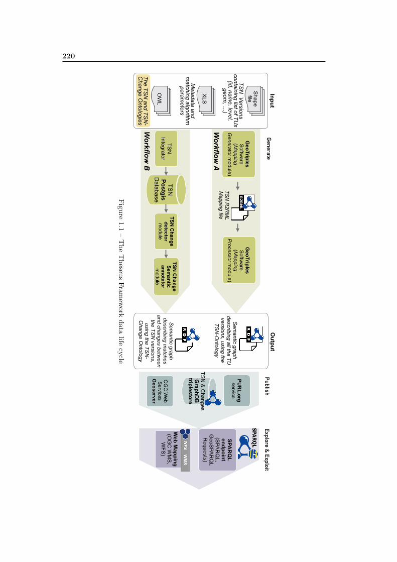
220

Metadata and

matching algorithm

param

eters

Sem

antic graph describing all the TU

versions, using the

TSN

-Ontology

Sem

antic graph describing m

atches and changes betw

een the TS

N versions,

using the TSN

-C

hange Ontology

Input

Shape file

XLS

OW

L

GeoTriples S

oftware

(Mapping

Generator m

odule)TS

N R

2RM

L M

apping file

TSN

Integrator

TSN

Postgis

Database

TSN C

hange detector m

odule

Output

Generate Publish

PUR

L.org service

TSN

& C

hanges G

raphDB

triplestore

OG

C W

eb S

ervices G

eoserver

Explore & Exploit

SPAR

QL

endpoint (S

PAR

QL,

GeoS

PAR

QL

Requests)

Web M

apping (O

GC

WM

S,

WFS

) WM

S

TSN

Versions containing list of TU

s (id, nam

e, level, geom

, …)

The TSN

and TSN

-C

hange Ontologies

Workflow

A

Workflow

B

TSN C

hange Sem

antic annotator

module

GeoTriples S

oftware

(Mapping

Processor m

odule)

Figure

1.1–The

Theseus

Framew

orkdata

lifecycle

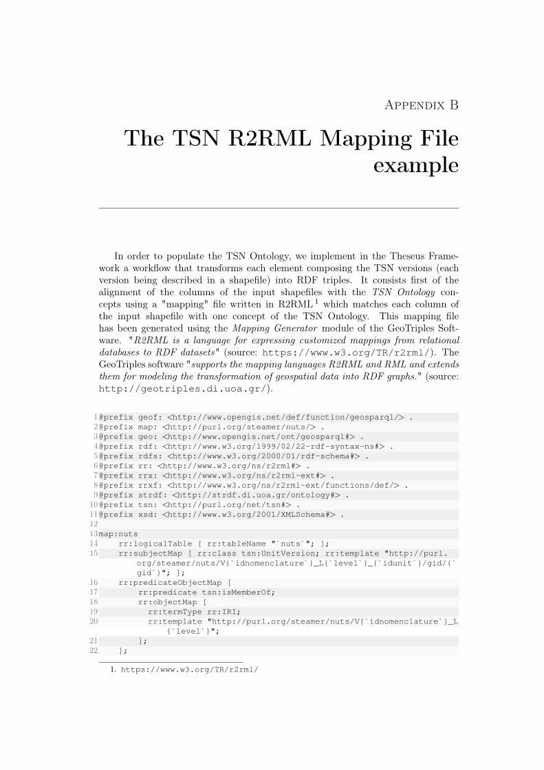
Appendix B

The TSN R2RML Mapping Fileexample

In order to populate the TSN Ontology, we implement in the Theseus Frame-work a workflow that transforms each element composing the TSN versions (eachversion being described in a shapefile) into RDF triples. It consists first of thealignment of the columns of the input shapefiles with the TSN Ontology con-cepts using a "mapping" file written in R2RML 1 which matches each column ofthe input shapefile with one concept of the TSN Ontology. This mapping filehas been generated using the Mapping Generator module of the GeoTriples Soft-ware. "R2RML is a language for expressing customized mappings from relationaldatabases to RDF datasets" (source: https://www.w3.org/TR/r2rml/). TheGeoTriples software "supports the mapping languages R2RML and RML and extendsthem for modeling the transformation of geospatial data into RDF graphs." (source:http://geotriples.di.uoa.gr/).

1@prefix geof: <http://www.opengis.net/def/function/geosparql/> .2@prefix map: <http://purl.org/steamer/nuts/> .3@prefix geo: <http://www.opengis.net/ont/geosparql#> .4@prefix rdf: <http://www.w3.org/1999/02/22-rdf-syntax-ns#> .5@prefix rdfs: <http://www.w3.org/2000/01/rdf-schema#> .6@prefix rr: <http://www.w3.org/ns/r2rml#> .7@prefix rrx: <http://www.w3.org/ns/r2rml-ext#> .8@prefix rrxf: <http://www.w3.org/ns/r2rml-ext/functions/def/> .9@prefix strdf: <http://strdf.di.uoa.gr/ontology#> .10@prefix tsn: <http://purl.org/net/tsn#> .11@prefix xsd: <http://www.w3.org/2001/XMLSchema#> .1213map:nuts14 rr:logicalTable [ rr:tableName "`nuts`"; ];15 rr:subjectMap [ rr:class tsn:UnitVersion; rr:template "http://purl.

org/steamer/nuts/V{`idnomenclature`}_L{`level`}_{`idunit`}/gid/{`gid`}"; ];

16 rr:predicateObjectMap [17 rr:predicate tsn:isMemberOf;18 rr:objectMap [19 rr:termType rr:IRI;20 rr:template "http://purl.org/steamer/nuts/V{`idnomenclature`}_L

{`level`}";21 ];22 ];

1. https://www.w3.org/TR/r2rml/

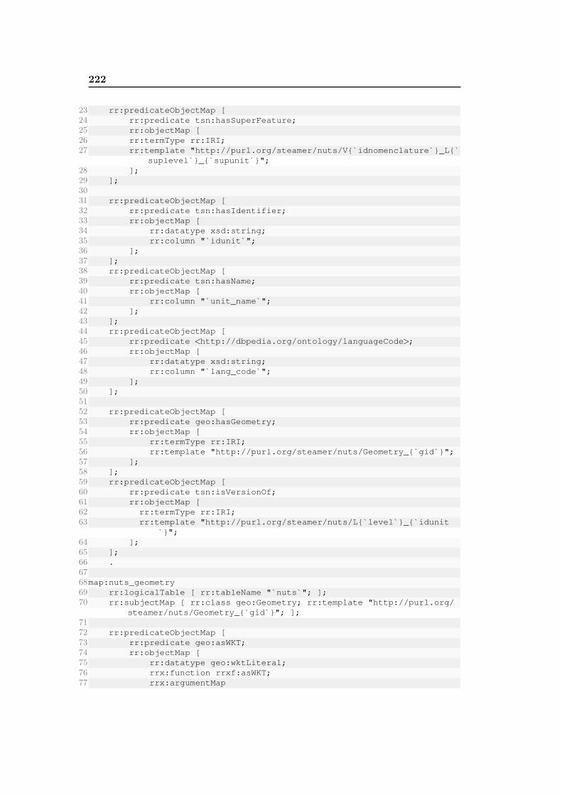
222

23 rr:predicateObjectMap [24 rr:predicate tsn:hasSuperFeature;25 rr:objectMap [26 rr:termType rr:IRI;27 rr:template "http://purl.org/steamer/nuts/V{`idnomenclature`}_L{`

suplevel`}_{`supunit`}";28 ];29 ];3031 rr:predicateObjectMap [32 rr:predicate tsn:hasIdentifier;33 rr:objectMap [34 rr:datatype xsd:string;35 rr:column "`idunit`";36 ];37 ];38 rr:predicateObjectMap [39 rr:predicate tsn:hasName;40 rr:objectMap [41 rr:column "`unit_name`";42 ];43 ];44 rr:predicateObjectMap [45 rr:predicate <http://dbpedia.org/ontology/languageCode>;46 rr:objectMap [47 rr:datatype xsd:string;48 rr:column "`lang_code`";49 ];50 ];5152 rr:predicateObjectMap [53 rr:predicate geo:hasGeometry;54 rr:objectMap [55 rr:termType rr:IRI;56 rr:template "http://purl.org/steamer/nuts/Geometry_{`gid`}";57 ];58 ];59 rr:predicateObjectMap [60 rr:predicate tsn:isVersionOf;61 rr:objectMap [62 rr:termType rr:IRI;63 rr:template "http://purl.org/steamer/nuts/L{`level`}_{`idunit

`}";64 ];65 ];66 .6768map:nuts_geometry69 rr:logicalTable [ rr:tableName "`nuts`"; ];70 rr:subjectMap [ rr:class geo:Geometry; rr:template "http://purl.org/

steamer/nuts/Geometry_{`gid`}"; ];7172 rr:predicateObjectMap [73 rr:predicate geo:asWKT;74 rr:objectMap [75 rr:datatype geo:wktLiteral;76 rrx:function rrxf:asWKT;77 rrx:argumentMap

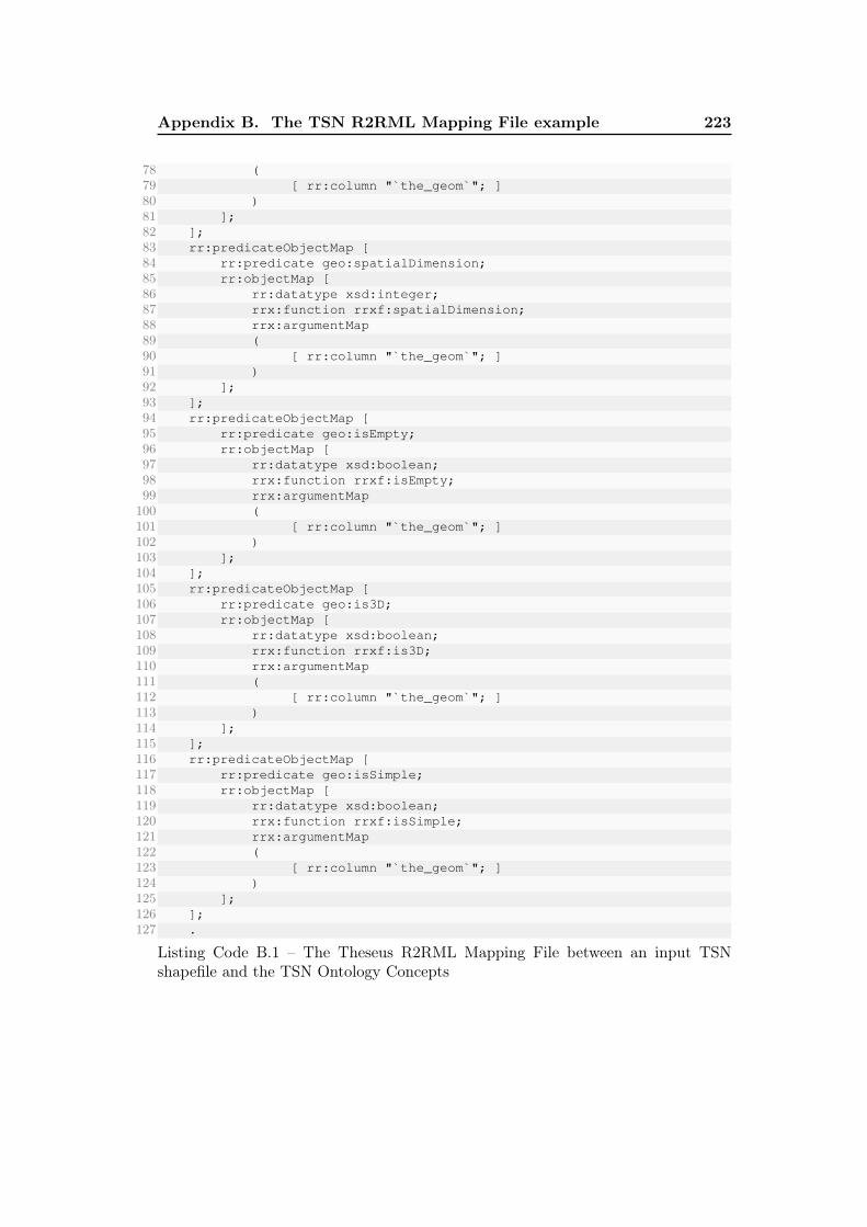
Appendix B. The TSN R2RML Mapping File example 223

78 (79 [ rr:column "`the_geom`"; ]80 )81 ];82 ];83 rr:predicateObjectMap [84 rr:predicate geo:spatialDimension;85 rr:objectMap [86 rr:datatype xsd:integer;87 rrx:function rrxf:spatialDimension;88 rrx:argumentMap89 (90 [ rr:column "`the_geom`"; ]91 )92 ];93 ];94 rr:predicateObjectMap [95 rr:predicate geo:isEmpty;96 rr:objectMap [97 rr:datatype xsd:boolean;98 rrx:function rrxf:isEmpty;99 rrx:argumentMap

100 (101 [ rr:column "`the_geom`"; ]102 )103 ];104 ];105 rr:predicateObjectMap [106 rr:predicate geo:is3D;107 rr:objectMap [108 rr:datatype xsd:boolean;109 rrx:function rrxf:is3D;110 rrx:argumentMap111 (112 [ rr:column "`the_geom`"; ]113 )114 ];115 ];116 rr:predicateObjectMap [117 rr:predicate geo:isSimple;118 rr:objectMap [119 rr:datatype xsd:boolean;120 rrx:function rrxf:isSimple;121 rrx:argumentMap122 (123 [ rr:column "`the_geom`"; ]124 )125 ];126 ];127 .

Listing Code B.1 – The Theseus R2RML Mapping File between an input TSNshapefile and the TSN Ontology Concepts