INSTITUTE OF PHYSICS PUBLISHING CLASSICAL AND QUANTUM GRAVITY

Class. Quantum Grav. 23 (2006) 1801–1814 doi:10.1088/0264-9381/23/5/019

Identifying deterministic signals in simulatedgravitational wave data: algorithmic complexityand the surrogate data method

Yi Zhao1, Michael Small1, David Coward2, Eric Howell2,Chunnong Zhao2, Li Ju2 and David Blair2

1 Hong Kong Polytechnic University, Kowloon, Hong Kong, People’s Republic of China2 School of Physics, The University of Western Australia, Crawley, WA 6009, Australia

E-mail: zhao.yi@polyu.edu.hk

Received 21 June 2005, in final form 3 January 2006Published 20 February 2006Online at stacks.iop.org/CQG/23/1801

AbstractWe describe the application of complexity estimation and the surrogate datamethod to identify deterministic dynamics in simulated gravitational wave(GW) data contaminated with white and coloured noises. The surrogate methoduses algorithmic complexity as a discriminating statistic to decide if noisydata contain a statistically significant level of deterministic dynamics (the GWsignal). The results illustrate that the complexity method is sensitive to a smallamplitude simulated GW background (SNR down to 0.08 for white noise and0.05 for coloured noise) and is also more robust than commonly used linearmethods (autocorrelation or Fourier analysis).

PACS numbers: 04.30.Dd, 04.80.Nn, 97.60.Jd, 98.70.Vc, 98.80.!k

(Some figures in this article are in colour only in the electronic version)

1. Introduction

1.1. Simulating a GW background from cosmological supernova

Three long-baseline laser interferometer GW detectors have been, or are nearly, constructed.The US LIGO (Laser Interferometer Gravitational-wave Observatory) has started observationwith two 4 km arm detectors situated at Hanford, Washington, and Livingston, Louisiana; theHanford detector also contains a 2 km interferometer. The Italian/French VIRGO project iscommissioning a 3 km baseline instrument at Cascina, near Pisa. There are detectors beingdeveloped at Hannover (the German/British GEO project with a 600 m baseline, which had itsfirst test runs in 2002) and near Perth (the Australian International Gravitational Observatory,AIGO, initially with an 80 m baseline). A detector at Tokyo (TAMA, 300 m baseline) has

0264-9381/06/051801+14$30.00 © 2006 IOP Publishing Ltd Printed in the UK 1801

1802 Y Zhao et al

been in operation since 2001. The astrophysical detection rates are expected to be low for thecurrent interferometers, such as ‘Initial LIGO’, but second-generation observatories with highoptical power are in the early stages of development; these ‘advanced’ interferometers havetarget sensitivities that are predicted to provide a practical detection rate.

Our interest is in developing new signal-processing methods for detecting the GWbackground generated by transient events throughout the Universe, in particular supernova.For an assumed local GW transient source rate density, r0, we have developed methods tosimulate the GW amplitude and temporal distribution of cosmic transient GW events, e.g.supernova [1–4]. The simulations provide a tool to model the signature of the GW signalcomprising many unresolved GW transients in interferometric data.

With the assumption that interferometer noise is Gaussian and stationary, we usesimulated GW time series using the procedure described in [1, 3]. The simulation procedureincorporates source rate evolution based on the evolving star formation rate. We use r0 " 5 #10!12 s!1 Mpc!3 for the z = 0 (local rate density) of core-collapse supernova and an evolutionlocked to the star formation rate model developed by Hernquist and Springel [5] in a flat-!(0.3, 0.7) cosmology. Meanwhile, there are some significant efforts to model realistic non-stationary noise for the interferometric data in the VIRGO group [6] and the LIGO group [7].

There is much uncertainty in the GW emissions from stellar core-collapse. For example,earlier models (DFM) [8] predicted that the maximum GW amplitude occurs at the time ofcore bounce; however, recent hydrodynamical simulations of Muller et al [9] suggest thatthe dominant contribution to the GW emission is not produced by stellar core bounce, butby neutrino convection behind the SN shock—this results in GW amplitudes an order ofmagnitude larger at 100 ms after the core bounce.

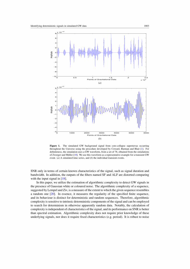
For illustrative purposes, we use here a highly simplified input waveform, h(t)—a quasi-monochromatic damped sinusoid of characteristic rest-frame frequency 1 kHz and duration10 ms, with a maximum dimensionless strain amplitude of 7 # 10!24 at a fiducial distance of10 Mpc. The waveform duration is approximately that of strongest GW emission of a DFMtype I (regular collapse) waveform, corresponding roughly to the ringdown phase.

In addition to the input waveform, we assume an all-sky cumulative core-collapse rateof about 25 s!1. Figure 1(a) shows a simulated GW signal from supernovas throughout theUniverse; the other shorter section—figure 1(b)—shows the individual events. The cumulativesignal from transient GW sources at cosmological distances is commonly described as astochastic background because of the temporal randomness of the individual events.

1.2. GW data detection

Techniques developed from the domains of signal processing and nonlinear analysis havebeen verified to detect GW bursts from the noise. The standard matched filter technique isthe optimal solution when the detected waveforms buried in stationary and Gaussian noise areknown. For the same reason, this optimal method may be impossible in practice. Recentlyfeasible filtering methods have been developed by European, American and Japanese groups.Flanagan and Hughes [11] have described in detail the features for GW detection from thethree different phases of coalescence events. Anderson et al [12, 13] further developed theexcess power method to detect gravitational bursts of unknown waveform. Time–frequencydetection algorithms are also proposed to identify short bursts of gravitational radiation[14, 15]. Meanwhile, a set of practical filters with high robustness is designed to detectgravitational wave burst signals, and the performances and efficiencies of these filters are alsostudied [16–18]. Beauville et al firstly compared search methods for GW bursts using LIGOand VIRGO simulated data [19]. These improved filter techniques can obtain the optimal

Identifying deterministic signals in simulated GW data 1803

0 0.5 1 1.5 2 2.5

x 104

!10

!8

!6

!4

!2

0

2

4

6

8x 10

!27

Points of Gravitational Data

Ampli

tude

0 1000 2000 3000 4000 5000 6000!5

!4

!3

!2

!1

0

1

2

3

4

5x 10

!27

Points of Gravitational Data

Ampli

tude

(a)

(b)

Figure 1. The simulated GW background signal from core-collapse supernovas occurringthroughout the Universe using the procedure developed by Coward, Burman and Blair [1]. Fordefiniteness, the simulation uses a GW waveform, from a set of 78, obtained from the simulationsof Zwerger and Muller [10]. We use this waveform as a representative example for a transient GWevent. (a) A simulated time series, and (b) the individual transient events.

SNR only in terms of certain known characteristics of the signal, such as signal duration andbandwidth. In addition, the outputs of the filters named SF and ALF are distorted comparingwith the input signal in [18].

In this paper, we utilize the estimation of algorithmic complexity to detect GW signals inthe presence of Gaussian white or coloured noise. The algorithmic complexity of a sequence,suggested by Lempel and Ziv, is a measure of the extent to which the given sequence resemblesa random one [20]. In essence, it measures the regularity of the specified finite sequence,and its behaviour is distinct for deterministic and random sequences. Therefore, algorithmiccomplexity is sensitive to intrinsic deterministic components of the signal and can be employedto search for determinism in otherwise apparently random data. Notably, the calculation ofcomplexity is independent of characteristics of the signal, and its performance on SNR is betterthan spectral estimation. Algorithmic complexity does not require prior knowledge of theseunderlying signals, nor does it require fixed characteristics (e.g. period). It is robust to noise

1804 Y Zhao et al

and may be applied in conjunction with existing filtering methods as a further improvement todetection performance. Hence, comparison to existing techniques is largely irrelevant as thismethod will actually augment these existing methods.

But estimating complexity is not sufficient to make a decision on the data: one cannotdetermine with certainty (or even probability) that a particular value of complexity indicatesthe presence of deterministic dynamics. To address this problem, we employ the surrogatedata method (a form of statistical hypothesis testing). Algorithmic complexity provides aquantitative measure of deterministic dynamics in time series. The surrogate data method maybe employed to benchmark these statistical results and compare them to the results expectedfor various types of pure noise processes. Significantly, the VIRGO group has described thesurrogate data method with the hypothesis of NH1 (see section 3) to test for the nonlinearityof the data of the VIRGO interferometer [21]. According to this hypothesis we can rejectthat the data are not linear noise but it may be insufficient to determine whether the datacontain nonlinearity. Moreover, our application of the surrogate data method is different. In[21] the surrogate data method was used to test for nonlinearity in the underlying data (areasonably likely hypothesis). We use the surrogate data method to provide a benchmark forour algorithmic complexity results. The surrogate data method provides a method to determinewhether algorithmic complexity indicates significant nonlinear determinism in the underlyingdata (unlike [21] algorithmic complexity is specifically testing for deterministic dynamics—such as GW data). Here we adopt the surrogate data method with the hypotheses of NH0 andNH1 so as to attach statistical significance to the results of algorithmic complexity and alsoensure that the data distinguished by complexity are not linear filtered noise. For our choiceof test statistics, we propose to replace the popular statistics, correlation dimension [22], withalgorithmic complexity. Since correlation dimension estimates are quite sensitive to the noise,in even uncorrelated noise they are not applicable to field measurements [23]. Comparingwith the existing statistics, complexity has the great advantage of small computational costand is suited for real-time implementation.

2. The algorithm of complexity

Let us assume that a sequence S of length n is fully specified by S = (s1, s2, . . . , sn) whereeach si is one of d symbols, si $ A = {a1, a2, a3, . . . , ad}. Note that for the binary caseA = {0, 1} , i.e. S is composed of only zeros and ones. For the general case in this paper, let A

be an alphabet of d (d ! 2) symbols. Let c(n) be the counter of the novel sub-sequences in thesequence S; P and Q denote two sequences which are substrings of S; PQ is the concatenationof P and Q; and PQ" represents the sequence which is the concatenation of P and Q and withthe last symbol deleted. Let v(PQ") denote the set of all the substrings of PQ" .

The procedure for calculating the algorithmic complexity of the sequence S ={si}i=1,2,...,n, where si $ A, is as follows:

(1) Initialize c(n) = 1, P = s1,Q = s2. So PQ" = s1. If Q $ v(PQ"), leave P unchangedand update Q = s2s3; if Q /$ v(PQ"), add one to c(n), update P = s1s2 and Q = s3.

(2) Continue from the previous step. Now assume that P = s1s2 · · · sr ,Q = sr+1. IfQ $ v(PQ"), leave P unchanged and update Q = sr+1sr+2, and then judge whetherQ belongs to v(PQ").3 Repeat the previous comparison, until Q /$ v(PQ"). Soc(n) = c(n) + 1. Let us assume Q = sr+1sr+2 · · · sr+i at this time. Then let P be updatedto P = s1s2 · · · srsr+1sr+2 · · · sr+i and set Q = sr+i+1.

3 Since Q is updated, PQ" must be updated too.

Identifying deterministic signals in simulated GW data 1805

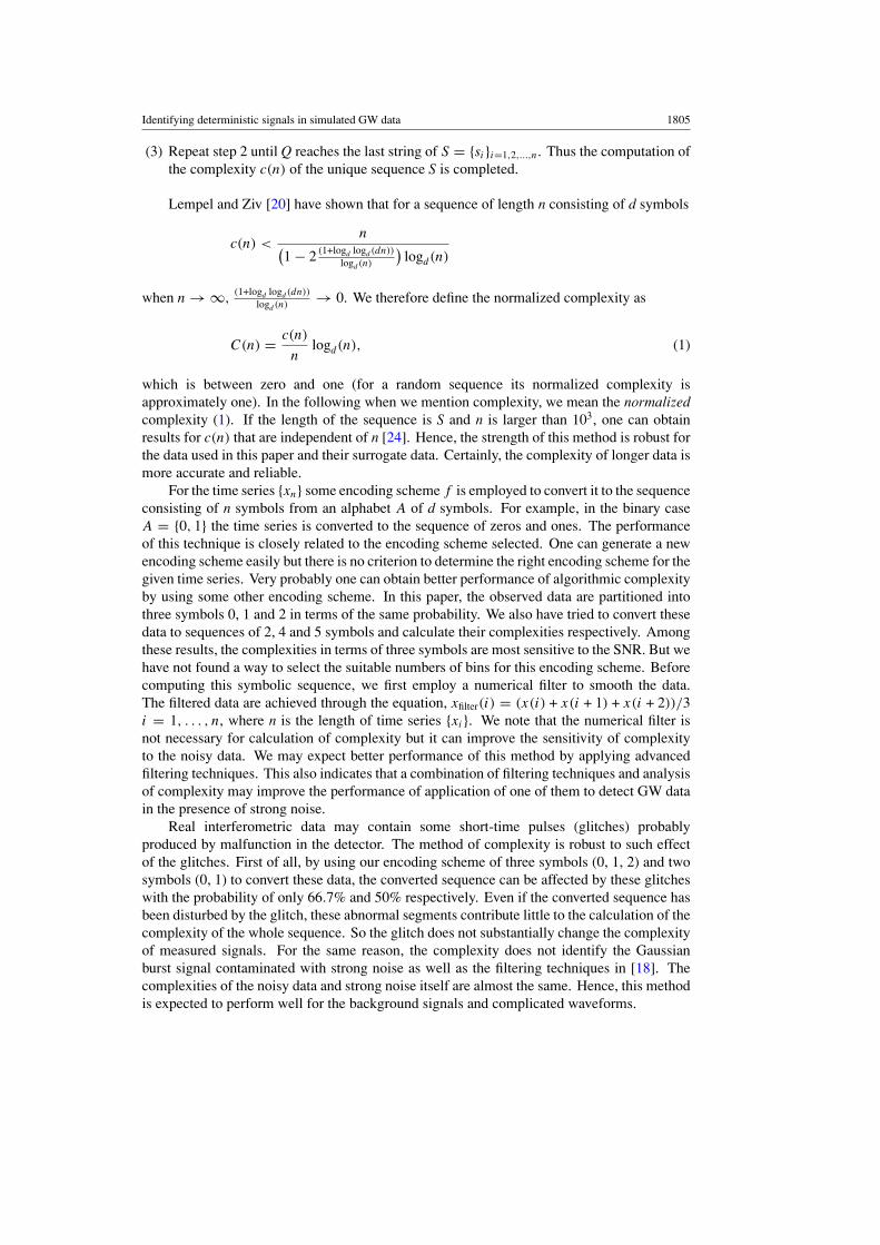
(3) Repeat step 2 until Q reaches the last string of S = {si}i=1,2,...,n. Thus the computation ofthe complexity c(n) of the unique sequence S is completed.

Lempel and Ziv [20] have shown that for a sequence of length n consisting of d symbols

c(n) <n

!1 ! 2 (1+logd logd (dn))

logd (n)

"logd(n)

when n % &,(1+logd logd (dn))

logd (n)% 0. We therefore define the normalized complexity as

C(n) = c(n)

nlogd(n), (1)

which is between zero and one (for a random sequence its normalized complexity isapproximately one). In the following when we mention complexity, we mean the normalizedcomplexity (1). If the length of the sequence is S and n is larger than 103, one can obtainresults for c(n) that are independent of n [24]. Hence, the strength of this method is robust forthe data used in this paper and their surrogate data. Certainly, the complexity of longer data ismore accurate and reliable.

For the time series {xn} some encoding scheme f is employed to convert it to the sequenceconsisting of n symbols from an alphabet A of d symbols. For example, in the binary caseA = {0, 1} the time series is converted to the sequence of zeros and ones. The performanceof this technique is closely related to the encoding scheme selected. One can generate a newencoding scheme easily but there is no criterion to determine the right encoding scheme for thegiven time series. Very probably one can obtain better performance of algorithmic complexityby using some other encoding scheme. In this paper, the observed data are partitioned intothree symbols 0, 1 and 2 in terms of the same probability. We also have tried to convert thesedata to sequences of 2, 4 and 5 symbols and calculate their complexities respectively. Amongthese results, the complexities in terms of three symbols are most sensitive to the SNR. But wehave not found a way to select the suitable numbers of bins for this encoding scheme. Beforecomputing this symbolic sequence, we first employ a numerical filter to smooth the data.The filtered data are achieved through the equation, xfilter(i) = (x(i) + x(i + 1) + x(i + 2))/3i = 1, . . . , n, where n is the length of time series {xi}. We note that the numerical filter isnot necessary for calculation of complexity but it can improve the sensitivity of complexityto the noisy data. We may expect better performance of this method by applying advancedfiltering techniques. This also indicates that a combination of filtering techniques and analysisof complexity may improve the performance of application of one of them to detect GW datain the presence of strong noise.

Real interferometric data may contain some short-time pulses (glitches) probablyproduced by malfunction in the detector. The method of complexity is robust to such effectof the glitches. First of all, by using our encoding scheme of three symbols (0, 1, 2) and twosymbols (0, 1) to convert these data, the converted sequence can be affected by these glitcheswith the probability of only 66.7% and 50% respectively. Even if the converted sequence hasbeen disturbed by the glitch, these abnormal segments contribute little to the calculation of thecomplexity of the whole sequence. So the glitch does not substantially change the complexityof measured signals. For the same reason, the complexity does not identify the Gaussianburst signal contaminated with strong noise as well as the filtering techniques in [18]. Thecomplexities of the noisy data and strong noise itself are almost the same. Hence, this methodis expected to perform well for the background signals and complicated waveforms.

1806 Y Zhao et al

3. The linear surrogate data method

Surrogate data tests are examples of Monte Carlo hypothesis tests. For time series from systemswhich one suspects to contain nonlinearity and determinism, it is reasonable to choose a nullhypothesis which falsifies these properties. The rationale of surrogate data hypothesis testingis to generate an ensemble of artificial surrogate data (abbreviated to surrogates) which isconsistent with that hypothesis, and then evaluate some suitable quantity (or test statistic) bothfor the original data set and surrogates. If the results for the original are significantly differentfrom those for the surrogates, one can reject the given null hypothesis: the original data set isstatistically unlikely to be generated by a process consistent with the null hypothesis. If not,one merely fails to reject it: note that failure to reject does not imply that the null hypothesisis true, only that we have found no evidence that it is false. In this way, the surrogate datamethod provides a rigorous way to apply statistical hypothesis testing to experimental timeseries.

There are three commonly employed null hypotheses, known as NH0, NH1 and NH2,which form a hierarchy [25]:

• NH0: The data are independent and identically distributed (i.i.d.) noise.• NH1: The data are linearly filtered noise.• NH2: The data are a static monotonic nonlinear transformation of linearly filtered noise.

The three hypotheses are all forms of linear noise process (albeit a possible static nonlinearfilter). According to these hypotheses, we can determine whether the observed time seriesare linear noise. The three algorithms to generate surrogates are known as algorithm 0,algorithm 1 and algorithm 2 [25] corresponding to NH0, NH1 and NH2, respectively. Theexact nature of the algorithm used to generate surrogates should be consistent with the chosenhypotheses.

Algorithm 0. Shuffle the order of the original data eliminating any temporal correlation.In essence the surrogates are random data (i.i.d. noise) consistent with the same probabilitydistribution as the original data. For the hypothesis NH0, algorithm 0 is adopted to generatesurrogates.

Algorithm 1. Surrogate data produced by this algorithm are linearly filtered noise. Oneemploys the discrete Fourier transform (DFT) of the data and shuffles (or randomizes) thephases of the complex conjugate pairs to generate these surrogates. The surrogates are theinverse discrete Fourier transform. By shuffling the phases but maintaining the amplitude ofthe complex conjugate pairs, the surrogate will have the same power spectrum as the data, butwill have no nonlinear determinism.

Algorithm 2. Amplitude adjusted Fourier transform (AAFT) algorithm. Surrogates generatedby this algorithm are static monotonic nonlinear transformations of linearly filtered noise. Onerescales values of the original data so that they are Gaussian, and then applies algorithm 1to generate the surrogates that have the same power spectra as the rescaled data. Finally, thegenerated surrogates are rescaled back to keep the same amplitude distribution as the originaldata.

Algorithms 1 and 2 (particularly algorithm 2) are hampered by technical issues relatedto the Fourier transformation. If the original time series is stationary and adequately long,algorithm 1 can work well without limitation [25]. Note that for the real data we need toanalyse the stationarity of the data before applying the surrogate data method with one of thetwo algorithms to it. Otherwise, non-stationary data would increase false rejections of thegiven testings. Surrogates generated by algorithm 2 usually fail to keep exactly the same power

Identifying deterministic signals in simulated GW data 1807

spectra as the original and such systematic errors can result in high false rejections [26, 27].Solutions to technical problems of this algorithm are also available in the same literature butrequire great computational cost. Actually, the careful application of the above algorithms canprovide significant results [28]. In addition, there are other algorithms to produce surrogatedata, such as the pseudo-periodic surrogate (PPS) algorithm [29] and cycle-shuffled surrogatealgorithm [30]. The surrogate data method with these algorithm tests examines the hypothesesthat an observed time series is a noise-driven periodic orbit, which is not applicable to thecurrent GW signals.

4. Identification of GW transients

In sections 4.1 and 4.2, we apply our estimation of algorithmic complexity and the surrogatedata method to detection of the background from different levels of noises, including bothwhite Gaussian and coloured noises; in section 4.3, we try to localize each single event incertain strong noise by algorithmic complexity. There are several forms of SNR, such asequation (24) in [31], equation (1) in [19] and equation (29) in [32]. For consistency, wechoose for our definition of SNR the square root of the ratio of the power spectral densities ofthe signal and noise integrated over all frequencies.

To compare the performance of this method to existing techniques, we also calculate linearautocorrelation as an alternative criterion. The numerical results indicate that applicationof algorithmic complexity can distinguish deterministic GW data from both the white andcoloured noises. By comparison autocorrelation failed to identify the GW signals in thepresence of coloured noise. Our general computational scheme is illustrated as follows:

(1) Add different levels of white Gaussian noise to the GW data (from the very low SNR tohigh SNR) and then calculate the complexity of the sum with different signal-to-noiseratios. Higher SNR indicates that the GW data are dominant and the calculated complexityis closer to the complexity of the noise-free GW data and vice versa. By varying the SNRwe can therefore test how much noise this complexity measure is able to overcome.

(2) Verify the sensitivity of complexity to the GW data with different levels of coloured (thatis, linearly filtered) noises. The coloured noise is generated by white Gaussian noise plusthe same noise with a certain delay time. We add the coloured noise to the original datain the same way as step (1).

(3) Apply the surrogate data method to the same data. For the data contaminated with whitenoise, we employ the surrogate data method to determine whether to reject the hypothesis,NH0, that the data can be described as i.i.d. noise. (For white noise, this hypothesis istrue; for the GW data, it is false.) At each SNR we generate 30 surrogates and calculatethe complexity for the surrogates and the original data to make a decision. Accordingto the results, we can determine the minimum SNR for which complexity can presentmeaningful results.

(4) For the data contaminated with coloured noise, we apply the hypothesis, NH1, that thesegenerated data are linearly filtered noise. We then repeat the above procedure. Rejectionof the first case (step (3)) indicates that the data exhibit temporal correlation. This is truefor both linearly filtered noise and deterministic signals such as the GW data. Rejectionof the second case (step (4)) indicates that the data are also inconsistent with simple linearnoise.

(5) To compare the results of this test with more standard (albeit linear) statistics, we makefurther comparative experiments (following the procedure in steps (3) and (4)) usingthe autocorrelation as the discriminating statistic d(·) in the surrogate test. That is,

1808 Y Zhao et al

10!2

10!1

100

101

102

0.1

0.2

0.3

0.4

0.5

0.6

0.7

0.8

0.9

SNR

Comp

lexity

10!2

10!1

100

101

0.1

0.2

0.3

0.4

0.5

0.6

0.7

0.8

SNR

Comp

lexity

(a)

(b)

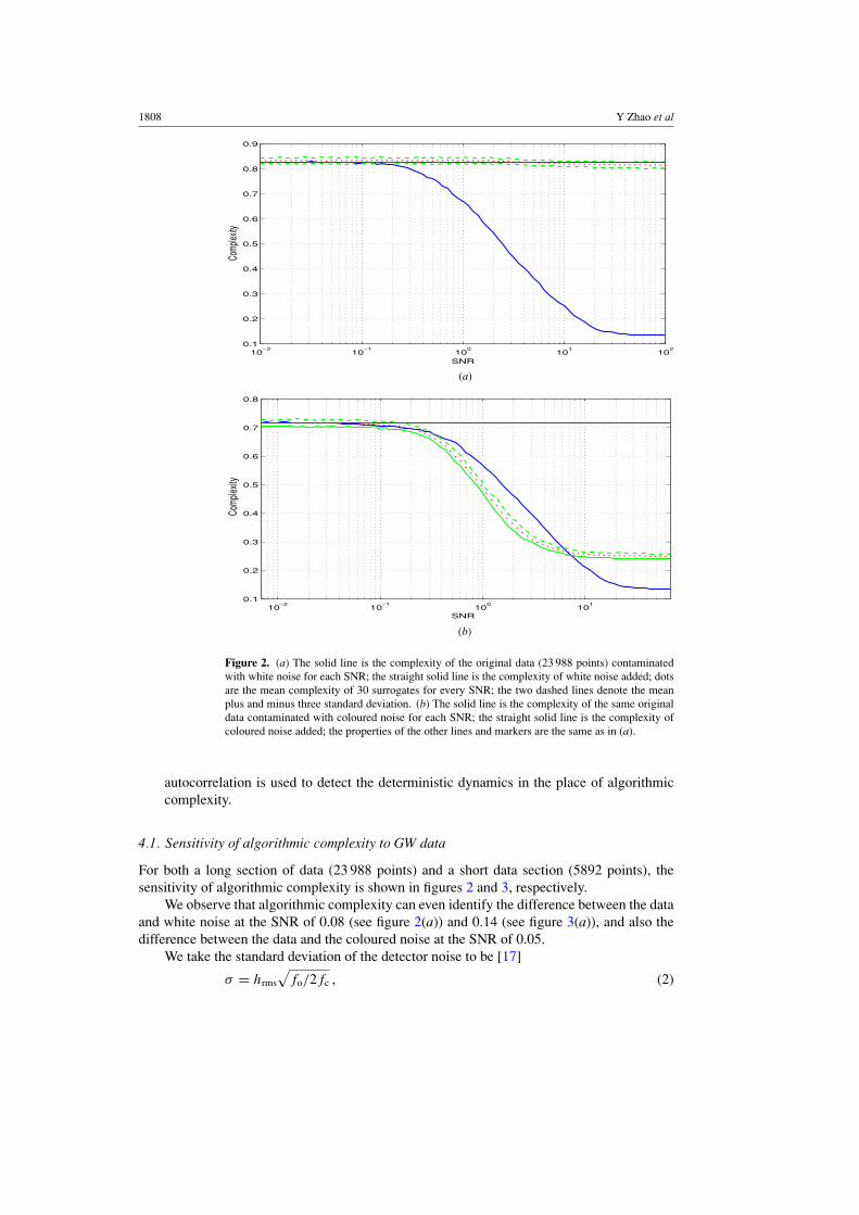
Figure 2. (a) The solid line is the complexity of the original data (23 988 points) contaminatedwith white noise for each SNR; the straight solid line is the complexity of white noise added; dotsare the mean complexity of 30 surrogates for every SNR; the two dashed lines denote the meanplus and minus three standard deviation. (b) The solid line is the complexity of the same originaldata contaminated with coloured noise for each SNR; the straight solid line is the complexity ofcoloured noise added; the properties of the other lines and markers are the same as in (a).

autocorrelation is used to detect the deterministic dynamics in the place of algorithmiccomplexity.

4.1. Sensitivity of algorithmic complexity to GW data

For both a long section of data (23 988 points) and a short data section (5892 points), thesensitivity of algorithmic complexity is shown in figures 2 and 3, respectively.

We observe that algorithmic complexity can even identify the difference between the dataand white noise at the SNR of 0.08 (see figure 2(a)) and 0.14 (see figure 3(a)), and also thedifference between the data and the coloured noise at the SNR of 0.05.

We take the standard deviation of the detector noise to be [17]

# = hrms

#fo/2fc , (2)

Identifying deterministic signals in simulated GW data 1809

10!2

10!1

100

101

102

0.1

0.2

0.3

0.4

0.5

0.6

0.7

0.8

0.9

SNR

Comp

lexity

10!2

10!1

100

101

0.1

0.2

0.3

0.4

0.5

0.6

0.7

0.8

SNR

Comp

lexity

(a)

(b)

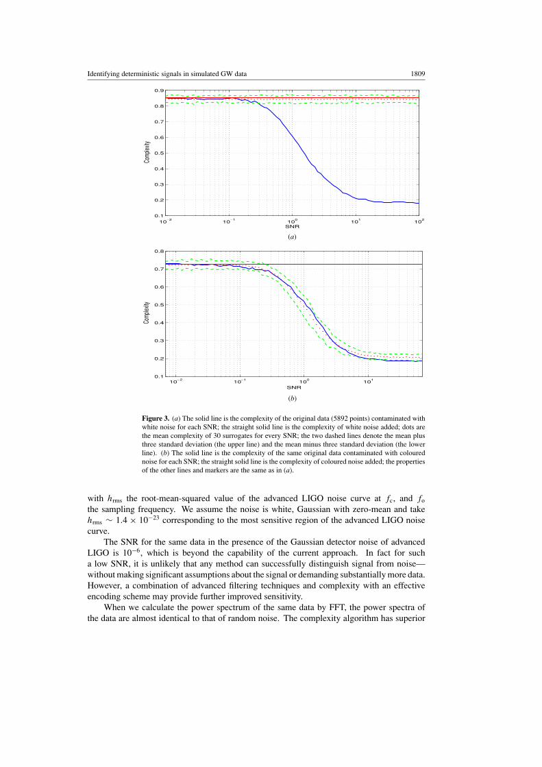
Figure 3. (a) The solid line is the complexity of the original data (5892 points) contaminated withwhite noise for each SNR; the straight solid line is the complexity of white noise added; dots arethe mean complexity of 30 surrogates for every SNR; the two dashed lines denote the mean plusthree standard deviation (the upper line) and the mean minus three standard deviation (the lowerline). (b) The solid line is the complexity of the same original data contaminated with colourednoise for each SNR; the straight solid line is the complexity of coloured noise added; the propertiesof the other lines and markers are the same as in (a).

with hrms the root-mean-squared value of the advanced LIGO noise curve at fc, and fo

the sampling frequency. We assume the noise is white, Gaussian with zero-mean and takehrms ' 1.4 # 10!23 corresponding to the most sensitive region of the advanced LIGO noisecurve.

The SNR for the same data in the presence of the Gaussian detector noise of advancedLIGO is 10!6, which is beyond the capability of the current approach. In fact for sucha low SNR, it is unlikely that any method can successfully distinguish signal from noise—without making significant assumptions about the signal or demanding substantially more data.However, a combination of advanced filtering techniques and complexity with an effectiveencoding scheme may provide further improved sensitivity.

When we calculate the power spectrum of the same data by FFT, the power spectra ofthe data are almost identical to that of random noise. The complexity algorithm has superior

1810 Y Zhao et al

power to detect determinism compared to the standard of FFT, especially for long and non-stationary data sets. The power spectrum estimated by FFT seeks to describe the signal asthe average frequency content over the entire data length. For longer samples with severalpulses of different frequency, this approach does not make sense. For short samples, there areinsufficient data. However, the complexity algorithm looks for patterns in the data: and candetect such patterns, even if the dominant frequency changes.

In the following we not only determine to what extent the complexity of these data issignificantly different from that of random noise, but also test whether more sophisticatedcoloured noise could contribute to the observed difference in complexity. To address boththese questions we employ the surrogate data method.

4.2. Application of the surrogate data method

For the case of added white noise, the given hypothesis is that the contaminated signal is i.i.d.noise and the surrogate generation algorithm 0 is required; for added coloured noise the givenhypothesis is that the contaminated noise is linear noise and algorithm 1 is used to generatesurrogate data. We then calculate the complexity for both surrogate data and the original tomake a decision.

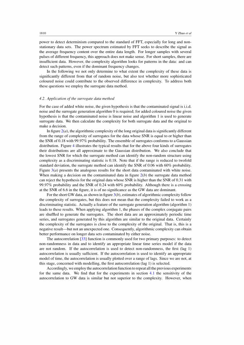
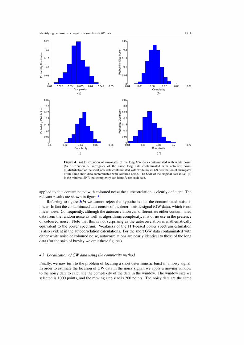
In figure 2(a), the algorithmic complexity of the long original data is significantly differentfrom the range of complexity of surrogates for the data whose SNR is equal to or higher thanthe SNR of 0.18 with 99.97% probability. The ensemble of surrogates conforms to a Gaussiandistribution. Figure 4 illustrates the typical results that for the above four kinds of surrogatestheir distributions are all approximate to the Gaussian distribution. We also conclude thatthe lowest SNR for which the surrogate method can identify the non-random structure usingcomplexity as a discriminating statistic is 0.18. Note that if the range is reduced to twofoldstandard deviation, the surrogate method can identify the SNR of 0.06 with 60% probability.Figure 3(a) presents the analogous results for the short data contaminated with white noise.When making a decision on the contaminated data in figure 2(b) the surrogate data methodcan reject the hypothesis for the original data whose SNR is higher than the SNR of 0.31 with99.97% probability and the SNR of 0.24 with 60% probability. Although there is a crossingat the SNR of 6.6 in the figure, it is of no significance as the GW data are dominant.

For the short GW data, as shown in figure 3(b), estimates of algorithmic complexity followthe complexity of surrogates, but this does not mean that the complexity failed to work as adiscriminating statistic. Actually a feature of the surrogate generation algorithm (algorithm 1)leads to these results. When applying algorithm 1, the phases of the complex conjugate pairsare shuffled to generate the surrogates. The short data are an approximately periodic timeseries, and surrogates generated by this algorithm are similar to the original data. Certainlythe complexity of the surrogates is close to the complexity of the original. That is, this is anegative result—but not an unexpected one. Consequently, algorithmic complexity can obtainbetter performance on longer data sets contaminated by either noise.

The autocorrelation [33] function is commonly used for two primary purposes: to detectnon-randomness in data and to identify an appropriate linear time series model if the dataare not random. If the autocorrelation is used to detect non-randomness, the first (lag 1)autocorrelation is usually sufficient. If the autocorrelation is used to identify an appropriatemodel of time, the autocorrelation is usually plotted over a range of lags. Since we are not, atthis stage, concerned with modelling, the first autocorrelation (lag 1) is selected.

Accordingly, we employ the autocorrelation function to repeat all the previous experimentsfor the same data. We find that for the experiments in section 4.1 the sensitivity of theautocorrelation to GW data is similar but not superior to the complexity. However, when

Identifying deterministic signals in simulated GW data 1811

0.82 0.825 0.83 0.835 0.84 0.845 0.850

0.05

0.1

0.15

0.2

0.25

Complexity

Pro

babi

lity

Dis

trib

utio

n

0.64 0.65 0.66 0.67 0.68 0.690

0.05

0.1

0.15

0.2

0.25

Complexity

Pro

babi

lity

Dis

trib

utio

n

0.8 0.82 0.84 0.86 0.880

0.05

0.1

0.15

0.2

0.25

0.3

0.35

Complexity

Pro

babi

lity

Dis

trib

utio

n

0.64 0.66 0.68 0.7 0.720

0.05

0.1

0.15

0.2

0.25

0.3

0.35

Complexity

Pro

babi

lity

Dis

tribu

tion

(a) (b)

(c) (d )

Figure 4. (a) Distribution of surrogates of the long GW data contaminated with white noise;(b) distribution of surrogates of the same long data contaminated with coloured noise;(c) distribution of the short GW data contaminated with white noise; (d) distribution of surrogatesof the same short data contaminated with coloured noise. The SNR of the original data in (a)–(c)is the minimal SNR that complexity can identify for such data.

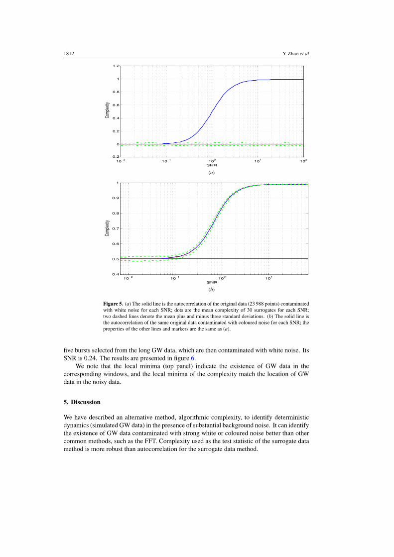
applied to data contaminated with coloured noise the autocorrelation is clearly deficient. Therelevant results are shown in figure 5.

Referring to figure 5(b) we cannot reject the hypothesis that the contaminated noise islinear. In fact the contaminated data consist of the deterministic signal (GW data), which is notlinear noise. Consequently, although the autocorrelation can differentiate either contaminateddata from the random noise as well as algorithmic complexity, it is of no use in the presenceof coloured noise. Note that this is not surprising as the autocorrelation is mathematicallyequivalent to the power spectrum. Weakness of the FFT-based power spectrum estimationis also evident in the autocorrelation calculations. For the short GW data contaminated witheither white noise or coloured noise, autocorrelations are nearly identical to those of the longdata (for the sake of brevity we omit these figures).

4.3. Localization of GW data using the complexity method

Finally, we now turn to the problem of locating a short deterministic burst in a noisy signal.In order to estimate the location of GW data in the noisy signal, we apply a moving windowto the noisy data to calculate the complexity of the data in the window. The window size weselected is 1000 points, and the moving step size is 200 points. The noisy data are the same

1812 Y Zhao et al

10!2

10!1 100

101

102

!0.2

0

0.2

0.4

0.6

0.8

1

1.2

SNR

Comp

lexity

10!2 10!1 100

101

0.4

0.5

0.6

0.7

0.8

0.9

1

SNR

Comp

lexity

(a)

(b)

Figure 5. (a) The solid line is the autocorrelation of the original data (23 988 points) contaminatedwith white noise for each SNR; dots are the mean complexity of 30 surrogates for each SNR;two dashed lines denote the mean plus and minus three standard deviations. (b) The solid line isthe autocorrelation of the same original data contaminated with coloured noise for each SNR; theproperties of the other lines and markers are the same as (a).

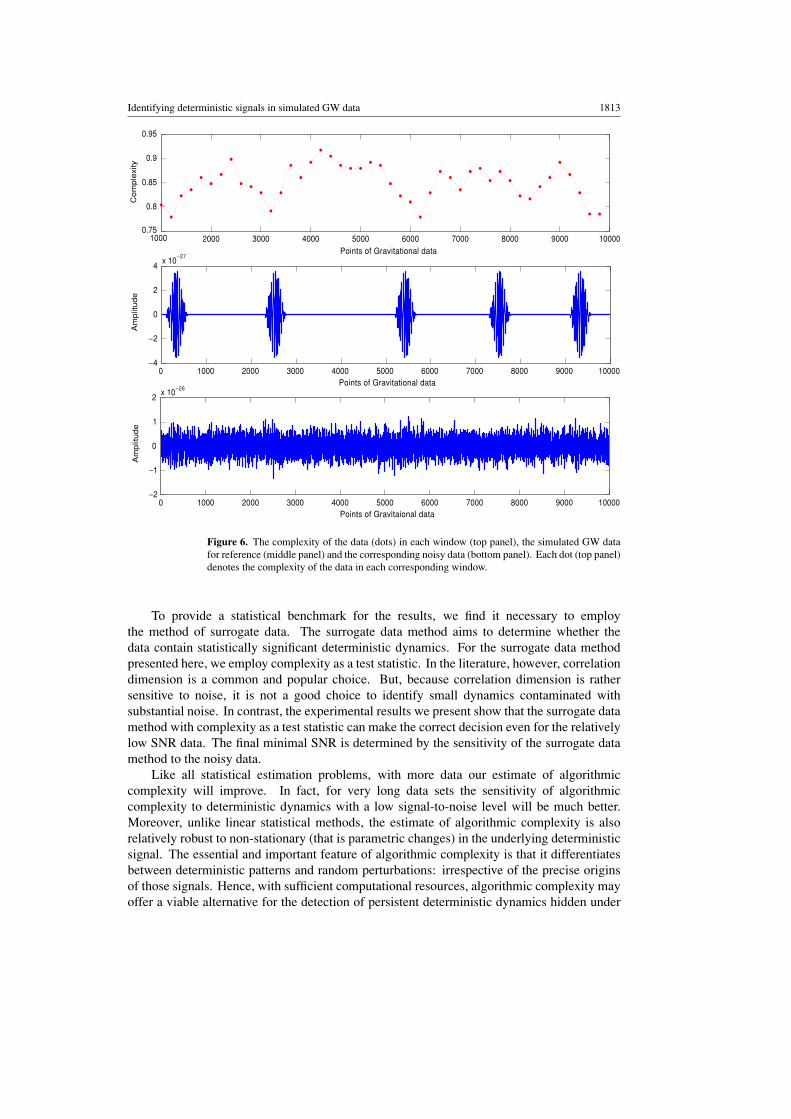
five bursts selected from the long GW data, which are then contaminated with white noise. ItsSNR is 0.24. The results are presented in figure 6.

We note that the local minima (top panel) indicate the existence of GW data in thecorresponding windows, and the local minima of the complexity match the location of GWdata in the noisy data.

5. Discussion

We have described an alternative method, algorithmic complexity, to identify deterministicdynamics (simulated GW data) in the presence of substantial background noise. It can identifythe existence of GW data contaminated with strong white or coloured noise better than othercommon methods, such as the FFT. Complexity used as the test statistic of the surrogate datamethod is more robust than autocorrelation for the surrogate data method.

Identifying deterministic signals in simulated GW data 1813

1000 2000 3000 4000 5000 6000 7000 8000 9000 100000.75

0.8

0.85

0.9

0.95

Points of Gravitational data

Co

mp

lexi

ty

0 1000 2000 3000 4000 5000 6000 7000 8000 9000 10000!4

!2

0

2

4 x 10!27

Points of Gravitational data

Am

plit

ud

e

0 1000 2000 3000 4000 5000 6000 7000 8000 9000 10000!2

!1

0

1

2 x 10!26

Points of Gravitaional data

Am

plit

ud

e

Figure 6. The complexity of the data (dots) in each window (top panel), the simulated GW datafor reference (middle panel) and the corresponding noisy data (bottom panel). Each dot (top panel)denotes the complexity of the data in each corresponding window.

To provide a statistical benchmark for the results, we find it necessary to employthe method of surrogate data. The surrogate data method aims to determine whether thedata contain statistically significant deterministic dynamics. For the surrogate data methodpresented here, we employ complexity as a test statistic. In the literature, however, correlationdimension is a common and popular choice. But, because correlation dimension is rathersensitive to noise, it is not a good choice to identify small dynamics contaminated withsubstantial noise. In contrast, the experimental results we present show that the surrogate datamethod with complexity as a test statistic can make the correct decision even for the relativelylow SNR data. The final minimal SNR is determined by the sensitivity of the surrogate datamethod to the noisy data.

Like all statistical estimation problems, with more data our estimate of algorithmiccomplexity will improve. In fact, for very long data sets the sensitivity of algorithmiccomplexity to deterministic dynamics with a low signal-to-noise level will be much better.Moreover, unlike linear statistical methods, the estimate of algorithmic complexity is alsorelatively robust to non-stationary (that is parametric changes) in the underlying deterministicsignal. The essential and important feature of algorithmic complexity is that it differentiatesbetween deterministic patterns and random perturbations: irrespective of the precise originsof those signals. Hence, with sufficient computational resources, algorithmic complexity mayoffer a viable alternative for the detection of persistent deterministic dynamics hidden under

1814 Y Zhao et al

substantial noise—even when the exact forms of both the noise and the deterministic dynamicare unknown and may change with time.

In practical applications, due to the limitation of current interferometer technology, thedata are usually contaminated with unknown noise sources, which may contain GW signals.It is possible to generate Gaussian noise with the same energy as the noisy data and applycomplexity to both this data set and the noisy data. If the complexity of the data is smallerthan that of the noise we could utilize the surrogate data method to assess the level ofdeterministic dynamics. Algorithmic complexity, therefore, a potentially available method todetect deterministic dynamics in GW data where the signal power is significantly smaller thanthe noise level.

Acknowledgments

This work was supported by Hong Kong University Research Council Grant (PolyU 5235/03E)and the Australian Research Council.

References

[1] Coward D M, Burman R R and Blair D G 2001 Mon. Not. R. Astron. Soc. 324 1015[2] Coward D M, Burman R R and Blair D G 2002b Class. Quantum Grav. 19 1303[3] Coward D M, Putten H P M and Burman R R 2002a Astrophys. J. 580 1024[4] Howell E, Coward D, Burman R R and Blair D G 2005 Class. Quantum Grav. 22 723[5] Hernquist L and Springel V 2003 Mon. Not. R. Astron. Soc. 341 1253[6] Cuoco E et al 2001 Class. Quantum Grav. 18 1727[7] Mukherjee S 2004 Class. Quantum Grav. 21 S1783[8] Dimmelmeier H, Font J and Muller E 2002 Astron. Astrophys. 393 523 (DFM)[9] Muller E, Rampp M, Buras R, Janka H and Shoemaker 2004 Astrophys. J. 603 221

[10] Zwerger T and Muller E 1997 Astron. Astrophys. 320 209[11] Flanagan E E and Hughes S A 1998 Phys. Rev. D 57 4535[12] Anderson W G et al 2000 Int. J. Mod. Phys. D 9 303[13] Anderson W G et al 2001 Phys. Rev. D 63 042003[14] Anderson W G and Balasubramanian R 1999 Phys. Rev. D 60 102001[15] Sylvestre J 2002 Phys. Rev. D 66 102004[16] Arnaud N et al 1999 Phys. Rev. D 59 082002[17] Pradier T et al 2001 Phys. Rev. D 63 042002[18] Arnaud N et al 2003 Phys. Rev. D 67 062004[19] Beauville F et al 2005 Class. Quantum Grav. 22 s1293-s1301[20] Lempel A and Ziv J 1976 IEEE Trans. Inf. Theory 22 75–81[21] The VIRGO Collaboration 2003 Class. Quantum Grav. 20 S915–S924[22] Grassberger P and Procaccia I 1983 Physica D 9 189[23] Kantz H and Schreiber T 1998 Inst. Electr. Eng. Proc. Sci. Meas. Technol. 145 279–84[24] Kaspar F and Schuster H G 1987 Phys. Rev. A 36 842–8[25] Theiler J et al 1992 Physica D 58 77–94[26] Schreiber T and Schmitz A 1996 Phys. Rev. Lett. 77 635–8[27] Nakamura T et al 2005 Phys. Rev. E 72 055201(R)[28] Small M and Tse C K 2003 IEEE Trans. Circuits Syst. I 50 663–72[29] Small M et al 2001 Phys. Rev. Lett. 87 188101[30] Theiler J 1995 Phy. Lett. A 196 335–41[31] Maggiore M 2000 Phys. Rep. 331 6[32] Thorne K S 1989 Three Hundred Years of Gravitation ed S W Hawking and W Israel (London: Cambridge

University Press) p 368[33] Box G E P and Jenkins G M 1976 Time Series Analysis: Forecasting and Control (Oakland, CA: Holden-Day)