detecting determinism in time series: the method of surrogate data

IEEE TRANSACTIONS ON CIRCUITS AND SYSTEMS—I: FUNDAMENTAL THEORY AND APPLICATIONS, VOL. 50, NO. 5, MAY 2003 663

Detecting Determinism in Time Series: The Methodof Surrogate Data

Michael Small, Member, IEEE,and Chi K. Tse, Senior Member, IEEE

Abstract—We review a relatively new statistical test that may beapplied to determine whether an observed time series is inconsis-tent with a specific class of dynamical systems. Thesesurrogate datamethods may test an observed time series against the hypotheses of:i) independent and identically distributed noise; ii) linearly filterednoise; and iii) a monotonic nonlinear transformation of linearly fil-tered noise. A recently suggested fourth algorithm for testing thehypothesis of a periodic orbit with uncorrelated noise is also de-scribed. We propose several novel applications of these methods forvarious engineering problems, including: identifying a determin-istic (message) signal in a noisy time series; and separating deter-ministic and stochastic components. When employed to separatedeterministic and noise components, we show that the applicationof surrogate methods to the residuals of nonlinear models is equiv-alent to fitting that model subject to an information theoretic modelselection criteria.

Index Terms—Hypothesis testing, minimum description length,noise separation, nonlinear modeling, surrogate data.

I. INTRODUCTION

A N IMPORTANT problem in many areas of signal pro-cessing is to determine whether an observed time series is

deterministic, contains a deterministic component, or is purelystochastic. Equivalently, one may consider the problem of sep-arating an observed time series into deterministic (message)and stochastic (noise) components. In this paper we review themethod of surrogate data and suggest two alternative techniquesthat may be employed for effective system identification andseparation of signal and noise.

The method of surrogate data provides a rigorous way toapply statistical hypothesis testing to experimental time series.One may apply the method of surrogate data to determinewhether an observed time series has statistically significantdeterministic component. Three standard linear techniques arewidely applied in the physical and biological sciences (seefor example, [1]) to test the hypotheses of [2]: i) independentand identically distributed (i.i.d.) noise1 ; ii) linearly filterednoise; and (iii) static monotonic nonlinear transformationof linearly filtered noise. Surrogate methods require one togenerate an ensemble of artificial time series (thesurrogates)that are both “like” the data being tested and consistent with

Manuscript received January 15, 2002; revised October 29, 2002. This workwas supported by the Hong Kong Polytechnic University under Grant G-YW55.This paper was recommended by Associate Editor N. Ling.

The authors are with the Department of Electronic and Information Engi-neering, Hong Kong Polytechnic University, Kowloon, Hong Kong (e-mail:[email protected]).

Digital Object Identifier 10.1109/TCSI.2003.811020

1By i.i.d. we mean that the time series observations are drawnindependentlyfrom identicalprobability distributions.

the hypothesis of interest. One then statistically compares thedata and surrogates. Many extensions of this basic method havebeen suggested ([3] and [4]) but, in this current work, we areparticularly interested in a method that may be applied to testfor nonlinear nonperiodic determinism in apparently periodictime series [5], [6].

Surrogate methods identify whether an observed time seriescontains determinism. By themselves, they cannot separatethe noise and deterministic components. We employ nonlinearmodeling techniques [7] that utilize the information theoreticminimum description length(MDL) [8] to fit data without overfitting. These methods have been successfully employed toidentify and model the deterministic component of time seriesof many experimental systems [9]–[11]. We show that thesemethods may be employed to separate the noise and signal in anobserved time series. Alternatively, we show that surrogate datamethods applied to the model residuals may also be used as amodel fitting criterion. Surrogate data methods may then be usedto separate certain classes of noise, such as i.i.d. or colored noise,from complex deterministic dynamics in a data set. A similarinterpretation of surrogate data methods has been suggested byTakens [12]. Takens considered fitting some model to a timeseries and applying i.i.d. surrogate tests to the residuals. Heshowed that if the residuals are i.i.d., then the model offers agood fit to the data. We extend this result and use it to showthat surrogates may be employed to determine whether a modelcaptures all the deterministic structure in a time series.

Section II gives a review of existing surrogate data methodsand describes the application of pseudoperiodic surrogates(PPSs) in more detail. In Section III, we present several exam-ples of these methods, both to detect deterministic dynamicsand filtered noise in an observed signal. Finally, in Section IVwe conclude.

II. SURROGATEDATA AND NONLINEAR MODELING

In this section, we review the three main techniques employedin this paper. Section II-A concerns the application of surrogatedata hypothesis testing: a standard method in the dynamical sys-tems literature. In Section II-B, we describe the PPS generationscheme, introduced recently by Small and coworkers [5]. Sec-tion II-B also discusses some new work concerning the applica-tion of this algorithm to arbitrary time series data (not just thosethat exhibit periodic trends). Finally, in Section II-C, we reviewthe nonlinear modeling and information theoretic techniques weemploy to model time series data. This modeling method hasbeen utilized in several previous publications. Here, we pro-pose that also be employed to separate noise from deterministicdynamics.

1057-7122/03$17.00 © 2003 IEEE

Authorized licensed use limited to: Hong Kong Polytechnic University. Downloaded on December 18, 2008 at 20:49 from IEEE Xplore. Restrictions apply.

664 IEEE TRANSACTIONS ON CIRCUITS AND SYSTEMS—I: FUNDAMENTAL THEORY AND APPLICATIONS, VOL. 50, NO. 5, MAY 2003

A. Linear Surrogate Methods

Standard surrogate techniques were first suggested byTheiler and colleagues in 1992 [2]. Using surrogate datamethods, one tests an experimental time series for membershipof a specific class of dynamical systems. That is, we testwhether the process that generated a time series is an instanceof a specific form of system—for example, i.i.d. or linearlyfiltered noise. Let denote atime series of measurements. Where the meaning is clearwe will drop the indexing and abbreviate this to . Foreach class of dynamical system , one generates an ensembleof surrogates ( ), consistent withboth the data and the class of dynamical systems beingtested. These surrogates represent typical realizations of,the dynamical system that generated , if . Onethen computes some statistic for the data and surrogates. If

is significantly different from the ensemble( ), then, the class of dynamical systemsmay be rejected as the likely origin of . If is notatypical of { } then membership of maynot be rejected. It is important to note that failure to reject aparticular class of dynamical systems is not the same thing asaccepting that class as the likely origin of the data. Failure toreject only implies that the particular statistic was unableto distinguish between data and surrogates.

Two issues remain to be addressed: the exact nature of the al-gorithm used to generate surrogates consistent with meaningfulhypotheses; and the selection of .

Surrogate generation algorithms are best illustrated bysummarizing those originally suggested by Theiler and col-leagues [2]. The three algorithms are known as Algorithms 0,1, and 2.

Algorithm 0 Surrogates generated by this algorithm are i.i.d.noise. To generate i.i.d. noise surrogates, onesimply shuffles the data. The shuffling processwill destroy any temporal correlation and sur-rogates thus generated are essentially randomobservations drawn (without replacement) fromthe same probability distribution as the data.

Algorithm 1 Surrogates generated by this algorithm are lin-early filtered noise. To generate these surro-gates one takes the discrete Fourier transform ofthe data and shuffles (or randomise) the phasesof the complex conjugate pairs. Note that thephases of the complex numbers must be shuf-fled pairwise to preserve the realness of theinverse Fourier transformation. The surrogateis the inverse Fourier transform. By shufflingthe phases but maintaining the amplitude of thecomplex conjugate pairs the surrogate will havethe same power spectrum (and autocorrelation)as the data, but will have no nonlinear deter-minism.

Algorithm 2 Surrogates generated by this algorithm are (ap-proximately, see [4] and [6]) static monotonicnonlinear transformations of linearly filtered

noise. Generating surrogates with this algo-rithm can be somewhat awkward. The variouscaveats are amply discussed in the literature [4],[6] and will not be discussed here. The algo-rithm aims to preserve both the power spectrumand probability distribution of the data (andis therefore well suited to non-Gaussian timeseries). Generate a Gaussian time series of thesame length as the data, and reorder it to havethe same rank distribution. Take the Fouriertransform of this and randomise the phases(as for Algorithm 1). Finally, the surrogateis obtained by reordering the original data tohave the same rank distribution as the inverseFourier transform. By rank distribution wemean that theth value in both the time seriesand surrogate data sets will be theth largest,for all and .

We note that there is considerable discussion of the merits ofthese algorithms (particularly Algorithm 2) in the literature. Inmost cases the cautious application of these algorithms shouldprovide adequate results, for more information on the technicaldetails we refer the reader to the review [4] or the discussion of[6].

Finally, to apply these surrogate methods one must choosea suitable statistic . As these methods were originally intro-duced as a “sanity test” for correlation dimension estimation [2],correlation dimension is a popular choice [1], [6]. A completediscussion of choice of statistic may be found in [13], and Smalland Judd [3] demonstrate that correlation dimension is indeed agood choice. We will paraphrase these results and say that thechosen statistic should be independent of the surrogate gener-ation method (linear autocorrelation or mean are therefore badchoices for Algorithm 2) and yet sensitive to deviation from theclass of dynamical systems being tested (thus, nonlinear predic-tion is a good choice for the three linear hypotheses). The resultsin this paper use a correlation dimension estimation algorithmproposed by Judd [14], [15] that has been shown to be a goodchoice of test statistic for many classes of dynamical systems ofinterest [3]. For the sake of brevity, we do not define correlationdimension here, other than to say that it is a measure of struc-tural complexity in the observed dynamics.

B. PPSs

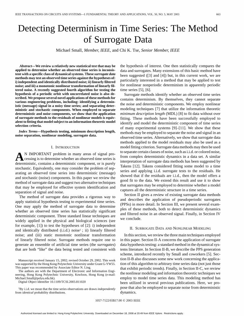
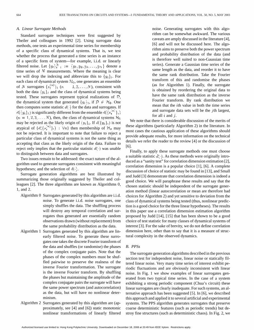
The surrogate generation algorithms described in the previoussection test for independent noise, linear noise or statically fil-tered linear noise. Very many time series of interest exhibit pe-riodic fluctuations and are obviously inconsistent with linearnoise. In Fig. 1 we show examples of linear surrogates gen-erated from two typical time series. In the case of a systemexhibiting a strong periodic component (Chua’s circuit) theselinear surrogates are clearly inadequate. For such systems, an al-ternative approach has been suggested [5]. In [6], we describedthis approach and applied it to several artificial and experimentalsystems. The PPS algorithm generates surrogates that preservecoarse deterministic features (such as periodic trends) but de-stroy fine structures (such as deterministic chaos). In Fig. 2, we


SMALL AND TSE: DETECTING DETERMINISM IN TIME SERIES 665

Fig. 1. Linear (Algorithms 0, 1, and 2) surrogates for two time series. The Ikeda map contaminated with linear noise (left side panels) and Chua’s circuit inits chaotic regime with both dynamic and observational noise (right). The top two panels are the original time series. Below these are (in order): Algorithm 0,Algorithm 1, and Algorithm 2 surrogates. Note that the surrogates appear qualitatively like the Ikeda data, but dissimilar to the Chua’s circuit simulation. Chua’scircuit contains nonlinear determinism which is not modeled adequately as a static monotonic nonlinear transformation of linear filtered noise. Quantitative analysisreveals that both these data sets are clearly distinct from these surrogates.

show that this method can be applied to differentiate betweendeterministic chaos with noise and a periodic orbit. The algo-rithm generates surrogates that are very like the original data,yet only have the large-scale deterministic features.

The basic algorithm for this method is the following.

1. Construct the vector delay embeddingfrom the scalar time series

according to

where the embedding dimension and em-bedding lag remain to be selected.The embedding window is defined by

.2. Call the recon-structed attractor .3. Choose an initial condition atrandom.4. Let .5. Choose a near neighbor of ac-cording to the probability distribution

where the parameter is the noise radius .6. Let be the successor to .7. Increment .8. If go to step 5.9. The surrogate time series is

, the scalarfirst components of .

The above algorithm has three parameters:, , and .Selection of embedding parameters and is discussed atlength in the literature (see, for example, [16] and the refer-ences therein) and we do not consider this problem here. Thenoise radius is selected according to the suggestions of [5].We choose such that the expected number of sequences oflength two or more that are identical for data and surrogates is

Fig. 2. Surrogates generated by the PPS algorithm for Chua’s circuit data.Note that the data and surrogates are qualitatively similar. However, quantitativeanalysis reveals that this data is clearly distinct from the system modeled bythe surrogates—a period orbit with uncorrelated noise. Each of these surrogateslacks the deterministic “signature” of chaos. The original data are depicted inthe top panel.

maximized. This selection criteria provides a balance between:1) too much randomization (few identical sequences of length;and 2) too little (data and surrogate near identical).

According to [5], this algorithm can be applied to test for non-periodic deterministic dynamics in pseudoperiodic time series.2

Conversely, dynamical systems consistent with these surrogatesexhibit a periodic orbit with uncorrelated noise. For time seriesexhibiting pseudoperiodic dynamics, rejection of this class ofsystems implies the existence of nonperiodic deterministic dy-namics. However, for time series that do not exhibit pseudope-riodic dynamics, we have shown [6] that surrogates generatedby this method are actually consistent with short-term deter-ministic dynamics. Rejection of this test therefore is evidencefor long-term deterministic dynamics. The distinction between“long term” and “short term” is perhaps ill defined, and certainlydependent on the selection of. However, for the current studya more precise definition is beyond our requirements. It is suf-ficient to note that surrogates generated by this method appear

2A pseudoperiodic time series is one which exhibits a definite periodic trend:there exists� > 0 such that the autocorrelation�(�) has a nontrivial peak�(� ) > 0 at � .



much more like the data than Algorithms 0, 1, and 2 surrogates.Rejection of the PPS algorithm indicates the presence of non-trivial deterministic dynamics in the data.

C. Nonlinear Modeling

In the last two sections, we have discussed various surrogatetechniques. We now turn our attention to a class of nonlinearmodels [7] utilising an information theoretic stopping criterion[8]. The difference between these techniques is not as great asit may seem. In the previous sections, we have deliberately de-scribed surrogate datahypothesis testingin terms of dynamicalsystems and classes of models. Conversely, in [3] and [12], ithas been shown that noisy iterated predictions of a model maybe used as a form of hypothesis testing.

For a scalar time series we perform a time delay em-bedding [17] according to

(1)

(There is a minor notational change between this embeddingand that in Section II-B. This distinction is cosmetic and largelya matter of convenience.) We then model the dynamics of themap by the construction of a function such that

where theresiduals are expected to be i.i.d. random variates.The function is of the form

(2)

where are theweights; such thatare thelags; are thebasis func-

tions; are thecenters; and are the radii.In fact, an often more useful generalization of this scheme isdescribed in [9]. In addition to each of these parameters, themodel size ( ) must also be selected3 so that the variate

are indeed i.i.d. but yet model overfitting must be avoided.Note that the selection of the model form (2) is based solely onthe computational algorithms at our disposal. Consideration ofmany other similar schemes may be found in the literature (see,for example, [11]).

To provide a suitable model fitting criterion we employmin-imum description length(MDL) as described by Rissanen [8]and applied to radial basis modeling by Judd and Mees [7].Roughly speaking, the description length of a data set is thelength of shortest description that can be employed to recon-struct the entire data set. For random variates, that code willsimply be the data itself and the description length will be thelength of that data set. For data containing some determinism,the shortest description length of that data will be the descrip-tion of a model of the deterministic component and the modelprediction errors.

Rissanen [8] showed that the description length of a parame-ters (specified to some finiteprecision ) is

3The model selection scheme described in [7] implies thatm andn are notindependent.

where is a constant related to the number of bits in the mantissaof the binary representation of . Denote by the model pa-rameters . Then, if we assume4 that the model(2) may be completely described by the linear parameters( ) then the description length of the modelis

(3)

The description length of the datawith this modelis then givenby

(4)

where is the negative log likelihood of the model pre-diction errors under the assumed distribution (5). The likelihoodof a data set is the probability of observing that particular set ofvalues. Assuming that the model prediction errors are Gaussiandistributed noise with standard deviation, the negative loglikelihood is given by

(5)

Typically, one will substitute the estimate for theunknown variance of the noise.

A model may then be assessed based on its description lengthas given in (4). The best model of a particular data set is that forwhich this quantity is lowest.

One observes that the important quantity in the above com-putation is the set of precisions of the parameters. It can beshown [7] that these precisions may be calculated as the solu-tion of

(6)

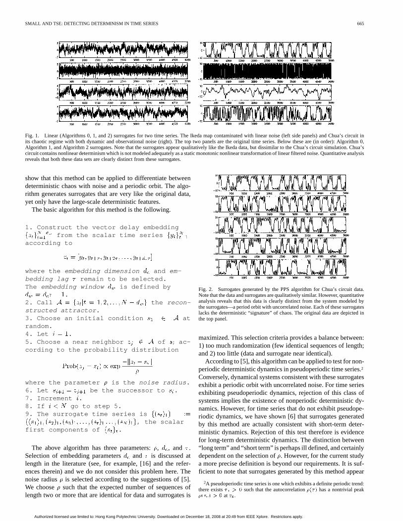
where is the second partial derivative of with respect tothe model parameters. In Fig. 3, we show the typical behaviorof MDL and root-mean-square error for a model of the datadepicted in (2).

III. D ETECTING AND EXTRACTING DETERMINISM

We now apply the methods discussed in Section II to simu-lated and experimental data. We show that linear and nonlinearsurrogates as described in Sections II-A and II-B can be suc-cessfully applied to realistic data to differentiate between de-terminism and stochastic behavior. We then consider the appli-cation of surrogate techniques to nonlinear modeling and showthat they behave the same as minimum description length andmay be used as a form of model selection criteria.

In Section III-A, we present the application of surrogatemethods to various engineering systems. Section III-B com-pares minimum description length and surrogate methods asmodel selection criteria.

4This is an approximation intended to make the calculations that follow sub-stantially easier. A full treatment is provided in [9].



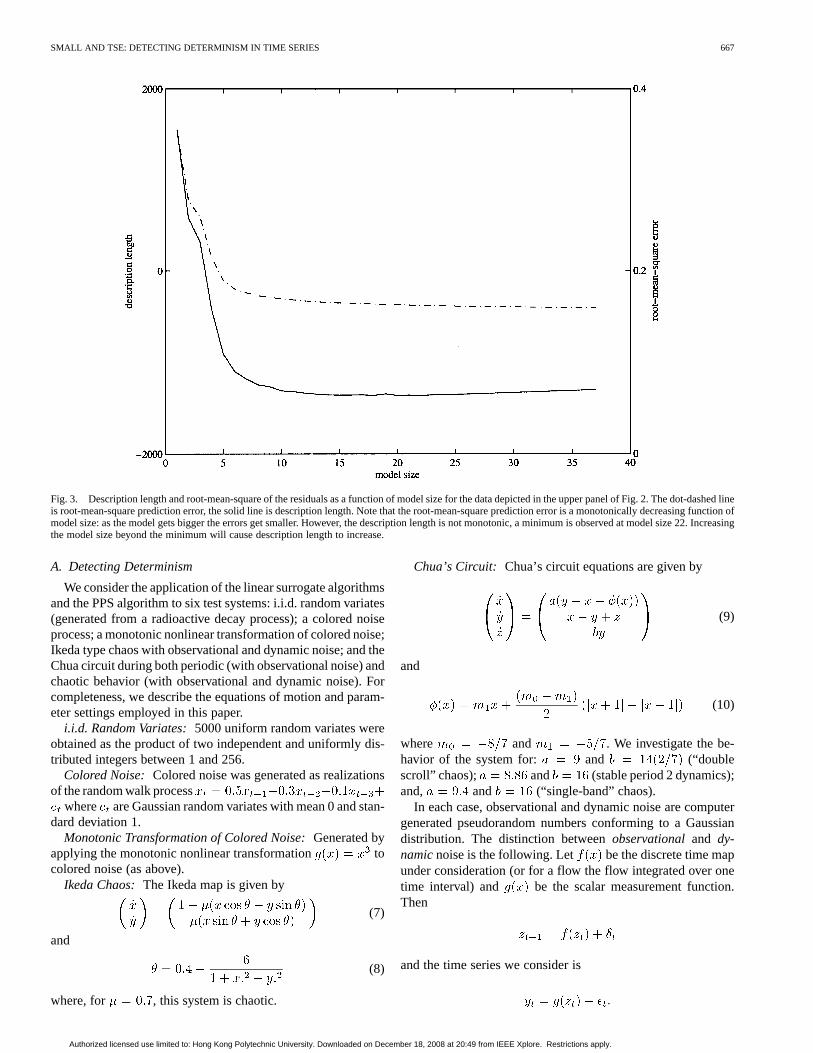
Fig. 3. Description length and root-mean-square of the residuals as a function of model size for the data depicted in the upper panel of Fig. 2. The dot-dashed lineis root-mean-square prediction error, the solid line is description length. Note that the root-mean-square prediction error is a monotonically decreasing function ofmodel size: as the model gets bigger the errors get smaller. However, the description length is not monotonic, a minimum is observed at model size 22. Increasingthe model size beyond the minimum will cause description length to increase.

A. Detecting Determinism

We consider the application of the linear surrogate algorithmsand the PPS algorithm to six test systems: i.i.d. random variates(generated from a radioactive decay process); a colored noiseprocess; a monotonic nonlinear transformation of colored noise;Ikeda type chaos with observational and dynamic noise; and theChua circuit during both periodic (with observational noise) andchaotic behavior (with observational and dynamic noise). Forcompleteness, we describe the equations of motion and param-eter settings employed in this paper.

i.i.d. Random Variates:5000 uniform random variates wereobtained as the product of two independent and uniformly dis-tributed integers between 1 and 256.

Colored Noise: Colored noise was generated as realizationsof the random walk process

where are Gaussian random variates with mean 0 and stan-dard deviation 1.

Monotonic Transformation of Colored Noise:Generated byapplying the monotonic nonlinear transformation tocolored noise (as above).

Ikeda Chaos:The Ikeda map is given by

(7)

and

(8)

where, for , this system is chaotic.

Chua’s Circuit: Chua’s circuit equations are given by

(9)

and

(10)

where and . We investigate the be-havior of the system for: and (“doublescroll” chaos); and (stable period 2 dynamics);and, and (“single-band” chaos).

In each case, observational and dynamic noise are computergenerated pseudorandom numbers conforming to a Gaussiandistribution. The distinction betweenobservationaland dy-namicnoise is the following. Let be the discrete time mapunder consideration (or for a flow the flow integrated over onetime interval) and be the scalar measurement function.Then

and the time series we consider is



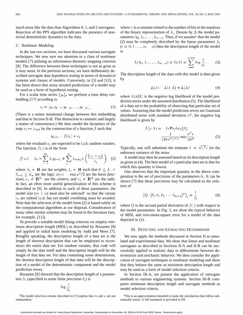
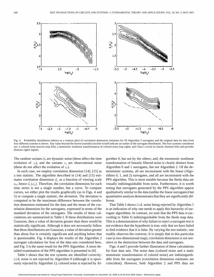
Fig. 4. Probability distribution (shown as a contour plot) of correlation dimension estimates for 50 Algorithm 2 surrogates and the original data fordata fromfour different systems is shown. Any value beyond the lowest (outside) isocline would indicate an outlier of the surrogate distribution. The four systems consideredare: a colored noise process (top left), a monotonic nonlinear transformation of colored noise (top right), and Chua’s circuit in chaotic (bottom left) and periodic(bottom right) regime.

The random variates are dynamic noise (these affect the timeevolution of ), and the variates are observational noise(these do not affect the evolution of).

In each case, we employ correlation dimension [14], [15] asa test statistic. The algorithm described in [14] and [15] esti-mates correlation dimension as a function of viewing scale

, hence . Therefore, the correlation dimension for eachtime series is not a single number, but a curve. To comparecurves, we either plot the results graphically (as in Figs. 4 and5) or compute a single statistic, thedeviation. The deviation iscomputed to be the maximum difference between the correla-tion dimension estimated for the data and the mean of the cor-relation dimension for the surrogates, expressed in terms of thestandard deviation of the surrogates. The results of these cal-culations are summarized in Table I. If these distributions wereGaussian, then a value of deviation greater than three would bestatistically significant. Although it does not necessarily followthat these distributions are Gaussian, a value of deviation greaterthan about five is certainly significant and anything below thatis questionable. Fig. 4 displays the results of the Algorithm 2surrogate calculation for four of the data sets considered here,and Fig. 5 is the same result for the PPS Algorithm. A more de-tailed examination of the PPS algorithm is presented in [6].

Table I shows that the test systems are identified correctly:i.i.d. noise is not rejected by Algorithm 0 (although it is spuri-ously rejected by Algorithm 1); colored noise is rejected by Al-

gorithm 0, but not by the others; and, the monotonic nonlineartransformation of linearly filtered noise is clearly distinct fromAlgorithm 0 and 1 surrogates, but not Algorithm 2. Of the de-terministic systems, all are inconsistent with the linear (Algo-rithms 0, 1, and 2) surrogates, and all are inconsistent with thePPS algorithm. This is most notable because the Ikeda data arevisually indistinguishable from noise. Furthermore, it is worthnoting that surrogates generated by the PPS algorithm appearqualitatively similar to the data (unlike the linear surrogates) butquantitative analysis demonstrates that they are significantly dif-ferent.

That Table I shows i.i.d. noise being rejected by Algorithm 1is an indication of why one needs to apply this hierarchy of sur-rogate algorithms. In contrast, we note that the PPS data is (ac-cording to Table I) indistinguishable from the Ikeda map data.This is a demonstration of why failure to reject a surrogate test isnot evidence that the hypothesis is true; only that we have failedto find evidence that it is false. By varying the test statistic, onereadily observes the converse. It is simply that in this particularcase (a two-dimensional map), correlation dimension is not sen-sitive to the distinction between the data and surrogates.

Figs. 4 and 5 provide further illustration of these calculationsfor four data sets. The noise data (colored noise and a staticmonotonic transformation of colored noise) are indistinguish-able from the surrogates (correlation dimension estimates arecoincident). However, both Algorithm 2 and PPS data are



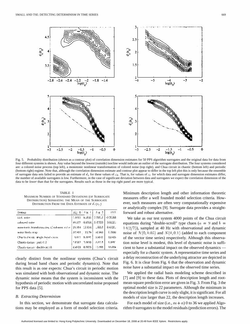
Fig. 5. Probability distribution (shown as a contour plot) of correlation dimension estimates for 50 PPS algorithm surrogates and the original data for data fromfour different systems is shown. Any value beyond the lowest (outside) isocline would indicate an outlier of the surrogate distribution. The four systems consideredare: a colored noise process (top left), a monotonic nonlinear transformation of colored noise (top right), and Chua circuit in chaotic (bottom left)and periodic(bottom right) regime. Note that, although the correlation dimension estimate and contour plot appear to differ in the top left plot this is only because the ensembleof surrogate data sets failed to provide an estimate ofd for these values of" . That is, for values of" for which data and surrogate dimension estimates differ,the number of available surrogates is low. Furthermore, in the case of significant deviation between data and surrogates we expect the correlation dimension of thedata to belower than that for the surrogates. Results such as those in the top right panel are more typical.

TABLE IMAXIMUM NUMBER OF STANDARD DEVIATIONS (OF SURROGATE

DISTRIBUTION) SEPARATING THE MEAN OF THE SURROGATE

DISTRIBUTION FROM THE DATA ESTIMATE OF d (" )

clearly distinct from the nonlinear systems (Chua’s circuitduring broad band chaos and periodic dynamics). Note thatthis result is as one expects: Chua’s circuit in periodic motionwas simulated with both observational and dynamic noise. Thedynamic noise means that the system is inconsistent with thehypothesis of periodic motion with uncorrelated noise proposedfor PPS data [5].

B. Extracting Determinism

In this section, we demonstrate that surrogate data calcula-tions may be employed as a form of model selection criteria.

Minimum description length and other information theoreticmeasures offer a well founded model selection criteria. How-ever, such measures are often very computationally expensiveor analytically complex [9]. Surrogate data provides a straight-forward and robust alternative.

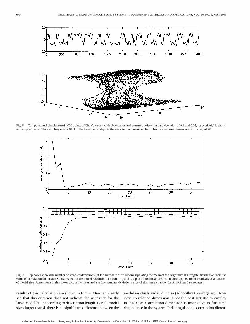
We take as our test system 4000 points of the Chua circuitequations during “double-scroll” type chaos ( and

), sampled at 40 Hz with observational and dynamicnoise of and (added to each componentof the vector time series) respectively. Although this observa-tion noise level is modest, this level of dynamic noise is suffi-cient to have a substantial impact on the observed dynamics —especially for a chaotic system. A representative time series anda delay reconstruction of the underlying attractor are depicted inFig. 6. It is clear from Fig. 6 that the observation and dynamicnoise have a substantial impact on the observed time series.

We applied the radial basis modeling scheme described in[7] and [9] to these data. Plots of description length and root-mean-square prediction error are given in Fig. 3. From Fig. 3 theoptimal model size is 22 parameters. Although the minimum inthe description length curve is only slight, it is significant. For allmodels of size larger than 22, the description length increases.

For each model of size (i.e., ) 0 to 36 we applied Algo-rithm 0 surrogates to the model residuals (prediction errors). The



Fig. 6. Computational simulation of 4000 points of Chua’s circuit with observation and dynamic noise (standard deviation of 0.1 and 0.05, respectively) is shownin the upper panel. The sampling rate is 40 Hz. The lower panel depicts the attractor reconstructed from this data in three dimensions with a lag of 20.

Fig. 7. Top panel shows the number of standard deviations (of the surrogate distribution) separating the mean of the Algorithm 0 surrogate distribution from thevalue of correlation dimensiond estimated for the model residuals. The bottom panel is a plot of nonlinear prediction error applied to the residuals as a functionof model size. Also shown in this lower plot is the mean and the five standard deviation range of this same quantity for Algorithm 0 surrogates.

results of this calculation are shown in Fig. 7. One can clearlysee that this criterion does not indicate the necessity for thelarge model built according to description length. For all modelsizes larger than 4, there is no significant difference between the

model residuals and i.i.d. noise (Algorithm 0 surrogates). How-ever, correlation dimension is not the best statistic to employin this case. Correlation dimension is insensitive to fine timedependence in the system. Indistinguishable correlation dimen-



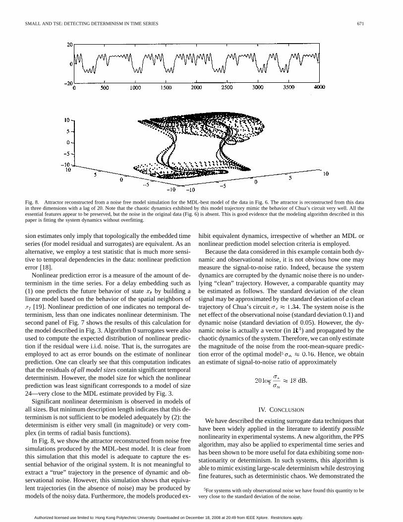
Fig. 8. Attractor reconstructed from a noise free model simulation for the MDL-best model of the data in Fig. 6. The attractor is reconstructed from this datain three dimensions with a lag of 20. Note that the chaotic dynamics exhibited by this model trajectory mimic the behavior of Chua’s circuit very well. All theessential features appear to be preserved, but the noise in the original data (Fig. 6) is absent. This is good evidence that the modeling algorithm described in thispaper is fitting the system dynamics without overfitting.

sion estimates only imply that topologically the embedded timeseries (for model residual and surrogates) are equivalent. As analternative, we employ a test statistic that is much more sensi-tive to temporal dependencies in the data: nonlinear predictionerror [18].

Nonlinear prediction error is a measure of the amount of de-terminism in the time series. For a delay embedding such as(1) one predicts the future behavior of stateby building alinear model based on the behavior of the spatial neighbors of

[19]. Nonlinear prediction of one indicates no temporal de-terminism, less than one indicates nonlinear determinism. Thesecond panel of Fig. 7 shows the results of this calculation forthe model described in Fig. 3. Algorithm 0 surrogates were alsoused to compute the expected distribution of nonlinear predic-tion if the residual were i.i.d. noise. That is, the surrogates areemployed to act as error bounds on the estimate of nonlinearprediction. One can clearly see that this computation indicatesthat the residualsof all model sizescontain significant temporaldeterminism. However, the model size for which the nonlinearprediction was least significant corresponds to a model of size24—very close to the MDL estimate provided by Fig. 3.

Significant nonlinear determinism is observed in models ofall sizes. But minimum description length indicates that this de-terminism is not sufficient to be modeled adequately by (2): thedeterminism is either very small (in magnitude) or very com-plex (in terms of radial basis functions).

In Fig. 8, we show the attractor reconstructed from noise freesimulations produced by the MDL-best model. It is clear fromthis simulation that this model is adequate to capture the es-sential behavior of the original system. It is not meaningful toextract a “true” trajectory in the presence of dynamic and ob-servational noise. However, this simulation shows that equiva-lent trajectories (in the absence of noise) may be produced bymodels of the noisy data. Furthermore, the models produced ex-

hibit equivalent dynamics, irrespective of whether an MDL ornonlinear prediction model selection criteria is employed.

Because the data considered in this example contain both dy-namic and observational noise, it is not obvious how one maymeasure the signal-to-noise ratio. Indeed, because the systemdynamics are corrupted by the dynamic noise there is no under-lying “clean” trajectory. However, a comparable quantity maybe estimated as follows. The standard deviation ofthe cleansignal may be approximated by the standard deviation ofacleantrajectory of Chua’s circuit . The system noise is thenet effect of the observational noise (standard deviation 0.1) anddynamic noise (standard deviation of 0.05). However, the dy-namic noise is actually a vector (in ) and propagated by thechaotic dynamics of the system. Therefore, we can only estimatethe magnitude of the noise from the root-mean-square predic-tion error of the optimal model5 . Hence, we obtainan estimate of signal-to-noise ratio of approximately

dB

IV. CONCLUSION

We have described the existing surrogate data techniques thathave been widely applied in the literature to identifypossiblenonlinearity in experimental systems. A new algorithm, the PPSalgorithm, may also be applied to experimental time series andhas been shown to be more useful for data exhibiting some non-stationarity or determinism. In such systems, this algorithm isable to mimic existing large-scale determinism while destroyingfine features, such as deterministic chaos. We demonstrated the

5For systems with only observational noise we have found this quantity to bevery close to the standard deviation of the noise.



application of these four algorithms to seven test systems andcorrectly identified the origin of the signal in each case.

To date, surrogate techniques have largely been appliedwithin the nonlinear time series community to screen data priorto analysis with nonlinear methods. Data that is likely to beconsistent with these linear algorithms is ignored in favor ofmore interesting time series. Once such set of data is shownto be distinct from a monotonic nonlinear transformation oflinearly filtered noise, it is usual to proceed to the application ofmore sophisticated data analysis techniques. In an engineeringcontext, these techniques may be applied to observed data todetect significant determinism. One can apply these methodsto search for deterministic signals hidden within an apparentlyrandom background. For example, surrogate techniques shouldprove useful for identifying a communication signal encodedwith chaotic shift keying: unmasking chaotic masking.

However, to unmask a chaotic signal one needs to know morethan its existence. For this reason, we described a nonlinearmodeling methods that can separate deterministic and stochasticcomponents in a time series. A common problem for all mod-eling regimes is how large should one make the model. Thealgorithm described in this paper addressed this problem withthe information theoretic minimum description length. For thedata we considered here we found that nonlinear prediction errorand surrogate data methods could be employed to provide anequivalent model selection criteria: the best model is achievedwhen the model prediction errors (residuals) are indistinguish-able from i.i.d. variates. We showed that either method could beemployed to recover a chaotic attractor from a time series con-taminated with dynamic and observational noise.

Apart from the application considered here, a variant on thismodel selection algorithm may be employed to reduce the resid-uals to a less trivial form. If the objective were to separate theobserved time series into a nonlinear component and a colorednoise component one could apply the modeling algorithm untilthe model residuals are indistinguishable from Algorithm 1 or 2surrogates. Such a technique could be useful when one is awareof the form of the noise but is only interested in more complexnonlinear structure. However, successful implementation of thiswould rely on ensuring that the modeling algorithm did not at-tempt to fit the linear stochastic structure first.

REFERENCES

[1] M. Small, K. Judd, M. Lowe, and S. Stick, “Is breathing in infantschaotic? Dimension estimates for respiratory patterns during quietsleep,”J. Appl. Physiol., vol. 86, pp. 359–376, 1999.

[2] J. Theiler, S. Eubank, A. Longtin, B. Galdrikian, and J. D. Farmer,“Testing for nonlinearity in time series: The method of surrogate data,”Phys. D, vol. 58, pp. 77–94, 1992.

[3] M. Small and K. Judd, “Correlation dimension: A pivotal statistic fornonconstrained realizations of composite hypotheses in surrogate dataanalysis,”Phys. D, vol. 120, pp. 386–400, 1998.

[4] T. Schreiber and A. Schmitz, “Surrogate time series,”Phys. D, vol. 142,pp. 346–382, 2000.

[5] M. Small, D. J. Yu, and R. G. Harrison, “A surrogate test for pseudo-periodic time series data,”Phys. Rev. Lett., vol. 87, p. 188101, 2001.

[6] M. Small and C. K. Tse, “Applying the method of surrogate data to cyclictime series,”Phys. D, vol. 164, pp. 182–202, 2002.

[7] K. Judd and A. Mees, “On selecting models for nonlinear time series,”Phys. D, vol. 82, pp. 426–444, 1995.

[8] J. Rissanen,Stochastic Complexity in Statistical Inquiry. Singapore:World Scientific, 1989.

[9] M. Small and K. Judd, “Comparison of new nonlinear modeling tech-niques with applications to infant respiration,”Phys. D, vol. 117, pp.283–298, 1998.

[10] M. Small, D. J. Yu, and R. G. Harrison, “Period doubling bifurcationroute in human ventricular fibrillation,”Int. J. Bifurcation Chaos, vol.13, 2003, to be published.

[11] M. Small, K. Judd, and A. Mees, “Modeling continuous processes fromdata,”Phys. Rev. E, vol. 65, p. 046704, 2002.

[12] F. Takens, “Detecting nonlinearities in stationary time series,”Int. J. Bi-furcation Chaos, vol. 3, pp. 241–256, 1993.

[13] J. Theiler and D. Prichard, “Constrained-realization Monte-Carlomethod for hypothesis testing,”Phys. D, vol. 94, pp. 221–235, 1996.

[14] K. Judd, “An improved estimator of dimension and some comments onproviding confidence intervals,”Phys. D, vol. 56, pp. 216–228, 1992.

[15] , “Estimating dimension from small samples,”Phys. D, vol. 71, pp.421–429, 1994.

[16] H. D. I. Abarbanel,Analysis of Observed Chaotic Data. New York:Springer-Verlag, 1996.

[17] F. Takens, “Detecting strange attractors in turbulence,”Lect. NotesMath., vol. 898, pp. 366–381, 1981.

[18] R. Hegger, H. Kantz, and T. Schreiber, “Practical implementation of non-linear time series methods: The TISEAN package,”Chaos, vol. 9, pp.413–435, 1999.

[19] G. Sugihara and R. M. May, “Nonlinear forecasting as a way of distin-guishing chaos from measurement error in time series,”Nature, vol. 344,pp. 737–740, 1990.

Michael Small (M’01) received the B.Sc. (Hons)degree in pure mathematics and the Ph.D. degreein applied mathematics from the University ofWestern Australia, Perth, Australia, in 1994 and1998, respectively.

He is presently an Assistant Professor with theHong Kong Polytechnic University, Hong Kong,and his research is in the area of nonlinear dynamicsand nonlinear time series analysis. His researchemphasizes the application of nonlinear time seriestechniques in a diverse range of areas including:

infant respiratory patterns, human cardiac arrhythmia, financial analysis andtelecommunications. Prior to his current appointment he has held research postsat Hong Kong Polytechnic University, Hong Kong, Heriot-Watt University,Edinburgh, Scotland, Stellenbosch University, Stellenbosch, South Africa, andthe University of Western Australia.

Chi K. Tse (M’90–SM’97) received the B.Eng.(Hons.) degree with first class honors in electricalengineering and the Ph.D. degree from the Univer-sity of Melbourne, Melbourne, Australia, in 1987and 1991, respectively.

He is presently a Professor with the HongKong Polytechnic University, Hong Kong, and hisresearch interests include chaotic dynamics, powerelectronics, and chaos-based communications. He isthe author ofLinear Circuit Analysis(London, U.K.:Addison-Wesley, 1998) andComplex Behavior of

Switching Power Converters(Boca Raton, FL: CRC Press, 2003), coauthorof Chaos-Based Digital Communication Systems(Heidelberg, Germany:Springer-Verlag, 2003), and coholder of a U.S. patent.

Prof. Tse served as an Associate Editor of the IEEE TRANSACTIONS ON

CIRCUITS AND SYSTEMSPART I—FUNDAMENTAL THEORY AND APPLICATIONS,from 1999 to 2001, and since 1999, he has been an Associate Editor of theIEEE TRANSACTIONS ONPOWER ELECTRONICS. In 1987, he was awarded theL.R. East Prize by the Institution of Engineers, Australia, and in 2001, theIEEE TRANSACTIONS ON POWER ELECTRONICS, Prize Paper Award. Whilewith the university, he received twice the President’s Award for Achievementin Research, the Faculty’s Best Researcher Award and a few other teachingawards. Since 2002, he has been appointed as Advisory Professor by theSouthwest China Normal University, Chongqing, China.


detecting determinism in time series: the method of surrogate data

Documents