path detection: a quantum algorithmic primitive
TRANSCRIPT

Path Detection: A Quantum Algorithmic Primitive
Shelby KimmelMiddlebury College
Based on work with Stacey Jeffery: arXiv: 1704.00765 (Quantum vol 1 p 26)Michael Jarret, Stacey Jeffery, Alvaro Piedrafita, arXiv:1804.10591 (ESA 2018)Kai DeLorenzo, Teal Witter, arXiv:1904.05995 (TQC 2019)

Primitives!
• Quantum algorithmic primitives1. Widely applicable2. Can be used in a black box manner (with easily
analyzable behavior)

Primitives!
• Quantum algorithmic primitives1. Widely applicable2. Can be used in a black box manner (with easily
analyzable behavior)
– Ex: Searching unordered list of 𝑛 items– Classically, takes Ω(𝑛) time– Quantumly, takes 𝑂( 𝑛) time

Primitives!
• Quantum algorithmic primitives1. Widely applicable2. Can be used in a black box manner (with easily
analyzable behavior)
– Ex: Searching unordered list of 𝑛 items– Classically, takes Ω(𝑛) time– Quantumly, takes 𝑂( 𝑛) time
Good primitive: 𝒔𝒕-connectivity
Outline:
A. Introduction to st-connectivityB. st-connectivity makes a good algorithmic primitive
1. Widely applicable2. Easy to analyze
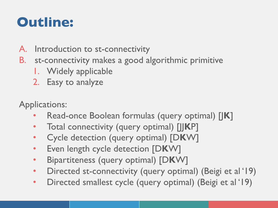
Outline:
A. Introduction to st-connectivityB. st-connectivity makes a good algorithmic primitive
1. Widely applicable2. Easy to analyze
Applications:• Read-once Boolean formulas (query optimal) [JK] • Total connectivity (query optimal) [JJKP]• Cycle detection (query optimal) [DKW]• Even length cycle detection [DKW]• Bipartiteness (query optimal) [DKW]• Directed st-connectivity (query optimal) (Beigi et al ‘19)• Directed smallest cycle (query optimal) (Beigi et al ‘19)
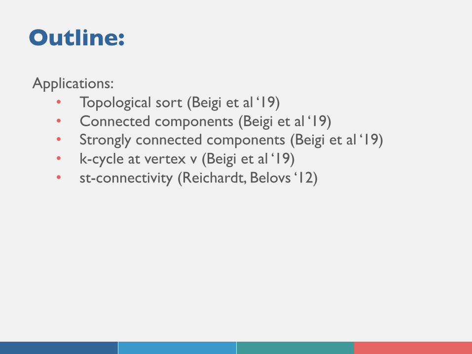
Outline:
Applications:• Topological sort (Beigi et al ‘19)• Connected components (Beigi et al ‘19)• Strongly connected components (Beigi et al ‘19)• k-cycle at vertex v (Beigi et al ‘19)• st-connectivity (Reichardt, Belovs ‘12)
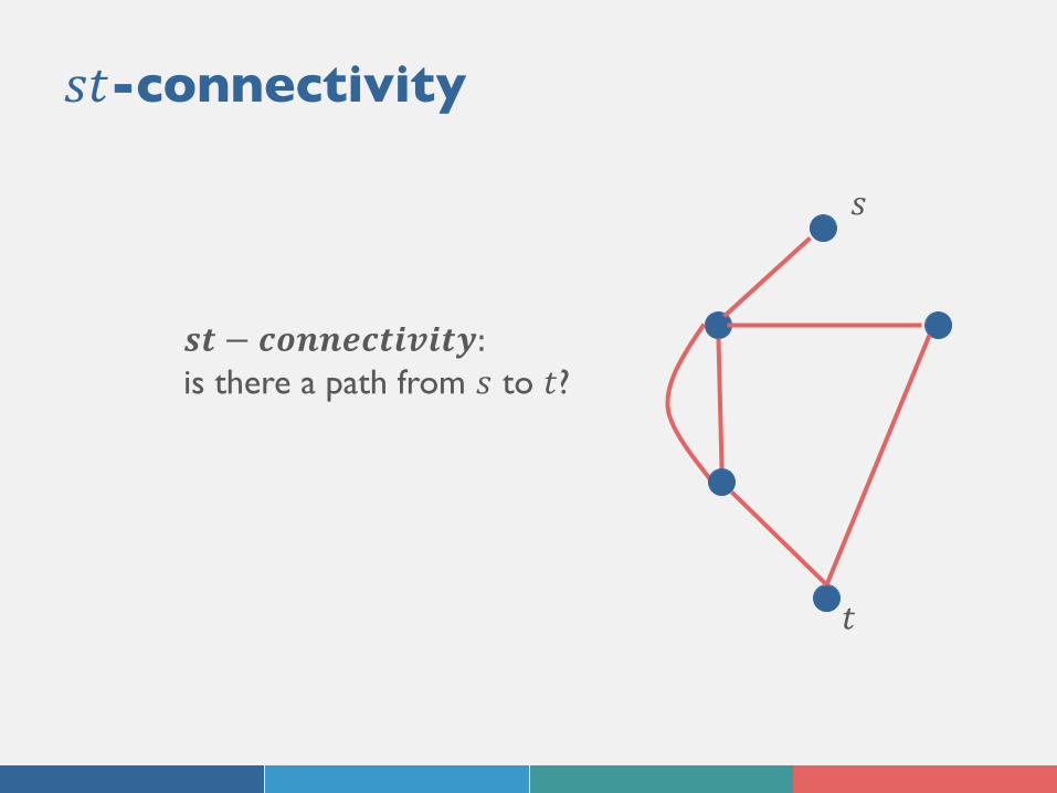
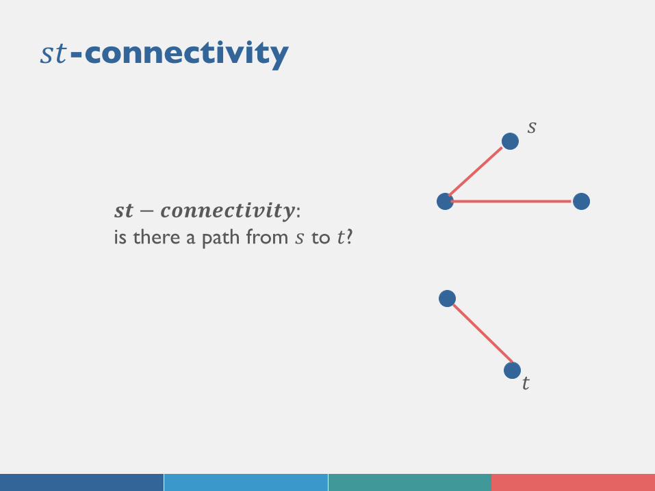
𝑠𝑡-connectivity
𝑠
𝑡
𝒔𝒕 − 𝒄𝒐𝒏𝒏𝒆𝒄𝒕𝒊𝒗𝒊𝒕𝒚:is there a path from 𝑠 to 𝑡?
𝑠𝑡-connectivity
𝑠
𝑡
𝒔𝒕 − 𝒄𝒐𝒏𝒏𝒆𝒄𝒕𝒊𝒗𝒊𝒕𝒚:is there a path from 𝑠 to 𝑡?
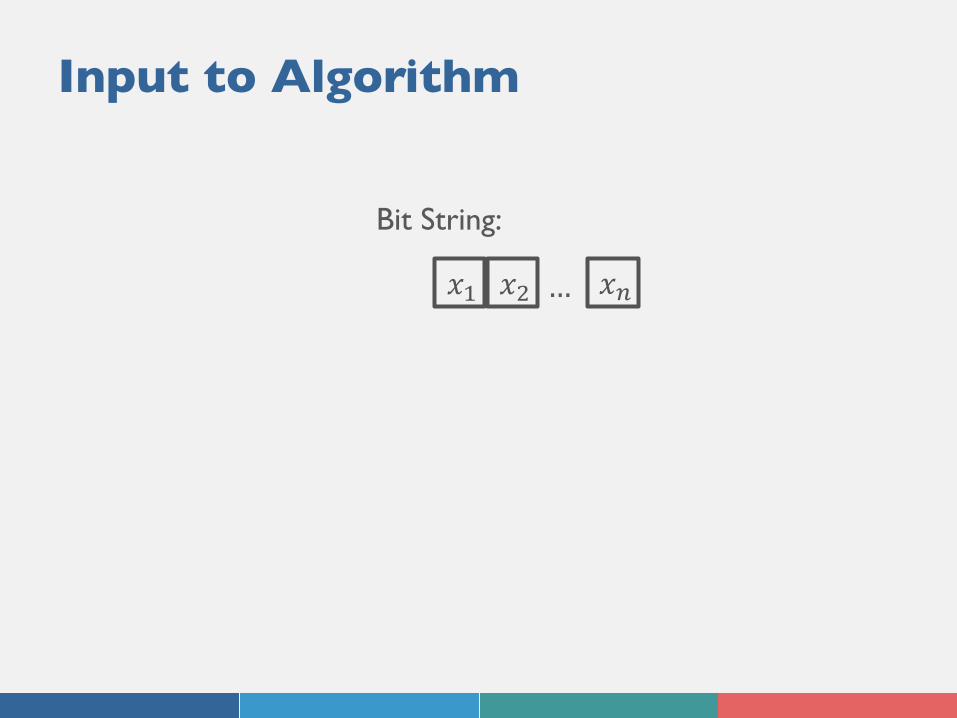
Input to Algorithm
Bit String:
𝑥! 𝑥" 𝑥#…
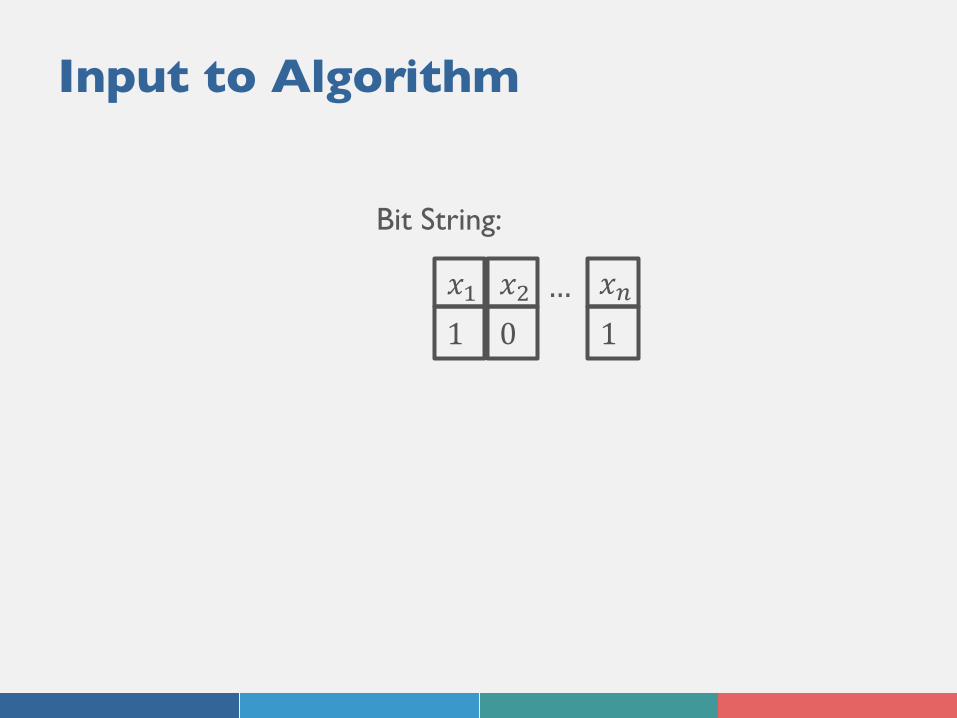
Input to Algorithm
Bit String:
𝑥! 𝑥" 𝑥#101
…
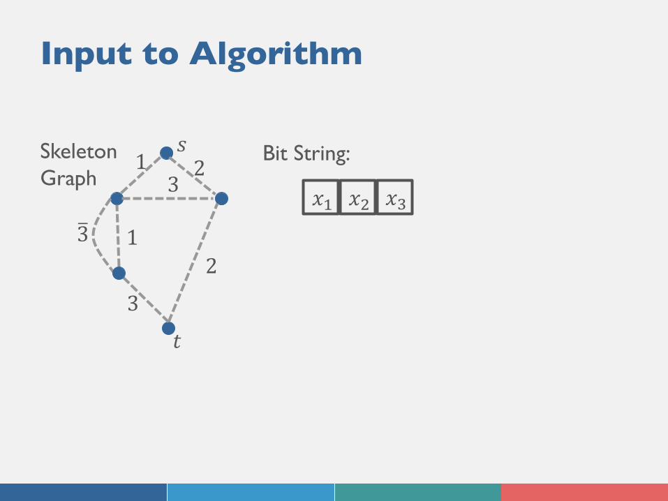
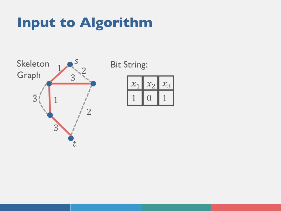
Input to Algorithm
𝑥! 𝑥" 𝑥$
Skeleton Graph
Bit String:2
83 1
3
2
13
𝑠
𝑡
Input to Algorithm
2
1
3
2
13
𝑠
𝑡
𝑥! 𝑥" 𝑥$101
Skeleton Graph
Bit String:
83

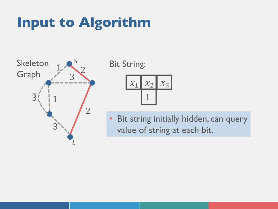
Input to Algorithm
2
1
3
2
13
𝑠
𝑡
𝑥! 𝑥" 𝑥$100
Skeleton Graph
Bit String:
83
Input to Algorithm
2
1
3
2
13
𝑠
𝑡
𝑥! 𝑥" 𝑥$1
Skeleton Graph
Bit String:
• Bit string initially hidden, can query value of string at each bit.
83
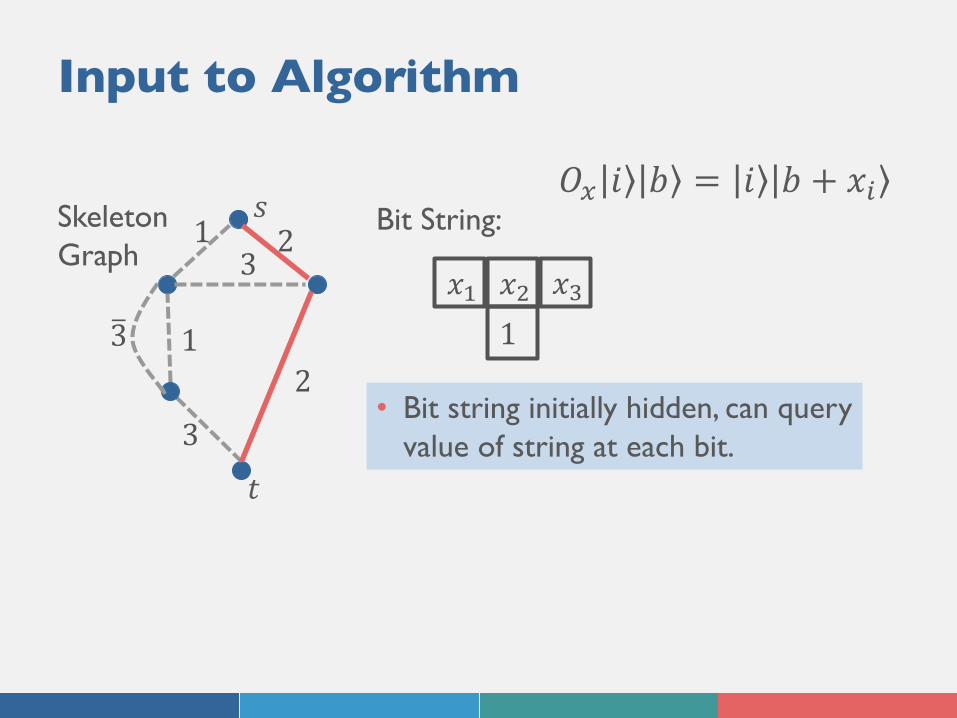
Input to Algorithm
2
1
3
2
13
𝑠
𝑡
𝑥! 𝑥" 𝑥$1
Skeleton Graph
Bit String:
• Bit string initially hidden, can query value of string at each bit.
83
𝑂! 𝑖 𝑏 = 𝑖 𝑏 + 𝑥"
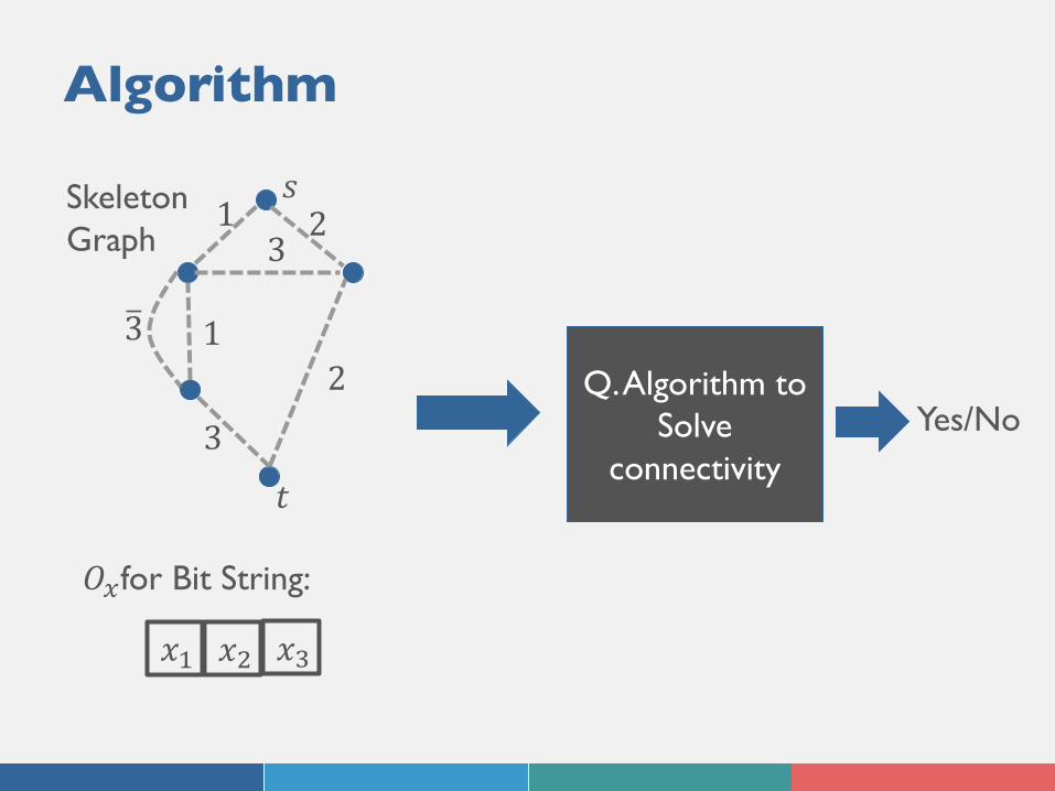
Algorithm
𝑥! 𝑥" 𝑥$
Skeleton Graph
𝑂%for Bit String:
2
83 1
3
2
13
𝑠
𝑡
Q. Algorithm to Solve
connectivityYes/No

Outline:
A. Introduction to st-connectivityB. st-connectivity makes a good algorithmic primitive
1. Widely applicable2. Easy to analyze
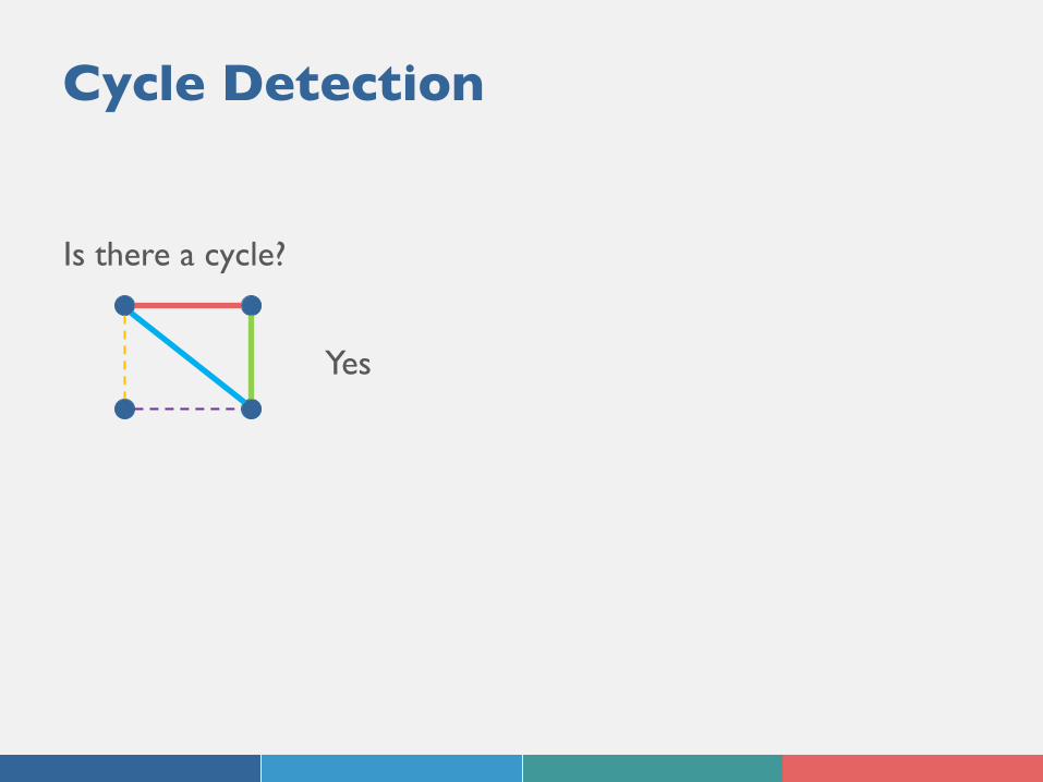
Cycle Detection
Is there a cycle?
Yes
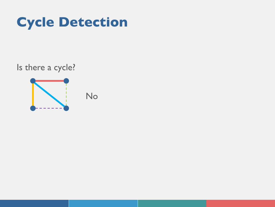
Cycle Detection
Is there a cycle?
No
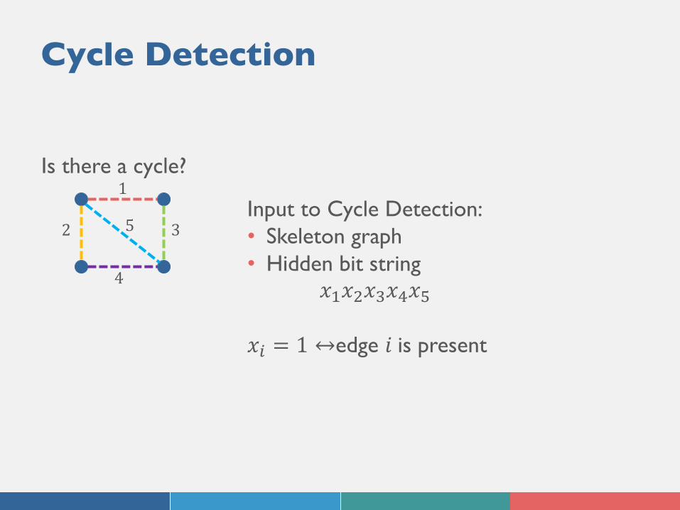
Cycle Detection
1
2 3
4
5
Is there a cycle?
Input to Cycle Detection: • Skeleton graph• Hidden bit string
𝑥!𝑥"𝑥$𝑥+𝑥,
𝑥- = 1 ↔edge 𝑖 is present
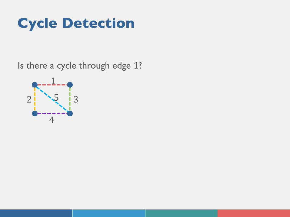
Cycle Detection
Is there a cycle through edge 1?
1
2 3
4
5
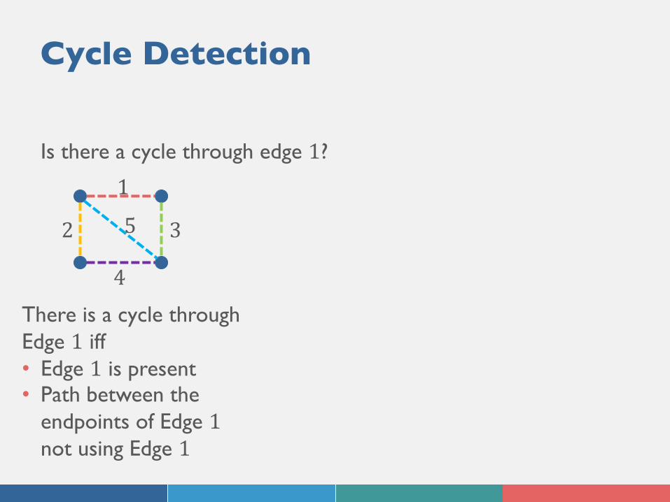
Cycle Detection
There is a cycle through Edge 1 iff • Edge 1 is present• Path between the
endpoints of Edge 1not using Edge 1
1
2 3
4
5
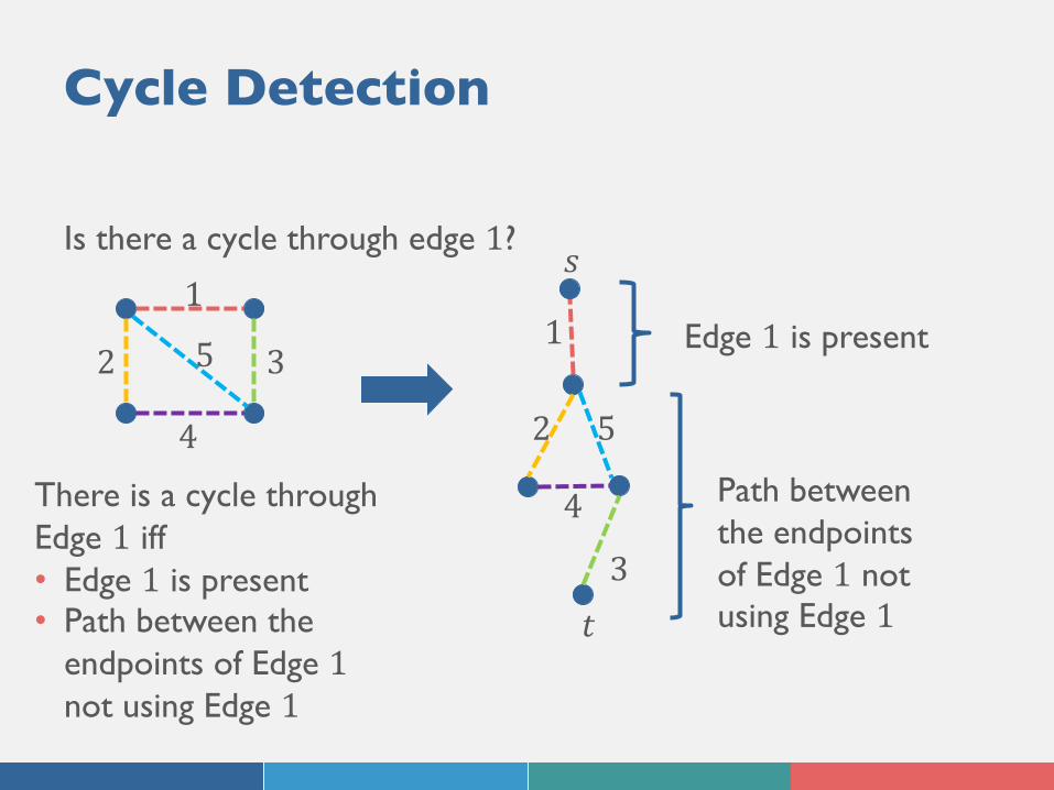
Is there a cycle through edge 1?
Cycle Detection
There is a cycle through Edge 1 iff • Edge 1 is present• Path between the
endpoints of Edge 1not using Edge 1
1
2 3
4
5
Is there a cycle through edge 1?
1
2
3
4
5
𝑠
𝑡
Edge 1 is present
Path between the endpoints of Edge 1 not using Edge 1
Cycle Detection
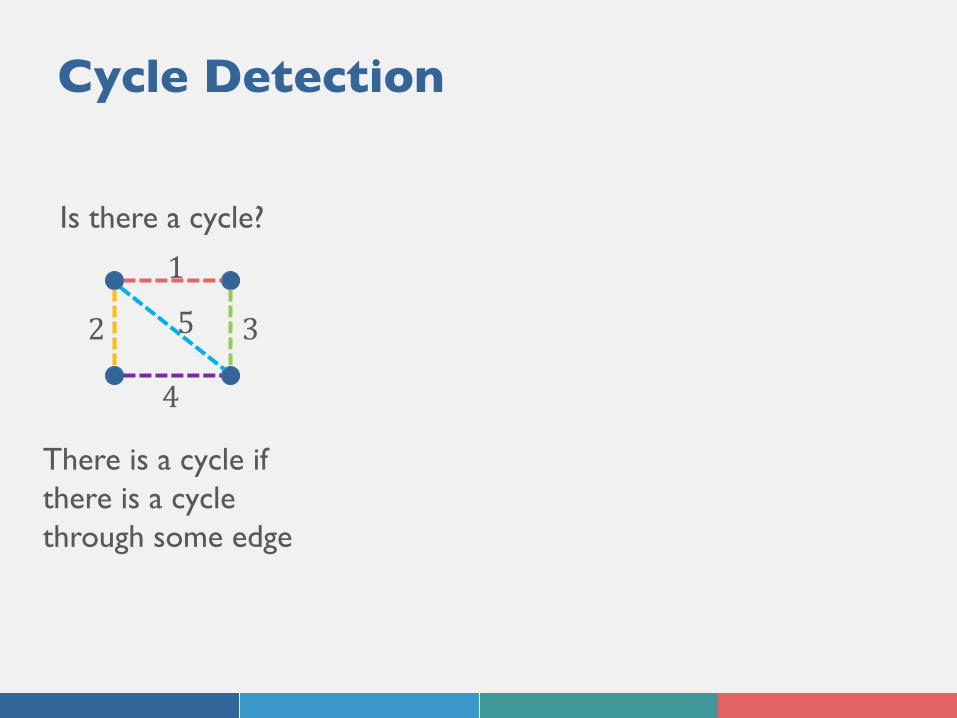
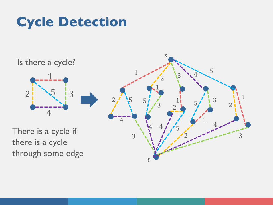
Is there a cycle?
There is a cycle if there is a cycle through some edge
1
2 3
4
5
Cycle Detection
Is there a cycle?
There is a cycle if there is a cycle through some edge
1
2 3
4
5
1
2
3
4
5
𝑠
𝑡
12
3
4 5
2
3
4
5
1
1
2
3
4
51
2
3
5
4
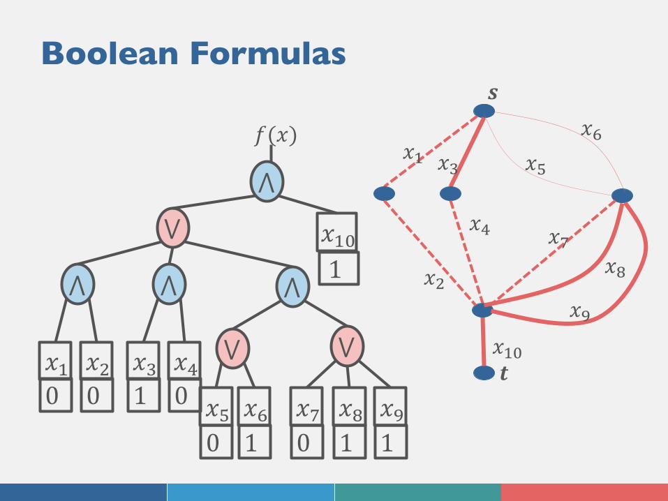
Boolean Formulas
⋀
⋁
⋀ ⋀ ⋀
⋁ ⋁
𝑥#$
𝑥# 𝑥% 𝑥& 𝑥'𝑥( 𝑥) 𝑥* 𝑥+ 𝑥,
𝑓(𝑥)
1
0 0 1 0
0 1 0 1 1
𝒔
𝒕𝑥!0
𝑥!
𝑥"
𝑥$
𝑥+
𝑥,
𝑥1
𝑥2𝑥3
𝑥4

Outline:
A. Introduction to st-connectivityB. st-connectivity makes a good algorithmic primitive
1. Widely applicable2. Easy to analyze
Algorithm Analysis:
Space Complexity: 𝑂 log(# 𝑒𝑑𝑔𝑒𝑠 𝑖𝑛 𝑠𝑘𝑒𝑙𝑒𝑡𝑜𝑛 𝑔𝑟𝑎𝑝ℎ)
Algorithm Analysis:
Query Complexity:
• Bit string initially unknown• Minimum # of oracle uses to
determine w.h.p. on worst input
Algorithm Analysis:
Query Complexity:
• Bit string initially unknown• Minimum # of oracle uses to
determine w.h.p. on worst input
≈Time Complexity

Algorithm Analysis:
Query Complexity:
𝑂 max!"##$!%$& '
𝑅(,% 𝐺 max#"% !"##$!%$& '
𝐶(,% 𝐺
Effective resistance Effective capacitance
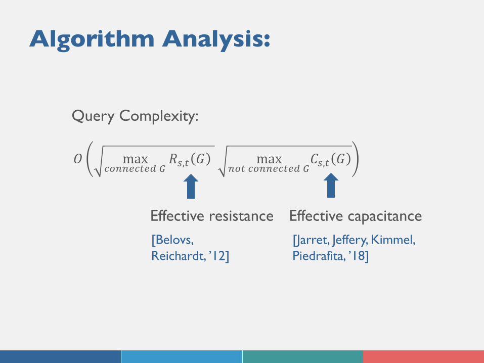
Algorithm Analysis:
Query Complexity:
𝑂 max!"##$!%$& '
𝑅(,% 𝐺 max#"% !"##$!%$& '
𝐶(,% 𝐺
Effective resistance Effective capacitance[Belovs, Reichardt, ’12]
[Jarret, Jeffery, Kimmel, Piedrafita, ’18]
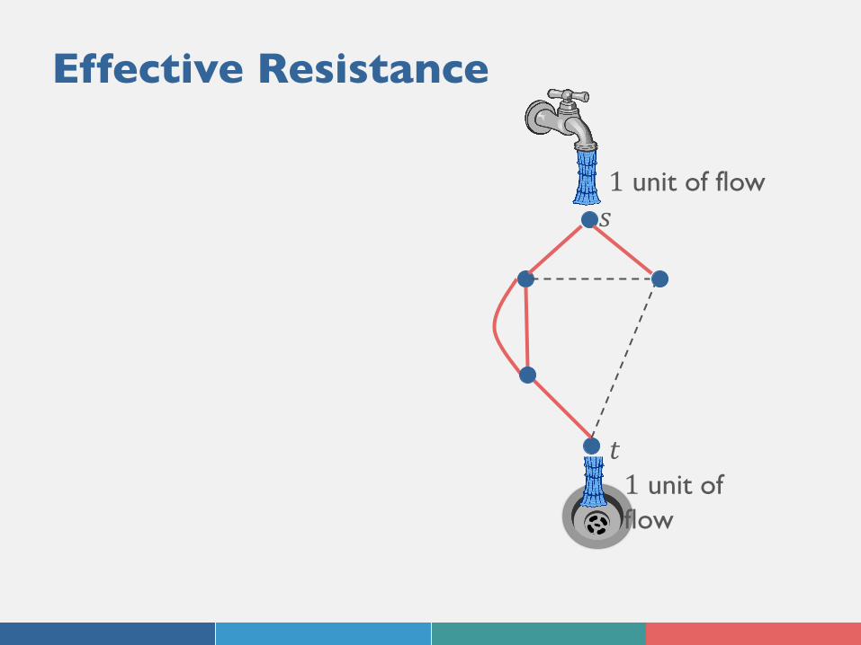
Effective Resistance
𝑠
𝑡
1 unit of flow
1 unit of flow
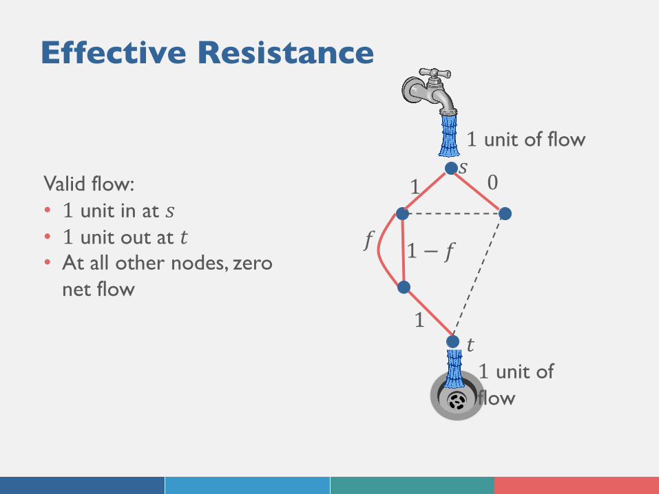
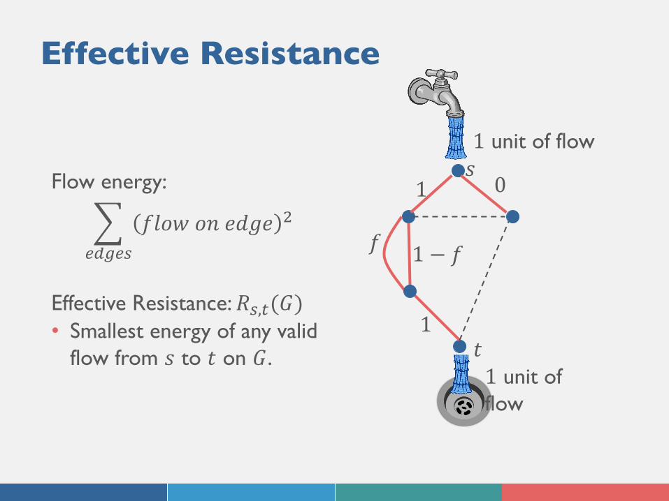
Effective Resistance
Valid flow:• 1 unit in at 𝑠• 1 unit out at 𝑡• At all other nodes, zero
net flow
𝑠
𝑡
1 unit of flow
1 unit of flow
1
1
𝑓 1 − 𝑓
0
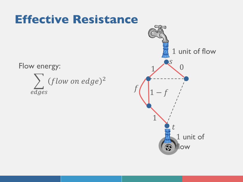
Effective Resistance
Flow energy:
N56758
𝑓𝑙𝑜𝑤 𝑜𝑛 𝑒𝑑𝑔𝑒 "
𝑠
𝑡
1 unit of flow
1 unit of flow
1
1
𝑓 1 − 𝑓
0
Effective Resistance
Flow energy:
N56758
𝑓𝑙𝑜𝑤 𝑜𝑛 𝑒𝑑𝑔𝑒 "
Effective Resistance: 𝑅8,:(𝐺)• Smallest energy of any valid
flow from 𝑠 to 𝑡 on 𝐺.
𝑠
𝑡
1 unit of flow
1 unit of flow
1
1
𝑓 1 − 𝑓
0
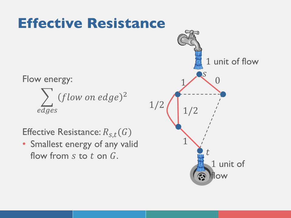
Effective Resistance
𝑠
𝑡
1 unit of flow
1 unit of flow
1
1
1/2 1/2
0Flow energy:
N56758
𝑓𝑙𝑜𝑤 𝑜𝑛 𝑒𝑑𝑔𝑒 "
Effective Resistance: 𝑅8,:(𝐺)• Smallest energy of any valid
flow from 𝑠 to 𝑡 on 𝐺.

Algorithm Analysis:
Query Complexity:
𝑂 max!"##$!%$& '
𝑅(,% 𝐺 max#"% !"##$!%$& '
𝐶(,% 𝐺
Effective resistance Effective capacitance
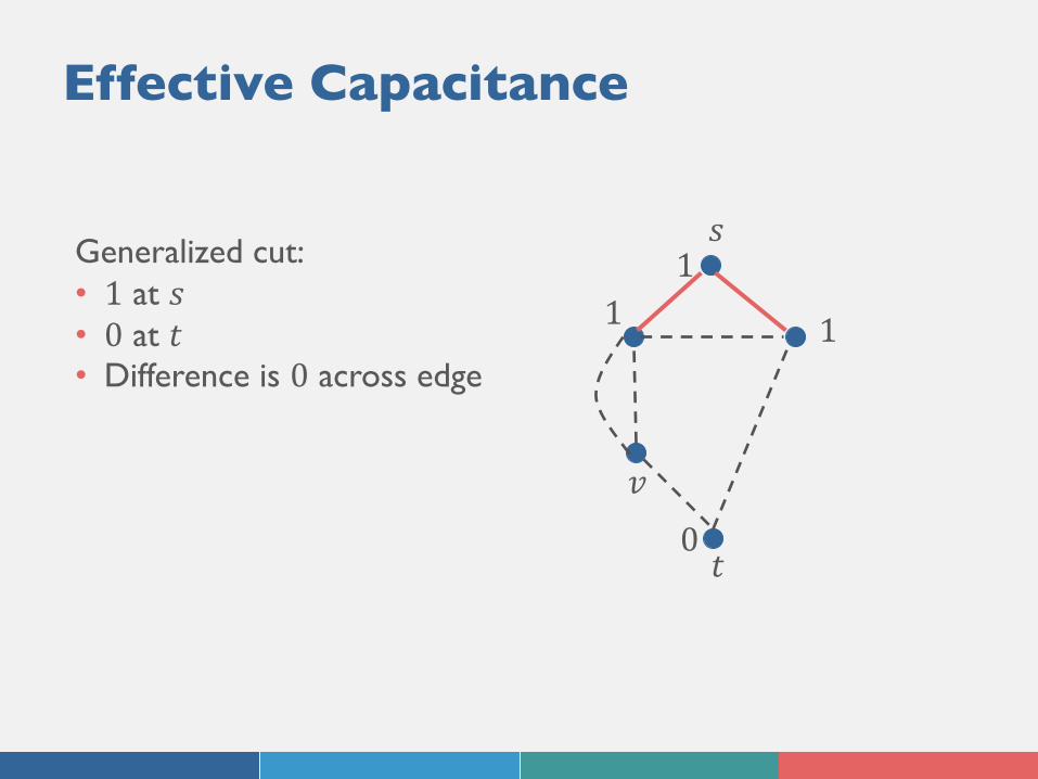
Effective Capacitance
Generalized cut:• 1 at 𝑠• 0 at 𝑡• Difference is 0 across edge
𝑠
𝑡
11 1
0𝑣
Effective Capacitance
𝑠
𝑡
11 1
0𝑣
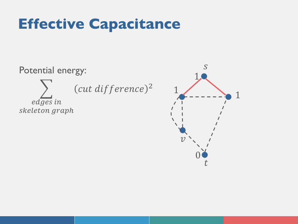
Potential energy:
N56758 -#
8;5<5:=# 7>?@A
𝑐𝑢𝑡 𝑑𝑖𝑓𝑓𝑒𝑟𝑒𝑛𝑐𝑒 "
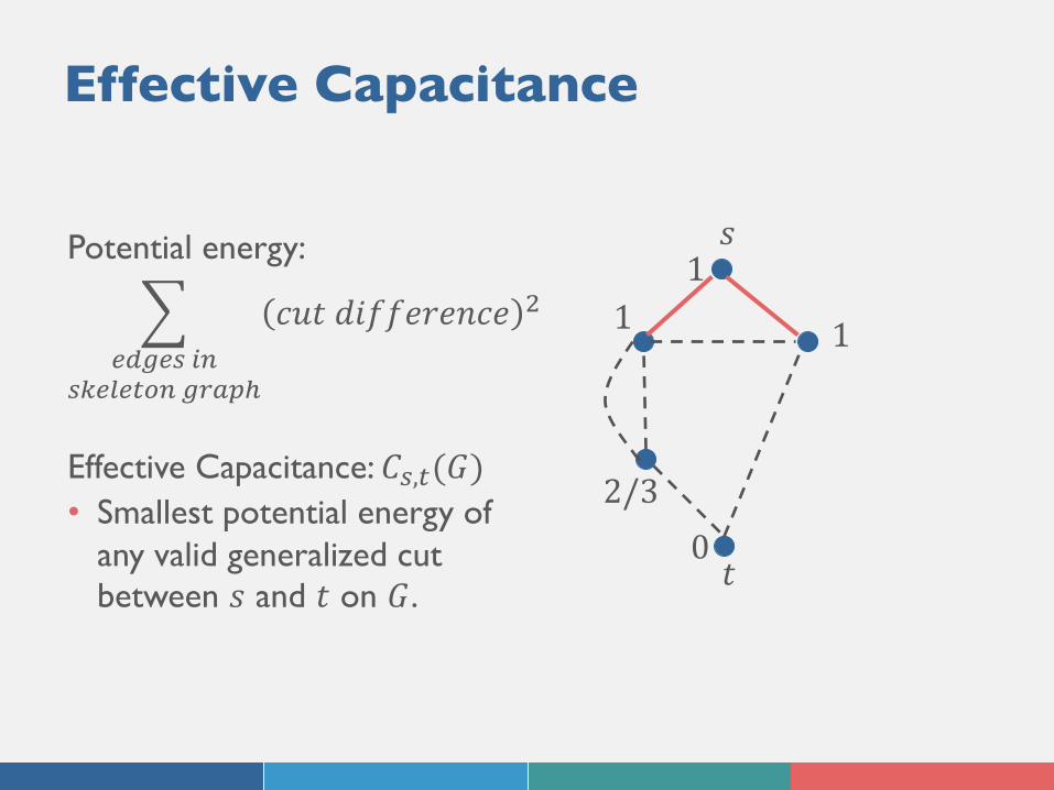
Effective Capacitance
Potential energy:
N56758 -#
8;5<5:=# 7>?@A
𝑐𝑢𝑡 𝑑𝑖𝑓𝑓𝑒𝑟𝑒𝑛𝑐𝑒 "
Effective Capacitance: 𝐶8,:(𝐺)• Smallest potential energy of
any valid generalized cut between 𝑠 and 𝑡 on 𝐺.
𝑠
𝑡
11 1
02/3

Algorithm Analysis:
Query Complexity:
𝑂 max!"##$!%$& '
𝑅(,% 𝐺 max#"% !"##$!%$& '
𝐶(,% 𝐺
Effective resistance Effective capacitance
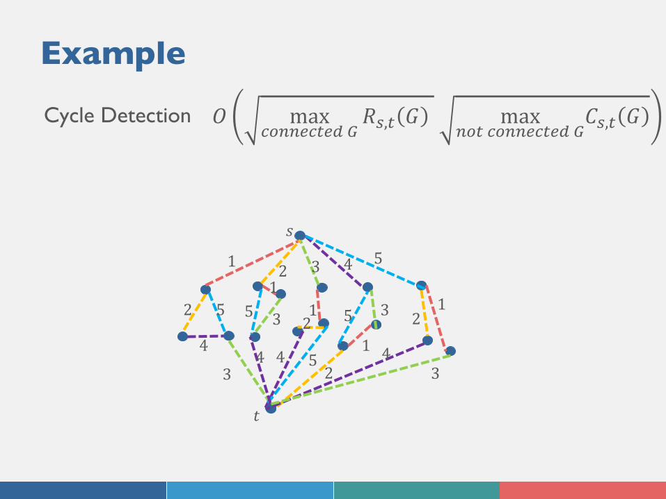
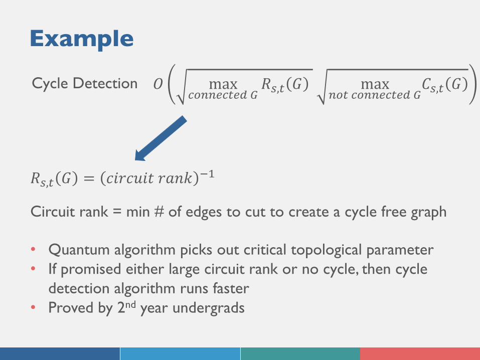
Example
1
2
3
4
5
𝑠
𝑡
12
3
4 5
2
3
4
51
12
3
4
51
2
3
5
4
Cycle Detection 𝑂 maxB=##5B:56 C
𝑅8,: 𝐺 max#=: B=##5B:56 C
𝐶8,: 𝐺
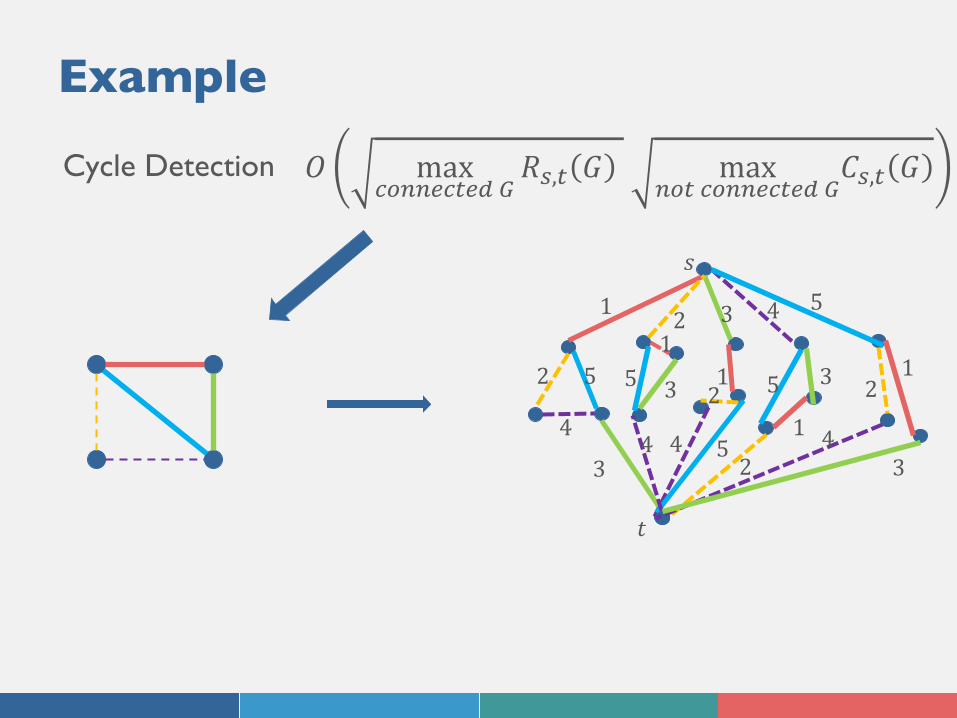
Example
Cycle Detection
1
2
3
4
5
𝑠
𝑡
12
3
4 5
2
3
4
51
12
3
4
51
2
3
5
4
𝑂 maxB=##5B:56 C
𝑅8,: 𝐺 max#=: B=##5B:56 C
𝐶8,: 𝐺
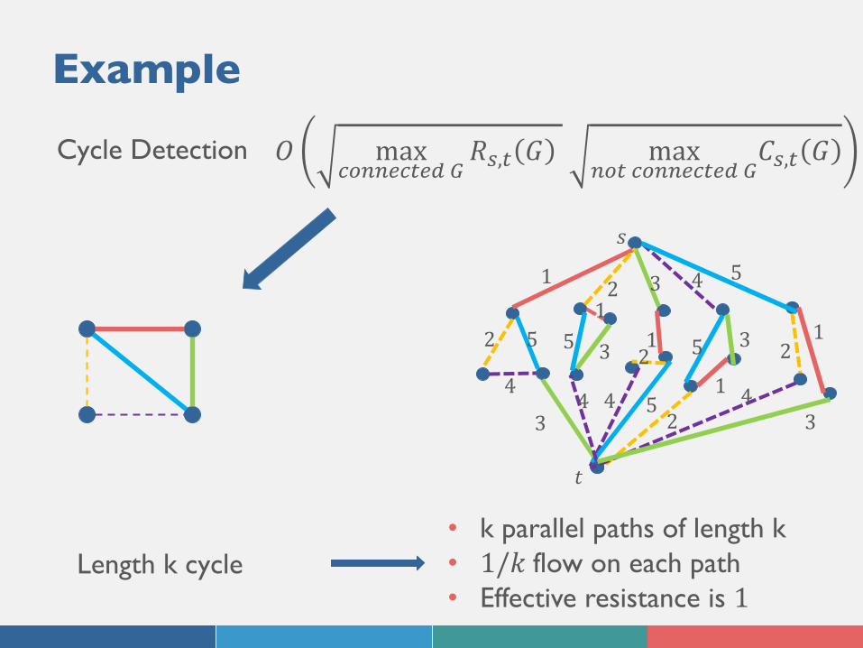
Example
Cycle Detection
1
2
3
4
5
𝑠
𝑡
12
3
4 5
2
3
4
51
12
3
4
51
2
3
5
4
𝑂 maxB=##5B:56 C
𝑅8,: 𝐺 max#=: B=##5B:56 C
𝐶8,: 𝐺
Length k cycle• k parallel paths of length k• 1/𝑘 flow on each path• Effective resistance is 1
Example
Cycle Detection
1
2
3
4
5
𝑠
𝑡
12
3
4 5
2
3
4
51
12
3
4
51
2
3
5
4
𝑂 maxB=##5B:56 C
𝑅8,: 𝐺 max#=: B=##5B:56 C
𝐶8,: 𝐺
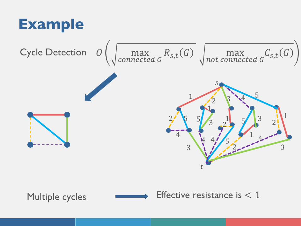
Multiple cycles Effective resistance is < 1
Example
Cycle Detection
1
2
3
4
5
𝑠
𝑡
12
3
4 5
2
3
4
51
12
3
4
51
2
3
5
4
𝑂 maxB=##5B:56 C
𝑅8,: 𝐺 max#=: B=##5B:56 C
𝐶8,: 𝐺
Example
Cycle Detection
1
2
3
4
5
𝑠
𝑡
12
3
4 5
2
3
4
51
12
3
4
51
2
3
5
4
𝑂 maxB=##5B:56 C
𝑅8,: 𝐺 max#=: B=##5B:56 C
𝐶8,: 𝐺
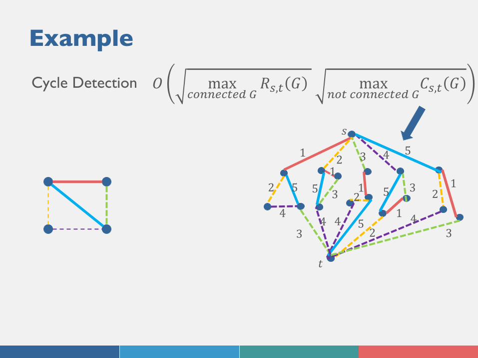
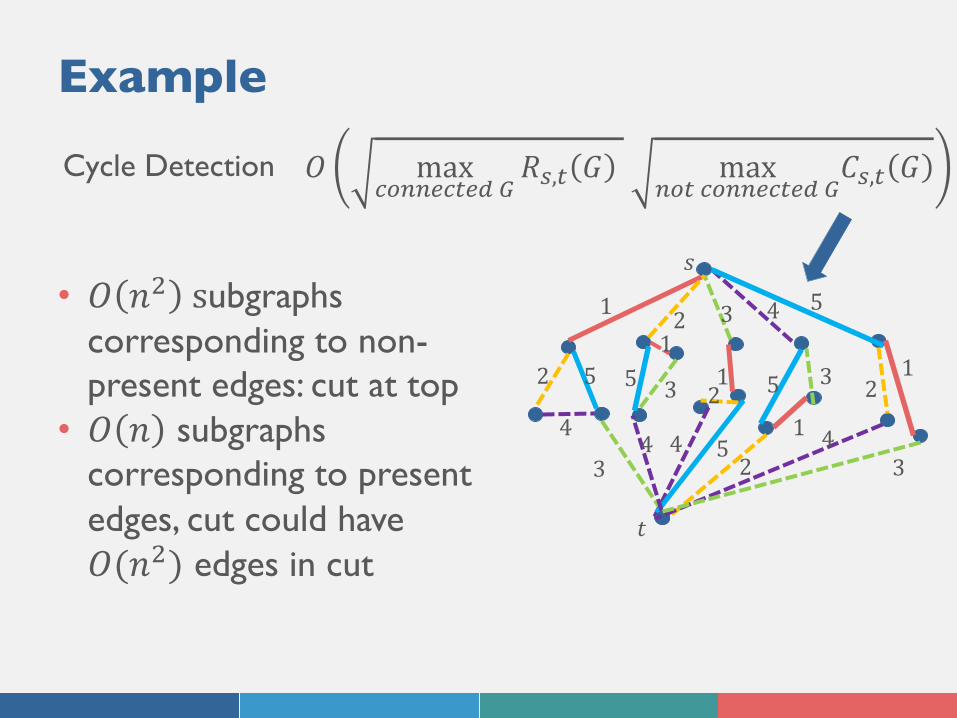
• 𝑂 𝑛% subgraphs corresponding to non-present edges: cut at top
• 𝑂 𝑛 subgraphs corresponding to present edges, cut could have 𝑂(𝑛%) edges in cut
Example
Cycle Detection 𝑂 maxB=##5B:56 C
𝑅8,: 𝐺 max#=: B=##5B:56 C
𝐶8,: 𝐺
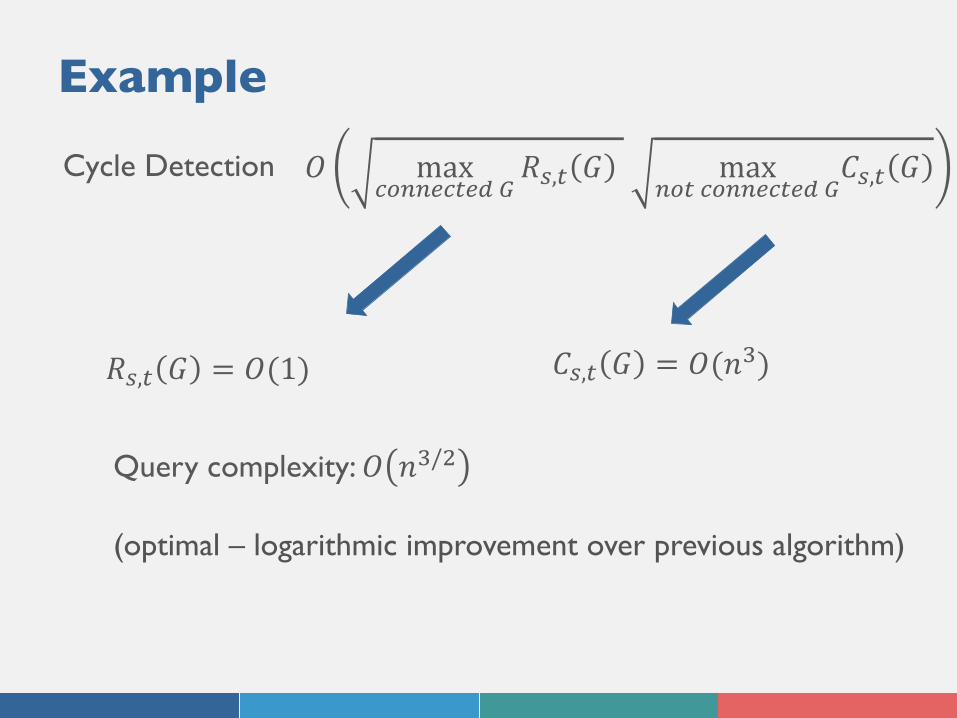
𝐶8,: 𝐺 = 𝑂(𝑛$)𝑅8,: 𝐺 = 𝑂(1)
Query complexity: 𝑂 𝑛$/"
(optimal – logarithmic improvement over previous algorithm)
Example
Cycle Detection 𝑂 maxB=##5B:56 C
𝑅8,: 𝐺 max#=: B=##5B:56 C
𝐶8,: 𝐺
𝑅8,: 𝐺 = 𝑐𝑖𝑟𝑐𝑢𝑖𝑡 𝑟𝑎𝑛𝑘 E!
Circuit rank = min # of edges to cut to create a cycle free graph
• Quantum algorithm picks out critical topological parameter• If promised either large circuit rank or no cycle, then cycle
detection algorithm runs faster• Proved by 2nd year undergrads
Estimation Algorithm:
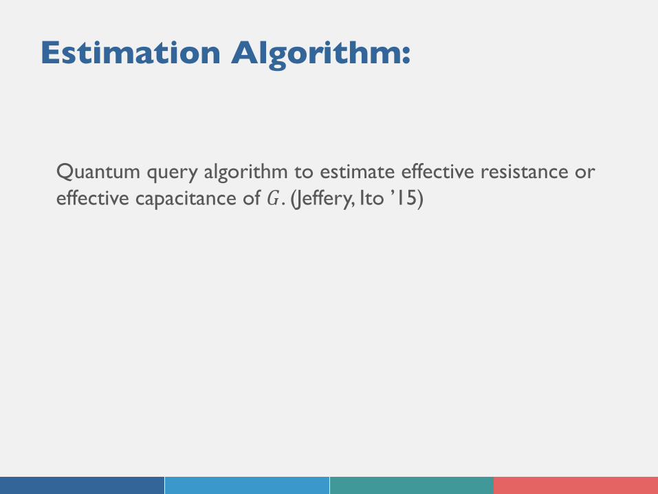
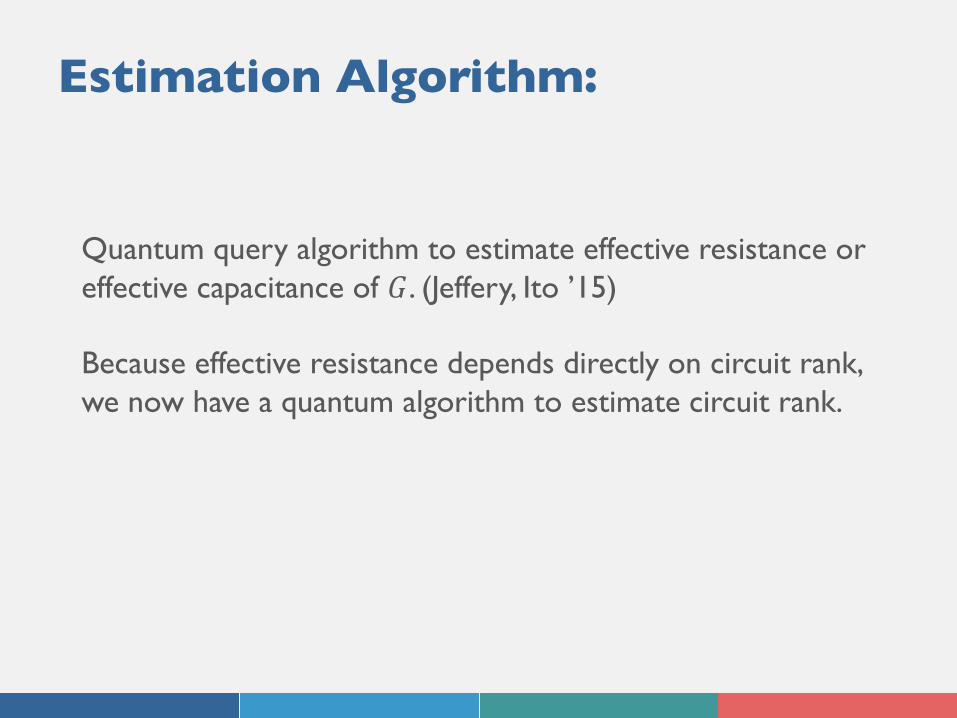
Quantum query algorithm to estimate effective resistance or effective capacitance of 𝐺. (Jeffery, Ito ’15)
Estimation Algorithm:
Quantum query algorithm to estimate effective resistance or effective capacitance of 𝐺. (Jeffery, Ito ’15)
Because effective resistance depends directly on circuit rank, we now have a quantum algorithm to estimate circuit rank.

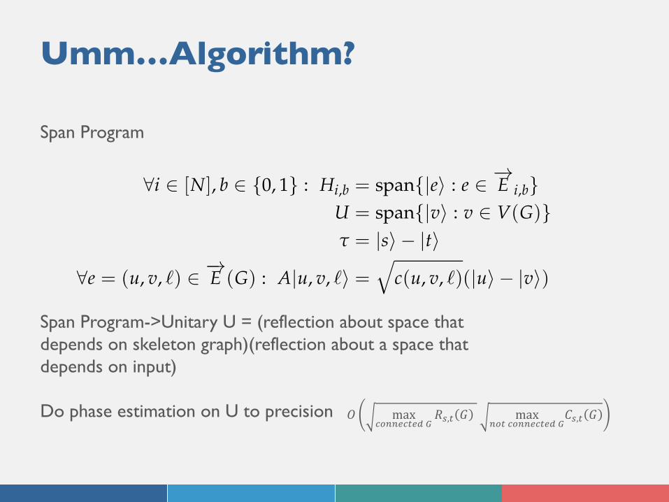
Umm…Algorithm?
Umm…Algorithm?
Theorem 14. Let U(P, x) = (2Πker A − I)(2ΠH(x)− I). Fix X ⊆ {0, 1}N and f : X → {0, 1}, and let P be a span
program on {0, 1}N that decides f . Let W+( f , P) = maxx∈ f −1(1) w+(x, P) and W−( f , P) = maxx∈ f −1(0) w−(x, P).
Then there is a bounded error quantum algorithm that decides f by making O(!
W+( f , P)W−( f , P)) calls to U(P, x),and elementary gates. In particular, this algorithm has quantum query complexity O(
!W+( f , P)W−( f , P)).
Ref. [IJ16] defines the approximate positive and negative witness sizes, w̃+(x, P) and w̃−(x, P). These aresimilar to the positive and negative witness sizes, but with the conditions |w⟩ ∈ H(x) and ωAΠH(x) = 0relaxed.
Definition 15 (Approximate Positive Witness). For any span program P on {0, 1}N and x ∈ {0, 1}N, we definethe positive error of x in P as:
e+(x) = e+(x, P) := min"###ΠH(x)⊥|w⟩
###2
: A|w⟩ = τ
$. (14)
We say |w⟩ is an approximate positive witness for x in P if###ΠH(x)⊥ |w⟩
###2= e+(x) and A|w⟩ = τ. We define
the approximate positive witness size as
w̃+(x) = w̃+(x, P) := min"∥|w⟩∥2 : A|w⟩ = τ,
###ΠH(x)⊥ |w⟩###
2= e+(x)
$. (15)
If x ∈ P1, then e+(x) = 0. In that case, an approximate positive witness for x is a positive witness, andw̃+(x) = w+(x). For negative inputs, the positive error is larger than 0.
We can define a similar notion of approximate negative witnesses (see [IJ16]).
Theorem 16 ([IJ16]). Let U(P, x) = (2Πker A − I)(2ΠH(x) − I). Fix X ⊆ {0, 1}N and f : X → R≥0. Let P be a
span program on {0, 1}N such that for all x ∈ X, f (x) = w−(x, P) and define %W+ = %W+(P) = maxx∈X w̃+(x, P).
Then there exists a quantum algorithm that estimates f to accuracy ϵ and that uses %O&
1ϵ3/2
'w−(x) %W+
(calls to
U(P, x) and elementary gates.
A span program for st-connectivity An important example of a span program is one for st-connectivity,first introduced in [KW93], and used in [BR12] to give a new quantum algorithm for st-connectivity. Westate this span program below, somewhat generalized to include weighted graphs, and to allow the inputto be specified as a subgraph of some parent graph G that is not necessarily the complete graph. We allowa string x ∈ {0, 1}N to specify a subgraph G(x) of G in a fairly general way, as described in Section 2.2.In particular, for i ∈ [N], let
−→E i,1 ⊆ −→
E (G) denote the set of (directed) edges associated with the literal xi,and
−→E i,0 the set of edges associated with the literal xi. Note that if (u, v, ℓ) ∈ −→
E i,b then we must also have(v, u, ℓ) ∈ −→
E i,b, since G(x) is an undirected graph. We assume G has some implicit weighting function c.Then we refer to the following span program as PG:
∀i ∈ [N], b ∈ {0, 1} : Hi,b = span{|e⟩ : e ∈ −→E i,b}
U = span{|v⟩ : v ∈ V(G)}τ = |s⟩ − |t⟩
∀e = (u, v, ℓ) ∈ −→E (G) : A|u, v, ℓ⟩ =
'c(u, v, ℓ)(|u⟩ − |v⟩) (16)
One can check that if s and t are connected, then if |w⟩ represents a weighted st-path or linear combinationof weighted st-paths in G(x), then |w⟩ is a positive witness for x. Furthermore, this is the only possibilityfor a positive witness, so x is a positive input for PG if and only if G(x) is st-connected, and in particular,w+(x, PG) = 1
2 Rs,t(G(x)) [BR12]. Since the weights c(e) are positive, the set of positive inputs of PG areindependent of the choice of c, however, the witness sizes will depend on c.
10
Span Program
Span Program->Unitary U = (reflection about space that depends on skeleton graph)(reflection about a space that depends on input)
Do phase estimation on U to precision 𝑂 max!"##$!%$& '
𝑅(,% 𝐺 max#"% !"##$!%$& '
𝐶(,% 𝐺
Open Questions and Current Directions
• How to choose edge weights? (Beigi et al ‘19)• Conditions when st-connectivity reduction optimal? • What is the classical time/query complexity of st-
connectivity in the black box model? Under the promise of small capacitance/resistance?
• Better estimation algorithm for st-connectivity effective resistance/capacitance
• Primitives/Pedagogical Problems?
Thank you!
Andrew Zhao
Teal Witter
Kai De Lorenzo
Stacey Jeffery
Michael Jarret
Alvaro Piedrafita