algorithmic optimization of sensor placement on civil
TRANSCRIPT

i
Algorithmic Optimization of Sensor Placement on
Civil Structures for Fault Detection and Isolation
A Thesis submitted to the
Division of Research and Advanced Studies
of the University of Cincinnati
in partial fulfillment of the
requirements for the degree of
MASTER OF SCIENCE (M.S.)
in the School of Electronics and Computing Systems
of the College of Engineering and Applied Sciences
2012
By
RATHISH MOHAN
B.Tech. (Electronics and Instrumentation Engineering),
Uttar Pradesh Technical University, India 2008
Thesis Advisor and Committee Chair: Arthur J. Helmicki, Ph.D.

ii
ABSTRACT
Damage detection and isolation (DDI) is a task that can be divided into two major portions.
Damage detection constitutes the first part of the problem, where the goal is to determine when a
structural anomaly has occurred. Once an anomaly has been detected, algorithms must be
employed to determine if the anomaly is a structural damage, or is due to system noise, sensor
failure, or another non-structural event. Having confirmed the presence of a structural anomaly,
the second part of the problem, damage isolation, is to determine where that anomaly has
occurred.
The principles of DDI have been used for decades on critical infrastructures, but the
advancements in computational power, instrumentation, and wireless communication and high
bandwidth have enabled evolutionary development in structural health monitoring. Structural
health monitoring (SHM), in its infancy, meant implementation of a suite of instruments and a
data acquisition system. The data acquisition system sampled less data and required manual
downloading of the acquired data before any analysis or processing could begin. In the second
generation of systems, the manual downloading could be eliminated by using remote access and
data transfer. This enabled convenient and frequent data analysis and synthesis. With the recent
developments in data acquisition systems, more on-site data analysis and synthesis can be
performed, allowing more rapid responses when anomalies are detected.
The specific aim of this research is to develop, calibrate, and validate sophisticated damage
detection and isolation procedures that can be implemented on the next generation of structural
health monitoring systems.

iii

iv
ACKNOWLEDGMENT
I would like to take this opportunity to express my sincere gratitude towards my advisor Dr.
Arthur J. Helmicki for his guidance, encouragement, and support during my research. His
continued effort of giving valuable suggestions greatly helped me realize the research goals.
I would like to thank Dr. James A. Swanson for his immense help and encouragement that I
received in all stages of my research. His invaluable help in teaching me the structural
engineering aspects of the research, the ideas of objective function and the computational
methods, and the time he took to answer all my doubts and questions are deeply appreciated.
I am greatly thankful to Dr. Victor Hunt in helping me understand the goals of the research, and
his valuable suggestions and insights that he provided throughout the course of the work. His
efforts and patience in helping me with presentation skills are deeply acknowledged.
I thank the SECS IT department for the technical assistance and the University libraries for all
the facilities.
I would like to extend my deepest gratitude towards my family who always believed in me and
have been a constant support without which this work would not have been possible. I also thank
my friends and colleagues at University of Cincinnati for being there for me whenever I need
them and otherwise.

v
Table of Contents
ABSTRACT .................................................................................................................................... ii
ACKNOWLEDGMENT................................................................................................................ iv
Table of Contents ............................................................................................................................ v
List of Figures .............................................................................................................................. viii
Chapter 1: Introduction ................................................................................................................... 1
1.1 Motivations for SHM ............................................................................................................ 1
1.2 Bridge Monitoring ................................................................................................................ 2
1.3 Bridge Monitoring Challenges .............................................................................................. 3
1.4 Bridge Monitoring Types ...................................................................................................... 5
1.5 Problem Statement ................................................................................................................ 6
Chapter 2: Literature Survey and Background ............................................................................. 10
2.1 Approaches to SHM ............................................................................................................ 11
2.2 Data Based SHM................................................................................................................. 11
2.3 Model Based ....................................................................................................................... 12
2.4 Damage Indicators .............................................................................................................. 14
2.4.1 Natural Frequencies ..................................................................................................... 14
2.4.2 Damping ....................................................................................................................... 14
2.4.3 Probability Density Functions ..................................................................................... 14
2.4.4 Mode Shapes ................................................................................................................ 15
2.4.5 Strain (or curvature) Mode shapes ............................................................................... 16
2.5 Background ......................................................................................................................... 16
2.6 Member Sizes...................................................................................................................... 17
2.7 Methodology and Process ................................................................................................... 18
Chapter 3: Design Specification and Data Generation ................................................................. 20
3.1 Truss Bridge ........................................................................................................................ 20
3.1.1 Data Generation ........................................................................................................... 23
3.2 Frame Bridge ...................................................................................................................... 24
3.2.1 Data Generation ........................................................................................................... 28
vi
3.3 Initial Analysis Methods ..................................................................................................... 29
3.4 Initial Analysis Sensor Locations ....................................................................................... 38
Chapter 4: Optimization of Instrumentation ................................................................................. 40
4.1 Analysis Approach .............................................................................................................. 40
4.2 Modal Assurance Criterion (MAC) .................................................................................... 42
4.2.1 Illustration .................................................................................................................... 43
4.2.2 Bubble Charts............................................................................................................... 44
4.3 Removal of Non-Redundant Members ............................................................................... 50
4.4 Aliasing or AutoMAC......................................................................................................... 51
Chapter 5: Optimization Routines ................................................................................................ 57
5.1 Problem Statement Revisited .............................................................................................. 57
5.2 Failure Detection ................................................................................................................. 58
5.3 Brute Force Optimization ................................................................................................... 63
5.3.1 Roadblocks ................................................................................................................... 66
5.4 Condensation Optimization ................................................................................................ 67
5.5 Failure Isolation .................................................................................................................. 71
5.6 Virtual Machine .................................................................................................................. 72
5.6.1 Failure Detection and Isolation .................................................................................... 72
5.6.2 Adding Noise ............................................................................................................... 74
Chapter 6: Results – System Design ............................................................................................. 77
6.1 Bubble Charts...................................................................................................................... 77
6.1.1 Absolute Values ........................................................................................................... 78
6.1.2 Percent Difference Values ........................................................................................... 78
6.1.2.1 Percent Difference Max Moments ........................................................................ 79
6.1.2.2 Removing Non-Redundant Members and Optimization ...................................... 80
6.1.3 Relative Value .............................................................................................................. 82
6.1.3.1 Relative Values Max Moments ............................................................................. 83
6.1.3.2 Removing Non-Redundant Members and Optimizing ......................................... 84
6.1.3.3 Damage Case 50% ................................................................................................ 85
6.2 Sensor Plans ........................................................................................................................ 86
6.3 Brute Force Results ............................................................................................................. 90

vii
6.4 Condensation Method Results ............................................................................................ 92
6.5 Results Comparison ............................................................................................................ 96
Chapter 7: Results - False Detection and Isolation ..................................................................... 100
7.1 Action Values to Strain Conversion ................................................................................. 100
7.2 Damage Isolation .............................................................................................................. 101
7.3 Missed Detection and Isolation ......................................................................................... 102
7.4 Conclusion ........................................................................................................................ 107
Chapter 8: Future Work .............................................................................................................. 109
8.1 Multithreading/Parallel Processing and Speeding Up ...................................................... 109
8.2 Rathish Divide and Conquer Algorithm and Pattern Recognition.................................... 112
8.3 Statistical Methods ............................................................................................................ 112
8.4 Precipitation ...................................................................................................................... 113
8.5 Machine Learning ............................................................................................................. 113
References ................................................................................................................................... 114
Appendix ..................................................................................................................................... 117
Software Used ......................................................................................................................... 117
viii
List of Figures Figure 1.1 General Flow Chart of the Proposed Method ................................................................ 9
Figure 2.1 Two Slope System ....................................................................................................... 15
Figure 2.2 PDF of the output from two-slope systems loaded by a zero mean value Gaussian
Input, ............................................................................................................................................. 15
Figure 2.3 Loaded Structure ......................................................................................................... 17
Figure 3.1 Structure ...................................................................................................................... 21
Figure 3.2 Data Generation Flowchart (Truss) ............................................................................. 24
Figure 3.3 Beam ............................................................................................................................ 25
Figure 3.4 Bending Moment ......................................................................................................... 26
Figure 3.5 DOF ............................................................................................................................. 26
Figure 3.6 Axial Force Diagram ................................................................................................... 27
Figure 3.7 Bending Moment Diagram .......................................................................................... 27
Figure 3.8 Data Generation Flowchart (Frame) ............................................................................ 29
Figure 3.9 Instrumented Member ................................................................................................. 30
Figure 3.10 Member 1 Axial Force and Bending Moment Responses for 50% Damage ............ 31
Figure 3.11 Member 3 Axial Force and Bending Moment Responses for 50% Damage ............ 32
Figure 3.12 Member 1 Axial Force and Bending Moment Responses for 100% Damage .......... 33
Figure 3.13 Member 3 Axial Force and Bending Moment Responses for 100% Damage .......... 33
Figure 3.14 Axial Force Responses for 100% Damage Non-Redundant Members Removed ..... 36
Figure 3.15 BM 1 Responses for 100% Damage Non-Redundant Members Removed ............... 37
Figure 3.16 Sensor Plan ................................................................................................................ 38
Figure 4.1 Vectors Used ............................................................................................................... 41
Figure 4.2 Matrix of Damaged States ........................................................................................... 42
Figure 4.3 Matrix of MAC Values ................................................................................................ 44
Figure 4.4 Bubble Chart Flow ...................................................................................................... 45
Figure 4.5 a Bubble Chart Process ................................................................................................ 46
Figure 4.5 b Bubble Chart Process ............................................................................................... 47
Figure 4.6 Complete Bubble Chart ............................................................................................... 48
Figure 4.7 Bubble Chart ................................................................................................................ 49
Figure 4.9 Reduced Matrix ........................................................................................................... 50
Figure 4.10 Bubble Chart for 28 Sensors...................................................................................... 52
Figure 4.11 Damage Detection using 47 Sensors ......................................................................... 53
Figure 4.12 Damage Detection using 28 Sensors ......................................................................... 53
Figure 4.13 Damage Isolation using 47 Sensors ........................................................................... 54
Figure 4.14 Damage Isolation using 28 Sensors ........................................................................... 55
Figure 4.15 Fully Instrumented Structure ..................................................................................... 56
Figure 4.16 Optimized 28 Sensors ................................................................................................ 56
ix
Figure 5.1 Failure Detection ......................................................................................................... 59
Table 5.1 ....................................................................................................................................... 60
Table 5.2 ....................................................................................................................................... 61
Table 5.3 ....................................................................................................................................... 62
Figure 5.2 Optimization Flowchart ............................................................................................... 65
Figure 5.3 Recursive Flowchart .................................................................................................... 67
Figure 5.4 Condensation Flowchart .............................................................................................. 68
Table 5.4 ....................................................................................................................................... 70
Table 5.5 ....................................................................................................................................... 70
Figure 5.5 Failure Isolation ........................................................................................................... 71
Figure 5.6 Detection and Isolation ................................................................................................ 73
Figure 5.7 Virtual Machine Output Template............................................................................... 76
Figure 6.1 Absolute Values........................................................................................................... 78
Figure 6.2 Percent Difference ....................................................................................................... 79
Figure 6.3 Per. Diff. Max Moments .............................................................................................. 80
Figure 6.4 Optimized 28 Actions .................................................................................................. 81
Figure 6.5 Relative Values ............................................................................................................ 83
Figure 6.6 Relative Value Max Moments ..................................................................................... 84
Figure 6.7 Optimized 28 Actions .................................................................................................. 85
Table 6.1 Sensor Count and Average Off Diagonal Values ......................................................... 86
Figure 6.8 All 60 Sensors.............................................................................................................. 87
Figure 6.9 Force and Max Moments ............................................................................................. 88
Figure 6.10 Max Moments Non-Redundant Members ................................................................. 88
Figure 6.11 Optimized 28 Actions ................................................................................................ 89
Figure 6.12 All 48 Sensors............................................................................................................ 90
Figure 6.13 Optimized 47 Sensors ................................................................................................ 91
Figure 6.14 Optimized 46 Sensors ................................................................................................ 91
Figure 6.15 Optimized 41 Sensors ................................................................................................ 92
Figure 6.16 Optimized 28 Sensors ................................................................................................ 93
Figure 6.17 Bubble Chart for 28 Sensors...................................................................................... 94
Figure 6.18 Optimized 29 Sensors ................................................................................................ 95
Figure 6.19 Bubble Chart for 29 Sensors...................................................................................... 95
Table 6.2 Brute Force vs. Condensation ....................................................................................... 96
Figure 6.20 Initial Analysis Sensor Suite ..................................................................................... 97
Figure 6.21 Initial Analysis Bubble Chart .................................................................................... 97
Figure 6.22 Brute Force 6 Sensor Suite ........................................................................................ 98
Figure 6.23 Bubble Chart Brute Force 6 Sensor Suite.................................................................. 98
Figure 6.24 Condensation 6 Sensor Suite ..................................................................................... 99
Figure 6.25 Bubble Chart Condensation 6 Sensor Suite............................................................... 99
Figure 7.1 Damage Isolation Initial Analysis ............................................................................. 101
x
Figure 7.2 Damage Isolation Brute Force ................................................................................... 102
Figure 7.3 Brute 42 Missed Detections & False Isolation .......................................................... 103
Figure 7.4 Condensation 42 Missed Detection & False Isolation .............................................. 103
Figure 7.5 Brute 41 Missed Detections & False Isolation .......................................................... 104
Figure 7.6 Condensation 41 Missed Detection & False Isolation .............................................. 105
Figure 7.7 Brute Force vs. Condensation 42 Missed Detections & False Isolation ................... 106
Figure 7.8 Brute Force vs. Condensation 41 Missed Detections & False Isolation ................... 107
Figure 8.1 Creating Chunks of Combinations ............................................................................ 110
Figure 8.2 Description of Chunks ............................................................................................... 111

1
Chapter 1: Introduction
The field of Structural Health Monitoring (SHM) focuses on developing strategies and methods
through which engineering structures are observed over time to identify anomalous changes.
These changes can be in material or geometric properties of the structural system, and can
adversely affect the system’s performance. SHM involves observing the system over an extended
period of time. This would entail recording dynamic and/or static responses obtained from a set
of sensors placed on structures and identifying any fault or damage from these measurements.
Once a fault has been flagged, statistical analysis and interpretation of the data obtained can be
used to determine the current health of the system. In short, as said in [1], the broad aim of an
SHM system is to be able to identify, at an early stage, occurrences of damage that may
ultimately lead to failure of the individual component or system.
1.1 Motivations for SHM
One can see the obvious reasons behind SHM, such as the following:
Using the resources to monitor a structure with minimum closure or downtime, and avoid
failures.
To provide contractors and owners a detailed analysis of their product.
To plan maintenance and repair tasks which are qualitatively and quantitatively better and
involve least human intervention.
Aging of transportation structures and their degradation pose a serious safety threat as their use
increases over time and the health deteriorates. The economic issue furthers the problem for

2
critical structures such as bridges, as replacement is not an option, and maintaining and repairing
them would involve enormous amount of funds. As stated in [2], the US Federal Highway
Administration has classified over 25% of the bridges in the United States as either structurally
deficient or functionally obsolete. This fact stresses the importance of SHM to ensure public
safety. Structural health monitoring techniques based on changes in dynamic characteristics have
been studied and developed extensively over the last three decades when compared to those
based on static data. As pointed out by Jenkins however, for structural damage detection, static
responses show more local sensitivity than shown by frequency responses [3]. When the damage
is substantial, these methods have some success in determining if damage has occurred. At
incipient stages of damage, however, the existing methods are not as successful [4].
1.2 Bridge Monitoring
With increase in traffic in both urban and rural areas, bridge networks are subjected to a greater
burden than they were intended to handle [5]. Authorities and bridge engineers are required to
ensure the integrity of bridges and smooth operation of road networks. One way to do this is
visual inspection. Visual inspections are not only expensive, they are time consuming too.
Though this level of observing the structure provides detailed and useful information for
network-level bridge management, the information collected is not quantitative. Moreover,
visual inspection of structures is highly variable and puts a significant amount of limitation on
the data collected.
Before it is determined whether a bridge is safe or not, there are many types of damage and
deterioration metrics that need to be analyzed. Among them are those which are not possible to
detect visually. Moreover, operational performance on congestion, accident history, creep, and

3
fatigue, are not collected during routine visits. [5] correctly sums it up saying, visual inspections
are qualitative in nature. That is, they give only outward assessment; any damage existing
internally can go unnoticed for a long time.
With the above discussion in mind, to ensure safe operation of bridges (and of the commuters), it
becomes necessary that the structure be monitored on all feasible critical parameters and metrics.
Monitoring will mean collecting bridge data through some robust and efficient system, i.e. a
system which monitors those operational indices over an extended period of time instead of
yearly or bi-annually. Why continuous monitoring? Because that would ensure that every event
through the bridge’s operational history is captured, and any anomaly could be compared to the
nominal operational condition of healthy bridge. This task would be achieved by a monitoring
schema that is designed taking into account the physical, mechanical, and many other properties
of the structure. The structural properties of a bridge should be taken into account in order to
properly of place the data acquisition systems on certain location or elements. This can help the
system or the monitors to capture the most out of the response from the structure.
1.3 Bridge Monitoring Challenges
The task of field monitoring of civil infrastructure involves the interlocking of many tiers of
hardware and software systems that are currently used for structural health monitoring. This
involves placing of sensors on the bridge to monitor how the structure behaves, recording data,
and signal conditioning of the sensor output. The recorded values can be further transformed into
the required format through a data acquisition system. All of these steps help in the analysis
which decides how well the structure performs. The Commercial off-The-Shelf (COTS)
software-based modern information technology enables an economical and efficient way to

4
integrate such disparate systems as one single system approach to monitor the performance of
civil infrastructure [6].
Limitations in sensor power, data transmission, storage of data, and finally the analysis, have
been overcome since computing power and advancements in wireless communications have
made the devices and services better. With the pace at which technology is advancing, soon
structures with thousands of sensors which can monitor a myriad of responses such as
temperature, traffic conditions, corrosion, fatigue, and many other performance metrics, will be
erected. The result will be a data-intense instrumented structure, and an environment having
large number of data streams from arrays of sensors at several locations throughout the bridge
[6].
One of the major challenges in such cases will be to record and organize the data inflows which,
sampled at high frequency, will easily produce gigabytes of data in a matter of weeks or days.
Having to store this amount of data, and provide efficient means of data interpretation,
underscores the need of advanced database design. The next big challenge is the need to relate
the various streams of data to one another in a hierarchical manner. These hierarchical types can
be classified as spatial, temporal, or functional performances. Functional and temporal hierarchy
can be associated as continuous data related to an input force such as strain, displacement, load,
etc., on the structure, as opposed to an intermittent data related to damage such as acoustic-
emission data; whereas spatially, the hierarchy of association pertains to a specific bridge,
roadway girder, or a specific location [6]. Hierarchy and association is necessary to efficiently
analyze the structure’s performance in a consolidated approach, rather than analyzing several
dozens of data streams which are independent.

5
The diversity of data acquisition platforms and the proper integration of the recorded data is
another major challenge on a structure that has many sensors. With the advancement of sensor
technology, better sensors will continue to be available over time. Hence it is not possible to
assume that all the sensors on the bridge will be operated through the same data acquisition
system and be providing a coherent and consistent storage of data.
The fourth challenge includes capturing live data and inferring results from it through analysis
when needed. As discussed previously, this means obtaining an environment which is data-
intense and knowledge-rich, from a data intense and knowledge-poor one. A smart SHM system,
then, is expected to provide a way to digest live streams of data and issue immediate warnings of
impending fault or danger. Warnings can include information about a malfunction in a gauge,
drastic change in the load on the structure, or a radical change in the performance of the structure
outside the normal operating conditions. Combined with these warnings is the prognosis of the
future performance of the bridge and assessment of the structural properties in order to assist the
bridge engineers in making proper decisions regarding the maintenance and safety of the bridge.
1.4 Bridge Monitoring Types
Bridge monitoring can be classified in two broad categories:
Continuous Monitoring
Portable Testing
Long-Term Continuous Monitoring Systems - Data is collected over a long period of time -
months, years, or permanently. This type of monitoring can provide behavior and health
response, fatigue performance, or general operation information over an extended period of time.

6
This continuously operated and unattended system must be optimally designed for high
reliability and remote operation.
Portable Testing - Systems are installed temporarily on a structure to assess the current condition
of a structure or its components.
Examples of sensor types used for bridge monitoring can be listed as follows:
Accelerometers
Strain Gages
Displacement Sensors
Tilt Meters/Tilt Sensors
Wind Speed and Direction Sensors
Temperature Sensors
Piezometers
Traffic Sensors
Smart Sensors
1.5 Problem Statement
Following the discussion from the previous sections so far, bridge monitoring strives to achieve
the following:
Ensure the safety of commuters.

7
Make optimum usage of the resources in monitoring.
Use the information obtained from data acquisition systems to better plan maintenance of
the structure before a catastrophic event happens.
The above tasks can be achieved by placing an immense amount of sensors on the bridge so that
each part or area can be monitored precisely. Response from each sensor can then be analyzed
individually to look for any anomaly from the previously (normal operational state) observed
results.
This method may not be the optimal strategy because:
It is not an optimized use of hardware resources as many sensors will be redundantly
placed when the task can been achieved by fewer sensors.
More sensors will contribute many data streams. If the sampling rate of a data acquisition
system is high enough, terabytes of data will be captured in a very short period of time.
Therefore, the relational database also needs to be large enough to store these values.
Even before analysis of data streams start, data has to go through all kinds of cleansing,
transformation, normalization, etc., and the more the data to be parsed or processed, the
longer it will take to reach the analysis and hence the prognosis part.
Processing each of the sensor response individually will not only be time taking, but also
prone to errors. There are also chances of dumb voters or erroneous sensors, when the
member or element where they were placed may be in perfect condition, and because of a
fault in the sensor or hardware a fault will be declared.

8
As discussed in the earlier paragraphs, for long term monitoring, which is what this work is
mostly concerned of, the basic steps involved when talking about health monitoring of bridges
can be listed as:
1. An optimized strategy of sensor placement on the structure.
2. Reliable interpretation of the response from sensors.
3. Reliable algorithm to process data and infer decisions.
4. Identify a failure or fault before it becomes catastrophic.
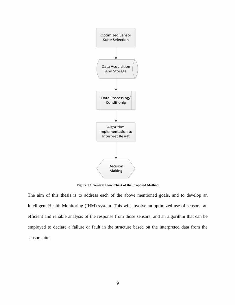
The above-mentioned points can be summarized in Figure 1.
9
Optimized Sensor Suite Selection
Data Processing/Conditionig
Data AcquisitionAnd Storage
Algorithm Implementation to
Interpret Result
Decision Making
Figure 1.1 General Flow Chart of the Proposed Method
The aim of this thesis is to address each of the above mentioned goals, and to develop an
Intelligent Health Monitoring (IHM) system. This will involve an optimized use of sensors, an
efficient and reliable analysis of the response from those sensors, and an algorithm that can be
employed to declare a failure or fault in the structure based on the interpreted data from the
sensor suite.

10
Chapter 2: Literature Survey and Background
To identify damage, the analysis is reliant on features that indicate the presence of damage;
hence it becomes imperative that these features are identified correctly. The motivation behind
such need is that as the structure is damaged, or generally speaking, as structure changes, its
dynamic and/or static responses changes. Some of these changes can then be separated based on
the level of sensitivity that they demonstrate over others. This separation of more sensitive
features over others can be referred to as feature extraction. Once the required features are
extracted, they can then be converted into feature vectors and can be used in analysis.
The most commonly applied features can be listed as below [1]:
Static Strains
Transverse Load
Modeshape
Modeshape Curvature/Modal Strain Energy
Natural Frequencies
Dynamic Flexibility
Operational Deflection Shapes
Frequency Response Functions and Transmissibilities
Damping Coefficients

11
2.1 Approaches to SHM
Broadly speaking, structural health monitoring literature defines two types towards SHM:
Data Based
Model based
2.2 Data Based SHM
This approach takes into consideration the construction of a model which is statistical.
Experimentally acquired data is fed through machine learning or pattern recognition algorithm to
establish the model. This method eliminates the need for a numerical model since the model is
totally based on the data, and also accommodates any measurement variability. However, this
method cannot take into consideration physical mechanisms of the structure that can explain how
and where the damage took place.
Supervised learning methods require the data of both damaged and undamaged conditions of the
bridge. Examples of such techniques include Kernel Discriminant Analysis (KDA) [7], Artificial
Neural Networks (ANN), and Support Vector Machine (SVM) [8], to name a few. Although the
undamaged data of the bridge from various elements can be monitored and various adjustments
can be applied to the data to find the normal or undamaged operational condition, the data for
damaged condition is very rarely available; hence this data scarcity becomes a huge challenge in
applying this method.
Another type of machine learning technique, unsupervised learning using outlier analysis, has
also been explored in control chart methods [9], and outlier analysis in [10].

12
2.3 Model Based
This alternative approach is based on developing a Finite Element model (FE) which represents
the bridge or structure in consideration. This model is then updated using experimental data to
more accurately represent an actual structure. The dynamic properties that are updated can be
mass, stiffness, damping, etc. After this, an inverse problem can be posed using the data from an
experimental model to detect, localize, and quantify damage. Several notable papers on this
approach have been published. [11] talks about identifying damage in a 7 story structure,
whereas [12] talks about an update applied in the Z24 highway bridge in Switzerland.
These methods however, are prone to the uncertainty which can be attributed to modeling errors
and variable measurements. Modeling of damage is very crucial in these methods; for example,
damage can mean a 20% or 50% reduction in the mass of the element, or complete removal.
Moreover, modeling simplification is made to model non-trivial tasks like complex substructures
such as joints, and there are methods discussed in literature which talk about acceptable update
methods of parameterizing joints [13]. So, two classes of errors can be defined in model
parameters: other parameters and damage parameters. The other parameters arise from modeling
and experimental errors.
Problem of damage identification is broken by [14] in a hierarchical fashion. Following it,
damage identification can be defined in levels as:
1. Detection – A qualitative indication that something is not right in the structure (fault).
2. Localization – Isolate the location of the damage from the many locations where sensors
are put.

13
3. Assessment – Quantify the extent and classify the kind of damage.
4. Consequence – A report about the actual safety of the structure.
In [1], Robert Barthrope talks about another addition to the above mentioned steps as:
5. Prediction – The actual residual life of the system in the current damage conditions.
It is very important here to note that at any given higher level hierarchy, success is solely
dependent on the success at the lower level. In simpler terms if damage cannot be detected
correctly, it cannot be localized; or if damage cannot be localized, it will be impossible to assess
the extent and hence predict the future of the structure.
What SHM is supposed to achieve, then, is an integration of the above steps in a holistic fashion,
and provide a system that can produce a summary of the steps combined as well as the report of
each step taken individually.
To analyze any structural response, before any step can be carried out, selection of ‘changes’ in
the dynamic behavior of a structure as an effect of damage is required. Natural frequencies,
modeshapes, strain-modeshapes, deflections, and damping coefficients are some of the
parameters that can be used to characterize the dynamical behavior of the structure. These
parameters are called DAMAGE INDICATOR (DI): A dynamic quantity, which can be used to
identify that damage, exists in a structure [14].

14
2.4 Damage Indicators
2.4.1 Natural Frequencies
Natural Frequency is without a doubt the most that has been, and is being, used for indicating
damage. Its popularity owes to the simple acquisition and high rate of accuracy, where a sensor
connected to an analyzer can estimate natural frequencies for both local and global damage.
Although Natural Frequencies are reasonable to use, literature exists where they are rejected as
DI’s. [15] and [16] conclude that if they are used alone they are not sufficient to detect damage.
2.4.2 Damping
The damping capacity of a structure will change if it is subject to damage. This property can be
used as a possible DI. There can be several sources of damping such as water, material,
connectivity, air, and soil or artificial. This method is not celebrated too much in the research
community as it was found to be unreliable and less sensitive to small scale damage. The
accuracy of the measured response is poor, and no relationship between damage and measured
damping was found which was consistent [17-19]. A real structure will have damping that may
include portions of many kinds of damping. Separating them based on the sources becomes an
impossible task when high accuracy is required. So, it’s very likely that a damage induced
damping can be easily missed. These factors seem to be the reason that it is mentioned as DI in
many papers but not really used in many.
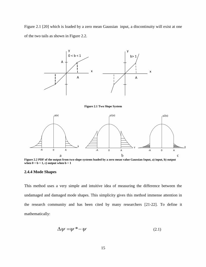
2.4.3 Probability Density Functions
With the output obtained from a structure, non-linearities can be observed which can in turn be
used as damage indicators. [20] brings to attention that given a bi-linear system as shown in
15
Figure 2.1 [20] which is loaded by a zero mean Gaussian input, a discontinuity will exist at one
of the two tails as shown in Figure 2.2.
A
y
x
b> 1
A
A
y
x
0 < b < 1
Figure 2.1 Two Slope System
-A A0
X
p(x)
-A A0Y
p1(x)
A0
p2(x)
-AY
a b c Figure 2.2 PDF of the output from two-slope systems loaded by a zero mean value Gaussian Input, a) input, b) output
when 0 < b < 1, c) output when b > 1
2.4.4 Mode Shapes
This method uses a very simple and intuitive idea of measuring the difference between the
undamaged and damaged mode shapes. This simplicity gives this method immense attention in
the research community and has been cited by many researchers [21-22]. To define it
mathematically:
*
(2.1)

16
Where represents the undamaged or normalized mode shape, and * represents the
damaged mode shape. represents the calculated change in the mode shape vector. So, in
the case of an undamaged state the delta value should theoretically be equal to zero. The
normalization or scaling of the mode shape vector is necessary as the scale of mode shapes is
arbitrary.
Damage in the structure is supposed to cause a localized stiffness reduction, and the location of
the damage is expected to reflect the greatest change in the mode shape amplitude. This method
although being able to detect the presence of damage locally, cannot localize it if used alone. So
this achieves the Level 1 of the damage detection i.e. one which is capable of detecting the
presence but not the exact location of damage.
2.4.5 Strain (or curvature) Mode shapes
To make the analysis of the dynamic and fatigue strength of the system more accurate, there has
been a trend of studying the structural strain/stress response prediction in the past decade [23].
[24] considers strain mode shape as a sensitive parameter to damage due to its local behavior.
This fact can be used, since the changes in the curvature mode shapes increases with increasing
size of damage [25], in establishing the extent of damage by studying the curvature.
2.5 Background
This work is based on the exploration of the strain mode shape method for detection of damage
instead of deflected shapes on the following types of structure:
1. A 20 member simple truss bridge.
17
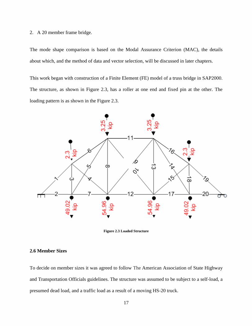
2. A 20 member frame bridge.
The mode shape comparison is based on the Modal Assurance Criterion (MAC), the details
about which, and the method of data and vector selection, will be discussed in later chapters.
This work began with construction of a Finite Element (FE) model of a truss bridge in SAP2000.
The structure, as shown in Figure 2.3, has a roller at one end and fixed pin at the other. The
loading pattern is as shown in the Figure 2.3.
Figure 2.3 Loaded Structure
2.6 Member Sizes
To decide on member sizes it was agreed to follow The American Association of State Highway
and Transportation Officials guidelines. The structure was assumed to be subject to a self-load, a
presumed dead load, and a traffic load as a result of a moving HS-20 truck.
18
The members material was taken as steel. The cross sectional area was taken as 19.01 inch2;
moment of inertia was taken as 174 inch4, and the young’s modulus to be 29000 ksi.
2.7 Methodology and Process
Analysis began by observing the response to damage inflicted through simulation on each of the
members of the structure, and recording response from it. This damage was done by removing
the member completely, i.e., setting the area for that member to be equal to 0 in the code. The
response was hoped to give an insight to a pattern of damage, and the most suitable way and
locations of installing sensors. Since it is a truss structure (later extended to frame also), the only
response obtained was Axial Force recorded in KSI. Various damage scenarios were
investigated, e.g. damaging only the lower cord, upper cords, posts, diagonals, 50% damage,
100% damage, etc., each of which will be discussed in detail in later chapters.
Each damage case was converted to a vector where each vector consisted of 20 elements. As
discussed in the mode shape indicator section, two types of vector namely, a) Nominal
(undamaged state) and b) Damaged were compared.
After truss, the structure was converted to a frame structure which included two more indicators;
Bending Moment 1 (BM1) at the first end, and Bending Moment 2 (BM2) at the second end.
Now the vector for each of the nominal and damaged state contained a total of 60 elements (20
Axial Forces, 20 BM1 and 20 BM2).
The next goal was to decide which of the respective elements (sensors) should be chosen which
give the optimized number, and can resolve each of the damage state from each other. This was
done using an optimization strategy. Two such strategies were looked at namely:

19
Brute Force.
Condensation.
Having obtained the sensor suite which gives an optimal solution, an algorithm to use these
sensors is discussed that can analyze the data from the bridge and do the following:
1. Detect if the unknown data is damaged or undamaged one.
2. If damaged, run a nested method to localize or isolate the damage, i.e. return the member
which is damaged.
The deliverables of the work can be listed as follows:
1. Optimized sensor suite selection.
2. Accurate classification of damage and no damage cases of the unknown data vector from
the structure.
3. Feasible number of false detection and isolation.
4. Least missed detection.
Chapter 3 talks about the details of the structure, damage indicators used, the rudimentary work,
initial results from both truss and frame structure, and finally, the motivation to use MAC as an
objective function.

20
Chapter 3: Design Specification and Data Generation
This chapter describes the two types of structures that were investigated, viz. the Truss model
and the Frame model. The sections following each model describe the details of the structure,
data generation process, and the initial analysis that was done.
3.1 Truss Bridge
This section begins by discussing the design of the structure when modeled as Truss. In
structural engineering, a truss is a structure which is composed of a number of members pin
connected at their ends to form a stable framework. The units are triangular with straight
members, and the joints are referred as nodes. One end of the structure is supported by a pin
while the other is supported by a roller connection. Following are the assumptions that will be
observed for analysis purposes:
1. Joints are frictionless hinges.
2. All the members (bars) are pin connected.
3. Loads act only on the joints.
4. Stress in each element is constant along its length.
Since all the joints are assumed to be frictionless hinges, i.e. they are treated as revolute joints (A
revolute joint (also called pin joint or hinge joint) is a one degree of freedom kinematic pair
used in mechanisms [26]), moments (torques) are excluded and any external force and reactions
result in either tensile or compressive forces in members.
21
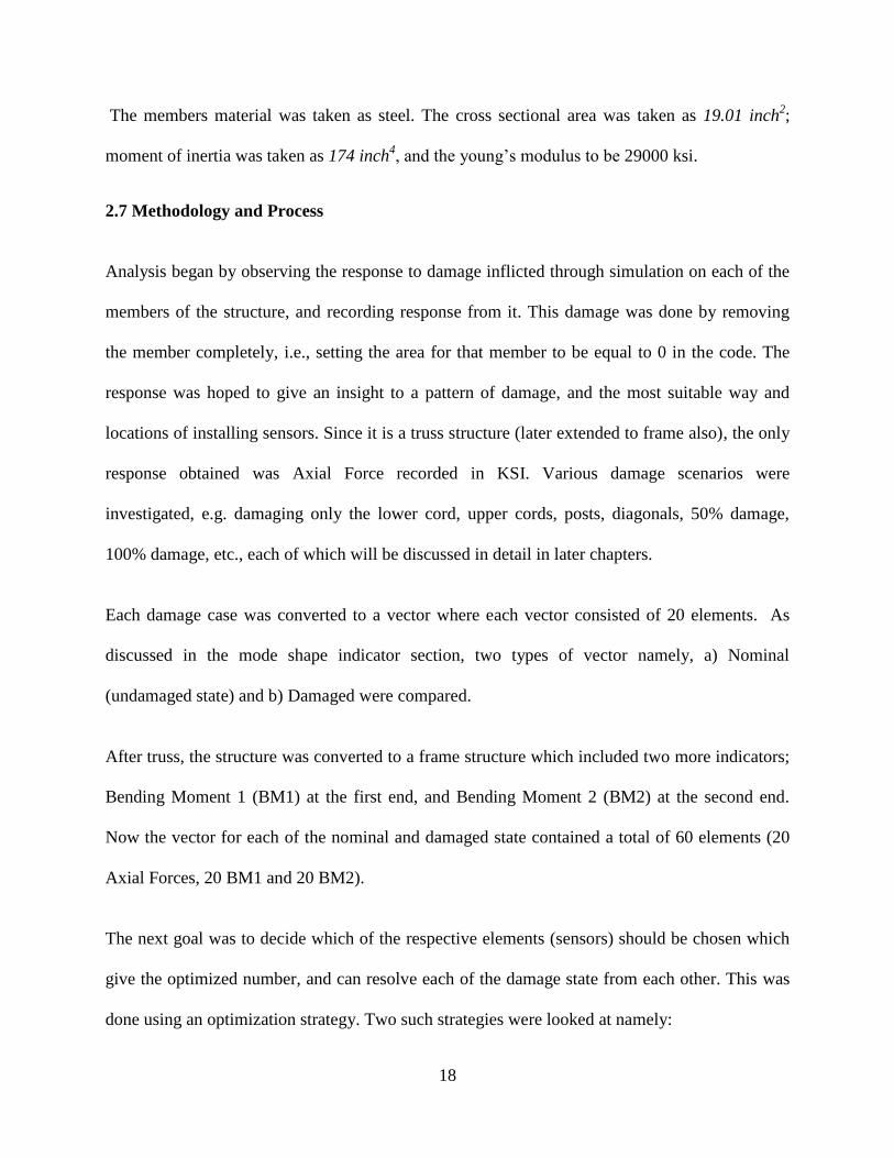
Figure 3.1 Structure
Referring to Figure 3.1, as the structure is loaded, the load will generate axial force. The
objective of analyzing the truss is to determine how the member forces change in all the
members when one of them is damaged.
An FE model of the truss shown in Figure 3.1 was built in SAP2000 V14 to record member
forces (forces, bending moment at end 1, and bending moment at end 2 in case of frame). This
reading was stored as reference (nominal) reading for the member forces when the structure is
loaded and undamaged. Each member was then damaged individually and response change in
other members was recorded. Carrying out this task turned out to be extremely cumbersome
when done in SAP2000 as it had to be done manually, and then each damaged case data had to
be manually extracted and stored for analysis. An alternate model of the same truss was then
generated in MATLAB through the use of matrix manipulation to mimic the same task as
SAP2000 does. To verify if the model in MATLAB could produce results exactly as SAP2000,

22
several damage case results were compared from both models and the results were found to be
exactly the same.
After proving that MATLAB produces the same results task as SAP2000, the process was
automated. In a single run for a particular damaged state, the member forces in each member
could be calculated in substantially less time as compared to manually calculating it from
SAP2000.
Here some terms are defined which will be referred to in the rest of the chapters too.
1. Damage – Reduction in area of a member by some percentage (can be 25%, 50% or
complete removal of member).
2. Nominal Force – The member force when the structure is in perfect condition, i.e. no
member is damaged and the system is in perfect equilibrium.
3. Damaged Force – The member force when one of the members in the structure has been
damaged. Only one set of member forces will be nominal, (termed as nominal or
undamaged state) along with 20 sets of damaged member forces, since each damaged
state (member) will generate 20 forces in each member.
4. Nominal Stress – Stress in the members without any damaged member.
5. Damaged Stress - Stress in the members with a member damaged.

23
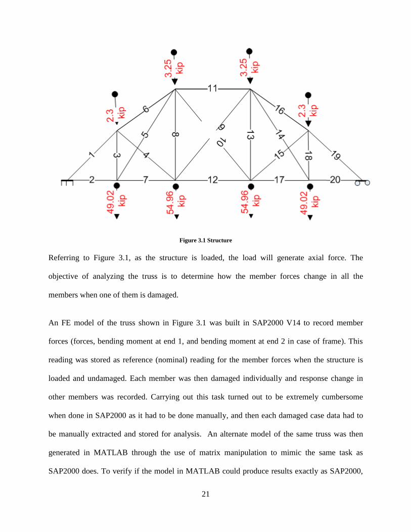
3.1.1 Data Generation
The analysis process starts with calculating the nominal forces in all the members. This data is
stored as reference, and then each member is damaged systematically, and member forces of all
members for each damage state are calculated and saved.
The process can be summarized in steps as follows:
1. Calculation of nominal forces - results in 20 axial forces in each member.
2. Reduction in area of member ‘i’ by x%; calculate force damaged – results in 20 axial
forces which is referred to as damaged force.
3. Restoration of area of member ‘i’ back to nominal value; reduce area of member (i+1) by x
%; calculate force damaged – results in a different set of 20 axial forces as damaged force.
4. Repeating the process for all 20 members.
The following flowchart, Figure 3.2, explains the process in a schematic fashion.
24
Calculate Nominal
Member Data
Save the Nominal State
data
Matlab Model
Damage Member ‘i’
Calculate Damaged
Member Data for damage
state ‘i’
Restore member ‘i’ to
nominal
Save damaged data for
damage state ‘i’
Initialize i=0
Increment ‘i’
Is i= 20
No
Save dataEnd Process
Yes
Start
Figure 3.2 Data Generation Flowchart (Truss)
So, for all damaged states (percent reduction in area) calculation, there will be a total of 400
damaged member forces (20 for each member damaged).
3.2 Frame Bridge
Similar to trusses, frames are composed of triangular members connected at joints. The
difference in construction lies in the fact that in the case of a truss, the joints are pins, and hence
the members are free to rotate about the pin, whereas members of frames are connected rigidly

25
by means of welding or bolting at the joints. A truss cannot transfer moments whereas frames
transfer moments in addition to the axial loads. To model a frame structure the members were
considered as beams shown in Figure 3.3 [29]. A beam deforms, and stresses develop inside it
when a transverse load is applied on it.
Figure 3.3 Beam [Diagram from 29]
There are two forms of internal stresses caused by transverse loads:
Shear Stress
Compressive and Tensile Stress.
The last two quantities are equal and opposite in direction and form a couple or moment. This
bending moment resists the sagging deformation of the beam. Bending moment is the summation
of the product of the stress and the distance to the neutral axis. To show the bending moment
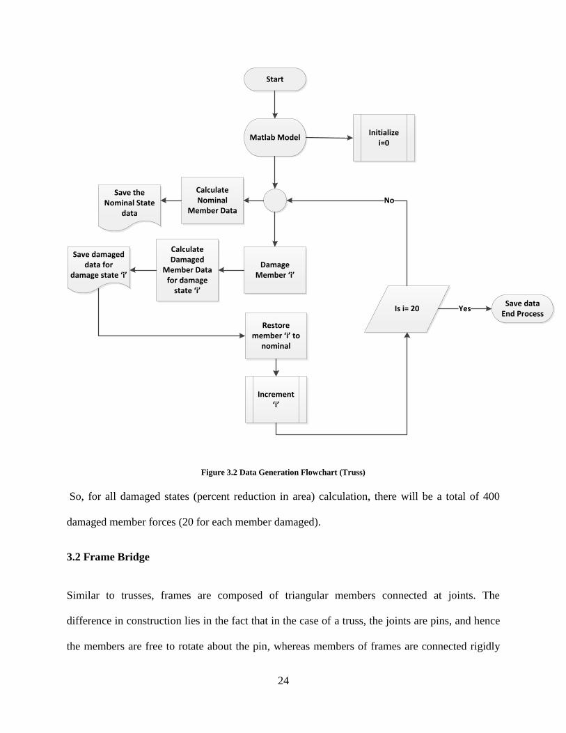
Figure 3.4 [30] is presented.
26
Figure 3.4 Bending Moment [Diagram from 30]
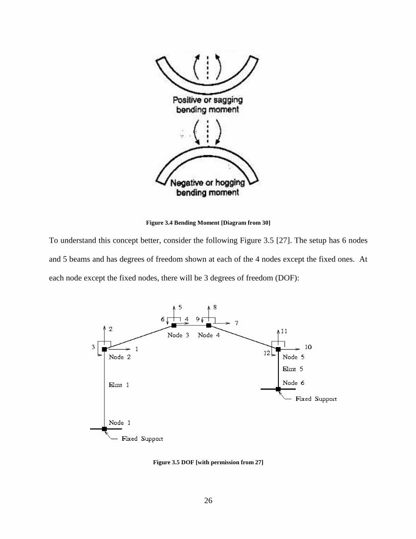
To understand this concept better, consider the following Figure 3.5 [27]. The setup has 6 nodes
and 5 beams and has degrees of freedom shown at each of the 4 nodes except the fixed ones. At
each node except the fixed nodes, there will be 3 degrees of freedom (DOF):
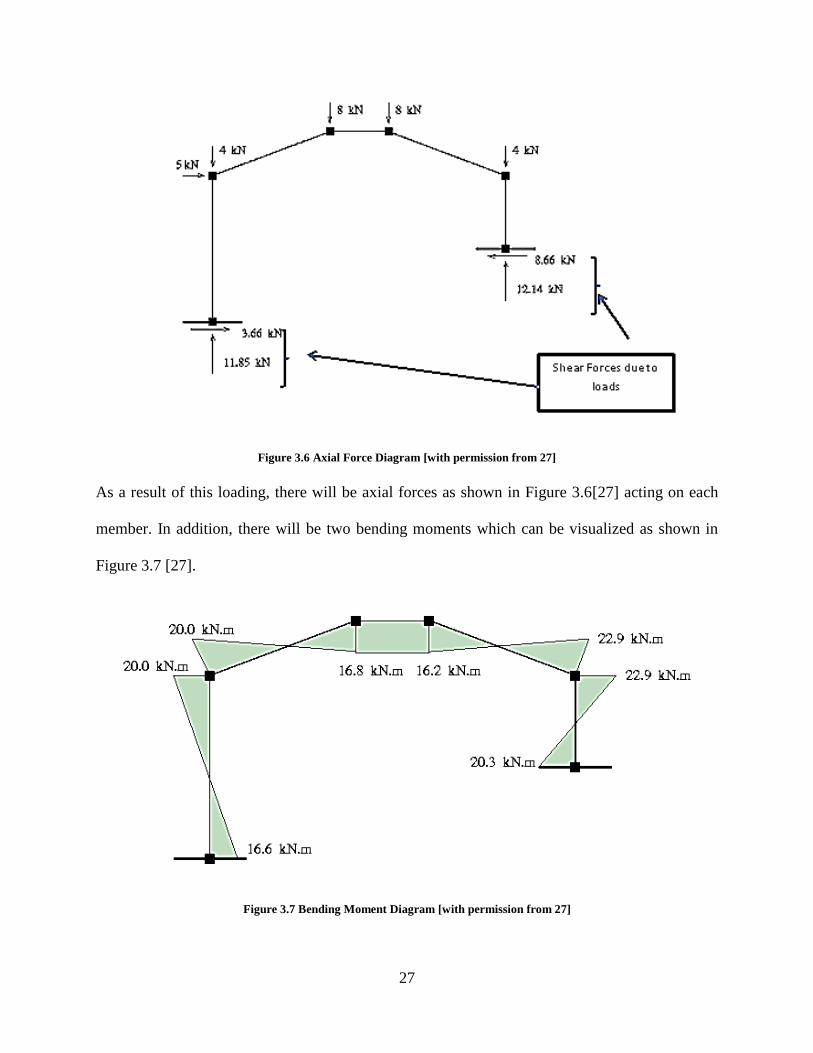
Figure 3.5 DOF [with permission from 27]
27
Figure 3.6 Axial Force Diagram [with permission from 27]
As a result of this loading, there will be axial forces as shown in Figure 3.6[27] acting on each
member. In addition, there will be two bending moments which can be visualized as shown in
Figure 3.7 [27].
Figure 3.7 Bending Moment Diagram [with permission from 27]

28
Before moving to the investigation of frame, it is imperative to define some terms as they will be
used in the rest of the text frequently. When truss is used as a structure, there is only one
response that is obtained from the structure which is axial force. Switching to a frame adds two
more measurements, namely end moments BM1 and BM2. From here on, each of these
responses will collectively be termed as ‘end actions’.
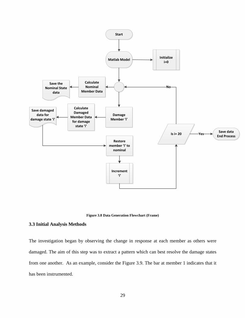
3.2.1 Data Generation
A similar procedure was employed for frame structure to generate data as was used in the case of
truss. The changes however will be explained as follows:
1. Calculation of nominal actions - results in 60 end actions (20 axial forces, 20 BM1 and
20 BM2 in each member).
2. Reduction in area of member ‘i’ by x%; calculate damaged end actions – results in 60
end actions which is referred to as damaged end actions.
3. Restoration of area of member ‘i’ back to nominal value; reduce area of member (i+1) by
x %; calculate damaged end actions – results in a different set of 60 damaged end actions.
4. Repeating the process for all 20 members.
A total of 1200 damaged values were obtained after each member had been damaged. Figure 3.8
explains the step by step process in a schematic.
29
Calculate Nominal
Member Data
Save the Nominal State
data
Matlab Model
Damage Member ‘i’
Calculate Damaged
Member Data for damage
state ‘i’
Restore member ‘i’ to
nominal
Save damaged data for
damage state ‘i’
Initialize i=0
Increment ‘i’
Is i= 20
No
Save dataEnd Process
Yes
Start
Figure 3.8 Data Generation Flowchart (Frame)
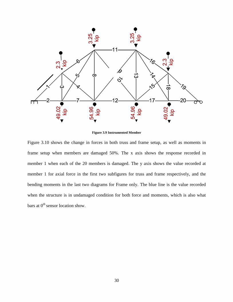
3.3 Initial Analysis Methods
The investigation began by observing the change in response at each member as others were
damaged. The aim of this step was to extract a pattern which can best resolve the damage states
from one another. As an example, consider the Figure 3.9. The bar at member 1 indicates that it
has been instrumented.
30
Figure 3.9 Instrumented Member
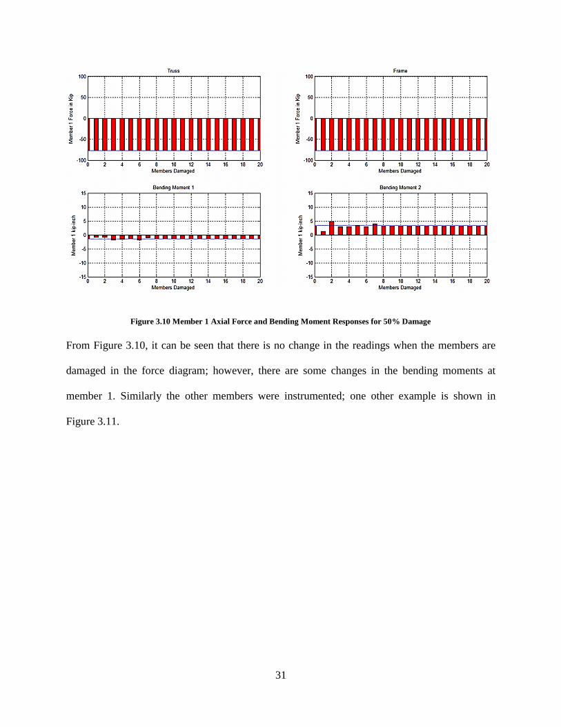
Figure 3.10 shows the change in forces in both truss and frame setup, as well as moments in
frame setup when members are damaged 50%. The x axis shows the response recorded in
member 1 when each of the 20 members is damaged. The y axis shows the value recorded at
member 1 for axial force in the first two subfigures for truss and frame respectively, and the
bending moments in the last two diagrams for Frame only. The blue line is the value recorded
when the structure is in undamaged condition for both force and moments, which is also what
bars at 0th
sensor location show.
31
Figure 3.10 Member 1 Axial Force and Bending Moment Responses for 50% Damage
From Figure 3.10, it can be seen that there is no change in the readings when the members are
damaged in the force diagram; however, there are some changes in the bending moments at
member 1. Similarly the other members were instrumented; one other example is shown in
Figure 3.11.
32
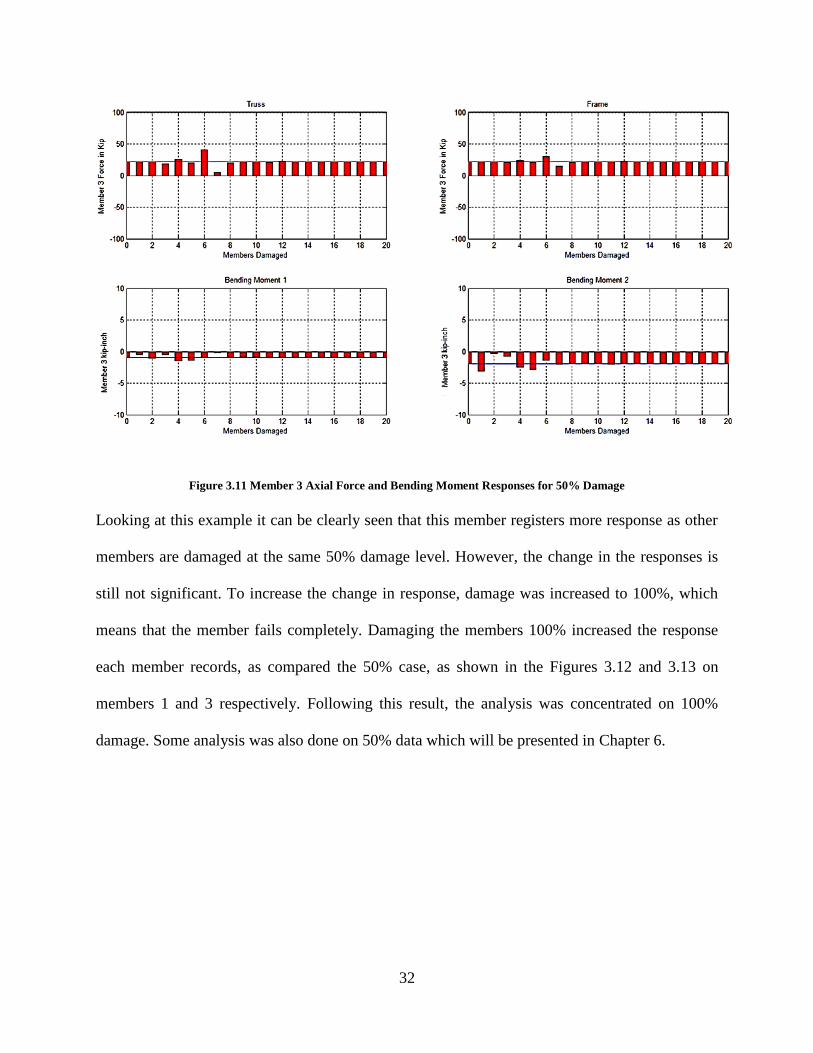
Figure 3.11 Member 3 Axial Force and Bending Moment Responses for 50% Damage
Looking at this example it can be clearly seen that this member registers more response as other
members are damaged at the same 50% damage level. However, the change in the responses is
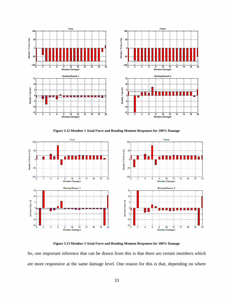
still not significant. To increase the change in response, damage was increased to 100%, which
means that the member fails completely. Damaging the members 100% increased the response
each member records, as compared the 50% case, as shown in the Figures 3.12 and 3.13 on
members 1 and 3 respectively. Following this result, the analysis was concentrated on 100%
damage. Some analysis was also done on 50% data which will be presented in Chapter 6.
33
Figure 3.12 Member 1 Axial Force and Bending Moment Responses for 100% Damage
Figure 3.13 Member 3 Axial Force and Bending Moment Responses for 100% Damage
So, one important inference that can be drawn from this is that there are certain members which
are more responsive at the same damage level. One reason for this is that, depending on where
34
the member is constructed in the structure, the change in force that it records varies. But no
single member is capable of correctly isolating one damaged state from another, as some
members when damaged, have no effect on the reading of the single instrumented member. For
example, when members 12, 14, 15, 16, 17, and 18 are damaged there is no or negligible change
in the readings of member 3.Having noticed that, the next step was to use combinations of
members to record responses.
In the previous discussion it was mentioned that certain members are better indicators for
damage than the others, so combinations of such members or groups of members were made, e.g.
all the upper chords, all the lower chords, all the posts, and all the diagonals, etc. One thing
worth pointing out here is that there are certain members which when damaged make the
structure unstable and eventually cause complete failure. These members are called non-
redundant members. The other members will be called redundant members as when they fail, the
system is still stable because of the distribution of actions along the other members.
The analysis now tries to observe the combined response of a group of sensors to detect and
isolate damaged states from one another. This process involves a two tier approach of analyzing
data which will be discussed in the following paragraphs.
At this stage, it is important to define some initial terms here which will be extended and stated
in more concrete form later.
Detection - Assuming that a baseline can be established (which is the value a sensor reads
when the structure is in healthy condition), the damaged reading can be seen as an
increase, a decrease, or a reversal.
35
1. Increase - If the nominal reading is x or –x and the damaged reading is (x+5) or (-x-
5) respectively.
2. Decrease - If the nominal reading is x or –x and the damaged reading is (x-5) or (-
x+5) respectively
3. Reversal - If the nominal reading is x or –x and the damaged reading is –x or x
respectively, i.e. the direction of the vector changes sign no matter how small or large
the reading is.
Isolation - Once damage is detected, i.e. if the current reading is greater, less, or reversed
from the baseline reading, the goal now is to resolve which member(s) are damaged.
1. If just one member changes uniquely from the above categories separate it at stage 1
(detection phase).
2. If more than 1 member is damaged in any of the category, bending moment 1 is
investigated to separate them from one another. The current bending moment will be
compared with the baseline bending moment in both magnitude and direction.
Having defined these points, the patterns were analyzed to resolve the damaged states. The
analysis is based on detecting some damaged members based on axial force alone while others
are based on both axial force and bending moment 1. The crosses on the members 1, 2, 19, and
20 signify that they are non-redundant members and will be ignored from analysis as shown in
Figure 3.14.
36
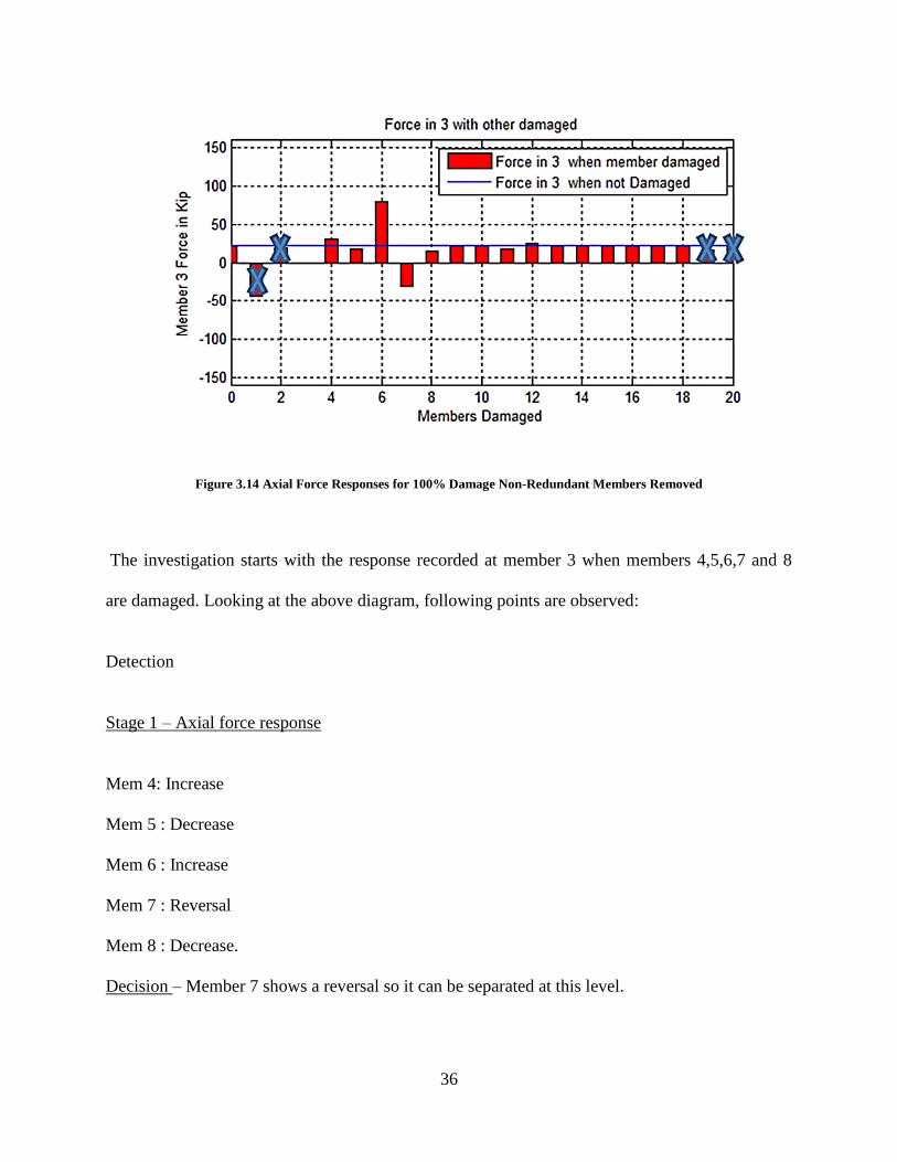
Figure 3.14 Axial Force Responses for 100% Damage Non-Redundant Members Removed
The investigation starts with the response recorded at member 3 when members 4,5,6,7 and 8
are damaged. Looking at the above diagram, following points are observed:
Detection
Stage 1 – Axial force response
Mem 4: Increase
Mem 5 : Decrease
Mem 6 : Increase
Mem 7 : Reversal
Mem 8 : Decrease.
Decision – Member 7 shows a reversal so it can be separated at this level.
37
Members 4 and 6 cause an increase, whereas 5 and 7 show a decrease in reading at 3. So at this
stage, it can be recognized that fault exists, but which member was damaged will be decided
based on bending moment response.
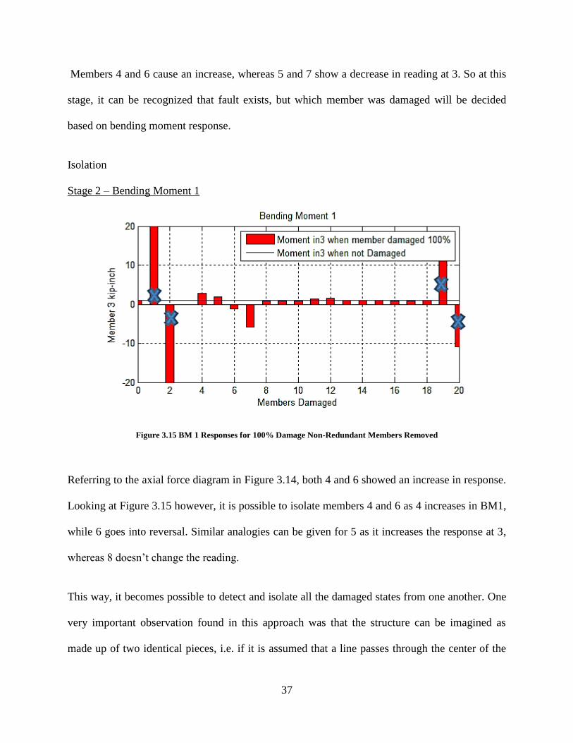
Isolation
Stage 2 – Bending Moment 1
Figure 3.15 BM 1 Responses for 100% Damage Non-Redundant Members Removed
Referring to the axial force diagram in Figure 3.14, both 4 and 6 showed an increase in response.
Looking at Figure 3.15 however, it is possible to isolate members 4 and 6 as 4 increases in BM1,
while 6 goes into reversal. Similar analogies can be given for 5 as it increases the response at 3,
whereas 8 doesn’t change the reading.
This way, it becomes possible to detect and isolate all the damaged states from one another. One
very important observation found in this approach was that the structure can be imagined as
made up of two identical pieces, i.e. if it is assumed that a line passes through the center of the
38
structure, one side will be a mirror image of the other. So if sensors are placed at member 18,
which is the equivalent post for member 3, members 14, 15, 16, 17 can be isolated in the same
way.
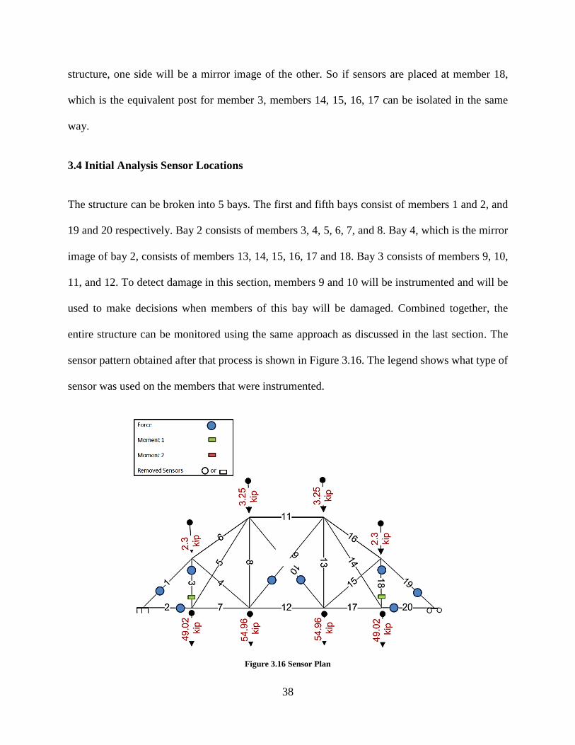
3.4 Initial Analysis Sensor Locations
The structure can be broken into 5 bays. The first and fifth bays consist of members 1 and 2, and
19 and 20 respectively. Bay 2 consists of members 3, 4, 5, 6, 7, and 8. Bay 4, which is the mirror
image of bay 2, consists of members 13, 14, 15, 16, 17 and 18. Bay 3 consists of members 9, 10,
11, and 12. To detect damage in this section, members 9 and 10 will be instrumented and will be
used to make decisions when members of this bay will be damaged. Combined together, the
entire structure can be monitored using the same approach as discussed in the last section. The
sensor pattern obtained after that process is shown in Figure 3.16. The legend shows what type of
sensor was used on the members that were instrumented.
Figure 3.16 Sensor Plan

39
For a structure of this size, visually diagnosing a fault and isolation of damage states is easier,
but as the structure increases in size it becomes more difficult. Solving this problem will require
an efficient and sophisticated mathematical procedure which takes all the possible cases and
scenarios into account. Pattern recognition, genetic algorithms, machine learning, or similar
artificial intelligence based methods are some of the many methods that can be used.
This work will be focused on comparing vectors of measured data to the nominal (undamaged)
and damaged data. The key to this approach is successfully correlating the measured data to the
undamaged and the modeled damaged states, as well as to find the damaged state which gives
the highest correlation measure in case the measured data is damaged data. The vector of states
which gives the highest correlation will mean that it aligns most closely with the measured data.
Depending on what that state signifies in the database (damaged or nominal), the measured data
will be classified.
The methodology followed to do this is the Modal Assurance Criterion (MAC) which is the core
of the research and will be discussed in the following chapters.
40
Chapter 4: Optimization of Instrumentation
This chapter delves into the details of the analysis and the methods used in deciding the
optimized sensor placements on bridges. The concept of Modal Assurance Criterion (MAC) is
also discussed in detail.
4.1 Analysis Approach
The analysis process considers baseline forces due to gravity loads. Each time a member is
damaged, it is a 100% section loss, or the member is removed completely. Just to refresh the
previous concepts, consider the following terms:
Nominal value - Member force and moments when every member is undamaged.
Damaged value - Member force and moments when every member in 0% area damaged.
Process of damage carried 20 times - Member forces and moments for all 20 damaged
states calculated.
There are three output values for each member:
Force(F) – Axial Force
Bending Moment 1(BM1) – Bending Moment at end 1
Bending Moment 2(BM2) – Bending Moment at end 2
For all 20 members the values obtained would be:
N = (20x3) = 60 values (or actions), where Action = Collective term for Force and
Moments.
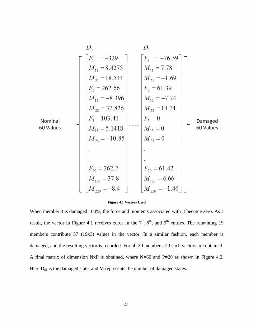
Having established the above concepts, every single vector consists of 60 values. Figure 4.1
shows examples of a nominal vector D0 and the vector D3 when member 3 is damaged.
41
Figure 4.1 Vectors Used
When member 3 is damaged 100%, the force and moments associated with it become zero. As a
result, the vector in Figure 4.1 receives zeros in the 7th
, 8th
, and 9th
entries. The remaining 19
members contribute 57 (19x3) values in the vector. In a similar fashion, each member is
damaged, and the resulting vector is recorded. For all 20 members, 20 such vectors are obtained.
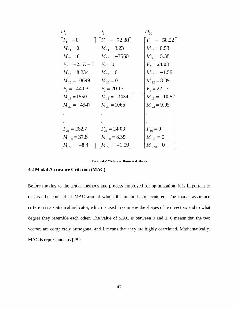
A final matrix of dimension NxP is obtained, where N=60 and P=20 as shown in Figure 4.2.
Here DM is the damaged state, and M represents the number of damaged states.
42
0
0
0
.
.
95.9
82.10
17.22
39.8
59.1
03.24
38.5
58.0
22.50
..........
59.1
39.8
03.24
.
.
1065
3434
15.20
0
0
0
7560
23.3
38.72
4.8
8.37
7.262
.
.
4947
1550
03.44
10699
234.8
71.2
0
0
0
220
120
20
23
13
3
22
12
2
21
11
1
220
120
20
23
13
3
22
12
2
21
11
1
220
120
20
23
13
3
22
12
2
21
11
1
2021
M
M
F
M
M
F
M
M
F
M
M
F
M
M
F
M
M
F
M
M
F
M
M
F
M
M
F
M
M
F
M
M
EF
M
M
F
DDD
Figure 4.2 Matrix of Damaged States
4.2 Modal Assurance Criterion (MAC)
Before moving to the actual methods and process employed for optimization, it is important to
discuss the concept of MAC around which the methods are centered. The modal assurance
criterion is a statistical indicator, which is used to compare the shapes of two vectors and to what
degree they resemble each other. The value of MAC is between 0 and 1. 0 means that the two
vectors are completely orthogonal and 1 means that they are highly correlated. Mathematically,
MAC is represented as [28]:
43
}){*}({*}){*}({
|}{*}{|},{
2
j
T
ji
T
i
j
T
i
jiMAC
(4.1)
Where Ψi and Ψj are the vectors being correlated.
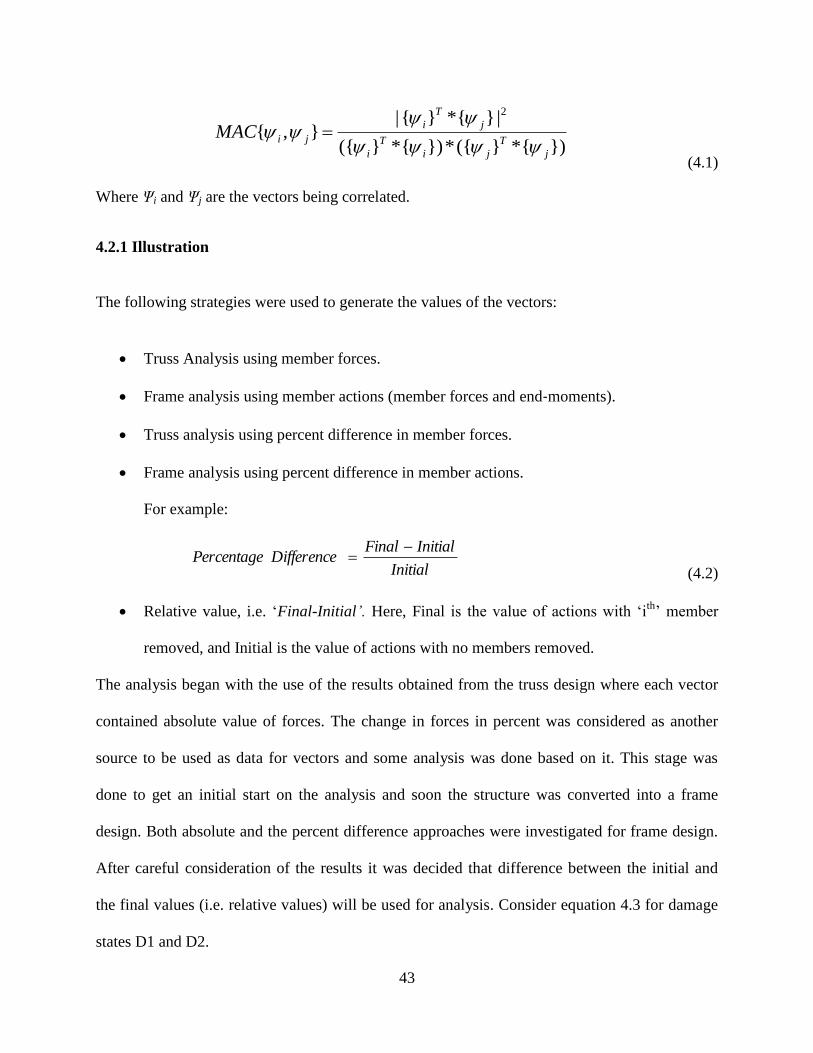
4.2.1 Illustration
The following strategies were used to generate the values of the vectors:
Truss Analysis using member forces.
Frame analysis using member actions (member forces and end‐moments).
Truss analysis using percent difference in member forces.
Frame analysis using percent difference in member actions.
For example:
Initial
InitialFinalDifferencePercentage
(4.2)
Relative value, i.e. ‘Final-Initial’. Here, Final is the value of actions with ‘ith
’ member
removed, and Initial is the value of actions with no members removed.
The analysis began with the use of the results obtained from the truss design where each vector
contained absolute value of forces. The change in forces in percent was considered as another
source to be used as data for vectors and some analysis was done based on it. This stage was
done to get an initial start on the analysis and soon the structure was converted into a frame
design. Both absolute and the percent difference approaches were investigated for frame design.
After careful consideration of the results it was decided that difference between the initial and
the final values (i.e. relative values) will be used for analysis. Consider equation 4.3 for damage
states D1 and D2.

44
}){*}({*}){*}({
|}{*}{|},{
2211
2
2121
DDDD
DDDDMAC
TT
T
(4.3)
The above formula calculates MAC value for D1 and D2 which gives a scalar value. For all
combination of the 20 damaged states, a matrix of 20x20 values will be obtained which will look
like Figure 4.3
},{....}.,{},{
..
..
..
..
..
..
..
..................
},{.....}.,{},{
},{.}.,{},{},{
2020220120
2022212
201312111
DDMACDDMACDDMAC
DDMACDDMACDDMAC
DDMACDDMACDDMACDDMAC
Figure 4.3 Matrix of MAC Values
The goal of the process is to separate the damaged states from one another so that each damaged
state can be isolated from one another. This would mean that each damaged state can be resolved
so that every damaged state is independent from the others. In order to proceed in that direction,
bubble charts were drawn to understand how the output values of MAC are distributed.
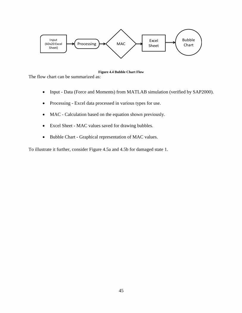
4.2.2 Bubble Charts
Figure 4.4 illustrates the basic flow of how the bubble chart is drawn
45
Excel Sheet
Input(60x20 Excel
Sheet)Processing
Bubble ChartMAC
Figure 4.4 Bubble Chart Flow
The flow chart can be summarized as:
Input - Data (Force and Moments) from MATLAB simulation (verified by SAP2000).
Processing - Excel data processed in various types for use.
MAC - Calculation based on the equation shown previously.
Excel Sheet - MAC values saved for drawing bubbles.
Bubble Chart - Graphical representation of MAC values.
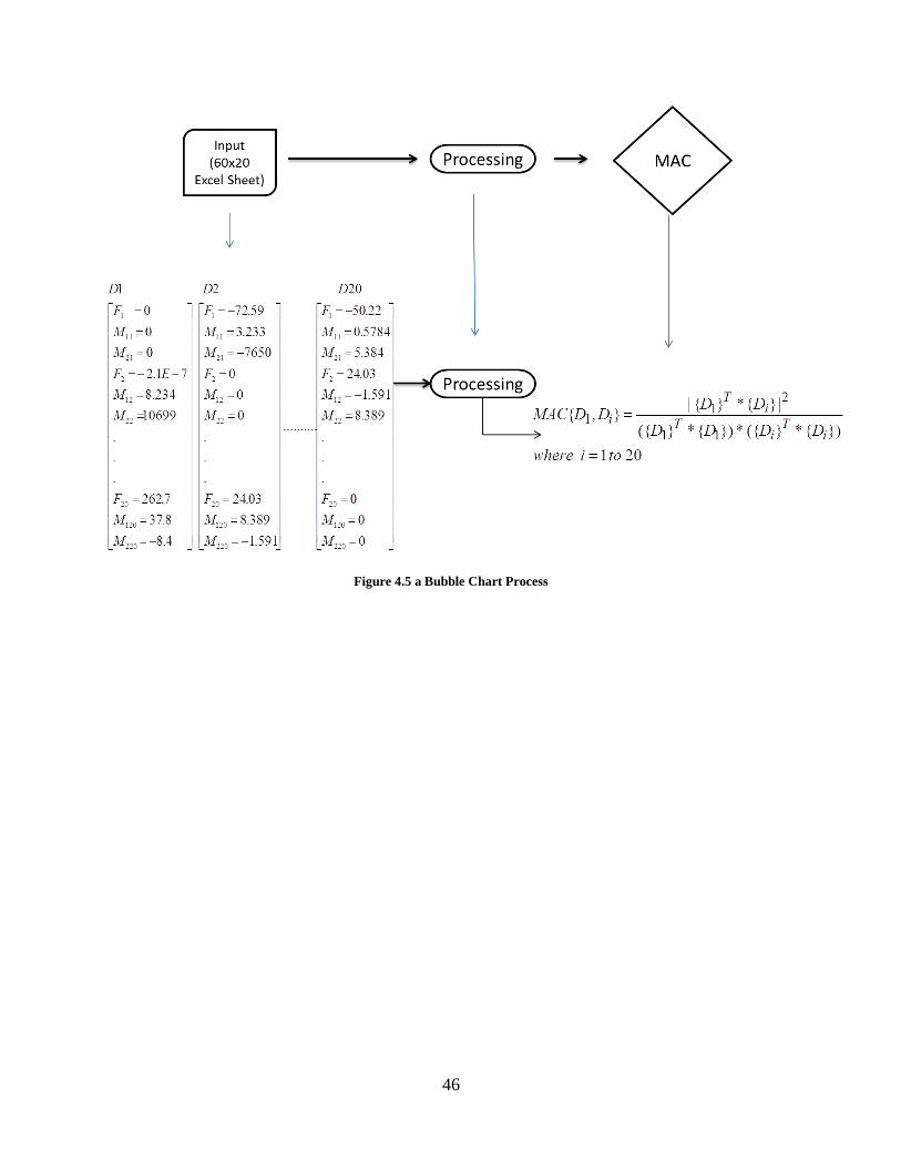
To illustrate it further, consider Figure 4.5a and 4.5b for damaged state 1.
46
Figure 4.5 a Bubble Chart Process
47
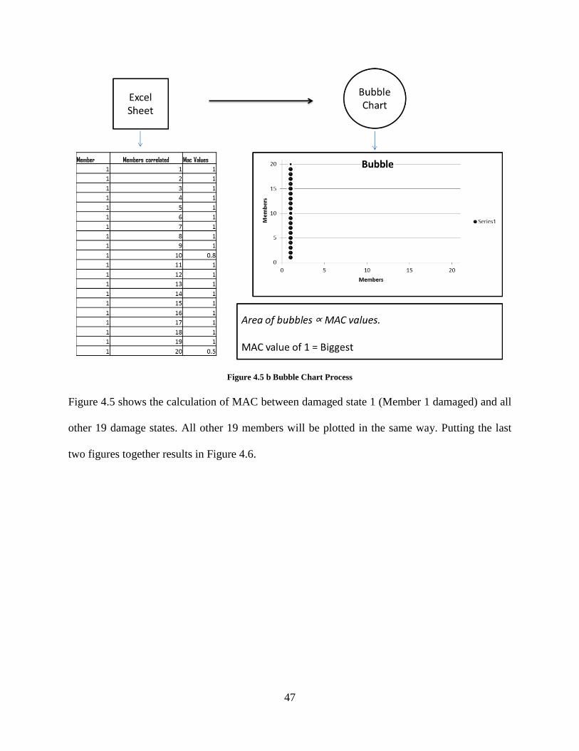
Figure 4.5 b Bubble Chart Process
Figure 4.5 shows the calculation of MAC between damaged state 1 (Member 1 damaged) and all
other 19 damage states. All other 19 members will be plotted in the same way. Putting the last
two figures together results in Figure 4.6.
48
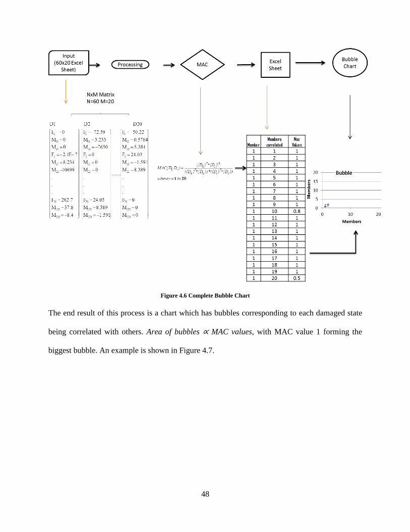
Figure 4.6 Complete Bubble Chart
The end result of this process is a chart which has bubbles corresponding to each damaged state
being correlated with others. Area of bubbles ∝ MAC values, with MAC value 1 forming the
biggest bubble. An example is shown in Figure 4.7.
49
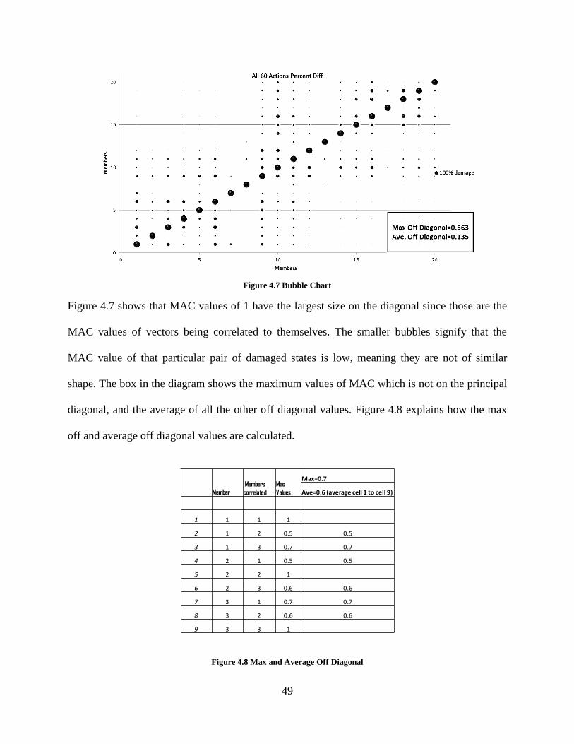
Figure 4.7 Bubble Chart
Figure 4.7 shows that MAC values of 1 have the largest size on the diagonal since those are the
MAC values of vectors being correlated to themselves. The smaller bubbles signify that the
MAC value of that particular pair of damaged states is low, meaning they are not of similar
shape. The box in the diagram shows the maximum values of MAC which is not on the principal
diagonal, and the average of all the other off diagonal values. Figure 4.8 explains how the max
off and average off diagonal values are calculated.
MemberMembers
correlated
Mac
Values
Max=0.7
Ave=0.6 (average cell 1 to cell 9)
1 1 1 1
2 1 2 0.5 0.5
3 1 3 0.7 0.7
4 2 1 0.5 0.5
5 2 2 1
6 2 3 0.6 0.6
7 3 1 0.7 0.7
8 3 2 0.6 0.6
9 3 3 1
Figure 4.8 Max and Average Off Diagonal
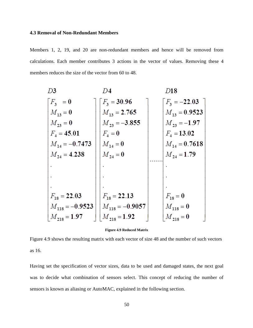
50
4.3 Removal of Non-Redundant Members
Members 1, 2, 19, and 20 are non-redundant members and hence will be removed from
calculations. Each member contributes 3 actions in the vector of values. Removing these 4
members reduces the size of the vector from 60 to 48.
Figure 4.9 Reduced Matrix
Figure 4.9 shows the resulting matrix with each vector of size 48 and the number of such vectors
as 16.
Having set the specification of vector sizes, data to be used and damaged states, the next goal
was to decide what combination of sensors select. This concept of reducing the number of
sensors is known as aliasing or AutoMAC, explained in the following section.

51
4.4 Aliasing or AutoMAC.
MAC correlates the data in a vector to produce values between 0 and 1. The AutoMAC on the
other hand, compares a subset of the data (or modes) from the vector for correlation. This is done
in order to determine if the number and location of the selected actions would be able to resolve
the damaged states from each other.
Deciding an optimized sensor suite will require an exhaustive search of all possible combinations
of actions which gives the best end result, which in this case will be a clean or a near clean
diagonal with no or very little off diagonal values. The idea behind obtaining a clean diagonal
and very small values on the off diagonal is that if a sensor suite can give such distribution of
MAC values, it will be able to resolve the damaged states. This sensor suite would not be
confused in deciding between one damaged state from the other since small value on the off
diagonal means that the vectors being correlated are not of the same shape, i.e., one damaged
state can be made independent or nearly independent from the other.
To elaborate the above statement, consider Figure 4.10 which shows one of the many results of
the work just to illustrate the concept.
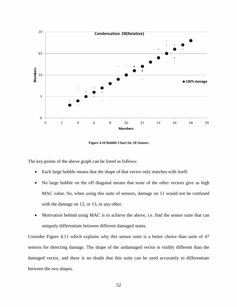
52
Figure 4.10 Bubble Chart for 28 Sensors
The key points of the above graph can be listed as follows:
Each large bubble means that the shape of that vector only matches with itself.
No large bubble on the off diagonal means that none of the other vectors give as high
MAC value. So, when using this suite of sensors, damage on 11 would not be confused
with the damage on 12, or 13, or any other.
Motivation behind using MAC is to achieve the above, i.e. find the sensor suite that can
uniquely differentiate between different damaged states.
Consider Figure 4.11 which explains why this sensor suite is a better choice than suite of 47
sensors for detecting damage. The shape of the undamaged vector is visibly different than the
damaged vector, and there is no doubt that this suite can be used accurately to differentiate
between the two shapes.
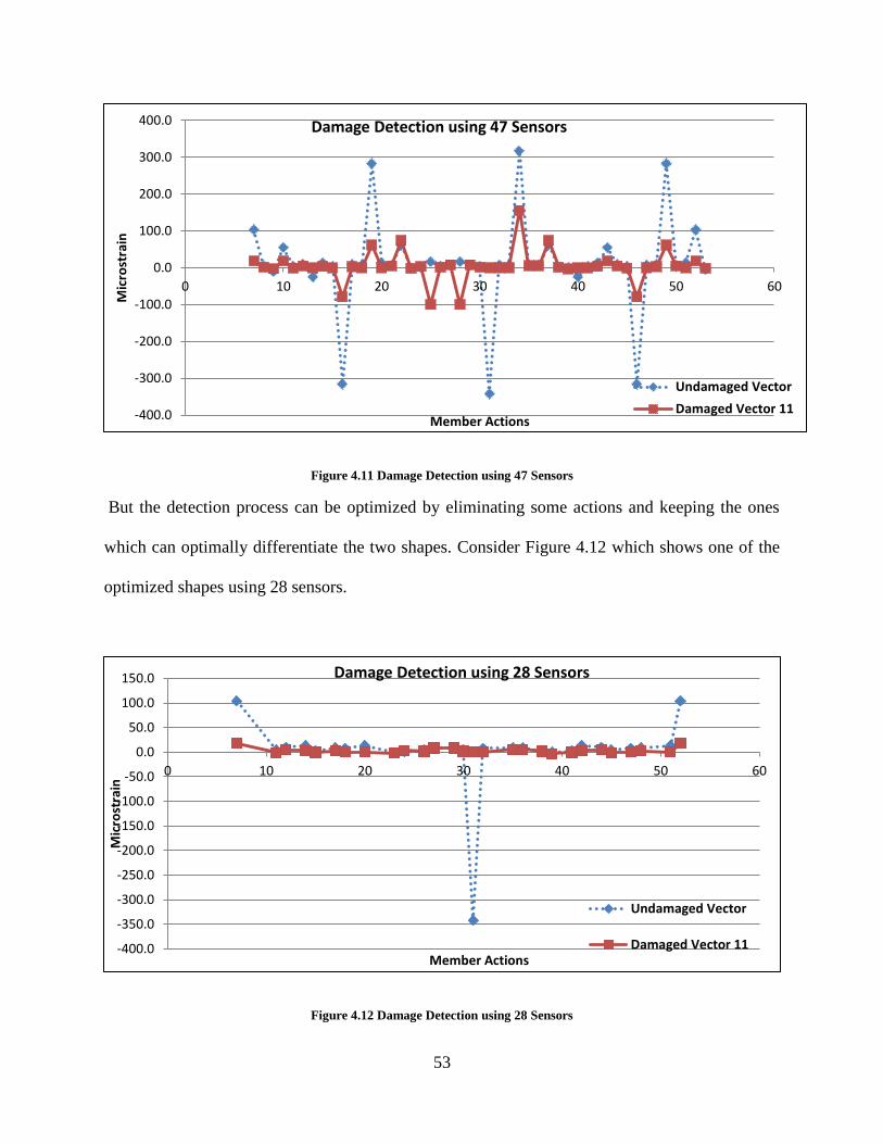
53
Figure 4.11 Damage Detection using 47 Sensors
But the detection process can be optimized by eliminating some actions and keeping the ones
which can optimally differentiate the two shapes. Consider Figure 4.12 which shows one of the
optimized shapes using 28 sensors.
Figure 4.12 Damage Detection using 28 Sensors
-400.0
-300.0
-200.0
-100.0
0.0
100.0
200.0
300.0
400.0
0 10 20 30 40 50 60
Mic
rost
rain
Member Actions
Damage Detection using 47 Sensors
Undamaged Vector
Damaged Vector 11
-400.0
-350.0
-300.0
-250.0
-200.0
-150.0
-100.0
-50.0
0.0
50.0
100.0
150.0
0 10 20 30 40 50 60
Mic
rost
rain
Member Actions
Damage Detection using 28 Sensors
Undamaged Vector
Damaged Vector 11
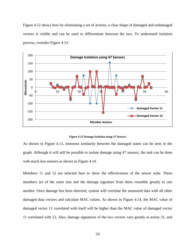
54
Figure 4.12 shows how by eliminating a set of actions, a clear shape of damaged and undamaged
vectors is visible and can be used to differentiate between the two. To understand isolation
process, consider Figure 4.13.
Figure 4.13 Damage Isolation using 47 Sensors
As shown in Figure 4.13, immense similarity between the damaged states can be seen in the
graph. Although it will still be possible to isolate damage using 47 sensors, the task can be done
with much less sensors as shown in Figure 4.14.
Members 11 and 12 are selected here to show the effectiveness of the sensor suite. These
members are of the same size and the damage signature from them resemble greatly to one
another. Once damage has been detected, system will correlate the measured data with all other
damaged data vectors and calculate MAC values. As shown in Figure 4.14, the MAC value of
damaged vector 11 correlated with itself will be higher than the MAC value of damaged vector
11 correlated with 12. Also, damage signatures of the two vectors vary greatly at action 31, and
-200
-150
-100
-50
0
50
100
150
200
0 10 20 30 40 50 60
Mic
rost
rain
Member Actions
Damage Isolation using 47 Sensors
Damaged Vector 11
Damaged Vector 12
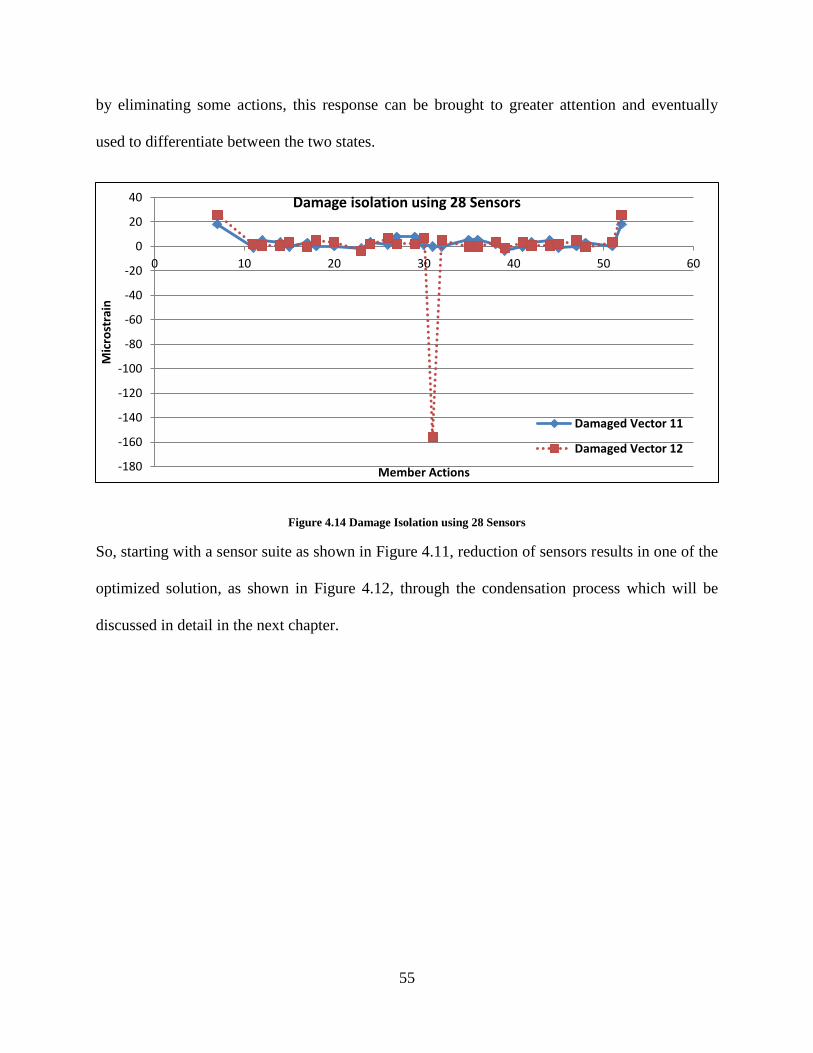
55
by eliminating some actions, this response can be brought to greater attention and eventually
used to differentiate between the two states.
Figure 4.14 Damage Isolation using 28 Sensors
So, starting with a sensor suite as shown in Figure 4.11, reduction of sensors results in one of the
optimized solution, as shown in Figure 4.12, through the condensation process which will be
discussed in detail in the next chapter.
-180
-160
-140
-120
-100
-80
-60
-40
-20
0
20
40
0 10 20 30 40 50 60
Mic
rost
rain
Member Actions
Damage isolation using 28 Sensors
Damaged Vector 11
Damaged Vector 12
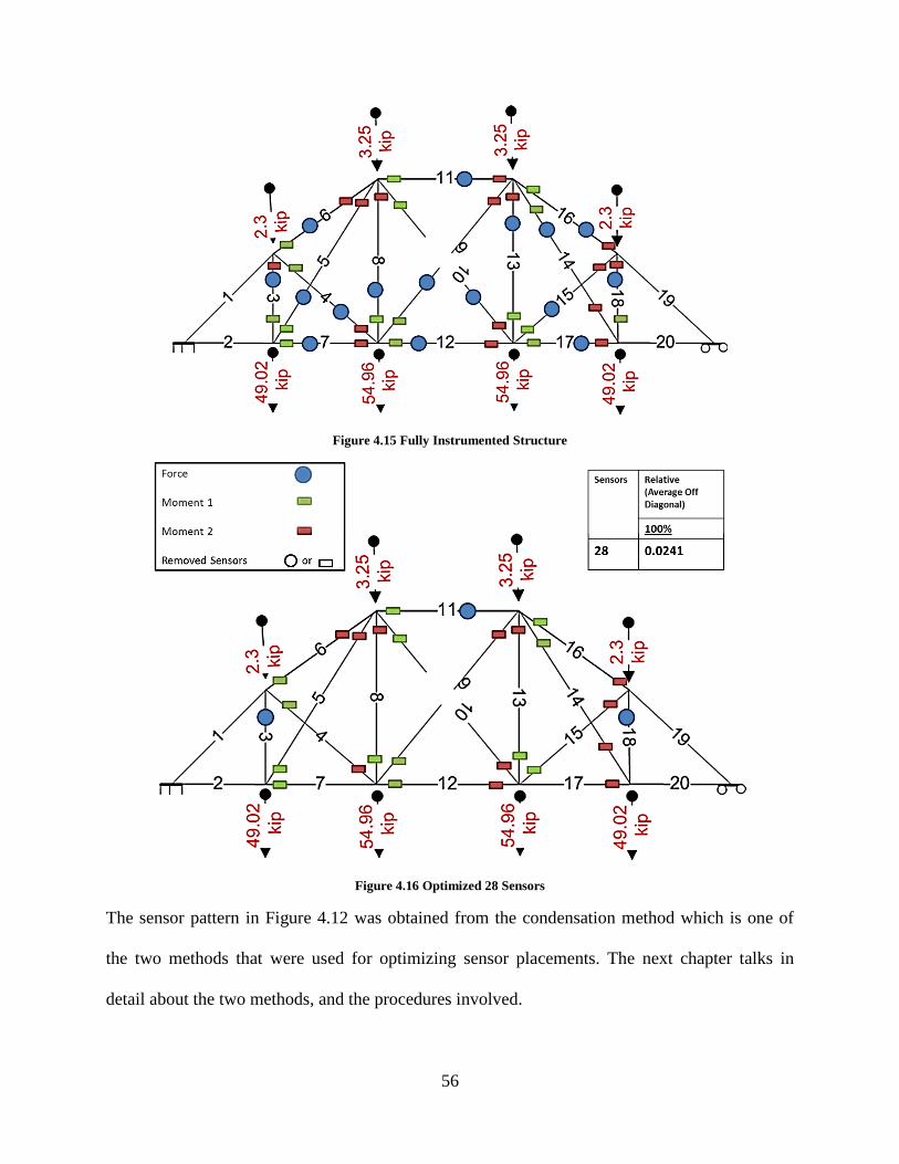
56
Figure 4.15 Fully Instrumented Structure
Figure 4.16 Optimized 28 Sensors
The sensor pattern in Figure 4.12 was obtained from the condensation method which is one of
the two methods that were used for optimizing sensor placements. The next chapter talks in
detail about the two methods, and the procedures involved.
57
Chapter 5: Optimization Routines
This chapter discusses the computational aspect of the research work. The sections to follow will
talk about the optimization methods employed to reach the desired sensor patterns, roadblocks
that were faced, resource constraints, and the proposed solution to them.
Before moving into further discussion, it is important to restate the problem statement, elaborate
it more and explain what this work aims to achieve.
5.1 Problem Statement Revisited
The system or method this research aims to build is one which will receive data from a source
and will decide in real time, what category it belongs to, viz., damaged or undamaged. So, a
bridge data/reading/event can be classified as:
No Event (anomaly/failure).
OR
Fault happened. Once decided that a fault has happened, the system should be able to
classify what happened and where is that event located.
Concretely, this system should be able to successfully do the following which will be discussed
later in the chapter:
Failure Detection
Failure Isolation
To achieve the mentioned two steps, a sensor suite is needed which can:
Uniquely identify damage from undamaged state.

58
Best classify between a specific damaged state from the rest.
So going back to the bubble chart, visually, the aim is to get a sensor suite that has high values
on the principal diagonal, and no or very small value on the off diagonal. The entire work can be
visualized as broken into 3 parts:
1. System Design – finding a sensor suite that can help in Failure ‘Detection and Isolation’,
with acceptable false detection and isolation and missed detection and isolation.
2. Damage Detection
3. Damage Isolation
Success of damage detection and isolation greatly rely on the system design, and hence, a great
deal of time was spent on this part.
5.2 Failure Detection
The first step in the process is to classify the unlabeled or the measured data that will be received
as either damaged or undamaged. This was done by calculating the MAC value of received data
vector and the undamaged vector stored in the database. A high MAC value will mean that there
is high correlation between the undamaged data vector and the unknown vector that was
received. So, it is highly likely that the received data is undamaged data. A low MAC value on
the other hand will signify that the data received is likely to be damaged data. The above process
can be summarized as a flowchart in Figure 5.1. The table in Figure 5.1 depicts the sensor
location, undamaged vector, and the damaged vector. Here it is important to mention that the
sensors in the first column will be found by one of the optimization routines discussed later in
chapter. Once this sensor suite has been obtained, these sensors will be instrumented on the
structure which will record data.
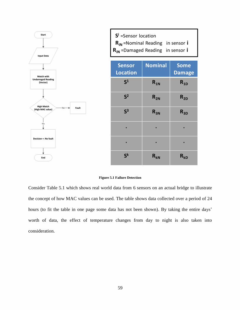
59
Input DataInput Data
Match with Undamaged Reading
(Vector)
Match with Undamaged Reading
(Vector)
High Match(High MAC value)
High Match(High MAC value)
Decision =: No faultDecision =: No fault
Yes
Fault Fault No
StartStart
EndEnd
Sensor Location
Nominal Some Damage
S1 R1N R1D
S2 R2N R2D
S3 R3N R3D
. . .
. . .
Sk RkN RkD
SSi =Sensor location
RiN =Nominal Reading in sensor iRiN =Damaged Reading in sensor i
Figure 5.1 Failure Detection
Consider Table 5.1 which shows real world data from 6 sensors on an actual bridge to illustrate
the concept of how MAC values can be used. The table shows data collected over a period of 24
hours (to fit the table in one page some data has not been shown). By taking the entire days’
worth of data, the effect of temperature changes from day to night is also taken into
consideration.
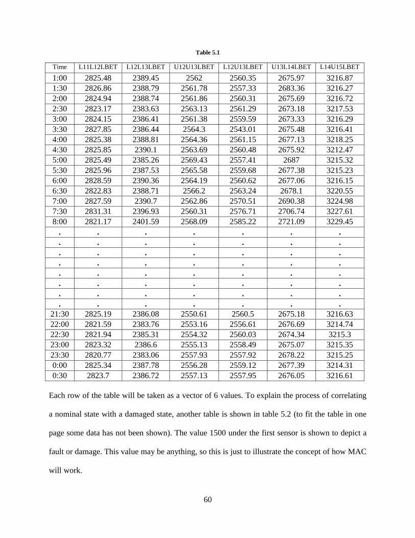
60
Table 5.1
Time L11L12LBET L12L13LBET U12U13LBET L12U13LBET U13L14LBET L14U15LBET
1:00 2825.48 2389.45 2562 2560.35 2675.97 3216.87
1:30 2826.86 2388.79 2561.78 2557.33 2683.36 3216.27
2:00 2824.94 2388.74 2561.86 2560.31 2675.69 3216.72
2:30 2823.17 2383.63 2563.13 2561.29 2673.18 3217.53
3:00 2824.15 2386.41 2561.38 2559.59 2673.33 3216.29
3:30 2827.85 2386.44 2564.3 2543.01 2675.48 3216.41
4:00 2825.38 2388.81 2564.36 2561.15 2677.13 3218.25
4:30 2825.85 2390.1 2563.69 2560.48 2675.92 3212.47
5:00 2825.49 2385.26 2569.43 2557.41 2687 3215.32
5:30 2825.96 2387.53 2565.58 2559.68 2677.38 3215.23
6:00 2828.59 2390.36 2564.19 2560.62 2677.06 3216.15
6:30 2822.83 2388.71 2566.2 2563.24 2678.1 3220.55
7:00 2827.59 2390.7 2562.86 2570.51 2690.38 3224.98
7:30 2831.31 2396.93 2560.31 2576.71 2706.74 3227.61
8:00 2821.17 2401.59 2568.09 2585.22 2721.09 3229.45
. . . . . . .
. . . . . . .
. . . . . . .
. . . . . . .
. . . . . . .
. . . . . . .
. . . . . . .
. . . . . . .
21:30 2825.19 2386.08 2550.61 2560.5 2675.18 3216.63
22:00 2821.59 2383.76 2553.16 2556.61 2676.69 3214.74
22:30 2821.94 2385.31 2554.32 2560.03 2674.34 3215.3
23:00 2823.32 2386.6 2555.13 2558.49 2675.07 3215.35
23:30 2820.77 2383.06 2557.93 2557.92 2678.22 3215.25
0:00 2825.34 2387.78 2556.28 2559.12 2677.39 3214.31
0:30 2823.7 2386.72 2557.13 2557.95 2676.05 3216.61
Each row of the table will be taken as a vector of 6 values. To explain the process of correlating
a nominal state with a damaged state, another table is shown in table 5.2 (to fit the table in one
page some data has not been shown). The value 1500 under the first sensor is shown to depict a
fault or damage. This value may be anything, so this is just to illustrate the concept of how MAC
will work.
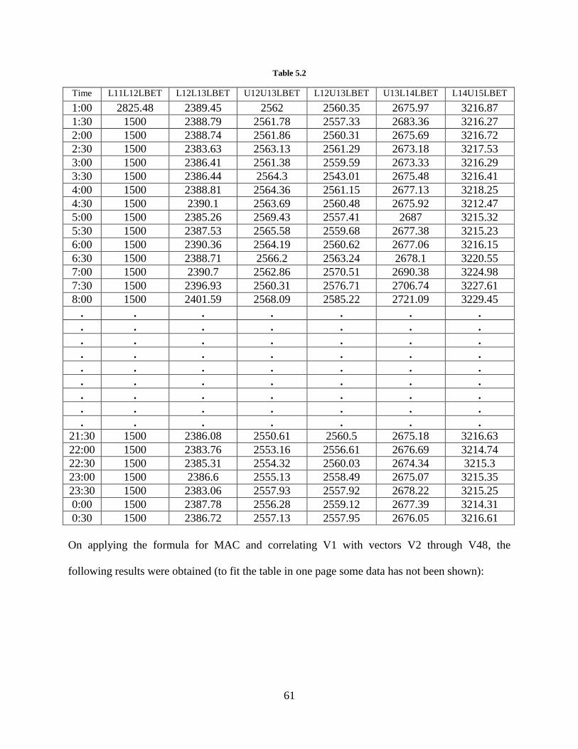
61
Table 5.2
Time L11L12LBET L12L13LBET U12U13LBET L12U13LBET U13L14LBET L14U15LBET
1:00 2825.48 2389.45 2562 2560.35 2675.97 3216.87
1:30 1500 2388.79 2561.78 2557.33 2683.36 3216.27
2:00 1500 2388.74 2561.86 2560.31 2675.69 3216.72
2:30 1500 2383.63 2563.13 2561.29 2673.18 3217.53
3:00 1500 2386.41 2561.38 2559.59 2673.33 3216.29
3:30 1500 2386.44 2564.3 2543.01 2675.48 3216.41
4:00 1500 2388.81 2564.36 2561.15 2677.13 3218.25
4:30 1500 2390.1 2563.69 2560.48 2675.92 3212.47
5:00 1500 2385.26 2569.43 2557.41 2687 3215.32
5:30 1500 2387.53 2565.58 2559.68 2677.38 3215.23
6:00 1500 2390.36 2564.19 2560.62 2677.06 3216.15
6:30 1500 2388.71 2566.2 2563.24 2678.1 3220.55
7:00 1500 2390.7 2562.86 2570.51 2690.38 3224.98
7:30 1500 2396.93 2560.31 2576.71 2706.74 3227.61
8:00 1500 2401.59 2568.09 2585.22 2721.09 3229.45
. . . . . . .
. . . . . . .
. . . . . . .
. . . . . . .
. . . . . . .
. . . . . . .
. . . . . . .
. . . . . . .
. . . . . . .
21:30 1500 2386.08 2550.61 2560.5 2675.18 3216.63
22:00 1500 2383.76 2553.16 2556.61 2676.69 3214.74
22:30 1500 2385.31 2554.32 2560.03 2674.34 3215.3
23:00 1500 2386.6 2555.13 2558.49 2675.07 3215.35
23:30 1500 2383.06 2557.93 2557.92 2678.22 3215.25
0:00 1500 2387.78 2556.28 2559.12 2677.39 3214.31
0:30 1500 2386.72 2557.13 2557.95 2676.05 3216.61
On applying the formula for MAC and correlating V1 with vectors V2 through V48, the
following results were obtained (to fit the table in one page some data has not been shown):
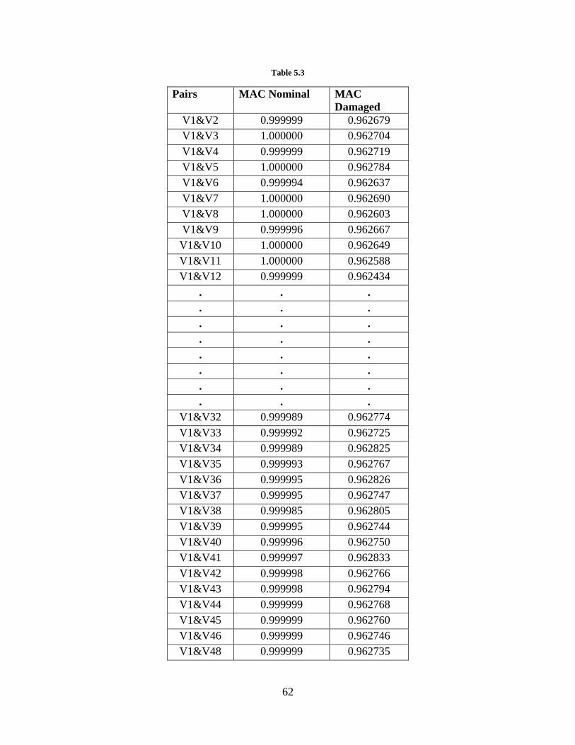
62
Table 5.3
Pairs MAC Nominal MAC
Damaged
V1&V2 0.999999 0.962679
V1&V3 1.000000 0.962704
V1&V4 0.999999 0.962719
V1&V5 1.000000 0.962784
V1&V6 0.999994 0.962637
V1&V7 1.000000 0.962690
V1&V8 1.000000 0.962603
V1&V9 0.999996 0.962667
V1&V10 1.000000 0.962649
V1&V11 1.000000 0.962588
V1&V12 0.999999 0.962434
. . .
. . .
. . .
. . .
. . .
. . .
. . .
. . .
V1&V32 0.999989 0.962774
V1&V33 0.999992 0.962725
V1&V34 0.999989 0.962825
V1&V35 0.999993 0.962767
V1&V36 0.999995 0.962826
V1&V37 0.999995 0.962747
V1&V38 0.999985 0.962805
V1&V39 0.999995 0.962744
V1&V40 0.999996 0.962750
V1&V41 0.999997 0.962833
V1&V42 0.999998 0.962766
V1&V43 0.999998 0.962794
V1&V44 0.999999 0.962768
V1&V45 0.999999 0.962760
V1&V46 0.999999 0.962746
V1&V48 0.999999 0.962735
63
The second column shows the MAC values when sensor L11L12LBET was recording data and
the third column shows the MAC values when the value for this sensor was set to 1500. The
range of MAC values obtained under nominal operating condition was between 0.999999 and
0.999901, whereas for damaged case it was between 0.962833 and 0.961657. For undamaged
case the change in MAC values is at the 5th
decimal place over an entire day. So, the system can
be calibrated based on this observation: that if the MAC value changes beyond the 5th
or 6th
decimal place, it is likely to be in a healthy condition. For damage however the change in MAC
is at the 2nd
decimal place, which is easy to spot. As mentioned before, the previous tables and
the values are shown to give an idea of how the process will work. The value of 1500 was taken
arbitrarily to depict that a fault has happened. This data was taken as it was received without any
processing or taking out the noise effect.
5.3 Brute Force Optimization
The number of sensors to be used was one of the biggest challenges of this research. The brute
force method takes into consideration every ‘n’ possible combinations from a particular set of ‘k’
actions (i.e. an ‘nchoosek’ problem). Just to give an idea of the size of the problem, consider
starting with 32 actions. To choose k sensors out of n given possibilities, the following formula
was used:
)!()!(
!
kkn
n
k
n
(5.1)
In this case n = 32 and for k = 28, the following number of combinations will have to be
considered:
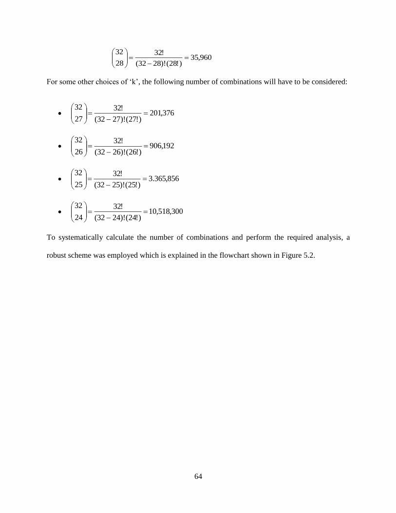
64
960,35)!28()!2832(
!32
28
32
For some other choices of ‘k’, the following number of combinations will have to be considered:
376,201)!27()!2732(
!32
27
32
192,906)!26()!2632(
!32
26
32
856,365.3)!25()!2532(
!32
25
32
300,518,10)!24()!2432(
!32
24
32
To systematically calculate the number of combinations and perform the required analysis, a
robust scheme was employed which is explained in the flowchart shown in Figure 5.2.
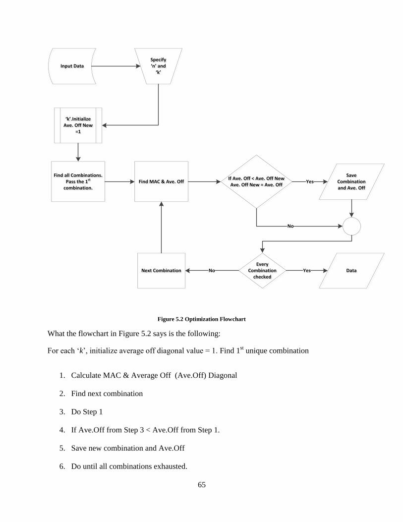
65
Input DataInput DataSpecify ‘n’ and
‘k’
Specify ‘n’ and
‘k’
‘k’.Initialize Ave. Off New
=1
‘k’.Initialize Ave. Off New
=1
Find all Combinations. Pass the 1st
combination.
Find all Combinations. Pass the 1st
combination.Find MAC & Ave. OffFind MAC & Ave. Off If Ave. Off < Ave. Off New
Ave. Off New = Ave. Off
If Ave. Off < Ave. Off NewAve. Off New = Ave. Off
Save Combination and Ave. Off
Save Combination and Ave. Off
Yes
No
Every Combination
checked
Every Combination
checkedData Data YesNext CombinationNext Combination No
Figure 5.2 Optimization Flowchart
What the flowchart in Figure 5.2 says is the following:
For each ‘k’, initialize average off diagonal value = 1. Find 1st unique combination
1. Calculate MAC & Average Off (Ave.Off) Diagonal
2. Find next combination
3. Do Step 1
4. If Ave.Off from Step 3 < Ave.Off from Step 1.
5. Save new combination and Ave.Off
6. Do until all combinations exhausted.

66
7. Output top 10 least Ave.Off and combinations.
5.3.1 Roadblocks
Since the brute force method calculates all possible combinations, as the number of combinations
increased, so did the computational complexity. The method to find all the combinations was
done in MATLAB which uses a built in function. This function stored all the combinations of a
particular set at once and then the rest of the calculation was carried out. Since all the
combinations were first saved for large combinations, the computers ran out of memory. To
resolve this problem a recursive code was written that takes into consideration only one
combination at a time before calculating the next combination. Figure 5.3 illustrates the edited
process flowchart.
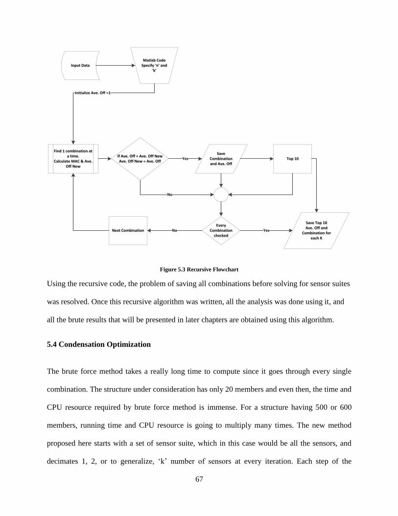
67
Input DataInput DataMatlab Code
Specify ‘n’ and ‘k’
Matlab CodeSpecify ‘n’ and
‘k’
Find 1 combination at a time.
Calculate MAC & Ave. Off New
Find 1 combination at a time.
Calculate MAC & Ave. Off New
Initialize Ave. Off =1
If Ave. Off < Ave. Off NewAve. Off New = Ave. Off
If Ave. Off < Ave. Off NewAve. Off New = Ave. Off
Save Combination and Ave. Off
Save Combination and Ave. Off
Yes
No
Every Combination
checked
Every Combination
checked
Save Top 10 Ave. Off and
Combination for each K
Save Top 10 Ave. Off and
Combination for each K
YesNext CombinationNext Combination No
Top 10Top 10
Figure 5.3 Recursive Flowchart
Using the recursive code, the problem of saving all combinations before solving for sensor suites
was resolved. Once this recursive algorithm was written, all the analysis was done using it, and
all the brute results that will be presented in later chapters are obtained using this algorithm.
5.4 Condensation Optimization
The brute force method takes a really long time to compute since it goes through every single
combination. The structure under consideration has only 20 members and even then, the time and
CPU resource required by brute force method is immense. For a structure having 500 or 600
members, running time and CPU resource is going to multiply many times. The new method
proposed here starts with a set of sensor suite, which in this case would be all the sensors, and
decimates 1, 2, or to generalize, ‘k’ number of sensors at every iteration. Each step of the
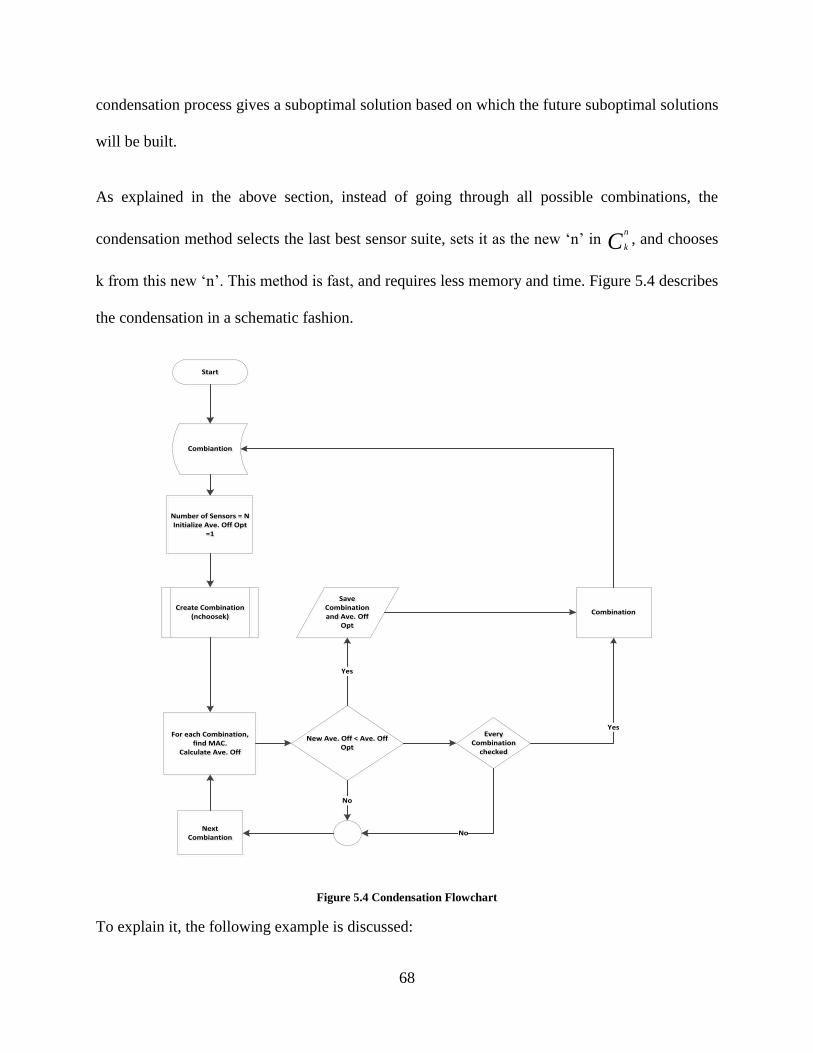
68
condensation process gives a suboptimal solution based on which the future suboptimal solutions
will be built.
As explained in the above section, instead of going through all possible combinations, the
condensation method selects the last best sensor suite, sets it as the new ‘n’ in Cn
k, and chooses
k from this new ‘n’. This method is fast, and requires less memory and time. Figure 5.4 describes
the condensation in a schematic fashion.
CombiantionCombiantion
Create Combination(nchoosek)
Create Combination(nchoosek)
New Ave. Off < Ave. Off Opt
New Ave. Off < Ave. Off Opt
Save Combination and Ave. Off
Opt
Save Combination and Ave. Off
Opt
Every Combination
checked
Every Combination
checked
For each Combination, find MAC.
Calculate Ave. Off
For each Combination, find MAC.
Calculate Ave. Off
CombinationCombination
StartStart
Number of Sensors = NInitialize Ave. Off Opt
=1
Number of Sensors = NInitialize Ave. Off Opt
=1
Yes
No
Next Combiantion
Next Combiantion
No
Yes
Figure 5.4 Condensation Flowchart
To explain it, the following example is discussed:

69
Starting with 48 actions, Number of Sensors N=48. Length of Input vector for combination=48.
1. Choose best 47 sensor based on least Ave.off MAC value.
2. New length of Input Vector =47, choose 46. Where the new 47 are the best sensor
location obtained from 1.
3. New length of Input Vector =46, choose 45. Where the new 46 are the best sensor
location obtained from 2.
and so on until the desired number of sensors are reached.
The results (i.e. Ave. off diagonal values) from this approach were exactly equal to some of the
sensor choices made by the brute force, while very close to the brute force approach for some
other as shown in Tables 5.4 and 5.5 respectively.
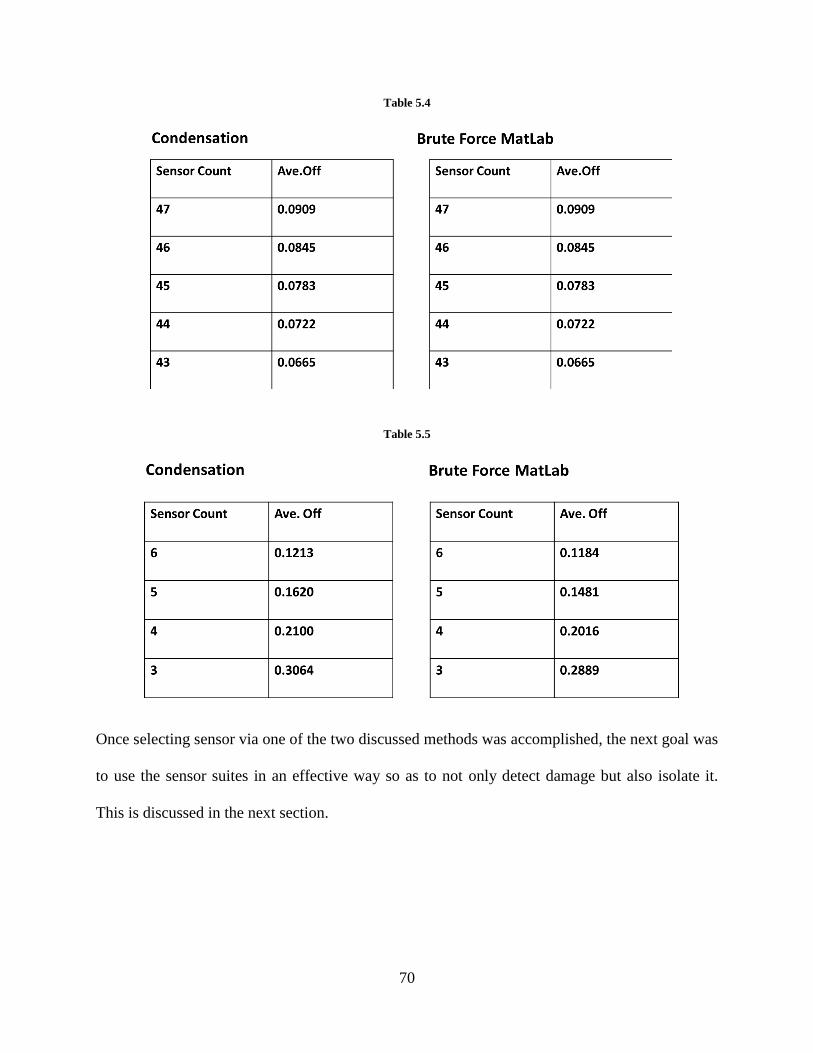
70
Table 5.4
Table 5.5
Once selecting sensor via one of the two discussed methods was accomplished, the next goal was
to use the sensor suites in an effective way so as to not only detect damage but also isolate it.
This is discussed in the next section.
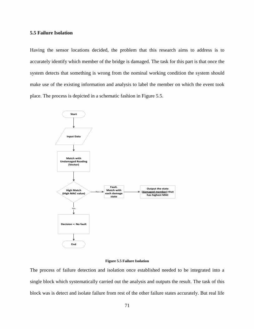
71
5.5 Failure Isolation
Having the sensor locations decided, the problem that this research aims to address is to
accurately identify which member of the bridge is damaged. The task for this part is that once the
system detects that something is wrong from the nominal working condition the system should
make use of the existing information and analysis to label the member on which the event took
place. The process is depicted in a schematic fashion in Figure 5.5.
Input DataInput Data
Match with Undamaged Reading
(Vector)
Match with Undamaged Reading
(Vector)
High Match(High MAC value)
High Match(High MAC value)
Decision =: No faultDecision =: No fault
Fault. Match with
each damage state
Fault. Match with
each damage state
StartStart
EndEnd
Yes
NoOutput the state
(damaged member) that has highest MAC
Output the state (damaged member) that
has highest MAC
Figure 5.5 Failure Isolation
The process of failure detection and isolation once established needed to be integrated into a
single block which systematically carried out the analysis and outputs the result. The task of this
block was is detect and isolate failure from rest of the other failure states accurately. But real life
72
data comes buried in noise and hence, careful consideration was taken to accommodate the noise
factor to make the system robust and practical. This gave rise to a virtual machine developed by
Dr. James Swanson of the School of Advanced Structure at University of Cincinnati, discussed
in the following section.
5.6 Virtual Machine
The aim of the Virtual Machine (VM) is to assist the system which this research is trying to build
by establishing the effectiveness of the sensor suites generated by the two sensor selection
method.
5.6.1 Failure Detection and Isolation
The two processes are so closely connected that the success of one greatly depends on the
success of the other. Given an unknown data, the holistic approach strives to achieve the
following goals:
Flag No Failure – If the unknown data matches with the zero or nominal data.
Failure Detection – If the unknown data does not matches with the nominal vector.
Missed Detection – Damaged data classified as undamaged.
False Detection – Undamaged data classified as any of the damaged states.
Failure Isolation – In case of failure, correct member picked which is damaged.
False Isolation – Failure detected but wrong member picked.
Do not Flag False Alarm – Input Member (data) = Undamaged Member (data) but,
Output (Decision) =Damage (Fault).
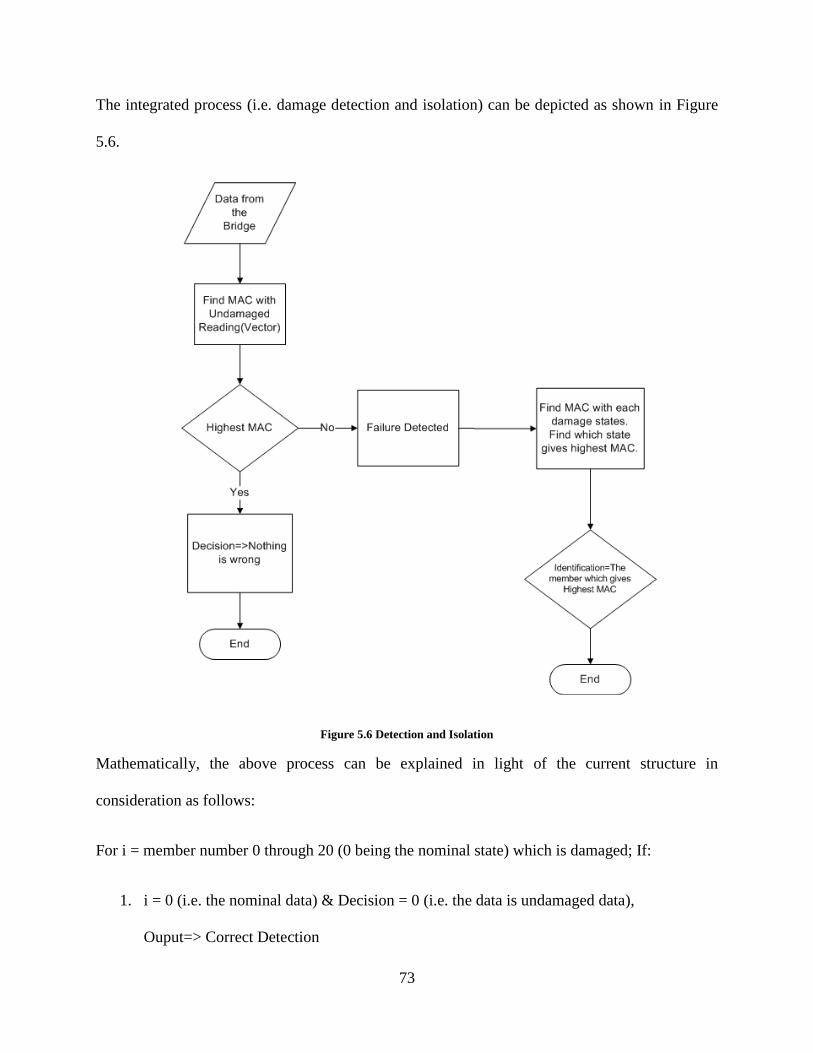
73
The integrated process (i.e. damage detection and isolation) can be depicted as shown in Figure
5.6.
Figure 5.6 Detection and Isolation
Mathematically, the above process can be explained in light of the current structure in
consideration as follows:
For i = member number 0 through 20 (0 being the nominal state) which is damaged; If:
1. i = 0 (i.e. the nominal data) & Decision = 0 (i.e. the data is undamaged data),
Ouput=> Correct Detection
74
2. i > 0 (i.e. one of the members is damaged) & Decision = 0 (i.e. the data is undamaged
data ), Output => Missed Detection
3. i = 0 (i.e. the nominal data) & Decision ≠ 0 (i.e. ‘a’ damage exists),
Output => False Alarm
4. i > 0 (i.e. one of the members is damaged) & Decision > 0 (i.e. ‘a’ damage exists), &
Decision Member ≠ (i.e. wrong member flagged as damaged),
Output => False Isolation
5. i > 0 (i.e. one of the members is damaged) & Decision > 0 (i.e. ‘a’ damage exists), &
Decision Member = i, (i.e. correct member flagged as damaged),
Output => Correct Isolation
5.6.2 Adding Noise
As mentioned earlier, it is very important to take into consideration the effect of noise in order to
make the system practical in sense. To do that, noise was added in the VM by taking data from
an actual bridge, Jeremiah Morrow, which is a continuous truss bridge on the Little Miami
River gorge between Fort Ancient and Oregonia, Ohio. This bridge is instrumented and is under
continuous monitoring by the research group at University of Cincinnati Infrastructure Institute.
Randomly, one sensor was selected and six months of data was collected. 8726 values from the
sensor were obtained. This data obtained includes the electronic, as well as temperature noise.
No special processing was done to remove temperature or electronic noise as the aim was first to
test how well the system performs if the data fed to it contained some amount of any noise. The
following steps were followed in adding noise to the VM:
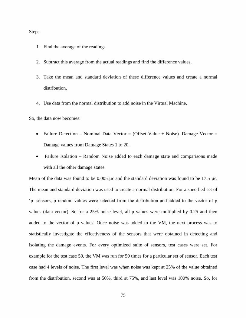
75
Steps
1. Find the average of the readings.
2. Subtract this average from the actual readings and find the difference values.
3. Take the mean and standard deviation of these difference values and create a normal
distribution.
4. Use data from the normal distribution to add noise in the Virtual Machine.
So, the data now becomes:
Failure Detection – Nominal Data Vector = (Offset Value + Noise). Damage Vector =
Damage values from Damage States 1 to 20.
Failure Isolation – Random Noise added to each damage state and comparisons made
with all the other damage states.
Mean of the data was found to be 0.005 µϵ and the standard deviation was found to be 17.5 µϵ.
The mean and standard deviation was used to create a normal distribution. For a specified set of
‘p’ sensors, p random values were selected from the distribution and added to the vector of p
values (data vector). So for a 25% noise level, all p values were multiplied by 0.25 and then
added to the vector of p values. Once noise was added to the VM, the next process was to
statistically investigate the effectiveness of the sensors that were obtained in detecting and
isolating the damage events. For every optimized suite of sensors, test cases were set. For
example for the test case 50, the VM was run for 50 times for a particular set of sensor. Each test
case had 4 levels of noise. The first level was when noise was kept at 25% of the value obtained
from the distribution, second was at 50%, third at 75%, and last level was 100% noise. So, for
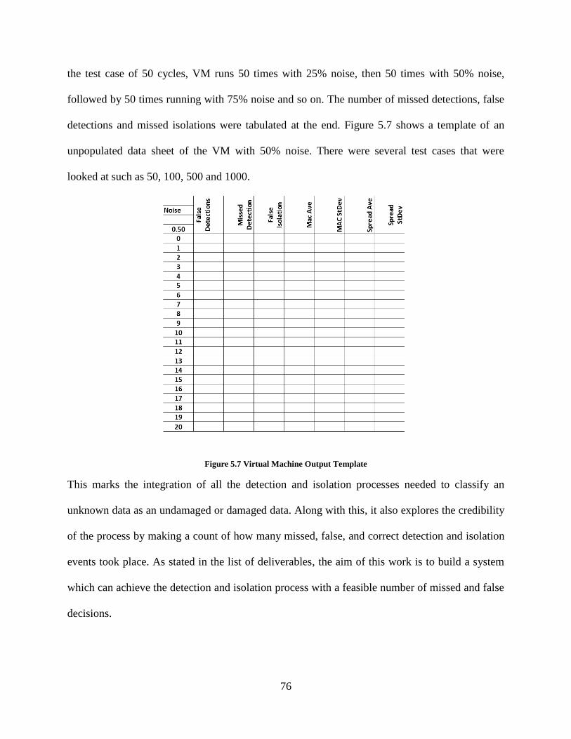
76
the test case of 50 cycles, VM runs 50 times with 25% noise, then 50 times with 50% noise,
followed by 50 times running with 75% noise and so on. The number of missed detections, false
detections and missed isolations were tabulated at the end. Figure 5.7 shows a template of an
unpopulated data sheet of the VM with 50% noise. There were several test cases that were
looked at such as 50, 100, 500 and 1000.
Figure 5.7 Virtual Machine Output Template
This marks the integration of all the detection and isolation processes needed to classify an
unknown data as an undamaged or damaged data. Along with this, it also explores the credibility
of the process by making a count of how many missed, false, and correct detection and isolation
events took place. As stated in the list of deliverables, the aim of this work is to build a system
which can achieve the detection and isolation process with a feasible number of missed and false
decisions.

77
Chapter 6: Results – System Design
This chapter starts with the presentation and discussion of the initial results obtained from the
MAC analysis which builds up the system design. The initial results are presented as a
foundation for the results obtained when the three parts viz., system design, damage detection,
and damage isolation are used as one system. The results in the sections to follow talk about
reducing the problem size before moving to false detection and isolation. Reducing the problem
size can be divided into the following categories.
Physical Basis
Strategic Action Selection (Using Max Moments)
Reduced Member Instrumentation (Removing Non-Redundant Members)
Algorithmic
Brute Force
Condensation
Precipitation ( explained in future work chapter)
The results presented in later sections will specify which of the above mentioned method were
used to reduce the problem size.
6.1 Bubble Charts
The analysis presented in this section will give an overview of how the MAC values are plotted
for choices of sensor suites. Figure 6.1 shows the very first result that was found when the data
from each damaged state was just taken as absolute values of axial forces(F), bending moment
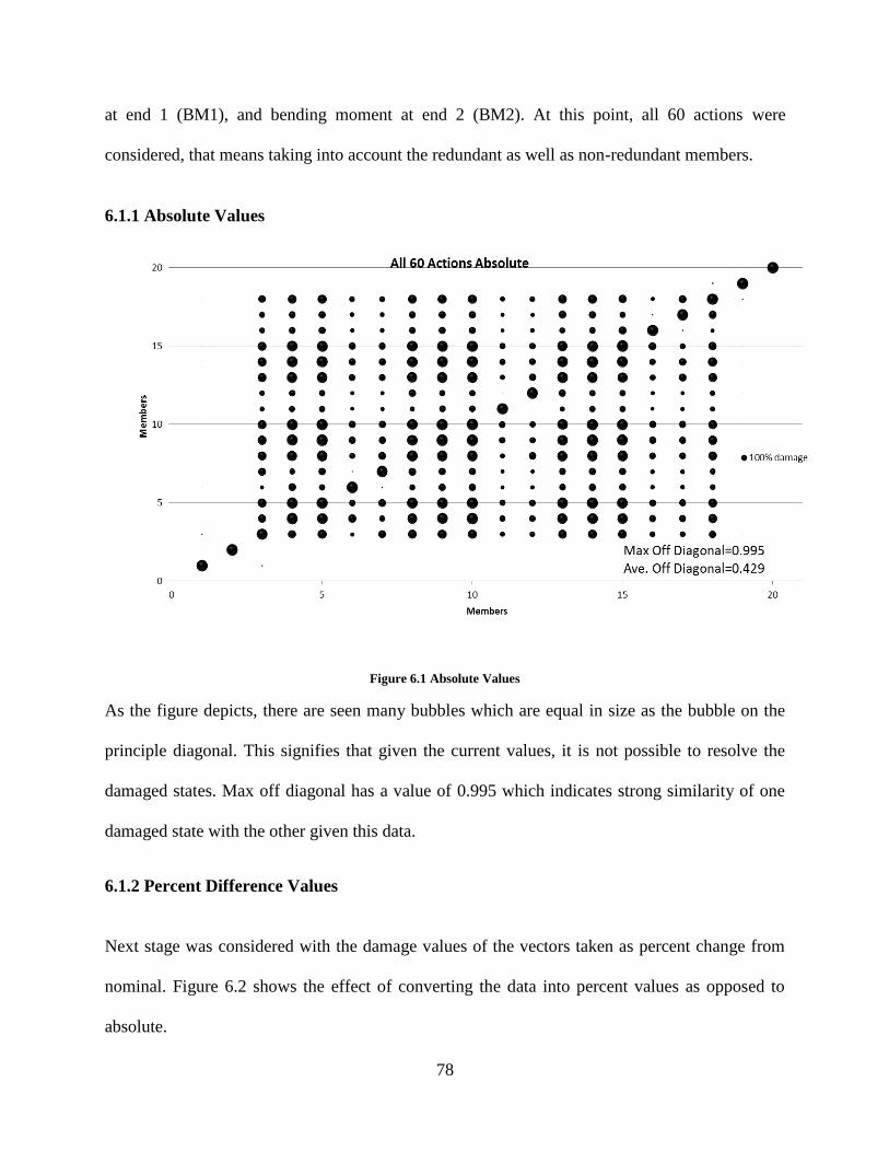
78
at end 1 (BM1), and bending moment at end 2 (BM2). At this point, all 60 actions were
considered, that means taking into account the redundant as well as non-redundant members.
6.1.1 Absolute Values
Figure 6.1 Absolute Values
As the figure depicts, there are seen many bubbles which are equal in size as the bubble on the
principle diagonal. This signifies that given the current values, it is not possible to resolve the
damaged states. Max off diagonal has a value of 0.995 which indicates strong similarity of one
damaged state with the other given this data.
6.1.2 Percent Difference Values
Next stage was considered with the damage values of the vectors taken as percent change from
nominal. Figure 6.2 shows the effect of converting the data into percent values as opposed to
absolute.
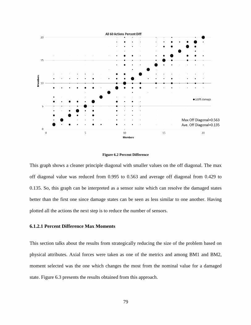
79
Figure 6.2 Percent Difference
This graph shows a cleaner principle diagonal with smaller values on the off diagonal. The max
off diagonal value was reduced from 0.995 to 0.563 and average off diagonal from 0.429 to
0.135. So, this graph can be interpreted as a sensor suite which can resolve the damaged states
better than the first one since damage states can be seen as less similar to one another. Having
plotted all the actions the next step is to reduce the number of sensors.
6.1.2.1 Percent Difference Max Moments
This section talks about the results from strategically reducing the size of the problem based on
physical attributes. Axial forces were taken as one of the metrics and among BM1 and BM2,
moment selected was the one which changes the most from the nominal value for a damaged
state. Figure 6.3 presents the results obtained from this approach.
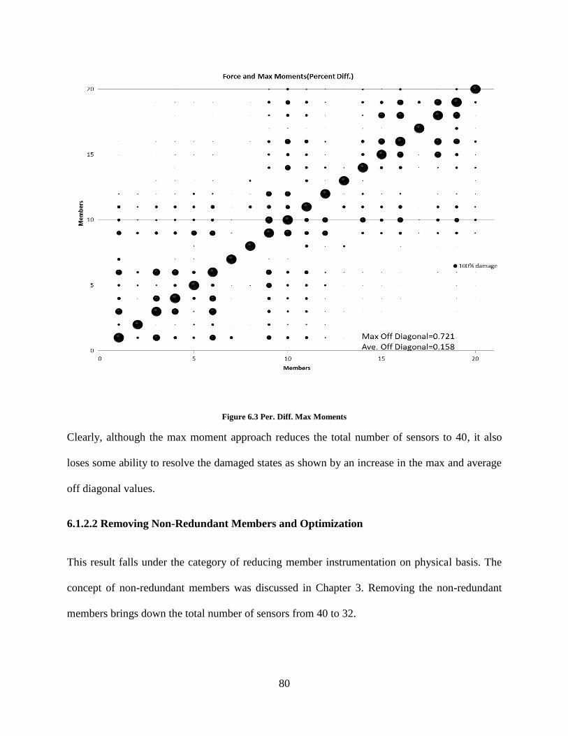
80
Figure 6.3 Per. Diff. Max Moments
Clearly, although the max moment approach reduces the total number of sensors to 40, it also
loses some ability to resolve the damaged states as shown by an increase in the max and average
off diagonal values.
6.1.2.2 Removing Non-Redundant Members and Optimization
This result falls under the category of reducing member instrumentation on physical basis. The
concept of non-redundant members was discussed in Chapter 3. Removing the non-redundant
members brings down the total number of sensors from 40 to 32.
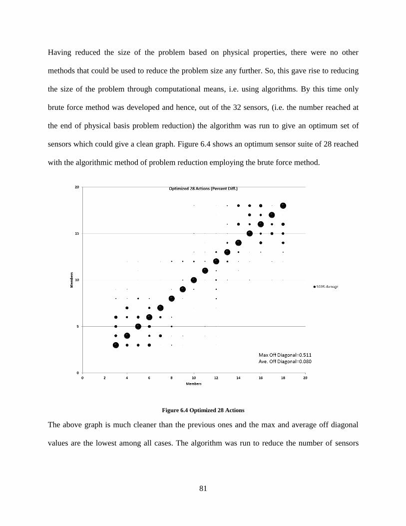
81
Having reduced the size of the problem based on physical properties, there were no other
methods that could be used to reduce the problem size any further. So, this gave rise to reducing
the size of the problem through computational means, i.e. using algorithms. By this time only
brute force method was developed and hence, out of the 32 sensors, (i.e. the number reached at
the end of physical basis problem reduction) the algorithm was run to give an optimum set of
sensors which could give a clean graph. Figure 6.4 shows an optimum sensor suite of 28 reached
with the algorithmic method of problem reduction employing the brute force method.
Figure 6.4 Optimized 28 Actions
The above graph is much cleaner than the previous ones and the max and average off diagonal
values are the lowest among all cases. The algorithm was run to reduce the number of sensors
82
further but the number of combination beyond this stage were far too many for the computers to
process. This led the machines to run out of memory resources and not produce any more results.
So, percent difference definitely provides better results than absolute values and is a good choice
to be used as a data source. There is however one issue with this approach. Theoretically it gives
great results but the problem with this approach is that even a small change from nominal will be
magnified and will come out as a major change when it may be a value which is below the
resolution of the instrumentation or sensors. For example if the nominal value of the gage reads
1.50 µϵ and the new value reads 1.00 µϵ, the change in percent is 33, but the value of 0.50 µϵ
may not get recorded. Although ideally it may be a good metric to consider, practically it may
run into sensor resolution and signal processing issue. So the analysis was shifted to consider
relative values.
6.1.3 Relative Value
The concept of relative values was discussed in Chapter 4. Figure 6.5 shows initial results
obtained from this approach. This graph takes into account all 60 actions to start.
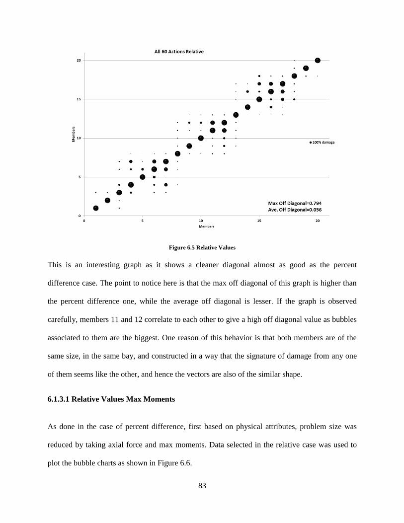
83
Figure 6.5 Relative Values
This is an interesting graph as it shows a cleaner diagonal almost as good as the percent
difference case. The point to notice here is that the max off diagonal of this graph is higher than
the percent difference one, while the average off diagonal is lesser. If the graph is observed
carefully, members 11 and 12 correlate to each other to give a high off diagonal value as bubbles
associated to them are the biggest. One reason of this behavior is that both members are of the
same size, in the same bay, and constructed in a way that the signature of damage from any one
of them seems like the other, and hence the vectors are also of the similar shape.
6.1.3.1 Relative Values Max Moments
As done in the case of percent difference, first based on physical attributes, problem size was
reduced by taking axial force and max moments. Data selected in the relative case was used to
plot the bubble charts as shown in Figure 6.6.
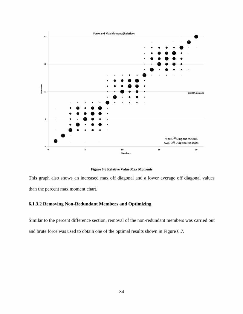
84
Figure 6.6 Relative Value Max Moments
This graph also shows an increased max off diagonal and a lower average off diagonal values
than the percent max moment chart.
6.1.3.2 Removing Non-Redundant Members and Optimizing
Similar to the percent difference section, removal of the non-redundant members was carried out
and brute force was used to obtain one of the optimal results shown in Figure 6.7.
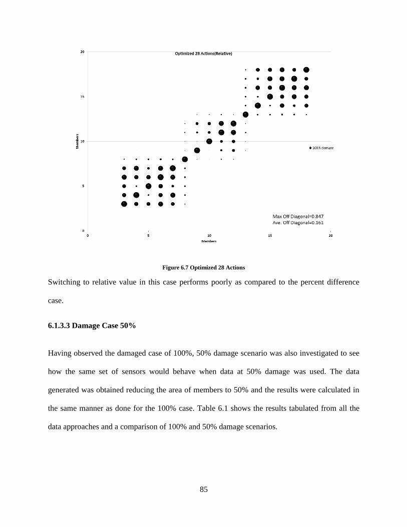
85
Figure 6.7 Optimized 28 Actions
Switching to relative value in this case performs poorly as compared to the percent difference
case.
6.1.3.3 Damage Case 50%
Having observed the damaged case of 100%, 50% damage scenario was also investigated to see
how the same set of sensors would behave when data at 50% damage was used. The data
generated was obtained reducing the area of members to 50% and the results were calculated in
the same manner as done for the 100% case. Table 6.1 shows the results tabulated from all the
data approaches and a comparison of 100% and 50% damage scenarios.
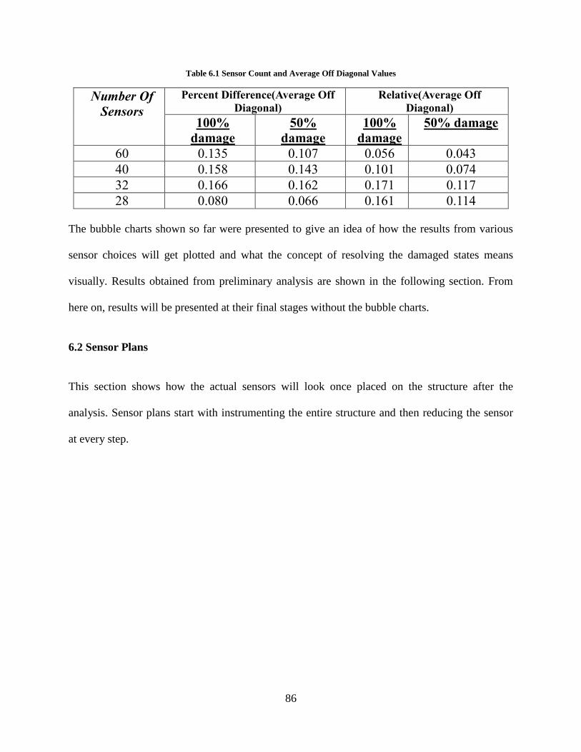
86
Table 6.1 Sensor Count and Average Off Diagonal Values
Number Of
Sensors
Percent Difference(Average Off
Diagonal)
Relative(Average Off
Diagonal)
100%
damage
50%
damage
100%
damage
50% damage
60 0.135 0.107 0.056 0.043
40 0.158 0.143 0.101 0.074
32 0.166 0.162 0.171 0.117
28 0.080 0.066 0.161 0.114
The bubble charts shown so far were presented to give an idea of how the results from various
sensor choices will get plotted and what the concept of resolving the damaged states means
visually. Results obtained from preliminary analysis are shown in the following section. From
here on, results will be presented at their final stages without the bubble charts.
6.2 Sensor Plans
This section shows how the actual sensors will look once placed on the structure after the
analysis. Sensor plans start with instrumenting the entire structure and then reducing the sensor
at every step.
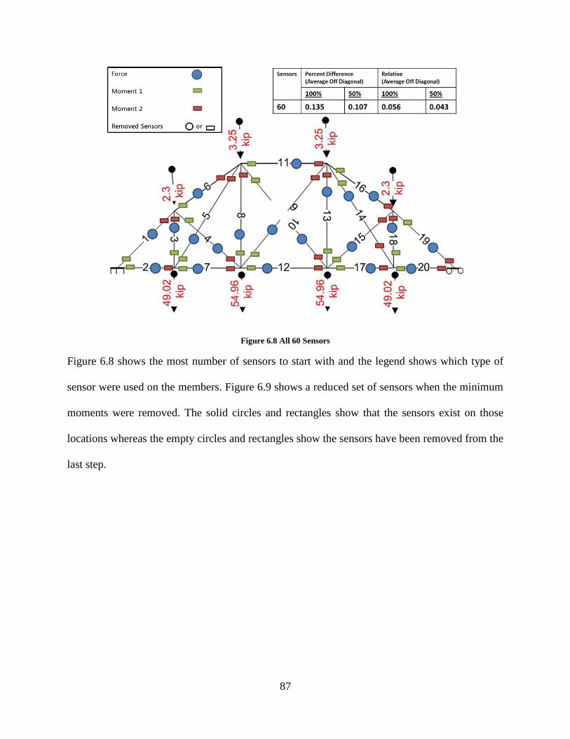
87
Figure 6.8 All 60 Sensors
Figure 6.8 shows the most number of sensors to start with and the legend shows which type of
sensor were used on the members. Figure 6.9 shows a reduced set of sensors when the minimum
moments were removed. The solid circles and rectangles show that the sensors exist on those
locations whereas the empty circles and rectangles show the sensors have been removed from the
last step.
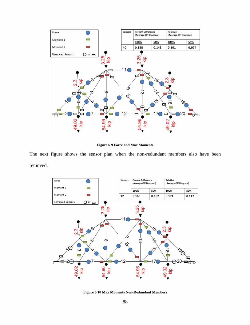
88
Figure 6.9 Force and Max Moments
The next figure shows the sensor plan when the non-redundant members also have been
removed.
Figure 6.10 Max Moments Non-Redundant Members
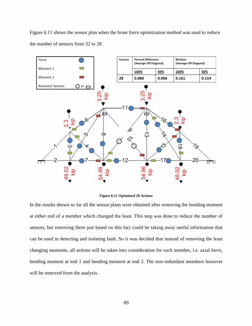
89
Figure 6.11 shows the sensor plan when the brute force optimization method was used to reduce
the number of sensors from 32 to 28.
Figure 6.11 Optimized 28 Actions
In the results shown so far all the sensor plans were obtained after removing the bending moment
at either end of a member which changed the least. This step was done to reduce the number of
sensors, but removing them just based on this fact could be taking away useful information that
can be used in detecting and isolating fault. So it was decided that instead of removing the least
changing moments, all actions will be taken into consideration for each member, i.e. axial force,
bending moment at end 1 and bending moment at end 2. The non-redundant members however
will be removed from the analysis.
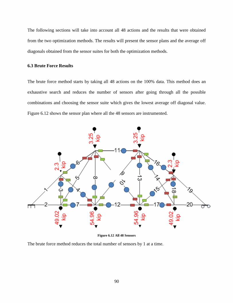
90
The following sections will take into account all 48 actions and the results that were obtained
from the two optimization methods. The results will present the sensor plans and the average off
diagonals obtained from the sensor suites for both the optimization methods.
6.3 Brute Force Results
The brute force method starts by taking all 48 actions on the 100% data. This method does an
exhaustive search and reduces the number of sensors after going through all the possible
combinations and choosing the sensor suite which gives the lowest average off diagonal value.
Figure 6.12 shows the sensor plan where all the 48 sensors are instrumented.
Figure 6.12 All 48 Sensors
The brute force method reduces the total number of sensors by 1 at a time.
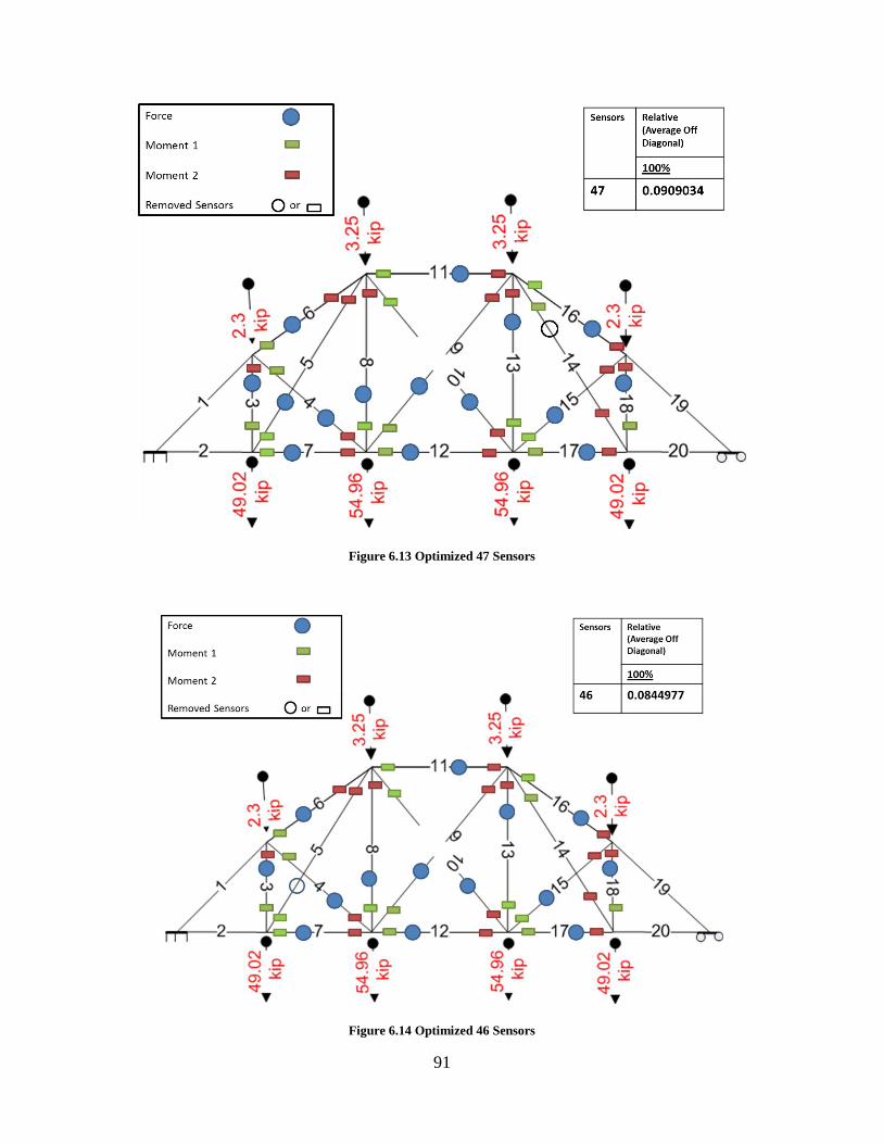
91
Figure 6.13 Optimized 47 Sensors
Figure 6.14 Optimized 46 Sensors
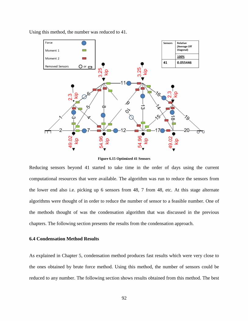
92
Using this method, the number was reduced to 41.
Figure 6.15 Optimized 41 Sensors
Reducing sensors beyond 41 started to take time in the order of days using the current
computational resources that were available. The algorithm was run to reduce the sensors from
the lower end also i.e. picking up 6 sensors from 48, 7 from 48, etc. At this stage alternate
algorithms were thought of in order to reduce the number of sensor to a feasible number. One of
the methods thought of was the condensation algorithm that was discussed in the previous
chapters. The following section presents the results from the condensation approach.
6.4 Condensation Method Results
As explained in Chapter 5, condensation method produces fast results which were very close to
the ones obtained by brute force method. Using this method, the number of sensors could be
reduced to any number. The following section shows results obtained from this method. The best
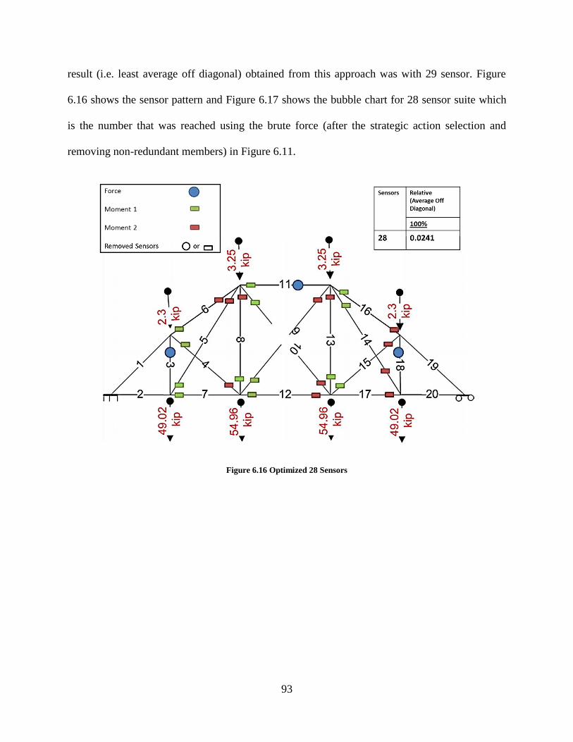
93
result (i.e. least average off diagonal) obtained from this approach was with 29 sensor. Figure
6.16 shows the sensor pattern and Figure 6.17 shows the bubble chart for 28 sensor suite which
is the number that was reached using the brute force (after the strategic action selection and
removing non-redundant members) in Figure 6.11.
Figure 6.16 Optimized 28 Sensors
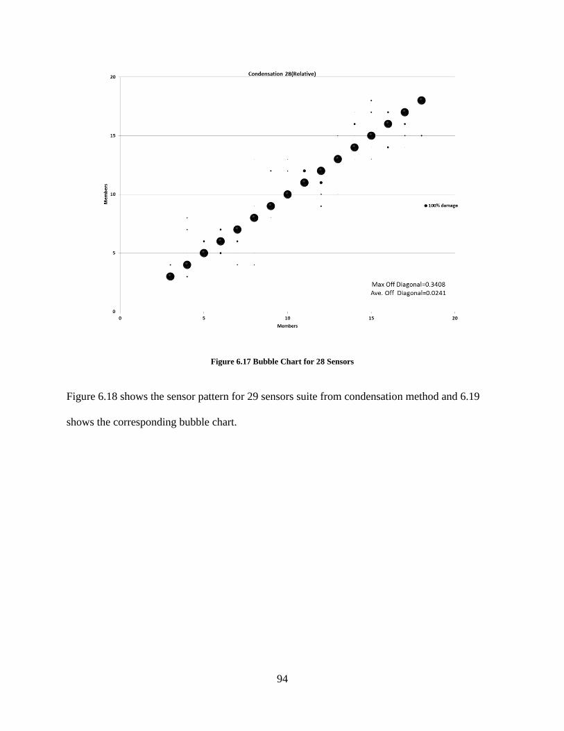
94
Figure 6.17 Bubble Chart for 28 Sensors
Figure 6.18 shows the sensor pattern for 29 sensors suite from condensation method and 6.19
shows the corresponding bubble chart.
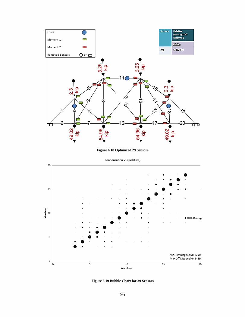
95
Figure 6.18 Optimized 29 Sensors
Figure 6.19 Bubble Chart for 29 Sensors
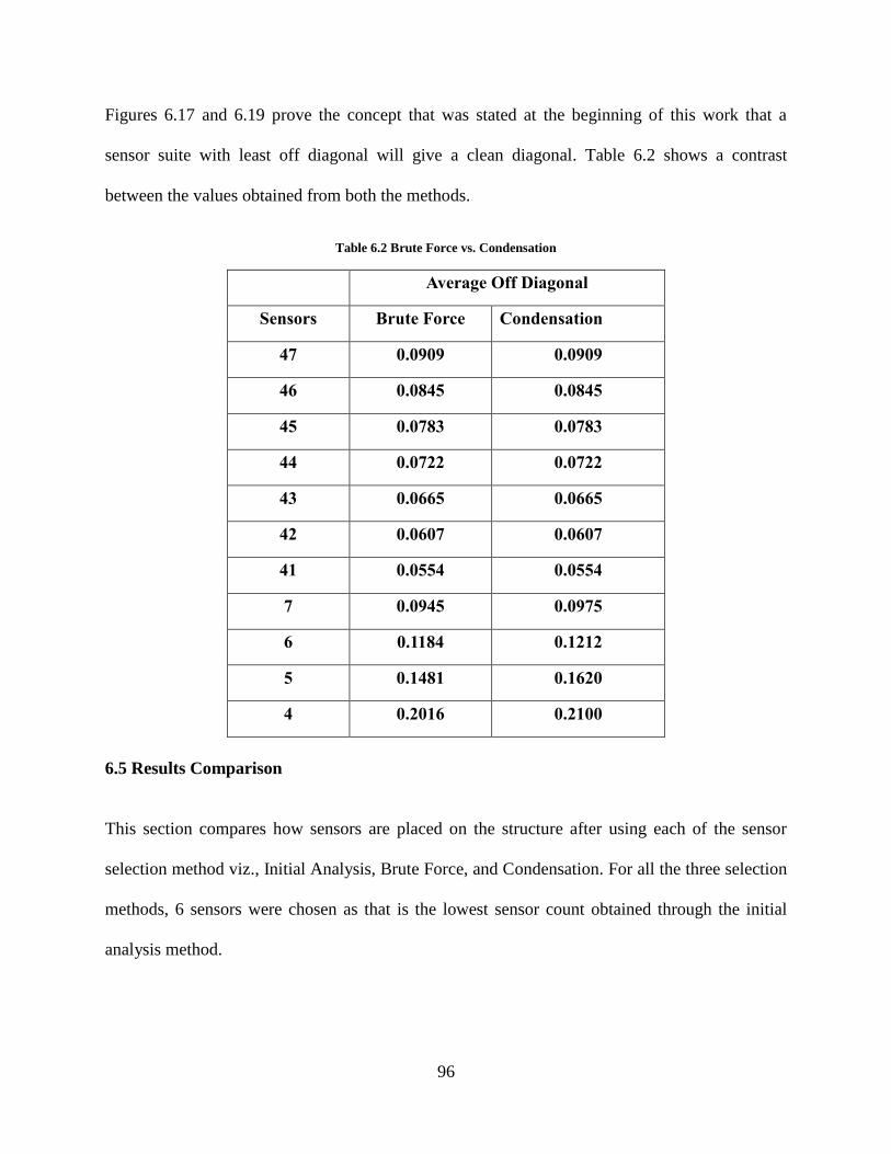
96
Figures 6.17 and 6.19 prove the concept that was stated at the beginning of this work that a
sensor suite with least off diagonal will give a clean diagonal. Table 6.2 shows a contrast
between the values obtained from both the methods.
Table 6.2 Brute Force vs. Condensation
Average Off Diagonal
Sensors Brute Force Condensation
47 0.0909 0.0909
46 0.0845 0.0845
45 0.0783 0.0783
44 0.0722 0.0722
43 0.0665 0.0665
42 0.0607 0.0607
41 0.0554 0.0554
7 0.0945 0.0975
6 0.1184 0.1212
5 0.1481 0.1620
4 0.2016 0.2100
6.5 Results Comparison
This section compares how sensors are placed on the structure after using each of the sensor
selection method viz., Initial Analysis, Brute Force, and Condensation. For all the three selection
methods, 6 sensors were chosen as that is the lowest sensor count obtained through the initial
analysis method.
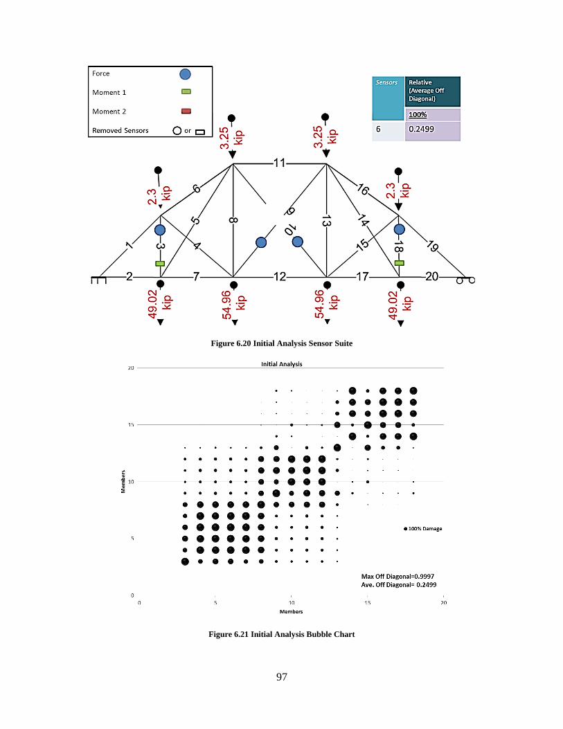
97
Figure 6.20 Initial Analysis Sensor Suite
Figure 6.21 Initial Analysis Bubble Chart
98
Figure 6.22 Brute Force 6 Sensor Suite
Figure 6.23 Bubble Chart Brute Force 6 Sensor Suite
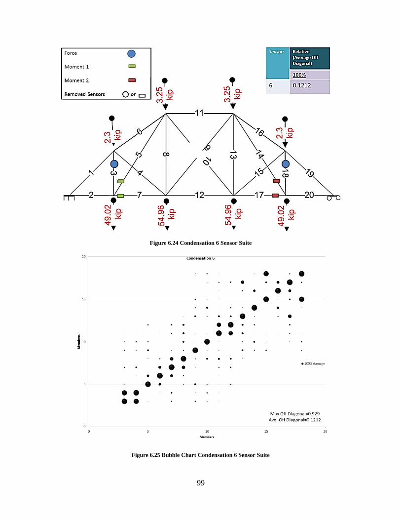
99
Figure 6.24 Condensation 6 Sensor Suite
Figure 6.25 Bubble Chart Condensation 6 Sensor Suite
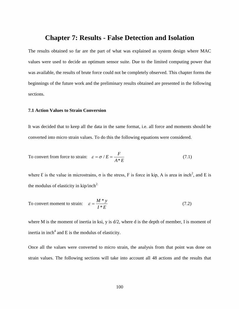
100
Chapter 7: Results - False Detection and Isolation
The results obtained so far are the part of what was explained as system design where MAC
values were used to decide an optimum sensor suite. Due to the limited computing power that
was available, the results of brute force could not be completely observed. This chapter forms the
beginnings of the future work and the preliminary results obtained are presented in the following
sections.
7.1 Action Values to Strain Conversion
It was decided that to keep all the data in the same format, i.e. all force and moments should be
converted into micro strain values. To do this the following equations were considered.
To convert from force to strain: EA
FE
*/ (7.1)
where Ɛ is the value in microstrains, σ is the stress, F is force in kip, A is area in inch2, and E is
the modulus of elasticity in kip/inch2.
To convert moment to strain: EI
yM
*
* (7.2)
where M is the moment of inertia in ksi, y is d/2, where d is the depth of member, I is moment of
inertia in inch4 and E is the modulus of elasticity.
Once all the values were converted to micro strain, the analysis from that point was done on
strain values. The following sections will take into account all 48 actions and the results that
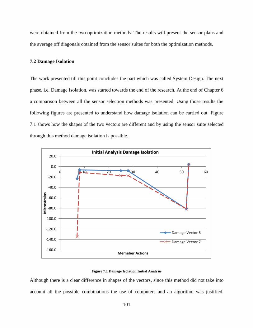
101
were obtained from the two optimization methods. The results will present the sensor plans and
the average off diagonals obtained from the sensor suites for both the optimization methods.
7.2 Damage Isolation
The work presented till this point concludes the part which was called System Design. The next
phase, i.e. Damage Isolation, was started towards the end of the research. At the end of Chapter 6
a comparison between all the sensor selection methods was presented. Using those results the
following figures are presented to understand how damage isolation can be carried out. Figure
7.1 shows how the shapes of the two vectors are different and by using the sensor suite selected
through this method damage isolation is possible.
Figure 7.1 Damage Isolation Initial Analysis
Although there is a clear difference in shapes of the vectors, since this method did not take into
account all the possible combinations the use of computers and an algorithm was justified.
-160.0
-140.0
-120.0
-100.0
-80.0
-60.0
-40.0
-20.0
0.0
20.0
0 10 20 30 40 50 60
Mic
rost
rain
s
Memeber Actions
Initial Analysis Damage Isolation
Damage Vector 6
Damage Vector 7
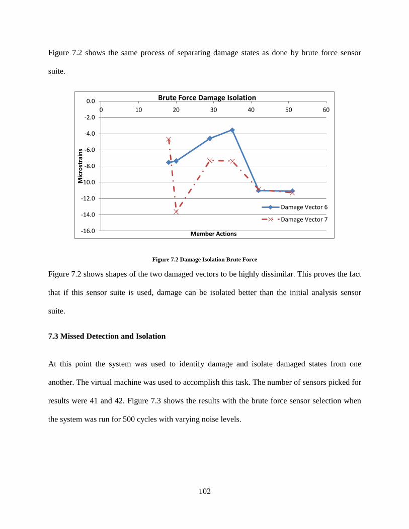
102
Figure 7.2 shows the same process of separating damage states as done by brute force sensor
suite.
Figure 7.2 Damage Isolation Brute Force
Figure 7.2 shows shapes of the two damaged vectors to be highly dissimilar. This proves the fact
that if this sensor suite is used, damage can be isolated better than the initial analysis sensor
suite.
7.3 Missed Detection and Isolation
At this point the system was used to identify damage and isolate damaged states from one
another. The virtual machine was used to accomplish this task. The number of sensors picked for
results were 41 and 42. Figure 7.3 shows the results with the brute force sensor selection when
the system was run for 500 cycles with varying noise levels.
-16.0
-14.0
-12.0
-10.0
-8.0
-6.0
-4.0
-2.0
0.0
0 10 20 30 40 50 60
Mic
rost
rain
s
Member Actions
Brute Force Damage Isolation
Damage Vector 6
Damage Vector 7
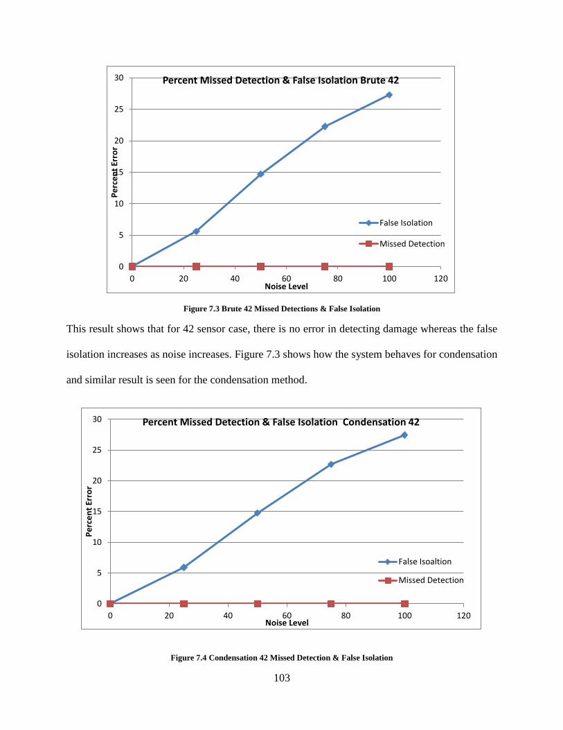
103
Figure 7.3 Brute 42 Missed Detections & False Isolation
This result shows that for 42 sensor case, there is no error in detecting damage whereas the false
isolation increases as noise increases. Figure 7.3 shows how the system behaves for condensation
and similar result is seen for the condensation method.
Figure 7.4 Condensation 42 Missed Detection & False Isolation
0
5
10
15
20
25
30
0 20 40 60 80 100 120
Pe
rce
nt
Erro
r
Noise Level
Percent Missed Detection & False Isolation Brute 42
False Isolation
Missed Detection
0
5
10
15
20
25
30
0 20 40 60 80 100 120
Pe
rce
nt
Erro
r
Noise Level
Percent Missed Detection & False Isolation Condensation 42
False Isoaltion
Missed Detection
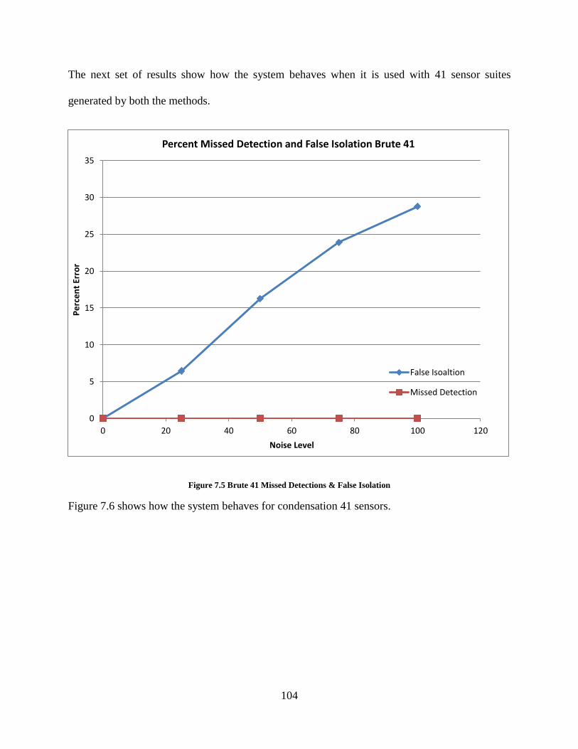
104
The next set of results show how the system behaves when it is used with 41 sensor suites
generated by both the methods.
Figure 7.5 Brute 41 Missed Detections & False Isolation
Figure 7.6 shows how the system behaves for condensation 41 sensors.
0
5
10
15
20
25
30
35
0 20 40 60 80 100 120
Pe
rce
nt
Erro
r
Noise Level
Percent Missed Detection and False Isolation Brute 41
False Isoaltion
Missed Detection
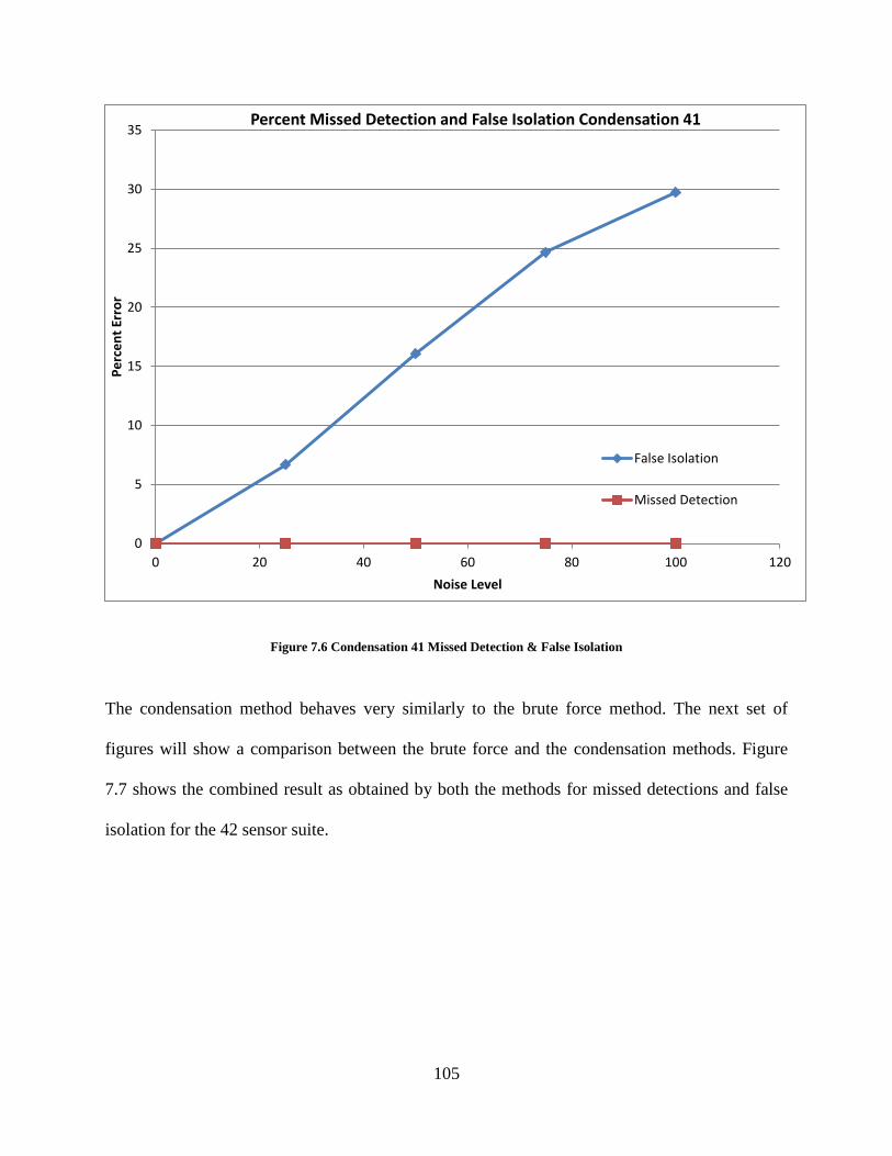
105
Figure 7.6 Condensation 41 Missed Detection & False Isolation
The condensation method behaves very similarly to the brute force method. The next set of
figures will show a comparison between the brute force and the condensation methods. Figure
7.7 shows the combined result as obtained by both the methods for missed detections and false
isolation for the 42 sensor suite.
0
5
10
15
20
25
30
35
0 20 40 60 80 100 120
Pe
rce
nt
Erro
r
Noise Level
Percent Missed Detection and False Isolation Condensation 41
False Isolation
Missed Detection

106
Figure 7.7 Brute Force vs. Condensation 42 Missed Detections & False Isolation
As shown in Figure 7.7, for 42 sensors, both methods behave perfectly in the case of detecting
damage. In case of false isolation brute force does better than the condensation as noise
increases. Similar results were obtained for the 41 sensor case as shown in Figure 7.8.
0
5
10
15
20
25
30
0 20 40 60 80 100 120
Pe
rce
nt
Erro
r
Noise Level
Percent Missed Detection & False Isolation Brute & Condensation42
False Isolation Brute
Missed Detection Brute
False Isolation Brute
Missed Detection Brute
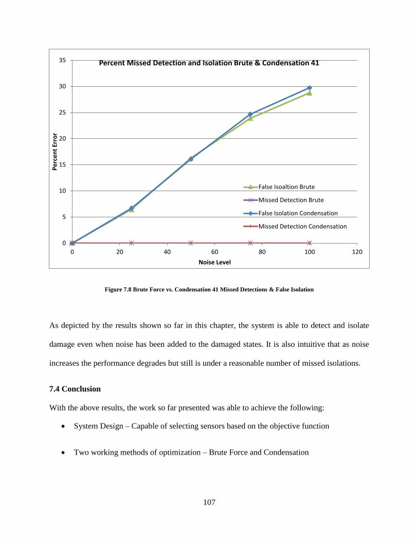
107
Figure 7.8 Brute Force vs. Condensation 41 Missed Detections & False Isolation
As depicted by the results shown so far in this chapter, the system is able to detect and isolate
damage even when noise has been added to the damaged states. It is also intuitive that as noise
increases the performance degrades but still is under a reasonable number of missed isolations.
7.4 Conclusion
With the above results, the work so far presented was able to achieve the following:
System Design – Capable of selecting sensors based on the objective function
Two working methods of optimization – Brute Force and Condensation
0
5
10
15
20
25
30
35
0 20 40 60 80 100 120
Pe
rce
nt
Erro
r
Noise Level
Percent Missed Detection and Isolation Brute & Condensation 41
False Isoaltion Brute
Missed Detection Brute
False Isolation Condensation
Missed Detection Condensation

108
Failure Detection shows promising results – The detection part of the system had zeros
errors.
Failure Isolation process needs more work –Isolation part needs more work to make it
efficient
Need to complete all the results for Brute Force Method

109
Chapter 8: Future Work
This chapter discusses about the problems in the strategies that were discussed in earlier chapter
and proposes solutions for them. As future work, some strategies and methods are discussed that
can be employed to address the problem in a more robust and efficient way.
8.1 Multithreading/Parallel Processing and Speeding Up
As explained in the previous chapters, brute force method requires immense CPU time and
resources to generate all the combinations and carry out MAC calculations. Along with that, part
of research that could not be completed due to the limited computing power available was to
obtain the results for sensor count 40 through 10. This was not possible at the time this work was
carried out because the machines that were employed could not process the immense number of
combinations and the corresponding MAC calculations. The biggest challenge was to calculate
the combination faster. To do this, several ideas were discussed and finally it was decided to
make use of multithreading capacity of the machines and MATLAB. In order to do so, it was
proposed that if somehow the number of combinations could be broken into chunks and each
thread or in case of distributed computing, each machine will calculate 1 chunk and then
contribute to the total number of combinations. This required dividing the calculation of
combinations by specifying the starting points of segments of combinations. The process
considerably reduced the time taken to calculate the combinations and MAC values for the
sensor choices which otherwise was taking a really long time. This method is still in the process
of development. Consider the following discussion and Figure 8.1 to understand the concept
discussed.
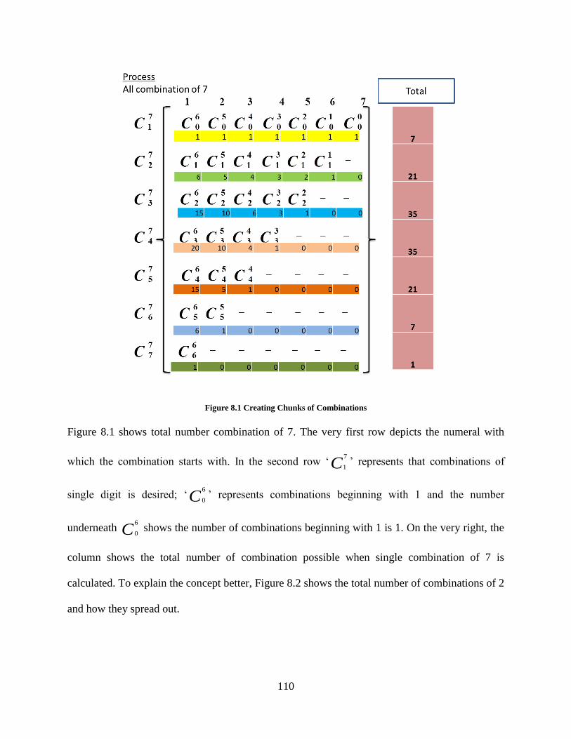
110
Figure 8.1 Creating Chunks of Combinations
Figure 8.1 shows total number combination of 7. The very first row depicts the numeral with
which the combination starts with. In the second row ‘C7
1’ represents that combinations of
single digit is desired; ‘C6
0’ represents combinations beginning with 1 and the number
underneath C6
0 shows the number of combinations beginning with 1 is 1. On the very right, the
column shows the total number of combination possible when single combination of 7 is
calculated. To explain the concept better, Figure 8.2 shows the total number of combinations of 2
and how they spread out.
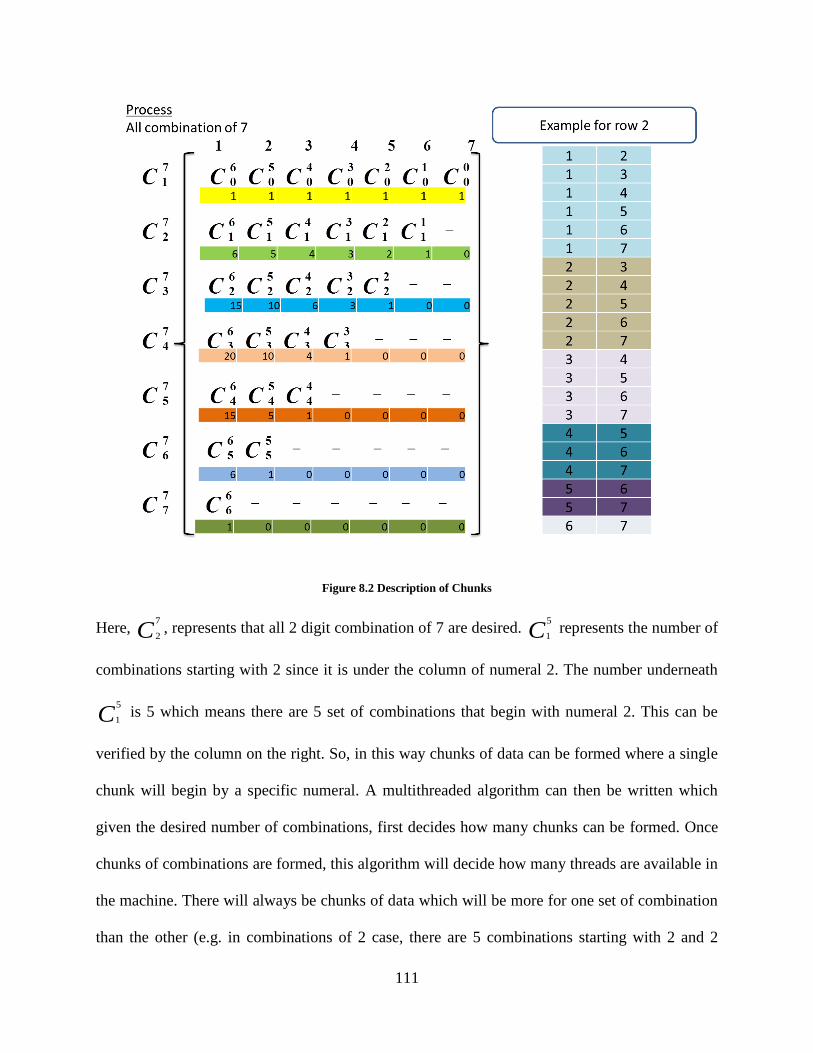
111
Figure 8.2 Description of Chunks
Here, C7
2, represents that all 2 digit combination of 7 are desired. C
5
1 represents the number of
combinations starting with 2 since it is under the column of numeral 2. The number underneath
C5
1 is 5 which means there are 5 set of combinations that begin with numeral 2. This can be
verified by the column on the right. So, in this way chunks of data can be formed where a single
chunk will begin by a specific numeral. A multithreaded algorithm can then be written which
given the desired number of combinations, first decides how many chunks can be formed. Once
chunks of combinations are formed, this algorithm will decide how many threads are available in
the machine. There will always be chunks of data which will be more for one set of combination
than the other (e.g. in combinations of 2 case, there are 5 combinations starting with 2 and 2
112
combinations that stat with the numeral 5). This algorithm will be able to prioritize the
delegation of data chunks to individual threads based on the size of the data, and reassign the
threads that have finished calculation to start calculating for other chunk of data. Once all the
threads have finished calculating combinations the results from individual threads can be merged
to generate a complete output. This algorithm can be employed to both multithreading and
parallel processing depending upon the size of the problem and available computing power.
8.2 Rathish Divide and Conquer Algorithm and Pattern Recognition
As was discussed in Chapter 3 section 3.3, the structure can be divided into ‘bays’, and analysis
can be focused to one bay at a time to observe the change in member actions. Combining the
results from all the bays a total output can be obtained to decide what sensor plan can be
employed. If symmetry can be found in the structure, (as in the current structure), member
response can be observed for one part of the structure and be mimicked on the mirror image of
the structure. Now as mentioned before too, for a large structure, manually doing this may not be
possible. To do it computationally, the same process will have to be integrated with some
advanced algorithm requiring pattern recognition.
8.3 Statistical Methods
In the processes so far, average off diagonal and max off diagonal (for a limited extent) were
used as objective functions to decide an optimized sensor suite. These sensors were then tested
for the number of false detection and identification. Instead, another objective function can be
devised which takes all the combinations of sensors suites and selects the one which gives least
false detection or false isolations. This is an even bigger problem computationally than the one at

113
hand. Hence the use and investment of hardware and programmer time in developing a
multithreaded algorithm is even more justified.
8.4 Precipitation
This method can be viewed as an opposite approach to the condensation method. In
condensation, the method starts by taking into all possible sensors, and then decimates sensors
one by one and updates the total number of sensors to be used in next iteration. Precipitation on
the other hand will start with a single or a small set of sensors and then will add sensors based on
an objective function.
8.5 Machine Learning
Machine learning algorithms provide an efficient and self-adjusting means to digest the data.
Multinomial Logistic Regression, for example can be used to train several classifiers. These
classifiers will learn overtime the nature of the data when it is in the undamaged state. Some
simulated data of the faults will be need to be fed to these classifiers in order to train them for the
damaged cases to. All classifiers will be working together and will give output based on a
weighted sum of the results obtained from each of the classifiers. One benefit of this kind of
approach can be that the nose factor can also be trained in the classifiers i.e. after digesting many
years of data it will be able to classify an event which is caused by noise or temperature as a
benign event. Support Vector Machines and Principal Component Analysis are some of the other
algorithm to solve the non-linear nature of the problem at hand.
114
References
1. Barthrope, R. J. (2010). "On Model- and Data-based Approaches to Structural
Health Monitoring". Doctor of Philosophy. University of Sheffield, Sheffield.
2. Harms, T., Sedigh, S., and Bastianini, F. (2010). "Structural Health Monitoring
of Bridges Using Wireless Sensor Networks." Instrumentation & Measurement
Magazine, IEEE, 13(6), 14-18.
3. Jenkins, C. H., Kjerengtroen, L., and Oestensen, H. (1997). "Sensitivity of
parameter changes in structural damage detection." Shock Vib, 10(4), 135-142.
4. Chang, P. C., Flatau, A., and Liu, S. C. (2003). "Review Paper: Health
Monitoring of Civil Infrastructure." Structural Health Monitoring, 2(3), 257-
267.
5. Gastineau, A., Johnson, T., and Schultz, A. (2009). "Bridge Health Monitoring
and Inspections- A Survey of Methods." Minnesota Department of
Transportation, Minneapolis,MN.
6. Giangarra, P. P., Metrovich, B., Schwitters, M. M., and Semple, B. P. (2011).
"Smarter bridges through advanced structural health monitoring." IBM Journal
of Research and Development, 55(1.2), 9:1-9:10.
7. Worden, K., and Manson, G. (2000). "Damage identification using multivariate
statistics:Kernel Discriminant Analysis." Inverse Problems in
Engineering, 8(1), 25-46.
8. Worden, K., and Lan , A. J. (2001). "Damage identification using support
vector machine." Smart Materials and Structures, 10(3), 540-547.
9. Kulla, J. (2003). "Damage detection of the z24 bridge using control
charts." Mechanical Systems and Signal Processing, 17(1), 163-170.
10. Worden, K., Manson, G., and Fieller, N. R. J. (2000). "Damage Detection using
Outlier Analysis." Journal of Sound and Vibration, 229(3), 647-667.
115
11. Moaveni, B., Conte, J. P., and Hemez, F. M. (2009). "Uncertainty and
Sensitivity Analysis of Damage Identification Results Obtained Using Finite
Element Modeling Updating." Computer-Aided Civil and Infrastructure
Engineering, 24(5), 320-334.
12. Teughels, A., and Roeck, G. D. (2004). "Structural damage identification of the
highway bridge z24 by FE model updating." Journal of Sound and
Vibration, 278(3), 589-610.
13. Friswell, M. I., and Mottershead, J. E. (2001). "Physical Understanding of
Structures by Model Updating." International Conference on Structural System
Identification, Kassel, Germany, 1-94.
14. Rytter, A. (1993). "Physical Understanding of Structures by Model Updating".
Doctor of Philosophy. Aalborg University, Denmark.
15. Alampalli, S., Fu, G., and Aziz, J. A. (1992). "Modal Analysis as a Bridge
Inspection Tool." 10th International Modal Analysis Conference, 1359-1366.
16. Fox, C. H. J. (1992). "The location of defects in structures: A comparison of the
use of natural frequency and mode shape data." 10th International Modal
Analysis Conference, San Diego, CA, 522-528.
17. Adams, E. D., Walton, D., Flitcroft, J. E., and Short, D. (1975). "Vibration
Testing as a Nondestructive Test Tool for Composite Material." Composite
Reliability, Las Vegas,NV, 159-175.
18. Casas, J. R., and Aparicio, A. C. (1994). "Structural damage identification from
dynamic-test data." Journal of Structural Engineering ASCE, 120(8), 2437-
2450.
19. Salawu, O. S., and Williams, C. (1995). "Rivew of full-scale dynamic testing of
bridge structures." Engineering Structures, 17(2), 113-121.
20. Bendat, J. S. (1990). Nonlinear System Analysis & Identification from Random
Data. Wiley-Interscience, .
116
21. Mazurek, D. F., and DeWolf, J. T. (1990). "Experimental Study of Bridge
Monitoring Technique." Journal of Structural Engineering, ASCE, 116(9),
2535-2549.
22. Srinivasan, M. G., and Kot, C. A. (1992). "Effects of damage on the modal
parameters of a cylindrical shell." 10th International Modal Analysis
Conference, San Diego, CA, 529-535.
23. Yam, L. H., Li, D. B., Leung, T. P., and Xue, K. Z. (1994). "Experimental
study on modal strain analysis of rectangular thin plates with small holes." 12th
International Modal Analysis Conference, Honolulu,HI, 1415-1418.
24. Li, Y. Y., Chenga, L., Yam, L. H., and Wong, W. O. (2002). "Identification of
damage locations for plate-like structures using damage sensitive indices: strain
modal approach." Computers & Structures, 80(25), 1881-1894.
25. Pandey, A. K., Biswas, M., and Samman, M. M. (1991). "Damage detection
from changes in curvature mode shapes." Journal of Sound and
Vibration, 145(2), 321-332.
26. Norton, R. L. (2007). Design of Machinery. McGraw-Hill
Companies,Incorporated, 2007, Boston.
27. Austin, A (1998). "Structural Analysis of Moment-Resistant
Frame." http://www.isr.umd.edu/~austin/aladdin.d/wjlin-mrf.html (October/10,
2012).
28. Allemang, R. J. (2003). "The Modal Assurance Criterion –Twenty Years of
Use and Abuse." Sound and Vibration, 37(8), 14-21.
29. CustomPartNet.(2009)."Material." http://www.custompartnet.com/wu/images/
milling/i-beam.png (October/18, 2012).
30. Transtutors.(2012)."Bendingmoment." http://www.transtutors.com/homework-
help/mechanical-engineering/bending-moment-and-shear-force/bending-
moment.aspx (October/18, 2012).

117
Appendix
Software Used
SAP2000 V14 – This software was used to generate an FE model of the structure. Using this as a
standard, values obtained from MTLAB were verified.
MATLAB – An alternate model of the structure was generated using matrix manipulation that
mimicked the structure generated by SAP2000.
Microsoft Excel 2010 – Excel was used to plot graph and bubble charts. Once the Virtual
Machine was developed, the analysis of Failure Detection and Isolation was also done through it.