hyper-bag-graphs and their applications thÈse - cern
TRANSCRIPT

CER
N-T
HES
IS-2
020-
048
13/0
3/20
20
UNIVERSITÉ de GENÈVE FACULTÉ DES SCIENCESDépartement d’Informatique Professeur Stéphane Marchand-MailletCERNDépartement IPT Docteur Jean-Marie Le Goff
Hyper-bag-graphs and their applicationsModeling, Analyzing and VisualizingComplex Networks of Co-occurrences
THÈSEprésentée à la Faculté des Sciences de l’Université de Genève
pour obtenir le grade de Docteur ès Sciences, mention Informatique
par
Xavier OUVRARD
de
Chevry, France
Thèse N° 5449
GENÈVECentre d’impression de l’Université de Genève
2020

Abstract
Obtaining insights in the tremendous amount of data in which the Big Data era hasbrought us, requires to develop specific tools, that are not only summaries of datathrough classical charts and tables, but that allow full navigation and browsing of adataset. The proper modeling of databases can enable such navigation and we proposein this Thesis a methodology to achieve the browsing of an information space, through itsdifferent facets. To achieve the modeling of such an information space, co-occurrencesof data instances are built referring to a common reference type. Historically, theco-occurrences were seen as pairwise relationships and developed as such. The moveto hypergraphs enables the possibility to take into account the multi-adicity of therelationships, and to have a representation through the incident graph that simplifiesdeeply its 2-section.Nonetheless, representing large hypergraphs calls for a coarsening of the information byhaving insights on important vertices and hyperedges. One classical way to achieve itis to use a diffusion process over the network. Achieving it using an incident matrix isfeasible but brings us to a pitfall, as it brings us back to a pairwise relationship. Makingproper diffusion requires a tensor approach. This is well known for uniform hypergraphs,where all the hyperedges have same cardinality, but still very challenging for generalhypergraphs. After redefining the concept of adjacency in general hypergraphs, wepropose a first e-adjacency tensor, that involves a Hypergraph Uniformisation Processand a Polynomial Homogenization Process. This is achieved by uniformisation of theoriginal hypergraph by decomposing it into layers—each of them containing a uniformhypergraph—and filling each layer with additional special vertices and merging themtogether. This process requires to have as many additional vertices as the number oflayers.In order to reduce the number of special vertices, we need to have the possibility of re-peating a vertex when filling, which is not possible with hyperedges as they are sets. Weneed multisets. It, therefore, requires a new mathematical structure, that we have intro-duced and called hyper-bag-graph—hb-graph for short—, which is a family of multisetsof a given universe.Co-occurrences can also have repetitions or individual weighting of their vertices insidea given co-occurrence and hb-graphs fit to handle it. Hence, we introduce a hb-graphframework for co-occurrence networks. We then work on diffusion on such structures,using, in a first step, a matrix approach. Aggregating the ranking of vertices and hb-edges of this diffusion on each of the facet of the information space is achieved by usinga multi-diffusion scheme. Since different facets might have different focus of interest,we introduce a biased diffusion that enables a tuning on the point of emphasis on thefeature we are interested in.Finally, coming back to e-adjacency tensor, we propose three e-adjacency tensors of hb-graphs, that are based on different ways of filling the hb-edges. The m-uniformisation

iv Summary
that is achieved is evaluated and compared to the ones achieved by hb-edge splitting,concluding that any m-uniformisation process has an influence on the exchange-baseddiffusion that we propose. Hence, we conclude that diffusion using the tensor approachmust be done in an informed manner to account for this diffusion change. We finallydiscuss different possible of achieving it and present a new Laplacian that can help toachieve it.
Résumé
À l’ère du Big Data, l’énorme quantité et la variété des données imposent, pour générerun aperçu signifiant, de développer des outils spécifiques qui ne se réduisent pas sim-plement à des graphiques ou à des tableaux de synthèse classiques ; ils doivent aussipermettre une navigation complète dans le jeu de données.
La modélisation appropriée de ces données va favoriser une telle navigation. Cette Thèsepropose précisément un cadre adapté à la navigation dans tout espace d’infor- mationmulti-facettes. Cette modélisation nécessite la construction de cooccurrences d’instancesde données en se référant à un (ou des) type(s) commun(s) servant de référence. Pen-dant très longtemps, les cooccurrences, vues comme collaborations, ont été perçuescomme des relations par paires : leur représentation était alors développée en tant quetelles. Le passage aux hypergraphes pour modéliser les réseaux de cooccurrences laissela possibilité de prendre en compte la multiplicité des relations. Cela permet égalementd’avoir une représentation via le graphe d’incidence de l’hypergraphe, ce qui simplifieprofondément la visualisation obtenue par 2-section de l’hypergraphe.
Néanmoins, quand la taille des hypergraphes augmente, et afin de pouvoir continuerà les visualiser convenablement, il faut un tri de l’information pour révéler au mieuxles sommets et hyper-arêtes importants du réseau. En ce domaine, une des méthodesclassiques consiste à utiliser un processus de diffusion. Une première approche résidedans l’utilisation de la matrice d’incidence de l’hypergraphe. Mais cela comporte unpossible piège, car, en raison de sa nature matricielle, la matrice d’incidence induitdes relations par paires, soit explicitement soit implicitement. Aussi une autre ap-proche de la diffusion est indispensable : il faut tenir compte des relations d’ordresupérieures induites par les hyper-arêtes et donc adopter une approche tensorielle.La diffusion tensorielle, via le Laplacien, est bien connue pour les hypergraphes uni-formes, où toutes les hyper-arêtes ont la même cardinalité ; mais elle reste encore unvaste champ d’études pour les hypergraphes généraux. Après avoir redéfini le conceptd’adjacence dans les hypergraphes généraux, nous proposons donc un premier tenseurd’e-adjacence, qui implique un processus d’uniformisation de l’hypergraphe et un proces-sus d’homogénéisation polynomiale. Aussi, afin de représenter les relations d’e-adjacenced’un hypergraphe de manière tensorielle, on uniformise l’hypergraphe d’origine en le dé-composant en couches d’hypergraphes uniformes, puis en remplissant chaque coucheavec des sommets n’appartenant pas à l’hypergraphe d’origine et enfin en fusionnantces couches. Ce processus nécessite à une unité près d’avoir autant de sommets que lataille maximale d’une hyper-arête.
En outre, pour réduire le nombre de sommets ajoutés, tout en gardant l’interprétabi-lité en terme d’uniformisation, il faut avoir la possibilité de répéter un sommet lorsdu remplissage. Or, comme cela n’est pas envisageable avec les hypergraphes du faitde leur définition ensembliste, cela requiert les multi-ensembles (ou multisets). En ré-sulte la nécessité d’une nouvelle structure mathématique qui est introduite dans cette
vi Résumé
Thèse et appelée hyper-bag-graphes (ou hb-graphes de manière abrégée) : les hb-graphessont définis comme étant des familles de multi-ensembles d’un univers donné, considérécomme l’ensemble des sommets.
C’est à la lueur de cette nouvelle structure que l’on peut dès lors proposer une modéli-sation raffinée de l’espace d’information multi-facettes. Cela permet de tenir compte dufait que chaque cooccurrence peut contenir des répétitions ou nécessiter une pondérationindividuelle de ses sommets. Chaque facette est alors modélisée par un hb-graphe. Endécoule l’importance d’une étude de la diffusion sur les hb-graphes utilisant en premièreinstance une approche matricielle. L’agrégation du classement des hb-arêtes obtenulors de la diffusion sur chacune des facettes de l’espace d’information est alors réaliséeà l’aide d’un schéma de multi-diffusion. Et, comme différentes facettes amènent à sefocaliser sur différents centres d’intérêt, nous avons introduit une diffusion biaisée : ellepermet d’ajuster l’accent mis sur la caractéristique qui nous intéresse ainsi que sur letype de valeurs considérées comme importantes.
Enfin, pour en revenir au tenseur d’e-adjacence, trois tenseurs d’e-adjacence de hb-graphes sont proposés, utilisant différentes manières de remplir les hb-arêtes. La m-uniformisation utilisée est évaluée par comparaison à celle obtenue par la division d’hb-arêtes qui avait été proposée dans un tenseur d’e-adjacence étudié antérieurement pard’autres auteurs. La conclusion de cette évaluation est la suivante : tout processus dem-uniformisation a une influence sur la diffusion par échanges ; mais seule celle obtenuepar addition de sommets spéciaux permet d’avoir une perturbation compréhensible surle classement des sommets. Par ailleurs, cette perturbation peut être évitable, mais auprix d’un calcul moins direct des degrés des sommets. On peut alors en déduire que ladiffusion utilisant l’approche tensorielle doit être faite de manière informée de sorte àtenir compte de ce changement de diffusion. Reste ensuite à étudier les différentes straté-gies possibles pour réaliser cette diffusion et finalement proposer un nouveau Laplacientensoriel.

Acknowledgments
I am deeply grateful and thankful to Pr. Stéphane Marchand-Maillet for the directionof this Thesis and to Dr. Jean-Marie Le Goff for his co-direction: for their continuoussupervision, discussions and advices, and their infinite patience during this thesis, theco-supervision having given some fruitful exchanges and refinements.
To the dissertation reviewers and Defence Jury members, Pr. Zdzislaw Burda (AGHUniversity of Science and Technology, Kraków), Pr. András Telcs (Budapest Universityof Technology and Economics) and Pr. Gilles Falquet (University of Geneva), to haveaccept to review this work, and for evaluating this work,
I am also grateful:
To CERN, for having funded a doctoral position that has allowed me to be dedicatedfull time on my PhD, and, more particularly, to the IPT department and his departmenthead, Mr. Thierry Lagrange.
To the members of the Collaboration Spotting project at CERN, Dimitrios Dardanis(University of Geneva / CERN), Richard Forster (CERN), and last, but not least AndréRattinger (University of Gratz / CERN), for the discussions and exchange we had duringall the thesis,
To the University of Geneva and to the Swiss Doctoral Program, CUSO, which has beena precious aid for training and exchanges during the doctoral studies,
To CUI, University of Besançon, which has allowed me to do remote studies to reachthe Master level in Computer Science,
To Edoardo Provenzi (University of Bordeaux), for his advice on the presentation oftensors,
To Tullio Basaglia (CERN), for his precious advices on the application of the DataHb-Edron to publication searches,
To Linn Tvelde (CERN), which has helped in improving the English in some parts ofthis Thesis,
To all the ones, met during conferences and seminars, that have given me some previousadvice or went to fruitful discussions,
Finally, a big thanks:
To my wife, Cécile, for her support in those late studies, for her full support on theeveryday life and her precious advices in the moment of choices and doubts.


Contents ix
ContentsAbstract .............................................................................................. iii
Résumé................................................................................................ v
Acknowledgments................................................................................. vii
Table of contents.................................................................................. ix
Nomenclature ...................................................................................... xv
List of Figures......................................................................................xvii
List of Tables ....................................................................................... xxi
List of Algorithms................................................................................xxiii
Introduction ........................................................................................ 1
1. An introduction to hb-graphs........................................................... 9
1.1. Motivation.......................................................................................... 9
1.2. Related work ...................................................................................... 10
1.3. Generalities ........................................................................................ 11
1.4. Additional concepts for natural hb-graphs ........................................... 14
1.4.1. Numbered copy hypergraph of a natural hb-graph ............................................... 14
1.4.2. Paths, distance and connected components ........................................................ 15
1.4.3. Adjacency .................................................................................................. 16
1.4.4. Sum of two hb-graphs ................................................................................... 17
1.4.5. An example ................................................................................................ 17
1.4.6. Hb-graph representations ............................................................................... 18
1.4.6.1. Subset standard .................................................................................... 18
1.4.6.2. Edge standard ...................................................................................... 19
1.4.7. Incidence matrix of a hb-graph ........................................................................ 20
1.5. Some (potential) applications .............................................................. 20
1.5.1. Prime decomposition representation and elementary operations on hb-graphs ............. 21
1.5.2. Graph pebbling and families of multisets ........................................................... 23
1.5.3. Chemical reaction networks and hb-graphs ......................................................... 24
1.5.4. Multiset cover problems and hb-graph transversals ............................................... 25
1.5.5. Networks .................................................................................................... 25
1.5.5.1. Computer networks ............................................................................... 25
1.5.5.2. Neural networks .................................................................................... 26
1.6. Further comments on hb-graphs.......................................................... 26
2. Diffusion in hb-graphs (matrix approach) ......................................... 27
2.1. Motivation.......................................................................................... 27
x Contents
2.2. Related work ...................................................................................... 28
2.3. Exchange-based diffusion in hb-graphs ................................................ 29
2.4. Results and evaluation ........................................................................ 37
2.4.1. Validation on random hb-graphs ...................................................................... 37
2.4.2. Two use cases ............................................................................................. 49
2.4.2.1. Application to Arxiv querying .................................................................. 49
2.4.2.2. Application to an image database ............................................................. 50
2.5. Future work and Conclusion ............................................................... 51
3. e-adjacency tensor of natural hb-graphs ........................................... 55
3.1. Motivation.......................................................................................... 55
3.2. Related work ...................................................................................... 56
3.3. e-adjacency tensor of a natural hb-graph ............................................. 56
3.3.1. Expectations for the e-adjacency tensor ............................................................. 56
3.3.2. Elementary hb-graph ..................................................................................... 57
3.3.3. Normalised k-adjacency tensor of an elementary hb-graph ..................................... 58
3.3.4. Hb-graph polynomial .................................................................................... 59
3.3.5. k-adjacency hypermatrix of a m-uniform natural hb-graph ..................................... 60
3.3.6. Elementary operations on hb-graphs ................................................................. 61
3.3.7. Processes involved for building the e-adjacency tensor .......................................... 64
3.3.8. On the choice of the technical coefficient cei ...................................................... 65
3.3.9. Straightforward approach ............................................................................... 66
3.3.10. Silo approach ............................................................................................. 69
3.3.11. Layered approach ....................................................................................... 71
3.3.12. Examples related to e-adjacency hypermatrices for general hb-graphs ..................... 75
3.3.12.1. Layered filling option ............................................................................ 75
3.3.12.2. Silo filling option ................................................................................. 76
3.3.12.3. Straightforward filling option .................................................................. 77
3.4. Results on the constructed tensors ...................................................... 78
3.4.1. Fulfillment of the expectations ........................................................................ 78
3.4.2. Information on hb-graph ................................................................................ 79
3.4.2.1. m-degree of vertices .............................................................................. 79
3.4.2.2. Additional vertex information ................................................................... 80
3.4.3. First results on hb-graph spectral analysis .......................................................... 83
3.4.4. Categorization of the constructed tensors .......................................................... 84
3.4.4.1. Classification of the tensors built .............................................................. 84
3.4.4.2. Connected components and uniformisation process ....................................... 86

Contents xi
3.5. Evaluation and first choice .................................................................. 86
3.5.1. Evaluation .................................................................................................. 86
3.5.2. First choice ................................................................................................. 87
3.5.3. Hypergraphs and hb-graphs ............................................................................ 87
3.6. Further comments............................................................................... 88
4. m-uniformisation processes and exchange-based diffusion ................. 91
4.1. Motivation.......................................................................................... 91
4.2. Impact of the m-uniformisation process on the exchange-based diffusion 92
4.2.1. Additional vertices filling m-uniformisation approach ............................................ 92
4.2.2. Hb-edge splitting m-uniformisation approach ...................................................... 95
4.3. e-adjacency tensors require compromises............................................. 98
4.4. Further comments............................................................................... 100
5. Diffusion in hb-graphs (tensor approach).......................................... 101
5.1. Motivation.......................................................................................... 101
5.2. Related work ...................................................................................... 101
5.2.1. Operators ................................................................................................... 102
5.2.2. Diffusion operators ....................................................................................... 102
5.2.3. Diffusion processes in graphs .......................................................................... 103
5.2.4. Diffusion processes in hypergraphs ................................................................... 104
5.2.4.1. Matrix Laplacians ................................................................................. 104
5.2.4.2. Tensor Laplacians ................................................................................. 106
5.2.4.3. Hypergraph Laplacian and diffusion process ................................................ 106
5.3. A diffusion operator for general hb-graphs .......................................... 107
5.3.1. Global exchange-based diffusion ...................................................................... 107
5.3.2. Taking into account the different layers of uniformity. .......................................... 108
5.3.2.1. Tensor approach ................................................................................... 108
5.3.2.2. Polynomial approach .............................................................................. 108
5.3.2.3. First properties of the layered Laplacian hypermatrix ..................................... 111
6. Hb-graph framework........................................................................ 113
6.1. Motivation.......................................................................................... 113
6.2. Related work ...................................................................................... 114
6.3. Modeling co-occurrences in datasets.................................................... 115
6.3.1. Axioms and postulates on the information space ................................................. 115
6.3.2. Hypothesis and expectations of the hb-graph framework ....................................... 116
6.3.3. The hb-graph framework ............................................................................... 118
6.3.3.1. Enhancing navigation ............................................................................. 119

xii Contents
6.3.3.2. Visualisation hb-graphs corresponding to facets ........................................... 119
6.3.3.3. Navigability through facets ...................................................................... 123
6.3.3.4. Change of reference ............................................................................... 126
6.3.3.5. The case of multiple references ................................................................ 126
6.3.4. The DataHbEdron ........................................................................................ 128
6.3.5. Validation and discussion ............................................................................... 128
6.3.5.1. Fulfillment of expectations ...................................................................... 128
6.3.5.2. Comparison with existing solutions ............................................................ 131
6.3.6. A use case .................................................................................................. 131
6.3.7. Intermediate conclusion ................................................................................. 134
6.4. Further comments............................................................................... 134
7. Multi-diffusion in an information space ............................................ 135
7.1. Motivation.......................................................................................... 135
7.2. Mathematical background and related work ........................................ 136
7.2.1. The problem of ranking aggregation ................................................................. 136
7.2.2. Classical distances between rankings ................................................................. 136
7.2.3. Origin of the ranking aggregation problem ......................................................... 137
7.2.4. Kemeny-Young order .................................................................................... 137
7.2.5. A revival of interest ...................................................................................... 138
7.2.6. Comparison of rankings ................................................................................. 140
7.3. Multi-diffusing in an information space ............................................... 141
7.3.1. Laying the first stones ................................................................................... 141
7.3.2. Strategies for ranking references ...................................................................... 142
7.3.3. Ranking aggregation by modified weighted MC4 ................................................. 142
7.3.4. Results and evaluation .................................................................................. 143
7.3.4.1. Randomly generated information space ...................................................... 143
7.3.4.2. Application to the Arxiv information space ................................................. 148
7.4. Further comments............................................................................... 150
Conclusion ........................................................................................... 155
Bibliography ........................................................................................ 159
Index ................................................................................................... 175
A. List of talks and conferences............................................................ 185
B. Mathematical background................................................................ 187
B.1. Hypergraphs ...................................................................................... 187
B.1.1. Generalities ................................................................................................ 187
B.1.2. Weighted hypergraph ................................................................................... 188

Contents xiii
B.1.3. Hypergraph features ..................................................................................... 188
B.1.4. Paths and related notions .............................................................................. 189
B.1.5. Multi-graph, graph, 2-section ......................................................................... 189
B.1.6. Sum of hypergraphs ..................................................................................... 190
B.1.7. Matrices associated to hypergraphs ................................................................. 190
B.1.7.1. Incidence matrix ................................................................................... 190
B.1.7.2. Adjacency matrix ................................................................................. 190
B.1.8. Hypergraph visualisation ............................................................................... 191
B.2. Multisets............................................................................................ 196
B.2.1. Generalities ................................................................................................ 196
B.2.2. Algebraic representation of a natural multiset ..................................................... 199
B.2.3. Morphisms, category and multisets .................................................................. 199
B.2.4. Topologies on multisets ................................................................................. 200
B.2.5. Applications of multisets ............................................................................... 201
B.3. Tensors and hypermatrices ................................................................. 202
B.3.1. An introduction on tensors ............................................................................ 202
B.3.2. Restricted approach of tensors as hypermatrices ................................................. 204
B.3.3. On classification of hypermatrices ................................................................... 205
B.3.4. Eigenvalues ................................................................................................ 206
C. Complements Chapter 1: An introduction to hb-graphs ................... 209
C.1. An example using hypergraphs for modeling co-occurrence networksand showing their limitations ..................................................................... 209
C.2. Homomorphisms of natural hb-graphs ................................................ 210
D. Complements Chapter 2: Diffusion in hb-graphs.............................. 213
D.1. Facets and Biased diffusion ................................................................ 213
D.1.1. Motivation ................................................................................................. 213
D.1.2. Related work .............................................................................................. 213
D.1.3. Biased diffusion in hb-graphs ......................................................................... 214
D.1.3.1. Abstract information functions and bias ..................................................... 214
D.1.3.2. Biased diffusion by exchange ................................................................... 215
D.1.3.3. Results and evaluation ........................................................................... 220
D.1.3.4. Further comments ................................................................................ 222
E. Complements Chapter 3: e-adjacency tensor of natural hb-graphs.... 227
E.1. Building a tensor of e-adjacency for general hypergraphs .................... 227
E.1.1. Motivation ................................................................................................. 227
E.1.2. Adjacency in hypergraphs .............................................................................. 228
E.1.3. Background and related work ......................................................................... 229
xiv Contents
E.1.3.1. The matrix approach ............................................................................. 229
E.1.3.2. Existing k and e-adjacency tensors ........................................................... 229
E.1.4. Towards an e-adjacency tensor of a general hypergraph ........................................ 233
E.1.4.1. Family of tensors attached to a hypergraph ................................................ 233
E.1.4.2. Expectations for an e-adjacency tensor for a general hypergraph ...................... 234
E.1.4.3. Tensors family and family of homogeneous polynomials ................................. 236
E.1.4.4. Uniformisation and homogenization processes ............................................. 237
E.1.4.5. Building an unnormalized symmetric tensor from this family of homogeneous poly-nomials .......................................................................................................... 242
E.1.4.6. Interpretation and choice of the coefficients for the unnormalized tensor ........... 243
E.1.4.7. Fulfillment of the unnormalized e-adjacency tensor expectations ...................... 245
E.1.4.8. Interpretation of the e-adjacency tensor ..................................................... 247
E.1.5. Some comments on the e-adjacency tensor ........................................................ 249
E.1.5.1. The particular case of graphs .................................................................. 249
E.1.5.2. e-adjacency tensor and disjunctive normal form ........................................... 249
E.1.5.3. First results on spectral analysis of e-adjacency tensor ................................... 250
E.1.6. Evaluation .................................................................................................. 252
E.1.7. Further comments ........................................................................................ 252
E.2. Examples of hypermatrices for general hypergraphs............................ 254
E.2.1. An example of the e-adjacency hypermatrix proposed by [BCM17] .......................... 254
E.2.2. An example of layered e-adjacency hypermatrix for general hypergraph .................... 254
F. Used Fraktur fonts........................................................................... 257
Appendices
Nomenclature
Hypergraphs
H = (V,E) Hypergraph of vertex set V and hyperedge set E
V = {vi : i ∈ JnK} Vertex set of a hypergraph H
E = (ej)j∈JpK Hyperedge family of a hypergraph
H(v) Star of a vertex v ∈ V
H∗ Dual of a hypergraph H
Γ (v) Neighbourhood of a vertex v ∈ V
Hw = (V,E,w) Weighted hypergraph of vertex set V , edge family E andweight function w
oH Order of a hypergraph H
rH Rank of a hypergraph H
sH Anti-rank of a hypergraph H
[H]2 2-section of the hypergraph H
[H]I Interection graph of the hypergraph H
H1 +H2 Sum of two hypergraphs H1 and H2
H1 ⊕H2 Direct sum of two hypergraphs H1 and H2
H Incidence matrix of a hypergraph
A Adjacency matrix of a hypergraph
Aw Adjacency matrix of a weighted hypergraph
l (P) Length of a path P
d (u, v) Distance between two vertices u and v
Hb-graphs
H = (V,E) Hb-graph H of vertex set V and hb-edge family E
V = {vi : i ∈ JnK} Vertex set of a hb-graph H

xvi Nomenclature
E = (ej)j∈JpK Hb-edge family of a hb-graph H, where ej are multisetsof universe V
mej or mj Multiplicity function of the hb-edge ej
mej (vi) or mij Multiplicity value of the vertex vi of the hb-edge ej
O (H) Order of a hb-graph H
H Support hypergraph of a hb-graph H
rm (H) m-rank of a hb-graph H
r (H) Range of a hb-graph H
crm (H) m-co-rank of a hb-graph H
#mH Global m-cardinality of a hb-graph H
cr (H) Co-range of a hb-graph H
h (v) Hb-star of a vertex v ∈ V
degm(v) m-degree of a vertex v ∈ V
∆m Maximal m-degree of a hb-graph H
H0 Numbered-copy-hypergraph of the hb-graph H
H Dual of the hb-graph H
l (P) Length of a path P
d (u, v) Distance between two vertices u and v
General
#mAm m-cardinality of a multiset Am
JnK Integers from 1 to n
A∗m Support of the multiset Am
Am = (A,m) Multiset of universe A and multiplicity function m
M (A) Set of all multisets of universe A
a⊗ b Segre outerproduct of two vectors a and b
List of Figures
0.1. A reading help guide. . . . . . . . . . . . . . . . . . . . . . . . . . . . . . 5
1.1. Hb-graph (a) and its dual (b) given in Example 1.4.1 in their multipartitegraph representation with in superposition the corresponding supporthypergraph in the Euler representation. . . . . . . . . . . . . . . . . . . 18
1.2. Finding the prime decomposition ofmn from the decomposition ofm andn with m = 900 and n = 945. . . . . . . . . . . . . . . . . . . . . . . . . 22
1.3. Finding the prime decomposition of gcd (m,n) from the decompositionof m and n with m = 900 and n = 945. . . . . . . . . . . . . . . . . . . 22
1.4. Finding the prime decomposition of lcm (m,n) from the decompositionof m and n with m = 900 and n = 945. . . . . . . . . . . . . . . . . . . 23
1.5. Illustrating the property lcm (m,n)×gcd (m,n) = mn with m = 900 andn = 945. . . . . . . . . . . . . . . . . . . . . . . . . . . . . . . . . . . . . 23
2.1. Diffusion by exchange: principle, with:δεt+ 1
2(ej | vi)
∆= mj (vi)we (ej)dw,vi
αt (vi) and δαt+1 (vi | ej)∆= mj (vi)
#mejεt+ 1
2(ej) . 30
2.2. Random hb-graph generation principle. . . . . . . . . . . . . . . . . . . 382.3. Relative eccentricity: finding the length of a maximal shortest path in
the hb-graph starting from a given vertex v0 of S and finishing with anyvertex in V \S. . . . . . . . . . . . . . . . . . . . . . . . . . . . . . . . . 39
2.4. Maximum path length and percentage of vertices in AV (s) over verticesin V vs ratio rV . . . . . . . . . . . . . . . . . . . . . . . . . . . . . . . . 40
2.5. Alpha value of vertices at step 200 and degree of vertices. . . . . . . . . 412.6. Alpha value of vertices at step 200 and m-degree of vertices. . . . . . . . 412.7. Path maximum length and percentage of vertices in AE(s) vs ratio. . . . 422.8. Epsilon value of hb-edge at stage 199+1
2 and cardinality of hb-edge. . . 422.9. Epsilon value of hb-edge at stage 199+1
2 and (m-)cardinality of hb-edge. 432.10. Alpha value convergence of the vertices vs number of iterations. The
plots are m-degree-based with gradient coloring. . . . . . . . . . . . . . 452.13. Comparison of the rank obtained by a thousand modified random walks
after total discovery of the vertices in the hb-graph and the rank obtainedwith 200 iterations of the exchange-based diffusion process. . . . . . . . 45
2.11. Epsilon value convergence of hb-edges vs number of iterations. The plotsare m-cardinality-based colored using gradient colors. . . . . . . . . . . . 46
2.14. Comparison of the rank obtained by a thousand modified random walksafter total discovery of the vertices in the hb-graph and m-degree of vertices. 46
2.15. Comparison of the rank obtained by a thousand modified random walksafter total discovery of the vertices in the hb-graph and degree of vertices. 47

xviii List of Figures
2.16. Comparison of the rank obtained by a thousand classical random walksafter total discovery of the vertices in the hb-graph and rank obtainedwith 200 iterations of the exchange-based diffusion process. . . . . . . . 47
2.17. Comparison of the rank obtained by a thousand classical random walksafter total discovery of the vertices in the hb-graph and m-degree of vertices. 48
2.18. Comparison of the rank obtained by a thousand classical random walksafter total discovery of the vertices in the hb-graph and degree of vertices. 48
2.12. Exchange-based diffusion in a hb-graph (a) and its support hypergraph(b) after 200 iterations of Algorithm 2.1: highlighting important hb-edges.Simulation with 848 vertices (chosen randomly out of 10 000) gatheredin 5 groups of vertices (with 5, 9, 14, 16 and 9 important vertices and 2important vertices per hb-edge), 310 hb-edges (with cardinality of supportless or equal to 20), 10 vertices in between the 5 groups. Extra-verticeshave square shape and are colored with the hb-edge color scale. . . . . . 52
2.19. Querying Arxiv. The search performed is “content-based multimediaindexing” for which (a) 50 most—respectively (b) 100 most—relevantarticles have been retrieved. . . . . . . . . . . . . . . . . . . . . . . . . 53
2.20. Exchange-based diffusion on the sub-hb-graph first component with 177images of a hb-graph of 200 images of the COCO 2014 training dataset. 54
3.1. Operations on the original hb-graph for its m-uniformization in the straight-forward approach. Parenthesis with vertical dots indicate parallel opera-tions. . . . . . . . . . . . . . . . . . . . . . . . . . . . . . . . . . . . . . . 67
3.2. Operations on the original hb-graph for its m-uniformisation in the siloapproach. Parenthesis with vertical dots indicate parallel operations. . . 69
3.3. Operations on the original hb-graph for its m-uniformisation in the lay-ered approach. Parenthesis with vertical dots indicate parallel operations. 72
3.4. Example of hb-graph for m-uniformisation principle . . . . . . . . . . . 753.5. Layered filling on the example of Figure 3.4 . . . . . . . . . . . . . . . . 763.6. Silo filling on the example of Figure 3.4 . . . . . . . . . . . . . . . . . . 763.7. Straightforward filling on the example of Figure 3.4 . . . . . . . . . . . . 77
4.1. Representation of the 5-m-uniform hb-graph H = (V,E) with V = {vi : i ∈ J5K}and E = (ej)j∈J4K, where: e1 =
{{v2
1, v22, v
15}}, e2 =
{{v1
2, v23, v
24}},
e3 ={{v1
2, v23, v
25}}
and e4 ={{v1
2, v33, v
14}}. . . . . . . . . . . . . . . . . 99
6.1. Schema hypergraph, Extended schema hypergraph, Extracted extendedschema hypergraph: exploded view shown on an example of publicationdataset. . . . . . . . . . . . . . . . . . . . . . . . . . . . . . . . . . . . . 120
6.2. A simplified publication network. . . . . . . . . . . . . . . . . . . . . . . 1216.3. Navigating between facets of the information space. . . . . . . . . . . . 1246.4. Navigating between facets in the publication network: visualizing orga-
nization co-occurrences with reference keywords and switching to subjectcategories with reference keywords. . . . . . . . . . . . . . . . . . . . . . 125
6.5. Changing reference in the publication network: visualizing organizationco-occurrences with reference keywords and switching to reference subjectcategories. . . . . . . . . . . . . . . . . . . . . . . . . . . . . . . . . . . . 127
6.6. DataHbEdron: (a) cube shape (b) carousel shape. . . . . . . . . . . . . 129
List of Figures xix
6.7. First facet of the DataHbEdron: a well-known look like of a classicalverbatim interface. . . . . . . . . . . . . . . . . . . . . . . . . . . . . . . 132
6.8. Performed search. . . . . . . . . . . . . . . . . . . . . . . . . . . . . . . . 133
7.1. Average Kendall tau correlation coefficient between the WT-MC4 rankingaggregation compared to the non-zero weight facet rankings dependingon the number of non-zero weight facet rankings—corresponding data isshown in Table 7.2—(100 information spaces for each value of the numberof facets). . . . . . . . . . . . . . . . . . . . . . . . . . . . . . . . . . . . 146
7.2. Average Kendall tau correlation coefficient between the ranking obtainedby Borda aggregation of the facet diffusion by exchange rankings and theWT-MC4 realized with equi-weight on non-zero equal weight facets—correspondingdata is shown in Table 7.4—(100 information spaces for each value of thenumber of facets). . . . . . . . . . . . . . . . . . . . . . . . . . . . . . . 147
7.3. Average Kendall tau between Borda aggregation of the rankings obtainedon references via diffusion by exchange and the WT-MC4 with equi-weight on non-zero equal weight facets—it corresponds to data shown inTable 7.5—(1000 random information spaces for each value of the numberof facets are generated). . . . . . . . . . . . . . . . . . . . . . . . . . . . 147
7.4. Comparison of different queries Kendall tau correlation coefficients be-tween Borda aggregation ranking and the rankings obtained either di-rectly by diffusion on the corresponding facet (Authors and Keywords)or by WT-MC4 with equi-weights, when querying the Arxiv database (27queries). . . . . . . . . . . . . . . . . . . . . . . . . . . . . . . . . . . . . 151
7.5. Comparison of different queries Kendall tau correlation coefficients be-tween Borda aggregation ranking and the rankings obtained either di-rectly by diffusion on the corresponding facet or by WT-MC4 with equi-weights, when querying the Arxiv database (27 queries). . . . . . . . . . 152
7.6. Comparison of different queries Kendall tau correlation coefficients be-tween Borda aggregation ranking and the rankings obtained either di-rectly by diffusion on the corresponding facet or by WT-MC4 with equi-weights, when querying the Arxiv database (27 queries). . . . . . . . . . 153
B.1. Hypergraph of organizations: Sub-figures (a) and (b) refer to the search:title:((bgo AND cryst*) OR (bgo AND calor*)) abstract:((bgo AND cryst*)OR (bgo AND calor*)) from [OLGMM17b]. . . . . . . . . . . . . . . . . 192
B.2. Keyword collaborations from search: “TITLE: hypergraph”. . . . . . . . 193B.3. Organization collaborations from search: “TITLE:graph”. . . . . . . . . 194B.4. Principle of the calculation of coordinates for large hypergraphs. . . . . 195
C.1. Example of a publication co-occurrence network with three facets . . . . 209
D.1. Strict Kendall tau correlation coefficient for node ranking with biases.Realized on 100 random hb-graphs with 200 hb-edges of maximal size 20,with 5 groups. . . . . . . . . . . . . . . . . . . . . . . . . . . . . . . . . . 222
D.2. Large Kendall tau correlation coefficient for node ranking with biases.Realized on 100 random hb-graphs with 200 hb-edges of maximal size 20,with 5 groups. . . . . . . . . . . . . . . . . . . . . . . . . . . . . . . . . . 223
xx List of Figures
D.3. Strict Kendall tau correlation coefficient for hb-edge ranking with biases.Realized on 100 random hb-graphs with 200 hb-edges of maximal size 20,with 5 groups. . . . . . . . . . . . . . . . . . . . . . . . . . . . . . . . . . 224
D.4. Large Kendall tau correlation coefficient for hb-edge ranking with biases.Realized on 100 random hb-graphs with 200 hb-edges of maximal size 20,with 5 groups. . . . . . . . . . . . . . . . . . . . . . . . . . . . . . . . . . 225
D.5. Effect of vertex biases on ranking. . . . . . . . . . . . . . . . . . . . . . 226
E.1. Illustration of a hypergraph decomposed in three layers of uniform hy-pergraphs. . . . . . . . . . . . . . . . . . . . . . . . . . . . . . . . . . . . 234
E.2. Construction phases of the e-adjacency tensor. . . . . . . . . . . . . . . 240E.3. Illustration of the iterative approach concept on an example.
In the iterative approach, the layers of level n and n + 1 are mergedtogether into the layer n+ 1 by adding a filling vertex to the hyperedgesof the layer n. On this example, during the first step the layer 1 and2 are merged to form a 2-uniform hypergraph. In the second step, the2-uniform hypergraph obtained in the first step is merged to the layer 3to obtain a 3-uniform hypergraph. . . . . . . . . . . . . . . . . . . . . . 248
List of Tables
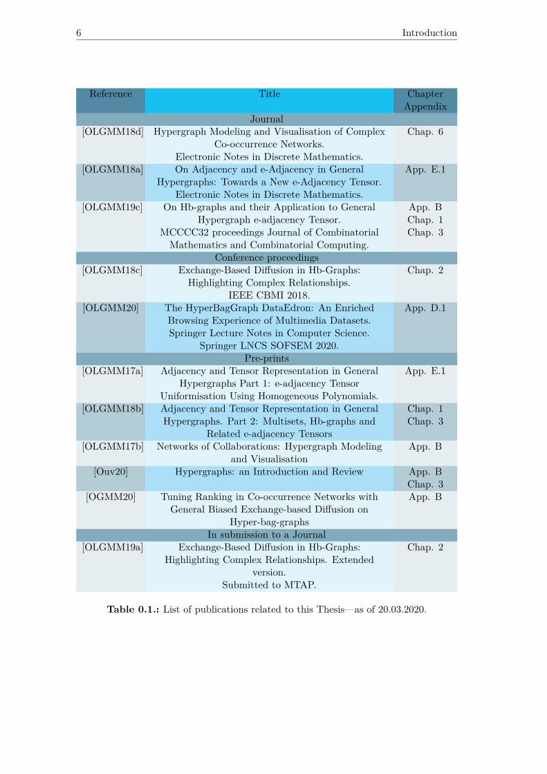
0.1. List of publications related to this Thesis—as of 20.03.2020. . . . . . . . 60.2. List of personal contributions related to this Thesis. . . . . . . . . . . . 7
1.1. Dualities between a hb-graph and its dual. . . . . . . . . . . . . . . . . . 14
2.1. Time taken for doing 100, 200, 500 and 1000 iterations of the diffusionalgorithm and 100, 200, 500 and 1000 classical and modified randomwalks on different hb-graphs. . . . . . . . . . . . . . . . . . . . . . . . . 49
3.1. Evaluation of the hb-graph e-adjacency tensor depending on construction. 893.2. Evaluation of the hypergraph e-adjacency tensor. . . . . . . . . . . . . . 90
4.1. Number and multiplicity of special vertices and weights introduced forthe three m-uniformisation process introduced in Chapter 3, with: k ∈JnprocK , j ∈ JpK . . . . . . . . . . . . . . . . . . . . . . . . . . . . . . . . 93
5.1. Ways of defining matrix Laplacian of a hypergraph. . . . . . . . . . . . . 105
6.1. Synthesis of the framework. . . . . . . . . . . . . . . . . . . . . . . . . . 1186.2. Elements of comparison between different multi-faceted visualization frame-
works. . . . . . . . . . . . . . . . . . . . . . . . . . . . . . . . . . . . . . 131
7.1. Different ranking comparison features—as defined in Section 7.2.6 be-tween Borda ranking and current ranking on 1000 generated informationspaces of 3 facets with similar parameters. . . . . . . . . . . . . . . . . . 145
7.2. Kendall tau of 1000 WT-MC4 ranking aggregation compared to the facetrankings (average on the 1000 information) depending on the weights puton the facets. The average features of the facets are given in Table 7.1. . 145
7.3. Average Kendall tau of the WT-MC4 ranking aggregation compared tothe non-zero weight facet rankings (average on 100 information spaces)depending on the number of facets having non-zero equal weights. Pa-rameters of facet hb-graphs similar to Table 7.1. . . . . . . . . . . . . . 145
7.4. Average Kendall tau of the WT-MC4 ranking aggregation—with non-zeroweights as indicated—compared to the Borda aggregation ranking—on allfacet rankings—(average on 100 information spaces) depending on thenumber of facets having non-zero weights. Parameters of facet hb-graphssimilar to Table 7.1. . . . . . . . . . . . . . . . . . . . . . . . . . . . . . 146
7.5. Average Kendall tau of the WT-MC4 ranking aggregation compared tothe non-zero equal weight facet rankings (average on 1000 informationspaces) depending on the number of facets having non-zero weights. Pa-rameters of facet hb-graphs similar to Table 7.1. . . . . . . . . . . . . . 147

xxii List of Tables
7.6. Strict Kendall tau correlation coefficient between two facets exchange-based diffusion rankings and some additional statistics on facets whenquerying Arxiv, on first top 1000 answers returned by the Arxiv API. . 149
7.7. Strict Kendall tau correlation coefficient between Borda aggregation rank-ing and the rankings obtained either directly by diffusion on the corre-sponding facet or by WT-MC4 with different weights, when querying theArxiv database (on 29 queries) for the first 100, 200 and 1000 resultsreturned by the API. . . . . . . . . . . . . . . . . . . . . . . . . . . . . . 149
7.8. Kendall tau correlation coefficient between Borda aggregation rankingand the rankings obtained either directly by diffusion on the correspond-ing facet or by WT-MC4 with different weights, when querying the Arxivdatabase (27 queries). . . . . . . . . . . . . . . . . . . . . . . . . . . . . 150
A.1. List of talks and posters related to this Thesis—as of 07.12.2019. . . . . 186
C.1. Co-occurrences of organizations built using Publication as reference . . . 209C.2. Co-occurrences of organizations built using Keywords as reference . . . 210
D.1. Features used in the exchange-based diffusion of Chapter 2. . . . . . . . 214D.2. Biases used during the 15 experiments. . . . . . . . . . . . . . . . . . . . 220
E.1. Evaluation of the e-adjacency tensor. . . . . . . . . . . . . . . . . . . . . 253

List of Algorithms
2.1. Exchange-based diffusion algorithm. . . . . . . . . . . . . . . . . . . . . 372.2. Modified random walk in hb-graphs. . . . . . . . . . . . . . . . . . . . . 44
7.1. MC4 algorithm as proposed in [DKNS01]. . . . . . . . . . . . . . . . . . 1397.2. The WT-MC4 algorithm. . . . . . . . . . . . . . . . . . . . . . . . . . . 143


Introduction
Big Data with its five Vs implies a lot of innovative visual analytics tools to have deeperinsights into the DataSet. As the Volume of information is increasing and at the sametime the Variety is gaining in heterogeneity, new tools need to consider all the Varietyof the information space, serving it with Velocity. The Veracity of information is a bigchallenge and requires different strategies: it requires not only dataset consolidation anddata linkage, but also to gain insight into datasets in order to retrieve meaningful andgenuine information.
This quest for Veracity is linked to the Value of the Data: Big Data calls for improvedmining, aggregation, linkage of data,... Different approaches exist to visualize and sum-marize information in an information space. Datasets composed only of numerical dataappear as the easiest case: plethoric treatments exist to enhance proper visualisationand summarization; links can often be retrieved by different methods either using classi-cal statistic methods or more modern approaches such as neural nets and deep learning.When coming to non-numerical data, the summarization is often left to very basic ap-proaches such as histograms and the data interactivity is often let behind. To findinherent links, machine learning methods can help, but they need a strong frameworkto enhance the structure of the dataset. In multimedia datasets, data instances are ablend of text, audio, image and/or video content all linked by some physical references.Variety induces new ways to address datasets.
There are different approaches to model databases, such as the relational databasemodel introduced by Codd in [Cod70], based on sets and relations. A relational databaseschema is shown as a hypergraph with convenient properties in [Fag83]. Graph databasesuse a graph as schema and have been introduced in the 1990s as it is mentioned in[AG08] to overcome the limitations of traditional databases for capturing the inherentgraph structure of data in various situations such as in hypertext or geographic databasesystems. The Knowledge Graph1 introduced by Google in 2012 is a good example ofthe inherent graph structure of data.
In [Ran45], Ranganathan exposes the concept of facets in an information space—heintroduced these concepts already in 1924. Ranganathan considers that a documentcan be described by five facets, with a rule of thumbs called PMEST: Personality,Matter, Energy, Space and Time. Personality reveals the focal subject of the document,Matter reflects a substance or a property of the subject, Energy reflects the operationor action done on the subject, Space is considering the geographical location and Timethe chronological and temporal situation of the subject.
The concept of multi-faceted information space can be extended to any document andenlarge to different views of the information space within which the Dataset lives. Each1https://googleblog.blogspot.com/2012/05/introducing-knowledge-graph-things-not.html
2 Introduction
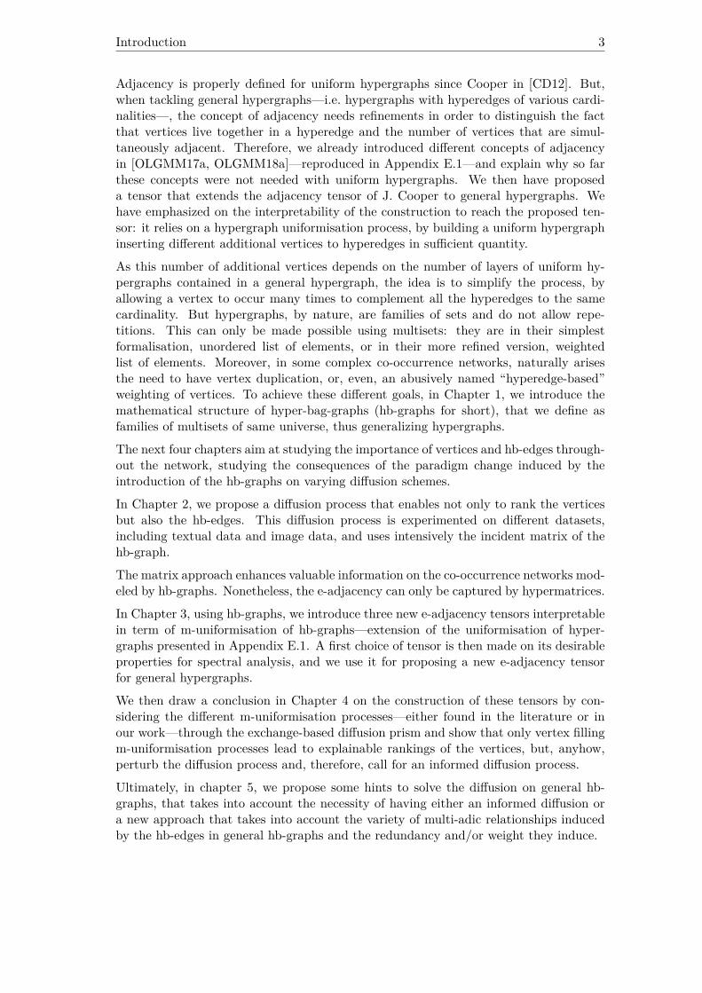
facet of an information space can be modeled as a network of co-occurrences built oncommon references as we will show in Chapter 6.
Networks of co-occurrences can be modeled with different approaches: eitherco-occurrences are seen as pairwise relationships like in [New01a, New01b] or seen asproper multi-adic relationships as it is done in [TCR10], using hypergraphs that wereintroduced by Berge in [Ber73].
Hypergraphs extend graphs by considering a family of subsets of a vertex set. Hyper-graphs naturally support multi-adicity where graphs support only 2-adicity, i.e. pairwiserelationships. If the concept of incidence of vertices to edges in a graph clearly extendsto hyperedges in hypergraphs, it does not hold for adjacency, for which the concept hasto be refined.
Different hypergraph representations exist as mentioned already in [Mäk90], some withthe subset standard using Venn or Euler diagrams—that are not scaling up prop-erly—and some with the edge standard, consisting in transforming the hypergraph intoa graph. The edge-standard comprises two main representations: the clique represen-tation and the extra-node representation. The clique representation, corresponds to agraph view of the hypergraph 2-section, developing each hyperedge of the original hy-pergraph in its combination of pairwise relationships. The extra-node representationcorresponds to the hypergraph incident graph—also called Levi graph—, each hyper-edge being assorted with an extra-node and vertices of the hyperedge being linked tothis extra-node.
We have shown in [OLGMM17b], that visualizing hypergraphs through their incidentgraph allows to diminish the cognitive load of the 2-section of the hypergraph—the2-section being no more than the representation of a pairwise relationship. Moreover,the 2-section of a hypergraph looses the group information: two hypergraphs can havethe same 2-section—which is in general not desirable. The incident graph is unique fora given hypergraph. Incident graph of hypergraphs are bipartite graphs and can beviewed as a developed version of the hypergraph: they are a lesser evil than the subsetstandard representation or the 2-section graph when the hypergraph becomes larger.
When scaling up large hypergraph representations, the hypergraph visualisation gener-ative model requires at a point a coarsening of the hypergraph, that can be achieved,among other techniques, by enhancing diffusion over the structure.
Hypergraphs as graphs cannot be reduced to their incident graphs even if they are linkedin a one-to-one manner; the set relationship induced by the hyperedge is powerful andregroups the information in a single object. The incidence relationships between verticesand hyperedges in hypergraphs is modeled by a rectangular matrix. This rectangularmatrix when multiplied conveniently by its transpose represents the pairwise relationshipbetween vertices: it is taken as the basis for an adjacency matrix for hypergraphs;but, this adjacency matrix reflects in fact the adjacency in the 2-section graph of thehypergraph. Also different hypergraphs can have the same adjacency matrix which isnot desirable. Hence, a proper modeling of adjacency in a hypergraph calls for tensorsto enable the capture of the multi-adicity.
In Appendix B, we present the necessary mathematical requirements for this Thesis. Itincludes all the necessary elements on hypergraphs, on multisets and, on tensors andhypermatrices.
Introduction 3
Adjacency is properly defined for uniform hypergraphs since Cooper in [CD12]. But,when tackling general hypergraphs—i.e. hypergraphs with hyperedges of various cardi-nalities—, the concept of adjacency needs refinements in order to distinguish the factthat vertices live together in a hyperedge and the number of vertices that are simul-taneously adjacent. Therefore, we already introduced different concepts of adjacencyin [OLGMM17a, OLGMM18a]—reproduced in Appendix E.1—and explain why so farthese concepts were not needed with uniform hypergraphs. We then have proposeda tensor that extends the adjacency tensor of J. Cooper to general hypergraphs. Wehave emphasized on the interpretability of the construction to reach the proposed ten-sor: it relies on a hypergraph uniformisation process, by building a uniform hypergraphinserting different additional vertices to hyperedges in sufficient quantity.
As this number of additional vertices depends on the number of layers of uniform hy-pergraphs contained in a general hypergraph, the idea is to simplify the process, byallowing a vertex to occur many times to complement all the hyperedges to the samecardinality. But hypergraphs, by nature, are families of sets and do not allow repe-titions. This can only be made possible using multisets: they are in their simplestformalisation, unordered list of elements, or in their more refined version, weightedlist of elements. Moreover, in some complex co-occurrence networks, naturally arisesthe need to have vertex duplication, or, even, an abusively named “hyperedge-based”weighting of vertices. To achieve these different goals, in Chapter 1, we introduce themathematical structure of hyper-bag-graphs (hb-graphs for short), that we define asfamilies of multisets of same universe, thus generalizing hypergraphs.
The next four chapters aim at studying the importance of vertices and hb-edges through-out the network, studying the consequences of the paradigm change induced by theintroduction of the hb-graphs on varying diffusion schemes.
In Chapter 2, we propose a diffusion process that enables not only to rank the verticesbut also the hb-edges. This diffusion process is experimented on different datasets,including textual data and image data, and uses intensively the incident matrix of thehb-graph.
The matrix approach enhances valuable information on the co-occurrence networks mod-eled by hb-graphs. Nonetheless, the e-adjacency can only be captured by hypermatrices.
In Chapter 3, using hb-graphs, we introduce three new e-adjacency tensors interpretablein term of m-uniformisation of hb-graphs—extension of the uniformisation of hyper-graphs presented in Appendix E.1. A first choice of tensor is then made on its desirableproperties for spectral analysis, and we use it for proposing a new e-adjacency tensorfor general hypergraphs.
We then draw a conclusion in Chapter 4 on the construction of these tensors by con-sidering the different m-uniformisation processes—either found in the literature or inour work—through the exchange-based diffusion prism and show that only vertex fillingm-uniformisation processes lead to explainable rankings of the vertices, but, anyhow,perturb the diffusion process and, therefore, call for an informed diffusion process.
Ultimately, in chapter 5, we propose some hints to solve the diffusion on general hb-graphs, that takes into account the necessity of having either an informed diffusion ora new approach that takes into account the variety of multi-adic relationships inducedby the hb-edges in general hb-graphs and the redundancy and/or weight they induce.
4 Introduction
The following chapter—Chapter 6—pushes the thought further on co-occurrence net-works for modeling an information space. Co-occurrences can be seen as multisets;hence hb-graphs can model co-occurrence networks, and refine the hypergraph frame-work approach used to model an information space as we have succinctly presented in[OLGMM18d] by a framework using a hb-graph approach.
We then propose, in Chapter 7, a multi-diffusion process in an information space usingsimultaneously the hb-graph framework presented in Chapter 6 and the exchange-baseddiffusion proposed in Chapter 2, in order to aggregate the rankings obtained for thehb-edge attached references of the different facet visualisation hb-graphs.
As the importance put on the different features can differ from one facet to the other,we give as a complement in Appendix D.1 some biased diffusion that generalize theone proposed already in Chapter 2: this allows to emphasize some values during thediffusion process, and refine the facet ranking depending on its specificity.
We finish by concluding on what we realized during this Thesis and give a list of possibleresearch questions for future work.
Most of the chapters are based on preprints or publications that have been acceptedor in submission during the three years of our PhD. We show in Table 0.1 the listof publications and their corresponding chapter. In Appendix A, we give a list ofconferences we participated with the kind of contribution realized. In Table 0.2, wepresent the list of our contributions per chapter.
In Figure 0.1, we propose a reading help guide: Chapter 1 is the entry point and thedirected edges indicates an order of reading: A → B indicates that Chapter A shouldbe read before Chapter B. In this case, the reader can refer to the prerequisites placedat the head of each chapter to know if only specific sections of Chapter A are needed.

Introduction 5
App.A: Mathematicalbackground
App.C: Hypergraphe-adj. tensor
Ch.1: Hb-graphs Ch.3: Hb-graphe-adj. tensor
Ch.6: Hb-graphframework
Ch.2: Diffusionin hb-graphs
(matrix approach)Ch.4: Hm-UPand hb-graphs
Ch.7: Multi-diffusionin an info. space
App.F: Facets andBiased diffusion
Ch.5: Diffusionin hb-graphs
(tensor approach)
Entry pointPre-requisites Core Extra use-cases Appendices
Thesis
hypergraph,tensor
tensor,multiset
(hypergraph),multiset
Figure 0.1.: A reading help guide.
6 Introduction
Reference Title ChapterAppendix
Journal[OLGMM18d] Hypergraph Modeling and Visualisation of Complex
Co-occurrence Networks.Electronic Notes in Discrete Mathematics.
Chap. 6
[OLGMM18a] On Adjacency and e-Adjacency in GeneralHypergraphs: Towards a New e-Adjacency Tensor.
Electronic Notes in Discrete Mathematics.
App. E.1
[OLGMM19c] On Hb-graphs and their Application to GeneralHypergraph e-adjacency Tensor.
MCCCC32 proceedings Journal of CombinatorialMathematics and Combinatorial Computing.
App. BChap. 1Chap. 3
Conference proceedings[OLGMM18c] Exchange-Based Diffusion in Hb-Graphs:
Highlighting Complex Relationships.IEEE CBMI 2018.
Chap. 2
[OLGMM20] The HyperBagGraph DataEdron: An EnrichedBrowsing Experience of Multimedia Datasets.Springer Lecture Notes in Computer Science.
Springer LNCS SOFSEM 2020.
App. D.1
Pre-prints[OLGMM17a] Adjacency and Tensor Representation in General
Hypergraphs Part 1: e-adjacency TensorUniformisation Using Homogeneous Polynomials.
App. E.1
[OLGMM18b] Adjacency and Tensor Representation in GeneralHypergraphs. Part 2: Multisets, Hb-graphs and
Related e-adjacency Tensors
Chap. 1Chap. 3
[OLGMM17b] Networks of Collaborations: Hypergraph Modelingand Visualisation
App. B
[Ouv20] Hypergraphs: an Introduction and Review App. BChap. 3
[OGMM20] Tuning Ranking in Co-occurrence Networks withGeneral Biased Exchange-based Diffusion on
Hyper-bag-graphs
App. B
In submission to a Journal[OLGMM19a] Exchange-Based Diffusion in Hb-Graphs:
Highlighting Complex Relationships. Extendedversion.
Submitted to MTAP.
Chap. 2
Table 0.1.: List of publications related to this Thesis—as of 20.03.2020.

Introduction 7
CorpusChapter 1 • Introduction of hb-graphs: all the concepts in the chapter but
the related work.Chapter 2 • Exchange-based diffusion in co-occurrence networksChapter 3 • e-adjacency tensors of general hb-graphs.Chapter 4 • Impact of the m-uniformisation process on diffusion.Chapter 5 • A layered Laplacian for general hb-graphsChapter 6 • Hb-graph framework for co-occurrence networks modeling.Chapter 7 • Multi-diffusion principle in an information space;
• WT-MC4 for aggregation ranking.Appendix
Appendix B • Review on hypergraphs;• Visualisation of large hypergraphs.
Appendix C.2 • Homomorphisms of hb-graphsAppendix E.1 • e-adjacency tensor for general hypergraphsAppendix D.1 • Facets and biased diffusion.
Table 0.2.: List of personal contributions related to this Thesis.

1. An introduction to hb-graphs
Highlights
1.1. Motivation . . . . . . . . . . . . . . . . . . . . . . . . . . . . . . . . . . 91.2. Related work . . . . . . . . . . . . . . . . . . . . . . . . . . . . . . . . . 101.3. Generalities . . . . . . . . . . . . . . . . . . . . . . . . . . . . . . . . . . 111.4. Additional concepts for natural hb-graphs . . . . . . . . . . . . . . . . . 141.5. Some (potential) applications . . . . . . . . . . . . . . . . . . . . . . . . 201.6. Further comments on hb-graphs . . . . . . . . . . . . . . . . . . . . . . . 26
This chapter is based on [OLGMM18b, OLGMM18c, OLGMM19a, OLGMM19c].In this Chapter and in Appendix C.2, we extend the work on hyper-bag-graphs (hb-graphs for short) introduced in [OLGMM18c], and that has been extensively presentedin [OLGMM18b, OLGMM19c]. Hb-graphs extend hypergraphs by substituting familiesof subsets of a vertex set by families of multisets of same universe, playing the role of thevertex set. After their introduction, we extend to hb-graphs some of the results foundin [Bre13] for hypergraphs. The reader, not familiar with the mathematical notions atstake in this Chapter, can refer to Appendix B: more particularly the sections concerninghypergraphs—Section B.1—and multisets—Section B.2.Prerequisites: Section B.1 and B.2 of Appendix B.
1.1. Motivation
There are different motivations that converge for the introduction of hb-graphs.A very first motivation is that multisets are appropriate to enhance repetition of elementson a given universe. In Appendix B.2.5, multisets are shown to be intensively used indifferent fields as we already mentioned.Moreover, in the case of complex co-occurrences networks, a second motivation is thatthe co-occurrences themselves can require this kind of repetitions, by the way the co-occurrences are built—such an example is given in Section C.1 of Appendix C—, orindividual weighting, naturally enhancing families of multisets on a given universe.A third motivation for introducing hb-graphs is related to the representation of largehypergraphs as it is presented in Section B.1.8 of Appendix B; large hypergraph repre-sentations call for a coarsening in their generative model for enhancing a representation
10 1. An introduction to hb-graphs
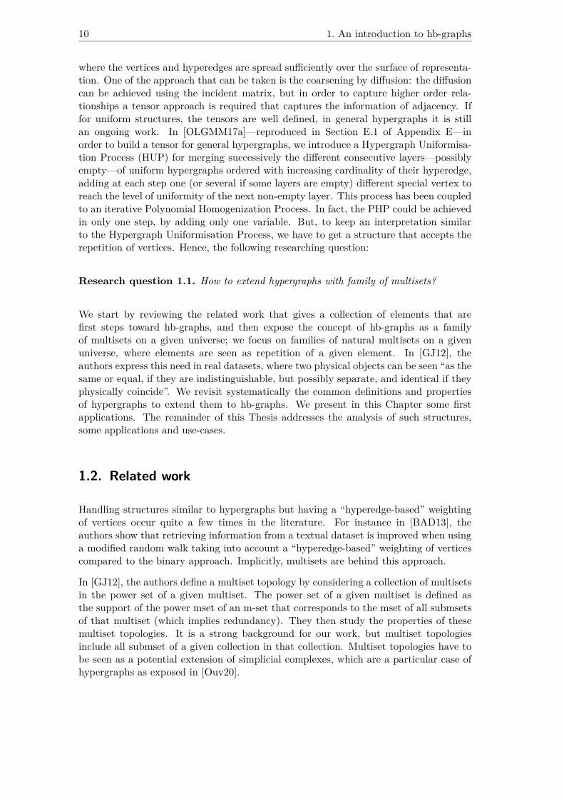
where the vertices and hyperedges are spread sufficiently over the surface of representa-tion. One of the approach that can be taken is the coarsening by diffusion: the diffusioncan be achieved using the incident matrix, but in order to capture higher order rela-tionships a tensor approach is required that captures the information of adjacency. Iffor uniform structures, the tensors are well defined, in general hypergraphs it is stillan ongoing work. In [OLGMM17a]—reproduced in Section E.1 of Appendix E—inorder to build a tensor for general hypergraphs, we introduce a Hypergraph Uniformisa-tion Process (HUP) for merging successively the different consecutive layers—possiblyempty—of uniform hypergraphs ordered with increasing cardinality of their hyperedge,adding at each step one (or several if some layers are empty) different special vertex toreach the level of uniformity of the next non-empty layer. This process has been coupledto an iterative Polynomial Homogenization Process. In fact, the PHP could be achievedin only one step, by adding only one variable. But, to keep an interpretation similarto the Hypergraph Uniformisation Process, we have to get a structure that accepts therepetition of vertices. Hence, the following researching question:
Research question 1.1. How to extend hypergraphs with family of multisets?
We start by reviewing the related work that gives a collection of elements that arefirst steps toward hb-graphs, and then expose the concept of hb-graphs as a familyof multisets on a given universe; we focus on families of natural multisets on a givenuniverse, where elements are seen as repetition of a given element. In [GJ12], theauthors express this need in real datasets, where two physical objects can be seen “as thesame or equal, if they are indistinguishable, but possibly separate, and identical if theyphysically coincide”. We revisit systematically the common definitions and propertiesof hypergraphs to extend them to hb-graphs. We present in this Chapter some firstapplications. The remainder of this Thesis addresses the analysis of such structures,some applications and use-cases.
1.2. Related work
Handling structures similar to hypergraphs but having a “hyperedge-based” weightingof vertices occur quite a few times in the literature. For instance in [BAD13], theauthors show that retrieving information from a textual dataset is improved when usinga modified random walk taking into account a “hyperedge-based” weighting of verticescompared to the binary approach. Implicitly, multisets are behind this approach.
In [GJ12], the authors define a multiset topology by considering a collection of multisetsin the power set of a given multiset. The power set of a given multiset is defined asthe support of the power mset of an m-set that corresponds to the mset of all submsetsof that multiset (which implies redundancy). They then study the properties of thesemultiset topologies. It is a strong background for our work, but multiset topologiesinclude all submset of a given collection in that collection. Multiset topologies have tobe seen as a potential extension of simplicial complexes, which are a particular case ofhypergraphs as exposed in [Ouv20].

1.3. Generalities 11
In [PZ14], the authors introduce what they call [PZ-]1multi-hypergraphs2 using multi-sets, allowing repetitions of vertices in the hyperedges, but where two hyperedges cannotbe duplicates. [PZ-]Multi-hypergraphs are a particular case of hb-graphs as we definethem in this Chapter: we call them natural hb-graphs with no repeated hb-edge. Waitingfor the definitions given in Section 1.3, we call them temporarily PZ-multi-hypergraphs.
Definition 1.1. A PZ-multi-hypergraph...H is a pair (V,E) , where E is a set of multisets
of V. The elements of V are called the vertices and the elements of E are called the edges.
In [PZ14], when the hyperedges are all of same cardinality k the PZ-multi-hypergraphis said k-uniform, and called k-multigraph3. (PZ-)Multi-hypergraphs are in fact a par-ticular case of hb-graphs as we define in this Chapter. They define some additionalnotions such as a chain in a (PZ-)multi-hypergraph, the notion of connected (PZ-)multi-hypergraph and the notion of k-(PZ-)multi-hypergraphs.Independently in [KPP+19]—at the same time we were introducing hb-graphs in[OLGMM18b]—the authors consider a hypergraph where the hyperedges are multi-sets, transforming the initial definition of hypergraphs, to extend the Cheng-Lu modelto hypergraphs, to achieve clustering via hypergraph modularity. They use a family ofmultisets and define the degree of a vertex as the sum of multiplicities and the size ofa hyperedge as the sum of the multiplicities of its elements. They obtain good resultswith their proposed modularity getting a smaller number of hyperedges cut comparedto the one achieved with the 2-section of the hypergraph.In [CR19], published after [OLGMM18c], a hypergraph with hyperedge-dependent ver-tex weights is defined by considering a quadruple H = (V,E, ω, γ) where ω is the edgeweight vector, and γ is refined in a weight γe (v) for every hyperedge e ∈ E. The au-thors are then using implicitly multisets, but without considering the related algebra.In a recent paper [PVAdST19], the authors introduce a continuous incident matrix formultimedia retrieval, which is no more than our hb-graph incident matrix.
1.3. Generalities
Let V = {vi : i ∈ JnK} be a nonempty finite set.A hyper-bag-graph or hb-graph for short over V is defined in [OLGMM18c] as afamily of msets with universe V and support a subset of V . The msets are called thehb-edges and the elements of V the vertices.We consider for the remainder of the Thesis a hb-graph H = (V,E), with V = {vi : i ∈ JnK}and E = (ej)j∈JpK the family of its hb-edges.Each hb-edge ej ∈ E is of universe V and has a multiplicity function associated to it:mej : V → W where W ⊆ R+. When the context is clear the notation mj is used formej and mij for mej (vi) .1[...] is used in italic as abbreviation for [Thesis Author’s Note: ...]2Multi-hypergraph is in fact polysemic: multi-hypergraphs originally represent hypergraphsH = (V,E)where the repetition of hyperedges is authorized in E i.e. E is considered as a family [Bre13] or amultiset [CF88], which is the direct extension of multi-graph.
3It is also a polysemy: in [Maj87] k-multigraphs are multi-graphs—where multiple edges between acouple of vertices can occur—which are also k-graphs—i.e. graphs that are k-regular.
12 1. An introduction to hb-graphs
A hb-graph is said to be with no repeated hb-edge if:
∀j1 ∈ JpK ,∀j2 ∈ JpK : ej1 = ej2 ⇒ j1 = j2.
A hb-graph where each hb-edge is a natural mset is called a natural hb-graph.The empty hb-graph is the hb-graph with an empty set of vertices. A trivial hb-graph is a hb-graph with a non empty set of vertices and an empty family of hb-edges.For a general hb-graph, every hb-edge has to be seen as a weighted system of vertices,where the weights of each vertex are hb-edge dependent. In a natural hb-graph, themultiplicity function can be viewed as a duplication of the vertices.In [PZ14], the authors have introduced what they call abusively multi-hypergraphswhere the hyperedge set is composed of multisets of vertices. It corresponds to naturalhb-graphs with no repeated hb-edges, name that we keep, as multi-hypergraphs arehypergraphs where the subsets of vertices the hyperedges correspond to can be repeated,i.e. constitute either a multiset of subsets of vertices [CF88] or a family of subsets ofvertices [Bre13].
The order of a hb-graph H—written O (H)—is given by: O (H) ∆= ∑i∈JnK
maxe∈E
(me (vi)) .
The size of a hb-graph corresponds to the number of its hb-edges.If ⋃
j∈JpKe?j = V, then the hb-graph is said with no isolated vertices. Otherwise, the
elements of V \ ⋃j∈JpK
e?j are called the isolated vertices. They correspond to elements
of hb-edges with zero-multiplicity for all hb-edges.A hypergraph is a natural hb-graph where the vertices of the hb-edges have multiplicityone for any vertex of their support and zero otherwise.The support hypergraph of a hb-graph H = (V,E) is the hypergraph whose verticesare the ones of the hb-graph and whose hyperedges are the support of the hb-edges. Wewrite H
∆= (V,E) with E ∆= (e?)e∈E , the support hypergraph of H.We note that given a hypergraph H, an infinite set CH of hb-graphs can be generatedthat all have this hypergraph as support. A hb-edge family is attached to each of thehb-graphs in CH : each hb-edge support corresponds at least to one hyperedge in H and,reciprocally, each hyperedge of H is at least the support of one hb-edge per hb-graph ofCH. The unicity of the correspondence is ensured only for hypergraphs and hb-graphswithout repeated hyperedges.In this case, an equivalence relationR can be defined that puts in relation two hb-graphsif they have same hypergraph as hb-graph support. Hence, considering the quotient ofthe set of all hb-graphs with no-repeated hb-edges by R, it is isomorph to the set ofhypergraphs with no-repeated hyperedge.
The m-rank of a hb-graph—written rm (H)—is by definition4: rm (H) ∆= maxe∈E
#me.
The rank of a hb-graph H—written r (H)—is the rank of its support hypergraph H.
The m-co-rank of a hb-graph—written crm (H)—is by definition:crm (H) ∆= mine∈E
#me.
4see Section B.2.1 for the definition of the notation #me.
1.3. Generalities 13
The co-rank of a hb-graph H—written cr (H)—is the co-rank of its support hypergraphH.
The global m-cardinality of a hb-graph H—written #mH—is the sum of the m-cardinality of its hb-edges.
A hb-graph is said k-m-uniform if all its hb-edges have the same m-cardinality k.
A hb-graph is said k-uniform if its support hypergraph is k-uniform.
Proposition 1.1. A hb-graph H is k-m-uniform, if and only if: rm (H) = crm (H) = k.
We can still refer for vertices of a hb-graph H = (V,E) to the degree of v ∈ Vwritten deg (v) = d(v): it corresponds to the degree of the same vertex in the supporthypergraph H. The maximal degree of a hb-graph H is written ∆ and corresponds tothe maximal degree of the support hypergraph H.
Nonetheless, in hb-graphs, due to the multiplicity function attached to each hb-edge,we can consider another kind of degree. To complete its proper definition, we define thehb-star h (v) of a vertex v ∈ V as the multiset: h(v) ∆=
{eme(v) : e ∈ E ∧ v ∈ e?
}. The
support of h(v) is exactly the star of this vertex in the support hypergraph H and thecardinality of h?(v) is exactly the degree of v.
The m-degree of a vertex v ∈ V of a hb-graph H is then defined as the m-cardinalityof the hb-star attached to this vertex:
degm(v) ∆= #mh(v).
We also consider the maximal m-degree of a hb-graph H; we write it:
∆m∆= max
v∈Vdegm(v).
A hb-graph having all its hb-edges of the same m-degree k is said m-regular or k-m-regular. A hb-graph is said regular if its support hypergraph is regular.
It is immediate that:
Proposition 1.2. For any vertex v ∈ V of a natural hb-graph: d(v) 6 dm(v) 6 ∆m.
This property is not true for non-natural hb-graphs.
Proposition 1.3. If a hb-graph with a non-negative multiplicity function range is suchthat: d(v) = dm(v) for all its vertices, then this hb-graph is a hypergraph.
We define now the dual of a hb-graph H = (V,E) as the hb-graph H∆=(V , E
)such
that its set of vertices V ∆= {vj : j ∈ JpK} is in bijection f : E → V with the family ofhb-edges E of H such that:
∀vj ∈ V , ∃!ej ∈ E : vj = f (ej) .

14 1. An introduction to hb-graphs
And its family of hb-edges E∆= (ei)i∈JnK is in bijection g : V → E such that g (vi) = ei
for all i ∈ JnK, where:
ei∆={vjmej (vi) : j ∈ JpK ∧ vj = f (ej) ∧ vi ∈ e?j
}.
We summarize some dualities between a hb-graph and its dual in Table 1.1.
H HVertices vi, i ∈ JnK vj = f (ej) , j ∈ JpKHb-edges ej , j ∈ JpK ei = g (vi) , i ∈ JnK
Multiplicity vi ∈ ej with mej (vi) vj ∈ ei with mei (vj)dm (vi) #meim-degrees vs m-cardinality #mei dm (vj)
k-m-uniform k-m-regularm-uniformity vs m-regularityk-m-regular k-m-uniform
Table 1.1.: Dualities between a hb-graph and its dual.
1.4. Additional concepts for natural hb-graphs
1.4.1. Numbered copy hypergraph of a natural hb-graph
In natural hb-graphs, hb-edge multiplicity functions have their range which is a subsetof N. The vertices in a hb-edge with multiplicity strictly greater than 1 can be seen ascopies of the original vertex.Indexing the copies of the original vertex makes them seen as “numbered” copies. Weconsider a vertex vi belonging to two hb-edges ej1 and ej2 of the hb-graph H = (V,E) ,with a multiplicitymej1
in ej1 andmej2in ej2 . Then ej1∩ej2 holds min
(mej1
(vi) ,mej2(vi)
)copies: by convention, the ones “numbered” from 1 to min
(mej1
,mej2
). The remain-
ing copies will be either in ej1 xor ej2 depending on which multiset has the highestmultiplicity for vi.More generally, we define the numbered-copy set of a natural multiset Am = {xmii : i ∈ JnK}as the copy-set Am
∆={
[xi j ]mi : i ∈ JnK}
where: [xi j ]mi is a shortcut to indicate thenumbered copies of the original element xi: xi 1 to ximi and j is designated as the copynumber of the element xi.We define the maximum multiplicity function of H as the function m : V → Nsuch that for all v ∈ V : m(v) ∆= max
e∈Eme(v) and consider the numbered-copy-set
V∆={
[vi j ]m(vi) : i ∈ JnK}of the multiset
{vm(vi)i : i ∈ JnK
}.
Then each hb-edge ek ={vmk ijij
: j ∈ JkK ∧ ij ∈ JnK}is associated to a copy-set / equiv-
alency relation < ek 0, ρk > which elements are in V with the smallest copy numberspossible for any vertex in ek. The hypergraph H0
∆=(V , E0
)where E0
∆= (ek 0)k∈JpK iscalled the numbered-copy-hypergraph of H.

1.4. Additional concepts for natural hb-graphs 15
Proposition 1.4. A numbered-copy-hypergraph is unique for a given hb-graph.
Proof. It is immediate by the way the numbered-copy-hypergraph is built from thehb-graph.
Allowing duplicates to be numbered prevents ambiguities; nonetheless, it has to be seenas a conceptual approach since duplicates are entities that are actually not discernible.
1.4.2. Paths, distance and connected components
Defining a path in a hb-graph is not straightforward due to vertex duplication. Wedefine two concepts of m-paths. The first imposes to the duplicate of a vertex insidea path to occur strictly at the intersection of two consecutive hb-edges. The secondrelaxes this hypothesis by allowing the vertex to be any duplicate in the union of twoconsecutive hb-edges—with of course one of the duplicate in the intersection.
More precisely, a strict m-path vi0ej1vi1 . . . ejsvis in a hb-graph H from a vertex u to avertex v is a vertex / hb-edge alternation with s hb-edges ejk such that: ∀k ∈ JsK , jk ∈JpK and s+ 1 vertices vik with ∀k ∈ {0} ∪ JsK , ik ∈ JnK and such that vi0 = u, vis = v,u ∈ ej1 and v ∈ ejs and that for all k ∈ Js− 1K, vik ∈ ejk ∩ ejk+1 .
A large m-path vi0ej1vi1 . . . ejsvis in a hb-graph H from a vertex u to a vertex v is avertex / hb-edge alternation with s hb-edges ejk such that: ∀k ∈ JsK , jk ∈ JpK and s+ 1vertices vik with ∀k ∈ {0} ∪ JsK , ik ∈ JnK and such that vi0 = u, vis = v, u ∈ ej1 andv ∈ ejs and that for all k ∈ Js− 1K, vik ∈ ejk ∪ ejk+1 and that there exists a copy of vikin ejk ∩ ejk+1 .
The length of a m-path from u to v is the number of hb-edges it traverses; givena path P, we write l (P) its length. It holds that if P = vi0ej1vi1 . . . ejsvis , we havewhatever the path is—strict or large—: l (P) = s.
In a path P = vi0ej1vi1 . . . ejsvis , the vertices vik , k ∈ Js− 1K are called the interiorvertices of the m-path and vi0 and vis are called the extremities of the m-path.
If the extremities are different copies of the same object, then the m-path is said to bean almost cycle. If the extremities designate exactly the same copy of one object, them-path is said to be a cycle.
Proposition 1.5. 1. For a strict m-path, there are ∏k∈Js−1K
mejk∩ejk+1(vik) possibil-
ities of choosing the interior vertices along a given m-path vi0ej1vi1 . . . ejsvis and
mej1(vi0)
( ∏k∈Js−1K
mejk∩ejk+1(vik)
)mejs (vis)possible strict m-paths in between the
extremities.
2. For a large m-path, there are ∏k∈Js−1K
mejk∪ejk+1(vik) possibilities of choosing the in-
terior vertices along a given m-path vi0ej1vi1 . . . ejsvis and
mej1(vi0)
( ∏k∈Js−1K
mejk∪ejk+1(vik)
)mejs (vis) possible large m-paths in between the
extremities.

16 1. An introduction to hb-graphs
3. As large m-paths between two extremities for a given sequence of interior verticesand hb-edges include strict m-paths, we often refer as m-paths for large m-paths.
4. If an m-path exists from u to v, then an m-path also exists from v to u.
Proof. All these results come directly of combinatorics over the multisets involved inthe different paths.
An m-path vi0ej1vi1 . . . ejsvis in a hb-graph corresponds to a unique path in the hb-graphsupport hypergraph called the support path.
Proposition 1.6. Every m-path vi0ej1vi1 . . . ejsvis traversing the same hb-edges andhaving similar vertices as intermediate and extremity vertices share the same supportpath.
Proof. The common support path is then vi0e?j1vi1 . . . e?jsvis .
The notion of distance is similar to the one defined for hypergraphs.
The hb-graph distance d (u, v) between two vertices u and v of a hb-graph is thelength of the shortest m-path between u and v, if there exists, that can be found in thehb-graph. In the case where there is no path between the two vertices, they are saiddisconnected, and we set: d (u, v) = +∞. A hb-graph is said connected if its supporthypergraph is connected, disconnected otherwise.
A connected component of a hb-graph is the maximal mset of vertices for whichthere exists a m-path in between every pair of vertices of the mset in the hb-graph.
Proposition 1.7. A connected component of a hb-graph is a connected component ofone of its copy hypergraph.
The diameter of a hb-graph H—written diam (H)—is defined as:
diam (H) ∆= maxu,v∈V
d(u, v).
1.4.3. Adjacency
In [OLGMM18a], we have introduced different concepts of adjacency for hypergraphs.We extend here those concepts to hb-graphs, with some refinements.
We consider a hb-graph H = (V,E), a positive integer k and k vertices not necessarilydistinct belonging to V . We write Vk,m the mset consisting of these k vertices withmultiplicity function m.
The k vertices of Vk,m are said k-adjacent in H if there exists e ∈ E such that Vk,m ⊆ e.
Considering a hb-graph H of m-rank k = rm (H), the hb-graph cannot handle any k-adjacency for k strictly greater than rm (H). This maximal k-adjacency is called thek-adjacency of H.
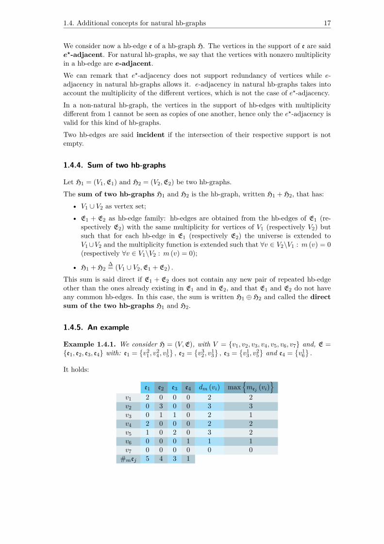
1.4. Additional concepts for natural hb-graphs 17
We consider now a hb-edge e of a hb-graph H. The vertices in the support of e are saide?-adjacent. For natural hb-graphs, we say that the vertices with nonzero multiplicityin a hb-edge are e-adjacent.We can remark that e?-adjacency does not support redundancy of vertices while e-adjacency in natural hb-graphs allows it. e-adjacency in natural hb-graphs takes intoaccount the multiplicity of the different vertices, which is not the case of e?-adjacency.In a non-natural hb-graph, the vertices in the support of hb-edges with multiplicitydifferent from 1 cannot be seen as copies of one another, hence only the e?-adjacency isvalid for this kind of hb-graphs.Two hb-edges are said incident if the intersection of their respective support is notempty.
1.4.4. Sum of two hb-graphs
Let H1 = (V1,E1) and H2 = (V2,E2) be two hb-graphs.The sum of two hb-graphs H1 and H2 is the hb-graph, written H1 + H2, that has:
• V1 ∪ V2 as vertex set;• E1 + E2 as hb-edge family: hb-edges are obtained from the hb-edges of E1 (re-
spectively E2) with the same multiplicity for vertices of V1 (respectively V2) butsuch that for each hb-edge in E1 (respectively E2) the universe is extended toV1∪V2 and the multiplicity function is extended such that ∀v ∈ V2\V1 : m (v) = 0(respectively ∀v ∈ V1\V2 : m (v) = 0);
• H1 + H2∆= (V1 ∪ V2,E1 + E2) .
This sum is said direct if E1 + E2 does not contain any new pair of repeated hb-edgeother than the ones already existing in E1 and in E2, and that E1 and E2 do not haveany common hb-edges. In this case, the sum is written H1 ⊕ H2 and called the directsum of the two hb-graphs H1 and H2.
1.4.5. An example
Example 1.4.1. We consider H = (V,E), with V = {v1, v2, v3, v4, v5, v6, v7} and, E ={e1, e2, e3, e4} with: e1 =
{v2
1, v24, v
15}, e2 =
{v3
2, v13}, e3 =
{v1
3, v25}and e4 =
{v1
6}.
It holds:
e1 e2 e3 e4 dm (vi) max{mej (vi)
}v1 2 0 0 0 2 2v2 0 3 0 0 3 3v3 0 1 1 0 2 1v4 2 0 0 0 2 2v5 1 0 2 0 3 2v6 0 0 0 1 1 1v7 0 0 0 0 0 0
#mej 5 4 3 1
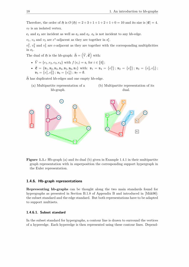
18 1. An introduction to hb-graphs
Therefore, the order of H is O (H) = 2 + 3 + 1 + 1 + 2 + 1 + 0 = 10 and its size is |E| = 4.v7 is an isolated vertex.e1 and e3 are incident as well as e3 and e2. e4 is not incident to any hb-edge.v1, v4 and v5 are e?-adjacent as they are together in e?1.
v21, v2
4 and v15 are e-adjacent as they are together with the corresponding multiplicities
in e1.
The dual of H is the hb-graph: H =(V , E
)with:
• V = {e1, e2, e3, e4} with f (ei) = ei for i ∈ J4K ;• E = {v1, v2, v3, v4, v5, v6, v7} with: v1 = v4 =
{e2
1}
; v2 ={e3
2}
; v3 ={e1
2, e13}
;v5 =
{e1
1, e23}
; v6 ={e1
4}
; v7 = ∅.H has duplicated hb-edges and one empty hb-edge.
(a) Multipartite representation of ahb-graph.
(b) Multipartite representation of itsdual.
v1
v5
v4
v2
v3
v7
v6
e1 e2
e3
e4
e1
e2
e3
e4
v1 v4
v5
v3
v2
v7
v6
Figure 1.1.: Hb-graph (a) and its dual (b) given in Example 1.4.1 in their multipartitegraph representation with in superposition the corresponding support hypergraph inthe Euler representation.
1.4.6. Hb-graph representations
Representing hb-graphs can be thought along the two main standards found forhypergraphs as presented in Section B.1.8 of Appendix B and introduced in [Mäk90]:the subset standard and the edge standard. But both representations have to be adaptedto support multisets.
1.4.6.1. Subset standard
In the subset standard for hypergraphs, a contour line is drawn to surround the verticesof a hyperedge. Each hyperedge is then represented using these contour lines. Depend-

1.4. Additional concepts for natural hb-graphs 19
ing on how their intersection is represented, we obtain a Venn diagram or an Eulerdiagram representation of the hypergraph. A Venn diagram systematically representseach possible intersection between hyperedges, while an Euler diagram addresses onlythe intersections that are needed for the representation. Hence, the Euler diagram isoften preferred as this representation scales up a bit better than the Venn diagram does;but neither representations scale up to large hypergraphs.When moving to multisets, a contour line is also drawn around the vertices that are nowduplicated. In [Rad15], two Venn diagram representations of multisets are proposed forthe representation of 2 and 3 multisets: a simplified representation where the parts arenot disjoint and a complex representation where the parts are disjoint. Scaling up thenumber of multisets seems to be hard to achieve. Euler representation of multisets canbe based on this work: a simplified and a complex representation can be drawn to depictonly the parts needed to be represented. It simplifies the Venn representation and helpsto scale up to somewhat larger hb-graphs.
1.4.6.2. Edge standard
For hypergraphs, there are two main representations in the edge standard: the cliquerepresentation and the extra-node representation, as presented in Section B.1.8. Theclique representation transforms the hypergraph in its 2-section graph joining every pairof vertices of a hyperedge by an edge, while the extra-node representation corresponds tothe incident graph—also called Levi graph—which is the graph obtained by representingeach hyperedge as an extra-vertex and joining it to each vertex of the correspondinghyperedge.For hb-graphs, the 2-section graph is always representable by considering each hb-edgesupport: but the quantity of information to display as well as its quality is not optimalin this representation.Hence, we propose other alternatives based on the extra-node representation. Each hb-edge is represented by an extra-node. For natural hb-graph a first representation calledthe extra-node multipartite representation is achieved by joining each vertex ofthe hb-edge to the extra node with a number of edges that corresponds to the vertexmultiplicity—which can be considered as a multipartite version of the incident graph ofthe hb-graph that takes into account the multiplicity of vertices through the number ofedges linking the vertex to the extra-node representing the hb-edge. This representationdoes not fit for non-natural hb-graphs; moreover, it is hard to scale up when the valuesof multiplicities increase. We give an example of such a representation in Figure 1.1using the hb-graph and its dual given in Example 1.4.1.For hb-graphs with non-negative multiplicity ranges, we propose a second representa-tion based on the extra-node representation of the support hypergraph, but where thethickness of the edges linking the vertices of the hb-edge with its extra-node are propor-tional either directly to the multiplicity (absolute version) or to the relative multiplicityof the vertex in the hb-edge (unnormalized version).The relative multiplicity of a vertex vi in a hb-edge ej is defined as:
mr ej (vi)∆=mej (vi)#mej
.
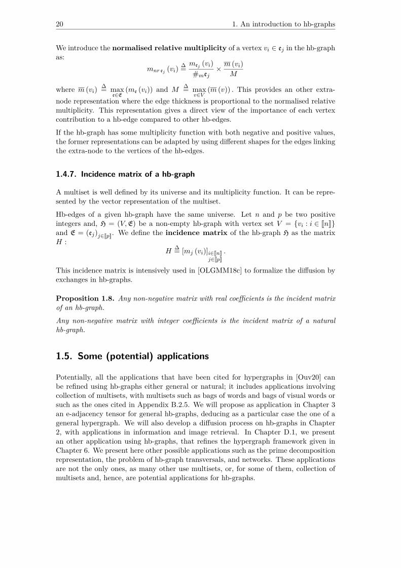
20 1. An introduction to hb-graphs
We introduce the normalised relative multiplicity of a vertex vi ∈ ej in the hb-graphas:
mnr ej (vi)∆=mej (vi)#mej
× m (vi)M
where m (vi)∆= max
e∈E(me (vi)) and M
∆= maxv∈V
(m (v)) . This provides an other extra-node representation where the edge thickness is proportional to the normalised relativemultiplicity. This representation gives a direct view of the importance of each vertexcontribution to a hb-edge compared to other hb-edges.
If the hb-graph has some multiplicity function with both negative and positive values,the former representations can be adapted by using different shapes for the edges linkingthe extra-node to the vertices of the hb-edges.
1.4.7. Incidence matrix of a hb-graph
A multiset is well defined by its universe and its multiplicity function. It can be repre-sented by the vector representation of the multiset.
Hb-edges of a given hb-graph have the same universe. Let n and p be two positiveintegers and, H = (V,E) be a non-empty hb-graph with vertex set V = {vi : i ∈ JnK}and E = (ej)j∈JpK. We define the incidence matrix of the hb-graph H as the matrixH :
H∆= [mj (vi)]i∈JnK
j∈JpK.
This incidence matrix is intensively used in [OLGMM18c] to formalize the diffusion byexchanges in hb-graphs.
Proposition 1.8. Any non-negative matrix with real coefficients is the incident matrixof an hb-graph.
Any non-negative matrix with integer coefficients is the incident matrix of a naturalhb-graph.
1.5. Some (potential) applications
Potentially, all the applications that have been cited for hypergraphs in [Ouv20] canbe refined using hb-graphs either general or natural; it includes applications involvingcollection of multisets, with multisets such as bags of words and bags of visual words orsuch as the ones cited in Appendix B.2.5. We will propose as application in Chapter 3an e-adjacency tensor for general hb-graphs, deducing as a particular case the one of ageneral hypergraph. We will also develop a diffusion process on hb-graphs in Chapter2, with applications in information and image retrieval. In Chapter D.1, we presentan other application using hb-graphs, that refines the hypergraph framework given inChapter 6. We present here other possible applications such as the prime decompositionrepresentation, the problem of hb-graph transversals, and networks. These applicationsare not the only ones, as many other use multisets, or, for some of them, collection ofmultisets and, hence, are potential applications for hb-graphs.

1.5. Some (potential) applications 21
1.5.1. Prime decomposition representation and elementary operations onhb-graphs
In [Cor04], a natural number network based on common divisors of two vertices isproposed to replace the search for real scale-free networks by the generation of a deter-ministic network that is also scale-free. Degrees of vertices are studied as well as theclustering coefficient and the average distance of vertices in the graph. Some topologicalproperties of such networks are addressed in [ZWHC06]. In [FCS12], the authors studythe page rank of an integer network built using a directed graph where the vertices arelabeled by non-negative integers; an edge links two vertices m and n if m divides n, mbeing different of 1 and n, with a weight k corresponding to the maximal k such thatmk divides n, i.e. the valuation of m in n. All these approaches are built using graphsand pairwise relationships.
As already mentioned, multisets can be used for prime decomposition ([Bli88]). In par-ticular, multisets are intensively used in [Tar14] to achieve primality decomposition ofnumbers and to achieve product, division, gcd and lcd of numbers. Using hb-graphs,we can revisit some of the results of [Tar14], and have a visual representation of si-multaneous decomposition of numbers interpretable in term of elementary operationsthat transform a hb-graph representation into another one. It should also induce somerefinement of results obtained with graphs since multisets handle not solely the multi-adic relationships that could have been achieved using sets, but also the hb-edge basedweighting of the divisors.
We focus on the prime decomposition of numbers. Considering the set P of primenumbers, any positive integer n greater or equal to 2 can be decomposed into a productof prime numbers: pi1 with multiplicity mn (i1) to pin with multiplicity mn (in) . Thisdecomposition is then uniquely described by the multiset: en =
{pmi1i1
, ..., pminin
}. The
prime decomposition hb-graph HP∆= (P,E) , is the hb-graph of universe P and of hb-
edges E∆= (en)n∈N\{0,1} that correspond to the prime decomposition of the integers
greater than 2. It contains all the possible natural multisets composed of elements of P.To represent this hb-graph, each extra-node is labeled by the corresponding number nwhich decomposition in prime numbers constitutes the multiset en =
{pmi1i1
, ..., pminin
}.
We consider a subset A of the hb-edges of HP and write HA∆= (P, A) the sub-hb-graph
of HP associated to A. We also consider elementary operations on the multipartiteextra-node representation of the natural hb-graphs constructed to switch between thedecomposition involved by the two integers and the prime decomposition of the results.We observed that these elementary operations are similar to the elementary operationsinvolved in the graph edit distance [GXTL10], albeit the fact that, with extra-nodes,some supplementary operations are possible: deletion of an edge, relabeling of an extra-node, deletion of an extra-node, merging of two extra-nodes.
The decomposition in primes of the product mn of two integers m and n is representedby a hb-edge emn of HP which is such that emn = em ] en. The multi-partite extra-noderepresentation of H{emn} is obtained from the one of H{em,en} by merging the two extra-nodes n and m of the en and em representations, while keeping all the existing edges oftheir respective representation. This is illustrated on an example in Figure 1.2.
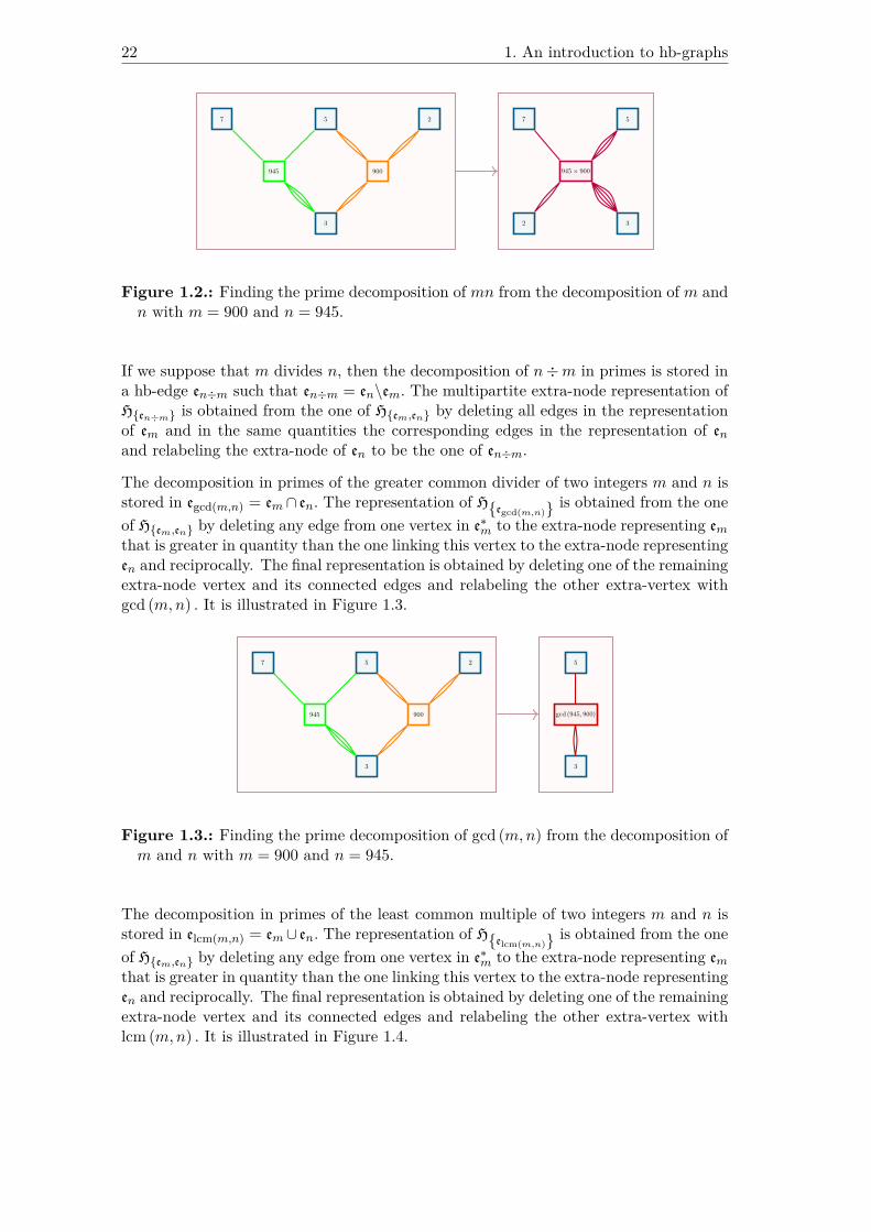
22 1. An introduction to hb-graphs
7 5 2
3
945 900
7 5
32
945× 900
Figure 1.2.: Finding the prime decomposition of mn from the decomposition of m andn with m = 900 and n = 945.
If we suppose that m divides n, then the decomposition of n÷m in primes is stored ina hb-edge en÷m such that en÷m = en\em. The multipartite extra-node representation ofH{en÷m} is obtained from the one of H{em,en} by deleting all edges in the representationof em and in the same quantities the corresponding edges in the representation of enand relabeling the extra-node of en to be the one of en÷m.
The decomposition in primes of the greater common divider of two integers m and n isstored in egcd(m,n) = em∩ en. The representation of H{egcd(m,n)} is obtained from the oneof H{em,en} by deleting any edge from one vertex in e∗m to the extra-node representing emthat is greater in quantity than the one linking this vertex to the extra-node representingen and reciprocally. The final representation is obtained by deleting one of the remainingextra-node vertex and its connected edges and relabeling the other extra-vertex withgcd (m,n) . It is illustrated in Figure 1.3.
7 5 2
3
945 900
5
3
gcd (945, 900)
Figure 1.3.: Finding the prime decomposition of gcd (m,n) from the decomposition ofm and n with m = 900 and n = 945.
The decomposition in primes of the least common multiple of two integers m and n isstored in elcm(m,n) = em∪ en. The representation of H{elcm(m,n)} is obtained from the oneof H{em,en} by deleting any edge from one vertex in e∗m to the extra-node representing emthat is greater in quantity than the one linking this vertex to the extra-node representingen and reciprocally. The final representation is obtained by deleting one of the remainingextra-node vertex and its connected edges and relabeling the other extra-vertex withlcm (m,n) . It is illustrated in Figure 1.4.

1.5. Some (potential) applications 23
7 5 2
3
945 900
7 5
32
lcm (945, 900)
Figure 1.4.: Finding the prime decomposition of lcm (m,n) from the decomposition ofm and n with m = 900 and n = 945.
We can then formulate the property:
mn = gcd(m,n)× lcm (m,n)
by using the hb-graphs H{emn} and H{egcd(m,n),elcm(m,n)}.
It holds: emn = egcd(m,n) ] elcm(m,n), which can be written: emn = (em ∩ en)] (em ∪ en) ,which can be easily observed on the results shown in Figure 1.2 and Figure 1.5.
7 5
32
lcm (945, 900) gcd (945, 900)
7 5
32
lcm (945, 900)×
gcd (945, 900)
Figure 1.5.: Illustrating the property lcm (m,n)× gcd (m,n) = mn with m = 900 andn = 945.
It follows that any connected natural hb-graph can be attached to a number by labelingvertices with prime numbers and multiplying successively the hb-edges by this number:in some way it makes a summary of this hb-graph. Finding the prime labeling such thatthe number the natural hb-graph represents is minimal is a NP-hard problem.Reciprocally, being given a number we can use its decomposition to create a collectionof hb-graphs that have this number as overall representation.
1.5.2. Graph pebbling and families of multisets
In [BBCH03], the authors use families of multisets to enounce analogs of two theoremson graph pebbling for multisets and improve some bounds on the random pebblingthreshold for sequence of paths in graphs. The authors consider a pebbling problem ongraphs in the following variant: from an initial pebble distribution on graph vertices,
24 1. An introduction to hb-graphs
they consider a vertex with two pebbles and move one of the pebbles to an adjacentvertex, with the aim of repeating the operation until only one pebble is remaining on apredetermined root vertex. All the configurations are not always solvable depending onthe number of pebbles distributed.
A classical variant of the pebble problem consists in moving labeled pebbles on a graphfrom a given configuration to an other one with a constraint on the maximal number ofpebbles that can be found on a vertex at any time. Pebble motion problems have ap-plications in multi-robot motion planning and network routing. Famous pebble motionproblems are sliding puzzles like the 15-puzzle. An other variation of a pebble problemhas been used in [ST09] to characterize the sparsity of hypergraphs. In [BS17], the au-thors use the former work to extract rigidity and flexibility information of bio-moleculesusing a phased pebble-game on a multi-graph that reflects the mechanical model of theatom-bond network.
One can, therefore, consider another variation of these problems solving some naturalhb-graph pebbling problems, such that pebbles occupy vertices of natural hb-graphswith allocated resources, that depends on the hb-edges the pebbles are coming from.This game would take into account the constraints that are depending on the hb-edgeitself to allocate resources on one of its vertex.
1.5.3. Chemical reaction networks and hb-graphs
As mentioned in [CTTV15], chemical reaction network (CRN for short) theory is atthe confluence of computer science and the study of interactions in natural sciencesand chemistry; it is also used as model for natural programming. CRN theory focuseson the kinetic of the various components involved in the reactions. The authors in[Gun03] use sets of multisets to model complexes of species; chemical reactions occuron complexes transforming a complex into another complex. Each chemical reactionis associated to a rate. The complexes of the chemical reaction network constitute ahb-graph of universe the entities and where the hb-edges represent the complexes. Thereactions can be seen as morphisms on this hb-graph, that are pondered with a rate.In [CTTV15], the authors focus on the kinetic of such networks with semantics basedon ordinary differential equations. In [LSP16], the states of the CRN are viewed asmultisets of species. Hence the reactions reflect the possibility to go from one state toanother. Succession of reactions are called traces and valid traces are the ones that arepossible, i.e. with sufficient reactant at each step.
A reaction can be seen as a replacement rule in the current multiset that is possibleonly if all its reactants are present in sufficient quantity in the hb-edge. Using directedhb-graphs over a universe, with a source and a target in each hb-edge, the reactions areviewed as directed hb-edges such that source and target are not overlapping multisets. Atrace is a transversal of the hb-graph of states by directed hb-edges such that each sourceof the reaction is a submset of the current state and the target state is a submset of thenew state, where the new state is written using operation on multisets: Sf = (Si\R)]P ,where R|P is the directed hb-edge of the reaction, Sf represents the final state and Sithe initial state.

1.5. Some (potential) applications 25
1.5.4. Multiset cover problems and hb-graph transversals
Set cover problems consist in covering a given set U with a set of subsets which unioncorresponds to the initial set U , using a minimum amount of those subsets: it is an NP-complete problem listed in Karp’s NP complete problems in [Kar72]. Different flavorsof this problem exist: some of them impose a covering of maximal size, some give a costto each subset or impose a maximal number of repetitions, imposing to each subset tohave a maximal covering capacity that should not be exceeded.In [RV93], the authors study the multiset multicover problem, similar to the set coverproblem, replacing subsets by sub-multisets to cover a multiset of N elements. Theysee the multisets as copy-sets and adapt the parallel algorithm given in the case of setsto give an approximation of the solution of the problem using a greedy multiset coveralgorithm. In [HYLW09], the authors describe a multiset multicover problem and givean exact algorithm to solve it in both cases i.e. without and with multiplicity constraintson the number of times the submset can be picked up. Multisets are viewed as copy-setsand transformed as such.The problem of hypergraph vertex covering, or known also as the problem of hypergraphtransversal is a well studied NP-hard problem—see for instance [EG95] that gives alsoapplications in database and model-based diagnosis. It consists in finding a minimal setof vertices that intersects each hyperedge. This is equivalent to the set cover problem asit is shown in [Hal02] by considering the dual hypergraph: the set to cover is constitutedin this case of the—non-repeated—hyperedges and the subsets that are at the basis ofthe covering corresponds to the dual hypergraph hyperedges, which contain the incidentoriginal hypergraph hyperedges of each vertex. In [SK12], the authors propose an ap-proximation algorithm to handle hypergraph cover with hard capacities, which is seenas analogous to consider set systems with constrained belongings. Hypergraph mini-mal transversal is fruitful in data mining. A recent application occurs in the frequentitem-set hiding problem in [SVK16] and security in [RKS17].Hence, for hb-graphs the problem of vertex covering can be seen as an extension ofthe hypergraph transversal problem to a minimal multiset of vertices that intersecteach hb-edge and is similarly equivalent to the multiset cover problem by consideringthe dual hb-graph: the multiset to cover is the one of the hb-edges and the family ofmultisets used for the covering corresponds to the dual hb-edges, attached to each vertexof the original incident hb-edges. This kind of problems can be linked to constrainedoptimization problems of fuzzy relational equations [HF11] and relates to set coverproblems as it is mentioned in [CW02] and in [Mar05].
1.5.5. Networks
1.5.5.1. Computer networks
Byzantine-fault problems often consider some multisets for representing the informationcollected by one agent in the network as in [MHVG15]. In [Geo17], multisets are usedto model beliefs of agents and also desirable believes.Hb-graphs can definitively model this kind of interaction between agents, even giving away to encode additional information that sets cannot capture.
26 1. An introduction to hb-graphs
1.5.5.2. Neural networks
In [XHLJ18], the authors use multisets in graph neural networks, to focus on the neigh-borhood. In graph neural networks, the aim is to learn the graph through the neuralnetwork by a recursive neighborhood aggregation, where the information of the neigh-borhood of the node contained in different vectors is aggregated to create its own featurevector. The authors propose to model this neighborhood using multisets combined withsome convenient function.
Hypergraph neural networks that encode higher order relationships are proposed in[FYZ+19] and are shown to overtake classical methods.
Learning hb-graph through neural networks can, therefore, open up a wide range ofapplications, since it could also capture the multiplicity of elements.
1.6. Further comments on hb-graphs
Shifting to hb-graphs is not only a change in modeling for visualisation: it is also ameans to refine any network in which hb-edge-based individual weighting of vertices isrequired. Natural hb-graphs constitute a new category, as it is shown in Appendix C.2.
We have already shown in [OLGMM18c] that diffusion by exchange in hb-graphs—asit will be presented in Chapter 2—provides a fine ranking not only of vertices but alsoof hb-edges. We think that extending the definitions of hb-graphs to support negativemultiplicities or even complex values could open the door to yet a wider variety ofapplications.
We can foresee many applications of hb-graphs, as they give the best of several worlds:multisets, sets, graphs, and, also, as we will see in the Chapter 3, algebraic and polyno-mial approaches. Natural hb-graphs support the duplication of elements, while generalhb-graphs allow the weighting of elements in a refined manner with respect to hyper-graphs.

2. Diffusion in hb-graphs (matrix approach)
Highlights
2.1. Motivation . . . . . . . . . . . . . . . . . . . . . . . . . . . . . . . . . . 27
2.2. Related work . . . . . . . . . . . . . . . . . . . . . . . . . . . . . . . . . 28
2.3. Exchange-based diffusion in hb-graphs . . . . . . . . . . . . . . . . . . . 29
2.4. Results and evaluation . . . . . . . . . . . . . . . . . . . . . . . . . . . . 37
2.5. Future work and Conclusion . . . . . . . . . . . . . . . . . . . . . . . . . 51
This chapter is based on [OLGMM19a], which is an extension of [OLGMM18c].
Prerequisites: Section 1.3.
2.1. Motivation
Highlighting important information in networks is commonly achieved using randomwalks. In 1905, Pearson was using the idea of random walk to model a population ofmosquitoes in a forest; previously, Rayleigh studied acoustic waves using random walks.The term itself was introduced by Polya during the 1920s. A random walk is a stochasticprocess related to a Markov chain. A random walk is a succession of steps, of eventuallyconstant length, executed in a random manner regarding the direction and the lengthof the walk. Constrained to a network structure, the random walker is supposed torandomly move from a vertex to a neighborhood vertex.
Random walks, by the phenomena involved, are tied up to diffusion over the structure,and have been largely used to retrieve centrality of information in graphs. Randomwalks have had a revival of interest since the raise of Internet. They are at the originof the PageRank algorithm developed by Google to rank websites [PBMW99].
Random walks on hypergraphs and diffusion have also been well studied since [ZHS07];in [BAD13], the authors show that the weighting of vertices at the level of the hyperedgesin a hypergraph provides better information retrieval. These two approaches—[ZHS07,BAD13]—mainly focus on vertices. But, more generally, as hb-edges of a hb-graph arelinked to references that can be used as pivots in between the different facets as shownin Chapter 6, it is also interesting to highlight important hb-edges. Hence, the followingresearch question:

28 2. Diffusion in hb-graphs (matrix approach)
Research question 2.1. Can we find a diffusion process that not only ranks verticesbut also ranks hb-edges in hb-graphs?
We start by reviewing existing work, and propose a model of diffusion on the hb-graph,that is exchange-based: this process requires two-phase steps. We then evaluate thisframework with generated data and apply it to two real data frameworks, one based onqueries over Arxiv database.
2.2. Related work
Random walks are largely used to evaluate the importance of vertices in networks, eitherseen as graphs or as hypergraphs. In [Lo93], a survey is achieved on random walks ongraphs; it includes connections with eigenvalues of the adjacency matrix of graphs aswell as estimates on important features such as access time and cover time. Randomwalks are closely related to diffusion processes.
Diffusion kernels have been introduced in [KL02]: they are shown to be efficient on dif-ferent kinds of graphs. In [BN03], the authors build a neighboring weighted graph usinga truncated heat kernel to weight the proximity of two vertices, and achieve nonlineardimensionality reduction preserving the local properties. In [MYLK08], the authorsuse a heat diffusion process for marketing candidates selection in social networks, and,in [MKL11], for mining web graphs for recommendations. In [TDKF17], the authorsuses a sum of heat diffusion processes to learn about the hidden graph structure. Theinterested reader can refer to the extensive survey on random walks and diffusion overnetworks done in [MPL17].
In [ZHS07], a random walk on a hypergraph is defined by choosing a hyperedge ej witha probability proportional to we (ej) , and within that hyperedge a vertex is randomlychosen using a uniform law. The probability transition from a vertex vi1 to a vertex vi2is:
p(vi1 , vi2) =∑j∈JpK
we (ej)hi1jdi1× hi2j
δj,
where δj = deg (ej) , j ∈ JpK is the degree of a hyperedge defined in [ZHS07] as itscardinality. This random walk has a stationary state which is shown to be π = (πi)i∈JnK
with πi = divolV for i ∈ JnK—[DB14]. This process differs from the one we propose: our
diffusion process is done in successive steps on vertices and hyperedges from a randominitial vertex.
In [BAD13], the authors define a random walk for weighted hypergraphs using weightfunctions both for hyperedges and vertices: for each vertex, a vector of weights is builtmaking weights of vertices hyperedge-based; a random walk similar to the one above isthen built that takes into account the vertex weight. The evaluation is performed on ahypergraph built from a public dataset of computer science conference proceedings; eachdocument is seen as a hyperedge that contains keywords; hyperedges are weighted bycitation score and vertices of a hyperedge are weighted with a tf-idf score. In [BAD13],the authors show that a random walk on the (double-) weighted hypergraph enablesvertex ranking with higher precision than random walks using unweighted vertices.
2.3. Exchange-based diffusion in hb-graphs 29
This process differs also from our proposal: our process not only enables simultaneousalternative updates of vertices and hb-edges values but also provides hb-edge ranking.We also introduce a new theoretical framework to perform our diffusion process.Random walks relate to diffusion processes. Diffusion processes are extensively used forinformation retrieval: [DB13] is an extensive survey on the subject. More particularly,random walks are used with hypergraphs for image matching—[LCL11]. Higher orderrandom walks in hypergraph are built in [LP11], where a generalised Laplacian attachedto the graphs generated from these random walks is constructed. In [GMM+13], theauthors propose a co-occurrence based diffusion for expert search on the web: the modeluses the heat diffusion over a heterogeneous co-occurrence network—composed of co-occurrences of persons and keywords—that is reduced to its 2-section when enabling thediffusion, considering hyperedge-based weighting of vertices, i.e. a hb-graph structure.They achieve good performances on retrieval of the experts on ground truth datasets. In[MSCM16], the authors propose a multi-scale hypergraph framework for image annota-tion, that exploits the eigenvalues of the hypergraph Laplacian matrix in the definitionof the heat kernel. This latter includes a parameter to tune the scale of propagation ofthe labels in order to solve the problem of class imbalance in the data.
2.3. Exchange-based diffusion in hb-graphs
Diffusion processes result in homogenising information over a structure; an initial strokeis done on a vertex that propagates over the network structure. This propagation is oftenmodeled by a random walk on the network. Random walks in hypergraphs rank verticesby the number of times they are reached, and this ranking is related to the networkstructure itself. Several random walks with random choices for the starting vertex areneeded to achieve a ranking by averaging. Moreover, to avoid loops, teleportation ofvertices is needed.We consider a weighted hb-graph H = (V,E, we) with |V | = n and |E| = p; we write Hthe incidence matrix of the hb-graph.At time t, we set a distribution of values over the vertex set:
αt :{
V → Rvi 7→ αt (vi)
.
and a distribution of values over the hb-edge set:
εt :{
E→ Rej 7→ εt (ej)
.
We write PV,t = (αt (vi))i∈JnK the row state vector of the vertices at time t and PE,t =(εt (ej))j∈JpK the row state vector of the hb-edges.
The initialisation is done such that ∑vi∈V
α0 (vi) = 1 and the information value is con-
centrated uniformly on the vertices at the beginning of the diffusion process and, con-sequently, each hb-edge has a zero value associated to it. Writing αref = 1
|V |, we set for
all vi ∈ V : α0 (vi) = αref and for all ej ∈ E, ε (ej) = 0.
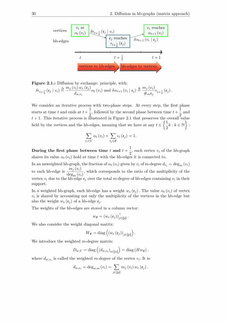
30 2. Diffusion in hb-graphs (matrix approach)
t t+ 12 t+ 1
vertices to hb-edges hb-edges to vertices
vertices vi atαt (vi) δεt+ 1
2(ej | vi)
ej reachesεt+ 1
2(ej)
δαt+1 (vi | ej)
vi reachesαt+1 (vi)
hb-edges
Figure 2.1.: Diffusion by exchange: principle, with:δεt+ 1
2(ej | vi)
∆= mj (vi)we (ej)dw,vi
αt (vi) and δαt+1 (vi | ej)∆= mj (vi)
#mejεt+ 1
2(ej) .
We consider an iterative process with two-phase steps. At every step, the first phasestarts at time t and ends at t+ 1
2 , followed by the second phase between time t+ 12 and
t+ 1. This iterative process is illustrated in Figure 2.1 that preserves the overall valueheld by the vertices and the hb-edges, meaning that we have at any t ∈
{12k : k ∈ N
}:
∑vi∈V
αt (vi) +∑ej∈E
εt (ej) = 1.
During the first phase between time t and t + 12 , each vertex vi of the hb-graph
shares its value αt (vi) hold at time t with the hb-edges it is connected to.In an unweighted hb-graph, the fraction of αt (vi) given by vi of m-degree dvi = degm (vi)
to each hb-edge is mj (vi)degm (vi)
, which corresponds to the ratio of the multiplicity of thevertex vi due to the hb-edge ej over the total m-degree of hb-edges containing vi in theirsupport.In a weighted hb-graph, each hb-edge has a weight we (ej) . The value αt (vi) of vertexvi is shared by accounting not only the multiplicity of the vertices in the hb-edge butalso the weight we (ej) of a hb-edge ej .
The weights of the hb-edges are stored in a column vector:
wE = (we (ej))>j∈JpK .
We also consider the weight diagonal matrix:
WE = diag((we (ej))j∈JpK
).
We introduce the weighted m-degree matrix:
Dw,V = diag((dw,vi)i∈JnK
)= diag (HwE) .
where dw,vi is called the weighted m-degree of the vertex vi. It is:
dw,vi = degw,m (vi) =∑j∈JpK
mj (vi)we (ej) .
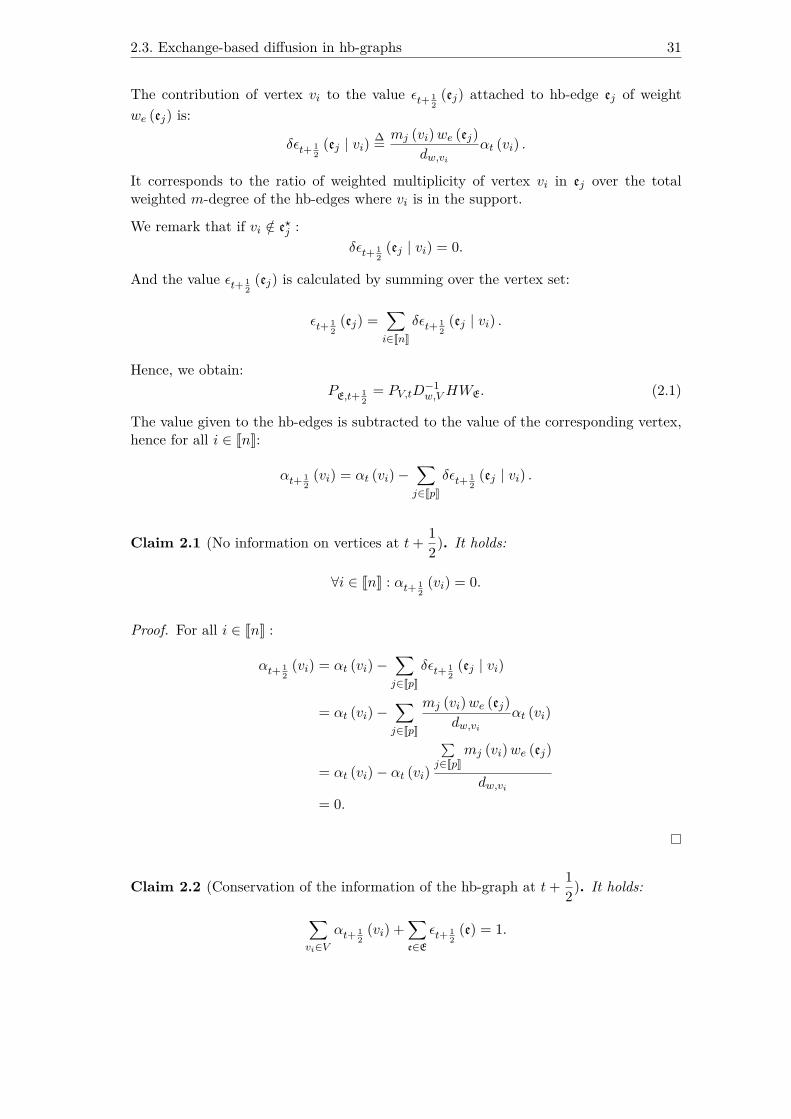
2.3. Exchange-based diffusion in hb-graphs 31
The contribution of vertex vi to the value εt+ 12
(ej) attached to hb-edge ej of weightwe (ej) is:
δεt+ 12
(ej | vi)∆= mj (vi)we (ej)
dw,viαt (vi) .
It corresponds to the ratio of weighted multiplicity of vertex vi in ej over the totalweighted m-degree of the hb-edges where vi is in the support.
We remark that if vi /∈ e?j :δεt+ 1
2(ej | vi) = 0.
And the value εt+ 12
(ej) is calculated by summing over the vertex set:
εt+ 12
(ej) =∑i∈JnK
δεt+ 12
(ej | vi) .
Hence, we obtain:PE,t+ 1
2= PV,tD
−1w,VHWE. (2.1)
The value given to the hb-edges is subtracted to the value of the corresponding vertex,hence for all i ∈ JnK:
αt+ 12
(vi) = αt (vi)−∑j∈JpK
δεt+ 12
(ej | vi) .
Claim 2.1 (No information on vertices at t+ 12). It holds:
∀i ∈ JnK : αt+ 12
(vi) = 0.
Proof. For all i ∈ JnK :
αt+ 12
(vi) = αt (vi)−∑j∈JpK
δεt+ 12
(ej | vi)
= αt (vi)−∑j∈JpK
mj (vi)we (ej)dw,vi
αt (vi)
= αt (vi)− αt (vi)
∑j∈JpK
mj (vi)we (ej)
dw,vi
= 0.
Claim 2.2 (Conservation of the information of the hb-graph at t+ 12). It holds:∑
vi∈Vαt+ 1
2(vi) +
∑e∈E
εt+ 12
(e) = 1.

32 2. Diffusion in hb-graphs (matrix approach)
Proof. We have:∑vi∈V
αt+ 12
(vi) +∑e∈E
εt+ 12
(e) =∑ej∈E
εt+ 12
(ej)
=∑ej∈E
∑i∈JnK
δεt+ 12
(ej | vi)
=∑ej∈E
∑i∈JnK
mj (vi)we (ej)dw,vi
αt (vi)
=∑i∈JnK
αt (vi)
∑ej∈E
mj (vi)we (ej)
dw,vi
=∑i∈JnK
αt (vi)
= 1.
During the second phase which starts at time t + 12 , the hb-edges share their
values across the vertices they hold taking into account the vertex multiplicities in thehb-edge.
The contribution to αt+1 (vi) given by a hb-edge ej is proportional to εt+ 12in a factor
corresponding to the ratio of the multiplicity mj (vi) of the vertex vi to the hb-edgem-cardinality:
δαt+1 (vi | ej)∆= mj (vi)
#mejεt+ 1
2(ej) .
The value αt+1 (vi) is then obtained by summing on all values associated to the hb-edgesthat are incident to vi :
αt+1 (vi) =∑j∈JpK
δαt+1 (vi | ej) .
Writing DE = diag((#mej)j∈JpK
)the diagonal matrix of size p× p, it comes:
PE,t+ 12D−1
E H> = PV,t+1. (2.2)
The values given to the vertices are subtracted to the value associated to the corre-sponding hb-edge. Hence, for all j ∈ JpK :
εt+1 (ej) = εt+ 12
(ej)−∑i∈JnK
δαt+1 (vi | ej) .
Claim 2.3 (The hb-edges have 0 value at t+ 1). It holds:
εt+1 (ej) = 0.
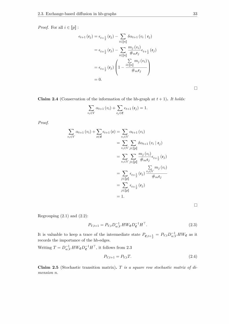
2.3. Exchange-based diffusion in hb-graphs 33
Proof. For all i ∈ JpK :
εt+1 (ej) = εt+ 12
(ej)−∑i∈JnK
δαt+1 (vi | ej)
= εt+ 12
(ej)−∑i∈JnK
mj (vi)#mej
εt+ 12
(ej)
= εt+ 12
(ej)
1−
∑i∈JnK
mj (vi)
#mej
= 0.
Claim 2.4 (Conservation of the information of the hb-graph at t+ 1). It holds:∑vi∈V
αt+1 (vi) +∑ej∈E
εt+1 (ej) = 1.
Proof. ∑vi∈V
αt+1 (vi) +∑e∈E
εt+1 (e) =∑vi∈V
αt+1 (vi)
=∑vi∈V
∑j∈JpK
δαt+1 (vi | ej)
=∑vi∈V
∑j∈JpK
mj (vi)#mej
εt+ 12
(ej)
=∑j∈JpK
εt+ 12
(ej)
∑vi∈V
mj (vi)
#mej
=∑j∈JpK
εt+ 12
(ej)
= 1.
Regrouping (2.1) and (2.2):
PV,t+1 = PV,tD−1w,VHWED
−1E H>. (2.3)
It is valuable to keep a trace of the intermediate state PE,t+ 12
= PV,tD−1w,VHWE as it
records the importance of the hb-edges.Writing T = D−1
w,VHWED−1E H>, it follows from 2.3
PV,t+1 = PV,tT. (2.4)
Claim 2.5 (Stochastic transition matrix). T is a square row stochastic matrix of di-mension n.

34 2. Diffusion in hb-graphs (matrix approach)
Proof. Let consider: A = (aij)i∈JnKj∈JpK
= D−1w,VHWE ∈ Mn,p and B = (bjk)j∈JpK
k∈JnK=
D−1E H> ∈Mp,n.
A and B are non-negative rectangular matrices. Moreover:
aij = mj (vi)we (ej)dw,vi
and, it holds:∑j∈JpK
aij =
∑j∈JpK
mj (vi)we (ej)
dw,vi= 1.
bjk = mj (vk)#m (ej)
and it holds:
∑k∈JnK
bjk =
∑k∈JnK
mj (vk)
#mej= 1.
We have PV,t+1 = PV,tAB where AB =( ∑j∈JpK
aijbjk
)i∈JnKk∈JnK
.
It yields: ∑k∈JnK
∑j∈JpK
aijbjk =∑j∈JpK
aij∑k∈JnK
bjk
=∑j∈JpK
aij
= 1.
Hence AB is a non-negative square matrix with its row sums all equal to 1: it is a rowstochastic matrix.
Claim 2.6 (Properties of T). Supposing that the hb-graph is connected, the exchange-based diffusion matrix T is aperiodic and irreducible.
Proof. This stochastic matrix is aperiodic, due to the fact that any vertex of the hb-graph retrieves a part of the value it has given to the hb-edge, hence tii > 0 for alli ∈ JnK.Moreover, as the hb-graph is connected, the matrix is irreducible as every state can bejoined from any other state.
Claim 2.7. The sequence (PV,t)t∈N , with PV,t = (αt (vi))i∈JnK , in a connected hb-graphconverges to the state vector πV such that:
πV =
dw,vi∑k∈JnK
dw,vk
i∈JnK
.
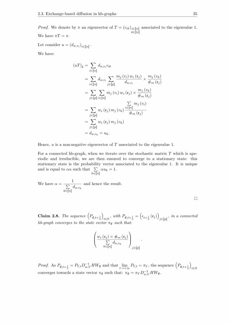
2.3. Exchange-based diffusion in hb-graphs 35
Proof. We denote by π an eigenvector of T = (cik) i∈JnKk∈JnK
associated to the eigenvalue 1.
We have πT = π.
Let consider u = (dw,vi)i∈JnK .
We have:
(uT )k =∑i∈JnK
dw,vicik
=∑i∈JnK
dw,vi∑j∈JpK
mj (vi)we (ej)dw,vi
× mj (vk)#m (ej)
=∑j∈JpK
∑i∈JnK
mj (vi)we (ej)×mj (vk)#m (ej)
=∑j∈JpK
we (ej)mj (vk)
∑i∈JnK
mj (vi)
#m (ej)
=∑j∈JpK
we (ej)mj (vk)
= dw,vk = uk.
Hence, u is a non-negative eigenvector of T associated to the eigenvalue 1.
For a connected hb-graph, when we iterate over the stochastic matrix T which is ape-riodic and irreducible, we are then ensured to converge to a stationary state: thisstationary state is the probability vector associated to the eigenvalue 1. It is uniqueand is equal to αu such that ∑
k∈JnKαuk = 1.
We have α = 1∑k∈JnK
dw,vkand hence the result.
Claim 2.8. The sequence(PE,t+ 1
2
)t∈N
, with PE,t+ 12
=(εt+ 1
2(ej)
)j∈JpK
, in a connectedhb-graph converges to the state vector πE such that:
we (ej)×#m (ej)∑k∈JnK
dw,vk
j∈JpK
.
Proof. As PE,t+ 12
= PV,tD−1w,VHWE and that lim
t→+∞PV,t = πV , the sequence
(PE,t+ 1
2
)t∈N
converges towards a state vector πE such that: πE = πVD−1w,VHWE.

36 2. Diffusion in hb-graphs (matrix approach)
We have:
πE =
∑i∈JnK
dw,vi∑k∈JnK
dw,vk× mj (vi)× we (ej)
dw,vi
j∈JpK
=
∑i∈JnK
mj (vi)× we (ej)∑k∈JnK
dw,vk
j∈JpK
=
we (ej)×∑i∈JnK
mj (vi)∑k∈JnK
dw,vk
j∈JpK
=
we (ej)×#m (ej)∑k∈JnK
dw,vk
j∈JpK
.
All components are non-negative and we check that the components of this vector sumto one:
∑j∈JpK
πE,j =
∑j∈JpK
we (ej)×∑i∈JnK
mj (vi)∑k∈JnK
dw,vk
=
∑i∈JnK
∑j∈JpK
we (ej)×mj (vi)∑k∈JnK
dw,vk
=
∑i∈JnK
dw,vi∑k∈JnK
dw,vk
= 1.
These two claims show that this exchange-based process ranks vertices by their weightedm-degree and hb-edges by their weighted m-cardinality.
We have gathered the two-phase steps of the exchange-based diffusion process in Al-gorithm 2.1. The time complexity of this algorithm is O (T (dHn+ rHp)) where dH =maxvi∈V
(di) is the maximal degree of vertices in the hb-graph and rH = maxej∈E
∣∣∣e?j ∣∣∣ is themaximal cardinality of the support of a hb-graph. Usually, dH and rH are small com-pared to n and p. Algorithm 2.1 can be refined to determine automatically the numberof iterations needed, fixing an accepted error to ensure convergence on the values of thevertices and storing the previous state.
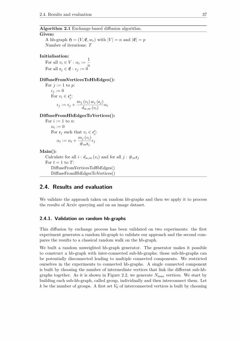
2.4. Results and evaluation 37
Algorithm 2.1 Exchange-based diffusion algorithm.Given:
A hb-graph H = (V,E, we) with |V | = n and |E| = pNumber of iterations: T
Initialisation:For all vi ∈ V : αi := 1
nFor all ej ∈ E : εj := 0
DiffuseFromVerticesToHbEdges():For j := 1 to p:εj := 0For vi ∈ e?j :
εj := εj + mj (vi)we (ej)dw,m (vi)
αi
DiffuseFromHbEdgesToVertices():For i := 1 to n:αi := 0For ej such that vi ∈ e?j :
αi := αi + mj (vi)#mej
εj
Main():Calculate for all i : dw,m (vi) and for all j : #mejFor t = 1 to T :
DiffuseFromVerticesToHbEdges()DiffuseFromHbEdgesToVertices()
2.4. Results and evaluation
We validate the approach taken on random hb-graphs and then we apply it to processthe results of Arxiv querying and on an image dataset.
2.4.1. Validation on random hb-graphs
This diffusion by exchange process has been validated on two experiments: the firstexperiment generates a random hb-graph to validate our approach and the second com-pares the results to a classical random walk on the hb-graph.We built a random unweighted hb-graph generator. The generator makes it possibleto construct a hb-graph with inter-connected sub-hb-graphs; those sub-hb-graphs canbe potentially disconnected leading to multiple connected components. We restrictedourselves in the experiments to connected hb-graphs. A single connected componentis built by choosing the number of intermediate vertices that link the different sub-hb-graphs together. As it is shown in Figure 2.2, we generate Nmax vertices. We start bybuilding each sub-hb-graph, called group, individually and then interconnect them. Letk be the number of groups. A first set V0 of interconnected vertices is built by choosing

38 2. Diffusion in hb-graphs (matrix approach)
N0 vertices out of the Nmax. The remaining Nmax−N0 vertices are then separated into ksubsets (Vj)j∈JkK . In each of these k groups Vj , we generate two subsets of vertices: a firstset Vj,1 of Nj,1 vertices and, a second set Vj,2 of Nj,2 vertices with Nj,1 � Nj,2, j ∈ JkK .The number of hb-edges to be built is adjustable: their number is shared between thedifferent groups. The m-cardinality #m (e) of a hb-edge is chosen randomly below amaximum tunable threshold. The Vj,1 vertices are considered as important vertices andmust be present in a certain number of hb-edges per group; the number of importantvertices in a hb-edge is randomly fixed below a maximum number. The completion ofthe hb-edge is done by choosing vertices randomly in the Vj,2 set. The random choicemade into these two groups is tuned to follow a power law distribution. It implies thatsome vertices occur more often than others. Interconnection between the k componentsis achieved by choosing vertices in V0, and inserting them randomly into the hb-edgesbuilt.
Nmax vertices are generated
V0 V1 Vj VjVk
Nj,1important vertices
Nj,2remaining vertices
N0 interconnected vertices Nmax −N0 vertices in k groups
Nj,1 � Nj,2
Figure 2.2.: Random hb-graph generation principle.
We apply the exchange-based diffusion process on this generated hb-graph: after afew iterations, we visualize the hb-graph to observe the evolution of the vertex valuesusing a gradient coloring scale. We also take advantage of the first phase of each stepto highlight hb-edges in the background, and show hb-edge importance using anothergradient coloring scale.To get proper evaluation and show that vertices with the highest α-values correspondto the important vertices of the network—in the sense of being central for the connec-tivity—, we compute the eccentricity of vertices from a subset S of the vertex set V tothe remaining V \S of the vertices. The eccentricity of a vertex in a graph is the lengthof a maximal shortest path between this vertex and the other vertices of this graph:extending this definition to hb-graphs is straightforward. If the graph is disconnected,then each vertex has infinite eccentricity.For the purpose of evaluation, in this Thesis, we define a relative eccentricity as thelength of a maximal shortest path starting from a given vertex in S and ending with anyvertices of V \S. The relative eccentricity is calculated for each vertex of S provided thatit is connected to vertices of V \S; otherwise, it is set to −∞. The concept of relativeeccentricity is illustrated in Figure 2.3.For the vertex set V, the subset used for relative eccentricity is built by using a thresholdvalue sV : vertices with α value above this threshold are gathered into a subset AV (sV )of V. We consider BV (sV ) ∆= V \AV (sV ) , the set of vertices with α values below this
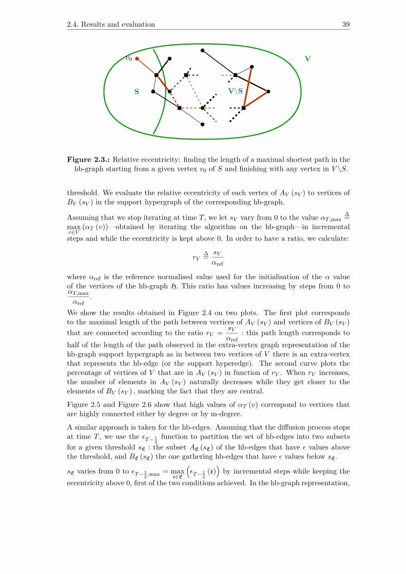
2.4. Results and evaluation 39
V
S V\S
v0
Figure 2.3.: Relative eccentricity: finding the length of a maximal shortest path in thehb-graph starting from a given vertex v0 of S and finishing with any vertex in V \S.
threshold. We evaluate the relative eccentricity of each vertex of AV (sV ) to vertices ofBV (sV ) in the support hypergraph of the corresponding hb-graph.
Assuming that we stop iterating at time T, we let sV vary from 0 to the value αT,max∆=
maxv∈V
(αT (v))—obtained by iterating the algorithm on the hb-graph—in incrementalsteps and while the eccentricity is kept above 0. In order to have a ratio, we calculate:
rV∆= sVαref
where αref is the reference normalised value used for the initialisation of the α valueof the vertices of the hb-graph H. This ratio has values increasing by steps from 0 toαT,maxαref
.
We show the results obtained in Figure 2.4 on two plots. The first plot correspondsto the maximal length of the path between vertices of AV (sV ) and vertices of BV (sV )that are connected according to the ratio rV = sV
αref: this path length corresponds to
half of the length of the path observed in the extra-vertex graph representation of thehb-graph support hypergraph as in between two vertices of V there is an extra-vertexthat represents the hb-edge (or the support hyperedge). The second curve plots thepercentage of vertices of V that are in AV (sV ) in function of rV . When rV increases,the number of elements in AV (sV ) naturally decreases while they get closer to theelements of BV (sV ) , marking the fact that they are central.
Figure 2.5 and Figure 2.6 show that high values of αT (v) correspond to vertices thatare highly connected either by degree or by m-degree.
A similar approach is taken for the hb-edges. Assuming that the diffusion process stopsat time T , we use the εT− 1
2function to partition the set of hb-edges into two subsets
for a given threshold sE : the subset AE (sE) of the hb-edges that have ε values abovethe threshold, and BE (sE) the one gathering hb-edges that have ε values below sE.
sE varies from 0 to εT− 12 ,max = max
e∈E
(εT− 1
2(e))by incremental steps while keeping the
eccentricity above 0, first of the two conditions achieved. In the hb-graph representation,

40 2. Diffusion in hb-graphs (matrix approach)
0 2 4 6 8 103.0
3.5
4.0
4.5
5.0
5.5
6.0
maxPath
0
20
40
60
80
100
percentOfNodesAboveRatio
rV
Figure 2.4.: Maximum path length and percentage of vertices in AV (s) over verticesin V vs ratio rV .
each hb-edge corresponds to an extra-vertex. Each time, we evaluate the length of themaximal shortest path linking one vertex of AE (sE) to one vertex of BE (sE) for theconnected vertices in the hb-graph support hypergraph incident graph: the length ofthe path corresponds to half of the one obtained from the graph for the same reasonthan before.
We define the ratio:rE
∆= sEβref
where βref∆= 1|E|
that corresponds to the normalised value that would be used in thedual hb-graph to initialize the diffusion process. In Figure 2.7, we observe for the hb-edges the same trend than the one observed for vertices: the length of the maximalshortest path between a hb-edge of AE (sE) and any hb-edge of BE (sE) decreases as theratio rE increases, while the percentage of hb-edges in AE (sE) over E decreases.
Figure 2.8 shows the high correlation between the value of ε(e) and the cardinality of e;Figure 2.9 shows that the correlation between value of ε(e) and the m-cardinality of eis even stronger.
The number of iterations needed to have a significant convergence depends on the initialconditions; we tried different initializations, either uniform, or applying some strokeson a different number of nodes. We observed that the more uniform the informationon the network is, the less number of iterations for convergence is needed. No matterthe configuration, the most important vertices in term of connectivity are always themost highlighted. Figure 2.10 and in Figure 2.11 depict the convergence observed on auniform initial distribution as described in the former section. In Figure 2.10, we can seehow the α-values, as observed in Figure 2.5, reflect the m-degree of the vertex they areassociated to: 200 iterations is far enough to rank the vertices by m-degree. In Figure2.11, we can observe an analogous phenomena with the ε-value associated to hb-edgesthat reflect the m-cardinality of the hb-edges. Again 200 iterations are sufficient toconverge in studied cases.
2.4. Results and evaluation 41
0.0 2.5 5.0 7.5 10.0 12.5 15.0 17.5 20.0deg(v)
0
2
4
6
8
10
12
14
α 200(v)
correlation: 0.989
Figure 2.5.: Alpha value of vertices at step 200 and degree of vertices.
0 5 10 15 20 25degm(v)
0
2
4
6
8
10
12
14
α 200(v)
correlation: 1.0
Figure 2.6.: Alpha value of vertices at step 200 and m-degree of vertices.
The number of iterations needed to converge depends on the structure of the network.In the transitory phase, the vertices need to exchange with the hb-edges; the processrequires some iterations before converging and its behavior depends on the node con-nectivity and the hb-edge composition. It remains as an open question to investigate onthis transitory phase to have more indications on the way the ε and the α-values vary.We show an example of exchange-based diffusion on a lab-generated hb-graph in Figure2.12 (a) and on its support hypergraph in Figure 2.12 (b). The vertices are coloreddepending on the value of the ratio:
cα (v) ∆= αT (v)αref
using the scale of colors on the right. Vertices with near zero cα (v) values—i.e. lowαT (v) values compared to αref—are dark bluish colored; on the opposite, with highcα (v) values—i.e. with high αT (v) values compared to αref—are yellowish colored; when
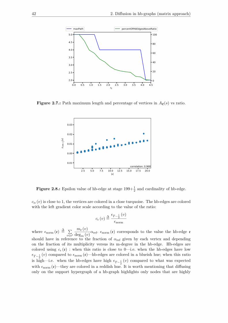
42 2. Diffusion in hb-graphs (matrix approach)
0.0 0.5 1.0 1.5 2.0 2.5 3.0 3.5 4.0 4.52.0
2.5
3.0
3.5
4.0
4.5
5.0
maxPath
0
20
40
60
80
100
percentOfHbEdgesAboveRatio
rE
Figure 2.7.: Path maximum length and percentage of vertices in AE(s) vs ratio.
2.5 5.0 7.5 10.0 12.5 15.0 17.5 20.0|�|
−0.01
0.00
0.01
0.02
0.03
ε 199
+1 2(�)
correlation: 0.968
Figure 2.8.: Epsilon value of hb-edge at stage 199+12 and cardinality of hb-edge.
cα (v) is close to 1, the vertices are colored in a close turquoise. The hb-edges are coloredwith the left gradient color scale according to the value of the ratio:
cε (v) ∆=εT− 1
2(v)
εnorm
where εnorm (e) ∆= ∑v∈e?
me (v)degm (v)αref. εnorm (e) corresponds to the value the hb-edge e
should have in reference to the fraction of αref given by each vertex and dependingon the fraction of its multiplicity versus its m-degree in the hb-edge. Hb-edges arecolored using cε (e) : when this ratio is close to 0—i.e. when the hb-edges have lowεT− 1
2(v) compared to εnorm (e)—hb-edges are colored in a blueish hue; when this ratio
is high—i.e. when the hb-edges have high εT− 12
(v) compared to what was expectedwith εnorm (e)—they are colored in a reddish hue. It is worth mentioning that diffusingonly on the support hypergraph of a hb-graph highlights only nodes that are highly
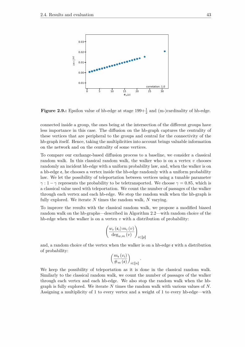
2.4. Results and evaluation 43
0 5 10 15 20 25 30#m(�)
−0.01
0.00
0.01
0.02
0.03
ε 199
+1 2(�)
correlation: 1.0
Figure 2.9.: Epsilon value of hb-edge at stage 199+12 and (m-)cardinality of hb-edge.
connected inside a group, the ones being at the intersection of the different groups haveless importance in this case. The diffusion on the hb-graph captures the centrality ofthese vertices that are peripheral to the groups and central for the connectivity of thehb-graph itself. Hence, taking the multiplicities into account brings valuable informationon the network and on the centrality of some vertices.To compare our exchange-based diffusion process to a baseline, we consider a classicalrandom walk. In this classical random walk, the walker who is on a vertex v choosesrandomly an incident hb-edge with a uniform probability law, and, when the walker is ona hb-edge e, he chooses a vertex inside the hb-edge randomly with a uniform probabilitylaw. We let the possibility of teleportation between vertices using a tunable parameterγ : 1− γ represents the probability to be teletransported. We choose γ = 0.85, which isa classical value used with teleportation. We count the number of passages of the walkerthrough each vertex and each hb-edge. We stop the random walk when the hb-graph isfully explored. We iterate N times the random walk, N varying.To improve the results with the classical random walk, we propose a modified biasedrandom walk on the hb-graphs—described in Algorithm 2.2—with random choice of thehb-edge when the walker is on a vertex v with a distribution of probability:(
we (ei)mi (v)degw,m (v)
)i∈JpK
and, a random choice of the vertex when the walker is on a hb-edge e with a distributionof probability: (
me (vi)#m (e)
)i∈JnK
.
We keep the possibility of teleportation as it is done in the classical random walk.Similarly to the classical random walk, we count the number of passages of the walkerthrough each vertex and each hb-edge. We also stop the random walk when the hb-graph is fully explored. We iterate N times the random walk with various values of N.Assigning a multiplicity of 1 to every vertex and a weight of 1 to every hb-edge—with
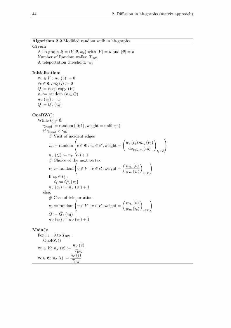
44 2. Diffusion in hb-graphs (matrix approach)
Algorithm 2.2 Modified random walk in hb-graphs.Given:
A hb-graph H = (V,E, we) with |V | = n and |E| = pNumber of Random walks: TRWA teleportation threshold: γth
Initialisation:∀v ∈ V : nV (v) := 0∀e ∈ E : nE (e) := 0Q := deep copy (V )v0 := random (v ∈ Q)nV (v0) := 1Q := Q\ {v0}
OneRW():While Q 6= ∅:γrand := random ([0; 1] ,weight = uniform)if γrand < γth :
# Visit of incident edges
ec := random
e ∈ E : vc ∈ e?,weight =(we (ej)mej (v0)
degwe,m (v0)
)ej∈E
nV (ec) := nV (ec) + 1# Choice of the next vertex
v0 := random(v ∈ V : v ∈ e?c ,weight =
(mec (v)#m (ec)
)v∈V
)If v0 ∈ Q :Q := Q\ {v0}
nV (v0) := nV (v0) + 1else:
# Case of teleportation
v0 := random(v ∈ V : v ∈ e?c ,weight =
(mec (v)#m (ec)
)v∈V
)Q := Q\ {v0}nV (v0) := nV (v0) + 1
Main():For i := 0 to TRW :
OneRW()∀v ∈ V : nV (v) := nV (v)
TRW
∀e ∈ E: nE (e) := nE (e)TRW

2.4. Results and evaluation 45
Figure 2.10.: Alpha value convergence of the vertices vs number of iterations. Theplots are m-degree-based with gradient coloring.
the vertex degree and the hb-edge cardinality instead of the multiplicity—retrieves theclassical random walk from the modified random walk.
0 100 200 300 400 500 600Rank in diffusion process
0
100
200
300
400
500
600
Rank using random walks
number of iterations: 1000correlation: 0.952
Diffusion vs modified random walk by number of vertex visits
Figure 2.13.: Comparison of the rank obtained by a thousand modified random walksafter total discovery of the vertices in the hb-graph and the rank obtained with 200iterations of the exchange-based diffusion process.

46 2. Diffusion in hb-graphs (matrix approach)
Figure 2.11.: Epsilon value convergence of hb-edges vs number of iterations. The plotsare m-cardinality-based colored using gradient colors.
0 5 10 15 20 25degm(v)
0
200
400
600
800
rank
of v
correlation: -0.476Modified random walk by number of vertex visits: m-degree
Figure 2.14.: Comparison of the rank obtained by a thousand modified random walksafter total discovery of the vertices in the hb-graph and m-degree of vertices.

2.4. Results and evaluation 47
0.0 2.5 5.0 7.5 10.0 12.5 15.0 17.5 20.0deg(v)
0
200
400
600
800
rank
of v
correlation: -0.452Modified random walk by number of vertex visits: degree
Figure 2.15.: Comparison of the rank obtained by a thousand modified random walksafter total discovery of the vertices in the hb-graph and degree of vertices.
Figure 2.13 shows that there is a good correlation between the rank obtained by athousand modified random walks and two hundreds iterations of our diffusion process,especially for the first hundred vertices of the network, which is generally the ones thatare targeted. The lack of correlation between the rank obtained by the random walkwith the degree of the vertices and the m-degree of vertices as shown respectively inFigure 2.14 and Figure 2.15 is mainly due to the vertices with low m-degrees / degrees.
0 100 200 300 400 500 600Rank in diffusion process
0
100
200
300
400
500
600
Rank using random walks
number of iterations: 1000correlation: 0.931
Diffusion vs classical random walk by number of vertex visits
Figure 2.16.: Comparison of the rank obtained by a thousand classical random walksafter total discovery of the vertices in the hb-graph and rank obtained with 200iterations of the exchange-based diffusion process.
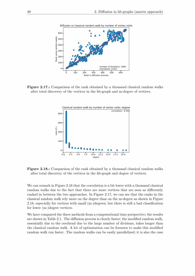
48 2. Diffusion in hb-graphs (matrix approach)
0 100 200 300 400 500 600Rank in diffusion process
0
100
200
300
400
500
600
Rank using random walks
number of iterations: 1000correlation: 0.931
Diffusion vs classical random walk by number of vertex visits
Figure 2.17.: Comparison of the rank obtained by a thousand classical random walksafter total discovery of the vertices in the hb-graph and m-degree of vertices.
0.0 2.5 5.0 7.5 10.0 12.5 15.0 17.5 20.0deg(v)
0
200
400
600
800
rank of v
correlation: -0.453Classical random walk by number of vertex visits: degree
Figure 2.18.: Comparison of the rank obtained by a thousand classical random walksafter total discovery of the vertices in the hb-graph and degree of vertices.
We can remark in Figure 2.16 that the correlation is a bit lower with a thousand classicalrandom walks due to the fact that there are more vertices that are seen as differentlyranked in between the two approaches. In Figure 2.17, we can see that the ranks in theclassical random walk rely more on the degree than on the m-degree as shown in Figure2.18, especially for vertices with small (m-)degrees; but there is still a bad classificationfor lower (m-)degree vertices.
We have compared the three methods from a computational time perspective; the resultsare shown in Table 2.1. The diffusion process is clearly faster; the modified random walk,essentially due to the overhead due to the large number of divisions, takes longer thanthe classical random walk. A lot of optimization can be foreseen to make this modifiedrandom walk run faster. The random walks can be easily parallelized; it is also the case

2.4. Results and evaluation 49
|E| |V | k N1 N0 Type of algorithm 100 200 500 100055 106 1 5 5 classical random walk 0.40 ± 0.05 0.78 ± 0.07 1.92 ± 0.10 3.82 ± 0.1455 106 1 5 5 diffusion 0.05 ± 0.02 0.08 ± 0.02 0.20 ± 0.04 0.39 ± 0.0655 306 1 5 5 modified random walk 0.71 ± 0.06 1.43 ± 0.09 3.56 ± 0.17 7.12 ± 0.2355 132 3 5 5 classical random walk 0.49 ± 0.05 0.96 ± 0.06 2.36 ± 0.08 4.71 ± 0.1255 132 3 5 5 diffusion 0.05 ± 0.02 0.09 ± 0.02 0.21 ± 0.04 0.42 ± 0.0555 132 3 5 5 modified random walk 0.89 ± 0.06 1.77 ± 0.09 4.43 ± 0.13 8.85 ± 0.1955 91 5 5 5 classical random walk 0.30 ± 0.04 0.59 ± 0.05 1.44 ± 0.06 2.85 ± 0.0755 91 5 5 5 diffusion 0.04 ± 0.02 0.07 ± 0.02 0.16 ± 0.03 0.31 ± 0.0455 91 5 5 5 modified random walk 0.55 ± 0.05 1.09 ± 0.06 2.71 ± 0.09 5.42 ± 0.14305 534 1 5 5 classical random walk 4.05 ± 0.16 8.07 ± 0.26 20.10 ± 0.45 40.17 ± 0.85305 534 1 5 5 diffusion 0.29 ± 0.06 0.57 ± 0.08 1.35 ± 0.09 2.64 ± 0.10305 534 1 5 5 modified random walk 6.86 ± 0.28 13.71 ± 0.41 34.16 ± 0.75 68.28 ± 1.21305 491 3 5 5 classical random walk 3.51 ± 0.13 6.98 ± 0.21 17.39 ± 0.38 34.77 ± 0.70305 491 3 5 5 diffusion 0.27 ± 0.05 0.53 ± 0.09 1.25 ± 0.11 2.43 ± 0.11305 491 3 5 5 modified random walk 6.02 ± 0.22 12.03 ± 0.41 30.10 ± 0.73 60.23 ± 1.34305 499 5 5 5 classical random walk 3.31 ± 0.15 6.58 ± 0.20 16.38 ± 0.34 32.72 ± 0.51305 499 5 5 5 diffusion 0.24 ± 0.04 0.47 ± 0.06 1.12 ± 0.06 2.18 ± 0.08305 499 5 5 5 modified random walk 5.86 ± 0.26 11.70 ± 0.37 29.26 ± 0.58 58.51 ± 0.89
Table 2.1.: Time taken for doing 100, 200, 500 and 1000 iterations of the diffusionalgorithm and 100, 200, 500 and 1000 classical and modified random walks on differenthb-graphs.
for the diffusion process. The number of iterations in the diffusion process can also beoptimized. These issues will be addressed in future work.
2.4.2. Two use cases
2.4.2.1. Application to Arxiv querying
We used the standard Arxiv API1 to perform searches on Arxiv database. When per-forming a search, the query is transformed into a vector of words which is the basisfor the retrieval of documents. The most relevant documents are retrieved based on asimilarity measure between the query vector and the word vectors associated to indi-vidual documents. Arxiv relies on Lucene’s built-in Vector Space Model of informationretrieval and the Boolean model2. The Arxiv API returns the metadata associated tothe document with highest scores for the query performed.
This metadata, filled by the authors during their submission of a preprint, containsdifferent information such as authors, Arxiv categories and abstract.
We process these abstracts using TextBlob, a Python natural language processing li-brary3 and extract the nouns using the tagged text.
Nouns in the abstract of each document are scored with TF-IDF, the Term Frequency-Invert Document Frequency, defined as:
TF-IDF (x, d) ∆= TF(x, d)×IDF(x, d)1https://arxiv.org/help/api/index2https://lucene.apache.org/core/2_9_4/scoring.html3https://textblob.readthedocs.io/en/dev/

50 2. Diffusion in hb-graphs (matrix approach)
with TF(x, d) the relative frequency of x in d and IDF (x, d) the invert document fre-quency.Writing nd the total number of terms in document d and nx the number of occurrencesof x :
TF(x, d) ∆= nxnd
and, writing N the total number of documents and nx∈d the number of documentshaving an occurrence of x, we have:
IDF (x, d) ∆= log10
(N
nx∈d
).
Scoring each noun in each abstract of the retrieved documents generates a hb-graph HQof universe the nouns contained in the abstracts. Each hb-edge contains a set of nounsextracted from a given abstract with a multiplicity function that represents the TF-IDFscore of each noun.The exchange-based diffusion process is applied to the hb-graph HQ. We show twotypical examples on the same query of the first 50 results in Figure 2.19 (a) and of thefirst 100 results in Figure 2.19 (b). The number of iterations needed to have convergenceis less than 10 in these two cases; with 500 results, around 10 iterations are needed forall hb-edges, but for one, where 30 iterations are needed.As the hb-edges correspond to documents in Arxiv database, we compare the centraldocuments obtained in the results of the queries: we observe that the ranking obtainedbased on the ε49+ 1
2differs significantly from the ranking by pertinence given by Arxiv
API. In the exchange-based diffusion, the ranking sorts documents depending on theirword weights and their centrality as we have seen in the experimental part on randomhb-graphs.Moreover, we have observed that when the number of results retrieved increases the top5 (respectively top 10) documents—out of the documents retrieved— can sometimeschange drastically depending on the retrieval of new documents that are more centralwith relation to the words they contain. If the gap seems small with a few documentsretrieved, this gap increases as the number of documents increases. The increasingnumber of results reveals the full theoretical hb-graph obtained from the whole datasetperforming the querying, and hence, reveals central subjects in this dataset. Hence thediffusion process can allow to highlight the importance of documents by consideringcentral subjects in the processing of the query results.
2.4.2.2. Application to an image database
We have applied the exchange-based diffusion to a database of images. We have useda hb-graph modeling of the objects detected on individual images to build a networkof co-occurrences. Each image has been processed using a Retina neural network tolabel the objects it contains, and each object is then counted in its own category. Thedatabase used is the 2014 training set of the COCO dataset4 [LMB+14]. The use of apre-trained Retina net5 allows to give bounding boxes corresponding to concepts, with a4http://cocodataset.org/#home.5https://github.com/fizyr/keras-retinanet

2.5. Future work and Conclusion 51
probability associated to them. A threshold of 0.5 is chosen—as proposed by the librarydeveloper—below which the bounding box is rejected. Hence, each image is associatedto its concepts and their multiplicity.
Out of this association, two hb-graphs can be build. First, a hb-graph of images HIm,where the vertex set is constituted of the different concepts—objects—that the imageholds and where a hb-edge is related to an image, regrouping the different concepts withtheir respective multiplicity. The second hb-graph is the hb-graph of concepts HCo : thevertex set corresponds to the image set, and a hb-edge regroups the images holding theconcept with a multiplicity that corresponds to the number of times the correspondingconcept occurs in the image. These two hb-graphs are dual one of the other. We nowfocus on the hb-graph of images.
We randomly select 200 images of the COCO 2014 training dataset, building the orig-inal image hb-graph. To ensure connectivity, we focus on the first main componentof the original image hb-graph. This component is designated as the hb-graph in theremainder. We then enhance the diffusion on this connected hb-graph. A typical re-sult is presented in Figure 2.20: the concepts are the vertices, the images represent theextra-vertices corresponding to the hb-edges. The coloration of vertices—i.e. the nodesof the concepts— and of hb-edges—i.e. the extra-nodes representing images— is thesame than the one used in Figure 2.12. The closer to red the images are, the morecentral to the sample drawn they are; hence, these images can potentially be used tomake a summary of this sample.
2.5. Future work and Conclusion
The results obtained by using hb-graph highlight the possibility of using hb-edges foranalyzing networks; they confirm that vertices are highlighted due to their connectivity.The highlighting of the hb-edges has been achieved by using the intermediate step of ourdiffusion process. Different applications can be thought in particular in the search oftagged multimedia documents for refining the results and scoring of documents retrieved.Using tagged documents ranking by this means could help in creating summary for vi-sualisation. Our approach is seen as a strong basis to refine the approach of [XDYF16].This approach can also be viewed as a means to make query expansion and disambigua-tion by using additional high scored words in the network and a way of making somerecommendation based on the scoring of a document based on its main words. We havealso proposed a generalization of this approach in Appendix Section D.1 using vertexand hb-edge abstract information functions and biased probability transition.

52 2. Diffusion in hb-graphs (matrix approach)
(a) Exchange-based diffusion on the hb-graph
(b) Exchange-based diffusion on the hb-graph support
Figure 2.12.: Exchange-based diffusion in a hb-graph (a) and its support hypergraph(b) after 200 iterations of Algorithm 2.1: highlighting important hb-edges. Simulationwith 848 vertices (chosen randomly out of 10 000) gathered in 5 groups of vertices(with 5, 9, 14, 16 and 9 important vertices and 2 important vertices per hb-edge), 310hb-edges (with cardinality of support less or equal to 20), 10 vertices in between the5 groups. Extra-vertices have square shape and are colored with the hb-edge colorscale.
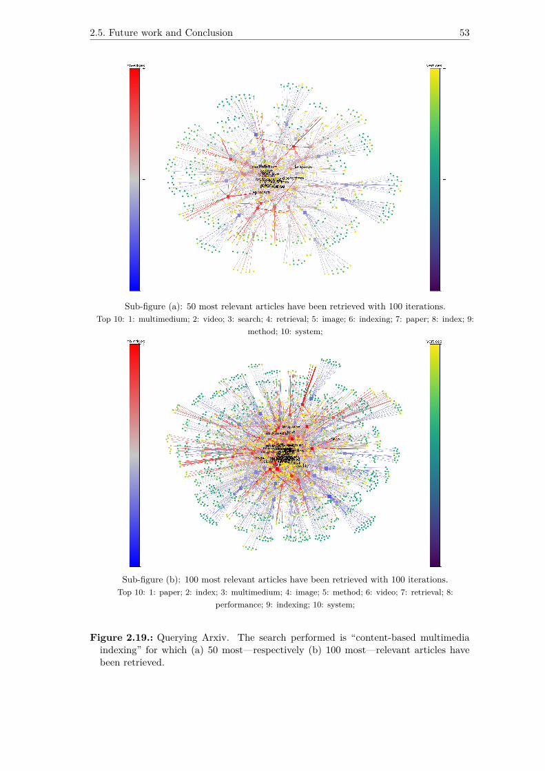
2.5. Future work and Conclusion 53
Sub-figure (a): 50 most relevant articles have been retrieved with 100 iterations.Top 10: 1: multimedium; 2: video; 3: search; 4: retrieval; 5: image; 6: indexing; 7: paper; 8: index; 9:
method; 10: system;
Sub-figure (b): 100 most relevant articles have been retrieved with 100 iterations.Top 10: 1: paper; 2: index; 3: multimedium; 4: image; 5: method; 6: video; 7: retrieval; 8:
performance; 9: indexing; 10: system;
Figure 2.19.: Querying Arxiv. The search performed is “content-based multimediaindexing” for which (a) 50 most—respectively (b) 100 most—relevant articles havebeen retrieved.
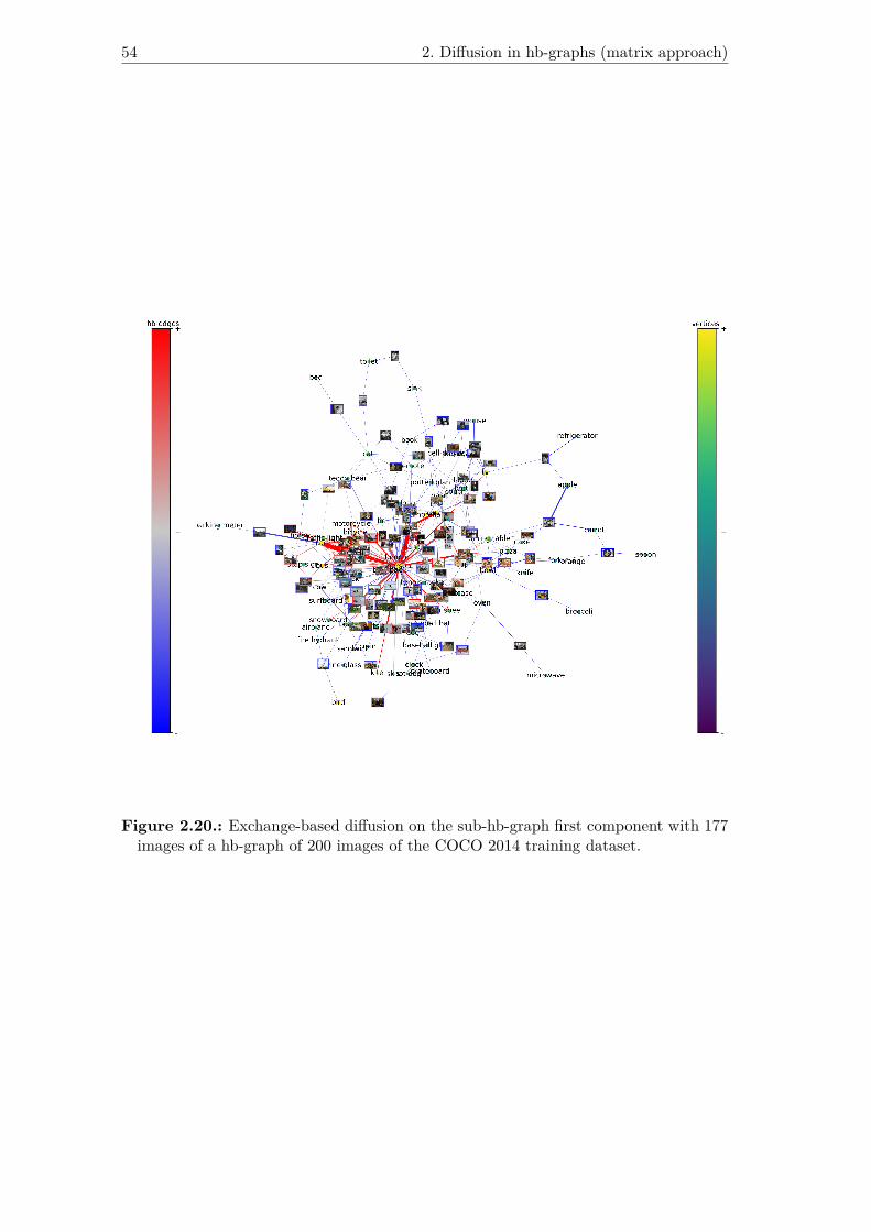
54 2. Diffusion in hb-graphs (matrix approach)
Figure 2.20.: Exchange-based diffusion on the sub-hb-graph first component with 177images of a hb-graph of 200 images of the COCO 2014 training dataset.

3. e-adjacency tensor of natural hb-graphs
Highlights
3.1. Motivation . . . . . . . . . . . . . . . . . . . . . . . . . . . . . . . . . . 55
3.2. Related work . . . . . . . . . . . . . . . . . . . . . . . . . . . . . . . . . 56
3.3. e-adjacency tensor of a natural hb-graph . . . . . . . . . . . . . . . . . . 56
3.4. Results on the constructed tensors . . . . . . . . . . . . . . . . . . . . . 78
3.5. Evaluation and first choice . . . . . . . . . . . . . . . . . . . . . . . . . . 86
3.6. Further comments . . . . . . . . . . . . . . . . . . . . . . . . . . . . . . 88
This chapter is based on [OLGMM18b, OLGMM19a, OLGMM19c].
Prerequisites: Sections 1.3 and 1.4, Appendix B—particularly Section B.3—, andpossibly Appendix Section E.1.4.
3.1. Motivation
In [OLGMM17a, OLGMM18a]—reproduced in Appendix Section E.1—we have pre-sented a first e-adjacency tensor for general hypergraphs. Its construction has beenachieved by involving a Hypergraph Uniformisation Process, coupled to a PolynomialHomogenization Process. The Uniformisation requires the addendum of several specialvertices, one per layer of the hypergraph decomposition.
Nonetheless, in Chapter 1, one of the motivations for the introduction of hb-graph wasthat hb-graphs are a way of reducing the number of variables used in the PolynomialHomogenization Process, while keeping the Uniformisation of the Structure interpretablein term of m-uniformisation of hb-graphs.
Research question 3.1. Which e-adjacency tensor(s) can we build for general hb-graphs?
In this chapter, we mostly rely on the related work presented in [OLGMM17a]. We thenpresent our expectations on the desirable properties the e-adjacency tensors of generalhb-graphs should have and present three possible solutions. After discussing their prop-erties, we justify the choice for the best candidate, and apply it to the particular caseof general hypergraphs. This choice will be refined in Chapter 4.
56 3. e-adjacency tensor of natural hb-graphs
3.2. Related work
In addition to the related work presented in Appendix Section E.1 for general hy-pergraphs, we found, after having developed the whole theory on hb-graphs, [PZ15].Nonetheless, as it is a strong anteriority, we mention it here.
A [k-]adjacency tensor for k-PZ-multigraphs—i.e. k-m-uniform natural hb-graphwith no repeated hb-edge—is defined as follow:
Definition 3.1. Let...Hk = (V,E) be a k-PZ-multigraph on a finite set of vertices V =
{vi : i ∈ JnK} and a set of edges E = (ej)j∈JpK .
The [k-]adjacency tensor of a k-PZ-multigraph is the symmetric tensor A ...Hm∈ Tk,n
of CHR A ...Hk
= (ai1,...,ik)i1,...,ik∈JnK such that:
ai1,...,ik =
mj1 ! . . .mjs !
(m− 1)! , if {{vi1 , ..., vim}} ={vmj1j1
, ..., vmjsjs
}∈ E;
0, otherwise.
The authors then study some spectral properties of k-PZ-multigraph. However, thesubject of general natural hb-graphs remains to be tackled.
3.3. e-adjacency tensor of a natural hb-graph
Postulate 3.1. In this section, we consider only natural hb-graphs with no repeatedhb-edge.
To build the e-adjacency tensor A (H) of a natural hb-graph H = (V,E) without repeatedhb-edge—of vertex set V = {vi : i ∈ JnK} and hb-edge set E = (ej)j∈JpK—, we takean approach similar to Appendix Section E.1 using the strong link between cubicalsymmetric tensors and homogeneous polynomials.
3.3.1. Expectations for the e-adjacency tensor
We formulate the expected properties for the e-adjacency tensor of a natural hb-graph wewant to construct. For general hypergraphs, we have insisted on the interpretation of theconstruction using a Hypergraph Uniformisation Process: that has required the fillingof the hyperedges with additional and two-by-two different vertices since hyperedgescannot have duplicated elements.
As natural hb-graphs “naturally” allow vertices to be duplicated, we can think of differ-ent ways of filling the hb-edges with additional vertices. We have chosen three of them:the straightforward approach, the silo approach and the layered approach—as it wasalready done for the layered approach for general hypergraphs in Appendix Section E.1.
We first give some expected properties of such a tensor, some of them being morequalitative than quantifiable.

3.3. e-adjacency tensor of a natural hb-graph 57
Expectation 3.1. The e-adjacency tensor should be non-negative, symmetric and itsgeneration should be as simple as possible.
Since non-negative symmetric hypermatrices can be described with a small number ofvalues, a hb-edge is representable with only one tuple of indices and their correspondingcoefficient, the other coefficients of the tensor being obtained by permuting the indices ofthe first one while the same value is kept. Moreover, in the spectral theory, symmetricnon-negative nonzero tensors ensure interesting properties as their spectral radius ispositive [QL17]; furthermore, there is at most one H-eigenvalue that corresponds to thespectral radius with a positive Perron H-eigenvector.
Expectation 3.2. The tensor should be globally invariant to vertex permutation in theoriginal hb-graph.
By globally invariant, we mean that a permutation of rows on each face of the hyper-matrix follows the same permutation than the one involved in the vertex permutation.We do not expect the special vertices added for the filling of the hb-edges to follow thesame rule.
Expectation 3.3. The e-adjacency tensor should induce a unique reconstruction of thehb-graph it is originated from.
The e-adjacency tensor should describe the hb-graph in a unique way up to a permu-tation of indices, so that no two hb-graphs have the same e-adjacency tensor unlessthey are isomorphic. This is a strong requirement as it enforces the addition of specialvertices even for k-m-uniform hb-graphs, where k-adjacency corresponds to k-adjacency.Hence, the special vertices will be systematically generated and added to the final tensorin order to meet this expectation.
Expectation 3.4. Given the choice of two representations the one that can be de-scribed with the least possible number of elements should be chosen. Then the sparseste-adjacency tensor should be chosen.
It forces the hypermatrix to be easily describable before ensuring the lowest sparsitypossible. The fact that the hypermatrix is symmetric will help.
Expectation 3.5. The e-adjacency tensor should allow direct retrieval of the vertexdegrees.
This is required for all k-adjacency tensors of uniform hypergraphs. It is also the casefor the e-adjacency tensors of [SZB19, BCM17] and for the first e-adjacency tensor webuilt for general hypergraphs.
3.3.2. Elementary hb-graph
A hb-graph that has only one non repeated hb-edge in its hb-edge family is called anelementary hb-graph.
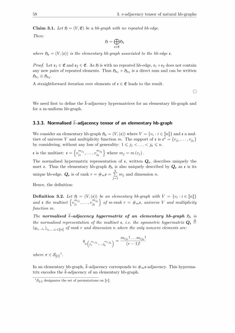
58 3. e-adjacency tensor of natural hb-graphs
Claim 3.1. Let H = (V,E) be a hb-graph with no repeated hb-edge.
Then:H =
⊕e∈E
He
where He = (V, (e)) is the elementary hb-graph associated to the hb-edge e.
Proof. Let e1 ∈ E and e2 ∈ E. As H is with no repeated hb-edge, e1 +e2 does not containany new pairs of repeated elements. Thus He1 + He2 is a direct sum and can be writtenHe1 ⊕ He2 .
A straightforward iteration over elements of e ∈ E leads to the result.
We need first to define the k-adjacency hypermatrices for an elementary hb-graph andfor a m-uniform hb-graph.
3.3.3. Normalised k-adjacency tensor of an elementary hb-graph
We consider an elementary hb-graph He = (V, (e)) where V = {vi : i ∈ JnK} and e a mul-tiset of universe V and multiplicity function m. The support of e is e? = {vj1 , . . . , vjk}by considering, without any loss of generality: 1 6 j1 < . . . < jk 6 n.
e is the multiset: e ={vmj1j1
, . . . , vmjkjk
}where mj = m (vj) .
The normalised hypermatrix representation of e, written Qe, describes uniquely themset e. Thus the elementary hb-graph He is also uniquely described by Qe as e is its
unique hb-edge. Qe is of rank r = #me =k∑j=1
mj and dimension n.
Hence, the definition:
Definition 3.2. Let H = (V, (e)) be an elementary hb-graph with V = {vi : i ∈ JnK}and e the multiset
{vmj1j1
, . . . , vmjkjk
}of m-rank r = #me, universe V and multiplicity
function m.
The normalised k-adjacency hypermatrix of an elementary hb-graph He isthe normalised representation of the multiset e, i.e. the symmetric hypermatrix Qe
∆=(qi1...ir)i1,...,ir∈JnK of rank r and dimension n where the only nonzero elements are:
qσ
(jmi j11 ,...,j
mi jkk
) = mij1 ! . . .mijk !(r − 1)!
where σ ∈ SJrK1.
In an elementary hb-graph, k-adjacency corresponds to #me-adjacency. This hyperma-trix encodes the k-adjacency of an elementary hb-graph.1SJrK designates the set of permutations on JrK.
3.3. e-adjacency tensor of a natural hb-graph 59
3.3.4. Hb-graph polynomial
Homogeneous polynomial associated to a hypermatrix:
With an approach similar to Appendix Section E.1 where full details are given, lete1, . . . , en be the canonical basis of Rn.(ei1 ⊗ . . .⊗ eik)i1,...,ik∈JnK is a basis of L0
k (Kn) , where ⊗ is the Segre outerproduct.
A tensor Q ∈ L0k (Kn) is associated to a hypermatrix Q = (q i1...ir)i1,...,ir∈JnK by writing
Q as:Q =
∑i1,...,ir∈JnK
q i1...irei1 ⊗ . . .⊗ eir .
Q is called the canonical hypermatrix representation (CHR for short) of Q.Considering n variables zi attached to the n vertices vi and z = ∑
i∈JnKziei, the multilinear
matrix product (z, . . . , z) .Q = (z)[r] . Q is a polynomial P (z0)2:
P (z0) =∑
i1,...,ir∈JnK
q i1...irzi1 . . . zir
of degree r.
Elementary hb-graph polynomial:
Let He = (V, (e)) be an elementary hb-graph with V = {vi : i ∈ JnK} and e the multiset{vmj1j1
, . . . , vmjkjk
}of m-rank r = #me, universe V and multiplicity function m.
Using the normalised k-adjacency hypermatrix Qe = (q i1...ir)i1,...,ir∈JnK , which is sym-metric, we can write the reduced version of its attached homogeneous polynomial Pe :
Pe (z0) = r!mj1 ! . . .mjk !qj
mj11 ...j
mjkk
zmj1j1
. . . zmjkjk
= #me zmj1j1
. . . zmjkjk
.
Hb-graph polynomial:
Considering a hb-graph H = (V,E) with no-repeated hb-edge, with V = {vi : i ∈ JnK}and E = (ei)i∈JpK .
This hb-graph can be summarized by a polynomial of degree rH = maxe∈E
#m (e) :
P (z0) ∆=∑i∈JpK
ceiPei (z0)
=∑i∈JpK
ceiri!
mij1 ! . . .mijki!qjmi j11 ...j
mi jkiki
zmij1j1
. . . zmijkijki
=∑i∈JpK
cei#mei zmij1j1
. . . zmijkijki
2Where: z0 = (z1, ..., zn)
60 3. e-adjacency tensor of natural hb-graphs
where cei is a technical coefficient. P (z0) is called the hb-graph polynomial. Thechoice of cei will be further made in Section 3.3.8 in order to retrieve the m-degree ofthe vertices from the e-adjacency tensor.
3.3.5. k-adjacency hypermatrix of a m-uniform natural hb-graph
We now extend to m-uniform hb-graphs the k-adjacency hypermatrix obtained in thecase of an elementary hb-graph.
In the case of a r-m-uniform natural hb-graph with no repeated hb-edge, each hb-edge has the same m-cardinality r. Hence, the k-adjacency of a r-m-uniform hb-graphcorresponds to r-adjacency where r is the m-rank of the hb-graph. The k-adjacencytensor of the hb-graph has rank r and dimension n. The elements of the k-adjacencyhypermatrix are: ai1...ir with i1, . . . , ir ∈ JnK.
The associated hb-graph polynomial is homogeneous of degree r.
We obtain the definition of the k-adjacency tensor of a r-m-uniform hb-graph by sum-ming the k-adjacency tensor attached to each hb-edge with a coefficient ci equals to 1for each hb-edge.
Definition 3.3. Let H = (V,E) be a hb-graph with V = {vi : i ∈ JnK}.
The k-adjacency hypermatrix of a r-m-uniform hb-graph H = (V,E) is thehypermatrix AH = (ai1...ir)i1,...,ir∈JnK defined by:
AH∆=∑i∈JpK
Qei
where Qei is the k-adjacency hypermatrix of the elementary hb-graph associated to thehb-edge ei =
{vmij1j1
, . . . , vmijkijki
}∈ E.
The only non-zero elements of Qei are the elements with indices obtained by permutationof the elements of the multiset
{jmij11 , . . . , j
mijkiki
}and are all equal to:
mij1 ! . . .mijki!
(r − 1)! .
This definition corresponds to the definition given by [PZ15], which is a symmetrizedversion of the one given in [PZ14].
We can remark that when a r-m-uniform hb-graph has 1 as vertex multiplicity forany vertices in each hb-edge support of all hb-edges, then this hb-graph is a r-uniformhypergraph: in this case, we retrieve the result of the degree-normalized tensor definedin [CD12].
Claim 3.2. The m-degree of a vertex vj in a r-m-uniform hb-graph H of the k-adjacencyhypermatrix is:
degm (vj) =∑
j2,...,jr∈JnK
ajj2...jr .

3.3. e-adjacency tensor of a natural hb-graph 61
Proof. ∑j2,...,jr∈JnK
ajj2...jr has non-zero terms only for the corresponding hb-edges ei con-
taining vj . Such a hb-edge is described by:
ei ={vmi jj , v
mi l2l2
, . . . , vmi lkilki
}.
It means that the multiset {{j2, . . . , jr}} corresponds exactly to the multiset:
{jmi j−1 , l
mi l22 , . . . , l
mi lkiki
}.
For each ei such that vj ∈ ei, there are (r − 1)!(mi j − 1)!mi l2 ! . . .mi lki
! possible permutations
of the indices j2 to jl and:
ajj2...jr =mi j !mi l2 ! . . .mi lki
!(r − 1)! .
Also: ∑j2,...,jr∈JnK
ajj2...jr =∑
i∈JpK : vj∈ei
mi j = degm (vj) .
3.3.6. Elementary operations on hb-graphs
In Appendix Section E.1, we describe two elementary operations that are used in thehypergraph uniformisation process. We describe here similar operations for hb-graphs.
Operation 3.3.1. Let H = (V,E) be a hb-graph.Let w1 be a constant weighted function on hb-edges with constant value 1.The weighted hb-graph H1
∆= (V,E, w1) is called the canonical weighted hb-graphof H.The application φcw : H 7→ H1 is called the canonical weighting operation.
Operation 3.3.2. Let H1 = (V,E, w1) be a canonical weighted hb-graph.Let c ∈ R++. Let wc be a constant weighted function on hb-edges with constant valuec.The weighted hb-graph Hc
∆= (V,E, wc) is called the c-dilated hb-graph of H.The application φc-d : H1 7→ Hc is called the c-dilatation operation.
62 3. e-adjacency tensor of natural hb-graphs
Operation 3.3.3. Let Hw = (V,E, w) be a weighted hb-graph. Let y be a vertex that isnot in V. The y-complemented hb-graph of Hw is the hb-graph Hyc
∆= (Vyc ,Eyc , wyc)where:
• Vyc∆= V ∪ {y} ;
• Eyc∆= (ξ (e))e∈E where the map ξ : E → M (Vyc) is such
that for all e ∈ E, ξ (e) ∆={xmξ(e)(x) : x ∈ Vyc
}∈ M (Vyc) with
mξ(e)(x) ∆={me(x) if x ∈ e?;rH −#me if x = y;
• the weight function wyc is such that ∀e ∈ E: wyc (ξ(e)) ∆= w(e).
The application φy-c : Hw 7→ Hyc is called the y-complemented operation.
Operation 3.3.4. Let Hw = (V,E, w) be a weighted hb-graph. Let y be a vertex thatis not in V. Let α ∈ R++. The yα-vertex-increased hb-graph of Hw is the hb-graphH+w+
∆=(V +,E+, w+) where:
• V + ∆= V ∪ {y} ;
• E+ ∆= (φ (e))e∈E where the map φ : E → M(V +) such that
for all e ∈ E, φ (e) ∆={xmφ(e)(x) : x ∈ V +
}∈ M
(V +) with
mφ(e)(x) ∆={me(x) if x ∈ e?;α if x = y;
• the weight function is w+ is such that ∀e ∈ E: w+ (φ(e)) ∆= w(e).
The application φyα-v : Hw 7→ H+w+ is called the yα-vertex-increasing operation.
3.3. e-adjacency tensor of a natural hb-graph 63
Operation 3.3.5. The merged hb-graph Hw∆=(V , E, w
)of a family (Hi)i∈I of
weighted hb-graphs with ∀i ∈ I : Hi = (Vi,Ei, wi) is the weighted hb-graph where:
• V∆= ⋃i∈I
Vi;
• E∆= (ψ (e))e∈∑
i∈IEi
a where the map ψ : ∑i∈I
Ei → M(V)
such that for all
e ∈∑i∈I
Ei, ψ (e) ∈ M(V)
and is the multiset{xmψ(e)(x) : x ∈ V
}, with
mψ(e)(x) ∆={me(x) if x ∈ e?;0 otherwise;
• ∀e ∈ Ei, w(e) ∆= wi(e).
The application φm : (Hi)i∈I 7→ H is called the merging operation.a∑i∈I
Ei is the family obtained with all elements of each family Ei.
Operation 3.3.6. Decomposing a hb-graph H = (V,E) into a family of hb-graphs(Hi)i∈I , where Hi = (V,Ei) such that H = ⊕
i∈IHi is called a decomposition operation
φd : H 7→ (Hi)i∈I .
The direct sum of two hb-graphs appears as a merging operation in one way and as adecomposition operation in the other. For a given hb-graph, different decompositionoperations exist. Nonetheless, the decomposition in elementary hb-graph is unique aswell as the decomposition in m-uniform hb-graphs representing the different levels ofm-uniformity in that hb-graph.
We now focus on the preservation of e-adjacency through these different operations, asit is fundamental to ensure the soundness of the constructed hypermatrix.
Definition 3.4. Let H = (V,E) and H′ = (V ′,E′) be two hb-graphs.
Let φ : H 7→ H′.
φ is said preserving e-adjacency if vertices of V ′ that are e-adjacent in H′ and alsoin V are e-adjacent in H.
φ is said preserving exactly e-adjacency if vertices that are e-adjacent in H′ aree-adjacent in H and reciprocally.
We can extend these definitions to ψ : (Hi)i∈I 7→ H′.
Definition 3.5. Let (Hi)i∈I be a family of hb-graphs with ∀i ∈ I, Hi = (Vi,Ei) andH′ = (V ′,E′) a hb-graph.
Let consider ψ : (Hi)i∈I 7→ H′.
ψ is said preserving e-adjacency if vertices that are e-adjacent in H′, restricted tothe ones that belong to V = ⋃
i∈IVi, are e-adjacent vertices in exactly one of the Hi, i ∈ I.
64 3. e-adjacency tensor of natural hb-graphs
ψ is said preserving exactly e-adjacency if vertices that are e-adjacent in H′ aree-adjacent in exactly one of the Hi, i ∈ I and reciprocally.
We can extend these definitions to ν : H 7→ (Hi)i∈I .
Definition 3.6. Let (Hi)i∈I be a family of hb-graphs with ∀i ∈ I, Hi = (Vi,Ei) andH = (V,E) a hb-graph.
Let consider ν : H 7→ (Hi)i∈I .
ν is said preserving e-adjacency if vertices that are e-adjacent in one of the Hi, i ∈ I,restricted to the ones that belong to V, are e-adjacent in H.
ν is said preserving exactly e-adjacency if vertices that are e-adjacent in one of theHi, i ∈ I are e-adjacent in H and reciprocally.
The two following claims have immediate proofs.
Claim 3.3. Let H = (V,E) be a hb-graph.
The canonical weighting operation, the c-dilatation operation, the merging operationand, the decomposition operation preserve exactly e-adjacency.
The y-complemented operation and the yα-vertex-increasing operation preservee-adjacency.
Claim 3.4. The composition of two operations which preserves (respectively exactly)e-adjacency preserves (respectively exactly) e-adjacency.
The composition of two operations where one preserves exactly e-adjacency and the otherpreserves e-adjacency preserves e-adjacency.
3.3.7. Processes involved for building the e-adjacency tensor
In a general natural hb-graph H, hb-edges do not have the same m-cardinality: the rankof the k-adjacency tensor of the elementary hb-graph associated to each hb-edge dependson the m-cardinality of the hb-edge. As a consequence, the hb-graph polynomial is nomore homogeneous. Nonetheless, techniques to homogenize such a polynomial are wellknown.
We introduce here the hb-graph m-uniformisation process (Hm-UP for short) whichtransforms a given hb-graph of m-rank rH into a rH-m-uniform hb-graph written H :this uniformisation can be mapped to the homogenization of the attached polynomialof the original hb-graph, called the polynomial homogenization process (PHP).
The Hm-UP can be achieved by different means of filling the not-at-the-level hb-edgesso they reach a m-rank of rH :
• straightforward m-uniformisation levels directly all hb-edges by adding a Nullvertex Y1 with a multiplicity being the difference between the hb-graph m-rankand the hb-edge m-cardinality. It is achieved by considering the Y1-complementedhb-graph of H.

3.3. e-adjacency tensor of a natural hb-graph 65
• silo m-uniformisation processes each of the m-uniform sub-hb-graphs obtainedby gathering all hb-edges of a given m-cardinality r in a single sub-hb-graph,which is then Y rH−r
r -vertex-increased. A single rH-m-uniformized hb-graph is thenobtained by merging them.
• layered m-uniformisation processes m-uniform sub-hb-graphs of increasing m-cardinality by successively adding a vertex and merging it to the sub-hb-graphof the above layer. The layered homogenization process applied to hypergraphswas explained with full details in Appendix Section E.1; it involves two-phase stepiterations based on successive
{Y 1k
}-vertex-increased hb-graphs and merging with
the dilated weighted hb-graph of the next layer.All the hb-graph m-uniformisation process and constructed tensors are illustrated on anexample given in Section 3.3.12.
3.3.8. On the choice of the technical coefficient cei
To comply to the expectations, the technical coefficient cei has to be chosen such thatby using the elements of the e-adjacency hypermatrix A = (ai1...ir)i1,...,ir∈JnK , one canretrieve:
1. the m-degree of the vertices: ∑i2,...,ir∈JnK
aii2...ir = degm (vi) ;
2. the number of hb-edges |E|.Similarly to Appendix Section E.1, we consider a hb-graph H = (V,E) that we decom-pose in a family of r-m-uniform hb-graphs (Hr)r∈JrHK .
We consider R the equivalency relation defined on the family of hb-edges E of H :
eRe′ ⇔ #me = #me′.
E/R is the set of classes of hb-edges of same m-cardinality. The elements of E/R arethe sets:
Er = {e ∈ E : #me = r} .
Considering R = {r : Er ∈ E/R} , we set Er = ∅ for all r ∈ JrHK \R.For all r ∈ JrHK , Hr = (V,Er) is r-m-uniform.It holds: E = ⋃
r∈JrHKEr and Er1 ∩ Er2 = ∅ for all r1 6= r2, hence (Er)r∈JrHK constitutes a
partition of E which is unique from the way it has been defined.Hence:
H =⊕r∈JrHK
Hr.
Each of these r-m-uniform hb-graph Hr, where the k-adjacency is achieved by r-adjacency,can be associated to a k-adjacency tensor Ar viewed as a hypermatrix AHr =
(a(r)i1...ir
)of order r, hyper-cubic and symmetric of dimension |V | = n.
We write:(ai1...irH
)i1,...,irH∈Jn1K
the e-adjacency hypermatrix associated to H wheren1 = n + nA, nA corresponds to the number of different special vertices added to thehb-edges. nA depends on the way the hypermatrix is built:
66 3. e-adjacency tensor of natural hb-graphs
• nA = 1 for the straightforward process;• nA = rH − 1 for the silo process;• nA = rH − 1 for the layered process.
For a given r ∈ JrHK , the number of hb-edges in Hr is given by summing the elementsof AHr :
∑i1,...,ir∈JnK
a(r)i1...ir =n∑i=1
∑i2,...,ir∈JnK
a(r)ii2...ir
=n∑i=1
degm (vi)
= r |Er| .
In the m-uniformized hb-graph of H, the number of hb-edges can also be calculatedusing: ∑
i1,...,irH∈Jn1K
ai1...irH = rH |E| .
As:
|E| =rH∑r=1|Er|
=rH∑r=1
1r
∑i1,...,ir∈JnK
a(r)i1...ir ,
it follows:∑
i1,...,irH∈Jn1K
ai1...irH =rH∑r=1
rHr
∑i1,...,ir∈JnK
a(r)i1...ir .
Also, choosing for all i ∈ JpK: cei = rHr
where r = #mei, we write for all r ∈ JrHK :
cr∆= rH
r.
cr is the technical coefficient for the corresponding layer of level r of the hb-graph H.
3.3.9. Straightforward approach
Straightforward m-uniformisation:
We first decompose H = ⊕r∈JrHK
Hr as seen in Section 3.3.8.
We then transform each Hr, r ∈ JrHK into a canonical weighted hb-graph Hr,1 that isdilated with the help of the dilatation coefficient cr to obtain the cr-dilated hb-graphHr,cr .
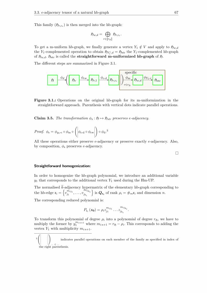
3.3. e-adjacency tensor of a natural hb-graph 67
This family (Hr,cr) is then merged into the hb-graph:
Hw,d =⊕r∈JrHK
Hr,cr .
To get a m-uniform hb-graph, we finally generate a vertex Y1 /∈ V and apply to Hw,dthe Y1-complemented operation to obtain HY c1 ,d = Hstr the Y1-complemented hb-graphof Hw,d. Hstr is called the straightforward m-uniformized hb-graph of H.
The different steps are summarized in Figure 3.1.
H
(..........
Hrφd Hr,1
φcw φc-d Hr,cr
specific
...
...
...
.)r∈rH
φm Hw,dφY1-c
Hstr
Figure 3.1.: Operations on the original hb-graph for its m-uniformization in thestraightforward approach. Parenthesis with vertical dots indicate parallel operations.
Claim 3.5. The transformation φs : H 7→ Hstr preserves e-adjacency.
Proof. φs = φy1-c ◦ φm ◦(..........φc-d ◦ φcw
...
...
...
.)◦ φd.
3
All these operations either preserve e-adjacency or preserve exactly e-adjacency. Also,by composition, φs preserves e-adjacency.
Straightforward homogenization:
In order to homogenize the hb-graph polynomial, we introduce an additional variabley1 that corresponds to the additional vertex Y1 used during the Hm-UP.
The normalised k-adjacency hypermatrix of the elementary hb-graph corresponding tothe hb-edge ei =
{vmij1j1
, . . . , vmijkijki
}is Qei of rank ρi = #mei and dimension n.
The corresponding reduced polynomial is:
Pei (z0) = ρizmij1j1
. . . zmijkijki
.
To transform this polynomial of degree ρi into a polynomial of degree rH, we have tomultiply the former by ymi n+1
1 where mi n+1 = rH − ρi. This corresponds to adding thevertex Y1 with multiplicity mi n+1.
3
(..........
...
...
...
.)... ∈ ...
indicates parallel operations on each member of the family as specified in index of
the right parenthesis.
68 3. e-adjacency tensor of natural hb-graphs
The term Pei (z0) with the attached tensor Pei of rank ρi and dimension n is transformedin4:
Rei (z1) = Pei (z0) ymi n+11 = ρiz
mij1j1
. . . zmijkijki
ymi n+11
with the attached tensor Rei of rank rH and dimension n+ 1.
The CHR of the tensor Rei is the hypermatrix Rei =(ri1...irH
). The elements that are
non-zero in Rei have all the same value:
ρstr,ei = ρimij1 ! . . .mijki
!mi n+1!rH! .
The indices of the non-zero elements of Rei are obtained by permutation of the elementsof the multiset: {
jmij11 , . . . , j
mijkiki
, (n+ 1)mi n+1}.
The number of possible permutations is:
rH!mij1 ! . . .mijki
!mi n+1! .
The hb-graph polynomial P (z0) = ∑i∈JpK
ciPei (z0) is transformed into a homogeneous
polynomial:R (z1) =
∑i∈JpK
ciRei (z1) =∑i∈JpK
cizmij1j1
. . . zmijkijki
ymi n+11
representing the straightforward m-uniformized hb-graph Hstr of H with attached hyper-matrix R =
p∑i=1
ceiRei where cei = rHρi
= rH#mei
. This provides a direct homogenizationof the whole hb-graph polynomial.
Definition 3.7. The straightforward e-adjacency tensor Astr,H of a hb-graphH = (V,E) is the tensor of CHR Astr,H defined by:
Astr,H∆=∑i∈JpK
ceiRei .
where for ei ={vmij1j1
, . . . , vmijkijki
}∈ E :
cei = rH#mei
is the dilatation coefficient and where Rei =(ri1...irH
)is the hypermatrix whose elements
have only two possible values, 0 and:
ρstr,ei =mij1 ! . . .mijki
!mi n+1!rH! #mei
with mi n+1 = rH −#mei. The indices of the non-zero elements of Rei are obtained bypermutation of the elements of the multiset:{
jmij11 , . . . , j
mijkiki
, (n+ 1)mi n+1}.
4zk = (z1, ..., zn, y1, ..., yk) for k ∈ JrH − 1K
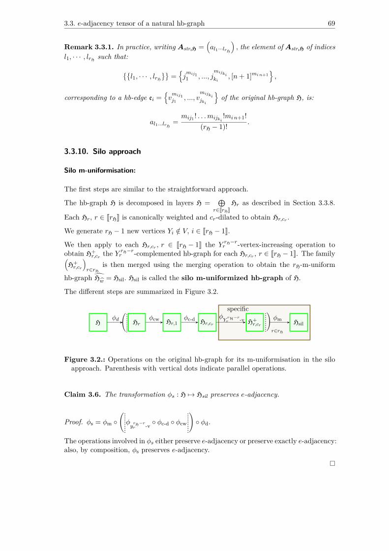
3.3. e-adjacency tensor of a natural hb-graph 69
Remark 3.3.1. In practice, writing Astr,H =(al1···lrH
), the element of Astr,H of indices
l1, · · · , lrH such that:
{{l1, · · · , lrH
}}={jmij11 , ..., j
mijkiki
, [n+ 1]mi n+1},
corresponding to a hb-edge ei ={vmij1j1
, ..., vmijkijki
}of the original hb-graph H, is:
al1...lrH =mij1 ! . . .mijki
!mi n+1!(rH − 1)! .
3.3.10. Silo approach
Silo m-uniformisation:
The first steps are similar to the straightforward approach.
The hb-graph H is decomposed in layers H = ⊕r∈JrHK
Hr as described in Section 3.3.8.
Each Hr, r ∈ JrHK is canonically weighted and cr-dilated to obtain Hr,cr .
We generate rH − 1 new vertices Yi /∈ V, i ∈ JrH − 1K.
We then apply to each Hr,cr , r ∈ JrH − 1K the Y rH−rr -vertex-increasing operation to
obtain H+r,cr the Y
rH−rr -complemented hb-graph for each Hr,cr , r ∈ JrH − 1K. The family(
H+r,cr
)r∈rH
is then merged using the merging operation to obtain the rH-m-uniform
hb-graph Hw = Hsil. Hsil is called the silo m-uniformized hb-graph of H.
The different steps are summarized in Figure 3.2.
H
(..........
Hrφd Hr,1
φcw φc-d Hr,cr
specificφYrH−rr -v H+
r,cr..........)r∈rH
φmHsil
Figure 3.2.: Operations on the original hb-graph for its m-uniformisation in the siloapproach. Parenthesis with vertical dots indicate parallel operations.
Claim 3.6. The transformation φs : H 7→ Hsil preserves e-adjacency.
Proof. φs = φm ◦(..........φyrH−rr -v ◦ φc-d ◦ φcw
...
...
...
.)◦ φd.
The operations involved in φs either preserve e-adjacency or preserve exactly e-adjacency:also, by composition, φs preserves e-adjacency.

70 3. e-adjacency tensor of natural hb-graphs
Silo homogenization:
In this homogenization process, we suppose that the hb-edges are sorted by m-cardinality.
During the silo uniformisation, we added rH − 1 vertices Y1 to YrH−1 into the universe,i.e. the vertex set. These vertices correspond to rH − 1 additional variables respectivelyy1 to yrH−1 that we introduced to homogenize the hb-graph polynomial.
The normalised k-adjacency hypermatrix of the elementary hb-graph corresponding tothe hb-edge ei =
{vmij1j1
, . . . , vmijkijki
}is Qei of rank ρi = #mei and dimension n.
The corresponding reduced polynomial is:
Pei (z0) = ρizmij1j1
. . . zmijkijki
attached to tensor Pei has for degree the m-cardinality of the hb-edge ei, i.e. #mei. Totransform it into a polynomial of degree rH, we use the additional variable y#mei withmultiplicity mi#mei = rH −#mei.
The term Pei (z0) attached to tensor Pei of rank #mei and dimension n is transformedin:
Rei (z#mei) = Pei (z0) ymi n+#mei
#mei
with attached tensor Rei of rank rH and dimension n+ 1.
The CHR of the tensor Rei is the hypermatrix Rei =(ri1...irH
). The elements of Rei
that are non-zero elements have all the same value:
ρsil,ei = ρimij1 ! . . .mijki
!mi n+#mei !rH!
with mi n+#mei = rH −#mei. The indices of the non-zero elements of Rei are obtainedby permutation of the multiset:{
jmij11 , . . . , j
mijkiki
, [n+ #mei]mi n+#mei
}.
P is transformed into a homogeneous polynomial:
R (zrH−1) =∑i∈JpK
ciRei (z#mei) =
∑i∈JpK
cizmij1j1
. . . zmijkijki
ymi n+#mei#mei
representing the silo m-uniformized hb-graph Hsil of H with attached hypermatrix R =∑i∈JpK
ceiRei where:
cei = rHρi
= rH#mei
.
Definition 3.8. The silo e-adjacency tensor Asil,H of a hb-graph H = (V,E) isthe tensor of CHR Asil,H
∆=(ai1...irH
)i1,...,irH∈JnK
defined by:
Asil,H∆=∑i∈JpK
ceiRei

3.3. e-adjacency tensor of a natural hb-graph 71
and where for ei ={vmij1j1
, . . . , vmijkijki
}∈ E :
cei = rH#mei
is the dilatation coefficient and Rei =(ri1...irH
)is the hypermatrix whose elements have
only two possible values, 0 and:
ρsil,ei =mij1 ! . . .mijki
!mi n+#mei !rH! #mei
with mi n+#mei = rH −#mei.
The indices of the non-zero elements of Rei are obtained by permutation of the elementsof the multiset: {
jmij11 , . . . j
mijkiki
, [n+ #mei]mi n+#mei
}.
Remark 3.3.2. In this case:
Asil,H =∑
r∈JrHK
cr∑
ei∈{e:#me=r}Rei
where cr = rHr.
Remark 3.3.3. In practice, writing Asil,H =(al1···lrH
), the element of Asil,H of indices
l1, · · · , lrH such that:{{l1, ..., lrH
}}={jmij11 , ..., j
mijkiki
, [n+ #mei]mi n+#mei
},
corresponding to a hb-edge ei ={vmij1j1
, ..., vmijkijki
}of the original hb-graph H, is:
al1...lrH =mij1 ! . . .mijki
!mi n+#mei !(rH − 1)! .
3.3.11. Layered approach
Layered uniformisation:
The first steps are similar to the straightforward approach.
The hb-graph H is decomposed into layers H = ⊕r∈JrHK
Hr as described in Section 3.3.8.
Each Hr, r ∈ JrHK is canonically weighted and cr-dilated to obtain Hr,cr .
We generate rH − 1 additional different vertices Yi /∈ V, i ∈ JrH − 1K and write Vs ={Yi : i ∈ JrH − 1K} .
A two-phase steps iteration is considered: the inflation phase (IP) and the mergingphase (MP). At step k = 0, K0 = H1,c1 and no further action is made but increasing kby 1. At step k > 0, the input is the k-m-uniform weighted hb-graph Kk obtained from
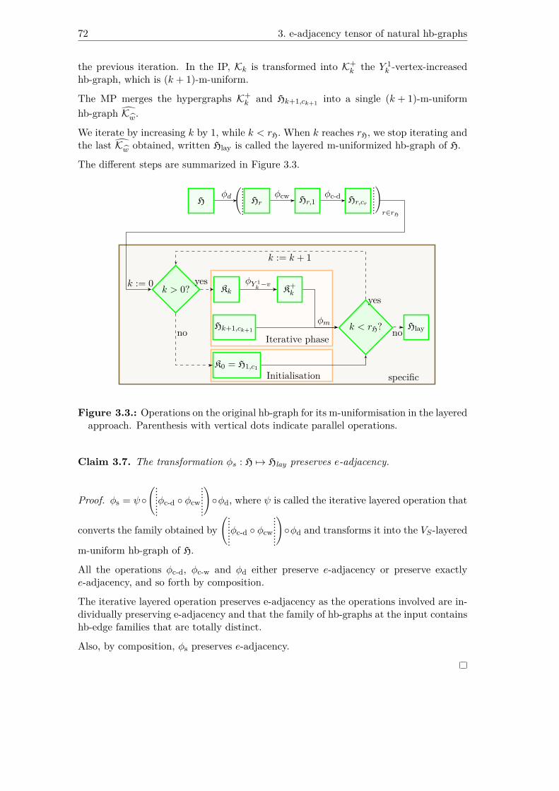
72 3. e-adjacency tensor of natural hb-graphs
the previous iteration. In the IP, Kk is transformed into K+k the Y 1
k -vertex-increasedhb-graph, which is (k + 1)-m-uniform.
The MP merges the hypergraphs K+k and Hk+1,ck+1 into a single (k + 1)-m-uniform
hb-graph Kw.
We iterate by increasing k by 1, while k < rH.When k reaches rH, we stop iterating andthe last Kw obtained, written Hlay is called the layered m-uniformized hb-graph of H.
The different steps are summarized in Figure 3.3.
H
(..........
Hrφd Hr,1
φcw φc-d Hr,cr
specific
...
...
...
.)r∈rH
Iterative phase
Initialisation
Kk K+k
φY 1k−v
Hk+1,ck+1 k < rH?φm
yes
no
k := k + 1
Hlay
k > 0?
K0 = H1,c1
k := 0
no
yes
Figure 3.3.: Operations on the original hb-graph for its m-uniformisation in the layeredapproach. Parenthesis with vertical dots indicate parallel operations.
Claim 3.7. The transformation φs : H 7→ Hlay preserves e-adjacency.
Proof. φs = ψ◦(..........φc-d ◦ φcw
...
...
...
.)◦φd, where ψ is called the iterative layered operation that
converts the family obtained by(..........φc-d ◦ φcw
...
...
...
.)◦φd and transforms it into the VS-layered
m-uniform hb-graph of H.
All the operations φc-d, φc-w and φd either preserve e-adjacency or preserve exactlye-adjacency, and so forth by composition.
The iterative layered operation preserves e-adjacency as the operations involved are in-dividually preserving e-adjacency and that the family of hb-graphs at the input containshb-edge families that are totally distinct.
Also, by composition, φs preserves e-adjacency.

3.3. e-adjacency tensor of a natural hb-graph 73
Layered homogenization:
The idea is to sort the hb-edges as in the silo homogenization and consider also rH − 1additional vertices Y1 to YrH−1 into the universe, corresponding to rH − 1 additionalvariables respectively y1 to yrH−1.
But in this case, these vertices are added successively to each hb-edge to fill them sothey reach all the same m-cardinality rH: a hb-edge of initial cardinality #me will befilled with elements Y#me to YrH−1. This corresponds to adding the k-m-uniform sub-hb-graph Hk with the k + 1-m-uniform sub-hb-graph Hk+1 by filling the hb-edge of Hkwith the additional vertex Yk to get a homogenized k + 1-m-uniform sub-hb-graph ofthe homogenized hb-graph H.
The normalised k-adjacency hypermatrix of the elementary hb-graph corresponding tothe hb-edge ei =
{vmij1j1
, . . . , vmijkijki
}is Qei of rank ρi = #mei and dimension n. The
corresponding reduced polynomial is:
Pei (z0) = ρizmij1j1
. . . zmijkijki
of degree #mei.
All the hb-edges of same m-cardinality belongs to the same layer. In order to transformall the hb-edges of m-cardinality #mei into hb-edges of m-cardinality #mei + 1, we fillthem with the corresponding element Y#mei .
In this case, the polynomial Pei (z0) is transformed into:
R(1)ei (z#mei) = Pei (z0) y1
#mei
of degree #mei + 1.
Iterating over the layers, the original hb-edge ei is successively filled with additionalvertices Yi, with i ∈ J#mei; rH − 1K , and the polynomial Pei (z0) is transformed into thepolynomial:
R(rH−#mei)ei (zrH−1) = Pei (z0) y1#mei . . . y
1rH−1
of degree rH.
The polynomial Pei (z0) with attached tensor Pei of rank #mei and dimension n istransformed in:
R(rH−#mei)ei (zrH−1) = Rei (z0) y1#mei . . . y
1rH−1
with attached tensor R(rH−#mei)ei of rank rH and dimension n+ rH − 1.
The CHR of the tensor R(rH−#mei)ei is the hypermatrix:
R(rH−#mei)ei=(r(rH−#mei) i1...irH
).
The elements of R(rH−#mei)eihave only two possible values, 0 and:
ρlay,(rH−#mei)ei = ρimij1 ! . . .mijki
!rH! .

74 3. e-adjacency tensor of natural hb-graphs
The indices of the non-zero elements of R(rH−#mei)eiare obtained by permutation of
the elements of the multiset:{jmij11 , . . . , j
mijkiki
, [n+ #mei]1 , . . . , [n+ rH − 1]1}.
And P is transformed into a homogeneous polynomial:
R (zrH−1) =∑i∈JpK
ciR(rH−#mei)ei (zrH−1)
=∑i∈JpK
ciρizmij1j1
. . . zmijkijki
y1#mei . . . y
1rH−1
representing the layered m-uniformized hb-graph Hlay with attached hypermatrix:
R =∑i∈JpK
ceiR(rH−#mei)ei,
where:cei = rH
ρi= rH
#mei.
Definition 3.9. The layered e-adjacency tensor Alay,H of a hb-graph H = (V,E)is the tensor of CHR Alay,H
∆=(ai1...irH
)i1,...,irH∈JnK
defined by:
Alay,H∆=∑i∈JpK
ceiR(rH−#mei)ei
where for ei ={vmij1j1
, . . . , vmijkijki
}∈ E :
cei = rH#mei
is the dilatation coefficient and R(rH−#mei)ei=(r(rH−#mei)i1...irH
)is the hypermatrix
whose elements have only two possible values 0 and:
ρlay,(rH−#mei)ei =mij1 ! . . .mijki
!rH! #mei.
The indices of the non-zero elements of R(rH−#mei)eiare obtained by permutation of
the elements of the multiset:{jmij11 , . . . , j
mijkiki
, [n+ #mei]1 , . . . , [n+ rH − 1]1}.
Remark 3.3.4. Alay,H can also be written:
Alay,H =∑
r∈JrHK
cr∑
ei∈{e:#me=r}Rei ,
where cr = rHr.
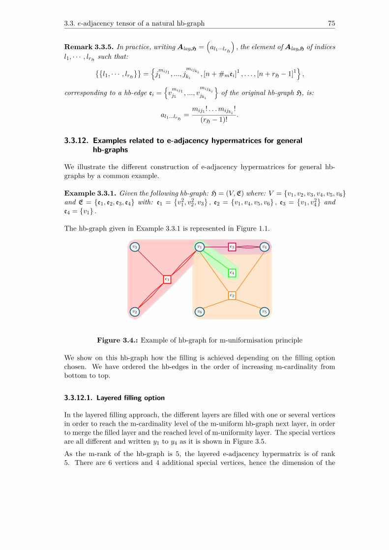
3.3. e-adjacency tensor of a natural hb-graph 75
Remark 3.3.5. In practice, writing Alay,H =(al1···lrH
), the element of Alay,H of indices
l1, · · · , lrH such that:{{l1, · · · , lrH
}}={jmij11 , ..., j
mijkiki
, [n+ #mei]1 , . . . , [n+ rH − 1]1},
corresponding to a hb-edge ei ={vmij1j1
, ..., vmijkijki
}of the original hb-graph H, is:
al1...lrH =mij1 ! . . .mijki
!(rH − 1)! .
3.3.12. Examples related to e-adjacency hypermatrices for generalhb-graphs
We illustrate the different construction of e-adjacency hypermatrices for general hb-graphs by a common example.
Example 3.3.1. Given the following hb-graph: H = (V,E) where: V = {v1, v2, v3, v4, v5, v6}and E = {e1, e2, e3, e4} with: e1 =
{v2
1, v22, v3
}, e2 = {v1, v4, v5, v6} , e3 =
{v1, v
24}and
e4 = {v1} .
The hb-graph given in Example 3.3.1 is represented in Figure 1.1.
v3
v2
v1 v4
v6 v5
e1
e2
e3
e4
Figure 3.4.: Example of hb-graph for m-uniformisation principle
We show on this hb-graph how the filling is achieved depending on the filling optionchosen. We have ordered the hb-edges in the order of increasing m-cardinality frombottom to top.
3.3.12.1. Layered filling option
In the layered filling approach, the different layers are filled with one or several verticesin order to reach the m-cardinality level of the m-uniform hb-graph next layer, in orderto merge the filled layer and the reached level of m-uniformity layer. The special verticesare all different and written y1 to y4 as it is shown in Figure 3.5.As the m-rank of the hb-graph is 5, the layered e-adjacency hypermatrix is of rank5. There are 6 vertices and 4 additional special vertices, hence the dimension of the

76 3. e-adjacency tensor of natural hb-graphs
e1 : v1 v1 v2 v2 v3
e2 : v1 v4 v5 v6
e3 : v1 v4 v4
e4 : v1
e1 : v1 v1 v2 v2 v3
e2 : v1 v4 v5 v6
e3 : v1 v4 v4
e4 : v1 y1
e1 : v1 v1 v2 v2 v3
e2 : v1 v4 v5 v6
e3 : v1 v4 v4
e4 : v1 y1 y2
e1 : v1 v1 v2 v2 v3
e2 : v1 v4 v5 v6
e3 : v1 v4 v4 y3
e4 : v1 y1 y2 y3
e1 : v1 v1 v2 v2 v3
e2 : v1 v4 v5 v6 y4
e3 : v1 v4 v4 y3 y4
e4 : v1 y1 y2 y3 y4
Layered filling: fill and merge
Figure 3.5.: Layered filling on the example of Figure 3.4
hypermatrix is 10, the place 1 to 6 storing the information for v1 to v6 in this orderand the places 7 to 10 the information for y1 to y4. We write the layered e-adjacencyhypermatrix Alay = (alay i1i2i3i4i5)∀j∈J5K:ij∈J10K .
Considering all permutations of the indices σ ∈ S5, we have:
• e1 stored in all the elements: alayσ(1 1 2 2 3) of value 16 .
• e2 stored in all the elements: alayσ(1 4 5 6 10) of value 124 .
• e3 stored in all the elements: alayσ(1 4 4 9 10) of value 112 .
• e4 stored in all the elements: alayσ(1 7 7 7 7) of value 1.• The other elements of Alay are equal to zero.
3.3.12.2. Silo filling option
In the silo approach, the different layers of m-uniformity are filled up to the m-rangeof the hb-graph with different special vertices that depend only on the layer of m-uniformity, as it is shown in Figure 3.6.
e1 : v1 v1 v2 v2 v3
e2 : v1 v4 v5 v6
e3 : v1 v4 v4
e4 : v1
e1 : v1 v1 v2 v2 v3
e2 : v1 v4 v5 v6
e3 : v1 v4 v4
e4 : v1 y1 y1 y1 y1
e1 : v1 v1 v2 v2 v3
e2 : v1 v4 v5 v6
e3 : v1 v4 v4 y3 y3
e4 : v1 y1 y1 y1 y1
e1 : v1 v1 v2 v2 v3
e2 : v1 v4 v5 v6 y4
e3 : v1 v4 v4 y3 y3
e4 : v1 y1 y1 y1 y1
Silo filling
Figure 3.6.: Silo filling on the example of Figure 3.4
As the m-rank of the hb-graph is 5, the silo e-adjacency hypermatrix is of rank 5. Thereare 6 vertices and 4 additional special vertices, hence the dimension of the hypermatrix

3.3. e-adjacency tensor of a natural hb-graph 77
is 10, the place 1 to 6 storing the information for v1 to v6 in this order and the places7 to 10 the information for y1 to y4. We write the layered e-adjacency hypermatrixAsil = (asil i1i2i3i4i5)∀j∈J5K:ij∈J10K .
Considering all permutations of the indices σ ∈ S5, we have:
• e1 stored in all the elements: asilσ(1 1 2 2 3) of value 16 .
• e2 stored in all the elements: asilσ(1 4 5 6 10) of value 124 .
• e3 stored in all the elements: asilσ(1 4 4 9 9) of value 16 .
• e4 stored in all the elements: asilσ(1 7 7 7 7) of value 1.
• The other elements of Asil are equal to zero.
3.3.12.3. Straightforward filling option
In the straightforward approach, all the hb-edges are filled up to reaching a m-cardinalitycorresponding to the hb-graph m-range as it is shown in Figure 3.7.
e1 : v1 v1 v2 v2 v3
e2 : v1 v4 v5 v6
e3 : v1 v4 v4
e4 : v1
e1 : v1 v1 v2 v2 v3
e2 : v1 v4 v5 v6 y1
e3 : v1 v4 v4 y1 y1
e4 : v1 y1 y1 y1 y1
Straightforward filling
Figure 3.7.: Straightforward filling on the example of Figure 3.4
As the m-rank of the hb-graph is 5, the straightforward e-adjacency hypermatrix isof rank 5. There are 6 vertices and 1 additional special vertex, hence the dimensionof the hypermatrix is 7, the place 1 to 6 storing the information for v1 to v6 in thisorder and the place 7 to y1. We write the layered e-adjacency hypermatrix Astr =(astr i1i2i3i4i5)∀j∈J5K:ij∈J7K .
Considering all permutations of the indices σ ∈ S5, we have:
• e1 stored in all the elements: astrσ(1 1 2 2 3) of value 16 .
• e2 stored in all the elements: astrσ(1 4 5 6 7) of value 124 .
• e3 stored in all the elements: astrσ(1 4 4 7 7) of value 16 .
• e4 stored in all the elements: astrσ(1 7 7 7 7) of value 1.
• The other elements of Astr are equal to zero.
78 3. e-adjacency tensor of natural hb-graphs
3.4. Results on the constructed tensors
We recall that each of the tensors obtained is of rank rH and of dimension n+nA wherenA is:
• in the straightforward approach: nA = 1;• in the silo approach: nA = rH − 1;• and, in the layered approach: nA = rH − 1.
3.4.1. Fulfillment of the expectations
We revisit the expectations formulated in Section 3.3.1 and prove that they are all met.
Guarantee 3.1. The e-adjacency tensor should be non-negative, symmetric and itsgeneration should be as simple as possible.
Proof. The tensors that have been built are all non-negative and symmetric. Theirgeneration mostly depends on the content of the hb-edges. Only the layered approachhas a more complex generation process; however, it is retained, as it is the only possibleapproach that keeps hypergraph interpretability via Hm-UP without needing hb-graphsfor general hypergraphs.
Guarantee 3.2. The tensor should be globally invariant to vertex permutation in theoriginal hb-graph.
Proof. Let H = (V,E) be a hb-graph with vertex set V = {vi : i ∈ JnK} and E =(ej)j∈JpK .We do the proof only for the straightforward tensor, since the other proofs aresimilar.Let consider a permutation π ∈ Sn, that corresponds to a relabeling of the vertices fromthe universe of the original hb-graph. Applying this relabeling to the content of thehb-edge:
ej ={vmj i1i1
, ..., vmj ijij
}transforms it into:
ej ={vmj i1π(i1) , ..., v
mj ijπ(ij)
}.
The original hb-edge was stored in the elements of the form:
aimj i11 ...i
mj ijj (n+1)rH−#mej
and the ones obtained by permutation of the indices.It follows that the relabeled hb-graph will have its elements stored in:
aπ(i1)mj i1 ...π(ij)
mj ij (n+1)rH−#mej
and all the ones obtained by permutation of the elements of:{π (i1)mj i1 , ..., π (ij)mj ij , (n+ 1)rH−#mej
}

3.4. Results on the constructed tensors 79
This corresponds to a permutation of the elements in the tensor according to the rela-beling: the two tensors differ only by a reshuffling of the indices due to the permutationπ, which means that the constructed tensor is globally invariant to a relabeling in theoriginal hb-graph.
Guarantee 3.3. The e-adjacency tensor should induce a unique reconstruction of thehb-graph it is originated from.
Proof. From the way the elements have been constructed, there is a one-to-one mappingbetween the hb-edge and the ordered indices of the coefficient in the tensor. From theseindices, the hb-graph can be reconstructed with no ambiguity.
Guarantee 3.4. Given the choice of two representations the one that can be describedwith the least possible number of elements should be chosen. Then the sparsest e-adjacency tensor should be chosen.
Proof. The straightforward tensor requires only one additional element to capture theinformation. The three representations are anyway economic as only one element eachtime needs to be described in the hypermatrix for a given hb-edge, the others beingobtained by permutation of its indices.
Guarantee 3.5. The e-adjacency tensor should allow direct retrieval of the vertex de-grees.
Proof. The proof will be given in the next Section.
3.4.2. Information on hb-graph
3.4.2.1. m-degree of vertices
We built the different tensors such that the retrieval of the vertex m-degree is possible;the null vertex(-ices) added during the Hm-UP give(s) additional information on thestructure of the hb-graph.
Claim 3.8. Let us consider for j ∈ JnK, a vertex vj ∈ V.
Then for each of the e-adjacency tensors built, it holds:∑j2,...,jrH∈Jn+nAK
ajj2...jrH =∑
i : vj∈eimi j = degm (vj) .
80 3. e-adjacency tensor of natural hb-graphs
Proof. For j ∈ JnK ,∑
j2,...,jrH∈Jn+nAKajj2...jrH has non-zero terms only for the correspond-
ing hb-edges of the original hb-graph ei containing vj . Such a hb-edge is described byei =
{vmi jj , v
mi l2l2
, . . . , vmi lklk
}. This means that the multiset
{{j2, . . . , jrH
}}corresponds
exactly to the multiset{jmi j−1, l
mi l22 , . . . , l
mi lkk
}.
In the straightforward approach, for each ei such that vj ∈ ei, there are:
(rH − 1)!(mi j − 1)!mi l2 ! . . .mi lk !mi n+1!
possible permutations of the indices j2 to jrH and:
ajj2...jrH = mi j !mi l2 ! . . .mi lk !mi n+1!(rH − 1)! .
In the silo approach, for each ei such that vj ∈ ei, there are:
(rH − 1)!(mi j − 1)!mi l2 ! . . .mi lk !mi n+#mei !
possible permutations of the indices j2 to jrH and:
ajj2...jrH = mi j !mi l2 ! . . .mi lk !mi n+#mei !(rH − 1)! .
In the layered approach, for each ei such that vj ∈ ei, there are:
(rH − 1)!(mi j − 1)!mi l2 ! . . .mi lk !
possible permutations of the indices j2 to jrH which have all the same value equal to:
ajj2...jrH = mi j !mi l2 ! . . .mi lk !(rH − 1)! .
So, whatever the approach taken is, it holds:∑j2,...,jrH∈JnK
ajj2...jrH =∑
i : vj∈eimi j = degm (vj) .
3.4.2.2. Additional vertex information
The additional vertices carry information on the hb-edges of the hb-graph: the infor-mation carried depends on the approach taken.
Claim 3.9. The layered e-adjacency tensor allows the retrieval of the distribution ofthe hb-edges.
3.4. Results on the constructed tensors 81
Proof. For j ∈ JnAK: ∑j2,...,jrH∈Jn+nAK
an+jj2...jrH
has non-zero terms only for the corresponding hb-edges of the m-uniformized hb-graphei containing vj . Such a hb-edge is described by5:
ei ={vmi kk : k ∈ Jn+ nAK
}.
This means that the multiset: {{j2, . . . , jrH
}}corresponds exactly to the multiset:{
(n+ j)mi n+j−1}
+ {kmi k : k ∈ Jn+ nAK ∧ k 6= j} .
The number of possible permutations of elements in this multiset is:
(rH − 1)!(mi n+j − 1)! ∏
k∈JnKmi k!
∏k∈Jn+1;n+nAK
k 6=j
mi k!
and the elements corresponding to one hb-edge are all equal to:∏k∈JnAK
mi k!
(rH − 1)! .
Thus: ∑j2,...,jrH∈Jn+nAK
an+jj2...jrH =∑
j2,...,jrH∈JnK
mi n+j = degm (Yj) .
The interpretation differs between the different approaches.
For the silo approach:
There is one added vertex in each hb-edge. The silo of hb-edges of m-cardinality ms
(ms ∈ JrH − 1K) is associated to the null vertex Yms . The multiplicity of Yms in eachhb-edge of the silo is rH −ms.
Hence:degm (Yj)rH −ms
= |{e : #me = ms}| .
The number of hb-edges in the silo ms is then deduced by the following formula:
|{e : #me = ms}| = |E| −∑
ms∈JrH−1K
degm (Yj)rH −ms
.
For the layered approach:
The vertex Yj corresponds to the layer of level j added to each hb-edge with m-cardinality less or equal to j with a multiplicity of 1.5With the convention, that for j ∈ JnAK:vn+j = yj
82 3. e-adjacency tensor of natural hb-graphs
Also:degm (Yj) = |{e : #me 6 j}| .
Hence, for j ∈ J2; rH − 1K:|{e : #me = j}| = degm (Yj)− degm (Yj−1) .
It yields:|{e : #me = 1}| = degm (Y1)
and:|{e : #me = rH}| = |E| − degm
(YrH−1
).
For the straightforward approach:In a hb-edge of m-cardinality j ∈ JrH − 1K, the vertex Y1 is added with multiplicityrH − j. The number of hb-edges with m-cardinality j can be retrieved by consideringthe elements of Astr,H of index (n + 1)i1 . . . irH−1 where 1 6 i1 6 ... 6 ij 6 n andij+1 = . . . = irH−1 = n+ 1 and the elements with indices obtained by permutation.It follows for j ∈ JrH − 1K :
|{e : #me = j}| = |{e : Y1 ∈ e ∧me (Y1) = rH − j}|=
∑i1,...,irH−1∈Jn+1K|{ik=n+1}|=rH−j−1
an+1i1...irH−1 .
The terms an+1i1...irH−1 of this sum are non-zero only for the corresponding hb-edges eof the m-uniformized hb-graph having Y1 with multiplicity rH − j in it. Such a hb-edgeis described by:
ei ={vmi kk : 1 6 k 6 n
}+{YrH−j
1
}.
It means that the multiset: {{i1, . . . , irH−1
}}corresponds exactly to the multiset:
{kmi k : k ∈ JnK}+{n+ 1rH−j−1
}.
The number of possible permutations in this multiset is:(rH − 1)!∏
k∈JnKmi k! (rH − j − 1)!
and the elements corresponding to one hb-edge are all equal to:∏k∈JnK
mi k!× (rH − j)!
(rH − 1)! .
Hence:1
rH − j∑
i2,...,irH∈Jn+1K|{ik=n+1:k∈J2;rHK}|=rH−j−1
an+1i2...irH = |{e : #me = j}| .
The number of hb-edges of m-cardinality rH can be retrieved by:|{e : #me = rH}| = |E| −
∑j∈JrH−1K
|{e : #me = j}| .
3.4. Results on the constructed tensors 83
3.4.3. First results on hb-graph spectral analysis
Let H = (V,E) be a general hb-graph of e-adjacency tensorAH of CHR AH =(ai1...ikmax
)of order kmax and dimension n+ nA.
We write dm,i = degm (vi) if i ∈ JnK and dm,n+i = degm (Yi) if i = n+ j, j ∈ JnAK .
In the e-adjacency hypermatrix AH, the diagonal entries are no longer equal to zero. Asall elements of AH are non-negative real numbers, and as we have shown in the previousSection that: ∑
i2,...,im∈Jn+nAK
aii2...irH ={dm,i if i ∈ JnKdm,n+j if i = n+ j, j ∈ JnAK ,
it follows:
Claim 3.10. The e-adjacency tensor AH of a general hb-graph H = (V,E) has eigen-values λ of its CHR AH such that:
|λ| 6 max (∆m,∆?m) (3.1)
where ∆m = maxi∈JnK
(dm,i) and ∆?m = max
i∈JnAK(dm,n+i) .
Proof. From:∀i ∈ J1, nK ,
(Axm−1
)i
= λxm−1i , (3.2)
since aii2...imare non-negative real numbers, it holds for all λ that:
|λ− ai...i| 6∑
i2,...,im∈Jn+nAKδii2...im=0
aii2...im . (3.3)
Considering the triangular inequality, it follows:
|λ| 6 |λ− ai...i|+ |ai...i| . (3.4)
Combining 3.3 and 3.4 yield:
|λ| 6∑
i2,...,im∈Jn+nAKδii2...im=0
aii2...im + |ai...i| . (3.5)
But, irrespective of the approach taken, if {irH} is an hb-edge of the hb-graph, then:
|ai...i| = rH
otherwise:|ai...i| = 0
and, thus, writing ∆m = maxi∈JnK
(degm (vi)) and ∆?m = max
i∈JnAK(degm (Ni)) and, using 3.5
and dm,i = ∑i2,...,im∈Jn+nAK
δii2...im=0
aii2...im + ai...i yield:
|λ| 6 max (∆m,∆?m) .
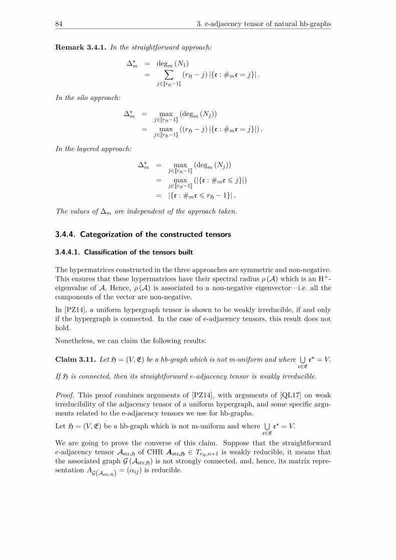
84 3. e-adjacency tensor of natural hb-graphs
Remark 3.4.1. In the straightforward approach:
∆?m = degm (N1)
=∑
j∈JrH−1K
(rH − j) |{e : #me = j}| .
In the silo approach:
∆?m = max
j∈JrH−1K(degm (Nj))
= maxj∈JrH−1K
((rH − j) |{e : #me = j}|) .
In the layered approach:
∆?m = max
j∈JrH−1K(degm (Nj))
= maxj∈JrH−1K
(|{e : #me 6 j}|)
= |{e : #me 6 rH − 1}| .
The values of ∆m are independent of the approach taken.
3.4.4. Categorization of the constructed tensors
3.4.4.1. Classification of the tensors built
The hypermatrices constructed in the three approaches are symmetric and non-negative.This ensures that these hypermatrices have their spectral radius ρ (A) which is an H+-eigenvalue of A. Hence, ρ (A) is associated to a non-negative eigenvector—i.e. all thecomponents of the vector are non-negative.
In [PZ14], a uniform hypergraph tensor is shown to be weakly irreducible, if and onlyif the hypergraph is connected. In the case of e-adjacency tensors, this result does nothold.
Nonetheless, we can claim the following results:
Claim 3.11. Let H = (V,E) be a hb-graph which is not m-uniform and where ⋃e∈E
e? = V.
If H is connected, then its straightforward e-adjacency tensor is weakly irreducible.
Proof. This proof combines arguments of [PZ14], with arguments of [QL17] on weakirreducibility of the adjacency tensor of a uniform hypergraph, and some specific argu-ments related to the e-adjacency tensors we use for hb-graphs.
Let H = (V,E) be a hb-graph which is not m-uniform and where ⋃e∈E
e? = V.
We are going to prove the converse of this claim. Suppose that the straightforwarde-adjacency tensor Astr,H of CHR Astr,H ∈ TrH,n+1 is weakly reducible, it means thatthe associated graph G (Astr,H) is not strongly connected, and, hence, its matrix repre-sentation AG(Astr,H) = (αij) is reducible.

3.4. Results on the constructed tensors 85
As Astr,H is symmetric, its associated graph G (Astr,H) is bidirectional and AG(Astr,H) =(αij) is symmetric.
This means that there exists a nonempty proper subset J of Jn+ 1K such that ∀i ∈J, ∀j ∈ Jn+ 1K \J : αij = 0.
As H is not m-uniform, J cannot be reduced to the singleton {n+ 1} since the specialvertex has to be linked to vertices of the hb-edges of m-cardinality value less than themaximal m-rank.
For symmetric reasons, J cannot be JnK , otherwise, it would mean that the specialvertex n+ 1 is isolated, which is not possible as the hb-graph is not m-uniform.
Thus, there exists at least one i1 ∈ J which represents an original vertex of H such thatai1i2...irH = 0 when at least one of the indices i2, ..., irH is in Jn+ 1K \J . In these rH − 1indices, at least one corresponds to an original vertex of H.
It indicates in this case that the group of original vertices of H represented in J aredisconnected from the original vertices that are in Jn+ 1K \J . Hence the hb-graph isdisconnected.
With: ⋃e∈E
e? = V, we require that there is no unused vertices in the universe.
If the hb-graph is m-uniform and connected, the straightforward e-adjacency tensorAstr,H is weakly reducible as the additional vertex is not used and hence is isolated inthe associated graph ofAstr,H. In this case, one can use Astr,H|JnK the principal sub-tensorof Astr,H related to JnK which is weakly irreducible. As Astr,H|JnK is weakly irreducible,it is strictly non-negative and, the Astr,H is a non-trivially non-negative tensor, whichmeans by using the theorem from [QL17] that Astr,H has a positive eigenvalue and henceρ (Astr,H) > 0.
Non-negative tensor weak irreducibility is a desirable property as it ensures that thetensor has a unique positive Perron vector (up to a multiplicative constant) associatedto its spectral positive radius ρ (A) . In this case, the algorithms to calculate the Perronvector converge.
To ensure weak irreducibility, we could transform the straightforward e-adjacency tensorin such a way that its associated graph is always strongly connected. It is sufficient toadd the special vertex to each of the hb-edges: in this case, it will force the associatedgraph to be connected, albeit the spectral radius upper-bound to be increased to themaximum between the maximal m-degree and the number of hb-edges.
Moreover:
Claim 3.12. The three e-adjacency tensors built for hb-graphs are non-trivially non-negative tensors when the hb-graph is connected and the union of the support of hb-edgescovers the vertex set.
Proof. We already know that for a connected hb-graph which is not m-uniform, thestraightforward e-adjacency tensor is weakly irreducible, hence non-trivially non-negative.

86 3. e-adjacency tensor of natural hb-graphs
For a m-uniform hb-graph, the principal sub-tensor of Astr,H composed of its first n in-dices is weakly irreducible, hence strictly non-negative. The proof is similar to the oneof [PZ14] and [QL17] for hypergraphs.
We have already explained in [OLGMM18b] how a hb-graph H = (V,E) can be decom-posed in layers by considering Ek = {e ∈ E, ]me = k} and the hb-graphs Hk = (V,Ek)to obtain H = ⊕
k∈JrHKHk.
For the silo e-adjacency tensor, the principal sub-tensor to be considered is the oneobtained using J = JnK ∪ {n+ k : k ∈ JrH − 1K ∧ Ek 6= ∅} . Asil,H|J is then weakly ir-reducible, hence strictly non-negative. The tensor Asil,H is, therefore, a non-triviallynon-negative tensor.
For the layered e-adjacency tensor Alay,H, we consider the principal sub-tensor Alay,H|Kwhere K = JnK ∪ {n+ k : k ∈ Jkmin, rH − 1K} with kmin = min {k : Ek 6= ∅} . This prin-cipal sub-tensor is weakly irreducible as the hb-graph is connected, hence strictly non-negative. Therefore, the tensor Alay,H is non-trivially non-negative.
As a consequence the spectral radii of these tensors are positive.
3.4.4.2. Connected components and uniformisation process
The uniformisation process used to built the three tensors leads to the addition of somevertices to the hb-edges; while it does not change the number of hb-edges and the degreeof the vertices that are in the original hb-graph, it has an impact on the connectivity ofthe uniform hb-graph compared to the original one.
Nonetheless, to address this problem, it is always possible to consider each connectedcomponent of the original hb-graph separately and build a tensor for each of theseconnected components. In this case, the number of connected components remainsunchanged, even if we modify the internal connectivity of a connected component withthe added vertices.
So we can always suppose that we address only connected hb-graphs.
3.5. Evaluation and first choice
3.5.1. Evaluation
We have put together some key features of the e-adjacency tensors proposed in thisThesis: the straightforward approach tensor Astr,H, the silo approach tensor Asil,H andAlay,H for the layered approach.
The CHR of the constructed tensors have all same order rH. Asil,H and Alay,H dimensionsare rH − 2 bigger than Astr,H (n − 2 in the worst case). Astr,H has a total number of
elements (n+ 1)rH(n+ rH − 1)rH times smaller than the two other tensors.

3.5. Evaluation and first choice 87
Elements of Astr,H—respectively Asil,H—are repeated 1nj !
—respectively 1nj k!
—timesless than elements of Alay,H. The total number of non-zero elements filled for a givenhb-graph in Astr,H and Asil,H are the same and is smaller than the total number ofnon-zero elements in Alay,H.
Since whatever the approach taken, the tensors are symmetric, a unique value is neededto fully describe an hb-edge; moreover, this value depends only on the hb-edge compo-sition as well as the number of elements to be filled.
All tensors are symmetric and allow the reconstruction of the hb-graph from theseelements.
Node’s degrees can be retrieved as it has been shown previously. Additional informationon individual hb-edges is easier to retrieve with the silo and the layered approach.
3.5.2. First choice
Insofar, as the straightforward tensor is weakly irreducible for non m-uniform connectedhb-graph and, as this is a sufficient desirable property to choose it, even if this choice isat the price of less practicability to retrieve information on hb-edges, we take Astr,H fordefinition of the e-adjacency tensor of a hb-graph. The information on the shape of thehb-edges is preserved through the added special vertex, which enhances the retrieval ofinformation on the hb-edge cardinality.
3.5.3. Hypergraphs and hb-graphs
Hypergraphs are particular case of hb-graphs and, hence, the e-adjacency tensor definedfor hb-graphs can be used for hypergraphs. Since the multiplicity function for verticesof a hyperedge seen as hb-edge has its values in {0, 1}, the e-adjacency tensor elementsdiffer only by a factorial number due to the cardinality of the hyperedge.
The definition that is retained for the e-adjacency tensor of a hypergraph is:
Definition 3.10. The e-adjacency tensor of a hypergraph H = (V,E) having maximalcardinality of its hyperedges kmax is the tensor AH of CHR:
AH∆=(ai1...irH
)16i1,...,irH6n
defined by:AH
∆=∑i∈JpK
ceiRei
and where for ei ={vj1 , . . . , vjki
}∈ E, cei = kmax
kiis the dilatation coefficient and
Rei =(ri1...irH
)is the associated tensor to ei, having all non-zero elements of same
value. The non-zero elements of Rei are:
rj1...jki (n+1)kmax−ki = (kmax − ki)!kmax! ki
88 3. e-adjacency tensor of natural hb-graphs
and all the ones whose indices are obtained by permutation of:
j1 . . . jki (n+ 1)kmax−ki .
In practice, writing AH =(al1...lkmax
), the element of AH of indices l1, · · · , lkmax such
that: {{l1, · · · , lrH
}}={j1, ..., jki , [n+ 1]kmax−ki
},
corresponding to a hyperedge ei ={vj1 , ..., vjki
}of the original hypergraph H, is:
al1...lrkmax= (kmax − ki)!
(kmax − 1)! .
Remark 3.5.1.
As in [OLGMM17a] we compare the e-adjacency tensors obtained by [BCM17] and by[SZB19] with the one chosen in this Thesis. The results are presented in Table 3.2.
3.6. Further comments
Extending the concept of hypergraphs to support multisets and introducing hb-graphshave allowed us to define a systematic approach for building the e-adjacency tensor ofa hb-graph. Conversely, as hypergraphs appear as particular case of hb-graphs, the e-adjacency tensors are applicable to general hypergraphs. Hb-graphs are a good modelingframework for many real problems and have induced already some nice refinements inexisting work.
The tensor constructed in [BCM17] can be seen as a transformation of the hypergraphH = (V,E) into a weighted hb-graph HB = (V,E′, we): with the same vertex set butwith hb-edges obtained from the hyperedges of the original hypergraph such that for agiven hyperedge all the hb-edges having this hyperedge as support are considered withmultiplicities of vertices such that it reaches kmax.
We still have to analyze the behavior of our constructed e-adjacency tensor with regardto the diffusion process. The fact that information on hb-edges for hb-graphs and,therefore, for hyperedges in hypergraphs are stored in the e-adjacency tensor shouldprovide a nice explanation of the role of the variety of hb-edge m-cardinality.
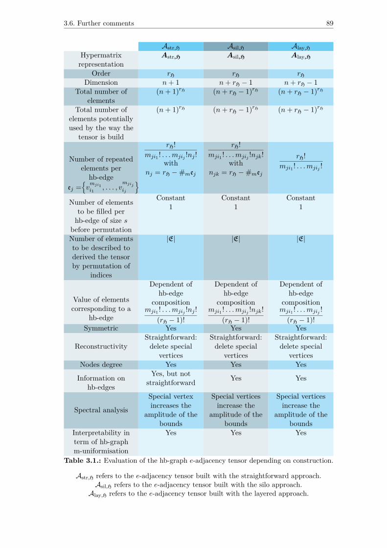
3.6. Further comments 89
Astr,H Asil,H Alay,HHypermatrixrepresentation
Astr,H Asil,H Alay,H
Order rH rH rHDimension n+ 1 n+ rH − 1 n+ rH − 1
Total number ofelements
(n+ 1)rH (n+ rH − 1)rH (n+ rH − 1)rH
Total number ofelements potentiallyused by the way the
tensor is build
(n+ 1)rH (n+ rH − 1)rH (n+ rH − 1)rH
Number of repeatedelements per
hb-edgeej =
{vmji1i1
, . . . , vmjijij
}
rH!mji1 ! . . .mjij !nj !
withnj = rH −#mej
rH!mji1 ! . . .mjij !njk!
withnjk = rH −#mej
rH!mji1 ! . . .mjij !
Number of elementsto be filled perhb-edge of size s
before permutation
Constant1
Constant1
Constant1
Number of elementsto be described toderived the tensorby permutation of
indices
|E| |E| |E|
Value of elementscorresponding to a
hb-edge
Dependent ofhb-edge
compositionmji1 ! . . .mjij !nj !
(rH − 1)!
Dependent ofhb-edge
compositionmji1 ! . . .mjij !njk!
(rH − 1)!
Dependent ofhb-edge
compositionmji1 ! . . .mjij !
(rH − 1)!Symmetric Yes Yes Yes
ReconstructivityStraightforward:delete special
vertices
Straightforward:delete special
vertices
Straightforward:delete special
verticesNodes degree Yes Yes Yes
Information onhb-edges
Yes, but notstraightforward Yes Yes
Spectral analysis
Special vertexincreases the
amplitude of thebounds
Special verticesincrease the
amplitude of thebounds
Special verticesincrease the
amplitude of thebounds
Interpretability interm of hb-graphm-uniformisation
Yes Yes Yes
Table 3.1.: Evaluation of the hb-graph e-adjacency tensor depending on construction.
Astr,H refers to the e-adjacency tensor built with the straightforward approach.Asil,H refers to the e-adjacency tensor built with the silo approach.Alay,H refers to the e-adjacency tensor built with the layered approach.

90 3. e-adjacency tensor of natural hb-graphs
BH SH AHHypermatrixrepresentation
BH SH AH
Order kmax kmax kmaxDimension n n n+ 1
Total number ofelements
nkmax nkmax (n+ 1)kmax
Total number ofelements potentiallyused by the way the
tensor is build
nkmax nkmax (n+ 1)kmax
Number of non-zeroelements for a given
hypergraph
kmax∑s=1
αs |Es| withαs =
ps (kmax) kmax!k1!...ks!
kmax∑s=1
s! |Es|
kmax∑s=1
αs |Es| with
αs = kmax!(kmax − s)!
Number of repeatedelements per hyperedge
of size s
kmax!k1!...ks!
s kmax!(kmax − s)!
Number of elements tobe filled per hyperedge
of size s beforepermutation
Varyingps (kmax) =(kmax − 1s− 1
)Varying s ifprefix is
considered asnon-permuting
part
Constant1
Number of elements tobe described to derived
the tensor bypermutation of indices
kmax∑s=1
ps (kmax) |Es|kmax∑s=1
s |Es| |E|
Value of elementscorresponding to a
hyperedge
Dependent ofhyperedgecomposition
s
αs
Dependent ofhyperedgecomposition
1(s− 1)!
Dependent ofhyperedge size
(kmax − s)!(kmax − 1)!
Symmetric Yes No Yes
Reconstructivity Need computation ofduplicated vertices
Needcomputation of
duplicatedvertices
Straightforward:delete special
vertices
Nodes degree Yes Yes Yes
Hyperedge cardinality Not straightforward Notstraightforward Yes
Spectral analysis Yes Yes
Special verticesincrease the
amplitude of thebounds
Interpretability in termof hypergraph /
hb-graph(m-)uniformisation
No / No No / No No / Yes
Table 3.2.: Evaluation of the hypergraph e-adjacency tensor.
BH designates the adjacency tensor defined in [BCM17].SH designates the adjacency tensor defined in [SZB19].
AH refers to the e-adjacency tensor as defined in this Thesis.
4. m-uniformisation processes andexchange-based diffusion
Highlights
4.1. Motivation . . . . . . . . . . . . . . . . . . . . . . . . . . . . . . . . . . 914.2. Impact of the m-uniformisation process on the exchange-based diffusion 924.3. e-adjacency tensors require compromises . . . . . . . . . . . . . . . . . . 984.4. Further comments . . . . . . . . . . . . . . . . . . . . . . . . . . . . . . 100
Prerequisites: Section 1.3 and, Chapters 2 and 3.
4.1. Motivation
An expectation that has not been formulated while constructing the e-adjacency tensors,as we wanted to expand the current adjacency tensors for uniform hypergraphs, is anexpectation on the diffusion process.
Expectation 4.1. The construction of the e-adjacency tensor should have minimalimpact on the matrix exchange-based diffusion process of a connected hb-graph.
As we need a hb-graph m-uniformisation to allow the storing of the elements in a singlecubical tensor, we transform the original hb-graph H of incident matrix H of dimensionn × p in a m-uniform hb-graph H(m) of incident matrix H(m) of dimension (n+ nA) pwhere nA is the number of special vertices added during the m-uniformisation process.The matrix exchange-based diffusion process on a hb-graph depends on the incidentmatrix of the hb-graph. Considering the stationary states for vertices and hb-edges,we can measure the similarity between the two diffusions by considering the state ofthe vertices / hb-edges of the original hb-graph and the state of the vertices / hb-edgesin the m-uniformized hb-graph. Let πV (respectively πV (m)) be the stationary state ofvertices and πE (respectively πE(m)) the stationary state of the hb-edges of the originalhb-graph (respectively of the m-uniformized hb-graph).We can reformulate mathematically the problem by finding, if there exists, an e-adjacencytensor T0 ∈ Sm,n ∩Nm,n such that:
T0 = argminT ∈Sm,n∩Nm,n
(d(πV , πV (m)[n]
)+ d
(πE, πE(m)
))

92 4. m-uniformisation processes and exchange-based diffusion
where πV (m)[n] is the truncated vector πV (m) to its first n coordinates (the ones repre-senting the states of the original vertices) and d (·, ·) is a distance, such as the Euclideandistance.
If this problem is tractable, which is in fact an open question, finding its solution isdefinitively NP-hard. Evaluating the impact on the diffusion at the end of the construc-tion of the proposed tensors is then already a first step.
Research question 4.1. What is the impact of the Hb-graph m-Uniformisation Processon the diffusion process?
4.2. Impact of the m-uniformisation process on theexchange-based diffusion
We consider a connected unweighted hb-graph H = (V,E) with no repeated hb-edges,incident matrix H and m-rank rH. We now focus on the impact of the m-uniformisationprocess on the exchange-based diffusion that is involved, i.e. the formalization of thestable states for the m-uniformized hb-graphs obtained during the construction of thetensors.
In Chapter 3, we built the e-adjacency tensors by m-uniformizing the original hb-graphwith the addition of special vertices to the hb-edge universe and the filling of the hb-edgeswith sufficient multiplicities on these vertices. We call this approach the additionalvertices filling m-uniformisation approach.
An other approach, taken in [BCM17] and [SZB19], was to share the elements in betweenfree places of the built tensor, i.e. elements of the tensor having repeated indices: thisprocess can be assimilated to adding hb-edges to the corresponding hypergraph, viewedas a hb-graph. The original hb-graph is m-uniformized by splitting hb-edges that are notcomplete (in the sense that they have a m-cardinality strictly less than the m-rank of theoriginal hb-graph) into multiple copies of these hb-edges and filling them by repeatingthe original vertices in different ways depending on the approach. We call this approachthe hb-edge splitting m-uniformisation approach.
Both approaches have a potential impact on the exchange-based diffusion since the orig-inal structure is modified. A third approach would consist in using a combination of thetwo previous ones. Nonetheless, as this approach potentially combines the drawbacks,and particularly increases the number of hb-edges, we do not think it is worth consid-ering it, since the additional vertices filling m-uniformisation approach does not requireany increase of the number of vertices.
4.2.1. Additional vertices filling m-uniformisation approach
We formulate the calculus for the general case.
We write Hproc∆= (Vproc,Eproc, wproc) the hb-graph obtained by additional vertices filling
m-uniformisation process of the original hb-graph and write its incident matrix Hproc ∈M(n+nproc),p. We have: Vproc = V ∪ {yi : i ∈ JnprocK} .
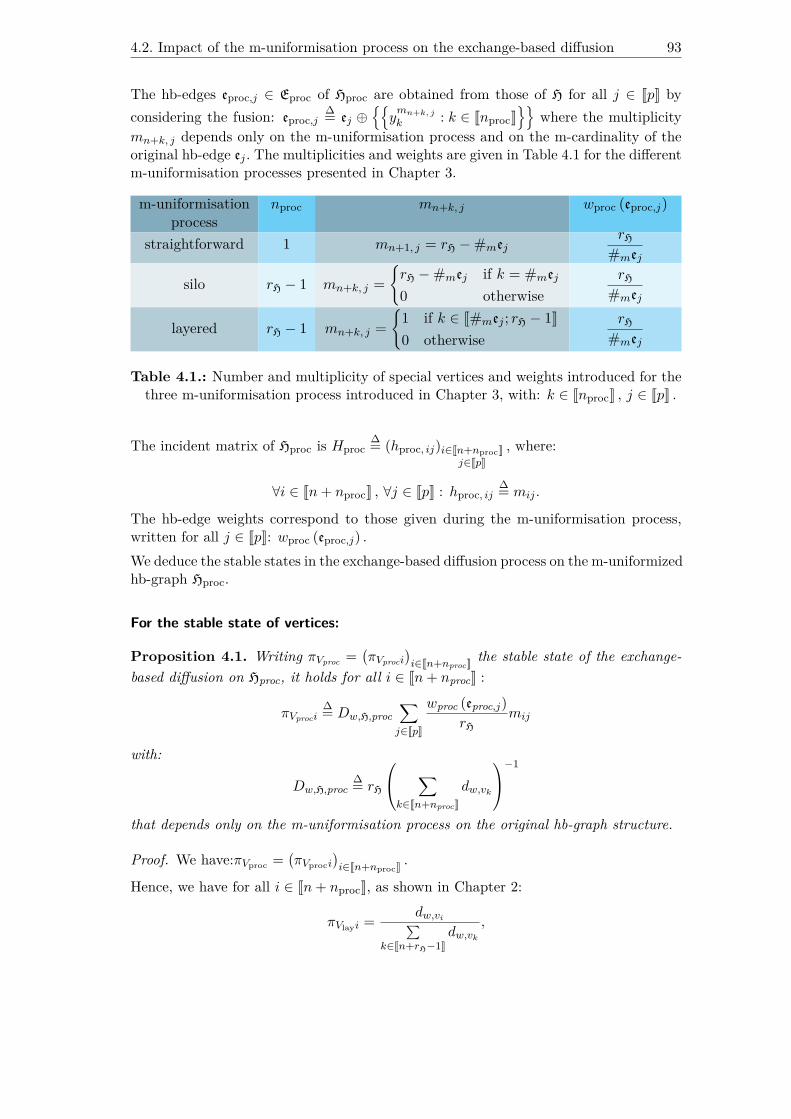
4.2. Impact of the m-uniformisation process on the exchange-based diffusion 93
The hb-edges eproc,j ∈ Eproc of Hproc are obtained from those of H for all j ∈ JpK byconsidering the fusion: eproc,j
∆= ej ⊕{{ymn+k, jk : k ∈ JnprocK
}}where the multiplicity
mn+k, j depends only on the m-uniformisation process and on the m-cardinality of theoriginal hb-edge ej . The multiplicities and weights are given in Table 4.1 for the differentm-uniformisation processes presented in Chapter 3.
m-uniformisationprocess
nproc mn+k, j wproc (eproc,j)
straightforward 1 mn+1, j = rH −#mejrH
#mej
silo rH − 1 mn+k, j ={rH −#mej if k = #mej
0 otherwiserH
#mej
layered rH − 1 mn+k, j ={
1 if k ∈ J#mej ; rH − 1K0 otherwise
rH#mej
Table 4.1.: Number and multiplicity of special vertices and weights introduced for thethree m-uniformisation process introduced in Chapter 3, with: k ∈ JnprocK , j ∈ JpK .
The incident matrix of Hproc is Hproc∆= (hproc, ij)i∈Jn+nprocK
j∈JpK, where:
∀i ∈ Jn+ nprocK , ∀j ∈ JpK : hproc, ij∆= mij .
The hb-edge weights correspond to those given during the m-uniformisation process,written for all j ∈ JpK: wproc (eproc,j) .We deduce the stable states in the exchange-based diffusion process on the m-uniformizedhb-graph Hproc.
For the stable state of vertices:
Proposition 4.1. Writing πVproc =(πVproci
)i∈Jn+nprocK the stable state of the exchange-
based diffusion on Hproc, it holds for all i ∈ Jn+ nprocK :
πVproci∆= Dw,H,proc
∑j∈JpK
wproc (eproc,j)rH
mij
with:
Dw,H,proc∆= rH
∑k∈Jn+nprocK
dw,vk
−1
that depends only on the m-uniformisation process on the original hb-graph structure.
Proof. We have:πVproc =(πVproci
)i∈Jn+nprocK .
Hence, we have for all i ∈ Jn+ nprocK, as shown in Chapter 2:
πVlayi = dw,vi∑k∈Jn+rH−1K
dw,vk,

94 4. m-uniformisation processes and exchange-based diffusion
where, for i ∈ Jn+ nprocK : dw,vi = ∑j∈JpK
mijwproc (eproc,j)
rH.
Writing: Dw,H,proc = rH
( ∑k∈Jn+nprocK
dw,vk
)−1
the result follows.
In the three m-uniformisation processes considered in Table 4.1, the weights attachedto the hb-edges of the m-uniformized hb-graphs are for all j ∈ JpK given by:
wproc (eproc,j) = rH#mej
.
With this weighting, it holds: πVproci = Dw,H,proc∑j∈JpK
mij
#mej.
Hence, the stable state of vertices depends on the relative multiplicity compared to them-cardinality of the hb-edges: thus, the more isolated a vertex in a hb-edge, the higherthe ranking of this vertex.
Remark 4.2.1. We introduced the technical coefficient in the Hm-UP to preserve thenumber of hb-edges. Keeping this coefficient at a constant value c—and in particular to1—independently of the hb-edge—i.e. for all j ∈ JpK : wproc (eproc,j) = c—, we have:
πVproci = Dw,H,procc∑j∈JpK
mij ∝ degm (vi)
This means that the ranking of the vertices achieved in the exchange-based diffusion ispreserved in this case (at the cost of having more difficulties to retrieve the m-degree ofvertices from the e-adjacency tensor).All other weightings of the original hb-edges have a potential influence on the rankingof vertices during the diffusion process.
To compare the vertex stable state obtained with the m-uniformized hb-graph and theoriginal hb-graph, one can compute the distance between these two stable states. It isgiven by:
Proposition 4.2.
d(πV ,
(πVproci
)i∈JnK
)=
√√√√√∑i∈JnK
∑j∈JpK
( 1#mH
− Dw,H,procwproc (eproc,j)rH
)mij
2
.
Proof. Immediate as: d(πV ,
(πVproci
)i∈JnK
)2= ∑
i∈JnK
(πV i − πVproci
)2.
Also, the perturbation of diffusion in the m-uniformized hb-graph is dependent on theshape of the original hb-graph and from how far away it is from m-uniformity.Other features such as the Kendall’s tau or the scaled Spearman footrule coefficientscan be calculated to compare the rankings obtained from the two diffusions.

4.2. Impact of the m-uniformisation process on the exchange-based diffusion 95
For the stable state of the hb-edges:
Proposition 4.3. Writing πEproc =(πEprocj
)j∈JpK
the stable state of hb-edges in theexchange-based diffusion on Hproc, we have for all j ∈ JpK :
πEprocj = Dw,H,procwproc (eproc,j) .
Proof. πEprocj = wproc (eproc,j)×#m (eproc,j)∑k∈Jn+nprocK
dw,vk= wproc (eproc,j)× rH∑
k∈Jn+nprocKdw,vk
= Dw,H,procwproc (eproc,j) .
The stable state no longer reflects the m-cardinality of the hb-edge.
Remark 4.2.2. Again the stable state of the diffusion for the hb-edges is highly disruptedby the weights of the Hm-UP process. If these weights are put equal to 1, it holds forall j ∈ JpK : πEprocj = 1
pwhich implies that the diffusion is non discriminative on the
hb-edges.
4.2.2. Hb-edge splitting m-uniformisation approach
We do not formulate systematically the approach but, instead, give the outlines andfocus on the m-uniformisation process induced by the tensor proposed in [BCM17] fora general hypergraph H = (V,E) of rank rH.
In Appendix Section E.1, for the tensor proposed in [BCM17], we have noticed thathyperedges of lower cardinality than the rank rH are stored in elements of repeatedindices of the e-adjacency tensor with rank rH and dimension |V | . To keep the tensorsymmetric, all the s-compositions of rH in s = #ej elements have to be consideredand from there all the combinations of indices reflecting the s-composition. Hence, theprocess cannot be interpreted in term of hypergraph uniformisation since the verticesmust be repeated and it requires a hb-graph m-uniformisation process: we propose thisinterpretation in this Section.
We have also mentioned that in the tensor proposed in [BCM17] a given hyperedgeej = {vl1 , ..., vls} is stored through a set of elements of the e-adjacency tensor of rankrH and dimension n = |V | whose indices corresponds to permutations of the differentmultisets
{{lkii , i ∈ JsK
}}such that: ∀i, ki > 1 and ∑
i∈JsKki = rH.
Hence, taking a hb-graph m-uniformisation interpretation means that the hyperedge ejconsidered as a hb-edge is transformed into a collection of hb-edges of universe V. Torefine this interpretation, we consider P#ej (rH) the set of compositions of rH in #ejelements defined by:
P#ej (rH) ∆=
(ki)i∈J#ejK : ∀i ∈ J#ejK , ki > 1 ∧∑
i∈J#ejKki = rH
.
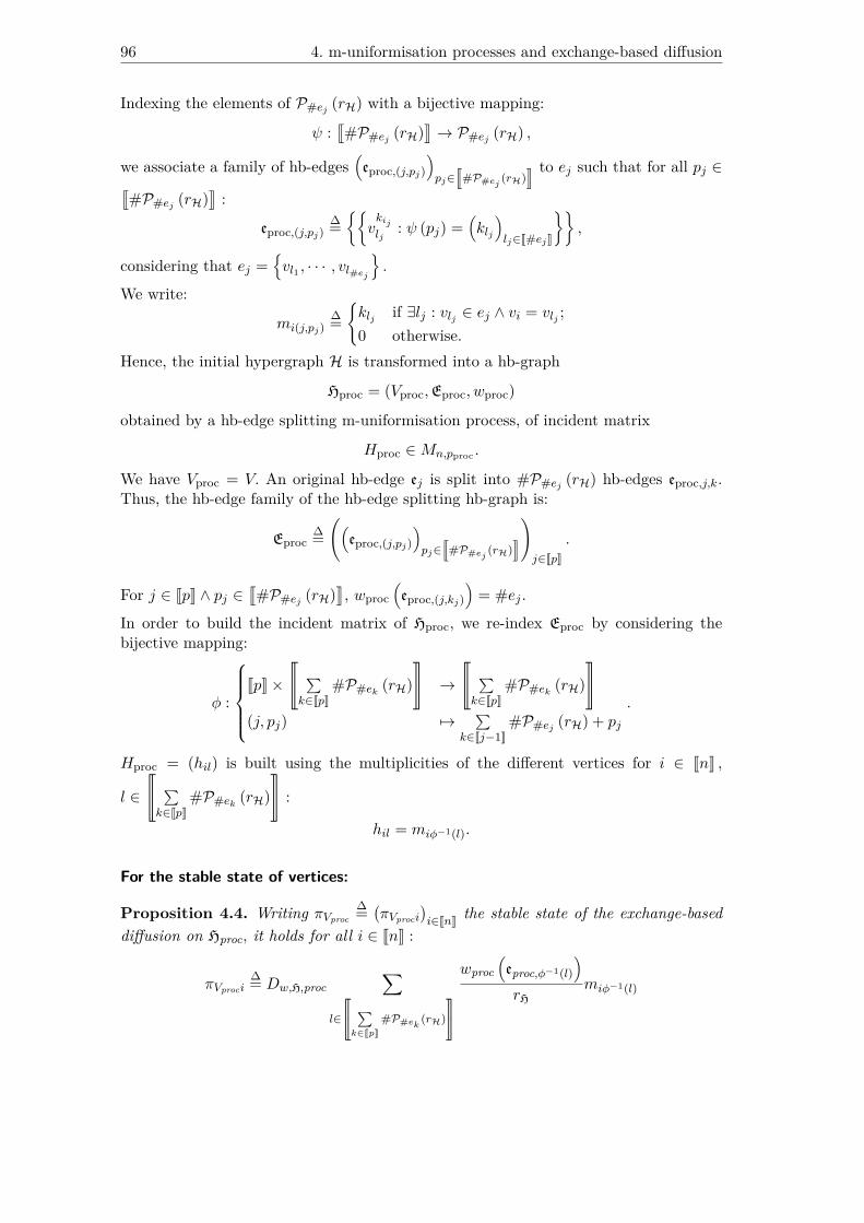
96 4. m-uniformisation processes and exchange-based diffusion
Indexing the elements of P#ej (rH) with a bijective mapping:
ψ :q#P#ej (rH)
y→ P#ej (rH) ,
we associate a family of hb-edges(eproc,(j,pj)
)pj∈
r#P#ej (rH)
z to ej such that for all pj ∈q#P#ej (rH)
y:
eproc,(j,pj)∆={{
vkijlj
: ψ (pj) =(klj
)lj∈J#ejK
}},
considering that ej ={vl1 , · · · , vl#ej
}.
We write:
mi(j,pj)∆={klj if ∃lj : vlj ∈ ej ∧ vi = vlj ;0 otherwise.
Hence, the initial hypergraph H is transformed into a hb-graph
Hproc = (Vproc,Eproc, wproc)
obtained by a hb-edge splitting m-uniformisation process, of incident matrix
Hproc ∈Mn,pproc .
We have Vproc = V. An original hb-edge ej is split into #P#ej (rH) hb-edges eproc,j,k.Thus, the hb-edge family of the hb-edge splitting hb-graph is:
Eproc∆=((
eproc,(j,pj))pj∈
r#P#ej (rH)
z
)j∈JpK
.
For j ∈ JpK ∧ pj ∈q#P#ej (rH)
y, wproc
(eproc,(j,kj)
)= #ej .
In order to build the incident matrix of Hproc, we re-index Eproc by considering thebijective mapping:
φ :
JpK×
t ∑k∈JpK
#P#ek (rH)|
→
t ∑k∈JpK
#P#ek (rH)|
(j, pj) 7→∑
k∈Jj−1K#P#ej (rH) + pj
.
Hproc = (hil) is built using the multiplicities of the different vertices for i ∈ JnK ,
l ∈
t ∑k∈JpK
#P#ek (rH)|
:
hil = miφ−1(l).
For the stable state of vertices:
Proposition 4.4. Writing πVproc∆=(πVproci
)i∈JnK the stable state of the exchange-based
diffusion on Hproc, it holds for all i ∈ JnK :
πVproci∆= Dw,H,proc
∑l∈
u
v∑k∈JpK
#P#ek (rH)
}
~
wproc(eproc,φ−1(l)
)rH
miφ−1(l)
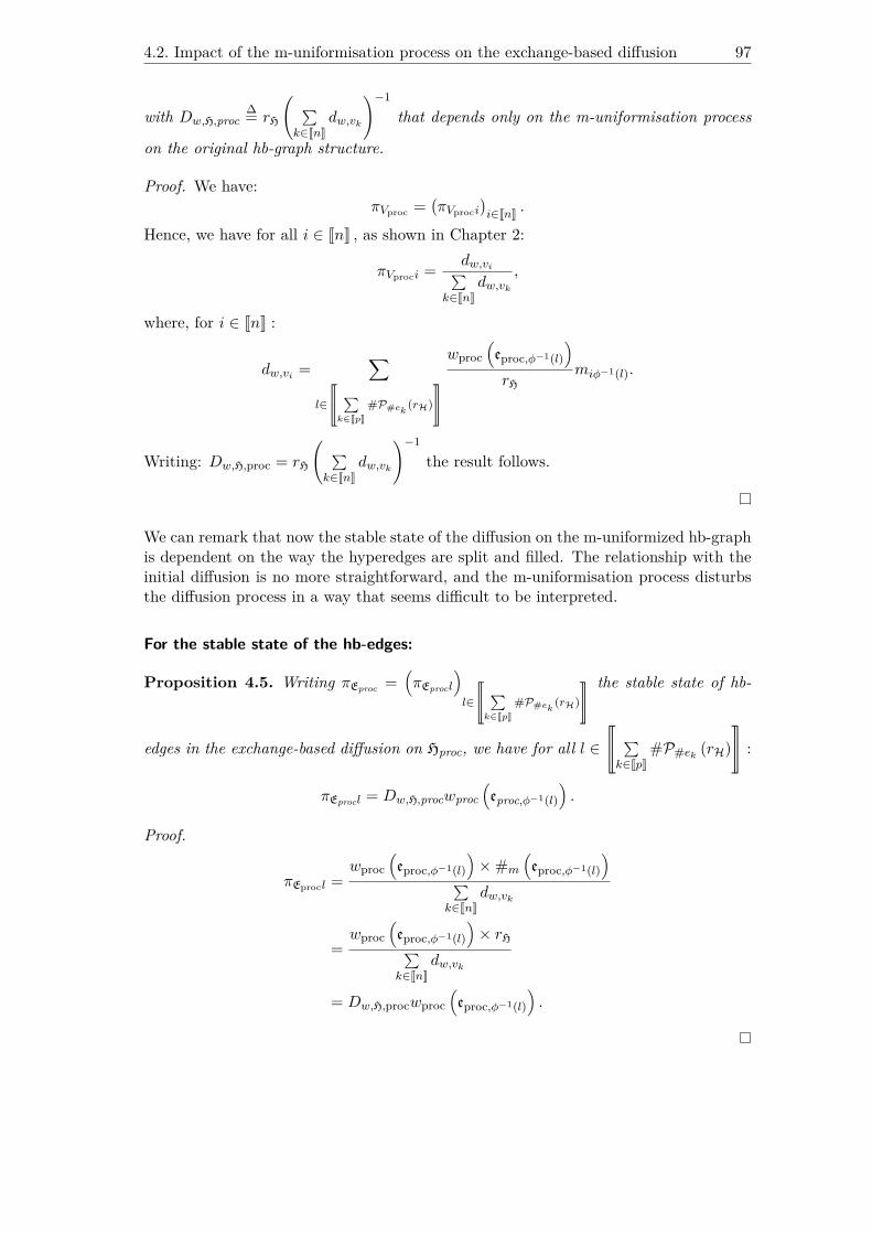
4.2. Impact of the m-uniformisation process on the exchange-based diffusion 97
with Dw,H,proc∆= rH
( ∑k∈JnK
dw,vk
)−1
that depends only on the m-uniformisation process
on the original hb-graph structure.
Proof. We have:πVproc =
(πVproci
)i∈JnK .
Hence, we have for all i ∈ JnK , as shown in Chapter 2:
πVproci = dw,vi∑k∈JnK
dw,vk,
where, for i ∈ JnK :
dw,vi =∑
l∈
u
v∑k∈JpK
#P#ek (rH)
}
~
wproc(eproc,φ−1(l)
)rH
miφ−1(l).
Writing: Dw,H,proc = rH
( ∑k∈JnK
dw,vk
)−1
the result follows.
We can remark that now the stable state of the diffusion on the m-uniformized hb-graphis dependent on the way the hyperedges are split and filled. The relationship with theinitial diffusion is no more straightforward, and the m-uniformisation process disturbsthe diffusion process in a way that seems difficult to be interpreted.
For the stable state of the hb-edges:
Proposition 4.5. Writing πEproc =(πEprocl
)l∈
u
v∑k∈JpK
#P#ek (rH)
}
~the stable state of hb-
edges in the exchange-based diffusion on Hproc, we have for all l ∈t ∑k∈JpK
#P#ek (rH)|
:
πEprocl = Dw,H,procwproc(eproc,φ−1(l)
).
Proof.
πEprocl =wproc
(eproc,φ−1(l)
)×#m
(eproc,φ−1(l)
)∑
k∈JnKdw,vk
=wproc
(eproc,φ−1(l)
)× rH∑
k∈JnKdw,vk
= Dw,H,procwproc(eproc,φ−1(l)
).

98 4. m-uniformisation processes and exchange-based diffusion
Writing φ−1 (l) = (j, kj) where j ∈ JpK, we have: wproc(eproc,φ−1(l)
)= #ej . Hence, the
stable state of the hb-edges reflects the m-cardinality of the original hb-graph, i.e. thecardinality of the hyperedges of the original hypergraph.
4.3. e-adjacency tensors require compromises
We start by giving some lemma:
Lemma 4.1. A splitting hb-edge m-uniformisation process with no additional verticespreserves only the e?-adjacency of the original non m-uniform hb-graph.
Proof. As the hb-graph H = (V,E) is non m-uniform, there exists a hb-edge e ∈ E suchthat #me < rH. As there are no additional vertices added during the m-uniformisation,the hb-edge is filled only by additional vertices of its support. The multiplicity of thecorresponding vertices is therefore changed compared to the original multiplicity, thusthe e-adjacency is not preserved and only the e?-adjacency is preserved.
Lemma 4.2. Preserving globally e-adjacency in a m-uniformisation process of a nonm-uniform hb-graph requires at least one additional vertex.
Proof. Either we extend the number of hb-edges by a splitting process, and, as seen inthe previous lemma, additional vertices are required, in order to keep the multiplicity ofexisting vertices and to allow the global preservation of e-adjacency. Or we add one ormore special vertices to fill the hb-edges of m-cardinality s < rH up to a m-cardinalityof rH, while preserving the multiplicity of the vertices of the original hb-graph and thusthe e-adjacency.
The presence of the additional vertices avoids to disturb the global e-adjacency, even ifthe strict e-adjacency is not preserved.
Remark 4.3.1. The preservation of e?-adjacency in a m-uniformisation process is notsufficient to preserve the stable state of vertices in the exchange-based diffusion of aconnected hb-graph.
Proof. If it was the case, it would mean that both a hb-graph and its support hyper-graph, that have same e?-adjacency would lead to the same exchange-based diffusionprocess, which is not always the case, even for a connected m-uniform hb-graph havinga uniform hypergraph as support, as the former is taking into account the multiplicitiesand the latter not.

4.3. e-adjacency tensors require compromises 99
v4
v3
v2
v5 v1
e4
e2
e3
e1
Figure 4.1.: Representation of the 5-m-uniform hb-graph H = (V,E) with V ={vi : i ∈ J5K} and E = (ej)j∈J4K, where: e1 =
{{v2
1, v22, v
15}}, e2 =
{{v1
2, v23, v
24}},
e3 ={{v1
2, v23, v
25}}
and e4 ={{v1
2, v33, v
14}}.
For instance, we consider the 5-m-uniform hb-graph H = (V,E) as represented in Figure4.1 , with V = {vi : i ∈ J5K} and E = (ej)j∈J4K, where: e1 =
{{v2
1, v22, v
15}}, e2 ={{
v12, v
23, v
24}}, e3 =
{{v1
2, v23, v
25}}
and e4 ={{v1
2, v33, v
14}}
of incident matrix:
H =
2 0 0 02 1 1 10 2 2 30 2 0 11 0 2 0
brings to the stable state of the vertices: πV = 1
20(
2 5 7 3 3)ᵀ
while the supporthypergraph H = (V,E) of H of incident matrix:
H =
1 1 0 01 1 1 10 1 1 10 1 0 11 0 1 0
leads to the stable state for the vertices: πV = 1
13(
2 4 3 2 2)ᵀ
which leads toan inversion of ranking between the vertices v2 and v3, and to tie v1, v4 and v5.
Theorem 4.1. There is no Hm-UP process that preserves both e-adjacency of the orig-inal hb-graph and preserves the exchange-based diffusion simultaneously on vertices andhb-edges.
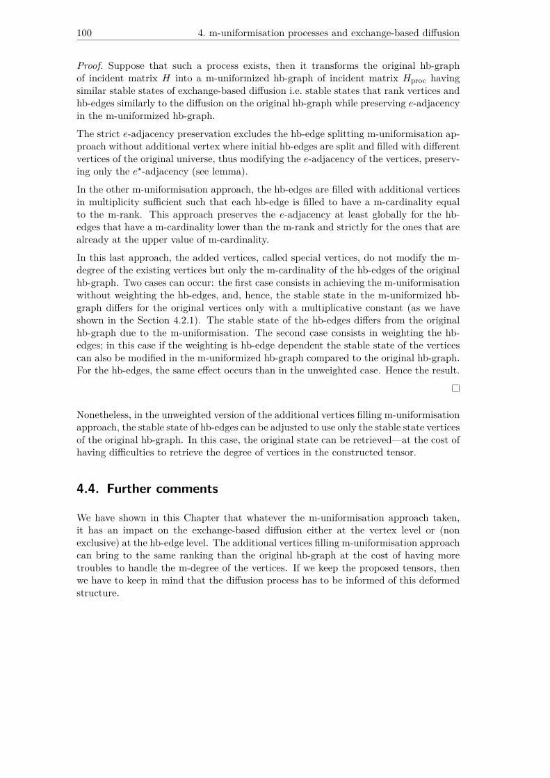
100 4. m-uniformisation processes and exchange-based diffusion
Proof. Suppose that such a process exists, then it transforms the original hb-graphof incident matrix H into a m-uniformized hb-graph of incident matrix Hproc havingsimilar stable states of exchange-based diffusion i.e. stable states that rank vertices andhb-edges similarly to the diffusion on the original hb-graph while preserving e-adjacencyin the m-uniformized hb-graph.
The strict e-adjacency preservation excludes the hb-edge splitting m-uniformisation ap-proach without additional vertex where initial hb-edges are split and filled with differentvertices of the original universe, thus modifying the e-adjacency of the vertices, preserv-ing only the e?-adjacency (see lemma).
In the other m-uniformisation approach, the hb-edges are filled with additional verticesin multiplicity sufficient such that each hb-edge is filled to have a m-cardinality equalto the m-rank. This approach preserves the e-adjacency at least globally for the hb-edges that have a m-cardinality lower than the m-rank and strictly for the ones that arealready at the upper value of m-cardinality.
In this last approach, the added vertices, called special vertices, do not modify the m-degree of the existing vertices but only the m-cardinality of the hb-edges of the originalhb-graph. Two cases can occur: the first case consists in achieving the m-uniformisationwithout weighting the hb-edges, and, hence, the stable state in the m-uniformized hb-graph differs for the original vertices only with a multiplicative constant (as we haveshown in the Section 4.2.1). The stable state of the hb-edges differs from the originalhb-graph due to the m-uniformisation. The second case consists in weighting the hb-edges; in this case if the weighting is hb-edge dependent the stable state of the verticescan also be modified in the m-uniformized hb-graph compared to the original hb-graph.For the hb-edges, the same effect occurs than in the unweighted case. Hence the result.
Nonetheless, in the unweighted version of the additional vertices filling m-uniformisationapproach, the stable state of hb-edges can be adjusted to use only the stable state verticesof the original hb-graph. In this case, the original state can be retrieved—at the cost ofhaving difficulties to retrieve the degree of vertices in the constructed tensor.
4.4. Further comments
We have shown in this Chapter that whatever the m-uniformisation approach taken,it has an impact on the exchange-based diffusion either at the vertex level or (nonexclusive) at the hb-edge level. The additional vertices filling m-uniformisation approachcan bring to the same ranking than the original hb-graph at the cost of having moretroubles to handle the m-degree of the vertices. If we keep the proposed tensors, thenwe have to keep in mind that the diffusion process has to be informed of this deformedstructure.

5. Diffusion in hb-graphs (tensor approach)
Highlights
5.1. Motivation . . . . . . . . . . . . . . . . . . . . . . . . . . . . . . . . . . 101
5.2. Related work . . . . . . . . . . . . . . . . . . . . . . . . . . . . . . . . . 101
5.3. A diffusion operator for general hb-graphs . . . . . . . . . . . . . . . . . 107
Prerequisites: Section 1.3 and, Chapters 2, 3 and 4.
5.1. Motivation
So far, we have used the incident matrix to enhance diffusion on hb-graphs. Build-ing an e-adjacency tensor for general hb-graphs and analyzing the impact of the m-uniformisation has led us to the conclusion that the m-uniformisation process impactsthe diffusion process. Hence, the necessity to have either an informed diffusion or tohave a diffusion that operates at the individual levels of the layered decomposition ofan hb-graph.
In this Chapter, we want to address the following research question:
Research question 5.1. How to enable a tensor-based diffusion in general hb-graphs?
We start by giving in Section 5.2 the related work and mathematical background ondiffusion over networks, seen as graphs or hypergraphs. We then propose in Section 5.3different lines of thoughts to tackle the problem of diffusion in general hb-graphs.
5.2. Related work
Diffusion kernels for graphs have been proposed in [KL02] linking them to exponentialkernels and stochastic processes on graphs, as well as lazy random walks. In [BN03], theauthors study the Laplace Beltrami operator on differentiable functions on a manifoldand show the tight link with the heat flow. In [LL05], diffusion kernels are introducedthat exploit the geometric structure of statistical models, particularly the multinomialkernel which allows to learn from discrete data; it is applied to some text corpus.

102 5. Diffusion in hb-graphs (tensor approach)
5.2.1. Operators
Definitions and results of this section are based on [Kat13], which is a reference book onoperators. Originally, operators refer to transformations that manipulate functions andgive back functions. Some people are restricting to transformations on a same space.An operator O : E → F is a mapping between two topological vector spaces E and Fwith scalars in a field K.An operator O : E → F is linear if:
∀ (λ, µ) ∈ K2, ∀ (f1, f2) ∈ E2, O (λf1 + µf2) = λO (f1) + µO (f2) .
In practice, the operator can be defined on a subspace D of E called definition domainof the operator.The rank of an operator O : E → F is the dimension of O(E).The kernel of O is the pre-image of 0F .In finite dimension, it holds rank (O) + dim (Ker (O)) = dim (E) . In finite dimension, alinear operator is uniquely represented by a matrix.The linear sum of two operators is an operator.
5.2.2. Diffusion operators
The results of this section are based on the attached reference1.A diffusion operator L on Rn is defined as a differential operator that can be written:
L =∑
i,j∈JnK
σij (x) ∂2
∂xi∂xj+∑i∈JnK
bi (x) ∂
∂xi
where bi and σij are continuous functions on Rn and such that for all x ∈ Rn :(σij (x))i,j∈JnK is a symmetric and non-negative matrix.
The Laplace operator ∆ = ∑i∈JnK
∂2
∂x2i
on Rn is a diffusion operator.
The author shows that diffusion operators satisfy a maximum principle:
Proposition 5.1. Maximum principle for diffusion operatorsLet f : Rn → R be a smooth function (such that f ∈ C∞ (Rn)) that reaches a localminimum at x. If L is a diffusion operator, then Lf(x) > 0.
Reciprocally, combined with linearity, the maximum principle characterizes a diffu-sion operator.
Theorem 5.1. Let L : C∞ (Rn) → C0 (Rn) be an operator such that L is linear andsuch that if f ∈ C∞ (Rn) has a local minimum at x, Lf(x) > 0.Then L is a diffusion operator.1https://fabricebaudoin.wordpress.com/2013/06/21/lecture-1-diffusion-operators/
5.2. Related work 103
This theorem is a particular case of the Courrège’s theorem given in [Cou65] that givesthe necessary and sufficient condition for a linear operator to satisfy the positive max-imum principle; an operator A : C∞c (Rn) 7→ C (Rn) is said to satisfy the positive max-imum principle, if for any function f of the space of smooth and compact supportedfunctions C∞c (Rn) that has a global maximum and, that is non-negative in x, thenAf(x) is non-negative.
5.2.3. Diffusion processes in graphs
In [FW93], the authors study different classical stochastic processes leading to diffusionprocesses on graphs, by studying diffusion in narrow tubes: each time they give theassociated second-order differential operator associated to the diffusion process.
In [Mer95], a full survey on graph Laplacian is realized. For small vibrations, theoscillations of a point on the membrane are approximately vertical, and depends onlyon the place on the drum and the time, i.e. z = f (x, y, t) with f ∈ C2 (R2) and the
equation of the movement is given by the wave equation ∂2f
∂t2= c2∆f, where ∆ is the
Laplacian operator on R2, as it has been defined in the previous section.
If ∂2f
∂t2is supposed to be oppositely proportional to the vertical move, i.e. ∂
2f
∂t2= −kf,
we have ∆f = − kc2 f.
Forgetting time, and considering a square grid of unit size h around (x, y) , i.e. takingfinite differences, we have:
f (x+ h, y) = f (x, y) + h∂f
∂x(x, y) + h2∂
2f
∂x2 (x, y) + o(h2). (5.1)
We can also write:
f (x− h, y) = f (x, y)− h∂f∂x
(x, y) + h2∂2f
∂x2 (x, y) + o(h2). (5.2)
By summing of (5.1) with (5.2) and rearranging, it holds that:
∂2f
∂x2 (x, y) ≈ 1h2 (f (x+ h, y) + f (x− h, y)− 2f (x, y)) . (5.3)
Similarly:∂2f
∂y2 (x, y) ≈ 1h2 (f (x, y + h) + f (x, y − h)− 2f (x, y)) . (5.4)
Globally, gathering (5.3) with (5.4), we have:
∆f ≈ 1h2 (f (x+ h, y) + f (x− h, y) + f (x, y + h) + f (x, y − h)− 4f (x, y)) .
It means that the Laplacian, close to (x, y) is the sum of the difference of values inbetween the neighbor values and the point itself.

104 5. Diffusion in hb-graphs (tensor approach)
Coming back to the grid and taking h = 1, it holds that the Laplacian of the 5 pointson the grid is:
L =
4 −1 −1 −1 −1−1 1 0 0 0−1 0 1 0 0−1 0 0 1 0−1 0 0 0 1
that corresponds to the matrix view of the operator ∆.Generalizing the concept for a graph, it becomes natural to define the Laplacian of agraph as L ∆= D −A with D = diag
((di)i∈JnK
)with di the degree of the vertex vi and
A = (aij)i,j∈JnK the adjacency matrix of the graph.Coming back to the oscillating membrane, it holds:
4f (x, y)− f (x+ h, y)− f (x− h, y)− f (x, y + h)− f (x, y − h) = kh2
c2 f (x, y)
Writing µ = kh2
c2 , µ appears to be an eigenvalue of ∆, and solving ∆f = µf is equivalentto finding the eigenpairs of the Laplacian operator. Hence, the problem reduces tofinding eigenpairs of L on the grid of finite elements.A lot of work has been done on the eigenvalues of the Laplacian and connecting theseeigenvalues to different features of the graph. The interested reader can refer to [Mer95].
5.2.4. Diffusion processes in hypergraphs
There are two kinds of approaches to define a Laplacian for hypergraph: the matrix andthe tensor approach. The matrix approach relies more or less on the adjacency matrixof a hypergraph, which is a pairwise view of the hypergraph and focuses on extendingthe properties obtained for the graph Laplacian to the hypergraph Laplacian. In therandom walks, the transition matrix are expressed using the incident matrix decoratedby additional matrices depending on the way the hypergraph is viewed as a graph.
5.2.4.1. Matrix Laplacians
Mainly three different approaches exist to define matrix Laplacians. The first approachconsists in using the adjacency matrix of the hypergraph. The second approach consistsin using the incident matrix. The third one relies on random walks achieved on thehypergraph to approximate the Laplacian. Whatever the method taken, as matricesare used, there is an underlying pairwise approach, either directly when considering theadjacency matrix, or indirectly with the incident matrix or with random walks. Wehave gathered in Table 5.1 the different methods.In [Chu93], a Laplacian based on homological considerations is introduced: the Lapla-cian of a k-uniform hypergraph is defined as the matrix L ∆= D −A+ ρ (K + (k − 1) I)where ρ = d
nwith d corresponding to the average degree, n being the number of vertices
of the hypergraph, D the diagonal matrix constituted of the degree of the vertices, A

5.2. Related work 105
Adjacency matrix Incident matrixHypergraph as a graph [ZSC99] [Rod03]Homological approach [Chu93]
Simple [ZHS07][CR19]Random walk based Higher-order [LP11]
Table 5.1.: Ways of defining matrix Laplacian of a hypergraph.
the adjacency matrix with coefficients corresponding to the binary presence of two givenvertices in one hyperedge, K the matrix associated to the complete graph and I theidentity matrix. This Laplacian is viewed as a self-adjoint operator.
An other matrix approach was introduced in [ZSC99] where the hypergraph is viewedin its 2-section. The Laplacian of the hypergraph is built from the adjacency matrixof the 2-section of the hypergraph, considering its adjacency matrix A = (aij) whereaij corresponds to the weight of the edge between vertex vi and vj having the verticesvi and vj in common. The Laplacian degree is defined as δl (vi)
∆= ∑j∈JnK
aij and the
Laplacian is defined as L ∆= D −A, where D ∆= diag((δl (vi))i∈JnK
).
In [Rod03], the authors take a similar approach, several bounds are then given ondifferent hypergraph features. This approach is more geometric in the sense that thehypergraph is seen as a multipartite graph or a weighted graph.
In [ZHS07], the approach is pairwise based using a Laplacian matrix defined from thedegree normalised adjacency matrix. This approach is deeply based on the transitionmatrix of a random walk defined on the hypergraph: being on a vertex, a randomincident hyperedge is chosen proportionally to the hyperedge weights and then a vertexis chosen uniformly at random. Defining the matrix Θ ∆= D
− 12
v HWD−1e HTD
− 12
v and theLaplacian matrix as ∆ ∆= I −Θ enhance a spectral partition of the hypergraph.
In [LP11], the authors start by classifying the two types of approaches taken by previousauthors to define a Laplacian for hypergraphs. Either the previous authors have ageometric / homological point of view by considering the self-joint operator on thefunction of the vertices, like it has been done for graphs in [Chu93] or they consider asymmetrization of the transition matrix of the random walk performed on a graph basedstructure. They introduce high-order random walks and define from them generalizedLaplacian matrices on hypergraphs.
In [CR19], the authors propose a hypergraph Laplacian corresponding to a symmetriza-tion of the random probability transition similar to the modified random walk we pro-posed in Chapter 2. The hypergraph has hyperedge-based weighting of the vertices, i.e.is a hb-graph. Writing P the probability transition matrix and π the stationary state,
they define a Laplacian as L ∆= π− πP + P Tπ
2 using a weighted directed graph that is adirected 2-section of the hb-graph adding double edges between any vertices and loopson every vertices. Nonetheless, as it is a matrix representation of a 2-section, it remainsan approximation of an ideal non-linear Laplacian.

106 5. Diffusion in hb-graphs (tensor approach)
5.2.4.2. Tensor Laplacians
In [LQY13], the authors introduce a Laplacian tensor for m-uniform hypergraph byconsidering for a hypergraph H = (V,E) a polynomial fH (x) ∆= ∑
i∈JnK
∑j∈JnK
δij (xi − xj)m
where
δij∆={
1 if i < j ∧ ∃el ∈ E : vi ∈ el ∧ vj ∈ el0 otherwise.
The authors define the Laplacian tensor L as Lxm∆= fH (x) and the associated
characteristic tensor of the hypergraph as C = −L. They then focus on m-uniformhypergraphs with m even: the maximum Z-eigenvalue of C is shown to be 0 and theyshow that the corresponding eigenspace has for dimension the number of connectedcomponents in the hypergraph. They also use the second maximal Z-eigenvalue togive a bound on the bi-partition width of a hypergraph—the bi-partition width is theminimal number of hyperedges that has to be cut such that the vertex set is cut in twoequal or one-unity difference parts.
In [Qi14], the Laplacian tensor of a uniform hypergraph is simply defined as:L ∆= D − A and the signless Laplacian as L ∆= D + A where D is the diagonal tensorcomposed of the degrees of the vertices. H-, H+- and H++-eigenvalues of these tensorsare then studied. An interesting definition is the one for a hyperedge ej = {vi1 , ..., vik}of a k-uniform hypergraph of a k-th order n-dimensional symmetric tensor L (ej) suchthat for x ∈ Cn :
L (ej)xk =∑l∈JkK
xkil − kxi1 ...xik .
In this case, we have: Lxk = ∑ej∈E
L (ej)xk.
This link between Laplacian tensor and multivariate polynomial is used in [DWL19] forstudying the Laplacian of general hypergraphs. As defined similarly to the e-adjacencytensor of [BCM17], this polynomial is of degree rH.
In [HQ15], the normalised signed Laplacian of a k-uniform hypergraph is defined asL ∆= I − A where A is the eigenvalue normalized k-adjacency tensor defined in SectionE.1.3.2. The remaining work focuses on studying the H- and H+-eigenvalues of thisnormalised Laplacian.
In [BCM17], two signed Laplacians are defined for general hypergraphs, one unnor-malized and one normalized: they are direct generalizations to general hypergraphs ofthe unnormalized version of [Qi14] and the normalized version of [HQ15] for uniformhypergraph.
We can note that none of these works are focusing on the diffusion process that is behindthe definition of the Laplacian.
5.2.4.3. Hypergraph Laplacian and diffusion process
In two successive papers, [CLTZ18] and [CTWZ19], the authors study a diffusion processon hypergraphs. In [CLTZ18], the diffusion process sends the flow of information from

5.3. A diffusion operator for general hb-graphs 107
vertices with maximal density in the hyperedge to the one with minimal density. In[CTWZ19], this diffusion process is refined: the flow of information goes from verticeswith higher density to vertices of the hyperedge with lower density using a mediator thatrelays this information to the lower density vertices. In both papers, they consider thediffusion operator linked to the diffusion process and deduce some spectral properties.A vertex acts as mediator depending on a parameter that is hyperedge dependent andtransmits only a difference of flow depending on the minimum and maximal values ofthe density of the other vertices in the hyperedge.The Laplacian associated to this diffusion is defined as the operator Lw on the densityf ∈ Rn, where n is the number of vertices such that Lwf = −df
dt. Spectral properties
of this Laplacian are then studied. This approach keeps a kind of pairwise relationship,diffusing the information only between higher density vertices and the lower ones.
5.3. A diffusion operator for general hb-graphs
As we have seen in Chapter 2, whatever the approach taken, the diffusion is disturbedby the m-uniformisation process involved to store the information into a symmetricalcubic tensor. In this Section, we propose different hints to handle this problem.
5.3.1. Global exchange-based diffusion
We start by giving here an extension of the exchange-based diffusion proposed in Chapter2 using the e-adjacency tensor built in Chapter 3.We consider for the moment a connected non-uniform unweighted hb-graph H = (V,E)with |V | = n and |E| = p; we write A its e-adjacency tensor defined in Chapter 3.At time t, we set a distribution of values over the vertex set: αt : V ∪ Vs → R.
We write PV,t = (αt (vi))i∈Jn+1K the column state vector of the vertices at time t, in-cluding the special vertex added in the m-uniformisation process. The initialisation issimilar to the one done in Chapter 2.Using the e-adjacency tensor proposed in Chapter 3, the information between verticescan be shared directly from one vertex to another group of vertex by using this tensor.In this approach, the state at time t + 1 of the vertices is retrieved using the state attime t, using the multilinear matrix multiplication:
λP[rH−1]V,t+1 = AP
rH−1V,t .
The left part is due to the fact that we want to keep homogeneity of the dimension—likeit is achieved in dimensional equations in physics—and the presence of the coefficient isdue to a normalisation that has to take place. Searching the stable state of this equationis then equivalent to finding the H-eigenvectors of A associated to the eigenvalue λ. Italso imposes to consider that the diffusion is the one of the m-uniformized structure,which we know it is far from being perfect from Chapter 4.The intermediate state of the hb-edges cannot be retrieved in this case; however, it isalways possible, either to consider the dual of the hb-graph and its e-adjacency tensor

108 5. Diffusion in hb-graphs (tensor approach)
(in this case the vertices correspond to the original hb-graph) or to use the incidentmatrix as it was done in Chapter 2.
5.3.2. Taking into account the different layers of uniformity.
5.3.2.1. Tensor approach
Keeping in mind that the diffusion is disturbed for general non-uniform hb-graphs, wecan start by keeping the previous approach of tensor Laplacians.
We consider as usual a hb-graph H = (V,E) with vertex set V = {vi : i ∈ JnK} andhb-edge family E = (ej)j∈JpK .
Similarly to the approach taken for uniform hypergraph, we define the Laplacian hy-permatrix as:
L∆= D −A
where D corresponds to the diagonal hypermatrix of the m-degrees of vertices of orderrH, including the one(s) added in the m-uniformisation process. More formally, D is ahypermatrix of order rH and dimension n+ nA, with nA the number of added verticesduring the m-uniformisation process, defined by:
D∆= diag
((dmi)i∈Jn+nAK
)with for i ∈ Jn+ nAK : dmi
∆= degm (vi) .
Let us consider as in Chapter 3, the attached variable xi to the vertex vi with i ∈ JnKand yi the variable attached to the special vertex Yi with i ∈ JnAK . We consider znA =(zi)i∈Jn+nAK such that: zi = xi for i ∈ JnK and zn+i = yi for i ∈ JnAK .
We define the m-uniformized L-polynomial2 as:
Lm-u (znA) ∆=∑
i∈Jn+nAK
dizrHi −
∑i1,...,irH∈Jn+nAK
ai1...irH
∏j∈JrHK
zij .
It holds:LzrHnA = Lm-u (znA) .
The impact of the m-uniformisation on this Laplacian relies on the exponent of thevariables in the degree part and in the coefficients of the built tensor, as well as theadditional variables induced by the m-uniformisation.
5.3.2.2. Polynomial approach
A-, D-, L- and Q-polynomials We now consider the decomposition of H = (V,E) indifferent layers of m-uniform hb-graphs using the decomposition operation 3.3.6.2We cannot use the term Laplacian polynomial as this is reserved for the characteristic polynomial ofthe Laplacian matrix for graphs.
5.3. A diffusion operator for general hb-graphs 109
We define Ek∆= (e : e ∈ E ∧#me = k) as the family of hb-edges of H of m-cardinality k,
eventually empty, for k ∈ JrHK and consider, for all k ∈ JrHK, the k-m-uniform hb-graphHk
∆= (V,Ek) . It holds: H = ⊕k∈JrHK
Hk.
Each of the k-m-uniform hb-graph Hk is associated to a k-adjacency tensor Ak of orderk and dimension n.
The corresponding signed Laplacian is: Lk∆= Dk−Ak where Dk = diag
((dm(k)i
)i∈JnK
)where for k ∈ JrHK and i ∈ JnK, dm(k)i corresponds to the m-degree of the vertex i inthe k-th hb-graph Hk.
The unsigned Laplacian is:Lk∆= Dk + Ak.
We then define, for each k ∈ JrHK , four polynomials, with z0 = (z1, ..., zn) as defined inSection 5.3.2.1:
• Dk (z0) ∆= ∑i∈JnK
dm(k)izki ;
• Ak (z0) ∆= ∑i1,...,ik∈JnK
a(k)i1...ik∏
j∈JkKzij ;
• Lk (z0) ∆= Dk (z0)−Ak (z0) ;
• Qk (z0) ∆= Dk (z0) +Ak (z0) .and we define four families of polynomials for a general hb-graph H as:
• the D-polynomial family: Dw (z0) ∆= ∑k∈JrHK
wkDk (z0) ;
• the A-polynomial family: Aw (z0) ∆= ∑k∈JrHK
wkAk (z0) ;
• the L-polynomial family: Lw (z0) ∆= Dw (z0)−Aw (z0) ;
• the Q-polynomial family: Qw (z0) ∆= Dw (z0) +Aw (z0) .where the coefficients w = (wk)k∈JrHK are weights given to each layer potentially withdifferent values.
Remark 5.3.1. Using here the k-adjacency hypermatrix defined in Section 3.3.5, wecan formulate the reduction of Ak (z0) as:
Ak (z0) ∆=∑
ej∈Ek
ej={vmji1i1
,...,vmjikjikj
} k∏l∈JkjK
zmjilil
.
Remark 5.3.2. Different strategies can be foreseen for weights. The first approachconsists in choosing w = (1)k∈JrHK: this puts on an equal footing every hb-edge, whateverits m-cardinality.If we want to have a polynomial that is similar in a sense to the m-uniformized Laplaciantensor polynomial, the choice of w = (ck)k∈JrHK is the most relevant.

110 5. Diffusion in hb-graphs (tensor approach)
A family of Laplacian hypermatrices Whatever the weights chosen, an homogenizedhb-graph L-polynomial can be obtained directly from the L-polynomial by considering:
Lhw (z1) ∆= yrH0 Lw
(z0y0
).
In this case, we can store the information into a hypermatrix, which is a layeredLaplacian: Lhw defined as:
LhwzrH1
∆= Lhw (z1) .
The same can be done with the Q-, D- and A- polynomials, defining:
• Qhw: QhwzrH1
∆= Qhw (z1) with Qhw (z1) ∆= yrH0 Qw
(z0y0
)
• Ahw: AhwzrH1
∆= Ahw (z1) with Ahw (z1) ∆= yrH0 Aw
(z0y0
)
• Dhw : DhwzrH1
∆= Dhw (z1) with Dhw (z1) ∆= yrH0 Dw
(z0y0
).
The advantage of these layered Laplacians (signed and unsigned) is that they take intoaccount each of the layers of m-uniformity contained in the hb-graph.
Some remarks on the polynomials There are two parts in a L-polynomial of a generalhb-graph: one that is related to the vertex degrees in the different layers correspondingto the D-polynomial and the second part to the adjacency in the layers of the hb-graphand corresponding to the A-polynomial. Having a good comprehension of the role ofeach part is fundamental.
These polynomials, and particularly the A-polynomial, opens the door to all the resultson multivariate polynomials. Particularly, it could be used for hb-graph reduction usingthe well-known techniques for multivariate polynomials3, and to define and find normalforms of a set of hb-graphs, i.e. hb-graphs that cannot be reduced to a given set ofhb-graphs.
A-polynomial for hypergraphs are already used, without the m-cardinality coefficientfor searching hypergraph extremal problems, i.e. determining the maximal number ofhyperedges a hypergraph should have to prevent a forbidden sub-hypergraph to occur;in this case, the Lagrangian used is defined as the polynomial sum of the hb-edgemonomials.
We conjecture that finding the stationary state of the exchange-based diffusion for aconnected hb-graph as we have done in Chapter 6 with a matrix approach can bereformulated here as the search for the value closest to zero of the L-polynomial underthe constraints that ∑
i∈JnKzi = 1, with for all i ∈ JnK : 0 < zi 6 1 and with equi-weights.
We then transform the problem into a constrained optimization problem, where a lot oftechniques are available.
3https://www.usna.edu/Users/cs/roche/courses/cs487/mvpoly.pdf
5.3. A diffusion operator for general hb-graphs 111
5.3.2.3. First properties of the layered Laplacian hypermatrix
Elements of the layered Laplacian hypermatrix We write:
Ak =(a(k)i1...ik
)i1,...,ik∈JnK
.
The non-zero elements of Ak correspond to hb-edges of H of m-cardinality k. Such anhb-edge ei =
{vmij1j1
, . . . , vmijkijki
}∈ Ek is stored in Ak—as we have already mentioned it
in Section 3.3.3—in k!mij1 ! . . .mijl !
elements:
a(k)σ
(jmi j11 ,...,j
mi jll
) = mij1 ! . . .mijl !(k − 1)!
where σ ∈ SJkK4.
Hence, the total value of the elements of Ak associated to ei ={vmij1j1
, . . . , vmijkijki
}∈ Ek
is k.When coming to Ahw =
(ai1...irH
)i1,...,irH∈Jn+1K
, the only non-zero elements which are
the ones corresponding to ei have to be stored in nei = rH!mij1 ! . . .mijl ! (rH − k)! elements,
considering that the missing indices will correspond to rH − k times the n+ 1-th place,i.e. the special vertex place.It holds:
aσ(rH)
(jmi j11 ,...,j
mi jll
[n+1]rH−k) = k
nei,
i.e.:aσ(rH)
(jmi j11 ,...,j
mi jll
[n+1]rH−k) = 1(
rHk
) × a(k)σ(k)
(jmi j11 ,...,j
mi jll
)where σ(i) ∈ SJiK, with i = k or rH.
The non-zero elements of Dk =(d(k)i1...ik
)i1,...,ik∈JnK
corresponds to elements of thediagonal. It holds, for i ∈ JnK :
d(k)ik = dm(k)i.
In Dhw =(di1...irH
)i1,...,irH∈Jn+1K
, d(k)ik is stored in the elements with indices that are
obtained by permutation of the elements of the multiset of indices{ik, [n+ 1]rH−k
},
i.e. in one of the(rHk
)elements dσ(rH)(ik[n+1]rH−k).
Hence:dσ(rH)(ik[n+1]rH−k) = 1(
rHk
)d(k)ik .
4SJkK designates the set of permutations on JkK.
112 5. Diffusion in hb-graphs (tensor approach)
The only non-zero elements of Dhw have indices in{ik, [n+ 1]rH−k
}for k ∈ JrHK .
We write Lhw =(li1...irH
)i1,...,irH∈Jn+1K
.
It holds:li1...irH = di1...irH − ai1...irH .
and similarly, writing Qhw =(qi1...irH
)i1,...,irH∈Jn+1K
.
It holds:qi1...irH = di1...irH + ai1...irH .
Remark 5.3.3. The diagonal of Dhw and Lhw have always a non-zero element; other-wise, the m-rank would not be rH.
Remark 5.3.4. When the hb-graph is a uniform hypergraph, we retrieve the classicalLaplacian: in this case, there are only zero elements on the n+ 1-th component of eachface. The classical Laplacian for a uniform hypergraph is then retrieved by extractingthe first n-th components of each face.
Remark 5.3.5. The L-polynomial attached to the hb-graph can be retrieved from Lhw
by considering LhwzrH1 with y0 = 1.
The same occurs with A-, Q- and D-polynomials.
Some additional comments on the layered Laplacian hypermatrix If the hb-graph ism-uniform, the elements of the n+1-th row of each face of the layered Laplacian hyper-matrix contain only zero elements, i.e. the layered Laplacian reduces by withdrawingthose rows to the Laplacian that would have been obtained directly derived from thek-adjacency hypermatrix as defined by [CD12].
This layered hypermatrix is symmetric and methods included in [QL17] to study suchhypermatrices are available.
We keep as remaining research questions the following—non-exhaustive—research ques-tions:
• What are the links between the hb-graph layered Laplacian eigenvalues and thehb-graph features such as the algebraic connectivity?
• How do we define the algebraic connectivity for hb-graphs?
• How does the diffusion process based on this layered Laplacian evolve with time?
• How can we use this layered Laplacian for clustering?
• Can we evaluate the perturbation on the exchange-based diffusion from the L-polynomial before uniformisation?

6. Hb-graph framework
Highlights
6.1. Motivation . . . . . . . . . . . . . . . . . . . . . . . . . . . . . . . . . . 1136.2. Related work . . . . . . . . . . . . . . . . . . . . . . . . . . . . . . . . . 1146.3. Modeling co-occurrences in datasets . . . . . . . . . . . . . . . . . . . . 1156.4. Further comments . . . . . . . . . . . . . . . . . . . . . . . . . . . . . . 134
This chapter is based on [OLGMM18d] and on [OLGMM19b], which has been acceptedto SOFSEM 2020 as [OLGMM20].Prerequisites: Section 1.3.
6.1. Motivation
Having insight into non-numerical data calls for the gathering of instances: classically(multi-entry) frequency arrays of occurrences are used. To get further insight into datainstances of a given type, one can regroup them using their links to instances of anothertype—used as reference. It generates a family of co-occurrences that can be viewedas a facet of the information space. Navigating across the different facets is achievedby iterating this process between different types of interest while keeping the samereference type: any of these types can be used as a reference. For instance, in scientificpublications, different information are linked in an article: the article reference, theauthors, the main keywords... All this metadata can potentially give insights into theinformation space and can be chosen as reference to build co-occurrences. Choosing asreference for instance the article reference, facets depict co-occurrence networks, eitherof homogeneous type, such as co-authors or co-keywords, or of heterogeneous types, i.e.combining multiple types together.We have presented a first model using hypergraphs in [OLGMM18d]. But, as co-occurrences can potentially contain repetitions or require an individual weighting: mod-eling them requires multisets instead of sets.Hb-graphs, by definition, introduce a potential refinement for storing information, andthus open up refined visualizations and processings. This observation brings us to theresearch question of this Chapter:
Research question 6.1. Are hb-graphs pertinent to achieve interactive navigation andvisualisation of facets in an information space?
114 6. Hb-graph framework
We start by giving the related work that motivates this approach, before fixing theassumptions and expectations on the framework. We then propose a mathematicalmodel, that we evaluate based on our expectations. We use a publication dataset as abreadcrumb trail example.
6.2. Related work
Discovering knowledge in an information space requires to gather meaningful informa-tion, either hierarchically or semantically organized. Semantic provides support to thedefinition of facets within an information space [Ran62].
The idea of visualizing search query results using graphs has been soon exposed in[CK97]. There are several proposals in the literature to explore large datasets by usinggraph—possibly multipartite—representations instead of the verbatim presentation.
In [vHP09], the authors present an interaction model to allow the user to interact directlywith the local context graph of a topic of interest: they extend to graphs the degree ofinterest introduced in [Fur86] for fish eye visualisation to focus on the vertices that areclose enough from the subject the surfer is looking for taking into account the a prioridegree of interest and the distance to the a priori, but also the user interest. The surferperforms a query and retrieves a list of subjects in a verbatim mode. The a priori isperformed from the initial query, and the dragging of one of the subject to the graphpart of the visualisation marks the user interest and the local context graph is built.Faceted search is also enabled when it is possible. The graph is based on this degreesof interest.
Previous approaches using a reference to articulate the different facets of an informationspace exist. In [NJY+10], the authors present a 2D multifaceted representation of aninformation space by using multi-relational graph combined with an optimized densitymap to highlight patterns and switching between the different facets. The facets areconsidered as classes of entities: the entities are interconnected using a similarity graphof the extracted entities. Facets are then superposed to reach a global facet visualisation.Similar entities are regrouped using an optimized density map. It is applied to twostudies, one on HIV infection and the other one on Diabetes. It allows to visualizeglobal and local relations. There is interactivity and filtering.
In [DRRD12], the authors give the possibility to change of reference between three facetssimultaneously shown by using one of them as a pivot; this pivot makes the connectionbetween a facet and the two others, but is limited to a small amount of pivots tobe visualized at the same time. In [JCCB13], an interactive exploration of implicitand explicit relations in faceted datasets is proposed. The space of visualisation isshared between different metadata with cross findings between metadata, partitioningthe space in categories. In [ADLGP17], the authors propose a visual analytics graph-based framework that reveals this information and facilitates knowledge discovery. Itprovides insights into different facets of an information space based on user-selectedperspectives. The dataset is stored as a labeled graph in a graph database. Choosing aperspective as reference and a facet as dimension, paths of the labeled graph are retrievedwith the same dimension extremities going through reference vertices. Visualisation
6.3. Modeling co-occurrences in datasets 115
comes in the form of navigable node-link graphs: edges materialize common referencesbetween vertices and are seen as pairwise collaboration between two vertices.
[TCR10] shows how the keeping of multi-adic relationships can help in gaining under-standing in the network evolution. In [OLGMM17b], we have shown the interest ofusing hypergraphs to simplify the visualisation of co-occurrence networks.
In this chapter, we provide the elements for a hb-graph-based framework that supportsinteractions between the different facets of an information space for optimal knowledgediscovery. The dataset—mostly textual—refers to physical entities with unique individ-ual references. Data instances are attached to metadata instances. We suppose thatthere is no metadata instance that does not have a data instance attached to it.
6.3. Modeling co-occurrences in datasets
Starting by giving the axioms and postulates needed for the framework, we then for-mulate the expectations on the framework. After giving the mathematical model, wecheck that the expectations are fulfilled. We finally give an example of implementationof the framework.
6.3.1. Axioms and postulates on the information space
We consider an information space, constituted of physical entities. Physical entitiesare described by metadata to which correspond data instances stored in a database.Metadata instances have types that are numerical, textual, or others such as pointersto images or videos or sound records. Metadata can be grouped by kinds. For instance,in a publication database, the physical entity corresponds to a publication, which hasa publication id, and some attached metadata such as organizations, keywords,... In acompany database, the physical entity would be the company, with a company id, andsome attached metadata such as economic activity, number of employees, countries,suppliers,...
We formulate the following axioms—in the sense of common propositions consideredas universally true—and postulates—in the sense of common propositions that capturethe specificity of a structure, that are discussable, but asserted here as true—on theinformation space and we will work in this shaped information space.
Axiom 6.1. The information space is constituted of physical entities that are describedby metadata and data.
This is a strong axiom that is needed to ensure a navigable schema: the physical entitiesensure the link between the different facets of the information space.
Axiom 6.2. Each physical entity has a unique identification.
This assumption is linked to the previous one and ensures that we do not have duplicatedinformation.
116 6. Hb-graph framework
Axiom 6.3. The types associated to metadata can be of varied sorts: numerical, textual,links, pointers to resources,...
This axiom is not restrictive in fact, as it allows data to be of various types.
Postulate 6.1. A facet of the information space is the simultaneous choice of:
• one or multiple types of the metadata used to build co-occurrences of this(these)metadata type(s), called visualisation type(s),
• and of one or multiple types—eventually the same than the ones used for the co-occurrences—called reference type(s).
This postulate defines a facet of an information space, as a perspective on the datasetthat enhances homogeneous—or even heterogeneous—co-occurrence networks built us-ing one—or multiple—references. Facets with homogeneous co-occurrences built withonly one type of references are called simple facets.
Postulate 6.2. The information space can be decomposed into at least three simplefacets—including the one of physical entities id.
This postulate can be relaxed to two facets, but in this case no navigation is possible oreven to one facet that corresponds to the facet of physical entities id. In the latter, thevisualisation will show only hb-graphs in which hb-edges represent ids and have supportreduced to singleton vertices.
Postulate 6.3. There are at least two kinds of metadata which are either nonnumerical,or that can be represented into categories.
Relaxing this postulate to a single kind of metadata disables navigation between thedifferent facets: it is always possible, even if it is not desirable. As any numerical datacan be treated in categories, the framework can accept any kind of data until they arerepresented as text or categories.
6.3.2. Hypothesis and expectations of the hb-graph framework
The hypothesis we formulate, related to the research question 6.1, is the following:
Hypothesis 6.1. Hb-graphs are pertinent to achieve a refined hypergraph frameworkthat supports interactive navigation and visualisation of facets in an information space,including the support of multiple references and heterogeneous co-occurrences.
To check this hypothesis, we refine it in expectations of what the theoretical frameworkshould answer. The fulfillment of the expectations will allow to validate Hypothesis6.1: hence, the visual querying of an information space and the browsing inside theinformation space by finding the links of co-occurrences inside a dataset will be validatedon a theoretical basis.

6.3. Modeling co-occurrences in datasets 117
Expectation 6.1. The framework should model the information space using hb-graphs.
Hb-graphs not only have like hypergraphs the capacity to handle multi-adic relation-ships—when graphs can handle only pairwise relationships—, but also individual hb-edge based multiplicities of vertices. Multiple authors—[New01b, TCR10]—acknowledgethe importance of modeling co-occurrence networks by hypergraphs, as it enhanceshigher order relationships than the pairwise model enables. As we have already un-derlined it, the database schema can be modeled, since [FMU82], using hypergraphswhich are anyway a particular case of hb-graphs. Handling multisets allow to store ad-ditional information, either with a view to reflecting the vertex multiplicity or individualweighting.
Expectation 6.2. The framework should provide the visualisation of co-occurrences ashb-graph representations.
This expectation is linked with the previous one. Pairwise relationships hide a part ofthe information in many cases as it is shown in [OLGMM17b].
Expectation 6.3. The framework should enable navigation and interaction between thedifferent facets of the information space.
This expectation is fundamental as we want to have a full browsing of the informationspace, thereby allowing to query the dataset in all sort of manners.
Expectation 6.4. The framework should enhance the visual querying of the informationspace.
We want a self contained browsing space that allows to query and display co-occurrencesthat are retrieved from the dataset.
Expectation 6.5. The zooming in the dataset should be possible through restrictionsto sub-hb-graphs.
Selecting a subset of the vertices displayed should allow to view their relations with theother facets.
Expectation 6.6. Heterogeneous co-occurrences should be possible.
This expectation is needed as the visualization of different facets on a single facet isthen possible. It could have already been introduced with hypergraphs. To reach thisexpectation, the visualisation must be achieved by an extra-node representation of thehb-graph, as the 2-section of the hb-graph would lead to hazardous interpretation.
Expectation 6.7. Multiple types of references should be possible.
This expectation is needed to support co-occurrences built from references of differenttypes that constitute a partition of the dataset.
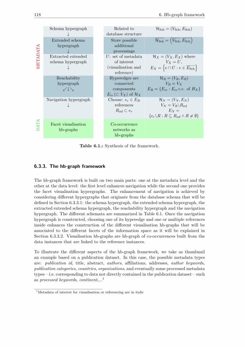
118 6. Hb-graph framework
MET
ADAT
A
Schema hypergraph↓
Related todatabase structure
HSch = (VSch, ESch)
Extended schemahypergraph
↓
Store possibleadditionalprocessings
HSch =(VSch, ESch
)
Extracted extendedschema hypergraph
↓
U : set of metadataof interest
(visualisation andreference)
HX = (VX , EX) whereVX = U ,
EX ={e ∩ U : e ∈ ESch
}Reachabilityhypergraph↙↓↘
Hyperedges areconnectedcomponents
Ecc (⊂ VX) of HX
HR = (VR, ER)VR = VX
ER = {Ecc : Ecc c.c. of HX}
Navigation hypergraph↓
Choose: er ∈ ERreferencesRref ⊂ er
HN = (VN , EN )VN = VR\Rref
EN ={er\R : R ⊆ Rref ∧R 6= ∅}
DAT
A
Facet visualisationhb-graphs
Co-occurrencenetworks ashb-graphs
Table 6.1.: Synthesis of the framework.
6.3.3. The hb-graph framework
The hb-graph framework is built on two main parts: one at the metadata level and theother at the data level: the first level enhances navigation while the second one providesthe facet visualisation hypergraphs. The enhancement of navigation is achieved byconsidering different hypergraphs that originate from the database schema that will bedefined in Section 6.3.3.1: the schema hypergraph, the extended schema hypergraph, theextracted extended schema hypergraph, the reachability hypergraph and the navigationhypergraph. The different schemata are summarized in Table 6.1. Once the navigationhypergraph is constructed, choosing one of its hyperedge and one or multiple referencesinside enhances the construction of the different visualisation hb-graphs that will beassociated to the different facets of the information space as it will be explained inSection 6.3.3.2. Visualisation hb-graphs are hb-graph of co-occurrences built from thedata instances that are linked to the reference instances.
To illustrate the different aspects of the hb-graph framework, we take as thumbnailan example based on a publication dataset. In this case, the possible metadata typesare: publication id, title, abstract, authors, affiliations, addresses, author keywords,publication categories, countries, organizations, and eventually some processed metadatatypes—i.e. corresponding to data not directly contained in the publication dataset—suchas processed keywords, continent,...1
1Metadata of interest for visualisation or referencing are in italic
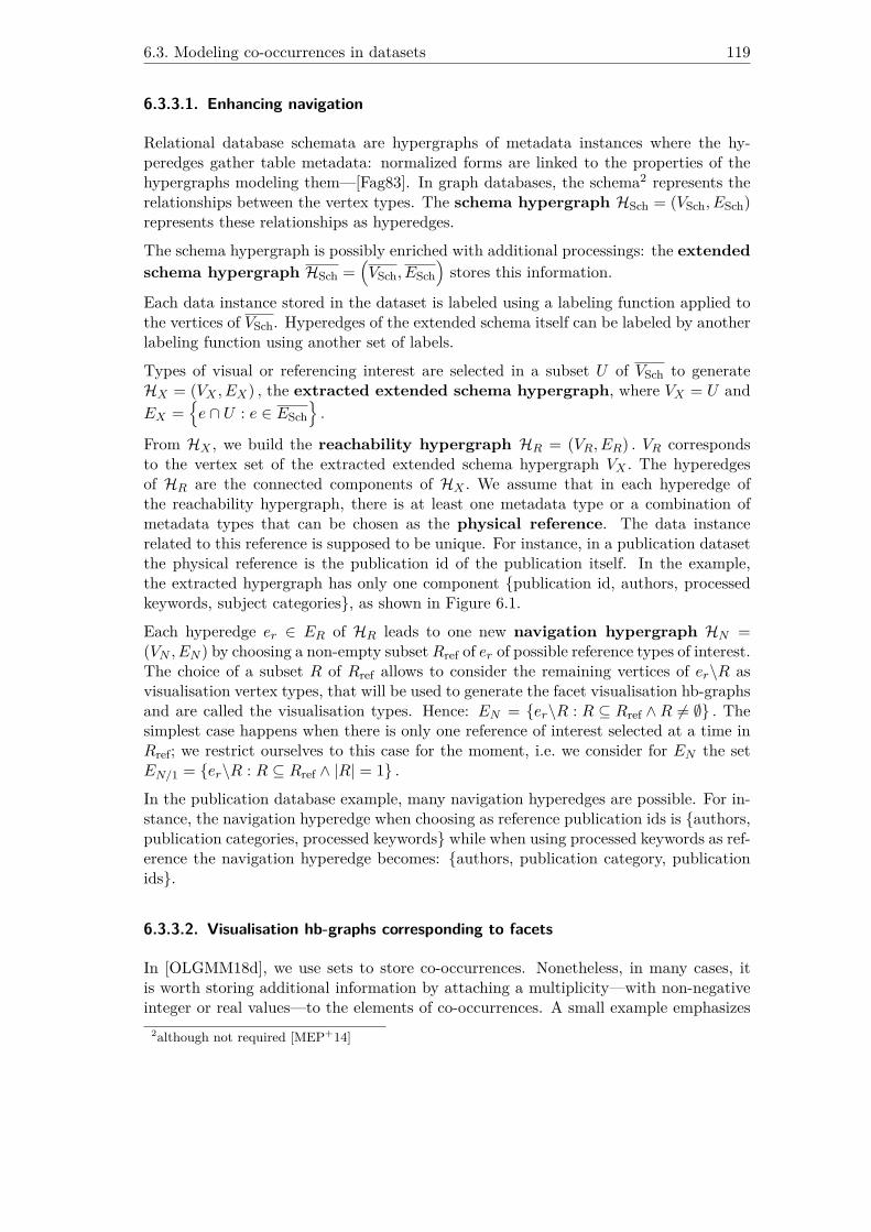
6.3. Modeling co-occurrences in datasets 119
6.3.3.1. Enhancing navigation
Relational database schemata are hypergraphs of metadata instances where the hy-peredges gather table metadata: normalized forms are linked to the properties of thehypergraphs modeling them—[Fag83]. In graph databases, the schema2 represents therelationships between the vertex types. The schema hypergraph HSch = (VSch, ESch)represents these relationships as hyperedges.
The schema hypergraph is possibly enriched with additional processings: the extendedschema hypergraph HSch =
(VSch, ESch
)stores this information.
Each data instance stored in the dataset is labeled using a labeling function applied tothe vertices of VSch. Hyperedges of the extended schema itself can be labeled by anotherlabeling function using another set of labels.
Types of visual or referencing interest are selected in a subset U of VSch to generateHX = (VX , EX) , the extracted extended schema hypergraph, where VX = U andEX =
{e ∩ U : e ∈ ESch
}.
From HX , we build the reachability hypergraph HR = (VR, ER) . VR correspondsto the vertex set of the extracted extended schema hypergraph VX . The hyperedgesof HR are the connected components of HX . We assume that in each hyperedge ofthe reachability hypergraph, there is at least one metadata type or a combination ofmetadata types that can be chosen as the physical reference. The data instancerelated to this reference is supposed to be unique. For instance, in a publication datasetthe physical reference is the publication id of the publication itself. In the example,the extracted hypergraph has only one component {publication id, authors, processedkeywords, subject categories}, as shown in Figure 6.1.
Each hyperedge er ∈ ER of HR leads to one new navigation hypergraph HN =(VN , EN ) by choosing a non-empty subsetRref of er of possible reference types of interest.The choice of a subset R of Rref allows to consider the remaining vertices of er\R asvisualisation vertex types, that will be used to generate the facet visualisation hb-graphsand are called the visualisation types. Hence: EN = {er\R : R ⊆ Rref ∧R 6= ∅} . Thesimplest case happens when there is only one reference of interest selected at a time inRref; we restrict ourselves to this case for the moment, i.e. we consider for EN the setEN/1 = {er\R : R ⊆ Rref ∧ |R| = 1} .
In the publication database example, many navigation hyperedges are possible. For in-stance, the navigation hyperedge when choosing as reference publication ids is {authors,publication categories, processed keywords} while when using processed keywords as ref-erence the navigation hyperedge becomes: {authors, publication category, publicationids}.
6.3.3.2. Visualisation hb-graphs corresponding to facets
In [OLGMM18d], we use sets to store co-occurrences. Nonetheless, in many cases, itis worth storing additional information by attaching a multiplicity—with non-negativeinteger or real values—to the elements of co-occurrences. A small example emphasizes2although not required [MEP+14]
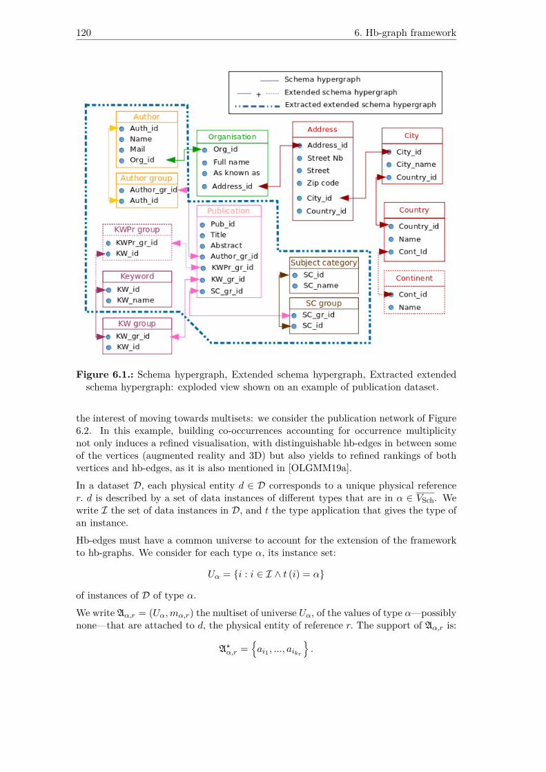
120 6. Hb-graph framework
Figure 6.1.: Schema hypergraph, Extended schema hypergraph, Extracted extendedschema hypergraph: exploded view shown on an example of publication dataset.
the interest of moving towards multisets: we consider the publication network of Figure6.2. In this example, building co-occurrences accounting for occurrence multiplicitynot only induces a refined visualisation, with distinguishable hb-edges in between someof the vertices (augmented reality and 3D) but also yields to refined rankings of bothvertices and hb-edges, as it is also mentioned in [OLGMM19a].In a dataset D, each physical entity d ∈ D corresponds to a unique physical referencer. d is described by a set of data instances of different types that are in α ∈ VSch. Wewrite I the set of data instances in D, and t the type application that gives the type ofan instance.Hb-edges must have a common universe to account for the extension of the frameworkto hb-graphs. We consider for each type α, its instance set:
Uα = {i : i ∈ I ∧ t (i) = α}
of instances of D of type α.We write Aα,r = (Uα,mα,r) the multiset of universe Uα, of the values of type α—possiblynone—that are attached to d, the physical entity of reference r. The support of Aα,r is:
A?α,r ={ai1 , ..., aikr
}.
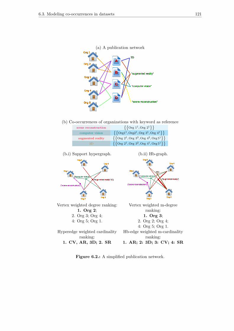
6.3. Modeling co-occurrences in datasets 121
(a) A publication network
(b) Co-occurrences of organizations with keyword as referencescene reconstruction
{{Org 11,Org 21
}}computer vision
{{Org11,Org21,Org 31,Org 41
}}augmented reality
{{Org 21,Org 33,Org 42,Org 51
}}3D
{{Org 21,Org 32,Org 41,Org 51
}}(b.i) Support hypergraph. (b.ii) Hb-graph.
Vertex weighted degree ranking:1. Org 2;
2. Org 3; Org 4;4: Org 5; Org 1.
Vertex weighted m-degreeranking:1. Org 3;
2. Org 2; Org 4;4: Org 5; Org 1.
Hyperedge weighted cardinalityranking:
Hb-edge weighted m-cardinalityranking:
1. CV, AR, 3D; 2. SR 1. AR; 2: 3D; 3: CV; 4: SR
Figure 6.2.: A simplified publication network.
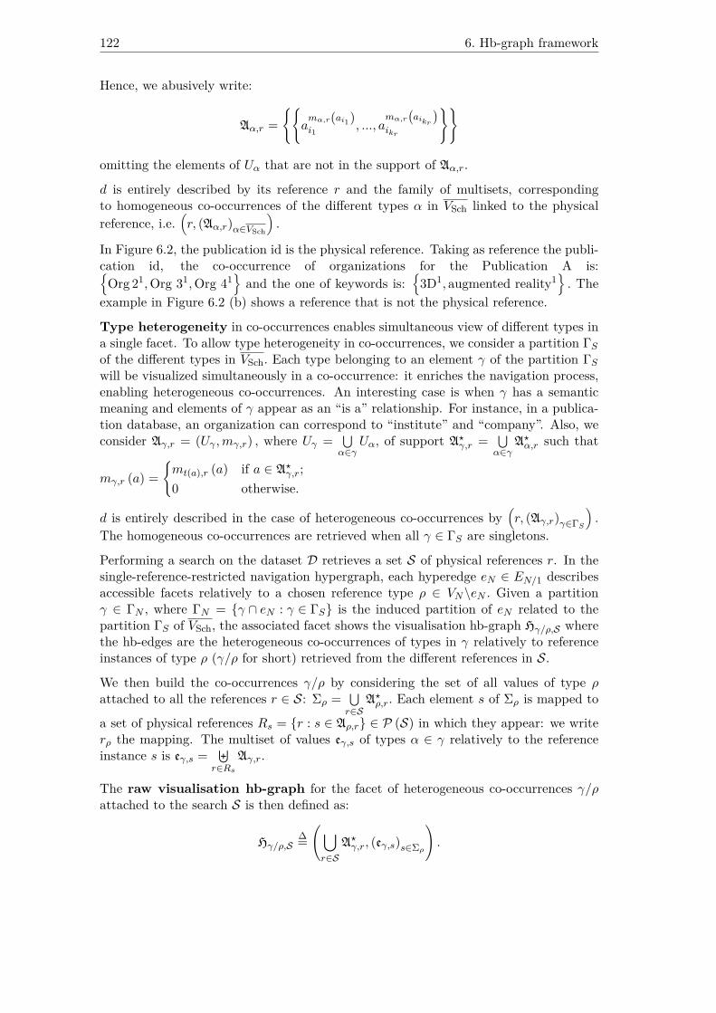
122 6. Hb-graph framework
Hence, we abusively write:
Aα,r ={{
amα,r(ai1)i1
, ..., amα,r
(aikr
)ikr
}}
omitting the elements of Uα that are not in the support of Aα,r.
d is entirely described by its reference r and the family of multisets, correspondingto homogeneous co-occurrences of the different types α in VSch linked to the physicalreference, i.e.
(r, (Aα,r)α∈VSch
).
In Figure 6.2, the publication id is the physical reference. Taking as reference the publi-cation id, the co-occurrence of organizations for the Publication A is:{Org 21,Org 31,Org 41
}and the one of keywords is:
{3D1, augmented reality1
}. The
example in Figure 6.2 (b) shows a reference that is not the physical reference.
Type heterogeneity in co-occurrences enables simultaneous view of different types ina single facet. To allow type heterogeneity in co-occurrences, we consider a partition ΓSof the different types in VSch. Each type belonging to an element γ of the partition ΓSwill be visualized simultaneously in a co-occurrence: it enriches the navigation process,enabling heterogeneous co-occurrences. An interesting case is when γ has a semanticmeaning and elements of γ appear as an “is a” relationship. For instance, in a publica-tion database, an organization can correspond to “institute” and “company”. Also, weconsider Aγ,r = (Uγ ,mγ,r) , where Uγ = ⋃
α∈γUα, of support A?γ,r = ⋃
α∈γA?α,r such that
mγ,r (a) ={mt(a),r (a) if a ∈ A?γ,r;0 otherwise.
d is entirely described in the case of heterogeneous co-occurrences by(r, (Aγ,r)γ∈ΓS
).
The homogeneous co-occurrences are retrieved when all γ ∈ ΓS are singletons.
Performing a search on the dataset D retrieves a set S of physical references r. In thesingle-reference-restricted navigation hypergraph, each hyperedge eN ∈ EN/1 describesaccessible facets relatively to a chosen reference type ρ ∈ VN\eN . Given a partitionγ ∈ ΓN , where ΓN = {γ ∩ eN : γ ∈ ΓS} is the induced partition of eN related to thepartition ΓS of VSch, the associated facet shows the visualisation hb-graph Hγ/ρ,S wherethe hb-edges are the heterogeneous co-occurrences of types in γ relatively to referenceinstances of type ρ (γ/ρ for short) retrieved from the different references in S.
We then build the co-occurrences γ/ρ by considering the set of all values of type ρattached to all the references r ∈ S: Σρ = ⋃
r∈SA?ρ,r. Each element s of Σρ is mapped to
a set of physical references Rs = {r : s ∈ Aρ,r} ∈ P (S) in which they appear: we writerρ the mapping. The multiset of values eγ,s of types α ∈ γ relatively to the referenceinstance s is eγ,s = ⊎
r∈RsAγ,r.
The raw visualisation hb-graph for the facet of heterogeneous co-occurrences γ/ρattached to the search S is then defined as:
Hγ/ρ,S∆=(⋃r∈S
A?γ,r, (eγ,s)s∈Σρ
).
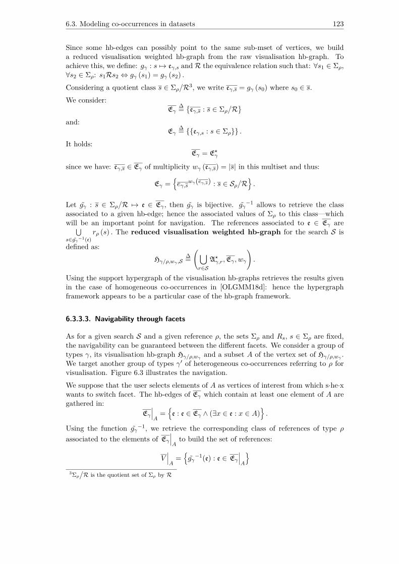
6.3. Modeling co-occurrences in datasets 123
Since some hb-edges can possibly point to the same sub-mset of vertices, we builda reduced visualisation weighted hb-graph from the raw visualisation hb-graph. Toachieve this, we define: gγ : s 7→ eγ,s and R the equivalence relation such that: ∀s1 ∈ Σρ,∀s2 ∈ Σρ: s1Rs2 ⇔ gγ (s1) = gγ (s2) .Considering a quotient class s ∈ Σρ
/R3, we write eγ,s = gγ (s0) where s0 ∈ s.
We consider:Eγ
∆={eγ,s : s ∈ Σρ
/R}
and:Eγ
∆= {{eγ,s : s ∈ Σρ}} .
It holds:Eγ = E?γ
since we have: eγ,s ∈ Eγ of multiplicity wγ (eγ,s) = |s| in this multiset and thus:
Eγ ={eγ,s
wγ(eγ,s) : s ∈ Sρ/R}.
Let gγ : s ∈ Σρ/R 7→ e ∈ Eγ , then gγ is bijective. gγ
−1 allows to retrieve the classassociated to a given hb-edge; hence the associated values of Σρ to this class—whichwill be an important point for navigation. The references associated to e ∈ Eγ are⋃s∈gγ−1(e)
rρ (s) . The reduced visualisation weighted hb-graph for the search S is
defined as:Hγ/ρ,wγ ,S
∆=(⋃r∈S
A?γ,r,Eγ , wγ
).
Using the support hypergraph of the visualisation hb-graphs retrieves the results givenin the case of homogeneous co-occurrences in [OLGMM18d]: hence the hypergraphframework appears to be a particular case of the hb-graph framework.
6.3.3.3. Navigability through facets
As for a given search S and a given reference ρ, the sets Σρ and Rs, s ∈ Σρ are fixed,the navigability can be guaranteed between the different facets. We consider a group oftypes γ, its visualisation hb-graph Hγ/ρ,wγ and a subset A of the vertex set of Hγ/ρ,wγ .We target another group of types γ′ of heterogeneous co-occurrences referring to ρ forvisualisation. Figure 6.3 illustrates the navigation.We suppose that the user selects elements of A as vertices of interest from which s·he·xwants to switch facet. The hb-edges of Eγ which contain at least one element of A aregathered in:
Eγ∣∣∣A
={e : e ∈ Eγ ∧ (∃x ∈ e : x ∈ A)
}.
Using the function gγ−1, we retrieve the corresponding class of references of type ρ
associated to the elements of Eγ∣∣∣Ato build the set of references:
V∣∣∣A
={gγ−1(e) : e ∈ Eγ
∣∣∣A
}3Σρ/R is the quotient set of Σρ by R

124 6. Hb-graph framework
Physical entity: dReference: r
S d1r1
. . . dSrS
Aγ,r
aγ1
...
aγr
Aρ,r
aρ1
...
aρr
Aγ′,r aγ′1 . . . aγ′r
Figure 6.3.: Navigating between facets of the information space.
of type ρ involved in the building of co-occurrences of type γ′. Each of the classes inV∣∣∣Acontains instances of type ρ that are gathered in a set Vρ,A. Each element of Vρ,A
is linked to a set of physical references by rρ. Hence we obtain the physical reference setinvolving elements of A: SA = ⋃
s∈νρ,ARs.
The raw visualisation hb-graph Hγ′/ρ
∣∣∣A
=( ⋃r∈SA
A?γ′,r,(eγ′,s
)s∈Vρ,A
)in the targeted
facet is now enhanced using SA as search set S. To obtain the reduced weighted versionwe use the same approach as above. The multiset of co-occurrences retrieved includes alloccurrences that have co-occurred with the references attached to one of the elements ofA selected in the first facet. Of course, if A = Aγ,S , the reduced visualisation hb-graphcontains all the instances of type γ′ attached to physical entities of the search S.
In Figure 6.2.b(ii), with A = {Org1} , two hb-edges can be retrieved: computer vi-sion—attached to PubB and PubC—and scene reconstruction—PubB. Hence: SA ={PubB,PubC} . Switching to the Publication facet and keeping as reference keywords,two hb-edges
{PubB1,PubC1
}and
{PubB1
}are retrieved. The same with A =
{Org1,Org2} retrieves all the co-occurrences of Publications with reference to keywords.
It can be of interest to put a filter on Hγ′/ρ
∣∣∣Ato retain only the references used in the
first facet to build the co-occurrences. In this case, we obtain a sub-hb-graph of Hγ′/ρ∣∣∣A
that is limited to the references of co-occurrences involved in the previous facet.
An other example is given in Figure 6.4. We navigate between organization co-occurrencesand the subject category co-occurrences both built using keywords as reference. We se-lect one of the organization in the organization facet. We show how the constructionof the hb-graph work for the targeted facet. Additionally, we present how the possiblefiltering of the targeted hb-graph works and how it restricts the view to the referencesof the first facet.
The reference type can always be shown in one of the facets as a visualisation hb-graphwhere all the hb-edges are constituted of the references themselves with multiplicity thenumber of time the reference occurs in the hb-graph.
Ultimately, by building a multi-dimensional network organized around groups of types,one can retrieve very valuable information from combined data sources. This processcan be extended to any number of data sources as long as they share one or more types.

6.3. Modeling co-occurrences in datasets 125
(a) The publication network with four facets.
(b) Organization co-occurrences with keyword as reference.scene reconstruction Pub B
{{Org 11,Org 21
}}computer vision Pub B, Pub C
{{Org11,Org21,Org 31,Org 41
}}augmented reality Pub A, Pub C, Pub D
{{Org 21,Org 33,Org 42,Org 51
}}3D Pub A, Pub D
{{Org 21,Org 32,Org 41,Org 51
}}
(c) Building subject category co-occurrences with keywords as reference.
(d) Visualization of the subject category co-occurrences with keywords as reference.(d.i) Unfiltered. (d.ii) Filtered.
Figure 6.4.: Navigating between facets in the publication network: visualizing orga-nization co-occurrences with reference keywords and switching to subject categorieswith reference keywords.
126 6. Hb-graph framework
Otherwise, the reachability hypergraph is not connected, and only separated navigationsare possible in this case.
6.3.3.4. Change of reference
Changing reference follows similar principles than navigating through facets. We con-sider a group of types γ, its visualisation hb-graph Hγ/ρ,wγ and a subset A of the vertexset of Hγ/ρ,wγ . But, this time, we target the same group of types γ of heterogeneousco-occurrences referring to a new reference type ρ′ for visualisation.We still suppose that the user selects elements of A as vertices of interest from whichs·he·x wants to switch facet. The hb-edges of Eγ , which contain at least one element ofA, are again gathered in:
Eγ∣∣∣A
={e : e ∈ Eγ ∧ (∃x ∈ e : x ∈ A)
}.
Using the function gγ−1, we retrieve the corresponding class of references of type ρ
associated to the elements of Eγ∣∣∣A, and build the set of references:
V∣∣∣A
={gγ−1(e) : e ∈ Eγ
∣∣∣A
}of type ρ involved in the building of co-occurrences of type γ. Each of the classes inV∣∣∣Acontains instances of type ρ that are gathered in a set Vρ,A. Each element of Vρ,A
is linked to a set of physical references by rρ. Hence, we obtain the physical referenceset involving elements of A :
SA =⋃
s∈νρ,ARs.
And, we can now enhance the raw visualisation hb-graph:
Hγ/ρ′∣∣∣A
=
⋃r∈SA
A?γ,r, (eγ,s)s∈Vρ′,A
with the new reference type using SA as search set S. To obtain the reduced weightedversion, we use the same approach as before. The multiset of co-occurrences retrievedincludes all occurrences that have co-occurred with the references attached to one of theelements of A selected in the first facet.It is worth mentioning that a change of reference from ρ to ρ′ may result in additionalelements of type γ in the corresponding co-occurrences. This is illustrated on the pub-lication network as shown in Figure 6.5.
6.3.3.5. The case of multiple references
Extending co-occurrences to multiple reference types chosen in eR ∈ ER is not straight-forward. There are two ways of doing so: a disjunctive and a conjunctive way. Weconsider the set R ⊂ eR of references and eN = eR\R the visualisation types.In the disjunctive way, each co-occurrence is built as before, considering successivelyeach type ρ ∈ R. This is particularly adapted for types that are partitioning the physical
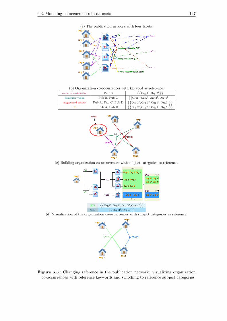
6.3. Modeling co-occurrences in datasets 127
(a) The publication network with four facets.
(b) Organization co-occurrences with keyword as reference.scene reconstruction Pub B
{{Org 11,Org 21
}}computer vision Pub B, Pub C
{{Org11,Org21,Org 31,Org 41
}}augmented reality Pub A, Pub C, Pub D
{{Org 21,Org 33,Org 42,Org 51
}}3D Pub A, Pub D
{{Org 21,Org 32,Org 41,Org 51
}}
(c) Building organization co-occurrences with subject categories as reference.
SC1{{
Org11,Org22,Org 32,Org 42}}
SC2{{
Org 31,Org 41}}
(d) Visualization of the organization co-occurrences with subject categories as reference.
Figure 6.5.: Changing reference in the publication network: visualizing organizationco-occurrences with reference keywords and switching to reference subject categories.
128 6. Hb-graph framework
references. It is the case for instance in the aggregation of two databases on two differentkind of physical data, such as publication and patent, where the co-occurrence of thechosen navigation type is built referring either to a publication or (non-exclusive) to apatent. The hb-graphs obtained are built by extending the family of hb-edges.In the conjunctive approach, we start by building the cross product of instances of thereferences and retrieve co-occurrences of elements for which the data d is attached tothe corresponding values of the cross-reference instances. Hence, co-occurrences arerestricted to the simultaneous presence of reference instances attached to the physicalentity.
6.3.4. The DataHbEdron
The DataHbEdron—the name we have given to the tool we have developed based onthese mathematical principles—provides soft navigation between the different facets ofthe information space. Each facet of the information space corresponding to a visuali-sation type includes a visualisation hb-graph viewed in its 2D extra-node representationwith a normalised thickness on hb-edges [OLGMM18b]. To enhance navigation, thedifferent facets are embedded in a 2.5D representation called the DataHbEdron. TheDataHbEdron4 can be toggled into either a cube with six faces—Figure 6.6(a)—or acarousel shape with n faces—Figure 6.6(b)—to ease navigation between facets. Thereference face shows a traditional verbatim list of references corresponding to the searchoutput.Faces of the DataHbEdron show different facets of the information space: the underlyingvisualisation hb-graphs support the navigability through facets. Hb-edges are selectableacross the different facets; since each hb-edge is linked to a subset of references, thecorresponding references can be used to highlight information in the different facets aswell as in the face containing the reference visualisation hb-graph.
6.3.5. Validation and discussion
6.3.5.1. Fulfillment of expectations
Now that the hb-graph framework has been built, we can check that each expectationexpressed in Section 6.3.2 is fulfilled.
Guarantee 6.1. The framework should model the information space using hb-graphs.
We reach this expectation, either by using hypergraphs—particular case of hb-graphs—atthe metadata level or by using hb-graphs at the visualisation level. Even if the databaseschema can always be modeled by a graph as in [ADLGP17], there are concepts thatbetter fit using hypergraphs to store the schema5. The other related work limit them-selves to a few facets and the toggling between those facets; moreover, they do not takeinto account multisets.4An animated presentation can be found on my research page: https://www.infos-informatique.net5A good example is given in https://blog.grakn.ai/modelling-data-with-hypergraphs-edff1e12edf0: if amarriage can be easily modeled by a table that contains an id, a husband id, and a wife id, which isalready a triple, a divorce has an id, an id of marriage, a petitioner id and a respondent id, which isa quadruple. In both cases, hypergraphs fit to model this situation.
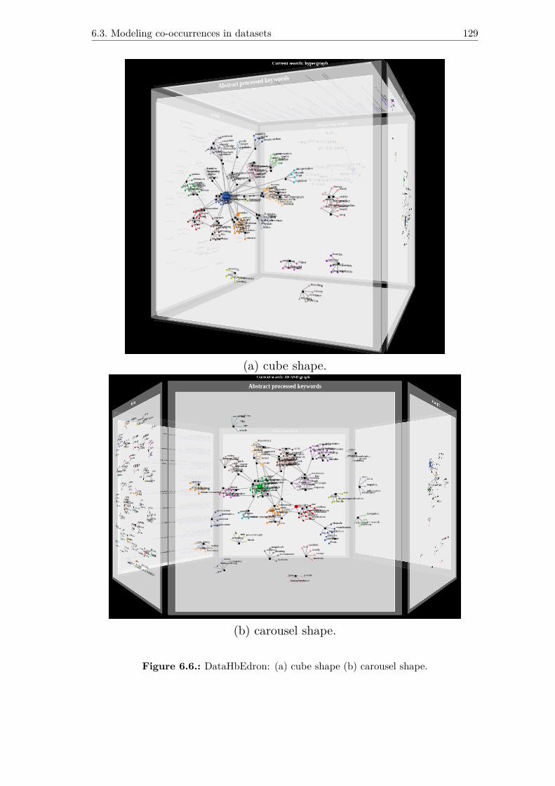
6.3. Modeling co-occurrences in datasets 129
(a) cube shape.
(b) carousel shape.
Figure 6.6.: DataHbEdron: (a) cube shape (b) carousel shape.
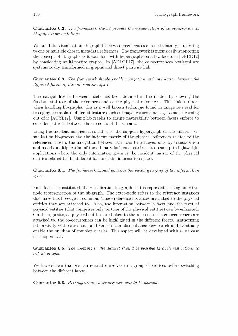
130 6. Hb-graph framework
Guarantee 6.2. The framework should provide the visualisation of co-occurrences ashb-graph representations.
We build the visualisation hb-graph to show co-occurrences of a metadata type referringto one or multiple chosen metadata references. The framework is intrinsically supportingthe concept of hb-graphs as it was done with hypergraphs on a few facets in [DRRD12]by considering multi-partite graphs. In [ADLGP17], the co-occurrences retrieved aresystematically transformed in graphs and direct pairwise link.
Guarantee 6.3. The framework should enable navigation and interaction between thedifferent facets of the information space.
The navigability in between facets has been detailed in the model, by showing thefundamental role of the references and of the physical references. This link is directwhen handling hb-graphs: this is a well known technique found in image retrieval forfusing hypergraphs of different features such as image features and tags to make learningout of it [ACYL17]. Using hb-graphs to ensure navigability between facets enforce toconsider paths in between the elements of the schema.
Using the incident matrices associated to the support hypergraph of the different vi-sualisation hb-graphs and the incident matrix of the physical references related to thereferences chosen, the navigation between facet can be achieved only by transpositionand matrix multiplication of these binary incident matrices. It opens up to lightweightapplications where the only information given is the incident matrix of the physicalentities related to the different facets of the information space.
Guarantee 6.4. The framework should enhance the visual querying of the informationspace.
Each facet is constituted of a visualisation hb-graph that is represented using an extra-node representation of the hb-graph. The extra-node refers to the reference instancesthat have this hb-edge in common. These reference instances are linked to the physicalentities they are attached to. Also, the interaction between a facet and the facet ofphysical entities (that comprises only vertices of the physical entities) can be enhanced.On the opposite, as physical entities are linked to the references the co-occurrences areattached to, the co-occurrences can be highlighted in the different facets. Authorizinginteractivity with extra-node and vertices can also enhance new search and eventuallyenable the building of complex queries. This aspect will be developed with a use casein Chapter D.1.
Guarantee 6.5. The zooming in the dataset should be possible through restrictions tosub-hb-graphs.
We have shown that we can restrict ourselves to a group of vertices before switchingbetween the different facets.
Guarantee 6.6. Heterogeneous co-occurrences should be possible.
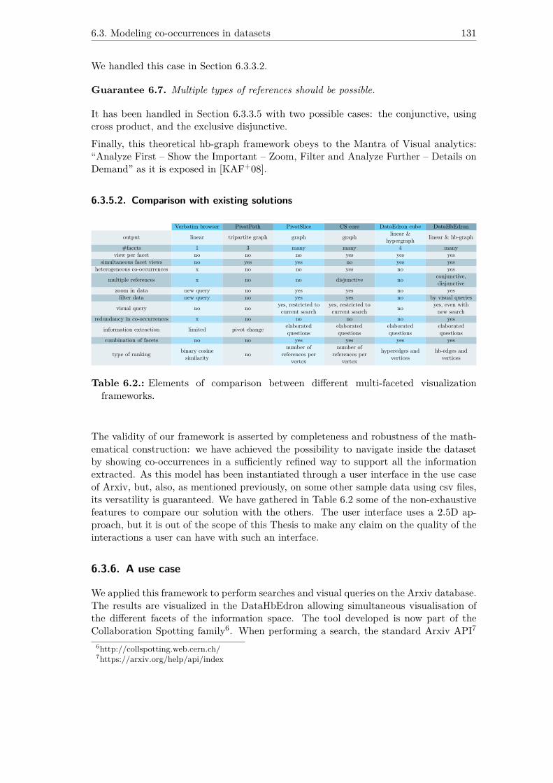
6.3. Modeling co-occurrences in datasets 131
We handled this case in Section 6.3.3.2.
Guarantee 6.7. Multiple types of references should be possible.
It has been handled in Section 6.3.3.5 with two possible cases: the conjunctive, usingcross product, and the exclusive disjunctive.Finally, this theoretical hb-graph framework obeys to the Mantra of Visual analytics:“Analyze First – Show the Important – Zoom, Filter and Analyze Further – Details onDemand” as it is exposed in [KAF+08].
6.3.5.2. Comparison with existing solutions
Verbatim browser PivotPath PivotSlice CS core DataEdron cube DataHbEdron
output linear tripartite graph graph graph linear &hypergraph linear & hb-graph
#facets 1 3 many many 4 manyview per facet no no no yes yes yes
simultaneous facet views no yes yes no yes yesheterogeneous co-occurrences x no no yes no yes
multiple references x no no disjunctive no conjunctive,disjunctive
zoom in data new query no yes yes no yesfilter data new query no yes yes no by visual queries
visual query no no yes, restricted tocurrent search
yes, restricted tocurrent search no yes, even with
new searchredundancy in co-occurrences x no no no no yes
information extraction limited pivot change elaboratedquestions
elaboratedquestions
elaboratedquestions
elaboratedquestions
combination of facets no no yes yes yes yes
type of ranking binary cosinesimilarity no
number ofreferences per
vertex
number ofreferences per
vertex
hyperedges andvertices
hb-edges andvertices
Table 6.2.: Elements of comparison between different multi-faceted visualizationframeworks.
The validity of our framework is asserted by completeness and robustness of the math-ematical construction: we have achieved the possibility to navigate inside the datasetby showing co-occurrences in a sufficiently refined way to support all the informationextracted. As this model has been instantiated through a user interface in the use caseof Arxiv, but, also, as mentioned previously, on some other sample data using csv files,its versatility is guaranteed. We have gathered in Table 6.2 some of the non-exhaustivefeatures to compare our solution with the others. The user interface uses a 2.5D ap-proach, but it is out of the scope of this Thesis to make any claim on the quality of theinteractions a user can have with such an interface.
6.3.6. A use case
We applied this framework to perform searches and visual queries on the Arxiv database.The results are visualized in the DataHbEdron allowing simultaneous visualisation ofthe different facets of the information space. The tool developed is now part of theCollaboration Spotting family6. When performing a search, the standard Arxiv API76http://collspotting.web.cern.ch/7https://arxiv.org/help/api/index
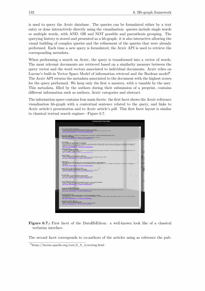
132 6. Hb-graph framework
is used to query the Arxiv database. The queries can be formulated either by a textentry or done interactively directly using the visualisation: queries include single wordsor multiple words, with AND, OR and NOT possible and parenthesis grouping. Thequerying history is stored and presented as a hb-graph: it is also interactive allowing thevisual building of complex queries and the refinement of the queries that were alreadyperformed. Each time a new query is formulated, the Arxiv API is used to retrieve thecorresponding metadata.
When performing a search on Arxiv, the query is transformed into a vector of words.The most relevant documents are retrieved based on a similarity measure between thequery vector and the word vectors associated to individual documents. Arxiv relies onLucene’s built-in Vector Space Model of information retrieval and the Boolean model8.The Arxiv API returns the metadata associated to the document with the highest scoresfor the query performed. We keep only the first n answers, with n tunable by the user.This metadata, filled by the authors during their submission of a preprint, containsdifferent information such as authors, Arxiv categories and abstract.
The information space contains four main facets: the first facet shows the Arxiv referencevisualisation hb-graph with a contextual sentence related to the query, and links toArxiv article’s presentation and to Arxiv article’s pdf. This first facet layout is similarto classical textual search engines—Figure 6.7.
Figure 6.7.: First facet of the DataHbEdron: a well-known look like of a classicalverbatim interface.
The second facet corresponds to co-authors of the articles using as reference the pub-8https://lucene.apache.org/core/2_9_4/scoring.html

6.3. Modeling co-occurrences in datasets 133
lication itself. The third facet is the co-keywords extracted from the abstracts. Thefourth facet is showing the Arxiv categories involved in the reference.
Co-keywords are extracted from the abstracts using TextBlob, a natural language pro-cessing Python library9. We extract only nouns using the tagged text, where lemmati-zation and singularization have been done.
Nouns in the abstract of each document are scored with TF-IDF, the Term Frequency-Invert Document Frequency. Scoring each noun in each abstract of the retrieved docu-ments generates a hb-graphs HQ of universe the nouns contained in the abstracts. Eachhb-edge contains a set of nouns extracted from a given abstract with a multiplicityfunction that represents the TF-IDF score of each noun. We keep only the first w wordsrelated to an abstract, where w is tunable by the end-user, in order to limit the size ofthe hb-edges.
The fifth facet shows the queries that have been performed during the session: the graphof those queries can be saved. The sixth facet is reserved to show additional informationsuch as the pdf of publications.
Any node on the facets is interactive, allowing to highlight information from one facet toanother one by showing the hb-edges that are mapped through the references. Queriescan be built using the vertices of the hb-graph, either isolated or by combining themwith the current search terms using AND, OR and NOT by keyboard shortcuts andmouse. The only query that has to be performed by typing is the first one. Mergingqueries from different users is immediate as it is only hb-edges in a hb-graph. Thequeries are potentially evolving, gathered, saved and re-sketched months later.
Figure 6.8.: Performed search.
We added the possibilities to display additional information related to authors usingDBLP10, but also to have information on keywords using both DuckDuckGo11 for dis-ambiguation and Wikipedia12 to enhance Arxiv information.9https://textblob.readthedocs.io/en/dev/
10https://dblp.org/11https://duckduckgo.com/12https://www.wikipedia.org/
134 6. Hb-graph framework
6.3.7. Intermediate conclusion
The framework supports dataset visual queries, possibly contextual, that either resultfrom searches on related subjects or refine the current search: it enables full navigabilityof the information space. It provides powerful insights into datasets using simultaneousfacet visualisation of the information space directly constructed from the query results.This framework is versatile enough to enhance user insight into many other datasets,particularly textual and multimedia ones.
6.4. Further comments
The full interactivity of facets is achieved; potentially, facets have to support largevisualisation hb-graphs composed of several hundred vertices and edges. The support ofthe visualisation of such hb-graphs relies mainly on the fine spreading of the informationdisplayed over the space of visualisation.
Different strategies can be used including component detection and their circular place-ment. But in random uniform and general hypergraphs, as well as in most of the realco-occurrence networks a giant component occurs—[SPS85, GZCN09, dP15]—and thiscomponent requires special attention on the placement of the vertices for visualisation.
The core idea is to focus on the central vertices to spread the information; we focus ourattention in the remaining parts of this Thesis on the detection of such vertices. Theidea is to use diffusion on the hb-graph to achieve the ranking of vertices and hb-edges.Hb-graphs hold higher order relationships that cannot be captured by matrices, as theydescribe pairwise relations either of adjacency or of incidence. Modeling diffusion andcapturing higher order relations require to use tensors. Hence our quest, from the nextChapter, to model adjacency in hb-graphs and to capture these higher order links.
7. Multi-diffusion in an information space
Highlights
7.1. Motivation . . . . . . . . . . . . . . . . . . . . . . . . . . . . . . . . . . 1357.2. Mathematical background and related work . . . . . . . . . . . . . . . . 1367.3. Multi-diffusing in an information space . . . . . . . . . . . . . . . . . . . 1417.4. Further comments . . . . . . . . . . . . . . . . . . . . . . . . . . . . . . 150
This chapter is based on ideas of a talk presented at CTW 20191.Prerequisites: Section 1.3 and, Chapters 2 and 6.
7.1. Motivation
In Chapter 6, we have shown how an information space can be modeled by using ahb-graph framework, composed of multiple facets showing visualisation hb-graphs anda reference hb-graph that displays the reference on the corresponding facet. In Chapter2, we have obtained an efficient way of ranking vertices and hb-edges: it can be appliedto the different visualisation hb-graphs separately. Nonetheless, we have shown that amapping exists between the references used to generate the co-occurrence networks andthe co-occurrences themselves. In this Chapter, we tackle the problem of aggregatingthe reference rankings obtained from the different facets. In the literature, the problemis known as rank aggregation or indifferently as ranking aggregation.The research question we want to answer in this Chapter is the following:
Research question 7.1. How to rank the references in an information space takinginto account individual rankings obtained from the different facets?
This question can be viewed as a refinement of the query results, which are traditionallybased on the decreasing values of the binary cosine similarity between the query and theresults. If the binary cosine similarity performs well in finding a list—not necessarilyordered—of results that matches the query and, if it is also fast to calculate, it is lessinformative for the results that have a non-zero similarity, and certainly not sufficientfor performing an efficient ranking. Moreover, additional information related to the1Published in the online proceedings of CTW 2019:
http://wwwhome.math.utwente.nl/∼ctw/CTW2019ProceedingsFinal.pdf.
136 7. Multi-diffusion in an information space
different facets can be retrieved. In this chapter, we aim at showing the influence ofthe different facet rankings to obtain an aggregated ranking. We propose a modifiedweighted approach of a classical method used for aggregation ranking and show theinfluence of weights on randomly generated information spaces and on real queries. Theintuition behind this method is to let the possibility to tune the aggregated ranking byputting more emphasize on some facets in an information space.We start by surveying the existing work and by giving the mathematical background ofthe approach prior to propose our new way of aggregating the rankings in an informationspace.
7.2. Mathematical background and related work
7.2.1. The problem of ranking aggregation
We consider a list L of N elements and m rankings (σi)i∈JmK of the list L . We writeL←→ the set of all possible rankings—including possible ties—of the list L . The aim ofranking aggregation is to find a consensus order σ? ∈ L←→ that aggregates the rankings(σi)i∈JmK while reflecting them as much as possible. This can be achieved either by usingdirectly ranks or by using a score function.Achieving a consensus by using directly ranks implies to use a distance d and an aggre-gation function Aggrr—often a sum, or a weighted sum—and the problem of consensusis formalized as finding σ? such that:
σ? = argminσ∈L←→
Aggrr (d (σi, σ)) .
When using a function s that scores each ranking σi, the consensus is obtained byusing a function Aggrs, that is used to minimize, maximize, average,... the differentscores obtained. Hence, the problem of consensus consists in finding σ? such that itcorresponds to a ranking obtained from the sorting of Aggrs (s (σi)) :
σ? = Rank (Sort (Aggrs (s (σi)))) .
7.2.2. Classical distances between rankings
To compare two rankings σ1 and σ2 of a list L , different distances have been defined.The Spearman footrule distance defined in [Spe87] between two rankings σ1 andσ2 of a list L corresponds to the displacement distance in absolute value between therankings:
F (σ1, σ2) ∆=∑l∈L
|σ1 (l)− σ2 (l)| .
In [Ken38] and [Ken48], two distances between two rankings σ1 and σ2 of a list L are in-troduced. The first is the Kendall tau ranking distance K (σ1, σ2) that correspondsto the number of inverted ranking between the two rankings. More formally:
K(σ1,σ2)∆=|{(i,j):i<j,(σ1(i)<σ1(j)∧σ2(i)>σ2(j))∨(σ1(i)>σ1(j)∧σ2(i)<σ2(j))}|
7.2. Mathematical background and related work 137
where σk (i) is the ranking of i in the list σk where k ∈ J2K .
Formulated an other way:
K (σ1, σ2) ∆=∑
{i,j}∈JmK
Ki,j (σ1, σ2)
with:
Ki,j(σ1,σ2)∆=
{1 if (σ1(i)<σ1(j)∧σ2(i)>σ2(j))∨(σ1(i)>σ1(j)∧σ2(i)<σ2(j))
0 otherwise.
At last, the normalised Kendall tau distance is defined as:
Kn (σ1, σ2) ∆= K (σ1, σ2)(n2
) .
7.2.3. Origin of the ranking aggregation problem
The ranking aggregation problem seeks to resolve the global ranking of elements for agiven list of rankings of those elements. The ranking aggregation problem has its originin election studies, before the French Revolution, and the research of a scrutiny that isfair to represent voters choice. In 1770, Borda presented to the French Royal Academyof Science a way of choosing the winner over the elector’s preferences for candidates byusing what is now known as the Borda method. The Borda method presented in [dB81]is a weighted vote system where the electors rank a list of the first k candidates theyprefer, where k is common to all voters. Each candidate is given a number of pointsthat corresponds to the number of candidates that are less preferred than himself. Thecandidate with the highest sum of points wins. Borda proposed this method to havean alternative to the method of Condorcet that Borda thought to be too complicated:in the Condorcet method presented in [No85], the candidate that is elected, called nowthe Condorcet winner, is the majority winner, if s·he·x exists, of a series of vote ona head-to-head basis between all the candidates. The fact that this method does notgive automatically a winner is called the Condorcet paradox2. Nonetheless, the Borda’smethod was largely criticized by Condorcet as it forces to have large consensus, but failsto the majority criterion and is subject to scrutiny manipulations, since, if some of thevoters are insincere, they can vote for an outsider they do not like in order to defeat aleading candidate and to promote a second choice candidate.
7.2.4. Kemeny-Young order
The Kemeny-Young order based on the Kendall tau distance was introduced in[Kem59]: it aims at finding a ranking that minimizes the number of disagreementsbetween the global ranking and each of the rankings by evaluating the sum of the Kendalltau distance between a candidate ranking and the different rankings. Mathematically2A typical example leading to the Condorcet paradox can be found onhttps://fr.wikipedia.org/wiki/Paradoxe_de_Condorcet.
138 7. Multi-diffusion in an information space
speaking, considering m rankings (σi)i∈JmK of a list of n objects, it searches the orderσ? such that it solves:
σ? = argminσ∈R
K (σ, σ1, ..., σm)
where:K (σ, σ1, ..., σm) =
∑k∈JmK
K (σ, σk) .
This method has the advantage to find a Condorcet winner if there exists. Moreover,in [YL78], the Kemeny’s order is shown to be the unique preference function, for agiven electorate, that gives a consensus, which is neutral—i.e. symmetric in the treat-ment of alternatives—, consistent—the preferred candidate does not depend on how theelectorate is split—and Condorcet—i.e. rank alternatives in function of the majority.
7.2.5. A revival of interest
Ranking aggregation has found a revival of interest with the raise of Internet: [DKNS01]is an authoritative paper on the subject where the authors develop techniques to over-come the difficulties of finding a common ranking to a list of rankings as finding aKemeny order is shown to be NP-hard even for m = 4 rankings.To this end, they consider the extended Condorcet Criterion introduced in [To98] whichstates that “If the set of alternatives can be partitioned in such a way that all membersof a subset of this partition defeat all alternatives belonging to subsets with a higherindex [N/A: (ranking)], then the former should obtain a better rank than the latter.”This allows to propose an admissible partition to recursively split the ties into a subsetof the partition such that it can be solved separately.Using any favorite aggregation method, in [DKNS01], the authors propose a localoptimization, called local Kemenization, such that it helps in improving the overallK (σ, σ1, ..., σm) by just successively transposing adjacent pair of elements if it decreasesthe value of K.In [SZ09], the authors compare different methods of rank aggregation and distinguishthree categories of ranking methods which include positional methods, comparison sortmethods and hybrid methods. Positional methods aim at finding an optimal permu-tation of the elements—ranking—in which the position of each element is “close to itsaverage position”; whereas comparison methods use directly the comparison betweenthe ranking of the elements and suppose to have a binary relation on the elements thatcompares their ranking. The binary relation ranks an element i before an element j ifa majority of the list of rankings has ordered them in this order. This relation is nottransitive and, hence, is not even a pre-order relation, as only reflexivity is ensured.Hybrid methods include methods that are both positional and comparison methods:they include the Markov chains introduced by [DKNS01] for web pages, especially theMarkov chain named MC4. MC4 is based on a random walk where the surfer decides tomove from a page P to a page Q on the majority rule based on the ranking of the twopages. The algorithm is given in Algorithm 7.1. The algorithm is shown to outperformother aggregation methods, both without or with local Kemenization.In [Lin10], three ranking method categories are proposed: distributional based that isnot described in [SZ09], heuristic, that includes both Borda’s method and Markov Chainapproaches, and stochastic optimization methods, aiming at minimizing a criteria.
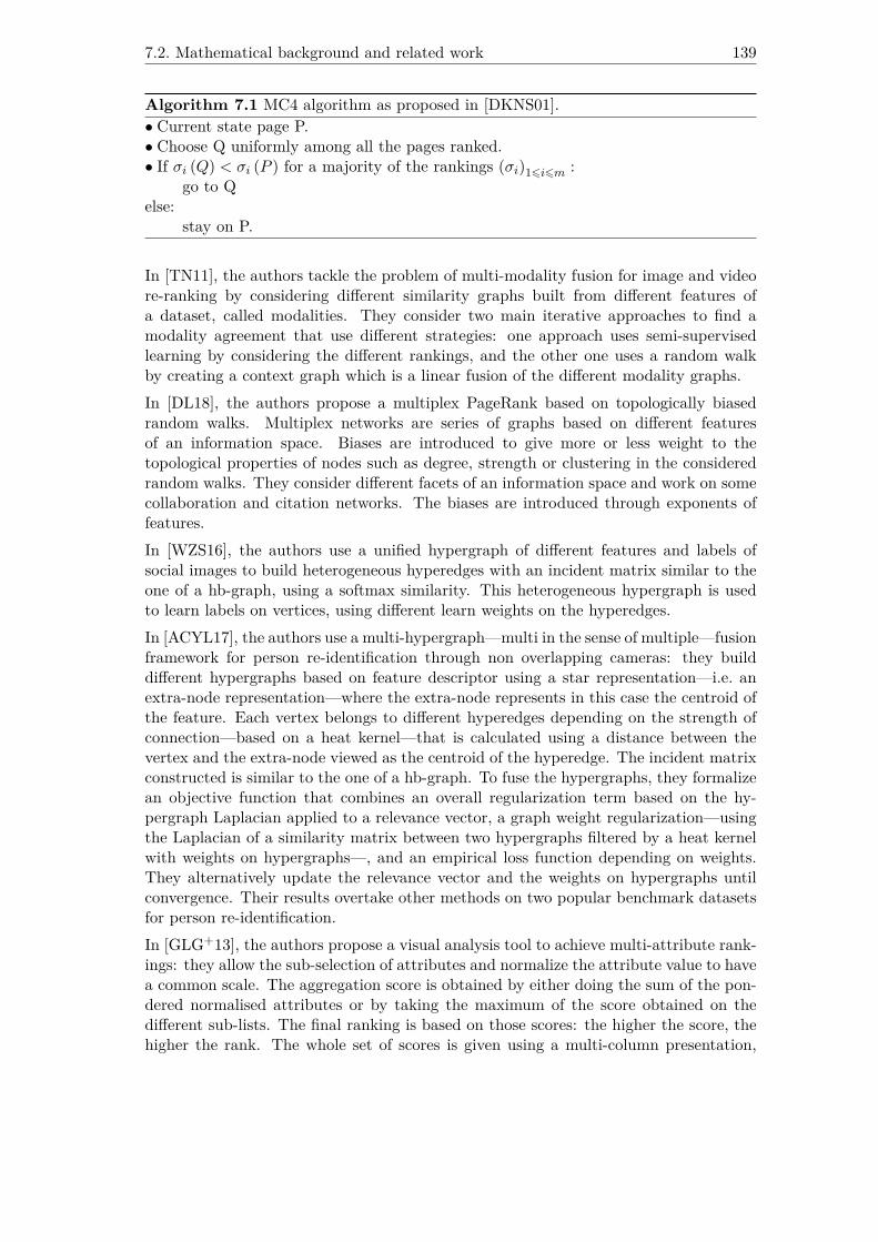
7.2. Mathematical background and related work 139
Algorithm 7.1 MC4 algorithm as proposed in [DKNS01].• Current state page P.• Choose Q uniformly among all the pages ranked.• If σi (Q) < σi (P ) for a majority of the rankings (σi)16i6m :
go to Qelse:
stay on P.
In [TN11], the authors tackle the problem of multi-modality fusion for image and videore-ranking by considering different similarity graphs built from different features ofa dataset, called modalities. They consider two main iterative approaches to find amodality agreement that use different strategies: one approach uses semi-supervisedlearning by considering the different rankings, and the other one uses a random walkby creating a context graph which is a linear fusion of the different modality graphs.In [DL18], the authors propose a multiplex PageRank based on topologically biasedrandom walks. Multiplex networks are series of graphs based on different featuresof an information space. Biases are introduced to give more or less weight to thetopological properties of nodes such as degree, strength or clustering in the consideredrandom walks. They consider different facets of an information space and work on somecollaboration and citation networks. The biases are introduced through exponents offeatures.In [WZS16], the authors use a unified hypergraph of different features and labels ofsocial images to build heterogeneous hyperedges with an incident matrix similar to theone of a hb-graph, using a softmax similarity. This heterogeneous hypergraph is usedto learn labels on vertices, using different learn weights on the hyperedges.In [ACYL17], the authors use a multi-hypergraph—multi in the sense of multiple—fusionframework for person re-identification through non overlapping cameras: they builddifferent hypergraphs based on feature descriptor using a star representation—i.e. anextra-node representation—where the extra-node represents in this case the centroid ofthe feature. Each vertex belongs to different hyperedges depending on the strength ofconnection—based on a heat kernel—that is calculated using a distance between thevertex and the extra-node viewed as the centroid of the hyperedge. The incident matrixconstructed is similar to the one of a hb-graph. To fuse the hypergraphs, they formalizean objective function that combines an overall regularization term based on the hy-pergraph Laplacian applied to a relevance vector, a graph weight regularization—usingthe Laplacian of a similarity matrix between two hypergraphs filtered by a heat kernelwith weights on hypergraphs—, and an empirical loss function depending on weights.They alternatively update the relevance vector and the weights on hypergraphs untilconvergence. Their results overtake other methods on two popular benchmark datasetsfor person re-identification.In [GLG+13], the authors propose a visual analysis tool to achieve multi-attribute rank-ings: they allow the sub-selection of attributes and normalize the attribute value to havea common scale. The aggregation score is obtained by either doing the sum of the pon-dered normalised attributes or by taking the maximum of the score obtained on thedifferent sub-lists. The final ranking is based on those scores: the higher the score, thehigher the rank. The whole set of scores is given using a multi-column presentation,
140 7. Multi-diffusion in an information space
with columns used as rank separators that allow to have not only the aspect of slopegraph but help to read the final ranking.
As it is emphasized in [LAYK+18], on the Internet, many websites use ranking policiesfor search results, advertisement, recommender systems. When a new ranking is pro-posed, the evaluation can be done either online—i.e. directly in production—using A/Btesting between the proposed ranking and the previous, or offline. The offline evalu-ation requires to use a click model as it is proposed in [CSdR13]. Other studies useadditional data to evaluate the ranking policy. For instance, in [LAYK+18], the authorsuse click logs of previous searches to construct estimators to evaluate the number ofclicks expected from the new ranking; it allows them to avoid ranking with poor results.
7.2.6. Comparison of rankings
We consider two rankings σ1 and σ2 of a list L of n elements indexed by i ∈ JnK .
The strict Kendall tau rank correlation coefficient, written τ, corresponds to theratio of the difference in the number of strict concordant pairs and strict discordantpairs related to the number of pairs. Its explicit expression is:
τ (σ1, σ2) ∆=
∑i,j∈JnK : i<j
sgn (σ1 (i)− σ1 (j)) sgn (σ2 (i)− σ2 (j))(n2
) .
This coefficient does not take into account the pairs that are matching, which can beimportant in case of ties.
For this, we can define the matching correlation coefficient ν defined as:
νmatch (σ1, σ2) ∆=
∑i,j∈JnK : i<j
1(σ1(i)==σ1(j))1(σ2(i)==σ2(j))(n2
) ,
where 1(φb) ={
1 if φb;0 otherwise,
with φb a Boolean condition statement.
We introduce a large Kendall tau rank correlation coefficient τL that takes intoaccount the agreement and disagreement on ties.
We define the disagreement on matching correlation coefficient:
νdisagree(σ1,σ2)∆=
∑i,j∈JnK : i<j
(1(σ1(i)!=σ1(j))1(σ2(i)==σ2(j)) + 1(σ1(i)==σ1(j))1(σ2(i)!=σ2(j))
)(n2
)
and:τL (σ1, σ2) ∆= τ (σ1, σ2) + νmatch (σ1, σ2)− νdisagree (σ1, σ2) .

7.3. Multi-diffusing in an information space 141
The scaled Spearman footrule correlation coefficient ρ is defined as:
ρ (σ1, σ2) ∆=
∑i∈JnK
|σ1 (i)− σ2 (i)|(n2
) .
Finally, we will also use the Jaccard index @k, k ∈ N\ {0}. To achieve this purpose,we extract sub-lists related to the two rankings corresponding to the top k elements`i = {l : l ∈ JnK ∧ σi (l) 6 k} , i = 1, 2. The Jaccard index @k of the rankings σ1 and σ2is defined as:
J@k (σ1, σ2) ∆= # (`1 ∩ `2)# (`1 ∪ `2) .
and the overlap coefficient @k, k ∈ N\ {0} , of the rankings σ1 and σ2 is defined as :
O@k (σ1, σ2) ∆= # (`1 ∩ `2)min (#`1,#`2) .
7.3. Multi-diffusing in an information space
After having simplified the notations used in Chapter 6, we start studying the differentstrategies that could be taken to aggregate the rankings of references. We then exposethe two strategies retained.
7.3.1. Laying the first stones
We consider an information space with K+1 facets (Fk)k∈JK+1K containing respectivelydata instances of different types (Tk)k∈JK+1K , one of them being chosen as the type ofreference. We can always consider that the data instances of the reference type areattached to the K+1-th facet, even if we need to re-index the facet and type sequences.We write R = VK+1 the set of references.
The data instances of a given type Tk, with k ∈ JK + 1K , constitute a set Vk attachedto the k-th facet. We write Hk =
(Vk,Ek, we,k
)the reduced visualisation hb-graph of
the facet Fk.
We consider:ρk : R→ Ek
such that:∀r ∈ R,∃e ∈ Ek : ρk(r) = e.
ρk is surjective.
The attached references to a given hb-edge can be found by defining:
νk : Ek → P (R) ,
such that:∀e ∈ Ek : νk (e) = {r ∈ R : ρk (r) = e} .
142 7. Multi-diffusion in an information space
7.3.2. Strategies for ranking references
To achieve the ranking of the references that are at the origin of the different facetvisualisation hb-graphs, we can think of different strategies.
A first strategy is to rank the hb-edges of each facet separately by using, for instancethe diffusion by exchange on each visualisation hb-graph for the different facets. Theranking aggregation takes place at the level of the references, by considering the differentrankings of hb-edges the references are related to. This strategy permits to use someclassical methods of ranking aggregation such as the Borda’s or Condorcet’s methods.Moreover, to enhance personalized rankings, we can put weights on the different facets:the rank aggregation can then be achieved by using a modified Borda method for in-stance or MC4 in [DKNS01], but might exclude some methods such as the Condorcetone.
Other strategies consider various hb-graphs involving both the references and the hb-edges attached to them, either at the hb-edge level or at the vertex level.
The second strategy would be to consider a hb-graph of hb-edges attached to a referenceand to enhance diffusion by exchange on it. However, in real world cases, this hb-graph ispotentially insufficiently connected, as hb-edges of the different facets might not repeatso often.
The third strategy consists in adding connectivity in the hb-graph proposed in thesecond strategy, by reporting the lattice of intersection of the hb-edges of each facetinto H, enriching the hb-edges of H with additional hb-edges that reflect the hb-edgeconnections in each facets. One possible pitfall of this method is that the facet hb-edges are loosing in a way the higher order information of the intersection as two facethb-edges will be connected if they intersect in the facet.
Other strategies consist of more sophisticated diffusion based on modified hb-graphs:they are out of scope of this chapter, but can be kept in mind as further possiblerefinements. Considering all these arguments, we only consider the first strategy in thisChapter.
7.3.3. Ranking aggregation by modified weighted MC4
In this approach, we consider that for each facet the exchange-based diffusion on thereduced visualisation hb-graph has been achieved, leading to a sorting of the hb-edges.As each hb-edge is by construction linked to one or more references, the ranks arereported to every attached references; we obtain a ranking σk of all the references r ∈ Rfor each facet Fk, k ∈ JKK , with possible ties.
In order to tune the rankings, we give tunable weights to the facets (wFk)k∈JKK suchthat: ∑
k∈JKKwFk = 1 and wFk > 0 for all k ∈ JKK .
We start by computing a weighted majority matrix M of elements obtained for eachcouple of references (ri1 , ri2) ∈ R2 by:
M (ri1 , ri2) =∑k∈JKK
wk1σk(ri1)<σk(ri2) −∑k∈JKK
wk1σk(ri1)>σk(ri2).

7.3. Multi-diffusing in an information space 143
Algorithm 7.2 The WT-MC4 algorithm.Prerequisite:A set of references R and K rankings (σk)k∈JKK of these referencesAlgorithm:Calculate for all (ri1 , ri2) ∈ R2 the elements of M :
M (ri1 , ri2) =∑k∈JKK
wk1σk(ri1)<σk(ri2) −∑k∈JKK
wk1σk(ri1)>σk(ri2).
Stack = R.L = [0 for r ∈ R] # To store the number of times the reference is visited.Choose a current state reference: rcurrent ∈ R.Remove rcurrent from Stack.While stack is not empty:
Choose a random number γChoose rnext uniformly among all the references in R.If γ > γ0:
rcurrent := rnextelse:
If M (rnext, rcurrent) > 0rcurrent := rnext
else:# stay in rcurrent.
L [rcurrent] + = 1.If rcurrent ∈ Stack:
Remove rcurrent from Stack.LoopWhile
We propose a modified version—that we callWT-MC4—of the Algorithm 7.1 shown asthe most efficient in [DKNS01]. This modified version includes teleportation and weightsand is presented in Algorithm 7.2. The teleportation is useful for the management ofties, so that the algorithm do not loop infinitely. The threshold γ0 is put at 0.85 which isa classical value used in the PageRank algorithm, even if we did not investigate furtherthe relevance and efficiency of this threshold.
7.3.4. Results and evaluation
We validate the approach using random generated information spaces and apply it tothe case of Arxiv querying.
7.3.4.1. Randomly generated information space
We generate each time an information space of Nfacet facets with visualisation hb-graphsgenerated using the same method as in Chapter 2. The number of hb-edges for each ofthese facets varies and it is set to a maximum value Pmax : it corresponds also to themaximal number of references. Each reference r ∈ JPmaxK is associated randomly to onehb-edge of each facet: in this way, some hb-edges are repeated.
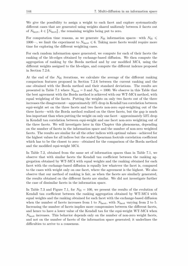
144 7. Multi-diffusion in an information space
We give the possibility to assign a weight to each facet and explore systematicallydifferent cases that are generated using weights shared uniformly between k facets outof Nfacet, k ∈ JNfacetK , the remaining weights being put to zero.
For computation time reasons, as we generate NIS information spaces—with NIS 61000—, we limit the experiment to Nfacet 6 6. Taking more facets would require moretime for exploring the different weighting cases.
For each random information space generated, we compute for each of their facets theranking of the hb-edges obtained by exchange-based diffusion. We then compute theaggregation of ranking by the Borda method and by our modified MC4, using thedifferent weights assigned to the hb-edges, and compute the different indexes proposedin Section 7.2.6.
At the end of the NIS iterations, we calculate the average of the different rankingcomparison features proposed in Section 7.2.6 between the current ranking and theone obtained with the Borda method and their standard deviations. The results arepresented in Table 7.1 where Nfacet = 3 and NIS = 1000. We observe in this Table thatthe best agreement with the Borda method is achieved with our WT-MC4 method, withequal weighting of the facets. Putting the weights on only two facets out of the threeincreases the disagreement—approximately 10% drop in Kendall tau correlation betweenequi-weight set on the three facets and two facets non-zero equi-weighting out of thethree facets—with the Borda method realized on the three facets, but the gap is muchless important than when putting the weight on only one facet—approximately 53% dropin Kendall tau correlation between equi-weight and one facet non-zero weighting out ofthe three facets. We will investigate later in this Chapter this phenomena, dependingon the number of facets in the information space and the number of non-zero weightedfacets. The results are similar for all the other indices with optimal values—achieved forthe highest values for all indices but the scaled Spearman footrule correlation coefficientwhich has to be the closest to zero—obtained for the comparison of the Borda methodand the modified equi-weight MC4.
In Table 7.2, obtained from the same set of information spaces than in Table 7.1, weobserve that with similar facets the Kendall tau coefficient between the ranking ag-gregation obtained by WT-MC4 with equal weights and the ranking obtained for eachfacet with the exchange-based diffusion is equally low whatever the facet is, comparedto the cases with weight only on one facet, where the agreement is the highest. We alsoobserve that our method of ranking is fair, as when the facets are similarly generated,the results obtained on the different facets are similar. We did not investigate furtherthe case of dissimilar facets in the information space.
In Table 7.3 and Figure 7.1, for NIS = 100, we present the results of the evolution ofKendall tau coefficient between the ranking aggregation obtained by WT-MC4 withequal weights and the ranking obtained for each facet with the exchange-based diffusionwhen the number of facets increases from 1 to Nfacet, with Nfacet varying from 2 to 5.Increasing the number of facets implies more compromises between the different facets,and hence to have a lower value of the Kendall tau for the equi-weight WT-MC4 whenNfacet increases. This behavior depends only on the number of non-zero weight facets,and not on the number of facets of the information space generated; it underlines thedifficulties to arrive to a consensus.
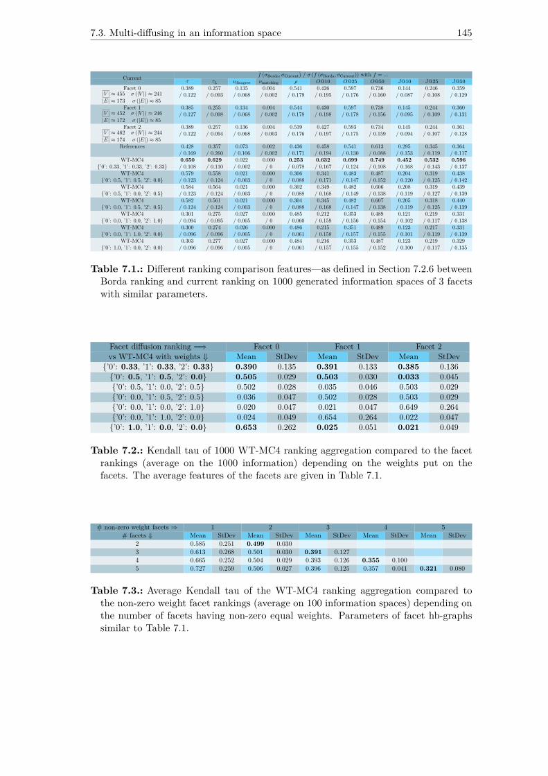
7.3. Multi-diffusing in an information space 145
f (σBorda, σCurrent) / σ (f (σBorda, σCurrent)) with f = ...Currentτ τL νdisagree νmatching ρ O@10 O@25 O@50 J@10 J@25 J@50
Facet 0|V | ≈ 455 σ (|V |) ≈ 241|E| ≈ 173 σ (|E|) ≈ 85
0.389/ 0.122
0.257/ 0.093
0.135/ 0.068
0.004/ 0.002
0.541/ 0.179
0.426/ 0.195
0.597/ 0.176
0.736/ 0.160
0.144/ 0.087
0.246/ 0.108
0.359/ 0.129
Facet 1|V | ≈ 452 σ (|V |) ≈ 246|E| ≈ 172 σ (|E|) ≈ 85
0.385/ 0.127
0.255/ 0.098
0.134/ 0.068
0.004/ 0.002
0.544/ 0.178
0.430/ 0.198
0.597/ 0.178
0.738/ 0.156
0.145/ 0.095
0.244/ 0.109
0.360/ 0.131
Facet 2|V | ≈ 462 σ (|V |) ≈ 244|E| ≈ 174 σ (|E|) ≈ 85
0.389/ 0.122
0.257/ 0.094
0.136/ 0.068
0.004/ 0.003
0.539/ 0.176
0.427/ 0.197
0.593/ 0.175
0.734/ 0.159
0.145/ 0.094
0.244/ 0.107
0.361/ 0.128
References 0.428/ 0.169
0.357/ 0.260
0.073/ 0.106
0.002/ 0.002
0.436/ 0.171
0.458/ 0.194
0.541/ 0.130
0.613/ 0.088
0.295/ 0.153
0.345/ 0.119
0.364/ 0.117
WT-MC4{’0’: 0.33, ’1’: 0.33, ’2’: 0.33}
0.650/ 0.108
0.629/ 0.110
0.022/ 0.002
0.000/ 0
0.253/ 0.078
0.632/ 0.167
0.699/ 0.124
0.749/ 0.108
0.452/ 0.168
0.532/ 0.143
0.596/ 0.137
WT-MC4{’0’: 0.5, ’1’: 0.5, ’2’: 0.0}
0.579/ 0.123
0.558/ 0.124
0.021/ 0.003
0.000/ 0
0.306/ 0.088
0.341/ 0.171
0.483/ 0.147
0.487/ 0.152
0.204/ 0.120
0.319/ 0.125
0.438/ 0.142
WT-MC4{’0’: 0.5, ’1’: 0.0, ’2’: 0.5}
0.584/ 0.123
0.564/ 0.124
0.021/ 0.003
0.000/ 0
0.302/ 0.088
0.349/ 0.168
0.482/ 0.149
0.606/ 0.138
0.208/ 0.119
0.319/ 0.127
0.439/ 0.139
WT-MC4{’0’: 0.0, ’1’: 0.5, ’2’: 0.5}
0.582/ 0.124
0.561/ 0.124
0.021/ 0.003
0.000/ 0
0.304/ 0.088
0.345/ 0.168
0.482/ 0.147
0.607/ 0.138
0.205/ 0.119
0.318/ 0.125
0.440/ 0.139
WT-MC4{’0’: 0.0, ’1’: 0.0, ’2’: 1.0}
0.301/ 0.094
0.275/ 0.095
0.027/ 0.005
0.000/ 0
0.485/ 0.060
0.212/ 0.159
0.353/ 0.156
0.489/ 0.154
0.121/ 0.102
0.219/ 0.117
0.331/ 0.138
WT-MC4{’0’: 0.0, ’1’: 1.0, ’2’: 0.0}
0.300/ 0.096
0.274/ 0.096
0.026/ 0.005
0.000/ 0
0.486/ 0.061
0.215/ 0.158
0.351/ 0.157
0.489/ 0.155
0.123/ 0.101
0.217/ 0.119
0.331/ 0.139
WT-MC4{’0’: 1.0, ’1’: 0.0, ’2’: 0.0}
0.303/ 0.096
0.277/ 0.096
0.027/ 0.005
0.000/ 0
0.484/ 0.061
0.216/ 0.157
0.353/ 0.155
0.487/ 0.152
0.123/ 0.100
0.219/ 0.117
0.329/ 0.135
Table 7.1.: Different ranking comparison features—as defined in Section 7.2.6 betweenBorda ranking and current ranking on 1000 generated information spaces of 3 facetswith similar parameters.
Facet diffusion ranking =⇒ Facet 0 Facet 1 Facet 2vs WT-MC4 with weights ⇓ Mean StDev Mean StDev Mean StDev
{’0’: 0.33, ’1’: 0.33, ’2’: 0.33} 0.390 0.135 0.391 0.133 0.385 0.136{’0’: 0.5, ’1’: 0.5, ’2’: 0.0} 0.505 0.029 0.503 0.030 0.033 0.045{’0’: 0.5, ’1’: 0.0, ’2’: 0.5} 0.502 0.028 0.035 0.046 0.503 0.029{’0’: 0.0, ’1’: 0.5, ’2’: 0.5} 0.036 0.047 0.502 0.028 0.503 0.029{’0’: 0.0, ’1’: 0.0, ’2’: 1.0} 0.020 0.047 0.021 0.047 0.649 0.264{’0’: 0.0, ’1’: 1.0, ’2’: 0.0} 0.024 0.049 0.654 0.264 0.022 0.047{’0’: 1.0, ’1’: 0.0, ’2’: 0.0} 0.653 0.262 0.025 0.051 0.021 0.049
Table 7.2.: Kendall tau of 1000 WT-MC4 ranking aggregation compared to the facetrankings (average on the 1000 information) depending on the weights put on thefacets. The average features of the facets are given in Table 7.1.
# non-zero weight facets ⇒ 1 2 3 4 5# facets ⇓ Mean StDev Mean StDev Mean StDev Mean StDev Mean StDev
2 0.585 0.251 0.499 0.0303 0.613 0.268 0.501 0.030 0.391 0.1274 0.665 0.252 0.504 0.029 0.393 0.126 0.355 0.1005 0.727 0.259 0.506 0.027 0.396 0.125 0.357 0.041 0.321 0.080
Table 7.3.: Average Kendall tau of the WT-MC4 ranking aggregation compared tothe non-zero weight facet rankings (average on 100 information spaces) depending onthe number of facets having non-zero equal weights. Parameters of facet hb-graphssimilar to Table 7.1.
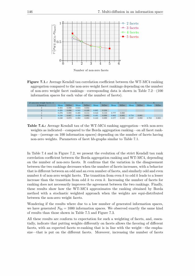
146 7. Multi-diffusion in an information space
0 1 2 3 4 5 60
0.5
1
Number of non-zero facets
τ(σ
WT
-MC
4,σ
Face
t)
2 facets3 facets4 facets5 facets
Figure 7.1.: Average Kendall tau correlation coefficient between the WT-MC4 rankingaggregation compared to the non-zero weight facet rankings depending on the numberof non-zero weight facet rankings—corresponding data is shown in Table 7.2—(100information spaces for each value of the number of facets).
# non-zero weight facets ⇒ 1 2 3 4 5 6# facets ⇓ Mean StDev Mean StDev Mean StDev Mean StDev Mean StDev Mean StDev
2 0.355 0.090 0.824 0.0533 0.295 0.096 0.582 0.109 0.665 0.1044 0.276 0.088 0.488 0.114 0.543 0.110 0.777 0.0605 0.248 0.087 0.420 0.092 0.491 0.098 0.662 0.085 0.710 0.0816 0.240 0.073 0.382 0.083 0.443 0.099 0.577 0.103 0.637 0.092 0.763 0.065
Table 7.4.: Average Kendall tau of the WT-MC4 ranking aggregation—with non-zeroweights as indicated—compared to the Borda aggregation ranking—on all facet rank-ings—(average on 100 information spaces) depending on the number of facets havingnon-zero weights. Parameters of facet hb-graphs similar to Table 7.1.
In Table 7.4 and in Figure 7.2, we present the evolution of the strict Kendall tau rankcorrelation coefficient between the Borda aggregation ranking and WT-MC4, dependingon the number of non-zero facets. It confirms that the variation in the disagreementbetween the two rankings decreases when the number of facets increases, with a behaviorthat is different between an odd and an even number of facets, and similarly odd and evennumber k of non-zero weight facets. The transition from even k to odd k leads to a lesserincrease than the transition from odd k to even k. Increasing the number of facets forranking does not necessarily improves the agreement between the two rankings. Finally,these results show how the WT-MC4 approximates the ranking obtained by Bordamethod with a stochastic weighted approach when the weights are equi-distributedbetween the non-zero weight facets.Wondering if the results where due to a low number of generated information spaces,we have generated NIS = 1000 information spaces. We observed exactly the same kindof results than those shown in Table 7.5 and Figure 7.3.All these results are conform to expectation for such a weighting of facets, and, essen-tially, indicate that putting weights differently on facets allows the favoring of differentfacets, with an expected facets re-ranking that is in line with the weight—the empha-size—that is put on the different facets. Moreover, increasing the number of facets

7.3. Multi-diffusing in an information space 147
0 1 2 3 4 5 60
0.5
1
Number of non-zero facets
τ(σ
Bor
da,σ
WT
-MC
4)
2 facets3 facets4 facets5 facets6 facets
Figure 7.2.: Average Kendall tau correlation coefficient between the ranking obtainedby Borda aggregation of the facet diffusion by exchange rankings and the WT-MC4 re-alized with equi-weight on non-zero equal weight facets—corresponding data is shownin Table 7.4—(100 information spaces for each value of the number of facets).
# non-zero weight facets ⇒ 1 2 3 4 5 6# facets ⇓ Mean StDev Mean StDev Mean StDev Mean StDev Mean StDev Mean StDev
2 0.357 0.096 0.821 0.0503 0.303 0.094 0.585 0.127 0.650 0.1124 0.272 0.093 0.485 0.116 0.545 0.116 0.771 0.0665 0.250 0.091 0.424 0.108 0.480 0.109 0.650 0.094 0.690 0.0856 0.239 0.086 0.393 0.096 0.455 0.101 0.592 0.089 0.628 0.090 0.755 0.058
Table 7.5.: Average Kendall tau of the WT-MC4 ranking aggregation compared to thenon-zero equal weight facet rankings (average on 1000 information spaces) dependingon the number of facets having non-zero weights. Parameters of facet hb-graphssimilar to Table 7.1.
0 1 2 3 4 5 60
0.5
1
Number of non-zero facets
τ(σ
Bor
da,σ
WT
-MC
4)
2 facets3 facets4 facets5 facets6 facets
Figure 7.3.: Average Kendall tau between Borda aggregation of the rankings obtainedon references via diffusion by exchange and the WT-MC4 with equi-weight on non-zero equal weight facets—it corresponds to data shown in Table 7.5—(1000 randominformation spaces for each value of the number of facets are generated).

148 7. Multi-diffusion in an information space
makes the agreement slower to reach, but at the end, the level of agreement with theBorda ranking depends essentially on the parity of the number of facets.
7.3.4.2. Application to the Arxiv information space
The main difficulty in applying multi-diffusion to a real case is that the facet visual-ization hb-graphs are essentially unconnected, which limits terribly the exchange-baseddiffusion ranking to ensure the convergence and the coherence of the ranking. It means,strictly speaking, that the exchange-based diffusion will give results that are coherentonly for the connected components. Refining the way the connected components areranked between one another is out of the scope of this section, and is an open researchquestion.However, we applied the multi-diffusion to three facets of Arxiv information space: au-thors, keywords and subject categories. In each facet, the hb-edge ranking is achievedby using the exchange-based diffusion. In Table 7.6, we summarize the top 1000 an-swers returned from the 27 Arxiv queries performed: most of the time, the only facetvisualization hb-graph that is connected is the one with keywords—or in the worst caseshas only a few components. As in the previous section, there is no correlation betweenthe rankings of the different facets. Since we are in fact interested in the ranking ag-gregation, and the way it works, we use these imperfect rankings on the overall facetvisualization hb-graphs as a basis to apply the ranking aggregation.We also consider the hb-graph of references based on their connection through hb-edgesand make some diffusion on it, even if again this hb-graph is not well connected. Withthe rankings obtained in individual facets, we perform an aggregation ranking using theBorda method and WT-MC4 with different weights, as it has been done in the randomcase. We compare the different rankings obtained byWT-MC4 with the different weightsto the rankings of the facets, the one of the Borda method and the one of the references,using the strict Kendall’s tau coefficient.The different ranking aggregation comparisons are given in Table 7.7: the results arebased on a limited number of 29 queries performed on Arxiv including the first 100results and 200 results; the queries performed are: 3D, printer, hypergraph, graph,“Higgs boson”, particle, snow, star, Laplacian, diffusion, nanotechnology, CNN, RNN,neural network, “machine learning”, “deep learning”, learning, machine, “informationretrieval”, “information”, “data mining”, entropy, information, adjacency, “3D printer”,physics, particle, network, neural. The results of the Borda aggregation ranking ismainly due to the author and keyword facets as it is both shown in the difference ofKendall’s tau coefficient with equi-weight WT-MC4 and a:0.5/k:0.5/t:0 WT-MC4. Key-word ranking or author ranking alone still perform well facing the Borda aggregationranking, but there is a true complementarity between the two, as the a:0.5/k:0.5/t:0WT-MC4 Kendall’s tau coefficient with Borda aggregation ranking method is improvedsignificantly (+0.23 for authors alone and +0.16 for keywords alone). The values ob-tained for equi-weight WT-MC4 are higher than the one we could expect with threerandom facets: this can be due to the nature of hb-graphs that are behind.Detailed results for the strict Kendall tau correlation coefficients of the different searchesare given in Table 7.8 and illustrated with a three 2-D diagrams in Figure 7.4 for thefacets of Authors and Keywords, Figure 7.5 for the facets of Authors and Tags and, in

7.3. Multi-diffusing in an information space 149
3D printer
hype
rgraph
grap
h
bosonHiggs
particle
snow
star
Laplacian
diffu
sion
nano
techno
logy
CNN
RNN
authors - keywords -0.001 -0.063 0.102 0.086 0.083 0.129 -0.049 0.064 0.115 0.13 -0.013 0.048 0.103authors - tags 0.055 0.051 -0.027 0.038 0.092 0.009 0.023 0.008 -0.027 -0.001 0.057 -0.044 -0.054keywords - tags -0.106 0.025 -0.077 -0.003 0.003 0.004 -0.051 -0.086 -0.009 -0.041 0.014 -0.038 -0.072
|V | 2948 825 1529 1868 1329 2146 13468 2366 1592 2124 3854 3228 2936|E| 953 219 883 945 817 943 685 934 895 935 969 969 960authors
# C.C. 627 193 403 656 337 787 283 489 598 779 698 655 597|V | 4884 2616 3248 3275 2051 3972 4700 4166 2796 3962 4707 4720 4476|E| 1000 230 1017 997 999 999 720 999 998 1000 1000 1000 1000keywords
# C.C. 2 1 1 1 1 2 2 3 1 1 1 1 1|V | 161 105 343 382 17 159 121 64 461 252 91 96 101|E| 271 121 423 491 25 312 205 90 575 396 221 217 238tags
# C.C. 10 13 5 7 1 7 11 15 7 8 6 3 3
neural
netw
ork
machine
learning
deep
learning
learning
machine
inform
ationretrieval
inform
ation
data
mining
entrop
y
adjacenc
y
3Dprinter
physics
netw
ork
neural
authors - keywords 0.062 0.097 0.082 0.051 0.07 0.041 0.105 0.052 0.092 0.109 -0.026 0.047 0.045 0.067authors - tags 0.009 -0.021 -0.006 0.008 -0.007 -0.016 -0.023 -0.046 -0.041 0.03 0.082 -0.04 0.084 0.006keywords - tags -0.014 -0.051 -0.038 -0.028 -0.054 0.005 -0.053 -0.006 -0.07 0.012 -0.069 -0.075 0.045 -0.017
|V | 2486 2594 2892 2491 2392 2357 1830 2542 1589 2053 2970 2143 2307 2533|E| 963 979 961 967 961 914 900 945 895 926 953 1530 951 967authors
# C.C. 795 761 728 668 783 629 692 717 696 737 679 1373 670 796|V | 3759 3561 3968 3490 3977 3935 3815 4600 3317 3958 5389 3570 3907 3910|E| 999 999 999 999 997 998 992 996 999 1000 1000 1832 999 1000keywords
# C.C. 2 2 1 1 2 2 3 1 1 1 2 8 1 1|V | 169 154 119 114 216 162 197 187 247 406 183 214 164 173|E| 367 288 281 220 398 301 380 368 379 537 288 553 352 369tags
# C.C. 9 4 6 2 8 5 12 9 5 20 10 2 5 8
Table 7.6.: Strict Kendall tau correlation coefficient between two facets exchange-baseddiffusion rankings and some additional statistics on facets when querying Arxiv, onfirst top 1000 answers returned by the Arxiv API.
Top 100 results Top 200 results Top 1000 results|V | |E| #C.C. τ100 σ (τ100) |V | |E| #C.C. τ200 σ (τ200) |V | |E| #C.C. τ1000 σ (τ1000)
authors (a) 241.9 97.8 89.1 0.437 0.095 484.7 118.0 167.1 0.440 0.088 2718.2 922.9 660.2 0.470 0.055keywords (k) 864.5 100.9 1.4 0.537 0.064 1384.1 199.9 1.4 0.541 0.057 3878.9 991.4 1.7 0.549 0.049
tags (t) 47.3 51.2 7.4 0.179 0.095 73.1 90.0 8.2 0.166 0.086 187.3 321.0 7.4 0.095 0.077references 249.9 100.9 x 0.096 0.162 481.6 199.9 x 0.130 0.159 2235.3 992.9 x 0.220 0.149
WT-MC4 a: 0.33, k: 0.33, t: 0.33 x x x 0.734 0.069 x x x 0.706 0.065 x x x 0.660 0.071WT-MC4 a: 0.5, k: 0.5, t: 0 x x x 0.687 0.060 x x x 0.699 0.050 x x x 0.741 0.041WT-MC4 a: 0.5, k: 0, t: 0.5 x x x 0.430 0.037 x x x 0.421 0.053 x x x 0.392 0.056WT-MC4 a: 0, k: 0.5, t: 0.5 x x x 0.545 0.063 x x x 0.526 0.050 x x x 0.475 0.043WT-MC4 a: 0, k: 0, t: 1 x x x 0.179 0.095 x x x 0.160 0.086 x x x 0.088 0.074WT-MC4 a: 0, k: 1, t: 0 x x x 0.533 0.064 x x x 0.538 0.056 x x x 0.546 0.048WT-MC4 a: 1, k: 0, t: 0 x x x 0.425 0.099 x x x 0.426 0.078 x x x 0.443 0.064
Table 7.7.: Strict Kendall tau correlation coefficient between Borda aggregation rank-ing and the rankings obtained either directly by diffusion on the corresponding facetor by WT-MC4 with different weights, when querying the Arxiv database (on 29queries) for the first 100, 200 and 1000 results returned by the API.

150 7. Multi-diffusion in an information space
3D printer
hype
rgraph
grap
h
bosonHiggs
particle
snow
star
Laplacian
diffu
sion
nano
techno
logy
CNN
RNN
authors (a) 0.472 0.378 0.504 0.49 0.476 0.482 0.445 0.498 0.456 0.498 0.473 0.502 0.535keywords (k) 0.505 0.476 0.553 0.534 0.606 0.609 0.485 0.563 0.544 0.566 0.503 0.534 0.553
tags (t) 0.052 0.292 0.066 0.181 0.055 0.107 0.082 -0.036 0.213 0.11 0.109 -0.002 -0.025references 0.292 -0.028 0.104 0.039 0.548 0.265 0.171 0.572 -0.022 0.142 0.292 0.405 0.389
WT-MC4 a: 0.33, k: 0.33, t: 0.33 0.577 0.738 0.695 0.748 0.56 0.665 0.619 0.559 0.806 0.728 0.582 0.551 0.648WT-MC4 a: 0.5, k: 0.5, t: 0 0.776 0.695 0.745 0.73 0.781 0.767 0.763 0.805 0.656 0.707 0.78 0.777 0.793WT-MC4 a: 0.5, k: 0, t: 0.5 0.421 0.436 0.406 0.431 0.448 0.403 0.35 0.372 0.443 0.373 0.405 0.426 0.356WT-MC4 a: 0, k: 0.5, t: 0.5 0.479 0.546 0.493 0.491 0.595 0.49 0.442 0.467 0.501 0.45 0.445 0.477 0.378WT-MC4 a: 0, k: 0, t: 1 0.044 0.293 0.037 0.125 0.044 0.107 0.076 -0.033 0.199 0.108 0.108 -0.006 -0.031WT-MC4 a: 0, k: 1, t: 0 0.502 0.474 0.551 0.532 0.605 0.604 0.483 0.561 0.54 0.561 0.499 0.532 0.551WT-MC4 a: 1, k: 0, t: 0 0.467 0.382 0.485 0.414 0.386 0.464 0.441 0.477 0.412 0.467 0.461 0.478 0.522
neural
netw
ork
machine
learning
deep
learning
learning
machine
inform
ationretrieval
inform
ation
data
mining
entrop
y
adjacency
3Dprinter
physics
netw
ork
neural
authors (a) 0.479 0.511 0.513 0.503 0.472 0.472 0.473 0.48 0.45 0.467 0.453 0.236 0.491 0.488keywords (k) 0.542 0.565 0.548 0.535 0.543 0.542 0.572 0.532 0.579 0.547 0.495 0.736 0.519 0.538
tags (t) 0.121 0.023 0.048 0.034 0.099 0.089 0.09 0.088 0.066 0.233 0.11 0.037 0.204 0.112references 0.178 0.311 0.269 0.344 0.195 0.206 0.178 0.174 0.179 0.03 0.232 0.198 0.075 0.202
WT-MC4 a: 0.33, k: 0.33, t: 0.33 0.709 0.6 0.667 0.591 0.671 0.65 0.662 0.72 0.679 0.783 0.594 0.603 0.706 0.709WT-MC4 a: 0.5, k: 0.5, t: 0 0.736 0.761 0.764 0.773 0.723 0.752 0.736 0.737 0.707 0.686 0.767 0.636 0.734 0.728WT-MC4 a: 0.5, k: 0, t: 0.5 0.386 0.427 0.38 0.398 0.388 0.387 0.391 0.374 0.347 0.437 0.411 0.157 0.446 0.373WT-MC4 a: 0, k: 0.5, t: 0.5 0.454 0.483 0.433 0.448 0.464 0.461 0.506 0.413 0.463 0.526 0.492 0.512 0.49 0.436WT-MC4 a: 0, k: 0, t: 1 0.119 0.016 0.05 0.033 0.098 0.083 0.086 0.087 0.066 0.214 0.108 0.041 0.201 0.107WT-MC4 a: 0, k: 1, t: 0 0.539 0.562 0.546 0.533 0.54 0.54 0.568 0.53 0.576 0.544 0.492 0.73 0.516 0.537WT-MC4 a: 1, k: 0, t: 0 0.454 0.486 0.5 0.483 0.446 0.439 0.403 0.457 0.392 0.462 0.445 0.178 0.482 0.477
Table 7.8.: Kendall tau correlation coefficient between Borda aggregation ranking andthe rankings obtained either directly by diffusion on the corresponding facet or byWT-MC4 with different weights, when querying the Arxiv database (27 queries).
Figure 7.6 for the facets of Keywords and Tags; it enhances the fluctuations dependingon the queries on the rankings depending on the different facets. The facets of authorsand keywords often contribute a lot in the final ranking obtained in WT-MC4 andcorroborate with Borda aggregation method. We observe that the tags have moreimportance in queries covering different subjects, i.e. when the categorization by tagsstarts to be discriminative of different topics.
7.4. Further comments
Rank aggregation in an information space requires to address different difficulties, in-cluding ties and the connectedness of the generated hb-graphs. We have proposed inthis study a way of aggregating the different facets by using a random surfing withteleportation in the information space, using a weighted criteria to handle the behaviorof the random surfer. This process is finally a stochastic barycentric Borda. Applyingit to real cases requires to find some ways of handling the different connected compo-nents in any real case applications, that might be very different in nature dependingon the facets. A way of handling this would certainly be to normalize the values of thediffusion according to the size of the components the vertices are in. This remains anopen question to implement it and evaluate it. Another approach could be to consider amodified exchange-based diffusion process that would take into account the links to the
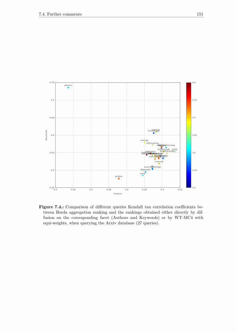
7.4. Further comments 151
0.2 0.25 0.3 0.35 0.4 0.45 0.5 0.550.45
0.5
0.55
0.6
0.65
0.7
0.75
3D
printer
hypergraph
graph
bosonhiggsparticle
snow
star
Laplacian
diffusion
nanotechnology
CNN
RNN
neuralnetwork
machinelearning
deeplearning
learningmachineinformationretrieval
information
datamining
entropy
adjacency
3Dprinter
physics
network
neural
Authors
Keywords
0.5
0.55
0.6
0.65
0.7
0.75
0.8
Figure 7.4.: Comparison of different queries Kendall tau correlation coefficients be-tween Borda aggregation ranking and the rankings obtained either directly by dif-fusion on the corresponding facet (Authors and Keywords) or by WT-MC4 withequi-weights, when querying the Arxiv database (27 queries).
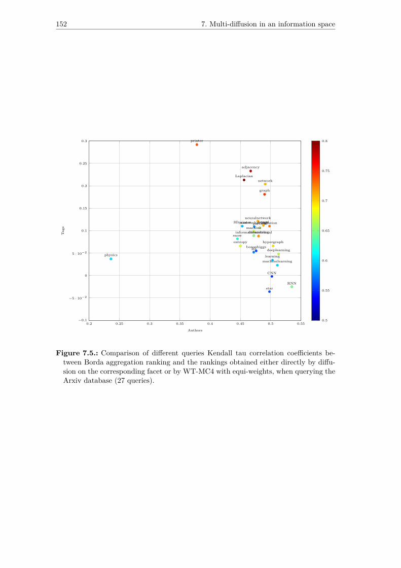
152 7. Multi-diffusion in an information space
0.2 0.25 0.3 0.35 0.4 0.45 0.5 0.55−0.1
−5 · 10−2
0
5 · 10−2
0.1
0.15
0.2
0.25
0.3
3D
printer
hypergraph
graph
bosonhiggs
particle
snow
star
Laplacian
diffusionnanotechnology
CNN
RNN
neuralnetwork
machinelearning
deeplearning
learning
machineinformationretrievaldatamining
entropy
adjacency
3Dprinter
physics
network
neural
Authors
Tags
0.5
0.55
0.6
0.65
0.7
0.75
0.8
Figure 7.5.: Comparison of different queries Kendall tau correlation coefficients be-tween Borda aggregation ranking and the rankings obtained either directly by diffu-sion on the corresponding facet or by WT-MC4 with equi-weights, when querying theArxiv database (27 queries).

7.4. Further comments 153
0.46 0.48 0.5 0.52 0.54 0.56 0.58 0.6 0.62 0.64 0.66 0.68 0.7 0.72 0.74−0.1
−5 · 10−2
0
5 · 10−2
0.1
0.15
0.2
0.25
0.3
3D
printer
hypergraph
graph
bosonhiggs
particle
snow
star
Laplacian
diffusionnanotechnology
CNN
RNN
neuralnetwork
machinelearning
deeplearning
learning
machineinformationretrievaldatamining
entropy
adjacency
3Dprinter
physics
network
neural
Keywords
Tags
0.5
0.55
0.6
0.65
0.7
0.75
0.8
Figure 7.6.: Comparison of different queries Kendall tau correlation coefficients be-tween Borda aggregation ranking and the rankings obtained either directly by diffu-sion on the corresponding facet or by WT-MC4 with equi-weights, when querying theArxiv database (27 queries).

154 7. Multi-diffusion in an information space
references. A third way could be to introduce a low weighted hyperedge that connectsall the vertices in one hyperedge, reflecting that the elements belong to the same search.The method we propose as any algorithm of this kind can be parallelized.

Conclusion
From a coarsening problem to visualize large hypergraphs in order to handle properlytheir layout, the quest to model the diffusion on such structures has led us to redefiningadjacency in hypergraphs. Modeling e-adjacency requires tensors. We have focused onpreserving the interpretability in terms of hypergraph uniformisation and polynomialhomogenization, which has led us to introduce hb-graphs, and particularly natural hb-graphs, to handle vertex redundancy.
Hb-graphs have proven to be effective to handle efficiently refined information in com-parison with hypergraphs and graphs. They have been an opportunity to introducean exchange-based diffusion that takes into account multiplicities of vertices and thatenables the ranking not only of vertices, but also of hb-edges.
Using natural hb-graphs, we proposed two additional e-adjacency tensors, and partic-ularly the straightforward one, which has some nice spectral properties. Nonetheless,using exchange-based diffusion, we have shown that the m-uniformisation processes in-volved have an influence on the diffusion over the structure itself. In this context, wehave evaluated the different proposed tensors presented in this Thesis as well as in theliterature.
Concluding by introducing a new Laplacian tensor for general hb-graphs, we have openedthe door to new theoretical developments to study tensor-based diffusion.
Concomitantly, hb-graphs fit for the modeling of co-occurrence networks. Their use inmulti-faceted information spaces leads us to propose a hb-graph framework, and theDataHbEdron, enabling full visual querying of a textual dataset.
Supporting redundancy, natural hb-graphs enable a dense space, that fills the space ofhypergraphs. They constitute a bridge between graph structures, multiset structuresand their set support, tensor approaches and polynomial views. A lot of their propertieshave still to be discovered or studied, such as the L-polynomial.
This research has lead us to explore different worlds, often precluded of difficult chal-lenges, but has been a charming journey. We hope to continue this exploration inforth-coming research: there are a lot of remaining open research questions that canappear as a research statement for future work. We gather here some of the researchquestions raised in this Thesis that require further investigations.
• On hb-graphs themselves: hb-graphs are a powerful structure to handle re-fined information on co-occurrences. We still have to investigate some of theirmathematical properties. This includes the following questions:
– Are general hb-graphs a separate category? We conjecture that this question has a positive answer, and that naturalhb-graphs are a sub-category.
156 7. Multi-diffusion in an information space
– What are extensions of hb-graphs to negative multiplicities? It could be very valuable to extend hb-graphs to negative multiplicities forhandling cases related to opinion mining.
– How to handle multi-variable multiplicities on hb-graphs? This could be a possibility to handle multiple features on a same hb-graphs,for instance multiplicity and weights, or in image processing.
– What is a coloring of a hb-graph? Hypergraph coloring has applications in divide and conquer approaches;hb-graph coloring, and particularly of natural hb-graphs could lead to refine-ments in this strategies.
– What kind of clustering algorithm to use with hb-graphs? Some work exists on structures that are not properly using hyperedge-based weighting of vertices and that are in practice similar to hb-graphs.These works have shown that taking into accounts multiplicities at the hb-edge level enhances clustering. Investigating further clustering on hb-graphscould lead to refined clustering algorithms that account for the higher orderrelationships.
• On multi-faceted information spaces and diffusion in facets: differentchallenges at every level exists: it includes an upstream work on the datasetsthemselves, on the way the data are fed into the information space, on the eval-uation of the visualization interface, as well on the extraction of the importantinformation from the networks themselves.
– What is the impact on the user to interact with multi-faceted visualisation ofan information space to solve tasks? A full evaluation including A/B testing is required to evaluate the Data-HbEdron compared to traditional verbatim interfaces for searching in aninformation space.
– How to improve the data feeding of the information space? The proposed framework is versatile enough to support various kind ofdata. The implementation of facets is done manually at the moment. Au-tomatic facet discovery could be one way of investigation to improve thefeeding of the information space. This subject encompasses also the problemof data linkage and the merging of heterogeneous sources, and automatic ex-ploration throughout the different datasets. All these problems are linked tothe FAIR-ability of data. FAIR—for Findable, Accessible, Interoperable andReusable— are principles that were edict in 2016 in [WDA+16] for improvinginfrastructures that supports the reuse of scholarly data.
– How to rank information in a disconnected hb-graph? How to rank an infor-mation space that is disconnected on some facets? Different strategies can be foreseen, one being to connect data with a dif-ferentiated link that would interconnect them by the fact they belong to thesame information space or are members of the same facet.
– How to enhance diffusion in other ways in the information space? Alternative strategies to the one taken for ranking aggregation can be

7.4. Further comments 157
foreseen based on diffusion. Some of them interconnect the different facetsvia links between them.
– Which sort of features to use as abstract information function? The influence of biases still have to be tested on the rank aggregation andon real datasets.
• On e-adjacency tensor and tensor-based diffusion: this aspect concernsadditional theoretical and experimental developments on the proposed e-adjacencytensor and layered Laplacian.– What is the disturbance on diffusion of the m-uniformisation process in sim-
ulated and real cases? Evaluating the real impact of m-uniformisation processes is still an openwork; it includes its testing on different real datasets, and finding measuresto evaluate it.
– How do we define the algebraic / analytic connectivity in hb-graphs? Whatare the links between the hb-graph layered Laplacian eigenvalues and the hb-graph features such as the algebraic / analytic connectivity? Algebraic connectivity in graphs corresponds to the second eigenvalue ofthe Laplacian matrix; extension to hypergraphs have been proposed for evenuniform hypergraphs as the second smallest Z-eigenvalue of the Laplacian in[HQ12]. To extend algebraic connectivity, [Qi14] uses the concept of ana-lytic connectivity for a uniform hypergraph via an optimization formulation.Extending this concept to hb-graphs may link to additional insights on theparticular structures, like it has been done for graphs with hypergraphs.
– How does the diffusion process based on this layered Laplacian evolve withtime? How can we use this layered Laplacian for clustering? Finding how the layered Laplacian helps to understand the underlying dif-fusion process is fundamental for having insights into the capture of higher or-der relationships. Coupled with the idea of the spectral clustering in graphs,the layered Laplacian could help clustering the hb-graph via spectral tech-niques.
– Can we evaluate the perturbation on the exchange-based diffusion from theL-polynomial before uniformisation? As the layered Laplacian is constructed using a polynomial homogeniza-tion, this homogenization corresponds to a m-uniformisation of the hb-graphand might have impacts on the diffusion process on the structure.
– What is a spectral analysis of hb-graphs? This is a vast topic, that could help to refine results in the particularstructures that are hypergraphs for hb-graphs, as hypergraphs already helpto refine graph spectral analysis. We already investigate some results in ourThesis on the built e-adjacency tensor for general hb-graphs.
• Further questions to be addressed that open up the subject, to different fieldsfrom visualisation, via ontologies and problems of data linkage and FAIR princi-ples:– How to enhance meaningful visualizations for heterogeneous datasets, mixing
textual and numerical values, while keeping the links?
158 7. Multi-diffusion in an information space
This is a key issue, as categorical data are often displayed as bar chartswhile textual data fit for hb-graph representation. Using our mechanismsin the hb-graph framework enhances new possibilities of visualisation andinteractivity, that still have to be investigated.
– How to give semantic to clusters in textual datasets? Finding the semantic of vertices gathered in communities is fundamentalin order to give insights on the visualization of very large hb-graphs, as theyneed to be presented using communities due to their complexity.
– In relation with the DataHbEdron, several sources of data can be used: howto ensure the coherence of what is going to be displayed? Behind, there is still the problem of interoperability and FAIR-ability ofthe data (even if it is not necessary scholar data); data cleansing and datalinking might be necessary to obtain sufficiently meaningful and coherentvisualizations.
It remains an open question on how diffusion over such structures should be handled, ifever possible. Diffusion is a clear concept on graphs. Generalizing this concept to (m-)uniform structures with the finite element approach in order to obtain the Laplacianremains valid thanks to the hb-edge / hyperedge uniformity. But it is still unclear ifthis concept can be generalized to non-uniform structures like general hypergraphs, anda posteriori to structures like general hb-graphs. A revision of the diffusion conceptto multi-diffusion—multi in the sense of multi-directed—is seen as a requirement forfurther developments.
Meyrin (Switzerland), March 2020, the 23rd.
Bibliography
[ABG06] Marianne Akian, Ravindra Bapat, and Stéphane Gaubert.Max-plus algebra. Handbook of linear algebra, 39, 2006,https://doi.org/10.1201/9781420010572.
[ACYL17] Le An, Xiaojing Chen, Songfan Yang, and Xuelong Li. Per-son re-identification by multi-hypergraph fusion. IEEE transactionson neural networks and learning systems, 28(11): 2763–2774, 2017,https://doi.org/10.1109/TNNLS.2016.2602082.
[ADLGP17] A. Agocs, D. Dardanis, J.-M. Le Goff, and D. Proios. Interac-tive graph query language for multidimensional data in CollaborationSpotting visual analytics framework. ArXiv e-prints, December 2017,https://arxiv.org/abs/1712.04202.
[AG08] Renzo Angles and Claudio Gutierrez. Survey of Graph DatabaseModels. ACM Comput. Surv., 40(1): 1:1–1:39, February 2008,http://doi.acm.org/10.1145/1322432.1322433.
[Alb91] Joseph Albert. Algebraic Properties of Bag Data Types.In VLDB, volume 91, pages 211–219. Citeseer, 1991,http://dl.acm.org/citation.cfm?id=645917.672310.
[BA16] Marina Blanton and Everaldo Aguiar. Private and oblivious set and mul-tiset operations. International Journal of Information Security, 15(5):493–518, October 2016, https://doi.org/10.1007/s10207-015-0301-1.
[BAD13] Abdelghani Bellaachia and Mohammed Al-Dhelaan. Random walks inhypergraph. In Proceedings of the 2013 International Conference onApplied Mathematics and Computational Methods, Venice Italy, pages187–194, 2013.
[BBCH03] Airat Bekmetjev, Graham Brightwell, Andrzej Czygrinow, and GlennHurlbert. Thresholds for families of multisets, with an application tograph pebbling. Discrete Mathematics, 269(1-3): 21–34, July 2003,https://doi.org/10.1016/S0012-365X(02)00745-8.
[BCM17] Anirban Banerjee, Arnab Char, and Bibhash Mondal. Spectra of generalhypergraphs. Linear Algebra and its Applications, 518: 14–30, April2017, https://doi.org/10.1016/j.laa.2016.12.022.
[BDE09] Alfred M. Bruckstein, David L. Donoho, and Michael Elad. FromSparse Solutions of Systems of Equations to Sparse Modeling of Sig-nals and Images. SIAM Review, 51(1): 34–81, February 2009,https://doi.org/10.1137/060657704.
[Ber67] Claude Berge. Graphes et hypergraphes. 1970. Dunod, Paris, 1967.

Bibliography
[Ber73] Claude Berge. Graphs and hypergraphs, volume 7. North-Holland pub-lishing company Amsterdam, 1973.
[BFR06] J.-P. Banâtre, P. Fradet, and Y. Radenac. Generalised multisets forchemical programming. Mathematical Structures in Computer Science,16(04): 557, August 2006, https://doi.org/10.1017/S0960129506005317.
[BFR07] Jean-Pierre Banâtre, Pascal Fradet, and Yann Radenac. Programmingself-organizing systems with the higher-order chemical language. IJUC,3(3): 161–177, 2007.
[BGLL08] Vincent D Blondel, Jean-Loup Guillaume, Renaud Lambiotte, and Eti-enne Lefebvre. Fast unfolding of communities in large networks. Journalof Statistical Mechanics: Theory and Experiment, 2008(10): P10008,October 2008, https://doi.org/10.1088/1742-5468/2008/10/P10008.
[Bli88] Wayne D. Blizard. Multiset theory. Notre Dame Jour-nal of Formal Logic, 30(1): 36–66, December 1988,https://doi.org/10.1305/ndjfl/1093634995.
[BLM93] Jean-Pierre Banâtre and Daniel Le Métayer. Programming by multisettransformation. Communications of the ACM, 36(1): 98–111, January1993, https://doi.org/10.1145/151233.151242.
[BMSW08] Ronald Brown, Ifor Morris, J Shrimpton, and Christopher D Wensley.Graphs of morphisms of graphs. the electronic journal of combinatorics,15(1): 1, 2008.
[BN03] Mikhail Belkin and Partha Niyogi. Laplacian Eigenmaps for Dimension-ality Reduction and Data Representation. Neural Computation, 15(6):1373–1396, June 2003, https://doi.org/10.1162/089976603321780317.
[Bre13] Alain Bretto. Hypergraph Theory. Mathematical Engineering. SpringerInternational Publishing, Heidelberg, 2013.
[BS17] Mojtaba Nouri Bygi and Ileana Streinu. Efficient pebble game algo-rithms engineered for protein rigidity applications. In 2017 IEEE 7thInternational Conference on Computational Advances in Bio and Med-ical Sciences (ICCABS), pages 1–6, Orlando, FL, October 2017. IEEE,https://doi.org/10.1109/ICCABS.2017.8114301.
[CAO+18] Nicholas Cummins, Shahin Amiriparian, Sandra Ottl, Maurice Ger-czuk, Maximilian Schmitt, and Bjorn Schuller. Multimodal Bag-of-Words for Cross Domains Sentiment Analysis. In 2018 IEEEInternational Conference on Acoustics, Speech and Signal Process-ing (ICASSP), pages 4954–4958, Calgary, AB, April 2018. IEEE,https://doi.org/10.1109/ICASSP.2018.8462660.
[CD12] Joshua Cooper and Aaron Dutle. Spectra of uniform hypergraphs.Linear Algebra and its Applications, 436(9): 3268–3292, May 2012,https://doi.org/10.1016/j.laa.2011.11.018.
[CDF+04] Gabriella Csurka, Christopher Dance, Lixin Fan, Jutta Willamowski,and Cédric Bray. Visual categorization with bags of keypoints. In Work-shop on statistical learning in computer vision, ECCV, volume 1, pages1–2. Prague, 2004.
Bibliography
[CF88] B. Chazelle and J. Friedman. A deterministic view of random samplingand its use in geometry. In [Proceedings 1988] 29th Annual Symposiumon Foundations of Computer Science, pages 539–549, White Plains, NY,USA, 1988. IEEE, https://doi.org/10.1109/SFCS.1988.21970.
[CGLM08] Pierre Comon, Gene Golub, Lek-Heng Lim, and Bernard Mourrain.Symmetric Tensors and Symmetric Tensor Rank. SIAM Journal onMatrix Analysis and Applications, 30(3): 1254–1279, January 2008,https://doi.org/10.1137/060661569.
[Chu93] F Chung. The Laplacian of a hypergraph. Expanding graphs (DIMACSseries), pages 21–36, 1993.
[CK97] S.Jeromy Carrière and Rick Kazman. WebQuery: searchingand visualizing the Web through connectivity. Computer Net-works and ISDN Systems, 29(8-13): 1257–1267, September 1997,https://doi.org/10.1016/S0169-7552(97)00062-7.
[CLTZ18] T.-H. Hubert Chan, Anand Louis, Zhihao Gavin Tang, and ChenziZhang. Spectral Properties of Hypergraph Laplacian and Approxi-mation Algorithms. Journal of the ACM, 65(3): 1–48, March 2018,https://doi.org/10.1145/3178123.
[Cod70] E. F. Codd. A relational model of data for large shared databanks. Communications of the ACM, 13(6): 377–387, June 1970,https://doi.org/10.1145/362384.362685.
[Cor04] Gilberto Corso. Families and clustering in a natural num-bers network. Physical Review E, 69(3): 036106, March 2004,https://doi.org/10.1103/PhysRevE.69.036106.
[Cou65] Philippe Courrege. Sur la forme intégro-différentielle des opérateurs de$C^ınfty_k$ dans $C$ satisfaisant au principe du maximum. SéminaireBrelot-Choquet-Deny. Théorie du Potentiel, 10(1): 1–38, 1965.
[CQU15] Pierre Comon, Yang Qi, and Konstantin Usevich. A Polynomial Formu-lation for Joint Decomposition of Symmetric Tensors of Different Orders.In Latent Variable Analysis and Signal Separation, volume 9237, pages22–30. Springer International Publishing, Cham, 2015.
[CR19] Uthsav Chitra and Benjamin J Raphael. RandomWalks on Hypergraphswith Edge-Dependent Vertex Weights. arXiv preprint arXiv:1905.08287,2019.
[CSdR13] Aleksandr Chuklin, Pavel Serdyukov, and Maarten de Rijke. Clickmodel-based information retrieval metrics. In Proceedings of the 36thinternational ACM SIGIR conference on Research and development ininformation retrieval - SIGIR ’13, page 493, Dublin, Ireland, 2013. ACMPress, https://doi.org/10.1145/2484028.2484071.
[CTTV15] Luca Cardelli, Mirco Tribastone, Max Tschaikowski, and Andrea Vandin.Forward and backward bisimulations for chemical reaction networks.arXiv preprint arXiv:1507.00163, 2015.

Bibliography
[CTWZ19] T.-H. Hubert Chan, Zhihao Gavin Tang, Xiaowei Wu, and ChenziZhang. Diffusion operator and spectral analysis for directed hypergraphLaplacian. Theoretical Computer Science, 784: 46–64, September 2019,https://doi.org/10.1016/j.tcs.2019.03.032.
[CW02] L. Chen and P. P. Wang. Fuzzy relation equations (I): the general andspecialized solving algorithms. Soft Computing - A Fusion of Founda-tions, Methodologies and Applications, 6(6): 428–435, September 2002,https://doi.org/10.1007/s00500-001-0157-3.
[dB81] Jean C de Borda. Mémoire sur les élections au scrutin. 1781.[DB13] Michael Donoser and Horst Bischof. Diffusion Processes for Retrieval
Revisited. In 2013 IEEE Conference on Computer Vision and PatternRecognition, pages 1320–1327, Portland, OR, USA, June 2013. IEEE,https://doi.org/10.1109/CVPR.2013.174.
[DB14] Aurélien Ducournau and Alain Bretto. Random walks in directedhypergraphs and application to semi-supervised image segmentation.Computer Vision and Image Understanding, 120: 91–102, March 2014,https://doi.org/10.1016/j.cviu.2013.10.012.
[DKNS01] Cynthia Dwork, Ravi Kumar, Moni Naor, and D. Sivakumar. Rank ag-gregation methods for the Web. In Proceedings of the tenth internationalconference on World Wide Web - WWW ’01, pages 613–622, Hong Kong,Hong Kong, 2001. ACM Press, https://doi.org/10.1145/371920.372165.
[DL18] Cangfeng Ding and Kan Li. Centrality Ranking via Topologically BiasedRandom Walks in Multiplex Networks. In 2018 International Joint Con-ference on Neural Networks (IJCNN), pages 1–8, Rio de Janeiro, July2018. IEEE, https://doi.org/10.1109/IJCNN.2018.8489403.
[DM11] Matthias Dehmer and Abbe Mowshowitz. A history of graph en-tropy measures. Information Sciences, 181(1): 57–78, January 2011,https://linkinghub.elsevier.com/retrieve/pii/S0020025510004147.
[DP99] Jiurgen DAËËOW and Gheorghe PaAUN. On the power of membranecomputing. Journal of Universal Computer Science, 5(2): 33–49, 1999.
[dP15] Élie de Panafieu. Phase transition of random non-uniform hyper-graphs. Journal of Discrete Algorithms, 31: 26–39, March 2015,https://doi.org/10.1016/j.jda.2015.01.009.
[DPN08] Thomas Deselaers, Lexi Pimenidis, and Hermann Ney. Bag-of-visual-words models for adult image classification and filter-ing. In 2008 19th International Conference on Pattern Recog-nition, pages 1–4, Tampa, FL, USA, December 2008. IEEE,http://ieeexplore.ieee.org/document/4761366/.
[DPP16] Megan Dewar, David Pike, and John Proos. Connectivity in Hyper-graphs. arXiv preprint arXiv:1611.07087, 2016.
[DRRD12] M. Dork, Nathalie Henry Riche, G. Ramos, and S. Dumais. PivotPaths:Strolling through Faceted Information Spaces. IEEE Transactions on Vi-sualization and Computer Graphics, 18(12): 2709–2718, December 2012,https://doi.org/10.1109/TVCG.2012.252.
Bibliography
[DW80] W. Dörfler and D. A. Waller. A category-theoretical approach to hy-pergraphs. Archiv der Mathematik, 34(1): 185–192, December 1980,https://doi.org/10.1007/BF01224952.
[DWL19] Cunxiang Duan, Ligong Wang, and Xihe Li. Some Properties ofthe Signless Laplacian and Normalized Laplacian Tensors of Gen-eral Hypergraphs. Taiwanese Journal of Mathematics, July 2019,https://doi.org/10.11650/tjm/190606.
[EG95] Thomas Eiter and Georg Gottlob. Identifying the MinimalTransversals of a Hypergraph and Related Problems. SIAMJournal on Computing, 24(6): 1278–1304, December 1995,https://doi.org/10.1137/S0097539793250299.
[ERV05] Ernesto Estrada and Juan A Rodriguez-Velazquez. Complex networksas hypergraphs. arXiv preprint physics/0505137, 2005.
[Fag83] Ronald Fagin. Degrees of acyclicity for hypergraphs and relationaldatabase schemes. Journal of the ACM, 30(3): 514–550, July 1983,https://doi.org/10.1145/2402.322390.
[FCS12] K M Frahm, A D Chepelianskii, and D L Shepelyansky. PageR-ank of integers. Journal of Physics A: Mathematical and Theo-retical, 45(40): 405101, October 2012, https://doi.org/10.1088/1751-8113/45/40/405101.
[FMU82] Ronald Fagin, Alberto O. Mendelzon, and Jeffrey D. Ullman. Asimplied universal relation assumption and its properties. ACMTransactions on Database Systems, 7(3): 343–360, September 1982,http://portal.acm.org/citation.cfm?doid=319732.319735.
[Fur86] G. W. Furnas. Generalized fisheye views, volume 17. April 1986.
[FW93] Mark I. Freidlin and Alexander D. Wentzell. Diffusion Processes onGraphs and the Averaging Principle. The Annals of Probability, 21(4):2215–2245, October 1993, https://doi.org/10.1214/aop/1176989018.
[FYZ+19] Yifan Feng, Haoxuan You, Zizhao Zhang, Rongrong Ji, and YueGao. Hypergraph Neural Networks. Proceedings of the AAAIConference on Artificial Intelligence, 33: 3558–3565, July 2019,https://doi.org/10.1609/aaai.v33i01.33013558.
[GD17] Debarghya Ghoshdastidar and Ambedkar Dukkipati. Uniform hyper-graph partitioning: Provable tensor methods and sampling techniques.Journal of Machine Learning Research, 18(50): 1–41, 2017.
[Geo17] Konstantinos Georgatos. Multi-agent Belief Revision Using Multisets.In Logic, Rationality, and Interaction, volume 10455, pages 466–479.Springer Berlin Heidelberg, Berlin, Heidelberg, 2017.
[GJ12] KP Girish and John Sunil Jacob. On multiset topologies. Theory andApplications of Mathematics & Computer Science, 2(1): 37–52, 2012.
[GLG+13] Samuel Gratzl, Alexander Lex, Nils Gehlenborg, Hanspeter Pfister, andMarc Streit. LineUp: Visual Analysis of Multi-Attribute Rankings. IEEE
Bibliography
Transactions on Visualization and Computer Graphics, 19(12): 2277–2286, December 2013, https://doi.org/10.1109/TVCG.2013.173.
[GMM+13] Ziyu Guan, Gengxin Miao, Russell McLoughlin, Xifeng Yan, and DengCai. Co-Occurrence-Based Diffusion for Expert Search on theWeb. IEEETransactions on Knowledge and Data Engineering, 25(5): 1001–1014,May 2013, https://doi.org/10.1109/TKDE.2012.49.
[Gun03] Jeremy Gunawardena. Chemical reaction network theory for in-silicobiologists. Notes available for download at http://vcp. med. harvard.edu/papers/crnt. pdf, 2003.
[GXTL10] Xinbo Gao, Bing Xiao, Dacheng Tao, and Xuelong Li. A survey ofgraph edit distance. Pattern Analysis and Applications, 13(1): 113–129,February 2010, https://doi.org/10.1007/s10044-008-0141-y.
[GZCN09] Gourab Ghoshal, Vinko Zlatić, Guido Caldarelli, and M. E. J. Newman.Random hypergraphs and their applications. Physical Review E, 79(6):066118, June 2009, https://doi.org/10.1103/PhysRevE.79.066118.
[Hal02] Eran Halperin. Improved Approximation Algorithms for theVertex Cover Problem in Graphs and Hypergraphs. SIAMJournal on Computing, 31(5): 1608–1623, January 2002,https://doi.org/10.1137/S0097539700381097.
[Har54] Zellig S. Harris. Distributional Structure. WORD, 10(2-3): 146–162,August 1954, https://doi.org/10.1080/00437956.1954.11659520.
[HF11] Cheng-Feng Hu and Shu-Cherng Fang. Set covering-based surrogate ap-proach for solving sup- $\mathcal{T}$ equation constrained optimiza-tion problems. Fuzzy Optimization and Decision Making, 10(2): 125–152,June 2011, https://doi.org/10.1007/s10700-011-9099-0.
[HQ12] Shenglong Hu and Liqun Qi. Algebraic connectivity of an even uniformhypergraph. Journal of Combinatorial Optimization, 24(4): 564–579,November 2012, http://link.springer.com/10.1007/s10878-011-9407-1.
[HQ15] Shenglong Hu and Liqun Qi. The Laplacian of a uniform hypergraph.Journal of Combinatorial Optimization, 29(2): 331–366, February 2015,https://doi.org/10.1007/s10878-013-9596-x.
[Hu13] Shenglong Hu. Spectral hypergraph theory. PhD Thesis, The Hong KongPolytechnic University, 2013.
[HYLW09] Qiang-Sheng Hua, Dongxiao Yu, Francis C. M. Lau, and Yuexuan Wang.Exact Algorithms for Set Multicover and Multiset Multicover Problems.In David Hutchison, Takeo Kanade, Josef Kittler, Jon M. Kleinberg,Friedemann Mattern, John C. Mitchell, Moni Naor, Oscar Nierstrasz,C. Pandu Rangan, Bernhard Steffen, Madhu Sudan, Demetri Terzopou-los, Doug Tygar, Moshe Y. Vardi, Gerhard Weikum, Yingfei Dong, Ding-Zhu Du, and Oscar Ibarra, editors, Algorithms and Computation, volume5878, pages 34–44. Springer Berlin Heidelberg, Berlin, Heidelberg, 2009.
[IT15] Ahmed Isah and Y. Tella. The Concept of Multiset Category. BritishJournal of Mathematics & Computer Science, 9(5): 427–437, January2015, https://doi.org/10.9734/bjmcs/2015/18415.
Bibliography
[JCCB13] Jian Zhao, Christopher Collins, Fanny Chevalier, and Ravin Bal-akrishnan. Interactive Exploration of Implicit and Explicit Re-lations in Faceted Datasets. IEEE Transactions on Visualiza-tion and Computer Graphics, 19(12): 2080–2089, December 2013,https://doi.org/10.1109/TVCG.2013.167.
[JVHB14] Mathieu Jacomy, Tommaso Venturini, Sebastien Heymann,and Mathieu Bastian. ForceAtlas2, a Continuous Graph Lay-out Algorithm for Handy Network Visualization Designed forthe Gephi Software. PLoS ONE, 9(6): e98679, June 2014,https://dx.plos.org/10.1371/journal.pone.0098679.
[KAF+08] Daniel Keim, Gennady Andrienko, Jean-Daniel Fekete, Carsten Görg,Jörn Kohlhammer, and Guy Melançon. Visual Analytics: Definition,Process, and Challenges. In Andreas Kerren, John T. Stasko, Jean-Daniel Fekete, and Chris North, editors, Information Visualization, vol-ume 4950, pages 154–175. Springer Berlin Heidelberg, Berlin, Heidelberg,2008.
[Kar72] Richard M. Karp. Reducibility among Combinatorial Problems. InRaymond E. Miller, James W. Thatcher, and Jean D. Bohlinger, ed-itors, Complexity of Computer Computations, pages 85–103. SpringerUS, Boston, MA, 1972.
[Kat13] Tosio Kato. Perturbation theory for linear operators, volume 132.Springer Science & Business Media, 2013.
[Kem59] John G Kemeny. Mathematics without numbers. Daedalus, 88(4): 577–591, 1959.
[Ken38] M. G. Kendall. A new measure of rank correlation. Biometrika, 30(1-2):81–93, June 1938, https://doi.org/10.1093/biomet/30.1-2.81.
[Ken48] Maurice George Kendall. Rank correlation methods. 1948.[KKC17] Han Kyul Kim, Hyunjoong Kim, and Sungzoon Cho. Bag-of-concepts:
Comprehending document representation through clustering words indistributed representation. Neurocomputing, 266: 336–352, November2017, https://doi.org/10.1016/j.neucom.2017.05.046.
[KL02] Risi Imre Kondor and John Lafferty. Diffusion kernels on graphs andother discrete input spaces. In ICML, volume 2, pages 315–322, 2002.
[Knu68] Donald Knuth. The art of computer programming 1: Fundamental algo-rithms 2: Seminumerical algorithms 3: Sorting and searching 4: Generat-ing all trees. History of Combinatorial Generation. MA: Addison-Wesley,30, 1968.
[KPP+19] Bogumił Kamiński, Valérie Poulin, Paweł Prałat, PrzemysławSzufel, and François Théberge. Clustering via hypergraphmodularity. PLOS ONE, 14(11): e0224307, November 2019,https://doi.org/10.1371/journal.pone.0224307.
[LAYK+18] Shuai Li, Yasin Abbasi-Yadkori, Branislav Kveton, S Muthukrishnan,Vishwa Vinay, and ZhengWen. Offline evaluation of ranking policies with
Bibliography
click models. In Proceedings of the 24th ACM SIGKDD InternationalConference on Knowledge Discovery & Data Mining, pages 1685–1694.ACM, 2018.
[LCL11] Jungmin Lee, Minsu Cho, and Kyoung Mu Lee. Hyper-graph matchingvia reweighted random walks. In Computer Vision and Pattern Recogni-tion (CVPR), 2011 IEEE Conference on, pages 1633–1640. IEEE, 2011.
[Lee13] John M Lee. Smooth manifolds. In Introduction to Smooth Manifolds,pages 1–31. Springer, 2013.
[Lim13] Lek-Heng Lim. Tensors and hypermatrices. Handbook of Linear Algebra,2nd Ed., CRC Press, Boca Raton, FL, pages 231–260, 2013.
[Lin10] Shili Lin. Rank aggregation methods. Wiley Interdisciplinary Reviews:Computational Statistics, 2(5): 555–570, 2010.
[LL05] John Lafferty and Guy Lebanon. Diffusion kernels on statistical mani-folds. Journal of Machine Learning Research, 6(Jan): 129–163, 2005.
[LMB+14] Tsung-Yi Lin, Michael Maire, Serge Belongie, James Hays, Pietro Per-ona, Deva Ramanan, Piotr Dollár, and C Lawrence Zitnick. Microsoftcoco: Common objects in context. In European conference on computervision, pages 740–755, 2014. tex.organization: Springer.
[Lo93] László Lovász and others. Random walks on graphs: A survey. Combi-natorics, Paul Erdos is eighty, 2(1): 1–46, 1993.
[Loe92] Daniel Loeb. Sets with a negative number of elements. Advances inMathematics, 91(1): 64–74, 1992.
[LP11] Linyuan Lu and Xing Peng. High-Ordered Random Walks and Gen-eralized Laplacians on Hypergraphs. In WAW, pages 14–25. Springer,2011.
[LQY13] Guoyin Li, Liqun Qi, and Gaohang Yu. The Z-eigenvalues of a symmetrictensor and its application to spectral hypergraph theory. NumericalLinear Algebra with Applications, 20(6): 1001–1029, 2013.
[LSP16] Matthew R Lakin, Darko Stefanovic, and Andrew Phillips. Modular ver-ification of chemical reaction network encodings via serializability anal-ysis. Theoretical computer science, 632: 21–42, 2016.
[Maj87] Zofia Majcher. Alternating cycles and realizations of a degree sequence.Commentationes Mathematicae Universitatis Carolinae, 28(3): 467–480,1987.
[Mäk90] Erkki Mäkinen. How to draw a hypergraph. InternationalJournal of Computer Mathematics, 34(3-4): 177–185, 1990,https://doi.org/10.1080/00207169008803875.
[Mar05] AV Markovskii. On the relation between equations with max-productcomposition and the covering problem. Fuzzy Sets and Systems, 153(2):261–273, 2005.
[MEP+14] Robert Campbell McColl, David Ediger, Jason Poovey, Dan Camp-bell, and David A. Bader. A Performance Evaluation of Open
Bibliography
Source Graph Databases. PPAA ’14, pages 11–18. ACM, 2014,https://doi.org/10.1145/2567634.2567638. event-place: Orlando,Florida, USA.
[Mer95] Russell Merris. A survey of graph Laplacians. Linear and MultilinearAlgebra, 39(1-2): 19–31, 1995.
[MHVG15] Hammurabi Mendes, Maurice Herlihy, Nitin Vaidya, and Vijay K Garg.Multidimensional agreement in Byzantine systems. Distributed Comput-ing, 28(6): 423–441, 2015.
[MKL11] Hao Ma, Irwin King, and Michael R Lyu. Mining web graphs for recom-mendations. IEEE Transactions on Knowledge and Data Engineering,24(6): 1051–1064, 2011.
[MN12] Tom Michoel and Bruno Nachtergaele. Alignment and inte-gration of complex networks by hypergraph-based spectral clus-tering. Physical Review E, 86(5): 056111, November 2012,https://doi.org/10.1103/PhysRevE.86.056111.
[MPL17] Naoki Masuda, Mason A Porter, and Renaud Lambiotte. Random walksand diffusion on networks. Physics Rep., 2017.
[MSCM16] Venkatesh N. Murthy, Avinash Sharma, Visesh Chari, and R. Manmatha.Image Annotation using Multi-scale Hypergraph Heat Diffusion Frame-work. In Proceedings of the 2016 ACM on International Conference onMultimedia Retrieval - ICMR ’16, pages 299–303, New York, New York,USA, 2016. ACM Press, https://doi.org/10.1145/2911996.2912055.
[MSWL18] Shuming Ma, Xu Sun, Yizhong Wang, and Junyang Lin. Bag-of-words astarget for neural machine translation. arXiv preprint arXiv:1805.04871,2018.
[MWW+17] Shervin Minaee, Siyun Wang, Yao Wang, Sohae Chung, Xiuyuan Wang,Els Fieremans, Steven Flanagan, Joseph Rath, and Yvonne W. Lui. Iden-tifying mild traumatic brain injury patients from MR images using bagof visual words. In 2017 IEEE Signal Processing in Medicine and Biol-ogy Symposium (SPMB), pages 1–5, Philadelphia, PA, December 2017.IEEE, https://doi.org/10.1109/SPMB.2017.8257054.
[MYLK08] Hao Ma, Haixuan Yang, Michael R Lyu, and Irwin King. Mining socialnetworks using heat diffusion processes for marketing candidates selec-tion. In Proceedings of the 17th ACM conference on Information andknowledge management, pages 233–242. ACM, 2008.
[New01a] M. E. J. Newman. Scientific collaboration networks. I. Network con-struction and fundamental results. Physical Review E, 64(1): 016131,June 2001, https://doi.org/10.1103/PhysRevE.64.016131.
[New01b] M. E. J. Newman. Scientific collaboration networks. II. Shortest paths,weighted networks, and centrality. Physical Review E, 64(1): 016132,June 2001, https://link.aps.org/doi/10.1103/PhysRevE.64.016132.
[Nik00] Mila Nikolova. Local Strong Homogeneity of a Regularized Estimator.SIAM Journal on Applied Mathematics, 61(2): 633–658, January 2000,https://doi.org/10.1137/S0036139997327794.
Bibliography
[NJY+10] Nan Cao, Jimeng Sun, Yu-Ru Lin, D Gotz, Shixia Liu, and Huamin Qu.FacetAtlas: Multifaceted Visualization for Rich Text Corpora. IEEETransactions on Visualization and Computer Graphics, 16(6): 1172–1181, November 2010, https://doi.org/10.1109/TVCG.2010.154.
[No85] Jean Antoine Nicolas and others. Essai sur l’application de l’analyseà la probabilité des décisions rendues à la pluralité des voix. Par M. lemarquis de Condorcet.... de l’Imprimerie Royale, 1785.
[OGMM20] Xavier Ouvrard, Jean-Marie Le Goff, and Stéphane Marchand-Maillet.Tuning ranking in co-occurrence networks with general biased exchange-based diffusion on hyper-bag-graphs. 2020. arXiv: 2003.07323 [cs.SI].
[OLGMM17a] Xavier Ouvrard, Jean-Marie Le Goff, and Stéphane Marchand-Maillet.Adjacency and Tensor Representation in General Hypergraphs Part 1:e-adjacency Tensor Uniformisation Using Homogeneous Polynomials.arXiv preprint arXiv:1712.08189, 2017.
[OLGMM17b] Xavier Ouvrard, Jean-Marie Le Goff, and Stéphane Marchand-Maillet.Networks of Collaborations: Hypergraph Modeling and Visualisation.arXiv preprint arXiv:1707.00115, 2017.
[OLGMM18a] Xavier Ouvrard, Jean-Marie Le Goff, and S. Marchand-Maillet. On Ad-jacency and e-Adjacency in General Hypergraphs: Towards a New e-Adjacency Tensor. Electronic Notes in Discrete Mathematics, 70: 71–76,December 2018, https://doi.org/10.1016/j.endm.2018.11.012.
[OLGMM18b] Xavier Ouvrard, Jean-Marie Le Goff, and Stéphane Marchand-Maillet.Adjacency and Tensor Representation in General Hypergraphs. Part 2:Multisets, Hb-graphs and Related e-adjacency Tensors. arXiv preprintarXiv:1805.11952, 2018.
[OLGMM18c] Xavier Ouvrard, Jean-Marie Le Goff, and Stéphane Marchand-Maillet. Diffusion by Exchanges in HB-Graphs: High-lighting Complex Relationships. CBMI Proceedings, 2018,https://doi.org/10.1109/CBMI.2018.8516525.
[OLGMM18d] Xavier Ouvrard, Jean-Marie Le Goff, and Stéphane Marchand-Maillet.Hypergraph Modeling and Visualisation of Complex Co-occurence Net-works. Electronic Notes in Discrete Mathematics, 70: 65–70, December2018, https://doi.org/10.1016/j.endm.2018.11.011.
[OLGMM19a] Xavier Ouvrard, Jean-Marie Le Goff, and Stéphane Marchand-Maillet.Diffusion by Exchanges in HB-Graphs: Highlighting Complex Relation-ships Extended version. Arxiv:1809.00190v2, 2019.
[OLGMM19b] Xavier Ouvrard, Jean-Marie Le Goff, and Stéphane Marchand-Maillet.The HyperBagGraph DataEdron: An Enriched Browsing Experience ofMultimedia Datasets. arXiv preprint arXiv:1905.11695, 2019.
[OLGMM19c] Xavier Ouvrard, Jean-Marie Le Goff, and Stéphane Marchand-Maillet.On Hb-graphs and their Application to General Hypergraph e-adjacencyTensor. MCCCC32 Special Volume of the Journal of CombinatorialMathematics and Combinatorial Computing, to be published, 2019.

Bibliography
[OLGMM20] Xavier Ouvrard, Jean-Marie Le Goff, and Stéphane Marchand-Maillet.The HyperBagGraph DataEdron: An Enriched Browsing Experience ofDatasets. LNCS, 46th International Conference on Current Trends inTheory and Practice of Computer Science (SOFSEM 2020), 2020.
[Ouv20] Xavier Ouvrard. Hypergraphs: an introduction and review. arXivpreprint arXiv:2002.05014, 2020.
[Pău11] Gheorghe Păun. Membrane Computing, volume 6501 of Lecture Notes inComputer Science. Springer Berlin Heidelberg, Berlin, Heidelberg, 2011.Citation Key Alias: paun2012membrane.
[PBMW99] Lawrence Page, Sergey Brin, Rajeev Motwani, and Terry Winograd. Thepagerank citation ranking: Bringing order to the web. Technical report,Stanford InfoLab, 1999.
[PK08] Ruzica Piskac and Viktor Kuncak. Decision Procedures for Multisetswith Cardinality Constraints. In Verification, Model Checking, and Ab-stract Interpretation, volume 4905, pages 218–232. Springer Berlin Hei-delberg, Berlin, Heidelberg, 2008.
[Po00] Phillip Poplin and others. The Semiring of Multisets. 2000.[PS15] Lynnette Purda and David Skillicorn. Accounting Variables, Decep-
tion, and a Bag of Words: Assessing the Tools of Fraud Detection.Contemporary Accounting Research, 32(3): 1193–1223, September 2015,https://doi.org/10.1111/1911-3846.12089.
[PSS05] S.U. Pillai, T. Suel, and Seunghun Cha. The Perron-Frobenius theorem:some of its applications. IEEE Signal Processing Magazine, 22(2): 62–75,March 2005, https://doi.org/10.1109/MSP.2005.1406483.
[Pu13] Li Pu. Relational Learning with Hypergraphs. 2013.[PVAdST19] Daniel Carlos Guimaraes Pedronette, Lucas Pascotti Valem, Jurandy
Almeida, and Ricardo da S. Torres. Multimedia Retrieval ThroughUnsupervised Hypergraph-Based Manifold Ranking. IEEE Trans-actions on Image Processing, 28(12): 5824–5838, December 2019,https://doi.org/10.1109/TIP.2019.2920526.
[PWWQ16] Xiaojiang Peng, Limin Wang, Xingxing Wang, and Yu Qiao.Bag of visual words and fusion methods for action recogni-tion: Comprehensive study and good practice. Computer Vi-sion and Image Understanding, 150: 109–125, September 2016,https://doi.org/10.1016/j.cviu.2016.03.013.
[PZ14] Kelly J. Pearson and Tan Zhang. On Spectral Hypergraph Theory ofthe Adjacency Tensor. Graphs and Combinatorics, 30(5): 1233–1248,September 2014, https://doi.org/10.1007/s00373-013-1340-x.
[PZ15] Kelly J. Pearson and Tan Zhang. The Laplacian tensor of a multi-hypergraph. Discrete Mathematics, 338(6): 972–982, June 2015,https://doi.org/10.1016/j.disc.2015.01.021.
[Qi14] Liqun Qi. $H^+$-eigenvalues of Laplacian and signless Laplacian ten-sors. Communications in Mathematical Sciences, 12(6): 1045–1064,2014, https://doi.org/10.4310/CMS.2014.v12.n6.a3.
Bibliography
[QL17] Liqun Qi and Ziyan Luo. Tensor Analysis: Spectral Theory and SpecialTensors. Society for Industrial and Applied Mathematics, Philadelphia,PA, April 2017.
[Rad15] Aurelian Radoaca. Simple Venn Diagrams for Multisets. In Symbolicand Numeric Algorithms for Scientific Computing (SYNASC), 2015 17thInternational Symposium on, pages 181–184. IEEE, 2015.
[Ran45] Shiyali Ramamrita Ranganathan. Elements of library classification:based on lectures delivered at the University of Bombay in December 1944.NK Publishing House, Poona, 1945.
[Ran62] Shiyali Ramamrita Ranganathan. Elements of library classification.1962.
[RKS17] MR Gauthama Raman, Kannan Kirthivasan, and VS Shankar Sriram.Development of rough set–hypergraph technique for key feature identifi-cation in intrusion detection systems. Computers & Electrical Engineer-ing, 59: 189–200, 2017.
[Rod03] J.A. Rodríguez. On the Laplacian Spectrum and Walk-regular Hyper-graphs. Linear and Multilinear Algebra, 51(3): 285–297, September 2003,https://doi.org/10.1080/0308108031000084374.
[RV93] Sridhar Rajagopalan and Vijay V Vazirani. Primal-dual RNC approxi-mation algorithms for (multi)-set (multi)-cover and covering integer pro-grams. In Proceedings of 1993 IEEE 34th Annual Foundations of Com-puter Science, pages 322–331. IEEE, 1993.
[Sha13] Jia-Yu Shao. A general product of tensors with applications. Lin-ear Algebra and its Applications, 439(8): 2350–2366, October 2013,https://doi.org/10.1016/j.laa.2013.07.010.
[SIYS07] D Singh, A Ibrahim, T Yohanna, and J Singh. An overview of theapplications of multisets. Novi Sad Journal of Mathematics, 37(3): 73–92, 2007.
[SJ12] Ravi Shekhar and C.V. Jawahar. Word Image Retrieval Using Bag ofVisual Words. In 2012 10th IAPR International Workshop on Docu-ment Analysis Systems, pages 297–301, Gold Coast, Queenslands, TBD,Australia, March 2012. IEEE, https://doi.org/10.1109/DAS.2012.96.
[SJP+16] Maximilian Schmitt, Christoph Janott, Vedhas Pandit, Kun Qian,Clemens Heiser, Werner Hemmert, and Björn Schuller. A bag-of-audio-words approach for snore sounds’ excitation localisation. In Speech Com-munication; 12. ITG Symposium, pages 1–5. VDE, 2016.
[SK12] Barna Saha and Samir Khuller. Set Cover Revisited: Hypergraph Coverwith Hard Capacities. In Automata, Languages, and Programming, vol-ume 7391, pages 762–773. Springer Berlin Heidelberg, Berlin, Heidelberg,2012.
[Spe87] C. Spearman. The Proof and Measurement of Association between TwoThings. The American Journal of Psychology, 100(3/4): 441, 1987,https://doi.org/10.2307/1422689.

Bibliography
[SPS85] Jeanette Schmidt-Pruzan and Eli Shamir. Component structure in theevolution of random hypergraphs. Combinatorica, 5(1): 81–94, March1985, https://doi.org/10.1007/BF02579445.
[ST09] Ileana Streinu and Louis Theran. Sparse hypergraphs and pebble gamealgorithms. European Journal of Combinatorics, 30(8): 1944–1964,November 2009, https://doi.org/10.1016/j.ejc.2008.12.018.
[Ste12] John G. Stell. Relations on Hypergraphs. In Relational and AlgebraicMethods in Computer Science, volume 7560, pages 326–341. SpringerBerlin Heidelberg, Berlin, Heidelberg, 2012.
[SVK16] Elias C. Stavropoulos, Vassilios S. Verykios, and Vasileios Kagklis. Atransversal hypergraph approach for the frequent itemset hiding prob-lem. Knowledge and Information Systems, 47(3): 625–645, June 2016,https://doi.org/10.1007/s10115-015-0862-3.
[SWG+18] Fernanda B. Silva, Rafael de O. Werneck, Siome Goldenstein, Salva-tore Tabbone, and Ricardo da S. Torres. Graph-based bag-of-wordsfor classification. Pattern Recognition, 74: 266–285, February 2018,https://doi.org/10.1016/j.patcog.2017.09.018.
[Syr01] Apostolos Syropoulos. Mathematics of Multisets. In Multiset Processing,volume 2235, pages 347–358. Springer Berlin Heidelberg, Berlin, Heidel-berg, 2001.
[Syr03] Apostolos Syropoulos. Categorical models of multisets. Romanian Jour-nal of Information Science and Technology, 6(3-4): 393–400, 2003.
[SZ03] Sivic and Zisserman. Video Google: a text retrieval approach to objectmatching in videos. In Proceedings Ninth IEEE International Conferenceon Computer Vision, pages 1470–1477 vol.2, Nice, France, 2003. IEEE,https://doi.org/10.1109/ICCV.2003.1238663.
[SZ09] Frans Schalekamp and Anke van Zuylen. Rank Aggregation: TogetherWe’re Strong. In 2009 Proceedings of the Eleventh Workshop on Algo-rithm Engineering and Experiments (ALENEX), pages 38–51. Society forIndustrial and Applied Mathematics, Philadelphia, PA, January 2009.
[SZB19] Lizhu Sun, Jiang Zhou, and Changjiang Bu. Spectral properties of gen-eral hypergraphs. Linear Algebra and its Applications, 561: 187–203,January 2019, https://doi.org/10.1016/j.laa.2018.09.029.
[Tar14] Paul Tarau. Towards a generic view of primality through multiset de-compositions of natural numbers. Theoretical Computer Science, 537:105–124, June 2014, https://doi.org/10.1016/j.tcs.2014.04.025.
[TCR10] Carla Taramasco, Jean-Philippe Cointet, and Camille Roth. Academicteam formation as evolving hypergraphs. Scientometrics, 85(3): 721–740, December 2010, https://doi.org/10.1007/s11192-010-0226-4.
[TDKF17] Dorina Thanou, Xiaowen Dong, Daniel Kressner, and Pascal Frossard.Learning Heat Diffusion Graphs. IEEE Transactions on Signal and In-formation Processing over Networks, 3(3): 484–499, September 2017,https://doi.org/10.1109/TSIPN.2017.2731164.

Bibliography
[TN11] Hung-Khoon Tan and Chong-Wah Ngo. Fusing heterogeneousmodalities for video and image re-ranking. In Proceedings ofthe 1st ACM International Conference on Multimedia Retrieval- ICMR ’11, pages 1–8, Trento, Italy, 2011. ACM Press,https://doi.org/10.1145/1991996.1992011.
[To98] Michel Truchon and others. An extension of the Condorcet criterion andKemeny orders. Citeseer, 1998.
[Tsa12] Chih-Fong Tsai. Bag-of-Words Representation in Image Annota-tion: A Review. ISRN Artificial Intelligence, 2012: 1–19, 2012,https://doi.org/10.5402/2012/376804.
[vHP09] F. van Ham and A. Perer. “Search, Show Context, Expand on Demand”:Supporting Large Graph Exploration with Degree-of-Interest. IEEETransactions on Visualization and Computer Graphics, 15(6): 953–960,November 2009, https://doi.org/10.1109/TVCG.2009.108.
[Vol09] Vitaly I Voloshin. Introduction to graph and hypergraph theory. NovaScience Publ., 2009.
[WDA+16] Mark D Wilkinson, Michel Dumontier, IJsbrand Jan Aalbersberg,Gabrielle Appleton, Myles Axton, Arie Baak, Niklas Blomberg, Jan-Willem Boiten, Luiz Bonino da Silva Santos, Philip E Bourne, and oth-ers. The FAIR Guiding Principles for scientific data management andstewardship. Scientific data, 3, 2016.
[WZS16] Leiquan Wang, Zhicheng Zhao, and Fei Su. Efficient multi-modalhypergraph learning for social image classification with complex la-bel correlations. Neurocomputing, 171: 242–251, January 2016,https://doi.org/10.1016/j.neucom.2015.06.064.
[XDYF16] Zihang Xu, Junping Du, Lingfei Ye, and Dan Fan. Multi-featureindexing for image retrieval based on hypergraph. In 2016 4thInternational Conference on Cloud Computing and Intelligence Sys-tems (CCIS), pages 494–500, Beijing, China, August 2016. IEEE,https://doi.org/10.1109/CCIS.2016.7790309.
[XHLJ18] Keyulu Xu, Weihua Hu, Jure Leskovec, and Stefanie Jegelka. How pow-erful are graph neural networks? arXiv preprint arXiv:1810.00826, 2018.
[Yag86] Ronald R. Yager. ON THE THEORY OF BAGS. Interna-tional Journal of General Systems, 13(1): 23–37, November 1986,https://doi.org/10.1080/03081078608934952.
[YL78] H. P. Young and A. Levenglick. A Consistent Extension of Condorcet’sElection Principle. SIAM Journal on Applied Mathematics, 35(2): 285–300, September 1978, http://epubs.siam.org/doi/10.1137/0135023.
[ZGC10] Vinko Zlatić, Andrea Gabrielli, and Guido Caldarelli. Topo-logically biased random walk and community finding in net-works. Physical Review E, 82(6): 066109, December 2010,https://doi.org/10.1103/PhysRevE.82.066109.

Bibliography
[ZHS07] Denny Zhou, Jiayuan Huang, and Bernhard Schölkopf. Learning withhypergraphs: Clustering, classification, and embedding. In Advances inneural information processing systems, pages 1601–1608, 2007.
[ZSC99] J.Y. Zien, M.D.F. Schlag, and P.K. Chan. Multilevel spectral hyper-graph partitioning with arbitrary vertex sizes. IEEE Transactions onComputer-Aided Design of Integrated Circuits and Systems, 18(9): 1389–1399, September 1999, https://doi.org/10.1109/43.784130.
[ZTH14] Li-Jun Zhao, Ping Tang, and Lian-Zhi Huo. Land-Use Scene Classifi-cation Using a Concentric Circle-Structured Multiscale Bag-of-Visual-Words Model. IEEE Journal of Selected Topics in Applied Earth Ob-servations and Remote Sensing, 7(12): 4620–4631, December 2014,https://doi.org/10.1109/JSTARS.2014.2339842.
[ZWHC06] Tao Zhou, Bing-Hong Wang, P.M. Hui, and K.P. Chan. Topo-logical properties of integer networks. Physica A: Statisti-cal Mechanics and its Applications, 367: 613–618, July 2006,https://linkinghub.elsevier.com/retrieve/pii/S0378437105011969.

Index
2-adjacent, 1892-section of a hypergraph, 189
Aabstract information function, 214adjacency matrix
unweighted hypergraph, 190weighted hypergraph, 191
adjacentvertexhypergraph, 228
almost cycle, 15anti-rank
hypergraph, 189associated graph, 205
Bbag, 196Banerjee e-adjacency hypermatrix
hypergraph, 231
Ccanonical hypermatrix representation, 204canonical weighted hb-graph, 61canonical weighting operation, 61cardinality of a multiset, 197c-dilatation
operation, 61c-dilated
hb-graph, 61CHR, 204component
hb-graphconnected, 16
hypergraphconnected, 189
connected component, 16, 189connected hb-graph, 16connected hypergraph, 189contravariant tensor, 204
copies, 198copy-set, 198co-rank
hb-graph, 13correlation coefficient
disagreement on matching, 140Kendall tau ranklarge, 140strict, 140
matching, 140scaled Spearman footrule, 141
covariant tensor, 203co-vector
tensor product, 203cycle
hb-graph, 15almost, 15
DDataHbEdron, 128decomposition
hypergraph, 233decomposition operation, 63definition domain, 102degree
hb-graphvertex, 13
vertexhypergraph, 189
diameterhb-graph, 16
diffusion operator, 102maximum principle, 102
direct sumhb-graph, 17hypergraph, 190
directedhypergraph, 190
directed graph
175
Index
strongly connected, 205distance
hb-graph, 16dual
hb-graph, 13hypergraph, 188vector space, 202basis, 202
Ee-adjacency hypermatrix
hb-graphlayered, 74silo, 70straightforward, 68
hypergraphBanerjee, 231Sun, 232
e-adjacentvertexhb-graph, 17hypergraph, 229
e?-adjacent, 17edge standard
hb-graph, 18hypergraph, 191
E-eigenvalue, 208E-eigenvector, 208eigenpair, 206eigenvalue, 206eigenvalues normalized adjacency tensor
hypergraph, 231eigenvector, 206elementary hb-graph, 57empty
hb-graph, 12empty multiset, 197essentially non-negative tensor, 207extended schema hypergraph, 119extracted extended schema hypergraph,
119extra-node representation
hb-graph, 19extremity, 15
Ggenerator, 196global m-cardinality, 13
graph, 189Laplacian, 104
ground, 196
Hhb-edge, 11
no repeated, 12hb-graph, 11
almost cycle, 15connected, 16connected component, 16co-rank, 13cycle, 15diameter, 16direct sum, 17dual, 13e-adjacent, 17e?-adjacent, 17elementary, 57empty, 12global m-cardinality, 13hb-edge, 11hb-graph distance, 16hb-star, 13homomorphism, 210hypergraph, 12hypermatrixe-adjacencylayered, 74silo, 70straight-forward, 68
incidence matrix, 20incident, 17isolated vertices, 12k-adjacency, 16k-adjacency hypermatrix, 60k-m-regular, 13k-m-uniform, 13k-uniform, 13maximum multiplicity function, 14m-co-rank, 12m-path, 15extremity, 15interior vertex, 15large, 15length, 15strict, 15support path, 16
m-rank, 12m-regular, 13
Index
m-uniform, 13m-uniformisationlayered, 65process, 64silo, 65straightforward, 64
natural, 12no repeated hb-edge, 12numbered-copy-hypergraph, 14operationcanonical weighting, 61c-dilatation, 61decomposition, 63e-adjacency preservation, 63exact e-adjacency preservation, 63merging, 63yα-vertex increasing, 62y-complemented, 62
order, 12polynomial, 60polynomial homogenizationprocess, 64
rank, 12regular, 13relative multiplicity, 19normalised, 20
representation, 18edge standard, 18extra-node, 19subset standard, 18
size, 12sum, 17support hypergraph, 12trivial, 12uniform, 13universe, 11vertex, 11degree, 13k-adjacent, 16maximal degree, 13maximal m-degree, 13m-degree, 13
hb-star, 13H-eigenvalue, 207H-eigenvector, 207Hm-UP, 64homomorphism
hb-graph, 210
hyper-bag-graph, 11hyper-degree
vertexhypergraph, 189
hyperedgehypergraph, 187no repeated, 188repeated, 187
hypergraph, 1872-section, 189adjacency matrix, 190adjacency matrix of a weighted, 191anti-rank, 189Banerjee e-adjacency hypermatrix,
231connected, 189connected component, 189decomposition, 233direct sum, 190directed, 190dual, 188eigenvalues normalized adjacency ten-
sor, 231hb-graphnumbered-copy-hypergraph, 14
hb-graph(as), 12hyperedge, 187hypergraph distance, 189incidence matrix, 190intersection graph, 190k-adjacency, 229k-uniform, 190Laplacian matrix, 104Laplacian tensor, 106linear, 188multi-hypergraph, 188no repeated hyperedge, 188normalized adjacency tensor, 230normalized Laplacian tensor, 231order, 188partial hypergraph, 188path, 189length, 189
rank, 188repeated hyperedges, 187representationedge standard, 191subset standard, 191
Index
simple, 188sub-hypergraph, 188sum, 190Sun e-adjacency hypermatrix, 232support of hb-graph, 12unnormalized adjacency tensor, 230vertex, 187degree, 189hyper-degree, 189k-adjacent, 228neighborhood, 188star, 188
weighted, 188hypergraph distance
hypergraph, 189hypermatrix
associated graph, 205canonical representation, 204E-eigenvalue, 208E-eigenvector, 208eigenpair, 206eigenvalue, 206eigenvector, 206H-eigenvalue, 207H-eigenvector, 207irreducible, 205multilinear matrix multiplication, 204reducible, 205spectral radius, 206spectrum, 206weakly irreducible, 205weakly reducible, 205Z-eigenvalue, 208Z-tensor, 207
Iincidence matrix
hb-graph, 20hypergraph, 190
incidenthb-graph, 17
interior vertex, 15intersection graph
hypergraph, 190irreducible
hypermatrix, 205weakly, 205
isolated vertices
hb-graph, 12
JJaccard index @k, 141
Kk-adjacency
hb-graph, 16hypergraph, 229
k-adjacency hypermatrixhb-graph, 60
k-adjacentvertexhb-graph, 16hypergraph, 228
Kemeny-Young order, 137Kendall tau ranking distance, 136kernel, 102k-m-regular, 13k-m-uniform, 13k-uniform
hb-graph, 13hypergraph, 190
LLaplace operator, 102Laplacian
graph, 104hb-graph, 108hypergraphmatrix, 104tensor, 106
layered e-adjacency hypermatrixhb-graph, 74
lengthm-path, 15path, 189
linearhypergraph, 188operator, 102
Mmaximal degree
vertexhb-graph, 13
maximal m-degree, 13maximum multiplicity function, 14maximum principle, 102m-cardinality, 197
Index
m-co-rank, 12m-degree, 13merged hb-graph, 63merged hypergraph, 239merging operation, 63m-path, 15
extremity, 15interior vertex, 15large, 15length, 15strict, 15support path, 16
m-rank, 12m-regular, 13mset, 196multi-graph, 189multi-hypergraph, 188multilinear form, 203
tensor product, 203multilinear matrix multiplication, 204multiplicity function, 196multiset, 196
cardinality, 197complementation, 198copies, 198copy-set, 198difference, 198empty, 197equal, 197fusion, 198ground, 196hypermatrix, 199inclusion, 197intersection, 197m-cardinality, 197multiplicity function, 196natural, 196numbered-copy-set, 14power set, 198submset, 197sum, 197support, 196generator, 196
union, 197vector representation, 199
m-uniform, 13m-uniformisation
layered, 65
silo, 65straightforward, 64
Nnatural
hb-graph, 12multiset, 196
navigation hypergraph, 119neighborhood
hypergraph, 188no repeated
hb-edge, 12hyperedge, 188
non-trivially non-negative tensor, 206normalised Kendall tau distance, 137normalised relative multiplicity, 20normalized adjacency tensor
hypergraph, 230normalized Laplacian tensor
hypergraph, 231numbered-copy-hypergraph, 14numbered-copy-set, 14
Ooperator, 102
definition domain, 102diffusion, 102kernel, 102Laplace, 102linear, 102rank, 102
orderhb-graph, 12hypergraph, 188
outerproduct, 204overlap coefficient @k, 141
Ppartial hypergraph, 188path
hypergraph, 189length, 189
PHPhb-graph, 64
physical reference, 119polynomial
hb-graph, 60power set
multiset, 198
Index
principal sub-tensor, 206
Rrank
hb-graph, 12hypergraph, 188operator, 102
raw visualisation hb-graph, 122reachability hypergraph, 119reducible
hypermatrix, 205weakly, 205
regularhb-graph, 13
relative multiplicity, 19repeated hyperedges, 187representation
hb-graph, 18edge standard, 18subset standard, 18
hypergraphedge standard, 191subset standard, 191
representative vector, 206
Sschema hypergraph, 119Segre outerproduct, 204silo e-adjacency hypermatrix
hb-graph, 70simple
hypergraph, 188size
hb-graph, 12Spearman footrule distance, 136spectral radius, 206spectrum, 206star, 188straightforward e-adjacency hypermatrix
hb-graph, 68strictly non-negative tensor, 206strongly connected
directed graph, 205sub-hypergraph, 188submset, 197subset standard
hb-graph, 18hypergraph, 191
sumhb-graph, 17hypergraph, 190
Sun e-adjacency hypermatrixhypergraph, 232
supportmultiset, 196generator, 196
support hypergraph, 12support path
hb-graph, 16
Ttensor
contravariant, 204covariant, 203essentially non-negative, 207non-trivially non-negative, 206principal sub-tensor, 206representative vector, 206strictly non-negative, 206
tensor productmultilinear form, 203
trivialhb-graph, 12
Uuniform
hb-graph, 13universe
hb-graph, 11unnormalized adjacency tensor
hypergraph, 230
Vvector space
co-vector, 202dual, 202basis, 202
multilinear form, 203vertex
adjacenthypergraph, 228
e-adjacenthypergraph, 229
hb-graph, 11degree, 13extremity, 15hb-star, 13

Index
interior, 15isolated, 12maximal degree, 13maximal m-degree, 13m-degree, 13
hypergraph, 187degree, 189hyper-degree, 189neighborhood, 188star, 188
Vs-layered uniform, 239
Wweakly irreducible
hypermatrix, 205weakly reducible
hypermatrix, 205weighted hypergraph, 188WT-MC4, 143
Yyα-vertex increasing operation, 62yα-vertex-increased hb-graph, 62y-complemented operation
hb-graph, 62operation, 62
y-vertex-augmented hypergraph, 238
ZZ-eigenvalue, 208Z-tensor, 207

Appendices


A. List of talks and conferences
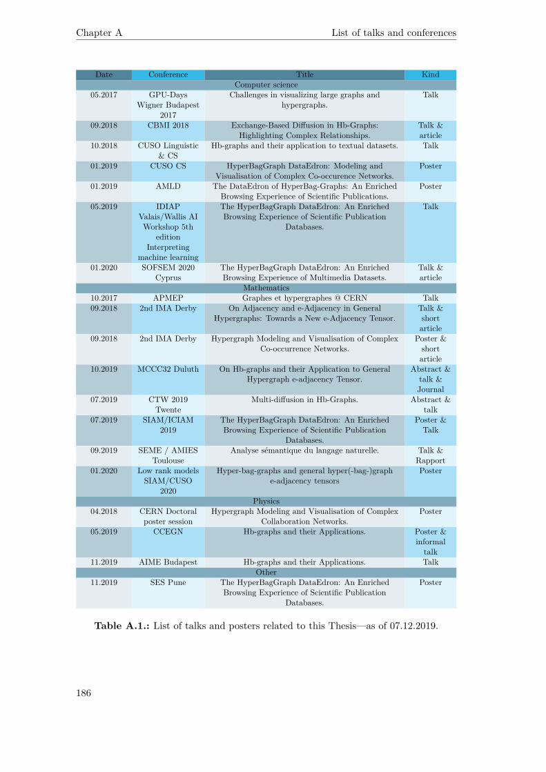
Chapter A List of talks and conferences
Date Conference Title KindComputer science
05.2017 GPU-DaysWigner Budapest
2017
Challenges in visualizing large graphs andhypergraphs.
Talk
09.2018 CBMI 2018 Exchange-Based Diffusion in Hb-Graphs:Highlighting Complex Relationships.
Talk &article
10.2018 CUSO Linguistic& CS
Hb-graphs and their application to textual datasets. Talk
01.2019 CUSO CS HyperBagGraph DataEdron: Modeling andVisualisation of Complex Co-occurence Networks.
Poster
01.2019 AMLD The DataEdron of HyperBag-Graphs: An EnrichedBrowsing Experience of Scientific Publications.
Poster
05.2019 IDIAPValais/Wallis AIWorkshop 5th
editionInterpreting
machine learning
The HyperBagGraph DataEdron: An EnrichedBrowsing Experience of Scientific Publication
Databases.
Talk
01.2020 SOFSEM 2020Cyprus
The HyperBagGraph DataEdron: An EnrichedBrowsing Experience of Multimedia Datasets.
Talk &article
Mathematics10.2017 APMEP Graphes et hypergraphes @ CERN Talk09.2018 2nd IMA Derby On Adjacency and e-Adjacency in General
Hypergraphs: Towards a New e-Adjacency Tensor.Talk &shortarticle
09.2018 2nd IMA Derby Hypergraph Modeling and Visualisation of ComplexCo-occurrence Networks.
Poster &shortarticle
10.2019 MCCC32 Duluth On Hb-graphs and their Application to GeneralHypergraph e-adjacency Tensor.
Abstract &talk &Journal
07.2019 CTW 2019Twente
Multi-diffusion in Hb-Graphs. Abstract &talk
07.2019 SIAM/ICIAM2019
The HyperBagGraph DataEdron: An EnrichedBrowsing Experience of Scientific Publication
Databases.
Poster &Talk
09.2019 SEME / AMIESToulouse
Analyse sémantique du langage naturelle. Talk &Rapport
01.2020 Low rank modelsSIAM/CUSO
2020
Hyper-bag-graphs and general hyper(-bag-)graphe-adjacency tensors
Poster
Physics04.2018 CERN Doctoral
poster sessionHypergraph Modeling and Visualisation of Complex
Collaboration Networks.Poster
05.2019 CCEGN Hb-graphs and their Applications. Poster &informaltalk
11.2019 AIME Budapest Hb-graphs and their Applications. TalkOther
11.2019 SES Pune The HyperBagGraph DataEdron: An EnrichedBrowsing Experience of Scientific Publication
Databases.
Poster
Table A.1.: List of talks and posters related to this Thesis—as of 07.12.2019.
186

B. Mathematical background
This Chapter is based on [OLGMM17a], [OLGMM17b], [OLGMM18b], [OLGMM18c],[OLGMM19a], [OLGMM19c] and [Ouv20]. It provides all the necessary backgroundconcepts used in this Thesis.
B.1. Hypergraphs
[Ber67] introduces hypergraphs as a means to generalize graphs. Graphs only supportpairwise relationships. Hypergraphs preserve the multi-adic relationships and, therefore,become a natural modeling of collaboration networks and various other situations. Theyalready allow a huge step in modeling, but some limitations remain that will be discussedfurther in this Thesis that has pushed us to introduce an extension of hypergraphs. Inthis Section, we aim at giving a short synthesis on hypergraphs based on [Ouv20] andintroduce the needed notations used throughout this Thesis. The interested reader canrefer to [Ouv20] for a full introduction on hypergraphs and their applications.
B.1.1. Generalities
As given in [Ber73], a hypergraph H = (V,E) on a finite set of vertices (or nodes)V
∆= {vi : i ∈ JnK}1 is defined as a family of hyperedges E ∆= (ej)j∈JpK where eachhyperedge is a non-empty subset of V and such that ⋃
j∈JpKej = V.
It means that in a hypergraph, a hyperedge links one or more vertices. In [Vol09], thedefinition of hypergraphs includes also hyperedges that are empty sets as hyperedgesare defined as a family of subsets of a finite vertex set and it is not necessary that theunion covers the vertex set. Both the vertex set and the family of hyperedges can beempty; it they are at the same time, the hypergraph is then designated as the emptyhypergraph. This definition of hypergraph opens their use in various collaborationnetworks. It is the one we choose in this Thesis.
In [Bre13], an intermediate definition is taken, relaxing only the covering of the vertexset by the union of the hyperedges enabling only isolated vertices in hypergraphs.
Other interesting definitions of hypergraphs, based on binary relations, exist that aregiven in [Ste12]; a full comparison is achieved in [Ouv20].
When needed, elements of V will be written (vi)i∈JnK and those of E will be written as(ej)j∈JpK . Abusively, ej will also designate the subset ι (ej) of V.
1We write for n ∈ N∗ : JnK = {i : i ∈ N∗ ∧ i 6 n}

Chapter B Mathematical background
Two hyperedges ej1 ∈ E and ej2 ∈ E, with j1, j2 ∈ JpK and j1 6= j2 such that ej1 = ej2are said repeated hyperedges.A hypergraph is said with no repeated hyperedge, if it has no repeated hyperedges.Following [CF88], where the hyperedge family is viewed as a multiset of hyperedges, ahypergraph with repeated hyperedges is called a multi-hypergraph.A hypergraph is said simple, if for any two hyperedges ej1 ∈ E and ej2 ∈ E :
ej1 ⊆ ej2 ⇒ j1 = j2.
Hence, a simple hypergraph has no repeated hyperedges.A hyperedge e ∈ E such that: |e| = 1 is called a loop.A hypergraph is said linear if it is simple and such that every pair of hyperedges sharesat most one vertex.A sub-hypergraph K of a hypergraph H is the hypergraph formed by a subset W ofthe vertices of H and the hyperedges of H that are subsets of W .A partial hypergraph H′ generated by a subset E′ ⊆ E of the hyperedges is a hy-pergraph containing exactly these hyperedges and whose vertex set contains at least allthe vertices incident to this hyperedge subset.The star of a vertex v ∈ V of a hypergraph H, written H(v), is the family of hyper-edges containing v.The dual of a hypergraph H is the hypergraph H∗ whose vertices corresponds to thehyperedges of H and the hyperedges of H∗ are the vertices of H, with the incidentrelation that links each vertex to its star.The neighborhood of a vertex v ∈ V is the set Γ (v) of vertices that belongs to thehyperedges this vertex is belonging.
B.1.2. Weighted hypergraph
In [ZHS07], the definition of a weighted hypergraph is given, based on the definition of[Ber73] of a hypergraph.Hwe = (V,E,we) is a weighted hypergraph, if (V,E) is a hypergraph and we : E → Ris a function that associates to each hyperedge e ∈ E a weight we (e) .We can refine this definition to handle weights on individual vertices, by using a secondfunction wv : V → R that associates to each vertex v ∈ V a weight wv (v) . But puttingweights that are hyperedge dependent cannot be achieved with hypergraphs as it wouldimply to move to a new algebra, as we will see with the introduction of hb-graphs.
B.1.3. Hypergraph features
Hypergraph features are very similar to those of graphs with some arrangements toaccount for their differences in structure.The order oH of a hypergraph H is defined as oH
∆= |V | .
188
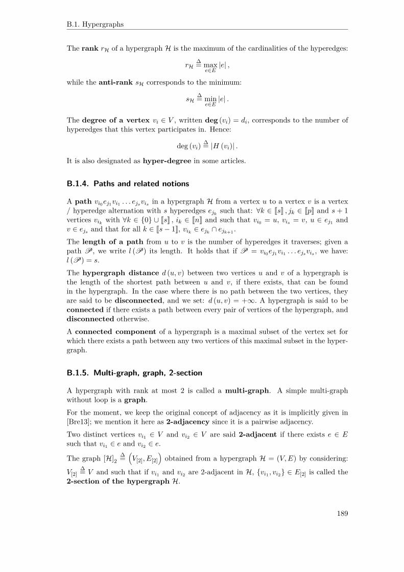
B.1. Hypergraphs
The rank rH of a hypergraph H is the maximum of the cardinalities of the hyperedges:
rH∆= max
e∈E|e| ,
while the anti-rank sH corresponds to the minimum:
sH∆= min
e∈E|e| .
The degree of a vertex vi ∈ V , written deg (vi) = di, corresponds to the number ofhyperedges that this vertex participates in. Hence:
deg (vi)∆= |H (vi)| .
It is also designated as hyper-degree in some articles.
B.1.4. Paths and related notions
A path vi0ej1vi1 . . . ejsvis in a hypergraph H from a vertex u to a vertex v is a vertex/ hyperedge alternation with s hyperedges ejk such that: ∀k ∈ JsK , jk ∈ JpK and s + 1vertices vik with ∀k ∈ {0} ∪ JsK , ik ∈ JnK and such that vi0 = u, vis = v, u ∈ ej1 andv ∈ ejs and that for all k ∈ Js− 1K, vik ∈ ejk ∩ ejk+1 .
The length of a path from u to v is the number of hyperedges it traverses; given apath P, we write l (P) its length. It holds that if P = vi0ej1vi1 . . . ejsvis , we have:l (P) = s.
The hypergraph distance d (u, v) between two vertices u and v of a hypergraph isthe length of the shortest path between u and v, if there exists, that can be foundin the hypergraph. In the case where there is no path between the two vertices, theyare said to be disconnected, and we set: d (u, v) = +∞. A hypergraph is said to beconnected if there exists a path between every pair of vertices of the hypergraph, anddisconnected otherwise.A connected component of a hypergraph is a maximal subset of the vertex set forwhich there exists a path between any two vertices of this maximal subset in the hyper-graph.
B.1.5. Multi-graph, graph, 2-section
A hypergraph with rank at most 2 is called a multi-graph. A simple multi-graphwithout loop is a graph.For the moment, we keep the original concept of adjacency as it is implicitly given in[Bre13]; we mention it here as 2-adjacency since it is a pairwise adjacency.Two distinct vertices vi1 ∈ V and vi2 ∈ V are said 2-adjacent if there exists e ∈ Esuch that vi1 ∈ e and vi2 ∈ e.
The graph [H]2∆=(V[2], E[2]
)obtained from a hypergraph H = (V,E) by considering:
V[2]∆= V and such that if vi1 and vi2 are 2-adjacent in H, {vi1 , vi2} ∈ E[2] is called the
2-section of the hypergraph H.
189
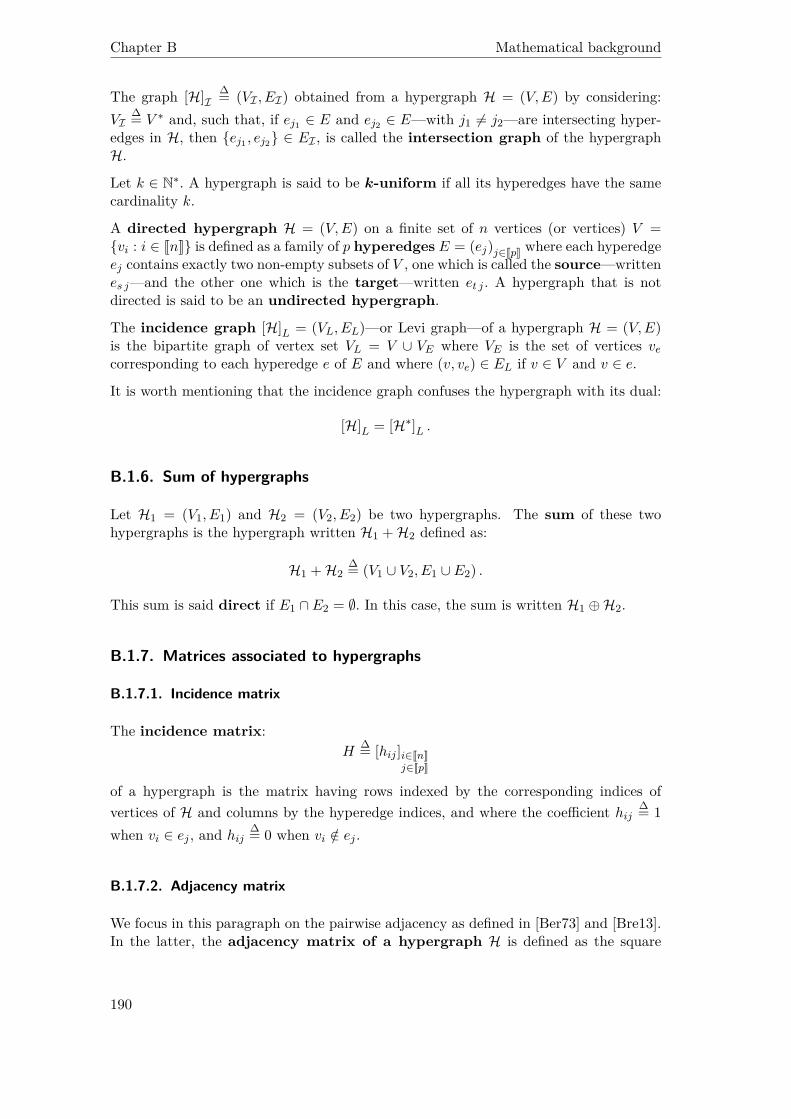
Chapter B Mathematical background
The graph [H]I∆= (VI , EI) obtained from a hypergraph H = (V,E) by considering:
VI∆= V ∗ and, such that, if ej1 ∈ E and ej2 ∈ E—with j1 6= j2—are intersecting hyper-
edges in H, then {ej1 , ej2} ∈ EI , is called the intersection graph of the hypergraphH.
Let k ∈ N∗. A hypergraph is said to be k-uniform if all its hyperedges have the samecardinality k.
A directed hypergraph H = (V,E) on a finite set of n vertices (or vertices) V ={vi : i ∈ JnK} is defined as a family of p hyperedges E = (ej)j∈JpK where each hyperedgeej contains exactly two non-empty subsets of V , one which is called the source—writtenes j—and the other one which is the target—written et j . A hypergraph that is notdirected is said to be an undirected hypergraph.
The incidence graph [H]L = (VL, EL)—or Levi graph—of a hypergraph H = (V,E)is the bipartite graph of vertex set VL = V ∪ VE where VE is the set of vertices vecorresponding to each hyperedge e of E and where (v, ve) ∈ EL if v ∈ V and v ∈ e.
It is worth mentioning that the incidence graph confuses the hypergraph with its dual:
[H]L = [H∗]L .
B.1.6. Sum of hypergraphs
Let H1 = (V1, E1) and H2 = (V2, E2) be two hypergraphs. The sum of these twohypergraphs is the hypergraph written H1 +H2 defined as:
H1 +H2∆= (V1 ∪ V2, E1 ∪ E2) .
This sum is said direct if E1 ∩ E2 = ∅. In this case, the sum is written H1 ⊕H2.
B.1.7. Matrices associated to hypergraphs
B.1.7.1. Incidence matrix
The incidence matrix:H
∆= [hij ]i∈JnKj∈JpK
of a hypergraph is the matrix having rows indexed by the corresponding indices ofvertices of H and columns by the hyperedge indices, and where the coefficient hij
∆= 1when vi ∈ ej , and hij
∆= 0 when vi /∈ ej .
B.1.7.2. Adjacency matrix
We focus in this paragraph on the pairwise adjacency as defined in [Ber73] and [Bre13].In the latter, the adjacency matrix of a hypergraph H is defined as the square
190

B.1. Hypergraphs
matrix A∆= [aij ] having rows and columns indexed by indices corresponding to the
indices of vertices of H and where for all i, j ∈ JpK , i 6= j :
aij∆= |{e ∈ E : vi ∈ e ∧ vj ∈ e}|
and for all i ∈ JpK :aii
∆= 0.
It holds, following [ERV05]:A = HHᵀ −DV
where DV∆= diag
((di)i∈JnK
)is the diagonal matrix containing vertex degrees.
The adjacency matrix of a weighted hypergraph Hw is defined in [ZHS07] as thematrix Aw of size n× n defined as:
Aw∆= HWHᵀ −Dw
where:W
∆= diag((wj)j∈JpK
)is a diagonal matrix of size p × p containing the weights (wj)j∈JpK of the respectivehyperedges (ej)j∈JpK and Dw is the diagonal matrix of size n× n:
Dw∆= diag
((dw (vi))i∈JnK
)and where for all i ∈ JnK:
dw (vi)∆=
∑j∈{k:k∈JpK∧vi∈ek}
wj
is the weighted degree of the vertex vi ∈ V.
We will refine the concept of adjacency in general hypergraphs in the next Chapter.
B.1.8. Hypergraph visualisation
In [Mäk90], hypergraph visualizations are classified in two categories called the “subsetstandard” and the “edge standard”. These two types of representations reflect the twofacets of hypergraphs. The subset standard reflects that hyperedges are subsets ofthe vertex set: the vertices of a hyperedge are drawn as points and hyperedges as closedenvelopes. The edge standard reflects that vertices of a hyperedge maintain togethera multi-adic relationship: two main representations are the clique representation,which corresponds to the 2-section graph of the hypergraph and the extra-node rep-resentation, which corresponds to the incidence graph—also called Levi graph—of thehypergraph.
To have full details on these representations, and others like the Zykov representation,the reader can refer to [Ouv20]. We just tackle here the problem of large hypergraphvisualization, which is central in some ways, to the foundations of this Thesis.
191
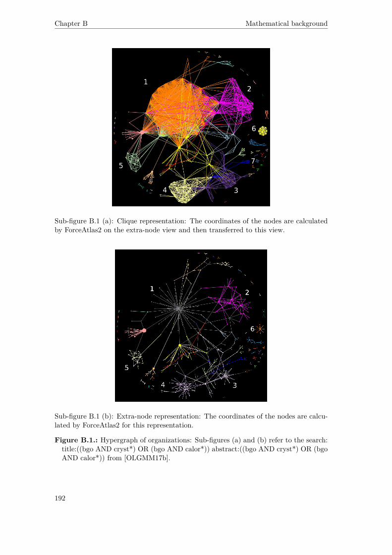
Chapter B Mathematical background
Sub-figure B.1 (a): Clique representation: The coordinates of the nodes are calculatedby ForceAtlas2 on the extra-node view and then transferred to this view.
Sub-figure B.1 (b): Extra-node representation: The coordinates of the nodes are calcu-lated by ForceAtlas2 for this representation.
Figure B.1.: Hypergraph of organizations: Sub-figures (a) and (b) refer to the search:title:((bgo AND cryst*) OR (bgo AND calor*)) abstract:((bgo AND cryst*) OR (bgoAND calor*)) from [OLGMM17b].
192
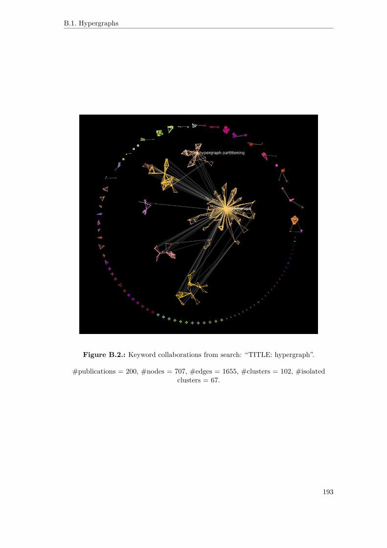
B.1. Hypergraphs
Figure B.2.: Keyword collaborations from search: “TITLE: hypergraph”.
#publications = 200, #nodes = 707, #edges = 1655, #clusters = 102, #isolatedclusters = 67.
193
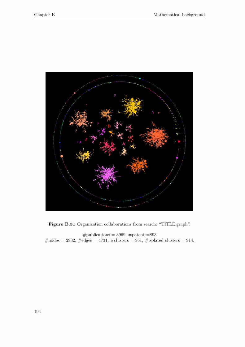
Chapter B Mathematical background
Figure B.3.: Organization collaborations from search: “TITLE:graph”.
#publications = 3969, #patents=893#nodes = 2932, #edges = 4731, #clusters = 951, #isolated clusters = 914.
194

B.1. Hypergraphs
Hypergraph
Connected components Connected componentsQuotient Hypergraph
Connected componentsQuotient Hypergraph
Layout
Hypergraphlayout
+
Connected component
Communities detectionCommunities
Quotient Hypergraph
CommunitiesQuotient
HypergraphLayout
Size and centerof connectedcomponent
Community
Coarsening
Layout
Important nodes
+
Other nodes
+
Overlappingoptimisation
Size and centerof community
(xCC − ωCC , yCC − ωCC)
(xCl − ωCl, yCl − ωCl)
(xN − ωC , yN − ωC)
Figure B.4.: Principle of the calculation of coordinates for large hypergraphs.
Large hypergraphs require strategies to be properly visualized. We have shown in[OLGMM17b] that switching from the 2-section representation to the incidence rep-resentation reduces considerably the overall cognitive load, as the number of edges tobe represented is effectively highly diminished in real networks; moreover, true collabo-rations are seen more distinguishably. An example is given in Figure B.1, that shows howthe representation of the same hypergraph in two different modes impact the cognitiveload of the information that is represented.
Complex co-occurrence networks can be modeled in a first instance by modeling them byhypergraphs as we have presented it in [OLGMM18d], where the hyperedges representco-occurrences attached to a given reference; we will refine this approach in Chapter 6using hb-graphs. When scaling up, such representations of large hypergraphs requiredifferent strategies in order to improve the global layout and the information displaying.These strategies include the segmentation of the hypergraph into connected components:they are ordered firstly by the number of references attached to the co-occurrences con-stituting them and secondly with respect to the number of vertices within co-occurrencesthey contain. The layout of each connected component is computed separately, by con-sidering the communities based on the Louvain algorithm presented in [BGLL08] andusing a force directed algorithm, named ForceAtlas2, presented in [JVHB14], to ensurethe layout of the communities and of the vertices inside the communities. To achieve aproper layout, vertices of importance for the community are placed first and the remain-ing vertices are then placed around those fixed important vertices, with an optimizationof the layout. The principle of the calculus is given in Figure B.4 and the results isshown in Figure B.2 and Figure B.3.
Optimizing the layout of a large hypergraph is a challenging task. It requires to capture
195
Chapter B Mathematical background
important vertices of the hypergraph, i.e. the ones we do not want to loose by over-whelming or overlapping in the representation. This requirement has been the startingpoint of our quest for a diffusion tensor.
B.2. Multisets
This section is extracted from a section of [OLGMM19c].
B.2.1. Generalities
The concept of multisets is known from the ancient times. [Knu68] mentioned that N.G.de Bruijn coined the word “multiset” to designate structures that were previouslycalled “list, bunch, bag, heap, sample, weighted set, collection” in the literature. In[Yag86], the theory of bags and fuzzy bags is developed. In [Alb91], definitions andalgebraic properties on bags are given, with the aim of having a convenient modelingdata structure. In [Bli88], the concept of multiset is traced back to the very origin ofnumbers, when numbers were represented by repeating occurrences of symbols.
In [Bli88], the authors start by giving the following naive concept of multiset beforebuilding the theory MST of multisets:
“The naive concept of multiset that we now formalize has the following properties: (i) amultiset is a collection of elements in which certain elements may occur more than once;(ii) occurrences of a particular element in a multiset are indistinguishable; (iii) eachoccurrence of an element in a multiset contributes to the cardinality of the multiset;(iv) the number of occurrences of a particular element in a multiset is a (finite) positiveinteger; (v) the number of distinguishable (distinct) elements in a multiset needs to befinite; and (vi) a multiset is completely determined if we know which elements belongto it and the number of times each element belongs to it.”
Nonetheless, the requirement (v) on the finitude is not necessary and, relying on [SIYS07],we will give the definitions on multisets without this constraint and this will hold in theremaining of this Thesis.
We consider a countable set A of distinct objects and a subset W ⊆ R+. We considerm an application from A to W. Then Am
∆= (A,m)2 is called a multiset—or mset orbag— on A. A is called the ground or the universe of the multiset Am, m is calledthe multiplicity function of the multiset Am. A?m
∆= {x ∈ A : m(x) 6= 0} is called thesupport of Am. The elements of the support of a mset are called its generators. Amultiset where W ⊆ N is called a natural multiset.
We write M (A) the set of all multisets of universe A. Some extensions of multisets existwhere the multiplicity function can have its range in Z—called hybrid set in [Loe92].Some other extensions exist like fuzzy multisets ([Syr01]). Most definitions when notrestricted to natural multisets can extend to W ⊆ R.2We systematically use fraktur font to designate multisets or mathematical objects that involves mul-tisets. For the reader that is not familiar to fraktur font, see Appendix F to have used letters andtheir correspondence in the text font.
196
B.2. Multisets
Several notations of msets exist. One common notation which we will use here is:Am = {xmii : i ∈ JnK ∧ xi ∈ A} with A = {xi : i ∈ JnK} the universe of the mset Am andthe notation ∀i ∈ JnK : mi = m (xi) . When the universe is made clear by the context,we can abusively write: Am = {xmii : i ∈ JnK ∧ xi ∈ A ∧mi 6= 0} .An other useful notation for a natural multiset is the one similar to an unordered list:
Am =
x1, . . . , x1︸ ︷︷ ︸
m1 times
, . . . , xn, . . . , xn︸ ︷︷ ︸mn times
.
In this last representation, we do not write the elements that are not in the support,also the universe has to be clearly stated.The m-cardinality #mAm of a mset Am corresponds to the sum of the multiplicitiesof the elements of its universe:
#mAm∆=∑x∈A
m(x)
while the cardinality #Am of a mset Am is the number of elements of its support:
#Am = |A?m| .
There exists only one multiset of universe A with an empty support that is called theempty multiset of universe A and written ∅A.Different operations can be defined on the set of all multisets of the same universe. Weconsider up to the end of this Section two msets A = (U,mA) and B = (U,mB) onthe same universe U. We define different operations such as inclusion, equality, union,intersection, sum,...The inclusion of A in B—written A ⊆ B—holds if for all x ∈ U :
mA(x) 6 mB(x).
A is then called a submset of B and said to be included in B.
If A ⊆ B and B ⊆ A, then A and B are said to be equal.
The union of A and B is the mset C ∆= A∪B of universe U and of multiplicity functionmC such that for all x ∈ U :
mC(x) ∆= max (mA(x),mB(x)) .
The intersection of A and B is the mset D ∆= A∩B of universe U and of multiplicityfunction mD such that for all x ∈ U :
mD(x) ∆= min (mA(x),mB(x)) .
The sum of A and B is the mset S ∆= A]B of universe U and of multiplicity functionmS such that for all x ∈ U :
mS(x) ∆= mA(x) +mB(x).
197

Chapter B Mathematical background
It is worth reminding that ∪, ∩ and ] are commutative and associative laws on msetsof the same universe. The empty mset of same universe corresponds to the identity forthese operations. ] is distributive for ∪ and ∩. ∪ and ∩ are distributive one for theother. ∪ and ∩ are idempotent.
The difference of two msets is the mset T ∆= A −B of universe U and of multiplicityfunction mT such that for all x ∈ U :
mT(x) ∆= mA(x)−mA∩B(x).
A set can be viewed as a natural mset where the multiplicities are in {1} , i.e. a naturalmultiset where the support corresponds to the universe and such that the multiplicityof the elements is always 1.
We can note that the classical property for sets: (A−B) ∩B = ∅U does not hold formultisets—see [SIYS07] for an example.
The complementation of A referring to a family R of multisets (Ai)i∈I of universeU is the multiset Ac of universe U and of multiplicity function mAc such that for allx ∈ U :
mAc(x) ∆= maxi∈I
(mAi(x))−mA(x).
Finally, the power set of a multiset Am—written P (Am)—is defined as the set of allsubmsets of Am.
We define the fusion of two msets A of universe U and B of universe V as the multisetF
∆= A⊕B of universe U∪V and of multiplicity function mF such that for all x ∈ U∪V :
mF (x) ∆=
mA (x) if x ∈ U\VmA (x) +mB (x) if x ∈ U ∩ VmB (x) if x ∈ V \U.
An interesting alternative approach to define multisets is the one given in [Syr01] wherea natural multiset Am = (A,m) is viewed as a couple 〈A0, ρ〉 , where A0 is the set ofinstances of elements of A, that includes copies of elements, and ρ is an equivalencyrelation ρ over A0 :
∀x ∈ A0, ∀x′ ∈ A0 : xρx′ ⇔ ∃!c ∈ A : xρc ∧ x′ρc.
Two elements of A0 such that: xρx′ are said copies of one another. The unique c ∈ Ais called the original element. x and x′ are said copies of c.
Also, A0/ρ is isomorphic to A and:
∀x ∈ A0/ρ,∃!c ∈ A : |{x : x ∈ x}| = m(c) ∧ ∀x ∈ x : xρc.
The set A0 is then called a copy-set of the multiset Am.
We can remark that a copy-set for a given multiset is not unique. Sets of equivalencyclasses of two couples < A0, ρ > and < A′0, ρ
′ > of a given multiset are isomorphic.
198
B.2. Multisets
B.2.2. Algebraic representation of a natural multiset
We propose in this Section two algebraic representations of a natural multiset Am =(A,m) of countable universe A = {xi : i ∈ JnK} and multiplicity function m.
Vector representation of a natural multiset
A multiset Am can be conveniently represented by a vector of length the cardinalityof the universe and where its components represent the multiplicity of the correspond-ing element. We suppose that the elements of A are given in a fixed order—it is al-ways possible to index these elements by a subset of the positive integer set. Hence−→Am
∆= (m (xi))xi∈A is called a vector representation of the multiset Am. Thisrepresentation requires |A| space and has |A| − |A?m| null elements.
The sum of the elements of −→Am is #mAm.
This representation will be useful later when considering family of multisets in order tobuild the incident matrix of a hb-graph.An alternative representation is obtained using a symmetric hypermatrix. This approachis needed to reach our goal of constructing an e-adjacency tensor for general hb-graphsand hypergraphs.
Hypermatrix representations of a natural multiset
The unnormalized hypermatrix representation of the natural multiset Am =(A,m) is the symmetric hypermatrix Au
∆= (au,i1...ir)i1,...,ir∈JnK of order r = #mAm anddimension n such that au,i1...ir = 1 if ∀j ∈ JrK : ij ∈ JnK∧ xij ∈ A?m. The other elementsare null.
Hence the number of non-zero elements in Au is r!∏x∈A?m
m (x) out of the nr elements of
the representation.
The sum of the elements of Au is then: r!∏x∈A?m
m (x) .
To normalize Au, we enforce the sum of the elements of the hypermatrix to be them-rank of the multiset it encodes.The normalized hypermatrix representation of the multiset Am is the symmetrichypermatrix A
∆= (ai1...ir)i1,...,ir∈JnK of order r = #mAm and dimension n such that
ai1...ir =
∏x∈A?m
m (x)
(r − 1)! if ∀j ∈ JrK : ij ∈ JnK ∧ xij ∈ A?m. The other elements are null.
B.2.3. Morphisms, category and multisets
In [Syr01], the author introduces two equivalent categories of multisets, calledMSet andBags: MSet reflects the multiplicity approach while Bags reflects the copy approach
199

Chapter B Mathematical background
and reserved to what is called pure multisets in [Syr03], i.e. what we have called naturalmultisets.
MSet objects are pairs (A,P ) constituted of a set A and P : A → Set a presheaf3on A, that describes a multiset, as P (a) with a ∈ A is a set of cardinality equals tothe multiplicity of a in the multiset. An arrow between two objects of MSet is a pairconstituted of a function and a natural transformation, i.e. a family of functions.
The definition of Bags is based on a function p : X → A where X represents the set ofall copies of elements of A. The objects of Bags are pairs (A, p) and an arrow betweentwo objects (A, p) and (B, q) , with p : X → A and q : Y → B of Bags is a pair (f, g)such that f : A→ B and g : X → Y and such that q ◦ g = f ◦ p.
In [Syr03], the author introduces a third category called Mul and linked it to a newdefinition of general multisets. A multiset is defined in this reference as a pair (A, ρ)where A is a set and ρ is an equivalence relation on A. A morphism of two multisets(A, ρ) and (A′, ρ′) is defined as a function f : A → A′ such that for all x1 and x2 inA, if x1ρx2, then f (x1) ρ′f (x2) . In Mul, the objects correspond to the multisets andthe arrows to the morphisms of the multisets. This last definition is the one retainedin [IT15], where the author characterizes the different kind of morphisms encounteredin Mul: it includes the monomorphisms that corresponds exactly to the injective mor-phisms, the epimorphisms corresponding to the surjective functions, and shows that anysplit monomorphism is a monomorphism and that any split epimorphism is an epimor-phism. Moreover, the composition of arrows keeps monomorphisms, epimorphisms andbimorphisms. In Mul, every isomorphism is a bimorphism but the converse does nothold, which would have made Mul a balanced category.
B.2.4. Topologies on multisets
Defining topologies on multisets requires to handle the problem of the complementationon multisets. In [GJ12], the authors consider [A]∞ the set of all multisets of universeA and [A]w the set of all multisets where elements have a multiplicity in JwK∪ {0} . Allmultisets are then considered in [A]w and the complementation of a multiset A ∈ [A]wis done using this family.
The sum of two multisets A and B in [A]w is redefined as the mset Sw ∆= A ] B ofuniverse A and of multiplicity function mSw such that for all a ∈ A :
mSw (a) ∆= min {w,mA (a) +mB (a)} .
The authors consider different kind of submsets of a mset A in [A]w: the whole submsetwhere the elements of the support of the submset have same multiplicity than in Aand the full submset where the elements of the submset have a multiplicity less orequal to the one of A. For each kind corresponds a power mset, either whole—writtenPW (A)—or full—denoted PF (A)—, which are both sets of all whole or full submsetsof a given mset. These two power msets are ordinary sets. The cardinality of PW (A)3A presheaf F on a category C is a contravariant functor: F : Cop → Set. When C is a discretecategory, i.e. a category having only objects and no arrows, Cop = C, which is the case for a set Aconsidered as a category.
200
B.2. Multisets
is 2n where n = #A? and the cardinality of PF (A) is ∏a∈A?
m (a) . In both cases, Cantor
power set theorem—that stipulates for sets that the cardinality of a set—is strictly lessthan the cardinality of its power set fails in the case of msets. In order to preservethis theorem for multisets, the authors introduce a power mset P (A), that takes intoaccount the repetitions of msets. They then consider different operation on a collectionof msets drawn from [A]w including Cartesian product of two msets and a mset relationon a mset.
Finally, the authors introduce a multiset topology τ ⊆ P? (A) of a multiset A ∈ [A]wwith the classical axioms of a topology, called A-topology: these axioms includes thefact that the m-set union of any sub-collection of τ is in τ and the same for the msetintersection of any finite sub-collection, and the fact that A and ∅A are in τ. Classi-cal topology is then considered including closure, interior and limit point as well ascontinuous multiset functions.
The key point in this work has been to introduce the power mset of a multiset.
B.2.5. Applications of multisets
This section is partly based on [OLGMM19a].
Multisets, under the appellation bag, appear in different domains such as text modeling,image description and audio [SJP+16]. In text representation, bag of words have beenfirst introduced in [Har54]: bags are lists of words with repetitions, i.e. multisets ofwords on a universe. Many applications occur with different approaches. Bags of wordshave been used for instance in fraud detection [PS15]. More recently, bag of words havebeen used successfully for translation by neural nets as a target for the translation,since a sentence can be translated in many different ways [MSWL18]. In [CAO+18],multi-modal bag of words have been used for cross domains sentiment analysis.
Bags of visual words is the transcription to image of textual bags of words; in bagsof visual words, a visual vocabulary based on image features is built to enabling thedescription of images as bags of these features. Since their introduction in [SZ03],many applications have been realized: in visual categorization [CDF+04], in imageclassification and filtering [DPN08], in image annotation [Tsa12], in action recognition[PWWQ16], in land-use scene classification [ZTH14], in identifying mild traumatic braininjuries [MWW+17] and in word image retrieval [SJ12].
Bags of concepts are an extension of bags of words to successive concepts in a text[KKC17]. A recent extension of these concepts is given in [SWG+18] where bag ofgraphs are introduced to encode in graphs the local structure of a digital object: bagsof graphs are available as bags of singleton graphs and bags of visual graphs. Using thehb-graphs as we propose in this Thesis will allow to extend this approach, by takingadvantage of multi-adic relationships, and, also, of the multiplicity of vertices specificto each hb-edge.
Additional applications to mathematics can be found in [SIYS07]: it includes the integerprime factorization, the representation of monic polynomials by the mset of its roots andcorrespondence between polynomial operations and mset operations, the zeros and polesof meromorphic functions. Other non-straightforward applications in mathematics are
201

Chapter B Mathematical background
considered such as the semi-ring of multisets developed in [Po00] making connectionsbetween eigenvalues and eigenvectors of max-plus algebra4 and the non-negative realnumber systems.Different approaches exist in computing, either theoretical or practical, that uses mul-tisets. For instance, in [BLM93] the authors present a formalism where programs arepresented in terms of multiset transformations, giving birth to the GAMMA programs,the first version of chemical programming5; other approaches exist such as the one usinggeneralised multisets in [BFR06] or higher-order chemical language in [BFR07]. Mul-tisets are used in membrane computing, a part of computer science that seeks to findcomputational models that mimic biological systems as introduced by Păun6 in 1998,to describe objects in super-cells in [DP99].In [PK08], the authors use decision procedures for multisets using cardinality con-straints. Collection of multisets are found in software verification and interactive the-orem proving. They emphasize the useful operations and relations on multisets, par-ticularly formulas on the number of occurrences of each element in a multiset, usingquantifier-free Presburger arithmetic (QFPA for short) which is a first order decidabletheory that uses an arithmetic containing only addition and recurrence statement. Theypropose an algorithm for reducing multiset formulas to sum normal form, introducingconstraints on multisets; the satisfiability is achieved using an extension of QFPA tounbounded expressions.More recently in [BA16], the authors introduce multiset operations for privacy-preservingset operations among multiple players, such as computing database intersection of dif-ferent organizations.
B.3. Tensors and hypermatrices
B.3.1. An introduction on tensors
A rigorous introduction of tensors is achieved in [Lee13]: we rely on it in this introduc-tion.First, we introduce the notion of co-vector.We consider a finite dimension vector space V over R. A co-vector is a linear form i.e.an application ω : V → R which is linear7. The set of all co-vectors of V constitutes thedual space V ? of V.For a given basis (ei)i∈JnK of V, the co-vectors
(εj)j∈JnK of V ? are defined by:
εj (ei)∆= δij ,
where: δij∆={
1 if i = j
0 otherwiseis the Kronecker delta symbol. The co-vectors
(εj)j∈JnK
constitutes a basis of V ?, called the dual basis of (ei)i∈JnK .
4Cf for instance [ABG06] for a definition of max-plus algebra5For a cool introduction, see: http://gigasquidsoftware.com/chemical-computing/index.html6Cf [Pău11] for a reference book on membrane computing7An application f : V → W , where V and W are two vector spaces, is linear if for all v, v′ ∈ V andλ, µ, f (λv + µv′) = λf (v) + µf (v′) .
202
B.3. Tensors and hypermatrices
We define the tensor product of two co-vectors ω and ω′ of V ? as the map:
ω ⊗ ω′ : V × V → R,
such that for (v1, v2) ∈ V × V :
ω ⊗ ω′ (v1, v2) ∆= ω (v1) · ω′ (v2) .
The tensor product of two co-vectors can be generalized to any two multilinear forms.
Considering k vector spaces (Vj)j∈JkK , a multilinear form is an application F : V1 ×...× Vk → R which is linear in each of its variables. We write L (V1, ..., Vk;R) the spaceof the multilinear forms on the vector space V1 × ...× Vk.
The tensor product of two multilinear forms F : V1 × ... × Vk → R and G :W1 × ... ×Wl → R is defined as the map: F ⊗ G : V1 × ... × Vk ×W1 × ... ×Wl → Rsuch that for all (v1, ..., vk) ∈ V1 × ...× Vk and (w1, ..., wl) ∈W1 × ...×Wl, it holds:
F ⊗G (v1, ..., vk, w1, ..., wl)∆= F (v1, ..., vk) ·G (w1, ..., wl) .
F ⊗G is a multilinear form of k + l variables and lives in L (V1, ..., Vk,W1, ...,Wl;R) .
Hence, considering k vector spaces (Vj)j∈JkK and k linear forms ωj ∈ V ?j , with j ∈ JkK,⊗
j∈JkKωj is a multilinear form of L (V1, ..., Vk;R) and for (v1, ..., vk) ∈ V1 × ...× Vk :
⊗j∈JkK
ωj (v1, ..., vk)∆=∏j∈JkK
ωj (vj) .
It follows that considering a basis(e(j) ij
)ij∈JnjK
for each of the vector space Vj of
dimension nj with j ∈ JkK and, considering the corresponding dual spaces(εij(j)
)ij∈JnjK
,it holds that: ⊗
j∈JkK
εij(j)
i1∈Jn1K,...,ik∈JnkK
is a basis of L (V1, ..., Vk;R) .
This means that any multilinear form F ∈ L (V1, ..., Vk;R) can be decomposed in:
F =∑
i1∈Jn1K,...,ik∈JnkK
Fi1...ik⊗j∈JkK
εij(j).
With the same idea, and without developing all the arguments that can be found in[Lee13], the same approach can be taken to build a new vector space V1 ⊗ ...⊗ Vk inwhich elements are of the type v1 ⊗ ...⊗ vk such that they are linear in each of the vi,i ∈ JkK. It is shown that V ?
1 ⊗ ...⊗ V ?k is isomorphic to L (V1, ..., Vk;R) and that by
duality: V1⊗ ...⊗ Vk is isomorphic to L (V ?1 , ..., V
?k ;R) .
With V1 = ... = Vk = V a finite dimensional space, a covariant cubical tensor onV of order (or rank) k is an element of V ?⊗ ...⊗ V ?︸ ︷︷ ︸
ktimes
i.e. a multilinear form of k
203

Chapter B Mathematical background
elements of V. We write: L0k (V ) the space of the covariant cubical tensor on V of rank
k. An element of V ⊗ ...⊗V is called a contravariant cubical tensor on V of rankk. We write: Lk0 (V ) the space of the contravariant cubical tensor on V of rank k. Moregenerally an element of V ⊗ ...⊗ V︸ ︷︷ ︸
ktimes
⊗ V ?⊗ ...⊗ V ?︸ ︷︷ ︸ltimes
is called a mixed tensor of type
(k, l) . The corresponding space is Llk (V ) .Only elements of L0
k (V ) admits the restricted approach that is presented in the nextsection.
B.3.2. Restricted approach of tensors as hypermatrices
As we are interested only in cubical tensors8 that are abusively identified to hypermatri-ces, we give a straightforward presentation of tensors and their relative hypermatrices.We write L0
k (Rn) the space of cubical tensors of rank k and dimension n with values inR, and Ak one of its elements.The Segre outerproduct ⊗ of a = [ai] ∈ Rl and b = [bj ] ∈ Rm is defined as:
a⊗ b = [aibj ] i∈JlKj∈JmK
∈ Rl×m.
More generally, as given in [CGLM08], the outerproduct of k vectors u(i) ∈ Rni , withi ∈ JkK and where ∀i ∈ JkK , ni ∈ N∗, is defined as:
k⊗i=1
u(i)∆=[k∏i=1
u(i)ji
]j1∈Jn1K,..,jk∈JnkK
∈ Rn1×...×nk .
Here, we consider ni = n for all i ∈ [k] . Writing e1, ..., en the canonical basis of Rn,(ei1 ⊗ ...⊗ eik)i1,...,ik∈JnK is a basis of L0
k (Rn) .
Then the tensor Ak ∈ L0k (Rn) is associated to a hypermatrix Ak =
(a(k) i1...ik
)i1,...,ik∈JnK
by writing Ak as:Ak =
∑i1,...,ik∈JnK
a(k) i1...ikei1 ⊗ ...⊗ eik .
Ak is called the canonical hypermatrix representation (CHR for short) of Ak.In [Lim13], amultilinear matrix multiplication is defined considering A ∈ Rn1×...×nd
and Xj =[x(j)kl
]∈ Rmj×nj for j ∈ JdK as:
A′∆= (X1, ..., Xd) .A
where A′ is the hypermatrix of Km1×...×md of coefficients:
a′j1...jd∆=
∑k1∈Jn1K,...,kd∈JndK
x(1)j1k1 ...x(d)jdkdak1...kd
for ji ∈ JmiK with i ∈ JdK .8We often abusively use the word tensor for its hypermatrix representation in a canonical basis inthe verbatim of this Thesis, following the abuse made in [QL17]. Nonetheless, when writing itmathematically we make the difference between the tensor A of dimension n and rank r and itscanonical hypermatrix representation (CHR for short), written A = (ai1...ir ) as defined in thisSection.
204
B.3. Tensors and hypermatrices
B.3.3. On classification of hypermatrices
This Section is extracted from [OLGMM19c].
Most of the definitions and results of this Section are taken directly from [QL17], whichis the first book on tensor spectral analysis.
We consider a tensor A and its CHR of order m and dimension n:
A = (ai1...im)i1,...,im∈JnK .
The set of such hypermatrices is written Tm,n. The subset of Tm,n of hypermatrices withonly non-negative9 coefficients is written Nm,n.
A hypermatrix A = (ai1...im)i1,...,im∈JnK ∈ Tm,n is said reducible if there exists anonempty proper subset J ( JnK such that:
∀i1 ∈ J, ∀ (i2, ..., im) ∈ (JnK \J)m−1 : ai1...im = 0.
A hypermatrix that is not reducible is said irreducible. The notion of reducibility hasto be seen as a possible way of reducing the dimensionality of the problem.
Irreducible non-negative hypermatrices have plenty of nice properties, particularly thePerron-Frobenius theorem for irreducible non-negative hypermatrices which is one ofthe two declinations of the extension of the Perron-Frobenius theorem for irreduciblenon-negative matrices.
The Perron-Frobenius theorem for irreducible non-negative matrices states that theeigenvector associated to the spectral radius of a non-negative matrix is non-negative,and, if, moreover, this matrix is irreducible, then this eigenvector is positive10 and itseigenvalue is the unique one associated with a non-negative eigenvector.
The Perron-Frobenius theorem has a lot of applications in probability with stochasticmatrices and is the basis for algorithms such as PageRank, ensuring that the convergenceis feasible [PSS05].
But hypermatrices manipulated in hypergraph theory are reducible. In this case, thisfirst extension of the theorem of Perron-Frobenius cannot be used.
Weak irreducibility of non-negative hypermatrices has been introduced to help to solvethis problem. To define weak irreducibility, an associated graph G (A) is built out ofthe non-negative hyper-cubic CHR A which represents A by considering as vertex setJnK and building the edges by considering an edge from i to j if there exists aii2...im 6= 0such that j ∈ {i2, ..., im} .
A directed graph is strongly connected if for any ordered pair of vertices (i, j) of thegraph, there exists a directed path from i to j.
A tensor A is said weakly irreducible if its associated graph is strongly connected. Atensor that is not weakly irreducible is said weakly reducible.
We consider now a tensor A of non-negative CHR A = (ai1...im) ∈ Nm,n.
9I.e. either positive or equals to zero.10I.e. all the coefficients are strictly greater than zero.
205

Chapter B Mathematical background
The representative vector of A is the vector u (A) of coordinates:
ui (A) ∆=∑
i2,...,im∈JnK
aii2...in .
A is called a strictly non-negative tensor if its representative vector is positive.
Let now J be a proper nonempty subset of JnK . The tensor AJ of CHR AJ∆= (αi1...im) ∈
Nm,|J | such that: αi1...im∆= ai1...im if i1, ..., im ∈ J is called the principal sub-tensor
of A associated to J.
A is said a non-trivially non-negative tensor if there exists a principal sub-tensorof A that is a strictly non-negative tensor.
The following proposition will be helpful in the spectral analysis of hb-graphs.
Proposition B.1. A non-negative tensor has a positive eigenvalue if and only if it isnon-trivially non-negative.
As a consequence, a non-trivially non-negative tensor has its spectral radius positive.
In [QL17], a procedure is given to check easily if a non-negative tensor is non-triviallynegative or not.
B.3.4. Eigenvalues
The definitions and results of this Section are based on [QL17]. Proofs can be found inthis reference.
Let Tm,n be the set of all real hypermatrices of order m and dimension n and Sm,n thesubset of Tm,n of symmetric hypermatrices, i.e. hypermatrices such that are invariantby any permutations of the indices.
Let A = (ai1...im) ∈ Tm,n. Let I ∈ Tm,n designates the identity tensor.
Definition B.1. A number λ ∈ C is an eigenvalue of A if there exists a nonzerovector x ∈ Cn such that:
∀i ∈ J1, nK ,(Axm−1
)i
= λxm−1i . (B.1)
In this case, x is called an eigenvector of A associated with the eigenvalue λ and (x, λ)is called an eigenpair of A.
The set of all eigenvalues of A is called the spectrum of A. The largest modulus of alleigenvalues is called the spectra radius of A, denoted as ρ (A) .
Remark B.3.1. Writing x[m−1] =(xm−1i
)i∈JnK
, B.1 can be transformed into:
Axm−1 = λx[m−1].
206

B.3. Tensors and hypermatrices
Proposition B.2. Let α and β be two real numbers.
If (λ, x) is an eigenpair of A, then (αλ+ β, x) is an eigenpair of αA + βI.
Definition B.2. A H-eigenvalue is an eigenvalue λ of A that has a real eigenvectorx associated to it. x is called in this case an H-eigenvector.
Proposition B.3. A H-eigenvalue is real.
A real eigenvalue is not necessarily a H-eigenvalue.
The following theorem holds for symmetric tensors:
Theorem B.1. Let A ∈ Sm,n. If m is even, then A always have H-eigenvalues and, Ais positive definite (resp. semi-definite) if and only if its smallest H-eigenvalue λHmin (A)is positive (resp. non-negative).
Theorem B.2. Let A ∈ Tm,n be a non-negative tensor. Then A has at least oneH-eigenvalue and λHmax (A) = ρ (A) . Furthermore λHmax (A) has a non-negative H-eigenvector.
Definition B.3. A tensor is called an essentially non-negative tensor if all itsoff-diagonal entries are non-negative.
A tensor is called a Z-tensor if its off-diagonal entries are non-positive.
Theorem B.3. Essentially non-negative tensors and Z-tensors always have H-eigenvalues.
Definition B.4. Let A = (ai1...im) ∈ Tm,n.
The diagonal elements of A are the elements ai...i for i ∈ JnK .
The off-diagonal elements of A are the other elements.
An important result is the following:
Proposition B.4. Let A ∈ Tm,n. Then the eigenvalues of A belong to the union of ndisks in C. These n disks have the diagonal entries of A as their centers and the sumsof the absolute values of the off-diagonal entries as their radii.
Remark B.3.2. The proof shows that if (λ, x) is an eigenpair of A = (ai1...im), it holdsfor i ∈ JmK such that: |xi| = max {|xj | : j ∈ JnK} :
|λ− ai...i| 6∑
i2,...,im∈JnKδii2...im=0
|aii2...im | . (B.2)
Corollary B.1. If A is a non-negative tensor of Tm,n with an equal row sum r, then ris the spectral radius of A.
207

Chapter B Mathematical background
Other types of eigenvalues also exist. It is worth mentioning E-eigenvalues and Z-eigenvalues since they are part of the related work of this Thesis.
Given a tensor A = (ai1...im) of Tm,n, λ ∈ C is an E-eigenvalue of A if there exists avector x ∈ Cn, called an E-eigenvector, such that: Axm−1 = λx with: x>x = 1.
A Z-eigenvalue is an E-eigenvalue associated to a real E-eigenvector. A Z-eigenvalueis always real—but a real E-eigenvalue is not necessary a Z-eigenvalue.
Any symmetric tensor has Z-eigenvalues.
208
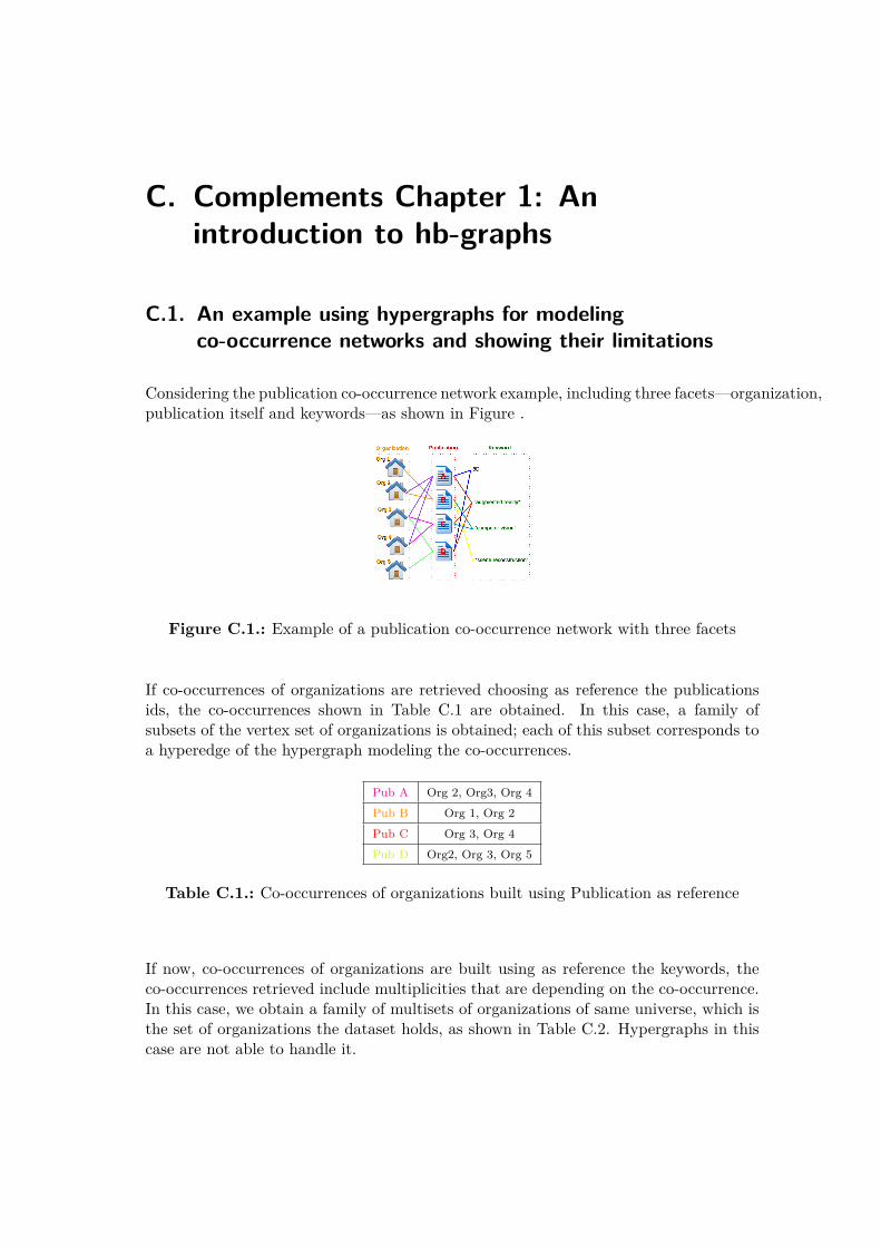
C. Complements Chapter 1: Anintroduction to hb-graphs
C.1. An example using hypergraphs for modelingco-occurrence networks and showing their limitations
Considering the publication co-occurrence network example, including three facets—organization,publication itself and keywords—as shown in Figure .
Figure C.1.: Example of a publication co-occurrence network with three facets
If co-occurrences of organizations are retrieved choosing as reference the publicationsids, the co-occurrences shown in Table C.1 are obtained. In this case, a family ofsubsets of the vertex set of organizations is obtained; each of this subset corresponds toa hyperedge of the hypergraph modeling the co-occurrences.
Pub A Org 2, Org3, Org 4
Pub B Org 1, Org 2
Pub C Org 3, Org 4
Pub D Org2, Org 3, Org 5
Table C.1.: Co-occurrences of organizations built using Publication as reference
If now, co-occurrences of organizations are built using as reference the keywords, theco-occurrences retrieved include multiplicities that are depending on the co-occurrence.In this case, we obtain a family of multisets of organizations of same universe, which isthe set of organizations the dataset holds, as shown in Table C.2. Hypergraphs in thiscase are not able to handle it.
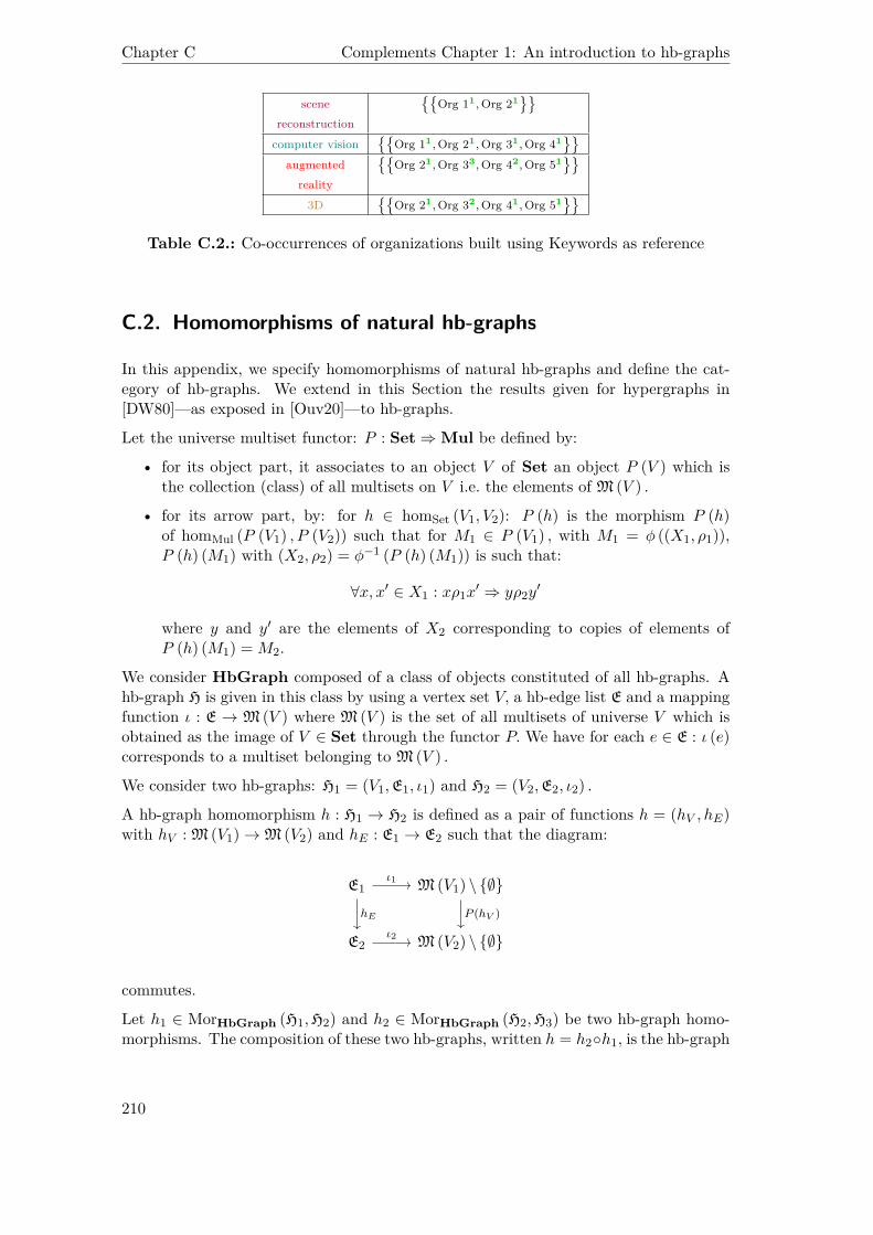
Chapter C Complements Chapter 1: An introduction to hb-graphs
scenereconstruction
{{Org 11,Org 21
}}computer vision
{{Org 11,Org 21,Org 31,Org 41
}}augmented
reality
{{Org 21,Org 33,Org 42,Org 51
}}3D
{{Org 21,Org 32,Org 41,Org 51
}}Table C.2.: Co-occurrences of organizations built using Keywords as reference
C.2. Homomorphisms of natural hb-graphs
In this appendix, we specify homomorphisms of natural hb-graphs and define the cat-egory of hb-graphs. We extend in this Section the results given for hypergraphs in[DW80]—as exposed in [Ouv20]—to hb-graphs.
Let the universe multiset functor: P : Set⇒Mul be defined by:
• for its object part, it associates to an object V of Set an object P (V ) which isthe collection (class) of all multisets on V i.e. the elements of M (V ) .
• for its arrow part, by: for h ∈ homSet (V1, V2): P (h) is the morphism P (h)of homMul (P (V1) , P (V2)) such that for M1 ∈ P (V1) , with M1 = φ ((X1, ρ1)),P (h) (M1) with (X2, ρ2) = φ−1 (P (h) (M1)) is such that:
∀x, x′ ∈ X1 : xρ1x′ ⇒ yρ2y
′
where y and y′ are the elements of X2 corresponding to copies of elements ofP (h) (M1) = M2.
We consider HbGraph composed of a class of objects constituted of all hb-graphs. Ahb-graph H is given in this class by using a vertex set V, a hb-edge list E and a mappingfunction ι : E → M (V ) where M (V ) is the set of all multisets of universe V which isobtained as the image of V ∈ Set through the functor P. We have for each e ∈ E : ι (e)corresponds to a multiset belonging to M (V ) .
We consider two hb-graphs: H1 = (V1,E1, ι1) and H2 = (V2,E2, ι2) .
A hb-graph homomorphism h : H1 → H2 is defined as a pair of functions h = (hV , hE)with hV : M (V1)→M (V2) and hE : E1 → E2 such that the diagram:
E1 M (V1) \ {∅}
E2 M (V2) \ {∅}
ι1
hE P (hV )ι2
commutes.
Let h1 ∈ MorHbGraph (H1,H2) and h2 ∈ MorHbGraph (H2,H3) be two hb-graph homo-morphisms. The composition of these two hb-graphs, written h = h2◦h1, is the hb-graph
210
C.2. Homomorphisms of natural hb-graphs
homomorphism: h = (hV , hE) such that: hV = hV,2 ◦ hV,1 and hE = hE,2 ◦ hE,1. Thiscomposition is associative.
For every object H, the identity hb-graph morphism 1H keeps the hb-edges identical andkeeps each hb-edge in the same state.
Hence, considering objects as hb-graphs and arrows as hb-graph homomorphisms, Hb-Graph is a category.
The following lemmata occur:
Lemma C.1. Hyp is a full sub-category of HbGraph.
Proof. We consider the inclusion functor: J : Hyp⇒ HbGraph defined as:
• for the object part: H → J (H) where J (H) is the hb-graph of universe the vertexset of H and where the hb-edges are linked to multisets with multiplicity no morethan one;
• for the arrow part: at each hypergraph homomorphism corresponds a unique hb-graph homomorphism that behaves similarly on vertices and hb-edges than theone on hypergraph.
Lemma C.2. Duality of hb-graphs is a covariant functor d : HbGraph⇒ HbGraph
Proof. The object part of the functor associates to a hb-graph its dual: for H =(V,E, ι) ∈ HbGraph, d (H) = H with H = (E,V, ι) where: ι : V → M (E) suchthat: ι (v) corresponds to the multiset described by:
{{eme(v) : v ∈ ι (e)
}}.
The arrow part of the functor associates to one hb-graph homomorphism h ∈ HomHbGraph (H1,H2)the hb-graph homomorphism corresponding to the duals: d (h) : d (H1) → d (H2) suchthat d (h) (x) = h (x) for x ∈ V ∪ E.
If we take H = H1 = H2 and h = IdH, we have d (IdH) = Idd(H).
Taking h1 ∈ HomHbGraph (H1,H2) and h2 ∈ HomHbGraph (H2,H3), we have:
d (h1 ◦ h2) = h1 ◦ h2 = d (h1) ◦ d (h2) .
We write TGraph the category of all graphs as defined in [BMSW08].
Lemma C.3. The incidence multipartite graph of a hb-graph induces a covariant func-tor M : HbGraph→ TGraph.
Proof. We have explained in Section 1.4.6.2 how we can associate a unique extra-vertexmultipartite graph GH to a hb-graph H.
We consider for M :
• for the object part: M : H→M (H) where M (H) = GH.
211
Chapter C Complements Chapter 1: An introduction to hb-graphs
• for the arrow part: given h ∈ HomHbGraph (H1,H2) , we consider M (h) : GH1 →GH2 such that: v → h (v) and e → h (e) such that any copies of a vertex in ahb-edge has its image that is the copy of the image of the copies in the hb-edgeimage.
If we take H = H1 = H2 and h = IdH, copies of vertices will remain the same byM (IdH)as well as hb-edges and M (IdH) = IdM(H).
Moreover, taking h1 ∈ HomHbGraph (H1,H2) and h2 ∈ HomHbGraph (H2,H3), we have:
M (h2 ◦ h1) = M (h2) ◦M (h1) .
We conjecture that general hb-graphs constitute a new category, but this remains anopen question.
212
D. Complements Chapter 2: Diffusion inhb-graphs
D.1. Facets and Biased diffusion
This chapter is extending the approach presented in Chapter 2 and in [OLGMM19a].It has been published after this Thesis Defense in [OGMM20].Prerequisites: Section 1.3 and, preferably Chapter 2.
D.1.1. Motivation
Facets are not all of same nature in an information space; depending on the informationthey carry, the ranking of the information hold by their visualisation hb-graph has tobe performed on different features, and the importance stressed on the lower, higher ormedium values depending on the application. Hence, the necessity of extending to amore general approach the exchange-based diffusion that is already coupled to a biasedrandom walk given in [OLGMM19a] and presented in Chapter 2.In this Section, we want to tackle the following Research Question:
Research question D.1. How to extend the exchange-based diffusion on hb-graphs tosupport a general biased-feature-exchange-based diffusion?
We start by reviewing what has been achieved so far on biased diffusion, and propose aframework to achieve such a kind of diffusion.
D.1.2. Related work
In [DM11], the authors introduce an abstract information function f : V → R+ whichis associated to a probability for each vertex vi ∈ V :
pf (vi) = f (vi)∑j∈J|V |K
f (vj).
In [ZGC10], a bias is introduced in the transition probability of a random walk in orderto explore communities in a network. The bias is either related to a vertex propertyxi, such as the degree, or to an edge property yj , such as the edge multiplicity or theshortest path betweenness. For a vertex, the new transition probability between vertexvi and vj is given by:
Tij (x, β) = aijeβxi∑
laljeβxl
,

Chapter D Complements Chapter 2: Diffusion in hb-graphs
where A = (aij)i,j∈JnK is the adjacency matrix of the graph and β is a parameter.
A same kind of bias, can be used related to the edges and can be combined to the formerto have the overall transition probability from one vertex to an other.
D.1.3. Biased diffusion in hb-graphs
We consider a weighted hb-graph H = (V,E, we) with |V | = n and |E| = p; we write Hthe incidence matrix of the hb-graph.
D.1.3.1. Abstract information functions and bias
We consider a hb-edge based vertex abstract information function:
fV : V × E→ R+.
The exchange-diffusion that we have presented in Chapter 2 is a particular example ofbiased diffusion, where the biases are given in Table D.1. An unbiased diffusion wouldbe to have a vertex abstract function and a hb-edge vertex function that is put to 1 forevery vertices and hb-edges, i.e. equi-probability for every vertices and every hb-edges.
Hb-edge based vertex abstractinformation function
fV (vi, ej) = mj (vi)w (ej)
Vertex abstract information function FV (vi) = dw,viVertex bias function gV (x) = xVertex overall bias GV (vi) = dw,vi
Vertex-based hb-edge abstractinformation function
fE (ej , vi) = mj (vi)w (ej)
Hb-edge abstract information function FE (ej) = w (ej) #mejHb-edge bias function gE (x) = xHb-edge overall bias GE (ej) = w (ej) #mej
Table D.1.: Features used in the exchange-based diffusion of Chapter 2.
We define the vertex abstract information function: FV : V → R+ such that:
FV (vi)∆=∑j∈JpK
fV (vi, ej) .
We define the probability corresponding to the hb-edge based vertex abstractinformation as:
pfV (ej |vi)∆= fV (vi, ej)
FV (vi).
If we now consider a vertex bias function: gV : R+ → R+ applied to fV (vi, ej) , wecan define a biased probability on the transition from vertices to hb-edges as:
pV (ej |vi)∆= gV (fV (vi, ej))
GV (vi),
214
D.1. Facets and Biased diffusion
where GV (vi), the vertex overall bias, is defined as:
GV (vi)∆=∑j∈JpK
gV (fV (vi, ej)) .
Typical choices for gV are: gV (x) = xα or gV (x) = eαx.When α > 0, higher values of fVare encouraged, and on the contrary, when α < 0 smaller values of fV are encouraged.Similarly, we introduce the vertex-based hb-edge abstract information function:fE : E× V → R+.
We define the hb-edge abstract information function: FE : V → R+ as:
FE (ej)∆=∑i∈JnK
fE (ej , vi) .
We define the probability corresponding to the vertex-based hb-edge abstractinformation as:
pfE (vi|ej)∆= fE (ej , vi)
FE (ej).
If we now consider a vertex bias function: gE : R+ → R+ applied to fE (ej , vi) , we candefine a biased probability on the transition from hb-edges to vertices as:
pE (vi|ej)∆= gE (fE (ej , vi))
GE (ej),
where GE (ej), the hb-edge overall bias is defined as:
GE (ej) =∑i∈JnK
gE (fE (ej , vi)) .
Typical choices for gE are: gE (x) = xα or gE (x) = eαx.When α > 0, higher values of fEare encouraged, and on the contrary, when α < 0 smaller values of fE are encouraged.
D.1.3.2. Biased diffusion by exchange
We now consider a two-phase step diffusion by exchange, with a similar approach thanin Chapter 2; we just describe here what differs from this approach.The vertices hold an information value at time t given by: αt : V → [0; 1] .The hb-edges hold an information value at time t given by: εt : E→ R.
During the first phase between time t and time t + 12 , the contribution to the
value εt+ 12
(ej) from the vertex vi is now given by:
δεt+ 12
(ej |vi) = pV (ej |vi)αt (vi)
andεt+ 1
2(ej) =
n∑i=1
δεt+ 12
(ej | vi) .
We still have:αt+ 1
2(vi) = αt (vi)−
p∑j=1
δεt+ 12
(ej | vi) .
215
Chapter D Complements Chapter 2: Diffusion in hb-graphs
Claim D.1 (No information on vertices at t+ 12). It holds:
∀i ∈ JnK : αt+ 12
(vi) = 0.
Proof. For all i ∈ JnK :
αt+ 12
(vi) = αt (vi)−∑j∈JpK
δεt+ 12
(ej | vi)
= αt (vi)−∑j∈JpK
gV (fV (vi, ej))GV (vi)
αt (vi)
= αt (vi)− αt (vi)
∑j∈JpK
gV (fV (vi, ej))
GV (vi)= 0.
Claim D.2 (Conservation of the information of the hb-graph at t+ 12). It holds:∑
vi∈Vαt+ 1
2(vi) +
∑ej∈E
εt+ 12
(ej) = 1.
Proof. We have:∑vi∈V
αt+ 12
(vi) +∑ej∈E
εt+ 12
(ej) =∑ej∈E
εt+ 12
(ej)
=∑ej∈E
∑i∈JnK
δεt+ 12
(ej | vi)
=∑ej∈E
∑i∈JnK
gV (fV (vi, ej))GV (vi)
αt (vi)
=∑i∈JnK
αt (vi)
∑ej∈E
gV (fV (vi, ej))
GV (vi)
=∑i∈JnK
αt (vi)
= 1.
We introduce the vertex overall bias matrix:
GV∆= diag
((GV (vi))i∈JnK
)and the biased vertex-feature matrix:
BV∆= [gV (fV (vi, ej))]i∈JnK
j∈JpK.
216
D.1. Facets and Biased diffusion
It holds:PE,t+ 1
2= PV,tG
−1V BV . (D.1)
During the second phase that starts at time t+ 12 , the values held by the hb-edges
are transferred to the vertices.
The contribution to αt+1 (vi) given by a hb-edge ej is proportional to εt+ 12in a factor
corresponding to the biased probability pE (vi|ej) :
δαt+1 (vi | ej) = pE (vi|ej) εt+ 12
(ej) .
Hence, we have:
αt+1 (vi) =p∑j=1
δαt+1 (vi | ej)
and:
εt+1 (ej) = εt+ 12
(ej)−n∑i=1
δαt+1 (vi | ej) .
Claim D.3 (The hb-edges have no value at t+ 1). It holds:
εt+1 (ej) = 0.
Proof. For all i ∈ JpK :
εt+1 (ej) = εt+ 12
(ej)−∑i∈JnK
δαt+1 (vi | ej)
= εt+ 12
(ej)−∑i∈JnK
pE (vi|ej) εt+ 12
(ej)
= εt+ 12
(ej)
1−
∑i∈JnK
gE (fE (ej , vi))
GE (ej)
= 0.
Claim D.4 (Conservation of the information of the hb-graph at t+ 1). It holds:
∑vi∈V
αt+1 (vi) +∑ej∈E
εt+1 (ej) = 1.
217
Chapter D Complements Chapter 2: Diffusion in hb-graphs
Proof. ∑vi∈V
αt+1 (vi) +∑ej∈E
εt+1 (ej) =∑vi∈V
αt+1 (vi)
=∑vi∈V
∑ej∈E
δαt+1 (vi | ej)
=∑vi∈V
∑ej∈E
pE (vi|ej) εt+ 12
(ej)
=∑ej∈E
εt+ 12
(ej)
∑vi∈V
gE (fE (ej , vi))
GE (ej)
=∑ej∈E
εt+ 12
(ej)
= 1.
We now introduce GE∆= diag
((GE (ej))j∈JpK
)the diagonal matrix of size p× p and the
biased hb-edge-feature matrix:
BE∆= [gE (fE (ej , vi))]j∈JpK
i∈JnK,
it comes:PE,t+ 1
2G−1
E BE = PV,t+1. (D.2)
Regrouping (D.1) and (D.2):
PV,t+1 = PV,tG−1V BVG
−1E BE . (D.3)
It is valuable to keep a trace of the intermediate state:
PE,t+ 12
= PV,tG−1V BV
as it records the information on hb-edges.Writing T = G−1
V BVG−1E BE , it follows from D.3:
PV,t+1 = PV,tT. (D.4)
Claim D.5 (Stochastic transition matrix). T is a square row stochastic matrix of di-mension n.
Proof. Let consider:A = (aij)i∈JnK
j∈JpK= G−1
V BV ∈Mn,p
andB = (bjk)j∈JpK
k∈JnK= G−1
E BE ∈Mp,n.
A and B are non-negative rectangular matrices. Moreover:
218

D.1. Facets and Biased diffusion
• aij = pV (ej |vi) and it holds:∑j∈JpK
aij =∑j∈JpK
pV (ej |vi)
=∑j∈JpK
gV (fV (vi, ej))GV (vi)
= 1;
• bjk = pE (vk|ej) and it holds:∑k∈JnK
bjk =∑k∈JnK
pE (vk|ej)
=
∑k∈JnK
gE (fE (ej , vk))
GE (ej)= 1.
We have:PV,t+1 = PV,tAB,
where:
AB =
∑j∈JpK
aijbjk
i∈JnKk∈JnK
.
It yields: ∑k∈JnK
∑j∈JpK
aijbjk =∑j∈JpK
aij∑k∈JnK
bjk
=∑j∈JpK
aij
= 1.
Hence AB is a non-negative square matrix with its row sums all equal to 1: it is a rowstochastic matrix.
Claim D.6 (Properties of T). Assuming that the hb-graph is connected, the biasedfeature exchange-based diffusion matrix T is aperiodic and irreducible.
Proof. This stochastic matrix is aperiodic, due to the fact that any vertex of the hb-graph retrieves a part of the value it has given to the hb-edge, hence tii > 0 for alli ∈ JnK.
Moreover, as the hb-graph is connected, the matrix is irreducible as any state can bejoined from any other state.
219
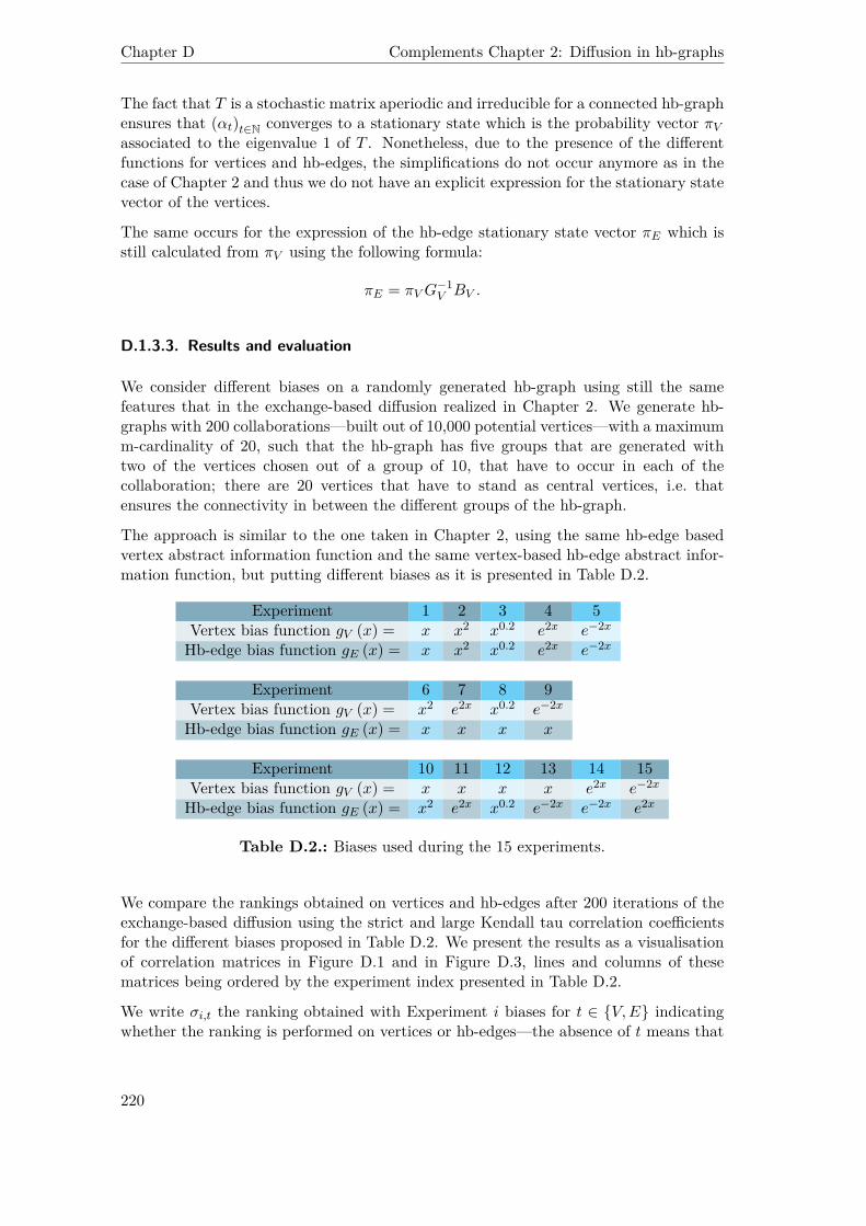
Chapter D Complements Chapter 2: Diffusion in hb-graphs
The fact that T is a stochastic matrix aperiodic and irreducible for a connected hb-graphensures that (αt)t∈N converges to a stationary state which is the probability vector πVassociated to the eigenvalue 1 of T . Nonetheless, due to the presence of the differentfunctions for vertices and hb-edges, the simplifications do not occur anymore as in thecase of Chapter 2 and thus we do not have an explicit expression for the stationary statevector of the vertices.
The same occurs for the expression of the hb-edge stationary state vector πE which isstill calculated from πV using the following formula:
πE = πVG−1V BV .
D.1.3.3. Results and evaluation
We consider different biases on a randomly generated hb-graph using still the samefeatures that in the exchange-based diffusion realized in Chapter 2. We generate hb-graphs with 200 collaborations—built out of 10,000 potential vertices—with a maximumm-cardinality of 20, such that the hb-graph has five groups that are generated withtwo of the vertices chosen out of a group of 10, that have to occur in each of thecollaboration; there are 20 vertices that have to stand as central vertices, i.e. thatensures the connectivity in between the different groups of the hb-graph.
The approach is similar to the one taken in Chapter 2, using the same hb-edge basedvertex abstract information function and the same vertex-based hb-edge abstract infor-mation function, but putting different biases as it is presented in Table D.2.
Experiment 1 2 3 4 5Vertex bias function gV (x) = x x2 x0.2 e2x e−2x
Hb-edge bias function gE (x) = x x2 x0.2 e2x e−2x
Experiment 6 7 8 9Vertex bias function gV (x) = x2 e2x x0.2 e−2x
Hb-edge bias function gE (x) = x x x x
Experiment 10 11 12 13 14 15Vertex bias function gV (x) = x x x x e2x e−2x
Hb-edge bias function gE (x) = x2 e2x x0.2 e−2x e−2x e2x
Table D.2.: Biases used during the 15 experiments.
We compare the rankings obtained on vertices and hb-edges after 200 iterations of theexchange-based diffusion using the strict and large Kendall tau correlation coefficientsfor the different biases proposed in Table D.2. We present the results as a visualisationof correlation matrices in Figure D.1 and in Figure D.3, lines and columns of thesematrices being ordered by the experiment index presented in Table D.2.
We write σi,t the ranking obtained with Experiment i biases for t ∈ {V,E} indicatingwhether the ranking is performed on vertices or hb-edges—the absence of t means that
220

D.1. Facets and Biased diffusion
it works for both rankings. The ranking obtained by Experiment 1 is the one of Chapter2, and is called the reference ranking.
In Experiments 2 to 5, the same bias is applied to both vertices and hb-edges. In Ex-periments 2 and 3, the biases are increasing functions on [0; +∞[ , while in Experiments4 and 5, they are decreasing functions.
Experiments 2 and 3 lead to rankings that are well correlated with the reference rankinggiven the large Kendall tau correlation coefficient value. The higher value of τL (σi, σj)compared to the one of τ (σi, σj) marks the fact that the rankings with pair of sim-ilar biases agree with the ties in this case. The exponential bias yields to a rankingthat is more granular in the tail for vertices, and reshuffles the way the hb-edges areranked; similar observations can be done for both the vertex and hb-edge rankings inExperiments 2 and 3.
In Experiments 4 and 5, the rankings remain well correlated with the reference rankingbut the large Kendall tau correlation coefficient values show that there is much lessagreement on the ties, but it is very punctual in the rankings, with again more discrim-ination with an exponential bias. This slight changes imply a reshuffling of the hb-edgerankings in both cases, significantly emphasized by the exponential form.
None of these simultaneous pairs of biases reshuffle very differently the rankings obtainedin the head of the rankings of vertices, but most of them have implications on the headof the rankings of the hb-edges: typical examples are given in Figure D.5. It would needfurther investigations using the Jaccard index.
Dissimilarities in rankings occur when the bias is applied only to vertices or to hb-edges. The strict Kendall tau correlation coefficients between the rankings obtainedwhen applying the bias of Experiments 6 to 9—bias on vertices—and 10 to 13—bias onhb-edges—and the reference ranking for the vertices show weak consistency for verticeswith values around 0.4—Figure D.1—, while the large Kendall tau correlation coefficientvalues show a small disagreement with values around -0.1—Figure D.2. For hb-edges,the gap is much less between the strict—values around 0.7 as shown in Figure D.3—andlarge Kendall tau correlation coefficient values—with values around 0.6 as shown inFigure D.4.
Biases with same monotony variations—gt (x) = x2 and gt (x) = e2x on the one hand andgt (x) = x0.2 and gt (x) = e−2x on the other hand—have similar effects independently oftheir application to vertices xor to hb-edges. It is also worth to remark that increasingbiases lead to rankings that have no specific agreement or disagreement with rankingsof decreasing biases—as it is shown with τL (σi, σj) and τ (σi, σj) for i ∈ J6; 13K .
We remark also that increasing biases applied only to vertices correlate with the corre-sponding decreasing biases applied only to hb-edges, and vice-versa. This is the case forExperiments 6 and 12, Experiments 7 and 13, Experiments 8 and 10, and Experiments9 and 11 for both vertices—Figures D.1 and D.2—and hb-edges—Figures D.3 and D.4.
Finally, we conduct two more experiments—Experiments 14 and 15—combining thebiases gt (x) = e2x and gt (x) = e−2x in two different manners. With no surprise,they reinforce the disagreement with the reference ranking both on vertices and hb-edges, with a stronger disagreement when the decreasing bias is put on vertices. Wecan remark that Experiment 14—gV (x) = e2x and gE (x) = e−2x—has the strongest
221

Chapter D Complements Chapter 2: Diffusion in hb-graphs
correlations with the rankings of dissimilar biases that are either similar to the one ofvertices—Experiments 6 and 7— or to the one of hb-edges—Experiments 12 and 13.
Figure D.1.: Strict Kendall tau correlation coefficient for node ranking with biases.Realized on 100 random hb-graphs with 200 hb-edges of maximal size 20, with 5groups.
A last remark is on the variability of the results: if the values of the correlation coef-ficients change, from one hb-graph to another, the phenomenon observed remains thesame, whatever the first hb-graph observed; however, the number of experiments per-formed ensures already a minimized fluctuation in these results.
D.1.3.4. Further comments
The biased-exchange-based diffusion proposed in this Chapter enhances a tunable diffu-sion that can be integrated into the hb-graph framework to tune adequately the rankingof the facets. The results obtained on randomly generated hb-graphs have still to beapplied to real hb-graphs, with the known difficulty of the connectedness: it will be ad-
222
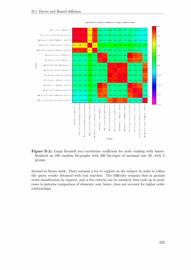
D.1. Facets and Biased diffusion
Figure D.2.: Large Kendall tau correlation coefficient for node ranking with biases.Realized on 100 random hb-graphs with 200 hb-edges of maximal size 20, with 5groups.
dressed in future work. There remains a lot to explore on the subject in order to refinethe query results obtained with real searches. The difficulty remains that in groundtruth classification by experts, only a few criteria can be retained, that ends up in mostcases in pairwise comparison of elements, and, hence, does not account for higher orderrelationships.
223
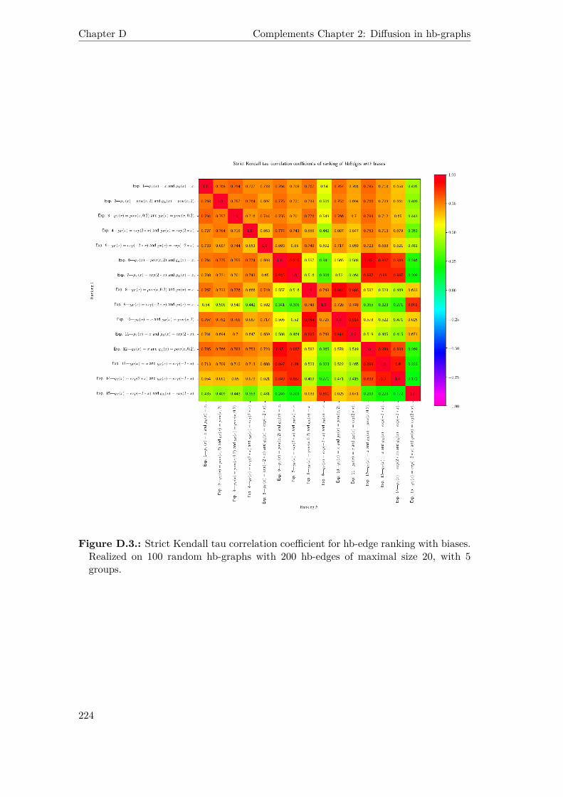
Chapter D Complements Chapter 2: Diffusion in hb-graphs
Figure D.3.: Strict Kendall tau correlation coefficient for hb-edge ranking with biases.Realized on 100 random hb-graphs with 200 hb-edges of maximal size 20, with 5groups.
224

D.1. Facets and Biased diffusion
Figure D.4.: Large Kendall tau correlation coefficient for hb-edge ranking with biases.Realized on 100 random hb-graphs with 200 hb-edges of maximal size 20, with 5groups.
225
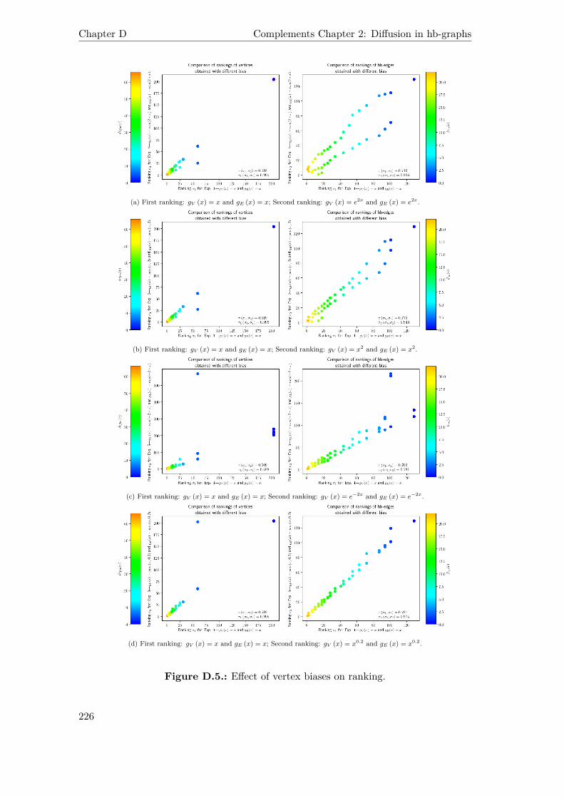
Chapter D Complements Chapter 2: Diffusion in hb-graphs
(a) First ranking: gV (x) = x and gE (x) = x; Second ranking: gV (x) = e2x and gE (x) = e2x.
(b) First ranking: gV (x) = x and gE (x) = x; Second ranking: gV (x) = x2 and gE (x) = x2.
(c) First ranking: gV (x) = x and gE (x) = x; Second ranking: gV (x) = e−2x and gE (x) = e−2x.
(d) First ranking: gV (x) = x and gE (x) = x; Second ranking: gV (x) = x0.2 and gE (x) = x0.2.
Figure D.5.: Effect of vertex biases on ranking.
226
E. Complements Chapter 3: e-adjacencytensor of natural hb-graphs
E.1. Building a tensor of e-adjacency for general hypergraphs
This chapter is based on [OLGMM17a]. A condensed version has been published in[OLGMM18a].Prerequisites: Section B.1 and B.3.
E.1.1. Motivation
An edge in a graph connects only two vertices while a hyperedge in a hypergraph en-ables multiple vertices to be connected. Recent improvements in tensor spectral theoryhave made the research on the spectra of hypergraphs more relevant. For studyingsuch spectra, a proper definition of general hypergraph Laplacian tensor is needed and,therefore, the concepts of adjacency and consequently of (—as it will be defined later—e-)adjacency tensor must be properly defined.In [Pu13], a clear distinction is made between the pairwise relationship which is a binaryrelation and the co-occurrence relationship which is presented as the extension of thepairwise relationship to a multi-adic relationship. The notion of co-occurrence is oftenused in linguistic data as the simultaneous appearance of linguistic units in a reference.The co-occurrence concept can be easily extended to vertices contained in a hyperedge:we designate it in hypergraphs by the term e-adjacency.Nonetheless, it is more than an extension. Graph edges connect vertices by pair: graphadjacency concept is clearly a pairwise relationship. For a given edge, only two verticescan be e-adjacent. Thus, adjacency and e-adjacency are equivalent in graphs.Extending the adjacency notion to hypergraphs, two vertices are said adjacent if thereexists a hyperedge that connects them. Hence, the adjacency notion still captures abinary relationship and can be modeled by an adjacency matrix. But, in this case,e-adjacency is no more a pairwise relationship, as, for a given hyperedge, more thantwo vertices can occur, since a hyperedge contains potentially multiple vertices. Also, amulti-adic relationship has to be captured and to be modeled using tensor. Hence, theadjacency matrix and the e-adjacency tensor of a hypergraph are two separated notions.Nonetheless, the e-adjacency tensor is often abusively named the adjacency tensor inthe literature.We aim at answering in this chapter the following research questions:
Research question E.1. What is the proper concept of adjacency for general hyper-graphs?

Chapter E Complements Chapter 3: e-adjacency tensor of natural hb-graphs
This research question aim is to redefine adjacency in hypergraphs, by considering dif-ferent kinds of adjacency.
Research question E.2. How to achieve the modeling of the newly defined adjacencyconcept with a tensor which not only preserves all the structural information of thehypergraph, but, also, captures separately the information on its hyperedges, and that isinterpretable in term of hypergraph-based process?
This second research question will bring us to consider an uniformisation process thattransforms a general hypergraph into a uniform hypergraph, and that will lead to defin-ing a new (e-)adjacency tensor which will not solely preserve all the structural infor-mation of the hypergraph, but, also, will capture separately the information on itshyperedges.After sketching the background and the related work on the adjacency and e-adjacencyconcepts for hypergraphs in Section E.1.3, we propose a new unnormalized e-adjacencytensor in Section E.1.4. Section E.1.5 tackles the particular case of graphs seen as 2-uniform hypergraphs and the link with the Disjunctive Normal Form (DNF for short).Some additional comments are addressed in Section E.1.7. A full example is given inAppendix E.2.2.
Notation Exponents are indicated into parenthesis—for instance y(n)—when they referto the order of the corresponding tensor. Indices are written into parenthesis when theyrefer to a sequence of objects—for instance a(k)ij is the elements at row i and column jof the matrix A(k). The context should make it clear.For the convenience of readability, we write z0 for z1, ..., zn. Hence given a polynomialP, P (z0) has to be understood as P
(z1, ..., zn
).
Given additional variables y1, ..., yk, we write zk for z1, ..., zn, y1, ..., yk.
Sk is the set of permutations on the set JkK .
Hypergraph basic definitions are reminded in Chapter B. In this chapter, we make thefollowing postulate:
Postulate E.1. The hypergraphs considered are undirected and with no repeated hyper-edges.
E.1.2. Adjacency in hypergraphs
We consider a hypergraph H = (V,E), with V = {vi : i ∈ JnK} and E = (ej)j∈JpK , andtwo vertices vi1 ∈ V and vi2 ∈ V with i1 ∈ JnK and i2 ∈ JnK . Traditionally, vi1 and vi2are said adjacent if there exists e ∈ E such that vi1 ∈ e and vi2 ∈ e. This adjacency isa pairwise concept.To switch to a higher order concept of adjacency, we consider an integer k > 1 and kvertices vij , with ij ∈ JnK for all j ∈ JkK and say that vi1 , ..., vik are k-adjacent if thereexists e ∈ E such that for all j ∈ JkK , vij ∈ e.With k = 2, the usual notion of adjacencyis retrieved.Trivially:
228
E.1. Building a tensor of e-adjacency for general hypergraphs
Proposition E.1. If k vertices are k-adjacent, then any subset of these k vertices ofsize l 6 k is l-adjacent.
The maximal k-adjacency a hypergraph can support is called the k-adjacency. As themaximal number of vertices a hyperedge can have in a general hypergraph correspondsto the rank of this hypergraph, the k-adjacency corresponds to rH-adjacency.
We now consider a hyperedge e ∈ E. The vertices constituting e are said e-adjacentvertices.
If the hypergraph is k-uniform, then the k-adjacency is exactly the k-adjacency and isequivalent to the e-adjacency of vertices in a hyperedge.
For a general hypergraph, if it is true that k-adjacency implies e-adjacency, the reciprocalis no longer true, as any hyperedge e ∈ E such that |e| < rH
1 does not hold anyk-adjacent vertices. In this case, the notions of k-adjacency and of e-adjacency aredefinitively distinct.
E.1.3. Background and related work
E.1.3.1. The matrix approach
In Section B.1.7.2, we already mentioned that the adjacency matrix does not keep themulti-adicity. The adjacency matrix captures only links between pair of vertices: this isequivalent to extend the hypergraph to its 2-section and to capture the information ofthe corresponding graph. Therefore, the multi-adicity cannot be captured by a matrix.
Following a lemma cited in [DPP16], the following lemma can be enunciated:
Lemma E.1. Let H = (V,E) be a hypergraph and let vi1 , vi2 ∈ V. If vi1 and vi2 are2-adjacent in H, then they are adjacent in the 2-section [H]2 .
Reciprocally, two vertices that are adjacent in the 2-section of a hypergraph are also 2-adjacent in the hypergraph. Nonetheless, it doesn’t imply any isomorphism between Hand [H]2: [H]2 appears as an equivalence class of the equivalence relation R defined onthe set of hypergraphs with no loop, where two hypergraphs are in relation by R, if theyhave the same graph as 2-section. Therefore, the 2-section of a hypergraph correspondsto an equivalence class of 2-adjacency.
Moving to the concept of e-adjacency will preserve the higher order relationships heldin the hypergraph.
E.1.3.2. Existing k and e-adjacency tensors
In [MN12], an unnormalized version of the k−adjacency tensor of a k-uniform hyper-graph is given. This definition is also adopted in [GD17].1rH is the rank of the hypergraph H as defined in Section B.1.3.
229

Chapter E Complements Chapter 3: e-adjacency tensor of natural hb-graphs
Definition E.1. The unnormalized [k-]adjacency tensor of a k-uniform hypergraphH = (V,E) on a finite set of vertices V = {vi : i ∈ JnK} and a family of hyperedges E =(ej)j∈JpK of equal cardinality k is the tensor Araw of CHR Araw = (araw i1...ik)i1,...,ik∈JnKsuch that:
araw i1...ik ={
1 if {vi1 , ..., vik} ∈ E;0 otherwise.
In [CD12], a slightly different version exists for the definition of the adjacency tensor,called the degree normalized k-adjacency tensor.
Definition E.2. The [degree normalized k-]adjacency tensor of a k-uniform hyper-graph H = (V,E) on a finite set of vertices V = {vi : i ∈ JnK} and a family of hyperedgesE = (ej)j∈JpK of equal cardinality k is the tensor A of CHR A = (ai1...ik)i1,...,ik∈JnK suchthat:
ai1...ik = 1(k − 1)!
{1 if ∃e ∈ E : e = {vi1 , ..., vik} ;0 otherwise.
Introducing in this definition, the coefficient 1(k − 1)! allows to retrieve the degree of a
vertex vi summing the elements of index i on the first mode of the tensor. Hence, wecall it the degree normalized adjacency tensor.
Proposition E.2. Let H = (V,E) be a k-uniform hypergraph. Let vi ∈ V be avertex. It holds by considering the degree normalized k−adjacency tensor A of CHRA = (ai1...ik)i1,...,ik∈JnK :
deg (vi) =∑
i2,...,ik∈JnK
aii2...ik .
Proof. On the first mode of the degree normalized adjacency tensor, for a given vertexvi that occurs in a hyperedge e = {vi, vi2 , ..., vik} , the elements aiσ(i2)...σ(ik) = 1
(k − 1)! ,
where σ ∈ Sk−1, exist in quantity (k − 1)! in the first mode. Hence ∑σ∈Sk−1
aiσ(i2)...σ(ik) =
1.
Repeating it for all hyperedges where vi is an element retrieves the degree of vi.
This definition could be interpreted as the definition of the e-adjacency tensor for auniform hypergraph since the notion of k-adjacency and e-adjacency are equivalent ina k-uniform hypergraph.
In [Hu13], a full study of the spectra of an uniform hypergraph using the Laplaciantensor is given. The definition of the Laplacian tensor is linked to the existence anddefinition of the normalized [k-]adjacency tensor.
230

E.1. Building a tensor of e-adjacency for general hypergraphs
Definition E.3. The [eigenvalues] normalized [k-]adjacency tensor of a k-uniformhypergraph H = (V,E) on a finite set of vertices V = {vi : i ∈ JnK} and a family of hyper-edges E = (ej)j∈JpK of equal cardinality k is the tensor A of CHR A = (ai1...ik)i1,...,ik∈JnKsuch that:
ai1...ik =
1
(k − 1)!∏
16j6k
1k
√dij
if {vi1 , ..., vik} ∈ E;
0 otherwise.
The aim of the normalization is motivated by the need of bounding the different tensoreigenvalues.
The normalized Laplacian tensor L is given in the following definition.
Definition E.4. The normalized Laplacian tensor of a k-uniform hypergraph H =(V,E) on a finite set of vertices V = {vi : i ∈ JnK} and a family of hyperedges E =(ej)j∈JpK of equal cardinality k is the tensor L = I − A where I is the k-th order n-dimensional diagonal tensor of CHR that has its j-th diagonal element ij...j = 1 if dj > 0and 0 otherwise.
In [BCM17], the definition of the [e-]adjacency tensor is extended to general hyper-graphs. The information on hyperedges of lower cardinality is spread inside the tensor.This approach focuses on the spectra of the constructed hypermatrix.
Definition E.5. Let H = (V,E) be a general hypergraph on a finite set of verticesV = {vi : i ∈ JnK} and a family of hyperedges E = (ej)j∈JpK of rank rH.
The [e-]adjacency hypermatrix of H written BH of CHR:
BH =(bi1...irH
)16i1,...,irH6n
is such that for a hyperedge: e = {vl1 , ..., vls} of cardinality s 6 rH, we have:
bp1...prH= s
α, where α =
∑k1,...,ks>1∑i∈JsK
ki=rH
rH!k1!...ks!
with p1, ..., prH chosen in all possible ways from {l1, ..., ls} with at least once from eachelement of {l1, ..., ls} .
The other values of the hypermatrix are zero.
The e-adjacency cubical hypermatrix of order the rank of the hypergraph rH is keptat a dimension corresponding to the number of vertices n at the cost of splitting theinformation of the hyperedges in a varying number of elements of the tensor dependingon the hyperedge cardinalities. A hyperedge e, of cardinality #e = s, is represented bya set of elements in the tensor whose indices correspond to permutations of the differentmultisets
{{lkii , i ∈ JsK
}}such that: ∀i, ki > 1 and ∑
i∈JsKki = rH, i.e. all the multisets
231
Chapter E Complements Chapter 3: e-adjacency tensor of natural hb-graphs
that can be built of universe {l1, ..., ls} and of support {l1, ..., ls} and m-cardinality rH.A detailed example is given in Appendix E.2.1.
We will come back to the consequences of filling the tensor elements this way in Chapter4.
A s-composition of an integer m is a tuple (ki)i∈JsK such that ∑i∈JsK
ki = m.
Let (ki)i∈JsK be a s-composition of rH with ki > 1 for all i ∈ JsK . Then the numberof combinations of rH elements of {l1, ..., ls} , at least repeated once and following thedistribution given by (ki)i∈JsK , is given by the multinomial coefficient:(
rHk1 ... ks
)= rH!∏
i∈JsKki!.
We now focus on the number of compositions ps(m) of an integer m in s ordered parts.A composition of an integer is a tuple. This is equivalent to putting s− 1 sticks in thespace between two stones of a line of m stones, i.e. in m− 1 spaces. We have then:
ps (m) =(m− 1s− 1
)
possibilities to do it.
Hence for representing a single hyperedge of cardinality s, ps (rH) partitions (ki)i∈JsK ofrH are involved, each of them implies to fill:(
rHk1 ... ks
)= rH!∏
i∈JsKki!
elements of the tensor.
It is worth mentioning another definition of e-adjacency tensor that has been recentlypublished in [SZB19].
Definition E.6. The [prefixed e-]adjacency tensor—written SH—of a general hy-pergraph H = (V,E) , with V as vertex set—[identified to JnK]—and E as hyperedgeset is the cubical tensor of CHR SH =
(si1...irH
)of order rH and dimension |V | with
entries:
si1...irH =
1
(s− 1)! i1 = ... = ik−s+1, {ik−s+1, ..., ik} ∈ E;
0 otherwise.
This definition has the advantage of reducing the number of elements that containinformation, at the cost of having a non-symmetric hypermatrix.
In this Thesis, the proposed method to elaborate an e-adjacency tensor focuses on thefact that the construction is interpretable: a uniformisation process is proposed in whicha general hypergraph is transformed into a uniform hypergraph by adding elements. Thestrong link made with homogeneous polynomials reinforces the choice made and allows
232
E.1. Building a tensor of e-adjacency for general hypergraphs
to retrieve a proper matrix of a uniform hypergraph at the end of the process. Theadditional vertices help capturing not solely the e-adjacency but also give the ability tohold the information on k-adjacency at whatever level it occurs.
The approach is based on the homogenization of sums of polynomials of different degreesand by considering a family of uniform hypergraphs. It is also motivated by the factthat the information on the cardinality of the hyperedges has to be kept in some waysand, that the elements should not be mixed with the different layers of the hypergraph.
E.1.4. Towards an e-adjacency tensor of a general hypergraph
To build an e-adjacency tensor for a general hypergraph, we need a way to store elementswhich represent the hyperedges. As these hyperedges have different cardinalities, therepresentation of the e-adjacency for vertices in a unique tensor can be achieved only byfilling the hyperedges with additional elements. The problem of finding an e-adjacencytensor of a general hypergraph is then transformed into a uniformisation problem.
This uniformisation process should be at least interpretable in term of uniform hyper-graphs. It should capture the structural information of the hypergraph, which includesinformation on the number of hyperedges, degrees of vertices and additional informationon the main features of the hypergraph.
We propose a framework based on homogeneous polynomials that are iteratively summedby weighting with technical coefficients and homogenized. This uniformisation processallows the construction of a weighted uniform hypergraph. The technical coefficients areadjusted such that the handshake lemma holds in the constructed uniform hypergraph.
E.1.4.1. Family of tensors attached to a hypergraph
Let H = (V,E) be a hypergraph. A hypergraph can be decomposed in a family ofuniform hypergraphs.
To achieve it, let R be the equivalency relation: eRe′ ⇔ |e| = |e′| .
E/R is the set of classes of hyperedges of same cardinality. The elements of E/R arethe sets: Ek
∆= {e ∈ E : |e| = k} .
Considering K = {k : Ek ∈ E/R} , we set Ek∆= ∅ for all k ∈ JrHK \K.
Let us consider the hypergraphs: Hk∆= (V,Ek) for all k ∈ JrHK which are all k-uniform.
It holds that: E = ⋃k∈JrHK
Ek and Ej ∩Ek = ∅ for all j 6= k, hence the family (Ek)k∈JrHK
forms a partition of E which is unique by the way it has been defined.
Hence:H =
⊕k∈JrHK
Hk.
The hypergraph H is said to be decomposed into a family of hypergraphs (Hk)k∈JrHKwhere Hk is k-uniform.
233

Chapter E Complements Chapter 3: e-adjacency tensor of natural hb-graphs
An illustration of the decomposition of a hypergraph into a family of uniform hyper-graphs is shown in Figure E.1. This family of uniform hypergraphs decomposes theoriginal hypergraph in layers. A layer holds a k-uniform hypergraph—with k ∈ JrHK—:therefore, the layer is said to be of level k.
Figure E.1.: Illustration of a hypergraph decomposed in three layers of uniform hy-pergraphs.
At each k-uniform hypergraph Hk can be mapped a (k-adjacency) e-adjacency tensorAk with CHR Ak of order k which is hyper-cubic and symmetric of dimension |V | = n.This hypermatrix can be unnormalized or normalized, but this choice has to be madethe same for the whole family of Hk.
Once chosen a type of tensor—normalized or unnormalized—, the hypergraph H is thenfully described by the family of e-adjacency tensors AH = (Ak) . In the case where allthe Ak are chosen normalized, this family is said pre-normalized. The final choice willbe made further in Section E.1.4.7 and explained to fulfill the expectations listed in thenext section.
E.1.4.2. Expectations for an e-adjacency tensor for a general hypergraph
The definition of the family of tensors attached to a general hypergraph has the ad-vantage to open the way to the spectral theory for uniform hypergraphs which is quiteadvanced.
Nonetheless, many problems remain in keeping a family of tensors of different orders:for instance, studying the spectra of the whole hypergraph could be hard to achieve bythis means. Also, it is necessary to get an e-adjacency tensor for the whole hypergraphwhich retains the information on the whole structure.
The underlying idea is to “fill” the hyperedges with sufficient elements such that thegeneral hypergraph is transformed into an uniform hypergraph through a uniformisationprocess. A similar approach has been taken in [BCM17] where the filling elements arethe vertices belonging to the hyperedge itself, involving a hb-graph m-uniformisation,as we will tackle it in Chapter 3. In the next sections, the justification of the approachtaken will be made via homogeneous polynomials. Before getting to the construction,expected properties of such a tensor have to be listed.
234
E.1. Building a tensor of e-adjacency for general hypergraphs
Expectation E.1. The tensor should be symmetric and its generation should be simple.
This expectation emphasizes the fact that in between two constructed e-adjacency ten-sors, the one that can be easily generated has to be chosen: this includes the fact thatthe tensor has to be described in a simple way.
Expectation E.2. The unnormalized e-adjacency tensor keeps the overall structure ofthe hypergraph.
This expectation emphasized the fact that the e-adjacency tensor should help to retrievethe different layers of the hypergraph, in such a way that it respects the structure ofeach layer.
Expectation E.3. The e-adjacency tensor should allow the retrieval of the vertex de-grees.
In the adjacency matrix of a graph, the information on the vertex degrees is encodeddirectly. It is still the case with the k-adjacency degree normalised tensor defined by[Sha13] and [PZ14].
Expectation E.4. The e-adjacency tensor should allow the retrieval of the number ofhyperedges of same cardinality.
This expectation is linked with the expectation on the keeping of the overall structureof the hypergraph.
Expectation E.5. The tensor should be invariant to vertex permutations either globallyor at least locally.
This expectation is motivated by the fact that in a hyperedge the vertices have noorder. This expectation can be local, since the special vertices will not have the samestatus than the ones of the original hypergraph. Also, the invariance by permutation isexpected on the vertices of the original hypergraph.
Expectation E.6. The e-adjacency tensor should allow the unique retrieval of thehypergraph it is originated from.
This expectation seems important when rebuilding the original hypergraph from its e-adjacency tensor. Hence, all the necessary information to uniquely retrieve the originalhyperedges has to be encoded in the tensor.
Expectation E.7. Giving the choice of two representations the e-adjacency tensorchosen should be the sparsest one.
Sparsity enables information compression, and lowers both the space and the complexitycalculus. Also, sparsity is a desirable property for some statistical reasons as shown in[Nik00] or expected in [BDE09] for signal processing and image encoding.
235

Chapter E Complements Chapter 3: e-adjacency tensor of natural hb-graphs
E.1.4.3. Tensors family and family of homogeneous polynomials
To construct a homogeneous polynomial representing a general hypergraph, the familyof e-adjacency tensors obtained in the previous section has to be mapped to a familyof homogeneous polynomials. This mapping is used in [CQU15] where the author linkssymmetric tensors and homogeneous polynomials of degree s to show that the problemof the CP decomposition of different symmetric tensors of different orders and thedecoupled representation of multivariate polynomial maps are related.
Homogeneous polynomials family of a hypergraph We consider a hypergraph H withits family of unnormalized tensor AH = (Ak) of CHR which is cubical and symmetric oforder k and dimension n. We can also attach to H a family PH = (Pk) of homogeneouspolynomials with deg (Pk) = k. To achieve this, we consider a vector z ∈ Kn andthe multilinear matrix multiplication defined in B.3.2: it holds that (z)[k].Ak—with(z)[k]
∆= (z, ..., z) ∈ (Kn)k—contains only one element written Pk(z1, ..., zn
)= Pk (z0)
such that:Pk (z0) =
∑i1,...,ik∈JnK
a(k) i1...ikzi1 ...zik . (E.1)
The formulation of Pk can be reduced taking into account that Ak is symmetric for auniform hypergraph:
Pk (z0) =∑
16i16...6ik6nk!a(k) i1...ikz
i1 ...zik . (E.2)
Writing:Pk (z0) =
∑16i16...6ik6n
a(k) i1...ikzi1 ...zik . (E.3)
the reduced form of Pk, it holds:
Pk (z0) = k!Pk (z0) .
Writing for 1 6 i1 6 ... 6 ik 6 n:
α(k) i1...ik∆= k!a(k) i1...ik
and: α(k)σ(i1)...σ(ik)∆= 0 for σ ∈ Sk, σ 6= Id.
It holds:
Pk (z0) =∑
16i16...6ik6nα(k) i1...ikz
i1 ...zik
=∑
16i1,...,ik6nα(k) i1...ikz
i1 ...zik . (E.4)
and:Pk (z0) =
∑16i16...6ik6n
α(k) i1...ikk! zi1 ...zik . (E.5)
236
E.1. Building a tensor of e-adjacency for general hypergraphs
Reversibility of the process Reciprocally, given a homogeneous polynomial of degreek, a unique hyper-cubic tensor of order k can be built: its dimension is the numberof different variables in the homogeneous polynomial. If the homogeneous polynomialof degree k is supposed reduced and ordered, then only one hyper-cubic and symmet-ric hypermatrix can be built. It reflects uniquely a k-uniform hypergraph adding theconstraint that each monomial is composed of the product of k different variables.
Proposition E.3. Let P (z0) = ∑i1,...,ik∈JnK
ai1...ikzi1 ...zik be a homogeneous polynomial
of degree k where:
• for j 6= k : zj 6= zk;
• for all j ∈ JnK : deg(zj)
= 1;
• and such that for all σ ∈ Sk : aσ(i1)...σ(ik) = ai1...ik .
Then P is the homogeneous polynomial attached to a unique k-uniform hypergraph H =(V,E,w)—up to the indexing of vertices.
Proof. Considering the vertices (vi)i∈JnK labeled by the elements of JnK .
If ai1...ik 6= 0, then for all σ ∈ Sk : aσ(i1)...σ(ik) a unique hyperedge ej is attachedcorresponding to the vertices vi1 , ..., vik and which has weight w(ej) = kai1...ik .
E.1.4.4. Uniformisation and homogenization processes
A single tensor is always easier to use than a family of tensors; the same applies for ho-mogeneous polynomials. Building a single tensor from tensors of different order requiresto fill in the “gaps”; summing homogeneous polynomials of varying degrees always givesa new polynomial: but, most frequently, this polynomial is not anymore homogeneous.Homogenization techniques for polynomials are wellknown and require additional vari-ables.
Different homogenization processes can be envisaged to get a homogeneous polynomialthat represents a single cubic and symmetric tensor by making different choices on thevariables added in the homogenization phase. As a link has been made between the vari-ables and the vertices of the hypergraph, we want that this link continues to occur duringthe homogenization of the polynomial as each term of the reduced polynomial corre-sponds to a unique hyperedge in the original hypergraph; the homogenization process isinterpretable in terms of hypergraph uniformisation process of the original hypergraph:hypergraph uniformisation process and polynomial homogenization process are the twosides of the same coin.
So far, we have separated the original hypergraph H in layers of increasing k-uniformhypergraphs Hk such that:
H =⊕
k∈JrHK
Hk.
Each k-uniform hypergraph can be represented by a symmetric and cubic tensor. Thissymmetric and cubic tensor is mapped to a homogeneous polynomial. The reduced
237

Chapter E Complements Chapter 3: e-adjacency tensor of natural hb-graphs
homogeneous polynomial is interpretable, if we omit the coefficients of each term, as adisjunctive normal form. Each term of the homogeneous polynomial is a conjunctiveform which corresponds to simultaneous presence of vertices in a hyperedge: adding allthe layers allows to retrieve the original hypergraph; adding the different homogeneouspolynomials allows to retrieve the disjunctive normal form associated with the originalhypergraph.In the hypergraph uniformisation process, iterative steps are done starting with the lowerlayers to the upper layers of the hypergraph. In parallel, the polynomial homogenizationprocess is the algebraic justification of the hypergraph uniformisation process. It allowsto retrieve a polynomial attached to the uniform hypergraph built at each step andhence a tensor.
Hypergraph uniformisation process We can describe algorithmically the hypergraphuniformisation process: it transforms the original hypergraph in a uniform hypergraph.
Initialisation The initialisation requires that each layer hypergraph is associated to aweighted hypergraph.To each uniform hypergraphHk, we associate a weighted hypergraphHwk,k = (V,Ek, wk) ,with: ∀e ∈ Ek : wk(e) = ck, ck ∈ R+∗.
The coefficients ck are technical coefficients that will be chosen when considering thehomogenization process and the fulfillment of the expectations of the e-adjacency tensor.The coefficients ck can be seen as dilatation coefficients only dependent of the layers ofthe original hypergraph.We initialize: k := 1 and Kw := Hw1,1 and generate rH − 1 distinct vertices yj , j ∈JrH − 1K that are not in V.
Iterative steps Each step in the hypergraph uniformisation process includes threephases: an inflation phase, a merging phase and a concluding phase.
Inflation phase: The inflation phase consists in increasing the cardinality of eachhyperedge obtained from the hypergraph built at the former step to reach the cardinalityof the hyperedges of the second hypergraph used in the merge phase.We define a first operation that consists in inflating each hyperedge of the hypergraphwith an additional vertex that does not belong to the original vertex to obtain a vertex-augmented hypergraph.
Definition E.7. The y-vertex-augmented hypergraph of a weighted hypergraphHw = (V,E,w) is the hypergraph Hw
∆=(V ,E,w
)obtained by the following rules:
• y /∈ V ;
• V∆= V ∪ {y} ;
• Writing φ : P (V ) → P(V)the map such that for A ∈ P (V ) : φ(A) = A ∪ {y} ,
it holds:
238
E.1. Building a tensor of e-adjacency for general hypergraphs
– E∆= {φ (e) : e ∈ E} ;
– ∀e ∈ E, w (φ(e)) ∆= w(e).
Proposition E.4. The vertex-augmented hypergraph of a k-uniform hypergraph is ak + 1-uniform hypergraph.
The inflation phase at step k generates from Kw the yk-vertex augmented hypergraphKw.
As Kw is k-uniform at step k, Kw is k + 1-uniform.
Merging phase: The merging phase generates the sum of two weighted hypergraphscalled the merged hypergraph.
We start by defining the merging operation of two hypergraphs.
Definition E.8. The merged hypergraph Hw∆=(V , E, w
)of two weighted hyper-
graphs Ha = (Va, Ea, wa) and Hb = (Vb, Eb, wb) is the weighted hypergraph defined asfollow:
• V∆= Va ∪ Vb;
• Ek+1∆= Ea ∪ Eb;
• ∀e ∈ Ea : w(e) ∆= wa(e) and ∀e ∈ Eb : w(e) ∆= wb.
The merging phase at step k generates from Kw and Hwk+1,k+1 the merged hypergraphKw. As it is generated from two k + 1-uniform hypergraphs, it is also a k + 1-uniformhypergraph.
Ending phase: If k equals rH − 1, the iterative part ends and returns Kw.
Otherwise, a next step is needed with Kw := Kw and k := k + 1.
Termination: We obtain by this algorithm a weighted rH-uniform hypergraph asso-ciated to H which is the returned hypergraph from the iterative part: we write itHw =
(V , E, w
).
Definition E.9. Writing Vs = {yj : j ∈ JrH − 1K} , Hw∆=(V , E, w
)is called the Vs-
layered uniform of H.
Proposition E.5. Let H = (V,E) be a hypergraph of order rH.
Let consider Vs = {yj : j ∈ J1, rH − 1K} such that V ∩ Vs = ∅ and let Hw =(V , E, w
)be the Vs-layered uniform of H. Then:
• (V, Vs) is a partition of V ;
239

Chapter E Complements Chapter 3: e-adjacency tensor of natural hb-graphs
• ∀e ∈ E,∃!e ∈ E : e ⊆ e ∧ e\e = {yj : j ∈ J|e| , rH − 1K} .
Proof. The way the Vs-layered uniform of H is generated justifies the results.
Proposition E.6. Let H = (V,E) be a hypergraph of order rH.Let consider Vs,i = {yj : j ∈ JrH − 1K} such that Vs = ⋃
i∈JrH−1KVs,i, V ∩ Vs = ∅ and let
Hw =(V , E, w
)be the Vs-layered uniform of H.
Then, the vertices of H that are e-adjacent in H in a hyperedge e are e-adjacent withthe vertices of Vs,|e| in Hw.
Reciprocally, if vertices are e-adjacent in Hw, the ones that are not in Vs are e-adjacentin H.
As a consequence, Hw captures the e-adjacency of H.
Polynomial homogenization process In the polynomial homogenization process, webuild a new family RH = (Rk) of homogeneous polynomials of degree k iteratively fromthe family of homogeneous polynomials PH = (Pk) by following the subsequent stepsthat respect the construction phases in Figure E.2. Each of these steps can be linkedto the steps of the homogenization process.
HHypergraph
uniformisation process
(Hk)Uniform hypergraphs
layers of H
(Tk)Family
of tensors
PkFamily of homogeneous
polynomials
×ck
+
if k < kmaxR1 = c1P1If k > 1:
Rk = ckPk +Rk−1yk−1
Homogeneouspolynomial of
aggregated layersof level 1 to k
RkmaxGlobal homogeneouspolynomial of H
ifk = kmax
Te-adjacencytensor of H
Figure E.2.: Construction phases of the e-adjacency tensor.
Initialisation Each polynomial Pk, k ∈ JrHK attached to the corresponding layer k-uniform hypergraph Hk is multiplied by a coefficient ck equal to the corresponding di-latation coefficient of the hypergraph uniformisation process as discussed further in Sec-tion E.1.4.6. ckPk represents the reduced homogeneous polynomial attached to Hwk,k.
240
E.1. Building a tensor of e-adjacency for general hypergraphs
Using the notations zk−1 and z0 as defined in E.1.1, we initialize: k := 1 and:
Rk (zk−1) = R1 (z0) = c1P1 (z0) = c1
n∑i=1
a(1) izi.
We generate rH − 1 distinct 2 by 2 variables yj , j ∈ JrH − 1K that are also pairwisedistinct from the zi, i ∈ JnK .
Iterative steps At each step, we sum the current Rk (zk−1) with the next layer coeffi-ciented polynomial ck+1Pk+1 in a way to obtain a homogeneous polynomial Rk+1 (zk) .To help the understanding we describe the first step, then generalize to any step.
Case k = 1: To build R2, an homogenization of the sum of R1 and c2P2 is needed. Itholds:
R1 (z0) + c2P2 (z0) = c1∑i∈JnK
a(1) izi + c2
∑i1,i2∈JnK
a(2) i1i2zi1zi2 .
To achieve the homogenization of R1 (z0) + c2P2 (z0) , a new variable y1 is introduced.
It follows for y1 6= 0 :
R2 (z1) = R2(z0, y
1)
= y1(2)(R1
(z0y1
)+ c2P2
(z0y1 (2)
))= c1
∑i∈JnK
a(1) iziy1 + c2
∑i1,i2∈JnK
a(2) i1i2zi1zi2 .
By continuous prolongation of R2, it is set:
R2 (z0, 0) = c2∑
i1,i2∈JnK
a(2) i1i2zi1zi2 .
In this step, the weighted degree 1 polynomial R1 (z0) = c1P1 (z0) attached to Hw1,1 istransformed in a degree 2 homogeneous polynomial y1R1 (z0) = c1y
1P1 (z0) : y1R1 (z0)corresponds to the homogeneous polynomial of the weighted y1-vertex-augmented 1-uniform hypergraph Hw1,1 built during the inflation phase in the hypergraph uniformi-sation process.
y1R1 (z0) is then summed with the homogeneous polynomial c2P2 attached to Hw2,2to get a homogeneous polynomial of degree 2: R2 (z1) . R2 (z1) is the homogeneouspolynomial of the merged 2-uniform hypergraph Hw1,1 of Hw1,1 and Hw2,2.
General case: Assuming that Rk (zk−1) is a homogeneous polynomial of degree k thatcan be written as:
Rk (zk−1) =∑j∈JkK
cj∑
i1,...,ij∈JnK
a(j) i1...ijzi1 ...zij
k−1∏l=j
yl,
with the convention that:k−1∏l=j
yl = 1 if j > k − 1 and zk−1 = z1, ..., zn, y1, ..., yk−1.
241

Chapter E Complements Chapter 3: e-adjacency tensor of natural hb-graphs
Rk+1 is built as a homogeneous polynomial from the sum of Rk and ck+1Pk+1 by addinga variable yk and factorizing by its k + 1-th power.Therefore, for yk−1 6= 0 :
Rk+1 (zk) = yk (k+1)(Rk
(zk−1yk (k)
)+ ck+1Pk+1
(z0
yk (k+1)
))
=
∑j∈JkK
cj∑
i1,...,ij∈JnK
a(j) i1...ijzi1 ...zij
k−1∏l=j
yl
yk+ck+1
∑i1,...,ik+1∈JnK
a(k+1) i1 ... ik+1zi1 ...zik+1 .
And for yk = 0, it is set by continuous prolongation:
Rk+1 (zk−1, 0) = ck+1∑
i1,...,ik+1∈JnK
a(k+1) i1 ... ik+1zi1 ...zik+1 .
The fact that Pk+1 (z0) can be null does not prevent to do the step: the degree of Rkwill then be elevated of 1.The interpretation of this step is similar to the one done for the case k = 1.
End step phase: If k equals rH − 1, the iterative part ends up, else k := k + 1 and,the next iteration is started.
Conclusion: The algorithm build a family of homogeneous polynomial which is inter-pretable in term of uniformisation of a hypergraph.
E.1.4.5. Building an unnormalized symmetric tensor from this family ofhomogeneous polynomials
Based on RH :It is now insightful to interpret the built polynomials.The notation w(k) = w1
(k), ..., wn+k−1(k) is used, with for i ∈ JnK : wi(k) = zi and for
j ∈ Jk − 1K : wn+j(k) = yj .
• The interpretation of R1 is trivial as it holds the single element hyperedges of thehypergraph;
• R2 is a homogeneous polynomial with n+ 1 variables of order 2:
R2 (z1) = c1∑i∈JnK
a(1) iziy1 + c2
∑i1,i2∈JnK
a(2) i1i2zi1zi2
= c1∑i∈JnK
α(1) iziy1 + c2
∑16i16i26n
α(2) i1i2zi1zi2 .
It can be rewritten:
R2(w(2)
)=
∑i1,i2∈Jn+1K
r(2) i1i2wi1(2)w
i2(2)
where:
242
E.1. Building a tensor of e-adjacency for general hypergraphs
– for 1 6 i1 6 i2 6 n and σ ∈ S2 :
r(2)σ(i1)σ(i2) =c2α(2) i1i2
2! = c2a(2) i1i2 ;
– for i ∈ JnK and σ ∈ S2 :
r(2)σ(i)σ(n+1) =c1α(1) i
2! =c1a(1) i
2! ;
– the other coefficients: r(2) i1i2 are null.Also R2 can be linked to a symmetric hyper-cubic tensor of order 2 and dimensionn+ 1.
• Rk is a homogeneous polynomial with n+ k − 1 variables of order k.
Rk (zk−1) =∑j∈JkK
cj∑
i1,...,ij∈JnK
a(j) i1...ijzi1 ...zij
k−1∏l=j
yl
=∑j∈JkK
cj∑
16i16...6ij6nα(j) i1...ijz
i1 ...zijk−1∏l=j
yl
with the convention that:k−1∏l=j
yl = 1 if j > k − 1.
It can be rewritten:
Rk(w(k)
)=
∑i1,...,ik∈Jn+k−1K
r(k) i1 ... ikwi1(k)...w
ik(k),
where:– for 1 6 i1 6 ... 6 ik 6 n, for all j ∈ Jk − 1K , for all σ ∈ Sk :
∗ r(k)σ(i1)...σ(ik) =ckα(k) i1...ik
k! = cka(k) i1...ik ;
∗ r(k)σ(i1)...σ(ij)σ(n+j)...σ(n+k−1) =cjα(j) i1...ij
k! = j!k!cja(j) i1...ij ;
– the other elements r(k) i1 ... ik are null.Also Rk can be linked to a symmetric hyper-cubic tensor of order k and dimensionn+ k − 1 written Rk whose elements are r(k) i1 ... ik .
The hypermatrix RrH is called the unnormalized e-adjacency hypermatrix.
E.1.4.6. Interpretation and choice of the coefficients for the unnormalized tensor
There are different ways of setting the coefficients c1, ..., ckmax that are used. Thesecoefficients can be seen as a way of normalizing the tensors of e-adjacency generatedfrom the k-uniform hypergraphs.A first way of choosing them is to set them all equal to 1. In this case, no normalizationoccurs. The impact on the e-adjacency tensor of the original hypergraph is that e-adjacency in hyperedges of size k have a weight of k times bigger than the e-adjacencyin hyperedges of size 1.
243

Chapter E Complements Chapter 3: e-adjacency tensor of natural hb-graphs
A second way of choosing these coefficients is to consider that in a k-uniform hyper-graph, every hyperedge holds k vertices and then contributes k to the total degree.Representing this k-uniform hypergraph by the k−adjacency degree normalized ten-sor Ak of CHR Ak =
(a(k) i1...ik
)i1,...,ik∈JnK
, it holds a revisited hand-shake lemma fork-uniform hypergraphs:
∑16i1,...,ik6n
a(k) i1...ik =∑i∈JnK
∑i2,...,ik∈JnK
a(k) ii2...ik
=∑i∈JnK
d(k) i
= k |Ek|
where d(k) i is the degree of the vertex vi in Hk.
This formula can be extended to general hypergraphs:
|E| =∑
k∈JrHK
|Ek|
=∑
k∈JrHK
1k
∑i∈JnK
d(k) i
=∑
k∈JrHK
1k
∑i1,...,ik∈JnK
a(k) i1...ik .
For general hypergraphs, the tensor is of order rH.∑i1,...,irH∈Jn+rH−1K
ri1...irH =∑
i∈Jn+rH−1K
∑i2,...,ik∈Jn+rH−1K
rii2...irH
=∑i∈JnK
deg (vi) +n+rH−1∑i=n+1
deg (yi) .
The constructed tensor corresponds to the tensor of a rH-uniform hypergraph withn+ rH − 1 vertices. It holds:
∑i1,...,irH∈Jn+rH−1K
ri1...irH = rH|E|.
And, therefore:
∑i1,...,irH∈Jn+rH−1K
ri1...irH =∑
k∈JrHK
rHk
∑i1,...,ik∈JnK
a(k) i1...ik .
Also, ck = rHk
seems to be a good choice in this case.
The final choice will be taken in the next paragraph to answer to the required specifi-cations on degrees. It will also fix the matrix chosen for the uniform hypergraphs.
244
E.1. Building a tensor of e-adjacency for general hypergraphs
E.1.4.7. Fulfillment of the unnormalized e-adjacency tensor expectations
Guarantee E.1. The tensor should be symmetric and its generation should be simple.
Proof. By construction, the e-adjacency tensor is symmetric. To generate it, only oneelement has to be described for a given hyperedge the other elements obtained bypermutation of the indices being the same. Also, the built e-adjacency tensor is fullydescribed by giving |E| elements.
Guarantee E.2. The unnormalized e-adjacency tensor keeps the overall structure ofthe hypergraph.
Proof. By construction, the layer of level equal or under j can be seen in the mode 1 atthe n + j-th component of the mode. To have only elements of level j one can projectthis mode so that it keeps only the first n dimensions.
In the expectations of the built co-tensors listed in the paragraph E.1.4.2, the e-adjacencytensor should allow the retrieval of the degree of the vertices. It implies to fix the choiceof the k-adjacency tensors used to model each layer of the hypergraph as well as thenormalizing coefficient.Let consider for k ∈ JrHK, l ∈ J2, rHK and i ∈ Jn+ rH − 1K :
Ik,l,i = {(i1, ..., il) : i1 = i ∧ ∀j ∈ J2, lK : ij ∈ Jn+ k − 1K}
and its subset of ordered tuples:
OIk,l,i={(i1,...,il):(i1,...,il)∈Ik,l,i∧(l>2 =⇒ ∀(j1,j2)∈J2,lK2:j1<j2 =⇒ ij1<ij2)}.
Then: ∑(i1,...,irH)∈IrH,rH,i
ri1...irH =∑
(i1,...,irH)∈OIrH,rH,i(rH − 1)!ri1...irH
=rH∑j=1
∑(i1,...,ij)∈OIrH,j,i
j!cja(j) i1...ijrH
.
Hence, the expectation on the retrieval of degree imposes to set cja(j) i1...ij = rHj! for the
elements of A(j) that are not null, which is coherent with the usage of the coefficientcj = rH
jand of the degree-normalized tensor for j-uniform hypergraph where not null
elements are equals to: 1(j − 1)! . This choice is then made for the rest of the Chapter.
Remark E.1.1. By choosing cj = rHj
and the degree-normalized tensor for j-uniform
hypergraph where non-zero elements are equals to: 1(j − 1)! , it follows that:
ri1...irH = 1(rH − 1)!
245
Chapter E Complements Chapter 3: e-adjacency tensor of natural hb-graphs
for all elements which is consistent with the fact that we have built a rH-uniform hy-pergraph by filling each hyperedge with additional vertices. This method is similar tomake a plaster molding from a footprint in the sand: the filling elements help reveal theunderlying structure.
With this choice, writing 1e∈E :{
1 if e ∈ E0 otherwise
, it holds:
∑(i1,...,irH)∈IrH,rH,i
ri1...irH =∑
j∈JrHK
∑(i1,...,ij)∈OIrH,j,i
1{vi1 ,...,vij
}∈E .
It follows immediately:
Guarantee E.3. The unnormalized e-adjacency tensor allows the retrieval of the degreeof the vertices of the hypergraph.
Proof. Defining for i ∈ JnK: di = deg (vi) .From the previous choice, it follows that:∑
(i1,...,irH)∈IrH,rH,iri1...irH =
∑(i1,...,irH)∈OIrH,rH,i
(rH − 1)!ri1...irH
=∑
j∈JrHK
∑(i1,...,ij)∈OIrH,j,i
j!cja(j) i1...ijrH
=∑
j∈JrHK
∑(i1,...,ij)∈OIrH,j,i
1{vi1 ,...,vij
}∈E
= deg (vi)
asj!cja(j) i1...ij
rH= 1 only for hyperedges where vi is in it (and they are counted only
once for each hyperedge).
Guarantee E.4. The unnormalized e-adjacency tensor allows the retrieval of the num-ber of hyperedges of same cardinality.
Proof. Defining dn+i = |{e : |e| 6 i}| for i ∈ JrHK .
∑(i1,...,irH)∈IrH,rH,n+i
ri1...irH =∑j∈JiK
∑16l1<...<lj6n
(rH − 1)!j!cja(j) i1...ij
rH!
=∑j∈JiK
∑16l1<...<lj6n
1{vl1 ,...,vlj
}∈E
due to the fact that rn+i i2...irH 6= 0 if and only if there exists at most i indices i2 to irHthat are between 1 and n which correspond to vertices in the general hypergraph andthe other indices have value strictly above n which represent additional vertices.
246

E.1. Building a tensor of e-adjacency for general hypergraphs
It follows: ∑(i1,...,irH)∈IrH,rH,n+i
ri1...irH = dn+i.
We set: dn+rH = |E| .Also dn+j allows to retrieve the number of hyperedges of cardinality equal or less thanj.Therefore:
• for j ∈ J2, rHK: |{e : |e| = j}| = dn+j − dn+j−1;• for j = 1: |{e : |e| = 1}| = dn+1.
An other way of keeping directly the cardinality of the layer rH in the e-adjacency tensorwould be to store it in an additional variable yrH .
We gather here the fullfilment of Expectation E.5 and E.6.
Guarantee E.5. The e-adjacency tensor is unique up to the labeling of the vertices fora given hypergraph.Reciprocally, given the e-adjacency tensor and the number of vertices, the associatedhypergraph is unique.
Proof. Given a hypergraph, the process of decomposition in layers is bijective as wellas the formalization by degree normalized k-adjacency tensor. Given the coefficients,the process of building the e-adjacency homogeneous polynomial is also unique and thereversion to a symmetric cubic tensor is unique.Given the e-adjacency tensor and the number of vertices, as the e-adjacency tensoris symmetric, up to the labeling of the vertices, considering that the first n variablesencoded in the e-adjacency tensor in each direction represents variables associated tovertices of the hypergraph and the last variables in each direction encode the informa-tion of cardinality, it is possible to retrieve each layer of the hypergraph uniquely and,consequently, the whole hypergraph.
Expectation E.7 will be used in Chapter 3 for the final choice of the tensor.
E.1.4.8. Interpretation of the e-adjacency tensor
The general hypergraph layer decomposition allows to retrieve uniform hypergraphsthat can be separately modeled by e-adjacency (or equivalently k-adjacency) tensor ofk-uniform hypergraphs. We have shown that filling these different layers with additionalvertices help to uniformize the original hypergraph by keeping the e-adjacency. Thecoefficients used in the iterative process have to be seen as weights on the hyperedges ofthe final rH-uniform hypergraph: these coefficients allow to retrieve the right number of
247
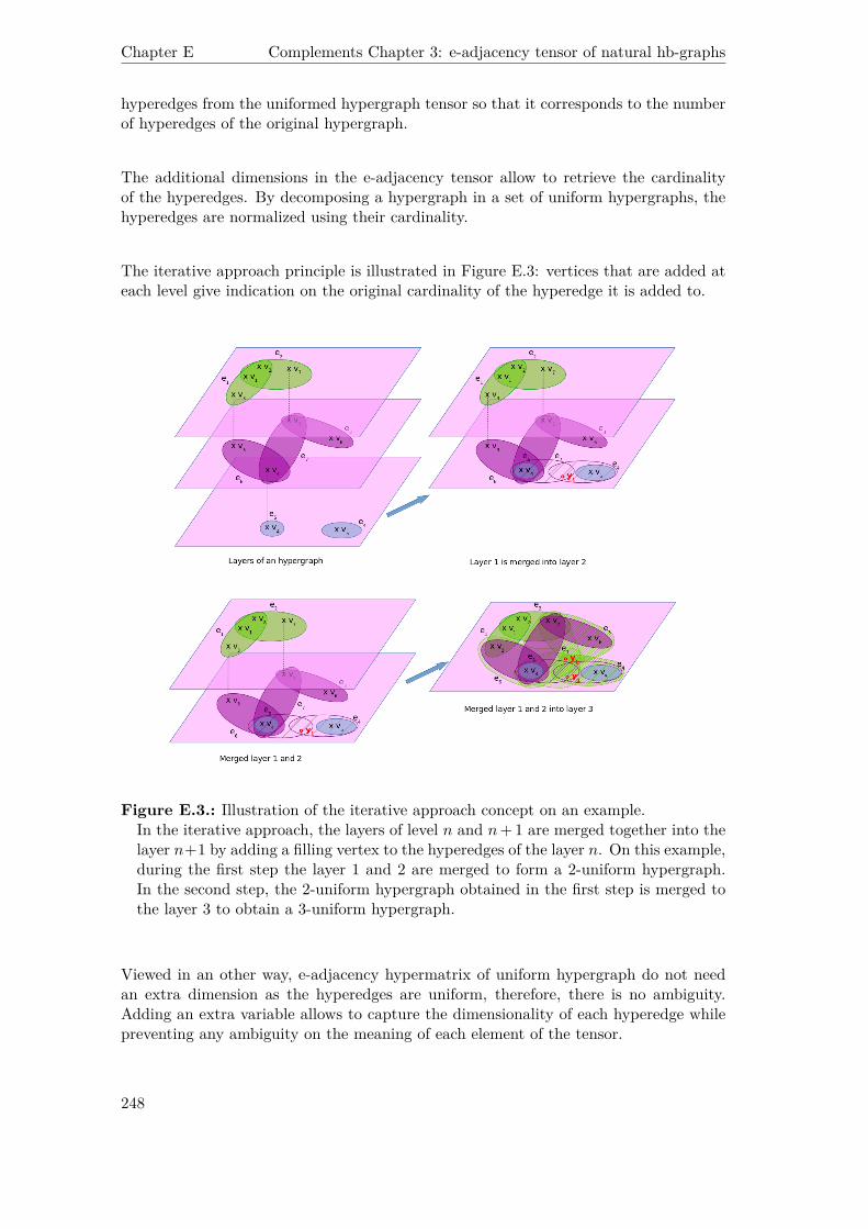
Chapter E Complements Chapter 3: e-adjacency tensor of natural hb-graphs
hyperedges from the uniformed hypergraph tensor so that it corresponds to the numberof hyperedges of the original hypergraph.
The additional dimensions in the e-adjacency tensor allow to retrieve the cardinalityof the hyperedges. By decomposing a hypergraph in a set of uniform hypergraphs, thehyperedges are normalized using their cardinality.
The iterative approach principle is illustrated in Figure E.3: vertices that are added ateach level give indication on the original cardinality of the hyperedge it is added to.
Figure E.3.: Illustration of the iterative approach concept on an example.In the iterative approach, the layers of level n and n+ 1 are merged together into thelayer n+1 by adding a filling vertex to the hyperedges of the layer n. On this example,during the first step the layer 1 and 2 are merged to form a 2-uniform hypergraph.In the second step, the 2-uniform hypergraph obtained in the first step is merged tothe layer 3 to obtain a 3-uniform hypergraph.
Viewed in an other way, e-adjacency hypermatrix of uniform hypergraph do not needan extra dimension as the hyperedges are uniform, therefore, there is no ambiguity.Adding an extra variable allows to capture the dimensionality of each hyperedge whilepreventing any ambiguity on the meaning of each element of the tensor.
248

E.1. Building a tensor of e-adjacency for general hypergraphs
E.1.5. Some comments on the e-adjacency tensor
E.1.5.1. The particular case of graphs
As a graph G = (V,E) with |V | = n can always be seen as a 2-uniform hypergraphHG, the approach given in this paragraph should allow to retrieve in a coherent way thespectral theory for normal graphs.
The hypergraph that contains the 2-uniform hypergraph is then composed of an emptylevel 1 layer and a level 2 layer that contains only HG.
Let A be the adjacency matrix of G. The e-adjacency tensor of the corresponding2-uniform hypergraph is of order 2 and obtained from A by multiplying it by c2 andadding one row and one column of zero. Therefore, the e-adjacency tensor of the two
levels of the corresponding hypergraph is: A=(c2A 0
0 0
).
Also, as an eigenvalue λ of A seen as a matrix is a solution of the characteristic poly-nomial det (A− λI) = 0 ⇔ −λ det (c2A− λI) = 0 ⇔ −λcn2 det
(A− λ
c2I
)= 0, the
eigenvalues of A are c2 times the ones of A and one additional 0 eigenvalue. This lasteigenvalue is attached to the eigenvector (0...0 1)T . The other eigenvalues have sameeigenvectors than A with one additional n+ 1 component which is 0.
Proof. Let consider Y =(Xy
)with X vector of dimension n. Let λ be an eigenvalue
of A and Y an eigenvector of A.
AY = λY ⇔ A(Xy
)= λ
(Xy
)⇔ (c2A− λIn)X = 0 ∧ −λy = 0 ⇔ X eigenvalue
of A attached to λ
c2. y can be always taken equals to 0 to fit the second condition.
Therefore, globally there is no change in the spectrum: the eigenvectors remain, theeigenvalues of the initial graph are multiplied by the normalizing coefficient.
E.1.5.2. e-adjacency tensor and disjunctive normal form
Let H = (V,E) be a hypergraph, A its e-adjacency tensor and RrH the reduced attachedhomogeneous polynomial:
RrH
(w(rH)
)=
∑16i1<...<ik6n+rH−1
r(rH) i1 ... irHwi1(rH)...w
irH(rH)
with r(rH) i1 ... irH = rH!r(rH) i1 ... irH .
The variables(wi(rH)
)i∈Jn+rH−1K
of Rkmax can be considered as Boolean variables and,therefore, Rkmax can be considered as a Boolean function. The variables wi(rH) for
249
Chapter E Complements Chapter 3: e-adjacency tensor of natural hb-graphs
i ∈ JnK captures whether a vertex belongs to the considered hyperedge and for i ∈Jn+ 1, n+ rH − 1K to the layer of level i− n.
This Boolean homogeneous polynomial PB(w(rH)
)is in full disjunctive normal form
as it is a sum of products of Boolean variables holding only once in each product andwhere the conjunctive terms are made of rH variables.
PB rH (z0) = PB
z0, 0, ..., 0︸ ︷︷ ︸rH−1
allows to retrieve the part of the full DNF which stores
hyperedges of size rH.
PB rH−1 (z0) = PB
z0, 0, ..., 0︸ ︷︷ ︸rH−2
, 1
− PB
z0, 0, ..., 0︸ ︷︷ ︸rH−1
allows to retrieve the full DNF
which stores hyperedges of size rH − 1.
PB rH−j (z0) = PB
z0, 0, ..., 0︸ ︷︷ ︸rH−j−1
, 1, ..., 1︸ ︷︷ ︸j
−PBz0, 0, ..., 0︸ ︷︷ ︸
rH−j−2
, 1, ..., 1︸ ︷︷ ︸j−1
allows to retrieve the
full DNF which stores hyperedges of size rH − j.
Stopping at PB 1 (z0) = PB
z0, 1, ..., 1︸ ︷︷ ︸rH−1
−PBz0, 0, 1, ..., 1︸ ︷︷ ︸
rH−2
allows to retrieve the full
DNF which stores hyperedges of size 1.Considering the adjacency matrix of [ZHS07] of this unweighted hypergraph, it holdsthat w>0 Aw0 can be considered as a Boolean homogeneous polynomial in full disjunctiveform where the conjunctive terms are composed of only two variables. This shows, ifnecessary, that this approach is a pairwise approximation of the e-adjacency tensor.The homogeneous polynomial attached to [BCM17] tensor can be mapped to a Booleanpolynomial function by considering the same term elements with coefficient being 1when the original homogeneous polynomial has a non-zero coefficient and, 0 otherwise.Nonetheless, this Boolean function is no more in DNF. Reducing it to DNF yields to
the expression of PB
z0, 1, ..., 1︸ ︷︷ ︸rH−1
.
E.1.5.3. First results on spectral analysis of e-adjacency tensor
Let H = (V,E) be a general hypergraph of e-adjacency tensor AH of CHR AH =(ai1...irH
).
In the e-adjacency tensor AH built, the diagonal entries are equal to zero. As allelements of AH are all non-negative real numbers and as we have shown that:
∀i ∈ Jn+ rH − 1K :∑
i2,...,irH∈Jn+rH−1Kδii2...irH=0
aii2...irH = di.
It follows:
250
E.1. Building a tensor of e-adjacency for general hypergraphs
Theorem E.1. The e-adjacency tensor AH of CHR AH =(ai1...irH
)of a general
hypergraph H = (V,E) has its eigenvalues λ such that:
|λ| 6 max (∆,∆?) (E.6)
where: ∆ ∆= maxi∈JnK
(di) and ∆? ∆= maxi∈JrH−1K
(dn+i) .
Proof. From B.2, we can write, as ai...i = 0 and aii2...irHare non-negative numbers, thatfor all λ it holds:
|λ| 6∑
i2,...,irH∈Jn+rH−1Kδii2...irH=0
aii2...irH
and thus writing ∆ = maxi∈JnK
(di) and ∆? = maxi∈JrH−1K
(dn+i) , it holds: |λ| 6 max (∆,∆?) .
Proposition E.7. Let H be a r-regular r-uniform hypergraph. Then this maximum isreached.
Proof. In this case:∀i ∈ JnK , di = ∆ = r
and:∆? = 0,
also:max (∆,∆?) = r.
Considering λ = r and the vector 1 which components are only 1, (r,1) is an eigenpairof AH as for all i ∈ JnK :
∑i2,...,irH∈Jn+rH−1K
aii2...irHxi2 ...xirH = λxrH−1i
⇔∑
i2,...,irH∈Jn+rH−1Kaii2...irH = r
⇔ di = r.
Remark E.1.2. We see that this bound includes ∆? which can be close to the numberof hyperedges, for instance where the hyperedges would be constituted of only one vertexper hyperedge except one hyperedge with rH 6= 1 vertices in it.
251
Chapter E Complements Chapter 3: e-adjacency tensor of natural hb-graphs
E.1.6. Evaluation
We have gathered in Table E.1 some key features of both the e-adjacency tensor proposedby [BCM17]—written BH—, the new e-adjacency tensor proposed by [SZB19]—writtenSH—and the one constructed in this Thesis—written AH. The constructed tensor hassame order than the two others. The dimension of AH is rH−1 bigger than BH and SH(n− 1 in the worst case). The way AH and SH are built uses potentially (n+ rH − 1)!
(n− 1)!nrH
times less elements than for BH—O
(n!nn
)in the worst case. The number of non-
zero elements filled in AH and SH for a given hypergraph is(
1 + rH − 1n
)rHtimes
the number of elements of BH (O (4n) times in the worst case). But, the number ofelements to be filled to have full description of a hyperedge of size s by permutationof indices due to the symmetry of the tensor is only 1 in the case of AH , which is
1ps (rH) times less than for a hyperedge stored in BH and 1
sfor a hyperedge stored in
SH. The minimum number of elements needed to be described the other being obtainedby permutation is 1
|E|∑
s∈JrHKps (rH) |Es| bigger for BH than for AH and 1
|E|∑
s∈JrHKs |Es|
bigger for SH than for AH. Moreover, the value of the elements in BH and SH varieswith the cardinality of the hyperedge; in AH, any element has same value. Both tensorsallow the reconstruction of the original hypergraph; for BH, it requires at least ps (rH)checks per hyperedge and s in SH as for AH it requires only one element per hyperedge.
In both cases, node degrees can be deduced from the e-adjacency tensor. AH allows theretrieval of the structure of the hypergraph in term of hyperedges cardinality which isnot straightforward in the case of BH and SH.
The fact that AH can be interpreted in terms of hypergraph uniformisation is possible asit is the e-adjacency tensor of the Vs-layered uniform hypergraph Hw obtained from H.BH and SH are not interpretable in term of hypergraph uniformisation, as hyperedgesdo not allow repetition of vertices; we will have to wait the introduction of hb-graphsto get a meaningful interpretation—Chapter 4.
E.1.7. Further comments
The importance of defining properly the concept of adjacency in a hypergraph hashelped us to build a proper e-adjacency tensor in a way that allows to contain impor-tant information on the structure of the hypergraph. This work contributes to givea methodology to build a uniform hypergraph and hence a cubical symmetric tensorfrom the different layers of uniform hypergraphs contained in a hypergraph. The builttensor allows to reconstruct with no ambiguity the original hypergraph. Nonetheless,first results on spectral analysis show difficulties to use the tensor built as the additionalvertices inflate the spectral radius bound. The uniformisation process is a strong basisfor building alternative proposals.
252
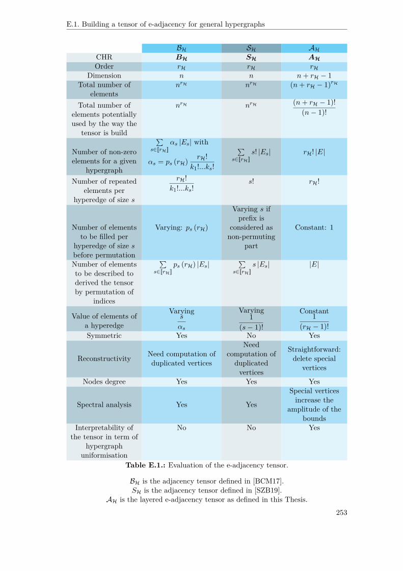
E.1. Building a tensor of e-adjacency for general hypergraphs
BH SH AHCHR BH SH AHOrder rH rH rH
Dimension n n n+ rH − 1Total number of
elementsnrH nrH (n+ rH − 1)rH
Total number ofelements potentiallyused by the way the
tensor is build
nrH nrH (n+ rH − 1)!(n− 1)!
Number of non-zeroelements for a given
hypergraph
∑s∈JrHK
αs |Es| with
αs = ps (rH) rH!k1!...ks!
∑s∈JrHK
s! |Es| rH! |E|
Number of repeatedelements per
hyperedge of size s
rH!k1!...ks!
s! rH!
Number of elementsto be filled per
hyperedge of size sbefore permutation
Varying: ps (rH)
Varying s ifprefix is
considered asnon-permuting
part
Constant: 1
Number of elementsto be described toderived the tensorby permutation of
indices
∑s∈JrHK
ps (rH) |Es|∑
s∈JrHKs |Es| |E|
Value of elements ofa hyperedge
Varyings
αs
Varying1
(s− 1)!
Constant1
(rH − 1)!Symmetric Yes No Yes
Reconstructivity Need computation ofduplicated vertices
Needcomputation of
duplicatedvertices
Straightforward:delete special
vertices
Nodes degree Yes Yes Yes
Spectral analysis Yes Yes
Special verticesincrease the
amplitude of thebounds
Interpretability ofthe tensor in term of
hypergraphuniformisation
No No Yes
Table E.1.: Evaluation of the e-adjacency tensor.
BH is the adjacency tensor defined in [BCM17].SH is the adjacency tensor defined in [SZB19].
AH is the layered e-adjacency tensor as defined in this Thesis.253
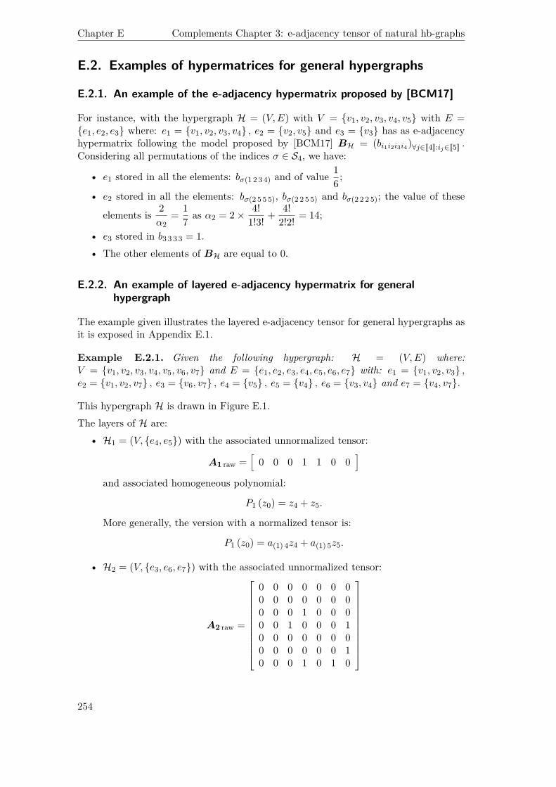
Chapter E Complements Chapter 3: e-adjacency tensor of natural hb-graphs
E.2. Examples of hypermatrices for general hypergraphs
E.2.1. An example of the e-adjacency hypermatrix proposed by [BCM17]
For instance, with the hypergraph H = (V,E) with V = {v1, v2, v3, v4, v5} with E ={e1, e2, e3} where: e1 = {v1, v2, v3, v4} , e2 = {v2, v5} and e3 = {v3} has as e-adjacencyhypermatrix following the model proposed by [BCM17] BH = (bi1i2i3i4)∀j∈J4K:ij∈J5K .Considering all permutations of the indices σ ∈ S4, we have:
• e1 stored in all the elements: bσ(1 2 3 4) and of value 16;
• e2 stored in all the elements: bσ(2 5 5 5), bσ(2 2 5 5) and bσ(2 2 2 5); the value of these
elements is 2α2
= 17 as α2 = 2× 4!
1!3! + 4!2!2! = 14;
• e3 stored in b3 3 3 3 = 1.• The other elements of BH are equal to 0.
E.2.2. An example of layered e-adjacency hypermatrix for generalhypergraph
The example given illustrates the layered e-adjacency tensor for general hypergraphs asit is exposed in Appendix E.1.
Example E.2.1. Given the following hypergraph: H = (V,E) where:V = {v1, v2, v3, v4, v5, v6, v7} and E = {e1, e2, e3, e4, e5, e6, e7} with: e1 = {v1, v2, v3} ,e2 = {v1, v2, v7} , e3 = {v6, v7} , e4 = {v5} , e5 = {v4} , e6 = {v3, v4} and e7 = {v4, v7}.
This hypergraph H is drawn in Figure E.1.The layers of H are:
• H1 = (V, {e4, e5}) with the associated unnormalized tensor:
A1 raw =[
0 0 0 1 1 0 0]
and associated homogeneous polynomial:
P1 (z0) = z4 + z5.
More generally, the version with a normalized tensor is:
P1 (z0) = a(1) 4z4 + a(1) 5z5.
• H2 = (V, {e3, e6, e7}) with the associated unnormalized tensor:
A2 raw =
0 0 0 0 0 0 00 0 0 0 0 0 00 0 0 1 0 0 00 0 1 0 0 0 10 0 0 0 0 0 00 0 0 0 0 0 10 0 0 1 0 1 0
254

E.2. Examples of hypermatrices for general hypergraphs
and associated homogeneous polynomial:
P2 (z0) = 2z3z4 + 2z6z7 + 2z4z7.
More generally, the version with a normalized tensor is:
P2 (z0) = 2!a(2) 3 4z3z4 + 2!a(2) 6 7z6z7 + 2!a(2) 4 7z4z7.
• H3 = (V, {e1, e2}) with the associated unnormalized tensor:
A3 raw =
0 0 0 0 0 0 00 0 1 0 0 0 10 1 0 0 0 0 00 0 0 0 0 0 00 0 0 0 0 0 00 0 0 0 0 0 00 1 0 0 0 0 0
∣∣∣∣∣∣∣∣∣∣∣∣∣∣∣∣
0 0 1 0 0 0 10 0 0 0 0 0 01 0 0 0 0 0 00 0 0 0 0 0 00 0 0 0 0 0 00 0 0 0 0 0 01 0 0 0 0 0 0
∣∣∣∣∣∣∣∣∣∣∣∣∣∣∣∣
0 1 0 0 0 0 01 0 0 0 0 0 00 0 0 0 0 0 00 0 0 0 0 0 00 0 0 0 0 0 00 0 0 0 0 0 00 0 0 0 0 0 0
∣∣∣∣∣∣∣∣∣∣∣∣∣∣∣∣0| 0| 0|
0 1 0 0 0 0 01 0 0 0 0 0 00 0 0 0 0 0 00 0 0 0 0 0 00 0 0 0 0 0 00 0 0 0 0 0 00 0 0 0 0 0 0
∣∣∣∣∣∣∣∣∣∣∣∣∣∣∣∣
and associated homogeneous polynomial:
P3 (z0) = 3!z1z2z3 + 3!z1z2z7.
More generally, the version with a normalized tensor is:
P3 (z0) = 3!a(3) 1 2 3z1z2z3 + 3!a(3) 1 2 7z1z2z7.
The iterative process of homogenization is then the following using the degree-normalizedadjacency tensor Ak = 1
(k − 1)!Ak raw and the normalizing coefficients ck = kmaxk
, withkmax = 3 :
• R1 (z0) = 31P1 (z0) ;
• R2 (z1) = R1 (z0) y1 + 32P2 (z0) ;
• R3 (z2) = R2 (z1) y2 + 33P3 (z0) .
Hence:
R3 (z2) = 3(a(1) 4z4 + a(1) 5z5
)y1y2
+32 × 2!
(a(2) 3 4z3z4 + a(2) 6 7z6z7 + a(2) 4 7z4z7
)y2
+3!(a(3) 1 2 3z1z2z3 + a(3) 1 2 7z1z2z7
).
Therefore, the e-adjacency tensor of H is obtained by writing the corresponding sym-metric cubical tensor of order 3 and dimension 9, described by: r489 = r589 = r349 =r679 = r479 = r123 = r127 = 1
2 . The other remaining not null elements are obtained bypermutation on the indices.
Finding the degree of one vertex from the tensor is easily achievable; for instancedeg (v4) = 2! (r489 + r349 + r479) = 3.
255


F. Used Fraktur fonts
Fraktur font A B C D E e F H h I P R S T V vClassical font A B C D E e F H h I P R S T V v