thÈse wissam benjilali
TRANSCRIPT

THÈSE
Pour obtenir le grade de
DOCTEUR DE L’UNIVERSITÉ GRENOBLE ALPES Spécialité : NANO ELECTRONIQUE ET NANO TECHNOLOGIES
Arrêté ministériel : 25 mai 2016 Présentée par
Wissam BENJILALI Thèse dirigée par Gilles Sicard, Ingénieur de recherche, HDR,
CEA-LETI, encadré par William Guicquero, Ingénieur de recherche, CEA-LETI et co-encadré par Laurent Jacques, Professeur, UCLouvain. préparée au sein du CEA-LETI dans l’école doctorale Electronique, Electrotechnique, Automatique, Traitement du Signal (EEATS) Etude d'architectures d'imageurs exploitant l'acquisition compressive pour la classification d'images à basse consommation énergétique Exploring analog-to-information CMOS image sensor design taking advantage of recent advances in compressive sensing for low-power image classification Thèse soutenue publiquement le 16 décembre 2019, devant le jury composé de :
Madame Valérie Perrier Professeur des universités, Grenoble INP, Grenoble, France, Président
Monsieur Ricardo Carmona Galan Chercheur, Instituto de Microelectrónica de Sevilla, IMSE-CNM, Séville, Espagne, Rapporteur
Monsieur François Berry Professeur des universités, Université Clermont Auvergne, Clermont-Ferrand, France, Rapporteur
Monsieur Gianluca Setti Professeur, Politecnico di Torino, Turin, Italie, Examinateur
Monsieur Laurent Jacques Professeur, UCLouvain, Louvain-la-Neuve, Belgique, Co-encadrant
Monsieur William Guicquero Ingénieur de recherche, CEA-LETI, Grenoble, France, Encadrant
Monsieur Gilles Sicard Ingénieur de recherche, HDR, CEA-LETI, Grenoble, France, Directeur


The more I read,
the more I acquire,
the more certain I am that I know nothing.
— Voltaire
To my parents . . .


Acknowledgements
I would like to express my gratitude and thanks to my thesis advisor, William Guicquero,
for being the great mentor, guide and collaborator. This thesis would never have seen the
light of day without his commitment and availability. I thank him for introducing me to
the smart image sensor world, for giving me enough insights and original views to explore
multi-disciplinary research axes and for showing me how to methodically achieve, analyze
and communicate results. I am also grateful to Laurent Jacques who kindly accepted to be my
co-advisor. I thank him for the many remote but fruitful discussions we had during the last
two years as well as for his mathematical rigor and theoretical background from whose I have
tremendously benefited. My thanks, of course, go also to Gilles Sicard, my thesis director, for
being always open and of great support.
I would like to thank Ricardo Carmona Galan and François Berry, my thesis reviewers, for
reading the thesis and for their detailed and relevant comments on the manuscript in a
relatively short time. I also thank Gianluca Setti, my thesis examiner, and Valérie Perrier, the
president of the jury, for the interest they have shown to my work.
I would like to thank all my friends and colleagues from the smart imaging and display lab
for adopting me so fast and making me feel at home. Special thanks to Camille, Nicolas, and
Yoann, my office mates, for the many interesting discussions, and Yoann for the intuitive
explanations of the IC design world. I also want to thank the coffee break team with Amaury,
Margot, Simon and Yohan, that I had the pleasure, with the office mates, to host in the "Ph.D.
students office". My thanks extend to Arnaud V. and P. for the sparse technical discussions,
Laurent A. for his kindness and humor, Laurent M. for the feedbacks on my figures and for
blessing them, Bertrand for sharing the stories of his amazing trips, Jean-Alain, the only
football supporter of the lab, for the post champions league matchs discussions, and Jean-
Pierre and Thomax for their kindness. I am thankful to Fabrice, for accepting me in his team
first as an intern and second as a Ph.D. student. It has been a pleasure for me to work in the
DACLE department with its great atmosphere and rich technical environment.
I can never forget my good friends in Paris, Lyon and Grenoble for making my stay in France
so much more pleasant. They were like a second family to me and were always been there for
me.
With all my heart, I thank my parents and my brothers for their constant and endless support.
Grenoble, December 2019 W. B.


Abstract
Recent advances in the field of CMOS Image Sensors (CIS) tend to revisit the canonical
image acquisition and processing pipeline to enable on-chip advanced image processing
applications such as decision making. Despite the tremendous achievements made possible
thanks to technology node scaling and 3D integration, designing a CIS architecture with on-
chip decision making capabilities still a challenging task due to the amount of data to sense and
process, as well as the hardware cost to implement state-of-the-art decision making algorithms.
In this context, Compressive Sensing (CS) has emerged as an alternative signal acquisition
approach to sense the data in a compressed representation. When based on compact devices
to on-the-fly generate sensing patterns, CS enables drastic hardware saving through the
reduction of Analog to Digital conversions and data off-chip throughput while providing
a meaningful information for either signal recovery or signal processing. Traditionally, CS
has been exploited in CIS applications for compression tasks coupled with a remote signal
recovery algorithm involving high algorithmic complexity. To alleviate this complexity, signal
processing on CS provides solid theoretical guarantees to perform signal processing directly
on CS measurements without significant performance loss opening as a consequence new
ways towards the design of low-power smart sensor nodes.
Built on algorithm and hardware research axes, this thesis illustrates how Compressive Sensing
can be exploited to design low-power sensor nodes with efficient on-chip decision making
algorithms. After an overview of the fields of Compressive Sensing and Machine Learning with
a particular focus on hardware implementations, this thesis presents four main contributions
to study efficient sensing schemes and decision making approaches for the design of compact
CMOS Image Sensor architectures. First, an analytical study explores the interest of solving
basic inference tasks on CS measurements for highly constrained hardware. It aims at find-
ing the most beneficial setting to perform decision making on Compressive Sensing based
measurements. Next, a novel sensing scheme for CIS applications is presented. Designed
to meet both theoretical and hardware requirements, the proposed sensing model is shown
to be suitable for CIS applications addressing both image rendering and on-chip decision
making tasks. On the other hand, to deal with on-chip computational complexity involved
by standard decision making algorithms, new methods to construct a hierarchical inference
tree are explored to reduce MAC (Multiply-ACcumulate) operations related to an on-chip
multi-class inference task. This leads to a joint acquisition-processing optimization when
combining hierarchical inference with Compressive Sensing. Finally, all the aforementioned
contributions are brought together to propose a compact CMOS Image Sensor architecture

iv
enabling on-chip object recognition facilitated by the proposed CS sensing scheme, reducing
as a consequence on-chip memory needs. The proposed architecture takes advantage of a
pseudo-random data mixing circuit of reduced silicon footprint, an in-Σ∆ ±1 modulator and
a small Digital Signal Processor (DSP) to achieve on-chip inference. In addition to the data
dimensionality reduction made possible thanks to CS, several hardware optimizations are
presented to fit requirements of future ultra-low power (∼µW) CIS design. Typically, through
the reduction of CS measurements resolutions as well as digital operations resolutions at the
DSP level.
Key words: CMOS Image Sensor, compressive sensing, random permutations, random mod-
ulations, Sigma-Delta, machine learning, hierarchical inference, support vector machines,
neural networks.
Résumé
Les avancés récents dans le domaine des capteurs d’image CMOS repose sur la remise en
question du schéma classique d’acquisition et de traitement d’images, cela, afin de permettre
des traitements avancés sur puce tels que la prise de décision. Malgré les réalisations ren-
dues possibles grâce à l’utilisation des nœuds technologiques avancés et à l’intégration 3D,
la conception de capteurs avec des capacités de prise de décision reste une tâche ardue en
raison de la quantité de données acquise et à traiter, ainsi que du coût matériel que repré-
sente l’implémentation des algorithmes de prise de décisions classiques. Dans ce contexte,
l’Acquisition Compressive (AC) semble une approche alternative pour inspecter des données
en profitant de la réduction de dimensionnalité. Dans le cas où l’AC exploite des motifs géné-
rés à l’aide de structures matérielles compactes ayant un comportement pseudo-aléatoire,
il permet une réduction considérable en réduisant les conversions analogique-numérique
ainsi que du débit des données collectées, tout en conservant les informations pertinentes
intrinsèques afin de permettre à la fois la reconstruction du signal ou bien son traitement
dans sa nouvelle forme de représentation. Traditionnellement, l’AC a été exploité dans des
applications de capteurs d’image pour des tâches de compression couplées à des algorithmes
de reconstruction distants impliquant une complexité algorithmique élevée. Pour relâcher
cette complexité, il apparaît dans la littérature des garanties théoriques solides pour effectuer
le traitement du signal directement dans le domaine compressé sans perte significative de
performance, ce qui constitue donc une nouvelle piste pour concevoir des nœuds de capteurs
intelligents à basse consommation énergétique.
Basée sur des axes de recherche traitant de l’algorithmique et de l’implémentation maté-
rielle, cette thèse étudie des voies de développement exploitant l’acquisition compressive
pour concevoir des nœuds de capteurs dotés de capacités de prise de décision sur puce à
basse consommation énergétique. Après une présentation du contexte matériel et algorith-
mique lié à l’acquisition compressive et les techniques d’apprentissage machine, la thèse
présente quatre contributions principales pour optimiser les schémas d’acquisition du signal
et des traitements associés dans le contexte des capteurs d’image CMOS. Dans un premier
temps, une étude analytique explore l’intérêt de résoudre des tâches d’inférence à partir
des mesures compressées pour des applications à forte contraintes matériels. L’objectif est
d’identifier une approche pertinente en terme de complexité matérielle et algorithmique
permettant d’implémenter des traitements de prise de décisions à partir de mesures compres-
sées. Ensuite, un nouveau schéma d’acquisition compressive dédié aux applications imageurs
CMOS est présenté. Conçu pour répondre à la fois aux exigences théoriques et matérielles,

vi
le modèle s’avère être approprié pour les capteurs qui traitent à la fois des tâches de rendu
d’image et de prise de décision sur puce. D’autre part, pour réduire la complexité de calcul sur
puce impliquée par les algorithmes de prise de décision standard, de nouvelles méthodes de
construction d’arbres d’inférence hiérarchique sont explorées afin de réduire les opérations
MAC (Multiply-ACcumulate) liées à une tâche d’inférence pour de la classification en classes
multiples sur puce. Cela conduit à une optimisation conjointe traitement-acquisition lors
de la combinaison de l’inférence hiérarchique avec l’acquisition compressive. Enfin, une
architecture compacte d’un capteur d’image embarquant les contributions algorithmiques
susmentionnées est présentée permettant la reconnaissance d’objets sur puce à faible em-
preinte matérielle. L’architecture proposée exploite principalement un mélangeur analogique
permettant la permutation pseudo-aléatoire des pixels des lignes sélectionnées dans un mode
de lecture en rolling shutter ; un convertisseur analogique-numérique Sigma-Delta (Σ∆) incré-
mental de premier ordre pour implémenter la modulation pseudo-aléatoire, la sommation
des pixels mélangés ainsi que la conversion analogique-numérique ; et un petit processeur de
signal numérique (DSP) pour implémenter la fonction affine de prise de décision. En plus de
la réduction de dimension rendu possible grâce à l’AC, différentes optimisations matérielles
sont présentées pour répondre aux exigences de la conception des futures capteurs CMOS
dits ultra-basse consommation (∼ µW), à savoir, la réduction de la résolution des mesures
compressées extraites ainsi que la résolution des opérations logiques au niveau du DSP.
Mots clefs : Capteur d’image CMOS, acquisition compressive, permutations aléatoires, modu-
lations aléatoires, Sigma-Delta, apprentissage machine, inférence hiérarchique, machines à
vecteurs de support, réseaux de neuronnes.

Notations
x, X denotes a scalar
x denotes a vector
X denotes a matrix or a linear operator
xi denotes the i th component of a vector x
X i denotes the i th column of a matrix X
Xi j denotes the entry on the i th row and j th column
x>, X > denotes the transpose of a vector x or a matrix X
X −1 denotes the inverse of a matrix X
X † denotes the Moore-Penrose pseudoinverse of a matrix X defined as X † := (X >X
)−1X >
N denotes the set of all natural numbers
R denotes the set of all real numbers
[n] denotes the set of indices such that [n] := {1, . . . ,n}
I n denotes the n ×n identity matrix
1n denotes a n-dimensional vector with all entries equal to one
0n denotes a n-dimensional vector with all entries equal to zero
supp(x) denotes the support of a vector x ∈Rn , such that, supp(x) := {i ∈ [n] , xi 6= 0}
sign(x) denotes the sign function that extracts the sign of a scalar x
|x| denotes the absolute value of a scalar x
‖x‖p denotes the `p norm of a vector x defined as ‖x‖p := (∑i |x|p
) 1p for p > 1
‖x‖0 denotes the `0 norm of a vector x defined as the support of x , i.e., ‖x‖0 := supp(x)
‖X ‖F denotes the Frobenius norm of a matrix X defined as ‖X ‖F :=√∑
i∑
j |Xi j |2

viii
⟨x , y⟩ denotes the standard inner product in the Euclidean space between two vectors x, y ∈Rn
defined as y>x :=∑ni=1 xi yi
x ∗ y denotes the convolution between two vectors x , y ∈Rn
x ◦ y denotes the Hadamard product between two vectors x, y ∈Rn
X ⊗Y denotes the Kronecker product between two matrices
C denotes a set
card(C ) denotes the cardinality of a set C , indicating the number of the elements of the set
g (x) =O(
f (x))
denotes that | f (x)g (x) | is bounded as x →∞
N(µ,σ2
)denotes the Gaussian distribution with mean µ and variance σ2
U (a,b) denotes the Uniform distribution on the interval [a,b]

Contents
Acknowledgements i
Abstract (English/Français) iii
Notations vii
List of figures xiii
List of tables xvii
1 Introduction 1
2 State Of The Art 7
2.1 Compressive Sensing background . . . . . . . . . . . . . . . . . . . . . . . . . . . 8
2.1.1 An Invitation to Compressive Sensing . . . . . . . . . . . . . . . . . . . . . 8
2.1.2 Basic Algorithmic Tools . . . . . . . . . . . . . . . . . . . . . . . . . . . . . 11
2.1.3 CS Sensing Matrix Properties . . . . . . . . . . . . . . . . . . . . . . . . . . 12
2.1.4 CS Sensing Market . . . . . . . . . . . . . . . . . . . . . . . . . . . . . . . . 14
2.1.5 Signal Processing in CS Domain . . . . . . . . . . . . . . . . . . . . . . . . 16
2.1.6 CS Hardware Implementations . . . . . . . . . . . . . . . . . . . . . . . . . 17
2.2 Machine Learning background . . . . . . . . . . . . . . . . . . . . . . . . . . . . . 22
2.2.1 Machine Learning Algorithms Market . . . . . . . . . . . . . . . . . . . . . 22
2.2.2 Edge AI . . . . . . . . . . . . . . . . . . . . . . . . . . . . . . . . . . . . . . . 28
2.3 Conclusion and discussion . . . . . . . . . . . . . . . . . . . . . . . . . . . . . . . 30
3 Inference Tasks On Compressive Measurements 33
3.1 ML-DR Learning Mathematical Background . . . . . . . . . . . . . . . . . . . . . 34
3.1.1 LDA (Linear Discriminant Analysis) . . . . . . . . . . . . . . . . . . . . . . 35
3.1.2 SVM (Support Vector Machine) . . . . . . . . . . . . . . . . . . . . . . . . . 35
3.1.3 DLSI (Dictionary Learning with Structured Incoherence) . . . . . . . . . 36
3.2 Classification Combining ML-DR and CS-DR . . . . . . . . . . . . . . . . . . . . 37
3.2.1 Approach A: Inference Learned in The CS Domain . . . . . . . . . . . . . 38
3.2.2 Approach B: Projection Based Inference . . . . . . . . . . . . . . . . . . . 39
3.2.3 Approach C: Inference in The Reconstructed Signal Domain . . . . . . . 41
3.3 Embedded Resources Requirements Study . . . . . . . . . . . . . . . . . . . . . . 43

Contents x
3.3.1 Approach A: Inference Learned in CS Domain . . . . . . . . . . . . . . . . 43
3.3.2 Approach B: Projection Based Inference . . . . . . . . . . . . . . . . . . . 45
3.3.3 Approach C: Inference in The Reconstructed Signal Domain . . . . . . . 45
3.3.4 Complexity Analysis . . . . . . . . . . . . . . . . . . . . . . . . . . . . . . . 47
3.4 Experimental Results . . . . . . . . . . . . . . . . . . . . . . . . . . . . . . . . . . . 47
3.5 Conclusion . . . . . . . . . . . . . . . . . . . . . . . . . . . . . . . . . . . . . . . . . 49
4 Random Permutations and Modulations for Compressive Imaging 53
4.1 Proposed Sensing Scheme . . . . . . . . . . . . . . . . . . . . . . . . . . . . . . . . 54
4.2 CS Properties Verification . . . . . . . . . . . . . . . . . . . . . . . . . . . . . . . . 58
4.2.1 On The Non-Universality of The Proposed CS Model . . . . . . . . . . . . 58
4.2.2 Analytical Study . . . . . . . . . . . . . . . . . . . . . . . . . . . . . . . . . . 60
4.2.3 Coherence Analysis . . . . . . . . . . . . . . . . . . . . . . . . . . . . . . . . 61
4.2.4 Compressive Embedding Analysis . . . . . . . . . . . . . . . . . . . . . . . 64
4.3 Signal Recovery Using the Proposed Sensing Scheme . . . . . . . . . . . . . . . . 67
4.3.1 Reconstruction of Sparse Signals . . . . . . . . . . . . . . . . . . . . . . . . 67
4.3.2 Reconstruction of Compressible Signals . . . . . . . . . . . . . . . . . . . 68
4.4 Inference Using the Proposed Sensing Scheme . . . . . . . . . . . . . . . . . . . 72
4.5 Dedicated Hardware Implementations and Conclusion . . . . . . . . . . . . . . 73
5 Hierarchical Decision Making 75
5.1 Hierarchical Classification on CS: Key Concepts . . . . . . . . . . . . . . . . . . . 76
5.2 Proposed Hierarchical Learning Methods . . . . . . . . . . . . . . . . . . . . . . . 77
5.2.1 Notations . . . . . . . . . . . . . . . . . . . . . . . . . . . . . . . . . . . . . 77
5.2.2 Binary SVM . . . . . . . . . . . . . . . . . . . . . . . . . . . . . . . . . . . . 77
5.2.3 Training the Hierarchical Classifier . . . . . . . . . . . . . . . . . . . . . . 78
5.2.4 Testing the Hierarchical-Based Inference . . . . . . . . . . . . . . . . . . . 81
5.2.5 Embedded Resources Requirements Analysis . . . . . . . . . . . . . . . . 82
5.3 Simulation Results . . . . . . . . . . . . . . . . . . . . . . . . . . . . . . . . . . . . 83
5.4 Conclusion . . . . . . . . . . . . . . . . . . . . . . . . . . . . . . . . . . . . . . . . . 85
6 Hardware implementations 87
6.1 Proposed image sensor architecture . . . . . . . . . . . . . . . . . . . . . . . . . . 88
6.1.1 Dedicated PRG for the PRP . . . . . . . . . . . . . . . . . . . . . . . . . . . 89
6.1.2 Pseudo Random-Permutations (PRP) . . . . . . . . . . . . . . . . . . . . . 94
6.1.3 RMΣ∆ . . . . . . . . . . . . . . . . . . . . . . . . . . . . . . . . . . . . . . . . 102
6.1.4 On-Chip Inference (DSP) . . . . . . . . . . . . . . . . . . . . . . . . . . . . 107
6.2 Inference with tunable algorithmic complexity . . . . . . . . . . . . . . . . . . . 111
6.2.1 Notations . . . . . . . . . . . . . . . . . . . . . . . . . . . . . . . . . . . . . 112
6.2.2 One-vs.-all SVM . . . . . . . . . . . . . . . . . . . . . . . . . . . . . . . . . . 112
6.2.3 Hierarchical SVM . . . . . . . . . . . . . . . . . . . . . . . . . . . . . . . . . 113
6.2.4 Neural Network . . . . . . . . . . . . . . . . . . . . . . . . . . . . . . . . . . 114
6.2.5 Complexity analysis . . . . . . . . . . . . . . . . . . . . . . . . . . . . . . . 114

xi Contents
6.3 Simulations and performance optimization . . . . . . . . . . . . . . . . . . . . . 115
6.3.1 Background . . . . . . . . . . . . . . . . . . . . . . . . . . . . . . . . . . . . 115
6.3.2 PRP optimization . . . . . . . . . . . . . . . . . . . . . . . . . . . . . . . . . 116
6.3.3 RMΣ∆ optimization . . . . . . . . . . . . . . . . . . . . . . . . . . . . . . . 116
6.3.4 DSP optimization . . . . . . . . . . . . . . . . . . . . . . . . . . . . . . . . . 119
6.3.5 Simulation results . . . . . . . . . . . . . . . . . . . . . . . . . . . . . . . . 121
6.4 Conclusion . . . . . . . . . . . . . . . . . . . . . . . . . . . . . . . . . . . . . . . . . 122
7 Conclusions 125
Publications & Patent 129
Bibliography 151

List of Figures
1.1 CIS market dynamics by Yole Développement. . . . . . . . . . . . . . . . . . . . . 2
1.2 Imaging system pipeline. . . . . . . . . . . . . . . . . . . . . . . . . . . . . . . . . 3
2.1 The canonical compression scheme (top) Compressive Sensing scheme (bottom). 8
2.2 An illustration of the rare eclipse problem. . . . . . . . . . . . . . . . . . . . . . . 16
2.3 A mind-map of the main compressive imaging techniques. . . . . . . . . . . . . 21
2.4 An illustration of the projection in the LDA domain for C = 3. . . . . . . . . . . . 24
2.5 An illustration of the SVM classifier for c = 4: (a) One-vs.-all strategy; (b) One-vs.-
one strategy for the blue class. . . . . . . . . . . . . . . . . . . . . . . . . . . . . . 25
2.6 Structure of the coefficient matrix in a sparse representation. . . . . . . . . . . . 26
2.7 An illustration of a CNN network from [1]. . . . . . . . . . . . . . . . . . . . . . . 28
3.1 An illustration of the projections involved by the studied inference approaches.
y and y are an observed unknown sample and its projection in the CS domain
usingΦ respectively; and c is the predicted class of y . . . . . . . . . . . . . . . . 37
3.2 Schematic description of "inference learned in CS domain" (Approach A). . . . 38
3.3 Schematic description of "projection based inference" (Approach B). . . . . . . 40
3.4 Schematic description of "inference in the reconstructed signal domain" (Ap-
proach C). . . . . . . . . . . . . . . . . . . . . . . . . . . . . . . . . . . . . . . . . . 42
3.5 Inference accuracy for the AT&T and MNIST databases using a Rademacher and
Gaussian distributions. We set n1 = n2 = 5 for AT&T; and n1 = 5000,n2 = 1000 for
MNIST. (c) Robustness to additive noise. (d) Robustness to hardware variations.
Blue, green and red lines refer approaches A, B and C respectivelly. . . . . . . . 49
3.6 Robustness to additive noise and hardware alterations for the LDA, SVM and
DLSI. Blue, green and red lines refer approaches A, B and C respectivelly. . . . 52
4.1 Schematic 2D representation of the proposed CS sensing scheme for one snap-
shot. In particular, all the pixels sharing the same color are readout through to
the same colorized end-of-column circuitry. Each pixel of the matrix U is also
being modulated by the factor ±1. . . . . . . . . . . . . . . . . . . . . . . . . . . . 54
4.2 Matrix representation of the proposed CS sensing scheme for a single snapshot. 57

List of Figures xiv
4.3 An analytical proof of the compressive embedding of the proposed sensing
scheme in (4.3). (a) shows concentration of pairwise distances of our model and
a Bernoulli distribution in the canonical basis around the pairwise distances
in the signal domain (bisector axis) for n = 1024, k = 10 and m = 128 (s = 4);
(b) report the histogram of distances to the bisector axis of our model and a
Bernoulli distribution; (c) and (d) report the extracted plots in the DCT basis. . 60
4.4 Testbench for sparse image recovery. . . . . . . . . . . . . . . . . . . . . . . . . . 68
4.5 Phase-transition diagrams. Black, red and magenta lines show the transitions
to a success reconstruction above 40 dB for per-column Bernoulli (Col-Bern),
our model without permutations (W/o perm) and our model sensing schemes
(modPerm) respectivelly. . . . . . . . . . . . . . . . . . . . . . . . . . . . . . . . . 69
4.6 Quality of reconstruction of our sensing compared to a per-column Bernoulli
acquisition scheme: (top) 25 snapshots, i.e., 20.48 compression ratio (bottom)
50 snapshots, i.e., 10.24 compression ratio. . . . . . . . . . . . . . . . . . . . . . 70
4.7 Quality of reconstruction of our sensing compared to a per-column Bernoulli
acquisition scheme: (top) 75 snapshots, i.e., 6.82 compression ratio (bottom)
100 snapshots, i.e., 5.12 compression ratio . . . . . . . . . . . . . . . . . . . . . . 71
4.8 Quality of reconstruction of our sensing model compared to a per-column
Bernoulli acquisition scheme over 10 batches. . . . . . . . . . . . . . . . . . . . 72
4.9 Classification accuracy for the AT&T and MNIST databases. . . . . . . . . . . . 73
4.10 Top-level architecture of a pseudo-random modulations & permutations com-
pressive image sensor. . . . . . . . . . . . . . . . . . . . . . . . . . . . . . . . . . . 74
5.1 An illustration of the hierarchical learning. The input multi-class dataset to
be classified is presented at Level 0. A first balanced clustering (2 clusters,
each associated to the same number of classes) is performed at Level 1, then
a binary classifier is trained. This process is repeated for each cluster until the
construction of a single-class cluster at each terminal node. Here, C ( j)i represents
j th cluster at level i . . . . . . . . . . . . . . . . . . . . . . . . . . . . . . . . . . . . 79
5.2 The inference process in the case of a binary hierarchical tree for an unknown
sample (represented by the blue square in this figure). . . . . . . . . . . . . . . . 82
6.1 Image sensor top-level architecture. . . . . . . . . . . . . . . . . . . . . . . . . . . 89
6.2 A 8-bit LFSR: (a) Architecture; (b) Generated outputs. . . . . . . . . . . . . . . . . 90
6.3 A 8-bit cellular automata: (a) Architecture; (b) Generated outputs. . . . . . . . . 91
6.4 Process of codes generation performed by the proposed PRG. . . . . . . . . . . . 92
6.5 Register outputs for 255 clock cycles of the proposed codes generator. . . . . . . 92
6.6 Autocorrelation of the generated sequence using the proposed pseudo-random
codes generator and the MATLAB random permutations algorithm for different
code lengths. . . . . . . . . . . . . . . . . . . . . . . . . . . . . . . . . . . . . . . . 93
6.7 An illustration of the hardware implementation of the proposed pseudo-random
sequences generator for 8-bit codes . . . . . . . . . . . . . . . . . . . . . . . . . . 95
6.8 Fully connected pseudo-random multiplexer based PRP. . . . . . . . . . . . . . . 96
xv List of Figures
6.9 Analog ransmission gate. . . . . . . . . . . . . . . . . . . . . . . . . . . . . . . . . 96
6.10 Equivalent silicon footprint involved by the interconnect wires of the fully con-
nected pseudo-random multiplexer based PRP . . . . . . . . . . . . . . . . . . . 97
6.11 Block-parallel pseudo-random multiplexer based PRP. . . . . . . . . . . . . . . . 98
6.12 Equivalent silicon footprint involved by the interconnect wires of the fixed scram-
bling layer. . . . . . . . . . . . . . . . . . . . . . . . . . . . . . . . . . . . . . . . . . 99
6.13 A 8×8 Benes network. . . . . . . . . . . . . . . . . . . . . . . . . . . . . . . . . . . 100
6.14 Benes network based PRP. . . . . . . . . . . . . . . . . . . . . . . . . . . . . . . . . 101
6.15 Various examples of Butterfly circuits. . . . . . . . . . . . . . . . . . . . . . . . . . 101
6.16 A 9-bit PRG. . . . . . . . . . . . . . . . . . . . . . . . . . . . . . . . . . . . . . . . . 102
6.17 Enumerations of each mapping input/output performed by the PRP for a single
snapshot. . . . . . . . . . . . . . . . . . . . . . . . . . . . . . . . . . . . . . . . . . . 103
6.18 Enumerations of similar generated sequences. . . . . . . . . . . . . . . . . . . . . 103
6.19 Incremental Σ∆ ADC. . . . . . . . . . . . . . . . . . . . . . . . . . . . . . . . . . . . 104
6.20 Averaging and quantization through an incremental Σ∆ ADC. (Top): input sig-
nals; (Middle): integrator output; (Bottom): counter output highlighting the fact
that the output of the signal and its average is the same. . . . . . . . . . . . . . . 105
6.21 System level concept of the RMΣ∆. . . . . . . . . . . . . . . . . . . . . . . . . . . 105
6.22 Double-path integration based RMΣ∆. . . . . . . . . . . . . . . . . . . . . . . . . 107
6.23 Evolution of RMΣ∆ counter output with respect to various types of inputs
demonstrating modulation-averaging operations. (Top): input signals; (Middle):
counter output of the modulated inputs; (Bottom): counter output without
modulation of the input signal. . . . . . . . . . . . . . . . . . . . . . . . . . . . . . 108
6.24 Schematic representation of the affine function performed by the DSP. . . . . . 109
6.25 Parallel DSP . . . . . . . . . . . . . . . . . . . . . . . . . . . . . . . . . . . . . . . . 109
6.26 Conditional DSP . . . . . . . . . . . . . . . . . . . . . . . . . . . . . . . . . . . . . 110
6.27 Iterative DSP . . . . . . . . . . . . . . . . . . . . . . . . . . . . . . . . . . . . . . . . 110
6.28 Three presented approaches, dashed lines represents projector-orthogonal hy-
perplanes: (a) SVM; (b) Hierarchical SVM; (c) First layer of the proposed neural
network. . . . . . . . . . . . . . . . . . . . . . . . . . . . . . . . . . . . . . . . . . . 111
6.29 Iterative Argmax circuit. . . . . . . . . . . . . . . . . . . . . . . . . . . . . . . . . . 113
6.30 Topology of the proposed Neural Network. . . . . . . . . . . . . . . . . . . . . . . 114
6.31 PRP fixed scrambing. . . . . . . . . . . . . . . . . . . . . . . . . . . . . . . . . . . . 116
6.32 Performance optimization of the RMΣ∆. . . . . . . . . . . . . . . . . . . . . . . . 118
6.33 A 5-bit up/down conditional counter (↑↓ counter). . . . . . . . . . . . . . . . . . 119
6.34 DSP MAC . . . . . . . . . . . . . . . . . . . . . . . . . . . . . . . . . . . . . . . . . . 121
6.35 Optimized iterative DSP . . . . . . . . . . . . . . . . . . . . . . . . . . . . . . . . . 121
6.36 DSP MAC . . . . . . . . . . . . . . . . . . . . . . . . . . . . . . . . . . . . . . . . . . 122

List of Tables
3.1 Embedded resources requirements to perform near sensor decision making for
the studied inference approaches (A, B and C) and techniques (LDA, SVM and
DLSI). . . . . . . . . . . . . . . . . . . . . . . . . . . . . . . . . . . . . . . . . . . . 51
5.1 A comparison of embedded resources requirements of hierarchical learning
approach compared to the one-vs.-all and one-vs.-one strategies. . . . . . . . . 83
5.2 Classification accuracy of our methods compared to one-vs.-all approach, one-
vs.-one approach and the K-means based hierarchical learning. ?with a Com-
pression Ratio of 25%. ??Number of projections to perform at the inference
stage. . . . . . . . . . . . . . . . . . . . . . . . . . . . . . . . . . . . . . . . . . . . . 84
6.1 Number of MSB and LSB bits to swap in function of the desired code length. . . 94
6.2 Number of possible bits swapping over the n! possible permutations of a n-
length register. . . . . . . . . . . . . . . . . . . . . . . . . . . . . . . . . . . . . . . . 94
6.3 A comparison of embedded resources requirements of a one-vs.all SVM, hierar-
chical SVM and Neural Network inference strategies. . . . . . . . . . . . . . . . . 115
6.4 GIT-10 SVM recognition accuracy for different levels of description of our archi-
tecture. # measurements are reported between parentheses. . . . . . . . . . . . 120
6.5 Recognition accuracy for different datasets and infrence strategies using the
proposed architecture. . . . . . . . . . . . . . . . . . . . . . . . . . . . . . . . . . . 123


Chapter 1
Introduction
The last few years have witnessed the tremendous growth of the filed of CMOS Image Sen-
sors (CIS). They are now ubiquitous in many disciplines of science and industry. Driven by
consumer electronic products (e.g., mobile phones, tablets, gaming, cameras), the overall CIS
market has reached $15.5 billion in 2018 with 12% Year-on-Year (YoY) growth as reported in
Figure 1.1. This dynamic is expected to improve significantly in the next three years with 10%
YoY growth as expected by Yole Développement, a market research and strategy consulting
company. Yet, emerging applications such as ADAS (Advanced driver-assistance systems),
drones and IP cameras could potentially reshape the current CIS landscape pushing the main
CIS’s players (e.g., Sony, Samsung, OmniVision) to suggest innovative approaches to meet the
increasing needs in terms of CIS resolution, dynamic rage, wavelengths and more recently the
ability to embed smart on-chip image processing and/or analysis, typically, with the democra-
tization of machine learning tools. As widely discussed in the CIS literature, the current trend
moves forward machine vision applications (e.g., object detection/avoidance/tracking, quality
control). In such specific tasks, signal processing is essential to extract the most significant
and interpretable information. However, designing such systems to handle large-scale data
and extract meaningful informations involves considerable amount of computational and
hardware resources limiting as a consequence their use for end-user applications. The main
challenge consists then in the design of smart low-power compact imagers that seemingly
involves to revisit the canonical image acquisition and processing pipeline.
In the conventional image acquisition and processing pipeline (cf., Figure 1.2), sensing and
analysing an observed scene is achieved through the following steps [2]. First, the light rays
reflected by the observed scene are focused on the image sensor using an imaging lens. The CIS
chip is composed of an array of pixels and peripheral circuits. Based on the photoconversion
phenomena enabled by each pixel photodiode, the accumulated charge or its equivalent
voltage or current value are read out in a rolling shutter fashion (i.e., sequential line scanning)
after a certain exposure time. Through this readout scheme, the quality of the sensed image
is influenced by technological dispersions as well as pixels response nonuniformity. This

Chapter 1. Introduction 2
Figure 1.1 – CIS market dynamics by Yole Développement.
nonideality is known formally by the Fixed-Pattern Noise (FPN) and generally modeled as an
affine mapping of the pixels values. To handle the offset FPN, a Correlated Double Sampling
(CDS) circuit is typically implemented at the end-of-column circuitry [3]. Indeed, the pixel
value is readout twice, at the reset and the end of the integration. This way, the pixel value
at the reset is subtracted from the one after the integration allowing to suppress the offset
PFN induced throughout the acquisition. The CDS output is then amplified and converted
into a digital representation using an Analog-to-Digital Converter (ADC) [4]. Furthermore, an
on-chip microlens array is typically deposited on top of pixel array to collimate incident light
to the photodiode that occupies a percentage of the pixel area known as the fill-factor. On the
other hand, to perform color imaging, an on-chip Color Filter Array (CFA) is built above the
pixel array to separate colors through a certain pattern (e.g., RGB Bayer filter). To recover a full
color image, a demosaicking algorithm is typically used based on color interpolation. Further
digital processing can be done, for instance, color correction for image enhancement; and
image compression to reduce the amount of data to store or sent to a remote processing station.
Finally, to perform scene analysis (e.g., pattern recognition, decision making), State-Of-The-
Art (SOTA) machine learning algorithms can be used. However, designing compact machine
vision systems with on-chip decision making capabilities will involve high on-chip complexity
either at the hardware level (e.g., power consumption, memory needs) or algorithmic one due
to digital operations involved by SOTA heavy algorithms. A relevant approach to overcome
these limitations consists in exploring alternative signal acquisition schemes allowing to
reduce on-chip constraints and perform low-power on-chip decision making processing, for

3
instance, for always-on sensor nodes that trigger signal when detecting specific patterns in
the image scene.
Figure 1.2 – Imaging system pipeline.
In the last decade, a new signal acquisition scheme called Compressive Sensing (CS) has
emerged as an alternative framework extending the classical Nyquist-Shannon sampling
theorem. In the imaging context, CS is generally presented as a Dimensionality Reduction (DR)
technique that maps a full-resolution image into a compressed vector. Since the early works in
the field of CS, a deep theoretical study has been performed to highlight the interest of CS for
sensor node applications. Based on a solid theoretical background, the CS framework provides
several tools enabling the design of CS sensing schemes (i.e., structured/non-structured
DR operators), effective original signal recovery at the decoder level and finally effective
signal processing on CS measurements. Moreover, some initial steps have been proposed to
implement CS sensing schemes in the CMOS focal plane pushing forward the design of low-
power sensor nodes. In fact, the main interest of CS is the dimensionality reduction performed
in the analog domain leading to a drastic reduction of the amount of A/D conversions which
is one of the most energy-hungry component of a CIS, in the absence of embedded digital
processing. In addition, the extracted compressed measurements allows to reduce on-chip
digital Multiply and Accumulate (MAC) operations related to machine learning algorithms. For
these reasons, CS is considered as a powerful sensing scheme for future low-power (µW ) CIS
design. In this context, this thesis explores new paths towards the design of smart low-power
CIS taking advantage of CS as a preliminary feature extraction stage combined with dedicated
machine learning algorithms for cutting-edge applications with on-chip Artificial Intelligence
(AI) capabilities.
Layout of the manuscript
This thesis explores the design of CMOS image sensors taking advantage of CS to alleviate hard-
ware constraints to perform basic on-chip inference tasks. To this end, two complementary
parts are exposed. The first one (Chapter 3, 4 and 5), identifies mathematical and algorithmic
enablers for efficient on-chip CS and inference problem solving tasks. In the second one
(Chapter 6), we study how to efficiently design a compact CIS allowing to extract CS measure-
ments and perform on-chip decision making without major modification of a canonical CIS
architecture with well optimized standard pixels taking advantage of industrial-rated pixel
Chapter 1. Introduction 4
optimizations (e.g., fill factor, full well capacity density, reset and read noise) enabling as a
consequence various functioning modes (e.g., CS, features extraction, classification, standard
high resolution and low noise acquisition). The layout of the manuscript is as follows.
Chapter 2 presents an overview of the Compressive Sensing and Machine Learning landscapes.
It first introduces key theoretical concepts and fundamentals for the design and study
of CS sensing schemes. Next, it provides a non-exhaustive listing of SOTA recovery
algorithms and theoretical guarantees for efficient signal processing on compressed
measurements without major loss of the processing performance compared to signal
processing on original data. SOTA efforts to design CIS devices with on-chip CS are
reported with a focus on CMOS implementations highlighting the relevance of each
approach regarding concrete applications. On the other hand, an overview of the SOTA
of supervised machine learning techniques is presented. We finally highlight the current
efforts towards the design of CIS devices with on-chip decision making tasks as well as
dedicated System-On-Chip (SOC) for inference problem solving with either algorithmic
or hardware optimizations (e.g., binary deep learning accelerators).
Chapter 3 studies the interest of solving basic inference tasks on compressed measurements for
highly constrained hardware (e.g., always-on ultra low power vision systems). In par-
ticular, it tries to find the most beneficial setting to perform on-chip inference tasks
on compressed measurements. Based on commonly known randomly generated CS
matrices, three approaches to perform the inference on CS are presented for different
SOTA machine learning algorithms involving different levels of complexity. The rele-
vance of each approach is evaluated through the accuracy of the inference for real-world
inference tasks as well as general considerations of the hardware complexity in terms of
computing, memory needs and robustness to some hardware variations for two object
recognition applications.
Chapter 4 proposes a novel compressive sensing scheme for CIS applications. It is formally gen-
erated based on random modulation and permutation matrices enabling the use of
pseudo-random generators to extract compressed measurements and, thus, relax hard-
ware constraints to generate the CS matrix. The proposed sensing model being basically
designed to meet both theoretical (i.e., stable embedding) and hardware requirements
(i.e., power consumption, silicon footprint), is highly suitable for image sensor applica-
tions addressing both image rendering and on-chip decision making tasks. The main
contributions of this chapter are summarized as follows: we first provide theoretical
and analytical analyses of the proposed sensing scheme based on CS theoretical tools to
address inference tasks. On the other hand, we provide several numerical experiments
to highlight the improvements enabled compared to SOTA CS based CIS architectures.
Chapter 5 deals with on-chip computational complexity involved by canonical decision making
algorithms. It explores hierarchical learning in order to reduce MAC operations related
to an embedded multi-class inference task. It typically introduces new methods to

5
construct the hierarchical tree in order to train a hierarchical classifier (i.e., a binary
decision tree) minimizing as a consequence the number of decision nodes, and thus,
the number of binary classifiers to perform at the inference level. Indeed, in the con-
text of limited processing and memory resources, CS is considered as a preliminary
feature extraction stage for both training and inference problem solving allowing as a
consequence a joint acquisition-processing optimization to meet highly constrained
on-chip inference tasks. Finally, several simulation are carried out to show the relevance
of the proposed methods for real-world inference tasks in terms of both decision making
accuracy and hardware saving.
Chapter 6 heart of this thesis, packs conclusions of previous chapters together to define the archi-
tecture of a compact compressive CIS with dedicated CS sensing scheme and optimized
inference strategies. It studies possible paths to implement the CS sensing scheme
proposed in Chapter 3 using passive analog routines and an optimized ADC architecture
enabling significant hardware saving. To show the relevance of the proposed architec-
ture for real-world applications, two object recognition tasks are carried out using a
dedicated Digital Signal Processing (DSP) architecture adapted to address the first stage
of various inference algorithms, compliant with the proposed architecture, and there-
fore well adapted to the context of highly limited hardware implementations. Although
being based on high-level simulations, several levers have been identified to make this
implementation hardware-friendly, typically, to reduce the number of clock cycles in
an incremental ADC (generally the most power hungry component of a CIS core in
the absence of embedded digital processing neglecting IO-ring related power); lower
extracted CS measurements resolution; and finally in-sensor memory needs.
Chapter 7 summaries, finally, the main contributions of each chapter and discusses possible
outlooks and open questions not fully addressed throughout this thesis.


Chapter 2
State Of The Art
The goal of this chapter is to provide an overview of the research area related to this thesis. At
the intersection of the fields of microelectronics, signal processing and machine learning, we
present in details the elements that are most relevant to apprehend this work and in a nutshell
the topics and tools related but not necessary to understand the contributions of this work. In
particular, we illustrate how randomness can be exploited to design efficient signal acquisition
devices and give enough theoretical guarantees to design algorithms that process random
measurements enabling a compact signal acquisition and processing pipeline.
The chapter is divided into two major sections. The first section deals with the theoreti-
cal background of Compressive Sensing (CS) and related algorithmic tools, then with the
main contributions of the CMOS Image Sensor (CIS) community regarding the design of
imaging devices and systems with a particular focus on the compressive imaging schemes
State-Of-The-Art (SOTA). The interest and guarantees of signal processing on compressed
measurements framework are then presented. This alternative signal processing paradigm
(i.e., CS) has emerged as an attractive approach to tackle hardware drawbacks related to highly
constrained embedded applications. The second section shifts the focus to the problem of
pattern recognition and machine learning. It provides a review of the commonly used ma-
chine learning techniques with a particular focus on supervised learning algorithms. It further
discusses several hardware contributions to implement SOTA inference techniques, both by
analog pre-processing and dedicated digital hardware accelerators. Finally, some initial steps
towards compressive sensing based decision making systems are presented and discussed for
specific applications.

Chapter 2. State Of The Art 8
2.1 Compressive Sensing background
2.1.1 An Invitation to Compressive Sensing
The last few years have testified a widespread of connected nodes and data specific processing
units. The trend for cost-optimized and value-added mixed IC design [5] has made consider-
able contributions in the world of Internet of Things (IoT) as well as smart sensors [6, 7]. In
this context, the amount of data to sense, store and process has grown in leaps and bounds
leading to power, multiply–accumulate (MAC) and memory hungry systems. To deal with
the complexity bottleneck involved by the data dimensionality, a compression technique is
typically introduced in the signal processing pipeline [8]. Several data compression algorithms
have been developed to tackle this issue. In particular, transform coding is widely used as a
fast and efficient compression technique, and aims typically to find sparse or compressible
representations of the signals of interest in specific bases [9]. Considering a signal x ∈ Rn
(e.g., an image with n pixels), the concept of sparse representation allows to express x us-
ing a few non-zeros coefficients [10]. Thus, given an orthonormal basisΨ ∈ Rn×n , x can be
approximated by k non-zeros coefficients in Ψ, i.e., x = Ψα, with k = ‖α‖0 = supp(α) is
the degree of sparsity of x inΨ. For compressible signals, the coefficients of x inΨ (i.e., α)
tend rapidly to 0 when sorted by decreasing order of magnitude. Sparse representations are
used in many compression standards like MP3, JPEG, JPEG 2000 and MPEG. Hopefully, the
sparsity property of the signals also involves a low entropy of the data in the sparse domain,
implying a direct possible usage of entropy coders to efficiently perform compression in terms
of bitstream. Furthermore, with the rise of advanced CIS technology nodes, several works
have focused on implementing near image sensor compression techniques [11, 12]. However,
these implementations bring high computational and memory costs mainly related to the
transform coding but also to the signal analysis needed for adaptive entropy coding.
Figure 2.1 – The canonical compression scheme (top) Compressive Sensing scheme (bottom).
On the other hand, Compressive Sensing (CS) has emerged as a powerful hardware-friendly
framework for signal acquisition and sensor design based on random measurements. In
contrast to the canonical approach where a signal is first sampled with respect to the Nyquist-
Shannon theorem, converted to a digital representation using an Analog-to-Digital Converter
(ADC) and then compressed using a compression standard (cf., Figure. 2.1), CS proposes to
9 2.1. Compressive Sensing background
directly sense the observed signal in a compressed representation promising a large reduction
of the hardware-algorithm complexity. Indeed, CS allows to dramatically reduce the amount
of A/D conversions and digital operations and thus the power consumption of the signal ac-
quisition and processing pipeline thanks to its signal-independent dimensionality reduction.
Based on the works of E. Candès, J. Romberg, T. Tao and D. Donoho [13, 14], CS attests via a
set of theoretical results that a sparse or compressible signal can be faithfully recovered from a
small set of compressed measurements extracted based on non-adaptive linear projections
[15, 16, 17]. However, the major limitations of CS based systems are typically the processing
complexity related to the signal recovery compared to the classical approach as well as the
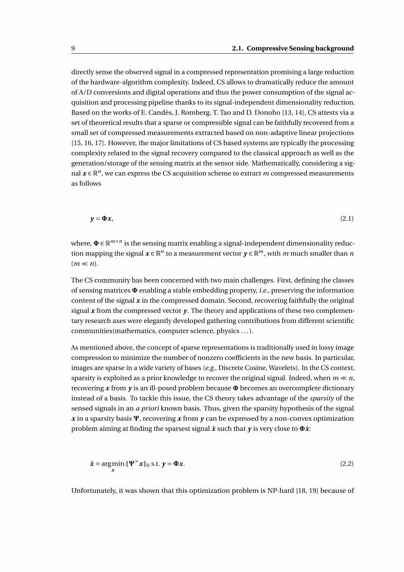
generation/storage of the sensing matrix at the sensor side. Mathematically, considering a sig-
nal x ∈Rn , we can express the CS acquisition scheme to extract m compressed measurements
as follows
y =Φx , (2.1)
where,Φ ∈Rm×n is the sensing matrix enabling a signal-independent dimensionality reduc-
tion mapping the signal x ∈Rn to a measurement vector y ∈Rm , with m much smaller than n
(m ¿ n).
The CS community has been concerned with two main challenges. First, defining the classes
of sensing matricesΦ enabling a stable embedding property, i.e., preserving the information
content of the signal x in the compressed domain. Second, recovering faithfully the original
signal x from the compressed vector y . The theory and applications of these two complemen-
tary research axes were elegantly developed gathering contributions from different scientific
communities(mathematics, computer science, physics . . . ).
As mentioned above, the concept of sparse representations is traditionally used in lossy image
compression to minimize the number of nonzero coefficients in the new basis. In particular,
images are sparse in a wide variety of bases (e.g., Discrete Cosine, Wavelets). In the CS context,
sparsity is exploited as a prior knowledge to recover the original signal. Indeed, when m ¿ n,
recovering x from y is an ill-posed problem becauseΦ becomes an overcomplete dictionary
instead of a basis. To tackle this issue, the CS theory takes advantage of the sparsity of the
sensed signals in an a priori known basis. Thus, given the sparsity hypothesis of the signal
x in a sparsity basisΨ, recovering x from y can be expressed by a non-convex optimization
problem aiming at finding the sparsest signal x such that y is very close toΦx :
x = argminx
‖Ψ>x‖0 s.t. y =Φx . (2.2)
Unfortunately, it was shown that this optimization problem is NP-hard [18, 19] because of

Chapter 2. State Of The Art 10
the `0 norm which is non-convex. However, because of ‖Ψ>x‖qq approaches ‖Ψ>x‖0 as q > 0
tends to 0 [20, 21], we can approximate (2.2) by
x = argminx
‖Ψ>x‖q s.t. y =Φx . (2.3)
In the specific case of q = 1, this relaxation becomes convex and allows therefore to solve a
much simpler `1-minimization problem rather than the `0 problem leading to the following
Basis Pursuit (BP):
x = argminx
‖Ψ>x‖1 s.t. y =Φx . (2.4)
However, the success of exact recovery via BP is achieved with respect to a certain condi-
tion expressed by the spasity level. Indeed, the bound defining the sparsity level required
to ensure this equivalence is provided by the works of D. Donoho, X. Huo, M. Elad and A.
Bruckstein [22, 23, 24]. Furthermore, we can reformulate (2.4) alternatively to extend this opti-
mization problem to a more general `1-minimization taking measurements error as well as
compressible signals into account. In fact, due to sensors nonidealities, noisy measurements
can probably be extracted leading to a recovered signal with m nonzero components instead
of k. On the other hand, real-world images are generally compressible rather than sparse
with the existence of sparse approximations that approximate them by sparse vectors. Given
these considerations, it becomes reasonable to consider the following Basis Pursuit Denoising
(BPDN) under the assumption of an Additive white Gaussian noise (AWGN):
x = argminx
‖Ψ>x‖1 s.t. ‖y −Φx‖22 ≤ ε. (2.5)
Equivalently, (2.5) can be expressed using its augmented Lagrangian form:
x = argminx
‖Ψ>x‖1 +λ‖y −Φx‖22, (2.6)
where λ is an inner regularization parameter allowing to control the energy of the fidelity
term, i.e., the sparsity level on the recovered signal. There exists a wide variety of algorithms
to solve the `1-minimization problems stated in (2.4), (2.5) and (2.6). In the next section we
provide a sparse insight about the commonly used methods for sparse signal recovery or

11 2.1. Compressive Sensing background
sparse approximation problems.
2.1.2 Basic Algorithmic Tools
Once the CS measurements extracted in the sensor side, a reconstruction algorithm is typically
needed to solve the `1-minimization problems expressed by (2.4) and (2.5). In the CS portfolio,
there exists a wide variety of algorithms that guarantee a faithful and efficient signal recovery.
Efficiency of these algorithms depends however on the complexity in terms of speed and
memory needs as well as the quality of recovery in terms of reconstruction error. Several
classifications have been proposed in the literature to group sparse recovery methods under
different categories [25, 26, 27]. Here, three major classes are considered to solve sparse
approximation problems: recast-based methods, greedy methods and non-convex methods.
In the following, we give some elementary materials related to each algorithms class.
Recast-based Methods
Before discussing recast-based methods, we note that in convex optimization [28] an optimiza-
tion problem is generally expressed as:
x = argminx
f0 (x) s.t. fi (x) ≤ bi , i ∈ [n] , (2.7)
where f0 : Rn → R is called an objective function, fi : Rn → R, i ∈ [n] are called constraint
functions and the constants bi are called bounds for the constraints. Notice that when fi ’s
are all linear, the problem is called a linear program. If fi ’s are all convex, then the problem is
called a convex optimization problem and consequently its equivalent augmented Lagrangian
as well.
We have mentioned previously that CS signal recovery can be expressed as a convex problem
thanks to a convex relaxation leading to the `1-minimization problem (i.e., equations (2.4)
and (2.5)). In addition, it was shown that the problem in (2.4) can be recast as a linear program
by introducing slack variables [29]. This way, one can use the classical Dantzig’s Simplex
method [28] to solve (2.4). However, in the most physical-friendly approach (i.e., BPDN in
(2.5)), the signal recovery problem becomes a second-order cone problem, i.e., a problem
with quadratic constraint functions. The interior-point methods [30, 31] were among the first
methods used to solve sparse approximation problems by convex optimization [32] expressed
with a quadratic constrain (i.e., (2.5)). However, although their low complexity, they are less
competitive compared to greedy methods, specifically designed for `1-minimization. Indeed,
their performance is insensitive to the sparsity of the reconstructed signals or the value of the
regularization parameter (i.e., (2.6)).

Chapter 2. State Of The Art 12
Greedy Methods
A greedy method refers to a step-by-step fashion to recover a sparse signal [33, 34, 35, 36, 37, 38,
39, 40, 41]. This signal recovery selection can advantageously be combined with a thresholding
routine leading to a precise tuning of the sparsity level of the estimated signal. In addition,
greedy algorithms are known to be simple to implement, fast and applicable to large-datasets.
These methods therefore provide strong theoretical guarantees for sparse signal recovery. A
non-exhaustive list of the commonly used greedy methods can be found in [42] as well as
recovery proofs and algorithms complexity in terms of computation and storage costs.
Non-convex Methods
From an optimization point of view, non-convex methods refer to sparse recovery methods
dealing with non-convex cost functions [43, 44], i.e., ‖Ψ>x‖q with 0 < q < 1 in (2.3). In [45], it
was shown that an exact recovery of sparse signals can be achieved with fewer measurements
than when q = 1 (i.e., (2.4)). Non-convex methods could probably be interesting to recover
sparse signals in the field of quantized compressive sensing [46] where non-convex constraint
functions are widely used [47]. Furthermore, we can also include under non-convex methods
Bayesian methods where a prior distribution is considered to recover the unknown coefficients
that promotes sparsity [48, 49, 50, 51]. It was shown that Bayesian methods can achieve fast
and low error recovery thanks to a prior knowledge of the sparse coefficients distribution
[52]. Finally, in some recent works Deep Neural Networks (DNN) have been explored for
signal recovery by learning structured representations from a training dataset of compressed
samples [53, 54, 55]. In fact, DNN-based methods show significant improvements in terms
of speed and quality of recovery. However, neither computational complexity nor memory
needs have been provided in these works. Indeed, the complexity involved by these kind
of algorithms could be higher compared to the commonly-used greedy methods due to the
training dependency that involves many nonliear operations.
2.1.3 CS Sensing Matrix Properties
To provide guarantees of faithful (stable) reconstruction of the observed signals, compressive
sensing theory has introduced several metrics to measure the ability of the sensing matrix
Φ to generate independent measurement and to spread out the information in the sensed
signal among the extracted measurements. In the following, we will carry out the main metrics
studied in the CS theory known as the coherence and the Restricted Isometry Property (RIP)
enabling exact recovery of k-sparse signals via the `1-minimization problems stated in (2.4)
and (2.5). These properties are basically used to study theoretical bounds of sparse signal
recovery algorithms. On the other hand, when dealing with sparse (or compressible) signals
in some bases different from the sensing basis (e.g., a selfie taken in front of the Eiffel Tower
is not sparse in the canonical basis but sparse in a wavelet basis), it turns out that we can
sense the observed signal directly in its original domain without significant loss of the sensing

13 2.1. Compressive Sensing background
robustness thanks to the universality property.
Coherence
A simple and easy measurable metric to assess the robustness of a sensing matrix is the
coherence [56, 57]. It evaluates the cross-correlations between any two columns of the sensing
matrixΦ expressed as:
Definition 1. LetΦ ∈Rm×n be a matrix with `2-normalized columnsΦ1, . . . ,Φn , i.e., ‖Φi‖22 = 1
for all i ∈ [n]. The coherence µ (Φ) of the matrixΦ is defined as:
µ (Φ) = max1≤i 6= j≤n
|⟨Φi ,Φ j ⟩|. (2.8)
As a general consideration, the smaller the coherence of the sensing matrix the better is
the recovery. Furthermore, it was shown that the coherence can be bounded as follows:
µ (Φ) ∈[√
n−mm(n−1) ,1
]. The lower bound is known as the Welch bound [58], and for m ¿ n it
becomes µ (Φ) ' 1pm
. Based on the coherence, sufficient conditions were carried out for exact
sparse recovery [57, 59], e.g.,
µ (Φ) < 1
2k −1, (2.9)
with k is the sparsity level.
Restricted Isometry Property
In [60] the concept of the Restricted Isometry Property (RIP) is introduced as a powerful metric
to assess the quality of a sensing matrix and ensure the success of signal recovery in the context
of CS.
Definition 2. A matrixΦ is said to satisfy the Restricted Isometry Property (RIP) of order k if,
for all k-sparse vectorsα, there exists a constant δk ∈ (0,1) such that:
(1−δk )∥∥α∥∥2
2 ≤∥∥Φα∥∥2
2 ≤ (1+δk )∥∥α∥∥2
2. (2.10)
As for the coherence, small restricted isometry constants δk are desired. In addition, when
respecting the RIP, the linear mappingΦ preserves the energy of the sensed signal and is said
to be a stable embedding. Notice that if the RIP is satisfied for a certain sparsity level k, it is
therefore satisfied for any k ′ < k with δk ′ < δk . On the other hand, respecting the RIP over
all 2k-sparse vectors implies to preserve the pairwise distances between any two k-sparse
vectors.

Chapter 2. State Of The Art 14
The RIP has a major role to deal with noisy measurements and guarantee a stable embedding.
In fact, to tackle issues related to sensors nonidealities, the RIP ensures that noisy measure-
ments have negligible impact on the quality of recovery. Furthermore, respecting the RIP is a
sufficient condition for a wide variety of algorithms to guarantee an exact recovery [61, 62].
Finally, to establish a connection between the dimensions of the problem (i.e., n,m and k),
a certain number of measurement is necessary to achieve the RIP and can be expressed for
randomly generated sensing matrices as follows:
m >C k log(n
k
), (2.11)
where C > 0 is is a universal constant (independent of k, m, and n) [26].
It is worth pointing out that the RIP property has been established for infinite sets of signals.
Furthermore, verifiyng the RIP is a NP-hard problem. For instance, the Johnson–Lindenstrauss
Lemma (JLL) [63] can simplify verifying the stable embedding of a finite set of points [64].
Lemma 1. Let 0 < t < 1. For every set X of cardX points in Rn , if m is a positive integer such
that m >O(
log(cardX )t 2
), there exists a Lipschitz mapping f (u) =Φu such that
(1− t )‖u −v‖2 ≤ ‖ f (u)− f (v )‖2 ≤ (1+ t )‖u −v‖2, (2.12)
for all u, v ∈X .
Universality
In the context of vision systems involving visible images, sparsity is generally not verified in the
canonical basis but rather in some other orthonormal basis (e.g., Fourier, Wavelets). However,
for a fixed sensing matrixΦ, the concept of universality ensures to sense any sparse signal in
any representation domain without significant loss of the sensing robustness. We emphasize,
however, that universality is not respected implicitly. For example structured matrices are not
universal as it will be discussed in next section.
2.1.4 CS Sensing Market
In this section, we turn to the problem of constructing sensing matrices that satisfy CS re-
quirements. The CS community has proved the existence of RIP matrices allowing a faithful
recovery of compressively sensed signals. These matrices can be deterministic [65, 66, 67] or
randomly generated [68, 69]. Inspired by the classification proposed in [70], here we divide
the SOTA sensing matrices into three main categories: random sub-Gaussian matrices, bases
random selection and random convolutions.

15 2.1. Compressive Sensing background
Random sub-Gaussian Matrices
Based on the the theory of concentration of measures [71], it was shown that sub-Gaussian
matrices have interesting properties leading to a wide use in the CS context [68, 72]. For
example, the sensing matrixΦ ∈Rm×n can be generated identically and independently (i.i.d.)
as a normalized Gaussian random variable of variance 1m [69], i.e.,Φi j ∼N
(0, 1
m
). In addition,
Φ can be generated as the realization of a Bernoulli distribution with probability of success12 , i.e.,Φi j ∼± 1p
m. These realizations show interesting properties from a theoretical point of
view [68], but also hardware implementations such they can be advantageously generated as
a deterministic and reproducible process taking advantage of Pseudo-Random Generators
(PRG) [73, 74].
Bases Random Selection
In the second class of CS matrices random sub-sampling of orthonormal bases can be consid-
ered to construct the sensing matrixΦ [75, 76]. In fact, given an orthonormal basis U ∈Rn×n ,
one can picks randomly m components of each n-dimensional vectors, i.e.,
Φ= SU , (2.13)
with S ∈ Rm×n represents the random selection matrix. We notice, however, that the basis
U must be sufficiently incoherent with the sparsity basisΨ. This measure can be evaluated
using the coherence of the dictionaryΦΨ as expressed in (2.8). Typical constructions can be
achieved using this framework. For instance, it was shown that the Fourier basis is incoherent
with the canonical basis [75]; and the Noiselet is highly incoherent with the wavelet one [76].
On the other hand, random Fourier basis selection can advantageously be combined with
a specific signal randomizers (e.g., random bit flips, Bernoulli distributions) to achieve the
universality [77, 78, 79]. Interestingly, this approach enables fast signal recovery, but involves
higher memory needs to store the sensing matrix for physical implementations.
Random Convolutions
In [80], a different approach to construct the sensing matrixΦ is proposed. Based on random
convolutions, this approach corresponds to pick randomly m measurements of the results of
the convolution of the observed signal x and a random complex sequence of unit amplitude.
This way, the sensing matrixΦ can be expressed as:
Φ= SF∗ΣF , (2.14)

Chapter 2. State Of The Art 16
withΣ ∈Rn×n is a complex diagonal matrix made of unit amplitude and random phase entries;
and F ∈Rn×n is the complex discrete Fourier transform. Notice that this approach can take
advantage of simple and fast recovery algorithms based on Fast Fourier Transforms (FFTs).
2.1.5 Signal Processing in CS Domain
Despite the growing potential of CS to tackle hardware issues related to highly constrained
applications, the major limitation of CS based systems is the processing complexity related
to the signal recovery. This consideration highly restricts the use of CS to niche applications.
In fact, in most "real-world" applications we are mainly interested to extract a meaningful
information and filtering the rest. Considering any kind of computer vision problem (e.g.,
Advanced Driver-Assistance Systems), image descriptors (e.g., HOG, LBP) combined with a
proper classification algorithm (e.g., Artificial Neural Networks) are used to enable objects
detection and/or classification. In this context, some first steps have been taken to circumvent
signal recovery and bridge the gap between compressive sensing and signal processing [81, 82,
83, 84]. For instance, in [84] several theoretical bounds and experiments have been reported
to show the relevance of CS for basic signal processing tasks (e.g., detection, classification,
estimation, filtering).
Figure 2.2 – An illustration of the rare eclipse problem.
From a decision making point of view, two main approaches have been adopted for classifica-
tion in the CS (compressed) domain. First based on the RIP property, R. Calderbank et al. show
that the Euclidean distance between low complexity signals (e.g., k-sparse) is preserved in the
CS domain [85]. This allows to perform decision algorithms directly in the CS domain since
pairwise distance is a primitive operation in numerous classification and machine learning
algorithms. In particular, they provide some theoretical bounds demonstrating that the linear
Support Vector Machine (SVM) classifier in the CS domain has a classification accuracy close
to its classification accuracy in the signal domain. On the other hand, when dealing with
linearly separable convex sets, the rare eclipse problem [86, 87] provides a lower bound of the
number of measurements m required to preserve the disjointedness between two classes (e.g.,
images with n pixels) in the CS domain (cf., Figure 2.2).

17 2.1. Compressive Sensing background
2.1.6 CS Hardware Implementations
Inspired by the potential of CS, several strategies have been explored to design sensors with
CS capability, i.e., acquiring random compressed measurements. It was shown therefore that
CS can be applied to wide variety of sensors, e.g., Magnetic Resonance Imaging (MRI) [88],
Terahertz (THz) [89], Time-of-Flight (TOF) [90], Radars [91], Hyper/Multispectral imaging
[92, 93]. In this thesis we are mainly interested by sensors in the visible electromagnetic
spectrum. In the following, we will present two major classes to implement the CS sensing
scheme either in the optical domain or in the electronic one.
CS Optical Implementations
Optically implemented CS strategies performs basically the CS linear measurements in (2.1)
using appropriate optical devices. This way, CS is performed in the analog domain enabling
considerable saving at the analog-to-digital conversion level as well as digital signal processing.
Under this category, four main contributions can be listed: Single Pixel Camera (SPC), coded
aperture, random lens, lensless imaging and the imaging with nature techniques.
Single Pixel Camera (SPC): The SPC [94, 95] was the first device to implement optical com-
pressive imaging. Based on single photodiode, the SPC uses a Digital Micromirror
Device (DMD) to sequentially capture the CS measurements. Here, the pseudo-random
projections are achieved thanks to the DMD which is electronically controlled to reflect
the incident light towards the photodiode or away. Despite the interest that shows a
SPC, this one suffers from major limitations related mainly to the amount of snapshots
to perform in order to guaranty a faithful reconstruction due to optical non perfect
characterization and nonlinear issues in general. This approach also has the drawback
of implying bulky optical elements which can be a limitation for embedded systems.
Coded aperture: Coded aperture systems basically use spatial light modulators to block or
permit the projection of the incident light onto a photosensitive element, this one can
be a 2D detector, a line-detector, or extremely, a single-pixel detector. Unlike the SPC,
CS measurements extracted using a coded aperture based system can advantageously
be parallelized leading to low latency CS systems compared to the SPC without any
additional cost at the silicon level. Up to date, several applications have been addressed
using a coded aperture approach. Non-exhaustively we can list: super resolution [96],
high speed imaging [97], spectral imaging [98], terahertz imaging [89] and depth imaging
[99].
Random lens: In the case of using an ordinary lens, the incident light rays from a point in
a geometrical space are mapped onto the same location of the sensor array. However,
using random lenses, this mapping becomes pseudo-random. In [100], this randomness
is built up taking advantage of a multi-faceted mirror. The main drawback of this set-up
is however the complex calibration needed to make the system operational limiting the

Chapter 2. State Of The Art 18
use of this approach for end-user applications.
Imaging with nature: The concept of random lens is advantageously extended using the
natural randomness of wave propagation. Indeed, in [101] the concept of "imaging
with nature" is introduced taking advantage of a multiply scattering media. In fact, the
incident light reflected by an object is propagated through a multiply scattering medium
creating a random speckle pattern. After the propagation, the CS measurements are
extracted using a limited number of sensors (m sensors to extract m measurements).
Interestingly, this system is currently used as Optical Processing Unit (OPU) promising
accelerated random feature extraction for classification tasks [102].
Lensless imaging: Leveraging the limitations involved by lenses in cameras, an alternative
approach to acquire compressed measurements is explored using lensless imaging
systems [103]. In [104], a lensless compressive imaging architecture is proposed. It takes
advantage of a single photosensitive element and a LCD screen as an aperture array
where each element is individually controlled. Thus, each CS measurement corresponds
to all the rays modulated by a ±1 achieved thanks to the LCD screen. Although the com-
plexity of the acquisition process (as many snapshots as measurements), the imaging
device proposed in this work is more compact compared to the commercial cameras.
Furthermore, to circumvent the acquisition latency, a block-based lensless compressive
camera is proposed in a more recent work [105].
Although the interest that presents optically generated randomness, this approach still suffers
from several drawbacks as listed above limiting its use to niche applications. An appealing
approach consists in performing CS in the focal plane taking advantage of the technological
evolutions of the CMOS Image Sensor (CIS) world.
CS Electronic Implementations
Inspired by the potential of CS, the CMOS Image Sensor (CIS) community has focused on
implementing on-chip sensing schemes to deal with either hardware (Analog/Digital con-
version, fill-factor, silicon footprint) or algorithm constraints (fast and efficient recovery) for
image rendering. In the following we report some of the efforts made by the CIS community
to implement in-focal plane CS implementations. We mainly focus on two main approaches
to address this challenge: in-focal plane and end-of-column implementations.
In-focal plane implementations : In-focal plane implementations refers typically to CS CMOS
implementations performing CS at the pixel level before A/D conversions (i.e., in the
analog domain). In [106, 107] a generic implementation is proposed to implement any
separable transform in the focal plane. The main interest of this implementation is its
capability to implement the 2D separable transform (i.e., line and column projection)
Y σ = A>PσB in an overlapping block-based fashion, with A and B are the transforma-
tion matrices, Y is the output, P is the acquired image and σ is selected sub-matrix. To
19 2.1. Compressive Sensing background
perform in-focal plane CS, this work proposes to select randomly m measurements from
each 16×16 block. Despite using analog memories to store the separable transform
in order to reduce power consumption, this work still suffers from major limitations
mainly related to the lower fill factor, the silicon-footprint and its disability to perform
on-chip CDS to deal with the Fixed Pattern Noise.
The second interesting implementation exploits the random convolution based sensing
scheme proposed in [80]. The CMOS implementation of this scheme gives the priority
to a fast and efficient image reconstruction but involving high on-chip complexity.
Indeed, as presented in [108, 109], this architecture basically requires a 2D pixels array
with in-situ memories to store a randomly generated Rademacher distribution (i.e.,
±1 entries with equal probability). In fact, to extract one CS measurement, an initial
seed is generated and stored on-chip using a Linear Feedback Shift Register (LFSR).
Then, depending on the weight sign, the output current of each pixel is conveyed either
to the positive or negative input of a transimpedance amplifier (TIA) for summation.
Finally, to extract m measurements, m shifts of the LFSR have to be done. Indeed, the
random convolution in the Fourrier domain allows to simplify the matrix-to-vector
multiplication at the reconstruction stage to some FFTs of low complexity. However,
implementing a flip-flop per pixel results in either lower fill-factor (percentage of area
occupied by the photodiode in the pixel) or larger pixel sizes.
Finally, in-focal plane coded aperture has emerged as an appealing approach for high
speed imaging. In [110], a multi-aperture CIS is proposed for compressive imaging.
Indeed, The photo-carriers generated in the photodiode are temporally modulated
with a per-block shutter pattern and accumulated in the in-pixel charge memory. The
imager has the advantage of modulating pixels values at the photodiode level, elec-
tronically, without external bulky and expensive optical components. In some recent
works [111, 112], pixelwise spatial and temporal coding are proposed allowing more
CS-friendly sensing schemes. Notice that the main drawback of such architectures
is the lower fill factor because of memory needs at each pixel design complexity. We
believe, however, that this bottleneck could advantageously be surpassed thank to the
3D stacked technology [113].
End-of-column implementations : In contrast to in-focal plane CS implementations, end-
of-column implementations take advantage of standard pixel architectures (e.g., 3T or
4T APS) and canonical rolling shutter readout while performing CS measurements at
the end-of-column circuitry. One interesting common point of end-of-column imple-
mentations is the the parallelization proposed to extract CS measurements which is
very important and the kept of standard CIS readout architecture as well. Thus, the CS
sensing scheme in (2.1) becomes:
Y =ΦX , (2.15)
Chapter 2. State Of The Art 20
where X ∈ Rnr ×nc is the 2D representation of the observed image, Φ ∈ Rm×nr is the
sensing matrix applied in parallel to all the columns of X , and Y ∈Rm×nc is the matrix
representation of the extracted CS measurements. Notice that Bernoulli (i.e., 0/1 entries)
or Rademacher (i.e., ±1 entries) sensing matrices are preferable in this case for their
simple and compact implementations using Pseudo-Random Generators (PRG).
In one of the first end-of-column implementations, [114] takes advantage of incre-
mental Σ∆ Analog-to-Digital converters to perform summation/averaging operation
during A/D conversion to extract per-block CS measurements. This concept was first
introduced in [115] to implement a block matrix transform method for image com-
pression. In [114], a compressed sensing multiplexer (CS-MUX) controlled by a PRG
(Linear Feedback Shift Register) perform CS measurements over 16×16 pixel blocks.
Thanks to the PRG, a random scrambling is thus performed at the input of each Σ∆ ADC
enabling a per-column parallel summation and conversion of the randomly selected
pixels. This architecture has the advantage of using an optimized 4T pixel architecture
while performing end-of-column CS without major modification of a canonical sensor
design. However, although the technical breakthrough that proposes this architecture,
the reduced support dimensionality to perform per-block CS measurements can lead
to a poor theoretical bound to achieve the RIP property (or not) and have to deal with
artifacts at the reconstruction side.
An other approach to extract CS measurements is based on capacitive measurements.
The underlying motivation of this approach is the reduced power consumption thanks
to the use of small charge transfers to readout CS measurements. For instance, in [116]
a more CS-friendly scheme is proposed based on a Rademacher per-column sensing
matrix generated using an external LFSR at the expense of a more complex in-pixel
hardware. Indeed, the proposed CIS uses a local capacitor inside the pixel and two
separate column lines for column-parallel pixels readout. Thus, depending on the
LFSR’s generated bit, the pixel output is either multiplied by 1 (for a logical one) or
−1 (for a logical zero) and summed in the charge domain using a comparator-based
switched capacitor. However, this implementation have several limitations mainly
related to the reduced fill factor and the silicon footprint needed to design the end-of-
column capacitors. On the other hand, in [117] standard 3T pixels are used to mitigate
the problem of pixel fill factor in a per-block CS fashion. Indeed, a switched-capacitor is
used to perform summation of randomly selected measurements from 4×4 blocks in the
analog domain during the integration time. However, one major drawback of this set-up
is the number of connection lines to perform averaging. In fact, for the proposed block
size (i.e., 4×4), 16 readout wires are necessary for each block leading to an important
capacitive noise and matching issues.
Finally, [118] describes a scalable and low-complexity column based CS scheme using
a Cellular Automaton (CA) that shows a chaotic behavior to on-the-fly generate the
sensing matrix. Indeed, the implemented sensing scheme consists in a per-column
normalized Bernoulli distribution (i.e., 0/1 entries) where each column is measured
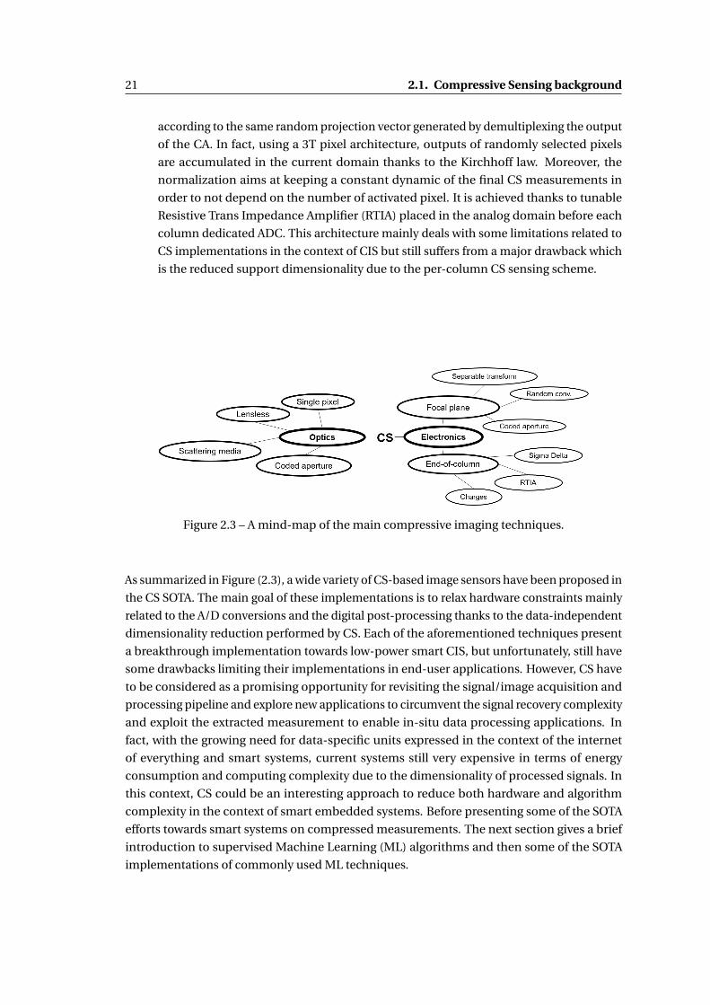
21 2.1. Compressive Sensing background
according to the same random projection vector generated by demultiplexing the output
of the CA. In fact, using a 3T pixel architecture, outputs of randomly selected pixels
are accumulated in the current domain thanks to the Kirchhoff law. Moreover, the
normalization aims at keeping a constant dynamic of the final CS measurements in
order to not depend on the number of activated pixel. It is achieved thanks to tunable
Resistive Trans Impedance Amplifier (RTIA) placed in the analog domain before each
column dedicated ADC. This architecture mainly deals with some limitations related to
CS implementations in the context of CIS but still suffers from a major drawback which
is the reduced support dimensionality due to the per-column CS sensing scheme.
Figure 2.3 – A mind-map of the main compressive imaging techniques.
As summarized in Figure (2.3), a wide variety of CS-based image sensors have been proposed in
the CS SOTA. The main goal of these implementations is to relax hardware constraints mainly
related to the A/D conversions and the digital post-processing thanks to the data-independent
dimensionality reduction performed by CS. Each of the aforementioned techniques present
a breakthrough implementation towards low-power smart CIS, but unfortunately, still have
some drawbacks limiting their implementations in end-user applications. However, CS have
to be considered as a promising opportunity for revisiting the signal/image acquisition and
processing pipeline and explore new applications to circumvent the signal recovery complexity
and exploit the extracted measurement to enable in-situ data processing applications. In
fact, with the growing need for data-specific units expressed in the context of the internet
of everything and smart systems, current systems still very expensive in terms of energy
consumption and computing complexity due to the dimensionality of processed signals. In
this context, CS could be an interesting approach to reduce both hardware and algorithm
complexity in the context of smart embedded systems. Before presenting some of the SOTA
efforts towards smart systems on compressed measurements. The next section gives a brief
introduction to supervised Machine Learning (ML) algorithms and then some of the SOTA
implementations of commonly used ML techniques.

Chapter 2. State Of The Art 22
2.2 Machine Learning background
There is no doubt that Artificial Intelligence (AI) is drawing attention in many scientific and
engineering fields. Today, AI softwares can understand and translate speech [119], interpret
images [120], assist medical diagnostics [121] and even defeat a world champion in the game
of Go [122]. In fact, AI allows machines to be intelligent by gathering knowledge by experience,
in a nutshell, machines learn by doing. This capability to learn and make decisions is what
we call explicitly Machine Learning (ML). ML has had a long and rich history, in its early
days, programmable computers were built to solve mathematical problems difficult to solve
intellectually and thus said intelligent. However, building machines that think and make
decisions involves a huge amount of mathematical operations leading to a brick wall toward
intelligent machines. Advantageously, the last decade has testified a wide development of
computing infrastructures (e.g., Cloud, GPU, TPU) making the current "AI spring" [123]. In
the rest of this section, we provide an informal introduction to the ML techniques and present
some of the current efforts to run ML algorithms in an efficient way in the edge to tackle issues
related to privacy, latency and algorithm-hardware complexity.
2.2.1 Machine Learning Algorithms Market
A machine learning algorithm is an algorithm that is able to learn from data [124]. Learning
is more precise in the definition of T. Mitchell [125]: "A computer program is said to learn
from experience E with respect to some class of tasks T and performance measure P , if its
performance at tasks in T , as measured by P , improves with experience E." For instance,
one can build a ML algorithm to perform a classification task to decide to which category
an object belongs to; or a regression task to predict a numerical value given some inputs. A
performance measure is basically used to evaluate the robustness of a ML technique. In
general, the accuracy (i.e., ratio of correct outputs) or error rate (i.e., ratio of incorrect outputs)
are the most common performance measure used in ML. Finally, a ML algorithm generally
experience a dataset to improve its performance P on a task T. A dataset is generally defined as
a collection of data measured using a sensor (e.g., images with a certain number of pixels) or
extracted from experimental measurements (e.g., length and width).
In particular, supervised learning algorithms experience a dataset containing samples/features
associated with labels. Let’s consider a faces recognition problem. The goal is then to build
a machine that takes unknown images and decide about the identity of the faces. To learn
our ML algorithm we need first a large dataset of images X tr ai n called a training set in which
each image contains n pixels associated with labels y tr ai n which represent the identity of each
image. The result of learning a supervised ML algorithm can be expressed as a function fW (x i )
that takes a new sample x i and generate an output vector y i with respect to the learned
patterns W . During the training the weights W are tuned to minimize the empirical risk
L (W ) = 1ns
∑ns
i L(
fW (x i ) , yi), with ns is the number of training samples. The empirical risk
L (W ) can take several forms, e.g., Mean Squared Error (MSE), `2-norm, Kullback Leibler (KL)

23 2.2. Machine Learning background
Divergence, Hinge loss. Thus, the training error will measure how well is this minimization on
the training set. Note, however, that the most important error is the generalization error also
called test error that evaluates the performance of the trained algorithm on unknown samples.
The main goal is then to learn algorithms that make the training error as small as possible
while making the gap between training and test error small too. These tow goals refer to two
central challenges knows as underfitting and overfitting. In fact, underfitting occurs when the
trained algorithm is not able to obtain a sufficiently low training error. However, overfitting
occurs when the trained algorithm fits too well the training set but fails to generalize to new
samples.
To deal with overfitting and to design an algorithm that performs well on a specific task, we
can build a set of preferences to constrain the learning model. As in convex optimization
mentioned in Section 2.1.1, a regularization is typically used to constraint the algorithm design
and express the preferences for specific solutions. As defined in [124], "Regularization is any
modification we make to a learning algorithm that is intended to reduce its generalization
error but not its training error". This way, the empirical error can be expressed with respect to
a regularization term as follows:
L (W ) = 1
ns
ns∑i
L(
fW (x i ) , yi)+λR (W ) , (2.16)
with λ is an inner parameter that control the impact of the regularization term.
In many practical applications the input data is typically pre-processed to extract meaningful
information and thus relax constraints related to the amount of data to process. For instance,
a data normalization stage is basically used to rescale the input data into a common range
to improve training robustness. Commonly used normalization approaches are min-max
normalization that consists in rescaling the range of data in [0,1]; or standardization which
allows to have zero-mean and unit-variance data. Pre-processing can also refer to feature
extraction that allows to project the input data into a low dimensional feature space where the
intended task is hoped to be easier to learn. For example, in computer vision a wide range of
feature extraction methods have been proposed. Non-exhaustively we can cite: Histograms
of Oriented Gradients (HOG) to extract descriptors by accumulating histograms of oriented
gradients over blocks [126]; Local Binary Patterns (LBP) that allows to recognizes pre-defined
patterns over blocks; Scale-invariant feature transform (SIFT) [127], Fast Retina Keypoint
(FREAK) [128] and Binary Robust Invariant Scalable Keypoints (BRISK) [129] to extract local
keypoints; Convolutional Neural Networks to extract shift and space invariant features [130];
and random projections shown to perform a distance-preserving embedding of the data [131].
Roughly speaking, three main classes of supervised machine learning techniques can be found
in the literature: statistical learning, dictionary learning and deep learning. The rest of this
section will give a definition to each class and present commonly used algorithms based on

Chapter 2. State Of The Art 24
some useful textbooks written by C. Bishop [132], G. James et al. [133], B. Dumitrescu et
al. [134] and I. Goodfellow et al. [124].
Statistical Learning
Statistical learning refers to ML techniques that involve learning a statistical method for
predicting or estimating an output based on one or more inputs [133]. For instance, a Linear
Discriminant Analysis (LDA) [135] learns a function that projects a n-dimensional data that
belongs to C classes into a (C −1)-dimensional space (cf., Figure 2.4). It aims at finding the
best projections respecting the Fisher’s criteria [136], i.e., minimizing the within-class variance
SW while maximizing between classes variance SB . Although it is basically considered as a
dimensionality reduction technique for data visualization, the LDA can also be considered
as a multi-class classification technique thanks to the discriminant representation in the
low-dimensional space. To deal with classes that are nonlinearly separable, kernel tricks can
typically be used to project the data into a high-dimensional space that makes the data linearly
separable [136]. However, a major drawback of the LDA is the assumptions required about the
data limiting the use of the LDA to samples with Gaussian distributions.
Figure 2.4 – An illustration of the projection in the LDA domain for C = 3.
On the other hand, one more powerful statistical technique is the Support Vector Machine
(SVM) [137]. Initially proposed to create a binary decision boundary that maximizes the
margin between two classes associated with positive or negative labels. Here, the margin refers
to the small distance between the decision boundary and the closest sample of the dataset.
Indeed, learning a binary SVM leads to an affine function expressed as fw ,b (x) = w>x +b.
Thus, for an unknown sample x i , the binary SVM predicts a positive label if fw ,b (x) is positive
and a negative one if fw ,b (x) is negative. As for the LDA, the SVM classifier can take advantage
of kernel tricks to deal with nonlinearly separable datasets. However, one major limitation of
kernel machines is the computational cost of the training when the dataset is large.
The concept of SVM can advantageously be extended to multi-class classification problems
using a series of binary SVMs [138] (cf., Figure 2.5). Given a C -classes classification problem,
for a one-vs.-all strategy learns C binary SVMs between each class and the rest. In this case,
the inference is achieved using a winner-takes-all strategy to assign an unknown sample to
the class with the highest margin. Moreover, for one-vs.-one strategy a binary SVM is learned

25 2.2. Machine Learning background
between each pair of classes i , j , with i 6= j . Thus, c(c−1)2 binary classifiers are built. For the
inference a max-wins strategy increases the vote of each class predicted by the learned binary
SVMs. Finally, the unknown sample belongs to the class with the largest vote.
(a) One-vs.-all strategy. (b) One-vs.-one strategy.
Figure 2.5 – An illustration of the SVM classifier for c = 4: (a) One-vs.-all strategy; (b) One-vs.-one strategy for the blue class.
Dictionary Learning
As shown in Section 2.1, sparse representations have emerged as a powerful framework for
signal/image compression and signal recovery. More recently, sparse representations have
been explored to learn sparse discriminative features. Indeed, in the "Sparse-Land" [10]
the sparsifying basis is usually called a dictionary and the signal can be approximated by a
linear combination of few elements of the dictionary called atoms [139]. In this context, a
Sparse Representation-based Classifier (SRC) was initially proposed in [140] for (robust) face
recognition. In SRC, a test sample y (e.g., face) is expressed as a sparse combination of all
the training samples represented by the dictionary D = [D1 . . .Dc ], where D i (i ∈ [c]) contains
samples of class i , i.e., y = D x , with x is the coefficients vector whose entries are zero except
those associated to the i th class, said to be the predicted class of y . This way, for a set of
samples Y = [Y 1 . . .Y c ], the coefficients matrix X will be a block diagonal sparse matrix (cf.,
Figure 2.6). However, the main disadvantages of the SRC is the complexity that depends
linearly on the size of the training set, i.e., as large dictionary dimensionality as the training
set size.
A straightforward approach for classification tasks is to learn dictionaries that promote spar-
sity as well as classes separability, this approach is called Dictionary Learning (DL). Thus,
assuming non-overlapped discriminant features, regularization terms are basically introduced
to promote class-specific dictionaries (i.e., atoms) independency. For instance, in [141] the
Dictionary Learning with Structured Incoherence (DLSI) takes advantage of a regularization
term that encourages the dictionaries to be as independent as possible based on a Frobenius
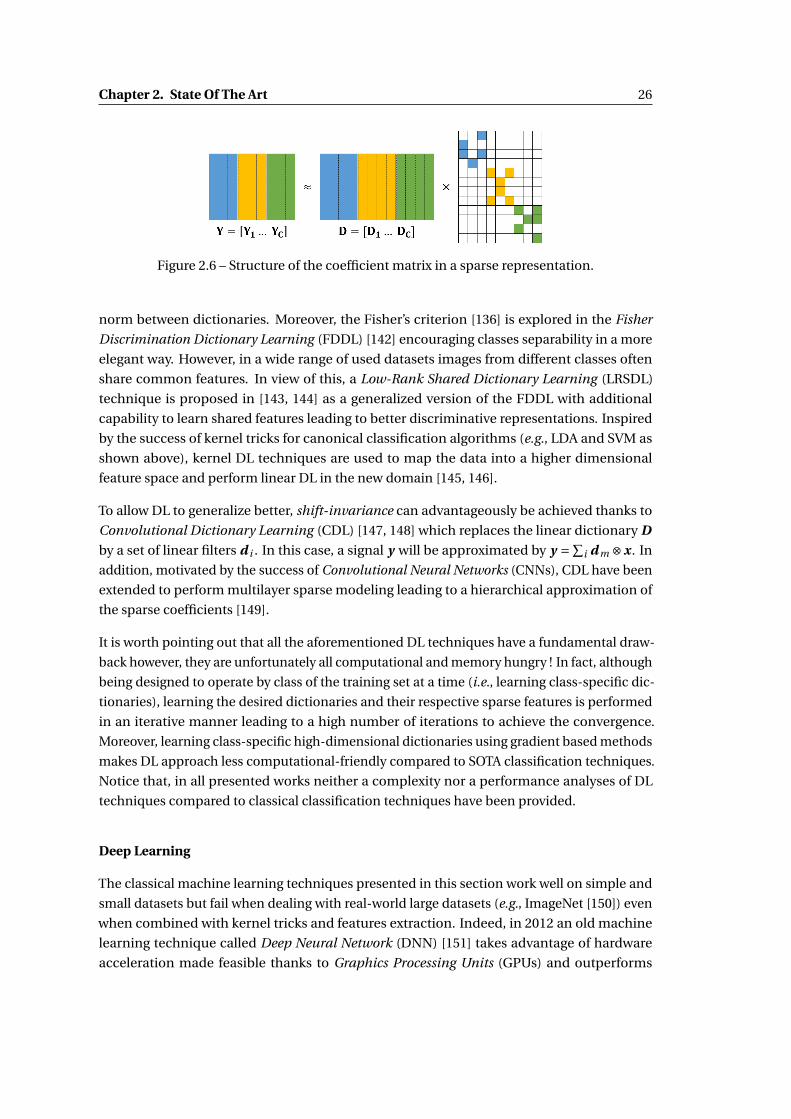
Chapter 2. State Of The Art 26
Figure 2.6 – Structure of the coefficient matrix in a sparse representation.
norm between dictionaries. Moreover, the Fisher’s criterion [136] is explored in the Fisher
Discrimination Dictionary Learning (FDDL) [142] encouraging classes separability in a more
elegant way. However, in a wide range of used datasets images from different classes often
share common features. In view of this, a Low-Rank Shared Dictionary Learning (LRSDL)
technique is proposed in [143, 144] as a generalized version of the FDDL with additional
capability to learn shared features leading to better discriminative representations. Inspired
by the success of kernel tricks for canonical classification algorithms (e.g., LDA and SVM as
shown above), kernel DL techniques are used to map the data into a higher dimensional
feature space and perform linear DL in the new domain [145, 146].
To allow DL to generalize better, shift-invariance can advantageously be achieved thanks to
Convolutional Dictionary Learning (CDL) [147, 148] which replaces the linear dictionary D
by a set of linear filters d i . In this case, a signal y will be approximated by y =∑i d m ⊗ x . In
addition, motivated by the success of Convolutional Neural Networks (CNNs), CDL have been
extended to perform multilayer sparse modeling leading to a hierarchical approximation of
the sparse coefficients [149].
It is worth pointing out that all the aforementioned DL techniques have a fundamental draw-
back however, they are unfortunately all computational and memory hungry ! In fact, although
being designed to operate by class of the training set at a time (i.e., learning class-specific dic-
tionaries), learning the desired dictionaries and their respective sparse features is performed
in an iterative manner leading to a high number of iterations to achieve the convergence.
Moreover, learning class-specific high-dimensional dictionaries using gradient based methods
makes DL approach less computational-friendly compared to SOTA classification techniques.
Notice that, in all presented works neither a complexity nor a performance analyses of DL
techniques compared to classical classification techniques have been provided.
Deep Learning
The classical machine learning techniques presented in this section work well on simple and
small datasets but fail when dealing with real-world large datasets (e.g., ImageNet [150]) even
when combined with kernel tricks and features extraction. Indeed, in 2012 an old machine
learning technique called Deep Neural Network (DNN) [151] takes advantage of hardware
acceleration made feasible thanks to Graphics Processing Units (GPUs) and outperforms
27 2.2. Machine Learning background
the SOTA accuracy on the ImageNet dataset. The proposed DNN called AlexNet [152] has
inaugurated then the DNN spring. Indeed, DNNs provide a very powerful framework for
supervised learning by adding more layers and projections by layer. In fact, a DNN consists in
mapping an input vector (e.g., vectorized image with n pixels) to an output given a sufficiently
large dataset that covers all the possible realization of the desired inference task.
Basic DNN architectures are often called Multi-Layer Perceptrons (MLP), Feedforward Neu-
ral Networks (FNN)or Fully Connected Networks (FCN) [132]. For instance, the mapping
performed by a L-layer MLP is mathematically expressed as:
fW ,b (x) = f (L)W (L),b(L)
(. . . f (2)
W (2),b(2)
(f (1)
W (1),b(1) (x)))
, (2.17)
where L is the depth of the MLP; W (i )’s and b(i )’s are the weight matrices and offset vectors
respectively at each layer i ; and the functions f (i )W (i ),b(i ) are the classification functions perform-
ing the mapping x → σ(W (i )x +b(i )) with σ (x) is an activation function that can be linear
or nonlinear. In this chain structure, f (1)W (1),b(1) is called the input layer, f (L)
W (L),W (L) the output
layer and f (2...L−1)W (2...L−1),b(2...L−1) are the hidden layers. Typical nonlinear activation functions are the
sigmoid function (i.e., σ (x) = 11+exp(−x) ), hyperbolic tangent function (i.e., σ (x) = tanh(x)) and
the Parametric Rectified Linear Units (PReLU) (i.e., σ (x) = max(αx , x), with α ∈R+).
A more powerful DNN is the so-called Convolutional Neural Networks (CNN) [130] (cf., Figure
2.7). In CNNs, convolutions are basically used in the first layers to learn specific filters or
kernels to extract features [124]. The main advantage of CNNs is the shift-invariance property
highly suitable for image analysis achieved thanks to the convolutions. A typical layer of a CNN
consists of three successive operations. First, the layer performs a series of convolutions to
produce a set of features followed by a classification function that performs linear/nonlinear
projections. Finally a pooling function reduces the dimension of the data by locally combining
the outputs into one neuron. A commonly used pooling approach is the max pooling that
outputs the maximum value within a rectangular neighborhood.
To learn a DNN, a gradient based algorithm is a practical approach but computationally
expensive. To circumvent this issue, the back-propagation estimates the gradient at each layer
using the chain-rule making the gradient algorithm (e.g., stochastic gradient descent) simple
and inexpensive.
In 2016, DNNs have officially outperform human ability at the ImageNet Large Scale Visual
Recognition Challenge (ILSVRC) 1. However, although the outstanding performance that
show DNNs, both the training of a DNN and the inference on unknown samples are typically
executed on power-hungry CPU servers or GPUs in the cloud. Some initial steps toward
1http://image-net.org/

Chapter 2. State Of The Art 28
Figure 2.7 – An illustration of a CNN network from [1].
energy compliant DNNs have been explored from an algorithm point-of-view leading to some
optimization methods to relax DNNs complexity, namely, binarizing weights and activations
[153], dropping out randomly components of each layer [154, 155] or training sparse DNNs
[156]. We believe, however, that overcoming the computation-memory bottleneck in deep
learning and address challenging applications in the context of highly constrained hardware
requires a joint optimization of the algorithm and the hardware components. In this regard, in
the rest of this section we present some hardware breakthroughs toward embedded machine
learning known currently as edge AI. We briefly introduce the SOTA of AI dedicated processors
and hardware accelerators while focusing on edge AI for imaging applications in the context
of smart low power CMOS Image Sensors (CISs).
2.2.2 Edge AI
One challenge of the CIS community is proposing compact sensors with AI capabilities.
Traditionally, CIS researchers have focused on noise-reduction/suppression for image quality
enhancement [157, 158]; reducing the silicon footprint through pixel-pitch [159, 160]; and
improving power-consumption [161, 162]. Nowadays, drived by machine-sensing applications
(e.g., autonomous cars/robots, humane-machine interfaces), CMOS VIsion Sensors (CVISs)
have been introduced as CISs performing computer vision tasks in the focal plane [163]. In
this case, the output of a CVIS will not be an image but either image features or a decision
based on a spatio-temporal analysis of the sensed image. Yet, the input of the CVIS is like
the CIS, i.e., an image sensed by a pixel-array of photo-detectors. Thus, to meet machine
learning tasks, analog pre-processing as well as dedicated System-on-Chip (SoC) have been
explored to deal with inference problems in the context of low-power CVISs. Indeed, three
main contributions can be identified in the CIS/CVIS SOTA: in-focal plane feature extraction,
near CIS object recognition and embedded inference dedicated processors.
29 2.2. Machine Learning background
In-Focal Plane Feature Extraction
In the last decade the trend in computer vision was to propose powerful feature extraction
techniques to extract discriminative features in order to address a classification task (cf.,
Section 2.2.1). The CIS community has then followed the trend and proposed several in-focal
plane feature extraction implementations. For instance, a 256×256 motion-triggered feature
extraction CIS is proposed in [164]. The proposed CIS has three different modes of operation:
motion-sensing, feature extraction and imaging and storing modes. Indeed, for a power
saving purpose, the sensor operates in a motion-sensing until it is triggered by motion. In the
motion-sensing mode, in-pixel capacitors serve as frame memory and the frame difference
is thus quantized to 1-b signal and compared with an adjustable threshold. Once motion
detected, the sensor wakes-up and turns into the feature extraction mode to extract 8-bit
HOG features [126]. In this mode, gradients are calculated in the digital domain in both
horizontal and vertical directions and the orientations in the analog domain using a mixed
circuit. However, although the reduced power consumption (50µW @ 15 fps) achieved by
the proposed architecture, it doesn’t take advantage of feature extraction to relax hardware
constraints (e.g., ADC clock cycles, memory needs) such features are extracted in the digital
domain. To overcome this drawback, an implementation of the BRISK feature extraction
technique [129] is proposed in [165]. In this work, the amount of data to send to an off-line
digital processor is reduced by implementing the BRISK in the analog domain before ADC
conversion. Indeed, in a canonical CIS readout (i.e., rolling shutter + CDS), an analog memory
is used to store the lines corresponding to the operand of the BRISK at each frame. Thus, using
a column-parallel mixed-signal circuit and a Successive Approximation Register (SAR) ADC, a
set of comparisons with each pixel neighbors are performed to detect corners and then BRISK
features. Finally, to achieve scale-invariance, scale-space is generated by pixels averaging and
stored in the analog line memory.
In fact, other works have implemented feature extraction techniques in the focal plane in
the context of smart CIS or CVIS, namely, the SIFT algorithm [166] in a Gaussian pyramidal
setup [167] for multi-scale feature extraction as in [168]; the LBP in [169, 170]; the SURF
[171] in [172] and log-gradients in [173]. All the aforementioned implementations can be
considered as milestones towards compact edge AI applications in the context of CIS/CVIS.
They practically all focus on reducing the amount of data to extract in the focal plane to enable
object recognition in dedicated off-line SoCs. However, to deal with privacy and latency issues,
some recent works have proposed to perform object recognition in (or near) the focal plane as
it will be presented in the rest of this section.
Near CIS Object Recognition
Unlike in-focal plane feature extraction, in a near CIS object recogntition embodiment we
are only interested by the result of the inference task. In this context, several strategies have
been explored to deal with inference problems in the context of low-power CIS. For example,
[174, 175] propose a CIS with embedded always-on face detector based on Haar-like filtering

Chapter 2. State Of The Art 30
and a CNN processor for face recognition. More recently, an Analog Convolution (A-Conv)
processor is proposed in [176] to implement the first layer of the CNN processor in [175].
Indeed, the A-Conv consists of a weighted-sum unit which can calculate partial sum of 3×3
weight kernels, a ReLU unit, and a ternary quantizer allowing to quantize the output of the
ReLU unit and thus remove the ADC in [176]. The features extracted by the A-Conv layer serve
as input of the face detection CNN processor and if a face is detected the face recognition
CNN is triggered. On the other hand, [177] deals with memory requirements related to a face
recognition processor. The proposed processor performs first face detection using a cascaded
Viola-Jones Haar feature cascaded detectors [178] and then a Principal Component Analysis
(PCA) [179] to extract features of reduced dimensionality combined with a nonlinear SVM
for face recognition. We notice however that the listed implementations have implemented
SOTA machine learning techniques without any optimization of the algorithm component or
hardware parallelization/acceleration. In the rest of this section we present some of the SOTA
hardware accelerators for dedicated machine learning techniques (e.g., SVM, CNN).
Embedded Inference Dedicated Processors
For less constrained applications, several CNN processors have been proposed in the litera-
ture addressing the challenge of low-power and accurate embedded decision making tasks
[180]. The early implementations of edge AI have focused on implementing SOTA algorithms
without any typical optimizations, e.g., SVM [181] and DNN [182, 183]. However, to deal
with the power-consumption bottleneck, [184] introduces the concept of hierarchical recog-
nition using a hierarchy of increasingly complex individually trained CNNs and increasing
computational precision. For further hardware complexity reduction, [185] analyzed the
accuracy-energy trade-off by exploiting quantization and precision scaling to reduce CNN
processors power consumption. Following the trend for low precision CNNs, some processors
have been proposed with fixed-point weights [186] or extremely quantized weights, i.e., binary
weights [187, 188, 180]. Furthermore, a pre-defined sparse MLP is proposed in [189] to reduce
the complexity during both training and inference. In these implementations one can note
that the circuit and system community has fully taking advantange of the algorithmic opti-
mization of the CNNs presented in Section 2.2.1. More recently, hardware accelerators have
been proposed to optimize convolutions because of their computational time [190, 191, 192].
We note, however, that these works focus on optimizing circuit design to achieve low-power
processing; they do not unfortunately address design constraints related to image acquisition
such as the data dimensionality or the number of ADC clock cycles.
2.3 Conclusion and discussion
Throughout this chapter we have provided a sparse insight about the fields of Compressive
Sensing and Machine Learning. Indeed, CS relaxes hardware constraints (e.g., A/D conver-
sions) related to the data dimensionality based on pseudo-random measurements. Moreover,

31 2.3. Conclusion and discussion
supervised ML techniques allow data processing units to automate decision making tasks. In
the CS and ML SOTA, several breakthroughs have been proposed to implement near image
sensor CS or decision making tasks. Despite the important contributions in both CS and
ML literature, neither CS implementations have taken advantage of ML to perform near CIS
decision making nor viceversa. In fact, the amount of compressed measurements (features)
can dramatically be reduced to address decision making tasks leading to more hardware
relaxation in terms of A/D conversions and memory needs. Indeed, in some recent works
CS have been explored for basic feature extraction and classification tasks for biomedical
applications [193, 194] or dedicated decision making systems [195, 196]. In this thesis, we
take some initial steps towards compact compressive CMOS image sensors taken advantage
of the theoretical advances in signal processing on compressive measurements [84, 85, 86].
We propose to take the challenge of smart CIS a step further and take advantage of CS to
reduce hardware-algorithm constraints to implement on-chip decision making algorithms.
Finally, some algorithmic optimizations will be discussed to make decision making more
hardware-friendly.


Chapter 3
Inference Tasks On CompressiveMeasurements
One of the main challenges in the design of compact smart CIS is the power consumption
related to the amount of data to extract (i.e., A/D conversions) and process (i.e., digital pro-
cessing and memory needs). For instance, to handle high-dimensional inference tasks, a
straightforward approach is to compress the sensed data or extract meaningful features to
make the inference task lighter. Considering any kind of computer vision problem (e.g., ADAS),
image descriptors (e.g., HOG, LBP) combined with a proper classification algorithm (e.g.,
Artificial Neural Networks) are typically used to enable objects detection and/or classifica-
tion. However, embedding such system with high dimensional data and complex algorithms
requires considerable memory and computational requirements.
Recent advances in signal processing and pattern recognition tend to deal with high-dimensional
problems by introducing new and efficient techniques in terms of computing and storage
resources. For example, Dimensionality Reduction (DR) [197] relies on the projection of a
high-dimensional data into a relevant low-dimensional feature domain that preserves data
intrinsic properties (e.g., statistical or geometrical properties). Various DR techniques can
be found in the literature, they can be either linear or nonlinear, supervised or unsupervised
[132, 198]. One can identify two distinct approaches to achieve dimensionality reduction.
First, DR can be performed by a learned projection that optimizes a regularized objective
function. These techniques are basically introduced as machine learning algorithms to per-
form decision making in low dimensional domains. However, embedding such techniques
involves dedicated hardware resources to store ex-situ signal dependent learned patterns
as presented in Chapter 2. Alternatively, DR can be signal independent and achieved by
unlearned projections. Most popular unlearned DR are pooling operations widely used in
CNN architectures as downsampling filters [199]; random drop out and structured pruning in
DNN (cf., Section 2.2.1); pixel-binning to capture low-resolution images by combining charges
of neighboring pixels in a block of pixels during the readout [200]; or either sub-sampling the

Chapter 3. Inference Tasks On Compressive Measurements 34
resulting coefficients of the projection onto an orthonormal basis (e.g., DCT) under some pri-
ors (e.g., sub-sampling in a specific frequency band). However, the most theoritically studied
unlearned DR are random projections that allows to project the original data onto a subspace
of reduced dimensionality using a randomly generated matrix [71]. It represents therefore a
computationally simple DR technique that allows to preserve the Euclidean distance of any
two signals through the projection [201, 202]. Indeed, random matrices are typically used to
acquire compressed features as a universal sensing scheme for CS based systems with remote
signal recovery [17]. In this case, the design of related sensing matrices has to satisfy the RIP
property to guarantee a stable embedding property and to preserve geometrical properties
as discussed in Chapter 2. In particular, pseudo-random generators (e.g., LFSR [203], cellular
automata [73]) can advantageously be used to generate on-the-fly the sensing matrix as a
deterministic and reproducible process relaxing as a consequence design constraints, namely,
memory needs. For the sake of clarity, in the rest of this chapter we call ML-DR DR performed
by learned projections, and CS-DR DR via random projections.
In this chapter, we study the interest of using ML-DR and CS-DR for basic on-chip inference
tasks in the context of highly constrained hardware (e.g., always-on ultra low power vision
systems). In particular, we try to find the most beneficial setting to perform near CIS inference
on compressed measurements. In general, two processing stages have to be considered when
dealing with embedded inference tasks: learning ML-DR in an off-line system on labeled
data, and then performing embedded inference on compressed data whose related class is
unknown (e.g., considering embedded inference in a CS image sensor). As a comparative
study, we propose various learning and inference strategies for three ML-DR methods briefly
presented in Chapter 2, namely, Linear Discriminant Analysis (LDA) [135], Support Vector
Machine (SVM) [137] and Dictionary Learning with Structured Incoherence (DLSI) [141]. For
each technique, we present and compare three approaches to perform on-chip decision
making in the context of hardware limited systems. The first approach consists in performing
ML-DR learning and embedded inference on compressed measurements taking advantage on
CS-DR to reduce embedded resources requirements. In the second and third ones, dedicated
inference solutions are presented to deal with compressed measurements extracted using a
CS device whose sensing scheme is not necessarly a priori known (e.g., for security purposes
[204, 205] or to manage sensor non-idealities [206]). In the rest of this chapter, we first present
a mathematical description of each ML-DR technique and then present the studied inference
approaches and the inference scheme related to each ML-DR technique. The performance
of ML-DR methods is evaluated based on the inference accuracy regarding the learning
approach, as well as general considerations on memory resources, computational complexity
and robustness to some hardware variations for two object recognition applications.
3.1 ML-DR Learning Mathematical Background
Let us consider a database of n-length “vectors” in Rn (e.g., images with n pixels) composed
of C classes. This database is separated into two subsets: a “train” set X ∈ Rn×n1C , where
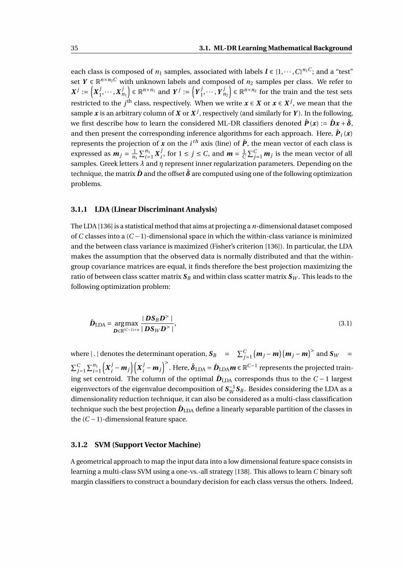
35 3.1. ML-DR Learning Mathematical Background
each class is composed of n1 samples, associated with labels l ∈ {1, · · · ,C }n1C ; and a “test”
set Y ∈ Rn×n2C with unknown labels and composed of n2 samples per class. We refer to
X j :=(
X j1, · · · , X j
n1
)∈ Rn×n1 and Y j :=
(Y j
1, · · · ,Y jn2
)∈ Rn×n2 for the train and the test sets
restricted to the j th class, respectively. When we write x ∈ X or x ∈ X j , we mean that the
sample x is an arbitrary column of X or X j , respectively (and similarly for Y ). In the following,
we first describe how to learn the considered ML-DR classifiers denoted P (x) := D x + δ,
and then present the corresponding inference algorithms for each approach. Here, P i (x)
represents the projection of x on the i th axis (line) of P , the mean vector of each class is
expressed as m j = 1n1
∑n1i=1 X j
i , for 1 ≤ j ≤ C , and m = 1C
∑Cj=1 m j is the mean vector of all
samples. Greek letters λ and η represent inner regularization parameters. Depending on the
technique, the matrix D and the offset δ are computed using one of the following optimization
problems.
3.1.1 LDA (Linear Discriminant Analysis)
The LDA [136] is a statistical method that aims at projecting a n-dimensional dataset composed
of C classes into a (C −1)-dimensional space in which the within-class variance is minimized
and the between class variance is maximized (Fisher’s criterion [136]). In particular, the LDA
makes the assumption that the observed data is normally distributed and that the within-
group covariance matrices are equal, it finds therefore the best projection maximizing the
ratio of between class scatter matrix SB and within class scatter matrix SW . This leads to the
following optimization problem:
DLDA = argmaxD∈R(C−1)×n
| DSB D> || DSW D> | , (3.1)
where | . | denotes the determinant operation, SB = ∑Cj=1
(m j −m
)(m j −m
)> and SW =∑Cj=1
∑n1i=1
(X j
i −m j
)(X j
i −m j
)>. Here, δLDA = DLDAm ∈RC−1 represents the projected train-
ing set centroid. The column of the optimal DLDA corresponds thus to the C − 1 largest
eigenvectors of the eigenvalue decomposition of S−1W SB . Besides considering the LDA as a
dimensionality reduction technique, it can also be considered as a multi-class classification
technique such the best projection DLDA define a linearly separable partition of the classes in
the (C −1)-dimensional feature space.
3.1.2 SVM (Support Vector Machine)
A geometrical approach to map the input data into a low dimensional feature space consists in
learning a multi-class SVM using a one-vs.-all strategy [138]. This allows to learn C binary soft
margin classifiers to construct a boundary decision for each class versus the others. Indeed,

Chapter 3. Inference Tasks On Compressive Measurements 36
for the j th class C j , a 2-class SVM is learned to separate the samples that belong to C j from the
remaining samples (i.e., samples from class C j ′ with j ′ 6= j ). Thus, for each class j , a positive
margin is assigned to the sample’s class and a negative margin to the others (i.e., l jk = 1 if the
kth sample belongs to class j , and −1 otherwise). The C binary classifiers are then combined
together to build a multi-class classifier. Mathematically speaking:
{DSVM, j , δSVM, j , ξ j } = argminD∈RN ,δ,ξ∈Rn1
(‖D‖2
2 +λn1∑
k=1ξk
)s.t. l j
k (D x +δ) j ≥ 1−ξk , ξk ≥ 0, ∀1 ≤ k ≤ n1. (3.2)
We define P SVM, j (x) := DSVM, j x + δSVM, j , for 1 ≤ j ≤ C . Unlike the LDA which is sensi-
tive to outliers, the SVM introduces the matrix ξ := (ξ1, · · · , ξC
)>made of n1C slack vari-
ables that allow to deal with outliers, each variable is then associated to one training sam-
ple. Here DSVM := (D1, · · · ,DC
)> ∈ RC×N , i.e., the vertical concatenation of DSVM, j ’s and
δSVM := (δSVM,1, · · · , δSVM,C
)> ∈RC .
3.1.3 DLSI (Dictionary Learning with Structured Incoherence)
As discussed in Section 2.2.1, dimensionality reduction can also be achieved by dictionary
learning. In contrast to the LDA and the SVM techniques, for each class a specific dictionary
can be build up to learn specific low dimensional discriminative features with tunable atoms
allowing a certain flexibility to the algorithm to deal with more or less complex datasets.
For instance, in the DLSI [141], class-intrinsic features are exploited to construct the DR
projection. This involves solving an objective function with respect to a constraint term that
encourages independency between sub-dictionaries {B j ∈ RN×d1 : 1 ≤ j ≤C }, where d1 ≤ N
is the dimension induced by each B j . Generally, the cost function aims at minimizing the
error between the training sample and its projection. Thus, training the DLSI corresponds to
constructing as incoherent as possible sub-dictionaries by solving:
{B ,α} = argminB , α
C∑j=1
{‖X j −B jα j‖2F + λ‖α j‖1}+η ∑
i , j :i 6= j‖B>
i B j‖2F , (3.3)
with B := (B 1, · · · , BC
) ∈ RN×d1C , α := (α>
1 , · · · ,α>C
)> ∈ Rd1C×n1C and α j ∈ Rd1×n1C . We define
DDLSI, j := B†j , thus, δDLSI, j = DDLSI, j m j ∈ Rd1 for 1 ≤ j ≤ C , and DDLSI can be defined as:
DDLSI :=(D
>DLSI,1, · · · ,D
>DLSI,C
)> ∈ Rd1C×N .

37 3.2. Classification Combining ML-DR and CS-DR
3.2 Classification Combining ML-DR and CS-DR
Despite the milestones in the design of compressive CIS for image rendering, signal recovery is
not necessary in many computer vision problems. In fact, most current Image Signal Processor
(ISP) design efforts focus on extracting meaningful informations and solving inference prob-
lems [207]. In this section, we take an initial step towards the design of compact compressive
CIS with inference capabilities. We analyze three inference strategies to solve an inference task
given compressed measurements in the context of highly constrained hardware. We highlight
that in all the explored approaches we can take advantage of Pseudo-Random Generators
(PRGs) to generate pseudo-random CS matrices in order to extract CS measurements without
considerable on-chip supplementary materials.
In the rest of this section, three approaches to solve an inference problem on compressed
measurements will be presented. In the first approach, the ML-DR projection is learned on
compressed measurements extracted by a pseudo-random CS-DR as performed in the classi-
cal framework [84]. In this case, the inference task is performed in the compressed domain
based on the learned ML-DR affine projection. In the second approach, the ML-DR is learned
in the signal domain without the knowledge of the sensing matrix and then projected in the
CS domain using a pseudo-randomly generated sensing matrix Φ. In contrast to the first
and second approaches, the third one introduces a dedicated DSP allowing to implement a
reconstruction-like algorithm to perform the inference from compressed measurements using
a ML-DR transform learned in the signal domain. In the following, studied DR techniques will
be denoted P cs−LDA, P proj−LDA and P sig−LDA (for the LDA using approach A, B and C respec-
tively), P cs−SVM, P proj−SVM and P sig−SVM (for the SVM using approach A, B and C respectively)
and P cs−DLSI, P proj−DLSI and P sig−DLSI (for the DLSI using approach A, B and C respectively).
An illustration of the projections involved by each approach is provided in Figure 3.1.
Figure 3.1 – An illustration of the projections involved by the studied inference approaches.y and y are an observed unknown sample and its projection in the CS domain using Φrespectively; and c is the predicted class of y .

Chapter 3. Inference Tasks On Compressive Measurements 38
3.2.1 Approach A: Inference Learned in The CS Domain
A desirable compressive CIS sensor property is the capability to acquire a compact signal with
a sparse representation that allows to extract its inherent information. Indeed, it was shown
that CS measurements can universally extract a meaningful information for many signal
processing tasks (e.g., inference) without requiring a strong knowledge of the sparsity basis
[84]. In this case, the number of measurements to extract depends only on the complexity
of both the inference task (e.g., number of classes) and the observed signal (e.g., sparsity
level) [84, 86]. To formulate the inference learned in the compressed domain, let us consider
X =ΦX ∈ Rm×n1C and Y =ΦY ∈ Rm×n2C the training and test sets observed respectively in
the compressed domain using the CS matrixΦ ∈Rm×n with m ¿ n. This implies that all the
training samples are of lowered dimensionality leading to a reduced computational complexity
for both the training and the inference (cf., Figure 3.2). Thus, the equations (3.1), (3.2) and
(3.3) can be solved in the compressed domain and the training samples from X (i.e., x) are
replaced by their projections in X (i.e., x).
Figure 3.2 – Schematic description of "inference learned in CS domain" (Approach A).
Inference for the LDA
As the LDA clusters samples of the same class using a statistical criteria (i.e., minimize within-
class variance and maximize the between class variance), an Euclidean distance can typically
be used for the inference. Indeed, an unknown sample y is assigned to the nearest class
represented by its center in the projected domain (i.e., RC−1). Thus, we can estimate the class
c of y by:
c = argmin1≤i≤C
‖P cs−LDA(
y)− P cs−LDA (mi )‖2
2, (3.4)
where mi = Φmi is the mean class vector in the CS domain and P cs−LDA (x) = Dcs−LDAx +δcs−LDA. Notice that for an on-chip/embedded application P cs−LDA (mi ) is generally computed
off-line leading to a reduced on-chip resulting complexity.
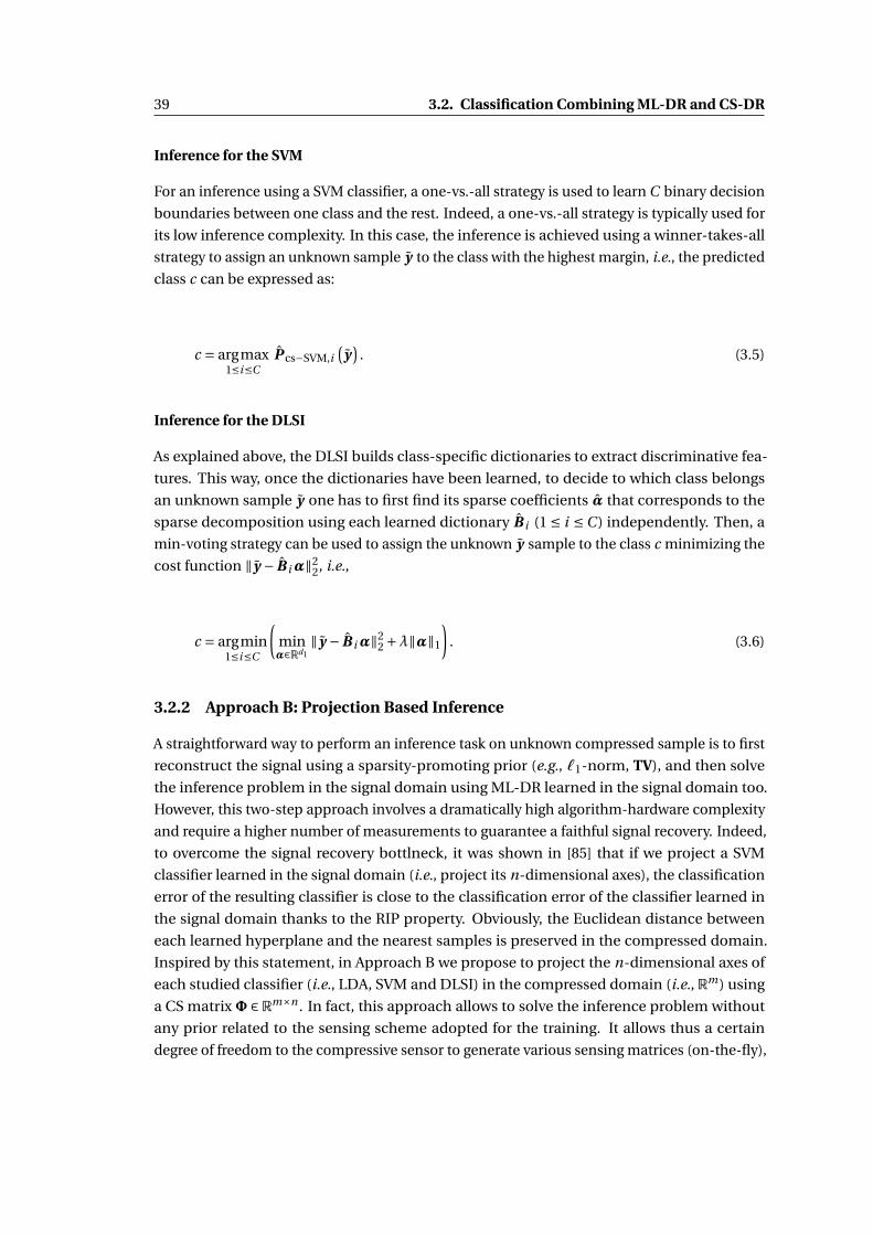
39 3.2. Classification Combining ML-DR and CS-DR
Inference for the SVM
For an inference using a SVM classifier, a one-vs.-all strategy is used to learn C binary decision
boundaries between one class and the rest. Indeed, a one-vs.-all strategy is typically used for
its low inference complexity. In this case, the inference is achieved using a winner-takes-all
strategy to assign an unknown sample y to the class with the highest margin, i.e., the predicted
class c can be expressed as:
c = argmax1≤i≤C
P cs−SVM,i(
y)
. (3.5)
Inference for the DLSI
As explained above, the DLSI builds class-specific dictionaries to extract discriminative fea-
tures. This way, once the dictionaries have been learned, to decide to which class belongs
an unknown sample y one has to first find its sparse coefficients α that corresponds to the
sparse decomposition using each learned dictionary B i (1 ≤ i ≤C ) independently. Then, a
min-voting strategy can be used to assign the unknown y sample to the class c minimizing the
cost function ‖y − B iα‖22, i.e.,
c = argmin1≤i≤C
(minα∈Rd1
‖y − B iα‖22 +λ‖α‖1
). (3.6)
3.2.2 Approach B: Projection Based Inference
A straightforward way to perform an inference task on unknown compressed sample is to first
reconstruct the signal using a sparsity-promoting prior (e.g., `1-norm, TV), and then solve
the inference problem in the signal domain using ML-DR learned in the signal domain too.
However, this two-step approach involves a dramatically high algorithm-hardware complexity
and require a higher number of measurements to guarantee a faithful signal recovery. Indeed,
to overcome the signal recovery bottlneck, it was shown in [85] that if we project a SVM
classifier learned in the signal domain (i.e., project its n-dimensional axes), the classification
error of the resulting classifier is close to the classification error of the classifier learned in
the signal domain thanks to the RIP property. Obviously, the Euclidean distance between
each learned hyperplane and the nearest samples is preserved in the compressed domain.
Inspired by this statement, in Approach B we propose to project the n-dimensional axes of
each studied classifier (i.e., LDA, SVM and DLSI) in the compressed domain (i.e., Rm) using
a CS matrixΦ ∈Rm×n . In fact, this approach allows to solve the inference problem without
any prior related to the sensing scheme adopted for the training. It allows thus a certain
degree of freedom to the compressive sensor to generate various sensing matrices (on-the-fly),
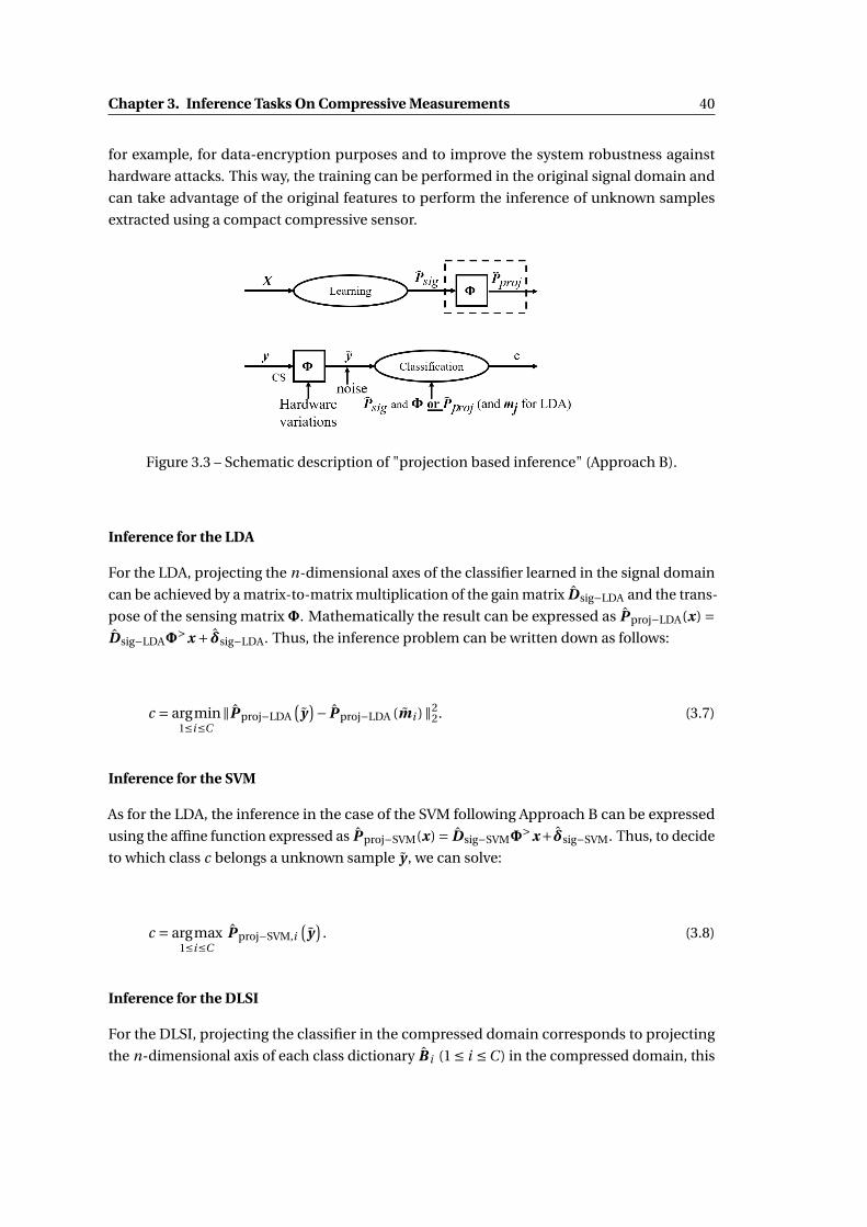
Chapter 3. Inference Tasks On Compressive Measurements 40
for example, for data-encryption purposes and to improve the system robustness against
hardware attacks. This way, the training can be performed in the original signal domain and
can take advantage of the original features to perform the inference of unknown samples
extracted using a compact compressive sensor.
Figure 3.3 – Schematic description of "projection based inference" (Approach B).
Inference for the LDA
For the LDA, projecting the n-dimensional axes of the classifier learned in the signal domain
can be achieved by a matrix-to-matrix multiplication of the gain matrix Dsig−LDA and the trans-
pose of the sensing matrixΦ. Mathematically the result can be expressed as P proj−LDA(x) =Dsig−LDAΦ
>x + δsig−LDA. Thus, the inference problem can be written down as follows:
c = argmin1≤i≤C
‖P proj−LDA(
y)− P proj−LDA (mi )‖2
2. (3.7)
Inference for the SVM
As for the LDA, the inference in the case of the SVM following Approach B can be expressed
using the affine function expressed as P proj−SVM(x) = Dsig−SVMΦ>x+δsig−SVM. Thus, to decide
to which class c belongs a unknown sample y , we can solve:
c = argmax1≤i≤C
P proj−SVM,i(
y)
. (3.8)
Inference for the DLSI
For the DLSI, projecting the classifier in the compressed domain corresponds to projecting
the n-dimensional axis of each class dictionary B i (1 ≤ i ≤C ) in the compressed domain, this

41 3.2. Classification Combining ML-DR and CS-DR
way the inference problem can be expressed as:
c = argmin1≤i≤C
(minα∈Rd1
‖y −ΦB iα‖22 +λ‖α‖1
). (3.9)
3.2.3 Approach C: Inference in The Reconstructed Signal Domain
To perform the inference independently of the training acquisition scheme, a relevant ap-
proach can merge signal recovery and the inference. Indeed, instead of reconstructing for an
image rendering purpose, one can reconstruct to promote a discriminative criteria in order
to solve the inference task. Thus, given a compressed observation y =Φy ∈ Y , the inference
can be achieved by reconstructing a signal α ∈ RC in the inference domain that minimizes
the Euclidean distance to the compressed signal y via first a backprojection in the signal
domain (i.e., an inverse mapping from the inference domain to the signal domain); and then a
projection in the compressed domain using the sensing matrixΦ. In fact, for a signalα ∈RC
in the inference domain, its inverse mapping can be defined by minimizing the following
`2-minimization problem:
u = argminu∈Rn
‖u‖22 subject to P (u) =α. (3.10)
The solution of (3.10) can be expressed as: u = P†(α), where † denotes the Moore-Penrose
pseudo-inverse operator. Thus, under a regularization term promoting classes separability
in the inference domain, the reconstructed signal α minimizing the energy ‖y −ΦP†(α)‖2
2
will correspond to the projection of y in the inference domain. It allows as a consequence to
decide to which class an unknown compressed sample signal belongs to using advantageously
a classifier learned in the signal domain. Moreover, the regularization function can typically
take advantage of intrinsic properties of each method (e.g., statistical and geometrical). In the
following, this framework is applied for the studied ML-DR techniques (i.e., LDA, SVM and
DLSI) to perform the embedded inference on CS measurements using a reconstruction-like
algorithm involving dedicated regularization functions on the vector in the inference domain.
Inference for the LDA
For the LDA, we can typically take advantage of the Fisher’s criteria to recover the targeted
signal α. Thus, given the CS matrixΦ and the LDA ML-DR transform P sig−LDA, we can find for
each class i the corresponding vector αi ∈RC−1 using a constraint encouraging the recovered
signal to be as close as possible to the class centroid. Thus, the regularization term can be
defined as RLDA,i (α) = ‖α− P sig−LDA(mi )‖22. Finally, the vectors αi are used to find the class c

Chapter 3. Inference Tasks On Compressive Measurements 42
Figure 3.4 – Schematic description of "inference in the reconstructed signal domain" (Ap-proach C).
that minimizes the inference cost function as follows:
αi = argminα∈RC−1
‖y −ΦP†sig−LDA (α)‖2
2 +λRLDA,i (α) , (3.11)
c = argmin1≤i≤C
‖αi − P sig−LDA (mi )‖22. (3.12)
Inference for the SVM
In a one-vs.-all SVM strategy, solving the inference problem (e.g., (3.5)) involves seeking
for the class c maximizing the positive margin of an unknown sample y in the inference
domain, i.e., seeking for the argument of the largest entry of α. Inspired by this strategy, we
propose a regularization function that promotes a peaked response of positive margins and
force negative ones to be as small as possible, in other words, reinforce sparsity of positive
margins. Thus, the proposed regularization function can be expressed using the `1 norm
applied to the exp function as follows: RSVM (α) = ‖exp(α)‖1 (notice that the `1 norm can
be replaced by any function promoting positive margin, typically the ReLU function). To
overcome the computational cost bottleneck, a `2-relaxation can be used leading to the
following regularization function: RSVM (α) = ‖exp(α)‖22. Indeed, in the specific case of
the exp function the `2 norm is totally equivalent the `1 norm because of the fact that the
derivative of exp(x) is exp(x) itself. Thus, solving the inference problem of the SVM can be
expressed as recovering the vector αwith the highest positive margin, i.e., :
α= argminα∈RC
‖y −ΦP†sig−SVM (α)‖2
2 +λRSVM (α) , (3.13)

43 3.3. Embedded Resources Requirements Study
c = argmax1≤i≤C
αi . (3.14)
Inference for the DLSI
For the DLSI, one can take advantage of the sparse decomposition to recover a vector α
promoting a sparse decomposition of the observed signal y in the inference domain. Thus,
the `1 norm constraint used in (3.9) can be preserved to solve the inference problem following
Approach C, i.e.,
αi = argminα∈Rd1
‖y −ΦB iα‖22 +λ‖α‖1, (3.15)
c = argmin1≤i≤C
‖y −ΦB i αi‖22 +λ‖αi‖1. (3.16)
3.3 Embedded Resources Requirements Study
In the quest for the "most" hardware-friendly approach depending on the targeted application
requirements to perform on-chip decision making, we compare in this section the embedded
resources requirements of each approach. Indeed, depending on the targeted application
specifications, we evaluate memory needs in terms of the number of coefficients to store as
well as computational complexity in terms of the total number of operations (MACs) for each
approach (i.e., A, B and C).
3.3.1 Approach A: Inference Learned in CS Domain
Inference for the LDA
To solve the inference task of the LDA in (3.4), i.e.,
c = argmin1≤i≤C
‖P cs−LDA(
y)− P cs−LDA (mi )‖2
2, (3.17)
one has to store on-chip the ex-situ learned patterns learned on CS measurements (i.e.,
Dcs−LDA ∈ RC−1×m and δcs−LDA ∈ RC−1); and C classes centroids (i.e., P cs−LDA (mi ) ∈ RC−1).
Thus, the total amount of coefficients to store in order to solve a LDA inference task following

Chapter 3. Inference Tasks On Compressive Measurements 44
Approach A is O(C 2 +mC
).
On the other hand, to solve the inference problem in (3.4), one has to first project the extracted
CS vector y in the inference domain using the affine function P cs−LDA. This projection has the
complexity of a matrix-to-vector multiplication, i.e., mC . In addition, C Euclidean distances
have to be calculated (i.e., O(C 2
)) as well as a search for the index of the minima in a (C −1)-
length unsorted array (i.e., O (C )). Thus, the computing complexity to solve the LDA inference
task using Approach A is O(C 2 +mC
).
Inference for the SVM
For the SVM, solving the inference task in (3.5), i.e.,
c = argmax1≤i≤C
P cs−SVM,i(
y)
, (3.18)
involves storing the ex-situ learned patterns (i.e., Dcs−SVM ∈ RC×m and δcs−SVM ∈ RC ). Thus,
the total amount of coefficients to store in order to solve a SVM inference task following
Approach A is O (mC ). In addition, to decide to which class a compressed unknown sample
y belongs to, one has to first map the compressed vector into the inference domain using
P cs−SVM (i.e., C (mC )) and then search for the argument of the maxima in a C -length unsorted
array (i.e., O (C )). Finally, the computing complexity to solve the SVM inference task using
Approach A is O (mC ).
Inference for the DLSI
As for the LDA and the SVM, solving the inference task for the DLSI, i.e.,
c = argmin1≤i≤C
(minα∈Rd1
‖y − B iα‖22 +λ‖α‖1
), (3.19)
requires storing the classes specific dictionaries learned off-line, i.e., B i ∈Rm×d1 (1 ≤ i ≤C ).
Thus, the total amount of coefficients to store in order to solve the DLSI inference task following
Approach A is O (d1mC ). However, to decide to which class belongs an unknown sample y ,
one has to solve an optimization problem to find a sparse decomposition of the extracted CS
vector in each class dictionary B i . Once the sparse coefficients α estimated, one can then
find the class i minimizing the cost function decided to be the predicted class of y . Indeed,
when the dictionary B i is fixed, the sparse coefficients α for a class i can be estimated by
solving an iterative gradient based algorithm (e.g., FISTA [40]). In this case, for each iteration

45 3.3. Embedded Resources Requirements Study
q , the most computational task is to compute B>i B iα− B
>i y . Supposing B
>i B i to be pre-
computed and stored on-chip, this term can be computed with complexity d 21 +md1. Thus, for
C classes, estimating the sparse coefficients requires performing O(q
(d 2
1 +md1)
C)
embedded
operations and a search for the argument of the maxima in a C -length unsorted array (i.e.,
O (C )) leading to the following complexity O(q
(d 2
1 +md1)
C).
3.3.2 Approach B: Projection Based Inference
Aiming at taking advantage of the original signal domain to perform the training of the
studied classifiers (i.e., LDA, SVM and DLSI). In Approach B, a post-training projection of
the n-dimensional axes of each classifier in the compressed domain using a CS matrixΦ ∈Rm×n is adopted to perform the embedded inference on compressive measurements. This
allows to perform the embedded inference in the compressed domain without any on-chip
supplementary complexity (i.e., memory and computing complexity) compared to Approach
A (cf., section 3.3.1). Thus, the total amount of coefficients to store following Approach B
are O(C 2 +mC
), O (mC ) and O (d1mC ) for the LDA, SVM and DLSI respectively. In addition,
solving the inference tasks in (3.7), (3.8) and (3.9) requires a computing complexity of the
order of O(C 2 +mC
), O (mC ) and O
(q
(d 2
1 +md1)
C)
for the LDA, SVM and DLSI respectively.
3.3.3 Approach C: Inference in The Reconstructed Signal Domain
In approach C, the inference is achieved by first reconstructing a signal α in the inference
domain that minimizes the Euclidean distance to the compressed signal y , then find the class
that fits the best with the inference criteria. The reconstruction like problem can generally
be expressed by the following optimization problem: α= argminα ‖y −ΦP†
(α)‖22 +λR (α),
with P†
(α) = D†
(α−δ) and R (α) is a regularization term promoting an inference criteria
depending on the intrinsic properties of each classification technique. This optimization
problem can be solved by using an iterative gradient based algorithm (e.g., FISTA [40]). In this
case, for each iteration q , the most computational task is to compute(ΦD
†)>ΦD
† (α− δ)−(
ΦD†)>
y . Two case-studies can be considered depending of the sensing matrixΦ, if it is a
priori known or not. For each inference technique we will provide the complexity analysis
depending of the two cases.
Inference for the LDA
When the sensing matrix is not a priori known, to solve the inference task using the LDA classi-
fier and Approach C (i.e., (3.11) and (3.12)), one has to store the ex-situ learned patterns learned
on original samples (i.e., Dsig−LDA ∈ RC−1×n ; and δsig−LDA ∈ RC−1) and C classes centroids.
Thus, the total amount of coefficients to store on-chip in order to solve a LDA inference task
following Approach C is O(C 2 +nC
). On the other hand, to decide to which class an unknown
compressed sample y belongs to, one has to find for each class i the corresponding vector
Chapter 3. Inference Tasks On Compressive Measurements 46
αi ∈RC−1 using a constraint function RLDA,i (α) (cf., (3.11)). In this case, to solve the aforemen-
tioned optimization problem (i.e., αi = argminα∈RC−1 ‖y −ΦP†sig−LDA (α)‖2
2+λRLDA,i (α)), one
has to compute for each class i and iteration q the term(ΦD
†sig−LDA
)>ΦD
†sig−LDA
(α− δsig−LDA
)−(ΦD
†sig−LDA
)>y . Supposing D
†sig−LDA to be pre-computed and stored on-chip, this term in-
volves a computing complexity of the order of O(mC 2 +mnC
)leading to the total computing
complexity O(qmC 3 +qmnC 2
).
Notice, however, that when the sensing matrix Φ is a priori known the memory needs and
the computing complexity can dramatically be reduced thanks to the data independent di-
mensionality reduction allowed by CS. In this case theΦD†sig−LDA can be computed off-line
and stored on-chip enabling a reduction of the memory needs, i.e., O(C 2 +mC
). In addi-
tion, supposing(ΦD
†sig−LDA
)>ΦD
†sig−LDA ∈RC−1×C−1 to be pre-computed too, the complexity
of the term(ΦD
†sig−LDA
)>ΦD
†sig−LDA
(α− δsig−LDA
)becomes O
(C 2
); and the complexity of(
ΦD†sig−LDA
)>y becomes O (mC ). Finally, when the sensing matrix Φ is a priori known the
computing complexity of the LDA following Approach C is O(qC 3 +qmC 2
).
Inference for the SVM
When the sensing matrix Φ is not a priori known, solving the inference task using an SVM
classifier (i.e., (3.13) and (3.14)) involves storing the ex-situ learned patterns (i.e., Dsig−SVM ∈RC×n and δsig−SVM ∈ RC ). Thus, the total amount of coefficients to store on-chip is: O (nC ).
On the other hand, to decide to which class an unknown compressed sample y belongs to, the
optimization problem in (3.13) (i.e., α= argminα∈RC ‖y−ΦP†sig−SVM (α)‖2
2+λRSVM (α)) can be
solved using an iterative gradient method. In this case, for each iteration q , one has to compute
the term(ΦD
†sig−SVM
)>ΦD
†sig−SVM
(α− δsig−SVM
)− (ΦD
†sig−SVM
)>y . As discussed above, this
term involves a computing complexity of the order of O(mC 2 +mnC
)leading to the total
computing complexity O(qmC 2 +qmnC
). However, when the sensing matrix Φ is a priori
known, the termsΦD†sig−SVM and
(ΦD
†sig−SVM
)>ΦD
†sig−SVM ∈RC×C can be computed off-line
leading to a reduced memory needs, i.e., O (mC ); and a computing complexity O(qC 2 +qmC
).
Inference for the DLSI
As for the LDA and SVM, when the sensing matrix Φ is not a priori known, the amount of
memory to store the ex-situ learned dictionaries depends on the signal dimensionality in the
signal domain. Thus, the total amount of memory to store the dictionaries learned using the
DLSI (B ∈Rn×d1C ) and following Approach C is O (d1nC ). In addition solving the optimization
problem in (3.11) (i.e., αi = argminα∈Rd1 ‖y −ΦB iα‖22 +λ‖α‖1) using an iterative method to
find the sparse decomposition of an unknown compressed sample y involves computing
at each iteration q the term(ΦB i
)>ΦB iα− (
ΦB i)>
y . Supposing B i to be stored on-chip,

47 3.4. Experimental Results
the computing complexity of the DLSI can be expressed as: O(qm
(d 2
1 +nd1)
C). However,
when the sensing matrix Φ is a priori known, the terms ΦB i and(ΦB i
)>ΦB i ∈ Rd1×d1 can
be computed off-line leading to a reduced memory needs, i.e., O (d1mC ); and embedded
computing complexity O(q
(d 2
1 +md1)
C).
3.3.4 Complexity Analysis
Table 3.1 summarises the study of embedded resources requirements to implement the stud-
ied inference strategies. Indeed, two main categories can be observed in Table 3.1: the affine
projection based techniques and strategies (i.e., LDA and SVM in Approach A and B); and regu-
larized based ones (i.e., LDA and SVM in Approach C, and the DLSI for all studied approaches).
Let us consider the affine projection based category, in this case memory requirements are
generally limited to the ex-situ learned patterns with an additional memory cost in the special
case of the LDA related the storage of the C classes centroids. Furthermore, this category
involves a relatively low computing complexity related to a matrix-to-vector multiplication
drastically reduced when the sensing matrixΦ is a priori known. In the second category, i.e.,
regularizing based techniques and strategies, memory needs are also limited to the ex-situ
learned patterns and advantageously reduced when considering the sensing matrixΦ as a
priori known (i.e., LDA and SVM in Approach C and the DLSI in all approaches). However,
solving the inference task using regularizing based techniques (e.g., DLSI) or strategies (e.g.,
Approach C) involves a high computing complexity mainly related to the involved iterative
gradient based algorithms that basically requires a high number of iterations q to ensure the
convergence (here, we set q = 100). Finally, the reported complexity study clearly shows that
the SVM classifier exhibits the lowest memory and computational costs when performed using
Approach A or B. However, when designing a sensor or system with unknown sensing matrix
Φ, i.e., Approach C; the DLSI exhibits the lowest computing complexity thanks to the reduced
dictionary sizes involved in each iteration.
3.4 Experimental Results
To test the relevance of the studied approaches in real-world inference tasks, we build up a
testbench composed of two databases:
AT&T faces database [208]: composed of ten different images of 40 distinct persons (classes)
with 256 gray levels per pixel. The images were taken at different times, varying the
lighting, facial expressions (open / closed eyes, smiling / not smiling) and facial details
(glasses / no glasses). Moreover, all the images were taken against a dark homogeneous
background. Each image is resized to 32×32 using a bicubic interpolation.
MNIST digits database [209]: a 10-classes handwritten digits database (0 . . . 9) composed of
60000 training images and 10000 testing images. Each digit is centered in a 28×28 image
with 256 gray levels per pixel.

Chapter 3. Inference Tasks On Compressive Measurements 48
In addition, the sensing matrixΦ ∈ Rm×n is generated either as a realization of the discrete
Rademacher distribution with probability 12 , identically and independently (iid) for each
entry of the matrix, i.e., Φi j ∼i i d ± 1pm
; or as the realization of a normalized Gaussian random
variable with variance 1m , i.e., Φi j ∼i i d N
(0, 1
m
).
Given this testbench, we evaluate the error rate (ratio of incorrect predictions to the total
number of test samples) and its standard deviation for an inference task using the studied
approaches (i.e., Approach A, B and C) and techniques (i.e., LDA, SVM and DLSI) over random
batches using the AT&T and MNIST databases. In addition, we also explore the robustness of
the proposed approaches in the presence of some hardware variations such as additive noise
on extracted measurements and CS matrix alterations due to hardware alterations.
First and foremost, Figure 3.5 stands for the inference accuracy of the studied approaches (i.e.,
Approach A, B and C) and techniques (i.e., LDA, SVM and DLSI) using the AT&T (i.e., 3.5a and
3.5b) and MNIST (i.e., 3.5c and 3.5d) databases. A first observation of the simulation results
attests that Approach A (blue lines) outperforms Approach B and C (green and red lines).
Indeed, it analytically demonstrates that learning the inference patterns in the CS domain
allows to achieve higher compression ratios thanks to the intrinsic properties of the sensing
matrix [84]. Despite learning the ML-DR transform on original data combined with a proper
regularization term, Approach C still exhibits a lower inference accuracy for high compression
ratios while being better than approach B for low compression ratios. Regarding considered
ML-DR techniques, Figures 3.5a and 3.5b show that the LDA classifier slightly underperforms
the SVM for the face recognition task (AT&T) even if all required assumptions are not met (i.e.,
normally distributed classes). Moreover, in the special case of the DLSI, one can see that the
inference accuracy is approximately the same for all approaches. Finally, the impact of the
sensing scheme is relatively negligible compared to the used classifier or approach.
On the other hand, one can consider the impact of hardware variations on the inference
robustness. For example, in the presence of Additive White Gaussian Noise (AWGN) implying
a certain SNR, Figure 3.6a, Figure 3.6c and Figure 3.6e report that approach A still exhibits the
best error rate while sharing the general behavior with approaches B and C, i.e., the error rate
massively increases for low SNR (i.e., below 10 Db). In the special case of the LDA, one can see
that Approach B outperform Approach A below 5 Db. In the second setting, binary alterations
of the commonly used Rademacher sensing matrix are considered. Indeed, random bit flips
can typically occurs during the sensing matrix generation because of nonideal hardware
behaviors. Unsurprisingly, Figure 3.6b, Figure 3.6d and Figure 3.6f show that Approach B and
C (green and red plain lines) are more robust to such variations when there are known as
a prior for the inference stage (green and red solid lines). Indeed, in the sensing device the
actual "on-the-fly" generated sensing matrix can be provided to the hardware component
performing the inference in order to be taken into account. However, when not considered
because of its hardware cost (dashed lines) these approaches (B and C) are still less robust
than A.

49 3.5. Conclusion
(a) AT&T - Rademacher (b) AT&T - Gaussian
(c) MNIST - Rademacher (d) MNIST - Gaussian
Figure 3.5 – Inference accuracy for the AT&T and MNIST databases using a Rademacher andGaussian distributions. We set n1 = n2 = 5 for AT&T; and n1 = 5000,n2 = 1000 for MNIST. (c)Robustness to additive noise. (d) Robustness to hardware variations. Blue, green and red linesrefer approaches A, B and C respectivelly.
3.5 Conclusion
This chapter provides some initial steps towards the design of compact sensors with embedded
inference tasks. In the context of highly constrained hardware, three algorithmic approaches
for on-chip decision making were investigated. Our experimental results (based on AT&T and
MNIST databases) show that a compression ratio of 10% can be reached while performing
an equivalent inference accuracy as traditional linear classifiers. It is worth pointing out that
the testbenches proposed in this section are based on relatively small datasets making as a
consequence the extracted measurements at a 10% compression ratio small too (e.g., only
78 measurements for MNIST involving 28×28 image resolutions). Obviously, the number
of CS measurements to extract depends linearly on the signal dimensionality (here image
resolution) for a fixed compression ratio. Thus, for commonly used image resolutions (e.g.,
640×480 VGA resolution) one can either reduce the compression ratio for further hardware

Chapter 3. Inference Tasks On Compressive Measurements 50
saving or improve the inference accuracy for the same compression ratio by extracting more
CS measurements.
On the other hand, to design a on-chip decision making oriented hardware, we show that
performing the inference in the CS domain needs far less resources and MACs compared to
an inference in the signal domain. However, when dealing with specific design constraints
(e.g., for privacy purposes), one can take advantage on dedicated algorithms to perform the
inference on CS measurements while preserving a good trade-off between accuracy and
robustness to unexpected hardware variations.
To address the design of compact sensors with embedded inference tasks three main conclu-
sions can be extracted from this analytical study:
• Approach A, i.e., learning and solving the inference problem in compressed domain, ex-
hibits the best performance regarding the error rate and the robustness to additive noise.
Indeed, performing the training and the inference directly in the compressed domain
allows to drastically reduce the complexity in terms of both memory and computing
needs. Furthermore, we analytically show that this approach allows to achieve higher
compression ratios for the considered inference tasks (i.e., LDA, SVM and DLSI) joining
as a consequence the theoretical bounds presented in [84] for a specifically designed
classifier.
• When dealing with highly limited hardware resources and relatively small datasets, the
SVM classifier provides a powerful framework for embedded inference tasks limiting
embedded resources to the ex-situ learned patterns for memory needs and a matrix-to-
vector multiplication to map the acquired measurements to the inference domain.
• When designing a compressed sensor or system with specific constraints limiting the
access to the sensing matrix (e.g., for privacy purposes), Approach C presents a relevant
strategy to perform the inference on compressed measurements. Indeed, when com-
bined with a regularized inference scheme (e.g., DLSI), the bottleneck of compression
ratio encountered with the LDA and SVM can advantageously be overcame enabling a
certain trade-off between the inference accuracy and the hardware requirements.
Based on these conclusions, the next chapters deal with a new way to design a compact CIS
with embedded inference tasks capabilities. We start first by proposing a hardware-friendly CS
scheme enabling feature extraction in the focal plan with reduced dimensionality. Based on
the fact that in the SOTA of canonical CIS design no specific constraints are required (e.g., data
privacy), we will consider approach A as a straightforward strategy combined with commonly
used classifiers (e.g., SVM, Neural Networks) or optimized classification schemes to design a
compact CIS with embedded inference capabilities.

51 3.5. Conclusion
Em
bed
ded
req
uir
edre
sou
rces
DR
Infe
ren
cele
arn
edP
roje
ctio
nb
ased
Infe
ren
cein
the
reco
nst
ruct
edin
CS
do
mai
n(A
pp
roac
hA
)in
fere
nce
(Ap
pro
ach
B)
sign
ald
om
ain
(Ap
pro
ach
C)
Mem
ory
nee
ds
LDA
O( C
2+m
C)
O( C
2+m
C)
O( C
2+n
C) (Φ
un
know
n)
O( C
2+m
C) (Φ
know
n)
SVM
O(m
C)
O(m
C)
O(n
C)
(Φu
nkn
own
)O
(mC
)(Φ
know
n)
DLS
IO
(d1
mC
)O
(d1
mC
)O
(d1
nC
)(Φ
un
know
n)
O(d
1m
C)
(Φkn
own
)
Co
mp
uti
ng
com
ple
xity
LDA
O( C
2+m
C)
O( C
2+m
C)
O( q
mC
3+q
mn
C2) (Φ
un
know
n)
O( q
C3+q
mC
2) (Φ
know
n)
SVM
O(m
C)
O(m
C)
O( q
mC
2+q
mn
C) (Φ
un
know
n)
O( q
C2+q
mC
) (Φkn
own
)
DLS
IO
( q( d
2 1+m
d1) C
)O
( q( d
2 1+m
d1) C
)O
( qm
( d2 1+n
d1) C
) (Φu
nkn
own
)O
( q( d
2 1+m
d1) C
) (Φkn
own
)
Tab
le3.
1–
Em
bed
ded
reso
urc
esre
qu
irem
ents
top
erfo
rmn
ear
sen
sor
dec
isio
nm
akin
gfo
rth
est
ud
ied
infe
ren
ceap
pro
ach
es(A
,Ban
dC
)an
dte
chn
iqu
es(L
DA
,SV
Man
dD
LSI)
.

Chapter 3. Inference Tasks On Compressive Measurements 52
(a) LDA - Robustness to additive noise (b) LDA - Acquisition scheme variations
(c) SVM - Robustness to additive noise (d) SVM - Acquisition scheme variations
(e) DLSI - Robustness to additive noise (f) DLSI - Acquisition scheme variations
Figure 3.6 – Robustness to additive noise and hardware alterations for the LDA, SVM and DLSI.Blue, green and red lines refer approaches A, B and C respectivelly.

Chapter 4
Random Permutations andModulations for Compressive Imaging
Several hardware architectures have been proposed in the SOTA enabling the acquisition of
CS measurements in imaging systems. Indeed, the CS scheme is implemented either in the
optical level or the electronic one. This thesis mainly focus on electronic implementations.
This setting takes generally advantage of compact CMOS circuitry to extract CS measure-
ments at the pixel level or the end-of-column circuitry. As discussed in Section 2.1.6, several
breakthroughs have been proposed to deal with either on-chip hardware complexity or signal
recovery bottleneck. However, these implementations suffer from several drawbacks, namely,
the higher on-chip complexity related to the memory needs as in [106, 107, 108, 109] and the
restricted support of the CS measurements leading to correlated CS measurements (e.g., CS
per-column or block) as in [114, 116, 118].
In this chapter, we present a new compressive sensing acquisition scheme well-adapted for
highly constrained hardware implementations. The proposed sensing model being basically
designed to meet both theoretical (i.e., stable embedding) and hardware requirements (i.e.,
power consumption, silicon footprint), is highly suitable for image sensor applications ad-
dressing both image rendering and embedded decision making tasks. Furthermore, it is
formally generated based on a random modulation matrix and random permutation matrices
enabling the use of pseudo-random generators to extract compressed measurements and,
thus, relax hardware constraints to generate the CS matrix. In fact, for a given pixels array,
we first apply a random modulation to the sensed pixel values, and then perform a random
column permutation which is different for each selected row before averaging the column
output in a rolling shutter readout fashion [114]. Intuitively, the purpose of the modulation
is to build a zero expectation CS matrix enabling to center CS measurements distribution
and thus extract zero mean features, a pre-processing operation highly desirable in machine
learning algorithms. On the other hand, the permutations allow to increase the information
content (diversity) of each measurement with uncorrelated measurements supports. For

Chapter 4. Random Permutations and Modulations for Compressive Imaging 54
instance, given a centred image with uniform background, applying just the modulation and
performing per-column averaging could result in correlated CS measurements, thus the inter-
est of the independent permutations. Advantageously, the proposed sensing scheme enables
the reuse of a standard rolling shutter acquisition scheme as well as an array of canonical pixel
architectures (e.g., 3T, 4T). This model is shown to be relevant as it has the same theoretical
performance as a randomly generated sensing scheme as well as a low silicon footprint for a
physical implementation. Various theoretical and numerical results as well as a discussion
on possible implementations will be presented to show the robustness and the efficiency of
the proposed model in non-canonical sparsity bases, e.g., universal bases. In the rest of this
chapter, we first describe the proposed sensing scheme and then carry out some analytical and
theoretical studies to evaluate the robustness of the proposed compressive imaging scheme
for both image rendering and decision making tasks. Finally, we provide a discussion on some
possible hardware implementations in the context of a highly constrained hardware for near
CIS embedded inference.
4.1 Proposed Sensing Scheme
Figure 4.1 – Schematic 2D representation of the proposed CS sensing scheme for one snapshot.In particular, all the pixels sharing the same color are readout through to the same colorizedend-of-column circuitry. Each pixel of the matrix U is also being modulated by the factor ±1.
As discussed in Section 2.1.6, CS end-of-column implementations generally take advantage of
parallel processing to alleviate hardware constraints at the expense of reduced measurements
support, i.e., per-column or per-block data mixing. An ideal CS hardware implementation is
therefore a CIS that maintain parallel processing while extending the measurements support
to the overall acquired 2D image. To meet this wish-list, in this section we present a hardware-
friendly CS sensing scheme to provide more independent measurements by extending the
measurements support while still addressing highly constrained hardware design (e.g., ultra-
low power image sensor) by maintaining the parallel processing to extract the CS vector. The
proposed framework is mathematically defined as a combination of a random modulation
matrix and random permutation matrices. In the rest of this section, we first describe the
mathematical model of the proposed sensing scheme for a single image readout and then
generalize the model to enable multiple snapshots acquisition leading to various compression
ratios.

55 4.1. Proposed Sensing Scheme
In this chapter, U = (u1, · · · ,unr )> ∈ Rnr ×nc refers to the observed nr ×nc k-sparse or com-
pressible image in a proper sparsity basis as depicted in Figure 4.1 (nr and nc are the numbers
of rows and columns respectively). Here, ui ∈ Rnc refers to the vector containing the pixel
values of the i th row with i ∈ [nr ] := {1, · · · ,nr }. As made clear below, it is useful to denote the
per-row vectorized representation of the observed image as u = (u1>, · · · ,u>
nr)> ∈ Rnr nc .
For a single focal plane readout (that we will call a snapshot), our sensing model expressed
using the CS matrixΦ corresponds to applying in a rolling shutter readout the following steps:
1. Apply for each selected row of the observed nr ×nc image a random modulation by
multiplying each pixel by a ±1 weight generated as a realization of the discrete Bernoulli
distribution with probability 12 .
2. Apply for each nc -dimensional row a random scrambling of the modulated pixels using
nr independent realization picked in the nc ! possible permutations.
3. Averaging randomly modulated and scrambled rows to extract a compressed nc -dimensional
vector.
The aforementioned steps can formally be described by first applying a pointwise prod-
uct of the matrix U by the modulation matrix whose entries are the realization of the dis-
crete Bernoulli distribution, i.e., ±1; and then apply a matrix-to-vector multiplication of the
per-row vectorized image u by the horizontal concatenation of nr permutation matrices to
accumulate randomly selected pixels from each modulated row and therefore extract the
compressed vector y ∈ Rnc composed of nc measurements as depicted in Figure 4.2. Fur-
thermore, to extract further measurements, s different snapshots can be performed using
different modulations and permutations to extract m = snc CS measurements. Mathemat-
ically speaking, let P (i ) =(
p (i )1 , · · · , p (i )
nr
)∈ {0,1}nc×nc nr be the horizontal concatenation of nr
permutation matrices, where p (i )j ∈ {0,1}nc×nc is a random permutation matrix applied to
the j th row of U at snapshot i (1 ≤ i ≤ s). Indeed, each p (i )j ∈ {0,1}nc×nc is picked up inde-
pendently and uniformly at random among the nc ! possible permutations of {1, . . . ,nc }. We
also consider M (i ) = diag(ϕ(i )
1 , · · · ,ϕ(i )nr
)∈ Rnr nc×nr nc a random modulation diagonal matrix
and ϕ(i ) =(ϕ(i )
1>
, · · · ,ϕ(i )nr
>)>the vertical concatenation of ϕ(i )
j ’s, where ϕ(i )j ∈ {±1}nc is the
modulation vector applied to the j th row of U at snapshot i and whose entries are generated as
a realization of the discrete Bernoulli distribution with probability 12 . Written M (i )
k = diagϕ(i )k ,
the sensing model can be described for the i th snapshot by:
y (i ) =nr∑
k=1p (i )
k M (i )k uk ∈Rnc . (4.1)
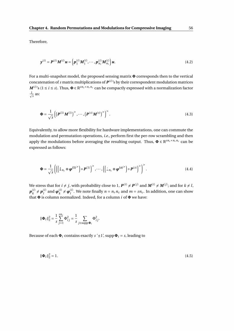
Chapter 4. Random Permutations and Modulations for Compressive Imaging 56
Therefore,
y (i ) = P (i )M (i )u =(
p (i )1 M (i )
1 , · · · , p (i )nr
M (i )nr
)u. (4.2)
For a multi-snapshot model, the proposed sensing matrixΦ corresponds then to the vertical
concatenation of s matrix multiplications of P (i )’s by their correspondent modulation matrices
M (i )’s (1 ≤ i ≤ s). Thus,Φ ∈Rsnc×nr nc can be compactly expressed with a normalization factor1p
sas:
Φ= 1ps
((P (1)M (1))> , · · · ,
(P (s)M (s))>)>
. (4.3)
Equivalently, to allow more flexibility for hardware implementations, one can commute the
modulation and permutation operations, i.e., perform first the per-row scrambling and then
apply the modulations before averaging the resulting output. Thus, Φ ∈ Rsnc×nr nc can be
expressed as follows:
Φ= 1ps
(((1nc ⊗ϕ(1)>
)◦P (1)
)>, · · · ,
((1nc ⊗ϕ(s)>
)◦P (s)
)>)>. (4.4)
We stress that for i 6= j , with probability close to 1, P (i ) 6= P ( j ) and M (i ) 6= M ( j ); and for k 6= l ,
p (i )k 6= p (i )
l and ϕ(i )k 6=ϕ(i )
l . We note finally n = nr nc and m = snc . In addition, one can show
thatΦ is column normalized. Indeed, for a column i ofΦwe have:
‖Φi‖22 =
1
s
snc∑j=1
Φ2i j =
1
s
∑j∈suppΦi
Φ2i j .
Because of eachΦi contains exactly s ’±1’, suppΦi = s, leading to
‖Φi‖22 = 1. (4.5)
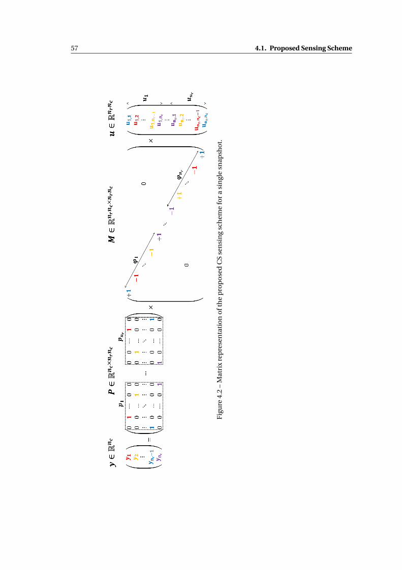
57 4.1. Proposed Sensing Scheme
Fig
ure
4.2
–M
atri
xre
pre
sen
tati
on
oft
he
pro
po
sed
CS
sen
sin
gsc
hem
efo
ra
sin
gle
snap
sho
t.
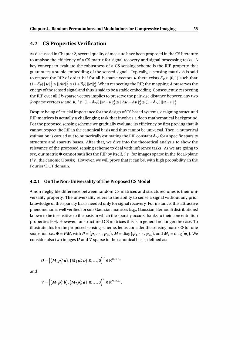
Chapter 4. Random Permutations and Modulations for Compressive Imaging 58
4.2 CS Properties Verification
As discussed in Chapter 2, several quality of measure have been proposed in the CS literature
to analyse the efficiency of a CS matrix for signal recovery and signal processing tasks. A
key concept to evaluate the robustness of a CS sensing scheme is the RIP property that
guarantees a stable embedding of the sensed signal. Typically, a sensing matrix A is said
to respect the RIP of order k if for all k-sparse vectors u there exists δk ∈ (0,1) such that:
(1−δk )‖u‖22 ≤ ‖Au‖2
2 ≤ (1+δk )‖α‖22. When respecting the RIP, the mapping A preserves the
energy of the sensed signal and thus is said to be a stable embedding. Consequently, respecting
the RIP over all 2k-sparse vectors implies to preserve the pairwise distance between any two
k-sparse vectors u and v , i.e., (1−δ2k )‖u −v‖22 ≤ ‖Au − Av‖2
2 ≤ (1+δ2k )‖u −v‖22.
Despite being of crucial importance for the design of CS based systems, designing structured
RIP matrices is actually a challenging task that involves a deep mathematical background.
For the proposed sensing scheme we gradually evaluate its efficiency by first proving thatΦ
cannot respect the RIP in the canonical basis and thus cannot be universal. Then, a numerical
estimation is carried out to numerically estimating the RIP constant δ2k for a specific sparsity
structure and sparsity bases. After that, we dive into the theoretical analysis to show the
relevance of the proposed sensing scheme to deal with inference tasks. As we are going to
see, our matrixΦ cannot satisfies the RIP by itself, i.e., for images sparse in the focal-plane
(i.e., the canonical basis). However, we will prove that it can be, with high probability, in the
Fourier/DCT domain.
4.2.1 On The Non-Universality of The Proposed CS Model
A non negligible difference between random CS matrices and structured ones is their uni-
versality property. The universality refers to the ability to sense a signal without any prior
knowledge of the sparsity basis needed only for signal recovery. For instance, this attractive
phenomenon is well verified for sub-Gaussian matrices (e.g., Gaussian, Bernoulli distributions)
known to be insensitive to the basis in which the sparsity occurs thanks to their concentration
properties [69]. However, for structured CS matrices this is in general no longer the case. To
illustrate this for the proposed sensing scheme, let us consider the sensing matrixΦ for one
snapshot, i.e.,Φ= P M , with P = (p1, · · · , pnr
), M = diag
(ϕ1, · · · ,ϕnr
), and M i = diag
(ϕi
). We
consider also two images U and V sparse in the canonical basis, defined as:
U =((
M 1p>1 a
),(M 2p>
2 b)
,0, . . . ,0)> ∈Rnr ×nc
and
V =((
M 1p>1 b
),(M 2p>
2 a)
,0, . . . ,0)> ∈Rnr ×nc ,

59 4.2. CS Properties Verification
with a and b ∈ Rnc sparse vectors in the canonical basis. Considering u and v , the per-row
vectorization of U and V respectively, we have:
Φu =nr∑
k=1pk M k uk
= p1M 1M 1p>1 a +p2M 2M 2p>
2 b
= a +b.
Φv =nr∑
k=1pk M k v k
= p1M 1M 1p>1 b +p2M 2M 2p>
2 a
= a +b.
Based on this example, we have shown that there exists at least two images sparse in the
canonical basis such that their measurements are the same, i.e., one cannot distinguish the
observed images for an image rendering or classification tasks. Thus,Φ cannot respect the
RIP with respect to the canonical basis, at least for one snapshot. Notice that this conclusion
can be extended to all support reduction based CS sensing schemes, i.e., CS sensing schemes
performing projections sequentially or in parallel in disjoint subsets of the observed image (e.g.,
per-column or block-based Bernoulli projections) following the same approach to provide
counter-examples of the universality. Hopefully, it is not an issue in practice since we can
reasonably expect that natural images are not sparse in their original domain but rather
sparse in specific frequency domains. Moreover, the nature of this sensing scheme seems
well adapted for images that exhibit a 2D-separable sparsity for which the "structure" when
projected on 1D disappear. In the following the robustness of the proposed sensing model is
analyzed following a Monte-Carlo simulation to estimate numerically the RIP constant, and
then, following a theoretical analysis to estimate the coherence of the mathematical model
and its Johnson and Lindenstrauss Lemma (JLL) (i.e., ability to preserve Euclidean distances
in the compressed domain). First, as in the addressed applications the probability to observe
images with the same properties as the counter-example mentioned above is very small, the
Monte-Carlo simulation is performed considering the canonical basis as a sparsity basis (i.e.,
acquiring images sparse in the focal-plane). Next, to fit the intrinsic properties of the images
observed in the context of CMOS image sensor, a DCT basis is considered as a sparsity basis. It
allows to alleviate the limitations regarding the RIP in the canonical basis due to the existence
of counter-examples. Finally, a theoretical analysis is provided to estimate the coherence of
the mathematical model of the proposed CS sensing scheme as well as its JLL property.

Chapter 4. Random Permutations and Modulations for Compressive Imaging 60
4.2.2 Analytical Study
(a) Concentration of pairwise distances(canonical basis).
(b) Distances to the bisector axis (canonicalbasis).
(c) Concentration of pairwise distances (DCTbasis).
(d) Distances to the bisector axis (DCT basis).
Figure 4.3 – An analytical proof of the compressive embedding of the proposed sensingscheme in (4.3). (a) shows concentration of pairwise distances of our model and a Bernoullidistribution in the canonical basis around the pairwise distances in the signal domain (bisectoraxis) for n = 1024, k = 10 and m = 128 (s = 4); (b) report the histogram of distances to thebisector axis of our model and a Bernoulli distribution; (c) and (d) report the extracted plots inthe DCT basis.
To numerically approximate the RIP constant δ2k , Let’s consider a dataset of 1000 10-sparse
signals in the canonical basis. Each generated vector is of length 1024 (i.e., nc = nr = 32) and
has k = 10 non-zero coefficients normally generated on its support (i.e., subset of nonzero
entries). Because of the fact that generating normalized vectors with disjoint supports leads
to a constant Euclidean distance equal to 2, an overlap parameter is considered to randomly
overlap the supports of the generated vectors. Furthermore, it is worth pointing out that this
simulation cannot easily generate the counter-examples mentioned in Section 4.2.1 as they
are rare according to the adopted testbench.
The generated dataset is projected in the CS domain using either the proposed sensing scheme
in (4.3) or a full Bernoulli ±1 random matrix to extract m = 128 measurements (i.e., performing
4 snapshots). The main idea behind this study is to show that the embedding performed by

61 4.2. CS Properties Verification
our model preserves the pairwise distance between any two k-sparse vectors of the generated
dataset as well as the Bernoulli random matrix with respect to a constant δ2k . Thus, to
evaluate the distortion of the projected distances, Figure 4.3a exhibits a point cloud mapping
the pairwise distances between the generated samples in the signal domain (X axis) to the
distances computed in compressed domain (Y axis) using either the proposed sensing scheme
or the Bernoulli random matrix over 100 trials to generate the sensing matrices. As it can
be seen in Figure 4.3a, the point cloud of the proposed sensing scheme is well concentrated
around the bisector axis (blue line) and its regression line perfectly fits the Bernoulli’s one. We
can therefore qualitatively validate the fact that our model preserve the pairwise distances
with respect to a distortion constant, expressed as the RIP constant δ2k .
In fact, the RIP constant δ2k can be approximated in this analytical study as the aperture
of the cone defined by the point cloud related to the proposed sensing scheme. In Figure
4.3b we establish the histogram of distances to the bisector axis for every point of Figure
4.3a to get an estimation of the RIP constant of our model and compare it to the Bernoulli
random matrix. For instance in the canonical basis at 3σ, δ2k = 0.044 for our model and
δ2k = 0.044 for the Bernoulli matrix. In the DCT, δ2k = 0.049 for our model and δ2k = 0.046
for the Bernoulli matrix. This means that we can reasonably attest that the proposed model
respects the RIP with a small distortion constant, and guarantee to recover signals with specific
sparsity structures or sensed in non-canonical bases.
In the rest of this chapter, we will study the robustness of our sensing scheme from a theoretical
point of view. Indeed, we will study the robustness of our sensing scheme using the CS matrices
properties presented in Chapter 2 known as the coherence and the Johnson and Lindenstrauss
Lemma (JLL). Before that, we first present some useful tools from probability that will be used
in the different mathematical proofs that we will provide.
4.2.3 Coherence Analysis
Useful Tools from Probability
The major SOTA contributions in analysing efficiency of CS matrices are generally obtained
using random matrices and thus involves tools from probability theory to measure concen-
tration [69, 77]. In this section, we recall the necessary materials related to the theoretical
analysis carried out in this chapter. For more mathematical background related to the CS
theory the reader can refer back to chapters 7 and 8 of [26].
Union bound: Also known as Bonferroni’s inequality or Boole’s inequality, states that for a
collection of events Bl , l ∈ [n] the probability that at least one of the events happens is

Chapter 4. Random Permutations and Modulations for Compressive Imaging 62
no greater than the sum of the probabilities of the individual events, i.e., we have
P(∪n
l=1Bl)≤ n∑
l=1P (Bl ) . (4.6)
Hoeffding’s Concentration Inequality: It provides an upper bound on the probability that
the sum of bounded independent random variables deviates from its expected value
by more than a certain threshold [210]. Let X1, . . . , Xm be a sequence of independent
random variables such that EXl = 0 and |Xl | ≤ Bl almost surely, l ∈ [m], then for all t > 0,
P
(|
m∑l=1
Xl | ≥ t
)≤ 2exp
(− t 2
2∑m
l=1 B 2l
). (4.7)
Coherence
A simple and easy measurable metric to assess the robustness of a sensing matrix is the
coherence [56, 57]. It provides a metric to evaluate the ability of a sensing matrixΦ to gen-
erate as independent (uncorrelated) as possible measurements. Indeed, it evaluates the
cross-correlations between any two columns of the sensing matrixΦ expressed as: µ (Φ) =max1≤i 6= j≤n |⟨Φi ,Φ j ⟩|. As a general consideration, the smaller the coherence of the sensing
matrix the more suitable is the matrix and therefore the better is the recovery. Indeed, it was
shown that the quality of recovery of numerous reconstruction algorithms can be analysed
using the coherence and therfore establish sufficient conditions for exact recovery based
on this CS matrix intrinsic property [26]. Furthermore, it was shown that the coherence of
a column normalized sensing model can be bounded as follows: µ (Φ) ∈[√
n−mm(n−1) ,1
]. The
lower bound is known as the Welch bound [58], and for m ¿ n it becomes µ (Φ) ' 1pm
.
To evaluate the coherence of the proposed sensing scheme described in (4.3), let us consider
images sparse per-row in a universal basis (e.g., Fourier transform or Hadamard transform).
The sparsity basis can be described as Ψ= diag(Ψ(1), . . . ,Ψ(nr )
) ∈Rnr nc×nr nc , with |Ψ(k)i j | ≤
pKpnc
for all i , j ,k and K independent of nc . In this case, one can evaluate the coherence of the
dictionaryΦΨ reported in the following proposition.
Proposition 1. GivenΦ in (4.3) and a sparsity basis Ψ= diag(Ψ(1), . . . ,Ψ(nr )
)such that |Ψ(k)
i j | ≤pKpnc
for all i , j ∈ [nc ], k ∈ [nr ] and K > 0 a constant independent of nc , then with probability at
least 1−δ, the coherence µ(ΦΨ
)ofΦΨ is upper bounded by O
(√K log
(mδ
)m
), with m = snc .
Proof. To find an upper bound of the cross-correlations between any two columns of the
sensing matrixΦΨwe note µi j := ⟨(ΦΨ)i ,
(ΦΨ
)j ⟩, with
(ΦΨ
)i =ΦΨi and
(ΦΨ
)j =ΦΨ j are

63 4.2. CS Properties Verification
two distinct columns ofΦΨ (i.e., i 6= j ). In fact, Ψ= diag(Ψ(1), . . . ,Ψ(nr )
), thus, Ψi = eb ⊗Ψ(b)
a ,
with a = [(i −1) mod nc ]+1 and b = b i−1nc
c+1. Therefore, µi j can be then expressed as follows:
µi j =s∑
l=1
1
s⟨(
p (l )1 M (l )
1 , . . . , p (l )nr
M (l )nr
)(eb(i ) ⊗Ψ(b(i ))
a(i )
),(
p (l )1 M (l )
1 , . . . , p (l )nr
M (l )nr
)(eb( j ) ⊗Ψ(b( j ))
a( j )
)⟩
=s∑
l=1
1
s⟨p (l )
b(i )M (l )b(i )Ψ
(b(i ))a(i ) , p (l )
b( j )M (l )b( j )Ψ
(b( j ))a( j ) ⟩.
Therefore, if b(i ) = b( j ), we have a(i ) 6= a( j ) since i 6= j , then:
µi j =s∑
l=1
1
s⟨Ψ(b(i ))
a(i ) ,Ψ(b(i ))a( j ) ⟩
= ⟨Ψ(b(i ))a(i ) ,Ψ(b(i ))
a( j ) ⟩= 0.
For b(i ) 6= b( j ), we have:
µi j =s∑
l=1
1
s⟨p (l )
b(i )M (l )b(i )Ψ
(b(i ))a(i ) , p (l )
b( j )M (l )b( j )Ψ
(b( j ))a( j ) ⟩
=s∑
l=1
s∑k=1
1
s
(e>
k p (l )b(i )M (l )
b(i )Ψ(b(i ))a(i )
)(e>
k p (l )b( j )M (l )
b( j )Ψ(b( j ))a( j )
)=
s∑l=1
s∑k=1
Zk,l(i , j
),
with Zk,l(i , j
)= 1s
(e>
k p (l )b(i )M (l )
b(i )Ψ(b(i ))a(i )
)(e>
k p (l )b( j )M (l )
b( j )Ψ(b( j ))a( j )
). By independence of M (l )
b(i ) and
M (l )b( j ) (generated by construction as the realization of a Bernoulli random variable identically
and independently), Zk,l(i , j
)are independent too. Furthermore, Zk,l
(i , j
)is bounded in
absolute value by Ksnc
(since |Ψ(q)i j | ≤
pKpnc
for all i , j , q). Therefore, By Hoeffding’s inequality in
(4.7) we can write:

Chapter 4. Random Permutations and Modulations for Compressive Imaging 64
P(|µi j | ≥ t
)≤ 2exp
− t 2
2∑s
l=1
∑nc
l ′=1
(K
snc
)2
≤ 2exp
(− snc t 2
2K
).
By union bound in (4.7) we have:
P
(max
1≤i 6= j≤snc
|µi j | ≥ t
)=P(∃i , j /|µi j | ≥ t
)≤∑
i jP
(|µi j | ≥ t)
≤snc∑i=1
snc∑j=1
2exp
(− snc t 2
2K
)
≤ 2s2n2c exp
(− snc t 2
2K
).
We choose δ= 2s2n2c exp
(− snc t 2
2K
), thus t =
√2K log
(2s2n2
cδ
)snc
, leading to the following:
P
max1≤i 6= j≤snc
|µi j | ≤
√√√√2K log(
2s2n2c
δ
)snc
≥ 1−δ.
Therefore, with probability at least 1−δ the mutual coherence ofΦ in a universal basis (i.e.,
µ (ΦΨ)) is upper bounded by O
(√K log
(mδ
)m
)(m = snc ), which is close to the optimal bound,
i.e., 1pm
.
4.2.4 Compressive Embedding Analysis
Compressive embedding refers to a stable embedding property allowing to preserve distances
between low-complexity samples in the compressed domain up to a distortion factor using a
sensing matrixΦ. This statement is explicitely stated by the Johnson–Lindenstrauss Lemma
(JLL) for finite sets of vectors [64]. As preserving pairwise distances is the cornerstone in
numerous machine learning tasks, in this section we focus on verifying when the proposed
sensing scheme preserves the separability of k-sparse images. Thus, let us consider the

65 4.2. CS Properties Verification
following JLL:
Proposition 2. Given 0 < t < 1 , a set X of r points in Rn , the linear mapping f (u) =ΦΨu such
that
(1− t )‖u −v‖2 ≤ ‖ f (u)− f (v )‖2 ≤ (1+ t )‖u −v‖2, (4.8)
holds for all u, v ∈ X with probability at least 1− r 2 exp(−c st 2
nr
).
To show that our CS modelΦ in (4.3) respects the JLL in the DCT basis, we will first find a con-
centration property of the proposed model, i.e., showing that ‖ΦΨu‖22 is highly concentrated
around ‖u‖22 and then extend the concentration property to show that the JLL holds with high
probability in the case of the proposed sensing scheme in (4.3).
Concentration property
Without loss of generality let us consider a unit vector u ∈ Rnr nc and the sensing scheme
in (4.3) defined as Φ = 1ps
((P (1)M (1)
)>, · · · ,
(P (s)M (s)
)>)>, and the sparsity basis defined as
Ψ= diag(Ψ(1), . . . ,Ψ(nr )
). We have:
∥∥ΦΨu∥∥2
2∥∥u∥∥2
2
= 1
s
s∑i=1
∥∥P (i )M (i )Ψu∥∥2
2
= 1
s
s∑i=1
∥∥ nr∑j=1
p (i )j diag
(ϕ(i )
j
)Ψ( j )u j
∥∥22
= 1
s
s∑i=1
∥∥ nr∑j=1
p (i )j M (i )
j Ψ( j )u j
∥∥22
= 1
s
s∑i=1
nr∑j k⟨p (i )
j M (i )j Ψ
( j )u j , p (i )k M (i )
k Ψ(k)uk⟩
= 1+ 1
s
s∑i=1
nr∑j 6=k
⟨p (i )j M (i )
j Ψ( j )u j , p (i )
k M (i )k Ψ
(k)uk⟩
Thus,
∥∥ΦΨu∥∥2
2 −∥∥u
∥∥22 =
s∑i=1
Zi ,
with Zi = 1s
∑nr
j 6=k⟨p (i )j M (i )
j Ψ( j )u j , p (i )
k M (i )k Ψ
(k)uk⟩.

Chapter 4. Random Permutations and Modulations for Compressive Imaging 66
To find a concentration property of∥∥ΦΨu
∥∥22−
∥∥u∥∥2
2 around 0, we can use Hoeffding’s inequality
in (4.7). To do that, we have to show that Zi ’s are zero-mean and bounded in absolute value.
First, because the main diagonal entries of M (i )j are Bernoulli variables with E
(diag M (i )
j
)= 0,
with M (i )j and M (k)
l independent if i 6= k and j 6= l , we can show that E (Zi ) = 0. Indeed,
E (Zi ) = E(
1
s∥∥u
∥∥22
nr∑j 6=k
⟨p (i )j M (i )
j Ψ( j )u j , p (i )
k M (i )k Ψ
(k)uk⟩)
= 1
s∥∥u
∥∥22
nr∑j 6=k
E
((p (i )
j M (i )j Ψ
( j )u j
)> (p (i )
k M (i )k Ψ
(k)uk
))
= 1
s∥∥u
∥∥22
nr∑j 6=k
u j>Ψ( j )>E
((M (i )
j
)>)E
((p (i )
j
)>)E(
p (i )k
)E(
M (i )k
)ukΨ
(k)
= 0
On the other hand, by Cauchy-Shwarz we have
Zi = 1
s∥∥u
∥∥22
nr∑j 6=k
⟨p (i )j M (i )
j Ψ( j )u j , p (i )
k M (i )k Ψ
(k)uk⟩
≤ 1
s∥∥u
∥∥22
nr∑j 6=k
∥∥p (i )j M (i )
j Ψ( j )u j
∥∥∥∥p (i )k M (i )
k Ψ(k)uk
∥∥.
Because p (i )j , M (i )
j andΨ( j ) are orthonormal matrices,∥∥p (i )
j M (i )j Ψ
( j )u j∥∥= ∥∥u j
∥∥. Thus,
Zi ≤ 1
s
nr∑j 6=k
∥∥u j∥∥∥∥uk
∥∥≤ 1
s
(nr∑
j=1
∥∥u j∥∥)2
≤ nr
s‖u‖2 = nr
s
Finally we can apply Hoeffding’s inequality in (4.7) to find the following concentration prop-
erty:
P(|∥∥ΦΨu
∥∥22 −
∥∥u∥∥2
2| ≤ t∥∥u
∥∥22
)≥ 1−2exp
(−c
st 2
nr
), (4.9)

67 4.3. Signal Recovery Using the Proposed Sensing Scheme
with c = 12 .
Johnson-Lindenstrauss Lemma
To show that our modelΦ in (4.3) respects the JLL in (4.8), we consider the set E defined as:
E = {ui −u j : 1 ≤ i < j ≤ r }, (4.10)
with card(E) ≤ r (r−1)2 .
For any fixed v ∈ E our model Φ respects the concentration inequality in (4.9). Thus, it is
enough to show that the concentration inequality holds for all v ∈ E . One can see that thanks
to union bound, (4.8) holds for all v ∈ E with probability at least 1− r 2 exp(−c st 2
nr
). Thus, with
r 2 exp(−c st 2
nr
)≤ 1, we need s ≥ nr t−2 log(r ), i.e., we need approximately to sense the hole
image to ensure the JLL which is unfortunately not realistic. To handle this issue, the JLL
analysis have to benefit of the structure of the sparsity basisΨ (e.g., |Ψi j | ≤p
Kpnc
) by restricting
the set of images to those that are sparse in Ψ only. This will maybe have only to respect
s ≥ t−2 log(r ) which is realistic.
4.3 Signal Recovery Using the Proposed Sensing Scheme
4.3.1 Reconstruction of Sparse Signals
Although verifying the ability to preserve pairwise distances, it is relevant to analyze the ef-
ficiency of signal recovery for image rendering tasks. Our testbench is mainly composed of
the commonly used images, i.e., Barbara, Monkey, Boat, Cameraman and Lena as depicted
in Figure 4.4. These images are resized to 128×128 for simulation purposes (speed of con-
vergence). As already discussed, natural images are generally compressible and not really
sparse (i.e., most components are practically of small magnitudes but not zero). Indeed, to
ensure the sparsity of our testbench for phase-transition diagnosis purposes, each image is
first projected in the wavelet domain and small magnitude are then zeroed with respect to a
pre-computed threshold enabling a certain sparsity level. Finally, each image is backprojected
in the canonical basis using the wavelet inverse transform.
Signal recovery is achieved using the Daubechies-6 wavelet basis as a sparsity basisΨ [211].
The signal recovery can then be expressed as:
x = argminx
‖Ψ (x)‖1 +λ‖y −Φx‖22, (4.11)
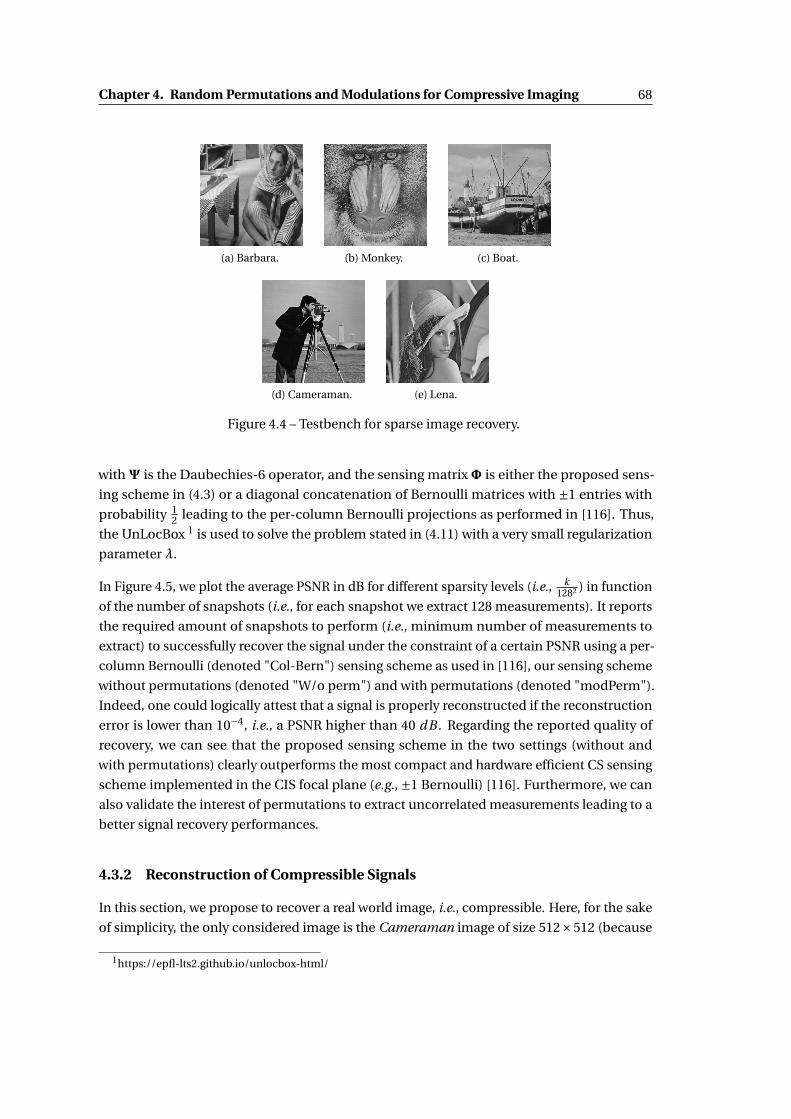
Chapter 4. Random Permutations and Modulations for Compressive Imaging 68
(a) Barbara. (b) Monkey. (c) Boat.
(d) Cameraman. (e) Lena.
Figure 4.4 – Testbench for sparse image recovery.
withΨ is the Daubechies-6 operator, and the sensing matrixΦ is either the proposed sens-
ing scheme in (4.3) or a diagonal concatenation of Bernoulli matrices with ±1 entries with
probability 12 leading to the per-column Bernoulli projections as performed in [116]. Thus,
the UnLocBox 1 is used to solve the problem stated in (4.11) with a very small regularization
parameter λ.
In Figure 4.5, we plot the average PSNR in dB for different sparsity levels (i.e., k1282 ) in function
of the number of snapshots (i.e., for each snapshot we extract 128 measurements). It reports
the required amount of snapshots to perform (i.e., minimum number of measurements to
extract) to successfully recover the signal under the constraint of a certain PSNR using a per-
column Bernoulli (denoted "Col-Bern") sensing scheme as used in [116], our sensing scheme
without permutations (denoted "W/o perm") and with permutations (denoted "modPerm").
Indeed, one could logically attest that a signal is properly reconstructed if the reconstruction
error is lower than 10−4, i.e., a PSNR higher than 40 dB . Regarding the reported quality of
recovery, we can see that the proposed sensing scheme in the two settings (without and
with permutations) clearly outperforms the most compact and hardware efficient CS sensing
scheme implemented in the CIS focal plane (e.g., ±1 Bernoulli) [116]. Furthermore, we can
also validate the interest of permutations to extract uncorrelated measurements leading to a
better signal recovery performances.
4.3.2 Reconstruction of Compressible Signals
In this section, we propose to recover a real world image, i.e., compressible. Here, for the sake
of simplicity, the only considered image is the Cameraman image of size 512×512 (because
1https://epfl-lts2.github.io/unlocbox-html/

69 4.3. Signal Recovery Using the Proposed Sensing Scheme
(a) Col-Bern. (b) W/o perm. (c) modPerm.
Figure 4.5 – Phase-transition diagrams. Black, red and magenta lines show the transitions to asuccess reconstruction above 40 dB for per-column Bernoulli (Col-Bern), our model withoutpermutations (W/o perm) and our model sensing schemes (modPerm) respectivelly.
of its intrinsic image characteristics). Two regularization operators are used to recover this
image instead of a simple `1-constraint in a wavelet basis:
1. The anisotropic Total Variation (TV) operator defined using the horizontal and vertical
gradients (respectively ∇h and ∇v ) as:
TV(x) = ‖∇v x‖1 +‖∇h x‖1. (4.12)
Thus, the signal recovery problem can be expressed as:
x = argminx
TV(x)+λ‖y −Φx‖22, (4.13)
2. the mDWT-TV operator defined as the sum of the `1 norm of the components (horizontal
and vertical) of the gradient of the image in multiple wavelet transforms (denoted as
matricesΨi ) [212, 118]:
mDWT-TV(x) =3∑
i=1‖Ψi∇v x‖1 +‖Ψi∇h x‖1. (4.14)
Indeed, natural images generally involve several structures with sparse representations
in different basis. It turns out therefore that promoting average sparsity over multiple
bases rather than a single one represents a powerful prior [213]. Thus, the signal recovery
problem can be expressed using three wavelet transforms known as Db-2 (Ψ1), Db-6
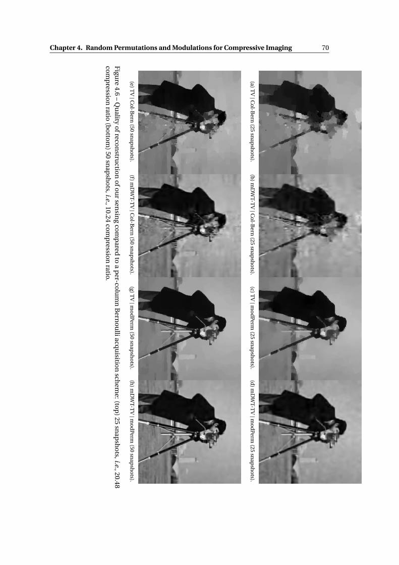
Chapter 4. Random Permutations and Modulations for Compressive Imaging 70
(a)T
V|Co
l-Bern
(25sn
apsh
ots).
(b)
mD
WT-T
V|Co
l-Bern
(25sn
apsh
ots).
(c)T
V|mo
dPerm
(25sn
apsh
ots).
(d)m
DW
T-TV|m
odPerm
(25sn
apsh
ots).
(e)T
V|Co
l-Bern
(50sn
apsh
ots).
(f)m
DW
T-TV|C
ol-B
ern(50
snap
sho
ts).(g)
TV|m
od
Perm(50
snap
sho
ts).(h
)mD
WT-T
V|mod
Perm(50
snap
shots).
Figu
re4.6
–Q
uality
ofreco
nstru
ction
ofo
ur
sensin
gco
mp
aredto
ap
er-colu
mn
Bern
ou
lliacqu
isition
schem
e:(top
)25
snap
sho
ts,i.e.,20.48co
mp
ression
ratio(b
otto
m)
50sn
apsh
ots,i.e.,10.24
com
pressio
nratio.
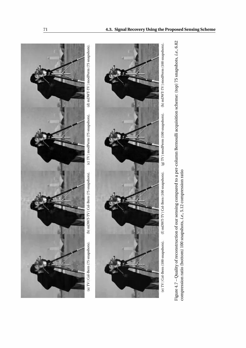
71 4.3. Signal Recovery Using the Proposed Sensing Scheme
(a)
TV|C
ol-
Ber
n(7
5sn
apsh
ots
).(b
)m
DW
T-T
V|C
ol-
Ber
n(7
5sn
apsh
ots
).(c
)T
V|m
od
Perm
(75
snap
sho
ts).
(d)m
DW
T-T
V|m
odPe
rm(7
5sn
apsh
ots)
.
(e)
TV|C
ol-
Ber
n(1
00sn
apsh
ots
).(f
)m
DW
T-T
V|C
ol-
Ber
n(1
00sn
apsh
ots
).(g
)T
V|m
od
Perm
(100
snap
sho
ts).
(h)m
DW
T-T
V|m
odPe
rm(1
00sn
apsh
ots)
.
Fig
ure
4.7
–Q
ual
ity
ofr
eco
nst
ruct
ion
ofo
ur
sen
sin
gco
mp
ared
toa
per
-co
lum
nB
ern
ou
lliac
qu
isit
ion
sch
eme:
(to
p)
75sn
apsh
ots
,i.e
.,6.
82co
mp
ress
ion
rati
o(b
ott
om
)10
0sn
apsh
ots
,i.e
.,5.
12co
mp
ress
ion
rati
o
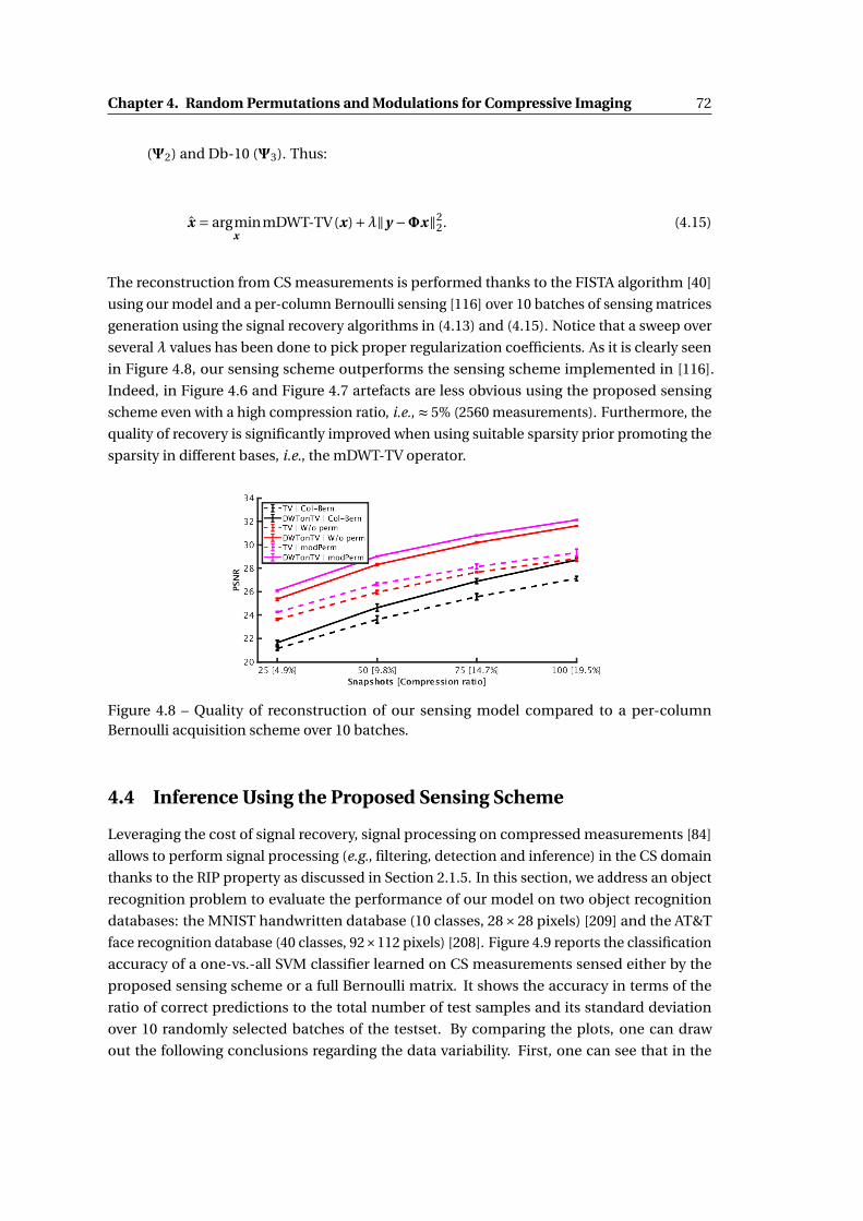
Chapter 4. Random Permutations and Modulations for Compressive Imaging 72
(Ψ2) and Db-10 (Ψ3). Thus:
x = argminx
mDWT-TV(x)+λ‖y −Φx‖22. (4.15)
The reconstruction from CS measurements is performed thanks to the FISTA algorithm [40]
using our model and a per-column Bernoulli sensing [116] over 10 batches of sensing matrices
generation using the signal recovery algorithms in (4.13) and (4.15). Notice that a sweep over
several λ values has been done to pick proper regularization coefficients. As it is clearly seen
in Figure 4.8, our sensing scheme outperforms the sensing scheme implemented in [116].
Indeed, in Figure 4.6 and Figure 4.7 artefacts are less obvious using the proposed sensing
scheme even with a high compression ratio, i.e., ≈ 5% (2560 measurements). Furthermore, the
quality of recovery is significantly improved when using suitable sparsity prior promoting the
sparsity in different bases, i.e., the mDWT-TV operator.
Figure 4.8 – Quality of reconstruction of our sensing model compared to a per-columnBernoulli acquisition scheme over 10 batches.
4.4 Inference Using the Proposed Sensing Scheme
Leveraging the cost of signal recovery, signal processing on compressed measurements [84]
allows to perform signal processing (e.g., filtering, detection and inference) in the CS domain
thanks to the RIP property as discussed in Section 2.1.5. In this section, we address an object
recognition problem to evaluate the performance of our model on two object recognition
databases: the MNIST handwritten database (10 classes, 28×28 pixels) [209] and the AT&T
face recognition database (40 classes, 92×112 pixels) [208]. Figure 4.9 reports the classification
accuracy of a one-vs.-all SVM classifier learned on CS measurements sensed either by the
proposed sensing scheme or a full Bernoulli matrix. It shows the accuracy in terms of the
ratio of correct predictions to the total number of test samples and its standard deviation
over 10 randomly selected batches of the testset. By comparing the plots, one can draw
out the following conclusions regarding the data variability. First, one can see that in the

73 4.5. Dedicated Hardware Implementations and Conclusion
case of the MNIST (small and low variable samples), we can achieve a no-loss classification
compared to a no-CS setting from 10 snapshots, (i.e., ≈ 35% compression ratio and 320
measurements). However, with more variability and informational content (i.e., AT&T), we
achieve the same performance from approximatively 10 snapshots, (i.e., ≈ 5% compression
ratio and 520 measurements). It is finally clear that what practically matter is the number of
CS measurements (or its equivalent number of snapshots) to extract and not the compression
ratio.
Figure 4.9 – Classification accuracy for the AT&T and MNIST databases.
4.5 Dedicated Hardware Implementations and Conclusion
A system overview of possible physical implementations of the proposed sensing scheme is
illustrated in Figure 4.10. Indeed, several possible embodiments can be proposed to perform
on-chip pseudo-random modulations and permutations. To perform permutations, one
can design a dedicated pseudo-random generator to generate a pseudo-randomly permuted
sequence to address the columns leading to pseudo-random shuffle of each selected row.
Furthermore, this task can also be achieved thanks to a butterfly network [214] controlled
by a pseudo-random generator (PRG) (e.g., LFSR [203] or Cellular automata [73]). On the
other hand, the pseudo-random modulations and the sum can be achieved using either a
CTIA [116] combined with a classical ADC (e.g., SAR) or design dedicated ADC that takes
advantage of a canonical incremental Σ∆ converter enabling pseudo-random modulations,
averaging and A/D conversions [114]. It is worth pointing out that all the cited possible
implementations can be implemented at the end-of-column circuitry in the analog domain or
during A/D conversions allowing to alleviate hardware resources and keeping standard pixel
architectures (e.g., 3T or 4T) with canonical image readout enabling CDS operation to deal
with FPN resulting noise. For multiple snapshots, our scheme requires non-destructive pixel
readout both in the case of rolling shutter and global shutter acquisitions thanks to relaxed
constraints on ADC speed.
In conclusion, in this chapter we propose a new CS sensing scheme based on random modula-
tions & permutations to meet highly constrained hardware tasks while respecting theoretical
properties of a CS matrix. Several analytical, theoretical and simulation results have been

Chapter 4. Random Permutations and Modulations for Compressive Imaging 74
Figure 4.10 – Top-level architecture of a pseudo-random modulations & permutations com-pressive image sensor.
presented to show the efficiency of the proposed sensing scheme for both image rendering and
inference tasks. Indeed, the proposed sensing scheme clearly outperforms the most compact
implementation of a CS sensing scheme in both signal recovery and inference. Furthermore,
the main advantage of the proposed sensing scheme is its relevance in terms of hardware
implementation such it can be advantageously implemented at the end-of-column circuitry
without major additional materials compared to a canonical CIS architecture [215] while
reducing the total amount of data to extract and convert to the digital domain leading to
a significant power consumption save and enabling advanced signal processing tasks, e.g.,
on-chip decision making as it will be discussed in Chapter 6.

Chapter 5
Hierarchical Decision Making
As discussed in Section 2.2, the trend in smart CIS consists in designing computational-friendly,
always-on compact CIS with on-chip AI capabilities. The design of this new devices tends to
take advantage of recent advances in signal acquisition schemes and inference algorithms,
well optimized for low-power systems. Moreover, the design of this kind of information-
retrieval signal processing architectures have to deal with on-chip constraints related to the
data dimensionality and algorithms complexity. Throughout this thesis, we aim at providing
some initial steps towards the design of smart compact CIS with on-chip inference capabilities.
As seen in Chapter 4, compressive sensing has been explored to reduce data dimensionality
during the image acquisition process without heavy additional materials leading to drastic
hardware resources saving. However, achieving our goal, i.e., on-chip inference, is still limited
by the algorithm complexity at the device level when implementing standard machine learning
algorithms.
To deal with the on-chip computational complexity bottleneck related to a canonical inference
algorithm, hierarchical machine learning algorithms [216, 217, 218, 219] can significantly
reduce memory and computational requirements related to an embedded decision making
algorithm. Considering a multi-class image classification system based on binary classifiers
such as SVMs, three popular strategies are usually adopted with different levels of complexity.
The complexity of such systems is generally expressed based on the number of binary classi-
fiers involved during the inference. The first approach called one-vs.-all, involves the training
of C classifiers for a C classes problem. The second one is the one-vs.-one strategy and trains
C (C −1)/2 classifiers for the same C classes problem. Finally, for more flexibility to define
the number of classifiers and the depth width (i.e., cascading many classification layers),
the DNN took over the reins of multi-class image classification by learning αC classifiers
in the first layer (α > 1) combined with nonlinear activation functions and adaptive depth
width depending on the complexity of the classification task. However, thanks to its intrinsic
nature, a hierarchical inference dynamically requires to run only O (log2 C ) cascaded binary
classifiers lowering as a consequence the number of binary operations (i.e., multiplication and

Chapter 5. Hierarchical Decision Making 76
accumulation) as well as memory needs required for on-chip applications. Thus, for a highly
constrained embedded system (e.g., smart always-on sensor), it seems relevant to investigate
hierarchical strategies on CS measurements to relax hardware requirements related to signal
acquisition (e.g., A/D conversion, power consumption) and data processing (e.g., memory
needs) to perform embedded multi-class inference.
In this chapter, we mainly focus on hierarchical learning in the context of highly constrained
hardware in order to reduce hardware requirements related to an embedded multi-class
inference. We introduce new methods to construct the hierarchical tree to train a hierarchical
classifier (i.e., a binary decision tree) minimizing as a consequence the number of decision
nodes, end thus, the number of binary classifiers to perform at the inference level. Indeed,
as already discussed in the previous section, a powerful binary classifier is the so-called
2-classes SVM thanks to its ability to handle outliers. Using classes centroids and sample
labels of a training database, three methods have been investigated to create two clusters at
each node that are balanced in terms of number of classes: (Method 1): sequential C -means
clustering, (Method 2): SVM-based clustering and (Method 3): a clustering based on the
Principal Component Analysis (PCA). Each proposed method assumes specific priors on intra-
class & inter-class data distribution to construct the decision tree. In Method 1, we propose a
K-means-inspired [220] algorithm to construct two balanced clusters limiting the decision
tree depth. In Method 2, we construct balanced clusters that directly maximize the soft margin
of a SVM performed on samples data belonging to each class-clusters. Finally, Method 3
takes advantage of a new basis estimated from a PCA [221] that better represents the classes
centroids variability to define a separation threshold identifying two classes clusters. In the
following, we will present our proposed clustering methods as well as general considerations
on hardware and an evaluation of classification accuracy for a basic inference problem. In the
context of limited processing and memory resources, we consider CS measurements as raw
data for both training and testing.
5.1 Hierarchical Classification on CS: Key Concepts
In the SOTA, several works have addressed hierarchical classification each proposing a different
criteria to construct the decision tree. For example, [217] describes statistical criteria to
hierarchically cluster similar classes in a multi-class classification problem. In addition, a
binary SVM is trained to geometrically separate clusters at each level. More recently, with
the rise of dictionary learning techniques for image representation and classification, various
constrained dictionary learning methods were proposed to learn discriminative class-specific
dictionaries allowing images classification. As for [217], a hierarchical dictionary learning
approach provide a coarse-to-fine representation to describe patterns of different level of
similarities. For instance, [218] proposes a hierarchical dictionary learned such that the
upper-level dictionaries represent common patterns of high level classes while lower-level
dictionaries describe specific patterns of a set of classes. On the other hand, [222] proposes a
hierarchical-structured dictionary learning method based on a Fisher criterion [136]. Hence,
77 5.2. Proposed Hierarchical Learning Methods
a constrained dictionary is learned at each level and described as a concatenation of the
shared dictionary of the upper level and the class-specific dictionary. Indeed, to construct the
hierarchical tree, [223] uses a K-means algorithm [224]. In this work, the sparse coefficients
extracted at each node are then used to train a multi-class SVM to classify the images. Finally,
[219] addresses the problem of hierarchical tree construction using classes similarity based on
an inter-class distance metric, combining clustering on data variability with path-searching
for the inference.
On the other hand, hierarchical learning on CS measurements refers to constructing the hier-
archical decision tree directly in the compressed domain. Indeed, as mentioned in previous
sections, based on the outstanding results in the field of signal processing on compressive
measurements [84, 85, 87], we can advantageously take advantage of the stable embedding
of a CS sensing scheme to preserve the distance between the two subsets learned at each
node of the binary decision tree. In the rest of this chapter, we will first present the proposed
hierarchical algorithms and then present the results of combining the proposed methods with
a CS sensing matrix.
5.2 Proposed Hierarchical Learning Methods
5.2.1 Notations
Let us consider a database of n-length “vectors” in Rn (e.g., signals with n samples, or images
with n pixels) composed of C classes. This database is separated into two databases: a
“train” set X ∈ Rn×n1C , where each class is composed of n1 samples, associated with labels
l ∈ {1, · · · ,C }n1C ; and a “test” set Y ∈Rn×n2C with unknown labels and composed of n2 samples
per class. We refer to X j = (X j1, · · · , X j
n1) ∈ Rn×n1 and Y j = (Y j
1, · · · ,Y jn2
) ∈ Rn×n2 for the train
and the test sets restricted to the j th class, respectively. The notation x ∈ X or x ∈ X j , means
that the sample x is an arbitrary column of X or X j , respectively (and similarly for Y ). The
mean vectors of each class (i.e., class centroids) are expressed as µ j = 1n1
∑n1i=1 X j
i , for 1 ≤ j ≤C .
Moreover, we denote by the distance matrix the matrix containing the euclidean distances
between the mean vectors defined as:
D = (∥∥µp −µq
∥∥2)1≤(p,q)≤C . (5.1)
5.2.2 Binary SVM
A binary (2-class) SVM refers to learning a hyperplane separating the n-dimensional space
between two classes. Obviously, the best separation is achieved by the hyperplane maximizing
the distance to the nearest training sample of any class, i.e., maximum margin. Thus, given
{(x1, l1) , . . . , (xk , lk ) , . . . ,(x2n1 , l2n1
)} ⊂ RN × {−1,1} samples of two different classes in X . The
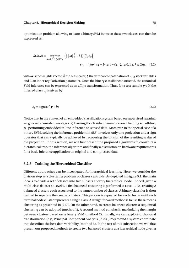
Chapter 5. Hierarchical Decision Making 78
optimization problem allowing to learn a binary SVM between these two classes can then be
expressed as:
{ω, b, ξ} = argminω∈Rn ,b,ξ∈R2n1
(12
∥∥ω∥∥22 +λ
∑2n1
k=1 ξk
)s.t. lk (ω>xk +b) ≥ 1−ξk , ξk ≥ 0,1 ≤ k ≤ 2n1, (5.2)
with ω is the weights vector, b the bias scalar, ξ the vertical concatenation of 2n2 slack variables
and λ an inner regularization parameter. Once the binary classifier constructed, the canonical
SVM inference can be expressed as an affine transformation. Thus, for a test sample y ∈ Y the
inferred class cy is given by:
cy = sign(ω>y +b) (5.3)
Notice that in the context of an embedded classification system based on supervised learning,
we generally consider two stages: i ) learning the classifier parameters on a training set, off-line,
i i ) performing embedded in-line inference on sensed data. Moreover, in the special case of a
binary SVM, solving the inference problem in (5.3) involves only one projection and a sign
operator that can typically be achieved by recovering the bit sign of the resulting scalar of
the projection. In this section, we will first present the proposed algorithms to construct a
hierarchical tree, the inference algorithm and finally a discussion on hardware requirements
for a basic inference application on original and compressed data.
5.2.3 Training the Hierarchical Classifier
Different approaches can be investigated for hierarchical learning. Here, we consider the
division step as a clustering problem of classes centroids. As depicted in Figure 5.1, the main
idea is to divide a set of classes into two subsets at every hierarchical node. Indeed, given a
multi-class dataset at Level 0, a first balanced clustering is performed at Level 1, i.e., creating 2
balanced clusters each associated to the same number of classes. A binary classifier is then
trained to separate the created clusters. This process is repeated for each cluster until each
terminal node cluster represents a single class. A straightforward method is to use the K-means
clustering as presented in [217]. On the other hand, to create balanced clusters a sequential
clustering can be adopted (method 1). A second method consists in maximizing the margin
between clusters based on a binary SVM (method 2). Finally, we can explore orthogonal
transformation (e.g., Principal Component Analysis (PCA) [225]) to find a system coordinate
that describes the best data variability (method 3). In the rest of this subsection we will first
present our proposed methods to create two balanced clusters at a hierarchical node given a

79 5.2. Proposed Hierarchical Learning Methods
Figure 5.1 – An illustration of the hierarchical learning. The input multi-class dataset to beclassified is presented at Level 0. A first balanced clustering (2 clusters, each associated tothe same number of classes) is performed at Level 1, then a binary classifier is trained. Thisprocess is repeated for each cluster until the construction of a single-class cluster at each
terminal node. Here, C ( j)i represents j th cluster at level i .
set of classes (Algorithm 1-3). Secondly, we describe the algorithm used to create the decision
tree (Figure 5.2), then used for the inference (Algorithm 4).
Sequential C -means Clustering (Method 1)
Algorithm 1 Sequential C-means clustering (Method 1)
1: Input µ ∈Rn×C centroids of C classes in X and D2: {m1,m2} ← argmaxi , j D i j ;3: c 1 ← µm1
; c 2 ← µm2;
4: C1 ← {c 1}; C2 ← {c 2};5: µ←µr {µm1
,µm2};
6: while µ 6= {ø} do7: m1 ← argmin j
∥∥c 1 −µ j
∥∥2 ;
8: m2 ← argmin j
∥∥c 2 −µ j
∥∥2 ;
9: c 1 ← µm1; c 2 ← µm2
;10: C1 ←C1 ∪ {c 1}; C2 ←C2 ∪ {c 2} ;11: µ←µr {µm1
,µm2};
12: c 1 ← centroid of C1; c 2 ← centroid of C1 ;13: end while14: return C1 and C2
The hierarchical learning proposed in Method 1 is typically inspired by the K -means cluster-
ing technique known also as the Lloyd’s algorithm. The K -means algorithm is a canonical
clustering technique that aims at minimizing the average squared distance between samples
in the same cluster [226]. Indeed, the K -means first chooses K arbitrary samples chosen

Chapter 5. Hierarchical Decision Making 80
randomly from the input dataset as initial centroids. Each point is then assigned to the nearest
centroid, and each centroid is recomputed as the mean vector of all samples assigned to it.
These last two steps are repeated until the process stabilizes, i.e., when the assignments no
longer change. Thus, given centroids of a C -classes dataset represented by the matrixµ ∈Rn×C
and their corresponding distance matrix D ∈RC×C , Method 1 aims at creating two balanced
clusters based on classes centroids too. Inspired by the K -means, the algorithm of Method 1 is
first initialized to the centroids maximizing the Euclidean constrained distances, i.e., centroids
separated with the highest Euclidean distance that we will denote c 1 and c 2. Then, at each
iteration we sequentially assign to each cluster the centroid minimizing the Euclidean distance
to their centers. In addition, c 1 and c 2 are recomputed at each iteration, i.e., we calculate the
mean vector of their clusters, respectively. This process is repeated until the assignment of all
initial centroids. Finally, the algorithm returns two clusters C1 and C2 allowing to cluster a set
of centroids at a given node as described in Algorithm 1.
SVM Based Balanced Clustering (Method 2)
Algorithm 2 SVM based clustering (Method 2)
1: Input C classes in X , centroids µ ∈Rn×C and D2: {m1,m2} ← argmaxi , j D i j ;3: c 1 ← µm1
; c 2 ← µm2;
4: C1 ← {X m1 }; C2 ← {X m2 };5: µ=µr {µm1
,µm2};
6: while µ 6= {ø} do7: associate C1 to {1}n1card(C1);8: associate C2 to {−1}n1card(C2);9: for all xk ∈C1 ∪C2 :
{ω, b, ξ} = argminω,b,ξ
(12
∥∥ω∥∥22 +λ
∑k ξk
)s.t. lk (ω>xk +b) ≥ 1−ξk , ξk ≥ 0,1 ≤ k ≤ n1card(C1)+n1card(C2).
10: m1 = argmax j ω>µ j + b ;
11: m2 = argmin j ω>µ j + b ;
12: c 1 ← µm1; c 2 ← µm2
;13: C1 ←C1 ∪ {X m1 }; C2 ←C2 ∪ {X m2 };14: µ=µr {µm1
,µm2};
15: end while16: return C1 and C2
Method 2 takes advantage of the intrinsic properties of the SVM classifier to directly learn
the hierarchical decision tree. In this second method, the algorithm is also initialized to the
centroids maximizing the Euclidean distance (i.e., c 1 and c 2) as described in Algorithm 2.
Indeed, at the first iteration the binary SVM is trained on the samples associated to the classes
whose centroids are c 1 and c 2, i.e., centroids maximizing the Euclidean distance (in matrix
D). For the second step, Method 2 assigns the class centroid µm1maximizing the positive

81 5.2. Proposed Hierarchical Learning Methods
margin to the first cluster C1 and the class centroidµm2minimizing the negative margin to C2
using the affine function presented in (5.3). An update of the binary SVM hyperplane is then
performed by relearning it but this time on all the data samples associated to the centroids
of each cluster. The last two steps are repeated until the assignment of all centroids with a
SVM decision boundary learned on the finally generated clusters. The main advantage of this
approach is the ability to update the decision boundary at each iteration taken into account
the new assigned centroids and thus samples associated to each cluster.
PCA Based Balanced Clustering (Method 3)
Algorithm 3 PCA based clustering (Method 3)
1: Input µ ∈Rn×C centroids of C classes in X2: SVD [227] : µ=UΣV > s.t. U = [u1 . . .uC−1].3: θ← median value of u1
>µ ;4: C1 ← (µ) j s.t. u1
>µ j < θ ;
5: C2 ← (µ) j s.t. u1>µ j ≥ θ ;
6: return C1 and C2
The main idea of Method 3 is to find a new basis that best describes data variability of class
centroids enabling then the construction of two balanced half-spaces. Indeed, dimensionality
reduction techniques [197] provide a powerful framework to find new bases that preserve
intrinsic properties of the processed data. A widely used technique is the Principal Compo-
nent Analysis (PCA) that seeks to project the observed data into a set of linearly uncorrelated
vectors called principal components. The new basis is constructed such that the first prin-
cipal component has the largest variance of the data, and each succeeding component is
constructed under the constraint that it is orthogonal to the preceding components with
decreasing variance. The PCA decomposition is usually achieved via eigendecomposition of
the covariance matrix or by Singular Value Decomposition (SVD) [227]. Thus, to create two
balanced clusters, a promising approach consists in projecting the centroids into the first
principal component of the matrix µ ∈Rn×C composed of the mean vectors of each class of
the C -classes dataset. This way, once the projection is learned, one can construct two clusters
such that the centroids bellow the median of the projection in the PCA domain are assigned to
the first cluster and the ones above this threshold are assigned to the second. This way, the
median enables a balanced clustering.
5.2.4 Testing the Hierarchical-Based Inference
Given the balanced clustering methods presented in Section 5.2, the binary decision tree is
recursively constructed using one of the aforementioned balanced methods at each node.
Indeed, in each node two balanced clusters are typically constructed allowing to train a binary
SVM (i.e., (5.2)) on the created clusters as described formally in Algorithm 4.

Chapter 5. Hierarchical Decision Making 82
Algorithm 4 Decision tree construction
1: Input training set X2: level ← 1 and node ← 13: create two balanced clusters C (1)
1 ; C (2)1 on X ;
4: solve (5.2) on C (1)1 and C (2)
1 to learn SV M (1)1 classifier
5: while level 6= ceil(log2 C )−1 do6: level ← l evel +1 and node ← 2l evel−1
7: for n in 1 to node do8: if card(C (n)
level ) 6= n1 then
9: Create two balanced clusters C (2n−1)level+1
and C (2n)level+1 on C (n)
level
10: solve (5.2) on C (2n−1)l evel+1 and C (2n)
level+1 to learn
SV M (n)level+1 classifier
11: end if12: end for13: end while
Figure 5.2 – The inference process in the case of a binary hierarchical tree for an unknownsample (represented by the blue square in this figure).
As previously mentioned, training the hierarchical tree allows to construct a binary decision
tree where each path from a root to a leaf is associated to a decision rule defined by the binary
inference of the learned SVM presented in (5.3). Therefore, for an unknown test sample y ∈ Y ,
a decision rule (i.e., (5.3)) is applied at every node where the margin sign is used to decide to
which next branch the sample belongs to. Thus, the predicted class is provided by the path
indicated by the successive decisions (cf., Figure 5.2).
5.2.5 Embedded Resources Requirements Analysis
To show the relevence of solving an embedded inference task using a hierarchical classifier,
Table 5.1 summarizes embedded resources requirements related to a one-vs.-all approach,
a one-vs.-one approach and the proposed binary hierarchical learning approach for a n-
dimensional C -classes classification problem. Indeed, in the context of an embedded system,

83 5.3. Simulation Results
since the training is performed in an off-line system, we are mainly interested by the require-
ments related to the inference part, i.e., memory needs to store ex-situ learned patterns and
computing complexity related to the inference. In fact, in the case of the one-vs.-all, C classi-
fiers are learned and thus have to be stored to perform C n-dimensional projections. For a
one-vs.-one, C (C −1)/2 classifiers are learned. However, when using a hierarchical approach,
the number of classifiers to learn is reduced to C −1 to perform only dlog2 Ce n-dimensional
projections (m-dimensional in the CS case). It is worth pointing out that although needing
to store C −1 classifier, only dlog2 Ce memory accesses are needed leading to a drastic power
consumption saving as the most energy-hungry component of a digital circuit is the amount
of memory accesses involved to read the data from local memories.
Let us now consider the sensing matrixΦ ∈Rm×n composed of m ¿ n measurement vectors
that are properly designed to perform CS. It allows, for a n-length vector x ∈Rn , to acquire a
CS measurement vector using the sensing model described as x =Φx ∈Rm . Table 5.1 exhibits
the underlying motivations related to the proposed hierarchical approach. Indeed, it clearly
shows the interest of hierarchical learning, in particular, when combined with compressed
measurements in a CS based system. In fact, when learning the hierarchical classifier on
compressed measurements, hardware requirements are dramatically reduced thanks to the
signal independent dimensionality reduction performed by CS as well as the computing
complexity reduced thanks to the hierarchical approach leading to a joint optimization at both
the signal acquisition level (i.e., the focal plane for a CMOS image sensor) and the inference
one. Making this approach (i.e., hierarchical learning on compressed measurements) highly
suitable for wearable devices with limited energy and memory budgets.
Learning Memory ComputingOne-vs.-all nC O (nC )
One-vs.-one nC (C −1)/2 O (nC (C −1)/2)Hierarchical n(C −1) O (n log2 C )
Hierarchical+CS m(C −1) O (m log2 C )
Table 5.1 – A comparison of embedded resources requirements of hierarchical learning ap-proach compared to the one-vs.-all and one-vs.-one strategies.
5.3 Simulation Results
To test the relevance of the proposed hierarchical methods for real-world inference tasks, we
build up a testbench composed of two databases:
AT&T faces database [208]: composed of ten different images of 40 distinct persons (classes)
with 256 gray levels per pixel. The images were taken at different times, varying the
lighting, facial expressions (open / closed eyes, smiling / not smiling) and facial details
(glasses / no glasses). Moreover, all the images were taken against a dark homogeneous
background.

Chapter 5. Hierarchical Decision Making 84
Linear
SVM
Hierarch
icalmeth
od
s(SV
M-b
asedtree
decisio
n)
On
e-vs.-on
eO
ne-vs.-all
K-m
eans
Ou
rm
etho
ds
Meth
od
1M
etho
d2
Meth
od
3
Accu
racy(%
)
AT&
T(w
/oC
S)96.15±
1.4196.75±
1.5690.07±
2.5189.35±
3.3092.87±
2.4491.51±
2.27C
OIL
(w/o
CS)
98.32±1.22
95.76±1.42
96.40±1.65
93.06±2.10
95.10±1.62
95.07±1.25
AT&
T(w
/C
S?
)95.52±
1.6195.03±
1.5687.80±
2.3584.75±
3.9190.41±
2.4489.85±
2.50C
OIL
(w/
CS?
)97.82±
1.0293.71±
1.3294.17±
1.5787.30±
3.0392.09±
1.8391.82±
1.41
Nb
.ofSV
Ms??
AT&
T40
7808
66
6C
OIL
32496
75
55
Table
5.2–
Classifi
cationaccu
racyofou
rmeth
ods
comp
aredto
one-vs.-allap
proach
,one-vs.-on
eap
proach
and
the
K-m
eans
based
hierarch
icallearn
ing.
?w
itha
Co
mp
ression
Ratio
of25%
.??
Nu
mb
ero
fpro
jection
sto
perfo
rmatth
ein
ference
stage.
85 5.4. Conclusion
COIL-100 database [228]: Composed of 7,200 images of 100 objects. Each object was turned
on a turntable through 360 degrees to vary object pose with respect to a fixed color
camera. Images of the objects were taken at pose intervals of 5 degrees. This corresponds
to 72 poses per object. There images were then size normalized. Objects have a wide
variety of complex geometric and reflectance characteristics.
In addition, each image is resized to a n = 32×32 resolution via bicubic interpolation and
standardized using the feature scaling method [229] to stay in the scope of a highly constrained
image sensor hardware. Two setups are proposed. In the first one, simulations are performed
in the signal domain using the original training and test sets (i.e., X ∈Rn×n1C and Y ∈Rn×n1C
respectively). In the second one, simulations are performed in the compressed domain
using the sensing matrix Φ ∈ Rm×n to simulate feature extraction of CS based system (e.g.,
compressive CIS). In this case, the training and test sets are acquired using the matrix Φ
and the hierarchical algorithms are learned directly in the compressed domain using the
compressed training and test sets (i.e., X =ΦX ∈Rm×n1C and Y =ΦY ∈Rm×n1C respectively).
For the sake of simplicity, simulations are performed using a sensing matrixΦ generated as
the realization of a discrete Bernoulli distribution with probability 12 composed of m = 128
projection vector enabling a compression ratio of 25% (i.e., m = n/4). We stress that for an
embedded application the sensing matrix can be generated "on-the-fly" thanks to digital
pseudo-random generators (e.g., LFSR, cellular automaton) as discussed in the previous and
next sections.
Based on the AT&T and COIL-100 databases, our results show the relevance of the hierar-
chical learning associated to the proposed clustering methods compared to the alternative
approaches as summarized in Table 5.2. Indeed, in terms of classification accuracy, hier-
archical learning yet reduces the average algorithm accuracy by ≈ 3% on original data and
≈ 4% on compressed data compared to a straight linear SVM. On the other hand, regarding
the decision tree depth (i.e., number of decisions to compute at the inference), our methods
deeply outperform the one-vs.-all method, and even more the one-vs.-one. Indeed, in the
case of the AT&T, the number of projections to be performed is divided by ≈ 6.6 (6.4 for COIL-
100) compared to a one-vs.-all strategy. Finally, it means an equivalent reduction in terms of
algorithm complexity and thus power consumption, considering hardware implementation.
Note that, the impact of CS is twofold, reducing the size of the SVM coefficients to store and
the total amount of multiply-accumulate (MAC) operations to perform on-chip.
5.4 Conclusion
In this chapter, we have proposed three balanced clustering methods allowing the training of
hierarchical classifiers based on a binary SVM with linear kernel. Indeed, simulation results
based on two databases as well as hardware complexity analysis show the great interest of the
proposed methods in terms of hardware requirements (computing complexity and memory
access needs) with an acceptable impact on the classification accuracy. In addition, when

Chapter 5. Hierarchical Decision Making 86
combined with Compressive Sensing, the overall memory and on-chip MAC operation needs
can even be lowered thanks to the signal-independent dimensionality reduction enabled
by CS. This chapter have thus demonstrated that decision making algorithms can fully take
advantage of the hierarchical learning approach combined with CS to tackle issues related
to hardware needs if the classification accuracy doesn’t require to be excessively high (e.g.,
low-power sensing nodes). It allows then a joint acquisition-processing optimization to meet
highly constrained on-chip inference tasks. Finally, although involving basic classification
algorithms (i.e., SVM), this approach can take advantage of more powerful algorithm tools
such as deep neural networks or dictionary learning methods to improve the classification
accuracy. Furthermore, for more classification efficiency one can also adapt the number of
the CS measurements to extract in function of the depth of the binary decision tree such as
the complexity of the inference depends on the data variability at each node. Thus, one can
first extract semantic features at each node (e.g., variance [230]) and adapt the number of CS
measurements taking into account the feedback of the first data variability evaluation stage,
enabling therefore a tunable compression ratio depending on the complexity of the inference
task. On the other hand, a possible extension of hierarchical inference could create inter-class
clusters to reduce inter-class data variability to its minimum and allows therefore to tackle
outliers. Finally, it is worth pointing out that the main interest of hierarchical inference is its
simple hardware implementation that can take advantage of iterative projections involving as
a consequence tiny digital processing block circuits as it will be discussed in the next section.

Chapter 6
Hardware implementations
The market of CMOS image sensors has testified an increasing growth in the last years due to
the rapid deployment of image sensors in wearable devices. Moreover, the trend to design high
resolution [231] and high frame rate [232] sensors makes the design of CIS more challenging.
As widely mentioned in the CIS literature, the most energy-hungry components are the A/D
conversions and I/O ring. The power consumption and the bandwidth of the CIS increase
as the resolution and frame rate increase as well. In this context, the main advantage of
Compressive Sensing based CIS is the power consumption saving thanks to the reduced
amount of A/D conversions and therefore the output readout. Moreover, acquiring the image
in a compressed representation leads to a (standard) compression-free system, and thus,
further power and silicon saving.
Throughout this thesis we have discussed current efforts to tackle issues related to hard-
ware/algorithm constraints (e.g., A/D conversions, memory needs, computing complexity)
in the context of smart CIS. However, most of the SOTA CIS architectures lack the ability to
enable low-power on-chip inference tasks due to either the hardware complexity (additional
heavy circuitry in the focal plane) or computing complexity involved by canonical machine
learning techniques. To remedy these shortcomings, in Chapter 3 we have shown the interest
of solving an inference problem on compressed measurements leading to a drastic reduction
of memory needs and computing complexity at both the training and inference sides. On the
other hand, to extract compressed measurements in the focal plane, several strategies have
been proposed in the SOTA but unfortunately suffer from some limitations mainly related to
the higher on-chip complexity or reduced measurements support for column/block based
parallel implementations. To enable a better on-chip data mixing while taking advantage
of parallel processing and pseudo-random generators to generate the CS sensing matrix, in
Chapter 4 we have proposed a novel CS sensing scheme based on random modulations and
permutations and provided a preliminary theoretical study to show its relevance for both
image rendering and inference tasks. Finally, to achieve low-power on-chip inference, in
Chapter 5 we have discussed the interest of hierarchical techniques to reduce the amount of
Chapter 6. Hardware implementations 88
MAC operations and memory accesses especially when combined with Compressive Sensing.
All the previous contributions lay algorithmic and mathematical foundations for designing
compact low-power CIS with on-chip inference capabilities. Indeed, they can be considered
as the key driver to take the challenge of smart low-power CIS a step further. These consid-
erations bring us as a consequence to the final chapter of this thesis where we propose to
pack conclusions of previous chapters together to define the architecture of a compact com-
pressive CIS with dedicated CS sensing scheme and optimized (tuned) inference strategies.
This chapter is organized as follows: first, a top level view of the proposed CIS architecture is
presented underlining the basic block circuits to implement the CS sensing scheme presented
in Chapter 4. Second, the proposed compressive CIS architecture is presented in detail with
the main motivations related to each block circuit. Then, a set of optimizations to reduce the
number of clock cycles in an incremental ADC, lower measurements resolution and memory
needs are presented to enable further hardware saving. Finally, to show the relevance of the
proposed architecture for real-world applications, two object recognition tasks are carried
out using an optimized Digital Signal Processing (DSP) architecture adapted to solve three
inference problems with different complexities, compliant with the proposed architecture,
and therefore well adapted to the context of highly limited hardware implementations.
6.1 Proposed image sensor architecture
Before presenting a top level view of the proposed compressive CIS architecture, let us recall
the proposed sensing scheme presented in Chapter 4. Indeed, for an observed nr ×nc image in
the focal plane denoted U = (u1, · · · ,unr )> ∈Rnr ×nc , the proposed sensing scheme consists in
applying for each selected row a random modulation by multiplying each pixel by a ±1 weight
generated as the realization of a Bernoulli distribution with probability 12 , randomly permuting
the pixels of each selected row and finally averaging the output of each column to extract
a compressed vector. This process can be repeated to extract more measurements using
different modulations and permutations at each snapshot. Mathematically, the proposed
sensing matrixΦ ∈Rsnc×nr nc can be expressed using the vertical concatenation of s randomly
generated permutation matrices P (i ) modulated by a random diagonal modulation matrix
M (i ) as: Φ= 1ps
((P (1)M (1)
)>, · · · ,
(P (s)M (s)
)>)>.
Under the constraint of keeping a standard pixel architecture (e.g., 3T or 4T) and a canonical
rolling shutter readout, the proposed architecture extracts CS measurements by performing
operations during A/D conversions and via basic analog routings before the ADC. It takes
advantage of specifically designed circuits to perform pseudo-random permutations and
modulations as presented in the previous section. As depicted in Figure 6.1, the proposed
architecture is mainly composed of:
• A (nr = 480)× (nc = 640) array of canonical pixels enabling a non-destructive readout.
• A Shift Register (SR) for sequential row select in a rolling shutter readout fashion com-

89 6.1. Proposed image sensor architecture
bined with digital circuitry for timing and control management.
• A Pseudo Random-Permutations (PRP) circuit controlled by a Pseudo-Random Genera-
tor (PRG) for per-row data mixing.
• A column parallel dedicated first order incremental pseudo-Random Modulation Σ∆
(RMΣ∆) for pseudo-random modulation, pixel averaging and A/D conversations.
• An optimized DSP for on-chip inference on CS measurements (using pseudo-random
realization of P and M) combined with an on-chip memory to store off-line learned
patterns related to an inference solving problem.
Finally, it is worth pointing out that the additional circuitry to extract CS measurements has
limited impact on the overall CIS design as it will be detailed in the next sections. In the
rest of this section, explored avenues to implement the aforementioned block circuits will
be presented as well as hardware optimisations to fit with constraints related to low-power
vision systems. Notice that the most challenging tasks are the per-row data mixing and the
pseudo-random modulations seldomly used in imaging applications.
Figure 6.1 – Image sensor top-level architecture.
6.1.1 Dedicated PRG for the PRP
In the proposed CS sensing scheme presented in Chapter 4, the random permutations are
of particular interest to overcome issues related to support dimensionality reduction as in
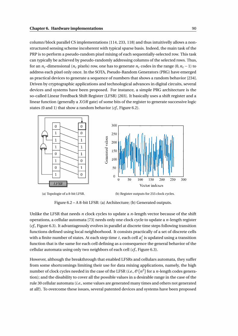
Chapter 6. Hardware implementations 90
column/block parallel CS implementations [114, 233, 118] and thus intuitivelly allows a non-
structured sensing scheme incoherent with typical sparse basis. Indeed, the main task of the
PRP is to perform a pseudo-random pixel mixing of each sequentially-selected row. This task
can typically be achieved by pseudo-randomly addressing columns of the selected rows. Thus,
for an nc -dimensional (nc pixels) row, one has to generate nc codes in the range (0,nc −1) to
address each pixel only once. In the SOTA, Pseudo-Random Generators (PRG) have emerged
as practical devices to generate a sequence of numbers that shows a random behavior [234].
Driven by cryptographic applications and technological advances in digital circuits, several
devices and systems have been proposed. For instance, a simple PRG architecture is the
so-called Linear Feedback Shift Register (LFSR) [203]. It basically uses a shift register and a
linear function (generally a XOR gate) of some bits of the register to generate successive logic
states (0 and 1) that show a random behavior (cf., Figure 6.2).
(a) Topologie of a 8-bit LFSR. (b) Register outputs for 255 clock cycles.
Figure 6.2 – A 8-bit LFSR: (a) Architecture; (b) Generated outputs.
Unlike the LFSR that needs n clock cycles to update a n-length vector because of the shift
operations, a cellular automata [73] needs only one clock cycle to update a n-length register
(cf., Figure 6.3). It advantageously evolves in parallel at discrete time steps following transition
functions defined using local neighborhood. It consists practically of a set of discrete cells
with a finite number of states. At each step time t , each cell ati is updated using a transition
function that is the same for each cell defining as a consequence the general behavior of the
cellular automata using only two neighbors of each cell (cf., Figure 6.3).
However, although the breakthrough that enabled LFSRs and cellulars automata, they suffer
from some shortcomings limiting their use for data mixing applications, namely, the high
number of clock cycles needed in the case of the LFSR (i.e., O(n2
)for a n-length codes genera-
tion); and the disability to cover all the possible values in a desirable range in the case of the
rule 30 cellular automata (i.e., some values are generated many times and others not generated
at all!). To overcome these issues, several patented devices and systems have been proposed

91 6.1. Proposed image sensor architecture
(a) A 8-bit cellular automata follow-ing the Wolfram rule 30.
(b) Register outputs for 255 clock cycles.
Figure 6.3 – A 8-bit cellular automata: (a) Architecture; (b) Generated outputs.
but unfortunately involve higher hardware-algorithm complexity limiting their use for on-chip
applications (e.g., low-power CIS) [235, 236, 237]. To tackle these limitations, we propose in
the next section a hardware-friendly solution to generate pseudo-random sequences and
therefore enable pseudo-random permutation of a given vector of analog/digital values. This
solution is deemed to be simple, implementable and scalable and could be considered as a
consequence the keystone towards an efficient implementation of per-row pixel mixing.
Proposed PRG
The proposed dedicated pseudo-random codes generator basically takes advantage of pre-
defined bits swapping and a simple bijective mapping. As depicted in Figure 6.4, for a given
initial seed, the process of codes generation consists in first performing a pre-defined bits
swapping of some Most Significant Bits (MSB) and Least Significant Bits (LSB), and then apply
a Gray coding using basic XOR logical gates to reinforce the chaotic behavior of the generated
codes (output after each pre-defined bits swapping and Gray coding iteration). This way, after
2n −1 iteration, a sequence of pseudo-random codes is generated to address the indexes of a
given n-length vector.
To quantify the chaotic behavior of the proposed patented solution (cf., Figure 6.5), the
autocorrelation of the generated sequence is adopted as a basic measure of similarity of the
sequence with shifted representations of itself. Figure 6.6 reports the autocorrelation of a n-bit
(n ∈ {7,8,9,14,15,16}) generated sequence using the proposed PRG and a sequence generated
using the MATLAB random permutations algorithm. Indeed, one can see that the generated
sequences have regular autocorrelations with few picks of approximatively high correlation
compared to small fluctuations of the MATLAB algorithm. However, regarding the mean over

Chapter 6. Hardware implementations 92
Figure 6.4 – Process of codes generation performed by the proposed PRG.
2n −1 , the mean autocorrelation is approximatively the same for both techniques. This way,
we can validate the relevance of the proposed pseudo-random codes generator in terms of
both hardware compactness and chaotic behavior.
Figure 6.5 – Register outputs for 255 clock cycles of the proposed codes generator.
A practical implementation of the proposed solution is presented in Figure 6.7 for a 8-bit
codes generation. Indeed, for a given 8-bit seed in the input register, the architecture swap
the two MSBs and LSBs and then apply a Gray coding to the resulting word. This process is
repeated at each clock cycle until the generation of 255 (28 −1) codes. In the specific case of
this code length, bits swapping is applied to two MSB and LSB bits. However, for other code
lengths, Table 6.1 report the number of MSB and LSB bits to swap for a given code length
between 4 and 16 bits, i.e., to generate pseudo-random sequences in the ranges (1,15) and
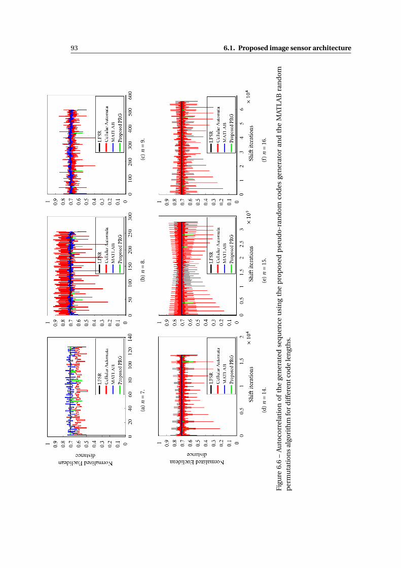
93 6.1. Proposed image sensor architecture
(a)
n=
7.(b
)n=
8.(c
)n=
9.
(d)
n=
14.
(e)
n=
15.
(f)
n=
16.
Fig
ure
6.6
–A
uto
corr
elat
ion
of
the
gen
erat
edse
qu
ence
usi
ng
the
pro
po
sed
pse
ud
o-r
and
om
cod
esge
ner
ato
ran
dth
eM
AT
LA
Bra
nd
om
per
mu
tati
on
sal
gori
thm
for
dif
fere
ntc
od
ele
ngt
hs.

Chapter 6. Hardware implementations 94
(1,65535) respectively. Notice that numerous bits swapping patterns can be performed as
reported in Table 6.2. For the sake of simulation issues, these patterns were validated for codes
generation with lengths between 4 and 10 bits through an exhaustive sweep of all the possible
permutation patterns. However, swapping only MSB and LSB bits still the most compact
solution, allowing to avoid crossed connections between each successive registers.
Number of bits to swap1 2 3 4 5 6 7
Code lengths
4 x5 x6 x7 x x8 x9 x
1011 x x12 x13 x x14 x15 x16 x
Table 6.1 – Number of MSB and LSB bits to swap in function of the desired code length.
Code lengths 4 5 6 7 8 9 10Number of possible 2 24 66 600 2213 30329 165828
bits swapping (8%) (20%) (9%) (11%) (5%) (8%) (4%)
Table 6.2 – Number of possible bits swapping over the n! possible permutations of a n-lengthregister.
To summarize, the proposed pseudo-random codes generator has compact hardware im-
plementation in terms of both clock cycles and the covered generated codes while showing
a chaotic behavior making it a relevant choice to address data mixing tasks compared to
commonly used PRGs used in the CS SOTA (i.e., LFSR [108, 114], Cellular Automata [118, 238]).
It can be therefore considered as the keydriver of the possible PRP architectures that we will
discuss in the next section in order to perform per-row pixel scrambling to extract compressed
measurements using the proposed CS sensing scheme.
6.1.2 Pseudo Random-Permutations (PRP)
Based on the proposed pseudo-random codes generator, three possible implementations have
been explored to achieve per-row pixel mixing with different hardware complexity, namely,
a fully connected pseudo-random multiplexer based PRP, a block-parallel pseudo-random
multiplexer based PRP and a Benes network based PRP. These three architectures will be

95 6.1. Proposed image sensor architecture
Fig
ure
6.7
–A
nil
lust
rati
on
oft
he
har
dw
are
imp
lem
enta
tio
no
fth
ep
rop
ose
dp
seu
do
-ran
do
mse
qu
ence
sge
ner
ato
rfo
r8-
bit
cod
es

Chapter 6. Hardware implementations 96
detailed in the rest of this section with basic consideration of the hardware complexity in
terms of additional silicon footprint and readout power consumption.
Fully connected pseudo-random multiplexer based PRP
A straightforward approach to perform pseudo-random permutations may introduces a nc
to nc fully connected multiplexer (MUX) (cf., Figure 6.9) controlled by the proposed pseudo-
random codes generator (cf., Section 6.1.1), with nc is the number of columns. Indeed, using
a column decoder, each MUX output can pseudo-randomly selects one and only one pixel
output from the selected row. As depicted in Figure 6.8, in the first embodiment a pseudo-
randomly permuted sequence is generated to address the columns of the selected row in a
serial fashion using the pseudo-random codes generator initialized using a pseudo-random
seed as presented in the previous section. It is updated for each row select leading to a set of
independent permutation matrices p j (1 ≤ j ≤ nr ). This way, a pseudo-randomly permuted
sequence in the range (1, . . . ,nc ) is generated to pseudo-randomly address the readout voltage
values(V1, . . . ,Vnc
)leading to the permuted output
(Vp1 , . . . ,Vpnc
).
Figure 6.8 – Fully connected pseudo-random multiplexer based PRP.
Figure 6.9 – Analog ransmission gate.
Despite generating low correlated sequences thanks to the dedicated pseudo-random codes
generator, this PRP architecture involves a heavy MUX to connect each output to all the

97 6.1. Proposed image sensor architecture
input voltage values leading to n2c needed interconnect buses to perform the permutation
task. These additional interconnect buses will introduce a non-negligible effect on the CIS
performance (i.e., silicon footprint, power consumption and parasitic noise). To evaluate the
additional cost related to the interconnect buses, let us suppose that for a given pitch pixel (e.g.,
3µm ×3µm), the silicon thickness of 10 interconnect buses is approximatively equivalent to
one pixel width denoted Wpi x . Through this assumption, an approximation of the additional
hardware cost of the fully connected pseudo-random multiplexer based PRP architecture can
be performed. Indeed, as depicted in Figure 6.10, the silicon footprint of the PRP involved by
the interconnect wires is approximatively:
ncWpi x
10×Lar r ay ≈ 0.1War r ay Lar r ay = 0.1S, (6.1)
with Lar r ay and War r ay are the pixel array silicon length and width respectively; and S is the
pixel array silicon area. Notice, however, that this approximation doesn’t take into account the
silicon footprint related to the digital control (select switches in Figure 6.10). Obviously, it will
introduce an offset silicon cost depending on the shape of the transmission gate layout.
Figure 6.10 – Equivalent silicon footprint involved by the interconnect wires of the fullyconnected pseudo-random multiplexer based PRP
On the other hand, this PRP topology has an impact in terms of parasitic noise and power
consumption too. Indeed, under the assumption that the length of each interconnect wire is
equivalent to the column bus length, the capacitance of the bus will be at least two times the
capacitance of the column bus. Therefore, the parasitic noise and power consumption relative

Chapter 6. Hardware implementations 98
to voltage readout will be doubled using the fully connected pseudo-random multiplexer
based PRP. Finally, given the aforementioned drawbacks, we can conclude that this topology
can not be adopted for a low-power CIS application.
Block-parallel pseudo-random multiplexer based PRP
To tackle hardware issues due to the important number of connection lines to establish in
the case of a fully connected pseudo-random multiplexer based PRP (e.g., silicon footprint,
parasitic capacitance), an alternative approach can deploy a two-level PRP composed of a
fixed pseudo-random scrambling and a set of block-parallel MUXs controlled by the proposed
pseudo-random codes generator presented in Section 6.1.1. Indeed, for the purpose of inter-
connect wires saving, the fixed-scrambling layer aims at applying a fixed permutation pattern
to each selected row similarly. Furthermore, to generate independent permutations with , a
set of parallel nblk to nbl k pseudo-random MUXs that share the same b-bit (b = log2 (nbl k ))
pseudo-random codes generator are used to perform a pseudo-random pixel mixing for each
block of size nbl k in a block-parallel fashion (cf., Figure 6.11).
Figure 6.11 – Block-parallel pseudo-random multiplexer based PRP.
In fact, as depicted in Figure 6.12, the fixed scrambling layer needs nc buses to connect each
output to a pre-defined voltage input. Thus, under the assumption that the silicon thickness
of 10 interconnect buses is approximatively equivalent to one pixel width denoted Wpi x , the
additional silicon footprint of the fixed scrambling layer is approximatively:
ncWpi x
10×Lar r ay ≈ 0.1War r ay Lar r ay = 0.1S. (6.2)
This additional silicon to implement the fixed scrambling layer is therefore equivalent to
approximatively 10% of the silicon footprint of the pixel array. On the other hand, the block
parallel MUXs will involve the following silicon area:
nblkWpi x
10×Lar r ay ≈ 0.1
nc
BWpi x Lar r ay = 0.1
BS, (6.3)

99 6.1. Proposed image sensor architecture
with B is the total number of block-parallel MUXs. This estimation clearly shows the interest
of this approach to reduce the silicon footprint compared to a fully connected pseudo-random
MUX. In addition, the number of select switches is reduced by a factor B . This way, we can
reasonably target to put the block-parallel MUXs on the bottom of the fixed scrambling.
Figure 6.12 – Equivalent silicon footprint involved by the interconnect wires of the fixedscrambling layer.
Benes network based PRP
For more hardware-friendly pseudo-random permutations in terms of both silicon footprint
involved by the number of interconnect wires, i.e., the silicon footprint as well as the parasitic
capacitance, a relevant approach consists in spreading out the permutation over a multi-
level set-up with limited interconnect wires involved at each level. This task can typically be
achieved using a Benes network [239]. As depicted in Figure 6.14 a Benes network consists in
a concatenation of a butterfly and an inverse butterfly networks based on a 2 : 1 digital multi-
plexer at each node with dedicated control bit. Benes networks are basically used in digital
circuits for bits permutations as presented in [214]. In the special case of a Benes network
based PRP, the multiplexers are analog and can be implemented using analog transmission
gates as presented in Figure 6.9.
Although the interest that shows the Benes network to reduce the interconnect wires to
perform a desired permutation, its use is limited to vectors of length expressed as power
of two. However, customized architectures can be implemented depending on the given
CIS resolution. For instance, for a VGA resolution (i.e., (nr = 480)× (nc = 640)), 10 Benes
network can be used for each block of 64 columns combined with a fixed pseudo-random

Chapter 6. Hardware implementations 100
Figure 6.13 – A 8×8 Benes network.
scrambling to extend the support of permutations. Figure 6.14 stands for a pseudo-random
columns permutation of a selected row using a multi-level permutation process composed
of a fixed pseudo-random scrambling and a 9-stages Benes network. It consists basically in
the concatenation of a butterfly network, a fixed pseudo-random scrambling and an inverse
butterfly network allowing to generate permutations of the nc input voltage values. For each
butterfly or inverse butterfly level, voltage values are partitioned into blocks and swapped -or
not- via a series of 2 : 1 MUX circuits (i.e., Btfly_64. . . Ibtfly_16 in Figure 6.15). Indeed, block
sizes vary from 64 (Btfly_64) to 2 (Btfly_2) for the butterfly network; and from 4 (Ibtfly_4) to
16 (Ibtfly_16) for the inverse butterfly network. Here, for further silicon saving, each layer
of the Benes network is controlled by an unique binary signal, leading to a 9-bit input code
(9 = d(log2(480))e).
On the other hand, to generate low-correlated permutations, a 9-bit PRG can be designed
based on the proposed pseudo-random codes generator presented in Section 6.1.1 to on-
the-fly generate control codes with the longest cycle length and the lowest circuit impacts as
presented Figure 6.16. Figure 6.17, shows the enumerations of selections for each input column
corresponding to an output one. We can observe that each 64-block of column outputs are
therefore mapped to 64 randomly distributed input ones thanks to the fixed pseudo-random
scrambling. In addition, each PRP output selects a pixel from the same column at most four
times for a fixed snapshot. This means that desired task, i.e., mixing non-uniform pixels zone,
is achievable with high probability. Moreover, if we want to build a matrix full of ones, one can
increases the size of the first Benes level at the expense of an additional hardware overload.
On the other hand, to show that the proposed PRP generates independent permutations,
Figure 6.18 stands for the enumeration of similar generated sequences based on an Euclidean
distance metric between each pair of the generated sequences. Indeed, one can clearly see
that except the main entries (i.e., distance between the sequence and itself), the entries of the
matrix are equal to zero and therefore each permutation is generated once and only once.
Regarding the silicon footprint of the Benes network based PRP, the additional silicon footprint
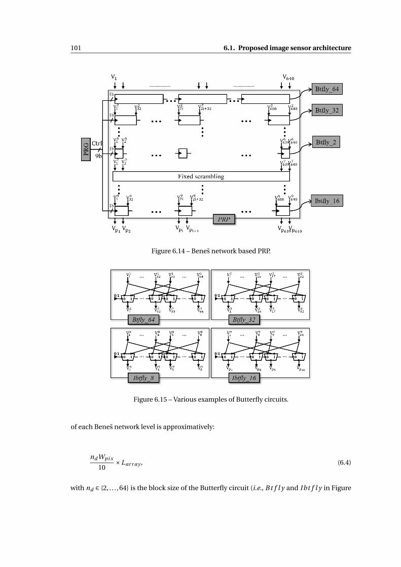
101 6.1. Proposed image sensor architecture
Figure 6.14 – Benes network based PRP.
Figure 6.15 – Various examples of Butterfly circuits.
of each Benes network level is approximatively:
nd Wpi x
10×Lar r ay , (6.4)
with nd ∈ {2, . . . ,64} is the block size of the Butterfly circuit (i.e., B t f l y and I bt f l y in Figure

Chapter 6. Hardware implementations 102
Figure 6.16 – A 9-bit PRG.
6.14) at each Benes network level. Thus, for the proposed 10 levels Benes network in Figure
6.14, the silicon footprint of the Benes network based PRP is approximatively:
(64+32+16+8+4+2+4+8+16)Wpi x
10×Lar r ay ≈ 15Wpi x Lar r ay , (6.5)
i.e., approximatively 15 rows of the CIS focal plane. Finally, despite the drastic saving compared
to the previous architectures, deep optimization of the silicon footprint can only be done at
simulation level given the design rules and using advanced layout generation and common
digital design tools and to implement the Benes network under the fixed scrambling layer that
could be easily implemented using only top metal layers.
6.1.3 RMΣ∆
Inspired by the incremental Σ∆ [240, 241] that simultaneously performs both averaging and
quantization [114, 242, 243], a dedicated incremental RMΣ∆ is proposed to perform pseudo-
random modulations, per-column averaging and A/D conversions. Indeed, each column
of the PRP is connected to one RMΣ∆ allowing a column-parallel processing. Furthermore,
the main advantage of the proposed architecture is its ability to deal with pseudo-random
±1 modulations, highly desirable in many CS applications. Two possible embodiments are
presented to deal with ±1 modulations using an incremental Σ∆. The first one is implemented
using a switched-capacitor circuit as presented in [115] and the second one is implemented
using a double-path Σ∆with double-path integration (one integrator for each sign) controlled
by a nc -bit SR (each cell control one RMΣ∆). In the rest of this section, we will first present
some basic concepts related to the incremental Σ∆ ADC and then present the proposed
operational block to implement ±1 modulations, averaging and A/D conversions.

103 6.1. Proposed image sensor architecture
Figure 6.17 – Enumerations of each mapping input/output performed by the PRP for a singlesnapshot.
Figure 6.18 – Enumerations of similar generated sequences.
Unsigned Incremental Σ∆ ADC
The main advantage of an incremental Σ∆ ADC is its capability to perform simultaneously
averaging and quantization. As depicted in Figure 6.19, the incremental Σ∆ ADC comprises
basically an integrator, a single-bit comparator and a decimating counter. The averaging
and quantization operations are achieved as follows: the integrator, counter and Digital-to-
Analog Converter (DAC) are first reseted. Then, for a set of analog input values (in our case
the permuted pixels Vpi ), the inputs are sequentially integrated and compared to a certain
threshold (generally half the dynamic range). Depending on the comparator output, an
analog value is subtracted to the input. The subtraction is achieved thanks to the DAC that
is controlled by the output of the comparator. The output of the comparator is therefore a
bitstream composed of OSR (Over-Sampling Ratio) bits. The output from the modulator is

Chapter 6. Hardware implementations 104
finally decimated using a digital filter (generally a counter) to obtain a digital representation
of the average of the integrated voltage values, in our case the permuted pixels Vpi . After nr
cycles of the rolling shutter SR (i.e., nr integration of nr rows), 640 (i.e., 1/480 compression
ratio) 9-bits (9 = log2(nr )) CS measurements are produced with only one clock cycle for each
row, meaning that we can dramatically reduce power consumption to perform the inference.
Figure 6.19 – Incremental Σ∆ ADC.
Figure 6.20 shows simulation results for an ideal first-order Σ∆ ADC with 64 sampling cycles
corresponding to a 6-bit quantization. On the right, we plot the output of the modulator and
its decimated value when a set of input voltage values in the range (Vmi n = 0.7V ,Vmax = 2.7V )
is applied to the Σ∆ ADC. On the left, we plot the output of the modulator and its decimated
value for a constant input equals to the average of the variable inputs. Finally, one can see that
the final integrator voltages and their respective decimated values (i.e., counter outputs) are
equal in both cases (i.e., variable inputs and constant one). This illustrates that the incremental
Σ∆ ADC performs simultaneously averaging and quantization when a set of voltage values are
sequentially applied to it.
However, although the interest that presents an incremental Σ∆ ADC in terms of simultaneous
averaging and quantization, implementing the ±1 modulations is still a challenging task
towards an efficient hardware implementation of the proposed sensing scheme based on
pseudo-random permutations and modulations. As depicted in Figure 6.21, the main idea
of the RMΣ∆ is to multiply the input voltage values by pseudo-random ±1 modulations. In
fact, two possible embodiments can be explored to apply a pseudo-random ±1 modulations
to the outputs of the PRP, i.e., Vpi : the first one is based on switched-capacitors at the input of
each Σ∆. The second one deals with a double-path Σ∆ with an up/down counter as it will be
discussed in the rest of this section.
Switched-capacitor based RMΣ∆
A possible implementation of the multiplication by ±1 is to create a virtual zero in the dynamic
range of the pixel outputs defined by the reset voltage (i.e., Vmi n) and the minimum voltage
value achievable at the end of the integration time (i.e., Vmax ). Indeed, the virtual zero can
be defined at the half of the dynamic range (Vmi n ,Vmax ), i.e., Vr e f = Vmax+Vmi n2 , by limiting
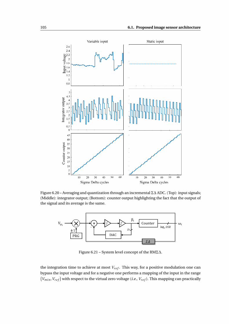
105 6.1. Proposed image sensor architecture
Figure 6.20 – Averaging and quantization through an incrementalΣ∆ ADC. (Top): input signals;(Middle): integrator output; (Bottom): counter output highlighting the fact that the output ofthe signal and its average is the same.
Figure 6.21 – System level concept of the RMΣ∆.
the integration time to achieve at most Vr e f . This way, for a positive modulation one can
bypass the input voltage and for a negative one performs a mapping of the input in the range(Vmi n ,Vr e f
)with respect to the virtual zero voltage (i.e., Vr e f ). This mapping can practically

Chapter 6. Hardware implementations 106
be defined as:
f(Vpi
)= 2Vr e f −Vpi , (6.6)
with Vpi is the input voltage value in the range(Vr e f ,Vmax
). This operation can advanta-
geously be implemented using active switched capacitors [244] as proposed in several SOTA
systems with dedicated circuits for analog computing [115, 245, 246]. Such active circuits
offer a practical implementation to perform subtractions based on charge/discharge of inner
capacitors but rely on active circuits that can suffer from stability and sensitivity problems. To
tackle this issue, passive switched capacitors can be explored to implement the subtraction
operation [247]. However, one has still to handle the generation of complex non-overlapped
digital control signals to charge/discharge inner capacitors and to manage carefully with re-
spect to gain accuracy, residual charges and noise in general. Furthermore, the main limitation
involved by switched-capacitors based RMΣ∆ is the restricted dynamic range if we set the
virtual zero at half the possible dynamic range enabled by the CIS. To overcome this limitation,
an alternative approach can mutualise two incremental Σ∆ converters that share the same
DAC but using an up/down counter as a decimation filter as discussed in the next section.
Double-path integration based RMΣ∆
To take advantage of the full dynamic range enabled by the CIS, a double-path RMΣ∆ can be
proposed. In fact, as depicted in Figure 6.22, a double-path integration based RMΣ∆ is mainly
composed of two modulators that share the analog comparator and the Digital-to-Analog
Converter (DAC). Indeed, for a column i , the integrators and the DAC are first reseted and the
voltage outputs Vpi ’s of the PRP are sequentially applied to the input of the dedicated RMΣ∆.
Following the SRi bit control generated by the PRG, Vpi is either integrated in the first or the
second integrator. Indeed, for a positive modulation (i.e., multiplication by +1), the voltage
input is integrated in the first path and the ↑↓ counter is incremented if the comparator is
activated. However, for a negative modulation (i.e., multiplication by −1), the voltage input is
integrated in the second path and the ↑↓ counter is decremented if the comparator is activated.
Finally, the ↑↓ counter output will represent a digital representation of the averaged integrated
Vpi ’s.
Now, let us take a closer look on the internal behavior of the proposed RMΣ∆. In Figure
6.23, we plot the outputs of a RMΣ∆ after 64 cycles for two different input signals leading to
6-bit quantization and averaging of voltage inputs with the same means; with and without
modulation. On the left, we plot the output of the counter outputs when a set of input voltage
values in the range (Vmi n = 0.7V ,Vmax = 2.7V ) is applied to the RMΣ∆ ADC with and without
modulation (middle and bottom plots respectively). On the right, we plot the output of the
counter outputs when a constant input equals to the average of the variable inputs is applied
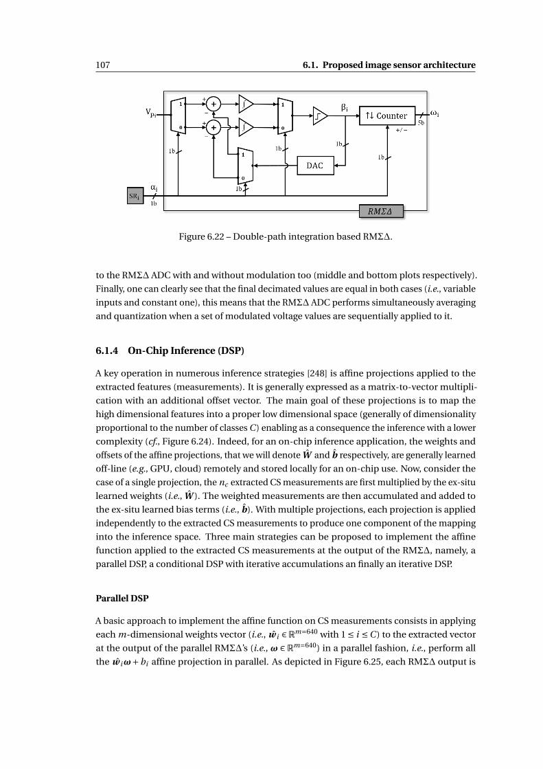
107 6.1. Proposed image sensor architecture
Figure 6.22 – Double-path integration based RMΣ∆.
to the RMΣ∆ ADC with and without modulation too (middle and bottom plots respectively).
Finally, one can clearly see that the final decimated values are equal in both cases (i.e., variable
inputs and constant one), this means that the RMΣ∆ ADC performs simultaneously averaging
and quantization when a set of modulated voltage values are sequentially applied to it.
6.1.4 On-Chip Inference (DSP)
A key operation in numerous inference strategies [248] is affine projections applied to the
extracted features (measurements). It is generally expressed as a matrix-to-vector multipli-
cation with an additional offset vector. The main goal of these projections is to map the
high dimensional features into a proper low dimensional space (generally of dimensionality
proportional to the number of classes C ) enabling as a consequence the inference with a lower
complexity (cf., Figure 6.24). Indeed, for an on-chip inference application, the weights and
offsets of the affine projections, that we will denote W and b respectively, are generally learned
off-line (e.g., GPU, cloud) remotely and stored locally for an on-chip use. Now, consider the
case of a single projection, the nc extracted CS measurements are first multiplied by the ex-situ
learned weights (i.e., W ). The weighted measurements are then accumulated and added to
the ex-situ learned bias terms (i.e., b). With multiple projections, each projection is applied
independently to the extracted CS measurements to produce one component of the mapping
into the inference space. Three main strategies can be proposed to implement the affine
function applied to the extracted CS measurements at the output of the RMΣ∆, namely, a
parallel DSP, a conditional DSP with iterative accumulations an finally an iterative DSP.
Parallel DSP
A basic approach to implement the affine function on CS measurements consists in applying
each m-dimensional weights vector (i.e., w i ∈Rm=640 with 1 ≤ i ≤C ) to the extracted vector
at the output of the parallel RMΣ∆’s (i.e., ω ∈ Rm=640) in a parallel fashion, i.e., perform all
the w iω+bi affine projection in parallel. As depicted in Figure 6.25, each RMΣ∆ output is

Chapter 6. Hardware implementations 108
Figure 6.23 – Evolution of RMΣ∆ counter output with respect to various types of inputsdemonstrating modulation-averaging operations. (Top): input signals; (Middle): counteroutput of the modulated inputs; (Bottom): counter output without modulation of the inputsignal.
first multiplied by the weights of the correspondent column of W (the j th measurement is
multiplied by the weights of column j in parallel) leading to C weighted CS measurements.
The outputs of the i th multipliers (1 ≤ i ≤C ) are then accumulated to extract C components of
the low-dimensional vector, i.e., m1, . . . ,mC . Although the interest that shows this approach, it
unfortunately involves a non negligible number of computing gates (i.e., adder and multipliers)
that depends on the number of classes C , leading therefore to high silicon footprint.
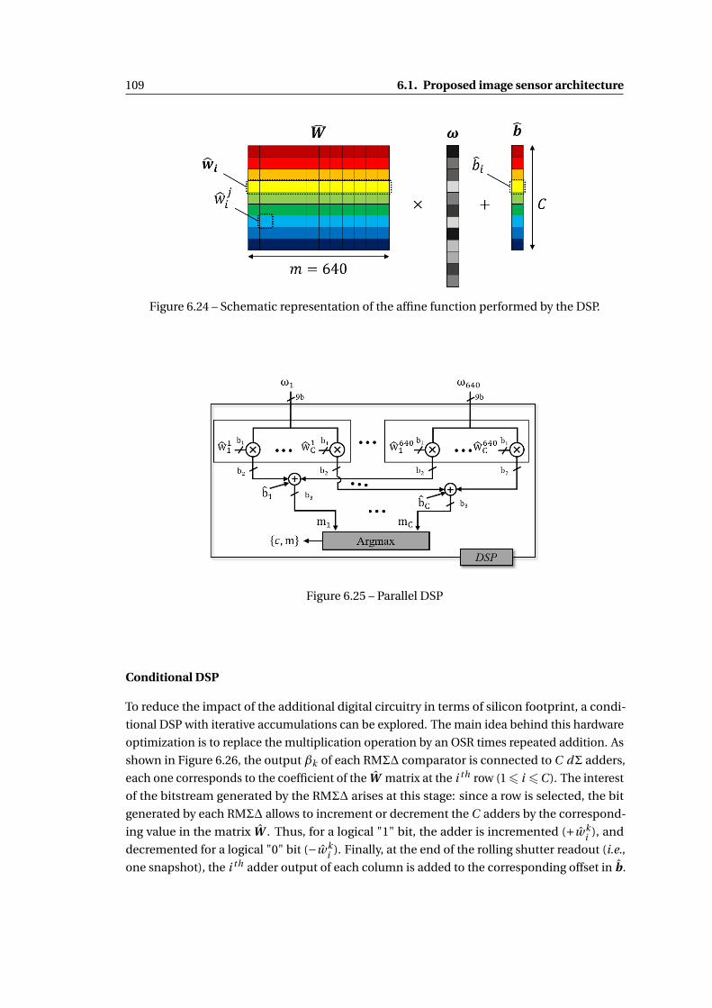
109 6.1. Proposed image sensor architecture
Figure 6.24 – Schematic representation of the affine function performed by the DSP.
Figure 6.25 – Parallel DSP
Conditional DSP
To reduce the impact of the additional digital circuitry in terms of silicon footprint, a condi-
tional DSP with iterative accumulations can be explored. The main idea behind this hardware
optimization is to replace the multiplication operation by an OSR times repeated addition. As
shown in Figure 6.26, the output βk of each RMΣ∆ comparator is connected to C dΣ adders,
each one corresponds to the coefficient of the W matrix at the i th row (16 i 6C ). The interest
of the bitstream generated by the RMΣ∆ arises at this stage: since a row is selected, the bit
generated by each RMΣ∆ allows to increment or decrement the C adders by the correspond-
ing value in the matrix W . Thus, for a logical "1" bit, the adder is incremented (+wki ), and
decremented for a logical "0" bit (−wki ). Finally, at the end of the rolling shutter readout (i.e.,
one snapshot), the i th adder output of each column is added to the corresponding offset in b.

Chapter 6. Hardware implementations 110
Figure 6.26 – Conditional DSP
Iterative DSP with block parallel processing
The key operation to implement an unique or multiple projections is the multiply-accumulate
(MAC). In order to guarantee a certain agility to the proposed architecture, a dedicated MAC
is developed to deal with a tunable number of projections depending on the inference algo-
rithm strategy. To this end, a multi-level precision MAC topology is proposed. As depicted in
Figure 6.27, at the first level, the pointwise multiplication is implemented. At the second one,
weighted CS measurements are partitioned into distinct blocks and accumulated allowing par-
allel computing. A set of optimizations of the bit-resolution of all the pipelined digital adders
can be done to cap the silicon footprint. It can consists in limiting the binary dynamic range,
keeping only relevant bits by removing insignificant bits and thresholding under unreached
highly significant bits. Finally, as a last stage, the bias term is added to the accumulated
weighted CS measurements in order to output a proper scalar value, being usable for decision
making. This way, a single projection is performed at a time, with highly limited hardware.
This generic approach allows the architecture to sequentially compute an adaptable number
of projections.
Figure 6.27 – Iterative DSP
For more efficiency in terms of power consumption and silicon footprint, various optimiza-
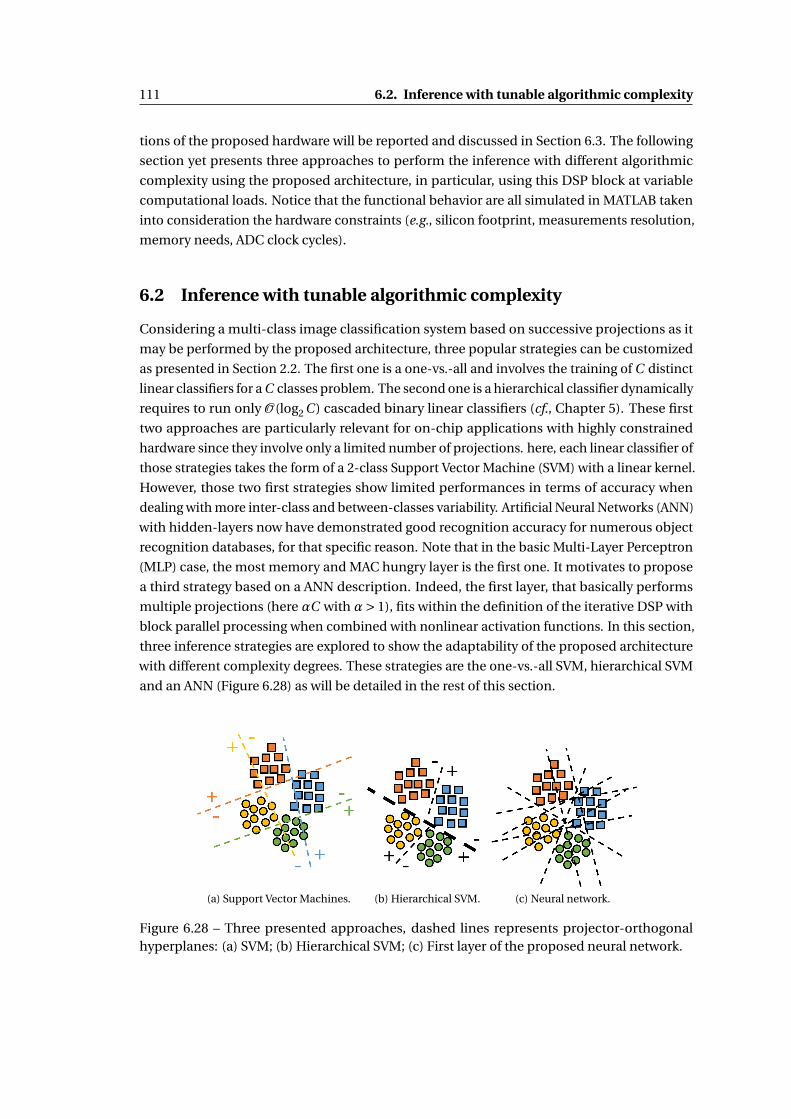
111 6.2. Inference with tunable algorithmic complexity
tions of the proposed hardware will be reported and discussed in Section 6.3. The following
section yet presents three approaches to perform the inference with different algorithmic
complexity using the proposed architecture, in particular, using this DSP block at variable
computational loads. Notice that the functional behavior are all simulated in MATLAB taken
into consideration the hardware constraints (e.g., silicon footprint, measurements resolution,
memory needs, ADC clock cycles).
6.2 Inference with tunable algorithmic complexity
Considering a multi-class image classification system based on successive projections as it
may be performed by the proposed architecture, three popular strategies can be customized
as presented in Section 2.2. The first one is a one-vs.-all and involves the training of C distinct
linear classifiers for a C classes problem. The second one is a hierarchical classifier dynamically
requires to run only O (log2 C ) cascaded binary linear classifiers (cf., Chapter 5). These first
two approaches are particularly relevant for on-chip applications with highly constrained
hardware since they involve only a limited number of projections. here, each linear classifier of
those strategies takes the form of a 2-class Support Vector Machine (SVM) with a linear kernel.
However, those two first strategies show limited performances in terms of accuracy when
dealing with more inter-class and between-classes variability. Artificial Neural Networks (ANN)
with hidden-layers now have demonstrated good recognition accuracy for numerous object
recognition databases, for that specific reason. Note that in the basic Multi-Layer Perceptron
(MLP) case, the most memory and MAC hungry layer is the first one. It motivates to propose
a third strategy based on a ANN description. Indeed, the first layer, that basically performs
multiple projections (here αC with α> 1), fits within the definition of the iterative DSP with
block parallel processing when combined with nonlinear activation functions. In this section,
three inference strategies are explored to show the adaptability of the proposed architecture
with different complexity degrees. These strategies are the one-vs.-all SVM, hierarchical SVM
and an ANN (Figure 6.28) as will be detailed in the rest of this section.
(a) Support Vector Machines. (b) Hierarchical SVM. (c) Neural network.
Figure 6.28 – Three presented approaches, dashed lines represents projector-orthogonalhyperplanes: (a) SVM; (b) Hierarchical SVM; (c) First layer of the proposed neural network.

Chapter 6. Hardware implementations 112
6.2.1 Notations
Let us consider a database of m-length “vectors” inRm acquired using the proposed CS sensing
scheme presented in Chapter 4 (i.e., Φ= 1ps
((P (1)M (1)
)>, · · · ,
(P (s)M (s)
)>)>) and composed
of C classes. This database is separated into two databases: a “train” set X ∈Rm×n1C , where
each class is composed of n1 samples, associated with labels l ∈ {1, · · · ,C }n1C ; and a “test” set
Y ∈ Rm×n2C with unknown labels and composed of n2 samples per class. To perform our
supervised embedded inference, two-stages have to be considered: First, training the patterns
in an off-line system on the compressed training set X . Second, the embedded inference is
performed on a compressed test set Y . Here, both the training and test sets are acquired by
the proposed architecture using the specific sensing matrixΦ. Thus, the proposed inference
strategies are as follows.
6.2.2 One-vs.-all SVM
As discussed in Section 6.1, learning a one-vs-all SVM implies solving the following problem:
{w i , bi , ξi } = argminw∈Rm ,b,ξ∈Rn1
(12
∥∥w∥∥2
2 +λ∥∥ξ∥∥1
)s.t. l i
j (d>x ij +b) ≥ 1−ξ j , ξ j ≥ 0,1 ≤ j ≤ n1. (6.7)
Let us define the gain matrix W := (w 1, · · · , wC )>, i.e., the vertical concatenation of w i and
b := (b1, · · · , bC
)>the offset vector. Once the C classifiers are off-line learned, W and b can
be stored on-chip. Thus, a winner-takes-all strategy allows to assign a compressed sample
y ∈Rnc to the class c maximizing the margin, i.e.,
c = argmax1≤i≤C w>i y + bi . (6.8)
From a hardware point of view, the CS measurements vector y is successively multiplied
by the weight matrices w i and added to the offset scalars bi to iteratively extract a vector
of length C using the DSP presented in Section 6.1. Finally, the argmax operation can be
implemented following an iterative approach using a single 2 : 1 multiplexer controlled by a
bitwise comparator [249]. As depicted in Figure 6.29, at each iteration, the resulting output
consist in the current max value and its index (i.e., max and argmax).

113 6.2. Inference with tunable algorithmic complexity
Figure 6.29 – Iterative Argmax circuit.
6.2.3 Hierarchical SVM
As discussed in Chapter 5, the main idea of a hierarchical learning is to divide a set of
classes into two subsets at every hierarchical node in order to construct a binary decision
tree. Thus, using the balanced clustering method in Algorithm 2 presented in Section 5.2.3,
a decision tree is recursively constructed, training a binary SVM at each node, i.e., given
{(x1, l1) , . . . , (xk , lk ) , . . . ,(x2n1 , l2n1
)} ⊂ Rm × {−1,1} samples of two different classes in X . The
binary SVM optimization problem between this two classes is written as:
{w , b, ξ} = argminw∈RN ,b,ξ∈R2n1
(12
∥∥w∥∥2
2 +λ∑2n1
k=1 ξk
)s.t. lk (w>xk +b) ≥ 1−ξk , ξk ≥ 0,1 ≤ k ≤ 2n1, (6.9)
Thus, for a test sample y ∈ Y the inferred class c is given by:
c = sign(w> y +b
). (6.10)
Training the hierarchical tree allows to construct a binary decision tree where each path from
a root to a leaf is associated to a decision rule defined by the binary test referred in (6.10)
and being learned by a binary SVM. Thus, for a new test sample y ∈ Y , a decision rule (cf.,
(6.10)) is applied at every node where the margin sign is used to decide to which next branch
the sample belongs to. Thus, the predicted class is provided by the path indicated by the
successive decisions running only O (log2 C ) projections.
At the hardware side, the CS measurements vector y is first multiplied by weights and then
added to the bias of the first decision rule (cf., (6.10)) at level 1 of the decision tree). The margin
sign (i.e., sign bit at the output of the DSP) is then used to decide which weights and bias load
from the local memory in order to apply the second decision rule. This is repeated until the
last node to decide to which class the sample y belongs.

Chapter 6. Hardware implementations 114
6.2.4 Neural Network
When dealing with databases with higher inter-class and between-classes variability, a Neural
Network can advantageously improve the recognition accuracy but using a higher number
of projections (αC with α > 1). In this section a simple topology is proposed to perform
parametric projections combined with nonlinear functions. As depicted in Figure 6.30, the
proposed topology is composed first by a fully-connected layer combined with an activation
function to perform αC projections, where α > 1 is an inner adjustable parameter. Here,
a ReLU activation function ( f (x) = max(0, x)) is adopted for the simplicity of its hardware
implementation. It allows to introduce nonlinearity to enhance the separability between
classes. A 1D max-pooling function over each α projections is then introduced to reduce the
dimensionality of the extracted αC -length extracted vector. Finally, a C fully-connected layer
with softmax activation extracts a C -length vector allowing the decision making. We stress
that the quantization of weights and biases of the topology is performed at the training stage
[250], namely in order to alleviate over-sized needs both in terms of memory and computing.
Figure 6.30 – Topology of the proposed Neural Network.
The hardware implementation of this topology can hopefully take advantage of the proposed
DSP in Section 6.1.4 and the argmax circuit (Figure 6.29). Indeed, the CS measurements
vector y is successively multiplied by the weight matrices w i and added to the offset scalars
bi learned at the first layer to extract a vector of length αC . With proper initializations and
resets, the argmax structure can be used to perform 1D max pooling sequentially outputting
C values used as inputs for the second (and output) layer.
6.2.5 Complexity analysis
Table 6.3 stands for embedded resources requirements related to a one-vs.-all inference
strategy, a hierarchical SVM and the proposed Neural Network for a m-dimensional C -classes
inference problem. In the context of an embedded system, we only consider the case where
first a supervised training stage is performed outside the chip using a remote computer station
and then the sensor is programmed using those learned patterns. This way, the sensor can

115 6.3. Simulations and performance optimization
be reprogrammed as wanted, with a somehow generic hardware that could address various
image recognition tasks. Indeed, the computationally-intensive operation that represents the
learning, do not need to be done by the sensor device itself. Therefore, here, we are mainly
interested into the requirements related to the inference part, i.e., memory needs to store
ex-situ learned patterns and computational complexity related to the inference. In fact, in
the case of the one-vs.-all, C classifiers are learned and thus have to be stored to perform C
m-dimensional projections. For a hierarchical approach, the number of classifiers to learn is
reduced to C −1 to perform only dlog2 Ce m-dimensional projections. However, when using
our Neural Network, O (αC ) "SVM-equivalent" classifiers are learned and thus have to be
stored to perform O (αC ) projections.
Table 6.3 exhibits the underlying motivations related to the proposed DSP architecture. It
clearly demonstrates the interest of hierarchical learning to reduce the amount of MAC op-
erations for highly limited hardware. Moreover, it also shows the ability of the proposed
architecture to deal with a higher number of projections to fit within algorithmic needs (i.e.,
one-vs.-all and Neural Network strategies) with respect to an increase of the local memory
budget required to store ex-situ learned patterns.
Learning Memory ComputingOne-vs.-all mC O (mC )
Hierarchical m(C −1) O (m log2 C )ANN O (αC ) O (αmC +αC 2)
Table 6.3 – A comparison of embedded resources requirements of a one-vs.all SVM, hierarchicalSVM and Neural Network inference strategies.
6.3 Simulations and performance optimization
6.3.1 Background
To demonstrate the efficiency of the proposed architecture, two object classification databases
have been used for the hardware top-level simulations:
Georgia Tech face database (GIT) [251]: contains images of 50 people. All people in the
database are represented by 15 color images with cluttered background taken at resolu-
tion 640×480 pixels. The average size of the faces in these images is 150×150 pixels.
The pictures show frontal and/or tilted faces with different facial expressions, lighting
conditions and scale.
COIL-100 database [228]: composed of 7,200 images of 100 objects. Each object was turned
on a turntable through 360 degrees to vary object pose with respect to a fixed color
camera. Images of the objects were taken at pose intervals of 5 degrees. This corresponds
to 72 poses per object. There images were then size normalized. Objects have a wide
variety of complex geometric and reflectance characteristics.

Chapter 6. Hardware implementations 116
To fit within specifications of the proposed architecture, each image is resized to a VGA resolu-
tion via bicubic interpolation and then subsampled using a simulated RGB Bayer filter. In this
section, we will first present a set of optimizations to reduce silicon footprint, CS measure-
ments and DSP resolutions, and then summarize inference accuracy for the aforementioned
databases with different numbers of classes. For the sake of clarity, the presented hardware
optimizations have been done based on C = 10 randomly selected classes of the GIT database
and for the one-vs.-all SVM inference strategy.
6.3.2 PRP optimization
As mentioned in Section 6.1.2, the most hardware-friendly solution takes advantage of a fixed
pseudo-random scrambling and a 9-stages Benes network. The goal of the fixed scrambling
is to reinforce pseudo-random permutation before addressing the Benes network. Figure
6.31 shows the inference accuracy achieved with different scrambling block sizes for the GIT
(C = 10) database. The simulated sizes varies between 1 (i.e., without fixed scrambling) and
640 (i.e., scrambling all columns of the selected row). In addition, for each size, the fixed
pseudo-random scrambling is selected as the realization minimizing the autocorrelation
peak amongst 100 realizations generated using the randperm MATLAB function. Figure 6.31,
clearly exhibits the interest of the fixed scrambling over all the selected row. This could be
explained by the fact that a larger support of mixing allows to deal with uniform zones (i.e.,
low frequencies), and thus, a better diversity of the extracted CS measurements.
Figure 6.31 – PRP fixed scrambing.
6.3.3 RMΣ∆ optimization
As the proposed CIS is designed to meet requirements of highly constrained hardware, its
performance can typically be optimized thanks to the prior knowledge on the distribution
of the CS measurements (Figure 6.32a), the entries of W (Figure 6.32b) and the components
of b (Figure 6.32c). Thus, given the distribution of CS measurements (range = [−20,20] ),

117 6.3. Simulations and performance optimization
the resolution of the RMΣ∆ can advantageously be reduced by saturating the ↑↓ counter in
Figure 6.22 to a lower number of bits instead of 9-bits (log2(nv )) by benefiting of the intrinsic
property of the incremental Σ∆ [114]. Figure 6.32d, stands for the probability of error at the
output of the RMΣ∆ for different resolutions (from 2-bit to 9-bit). Here, the error refers to
the difference between the original output without saturation and the quantized one. Thus,
as shown in Figure 6.32d, the probability of error at the output of the RMΣ∆ tends to 0 for a
resolution of 5-bit of the CS measurements. Moreover, the trade-off between CS measurements
resolution and the classification accuracy is also taken into account in Figure 6.32e. It shows
the classification error for different counter resolution, i.e., CS measurements resolution. We
clearly observe that the classification error floors to 4% from a 5-bit resolution, i.e., we can
advantageously reduce the resolution of the CS measurement to 5-bit without any loss in
terms of the classification accuracy.

Chapter 6. Hardware implementations 118
(a) Real data disribution at the output of the column parallel
Sigma-Delta.
(b) Distribution of the entries of W .
(c) Distribution of b values. (d) Probability of error at the output of each RMΣ∆.
(e) Probability of error vs. classification accuracy.
Figure 6.32 – Performance optimization of the RMΣ∆.

119 6.3. Simulations and performance optimization
Figure 6.33 illustrates how a single input (in our case the output βi of the incremental Σ∆
comparator) can be used to control the behavior of a 5-bit counter. Depending on the logic
state of the SR i input (high/down logic state), the counter can be set up as an up/down
counter using JK flip-flops. In this case, the inputs of each JK are permanently connected
to the Q output of the previous flip-flops except the first one which permanently connected
to a logic 1. Typically, when both J and K inputs of a given flip-flops are logic 1, the output
toggles at each clock pulse. This way Q0 toggles at each clock pulse; Q1 toggles only when Q0
is high; Q2, Q3 and Q4 toggle when all the previous flip-flops Q outputs are high using AN D
gates. On the other hand, for the down counter setup each flip-flops inputs are wired to the
complement output of the previous one (i.e., Q), except the first one which still connected to a
logic 1 allowing to reverse the count of the counter. To switch between the two operational
modes, a signal control (i.e., SR i ) combined with a set of AN D and OR gates can be used to
enable either the up or down modes.
Figure 6.33 – A 5-bit up/down conditional counter (↑↓ counter).
6.3.4 DSP optimization
As mentioned above, to perform embedded inference, the matrix W and the offset vector b
have to be stored within an on-chip memory. Thus, as the histogram of the matrix W have
a centred, peaked, Gaussian-like distribution (cf., Figure 6.32b), we have chosen a uniform
quantizer using a dynamic range limited to 2/3 of the whole dynamic of the matrix. However,
as the offset vector b has a flattened distribution, the uniform quantizer is applied on the
whole range covered by the components b. Thus, regarding the distribution and the dynamic
range of W and b, we have empirically chosen to set a signed 4-bit resolution for the entries of
W and a signed 14-bit for b. Finally, the memory requirements to store the ex-situ learned
weights and biases in order to perform object recognition on the GIT database (10 classes)
is limited to 10×640×5+10×15 bits ' 32 kbit for one snapshot readout while achieving a
satisfactory accuracy (' 97%, Table 6.4).
Given the 5-bit CS measurements and the quantized on-chip stored patterns, the DSP basically
requires 640 10-bit (output) multipliers and one iterative 20-bit adder. As presented in Section

Chapter 6. Hardware implementations 120
RG
BB
ayerC
Sm
easurem
ents
Ou
rsen
sing
schem
eO
ur
sensin
gsch
eme
Ou
rsen
sing
schem
e
with
ou
tCS
Bern
ou
llidistrib
utio
nw
ithM
atlabran
dp
ermim
plem
.w
itho
utq
uan
tization
with
ou
tsaturatio
n
95.6%
(≈300K
)94.1
%(≈
600)95.6
%(≈
600)97.2
%(≈
600)97.2
%(≈
600)
Ou
rsim
ulated
architectu
reO
ur
simu
latedarch
itecture
(with
qu
ant.&
sat.)(F
PN
with
stdo
f1%)
97.2%
(≈600)
95.6%
(≈600)
Table
6.4–
GIT-10
SVM
recogn
ition
accuracy
for
differen
tlevels
ofd
escriptio
no
fou
rarch
itecture.
#m
easurem
ents
arerep
orted
betw
eenp
arenth
eses.

121 6.3. Simulations and performance optimization
6.1.4, the proposed MAC performs multi-level processing allowing low resolutions. Thus, at
the first level, the pointwise operation is implemented using 640 10-bit parallel multipliers.
At the second one, weighted CS measurements are partitioned into blocks and accumulated
to reduce the resolution of the digital adder needed to perform the accumulation operation.
Figure 6.34, shows the optimized resolution in function of the block size at the first and second
adder levels. It exhibits the interest of reducing the block size and parallel processing to reduce
the resolution related to MACs operations at the expense of increasing the number of adders.
Thus, as depicted in Figure 6.35, a iterative DSP with 32-block parallel adders is finally adopted
as optimized DSP for the proposed CIS because the trade-off that it enables in terms of adders
resolution and the total number of blocks (reported between brackets in Figure 6.34)
Figure 6.34 – DSP MAC
Figure 6.35 – Optimized iterative DSP
6.3.5 Simulation results
Figure 6.36 reports the classification accuracy as a function of the number of measurements
(equivalent to a ratio of a number of snapshots) for C = 10 randomly selected classes of the
GIT database and for the one-vs.-all SVM inference strategy. It shows that in this setup the
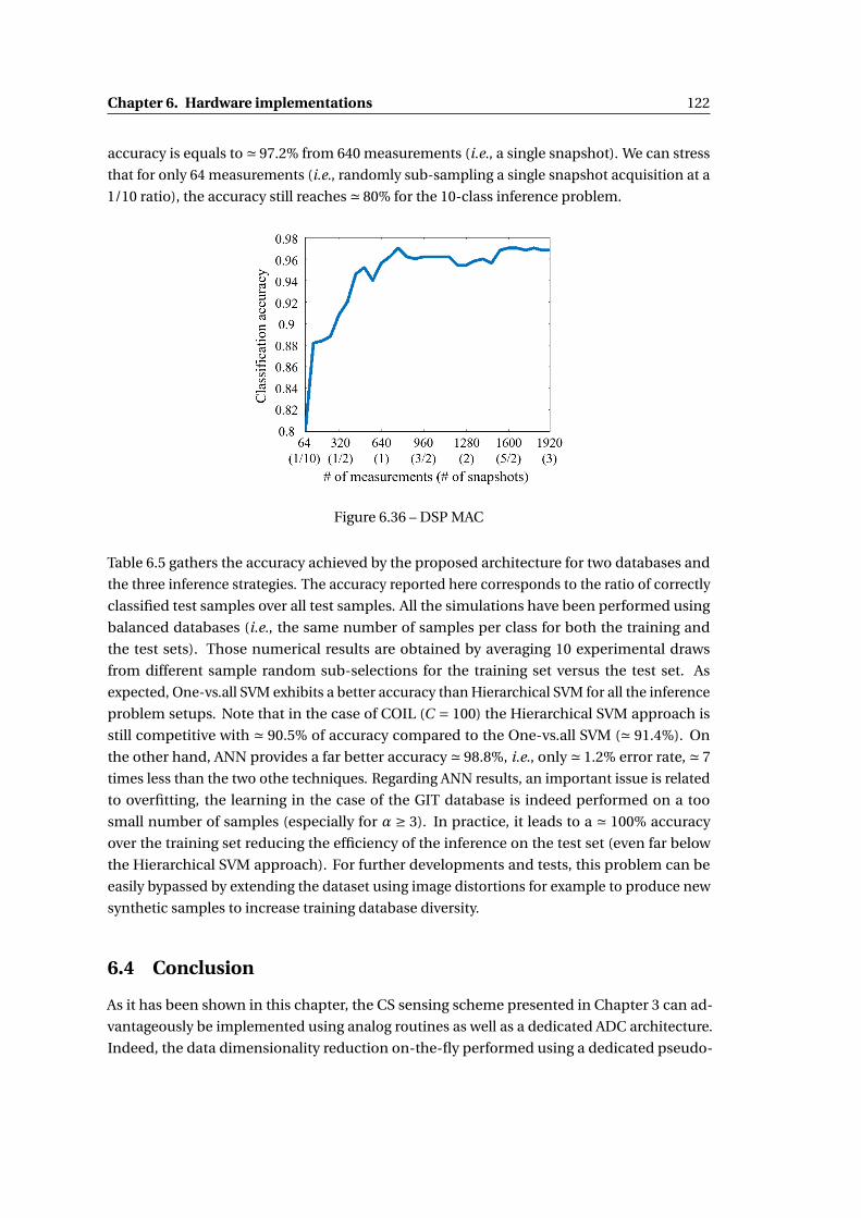
Chapter 6. Hardware implementations 122
accuracy is equals to ' 97.2% from 640 measurements (i.e., a single snapshot). We can stress
that for only 64 measurements (i.e., randomly sub-sampling a single snapshot acquisition at a
1/10 ratio), the accuracy still reaches ' 80% for the 10-class inference problem.
Figure 6.36 – DSP MAC
Table 6.5 gathers the accuracy achieved by the proposed architecture for two databases and
the three inference strategies. The accuracy reported here corresponds to the ratio of correctly
classified test samples over all test samples. All the simulations have been performed using
balanced databases (i.e., the same number of samples per class for both the training and
the test sets). Those numerical results are obtained by averaging 10 experimental draws
from different sample random sub-selections for the training set versus the test set. As
expected, One-vs.all SVM exhibits a better accuracy than Hierarchical SVM for all the inference
problem setups. Note that in the case of COIL (C = 100) the Hierarchical SVM approach is
still competitive with ' 90.5% of accuracy compared to the One-vs.all SVM (' 91.4%). On
the other hand, ANN provides a far better accuracy ' 98.8%, i.e., only ' 1.2% error rate, ' 7
times less than the two othe techniques. Regarding ANN results, an important issue is related
to overfitting, the learning in the case of the GIT database is indeed performed on a too
small number of samples (especially for α ≥ 3). In practice, it leads to a ' 100% accuracy
over the training set reducing the efficiency of the inference on the test set (even far below
the Hierarchical SVM approach). For further developments and tests, this problem can be
easily bypassed by extending the dataset using image distortions for example to produce new
synthetic samples to increase training database diversity.
6.4 Conclusion
As it has been shown in this chapter, the CS sensing scheme presented in Chapter 3 can ad-
vantageously be implemented using analog routines as well as a dedicated ADC architecture.
Indeed, the data dimensionality reduction on-the-fly performed using a dedicated pseudo-
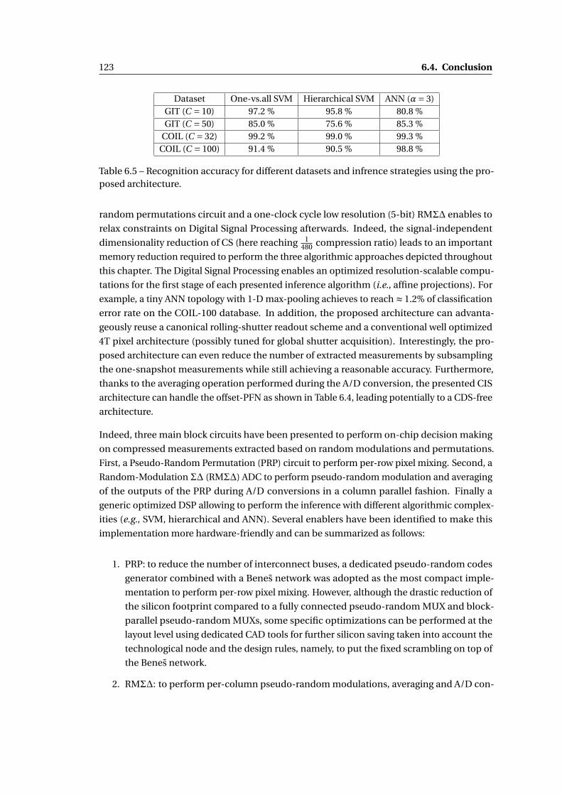
123 6.4. Conclusion
Dataset One-vs.all SVM Hierarchical SVM ANN (α= 3)GIT (C = 10) 97.2 % 95.8 % 80.8 %GIT (C = 50) 85.0 % 75.6 % 85.3 %
COIL (C = 32) 99.2 % 99.0 % 99.3 %COIL (C = 100) 91.4 % 90.5 % 98.8 %
Table 6.5 – Recognition accuracy for different datasets and infrence strategies using the pro-posed architecture.
random permutations circuit and a one-clock cycle low resolution (5-bit) RMΣ∆ enables to
relax constraints on Digital Signal Processing afterwards. Indeed, the signal-independent
dimensionality reduction of CS (here reaching 1480 compression ratio) leads to an important
memory reduction required to perform the three algorithmic approaches depicted throughout
this chapter. The Digital Signal Processing enables an optimized resolution-scalable compu-
tations for the first stage of each presented inference algorithm (i.e., affine projections). For
example, a tiny ANN topology with 1-D max-pooling achieves to reach ≈ 1.2% of classification
error rate on the COIL-100 database. In addition, the proposed architecture can advanta-
geously reuse a canonical rolling-shutter readout scheme and a conventional well optimized
4T pixel architecture (possibly tuned for global shutter acquisition). Interestingly, the pro-
posed architecture can even reduce the number of extracted measurements by subsampling
the one-snapshot measurements while still achieving a reasonable accuracy. Furthermore,
thanks to the averaging operation performed during the A/D conversion, the presented CIS
architecture can handle the offset-PFN as shown in Table 6.4, leading potentially to a CDS-free
architecture.
Indeed, three main block circuits have been presented to perform on-chip decision making
on compressed measurements extracted based on random modulations and permutations.
First, a Pseudo-Random Permutation (PRP) circuit to perform per-row pixel mixing. Second, a
Random-Modulation Σ∆ (RMΣ∆) ADC to perform pseudo-random modulation and averaging
of the outputs of the PRP during A/D conversions in a column parallel fashion. Finally a
generic optimized DSP allowing to perform the inference with different algorithmic complex-
ities (e.g., SVM, hierarchical and ANN). Several enablers have been identified to make this
implementation more hardware-friendly and can be summarized as follows:
1. PRP: to reduce the number of interconnect buses, a dedicated pseudo-random codes
generator combined with a Benes network was adopted as the most compact imple-
mentation to perform per-row pixel mixing. However, although the drastic reduction of
the silicon footprint compared to a fully connected pseudo-random MUX and block-
parallel pseudo-random MUXs, some specific optimizations can be performed at the
layout level using dedicated CAD tools for further silicon saving taken into account the
technological node and the design rules, namely, to put the fixed scrambling on top of
the Benes network.
2. RMΣ∆: to perform per-column pseudo-random modulations, averaging and A/D con-

Chapter 6. Hardware implementations 124
version, a double-path incremental Σ∆ fits highly with constraints of low-power CIS
applications. Indeed, in contrast to a standard Σ∆ ADC that needs 29 = 512 clock cy-
cles per-row to extract 9-bit measurements, the proposed RMΣ∆ ADC needs only one
clock cycle per-row leading to drastic power-consumption saving related to the ADC
which represents generally the most power hungry component of a CIS. Moreover, for
further digital design relaxation, the resolution of the extracted CS measurements can
advantageously be reduced to 5-bit by saturating the RMΣ∆ counter thanks to the prior
knowledge of the data distribution at the training stage. However, some specific opti-
mizations can be performed at the transistor level, e.g., mismatch of the integrators of
the RMΣ∆.
3. DSP: to enable on-chip inference, an optimized resolution-scalable DSP architecture is
proposed to implement the first stage of each presented inference algorithm (i.e., affine
projections). Indeed, pipelined MAC operations as well as reduced weights/biases and
computing unit (i.e., digital adders and multipliers) resolutions have been identified as
compact enablers to reduce memory needs and logical gates needed to solve the infer-
ence problem on CS measurements with negligible impact on the inference accuracy.
Finally, to handle classification tasks with higher inter-class and between-classes vari-
ability, Neural Networks provide a flexible framework to adapt the number of projections
and nonlinear layers to the complexity of the classification tasks. As discussed in Section
6.2, the first layer of an ANN topology (most MAC hungry layer) can advantageously be
implemented using low hardware complexity routines.
Chapter 7
Conclusions
In this thesis, we have explored new paths to extract compressed features enabling on-chip
decision making in the context of CMOS Image Sensor design. We have presented a number
of algorithm/hardware methods that take advantage of the concept of Compressed Sensing
as a data agnostic dimensionality reduction technique allowing as a consequence to reduce
the amount of data to process/store, and thus, relax hardware constraints related to basic
inference tasks. All the contributions presented throughout this thesis lay algorithmic and
hardware foundations for efficient design of future ultra-low power CMOS Image Sensor
applications (µW ). In particular, we have focused on:
• Inference on compressive measurements (Chapter 3): among the state-of-the-art di-
mensionality reduction techniques, Compressive Sensing has emerged as the most
hardware-friendly framework to extract compressed features taking advantage of pseudo-
random generators. Based on this statement, three algorithmic approaches for on-chip
decision making on compressed measurements have been investigated. Indeed, based
on an analytical study, the simulation results highlight significant improvement of the
approach involving a learning and inference problem solving in the compressed domain.
It exhibits the best performance regarding the quality of the inference as well as the
robustness to additive noise. Furthermore, performing the training and the inference
directly in the compressed domain allows to drastically reduce the complexity in terms
of both memory and computing needs.
However, although covering different inference algorithms, this analytical study is lim-
ited to inference tasks dealing with linearly separable datasets. A first interesting outlook
could investigate the interest of CS for nonlinearly separable datasets, even analytically
using synthetic datasets. It can take advantage of commonly known nonlinear acti-
vation function as performed in Artificial Neural Networks to find the best setting to
deal with more challenging inference tasks. On the other hand, the concept of signal
processing on CS measurements can be extended to signal processing on quantized

Chapter 7. Conclusions 126
CS measurements as quantization allows to reduce the resolution of CS measurements,
and thus, further saving at the digital signal processing level. This might be interesting
in the context of binary neural networks that show interesting properties for on-chip
applications in order to extract cascaded binary features. Typically, CS can be used as a
dimensionality reduction layer of the activation layer outputs of a Deep Neural Network
architecture.
• Random modulations & permutations for compressive imaging (Chapter 4): in Chap-
ter 4, a novel Compressive Sensing scheme has been presented for compressive imaging
applications. Based on random modulations and permutations this CS model allows
to circumvent shortcomings of SOTA CIS architectures implementing CS on-chip by
extending measurements support leading as a consequence to low correlated CS mea-
surements. This property enables to solve inference tasks with few CS measurements
(i.e., achieving high compression ratios, e.g., 1 ‰of the observed image), and thus
allows to relax hardware needs to solve the inference problem. In addition, random
modulations leads to a zero expectation CS matrix enabling to center CS measurements
distribution and thus extract zero mean features, a pre-processing operation highly
desirable in machine learning algorithms. Through theoretical, analytical and exper-
imental results, we have shown that the proposed CS framework is able to address
both image rendering and inference tasks and finally outperforms SOTA CS based CIS
architectures.
The proposed CS sensing scheme highlights the interest of in-focal plane data mixing for
on-chip inference tasks. Being basically designed based on experimental observations,
an immediate future work related to this axis would focus on providing stronger theo-
retical guarantees for both image recovery and inference problems. Although we have
proven that the proposed sensing model cannot respect the RIP in the canonical basis,
numerical and theoretical analyses show that exploring specific sparsity structures and
sparsity bases can fortunately circumvent this issue. It seems then that proving the JLL
in a specific sparsity basis is an immediate extension to study the robustness of the
proposed sensing scheme. A final research axis related to this chapter, would extend the
theoretical analysis to quantized version of the JLL such all hardware implementations
in the context of CIS applications deal typically with quantized CS measurements.
• Hierarchical learning for on-chip inference (Chapter 5): at the inference level, hierar-
chical learning have been explored as a practical approach to reduce the amount of MAC
operations needed to solve the inference problem thanks to the reduction of the number
of binary projections by a log factor. In this context, three new methods have been
proposed to construct the hierarchical tree to train a hierarchical classifier based on
binary decision rules (2-classes SVM) minimizing as a consequence the number of deci-
sion nodes, and thus, the number of binary classifiers to perform at the inference level.
Simulation results show the great interest of the proposed methods in terms of hard-
ware requirements (computing complexity and memory access needs), especially, when
combined with Compressive Sensing. The overall memory and on-chip MAC operations
127
needs can advantageously be lowered thanks to the signal-independent dimensionality
reduction enabled by CS leading to a joint acquisition-processing optimization to fit
hardware needs involved by highly constrained on-chip inference tasks.
Although involving basic classification algorithms (i.e., SVM) hierarchical learning ap-
proach can take advantage of more powerful algorithm tools such as Deep Neural
Networks or dictionary learning methods to improve the classification accuracy taking
advantage of nonlinear kernels (or activation functions in the deep learning jargon).
Some initial steps combining hierarchical learning and neural networks, not reported in
this thesis, have been done and show significant improvements compared to hierarchi-
cal algorithms involving 2-classes SVMs. The main idea consists in replacing each node
binary decision rule by a tiny neural network or even learn the binary decision tree using
the commonly used forward-backward algorithm. This way one can take advantage
of nonlinear activation functions and tune the number of projections to the inference
complexity. Furthermore, one can also adapt the number of CS measurements to extract
in function of the depth of the binary decision tree based on semantic features at each
node. From a hardware point of view, hierarchical learning represents an appropriate
candidate for cascaded systems with multi-stage wake-up levels [184]. This approach
is deemed to minimize energy consumption such the digital processing is customized
depending on the inference task complexity (generally of increasingly complexity).
• Compact image sensor architecture with on-chip inference capabilities (Chapter 6):
the heart of this thesis is the study of a compact CMOS Image Sensor architecture tak-
ing advantage of the proposed CS sensing scheme based on random modulations and
permutations to extract compressed features enabling on-chip inference with lower
hardware complexity. Indeed, through passive analog routines and optimized ADC
architecture, the data dimensionality reduction is achieved using low-footprint pseudo-
random permutation circuit and a one-clock cycle low resolution (5-bit) RMΣ∆. It
enables thus to relax constraints on Digital Signal Processing afterwards. Indeed, the
signal-independent dimensionality reduction of CS (reaching 1480 compression ratio)
leads to an important memory reduction required to perform the inference approaches
reported in Chapter 5. The digital processing enables an optimized resolution-scalable
computations for the first stage of each presented inference algorithm. Interestingly,
the proposed architecture can advantageously reuse a canonical rolling-shutter readout
scheme and a conventional well optimized 4T pixel architecture. The top-level architec-
ture of the proposed CIS has been validated based on high-level simulations of unitary
components functional behavior.
Although being based on high-level simulations, several enablers have been identified
to make this implementation more hardware friendly. An immediate continuity of the
study of this architecture would be to design the additional block circuits compared to a
canonical CIS architecture, i.e., Pseudo-Random Permutation (PRP) circuit and double-
path Σ∆ (RMΣ∆) ADC. Indeed, several optimizations can be done at the electrical and
layout levels, typically to properly estimate the silicon-footprint of the PRP and handle

Chapter 7. Conclusions 128
the gain mismatch that can be involved by the RMΣ∆. Related to the preliminary study,
several mid-term perspectives can be explored. In particular, to extend the inference
capability to deal with shifted non-centred patterns, multi-scale pattern detection and
recognition can advantageously be investigated to perform multi-resolution searches in
the focal plane. At the system level, cascaded wake-up processing can advantageously
be explored for end-user always-on applications. For instance, one can imagine a first
motion-detection event based on basic inter-frame binary differences triggering a first
decision making level enabling or not the dedicated inference task. This approach is
deemed to be highly suitable for ultra-low power applications, e.g., IoT sensor nodes.
For future ultra-low power (µW) CIS, the aforementioned conclusions and perspectives pro-
vide some initial algorithm-hardware enablers for the design of compact CIS with on-chip
decision making capabilities. This kind of targeted IoT-like application has been proven to be
relevant in terms of power budget for customer handheld devices.

Publications & Patent
Journal
• W. Benjilali, W. Guicquero, L. Jacques, and G. Sicard, "Hardware-Compliant Compres-
sive Image Sensor Architecture Based on Random Modulations & Permutations For
Embedded Inference," in IEEE Transactions on Circuits and Systems I: Regular Papers.
[Accepted for publication]
International Conferences
• W. Benjilali, W. Guicquero, L. Jacques, and G. Sicard, "Near Sensor Decision Making via
Compressed Measurements for Highly Constrained Hardware," in 2019 53rd Asilomar
Conference on Signals, Systems and Computers, Pacific Grove, CA, 2019. [Accepted for
publication]
• W. Benjilali, W. Guicquero, L. Jacques and G. Sicard, "Hardware-Friendly Compressive
Imaging Based on Random Modulations & Permutations for Image Acquisition and
Classification," 2019 IEEE International Conference on Image Processing (ICIP), Taipei,
Taiwan, 2019.
• W. Benjilali, W. Guicquero, L. Jacques and G. Sicard, "An Analog-to-Information VGA
Image Sensor Architecture for Support Vector Machine on Compressive Measurements,"
2019 IEEE International Symposium on Circuits and Systems (ISCAS), Sapporo, Japan,
2019. [Student Best Paper Runner-up Award]
• W. Benjilali, W. Guicquero, L. Jacques and G. Sicard, "Exploring Hierarchical Machine
Learning for Hardware-Limited Multi-Class Inference on Compressed Measurements,"
2019 IEEE International Symposium on Circuits and Systems (ISCAS), Sapporo, Japan,
2019.
• W. Benjilali, W. Guicquero, L. Jacques and G. Sicard, "A Low-Memory Compressive Image
Sensor Architecture for Embedded Object Recognition," 2018 IEEE 61st International
Midwest Symposium on Circuits and Systems (MWSCAS), Windsor, ON, Canada, 2018.
[Finalist of the student contest]

Chapter 7. Publications & Patent 130
Workshops
• W. Benjilali, W. Guicquero, L. Jacques and G. Sicard, ”A hardware friendly compres-
sive sensing scheme for analog-to-information image sensor”, GDR-ISIS, Paris, France,
November, 2018. [One page abstract]
• W. Benjilali, W. Guicquero, L. Jacques and G. Sicard, ”Architecture d’un capteur d’image
compressive compacte pour la reconnaissance d’objets embarquée”, Journées Imagerie
Optique Non Conventionnelle, Paris, France, Mars, 2018. [One page abstract]
Patent
• W. Benjilali and W. Guicquero, ”Générateur d’une permutation pseudo-aléatoire”. [Patent
application]

Bibliography
[1] Learn About Convolutional Neural Networks - MATLAB & Simulink - MathWorks France.
[2] Junichi Nakamura, editor. Image sensors and signal processing for digital still cameras.
Taylor & Francis, Boca Raton, FL, 2006.
[3] T. Sugiki, S. Ohsawa, H. Miura, M. Sasaki, N. Nakamura, I. Inoue, M. Hoshino,
Y. Tomizawa, and T. Arakawa. A 60 mW 10 b CMOS image sensor with column-to-
column FPN reduction. In 2000 IEEE International Solid-State Circuits Conference.
Digest of Technical Papers (Cat. No.00CH37056), pages 108–109, February 2000.
[4] Juan A. Leñero-Bardallo, Jorge Fernández-Berni, and Ángel Rodríguez-Vázquez. Review
of ADCs for imaging. page 90220I, San Francisco, California, USA, March 2014.
[5] A. B. Kahng. Scaling: More than Moore’s law. IEEE Design Test of Computers, 27(3):86–87,
May 2010.
[6] M. H. Miraz, M. Ali, P. S. Excell, and R. Picking. A review on Internet of Things (IoT),
Internet of Everything (IoE) and Internet of Nano Things (IoNT). In 2015 Internet
Technologies and Applications (ITA), pages 219–224, September 2015.
[7] T. Ernst, R. Guillemaud, P. Mailley, J. P. Polizzi, A. Koenig, S. Boisseau, E. Pauliac-Vaujour,
C. Plantier, G. Delapierre, E. Saoutieff, R. Gerbelot-Barillon, E. C. Strinati, S. Hentz,
E. Colinet, O. Thomas, P. Boisseau, and P. Jallon. Sensors and related devices for IoT,
medicine and s mart-living. In 2018 IEEE Symposium on VLSI Technology, pages 35–36,
June 2018.
[8] S. G. Mallat. A wavelet tour of signal processing: the sparse way. Elsevier/Academic Press,
Amsterdam ; Boston, 3rd ed edition, 2009.
[9] M. Elad, M. A. T. Figueiredo, and Y. Ma. On the Role of Sparse and Redundant Represen-
tations in Image Processing. Proceedings of the IEEE, 98(6):972–982, June 2010.
[10] Michael Elad. Sparse and Redundant Representations: From Theory to Applications in
Signal and Image Processing. Springer-Verlag, New York, 2010.
Bibliography 132
[11] Milin Zhang and Amine Bermak. CMOS Image Sensor with On-Chip Image Compres-
sion: A Review and Performance Analysis. Journal of Sensors, 2010, 2010.
[12] L. Alacoque, L. Chotard, M. Tchagaspanian, and J. Chossat. A small footprint, stream-
ing compliant, versatile wavelet compression scheme for cameraphone imagers. In
International Image Sensors Workshop (IISW), volume 9, 2009.
[13] D. L. Donoho. Compressed sensing. IEEE Transactions on Information Theory,
52(4):1289–1306, April 2006.
[14] E. J. Candès and M. B. Wakin. An Introduction To Compressive Sampling. IEEE Signal
Processing Magazine, 25(2):21–30, March 2008.
[15] E. J. Candes, J. Romberg, and T. Tao. Robust uncertainty principles: exact signal re-
construction from highly incomplete frequency information. IEEE Transactions on
Information Theory, 52(2):489–509, February 2006.
[16] E. J. Candès, Justin Romberg, and Terence Tao. Stable signal recovery from incomplete
and inaccurate measurements. Communications on Pure and Applied Mathematics,
59(8):1207–1223, August 2006.
[17] E. J. Candès and T. Tao. Near-Optimal Signal Recovery From Random Projections:
Universal Encoding Strategies? IEEE Transactions on Information Theory, 52(12):5406–
5425, December 2006.
[18] Xiaojun Chen, Dongdong Ge, Zizhuo Wang, and Yinyu Ye. Complexity of unconstrained
L2-Lp minimization. Mathematical Programming, 143(1-2):371–383, February 2014.
[19] Thi Thanh Nguyen, Charles Soussen, Jérôme Idier, and El-Hadi Djermoune. NP-
hardness of l0 minimization problems: revision and extension to the non-negative
setting. In 13th International Conference on Sampling Theory and Applications, SampTA
2019, Bordeaux, France, July 2019.
[20] J. A. Tropp. Just relax: convex programming methods for identifying sparse signals in
noise. IEEE Transactions on Information Theory, 52(3):1030–1051, March 2006.
[21] R. Gribonval and M. Nielsen. Highly sparse representations from dictionaries are unique
and independent of the sparseness measure. Applied and Computational Harmonic
Analysis, 22(3):335–355, May 2007.
[22] D.L. Donoho and X. Huo. Uncertainty principles and ideal atomic decomposition. IEEE
Transactions on Information Theory, 47(7):2845–2862, November 2001.
[23] M. Elad and A. M. Bruckstein. On sparse signal representations. In Proceedings 2001
International Conference on Image Processing (Cat. No.01CH37205), volume 1, pages
3–6 vol.1, October 2001.

133 Bibliography
[24] M. Elad and A. M. Bruckstein. A generalized uncertainty principle and sparse repre-
sentation in pairs of bases. IEEE Transactions on Information Theory, 48(9):2558–2567,
September 2002.
[25] J. A. Tropp and S. J. Wright. Computational Methods for Sparse Solution of Linear
Inverse Problems. Proceedings of the IEEE, 98(6):948–958, June 2010.
[26] Simon Foucart. Mathematical introduction to compressive sensing. Springer-Verlag New
York, Place of publication not identified, 2015. OCLC: 953842807.
[27] E. Crespo Marques, N. Maciel, L. Naviner, H. Cai, and J. Yang. A Review of Sparse
Recovery Algorithms. IEEE Access, 7:1300–1322, 2019.
[28] Stephen P. Boyd and Lieven Vandenberghe. Convex optimization. Cambridge University
Press, Cambridge, UK ; New York, 2004.
[29] Joachim H. G. Ender. On compressive sensing applied to radar. Signal Processing,
90(5):1402–1414, May 2010.
[30] A. Forsgren, P. Gill, and M. Wright. Interior Methods for Nonlinear Optimization. SIAM
Review, 44(4):525–597, January 2002.
[31] Arkadi Nemirovski and Michael Todd. Interior-point methods for optimization. Acta
Numerica, 17:191–234, May 2008.
[32] S. Chen, D. Donoho, and M. Saunders. Atomic Decomposition by Basis Pursuit. SIAM
Journal on Scientific Computing, 20(1):33–61, January 1998.
[33] S. Mallat and Z. Zhang. Adaptive time-frequency decomposition with matching pursuits.
In [1992] Proceedings of the IEEE-SP International Symposium on Time-Frequency and
Time-Scale Analysis, pages 7–10, October 1992.
[34] Y. C. Pati, R. Rezaiifar, and P. S. Krishnaprasad. Orthogonal matching pursuit: recursive
function approximation with applications to wavelet decomposition. In Proceedings
of 27th Asilomar Conference on Signals, Systems and Computers, pages 40–44 vol.1,
November 1993.
[35] D. L. Donoho, Y. Tsaig, I. Drori, and J. Starck. Sparse Solution of Underdetermined Sys-
tems of Linear Equations by Stagewise Orthogonal Matching Pursuit. IEEE Transactions
on Information Theory, 58(2):1094–1121, February 2012.
[36] D. Needell and J. A. Tropp. CoSaMP: Iterative signal recovery from incomplete and
inaccurate samples. Applied and Computational Harmonic Analysis, 26(3):301–321,
May 2009.
[37] W. Dai and O. Milenkovic. Subspace Pursuit for Compressive Sensing Signal Reconstruc-
tion. IEEE Transactions on Information Theory, 55(5):2230–2249, May 2009.

Bibliography 134
[38] Thomas Blumensath and Mike E. Davies. Iterative Thresholding for Sparse Approxima-
tions. Journal of Fourier Analysis and Applications, 14(5):629–654, December 2008.
[39] Ingrid Daubechies, Michel Defrise, and Christine De Mol. An iterative thresholding
algorithm for linear inverse problems with a sparsity constraint. July 2003.
[40] Amir Beck and Marc Teboulle. A fast iterative shrinkage-thresholding algorithm for
linear inverse problems. Siam Journal on Imaging Sciences, 2(1), 2009.
[41] David L. Donoho, Arian Maleki, and Andrea Montanari. Message Passing Algorithms for
Compressed Sensing. July 2009.
[42] Michael Davies, Gabriel Rilling, and Thomas Blumensath. Greedy algorithms for com-
pressed sensing. In Yonina Eldar and Gitta Kutyniok, editors, Compressed Sensing, pages
348–393. Cambridge University Press, United States, 2012.
[43] M. Hyder and K. Mahata. An approximate L0 norm minimization algorithm for com-
pressed sensing. In 2009 IEEE International Conference on Acoustics, Speech and Signal
Processing, pages 3365–3368, April 2009.
[44] D. Kanevsky, A. Carmi, L. Horesh, P. Gurfil, B. Ramabhadran, and T. N. Sainath. Kalman
filtering for compressed sensing. In 2010 13th International Conference on Information
Fusion, pages 1–8, July 2010.
[45] R. Chartrand. Exact Reconstruction of Sparse Signals via Nonconvex Minimization.
IEEE Signal Processing Letters, 14(10):707–710, October 2007.
[46] Petros T. Boufounos, Laurent Jacques, Felix Krahmer, and Rayan Saab. Quantization
and Compressive Sensing. May 2014.
[47] Xiaolin Huang and Ming Yan. Nonconvex penalties with analytical solutions for one-bit
compressive sensing. June 2017.
[48] D. P. Wipf and B. D. Rao. Bayesian learning for sparse signal reconstruction. In 2003 IEEE
International Conference on Acoustics, Speech, and Signal Processing, 2003. Proceedings.
(ICASSP ’03)., volume 6, pages VI–601, April 2003.
[49] H. Zayyani, M. Babaie-Zadeh, and C. Jutten. Bayesian Pursuit algorithm for sparse
representation. In 2009 IEEE International Conference on Acoustics, Speech and Signal
Processing, pages 1549–1552, April 2009.
[50] A. Drémeau, C. Herzet, and L. Daudet. Structured Bayesian Orthogonal Matching
Pursuit. In 2012 IEEE International Conference on Acoustics, Speech and Signal Processing
(ICASSP), pages 3625–3628, March 2012.
[51] S. Ji, Y. Xue, and L. Carin. Bayesian Compressive Sensing. IEEE Transactions on Signal
Processing, 56(6):2346–2356, June 2008.

135 Bibliography
[52] Youness Arjoune, Naima Kaabouch, Hassan El Ghazi, and Ahmed Tamtaoui. Com-
pressive Sensing: Performance Comparison Of Sparse Recovery Algorithms. January
2018.
[53] Ali Mousavi, Ankit B. Patel, and Richard G. Baraniuk. A Deep Learning Approach to
Structured Signal Recovery. August 2015.
[54] Ali Mousavi and Richard G. Baraniuk. Learning to Invert: Signal Recovery via Deep
Convolutional Networks. January 2017.
[55] Yan Wu, Mihaela Rosca, and Timothy Lillicrap. Deep Compressed Sensing. May 2019.
[56] S. G. Mallat and Zhifeng Zhang. Matching pursuits with time-frequency dictionaries.
IEEE Transactions on Signal Processing, 41(12):3397–3415, December 1993.
[57] David L. Donoho and Michael Elad. Optimally sparse representation in general
(nonorthogonal) dictionaries via l1 minimization. Proceedings of the National Academy
of Sciences, 100(5):2197–2202, March 2003.
[58] L. Welch. Lower bounds on the maximum cross correlation of signals (Corresp.). IEEE
Transactions on Information Theory, 20(3):397–399, May 1974.
[59] R. Gribonval and M. Nielsen. Sparse representations in unions of bases. IEEE Transac-
tions on Information Theory, 49(12):3320–3325, December 2003.
[60] E. J. Candès and T. Tao. Decoding by linear programming. IEEE Transactions on Infor-
mation Theory, 51(12):4203–4215, December 2005.
[61] E. J. Candès, Justin Romberg, and Terence Tao. The restricted isometry property and its
implications for compressed sensing. Comptes Rendus Mathematique, 346(9):589–592,
May 2008.
[62] Mark A. Davenport. Random observations on random observations: Sparse signal acqui-
sition and processing. 2010.
[63] Sanjoy Dasgupta and Anupam Gupta. An elementary proof of a theorem of Johnson
and Lindenstrauss. Random Structures & Algorithms, 22(1):60–65, 2003.
[64] Richard Baraniuk, M Davenport, R DeVore, and M B Wakin. The Johnson-Lindenstrauss
lemma meets Compressed Sensing. IEEE Transactions on Information Theory, 52:1289–
1306, January 2006.
[65] Ronald A. DeVore. Deterministic constructions of compressed sensing matrices. Journal
of Complexity, 23(4):918–925, August 2007.
[66] Arash Amini and Farokh Marvasti. Deterministic Construction of Compressed Sensing
Matrices using BCH Codes. August 2009.
Bibliography 136
[67] MohamadMahdi Mohades and Mohamad Hossein Kahaei. A General Approach for
Construction of Deterministic Compressive Sensing Matrices. February 2018.
[68] Shahar Mendelson, Alain Pajor, and Nicole Tomczak-Jaegermann. Uniform Uncer-
tainty Principle for Bernoulli and Subgaussian Ensembles. Constructive Approximation,
28(3):277–289, December 2008.
[69] Richard Baraniuk, Mark Davenport, Ronald DeVore, and Michael Wakin. A Simple Proof
of the Restricted Isometry Property for Random Matrices. Constructive Approximation,
28(3):253–263, December 2008.
[70] Laurent Jacques and Pierre Vandergheynst. Compressed Sensing: “When Sparsity Meets
Sampling”. pages 507–527. April 2011.
[71] Roman Vershynin. Introduction to the non-asymptotic analysis of random matrices.
November 2010.
[72] Mark A. Davenport, Jason N. Laska, Petros T. Boufounos, and Richard G. Baraniuk. A
simple proof that random matrices are democratic. November 2009.
[73] Stephen Wolfram. Cellular automata and complexity: collected papers. Addison-Wesley
Pub. Co, Reading, Mass, 1994.
[74] Wade Keith Wan and Sherman (Xuemin) Chen. Pseudo-random number generation
based on periodic sampling of one or more linear feedback shift registers, September
2014.
[75] Mark Rudelson and Roman Vershynin. Sparse reconstruction by convex relaxation:
Fourier and Gaussian measurements. February 2006.
[76] R. Coifman, F. Geshwind, and Y. Meyer. Noiselets. Applied and Computational Harmonic
Analysis, 10(1):27–44, January 2001.
[77] T. T. Do, L. Gan, N. H. Nguyen, and T. D. Tran. Fast and Efficient Compressive Sensing
Using Structurally Random Matrices. IEEE Transactions on Signal Processing, 60(1):139–
154, January 2012.
[78] L. Gan, T. T. Do, and T. D. Tran. Fast compressive imaging using scrambled block
Hadamard ensemble. In 2008 16th European Signal Processing Conference, pages 1–5,
August 2008.
[79] T. T. Do, T. D. Tran, and Lu Gan. Fast compressive sampling with structurally random ma-
trices. In 2008 IEEE International Conference on Acoustics, Speech and Signal Processing,
pages 3369–3372, March 2008.
[80] J. Romberg. Sensing by Random Convolution. In 2007 2nd IEEE International Work-
shop on Computational Advances in Multi-Sensor Adaptive Processing, pages 137–140,
December 2007.

137 Bibliography
[81] J. Haupt, R. Castro, R. Nowak, G. Fudge, and A. Yeh. Compressive Sampling for Signal
Classification. In 2006 Fortieth Asilomar Conference on Signals, Systems and Computers,
pages 1430–1434, October 2006.
[82] Mark A. Davenport, Michael B. Wakin, and Richard G. Baraniuk. Detection and Estima-
tion with Compressive Measurements. Technical report, 2006.
[83] J. Haupt and R. Nowak. Compressive Sampling for Signal Detection. In 2007 IEEE Inter-
national Conference on Acoustics, Speech and Signal Processing - ICASSP ’07, volume 3,
pages III–1509–III–1512, April 2007.
[84] M. A. Davenport, P. T. Boufounos, M. B. Wakin, and R. G. Baraniuk. Signal Processing
With Compressive Measurements. IEEE Journal of Selected Topics in Signal Processing,
4(2):445–460, April 2010.
[85] Robert Calderbank, Sina Jafarpour, and Robert Schapire. Compressed learning: Univer-
sal sparse dimensionality reduction and learning in the measurement domain. Technical
report, 2009.
[86] Afonso S. Bandeira, Dustin G. Mixon, and Benjamin Recht. Compressive classification
and the rare eclipse problem. April 2014.
[87] V. Cambareri, C. Xu, and L. Jacques. The rare eclipse problem on tiles: Quantised
embeddings of disjoint convex sets. In 2017 International Conference on Sampling
Theory and Applications (SampTA), pages 241–245, July 2017.
[88] S. K. S and S. K. V. Reconstruction of MRI Images based on Compressive Sensing. In
2019 International Conference on Communication and Signal Processing (ICCSP), pages
0787–0791, April 2019.
[89] Claire M. Watts, David Shrekenhamer, John Montoya, Guy Lipworth, John Hunt, Timothy
Sleasman, Sanjay Krishna, David R. Smith, and Willie J. Padilla. Terahertz compressive
imaging with metamaterial spatial light modulators. Nature Photonics, 8(8):605–609,
August 2014.
[90] A. Kadambi and P. T. Boufounos. Coded aperture compressive 3-D LIDAR. In 2015 IEEE
International Conference on Acoustics, Speech and Signal Processing (ICASSP), pages
1166–1170, April 2015.
[91] M. Zhu, X. Zhang, Y. Qi, and H. Ji. Compressed Sensing Mask Feature in Time-Frequency
Domain for Civil Flight Radar Emitter Recognition. In 2018 IEEE International Con-
ference on Acoustics, Speech and Signal Processing (ICASSP), pages 2146–2150, April
2018.
[92] W. Guicquero, P. Vandergheynst, T. Laforest, A. Verdant, and A. Dupret. On multiple
spectral dependent blurring kernels for super-resolution and hyperspectral imaging. In
2014 IEEE Global Conference on Signal and Information Processing (GlobalSIP), pages
717–721, December 2014.

Bibliography 138
[93] K. Degraux, V. Cambareri, B. Geelen, L. Jacques, and G. Lafruit. Multispectral Com-
pressive Imaging Strategies Using Fabry–Pérot Filtered Sensors. IEEE Transactions on
Computational Imaging, 4(4):661–673, December 2018.
[94] M. F. Duarte, M. A. Davenport, D. Takhar, J. N. Laska, T. Sun, K. F. Kelly, and R. G.
Baraniuk. Single-pixel imaging via compressive sampling. IEEE Signal Processing
Magazine, 25(2):83–91, March 2008.
[95] Wai Lam Chan, K. Charan, D. Takhar, K. F. Kelly, R. G. Baraniuk, and D. M. Mittleman. A
single-pixel terahertz camera. In 2008 Conference on Lasers and Electro-Optics and 2008
Conference on Quantum Electronics and Laser Science, pages 1–2, May 2008.
[96] R. F. Marcia and R. M. Willett. Compressive coded aperture superresolution image
reconstruction. In 2008 IEEE International Conference on Acoustics, Speech and Signal
Processing, pages 833–836, March 2008.
[97] D. Reddy, A. Veeraraghavan, and R. Chellappa. P2c2: Programmable pixel compressive
camera for high speed imaging. In CVPR 2011, pages 329–336, June 2011.
[98] H. Rueda, H. Arguello, and G. R. Arce. Colored coded aperture compressive spectral
imaging: Design and experimentation. In 2015 IEEE Global Conference on Signal and
Information Processing (GlobalSIP), pages 601–604, December 2015.
[99] P. A. Shedligeri, S. Mohan, and K. Mitra. Data driven coded aperture design for depth
recovery. In 2017 IEEE International Conference on Image Processing (ICIP), pages 56–60,
September 2017.
[100] Rob Fergus, Antonio Torralba, and William T. Freeman. Random Lens Imaging. Septem-
ber 2006.
[101] Antoine Liutkus, David Martina, Sébastien Popoff, Gilles Chardon, Ori Katz, Geoffroy
Lerosey, Sylvain Gigan, Laurent Daudet, and Igor Carron. Imaging With Nature: Com-
pressive Imaging Using a Multiply Scattering Medium. Scientific Reports, 4:5552, July
2014.
[102] Alaa Saade, Francesco Caltagirone, Igor Carron, Laurent Daudet, Angélique Drémeau,
Sylvain Gigan, and Florent Krzakala. Random Projections through multiple optical
scattering: Approximating kernels at the speed of light. October 2015.
[103] V. Boominathan, J. K. Adams, M. S. Asif, B. W. Avants, J. T. Robinson, R. G. Baraniuk,
A. C. Sankaranarayanan, and A. Veeraraghavan. Lensless Imaging: A computational
renaissance. IEEE Signal Processing Magazine, 33(5):23–35, September 2016.
[104] G. Huang, H. Jiang, K. Matthews, and P. Wilford. Lensless imaging by compressive
sensing. In 2013 IEEE International Conference on Image Processing, pages 2101–2105,
September 2013.

139 Bibliography
[105] X. Yuan, G. Huang, H. Jiang, and P. A. Wilford. Block-wise lensless compressive cam-
era. In 2017 IEEE International Conference on Image Processing (ICIP), pages 31–35,
September 2017.
[106] R. Robucci, Leung Kin Chiu, J. Gray, J. Romberg, P. Hasler, and D. Anderson. Compressive
sensing on a CMOS separable transform image sensor. In 2008 IEEE International
Conference on Acoustics, Speech and Signal Processing, pages 5125–5128, March 2008.
[107] R. Robucci, J. D. Gray, L. K. Chiu, J. Romberg, and P. Hasler. Compressive Sensing on a
CMOS Separable-Transform Image Sensor. Proceedings of the IEEE, 98(6):1089–1101,
June 2010.
[108] L. Jacques, P. Vandergheynst, A. Bibet, V. Majidzadeh, A. Schmid, and Y. Leblebici. CMOS
compressed imaging by Random Convolution. In 2009 IEEE International Conference
on Acoustics, Speech and Signal Processing, pages 1113–1116, April 2009.
[109] V. Majidzadeh, L. Jacques, A. Schmid, P. Vandergheynst, and Y. Leblebici. A (256x256)
pixel 76.7mw CMOS imager/ compressor based on real-time In-pixel compressive
sensing. In Proceedings of 2010 IEEE International Symposium on Circuits and Systems,
pages 2956–2959, May 2010.
[110] F. Mochizuki, K. Kagawa, S. Okihara, M. Seo, B. Zhang, T. Takasawa, K. Yasutomi, and
S. Kawahito. Single-shot 200mfps 5x3-aperture compressive CMOS imager. In 2015
IEEE International Solid-State Circuits Conference - (ISSCC) Digest of Technical Papers,
pages 1–3, February 2015.
[111] Jie Zhang, Tao Xiong, Trac Tran, Sang Chin, and Ralph Etienne-Cummings. Compact
all-CMOS spatiotemporal compressive sensing video camera with pixel-wise coded
exposure. Optics Express, 24(8):9013–9024, April 2016.
[112] N. Sarhangnejad, N. Katic, Z. Xia, M. Wei, N. Gusev, G. Dutta, R. Gulve, H. Haim, M. M.
Garcia, D. Stoppa, K. N. Kutulakos, and R. Genov. 5.5 Dual-Tap Pipelined-Code-Memory
Coded-Exposure-Pixel CMOS Image Sensor for Multi-Exposure Single-Frame Compu-
tational Imaging. In 2019 IEEE International Solid- State Circuits Conference - (ISSCC),
pages 102–104, February 2019.
[113] P. Vivet, G. Sicard, L. Millet, S. Chevobbe, K. B. Chehida, L. Angel Cubero, M. Alegre,
M. Bouvier, A. Valentian, M. Lepecq, T. Dombek, O. Bichler, S. Thuriès, D. Lattard,
C. Séverine, P. Batude, and F. Clermidy. Advanced 3d Technologies and Architectures
for 3d Smart Image Sensors. In 2019 Design, Automation Test in Europe Conference
Exhibition (DATE), pages 674–679, March 2019.
[114] Y. Oike and A. El Gamal. CMOS Image Sensor With Per-Column Sigma-Delta ADC and
Programmable Compressed Sensing. IEEE Journal of Solid-State Circuits, 48(1):318–328,
January 2013.

Bibliography 140
[115] A. Olyaei and R. Genov. Focal-Plane Spatially Oversampling CMOS Image Compression
Sensor. IEEE Transactions on Circuits and Systems I: Regular Papers, 54(1):26–34, January
2007.
[116] N. Katic, M. Hosseini Kamal, M. Kilic, A. Schmid, P. Vandergheynst, and Y. Leblebici.
Column-separated compressive sampling scheme for low power CMOS image sensors.
In 2013 IEEE 11th International New Circuits and Systems Conference (NEWCAS), pages
1–4, June 2013.
[117] M. Dadkhah, M. Jamal Deen, and S. Shirani. Block-Based CS in a CMOS Image Sensor.
IEEE Sensors Journal, 14(8):2897–2909, August 2014.
[118] W. Guicquero, A. Dupret, and P. Vandergheynst. An Algorithm Architecture Co-Design for
CMOS Compressive High Dynamic Range Imaging. IEEE Transactions on Computational
Imaging, 2(3):190–203, September 2016.
[119] Chung-Cheng Chiu, Tara N. Sainath, Yonghui Wu, Rohit Prabhavalkar, Patrick Nguyen,
Zhifeng Chen, Anjuli Kannan, Ron J. Weiss, Kanishka Rao, Ekaterina Gonina, Navdeep
Jaitly, Bo Li, Jan Chorowski, and Michiel Bacchiani. State-of-the-art Speech Recognition
With Sequence-to-Sequence Models. December 2017.
[120] Edward Chou, Matthew Tan, Cherry Zou, Michelle Guo, Albert Haque, Arnold Milstein,
and Li Fei-Fei. Privacy-Preserving Action Recognition for Smart Hospitals using Low-
Resolution Depth Images. November 2018.
[121] Tomasz M. Rutkowski, Marcin Koculak, Masato S. Abe, and Mihoko Otake-Matsuura.
Brain correlates of task-load and dementia elucidation with tensor machine learning
using oddball BCI paradigm. June 2019.
[122] David Silver, Julian Schrittwieser, Karen Simonyan, Ioannis Antonoglou, Aja Huang,
Arthur Guez, Thomas Hubert, Lucas Baker, Matthew Lai, Adrian Bolton, Yutian Chen,
Timothy Lillicrap, Fan Hui, Laurent Sifre, George van den Driessche, Thore Graepel,
and Demis Hassabis. Mastering the game of Go without human knowledge. Nature,
550(7676):354, October 2017.
[123] Christina Warren. Google’s artificial intelligence chief says ’we’re in an AI spring’, 2016.
[124] Ian Goodfellow, Yoshua Bengio, and Aaron Courville. Deep learning. Adaptive computa-
tion and machine learning. The MIT Press, Cambridge, Massachusetts, 2016.
[125] Tom M. Mitchell. Machine Learning. McGraw-Hill series in computer science. McGraw-
Hill, New York, 1997.
[126] Navneet Dalal and Bill Triggs. Histograms of Oriented Gradients for Human Detection.
June 2005.
[127] David G. Lowe. Distinctive Image Features from Scale-Invariant Keypoints. International
Journal of Computer Vision, 60(2):91–110, November 2004.
141 Bibliography
[128] Alexandre Alahi, Raphaël Ortiz, and Pierre Vandergheynst. FREAK: Fast Retina Keypoint,
2012.
[129] S. Leutenegger, M. Chli, and R. Y. Siegwart. BRISK: Binary Robust invariant scalable
keypoints. In 2011 International Conference on Computer Vision, pages 2548–2555,
November 2011.
[130] Y. Lecun, L. Bottou, Y. Bengio, and P. Haffner. Gradient-based learning applied to
document recognition. Proceedings of the IEEE, 86(11):2278–2324, November 1998.
[131] R. Giryes, G. Sapiro, and A. M. Bronstein. Deep Neural Networks with Random Gaussian
Weights: A Universal Classification Strategy? IEEE Transactions on Signal Processing,
64(13):3444–3457, July 2016.
[132] Christopher M. Bishop. Pattern recognition and machine learning. Information science
and statistics. Springer, New York, 2006.
[133] Gareth James, Daniela Witten, Trevor Hastie, and Robert Tibshirani, editors. An intro-
duction to statistical learning: with applications in R. Number 103 in Springer texts in
statistics. Springer, New York, 2013. OCLC: ocn828488009.
[134] Bogdan Dumitrescu and Paul Irofti. Dictionary learning algorithms and applications.
Springer Science+Business Media, New York, NY, 2018.
[135] Volker Roth and Volker Steinhage. Nonlinear Discriminant Analysis using Kernel Func-
tions. In Advances in Neural Information Processing Systems, pages 568–574. MIT Press,
1999.
[136] S. Mika, G. Ratsch, J. Weston, B. Scholkopf, and K. R. Mullers. Fisher discriminant
analysis with kernels. In Neural Networks for Signal Processing IX: Proceedings of the
1999 IEEE Signal Processing Society Workshop (Cat. No.98TH8468), pages 41–48, August
1999.
[137] Corinna Cortes and Vladimir Vapnik. Support-vector networks. Machine Learning,
20(3):273–297, September 1995.
[138] J. Weston and C. Watkins. Multi-class support vector machines. Proceedings ESANN’99,
1999.
[139] A. Bruckstein, D. Donoho, and M. Elad. From Sparse Solutions of Systems of Equations
to Sparse Modeling of Signals and Images. SIAM Review, 51(1):34–81, February 2009.
[140] J. Wright, A. Y. Yang, A. Ganesh, S. S. Sastry, and Y. Ma. Robust Face Recognition via
Sparse Representation. IEEE Transactions on Pattern Analysis and Machine Intelligence,
31(2):210–227, February 2009.

Bibliography 142
[141] I. Ramirez, P. Sprechmann, and G. Sapiro. Classification and clustering via dictionary
learning with structured incoherence and shared features. In 2010 IEEE Computer
Society Conference on Computer Vision and Pattern Recognition, pages 3501–3508, June
2010.
[142] M. Yang, L. Zhang, X. Feng, and D. Zhang. Fisher Discrimination Dictionary Learning
for sparse representation. In 2011 International Conference on Computer Vision, pages
543–550, November 2011.
[143] T. H. Vu and V. Monga. Learning a low-rank shared dictionary for object classification.
In 2016 IEEE International Conference on Image Processing (ICIP), pages 4428–4432,
September 2016.
[144] T. H. Vu and V. Monga. Fast Low-Rank Shared Dictionary Learning for Image Classifica-
tion. IEEE Transactions on Image Processing, 26(11):5160–5175, November 2017.
[145] A. Golts and M. Elad. Linearized Kernel Dictionary Learning. IEEE Journal of Selected
Topics in Signal Processing, 10(4):726–739, June 2016.
[146] Z. Wang, Y. Wang, H. Liu, and H. Zhang. Structured Kernel Dictionary Learning With
Correlation Constraint for Object Recognition. IEEE Transactions on Image Processing,
26(9):4578–4590, September 2017.
[147] J. Liu, C. Garcia-Cardona, B. Wohlberg, and W. Yin. Online convolutional dictionary
learning. In 2017 IEEE International Conference on Image Processing (ICIP), pages
1707–1711, September 2017.
[148] C. Garcia-Cardona and B. Wohlberg. Convolutional Dictionary Learning: A Comparative
Review and New Algorithms. IEEE Transactions on Computational Imaging, 4(3):366–
381, September 2018.
[149] J. Sulam, V. Papyan, Y. Romano, and M. Elad. Multilayer Convolutional Sparse Modeling:
Pursuit and Dictionary Learning. IEEE Transactions on Signal Processing, 66(15):4090–
4104, August 2018.
[150] Olga Russakovsky, Jia Deng, Hao Su, Jonathan Krause, Sanjeev Satheesh, Sean Ma,
Zhiheng Huang, Andrej Karpathy, Aditya Khosla, Michael Bernstein, Alexander C. Berg,
and Li Fei-Fei. ImageNet Large Scale Visual Recognition Challenge. September 2014.
[151] Yann LeCun, Yoshua Bengio, and Geoffrey Hinton. Deep learning. Nature, 521(7553):436–
444, May 2015.
[152] Alex Krizhevsky, Ilya Sutskever, and Geoffrey E Hinton. ImageNet Classification with
Deep Convolutional Neural Networks. In F. Pereira, C. J. C. Burges, L. Bottou, and
K. Q. Weinberger, editors, Advances in Neural Information Processing Systems 25, pages
1097–1105. Curran Associates, Inc., 2012.

143 Bibliography
[153] Matthieu Courbariaux, Itay Hubara, Daniel Soudry, Ran El-Yaniv, and Yoshua Bengio. Bi-
narized Neural Networks: Training Deep Neural Networks with Weights and Activations
Constrained to +1 or -1. February 2016.
[154] Nitish Srivastava, Geoffrey Hinton, Alex Krizhevsky, Ilya Sutskever, and Ruslan Salakhut-
dinov. Dropout: A Simple Way to Prevent Neural Networks from Overfitting. Journal of
Machine Learning Research, 15:1929–1958, 2014.
[155] Geoffrey E. Hinton, Alexander Krizhevsky, Ilya Sutskever, and Nitish Srivastva. System
and method for addressing overfitting in a neural network, August 2016.
[156] Simon Alford, Ryan Robinett, Lauren Milechin, and Jeremy Kepner. Pruned and Struc-
turally Sparse Neural Networks. September 2018.
[157] A. Boukhayma, A. Peizerat, and C. Enz. A Sub-0.5 Electron Read Noise VGA Image
Sensor in a Standard CMOS Process. IEEE Journal of Solid-State Circuits, 51(9):2180–
2191, September 2016.
[158] A. Boukhayma, A. Peizerat, and C. Enz. Temporal Readout Noise Analysis and Reduction
Techniques for Low-Light CMOS Image Sensors. IEEE Transactions on Electron Devices,
63(1):72–78, January 2016.
[159] A. Tournier, F. Roy, G. Lu, and B. Deschamps. 1.4µm Pitch 50\% Fill-Factor 1t Charge-
Modulation Pixel for CMOS Image Sensors. IEEE Electron Device Letters, 29(3):221–223,
March 2008.
[160] O. Kumagai, A. Niwa, K. Hanzawa, H. Kato, S. Futami, T. Ohyama, T. Imoto, M. Nakamizo,
H. Murakami, T. Nishino, A. Bostamam, T. Iinuma, N. Kuzuya, K. Hatsukawa, F. Brady,
W. Bidermann, T. Wakano, T. Nagano, H. Wakabayashi, and Y. Nitta. A 1/4-inch 3.9mpixel
low-power event-driven back-illuminated stacked CMOS image sensor. In 2018 IEEE
International Solid - State Circuits Conference - (ISSCC), pages 86–88, February 2018.
[161] N. Couniot, G. de Streel, F. Botman, A. K. Lusala, D. Flandre, and D. Bol. A 65 nm
0.5 V DPS CMOS Image Sensor With 17 pJ/Frame.Pixel and 42 dB Dynamic Range for
Ultra-Low-Power SoCs. IEEE Journal of Solid-State Circuits, 50(10):2419–2430, October
2015.
[162] A. Nogier, G. Sicard, and A. Peizerat. A photovoltaic mode pixel Embedding energy
harvesting capability For future self-powered image sensors. In 2018 16th IEEE Interna-
tional New Circuits and Systems Conference (NEWCAS), pages 261–264, June 2018.
[163] A. Rodríguez-Vázquez, J. Fernández-Berni, J. A. Leñero-Bardallo, I. Vornicu, and
R. Carmona-Galán. CMOS Vision Sensors: Embedding Computer Vision at Imaging
Front-Ends. IEEE Circuits and Systems Magazine, 18(2):90–107, 2018.
[164] J. Choi, S. Park, J. Cho, and E. Yoon. A 3.4-µW Object-Adaptive CMOS Image Sensor
With Embedded Feature Extraction Algorithm for Motion-Triggered Object-of-Interest
Imaging. IEEE Journal of Solid-State Circuits, 49(1):289–300, January 2014.

Bibliography 144
[165] K. Bong, G. Kim, I. Hong, and H. Yoo. An 1.61mw mixed-signal column processor for
BRISK feature extraction in CMOS image sensor. In 2014 IEEE International Symposium
on Circuits and Systems (ISCAS), pages 57–60, June 2014.
[166] D. G. Lowe. Object recognition from local scale-invariant features. In Proceedings of the
Seventh IEEE International Conference on Computer Vision, volume 2, pages 1150–1157
vol.2, September 1999.
[167] F. D. V. R. Oliveira, J. G. R. C. Gomes, J. Fernández-Berni, R. Carmona-Galán, R. del
Río, and Á Rodríguez-Vázquez. Gaussian Pyramid: Comparative Analysis of Hardware
Architectures. IEEE Transactions on Circuits and Systems I: Regular Papers, 64(9):2308–
2321, September 2017.
[168] Y. Li, F. Qiao, Q. Wei, and H. Yang. Physical computing circuit with no clock to establish
Gaussian pyramid of SIFT algorithm. In 2015 IEEE International Symposium on Circuits
and Systems (ISCAS), pages 2057–2060, May 2015.
[169] T. Ojala, M. Pietikainen, and T. Maenpaa. Multiresolution gray-scale and rotation
invariant texture classification with local binary patterns. IEEE Transactions on Pattern
Analysis and Machine Intelligence, 24(7):971–987, July 2002.
[170] X. Zhong, Q. Yu, A. Bermak, C. Tsui, and M. Law. A 2pj/Pixel/Direction MIMO Processing
Based CMOS Image Sensor for Omnidirectional Local Binary Pattern Extraction and
Edge Detection. In 2018 IEEE Symposium on VLSI Circuits, pages 247–248, June 2018.
[171] Herbert Bay, Tinne Tuytelaars, and Luc Van Gool. SURF: Speeded Up Robust Features.
In Aleš Leonardis, Horst Bischof, and Axel Pinz, editors, Computer Vision – ECCV 2006,
Lecture Notes in Computer Science, pages 404–417. Springer Berlin Heidelberg, 2006.
[172] A. Luo, F. An, X. Zhang, L. Chen, and H. J. Mattausch. Resource-Efficient Object-
Recognition Coprocessor With Parallel Processing of Multiple Scan Windows in 65-nm
CMOS. IEEE Transactions on Very Large Scale Integration (VLSI) Systems, 26(3):431–444,
March 2018.
[173] C. Young, A. Omid-Zohoor, P. Lajevardi, and B. Murmann. A Data-Compressive
1.5b/2.75b Log-Gradient QVGA Image Sensor with Multi-Scale Readout for Always-
On Object Detection. In 2019 IEEE International Solid- State Circuits Conference -
(ISSCC), pages 98–100, February 2019.
[174] C. Kim, K. Bong, I. Hong, K. Lee, S. Choi, and H. Yoo. An ultra-low-power and mixed-
mode event-driven face detection SoC for always-on mobile applications. In ESSCIRC
2017 - 43rd IEEE European Solid State Circuits Conference, pages 255–258, September
2017.
[175] K. Bong, S. Choi, C. Kim, D. Han, and H. Yoo. A Low-Power Convolutional Neural Network
Face Recognition Processor and a CIS Integrated With Always-on Face Detector. IEEE
Journal of Solid-State Circuits, 53(1):115–123, January 2018.

145 Bibliography
[176] J. Kim, C. Kim, K. Kim, and H. Yoo. An Ultra-Low-Power Analog-Digital Hybrid CNN
Face Recognition Processor Integrated with a CIS for Always-on Mobile Devices. In 2019
IEEE International Symposium on Circuits and Systems (ISCAS), pages 1–5, May 2019.
[177] D. Jeon, Q. Dong, Y. Kim, X. Wang, S. Chen, H. Yu, D. Blaauw, and D. Sylvester. A 23-mW
Face Recognition Processor with Mostly-Read 5t Memory in 40-nm CMOS. IEEE Journal
of Solid-State Circuits, 52(6):1628–1642, June 2017.
[178] P. Viola and M. Jones. Rapid object detection using a boosted cascade of simple features.
In Proceedings of the 2001 IEEE Computer Society Conference on Computer Vision and
Pattern Recognition. CVPR 2001, volume 1, pages I–I, December 2001.
[179] T. Chin and D. Suter. Incremental Kernel Principal Component Analysis. IEEE Transac-
tions on Image Processing, 16(6):1662–1674, June 2007.
[180] D. Bankman, L. Yang, B. Moons, M. Verhelst, and B. Murmann. An Always-On 3.8
µJ/86% CIFAR-10 Mixed-Signal Binary CNN Processor With All Memory on Chip in
28-nm CMOS. IEEE Journal of Solid-State Circuits, 54(1):158–172, January 2019.
[181] A. Bytyn, J. Springer, R. Leupers, and G. Ascheid. VLSI implementation of LS-SVM train-
ing and classification using entropy based subset-selection. In 2017 IEEE International
Symposium on Circuits and Systems (ISCAS), pages 1–4, May 2017.
[182] S. Park, K. Bong, D. Shin, J. Lee, S. Choi, and H. Yoo. 4.6 A1.93tops/W scalable deep
learning/inference processor with tetra-parallel MIMD architecture for big-data appli-
cations. In 2015 IEEE International Solid-State Circuits Conference - (ISSCC) Digest of
Technical Papers, pages 1–3, February 2015.
[183] J. Sim, J. Park, M. Kim, D. Bae, Y. Choi, and L. Kim. 14.6 A 1.42tops/W deep convolu-
tional neural network recognition processor for intelligent IoE systems. In 2016 IEEE
International Solid-State Circuits Conference (ISSCC), pages 264–265, January 2016.
[184] K. Goetschalckx, B. Moons, S. Lauwereins, M. Andraud, and M. Verhelst. Optimized
Hierarchical Cascaded Processing. IEEE Journal on Emerging and Selected Topics in
Circuits and Systems, 8(4):884–894, December 2018.
[185] Bert Moons, Bert De Brabandere, Luc Van Gool, and Marian Verhelst. Energy-Efficient
ConvNets Through Approximate Computing. March 2016.
[186] H. Zhang, H. J. Lee, and S. Ko. Efficient Fixed/Floating-Point Merged Mixed-Precision
Multiply-Accumulate Unit for Deep Learning Processors. In 2018 IEEE International
Symposium on Circuits and Systems (ISCAS), pages 1–5, May 2018.
[187] X. Huang and Y. Zhou. A 20 TOp/s/W Binary Neural Network Accelerator. In 2019 IEEE
International Symposium on Circuits and Systems (ISCAS), pages 1–5, May 2019.

Bibliography 146
[188] B. Moons, D. Bankman, L. Yang, B. Murmann, and M. Verhelst. BinarEye: An always-
on energy-accuracy-scalable binary CNN processor with all memory on chip in 28nm
CMOS. In 2018 IEEE Custom Integrated Circuits Conference (CICC), pages 1–4, April
2018.
[189] Sourya Dey, Kuan-Wen Huang, Peter A. Beerel, and Keith M. Chugg. Pre-Defined Sparse
Neural Networks with Hardware Acceleration. IEEE Journal on Emerging and Selected
Topics in Circuits and Systems, pages 1–1, 2019.
[190] R. Andri, L. Cavigelli, D. Rossi, and L. Benini. YodaNN: An Architecture for Ultralow
Power Binary-Weight CNN Acceleration. IEEE Transactions on Computer-Aided Design
of Integrated Circuits and Systems, 37(1):48–60, January 2018.
[191] A. Biswas and A. P. Chandrakasan. Conv-RAM: An energy-efficient SRAM with embedded
convolution computation for low-power CNN-based machine learning applications.
In 2018 IEEE International Solid - State Circuits Conference - (ISSCC), pages 488–490,
February 2018.
[192] J. Yue, Y. Liu, Z. Yuan, Z. Wang, Q. Guo, J. Li, C. Yang, and H. Yang. A 3.77tops/W
Convolutional Neural Network Processor With Priority-Driven Kernel Optimization.
IEEE Transactions on Circuits and Systems II: Express Briefs, 66(2):277–281, February
2019.
[193] P. V. Rajesh, J. M. Valero-Sarmiento, L. Yan, A. Bozkurt, C. Van Hoof, N. Van Helleputte,
R. F. Yazicioglu, and M. Verhelst. 22.4 A 172µW compressive sampling photoplethys-
mographic readout with embedded direct heart-rate and variability extraction from
compressively sampled data. In 2016 IEEE International Solid-State Circuits Conference
(ISSCC), pages 386–387, January 2016.
[194] Venkata Rajesh Pamula, Chris Van Hoof, and Marian Verhelst. Compressed Domain
Feature Extraction. In Venkata Rajesh Pamula, Chris Van Hoof, and Marian Verhelst,
editors, Analog-and-Algorithm-Assisted Ultra-low Power Biosignal Acquisition Systems,
Analog Circuits and Signal Processing, pages 55–67. Springer International Publishing,
Cham, 2019.
[195] B. Hollis, S. Patterson, and J. Trinkle. Compressed Learning for Tactile Object Recogni-
tion. IEEE Robotics and Automation Letters, 3(3):1616–1623, July 2018.
[196] C. J. Della Porta, A. A. Bekit, B. H. Lampe, and C. Chang. Hyperspectral Image Classifi-
cation via Compressive Sensing. IEEE Transactions on Geoscience and Remote Sensing,
pages 1–14, 2019.
[197] L. J. P. van der Maaten, E. O. Postma, and H. J. van den Herik. Dimensionality Reduction:
A Comparative Review. 2008.
[198] Jake Lever, Martin Krzywinski, and Naomi Altman. Points of Significance: Principal
component analysis. Nature Methods, 14:641–642, June 2017.

147 Bibliography
[199] C. Lee, P. Gallagher, and Z. Tu. Generalizing Pooling Functions in CNNs: Mixed, Gated,
and Tree. IEEE Transactions on Pattern Analysis and Machine Intelligence, 40(4):863–875,
April 2018.
[200] Z. Pan, H. Shen, C. Li, S. Chen, and J. H. Xin. Fast Multispectral Imaging by Spatial Pixel-
Binning and Spectral Unmixing. IEEE Transactions on Image Processing, 25(8):3612–3625,
August 2016.
[201] T. Takiguchi, J. Bilmes, M. Yoshii, and Y. Ariki. Evaluation of random-projection-based
feature combination on speech recognition. In 2010 IEEE International Conference on
Acoustics, Speech and Signal Processing, pages 2150–2153, March 2010.
[202] Q. Du and J. E. Fowler. On the performance of random-projection-based dimensionality
reduction for endmember extraction. In 2010 IEEE International Geoscience and Remote
Sensing Symposium, pages 1277–1280, July 2010.
[203] Andreas Klein. Linear Feedback Shift Registers. In Andreas Klein, editor, Stream Ciphers,
pages 17–58. Springer London, London, 2013.
[204] Y. Zhang, L. Y. Zhang, J. Zhou, L. Liu, F. Chen, and X. He. A Review of Compressive
Sensing in Information Security Field. IEEE Access, 4:2507–2519, 2016.
[205] Y. Zhang, Y. Xiang, L. Y. Zhang, Y. Rong, and S. Guo. Secure Wireless Communications
Based on Compressive Sensing: A Survey. IEEE Communications Surveys Tutorials,
21(2):1093–1111, 2019.
[206] F. Qian, Y. Gong, G. Huang, M. Anwar, and L. Wang. Exploiting Memristors for Com-
pressive Sampling of Sensory Signals. IEEE Transactions on Very Large Scale Integration
(VLSI) Systems, 26(12):2737–2748, December 2018.
[207] Edwin Park. Ultra-low Power Always-On Computer Vision, March 2019.
[208] AT&T faces dataset. Available [online]: http://www.cl.cam.ac.uk/research/dtg/attarchive/facedatabase.html.
[209] MNIST handwritten digit database, Yann LeCun, Corinna Cortes and Chris Burges.
Available [online]: http://yann.lecun.com/exdb/mnist/.
[210] Wassily Hoeffding. Probability Inequalities for Sums of Bounded Random Variables.
Journal of the American Statistical Association, 58(301):13–30, March 1963.
[211] B. M. Kessler, G. L. Payne, and W. N. Polyzou. Wavelet Notes. May 2003.
[212] R. E. Carrillo, J. D. McEwen, D. Van De Ville, J. Thiran, and Y. Wiaux. Sparsity Averaging
for Compressive Imaging. IEEE Signal Processing Letters, 20(6):591–594, June 2013.
[213] R. E. Carrillo, J. D. McEwen, and Y. Wiaux. Sparsity Averaging Reweighted Analysis
(SARA): a novel algorithm for radio-interferometric imaging. May 2012.
Bibliography 148
[214] Y. Hilewitz and R. B. Lee. A New Basis for Shifters in General-Purpose Processors for
Existing and Advanced Bit Manipulations. IEEE Transactions on Computers, 58(8):1035–
1048, August 2009.
[215] A. El Gamal and H. Eltoukhy. CMOS image sensors. IEEE Circuits and Devices Magazine,
21(3):6–20, May 2005.
[216] S. Chakraborty, J. W. Stokes, L. Xiao, D. Zhou, M. Marinescu, and A. Thomas. Hierarchical
learning for automated malware classification. In MILCOM 2017 - 2017 IEEE Military
Communications Conference (MILCOM), pages 23–28, October 2017.
[217] Volkan Vural and Jennifer G. Dy. A hierarchical method for multi-class support vector
machines. January 2004.
[218] J. Yoon, J. Choi, and C. D. Yoo. A hierarchical-structured dictionary learning for image
classification. In 2014 IEEE International Conference on Image Processing (ICIP), pages
155–159, October 2014.
[219] Y. Qu, L. Lin, F. Shen, C. Lu, Y. Wu, Y. Xie, and D. Tao. Joint Hierarchical Category
Structure Learning and Large-Scale Image Classification. IEEE Transactions on Image
Processing, 26(9):4331–4346, September 2017.
[220] Sariel Har-Peled and Bardia Sadri. How Fast Is the k-Means Method? Algorithmica,
41(3):185–202, March 2005.
[221] I. T Jolliffe. Principal component analysis. Springer, New York, 2002. OCLC: 704495563.
[222] T. Chuang, C. Chiang, and S. Lai. Hierarchical Structured Dictionary Learning for image
categorization. In 2017 IEEE International Conference on Acoustics, Speech and Signal
Processing (ICASSP), pages 1263–1267, March 2017.
[223] T. Chuang, C. Chiang, and S. Lai. Hierarchical Structured Dictionary Learning for image
categorization. In 2017 IEEE International Conference on Acoustics, Speech and Signal
Processing (ICASSP), pages 1263–1267, March 2017.
[224] N. Keriven, N. Tremblay, Y. Traonmilin, and R. Gribonval. Compressive K-means. In
2017 IEEE International Conference on Acoustics, Speech and Signal Processing (ICASSP),
pages 6369–6373, March 2017.
[225] M. O. Ulfarsson and V. Solo. Sparse variable noisy PCA using l0 penalty. In 2010 IEEE
International Conference on Acoustics, Speech and Signal Processing, pages 3950–3953,
March 2010.
[226] David Arthur and Sergei Vassilvitskii. k-means++: The Advantages of Careful Seeding,
June 2006.

149 Bibliography
[227] P. Howland and H. Park. Generalizing discriminant analysis using the generalized
singular value decomposition. IEEE Transactions on Pattern Analysis and Machine
Intelligence, 26(8):995–1006, August 2004.
[228] Columbia Object Image Library (COIL-100) Dataset. Available [online]:
http://www1.cs.columbia.edu/CAVE/software/softlib/coil-100.php.
[229] A. Stolcke, S. Kajarekar, and L. Ferrer. Nonparametric feature normalization for SVM-
based speaker verification. In 2008 IEEE International Conference on Acoustics, Speech
and Signal Processing, pages 1577–1580, March 2008.
[230] W. Guicquero, A. Verdant, A. Dupret, and P. Vandergheynst. Nonuniform sampling
with adaptive expectancy based on local variance. In 2015 International Conference on
Sampling Theory and Applications (SampTA), pages 254–258, May 2015.
[231] Y. Oike, K. Akiyama, L. D. Hung, W. Niitsuma, A. Kato, M. Sato, Y. Kato, W. Nakamura,
H. Shiroshita, Y. Sakano, Y. Kitano, T. Nakamura, T. Toyama, H. Iwamoto, and T. Ezaki. 8.3
M-Pixel 480-fps Global-Shutter CMOS Image Sensor with Gain-Adaptive Column ADCs
and Chip-on-Chip Stacked Integration. IEEE Journal of Solid-State Circuits, 52(4):985–
993, April 2017.
[232] L. Millet, M. Vigier, G. Sicard, W. Uhring, N. Margotat, F. Guellec, and S. Martin. A 5
Million Frames Per Second 3d Stacked Image Sensor With In-Pixel Digital Storage. In
ESSCIRC 2018 - IEEE 44th European Solid State Circuits Conference (ESSCIRC), pages
62–65, September 2018.
[233] N. Katic, M. Hosseini Kamal, M. Kilic, A. Schmid, P. Vandergheynst, and Y. Leblebici.
Power-efficient CMOS image acquisition system based on compressive sampling. In
2013 IEEE 56th International Midwest Symposium on Circuits and Systems (MWSCAS),
pages 1367–1370, August 2013.
[234] J. Lan, W. L. Goh, Z. H. Kong, and K. S. Yeo. A random number generator for low power
cryptographic application. In 2010 International SoC Design Conference, pages 328–331,
November 2010.
[235] Jean-Philippe Wary. Method for the generation of pseudo-random permutation of an
N-digit word, October 2004.
[236] Richard J. Takahashi. Pipelined digital randomizer based on permutation and substitu-
tion using data sampling with variable frequency and non-coherent clock sources, July
2004.
[237] Rongzhen Yang, Huaning Niu, Wei Guan, and Hujun Yin. Partially random permutation
sequence generator, August 2013.

Bibliography 150
[238] M. Trevisi, A. Akbari, M. Trocan, Á Rodrmíguez-Vázquez, and R. Carmona-Galán. Com-
pressive Imaging using RIP-compliant CMOS Imager Architecture and Landweber Re-
construction. IEEE Transactions on Circuits and Systems for Video Technology, pages
1–1, 2019.
[239] V. E. Beneš. Optimal rearrangeable multistage connecting networks. The Bell System
Technical Journal, 43(4):1641–1656, July 1964.
[240] Petros Boufounos and Richard G. Baraniuk. Sigma Delta Quantization for Compressive
Sensing.
[241] H. Wang and W. D. Leon-Salas. An incremental sigma delta converter for compressive
sensing applications. In 2011 IEEE International Symposium of Circuits and Systems
(ISCAS), pages 522–525, May 2011.
[242] W. Guicquero, A. Verdant, and A. Dupret. High-order incremental sigma–delta for com-
pressive sensing and its application to image sensors. Electronics Letters, 51(19):1492–
1494, 2015.
[243] H. Lee, D. Seo, W. Kim, and B. Lee. A Compressive Sensing-Based CMOS Image Sensor
With Second-Order $\Sigma \Delta$ ADCs. IEEE Sensors Journal, 18(6):2404–2410,
March 2018.
[244] B. Razavi. The Switched-Capacitor Integrator [A Circuit for All Seasons]. IEEE Solid-State
Circuits Magazine, 9(1):9–11, 2017.
[245] S. Moutault, J. Klein, and A. Dupret. A universal switched capacitors operator for
the automatic synthesis of analog computation circuits. In 2003 IEEE International
Workshop on Computer Architectures for Machine Perception, pages 7 pp.–289, May
2003.
[246] A. Chacon-Rodriguez, S. Li, M. Stanacevic, L. Rivas, E. Baradin, and P. Julian. Low power
switched capacitor implementation of discrete Haar wavelet transform. In 2012 IEEE
3rd Latin American Symposium on Circuits and Systems (LASCAS), pages 1–4, February
2012.
[247] A. Boukhayma, A. Peizerat, and C. Enz. A correlated multiple sampling passive switched
capacitor circuit for low light CMOS image sensors. In 2015 International Conference on
Noise and Fluctuations (ICNF), pages 1–4, June 2015.
[248] Vincent Camus, Christian Enz, and Marian Verhelst. Survey of Precision-Scalable
Multiply-Accumulate Units for Neural-Network Processing. 2019 IEEE 1st International
Conference on Artificial Intelligence Circuits and Systems (AICAS), 2019.
[249] B. Yuce, H. F. Ugurdag, S. Gören, and G. Dündar. Fast and Efficient Circuit Topolo-
gies forFinding the Maximum of n k-Bit Numbers. IEEE Transactions on Computers,
63(8):1868–1881, August 2014.

151 Bibliography
[250] Raghuraman Krishnamoorthi. Quantizing deep convolutional networks for efficient
inference: A whitepaper. June 2018.
[251] A. V. Nefian and M. H. Hayes. Maximum likelihood training of the embedded HMM for
face detection and recognition. In Proceedings 2000 International Conference on Image
Processing (Cat. No.00CH37101), volume 1, pages 33–36 vol.1, September 2000.