Kaltrina Kajtazi

Lund ObservatoryLund University

High resolution imagingobservations ofexoplanet host stars

Degree project of 15 higher education creditsJune 2020

Supervisor: Sofia Feltzing

Lund ObservatoryBox 43SE-221 00 LundSweden

2020-EXA167

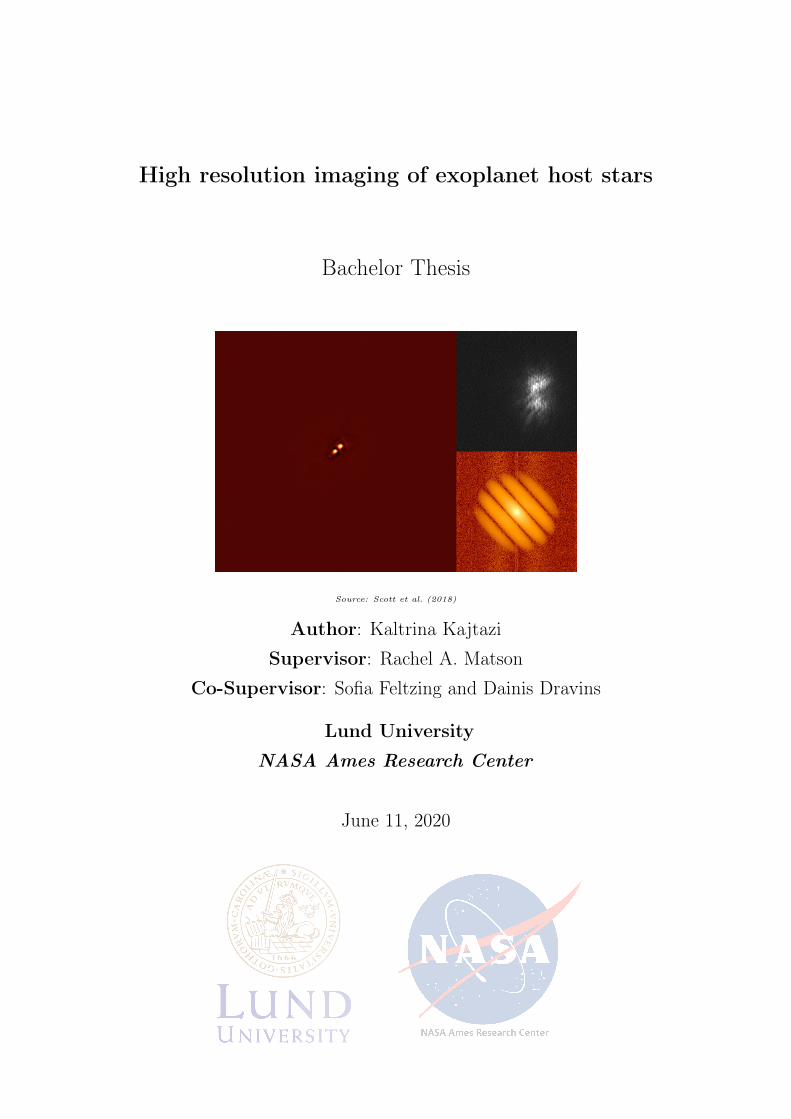
High resolution imaging of exoplanet host stars

Bachelor Thesis

Source: Scott et al. (2018)

Author: Kaltrina KajtaziSupervisor: Rachel A. Matson

Co-Supervisor: Sofia Feltzing and Dainis Dravins

Lund University

NASA Ames Research Center

June 11, 2020

Abstract

This is a thesis project, analysing data from high-resolution imaging observations, specif-ically speckle imaging, as a follow up study of exoplanet host stars observed with K2, thesecond operational phase of the space telescope Kepler. The project was accomplishedat NASA Ames research center under the guidance of Rachel A. Matson, during an in-ternship in collaboration with the Swedish National Space Agency. The speckle imagingdata is from observations with the instruments DSSI and NESSI conducted at the twintelescopes Gemini, in Chile and Hawaii, and WIYN in Arizona. The main goal of theseobservations is to identify possible binary or multiple stellar systems. Scientists have longbeen interested in binary systems mostly because they are not well understood and are agood laboratory for interesting phenomena such as planet formation. In this sample thereare only binaries.

With speckle imaging we can resolve stellar companions with angular separation lessthan 1.2′′, by taking 40ms images. From these images we can resolve all the stars andextract the following parameters; the position angle, the magnitude difference and theangular separation between the two stars. These parameters are then used to estimateproperties for each system studied in this project, aiming to better understand propertiesof binary stellar systems in our Galaxy.

In this project I have determined the following properties; The physical separation,the masses of the individual stars and the orbital period. Out of the total 100 potentialstellar binaries 26 are most likely bound. The stars in the sample have masses in therange 0.2 − 2M�. The systems consist of components that are usually far from eachother, up to 850AU and the closest pair at about 7AU. The orbital period ranges from 15to over 10000 years, most of them being within 3000 years. These calculations are at bestgood estimates of reality. However, this sample still provides a worthy sample of stellarbinaries to study further. The results were also compared in detail to a study of the stellarbinaries in the solar neighbourhood, (Raghavan et al., 2010), looking into similarities anddifferences. It was found that the distributions and trends of the properties agree wellwith Raghavan et al. (2010) and other work.

I find that in my sample the fraction of detected companions is roughly 14%. Be-cause the telescopes have different detection limits the observations were also separatedaccording to telescope; the fraction for Gemini is 15% and for WIYN 8%.

Populärvetenskaplig beskrivning

Stjärnor sägs vara astronomins tidskapsel, genom att studera stjärnor kan vi bättre förståmånga fenomen. Stjärnor är en viktig del av vårt universum från det att de skapas till detatt de dör. De berikar vårt universum med olika grundämnen som krävs för att planeterska bildas och för att liv ska uppstå. Det verkar då självklart varför man vill undersöka ochförstå alla aspekter kring stjärnbildning, stjärnornas livsutveckling och olika stjärnsystem.

Stjärnor bildas från gasmoln, som består av mestadels väte och helium. Ur ett sådantmoln kan många stjärnor i olika storlekar bildas. I den enklaste mening är en stjärnaen gas boll, som lyser tack vare förbränning av väte till helium i dess kärna. Under enstjärnas liv förbränner den tyngre och tyngre ämnen hela vägen till järn innan den dör.Exakt hur en stjärna dör ser olika ut beroende på storlek, men en sak gemensamt är attdet bildas grundämnen tyngre än järn under den stunden.

Att förstå dessa processer är viktigt för att kunna förstå andra relaterade fenomen såsom olika stjärnsystem och planetformation. Till exempel, är det vanligare att stjärnorbildas i par eller ensamma? Den här frågan har länge studerats främst i solens närhet, dådet är enklare att observera och se båda stjärnorna i ett stjärnpar, binärt stjärnsystem,som enskilda stjärnor när de är närmare oss. Det dröjde fram till 70-talet innan en obser-vations metod som kunde särskilja båda stjärnorna i kompakta stjärnpar längre bort komtill. Denna metod kallas "Speckle interfotometri", den bygger på att fotografera stjärn-system med hög optisk upplösning och kort exponeringstid. Från dessa bilder kan man fåut magnitudsskillnaden hos stjärnorna i det dubbla stjärnsystemet, positionsvinkeln förden sekundära stjärnan i jämförelse till huvudstjärnan och vinkelavståndet mellan dem.Idag kan man med ett stort teleskop särskilja båda stjärnorna i ett stjärnpar som är sånär som 1.2 bågsekunder ifrån varandra.

I detta arbete har data från speckle interfotometri analyserats. Med syftet att hitta föl-jande egenskaper från de observationer där en stjärngranne till huvudstjärnan har hittats;fysiskt avstånd mellan stjärnorna i systemet, massan hos varje stjärna och omloppstiden.Resultatet från dessa beräkningar kan användas för att förstå vad det finns för slags binärastjärnsystem i Vintergatan, hur många binära stjärnsystem det finns procentuellt och omde är lika de binära stjärnsystem i närheten av Solen.

Acknowledgements

The writer of this thesis gives big credit to the Swedish national space agency for theirwork and established opportunities for students to gain experience in their field throughdifferent internships such as the one at NASA. Where I completed this project in wonderfulsupervision of Rachel Matson, a scientist at NASA, whom I am very grateful to. She wasa great help, gave clear instructions and room to test the knowledge I have gained inmy studies by letting me try to solve problems myself before answering any questionsthoroughly. From this experience I have learned many new things about speckle imagingand other parts of a science carrier, such as improved skills in Python and informationresearch.

Another thank you goes to Steve B. Howell, chief of division at NASA Ames and headof the Speckle group, for all his help, support and ideas/tips for the project. Furthermore,I would like to thank my thesis supervisors at Lund university professor Sofia Feltzingand Dainis Dravins, for their help to proof read this report and tips until the report wassatisfying.

I also wish to thank my family for their support during application for and during theinternship and thesis writing. Lastly, thank you to the four people that wrote amazingrecommendation letters for me to use in my application for the NASA internship.

Contents

1 Introduction 7

2 Background 92.1 The K2 mission . . . . . . . . . . . . . . . . . . . . . . . . . . . . . . . . . 92.2 Speckle imaging . . . . . . . . . . . . . . . . . . . . . . . . . . . . . . . . . 10

2.2.1 Observations . . . . . . . . . . . . . . . . . . . . . . . . . . . . . . 132.2.2 Instrumentation . . . . . . . . . . . . . . . . . . . . . . . . . . . . . 142.2.3 Data reduction and processing . . . . . . . . . . . . . . . . . . . . . 15

2.3 The sample . . . . . . . . . . . . . . . . . . . . . . . . . . . . . . . . . . . 15

3 Estimation of stellar properties 193.1 Physical separation . . . . . . . . . . . . . . . . . . . . . . . . . . . . . . . 193.2 Masses . . . . . . . . . . . . . . . . . . . . . . . . . . . . . . . . . . . . . . 193.3 Orbital period . . . . . . . . . . . . . . . . . . . . . . . . . . . . . . . . . . 233.4 Error estimation . . . . . . . . . . . . . . . . . . . . . . . . . . . . . . . . 23

4 Results 25

5 Discussion and conclusion 385.1 Bound systems and fractions . . . . . . . . . . . . . . . . . . . . . . . . . . 385.2 Discussion of the method . . . . . . . . . . . . . . . . . . . . . . . . . . . . 395.3 General conclusions from results . . . . . . . . . . . . . . . . . . . . . . . . 405.4 Comparison to Raghavan et al. (2010) . . . . . . . . . . . . . . . . . . . . 435.5 Conclusion . . . . . . . . . . . . . . . . . . . . . . . . . . . . . . . . . . . . 45

6 References 47

Appendices 49

A More plots 49

B Collected data from ExoFOP 61

C Aperture Photometry 66C.1 Aperture photometry information . . . . . . . . . . . . . . . . . . . . . . . 67

D Tabulated results 70

E Comparing filters 84

List of Figures

1 An illustration of the Kepler/K2 space craft. Source: Howell et al. (2014) 92 An illustration of the speckle pattern and image processing that leads to

one signal for each star in a reconstructed image (to the right). Source:Labadie et al. (2010) . . . . . . . . . . . . . . . . . . . . . . . . . . . . . . 10

3 A layout of the instruments. Source: Horch et al. (2009) . . . . . . . . . . 144 Distribution of distances to all the primaries in the sample. Most of the

systems are within 1000 pc which is expected due to the limitations of themethod: Further away means smaller angular separation and harder toresolve. . . . . . . . . . . . . . . . . . . . . . . . . . . . . . . . . . . . . . . 16

5 The visual apparent magnitude as a function of the distance to the system,for all the primaries in the sample. Filter wise colour coded, see legend.Most primaries have magnitude brighter than 14. . . . . . . . . . . . . . . 17

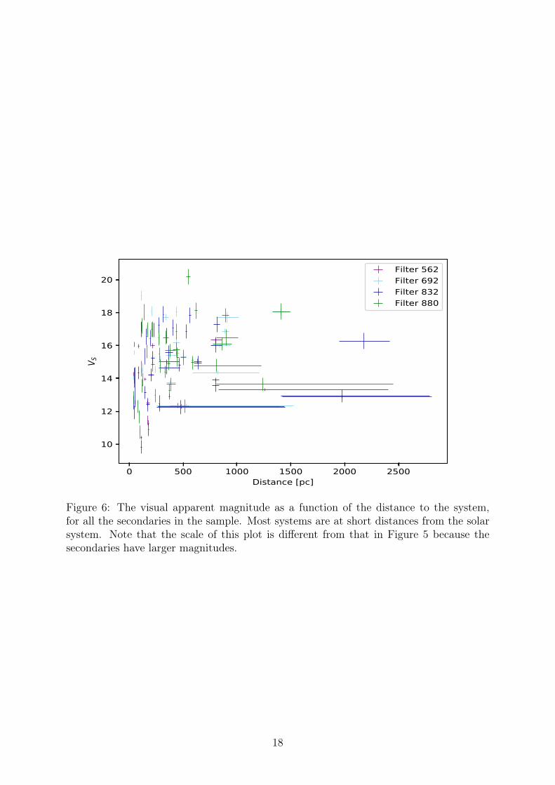
6 The visual apparent magnitude as a function of the distance to the system,for all the secondaries in the sample. Most systems are at short distancesfrom the solar system. Note that the scale of this plot is different from thatin Figure 5 because the secondaries have larger magnitudes. . . . . . . . . 18

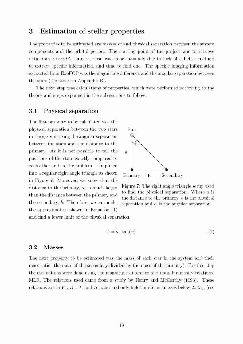
7 The right angle triangle setup used to find the physical separation. Wherea is the distance to the primary, b is the physical separation and α is theangular separation. . . . . . . . . . . . . . . . . . . . . . . . . . . . . . . . 19

8 Skewed distribution. Source: Siegel (2016) . . . . . . . . . . . . . . . . . . 249 A plot of the magnitude difference as a function of the angular separation.

The four filters are shown with different colours (see legend). The verticaldashed lines are at the angular separations 0.2′′ to 1.2′′ with step size of0.2′′, the percentages show the probability for bound stars at each region. . 25

10 The magnitude difference as a function of the angular separation for obser-vations at the Gemini telescopes. Example of detection limit curves andthe probability of being bound based on Matson et al. (2018) are includedhere, see legend. . . . . . . . . . . . . . . . . . . . . . . . . . . . . . . . . . 27

11 The magnitude difference as a function of the angular separation for ob-servation done at the WIYN telescope. The probability for bound stars ateach region is marked out and two detection limit curves are included, seelegend. . . . . . . . . . . . . . . . . . . . . . . . . . . . . . . . . . . . . . . 27

12 The magnitude difference as a function of the physical separation. The plotis the same as the one in 25 in Appendix A, but here optimized to includevalues less than 1000 AU so that the clump at short physical separation iseasier to see. . . . . . . . . . . . . . . . . . . . . . . . . . . . . . . . . . . 30

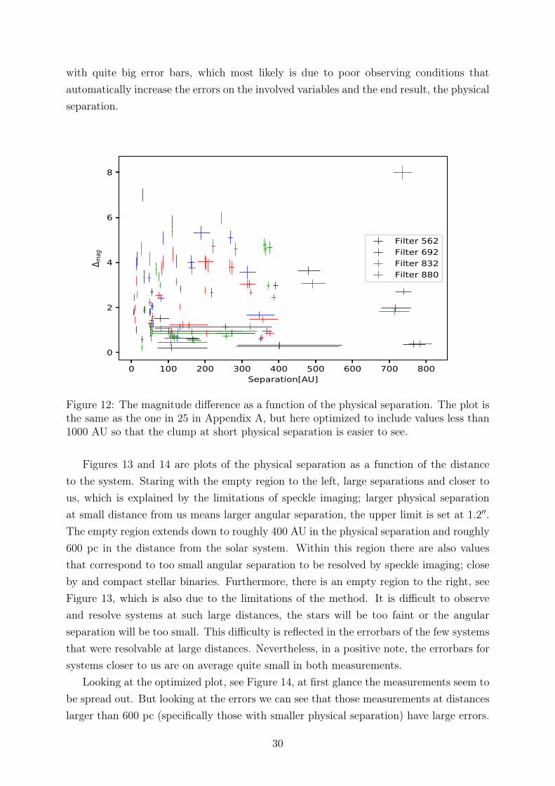
13 The physical separation as a function of the distance to the system. Theplot shows the distribution of the physical separation at different distancesand the quality of the measurements. . . . . . . . . . . . . . . . . . . . . . 31

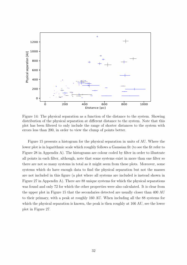
14 The physical separation as a function of the distance to the system. Show-ing distribution of the physical separation at different distance to the sys-tem. Note that this plot has been filtered to only include the range ofshorter distances to the system with errors less than 200, in order to viewthe clump of points better. . . . . . . . . . . . . . . . . . . . . . . . . . . . 32

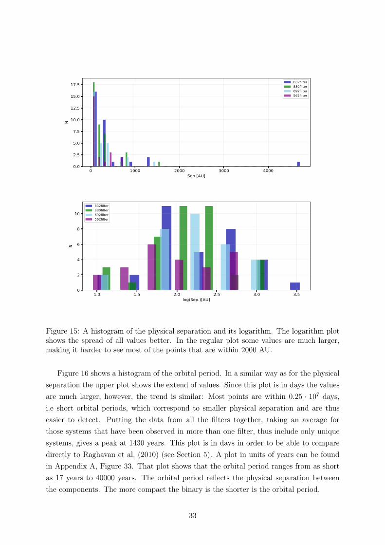
15 A histogram of the physical separation and its logarithm. The logarithmplot shows the spread of all values better. In the regular plot some valuesare much larger, making it harder to see most of the points that are within2000 AU. . . . . . . . . . . . . . . . . . . . . . . . . . . . . . . . . . . . . . 33

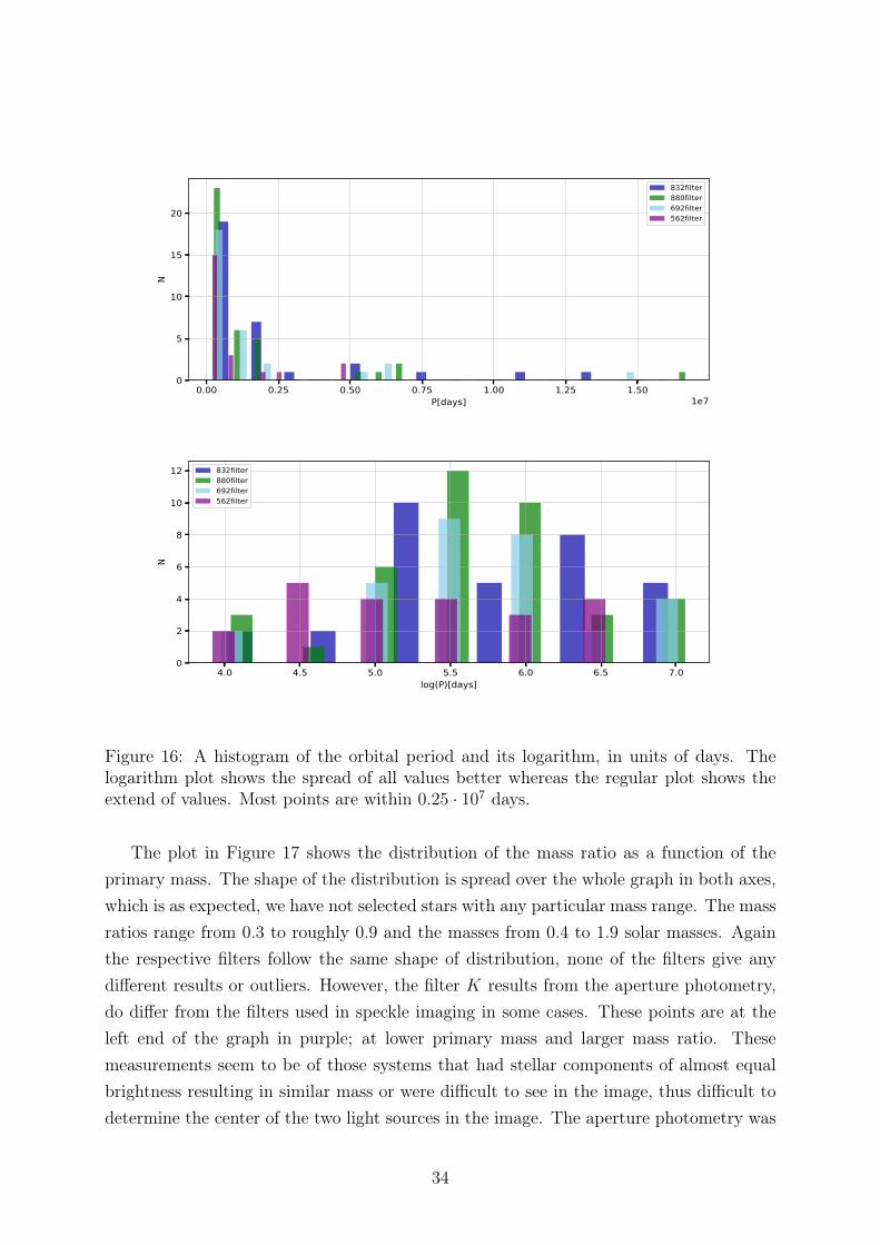
16 A histogram of the orbital period and its logarithm, in units of days. Thelogarithm plot shows the spread of all values better whereas the regularplot shows the extend of values. Most points are within 0.25 · 107 days. . . 34

17 The mass ratio as a function of the primary star mass in the binary. Thisplot also includes the results from aperture photometry in the K-band, seelegend. . . . . . . . . . . . . . . . . . . . . . . . . . . . . . . . . . . . . . . 35

18 The mass ratio as a function of the orbital period. Colour coded accordingto filter used for the observation, see legend. . . . . . . . . . . . . . . . . . 36

19 The mass ratio as a function of the orbital period. Same plot as the oneabove, but here the plot has been optimized in the x-axis, in order to givea better view of the range 0<P<1000 where most points are. . . . . . . . . 37

20 These two plots are a zoomed in version of the physical separation his-tograms shown in earlier sections and in appendices. The left one includesseparations out to 1000 AU, while the right one shows separations up to300 AU. . . . . . . . . . . . . . . . . . . . . . . . . . . . . . . . . . . . . . 43

21 The physical separation as a function of the mass of the primary star inthe binary. . . . . . . . . . . . . . . . . . . . . . . . . . . . . . . . . . . . . 49

22 The physical separation as a function of the mass of the primary star in thebinary. Giving an idea of how far away from each other stars in a systemwith certain primary mass are. This plot is a zoomed in version of the sameone above, in order to see the clump at smaller physical separation better. 50

23 The physical separation as a function of the mass ratio. It gives an idea ofhow far away from each other stars in a system with certain mass ratio are. 51

24 The physical separation as a function of the massratio, but here it is zoomedin to give a better view of the clump of points at shorter physical separation. 51

25 The magnitude difference as a function of the physical separation in unitsof AU. . . . . . . . . . . . . . . . . . . . . . . . . . . . . . . . . . . . . . . 52

26 The physical separation as a function of the number of systems where filtersare separated into subplots to better demonstrate the distribution of thedata from each filter. . . . . . . . . . . . . . . . . . . . . . . . . . . . . . . 53

27 The physical separation as a function of the number of systems, wherefilters are not given. . . . . . . . . . . . . . . . . . . . . . . . . . . . . . . . 54

28 The physical separation as a function of the number of systems, wherefilters are colour coded as shown in the legend. Note that this plot alsoshows the fitted Gaussian to be compared to the paper Raghavan et al.(2010), for the method used here to find the fit, the data must be normalized. 55

29 A histogram of the mass of the primary stars in the systems. It is a wayof displaying how the primary mass is spread out in the sample. . . . . . . 56

30 A histogram of the mass of the secondary star in the systems, showingwhich ranges are more represented. . . . . . . . . . . . . . . . . . . . . . . 56

31 A Mass ratio histogram where the filters are colour coded, see legend. It isa way of displaying how the mass ratio is spread out in the sample acrossthe filters. . . . . . . . . . . . . . . . . . . . . . . . . . . . . . . . . . . . . 57

32 A histogram of the mass ratio filter wise separated to show distribution ineach filter clearly. . . . . . . . . . . . . . . . . . . . . . . . . . . . . . . . . 58

33 A plot of the orbital period and its logarithm as a histogram. The logarithmplot better displays all the values, in a compact manner. This is orbitalperiod in units of years. . . . . . . . . . . . . . . . . . . . . . . . . . . . . 59

34 A histogram of the orbital period in units of days and its logarithm, wherean average Gaussian fit was applied. . . . . . . . . . . . . . . . . . . . . . . 60

35 An image from AO observations of the target with epicname 212703473conducted at Palomar telescope. Source: ExoFOP database. . . . . . . . . 66

List of Tables

1 The table below shows the information for the 26 potential bound systems(within 0.4′′ angular separation). The information consists of the epicname,the magnitude difference with errors, the angular separation (which has agiven error of 0.002′′) and the physical separation in units of AU withasymmetric errors. . . . . . . . . . . . . . . . . . . . . . . . . . . . . . . . 28

2 This table has all the information found on ExoFOP for the 562 filter. . . . 613 This table has all the information found on ExoFOP for the 692 filter. . . . 624 This table has all the information found on ExoFOP for the 832 filter. . . . 635 This table has all the information found on ExoFOP for the 880 filter. . . . 646 This table has all the information found on ExoFOP for the K-band. . . . 657 This table shows the information needed to repeat the aperture photometry

and get the same results. . . . . . . . . . . . . . . . . . . . . . . . . . . . . 678 This table shows the median of the physical separation in astronomical

units and the corresponding asymmetric errors. . . . . . . . . . . . . . . . 709 In this table the median of the primary mass, referred to as MP , the sec-

ondary mass, referred to as MS and the mass ratio, referred to as Ratio,together with their asymmetric errors referred to as "upper" and "lower"is shown for the 562 filter. . . . . . . . . . . . . . . . . . . . . . . . . . . . 74

10 In this table the median of the primary mass, MP , the secondary mass, MS

and the mass ratio, "Ratio", together with their asymmetric errors referredto as "upper" and "lower" are shown for the 692 filter. . . . . . . . . . . . 75

11 In this table the median of the primary mass, MP , the secondary mass, MS

and the mass ratio, "Ratio", together with their asymmetric errors referredto as "upper" and "lower" are shown for the 832 filter. . . . . . . . . . . . 76

12 In this table the median of the primary mass, MP , the secondary mass, MS

and the mass ratio, "Ratio", together with their asymmetric errors referredto as "upper" and "lower" are shown for the 880 filter. . . . . . . . . . . . 77

13 In this table the median of the primary mass, MP , the secondary mass,MS and the mass ratio, "Ratio", together with their asymmetric errorsreferred to as "upper" and "lower" are shown for the K-band. When everthere were more than one image the results from each image were averagedto one value. . . . . . . . . . . . . . . . . . . . . . . . . . . . . . . . . . . . 78

14 This table shows the results from photometry. Here are the values of themagnitude difference and the corresponding standard deviation. . . . . . . 79

15 This table shows the values of the orbital period and the correspondingasymmetric errors for all of the systems. . . . . . . . . . . . . . . . . . . . 80

16 This table shows the physical separation for all the systems which haveknown distances to the primary star. Here one can see the results from allfilters and compare to see if they match. . . . . . . . . . . . . . . . . . . . 84

17 This table shows the orbital period. Here one can see the results from allfilters and compare to see if they match. Note that those that have noresults is due to lack of reliable angular separation value and was not givenon ExoFOP at all. . . . . . . . . . . . . . . . . . . . . . . . . . . . . . . . 86

18 This table shows the mass of the primary, where it is easy to see the resultsfrom each filter and conclude how similar they are. In the same table thereis a column with the results from aperture photometry in K-band. . . . . . 88

19 This table shows the mass of the secondary, where it is easy to see theresults from each filter used in speckle imaging and the aperture photometryresults in K-band, to conclude how similar they are. . . . . . . . . . . . . . 90

20 This table shows the mass ratio, where it is easy to see the results fromeach filter used in speckle imaging. The results from the performed aperturephotometry are also included, in order to compare all the filters side by side. 92

1 Introduction

The existence of stellar binary systems has long been known. In fact it is believed thatmost stars are not born single. Rigorous statistical studies of the solar neighbourhood1

have investigated this idea to give a better picture of the fraction of stellar binaries. Thepercentage of stellar binaries in the solar neighbourhood is 40− 50%, which is consistentwith studies of samples of stars outside the solar neighbourhood as well (Raghavan et al.,2010; Matson et al., 2018). This will be shown to be true for the sample studied in thisproject.

The definition of a stellar binary system is as follows; two stars that are bound toeach other through gravity and orbit around a common center of mass. Stellar binariesas those detected in this sample usually consist of a more massive, brighter target star,which is easier to detect and a smaller, less bright companion. Moreover, it is worthnoting that there are many types of binary systems, in this project we are only interestedin binary systems with members that are still on the main sequence and are believed tohave planets. For reference other binary systems can consist of stars in other stages oftheir evolution such as neutron stars. All of these are interesting in different ways andare laboratories for different aspects of fundamental astrophysics. It is thus clear that theinterest for all known types of binaries has long been thriving and is well founded, it isindeed a part of the universe which needs more exploration and understanding.

Binary systems of stars on the main sequence became more important to pay attentionto from the moment we started searching and detecting planets outside of our solar system.Because there are many questions to be answered about planet formation in general, butespecially planet formation in stellar binary systems which we know little about. Bystudies of stellar binaries such as this one, we want to, amongst other aspects, betterunderstand the main properties of the systems such as the orbital period and the stellarmasses, to see if trends that have been proven to hold for stellar binaries without knownplanets in the solar neighbourhood are also visible in stellar binaries with planets in otherparts of the Galaxy.

More specific examples where exoplanet2 follow up programs such as speckle imaginghave been useful are the following: Identifying false positives, which refers to stellarcompanions (especially eclipsing3 ones) that in planet detection methods, such as thetransit method4, mimic a planet. A companion can as it moves along its orbit give rise to

1 In the papers mentioned and compared to in this thesis, the solar neighbourhood is defined to be outto 25 pc from the Sun.

2 Exoplanet is the term assigned to a planet not in the solar system.3 For eclipsing binaries the orbital plane that they move in, is close to the line of sight. Therefore the

stars obscure each other as they move in their orbit.4 The transit method is based on continuous measure of light from a star of interest. The measurements

are plotted as a so called light curve, presenting the change in brightness of the star over time. Decreasein the brightness is called a dip.

7

periodic dips in the light curve as it passes in front of the observed star in the same way asa planet would. By identifying such companions, scientists will be able to distinguish realplanets from false positives in their data. Moreover, detecting companions and knowingtheir properties can help to correct the planet radius of any planet in a stellar binarysystem by using relation formulas such as those in Teske et al. (2018). The planet radiusis underestimated due to that the flux from the companion is collected as part of thelight of the target star. Not correcting for this leads to an overestimation of small (rocky)planets, Hirsch et al. (2017).

These are just some examples of why stellar binary systems in particular are of interestto study. Binaries have many fundamental astrophysical properties yet to be understood,not only planet formation but also more underlying physics: How do stars interact in abinary? What are the conditions and consequences of stellar mergers at different evolu-tionary stages in binaries? What happens to the system as the stars evolve? How doesthat impact any existing planets? How do these systems compare to the solar neighbour-hood? What type of stars are usually found in binaries? The two later questions can beaddressed by looking at the K2 sample as done in this project. A sample of stars that werefirst observed by K2, the second operational phase of the space telescope Kepler in searchfor exoplanets. The main goals of this project are; to understand and characterize binarystars with exoplanets outside of the solar neighbourhood in terms of stellar properties andfrequency. The results are then compared to a study of nearby stellar binary systems inRaghavan et al. (2010). From this we hope to learn what type of stellar binaries haveplanets and how the distribution of their properties compare to the solar neighbourhood.

This thesis report will begin with a description of the K2 mission in Section 2.1. Athorough explanation about speckle imaging in Section 2.2; its theory, usage and limita-tions including a brief introduction to observations in Section 2.2.1, a presentation of theinstruments in Section 2.2.2 and an introduction of data reduction in Section 2.2.3. Thelast three sections mentioned contain a literature review of parts of speckle imaging thatare only meant as context and a brief presentation of the full picture of speckle imaging,thus are not actually performed by the student and writer of this report. The data usedwere already reduced beforehand and loaded into ExoFOP.5 The observations were doneby the NASA speckle imaging group over the years 2016-2018. The theory of calculationsand other methods used is given in Sections 3.1 through 3.3. Moreover, the extra stepfor a quick check of the derived masses; aperture photometry on adaptive optics images,is briefly explained in Appendix C. In Section 2.3 the full sample is presented and theresults are presented in Section 4. Furthermore, a discussion about the method, how theproject has gone, what the future goals are and the conclusions, are given in Section 5.

5 ExoFOP is a NASA database for Kepler, K2 and TESS exoplanet follow-up imaging and spectroscopyobservations. https://exofop.ipac.caltech.edu/k2/edit_target.php?id=201089381

8

2 Background

2.1 The K2 mission

As aforementioned K2 is the second operational phase of Kepler, a space telescope launchedby NASA in 2009, which was re-purposed due to a failure in two reaction wheels usedto align the telescope. This problem meant that the space craft could not maintain asteady pointing. This was solved for K2 by using solar radiation to balance the spacecraft. However, this fix also meant that the field of view needed to shift every 80 days,so that after every 80 days the telescope observed another part of the sky. Such a set ofobservations for 80 days is referred to as a campaign.

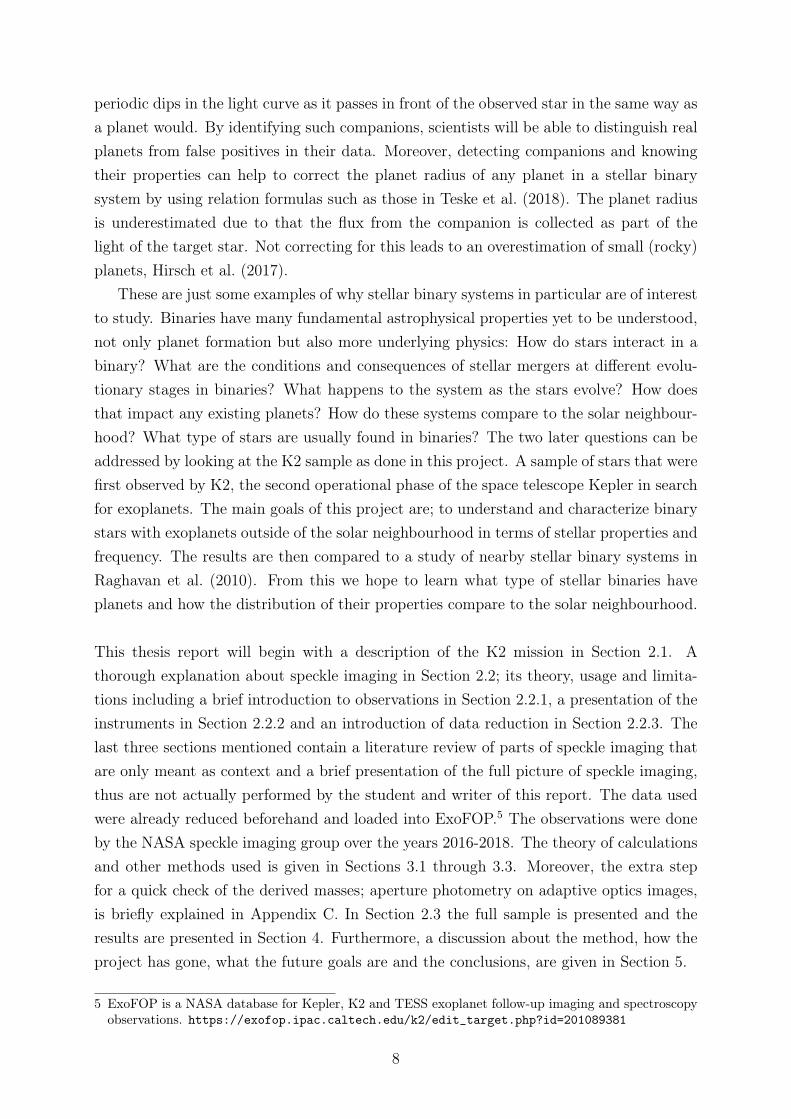
In this way K2 observations include different types of targets and environments thanfirst intended with Kepler (see Figure 1 for a schematic view of the spacecraft). Fur-thermore, K2 (and Kepler) were not intended to look for stellar binaries in particular,therefore the samples from these missions are not only randomized but also unbiased to-wards stellar binaries (Howell et al., 2014). Moreover, the K2 samples studied by speckleimaging and added to ExoFOP, have previously been shown to host exoplanet candidates,using transit observations, and for some cases planets have indeed been confirmed (Horchet al., 2012).

Figure 1: An illustration of the Kepler/K2space craft. Source: Howell et al. (2014)

The Kepler spacecraft orbits in a he-liocentric orbit at 0.5AU away from Earth,carrying a Schmidt telescope of 0.95m witha 110 degree field of view. The large field ofview makes it possible to observe many tar-gets at the same time, with high precisionphotometry (Howell et al., 2014). However,this also means that it cannot resolve anyclose companions, due to its low spatial res-olution and large pixel scale; any close com-panions fall within the same camera pixelas the targeted star (Hirsch et al., 2017).Henceforth, speckle imaging is an impor-tant follow up program, for finding andresolving any companions to the targetedstars and study them further (for more de-tailed reading about K2, see Howell et al. (2014)).

9

2.2 Speckle imaging

The most challenging problem with ground based telescopes is the disturbance and lim-itations caused by Earth’s atmosphere and weather conditions. However, there are waysto optimize the surroundings in order to get better results, such as choosing a good posi-tion; high grounds where air, humidity and weather conditions are at best many days ofthe year. Nevertheless, the effects from the atmosphere cannot be excluded completely.However, in attempts to minimize the loss of spatial resolution due to atmospheric distur-bances and quality, a new method based on short integration time and small field of viewwas explored in the 70s. Although, at that time due to technical limitations the methodwas only applicable to bright stars. Nevertheless, in the 90s, technology such as bettercameras and telescopes made this method possible to use on faint stars too.

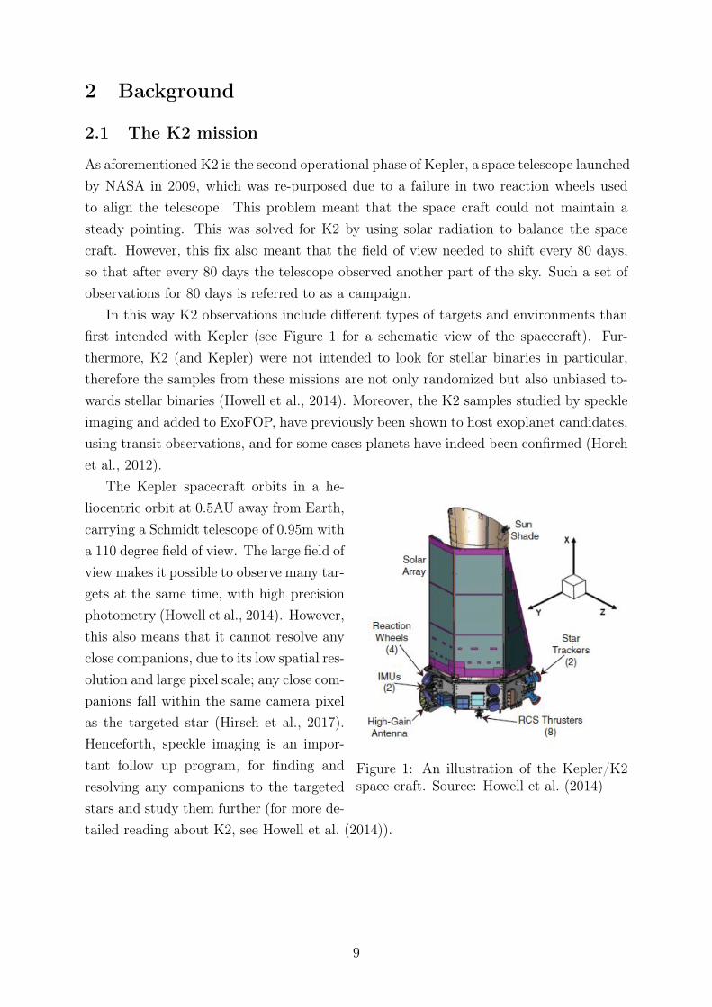
It turns out that by taking images with short integration time, 40ms-80ms, and highspatial resolution, the disturbance from the atmosphere is "frozen" in time resulting ina clean and high quality image, where only a few photons are collected per position(snapshots). These images can then be processed to, for example, find nearby companions.With longer exposure times the collected light tends to merge into a big blob of photonsall falling at different positions in the camera, leading to loss of information and inclusionof too much background noise from the atmosphere. It is also necessary to understandthat the longer the exposure the more elongated and blurred will the speckles be untilthey are no longer separated. Thereby, with this method of short exposures new usefulinformation is brought to light about the objects observed that is not visible in longexposures. Figure 2 illustrates how the speckle pattern looks like and how it compares toa long exposure image (the middle pictures).

Figure 2: An illustration of the speckle pattern and image processing that leads to onesignal for each star in a reconstructed image (to the right). Source: Labadie et al. (2010)

10

This method is called "Speckle imaging" or "Speckle interferometry" due to the patternseen on the images of a light source, which resembles many small speckles. This patternis visible for any point source, for which light is collected with short integration time,due to fluctuations caused by the seeing, which is how much the turbulence of Earth’satmosphere distorts an image (which is the reason why stars appear to twinkle on thenight sky). Single light sources will show a collection of many identical single specklesclosely spaced. While multiple stellar systems, such as binaries, give rise to pairs ofidentical speckles. This is mainly how targets with companions are directly distinguishedfrom single stars.

One can compare speckle imaging to Young’s double slit theory, where waves or par-ticles (that also behave as waves in certain cases) always show a fringe pattern as theyenter through two slits, because the waves interfere with themselves. The fringe pattern inFourier space (the frequency plane) of speckle images, is simply a result of self-interferenceof the photons as they fall through the atmosphere similar to that in the double slit ex-periment. In speckle observations the speckle pairs act as "the slits" which in Fourierspace give rise to a fringe pattern. Moreover, since the field of view is small the speckles(slits) are closely spaced. That is the photons that are collected from the two sourcesin principal fall through the same position in the atmosphere, which results in identicalspeckle pairs. This characteristic is important because it gives a clean fringe pattern,which is vital for high precision in the resulting parameters extracted from the images.The fringe pattern, how the waves self-interact similar to Young’s double slit experiment,can be demonstrated easily for the naked eye by stacking a couple of speckle images andshining monochromatic light through the speckles onto a blank background. Or it caneven be visible directly through a telescope (using real time video mode), when the seeingis exceptional and the telescope’s spatial resolution is good. Thereby, it becomes clear whythe pattern with speckle pairs is visible only for systems with two stars not for single stars.

This powerful observational method began as a way to resolve very close-by compan-ions to any star of interest in order to understand multiple stellar systems. Later whenexoplanets became a hot topic with the initiation of many missions to search for themsuch as Kepler, follow up speckle imaging programs were conducted both for Kepler andK2 (and other missions) stars in search for false positives; A dip in the light curve of theobserved star that indicates a planet but is caused by a background star or a physicalcompanion.

Moreover, as mentioned it was soon understood that a companion, background star orbinary companion, can cause us to underestimate the radii of exoplanets. A larger radiustranslates into higher density, meaning rocky planet, thus leading to an overestimation ofthat planet category. Therefore, it is vital for accurate characterization of all exoplanetsto correct the radius. It is also interesting to find correlations between stellar and exo-

11

planet properties and better understand planet formation and evolution in stellar binaries.

Even though speckle imaging is used in many studies with different purposes, sometimesjust as a method of fast, high spatial resolution imaging, the method has limitations, somebeing enforced by observing conditions and others by the method itself. The main one isthe detection limit on the magnitude of the companion, which depends on the telescopeparameters. There is a strong correlation between how faint the companion can be andthe size of the telescope mirrors that determines if a companion is detected. Moreover,the ability to detect a companion can be decreased by bad seeing conditions. In occasionswith bad seeing, for example 1.4′′, companions at a separation of less than roughly 1.3′′-1.2′′ , or very faint (larger than ≈11-10 magnitude) will not be clearly or at all resolvable,even if the same companions would be possible to see with that telescope otherwise. Thisproblem can be worked around by observing the same targets another night with betteratmospheric conditions. The speckle imaging method’s limitations, such as lower limit onresolvable angular separation, can only be improved by new and better instruments.

In order to account for these limitations for each observation, the minimum brightnessfor a companion to be detected at different distances from the target star, are put togetherinto a detection limit curve that is calculated for each target, filter and telescope at everyobserving run. From many such curves one can derive an average for each telescope andget a better view of what is the typical range of magnitude difference at different angularseparations that can be detected at that telescope (Matson et al., 2018; Howell et al.,2011). This is important to understand, because it shows what observers need to knowbefore hand and how far the method can be pushed without compromising the data.

Another constraint on the method involves angular separation between the target starand its companion. The detectable range of angular separations is usually set at between0.02 -1.2′′. The lower limit is enforced by the telescope parameters. That is the diffrac-tion limit of the telescope, which depends on the wavelength of the light collected and thediameter of the mirror, constraining how small angular separations we can resolve in theimages. The upper limit can be increased to 2′′, however, the data is not reliable at suchlarge separations. The reason being that the speckles get more elongated and the fringepattern more blurred as light does not fall through the same patch of the atmosphere,thus the speckles are no longer correlated. Moreover, sometimes speckle pairs can falloutside the field of view of the instrument. In both cases the fringe pattern in Fourierspace is not as clear or focused, resulting in unreliable parameters (Horch et al., 2012;Howell et al., 2011).

In conclusion speckle imaging is a powerful tool for observations which has opened upmany new fields of astronomy and is widely used.

12

2.2.1 Observations

Firstly, the observations of the sample in this project were not done by the student.Thus this section consists of a brief literature study of the main parts of speckle imagingobservations to give context and a complete picture of the subject.

All speckle imaging observations, that are done by the science group at NASA AmesResearch Center, are done at the Gemini-telescopes and WIYN using the instrumentsDSSI, Alopeke, NESSI and the newly commissioned Zorro instrument. The data used inthis thesis come from observations done at these telescopes using the instruments DSSIand NESSI.

The Gemini-telescopes are two twin telescopes located in Hawaii (Gemini-North) andChile (Gemini-South). These have 8.1m primary mirrors and secondary mirrors of 1m di-ameter.6 The WIYN telescope is smaller, it consists of a primary mirror of 3.5m diameterand a 1.2m in diameter secondary mirror, located in Arizona USA.7

In short the observing procedure includes software such as the image/video display pro-gram SAOImageDS9, a telescope and a speckle instrument. Nowadays, the observationscan easily be done remotely, but even on site it usually consists of computer work. Thescience target is viewed as an image or in real time using video mode in SAOImageDS9.To determine or change how much light is collected per image the parameter "gain" isadjusted manually. The parameter "gain" determines how much the signal is magnifiedby controlling the multiplication register in the detector before read out, so that the signalgets stronger. The goal is to collect enough light for a good signal without saturatingthe detector (which means photons "run over" into another pixel giving bad read outs,this happens at too large gain). For fainter targets the "gain" used must be higher, inthis way there will still be a useful signal even with few photons. The necessary amountof photons is around 10000 counts and no higher than roughly 30000, with a saturationlimit at roughly 65000 (Everett et al., 2015; Labadie et al., 2010).

Once the gain is set to the desired value different number of sets of 1000 framesare saved per target, reading out only 256x256 pixels of the full frame of the EMCCD(electron multiplying CCD) camera each time, because it is less time consuming and takesless storage space (Howell et al., 2011). The number of sets is determined by how faint thetarget and the companion are, if faint then the number of sets is increased but is alwayswithin the range of 3-12 sets (Everett et al., 2015; Horch et al., 2012).

The integration time for each image can be 40-80ms depending on which is best forthe instrument and telescope used. For the observations of this sample the integration

6 See more about the Gemini telescopes on the official telescope website: https://www.gemini.edu/observing/telescopes-and-sites/telescopes

7 See more about the WIYN telescope on the official telescope website: https://www.wiyn.org/About/overview.html

13

time was 40ms per image. In Howell et al. (2011), this was found to be best for speckleimaging observations with their instruments and is not varied with seeing.

2.2.2 Instrumentation

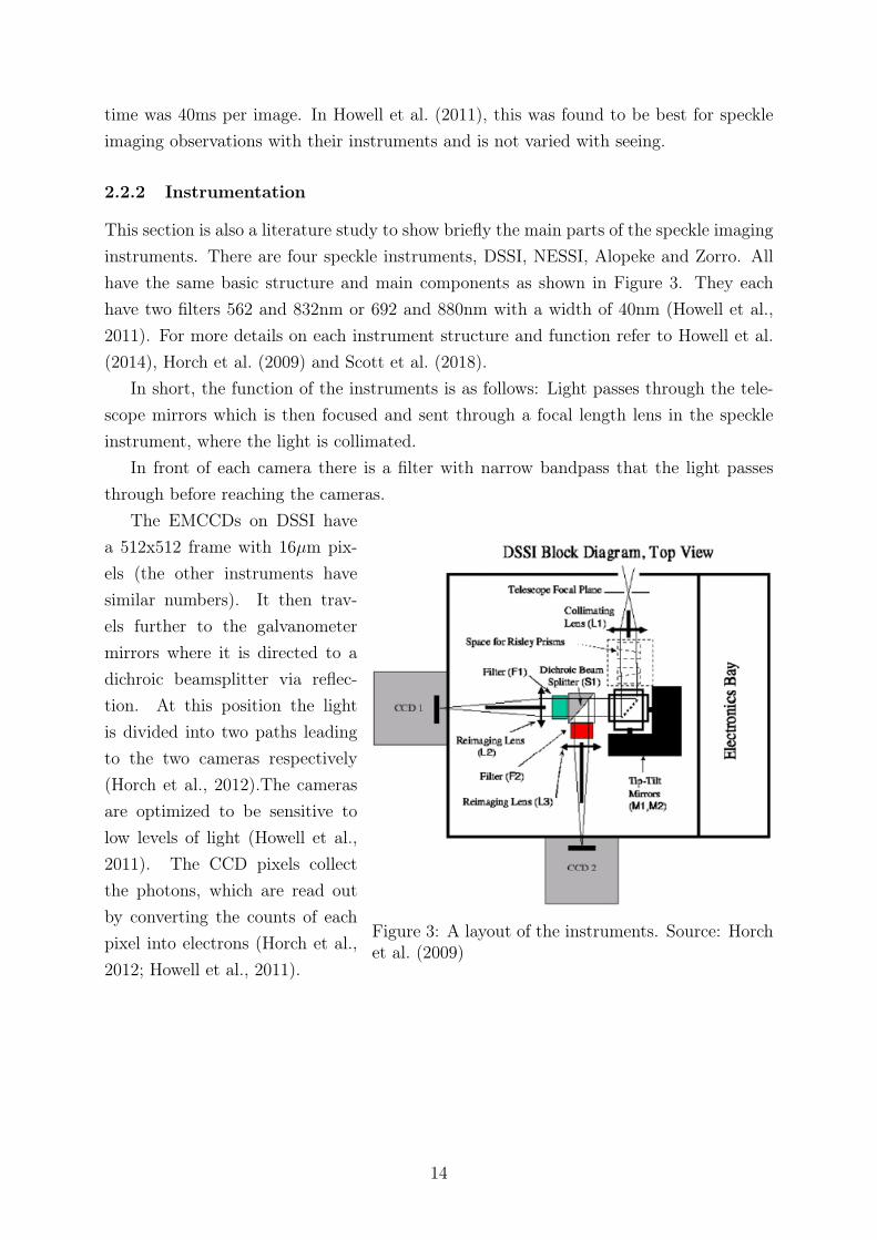
This section is also a literature study to show briefly the main parts of the speckle imaginginstruments. There are four speckle instruments, DSSI, NESSI, Alopeke and Zorro. Allhave the same basic structure and main components as shown in Figure 3. They eachhave two filters 562 and 832nm or 692 and 880nm with a width of 40nm (Howell et al.,2011). For more details on each instrument structure and function refer to Howell et al.(2014), Horch et al. (2009) and Scott et al. (2018).

In short, the function of the instruments is as follows: Light passes through the tele-scope mirrors which is then focused and sent through a focal length lens in the speckleinstrument, where the light is collimated.

In front of each camera there is a filter with narrow bandpass that the light passesthrough before reaching the cameras.

Figure 3: A layout of the instruments. Source: Horchet al. (2009)

The EMCCDs on DSSI havea 512x512 frame with 16µm pix-els (the other instruments havesimilar numbers). It then trav-els further to the galvanometermirrors where it is directed to adichroic beamsplitter via reflec-tion. At this position the lightis divided into two paths leadingto the two cameras respectively(Horch et al., 2012).The camerasare optimized to be sensitive tolow levels of light (Howell et al.,2011). The CCD pixels collectthe photons, which are read outby converting the counts of eachpixel into electrons (Horch et al.,2012; Howell et al., 2011).

14

2.2.3 Data reduction and processing

At the end of an observing run the data needs to be reduced. Today most instruments havea dedicated pipeline for this. The data from the different filters is processed separately.The reduction of the data used in this project was done by Mark Everett at NationalOptical Astronomy Observatory. Thus this section is included here only to give contextand a brief description.

In the first step the frames are looked through and removed if the pattern is unclearor has any other imperfections, such as too few photons. The pipeline then searcheseach frame to identify those with the same speckle separation, all these frames are thenstacked together for each set and averaged over all sets for better results and higher signalto noise ratio. This average is then Fourier transformed to its power spectrum; a spatialfrequency function in Fourier space (Horch et al., 1996; Horch et al., 2010). The resultingfringe pattern of the science target is then fitted to a fringe model, which finally gives theseparation between the stars and the magnitude difference (Horch et al., 2010).

To find the position angle8 of the companion, bispectral analysis is applied. Moreover,from this information a reconstructed image where both stars are visible as two lightsources can be reconstructed (Horch et al., 2012).

2.3 The sample

The sample for this project consists of stars with a mass range of 0.2-2M�, assumed to beon the main sequence. The speckle imaging observations were done with the instrumentsDSSI at Gemini north/south and NESSI at WIYN, where the aim was to look for closecompanions. These stars are KOI (K2 objects of interest) from the K2 mission, whichare believed to be exoplanet candidate hosts. Actually for this sample some systems dohave confirmed planets and some have confirmed candidates which is interesting, but inthis project the focus is on the stars in the system. We need to understand the stars first,then study aspects and questions related to the planets in stellar binaries.

8 The position angle is defined as the position in the sky of the companion compared to the targetedstar and us. Note that this parameter was not necessary for my calculations of the properties.

15

0 1000 2000 3000 4000 5000 6000Distance [pc]

0

5

10

15

20

25

30

35N

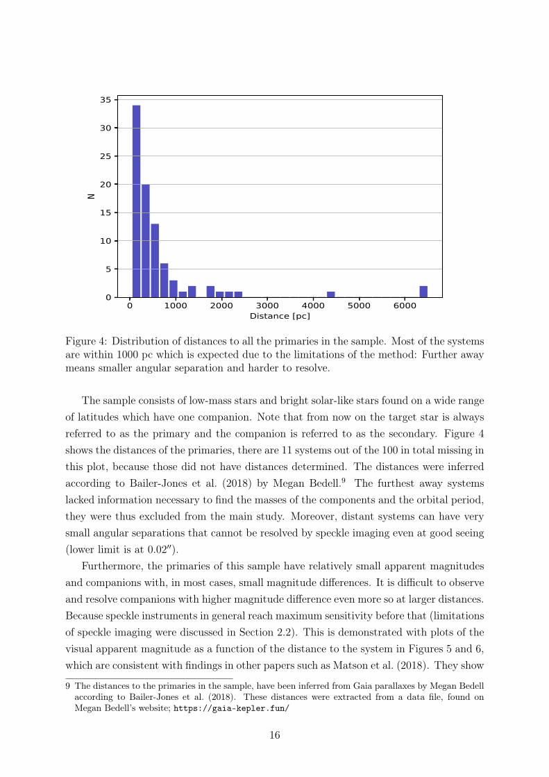
Figure 4: Distribution of distances to all the primaries in the sample. Most of the systemsare within 1000 pc which is expected due to the limitations of the method: Further awaymeans smaller angular separation and harder to resolve.

The sample consists of low-mass stars and bright solar-like stars found on a wide rangeof latitudes which have one companion. Note that from now on the target star is alwaysreferred to as the primary and the companion is referred to as the secondary. Figure 4shows the distances of the primaries, there are 11 systems out of the 100 in total missing inthis plot, because those did not have distances determined. The distances were inferredaccording to Bailer-Jones et al. (2018) by Megan Bedell.9 The furthest away systemslacked information necessary to find the masses of the components and the orbital period,they were thus excluded from the main study. Moreover, distant systems can have verysmall angular separations that cannot be resolved by speckle imaging even at good seeing(lower limit is at 0.02′′).

Furthermore, the primaries of this sample have relatively small apparent magnitudesand companions with, in most cases, small magnitude differences. It is difficult to observeand resolve companions with higher magnitude difference even more so at larger distances.Because speckle instruments in general reach maximum sensitivity before that (limitationsof speckle imaging were discussed in Section 2.2). This is demonstrated with plots of thevisual apparent magnitude as a function of the distance to the system in Figures 5 and 6,which are consistent with findings in other papers such as Matson et al. (2018). They show

9 The distances to the primaries in the sample, have been inferred from Gaia parallaxes by Megan Bedellaccording to Bailer-Jones et al. (2018). These distances were extracted from a data file, found onMegan Bedell’s website; https://gaia-kepler.fun/

16

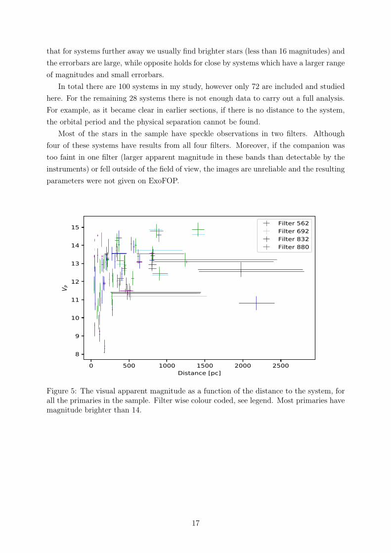
that for systems further away we usually find brighter stars (less than 16 magnitudes) andthe errorbars are large, while opposite holds for close by systems which have a larger rangeof magnitudes and small errorbars.

In total there are 100 systems in my study, however only 72 are included and studiedhere. For the remaining 28 systems there is not enough data to carry out a full analysis.For example, as it became clear in earlier sections, if there is no distance to the system,the orbital period and the physical separation cannot be found.

Most of the stars in the sample have speckle observations in two filters. Althoughfour of these systems have results from all four filters. Moreover, if the companion wastoo faint in one filter (larger apparent magnitude in these bands than detectable by theinstruments) or fell outside of the field of view, the images are unreliable and the resultingparameters were not given on ExoFOP.

0 500 1000 1500 2000 2500Distance [pc]

8

9

10

11

12

13

14

15

V P

Filter 562Filter 692Filter 832Filter 880

Figure 5: The visual apparent magnitude as a function of the distance to the system, forall the primaries in the sample. Filter wise colour coded, see legend. Most primaries havemagnitude brighter than 14.

17

0 500 1000 1500 2000 2500Distance [pc]

10

12

14

16

18

20

V S

Filter 562Filter 692Filter 832Filter 880

Figure 6: The visual apparent magnitude as a function of the distance to the system,for all the secondaries in the sample. Most systems are at short distances from the solarsystem. Note that the scale of this plot is different from that in Figure 5 because thesecondaries have larger magnitudes.

18

3 Estimation of stellar properties

The properties to be estimated are masses of and physical separation between the systemcomponents and the orbital period. The starting point of the project was to retrievedata from ExoFOP. Data retrieval was done manually due to lack of a better methodto extract specific information, and time to find one. The speckle imaging informationextracted from ExoFOP was the magnitude difference and the angular separation betweenthe stars (see tables in Appendix B).

The next step was calculations of properties, which were performed according to thetheory and steps explained in the sub-sections to follow.

3.1 Physical separation

Primary

�Sun

Secondaryb

a

α

Figure 7: The right angle triangle setup usedto find the physical separation. Where a isthe distance to the primary, b is the physicalseparation and α is the angular separation.

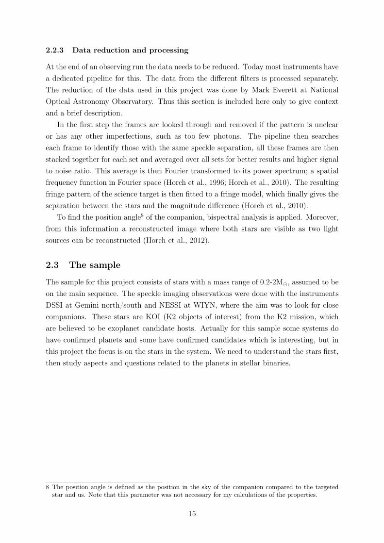
The first property to be calculated was thephysical separation between the two starsin the system, using the angular separationbetween the stars and the distance to theprimary. As it is not possible to tell thepositions of the stars exactly compared toeach other and us, the problem is simplifiedinto a regular right angle triangle as shownin Figure 7. Moreover, we know that thedistance to the primary, a, is much largerthan the distance between the primary andthe secondary, b. Therefore, we can makethe approximation shown in Equation (1)and find a lower limit of the physical separation.

b = a · tan(α) (1)

3.2 Masses

The next property to be estimated was the mass of each star in the system and theirmass ratio (the mass of the secondary divided by the mass of the primary). For this stepthe estimations were done using the magnitude difference and mass-luminosity relations,MLR. The relations used came from a study by Henry and McCarthy (1993). Theserelations are in V -, K-, J- and H-band and only hold for stellar masses below 2.5M� (see

19

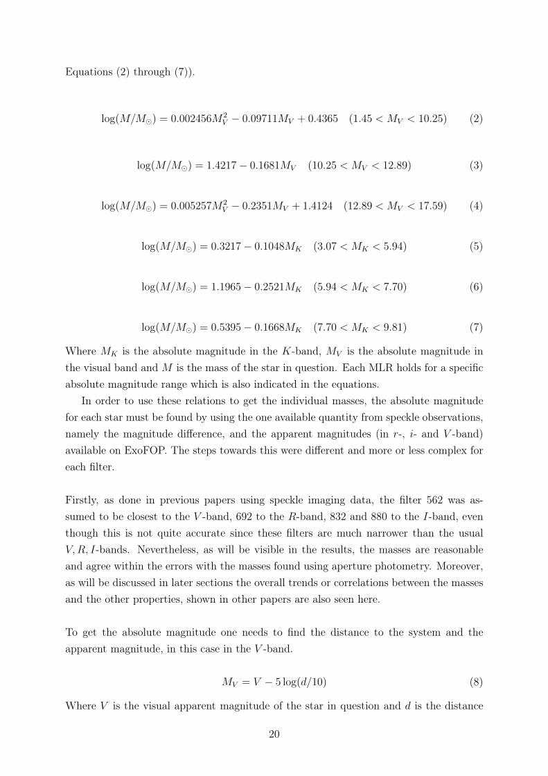
Equations (2) through (7)).

log(M/M�) = 0.002456M2V − 0.09711MV + 0.4365 (1.45 < MV < 10.25) (2)

log(M/M�) = 1.4217− 0.1681MV (10.25 < MV < 12.89) (3)

log(M/M�) = 0.005257M2V − 0.2351MV + 1.4124 (12.89 < MV < 17.59) (4)

log(M/M�) = 0.3217− 0.1048MK (3.07 < MK < 5.94) (5)

log(M/M�) = 1.1965− 0.2521MK (5.94 < MK < 7.70) (6)

log(M/M�) = 0.5395− 0.1668MK (7.70 < MK < 9.81) (7)

Where MK is the absolute magnitude in the K-band, MV is the absolute magnitude inthe visual band and M is the mass of the star in question. Each MLR holds for a specificabsolute magnitude range which is also indicated in the equations.

In order to use these relations to get the individual masses, the absolute magnitudefor each star must be found by using the one available quantity from speckle observations,namely the magnitude difference, and the apparent magnitudes (in r-, i- and V -band)available on ExoFOP. The steps towards this were different and more or less complex foreach filter.

Firstly, as done in previous papers using speckle imaging data, the filter 562 was as-sumed to be closest to the V -band, 692 to the R-band, 832 and 880 to the I-band, eventhough this is not quite accurate since these filters are much narrower than the usualV,R, I-bands. Nevertheless, as will be visible in the results, the masses are reasonableand agree within the errors with the masses found using aperture photometry. Moreover,as will be discussed in later sections the overall trends or correlations between the massesand the other properties, shown in other papers are also seen here.

To get the absolute magnitude one needs to find the distance to the system and theapparent magnitude, in this case in the V -band.

MV = V − 5 log(d/10) (8)

Where V is the visual apparent magnitude of the star in question and d is the distance

20

to the system. Note that extinction has been neglected because all systems are within1000pc and most of them within even shorter distance than that. However, this will affectthe mass estimates and the accuracy, resulting in smaller values, which we are aware of.Therefore, we see these masses as only estimates of a minimum and in the future for moreaccurate mass measurements the first step would be to include extinction.

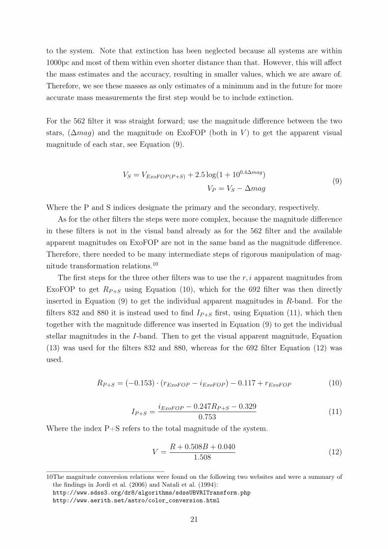
For the 562 filter it was straight forward; use the magnitude difference between the twostars, (∆mag) and the magnitude on ExoFOP (both in V ) to get the apparent visualmagnitude of each star, see Equation (9).

VS = VExoFOP (P+S) + 2.5 log(1 + 100.4∆mag)

VP = VS −∆mag(9)

Where the P and S indices designate the primary and the secondary, respectively.As for the other filters the steps were more complex, because the magnitude difference

in these filters is not in the visual band already as for the 562 filter and the availableapparent magnitudes on ExoFOP are not in the same band as the magnitude difference.Therefore, there needed to be many intermediate steps of rigorous manipulation of mag-nitude transformation relations.10

The first steps for the three other filters was to use the r, i apparent magnitudes fromExoFOP to get RP+S using Equation (10), which for the 692 filter was then directlyinserted in Equation (9) to get the individual apparent magnitudes in R-band. For thefilters 832 and 880 it is instead used to find IP+S first, using Equation (11), which thentogether with the magnitude difference was inserted in Equation (9) to get the individualstellar magnitudes in the I-band. Then to get the visual apparent magnitude, Equation(13) was used for the filters 832 and 880, whereas for the 692 filter Equation (12) wasused.

RP+S = (−0.153) · (rExoFOP − iExoFOP )− 0.117 + rExoFOP (10)

IP+S =iExoFOP − 0.247RP+S − 0.329

0.753(11)

Where the index P+S refers to the total magnitude of the system.

V =R + 0.508B + 0.040

1.508(12)

10The magnitude conversion relations were found on the following two websites and were a summary ofthe findings in Jordi et al. (2006) and Natali et al. (1994):http://www.sdss3.org/dr8/algorithms/sdssUBVRITransform.phphttp://www.aerith.net/astro/color_conversion.html

21

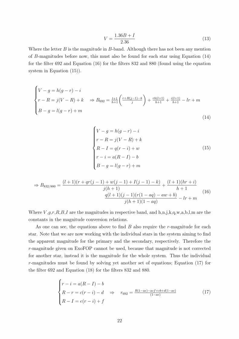
V =1.36B + I

2.36(13)

Where the letter B is the magnitude in B-band. Although there has not been any mentionof B-magnitudes before now, this must also be found for each star using Equation (14)for the filter 692 and Equation (16) for the filters 832 and 880 (found using the equationsystem in Equation (15)).

V − g = h(g − r)− i

r −R = j(V −R) + k ⇒ B692 = l+1h+1

(r+R(j−1)−k

j

)+ rh(l+1)

h+1+ i(l+1)

h+1− lr +m

B − g = l(g − r) +m

(14)

V − g = h(g − r)− i

r −R = j(V −R) + k

R− I = q(r − i) + w

r − i = a(R− I)− b

B − g = l(g − r) +m

(15)

⇒ B832/880 =(l + 1)(r + qr(j − 1) + w(j − 1) + I(j − 1)− k)

j(h+ 1)+

(l + 1)(hr + i)

h+ 1

q(l + 1)(j − 1)(r(1− aq)− aw + b)

j(h+ 1)(1− aq)− lr +m

(16)

Where V ,g,r,R,B,I are the magnitudes in respective band, and h,n,j,k,q,w,a,b,l,m are theconstants in the magnitude conversion relations.

As one can see, the equations above to find B also require the r-magnitude for eachstar. Note that we are now working with the individual stars in the system aiming to findthe apparent magnitude for the primary and the secondary, respectively. Therefore ther-magnitude given on ExoFOP cannot be used, because that magnitude is not correctedfor another star, instead it is the magnitude for the whole system. Thus the individualr-magnitudes must be found by solving yet another set of equations; Equation (17) forthe filter 692 and Equation (18) for the filters 832 and 880.

r − i = a(R− I)− b

R− r = c(r − i)− d ⇒ r692 = R(1−ae)−acf+cb+d(1−ae)(1−ae)

R− I = e(r − i) + f

(17)

22

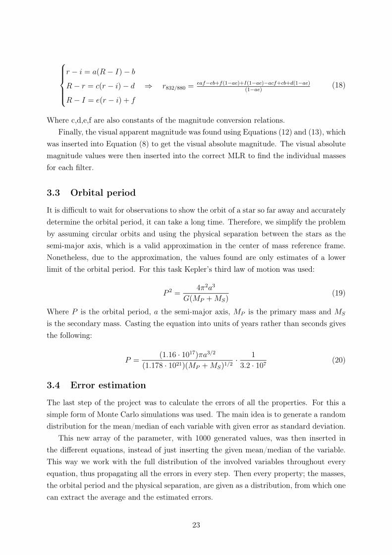
r − i = a(R− I)− b

R− r = c(r − i)− d ⇒ r832/880 = eaf−eb+f(1−ae)+I(1−ae)−acf+cb+d(1−ae)(1−ae)

R− I = e(r − i) + f

(18)

Where c,d,e,f are also constants of the magnitude conversion relations.Finally, the visual apparent magnitude was found using Equations (12) and (13), which

was inserted into Equation (8) to get the visual absolute magnitude. The visual absolutemagnitude values were then inserted into the correct MLR to find the individual massesfor each filter.

3.3 Orbital period

It is difficult to wait for observations to show the orbit of a star so far away and accuratelydetermine the orbital period, it can take a long time. Therefore, we simplify the problemby assuming circular orbits and using the physical separation between the stars as thesemi-major axis, which is a valid approximation in the center of mass reference frame.Nonetheless, due to the approximation, the values found are only estimates of a lowerlimit of the orbital period. For this task Kepler’s third law of motion was used:

P 2 =4π2a3

G(MP +MS)(19)

Where P is the orbital period, a the semi-major axis, MP is the primary mass and MS

is the secondary mass. Casting the equation into units of years rather than seconds givesthe following:

P =(1.16 · 1017)πa3/2

(1.178 · 1021)(MP +MS)1/2· 1

3.2 · 107(20)

3.4 Error estimation

The last step of the project was to calculate the errors of all the properties. For this asimple form of Monte Carlo simulations was used. The main idea is to generate a randomdistribution for the mean/median of each variable with given error as standard deviation.

This new array of the parameter, with 1000 generated values, was then inserted inthe different equations, instead of just inserting the given mean/median of the variable.This way we work with the full distribution of the involved variables throughout everyequation, thus propagating all the errors in every step. Then every property; the masses,the orbital period and the physical separation, are given as a distribution, from which onecan extract the average and the estimated errors.

23

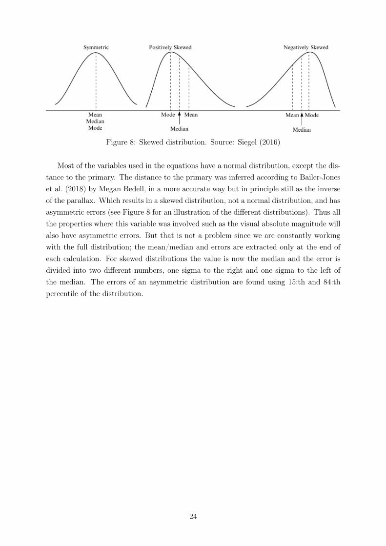
Figure 8: Skewed distribution. Source: Siegel (2016)

Most of the variables used in the equations have a normal distribution, except the dis-tance to the primary. The distance to the primary was inferred according to Bailer-Joneset al. (2018) by Megan Bedell, in a more accurate way but in principle still as the inverseof the parallax. Which results in a skewed distribution, not a normal distribution, and hasasymmetric errors (see Figure 8 for an illustration of the different distributions). Thus allthe properties where this variable was involved such as the visual absolute magnitude willalso have asymmetric errors. But that is not a problem since we are constantly workingwith the full distribution; the mean/median and errors are extracted only at the end ofeach calculation. For skewed distributions the value is now the median and the error isdivided into two different numbers, one sigma to the right and one sigma to the left ofthe median. The errors of an asymmetric distribution are found using 15:th and 84:thpercentile of the distribution.

24

4 Results

We now turn to a presentation of the results obtained using the methods of estimating theproperties explained in the preceding sections, which were implemented by the studentusing Python.

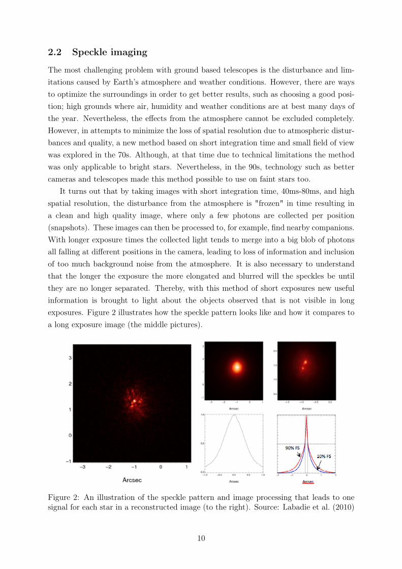
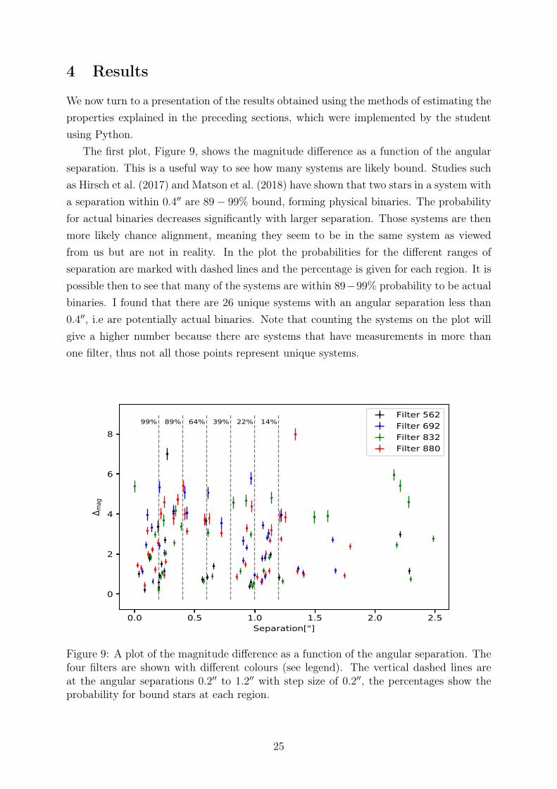
The first plot, Figure 9, shows the magnitude difference as a function of the angularseparation. This is a useful way to see how many systems are likely bound. Studies suchas Hirsch et al. (2017) and Matson et al. (2018) have shown that two stars in a system witha separation within 0.4′′ are 89− 99% bound, forming physical binaries. The probabilityfor actual binaries decreases significantly with larger separation. Those systems are thenmore likely chance alignment, meaning they seem to be in the same system as viewedfrom us but are not in reality. In the plot the probabilities for the different ranges ofseparation are marked with dashed lines and the percentage is given for each region. It ispossible then to see that many of the systems are within 89−99% probability to be actualbinaries. I found that there are 26 unique systems with an angular separation less than0.4′′, i.e are potentially actual binaries. Note that counting the systems on the plot willgive a higher number because there are systems that have measurements in more thanone filter, thus not all those points represent unique systems.

0.0 0.5 1.0 1.5 2.0 2.5Separation["]

0

2

4

6

8

mag

99% 89% 64% 39% 22% 14%Filter 562Filter 692Filter 832Filter 880

Figure 9: A plot of the magnitude difference as a function of the angular separation. Thefour filters are shown with different colours (see legend). The vertical dashed lines areat the angular separations 0.2′′ to 1.2′′ with step size of 0.2′′, the percentages show theprobability for bound stars at each region.

25

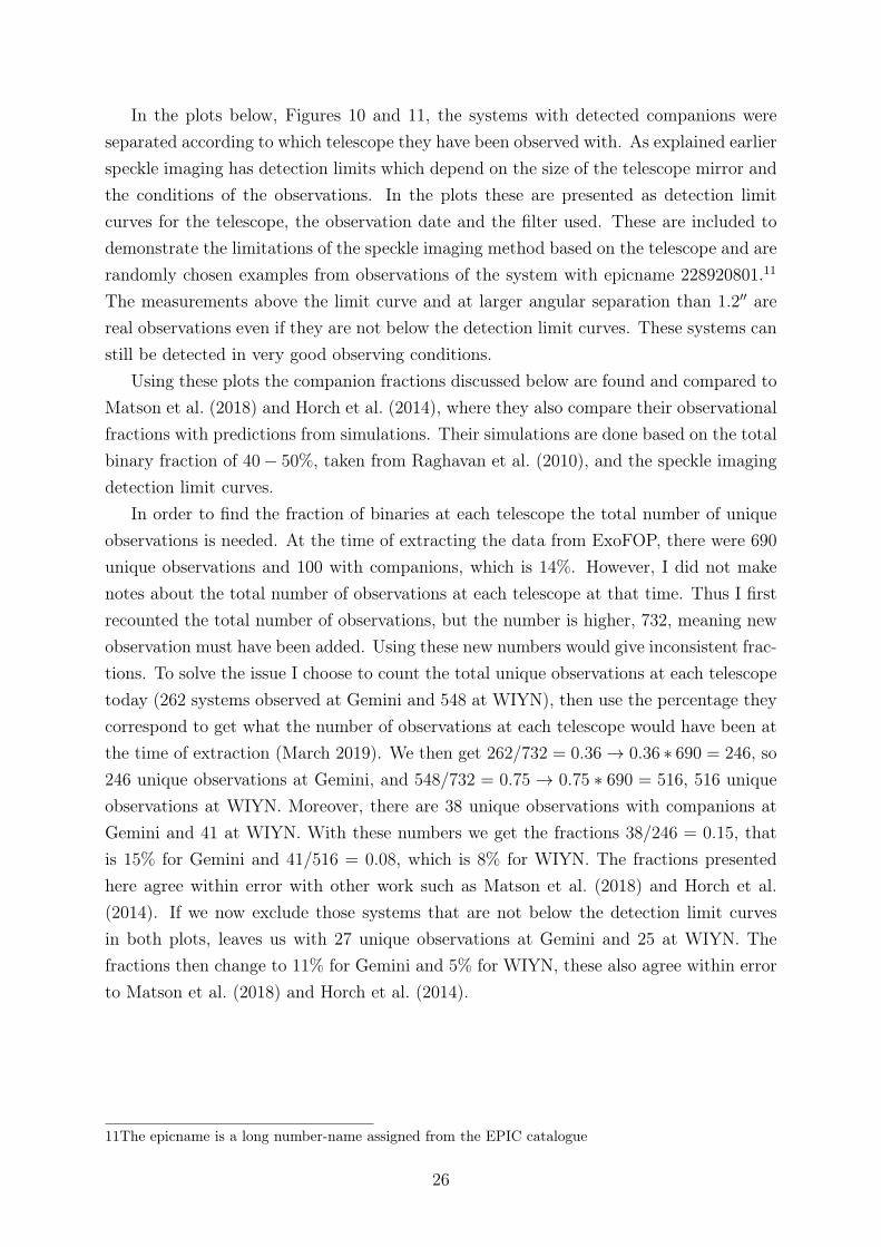
In the plots below, Figures 10 and 11, the systems with detected companions wereseparated according to which telescope they have been observed with. As explained earlierspeckle imaging has detection limits which depend on the size of the telescope mirror andthe conditions of the observations. In the plots these are presented as detection limitcurves for the telescope, the observation date and the filter used. These are included todemonstrate the limitations of the speckle imaging method based on the telescope and arerandomly chosen examples from observations of the system with epicname 228920801.11

The measurements above the limit curve and at larger angular separation than 1.2′′ arereal observations even if they are not below the detection limit curves. These systems canstill be detected in very good observing conditions.

Using these plots the companion fractions discussed below are found and compared toMatson et al. (2018) and Horch et al. (2014), where they also compare their observationalfractions with predictions from simulations. Their simulations are done based on the totalbinary fraction of 40− 50%, taken from Raghavan et al. (2010), and the speckle imagingdetection limit curves.

In order to find the fraction of binaries at each telescope the total number of uniqueobservations is needed. At the time of extracting the data from ExoFOP, there were 690unique observations and 100 with companions, which is 14%. However, I did not makenotes about the total number of observations at each telescope at that time. Thus I firstrecounted the total number of observations, but the number is higher, 732, meaning newobservation must have been added. Using these new numbers would give inconsistent frac-tions. To solve the issue I choose to count the total unique observations at each telescopetoday (262 systems observed at Gemini and 548 at WIYN), then use the percentage theycorrespond to get what the number of observations at each telescope would have been atthe time of extraction (March 2019). We then get 262/732 = 0.36→ 0.36 ∗ 690 = 246, so246 unique observations at Gemini, and 548/732 = 0.75 → 0.75 ∗ 690 = 516, 516 uniqueobservations at WIYN. Moreover, there are 38 unique observations with companions atGemini and 41 at WIYN. With these numbers we get the fractions 38/246 = 0.15, thatis 15% for Gemini and 41/516 = 0.08, which is 8% for WIYN. The fractions presentedhere agree within error with other work such as Matson et al. (2018) and Horch et al.(2014). If we now exclude those systems that are not below the detection limit curvesin both plots, leaves us with 27 unique observations at Gemini and 25 at WIYN. Thefractions then change to 11% for Gemini and 5% for WIYN, these also agree within errorto Matson et al. (2018) and Horch et al. (2014).

11The epicname is a long number-name assigned from the EPIC catalogue

26

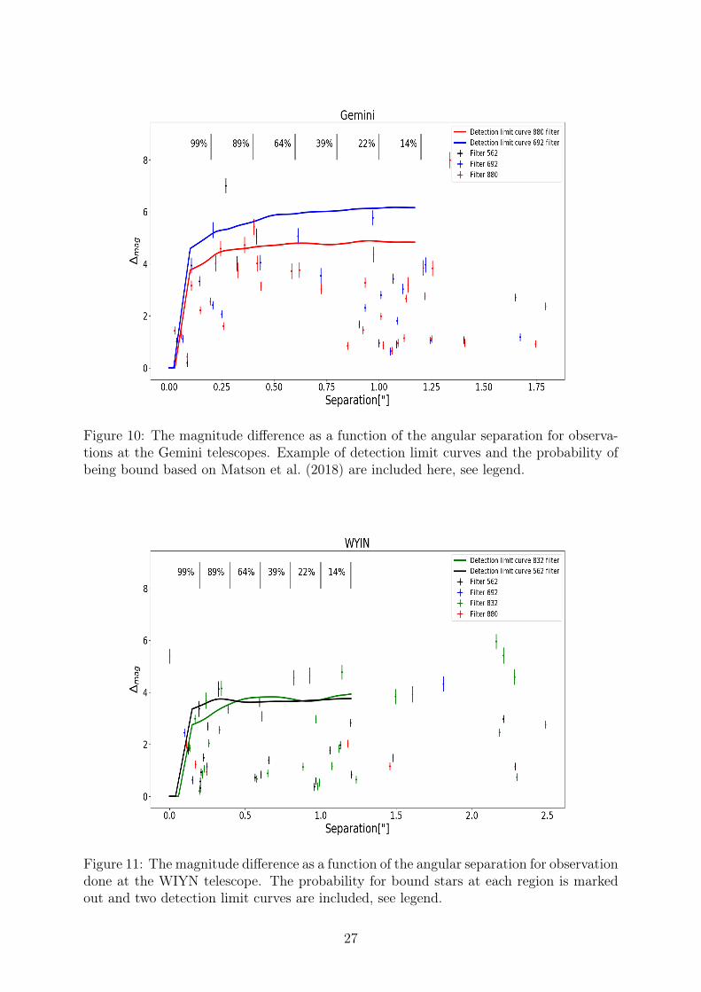
Figure 10: The magnitude difference as a function of the angular separation for observa-tions at the Gemini telescopes. Example of detection limit curves and the probability ofbeing bound based on Matson et al. (2018) are included here, see legend.

Figure 11: The magnitude difference as a function of the angular separation for observationdone at the WIYN telescope. The probability for bound stars at each region is markedout and two detection limit curves are included, see legend.

27

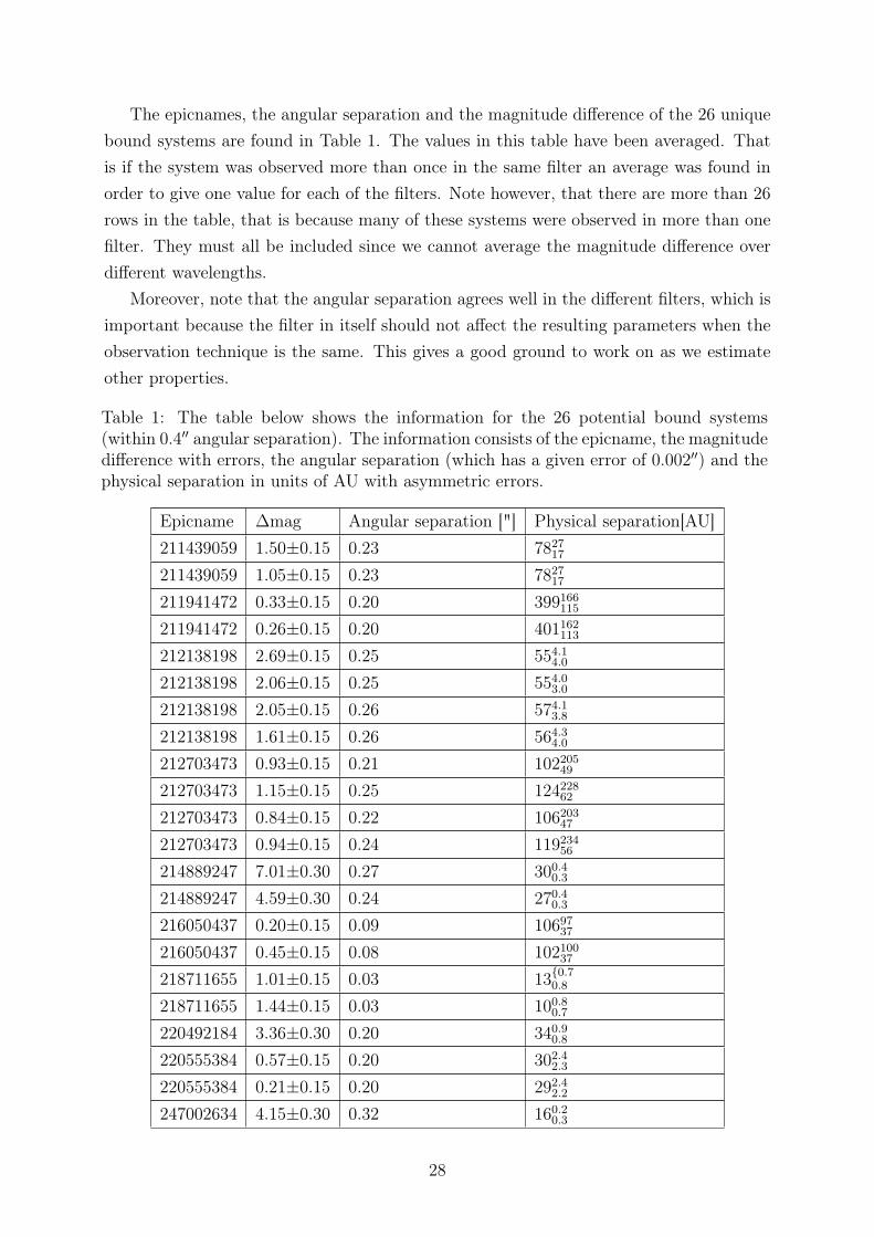
The epicnames, the angular separation and the magnitude difference of the 26 uniquebound systems are found in Table 1. The values in this table have been averaged. Thatis if the system was observed more than once in the same filter an average was found inorder to give one value for each of the filters. Note however, that there are more than 26rows in the table, that is because many of these systems were observed in more than onefilter. They must all be included since we cannot average the magnitude difference overdifferent wavelengths.

Moreover, note that the angular separation agrees well in the different filters, which isimportant because the filter in itself should not affect the resulting parameters when theobservation technique is the same. This gives a good ground to work on as we estimateother properties.

Table 1: The table below shows the information for the 26 potential bound systems(within 0.4′′ angular separation). The information consists of the epicname, the magnitudedifference with errors, the angular separation (which has a given error of 0.002′′) and thephysical separation in units of AU with asymmetric errors.

Epicname ∆mag Angular separation ["] Physical separation[AU]211439059 1.50±0.15 0.23 7827

17

211439059 1.05±0.15 0.23 782717

211941472 0.33±0.15 0.20 399166115

211941472 0.26±0.15 0.20 401162113

212138198 2.69±0.15 0.25 554.14.0

212138198 2.06±0.15 0.25 554.03.0

212138198 2.05±0.15 0.26 574.13.8

212138198 1.61±0.15 0.26 564.34.0

212703473 0.93±0.15 0.21 10220549

212703473 1.15±0.15 0.25 12422862

212703473 0.84±0.15 0.22 10620347

212703473 0.94±0.15 0.24 11923456

214889247 7.01±0.30 0.27 300.40.3

214889247 4.59±0.30 0.24 270.40.3

216050437 0.20±0.15 0.09 1069737

216050437 0.45±0.15 0.08 10210037

218711655 1.01±0.15 0.03 13{0.70.8

218711655 1.44±0.15 0.03 100.80.7

220492184 3.36±0.30 0.20 340.90.8

220555384 0.57±0.15 0.20 302.42.3

220555384 0.21±0.15 0.20 292.42.2

247002634 4.15±0.30 0.32 160.20.3

28

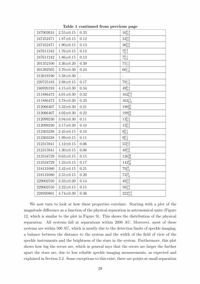
Table 1 continued from previous page247002634 2.55±0.15 0.33 160.3

0.2

247452471 1.87±0.15 0.12 340.80.9

247452471 1.90±0.15 0.13 360.90.8

247611242 1.76±0.15 0.12 70.20.1

247611242 1.86±0.15 0.13 70.10.2

201352100 3.36±0.20 0.39 751.41.5

201392505 3.70±0.30 0.24 661.71.6

212619190 5.38±0.30 - -220725183 2.98±0.15 0.17 791.7

1.9

246920193 4.15±0.30 0.34 490.40.5

211886472 4.01±0.30 0.32 1629.08.5

211886472 3.78±0.30 0.33 163118.8

212066407 5.32±0.30 0.21 1902520

212066407 4.02±0.30 0.22 1992422

212099230 3.94±0.30 0.11 130.20.3

212099230 3.17±0.20 0.10 130.30.2

212303338 2.45±0.15 0.10 80.10.2

212303338 1.99±0.15 0.11 90.10.2

212315941 1.12±0.15 0.06 556.95.7

212315941 1.30±0.15 0.06 486.05.0

212534729 0.63±0.15 0.15 1265633

212534729 1.23±0.15 0.17 1426740

218131080 2.42±0.15 0.21 79108.9

218131080 2.55±0.15 0.20 73107.6

229002550 3.33±0.20 0.14 493.83.5

229002550 2.22±0.15 0.15 504.03.4

228920801 4.74±0.30 0.36 2224.24.3

We now turn to look at how these properties correlate. Starting with a plot of themagnitude difference as a function of the physical separation in astronomical units (Figure12, which is similar to the plot in Figure 9). This shows the distribution of the physicalseparation. All systems fall at separations within 2000 AU. Moreover, most of thesesystems are within 500 AU, which is mostly due to the detection limits of speckle imaging;a balance between the distance to the system and the width of the field of view of thespeckle instruments and the brightness of the stars in the system. Furthermore, this plotshows how big the errors are, which in general says that the errors are larger the furtherapart the stars are, due to less reliable speckle imaging measurements, as expected andexplained in Section 2.2. Some exceptions to this exist, there are points at small separation

29

with quite big error bars, which most likely is due to poor observing conditions thatautomatically increase the errors on the involved variables and the end result, the physicalseparation.

0 100 200 300 400 500 600 700 800Separation[AU]

0

2

4

6

8

mag

Filter 562Filter 692Filter 832Filter 880

Figure 12: The magnitude difference as a function of the physical separation. The plot isthe same as the one in 25 in Appendix A, but here optimized to include values less than1000 AU so that the clump at short physical separation is easier to see.

Figures 13 and 14 are plots of the physical separation as a function of the distanceto the system. Staring with the empty region to the left, large separations and closer tous, which is explained by the limitations of speckle imaging; larger physical separationat small distance from us means larger angular separation, the upper limit is set at 1.2′′.The empty region extends down to roughly 400 AU in the physical separation and roughly600 pc in the distance from the solar system. Within this region there are also valuesthat correspond to too small angular separation to be resolved by speckle imaging; closeby and compact stellar binaries. Furthermore, there is an empty region to the right, seeFigure 13, which is also due to the limitations of the method. It is difficult to observeand resolve systems at such large distances, the stars will be too faint or the angularseparation will be too small. This difficulty is reflected in the errorbars of the few systemsthat were resolvable at large distances. Nevertheless, in a positive note, the errorbars forsystems closer to us are on average quite small in both measurements.

Looking at the optimized plot, see Figure 14, at first glance the measurements seem tobe spread out. But looking at the errors we can see that those measurements at distanceslarger than 600 pc (specifically those with smaller physical separation) have large errors.

30

That means that those points could be at smaller distance from us, as indicated by theerrorbars. If those values are at smaller physical separation, we can then see a somewhatlinear correlation between the properties, which most likely shows how speckle imagingworks. We detect stellar binaries with short physical separation if they are close to usand larger physical separation if they are further away. Because the further away thesmaller will the angular separation be (lower limit for speckle imaging is at 0.02′′ forgood observing conditions). Therefore, at distances further away stellar binaries musthave larger physical separation, which results in a large enough angular separation to beresolved.

0 2000 4000 6000 8000 10000Distance [pc]

0

2000

4000

6000

8000

10000

Phys

ical s

epar

ation

[AU]

Figure 13: The physical separation as a function of the distance to the system. The plotshows the distribution of the physical separation at different distances and the quality ofthe measurements.

31

0 200 400 600 800 1000Distance [pc]

0

200

400

600

800

1000

1200

Phys

ical s

epar

ation

[AU]

Figure 14: The physical separation as a function of the distance to the system. Showingdistribution of the physical separation at different distance to the system. Note that thisplot has been filtered to only include the range of shorter distances to the system witherrors less than 200, in order to view the clump of points better.

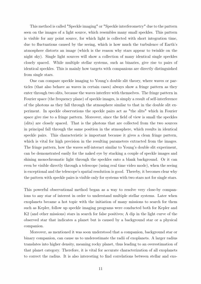
Figure 15 presents a histogram for the physical separation in units of AU. Where thelower plot is in logarithmic scale which roughly follows a Gaussian fit (to see the fit refer toFigure 28 in Appendix A). The histograms are colour coded by filter in order to illustrateall points in each filter, although, note that some systems exist in more than one filter sothere are not so many systems in total as it might seem from these plots. Moreover, somesystems which do have enough data to find the physical separation but not the massesare not included in this figure (a plot where all systems are included is instead shown inFigure 27 in Appendix A). There are 88 unique systems for which the physical separationswas found and only 72 for which the other properties were also calculated. It is clear fromthe upper plot in Figure 15 that the secondaries detected are usually closer than 400 AUto their primary, with a peak at roughly 160 AU. When including all the 88 systems forwhich the physical separation is known, the peak is then roughly at 166 AU, see the lowerplot in Figure 27.

32

0 1000 2000 3000 4000Sep.[AU]

0.0

2.5

5.0

7.5

10.0

12.5

15.0

17.5

N

832filter880filter692filter562filter

1.0 1.5 2.0 2.5 3.0 3.5log(Sep.)[AU]

0

2

4

6

8

10

N

832filter880filter692filter562filter

Figure 15: A histogram of the physical separation and its logarithm. The logarithm plotshows the spread of all values better. In the regular plot some values are much larger,making it harder to see most of the points that are within 2000 AU.

Figure 16 shows a histogram of the orbital period. In a similar way as for the physicalseparation the upper plot shows the extend of values. Since this plot is in days the valuesare much larger, however, the trend is similar: Most points are within 0.25 · 107 days,i.e short orbital periods, which correspond to smaller physical separation and are thuseasier to detect. Putting the data from all the filters together, taking an average forthose systems that have been observed in more than one filter, thus include only uniquesystems, gives a peak at 1430 years. This plot is in days in order to be able to comparedirectly to Raghavan et al. (2010) (see Section 5). A plot in units of years can be foundin Appendix A, Figure 33. That plot shows that the orbital period ranges from as shortas 17 years to 40000 years. The orbital period reflects the physical separation betweenthe components. The more compact the binary is the shorter is the orbital period.

33

0.00 0.25 0.50 0.75 1.00 1.25 1.50P[days] 1e7

0

5

10

15

20

N

832filter880filter692filter562filter

4.0 4.5 5.0 5.5 6.0 6.5 7.0log(P)[days]

0

2

4

6

8

10

12

N

832filter880filter692filter562filter

Figure 16: A histogram of the orbital period and its logarithm, in units of days. Thelogarithm plot shows the spread of all values better whereas the regular plot shows theextend of values. Most points are within 0.25 · 107 days.

The plot in Figure 17 shows the distribution of the mass ratio as a function of theprimary mass. The shape of the distribution is spread over the whole graph in both axes,which is as expected, we have not selected stars with any particular mass range. The massratios range from 0.3 to roughly 0.9 and the masses from 0.4 to 1.9 solar masses. Againthe respective filters follow the same shape of distribution, none of the filters give anydifferent results or outliers. However, the filter K results from the aperture photometry,do differ from the filters used in speckle imaging in some cases. These points are at theleft end of the graph in purple; at lower primary mass and larger mass ratio. Thesemeasurements seem to be of those systems that had stellar components of almost equalbrightness resulting in similar mass or were difficult to see in the image, thus difficult todetermine the center of the two light sources in the image. The aperture photometry was

34

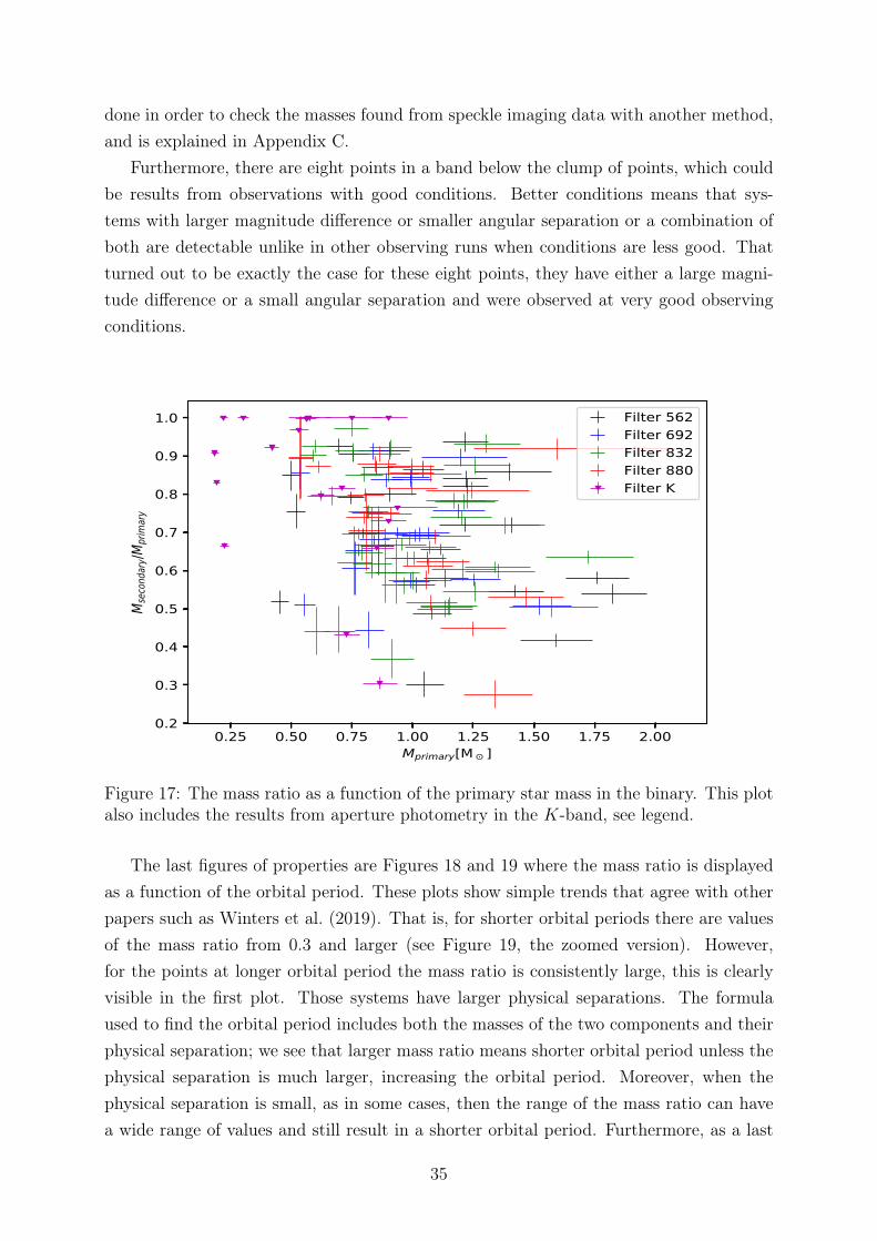
done in order to check the masses found from speckle imaging data with another method,and is explained in Appendix C.

Furthermore, there are eight points in a band below the clump of points, which couldbe results from observations with good conditions. Better conditions means that sys-tems with larger magnitude difference or smaller angular separation or a combination ofboth are detectable unlike in other observing runs when conditions are less good. Thatturned out to be exactly the case for these eight points, they have either a large magni-tude difference or a small angular separation and were observed at very good observingconditions.

0.25 0.50 0.75 1.00 1.25 1.50 1.75 2.00Mprimary[M ]

0.2

0.3

0.4

0.5

0.6

0.7

0.8

0.9

1.0

Mse

cond

ary/M

prim

ary

Filter 562Filter 692Filter 832Filter 880Filter K

Figure 17: The mass ratio as a function of the primary star mass in the binary. This plotalso includes the results from aperture photometry in the K-band, see legend.

The last figures of properties are Figures 18 and 19 where the mass ratio is displayedas a function of the orbital period. These plots show simple trends that agree with otherpapers such as Winters et al. (2019). That is, for shorter orbital periods there are valuesof the mass ratio from 0.3 and larger (see Figure 19, the zoomed version). However,for the points at longer orbital period the mass ratio is consistently large, this is clearlyvisible in the first plot. Those systems have larger physical separations. The formulaused to find the orbital period includes both the masses of the two components and theirphysical separation; we see that larger mass ratio means shorter orbital period unless thephysical separation is much larger, increasing the orbital period. Moreover, when thephysical separation is small, as in some cases, then the range of the mass ratio can havea wide range of values and still result in a shorter orbital period. Furthermore, as a last

35

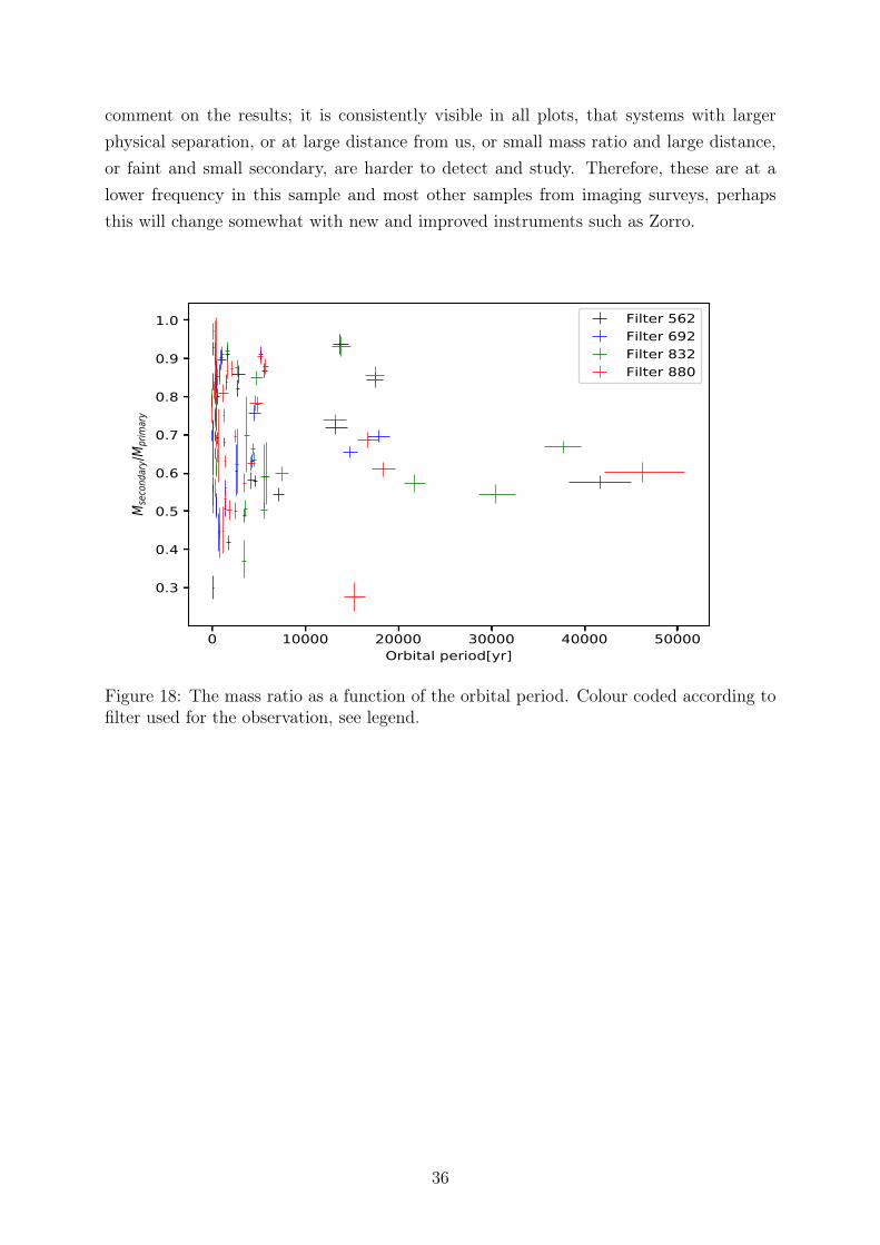
comment on the results; it is consistently visible in all plots, that systems with largerphysical separation, or at large distance from us, or small mass ratio and large distance,or faint and small secondary, are harder to detect and study. Therefore, these are at alower frequency in this sample and most other samples from imaging surveys, perhapsthis will change somewhat with new and improved instruments such as Zorro.

0 10000 20000 30000 40000 50000Orbital period[yr]

0.3

0.4

0.5

0.6

0.7

0.8

0.9

1.0

Mse

cond

ary/M

prim

ary

Filter 562Filter 692Filter 832Filter 880

Figure 18: The mass ratio as a function of the orbital period. Colour coded according tofilter used for the observation, see legend.

36

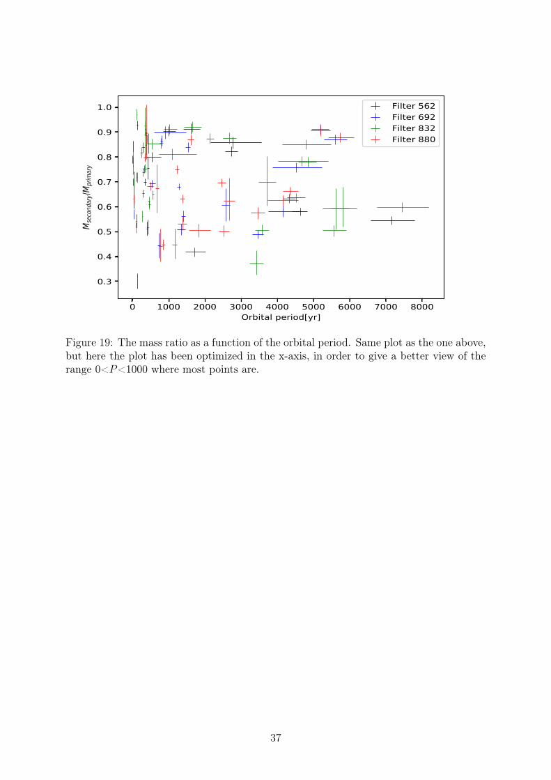
0 1000 2000 3000 4000 5000 6000 7000 8000Orbital period[yr]

0.3

0.4

0.5

0.6

0.7

0.8

0.9

1.0

Mse

cond

ary/M

prim

ary

Filter 562Filter 692Filter 832Filter 880

Figure 19: The mass ratio as a function of the orbital period. Same plot as the one above,but here the plot has been optimized in the x-axis, in order to give a better view of therange 0<P<1000 where most points are.

37

5 Discussion and conclusion

5.1 Bound systems and fractions

It is difficult to determine which of the systems are actual binaries. An attempt as donehere is to use a plot of the angular separation and the magnitude difference. Accordingto other studies such as Matson et al. (2018) systems within 0.4′′ are likely bound andtreated as such. For a more careful study of all systems even those outside the limit of0.4′′, which could still be bound, one can apply stellar isochrones to see if one commonisochrone goes through both the primary and the secondary, but that is outside of thescoop of this project, for details refer to for example Everett et al. (2015).

In this project the results from the plots in Figures 9, 10 and 11 will be satisfactory andthe fractions found will be compared to Raghavan et al. (2010), Horch et al. (2014) andMatson et al. (2018). The two later ones are studies of Kepler and K2 exoplanet candidatehost stars, respectively, similar to this project. The fraction of potential binaries found inthis project for speckle imaging observations during 2016-2018 is 14% (100 binaries out of690 unique observations) which agrees with Horch et al. (2014) and Matson et al. (2018).If we then look at the telescopes separately, because the telescope mirror determinesthe minimum angular separation resolvable and how faint the secondary can be. AtGemini the mirrors are larger, thus the minimum angular separation resolvable is smallerthan at WIYN and the detection limit on the magnitude difference is larger, making itpossible to detect more companions. Thus we expect to find more companions at Geminithan at WIYN, which is reflected by the fractions of binaries found in Section 4. Thefractions from the papers we want to compare to are: 23 ± 5% for Gemini and 6 ± 2%

for WIYN in Matson et al. (2018). Excluding any observations outside the limit curvethey found fractions of; 19± 5% for Gemini and 5± 2% for WIYN, which are consistentwith their simulated fractions, 24 ± 7% for Gemini and 8 ± 3% for WIYN. Horch et al.(2014) determine the fractions 22.8 ± 8.1% for Gemini and 7 ± 1.1% for WIYN afterexcluding observations outside the limit curve, with simulated fractions of 19.7 ± 0.4%

for Gemini and 7.8 ± 0.4% for WIYN. Both papers thus agree. The fractions extractedin my project also agree within the uncertainties with both papers. Furthermore, sincetheir simulations, which are based on the total binary fraction of 44± 9% for Gemini and40±9% for WIYN, based on findings in Raghavan et al. (2010), give the fraction for eachtelescope that agree within the uncertainties with the observed fractions in both papersand those found in my project. One can confidently say that the stellar binary fractionfor K2 exoplanet host stars outside the solar neighbourhood (> 25 pc) is in the range40− 50%, which is consistent with the results in Raghavan et al. (2010); the study of thesolar neighbourhood.

38

5.2 Discussion of the method

In this part the different aspects of the method used for finding the properties will bediscussed shortly. Furthermore, short remarks on improvements for speckle imaging willbe mentioned.

The method used for finding the properties was chosen according to examples in otherpapers that have been shown to work or that were the only possible choice with thelimited information about the sample. The method included some valid and necessaryassumptions and approximations, which means all the properties found in this project areestimates of reality.

The main general point to make about the method is about the errors. The firstthought was that the errors would be large and get larger the more complex the calcu-lations became, since more uncertainties were involved. Complex in the sense that moreequations with their own uncertainties were used. This was a worry specifically for themass calculations; for example for the data in the 562 filter the calculations were directlyin the visual band with fewer variables thus less error accumulation. Whereas for theother filters especially the filters 832 and 880, there were more steps and equations in-volved with each errors of their own accumulating to larger errors. However, this does notseem to be the case, the errors for not just the mass, but all the properties seem small.The quality of the estimated properties (size of the error bars) appears more to dependon the limitations of the speckle method and the conditions/quality of the individualobserving runs rather than the calculation method.

This is on second thought reasonable, even though it was not an optimal method touse when it comes to specifically the masses. Because all extra equations to find the visualapparent and the visual absolute magnitude came from well established magnitude con-version relations based on years of observations and were suitable for our stars. Moreover,the MLR, which also had uncertainties of their own, were well established and appropriatefor the sample as well. Moreover, all those errors were taken into account and properlypropagated through the calculations. Thus a more complex method with many more stepsshould in itself not dramatically increase the size of the errors, the size depends more onthe observation quality and the observation technique. For example the further away thesystems or the fainter the stars are, the harder it is to study them. Moreover, the poorerthe observing conditions, no matter if the stars are faint or far away, the less reliable willthe results be. This is what we see in general in all the plots. Nonetheless, as comparisonsto papers of similar studies, as done above and as follows below, show that the results ofthis project are reasonable and useful for future reference.

In the future a better method for finding the properties can be stellar isochronesas done in papers such as Everett et al. (2015). If the information is as limited as inmost cases in this sample or one wants to use something other than stellar isochrones,

39

a similar but better way to find the properties could be to use MLR as done here, butfind a relationship for the filters. Such a relationship between the filters used in speckleimaging and the regular filters, such as the SDSS system, can then be used directly tofind the individual visual apparent magnitudes instead of going through many conversionformulas. Moreover, we avoid assuming what regular magnitude band the filters used inspeckle imaging roughly correspond to.

As for the speckle observation method, it is already an impressive and useful highresolution imaging method, which makes it possible to study and detect close companionsthat no other method is better at. However, it needs to be sensitive to even more compactbinaries and larger magnitude differences, fainter companions. When that is possiblemultiplicity studies of stars as this one, corrections of planet radii and detection of falsepositives will be even more effective and accurate.

Moreover, choice of band-width is an important part of improving speckle instruments.A wider band-width makes it possible to observe fainter targets. However, it is a balancebetween wider band-width and increased atmospheric dispersion. The later also dependson the size of the telescope mirror, for a smaller mirror, wider band-width works betterand can even be necessary. For bigger telescope mirrors however, wider band-width canonly be used at low airmass if dispersion is kept low (Horch et al., 2012), but this ischallenging since it is hard to build in many different filters of different band-widths in thesame instrument. Another improvement would be to observe at even shorter wavelengthssince the resolution power of a telescope depends on both wavelength and mirror diameter.Nevertheless, speckle imaging can be improved in other ways in the future as technologycontinues to evolve, making for example new more sensitive cameras available.

5.3 General conclusions from results

In this part some general comments on the results will be given.Firstly, it is useful to look at the different filters and see if the resulting properties

match across the filters. Tables for each property where each system is treated filter wisewere made and can be found in Appendix E. For the masses a column with the K-bandaperture photometry results has been included.

Starting with the mass tables, the first thing to note is that most systems have beenobserved with only two filters, which is how speckle imaging observations usually are done.Only four have measurements in all the filters and a few in only one filter. Moreover,remember that the filters come in the sets 562 and 832, 692 and 880, which is just howthey are used when observing with speckle imaging. From the table of the mass of theprimary star, Table 18, it is clear that in most cases the results match well or at least agreewithin the uncertainties. There are exceptions to this, for example system 2121381198 wasobserved in all the filters where 562, 692 and 832 match within the uncertainties but not

40

880. This is most likely due to observing conditions, that results in worse estimates of thespeckle parameters in one filter than the other. The same reasoning applies to other caseswhere the results do not match even within the uncertainties or between, for example, thefilters 562 and 832nm which are used simultaneously. Because the atmosphere behavesslightly different for different wavelengths or the secondary is fainter in one wavelengththan the other; both cases result in not equally good images in both of the filters even ifthey were used simultaneously. This reasoning is enforced by looking at the detection limitcurve for that observation and filter; smaller maximum magnitude difference detectablethan 3-4 magnitudes, which is usual for speckle imaging, means worse conditions thusworse results. According to the points made here and in the previous subsection andtaking into account the good agreement with other papers, the method used for calculatingthe properties does not seem to be a significant reason for disagreeing results across thefilters. Therefore, this confirms further that the assumptions, the approximations and theoverall approach in this project is acceptable. The same conclusions can be made for theother two mass-tables, of the secondary mass and the mass ratio, Tables 19 and 20.

Looking instead at the filters compared to the results from the aperture photometry,there are more disagreements. Firstly, it is worth noting that in most images from AOobservations, to be used for the photometric study, the secondary was not visible makingthose images not usable. For those images that aperture photometry was performed,many disagree with the results from the speckle imaging data. At a closer look these weresystems that had images where the secondary was barely visible in SAOImageDS9 andnot at all visible on the Python plots of the image, making it difficult to give acceptableguesses of the center of the secondary, which was done manually. This is also the mostlikely explanation for the shape of the K-band results plotted in Figure 17; the pointsdisconnected from the rest. As mentioned in Appendix C this could be solved using theposition angle from speckle imaging observations to find the location of the secondary.But aperture photometry was an extra step only used to quickly check the masses, thusnot important enough to look further into. Overall the results from aperture photometryshow that when the images work the results agree within the uncertainties with the massesfound from speckle imaging data. Having the two methods, which are different, agree ingeneral is important, because that further strengthens the reliability of the method usedto find the masses via speckle imaging data.

The same type of conclusions can be drawn and the same behavior is seen in theother sets of tables for the last two properties, the physical separation and the orbitalperiod. Note that these properties were not estimated using the mass-results fromK-bandphotometry, therefore such a comparison does not exist. Nevertheless, the comparisonacross the filters used in speckle imaging observations shows the same results as for themass tables. There are mostly agreement within the uncertainties, as there should besince the only difference is the filter used, not the method of observation. However,

41

disagreements exist which are again most likely due to worse observing conditions andthe same reasoning as mentioned above. In observations with bad seeing and windyweather, conditions can change significantly in a short time causing images to be worsein one case or filter compared to another.

More detailed discussion about each property and graph will follow below in Subsection5.4 where the results are compared to Raghavan et al. (2010). However, looking in generalat the plots, all of the properties seem reasonable and have a distribution as expected andseen in other work.

One last noteworthy general comment to make here is about the physical separationsof the systems. Papers such as Kraus et al. (2016) have suggested, by looking at a sampleof Kepler/K2 exoplanet host stars, that there is a suppression of companions with physicalseparations < 50AU for exoplanet host stars: There cannot exist such a close companionif there also is a planet, or in other words no planets can form in compact binaries wherethe physical separation is less than 50 AU. This was investigated in Matson et al. (2018)too, they could not find any such indications. Same as in those papers the sample of myproject is considered to consist of exoplanet host stars. Looking then at the histogramplots of the physical separation in Figure 20, where the physical separations range from0-300 AU with bin size of 12 AU (to the right) same as in Matson et al. (2018) (see theirplots in figure 9) and 0-1000 AU (to the left) same as in Kraus et al. (2016) (see theirplots and arguments in figure 7).

It is clear that there is no indication of any suppression in either of the plots. More-over, unlike the Matson et al. (2018) paper, which only had 26 systems with detectedcompanions, there is a large enough number of companions in my sample (100 primarieswith one companion) to be able to say more confidently, that there is no such indication.However, same as for Matson et al. (2018), until all the binaries in this project have atleast one confirmed exoplanet the statement in question from Kraus et al. (2016) cannotbe properly disproved.

42

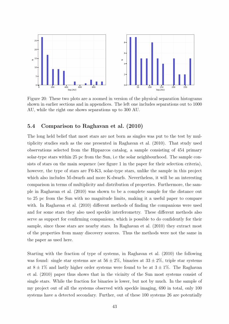
0 200 400 600 800Sep.[AU]

0

5

10

15

20

25

N

50 100 150 200 250Sep.[AU]

0

2

4

6

8

N

Figure 20: These two plots are a zoomed in version of the physical separation histogramsshown in earlier sections and in appendices. The left one includes separations out to 1000AU, while the right one shows separations up to 300 AU.

5.4 Comparison to Raghavan et al. (2010)

The long held belief that most stars are not born as singles was put to the test by mul-tiplicity studies such as the one presented in Raghavan et al. (2010). That study usedobservations selected from the Hipparcos catalog, a sample consisting of 454 primarysolar-type stars within 25 pc from the Sun, i.e the solar neighbourhood. The sample con-sists of stars on the main sequence (see figure 1 in the paper for their selection criteria),however, the type of stars are F6-K3, solar-type stars, unlike the sample in this projectwhich also includes M-dwarfs and more K-dwarfs. Nevertheless, it will be an interestingcomparison in terms of multiplicity and distribution of properties. Furthermore, the sam-ple in Raghavan et al. (2010) was shown to be a complete sample for the distance outto 25 pc from the Sun with no magnitude limits, making it a useful paper to comparewith. In Raghavan et al. (2010) different methods of finding the companions were usedand for some stars they also used speckle interferometry. These different methods alsoserve as support for confirming companions, which is possible to do confidently for theirsample, since those stars are nearby stars. In Raghavan et al. (2010) they extract mostof the properties from many discovery sources. Thus the methods were not the same inthe paper as used here.

Starting with the fraction of type of systems, in Raghavan et al. (2010) the followingwas found: single star systems are at 56 ± 2%, binaries at 33 ± 2%, triple star systemsat 8 ± 1% and lastly higher order systems were found to be at 3 ± 1%. The Raghavanet al. (2010) paper thus shows that in the vicinity of the Sun most systems consist ofsingle stars. While the fraction for binaries is lower, but not by much. In the sample ofmy project out of all the systems observed with speckle imaging, 690 in total, only 100systems have a detected secondary. Further, out of these 100 systems 26 are potentially

43

bound according to the probabilities shown in Figure 9. From these numbers the percent-age is 14%, same as in Matson et al. (2018), where they show that using fractions fromRaghavan et al. (2010) to simulate predicted fractions, results in fractions (both total andfor each telescope separately) that agree within the uncertainties with the fractions foundin my project.

As for the properties even though their methods are different all properties in generalhave similar distributions. Starting with orbital period; in Raghavan et al. (2010) thiswas presented as a histogram in units of days. Here the orbital period has been presentedboth in units of days and years; Figure 16 in Section 4 and Figure 33 in Appendix A.Focusing on the distribution in units of days in log-scale in comparison to Figure 13 inRaghavan et al. (2010), we see that the shape is similar and in the same manner roughlyfollows a Gaussian normal distribution (see Figure 34 for the fit). The differences arethe location of the peak and the maximum period. In the paper they choose to show aGaussian fit, which is not really explained why, but could be just to clearly illustrate ormaybe to be able to get the standard deviation of the distribution. For my project themean and standard deviation was found from the data directly, in log-scale. The peak ofthe orbital period for my project is at logP = 5.72 which corresponds to 1430 years, witha standard deviation of σlogP = 0.78 corresponding to 0.016 years. This is slightly higherthan the peak in Raghavan et al. (2010), which was at logP = 5.03 or 293 years.

Looking then at the same figure in the paper (figure 13) they also plot an axis for thephysical separation in log-scale. The mean of the physical separation in units of AU wasfound to be at log(a) ≈ 1.9, corresponding to roughly 80AU. Doing the same with thephysical separation as with the orbital period (see the distribution in Figure 15 and theGaussian fit of it in Figure 28) gives a mean at log(a) ≈ 2.2 which corresponds to roughly166 AU with a standard deviation at σlog(a) = 0.58 or 3.8AU (including all 88 systemsas shown in Figure 27). The peak is thus further out for this study compared to that inRaghavan et al. (2010). Looking at other papers such as Winters et al. (2019) which is astudy of only M-dwarfs in the solar neighbourhood, the peak for the physical separationis at 20AU. That does not agree at all with the sample in this project, but that could besince it is for only M-dwarfs. In my project the peak for the physical separation when onlyincluding M-dwarfs is lower than for the full sample, at 105 AU, but still much furtherout than in Winters et al. (2019).

Another study more similar to this project, where they also study stars within 25 pc,believed to have exoplanets and detect companions using speckle imaging, Ziegler et al.(2020). They found wider binaries than in Raghavan et al. (2010) with a peak at roughly200 AU, which is in better agreement with the results from my project. This could meanthat a peak further out simply is a feature of exoplanet host stars in binaries; a differencebetween stellar binaries in the solar neighbourhood and exoplanet hosting binaries, which

44

needs further investigation in the future. Furthermore, if the peak for the orbital periodis further out so will the peak for the physical separation be, since the orbital period is afunction of the physical separation.

A last interesting comparison with Raghavan et al. (2010) is the mass ratio distributionand the mass ratio as a function of the orbital period. Looking at the plot (to the left)in figure 16 in Raghavan et al. (2010), the mass ratio distribution is rather flat for ratios0.2-0.9, and increasing as we reach ratio one. The same type of plot in Figure 31 showsroughly the same behaviour; the mass ratio increases slightly towards ratios of 1, theseare easier to detect, but the increase is more significant than in Raghavan et al. (2010).This can be further investigated in the future with more accurate mass measurementsto see if it is consistent and real for stellar binaries outside of the solar neighbourhood.Nevertheless, the overall behaviour is still similar and has been seen in other studies, e.g.Winters et al. (2019).

Looking at Figure 17 in Raghavan et al. (2010) which looks at the mass ratio as afunction of the orbital period, it shows a lack of small mass companions. Figure 17 alsoshows a suggestion that the systems with shorter orbital periods also consist of smallermass companions. This is seen as a lack of small mass - short period combination ofsystems, which as mentioned in the paper, is not due to incompleteness or any bias, lackof such companions is real. The same conclusion can be seen in the plots of my project:Figures 18 and 19 show similar distribution, small mass-short period companions arerare, while most systems have the combination short period-large mass. However, it isnoteworthy that speckle imaging actually is not very sensitive to such systems, thus thenumber of those systems might increase with more complete samples and better sensitivity.For now the conclusion is that small mass-short period companions are rare same as in thesolar neighbourhood. Moreover, the longer period systems seem to most often correspondto larger mass companions (larger mass ratios), most of them being at mass ratios of 0.6and larger, exceptions exist but are rare. Furthermore, as mentioned in Raghavan et al.(2010), stellar binaries with like-mass components seem to prefer shorter orbital periods,that seems to be the case here too. However, this is harder to conclude from my results,since those systems are few and there are exceptions; there are systems with a mass ratioat 0.9 and a relatively wide range of periods out to 8000 years. However, there are nosystems with a mass ratio above 0.9 and long orbital period.

5.5 Conclusion

In this project the main goal was to analyze systems with detected companions fromfollow-up observations with speckle high resolution imaging, and for each of these systemsfind the following properties; the masses of the stars in the system, the orbital period andthe physical separation. The many assumptions and approximations associated with the

45

method used for finding the properties might seem worrisome, but the results from thecalculations show trends that agree in general with other studies of similar type and resultsfor the solar neighbourhood. Therefore, one can say with confidence that the method ofcalculations used in this project works well and can be applied to data from follow-upspeckle imaging observations.

By including detection limits and plotting the parameters derived from speckle imag-ing, the magnitude difference and the angular separation, the fractions of companionsdetected at each telescope were found. The resulting fractions were 15% for Gemini and8% for WIYN, which are in agreement within the uncertainties with Matson et al. (2018)and Horch et al. (2014) and their simulated predictions. Moreover, from the same plot afirst suggestion of which systems are bound was made; 26 of the 100 are within 0.4′′, thus99% likely to be bound.

This work also further suggests that there is no indication of suppression of compactexoplanet hosting binaries with separations less than 50AU as stated in Kraus et al. (2016).Furthermore, after having looked at all aspects and properties in detail and comparingto previous works the general trends agree with those papers. Specifically, it is clear thatthe spread of the orbital period is similar to that of nearby solar-type binaries just witha peak further out, which is within reason and could be a feature of exoplanet host starsin binaries. Further the same can be said for the distribution of the physical separation.Lastly, the mass ratio as a function of the orbital period also agrees with other papers andshows that systems with short period also prefer small mass companions, while systemswith long orbital period most often consist of a larger mass companions.

The comparisons in general have shown that the findings from this sample agree wellwith other studies and are useful for future work. The results will provide hints on whatto look for and focus on in future observations. Moreover, the agreement with studiesof solar-type binaries, confirms that the same overall trends exist in systems of binarieswith planets, outside the solar neighbourhood. Knowing properties such as the mass ratioand the orbital period gives an overview of the type of stars in binary systems that existout there and helps improve or change formation and evolution models. An importantexample are very compact binaries (<1AU) that are sometimes detected (not present inthis sample though), which cannot form that close instead they are examples of starsthat formed further apart, but moved close during their life time evolution. Furthermore,those same properties give clues about the formation of planets in stellar binaries thatneed to be studied in detail in the future.

In conclusion, the overall trends and distribution of the properties, specifically com-pared to each other, give clues to formation of planets in stellar binaries and hints forimprovements of formation and evolution models, and help us understand stellar binariesin general.

46

6 References

Bailer-Jones, C. A. L., Rybizki, J., Fouesneau, M., Mantelet, G., and Andrae, R. (2018).Estimating distance from parallaxes. IV. Distances to 1.33 billion stars in Gaia datarelease 2. AJ, 156:58.

Everett, M. E., Barclay, T., et al. (2015). High-resolution multi-band imaging for valida-tion and characterization of small Kepler planets. AJ, 149:55.

Henry, T. J. and McCarthy, Donald W., J. (1993). The Mass-Luminosity Relation forStars of Mass 1.0 to 0.08M(solar). AJ, 106:773.

Hirsch, L. A., Ciardi, D. R., et al. (2017). Assessing the effect of stellar companions fromhigh-resolution imaging of Kepler objects of interest. AJ, 153:117.

Horch, E. P., Dinescu, D. I., et al. (1996). Speckle Interferometry of Southern Dou-ble Stars.I.First Results of the Yale-San Juan Speckle Interferometry Program. AJ,111:1681.

Horch, E. P., Falta, D., et al. (2010). CCD speckle observations of binary stars with theWIYN telescope. VI. Measures during 2007-2008. AJ, 139.

Horch, E. P., Howell, S. B., Everett, M. E., and Ciardi, D. R. (2012). Observations ofbinary stars with the differential speckle survey instrument. IV. Observation of Kepler, CoRoT , and Hipparcos stars from the Gemini north telescope. AJ, 144:165.

Horch, E. P., Howell, S. B., Everett, M. E., and Ciardi, D. R. (2014). Most sub-arcsecondcompanions of Kepler exoplanet candidate host stars are gravitationally bound. ApJ,795:60.

Horch, E. P., Veillette, D. R., et al. (2009). Observations of Binary Stars with theDifferential Speckle Survey Instrument. AJ, 137:5057–5067.

Howell, S. B. (2000). Handbook of CCD astronomy. Cambrige University Press.

Howell, S. B., Everett, M. E., Sherry, W., Horch, E., and Ciardi, D. R. (2011). Specklecamera observations for the NASA Kepler mission follow-up program. AJ, 142:19.

Howell, S. B., Sobeck, C., et al. (2014). The K2 Mission: Characterization and earlyresults. PASP, 126:398–408.

Jordi, K., Grebel, E. K., and Ammon, K. (2006). Empirical color transformations betweenSDSS photometry and other photometric systems. AAP, 460:339–347.

Kraus, A. L., Ireland, M. J., Huber, D., Mann, A. W., and Dupuy, T. J. (2016). Theimpact of stellar multiplicity on planetary systems. AJ, 152:8.

47

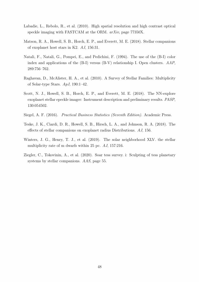
Labadie, L., Rebolo, R., et al. (2010). High spatial resolution and high contrast opticalspeckle imaging with FASTCAM at the ORM. arXiv, page 77350X.

Matson, R. A., Howell, S. B., Horch, E. P., and Everett, M. E. (2018). Stellar companionsof exoplanet host stars in K2. AJ, 156:31.

Natali, F., Natali, G., Pompei, E., and Pedichini, F. (1994). The use of the (B-I) colorindex and applications of the (B-I) versus (B-V) relationship I. Open clusters. AAP,289:756–762.

Raghavan, D., McAlister, H. A., et al. (2010). A Survey of Stellar Families: Multiplicityof Solar-type Stars. ApJ, 190:1–42.

Scott, N. J., Howell, S. B., Horch, E. P., and Everett, M. E. (2018). The NN-exploreexoplanet stellar epeckle imager: Instrument description and preliminary results. PASP,130:054502.

Siegel, A. F. (2016). Practical Business Statistics (Seventh Edition). Academic Press.

Teske, J. K., Ciardi, D. R., Howell, S. B., Hirsch, L. A., and Johnson, R. A. (2018). Theeffects of stellar companions on exoplanet radius Distributions. AJ, 156.

Winters, J. G., Henry, T. J., et al. (2019). The solar neighborhood XLV. the stellarmultiplicity rate of m dwarfs within 25 pc. AJ, 157:216.

Ziegler, C., Tokovinin, A., et al. (2020). Soar tess survey. i: Sculpting of tess planetarysystems by stellar companions. AAS, page 55.

48

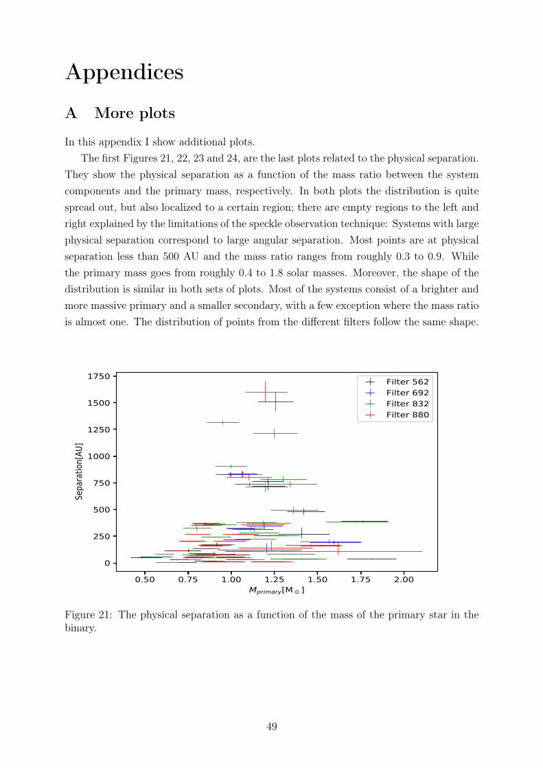
Appendices

A More plots

In this appendix I show additional plots.The first Figures 21, 22, 23 and 24, are the last plots related to the physical separation.

They show the physical separation as a function of the mass ratio between the systemcomponents and the primary mass, respectively. In both plots the distribution is quitespread out, but also localized to a certain region; there are empty regions to the left andright explained by the limitations of the speckle observation technique: Systems with largephysical separation correspond to large angular separation. Most points are at physicalseparation less than 500 AU and the mass ratio ranges from roughly 0.3 to 0.9. Whilethe primary mass goes from roughly 0.4 to 1.8 solar masses. Moreover, the shape of thedistribution is similar in both sets of plots. Most of the systems consist of a brighter andmore massive primary and a smaller secondary, with a few exception where the mass ratiois almost one. The distribution of points from the different filters follow the same shape.

0.50 0.75 1.00 1.25 1.50 1.75 2.00Mprimary[M ]

0

250

500

750

1000

1250

1500

1750

Sepa

ratio

n[AU

]

Filter 562Filter 692Filter 832Filter 880

Figure 21: The physical separation as a function of the mass of the primary star in thebinary.

49

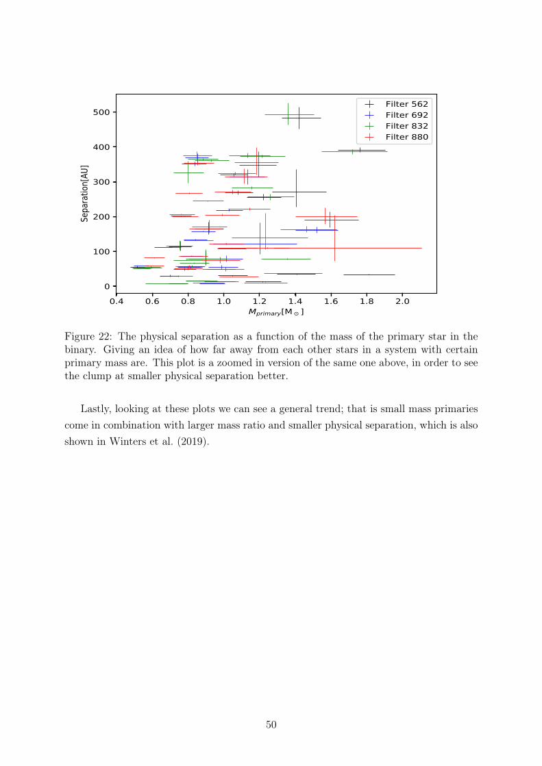
0.4 0.6 0.8 1.0 1.2 1.4 1.6 1.8 2.0Mprimary[M ]

0

100

200

300

400

500

Sepa

ratio

n[AU

]

Filter 562Filter 692Filter 832Filter 880

Figure 22: The physical separation as a function of the mass of the primary star in thebinary. Giving an idea of how far away from each other stars in a system with certainprimary mass are. This plot is a zoomed in version of the same one above, in order to seethe clump at smaller physical separation better.

Lastly, looking at these plots we can see a general trend; that is small mass primariescome in combination with larger mass ratio and smaller physical separation, which is alsoshown in Winters et al. (2019).

50

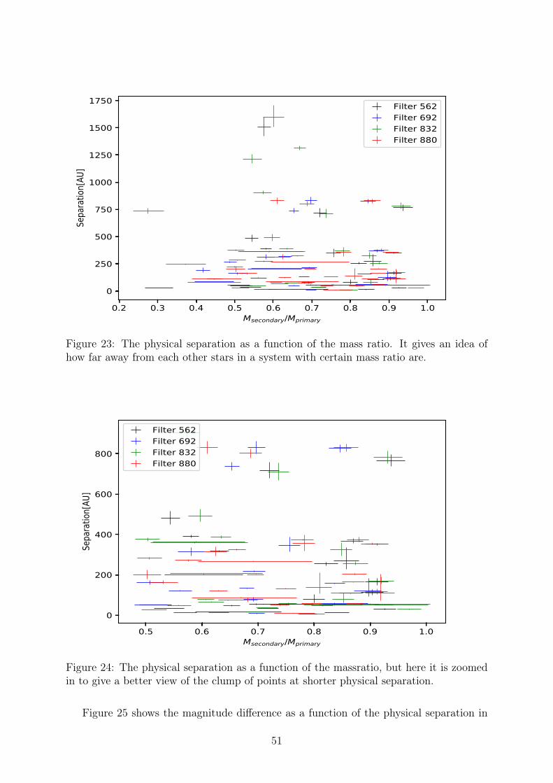
0.2 0.3 0.4 0.5 0.6 0.7 0.8 0.9 1.0Msecondary/Mprimary

0

250

500

750

1000

1250

1500

1750

Sepa

ratio

n[AU

]

Filter 562Filter 692Filter 832Filter 880

Figure 23: The physical separation as a function of the mass ratio. It gives an idea ofhow far away from each other stars in a system with certain mass ratio are.

0.5 0.6 0.7 0.8 0.9 1.0Msecondary/Mprimary

0

200

400

600

800

Sepa

ratio

n[AU

]

Filter 562Filter 692Filter 832Filter 880

Figure 24: The physical separation as a function of the massratio, but here it is zoomedin to give a better view of the clump of points at shorter physical separation.

Figure 25 shows the magnitude difference as a function of the physical separation in

51

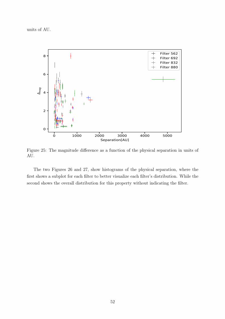
units of AU.

0 1000 2000 3000 4000 5000Separation[AU]

0

2

4

6

8

mag

Filter 562Filter 692Filter 832Filter 880

Figure 25: The magnitude difference as a function of the physical separation in units ofAU.

The two Figures 26 and 27, show histograms of the physical separation, where thefirst shows a subplot for each filter to better visualize each filter’s distribution. While thesecond shows the overall distribution for this property without indicating the filter.

52

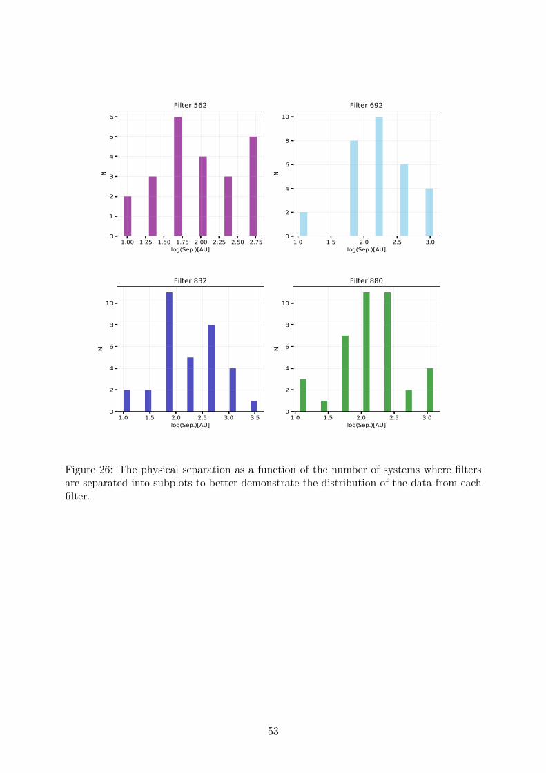
1.00 1.25 1.50 1.75 2.00 2.25 2.50 2.75log(Sep.)[AU]

0

1

2

3

4

5

6

NFilter 562

1.0 1.5 2.0 2.5 3.0log(Sep.)[AU]

0

2

4

6

8

10

N

Filter 692

1.0 1.5 2.0 2.5 3.0 3.5log(Sep.)[AU]

0

2

4

6

8

10

N

Filter 832

1.0 1.5 2.0 2.5 3.0log(Sep.)[AU]

0

2

4

6

8

10

NFilter 880

Figure 26: The physical separation as a function of the number of systems where filtersare separated into subplots to better demonstrate the distribution of the data from eachfilter.

53

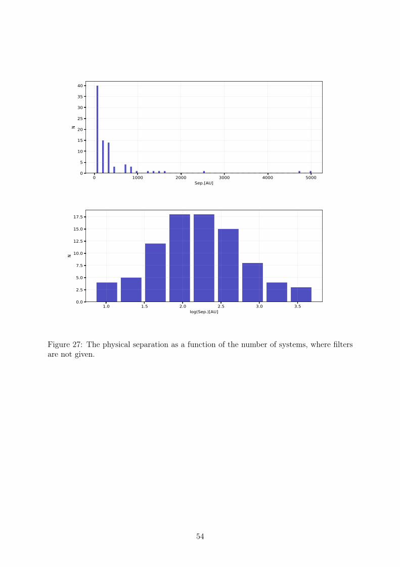
0 1000 2000 3000 4000 5000Sep.[AU]

0

5

10

15

20

25

30

35

40

N

1.0 1.5 2.0 2.5 3.0 3.5log(Sep.)[AU]

0.0

2.5

5.0

7.5

10.0

12.5

15.0

17.5

N

Figure 27: The physical separation as a function of the number of systems, where filtersare not given.

54

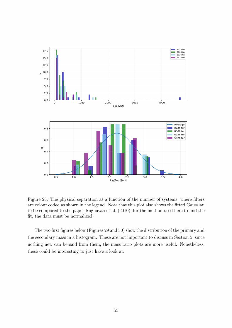
0 1000 2000 3000 4000Sep.[AU]

0.0

2.5

5.0

7.5

10.0

12.5

15.0

17.5

N

832filter880filter692filter562filter

0.5 1.0 1.5 2.0 2.5 3.0 3.5 4.0log(Sep.)[AU]

0.0

0.2

0.4

0.6

0.8

N

Average832filter880filter692filter562filter

Figure 28: The physical separation as a function of the number of systems, where filtersare colour coded as shown in the legend. Note that this plot also shows the fitted Gaussianto be compared to the paper Raghavan et al. (2010), for the method used here to find thefit, the data must be normalized.

The two first figures below (Figures 29 and 30) show the distribution of the primary andthe secondary mass in a histogram. These are not important to discuss in Section 5, sincenothing new can be said from them, the mass ratio plots are more useful. Nonetheless,these could be interesting to just have a look at.

55

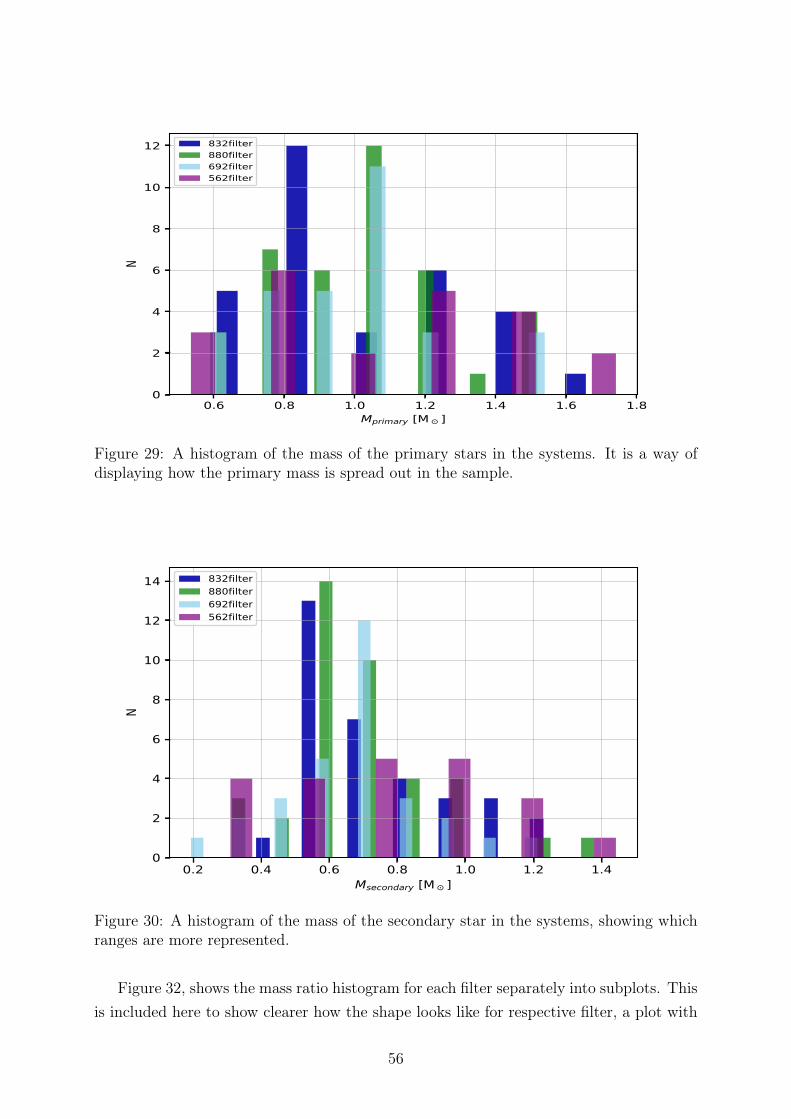
0.6 0.8 1.0 1.2 1.4 1.6 1.8Mprimary [M ]

0

2

4

6

8

10

12N

832filter880filter692filter562filter

Figure 29: A histogram of the mass of the primary stars in the systems. It is a way ofdisplaying how the primary mass is spread out in the sample.

0.2 0.4 0.6 0.8 1.0 1.2 1.4Msecondary [M ]

0

2

4

6

8

10

12

14

N

832filter880filter692filter562filter

Figure 30: A histogram of the mass of the secondary star in the systems, showing whichranges are more represented.

Figure 32, shows the mass ratio histogram for each filter separately into subplots. Thisis included here to show clearer how the shape looks like for respective filter, a plot with

56

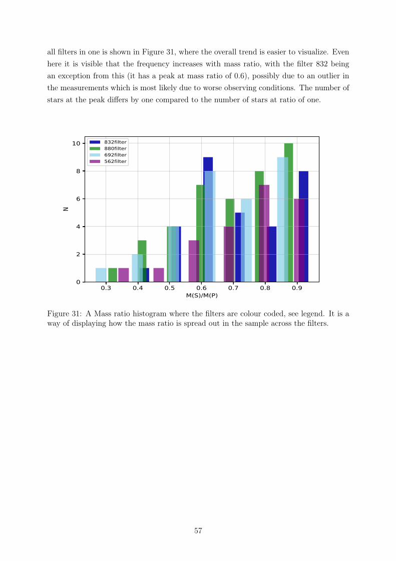
all filters in one is shown in Figure 31, where the overall trend is easier to visualize. Evenhere it is visible that the frequency increases with mass ratio, with the filter 832 beingan exception from this (it has a peak at mass ratio of 0.6), possibly due to an outlier inthe measurements which is most likely due to worse observing conditions. The number ofstars at the peak differs by one compared to the number of stars at ratio of one.

0.3 0.4 0.5 0.6 0.7 0.8 0.9M(S)/M(P)

0

2

4

6

8

10

N

832filter880filter692filter562filter

Figure 31: A Mass ratio histogram where the filters are colour coded, see legend. It is away of displaying how the mass ratio is spread out in the sample across the filters.

57

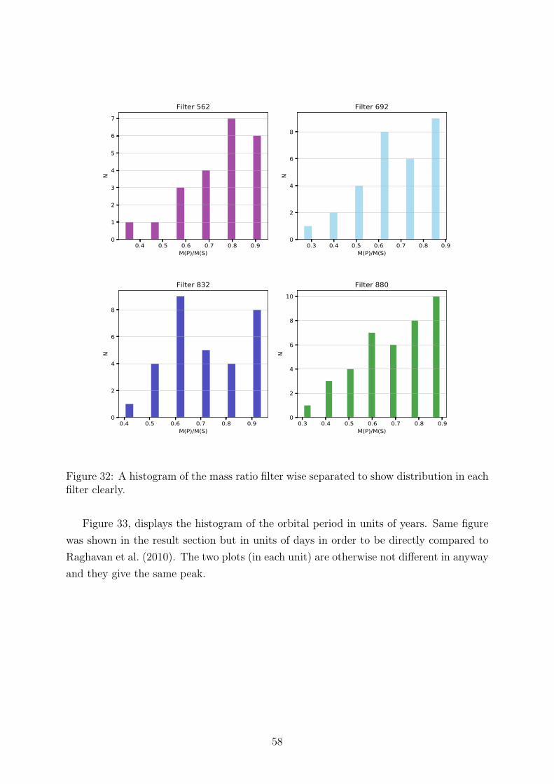
0.4 0.5 0.6 0.7 0.8 0.9M(P)/M(S)

0

1

2

3

4

5

6

7

NFilter 562

0.3 0.4 0.5 0.6 0.7 0.8 0.9M(P)/M(S)

0

2

4

6

8

N

Filter 692

0.4 0.5 0.6 0.7 0.8 0.9M(P)/M(S)

0

2

4

6

8

N

Filter 832

0.3 0.4 0.5 0.6 0.7 0.8 0.9M(P)/M(S)

0

2

4

6

8

10

NFilter 880

Figure 32: A histogram of the mass ratio filter wise separated to show distribution in eachfilter clearly.

Figure 33, displays the histogram of the orbital period in units of years. Same figurewas shown in the result section but in units of days in order to be directly compared toRaghavan et al. (2010). The two plots (in each unit) are otherwise not different in anywayand they give the same peak.

58

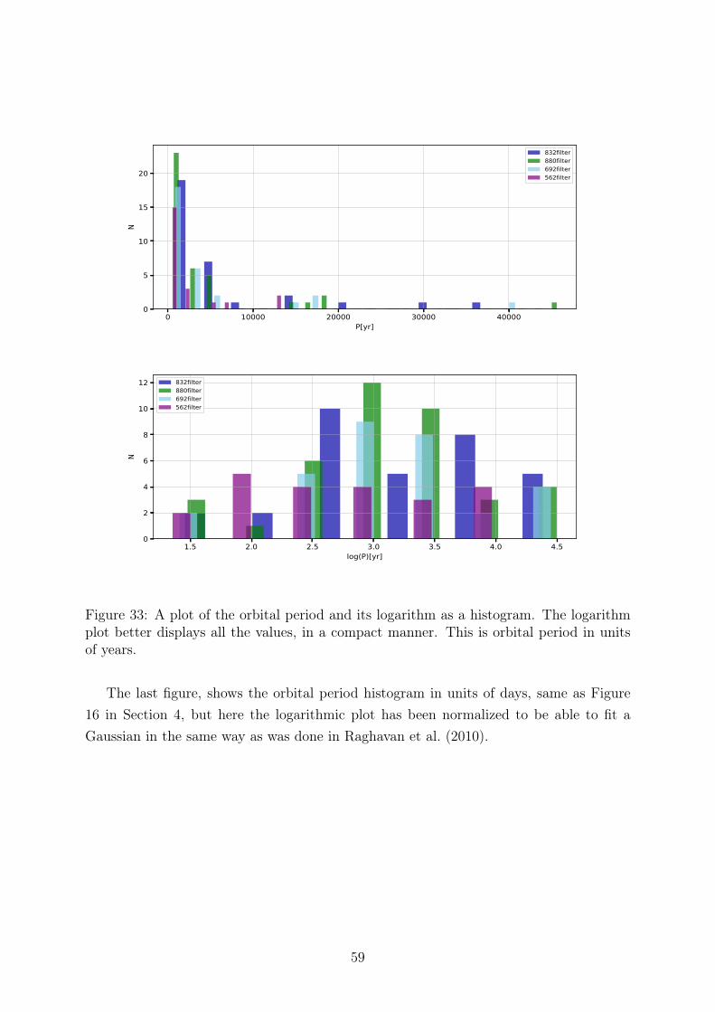
0 10000 20000 30000 40000P[yr]

0

5

10

15

20

N

832filter880filter692filter562filter

1.5 2.0 2.5 3.0 3.5 4.0 4.5log(P)[yr]

0

2

4

6

8

10

12

N

832filter880filter692filter562filter

Figure 33: A plot of the orbital period and its logarithm as a histogram. The logarithmplot better displays all the values, in a compact manner. This is orbital period in unitsof years.

The last figure, shows the orbital period histogram in units of days, same as Figure16 in Section 4, but here the logarithmic plot has been normalized to be able to fit aGaussian in the same way as was done in Raghavan et al. (2010).

59

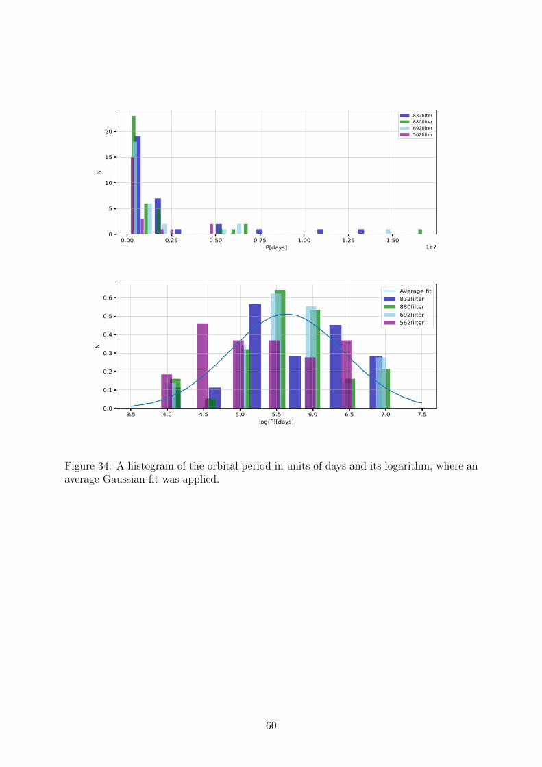
0.00 0.25 0.50 0.75 1.00 1.25 1.50P[days] 1e7

0

5

10

15

20

N

832filter880filter692filter562filter

3.5 4.0 4.5 5.0 5.5 6.0 6.5 7.0 7.5log(P)[days]

0.0

0.1

0.2

0.3

0.4

0.5

0.6

N

Average fit832filter880filter692filter562filter

Figure 34: A histogram of the orbital period in units of days and its logarithm, where anaverage Gaussian fit was applied.

60

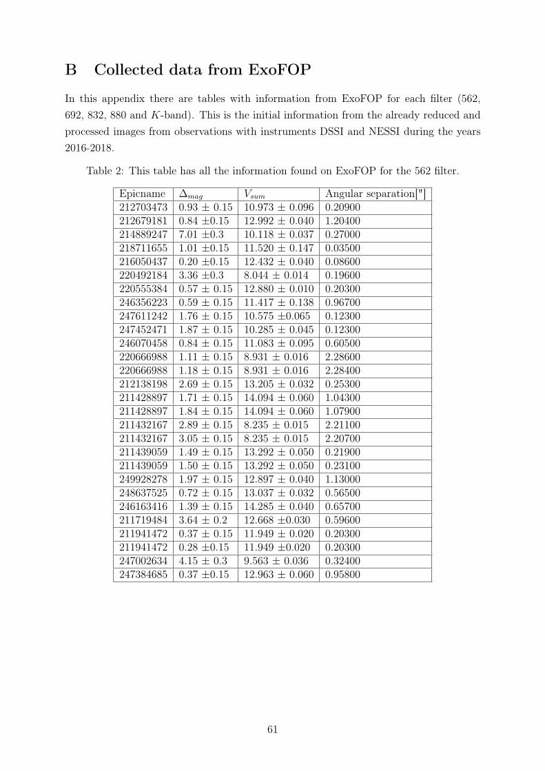
B Collected data from ExoFOP

In this appendix there are tables with information from ExoFOP for each filter (562,692, 832, 880 and K-band). This is the initial information from the already reduced andprocessed images from observations with instruments DSSI and NESSI during the years2016-2018.

Table 2: This table has all the information found on ExoFOP for the 562 filter.

Epicname ∆mag Vsum Angular separation["]212703473 0.93 ± 0.15 10.973 ± 0.096 0.20900212679181 0.84 ±0.15 12.992 ± 0.040 1.20400214889247 7.01 ±0.3 10.118 ± 0.037 0.27000218711655 1.01 ±0.15 11.520 ± 0.147 0.03500216050437 0.20 ±0.15 12.432 ± 0.040 0.08600220492184 3.36 ±0.3 8.044 ± 0.014 0.19600220555384 0.57 ± 0.15 12.880 ± 0.010 0.20300246356223 0.59 ± 0.15 11.417 ± 0.138 0.96700247611242 1.76 ± 0.15 10.575 ±0.065 0.12300247452471 1.87 ± 0.15 10.285 ± 0.045 0.12300246070458 0.84 ± 0.15 11.083 ± 0.095 0.60500220666988 1.11 ± 0.15 8.931 ± 0.016 2.28600220666988 1.18 ± 0.15 8.931 ± 0.016 2.28400212138198 2.69 ± 0.15 13.205 ± 0.032 0.25300211428897 1.71 ± 0.15 14.094 ± 0.060 1.04300211428897 1.84 ± 0.15 14.094 ± 0.060 1.07900211432167 2.89 ± 0.15 8.235 ± 0.015 2.21100211432167 3.05 ± 0.15 8.235 ± 0.015 2.20700211439059 1.49 ± 0.15 13.292 ± 0.050 0.21900211439059 1.50 ± 0.15 13.292 ± 0.050 0.23100249928278 1.97 ± 0.15 12.897 ± 0.040 1.13000248637525 0.72 ± 0.15 13.037 ± 0.032 0.56500246163416 1.39 ± 0.15 14.285 ± 0.040 0.65700211719484 3.64 ± 0.2 12.668 ±0.030 0.59600211941472 0.37 ± 0.15 11.949 ± 0.020 0.20300211941472 0.28 ±0.15 11.949 ±0.020 0.20300247002634 4.15 ± 0.3 9.563 ± 0.036 0.32400247384685 0.37 ±0.15 12.963 ± 0.060 0.95800

61

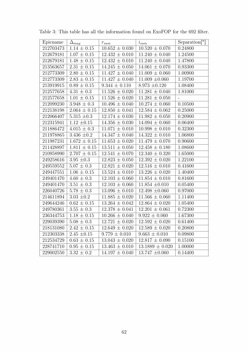
Table 3: This table has all the information found on ExoFOP for the 692 filter.

Epicname ∆mag rsum isum Separation["]212703473 1.14 ± 0.15 10.652 ± 0.030 10.520 ± 0.070 0.24800212679181 1.07 ± 0.15 12.432 ± 0.010 11.240 ± 0.040 1.24500212679181 1.48 ± 0.15 12.432 ± 0.010 11.240 ± 0.040 1.47800213563657 2.31 ± 0.15 14.245 ± 0.050 14.061 ± 0.070 0.93300212773309 2.80 ± 0.15 11.427 ± 0.040 11.009 ± 0.060 1.00900212773309 2.83 ± 0.15 11.427 ± 0.040 11.009 ±0.060 1.19700213919915 0.89 ± 0.15 9.344 ± 0.110 8.973 ±0.120 1.08400212577658 4.31 ± 0.3 11.526 ± 0.020 11.281 ± 0.040 1.81000212577658 1.01 ± 0.15 11.526 ± 0.020 11.281 ± 0.050 -212099230 3.948 ± 0.3 10.496 ± 0.040 10.274 ± 0.060 0.10500212138198 2.064 ± 0.15 12.850 ± 0.041 12.584 ± 0.062 0.25000212066407 5.315 ±0.3 12.174 ± 0.030 11.982 ± 0.050 0.20900212315941 1.12 ±0.15 14.356 ± 0.030 14.094 ± 0.060 0.06400211886472 4.015 ± 0.3 11.071 ± 0.010 10.998 ± 0.010 0.32300211978865 3.436 ±0.2 14.347 ± 0.040 14.322 ± 0.010 1.06800211987231 1.672 ± 0.15 11.653 ± 0.020 11.479 ± 0.070 0.90600211428897 1.811 ± 0.15 13.511 ± 0.050 12.458 ± 0.180 1.08600210958990 2.707 ± 0.15 12.541 ± 0.070 12.340 ± 0.320 1.65000249258616 3.95 ±0.3 12.823 ± 0.050 12.392 ± 0.020 1.22100249559552 5.07 ± 0.3 12.821 ± 0.020 12.516 ± 0.010 0.41600249447551 1.06 ± 0.15 13.524 ± 0.010 13.226 ± 0.020 1.40400249401470 4.60 ± 0.3 12.103 ± 0.060 11.854 ± 0.010 0.81600249401470 3.51 ± 0.3 12.103 ± 0.060 11.854 ±0.010 0.05400226040726 5.78 ± 0.3 13.096 ± 0.010 12.498 ±0.060 0.97000214611894 3.03 ±0.2 11.885 ± 0.020 11.566 ± 0.060 1.11400249644246 0.62 ± 0.15 13.264 ± 0.042 12.864 ± 0.020 1.05400249780361 3.55 ± 0.3 12.378 ± 0.041 12.201 ± 0.061 0.72300236344753 1.18 ± 0.15 10.266 ± 0.040 9.922 ± 0.060 1.67300229039390 5.08 ± 0.3 12.721 ± 0.020 12.592 ± 0.020 0.61400218131080 2.42 ± 0.15 12.649 ± 0.020 12.589 ± 0.020 0.20800212303338 2.45 ±0.15 9.779 ± 0.010 9.663 ± 0.010 0.09800212534729 0.63 ± 0.15 13.043 ± 0.020 12.817 ± 0.090 0.15100228741710 0.95 ± 0.15 13.463 ± 0.010 13.1889 ± 0.020 1.00000229002550 3.32 ± 0.2 14.197 ± 0.040 13.747 ±0.060 0.14400

62

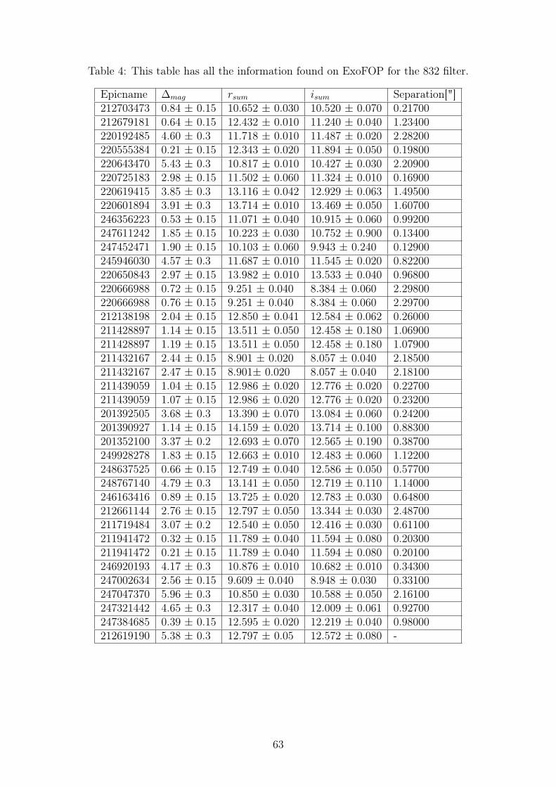
Table 4: This table has all the information found on ExoFOP for the 832 filter.

Epicname ∆mag rsum isum Separation["]212703473 0.84 ± 0.15 10.652 ± 0.030 10.520 ± 0.070 0.21700212679181 0.64 ± 0.15 12.432 ± 0.010 11.240 ± 0.040 1.23400220192485 4.60 ± 0.3 11.718 ± 0.010 11.487 ± 0.020 2.28200220555384 0.21 ± 0.15 12.343 ± 0.020 11.894 ± 0.050 0.19800220643470 5.43 ± 0.3 10.817 ± 0.010 10.427 ± 0.030 2.20900220725183 2.98 ± 0.15 11.502 ± 0.060 11.324 ± 0.010 0.16900220619415 3.85 ± 0.3 13.116 ± 0.042 12.929 ± 0.063 1.49500220601894 3.91 ± 0.3 13.714 ± 0.010 13.469 ± 0.050 1.60700246356223 0.53 ± 0.15 11.071 ± 0.040 10.915 ± 0.060 0.99200247611242 1.85 ± 0.15 10.223 ± 0.030 10.752 ± 0.900 0.13400247452471 1.90 ± 0.15 10.103 ± 0.060 9.943 ± 0.240 0.12900245946030 4.57 ± 0.3 11.687 ± 0.010 11.545 ± 0.020 0.82200220650843 2.97 ± 0.15 13.982 ± 0.010 13.533 ± 0.040 0.96800220666988 0.72 ± 0.15 9.251 ± 0.040 8.384 ± 0.060 2.29800220666988 0.76 ± 0.15 9.251 ± 0.040 8.384 ± 0.060 2.29700212138198 2.04 ± 0.15 12.850 ± 0.041 12.584 ± 0.062 0.26000211428897 1.14 ± 0.15 13.511 ± 0.050 12.458 ± 0.180 1.06900211428897 1.19 ± 0.15 13.511 ± 0.050 12.458 ± 0.180 1.07900211432167 2.44 ± 0.15 8.901 ± 0.020 8.057 ± 0.040 2.18500211432167 2.47 ± 0.15 8.901± 0.020 8.057 ± 0.040 2.18100211439059 1.04 ± 0.15 12.986 ± 0.020 12.776 ± 0.020 0.22700211439059 1.07 ± 0.15 12.986 ± 0.020 12.776 ± 0.020 0.23200201392505 3.68 ± 0.3 13.390 ± 0.070 13.084 ± 0.060 0.24200201390927 1.14 ± 0.15 14.159 ± 0.020 13.714 ± 0.100 0.88300201352100 3.37 ± 0.2 12.693 ± 0.070 12.565 ± 0.190 0.38700249928278 1.83 ± 0.15 12.663 ± 0.010 12.483 ± 0.060 1.12200248637525 0.66 ± 0.15 12.749 ± 0.040 12.586 ± 0.050 0.57700248767140 4.79 ± 0.3 13.141 ± 0.050 12.719 ± 0.110 1.14000246163416 0.89 ± 0.15 13.725 ± 0.020 12.783 ± 0.030 0.64800212661144 2.76 ± 0.15 12.797 ± 0.050 13.344 ± 0.030 2.48700211719484 3.07 ± 0.2 12.540 ± 0.050 12.416 ± 0.030 0.61100211941472 0.32 ± 0.15 11.789 ± 0.040 11.594 ± 0.080 0.20300211941472 0.21 ± 0.15 11.789 ± 0.040 11.594 ± 0.080 0.20100246920193 4.17 ± 0.3 10.876 ± 0.010 10.682 ± 0.010 0.34300247002634 2.56 ± 0.15 9.609 ± 0.040 8.948 ± 0.030 0.33100247047370 5.96 ± 0.3 10.850 ± 0.030 10.588 ± 0.050 2.16100247321442 4.65 ± 0.3 12.317 ± 0.040 12.009 ± 0.061 0.92700247384685 0.39 ± 0.15 12.595 ± 0.020 12.219 ± 0.040 0.98000212619190 5.38 ± 0.3 12.797 ± 0.05 12.572 ± 0.080 -

63

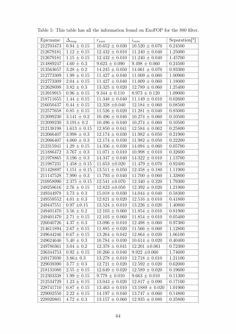
Table 5: This table has all the information found on ExoFOP for the 880 filter.

Epicname ∆mag rsum isum Separation["]212703473 0.94 ± 0.15 10.652 ± 0.030 10.520 ± 0.070 0.24500212679181 1.12 ± 0.15 12.432 ± 0.010 11.240 ± 0.040 1.25000212679181 1.15 ± 0.15 12.432 ± 0.010 11.240 ± 0.040 1.45700214889247 4.60 ± 0.3 9.623 ± 0.090 9.498 ± 0.060 0.24500213563657 3.28 ± 0.2 14.245 ± 0.050 14.061 ± 0.070 0.93300212773309 1.99 ± 0.15 11.427 ± 0.040 11.009 ± 0.060 1.00900212773309 2.04 ± 0.15 11.427 ± 0.040 11.009 ± 0.060 1.18000212628098 3.82 ± 0.3 13.325 ± 0.020 12.789 ± 0.060 1.25400213919915 0.96 ± 0.15 9.344 ± 0.110 8.973 ± 0.120 1.09000218711655 1.44 ± 0.15 11.348 ± 0.040 11.149 ± 0.010 0.02600216050437 0.44 ± 0.15 12.328 ±0.040 12.184 ± 0.060 0.08500212577658 0.85 ± 0.15 11.526 ± 0.020 11.281 ± 0.040 0.85000212099230 3.141 ± 0.2 10.496 ± 0.040 10.274 ± 0.060 0.10500212099230 3.191± 0.2 10.496 ± 0.040 10.274 ± 0.060 0.10500212138198 1.613 ± 0.15 12.850 ± 0.041 12.584 ± 0.062 0.25800212066407 3.998 ± 0.3 12.174 ± 0.030 11.982 ± 0.050 0.21900212066407 4.060 ± 0.3 12.174 ± 0.030 11.982 ± 0.050 0.22200212315941 1.29 ± 0.15 14.356 ± 0.030 14.094 ± 0.060 0.05700211886472 3.767 ± 0.3 11.071 ± 0.010 10.998 ± 0.010 0.32600211978865 3.196 ± 0.3 14.347 ± 0.040 14.322 ± 0.010 1.13700211987231 1.458 ± 0.15 11.653 ±0.020 11.479 ± 0.070 0.92400211428897 1.151 ± 0.15 13.511 ± 0.050 12.458 ± 0.180 1.11900211147528 7.990 ± 0.3 11.793 ± 0.040 11.700 ± 0.060 1.33800210958990 2.375 ± 0.15 12.541 ±0.070 12.340 ± 0.320 1.79300249258616 2.76 ± 0.15 12.823 ±0.050 12.392 ± 0.020 1.21900249344978 3.73 ± 0.3 15.018 ± 0.030 14.044 ± 0.040 0.58300249559552 4.01 ± 0.3 12.821 ± 0.020 12.516 ± 0.010 0.41800249447551 0.97 ±0.15 13.524 ± 0.010 13.226 ± 0.020 1.40800249401470 3.56 ± 0.2 12.103 ± 0.060 11.854 ± 0.010 0.81900249401470 2.71 ± 0.15 12.103 ± 0.060 11.854 ± 0.010 0.05400226040726 4.37 ± 0.3 13.096 ± 0.010 12.498 ± 0.060 0.97300214611894 2.67 ± 0.15 11.885 ± 0.020 11.566 ± 0.060 1.12800249644246 0.67 ± 0.15 13.264 ± 0.042 12.864 ± 0.020 1.06100249624646 5.40 ± 0.3 10.784 ± 0.030 10.614 ± 0.020 0.40400249780361 3.04 ± 0.2 12.378 ± 0.041 12.201 ±0.061 0.72300236344753 0.92 ± 0.15 10.266 ± 0.040 9.922 ±0.060 1.74600249173930 3.86± 0.3 13.278 ± 0.010 12.718 ± 0.010 1.21100229039390 3.77 ± 0.3 12.721 ± 0.020 12.592 ± 0.020 0.62000218131080 2.55 ± 0.15 12.649 ± 0.020 12.589 ± 0.020 0.19600212303338 1.99 ± 0.15 9.779 ± 0.010 9.663 ± 0.010 0.11300212534729 1.23 ± 0.15 13.043 ± 0.020 12.817 ± 0.090 0.17100228741710 0.87 ± 0.15 13.463 ± 0.010 13.1889 ± 0.020 1.01900229002550 2.22 ± 0.15 14.197 ± 0.040 13.747 ± 0.060 0.14800228920801 4.72 ± 0.3 13.157 ± 0.060 12.935 ± 0.080 0.35800

64

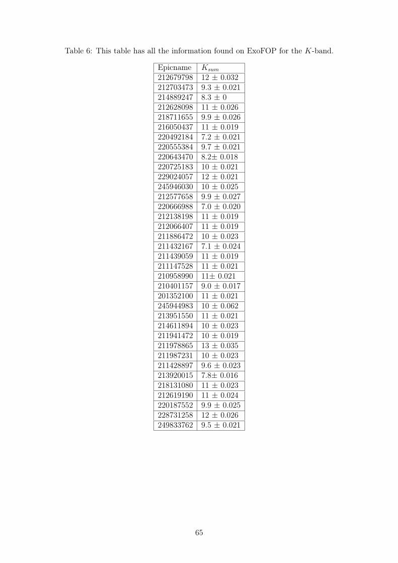
Table 6: This table has all the information found on ExoFOP for the K-band.

Epicname Ksum

212679798 12 ± 0.032212703473 9.3 ± 0.021214889247 8.3 ± 0212628098 11 ± 0.026218711655 9.9 ± 0.026216050437 11 ± 0.019220492184 7.2 ± 0.021220555384 9.7 ± 0.021220643470 8.2± 0.018220725183 10 ± 0.021229024057 12 ± 0.021245946030 10 ± 0.025212577658 9.9 ± 0.027220666988 7.0 ± 0.020212138198 11 ± 0.019212066407 11 ± 0.019211886472 10 ± 0.023211432167 7.1 ± 0.024211439059 11 ± 0.019211147528 11 ± 0.021210958990 11± 0.021210401157 9.0 ± 0.017201352100 11 ± 0.021245944983 10 ± 0.062213951550 11 ± 0.021214611894 10 ± 0.023211941472 10 ± 0.019211978865 13 ± 0.035211987231 10 ± 0.023211428897 9.6 ± 0.023213920015 7.8± 0.016218131080 11 ± 0.023212619190 11 ± 0.024220187552 9.9 ± 0.025228731258 12 ± 0.026249833762 9.5 ± 0.021

65

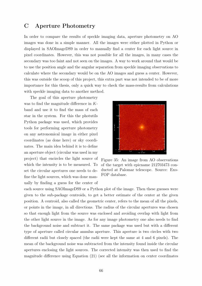
C Aperture Photometry

In order to compare the results of speckle imaging data, aperture photometry on AOimages was done in a simple manner. All the images were either plotted in Python ordisplayed in SAOImageDS9 in order to manually find a center for each light source inpixel coordinates. However, this was not possible for all the images, in many cases thesecondary was too faint and not seen on the images. A way to work around that would beto use the position angle and the angular separation from speckle imaging observations tocalculate where the secondary would be on the AO images and guess a center. However,this was outside the scoop of this project, this extra part was not intended to be of moreimportance for this thesis, only a quick way to check the mass-results from calculationswith speckle imaging data to another method.

Figure 35: An image from AO observationsof the target with epicname 212703473 con-ducted at Palomar telescope. Source: Exo-FOP database.

The goal of this aperture photometrywas to find the magnitude difference in K-band and use it to find the mass of eachstar in the system. For this the photutilsPython package was used, which providestools for performing aperture photometryon any astronomical image in either pixelcoordinates (as done here) or sky coordi-nates. The main idea behind it is to definean aperture object (circular was used in myproject) that encircles the light source ofwhich the intensity is to be measured. Toset the circular apertures one needs to de-fine the light sources, which was done man-ually by finding a guess for the center ofeach source using SAOImageDS9 or a Python plot of the image. Then these guesses weregiven to the sub-package centroids, to get a better estimate of the center at the givenposition. A centroid, also called the geometric center, refers to the mean of all the pixels,or points in the image, in all directions. The radius of the circular apertures was chosenso that enough light from the source was enclosed and avoiding overlap with light fromthe other light source in the image. As for any image photometry one also needs to findthe background noise and subtract it. The same package was used but with a differenttype of aperture called circular annulus aperture. This aperture is two circles with twodifferent radii but closely spaced (the radii were kept the same at 4 and 6 pixels). Themean of the background noise was subtracted from the intensity found inside the circularapertures enclosing the light sources. The corrected intensity was then used to find themagnitude difference using Equation (21) (see all the information on center coordinates

66

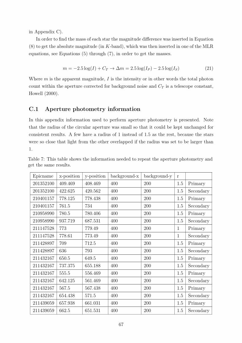
in Appendix C).In order to find the mass of each star the magnitude difference was inserted in Equation

(8) to get the absolute magnitude (inK-band), which was then inserted in one of the MLRequations, see Equations (5) through (7), in order to get the masses.

m = −2.5 log(I) + CT → ∆m = 2.5 log(IP )− 2.5 log(IS) (21)

Where m is the apparent magnitude, I is the intensity or in other words the total photoncount within the aperture corrected for background noise and CT is a telescope constant,Howell (2000).

C.1 Aperture photometry information

In this appendix information used to perform aperture photometry is presented. Notethat the radius of the circular aperture was small so that it could be kept unchanged forconsistent results. A few have a radius of 1 instead of 1.5 as the rest, because the starswere so close that light from the other overlapped if the radius was set to be larger than1.

Table 7: This table shows the information needed to repeat the aperture photometry andget the same results.

Epicname x-position y-position background-x background-y r201352100 409.469 408.469 400 200 1.5 Primary201352100 422.625 420.562 400 200 1.5 Secondary210401157 778.125 778.438 400 200 1.5 Primary210401157 761.5 734 400 200 1.5 Secondary210958990 780.5 780.406 400 200 1.5 Primary210958990 937.719 687.531 400 200 1.5 Secondary211147528 773 779.49 400 200 1 Primary211147528 778.61 773.49 400 200 1 Secondary211428897 709 712.5 400 200 1.5 Primary211428897 636 793 400 200 1.5 Secondary211432167 650.5 649.5 400 200 1.5 Primary211432167 737.375 655.188 400 200 1.5 Secondary211432167 555.5 556.469 400 200 1.5 Primary211432167 642.125 561.469 400 200 1.5 Secondary211432167 567.5 567.438 400 200 1.5 Primary211432167 654.438 571.5 400 200 1.5 Secondary211439059 657.938 661.031 400 200 1.5 Primary211439059 662.5 651.531 400 200 1.5 Secondary

67

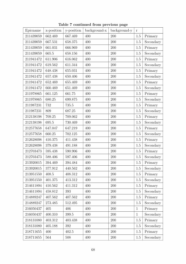
Table 7 continued from previous pageEpicname x-position y-position background-x background-y r211439059 662.469 667.469 400 200 1.5 Primary211439059 667.531 658.375 400 200 1.5 Secondary211439059 661.031 666.969 400 200 1.5 Primary211439059 665.5 658.156 400 200 1.5 Secondary211941472 611.906 616.062 400 200 1.5 Primary211941472 619.562 611.344 400 200 1.5 Secondary211941472 648.438 655.031 400 200 1.5 Primary211941472 657.438 650.406 400 200 1.5 Secondary211941472 652.469 655.469 400 200 1.5 Primary211941472 660.469 651.469 400 200 1.5 Secondary211978865 661.125 661.75 400 200 1.5 Primary211978865 680.25 699.875 400 200 1.5 Secondary211987231 732 735.5 400 200 1.5 Primary211987231 809 687.25 400 200 1.5 Secondary212138198 709.25 709.062 400 200 1.5 Primary212138198 695.5 730.469 400 200 1.5 Secondary212577658 647.047 647.219 400 200 1.5 Primary212577658 660.25 702.125 400 200 1.5 Secondary212628098 410.375 411.438 400 200 1.5 Primary212628098 379.438 491.188 400 200 1.5 Secondary212703473 595.438 590.906 400 200 1.5 Primary212703473 588.406 597.406 400 200 1.5 Secondary213920015 394.469 394.484 400 200 1.5 Primary213920015 377.912 440.562 400 200 1.5 Secondary213951550 408.5 408.312 400 200 1.5 Primary213951550 401.375 413.312 400 200 1.5 Secondary214611894 410.562 411.312 400 200 1.5 Primary214611894 458.812 393 400 200 1.5 Secondary214889247 407.562 407.562 400 200 1.5 Primary214889247 273.485 512.495 400 200 1.5 Secondary216050437 405 406 400 200 1 Primary216050437 400.310 399.5 400 200 1 Secondary218131080 403.312 403.438 400 200 1.5 Primary218131080 405.188 392 400 200 1.5 Secondary218711655 400 402.5 400 200 1.5 Primary218711655 564 508 400 200 1.5 Secondary

68

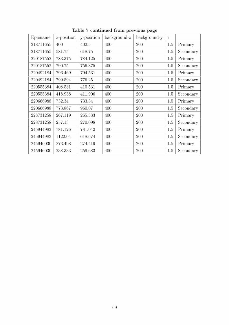
Table 7 continued from previous pageEpicname x-position y-position background-x background-y r218711655 400 402.5 400 200 1.5 Primary218711655 581.75 618.75 400 200 1.5 Secondary220187552 783.375 784.125 400 200 1.5 Primary220187552 790.75 756.375 400 200 1.5 Secondary220492184 796.469 794.531 400 200 1.5 Primary220492184 799.594 776.25 400 200 1.5 Secondary220555384 408.531 410.531 400 200 1.5 Primary220555384 418.938 411.906 400 200 1.5 Secondary220666988 732.34 733.34 400 200 1.5 Primary220666988 773.867 960.07 400 200 1.5 Secondary228731258 267.119 265.333 400 200 1.5 Primary228731258 257.13 270.098 400 200 1.5 Secondary245944983 781.126 781.042 400 200 1.5 Primary245944983 1122.04 618.674 400 200 1.5 Secondary245946030 273.498 274.419 400 200 1.5 Primary245946030 238.333 259.683 400 200 1.5 Secondary

69

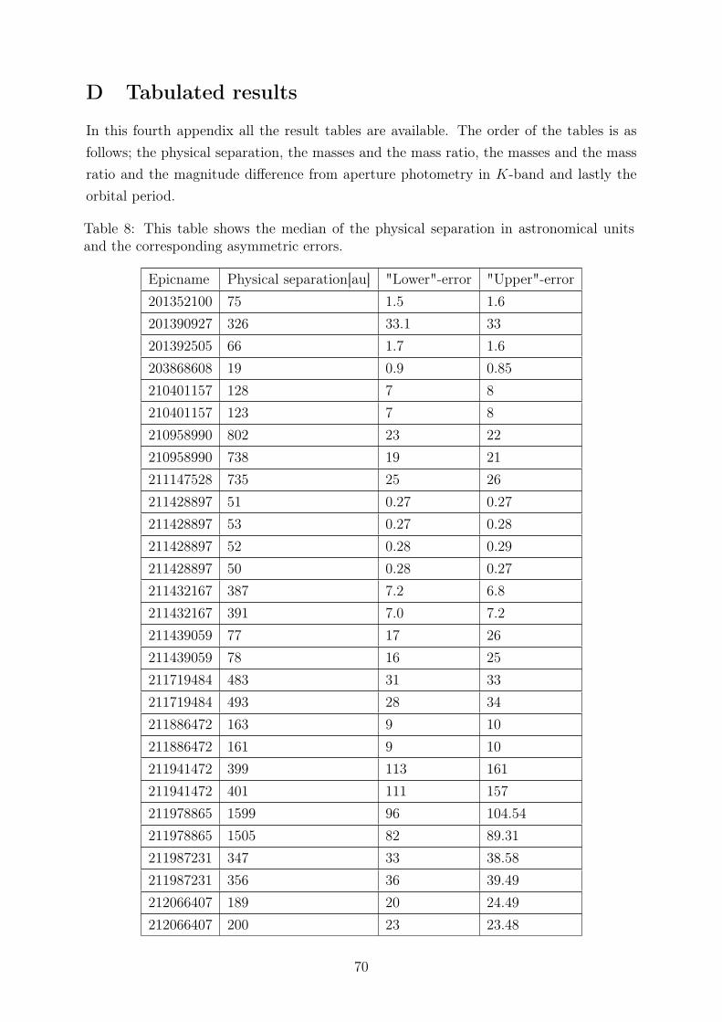
D Tabulated results

In this fourth appendix all the result tables are available. The order of the tables is asfollows; the physical separation, the masses and the mass ratio, the masses and the massratio and the magnitude difference from aperture photometry in K-band and lastly theorbital period.

Table 8: This table shows the median of the physical separation in astronomical unitsand the corresponding asymmetric errors.

Epicname Physical separation[au] "Lower"-error "Upper"-error201352100 75 1.5 1.6201390927 326 33.1 33201392505 66 1.7 1.6203868608 19 0.9 0.85210401157 128 7 8210401157 123 7 8210958990 802 23 22210958990 738 19 21211147528 735 25 26211428897 51 0.27 0.27211428897 53 0.27 0.28211428897 52 0.28 0.29211428897 50 0.28 0.27211432167 387 7.2 6.8211432167 391 7.0 7.2211439059 77 17 26211439059 78 16 25211719484 483 31 33211719484 493 28 34211886472 163 9 10211886472 161 9 10211941472 399 113 161211941472 401 111 157211978865 1599 96 104.54211978865 1505 82 89.31211987231 347 33 38.58211987231 356 36 39.49212066407 189 20 24.49212066407 200 23 23.48

70

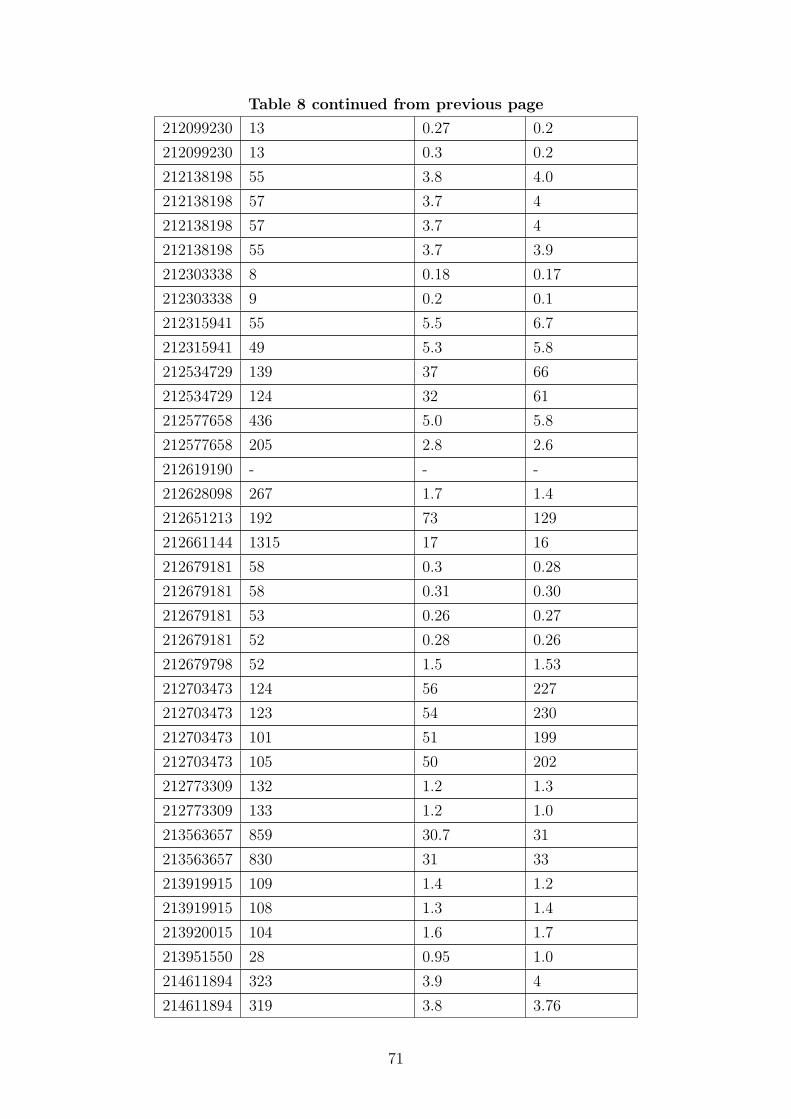
Table 8 continued from previous page212099230 13 0.27 0.2212099230 13 0.3 0.2212138198 55 3.8 4.0212138198 57 3.7 4212138198 57 3.7 4212138198 55 3.7 3.9212303338 8 0.18 0.17212303338 9 0.2 0.1212315941 55 5.5 6.7212315941 49 5.3 5.8212534729 139 37 66212534729 124 32 61212577658 436 5.0 5.8212577658 205 2.8 2.6212619190 - - -212628098 267 1.7 1.4212651213 192 73 129212661144 1315 17 16212679181 58 0.3 0.28212679181 58 0.31 0.30212679181 53 0.26 0.27212679181 52 0.28 0.26212679798 52 1.5 1.53212703473 124 56 227212703473 123 54 230212703473 101 51 199212703473 105 50 202212773309 132 1.2 1.3212773309 133 1.2 1.0213563657 859 30.7 31213563657 830 31 33213919915 109 1.4 1.2213919915 108 1.3 1.4213920015 104 1.6 1.7213951550 28 0.95 1.0214611894 323 3.9 4214611894 319 3.8 3.76

71

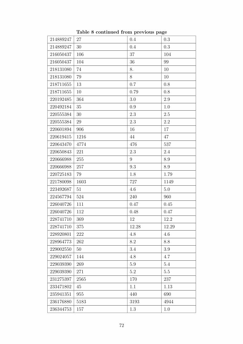
Table 8 continued from previous page214889247 27 0.4 0.3214889247 30 0.4 0.3216050437 106 37 104216050437 104 36 99218131080 74 8. 10218131080 79 8 10218711655 13 0.7 0.8218711655 10 0.79 0.8220192485 364 3.0 2.9220492184 35 0.9 1.0220555384 30 2.3 2.5220555384 29 2.3 2.2220601894 906 16 17220619415 1216 44 47220643470 4774 476 537220650843 221 2.3 2.4220666988 255 9 8.9220666988 257 9.3 8.9220725183 79 1.8 1.79221780098 1603 727 1149223492687 51 4.6 5.0224567794 524 240 960226040726 111 0.47 0.45226040726 112 0.48 0.47228741710 369 12 12.2228741710 375 12.28 12.29228920801 222 4.8 4.6228964773 262 8.2 8.8229002550 50 3.4 3.9229024057 144 4.8 4.7229039390 269 5.9 5.4229039390 271 5.2 5.5231275397 2565 170 237233471802 45 1.1 1.13235941351 955 440 690236176880 5183 3193 4944236344753 157 1.3 1.0

72

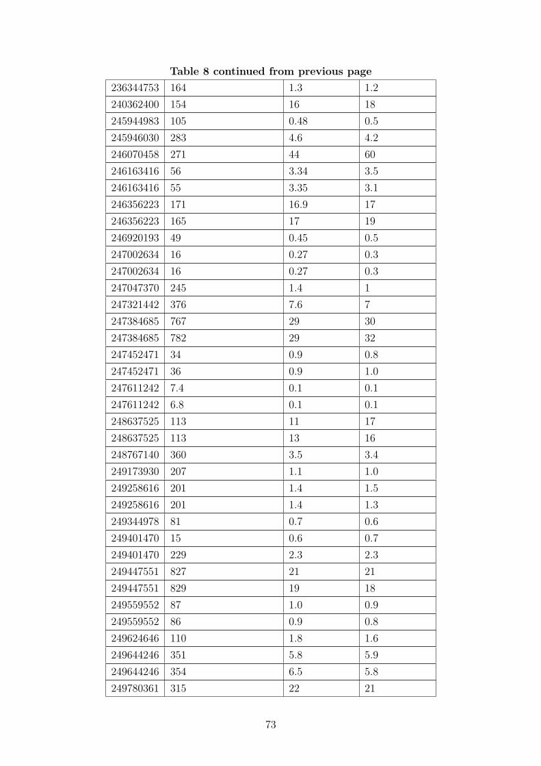
Table 8 continued from previous page236344753 164 1.3 1.2240362400 154 16 18245944983 105 0.48 0.5245946030 283 4.6 4.2246070458 271 44 60246163416 56 3.34 3.5246163416 55 3.35 3.1246356223 171 16.9 17246356223 165 17 19246920193 49 0.45 0.5247002634 16 0.27 0.3247002634 16 0.27 0.3247047370 245 1.4 1247321442 376 7.6 7247384685 767 29 30247384685 782 29 32247452471 34 0.9 0.8247452471 36 0.9 1.0247611242 7.4 0.1 0.1247611242 6.8 0.1 0.1248637525 113 11 17248637525 113 13 16248767140 360 3.5 3.4249173930 207 1.1 1.0249258616 201 1.4 1.5249258616 201 1.4 1.3249344978 81 0.7 0.6249401470 15 0.6 0.7249401470 229 2.3 2.3249447551 827 21 21249447551 829 19 18249559552 87 1.0 0.9249559552 86 0.9 0.8249624646 110 1.8 1.6249644246 351 5.8 5.9249644246 354 6.5 5.8249780361 315 22 21

73

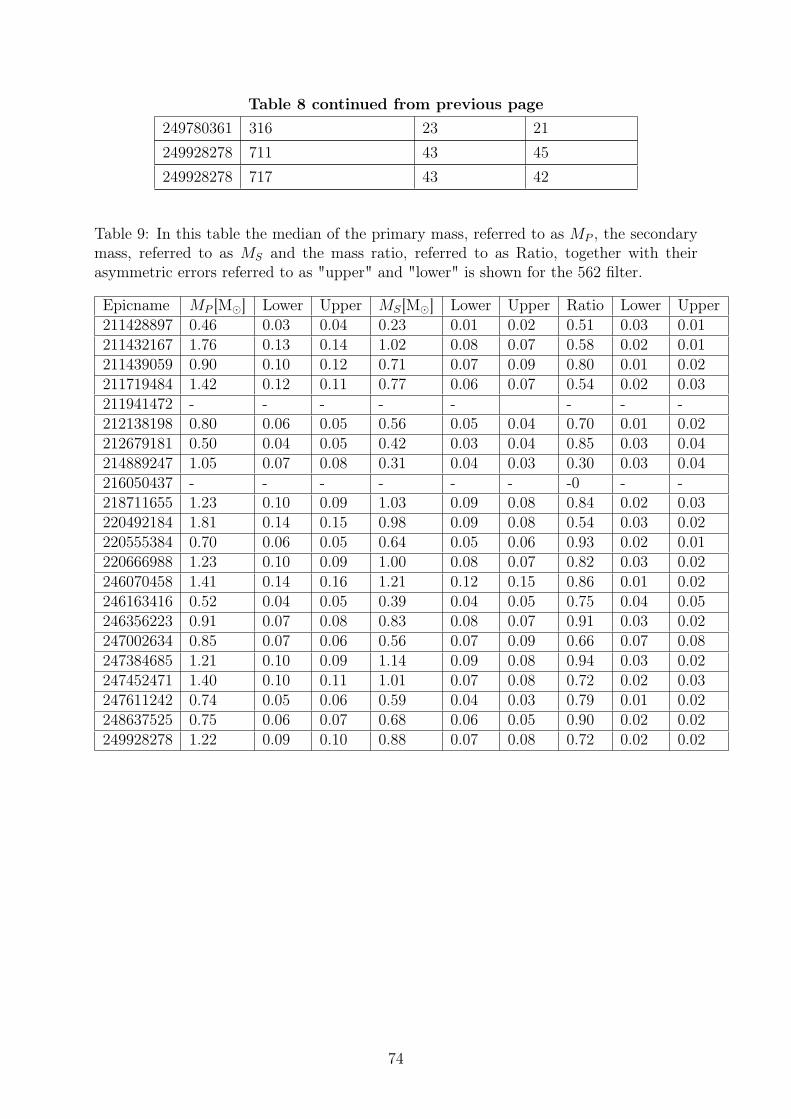
Table 8 continued from previous page249780361 316 23 21249928278 711 43 45249928278 717 43 42

Table 9: In this table the median of the primary mass, referred to as MP , the secondarymass, referred to as MS and the mass ratio, referred to as Ratio, together with theirasymmetric errors referred to as "upper" and "lower" is shown for the 562 filter.

Epicname MP [M�] Lower Upper MS[M�] Lower Upper Ratio Lower Upper211428897 0.46 0.03 0.04 0.23 0.01 0.02 0.51 0.03 0.01211432167 1.76 0.13 0.14 1.02 0.08 0.07 0.58 0.02 0.01211439059 0.90 0.10 0.12 0.71 0.07 0.09 0.80 0.01 0.02211719484 1.42 0.12 0.11 0.77 0.06 0.07 0.54 0.02 0.03211941472 - - - - - - - -212138198 0.80 0.06 0.05 0.56 0.05 0.04 0.70 0.01 0.02212679181 0.50 0.04 0.05 0.42 0.03 0.04 0.85 0.03 0.04214889247 1.05 0.07 0.08 0.31 0.04 0.03 0.30 0.03 0.04216050437 - - - - - - -0 - -218711655 1.23 0.10 0.09 1.03 0.09 0.08 0.84 0.02 0.03220492184 1.81 0.14 0.15 0.98 0.09 0.08 0.54 0.03 0.02220555384 0.70 0.06 0.05 0.64 0.05 0.06 0.93 0.02 0.01220666988 1.23 0.10 0.09 1.00 0.08 0.07 0.82 0.03 0.02246070458 1.41 0.14 0.16 1.21 0.12 0.15 0.86 0.01 0.02246163416 0.52 0.04 0.05 0.39 0.04 0.05 0.75 0.04 0.05246356223 0.91 0.07 0.08 0.83 0.08 0.07 0.91 0.03 0.02247002634 0.85 0.07 0.06 0.56 0.07 0.09 0.66 0.07 0.08247384685 1.21 0.10 0.09 1.14 0.09 0.08 0.94 0.03 0.02247452471 1.40 0.10 0.11 1.01 0.07 0.08 0.72 0.02 0.03247611242 0.74 0.05 0.06 0.59 0.04 0.03 0.79 0.01 0.02248637525 0.75 0.06 0.07 0.68 0.06 0.05 0.90 0.02 0.02249928278 1.22 0.09 0.10 0.88 0.07 0.08 0.72 0.02 0.02

74

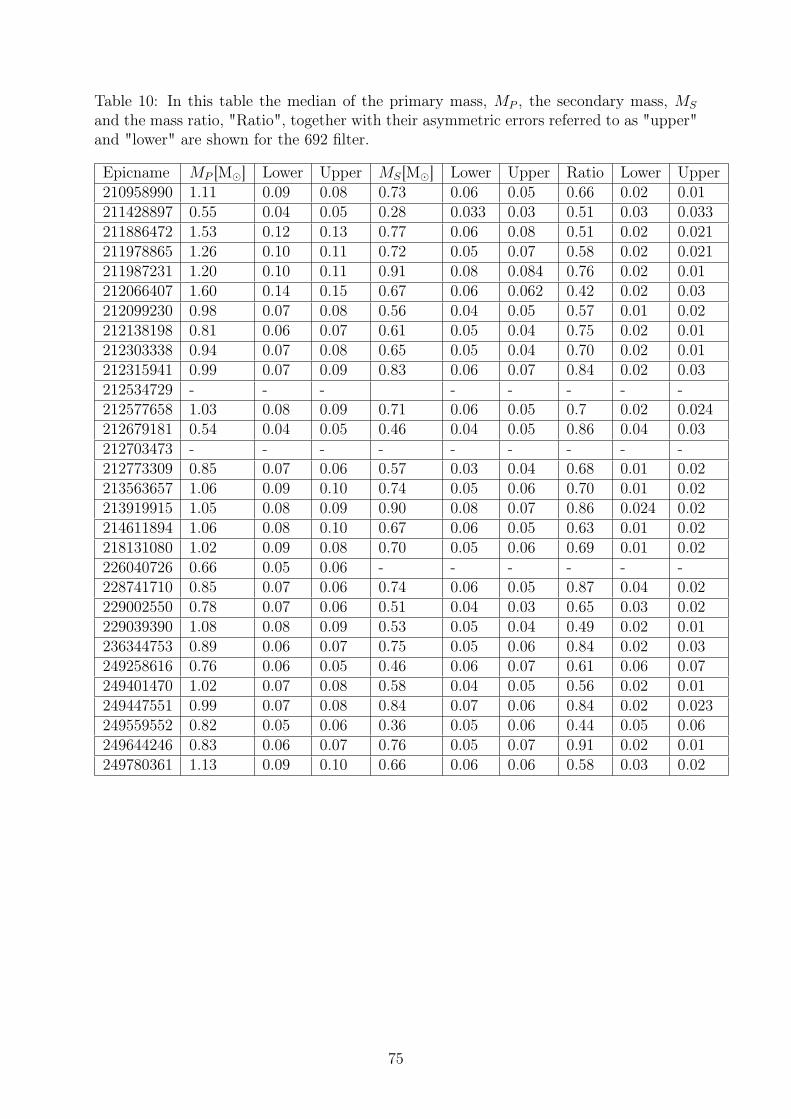
Table 10: In this table the median of the primary mass, MP , the secondary mass, MS

and the mass ratio, "Ratio", together with their asymmetric errors referred to as "upper"and "lower" are shown for the 692 filter.

Epicname MP [M�] Lower Upper MS[M�] Lower Upper Ratio Lower Upper210958990 1.11 0.09 0.08 0.73 0.06 0.05 0.66 0.02 0.01211428897 0.55 0.04 0.05 0.28 0.033 0.03 0.51 0.03 0.033211886472 1.53 0.12 0.13 0.77 0.06 0.08 0.51 0.02 0.021211978865 1.26 0.10 0.11 0.72 0.05 0.07 0.58 0.02 0.021211987231 1.20 0.10 0.11 0.91 0.08 0.084 0.76 0.02 0.01212066407 1.60 0.14 0.15 0.67 0.06 0.062 0.42 0.02 0.03212099230 0.98 0.07 0.08 0.56 0.04 0.05 0.57 0.01 0.02212138198 0.81 0.06 0.07 0.61 0.05 0.04 0.75 0.02 0.01212303338 0.94 0.07 0.08 0.65 0.05 0.04 0.70 0.02 0.01212315941 0.99 0.07 0.09 0.83 0.06 0.07 0.84 0.02 0.03212534729 - - - - - - - -212577658 1.03 0.08 0.09 0.71 0.06 0.05 0.7 0.02 0.024212679181 0.54 0.04 0.05 0.46 0.04 0.05 0.86 0.04 0.03212703473 - - - - - - - - -212773309 0.85 0.07 0.06 0.57 0.03 0.04 0.68 0.01 0.02213563657 1.06 0.09 0.10 0.74 0.05 0.06 0.70 0.01 0.02213919915 1.05 0.08 0.09 0.90 0.08 0.07 0.86 0.024 0.02214611894 1.06 0.08 0.10 0.67 0.06 0.05 0.63 0.01 0.02218131080 1.02 0.09 0.08 0.70 0.05 0.06 0.69 0.01 0.02226040726 0.66 0.05 0.06 - - - - - -228741710 0.85 0.07 0.06 0.74 0.06 0.05 0.87 0.04 0.02229002550 0.78 0.07 0.06 0.51 0.04 0.03 0.65 0.03 0.02229039390 1.08 0.08 0.09 0.53 0.05 0.04 0.49 0.02 0.01236344753 0.89 0.06 0.07 0.75 0.05 0.06 0.84 0.02 0.03249258616 0.76 0.06 0.05 0.46 0.06 0.07 0.61 0.06 0.07249401470 1.02 0.07 0.08 0.58 0.04 0.05 0.56 0.02 0.01249447551 0.99 0.07 0.08 0.84 0.07 0.06 0.84 0.02 0.023249559552 0.82 0.05 0.06 0.36 0.05 0.06 0.44 0.05 0.06249644246 0.83 0.06 0.07 0.76 0.05 0.07 0.91 0.02 0.01249780361 1.13 0.09 0.10 0.66 0.06 0.06 0.58 0.03 0.02

75

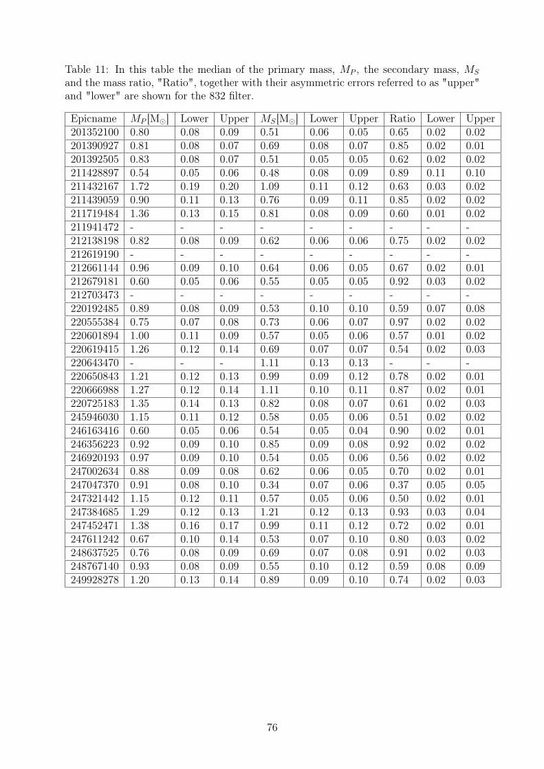
Table 11: In this table the median of the primary mass, MP , the secondary mass, MS

and the mass ratio, "Ratio", together with their asymmetric errors referred to as "upper"and "lower" are shown for the 832 filter.

Epicname MP [M�] Lower Upper MS[M�] Lower Upper Ratio Lower Upper201352100 0.80 0.08 0.09 0.51 0.06 0.05 0.65 0.02 0.02201390927 0.81 0.08 0.07 0.69 0.08 0.07 0.85 0.02 0.01201392505 0.83 0.08 0.07 0.51 0.05 0.05 0.62 0.02 0.02211428897 0.54 0.05 0.06 0.48 0.08 0.09 0.89 0.11 0.10211432167 1.72 0.19 0.20 1.09 0.11 0.12 0.63 0.03 0.02211439059 0.90 0.11 0.13 0.76 0.09 0.11 0.85 0.02 0.02211719484 1.36 0.13 0.15 0.81 0.08 0.09 0.60 0.01 0.02211941472 - - - - - - - - -212138198 0.82 0.08 0.09 0.62 0.06 0.06 0.75 0.02 0.02212619190 - - - - - - - - -212661144 0.96 0.09 0.10 0.64 0.06 0.05 0.67 0.02 0.01212679181 0.60 0.05 0.06 0.55 0.05 0.05 0.92 0.03 0.02212703473 - - - - - - - - -220192485 0.89 0.08 0.09 0.53 0.10 0.10 0.59 0.07 0.08220555384 0.75 0.07 0.08 0.73 0.06 0.07 0.97 0.02 0.02220601894 1.00 0.11 0.09 0.57 0.05 0.06 0.57 0.01 0.02220619415 1.26 0.12 0.14 0.69 0.07 0.07 0.54 0.02 0.03220643470 - - - 1.11 0.13 0.13 - - -220650843 1.21 0.12 0.13 0.99 0.09 0.12 0.78 0.02 0.01220666988 1.27 0.12 0.14 1.11 0.10 0.11 0.87 0.02 0.01220725183 1.35 0.14 0.13 0.82 0.08 0.07 0.61 0.02 0.03245946030 1.15 0.11 0.12 0.58 0.05 0.06 0.51 0.02 0.02246163416 0.60 0.05 0.06 0.54 0.05 0.04 0.90 0.02 0.01246356223 0.92 0.09 0.10 0.85 0.09 0.08 0.92 0.02 0.02246920193 0.97 0.09 0.10 0.54 0.05 0.06 0.56 0.02 0.02247002634 0.88 0.09 0.08 0.62 0.06 0.05 0.70 0.02 0.01247047370 0.91 0.08 0.10 0.34 0.07 0.06 0.37 0.05 0.05247321442 1.15 0.12 0.11 0.57 0.05 0.06 0.50 0.02 0.01247384685 1.29 0.12 0.13 1.21 0.12 0.13 0.93 0.03 0.04247452471 1.38 0.16 0.17 0.99 0.11 0.12 0.72 0.02 0.01247611242 0.67 0.10 0.14 0.53 0.07 0.10 0.80 0.03 0.02248637525 0.76 0.08 0.09 0.69 0.07 0.08 0.91 0.02 0.03248767140 0.93 0.08 0.09 0.55 0.10 0.12 0.59 0.08 0.09249928278 1.20 0.13 0.14 0.89 0.09 0.10 0.74 0.02 0.03

76

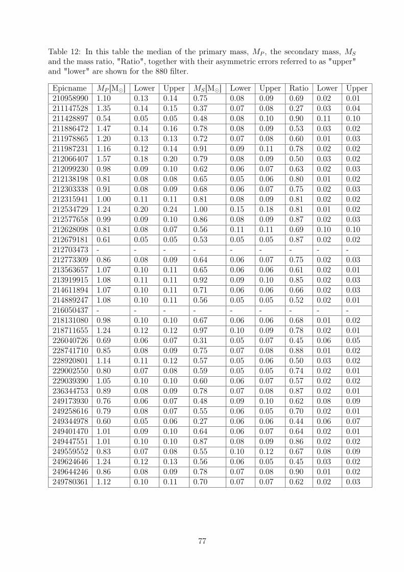
Table 12: In this table the median of the primary mass, MP , the secondary mass, MS

and the mass ratio, "Ratio", together with their asymmetric errors referred to as "upper"and "lower" are shown for the 880 filter.

Epicname MP [M�] Lower Upper MS[M�] Lower Upper Ratio Lower Upper210958990 1.10 0.13 0.14 0.75 0.08 0.09 0.69 0.02 0.01211147528 1.35 0.14 0.15 0.37 0.07 0.08 0.27 0.03 0.04211428897 0.54 0.05 0.05 0.48 0.08 0.10 0.90 0.11 0.10211886472 1.47 0.14 0.16 0.78 0.08 0.09 0.53 0.03 0.02211978865 1.20 0.13 0.13 0.72 0.07 0.08 0.60 0.01 0.03211987231 1.16 0.12 0.14 0.91 0.09 0.11 0.78 0.02 0.02212066407 1.57 0.18 0.20 0.79 0.08 0.09 0.50 0.03 0.02212099230 0.98 0.09 0.10 0.62 0.06 0.07 0.63 0.02 0.03212138198 0.81 0.08 0.08 0.65 0.05 0.06 0.80 0.01 0.02212303338 0.91 0.08 0.09 0.68 0.06 0.07 0.75 0.02 0.03212315941 1.00 0.11 0.11 0.81 0.08 0.09 0.81 0.02 0.02212534729 1.24 0.20 0.24 1.00 0.15 0.18 0.81 0.01 0.02212577658 0.99 0.09 0.10 0.86 0.08 0.09 0.87 0.02 0.03212628098 0.81 0.08 0.07 0.56 0.11 0.11 0.69 0.10 0.10212679181 0.61 0.05 0.05 0.53 0.05 0.05 0.87 0.02 0.02212703473 - - - - - - - - -212773309 0.86 0.08 0.09 0.64 0.06 0.07 0.75 0.02 0.03213563657 1.07 0.10 0.11 0.65 0.06 0.06 0.61 0.02 0.01213919915 1.08 0.11 0.11 0.92 0.09 0.10 0.85 0.02 0.03214611894 1.07 0.10 0.11 0.71 0.06 0.06 0.66 0.02 0.03214889247 1.08 0.10 0.11 0.56 0.05 0.05 0.52 0.02 0.01216050437 - - - - - - - - -218131080 0.98 0.10 0.10 0.67 0.06 0.06 0.68 0.01 0.02218711655 1.24 0.12 0.12 0.97 0.10 0.09 0.78 0.02 0.01226040726 0.69 0.06 0.07 0.31 0.05 0.07 0.45 0.06 0.05228741710 0.85 0.08 0.09 0.75 0.07 0.08 0.88 0.01 0.02228920801 1.14 0.11 0.12 0.57 0.05 0.06 0.50 0.03 0.02229002550 0.80 0.07 0.08 0.59 0.05 0.05 0.74 0.02 0.01229039390 1.05 0.10 0.10 0.60 0.06 0.07 0.57 0.02 0.02236344753 0.89 0.08 0.09 0.78 0.07 0.08 0.87 0.02 0.01249173930 0.76 0.06 0.07 0.48 0.09 0.10 0.62 0.08 0.09249258616 0.79 0.08 0.07 0.55 0.06 0.05 0.70 0.02 0.01249344978 0.60 0.05 0.06 0.27 0.06 0.06 0.44 0.06 0.07249401470 1.01 0.09 0.10 0.64 0.06 0.07 0.64 0.02 0.01249447551 1.01 0.10 0.10 0.87 0.08 0.09 0.86 0.02 0.02249559552 0.83 0.07 0.08 0.55 0.10 0.12 0.67 0.08 0.09249624646 1.24 0.12 0.13 0.56 0.06 0.05 0.45 0.03 0.02249644246 0.86 0.08 0.09 0.78 0.07 0.08 0.90 0.01 0.02249780361 1.12 0.10 0.11 0.70 0.07 0.07 0.62 0.02 0.03

77

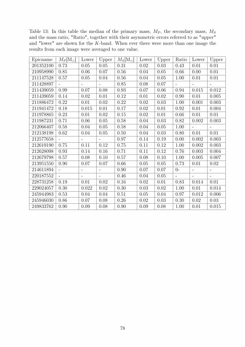
Table 13: In this table the median of the primary mass, MP , the secondary mass, MS

and the mass ratio, "Ratio", together with their asymmetric errors referred to as "upper"and "lower" are shown for the K-band. When ever there were more than one image theresults from each image were averaged to one value.

Epicname MP [M�] Lower Upper MS[M�] Lower Upper Ratio Lower Upper201352100 0.73 0.05 0.05 0.31 0.02 0.03 0.43 0.01 0.01210958990 0.85 0.06 0.07 0.56 0.04 0.05 0.66 0.00 0.01211147528 0.57 0.05 0.04 0.56 0.04 0.05 1.00 0.01 0.01211428897 - - - 0.85 0.08 0.07 - - -211439059 0.99 0.07 0.08 0.93 0.07 0.06 0.94 0.015 0.012211439059 0.14 0.02 0.01 0.12 0.01 0.02 0.90 0.01 0.005211886472 0.22 0.01 0.02 0.22 0.02 0.03 1.00 0.001 0.003211941472 0.18 0.015 0.01 0.17 0.02 0.01 0.92 0.01 0.004211978865 0.23 0.01 0.02 0.15 0.02 0.01 0.66 0.01 0.01211987231 0.71 0.06 0.05 0.58 0.04 0.03 0.82 0.002 0.003212066407 0.58 0.04 0.05 0.58 0.04 0.05 1.00 - -212138198 0.62 0.04 0.05 0.50 0.04 0.03 0.80 0.01 0.01212577658 - - - 0.97 0.14 0.19 0.00 0.002 0.003212619190 0.75 0.11 0.12 0.75 0.11 0.12 1.00 0.002 0.003212628098 0.93 0.14 0.16 0.71 0.11 0.12 0.76 0.003 0.004212679798 0.57 0.08 0.10 0.57 0.08 0.10 1.00 0.005 0.007213951550 0.90 0.07 0.07 0.66 0.05 0.05 0.73 0.01 0.02214611894 - - - 0.90 0.07 0.07 0- - -220187552 - - - 0.46 0.04 0.05 - - -228731258 0.19 0.01 0.02 0.16 0.02 0.01 0.83 0.014 0.01229024057 0.30 0.022 0.02 0.30 0.03 0.02 1.00 0.01 0.014245944983 0.53 0.04 0.04 0.51 0.05 0.04 0.97 0.012 0.006245946030 0.86 0.07 0.08 0.26 0.02 0.03 0.30 0.02 0.03249833762 0.90 0.09 0.08 0.90 0.09 0.08 1.00 0.01 0.015

78

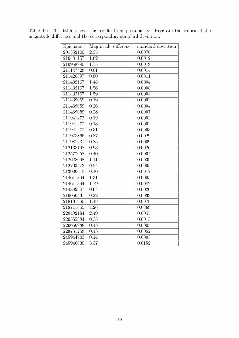
Table 14: This table shows the results from photometry. Here are the values of themagnitude difference and the corresponding standard deviation.

Epicname Magnitude difference standard deviation201352100 2.35 0.0076210401157 1.62 0.0012210958990 1.73 0.0019211147528 0.01 0.0014211428897 0.80 0.0011211432167 1.48 0.0004211432167 1.56 0.0008211432167 1.59 0.0004211439059 0.19 0.0003211439059 0.26 0.0004211439059 0.28 0.0007211941472 0.19 0.0002211941472 0.18 0.0002211941472 0.31 0.0008211978865 0.87 0.0029211987231 0.85 0.0009212138198 0.93 0.0026212577658 0.40 0.0004212628098 1.11 0.0039212703473 0.54 0.0005213920015 0.10 0.0017214611894 1.31 0.0005214611894 1.79 0.0042214889247 0.64 0.0020216050437 0.22 0.0039218131080 1.48 0.0078218711655 4.26 0.0369220492184 2.49 0.0045220555384 0.35 0.0015220666988 0.45 0.0005228731258 0.43 0.0052245944983 0.14 0.0003245946030 3.37 0.0152

79

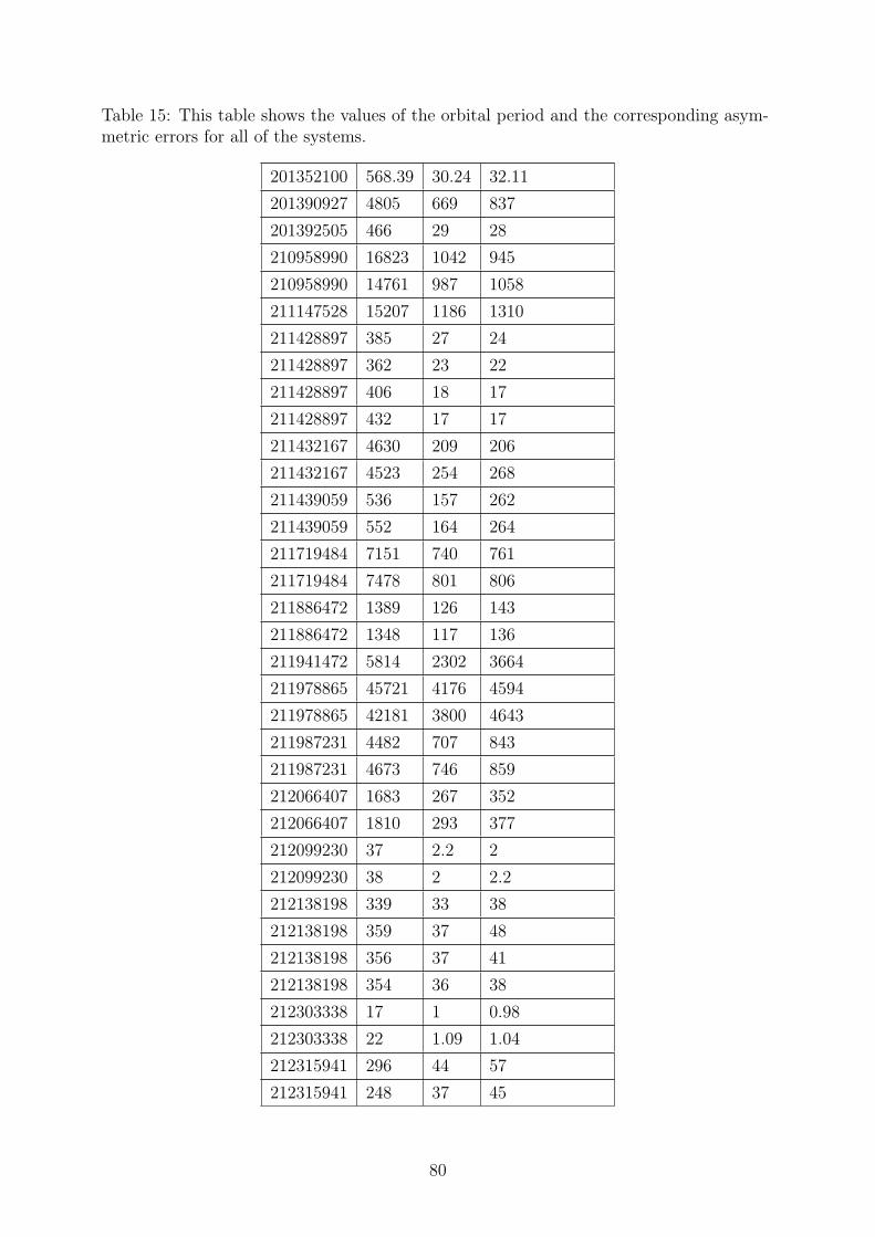
Table 15: This table shows the values of the orbital period and the corresponding asym-metric errors for all of the systems.

201352100 568.39 30.24 32.11201390927 4805 669 837201392505 466 29 28210958990 16823 1042 945210958990 14761 987 1058211147528 15207 1186 1310211428897 385 27 24211428897 362 23 22211428897 406 18 17211428897 432 17 17211432167 4630 209 206211432167 4523 254 268211439059 536 157 262211439059 552 164 264211719484 7151 740 761211719484 7478 801 806211886472 1389 126 143211886472 1348 117 136211941472 5814 2302 3664211978865 45721 4176 4594211978865 42181 3800 4643211987231 4482 707 843211987231 4673 746 859212066407 1683 267 352212066407 1810 293 377212099230 37 2.2 2212099230 38 2 2.2212138198 339 33 38212138198 359 37 48212138198 356 37 41212138198 354 36 38212303338 17 1 0.98212303338 22 1.09 1.04212315941 296 44 57212315941 248 37 45

80

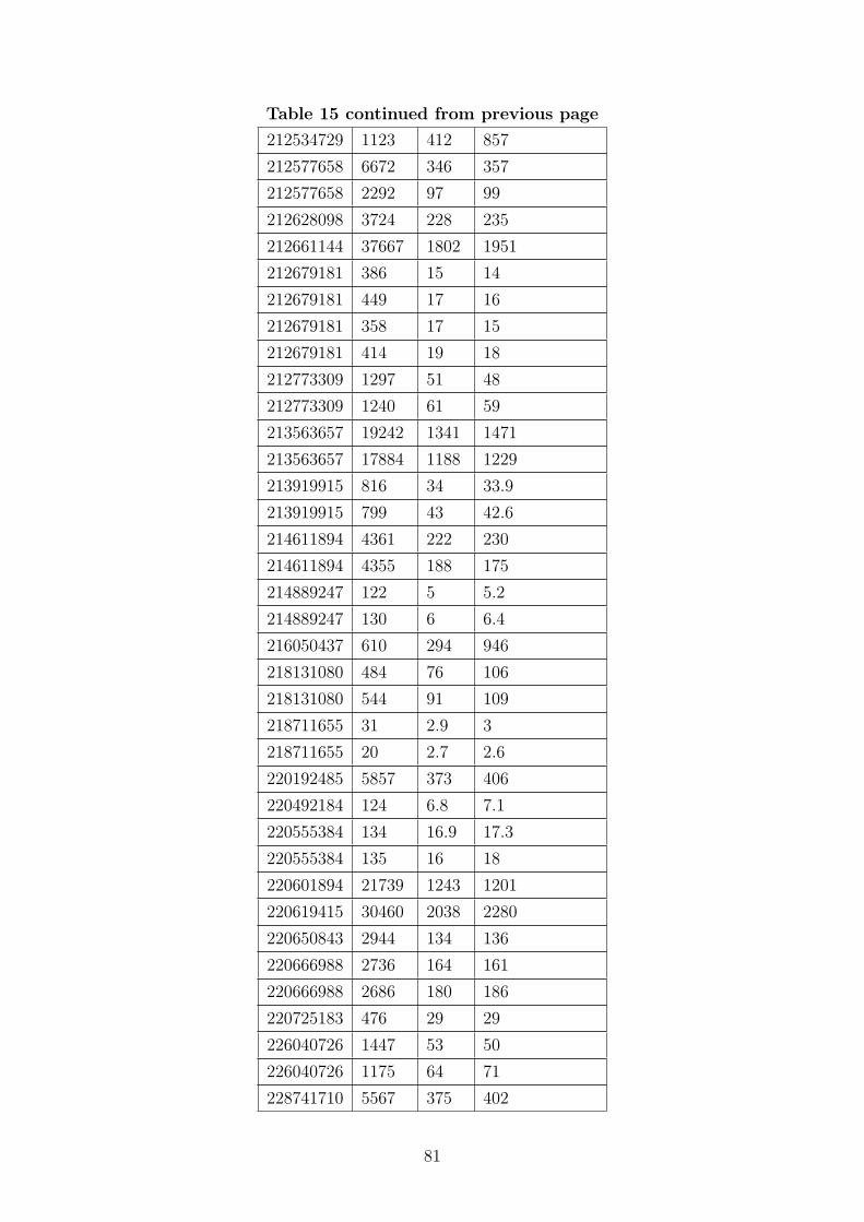
Table 15 continued from previous page212534729 1123 412 857212577658 6672 346 357212577658 2292 97 99212628098 3724 228 235212661144 37667 1802 1951212679181 386 15 14212679181 449 17 16212679181 358 17 15212679181 414 19 18212773309 1297 51 48212773309 1240 61 59213563657 19242 1341 1471213563657 17884 1188 1229213919915 816 34 33.9213919915 799 43 42.6214611894 4361 222 230214611894 4355 188 175214889247 122 5 5.2214889247 130 6 6.4216050437 610 294 946218131080 484 76 106218131080 544 91 109218711655 31 2.9 3218711655 20 2.7 2.6220192485 5857 373 406220492184 124 6.8 7.1220555384 134 16.9 17.3220555384 135 16 18220601894 21739 1243 1201220619415 30460 2038 2280220650843 2944 134 136220666988 2736 164 161220666988 2686 180 186220725183 476 29 29226040726 1447 53 50226040726 1175 64 71228741710 5567 375 402

81

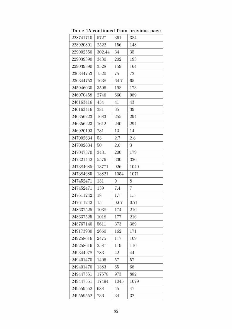
Table 15 continued from previous page228741710 5727 361 384228920801 2522 156 148229002550 302.44 34 35229039390 3430 202 193229039390 3528 159 164236344753 1520 75 72236344753 1638 64.7 65245946030 3596 198 173246070458 2746 660 989246163416 434 41 43246163416 381 35 39246356223 1683 255 294246356223 1612 240 294246920193 281 13 14247002634 53 2.7 2.8247002634 50 2.6 3247047370 3431 200 179247321442 5576 330 326247384685 13771 926 1040247384685 13821 1054 1071247452471 131 9 8247452471 139 7.4 7247611242 18 1.7 1.5247611242 15 0.67 0.71248637525 1038 174 216248637525 1018 177 216248767140 5611 373 389249173930 2660 162 171249258616 2475 117 109249258616 2587 119 110249344978 783 42 44249401470 1406 57 57249401470 1383 65 68249447551 17578 973 882249447551 17494 1045 1079249559552 688 45 47249559552 736 34 32

82

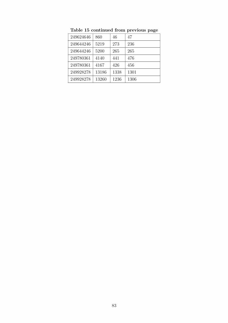
Table 15 continued from previous page249624646 860 46 47249644246 5219 273 236249644246 5200 265 265249780361 4140 441 476249780361 4167 426 456249928278 13186 1338 1301249928278 13260 1236 1306

83

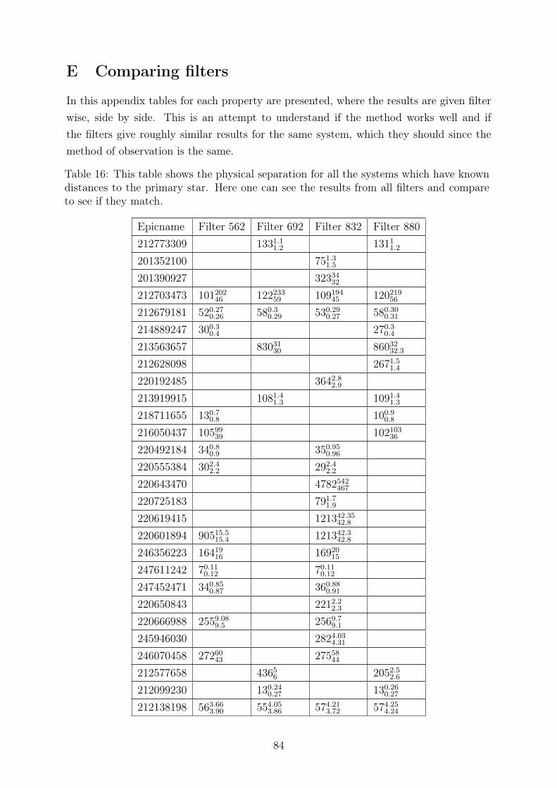
E Comparing filters

In this appendix tables for each property are presented, where the results are given filterwise, side by side. This is an attempt to understand if the method works well and ifthe filters give roughly similar results for the same system, which they should since themethod of observation is the same.

Table 16: This table shows the physical separation for all the systems which have knowndistances to the primary star. Here one can see the results from all filters and compareto see if they match.

Epicname Filter 562 Filter 692 Filter 832 Filter 880212773309 1331.1

1.2 13111.2

201352100 751.31.5

201390927 3233432

212703473 10120246 122233

59 10919445 120219

56

212679181 520.270.26 580.3

0.29 530.290.27 580.30

0.31

214889247 300.30.4 270.3

0.4

213563657 8303130 86032

32.3

212628098 2671.51.4

220192485 3642.82.9

213919915 1081.41.3 1091.4

1.3

218711655 130.70.8 100.9

0.8

216050437 1059939 102103

36

220492184 340.80.9 350.95

0.96

220555384 302.42.2 292.4

2.2

220643470 4782542467

220725183 791.71.9

220619415 121342.3542.8

220601894 90515.515.4 121342.3

42.8

246356223 1641916 16920

15

247611242 70.110.12 70.11

0.12

247452471 340.850.87 360.88

0.91

220650843 2212.22.3

220666988 2559.089.5 2569.7

9.1

245946030 2824.034.31

246070458 2726043 27558

44

212577658 43656 2052.5

2.6

212099230 130.240.27 130.26

0.27

212138198 563.663.90 554.05

3.86 574.213.72 574.25

4.24

84

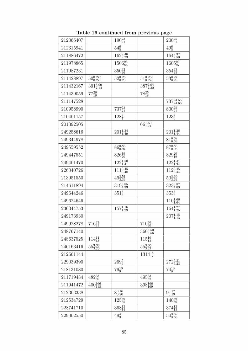
Table 16 continued from previous page212066407 19023

21 2002521

212315941 5465 496

5

211886472 1629.468.73 1649.37

9.50

211978865 15069586 160590

97

211987231 3504236 35443

35

211428897 500.2750.275 520.26

0.28 510.2650.275 530.27

0.28

211432167 3916.997.14 3877.04

7.32

211439059 772616 7825

18

211147528 73724.5524.66

210958990 7372321 80025

21

210401157 12887 1238

6

201392505 661.601.74

249258616 2011.341.49 2011.26

1.44

249344978 810.620.69

249559552 860.860.94 870.86

0.96

249447551 8261920 82920

19

249401470 1221.501.41 1221.41

1.34

226040726 1110.450.48 1120.45

0.44

213951550 493.513.33 503.69

3.63

214611894 3193.854.33 3233.87

4.03

249644246 35165 3536

5

249624646 1101.661.64

236344753 1571.161.29 1641.27

1.25

249173930 2071.151.13

249928278 7164341 71046

40

248767140 3603.503.56

248637525 1141413 11516

12

246163416 553.363.20 553.05

3.21

212661144 13141817

229039390 26956 2725.31

5.23

218131080 79109 7410

8

211719484 4823330 49533

32

211941472 400166118 398166

169

212303338 80.160.20 90.17

0.19

212534729 1255935 14069

36

228741710 3681214 37412

13

229002550 4943 503.69

3.63

85

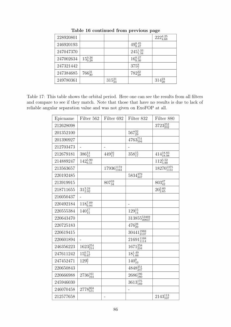
Table 16 continued from previous page228920801 2224.25

4.68

246920193 490.450.47

247047370 2451.331.34

247002634 150.260.28 160.27

0.30

247321442 37587

247384685 7663130 78232

29

249780361 3152124 31423

20

Table 17: This table shows the orbital period. Here one can see the results from all filtersand compare to see if they match. Note that those that have no results is due to lack ofreliable angular separation value and was not given on ExoFOP at all.

Epicname Filter 562 Filter 692 Filter 832 Filter 880212628098 3723252

232

201352100 5673229

201390927 4763751594

212703473 - - -212679181 38614

15 4491617 35815

17 41418.8318.98

214889247 1425.906.51 1125.52

5.90

213563657 1793611721164 182701375

1151

220192485 5834379347

213919915 8073334 80347

42

218711655 313.242.92 202.60

2.65

216050437 -220492184 1187.09

6.84 -220555384 14017

15 1291514

220643470 3138555346940837

220725183 4762829

220619415 3044119882137

220601894 - 2169111681114

246356223 1623254214 1671258

234

247611242 150.710.67 181.49

1.66

247452471 12967 1409

10

220650843 4848251247

220666988 2736161164 2686186

180

245946030 3613175189

246070458 2778804571 -

212577658 - 2143113107

86

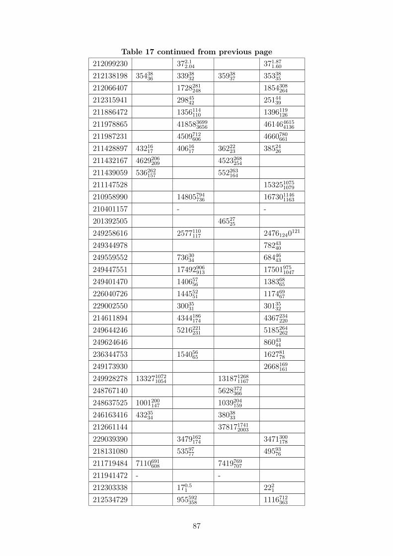
Table 17 continued from previous page212099230 372.1

2.04 371.871.60

212138198 3543836 33938

32 3593837 35338

35

212066407 1728281248 1854308

264

212315941 2984542 25144

39

211886472 1356114110 1396119

126

211978865 4185836993656 461464615

4136

211987231 4509712606 4660780

661

211428897 4321617 40616

17 3622223 38524

26

211432167 4629206209 4523268

254

211439059 536262157 552263

164

211147528 1532510751079

210958990 14805794736 167301146

1163

210401157 - -201392505 46527

25

249258616 2577110117 24761240121

249344978 7824340

249559552 7363034 68446

43

249447551 17492906913 17501975

1047

249401470 14065756 138368

65

226040726 14455251 117469

67

229002550 3003531 30135

32

214611894 4344186174 4367234

220

249644246 5216221231 5185264

262

249624646 8604344

236344753 15405665 162781

78

249173930 2668169161

249928278 1332710721054 131871268

1167

248767140 5628372366

248637525 1001200147 1039204

159

246163416 4323534 38038

33

212661144 3781717412003

229039390 3479162174 3471300

178

218131080 5359777 49593

76

211719484 7110691608 7419769

707

211941472 - -212303338 170.5

1 2221

212534729 955592358 1116712

363

87

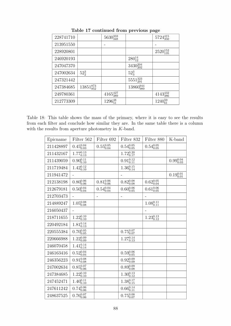
Table 17 continued from previous page228741710 5630333

348 5724415350

213951550 - -228920801 2520152

135

246920193 2801412

247047370 3430204202

247002634 5232 523

3

247321442 5551323291

247384685 13851873952 13860944

989

249780361 4165427389 4143432

386

212773309 12964851 124059

61

Table 18: This table shows the mass of the primary, where it is easy to see the resultsfrom each filter and conclude how similar they are. In the same table there is a columnwith the results from aperture photometry in K-band.

Epicname Filter 562 Filter 692 Filter 832 Filter 880 K-band211428897 0.450.04

0.03 0.550.050.04 0.540.05

0.05 0.540.050.05

211432167 1.770.130.13 1.720.20

0.17

211439059 0.900.110.10 0.910.12

0.11 0.990.040.03

211719484 1.420.120.10 1.360.15

0.14

211941472 - - 0.190.010.01

212138198 0.800.060.06 0.810.06

0.06 0.820.080.08 0.620.05

0.04

212679181 0.500.040.04 0.540.04

0.04 0.600.060.05 0.610.06

0.05

212703473 - - - -214889247 1.050.08

0.08 1.080.110.11

216050437 - -218711655 1.220.10

0.10 1.230.130.12

220492184 1.810.140.13

220555384 0.700.050.05 0.750.07

0.07

220666988 1.220.090.09 1.270.14

0.13

246070458 1.410.140.14

246163416 0.520.040.04 0.590.06

0.05

246356223 0.910.080.08 0.920.09

0.09

247002634 0.850.070.06 0.890.09

0.08

247384685 1.220.100.10 1.300.13

0.12

247452471 1.400.110.10 1.380.17

0.15

247611242 0.740.060.06 0.660.14

0.11

248637525 0.760.070.06 0.750.08

0.07

88

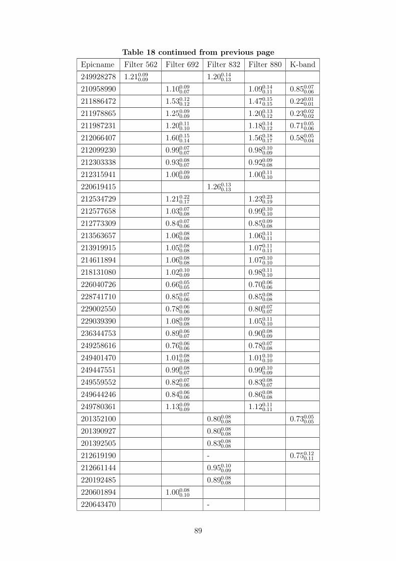
Table 18 continued from previous pageEpicname Filter 562 Filter 692 Filter 832 Filter 880 K-band249928278 1.210.09

0.09 1.200.140.13

210958990 1.100.090.07 1.090.14

0.11 0.850.070.06

211886472 1.530.120.12 1.470.15

0.15 0.220.010.01

211978865 1.250.090.09 1.200.13

0.12 0.230.020.02

211987231 1.200.110.10 1.180.14

0.12 0.710.050.06

212066407 1.600.150.14 1.560.18

0.17 0.580.050.04

212099230 0.990.070.07 0.980.10

0.09

212303338 0.930.080.07 0.920.09

0.08

212315941 1.000.090.09 1.000.11

0.10

220619415 1.260.130.13

212534729 1.210.220.17 1.230.23

0.19

212577658 1.030.070.08 0.990.10

0.10

212773309 0.840.070.06 0.850.09

0.08

213563657 1.060.080.08 1.060.11

0.11

213919915 1.050.080.08 1.070.11

0.11

214611894 1.060.080.08 1.070.10

0.10

218131080 1.020.100.09 0.980.11

0.10

226040726 0.660.050.05 0.700.06

0.06

228741710 0.850.070.06 0.850.08

0.08

229002550 0.780.060.06 0.800.07

0.07

229039390 1.080.090.08 1.050.11

0.10

236344753 0.890.060.07 0.900.08

0.09

249258616 0.760.060.06 0.780.07

0.08

249401470 1.010.080.08 1.010.10

0.10

249447551 0.990.080.07 0.990.10

0.09

249559552 0.820.070.06 0.830.08

0.07

249644246 0.840.060.06 0.860.08

0.08

249780361 1.130.090.09 1.120.11

0.11

201352100 0.800.080.08 0.730.05

0.05

201390927 0.800.080.08

201392505 0.830.080.08

212619190 - 0.750.120.11

212661144 0.950.100.09

220192485 0.890.080.08

220601894 1.000.080.10

220643470 -

89

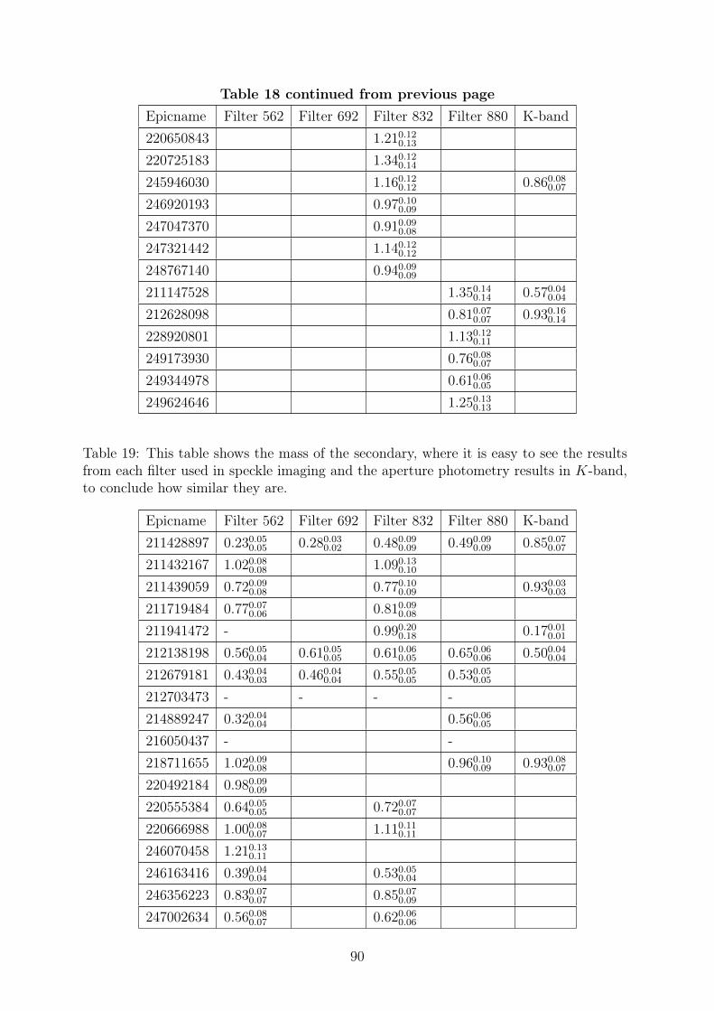
Table 18 continued from previous pageEpicname Filter 562 Filter 692 Filter 832 Filter 880 K-band220650843 1.210.12

0.13

220725183 1.340.120.14

245946030 1.160.120.12 0.860.08

0.07

246920193 0.970.100.09

247047370 0.910.090.08

247321442 1.140.120.12

248767140 0.940.090.09

211147528 1.350.140.14 0.570.04

0.04

212628098 0.810.070.07 0.930.16

0.14

228920801 1.130.120.11

249173930 0.760.080.07

249344978 0.610.060.05

249624646 1.250.130.13

Table 19: This table shows the mass of the secondary, where it is easy to see the resultsfrom each filter used in speckle imaging and the aperture photometry results in K-band,to conclude how similar they are.

Epicname Filter 562 Filter 692 Filter 832 Filter 880 K-band211428897 0.230.05

0.05 0.280.030.02 0.480.09

0.09 0.490.090.09 0.850.07

0.07

211432167 1.020.080.08 1.090.13

0.10

211439059 0.720.090.08 0.770.10

0.09 0.930.030.03

211719484 0.770.070.06 0.810.09

0.08

211941472 - 0.990.200.18 0.170.01

0.01

212138198 0.560.050.04 0.610.05

0.05 0.610.060.05 0.650.06

0.06 0.500.040.04

212679181 0.430.040.03 0.460.04

0.04 0.550.050.05 0.530.05

0.05

212703473 - - - -214889247 0.320.04

0.04 0.560.060.05

216050437 - -218711655 1.020.09

0.08 0.960.100.09 0.930.08

0.07

220492184 0.980.090.09

220555384 0.640.050.05 0.720.07

0.07

220666988 1.000.080.07 1.110.11

0.11

246070458 1.210.130.11

246163416 0.390.040.04 0.530.05

0.04

246356223 0.830.070.07 0.850.07

0.09

247002634 0.560.080.07 0.620.06

0.06

90

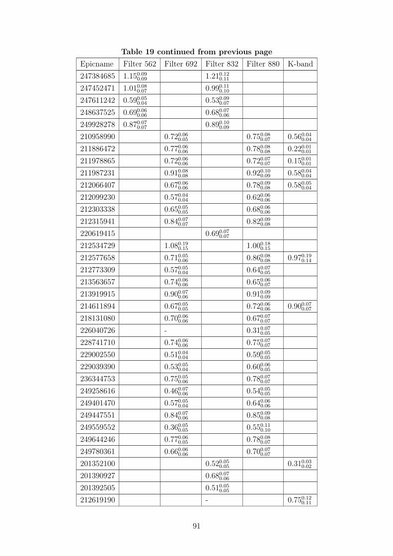
Table 19 continued from previous pageEpicname Filter 562 Filter 692 Filter 832 Filter 880 K-band247384685 1.150.09

0.09 1.210.120.11

247452471 1.010.080.07 0.990.11

0.10

247611242 0.590.050.04 0.530.09

0.07

248637525 0.690.060.06 0.680.07

0.06

249928278 0.870.070.07 0.890.10

0.09

210958990 0.720.060.05 0.750.08

0.07 0.560.040.04

211886472 0.770.060.06 0.780.08

0.08 0.220.010.01

211978865 0.720.060.06 0.720.07

0.07 0.150.010.01

211987231 0.910.080.08 0.920.10

0.09 0.580.040.04

212066407 0.670.060.06 0.780.09

0.08 0.580.050.04

212099230 0.570.040.04 0.620.06

0.06

212303338 0.650.050.05 0.680.06

0.06

212315941 0.840.070.07 0.820.09

0.08

220619415 0.690.070.07

212534729 1.080.190.15 1.000.18

0.15

212577658 0.710.050.06 0.860.08

0.08 0.970.190.14

212773309 0.570.050.04 0.640.07

0.05

213563657 0.740.060.06 0.650.06

0.07

213919915 0.900.070.06 0.910.09

0.09

214611894 0.670.050.05 0.720.06

0.06 0.900.070.07

218131080 0.700.060.06 0.670.07

0.07

226040726 - 0.310.070.05

228741710 0.740.060.06 0.750.07

0.07

229002550 0.510.040.04 0.590.05

0.05

229039390 0.530.050.04 0.600.06

0.05

236344753 0.750.050.06 0.780.07

0.07

249258616 0.460.070.06 0.540.05

0.05

249401470 0.570.050.04 0.640.06

0.06

249447551 0.840.070.06 0.850.09

0.08

249559552 0.360.050.05 0.550.11

0.10

249644246 0.770.060.05 0.780.08

0.07

249780361 0.660.060.06 0.700.07

0.07

201352100 0.520.050.05 0.310.03

0.02

201390927 0.680.070.06

201392505 0.510.050.05

212619190 - 0.750.120.11

91

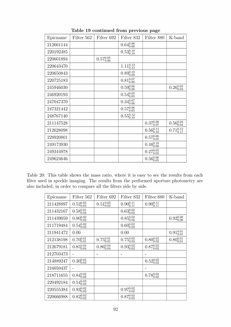
Table 19 continued from previous pageEpicname Filter 562 Filter 692 Filter 832 Filter 880 K-band212661144 0.640.06

0.06

220192485 0.530.100.10

220601894 0.570.050.06

220643470 1.110.130.12

220650843 0.890.100.09

220725183 0.810.070.08

245946030 0.590.060.06 0.260.03

0.03

246920193 0.540.050.05

247047370 0.340.070.06

247321442 0.570.060.05

248767140 0.550.120.10

211147528 0.370.080.07 0.560.04

0.04

212628098 0.560.120.10 0.710.12

0.11

228920801 0.570.060.05

249173930 0.480.100.08

249344978 0.270.050.05

249624646 0.560.060.05

Table 20: This table shows the mass ratio, where it is easy to see the results from eachfilter used in speckle imaging. The results from the performed aperture photometry arealso included, in order to compare all the filters side by side.

Epicname Filter 562 Filter 692 Filter 832 Filter 880 K-band211428897 0.520.03

0.03 0.510.030.03 0.900.11

0.11 0.900.110.11

211432167 0.580.010.02 0.630.02

0.02

211439059 0.800.020.02 0.850.02

0.02 0.920.000.00

211719484 0.540.020.02 0.600.02

0.02

211941472 0.00 0.00 0.910.010.01

212138198 0.700.010.01 0.750.01

0.01 0.750.020.02 0.800.02

0.02 0.800.010.01

212679181 0.850.040.04 0.860.04

0.04 0.930.020.02 0.870.02

0.02

212703473 - - - -214889247 0.300.04

0.03 0.520.020.02

216050437 - -218711655 0.840.02

0.02 0.780.020.02

220492184 0.540.030.03

220555384 0.930.020.02 0.970.02

0.02

220666988 0.820.020.02 0.870.02

0.02

92

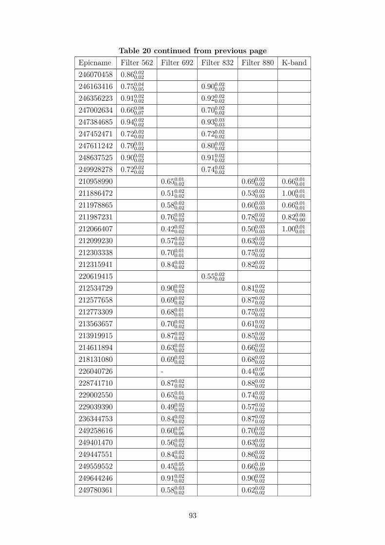
Table 20 continued from previous pageEpicname Filter 562 Filter 692 Filter 832 Filter 880 K-band246070458 0.860.02

0.02

246163416 0.750.040.05 0.900.02

0.02

246356223 0.910.020.02 0.920.02

0.02

247002634 0.660.080.07 0.700.02

0.02

247384685 0.940.020.02 0.930.03

0.03

247452471 0.720.020.02 0.720.02

0.02

247611242 0.790.010.02 0.800.02

0.02

248637525 0.900.020.02 0.910.02

0.02

249928278 0.720.020.02 0.740.02

0.02

210958990 0.650.010.02 0.690.02

0.02 0.660.010.01

211886472 0.510.020.02 0.530.02

0.03 1.000.010.01

211978865 0.580.020.02 0.600.03

0.03 0.660.010.01

211987231 0.760.020.02 0.780.02

0.02 0.820.000.00

212066407 0.420.020.02 0.500.03

0.03 1.000.010.01

212099230 0.570.020.02 0.630.02

0.02

212303338 0.700.010.01 0.750.02

0.02

212315941 0.840.020.02 0.820.02

0.02

220619415 0.550.020.02

212534729 0.900.020.02 0.810.02

0.02

212577658 0.690.020.02 0.870.02

0.02

212773309 0.680.010.01 0.750.02

0.02

213563657 0.700.020.02 0.610.02

0.02

213919915 0.870.020.02 0.850.02

0.02

214611894 0.630.020.02 0.660.02

0.02

218131080 0.690.020.02 0.680.02

0.02

226040726 - 0.440.070.06

228741710 0.870.020.02 0.880.02

0.02

229002550 0.650.010.02 0.740.02

0.02

229039390 0.490.020.02 0.570.02

0.02

236344753 0.840.020.02 0.870.02

0.02

249258616 0.600.070.06 0.700.02

0.02

249401470 0.560.020.02 0.630.02

0.02

249447551 0.840.020.02 0.860.02

0.02

249559552 0.450.050.05 0.660.10

0.09

249644246 0.910.020.02 0.900.02

0.02

249780361 0.580.030.02 0.620.02

0.02

93

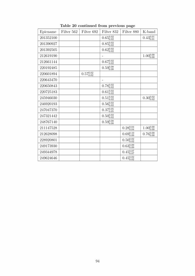
Table 20 continued from previous pageEpicname Filter 562 Filter 692 Filter 832 Filter 880 K-band201352100 0.650.02

0.02 0.430.010.01

201390927 0.850.020.02

201392505 0.620.020.02

212619190 - 1.000.000.00

212661144 0.670.020.02

220192485 0.590.080.08

220601894 0.570.020.02

220643470 -220650843 0.780.02

0.02

220725183 0.610.020.02

245946030 0.510.020.02 0.300.02

0.02

246920193 0.560.020.02

247047370 0.370.050.05

247321442 0.500.020.02

248767140 0.590.080.08

211147528 0.280.040.04 1.000.00

0.00

212628098 0.690.100.09 0.760.00

0.00

228920801 0.500.020.02

249173930 0.630.090.09

249344978 0.450.070.07

249624646 0.450.020.02

94