five kepler target stars that show multiple transiting exoplanet candidates

Five Kepler target stars that show multiple transiting exoplanetcandidates

Jason H. Steffen1, Natalie M. Batalha2, William J. Borucki3, Lars A. Buchhave4,5, DouglasA. Caldwell3,10, William D. Cochran6, Michael Endl6, Daniel C. Fabrycky4, Francois

Fressin4, Eric B. Ford7, Jonathan J. Fortney8, Michael J. Haas3, Matthew J. Holman4,Howard Isaacson9, Jon M. Jenkins3,10, David Koch3, David W. Latham4, Jack J. Lissauer3,

Althea V. Moorhead7, Robert C. Morehead7, Geoffrey Marcy9, Phillip J. MacQueen6,Samuel N. Quinn4, Darin Ragozzine4, Jason F. Rowe3, Dimitar D. Sasselov4 Sara Seager11

Guillermo Torres4, William F. Welsh12

1Fermilab Center for Particle Astrophysics, P.O. Box 500, Batavia, IL 605102Department of Astronomy and Physics, San Jose State University, San Jose, CA 95192

3NASA Ames Research Center, Moffett Field, CA 940354Harvard-Smithsonian Center for Astrophysics, 60 Garden St., Cambridge, MA 02138

5Niels Bohr Institute, Copenhagen University, DK-2100 Copenhagen, Denmark6McDonald Observatory, The University of Texas, Austin, TX 78712-2059 USA

7Department of Astronomy, University of Florida, 211 Bryant Space Science Center, Gainesville, FL32611-2055, USA

8Department of Astronomy and Astrophysics, Unvirsity of California, Santa Cruz, 950649Astronomy Department, UC Berkeley, Berkeley, CA 94720

10SETI Institute, 515 North Whisman Road, Mountain View, CA, 9404311Department of Physics, Massachussets Institute of Technology

12San Diego State University, 5500 Campanile Drive, San Diego, CA 92182

ABSTRACT

We present and discuss five candidate exoplanetary systems identified with the Kepler space-craft. These five systems show transits from multiple exoplanet candidates. Should these objectsprove to be planetary in nature, then these five systems open new opportunities for the field ofexoplanets and provide new insights into the formation and dynamical evolution of planetarysystems. We discuss the methods used to identify multiple transiting objects from the Keplerphotometry as well as the false-positive rejection methods that have been applied to these data.One system shows transits from three distinct objects while the remaining four systems showtransits from two objects. Three systems have planet candidates that are near mean motioncommensurabilities—two near 2:1 and one just outside 5:2. We discuss the implications thatmultitransiting systems have on the distribution of orbital inclinations in planetary systems, andhence their dynamical histories; as well as their likely masses and chemical compositions. AMonte Carlo study indicates that, with additional data, most of these systems should exhibitdetectable transit timing variations (TTV) due to gravitational interactions—though none areapparent in these data. We also discuss new challenges that arise in TTV analyses due to thepresence of more than two planets in a system.

Subject headings: planetary systems — Stars Individual (KIC 8394721, KIC 5972334, KIC 10723750,KIC 7287995, KIC 7825899) — techniques: spectroscopic, photometric

1

arX

iv:1

006.

2763

v1 [

astr

o-ph

.EP]

14

Jun

2010

1. Introduction

The discovery of dozens of transiting planetshas enabled astronomers to characterize key phys-ical properties of the planets, including their sizes,densities, atmospheric composition, thermal prop-erties, and the projected inclination of the orbitwith respect to the stellar spin axis (Charbon-neau et al. 2007). Ground-based transit searcheshave surveyed many more stars than radial ve-locity planet searches, allowing them to discoverrelatively rare planets, such as giant planets withorbital periods of less than two days. However,ground-based transit surveys are only efficient forlarge planets with relatively short orbital periods.These strong detection biases and the likely dy-namical instability of a system with multiple gi-ant planets packed close to the host star, may ex-plain why ground-based transit surveys have yetto detect a system with multiple transiting planetsorbiting the same star.

The Kepler mission was designed to detectterrestrial-size planets in the habitable zone of thehost star, necessitating both a large sample sizeand sensitivity to a much larger range of orbitalseparations than ground-based surveys (Boruckiet al 2010). The instrument is a differential pho-tometer with a wide (105 square degrees) field-of-view (FOV) that continuously and simultaneouslymonitors the brightness of approximately 150,000main-sequence stars. A comprehensive discussionof the characteristics and on-orbit performance ofthe instrument and spacecraft is presented in Kochet al (2010).

Its sensitivity to small planets over a widerange of separations gives Kepler the capability ofdiscovering multiple planet systems. For closelypacked planetary systems, nearly coplanar sys-tems, or systems with a very fortuitous geomet-ric alignment Kepler is likely to detect transits ofmultiple planets. For systems with widely spacedplanets or large relative inclinations not all plan-ets will transit, but some may still be detectablebased on transit timing variations (TTVs) dueto the gravitational perturbation of one or morenon-transiting planets (Agol et al. 2005; Holmanand Murray 2005). In other cases, non-transitingplanets may be detectable by follow-up observa-tions, such as radial velocity observations origi-nally intended to measure the mass of the transit-

ing planet(s) (Leger et al 2009; Queloz et al 2009).

Radial velocity (RV) surveys have shown thatgiant planets often reside in multiple planet sys-tems (Wright et al. 2009). Given the large numberof candidate planets identified by Kepler (Boruckiet al 2010), it is expected that some fraction ofthem will be in multiple planet systems and a frac-tion of those will have multiple planets that tran-sit. In addition to the ability to characterize phys-ical properites of each transiting planet, planetarysystems with multiple transiting planets presentseveral advantages. For example, the fact thateach planet formed from the same proto-planetarydisk provides more powerful constraints for modelsof planet formation and orbital migration. More-over, these systems are quite powerful for studyingthe detailed orbital dynamics through transit tim-ing variations and the masses of the planets maybe determined without measurements of stellar RVvariations.

In cases where RV measurements are ableto measure the planet masses independently ofTTVs, the two techniques can be combined tomeasure the mass and size of the host star with-out relying on stellar models (see Agol et al. 2005;Holman and Murray 2005). In cases where RVobservations are not practical (e.g., hot stars, fastrotators) or would require prohibitive observingtime (i.e. faint stars), the detection of TTVscan be used to confirm that transit candidatesorbit the same star—as opposed to being two ob-jects transiting two stars blended within a singlepoint-spread-function (PSF)—and to determineif the companions are of planetary mass. Heremultiple transiting systems are particularly pow-erful as the period, phase, and size of additionalplanets can be determined from the light curve.This additional information can simplify an other-wise challenging inverse problem (Steffen and Agol2007; Nesvorny and Morbidelli 2008; Meschiariand Laughlin 2010).

We present five planetary candidate systemswhere the transits of multiple objects can be seenin the first quarter of photometric data (a 33.5-daydata segment from May 13 to June 15 UT, 2009)from the Kepler spacecraft. While not confirmedplanet discoveries, these systems have passed sev-eral important tests that eliminate false-positivesignals. If all were ultimately shown to be plan-ets, then these systems would contain four plan-

2

ets with radii smaller than three Earth radii (thesmallest being two Earth radii), at least two pairsof planets in or very near a low-order mean-motionresonance (MMR), and one system with at leastthree distinct transiting planets.

For simplicity, we will refer to these objects as“planets” throughout this paper, recognizing thattheir confirmation as such is yet incomplete andthat some of these transit signals may be due toother astrophysics. The stellar references that wewill use throughout this paper are Kepler Objectsof Interest (KOI) 152, 191, 209, 877, and 896 withthe transiting planets denoted by “.01”, “.02”, etc.beginning in the order that they were identifiedwith the transit detection software from the Ke-pler pipeline. Thus, the planet number designa-tion does not necessarily reflect the order of theplanets within each system. We do not use letterdesignations, which by convention are reserved forconfirmed planets.

This paper will proceed as follows. First, wegive the known properties of the host stars (§2).In §3 we discuss the photometric reduction andthe algorithm used to identify the multiple can-didates within each system. We also outline thetests we have conducted to eliminate false-positivesystems. We present estimates of the orbital andphysical properties of these objects should theyprove to be planets. In §5 we discuss the possiblefuture detection of transit timing variations basedupon a Monte Carlo simulation of these candidatesystems. Finally, we discuss the implications ofthese results in §6.

2. Stellar properties

For each of the five stars, we obtained high res-olution echelle spectroscopy with resolution of ap-proximately R ' 50, 000 (depending upon the in-strument used) and with a low signal-to-noise ra-tio (SNR) of 5-30 per pixel with the goal of con-straining effective temperature Teff, surface grav-ity log g, projected rotational velocity for the starv sin i, and metallicity [M/H]. In all cases, thespectroscopic analysis was done by matching theobserved spectra to a library of synthetic spectra.The synthetic spectra cover the wavelength region5050-5360A(centered roughly on the Mg b lines).The grid has coarseness of 250 K in Teff, 1-4 km/sin vrot ' v sin i, and 0.5 dex in log g and [M/H],

implying uncertaintes of half those values.

For the host stars with low SNR spectra, weperformed a diagnostic using the J−K color toverify that their compositions are consistent withsolar metallicity, but the values we report are sim-ply from template-matching with [M/H] fixed at0. Table 1 lists the resulting stellar parameters forall five stars as well as the instruments used in theobservations. All five stars apparently reside nearor on the main sequence.

3. Kepler data and photometric analysis

3.1. Transit identification

Each of these systems was found using theTransiting Planet Search Pipeline (TPS) whichidentifies significant transit-like features, or Thresh-old Crossing Events (TCE), in the Kepler lightcurves (Jenkens et al 2010). Data showing TCEsare then passed to the Data Validation (DV)pipeline (Wu et al 2010). The purpose of the DVpipeling is twofold: 1) to fit a transiting planetmodel to the data, remove it from the light curve,and to return the result to TPS in an effort tofind additional transit features and 2) to com-plete a suite of statistical tests that are appliedto the data after all TCEs are identified in aneffort to assess the likelihood of false-positives.The binary discrimination statistics and the mo-tion detection statistic, in particular, speak tothe likelihood of astrophysical false positives suchas grazing eclipses and diluted eclipsing binaries.These statistics are described below.

After pipeline data processing and the photom-etry extraction, the time series is detrended with arunning 1-day median. All observations that occurduring transit are not included in the evaluationof the median. The transit lightcurve is modeledusing the analytic expressions of Mandel and Agol(2002) using non-linear limb darkening parametersClaret (2000) derived for the Kepler bandpass. Afirst estimate for M∗ and R∗ is obtained by com-paring the SME derived stellar Teff and log g valuesto a set of CESAM (Morel 1997) stellar evolutionmodels computed in steps of 0.1M� for solar com-position.

With M∗ and R∗ fixed to their initial values,a transit fit is then computed to determine theorbital inclination, planetary radius, and depthof the occultation (passing behind the star) as-

3

Table 1

Stellar properties and locations for the five candidate systems.

KOI KIC-ID RA DEC Kepmag Teff log g [M/H] v sin i vabs Nexp

(2000) (2000) (km/s) (km/s)

152 8394721 20 02 04.1 44 22 53.7 13.9 6500 4.5 0 (fixed) 14 -22.32 2a,b

191 5972334 19 41 08.9 41 13 19.1 15.0 5500 4.5 0 (fixed) 0 -62.98 1b

209 10723750 19 15 10.3 48 02 24.8 14.2 6100 4.1 -0.05 7.8 -12.78 4b

877 7287995 19 34 32.9 42 49 29.9 15.0 4500 4.0 0 (fixed) 0 0.531 2b,c

896 7825899 19 32 14.7 43 34 52.9 15.3 5000 4.0 0 (fixed) 1 -21.28 1c

Note.—Each system was analyzed by matching the observed spectra to the CfA library.Telescopes used for these observations:a, FIES/NOTb, McD 2.7mc, Keck-HIRES

suming a circular orbit. The best fit is foundusing a Levenberg-Marquardt minimization algo-rithm (Press et al. 1992). The best fit model isthen removed from the lightcurve and the resid-uals are then used to fit for the characteristics ofnext transit candidate identified by TPS. The lightcurves and transit models for these five systemsare shown in Figures 1, 2, 3, 4, and 5.

3.2. Candidate vetting from Kepler data

The depths of planetary transits should beconsistent from orbit to orbit as well as evenlyspaced in time. Eclipsing stellar binaries, onthe other hand, generally have primary and sec-ondary eclipses that need not be evenly spacedin phase. The binary discrimination test in-cludes two metrics: the Odd/Even statistic andthe Epoch statistic. The Odd/Even statistic isa comparison between the depth of the phase-folded, odd-numbered transits and the depth ofthe phase-folded, even-numbered transits. TheEpoch statistic compares the timing of the oddand even-numbered transits. Both statistics areconstructed as χ2 distributions, and the signif-icance (reported in Table 2) of the statistic isobtained by evaluation the χ2 cumulative distri-bution function for the appropriate number ofstatistical tests. The significance is the probabil-ity that the statistic is consistent with the binaryinterpretation.

The motion detection statistic identifies objectswith flux-weighted centroids that are highly corre-lated with a transit signature derived from the fluxtimeseries. The statistic is a χ2 variable with two

degrees of freedom (row and column). The prob-ability of producing a statistic of equal or lesservalue is reported as “Motion” in Table 2. It iscomputed by evaluating the χ2 cumulative distri-bution function at the value of the detection statis-tic given two degrees of freedom. The complementof this value is reported so that values near unityrepresent a small likelihood of a correlation. Cen-troids that are highly correlated with the transitsignature are indicative of a crowded photometricaperture—a warning that the transit could be dueto a nearby eclipsing binary diluting the flux ofthe target star. Such cases are denoted by a mo-tion significance near zero. A full description ofDV statistics is given in Wu et al (2010).

Outside of the pipeline, all TCEs are fitted witha planet transit model as described in Batalhaet al (2010). Those yielding an estimated planetradius less than 2 RJ are assigned a Kepler Ob-ject of Interest (KOI) number. The modeling re-turns an independent test of the Odd/Even statis-tic (Depth-sig in Table 2), expressed in units ofthe standard deviation. The modeling also testsfor the presence of secondary eclipses (or occulta-tions) at phase=0.5 and reports this as Eclipse-sigin Table 2, also in units of the standard deviation.

Figure 6 shows the normalized relative flux vs.centroid position (referred to as a “rain plot”) asdescribed in Batalha et al (2010) for each tar-get star. Here, the relative flux is plotted againstthe relative centroid position along rows (ut) andcolumns (◦). A centroid shift that is highly cor-related with the transit signature would appearas a diagonal deviation in the plot (see bottom-

4

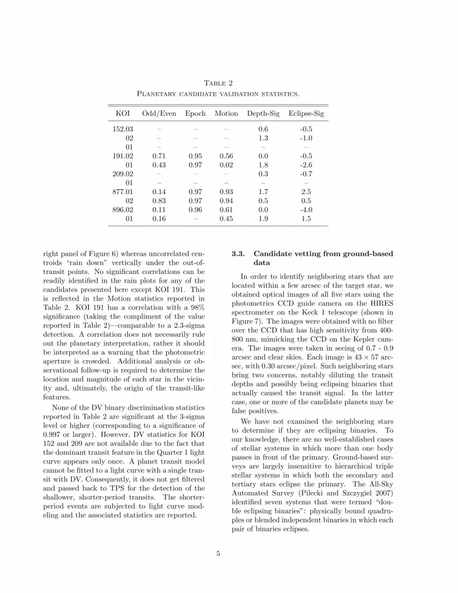
Table 2

Planetary candidate validation statistics.

KOI Odd/Even Epoch Motion Depth-Sig Eclipse-Sig

152.03 – – – 0.6 -0.502 – – – 1.3 -1.001 – – – – –

191.02 0.71 0.95 0.56 0.0 -0.501 0.43 0.97 0.02 1.8 -2.6

209.02 – – – 0.3 -0.701 – – – – –

877.01 0.14 0.97 0.93 1.7 2.502 0.83 0.97 0.94 0.5 0.5

896.02 0.11 0.96 0.61 0.0 -4.001 0.16 – 0.45 1.9 1.5

right panel of Figure 6) whereas uncorrelated cen-troids “rain down” vertically under the out-of-transit points. No significant correlations can bereadily identified in the rain plots for any of thecandidates presented here except KOI 191. Thisis reflected in the Motion statistics reported inTable 2. KOI 191 has a correlation with a 98%significance (taking the compliment of the valuereported in Table 2)—comparable to a 2.3-sigmadetection. A correlation does not necessarily ruleout the planetary interpretation, rather it shouldbe interpreted as a warning that the photometricaperture is crowded. Additional analysis or ob-servational follow-up is required to determine thelocation and magnitude of each star in the vicin-ity and, ultimately, the origin of the transit-likefeatures.

None of the DV binary discrimination statisticsreported in Table 2 are significant at the 3-sigmalevel or higher (corresponding to a significance of0.997 or larger). However, DV statistics for KOI152 and 209 are not available due to the fact thatthe dominant transit feature in the Quarter 1 lightcurve appears only once. A planet transit modelcannot be fitted to a light curve with a single tran-sit with DV. Consequently, it does not get filteredand passed back to TPS for the detection of theshallower, shorter-period transits. The shorter-period events are subjected to light curve mod-eling and the associated statistics are reported.

3.3. Candidate vetting from ground-baseddata

In order to identify neighboring stars that arelocated within a few arcsec of the target star, weobtained optical images of all five stars using thephotometrics CCD guide camera on the HIRESspectrometer on the Keck 1 telescope (shown inFigure 7). The images were obtained with no filterover the CCD that has high sensitivity from 400-800 nm, mimicking the CCD on the Kepler cam-era. The images were taken in seeing of 0.7 - 0.9arcsec and clear skies. Each image is 43× 57 arc-sec, with 0.30 arcsec/pixel. Such neighboring starsbring two concerns, notably diluting the transitdepths and possibly being eclipsing binaries thatactually caused the transit signal. In the lattercase, one or more of the candidate planets may befalse positives.

We have not examined the neighboring starsto determine if they are eclipsing binaries. Toour knowledge, there are no well-established casesof stellar systems in which more than one bodypasses in front of the primary. Ground-based sur-veys are largely insensitive to hierarchical triplestellar systems in which both the secondary andtertiary stars eclipse the primary. The All-SkyAutomated Survey (Pilecki and Szczygiel 2007)identified seven systems that were termed “dou-ble eclipsing binaries”: physically bound quadru-ples or blended independent binaries in which eachpair of binaries eclipses.

5

Fig. 1.— Light curve and transit models for thecandidates in KOI 152. The innermost planet isin the top panel and the outermost planet is in thebottom panel.

Fig. 2.— Light curve and transit models for thecandidates in KOI 191. The inner planet is in thetop panel and the outer planet is in the bottompanel.

6



7


Fig. 6.— Relative flux vs. centroid position forKOIs 152, 191, 209, 877, and 896 beginning in thetop left corner. The plot in the bottom right isfrom an eclipsing binary and is presented to il-lustrate the difference in the data between goodplanetary candidates and eclipsing binaries.

8

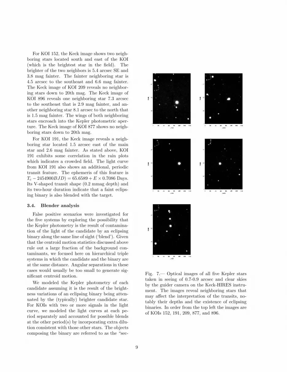
For KOI 152, the Keck image shows two neigh-boring stars located south and east of the KOI(which is the brightest star in the field). Thebrighter of the two neighbors is 5.4 arcsec SE and3.8 mag fainter. The fainter neighboring star is4.5 arcsec to the southeast and 6.6 mag fainter.The Keck image of KOI 209 reveals no neighbor-ing stars down to 20th mag. The Keck image ofKOI 896 reveals one neighboring star 7.3 arcsecto the southeast that is 2.9 mag fainter, and an-other neighboring star 8.1 arcsec to the north thatis 1.5 mag fainter. The wings of both neighboringstars encroach into the Kepler photometric aper-ture. The Keck image of KOI 877 shows no neigh-boring stars down to 20th mag.

For KOI 191, the Keck image reveals a neigh-boring star located 1.5 arcsec east of the mainstar and 2.6 mag fainter. As stated above, KOI191 exhibits some correlation in the rain plotswhich indicates a crowded field. The light curvefrom KOI 191 also shows an additional, periodictransit feature. The ephemeris of this feature isTc − 2454900BJD) = 65.6589 +E × 0.7086 Days.Its V-shaped transit shape (0.2 mmag depth) andits two-hour duration indicate that a faint eclips-ing binary is also blended with the target.

3.4. Blender analysis

False positive scenarios were investigated forthe five systems by exploring the possibility thatthe Kepler photometry is the result of contamina-tion of the light of the candidate by an eclipsingbinary along the same line of sight (‘blend’). Giventhat the centroid motion statistics discussed aboverule out a large fraction of the background con-taminants, we focused here on hierarchical triplesystems in which the candidate and the binary areat the same distance. Angular separations in thesecases would usually be too small to generate sig-nificant centroid motion.

We modeled the Kepler photometry of eachcandidate assuming it is the result of the bright-ness variations of an eclipsing binary being atten-uated by the (typically) brighter candidate star.For KOIs with two or more signals in the lightcurve, we modeled the light curves at each pe-riod separately and accounted for possible blendsat the other period(s) by incorporating extra dilu-tion consistent with those other stars. The objectscomposing the binary are referred to as the “sec-

Fig. 7.— Optical images of all five Kepler starstaken in seeing of 0.7-0.9 arcsec and clear skiesby the guider camera on the Keck-HIRES instru-ment. The images reveal neighboring stars thatmay affect the interpretation of the transits, no-tably their depths and the existence of eclipsingbinaries. In order from the top left the images areof KOIs 152, 191, 209, 877, and 896.

9

ondary” and “tertiary”, and the candidate is the“primary”. The procedure closely follows that de-scribed by Torres et al. (2004) and consists of cal-culating synthetic light curves that result from thethree objects for a wide range of eclipsing binaryparameters.

The brightness variations of the binary are gen-erated using detailed calculations including limbdarkening, gravity brightening, reflection, andproximity effects. The properties of the candi-date are tightly constrained by the spectroscopicparameters in Table 1 and were held fixed. Theparameters of the binary components were takenfrom model isochrones by Girardi et al. (2000),parametrized in terms of their mass. The sec-ondary and tertiary masses were allowed to varyover wide ranges (0.1–1.4 M�) in order to fit thelight curve, and the inclination angle was also afree parameter. We consider hierarchical configu-rations of two types: ones in which the tertiary is astar, and ones in which it is a planet contributingno light. In the latter case the size of the planetis a free parameter, which we varied between 0.1and 2.0 RJup. We account for the additional starsidentified by high resolution imaging by includingthe proper amount of extra light in our models.

In all five cases we find that configurations withstellar tertiaries are inconsistent with the Keplerlight curves, for any size secondary. Thus, hierar-chical triples involving a stellar binary are ruledout. When the tertiary is allowed to be a planet,we find that there is a range of possible solutionsthat yield acceptable matches to the Kepler pho-tometry, often times as good as obtained from atrue planet model fit. However, many of those so-lutions can also be excluded on other grounds.

For KOI 152, which is a mid F dwarf, the onlyconfigurations consistent with the Kepler lightcurves involve secondary stars that are at least asmassive as the primary—and therefore almost asbright or brighter. In all cases the planetary com-panions are roughly 0.5 RJup in size. Such brightsecondaries are unlikely as they would have beenseen spectroscopically, unless the velocity differ-ence with the target star happens to be very small.This cannot be completely ruled out if the twostars are in a wide orbit around each other, but itwould require a special set of circumstances giventhe constraints on the centroid motion. Thus, ex-cept for this particular case, this analysis supports

the planetary interpretation.

For KOI 209, a mid to late F dwarf, we againfind that the only blend configurations that fitthe Kepler light curve involve a secondary thatis as bright as the primary or brighter, and a ter-tiary about the size of Jupiter. A planetary in-terpretation is again favored. KOI 877 is a lateK dwarf. In addition to the blend solutions withbright secondary stars, we find acceptable fits tothe light curves with secondaries up to two magni-tudes fainter than the primary (spectral type M2-M3), which might not be noticed spectroscopically.The size of the tertiaries in these cases is about0.4 RJup. To rule out such configurations, addi-tional observational constraints are needed, suchas accurate multi-band photometry out of tran-sit to check for color inconsistencies (see, e.g.,O’Donovan et al. 2006). Our blend simulationsfor KOI 896, an early K star, again indicate thatthe secondaries required for a good fit to the lightcurve are similar in brightness to the primary, andthe tertiaries have sizes between 0.4 and 0.5 RJup.Solutions with smaller secondary stars are visiblyworse. Therefore, except for the somewhat arti-ficial case of twin stars, the Kepler photometryfavors a planetary interpretation.

KOI 191 has a companion separated by 1.5 arc-sec. We consider the hypothesis that it could be aneclipsing binary. For KOI 191.02 the light-curvefits allow blend scenarios in which the secondariesare smaller than the late G-type primary, down toa spectral type of late K. The tertiaries tend tohave radii around 0.3 RJup. In the case of KOI191.01 we find that the light curve prefers secon-daries that are as bright as or brighter than theprimary and tertiaries of ∼1.5 RJup.

In summary, the above blend analyses suggestthat KOI 152, 209 and 896 are most likely trueplanets orbiting a common star. KOI 191 and 877,on the other hand, could be blends of two plan-ets orbiting two separate stars. In none of thesesystems was a configuration of transiting starspreferred over transiting planet-sized objects. IfKOI 191 or 877 turned out to be a blend of twoplanetary systems orbiting different stars, this toowould be a unique discovery.

10

4. Planetary and system properties

4.1. Orbital properties

Of the five candidate planetary systems, thereare four pairs of planets with a well-characterizedorbital period ratio. Two pair are near the 2:1MMR (KOI 152.02/01 and KOI 877.01/02), onepair is slighly outside the 5:2 commensurability(KOI 896.02/01), and one pair is heirarchical witha period ratio exceeding 6:1 (KOI 191.02/01). Theproximity of KOI 152 and 877 to the 2:1 MMRhints that these systems are likely to have largeTTVs. However, the timescale for large TTVs inresonant systems can be quite long. For a sys-tem of Neptune-mass planets librating about a 2:1MMR, we would not expect to detect TTVs basedon the Q0 and Q1 data presented. Moreover, forlibrating systems with smaller masses or that arevery close exact resonance, the time needed todistinguish a TTV signal from a constant periodlengthens, also requiring additional data.

Inferring the relative frequency of planets withvarious orbital spacings will require a populationanalysis that corrects for the geometric transitprobabilities. Of course, there may be additionalnon-transiting planets, or small transiting plan-ets, between KOI 191.02 and 191.01 or in any ofthe candidate systems presented. In some cases,TTVs or radial velocity follow-up could identifysuch planets. In other cases, the non-transitingplanets will remain undetected, further complicat-ing a population analysis. The sample of multi-ple planet candidate systems presented here is toosmall—and not necessarily unbiased—for such ananalysis.

For two of the transit candidates presented,only one transit has been observed. There is asmall chance that a second transit occured duringa data gap. However, this is a priori unlikely andthe extended transit durations also support largeorbital periods. The periods listed in Table 4.1 arelower limits based upon the non-observation of asecond transit in the data. Also included, however,are estimates based upon the transit duration as-suming a circular orbit and a central transit of theplanet. With these latter estimates, it is temptingto identify the KOI 209 system as lying near a 3:1MMR and the KOI 152 system as being near a4:2:1 MMR. However, we caution that the uncer-tainty in the orbital period estimated from a single

transit is large.

For each neighboring pair of planet candidates,we measure the ratio ξ ≡ (Din/Dout)(Pout/Pin)1/3,where D is the transit duration and P is the or-bital period. In each case the ratio is near unity(see Table 3), as expected for a pair of objectson circular and coplanar orbits around a com-mon star. We compare these ratios to the resultsof Monte Carlo simulations of the distribution ofξ (denoted ξMC) for pairs of planets on circularand coplanar orbits with orbital periods similarto those observed. We assume random viewingangles, subject to the constraint that both planetstransit. The 16th, 50th, and 84th percentile ofthese distributions are included in Table 3. In nocase do we find evidence for a large eccentricity orfor a blend of multiple stars each with one tran-siting object. The largest deviation from unity isthat for KOI 191, but in this case the observedand expected values are very close, due to thelarge ratio of semimajor axes. In the cases of 209and 896, the ratio is slightly less than expected forcoplanar, circular orbits. However, this could beeasily reconciled if one planet in each system wereto have a modest eccentricity (∼ 0.05 for KOI 209,∼ 0.1 for KOI 896).

4.2. System coplanarity

One important question surrounding thesemulti-candidate systems is the geometric prob-ability that Kepler would see both planets tran-siting. Following Ragozzine and Holman (2010),and based on the method of Borucki and Sum-mers (1984), we calculate this probability by con-sidering the area of the region on the celestialsphere, centered on the star, that is aligned tosee both planets transit (see also Beatty and Sea-ger 2010; Gillon et al. 2010). We also note herethe analytical approximation given by Ragozzineand Holman (2010) for the probability of observ-ing both planets transit as a function of the truemutual inclination between the planets, φ. Theresult is different in low and high mutual inclina-tion regimes, with the critical angle between theregimes as φcrit ' R∗/a1 where R∗ is the radiusof the star and a1 is the orbital distance of theinnermost, transiting planet. In the low mutualinclination regime, the probability of seeing bothplanets transit is R∗/a2 where a2 is the orbitaldistance of the outer planet. Thus, the probabil-

11

Table 3

Orbital periods and transit epochs for the candidate planets.

Candidate Tec Period Period Ratio Duration ξ ξMC

BJD −2454900 (Days) (vs. inner) (Days) (obs.) (predicted)

152.03 69.622± 0.0053 13.478± 0.0098 - 0.2071± 0.0022 – –02 66.630± 0.0079 27.406± 0.0150 2.03 0.2823± 0.0060 0.9291 1.10+0.46

−0.09

01 91.747± 0.0026 > 27 (51.9) (3.85) 0.3432± 0.0013 1.0188 1.08+0.36−0.07

191.02 65.50± 0.16 2.420± 0.0006 - 0.0948± 0.0016 – –01 65.3847± 4× 10−4 15.359± 0.0004 6.347 0.1494± 0.0002 1.1751 1.15+0.60

−0.13

209.02 78.822± 0.0046 18.801± 0.0087 - 0.2884± 0.0018 – –01 68.635± 0.0036 > 29 (49.3) (2.62) 0.4252± 0.0007 0.9429 1.12+0.68

−0.11

877.01 103.952± 0.0028 5.952± 0.0024 - 0.0962± 0.0012 – –02 114.227± 0.0051 12.039± 0.0077 2.023 0.1192± 0.0021 1.0204 1.08+0.47

−0.07

896.02 107.051± 0.0028 6.311± 0.0024 - 0.1278± 0.0016 – –01 108.568± 0.0024 16.242± 0.0075 2.574 0.1916± 0.0017 0.9144 1.11+0.55

−0.10

Note.—The periods and period ratios listed in parentheses are estimates based upon the duration of asingle transit. The values listed for the predicted estimates ξMC correspond to the median with the errorscorresponding to the 16th and 84th percentiles.

ity of seeing both planets transit is equal to theprobability that the more distant planet transits.

In the high mutual inclination regime, this is nolonger true, and only observations along the lineof nodes of the orbital planes will see both plan-ets transit (Koch 1995; Holman and Murray 2005).In this regime, the probability of observing a tran-sit is R2

∗/(a1a2 sinφ), significantly lower than theprobability in the low inclination regime. Withthe three candidates seen in the KOI 152 system,the probability is more complicated as anothermutual inclination angle and mutual nodal angleare required to specify the system. Unlike in thetwo-planet case, it is easy to construct high mu-tual inclination systems where no observer wouldsee three-planets transit. If both mutual inclina-tions are low (i.e., below 1.5◦), then the proba-bility is P ' R∗/a3 ' 0.017, where a3 is the or-bital distance of the third planet. Introducing alarger mutual inclination between any pair of plan-ets can significantly reduce this probability. Evenif one pair of planets has a mutual inclination ofonly 10◦, the probability of seeing all three transitdrops to ∼ 0.0025. Based upon these probabilities,if these three objects are confirmed to be multiple

planetary systems, then they are very likely copla-nar to within a few degrees.

Next, we consider the expected number of sim-ilar systems for which the outer planet does nottransit. This requires a calculation of the proba-bility of seeing the outer planet transit given thatthe inner planet is known to transit. This can alsobe answered with the model of Ragozzine and Hol-man (2010) and also depends strongly on the mu-tual inclination. Instead of providing analyticalestimates, Figure 8 shows a Monte Carlo numeri-cal calculation of the fraction of random observersthat see both planets transit out of those observerswho see the inner planet transit. All of the KOIsystems are shown in this figure, including twocurves for KOIs 152.02/152.01 and 152.03/152.02.

Even in the coplanar case, for each observedmulti-transiting system there are a2/a1 multiplesystems where only the inner planet transits. Hi-erarchical systems like KOI 191, must have at least3.5 as many counterparts where only the 2-dayperiod planet is seen in transit. If any of thesesystems have large mutual inclinations, the num-ber of implied similar systems increases consid-erably. The short orbital periods and the likely

12

near-coplanar state of these systems has implica-tions for their formation. If these planets formedbeyond the snow line, some mechanism must beinvoked to bring them planets to their current lo-cations. We note that none of these systems arecandidates for formation by Kozai cycles with tidalfriction due to perturbations by a distant stellarcompanion (Fabrycky and Tremaine 2007), sincethe presence of the other planet would shut offKozai effects.

The two major classes of remaining theories formoving these planets in are planet-planet scat-tering (Rasio and Ford 1996) and disk migration(Goldreich and Tremaine 1980; Lin et al. 1996).Planet scattering tends to excite orbital eccentric-ity and inclination and has difficulty migratingplanets into short period orbits. Disk migrationis able to migrate multiple planets into short pe-riod orbits and tends to damp inclination. Thenear-resonant ratios of the observed systems fa-vors the disk migration hypothesis. However, con-tinued migration after resonant trapping exciteseccentricities and inclinations (Lee and Peale 2002;Lee and Thommes 2009).

4.3. Physical properties

We consider the physical properties of planets(e.g., mass and composition) that can be derivedfrom the Kepler photometry. For a given radiuswe estimate a range of masses that depends heav-ily on the possible bulk compositions. We use thisinformation to identify plausible masses for theseplanets in order to conduct a Monte Carlo studyof TTV signals (Section 5). For planets with radiilarger than Saturn, the planet mass is largely in-determinate because of the transition in the mass-radius relation from a Coulomb to an electron de-generacy dominated equation of state. The mass-radius curve turns over, so an object with a 1RJradius could be anything between a sub-Saturnmass planet (e.g., HAT-P-12b, 0.2MJ , Hartmanet al (2009)) to a brown dwarf (e.g., CoRoT-3b,21.7MJ , Deleuil et al (2008)). For a planet radiusup to that of Neptune, the planet mass is con-strained better between low-density objects rich ingas and volatiles and the rocky, iron-rich and high-density super-Earths. Interpreting the bulk com-position of super-Earth planets is more difficultdue to the degeneracies that arise with materialshaving different equations of state. The measured

planetary radius and the expected mass ranges ofthe candidate planets is shown in Table 4.

Under these limitations, we estimate a massrange for each object using theoretical models,that are consistent with this level of observationaluncertainty (Valencia et al. 2006, 2007; Fortneyet al. 2007; Seager et al. 2007; Grasset et al. 2009).These models of planetary interiors cover a widerange of physical constitutions—from pure hydro-gen to pure iron planets. Obviously, there wouldbe extremes that could not arise in nature. Oneconstrain masses based on pure iron and pure wa-ter super-Earths, arguing that planet formationscenarios would not allow for such pure constitu-tions (Valencia et al. 2007; Marcus et al. 2010;Marcus et al.).

In primary planet formation of any flavor, giantimpacts and late water delivery are the only plau-sible way to “purify” an initially mixed-materialsformation in a protoplanetary disk. For example,the iron-enhanced bulk composition of Mercury isexplained by an early head-on impact with a sim-ilar body. Marcus et al. (2010) find that a mass-dependent limit on final mean density (hence, ra-dius) should exist for super-Earth planets moremassive than 1 ME , which is significantly lessdense than pure iron. On the low-density bound(high radius), Marcus et al. show that more thanabout 75% by mass enrichment in pure water isnot possible, but here the upper envelope is noteasily constrained due to the possible addition ofa H/He envelope and/or extended atmosphere fora hot planet (Adams et al. 2008; Rogers and Sea-ger 2010).

Starting with the small-size objects, KOI191.02, with Rp = 2.0RE , may well be a super-Earth. It is half the size of the ice giant Uranus(4RE) and 30% smaller than GJ1214b (2.7RE).However, the mass range of 5 − 18ME spans therange between a water-rich world and an iron-richremnant of a giant impact collision (Marcus et al.2010). We use a mass of Mp = 10ME for KOI191.02.

Next we have KOI 877.01 and 02 have radii of2.6RE and 2.3RE , respectively. These planets arenear the transition to the ice giants Uranus andNeptune, but may be volatile-rich sub-Neptunesor super-Earths like GJ1214b (Charbonneau et al2009). The estimated mass range is 6− 40ME forKOI 877.01 and 5− 25ME for KOI 877.02. Since

13

Table 4

Planetary radii and likely range of masses.

Candidate Planet Radius Mass Range

152.03 0.30 RJ 9− 30 ME

02 0.31 RJ 9− 30 ME

01 0.58 RJ 20− 100 ME

191.02 2.04 RE 5− 18 ME

01 1.06 RJ 0.3− 15 MJ

209.02 0.68 RJ 25− 150 ME

01 1.05 RJ 0.3− 15 MJ

877.01 2.63 RE 6− 40 ME

02 2.34 RE 5− 25 ME

896.02 0.28 RJ 9− 30 ME

01 0.38 RJ 10− 40 ME

Fig. 8.— Geometric transit probabilities, assum-ing that the inner planet transits, as a func-tion of mutual inclination for multi-transiting sys-tems using the method described in the textand Ragozzine and Holman (2010). The curvesshown are for the 4 double-transiting systems, theKOI 152.02/01 pair, and the KOI 152.03/02 pair.These calculations assume solar-like stars and ne-glect the size of the planet.

the high-mass, high-density limits are difficult toexplain by existing planet formation scenarios weuse estimates of 15 and 10ME , respectively.

Three others, KOI 152.02/03 and KOI 896.02,have sizes similar to Neptune, so we assign them15ME , noting the large possible range of 9−30ME

and the anticipated transition to planets possess-ing larger H/He envelopes. This transition isthe reason why KOI 896.01 is estimated at onlyMp = 20ME despite being much larger than KOI896.02. The remaining 4 objects, if confirmed,are likely gas giant planets. KOI 152.01 (6.7RE)and 209.02 (7.6RE) have radii smaller than Sat-urn (9RE , 95ME), hence we assign them a smallermass of 60ME . They could be more massivethan Saturn with large cores (e.g., HD149026b)or lower mass objects with small cores that aredominated by a H/He envelope; the plausible massrange is consequently wide. The other two, KOI191.01 and 209.01, have Jupiter sizes and we as-sign them Jupiter masses noting the cautionarytale of HAT-P-12b and CoRoT-3b above, whichalso have Jupiter sizes.

We characterized the presumed planets individ-ually, based solely on their measured radii. How-ever, being in multi-transiting planetetary systemsallows further constraints on these mass and com-position estimates. The architecture of most ofthe systems presented here seems to imply copla-narity and mutual migration in the disk, ratherthan strong scattering evolution. In mutual migra-

14

tion scenarios, volatile-rich planets are not likelyto be in closer orbits than volatile-poor planets inthe same system. Unfortunately, none of the 5 sys-tems presented here has a configuration that canbe used to constrain this scenario using only thecomposition differences of the planets.

5. Dynamical interactions

In these data, we detect no significant TTV sig-nal given the short time baseline. However, usingthe measured periods and estimates of the plane-tary masses from Section 4.3, we conduct a MonteCarlo study to determine what TTV signals we ex-pect from these systems with more data. For thisstudy we assume coplanar orbits; since inclinationaffects the TTV signal at second order, these re-sults apply to systems with φ . 0.1, where φ isthe difference in the inclinations of the planets.

5.1. Monte Carlo outline

The masses and periods of the planets usedfor the Monte Carlo study are fixed to the val-ues shown in Table 5. Since the short-term TTVsignal (δt) scales in a known manner with planetmass (δt ∼ mpert for non-resonant systems andδt ∼ mtrans/(mtrans + mpert) for resonant sys-tems) it is straightforward to adjust these resultsfor other planetary masses.

Parameters that were adjusted in this MonteCarlo study include the eccentricity of both plan-ets, the longitudes of pericenter, and the meananomalies at the initial time. The eccentricitieswere chosen from a mixture of an exponential anda Rayleigh distribution

ecc(x) = αλe−λx + (1− α)x

σ2e−x

2/2σ2

(1)

where α = 0.38 gives the relative contributions ofthe two probability density functions, λ = 15 is thewidth parameter of the exponential distribution,and σ = 0.17 is the scale parameter of the Rayleighdistribution. The value of σ was found by fittingthe distribution of eccentricities in known multi-planet systems measured from radial velocity sur-veys using only systems with measured eccentrici-ties. The value of λ accounts for the planets foundto be in or near circular orbits. The values of thelongitudes of pericenter and mean anomalies werechosen from a uniform distribution rather than us-ing the observed relative longitudes of the various

planets in the systems. Thus, these results are ap-plicable to general systems with the measured pe-riod ratios—including the five systems presentedhere. For each system, a large sample of initialconditions was generated. Each realization wasintegrated for seven years, the time baseline of anextended Kepler mission. The transit times of theplanets in the system were tabulated and a linearephemeris was subtracted. Finally, the RMS valueof the timing residuals was recorded.

A full-scale investigation of the stability of thesystems used in the study was not feasible due tothe computational cost. Nevertheless, a few sim-ple criteria were used to eliminate systems thatare most likely to be unstable. First, if any twoplanets came within two Hill radii of each other(twice the sum of the Hill radii of the two planets)then the system was rejected. Second, if the semi-major axis of any planet changed by more than20% from its initial value then the system was re-jected. Third, if the resulting TTV signal for agiven planet was larger than the period ratio ofthe planets (greater than unity) times the periodof the planet then the system was rejected (Agolet al. (2005) showed that a TTV signal of orderthe period of the planet is possible, but that oc-curs only in the most favorable configuration of a2:1 MMR and a very massive perturbing planet).We note that this third criterion eliminated onlya small fraction (� 1%) of the systems under con-sideration. Table 6 indicates the number of orbitsof the innermost planet used in the study, the ini-tial number of systems used in the study, and thefinal number of systems that satisfied the stabilitycritera above.

5.2. Monte Carlo results

Here we present some of the results from thisstudy and give an estimate for the expected TTVsignal for the five systems considered. We use asan example the KOI 896 system and then show theessential outcomes for all five systems. Additionalinformation about the results of the Monte Carloresults is found in the Appendix.

The KOI 896 system has two Neptune-size plan-ets just outside the 5:2 mean motion resonance.Figure 9 shows the distribution of TTV signalsfrom the simulation. The likely minimum sizeof this TTV signal indicates that additional datashould show such deviations from a constant pe-

15

Table 5

Orbital and physical properties of the systems used in the Monte Carlo study.

System Stellar Mass Mass 1 Period 1 Mass 2 Period 2 Mass 3 Period 3(M�) (Days) (Days) (Days)

152 1.4 15 ME 13.5 15 ME 27.4 60 ME 51.9?

191 0.9 10 ME 2.42 1 MJ 15.4209 1.0 60 ME 18.8 1 MJ 49.3?

877 1.0 15 ME 5.96 10 ME 12.0896 0.8 15 ME 6.31 20 ME 16.2

Note.—An asterix indicates an orbital period estimated from the duration of a singletransit event.

Table 6

Information about the number of systems used in the Monte Carlo study.

System Inner Orbits Initial Systems Final Systems

152 185 200000 3477191 1033 15000 9069209 133 15000 12732877 208 15000 14701896 392 15000 9566

16

riod except in a limited set of configurations. Forexample, the fifth percentile of the distributionstill gives a TTV signal of a few minutes. In ad-dition, the fact that it is not precisely situated inan MMR might allow this system to be charac-terized by the analytic methods of Nesvorny andMorbidelli (2008) rather than the full numericalsimulations needed for resonant or near-resonantsystems.

The width of the resulting TTV distributioncan be understood as follows. The TTV signal isgenerally smaller when the orbits of the two plan-ets are nearly circular (there is some dependenceon the orientation of the orbits which can result ina very small TTV signal for a restricted range ofviewing angle). For the circular case, one can em-ploy equation (31) from Agol et al. (2005), extrap-olating (and simplifying) from the 2:1 MMR. Herewe would expect TTV signals for the inner planetof order δt ∼ mpert/m∗(P1/P2)Ptrans ∼ 30secwhich is consistent with the left-most edge of theTTV distribution in Figure 9.

The TTV signal will grow substantially withincreased eccentricity. Indeed, as the eccentric-ity of either planet grows beyond 0.1, there maybe substantial contributions from the nearby res-onances such as 5:2. The largest expected TTVsignal should be of order the period of the planetin question; for KOI 896 this is about 105 seconds.These two bounds on the TTV signal are apparentin the results of the Monte Carlo simulation. Asidefrom very few realizations that have TTV signalsless than 10 seconds, the simulation yields resultsconsistent with the bounds mentioned above. Themedian expected signal is roughly 2600 seconds forthe inner planet and 6700 seconds for the outer;the ratio of these two values is near their periodratio, also as expected.

Figure 10 shows the distribution of eccentrici-ties that survive the stability criteria. Also shownis the initial distribution for the eccentricities—the solid curve. While the surviving distributionof eccentricities tracks the initial distribution, onecan see that systems with lower eccentricities aresomewhat more likely to survive than larger ones.Note that this figure does not show the final eccen-tricities, rather it shows the initial eccentricities ofthe systems that pass all of the stability criteria.

Table 7 shows the median, fifth, and 95th per-centiles for the expected TTV signal for each of the

Fig. 9.— Distribution of the TTV signal for theKOI 896 system. The blue histogram is for theinterior planet and the orange is for the exteriorplanet. Both histograms overlap (dark region) formuch of the domain.

Fig. 10.— Eccentricity distributions for the sys-tems that survived the stability criteria for theKOI 896 system. The blue histogram is for theinterior planet while the orange is for the exteriorplanet.

17

candidate planets. Histograms similar to figures 9and 10 for each system are found in the Appendix.With the possible exception of KOI 191, each ofthe planets in these five systems will likely haveobservable transit timing variations by the end ofan extended Kepler mission. For KOI 191, even ifthe TTV signal is small it may yet be detectablesimply because there will be a large number oftransits (more than 1000) over the duration of anextended mission which may compensate for thelow signal-to-noise ratio of the TTV signal to thetransit time uncertainties.

The primary reason for the small signal in KOI191 is the large ratio of orbital periods, exceeding6:1. Thus, the TTV signal is weakened signifi-cantly. If the outermost planet in KOI 191 wereto have an eccentric orbit then the changing tidalfield, due to the changing orbital distance of theouter planet, would give a periodic TTV signalwith a period equal to that of the outer planet asdescribed in Section 4 of Agol et al. (2005) (seealso Borkovits et al. 2003).

For KOI 209, the expected TTV signal for theinner planet shows an abrupt cutoff and is ex-pected to be larger than a few hundred seconds.This fact illustrates one important aspect of theTTV signal—that the signal is linear in the pe-riod of the transiting planet. The candidate KOI209.02 has the longest period of all of the innerplanets. Given the time baseline of the extendedmission, planets with periods of a few tens of dayswill likely prove to be among the most interest-ing for TTV studies as they simultaneously havelonger periods and will have a sufficient number oftransits for a complete analysis.

The proximity of KOI 877 to the 2:1 MMR in-dicates that this system is likely to have very largevariations. The fifth percentile system has RMSdeviations near one hour. Below this percentilethe expected TTV signal drops to just a few min-utes. This steep drop in the expected signal oc-curs when the orbits are nearly circular. Figure 11shows an expanded view of the TTV signal forthe inner planet in KOI 877 as a function of theinner and outer planet eccentricities. From thisfigure one can see that, while the zero eccentricitycase exhibits a relatively small TTV signal, ec-centricities much larger than 0.01 cause the signalto increase beyond 103 seconds (∼ 15 minutes).Should the TTV signal be this size or smaller, it

should stringently constrain the eccentricities ofboth planets in the absence of any other data. Wenote that all of these results for the expected TTVsignal have significant dependence on the eccen-tricities of the planets. One consequence of thisfact is that, if a large fraction of these or othersystems do not show a TTV signal, then low ec-centricity orbits are much more common in multi-planet systems than in single planet systems.

The three-planet system of KOI 152 portendsthe exciting and challenging studies of systemswhere there are more than two planets and wheremultiple planets transit the star. This system isparticularly interesting given the relatively closeproximity to the 4:2:1 multibody resonance. How-ever, it is unlikely that this system occupies thisresonance given the estimated orbital periods ofthe planets. For KOI 152, the middle planet islikely to exhibit the largest TTV signal—beingjust outside the 2:1 MMR with an interior planetand perhaps just interior to the 2:1 MMR of theexterior planet. The innermost and outermostplanets are not likely to interact as strongly sincethe ratio of their periods is relatively far from 4:1(3.85) and planets near the 4:1 resonance gener-ate an inherently smaller TTV signal than planetsnear the 2:1 MMR.

5.3. Challenges for systems with morethan two planets

One challenge that three-planet systems, suchas KOI 152, pose is the confusion that can arisefrom multiple, competing perturbers in the TTVsignal for a particular planet. We present threebroad scenarios for consideration in future stud-ies, although other regimes may exist: 1) nonreso-nant/nonresonant where there is no mean motioncommensurability between any pair of planets, 2)resonant/nonresonant where one pair of planetshas a mean motion commensurability while theother does not, and 3) resonant/resonant whereany pair of planets lies near a mean motion com-mensurability.

For the first scenario, the TTV signal due toone perturber should be largely independent ofthe TTV signal due to the second perturber. Theeffect from both perturbers will be of order theperturber to stellar mass ratio, and therefore maybe comparable. But their contributions will con-tribute linearly to the overall signal and the peri-

18

Table 7

Median and quantile TTV signals expected for each planet in the five systems.

Candidate Median TTV 5% TTV 95% TTVsec (sec) (sec)

152.03 5350 293 9950002 26500 1640 28700001 15600 1430 239000

191.02 29 6 585001 20 9 3850

209.02 2230 488 7960001 2300 234 73100

877.01 16500 2620 4190002 79100 12500 200000

896.02 2630 103 8090001 6700 251 199000

Fig. 11.— Contour plot of the TTV signal for theinner planet in KOI 877 as a function of the in-ner and outer planet eccentricities. Note that thisis an expanded view of the lower-eccentricity sys-tems, the eccentricity distributions of both plan-ets extend beyond 0.6. The contours correspondto 103 and 104 seconds.

odicities in the TTV signal due to one perturberwill be independent of the periodicities inducedby the other. In other words, a Fourier transformof the TTV signal would likely show two sets ofindependent peaks (see Steffen 2006) that can bedistinguished provided the data have a sufficienttime baseline (tobs & 1/∆f where ∆f is the typi-cal difference in frequency of the most prominentFourier components between the TTV signals ofeach planet).

One’s ability to identify the orbital elements ofthe planets in the second scenario, with a reso-nant pair and a nonresonant companion, will de-pend upon which planet is transiting. If a planetin the resonant pair is transiting, then the systemis likely to be invertible for two reasons. First,the resonant signal will be significantly larger (bya factor of the stellar mass to the total planetarymass of the resonating system) and will thereforebe more readily identified due to its enhanced sig-nal to noise ratio. Second, similar to the first sce-nario, the TTV contribution from the nonresonantperturber will combine linearly with those of theresonant perturber and sufficient data will distin-guish their contributions.

Characterizing a system where the nonresonantplanet is transiting may be much more challeng-ing. Here, the transit times will vary on timescalesof the libration period of the perturbing, resonat-ing pair of planets. In general, a signal with a sim-

19

ilar period and amplitude may also be generatedwith a single planet whose orbital period is equalto a multiple of the libration period of the res-onating pair. In addition, resonating systems mayexhibit secular evolution on timescales of only afew years, which could also affect the nonresonantplanet in a measurable way.

The third scenario, where the system has mul-tiple pairs of planets near MMR, may present seri-ous challenges if only one planet transits. In favor-able configurations, sufficient data will allow oneto identify the dynamical interactions among var-ious planets. This may be more feasible when thesystem architecture, while resonant, is also heirar-chical. Consider, for example, a 1:2:8 heirarchywhere the 4:1 resonance between the outer twoplanets is likely to be much stronger than the as-sociated 8:1 resonance between the outermost andinnermost planets. On the other hand, compactand strongly interacting systems such as 1:2:4 or1:2:3 may produce TTV signals that mimic singleperturbing systems that are in a different reso-nance altogether (e.g., a 3:2 or 4:3 MMR).

All of the challenges in characterizing multi-body systems from the TTV signal that are listedabove are lessened significantly when multiplebodies transit the star. Most importantly, in amultiply transiting system the periods of morethan one planet are known—eliminating confu-sion regarding, for example, which resonance someplanets may occupy. In addition, if there is a non-transiting perturbing planet in a system with twoor more transiting planets then its effects will bepresent, though perhaps very small, in the TTVsignal of each of the transiting planets. Thus, cor-rectly identifying non-transiting perturbing plan-ets will likely be easier in a multiply transitingsystem, such as those presented here, than in asingly-transiting system.

We illustrate this point with a realization of theKOI 152 system, given by parameters in Table 8,starting with circular orbits. Figure 12 shows thetransit timing variations for all three planets andfor each pair of two planets separately. If the in-ner planet failed to transit, it may be difficult todetect from the transit times of the other planets(compare panels a and b). However, if the outerplanet failed to transit, its presence would be be-trayed because the two inner, transiting planetswould not oscillate with the same frequency, in

antiphase from each other, as they would if theywere alone (panel c). Finally, if the middle planetfailed to transit, the large TTVs of both the innerand outer planet would be too large to be due toeach other, and the economical hypothesis of anintervening planet could explain both their TTVpatterns.

6. Discussion

We presented five Kepler targets, each ofwhich has multiple transiting exoplanet candi-dates. These candidates have not been fully vet-ted and therefore none is a confirmed exoplanet.Yet, each of these systems have passed several im-portant validation steps that are used to eliminatefalse positive scenarios. It is difficult to constructviable astrophysical solutions that are consistentwith all of the data. Of particular importanceis the fact that many common false positives forsingly transiting systems are not viable false posi-tives for multiply transiting systems. For example,dynamical stability precludes triple star systemswith orbital periods of order unity. Another pos-sibility is a foreground star with two backgroundeclipsing binaries, which requires two backgroundeclipsing binaries to be blended within the samepoint-spread-function (PSF). Finally, it is unlikelythat two systems that have periodic planetarytransit features will have period ratios very neartwo-to-one.

If these systems are confirmed as planets andthey follow the observed mass-radius relationshipof known planets, the Kepler mission is likely tofind TTV signatures due to their mutual interac-tions with the possible exception of KOI 191. Overthe course of the mission, a detailed TTV analysisof these systems can constrain their libration am-plitudes, masses, and eccentricities. Additionally,the transits of multiple planets can provide betterestimates of the stellar properties (e.g., density,limb darkening model) than systems with only asingle transiting planet.

The possible observation of transit durationvariations (TDV) in these systems may identifyorbital precession, moons, or Trojan companions(Ford and Holman 2007; Kipping 2009; Kippinget al. 2009). For some multiple transiting sys-tems, it should be possible to constrain the relativeorital inclination based on TTVs, TDVs, and the

20

Table 8

Integration parameters for the KOI 152 representative system shown in Figure 12.

Candidate P (Days) λ (deg) e m (Earth)

03 13.48 -12.551885 0.00 1502 27.40 71.211695 0.00 1501 51.94 -74.197154 0.00 60

Note.—The initial epoch is t-2454900 = 120 and theassumed stellar mass is 1.4 M�

constraint of orbital stability. Once a sizable andminimally-biased population of multiple transitingsystems has been identified (rather than this smalland select sample), it will also be possible to char-acterize the frequency of multiple planet systems,the distribution of mutual orbital inclinations, andidentify the orbital architectures of planetary sys-tems. Collectively, this information will provideconsiderable insight into the formation, migration,and dynamical evolution of planetary systems.

21

Fig. 12.— Simulated transit times, relative to alinear ephemeris for a system based upon KOI152. (a) The full, 3-planet system with parame-ters given by Table 8. (b) The same system, exceptthe inner planet is absent. The two outer planetsinteract very similarly to the case with all threeplanets. (c) Now the exterior planet is absent.The inner planet interacts with the middle planetmuch as in the full system, but the middle planet,now with the dominant interaction of the outerplanet absent, oscillates in antiphase with the in-ner planet. (d) Now the middle planet is absent.The inner and outer planets are too widely sepa-rated for a significant TTV signal to be present.

22

A. Appendix

In this appendix we present the balance of the results from the Monte Carlo study of the TTV effect forthese systems. In particular, we start with KOI 877, then 209, 191, and finally the three-candidate systemof 152.

A.1. KOI 877

The KOI 877 (Figure 13) system lies very near, or possibly within, the 2:1 MMR; and therefore willlikely have a large TTV signal. The Monte Carlo study shows this as the median TTV signal from thissystem is several hours. Interestingly, the systems that survive the stability criteria have a virtually identicaleccentricity distribution to the initial distribution. Given the proximity to MMR, it is likely that an inde-pendent, in-depth study of the long-term dynamics would reject more of the high eccentricity systems andthe expected TTV signal would decline somewhat. Nevertheless, a system with nearly equal masses near a2:1 MMR is an ideal scenario to find a TTV signal—even at zero eccentricity.

A.2. KOI 209

For KOI 209, the smaller inner planet is likely to show the largest TTV signal. Interestingly, the survivingeccentricity distribution of the more massive outer planet is very skewed toward smaller values while theeccentricity of the inner planet more closely matches the initial distribution. The surviving eccentricitydistributions of the KOI 209 system (Figure 14) strongly favor a low-eccentricity outer planet. Consequently,the expected TTV signal for the outer planet has a tail toward lower values. This is typical of systems wherethe planets are not near a mean motion resonance, but interact on secular timescales to exchange significantangular momentum. The larger planet mass and semimajor axis means that a similar eccentricity resultsin a much larger angular momentum deficit for the outer planet. The maximum eccentricity of the innerplanet over a secular timescale can be more sensitive to the initial eccentricity of the outer planet than itsown initial eccentricity.

A.3. KOI 191

The heirarchical structure of the KOI 191 system (Figure 15) means that a TTV signal is likely to besignificant only if there is significant eccentricity in the orbit of either planet. The sharp peak in the TTVdistribution of the outer planet near 10 seconds agrees with the expectation for an outer transiting planetin a system where the planet interactions are negligible (section 3 of Agol et al. (2005)). In this scenario theouter planet probes the astrometric deviations of the star due to the inner planet. A rough estimate of thesize of this effect can be found by taking the characteristic displacement of the star from the barycenter anddivide by the characteristic velocity of the outer planet (a1m1/m∗)/(a2/P2) ' 10sec. It may be possible toobserve variations in the duration of the transit of the outer planet due to the movement of the star withinthe inner binary while the outer planet is transiting in other heirarchical systems, but perhaps not with theKOI 191 system.

A.4. KOI 152

For this system, all three planets should have a sizeable TTV signal due to the proximity of the 2:1MMR between the inner and outer pair. As mentioned above, the middle planet will likely show the largestTTV signal. One would expect the TTV signal for the outer planet to be roughly half that of the middleplanet—it has a factor of two larger period, but the perturbing, middle planet is only one quarter the mass.The eccentricity distribution of the outer two planets favor smaller eccentricities.

23

Fig. 13.— Left: Distributions of eccentricities that survive the stability criteria for the KOI 877 system.Right: Distributions of the TTV signal for the KOI 877 system. The blue histogram is for the interior planetwhile the orange is for the exterior planet.



24

Fig. 16.— Left: Distributions of eccentricities that survive the stability criteria for the KOI 152 system.Right: Distributions of the TTV signal for the KOI 152 system. The blue histogram is for the interior planet,orange is for the middle planet, and light gray is for the exterior planet.

25

REFERENCES

E. R. Adams, S. Seager, and L. Elkins-Tanton.ApJ, 673:1160–1164, February 2008.

E. Agol, J. Steffen, R. Sari, and W. Clarkson. MN-RAS, 359:567–579, May 2005.

N. M. Batalha et al . ApJ, 713:L103–L108, April2010.

T. G. Beatty and S. Seager. ApJ, 712:1433–1442,April 2010.

T. Borkovits, B. Erdi, E. Forgacs-Dajka, andT. Kovacs. A&A, 398:1091–1102, February2003.

W. J. Borucki and A. L. Summers. Icarus, 58:121–134, April 1984.

W. J. Borucki et al . Science, 327:977–, February2010.

D. Charbonneau, T. M. Brown, A. Burrows, andG. Laughlin. Protostars and Planets V, pages701–716, 2007.

D. Charbonneau et al . Nature, 462:891–894, De-cember 2009.

A. Claret. A&A, 363:1081–1190, November 2000.

M. Deleuil et al . A&A, 491:889–897, December2008.

D. Fabrycky and S. Tremaine. ApJ, 669:1298–1315, November 2007.

E. B. Ford and M. J. Holman. ApJ, 664:L51–L54,July 2007.

J. J. Fortney, M. S. Marley, and J. W. Barnes.ApJ, 659:1661–1672, April 2007.

M. Gillon, X. Bonfils, B. -. Demory, S. Seager, andD. Deming. ArXiv e-prints, February 2010.

L. Girardi, A. Bressan, G. Bertelli, and C. Chiosi.A&AS, 141:371–383, February 2000.

P. Goldreich and S. Tremaine. ApJ, 241:425–441,October 1980.

O. Grasset, J. Schneider, and C. Sotin. ApJ, 693:722–733, March 2009.

J. D. Hartman et al . ApJ, 706:785–796, November2009.

M. J. Holman and N. W. Murray. Science, 307:1288–1291, February 2005.

J. M. Jenkens et al . Proc. SPIE, in press, 7740,2010.

D. M. Kipping. MNRAS, 392:181–189, January2009.

D. M. Kipping, S. J. Fossey, and G. Campanella.MNRAS, 400:398–405, November 2009.

D. Koch. In Bulletin of the American Astronomi-cal Society, volume 27 of Bulletin of the Amer-ican Astronomical Society, pages 1157–+, June1995.

D. G. Koch et al . ApJ, 713:L79–L86, April 2010.

M. H. Lee and S. J. Peale. ApJ, 567:596–609,March 2002.

M. H. Lee and E. W. Thommes. ApJ, 702:1662–1672, September 2009.

A. Leger et al . A&A, 506:287–302, October 2009.

D. N. C. Lin, P. Bodenheimer, and D. C. Richard-son. Nature, 380:606–607, April 1996.

K. Mandel and E. Agol. ApJ, 580:L171–L175, De-cember 2002.

R. A. Marcus, D. Sasselov, L. Hernquist, and S. T.Stewart. ApJ, Accepted.

R. A. Marcus, D. Sasselov, L. Hernquist, and S. T.Stewart. ApJ, 712:L73–L76, March 2010.

S. Meschiari and G. Laughlin. ArXiv e-prints, May2010.

P. Morel. A&AS, 124:597–614, September 1997.

D. Nesvorny and A. Morbidelli. ApJ, 688:636–646,November 2008.

F. T. O’Donovan, D. Charbonneau, G. Torres,G. Mandushev, E. W. Dunham, D. W. Latham,R. Alonso, T. M. Brown, G. A. Esquerdo, M. E.Everett, and O. L. Creevey. ApJ, 644:1237–1245, June 2006.

26

B. Pilecki and D. M. Szczygiel. Information Bul-letin on Variable Stars, 5768:1–+, May 2007.

W. H. Press, S. A. Teukolsky, W. T. Vetterling,and B. P. Flannery. Numerical recipes in C.The art of scientific computing. 1992.

D. Queloz et al . A&A, 506:303–319, October 2009.

D. Ragozzine and M. J. Holman. in preparation,2010.

F. A. Rasio and E. B. Ford. Science, 274:954–956,November 1996.

L. A. Rogers and S. Seager. ApJ, 712:974–991,April 2010.

S. Seager, M. Kuchner, C. A. Hier-Majumder, andB. Militzer. ApJ, 669:1279–1297, November2007.

J. Steffen. PhD thesis, University of Washington,2006.

J. H. Steffen and E. Agol. In C. Afonso, D. Wel-drake, & T. Henning, editor, Transiting Extrap-olar Planets Workshop, volume 366 of Astro-nomical Society of the Pacific Conference Se-ries, pages 158–+, July 2007.

G. Torres, M. Konacki, D. D. Sasselov, and S. Jha.ApJ, 614:979–989, October 2004.

D. Valencia, R. J. O’Connell, and D. Sasselov.Icarus, 181:545–554, April 2006.

D. Valencia, D. D. Sasselov, and R. J. O’Connell.ApJ, 665:1413–1420, August 2007.

J. T. Wright, S. Upadhyay, G. W. Marcy, D. A.Fischer, E. B. Ford, and J. A. Johnson. ApJ,693:1084–1099, March 2009.

W. J. Wu et al . Proc. SPIE, in press, 7740, 2010.

This 2-column preprint was prepared with the AAS LATEXmacros v5.2.

27

five kepler target stars that show multiple transiting exoplanet candidates

Documents