arX

iv:m

ath/

9909

006v

1 [

mat

h.N

A]

1 S

ep 1

999

HIGH ACCURACY METHOD FOR INTEGRAL EQUATIONS WITH

DISCONTINUOUS KERNELS

SHEON-YOUNG KANG∗, ISRAEL KOLTRACHT∗, AND GEORGE RAWITSCHER†

Abstract. A new highly accurate numerical approximation scheme based on a Gauss typeClenshaw-Curtis Quadrature for Fredholm integral equations of the second kind

x(t) +

∫

b

a

k(t, s)x(s)ds = y(t)

whose kernel k(t, s) is either discontinuous or not smooth along the main diagonal, is presented. Thisscheme is of spectral accuracy when k(t, s) is infinitely differentiable away from the diagonal t = s,

and is also applicable when k(t, s) is singular along the boundary, and at isolated points on themain diagonal. The corresponding composite rule is described. Application to integro-differentialSchroedinger equations with non-local potentials is given.

Key words. discontinuous kernels, fast algorithms, non-local potentials

AMS subject classifications. 45B05, 45J05, 45L10, 65R20, 81U10

1. Introduction. Let the integral operator,

(Kx)(t) =

∫ b

a

k(t, s)x(s)ds, a ≤ t ≤ b,

map C q

[a,b], q > 1, into itself. In the present paper, we consider the numerical solution

of the corresponding Fredholm integral equation of the second kind,

x(t) +

∫ b

a

k(t, s)x(s)ds = y(t), y ∈ Cq, a ≤ t ≤ b.(1.1)

When the kernel k(t, s) has a discontinuity either by itself or in its partial derivativesalong the main diagonal t = s, one can not expect a high accuracy numerical ap-proximation based on Newton-Cotes or Gaussian Quadratures, ( see e.g. Figure 2 ofSection 6 ), since, except for the Trapezium rule, the standard error bounds for theserules are not applicable. In the present paper we introduce a high accuracy discretiza-tion technique based on a Gauss type Clenshaw-Curtis quadrature for a certain classof such kernels which we call semismooth.

Definition 1. A kernel k(t, s) is called (p1, p2) − semismooth, if

k(t, s) =

{

k1(t, s) if a ≤ s ≤ tk2(t, s) if t ≤ s ≤ b,

where k1(t, s) ∈ Cp1

[a,b]×[a,b] and k2(t, s) ∈ Cp2

[a,b]×[a,b] for some p1, p2 > 1.

Note that for our purpose each of the auxiliary kernels k1(t, s) and k2(t, s) must bedefined in the whole square [a, b]×[a, b]. The convergence of our method is of O(n1−r),where r = min{p1, p2, q}. When r = ∞, the convergence is superalgebraic, or spectral.Even for some singular kernels, when the obtained error estimates are not applicable,the method still shows good accuracy on numerical examples due to the clustering

∗Department of Mathematics, University of Connecticut, Storrs, CT 06269†Department of Physics, University of Connecticut, Storrs, CT 06269

1

2 S.-Y. KANG, I. KOLTRACHT AND G. RAWITSCHER

of mesh points around singularities. The 2-step method of Deferred Approach tothe Limit, based on the Trapezium rule, ( see e.g. Baker [3], p 363), works well fornonsingular kernels, but it is much more time consuming, for comparable accuracy,and is not applicable to kernels with singularities.

In a way the present method is an extension of a previously examined situation,which occurs when a second order differential equation, such as the Schroedinger equa-tion with local potentials, is transformed into an integral equation, [9]. The kernelof this integral equation is generally semismooth, but with the additional structureof k1,2(t, s) being of low rank. Such kernels we call semiseparable. In this casethe algorithms developed in [8], [9] are adequate and give fast and accurate solution.However, for Schroedinger equations with non-local potentials, the corresponding ker-nels may be semismooth but not semiseparable, for which our present technique isperfectly well suited. This situation is examined in more detail in Section 7.

In Section 2, we describe the discretization of equation (1.1) which is based on theClenshaw-Curtis quadrature for a smooth kernel k(t, s). This discretization is differ-ent from the usual Gauss-Chebyshev quadrature, (e.g. Delves-Mohamed, [5]), even forsmooth kernels, and from that of Reichel [15], based on Chebyshev polynomial expan-sions. In Section 3 we consider semismooth kernels and show that the application ofClenshaw-Curtis quadrature results in a linear system of equations whose coefficientmatrix is defined in terms of Schur, or componentwise, products of given matrices.The accuracy of approximation is determined by the smoothness of k1 and k2 only,and is not affected by the discontinuity along the diagonal t = s. For smooth ker-nels this discretization is identical with the one described in Section 2. The proposedmethod works well also for the case when a semi-smooth kernel has singularities on theboundary of the square [a, b] × [a, b], although the accuracy is not spectral anymore.The success of this method in this case is due to the clustering of Chebyshev supportpoints near the boundaries, where the singularities occur. In Section 4 we describethe corresponding composite rule and in Section 5 we apply it to kernels which havefinite number of singularities on the main diagonal t = s. In Section 6 we describenumerical experiments and comparisons with relevant existing methods for kernelswith various discontinuities and singularities. In Section 7 we apply the developedtechnique to the solution of radial Schroedinger integro-differential equations with anon-local potential.

2. Discretization of a Smooth Kernel. Let k(t, s) be differentiable in t ands. Assume that k(tk, s)x(s) as a function of s can be expanded in a finite set ofpolynomials , i.e.,

k(tk, s)x(s) =

n∑

j=0

akjTj(s), −1 ≤ s ≤ 1,(2.1)

where Tj(s) = cos(jarccos(s)), j = 0, 1, ..., n, are the Chebyshev polynomials.Without any loss of generality we assume for now that a = −1 and b = 1 in equation(1.1). Let

F (r) =

∫ r

−1

k(tk, s)x(s)ds =

n+1∑

j=0

bkjTj(r).

Clenshaw and Curtis [4] showed that

[bk0, bk1, ..., bkn+1]T

= SL [ak0, ak1, ..., akn]T,

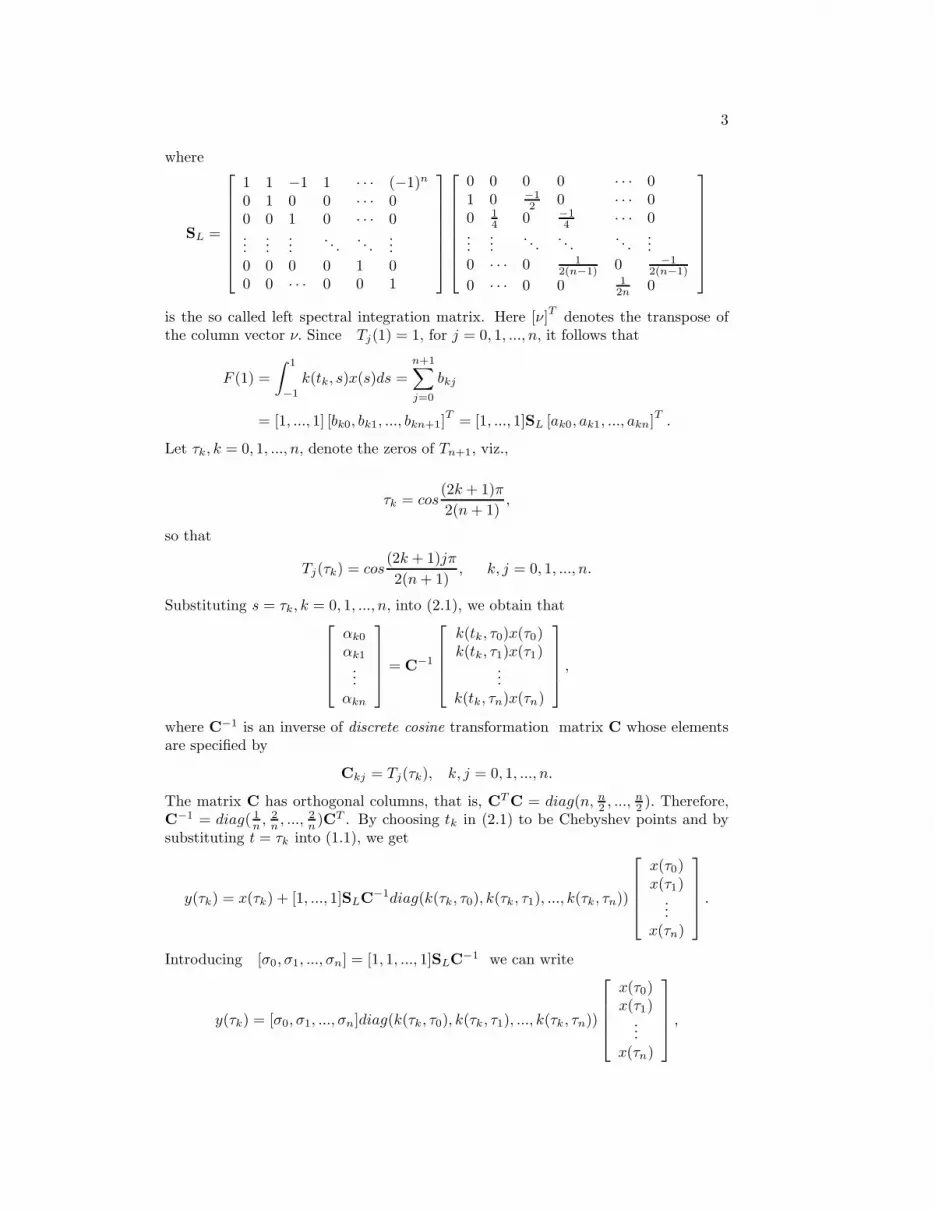
3

where

SL =

1 1 −1 1 · · · (−1)n

0 1 0 0 · · · 00 0 1 0 · · · 0...

......

. . .. . .

...0 0 0 0 1 00 0 · · · 0 0 1

0 0 0 0 · · · 01 0 −1

2 0 · · · 00 1

4 0 −14 · · · 0

......

. . .. . .

. . ....

0 · · · 0 12(n−1) 0 −1

2(n−1)

0 · · · 0 0 12n

0

is the so called left spectral integration matrix. Here [ν]T

denotes the transpose ofthe column vector ν. Since Tj(1) = 1, for j = 0, 1, ..., n, it follows that

F (1) =

∫ 1

−1

k(tk, s)x(s)ds =n+1∑

j=0

bkj

= [1, ..., 1] [bk0, bk1, ..., bkn+1]T

= [1, ..., 1]SL [ak0, ak1, ..., akn]T.

Let τk, k = 0, 1, ..., n, denote the zeros of Tn+1, viz.,

τk = cos(2k + 1)π

2(n+ 1),

so that

Tj(τk) = cos(2k + 1)jπ

2(n+ 1), k, j = 0, 1, ..., n.

Substituting s = τk, k = 0, 1, ..., n, into (2.1), we obtain that

αk0

αk1

...αkn

= C−1

k(tk, τ0)x(τ0)k(tk, τ1)x(τ1)

...k(tk, τn)x(τn)

,

where C−1 is an inverse of discrete cosine transformation matrix C whose elementsare specified by

Ckj = Tj(τk), k, j = 0, 1, ..., n.

The matrix C has orthogonal columns, that is, CT C = diag(n, n2 , ...,

n2 ). Therefore,

C−1 = diag( 1n, 2

n, ..., 2

n)CT . By choosing tk in (2.1) to be Chebyshev points and by

substituting t = τk into (1.1), we get

y(τk) = x(τk) + [1, ..., 1]SLC−1diag(k(τk, τ0), k(τk, τ1), ..., k(τk, τn))

x(τ0)x(τ1)

...x(τn)

.

Introducing [σ0, σ1, ..., σn] = [1, 1, ..., 1]SLC−1 we can write

y(τk) = [σ0, σ1, ..., σn]diag(k(τk, τ0), k(τk, τ1), ..., k(τk, τn))

x(τ0)x(τ1)

...x(τn)

,

4 S.-Y. KANG, I. KOLTRACHT AND G. RAWITSCHER

or equivalently,

y(τk) = [k(τk, τ0), k(τk, τ1), ..., k(τk, τn)]diag(σ0, σ1, ..., σn)

x(τ0)x(τ1)

...x(τn)

.

Therefore the discretization of the equation (1.1) for the case a = −1 and b = 1 isas follows,

[I + KDσ] x = y,(2.2)

where

K = (k(τi, τj))ni,j=0,

Dσ = diag(σ0, σ1, ..., σn),

x = [x(τ0), x(τ1), ..., x(τn)]T ,

y = [y(τ0), y(τ1), ..., y(τn)]T.

The formulas (2.2) can be generalized for interval [a, b] other than [-1, 1] by the linearchange of the variable h(τ) = 1

2 (b−a)τ+ 12 (a+b). Thus if ηj = h(τj), j = 0, 1, ..., n,

we have[

I +b− a

2KDσ

]

x = y,

where

K = (k(ηi, ηj))ni,j=0, Dσ = diag(σ0, σ1, ..., σn),

x = [x(η0), x(η1), ..., x(ηn)]T, y = [y(η0), y(η1), ..., y(ηn)]

T.

The accuracy of this discretization when k and x are not polynomials is discussed ina more general setting in the next section.

3. Gauss Type Quadrature for a Semismooth Kernel. We consider nowmore general semismooth kernels, as in Definition 1, for which we write

x(t) +

∫ t

a

k1(t, s)x(s)ds +

∫ b

t

k2(t, s)x(s)ds = y(t), a ≤ t ≤ b.(3.1)

In this section we describe the numerical technique for discretizing the equation (3.1).It is based on the Clenshaw-Curtis quadrature described in Section 2, which is wellsuited for computing antiderivatives. Let

F (t) =

∫ t

−1

k1(t, s)x(s)ds, G(t, λ) =

∫ λ

−1

k1(t, s)x(s)ds,

such that F (t) = G(t, t), and let

H(t) =

∫ 1

t

k2(t, s)x(s)ds, J(t, λ) =

∫ 1

λ

k2(t, s)x(s)ds.

5

Further, assume that k1(tk, s)x(s) can be expanded in a finite set of polynomials, i.e.,k1(tk, s)x(s) =

∑n

i=0 αkiTi(s). As we have seen in Section 2, if

G(tk, λ) =

n+1∑

j=0

βkjTj(λ),(3.2)

then

[βk0, βk1, ..., βkn+1]T

= SL [αk0, αk1, ..., αkn]T.(3.3)

Similarly, assume that k2(tk, s)x(s) =∑n

j=0 αkjTj(s). If

J(tk, λ) =

∫ 1

λ

k2(tk, s)x(s)ds =

n+1∑

j=0

βkjTj(λ),

then[

βk0, βk1, ..., βkn+1

]T

= SR [αk0, αk1, ..., αkn]T,(3.4)

where

SR =

1 1 1 1 · · · 10 −1 0 0 · · · 00 0 −1 0 · · · 0...

......

. . .. . .

...0 0 0 0 −1 00 0 · · · 0 0 −1

0 0 0 0 · · · 01 0 −1

2 0 · · · 00 1

4 0 −14 · · · 0

......

. . .. . .

. . ....

0 · · · 0 12(n−1) 0 −1

2(n−1)

0 · · · 0 0 12n

0

is the right spectral integration matrix. Let τk, k = 0, 1, ..., n, denote the zeros ofTn+1. Substituting λ = τk, k = 0, 1, ..., n, into (3.2), we obtain that

G(tk, τ0)G(tk, τ1)

...G(tk, τn)

= CSLC−1diag(k1(tk, τ0), ..., k1(tk, τn))

x(τ0)...

x(τn)

and, similarly,

J(tk, τ0)J(tk, τ1)

...J(tk, τn)

= CSRC−1diag(k2(tk, τ0), ..., k2(tk, τn))

x(τ0)...

x(τn)

.

We remark that in writing the equality sign in (3.3) and (3.4), we assume that βn+1

is set to zero. This is an acceptable assumption because G(tk, λ) is itself only ap-proximately represented by the polynomials in (3.2) and the overall accuracy is notaffected. Since F (τk) = G(τk, τk) we get

F (τk) = [0, ..., 0, 1, 0, ..., 0]CSLC−1diag(k1(τk, τ0), ..., k1(τk, τn))

x(τ0)...

x(τn)

6 S.-Y. KANG, I. KOLTRACHT AND G. RAWITSCHER

= [wk0, wk1, ..., wkn] diag(k1(τk, τ0), ..., k1(τk, τn))

x(τ0)...

x(τn)

= [wk0, wk1, ..., wkn] diag(x(τ0), ..., x(τn))

k1(τk, τ0)...

k1(τk, τn)

where [wk0, ..., wkn] is the (k+ 1)-st row of the matrix Wdef= CSLC−1. We need now

the following identity which can be verified by direct calculation.Lemma 3.1. Let A and B be n × n matrices and c = [c1, ..., cn]T . Then

(A ◦ B)c = diag(Adiag(c1, ..., cn)BT ), where A ◦ B denotes the Schur product of A

and B, (A ◦ B)ij = aijbij , i, j = 1, ..., n.Using this lemma we find that,

F (τ0)F (τ1)

...F (τn)

= diag(Wdiag(x(τ0), ..., x(τn))KT1 ) = (W ◦ K1)

x(τ0)...

x(τn)

,(3.5)

where K1 = (k1(τi, τj))ni,j=0. Similarly,

H(τ0)H(τ1)

...H(τn)

= (V ◦K2)

x(τ0)...

x(τn)

,(3.6)

where V = CSRC−1. The formulas (3.5) and (3.6) can be generalized for an interval[a, b] other than [−1, 1] by the linear change of variables, h(τ) = 1

2 (b− a)τ + 12 (a+ b).

Thus if ηj = h(τj), j = 0, 1, ..., n, and with the notation

Fa(t) =

∫ t

a

k1(t, s)x(s)ds, Hb(t) =

∫ b

t

k2(t, s)x(s)ds,

we have

Fa(η0)Fa(η1)

...Fa(ηn)

=b− a

2(W ◦ K1)

x(η0)x(η1)

...x(ηn)

(3.7)

and,

Hb(η0)Hb(η1)

...Hb(ηn)

=b− a

2(V ◦ K2)

x(η0)x(η1)

...x(ηn)

.(3.8)

Using (3.7) and (3.8) we can now discretize the equation (3.1) as follows,[

I +b− a

2(W ◦ K1 + V ◦ K2)

]

x = y,(3.9)

7

where x = [x(η0), ..., x(ηn)]T and y = [y(η0), ..., y(ηn)]T . Next we show that ifthe kernel function k(t, s) is smooth, such that k1 = k2, then the discretization (3.9)reduces to (2.2).

Proposition 1. Suppose that k(t, s) ∈ Cp

[a,b]×[a,b], and that k1(t, s) = k2(t, s) =

k(t, s). Then,[

I +b− a

2(W ◦ K1 + V ◦ K2)

]

x =

[

I +b− a

2KDσ

]

x.

.Proof. Without any loss of generality we assume that a = −1 and b = 1. For

t = tk, −1 ≤ tk ≤ 1,

x(tk) +G(tk, λ) + J(tk, λ) = y(tk)(3.10)

holds for any λ, −1 ≤ λ ≤ 1. Therefore if λ = 1, then J(tk, 1) = 0 and

G(tk, 1) =

n∑

j=0

βkj = [1, ..., 1]SL

αk0

...αkn

= [1, ..., 1]SLC−1diag(k(tk, τ0), ..., k(tk, τn))

x(τ0)...

x(τn)

= [σ0, σ1, ..., σn]diag(k(tk, τ0), ..., k(tk, τn))

x(τ0)...

x(τn)

= [k(tk, τ0), k(tk, τ1), ..., k(tk, τn)]diag(σ0, σ1, ..., σn)

x(τ0)x(τ1)

...x(τn)

.

Substituting tk = τk for k = 0, 1, ..., n, into (3.10), we obtain that

[I + KDσ] x = y.

The assertion now follows.We compared the numerical behavior of the discretization (2.2) and (3.9) for a

number of smooth kernels and found that numerical answers differed in accuracy atthe level of machine precision only.

We now estimate the accuracy of approximation of the integral equation (3.1) withthe linear system of equations (3.9). The following property of Chebyshev expansionscan be derived along the lines of an argument in Gottlieb and Orszag ([10], p.29).

Proposition 2. Let f ∈ Cr[−1, 1], r > 1, and let

f(t) =

∞∑

j=0

αjTj(t), −1 ≤ t ≤ 1.

Then

|αj | ≤2

π

∫ π

0

∣

∣

∣

∣

dr

dθrf(cosθ)

∣

∣

∣

∣

dθ1

jr=

c

jr

8 S.-Y. KANG, I. KOLTRACHT AND G. RAWITSCHER

and∣

∣

∣

∣

∣

∣

f(t) −

n∑

j=0

αjTj(t)

∣

∣

∣

∣

∣

∣

≤c

r − 1

1

nr−1.

It implies that if f(r) is analytic then the convergence of Chebyshev expansions

is superalgebraic. Let now Fl(x) =∫ x

−1 f(t)dt and Fr(x) =∫ 1

xf(t)dt. The

following result can be found in Greengard and Rokhlin [11].Proposition 3. Suppose that f ∈ Cr

[−1,1], r > 1, and that f = (f(τ0), ..., f(τn))T ,

is the vector of the function values at the roots of Tn+1(x). Suppose further that Fl

and Fr are defined by

Fl = (Fl(τ0), ..., Fl(τn))T , Fr = (Fr(τ0), ..., Fr(τn))T .

Then

||Fl − CSLC−1f ||∞ = O(1

nr−1)

and

||Fr − CSRC−1f ||∞ = O(1

nr−1).

Furthermore, all elements of the matrix CSLC−1 and CSRC−1 are strictly positive.Let now ηi = b−a

2 τi + a+b2 , where τi is a zero of Tn+1(x), for i = 0, 1, ..., n,

be the shifted Chebyshev points, and x = (x(η0), x(η1), ..., x(ηn))T be the vectorof values of solution x(t) of equation (3.1) at ηi. The following proposition followsimmediately from standard properties of the Riemann integral, (see e.g. [16], p.105).

Proposition 4. Let k(t, s) be (p1, p2)-semismooth and let y(t) ∈ Cq

[a,b], such

that r = min{p1, p2, q} > 1. Let the equation (3.1) define an invertible operator onCr

[a,b]. Then x ∈ Cr[a,b].

Let now

Fa = (Fa(η0), ..., Fa(ηn))T

and

Hb = (Hb(η0), ..., Hb(ηn))T .

It follows from Proposition 3 that in conditions of Proposition 4,

||Fa −b− a

2(W ◦ K1)x||∞ = O(

1

nr−1),

and

||Hb −b− a

2(V ◦ K2)x||∞ = O(

1

nr−1).

Combining the above results we obtain the following estimate for the residual.

9

Theorem 3.2. Let x be a solution vector of the equation (3.9), and x the vectorof values of the solution x(t) at t = ηi, i = 0, 1, ..., n. Suppose that k(t, s) is (p1, p2)-semismooth, and that y(t) ∈ Cq

[a,b]. Suppose further that the equation (3.1) defines an

invertible operator on Cr[a,b], where r = min{p1, p2, q} > 1. Then,

||(I +b− a

2(W ◦ K1 + V ◦ K2))(x − x)||∞ = O(

1

nr−1).

It follows from the collectively compact operator theory, see Anselone [1], thatfor sufficiently large n the matrices I + b−a

2 (W ◦ K1 + V ◦ K2), which depend on n,are invertible and their inverses are uniformly bounded. Therefore Theorem 1 impliesthat for increasing n, the convergence of x to x is of order O(n1−r). If p1 = p2 = q =∞, then the convergence is superalgebraic. Numerical examples in Section 5 indeeddemonstrate this type of convergence.

4. The Composite Rule. In this section, we describe the composite rule cor-responding to the quadrature of (3.9). Let

a = b0 ≤ b1 ≤ · · · ≤ bm = b

be a partition of the interval [a, b], and let

τ(j)k =

1

2(bj − bj−1)τk +

1

2(bj + bj−1), k = 0, 1, ..., nj,

be the Chebyshev support points mapped into [bj−1, bj]. Define

x(t) =

x1(t) if b0 ≤ t ≤ b1x2(t) if b1 < t ≤ b2

...xm(t) if bm−1 < t ≤ bm,

and

y(t) =

y1(t) if b0 ≤ t ≤ b1y2(t) if b1 < t ≤ b2

...ym(t) if bm−1 < t ≤ bm,

and rewrite the equation (1.1) as a system of m equations, for j = 1, ...,m,

xj(t) +

∫ b1

b0

k1(t, s)x1(s)ds+ · · · +

∫ t

bj−1

k1(t, s)xj(s)ds+

∫ bj

t

k2(t, s)xj(s)ds

+ · · · +

∫ bm−1

bm

k2(t, s)xm(s)ds = yj(t).(4.1)

Applying the quadrature of (3.9) to each of the integrals we obtain a system of linearequations as follows, for j = 1, ...,m,

b1 − b02

[(W + V) ◦ K1j ]x1 + · · · + [I +bj − bj−1

2(W ◦ Kjj + V ◦ Kjj)]xj +

+ · · · +bm − bm−1

2[(W + V) ◦Kmj ]xm = yj ,

10 S.-Y. KANG, I. KOLTRACHT AND G. RAWITSCHER

where

xj = [x(τ(j)0 ), x(τ

(j)1 ), ..., x(τ (j)

nj)]T , yj = [y(τ

(j)0 ), y(τ

(j)1 ), ..., y(τ (j)

nj)]T ,

Kjj = (k1(τ(j)p , τ (j)

q ))nj

p,q=0, Kjj = (k2(τ(j)p , τ (j)

q ))nj

p,q=0,

Kij = (k1(τ(j)p , τ (i)

q ))nj ,ni

p,q=0, if i < j,

Kij = (k2(τ(j)p , τ (i)

q ))nj ,ni

p,q=0, if i > j,

or in a block matrix form,

A11 A12 · · · A1m

A21 A22 · · · A2m

...Am1 Am2 · · · Amm

x1

x2

...xm

=

y1y2...ym

,(4.2)

where

Ajj = [I +bj − bj−1

2(W ◦ Kjj + V ◦ Kjj)],

Aij =bj − bj−1

2[(W + V) ◦ Kji], if i 6= j.

In this paper we do not consider the issue of how to partition the interval [a, b]. Anadaptive quadrature rule is possible here along the same lines as in [9], [14], namely,by using the size of last Chebyshev coefficients of k1, k2 and y in a given subintervalof partition to determine whether this subinterval should be further subdivided. Thisadaptive rule is a part of our research project in which we are going to compare thealgorithm of the present paper with existing algorithms for Schroedinger equationswith physically realistic nonlocal potentials.

In general, the matrix (4.2) is not structured, and is being solved by the standardGaussian elimination at the cost of O(m3) arithmetic operations, (we assume here thatm is much larger than the nj ’s). If however, the semismooth kernel k(t, s) has someadditional structure, then this structure is usually inherited by the matrix in (4.2). Forexample, if k1 and k2 are low rank kernels then the matrix A becomes semiseparable,and can be solved by existing linear complexity algorithms. We remark that in thecase of the Schroedinger equation with non-local potentials discussed in Section 7below, the overall kernel is obtained as the composition of the semi-separable Green’sfunction with the non-local potential. If the non-local potential is also semi-separable,which is the case when the non-locality arises from exchange terms, then the overallkernel is semi-separable as well, and the numerical techniques presented here, althoughstill applicable, can be replaced by the IEM methods ([8], [9]) previously developedfor local potentials. These methods give highly accurate linear complexity algorithmsfor the integral equation itself.

If the kernel k(t, s) depends on the difference of the arguments,

k(t, s) = k(|t− s|) =

{

k1(t− s) if 0 ≤ s ≤ tk2(t− s) if t < s ≤ T,

and if we use a uniform partition with the same number of points per partition, then,

kr(τ(i)p , τ (i)

q ) = kr(τp − τq), r = 1, 2,

11

and we obtain a block Toeplitz matrix,

A1 A2 A3 · · · Am

A2 A1 A2 · · · Am−1

A3 A2 A1 · · · Am−2

. . .. . .

. . .

Am Am−1 · · · A2 A1

x1

x2

...xm

=

y1y2...ym

,(4.3)

which can be solved in O(m log(m)) or O(m2) arithmetic operations by algorithmsavailable in the literature.

Finally we would like to point out that the above composite rule can be used tohandle kernels which have a finite number of singularities on the main diagonal, t = s.In this case one has to include all the singular points as a subset of all partition points.This is illustrated in the next section on a simplest case of one such singularity, butin full detail.

5. Kernels with Singularities on the Main Diagonal. Suppose that thekernel k(t, s) has a singularity at (c, c), a < c < b, inside the square [a, b]×[a, b]. Sincethe Chebyshev points ηi = b−a

2 τi + a+b2 , i = 0, 1, 2, ..., n, are clustered towards the

boundaries of the square [a, b]× [a, b], we do not have sufficient values of k(t, s) aroundsingular point (c, c) for a good approximation. Therefore we apply the composite ruleof Section 4 with c being a partition point. For the sake of simplicity we assume thatc is the only partition point, thus [a, b] is partitioned into two subintervals [a, c] and[c, b]. Without loss of generality, we consider the solution of

x(t) +

∫ 1

−1

k(t, s)x(s)ds = y(t),(5.1)

where

k(t, s) =

{

k1(t, s) if − 1 ≤ s ≤ tk2(t, s) if t < s ≤ 1,

and assume that the kernel k(t, s) has a singular point at (0,0). Define

x(t) =

{

x1(t) if − 1 ≤ t ≤ 0x2(t) if 0 < t ≤ 1

and

y(t) =

{

y1(t) if − 1 ≤ t ≤ 0y2(t) if 0 < t ≤ 1.

We can rewrite the equation (5.1) as a system of two equations. For −1 ≤ t ≤ 0,

x1(t) +

∫ t

−1

k(t, s)x1(s)ds+

∫ 0

t

k(t, s)x1(s)ds+

∫ 1

0

k(t, s)x2(s)ds = y1(t),(5.2)

and for 0 < t ≤ 1,

x2(t) +

∫ 0

−1

k(t, s)x1(s)ds+

∫ t

0

k(t, s)x2(s)ds+

∫ 1

t

k(t, s)x2(s)ds = y2(t).(5.3)

12 S.-Y. KANG, I. KOLTRACHT AND G. RAWITSCHER

Discretizations of the equations (5.2) and (5.3), respectively, are as follows.

[I +1

2(W ◦ K11 + V ◦ K11)]x1 +

1

2[(W + V) ◦ K21]x2 = y1(5.4)

and

1

2[(W + V) ◦ K12]x1 + [I +

1

2(W ◦ K22 + V ◦ K22)]x2 = y2,(5.5)

where

K11 = k1(τ(1)p , τ (1)

q )n1

p,q=0, K11 = k2(τ(1)p , τ (1)

q )n1

p,q=0, K12 = k1(τ(2)p , τ (1)

q )n2,n1

p,q=0,

K22 = k1(τ(2)p , τ (2)

q )n2

p,q=0, K22 = k2(τ(2)p , τ (2)

q )n2

p,q=0, K21 = k2(τ(1)p , τ (2)

q )n1,n2

p,q=0,

with

τ(1)i =

1

2τi −

1

2and τ

(2)j =

1

2τj +

1

2, i = 0, 1, ..., n1, j = 0, 1, ..., n2.

Here x1 = [x1(τ(1)1 ), ..., x1(τ

(1)n1

)]T and x2 = [x2(τ(2)1 ), ..., x2(τ

(2)n2

)]T . In the matrixform we write,

[

A11 A12

A21 A22

] [

x1

x2

]

=

[

y1y2

]

,(5.6)

where

A11 = [I +1

2(W ◦ K11 + V ◦ K11)],

A12 =1

2[(W + V) ◦ K21],

A21 =1

2[(W + V) ◦ K12],

A22 = [I +1

2(W ◦ K22 + V ◦ K22)].

The size of the matrix in the equation (5.6) is (n1+n2+2)×(n1+n2+2). The formulas(5.2) and (5.3) can be generalized for interval [a, c] and [c, b] other than [−1, 1] by thelinear change of the variable p(t) = 1

2 (c−a)t+ 12 (c+a) and q(t) = 1

2 (b−c)t+ 12 (b+c)

if (c, c) is a singular point of k(t, s). Thus if

τ(1)i = p(τi) and τ

(2)i = q(τi), i = 0, 1, 2, ..., ni,

then,[

A11 A12

A21 A22

] [

x1

x2

]

=

[

y1y2

]

,

where

A11 = [I +c− a

2(W ◦ K11 + V ◦ K11)],

A12 =b− c

2[(W + V) ◦ K21],

A21 =c− a

2[(W + V) ◦ K12],

A22 = [I +b − c

2(W ◦ K22 + V ◦ K22)],

with Ki,j defined as above. A numerical example illustrating this technique is givenin the next section.

13

6. Numerical Examples. In this section we compare our methods with someexiting algorithms for the following types of kernels,

• Type 1 : Discontinuity along the diagonal t = s.• Type 2 : Discontinuity in the first order partial derivatives along the diagonalt = s.

• Type 3 : Singularity on the boundary of the square and Type 2.• Type 4 : Singularity on the main diagonal.

These are the methods which have been implemented for comparison purposes,G-Leg : Nystrom discretization based on Gauss-Legendre quadrature.T-Def : Two step Deferred Approach to the limit. Approximate solutions x1, x2,

and x3 for subintervals of partition h, h2 , and h

4 , respectively, are computed.Then the numerical solution x(s) is obtained by ( see e.g. Baker [3])

x(s) =64x3(s) + x1(s) − 20x2(s)

45.

Atk-T : Atkinson’s iteration with the composite Trapezium rule. Applied to kernelsk(t, s) which have discontinuities in the first order partial derivatives alongthe diagonal t = s.

Alg-1 : Algorithm of Section 2, (2.2).Schur : Algorithm of Section 3, (3.9).Sch-C : Algorithm of Section 4, (4.2).

The number of points used in discretizations is denoted by n. Error denotes||x−xτ ||/||x||, where x and xτ are the analytic and the numerical soluions, respectively.In each plot, log(Error) is the common logarithm of the Error. All computations weredone on a DELL Workstation with operating system RedHat Linux 5.2 in doubleprecision. All examples are set-up by choosing a simple analytic solution and thencomputing the corresponding right hand side. We remark that the values of x(t) arefound inside the interval (or each of the subintervals of partition ) at Chebyshev pointsτ0, τ1, ..., τn. The value of x(t) for t 6= τk can be found as follows. Applying C−1 wecan find “Chebyshev-Fourier” coeffcients of x(t),

α0

α1

...αn

= C−1

x(τ0)x(τ1)

...x(τn)

.

Thus,

x(t) ∼=

n∑

j=0

αjTj(h(t)), a ≤ t ≤ b.

The value of Tj(t) for t 6= τk is found now using the recursion satisfied by Chebyshevpolynomials, Tj+1(t) = 2tTj(t) − Tj−1(t).Example 1.

x(t) + λ

∫ 1

−1

k(t, s)x(s)ds = y(t), −1 ≤ t ≤ 1,

where y(t) = λ(e+ e−1) + (1 − 2λ)e−t, and

k(t, s) =

{

1 if − 1 ≤ s ≤ t−1 if t < s ≤ 1.

14 S.-Y. KANG, I. KOLTRACHT AND G. RAWITSCHER

The analytical solution is x(t) = e−t. Since this kernel is discontinuous along thediagonal t = s, Gauss-Legendre quadrature gives low accuracy. The accuracy in theAtkinson’s iteration improves very slowly. The algorithm of Section 3 gives accuracyof order 10−15 with only 16 support points, whereas the 2-step method of DeferredApproach to the Limit method requires n = 256 points to achieve comparable accu-racy. Moreover, it requires computation of x2(t) and x3(t) at the cost of O((2n)3)and O((4n)3), respectively.

0 100 200 300 400 500 600−16

−14

−12

−10

−8

−6

−4

−2

0Fig 1

Number of points

log(

Err

or)

G−Leg

Atk−T

T−Def

Schur

Fig. 6.1. Comparison of numerical solutions of Example 1, λ = 0.1.

Example 2.

x(t) + λ

∫ T

0

k(t, s)x(s)ds = y(t), 0 ≤ t ≤ T

where y(t) = (1 − λsin2(T )2 + λ)sint+ (T

2 − t− sin(2T )4 )λcost, and

k(t, s) = sin(|t− s|) =

{

sin(t− s) if 0 ≤ s ≤ tsin(s− t) if t < s ≤ π

2 .

The analytical solution is x(t) = sin(t). This kernel has discontinuities in the firstorder partial derivatives along the diagonal, t = s. Again standard Nystrom-typediscretization methods fail to give high accuracy in this case. In the first experimentwe take T = π

2 and λ = − 4π. Our method shows the order of 10−14 accuracy with

only 16 points in [0, π2 ] without any partitioning. The 2-step method of Deferred

Approach to the Limit gives the accuracy of O(10−14) with n = 256, but at muchhigher cost than our method, see Fig 2. The second part of Example 2 is to comparethe composite rule described in Section 5 with the basic quadrature (3.9) of Section 4when the length of the interval of integration, [a, b], becomes increasingly large. HereM denotes the number of subintervals in [0, T ] and Mn stands for the total numberof support points in the given interval [0, T ].

15

0 100 200 300 400 500 600−15

−10

−5

0Fig 2

Number of points

log(

Err

or)

G−Leg

Atk−T

T−Def

Schur

Fig. 6.2. Comparison of numerical solutions of Example 2.

Table 1 ( T = 200π, λ = − 4π

)

M 1 1 1 2 4 8Mn 256 512 1024 256 512 1024

Error 2.4e+ 01 3.0e− 02 CPUtime limit exceed 1.2e+ 01 7.8e− 02 2.2e− 11

Without partitioning, i.e. with M = 1, we increase the number of support pointsfrom n = 128 to n = 1024. For n = 512 the accuracy is of order O(10−2), but forn = 1024 the CPU time limit is exceeded. When the interval is partitioned into 8subintervals and n = 128 i.e., the total number of points is 1024, the accuracy now isof order O(10−11).Example 3.

x(t) +

∫ 1

−1

k(t, s)x(s)ds = y(t), −1 ≤ t ≤ 1

where y(t) = 1 − t2 + 11−t2

(arctan(t) − arctan(−1)) − 1(1+t)(1+t2) , and

k(t, s) =

{

1(1−t2)(1−s4) if − 1 ≤ s ≤ t

−1(1−t4)(1−s2) if t < s ≤ 1.

The analytical solution is x(t) = 1 − t2. Since this kernel has singularities along theboundaries of the square [−1, 1]×[−1, 1] methods based on the Trapezium rule are notapplicable. Therefore we compare our algorithms of Section 1 and Section 3 with theNystrom-Gauss-Legendre discretization only. The algorithm of Section 1 shows thesame accuracy of numerical solution as the Gauss-Legendre quadrature. The methodof Section 3 gives O(10−13) accuracy with n = 32 points, whereas Nystrom-Gauss-Legendre quadrature gives O(10−3) with n = 256 points.

16 S.-Y. KANG, I. KOLTRACHT AND G. RAWITSCHER

0 50 100 150 200 250 300−14

−12

−10

−8

−6

−4

−2

0Fig 3

Number of points

log(

Err

or)

G−Leg

Alg−1

Schur

Fig. 6.3. Comparison of numerical solutions of Example 3.

Example 4.

x(t) +

∫ 1

−1

k(t, s)x(s)ds = y(t), −1 ≤ t ≤ 1

where y(t) = 2(1 − t2 + 2t3) + (1 + 2t4)ln(t2 + t4) − ln(1 + t2) − 2t4ln(1 + t4), and

k(t, s) =

{

1/(t2 + s4) if − 1 ≤ s ≤ t1/(s2 + t4) if t < s ≤ 1.

The analytical solution is x(t) = 4t3. The kernel k(t, s) has a singularity at (0, 0).

Also y(t) is singular at t = 0. Since Chebyshev points cos( (2i−1)2N

π), i = 1, 2, ..., n, areclustered towards the end points of interval [−1, 1], discretization formula (3.9) doesnot contain sufficient values of kernel near (t, s) = (0, 0). Therefore we partition [−1, 1]into [−1, 0] and [0, 1]. The choice of n = 256 Chebyshev points in each subinterval withthe total of n = 512 points gives O(10−11) accuracy. For comparison the best accuracyof the Gauss-Legendre quadrature without partitions and with n = 512 support pointsis O(10−4) while the best accuracy of the algorithm of Section 2 without partitionsis of O(10−6), see Fig 4.

7. Application to Non-Local Schroedinger Equations. In this section wedemonstrate that the developed numerical technique is also applicable to problemsother than integral equations, for example, to integro-differential equations. We chosehere the radial Schroedinger equation which models the quantum mechanical interac-tion between particles represented by spherically symmetric potentials. These poten-tials are usually local, i.e., they depend only on the distance between the two particles,in which case the equation is a differential equation which is routinely solved in com-putational physics. However, if there are more than two particles present, then thepotentials can become non-local and the differential Schroedinger equation becomes

17

0 100 200 300 400 500 600−11

−10

−9

−8

−7

−6

−5

−4

−3

−2Fig 4

Number of points

log(

Err

or)

G−Leg

Schur

Sch−C

Fig. 6.4. Comparison of numerical solutions of Example 4.

an integro-differential equation for the wave function ψ,

d2ψ(r)

dr2+ κ2ψ(r) =

∫ T

0

v(r, r′)ψ(r′)dr′,(7.1)

which is defined for 0 < r < ∞, satisfies the condition ψ(0) = 0, and is boundedat infinity. It is assumed that v(r, r′) is negligible for r > T or r′ > T, see e.g.[13]. Because it is numerically more difficult to solve the Schroedinger equation in thepresence of a nonlocal potential, the latter is customarily replaced by an approximatelocal equivalent potential. There is, however, a renewed interest in the nonlocalequations, and a significant number of papers on this subject appeared in the pastfew years, (our database search returned over 50 related publications).

Using the technique of [8] it easy to show that (7.1) is equivalent to the followingintegral equation,

ψ(r) +cos(κr)

κ

∫ r

0

sin(κr′)

∫ T

0

v(r′, p)ψ(p)dpdr′

+sin(κr)

κ

∫ T

r

cos(κr′)

∫ T

0

v(r′, p)ψ(p)dpdr′ = sin(κr).

or

ψ(r) +cos(κr)

κ

∫ T

0

k1(r, r′)ψ(r′)dr′ +

sin(κr)

κ

∫ T

0

k2(r, r′)ψ(r′)dr′(7.2)

= sin(κr),

where

k1(r, r′) =

∫ r

0

sin(κp)v(p, r′)dp, k2(r, r′) =

∫ T

r

cos(κp)v(p, r′)dp.

18 S.-Y. KANG, I. KOLTRACHT AND G. RAWITSCHER

We consider now the case when v(p, r′) is (p1, p2)-semismooth, such that

v(p, r′) =

{

v1(p, r′) if 0 ≤ p ≤ r′

v2(p, r′) if r′ ≤ p ≤ T.

In order to use the method which we developed in previous sections, we rewriteequation (7.2) as follows,

ψ(r) +c(r)

κ

∫ r

0

k1(r, r′)ψ(r′)dr′ +

c(r)

κ

∫ T

r

k1(r, r′)ψ(r′)dr′

+s(r)

κ

∫ r

0

k2(r, r′)ψ(r′)dr′ +

s(r)

κ

∫ T

r

k2(r, r′)ψ(r′)dr′ = s(r),(7.3)

where for notational convenience we abbreviate, c(r) = cos(κr), s(r) = sin(κr). Wehave

k1(r, r′) =

{

k11(r, r′) if 0 ≤ r′ ≤ r

k12(r, r′) if 0 ≤ r ≤ r′,

and

k2(r, r′) =

{

k21(r, r′) if r′ ≤ r ≤ T

k22(r, r′) if r ≤ r′ ≤ T,

where

k11(r, r′) =

∫ r′

0

s(p)v1(p, r′)dp+

∫ r

r′

s(p)v2(p, r′)dp,

=

∫ r′

0

s(p)v1(p, r′)dp+

∫ r

0

s(p)v2(p, r′)dp−

∫ r′

0

s(p)v2(p, r′)dp,

k12(r, r′) =

∫ r

0

s(p)v1(p, r′)dp

k21(r, r′) =

∫ T

r

c(p)v2(p, r′)dp

k22(r, r′) =

∫ r′

r

c(p)v1(p, r′)dp+

∫ T

r′

c(p)v2(p, r′)dp,

=

∫ T

r

c(p)v1(p, r′)dp−

∫ T

r′

c(p)v1(p, r′)dp+

∫ T

r′

c(p)v2(p, r′)dp.

Thus,

ψ(r) +c(r)

κ

∫ r

0

k11(r, r′)ψ(r′)dr′ +

c(r)

κ

∫ T

r

k12(r, r′)ψ(r′)dr′

+s(r)

κ

∫ r

0

k21(r, r′)ψ(r′)dr′ +

s(r)

κ

∫ T

r

k22(r, r′)ψ(r′)dr′ = s(r),(7.4)

Applying our quadrature to this equation we get,

[ I +T

2κDc(W ◦ K11 + V ◦ K12) +

T

2κDs(W ◦ K21 + V ◦ K22) ]ψ = s,(7.5)

19

where in more detail,

ψ = [ψ(t0), ψ(t1), ..., ψ(tn)]T ,

Dc = diag(cos(κt0), cos(κt1), ..., cos(κtn)),

Ds = diag(sin(κt0), sin(κt1), ..., sin(κtn)),

Dσ = diag([1, ..., 1]SLC−1),

s = [sin(κt0), sin(κt1), ..., sin(κtn)]T ,

W = CSLC−1, V = CSRC−1,

K11 = (k11(ti, tj))ni,j=0

=T

2[diag(WDs(V1 − V2)) + (WDsV2)]

K12 = (k12(ti, tj))ni,j=0

=T

2(WDsV1),

K21 = (k21(ti, tj))ni,j=0,

=T

2(VDcV2)

K22 = (k22(ti, tj))ni,j=0

=T

2[(VDcV1) + diag(VDc(V2 − V1))].

We illustrate now the obtained discretization with two examples. In the first examplewe use a prototype of the Yukawa potential, (e.g. [12], 23.c), which is simplified to adegree such that an analytic solution can be found. In our terminology this potentialis semiseparable. We note once more that the case of this semi-separable potentialcould be treated more easily by the techniques already presented in [8], and we use ithere only because the comparison with the analytic solution is possible.Example 1. Let

v(p, r′) =

{

λep−r′

if 0 ≤ p ≤ r′

λer′−p if r′ ≤ p ≤ T.

It is easy to see that if ψ(r) = e−r, then the right-hand side has the form,

y(r) = (1 −3λκ

4)e−r +

3λκ

4cos(r) −

λκ

2re−r.

By comparing the analytical solution given above with the numerical solution of (7.5)at the discretization points, we get the following relative errors in the case of λ =0.1, κ = 1 and T = 20.

n 16 32 64 128 256Error 1.2e+ 01 3.4e− 07 8.1e− 09 3.4e− 09 6.0e− 09

In the second example we consider a more interesting case for which the techniquesof [8] are not applicable. This time the non-locality is a prototype of the optical modelPerey-Buck potential, (e.g. [6], Ch. V.2). In our terminology this potential is semi-smooth, but not semiseparable.

20 S.-Y. KANG, I. KOLTRACHT AND G. RAWITSCHER

Example 2. Let

v(p, r′) =λe−

|r′−p|A

1 + e−|r′−p|

A

=

λep−r′

A

1+ep−r′

A

if 0 ≤ p ≤ r′

λer′−p

A

1+er′−p

A

if r′ ≤ p ≤ T.

Solving (7.5) at n shifted Chebyshev support points t(n)i , i = 1, ..., n, and 2n points

s(2n)i , i = 1, ..., 2n, we obtain numerical solutions ψ(n)(r) and ψ(2n)(r), respectively.

To get the values of ψ(2n)(r) at t(n)i , we follow the procedure described in the

beginning of Section 6. The error en is obtained by comparison of the solutions ψ(n)

and ψ(2n) as follows,

en = ||ψ(2n)(t(n)i ) − ψ(n)(t

(n)i )||∞/||ψ

(2n)(t(n)i )||∞.

Here we take λ = 0.1, κ = 1, A = 100, and T = 20.n 8 16 32 64 128 256en 1.0e− 0 1.2e− 03 1.6e− 09 7.7e− 15 1.6e− 14 4.8e− 14

We see that for this choice of λ the matrix is well conditioned and the double precisionaccuracy is obtained with 64 points.

8. Summary and Conclusions. In this paper, which is one of a sequence treat-ing integral equations, we describe a new method for solving integral equations forthe case when kernel can be discontinuous along the main diagonal. It has the fol-lowing advantages for a large class of such kernels: (i) for semismooth kernels it givesa much higher accuracy than it was ever possible with standard Gauss type quadra-ture rules; (ii) it is of comparable accuracy with Gauss type quadratures for smoothkernels; (iii) it exploits additional structure of the kernel such as a low semi-rank, ora displacement structure, for example, to allow for reduced complexity algorithms forthe discretized equations. (iv) the numerical examples provided in the present studyillustrate increased accuracy of our method compared to other more conventionalmethods.

Our method is also applicable to other problems, such as the computation ofeigenvalues and eigenfunctions of integral and differential operators and solution ofintegro-differential equations.

Our method may find applications in quantum mechanical atomic and nuclearphysics problems, where the requirement of indistinguishability of the electrons leadsto non localities in the potential contained in the Schroedinger equation due to thepresence of exchange terms. These, in turn, lead to integro-differential equationswhich are usually solved by iterative finite difference methods, or by orthogonal func-tion expansion methods. We plan to compare our new method with some of theexisting methods in future investigations on more realistic examples.

21

REFERENCES

[1] P.M. Anselone, Collectively Compact Operator Approximation Theory and Applica-

tions to Integral Equations, Prentice-Hall, Englewood Hills, 1971.[2] K.E. Atkinson, A Survey of Numerical Methods for the Solution of Fredholm Integral

Equations of the Second Kind, SIAM, Philadelphia, 1976.[3] C.T.H. Baker, The Numerical Treatment of Integral Equations, Oxford University

Press, 1977.[4] C.W. Clenshaw and A. R. Curtis, A method for numerical integration on an automatic

computer, Numer. Math. 2, 197(1960).[5] L.M. Delves and J.L. Mohamed, Computational Methods for Integral Equations, Cam-

bridge University Press, Cambridge, 1985.[6] H. Feshbach, Theoretical Nuclear Physics, Nuclear Physics, John Wiley and Sons,

1992.[7] I. Gohberg and I.A. Fel’dman, Convolution Equations and Projection Methods for

Their Solution, Transl. Math. Monograph, Vol 41, American Mathematical Soci-ety, Providence, RI, 1974.

[8] R.A Gonzales, J. Eisert, I. Koltracht, M. Neumann and G. Rawitscher, Integral Equa-

tion Method for the Continuous Spectrum Radial Schroedinger Equation, J. ofComput. Phys. 134, 134-149, 1997.

[9] R.A Gonzales, S.-Y. Kang, I. Koltracht and G. Rawitscher, Integral Equation Method

for Coupled Schroedinger Equations, J. of Comput. Phys. 153, 160(1999).[10] D. Gottlieb and S. Orszag, Numerical Analysis of Spectral Methods, SIAM, Philadel-

phia, 1977.[11] L. Greengard and V. Rokhlin, On the Numerical Solution of Two-Point Boundary

Value Problems, Commun. Pure Appl. Math. 44, 419(1991).[12] R.H. Landau, Quantum Mechanics II, John Wiley and Sons, 1990.[13] N.F. Mott and H.S. Massey, The Theory of Atomic Collision, 3rd ed. Oxford, Claren-

don 1965.[14] G.H. Rawitscher, B.D. Esry, E. Tiesinga, P. Burke, Jr. and I. Koltracht Comparison

of Numerical Methods for the Calculation of Cold Atomic Collisions, Submittedto J. Chem. Phys.

[15] L. Reichel, Fast Solution Methods for Fredholm Integral Equations of the Second

Kind, Numer. Math. 57, 719(1989).[16] H.L. Royden, Real Analysis, 3-rd Edition, Macmillan Publishing Company, NY, 1989.