Efficient scatter correction using asymmetric kernels

Josh Star-Lack*a, Mingshan Suna, Anders Kaestnerb, Rene Hassaneinb, Gary Virshup, Timo Berkusb, Markus Oelhafenb

aVarian Medical Systems, 2599 Garcia Ave, Mountain View, CA 94043; bVarian Medical Systems, Taefernstrasse 7, Baden, Switzerland CH-5405

ABSTRACT

X-ray cone-beam (CB) projection data often contain high amounts of scattered radiation, which must be properly modeled in order to produce accurate computed tomography (CT) reconstructions. A well known correction technique is the scatter kernel superposition (SKS) method that involves deconvolving projection data with kernels derived from pencil beam-generated scatter point-spread functions. The method has the advantages of being practical and computationally efficient but can suffer from inaccuracies. We show that the accuracy of the SKS algorithm can be significantly improved by replacing the symmetric kernels that traditionally have been used with nonstationary asymmetric kernels. We also show these kernels can be well approximated by combinations of stationary kernels thus allowing for efficient implementation of convolution via FFT. To test the new algorithm, Monte Carlo simulations and phantom experiments were performed using a table-top system with geometry and components matching those of the Varian On-Board Imager (OBI). The results show that asymmetric kernels produced substantially improved scatter estimates. For large objects with scatter-to-primary ratios up to 2.0, scatter profiles were estimated to within 10% of measured values. With all corrections applied, including beam hardening and lag, the resulting accuracies of the CBCT reconstructions were within ±25 Hounsfield Units (±2.5%). Keywords: Cone-beam computed tomography, CBCT, scatter correction, scatter kernel superposition, asymmetric kernel, offset-detector geometry.

1. INTRODUCTION The development and commercialization of large area amorphous silicon flat panel imagers has made 3-D cone-beam computed tomography (CBCT) imaging practical for many diverse applications. Examples of these applications include image-guided radiotherapy (IGRT) for patient verification and adaptive treatment planning 1, 2, interventional and diagnostic imaging with a C-Arm 3. In all cases, reconstruction of images with accurate Hounsfield Units (H.U.) is desired which, in turn, requires estimating and subtracting the scatter component of the raw data signal before the log normalization step of the reconstruction process.

1.1 Scatter correction

Due to a large area of irradiation, CBCT projection data may possess very high scatter-to-primary ratios (SPR’s > 2) even when an anti-scatter grid and bowtie filter are employed 4. Several methods have been proposed for estimating scatter in raw projection data. These include scatter deconvolution 5, 6, scatter modeling 7, modulators 8, 9, beam stop arrays 10, two scans 11 and a detector shadowing technique 12. The scatter deconvolution method, also known as scatter kernel superposition (SKS) has the advantages of not requiring extra hardware, preserving the entire field-of-view, and being computationally efficient, but has not proven to be as accurate as some of the other techniques.

In the SKS method, the x-ray cone-beam is modeled as an array of pencil beams that interact with the object-of-interest. For each of the pencil beams, a scatter kernel or point-spread function is determined based on measured responses to pencil beam irradiation. The total detected scatter estimate is then derived from the cumulative response to each of the scatter PSF’s operating on the raw projection data. The scatter estimation algorithm is inherently iterative since the kernel amplitudes and shapes depend on estimated primary values (Fig 1b). Previously, this type of model has been implemented for kV fan-beam CT 13, MV and/or kV- CBCT 14-16 using symmetric scatter point-spread functions. In this ------------------------------------------------------------------------------------------------------------------------------------------------ * josh.starlack@varian.com, phone: 650-623-1222

Medical Imaging 2009: Physics of Medical Imaging, edited by Ehsan Samei, Jiang Hsieh,Proc. of SPIE Vol. 7258, 72581Z · © 2009 SPIE

CCC code: 1605-7422/09/$18 · doi: 10.1117/12.811578

Proc. of SPIE Vol. 7258 72581Z-1

work, we show that asymmetric nonstationary kernels more accurately model scatter transport and that these kernels can be well approximated using combinations of stationary kernels thus allowing for efficient implementation of the convolution operation via FFT’s. The deficiencies of stationary kernels were independently recognized by Bertram et. al. 17.

1.2 Full-fan and half-fan geometries

Many clinical cone-beam CT systems use both centered-detector (full-fan) and offset-detector (half-fan) configurations. The full-fan configuration provides for adequate transaxial coverage for head and neck regions and allows for ‘180 deg + fan’ acquisitions, while the half-fan configuration is used to image larger fields-of-view but requires a full 360 degree scan. We have found that scatter correction of half-fan data is generally more difficult than for full-fan data due to the higher scatter-to-primary ratios (SPR)’s associated with thicker objects and the more complicated scatter profiles that emerge 11. Simple scatter approximations such as a constant correction generally fail. The goal of this study was to develop a robust kernel-based scatter correction method for both the half-fan and full-fan geometries.

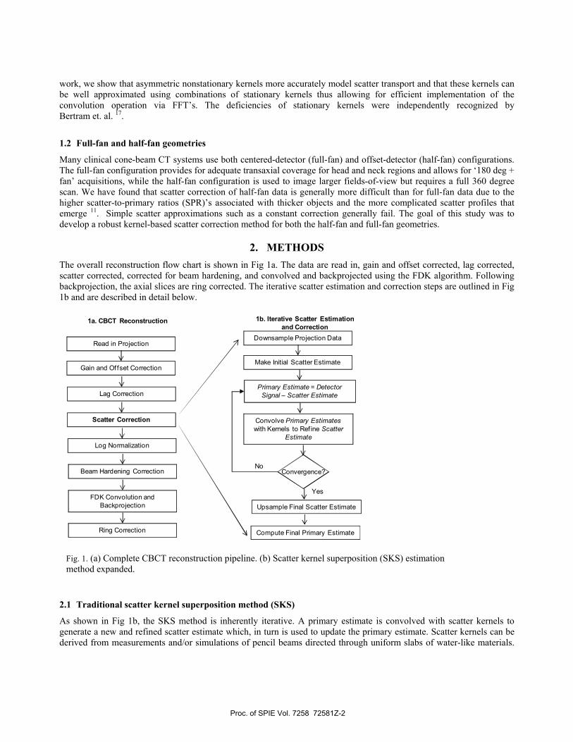
2. METHODS The overall reconstruction flow chart is shown in Fig 1a. The data are read in, gain and offset corrected, lag corrected, scatter corrected, corrected for beam hardening, and convolved and backprojected using the FDK algorithm. Following backprojection, the axial slices are ring corrected. The iterative scatter estimation and correction steps are outlined in Fig 1b and are described in detail below.

2.1 Traditional scatter kernel superposition method (SKS)

As shown in Fig 1b, the SKS method is inherently iterative. A primary estimate is convolved with scatter kernels to generate a new and refined scatter estimate which, in turn is used to update the primary estimate. Scatter kernels can be derived from measurements and/or simulations of pencil beams directed through uniform slabs of water-like materials.

Convolve Primary Estimateswith Kernels to Ref ine Scatter

Estimate

Primary Estimate = Detector Signal – Scatter Estimate

Make Initial Scatter Estimate

Convergence?No

Yes

Downsample Projection Data

Upsample Final Scatter Estimate

Gain and Of fset Correction

Read in Projection

1a. CBCT Reconstruction 1b. Iterative Scatter Estimationand Correction

Lag Correction

Scatter Correction

Log Normalization

Beam Hardening Correction

FDK Convolution and Backprojection

Ring Correction Compute Final Primary Estimate Fig. 1. (a) Complete CBCT reconstruction pipeline. (b) Scatter kernel superposition (SKS) estimation method expanded.

Proc. of SPIE Vol. 7258 72581Z-2

The kernels are symmetric with shape and amplitude parameters dependant on material density and thickness or, more specifically, on the ratio of attenuated primary signal (Ip) to the unattenuated beam signal (I0).

To generate scatter kernels for our experimental system, we performed Monte Carlo simulations (MCNP4c, Los Alamos National Laboratory) of a pencil beam directed through water slabs with thicknesses ranging from 3 to 50 cm. IPEM Rep78 spectral modeling software18 was used to create the x-ray spectra and the energy-integrating detector model assumed a 0.6 mm CsI scintillator thickness. The resulting symmetric scatter point spread functions (PSFsym) were fit to the following model based on the approach of Ohonesorge et.al. 13:

1 ----Amplitude Factor Af -------- ---------Form Function hs----------- The spatial position r= xi + yj is measured at the detector, Ip is the primary pencil beam signal, and I0 is the unattenuated (air) intensity value. The fitted parameters are α,β, A, B, σ1 and σ2 . Examples of fitted parameters are shown in Table 1. The scatter PSF described by Eq. 1 can be separated into an amplitude factor Af and form function hs. Note that only the amplitude factor varies as a function of primary attenuation (Ip) while the form function is stationary. This allows for efficient implementation of the convolution algorithm via FFT since the primary projection estimate can be pre-weighted by the spatially dependent amplitude factors Af before convolution with the form function.

Thus, to generate the scatter estimate at position (x,y), the convolution operation is written as a discrete summation:

( ) ( ) ( ) ( )', , , ,1 1

N MI x y I x y A x y h x x y yp m n m n m ns f s

n m∑= − −∑= =

2

where,

xm,yn are pixel coordinates that span a matrix of size M,N. To increase computational efficiency, the pixel matrix used for scatter calculation can be a downsampled version of the original projection matrix since the scatter PSF’s are of mainly low frequency content. The downsampled pixels are denoted henceforth as superpixels.

I’p(xm,yn) is the primary estimate

Af(xm,yn) is the amplitude factor from Eq. 1.

= A (I’p(xm,yn)/I0(xm,yn ))α (ln(I’0(xm,yn)/I’p(xm,yn)))β

hs(xm,ym) is the shifted form factor from Eq 1.

= exp(- (x-xm)2/2σ12) exp(- (y-yn)2/2σ1

2) + B exp(- (x-xm)2/2σ12) exp(- (y-yn)2/2σ2

2)

Eq. 2 is recognized as a double convolution that is more simply expressed using the 2-D convolution operator **:

( ) ( ) ( )( ) ( )', , , ** ,I x y I x y A x y h x ys p f s= 3

This spatial domain convolution is executed rapidly via 2-D FFT

( ) ( ) ( )( ) ( )( )( )', , , ,-1F F FI x y I x y A x y h x ys p f s= • 4

where F and F-1 are the forward and inverse FFT operators.

2.2 Modification for multiple thickness groups

We have found that it is difficult to fit the model of the scatter PSF’s as described by Eq 1 over a large range of object thicknesses. This is partly because the point-spread functions tend to broaden as material thicknesses increase. Thus, in order to better cover the wide dynamic range typically found in CT projection data, separate parameters for Eq. 1 were

( ) ( )( ) ( ) ( )2 2 2 2, , • / • ln / • exp 2 exp 20 0 0 1 2PSF I I r A I I I I r B rp psym p

α βσ σ

⎛ ⎞ ⎡ ⎤= − + −⎜ ⎟ ⎢ ⎥⎝ ⎠ ⎣ ⎦

Proc. of SPIE Vol. 7258 72581Z-3

'Ii

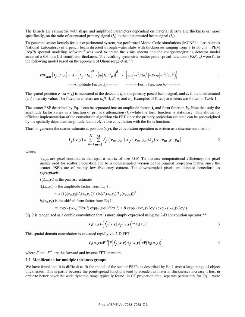
fit for three water thickness groups (<10 cm, 10-27.5 cm, > 27.5 cm) to form three families of kernels. Figure 2 shows fits for the three thickness groups and Table 1 displays the associated model parameters for the OBI geometry.

Thickness Group (g)

A (cm-2) B α β σ1 (cm) σ2 (cm)

1: < 10 cm 9.47×10-5 2.20 -0.131 1.02 19.5 3.23 2: 10- 27.5 cm 1.10×10-4 1.35 -0.173 0.978 21.3 2.95 3: > 27.5 cm 2.05×10-4 0.67 -0.270 0.421 21.2 2.52

Table 1: Scatter PSF parameter fits using the model in Eq. 1 for three thickness groups. Simulations are for the OBI geometry using a 125 kVp spectrum (14 degree target angle) with 5 mm Al beam filtration and a 0.6 mm CsI scintillator for the detector. A is normalized to a superpixel size of 1 cm2 assuming downsampling is an averaging process. .

20 40 60 80 100

20

40

60

20 40 60 80 100

20

40

60

20 40 60 80 100

20

40

60

20 40 60 80 100

20

40

60

20 40 60 80 100

20

40

60

20 40 60 80 100

20

40

60

20 40 60 80 100

20

40

60

20 40 60 80 100

20

40

60

Entire projection -Primary estimate

Group 1 (I’g1): < 10 cm Primary estimate

Partial Scatter estimates Entire Scatter Estimate

= + +

Partial Scatter estimates

Group 2 (I’g2): 10-25 cm Primary estimate

Group 3 (I’g3): >25 cm Primary estimate

1

2

3

Fig. 3. Method for efficient processing of multiple thickness groups in a single projection. Step 1 - The complete projection (top left) is parsed so that pixel values are assigned to one of three group arrays depending on the thickness estimate for that pixel . Step 2 - Convolution is then performed using the model parameters for each thickness group to create partial scatter estimates. Step 3 - the partial scatter estimates are summed to generate a complete scatter estimate (bottom left).

0 5 10 15 20 250

1

2

3

4

5

6x 10

-4

8 cm

3 cm

5 cm

Group1: 0 - 10 cm

0 5 10 15 20 250

1

2

3

4

5

6x 10-4

0 5 10 15 20 250

0.5

1

1.5

2

2.5

3x 10

-3 Group 2: 10 – 27.5cm

0 5 10 15 20 250

1

2

3x 10-3

15 cm

10 cm

20 cm

25 cm

0 5 10 15 20 250

0.002

0.004

0.006

0.008

0.01

0.012Group 3 : 27.5 - 50 cm

0 5 10 15 20 250

0.012

35 cm

30 cm

40 cm

45 cm

0.010

0.008

0.006

0.004

0.002

cm cm cm Fig. 2. Modeled (Eq. 1) symmetric scatter point spread functions (PSFsym) for three thickness groups for the OBI geometry. The fits (solid black curves) are made to Monte Carlo simulations (dots) of pencil beams directed through water slabs of varying thicknesses. Good fits are obtained across the thickness ranges. The fit parameters are shown in Table 1.

Proc. of SPIE Vol. 7258 72581Z-4

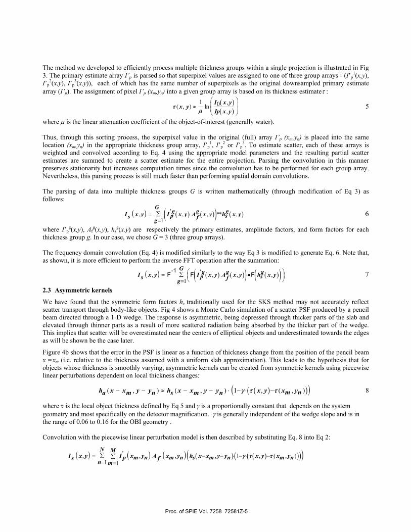
The method we developed to efficiently process multiple thickness groups within a single projection is illustrated in Fig 3. The primary estimate array I’p is parsed so that superpixel values are assigned to one of three group arrays - (I’p

1(x,y), I’p

2(x,y), I’p3(x,y)), each of which has the same number of superpixels as the original downsampled primary estimate

array (I’p). The assignment of pixel I’p (xm,yn) into a given group array is based on its thickness estimateτ :

( )( )

1 ,0( , ) ln,

I x yx y

Ip x yτ

μ

⎛ ⎞⎜ ⎟≈ ⎜ ⎟⎝ ⎠

5

where μ is the linear attenuation coefficient of the object-of-interest (generally water). Thus, through this sorting process, the superpixel value in the original (full) array I’p (xm,yn) is placed into the same location (xm,yn) in the appropriate thickness group array, I’p

1, I’p2 or I’p

3. To estimate scatter, each of these arrays is weighted and convolved according to Eq. 4 using the appropriate model parameters and the resulting partial scatter estimates are summed to create a scatter estimate for the entire projection. Parsing the convolution in this manner preserves stationarity but increases computation times since the convolution has to be performed for each group array. Nevertheless, this parsing process is still much faster than performing spatial domain convolutions. The parsing of data into multiple thickness groups G is written mathematically (through modification of Eq 3) as follows:

( ) ( ) ( )( ) ( )', , , ** ,1

G g g gI x y I x y A x y h x yp ss fg∑==

6

where I’pg(x,y), Af

g(x,y), hsg(x,y) are respectively the primary estimates, amplitude factors, and form factors for each

thickness group g. In our case, we chose G = 3 (three group arrays). The frequency domain convolution (Eq. 4) is modified similarly to the way Eq 3 is modified to generate Eq. 6. Note that, as shown, it is more efficient to perform the inverse FFT operation after the summation:

( ) ( ) ( )( ) ( )( )', , , ,1

-1F F F

G g g gI x y I x y A x y h x yp ss fg⎛ ⎞∑= •⎜ ⎟⎝ ⎠=

7

2.3 Asymmetric kernels

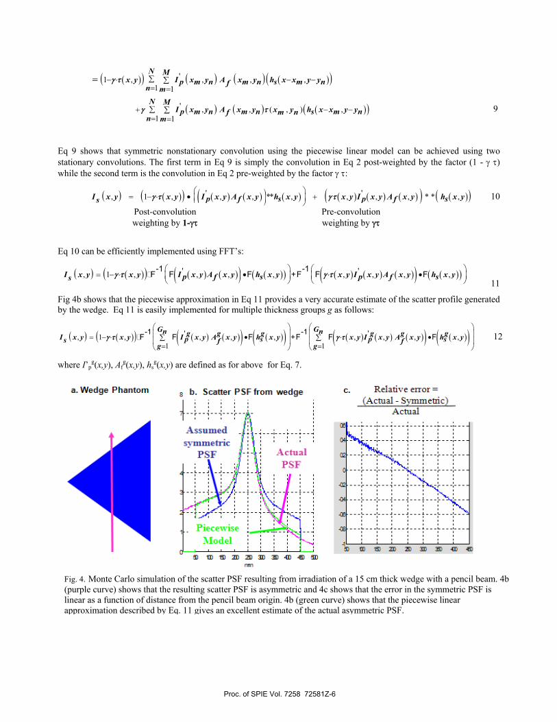
We have found that the symmetric form factors hs traditionally used for the SKS method may not accurately reflect scatter transport through body-like objects. Fig 4 shows a Monte Carlo simulation of a scatter PSF produced by a pencil beam directed through a 1-D wedge. The response is asymmetric, being depressed through thicker parts of the slab and elevated through thinner parts as a result of more scattered radiation being absorbed by the thicker part of the wedge. This implies that scatter will be overestimated near the centers of elliptical objects and underestimated towards the edges as will be shown be the case later.

Figure 4b shows that the error in the PSF is linear as a function of thickness change from the position of the pencil beam x =xm (i.e. relative to the thickness assumed with a uniform slab approximation). This leads to the hypothesis that for objects whose thickness is smoothly varying, asymmetric kernels can be created from symmetric kernels using piecewise linear perturbations dependent on local thickness changes:

( )( )( )( , ) ( , ) 1 , ( , )h x x y y h x x y y x y x ym na m n s m n γ τ τ− − ≈ − − ⋅ − ⋅ − 8

where τ is the local object thickness defined by Eq 5 and γ is a proportionally constant that depends on the system geometry and most specifically on the detector magnification. γ is generally independent of the wedge slope and is in the range of 0.06 to 0.16 for the OBI geometry . Convolution with the piecewise linear perturbation model is then described by substituting Eq. 8 into Eq 2:

( ) ( ) ( ) ( ) ( )( )( )( )', , , , 1 , ( , )1 1

N MI x y I x y A x y h x x y y x y x yp m n m n s m n m ns fn m

γ τ τ∑= − − ⋅ − ⋅ −∑= =

Proc. of SPIE Vol. 7258 72581Z-5

a. Wedge Phantom b. Scatter PSF from wedge

ti"i"hkAssumed

T II: 21: i

ActualPSF

UI 41: i

c. Relative error =(Actual - Svmnienic)

Actual

41

( )( ) ( ) ( ) ( )( )

( ) ( ) ( )( )

'1 , , , ,1 1

' , , ( , ) ,1 1

N Mx y I x y A x y h x x y yp m n m n s m nfn m

N MI x y A x y x y h x x y yp m n m n s m nf m n

n m

γ τ

γ τ

∑− ⋅ − −∑= =

+ − −∑ ∑= =

=

9

Eq 9 shows that symmetric nonstationary convolution using the piecewise linear model can be achieved using two stationary convolutions. The first term in Eq 9 is simply the convolution in Eq 2 post-weighted by the factor (1 - γ τ) while the second term is the convolution in Eq 2 pre-weighted by the factor γ τ:

( ) ( )( ) ( ) ( )( ) ( ) ( ) ( ) ( )( ) ( )( )' ', 1 , , , ** , , , , * * ,I x y x y I x y A x y h x y x y I x y A x y h x yp f s p f ss γ τ γ τ⎛ ⎞

= − ⋅ • +⎜ ⎟⎝ ⎠

10

Eq 10 can be efficiently implemented using FFT’s:

( ) ( )( ) ( ) ( )( ) ( )( ) ( ) ( ) ( )( ) ( )( )' ', 1 , , , , , , , ,-1 -1

F F F +F F FI x y x y I x y A x y h x y x y I x y A x y h x yp f s p f ss γ τ γ τ⎛ ⎞ ⎛ ⎞

= − ⋅ • ⋅ •⎜ ⎟ ⎜ ⎟⎝ ⎠ ⎝ ⎠ 11

Fig 4b shows that the piecewise approximation in Eq 11 provides a very accurate estimate of the scatter profile generated by the wedge. Eq 11 is easily implemented for multiple thickness groups g as follows:

( ) ( )( ) ( ) ( )( ) ( )( ) ( ) ( ) ( )( ) ( )( )' ', 1 , , , , , , , ,1 1

-1 -1F F F +F F F

G Gn ng g g g g gI x y x y I x y A x y h x y x y I x y A x y h x yp s p ss f fg g

γ τ γ τ⎛ ⎞ ⎛ ⎞⎜ ⎟ ⎜ ⎟= − ⋅ • ⋅ •∑ ∑⎜ ⎟ ⎜ ⎟

= =⎝ ⎠ ⎝ ⎠

where I’pg(x,y), Af

g(x,y), hsg(x,y) are defined as for above for Eq. 7.

Fig. 4. Monte Carlo simulation of the scatter PSF resulting from irradiation of a 15 cm thick wedge with a pencil beam. 4b (purple curve) shows that the resulting scatter PSF is asymmetric and 4c shows that the error in the symmetric PSF is linear as a function of distance from the pencil beam origin. 4b (green curve) shows that the piecewise linear approximation described by Eq. 11 gives an excellent estimate of the actual asymmetric PSF.

Post-convolution weighting by 1-γτ

Pre-convolution weighting by γτ

12

Proc. of SPIE Vol. 7258 72581Z-6

2.4 Entire scatter model

The complete scatter correction implementation was a follows: 1. The projection data were downsampled to superpixels. 2. Scatter associated with the detector housing was estimated and deconvolved non-iteratively. 3. Iterative estimates of object scatter were made using either Eq. 7 (symmetric model) or Eq. 12 (asymmetric model). Three iterations were used (our results showed that convergence was always obtained). 4. The resulting scatter estimate was upsampled to the original projection matrix size (1024x768). 5. The final primary estimate was made using a multiplicative correction implemented as follows: The scatter fraction SF was computed for each pixel (SF= Scatter Estimate/Raw Data Projection Value), and clipped to a maximum value of 0.8. Then the raw projection data were multiplied by (1 – the clipped SF) to generate the final primary estimate. This approach has the advantage of maintaining strict positivity 19.

Note that an anti-scatter grid can be incorporated into the object scatter model by weighting the form factor hs(x,y) by a function k(x,y) representing the scatter rejection response of the grid. For our system, the grid lamellas were oriented in the transaxial direction so that k was only a function of y and not of x. We obtained the form of k(y) from measurements and models 20.

2.5 Other corrections

As illustrated in Fig 1a, other pre- and post-processing corrections making up the reconstruction process included:

1. Lag/gain correction which addresses charge trapping of electron/hole pairs in the amorphous silicon photodiode. The correction we implemented utilizes an IIR filter that is applied to the raw data 21.

2. Beam hardening correction, which was applied as part of the log normalization process via a look-up table. Water equivalent thicknesses (WET) were generated for each projection pixel (x,y) using the relationship WET(x,y) = ln(I0(x,y)/Ip(x,y))/(u(I0,Ip,x,y))) where the dependence of u on I0,Ip is a function of beam quality and detector response 22. We used analytical models of the x-ray tube beam spectrum, beam line filtration, and detector response to generate the look-up tables. The models were informed and validated by Monte Carlo and pencil beam measurements. The look-up tables were spatially dependent to incorporate the aluminum bowtie into the model.

3. Ring correction was applied to the images after backprojection 23.

2.6 Experimental Methods

In this paper, only the results from the more challenging offset-detector geometry are reported although experiments have been performed with both the centered-detector and offset-detector geometries. Monte Carlo simulations (MCNP, Los Alamos National Laboratories) of A/P and lateral views of an elliptical water phantom measuring 38x30 cm2 were performed assuming a 125 kVp beam and a 0.6 mm CsI flat panel imager. Neither a bowtie nor a grid was included in the simulation. A large pelvis phantom measuring approximately 42 cm x28 cm was scanned on a tabletop CBCT system equipped with a Varian 4030CB flat panel detector and Varian G242 x-ray tube (125 kVp, 625 projections, 1250 mAs). The overall geometry of the experimental system matched that of the OBI (SID = 1500 mm, SAD = 1000 mm). A focused 10:1 linear grid and an 8:1 aluminum bowtie filter were used to reduce scatter. An aluminum ‘flattening’ filter, shaped like a wedge with 5 mm average thickness, was used to compensate for the heel effect thus making beam quality uniform across the FOV. For reconstruction, the transaxial reconstruction matrix size was 512x512 with a 500 mm FOV and axial slice thickness was 2.5 mm. Total reconstruction times for a 512x512x64 matrix were faster than 10 projections/sec using an 8-core (dual quad CPU’s) system (Dell 490). For both the Monte Carlo and experimental measurements, the detector offset was 16 cm. The accuracy of the scatter estimates was evaluated directly by comparing SKS-estimated scatter profiles to measured scatter profiles. Scatter was measured by subtracting a nearly ‘scatter-free’ projection data set, obtained by narrowing the axial collimator blades, from the full CBCT data set obtained with the blades in their fully open position 11. The result was then scaled by a small calibration factor (~1.1) to account for the fact that the narrow blade acquisition is not entirely scatter-free. The resulting scatter measurement is strictly valid only in the narrow region of overlap which is where comparisons were made between the various methods. To evaluate resulting image quality after reconstruction, measurements were made of image uniformity and HU accuracy.

Proc. of SPIE Vol. 7258 72581Z-7

00 500 600 7 800 900 1UUU

I J J

I I I I I I

00 )J 400 00 7iJJ 0 9J 1W

3. RESULTS 3.1 Monte Carlo Simulation of Elliptical Phantom

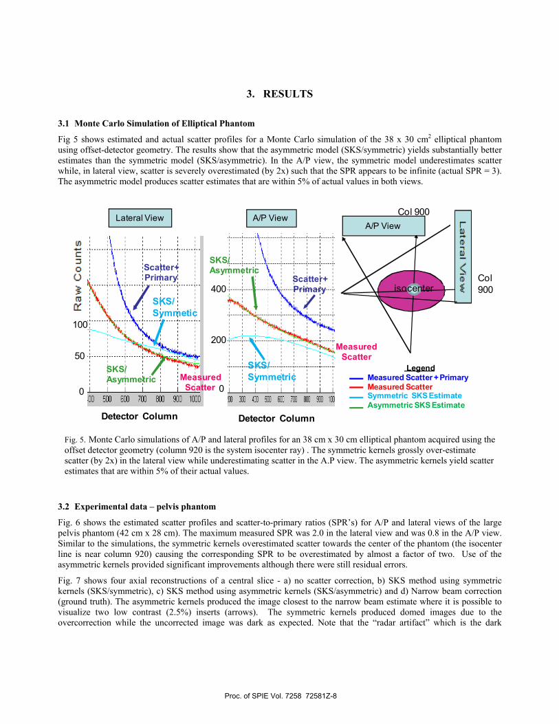
Fig 5 shows estimated and actual scatter profiles for a Monte Carlo simulation of the 38 x 30 cm2 elliptical phantom using offset-detector geometry. The results show that the asymmetric model (SKS/symmetric) yields substantially better estimates than the symmetric model (SKS/asymmetric). In the A/P view, the symmetric model underestimates scatter while, in lateral view, scatter is severely overestimated (by 2x) such that the SPR appears to be infinite (actual SPR = 3). The asymmetric model produces scatter estimates that are within 5% of actual values in both views.

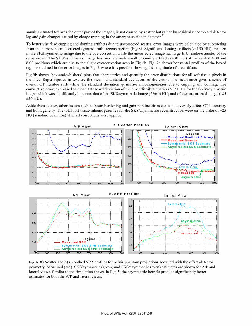
3.2 Experimental data – pelvis phantom

Fig. 6 shows the estimated scatter profiles and scatter-to-primary ratios (SPR’s) for A/P and lateral views of the large pelvis phantom (42 cm x 28 cm). The maximum measured SPR was 2.0 in the lateral view and was 0.8 in the A/P view. Similar to the simulations, the symmetric kernels overestimated scatter towards the center of the phantom (the isocenter line is near column 920) causing the corresponding SPR to be overestimated by almost a factor of two. Use of the asymmetric kernels provided significant improvements although there were still residual errors.

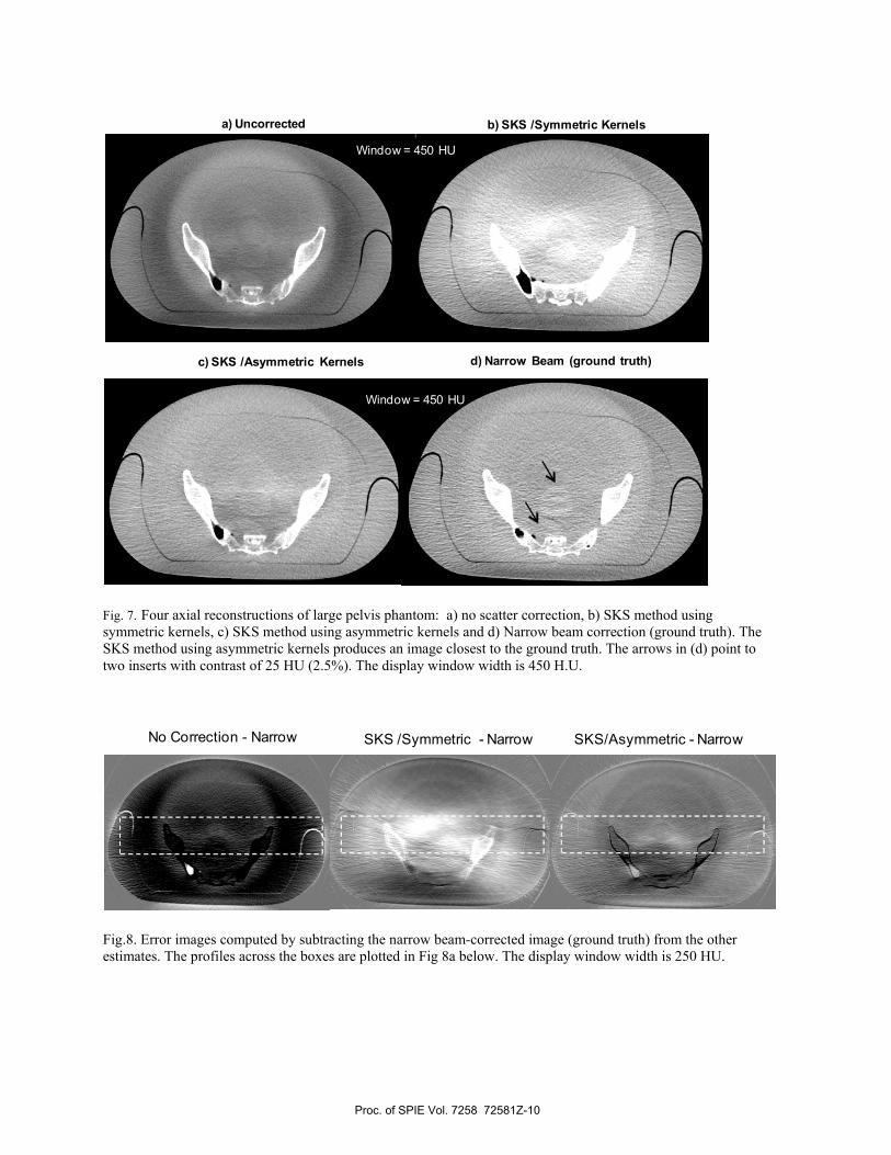
Fig. 7 shows four axial reconstructions of a central slice - a) no scatter correction, b) SKS method using symmetric kernels (SKS/symmetric), c) SKS method using asymmetric kernels (SKS/asymmetric) and d) Narrow beam correction (ground truth). The asymmetric kernels produced the image closest to the narrow beam estimate where it is possible to visualize two low contrast (2.5%) inserts (arrows). The symmetric kernels produced domed images due to the overcorrection while the uncorrected image was dark as expected. Note that the “radar artifact” which is the dark

Scatter+Primary

MeasuredScatter

Lateral View A/P ViewA/P View

Detector Column Detector Column

0

200

Scatter+Primary400

SKS/Asymmetric

SKS/SymmetricMeasured

Scatter

SKS/Symmetic

SKS/Asymmetric

50

0

100

LegendMeasured Scatter + PrimaryMeasured ScatterSymmetric SKS EstimateAsymmetric SKS Estimate

Col900

Col 900

isocenter

Fig. 5. Monte Carlo simulations of A/P and lateral profiles for an 38 cm x 30 cm elliptical phantom acquired using the offset detector geometry (column 920 is the system isocenter ray) . The symmetric kernels grossly over-estimate scatter (by 2x) in the lateral view while underestimating scatter in the A.P view. The asymmetric kernels yield scatter estimates that are within 5% of their actual values.

Proc. of SPIE Vol. 7258 72581Z-8

0.0

0.6

0.4

0.2

200 300 400 500 600 700 000 900 1000 400 500 600 700 800 900 1000

1100

1000

900

800

700

600

500

400

300

200

100

300 400 500 600 700 800 900 1000 400 500 600 700 600 900 1000

300

250

200

150

100

50

annulus situated towards the outer part of the images, is not caused by scatter but rather by residual uncorrected detector lag and gain changes caused by charge trapping in the amorphous silicon detector 21.

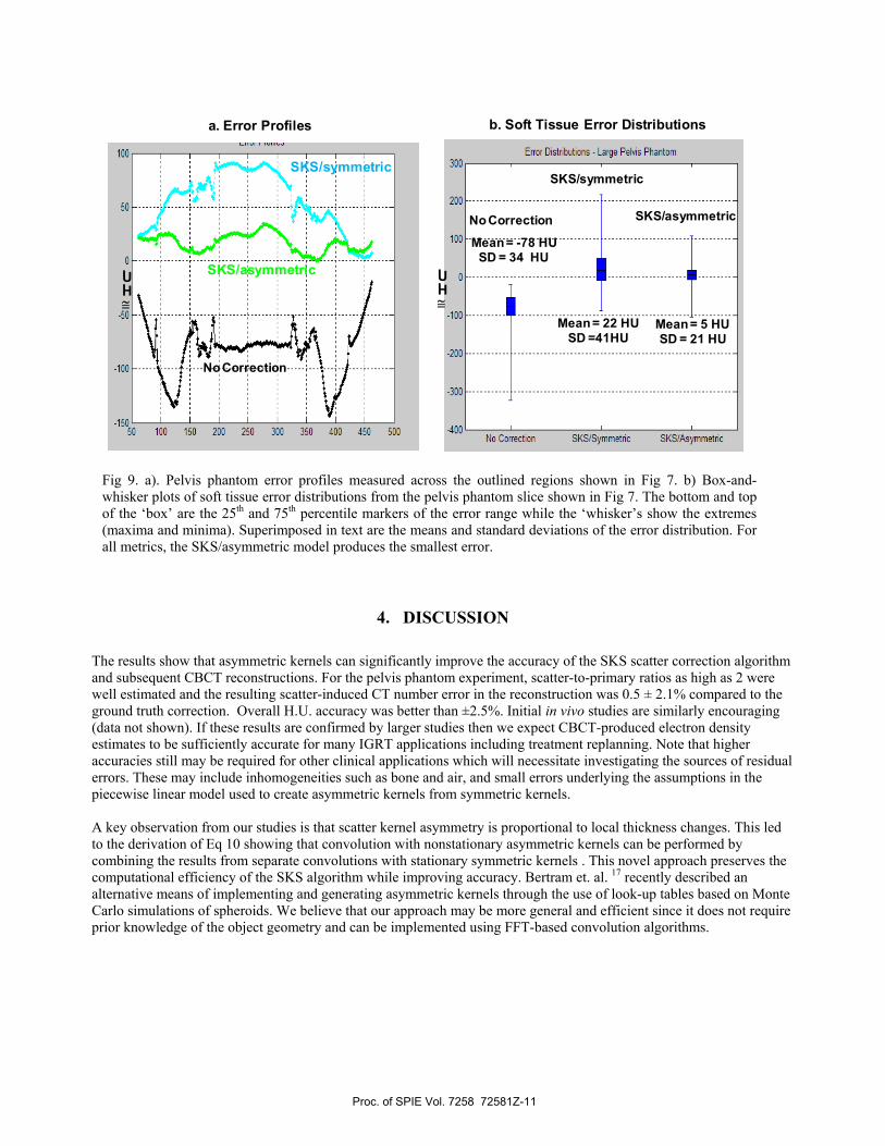
To better visualize cupping and doming artifacts due to uncorrected scatter, error images were calculated by subtracting from the narrow beam-corrected (ground truth) reconstruction (Fig 8). Significant doming artifacts (> 150 HU) are seen in the SKS/symmetric image due to the overcorrection while the uncorrected image has large H.U. underestimates of the same order. The SKS/asymmetric image has two relatively small blooming artifacts (~30 HU) at the central 4:00 and 8:00 positions which are due to the slight overcorrection seen in Fig 6b. Fig. 9a shows horizontal profiles of the boxed regions outlined in the error images in Fig. 8 where it is possible showing the magnitude of the artifacts.

Fig 9b shows ‘box-and-whiskers’ plots that characterize and quantify the error distributions for all soft tissue pixels in the slice. Superimposed in text are the means and standard deviations of the errors. The mean error gives a sense of overall CT number shift while the standard deviation quantifies inhomogeneities due to cupping and doming. The cumulative error, expressed as mean ±standard deviation of the error distributions was 5±21 HU for the SKS/asymmetric image which was significantly less than that of the SKS/symmetric image (28±46 HU) and of the uncorrected image (-85 ±36 HU).

Aside from scatter, other factors such as beam hardening and gain nonlinearities can also adversely affect CT# accuracy and homogeneity. The total soft tissue inhomogeneities for the SKS/asymmetric reconstruction were on the order of ±25 HU (standard deviation) after all corrections were applied.

a . S ca tter P ro fi les

b . S P R P ro fi les

asym m etric

sy m m et ric

m easu red

A /P V iew Late ra l V iew

La te ra l V iewA /P V iew

sym m etric

asym m etric m easu red

L eg en dM easu red Sc a t te r + Prim aryM easu red Sc a t te rS ym m e tric SK S Es t im ateA sym m etric S K S Es t im ate

L eg en dM easu re d S PRS ym m etric SK S SP R Es t im ateA sym m etric S K S SPR E s t im ate

Fig. 6. a) Scatter and b) smoothed SPR profiles for pelvis phantom projections acquired with the offset-detector geometry. Measured (red), SKS/symmetric (green) and SKS/asymmetric (cyan) estimates are shown for A/P and lateral views. Similar to the simulation shown in Fig. 5, the asymmetric kernels produce significantly better estimates for both the A/P and lateral views.

Proc. of SPIE Vol. 7258 72581Z-9

a) Uncorrected

c) SKS /Asymmetric Kernels

b) SKS /Symmetric Kernels

d) Narrow Beam (ground truth)

Window = 450 HUWindow = 450 HU

Window = 450 HU

Fig. 7. Four axial reconstructions of large pelvis phantom: a) no scatter correction, b) SKS method using symmetric kernels, c) SKS method using asymmetric kernels and d) Narrow beam correction (ground truth). The SKS method using asymmetric kernels produces an image closest to the ground truth. The arrows in (d) point to two inserts with contrast of 25 HU (2.5%). The display window width is 450 H.U.

No Correction - Narrow SKS /Symmetric - Narrow SKS/Asymmetric - Narrow

Fig.8. Error images computed by subtracting the narrow beam-corrected image (ground truth) from the other estimates. The profiles across the boxes are plotted in Fig 8a below. The display window width is 250 HU.

Proc. of SPIE Vol. 7258 72581Z-10

300

200

100

-100

-200

-300

-400

Error Distributions - Large Pelvis Phantom

rio Correctioio SKS/Symmetric SKS/Asymmetric

100

50

.50

-100

150] I I I I

50 100 150 200 250 300 360 100 450 E0O

4. DISCUSSION The results show that asymmetric kernels can significantly improve the accuracy of the SKS scatter correction algorithm and subsequent CBCT reconstructions. For the pelvis phantom experiment, scatter-to-primary ratios as high as 2 were well estimated and the resulting scatter-induced CT number error in the reconstruction was 0.5 ± 2.1% compared to the ground truth correction. Overall H.U. accuracy was better than ±2.5%. Initial in vivo studies are similarly encouraging (data not shown). If these results are confirmed by larger studies then we expect CBCT-produced electron density estimates to be sufficiently accurate for many IGRT applications including treatment replanning. Note that higher accuracies still may be required for other clinical applications which will necessitate investigating the sources of residual errors. These may include inhomogeneities such as bone and air, and small errors underlying the assumptions in the piecewise linear model used to create asymmetric kernels from symmetric kernels. A key observation from our studies is that scatter kernel asymmetry is proportional to local thickness changes. This led to the derivation of Eq 10 showing that convolution with nonstationary asymmetric kernels can be performed by combining the results from separate convolutions with stationary symmetric kernels . This novel approach preserves the computational efficiency of the SKS algorithm while improving accuracy. Bertram et. al. 17 recently described an alternative means of implementing and generating asymmetric kernels through the use of look-up tables based on Monte Carlo simulations of spheroids. We believe that our approach may be more general and efficient since it does not require prior knowledge of the object geometry and can be implemented using FFT-based convolution algorithms.

Mean = -78 HUSD = 34 HU

Mean = 22 HUSD =41HU

Mean = 5 HUSD = 21 HU

No Correction

SKS/symmetric

SKS/asymmetric

No Correction

SKS/asymmetric

SKS/symmetric

b. Soft Tissue Error Distributionsa. Error Profiles

≅ H.U.

≅ H.U.

Fig 9. a). Pelvis phantom error profiles measured across the outlined regions shown in Fig 7. b) Box-and-whisker plots of soft tissue error distributions from the pelvis phantom slice shown in Fig 7. The bottom and top of the ‘box’ are the 25th and 75th percentile markers of the error range while the ‘whisker’s show the extremes (maxima and minima). Superimposed in text are the means and standard deviations of the error distribution. For all metrics, the SKS/asymmetric model produces the smallest error.

Proc. of SPIE Vol. 7258 72581Z-11

5. REFERENCES

1. M. Oldham, D. Letourneau, L. Watt, G. Hugo, D. Yan, D. Lockman, L. H. Kim, P. Y. Chen, A. Martinez and J.

W. Wong, "Cone-beam-CT guided radiation therapy: A model for on-line application," Radiother Oncol 75, 271-278 (2005).

2. L. A. Dawson and D. A. Jaffray, "Advances in image-guided radiation therapy," J Clin Oncol 25, 938-946 (2007).

3. M. J. Daly, J. H. Siewerdsen, D. J. Moseley, D. A. Jaffray and J. C. Irish, "Intraoperative cone-beam CT for guidance of head and neck surgery: Assessment of dose and image quality using a C-arm prototype," Med Phys 33, 3767-3780 (2006).

4. J. H. Siewerdsen and D. A. Jaffray, "Cone-beam computed tomography with a flat-panel imager: magnitude and effects of x-ray scatter," Med Phys 28, 220-231 (2001).

5. L. A. Love and R. A. Kruger, "Scatter estimation for a digital radiographic system using convolution filtering," Med Phys 14, 178-185 (1987).

6. J. A. Seibert and J. M. Boone, "X-ray scatter removal by deconvolution," Med Phys 15, 567-575 (1988). 7. J. Wiegert, M. Bertram, G. Rose and T. Aach, "Model-based scatter correction for cone-beam computed

tomography," Proc. SPIE 5745, 271-282 (2005). 8. J. S. Maltz, B. Gangadharan, M. Vidal, A. Paidi, S. Bose, B. A. Faddegon, M. Aubin, O. Morin, J. Pouliot, Z.

Zheng, M. M. Svatos and A. R. Bani-Hashemi, "Focused beam-stop array for the measurement of scatter in megavoltage portal and cone beam CT imaging," Med Phys 35, 2452-2462 (2008).

9. L. Zhu, N. R. Bennett and R. Fahrig, "Scatter correction method for X-ray CT using primary modulation: theory and preliminary results," IEEE Trans Med Imaging 25, 1573-1587 (2006).

10. R. Ning, X. Tang and D. Conover, "X-ray scatter correction algorithm for cone beam CT imaging," Med Phys 31, 1195-1202 (2004).

11. G. Virshup, R. Suri and J. Star-Lack, "Scatter Characterization in Cone-Beam CT Systems with Offset Flat Panel Imagers," Med Phys 33, 2288 (2006).

12. J. H. Siewerdsen, M. J. Daly, B. Bakhtiar, D. J. Moseley, S. Richard, H. Keller and D. A. Jaffray, "A simple, direct method for x-ray scatter estimation and correction in digital radiography and cone-beam CT," Med Phys 33, 187-197 (2006).

13. B. Ohnesorge, T. Flohr and K. Klingenbeck-Regn, "Efficient object scatter correction algorithm for third and fourth generation CT scanners," Eur Radiol 9, 563-569 (1999).

14. H. Li, R. Mohan and X. R. Zhu, "Scatter kernel estimation with an edge-spread function method for cone-beam computed tomography imaging," Phys Med Biol 53, 6729-6748 (2008).

15. J. S. Maltz, B. Gangadharan, S. Bose, D. H. Hristov, B. A. Faddegon, A. Paidi and A. R. Bani-Hashemi, "Algorithm for X-ray scatter, beam-hardening, and beam profile correction in diagnostic (kilovoltage) and treatment (megavoltage) cone beam CT," IEEE Trans Med Imaging 27, 1791-1810 (2008).

16. S. F. Petit, W. J. van Elmpt, S. M. Nijsten, P. Lambin and A. L. Dekker, "Calibration of megavoltage cone-beam CT for radiotherapy dose calculations: correction of cupping artifacts and conversion of CT numbers to electron density," Med Phys 35, 849-865 (2008).

17. M. Bertram, S. Hohmann and J. Weiger, "Scatter Correction for Flat Detector Cone-Beam CT Based on Simulated Sphere Models," Med Phys 34, 2342 (2007).

18. K. Cranley, B. J. Gilmore, G. W. A. Fogarty and L. Desponds, Catalogue of diagnostic x-ray spectra and other data (Rep 78). (The Institute of Physics and Engineering in Medicine (IPEM), York, U.K., 1997).

19. M. Zellerhoff, B. Scholz, E. P. Ruhrnschopf and T. Brunner, "Low contrast 3D- reconstruction from C-arm data," Proc. SPIE 5745, 646-644 (2005).

20. G. J. Day and D. R. Dance, "X-ray transmission formula for antiscatter grids," Phys Med Biol 28, 1429-1433 (1983).

21. J. Starman, G. Virshup, J. Star-Lack and R. Fahrig, "Investigation into the cause of a new artifact in Cone Beam CT resonstructions on a flat panel imager," Med Phys 33, 2288 (2006).

22. A. C. Kak and M. Slaney, Principles of Computerized Tomographic Imaging. (IEEE Press, New York, 1988). 23. J. Star-Lack, J. Starman, P. Munro, A. Jeung, H. Richters, H. Mostafavi and J. Pavkovich, "A fast variable-

intensity ring suppression algorithm," Med Phys 33, 1997 (2006).

Proc. of SPIE Vol. 7258 72581Z-12