hidden in the layers interpretation of neural networks
TRANSCRIPT
HIDDEN IN THE LAYERSInterpretation of Neural Networks for
Natural Language Processing
David Mareček, Jindřich Libovický, Tomáš Musil, Rudolf Rosa,Tomasz Limisiewicz
STUDIES IN COMPUTATIONALAND THEORETICAL LINGUISTICS
David Mareček, Jindřich Libovický, Tomáš Musil, Rudolf Rosa,Tomasz Limisiewicz
HIDDEN IN THE LAYERSInterpretation of Neural Networks for Natural LanguageProcessing
Published by the Institute of Formal and Applied Linguisticsas the 20th publication in the seriesStudies in Computational and Theoretical Linguistics.
Editor-in-chief: Jan Hajič
Editorial board: Nicoletta Calzolari, Mirjam Fried, Eva Hajičová,Petr Karlík, Joakim Nivre, Jarmila Panevová,Patrice Pognan, Pavel Straňák, and Hans Uszkoreit
Reviewers: Pavel Král, University of West BohemiaPetya Osenova, Bulgarian Academy of Sciences
This book has been printed with the support of the grant 18-02196S “Linguistic StructureRepresentation in Neural Networks” of the Czech Science Foundation and of the institutionalfunds of Charles University.Printed by Printo, spol. s r. o.
Copyright © Institute of Formal and Applied Linguistics, 2020
ISBN 978-80-88132-10-3
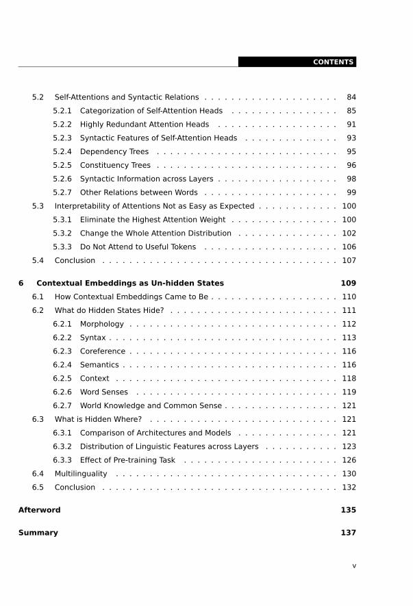
Contents
Preface 1
Introduction 3
1 Deep Learning 51.1 Fundamentals of Deep Learning . . . . . . . . . . . . . . . . . . . . . . . . 5
1.1.1 What is Machine Learning? . . . . . . . . . . . . . . . . . . . . . . . 51.1.2 Perceptron Algorithm . . . . . . . . . . . . . . . . . . . . . . . . . . 61.1.3 Multi-Layer Networks . . . . . . . . . . . . . . . . . . . . . . . . . . 71.1.4 Error Back-Propagation . . . . . . . . . . . . . . . . . . . . . . . . . 91.1.5 Representation Learning . . . . . . . . . . . . . . . . . . . . . . . . 10
1.2 Deep Learning Techniques in Computer Vision . . . . . . . . . . . . . . . . 101.2.1 Convolutional Networks . . . . . . . . . . . . . . . . . . . . . . . . 101.2.2 AlexNet and Image Classification on the ImageNet Challenge . . . . 121.2.3 Convolutional Networks after AlexNet . . . . . . . . . . . . . . . . . 14
1.3 Deep Learning Techniques in Natural Language Processing . . . . . . . . . 161.3.1 Word Embeddings . . . . . . . . . . . . . . . . . . . . . . . . . . . 171.3.2 Architectures for Sequence Processing . . . . . . . . . . . . . . . . 201.3.3 Generating Output . . . . . . . . . . . . . . . . . . . . . . . . . . . 27
1.4 Conclusion . . . . . . . . . . . . . . . . . . . . . . . . . . . . . . . . . . . 34
2 Notable Models 352.1 Word2Vec and the Others . . . . . . . . . . . . . . . . . . . . . . . . . . . 352.2 Attention and Machine Translation with Recurrent Neural Networks . . . . . 362.3 Transformer for Machine Translation . . . . . . . . . . . . . . . . . . . . . . 372.4 CoVe: Contextual Embeddings are Born . . . . . . . . . . . . . . . . . . . 382.5 ELMo: Sesame Street Begins . . . . . . . . . . . . . . . . . . . . . . . . . 39
iii
CONTENTS
2.6 BERT: Pre-trained Transformers . . . . . . . . . . . . . . . . . . . . . . . . 402.7 GPT and GPT-2 . . . . . . . . . . . . . . . . . . . . . . . . . . . . . . . . . 432.8 Conclusion . . . . . . . . . . . . . . . . . . . . . . . . . . . . . . . . . . . 44
3 Interpretation of Neural Networks 453.1 Supervised Methods: Probing . . . . . . . . . . . . . . . . . . . . . . . . . 473.2 Unsupervised Methods: Clustering and Component Analysis . . . . . . . . 473.3 Network Layers and Linguistic Units . . . . . . . . . . . . . . . . . . . . . . 48
3.3.1 Words versus States . . . . . . . . . . . . . . . . . . . . . . . . . . 493.3.2 Words versus Subwords . . . . . . . . . . . . . . . . . . . . . . . . 51
3.4 Conclusion . . . . . . . . . . . . . . . . . . . . . . . . . . . . . . . . . . . 52
4 Emblems of the Embeddings 554.1 Word Analogies . . . . . . . . . . . . . . . . . . . . . . . . . . . . . . . . . 55
4.1.1 Word2Vec and Semantic Arithmetic . . . . . . . . . . . . . . . . . . 554.1.2 Glove Word Analogies . . . . . . . . . . . . . . . . . . . . . . . . . 564.1.3 FastText Subword Correspondence . . . . . . . . . . . . . . . . . . . 59
4.2 Positioning Words . . . . . . . . . . . . . . . . . . . . . . . . . . . . . . . 594.3 Embedding Bands . . . . . . . . . . . . . . . . . . . . . . . . . . . . . . . 634.4 Visualising Word Embeddings with T-SNE . . . . . . . . . . . . . . . . . . . 634.5 Emoji Embeddings . . . . . . . . . . . . . . . . . . . . . . . . . . . . . . . 634.6 Principal Component Analysis . . . . . . . . . . . . . . . . . . . . . . . . . 66
4.6.1 Visualisation . . . . . . . . . . . . . . . . . . . . . . . . . . . . . . . 664.6.2 Correlations with Principal Components . . . . . . . . . . . . . . . . 664.6.3 Histograms of Principal Components . . . . . . . . . . . . . . . . . 694.6.4 Sentiment Analysis . . . . . . . . . . . . . . . . . . . . . . . . . . . 69
4.7 Independent Component Analysis . . . . . . . . . . . . . . . . . . . . . . . 724.8 Word Derivations . . . . . . . . . . . . . . . . . . . . . . . . . . . . . . . . 734.9 Mapping Embedding Spaces . . . . . . . . . . . . . . . . . . . . . . . . . . 754.10 Debiasing: Interpretation as Manipulation . . . . . . . . . . . . . . . . . . 764.11 Conclusion . . . . . . . . . . . . . . . . . . . . . . . . . . . . . . . . . . . 77
5 May I Have Your Attention? 795.1 Cross-Lingual Attentions and Word Alignment . . . . . . . . . . . . . . . . 80
iv
CONTENTS
5.2 Self-Attentions and Syntactic Relations . . . . . . . . . . . . . . . . . . . . 845.2.1 Categorization of Self-Attention Heads . . . . . . . . . . . . . . . . 855.2.2 Highly Redundant Attention Heads . . . . . . . . . . . . . . . . . . 915.2.3 Syntactic Features of Self-Attention Heads . . . . . . . . . . . . . . 935.2.4 Dependency Trees . . . . . . . . . . . . . . . . . . . . . . . . . . . 955.2.5 Constituency Trees . . . . . . . . . . . . . . . . . . . . . . . . . . . 965.2.6 Syntactic Information across Layers . . . . . . . . . . . . . . . . . . 985.2.7 Other Relations between Words . . . . . . . . . . . . . . . . . . . . 99
5.3 Interpretability of Attentions Not as Easy as Expected . . . . . . . . . . . . 1005.3.1 Eliminate the Highest Attention Weight . . . . . . . . . . . . . . . . 1005.3.2 Change the Whole Attention Distribution . . . . . . . . . . . . . . . 1025.3.3 Do Not Attend to Useful Tokens . . . . . . . . . . . . . . . . . . . . 106
5.4 Conclusion . . . . . . . . . . . . . . . . . . . . . . . . . . . . . . . . . . . 107
6 Contextual Embeddings as Un-hidden States 1096.1 How Contextual Embeddings Came to Be . . . . . . . . . . . . . . . . . . . 1106.2 What do Hidden States Hide? . . . . . . . . . . . . . . . . . . . . . . . . . 111
6.2.1 Morphology . . . . . . . . . . . . . . . . . . . . . . . . . . . . . . . 1126.2.2 Syntax . . . . . . . . . . . . . . . . . . . . . . . . . . . . . . . . . . 1136.2.3 Coreference . . . . . . . . . . . . . . . . . . . . . . . . . . . . . . . 1166.2.4 Semantics . . . . . . . . . . . . . . . . . . . . . . . . . . . . . . . . 1166.2.5 Context . . . . . . . . . . . . . . . . . . . . . . . . . . . . . . . . . 1186.2.6 Word Senses . . . . . . . . . . . . . . . . . . . . . . . . . . . . . . 1196.2.7 World Knowledge and Common Sense . . . . . . . . . . . . . . . . . 121
6.3 What is Hidden Where? . . . . . . . . . . . . . . . . . . . . . . . . . . . . 1216.3.1 Comparison of Architectures and Models . . . . . . . . . . . . . . . 1216.3.2 Distribution of Linguistic Features across Layers . . . . . . . . . . . 1236.3.3 Effect of Pre-training Task . . . . . . . . . . . . . . . . . . . . . . . 126
6.4 Multilinguality . . . . . . . . . . . . . . . . . . . . . . . . . . . . . . . . . 1306.5 Conclusion . . . . . . . . . . . . . . . . . . . . . . . . . . . . . . . . . . . 132
Afterword 135
Summary 137
v

CONTENTS
List of Figures 139
List of Tables 141
List of Abbreviations 144
Bibliography 145
Index 167
vi
Acknowledgement
This book is a result of a three-year research project conducted at the Institute of For-mal and Applied Linguistics, Faculty of Mathematics and Physics, Charles University,funded by the Czech Science Foundation (GAČR), project no. 18-02196S “LinguisticStructure Representation in Neural Networks.” We would like to thank our two re-viewers, Petya Osenova and Pavel Král, for their suggestions and comments.
vii

Preface
In recent years, deep neural networks dominated the area of Natural Language Pro-cessing (NLP). For a while, it might almost seem that all tasks became purely machinelearning problems, and the language itself became secondary. The primary problemsare technical: getting more and more data and making the learning algorithms moreefficient. Deep learning methods allow us to do machine translation, automatic textsummarization, sentiment analysis, question answering, and many other tasks in aquality that was hardly imaginable ten years ago. This unprecedented progress inour ability to solve NLP tasks has its downsides too. End-to-end-trained models areblack boxes that are very hard to interpret, and the model can manifest unintendedbehavior that can range from seemingly stupid and unexplainable errors to hiddengender or racial bias.
One of the main concerns of linguistics is to conceptualize language in such a waythat allows us to name and discuss complex language phenomena that would other-wise be difficult to grasp or to teach a non-native speaker. Traditionally, NLP tookover these conceptualizations and used them to represent language for solving prac-tical tasks. Over time, it appeared that not all concepts from linguistics are neces-sarily useful for NLP. With deep neural networks, almost all linguistic assumptionswere discarded. Sentences are treated merely as sequences of words that get split intosmaller subword units based on simple statistical heuristics. Dozens of hidden layersof neural networks learn presumably a more and more abstract and more informativerepresentation of the input until they ultimately provide the output without tellingus what the representations in between mean.
This situation in NLP puts us into a unique situation. We have machine learningmodels that can do tasks as skillfully as never before and develop their own languagerepresentation. This calls for an inspection to what extent the linguistic conceptualiza-tions are consistent with what the models learn. Do neural networks use morphologyand syntax the way people do when they talk about language? Or do they developtheir own better way? What is hidden in the layers?
1

Introduction
In this book, we try to peek into the black box of trained neural models, and to see howthe emergent representations correspond to traditional linguistic abstractions. Wemostly deal with large pre-trained language models and machine translation models.
In Chapter 1, we introduce the reader into the world of deep learning and its ap-plications in Natural Language Processing (NLP). Readers who are experts in deeplearning can skip this chapter. We hope others will find the introductory chapteruseful even beyond the scope of this book.
In Chapter 2, we show how the deep learning concepts are used in several notablemodels, including Word2Vec, Transformer and BERT. The subsequent chapters dealwith analyzing the models introduced in this chapter.
In Chapter 3, we look at the problem of interpreting trained neural network mod-els in general. We also outline the two approaches that we focus on in this book:supervised probing, and unsupervised clustering and visualisation.
In Chapter 4, we discuss the interpretation of Word2Vec and other word embed-dings. We show various methods for embedding space visualisation, componentanalysis and embedding space transformations for interpretation.
In Chapter 5, we analyze attention and self-attention mechanisms, in which we canobserve weighted links between representations of individual tokens. We particularlyfocus on syntax, summarizing the amount of syntax in the attentions across the layersof several NLP models.
In Chapter 6, we look at contextual word embeddings and the linguistically inter-pretable features they capture. We try to link the linguistic features to various levelsof linguistic abstraction, going from morphology over syntax to semantics.
3

1
Deep Learning
Before talking about the interpretation of neural networks in Natural Language Pro-cessing (NLP), we should explain what deep learning is and how it is used in NLP. Inthis chapter, we summarize the basic concepts of deep learning, briefly sketch the his-tory, and discuss details of neural architectures that we talk about in the later chaptersof the book.
1.1 Fundamentals of Deep Learning
Deep learning is a branch of Machine Learning (ML), and like many scientific concepts,it does not have an exact definition everyone would agree upon. By deep learning,we usually mean ML with neural networks that have many layers (Goodfellow et al.,2016). By ‘many,’ people usually mean more than experts before 2006 used to believewas numerically feasible (Hinton and Salakhutdinov, 2006; Bengio et al., 2007). Inpractice, the networks have dozens of layers.
The first method that allowed using multiple layers was unsupervised layer-wisepre-training (Bengio et al., 2007) that demonstrated the potential of deeper neuralnetworks. These methods were followed by innovations allowing training the modelsend-to-end by error back-propagation only (Srivastava et al., 2014; Nair and Hinton,2010; Ioffe and Szegedy, 2015; Ba et al., 2016; He et al., 2016) without any pre-training,which started the boom of deep learning methods after 2014.
1.1.1 What is Machine Learning?
Neural networks and other ML models are trained to fit training data, while still gen-eralizing for unseen data, i.e., instances that were not in the training set. For example,we train a machine translation system on pairs of sentences that are translations ofeach other, but of course, the goal is to have a model that can reliably translate anysentence, not only examples from the training data.
During training, we try to minimize the error the model makes on the training data.However, minimizing the training error does not guarantee that the model works wellfor data that are not in the training set. In other words, even with a low trainingerror, the model can overfit, i.e., perform well on the training data without generalizingfor data instances not encountered during training. To ensure that the model canmake correct predictions on data instances that were not used for training, we use
5
1 DEEP LEARNING
..
activation
.
function
.
input x
.
weights w
.
output
.∑x⊤w > 0?. y.xi .
·wi
.
x1
.
·w1
.
x2
.
·w2
.
...
.
...
.
xn
.
·wn
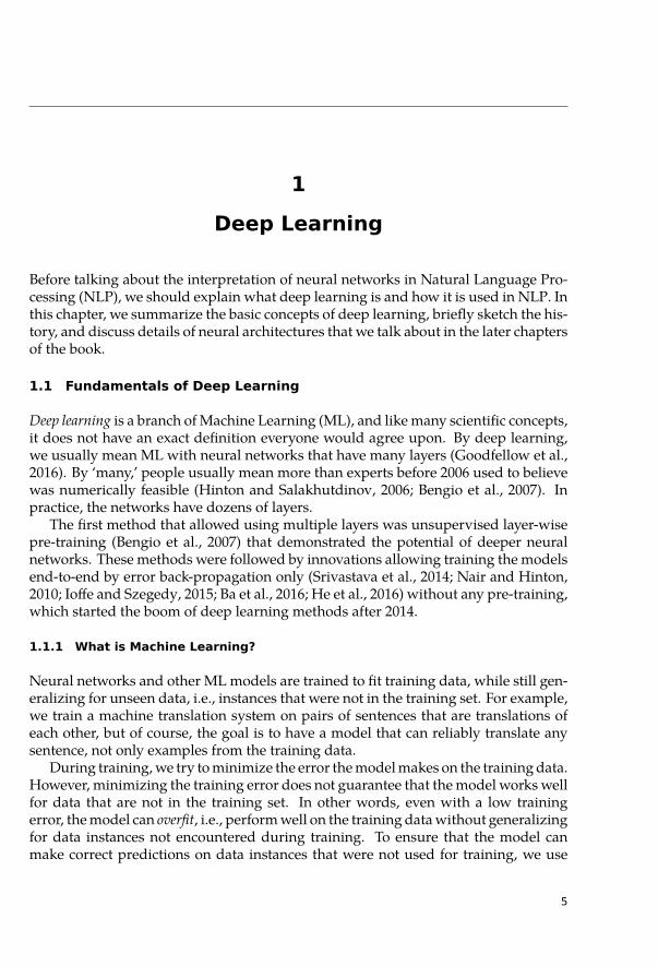
Figure 1.1: Illustration of a single artificial neuron with inputs x = (x1, . . . , xn) andweights w = (w1, . . . , wn).
another dataset, usually called the validation set that is only used for estimating theperformance of the model on unseen data.
Deep learning models are particularly prone to overfitting. With millions of train-able parameters, they can easily memorize entire training sets. We already insinuatedthat the crucial part of the deep learning story is techniques that allow training biggermodels with many layers. Bigger models have a bigger capacity to learn more com-plicated tasks. Large models are, on the other hand, more prone to overfitting. TheHistory of deep learning is a somewhat story of innovations that allow training largermodels and innovations that prevent large models from overfitting.
1.1.2 Perceptron Algorithm
Deep learning originates in studying artificial neural networks (Goodfellow et al.,2016, p. 12). Artificial neural networks are inspired by a simplistic model of a bio-logical neuron (McCulloch and Pitts, 1943; Rosenblatt, 1958; Widrow, 1960). In themodel, the neuron collects information on its dendrites. Based on that, it sends a sig-nal on the axon, its single output. Formally, we say that the artificial neuron has aninput, a vector x = (x1, . . . , xn) ∈ Rn of real numbers. For each input componentxi, there is a weight wi ∈ R corresponding to the importance of the input compo-nent. The weighted sum of the input is called the activation. We get the neuron outputby applying the activation function on the activation. In the simplest case, the acti-vation function is the signum function. More activation functions are discussed inSection 1.2. The model is illustrated in Figure 1.1.
6
1.1 FUNDAMENTALS OF DEEP LEARNING
The first successful experiments with such a model date back to the 1950s whenthe geometrically motivated perceptron algorithm (Rosenblatt, 1958) for learning themodel weights was first introduced. The model is used for the classification of theinputs into two distinct classes. The inputs are interpreted as points in a multi-dimen-sional vector space. The learning algorithm searches for a hyperplane separating oneclass of the inputs from the other. The trained weights are interpreted as a normalvector of the hyperplane. The algorithm iterates over the training examples: If anexample is misclassified, it rotates the hyperplane towards the misclassified exampleby subtracting the input from the weight vector. This simple algorithm is guaranteedto converge to a separating hyperplane if it exists (Novikoff, 1962). The linear-algebraicintuition developed for the perceptron algorithm is also important for the currentneural networks where inputs of network layers are also interpreted as points in multi-dimensional space.
During the following 60 years of ML and Artificial Intelligence (AI) development,neural networks fell out of the main research interest, especially during the so-calledAI winters in the 1970s and 1990s (Crevier, 1993, p. 203).
In the rest of the chapter, we do not closely follow the history of neural networksbut only discuss the innovations that seem to be the most important from the currentperspective. Techniques that are particularly useful for NLP are then discussed inSection 1.3. For a comprehensive overview of the history of neural network research,we refer the reader to a survey by Schmidhuber (2014).
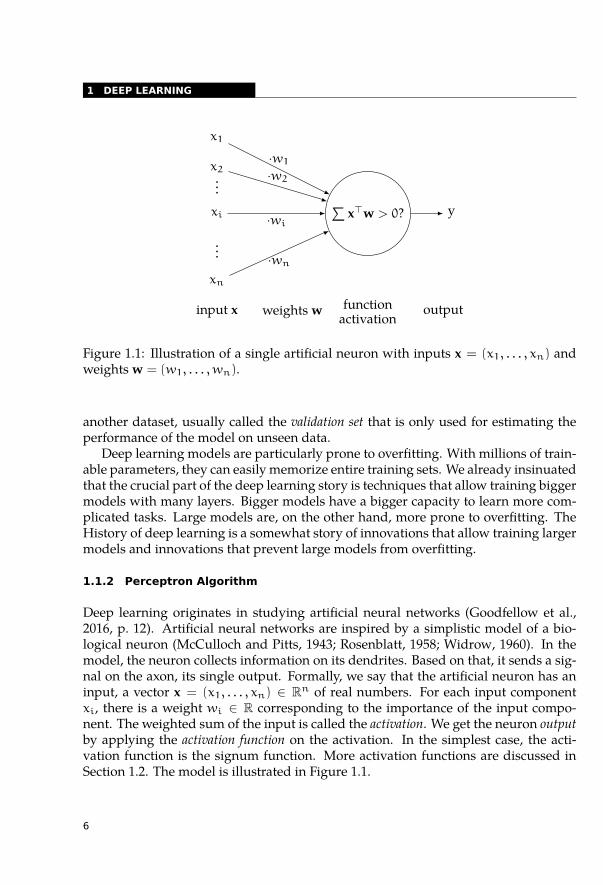
1.1.3 Multi-Layer Networks
The geometrically motivated perceptron learning algorithm cannot be efficiently gen-eralized to networks with a more complicated structure of interconnected neurons.With more a complex network structure, we no longer interpret the learning as a ge-ometric problem of finding a separating hyperplane. Instead, we view the networkas a parameterized continuous function. The goal of the learning is to optimize theparameter values with respect to a continuous error function, usually called the lossfunction. The loss function is usually some kind of continuous dissimilarity measurebetween the network output from the desired output.
During training, we treat the network as a function of its parameters, given a train-ing dataset that is considered constant at one training step. This allows computinggradients of the network parameters with respect to the loss function and updatingthe parameters accordingly. The training uses a simple property of derivative that itdetermines the direction in which a continuous function increases or decreases. Thisinformation can be used to shift the parameters in such a way that the loss functiondecreases. Note that each gradient is computed independently, and we only computethe derivatives at a particular point, so we can only shift the parameters by a small stepin the direction of the derivatives. Furthermore, with a large training set, we are ableto process only small batches of training data, which introduces stochasticity in the
7
1 DEEP LEARNING
..........inputs
.....................hidden layers
.....output
Figure 1.2: Multi-layer perceptron with two fully connected hidden layers.
training process, i.e., add random noise that increases the robustness of the training.The training algorithm is called stochastic gradient descent.
At inference time, the parameters are fixed, and the network is treated as a functionof its inputs with constant parameters.
The original perceptron used the signum function as the activation function. Inorder to make the function defined by the network differentiable, the signum func-tion was often replaced by sigmoid function or hyperbolic tangent, yielding valuesbetween -1 and 1.
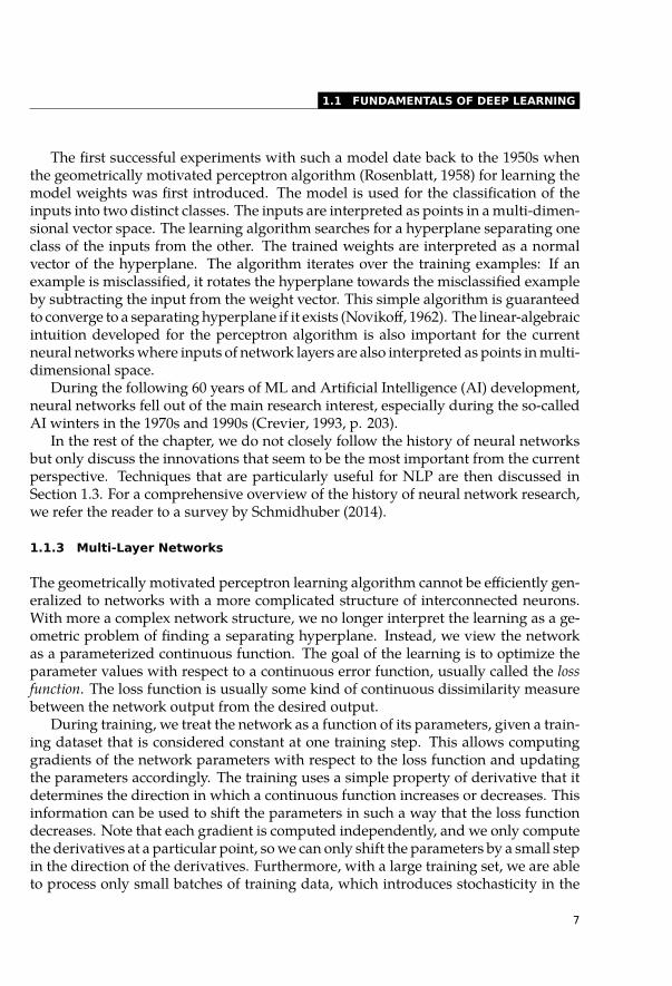
For the sake of efficiency, the neurons in artificial neural networks are almost al-ways organized in layers. This allows us to re-formulate the computation as a matrixmultiplication (Fahlman and Hinton, 1987). Layers implemented by matrix multi-plication are called fully connected or dense layers. Let hi = (h0
i , . . . , hni ) ∈ Rn be
the output of the i-th layer of the network and the input of the (i + 1)-th layer. LetA : R → R be the activation function. The value of the k-th neuron in the (i + 1)-thlayer of dimension m is
hki+1 = A
(n∑
l=0
hli ·w
(l,k)i + b
(k)i
)(1.1)
which is, in fact, the definition of matrix multiplication. It thus holds:
hi+1 = A (hiWi + bi) (1.2)
where Wi ∈ Rn×m is a parameter matrix, and bi ∈ Rm is a bias vector.Not only did this make the computation efficient, but it also led to a reconceptu-
alization of the network architectures. Current literature no longer talks about singleneurons, but almost always about network layers. This reconceptualization then al-lows innovations like attention mechanism (Bahdanau et al., 2014), residual connec-
8
1.1 FUNDAMENTALS OF DEEP LEARNING
..x.
W
.×
.
b
.+
.σ
.
h
.
forward graph
.
backward graph
.loss L
.
y∗
.
o
.σ ′
.
o ′
.+
.
b ′
.
h ′
.×
. x ′.
W ′
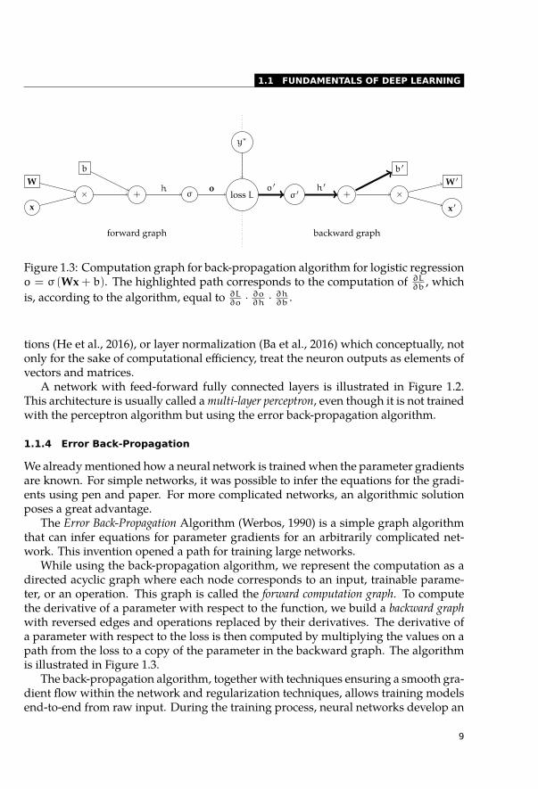
Figure 1.3: Computation graph for back-propagation algorithm for logistic regressiono = σ (Wx + b). The highlighted path corresponds to the computation of ∂L
∂b, which
is, according to the algorithm, equal to ∂L∂o
· ∂o∂h
· ∂h∂b
.
tions (He et al., 2016), or layer normalization (Ba et al., 2016) which conceptually, notonly for the sake of computational efficiency, treat the neuron outputs as elements ofvectors and matrices.
A network with feed-forward fully connected layers is illustrated in Figure 1.2.This architecture is usually called a multi-layer perceptron, even though it is not trainedwith the perceptron algorithm but using the error back-propagation algorithm.
1.1.4 Error Back-Propagation
We already mentioned how a neural network is trained when the parameter gradientsare known. For simple networks, it was possible to infer the equations for the gradi-ents using pen and paper. For more complicated networks, an algorithmic solutionposes a great advantage.
The Error Back-Propagation Algorithm (Werbos, 1990) is a simple graph algorithmthat can infer equations for parameter gradients for an arbitrarily complicated net-work. This invention opened a path for training large networks.
While using the back-propagation algorithm, we represent the computation as adirected acyclic graph where each node corresponds to an input, trainable parame-ter, or an operation. This graph is called the forward computation graph. To computethe derivative of a parameter with respect to the function, we build a backward graphwith reversed edges and operations replaced by their derivatives. The derivative ofa parameter with respect to the loss is then computed by multiplying the values on apath from the loss to a copy of the parameter in the backward graph. The algorithmis illustrated in Figure 1.3.
The back-propagation algorithm, together with techniques ensuring a smooth gra-dient flow within the network and regularization techniques, allows training modelsend-to-end from raw input. During the training process, neural networks develop an
9
1 DEEP LEARNING
input representation such that the task that we train the model for becomes easy tosolve (Bengio et al., 2003; LeCun et al., 2015). However, it took more than ten yearsbefore this remarkable property of the learning algorithm attracted the attention ofthe researchers.
1.1.5 Representation Learning
Deep learning dramatically changes how data is represented. In NLP, the text used tobe tokenized and enriched by automatic annotations that include part-of-speech tags,syntactic relations between words or entity detection. This representation was usu-ally used to get meaningful features for a ML model. In statistical Machine Transla-tion (MT), words are represented by monolingual and bilingual co-occurrence tables,which are used for probability estimations within the models. In deep learning mod-els, the text is represented with tensors of continuous values that are not explicitlyhand-designed but implicitly inferred during model optimization.
This is often considered to be one of the most important properties of neural net-works. Goodfellow et al. (2016, p. 5) even consider the representation learning abilityto be the feature that distinguishes deep learning from the previous ML techniques.In both Computer Vision (CV) and NLP models, consecutive layers learn more con-textualized and presumably more abstract representation of the input. As we willdiscuss in the following sections, the representations learned by the networks are of-ten general and can often be reused for solving different tasks than they were trainedfor.
1.2 Deep Learning Techniques in Computer Vision
Although this book is primarily about neural networks in NLP, the story of deeplearning would not be complete if we did not mention innovations that come fromCV. The success of deep neural networks in CV tasks started the increased interest inneural networks, and it is likely that without the progress made in CV, deep learningwould not be as successful in NLP either.
Images are usually represented as a table of three-channel (RGB: red, green, blue)pixels, i.e., a three-dimensional tensor. Note that if we disregard the exact number ofchannels, this is the same form as the input and output of most network layers. Thisallows us to treat the input in the same way as all other layers in the network.
1.2.1 Convolutional Networks
The main tool used in CV are convolutional networks (LeCun et al., 1998). The maincomponents used in Convolutional Neural Networks (CNNs) are convolutional andmax-pooling layers.
Two-dimensional convolutions can be explained as applying a sliding windowprojection over a 3D input tensor and measuring the similarity between the input
10
1.2 DEEP LEARNING TECHNIQUES IN COMPUTER VISION
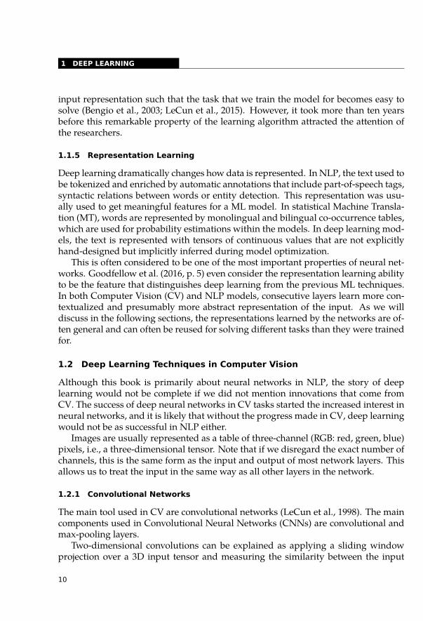
RGB image 9× 9× 3
convolutional map 4× 4× 6
stride 2
filter size 6kernel size
3
Figure 1.4: Illustration of a 2D convolution over a 9×9 RGB image with stride 2, kernelsize 3 and number of filters 6.
window and filters that are the learned parameters of the models. The two main hy-perparameters of a convolutional layer are the number of filters and the window size.Another attribute of the convolution is the stride which is the size of the step by whichthe window moves. The resulting feature map is roughly stride-times smaller in thefirst two dimensions (weight and height). A 2D convolution over an RGB image isillustrated in Figure 1.4.
Max-pooling is a dimensionality reduction technique that is used to decrease infor-mation redundancy during image processing. Similarly to convolutions, it proceedsas a sliding window and reduces each window into a single vector by taking the maxi-mum values from the window. Alternatively, average-pooling can be used that yieldsthe average of the window instead of the maximum.
Convolution is usually interpreted as a latent feature extraction over the input ten-sor where the filters correspond to the latent features. Max-pooling can be interpretedas a soft existential quantifier applied over the window, i.e., the result of max-poolingsays whether and how much the latent features are present in the given region of theimage.
Visualizations of trained convolution filters show that the representation in thenetwork is often similar to features used in classical CV methods such as edge detec-tion (Erhan et al., 2009). It also appears that with the growing number of layers, more
11
1 DEEP LEARNING
..0.00
.
0.05
.
0.10
.
0.15
.
0.20
.
0.25
.
0.30
. 2011. 2012. 2013. 2014. 2015. 2016. 2017.
5-be
ster
rorr
ate
.
err=.257
.
err=.153
.
err=.115
.
err=.074
.
err=.035
.
err=.029
.
err=.022
.
Sánchez and Perronnin (2011)
.
Krizhevsky et al. (2012)
..
Simonyan and Zisserman (2014)
.
He et al. (2016)
..
Hu et al. (2017)
.
AlexNet
.
VGG19
.
ResNet
.
Squeeze and Excitation
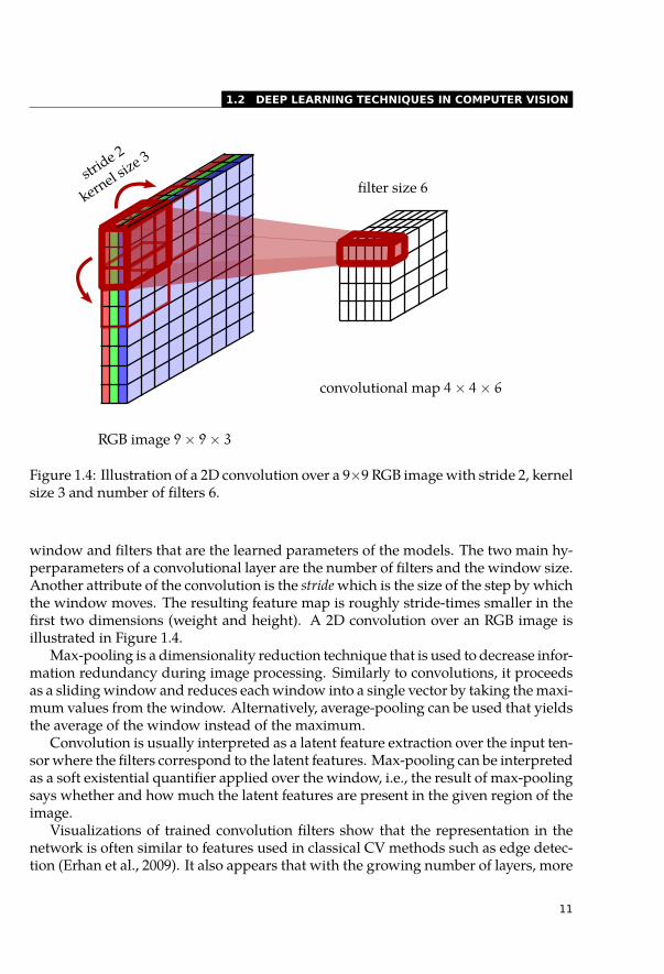
Figure 1.5: Development of performance in ImageNet image classification task be-tween 2011 and 2017. The figures are taken from the official website of the challenge.Columns without citations correspond to submissions that did not provide a citation.
abstract representations are learned (Mahendran and Vedaldi, 2015; Olah et al., 2017).Although, in theory, shallow networks with a single hidden layer have the same ca-pabilities (Hornik, 1991), in practice, well-trained deeper networks usually performbetter (Goodfellow et al., 2016, p. 192–194).
CNNs operating in only one dimension are also used in NLP. Deep one-dimen-sional CNNs got a lot of attention in 2017 because they offered a significant speedupcompared to methods that were popular at that time (e.g., in machine translation:Gehring et al., 2017; or question answering: Wu et al., 2017). However, soon the NLPcommunity shifted to Self-Attentive Networks (SANs) that allow the same speedupby parallelization and better performance.
1.2.2 AlexNet and Image Classification on the ImageNet Challenge
The mechanism of convolutional and max-pooling layers in CNNs is known since1998 when LeCun et al. (1998) used them for hand-written digit recognition, but theyreached mainstream popularity after Krizhevsky et al. (2012) used them in the Im-ageNet challenge (Deng et al., 2009). For a long time, the ImageNet challenge was
12
1.2 DEEP LEARNING TECHNIQUES IN COMPUTER VISION
the main venue where researchers in CV compared their methods, and many of thecrucial innovations in deep learning were introduced in the context of this challenge.
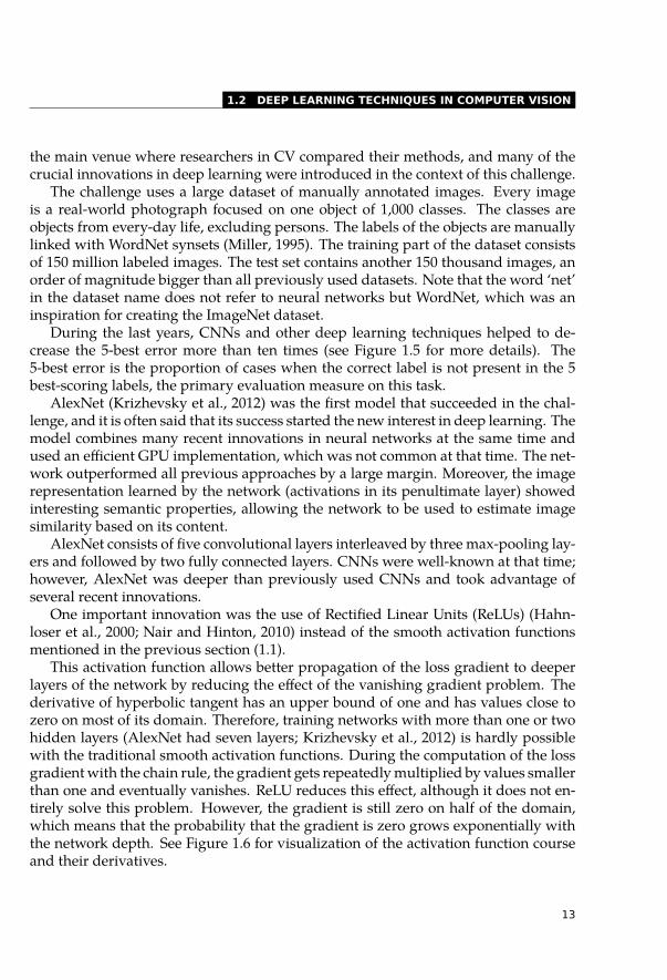
The challenge uses a large dataset of manually annotated images. Every imageis a real-world photograph focused on one object of 1,000 classes. The classes areobjects from every-day life, excluding persons. The labels of the objects are manuallylinked with WordNet synsets (Miller, 1995). The training part of the dataset consistsof 150 million labeled images. The test set contains another 150 thousand images, anorder of magnitude bigger than all previously used datasets. Note that the word ‘net’in the dataset name does not refer to neural networks but WordNet, which was aninspiration for creating the ImageNet dataset.
During the last years, CNNs and other deep learning techniques helped to de-crease the 5-best error more than ten times (see Figure 1.5 for more details). The5-best error is the proportion of cases when the correct label is not present in the 5best-scoring labels, the primary evaluation measure on this task.
AlexNet (Krizhevsky et al., 2012) was the first model that succeeded in the chal-lenge, and it is often said that its success started the new interest in deep learning. Themodel combines many recent innovations in neural networks at the same time andused an efficient GPU implementation, which was not common at that time. The net-work outperformed all previous approaches by a large margin. Moreover, the imagerepresentation learned by the network (activations in its penultimate layer) showedinteresting semantic properties, allowing the network to be used to estimate imagesimilarity based on its content.
AlexNet consists of five convolutional layers interleaved by three max-pooling lay-ers and followed by two fully connected layers. CNNs were well-known at that time;however, AlexNet was deeper than previously used CNNs and took advantage ofseveral recent innovations.
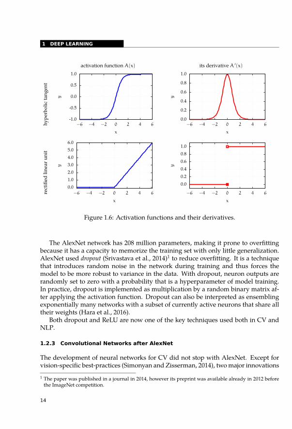
One important innovation was the use of Rectified Linear Units (ReLUs) (Hahn-loser et al., 2000; Nair and Hinton, 2010) instead of the smooth activation functionsmentioned in the previous section (1.1).
This activation function allows better propagation of the loss gradient to deeperlayers of the network by reducing the effect of the vanishing gradient problem. Thederivative of hyperbolic tangent has an upper bound of one and has values close tozero on most of its domain. Therefore, training networks with more than one or twohidden layers (AlexNet had seven layers; Krizhevsky et al., 2012) is hardly possiblewith the traditional smooth activation functions. During the computation of the lossgradient with the chain rule, the gradient gets repeatedly multiplied by values smallerthan one and eventually vanishes. ReLU reduces this effect, although it does not en-tirely solve this problem. However, the gradient is still zero on half of the domain,which means that the probability that the gradient is zero grows exponentially withthe network depth. See Figure 1.6 for visualization of the activation function courseand their derivatives.
13
1 DEEP LEARNING
activation function A(x) its derivative A ′(x)
hype
rbol
icta
ngen
t
-1.0
-0.5
0.0
0.5
1.0
−6 −4 −2 0 2 4 6
y
x
0.0
0.2
0.4
0.6
0.8
1.0
−6 −4 −2 0 2 4 6
y
x
rect
ified
linea
runi
t
0.01.02.03.04.05.06.0
−6 −4 −2 0 2 4 6
y
x
0.00.20.40.60.81.0
−6 −4 −2 0 2 4 6
y
x
Figure 1.6: Activation functions and their derivatives.
The AlexNet network has 208 million parameters, making it prone to overfittingbecause it has a capacity to memorize the training set with only little generalization.AlexNet used dropout (Srivastava et al., 2014)1 to reduce overfitting. It is a techniquethat introduces random noise in the network during training and thus forces themodel to be more robust to variance in the data. With dropout, neuron outputs arerandomly set to zero with a probability that is a hyperparameter of model training.In practice, dropout is implemented as multiplication by a random binary matrix af-ter applying the activation function. Dropout can also be interpreted as ensemblingexponentially many networks with a subset of currently active neurons that share alltheir weights (Hara et al., 2016).
Both dropout and ReLU are now one of the key techniques used both in CV andNLP.
1.2.3 Convolutional Networks after AlexNet
The development of neural networks for CV did not stop with AlexNet. Except forvision-specific best-practices (Simonyan and Zisserman, 2014), two major innovations
1 The paper was published in a journal in 2014, however its preprint was available already in 2012 beforethe ImageNet competition.
14
1.2 DEEP LEARNING TECHNIQUES IN COMPUTER VISION
come from image recognition, and that now play a crucial role in deep RecurrentNeural Networks (RNNs) and Transformers in NLP.
As we discussed in the previous section, one of the major problems of the deepneural network architectures is the vanishing gradient problem, which makes trainingof deeper models difficult. The ReLU activation function partially solved the problembecause the gradients are always either ones or zeros. Dropout can help by forcingupdates in neurons that would otherwise never change. Other techniques also helpto improve the gradient flow in the network during training.
One of them is the normalization of the network activation. These are regulariza-tion techniques that ensure that the neuron activations have almost zero mean andalmost unit variance. It makes propagation of the gradient easier by keeping the neu-ron activations near the values where the derivatives of the activation functions varythe most.
Batch normalization (Ioffe and Szegedy, 2015) and layer normalization (Ioffe andSzegedy, 2015) are the most frequently used. Batch normalization attempts to ensurethat activation values for each neuron are normally distributed over the training ex-amples. Layer normalization, on the other hand, normalizes the activations on eachlayer.
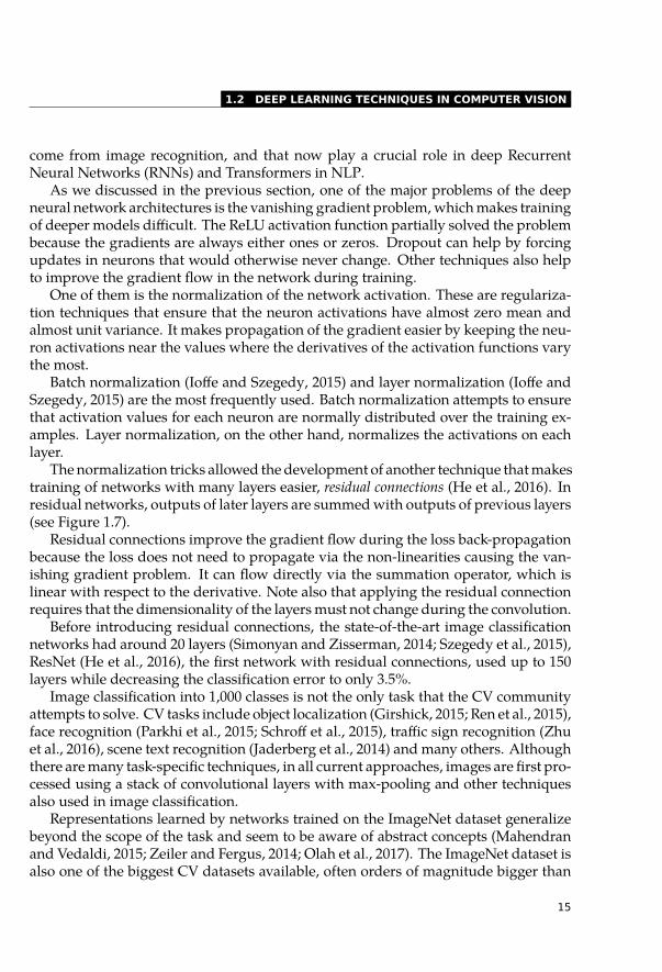
The normalization tricks allowed the development of another technique that makestraining of networks with many layers easier, residual connections (He et al., 2016). Inresidual networks, outputs of later layers are summed with outputs of previous layers(see Figure 1.7).
Residual connections improve the gradient flow during the loss back-propagationbecause the loss does not need to propagate via the non-linearities causing the van-ishing gradient problem. It can flow directly via the summation operator, which islinear with respect to the derivative. Note also that applying the residual connectionrequires that the dimensionality of the layers must not change during the convolution.
Before introducing residual connections, the state-of-the-art image classificationnetworks had around 20 layers (Simonyan and Zisserman, 2014; Szegedy et al., 2015),ResNet (He et al., 2016), the first network with residual connections, used up to 150layers while decreasing the classification error to only 3.5%.
Image classification into 1,000 classes is not the only task that the CV communityattempts to solve. CV tasks include object localization (Girshick, 2015; Ren et al., 2015),face recognition (Parkhi et al., 2015; Schroff et al., 2015), traffic sign recognition (Zhuet al., 2016), scene text recognition (Jaderberg et al., 2014) and many others. Althoughthere are many task-specific techniques, in all current approaches, images are first pro-cessed using a stack of convolutional layers with max-pooling and other techniquesalso used in image classification.
Representations learned by networks trained on the ImageNet dataset generalizebeyond the scope of the task and seem to be aware of abstract concepts (Mahendranand Vedaldi, 2015; Zeiler and Fergus, 2014; Olah et al., 2017). The ImageNet dataset isalso one of the biggest CV datasets available, often orders of magnitude bigger than
15
1 DEEP LEARNING
...projection orconvolution ·W1 + b1
.
non-linearity
.
projection orconvolution ·W2 + b2
.
+
.
resid
ual c
onne
ction
.
iden
tity
.
non-linearity
Figure 1.7: Network with a residual connection skipping one layer.
datasets for more specific tasks (Huh et al., 2016). This makes the representationslearned by the image classification networks suitable to use in other CV tasks (suchas object detection Girshick, 2015; animal species classification Branson et al., 2014;or satellite image Marmanis et al., 2016) as well as tasks combining vision with othermodalities (such as visual question answering, Antol et al., 2015; or image captioningVinyals et al., 2015). After 2018 (Peters et al., 2018a; Devlin et al., 2019), the reuse of pre-trained representations from networks trained for different tasks became standard inNLP as well.
1.3 Deep Learning Techniques in Natural Language Processing
Unlike CV that processes continuous signals that can be directly provided to a Neu-ral Network (NN), in NLP, we need to deal with the fact that language is writtenusing discrete symbols. The use of the symbols, how the symbols group into words,or larger units, the amount of information carried by a single symbol; this all variesdramatically across languages. Nevertheless, the symbols are always discrete. Deeplearning models for NLP thus need to convert the discrete input into a continuous rep-
16
1.3 DEEP LEARNING TECHNIQUES IN NATURAL LANGUAGE PROCESSING
resentation that is processed by the network before it eventually generates a discreteoutput.
In all NLP tasks, we can thus distinguish three phases of the computation:• Obtaining a continuous representation of the discrete input (often called word
or symbol embedding) by replacing the discrete symbols with continuous vectors;• Processing of the continuous representation (encoding) using various architec-
tures;• Generating discrete (or rarely continuous) output, sometimes called decoding.
Approaches to the phases may vary in complexity. This is most apparent in the case ofgenerating an output which can be done either using simple classification, sequencelabeling techniques such as conditional random fields (Lafferty et al., 2001) or con-nectionist temporal classification (Graves et al., 2006) or using relatively complex au-toregressive decoders (Sutskever et al., 2014).
The rest of the section discusses these three phases in more detail. First (Sec-tion 1.3.1), we discuss embedding of discrete symbols into a continuous space. Inthe following section (1.3.2), we discuss three main architectures that can be usedfor processing an embedded sequence: RNNs, CNNs, and SANs. The following sec-tion (1.3.3) summarizes classification and sequence labeling techniques as a means ofgenerating discrete output. Finally, we discuss autoregressive decoding which is atechnique that allows generating arbitrarily long sequences.
1.3.1 Word Embeddings
Neural networks rely on continuous mathematics. When using neural networks forNLP, we need to bridge the gap between the symbolic nature of the written languageand the continuous quantities processed by neural networks. The most intuitive wayof doing so is using a predefined finite indexed set of symbols called a vocabulary(those are typically words, characters, or sub-word units) and represent the input asone-hot vectors.
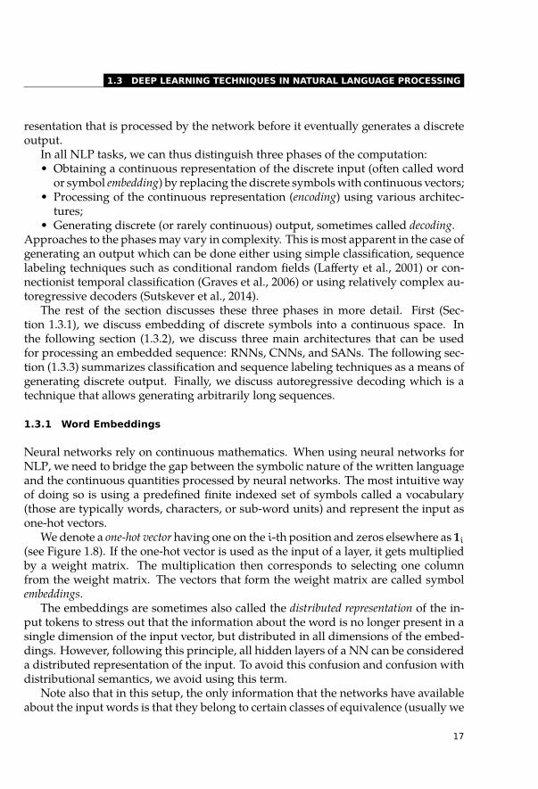
We denote a one-hot vector having one on the i-th position and zeros elsewhere as 1i(see Figure 1.8). If the one-hot vector is used as the input of a layer, it gets multipliedby a weight matrix. The multiplication then corresponds to selecting one columnfrom the weight matrix. The vectors that form the weight matrix are called symbolembeddings.
The embeddings are sometimes also called the distributed representation of the in-put tokens to stress out that the information about the word is no longer present in asingle dimension of the input vector, but distributed in all dimensions of the embed-dings. However, following this principle, all hidden layers of a NN can be considereda distributed representation of the input. To avoid this confusion and confusion withdistributional semantics, we avoid using this term.
Note also that in this setup, the only information that the networks have availableabout the input words is that they belong to certain classes of equivalence (usually we
17
1 DEEP LEARNING
.. · · ·. 0. 0. 0. 1. 0. · · ·..
doct
or
.
won
der
.
eart
h
.
happ
y
.
excl
usiv
e
Figure 1.8: Illustration of a one-hot vector.
consider words with the same spelling to be the equivalent) indicated by the one-hotvector. The only information that the network can later work with is the co-occurrenceof these classes of equivalence and their co-occurrence with target labels. The modelsthus heavily rely on the distributional hypothesis (Harris, 1954). The hypothesis saysthat the meaning of the words can be inferred from the contexts in which they areused. The success of neural networks for NLP shows that the hypothesis holds atleast to some extent.
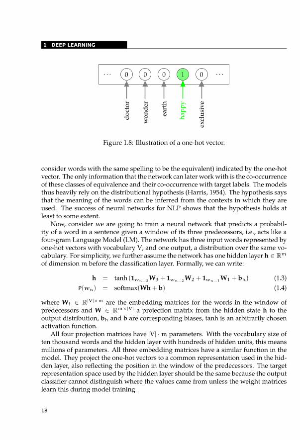
Now, consider we are going to train a neural network that predicts a probabil-ity of a word in a sentence given a window of its three predecessors, i.e., acts like afour-gram Language Model (LM). The network has three input words represented byone-hot vectors with vocabulary V , and one output, a distribution over the same vo-cabulary. For simplicity, we further assume the network has one hidden layer h ∈ Rm
of dimension m before the classification layer. Formally, we can write:
h = tanh (1wn−3W3 + 1wn−2
W2 + 1wn−1W1 + bh) (1.3)
P(wn) = softmax(Wh + b) (1.4)
where Wi ∈ R|V |×m are the embedding matrices for the words in the window ofpredecessors and W ∈ Rm×|V | a projection matrix from the hidden state h to theoutput distribution, bh and b are corresponding biases, tanh is an arbitrarily chosenactivation function.
All four projection matrices have |V | ·m parameters. With the vocabulary size often thousand words and the hidden layer with hundreds of hidden units, this meansmillions of parameters. All three embedding matrices have a similar function in themodel. They project the one-hot vectors to a common representation used in the hid-den layer, also reflecting the position in the window of the predecessors. The targetrepresentation space used by the hidden layer should be the same because the outputclassifier cannot distinguish where the values came from unless the weight matriceslearn this during model training.
18
1.3 DEEP LEARNING TECHNIQUES IN NATURAL LANGUAGE PROCESSING
..
1wn−3
..
.
·We
.
1wn−2
..
.
·We
.
1wn−1
..
.
·We
..
.
tanh
.
∑
.
·V3
.
·V2
.
·V1 + bh
..
.
softmax
.
·W + b
.
P(wn|wn−3, wn−2, wn−1)
Figure 1.9: Architecture of a feed-forward language model with window size 3 withshared word embeddings We.
Given this observation, we can factorize the matrices into two parts: the first oneperforming the projection to a common representation space of dimension m that canbe shared among the window of predecessors, and the second projection adapting thevector to the specific role in the network based on the word position. Formally:
h = tanh (1wn−3WeV3 + 1wn−2
WeV2 + 1wn−1WeV1 + bh) (1.5)
where We ∈ R|V |×m is the shared word embedding matrix and Vi are smaller projec-tion matrices of size m ×m. This step approximately halves the number of networkparameters. This is also the way that word embeddings are currently used in mostNLP tasks. The architecture of the described trigram LM is illustrated in Figure 1.9.
The previous thoughts led us exactly to the architecture of the first successful neu-ral LM (Bengio et al., 2003). The feed-forward architecture not only achieved decentquantitative results in terms of corpus perplexity, but it also developed word repre-sentations with interesting properties. Words with similar meaning tend to have sim-ilar vector representations in terms of Euclidean or cosine distance. Moreover, thelearned representations appear to be useful features for other NLP tasks (Collobertet al., 2011).
19
1 DEEP LEARNING
Mikolov et al. (2010) trained an RNN-based LM for speech recognition where theword representations manifest another interesting property. The vectors seemed tobehave linearly with respect to some semantic shifts, e.g., words that differ only ingender tend to have a constant difference vector. Mikolov et al. (2013c) further exam-ined this property of the word vectors and developed a simple feed-forward archi-tecture that was no longer a good LM but still produced word embeddings with allthe interesting properties, i.e., being useful machine-learning features for NLP tasks,clustering words with similar meaning and behaving linearly with respect to somesemantic shifts.
Pre-trained embeddings using one of the above-mentioned methods are an im-portant building block in NLP tasks with limited training data (dependency parsing:Chen and Manning, 2014, Straka and Straková, 2017; question answering: Seo et al.,2016) when the model is supposed to generalize for words which were not seen inthe training data, but for which we have good pre-trained embeddings. In tasks witha large amount of training data such as MT, we usually train the word embeddingstogether with the rest of the model (Qi et al., 2018).
The development of universally usable word vector representations became anindependent subfield of NLP research. The research community mostly focuses onstudying theoretical properties of the embeddings (Levy and Goldberg, 2014; Agirreet al., 2016) and multilingual embeddings either with or without the use of paralleldata (Luong et al., 2015; Conneau et al., 2017).
Word embeddings and their interpretations are discussed in detail in Chapter 4.
1.3.2 Architectures for Sequence Processing
In NLP, we usually treat the text as a sequence of tokens that correspond to words,subwords, or characters. Deep learning architectures for sequence processing thusmust be able to process sequential data of different lengths. The length of sentencesprocessed by the MT systems typically varies from a few words to tens of words. Inthe CzEng parallel (Bojar et al., 2016b) 90% of sentences have between 20 and 350tokens.
The architectures are used to produce an intermediate representation, so-calledhidden states which the network uses further for generating outputs. The intermediaterepresentation can be trained either end-to-end when learning an NLP task, or it canbe a pre-trained one. In this section, we describe how these architectures work whentreating them as a black box. We open the box and discuss possible interpretations inChapter 6.
Currently, there are two main types of architectures used: RNNs, and SANs. Thearchitectures are explained in detail in the following sections.
20
1.3 DEEP LEARNING TECHNIQUES IN NATURAL LANGUAGE PROCESSING
..A.
xt
.
ht
. =. A. h1.
x1
.
h1
. A. h2.
x2
.
h2
. A. h3.
x3
.
h3
. A. h4.
x4
.
h4
. h0. · · ·
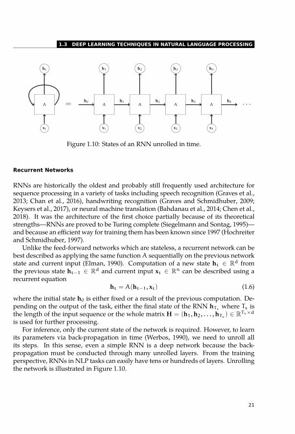
Figure 1.10: States of an RNN unrolled in time.
Recurrent Networks
RNNs are historically the oldest and probably still frequently used architecture forsequence processing in a variety of tasks including speech recognition (Graves et al.,2013; Chan et al., 2016), handwriting recognition (Graves and Schmidhuber, 2009;Keysers et al., 2017), or neural machine translation (Bahdanau et al., 2014; Chen et al.,2018). It was the architecture of the first choice partially because of its theoreticalstrengths—RNNs are proved to be Turing complete (Siegelmann and Sontag, 1995)—and because an efficient way for training them has been known since 1997 (Hochreiterand Schmidhuber, 1997).
Unlike the feed-forward networks which are stateless, a recurrent network can bebest described as applying the same function A sequentially on the previous networkstate and current input (Elman, 1990). Computation of a new state ht ∈ Rd fromthe previous state ht−1 ∈ Rd and current input xt ∈ Rn can be described using arecurrent equation
ht = A(ht−1, xt) (1.6)
where the initial state h0 is either fixed or a result of the previous computation. De-pending on the output of the task, either the final state of the RNN hTx
where Tx isthe length of the input sequence or the whole matrix H = (h1,h2, . . . ,hTx
) ∈ RTx×d
is used for further processing.For inference, only the current state of the network is required. However, to learn
its parameters via back-propagation in time (Werbos, 1990), we need to unroll allits steps. In this sense, even a simple RNN is a deep network because the back-propagation must be conducted through many unrolled layers. From the trainingperspective, RNNs in NLP tasks can easily have tens or hundreds of layers. Unrollingthe network is illustrated in Figure 1.10.
21
1 DEEP LEARNING
..
Ct−1
.
Ct
.
ht−1
.
ht
.
xt
.
σ
.
×
.
ft
.
σ
.
it
.
tanh
.
×
.
+
.
Ct
.
σ
.
ot
.
tanh
.
×
.
ht
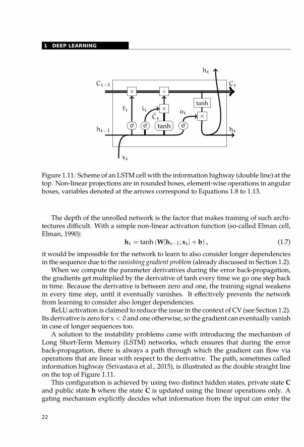
Figure 1.11: Scheme of an LSTM cell with the information highway (double line) at thetop. Non-linear projections are in rounded boxes, element-wise operations in angularboxes, variables denoted at the arrows correspond to Equations 1.8 to 1.13.
The depth of the unrolled network is the factor that makes training of such archi-tectures difficult. With a simple non-linear activation function (so-called Elman cell,Elman, 1990):
ht = tanh (W[ht−1; xt] + b) , (1.7)
it would be impossible for the network to learn to also consider longer dependenciesin the sequence due to the vanishing gradient problem (already discussed in Section 1.2).
When we compute the parameter derivatives during the error back-propagation,the gradients get multiplied by the derivative of tanh every time we go one step backin time. Because the derivative is between zero and one, the training signal weakensin every time step, until it eventually vanishes. It effectively prevents the networkfrom learning to consider also longer dependencies.
ReLU activation is claimed to reduce the issue in the context of CV (see Section 1.2).Its derivative is zero for x < 0 and one otherwise, so the gradient can eventually vanishin case of longer sequences too.
A solution to the instability problems came with introducing the mechanism ofLong Short-Term Memory (LSTM) networks, which ensures that during the errorback-propagation, there is always a path through which the gradient can flow viaoperations that are linear with respect to the derivative. The path, sometimes calledinformation highway (Srivastava et al., 2015), is illustrated as the double straight lineon the top of Figure 1.11.
This configuration is achieved by using two distinct hidden states, private state Cand public state h where the state C is updated using the linear operations only. Agating mechanism explicitly decides what information from the input can enter the
22
1.3 DEEP LEARNING TECHNIQUES IN NATURAL LANGUAGE PROCESSING
information highway (input gate), which part of the state should be deleted (forget gate)and what part of the private hidden state should be published (output gate).
Formally, an LSTM network of dimension d updates its two hidden states ht−1 ∈Rd and Ct−1 ∈ Rd based on the input xt in time step t in the following way:
ft = σ (Wf · [ht−1; xt] + bf) (1.8)it = σ (Wi · [ht−1; xt] + bi) (1.9)ot = σ (Wo · [ht−1; xt] + bo) (1.10)Ct = tanh (Wc · [ht−1; xt] + bC) (1.11)Ct = ft ⊙ Ct−1 + it ⊙ Ct (1.12)ht = ot ⊙ tanh Ct. (1.13)
where ⊙ denotes point-wise multiplication. The cell is shown in Figure 1.11.The values of the forget gate ft ∈ (0, 1)
d control how much information is keptin the memory cell by point-wise multiplication. In the next step, we compute thecandidate state C ∈ Rd in the same way as the new state is computed in the ElmanRNN cells. Values of this candidate state are not combined directly with the memory.First, they are weighted using the input gate it ∈ (0, 1)
d and added to the memoryalready pruned by the forget gate. The new output state ht is computed by applyingtanh non-linearity on the memory state Ct and weighting it by the output gate ot ∈(0, 1)
d.As previously mentioned, LSTM networks have two separate states Ct and ht.
The private hidden state Ct is only updated using addition and point-wise multipli-cation. The tanh non-linearity is only applied while computing the output state ht.The gradient from the output passes through only one non-linearity before enteringthe information highway.
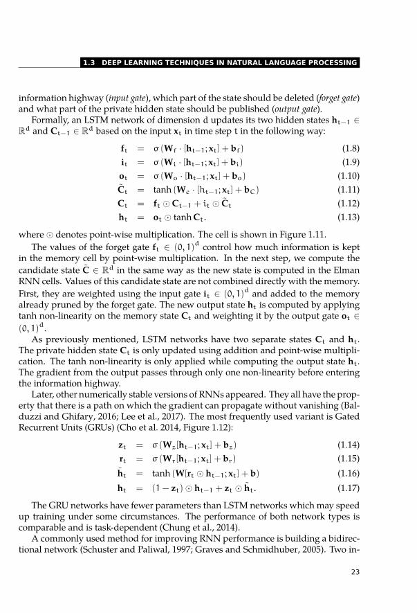
Later, other numerically stable versions of RNNs appeared. They all have the prop-erty that there is a path on which the gradient can propagate without vanishing (Bal-duzzi and Ghifary, 2016; Lee et al., 2017). The most frequently used variant is GatedRecurrent Units (GRUs) (Cho et al. 2014, Figure 1.12):
zt = σ (Wz[ht−1; xt] + bz) (1.14)rt = σ (Wr[ht−1; xt] + br) (1.15)ht = tanh (W[rt ⊙ ht−1; xt] + b) (1.16)ht = (1− zt)⊙ ht−1 + zt ⊙ ht. (1.17)
The GRU networks have fewer parameters than LSTM networks which may speedup training under some circumstances. The performance of both network types iscomparable and is task-dependent (Chung et al., 2014).
A commonly used method for improving RNN performance is building a bidirec-tional network (Schuster and Paliwal, 1997; Graves and Schmidhuber, 2005). Two in-
23
1 DEEP LEARNING
..
ht−1
.
ht
.
xt
.
+
.
×
.
1−
.
σ
.
zt
.
×
.tanh
.
ht
.
σ
.
×
.
rt
.
ht
Figure 1.12: Scheme of an GRU cell following the same conventions as Figure 1.11.
dependent RNN networks are used in parallel, each of them processing the sequencefrom one end. The output states are then concatenated. In this way, the network canbetter capture dependencies in both directions in the input sequence. BidirectionalRNNs became a standard in many NLP tasks (Bahdanau et al., 2014; Ling et al., 2015;Seo et al., 2016; Kiperwasser and Goldberg, 2016; Lample et al., 2016). Note that in thissetup, every network state may contain information about the complete sequence.
Self-Attentive Networks
SANs are neural networks where at least for some layers, the states of the next layer arecomputed as a linear combination of the states on the previous layer. It is called self-attention because states from a network layer are used to “attend”, collect informationfrom themself to create a new layer. The intuition that is often used to explain theSANs is that in every layer, every word collects relevant pieces of information fromother words and thus gets more informed about in what context it is used. Althoughwe will see in Chapter 5 that this intuition is often not entirely true, in this section, itwill help us to better understand the technicalities of the architecture.
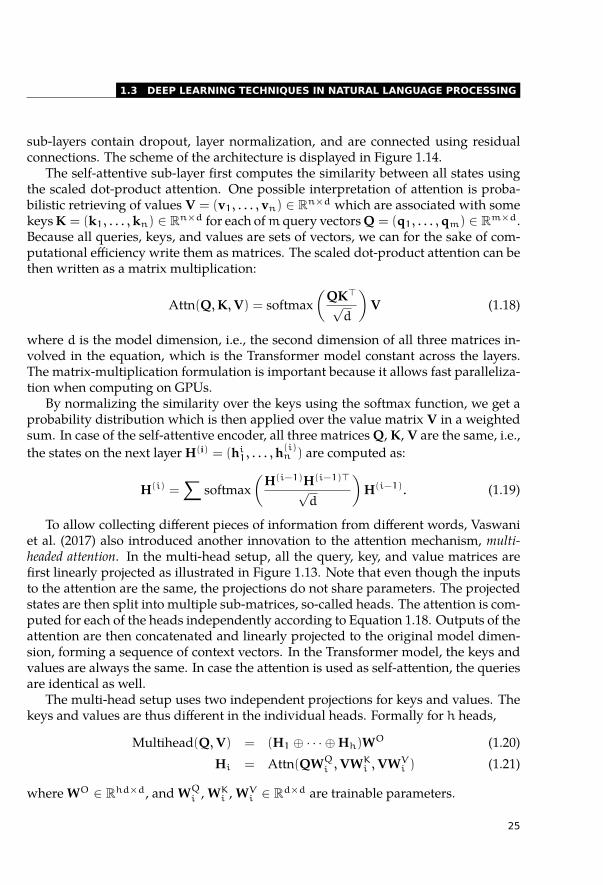
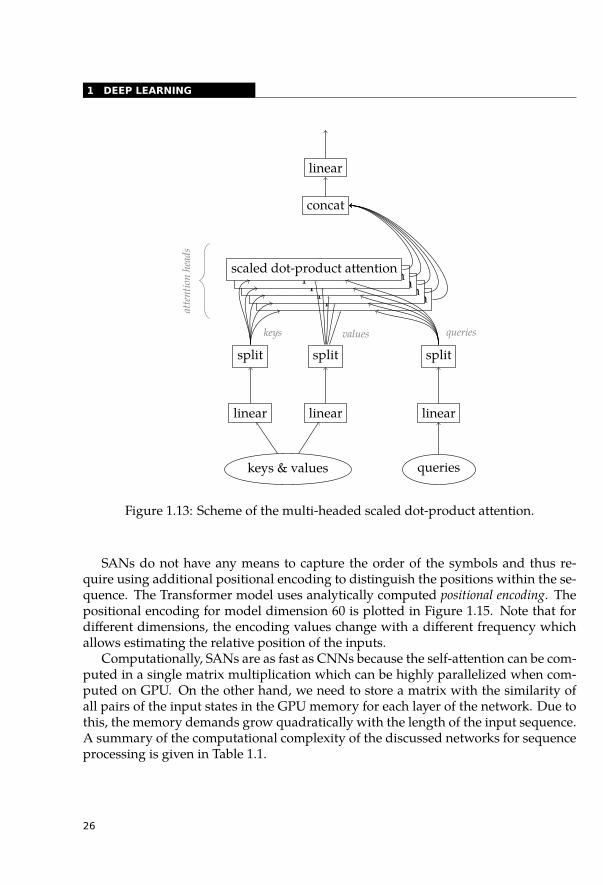
There exist several variants of SANs (Parikh et al., 2016; Lin et al., 2017). In this sec-tion, we discuss in detail the encoder part of the architecture introduced by Vaswaniet al. (2017), called Transformer, that achieves state-of-the-art results in MT.
A Transformer layer for sequence encoding consists of two sub-layers2.The first sub-layer is self-attentive, the second one is a non-linear projection to a
larger dimension followed by a linear projection back to the original dimension. All
2 Note that even the sub-layer consists of several network layers. A better term would probably be block asin ResNet (He et al., 2016), however, we follow the terminology introduced by Vaswani et al. (2017).
24
1.3 DEEP LEARNING TECHNIQUES IN NATURAL LANGUAGE PROCESSING
sub-layers contain dropout, layer normalization, and are connected using residualconnections. The scheme of the architecture is displayed in Figure 1.14.
The self-attentive sub-layer first computes the similarity between all states usingthe scaled dot-product attention. One possible interpretation of attention is proba-bilistic retrieving of values V = (v1, . . . , vn) ∈ Rn×d which are associated with somekeys K = (k1, . . . ,kn) ∈ Rn×d for each ofm query vectors Q = (q1, . . . ,qm) ∈ Rm×d.Because all queries, keys, and values are sets of vectors, we can for the sake of com-putational efficiency write them as matrices. The scaled dot-product attention can bethen written as a matrix multiplication:
Attn(Q,K,V) = softmax(
QK⊤√d
)V (1.18)
where d is the model dimension, i.e., the second dimension of all three matrices in-volved in the equation, which is the Transformer model constant across the layers.The matrix-multiplication formulation is important because it allows fast paralleliza-tion when computing on GPUs.
By normalizing the similarity over the keys using the softmax function, we get aprobability distribution which is then applied over the value matrix V in a weightedsum. In case of the self-attentive encoder, all three matrices Q, K, V are the same, i.e.,the states on the next layer H(i) = (hi
1, . . . ,h(i)n ) are computed as:
H(i) =∑
softmax(
H(i−1)H(i−1)⊤√d
)H(i−1). (1.19)
To allow collecting different pieces of information from different words, Vaswaniet al. (2017) also introduced another innovation to the attention mechanism, multi-headed attention. In the multi-head setup, all the query, key, and value matrices arefirst linearly projected as illustrated in Figure 1.13. Note that even though the inputsto the attention are the same, the projections do not share parameters. The projectedstates are then split into multiple sub-matrices, so-called heads. The attention is com-puted for each of the heads independently according to Equation 1.18. Outputs of theattention are then concatenated and linearly projected to the original model dimen-sion, forming a sequence of context vectors. In the Transformer model, the keys andvalues are always the same. In case the attention is used as self-attention, the queriesare identical as well.
The multi-head setup uses two independent projections for keys and values. Thekeys and values are thus different in the individual heads. Formally for h heads,
Multihead(Q,V) = (H1 ⊕ · · · ⊕ Hh)WO (1.20)Hi = Attn(QWQ
i ,VWKi ,VWV
i ) (1.21)
where WO ∈ Rhd×d, and WQi , WK
i , WVi ∈ Rd×d are trainable parameters.
25
1 DEEP LEARNING
..keys & values. queries.
linear
.
linear
.
linear
.
split
.
split
.
split
.
concat
.
linear
.
scaled dot-product attention
.
scaled dot-product attention
.
scaled dot-product attention
.
scaled dot-product attention
.
scaled dot-product attention
.
atte
ntio
nhe
ads
.
keys
.
values
.
queries
Figure 1.13: Scheme of the multi-headed scaled dot-product attention.
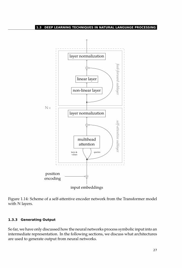
SANs do not have any means to capture the order of the symbols and thus re-quire using additional positional encoding to distinguish the positions within the se-quence. The Transformer model uses analytically computed positional encoding. Thepositional encoding for model dimension 60 is plotted in Figure 1.15. Note that fordifferent dimensions, the encoding values change with a different frequency whichallows estimating the relative position of the inputs.
Computationally, SANs are as fast as CNNs because the self-attention can be com-puted in a single matrix multiplication which can be highly parallelized when com-puted on GPU. On the other hand, we need to store a matrix with the similarity ofall pairs of the input states in the GPU memory for each layer of the network. Due tothis, the memory demands grow quadratically with the length of the input sequence.A summary of the computational complexity of the discussed networks for sequenceprocessing is given in Table 1.1.
26
1.3 DEEP LEARNING TECHNIQUES IN NATURAL LANGUAGE PROCESSING
..input embeddings.
⊕
.
positionencoding
.
self-attentivesublayer
..
multiheadattention
.
keys &values
.
queries
.
⊕
.
layer normalization
.
feed-forward
sublayer
..
non-linear layer
.
linear layer
.
⊕
.
layer normalization
.
N×
Figure 1.14: Scheme of a self-attentive encoder network from the Transformer modelwith N layers.
1.3.3 Generating Output
So far, we have only discussed how the neural networks process symbolic input into anintermediate representation. In the following sections, we discuss what architecturesare used to generate output from neural networks.
27
1 DEEP LEARNING
.
.
.
0
.
20
.
40
.Symbol position in the input sequence
.
0
.
10
.
20
.
30
.
40
.
50
.
Dim
ensi
onin
the
enco
ding
.
.
−0.5
.
0.0
.
0.5
.
1.0
Figure 1.15: Visualization of the position encoding used in the Transformer modelwith embedding dimension 60 and input length up to 8.
We discuss in detail three special cases:• The output is a symbol from a closed set of possible answers—classification;• The output is a sequence of symbols of the same length as the input—sequence
labeling;• The output is a sequence of symbols of an arbitrary length—autoregressive decod-
ing.
Classification
In the simplest case, the network produces only one discrete output, i.e., we want toclassify the input into a fixed set of previously known classes. An example of suchan NLP task is sentiment analysis (Pang et al., 2002; Pak and Paroubek, 2010) wherethe goal is to classify whether a text carries a positive or negative sentiment. Anotherexample can be classification of text into a set of genres (Kessler et al., 1997; Lee andMyaeng, 2002).
The most common approach to these tasks is applying a multi-layer perceptronover a fixed-size representation of the input. The fixed-size vector can be for instancethe final state of an RNN or a result of a pooling function applied over states pro-duced by one of the architectures mentioned in Section 1.3.2. The most frequentlyused methods are max-pooling and mean-pooling, computing the maximum or av-erage of the states in time, respectively.
28
1.3 DEEP LEARNING TECHNIQUES IN NATURAL LANGUAGE PROCESSING
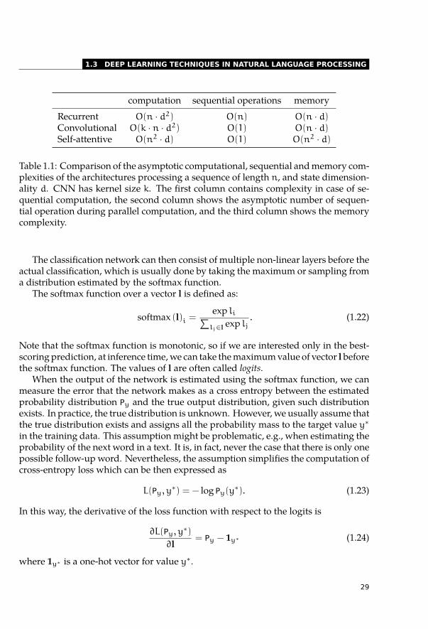
computation sequential operations memoryRecurrent O(n · d2) O(n) O(n · d)Convolutional O(k · n · d2) O(1) O(n · d)Self-attentive O(n2 · d) O(1) O(n2 · d)
Table 1.1: Comparison of the asymptotic computational, sequential and memory com-plexities of the architectures processing a sequence of length n, and state dimension-ality d. CNN has kernel size k. The first column contains complexity in case of se-quential computation, the second column shows the asymptotic number of sequen-tial operation during parallel computation, and the third column shows the memorycomplexity.
The classification network can then consist of multiple non-linear layers before theactual classification, which is usually done by taking the maximum or sampling froma distribution estimated by the softmax function.
The softmax function over a vector l is defined as:
softmax (l)i =exp li∑lj∈l exp lj
. (1.22)
Note that the softmax function is monotonic, so if we are interested only in the best-scoring prediction, at inference time, we can take the maximum value of vector l beforethe softmax function. The values of l are often called logits.
When the output of the network is estimated using the softmax function, we canmeasure the error that the network makes as a cross entropy between the estimatedprobability distribution Py and the true output distribution, given such distributionexists. In practice, the true distribution is unknown. However, we usually assume thatthe true distribution exists and assigns all the probability mass to the target value y∗
in the training data. This assumption might be problematic, e.g., when estimating theprobability of the next word in a text. It is, in fact, never the case that there is only onepossible follow-up word. Nevertheless, the assumption simplifies the computation ofcross-entropy loss which can be then expressed as
L(Py, y∗) = − log Py(y∗). (1.23)
In this way, the derivative of the loss function with respect to the logits is
∂L(Py, y∗)
∂l= Py − 1y∗ (1.24)
where 1y∗ is a one-hot vector for value y∗.
29
1 DEEP LEARNING
The loss gradient with respect to the logits is back-propagated to the network usingthe chain rule. The softmax function with cross-entropy loss is used not only in thecase of single-output classification but also in sequence labeling and autoregressivedecoding discussed in the following sections.
For completeness, we should also mention that when the output of the network issupposed to be a continuous value, we can perform a linear regression over the inputrepresentation and optimize the estimation using a mean squared error
L(y, y∗) = (y− y∗)2, (1.25)
which is differentiable and thus the error can be back-propagated to the network.
Sequence Labeling
When the desired output of a network is a sequence of discrete symbols having thesame length as the input and monotonically aligned with the input, we can applya multi-layer perceptron over each state of the network. In this case, the labels as-signed to every state are conditionally independent given the network states. Theloss function used to train the network is a sum of cross entropy over the networkoutput distributions.
In NLP, many tasks can be formulated as sequence labeling. Besides the moretheoretically motivated tasks such as part-of-speech tagging or semantic role labeling,we can mention information extraction where the goal is marking entities in a text ornamed entity recognition.
The labels assigned to the input symbols often have their own, usually simplegrammar rules. When we label the beginnings and ends of sequences, we need tomake sure the end symbol never comes before the start symbol. In these cases, condi-tional random fields can be applied over the state sequence (Lafferty et al., 2001; Doand Artieres, 2010).
Autoregressive Decoding
In some tasks such as MT or abstractive text summarization, the output cannot bemonotonically aligned with the input and the number of output symbols differs fromthe number of the input symbols. In such cases, we need a mechanism that is ableto generate output symbols in a general while loop and is conditioned on the entireinput. Such a while loop is sometimes called autoregressive decoder because the com-putation in every time step depends on the previous state of the loop and previousoutputs and generates the output symbols left-to-right.
Historically, autoregressive decoding has developed from discriminative languagemodeling using RNNs. We will thus first explain this principle on the RNN LMs andlater generalize the principle for CNNs and SANs.
30
1.3 DEEP LEARNING TECHNIQUES IN NATURAL LANGUAGE PROCESSING
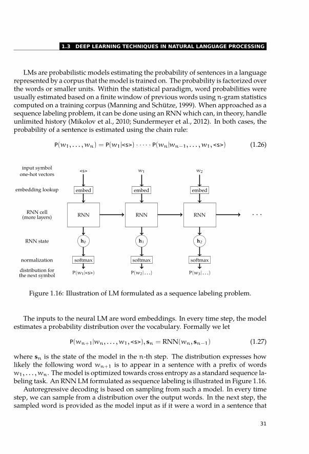
LMs are probabilistic models estimating the probability of sentences in a languagerepresented by a corpus that the model is trained on. The probability is factorized overthe words or smaller units. Within the statistical paradigm, word probabilities wereusually estimated based on a finite window of previous words using n-gram statisticscomputed on a training corpus (Manning and Schütze, 1999). When approached as asequence labeling problem, it can be done using an RNN which can, in theory, handleunlimited history (Mikolov et al., 2010; Sundermeyer et al., 2012). In both cases, theprobability of a sentence is estimated using the chain rule:
P(w1, . . . , wn) = P(w1|<s>) · · · · · P(wn|wn−1, . . . , w1, <s>) (1.26)
..
input symbol
.
one-hot vectors
.
embedding lookup
.RNN cell .(more layers)
.
RNN state
.
normalization
.
distribution for
.
the next symbol
.
<s>
.
embed
.RNN.
h0
.
softmax
.
P(w1|<s>)
.
w1
.
embed
. RNN.
h1
.
softmax
.
P(w2| . . .)
.
w2
.
embed
. RNN.
h2
.
softmax
.
P(w3| . . .)
. · · ·
Figure 1.16: Illustration of LM formulated as a sequence labeling problem.
The inputs to the neural LM are word embeddings. In every time step, the modelestimates a probability distribution over the vocabulary. Formally we let
P(wn+1|wn, . . . , w1, <s>), sn = RNN(wn, sn−1) (1.27)
where sn is the state of the model in the n-th step. The distribution expresses howlikely the following word wn+1 is to appear in a sentence with a prefix of wordsw1, . . . , wn. The model is optimized towards cross entropy as a standard sequence la-beling task. An RNN LM formulated as sequence labeling is illustrated in Figure 1.16.
Autoregressive decoding is based on sampling from such a model. In every timestep, we can sample from a distribution over the output words. In the next step, thesampled word is provided as the model input as if it were a word in a sentence that
31
1 DEEP LEARNING
..
embed
.RNN.
h0
.
softmax
.
P(w1|<s>)
.
sample
.
embed
. RNN.
h1
.
softmax
.
P(w2| . . .)
.
sample
.
embed
. RNN.
h2
.
softmax
.
P(w3| . . .)
.
sample
.
embed
. RNN.
h3
.
softmax
.
P(w4| . . .)
.
sample
.
<s>
. · · ·
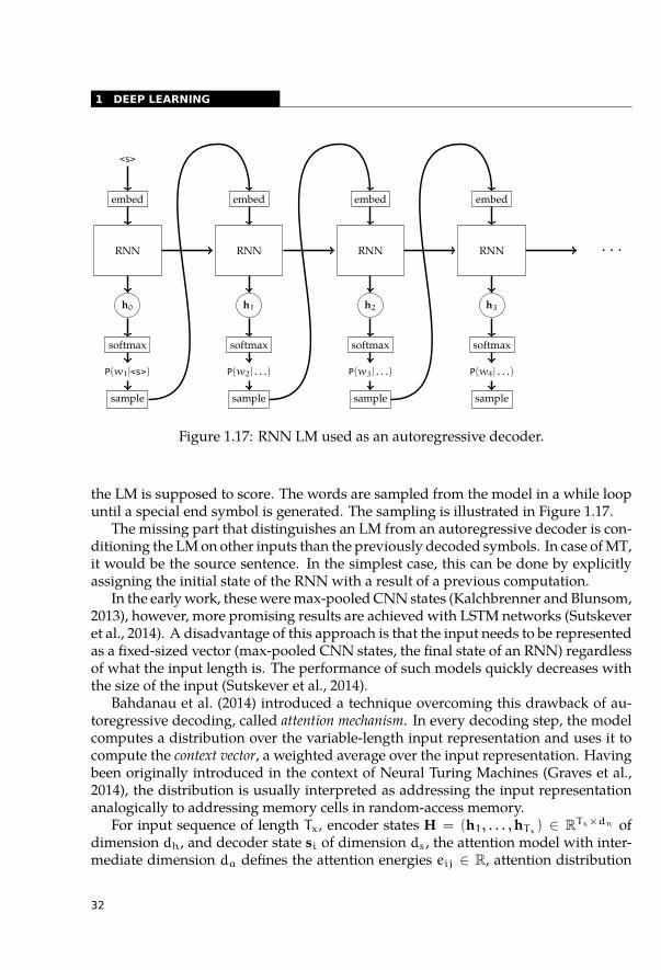
Figure 1.17: RNN LM used as an autoregressive decoder.
the LM is supposed to score. The words are sampled from the model in a while loopuntil a special end symbol is generated. The sampling is illustrated in Figure 1.17.
The missing part that distinguishes an LM from an autoregressive decoder is con-ditioning the LM on other inputs than the previously decoded symbols. In case of MT,it would be the source sentence. In the simplest case, this can be done by explicitlyassigning the initial state of the RNN with a result of a previous computation.
In the early work, these were max-pooled CNN states (Kalchbrenner and Blunsom,2013), however, more promising results are achieved with LSTM networks (Sutskeveret al., 2014). A disadvantage of this approach is that the input needs to be representedas a fixed-sized vector (max-pooled CNN states, the final state of an RNN) regardlessof what the input length is. The performance of such models quickly decreases withthe size of the input (Sutskever et al., 2014).
Bahdanau et al. (2014) introduced a technique overcoming this drawback of au-toregressive decoding, called attention mechanism. In every decoding step, the modelcomputes a distribution over the variable-length input representation and uses it tocompute the context vector, a weighted average over the input representation. Havingbeen originally introduced in the context of Neural Turing Machines (Graves et al.,2014), the distribution is usually interpreted as addressing the input representationanalogically to addressing memory cells in random-access memory.
For input sequence of length Tx, encoder states H = (h1, . . . ,hTx) ∈ RTx×dn of
dimension dh, and decoder state si of dimension ds, the attention model with inter-mediate dimension da defines the attention energies eij ∈ R, attention distribution
32
1.3 DEEP LEARNING TECHNIQUES IN NATURAL LANGUAGE PROCESSING
αi ∈ RTx , and the context vector ci ∈ Rdh in the i-th decoder step as:
eij = v⊤a tanh(Wasi + Uahj + ba) + be, (1.28)
αij =exp(eij)∑Tx
k=1 exp(eik), (1.29)
ci =Tx∑j=1
αijhj. (1.30)
The trainable parameters Wa ∈ Rds×da and Ua ∈ Rdh×da are projection matricesthat transform the decoder and encoder states si and hj into a common vector spaceand va ∈ Rda is a weight vector over the dimensions of this space, ba ∈ Rda and be ∈R are biases for the respective projections. The context vector ci is then concatenatedwith the decoder state si and used for classification of the following output symbol.
Together with techniques for data preprocessing (Sennrich et al., 2016b,c), the at-tention model was the crucial innovation that helped to improve neural MT qualityover the statistical MT and set a new state of the art in the field of MT.
SANs can be used similarly to CNNs. In the Transformer model (Vaswani et al.,2017), a stack of self-attentive and feed-forward sub-layers is applied on the alreadydecoded sequence and the result is used to produce the next output symbol. Similar tothe CNN decoder, the self-attentive layers are interleaved with cross-attentive layersattending the encoder states.
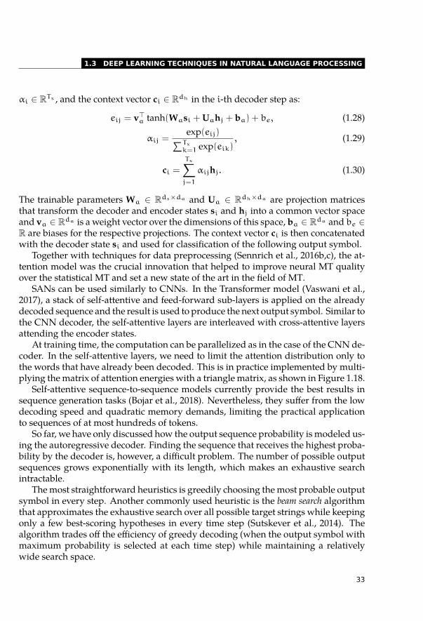
At training time, the computation can be parallelized as in the case of the CNN de-coder. In the self-attentive layers, we need to limit the attention distribution only tothe words that have already been decoded. This is in practice implemented by multi-plying the matrix of attention energies with a triangle matrix, as shown in Figure 1.18.
Self-attentive sequence-to-sequence models currently provide the best results insequence generation tasks (Bojar et al., 2018). Nevertheless, they suffer from the lowdecoding speed and quadratic memory demands, limiting the practical applicationto sequences of at most hundreds of tokens.
So far, we have only discussed how the output sequence probability is modeled us-ing the autoregressive decoder. Finding the sequence that receives the highest proba-bility by the decoder is, however, a difficult problem. The number of possible outputsequences grows exponentially with its length, which makes an exhaustive searchintractable.
The most straightforward heuristics is greedily choosing the most probable outputsymbol in every step. Another commonly used heuristic is the beam search algorithmthat approximates the exhaustive search over all possible target strings while keepingonly a few best-scoring hypotheses in every time step (Sutskever et al., 2014). Thealgorithm trades off the efficiency of greedy decoding (when the output symbol withmaximum probability is selected at each time step) while maintaining a relativelywide search space.
33
1 DEEP LEARNING
..v1.
v2
.
v3
....
.
vM
.
q1
.
q2
.
q3
.
. . .
.
qN
....... . . ..
. . .
.
. . .
.
. . .
....
...
..
Queries Q
.
Valu
esV
.
−∞Figure 1.18: Masking while computing energy values in the self-attention layer in theTransformer decoder. Masking prevents the self-attention to attend to symbols to theright from the previously decoded symbol.
The algorithm keeps track of k hypotheses (beam). A hypothesis is either a partiallygenerated sequence (unfinished), or a sequence that ends with a special end symbol(finished). In each step, all hypotheses are expanded with all possible tokens from thevocabulary. The expanded hypotheses are scored and k best of them are kept for thenext step.
1.4 Conclusion
After major success in CV in 2012 and 2013, deep learning attracted the attentionof the NLP research community. Soon after that, deep learning methods reachedstate-of-the-art results in most NLP tasks and became the first choice method. Thestandard deep learning architecture design consists of discrete symbol embedding,contextualizing the embeddings using an encoder, and using the representations togenerate discrete output.
In practice, the embeddings or the encoder are pre-trained on large corpora andonly the output layers are trained. This is discussed in more detail in the next chapter,together with NLP modeling breakthroughs from 2013 to 2020.
34
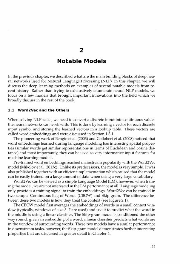
2
Notable Models
In the previous chapter, we described what are the main building blocks of deep neu-ral networks used for Natural Language Processing (NLP). In this chapter, we willdiscuss the deep learning methods on examples of several notable models from re-cent history. Rather than trying to exhaustively enumerate neural NLP models, wefocus on a few models that brought important innovations into the field which webroadly discuss in the rest of the book.
2.1 Word2Vec and the Others
When solving NLP tasks, we need to convert a discrete input into continuous valuesthe neural networks can work with. This is done by learning a vector for each discreteinput symbol and storing the learned vectors in a lookup table. These vectors arecalled word embeddings and were discussed in Section 1.3.1.
The pioneering work of Bengio et al. (2003) and Collobert et al. (2008) noticed thatword embeddings learned during language modeling has interesting spatial proper-ties (similar words get similar representations in terms of Euclidean and cosine dis-tance) and most importantly, they can be used as very informative input features formachine learning models.
Pre-trained word embeddings reached mainstream popularity with the Word2Vecmodel (Mikolov et al., 2013c). Unlike its predecessors, the model is very simple. It wasalso published together with an efficient implementation which caused that the modelcan be easily trained on a large amount of data when using a very large vocabulary.
Word2Vec can be viewed as a simple Language Model (LM), however, when train-ing the model, we are not interested in the LM performance at all. Language modelingonly provides a training signal to train the embeddings. Word2Vec can be trained intwo setups: Continuous Bag of Words (CBOW) and Skip-gram. The difference be-tween these two models is how they treat the context (see Figure 2.1).
The CBOW model first averages the embeddings of words in a small context win-dow (typically, windows of size 3–7 are used) and use it to predict what the word inthe middle is using a linear classifier. The Skip-gram model is conditioned the otherway round: given an embedding of a word, a linear classifier predicts what words arein the window of surrounding words. These two models have a similar performancein downstream tasks, however, the Skip-gram model demonstrates further interestingproperties that are discussed in greater detail in Chapter 4.
35
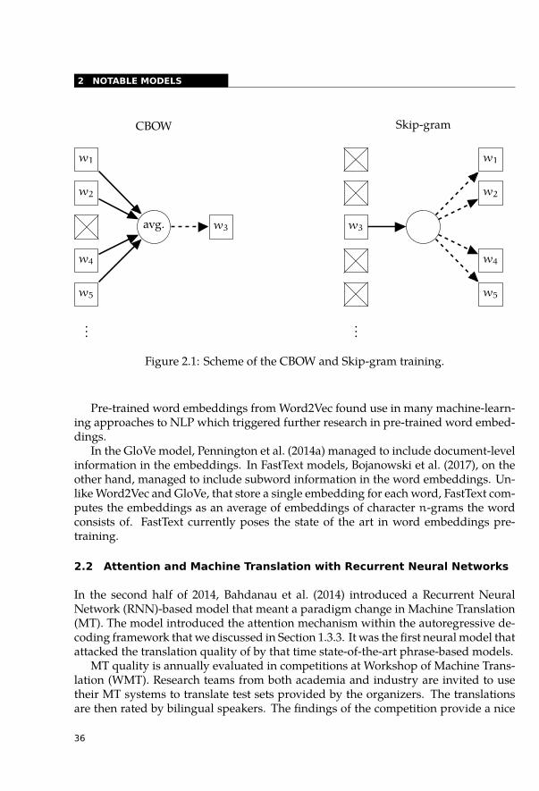
2 NOTABLE MODELS
..
CBOW
.
Skip-gram
.
avg.
.
w3
...w1.
w2
.
w4
.
w5
.
...
..
w3
. w1...
w2
...
w4
...
w5
...
...
Figure 2.1: Scheme of the CBOW and Skip-gram training.
Pre-trained word embeddings from Word2Vec found use in many machine-learn-ing approaches to NLP which triggered further research in pre-trained word embed-dings.
In the GloVe model, Pennington et al. (2014a) managed to include document-levelinformation in the embeddings. In FastText models, Bojanowski et al. (2017), on theother hand, managed to include subword information in the word embeddings. Un-like Word2Vec and GloVe, that store a single embedding for each word, FastText com-putes the embeddings as an average of embeddings of character n-grams the wordconsists of. FastText currently poses the state of the art in word embeddings pre-training.
2.2 Attention and Machine Translation with Recurrent Neural Networks
In the second half of 2014, Bahdanau et al. (2014) introduced a Recurrent NeuralNetwork (RNN)-based model that meant a paradigm change in Machine Translation(MT). The model introduced the attention mechanism within the autoregressive de-coding framework that we discussed in Section 1.3.3. It was the first neural model thatattacked the translation quality of by that time state-of-the-art phrase-based models.
MT quality is annually evaluated in competitions at Workshop of Machine Trans-lation (WMT). Research teams from both academia and industry are invited to usetheir MT systems to translate test sets provided by the organizers. The translationsare then rated by bilingual speakers. The findings of the competition provide a nice
36
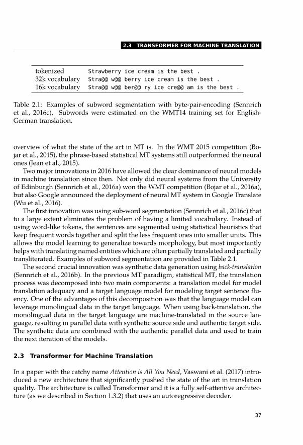
2.3 TRANSFORMER FOR MACHINE TRANSLATION
tokenized Strawberry ice cream is the best .32k vocabulary Stra@@ w@@ berry ice cream is the best .16k vocabulary Stra@@ w@@ ber@@ ry ice cre@@ am is the best .
Table 2.1: Examples of subword segmentation with byte-pair-encoding (Sennrichet al., 2016c). Subwords were estimated on the WMT14 training set for English-German translation.
overview of what the state of the art in MT is. In the WMT 2015 competition (Bo-jar et al., 2015), the phrase-based statistical MT systems still outperformed the neuralones (Jean et al., 2015).
Two major innovations in 2016 have allowed the clear dominance of neural modelsin machine translation since then. Not only did neural systems from the Universityof Edinburgh (Sennrich et al., 2016a) won the WMT competition (Bojar et al., 2016a),but also Google announced the deployment of neural MT system in Google Translate(Wu et al., 2016).
The first innovation was using sub-word segmentation (Sennrich et al., 2016c) thatto a large extent eliminates the problem of having a limited vocabulary. Instead ofusing word-like tokens, the sentences are segmented using statistical heuristics thatkeep frequent words together and split the less frequent ones into smaller units. Thisallows the model learning to generalize towards morphology, but most importantlyhelps with translating named entities which are often partially translated and partiallytransliterated. Examples of subword segmentation are provided in Table 2.1.
The second crucial innovation was synthetic data generation using back-translation(Sennrich et al., 2016b). In the previous MT paradigm, statistical MT, the translationprocess was decomposed into two main components: a translation model for modeltranslation adequacy and a target language model for modeling target sentence flu-ency. One of the advantages of this decomposition was that the language model canleverage monolingual data in the target language. When using back-translation, themonolingual data in the target language are machine-translated in the source lan-guage, resulting in parallel data with synthetic source side and authentic target side.The synthetic data are combined with the authentic parallel data and used to trainthe next iteration of the models.
2.3 Transformer for Machine Translation
In a paper with the catchy name Attention is All You Need, Vaswani et al. (2017) intro-duced a new architecture that significantly pushed the state of the art in translationquality. The architecture is called Transformer and it is a fully self-attentive architec-ture (as we described in Section 1.3.2) that uses an autoregressive decoder.
37
2 NOTABLE MODELS
Transformer-based models show better modeling capabilities, but still heavily de-pend on the innovations invented for RNN-based models, i.e., sub-word text segmen-tation and back-translation. Models based on the Transformer were the best-scoringmodels in all tasks in recent WMT competitions (Bojar et al., 2018; Barrault et al., 2019).
From today’s view, the invention of the Transformer architecture was the crucialinnovation that found use in almost all areas of NLP. Because it can be heavily par-allelized, it allows non-autoregressive text generation (Gu et al., 2018; Libovický andHelcl, 2018). Moreover, it is the basis of the current pre-trained representation models(Devlin et al., 2019; Liu et al., 2019b) that significantly pushed the state of the art inmany NLP tasks and that we also discuss later in the chapter.
In 2017, research teams competing in the annual WMT competition did not man-age to take advantage of the recent invention, the best-performing systems in the com-petition were based on RNNs (Sennrich et al., 2017; Bojar et al., 2017). However, in2018 and 2019, all the best-performing systems were already based on Transformers(Junczys-Dowmunt, 2018; Bojar et al., 2018; Barrault et al., 2019).
2.4 CoVe: Contextual Embeddings are Born
The first experiments with model probing (discussed in detail in Chapter 6) discov-ered that hidden states of the sequence processing network carry a lot of informationabout the input sentence. This was especially pronounced in the case of the MT en-coder that needs to capture the source meaning in such a way that the decoder cangenerate a full sentence in the target language (Hill et al., 2017; Adi et al., 2017).
McCann et al. (2017) leveraged this observation and used a trained encoder froman MT model for transfer learning. They were also the first ones to explicitly intro-duce the concept of contextual word vectors. In their approach, called CoVe ContextVectors (CoVe), they train a Neural Machine Translation (NMT) system with a 2-layerbidirectional Long Short-Term Memory (LSTM) encoder with Global Vectors for WordRepresentation (GloVe) word vectors on input, and then explicitly denote the result-ing hidden states as context vectors:
CoVe(w) = MT-LSTM(GloVe(w)) (2.1)
where w is the input word, GloVe is its pre-trained embedding vector, and MT-LSTMis the trained MT encoder state corresponding to the word; the equation is reproducedfrom (McCann et al., 2017).
Since CoVe, the term contextual word embeddings is often used to refer to hiddenstates of a model when these are used outside of the model as vector word repre-sentations. In this book, we often do not strictly differentiate between hidden statesand contextual word embeddings, as these are just different names for principally thesame thing; the terminology mostly reflects how the representations are used, not howthey are obtained.
38
2.5 ELMO: SESAME STREET BEGINS
Unlike standard NMT models that work with a relatively small vocabulary of tensof thousands of subword units, CoVe works on word level and uses GloVe embed-dings. These design decisions decrease the performance of the MT itself, on the otherhand, it allows using a large embedding table covering 2.2M word forms which wouldotherwise be impossible with an MT trained from random initialization.
CoVe was tested on a wide range of NLP tasks: sentiment analysis (Maas et al.,2011), question classification (Voorhees and Tice, 1999), entailment classification (Bow-man et al., 2015), and answer span selection (Rajpurkar et al., 2016) and reached state-of-the-art in all of them.
2.5 ELMo: Sesame Street Begins
Another pre-trained contextual representation model that attracted the attention ofthe NLP community is called Embeddings using Language Models (ELMo). A pre-print announcing CoVe was published in August 2017 on arXiv, and the first preprintof a paper announcing ELMo appeared only two months later on OpenReview. ELMois a part of the AllenNLP software package (Gardner et al., 2018) which also con-tributed to the popularity of the model before CoVe found wider use. Also, the paperintroducing ELMo was awarded as the best paper at the NAACL 2018 conference.
Unlike CoVe that uses the encoder from an NMT model, ELMo is pre-trained asa language model and thus only requires monolingual data for pre-training. This isa large advantage because parallel data in a sufficient amount are only available forrelatively few languages.
The architecture of ELMo (Peters et al., 2018a) is, in principle, similar to CoVe: itconsists of 2 two-layer unidirectional LSTMs. (It was preceded by a 1-layer variantcalled Language-Model-Augmented Sequence Tagger (TagLM) (Peters et al., 2017)which did not perform so well and did not receive such attention.) Instead of us-ing static word embeddings, ELMo uses a character-level Convolutional Neural Net-work (CNN) and a stack of feed-forward layers to obtain word representations that arepassed to the LSTMs, so the model can to some extent considered open-vocabulary.The scheme of the architecture is shown in Figure 2.2.
ELMo is trained as two LMs: one in the forward and one in the backward di-rection while sharing the input representation and the output layer. The standardbidirectional network cannot be used here. In bidirectional RNNs, every output statecontains information about the entire input sequence. The sequence-labeling com-ponent of the LM would only learn to copy the input tokens to the output withoutany generalization. As a result, 4 LSTM states correspond to each input word afterrunning the model.
The model was trained on the 1 billion word benchmark for language modeling(Chelba et al., 2014). Surprisingly, the forward and backward LM reach approximatelythe same perplexity. The evaluation using similar tasks as CoVe and several more
39
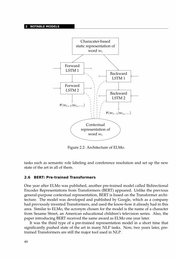
2 NOTABLE MODELS
..Characater-based
static representation ofword wi
.
ForwardLSTM 1
.
ForwardLSTM 2
.
P(wi+1|wi, . . .)
.
BackwardLSTM 1
.
BackwardLSTM 2
.
P(wi−1|wi, . . .)
.
Contextualrepresentation of
word wi
Figure 2.2: Architecture of ELMo.
tasks such as semantic role labeling and coreference resolution and set up the newstate of the art in all of them.
2.6 BERT: Pre-trained Transformers
One year after ELMo was published, another pre-trained model called BidirectionalEncoder Representations from Transformers (BERT) appeared. Unlike the previousgeneral-purpose contextual representation, BERT is based on the Transformer archi-tecture. The model was developed and published by Google, which as a companyhad previously invented Transformers, and used the know-how it already had in thisarea. Similar to ELMo, the acronym chosen for the model is the name of a characterfrom Sesame Street, an American educational children’s television series. Also, thepaper introducing BERT received the same award as ELMo one year later.
It was the third type of a pre-trained representation model in a short time thatsignificantly pushed state of the art in many NLP tasks. Now, two years later, pre-trained Transformers are still the major tool used in NLP.
40
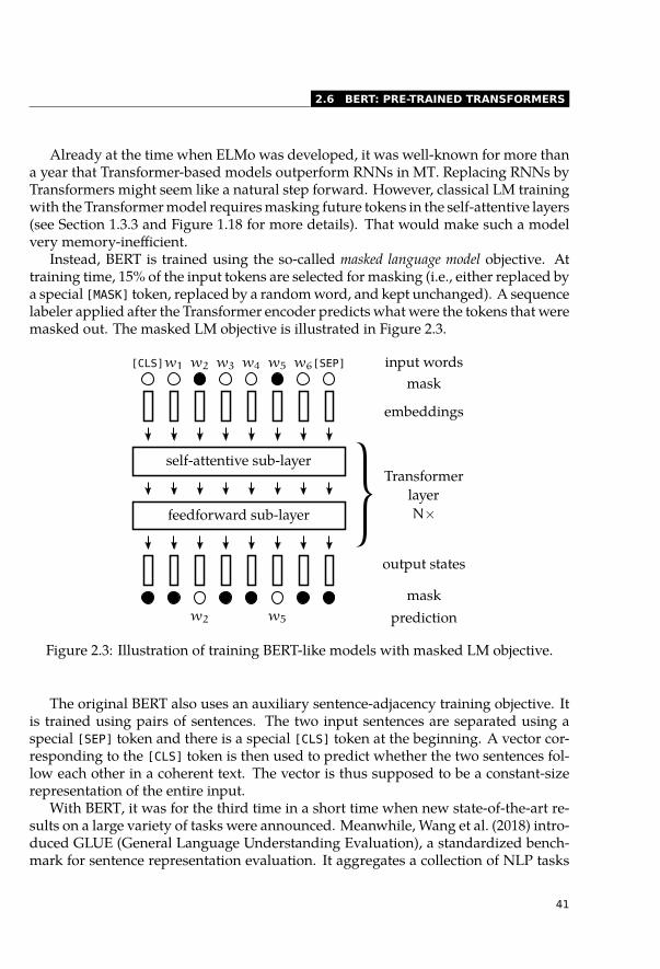
2.6 BERT: PRE-TRAINED TRANSFORMERS
Already at the time when ELMo was developed, it was well-known for more thana year that Transformer-based models outperform RNNs in MT. Replacing RNNs byTransformers might seem like a natural step forward. However, classical LM trainingwith the Transformer model requires masking future tokens in the self-attentive layers(see Section 1.3.3 and Figure 1.18 for more details). That would make such a modelvery memory-inefficient.
Instead, BERT is trained using the so-called masked language model objective. Attraining time, 15% of the input tokens are selected for masking (i.e., either replaced bya special [MASK] token, replaced by a random word, and kept unchanged). A sequencelabeler applied after the Transformer encoder predicts what were the tokens that weremasked out. The masked LM objective is illustrated in Figure 2.3.
self-attentive sub-layer
[CLS]w1 w2 w3 [SEP]w6w5w4
feedforward sub-layer
w2 w5
embeddings
maskinput words
maskprediction
output states
N×
Transformerlayer
Figure 2.3: Illustration of training BERT-like models with masked LM objective.
The original BERT also uses an auxiliary sentence-adjacency training objective. Itis trained using pairs of sentences. The two input sentences are separated using aspecial [SEP] token and there is a special [CLS] token at the beginning. A vector cor-responding to the [CLS] token is then used to predict whether the two sentences fol-low each other in a coherent text. The vector is thus supposed to be a constant-sizerepresentation of the entire input.
With BERT, it was for the third time in a short time when new state-of-the-art re-sults on a large variety of tasks were announced. Meanwhile, Wang et al. (2018) intro-duced GLUE (General Language Understanding Evaluation), a standardized bench-mark for sentence representation evaluation. It aggregates a collection of NLP tasks
41
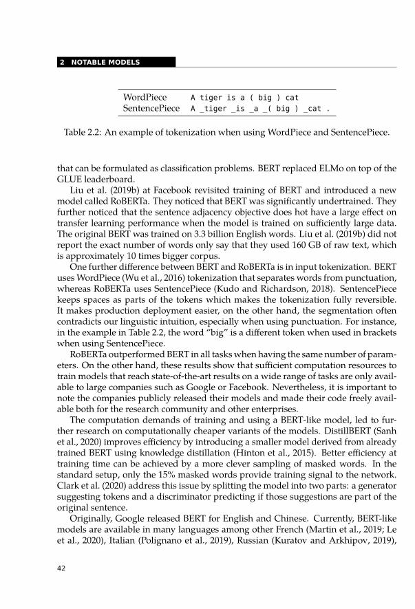
2 NOTABLE MODELS
WordPiece A tiger is a ( big ) catSentencePiece A _tiger _is _a _( big ) _cat .
Table 2.2: An example of tokenization when using WordPiece and SentencePiece.
that can be formulated as classification problems. BERT replaced ELMo on top of theGLUE leaderboard.
Liu et al. (2019b) at Facebook revisited training of BERT and introduced a newmodel called RoBERTa. They noticed that BERT was significantly undertrained. Theyfurther noticed that the sentence adjacency objective does hot have a large effect ontransfer learning performance when the model is trained on sufficiently large data.The original BERT was trained on 3.3 billion English words. Liu et al. (2019b) did notreport the exact number of words only say that they used 160 GB of raw text, whichis approximately 10 times bigger corpus.
One further difference between BERT and RoBERTa is in input tokenization. BERTuses WordPiece (Wu et al., 2016) tokenization that separates words from punctuation,whereas RoBERTa uses SentencePiece (Kudo and Richardson, 2018). SentencePiecekeeps spaces as parts of the tokens which makes the tokenization fully reversible.It makes production deployment easier, on the other hand, the segmentation oftencontradicts our linguistic intuition, especially when using punctuation. For instance,in the example in Table 2.2, the word “big” is a different token when used in bracketswhen using SentencePiece.
RoBERTa outperformed BERT in all tasks when having the same number of param-eters. On the other hand, these results show that sufficient computation resources totrain models that reach state-of-the-art results on a wide range of tasks are only avail-able to large companies such as Google or Facebook. Nevertheless, it is important tonote the companies publicly released their models and made their code freely avail-able both for the research community and other enterprises.
The computation demands of training and using a BERT-like model, led to fur-ther research on computationally cheaper variants of the models. DistillBERT (Sanhet al., 2020) improves efficiency by introducing a smaller model derived from alreadytrained BERT using knowledge distillation (Hinton et al., 2015). Better efficiency attraining time can be achieved by a more clever sampling of masked words. In thestandard setup, only the 15% masked words provide training signal to the network.Clark et al. (2020) address this issue by splitting the model into two parts: a generatorsuggesting tokens and a discriminator predicting if those suggestions are part of theoriginal sentence.
Originally, Google released BERT for English and Chinese. Currently, BERT-likemodels are available in many languages among other French (Martin et al., 2019; Leet al., 2020), Italian (Polignano et al., 2019), Russian (Kuratov and Arkhipov, 2019),
42
2.7 GPT AND GPT-2
Spanish (Cañete et al., 2020), Finish (Yang et al., 2020) or Turkish (Schweter, 2020),mostly developed either by local academic institutions or rarely by local enterprises.
In addition to that, the original release of BERT included a multilingual version ofBERT that was trained for 104 languages. During training, the model is not informedabout the language identity and only works with plain text. Facebook later appliedthe methodology used for RoBERTa to a multilingual model and developed XLM-R(Conneau et al., 2020) covering 100 languages and significantly outperforming mul-tilingual BERT. The multilingual model is used mostly for zero-shot learning withlanguages for which we do not have training data (Pires et al., 2019) or when traininga single model for multiple languages using the shared representation (Kondratyukand Straka, 2019).
2.7 GPT and GPT-2
At around the same as BERT, Radford et al. (2019a) from Open AI, a US-based non-profit private research laboratory published a pre-trained Transformer-based languagemodel which they called Generative Pre-Trained Transformer (GPT). Similar to BERTand ELMo, they used the hidden state of the model as input features in a wide rangeof downstream tasks, and for a time before BERT was published they set a new stateof the art in few NLP tasks.
The following version of the model from February 2019, GPT-2 (Radford et al.,2019b) attracted much more attention. It was trained on 40 GB of web text, approx-imately 5 times more than BERT. The biggest version of the model has around 1.5billion parameters, which is 18 times more than the standard version of BERT and 5times more than BERT Large.
GPT-2 showed an excellent performance in a so-called zero-shot setup in tasks likequestion answering or text summarization. In the zero-shot setup, the model is notfinetuned on task-specific training data but used in the generative setup. For questionanswering it means: the model is given the question on the input followed with anatural language command that an answer should follow (typically something like“Answer:”) and we let the model continue in the same way as when we generate atarget sentence in machine translation models. In most of the tasks, the performanceis significantly below the state of the art, however, the zero-shot performance was stilla large surprise for the community.
The authors of the model were reluctant to publish the model because of poten-tial misuse of the model (Solaiman et al., 2019), e.g., for better automation of fraudu-lent email management, generating abusive content on social networks, or fake news.Although it might be difficult for humans to distinguish a genuine and machine-generated text, it can be relatively easily automatically detected (Gehrmann et al.,2019). Also because of that, the authors decided that the benefits for the researchcommunity of having access to the model outweigh potential risks and released themodel in November 2019.
43
2 NOTABLE MODELS
2.8 Conclusion
In this chapter, we have described several models that from today’s perspective posemilestones for developing models for NLP. With the exception of MT, which is an im-portant task itself, all the other models only provide vector representation of languageinput that is later used in particular NLP tasks. The pre-trained word embeddingscombined with light-weight recurrent architectures are still an important choice inpractical applications under limited resource conditions and when model speed is anissue. However, nowadays, the pre-trained Transformers reach the state of the art inalmost all NLP tasks.
44
3
Interpretation of Neural Networks
Neural Networks (NNs) are state-of-the-art models in many Machine Learning (ML)tasks. These NNs are usually trained end-to-end and treated as a black box1 after train-ing. With rising capabilities and deployment of these models, the demand grows inthe last few years for understanding the inner workings, or interpretation, of thesemodels. Interpretability may be important for trusting the model in a real-world set-ting, general human curiosity, detecting bias in the models, or increasing social ac-ceptance of modern technologies (Molnar, 2020).
Interpretation as a source of trust is most important when ML models’ potentialerrors have serious consequences, such as in medical applications or self-driving cars.In Natural Language Processing (NLP), applications such as machine translation maybenefit from this approach to interpretation. Bias detection is vital in applicationssuch as automatic CV (curriculum vitae) analysis.
Human curiosity is also a strong motivation for posing questions concerning whichlinguistic concepts manifest in NNs and if NNs approach language differently fromhumans.
Just as there is not only a single reason to be interested in interpretation, there isno single definition of the concept of interpretation itself. There is no mathemati-cal definition of interpretation (Molnar, 2020). Lipton (2018) notes that “the task ofinterpretation appears underspecified,” and the “concept of interpretability appears si-multaneously important and slippery”. Miller (2019) defines interpretability as “thedegree to which a human can understand the cause of a decision,” which leaves uswith a similarly vague notion of understanding.
One way to avoid this issue in the context of a specific research question is to statein the beginning what does the presented view of interpretation entail (see Montavonet al. (2018) for an example2 of this practice). However, this approach is rarely usedin research papers, and it will not help us with a general overview. The use of the
1 “A Black Box Model is a system that does not reveal its internal mechanisms. In machine learning, ”blackbox” describes models that cannot be understood by looking at their parameters (e.g., a neural network).”(Molnar, 2020, Section 1.3)
2 They proceed by giving a sequence of definitions that are progressively more specific and delimit therange of methods that they are concerned with: “An interpretation is the mapping of an abstract concept(e.g., a predicted class) into a domain that the human can make sense of.”, “An explanation is the collectionof features of the interpretable domain, that have contributed for a given example to produce a decision(e.g., classification or regression).” (Montavon et al., 2018)
45
3 INTERPRETATION OF NEURAL NETWORKS
concept of interpretation of NNs varies significantly in the literature and is rarelymade explicit.
Since we cannot produce a unified concept, we may at least try to sort the var-ious ways in which researchers use the term. Lipton (2018) distinguishes betweentwo main groups of properties of interpretable models: transparency and post-hoc in-terpretability.
Transparency consists of understanding the mechanism by which the model works.The understanding is achieved by selecting a model architecture and a training algo-rithm that is sufficiently simple (or decomposable) to be understandable. Restrictingthe complexity of the machine learning model to achieve interpretability is also calledintrinsic interpretability (Molnar, 2020). Linear regression, logistic regression, and thedecision tree are often considered interpretable (Molnar, 2020). However, as Lipton(2018) points out, “neither linear models, rule-based systems, nor decision trees areintrinsically interpretable. Sufficiently high-dimensional models, unwieldy rule lists,and deep decision trees could all be considered less transparent than comparativelycompact neural networks.” Building transparent ML models is also sometimes calledexplainable Artificial Intelligence (AI). Due to the complexity of NLP tasks, models thatare simple enough to be interpretable in this sense cannot produce good results andtherefore are rarely used.
Post-hoc (or extrinsic) interpretability is a way of extracting information from mod-els that are already trained. The “advantage of this concept of interpretability is thatwe can interpret opaque models after-the-fact, without sacrificing predictive perfor-mance” (Lipton, 2018).
With the current deep NNs used in NLP, we can only talk about the extrinsic in-terpretability, which is also what we are interested in the rest of the book. Ratherthan developing intrinsically interpretable algorithms, we present empirical post-hocinterpretation of state-of-the-art NLP models in the last five years.
We can divide the methods of post-hoc interpretability into two categories, struc-tural and behavioral analysis; we can also distinguish visualization as a third separatemethod.
Structural analysis, with which we deal in this book, analyzes and interprets theinternal parameters of trained models, such as emergent word representations (em-beddings) or attentions. In linguistical structural interpretation, we try to find cor-respondences of the internal representations to existing linguistic abstractions, suchas part of speech labels or syntactic structures; this may involve (and typically in-volves) searching for linguistic abstractions which the model was not explicitly trainedto learn (e.g., searching for morphological features in a machine translation model).Structural analysis can be performed both in a supervised way (probing) as well as inunsupervised ways. We describe these two approaches in this section.
Behavioral analysis observes the behavior of the trained model on the task forwhich it was trained, typically using specially constructed inputs to investigate thebehavior of the model in specific situations to see what the model can or cannot do.
46
3.1 SUPERVISED METHODS: PROBING
Behavioral analysis treats the model as a black box, not directly analyzing its learnedparameters. We do not deal with behavioral analysis in this book; please refer, e.g.,to Section 4 of (Belinkov and Glass, 2019) for an overview.
Visualization methods are usually qualitative, and they can be used to present alarge amount of information.
Further information can also be found in the overview of methods for analyzingdeep learning models for NLP (Belinkov and Glass, 2019).
3.1 Supervised Methods: Probing
According to Belinkov and Glass (2019), the most common approach for examininglinguistic properties in neural network components is using a classifier to predictthese properties from activations of the neural network. We refer to this approach asprobing. Probing models are also sometimes called auxiliary or diagnostic classifiersLiu et al. (2019a). At first, the term probing was used in general to refer to any post-hoc interpretations of neural networks. However, gradually the term shifted and isnow almost exclusively used for training supervised classifiers (see, e.g., Hewitt andManning (2019)), which is how we use the term in this book.
Probing requires data annotated for the studied property. This means that withprobing, we can only reveal the kind of information that we have previously decidedto look for in the representations and for which we have an annotated dataset.
This introduces a systemic bias into the research. It is easier to probe for proper-ties that are already described in formal linguistic frameworks with large annotateddatasets. The results that find these properties in the representations then retroac-tively affirm the correctness of the conceptualization and design decisions made forthe annotation. There have been recent efforts for probing to standardize test data(Gül Şahin et al., 2019).
Peters et al. (2018a) use a linear classifier to probe for Part of Speech (PoS) in Em-beddings using Language Models (ELMo) and CoVe Context Vectors (CoVe), assert-ing that “[a]s the linear classifier adds only a small amount of model capacity, this is adirect test of the [contextual] representation”. We (Rosa et al., 2020) show that such anassertion may be problematic without careful evaluation of the memorization effect,which can occur even with a linear classifier, but in the setting used by authors, therisk of memorization is not large.
Hewitt and Liang (2019) measured probe’s selectivity, i.e., the difference of accu-racy for linguistic and control tasks. For instance, one linguistic task was PoS tagging,and the corresponding control task was retrieving randomly assigned tags to words.
3.2 Unsupervised Methods: Clustering and Component Analysis
Unsupervised methods go in the other direction than supervised methods. Super-vised methods start from the abstraction that we want to find and try to train a classi-
47
3 INTERPRETATION OF NEURAL NETWORKS
fier to extract it from the representation. With unsupervised methods, we first analyzethe features that emerge in the representations and only then do we try to map themto existing linguistic abstractions. A prototypical example of an unsupervised struc-tural analysis method is clustering. We first cluster the representations, then observethe clusters and search for an existing set of labels that can be assigned to them.
Unsupervised methods reduce the bias inherent in the choice of the informationto classify in probing. On the other hand, the results are usually harder to quantify.
We can illustrate this with an example. In (Musil, 2019), we show that it is possi-ble to train a probing classifier that labels PoS based on the Czech word embeddingsfrom a Neural Machine Translation (NMT) encoder. However, this merely shows thatit may be possible to divide the high dimensional space by criteria that are mostly ar-bitrary but do not by themselves prove that this division is important for the NMTsystem. The unsupervised approach shows that in the first few dimensions of Prin-cipal Component Analysis (PCA), the embeddings form clusters that correspond toPoS, suggesting that PoS is indeed important for the encoder. However, probing en-abled us to easily compare embeddings from different sources in a quantitative way,by comparing the accuracy of the probing classifier. That is not possible with theunsupervised approach.
There is a number of unsupervised approaches that can be used to analyze variouscomponents of the neural models, either analyzing the models directly or after apply-ing various transformations. We review here two groups of transformation methods:clustering and component analysis.
Clustering is a method of grouping datapoints together based on their similarity.The resulting groups (clusters) can then be assigned with labels. A shortcoming ofclustering is that it is “hard” by default, i.e., each data point belongs to exactly onecluster. This problem can be partially alleviated by hierarchical clustering, whichprovides more fine-grained information about similarities of the clusters and thusindirectly about the similarity of the data points in different clusters.
Component Analysis Component analysis is a process of transforming a multidi-mensional space (e.g., word embeddings) with the goal of obtaining interpretable fea-tures as the components of the transformed space. We describe two methods in detail,PCA in Section 4.6 and Independent Component Analysis (ICA) in Section 4.7.
3.3 Network Layers and Linguistic Units
In analyzing and interpreting internal NN representations of language input, we of-ten take the representations and investigate how they correspond to some existinglinguistic abstractions. For this, we obviously need to be able to map the representa-tions to individual language units, such as words and sentences.
48
3.3 NETWORK LAYERS AND LINGUISTIC UNITS
As most of the models we deal with in this book take a single sentence as theirinput, it is relatively straightforward to map their internal representations to the sen-tences.3
However, for analyzing words, we are facing two crucial problems. One is basedon the fact that in most NN models used in NLP, only the input-layer embeddingsdirectly correspond to words, while the hidden states4 in the subsequent process-ing layer cannot be easily mapped directly to words; one hidden state might encodevarious kinds of information about various words. Moreover, current NLP modelstypically do not operate on words but rather on subwords, making the mapping ofthe representations to words even harder.
In this section, we review the problems and discuss available ways of dealing withthem.
3.3.1 Words versus States
NLP models employ various mechanisms of passing information between individuallayers of the model. However, be it Convolutional Neural Networks (CNNs), Recur-rent Neural Networks (RNNs) or Self-Attentive Networks (SANs), what they all havein common is that the mechanism enables information about individual input wordsto be mixed, strengthened, weakened, shifted forward and backward, etc. In the ini-tial layer, the word representations (static embeddings) are context-independent, andthus the representation at a given position corresponds to and only to the input wordat the same position (i.e., the ith embedding corresponds to the ith input word). Insubsequent layers, however, the representations (hidden states) at any position may,in theory, correspond to any and all input words.5 It may thus be that a given ithstate corresponds mostly to the ith word, but it may also be that it mostly representsthe i+ 1th word, it may combine under various weights some information about thei − 1th word with some other information about the ith word, etc.6 Most NLP mod-els are not explicitly forced during training to keep the correspondence of the inputwords and hidden states at the same positions.7 On a related note, it has been shownthat the neural network models are apt at storing information useful for them at any
3 However, we do not largely deal with analyzing sentence-level representations in this book.4 As explained in Section 2.4, in our text, we often do not strictly differentiate between hidden states and
contextual word embeddings.5 The architecture may limit this to some extent, e.g., by using residual connections that explicitly pass
through the state from the previous layer, or CNNs which have a finite kernel size.6 Technically, as weights within a neural model are rarely exactly zero, a given state typically contains some
information about all of the input words to some extent. However, the distributions of the weights areoften quite peaked rather than flat, which means that a given hidden state is typically mostly determinedby only a few aspects of a few input words.
7 Residual connections may partially encourage this correspondence. Some models are also forced to rep-resent the input words by the output states at the corresponding positions, which may encourage them(but not force them) to keep this correspondence even in internal hidden states.
49
3 INTERPRETATION OF NEURAL NETWORKS
available place, especially if storing the information at the default place is disabled,as we will discuss later in Section 5.3.
However, multiple studies found that typically, the hidden states tend to be cen-tered on the input words, i.e., that the i-th hidden state typically mostly contains in-formation about the i-th input word.
Already the work of Bahdanau et al. (2014) states that “Each (hidden state) hi con-tains information about the whole input sequence with a strong focus on the partssurrounding the i-th word of the input sequence.”, and “Due to the tendency of RNNsto better represent recent inputs, the (hidden state) hj will be focused on the wordsaround xj.” However, it is not clear from the work whether the authors have somesolid arguments for these claims or whether these are rather intuitive expectations.
Some indirect evidence is provided by Koehn and Knowles (2017), who find thatin an attention-based NMT system, there is typically a 75% match between the sourceword most attended to while producing a given target word, and the source wordaligned to the target word by standard word-aligner. Supposing that the informationabout the aligned source word is the most important, we can deduce that the corre-sponding hidden state mostly contains information about that word. However, theauthors also found that for one of their examined setups, the attention is typically offby one, mostly attending to the word following the aligned word, which may either becaused by the decoder operating with the information about the word to translate inthe next step, and/or by the hidden state representations to be shifted by one withrespect to the input words (see Section 5.1).
Ethayarajh (2019) provides some further evidence, showing that for ELMo, Bidi-rectional Encoder Representations from Transformers (BERT) and Generative Pre-Trained Transformer (GPT) models, the cosine self-similarity of contextual represen-tations of a word (the similarity of contextual representations of occurrences of thesame word in different contexts) is practically always greater than the cosine similar-ity to contextual embeddings of other words.8 The context-specific information withinthe contextual embedding can become quite strong, but the signal corresponding tothe identity of the word at the given position seems to stay stronger than the signalscorresponding to any other word.
Thus, even though this is not perfectly accurate, it is common to refer to the i-thhidden state as a state corresponding to the i-th input word, implying that the i-th hid-den state somehow represents the i-th input word, in the context of the input sentence(as well as in the context of the task which the NN system is trained to perform).
8 The self-similarity is lowest for stopwords (such as common determiners, prepositions, and conjunctions),which are rather semantically vacuous and mostly fulfill a syntactic function within their immediate con-text.
50
3.3 NETWORK LAYERS AND LINGUISTIC UNITS
3.3.2 Words versus Subwords
As discussed in Sections 2.5 and 2.6, current NLP models typically do not operatedirectly on words, but their input is first tokenized into subwords, which has manyimportant benefits. Therefore, in the network, there are usually no explicit repre-sentations of words, as all embeddings and hidden states are only computed for thesubwords.
While subwords are a very useful concept for most NLP end tasks, they pose aproblem for linguistic interpretations of the trained models, as many linguistic for-malisms, such as PoS or syntax, are based on words. A notable exception is the no-tion of morphs and morphemes, which correspond to parts of words and are thussimilar to NN subwords in principle; however, multiple studies have found that mor-phemes and subwords seem to be very different and cannot be easily mapped to eachother (Sennrich et al., 2016c; Banerjee and Bhattacharyya, 2018; Bostrom and Durrett,2020). Therefore, the base unit on which most NN models operate, a subword, is hardto map to any linguistic abstraction, which poses important challenges for linguisticinterpretation of such models.
There are three common workarounds to this problem.
From Words to Subwords
The first option is modifying the linguistic abstraction to apply to subwords. For ex-ample, for PoS tagging, we might assign the same PoS tag to all subwords (so, e.g.,“hell ic opter” would be labelled “NOUN NOUN NOUN”). Alternatively we mightlabel the first subword with the tag of the original word and the subsequent sub-words with a special continuation tag (so “hell ic opter” would be labeled for ex-ample “NOUN –NOUN –NOUN” or “NOUN – –”). This is especially natural whendealing with linguistic abstractions that span multiple words, such as named entitiesor syntactic phrases, where it makes little difference whether the span is composedof several words or a slightly larger number of subwords (Mareček and Rosa, 2019).However, for strictly word-based concepts, such as PoS tags, morphological labels, ordependency syntax, this approach does not seem adequate, as it is not straightforwardto see which linguistic feature should be captured in which subword or subwords ofthe original word and thus how the individual subwords should be labeled. This ap-proach thus may be useful for training NLP models to solve such tasks, but not forlinguistically interpreting such models.
From Subwords to Words
A second option is to reconstruct word representations from the subword represen-tations ex post. This is usually done by taking the average of the subword representa-tions (i.e., mean-pooling), although other options are also possible, such as taking the
51
3 INTERPRETATION OF NEURAL NETWORKS
sum of the representations,9 max-pooling the representations, or training and apply-ing a small NN to perform a non-linear combination of the subword representations(Libovický et al., 2020). This makes it then straightforward to analyze the word rep-resentations for word-level linguistic features. However, it should be kept in mindthat in this case, we are not directly analyzing the representations in the network, butonly their transformation, which we performed ourselves, which makes the analysispartially indirect, and any findings obtained via this method should be carefully as-sessed on the possible influences of the used word embedding reconstruction ontothe analysis (for example, if we find that PoS is seemingly more strongly encodedin representations of short words than long words, it is quite possible that in fact, itis strongly encoded only in some subwords of the long words and therefore seemsweaker in the average of the subword representations).
Fully Word-Based Approach
The third workaround is to train the model for analysis in a word-based manner,without using the subword tokenization (Rosa et al., 2020). While this gets rid ofthe problem completely, making the interpretation straightforward, this also meansthat we are, in fact, analyzing different models than the ones that are actually used inpractice (typically, word-based models are significantly weaker than subword-basedmodels). If our goal is to understand a particular model or set of models used in prac-tice, it is quite unclear how an analysis of a slightly different model relates to this, asthe difference of using words instead of subwords may have a large impact on howthe models work internally. These kinds of analyses are thus highly trustworthy ininterpreting the analyzed word-based models – arguably more trustworthy than anysimilar analyses of the subword-based models, as they operate directly on words in allsteps without the need of the somewhat ad hoc word-to-subword or subword-to-wordmappings which may introduce some noise into the analyses. However, we shouldbe very wary about any interpretative claims about the subword-based models basedon analyses of word-based models, as there is no clear reason why the findings madefor one class of the models should also hold for the other class.
3.4 Conclusion
Although the concept of interpretation is somewhat vague and lacking a proper the-ory, we can distinguish a few important directions in the expanding field of interpret-ing neural networks in NLP. Training probing classifiers, transforming and visualiz-ing the variable space, and constructing challenge sets for behavioral analysis seem
9 Summation and mean-pooling are very similar operations and can often be used interchangeably. How-ever, since words are split into variable-length sequences of subwords, using summation instead of mean-pooling leads to the resulting vectors varying in their norm, which is irrelevant if they are only comparedusing, e.g., cosine distance, but may be important in other usages.
52

3.4 CONCLUSION
to be the most important areas of research. In further chapters, we deal with the firsttwo.
However, any interpretation approach is potentially problematic. We discussedsome of the problems in this chapter, including the threat of mistaking probing clas-sifier memorization for model abstraction (especially with strong probing classifiers)or the difficulties involved in mapping network states to input words.
53

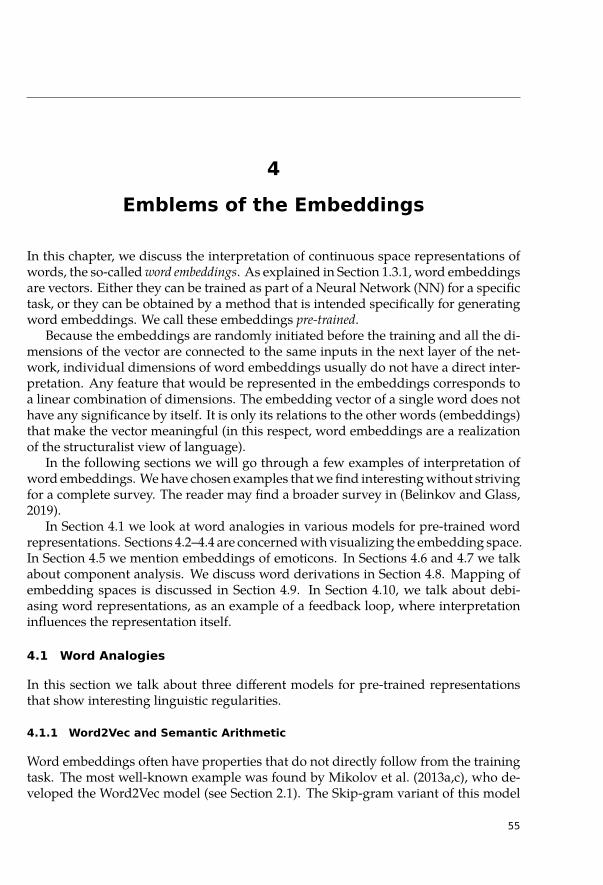
4
Emblems of the Embeddings
In this chapter, we discuss the interpretation of continuous space representations ofwords, the so-called word embeddings. As explained in Section 1.3.1, word embeddingsare vectors. Either they can be trained as part of a Neural Network (NN) for a specifictask, or they can be obtained by a method that is intended specifically for generatingword embeddings. We call these embeddings pre-trained.
Because the embeddings are randomly initiated before the training and all the di-mensions of the vector are connected to the same inputs in the next layer of the net-work, individual dimensions of word embeddings usually do not have a direct inter-pretation. Any feature that would be represented in the embeddings corresponds toa linear combination of dimensions. The embedding vector of a single word does nothave any significance by itself. It is only its relations to the other words (embeddings)that make the vector meaningful (in this respect, word embeddings are a realizationof the structuralist view of language).
In the following sections we will go through a few examples of interpretation ofword embeddings. We have chosen examples that we find interesting without strivingfor a complete survey. The reader may find a broader survey in (Belinkov and Glass,2019).
In Section 4.1 we look at word analogies in various models for pre-trained wordrepresentations. Sections 4.2–4.4 are concerned with visualizing the embedding space.In Section 4.5 we mention embeddings of emoticons. In Sections 4.6 and 4.7 we talkabout component analysis. We discuss word derivations in Section 4.8. Mapping ofembedding spaces is discussed in Section 4.9. In Section 4.10, we talk about debi-asing word representations, as an example of a feedback loop, where interpretationinfluences the representation itself.
4.1 Word Analogies
In this section we talk about three different models for pre-trained representationsthat show interesting linguistic regularities.
4.1.1 Word2Vec and Semantic Arithmetic
Word embeddings often have properties that do not directly follow from the trainingtask. The most well-known example was found by Mikolov et al. (2013a,c), who de-veloped the Word2Vec model (see Section 2.1). The Skip-gram variant of this model
55
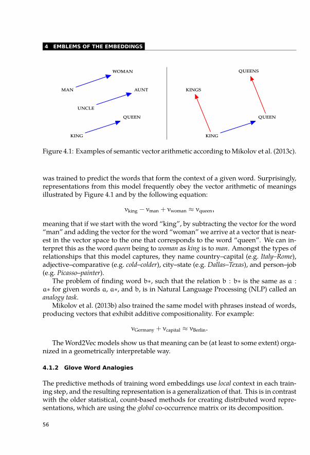
4 EMBLEMS OF THE EMBEDDINGS
..MAN.
WOMAN
.
UNCLE
. AUNT.
KING
.
QUEEN
..KINGS .
QUEENS
.
KING
.
QUEEN
Figure 4.1: Examples of semantic vector arithmetic according to Mikolov et al. (2013c).
was trained to predict the words that form the context of a given word. Surprisingly,representations from this model frequently obey the vector arithmetic of meaningsillustrated by Figure 4.1 and by the following equation:
vking − vman + vwoman ≈ vqueen,
meaning that if we start with the word “king”, by subtracting the vector for the word“man” and adding the vector for the word “woman” we arrive at a vector that is near-est in the vector space to the one that corresponds to the word “queen”. We can in-terpret this as the word queen being to woman as king is to man. Amongst the types ofrelationships that this model captures, they name country–capital (e.g. Italy–Rome),adjective–comparative (e.g. cold–colder), city–state (e.g. Dallas–Texas), and person–job(e.g. Picasso–painter).
The problem of finding word b∗, such that the relation b : b∗ is the same as a :a∗ for given words a, a∗, and b, is in Natural Language Processing (NLP) called ananalogy task.
Mikolov et al. (2013b) also trained the same model with phrases instead of words,producing vectors that exhibit additive compositionality. For example:
vGermany + vcapital ≈ vBerlin.
The Word2Vec models show us that meaning can be (at least to some extent) orga-nized in a geometrically interpretable way.
4.1.2 Glove Word Analogies
The predictive methods of training word embeddings use local context in each train-ing step, and the resulting representation is a generalization of that. This is in contrastwith the older statistical, count-based methods for creating distributed word repre-sentations, which are using the global co-occurrence matrix or its decomposition.
56
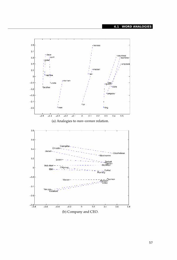
4.1 WORD ANALOGIES
(a) Analogies to man–woman relation.
(b) Company and CEO.
57
4 EMBLEMS OF THE EMBEDDINGS
(c) ZIP codes and cities.
(d) Comparison of adjectives.
Figure 4.2: Word analogies in the Glove embeddings. Reprinted from (Penningtonet al., 2014b).
58
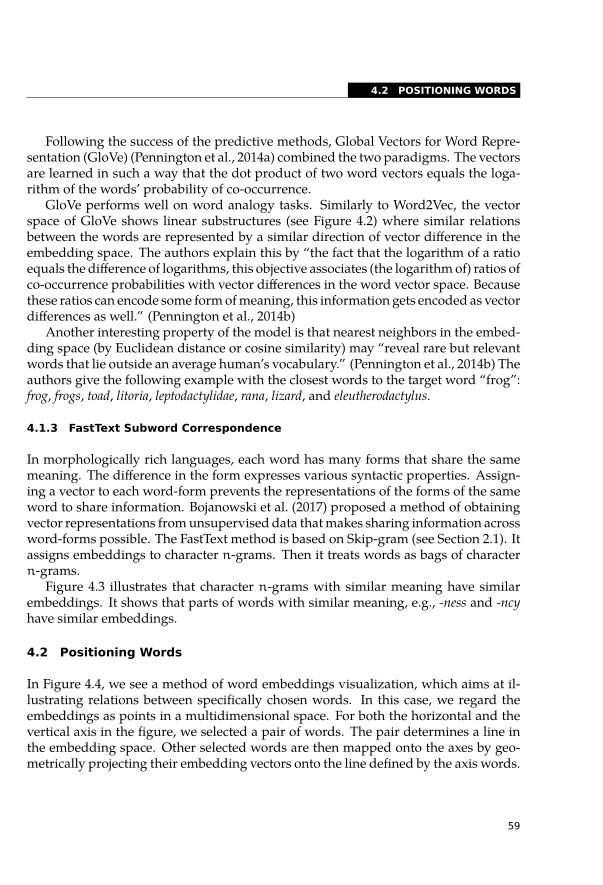
4.2 POSITIONING WORDS
Following the success of the predictive methods, Global Vectors for Word Repre-sentation (GloVe) (Pennington et al., 2014a) combined the two paradigms. The vectorsare learned in such a way that the dot product of two word vectors equals the loga-rithm of the words’ probability of co-occurrence.
GloVe performs well on word analogy tasks. Similarly to Word2Vec, the vectorspace of GloVe shows linear substructures (see Figure 4.2) where similar relationsbetween the words are represented by a similar direction of vector difference in theembedding space. The authors explain this by “the fact that the logarithm of a ratioequals the difference of logarithms, this objective associates (the logarithm of) ratios ofco-occurrence probabilities with vector differences in the word vector space. Becausethese ratios can encode some form of meaning, this information gets encoded as vectordifferences as well.” (Pennington et al., 2014b)
Another interesting property of the model is that nearest neighbors in the embed-ding space (by Euclidean distance or cosine similarity) may “reveal rare but relevantwords that lie outside an average human’s vocabulary.” (Pennington et al., 2014b) Theauthors give the following example with the closest words to the target word “frog”:frog, frogs, toad, litoria, leptodactylidae, rana, lizard, and eleutherodactylus.
4.1.3 FastText Subword Correspondence
In morphologically rich languages, each word has many forms that share the samemeaning. The difference in the form expresses various syntactic properties. Assign-ing a vector to each word-form prevents the representations of the forms of the sameword to share information. Bojanowski et al. (2017) proposed a method of obtainingvector representations from unsupervised data that makes sharing information acrossword-forms possible. The FastText method is based on Skip-gram (see Section 2.1). Itassigns embeddings to character n-grams. Then it treats words as bags of charactern-grams.
Figure 4.3 illustrates that character n-grams with similar meaning have similarembeddings. It shows that parts of words with similar meaning, e.g., -ness and -ncyhave similar embeddings.
4.2 Positioning Words
In Figure 4.4, we see a method of word embeddings visualization, which aims at il-lustrating relations between specifically chosen words. In this case, we regard theembeddings as points in a multidimensional space. For both the horizontal and thevertical axis in the figure, we selected a pair of words. The pair determines a line inthe embedding space. Other selected words are then mapped onto the axes by geo-metrically projecting their embedding vectors onto the line defined by the axis words.
59
4 EMBLEMS OF THE EMBEDDINGS
Figure 4.3: Similarity between character n-grams in FastText embeddings. Red in-dicates positive cosine, blue indicates negative. Reprinted from (Bojanowski et al.,2017).
60

4.2 POSITIONING WORDS
0.15
0.10
0.05
0.00
-0.05
-0.10
-0.15
-0.20
-0.25
-0.25 -0.20 -0.15 -0.10 -0.05 0.00 0.05 0.10 0.15 0.20 0.25sciencephilosophy
exac
tva
gue
semiotics
linguistics
math geology
biology
chemistryphysics
Figure 4.4: Word vectors for names of selected scientific disciplines ploted relative tothe axis formed by the vectors for the vector differences between the words philosophy–science and exact–vague. This image was generated by a web service that we are nolonger able to find.
50100150200250300Ve
ctor
dim
ensi
on
Vocabulary (frequency ordered)50000 100000 150000 200000 250000
Figure 4.5: Horizontal bands in the Glove word embeddings. Each column representsone embedding vector. The columns are sorted by the frequency of the words theyrepresent, with the most frequent on the right. Reprinted from (Pennington et al.,2014b).
61
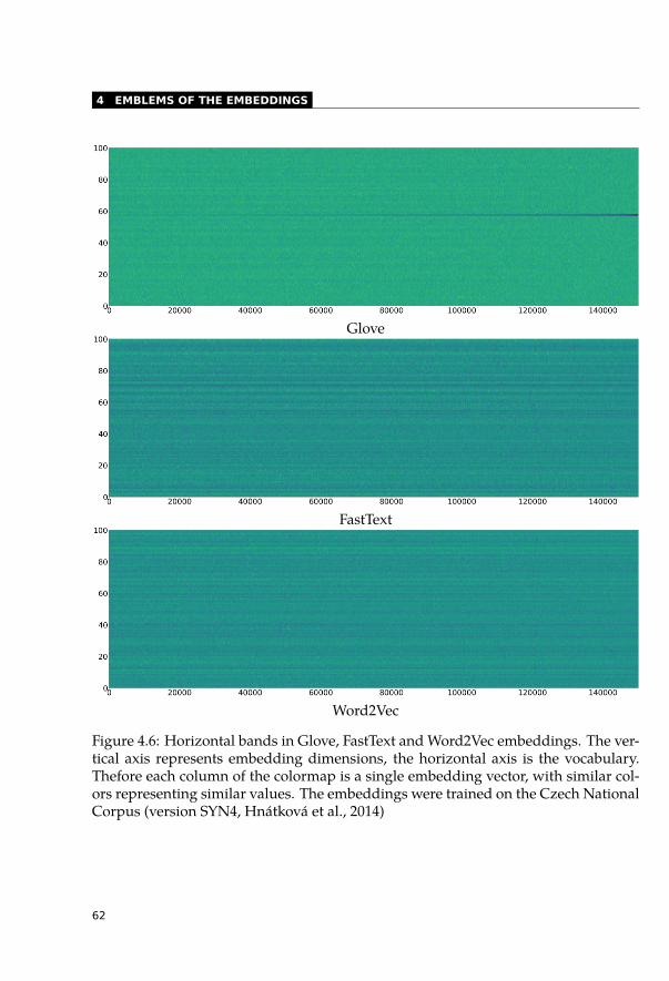
4 EMBLEMS OF THE EMBEDDINGS
Glove
FastText
Word2Vec
Figure 4.6: Horizontal bands in Glove, FastText and Word2Vec embeddings. The ver-tical axis represents embedding dimensions, the horizontal axis is the vocabulary.Thefore each column of the colormap is a single embedding vector, with similar col-ors representing similar values. The embeddings were trained on the Czech NationalCorpus (version SYN4, Hnátková et al., 2014)
62
4.3 EMBEDDING BANDS
4.3 Embedding Bands
An interesting way to visualize embeddings is a colormap where the color of eachpixel represents one numeric value, and each column represents an embedding for aparticular word (Pennington et al., 2014b). In Figure 4.5, we see that there are horizon-tal bands that are more pronounced for more frequent words. The vertical bands arecaused by clusters of similar words with similar frequencies (such as numbers). Thehorizontal bands may result from the fact that the cost function of the model containsa dot product of the embeddings. The vectors are multiplied component-wise in thedot product, and this has a greater impact than additive interactions. According toPennington et al. (2014b), the bands are unlikely to have a linguistic origin, and thisfeature is not unique to GloVe. Figure 4.6 shows that other word vector models havethis property as well.
4.4 Visualising Word Embeddings with T-SNE
Word embeddings typically have hundreds of dimensions. There are various ways toproject embeddings from the high-dimensional vector space to two or three dimen-sions to visualize them. One popular method is t-SNE (Maaten and Hinton, 2008).It is a stochastic method that aims to project vectors close to each other if they wereclose in the original vector space. You can see an example of t-SNE mapping in Fig-ure 4.7. The word embeddings in this figure are taken from a neural Language Model(LM), trained on the Czech part of the CzEng corpus (Bojar et al., 2016b). With Czechword embeddings, we can identify larger clusters organized by Part of Speech (PoS),divided into smaller clusters organized by meaning similarities.
4.5 Emoji Embeddings
An increasing volume of online communication contains emojis. Since they can berepresented in Unicode, it is possible to treat them the same way as standard text.
Illendula and Yedulla (2018) have successfully induced emoji embeddings basedon co-occurrence of emojis in tweets. The resulting embeddings helped them achievestate-of-the-art results in sentiment analysis, suggesting that the sentiment expressedby the emojis can be identified in this way.
A different approach was chosen by Eisner et al. (2016), who trained emoji em-beddings based on their Unicode descriptions. This also leads to better sentimentanalysis. The resulting embeddings visualized by t-SNE are shown in Figure 4.8. Wesee that emojis with similar meaning (e.g., state flags, astrological signs, animals) tendto form clusters.
63
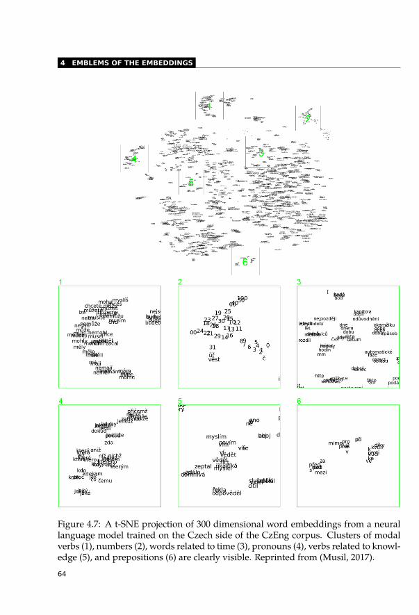
4 EMBLEMS OF THE EMBEDDINGS
Figure 4.7: A t-SNE projection of 300 dimensional word embeddings from a neurallanguage model trained on the Czech side of the CzEng corpus. Clusters of modalverbs (1), numbers (2), words related to time (3), pronouns (4), verbs related to knowl-edge (5), and prepositions (6) are clearly visible. Reprinted from (Musil, 2017).
64
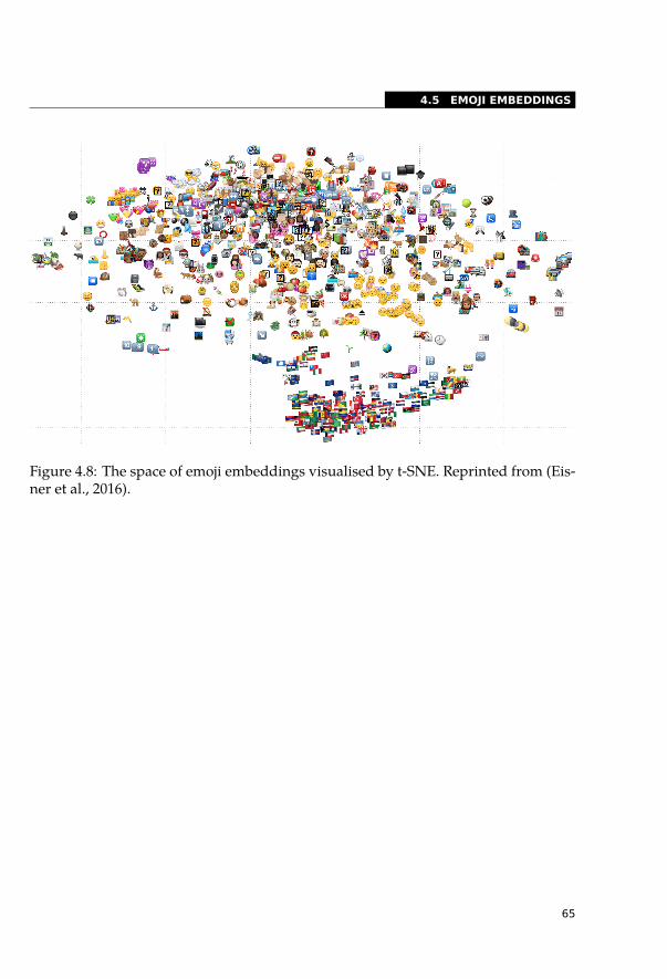
4.5 EMOJI EMBEDDINGS
Classification accuracy on entire dataset, N = 12920
Word Embeddings Random Forest Linear SVMGoogle News 57.5 58.5Google News + (Barbieri et al., 2016) 58.2* 60.0*
Google News + emoji2vec 59.5* 60.5*
Classification accuracy on tweets containing emoji, N = 2295
Word Embeddings Random Forrest Linear SVMGoogle News 46.0 47.1Google News + (Barbieri et al., 2016) 52.4* 57.4*
Google News + emoji2vec 54.4* 59.2*
Classification accuracy on 90% most frequent emoji, N = 2186
Word Embeddings Random Forrest Linear SVMGoogle News 47.3 45.1Google News + (Barbieri et al., 2016) 52.8* 56.9*
Google News + emoji2vec 55.0* 59.5*
Classification accuracy on 10% least frequent emoji, N = 308
Word Embeddings Random Forrest Linear SVMGoogle News 44.7 43.2Google News + (Barbieri et al., 2016) 53.9* 52.9*
Google News + emoji2vec 54.5* 55.2*
Table 1: Three-way classification accuracy on the Twitter sentiment analysis corpus using Random Forrests (Ho, 1995) and Linear
SVM (Fan et al., 2008) classifier with different word embeddings. ”*” denotes results with significance of p < 0.05 as calculated
by McNemar’s test, with the respect to classification with Google News embeddings per each classifier, and dataset
Figure 3: Emoji vector embeddings, projected down into a 2-dimensional space using the t-SNE technique. Note the clusters of
similar emojis like flags (bottom), family emoji (top left), zodiac symbols (top left), animals (left), smileys (middle), etc.Figure 4.8: The space of emoji embeddings visualised by t-SNE. Reprinted from (Eis-ner et al., 2016).
65
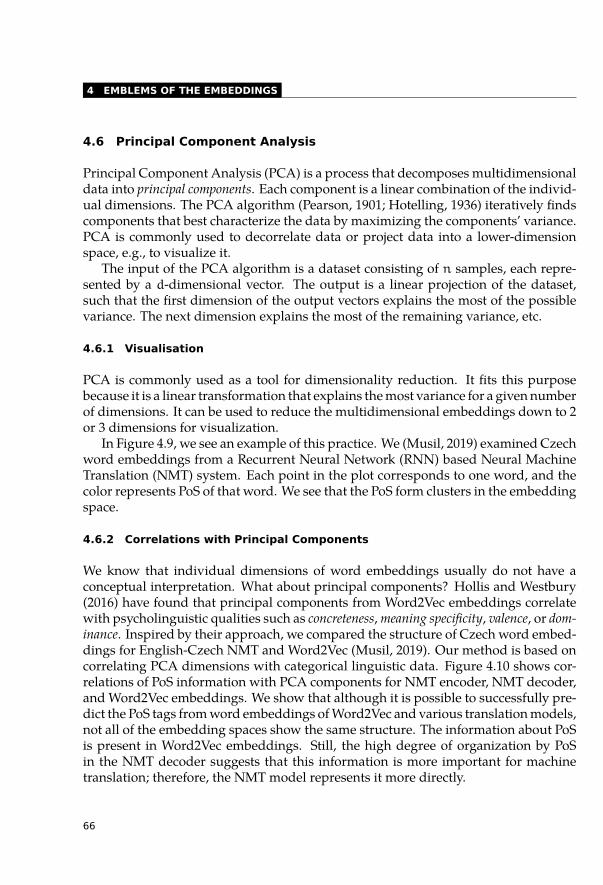
4 EMBLEMS OF THE EMBEDDINGS
4.6 Principal Component Analysis
Principal Component Analysis (PCA) is a process that decomposes multidimensionaldata into principal components. Each component is a linear combination of the individ-ual dimensions. The PCA algorithm (Pearson, 1901; Hotelling, 1936) iteratively findscomponents that best characterize the data by maximizing the components’ variance.PCA is commonly used to decorrelate data or project data into a lower-dimensionspace, e.g., to visualize it.
The input of the PCA algorithm is a dataset consisting of n samples, each repre-sented by a d-dimensional vector. The output is a linear projection of the dataset,such that the first dimension of the output vectors explains the most of the possiblevariance. The next dimension explains the most of the remaining variance, etc.
4.6.1 Visualisation
PCA is commonly used as a tool for dimensionality reduction. It fits this purposebecause it is a linear transformation that explains the most variance for a given numberof dimensions. It can be used to reduce the multidimensional embeddings down to 2or 3 dimensions for visualization.
In Figure 4.9, we see an example of this practice. We (Musil, 2019) examined Czechword embeddings from a Recurrent Neural Network (RNN) based Neural MachineTranslation (NMT) system. Each point in the plot corresponds to one word, and thecolor represents PoS of that word. We see that the PoS form clusters in the embeddingspace.
4.6.2 Correlations with Principal Components
We know that individual dimensions of word embeddings usually do not have aconceptual interpretation. What about principal components? Hollis and Westbury(2016) have found that principal components from Word2Vec embeddings correlatewith psycholinguistic qualities such as concreteness, meaning specificity, valence, or dom-inance. Inspired by their approach, we compared the structure of Czech word embed-dings for English-Czech NMT and Word2Vec (Musil, 2019). Our method is based oncorrelating PCA dimensions with categorical linguistic data. Figure 4.10 shows cor-relations of PoS information with PCA components for NMT encoder, NMT decoder,and Word2Vec embeddings. We show that although it is possible to successfully pre-dict the PoS tags from word embeddings of Word2Vec and various translation models,not all of the embedding spaces show the same structure. The information about PoSis present in Word2Vec embeddings. Still, the high degree of organization by PoSin the NMT decoder suggests that this information is more important for machinetranslation; therefore, the NMT model represents it more directly.
66
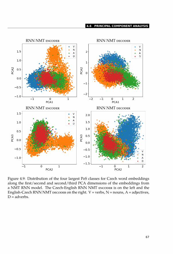
4.6 PRINCIPAL COMPONENT ANALYSIS
RNN NMT ENCODER RNN NMT DECODER
RNN NMT ENCODER RNN NMT DECODER
Figure 4.9: Distribution of the four largest PoS classes for Czech word embeddingsalong the first/second and second/third PCA dimensions of the embeddings froma NMT RNN model. The Czech-English RNN NMT ENCODER is on the left and theEnglish-Czech RNN NMT DECODER on the right. V = verbs, N = nouns, A = adjectives,D = adverbs.
67
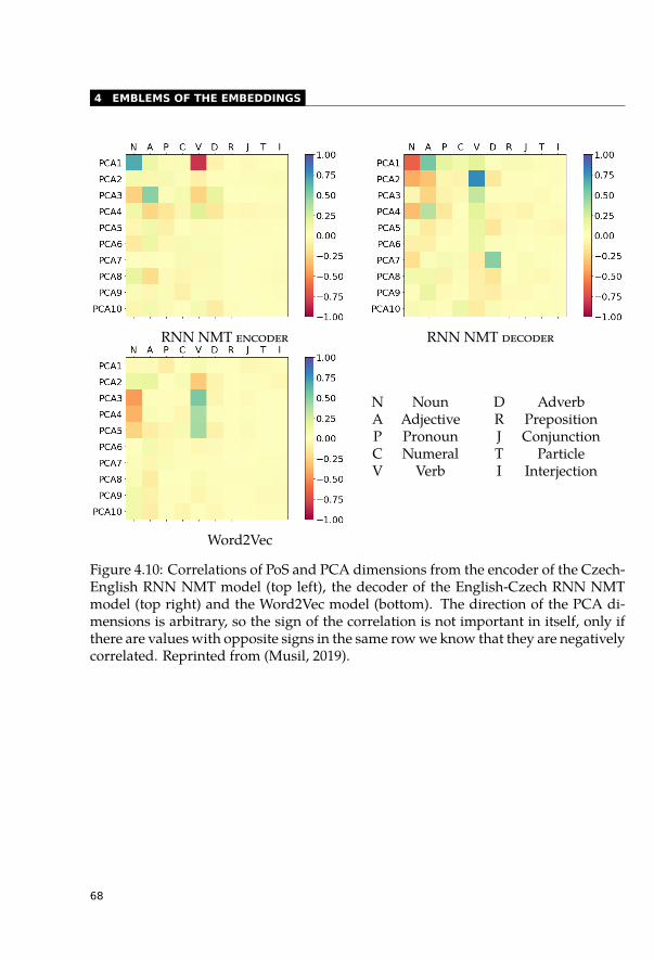
4 EMBLEMS OF THE EMBEDDINGS
RNN NMT ENCODER RNN NMT DECODER
N NounA AdjectiveP PronounC NumeralV Verb
D AdverbR PrepositionJ ConjunctionT ParticleI Interjection
Word2Vec
Figure 4.10: Correlations of PoS and PCA dimensions from the encoder of the Czech-English RNN NMT model (top left), the decoder of the English-Czech RNN NMTmodel (top right) and the Word2Vec model (bottom). The direction of the PCA di-mensions is arbitrary, so the sign of the correlation is not important in itself, only ifthere are values with opposite signs in the same row we know that they are negativelycorrelated. Reprinted from (Musil, 2019).
68
4.6 PRINCIPAL COMPONENT ANALYSIS
4.6.3 Histograms of Principal Components
We also show that further examining histograms of classes along the principal com-ponent is important to understand the structure of representation of information inembeddings (Musil, 2019):
Look at the histograms of the four most important PoS classes along the dimen-sions of the PCA of the embeddings in Figure 4.11. The histogram for the first dimen-sion of the RNN NMT ENCODER embeddings (Fig. 4.11, bottom left) demonstrates thatin this dimension, verbs are separated from the rest of the PoS categories.
For the first PCA dimension of the RNN NMT DECODER embeddings, nouns areconcentrated on one side, adjectives on the other side, and verbs with adverbs are inthe middle.
For the second PCA dimension of the RNN NMT DECODER embeddings, verbs areconcentrated on one side, and all other categories are on the other side.
The second PCA dimension shows an interesting distribution of nouns. There isa separate cluster of nouns, which is even more apparent if we plot the distributionalong two PCA dimensions in a planar graph in Figure 4.9. When we take a sampleof words from this cluster, it contains almost exclusively named entities: Fang, Eliáši,Još, Aenea, Bush, Eddie, Zlatoluna, Gordon, Bellondová, and Hermiona.
There is a similar distribution of nouns in the third PCA dimension of the RNNNMT DECODER embeddings. The smaller group again consists of named entities.
This is a stronger result than just being able to predict these categories with a clas-sifier: not only can the PoS (named entities, verb forms, and possibly other categories)be inferred from the embeddings, but the embeddings space is structured accordingto these categories.
4.6.4 Sentiment Analysis
Sentiment analysis is the task of deciding whether the given text is positive or nega-tive, how much, and what makes it so.
We have found (Musil, 2019) that the shape of the space of word embeddings fora model trained for sentiment analysis is triangular. We examined a ConvolutionalNeural Network (CNN) trained to predict the sentiment of comments in a Czechfilm database. In Figure 4.12, we see a sample of the words plotted along the firsttwo principal components. The first component represents the polarity of the words(good/bad); the second component represents intensity (strong/neutral). The trian-gular shape may be explained by the fact that words that are far from the center onthe polarity axis are never of low intensity. This is an example of a neural networkadapting to a specific task.
69
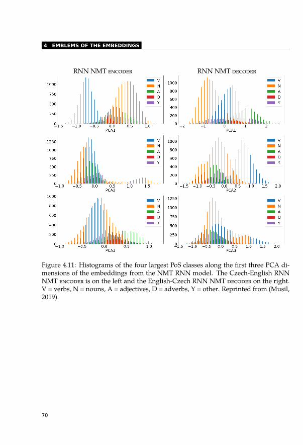
4 EMBLEMS OF THE EMBEDDINGS
RNN NMT ENCODER RNN NMT DECODER
Figure 4.11: Histograms of the four largest PoS classes along the first three PCA di-mensions of the embeddings from the NMT RNN model. The Czech-English RNNNMT ENCODER is on the left and the English-Czech RNN NMT DECODER on the right.V = verbs, N = nouns, A = adjectives, D = adverbs, Y = other. Reprinted from (Musil,2019).
70
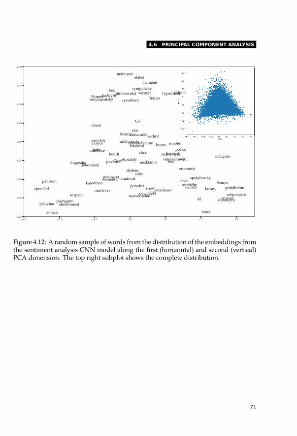
4.6 PRINCIPAL COMPONENT ANALYSIS
..−0.3
.−0.2
.−0.1
.0.0
.0.1
.0.2
.0.3
.
−0.20
.
−0.15
.
−0.10
.
−0.05
.
0.00
.
0.05
.
0.10
.
0.15
.
0.20
.
nezklamal
.
Stoupa
.
neúnosně
.
autobuse
.
vizí
.
cíleně
.
věky
.
vyvolával
.
Lugosiho
.
zraje
.
95
.
počkej
.
ovládnout
.
Co
.
mimozemská
.
sledem
.
krasny
.
nevadi
.
jedinců
.
nejdojemnější
.
dokoukání
.
Olga
.
slabsi
.
hodili
.
připomněl
.
luxusně
.
sympaticky
.
napodobeniny
.
bod
.
pochopím
.
sledovanost
.
neuvěřitelné
.
připadaly
.
provždy
.
zprznění
.
vypadnout
.
žlutá
.
srovnává
.
vysvětlení
.
box
.
chce
.
show
.
zvracet
.
kuře
.
nicméně
.
pořádná
.
pičovina
.
prvenství
.
Tereza
.
sice
.
pověsit
.
věčným
.
událostech
.
společenský
.
DiCaprio
.
velkolepější
.
penisem
.
budovat
.
sestřičky
.
utrpeni
.
sedmé
.
Mortal
.
nesympatický
.
úžasnými
.
mnoho
.
zábavnější
.
neznámými
.
jazyce
.
Hunter
.
dementů
.
každym
.
ka
.
studoval
.
umělecká
.
boom
.
rozvod
.
geniálnímu
Figure 4.12: A random sample of words from the distribution of the embeddings fromthe sentiment analysis CNN model along the first (horizontal) and second (vertical)PCA dimension. The top right subplot shows the complete distribution.
71
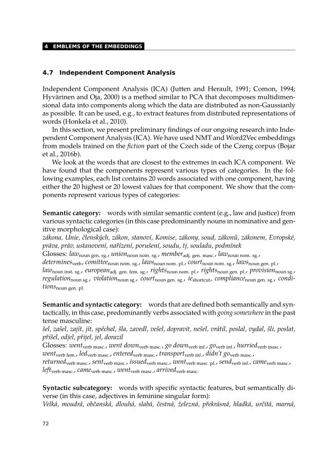
4 EMBLEMS OF THE EMBEDDINGS
4.7 Independent Component Analysis
Independent Component Analysis (ICA) (Jutten and Herault, 1991; Comon, 1994;Hyvärinen and Oja, 2000) is a method similar to PCA that decomposes multidimen-sional data into components along which the data are distributed as non-Gaussianlyas possible. It can be used, e.g., to extract features from distributed representations ofwords (Honkela et al., 2010).
In this section, we present preliminary findings of our ongoing research into Inde-pendent Component Analysis (ICA). We have used NMT and Word2Vec embeddingsfrom models trained on the fiction part of the Czech side of the Czeng corpus (Bojaret al., 2016b).
We look at the words that are closest to the extremes in each ICA component. Wehave found that the components represent various types of categories. In the fol-lowing examples, each list contains 20 words associated with one component, havingeither the 20 highest or 20 lowest values for that component. We show that the com-ponents represent various types of categories:
Semantic category: words with similar semantic content (e.g., law and justice) fromvarious syntactic categories (in this case predominantly nouns in nominative and gen-itive morphological case):zákona, Unie, členských, zákon, stanoví, Komise, zákony, soud, zákonů, zákonem, Evropské,práva, práv, ustanovení, nařízení, porušení, soudu, tj, souladu, podmínekGlosses: lawnoun gen. sg., unionnoun nom. sg., memberadj. gen. masc., lawnoun nom. sg.,determinesverb, comitteenoun nom. sg., lawsnoun nom. pl., courtnoun nom. sg., lawsnoun gen. pl.,lawnoun inst. sg., europeanadj. gen. fem. sg., rightsnoun nom. pl., rightsnoun gen. pl., provisionnoun sg.,regulationnoun sg., violationnoun sg., courtnoun gen. sg., ieshortcut, compliancenoun gen. sg., condi-tionsnoun gen. pl.
Semantic and syntactic category: words that are defined both semantically and syn-tactically, in this case, predominantly verbs associated with going somewhere in the pasttense masculine:šel, zašel, zajít, jít, spěchal, šla, zavedl, vešel, dopravit, nešel, vrátil, poslal, vydal, šli, poslat,přišel, odjel, přijel, jel, dorazilGlosses: wentverb masc., went downverb masc., go downverb inf., goverb inf., hurriedverb masc.,wentverb fem., ledverb masc., enteredverb masc., transportverb inf., didn’t goverb masc.,returnedverb masc., sentverb masc., issuedverb masc., wentverb masc. pl., sendverb inf., cameverb masc.,leftverb masc., cameverb masc., wentverb masc., arrivedverb masc.
Syntactic subcategory: words with specific syntactic features, but semantically di-verse (in this case, adjectives in feminine singular form):Velká, moudrá, občanská, dlouhá, slabá, čestná, železná, překrásná, hladká, určitá, marná,
72
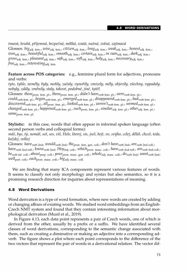
4.8 WORD DERIVATIONS
tmavá, hrubá, příjemná, bezpečná, měkká, svatá, nutná, volná, zajímaváGlosses: bigadj. fem., wiseadj. fem., citizenadj. fem., longadj. fem., weakadj. fem., honestadj. fem.,ironadj. fem., beautifuladj. fem., smoothadj. fem., certainadj. fem., in vainadj. fem., darkadj. fem.,grossadj. fem., pleasantadj. fem., safeadj. fem., softadj. fem., holyadj. fem., necessaryadj. fem.,freeadj. fem., interestingadj. fem.
Feature across POS categories: e.g., feminine plural form for adjectives, pronounsand verbs:tyto, tyhle, neměly, byly, mohly, začaly, vynořily, zmizely, měly, objevily, všechny, vypadaly,nebyly, zdály, změnily, staly, takové, podobné, jiné, tytéžGlosses: thesepron. fem. pl., thosepron. fem. pl., didn’t haveverb fem. pl., wereverb fem. pl.,couldverb fem. pl., beganverb fem. pl., emergedverb fem. pl., disappearedverb fem. pl., hadverb fem. pl.,discoveredverb fem. pl., allpron. fem. pl., lookedverb fem. pl., weren’tverb fem. pl., seemedverb fem. pl.,changedverb fem. pl., happenedverb fem. pl., suchpron. fem. pl., similaradj. fem. pl., otheradj. fem. pl.,samepron. fem. pl.
Stylistic: in this case, words that often appear in informal spoken language (oftensecond person verbs and colloquial forms):máš, bys, tý, nemáš, seš, ses, víš, Hele, kterej, sis, jseš, bejt, vo, svýho, celej, děláš, chceš, teda,každej, velkejGlosses: haveverb 2nd, wouldverb 2nd, thepron. fem. gen. coll., don’t haveverb 2nd, areverb 2nd coll.,haveverb 2nd refl., knowverb 2nd, Heyintj. coll., whichpron. masc. coll., haveverb 2nd refl., areverb 2nd coll.,beverb inf. coll., aboutprep. coll., yourpron. masc. gen. coll., wholeadj. masc. coll., doverb 2nd, wantverb 2nd,wellpart. coll., eachpron. masc. coll., bigadj. masc. coll.
We are finding that many ICA components represent various features of words.It seems to classify not only morphology and syntax but also semantics, so it is apromising research direction for inquiries about representations of meaning.
4.8 Word Derivations
Word derivation is a type of word formation, where new words are created by addingor changing affixes of existing words. We studied word embeddings from an English-Czech NMT system and found that they contain interesting information about mor-phological derivation (Musil et al., 2019).
In Figure 4.13, each data point represents a pair of Czech words, one of which isderived from the other, usually by a prefix or a suffix. We have identified severalclasses of word derivations, corresponding to the semantic change associated withthem, such as creating a diminutive or making an adjective into a corresponding ad-verb. The figure shows a plot where each point corresponds to the difference of thetwo vectors that represent the pair of words in a derivational relation. The vector dif-
73
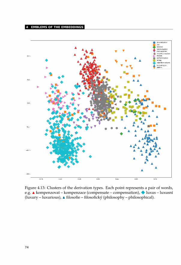
4 EMBLEMS OF THE EMBEDDINGS
Figure 4.13: Clusters of the derivation types. Each point represents a pair of words,e.g. ▲ kompenzovat – kompenzace (compensate – compensation), ■ luxus – luxusní(luxury – luxurious), ▲ filosofie – filosofický (philosophy – philosophical).
74
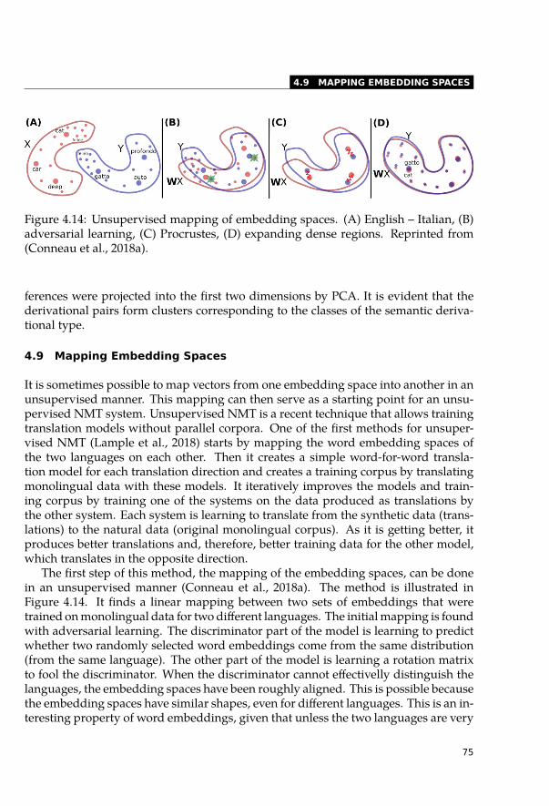
4.9 MAPPING EMBEDDING SPACES
Figure 4.14: Unsupervised mapping of embedding spaces. (A) English – Italian, (B)adversarial learning, (C) Procrustes, (D) expanding dense regions. Reprinted from(Conneau et al., 2018a).
ferences were projected into the first two dimensions by PCA. It is evident that thederivational pairs form clusters corresponding to the classes of the semantic deriva-tional type.
4.9 Mapping Embedding Spaces
It is sometimes possible to map vectors from one embedding space into another in anunsupervised manner. This mapping can then serve as a starting point for an unsu-pervised NMT system. Unsupervised NMT is a recent technique that allows trainingtranslation models without parallel corpora. One of the first methods for unsuper-vised NMT (Lample et al., 2018) starts by mapping the word embedding spaces ofthe two languages on each other. Then it creates a simple word-for-word transla-tion model for each translation direction and creates a training corpus by translatingmonolingual data with these models. It iteratively improves the models and train-ing corpus by training one of the systems on the data produced as translations bythe other system. Each system is learning to translate from the synthetic data (trans-lations) to the natural data (original monolingual corpus). As it is getting better, itproduces better translations and, therefore, better training data for the other model,which translates in the opposite direction.
The first step of this method, the mapping of the embedding spaces, can be donein an unsupervised manner (Conneau et al., 2018a). The method is illustrated inFigure 4.14. It finds a linear mapping between two sets of embeddings that weretrained on monolingual data for two different languages. The initial mapping is foundwith adversarial learning. The discriminator part of the model is learning to predictwhether two randomly selected word embeddings come from the same distribution(from the same language). The other part of the model is learning a rotation matrixto fool the discriminator. When the discriminator cannot effectivelly distinguish thelanguages, the embedding spaces have been roughly aligned. This is possible becausethe embedding spaces have similar shapes, even for different languages. This is an in-teresting property of word embeddings, given that unless the two languages are very
75
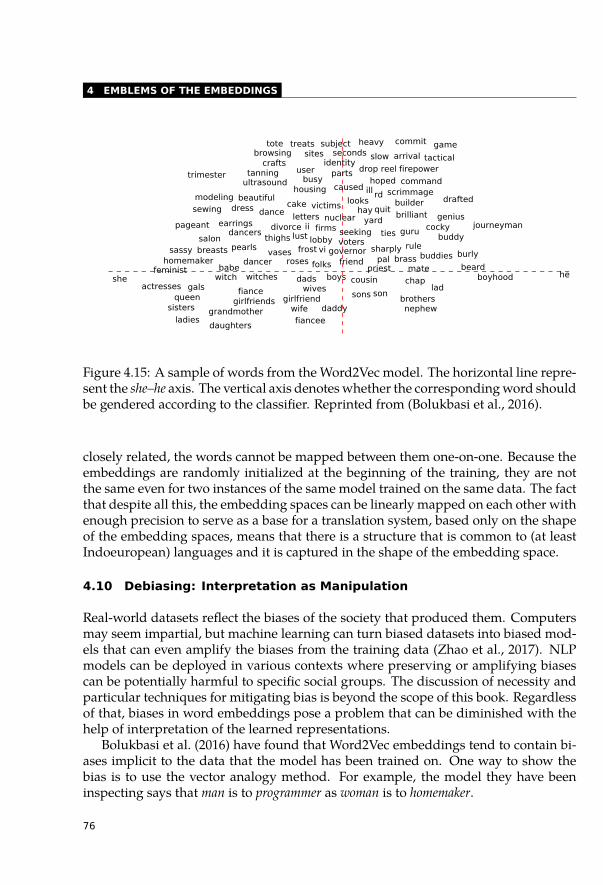
4 EMBLEMS OF THE EMBEDDINGS
heshe
geniusbrilliant
priesthomemaker
feminist
divorce
drafted
earrings
beautifuldress
dancers
modeling
crafts
dancerbuddies
guru
sewing
cocky
pearls
dance
salon
firepower
ultrasound
witch witches
sassy
builder
tactical
buddy
burly
tanningtrimester
mate
scrimmage
pageant
babe
command
tote
vasesrule
commit
thighs
journeyman
brotherssisters
queen
beard
breasts
chap
arrivalbrowsing
actressesfiance
nuclear
seconds
caused
drop
seeking
looks
subject
voters
friend
parts
sites
yard
housing
victims
governor
boys
heavy
slow
user
firms
busy hoped
ties
letters
identity
folks
quit
sharply
sonsgirlfriend
daughters
lobby
grandmother
cousin
ladies
cake
treats
wives
nephew
brassroses
daddy
fiancee
dads
reel
girlfriends
frost
lust
boyhoodgals
game
wife
lad
ill
ii
pal
hay
vi
rd
son
Figure 4.15: A sample of words from the Word2Vec model. The horizontal line repre-sent the she–he axis. The vertical axis denotes whether the corresponding word shouldbe gendered according to the classifier. Reprinted from (Bolukbasi et al., 2016).
closely related, the words cannot be mapped between them one-on-one. Because theembeddings are randomly initialized at the beginning of the training, they are notthe same even for two instances of the same model trained on the same data. The factthat despite all this, the embedding spaces can be linearly mapped on each other withenough precision to serve as a base for a translation system, based only on the shapeof the embedding spaces, means that there is a structure that is common to (at leastIndoeuropean) languages and it is captured in the shape of the embedding space.
4.10 Debiasing: Interpretation as Manipulation
Real-world datasets reflect the biases of the society that produced them. Computersmay seem impartial, but machine learning can turn biased datasets into biased mod-els that can even amplify the biases from the training data (Zhao et al., 2017). NLPmodels can be deployed in various contexts where preserving or amplifying biasescan be potentially harmful to specific social groups. The discussion of necessity andparticular techniques for mitigating bias is beyond the scope of this book. Regardlessof that, biases in word embeddings pose a problem that can be diminished with thehelp of interpretation of the learned representations.
Bolukbasi et al. (2016) have found that Word2Vec embeddings tend to contain bi-ases implicit to the data that the model has been trained on. One way to show thebias is to use the vector analogy method. For example, the model they have beeninspecting says that man is to programmer as woman is to homemaker.
76
4.11 CONCLUSION
They trained a classifier to determine the words that should be gendered. Fig-ure 4.15 shows a sample of words from the model. The horizontal axis represents theshe-he direction in the embedding space. The vertical axis represents the score from amodel that predicts whether the word should be gendered. The horizontal line sep-arates the gendered words (below), such as brother, or queen and words that shouldnot be inherently gendered, such as genius or tanning. The words above the line thatare far from the center on the horizontal axis show gender bias. The debiasing pro-cess consists of finding these words and removing the gender dimension from theirembeddings.
4.11 Conclusion
There are two main techniques of interpretation for word embeddings: probing andcomponent analysis. With probing, we can show that various linguistic features arerepresented in the embeddings, depending on the task that the model is trained for.With component analysis, we can show what features are important for a given task.However, for more complex tasks, such as language modeling or machine translation,we do not yet understand the structure of the embedding space completely.
Pretrained word embeddings contain information about both morphology and lex-ical semantics. When the embeddings are trained for a specific task, the embeddingstend to be organized by the information that is important for the given task (e.g., emo-tional polarity for sentiment analysis).
77

5
May I Have Your Attention?
With the advent of neural networks in Natural Language Processing (NLP), tradi-tional linguistics-based methods such as parsing or word-alignment are no longer apart of modern NLP solutions. Instead, new mechanisms were introduced that arecapable of generating these linguistic abstractions latently, but of course, only if theyare needed and in the form most suitable for the particular task. The attention mech-anism (described in Sections 1.3.2 and 2.2) allows the network to consider each com-ponent individually (typically words or subwords) of the input (typically sentences)and to decide how much this component will contribute to currently computed in-put representation. It provides weighted links between the language units that canbe interpreted as a sentence structure relevant to the particular task. These emergentstructures may be compared to explicit discrete linguistically motivated structuressuch as dependency trees, constituency trees, word alignment, coreference links, orsemantic relations.
For example, consider syntactic trees, which have been widely used in the past asa preprocessing step for various NLP tasks and provided the systems with informa-tion about relations between words. The syntactic trees were learned from manuallyannotated treebanks. Such annotations required many design decisions on how tocapture specific language phenomena in the tree structure. Moreover, various NLPtasks might benefit from differently annotated trees. The main limitation of using thetreebanks is that the tree structures are discrete and include only a limited number ofrelations between words.
In the current neural architectures, the attention mechanism learns the relationsbetween tokens in an unsupervised way. With the current complex architectures,models can capture many different weighted relations between the same tokens overdifferent layers and attention-heads. Therefore, the structures generated by the atten-tion mechanism overcome the drawbacks of using explicit syntactic structures. Theyconsist of multiple complete graphs with weighted edges optimized for the targetNLP task.
However, the price paid for using the attention mechanism is very difficult in-terpretability. The number of relations the current neural architectures consider isenormous and makes the attention hard to interpret even when it is fully trained. For
79
5 MAY I HAVE YOUR ATTENTION?
example, for one 10-words-long sentence, instead of 10 discrete labelled edges in adependency tree, we have 20,736 real numbers in the attention mechanism.1
Our goal is to organize these vast amounts of numbers, find the underlying struc-ture of the attention mechanism, and visualize it. We want to find out to what extentthe self-attentions resemble syntactic relations, and cross-lingual attentions resembleword alignment as we know them from the original non-neural systems. We alsowant to investigate whether these structures differ across NLP tasks.
5.1 Cross-Lingual Attentions and Word Alignment
The term attention was first introduced by Bahdanau et al. (2014) for modelling wordalignments in neural machine translation, and its generalization then became a uni-versal approximation of NLP structures. This work was a breakthrough for the Neu-ral Machine Translation (NMT) systems since it brought the translation quality to thelevel of previously widely used phrase-based systems (see Section 2.2). Each time thetranslation model generates a word, it attends to (“looks at”) all the positions (tokens)in the source sentence representation and chooses the ones that are most relevant forthe current translation. The weighted average of the attended representations is thenused as input into a classifier predicting the target word to be generated. It is im-portant that the search itself is “soft”; non-negative weights are assigned to all thepositions. In practice, however, a trained model assigns typically only a small num-ber of positions with weights significantly greater than zero. Therefore, the concept ofword-alignment was preserved in the modern NMT systems; it was only transformedinto a softer and more flexible shape.
In the previously used phrase-based systems (Koehn et al., 2007), the word align-ment was used as a preprocessing step for developing phrase dictionaries. The con-nections between tokens were discrete. Each connection either was there or was not.Even though the algorithms for unsupervised word alignment (Och and Ney, 2000)were based on Expectation-Maximization algorithm and used probability distribu-tions, the resulting alignments were discrete. A specific symmetrization approacheswere needed to get the final word-alignment from the two one-directional 1-to-manyalignments.
In the early NMT architectures using a fixed-size transition vector (Sutskever et al.,2014), the word alignment disappeared entirely since the only transition between en-coder and decoder was one fixed-sized vector.
The connections between individual positions in source and target sentences re-turned with the attention mechanism, but with the following essential differences.First, the attention mechanism is soft and may be represented as a complete bipar-tite graph with weighted edges. Second, the attention mechanism connects only the
1 We consider BERT’s base model using the initial [CLS] and final [SEP] tokens. The number is computedfor ten subword units.
80
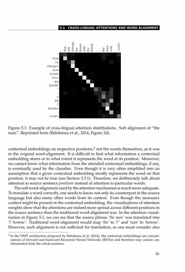
5.1 CROSS-LINGUAL ATTENTIONS AND WORD ALIGNMENT
" Th
isw
illch
an
ge
my
futu
rew
ith
my
fam
ily, " th
em
an
said
. <e
nd
>
"Ce la
vachanger
monavenir
avecma
famille",
adit
l'homme
.<end>
Figure 5.1: Example of cross-lingual attention distributions. Soft alignment of “theman”. Reprinted from (Bahdanau et al., 2014, Figure 3d).
contextual embeddings on respective positions,2 not the words themselves, as it wasin the original word-alignment. It is difficult to find what information a contextualembedding stores or to what extent it represents the word at its position. Moreover,we cannot know what information from the attended contextual embeddings, if any,is eventually used by the classifier. Even though it is very often simplified into anassumption that a given contextual embedding mostly represents the word on thatposition, it may not be true (see Section 3.3.1). Therefore, we deliberately talk aboutattention to source sentence positions instead of attention to particular words.
The soft word-alignment used by the attention mechanism is much more adequate.To translate a word correctly, one needs to know not only its counterpart in the sourcelanguage but also many other words from its context. Even though the necessarycontext might be present in the contextual embedding, the visualisations of attentionweights show that the attentions are indeed more spread across different positions inthe source sentence than the traditional word-alignment was. In the attention visual-isation in Figure 5.1, we can see that the source phrase ‘the man’ was translated into‘l’ homme’. Traditional word-alignment would map ‘the’ to ‘l’’ and ‘man’ to ‘homme’.However, such alignment is not sufficient for translation, as one must consider also
2 In the NMT architecture proposed by Bahdanau et al. (2014), the contextual embeddings are concate-nations of forward and backward Recurrent Neural Networks (RNNs) and therefore may contain anyinformation from the whole sentence.
81
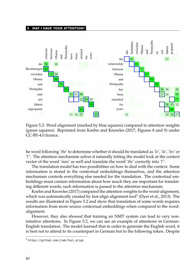
5 MAY I HAVE YOUR ATTENTION?
relatio
ns
between
Obama
and
Netanyahu
have
been
strained
for
years
.
dieBeziehungen
zwischen
Obama
undNetanjahu
sind
seit
Jahrenangespannt
.
56
89
72
16
26
96
79
98
42
11
11
14
38
22
84
23
54 10
98
49
das
Verhaltn
is
zwischen
Obama
und
Netanyahu
ist
seit
Jahren
gespannt
.
therelationship
between
Obama
andNetanyahu
has
been
stretched
foryears
. 11
47
81
72
87
93
95
38
21
17
16
14
38
19
33
90
32
26
54
77
12
17
Figure 5.2: Word alignment (marked by blue squares) compared to attention weights(green squares). Reprinted from Koehn and Knowles (2017, Figures 8 and 9) underCC-BY-4.0 licence.
he word following ‘the’ to determine whether it should be translated as ‘le’, ‘la’, ‘les’ or‘l’’. The attention mechanism solves it naturally letting the model look at the contextvector of the word ‘man’ as well and translate the word ‘the’ correctly into ‘l’’.
The translation model has two possibilities on how to deal with the context. Someinformation is stored in the contextual embeddings themselves, and the attentionmechanism controls everything else needed for the translation. The contextual em-beddings must contain information about how much they are important for translat-ing different words; such information is passed to the attention mechanism.
Koehn and Knowles (2017) compared the attention weights to the word-alignment,which was automatically created by fast-align alignment tool3 (Dyer et al., 2013). Theresults are illustrated in Figure 5.2 and show that translation of some words requiresinformation from more source contextual embeddings when compared to the word-alignment.
However, they also showed that training an NMT system can lead to very non-intuitive attentions. In Figure 5.2, we can see an example of attentions in German-English translation. The model learned that in order to generate the English word, itis best not to attend to its counterpart in German but to the following token. Despite
3 https://github.com/clab/fast_align
82
5.1 CROSS-LINGUAL ATTENTIONS AND WORD ALIGNMENT
such shifted attentions, this translation system had comparable results with other sys-tems, in which the attentions roughly matched the alignments.
The explanation of such a non-intuitive behaviour is probably a side effect of theend-to-end training setup. Although the architecture is designed to learn particu-lar words at particular places, it may sometimes be more convenient for the networkto learn the problem differently. Here the forward part of the encoder might put astrong emphasis on the previous word in its contextual representations. The atten-tion mechanism then prefers to attend to the following positions, which also representthe previous words well.
The mismatch between the attention mechanism and the word-alignment led someresearchers to develop systems that would increase the correspondence with word-alignments using some kind of supervision. For example, Liu et al. (2016) came withan additional loss function that penalized the disagreement between attention weightsand the conventional word-alignment models. In this way, they treated the attentionvariables as observable variables. The training objective then resembled that in themulti task-learning. However, all of these attempts gained no or only tiny improve-ments in translation quality.
Ghader and Monz (2017) published a more detailed analysis answering the ques-tion of what the attention-mechanism really models and how similar are attentionsto alignments in different syntactic phenomena. They show that attention followsdifferent patterns depending on the type of the word being generated.
For example, the attention model matches with word alignment to a high degreein the case of nouns. The attention distribution of nouns also has one of the lowestentropies meaning that on average, the attention of nouns tends to be concentrated.
A different situation was observed when translating verbs. The low correlationwith word-alignment confirms that attention to other parts of source sentence ratherthan the aligned word is necessary for translating verbs and that attention does notnecessarily have to follow alignments. The attention entropy of verbs is high andshows that the attention is more distributed compared to nouns. It also confirms thatthe correct translation of verbs requires the systems to pay attention to different partsof the source sentence. This may be the reason why the approaches pushing the at-tention mechanism to be more similar to alignments did not succeed.
In Table 5.1, Ghader and Monz (2017) show what types of tokens the translationmodel attends to when generating different parts-of-speech. When generating nouns,the most attended roles (besides their noun counetrparts) are adjectives and deter-miners. When generating verbs, the attention model covers auxiliary verbs, adverbs,negation particles, subjects, and objects.
These analyses were performed on German-English translation. We suppose thatthe observations may be different for other language pairs.
83
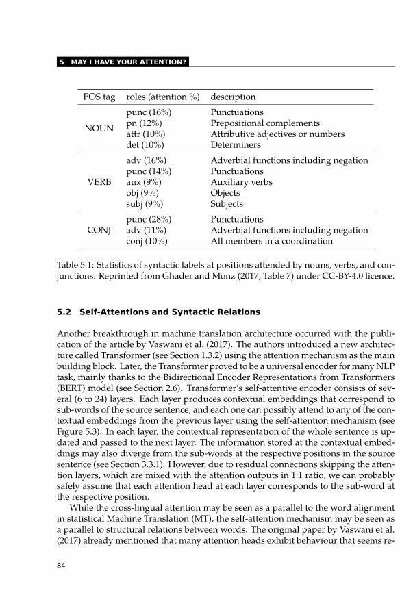
5 MAY I HAVE YOUR ATTENTION?
POS tag roles (attention %) description
NOUN
punc (16%) Punctuationspn (12%) Prepositional complementsattr (10%) Attributive adjectives or numbersdet (10%) Determiners
VERB
adv (16%) Adverbial functions including negationpunc (14%) Punctuationsaux (9%) Auxiliary verbsobj (9%) Objectssubj (9%) Subjects
CONJpunc (28%) Punctuationsadv (11%) Adverbial functions including negationconj (10%) All members in a coordination
Table 5.1: Statistics of syntactic labels at positions attended by nouns, verbs, and con-junctions. Reprinted from Ghader and Monz (2017, Table 7) under CC-BY-4.0 licence.
5.2 Self-Attentions and Syntactic Relations
Another breakthrough in machine translation architecture occurred with the publi-cation of the article by Vaswani et al. (2017). The authors introduced a new architec-ture called Transformer (see Section 1.3.2) using the attention mechanism as the mainbuilding block. Later, the Transformer proved to be a universal encoder for many NLPtask, mainly thanks to the Bidirectional Encoder Representations from Transformers(BERT) model (see Section 2.6). Transformer’s self-attentive encoder consists of sev-eral (6 to 24) layers. Each layer produces contextual embeddings that correspond tosub-words of the source sentence, and each one can possibly attend to any of the con-textual embeddings from the previous layer using the self-attention mechanism (seeFigure 5.3). In each layer, the contextual representation of the whole sentence is up-dated and passed to the next layer. The information stored at the contextual embed-dings may also diverge from the sub-words at the respective positions in the sourcesentence (see Section 3.3.1). However, due to residual connections skipping the atten-tion layers, which are mixed with the attention outputs in 1:1 ratio, we can probablysafely assume that each attention head at each layer corresponds to the sub-word atthe respective position.
While the cross-lingual attention may be seen as a parallel to the word alignmentin statistical Machine Translation (MT), the self-attention mechanism may be seen asa parallel to structural relations between words. The original paper by Vaswani et al.(2017) already mentioned that many attention heads exhibit behaviour that seems re-
84
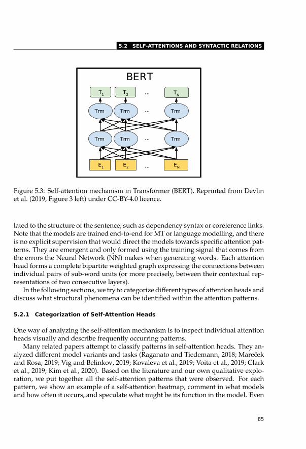
5.2 SELF-ATTENTIONS AND SYNTACTIC RELATIONS
BERT
Trm Trm Trm
Trm Trm Trm
...
...
T1 T2 TN...
E1E2 EN...
Figure 5.3: Self-attention mechanism in Transformer (BERT). Reprinted from Devlinet al. (2019, Figure 3 left) under CC-BY-4.0 licence.
lated to the structure of the sentence, such as dependency syntax or coreference links.Note that the models are trained end-to-end for MT or language modelling, and thereis no explicit supervision that would direct the models towards specific attention pat-terns. They are emergent and only formed using the training signal that comes fromthe errors the Neural Network (NN) makes when generating words. Each attentionhead forms a complete bipartite weighted graph expressing the connections betweenindividual pairs of sub-word units (or more precisely, between their contextual rep-resentations of two consecutive layers).
In the following sections, we try to categorize different types of attention heads anddiscuss what structural phenomena can be identified within the attention patterns.
5.2.1 Categorization of Self-Attention Heads
One way of analyzing the self-attention mechanism is to inspect individual attentionheads visually and describe frequently occurring patterns.
Many related papers attempt to classify patterns in self-attention heads. They an-alyzed different model variants and tasks (Raganato and Tiedemann, 2018; Marečekand Rosa, 2019; Vig and Belinkov, 2019; Kovaleva et al., 2019; Voita et al., 2019; Clarket al., 2019; Kim et al., 2020). Based on the literature and our own qualitative explo-ration, we put together all the self-attention patterns that were observed. For eachpattern, we show an example of a self-attention heatmap, comment in what modelsand how often it occurs, and speculate what might be its function in the model. Even
85
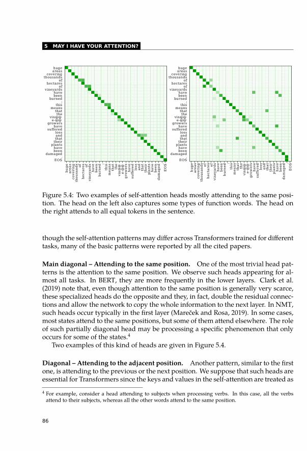
5 MAY I HAVE YOUR ATTENTION?
huge
areas
covering
thousa
nds
of
hectares
of
vineyard
shave
been
burn
ed ;
this
means
that
the
vin@@
e-@
@growers
have
suffered
loss
and
that
their
plants
have
been
damaged .
EOS
hugeareas
coveringthousands
ofhectares
ofvineyards
havebeen
burned;
thismeans
thatthe
vin@@e-@@
growershave
sufferedlossandthattheir
plantshavebeen
damaged.
EOS
Figure 5.4: Two examples of self-attention heads mostly attending to the same posi-tion. The head on the left also captures some types of function words. The head onthe right attends to all equal tokens in the sentence.
though the self-attention patterns may differ across Transformers trained for differenttasks, many of the basic patterns were reported by all the cited papers.
Main diagonal – Attending to the same position. One of the most trivial head pat-terns is the attention to the same position. We observe such heads appearing for al-most all tasks. In BERT, they are more frequently in the lower layers. Clark et al.(2019) note that, even though attention to the same position is generally very scarce,these specialized heads do the opposite and they, in fact, double the residual connec-tions and allow the network to copy the whole information to the next layer. In NMT,such heads occur typically in the first layer (Mareček and Rosa, 2019). In some cases,most states attend to the same positions, but some of them attend elsewhere. The roleof such partially diagonal head may be processing a specific phenomenon that onlyoccurs for some of the states.4
Two examples of this kind of heads are given in Figure 5.4.
Diagonal – Attending to the adjacent position. Another pattern, similar to the firstone, is attending to the previous or the next position. We suppose that such heads areessential for Transformers since the keys and values in the self-attention are treated as
4 For example, consider a head attending to subjects when processing verbs. In this case, all the verbsattend to their subjects, whereas all the other words attend to the same position.
86
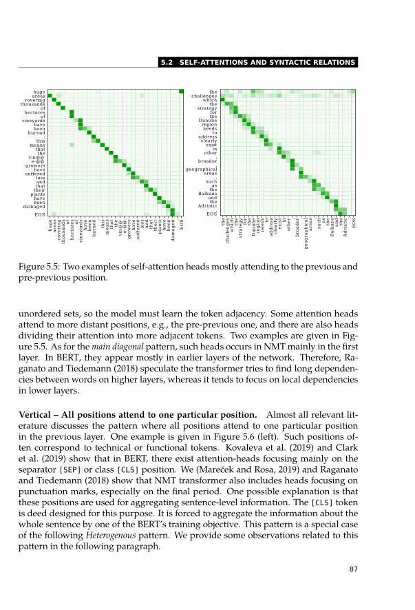
5.2 SELF-ATTENTIONS AND SYNTACTIC RELATIONS
huge
areas
covering
thousa
nds
of
hectares
of
vineyard
shave
been
burn
ed ;
this
means
that
the
vin@@
e-@
@growers
have
suffered
loss
and
that
their
plants
have
been
damaged .
EOS
hugeareas
coveringthousands
ofhectares
ofvineyards
havebeen
burned;
thismeans
thatthe
vin@@e-@@
growershave
sufferedlossandthattheir
plantshavebeen
damaged.
EOS
the
challenges
which
the
strategy
for
the
Danube
region
needs to
address
clearly
existin
other ,
broader ,
geographical
areas ,
such as
the
Balkans
and
the
Adriatic .
EOS
thechallenges
whichthe
strategyforthe
Danuberegionneeds
toaddressclearlyexist
inother
,broader
,geographical
areas,
suchasthe
Balkansandthe
Adriatic.
EOS
Figure 5.5: Two examples of self-attention heads mostly attending to the previous andpre-previous position.
unordered sets, so the model must learn the token adjacency. Some attention headsattend to more distant positions, e.g., the pre-previous one, and there are also headsdividing their attention into more adjacent tokens. Two examples are given in Fig-ure 5.5. As for the main diagonal pattern, such heads occurs in NMT mainly in the firstlayer. In BERT, they appear mostly in earlier layers of the network. Therefore, Ra-ganato and Tiedemann (2018) speculate the transformer tries to find long dependen-cies between words on higher layers, whereas it tends to focus on local dependenciesin lower layers.
Vertical – All positions attend to one particular position. Almost all relevant lit-erature discusses the pattern where all positions attend to one particular positionin the previous layer. One example is given in Figure 5.6 (left). Such positions of-ten correspond to technical or functional tokens. Kovaleva et al. (2019) and Clarket al. (2019) show that in BERT, there exist attention-heads focusing mainly on theseparator [SEP] or class [CLS] position. We (Mareček and Rosa, 2019) and Raganatoand Tiedemann (2018) show that NMT transformer also includes heads focusing onpunctuation marks, especially on the final period. One possible explanation is thatthese positions are used for aggregating sentence-level information. The [CLS] tokenis deed designed for this purpose. It is forced to aggregate the information about thewhole sentence by one of the BERT’s training objective. This pattern is a special caseof the following Heterogenous pattern. We provide some observations related to thispattern in the following paragraph.
87
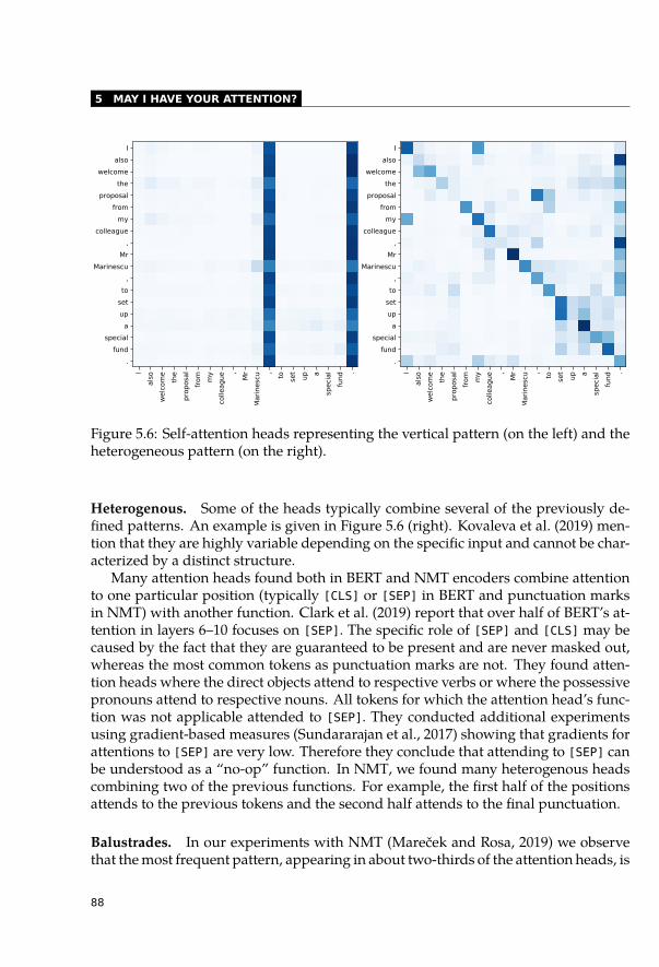
5 MAY I HAVE YOUR ATTENTION?
I
also
welcome
the
proposal
from
my
colleague ,
Mr
Marinescu ,
to set
up a
special
fund .
I
also
welcome
the
proposal
from
my
colleague
,
Mr
Marinescu
,
to
set
up
a
special
fund
.
I
also
welcome
the
proposal
from
my
colleague ,
Mr
Marinescu ,
to set
up a
special
fund .
I
also
welcome
the
proposal
from
my
colleague
,
Mr
Marinescu
,
to
set
up
a
special
fund
.
Figure 5.6: Self-attention heads representing the vertical pattern (on the left) and theheterogeneous pattern (on the right).
Heterogenous. Some of the heads typically combine several of the previously de-fined patterns. An example is given in Figure 5.6 (right). Kovaleva et al. (2019) men-tion that they are highly variable depending on the specific input and cannot be char-acterized by a distinct structure.
Many attention heads found both in BERT and NMT encoders combine attentionto one particular position (typically [CLS] or [SEP] in BERT and punctuation marksin NMT) with another function. Clark et al. (2019) report that over half of BERT’s at-tention in layers 6–10 focuses on [SEP]. The specific role of [SEP] and [CLS] may becaused by the fact that they are guaranteed to be present and are never masked out,whereas the most common tokens as punctuation marks are not. They found atten-tion heads where the direct objects attend to respective verbs or where the possessivepronouns attend to respective nouns. All tokens for which the attention head’s func-tion was not applicable attended to [SEP]. They conducted additional experimentsusing gradient-based measures (Sundararajan et al., 2017) showing that gradients forattentions to [SEP] are very low. Therefore they conclude that attending to [SEP] canbe understood as a “no-op” function. In NMT, we found many heterogenous headscombining two of the previous functions. For example, the first half of the positionsattends to the previous tokens and the second half attends to the final punctuation.
Balustrades. In our experiments with NMT (Mareček and Rosa, 2019) we observethat the most frequent pattern, appearing in about two-thirds of the attention heads, is
88
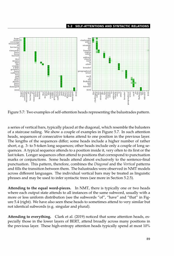
5.2 SELF-ATTENTIONS AND SYNTACTIC RELATIONS
huge
areas
covering
thousa
nds
of
hectares
of
vineyard
shave
been
burn
ed ;
this
means
that
the
vin@@
e-@
@growers
have
suffered
loss
and
that
their
plants
have
been
damaged .
EOS
hugeareas
coveringthousands
ofhectares
ofvineyards
havebeen
burned;
thismeans
thatthe
vin@@e-@@
growershave
sufferedlossandthattheir
plantshavebeen
damaged.
EOS
the
challenges
which
the
strategy
for
the
Danube
region
needs to
address
clearly
existin
other ,
broader ,
geographical
areas ,
such as
the
Balkans
and
the
Adriatic .
EOS
thechallenges
whichthe
strategyforthe
Danuberegionneeds
toaddressclearlyexist
inother
,broader
,geographical
areas,
suchasthe
Balkansandthe
Adriatic.
EOS
Figure 5.7: Two examples of self-attention heads representing the balustrades pattern.
a series of vertical bars, typically placed at the diagonal, which resemble the balustersof a staircase railing. We show a couple of examples in Figure 5.7. In such attentionheads, sequences of consecutive tokens attend to one position in the previous layer.The lengths of the sequences differ; some heads include a higher number of rathershort, e.g. 3- to 5-token long sequences; other heads include only a couple of long se-quences. A typical sequence attends to a position inside it, very often to its first or thelast token. Longer sequences often attend to positions that correspond to punctuationmarks or conjunctions. Some heads attend almost exclusively to the sentence-finalpunctuation. This pattern, therefore, combines the Diagonal and the Vertical patternsand fills the transition between them. The balustrades were observed in NMT modelsacross different languages. The individual vertical bars may be treated as linguisticphrases and may be used to infer syntactic trees (see more in Section 5.2.5).
Attending to the equal word-pieces. In NMT, there is typically one or two headswhere each output state attends to all instances of the same subword, usually with amore or less uniform distribution (see the subwords “of”, “have” and “that” in Fig-ure 5.4 (right). We have also seen these heads to sometimes attend to very similar butnot identical subwords (e.g. singular and plural).
Attending to everything. Clark et al. (2019) noticed that some attention heads, es-pecially those in the lower layers of BERT, attend broadly across many positions inthe previous layer. These high-entropy attention heads typically spend at most 10%
89
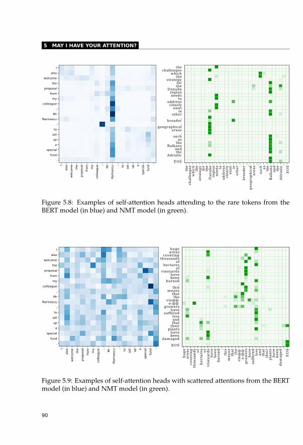
5 MAY I HAVE YOUR ATTENTION?
I
also
welcome
the
proposal
from
my
colleague ,
Mr
Marinescu ,
to set
up a
special
fund .
I
also
welcome
the
proposal
from
my
colleague
,
Mr
Marinescu
,
to
set
up
a
special
fund
.
the
challenges
which
the
strategy
for
the
Danube
region
needs to
address
clearly
existin
other ,
broader ,
geographical
areas ,
such as
the
Balkans
and
the
Adriatic .
EOS
thechallenges
whichthe
strategyforthe
Danuberegionneeds
toaddressclearlyexist
inother
,broader
,geographical
areas,
suchasthe
Balkansandthe
Adriatic.
EOS
Figure 5.8: Examples of self-attention heads attending to the rare tokens from theBERT model (in blue) and NMT model (in green).
I
also
welcome
the
proposal
from
my
colleague ,
Mr
Marinescu ,
to set
up a
special
fund .
I
also
welcome
the
proposal
from
my
colleague
,
Mr
Marinescu
,
to
set
up
a
special
fund
.
huge
areas
covering
thousa
nds
of
hectares
of
vineyard
shave
been
burn
ed ;
this
means
that
the
vin@@
e-@
@growers
have
suffered
loss
and
that
their
plants
have
been
damaged .
EOS
hugeareas
coveringthousands
ofhectares
ofvineyards
havebeen
burned;
thismeans
thatthe
vin@@e-@@
growershave
sufferedlossandthattheir
plantshavebeen
damaged.
EOS
Figure 5.9: Examples of self-attention heads with scattered attentions from the BERTmodel (in blue) and NMT model (in green).
90
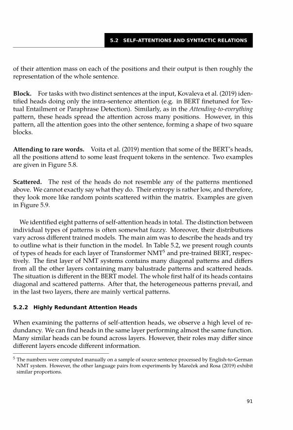
5.2 SELF-ATTENTIONS AND SYNTACTIC RELATIONS
of their attention mass on each of the positions and their output is then roughly therepresentation of the whole sentence.
Block. For tasks with two distinct sentences at the input, Kovaleva et al. (2019) iden-tified heads doing only the intra-sentence attention (e.g. in BERT finetuned for Tex-tual Entailment or Paraphrase Detection). Similarly, as in the Attending-to-everythingpattern, these heads spread the attention across many positions. However, in thispattern, all the attention goes into the other sentence, forming a shape of two squareblocks.
Attending to rare words. Voita et al. (2019) mention that some of the BERT’s heads,all the positions attend to some least frequent tokens in the sentence. Two examplesare given in Figure 5.8.
Scattered. The rest of the heads do not resemble any of the patterns mentionedabove. We cannot exactly say what they do. Their entropy is rather low, and therefore,they look more like random points scattered within the matrix. Examples are givenin Figure 5.9.
We identified eight patterns of self-attention heads in total. The distinction betweenindividual types of patterns is often somewhat fuzzy. Moreover, their distributionsvary across different trained models. The main aim was to describe the heads and tryto outline what is their function in the model. In Table 5.2, we present rough countsof types of heads for each layer of Transformer NMT5 and pre-trained BERT, respec-tively. The first layer of NMT systems contains many diagonal patterns and differsfrom all the other layers containing many balustrade patterns and scattered heads.The situation is different in the BERT model. The whole first half of its heads containsdiagonal and scattered patterns. After that, the heterogeneous patterns prevail, andin the last two layers, there are mainly vertical patterns.
5.2.2 Highly Redundant Attention Heads
When examining the patterns of self-attention heads, we observe a high level of re-dundancy. We can find heads in the same layer performing almost the same function.Many similar heads can be found across layers. However, their roles may differ sincedifferent layers encode different information.
5 The numbers were computed manually on a sample of source sentence processed by English-to-GermanNMT system. However, the other language pairs from experiments by Mareček and Rosa (2019) exhibitsimilar proportions.
91
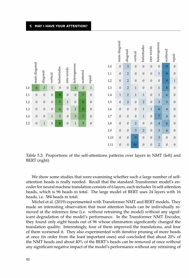
5 MAY I HAVE YOUR ATTENTION?
mai
ndi
agon
al
diag
onal
vert
ical
balu
stra
des
rare
wor
ds
hete
roge
nous
scat
tere
d
equa
lL0 6 3 1 0 0 4 2 1
L1 0 0 0 9 0 0 7 0
L2 0 0 0 7 1 0 8 0
L3 0 0 0 6 0 2 8 0
L4 0 0 1 3 0 3 7 0
L5 0 1 0 8 0 1 5 0m
ain
diag
onal
diag
onal
vert
ical
balu
stra
des
rare
wor
ds
hete
roge
nous
scat
tere
d
equa
l
L0 0 3 0 0 0 0 9 0
L1 0 2 0 0 0 1 9 0
L2 0 2 0 0 0 0 9 1
L3 0 2 1 0 0 1 8 0
L4 1 2 1 1 0 1 6 0
L5 0 2 0 2 0 3 5 0
L6 0 0 0 1 1 6 4 0
L7 0 0 0 1 0 7 4 0
L8 0 0 2 0 0 4 6 0
L9 0 0 3 2 0 3 4 0
L10 0 0 9 0 0 3 0 0
L11 0 0 10 0 0 2 0 0
Table 5.2: Proportions of the self-attentions patterns over layers in NMT (left) andBERT (right).
We show some studies that were examining whether such a large number of self-attention heads is really needed. Recall that the standard Transformer model’s en-coder for neural machine translation consists of 6 layers, each includes 16 self-attentionheads, which is 96 heads in total. The large model of BERT uses 24 layers with 16heads, i.e. 384 heads in total.
Michel et al. (2019) experimented with Transformer NMT and BERT models. Theymade an interesting observation that most attention heads can be individually re-moved at the inference time (i.e. without retraining the model) without any signif-icant degradation of the model’s performance. In the Transformer NMT Encoder,they found only eight heads out of 96 whose elimination significantly changed thetranslation quality. Interestingly, four of them improved the translations, and fourof them worsened it. They also experimented with iterative pruning of more headsat once (in order from the least important ones) and concluded that about 20% ofthe NMT heads and about 40% of the BERT’s heads can be removed at once withoutany significant negative impact of the model’s performance without any retraining of
92
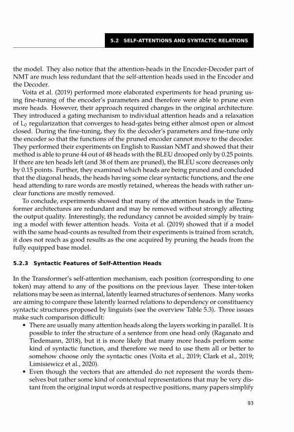
5.2 SELF-ATTENTIONS AND SYNTACTIC RELATIONS
the model. They also notice that the attention-heads in the Encoder-Decoder part ofNMT are much less redundant that the self-attention heads used in the Encoder andthe Decoder.
Voita et al. (2019) performed more elaborated experiments for head pruning us-ing fine-tuning of the encoder’s parameters and therefore were able to prune evenmore heads. However, their approach required changes in the original architecture.They introduced a gating mechanism to individual attention heads and a relaxationof L0 regularization that converges to head-gates being either almost open or almostclosed. During the fine-tuning, they fix the decoder’s parameters and fine-tune onlythe encoder so that the functions of the pruned encoder cannot move to the decoder.They performed their experiments on English to Russian NMT and showed that theirmethod is able to prune 44 out of 48 heads with the BLEU drooped only by 0.25 points.If there are ten heads left (and 38 of them are pruned), the BLEU score decreases onlyby 0.15 points. Further, they examined which heads are being pruned and concludedthat the diagonal heads, the heads having some clear syntactic functions, and the onehead attending to rare words are mostly retained, whereas the heads with rather un-clear functions are mostly removed.
To conclude, experiments showed that many of the attention heads in the Trans-former architectures are redundant and may be removed without strongly affectingthe output quality. Interestingly, the redundancy cannot be avoided simply by train-ing a model with fewer attention heads. Voita et al. (2019) showed that if a modelwith the same head-counts as resulted from their experiments is trained from scratch,it does not reach as good results as the one acquired by pruning the heads from thefully equipped base model.
5.2.3 Syntactic Features of Self-Attention Heads
In the Transformer’s self-attention mechanism, each position (corresponding to onetoken) may attend to any of the positions on the previous layer. These inter-tokenrelations may be seen as internal, latently learned structures of sentences. Many worksare aiming to compare these latently learned relations to dependency or constituencysyntactic structures proposed by linguists (see the overview Table 5.3). Three issuesmake such comparison difficult:
• There are usually many attention heads along the layers working in parallel. It ispossible to infer the structure of a sentence from one head only (Raganato andTiedemann, 2018), but it is more likely that many more heads perform somekind of syntactic function, and therefore we need to use them all or better tosomehow choose only the syntactic ones (Voita et al., 2019; Clark et al., 2019;Limisiewicz et al., 2020).
• Even though the vectors that are attended do not represent the words them-selves but rather some kind of contextual representations that may be very dis-tant from the original input words at respective positions, many papers simplify
93
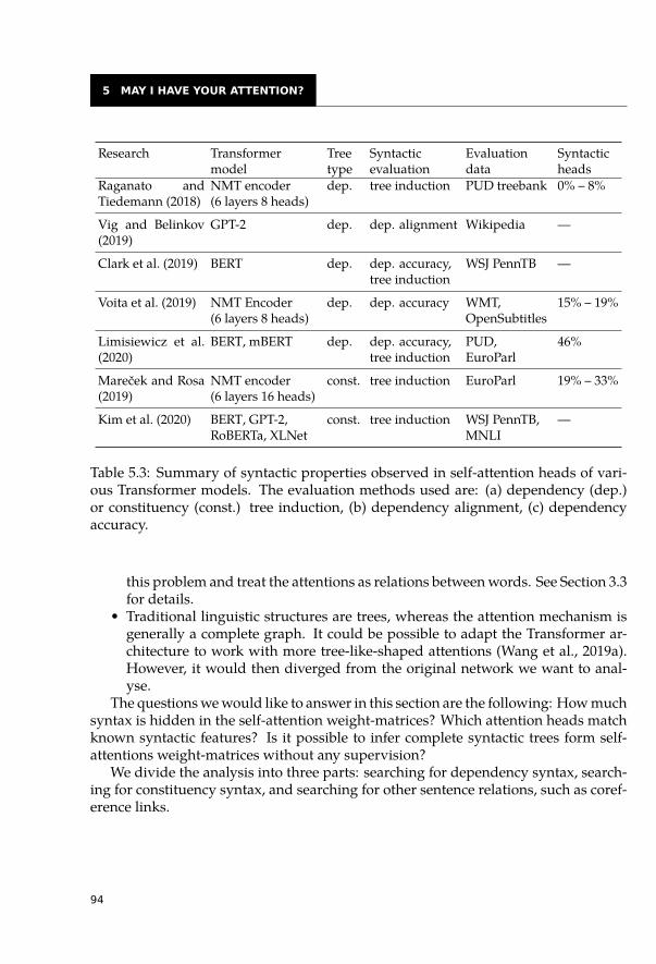
5 MAY I HAVE YOUR ATTENTION?
Research Transformermodel
Treetype
Syntacticevaluation
Evaluationdata
Syntacticheads
Raganato andTiedemann (2018)
NMT encoder(6 layers 8 heads)
dep. tree induction PUD treebank 0% – 8%
Vig and Belinkov(2019)
GPT-2 dep. dep. alignment Wikipedia —
Clark et al. (2019) BERT dep. dep. accuracy,tree induction
WSJ PennTB —
Voita et al. (2019) NMT Encoder(6 layers 8 heads)
dep. dep. accuracy WMT,OpenSubtitles
15% – 19%
Limisiewicz et al.(2020)
BERT, mBERT dep. dep. accuracy,tree induction
PUD,EuroParl
46%
Mareček and Rosa(2019)
NMT encoder(6 layers 16 heads)
const. tree induction EuroParl 19% – 33%
Kim et al. (2020) BERT, GPT-2,RoBERTa, XLNet
const. tree induction WSJ PennTB,MNLI
—
Table 5.3: Summary of syntactic properties observed in self-attention heads of vari-ous Transformer models. The evaluation methods used are: (a) dependency (dep.)or constituency (const.) tree induction, (b) dependency alignment, (c) dependencyaccuracy.
this problem and treat the attentions as relations between words. See Section 3.3for details.
• Traditional linguistic structures are trees, whereas the attention mechanism isgenerally a complete graph. It could be possible to adapt the Transformer ar-chitecture to work with more tree-like-shaped attentions (Wang et al., 2019a).However, it would then diverged from the original network we want to anal-yse.
The questions we would like to answer in this section are the following: How muchsyntax is hidden in the self-attention weight-matrices? Which attention heads matchknown syntactic features? Is it possible to infer complete syntactic trees form self-attentions weight-matrices without any supervision?
We divide the analysis into three parts: searching for dependency syntax, search-ing for constituency syntax, and searching for other sentence relations, such as coref-erence links.
94

5.2 SELF-ATTENTIONS AND SYNTACTIC RELATIONS
5.2.4 Dependency Trees
The first observations that some of the self-attention heads exhibit behaviour relatedto a syntactic structure were provided in the original paper introducing Transformer(Vaswani et al., 2017).
Raganato and Tiedemann (2018) induce dependency trees from self-attention ma-trices of NMT encoder. Their experiments were done for translations from English to7 different languages. Their approach assumes that the whole syntactic tree can be in-duced from just one attention head. For each head, they use the maximum spanningtree algorithm (Edmonds, 1967) to add edges for pairs of tokens with high attentionweights and assure that the obtained graph is a tree. They use the tree root from theannotated gold data to find the direction of the edges. The trees extracted in this wayare generally worse than the right-branching baseline6 and outperform it slightly fora few heads. Nevertheless, their experiments showed that the syntactic behaviour ofindividual heads changes along the layers and the most syntactic heads in NMT ap-pear at the top layers of the encoder. The results are visualized in the overview inFigure 5.11 under letter F.
Following articles focused on the analysis of individual features and classificationof Transformer’s self-attention heads.
Vig and Belinkov (2019) apply multiple metrics to examine properties of atten-tion matrices computed in GPT-2 language model. They showed that in some heads,the attentions concentrate on tokens representing specific POS tags, and the pairs oftokens are more often attended one to another if they are connected by an edge in de-pendency tree. They observe that the strongest dependency alignment occurs in themiddle layers of the model (4th and 5th counting from the input out of 12 layers intotal). They also point that different dependency types (relation labels) are capturedin different places of the model. Attentions in upper layers align more with subjectrelations whereas in the lower layer with modifying relations, such as auxiliaries, de-terminers, conjunctions, and expletives. This is also related to the fact that the higherthe layer, the more distant the attention connections are. See letter D in Figure 5.11.
Voita et al. (2019) analyzed NMT encoders of translation systems from Englishto three European languages and also observed an alignment with dependency re-lations. They picked four types of dependency labels (noun subject, direct object,adjective modifier, and adverbial modifier) and measured how t extent they are cap-tured by individual self-attention heads. -They separately address the cases where averb attends to its dependent subject, and a subject attends to its governor verb. Theheads with more than 10% improvement over positional baseline7 were identified assyntactic. Such heads were found in all encoder’s layers except from the first one.6 The right-branching baseline is a tree where each token is governed by its left neighbour.7 In the positional baseline, the most frequent offset is added to the index of relation’s dependent/governor
to find its governor/dependent, e.g., for the adjective-to-noun relations in English, the most frequentoffset is +1.
95

5 MAY I HAVE YOUR ATTENTION?
In the head-pruning experiments, which we described in Section 5.2.2, the authorsshowed that the share of syntactic heads rises from 17% in the original model to 40%when 75% heads are cut out, while a change in BLEU is negligible. These results sup-port the claim that the model’s ability to capture syntax is essential to its performancein not syntactic tasks.
A similar evaluation of dependency accuracy, but for BERT pre-trained model, wasconducted by (Clark et al., 2019). They identify syntactic heads that significantly out-perform positional baseline for syntactic labels: prepositional object, determiner, di-rect object, possession modifier, auxiliary passive, clausal component, marker, phrasalverb particle. Most of the syntactic heads were found in the middle layers (4th to 8thout of 12). However, there exist no single heads that would capture all the relationsof one type.
In another experiment, Clark et al. (2019) induce dependency tree from attentions.Instead of extracting structure from each head (Raganato and Tiedemann, 2018) theyuse probing to learn the weights of individual attention heads and then use maximumspanning tree on the weighted-average of the attention matrices. This approach pro-duces trees with 61% Unlabeled Attachment Score (UAS) and can be improved to 77%by making weights dependent on the static word representation (fixed GloVe vectors).Both the numbers are significantly higher than the right-branching baseline (27%).
We conduct a related analysis for English (BERT) and multilingual model (Multi-lingual BERT (mBERT)) in (Limisiewicz et al., 2020). We observe that the informationabout one dependency type can be split across many self-attention heads. In othercases, the opposite may happen: many heads perform the same syntactic function.Examples of two heads aligned with dependency relations are shown in Figure 5.10.We introduce algorithms for averaging self-attention matrices to obtain better depen-dency accuracy than in a single matrix. Furthermore, we extract labelled dependencytrees from the averaged heads and achieves 52% UAS and show that in the multi-lingual model (mBERT) specific relation (noun subject, determines) are found in thesame heads across typologically similar languages.
5.2.5 Constituency Trees
Less effort was devoted to analysing attention heads in terms of syntactic phrases andderiving constituency tree structures.
In Mareček and Rosa (2019), we examine the encoder of Transformer NMT sys-tem for translation between English, French, and German. We observe that in manyheads, continuous sequences of words attend to the same token, forming shapes sim-ilar to balusters (Figure 5.7). Furthermore, these continuous sequences often overlapwith syntactic phrases. This notion is employed in our method for constituency treeinduction. We compute weights for all such continuous sequences of tokens acrossall heads by summing the respective attentions. Then we induce constituency treesusing the CKY algorithm (Ney, 1991). As a result, we produce trees that achieve up to
96
5.2 SELF-ATTENTIONS AND SYNTACTIC RELATIONSth
ere is
cons
ider
able
ener
gysa
ving
poten
tial in
publ
icbu
ildin
gs ,fo
rex
ampl
e ,wh
ichwo
uld
facil
itate the
trans
ition
towa
rds a
stabl
e ,gr
een
econ
omy .
thereis
considerableenergysaving
potentialin
publicbuildings
,for
example,
whichwould
facilitatethe
transitiontowards
astable
,green
economy.
LAYE
R: 5
HEA
D: 7
AA
A
AA
AMOD D2P
ther
e isco
nsid
erab
leen
ergy
savi
ngpo
tentia
l inpu
blic
build
ings ,
for
exam
ple ,
which
woul
dfa
cilita
te the
trans
ition
towa
rds a
stabl
e ,gr
een
econ
omy .
LAYE
R: 7
HEA
D: 9
O
O
OBJ D2P
Figure 5.10: Self-attentions in particular heads of a Language Model (BERT) alignswith dependency relation adjective modifier and object. The gold relations are markedwith red crosses.
97
5 MAY I HAVE YOUR ATTENTION?
32.8% F1 score for English sentences, 43.6% for German and 44.2% for French.8 Theresults can be improved by selecting syntactic heads and using only them in the algo-rithm. This approach requires a sample of 100 annotated sentences for head selectionand raise F1 by up to 8% in English.
The extraction of constituency trees from several Transformer-based LanguageModels was described by Kim et al. (2020). They present a comprehensive studythat covers many different pre-trained networks, including BERT and Generative Pre-Trained Transformer (GPT)-2. Their approach is based on computing distances be-tween each pair of subsequent words. In each step, they perform tree branching in theplace where the distance is the highest. The authors propose three distance measuresfor pairs of contextual embeddings in a given layer: cosine, L1, and L2 distances; andtwo measures for comparing attention distributions of the subsequent words in eachself-attention head: Jensen-Shannon and Hellinger distances. The best parse trees,which were extracted from XLNet-base model using Helinger distance on averagedattentions in the 7th layer, achieved 40.1% F1 score on WSJ Penn Treebank. Generally,attention distribution distances perform better than contextual vector ones. Authorsalso observe that models trained on common language modelling objective (i.e., next-word prediction in GPT) captured syntax better than masked language models (e.g.,BERT). In line with the previous research, the middle layers of analyzed networkstend to be more syntactic.
5.2.6 Syntactic Information across Layers
Figure 5.11 summarizes the evaluation of syntactic information across layers for dif-ferent models and approaches. The values are normalized so that the best layer foreach method has 1.0. The methods A), B), C), and G) show undirected UAS trees ex-tracted by probing the n-th layer (Hewitt and Manning, 2019; Chi et al., 2020). Themethod D) shows the Dependency alignment averaged across all heads in the n-thlayer (Vig and Belinkov, 2019). The methods E) and F) show UAS of trees inducedfrom attention heads by maximum spanning tree algorithm (Raganato and Tiede-mann, 2018; Limisiewicz et al., 2020).
In Transformer-based language models (BERT, mBERT, and GPT-2), middle layersare the most syntactic. In the NMT models, the top layers of the encoder are the mostsyntactic. However, it is important to note that the NMT Transformer encoder is onlythe first half of the whole translation architecture. Therefore the most syntactic layeris, in fact, in the middle of the process. In RNN Language Model (ELMo) the firstlayer is more syntactic than the second one.
8 The evaluation was done on 1000 sentences for each language parsed with supervised Stanford Parser.9 The results for the best layer (corresponding to value 1.0 in the plot) are: A) 82.5; B) 79.8; C) 80.1; D) 22.3;
E) 24.3; F) en2cs: 23.9, en2de: 20.9, en2et: 22.1, en2fi: 24.0, en2ru: 22.4, en2tr: 17.5, en2zh: 21.6; G) 77.0.
98
5.2 SELF-ATTENTIONS AND SYNTACTIC RELATIONS
.. A)BE
RTlar
ge1-
12
. BERT
large
13-2
4
.
B)BE
RTba
se
.
C)m
BERT
base
.
D)GP
T-2
.
E)BE
RTba
se
.
F)N
MT
en2c
s
.
en2d
e
.
en2e
t
.
en2fi
.
en2r
u
.
en2t
r.
en2z
h.
G)EL
Mo
.
1
.
2
.
3
.
4
.
5
.
6
.
7
.
8
.
9
.
10
.
11
.
12
.
Laye
rnum
ber
.
.
0.4
.
0.5
.
0.6
.
0.7
.
0.8
.
0.9
.
1.0
Figure 5.11: Relative syntactic information across attention models and layers.9
We conjecture that the initial Transformer’s layers capture simple relations (e.g.,attending to next or previous tokens) and the last layers mostly capture task-specificinformation. Therefore, they are less syntactic.
We also observe that in supervised probing (Hewitt and Manning, 2019; Chi et al.,2020), relatively better results are obtained from initial and top layers than in unsuper-vised structure induction (Raganato and Tiedemann, 2018; Limisiewicz et al., 2020),i.e., the distribution across layers is smoother. It suggests that the syntactic structurecould be memorized to a more considerable extent in the probe instead of being cap-tured by non-syntactic layers.
5.2.7 Other Relations between Words
Self-attention heads do not capture only syntactic relations. Besides the trivial ones,which were overviewed in Section 5.2.1, there are heads that exhibit rather semanticor discourse functions. Vaswani et al. (2017) claim that some of the attention heads inthe Transformer NMT encoder are apparently involved in anaphora resolution (coref-erence). Clark et al. (2019) found a similar head performing coreference in the BERTmodel. This head achieved 65% accuracy at linking the coreferent to its antecedent,which is comparable to rule-based coreference resolvers. This is a very good result;
99
5 MAY I HAVE YOUR ATTENTION?
note that the learning is fully unsupervised. The attention head is particularly capableof fuzzy matching between synonyms.
5.3 Interpretability of Attentions Not as Easy as Expected
There has been a substantial amount of work done on interpreting attention mech-anisms across different tasks and architectures. Many papers suggested reasonableexplanations of the behaviour of the attention models, and it was generally assumedthat each attention mechanism could be explained. For example, Bahdanau et al.(2014) consider the attention is the explanation and does not dispute its validity inany way. However, in 2019 several papers appeared (Jain and Wallace, 2019; Serranoand Smith, 2019; Pruthi et al., 2019) showing that some of the interpretations may beuseless. Serrano and Smith (2019) suggest that an interpretable attention model must“not only suggest explanations that make sense to people, but also ensure that thoseexplanations accurately represent the true reasons for the model’s decisions.” This issometimes called a faithful explanation (Ross et al., 2017).
The basic questions that these articles raised are:• How do the model predictions change if we change the distributions of attention
weights?• Would alternative (or even contra-factual) attention weights necessarily yield
different results?• How much do the attention weights correlate with the importances of input
representations?Earlier studies (Serrano and Smith, 2019; Pruthi et al., 2019) focused mainly on
the text classification tasks, i.e., the tasks where a single sequence is classified into asmall number of classes and concluded that these tasks do not satisfy their definitionof being interpretable. Vashishth et al. (2019) extended the analysis to more com-plex tasks and showed that attention weights are interpretable in the architectures, inwhich attentions are essential for models predictions. In simple architectures, wherethe function of the attention mechanism may be equally performed by RNN gatingunits, the interpretability is questionable.
In the following text, we show three methods addressing the questions about in-terpretability of different types of neural architectures. This section aims to show thatwe cannot blindly interpret the attention weights as importances of individual inputsfor the network decisions. We always have to bear in mind that the information flowin the network may be different than expected.
5.3.1 Eliminate the Highest Attention Weight
One of the experiments that attempt to disprove the direct interpretability of atten-tions was proposed by Serrano and Smith (2019). It is based on zeroing out the high-est attention weight from the attention distribution and measuring how it affects the
100
5.3 INTERPRETABILITY OF ATTENTIONS NOT AS EASY AS EXPECTED
model’s output distributions. All the experiments were done at test time; training ofthe model remained unchanged.
Consider a trained model which is applied to a test data and consider one attentionlayer inside the model which is going to be examined. For each instance of the testdata, select the most attended input component i∗ (the one with the highest attentionweight), leave it out by setting the weight to 0, and renormalize all the other weightsso that they sum to 1. How does it affect the model? The impact of such change canbe measured using Jensen-Shannon (JS) divergence of the output distributions overlabels10 or by examining how many final decisions of the model were flipped.
Serrano and Smith (2019) performed experiments on single sequence tasks of topicclassification and sentiment analysis. Not surprisingly, when αi∗ was small, it causedalmost no changes in the output distribution. However, even for larger attentionweights as 0.4, the JS divergences were still close to zero. The number of model deci-sions that were flipped (changed from 0 to 1 or from 1 to 0) was also relatively small.Only slightly more than 10% of decisions has changed. These results suggested thatthe interpretation of such single-sequence tasks is at least questionable.
Vashishth et al. (2019) categorize NLP tasks into the three groups according to theirinputs and outputs:
• Single sequence tasks, e.g., sentiment analysis, topic classification,• Pair sequence tasks, e.g., natural language inference, question answering,• Generation tasks, e.g., machine translation, text summarization.
Unlike Serrano and Smith (2019), who tested their method only on the single sequencetasks, they applied the same method also on the pair-sequence and generation tasksand reported much more apparent correlations on them. Figure 5.12 shows that in themachine translation task, the components which are important according to the at-tention weights really have an impact on the results and zeroing the attentions harmsthe model predictions. They conclude that attention weights are interpretable in thearchitectures where attentions are essential for models predictions and do not onlybehave as gating units.
Serrano and Smith (2019) also showed results for different model architectures.They compared
• RNN architecture with an attention layer on top• Convolutional Neural Network (CNN) with an attention layer on top• no encoder, only one attention layer looking at the input word embeddings
and showed that zeroing out the attentions in the architecture without encoder provedto have a higher effect on the number of decision flips. This is probably caused by thefact that zeroing out an attention weight really eliminates the word from computa-tions. In contrast, RNN may propagate information about the important words to the
10 To be able to assess the magnitudes of the JS divergence, the authors compare it with the JS divergenceafter erasure of a random component r from the attention input. The difference between these two JSdivergences should then correlate with the differences of the zeroed-out attention weights αi∗ − αr.
101
5 MAY I HAVE YOUR ATTENTION?
Figure 5.12: Eliminating the highest attention weights affects the output distributions.Comparison for different types of NLP tasks. Reprinted from (Vashishth et al., 2019,Figure 3).
following representations. In CNN, information about the word can be present in asmany components as the window size is. The results are shown in Figure 5.13.
5.3.2 Change the Whole Attention Distribution
Another approach was suggested by Jain and Wallace (2019). Instead of zeroing outone attention weight, they propose to change the whole distribution of weights atonce and measure their impact on predictions. Putting together the works by Jainand Wallace (2019), Vashishth et al. (2019), and Wiegreffe and Pinter (2019), we foundfour tested variants for changing the attention weights:
• uniform – distribute the weights uniformly,• random – randomly sample weights from the uniform distribution U(0, 1) and
normalize,• random permutation – scramble the original weights, reassigning each value to an
arbitrary, randomly sampled index,• adversarial attention - search for such attention distribution that differs as much
as possible from the original attentions, but at the same time, does not substan-tially change the predictions.
Moreover, there are two possibilities when to apply the changes. We can eitheruse the original trained model and apply the changes of attention weights at inferencetime or manipulate with attention weights during training so that the other parame-ters of the model could adapt to these different conditions.
First, it is necessary to answer an important question: Is the attention mechanismneeded for a given task at all? Wiegreffe and Pinter (2019) argue that “if attentionmodels are not useful compared to very simple baselines, i.e. their parameter capac-ity is not being used, there is no point in using their outcomes for any type of expla-nation.” They performed a simple baseline experiment in which all attention weights
102
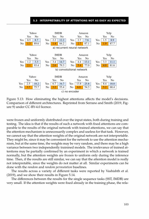
5.3 INTERPRETABILITY OF ATTENTIONS NOT AS EASY AS EXPECTED
Yahoo IMDBYes No Yes No
Yes 0.5 8.7 Yes 2.2 12.2No 1.3 89.6 No 1.4 84.2
Amazon YelpYes No Yes No
Yes 2.7 7.6 Yes 1.5 8.9No 2.7 87.1 No 1.9 87.7
Yahoo IMDBYes No Yes No
Yes 1.2 3.3 Yes 3.4 14.7No 2.1 93.4 No 2.6 79.3
Amazon YelpYes No Yes No
Yes 4.4 13.1 Yes 3.3 11.1No 5.4 77.0 No 4.0 81.6
Yahoo IMDBYes No Yes No
Yes 2.5 18.2 Yes 6.7 34.7No 3.7 75.7 No 3.2 55.4
Amazon YelpYes No Yes No
Yes 13.8 25.8 Yes 8.4 18.0No 6.0 54.3 No 5.2 68.4
a) recurrent neural network
b) convolutional network
c) no encoder
Figure 5.13: How eliminating the highest attentions affects the model’s decisions.Comparison of different architectures. Reprinted from Serrano and Smith (2019, Fig-ure 9) under CC-BY-4.0 licence.
were frozen and uniformly distributed over the input states, both during training andtesting. The idea is that if the results of such a network with fixed attentions are com-parable to the results of the original network with trained attentions, we can say thatthe attention mechanism is unnecessarily complex and useless for that task. However,we cannot say that the attention weights of the original network are not interpretable.They might be, since it may be convenient for the network to use the attention mecha-nism, but at the same time, the weights may be very random, and there may be a highvariance between two independently trainined models. The irrelevance of trained at-tentions may be partially confirmed by an experiment in which a network is trainednormally, but the attention weights are frozen to uniform only during the inferencetime. Then, if the results are still similar, we can say that the attention model is reallynot interpretable, since the weights do not matter at all. Similar experiments can bedone with the random and random permutation baselines.
The results across a variety of different tasks were reported by Vashishth et al.(2019), and we show their results in Figure 5.14.
The differences between the results for the single sequence tasks (SST, IMDB) arevery small. If the attention weights were fixed already in the training phase, the rela-
103
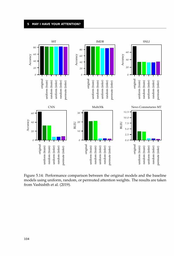
5 MAY I HAVE YOUR ATTENTION?
..
orig
inal
.
unifo
rm(tr
ain)
.
rand
om(tr
ain)
.
unifo
rm(in
fer)
.
rand
om(in
fer)
.
perm
ute
(infe
r)
.
0
.
20
.
40
.
60
.
80
.
Acc
urac
y
.
SST
..
orig
inal
.
unifo
rm(tr
ain)
.ra
ndom
(trai
n).
unifo
rm(in
fer)
.ra
ndom
(infe
r)
.
perm
ute
(infe
r)
.
0
.
20
.
40
.
60
.
80
.
Acc
urac
y
.
IMDB
..
orig
inal
.
unifo
rm(tr
ain)
.
rand
om(tr
ain)
.
unifo
rm(in
fer)
.
rand
om(in
fer)
.
perm
ute
(infe
r)
.
0
.
20
.
40
.
60
.
Acc
urac
y
.
SNLI
..
orig
inal
.
unifo
rm(tr
ain)
.
rand
om(tr
ain)
.
unifo
rm(in
fer)
.
rand
om(in
fer)
.
perm
ute
(infe
r)
.
0
.
20
.
40
.
60
.
Acc
urac
y
.
CNN
..
orig
inal
.
unifo
rm(tr
ain)
.
rand
om(tr
ain)
.
unifo
rm(in
fer)
.
rand
om(in
fer)
.
perm
ute
(infe
r)
.
0
.
10
.
20
.
30
.
BLEU
.
Multi30k
..
orig
inal
.
unifo
rm(tr
ain)
.
rand
om(tr
ain)
.
unifo
rm(in
fer)
.
rand
om(in
fer)
.
perm
ute
(infe
r)
.
0.0
.
2.5
.
5.0
.
7.5
.
10.0
.
12.5
.
BLEU
.
News Commetaries MT
Figure 5.14: Performance comparison between the original models and the baselinemodels using uniform, random, or permuted attention weights. The results are takenfrom Vashishth et al. (2019).
104
5.3 INTERPRETABILITY OF ATTENTIONS NOT AS EASY AS EXPECTED
tive drop in performance is about 1% compared to the original model. Therefore, theattention mechanism is not necessary for this type of tasks. 11
If the originally trained model was used instead, but the attention weights re-mained fixed to uniform/random/permuted during the inference, the performancedrops are higher. It is still quite small for the SST task, which means that the attentionweights of the original models cannot be interpreted since they are irrelevant for thepredictions. The performance drop on the IMDB dataset is higher, so the attentionweights are sometimes needed, but they bring only at most 7% improvement.
The performance drops on the pair sequence tasks (SNLI, CNN) and generationtasks (Multi30k, NC) are far more substantial, which proves the importance of theattention model in these tasks.
All the three baseline approaches of changing the attention distribution showed tohave a similar impact on the models.
Jain and Wallace (2019) introduced a method called adversarial attention with theaim of “explicitly seek out attention weights that differ as much as possible from theobserved attention distribution and yet leave the prediction effectively unchanged.”They want to examine whether the attention models provide transparency (Lipton,2018), i.e. whether the attention weights explain why the model generated a particu-lar output. They claim that if such adversarial attention distributions are found, theymay be viewed as an alternative and equally plausible explanation for the same outputand, therefore, violate the property of transparency. Their approach aims to find k ad-versarial attention distributions α(i) by maximizing their Jensen-Shannon divergencefrom the original attention distribution α and keeping the new output distributionssimilar to the original distributions. They show that for the single-sequence and pair-sequence tasks, they can find many mutually different attention weight distributionswith Jensen-Shanon Divergence about 0.512 and conclude that the explainability ofattention weights in such tasks is thus questionable.
However, Wiegreffe and Pinter (2019) pointed out that the adversarial distribu-tions proposed by (Jain and Wallace, 2019) do not confirm non-explainability of theattention model, because the attentions were not assigned arbitrarily by the model,but were computed separately on top of the originally trained parameters. Moreover,the adversarial distributions were computed independently for each instance, whichincreased the degree of freedom and therefore, the adversarial attentions were easyto find.11 We would need to investigate further what are the 1% of cases for which the original model is better; these
may be the hard cases that cannot be solved by the baseline models. However, it may also be possiblethat increasing the number of parameters by enlarging the vector sizes of the baseline models would alsobring such improvement.
12 Note that the Jensen-Shannon divergence between two categorical distributions is bounded from aboveby 0.69.
105
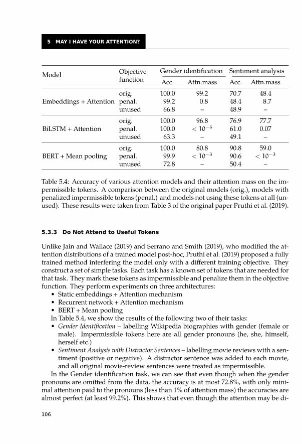
5 MAY I HAVE YOUR ATTENTION?
Model Objectivefunction
Gender identification Sentiment analysisAcc. Attn.mass Acc. Attn.mass
orig. 100.0 99.2 70.7 48.4Embeddings + Attention penal. 99.2 0.8 48.4 8.7
unused 66.8 – 48.9 –orig. 100.0 96.8 76.9 77.7
BiLSTM + Attention penal. 100.0 < 10−6 61.0 0.07unused 63.3 – 49.1 –orig. 100.0 80.8 90.8 59.0
BERT + Mean pooling penal. 99.9 < 10−3 90.6 < 10−3
unused 72.8 – 50.4 –
Table 5.4: Accuracy of various attention models and their attention mass on the im-permissible tokens. A comparison between the original models (orig.), models withpenalized impermissible tokens (penal.) and models not using these tokens at all (un-used). These results were taken from Table 3 of the original paper Pruthi et al. (2019).
5.3.3 Do Not Attend to Useful Tokens
Unlike Jain and Wallace (2019) and Serrano and Smith (2019), who modified the at-tention distributions of a trained model post-hoc, Pruthi et al. (2019) proposed a fullytrained method interfering the model only with a different training objective. Theyconstruct a set of simple tasks. Each task has a known set of tokens that are needed forthat task. They mark these tokens as impermissible and penalize them in the objectivefunction. They perform experiments on three architectures:
• Static embeddings + Attention mechanism• Recurrent network + Attention mechanism• BERT + Mean poolingIn Table 5.4, we show the results of the following two of their tasks:• Gender Identification – labelling Wikipedia biographies with gender (female or
male). Impermissible tokens here are all gender pronouns (he, she, himself,herself etc.)
• Sentiment Analysis with Distractor Sentences – labelling movie reviews with a sen-timent (positive or negative). A distractor sentence was added to each movie,and all original movie-review sentences were treated as impermissible.
In the Gender identification task, we can see that even though when the genderpronouns are omitted from the data, the accuracy is at most 72.8%, with only mini-mal attention paid to the pronouns (less than 1% of attention mass) the accuracies arealmost perfect (at least 99.2%). This shows that even though the attention may be di-
106
5.4 CONCLUSION
minished, the models are still able to rely on them. In the Sentiment analysis task, wecan see that reducing attention mass to impermissible tokens sometimes reduces over-all accuracy. The drop in accuracy depends on the complexity of the model. Whereaswe observe more than 20% drop for the simple Embeddings+Attention model, thedrop for BERT model is only 0.2%, even though the attention mass to impermissibletokes was lower than 0.001%. This can be explained by the fact that both RNN andBERT can transfer the needed information from one token to the contextual represen-tations of other tokens.
5.4 Conclusion
The attention mechanism is currently a central and important component of neuralnetworks used for solving NLP tasks. Naively, individual attention weights may be in-terpreted as importances of individual tokens or dependencies between them. Manystudies appeared showing that attention mechanism resembles some linguistic rela-tions. For example, cross-lingual attentions in machine translations align counterpartwords, some of the self-attentions heads capture specific syntactic functions betweenwords, some of the heads resemble coreferential links.
We categorized the self-attention heads into eight patterns and showed their dif-ferent distributions in the BERT and NMT models. We also summarized the distribu-tions of syntactic heads across layers and different models.
However, we must realize that the attentions might be sometimes misleading andmay carry very different information from which we would think based on the at-tended tokens.
• Even the attention with only a minimal weight may be significant, and, con-versely, the information from the most attended token may be discarded by themodel.
• The more complex models as RNNs or Transformers may easily transfer any in-formation between individual contextual representations of words. Therefore,attention to a contextual representation of one token may obtain properties of adifferent token.
• The attentions may be misleading mainly when a too strong neural network withmany parameters is used on a very simple and effortless task.
107

6
Contextual Embeddings as Un-hidden States
In this chapter, we deal with contextual word embeddings. We start by briefly lookingat how they emerged as reinterpretations of hidden states of neural models trainedfor various tasks in Section 6.1. The main section of this chapter, 6.2, summarizes thecurrent state of knowledge about various kinds of linguistically interpretable featuresthat can (or cannot) be found in contextual embeddings, going from morphology andsyntax to semantics, world knowledge and common sense. Section 6.3 takes a differentpoint of view, investigating to what extent these linguistic features can be found inindividual models and model layers. We also touch on the multilingual aspects ofcontextual embeddings in Section 6.4.
By contextual word embeddings, we understand word representations taken fromneural models trained for a Natural Language Processing (NLP) task, such as lan-guage modeling. As the model typically only needs unannotated plaintext data fortraining, which are available in large quantities, very strong contextual word embed-dings can be obtained in this way. These can then be directly used in many end tasks,where training even a very simple classifier on top of the contextual word embeddingsoften reaches or outperforms previous state-of-the-art. Those previous approachesare typically sophisticated models designed and tuned specifically for the end taskbut severely limited by only being trained on the end task dataset, not making fulluse of the general language knowledge learnable from the available vast plaintextdata.
The general understanding is that this power of contextual word embeddingscomes from the fact that a wide range of general features emerge in the represen-tations through training, capturing various important properties of the input wordsand sentences. While one might expect the model to learn only features necessary tosolve the task for which the model is trained, it seems that with a sufficiently chal-lenging and general training task, the model cannot easily “cheat” the task by learn-ing only a handful of features and ignoring most of the information on the input.Rather, it seems that it becomes economical for the model to latently develop somegeneral language understanding and use this to solve the task eventually. Thus, it is ofgreat interest to investigate this phenomenon, analyzing the contextual word embed-dings to see whether the emergent features somehow correspond to the traditionalways and abstractions in which linguists think about language understanding, suchas morphology, syntax, and semantics.
109
6 CONTEXTUAL EMBEDDINGS AS UN-HIDDEN STATES
6.1 How Contextual Embeddings Came to Be
Static word embeddings were a key invention that made it possible to efficiently useNeural Networks (NNs) for processing textual language data. Much has been saidabout the words’ properties captured by the word embeddings (see Chapter 4). How-ever, they are unable to capture information about the immediate context of the word;they are type-based, not token-based representations, fixed for the model’s vocabu-lary of words (or subwords).1 Static word embeddings are thus somewhat impracticalfor handling homonymous or polysemous words, where the word needs to be under-stood differently based on its context.2
Instead, what has been the mainstream approach practically since the boom ofdeep neural NLP are NN architectures which look at input words together with theirimmediate context, using Convolutional Neural Networks (CNNs), Recurrent NeuralNetworks (RNNs), and attentive meachanisms. In CNNs, filters look at short spans ofwords at once. In RNNs, the internal state when processing a word is influenced bythe previous words; or also following words in case of Bidirectional Recurrent NeuralNetworks (biRNNs). Attentive and self-attentive mechanisms allow the network toattend selectively to multiple words at once, or, while processing a word, to attend toother words that provide important context.
As an RNN iterates over the sequence of input words, the RNN cell passes througha series of hidden states until reaching a final state at the end of the sequence. One wayof looking at that, especially if the individual input words are of no further interest tous, is that the hidden states are only temporary intermediate states, and only the finalstate is of interest and represents the whole sentence.
In many cases, however, we are still interested in the individual words, e.g., in thecase of Part of Speech (PoS) tagging or Named Entity Recognition (NER).3 In suchcases, we are thus mostly interested in the hidden states – which might also be calledoutput states in such case, but the term hidden states is much more common – as thesemay serve as representations of the words in the context of the sentence and the endtask. Indeed, already the seminal work by Bahdanau et al. (2014) did choose to use thehidden states as representations of the input words for Neural Machine Translation(NMT) with great success, even though Machine Translation (MT) is, in principle, a
1 In this chapter, we will mostly talk about words, even if this can often mean subwords. The main reasonis that it is much more complicated to assign linguistic categories to subwords than to words. Therefore,all of the analyses of word representations that operate on subword representations need to deal with thisissue, typically by deriving word representations by averaging the subword representations, as has beendiscussed in Section 3.3.2.
2 While there have been attempts at disambiguating individual word senses and assigning them differentword embeddings, such as the work of Neelakantan et al. (2015), such methods are somewhat limited,never became the mainstream in NLP, and eventually mostly fell out of use.
3 Leaving aside the fact that the RNN final state usually turns out not to be a very good representation ofthe sentence (Graves, 2014; Hochreiter et al., 2001).
110
6.2 WHAT DO HIDDEN STATES HIDE?
sentence-to-sentence mapping task and so using the RNN final state as input repre-sentation might theoretically make more sense.
In this way, hidden states of recurrent neural encoders started to be used as con-textual word representations, at first only as intermediate representations within amodel trained for a given task.4 Gradually, however, researchers have realised thatthese representations are often more general and can be used as pre-trained wordrepresentations even for other tasks than the one they were originally trained for,within the concept of transfer learning. To understand why this is possible, manystudies investigated the representations using probing and other methods, showingthat, while containing some end-task-specific information, the representations oftencapture some linguistically interpretable features to some extent. For example, a lin-ear projection of the representations can often be found which quite accurately mapsonto some traditional PoS labels.
Once hidden states started to be used as word representations independently ofthe models within which they were trained, they started to be referred to as contextualword embeddings (see Section 2.4); since then, we could also metaphorically say thatthe hidden states stopped being hidden.5 The neural model which is trained and used toprovide the hidden states is typically referred to as a contextualizer, as it enriches staticword embeddings with information based on the immediate context of the words.
While nearly any model with a word-level encoder trained for any NLP task can beused as a contextualizer, it has been found that some models work better than others.At first, NMT models were typically used, with CoVe Context Vectors (CoVe) beinga typical representative. Later, it has been found that the Language Model (LM) taskseems to lead to better, more general and more expressive contextual word embed-dings, with Embeddings using Language Models (ELMo) being the first widely suc-cessful contextualizer. Further research then led to even more advanced and special-ized architectures and training methods. Currently, the most well-known and mostsuccessful contextualizer is Bidirectional Encoder Representations from Transformers(BERT) and its subsequent derivates.
6.2 What do Hidden States Hide?
In the next sections, we try to summarize the current state of knowledge about featuresthat tend to emerge in contextual word embeddings and can be mapped to variouslinguistic abstractions.
Generally, as explained, e.g., by Liu et al. (2019a), basic linguistically interpretablefeatures can be easily extracted from the representations, even with a linear classifier
4 It is usually assumed that the recurrent encoder’s ith hidden state can be thought of as a representationcorresponding to the ith input word. While this is by no means theoretically guaranteed, it has beenfound that, in practice, this mostly holds, as we discussed in Section 3.3.
5 As explained in Section 2.4, in our text, we often do not strictly differentiate between hidden states andcontextual word embeddings.
111
6 CONTEXTUAL EMBEDDINGS AS UN-HIDDEN STATES
(i.e., they are linearly encoded in the representations). For more fine-grained abstrac-tions, such as higher-order syntactic relations or semantics, it might be necessary totrain a more powerful Multi-Layer Perceptron (MLP) extractor; and still, some infor-mation simply seems not to be captured at all (e.g., third-order syntactic relations).
We would like to note that several surveys on this topic have already been pub-lished, which we have partially used as inspiration and which we can recommendto a reader interested in a more extensive list of existing work on the topic; in ourbook, we rather focus on summarizing the existing knowledge than on providing anexhaustive overview of all existing studies.
• Belinkov and Glass (2019) review analysis and visualization methods, challengesets (probing datasets), and include a table of works categorized by the compo-nent they analyze, the linguistic property they look for, and the method theyuse.6
• Rogers et al. (2020) review studies that analyze and interpret the representationsfrom BERT.
6.2.1 Morphology
In the last years, multiple researchers demonstrated that hidden states of trained NLPmodels usually encode various morphological information to some degree. Theymostly focused on PoS, but also investigated various other more fine-grained mor-phological features. They mostly utilized probing with linear models or MLPs (seeSection 3.1).
The general finding is that all models trained for any NLP task, such as MT or LM,seem to capture morphological information to some extent (Belinkov et al., 2017a;Peters et al., 2018a; Tenney et al., 2018). All contextual embeddings seem to capturemorphology to a greater extent than static embeddings, such as Skip-Gram (SG) orGlobal Vectors for Word Representation (GloVe) (Belinkov et al., 2017b; Blevins et al.,2018; Tenney et al., 2018). This is demonstrated by the probing models being able topredict PoS from the contextual embeddings with higher accuracies than from staticembeddings.
In multilayer contextualizers, we have the option to extract hidden states to use ascontextual embeddings from various layers. As we will discuss in Section 6.3.2, it hasbeen found that linguistic features tend to be mostly captured at different layers basedon the architecture of the contextualizer. For RNN-based contextualizers, such asELMo, all linguistic features tend to be most strongly captured in the first layer. How-ever, for Transformer-based contextualizers, different linguistic features are spreadacross the layers differently; morphology tends to be captured most strongly in thehidden states of the initial and middle layers of the model.
6 https://boknilev.github.io/nlp-analysis-methods/table1.html
112
6.2 WHAT DO HIDDEN STATES HIDE?
As we will discuss in more detail in Section 6.3.3, contextual embeddings obtainedfrom models trained for the LM task tend to capture morphological features morestrongly than models trained for other tasks (such as MT or autoencoding). This doesnot hold if the task itself contains strong morphological signals (such as PoS tagging,syntactic parsing or Semantic Role Labelling (SRL)), in which case PoS can be oftenpredicted from the hidden states with an accuracy approaching 100% (Blevins et al.,2018). A comparison of the PoS probing accuracies for several pre-training tasks canbe seen in Figure 6.4 on page 128.
There is also evidence that models which apply a character-level CNN to the inputstend to capture morphological features to a greater extent (Belinkov et al., 2017a).
6.2.2 Syntax
We have already discussed the possibility of looking for syntactic features in self-attentions (see Chapter 5). Probably an even wider range of works have successfullylooked for syntactic features in contextual word embeddings.
As even static embeddings have been shown to capture morphology to a consider-able extent, it came as no surprise that it is also captured by contextual embeddings.However, as static embeddings cannot in principle capture the syntactic structure ofa sentence, probing contextual embeddings for syntactic abstractions is of great inter-est.
Constituency Syntax
Various authors have shown that most deep NN models trained for NLP tasks doencode features which can be mapped to constituency syntax.
Most works focus on predicting syntactic constituent labels,7 showing that these canbe predicted from contextual embeddings with much higher accuracy than from staticembeddings, suggesting that such syntactic features emerge in the model. This hasbeen shown already for simple MT and LM models (Shi et al., 2016; Blevins et al.,2018), and later confirmed also for more complex contextualizers (Tenney et al., 2018;Peters et al., 2018b). The authors used classical probing, as well as other methods,such as edge probing of Tenney et al. (2018), probing gold node pairs for the constituentlabels, or indirect evidence provided by improvements observed when contextual em-beddings are used as input for training a syntactic parser (Peters et al., 2018b). Theseresults suggest that capturing the language’s syntax helps the models in understand-ing the language.
7 E.g., VP (verb phrase), NP (noun phrase), or SINV (inverted declarative sentence, using the VSO wordorder).
113
6 CONTEXTUAL EMBEDDINGS AS UN-HIDDEN STATES
The trained models have been also shown to capture features relevant for other lin-guistic abstractions, such as chunking boundaries8 or Combinatory Categorial Gram-mar (CCG) supertags9 (Liu et al., 2019a).
Dependency Syntax
The first studies aimed at looking for dependency syntax in trained neural networkmodels looked at activations of individual neurons. For example, Karpathy et al.(2015) found some patterns in gate activation statistics of individual neurons in LongShort-Term Memory (LSTM) cells in character-level LMs that correspond to variouslong-range dependencies in the sentence, concluding that such a neuron can capture,e.g., the correspondence relation of quotes or brackets.
Blevins et al. (2018) train a binary classifier on contextual representations of pairsof words, predicting whether there is a dependency edge between the two words. Allof the probed models showed a considerable amount of syntactic features.10
Tenney et al. (2018, 2019) use edge probing to probe contextual embeddings for de-pendency syntax. They use gold information about the dependency tree structure,taking gold syntactic edges as input and trying to predict the dependency edge re-lation label from the contextual representations of the two words. They find thatinformation about the edge label is rather easy to extract from the representations,suggesting that they do capture features that correspond to the syntactic relationsabstractions.
Hewitt and Manning (2019) take an unusual approach, designing structural probesand probing for various numeric structural descriptors rather than training binaryor multiclass classifiers. In this way, they are able to find linear transformations fromELMo and BERT contextual embeddings to node tree distance and to node tree depth,which achieve sufficiently high performance for the authors to claim that “entire syn-tax trees are embedded implicitly in deep models’ vector geometry”.11
8 In the syntactic sense, a chunk is a constituent phrase; the task of chunking, which is a simplification of thetask of full syntactic parsing, typically consists of splitting the sentence into a flat sequence of unlabeledchunks, instead of a hierarchy of labeled constituents.
9 CCG (Steedman and Baldridge, 2011) supertags encode partial constituent labels using forward and back-ward slashes; e.g., “the” could be labeled as NP/N as it must be completed by a noun (N) from the rightto form a noun phrase (NP).
10 Hidden states from an MT model led to a 73% accuracy, and hidden states from an LM model led to an80% accuracy in probing, compared to 95% accuracy achieved by using hidden states from a syntacticparser model; the random baseline is 50%.
11 We see these claims as probably inadequately strong, as the authors do not convincingly show that thesyntactic features are indeed embedded in the representations and not just, to some extent, memorizedby the strong probing classifier.
114
6.2 WHAT DO HIDDEN STATES HIDE?
More Complex Syntactic Relations
Liu et al. (2019a) investigate ELMo, finding that the contextual representations do notcapture information about third-order syntactic relations (great-grandparent predic-tion task) or conjuncts (identification of conjunct tokens in a coordination construc-tion), which is manifested by the fact that a linear probe is unable to extract suchinformation from the representations.
A stronger MLP probe is able to perform these predictions, which Liu et al. (2019a)interpret as the representations capturing information necessary to solve the task, butnot directly capturing features that would correspond to these more complex syntacticabstractions. As, obviously, the task is solvable even from plain text (even though astronger classifier would be needed), this only means that ELMo does not forget thenecessary features from the input and stores them in such a way that they can be easilyextracted and utilized by a strong-enough classifier.
Grammatical Correctness
One of the classical views of a Language Model is that of an LM being a tool whichdecides whether a given sentence is or is not valid in the given language. It is thusquite natural to ask whether LM representations capture features that would distin-guish between grammatical and agrammatical sentences; and whether these featuresare general, or whether they are rather limited to certain structures or phenomena.
Probably the first work that looked for evidence of trained NN models captur-ing syntax was the work of Linzen et al. (2016). The authors designed a task of pre-dicting the grammatical correctness of a sentence, with a number of hard cases pre-sumably requiring the model to understand morphological number agreement be-tween subject and predicate.12 They then probed a simple single-layer unidirectionalLSTM-based LM with a logistic regression probe. Based on the negative results onthe hard cases, the authors concluded that the model does not capture this syntacticphenomenon. However, they only used the final state of the LSTM, assuming thatit would capture information about the whole sentence. With the current state ofknowledge, we can see the flaw in the experiment, as the final state typically mostlycaptures information about the corresponding word (i.e., sentence-final punctuation)and, to some extent, neighboring words; e.g., the mean of all hidden states shouldhave been probed instead. Nevertheless, the authors also tried training the model di-rectly for the end task, this time obtaining positive results, and thus concluding thateven a simple LSTM-based model is capable of learning syntax if trained to do so.
The task of predicting grammatical correctness was revisited by Liu et al. (2019a),who trained a probe to predict token-level grammatical errors, i.e., for each token, the
12 The hard cases require a deeper syntactic understanding of language than only checking a small localcontext by containing intervening nouns or phrases between the agreement participants, as in “Alluvialsoils carried in the floodwaters add nutrients to the floodplains.”.
115
6 CONTEXTUAL EMBEDDINGS AS UN-HIDDEN STATES
task is to say whether the token needs to be edited to make the sentence grammati-cally correct; the authors posit that solving this task requires understanding of syntaxand grammar of the language. They probe ELMo representations, finding a similarsituation as with harder syntactic relations: the model captures some information nec-essary for solving the task (as shown by a successful MLP probe), but does not capturethe information about the grammatical correctness itself (attested by an unsuccessfullinear probe). Moreover, even the stronger probe reaches rather low accuracies inabsolute terms, even though it outperforms previous state-of-the-art (which is alsorather low), suggesting that this is a rather hard task, still beyond the capabilities ofcurrent models.
6.2.3 Coreference
In coreference, we deal with the phenomenon of several entities (typically pronounsor noun phrases) referring to the same real-world entity.13 While based on the per-formance of neural models on various tasks, we may assume that they have a wayof understanding this notion, we may ask how they capture this, and whether theirgrasp of the phenomenon is general or limited.
The contextual embeddings seem to understand coreference in easier cases whereit can be determined from morphosyntactic cues, as shown, for example, by Peterset al. (2018b), who find that the similarity of the embeddings of the referential pro-noun and the antecedent noun is often high enough for correct coreference resolution.
However, in harder coreference cases which require deeper semantic understand-ing, as represented by the Winograd coreference resolution dataset (Levesque et al.,2012),14 the contextual embeddings typically perform poorly, only slightly outper-forming static embeddings baselines (Tenney et al., 2018).
6.2.4 Semantics
In Chapter 4, we have seen that neural models can learn lexical semantics to a greatextent. In this section, we thus go beyond lexical semantics, particularly focusing onsemantic labels that are context-dependent, such as semantic roles or word senses.
A grave issue with any probing for semantic information is the strong threat offalsely positive results, as many semantic ambiguities can be resolved solely based onmorphosyntactic cues. As we already know that morphosyntactic features are wellcaptured by the contextual embeddings, a semantic probe can easily learn to perform
13 E.g., “John told Mary he liked her, and she let him kiss her on her cheek.”, where “John”, “he” and “him”refer to one entity (John) and “Mary”, “her” and “she” to another entity (Mary).
14 The Winograd scheme focuses on cases of coreference which are morphologically and syntactically am-biguous and irresolvable, such as “Characters entertain audiences because they want people to be happy.”where resolving whether “they” refers to characters or audiences requires semantic understanding oreven real-world knowledge.
116
6.2 WHAT DO HIDDEN STATES HIDE?
the semantic labeling based on these morphosyntactic cues, failing to reveal whetherthe semantic distinction is captured in the contextual representation explicitly.
When the analyses are properly executed and carefully examined, we typically findonly mildly positive results for various specific semantic labels, showing that some se-mantics is captured. It is rare to find a semantic feature which would be captured verystrongly in the representations; and if so, it is often the case that the seemingly seman-tic feature can actually be very well predicted based solely on morphosyntactic cues,and thus the probe does not prove that, beyond morphology and syntax, semanticswould also be captured.
Semantic Tagging
Various authors have probed contextual embeddings for various semantic labels, suchas semantic roles (Palmer et al., 2005),15 semantic proto-roles (Teichert et al., 2017;Rudinger et al., 2018),16 or sem-tagging (Bjerva et al., 2016).17 The general findingseems to be that the models do not capture deeper semantic features to a great extent,only lightly outperforming the static embeddings baselines (Belinkov et al., 2017b;Tenney et al., 2018).
We can also understand named entity labels18 as a kind of semantic labels. Here,contextual embeddings seem to capture information about named entity types tosome extent, strongly outperforming a static embeddings baseline but still being farfrom comparable state-of-the-art results (Liu et al., 2019a).
The good performance of some semantic label probes can usually be explained byinspecting the results more thoroughly, revealing that the good results are obtained,especially for the cases where the correct label can be easily determined solely frommorphosyntactic cues (Tenney et al., 2018). Thus, the experiments mostly only re-confirm the interpretation that the representations capture morphological and syn-tactic features, but do not seem to exhibit a deeper understanding of the meaning ofthe sentence.
However, any negative result in interpreting neural networks must be taken with agrain of salt. The aforementioned results clearly show that the probed neural modelsdo not seem to capture semantic features similar to various classical semantic labels.While a plausible explanation is that the models do not capture any semantic featuresat all, an alternative explanation is also possible: that the models do have a deeperunderstanding of language than we have been able to show, but that the way in whichthey encode the semantics of the language is so different from the labels we use thatwe just have not been able to recognize it yet.15 E.g., agent, location, purpose, direction.16 This is a more fine-grained variant of semantic roles.17 This is a semantic extension of PoS tagging, distinguishing, e.g., determiners into categories such as
proximal (e.g. “this”) and distal (e.g. “that”).18 E.g., person, organization, geographical entity.
117
6 CONTEXTUAL EMBEDDINGS AS UN-HIDDEN STATES
Noun Gender
It has been already discussed in Chapter 4 that even static embeddings do typicallycapture features which correspond to the morphological gender of nouns in languageswhere nouns are gendered, as in Czech. However, in this section, we are rather inter-ested in capturing the semantic gender of nouns, even and especially when this is notmorphologically marked, as in English.
Zhao et al. (2019) find that ELMo captures gender in nouns. The authors iden-tify two gender-related principal components of the representations using PrincipalComponent Analysis (PCA):
• contextual gender, based, e.g., on the occurrence of a “he” or “she” pronoun inthe sentence (so, e.g., a “librarian” is disambiguated as being male or female inthe given sentence),
• occupational gender, which is the gender embedded in the word itself, either ex-plicitly marked (e.g. “actress”) or stereotypical (e.g. a female “nurse” versus amale “developer”).
The authors interpret this as the contextual representations being gender-biased,which happens because of the inherent gender bias of the text corpora used to inducethe representations; the authors also present an effective way of debiasing the repre-sentations by augmenting the training data with gender-swapped sentences. This isrelated to the findings of static word embeddings capturing gender, as discussed inSection 4.10.
6.2.5 Context
It is logical to expect contextual word embeddings to encode the context of the wordto some extent. But is it only limited local immediate context, so that we could obtaincompetitive contextual embeddings just by mixing the static embeddings of severalneighboring words? Or are the embeddings also influenced by more distant wordsin more intricate ways? Research shows that the strongest component of a contextualword embedding still is the word identity, especially in shallow layers of the contex-tualizers. However, as we go to deeper layers of the contextualizers, the contextualembeddings capture wider and wider context, starting with immediate surroundingsbut eventually being able to capture information about other words from anywherein the sentence.
Tenney et al. (2018) compare the ELMo embeddings both to classical non-contextu-al embeddings, as well as to locally contextualized embeddings, obtained by applyinga word-level CNN with a kernel size of either 3 or 5 over the static word embeddings,i.e., integrating information about 1 or 2 neighboring words at each side of the word.They find that for morphological and syntactic probing tasks, not much is gained byfull contextual embeddings over the locally contextualized embeddings (0–2 percent-age points); this might mean that little non-local information is encoded in the con-textual embeddings or that non-local information is of little relevance for the probing
118
6.2 WHAT DO HIDDEN STATES HIDE?
tasks. The latter actually seems more likely, as the situation is quite different for thesemantic tasks; these seem to require more non-local information for the probe toperform well, and, accordingly, the full ELMo embeddings outperform the locallycontextualized embeddings more clearly (1-5 percentage points). Thus, the conclu-sion seems to be that ELMo embeddings are much more than just static embeddingsenriched with information about neighboring words, and do actually also captureimportant non-local features from the sentence.
Ethayarajh (2019) investigated how contextual the contextual embeddings reallyare. They found that the base of a contextual word embedding still seems to be astatic component shared by all occurrences of the same word. However, especially forhigher layers of multilayer contextualizers, the static component is rather weak, withthe cosine self-similarity of different occurrences of the same word getting weaker inthe higher layers, i.e., the representations are getting more context-specific.
Peters et al. (2018b) note that local syntax seems to be the dominant signal in thecontextual embeddings, encoding syntactic phrase pertinence and boundaries; i.e.,the contextualizer does not simply combine neighboring words weighted by their dis-tance, it does also take syntax into account.
6.2.6 Word Senses
A concept closely related to context are word senses, i.e., discriminating between mul-tiple senses of a single polysemous word (such as “train” in “I came on a train.” versus“I train young children.”). Trivially, static word embeddings are incapable of that dis-tinction since the same vector is used for the word in any context. As contextual wordembeddings do take context into account and represent the word with a differentvector in each context, we may expect that the word sense distinction could be madebased on the contextual embeddings. This turns out to be true, even to the extentthat the contextual embeddings pertaining to various occurrences of an individualpolysemous word often tend to form multiple clusters or clouds corresponding to itsindividual senses.
We might also be interested in the distinction between simply encoding contextand encoding features more directly corresponding to a word sense abstraction. Asa word sense is predominantly determined by the immediate context in which theword is used, such a distinction is not trivial to make. However, there seems to beevidence that the contextual representations do indeed go beyond simply encodingcontext and actually distinguish the individual senses.
Peters et al. (2018a) use a k-nearest neighbours (k-NN)-based approach to inves-tigate the relation of contextual word embeddings to word senses. They first com-pute CoVe and ELMo representations of words in sentences from SemCor 3.0 (Milleret al., 1994), a corpus with annotations of word senses. Then, for each sense of eachpolysemous word, they compute a representation of the sense as the average of thecontextual embeddings of these senses of the word which occur in the training part
119
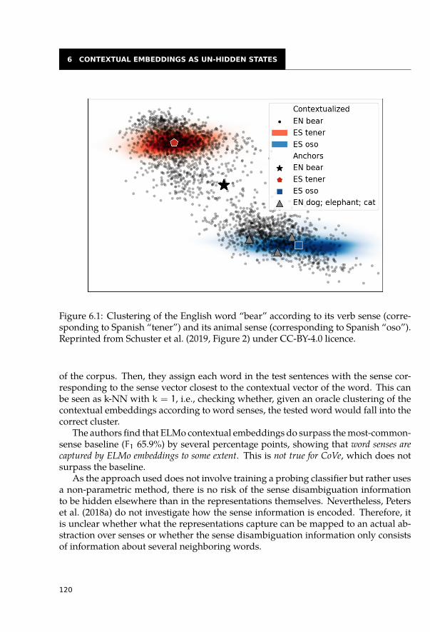
6 CONTEXTUAL EMBEDDINGS AS UN-HIDDEN STATES
Figure 6.1: Clustering of the English word “bear” according to its verb sense (corre-sponding to Spanish “tener”) and its animal sense (corresponding to Spanish “oso”).Reprinted from Schuster et al. (2019, Figure 2) under CC-BY-4.0 licence.
of the corpus. Then, they assign each word in the test sentences with the sense cor-responding to the sense vector closest to the contextual vector of the word. This canbe seen as k-NN with k = 1, i.e., checking whether, given an oracle clustering of thecontextual embeddings according to word senses, the tested word would fall into thecorrect cluster.
The authors find that ELMo contextual embeddings do surpass the most-common-sense baseline (F1 65.9%) by several percentage points, showing that word senses arecaptured by ELMo embeddings to some extent. This is not true for CoVe, which does notsurpass the baseline.
As the approach used does not involve training a probing classifier but rather usesa non-parametric method, there is no risk of the sense disambiguation informationto be hidden elsewhere than in the representations themselves. Nevertheless, Peterset al. (2018a) do not investigate how the sense information is encoded. Therefore, itis unclear whether what the representations capture can be mapped to an actual ab-straction over senses or whether the sense disambiguation information only consistsof information about several neighboring words.
120
6.3 WHAT IS HIDDEN WHERE?
Schuster et al. (2019) demonstrate that, for a fixed word form, ELMo contextualembeddings cluster according to the various senses of the word. In their example,reprinted in Figure 6.1, they show how the contextual embeddings for the Englishword “bear” cluster into two clouds, one corresponding to the verb meaning, and theother corresponding to the animal meaning; the image also shows that the represen-tation for the animal “bear” is closer, e.g., to “elephant” or “cat” than to the repre-sentation for the verb “bear”. They further claim that the word sense is the strongestsignal in the contextual embeddings, as they show that the representations of a givenword with an identical sense in different contexts are more similar to each other thanrepresentations of the same word in similar contexts but with different senses. Inter-estingly, all of these are just side-results for the authors, as their main goal is cross-lingual alignment of contextual word embeddings.
6.2.7 World Knowledge and Common Sense
Da and Kasai (2019) show that BERT captures some world knowledge or common-sense information to some extent, such as how large something is or whether some-thing is an animal. They show that using BERT for this kind of common sense reason-ing outperforms previous approaches, but that the model still often fails, suggestingthat BERT is unable to get sufficient world knowledge from its training data.
Rogers et al. (2020) review some works in this area, concluding that BERT can per-form well in some tasks focusing on world knowledge, reaching competitive perfor-mance to state-of-the-art question-answering systems (Petroni et al., 2019). However,BERT’s apparent world knowledge is rather of a stereotypical factoid nature, mostlybased on frequent cooccurrences but not able to infer more complex relations and in-teractions (Poerner et al., 2019). The BERT model thus seems to contain some worldknowledge but is not able to use for reasoning.
6.3 What is Hidden Where?
In the previous section, we looked at what kinds of linguistic features are captured bycontextual word embeddings, disregarding where the contextual embeddings comefrom. We now fill this gap by reviewing how the contextualizers differ in the num-ber of linguistic features captured and looking at how the linguistic features are dis-tributed among various layers of the contextualizer models.
6.3.1 Comparison of Architectures and Models
All of the contextual word embeddings, including hidden states taken from modelstrained for another purpose (such as NMT models), seem to capture morphology andsyntax rather well and even a little of semantics, typically to a greater extent than staticembeddings (Tenney et al., 2018).
121
6 CONTEXTUAL EMBEDDINGS AS UN-HIDDEN STATES
In this section, we focus mostly on the effect of the architecture of the contextual-izer; we will focus on the effect of the pre-training task in Section 6.3.3.
In general, the representations from simpler models, such as CoVe, typically seemto be weaker than representations from the more recent and complex contextualizers,as demonstrated by their lower probing accuracies; nevertheless, CoVe representa-tions still typically capture the linguistic features to a significantly higher degree thanstatic word embeddings (Tenney et al., 2018).
Tenney et al. (2018) find that ELMo seems to capture syntax better than CoVe.19
However, this difference can be mostly explained by the underlying character-CNNstatic word embeddings being more informative in this sense – i.e., already the char-acter-based static embeddings used in ELMo seem to be significantly more syntacticthan classical word-based embeddings, and the further layers seem to add a similaramount of contextual and syntactic information as in CoVe. It should also be notedthat these experiments did not control for the different data sizes of the contextualizerpre-training data, with CoVe being pre-trained on a several times smaller dataset.20
Even though BERT typically outperforms ELMo on practical tasks, it does not seemto capture the linguistic features to a considerably greater extent; it can be used topredict various linguistic accuracies with higher accuracy than ELMo (typically by 2to 3 percentage points), but only if the weights of the layer mix are trained on a task-specific dataset (Tenney et al., 2018). It is possible that a considerable portion of thisdifference is caused by tokenization, where ELMo uses rather standard tokenizationwhich matches the tokenization in the probing datasets to a great extent, while BERTuses a purely technical splitting into subwords and may thus operate on very differenttokens than what is used in the benchmarks.
A large improvement of BERT over ELMo can be observed for Winograd corefer-ence (see Section 6.2.3), where all previous models failed to significantly outperformthe static embeddings baseline. BERT is the first model to outperform the baselineby 6 percentage points, suggesting that it does capture some more elaborate semanticinformation.
Generative Pre-Trained Transformer (GPT) usually seems to be similar to ELMo orslightly weaker, but still way above CoVe (Tenney et al., 2018). I.e., although perform-ing better than BERT as an LM, it seems to be slightly weaker in capturing linguisticfeatures.
An exception to this general trend may be found in the work of Kim et al. (2020),who focused on extracting constituency trees from pre-trained LMs, finding that GPT-2 actually outperforms BERT on this task. The authors hypothesize that this may be
19 Probe accuracies consistently seem to be about 10% higher for ELMo than CoVe, regardless of whetherwe probe for, e.g., constituent labels or dependency relations.
20 As CoVe is an MT model, it requires parallel data, while monolingual data are sufficient for ELMo. Inthe work of Tenney et al. (2018), the particular probed models used 7 million sentences versus 30 millionsentences, respectively.
122
6.3 WHAT IS HIDDEN WHERE?
due to the training objective, with a standard auto-recursive LM being better suitedfor constituency phrases than a masked auto-decoding LM.
6.3.2 Distribution of Linguistic Features across Layers
In multilayer contextualizers, contextual representations can be taken from any layer,or multiple layers can be concatenated or mixed.21 We now investigate into whichlayers to look for what kind of linguistic features.
RNN-based models capture linguistic features in the first layer
We first look at the RNN-based models, such as CoVe and ELMo. These models pro-totypically contain two layers of hidden states, but some authors also investigateddeeper multilayer variants of these models.
Many authors show that, especially for morphological and syntactic annotation,the linguistic features can be best extracted by probes or projections applied to thefirst layer of the model, no matter whether the network has two or more layers (Zhangand Bowman, 2018; Liu et al., 2019a; Peters et al., 2018b). It is further claimed that thesecond layer (as well as potential subsequent layers) are already more task-specificand do not capture easily interpretable linguistic features very well (Liu et al., 2019a).
However, Peters et al. (2018a) show that for word sense disambiguation, using thesecond layer of a two-layer CoVe or ELMo model for prediction of the sense classactually leads to better results than using the first layer. This suggests that even inthe simpler models, some deeper linguistic information (such as some semantic as-pects) is better captured in deeper layers. Nevertheless, this may also be explainedas the word senses actually being crucial for the training task (machine translation orlanguage modeling). This would corroborate the hypothesis of other authors that thesubsequent layers are more task-specific but go against their implication of the deeperlayers thus being less useful for extracting linguistic features.
Figure 6.2, reprinted from (Tenney et al., 2019, figure A.1), provides yet anotherview on this issue. The authors show that morphological, syntactic as well as someshallow semantic features are mostly captured in the first layer of ELMo; while not-ing that the shallow semantic tasks – semantic role labeling and coreference – can bemostly solved using syntactic cues. For deeper semantic tasks (semantic proto-rolesand semantic relations), the information seems to be rather equally distributed amongthe first and second layer of ELMo; however, as ELMo is shown not to capture thesesemantic features to a great extent, this probably does not mean that semantic featuresare also captured in the second layer, but rather that they are not even captured in thefirst layer.
21 E.g., for ELMo, it is a standard approach to take a weighted combination of the individual layers to utilizefor transfer learning.
123
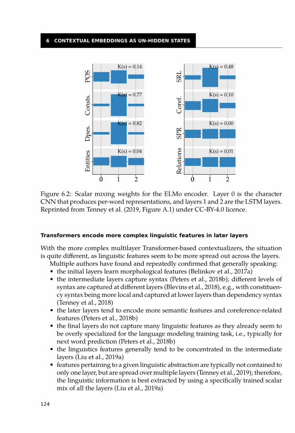
6 CONTEXTUAL EMBEDDINGS AS UN-HIDDEN STATES
0 1 20
Entit
ies
Dpe
s.C
onst
s.PO
S
K(s) = 0.04
K(s) = 0.82
K(s) = 0.77
K(s) = 0.14
0 1 20Re
latio
nsSP
RC
oref
.SR
L
K(s) = 0.01
K(s) = 0.00
K(s) = 0.10
K(s) = 0.48
Figure 6.2: Scalar mixing weights for the ELMo encoder. Layer 0 is the characterCNN that produces per-word representations, and layers 1 and 2 are the LSTM layers.Reprinted from Tenney et al. (2019, Figure A.1) under CC-BY-4.0 licence.
Transformers encode more complex linguistic features in later layers
With the more complex multilayer Transformer-based contextualizers, the situationis quite different, as linguistic features seem to be more spread out across the layers.
Multiple authors have found and repeatedly confirmed that generally speaking:• the initial layers learn morphological features (Belinkov et al., 2017a)• the intermediate layers capture syntax (Peters et al., 2018b); different levels of
syntax are captured at different layers (Blevins et al., 2018), e.g., with constituen-cy syntax being more local and captured at lower layers than dependency syntax(Tenney et al., 2018)
• the later layers tend to encode more semantic features and coreference-relatedfeatures (Peters et al., 2018b)
• the final layers do not capture many linguistic features as they already seem tobe overly specialized for the language modeling training task, i.e., typically fornext word prediction (Peters et al., 2018b)
• the linguistics features generally tend to be concentrated in the intermediatelayers (Liu et al., 2019a)
• features pertaining to a given linguistic abstraction are typically not contained toonly one layer, but are spread over multiple layers (Tenney et al., 2019); therefore,the linguistic information is best extracted by using a specifically trained scalarmix of all the layers (Liu et al., 2019a)
124
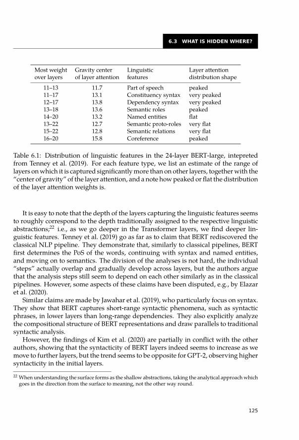
6.3 WHAT IS HIDDEN WHERE?
Most weight Gravity center Linguistic Layer attentionover layers of layer attention features distribution shape
11–13 11.7 Part of speech peaked11–17 13.1 Constituency syntax very peaked12–17 13.8 Dependency syntax very peaked13–18 13.6 Semantic roles peaked14–20 13.2 Named entities flat13–22 12.7 Semantic proto-roles very flat15–22 12.8 Semantic relations very flat16–20 15.8 Coreference peaked
Table 6.1: Distribution of linguistic features in the 24-layer BERT-large, intepretedfrom Tenney et al. (2019). For each feature type, we list an estimate of the range oflayers on which it is captured significantly more than on other layers, together with the“center of gravity” of the layer attention, and a note how peaked or flat the distributionof the layer attention weights is.
It is easy to note that the depth of the layers capturing the linguistic features seemsto roughly correspond to the depth traditionally assigned to the respective linguisticabstractions;22 i.e., as we go deeper in the Transformer layers, we find deeper lin-guistic features. Tenney et al. (2019) go as far as to claim that BERT rediscovered theclassical NLP pipeline. They demonstrate that, similarly to classical pipelines, BERTfirst determines the PoS of the words, continuing with syntax and named entities,and moving on to semantics. The division of the analyses is not hard, the individual“steps” actually overlap and gradually develop across layers, but the authors arguethat the analysis steps still seem to depend on each other similarly as in the classicalpipelines. However, some aspects of these claims have been disputed, e.g., by Elazaret al. (2020).
Similar claims are made by Jawahar et al. (2019), who particularly focus on syntax.They show that BERT captures short-range syntactic phenomena, such as syntacticphrases, in lower layers than long-range dependencies. They also explicitly analyzethe compositional structure of BERT representations and draw parallels to traditionalsyntactic analysis.
However, the findings of Kim et al. (2020) are partially in conflict with the otherauthors, showing that the syntacticity of BERT layers indeed seems to increase as wemove to further layers, but the trend seems to be opposite for GPT-2, observing highersyntacticity in the initial layers.
22 When understanding the surface forms as the shallow abstractions, taking the analytical approach whichgoes in the direction from the surface to meaning, not the other way round.
125
6 CONTEXTUAL EMBEDDINGS AS UN-HIDDEN STATES
We try to interpret the findings of Tenney et al. (2019) in Table 6.1. The authorsuse probes to extract the linguistic features from the layers employing layer attention,i.e., a trained task-specific linear combination of the model representations from themodel layers. This provides them with a set of layer weights for each of the tasks (i.e.,for each of the linguistic features which they probe for). The authors then interpretthese layer weights as a measure of the degree to which the given linguistic feature isencoded within the given layer.
For each linguistic feature type examined by the authors, we also report its “centerof gravity” (the authors’ term) of the layer attention from (Tenney et al., 2019, Fig-ure 1); please refer to the original paper for the full figure. The center of gravity is theweighted average of the layer numbers weighted by the layer attention weights, i.e.,it is the average layer capturing the given linguistic feature.
Figure 6.3, reprinted from (Tenney et al., 2019, figure 2), shows the distribution ofthe layer weights for the individual tasks. In Table 6.1, we estimate how peaked orflat the distribution of these weights is. Some features seem to be mostly captured ononly a few layers (the layer attention is rather peaked), while others seem to be morespread out (the layer attention is rather flat).
Thus, based on the graphs in Figure 6.3, we can estimate the layers on which thefeatures are mostly captured. Unfortunately, the authors present the data in the formof graphs, but the exact numbers are not listed. Therefore, the layers which seem tocapture the features significantly more than other layers were only approximately esti-mated from the graphs. In this way, we attempt to approximately answer the questionof on which layers the respective linguistic features are captured. However, pleasenote that this is all rather approximate, as there is no clear way of answering thatquestion; refer to (Tenney et al., 2019) for the original data and interpretations.
The table confirms the rough notion of the layer depth corresponding to the depthof the linguistic features, going from morphology over syntax and semantics, withcoreference being the deepest. However, the distribution of some features across lay-ers is actually quite flat, especially for the semantic ones; i.e., some features seem tobe spread quite evenly across most or all of the layers. We thus should be careful withany strong claims based on the observations.
6.3.3 Effect of Pre-training Task
Technically, any NLP task can be used to pre-trained a contextualizer to provide con-textual embeddings. However, not all pre-training tasks are equally good for thispurpose, as shown by several studies (Belinkov et al., 2017a,b; Peters et al., 2018b;Blevins et al., 2018; Zhang and Bowman, 2018; Liu et al., 2019a).
In general, many authors have found that using the LM task for pre-training is thebest choice in most cases, as such contextual embeddings seem to best transfer to othertasks. Relatedly, such contextual embeddings are also usually found to most strongly
126
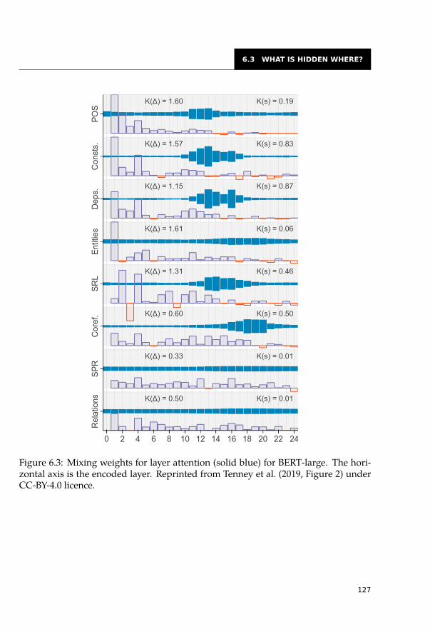
6.3 WHAT IS HIDDEN WHERE?
Figure 6.3: Mixing weights for layer attention (solid blue) for BERT-large. The hori-zontal axis is the encoded layer. Reprinted from Tenney et al. (2019, Figure 2) underCC-BY-4.0 licence.
127
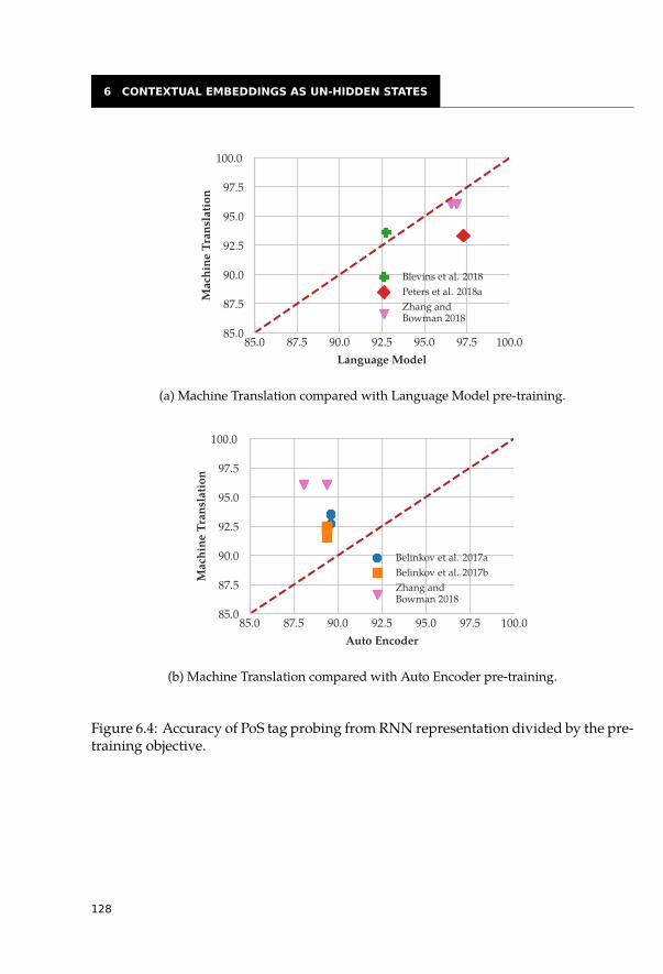
6 CONTEXTUAL EMBEDDINGS AS UN-HIDDEN STATES
..
85.0
.
87.5
.
90.0
.
92.5
.
95.0
.
97.5
.
100.0
.Language Model
.
85.0
.
87.5
.
90.0
.
92.5
.
95.0
.
97.5
.
100.0
.
Mac
hine
Tran
slat
ion
.
Blevins et al. 2018
.
Peters et al. 2018a
.
Zhang and
.
Bowman 2018
(a) Machine Translation compared with Language Model pre-training.
..
85.0
.
87.5
.
90.0
.
92.5
.
95.0
.
97.5
.
100.0
.Auto Encoder
.
85.0
.
87.5
.
90.0
.
92.5
.
95.0
.
97.5
.
100.0
.
Mac
hine
Tran
slat
ion
.
Belinkov et al. 2017a
.
Belinkov et al. 2017b
.
Zhang and
.
Bowman 2018
(b) Machine Translation compared with Auto Encoder pre-training.
Figure 6.4: Accuracy of PoS tag probing from RNN representation divided by the pre-training objective.
128
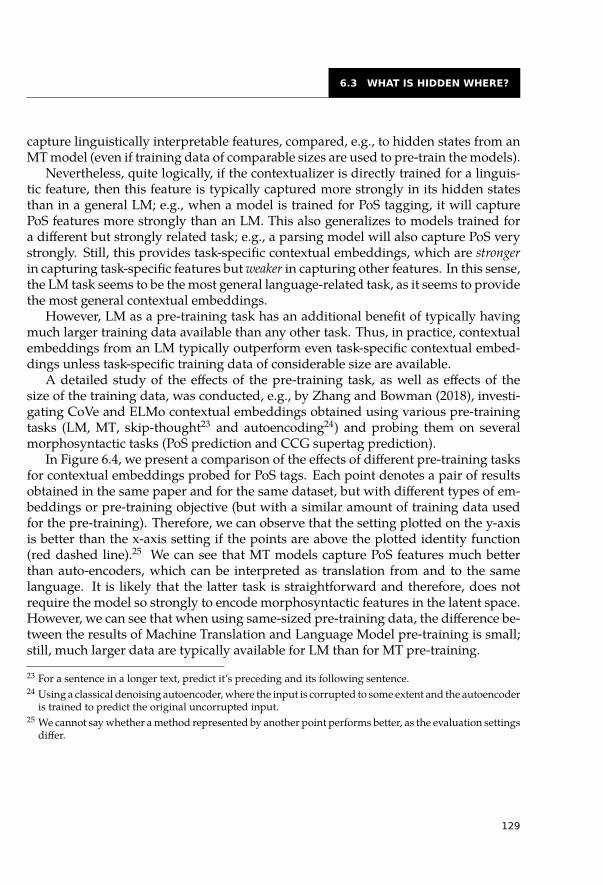
6.3 WHAT IS HIDDEN WHERE?
capture linguistically interpretable features, compared, e.g., to hidden states from anMT model (even if training data of comparable sizes are used to pre-train the models).
Nevertheless, quite logically, if the contextualizer is directly trained for a linguis-tic feature, then this feature is typically captured more strongly in its hidden statesthan in a general LM; e.g., when a model is trained for PoS tagging, it will capturePoS features more strongly than an LM. This also generalizes to models trained fora different but strongly related task; e.g., a parsing model will also capture PoS verystrongly. Still, this provides task-specific contextual embeddings, which are strongerin capturing task-specific features but weaker in capturing other features. In this sense,the LM task seems to be the most general language-related task, as it seems to providethe most general contextual embeddings.
However, LM as a pre-training task has an additional benefit of typically havingmuch larger training data available than any other task. Thus, in practice, contextualembeddings from an LM typically outperform even task-specific contextual embed-dings unless task-specific training data of considerable size are available.
A detailed study of the effects of the pre-training task, as well as effects of thesize of the training data, was conducted, e.g., by Zhang and Bowman (2018), investi-gating CoVe and ELMo contextual embeddings obtained using various pre-trainingtasks (LM, MT, skip-thought23 and autoencoding24) and probing them on severalmorphosyntactic tasks (PoS prediction and CCG supertag prediction).
In Figure 6.4, we present a comparison of the effects of different pre-training tasksfor contextual embeddings probed for PoS tags. Each point denotes a pair of resultsobtained in the same paper and for the same dataset, but with different types of em-beddings or pre-training objective (but with a similar amount of training data usedfor the pre-training). Therefore, we can observe that the setting plotted on the y-axisis better than the x-axis setting if the points are above the plotted identity function(red dashed line).25 We can see that MT models capture PoS features much betterthan auto-encoders, which can be interpreted as translation from and to the samelanguage. It is likely that the latter task is straightforward and therefore, does notrequire the model so strongly to encode morphosyntactic features in the latent space.However, we can see that when using same-sized pre-training data, the difference be-tween the results of Machine Translation and Language Model pre-training is small;still, much larger data are typically available for LM than for MT pre-training.
23 For a sentence in a longer text, predict it’s preceding and its following sentence.24 Using a classical denoising autoencoder, where the input is corrupted to some extent and the autoencoder
is trained to predict the original uncorrupted input.25 We cannot say whether a method represented by another point performs better, as the evaluation settings
differ.
129
6 CONTEXTUAL EMBEDDINGS AS UN-HIDDEN STATES
6.4 Multilinguality
So far, we have only talked about pre-trained representation models for a single lan-guage evaluated on English. However, pre-trained Transformers show remarkableability to work with multiple languages within a single model.
Multilingual BERT (mBERT) (Devlin et al., 2019), which was followed by XLM-RoBERTa (XLM-R) (Conneau et al., 2020) and DistilBERT (Sanh et al., 2020), gainedpopularity as a contextual representation for many multilingual tasks.
mBERT is a deep Transformer encoder that is trained in a multi-task learning setup,first, to be able to guess what words were masked-out in the input and, second, todecide whether two sentences follow each other in a coherent text.
It was trained using the same procedure as English BERT: a combination of amasked language model (MLM) objective and sentence-adjacency objective usingplain text in over 100 languages without making any difference among the languages.
Conneau et al. (2020) claim that the original mBERT is under-trained and traina similar model on a larger dataset that consists of two terabytes of plain text ex-tracted from CommonCrawl (Wenzek et al., 2020). Unlike mBERT, XLM-R uses aSentencePiece-based vocabulary (Kudo and Richardson, 2018) of 250k tokens, the restof the architecture remains the same as in the case of mBERT. The model is trainedusing the MLM objective, only without the sentence adjacency prediction.
Kondratyuk and Straka (2019) managed to achieve very strong results in depen-dency parsing in 75 languages by training a single model that used mBERT as an inputrepresentation without telling the model what the input language was. In this way,the model reached very good results even for languages where only test data and notraining data are available.
Often, the success of zero-shot transfer is implicitly considered to be the main mea-sure of language neutrality of a representation. Despite many positive results, somefindings in the literature are rather mixed, indicating limited language neutrality.
Zero-shot learning abilities were examined by Pires et al. (2019) on NER and PoStagging, showing that the success strongly depends on how typologically similar thelanguages are. Similarly, Wu and Dredze (2019) trained good multilingual models butstruggled to achieve good results in the zero-shot setup for POS tagging, NER, andXLNI. Rönnqvist et al. (2019) draw similar conclusions for language-generation tasks.
Wang et al. (2019b) succeeded in zero-shot dependency parsing, but required su-pervised projection trained on word-aligned parallel data. The results of Chi et al.(2020) on dependency parsing suggest that methods like structural probing (Hewittand Manning, 2019) might be more suitable for zero-shot transfer.
Pires et al. (2019) also assessed mBERT on cross-lingual sentence retrieval betweenthree language pairs. They observed that if they subtract the average difference be-tween the embeddings from the target language representation, the retrieval accuracysignificantly increases.
130
6.4 MULTILINGUALITY
XTREME (Hu et al., 2020) and XGLUE (Liang et al., 2020), two recently introducedbenchmarks for multilingual representation evaluation, assess representations on awider range of zero-shot transfer tasks that include natural language inference (Con-neau et al., 2018b) and question answering (Artetxe et al., 2019; Lewis et al., 2019).Their results show a clearly superior performance of XLM-R compared to mBERT.
Many works clearly show that downstream task models can extract relevant fea-tures from the multilingual representations (Wu and Dredze, 2019; Kudugunta et al.,2019; Kondratyuk and Straka, 2019). But they do not directly show language-neutrali-ty, i.e., to what extent similar phenomena are represented similarly across languages.It is thus impossible to say whether the representations are language-agnostic or ifthey contain some implicit language identification.
We (Libovický et al., 2019) argue that in zero-shot transfer from the source lan-guage to the target language, there is a risk of “overfitting” the source language –validation data in the source language are typically used to stop the training once theperformance on the data stops increasing, but this might mean that the model is al-ready too specialized to the source language, while a less specialized model might bemore transferable, i.e., the training should probably be stopped earlier.
We (Libovický et al., 2019) circumvent the identified problem by analyzing therepresentations on tasks of cross-lingual word-alignment, cross-lingual sentence re-trieval, and machine translation quality estimation, which directly utilize the pre-trained multilingual contextual embeddings with no further training; the embeddingsare simply averaged and compared using cosine distance to measure word or sentencesimilarity, which for each of the tasks should be maximized. We find that the multi-lingual contextual embeddings outperform bilingual static word embeddings whichwere explicitly trained to be cross-lingual, whereas the cross-linguality of the con-textual embeddings is an emergent property not explicitly imposed during training.We observe high accuracies for sentence retrieval and state-of-the-art performance forword alignment. For quality estimation, the results are very poor, suggesting that adeeper understanding of the meaning of the sentences is required than what is cap-tured by the representations.
Following Pires et al. (2019), we (Libovický et al., 2019) also show that, while therepresentations are already quite language-neutral, they in fact strongly encode thelanguage identity, actually leading to state-of-the-art results in language prediction.However, the language-neutral component and the language-specific component areeasy to separate: a language centroid can be computed as an average of representa-tions of sentences in the given language and subtracted from the contextual embed-ding to obtain a mostly language-neutral embedding. These language-neutral em-beddings perform even better in the cross-lingual tasks, while the language centroidscluster nicely according to traditional typological language families (see Figure 6.5).
131
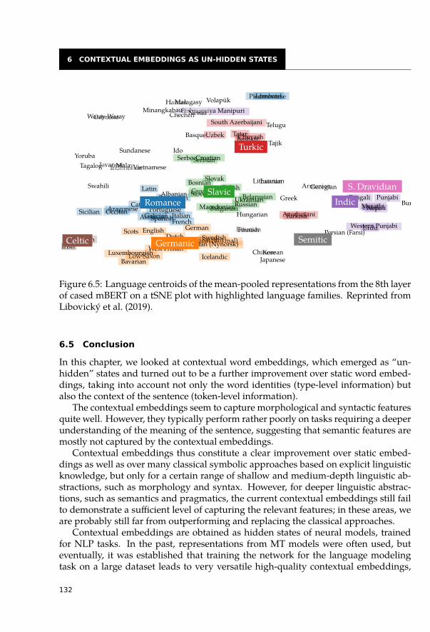
6 CONTEXTUAL EMBEDDINGS AS UN-HIDDEN STATES
..
Afrikaans
.
Albanian
.
Arabic
.
Aragonese
.
Armenian
.
Asturian
.
Azerbaijani
.
Bashkir
.
Basque
. Bavarian.
Belarusian
.
Bengali
.
Bishnupriya Manipuri
.
Bosnian
.
Breton
.
Bulgarian
.
Burmese
.
Catalan
.
Cebuano
.
Chechen
.Chinese
.
Chuvash
.
Croatian
.
Czech
.
Danish
.
Dutch
.
English
.
Estonian
.
Finnish
.
French
.
Galician
.
Georgian
.
German
.
Greek
.
Gujarati
.
Haitian
.
Hebrew
.
Hindi
.
Hungarian
.Icelandic
.
Ido
.
Indonesian
.
Irish
.
Italian
.Japanese
.
Javanese
.
Kannada
.
Kazakh
.
Kirghiz
.Korean
.
Latin
.
Latvian
.
Lithuanian
.
Lombard
.Low Saxon
.Luxembourgish
.
Macedonian
.
Malagasy
.
Malay
.
Malayalam
.
Marathi
.
Minangkabau
.
Nepali
.
Newar
.
Norwegian (Bokmal)
.
Norwegian (Nynorsk)
.
Occitan
.
Persian (Farsi)
.
Piedmontese
.
Polish
.
Portuguese
.
Punjabi
.
Romanian
.
Russian
.
Scots
.
Serbian
.
Serbo-Croatian
.
Sicilian
.
Slovak
.
Slovenian
.
South Azerbaijani
.
Spanish
.
Sundanese
.
Swahili
.
Swedish
.
Tagalog
.
Tajik
.
Tamil
.
Tatar
.
Telugu
.
Turkish
.
Ukrainian
.
Urdu
.
Uzbek
.
Vietnamese
.
Volapük
.
Waray-Waray
.
Welsh
.
West Frisian
.
Western Punjabi
.
Yoruba
.
Romance
.
Germanic
.
Slavic
.
Turkic
.
Indic
.
Celtic
.
S. Dravidian
.
Semitic
Figure 6.5: Language centroids of the mean-pooled representations from the 8th layerof cased mBERT on a tSNE plot with highlighted language families. Reprinted fromLibovický et al. (2019).
6.5 Conclusion
In this chapter, we looked at contextual word embeddings, which emerged as “un-hidden” states and turned out to be a further improvement over static word embed-dings, taking into account not only the word identities (type-level information) butalso the context of the sentence (token-level information).
The contextual embeddings seem to capture morphological and syntactic featuresquite well. However, they typically perform rather poorly on tasks requiring a deeperunderstanding of the meaning of the sentence, suggesting that semantic features aremostly not captured by the contextual embeddings.
Contextual embeddings thus constitute a clear improvement over static embed-dings as well as over many classical symbolic approaches based on explicit linguisticknowledge, but only for a certain range of shallow and medium-depth linguistic ab-stractions, such as morphology and syntax. However, for deeper linguistic abstrac-tions, such as semantics and pragmatics, the current contextual embeddings still failto demonstrate a sufficient level of capturing the relevant features; in these areas, weare probably still far from outperforming and replacing the classical approaches.
Contextual embeddings are obtained as hidden states of neural models, trainedfor NLP tasks. In the past, representations from MT models were often used, buteventually, it was established that training the network for the language modelingtask on a large dataset leads to very versatile high-quality contextual embeddings,
132
6.5 CONCLUSION
transferrable to many other tasks. If transferability is not required, better contextualembeddings can be obtained by training directly on the target task, but usually only ifa large-enough dataset is available; for tasks with small datasets, the LM-pre-trainedembeddings are a better choice.
As new and better NN models are introduced, often thanks to research in MT,better contextual embeddings can be obtained by training these new models for theLM task. However, even the simplest models usually lead to contextual embeddingswhich capture linguistic features way better than static word embeddings, and switch-ing to better models often brings only slight further improvements.
133

Afterword
The representations and structures that emerge in neural models have been shownto often have some similarity to classical linguistic abstractions. However, this onlyanswers the first and simplest of a sequence of logical questions. There are somesimilarities to classical linguistic structures, but what are the differences? Can we e.g.define a new syntactic formalism that would closely correspond to the features weobserve in the models? The latent linguistic features emergent in neural models haveproven themselves to be far more useful for solving various language processing tasksthan any abstractions previously defined by linguists; should we thus rethink the waywe describe and understand language to reflect this fact? And can we, in turn, furtherimprove the models we now use for processing language based on these new ways ofviewing language?
Still, all of these questions are only further steps on a path to the ultimate goal oflinguistics: Can a complex interpretation and understanding of what is really goingon in the state-of-the-art neural models bring us closer to actually understanding howlanguage works?
135

Summary
In this book, we explore neural-network architectures and models that are used forNatural Language Processing (NLP). We analyze their internal representations (word-embeddings, hidden states, attention mechanism, and contextual embeddings) andreview what properties these representations have and what kinds of linguisticallyinterpretable features emerge in them. We use our own experimental results, as wellas the results published by other research teams to present an overview of modelsand representations and their linguistic properties.
In the beginning, we explain the basic concepts of deep learning and its usagein NLP and discuss details of the most prominent neural architectures and models.Then, we outline the concept of interpretability, different views on it, and introducebasic supervised and unsupervised methods that are used for interpreting trainedneural-network models.
The next part is devoted to static word embeddings. We show various methods forembeddings space visualization, component analysis and embedding space transfor-mations for interpretation. Pretrained word embbedings contain information aboutboth morphology and lexical semantics. When the embbedings are trained for a spe-cific task, the embeddings tend to be organised by the information that is importantfor the given task (e.g. emotional polarity for sentiment analysis).
We also analyze attention mechanisms, in which we can observe weighted linksbetween representations of individual tokens. We show that the cross-lingual atten-tions mostly connect mutually corresponding tokens; however, in some cases, theymay be very different from the traditional word-alignments. We mainly focus on self-attentions in Transformers. Some heads connect tokens with certain syntactic rela-tions. This motivated researchers to infer syntactic trees from the self-attentions andcompare them to the linguistic annotations. We summarize the amount of syntax inthe attentions across the layers of several NLP models. We also point out the fact thatattentions might sometimes be very misleading and may carry very different infor-mation from which we would think based on the attended tokens.
In the last part, we look at contextual word embeddings and the linguistic featuresthey capture. They constitute a clear improvement over static word embeddings, es-pecially in terms of capturing morphological and syntactic features. However, somehigher linguistic abstractions, such as semantics, seem to be reflected in the currentcontextual embeddings only very weakly or not at all.
137

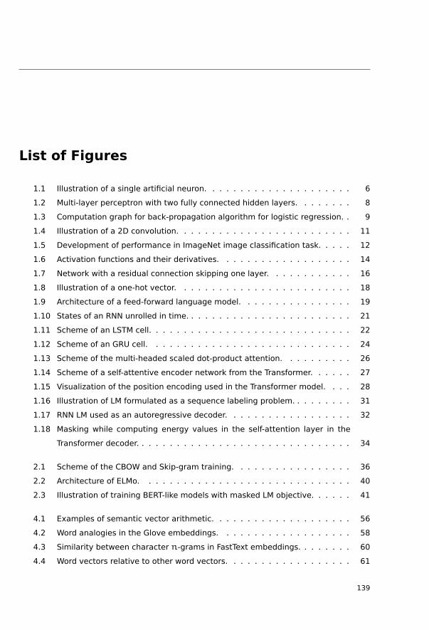
List of Figures
1.1 Illustration of a single artificial neuron. . . . . . . . . . . . . . . . . . . . . 61.2 Multi-layer perceptron with two fully connected hidden layers. . . . . . . . 81.3 Computation graph for back-propagation algorithm for logistic regression. . 91.4 Illustration of a 2D convolution. . . . . . . . . . . . . . . . . . . . . . . . . 111.5 Development of performance in ImageNet image classification task. . . . . 121.6 Activation functions and their derivatives. . . . . . . . . . . . . . . . . . . 141.7 Network with a residual connection skipping one layer. . . . . . . . . . . . 161.8 Illustration of a one-hot vector. . . . . . . . . . . . . . . . . . . . . . . . . 181.9 Architecture of a feed-forward language model. . . . . . . . . . . . . . . . 191.10 States of an RNN unrolled in time. . . . . . . . . . . . . . . . . . . . . . . . 211.11 Scheme of an LSTM cell. . . . . . . . . . . . . . . . . . . . . . . . . . . . . 221.12 Scheme of an GRU cell. . . . . . . . . . . . . . . . . . . . . . . . . . . . . 241.13 Scheme of the multi-headed scaled dot-product attention. . . . . . . . . . 261.14 Scheme of a self-attentive encoder network from the Transformer. . . . . . 271.15 Visualization of the position encoding used in the Transformer model. . . . 281.16 Illustration of LM formulated as a sequence labeling problem. . . . . . . . . 311.17 RNN LM used as an autoregressive decoder. . . . . . . . . . . . . . . . . . 321.18 Masking while computing energy values in the self-attention layer in the
Transformer decoder. . . . . . . . . . . . . . . . . . . . . . . . . . . . . . . 34
2.1 Scheme of the CBOW and Skip-gram training. . . . . . . . . . . . . . . . . 362.2 Architecture of ELMo. . . . . . . . . . . . . . . . . . . . . . . . . . . . . . 402.3 Illustration of training BERT-like models with masked LM objective. . . . . . 41
4.1 Examples of semantic vector arithmetic. . . . . . . . . . . . . . . . . . . . 564.2 Word analogies in the Glove embeddings. . . . . . . . . . . . . . . . . . . 584.3 Similarity between character n-grams in FastText embeddings. . . . . . . . 604.4 Word vectors relative to other word vectors. . . . . . . . . . . . . . . . . . 61
139
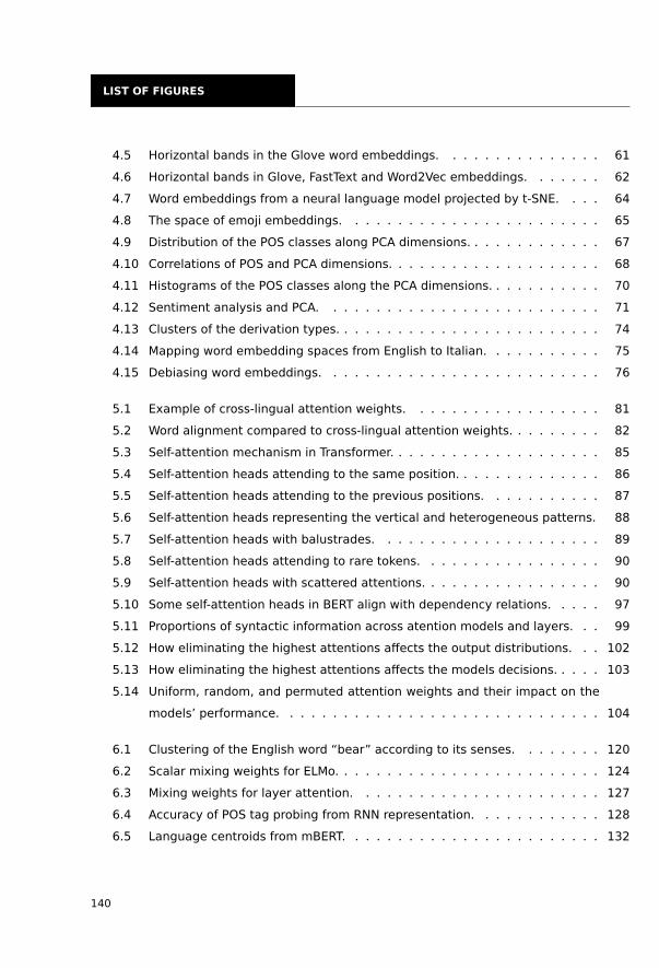
LIST OF FIGURES
4.5 Horizontal bands in the Glove word embeddings. . . . . . . . . . . . . . . 614.6 Horizontal bands in Glove, FastText and Word2Vec embeddings. . . . . . . 624.7 Word embeddings from a neural language model projected by t-SNE. . . . 644.8 The space of emoji embeddings. . . . . . . . . . . . . . . . . . . . . . . . 654.9 Distribution of the POS classes along PCA dimensions. . . . . . . . . . . . . 674.10 Correlations of POS and PCA dimensions. . . . . . . . . . . . . . . . . . . . 684.11 Histograms of the POS classes along the PCA dimensions. . . . . . . . . . . 704.12 Sentiment analysis and PCA. . . . . . . . . . . . . . . . . . . . . . . . . . 714.13 Clusters of the derivation types. . . . . . . . . . . . . . . . . . . . . . . . . 744.14 Mapping word embedding spaces from English to Italian. . . . . . . . . . . 754.15 Debiasing word embeddings. . . . . . . . . . . . . . . . . . . . . . . . . . 76
5.1 Example of cross-lingual attention weights. . . . . . . . . . . . . . . . . . 815.2 Word alignment compared to cross-lingual attention weights. . . . . . . . . 825.3 Self-attention mechanism in Transformer. . . . . . . . . . . . . . . . . . . . 855.4 Self-attention heads attending to the same position. . . . . . . . . . . . . . 865.5 Self-attention heads attending to the previous positions. . . . . . . . . . . 875.6 Self-attention heads representing the vertical and heterogeneous patterns. 885.7 Self-attention heads with balustrades. . . . . . . . . . . . . . . . . . . . . 895.8 Self-attention heads attending to rare tokens. . . . . . . . . . . . . . . . . 905.9 Self-attention heads with scattered attentions. . . . . . . . . . . . . . . . . 905.10 Some self-attention heads in BERT align with dependency relations. . . . . 975.11 Proportions of syntactic information across atention models and layers. . . 995.12 How eliminating the highest attentions affects the output distributions. . . 1025.13 How eliminating the highest attentions affects the models decisions. . . . . 1035.14 Uniform, random, and permuted attention weights and their impact on the
models’ performance. . . . . . . . . . . . . . . . . . . . . . . . . . . . . . 104
6.1 Clustering of the English word “bear” according to its senses. . . . . . . . 1206.2 Scalar mixing weights for ELMo. . . . . . . . . . . . . . . . . . . . . . . . . 1246.3 Mixing weights for layer attention. . . . . . . . . . . . . . . . . . . . . . . 1276.4 Accuracy of POS tag probing from RNN representation. . . . . . . . . . . . 1286.5 Language centroids from mBERT. . . . . . . . . . . . . . . . . . . . . . . . 132
140
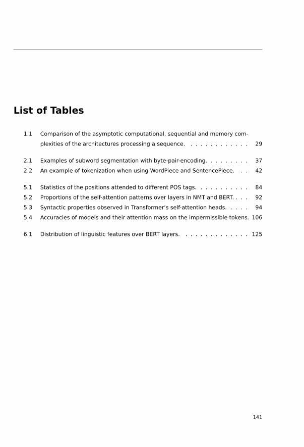
List of Tables
1.1 Comparison of the asymptotic computational, sequential and memory com-plexities of the architectures processing a sequence. . . . . . . . . . . . . 29
2.1 Examples of subword segmentation with byte-pair-encoding. . . . . . . . . 372.2 An example of tokenization when using WordPiece and SentencePiece. . . 42
5.1 Statistics of the positions attended to different POS tags. . . . . . . . . . . 845.2 Proportions of the self-attention patterns over layers in NMT and BERT. . . . 925.3 Syntactic properties observed in Transformer’s self-attention heads. . . . . 945.4 Accuracies of models and their attention mass on the impermissible tokens. 106
6.1 Distribution of linguistic features over BERT layers. . . . . . . . . . . . . . 125
141

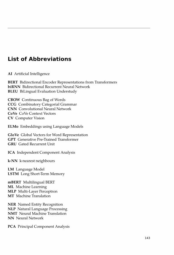
List of Abbreviations
AI Artificial Intelligence
BERT Bidirectional Encoder Representations from TransformersbiRNN Bidirectional Recurrent Neural NetworkBLEU BiLingual Evaluation Understudy
CBOW Continuous Bag of WordsCCG Combinatory Categorial GrammarCNN Convolutional Neural NetworkCoVe CoVe Context VectorsCV Computer Vision
ELMo Embeddings using Language Models
GloVe Global Vectors for Word RepresentationGPT Generative Pre-Trained TransformerGRU Gated Recurrent Unit
ICA Independent Component Analysis
k-NN k-nearest neighbours
LM Language ModelLSTM Long Short-Term Memory
mBERT Multilingual BERTML Machine LearningMLP Multi-Layer PerceptronMT Machine Translation
NER Named Entity RecognitionNLP Natural Language ProcessingNMT Neural Machine TranslationNN Neural Network
PCA Principal Component Analysis
143

List of Abbreviations
PoS Part of Speech
ReLU Rectified Linear UnitRNN Recurrent Neural Network
SAN Self-Attentive NetworkSG Skip-GramSRL Semantic Role Labelling
TagLM Language-Model-Augmented Sequence Tagger
UAS Unlabeled Attachment Score
WMT Workshop of Machine Translation
XLM-R XLM-RoBERTa
144
Bibliography
Yossi Adi, Einat Kermany, Yonatan Belinkov, Ofer Lavi, and Yoav Goldberg. Fine-grainedAnalysis of Sentence Embeddings Using Auxiliary Prediction Tasks. arXiv:1608.04207 [cs],February 2017. URL http://arxiv.org/abs/1608.04207. arXiv: 1608.04207.
Eneko Agirre, Carmen Banea, Daniel Cer, Mona Diab, Aitor Gonzalez-Agirre, Rada Mihal-cea, German Rigau, and Janyce Wiebe. Semeval-2016 task 1: Semantic textual similarity,monolingual and cross-lingual evaluation. In Proceedings of the 10th International Workshopon Semantic Evaluation (SemEval-2016), pages 497–511, San Diego, CA, USA, June 2016. As-sociation for Computational Linguistics. doi: 10.18653/v1/s16-1081. URL http://dx.doi.org/10.18653/v1/s16-1081.
Stanislaw Antol, Aishwarya Agrawal, Jiasen Lu, Margaret Mitchell, Dhruv Batra, LawrenceZitnick, and Devi Parikh. VQA: Visual question answering. In Proceedings of the 2015 IEEEInternational Conference on Computer Vision (ICCV), pages 2425–2433, Arucano Park, Chile,December 2015. IEEE Computer Society.
Mikel Artetxe, Sebastian Ruder, and Dani Yogatama. On the cross-lingual transferability ofmonolingual representations. CoRR, abs/1910.11856, 2019. URL http://arxiv.org/abs/1910.11856.
Lei Jimmy Ba, Ryan Kiros, and Geoffrey E Hinton. Layer Normalization. CoRR,abs/1607.06450, 2016. ISSN 2331-8422. URL https://arxiv.org/abs/1607.06450.
Dzmitry Bahdanau, Kyunghyun Cho, and Yoshua Bengio. Neural Machine Translation byJointly Learning to Align and Translate. CoRR, abs/1409.0473, 2014. ISSN 2331-8422. URLhttps://arxiv.org/abs/1409.0473.
David Balduzzi and Muhammad Ghifary. Strongly-Typed Recurrent Neural Networks. In Pro-ceedings of the 33rd International Conference on Machine Learning, volume 48 of Proceedings ofMachine Learning Research, pages 1292–1300, New York, NY, USA, June 2016. PMLR.
Tamali Banerjee and Pushpak Bhattacharyya. Meaningless yet meaningful: Morphologygrounded subword-level NMT. In Proceedings of the Second Workshop on Subword/CharacterLEvel Models, pages 55–60, 2018.
Loïc Barrault, Ondřej Bojar, Marta R. Costa-jussà, Christian Federmann, Mark Fishel, YvetteGraham, Barry Haddow, Matthias Huck, Philipp Koehn, Shervin Malmasi, Christof Monz,Mathias Müller, Santanu Pal, Matt Post, and Marcos Zampieri. Findings of the 2019 Con-ference on Machine Translation (WMT19). In Proceedings of the Fourth Conference on Ma-chine Translation (Volume 2: Shared Task Papers, Day 1), pages 1–61, Florence, Italy, Au-gust 2019. Association for Computational Linguistics. doi: 10.18653/v1/W19-5301. URLhttps://www.aclweb.org/anthology/W19-5301.
145
BIBLIOGRAPHY
Yonatan Belinkov and James Glass. Analysis Methods in Neural Language Processing: A Sur-vey. Transactions of the Association for Computational Linguistics, 7:49–72, April 2019. doi:10.1162/tacl_a_00254. URL https://doi.org/10.1162/tacl_a_00254.
Yonatan Belinkov, Nadir Durrani, Fahim Dalvi, Hassan Sajjad, and James Glass. What do Neu-ral Machine Translation Models Learn about Morphology? In Proceedings of the 55th An-nual Meeting of the Association for Computational Linguistics (Volume 1: Long Papers), pages861–872, Vancouver, Canada, July 2017a. Association for Computational Linguistics. doi:10.18653/v1/P17-1080. URL https://www.aclweb.org/anthology/P17-1080.
Yonatan Belinkov, Lluís Màrquez, Hassan Sajjad, Nadir Durrani, Fahim Dalvi, and James Glass.Evaluating Layers of Representation in Neural Machine Translation on Part-of-Speech andSemantic Tagging Tasks. In Proceedings of the Eighth International Joint Conference on Nat-ural Language Processing (Volume 1: Long Papers), pages 1–10, Taipei, Taiwan, November2017b. Asian Federation of Natural Language Processing. URL https://www.aclweb.org/anthology/I17-1001.
Yoshua Bengio, Réjean Ducharme, Pascal Vincent, and Christian Jauvin. A Neural ProbabilisticLanguage Model. Journal of Machine Learning Research, 3(Feb):1137–1155, 2003. ISSN ISSN1533-7928. URL http://www.jmlr.org/papers/v3/bengio03a.html.
Yoshua Bengio, Pascal Lamblin, Dan Popovici, and Hugo Larochelle. Greedy layer-wise train-ing of deep networks. In Advances in Neural Information Processing Systems 20, pages 153–160, Vancouver, Canada, December 2007. Curran Associates, Inc. ISBN 978-0-262-25691-9.doi: 10.7551/mitpress/7503.003.0024. URL http://dx.doi.org/10.7551/mitpress/7503.003.0024.
Johannes Bjerva, Barbara Plank, and Johan Bos. Semantic tagging with deep residual networks.arXiv preprint arXiv:1609.07053, 2016.
Terra Blevins, Omer Levy, and Luke Zettlemoyer. Deep RNNs Encode Soft Hierarchical Syn-tax. In Proceedings of the 56th Annual Meeting of the Association for Computational Linguis-tics (Volume 2: Short Papers), pages 14–19, Melbourne, Australia, July 2018. Association forComputational Linguistics. doi: 10.18653/v1/P18-2003. URL https://www.aclweb.org/anthology/P18-2003.
Piotr Bojanowski, Edouard Grave, Armand Joulin, and Tomas Mikolov. Enriching Word Vectorswith Subword Information. Transactions of the Association for Computational Linguistics, 5:135–146, 2017. URL http://arxiv.org/abs/1607.04606. arXiv: 1607.04606.
Ondřej Bojar, Rajen Chatterjee, Christian Federmann, Barry Haddow, Matthias Huck, ChrisHokamp, Philipp Koehn, Varvara Logacheva, Christof Monz, Matteo Negri, Matt Post, Car-olina Scarton, Lucia Specia, and Marco Turchi. Findings of the 2015 Workshop on StatisticalMachine Translation. In Proceedings of the Tenth Workshop on Statistical Machine Translation,pages 1–46, Lisbon, Portugal, September 2015. Association for Computational Linguistics.doi: 10.18653/v1/W15-3001. URL https://www.aclweb.org/anthology/W15-3001.
Ondřej Bojar, Rajen Chatterjee, Christian Federmann, Yvette Graham, Barry Haddow, MatthiasHuck, Antonio Jimeno Yepes, Philipp Koehn, Varvara Logacheva, Christof Monz, MatteoNegri, Aurélie Névéol, Mariana Neves, Martin Popel, Matt Post, Raphael Rubino, CarolinaScarton, Lucia Specia, Marco Turchi, Karin Verspoor, and Marcos Zampieri. Findings of the
146
BIBLIOGRAPHY
2016 Conference on Machine Translation. In Proceedings of the First Conference on MachineTranslation: Volume 2, Shared Task Papers, pages 131–198, Berlin, Germany, August 2016a.Association for Computational Linguistics. doi: 10.18653/v1/W16-2301. URL https://www.aclweb.org/anthology/W16-2301.
Ondřej Bojar, Ondřej Dušek, Tom Kocmi, Jindřich Libovický, Michal Novák, Martin Popel,Roman Sudarikov, and Dušan Variš. CzEng 1.6: Enlarged Czech-English Parallel Cor-pus with Processing Tools Dockered. In Petr Sojka, Aleš Horák, Ivan Kopeček, and KarelPala, editors, Text, Speech, and Dialogue: 19th International Conference, TSD 2016, LectureNotes in Artificial Intelligence, pages 231–238, Cham / Heidelberg / New York / Dor-drecht / London, 2016b. Springer International Publishing. ISBN 978-3-319-45509-9. doi:10.1007/978-3-319-45510-5_27. URL http://dx.doi.org/10.1007/978-3-319-45510-5_27.Backup Publisher: Masaryk University ISSN: 0302-9743 Issue: 9924.
Ondřej Bojar, Rajen Chatterjee, Christian Federmann, Yvette Graham, Barry Haddow, ShujianHuang, Matthias Huck, Philipp Koehn, Qun Liu, Varvara Logacheva, Christof Monz, Mat-teo Negri, Matt Post, Raphael Rubino, Lucia Specia, and Marco Turchi. Findings of the 2017Conference on Machine Translation (WMT17). In Proceedings of the Second Conference on Ma-chine Translation, pages 169–214, Copenhagen, Denmark, September 2017. Association forComputational Linguistics. doi: 10.18653/v1/W17-4717. URL https://www.aclweb.org/anthology/W17-4717.
Ondřej Bojar, Christian Federmann, Mark Fishel, Yvette Graham, Barry Haddow, PhilippKoehn, and Christof Monz. Findings of the 2018 Conference on Machine Translation(WMT18). In Proceedings of the Third Conference on Machine Translation: Shared Task Papers,pages 272–303, Brussels, Belgium, October 2018. Association for Computational Linguistics.
Tolga Bolukbasi, Kai-Wei Chang, James Zou, Venkatesh Saligrama, and Adam Kalai. Man isto Computer Programmer as Woman is to Homemaker? Debiasing Word Embeddings.arXiv:1607.06520 [cs, stat], July 2016. URL http://arxiv.org/abs/1607.06520. arXiv:1607.06520.
Kaj Bostrom and Greg Durrett. Byte pair encoding is suboptimal for language model pretrain-ing. arXiv preprint arXiv:2004.03720, 2020.
Samuel R. Bowman, Gabor Angeli, Christopher Potts, and Christopher D. Manning. A largeannotated corpus for learning natural language inference. In Proceedings of the 2015 Confer-ence on Empirical Methods in Natural Language Processing, pages 632–642, Lisbon, Portugal,September 2015. Association for Computational Linguistics. doi: 10.18653/v1/D15-1075.URL https://www.aclweb.org/anthology/D15-1075.
Steve Branson, Grant Van Horn, Serge J Belongie, and Pietro Perona. Bird Species Categoriza-tion Using Pose Normalized Deep Convolutional Nets. CoRR, abs/1406.2952, 2014. ISSN2331-8422.
José Cañete, Gabriel Chaperon, Rodrigo Fuentes, and Jorge Pérez. Spanish Pre-Trained BERTModel and Evaluation Data. In PML4DC at ICLR 2020, 2020.
William Chan, Navdeep Jaitly, Quoc V Le, and Oriol Vinyals. Listen, attend and spell: A neu-ral network for large vocabulary conversational speech recognition. In International Confer-ence on Acoustics, Speech and Signal Processing (ICASSP), pages 4960–4964, Shanghai, China,
147
BIBLIOGRAPHY
March 2016. IEEE Computer Society. ISBN 978-1-4799-9988-0. doi: 10.1109/icassp.2016.7472621. URL http://dx.doi.org/10.1109/icassp.2016.7472621.
Ciprian Chelba, Tomas Mikolov, Mike Schuster, Qi Ge, Thorsten Brants, Phillipp Koehn, andTony Robinson. One billion word benchmark for measuring progress in statistical lan-guage modeling. In Haizhou Li, Helen M. Meng, Bin Ma, Engsiong Chng, and Lei Xie,editors, INTERSPEECH 2014, 15th Annual Conference of the International Speech Communi-cation Association, Singapore, September 14-18, 2014, pages 2635–2639. ISCA, 2014. URLhttp://www.isca-speech.org/archive/interspeech_2014/i14_2635.html.
Danqi Chen and Christopher Manning. A Fast and Accurate Dependency Parser using Neu-ral Networks. In Proceedings of the 2014 Conference on Empirical Methods in Natural LanguageProcessing (EMNLP), pages 740–750, Doha, Qatar, 2014. Association for Computational Lin-guistics. doi: 10.3115/v1/D14-1082. URL http://aclweb.org/anthology/D14-1082.
Mia Xu Chen, Orhan Firat, Ankur Bapna, Melvin Johnson, Wolfgang Macherey, George Foster,Llion Jones, Mike Schuster, Noam Shazeer, Niki Parmar, Ashish Vaswani, Jakob Uszkoreit,Łukasz Kaiser, Zhifeng Chen, Yonghui Wu, and Macduff Hughes. The Best of Both Worlds:Combining Recent Advances in Neural Machine Translation. In Proceedings of the 56th An-nual Meeting of the Association for Computational Linguistics (Volume 1: Long Papers), pages76–86, Melbourne, Australia, July 2018. Association for Computational Linguistics.
Ethan A. Chi, John Hewitt, and Christopher D. Manning. Finding Universal Grammatical Rela-tions in Multilingual BERT. arXiv:2005.04511 [cs], May 2020. URL http://arxiv.org/abs/2005.04511. arXiv: 2005.04511.
Kyunghyun Cho, Bart van Merrienboer, Caglar Gulcehre, Dzmitry Bahdanau, Fethi Bougares,Holger Schwenk, and Yoshua Bengio. Learning Phrase Representations using RNNEncoder–Decoder for Statistical Machine Translation. In Proceedings of the 2014 Conference onEmpirical Methods in Natural Language Processing (EMNLP), pages 1724–1734, Doha, Qatar,October 2014. Association for Computational Linguistics. doi: 10.3115/v1/d14-1179. URLhttp://dx.doi.org/10.3115/v1/d14-1179.
Junyoung Chung, Çaglar Gülçehre, Kyunghyun Cho, and Yoshua Bengio. Empirical Evaluationof Gated Recurrent Neural Networks on Sequence Modeling. CoRR, abs/1412.3555, 2014.ISSN 2331-8422. URL https://arxiv.org/abs/1412.3555.
Kevin Clark, Urvashi Khandelwal, Omer Levy, and Christopher D. Manning. What Does BERTLook At? An Analysis of BERT’s Attention. arXiv:1906.04341 [cs], June 2019. URL http://arxiv.org/abs/1906.04341. arXiv: 1906.04341.
Kevin Clark, Minh-Thang Luong, Quoc V. Le, and Christopher D. Manning. ELECTRA: Pre-training Text Encoders as Discriminators Rather Than Generators. In 8th International Con-ference on Learning Representations, ICLR 2020, Addis Ababa, Ethiopia, April 26-30, 2020. Open-Review.net, 2020. URL https://openreview.net/forum?id=r1xMH1BtvB.
Ronan Collobert, Jason Weston, Leon Bottou, Michael Karlen, Koray Kavukcuoglu, and PavelKuksa. Natural Language Processing (Almost) from Scratch. NATURAL LANGUAGE PRO-CESSING, page 45, 2008.
Ronan Collobert, Jason Weston, Léon Bottou, Michael Karlen, Koray Kavukcuoglu, and PavelKuksa. Natural language processing (almost) from scratch. The Journal of Machine LearningResearch, 12(Aug):2493–2537, 2011. ISSN 1533-7928.
148
BIBLIOGRAPHY
Pierre Comon. Independent component analysis, a new concept? Signal processing, 36(3):287–314, 1994.
Alexis Conneau, Guillaume Lample, Marc’Aurelio Ranzato, Ludovic Denoyer, and Hervé Jé-gou. Word Translation Without Parallel Data. CoRR, abs/1710.04087, 2017. ISSN 2331-8422.URL https://arxiv.org/abs/1710.04087.
Alexis Conneau, Guillaume Lample, Marc’Aurelio Ranzato, Ludovic Denoyer, and Hervé Jé-gou. Word Translation Without Parallel Data. arXiv:1710.04087 [cs], January 2018a. URLhttp://arxiv.org/abs/1710.04087. arXiv: 1710.04087.
Alexis Conneau, Ruty Rinott, Guillaume Lample, Adina Williams, Samuel Bowman, HolgerSchwenk, and Veselin Stoyanov. XNLI: Evaluating cross-lingual sentence representations.In Proceedings of the 2018 Conference on Empirical Methods in Natural Language Processing,pages 2475–2485, Brussels, Belgium, October-November 2018b. Association for Computa-tional Linguistics. doi: 10.18653/v1/D18-1269. URL https://www.aclweb.org/anthology/D18-1269.
Alexis Conneau, Kartikay Khandelwal, Naman Goyal, Vishrav Chaudhary, Guillaume Wen-zek, Francisco Guzmán, Edouard Grave, Myle Ott, Luke Zettlemoyer, and Veselin Stoy-anov. Unsupervised Cross-lingual Representation Learning at Scale. In Proceedings of the58th Annual Meeting of the Association for Computational Linguistics, pages 8440–8451, On-line, July 2020. Association for Computational Linguistics. URL https://www.aclweb.org/anthology/2020.acl-main.747.
Daniel Crevier. AI: the tumultuous history of the search for artificial intelligence. Basic Books, NewYork, NY, 1993. ISBN 978-0-465-02997-6.
Jeff Da and Jungo Kasai. Cracking the Contextual Commonsense Code: Understanding Com-monsense Reasoning Aptitude of Deep Contextual Representations. arXiv:1910.01157 [cs],October 2019. URL http://arxiv.org/abs/1910.01157. arXiv: 1910.01157.
Jia Deng, Wei Dong, Richard Socher, Li-Jia Li, Kai Li, and Li Fei-Fei. ImageNet: A large-scale hi-erarchical image database. In Conference on Computer Vision and Pattern Recognition (CVPR),pages 248–255, Miami, FL, USA, June 2009. IEEE Computer Society. ISBN 978-1-4244-3992-8.
Jacob Devlin, Ming-Wei Chang, Kenton Lee, and Kristina Toutanova. BERT: Pre-training ofDeep Bidirectional Transformers for Language Understanding. In Proceedings of the 2019Conference of the North American Chapter of the Association for Computational Linguistics: HumanLanguage Technologies, Volume 1 (Long and Short Papers), pages 4171–4186, Minneapolis, Min-nesota, June 2019. Association for Computational Linguistics. doi: 10.18653/v1/N19-1423.URL https://www.aclweb.org/anthology/N19-1423.
Trinh–Minh–Tri Do and Thierry Artieres. Neural conditional random fields. In Proceedingsof the Thirteenth International Conference on Artificial Intelligence and Statistics, volume 9 ofProceedings of Machine Learning Research, pages 177–184, Sardinia, Italy, May 2010. PMLR.
Chris Dyer, Victor Chahuneau, and Noah A. Smith. A Simple, Fast, and Effective Reparam-eterization of IBM Model 2. In Proceedings of the 2013 Conference of the North AmericanChapter of the Association for Computational Linguistics: Human Language Technologies, pages644–648, Atlanta, Georgia, June 2013. Association for Computational Linguistics. URLhttps://www.aclweb.org/anthology/N13-1073.
149
BIBLIOGRAPHY
Jack Edmonds. Optimum branchings. Journal of Research of the National Bureau of Stan-dards Section B Mathematics and Mathematical Physics, 71B(4):233, October 1967. ISSN 0022-4340. doi: 10.6028/jres.071B.032. URL https://nvlpubs.nist.gov/nistpubs/jres/71B/jresv71Bn4p233_A1b.pdf.
Ben Eisner, Tim Rocktäschel, Isabelle Augenstein, Matko Bošnjak, and Sebastian Riedel.emoji2vec: Learning Emoji Representations from their Description. arXiv:1609.08359 [cs],November 2016. URL http://arxiv.org/abs/1609.08359. arXiv: 1609.08359.
Yanai Elazar, Shauli Ravfogel, Alon Jacovi, and Yoav Goldberg. When Bert Forgets How ToPOS: Amnesic Probing of Linguistic Properties and MLM Predictions. June 2020. URLhttps://arxiv.org/abs/2006.00995v1.
Jeffrey L Elman. Finding Structure in Time. Cognitive Science, 14(2):179–211, 1990. ISSN 1551-6709.
Dumitru Erhan, Yoshua Bengio, Aaron Courville, and Pascal Vincent. Visualizing Higher-Layer Features of a Deep Network. Technical report, Univeristé de Montréal, Montreal,Canada, January 2009.
Kawin Ethayarajh. How Contextual are Contextualized Word Representations? Comparingthe Geometry of BERT, ELMo, and GPT-2 Embeddings. arXiv:1909.00512 [cs], September2019. URL http://arxiv.org/abs/1909.00512. arXiv: 1909.00512.
Scott E Fahlman and Geoffrey E Hinton. Connectionist Architectures for Artificial Intelli-gence. IEEE Computer, 20(1):100–109, January 1987. ISSN 0018-9162. doi: 10.1109/mc.1987.1663364. URL http://dx.doi.org/10.1109/mc.1987.1663364.
Matt Gardner, Joel Grus, Mark Neumann, Oyvind Tafjord, Pradeep Dasigi, Nelson F. Liu,Matthew Peters, Michael Schmitz, and Luke Zettlemoyer. AllenNLP: A Deep Semantic Nat-ural Language Processing Platform. In Proceedings of Workshop for NLP Open Source Software(NLP-OSS), pages 1–6, Melbourne, Australia, July 2018. Association for Computational Lin-guistics. doi: 10.18653/v1/W18-2501. URL https://www.aclweb.org/anthology/W18-2501.
Jonas Gehring, Michael Auli, David Grangier, Denis Yarats, and Yann N Dauphin. Convolu-tional Sequence to Sequence Learning. In International Conference on Machine Learning, pages1243–1252, Sydney, Australia, August 2017. PMLR.
Sebastian Gehrmann, Hendrik Strobelt, and Alexander Rush. GLTR: Statistical Detection andVisualization of Generated Text. In Proceedings of the 57th Annual Meeting of the Association forComputational Linguistics: System Demonstrations, pages 111–116, Florence, Italy, July 2019.Association for Computational Linguistics. doi: 10.18653/v1/P19-3019. URL https://www.aclweb.org/anthology/P19-3019.
Hamidreza Ghader and Christof Monz. What does Attention in Neural Machine TranslationPay Attention to? arXiv:1710.03348 [cs], October 2017. URL http://arxiv.org/abs/1710.03348. arXiv: 1710.03348.
Ross B Girshick. Fast R-CNN. In Proceedings of the 2015 IEEE International Conference on Com-puter Vision (ICCV), pages 1440–1448, Arucano Park, Chile, December 2015. IEEE ComputerSociety. ISBN 978-1-4673-8391-2.
Ian Goodfellow, Yoshua Bengio, and Aaron Courville. Deep learning. MIT press, Cambridge,MA, USA, 2016. ISBN 978-0-262-03561-3.
150

BIBLIOGRAPHY
Alex Graves. Generating Sequences With Recurrent Neural Networks. arXiv:1308.0850 [cs],June 2014. URL http://arxiv.org/abs/1308.0850. arXiv: 1308.0850.
Alex Graves and Jürgen Schmidhuber. Framewise phoneme classification with bidirectionalLSTM and other neural network architectures. Neural Networks, 18(5-6):602–610, July 2005.ISSN 0893-6080. doi: 10.1016/j.neunet.2005.06.042. URL http://dx.doi.org/10.1016/j.neunet.2005.06.042.
Alex Graves and Jürgen Schmidhuber. Offline Handwriting Recognition with Multidimen-sional Recurrent Neural Networks. In Advances in Neural Information Processing Systems 21,pages 545–552, Vancouver, Canada, December 2009. Curran Associates, Inc.
Alex Graves, Santiago Fernández, Faustino Gomez, and Jürgen Schmidhuber. Connectionisttemporal classification: labelling unsegmented sequence data with recurrent neural net-works. In Proceedings of the 23rd International Conference on Machine Learning, pages 369–376,Pittsburgh, PA, USA, June 2006. JMLR.org.
Alex Graves, Abdel-rahman Mohamed, and Geoffrey E Hinton. Speech recognition with deeprecurrent neural networks. In International Conference on Acoustics, Speech and Signal Pro-cessing (ICASSP), pages 6645–6649, Vancouver, Canada, May 2013. IEEE Computer Society.ISBN 978-1-4799-0356-6. doi: 10.1109/icassp.2013.6638947. URL http://dx.doi.org/10.1109/icassp.2013.6638947.
Alex Graves, Greg Wayne, and Ivo Danihelka. Neural Turing Machines. CoRR, abs/1410.5401,2014. ISSN 2331-8422. URL https://arxiv.org/abs/1410.5401.
Jiatao Gu, James Bradbury, Caiming Xiong, Victor O. K. Li, and Richard Socher. Non-Autoregressive Neural Machine Translation. In 6th International Conference on Learning Rep-resentations, ICLR 2018, Vancouver, BC, Canada, April 30 - May 3, 2018, Conference Track Pro-ceedings. OpenReview.net, 2018. URL https://openreview.net/forum?id=B1l8BtlCb.
Gözde Gül Şahin, Clara Vania, Ilia Kuznetsov, and Iryna Gurevych. LINSPECTOR: Mul-tilingual Probing Tasks for Word Representations. CoRR, abs/1903.09442, 2019. URLhttp://arxiv.org/abs/1903.09442.
Richard HR Hahnloser, Rahul Sarpeshkar, Misha A Mahowald, Rodney J .Douglas, and Sebas-tian Seung. Digital selection and analogue amplification coexist in a cortex-inspired siliconcircuit. Nature, 405(6789):947, 2000. ISSN 1476-4687.
Kazuyuki Hara, Daisuke Saitoh, and Hayaru Shouno. Analysis of Dropout Learning Regardedas Ensemble Learning. In Alessandro E. P. Villa, Paolo Masulli, and Antonio Javier PonsRivero, editors, Artificial Neural Networks and Machine Learning - ICANN 2016 - 25th Interna-tional Conference on Artificial Neural Networks, Barcelona, Spain, September 6-9, 2016, Proceed-ings, Part II, volume 9887 of Lecture Notes in Computer Science, pages 72–79. Springer, 2016.doi: 10.1007/978-3-319-44781-0_9. URL https://doi.org/10.1007/978-3-319-44781-0_9.
Zellig S Harris. Distributional structure. Word, 10(2-3):146–162, 1954. ISSN 0043-7956.Kaiming He, Xiangyu Zhang, Shaoqing Ren, and Jian Sun. Deep residual learning for image
recognition. In Conference on Computer Vision and Pattern Recognition (CVPR), pages 770–778, Las Vegas, NV, USA, June 2016. IEEE Computer Society. ISBN 978-1-4673-8851-1. doi:10.1109/cvpr.2016.90. URL http://dx.doi.org/10.1109/cvpr.2016.90.
151
BIBLIOGRAPHY
John Hewitt and Percy Liang. Designing and Interpreting Probes with Control Tasks.arXiv:1909.03368 [cs], September 2019. URL http://arxiv.org/abs/1909.03368. arXiv:1909.03368.
John Hewitt and Christopher D. Manning. A Structural Probe for Finding Syntax in Word Rep-resentations. In Proceedings of the 2019 Conference of the North American Chapter of the Asso-ciation for Computational Linguistics: Human Language Technologies, Volume 1 (Long and ShortPapers), pages 4129–4138, Minneapolis, Minnesota, June 2019. Association for Computa-tional Linguistics. doi: 10.18653/v1/N19-1419. URL https://www.aclweb.org/anthology/N19-1419.
Felix Hill, Kyunghyun Cho, Sébastien Jean, and Yoshua Bengio. The representational geom-etry of word meanings acquired by neural machine translation models. Mach. Transl.,31(1-2):3–18, 2017. doi: 10.1007/s10590-017-9194-2. URL https://doi.org/10.1007/s10590-017-9194-2.
Geoffrey E Hinton and Ruslan Salakhutdinov. Reducing the Dimensionality of Data with Neu-ral Networks. Science, 313(5786):504–507, 2006. ISSN 0036-8075.
Geoffrey E. Hinton, Oriol Vinyals, and Jeffrey Dean. Distilling the Knowledge in a NeuralNetwork. CoRR, abs/1503.02531, 2015. URL http://arxiv.org/abs/1503.02531.
Milena Hnátková, Michal Kren, Pavel Procházka, and Hana Skoumalová. The SYN-series cor-pora of written Czech. In LREC, pages 160–164, 2014.
Sepp Hochreiter and Jürgen Schmidhuber. Long short-term memory. Neural Computation, 9(8):1735–1780, 1997. ISSN 0899-7667.
Sepp Hochreiter, Yoshua Bengio, Paolo Frasconi, and Jürgen Schmidhuber. Gradient flow inrecurrent nets: the difficulty of learning long-term dependencies. A field guide to dynamicalrecurrent neural networks. IEEE Press, 2001.
Geoff Hollis and Chris Westbury. The principals of meaning: Extracting semantic dimensionsfrom co-occurrence models of semantics. Psychonomic Bulletin & Review, 23(6):1744–1756,2016. ISSN 1531-5320. doi: 10.3758/s13423-016-1053-2.
Timo Honkela, Aapo Hyvärinen, and Jaakko J. Väyrynen. WordICA—emergence of lin-guistic representations for words by independent component analysis. Natural Lan-guage Engineering, 16(3):277–308, July 2010. ISSN 1351-3249, 1469-8110. doi: 10.1017/S1351324910000057. URL https://www.cambridge.org/core/product/identifier/S1351324910000057/type/journal_article.
Kurt Hornik. Approximation capabilities of multilayer feedforward networks. Neural Networks,4(2):251–257, 1991. ISSN 0893-6080.
Harold Hotelling. Relations between two sets of variates. Biometrika, 28(3/4):321–377, 1936.ISSN 00063444. URL http://www.jstor.org/stable/2333955.
Jie Hu, Li Shen, and Gang Sun. Squeeze-and-Excitation Networks. CoRR, abs/1709.01507,2017. ISSN 2331-8422.
Junjie Hu, Sebastian Ruder, Aditya Siddhant, Graham Neubig, Orhan Firat, and Melvin John-son. XTREME: A massively multilingual multi-task benchmark for evaluating cross-lingualgeneralization. CoRR, abs/2003.11080, 2020. URL https://arxiv.org/abs/2003.11080.
152
BIBLIOGRAPHY
Mi-Young Huh, Pulkit Agrawal, and Alexei A Efros. What makes ImageNet good for transferlearning? CoRR, abs/1608.08614, 2016. ISSN 2331-8422.
A. Hyvärinen and E. Oja. Independent component analysis: algorithms and applications.Neural Networks, 13(4-5):411–430, June 2000. ISSN 08936080. doi: 10.1016/S0893-6080(00)00026-5. URL https://linkinghub.elsevier.com/retrieve/pii/S0893608000000265.
Anurag Illendula and Manish Reddy Yedulla. Learning Emoji Embeddings using Emoji Co-occurrence Network Graph. arXiv:1806.07785 [cs], June 2018. URL http://arxiv.org/abs/1806.07785. arXiv: 1806.07785.
Sergey Ioffe and Christian Szegedy. Batch Normalization: Accelerating Deep Network Train-ing by Reducing Internal Covariate Shift. In Proceedings of the 32nd International Conferenceon International Conference on Machine Learning - Volume 37, ICML’15, pages 448–456, Lille,France, July 2015. JMLR.org.
Max Jaderberg, Karen Simonyan, Andrea Vedaldi, and Andrew Zisserman. Synthetic Data andArtificial Neural Networks for Natural Scene Text Recognition. CoRR, abs/1406.2227, 2014.ISSN 2331-8422.
Sarthak Jain and Byron C. Wallace. Attention is not Explanation. arXiv:1902.10186 [cs], May2019. URL http://arxiv.org/abs/1902.10186. arXiv: 1902.10186.
Ganesh Jawahar, Benoît Sagot, and Djamé Seddah. What Does BERT Learn about the Structureof Language? In Proceedings of the 57th Annual Meeting of the Association for ComputationalLinguistics, pages 3651–3657, Florence, Italy, 2019. Association for Computational Linguis-tics. doi: 10.18653/v1/P19-1356. URL https://www.aclweb.org/anthology/P19-1356.
Sébastien Jean, Orhan Firat, Kyunghyun Cho, Roland Memisevic, and Yoshua Bengio. MontrealNeural Machine Translation Systems for WMT’15. In Proceedings of the Tenth Workshop onStatistical Machine Translation, pages 134–140, Lisbon, Portugal, September 2015. Associationfor Computational Linguistics. doi: 10.18653/v1/W15-3014. URL https://www.aclweb.org/anthology/W15-3014.
Marcin Junczys-Dowmunt. Microsoft’s Submission to the WMT2018 News Translation Task:How I Learned to Stop Worrying and Love the Data. In Proceedings of the Third Conferenceon Machine Translation: Shared Task Papers, pages 425–430, Belgium, Brussels, October 2018.Association for Computational Linguistics. doi: 10.18653/v1/W18-6415. URL https://www.aclweb.org/anthology/W18-6415.
Christian Jutten and Jeanny Herault. Blind separation of sources, part I: An adaptive algorithmbased on neuromimetic architecture. Signal processing, 24(1):1–10, 1991.
Nal Kalchbrenner and Phil Blunsom. Recurrent Continuous Translation Models. In Proceedingsof the 2013 Conference on Empirical Methods in Natural Language Processing, pages 1700–1709,Seattle, Washington, USA, October 2013. Association for Computational Linguistics. URLhttps://www.aclweb.org/anthology/D13-1176.
Andrej Karpathy, Justin Johnson, and Li Fei-Fei. Visualizing and Understanding RecurrentNetworks. arXiv:1506.02078 [cs], November 2015. URL http://arxiv.org/abs/1506.02078.arXiv: 1506.02078.
Brett Kessler, Geoffrey Nunberg, and Hinrich Schütze. Automatic Detection of Text Genre. InProceedings of the 35th Annual Meeting of the Association for Computational Linguistics, pages32–38, Madrid, Spain, July 1997. Association for Computational Linguistics.
153
BIBLIOGRAPHY
Daniel Keysers, Thomas Deselaers, Henry A Rowley, Li-Lun Wang, and Victor Carbune. Multi-Language Online Handwriting Recognition. IEEE Trans. Pattern Anal. Mach. Intell., 39(6):1180–1194, June 2017. ISSN 0162-8828. doi: 10.1109/tpami.2016.2572693. URL http://dx.doi.org/10.1109/tpami.2016.2572693.
Taeuk Kim, Jihun Choi, Daniel Edmiston, and Sang-goo Lee. Are Pre-trained Language ModelsAware of Phrases? Simple but Strong Baselines for Grammar Induction. arXiv:2002.00737[cs], January 2020. URL http://arxiv.org/abs/2002.00737. arXiv: 2002.00737.
Eliyahu Kiperwasser and Yoav Goldberg. Simple and Accurate Dependency Parsing UsingBidirectional LSTM Feature Representations. Transactions of the Association for ComputationalLinguistics, 4:313–327, December 2016. ISSN 2307-387X. doi: 10.1162/tacl_a_00101. URLhttp://dx.doi.org/10.1162/tacl_a_00101.
Philipp Koehn and Rebecca Knowles. Six Challenges for Neural Machine Translation. In Pro-ceedings of the First Workshop on Neural Machine Translation, pages 28–39, Vancouver, Au-gust 2017. Association for Computational Linguistics. doi: 10.18653/v1/W17-3204. URLhttps://www.aclweb.org/anthology/W17-3204.
Philipp Koehn, Hieu Hoang, Alexandra Birch, Chris Callison-Burch, Marcello Federico, NicolaBertoldi, Brooke Cowan, Wade Shen, Christine Moran, Richard Zens, Chris Dyer, OndřejBojar, Alexandra Constantin, and Evan Herbst. Moses: Open source toolkit for statisticalmachine translation. In Proceedings of the 45th Annual Meeting of the Association for Compu-tational Linguistics Companion Volume Proceedings of the Demo and Poster Sessions, pages 177–180, Prague, Czech Republic, June 2007. Association for Computational Linguistics. URLhttps://www.aclweb.org/anthology/P07-2045.
Dan Kondratyuk and Milan Straka. 75 Languages, 1 Model: Parsing Universal DependenciesUniversally. In Proceedings of the 2019 Conference on Empirical Methods in Natural LanguageProcessing and the 9th International Joint Conference on Natural Language Processing (EMNLP-IJCNLP), pages 2779–2795, Hong Kong, China, November 2019. Association for Computa-tional Linguistics. doi: 10.18653/v1/D19-1279. URL https://www.aclweb.org/anthology/D19-1279.
Olga Kovaleva, Alexey Romanov, Anna Rogers, and Anna Rumshisky. Revealing the Dark Se-crets of BERT. In Proceedings of the 2019 Conference on Empirical Methods in Natural LanguageProcessing and the 9th International Joint Conference on Natural Language Processing (EMNLP-IJCNLP), pages 4365–4374, Hong Kong, China, November 2019. Association for Computa-tional Linguistics. doi: 10.18653/v1/D19-1445. URL https://www.aclweb.org/anthology/D19-1445.
Alex Krizhevsky, Ilya Sutskever, and Geoffrey E Hinton. Imagenet classification with deepconvolutional neural networks. In Advances in Neural Information Processing Systems 25, vol-ume 60, pages 1097–1105, Red Hook, NY, USA, May 2012. Curran Associates, Inc. ISBN978-1-62748-003-1.
Taku Kudo and John Richardson. SentencePiece: A simple and language independent sub-word tokenizer and detokenizer for Neural Text Processing. In Proceedings of the 2018 Con-ference on Empirical Methods in Natural Language Processing: System Demonstrations, pages66–71, Brussels, Belgium, November 2018. Association for Computational Linguistics. doi:10.18653/v1/D18-2012. URL https://www.aclweb.org/anthology/D18-2012.
154
BIBLIOGRAPHY
Sneha Kudugunta, Ankur Bapna, Isaac Caswell, and Orhan Firat. Investigating Multilin-gual NMT Representations at Scale. In Proceedings of the 2019 Conference on EmpiricalMethods in Natural Language Processing and the 9th International Joint Conference on Natu-ral Language Processing (EMNLP-IJCNLP), pages 1565–1575, Hong Kong, China, Novem-ber 2019. Association for Computational Linguistics. doi: 10.18653/v1/D19-1167. URLhttps://www.aclweb.org/anthology/D19-1167.
Yuri Kuratov and Mikhail Arkhipov. Adaptation of Deep Bidirectional Multilingual Trans-formers for Russian Language. CoRR, abs/1905.07213, 2019. URL http://arxiv.org/abs/1905.07213.
John Lafferty, Andrew McCallum, and Fernando Pereira. Conditional Random Fields: Proba-bilistic Models for Segmenting and Labeling Sequence Data. In Proceedings of the 18th Inter-national Conference on Machine Learning, pages 282–289, Williamstown, MA, USA, June 2001.Morgan Kaufmann. ISBN 1-55860-778-1.
Guillaume Lample, Miguel Ballesteros, Sandeep Subramanian, Kazuya Kawakami, and ChrisDyer. Neural Architectures for Named Entity Recognition. In Proceedings of NAACL-HLT,pages 260–270, San Diego, CA, USA, June 2016. Association for Computational Linguistics.doi: 10.18653/v1/n16-1030. URL http://dx.doi.org/10.18653/v1/n16-1030.
Guillaume Lample, Alexis Conneau, Ludovic Denoyer, and Marc’Aurelio Ranzato. Unsuper-vised Machine Translation Using Monolingual Corpora Only. arXiv:1711.00043 [cs], April2018. URL http://arxiv.org/abs/1711.00043. arXiv: 1711.00043.
Hang Le, Loïc Vial, Jibril Frej, Vincent Segonne, Maximin Coavoux, Benjamin Lecouteux,Alexandre Allauzen, Benoît Crabbé, Laurent Besacier, and Didier Schwab. FlauBERT:Unsupervised Language Model Pre-training for French. In Nicoletta Calzolari, FrédéricBéchet, Philippe Blache, Khalid Choukri, Christopher Cieri, Thierry Declerck, Sara Goggi,Hitoshi Isahara, Bente Maegaard, Joseph Mariani, Hélène Mazo, Asunción Moreno, JanOdijk, and Stelios Piperidis, editors, Proceedings of The 12th Language Resources and Evalua-tion Conference, LREC 2020, Marseille, France, May 11-16, 2020, pages 2479–2490. EuropeanLanguage Resources Association, 2020. URL https://www.aclweb.org/anthology/2020.lrec-1.302/.
Yann LeCun, Léon Bottou, Yoshua Bengio, and Patrick Haffner. Gradient-based learning ap-plied to document recognition. Proceedings of the IEEE, 86(11):2278–2324, 1998. ISSN 0018-9219.
Yann LeCun, Yoshua Bengio, and Geoffrey E Hinton. Deep learning. Nature, 521(7553):436–444, 2015. ISSN 1476-4687.
Kenton Lee, Omer Levy, and Luke Zettlemoyer. Recurrent Additive Networks. CoRR,abs/1705.07393, 2017. ISSN 2331-8422. URL https://arxiv.org/abs/1705.07393.
Yong-Bae Lee and Sung Hyon Myaeng. Text Genre Classification with Genre-revealing andSubject-revealing Features. In Proceedings of the 25th Annual International ACM SIGIR Con-ference on Research and Development in Information Retrieval, SIGIR ’02, pages 145–150, NewYork, NY, USA, August 2002. ACM. ISBN 1-58113-561-0. doi: 10.1145/564400.564403. URLhttp://dx.doi.org/10.1145/564376.564403. event-place: Tampere, Finland.
155
BIBLIOGRAPHY
Hector Levesque, Ernest Davis, and Leora Morgenstern. The winograd schema challenge. InThirteenth International Conference on the Principles of Knowledge Representation and Reasoning,2012.
Omer Levy and Yoav Goldberg. Neural word embedding as implicit matrix factorization. InAdvances in Neural Information Processing Systems 27, pages 2177–2185, Montreal, Canada,December 2014. Curran Associates, Inc.
Patrick S. H. Lewis, Barlas Oguz, Ruty Rinott, Sebastian Riedel, and Holger Schwenk. MLQA:evaluating cross-lingual extractive question answering. CoRR, abs/1910.07475, 2019. URLhttp://arxiv.org/abs/1910.07475.
Yaobo Liang, Nan Duan, Yeyun Gong, Ning Wu, Fenfei Guo, Weizhen Qi, Ming Gong, LinjunShou, Daxin Jiang, Guihong Cao, Xiaodong Fan, Bruce Zhang, Rahul Agrawal, Edward Cui,Sining Wei, Taroon Bharti, Ying Qiao, Jiun-Hung Chen, Winnie Wu, Shuguang Liu, FanYang, Rangan Majumder, and Ming Zhou. XGLUE: A new benchmark dataset for cross-lingual pre-training, understanding and generation. CoRR, abs/2004.01401, 2020. URLhttps://arxiv.org/abs/2004.01401.
Jindřich Libovický and Jindřich Helcl. End-to-End Non-Autoregressive Neural Machine Trans-lation with Connectionist Temporal Classification. In Proceedings of the 2018 Conference onEmpirical Methods in Natural Language Processing, pages 3016–3021, Brussels, Belgium, Oc-tober 2018. Association for Computational Linguistics. doi: 10.18653/v1/D18-1336. URLhttps://www.aclweb.org/anthology/D18-1336.
Jindřich Libovický, Rudolf Rosa, and Alexander Fraser. How Language-Neutral is MultilingualBERT? arXiv preprint arXiv:1911.03310, 2019.
Jindřich Libovický, Rudolf Rosa, and Alexander Fraser. On the Language Neutrality of Pre-trained Multilingual Representations. arXiv:2004.05160 [cs], September 2020. URL http://arxiv.org/abs/2004.05160. arXiv: 2004.05160.
Tomasz Limisiewicz, Rudolf Rosa, and David Mareček. Universal Dependencies according toBERT: both more specific and more general. arXiv:2004.14620 [cs], April 2020. URL http://arxiv.org/abs/2004.14620. arXiv: 2004.14620.
Zhouhan Lin, Minwei Feng, Cícero Nogueira dos Santos, Mo Yu, Bing Xiang, Bowen Zhou, andYoshua Bengio. A Structured Self-attentive Sentence Embedding. CoRR, abs/1703.03130,2017. ISSN 2331-8422. URL https://arxiv.org/abs/1703.03130.
Wang Ling, Chris Dyer, Alan W Black, Isabel Trancoso, Ramon Fermandez, Silvio Amir, LuisMarujo, and Tiago Luis. Finding Function in Form: Compositional Character Models forOpen Vocabulary Word Representation. In Proceedings of the 2015 Conference on Empiri-cal Methods in Natural Language Processing (EMNLP), pages 1520–1530, Lisbon, Portugal,September 2015. Association for Computational Linguistics. doi: 10.18653/v1/d15-1176.URL http://dx.doi.org/10.18653/v1/d15-1176.
Tal Linzen, Emmanuel Dupoux, and Yoav Goldberg. Assessing the ability of LSTMs to learnsyntax-sensitive dependencies. Transactions of the Association for Computational Linguistics, 4:521–535, 2016.
Zachary C. Lipton. The Mythos of Model Interpretability. Queue, 16(3):31–57, June 2018.ISSN 1542-7730. doi: 10.1145/3236386.3241340. URL https://doi.org/10.1145/3236386.3241340.
156
BIBLIOGRAPHY
Lemao Liu, Masao Utiyama, Andrew Finch, and Eiichiro Sumita. Neural Machine Transla-tion with Supervised Attention. In Proceedings of COLING 2016, the 26th International Confer-ence on Computational Linguistics: Technical Papers, pages 3093–3102, Osaka, Japan, December2016. The COLING 2016 Organizing Committee. URL https://www.aclweb.org/anthology/C16-1291.
Nelson F. Liu, Matt Gardner, Yonatan Belinkov, Matthew E. Peters, and Noah A. Smith. Lin-guistic Knowledge and Transferability of Contextual Representations. arXiv:1903.08855 [cs],April 2019a. URL http://arxiv.org/abs/1903.08855. arXiv: 1903.08855.
Yinhan Liu, Myle Ott, Naman Goyal, Jingfei Du, Mandar Joshi, Danqi Chen, Omer Levy, MikeLewis, Luke Zettlemoyer, and Veselin Stoyanov. RoBERTa: A Robustly Optimized BERTPretraining Approach. July 2019b. URL https://arxiv.org/abs/1907.11692v1.
Thang Luong, Hieu Pham, and Christopher D Manning. Bilingual Word Representations withMonolingual Quality in Mind. In Proceedings of the 1st Workshop on Vector Space Modelingfor Natural Language Processing, pages 151–159, Denver, CO, USA, June 2015. Association forComputational Linguistics. doi: 10.3115/v1/w15-1521. URL http://dx.doi.org/10.3115/v1/w15-1521.
Andrew L. Maas, Raymond E. Daly, Peter T. Pham, Dan Huang, Andrew Y. Ng, and Christo-pher Potts. Learning Word Vectors for Sentiment Analysis. In Proceedings of the 49th An-nual Meeting of the Association for Computational Linguistics: Human Language Technologies,pages 142–150, Portland, Oregon, USA, June 2011. Association for Computational Linguis-tics. URL https://www.aclweb.org/anthology/P11-1015.
Laurens van der Maaten and Geoffrey Hinton. Visualizing data using t-SNE. Journal of machinelearning research, 9(Nov):2579–2605, 2008.
Aravindh Mahendran and Andrea Vedaldi. Understanding deep image representations by in-verting them. In Conference on Computer Vision and Pattern Recognition (CVPR), pages 233–255, Boston, MA, USA, June 2015. IEEE Computer Society. ISBN 978-1-4673-6964-0.
Christopher D Manning and Hinrich Schütze. Foundations of Statistical Natural Language Pro-cessing. MIT Press, Cambridge, MA, USA, 1999. ISBN 0-262-13360-1.
David Mareček and Rudolf Rosa. From Balustrades to Pierre Vinken: Looking for Syntax inTransformer Self-Attentions. In Proceedings of the 2019 ACL Workshop BlackboxNLP: Analyz-ing and Interpreting Neural Networks for NLP, pages 263–275, Florence, Italy, August 2019.Association for Computational Linguistics. doi: 10.18653/v1/W19-4827. URL https://www.aclweb.org/anthology/W19-4827.
Dimitrios Marmanis, Mihai Datcu, Thomas Esch, and Uwe Stilla. Deep learning earth observa-tion classification using ImageNet pretrained networks. IEEE Geoscience and Remote SensingLetters, 13(1):105–109, January 2016. ISSN 1545598X.
Louis Martin, Benjamin Müller, Pedro Javier Ortiz Suárez, Yoann Dupont, Laurent Romary, ÉricVillemonte de la Clergerie, Djamé Seddah, and Benoît Sagot. CamemBERT: a Tasty FrenchLanguage Model. CoRR, abs/1911.03894, 2019. URL http://arxiv.org/abs/1911.03894.
Bryan McCann, James Bradbury, Caiming Xiong, and Richard Socher. Learned in Translation:Contextualized Word Vectors. In I. Guyon, U. V. Luxburg, S. Bengio, H. Wallach, R. Fergus,S. Vishwanathan, and R. Garnett, editors, Advances in Neural Information Processing Systems
157
BIBLIOGRAPHY
30, pages 6294–6305. Curran Associates, Inc., 2017. URL http://papers.nips.cc/paper/7209-learned-in-translation-contextualized-word-vectors.pdf.
Warren S McCulloch and Walter Pitts. A logical calculus of the ideas immanent in nervousactivity. The bulletin of mathematical biophysics, 5(4):115–133, December 1943. ISSN 1522-9602. doi: 10.1007/bf02459570. URL http://dx.doi.org/10.1007/bf02459570.
Paul Michel, Omer Levy, and Graham Neubig. Are Sixteen Heads Really Better than One?arXiv:1905.10650 [cs], November 2019. URL http://arxiv.org/abs/1905.10650. arXiv:1905.10650.
Tomas Mikolov, Kai Chen, Gregory S. Corrado, and Jeffrey Dean. Efficient Estimation of WordRepresentations in Vector Space. CoRR, abs/1301.3781, 2013a. URL http://arxiv.org/abs/1301.3781.
Tomas Mikolov, Ilya Sutskever, Kai Chen, Greg S Corrado, and Jeff Dean. Distributed Repre-sentations of Words and Phrases and their Compositionality. In Advances in Neural Informa-tion Processing Systems, pages 3111–3119, 2013b.
Tomas Mikolov, Wen-tau Yih, and Geoffrey Zweig. Linguistic Regularities in Continuous SpaceWord Representations. In Proceedings of the 2013 Conference of the North American Chapter ofthe Association for Computational Linguistics: Human Language Technologies, pages 746–751,Atlanta, Georgia, June 2013c. Association for Computational Linguistics. URL https://www.aclweb.org/anthology/N13-1090.
Tomáš Mikolov, Martin Karafiát, Lukáš Burget, Jan Černockỳ, and Sanjeev Khudanpur. Re-current Neural Network Based Language Model. In Eleventh Annual Conference of the In-ternational Speech Communication Association, pages 1045–1048, Makuhari, Japan, September2010. International Speech Communication Association.
George A Miller. WordNet: a lexical database for English. Communications of the ACM, 38(11):39–41, 1995. ISSN 0001-0782.
George A. Miller, Martin Chodorow, Shari Landes, Claudia Leacock, and Robert G. Thomas.Using a semantic concordance for sense identification. In HUMAN LANGUAGE TECH-NOLOGY: Proceedings of a Workshop held at Plainsboro, New Jersey, March 8-11, 1994, 1994.
Tim Miller. Explanation in artificial intelligence: Insights from the social sciences. Artificial In-telligence, 267:1–38, February 2019. ISSN 0004-3702. doi: 10.1016/j.artint.2018.07.007. URLhttp://www.sciencedirect.com/science/article/pii/S0004370218305988.
Christoph Molnar. Interpretable Machine Learning, 2020. URL https://christophm.github.io/interpretable-ml-book/.
Grégoire Montavon, Wojciech Samek, and Klaus-Robert Müller. Methods for interpreting andunderstanding deep neural networks. Digital Signal Processing, 73:1–15, February 2018.ISSN 1051-2004. doi: 10.1016/j.dsp.2017.10.011. URL http://www.sciencedirect.com/science/article/pii/S1051200417302385.
Tomáš Musil. Neural Language Models with Morphology for Machine Translation. Master’sthesis, September 2017. URL https://dspace.cuni.cz/handle/20.500.11956/90571.
Tomáš Musil. Examining Structure of Word Embeddings with PCA. In Kamil Ekštein, editor,Text, Speech, and Dialogue, pages 211–223, Cham, 2019. Springer International Publishing.ISBN 978-3-030-27947-9. doi: 10.1007/978-3-030-27947-9_18.
158
BIBLIOGRAPHY
Tomáš Musil, Jonáš Vidra, and David Mareček. Derivational Morphological Relations in WordEmbeddings. In Proceedings of the 2019 ACL Workshop BlackboxNLP: Analyzing and Interpret-ing Neural Networks for NLP, pages 173–180, Florence, Italy, August 2019. Association forComputational Linguistics. doi: 10.18653/v1/W19-4818.
Vinod Nair and Geoffrey E Hinton. Rectified linear units improve restricted boltzmann ma-chines. In Proceedings of the 27th International Conference on Machine Learning, pages 807–814,Haifa, Israel, June 2010. JMLR.org.
Arvind Neelakantan, Jeevan Shankar, Alexandre Passos, and Andrew McCallum. Efficientnon-parametric estimation of multiple embeddings per word in vector space. arXiv preprintarXiv:1504.06654, 2015.
H. Ney. Dynamic programming parsing for context-free grammars in continuous speech recog-nition. IEEE Transactions on Signal Processing, 39(2):336–340, February 1991. ISSN 1941-0476.doi: 10.1109/78.80816. Conference Name: IEEE Transactions on Signal Processing.
Alex B. Novikoff. On Convergence Proofs on Perceptrons. In Proceedings of the Symposium onthe Mathematical Theory of Automata, volume 12, pages 615–622, New York, NY, USA, April1962. Polytechnic Institute of Brooklyn.
Franz Josef Och and Hermann Ney. Improved Statistical Alignment Models. In Proceedings ofthe 38th Annual Meeting of the Association for Computational Linguistics, pages 440–447, HongKong, October 2000. Association for Computational Linguistics. doi: 10.3115/1075218.1075274. URL https://www.aclweb.org/anthology/P00-1056.
Chris Olah, Alexander Mordvintsev, and Ludwig Schubert. Feature Visualization. Distill, 2(11):e7, November 2017. ISSN 2476-0757.
Alexander Pak and Patrick Paroubek. Twitter as a Corpus for Sentiment Analysis and OpinionMining. In Proceedings of the Seventh International Conference on Language Resources and Eval-uation (LREC), volume 5, pages 1320–1326, Valletta, Malta, May 2010. European LanguageResources Association (ELRA). ISBN 2-9517408-6-7. doi: 10.17148/ijarcce.2016.51274. URLhttp://dx.doi.org/10.17148/ijarcce.2016.51274.
Martha Palmer, Daniel Gildea, and Paul Kingsbury. The proposition bank: An annotated cor-pus of semantic roles. Computational linguistics, 31(1):71–106, 2005. Publisher: MIT Press.
Bo Pang, Lillian Lee, and Shivakumar Vaithyanathan. Thumbs up? Sentiment Classificationusing Machine Learning Techniques. In Proceedings of the 2002 Conference on Empirical Meth-ods in Natural Language Processing (EMNLP), pages 79–86, Philadelphia, PA, USA, July 2002.Association for Computational Linguistics.
Ankur Parikh, Oscar Täckström, Dipanjan Das, and Jakob Uszkoreit. A Decomposable Atten-tion Model for Natural Language Inference. In Proceedings of the 2016 Conference on Em-pirical Methods in Natural Language Processing (EMNLP), pages 2249–2255, Austin, TX, USA,November 2016. Association for Computational Linguistics. doi: 10.18653/v1/d16-1244.URL http://dx.doi.org/10.18653/v1/d16-1244.
Omkar M Parkhi, Andrea Vedaldi, and Andrew Zisserman. Deep Face Recognition. In Pro-ceedings of the British Machine Vision Conference (BMVC), pages 41.1–41.12, Swansea, UnitedKingdom, September 2015. British Machine Vision Association. ISBN 1-901725-53-7.
159
BIBLIOGRAPHY
Karl Pearson. LIII. On lines and planes of closest fit to systems of points in space. The London,Edinburgh, and Dublin Philosophical Magazine and Journal of Science, 2(11):559–572, 1901. doi:10.1080/14786440109462720. URL https://doi.org/10.1080/14786440109462720.
Jeffrey Pennington, Richard Socher, and Christopher Manning. Glove: Global Vectors for WordRepresentation. In Proceedings of the 2014 Conference on Empirical Methods in Natural LanguageProcessing (EMNLP), pages 1532–1543, Doha, Qatar, October 2014a. Association for Compu-tational Linguistics. doi: 10.3115/v1/D14-1162. URL https://www.aclweb.org/anthology/D14-1162.
Jeffrey Pennington, Richard Socher, and Christopher Manning. GloVe: Global Vectors for WordRepresentation, 2014b. URL https://nlp.stanford.edu/projects/glove/.
Matthew Peters, Waleed Ammar, Chandra Bhagavatula, and Russell Power. Semi-supervisedsequence tagging with bidirectional language models. In Proceedings of the 55th AnnualMeeting of the Association for Computational Linguistics (Volume 1: Long Papers), pages 1756–1765, Vancouver, Canada, July 2017. Association for Computational Linguistics. doi:10.18653/v1/P17-1161. URL https://www.aclweb.org/anthology/P17-1161.
Matthew Peters, Mark Neumann, Mohit Iyyer, Matt Gardner, Christopher Clark, Kenton Lee,and Luke Zettlemoyer. Deep Contextualized Word Representations. In Proceedings ofthe 2018 Conference of the North American Chapter of the Association for Computational Lin-guistics: Human Language Technologies, Volume 1 (Long Papers), pages 2227–2237, New Or-leans, Louisiana, June 2018a. Association for Computational Linguistics. doi: 10.18653/v1/N18-1202. URL https://www.aclweb.org/anthology/N18-1202.
Matthew Peters, Mark Neumann, Luke Zettlemoyer, and Wen-tau Yih. Dissecting ContextualWord Embeddings: Architecture and Representation. In Proceedings of the 2018 Conferenceon Empirical Methods in Natural Language Processing, pages 1499–1509, Brussels, Belgium,October 2018b. Association for Computational Linguistics. doi: 10.18653/v1/D18-1179.URL https://www.aclweb.org/anthology/D18-1179.
Fabio Petroni, Tim Rocktäschel, Patrick Lewis, Anton Bakhtin, Yuxiang Wu, Alexander H.Miller, and Sebastian Riedel. Language models as knowledge bases? arXiv preprintarXiv:1909.01066, 2019.
Telmo Pires, Eva Schlinger, and Dan Garrette. How multilingual is Multilingual BERT?arXiv:1906.01502 [cs], June 2019. URL http://arxiv.org/abs/1906.01502. arXiv:1906.01502.
Nina Poerner, Ulli Waltinger, and Hinrich Schütze. Bert is not a knowledge base (yet): Factualknowledge vs. name-based reasoning in unsupervised qa. arXiv preprint arXiv:1911.03681,2019.
Marco Polignano, Pierpaolo Basile, Marco de Gemmis, Giovanni Semeraro, and Valerio Basile.AlBERTo: Italian BERT Language Understanding Model for NLP Challenging Tasks Basedon Tweets. In CLiC-it, 2019.
Danish Pruthi, Mansi Gupta, Bhuwan Dhingra, Graham Neubig, and Zachary C. Lipton.Learning to Deceive with Attention-Based Explanations. arXiv:1909.07913 [cs], September2019. URL http://arxiv.org/abs/1909.07913. arXiv: 1909.07913.
160
BIBLIOGRAPHY
Ye Qi, Devendra Sachan, Matthieu Felix, Sarguna Padmanabhan, and Graham Neubig. Whenand Why Are Pre-Trained Word Embeddings Useful for Neural Machine Translation? InProceedings of the 2018 Conference of the North American Chapter of the Association for Com-putational Linguistics: Human Language Technologies, Volume 2 (Short Papers), pages 529–535, New Orleans, LA, USA, June 2018. Association for Computational Linguistics. doi:10.18653/v1/n18-2084. URL http://dx.doi.org/10.18653/v1/n18-2084.
Alec Radford, Karthik Narasimhan, Tim Salimans, and Ilya Sutskever. Improving LanguageUnderstanding by Generative Pre-Training. page 12, 2019a.
Alec Radford, Jeffrey Wu, Rewon Child, David Luan, Dario Amodei, and Ilya Sutskever. Lan-guage Models are Unsupervised Multitask Learners. page 24, 2019b.
Alessandro Raganato and Jörg Tiedemann. An Analysis of Encoder Representations inTransformer-Based Machine Translation. In Proceedings of the 2018 EMNLP Workshop Black-boxNLP: Analyzing and Interpreting Neural Networks for NLP, pages 287–297, Brussels, Bel-gium, November 2018. Association for Computational Linguistics. doi: 10.18653/v1/W18-5431. URL https://www.aclweb.org/anthology/W18-5431.
Pranav Rajpurkar, Jian Zhang, Konstantin Lopyrev, and Percy Liang. SQuAD: 100,000+ Ques-tions for Machine Comprehension of Text. In Proceedings of the 2016 Conference on Em-pirical Methods in Natural Language Processing, pages 2383–2392, Austin, Texas, Novem-ber 2016. Association for Computational Linguistics. doi: 10.18653/v1/D16-1264. URLhttps://www.aclweb.org/anthology/D16-1264.
Shaoqing Ren, Kaiming He, Ross B Girshick, and Jian Sun. Faster r-cnn: Towards real-timeobject detection with region proposal networks. In Advances in Neural Information ProcessingSystems 28, volume 39, pages 91–99, Montreal, Canada, December 2015. Curran Associates,Inc.
Anna Rogers, Olga Kovaleva, and Anna Rumshisky. A Primer in BERTology: What we knowabout how BERT works. arXiv:2002.12327 [cs], February 2020. URL http://arxiv.org/abs/2002.12327. arXiv: 2002.12327.
Samuel Rönnqvist, Jenna Kanerva, Tapio Salakoski, and Filip Ginter. Is multilingual BERTfluent in language generation? In Proceedings of the First NLPL Workshop on Deep Learningfor Natural Language Processing, pages 29–36, Turku, Finland, 30 September 2019. LinköpingUniversity Electronic Press. URL https://www.aclweb.org/anthology/W19-6204.
Rudolf Rosa, Tomáš Musil, and David Mareček. Measuring memorization effect in word-levelneural networks probing. 2020.
Frank Rosenblatt. The perceptron: a probabilistic model for information storage and organiza-tion in the brain. Psychological review, 65(6):386–408, 1958. ISSN 0033-295X.
Andrew Slavin Ross, Michael C. Hughes, and Finale Doshi-Velez. Right for the Right Rea-sons: Training Differentiable Models by Constraining their Explanations. In Proceedingsof the Twenty-Sixth International Joint Conference on Artificial Intelligence, pages 2662–2670,Melbourne, Australia, August 2017. International Joint Conferences on Artificial Intelli-gence Organization. ISBN 978-0-9992411-0-3. doi: 10.24963/ijcai.2017/371. URL https://www.ijcai.org/proceedings/2017/371.
161
BIBLIOGRAPHY
Rachel Rudinger, Adam Teichert, Ryan Culkin, Sheng Zhang, and Benjamin Van Durme.Neural-Davidsonian Semantic Proto-role Labeling. arXiv preprint arXiv:1804.07976, 2018.
Victor Sanh, Lysandre Debut, Julien Chaumond, and Thomas Wolf. DistilBERT, a distilledversion of BERT: smaller, faster, cheaper and lighter. arXiv:1910.01108 [cs], February 2020.URL http://arxiv.org/abs/1910.01108. arXiv: 1910.01108.
Jürgen Schmidhuber. Deep Learning in Neural Networks: An Overview. CoRR, abs/1404.7828,2014. ISSN 2331-8422. URL https://arxiv.org/abs/1404.7828.
Florian Schroff, Dmitry Kalenichenko, and James Philbin. FaceNet: A unified embedding forface recognition and clustering. In Conference on Computer Vision and Pattern Recognition(CVPR), pages 815–823, Boston, MA, USA, June 2015. IEEE Computer Society. ISBN 978-1-4673-6964-0.
Mike Schuster and Kuldip K Paliwal. Bidirectional recurrent neural networks. IEEE Transac-tions on Signal Processing, 45(11):2673–2681, 1997. ISSN 1053-587X. doi: 10.1109/78.650093.URL http://dx.doi.org/10.1109/78.650093.
Tal Schuster, Ori Ram, Regina Barzilay, and Amir Globerson. Cross-Lingual Alignment of Con-textual Word Embeddings, with Applications to Zero-shot Dependency Parsing. February2019. URL https://arxiv.org/abs/1902.09492v2.
Stefan Schweter. BERTurk - BERT models for Turkish, April 2020. URL https://doi.org/10.5281/zenodo.3770924.
Rico Sennrich, Barry Haddow, and Alexandra Birch. Edinburgh Neural Machine TranslationSystems for WMT 16. In Proceedings of the First Conference on Machine Translation: Volume 2,Shared Task Papers, pages 371–376, Berlin, Germany, August 2016a. Association for Computa-tional Linguistics. doi: 10.18653/v1/W16-2323. URL https://www.aclweb.org/anthology/W16-2323.
Rico Sennrich, Barry Haddow, and Alexandra Birch. Improving Neural Machine TranslationModels with Monolingual Data. In Proceedings of the 54th Annual Meeting of the Associationfor Computational Linguistics (Volume 1: Long Papers), pages 86–96, Berlin, Germany, August2016b. Association for Computational Linguistics. doi: 10.18653/v1/p16-1009. URL http://dx.doi.org/10.18653/v1/p16-1009.
Rico Sennrich, Barry Haddow, and Alexandra Birch. Neural Machine Translation of RareWords with Subword Units. In Proceedings of the 54th Annual Meeting of the Association forComputational Linguistics (Volume 1: Long Papers), pages 1715–1725, Berlin, Germany, Au-gust 2016c. Association for Computational Linguistics. doi: 10.18653/v1/p16-1162. URLhttp://dx.doi.org/10.18653/v1/p16-1162.
Rico Sennrich, Alexandra Birch, Anna Currey, Ulrich Germann, Barry Haddow, KennethHeafield, Antonio Valerio Miceli Barone, and Philip Williams. The University of Edin-burgh’s Neural MT Systems for WMT17. In Proceedings of the Second Conference on Ma-chine Translation, pages 389–399, Copenhagen, Denmark, September 2017. Association forComputational Linguistics. doi: 10.18653/v1/W17-4739. URL https://www.aclweb.org/anthology/W17-4739.
Min Joon Seo, Aniruddha Kembhavi, Ali Farhadi, and Hannaneh Hajishirzi. Bidirectional At-tention Flow for Machine Comprehension. CoRR, abs/1611.01603, 2016. ISSN 2331-8422.URL https://arxiv.org/abs/1611.01603.
162
BIBLIOGRAPHY
Sofia Serrano and Noah A. Smith. Is Attention Interpretable? In Proceedings of the 57th AnnualMeeting of the Association for Computational Linguistics, pages 2931–2951, Florence, Italy, July2019. Association for Computational Linguistics. doi: 10.18653/v1/P19-1282. URL https://www.aclweb.org/anthology/P19-1282.
Xing Shi, Inkit Padhi, and Kevin Knight. Does String-Based Neural MT Learn Source Syntax?In Proceedings of the 2016 Conference on Empirical Methods in Natural Language Processing, pages1526–1534, Austin, Texas, November 2016. Association for Computational Linguistics. doi:10.18653/v1/D16-1159. URL https://www.aclweb.org/anthology/D16-1159.
Hava T Siegelmann and Eduardo D Sontag. On the computational power of neural nets. Journalof computer and system sciences, 50(1):132–150, 1995. ISSN 0022-0000.
Karen Simonyan and Andrew Zisserman. Very Deep Convolutional Networks for Large-ScaleImage Recognition. CoRR, abs/1409.1556, 2014. ISSN 2331-8422.
Irene Solaiman, Miles Brundage, Jack Clark, Amanda Askell, Ariel Herbert-Voss, Jeff Wu, AlecRadford, and Jasmine Wang. Release Strategies and the Social Impacts of Language Models.CoRR, abs/1908.09203, 2019. URL http://arxiv.org/abs/1908.09203.
Nitish Srivastava, Geoffrey E Hinton, Alex Krizhevsky, Ilya Sutskever, and Ruslan Salakhut-dinov. Dropout: A simple way to prevent neural networks from overfitting. The Journal ofMachine Learning Research, 15(1):1929–1958, 2014. ISSN 1532-4435.
Rupesh Kumar Srivastava, Klaus Greff, and Jürgen Schmidhuber. Highway Networks. CoRR,abs/1505.00387, 2015. ISSN 2331-8422. URL https://arxiv.org/abs/1505.00387.
Mark Steedman and Jason Baldridge. Combinatory categorial grammar. Non-TransformationalSyntax: Formal and explicit models of grammar, pages 181–224, 2011. Publisher: Wiley OnlineLibrary.
Milan Straka and Jana Straková. Tokenizing, POS Tagging, Lemmatizing and Parsing UD 2.0with UDPipe. In Proceedings of the CoNLL 2017 Shared Task: Multilingual Parsing from RawText to Universal Dependencies, pages 88–99, Vancouver, Canada, 2017. Association for Com-putational Linguistics. doi: 10.18653/v1/K17-3009. URL http://aclweb.org/anthology/K17-3009.
Mukund Sundararajan, Ankur Taly, and Qiqi Yan. Axiomatic attribution for deep networks.In Proceedings of the 34th International Conference on Machine Learning - Volume 70, ICML’17,pages 3319–3328, Sydney, NSW, Australia, August 2017. JMLR.org.
Martin Sundermeyer, Ralf Schlüter, and Hermann Ney. LSTM neural networks for languagemodeling. In Thirteenth Annual Conference of the International Speech Communication Associa-tion, pages 194–197, Portland, OR, USA, September 2012. International Speech Communi-cation Association.
Ilya Sutskever, Oriol Vinyals, and Quoc V Le. Sequence to Sequence Learning with Neural Net-works. In Advances in Neural Information Processing Systems 27, pages 3104–3112, Montreal,Canada, December 2014. Curran Associates, Inc.
Christian Szegedy, Wei Liu, Yangqing Jia, Pierre Sermanet, Scott E Reed, Dragomir Anguelov,Dumitru Erhan, Vincent Vanhoucke, and Andrew Rabinovich. Going deeper with convo-lutions. In Conference on Computer Vision and Pattern Recognition (CVPR), pages 1–9, Boston,MA, USA, June 2015. IEEE Computer Society. ISBN 978-1-4673-6964-0.
163
BIBLIOGRAPHY
Jorge Sánchez and Florent Perronnin. High-dimensional signature compression for large-scaleimage classification. In Conference on Computer Vision and Pattern Recognition (CVPR), pages1665–1672, Colorado Springs, CO, USA, June 2011. IEEE Computer Society. ISBN 978-1-4577-0394-2.
Adam Teichert, Adam Poliak, Benjamin Van Durme, and Matthew R. Gormley. Semantic proto-role labeling. In Thirty-First AAAI Conference on Artificial Intelligence, 2017.
Ian Tenney, Patrick Xia, Berlin Chen, Alex Wang, Adam Poliak, R. Thomas McCoy, NajoungKim, Benjamin Van Durme, Samuel R. Bowman, Dipanjan Das, and Ellie Pavlick. What doyou learn from context? Probing for sentence structure in contextualized word representa-tions. September 2018. URL https://openreview.net/forum?id=SJzSgnRcKX.
Ian Tenney, Dipanjan Das, and Ellie Pavlick. BERT Rediscovers the Classical NLP Pipeline.arXiv:1905.05950 [cs], August 2019. URL http://arxiv.org/abs/1905.05950. arXiv:1905.05950.
Shikhar Vashishth, Shyam Upadhyay, Gaurav Singh Tomar, and Manaal Faruqui. AttentionInterpretability Across NLP Tasks. arXiv:1909.11218 [cs], September 2019. URL http://arxiv.org/abs/1909.11218. arXiv: 1909.11218.
Ashish Vaswani, Noam Shazeer, Niki Parmar, Jakob Uszkoreit, Llion Jones, Aidan N Gomez,Łukasz Kaiser, and Illia Polosukhin. Attention is all you need. In Advances in Neural Informa-tion Processing Systems 30, pages 6000–6010, Long Beach, CA, USA, December 2017. CurranAssociates, Inc. URL http://arxiv.org/abs/1706.03762.
Jesse Vig and Yonatan Belinkov. Analyzing the Structure of Attention in a Transformer Lan-guage Model. In Proceedings of the 2019 ACL Workshop BlackboxNLP: Analyzing and Inter-preting Neural Networks for NLP, pages 63–76, Florence, Italy, August 2019. Association forComputational Linguistics. doi: 10.18653/v1/W19-4808. URL https://www.aclweb.org/anthology/W19-4808.
Oriol Vinyals, Alexander Toshev, Sammy Bengio, and Dumitru Erhan. Show and tell: A neuralimage caption generator. In Conference on Computer Vision and Pattern Recognition (CVPR),volume 00, pages 3156–3164, Boston, MA, USA, June 2015. IEEE Computer Society. ISBN978-1-4673-6964-0.
Elena Voita, David Talbot, Fedor Moiseev, Rico Sennrich, and Ivan Titov. AnalyzingMulti-Head Self-Attention: Specialized Heads Do the Heavy Lifting, the Rest Can BePruned. arXiv:1905.09418 [cs], May 2019. URL http://arxiv.org/abs/1905.09418. arXiv:1905.09418.
Ellen M. Voorhees and Dawn M. Tice. The TREC-8 Question Answering Track Evaluation. InEllen M. Voorhees and Donna K. Harman, editors, Proceedings of The Eighth Text REtrievalConference, TREC 1999, Gaithersburg, Maryland, USA, November 17-19, 1999, volume 500-246of NIST Special Publication. National Institute of Standards and Technology (NIST), 1999.URL http://trec.nist.gov/pubs/trec8/papers/qa8.pdf.
Alex Wang, Amanpreet Singh, Julian Michael, Felix Hill, Omer Levy, and Samuel Bowman.GLUE: A Multi-Task Benchmark and Analysis Platform for Natural Language Understand-ing. In Proceedings of the 2018 EMNLP Workshop BlackboxNLP: Analyzing and InterpretingNeural Networks for NLP, pages 353–355, Brussels, Belgium, November 2018. Association
164
BIBLIOGRAPHY
for Computational Linguistics. doi: 10.18653/v1/W18-5446. URL https://www.aclweb.org/anthology/W18-5446.
Yaushian Wang, Hung-Yi Lee, and Yun-Nung Chen. Tree transformer: Integrating tree struc-tures into self-attention. In Proceedings of the 2019 Conference on Empirical Methods in NaturalLanguage Processing and the 9th International Joint Conference on Natural Language Processing(EMNLP-IJCNLP), pages 1061–1070, Hong Kong, China, November 2019a. Association forComputational Linguistics. doi: 10.18653/v1/D19-1098. URL https://www.aclweb.org/anthology/D19-1098.
Yuxuan Wang, Wanxiang Che, Jiang Guo, Yijia Liu, and Ting Liu. Cross-lingual BERT trans-formation for zero-shot dependency parsing. In Proceedings of the 2019 Conference on Empir-ical Methods in Natural Language Processing and the 9th International Joint Conference on Nat-ural Language Processing (EMNLP-IJCNLP), pages 5725–5731, Hong Kong, China, Novem-ber 2019b. Association for Computational Linguistics. doi: 10.18653/v1/D19-1575. URLhttps://www.aclweb.org/anthology/D19-1575.
Guillaume Wenzek, Marie-Anne Lachaux, Alexis Conneau, Vishrav Chaudhary, FranciscoGuzmán, Armand Joulin, and Edouard Grave. CCNet: Extracting High Quality Mono-lingual Datasets from Web Crawl Data. In Proceedings of The 12th Language Resources andEvaluation Conference, pages 4003–4012, Marseille, France, May 2020. European LanguageResources Association. ISBN 979-10-95546-34-4. URL https://www.aclweb.org/anthology/2020.lrec-1.494.
Paul J Werbos. Backpropagation through time: what it does and how to do it. Proceedings of theIEEE, 78(10):1550–1560, 1990. ISSN 0018-9219.
Bernard Widrow. Adaptive ”Adaline” neuron using chemical ”memistors”. Technical ReportTechnical Report 1553-2, Stanford Electron. Labs., Stanford, CA, USA, October 1960.
Sarah Wiegreffe and Yuval Pinter. Attention is not not Explanation. arXiv:1908.04626 [cs],September 2019. URL http://arxiv.org/abs/1908.04626. arXiv: 1908.04626.
Felix Wu, Ni Lao, John Blitzer, Guandao Yang, and Kilian Q Weinberger. Fast Reading Com-prehension with ConvNets. CoRR, abs/1711.04352, 2017. ISSN 2331-8422. URL https://arxiv.org/abs/1711.04352.
Shijie Wu and Mark Dredze. Beto, bentz, becas: The surprising cross-lingual effectiveness ofBERT. In Proceedings of the 2019 Conference on Empirical Methods in Natural Language Process-ing and the 9th International Joint Conference on Natural Language Processing (EMNLP-IJCNLP),pages 833–844, Hong Kong, China, November 2019. Association for Computational Lin-guistics. doi: 10.18653/v1/D19-1077. URL https://www.aclweb.org/anthology/D19-1077.
Yonghui Wu, Mike Schuster, Zhifeng Chen, Quoc V. Le, Mohammad Norouzi, WolfgangMacherey, Maxim Krikun, Yuan Cao, Qin Gao, Klaus Macherey, Jeff Klingner, ApurvaShah, Melvin Johnson, Xiaobing Liu, Lukasz Kaiser, Stephan Gouws, Yoshikiyo Kato,Taku Kudo, Hideto Kazawa, Keith Stevens, George Kurian, Nishant Patil, Wei Wang,Cliff Young, Jason Smith, Jason Riesa, Alex Rudnick, Oriol Vinyals, Greg Corrado, Mac-duff Hughes, and Jeffrey Dean. Google’s Neural Machine Translation System: Bridgingthe Gap between Human and Machine Translation. CoRR, abs/1609.08144, 2016. URLhttp://arxiv.org/abs/1609.08144.
165
BIBLIOGRAPHY
Yi Yang, Mark Christopher Siy Uy, and Allen Huang. FinBERT: A Pretrained Language Modelfor Financial Communications. CoRR, abs/2006.08097, 2020. URL https://arxiv.org/abs/2006.08097.
Matthew D Zeiler and Rob Fergus. Visualizing and understanding convolutional networks.In European Conference on Computer Vision, pages 818–833, Zurich, Switzerland, September2014. Springer. ISBN 978-3-319-10590-1.
Kelly W. Zhang and Samuel R. Bowman. Language Modeling Teaches You More Syntax thanTranslation Does: Lessons Learned Through Auxiliary Task Analysis. September 2018.URL https://arxiv.org/abs/1809.10040v2.
Jieyu Zhao, Tianlu Wang, Mark Yatskar, Vicente Ordonez, and Kai-Wei Chang. Men Also LikeShopping: Reducing Gender Bias Amplification using Corpus-level Constraints. In Proceed-ings of the 2017 Conference on Empirical Methods in Natural Language Processing, pages 2979–2989, Copenhagen, Denmark, September 2017. Association for Computational Linguistics.doi: 10.18653/v1/D17-1323. URL https://www.aclweb.org/anthology/D17-1323.
Jieyu Zhao, Tianlu Wang, Mark Yatskar, Ryan Cotterell, Vicente Ordonez, and Kai-Wei Chang.Gender Bias in Contextualized Word Embeddings. arXiv:1904.03310 [cs], April 2019. URLhttp://arxiv.org/abs/1904.03310. arXiv: 1904.03310.
Zhe Zhu, Dun Liang, Songhai Zhang, Xiaolei Huang, Baoli Li, and Shimin Hu. Traffic-SignDetection and Classification in the Wild. In Conference on Computer Vision and Pattern Recog-nition (CVPR), pages 2110–2118, Las Vegas, NV, USA, June 2016. IEEE Computer Society.ISBN 978-1-4673-8851-1.
166
Index
activation function, 6analogy task, 56attention mechanism, 32autoregressive decoder, 30
back-translation, 37beam search, 33behavioral, 46bias, 76black box, 45
chunk, 114chunking, 114context vector, 32contextual gender, 118contextual word embeddings, 38, 111contextualizer, 111
deep learning, 5dropout, 14
edge probing, 113, 114embeddings, 17error back-propagation, 9explainable, 46
final state, 110
GloVe, 39
hidden states, 20, 110
interpretation, 45intrinsic interpretability, 46
layer attention, 126logits, 29loss function, 7
masked language model, 41
multi-layer perceptron, 9
occupational gender, 118one-hot vector, 17output states, 110
positional encoding, 26post-hoc interpretability, 46pre-trained, 55principal components, 66probing, 47psycholinguistic qualities, 66
residual connections, 15
stochastic gradient descent, 8structural, 46structural probes, 114subwords, 51syntactic constituent labels, 113
Transformer, 24transparency, 46, 105
understanding, 45unsupervised NMT, 75
vanishing gradient problem, 22
word embeddings, 55
167