arX

iv:0

901.

3749

v2 [

mat

h.ST

] 8

Feb

200

9

Equations for hidden Markov models

Alexander Schonhuth

Abstract

We will outline novel approaches to derive model invariants forhidden Markov and related models. These approaches are based ona theoretical framework that arises from viewing random processes aselements of the vector space of string functions. Theorems availablefrom that framework then give rise to novel ideas to obtain modelinvariants for hidden Markov and related models.

1 Introduction

In the following, we will outline how to obtain invariants for hidden Markovand related models, based on an approach which, in its most prevalent ap-plication, served to solve the identifiability problem for hidden Markov pro-cesses (HMPs) in 1992 [13]. Some of its foundations had been layed in thelate 50’s and early 60’s in order to get a grasp of problems related to that ofidentifying HMPs [5, 11, 6, 7, 8, 12]. The approach can be viewed as beingcentered around the definition of finite-dimensional discrete-time, discrete-valued stochastic processes (referred to as discrete random processes in thefollowing)1. It Examples of finite-dimensional discrete random processesother than HMPs are quantum random walks (QRWs). QRWs have beenbrought up mostly to emulate Markov chain related algorithms (e.g. MarkovChain Monte Carlo techniques) on quantum computers [1].

In the following, we will introduce finite-dimensional string functions andformally describe how to view discrete random processes as string functions.

1In the literature, finite-dimensional discrete random processes are alternatively re-ferred to as finitary [12] or linearly dependent [13] processes. In the following, we will staywith the term finite-dimensional (discrete random processes) in accordance with the latestcontributions on the topic [14, 10, 18, 19, 20]

1

We will further provide helpful characterizations and related theorems. Insec. 3 we will determine polynomials that generate the ideal of the invariantsof the finite-dimensional model, in the usual sense of algebraic statistics. Insec. 4, we will prove a theorem from which, as a corollary, one obtains aproof of conjecture 11.9 in [3]. This corollary will be listed in sec. 5 wherewe will draw the connections to the hidden Markov model in more detail. Insec. 6 we will show how to obtain invariants for the Markov models, basedon the results of the preceding sections. In sec. 7 we will briefly demonstratethat trace algebras, as well, can be viewed as certain finite-dimensional stringfunctions. Invariants of the finite-dimensional model are relatively easy toobtain

2 Preliminaries: String Functions

Detailed proofs and explanations of the following results can be found from[18]. Let Σ∗ = ∪n≥0Σ

n denote the set of all strings of finite length over thefinite alphabet Σ where the word � ∈ Σ0 of length |�| = 0 is the emptystring. Single letters are usually denoted by a, b whereas strings of arbitrarylength are denoted by v, w (for example, v = a1...an ∈ Σn, w = b1...bm ∈ Σm

where ai, bj ∈ Σ). We have the concatenation operation:

w ∈ Σm, v ∈ Σn =⇒ wv ∈ Σm+n. (1)

We denote the length of v ∈ Σn by |v| = n. We now direct our attention toreal-valued string functions

p : Σ∗ −→ R (2)

and further to RΣ∗, that is, to the real vector space of string functions over

Σ. The notation p is due to that discrete random processes will be viewedas string functions, which will be described in the following.

2.1 Discrete Random Processes as String Functions

Given a discrete random process (Xt) with values in the alphabet Σ, theprescription

pX(v = a1...an) = P({X1 = a1, ..., Xn = an})

2

gives rise to a string function pX associated with the random process.pX(a1...an) then just is the probability that the associated random processemits the string a1...an at periods t = 1, ..., n. String functions associatedwith discrete random processes can be characterized as follows.

Theorem 2.1. A string function p : Σ∗ → R is associated with a discreterandom process iff the following conditions hold.

(a) p(v) ≥ 0 for all v ∈ Σ∗.

(b)∑

a∈Σ p(va) = p(v) for all v ∈ Σ∗.

(c) p(�) = 1.

Note that (b) in combination with (c) implies

∀n ≥ 0 :∑

v∈Σn

p(v) = 1. (3)

Definition 2.2. A string function p : Σ∗ → R is called

• stochastic string function (SSF) if it is associated with a discrete ran-dom process, that is, iff (a), (b) and (c) of theorem 2.1 apply,

• unconstrained stochastic string function (USSF) if only (a) and (b) ap-ply (in accordance with the terminology of [16]) and

• generalized unconstrained stochastic string function (GUSSF) if only(b) applies.

In the following, the terms (generalized unconstrained) random processand (GU)SSF will be used interchangeably. Furthermore, note that p(a1...an)just is a different notation for pa1...al

which was used in [16].

2.2 Dimension of String Functions

The following definitions are fundamental for this work.

Definition 2.3. Let p : Σ∗ → R be a string function over Σ. Then

Pp := [p(wv)v,w∈Σ∗] ∈ RΣ∗×Σ∗

(4)

3

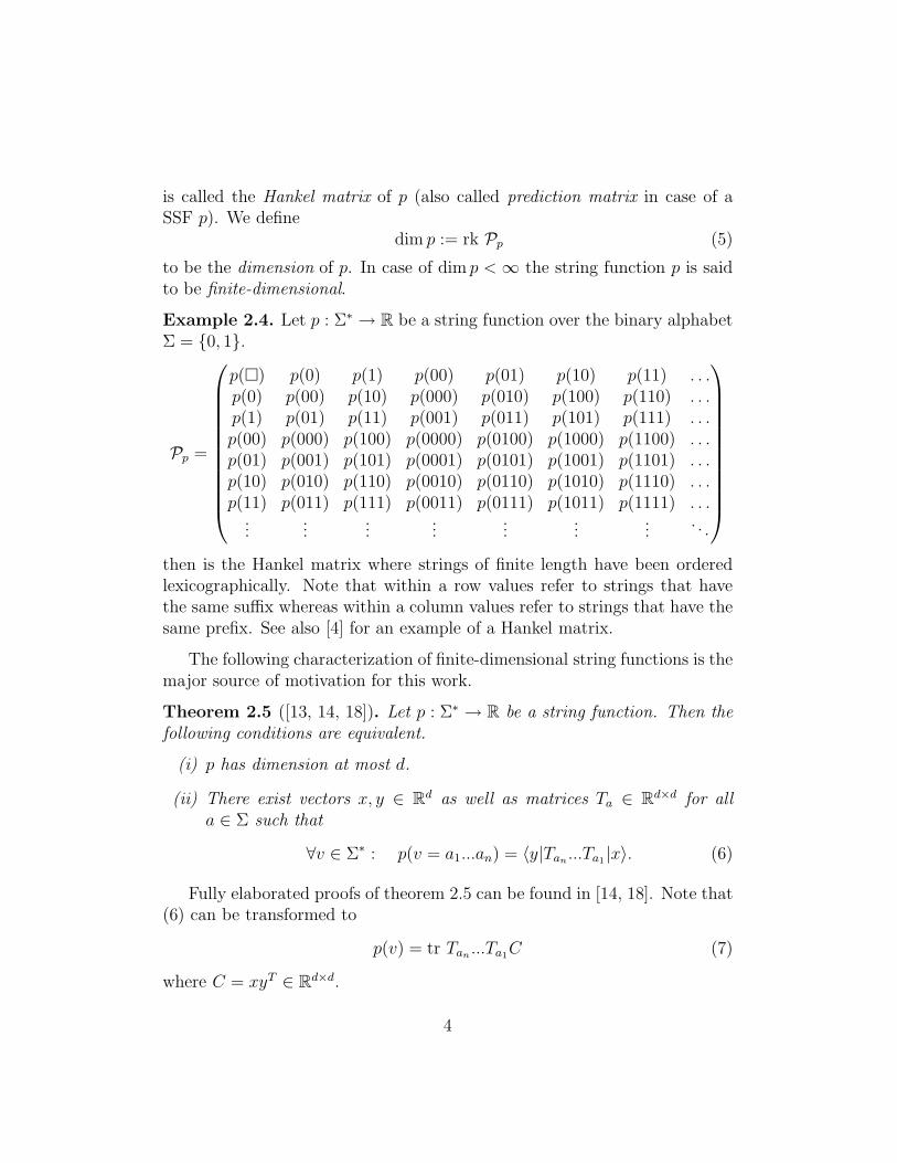
is called the Hankel matrix of p (also called prediction matrix in case of aSSF p). We define

dim p := rk Pp (5)

to be the dimension of p. In case of dim p < ∞ the string function p is saidto be finite-dimensional.

Example 2.4. Let p : Σ∗ → R be a string function over the binary alphabetΣ = {0, 1}.

Pp =

p(�) p(0) p(1) p(00) p(01) p(10) p(11) . . .

p(0) p(00) p(10) p(000) p(010) p(100) p(110) . . .

p(1) p(01) p(11) p(001) p(011) p(101) p(111) . . .

p(00) p(000) p(100) p(0000) p(0100) p(1000) p(1100) . . .

p(01) p(001) p(101) p(0001) p(0101) p(1001) p(1101) . . .

p(10) p(010) p(110) p(0010) p(0110) p(1010) p(1110) . . .

p(11) p(011) p(111) p(0011) p(0111) p(1011) p(1111) . . ....

......

......

......

. . .

then is the Hankel matrix where strings of finite length have been orderedlexicographically. Note that within a row values refer to strings that havethe same suffix whereas within a column values refer to strings that have thesame prefix. See also [4] for an example of a Hankel matrix.

The following characterization of finite-dimensional string functions is themajor source of motivation for this work.

Theorem 2.5 ([13, 14, 18]). Let p : Σ∗ → R be a string function. Then thefollowing conditions are equivalent.

(i) p has dimension at most d.

(ii) There exist vectors x, y ∈ Rd as well as matrices Ta ∈ Rd×d for alla ∈ Σ such that

∀v ∈ Σ∗ : p(v = a1...an) = 〈y|Tan...Ta1

|x〉. (6)

Fully elaborated proofs of theorem 2.5 can be found in [14, 18]. Note that(6) can be transformed to

p(v) = tr Tan...Ta1

C (7)

where C = xyT ∈ Rd×d.

4

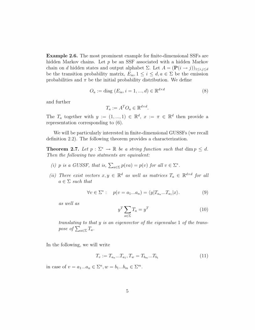
Example 2.6. The most prominent example for finite-dimensional SSFs arehidden Markov chains. Let p be an SSF associated with a hidden Markovchain on d hidden states and output alphabet Σ. Let A = (P(i → j))1≤i,j≤d

be the transition probability matrix, Eia, 1 ≤ i ≤ d, a ∈ Σ be the emissionprobabilities and π be the initial probability distribution. We define

Oa := diag (Eia, i = 1, ..., d) ∈ Rd×d (8)

and furtherTa := AT Oa ∈ R

d×d.

The Ta together with y := (1, ..., 1) ∈ Rd, x := π ∈ Rd then provide arepresentation corresponding to (6).

We will be particularly interested in finite-dimensional GUSSFs (we recalldefinition 2.2). The following theorem provides a characterization.

Theorem 2.7. Let p : Σ∗ → R be a string function such that dim p ≤ d.Then the following two statments are equivalent:

(i) p is a GUSSF, that is,∑

a∈Σ p(va) = p(v) for all v ∈ Σ∗.

(ii) There exist vectors x, y ∈ Rd as well as matrices Ta ∈ Rd×d for alla ∈ Σ such that

∀v ∈ Σ∗ : p(v = a1...an) = 〈y|Tan...Ta1

|x〉. (9)

as well asyT

∑

a∈Σ

Ta = yT (10)

translating to that y is an eigenvector of the eigenvalue 1 of the trans-pose of

∑

a∈Σ Ta.

In the following, we will write

Tv := Tan...Ta1

, Tw = Tbm...Tb1 (11)

in case of v = a1...an ∈ Σn, w = b1...bm ∈ Σm.

5

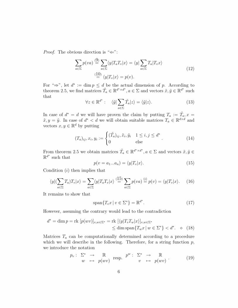
Proof. The obvious direction is “⇐”:

∑

a∈Σ

p(va)(9)=

∑

a∈Σ

〈y|TaTv|x〉 = 〈y|∑

a∈Σ

Ta|Tvx〉

(10)= 〈y|Tv|x〉 = p(v).

(12)

For “⇒”, let d∗ := dim p ≤ d be the actual dimension of p. According totheorem 2.5, we find matrices Ta ∈ Rd∗×d∗ , a ∈ Σ and vectors x, y ∈ Rd∗ suchthat

∀z ∈ Rd∗ : 〈y|

∑

a∈Σ

Ta|z〉 = 〈y|z〉. (13)

In case of d∗ = d we will have proven the claim by putting Ta := Ta, x =x, y = y. In case of d∗ < d we will obtain suitable matrices Ta ∈ Rd×d andvectors x, y ∈ Rd by putting

(Ta)ij, xi, yi :=

{

(Ta)ij , xi, yi 1 ≤ i, j ≤ d∗

0 else. (14)

From theorem 2.5 we obtain matrices Ta ∈ Rd∗×d∗ , a ∈ Σ and vectors x, y ∈

Rd∗ such thatp(v = a1...an) = 〈y|Tv|x〉. (15)

Condition (i) then implies that

〈y|(∑

a∈Σ

Ta)Tv|x〉 =∑

a∈Σ

〈y|TaTv|x〉(15)=

∑

a∈Σ

p(va)(i)= p(v) = 〈y|Tv|x〉. (16)

It remains to show that

span{Tvx | v ∈ Σ∗} = Rd∗ . (17)

However, assuming the contrary would lead to the contradiction

d∗ = dim p = rk [p(wv)]v,w∈Σ∗ = rk [〈y|TvTw|x〉]v,w∈Σ∗

≤ dim span{Twx |w ∈ Σ∗} < d∗. ⋄ (18)

Matrices Ta can be computationally determined according to a procedurewhich we will describe in the following. Therefore, for a string function p,we introduce the notation

pv : Σ∗ → R

w 7→ p(wv)resp.

pw : Σ∗ → R

v 7→ p(wv). (19)

6

That is, the pv resp. pv are the row resp. column vectors of the Hankel matrixPp. These are string functions in their own right. Note that p� = p� = p.Moreover, note that in case of a stochastic process p s.t. p(w = b1...bm) 6= 0it holds that

1

p(w)pw(v = a1...al)

= P({Xl′+1 = a1, ..., Xl′+l = al} | {X1 = b1, ..., Xl′ = bl′}). (20)

Therefore, 1p(w)

pw is just the discrete random process being governed by theprobabilities of p conditioned on that w has already been emitted.

The following is a generic algorithmic strategy to infer matrices Ta ∈ Rd×d

and x, y ∈ Rd corresponding to (6) from a finite-dimensional Hankel matrix.At this point, the algorithm needs the entire string function p as an input.We will explain how to obtain a practical version of this generic strategylater in this section.

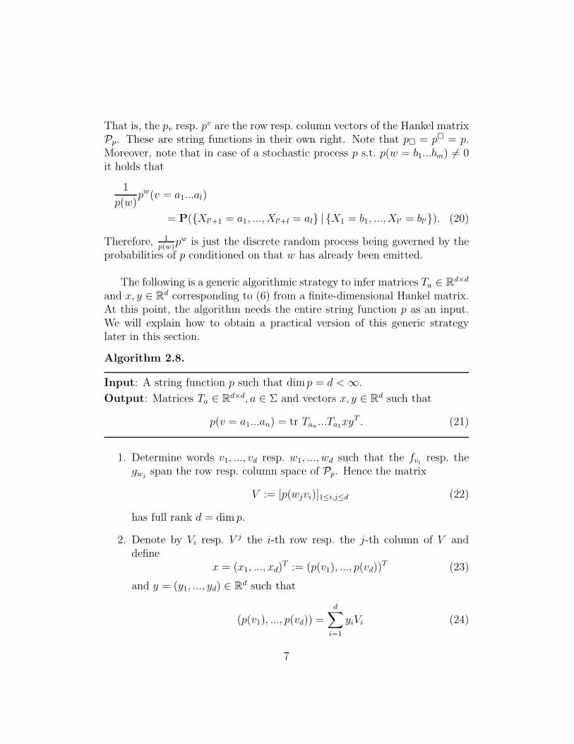
Algorithm 2.8.

Input: A string function p such that dim p = d < ∞.

Output: Matrices Ta ∈ Rd×d, a ∈ Σ and vectors x, y ∈ Rd such that

p(v = a1...an) = tr Tan...Ta1

xyT . (21)

1. Determine words v1, ..., vd resp. w1, ..., wd such that the fviresp. the

gwjspan the row resp. column space of Pp. Hence the matrix

V := [p(wjvi)]1≤i,j≤d (22)

has full rank d = dim p.

2. Denote by Vi resp. V j the i-th row resp. the j-th column of V anddefine

x = (x1, ..., xd)T := (p(v1), ..., p(vd))

T (23)

and y = (y1, ..., yd) ∈ Rd such that

(p(v1), ..., p(vd)) =

d∑

i=1

yiVi (24)

7

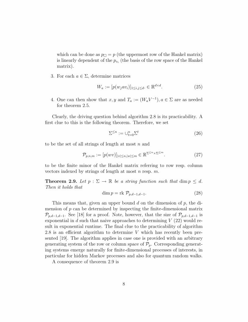
which can be done as p� = p (the uppermost row of the Hankel matrix)is linearly dependent of the pvi

(the basis of the row space of the Hankelmatrix).

3. For each a ∈ Σ, determine matrices

Wa := [p(wjavi)]1≤i,j≤d. ∈ Rd×d. (25)

4. One can then show that x, y and Ta := (WaV−1), a ∈ Σ are as needed

for theorem 2.5.

Clearly, the driving question behind algorithm 2.8 is its practicability. Afirst clue to this is the following theorem. Therefore, we set

Σ≤n := ∪nt=0Σ

t (26)

to be the set of all strings of length at most n and

Pp,n,m := [p(wv)]|v|≤n,|w|≤m ∈ RΣ≤n×Σ≤m

. (27)

to be the finite minor of the Hankel matrix referring to row resp. columnvectors indexed by strings of length at most n resp. m.

Theorem 2.9. Let p : Σ → R be a string function such that dim p ≤ d.Then it holds that

dim p = rk Pp,d−1,d−1. (28)

This means that, given an upper bound d on the dimension of p, the di-mension of p can be determined by inspecting the finite-dimensional matrixPp,d−1,d−1. See [18] for a proof. Note, however, that the size of Pp,d−1,d−1 isexponential in d such that naive approaches to determining V (22) would re-sult in exponential runtime. The final clue to the practicability of algorithm2.8 is an efficient algorithm to determine V which has recently been pre-sented [19]. The algorithm applies in case one is provided with an arbitrarygenerating system of the row or column space of Pp. Corresponding generat-ing systems emerge naturally for finite-dimensional processes of interests, inparticular for hidden Markov processes and also for quantum random walks.

A consequence of theorem 2.9 is

8

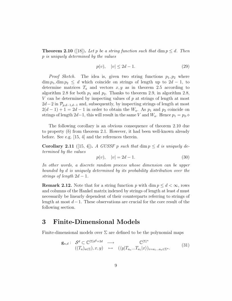
Theorem 2.10 ([18]). Let p be a string function such that dim p ≤ d. Thenp is uniquely determined by the values

p(v), |v| ≤ 2d − 1. (29)

Proof Sketch. The idea is, given two string functions p1, p2 wheredim p1, dim p2 ≤ d which coincide on strings of length up to 2d − 1, todetermine matrices Ta and vectors x, y as in theorem 2.5 according toalgorithm 2.8 for both p1 and p2. Thanks to theorem 2.9, in algorithm 2.8,V can be determined by inspecting values of p at strings of length at most2d−2 in Pp,d−1,d−1 and, subsequently, by inspecting strings of length at most2(d − 1) + 1 = 2d − 1 in order to obtain the Wa. As p1 and p2 coincide onstrings of length 2d−1, this will result in the same V and Wa. Hence p1 = p2.⋄

The following corollary is an obvious consequence of theorem 2.10 dueto property (b) from theorem 2.1. However, it had been well-known alreadybefore. See e.g. [15, 4] and the references therein.

Corollary 2.11 ([15, 4]). A GUSSF p such that dim p ≤ d is uniquely de-termined by the values

p(v), |v| = 2d − 1. (30)

In other words, a discrete random process whose dimension can be upperbounded by d is uniquely determined by its probability distribution over thestrings of length 2d − 1.

Remark 2.12. Note that for a string function p with dim p ≤ d < ∞, rowsand columns of the Hankel matrix indexed by strings of length at least d mustnecessarily be linearly dependent of their counterparts referring to strings oflength at most d−1. These observations are crucial for the core result of thefollowing section.

3 Finite-Dimensional Models

Finite-dimensional models over Σ are defined to be the polynomial maps

gn,d : Sd ⊂ C|Σ|d2+2d −→ C

|Σ|n

((Ta)a∈Σ), x, y) 7→ (〈y|Tan...Ta1

|x〉)v=a1...an∈Σn .(31)

9

where((Ta)a∈Σ), x, y) ∈ Sd :⇔ yT

∑

a∈Σ

Ta = yT . (32)

According to theorem 2.7, Sd comprises precisely the parameterizations ofthe generalized unconstrained random processes of dimension at most d. Ob-viously,

Sd ∼= C(|Σ|−1)d2+d(d−1)+2d. (33)

Therefore, the Zariski closure of image (gn,d) is an irreducible variety.

In the following, we will make use of the polynomial map (31) to derive aset-theoretic theorem with a strong view towards the invariants of the Zariskiclosure of the image of gn,d. In case of n ≥ 2d − 1, invariants for the imageof gn,d can be derived by inspection of the Hankel matrix. As in (27), letPp,n,m be the partial Hankel matrix that is filled with all values p(wv) suchthat |v| ≤ n, |w| ≤ m.

Theorem 3.1. Let n ≥ 2d − 1 and (p(v))v∈Σn be an (unconstrained) proba-bility distribution. Then it holds that

(p(v))v∈Σn ∈ image (gn,d)

if and only if the following two conditions apply where, in case of |u| < n,

p(u) =∑

u∈Σn−k

p(uv). (34)

(a)det [p(wjvi)]1≤i,j≤d+1 = 0 (35)

for all choices of words v1, ...vd+1, w1, ...wd+1 of length at most d − 1,which can be equivalently put as

rk Pp,d−1,d−1 ≤ d (36)

(b)rk Pp,⌈n

2⌉,⌊n

2⌋ = rk Pp,⌊n

2⌋,⌈n

2⌉ = rk Pp,d−1,d−1 (37)

10

(37) states that rows resp. columns in Pp,⌈n2⌉,⌊n

2⌋ and Pp,⌊n

2⌋,⌈n

2⌉ referring

to row strings v resp. column strings w where |v|, |w| ≥ d are linearly de-pendent of their counterparts in Pp,⌈n

2⌉,⌊n

2⌋ and Pp,⌊n

2⌋,⌈n

2⌉ that refer to row

resp. column strings of length at most d − 1.

Proof. “⇒”: Let (p(v))v∈Σn be in the image of gn,d. Theorem 2.5 statesthat the Hankel matrix Pp of p has rank at most d. This implies (a) as itjust expresses that some Hankel matrix minors of size d + 1 do not have fullrank.

Theorem 2.9 then states that bases of the row resp. the column spaceof Pp can be obtained by inspecting row resp. column vectors referring tostrings of length at most d − 1 which implies (b).

“⇐”: Let (p(u))u∈Σn s.t. (a), (b) apply. In order to prove that (p(u))u∈Σn ∈image gn,d, we have to provide a parameterization ((Ta)a∈Σ, x, y) ∈ Sd suchthat

p(u = a1...an) = yT Tan...Ta1

x (38)

for all strings u ∈ Σn. Therefore, we will provide a parameterization((Ta)a∈Σ, x, y) ∈ C|Σ|d2+2d such that

p(u = a1...ak) = yT Tak...Ta1

x (39)

for all strings u such that |u| ≤ n where p(u) is defined according to (34)in case of |u| < n. By this definition of p(u), |u| < n, it is straightforwardto show that ((Ta)a∈Σ, x, y) ∈ Sd which completes the proof. Furthermore,note that it suffices to provide a parameterization ((Ta)a∈Σ, x, y) ∈ Sd∗ forarbitrary d∗ ≤ d since, in case of d∗ < d, we extend the Ta as well as x, y byzero entries to obtain a d-dimensional parametrization from Sd. Combiningthese facts, we have to show that, for suitable d∗ ≤ d, there are matricesTa ∈ Rd∗×d∗ and vectors x, y ∈ Rd∗ such that (39) holds.

We obtain the desired parameterization ((Ta)a∈Σ, x, y) according to theideas of algorithm 2.8. First, determine strings v1, ..., vd∗ and w1, ..., wd∗ oflength at most d − 1 such that

V := [p(wjvi)]1≤i,j≤d∗ (40)

has full rank d∗ := rk Pp,d−1,d−1 ≤ d. We define

x = (x1, ..., xd∗)T := (p(v1), ..., p(vd∗))

T (41)

11

and y = (y1, ..., yd∗) ∈ Rd∗ such that

(p(v1), ..., p(vd∗)) =

d∗∑

i=1

yiVi (42)

where Vi = (p(viw1), ..., p(viwd∗)T is the i-th row of V which can be done since

the uppermost row of Pp,n,d−1 is linearly dependent of the rows referring tothe strings vi. Furthermore, for each a ∈ Σ, we determine matrices

Wa := [p(wjavi)]1≤i,j≤d∗. ∈ Rd∗×d∗ (43)

Note that probabilities in Wa may refer to strings of length up to 2d − 1which establishes the necessity of the assumption n ≥ 2d−1. We then claimthat defining

Ta := WaV−1 (44)

gives rise to the desired parametrization in terms of (39). We will obtain aneasy proof of this claim by three elementary lemmata.

Lemma 3.2. For all v, w ∈ Σ∗ such that |wv| ≤ ⌈n2⌉ (Tv = Tak

...Ta1, v =

a1...ak ∈ Σk):

Tv

p(wv1)...

p(wvd∗)

=

p(wvv1)...

p(wvvd∗)

(45)

Proof of lemma 3.2: Note first that |vi| ≤ d − 1 ≤ 2d−12

≤ n2

whichimplies |wvvi| ≤ n. As (p(wv1), ..., p(wvd∗))

T is contained in the columnspace of V it suffices to show the statement for w = wj. We do this byinduction on |v|:|v| = 1:

Ta

p(wjv1)...

p(wjvd∗)

= WaV

−1

p(wjv1)...

p(wjvd∗)

= Waej =

p(wjav1)...

p(wjavd∗)

. (46)

12

|v| → |v| + 1: Let v = av where a ∈ Σ.

Tv

p(wjv1)...

p(wjvd∗)

= TvTa

p(wjv1)...

p(wjvd∗)

|v|=1= Tv

p(wjav1)...

p(wjavd∗)

(∗)=

p(wjvav1)...

p(wjvavd∗)

=

p(wj vv1)...

p(wj vvd∗)

(47)

where (∗) follows from the induction hypothesis. ⋄

Lemma 3.3. For all v, w ∈ Σ∗ such that |w|, |v| ≤ ⌈n2⌉, |wv| ≤ n (Tv =

Tak...Ta1

, v = a1...ak ∈ Σk):

yTTv

p(wv1)...

p(wvd∗)

= p(wv). (48)

Proof of lemma 3.3: Note that the columns in Pp,⌊n2⌋,⌈n

2⌉ resp. Pp,⌈n

2⌉,⌊n

2⌋

referring to w is contained in the span of the columns referring to the wj’s,according to the choice of the wj. Therefore, it suffices to show the statementfor w = wj . We do this by induction on |v|:|v| = 0 (v = �, T� = Id):

yTT�

p(wjv1)...

p(wjvd∗)

= yT

p(wjv1)...

p(wjvd∗)

= p(wj) (49)

follows from the choice of y.|v| → |v| + 1: Let v = av, a ∈ Σ.

yTTv

p(wjv1)...

p(wjvd∗)

= yTTvTa

p(wjv1)...

p(wjvd∗)

L. 3.2= yT Tv

p(wjav1)...

p(wjavd∗)

(∗)= p(wav) = p(wv)

(50)

13

where (∗) follows from the induction hypothesis. ⋄

Proof of theorem 3.1 (cont.): Let u ∈ Σ∗ such that |u| ≤ n. Splitu = wv into two strings w, v such that |w|, |v| ≤ ⌈n

2⌉. We compute

yT Tux = yT TvTwx = yTTvTw

p(v1)...

p(vd∗)

= yTTvTwyTTvTw

p(�v1)...

p(�vd∗)

L. 3.2,|w�|≤⌈n2⌉

= yT Tv

p(wv1)...

p(wvd∗)

L. 3.3= p(wv) = p(u)

(51)

where we have replaced v resp. w of lemma 3.2 by w resp. � here in order toobtain the fourth equation. ⋄

Due to theorem 3.1, invariants that are induced by conditions (a) and(b) fully describe the finite-dimensional model gn,d for n ≥ 2d − 1, hencegenerate the ideal of model invariants.

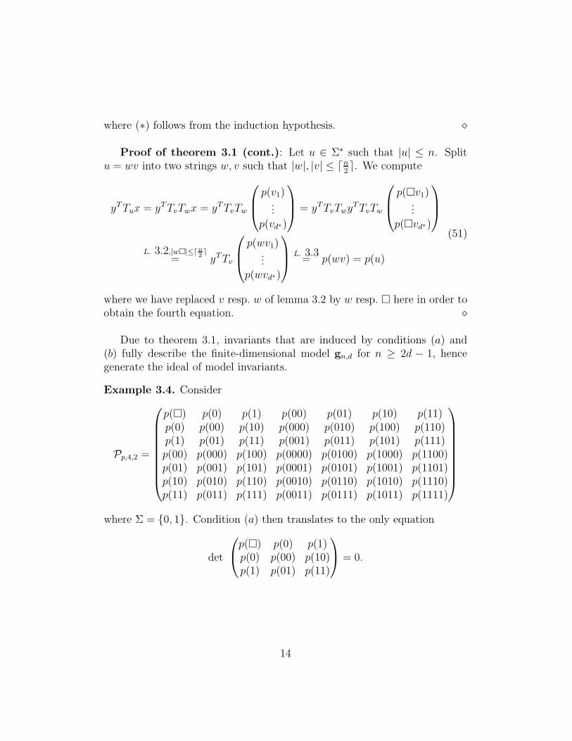
Example 3.4. Consider

Pp,4,2 =

p(�) p(0) p(1) p(00) p(01) p(10) p(11)p(0) p(00) p(10) p(000) p(010) p(100) p(110)p(1) p(01) p(11) p(001) p(011) p(101) p(111)p(00) p(000) p(100) p(0000) p(0100) p(1000) p(1100)p(01) p(001) p(101) p(0001) p(0101) p(1001) p(1101)p(10) p(010) p(110) p(0010) p(0110) p(1010) p(1110)p(11) p(011) p(111) p(0011) p(0111) p(1011) p(1111)

where Σ = {0, 1}. Condition (a) then translates to the only equation

det

p(�) p(0) p(1)p(0) p(00) p(10)p(1) p(01) p(11)

= 0.

14

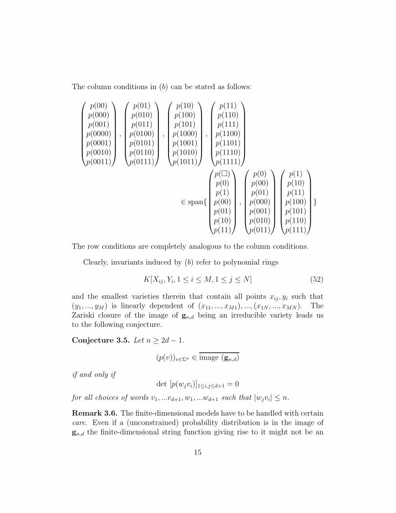
The column conditions in (b) can be stated as follows:

p(00)p(000)p(001)p(0000)p(0001)p(0010)p(0011)

,

p(01)p(010)p(011)p(0100)p(0101)p(0110)p(0111)

,

p(10)p(100)p(101)p(1000)p(1001)p(1010)p(1011)

,

p(11)p(110)p(111)p(1100)p(1101)p(1110)p(1111)

∈ span{

p(�)p(0)p(1)p(00)p(01)p(10)p(11)

,

p(0)p(00)p(01)p(000)p(001)p(010)p(011)

p(1)p(10)p(11)p(100)p(101)p(110)p(111)

}

The row conditions are completely analogous to the column conditions.

Clearly, invariants induced by (b) refer to polynomial rings

K[Xij , Yi, 1 ≤ i ≤ M, 1 ≤ j ≤ N ] (52)

and the smallest varieties therein that contain all points xij , yi such that(y1, ..., yM) is linearly dependent of (x11, ..., xM1), ..., (x1N , ..., xMN). TheZariski closure of the image of gn,d being an irreducible variety leads usto the following conjecture.

Conjecture 3.5. Let n ≥ 2d − 1.

(p(v))v∈Σn ∈ image (gn,d)

if and only ifdet [p(wjvi)]1≤i,j≤d+1 = 0

for all choices of words v1, ...vd+1, w1, ...wd+1 such that |wjvi| ≤ n.

Remark 3.6. The finite-dimensional models have to be handled with certaincare. Even if a (unconstrained) probability distribution is in the image ofgn,d the finite-dimensional string function giving rise to it might not be an

15

(unconstrained) stochastic process, meaning that the string function is notnecessarily non-negative, since values referring to longer strings as computedaccording to (6) might be negative. It is one of the big open problems ofthe theory of finite-dimensional processes how to algorithmically determinewhether a set of matrices as in (6) gives rise to a non-negative string function.

4 String Length Complexity

In this section, we will prove a set-theoretical theorem an ideal-theoreticalcounterpart of which would yield, as a corollary, a proof of conjecture 11.9,[3]. The theorem may be of interest in its own right, as the assumptions tobe met by the models under considerations are fairly mild.

Roughly speaking, an ideal-theoretical extension of the theorem would beabout how to lift sets of generators for models describing distributions overstrings of length n to generators for distributions over strings of length n+1,given that n is greater than the string length complexity of the underlyingmodels.

In the following,M ⊂ R

Σ∗

(53)

is a class of USSFs.

Definition 4.1. Let M ⊂ RΣ∗be a class of USSFs. We define the string

length complexity of M to be

SLC (M) :=

inf{N ∈ N | p1, p2 ∈ M : (p1)|Σn = (p2)|Σn ⇒ p1 = p2}. (54)

That is, members of M are uniquely determined by their distributions overstrings of length SLC (M).

Given a class of USSFs, let

Mn := {(p(v))v∈Σn | p ∈ M} (55)

be the set of distributions over strings of length n that are induced by themembers of M. In case of SLC (M) = n the map

πΣn : M −→ Mn

p 7→ p|Σn = (p(v))v∈Σn(56)

is one-to-one.

16

Theorem 4.2. Let M be a class of unconstrained random processes suchthat

(i)SLC (M) ≤ n − 1 < ∞. (57)

(ii)p ∈ M ⇒ ∀a ∈ Σ : pa ∈ M. (58)

Then it holds that

(p(u), u ∈ Σn+1) ∈ Mn+1 ⇔

{

(p(av), v ∈ Σn) ∈ Mn ∀a ∈ Σ

(p(v), v ∈ Σn) ∈ Mn

(59)

where p(v) =∑

a∈Σ p(va).

Remark 4.3. Theorem 4.2 is meant to be a first step to obtain an analo-gous theorem resulting from replacing Mn,Mn+1 by their Zariski closuresMn,Mn+1. Generators for the ideal of invariants of Mn+1, given generatorsfor the ideal of invariants of Mn, could be obtained by the following idea.If h ∈ C[Xv, v ∈ Σn] is one of the generators for Mn where the Xv areindeterminates for the probabilities p(v), v ∈ Σn, one obtains |Σ|+ 1 genera-tors for Mn+1 by replacing the indeterminates Xv, v ∈ Σn by indeterminatesXav, v ∈ Σn for all a ∈ Σ which results in new generators

ha ∈ C[Xav, v ∈ Σn] ⊂ C[Xu, u ∈ Σn+1] (60)

as well as replacing each Xv by the polynomials∑

a Xva ∈ C[Xu, u ∈ Σn+1]resulting in another generator

h+ ∈ C[∑

a

Xva, v ∈ Σn] ⊂ C[Xu, u ∈ Σn+1]. (61)

The theorem would state that the generators obtained by this proceduregenerate the ideal of invariants of Mn+1.

Note that in particular the maximum degree of the generators of Mn+1

would be at most that of Mn.

Proof. “⇒”: From (58) we obtain that (pa(v), v ∈ Σn) ∈ Mn for eacha ∈ Σ. The second part is just the trivial observation that (p(u), u ∈ Σn+1) ∈

17

Mn+1 implies (p(v), v ∈ Σn) ∈ Mn.

“⇐”: From the second case in (59) we obtain that (p(v), v ∈ Σn) ∈ Mn. Aselements of M are uniquely determined by their values for strings of lengthat least m and n ≥ m + 1 we obtain a USSF p ∈ M such that

p(v) = p(v) for all v ∈ Σn. (62)

It remains to show that also

p(w) = p(w) for all w ∈ Σn+1 (63)

which amounts to showing that

p(av) = p(av) = pa(v) for all (a, v) ∈ Σ × Σn. (64)

We further observe that

(pa(v), v ∈ Σn) ∈ Mn (65)

for all a ∈ Σ, because of n ≥ m + 1 > m, implies the existence of a uniqueqa ∈ M s.t.

qa(v) = pa(v) for all v, |v| ≤ n. (66)

As p ∈ M, we have that pa ∈ M for all a ∈ Σ, due to (58). Moreover, foru ∈ Σn−1,

pa(u) = p(au)(62)= p(au)

(66)= qa(u). (67)

As n − 1 ≥ m and paM and qaM coincide on strings of length n − 1 ≥ m,we obtain

pa = qa (68)

because of (i). We finally compute

p(av) = pa(v)(66)= qa(v)

(68)= pa(v) = p(av) (69)

which establishes (64). ⋄

18

4.1 Finite-Dimensional Models

Theorem 4.2 applies for the finite-dimensional models. Eq. 57 is establishedby theorem 2.10 in subsection 2.2 whose statement is that finite-dimensionalprocesses p of dimension at most d are uniquely determined by the valuesp(v), |v| = 2d − 1.

In terms of the language introduced here, we can restate theorem 2.10 asfollows.

Theorem 4.4. Let

Md := {p ∈ RΣ∗

; | p is USSF and dim p ≤ d}

be the class of unconstrained processes of dimension at most d. Then it holdsthat

SLC (Md) = 2d − 1.

Furthermore observe that

(pa)w(v) = pa(wv) = p(awv) = paw(v) (70)

for all a ∈ Σ, v, w ∈ Σ∗ which translates to

(pa)w = paw. (71)

Hence the column space of Ppa is contained in that of Pp which yields

dim pa ≤ dim p (72)

as dim p is just the dimension of the column space of Pp.This observation in combination with theorem 4.4 make the assumptions

of theorem 4.2 hold for Md, which yields the following corollary.

Corollary 4.5. Let n ≥ 2d. Then it holds that

(p(u), u ∈ Σn+1) ∈ image gn+1,d ⇔

{

(p(av), v ∈ Σn) ∈ image gn,d ∀a ∈ Σ

(p(v), v ∈ Σn) ∈ image gn,d

(73)

Again, an analogous ideal-theoretical result referring to the Zariski clo-sures of image gn,d, image gn+1,d would yield that the maximum degree of thegenerators would not increase for n ≥ 2d.

19

5 Hidden Markov Models

In the following, let

fn,l : Cl(l−1)+l(|Σ|−1)+l −→ C|Σ|n

((Ta = AT Oa)a∈Σ), x) 7→ (tr Tan...Ta1

x(1, ..., 1)T )v=a1...an∈Σn .

(74)where A and the Oa as in example 2.6, be the polynomial map associated withthe unconstrained (constrained if and only if

∑l

i=1 xi = 1) hidden Markovmodel referring to hidden Markov models acting on l hidden states and dis-tributions over strings of length n, as described in [16].

The following theorem of Heller resulted from the attempts set off in thelate 50’s [11, 6, 7, 8] to give novel characterizations of hidden Markov pro-cesses. Many of those results are based on the idea that HMPs have finitedimension, which was noticed earlier in that series of papers without explic-itly stating it. We give a version of Heller’s theorem that is adapted to thelanguage in use here. Heller’s version is formulated in the language of homo-logical algebra—without string functions and Hankel matrices. In his paper,discrete random processes are viewed as modules over certain rings. Thislanguage later has never been used in the theory of stochastic processes orrelated areas, probably as the required amount of prior knowledge unfamiliarto statisticians and probabilists is high. In the following we define

Cp := span{pw |w ∈ Σ∗} (75)

to be the column space of the Hankel matrix Pp of a string function p.

Theorem 5.1 (Heller, 1965). A string function p : Σ∗ → R is associated witha (unconstrained) hidden Markov process if and only if there are (U)SSFspi ∈ Cp, i = 1, ..., l s.t.

(a) p ∈ cone {pi | i = 1, ..., l},

(b) ∀w ∈ Σ∗ : (pi)w ∈ cone {pi | i = 1, ..., l}.

Note first that this again points out that hidden Markov processes p arefinite-dimensional as Cp ⊂ span{pi | i = 1, ..., l} hence dim p ≤ l. Note fur-ther that (a) in combination with (b) implies that pv ∈ cone {pi} for allv ∈ Σ∗ which renders cone {pi} to be full-dimensional. It is closed due to be-ing polyhedral and pointed due to being generated by SSFs which are strictly

20

positive string functions. Collecting properties results in cone {pi} being aproper, polyhedral cone.

Given a hidden Markov process p, the pi can be obtained as the randomprocesses starting from the hidden states (i.e. having initial probability distri-bution ei). The other direction requires more work. A translation of Heller’sproof [12] to the language of string functions can be found in [17]. A ratherstraightforward consequence of Heller’s theorem is the following corollary.

Corollary 5.2. Let p be a USSF of dimension of at most 2. Then p isassociated with an unconstrained hidden Markov process acting on 2 hiddenstates.

Proof Sketch: As all pw ≥ 0 the cone generated by all column vectors

cone {pw |w ∈ Σ∗} (76)

is pointed hence its closure is generated by its extremal rays. In two dimen-sions this is equivalent to the closure of cone {pw | v ∈ Σ∗} being polyhedral.It’s a routine exercise to check for the assumptions of Heller’s theorem tohold for this cone. ⋄

One might be tempted to infer that the ideal of model invariants of fn,2

can be computed by computing the invariants of the 2-dimensional model, asprovided by theorem 3.1. However, a 2-dimensional process need not be as-sociated with a hidden Markov process acting on 2 hidden states. Accordingto the proof of theorem 5.1, one might need up to 2|Σ| many hidden statesto describe an arbitrary 2-dimensional process by means of a hidden Markovparameterization.

5.1 Degree of Invariants

Heller’s theorem gives rise to an application of theorem 4.2 to hidden Markovprocesses where n ≥ 2l. Assumption (i) of theorem 4.2 is met since hiddenMarkov processes on l hidden states, as finite-dimensional random processesof dimension ≤ l, are determined by their distributions over the strings oflength 2l − 1. Assumption (ii) is met due to Heller’s theorem.2 The only

2Proofs for this can also be formulated in terms of the hidden Markov processes’ pa-rameterizations. However, such proofs are lengthy and technical exercises.

21

thing one has to be aware of is that the dimension of the column space of Ppa

can be lower than that of Pp itself. In this case, one obtains the necessarycone generators by projecting Cp onto Cpa (we recall that Cpa ⊂ Cp). In sum,the class of unconstrained hidden Markov processes meet the assumptions oftheorem 4.2, which yields

Corollary 5.3. Let n ≥ 2d. Then it holds that

(p(u), u ∈ Σn+1) ∈ image fn+1,l ⇔

{

(p(av), v ∈ Σn) ∈ image fn,l ∀a ∈ Σ

(p(v), v ∈ Σn) ∈ image fn,l

(77)

Note that an ideal-theoretic equivalent of theorem 5.3 would yield a proofof conjecture 11.9 from [3] as a corollary. However, an ideal-theoretical equiv-alent of theorem 5.3 would be a stronger result:

Conjecture 5.4. Let fn,l be the unconstrained hidden Markov model for l

hidden states and strings of length n. Then the maximum degree of the in-variants d(n, l) of fn,l does not increase for n ≥ 2l, that is,

...d(n + 1, l) ≤ d(n, l) ≤ d(n − 1, l) ≤ ... ≤ d(2l, l). (78)

As d(5, 2) = 1 (see [3], table 11.1 (?)), we would obtain that d(n, l) = 1 forn ≥ 5, that is, the ideal of invariants would be generated by linear equationsexclusively.

6 The Markov model

In the following, let (U)SSFs p be induced by Markov chains. That is,

p(v = a1...an) = π(a1)n

∏

i=2

Mai−1ai(79)

where π ∈ RΣ is a strictly positive vector (with entries not necessarily sum-ming up to one in case of a USSF p) and M ∈ RΣ2

is a matrix with theentries of a row summing up to one. Moreover, in this section, let

fn,l=|Σ| : Cl+l(l−1) −→ C|Σ|n

(π, M) 7→ (π(a1)∏n

i=2 Mai−1ai)v=a1...an∈Σn.

(80)

22

be the polynomial map (associated with the Markov model in case of π, M

being in accordance with the laws from above) with alphabet Σ on strings oflength n. In the language of string functions and Hankel matrices, we havethe following theorem.

Theorem 6.1. A (U)SSF p is associated with a Markov chain iff

∀a ∈ Σ : dim span{pva | v ∈ Σ∗} ≤ 1. (81)

A proof can be found in [17], for example.This can be straightforwardly exploited to obtain invariants of fn,l.

Theorem 6.2. Let (p(v), v ∈ Σn) be a (unconstrained) probability distribu-tion such that n ≥ 2|Σ| − 1. Then (p(v), v ∈ Σn) lies in the image of fn,l=|Σ|

if and only if

det

[

p(vau) p(wau)p(vau′) p(wau′)

]

= 0 (82)

for all choices u, u′, v, w ∈ Σ∗, a ∈ Σ such that |vau|, |vau′|, |wau|, |wau′| ≤ n

and, as usual, p(v) :=∑

w∈Σn−|v| p(vw) for strings v such that |v| < n.

Proof. “⇒” is obvious as for a Markov chain p, (82) is a necessaryconsequence of (81) in theorem 6.1.

“⇐” Clearly, (82) implies the assumptions (35) and (37) of theorem 3.1to hold, which yields that (p(v), v ∈ Σn) lies in the image of the finite-dimensional model. We thus find, by means of algorithm 2.8, (Ta)a∈Σ, x, y

such that the probabilities p(v) for all v up to length n ≥ 2|Σ| can be com-puted according to (6). Note that Ta maps pv onto pva where pv, pva areidentified with a coordinate representation induced by the basis of the col-umn spaces that one has found according to algorithm 2.8 (see remark 3.6).In this sense, (82) translates to

dim image Ta ≤ 1 (83)

for all a ∈ Σ. Clearly, this implies (81) of theorem 6.1 from which the asser-tion follows. ⋄

Remark 6.3. While the assumption n ≥ 2|Σ| − 1 helps to give a ratherconcise proof of theorem 6.2, we feel that it is not a necessary requirement.However, inference of Markov chain parameters giving rise to probabilitydistributions (p(v), v ∈ Σn) for which the determinantal invariants (82) ap-ply is a much more technical undertaking. Moreover, it seems that some(potentially more involved) pecularities have to be resolved.

23

7 Trace algebras

In this section, we will draw some connections between trace algebras andthe theory of finite-dimensional string functions. For a rigorous introductionto trace algebras see [9]. We recall that in Bernd’s preprint [2] the quartichidden Markov model invariant listed in [3] could be identified as a relationbetween trace polynomials.

Here, we shall try to shed some light on the general relationships betweentrace algebras and finite-dimensional models. In terms of the language oftrace algebras, we will derive some defining relations for the trace algebras.

Therefore, we introduce the following definition.

Definition 7.1. A string function p : Σ∗ → R is called traceable of order r

if there are matrices Xa ∈ Rr×r, a ∈ Σ such that

p(v = a1...an) = tr Xan...Xa1

. (84)

Traceable string functions are finite-dimensional, as can be seen by ap-plication of a simple lemma.

Lemma 7.2. Let pi, i = 1, ..., k be string functions of dimensions di. Letp :=

∑k

i=1 pi. Then it holds that

dim p ≤

k∑

i=1

di. (85)

This gives rise to

Theorem 7.3. Let p ∈ RΣ∗be traceable of order r. Then

dim p ≤ r2. (86)

Proof. Let pi ∈ RΣ∗, i = 1, ..., r be defined by

pi(v = a1...an) := tr Xan...Xa1

eieTi . (87)

From theorem 2.5 we obtain dim pi ≤ r. As Id =∑

i eieTi , which yields

p =∑

pi (88)

24

the assertion follows from application of lemma 7.2. ⋄

If the identity matrix Id =∑

i eieTi was presentable in the form Id = xyT

itself, traceable string functions of order r would be of dimension at most r,as given by theorem 2.5. As this is not the case, there are traceable stringfunctions of order r whose dimension is larger than r. Moreover, not everystring function of dimension r2 seems to be traceable. However, an exampleof that kind is yet to be delivered.

The consequences of theorem 7.3 for the theory of trace algebras arethat invariants which can be computed for the r2-dimensional models fn,r2

also apply as defining relations for the trace algebras generated by all tracepolynomials

tr (Xin ...Xi1), 1 ≤ ij ≤ d, n ≥ 0. (89)

The exact relationships between trace algebras, hidden Markov as well asthe finite-dimensional models are yet to be determined.

8 Open Questions

1. Theorem 5.1 characterizes hidden Markov chains within the theory offinite-dimensional random processes. Determine invariants that corre-spond to this characterization.

2. Determine the relationships between trace algebras and the modelsunder consideration here in more detail.

3. Deliver a proof for a more general version of theorem 6.2, as discussedabove.

4. Determine the peculiarities of differences between the two-dimensionalmodels and the hidden Markov models for 2 hidden states.

5. Tropicalization of Teichmuller spaces (see [2])?

References

[1] D. Aharonov, A. Ambainis, J. Kempe, U. Vazirani, ”Quantum walks ongraphs”, in Proc. of 33rd ACM STOC, New York, 2001, pp. 50-59.

25

[2] B. Sturmfels, “Trace Algebras, Hidden Markov Models and Tropicaliza-tion of Teichmuller Spaces”, preprint, 2008.

[3] N. Bray and J. Morton, “Equations defining hidden Markov models”, inAlgebraic Statistics for Computational Biology (L. Pachter and B. Sturm-fels, eds), Cambridge University Press, pp. 235-247, 2005.

[4] L. Finesso, A. Grassi and P. Spreij, “Approximation of stationary pro-cesses by hidden Markov models”, preprint, arXiv:math.OC/0606591.

[5] D. Blackwell and L. Koopmans, “On the identifiability problem for func-tions of finite markov chains”, Annals of Mathematical Statistics vol. 28,pp. 1011–1015, 1957.

[6] S.W. Dharmadhikari, “Functions of finite markov chains”, Annals ofMathematical Statistics, vol. 34, pp. 1022-1032, 1963.

[7] S.W. Dharmadhikari. “Sufficient conditions for a stationary process to bea function of a finite markov chain”, Annals of Mathematical Statistics,vol. 34, pp. 1033-1041, 1963.

[8] S.W. Dharmadhikari, A characterization of a class of functions of finitemarkov chains. Annals of Mathematical Statistics, vol. 36, pp. 524-528,1965.

[9] V. Drensky, Computing with matrix invariants. Math. Balk., New Ser. 21,No. 1-2, pp. 101-132, 2007.

[10] U. Faigle and A. Schoenhuth, “Asymptotic mean stationarity of sourceswith finite evolution dimension”, IEEE Trans. Inf. Theory, vol. 53(7),pp. 2342-2348, 2007

[11] E.J. Gilbert, ”On the identifiability problem for functions of finiteMarkov chains”, Ann. Math. Stat., vol. 30, pp. 688-697, 1959.

[12] A. Heller “On stochastic processes derived from Markov chains”, Annalsof Mathematical Statistics, vol. 36(4), pp. 1286-1291, 1965

[13] H. Ito, S.-I. Amari and K. Kobayashi “Identifiability of hidden Markovinformation sources and their minimum degrees of freedom”, IEEE Trans.Inf. Theory, vol. 38(2), pp. 324-333, 1992.

26

[14] H. Jaeger. “Observable operator models for discrete stochastic time se-ries”, Neural Computation, vol. 12(6), pp. 1371-1398, 2000.

[15] Y. Ephraim and N. Merhav, ”Hidden Markov processes”, IEEE Trans.Inf. Theory, vol. 48(6), pp. 1518-1569, 2002.

[16] L. Pachter and B. Sturmfels, Algebraic Statistics for Computational Bi-ology, Cambridge University Press, 2005.

[17] A. Schoenhuth, “Discrete-valued stochastic vector spaces”, PhD thesis(German), University Cologne, 2006.

[18] A. Schonhuth and H. Jaeger, “Character-ization of ergodic hidden Markov sources”,http://www.zaik.uni-koeln.de/∼paper/index.html?show=zaik2008-573,submitted to IEEE Trans. Inf. Theory, 2007.

[19] A. Schonhuth, “A simple and efficient solution of the identifiabil-ity problem for hidden Markov models and quantum random walks”,http://arxiv.org/abs/0808.2833, Proc. ISITA 2008, to appear, 2008.

[20] A. Schonhuth, “On analytic properties of entropy rate”, IEEETrans. Inf. Theory, to appear.

27