data analytics over hidden databases
TRANSCRIPT

DATA ANALYTICS OVER HIDDEN DATABASES
by
ARJUN DASGUPTA
Presented to the Faculty of the Graduate School of
The University of Texas at Arlington in Partial Fulfillment
of the Requirements
for the Degree of
DOCTOR OF PHILOSOPHY
THE UNIVERSITY OF TEXAS AT ARLINGTON
August 2010

Copyright c© by Arjun Dasgupta 2010
All Rights Reserved

To my mother and father whose constant support and guidance has been the driving force
in all my endeavours

ACKNOWLEDGEMENTS
I would like to thank my supervising professor and committee chair, Dr. Gautam
Das, who continually and convincingly conveyed words of encouragement and a spirit of
adventure in regard to research and scholarship. Without his guidance and persistent help,
this dissertation would not have been possible. In addition, I extend my sincere thanks to all
my committee members for showing interest in my research and serving on my committee.
I am especially grateful to Dr. Nan Zhang from George Washington University for
introducing me to some extraordinarily interesting problems and engaging me in exciting
research discussions.
I would also like to extend my gratitude to the department of Computer Science and
Engineering at the University of Texas at Arlington and my advisor, Dr. Das for providing
financial support required for my research.
Finally, I would like to thank my friends and family who stood by me throughout this
process. Special thanks to my colleague Senjuti Basu Roy for her constant support towards
my academic adventures.
July 15, 2010
iv
ABSTRACT
DATA ANALYTICS OVER HIDDEN DATABASES
Arjun Dasgupta, Ph.D.
The University of Texas at Arlington, 2010
Supervising Professor: Gautam Das
Web based access to databases have become a popular method of data delivery. A
multitude of websites provides access to their proprietary data through web forms. In order
to view this data, customers use the web form interface and pose queries on the underlying
database. These queries are executed and a resulting set of tuples (usually the top-k ones)
is served to the customer. Top-k along with strict limits on querying are constraints used
by the database providers to conserve the power of the underlying data distribution. De-
livering limited access only to tuples that satisfy a query enables providers to expose only
a small snippet of the entire inventory at a time. This method of data delivery prevents
analysts from deriving information on the holistic nature of data. Analytical queries on the
data statistics are hence blocked through these access restrictions.
The objective of this work is to provide detailed approaches that obtain results towards
inferring statistical information on such hidden databases, using their publicly available
front-end forms. To this end, we first explore the problem of random sampling of tuples
from hidden databases. Samples representing the underlying data open up a proprietary
database to a plethora of opportunities by giving external parties a glimpse into the holistic
aspects of the data. Analysts can use samples to pose aggregate queries and gain informa-
v

tion on the nature and quality of data. In addition to sampling, we also present efficient
techniques that directly produce unbiased estimate of various interesting aggregates. These
techniques can be also applied to address the more general problem of size estimation of
such databases.
In light of techniques towards inferring aggregates, we introduce and motivate the problem
of privacy preservation in hidden databases from the data provider’s perspective, where the
objective is to preserve the underlying aggregates while serving legitimate customers with
answers to their form-based queries.
vi
TABLE OF CONTENTS
ACKNOWLEDGEMENTS . . . . . . . . . . . . . . . . . . . . . . . . . . . . . . . iv
ABSTRACT . . . . . . . . . . . . . . . . . . . . . . . . . . . . . . . . . . . . . . . v
LIST OF FIGURES . . . . . . . . . . . . . . . . . . . . . . . . . . . . . . . . . . . xii
LIST OF TABLES . . . . . . . . . . . . . . . . . . . . . . . . . . . . . . . . . . . xv
Chapter Page
1. INTRODUCTION . . . . . . . . . . . . . . . . . . . . . . . . . . . . . . . . . 1
2. A RANDOM WALK APPROACH TO SAMPLING HIDDEN DATABASES . . 6
2.1 Introduction . . . . . . . . . . . . . . . . . . . . . . . . . . . . . . . . . . 6
2.2 Preliminaries . . . . . . . . . . . . . . . . . . . . . . . . . . . . . . . . . 10
2.2.1 Problem Specification . . . . . . . . . . . . . . . . . . . . . . . . 10
2.2.2 Random Walks through Query Space . . . . . . . . . . . . . . . . 12
2.2.3 Table of Notations . . . . . . . . . . . . . . . . . . . . . . . . . . 14
2.3 Random Walk based Sampling . . . . . . . . . . . . . . . . . . . . . . . . 15
2.3.1 Improving Efficiency by Early Detection of Underflows and ValidTuples . . . . . . . . . . . . . . . . . . . . . . . . . . . . . . . . . 15
2.3.2 Reducing Skew and Random Ordering of Attributes . . . . . . . . 18
2.3.3 Reducing Skew and Acceptance/Rejection Sampling . . . . . . . . 24
2.3.4 Algorithm HIDDEN-DB-SAMPLER . . . . . . . . . . . . . . . . 27
2.4 Extensions . . . . . . . . . . . . . . . . . . . . . . . . . . . . . . . . . . . 27
2.4.1 Generalizing for k > 1 . . . . . . . . . . . . . . . . . . . . . . . . 27
2.4.2 Categorical Databases . . . . . . . . . . . . . . . . . . . . . . . . 29
2.4.3 Numerical Databases . . . . . . . . . . . . . . . . . . . . . . . . 30
2.4.4 Interfaces that Return Result Counts . . . . . . . . . . . . . . . . . 31
vii
2.4.5 Interfaces that only Allow Positive Values to be Specified . . . . . 32
2.5 Related Work . . . . . . . . . . . . . . . . . . . . . . . . . . . . . . . . . 33
2.6 Experimention and Results . . . . . . . . . . . . . . . . . . . . . . . . . . 33
2.6.1 Experiments on Quality . . . . . . . . . . . . . . . . . . . . . . . 36
2.6.2 Experiments on Performance . . . . . . . . . . . . . . . . . . . . . 39
2.7 Conclusion . . . . . . . . . . . . . . . . . . . . . . . . . . . . . . . . . . 43
3. LEVERAGINING COUNT INFORMATION IN SAMPLINGHIDDEN DATABASES . . . . . . . . . . . . . . . . . . . . . . . . . . . . . . . 44
3.1 Introduction . . . . . . . . . . . . . . . . . . . . . . . . . . . . . . . . . . 44
3.1.1 Hidden Databases . . . . . . . . . . . . . . . . . . . . . . . . . . . 44
3.1.2 The Problem of Sampling from Hidden Databases . . . . . . . . . 45
3.1.3 Outline of Technical Results . . . . . . . . . . . . . . . . . . . . . 46
3.2 Preliminaries . . . . . . . . . . . . . . . . . . . . . . . . . . . . . . . . . 51
3.2.1 Models of Hidden Databases . . . . . . . . . . . . . . . . . . . . . 51
3.2.2 A Running Example . . . . . . . . . . . . . . . . . . . . . . . . . 52
3.2.3 Prior Sampling Algorithms . . . . . . . . . . . . . . . . . . . . . . 53
3.3 COUNT-DECISION-TREE . . . . . . . . . . . . . . . . . . . . . . . . . . 55
3.3.1 Motivation . . . . . . . . . . . . . . . . . . . . . . . . . . . . . . 56
3.3.2 Improving Efficiency: Query History . . . . . . . . . . . . . . . . 57
3.3.3 Improving Efficiency: Constructing Decision Tree . . . . . . . . . 62
3.3.4 Algorithm COUNT-DECISION-TREE . . . . . . . . . . . . . . . 67
3.4 ALERT-HYBRID . . . . . . . . . . . . . . . . . . . . . . . . . . . . . . . 69
3.4.1 Basic Ideas . . . . . . . . . . . . . . . . . . . . . . . . . . . . . . 69
3.4.2 Algorithm ALERT-HYBRID . . . . . . . . . . . . . . . . . . . . . 71
3.5 Experimental Results . . . . . . . . . . . . . . . . . . . . . . . . . . . . . 72
3.5.1 Experimental Setup . . . . . . . . . . . . . . . . . . . . . . . . . . 72
viii
3.5.2 Comparison with Existing Algorithms . . . . . . . . . . . . . . . . 75
3.5.3 Effects of History and Decision Tree for COUNT-DECISION-TREE . . . . . . . . . . . . . . . . . . . . . . . . . . . . . . . . 79
3.5.4 Analysis of ALERT-HYBRID . . . . . . . . . . . . . . . . . . . . 80
3.6 Related Work . . . . . . . . . . . . . . . . . . . . . . . . . . . . . . . . . 83
3.7 Conclusion . . . . . . . . . . . . . . . . . . . . . . . . . . . . . . . . . . 83
4. TURBO-CHARGING HIDDEN DATABASE SAMPLERS WITHOVERFLOWING QUERIES AND SKEW REDUCTION . . . . . . . . . . . . . 85
4.1 Introduction . . . . . . . . . . . . . . . . . . . . . . . . . . . . . . . . . . 85
4.1.1 Current State-of-the-Art Samplers . . . . . . . . . . . . . . . . . . 86
4.1.2 Main Technical Contributions . . . . . . . . . . . . . . . . . . . . 87
4.2 Preliminaries . . . . . . . . . . . . . . . . . . . . . . . . . . . . . . . . . 90
4.2.1 Model of Hidden Databases . . . . . . . . . . . . . . . . . . . . . 90
4.2.2 Performance Measures . . . . . . . . . . . . . . . . . . . . . . . . 93
4.2.3 HIDDEN-DB-SAMPLER . . . . . . . . . . . . . . . . . . . . . . 93
4.3 TURBO-DB-SAMPLER . . . . . . . . . . . . . . . . . . . . . . . . . . . 95
4.3.1 Improve Efficiency: Leverage Overflows . . . . . . . . . . . . . . 95
4.3.2 Reduce skew: Concatenate with Crawling . . . . . . . . . . . . . . 103
4.3.3 Algorithm TURBO-DB-SAMPLER . . . . . . . . . . . . . . . . . 108
4.4 Turbo-Charging Samplers for Static scoring Functions . . . . . . . . . . . 109
4.4.1 Improve Efficiency: Level-by-Level Sampling . . . . . . . . . . . . 109
4.4.2 Algorithm TURBO-DB-STATIC . . . . . . . . . . . . . . . . . . . 115
4.5 Discussions . . . . . . . . . . . . . . . . . . . . . . . . . . . . . . . . . . 116
4.5.1 Uniform Random Sampling vs Weighted and StratifiedSampling . . . . . . . . . . . . . . . . . . . . . . . . . . . . . . . 116
4.5.2 Extensions for Numerical Databases . . . . . . . . . . . . . . . . . 117
4.6 Experimental Results . . . . . . . . . . . . . . . . . . . . . . . . . . . . . 118
ix
4.6.1 Experimental Setup . . . . . . . . . . . . . . . . . . . . . . . . . . 118
4.6.2 Comparison with State-of-The-Art Samplers . . . . . . . . . . . . 119
4.6.3 Evaluation of Parameter Settings . . . . . . . . . . . . . . . . . . . 122
4.7 Related Work . . . . . . . . . . . . . . . . . . . . . . . . . . . . . . . . . 122
4.8 Conclusion . . . . . . . . . . . . . . . . . . . . . . . . . . . . . . . . . . 123
5. UNBIASED ESTIMATION OF SIZE AND OTHER AGGREGATES OVERHIDDEN DATABASES . . . . . . . . . . . . . . . . . . . . . . . . . . . . . . . 125
5.1 Introduction . . . . . . . . . . . . . . . . . . . . . . . . . . . . . . . . . . 125
5.2 Preliminaries . . . . . . . . . . . . . . . . . . . . . . . . . . . . . . . . . 131
5.2.1 Models of Hidden Databases . . . . . . . . . . . . . . . . . . . . . 131
5.2.2 Performance Measures . . . . . . . . . . . . . . . . . . . . . . . . 132
5.2.3 Simple Aggregate-Estimation Algorithms . . . . . . . . . . . . . . 133
5.2.4 Hidden Database Sampling . . . . . . . . . . . . . . . . . . . . . . 134
5.3 Unbiasedness for Size Estimation . . . . . . . . . . . . . . . . . . . . . . 134
5.3.1 Random Drill-Down With Backtracking . . . . . . . . . . . . . . . 135
5.3.2 Smart Backtracking for Categorical Data . . . . . . . . . . . . . . 139
5.3.3 Discussion . . . . . . . . . . . . . . . . . . . . . . . . . . . . . . 141
5.4 Variance Reduction . . . . . . . . . . . . . . . . . . . . . . . . . . . . . . 145
5.4.1 Weight Adjustment . . . . . . . . . . . . . . . . . . . . . . . . . . 145
5.4.2 Divide-&-Conquer . . . . . . . . . . . . . . . . . . . . . . . . . . 148
5.5 Discussions of Algorithms . . . . . . . . . . . . . . . . . . . . . . . . . . 154
5.5.1 HD-UNBIASED-SIZE . . . . . . . . . . . . . . . . . . . . . . . . 154
5.5.2 HD-UNBIASED-AGG . . . . . . . . . . . . . . . . . . . . . . . . 155
5.6 Experiments and Results . . . . . . . . . . . . . . . . . . . . . . . . . . . 156
5.6.1 Experimental Setup . . . . . . . . . . . . . . . . . . . . . . . . . . 156
5.6.2 Experimental Results . . . . . . . . . . . . . . . . . . . . . . . . . 161
x

5.7 Related Work . . . . . . . . . . . . . . . . . . . . . . . . . . . . . . . . . 166
5.8 Conclusion . . . . . . . . . . . . . . . . . . . . . . . . . . . . . . . . . . 167
6. PRIVACY PRESERVATION OF AGGREGATES IN HIDDEN DATABASES:WHY AND HOW? . . . . . . . . . . . . . . . . . . . . . . . . . . . . . . . . . 169
6.1 Introduction . . . . . . . . . . . . . . . . . . . . . . . . . . . . . . . . . . 169
6.2 Preliminaries . . . . . . . . . . . . . . . . . . . . . . . . . . . . . . . . . 174
6.2.1 Hidden Databases . . . . . . . . . . . . . . . . . . . . . . . . . . . 174
6.2.2 Privacy Requirements . . . . . . . . . . . . . . . . . . . . . . . . 175
6.2.3 Attack: Cost and Strategies . . . . . . . . . . . . . . . . . . . . . . 176
6.2.4 Defense: Dummy Insertion . . . . . . . . . . . . . . . . . . . . . . 177
6.3 COUNTER-SAMPLER . . . . . . . . . . . . . . . . . . . . . . . . . . . . 178
6.3.1 Algorithm COUTER-SAMPLER . . . . . . . . . . . . . . . . . . 178
6.3.2 Privacy Guarantee . . . . . . . . . . . . . . . . . . . . . . . . . . 178
6.3.3 Number of Inserted Dummy Tuples . . . . . . . . . . . . . . . . . 182
6.3.4 Efficiency and Implementation Issues . . . . . . . . . . . . . . . . 182
6.4 Experiments and Results . . . . . . . . . . . . . . . . . . . . . . . . . . . 183
6.4.1 Experimental Setup . . . . . . . . . . . . . . . . . . . . . . . . . . 184
6.4.2 Effectiveness of COUNTER-SAMPLER . . . . . . . . . . . . . . 186
6.4.3 Individual Effects of Neighbor Insertion and High-level Packing . . 192
6.5 Related Work . . . . . . . . . . . . . . . . . . . . . . . . . . . . . . . . . 193
6.6 Conclusion . . . . . . . . . . . . . . . . . . . . . . . . . . . . . . . . . . 195
REFERENCES . . . . . . . . . . . . . . . . . . . . . . . . . . . . . . . . . . . . . 197
BIOGRAPHICAL STATEMENT . . . . . . . . . . . . . . . . . . . . . . . . . . . . 204
xi
LIST OF FIGURES
Figure Page
2.1 Random walk through query space . . . . . . . . . . . . . . . . . . . . . . 13
2.2 Failure probability in i.i.d. databases as a function of the number of tuples . 18
2.3 The prob r(x) of random row having depth x in an i.i.d. database p = 0.5 . 20
2.4 The ratio Std[s]/E[s] as a function of the number of nodes . . . . . . . . . 22
2.5 Different Depths . . . . . . . . . . . . . . . . . . . . . . . . . . . . . . . . 26
2.6 Effect of Scaling Constant C on Skew for small datasets . . . . . . . . . . . 37
2.7 Effect of Scaling Constant C on Skew for Mixed Data . . . . . . . . . . . . 37
2.8 Effect of C on skew for Correlated data . . . . . . . . . . . . . . . . . . . . 37
2.9 Marginal Skew v/s C for synthetic large data . . . . . . . . . . . . . . . . . 38
2.10 Marginal Skew based measure for real large data . . . . . . . . . . . . . . . 39
2.11 Performance of HIDDEN-DB-SAMPLER for a top-1 query interface . . . . 39
2.12 Performance of HIDDEN-DB-SAMPLER for a top-1 query interface . . . . 40
2.13 Effect of varying top-k on performance . . . . . . . . . . . . . . . . . . . . 41
2.14 Performance for synthetic dataset with p = 0.3 . . . . . . . . . . . . . . . . 41
2.15 Marginal Skew based measure for real large data . . . . . . . . . . . . . . . 41
2.16 Performance versus Quality measure . . . . . . . . . . . . . . . . . . . . . 42
2.17 Quality Comparisons . . . . . . . . . . . . . . . . . . . . . . . . . . . . . 42
3.1 Attribute-Order Tree vs. Decision Tree . . . . . . . . . . . . . . . . . . . . 55
3.2 Examples of Decision Trees . . . . . . . . . . . . . . . . . . . . . . . . . . 59
3.3 The number of empty leaves vs. the number of tuples when k = 1 . . . . . . 61
3.4 Number of queries vs. samples . . . . . . . . . . . . . . . . . . . . . . . . 76
xii
3.5 Number of queries vs. samples . . . . . . . . . . . . . . . . . . . . . . . . 76
3.6 Bias vs. Number of samples . . . . . . . . . . . . . . . . . . . . . . . . . . 77
3.7 Number of queries vs. samples . . . . . . . . . . . . . . . . . . . . . . . . 77
3.8 Bias vs. Number of samples . . . . . . . . . . . . . . . . . . . . . . . . . . 78
3.9 # queries vs. # samples . . . . . . . . . . . . . . . . . . . . . . . . . . . . 78
3.10 Bias vs. Number of samples . . . . . . . . . . . . . . . . . . . . . . . . . . 78
3.11 # of queries saved by history . . . . . . . . . . . . . . . . . . . . . . . . . 79
3.12 # of queries vs. # of samples . . . . . . . . . . . . . . . . . . . . . . . . . 80
3.13 # of queries vs. # of samples . . . . . . . . . . . . . . . . . . . . . . . . . 81
3.14 Number of queries and bias vs. s1 for ALERT-HYBRID . . . . . . . . . . . 81
3.15 Number of queries and bias vs. cS for ALERT-HYBRID . . . . . . . . . . . 82
4.1 HIDDEN-DB-SAMPLER for the Running Example . . . . . . . . . . . . . 94
4.2 Designated Queries in the Running Example . . . . . . . . . . . . . . . . . 97
4.3 # of Queries vs SKEW . . . . . . . . . . . . . . . . . . . . . . . . . . . . . 120
4.4 Number of Queries vs. Number of Samples . . . . . . . . . . . . . . . . . . 120
4.5 Level of Skew vs. Number of Samples . . . . . . . . . . . . . . . . . . . . 121
4.6 Change of C for TURBO-DB-SAMPLER . . . . . . . . . . . . . . . . . . 121
4.7 Change of C for TURBO-DB-STATIC . . . . . . . . . . . . . . . . . . . . 121
5.1 Query Tree for the Running Example . . . . . . . . . . . . . . . . . . . . . 135
5.2 An Example of Smart Backtracking . . . . . . . . . . . . . . . . . . . . . . 140
5.3 A Worst-Case Scenario . . . . . . . . . . . . . . . . . . . . . . . . . . . . 144
5.4 An Example of Tree-based Partitioning . . . . . . . . . . . . . . . . . . . . 150
5.5 MSE vs. query cost . . . . . . . . . . . . . . . . . . . . . . . . . . . . . . 157
5.6 Relative error . . . . . . . . . . . . . . . . . . . . . . . . . . . . . . . . . 157
5.7 Error Bars . . . . . . . . . . . . . . . . . . . . . . . . . . . . . . . . . . . 158
5.8 SUM relative error . . . . . . . . . . . . . . . . . . . . . . . . . . . . . . . 158
xiii

5.9 SUM error bars . . . . . . . . . . . . . . . . . . . . . . . . . . . . . . . . 158
5.10 MSE vs. m . . . . . . . . . . . . . . . . . . . . . . . . . . . . . . . . . . . 159
5.11 Query cost vs. m . . . . . . . . . . . . . . . . . . . . . . . . . . . . . . . . 159
5.12 MSE, query cost vs. k . . . . . . . . . . . . . . . . . . . . . . . . . . . . . 159
5.13 Individual effects . . . . . . . . . . . . . . . . . . . . . . . . . . . . . . . 163
5.14 Yahoo! Auto . . . . . . . . . . . . . . . . . . . . . . . . . . . . . . . . . . 163
5.15 Effect of r . . . . . . . . . . . . . . . . . . . . . . . . . . . . . . . . . . . 164
5.16 Effect of DUB . . . . . . . . . . . . . . . . . . . . . . . . . . . . . . . . . 164
5.17 Toyota Corolla . . . . . . . . . . . . . . . . . . . . . . . . . . . . . . . . . 166
5.18 SUM(Price) . . . . . . . . . . . . . . . . . . . . . . . . . . . . . . . . . . 166
6.1 Query Trees for Examples A and B . . . . . . . . . . . . . . . . . . . . . . 183
6.2 Number of queries before and after COUNTER-SAMPLER for Boolean . . 185
6.3 Delay of sampling vs. Percentage of dummy tuples . . . . . . . . . . . . . 186
6.4 Number of queries before and after COUNTER-SAMPLER for Census . . . 186
6.5 Delay of sampling vs. number of dummy tuples . . . . . . . . . . . . . . . 187
6.6 Delay of sampling vs. cd for high-level packing . . . . . . . . . . . . . . . 189
6.7 Percentage of Dummy Tuples vs. Database Size . . . . . . . . . . . . . . . 190
6.8 Efficiency of sampling vs. Database Size . . . . . . . . . . . . . . . . . . . 190
6.9 Efficiency of sampling vs. k . . . . . . . . . . . . . . . . . . . . . . . . . . 191
6.10 Percentage of Dummy Tuples vs. k . . . . . . . . . . . . . . . . . . . . . . 192
6.11 HYBRID-SAMPLER . . . . . . . . . . . . . . . . . . . . . . . . . . . . . 192
6.12 RANDOM-COUNTER-SAMPLER . . . . . . . . . . . . . . . . . . . . . . 194
6.13 High-Level Packing Only . . . . . . . . . . . . . . . . . . . . . . . . . . . 194
6.14 Neighbor Insertion Only . . . . . . . . . . . . . . . . . . . . . . . . . . . . 194
xiv
LIST OF TABLES
Table Page
2.1 Notations used in the Chapter . . . . . . . . . . . . . . . . . . . . . . . . . 14
3.1 Example: Input Table . . . . . . . . . . . . . . . . . . . . . . . . . . . . . 52
3.2 Example: Saving . . . . . . . . . . . . . . . . . . . . . . . . . . . . . . . . 65
3.3 Example: SER for the root node . . . . . . . . . . . . . . . . . . . . . . . . 66
4.1 A Running Example for Hidden Databases . . . . . . . . . . . . . . . . . . 91
5.1 Example: Input Table . . . . . . . . . . . . . . . . . . . . . . . . . . . . . 132
5.2 Notations used in the Chapter . . . . . . . . . . . . . . . . . . . . . . . . . 135
5.3 MSE vs Query Cost . . . . . . . . . . . . . . . . . . . . . . . . . . . . . . 165
xv

CHAPTER 1
INTRODUCTION
A large portion of data available on the web is present in the so called deep web. The
deep web (or invisible web or hidden web) is the name given to pages on the World Wide
Web that are not part of the surface web (pages indexed by common search engines). It con-
sists of pages which are not linked to other pages (e.g., dynamic pages which are returned
in response to a submitted query). The deep web is believed to contain 500 times more data
than the surface web [1]. A major part of data present on the hidden web lies behind form
like interfaces. These form based interfaces are based on a back end proprietary database
and a limited top-k query interface. The query interface is generally represented as a web
form that takes input from users and translates them into SQL queries. These queries are
then presented to the proprietary database and the top-k results provided to the user on the
browser. Many online resource locater services are based on this model. Databases with
such public web-based interfaces are present for many commercial sites, as well as govern-
ment, scientific, and health agencies.
Database Sampling is the process of randomly selecting tuples from a dataset. Database
sampling has been used in the past to gather statistical information from databases. It
has a wide range of applications, such as data analysis and data mining, statistics esti-
mation (such as building histograms), query optimization, approximate query processing,
and so on. However, this statistics gathering process is generally done by the owner of
the database. Given complete and unrestricted access to the database, a wealth of tech-
niques has been developed for efficiently selecting a random sampling of the tuples of the
1
2
database [2, 3].
However, in today’s world where most databases are present behind a proprietary curtain,
there needs to be some way to obtain statistical information about the underlying data with
all these restrictions in place. This information can be then used to optimize and power a
multitude of applications. Statistics about a third party database can be used to obtain qual-
ity, freshness and size information inside web sources. It can be used to identify uniformity
or biases of topics. A typical example of an application which may use such information is
as follows: Consider a new web meta-service which retrieves data on restaurants in a city.
It fetches information from two or more web sources which provide data on restaurants
matching certain requirements. This service gets a query from the user and then feeds it to
the two or more participating restaurant search engines. The final result is a combined mix
of restaurant data from these underlying sources. Knowledge of the underlying databases
in this scenario would allow the makers of our restaurant service to call the database with
the best quality and data distribution (in relation to a specific query) preferentially over the
other sources.
Generating random samples from such hidden databases presents significant challenges.
The only view available into these databases is via the proprietary interface that allows
only limited access - e.g., the owner may place limits on the type of queries that can be
posed, or may limit the number of tuples that can be returned, or even charge access costs,
and so on. The traditional random sampling techniques that have been developed cannot
be easily applied as we do not have full access to the underlying tables.
Estimation of Aggregates is used heavily by analysts to understand the nature and quality
of data in a database. In the case of hidden databases, however, this is easier said than
done. The restrictive interfaces impose rules that prevent analysts from posing aggregate
queries. The size of online databases and constraints on querying load prevent such users
from downloading such datasets. Hence, mechanisms to estimate aggregates are essential

3
tools that would allow analysts to comprehend such data sources on the web.
In this work, we provide a detailed look at the problem of uniform random sam-
pling from hidden databases along with related applications on estimating aggregates and
counts.
We restrict our focus to structured web databases that follow the under the given model:
A database with a web based form which lets the user choose from a set of attributes
A1, A2, A3, ...Am where each attribute may be Boolean, categorical or numeric, e.g.,
cuisine, price, distance, etc. The user chooses desired values for one or more of the at-
tributes presented (or ranges in the case of numeric attributes). This results in a query that
is executed against a back-end restaurant database where each tuple represents a restaurant.
The top-k answers (according to a ranking function) returned from the database are then
presented to the user.
Types of Interfaces Although a large variety of interfaces to hidden databases exist on the
web, we restrict our focus on the simplest and most widely prevalent kind of query in-
terfaces. The first kind of interfaces allows users to specify range conditions on various
attributes - however, instead of returning all satisfying tuples, such interfaces restrict the re-
turned results to only a few (e.g., top-k) tuples, sorted by a suitable ranking function. Along
with these returned tuples, the interface may also alert the user if there was an “overflow”,
i.e., if there were other tuples besides the top-k that also satisfied the query conditions but
were not returned. We refer to such interfaces as TOP-k-ALERT interfaces. Examples in-
clude MSN Stock Screener ( http://moneycentral.msn.com/investor/finder/customstocksdl.
asp) which has k = 25 and Microsoft Solution Finder (https://solutionfinder.microsoft.com/
Solutions/SolutionsDirectory.aspx?mode=search) which has k = 500. The second kind in-
4
terfaces that we consider are similar to the above, except that instead of simply alerting
the user of an overflow, they provide a count of the total number of tuples in the database
that satisfy the query condition. We refer to such interfaces as TOP-k-COUNT interfaces.
An example is MSN Careers (http://msn.careerbuilder.com/JobSeeker/
Jobs/JobFindAdv.aspx) which has k = 4000.
We introduce the HIDDEN-DB-SAMPLER in Chapter 2 that aims to solve the prob-
lem of sampling from hidden databases having TOP-k-ALERT interfaces. It is based
on performing random walks over the space of queries, such that each execution of the
algorithm returns a random tuple of the database. HIDDEN-DB-SAMPLER follow a tech-
nique that starts with an extremely broad (therefore overflowing - Section 2.2) query,
and iteratively narrowing it down by adding random predicates, until a non-overflowing
query is reached. In Chapter 3, another sampler called COUNT-DECISION-TREE is
introduced which works on TOP-k-COUNT interfaces. It works by reducing costs by
utilizing information from historic queries issued by itself. Another sampler called the
HYBRID-SAMPLER which works by combining the HIDDEN-DB-SAMPLER and COUNT
-DECISION-TREE is also proposed in Chapter 3. All the above samplers work on valid
queries (Section 2.2) generated by queries on a web interface. Chapter 4 details the work-
ing of TURBO-DB-SAMPLER that uses the concept of a designated query that maps each
tuple in the database to a unique query (whether overflowing or not). This enables usage
of overflowing queries in the sampling process resulting in magnitudes of improvement in
efficiency.
There are two main objectives that all our sampling algorithms seeks to maximize:
• Quality of the sample: Due to the restricted nature of the interface, it is challeng-
ing to produce samples that are truly uniform, i.e., samples that deviate as little as
possible from the uniform distribution.
5
• Efficiency of the sampling process: We measure efficiency of the sampling process
by the number of queries that need to be executed via the interface in order to collect
a sample of a desired size.
In addition to the techniques for sampling hidden databases, Chapter 5 deals with unbiased
methods of estimation of aggregates and number of tuples (size) in a database. For size es-
timation, our main result is HD-UNBIASED-SIZE, an unbiased estimator with provably
bounded variance. For estimating other aggregates, we extend HD-UNBIASED-SIZE
to HD-UNBIASED-AGG which produces unbiased estimations for aggregate queries. Fi-
nally, in Chapter 6, we detail COUNTER-SAMPLER, which is a privacy-preserving algo-
rithm that inserts dummy tuples to prevent the efficient sampling of hidden databases along
with theoretical analysis on the privacy guarantee for sensitive aggregates provided by the
COUNTER-SAMPLER.

CHAPTER 2
A RANDOM WALK APPROACH TO SAMPLING HIDDEN DATABASES
2.1 Introduction
A large portion of data available on the web is present in the so called deep web. The
deep web (or invisible web or hidden web) is the name given to pages on the World Wide
Web that are not part of the surface web (pages indexed by common search engines). It con-
sists of pages which are not linked to other pages (e.g., dynamic pages which are returned
in response to a submitted query). The deep web is believed to contain 500 times more data
than the surface web [1]. A major part of data present on the hidden web lies behind form
like interfaces. These form based interfaces are based on a back end proprietary database
and a limited top-k query interface. The query interface is generally represented as a web
form that takes input from users and translates them into SQL queries. These queries are
then presented to the proprietary database and the top-k results provided to the user on the
browser. Many online resource locater services are based on this model. Databases with
such public web-based interfaces are present for many commercial sites, as well as govern-
ment, scientific, and health agencies. To illustrate this scenario let us consider the example
of a generic restaurant finder service:
Example 1: Consider a web based form which lets the user choose from a set of attributes
A1,A2,A3,...Am where each attribute may be Boolean, categorical or numeric, e.g., cui-
sine, price, distance, etc. The user chooses desired values for one or more of the attributes
presented (or ranges in the case of numeric attributes). This results in a query that is ex-
ecuted against a back-end restaurant database where each tuple represents a restaurant.
6
7
The top-k answers (according to a ranking function) returned from the database are then
presented to the user.
The principle problem that we consider in this chapter is: given such a restricted query in-
terface, how can one efficiently obtain a uniform random sample of the backend database
by only accessing the database via the public front end interface?
Database Sampling is the process of randomly selecting tuples from a dataset. Database
sampling has been used in the past to gather statistical information from databases. It
has a wide range of applications, such as data analysis and data mining, statistics esti-
mation (such as building histograms), query optimization, approximate query processing,
and so on. However, this statistics gathering process is generally done by the owner of
the database. Given complete and unrestricted access to the database, a wealth of tech-
niques has been developed for efficiently selecting a random sampling of the tuples of the
database [2, 3].
However, in today’s world where most databases are present behind a proprietary curtain,
there needs to be some way to obtain statistical information about the underlying data with
all these restrictions in place. This information can be then used to optimize and power a
multitude of applications. Statistics about a third party database can be used to obtain qual-
ity, freshness and size information inside web sources. It can be used to identify uniformity
or biases of topics. A typical example of an application which may use such information is
as follows: Consider a new web meta-service which retrieves data on restaurants in a city.
It fetches information from two or more web sources which provide data on restaurants
matching certain requirements. This service gets a query from the user and then feeds it to
the two or more participating restaurant search engines. The final result is a combined mix
of restaurant data from these underlying sources. Knowledge of the underlying databases
8
in this scenario would allow the makers of our restaurant service to call the database with
the best quality and data distribution (in relation to a specific query) preferentially over the
other sources.
However, generating random samples from such hidden databases presents significant chal-
lenges. The only view available into these databases is via the proprietary interface that
allows only limited access - e.g., the owner may place limits on the type of queries that can
be posed, or may limit the number of tuples that can be returned, or even charge access
costs, and so on. The traditional random sampling techniques that have been developed
cannot be easily applied as we do not have full access to the underlying tables.
In this chapter we initiate an investigation of this important problem. In particular, we
consider single-table databases with Boolean, categorical or numeric attributes, where the
front end interface allows queries in which the user can specify values of ranges on a sub-
set of the attributes, and the system returns a subset (top-k) of the matching tuples, either
according to a ranking function or arbitrarily, where k is a small constant such as 10 or 100.
Our main result is an algorithm called HIDDEN-DB-SAMPLER, which is based on per-
forming random walks over the space of queries, such that each execution of the algorithm
returns a random tuple of the database. This algorithm needs to be run an appropriate
number of times to collect a random sample of any desired size. Note that this process
may repeat samples - i.e., we produce samples “with replacement“. There are two main
objectives that our algorithm seeks to achieve:
• Quality of the sample: Due to the restricted nature of the interface, it is challenging
to produce samples that are truly uniform. Consequently, the task is to produce
samples that have small skew, i.e., samples that deviate as little as possible from
the uniform distribution.
• Efficiency of the sampling process: We measure efficiency of the sampling process
by the number of queries that need to be executed via the interface in order to collect
9
a sample of a desired size. The task is to design an efficient procedure that collects a
sample of the desired size as efficiently as possible.
Our algorithm is designed to achieve both goals - it is very efficient, and produces sam-
ples with small skew. The algorithm is based on three main ideas: (a) Early termination:
Often, a random walk may not lead to a tuple. To prevent wasted queries, our algorithm
is designed to detect such events as early as possible and restart a fresh random walk; (b)
Ordering of attributes: The ordering of attributes that guides the random walk crucially im-
pacts quality as well as efficiency we show that for Boolean databases a random ordering
of attributes is preferable over any fixed order, whereas for categorical databases with large
variance among the domain sizes of the attributes, a fixed ordering of attributes (from small
domains to large domains) is preferable for reducing skew; (c) Parameter to tradeoff skew
versus efficiency: Since sample quality and sampling efficiency are contradictory goals,
our algorithm is equipped with a parameter that can be tuned to provide tradeoffs between
skew and efficiency. A major contribution of this chapter is also a theoretical analysis of
the quantitative impact of the above ideas on improving efficiency and reducing skew. We
also describe a comprehensive set of experiments that demonstrate the effectiveness of our
sampling approach.
The rest of this chapter is organized as follows. In Section 2.2 we formally specify the prob-
lem and describe a simple but inefficient random-walk based strategy that forms the foun-
dation of our eventual algorithm. Section 2.3 is devoted to the development of HIDDEN-
DB-SAMPLER for the special case of Boolean databases. In Section 2.4 we extend the
algorithm for other types of data as well as other query interfaces. Section 2.5 discusses
related work, and Section 2.6 contains a detailed experimental evaluation of our proposed
approach. We conclude in Section 2.7.
10
2.2 Preliminaries
2.2.1 Problem Specification
Throughout this chapter our discussion revolves around hidden databases and their
public interfaces. We start by defining the simplest problem instance. Consider a database
table D with n tuples t1, ..., tn over a set of m attributes A = A1, ..., Am. Let us as-
sume that the attributes are Boolean later in Section 4 we extend this scenario such that
the attributes may be categorical or numeric. We also assume that duplicates do not exist,
i.e., no two tuples are identical. This hidden backend database is accessible to the users
through a public web-based interface. We assume a prototypical interface, where users can
query the database by specifying the values of a subset of attributes they are interested in.
Such queries are translated into SQL queries with conjunctive selection conditions of the
form SELECT * FROM D WHERE X1 = x1 AND ... AND Xs = xs, where each Xi is
an attribute from A and xi is either 0 or 1. The set of attributes X = X1, ..., Xs ⊆ A is
known as the set of attributes specified by the query, while the set Y = A − X is known
as the set of unspecified attributes. Let Sel(Q) ⊆ t1, , tn be the set of tuples that satisfy
Q. Most web query interfaces are designed such that if Sel(Q) is very large, only the top-k
tuples from the answer set are returned, where k is usually a fixed constant such as 10 or
100. The top-k tuples are selected by a ranking function, which is either specified by the
user or defined by the system (e.g., in home search websites, a popular ranking function is
to order the matching homes by price). In some applications, there may not even be any
ranking function, and the system simply returns an arbitrary set of k tuples from Sel(Q).
These scenarios, where the answer set cannot be returned in its entirety, are called over-
flows. At the other extreme, if the system returns no results (e.g., the query is too specific)
an underflow occurs. In all other cases, where the system returns k or less tuples, we have
a valid query result.

11
For the purpose of this work, we assume that when an overflow occurs, the user cannot
get complete access to Sel(Q) simply by scrolling through the rest of the answer list. The
user only gets to see the top-k results, and the website also notifies the user that there was
an overflow. The user will then have to pose a new query, perhaps by reformulating the
original with some additional conditions.
For most of the chapter, for ease of exposition, we restrict our attention to the case when
the front end interface restricts k = 1. I.e., for each query, either there is an overflow, or an
underflow, or a single valid tuple is returned. The case of k > 1 is discussed in Section 4.
The principal problem that we consider in this chapter is: given such a restricted query in-
terface, how can one efficiently obtain a uniform random sample of the backend database
by only accessing the database via the front end interface? Essentially the task is to de-
velop a hidden database sampler procedure, which when executed retrieves a random tuple
from D. Thus, such a sampler can be repeatedly executed an appropriate number of times
to get a random sample of any desired size.
Of course, since accessing the tuples of a hidden database uniformly at random is difficult,
such database samplers may not be able to achieve perfect uniformity in the tuple selection
process. To be able to measure the quality of the random samples obtained, we need to
measure how deviant is the sample distribution from the uniform distribution. More pre-
cisely, let the p(t) be the selection probability of t, i.e., probability that the sampler selects
tuple t from the database when executed once. We define the skew of the sample distribu-
tion as the standard deviation of these probabilities, i.e.,
skew =
√√√√∑16i6n
(p(ti)− 1n)2
n
Next, we define the notion of efficiency of the random sampler. We will measure effi-
ciency by simply counting the total number of queries posed by the sampler to the front
12
end interface in order to get a random sample of a desired size. Clearly, this notion of ef-
ficiency is rather simplistic for instance it assumes that all queries take the same time/cost
to execute. However, it is instructive to investigate sampling performance even with this
simplistic measure which we do in this work, and leave more robust efficiency measures
for future work.
Thus, our problem reduces to obtaining a random sample of a desired size with the least
skew in the most efficient way possible. As we shall see later, small skew and efficiency
are conflicting goals a very efficient sampler is likely to produce highly skewed samples
and vice versa. Indeed, as we shall see later, the samplers that we design do exhibit these
tradeoffs. In fact, the samplers that we develop have parameters that can smoothly tradeoff
skew against efficiency.
2.2.2 Random Walks through Query Space
In this sub-section, we develop a simple approach to designing such database sam-
plers. This approach is nave and inefficient, but it provides the foundation for the actual
algorithm that we develop in the next section.
Brute Force Sampler: One extremely simple algorithm that will produce perfect uniform
random samples is the BRUTE-FORCE-SAMPLER which does the following. Generate a
random Boolean tuple of m-bit, and query the interface to determine whether such a tuple
exists. I.e., the query will be a complete specification of all the tuple values, for which there
are two possible outcomes: either the query underflows, or else it returns a valid result. The
sampler repeats these randomly generate queries until a tuple is returned.
It is easy to see that this process will produce a perfect uniform random sample.
However, this is an extremely inefficient process, especially when we realize that the size
of most databases is much smaller that the size of the space of all possible tuples (i.e.,
n < 2m). Thus the success probability of BRUTE-FORCE-SAMPLER, i.e., the probabil-
13
631
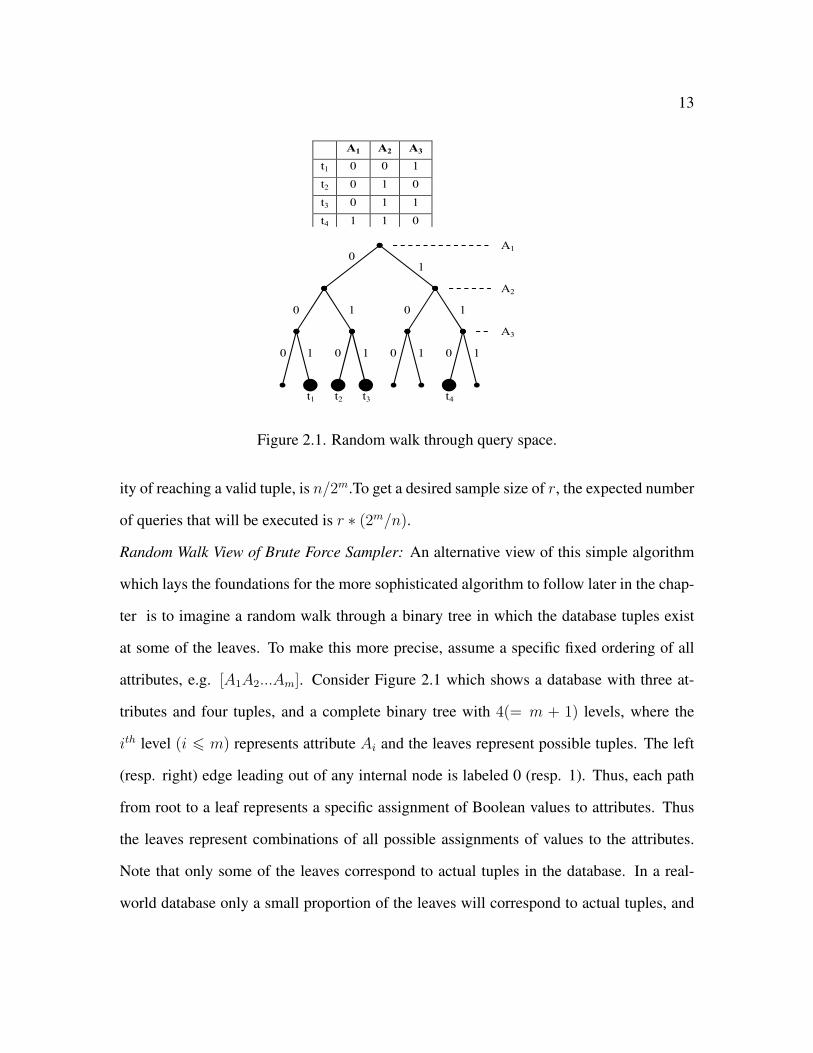
Figure 2.1. Random walk through query space.
ity of reaching a valid tuple, is n/2m.To get a desired sample size of r, the expected number
of queries that will be executed is r ∗ (2m/n).
Random Walk View of Brute Force Sampler: An alternative view of this simple algorithm
which lays the foundations for the more sophisticated algorithm to follow later in the chap-
ter is to imagine a random walk through a binary tree in which the database tuples exist
at some of the leaves. To make this more precise, assume a specific fixed ordering of all
attributes, e.g. [A1A2...Am]. Consider Figure 2.1 which shows a database with three at-
tributes and four tuples, and a complete binary tree with 4(= m + 1) levels, where the
ith level (i 6 m) represents attribute Ai and the leaves represent possible tuples. The left
(resp. right) edge leading out of any internal node is labeled 0 (resp. 1). Thus, each path
from root to a leaf represents a specific assignment of Boolean values to attributes. Thus
the leaves represent combinations of all possible assignments of values to the attributes.
Note that only some of the leaves correspond to actual tuples in the database. In a real-
world database only a small proportion of the leaves will correspond to actual tuples, and

14
vast majority of the remainder will be empty. The brute force sampler may be viewed as
executing a random walk in this tree. We start with the first attribute A1 and pick either
0 or 1 with equal probability. Next we pick either 0 or 1 as A2’s value and continue this
walk till we reach a leaf this tree. This random walk is essentially a random assignment of
values to all attributes i.e., it corresponds to the generation of a random query in the brute
force sampler described above. This randomly generated query is then fed to the interface,
which then either answers with a valid query, or fails (i.e. underflows).
2.2.3 Table of Notations
Table 5.3 lists all the notations that are used throughout the chapter (some of these
concepts will be introduced later in the chapter).
Table 2.1. Notations used in the Chapter
n Number of tuples in databasem Number of attributes in databaseSel(Q) Answer set of query Q, i.e., tuples that satisfy selection
condition of queryA1...Am Attributes of the databasep(t) Selection probability, i.e. the probability with which tuple
t gets selected by a random samplers(t) Access probability, i.e., the probability with which a tuple
is reached via a random walka(t) Acceptance probability, i.e., the probability with which a
tuple gets accepted into the sample, once it has beenreached by a random walk
d(t) Depth i.e. length of the shortest prefix of the path thatleads to t such that the corresponding query returns thesingleton tuple t
F Failure probability, i.e. the probability that a random walkleads to an underflow and has to be aborted
S Success probability, = 1− FC Scaling factor used to boost acceptance probabilities of all
tuples

15
2.3 Random Walk based Sampling
In this section we develop the main ideas behind HIDDEN-DB-SAMPLER, our al-
gorithm for sampling the tuples of a database that is hidden behind a proprietary front end
query interface. In this section we assume Boolean databases only.
2.3.1 Improving Efficiency by Early Detection of Underflows and ValidTuples
We propose the following modification to BRUTE-FORCE-SAMPLER that signif-
icantly improves its efficiency. Assume that we have selected a fixed ordering of the at-
tributes. Instead of taking the random walk all the way until we reach a leaf and then
making a single query, what if we make queries while we are coming down the path? To
make this more precise, suppose we have reached the ith level and the path thus far is
A1 = x1;A2 = x2...Ai−1 = xi−1. Before proceeding further, we can execute the query that
corresponds to this prefix of the walk. If the outcome is an underflow, we can immediately
abort the random walk. If the outcome is a single valid tuple, we can select that tuple into
that sample. And only if the outcome is an overflow do we proceed further down the tree.
This situation is described in Figure 2.1. Note that if the algorithm proceeded along the
path [00], it will detect the valid tuplet1 and stop. Similarly, if it proceeded along the path
[1], it will detect the valid tuple t4 and stop. However, to detect the valid tuple t3, it has to
proceed along the path [011].
We discuss the impact of this proposed modification to BRUTE-FORCE-SAMPLER. Con-
sider a tuple t in the database. Define the depth d(t) of t to be the length of the shortest
prefix of the path that leads to t such that the corresponding query returns the singleton
tuple t. Thus for the example in Figure 2.1, d(t1) = 2, d(t2) = 3, d(t3) = 3 and d(t4) = 1.
For certain databases and for certain ordering of attributes, the following significant im-
provements can occur:
16
• The average value of d(t) can be substantially smaller thanm, i.e., we will rarely have
to go all the way to the leaves. Likewise, the random walks that lead to underflows
can be fairly short.
• Moreover, the success probability (S) of a random walk leading to a valid tuple is
substantially larger than the brute force sampler.
For the example in Figure 2.1, the paths [00], [010], [011] and [1] lead to valid tuples
t1, t2, t3 and t4 respectively, whereas no paths lead to failure. Thus the success probability
is 1.
Of course, one has to remember that in the brute force sampler, each random walk is as-
sociated with only one query that is executed at the end of the walk, whereas in the early
detection approach we have to execute queries when visiting each node during a random
walk. In spite of this, the aggregated number of queries executed (for obtaining the same
sample size) in the latter is substantially smaller.
We now provide some theoretical justification as to why the success probability may be
substantially larger than that of the brute force sampler. Our theoretical results are limited
to certain simple i.i.d generated datasets (deriving success/failure probabilities for arbitrary
datasets appears to be substantially harder), but nevertheless they provide the inspiration
for our proposed algorithmic modification. Moreover, our experiments on a variety of real
as well as synthetic datasets (Section 6) also reinforce the advantage of this early detection
approach.
Consider a dataset D with n tuples having i.i.d. binary attributes with the probability of a 1
being p. Assume any arbitrary ordering of attributes, and consider a random walk starting
from the root of D. Let F (n, p) be the probability of a failure in the walk. We have the
following boundary conditions and recurrence for F (n, p):

17
Theorem 2.3.1. Given an i.i.d. Boolean dataset with probability of 1’s being p, and any
ordering of attributes, we have
F (1, p) = 0
F (0, p) = 1
F (n, p) =n∑i=0
(n
i
)pi(1− p)n−iF (i, p)
Clearly, in a tree with one tuple the query will return the tuple, and success is certain,
while in a tree with no tuples failure is certain. For a tree with n rows with attribute
values independent and identically distributed, with the probability of a 1 being p, the
right branch (corresponding to the value 1) will have i nodes with the binomial probability(ni
)pi(1− p)n−i, and the failure probability in the walk going to the right branch is F (i, p).
This concludes the proof of the theorem.
Note that if we interchange the values for the boundary conditions, we get an expression
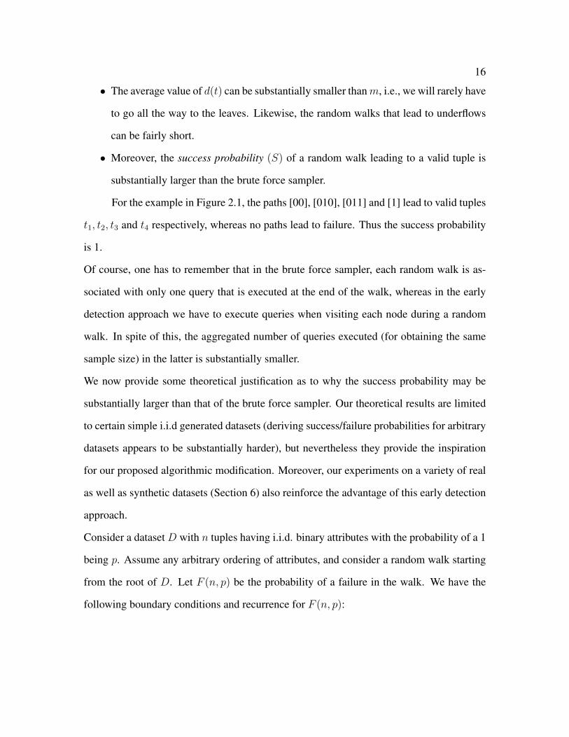
for the success of a random walk. Figure 2.2 shows a MATLAB simulation of F (n, p)
as a function of n for various values of p. We observe that the failure probability is the
smallest for p = 0.5, but even for other values of p the probability of success is reasonably
high. The convergence of the curves for F (n, p) are to be expected: the third equation in
Theorem 2.3.1 is satisfied by any function F (n, p) that is constant with respect to n.
In contrast, note that the success probability of the brute force sampler (n/2m) is
significantly smaller because it depends upon m. Thus, early detection of underflows is
crucial in increasing the efficiency of the sampler.
However, this increased efficiency comes at a price, as skew is introduced in the sample
distribution. We discuss the issue of skew next, and how it can be controlled.
Aside: There is one further issue that merits discussion. While a random walk is in progress
and queries are leading to overflow, legitimate database tuples are being returned via the
query interface (recall that for each overflowing query, the system returns k tuples from
Sel(Q). However, these tuples are useless for assembling into a random sample because
18
632
Figure 2.2. Failure probability in i.i.d. databases as a function of the number of tuples.
they have not been selected by a random procedure; they are either the top-k tuples with
the highest scores (in case a ranking function is used), or may even have been arbitrarily
picked by the system. Consequently they have to be ignored and the walk has to continue.
2.3.2 Reducing Skew and Random Ordering of Attributes
Early detection of underflows introduces skew into the sample. To see this, recall
from Table 5.3 that that s(t) is the access probability of tuple t, i.e., the probability that
tuple t is reached by a random walk (thus the selection probability, p(t) = s(t)/S where S
is the success probability of a random walk reaching any valid tuple). It is easy to see that
s(t) = 1/2d(t). But since there is variance among the depths at which the database tuples
are detected, there is variance among the values of s(t), which contributes to the skew. The
skew depends upon the specific database and the specific ordering of attributes used. For
the example in Figure 1, s(t1) = 1/4, s(t2) = 1/8, s(t3)=1/8 and s(t4)=1/2.
We first provide theoretical analysis that quantifies the skew for certain i.i.d. databases (as
before, we point out that analytical derivations of skew for general databases appears to
be extremely difficult). We follow this analysis with a discussion of techniques for signifi-

19
cantly reducing skew without adversely impacting efficiency.
Quantifying Skew: Let D be an i.i.d. 0-1 database with n rows where the probability of
a 1 is 0.5. Assume any ordering of the attributes. For a tuple t, we shall refer to t(1...x)
as the prefix corresponding to the first x values of the tuple according to this order. Since
skew is defined as the standard deviation of p(t), and p(t) = s(t)/S, we basically need to
analytically derive the standard deviation of s(t).
Theorem 2.3.2. Given an i.i.d. Boolean dataset with p= 0.5 and any ordering of attributes,
we have
E[S] ≈ 1
2n ln 2
V ar(s) ≈ 3
4 ln 2(n2 + n)− 1
4n2(ln 2)2
We will prove this theorem and at the same time provide some intuition for the distri-
bution of the probabilities Consider the distribution of the access probability of rows in the
i.i.d. model. Consider a row t in the database. Recall that the depth d(t) of t is the length
x of the shortest prefix t(1x) of t such that the query corresponding to this prefix returns
the singleton tuple t. Note that given the database D, the depth d(t) is a fixed quantity. We
analyze next the distribution of the depths of rows in the tree. Let q(x) be the probability
that a given tuplet in D has depth at most x. This happens if each of the other tuples u in
D differs from t in at least one of the positions 1...x, i.e., if for each u it is not the case that
u agrees with t on the x first positions, i.e., with probability (1 − 2−x). As the tuples are
independent, the probability that this happens for each of the n− 1 other rows in D is q(x)
= (1− 2−x)n−1. Thus the probability r(x) that the depth of a tuple t is exactly x is
r(x) = q(x)− q(x− 1) = (1− 2−x)n−1 − (1− 2−x+1)n−1
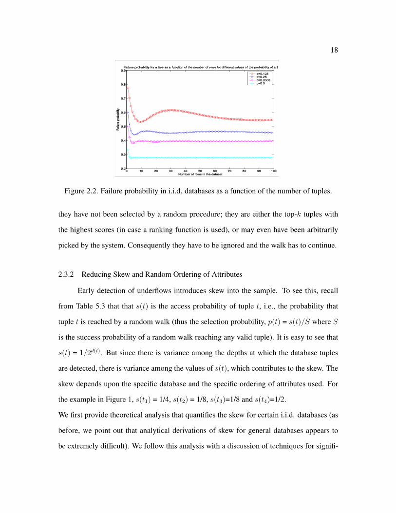
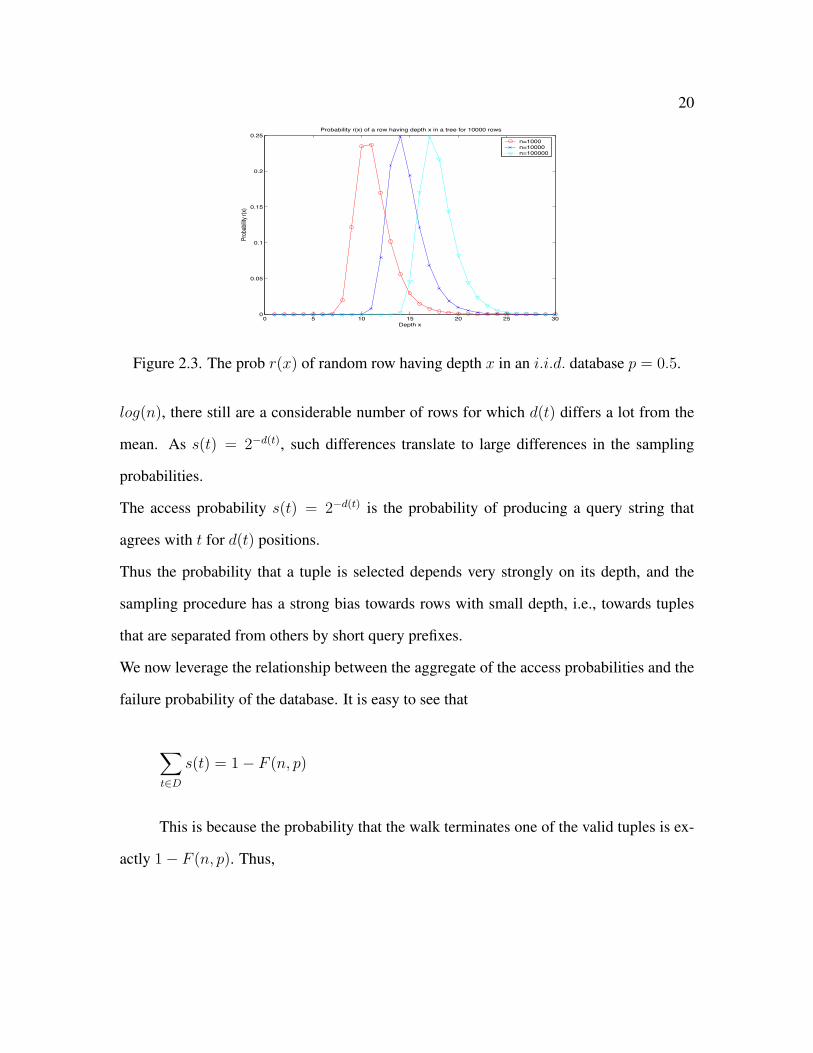
Figure 2.3 shows a MATLAB simulation of the distribution of r(x) for different val-
ues of n. We see that while most of the depths of the nodes are strongly concentrated around
20
0 5 10 15 20 25 300
0.05
0.1
0.15
0.2
0.25Probability r(x) of a row having depth x in a tree for 10000 rows
Depth x
Prob
abilit
y r(x)
n=1000n=10000n=100000
633
Figure 2.3. The prob r(x) of random row having depth x in an i.i.d. database p = 0.5.
log(n), there still are a considerable number of rows for which d(t) differs a lot from the
mean. As s(t) = 2−d(t), such differences translate to large differences in the sampling
probabilities.
The access probability s(t) = 2−d(t) is the probability of producing a query string that
agrees with t for d(t) positions.
Thus the probability that a tuple is selected depends very strongly on its depth, and the
sampling procedure has a strong bias towards rows with small depth, i.e., towards tuples
that are separated from others by short query prefixes.
We now leverage the relationship between the aggregate of the access probabilities and the
failure probability of the database. It is easy to see that
∑t∈D
s(t) = 1− F (n, p)
This is because the probability that the walk terminates one of the valid tuples is ex-
actly 1− F (n, p). Thus,

21∑t∈D
s(t) = 1− F (n, p) =∞∑x=0
nr(x)2−x
=∞∑x=0
n(q(x)− q(x− 1))2−x (2.1)
This gives a non-recursive expression for F (n, p). The values computed from (2.1)
correspond exactly to the values obtained from Theorem 2.3.1. An asymptotic analysis of
(2.1) can be done by replacing sums with integrals; we thus obtain
∑t∈D
s(t) =∞∑x=1
r(x)2−x
≈∫ inf
1
(q(x)− q(x− 1))2−x dx = (2 ln 1)−2 ≈ 0.7213
This is in good agreement with Figure 2.2. Thus the expected value of the access probabil-
ity is,
E[s] = (1/n)∞∑x=1
r(x)2−x ≈ (2n ln 2)−1
The variance of s(t) can also be evaluated. After some simplifications we obtain,
E[S2] =∞∑x=1
r(x)2−2x ≈∫ inf
1
(q(x)− q(x− 1))2−2x dx
=3
4 ln 2(n2 + n)−1
and
22
V ar[s] = E[s2]− E[s]2 =3
4 ln 2(n2 + n)− 1
4n2(ln 2)2
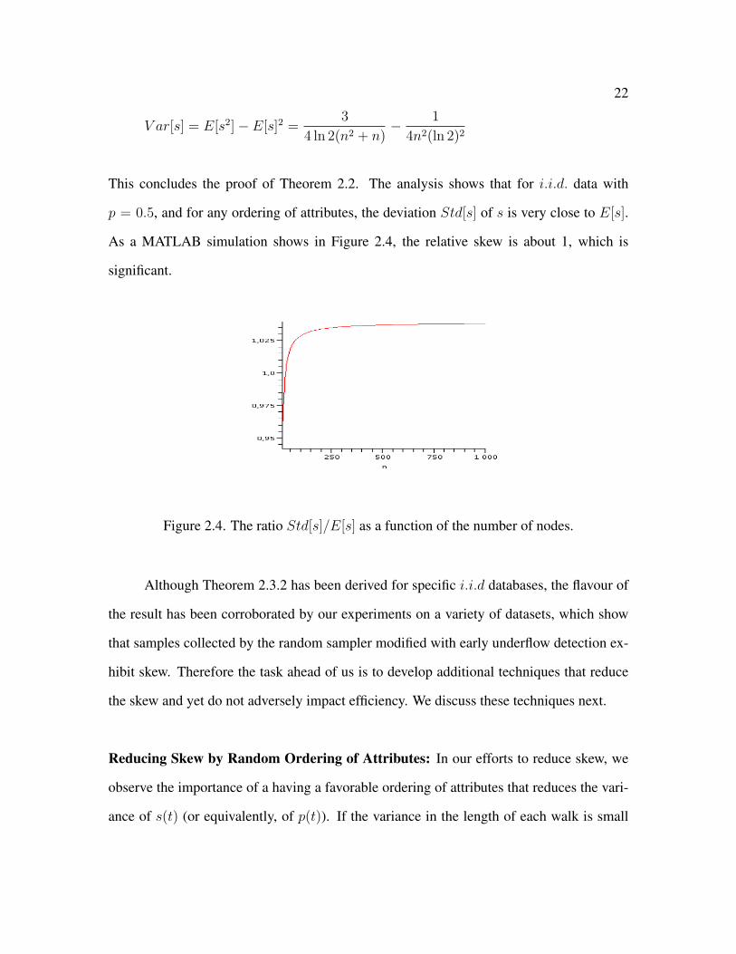
This concludes the proof of Theorem 2.2. The analysis shows that for i.i.d. data with
p = 0.5, and for any ordering of attributes, the deviation Std[s] of s is very close to E[s].
As a MATLAB simulation shows in Figure 2.4, the relative skew is about 1, which is
significant.
Figure 2.4. The ratio Std[s]/E[s] as a function of the number of nodes.
Although Theorem 2.3.2 has been derived for specific i.i.d databases, the flavour of
the result has been corroborated by our experiments on a variety of datasets, which show
that samples collected by the random sampler modified with early underflow detection ex-
hibit skew. Therefore the task ahead of us is to develop additional techniques that reduce
the skew and yet do not adversely impact efficiency. We discuss these techniques next.
Reducing Skew by Random Ordering of Attributes: In our efforts to reduce skew, we
observe the importance of a having a favorable ordering of attributes that reduces the vari-
ance of s(t) (or equivalently, of p(t)). If the variance in the length of each walk is small

23
the skew in the s(t) will also be small. A very simple approach that we adopt is to preface
each random walk with a random ordering of the attributes, and use the resultant ordering
to direct the random walk. In our case, the intuition behind random orderings of attributes
is as follows. For a fixed ordering, the depth of a tuple, d(t), is fixed. If d(t) is large, then
s(t) is large, and therefore t is less likely to be reached by a random walk, whereas if d(t)
is small, then s(t) is small, and t is more likely to be reached. With random orderings of
attributes, s(t) for a tuple t now becomes a random variable whose expected value is much
closer to the average value of the access probabilities of all tuples.
In fact, as we theoretically analyze below, it can be shown for i.i.d. datasets with p = 0.5,
if we employ random orderings before initiating random walks, the variance of the access
probabilities of all tuples turns out to zero, i.e., there is no skew in the sampling process.
We caution that this theoretical result does not extend to more general datasets (e.g., when
p is different from 0.5, or correlated for datasets), and thus only serves as in inspiration to
adopt random orderings in our sampler. However our experiments (Section 6) on a variety
of real and synthetic databases make it amply clear that random reordering does indeed
reduce skew, sometimes dramatically so, without any appreciable decrease in performance.
Consider a i.i.d Boolean dataset with p = 0.5. Now consider the sampling algorithm in
the case when the attributes are randomly reordered for each random walk. In this case the
depth d(t) of a row t is a random variable, and the access probability s(t) for t is obtained
by two randomizations: the first is the selection of the random ordering of the attributes,
and the second is the random walk determined by the random selection of values in the
query.
Theorem 2.3.3. Given an i.i.d. Boolean dataset with p = 0.5 and a random sampler with
random reordering of attributes as well as early termination, the resulting skew = 0.

24
The key observation is the following. As in Theorem 2.3.2, denote by r(x) the prob-
ability that a random tuple has depth x in an i.i.d. database; earlier we derived a simple
expression for r(x). Let then r(x) be the probability that a fixed tuple has depth x, when
the probability is taken over random reorderings of the attributes. We have r(x) = r(x) by
the i.i.d. property: a fixed tuple t has depth in a random reordering of the attributes exactly
with probability r(x). (I.e., as functions from 0, 1, 2, ... to nonnegative reals, the functions
r and r are identical.).
In a random walk with a fixed ordering of the attributes the probability that a fixed tuple
t will be reached is 2−d(t), which for most tuples is different from the uniform value of
(1− F (n, p))/n. However, in a randomly reordered run the probability that the fixed tuple
t is reached is,
∞∑x=0
r′(x)2−x =∞∑x=0
r(x)2−x =(1− F (n, p))
n
i.e., the randomly reordered random walk produces unskewed results. This concludes the
proof of Theorem 3.
The result that random reordering leads to unskewed sampling in the i.i.d. case does not
hold for arbitrary databases. For example, suppose that there is a specific tuple t such
that uinD|u(i) = 1, 1 6 i 6 m/2 = t, i.e., tuple t is the only tuple having a 1 for half of
the attributes. Then any random ordering will, with high probability, include one of these
attributes early on, and thus there is an overwhelming bias towards selecting row t. Thus,
in general, we need the acceptance/rejection method that will be discussed next.
2.3.3 Reducing Skew and Acceptance/Rejection Sampling
In this section we introduce yet another idea that serves to reduce skew. Thus far,
we had assumed that whenever a tuple is reached via a random walk, it is accepted into the
25
sample. But we know that the probability of reaching a tuple varies from tuple to tuple,
depending on the depth at which the tuple is uniquely identified. However, we know that
skew is the result of variance among the access probabilities, even after performing random
reorderings of attributes followed by random walks. To counter this skew, we propose
rejection sampling, a procedure by which tuples are probabilistically accepted or rejected
once they have been reached by the random walk. In other words, rejection sampling is
used to compensate for the deviation in the access probabilities. We make this idea precise
as follows. Consider tuple t that is reached by a random walk. For that specific order of
attributes, its access probability is s(t) = 1/2d(t). Let us define a(t) as the acceptance
probability for tuple t, i.e., once t is reached, it is accepted with probability a(t). Thus, the
overall probability of selecting tuple t (for that specific ordering of attributes) is,
s(t) × a(t) = a(t)/2d(tt). So what is an appropriate value for a(t)? Since our goal is to
make the probability of selecting a tuple the same for all tuples (i.e., skew = 0), this can be
achieved if we make a(t) proportional to 2d(t). However, since a(t) is a probability, we have
to ensure that it is between 0 and 1. One seemingly reasonable setting is a(t) = 2d(t)/2m,
which is guaranteed to be between 0 and 1 since 1 6 d(t) 6 m. This way, we can ensure
that the probability of selecting t is 1/2m, i.e., the same for all tuples. Clearly, we will
now be able to produce a sample without any skew, since this probability is the same for
all tuples. However, we have reintroduced inefficiency into the sampler, since even though
our random walks stop early, most of the time the destination tuple gets rejected, leading
to wasted walks. Fortunately, we observe that it is not necessary to set the acceptance
probabilities to be that small. Consider Figure 2.5 which shows a binary tree for a specific
ordering of attributes. Notice that tuples are reached or uniquely identified at different
depths.
Suppose we knew dmax, the largest value of d(t) over all possible trees (corre-
sponding to all possible attribute orders) and all tuples. It is easy to see that setting

26
Figure 2.5. Different Depths.
a(t) = 2d(t)/2dmax would also produce unbiased samples, but possibly more efficiently
than described above, in case dmax is smaller than m. However, dmax may still be very
large, rendering the approach inefficient. Moreover, it is unrealistic to assume that dmax
is known (or can be easily computed) beforehand. To overcome these problems, we adopt
the approach described next.
Boosting Acceptance Probabilities by Scaling Factor
We adopt the compromise approach where we boost the acceptance probabilities of each
tuple by a Scaling Factor C. Let C be a constant ≫= 1/2m. We define a(t) as,
a(t) = min(C2d(t), 1)
Let us discuss the impact of C on the sampling process. If C 6 1/2dmax then we would
still have un-skewed samples. However, if C 1/2dmax, then there is a chance that some
tuples that get identified after very long walks will get accepted with probability 1 (the min
operator is required in the definition of a(t) above to guarantee that it remains a probabil-
ity), thus introducing skew into the sample. Larger the C, more the chances of such tuples
entering the sample and thereby increasing skew. On the other hand, a large skew increases
efficiency, as the acceptance probabilities are boosted by C. Thus we may regard C as a

27
convenient parameter that provides tradeoffs between skew and efficiency.
How do we estimate a suitable value for C? Recall that random ordering of attributes is the
primary mechanism for reducing variance among the access probabilities. Based on our
experimental evidence, it appears that setting C to be 1/2d, where d is somewhat smaller
than the the average depth at which tuples get uniquely identified, will work well. This
can be done adaptively where the average tuple depth is learned as more and more random
walks are accomplished.
2.3.4 Algorithm HIDDEN-DB-SAMPLER
In summary, we have suggested three ideas that can improve the performance of
BRUTE-FORCE-SAMPLER, and which we adopt in our HIDDEN-DB-SAMPLER: These
ideas are (a) early detections of underflow and valid tuples, (b) random reordering of at-
tributes, and (c) boosting acceptance probabilities via a scaling factor C. Thus, three ran-
dom procedures must be followed, in sequence, before a tuple get accepted into the sample.
Algortihm 1 gives the pseudo-code of HIDDEN-DB-SAMPLER for Boolean databases.
2.4 Extensions
The algorithm we developed in Section 3 was for the simplest scenario, where the
database was Boolean and the number of returned tuples was at most 1. In this section we
extend the algorithm to work for more general scenarios.
2.4.1 Generalizing for k > 1
Most front end interfaces return more than one tuple, and k is usually in the range of
10-100. It is fairly straightforward to extend HIDDEN-DB-SAMPLER for more general
values of k. In fact, when k is large, the efficiency of the algorithm actually increases.

28
Algorithm 1 HIDDEN-DB-SAMPLER for Boolean Databases1: random permutation [A1A2...Am]
2: Q⇐
3: for i = 1 to m do
4: xi = random bit 0 or 1
5: Q = Q AND (Ai = xi)
6: Execute Q
7: if underflow then
8: go to 1
9: else if overflow then
10: continue
11: else
12: t = Sel(Q) /*when k = 1, Sel(Q) has one tuple*/
13: Toss coin with bias
14: min(C ∗ 2i, 1)
15: if head then
16: return t
17:
18: goto 1
19: end if
20: end if
21: end for
29
Essentially, the algorithm is the same as before, but the random walk terminates either
when there is an underflow, or when a valid result set is returned (say k 6 k tuples). One
can see that in the latter case the termination is at least log(k) levels higher. Once these k
tuples are returned, the algorithm picks one of the k tuples with probability 1/k. I.e., the
access probability of the tuple that gets picked is therefore,
s(t) =1
k′2d(t)−1
Then, the tuple is accepted with probability a(t) where,
a(t) = minCk′2d(t)−1, 1
where C is a scale factor that boosts the selection probabilities to make the algorithm effi-
cient.
2.4.2 Categorical Databases
We define a categorical database to be one where each attribute Ai can take one of
several values from a multi-valued categorical domain Domi. Many real-world databases
have categorical attributes, and most front end interfaces reveal the domains of each at-
tribute - usually via drop down lists in query forms. Most of the algorithmic ideas remain
the same as for the Boolean database, the only difference being that the fan out at a node
at the ith level of the tree is equal to the size of Domi. The random walk selects one of the
| Domi | edges at random. The access probability for tuple t is therefore defined as
s(t) =1∏
16i6d(t)
| Domi |
The rest of the extensions to the algorithm are straightforward. However, a crucial
point is worth discussing here. If the domain sizes of the attributes are more or less the
same, then the random ordering of attributes plays an important role in reducing skew.

30
However, if there is large variance among the domain sizes e.g., in a restaurants database
for a city, there may be attributes with large domains such as zipcode, along with a at-
tributes with small domains such as cuisine the fixed order of sorting the attributes from
smallest to largest domains produces smaller skew compared to random orderings. This is
because for this specific fixed order, since most of the small domain values have numerous
representative tuples, most of the walks proceed almost to the bottom of the tree before the
walk can uniquely identify these tuples. Hence the variation in depth is small. In contrast,
if a large domain attribute such as zipcode appears near the top of the tree in a random or-
der, the walk will encounter quite early sub-trees that contain very few tuples. Thus some
of the walks will terminate much faster and the depths will have more variance. Likewise,
the inverse argument says that ordering the attributes from largest to smallest domains will
be more efficient but will produce larger skew. In our experiments (Section 6) we include
some results involving real-world categorical databases.
2.4.3 Numerical Databases
Real-world databases often have numerical attributes. Most query interfaces reveal
the domain of such attributes and allow users to specify numeric ranges that they desire
(e.g., a Price column in a homes database may restrict users to specifying price ranges
between $0 and $1M).
If we can partition each numeric domain into suitable discrete ranges, our random sampler
can work for such databases by treating each discrete range as a categorical value. However,
there is a subtle problem that must be overcome: the discretization should be such that that
each tuple in the database is unique in the resulting categorical version of the database. If
the discretization is too coarse such that more than k tupes have identical representations in
the categorical version, then we cannot guarantee a random sample because some of these
tuple may be permanently hidden from users by an adversarial interface.

31
An alternate approach is to not discretize numeric columns in advance, but to repeatedly
keep narrowing the specified range in the query during the random walk. We make this
more precise as follows. For simplicity, consider a one-column database that has just one
numeric attribute, A. We can divide the domain of A into two halves, randomly select one
of the halves, and pose a query using this range. If there is an overflow, we can further
divide this range into two, and select one at random to query again. One can see that this
way we shall eventually be led to a valid tuple. This approach can be easily extended to a
multiple numeric attributes as follows. While the walk is progressing, a random attribute
is selected, including attributes already selected earlier. If we select an attribute selected
earlier, then we split its most recent queried range into two and pick one of the halves at
random to query.
This approach has the following disadvantage. Note that if the numeric data distribution
is spatially skewed (e.g, for a numeric attribute with domain [0, 1], the value of one tuple
may be 0, and the values of the remaining n− 1 tuples may be (1, 1− ε, 1− 2ε...), then the
first tuple will be selected for the sample with much higher probability than the remaining
tuples. One way of compensating for this effect is to dynamically partition the most recent
queried range into several ranges instead of just two halves, and then pick one of the ranges
at random. In general, an interesting open problem is how many queries in this query model
are needed to obtain an approximation to the probability density function of a real-valued
attribute.
2.4.4 Interfaces that Return Result Counts
Some query interfaces return to the user the top-k results, and in addition the total
count of all tuples that satisfy the query condition, | Sel(Q) |. E.g., most web search
engines will return the top-k web pages, but also reports the size of the result set. We
show how random sampling via such an interface can be done optimally without intro-
32
ducing skew. For simplicity, assume a Boolean database. Assume any ordering of the
attributes. For each node u of the tree, let n(u) represent the number of leaves in the
sub-tree rooted at u that correspond to actual tuples. In this scenario, a weighted random
walk can be performed which is guaranteed to reach an actual leaf tuples on every at-
tempt. Starting from the root, and at every node u, we select either the left or right branch
with probability n(left(u))/n(u) and n(right(u))/n(u) respectively. These cardinalities
can be retrieved by making appropriate queries via front end interface, At every node,
edges are given weights to represent the density of their underlying subtree. Moreover,
n(left(u))/n(u) + n(right(x))/n(x) = 1. It is thus not hard to see that the selection
probability of each tuple is 1/n, thus guaranteeing no skew.
2.4.5 Interfaces that only Allow Positive Values to be Specified
Some web query interfaces only allow the user to select positive Boolean values. For
example, a database of homes typically has a set of Boolean attributes such as a Swimming
Pool, 3-Car Garage and so on, and the user can only select a subset of these features to
query. Thus, there is no way a user can request for houses that do not have swimming
pools be retrieved.
While such interfaces are quite common, it is not always possible to collect a uniform
random sample from such databases. Consider a tuple t1 that dominates another tuple t2,
in the sense that for attributes that have value 1 in t2, the corresponding attributes in t1
are also 1. If k = 1, then t2 can be permanently hidden from the user by an adversarial
interface that always prefers to return t1 instead of t2. The only way to solve this problem
is to assume that no tuple dominates more than k other tuples.

33
2.5 Related Work
Traditionally database sampling has been used to reduce the cost of retrieving data
from a DBMS. Random sampling mechanisms have been studied in great detail e.g., [2–6].
Applications of random sampling include estimation methodologies for histograms and ap-
proximate query processing using techniques (see tutorial in [7]).
However, these techniques do not apply to a scenario where there is an absence of direct
access to the underlying database. A closely related area of sampling from a search en-
gines index using a public interface has been addressed in [8] and more recently [9]. The
technique proposed by [9], introduces the concept of a random walk on the documents on
the World Wide Web using the top-k results from a search engine. However, this document
based model is not directly applicable to hidden databases. In contrast to the database sce-
nario, the document space is not available as a direct input in the web model. This leads
to the use of estimation techniques which work on assumptions of uniformity of common
words across documents. Random sampling techniques on graphs have been implemented
using Markov Chain Monte Carlo techniques, e.g., Metropolis Hastings [10,11] techniques
and Acceptance/Rejection technique [12].
Hidden databases represent a major part of the World Wide Web and are commonly re-
ferred to as the hidden web. The size and nature of the hidden web has been addressed
in [1, 13–15]. Probing and classification techniques on textual hidden models have been
addressed by [16] while techniques on crawling the hidden web were studied by [17].
2.6 Experimention and Results
In this section, we describe our experimental setup, and our results using the HIDDEN-
DB-SAMPLER and draw conclusions on the quality and performance of our technique.
The results from a related model proposed by Bar-Yossef et. al. [BG06] for sampling web
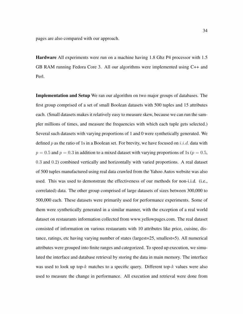
34
pages are also compared with our approach.
Hardware All experiments were run on a machine having 1.8 Ghz P4 processor with 1.5
GB RAM running Fedora Core 3. All our algorithms were implemented using C++ and
Perl.
Implementation and Setup We ran our algorithm on two major groups of databases. The
first group comprised of a set of small Boolean datasets with 500 tuples and 15 attributes
each. (Small datasets makes it relatively easy to measure skew, because we can run the sam-
pler millions of times, and measure the frequencies with which each tuple gets selected.)
Several such datasets with varying proportions of 1 and 0 were synthetically generated. We
defined p as the ratio of 1s in a Boolean set. For brevity, we have focused on i.i.d. data with
p = 0.5 and p = 0.3 in addition to a mixed dataset with varying proportions of 1s (p = 0.5,
0.3 and 0.2) combined vertically and horizontally with varied proportions. A real dataset
of 500 tuples manufactured using real data crawled from the Yahoo Autos website was also
used. This was used to demonstrate the effectiveness of our methods for non-i.i.d. (i.e.,
correlated) data. The other group comprised of large datasets of sizes between 300,000 to
500,000 each. These datasets were primarily used for performance experiments. Some of
them were synthetically generated in a similar manner, with the exception of a real world
dataset on restaurants information collected from www.yellowpages.com. The real dataset
consisted of information on various restaurants with 10 attributes like price, cuisine, dis-
tance, ratings, etc having varying number of states (largest=25, smallest=5). All numerical
attributes were grouped into finite ranges and categorized. To speed up execution, we simu-
lated the interface and database retrieval by storing the data in main memory. The interface
was used to look up top-k matches to a specific query. Different top-k values were also
used to measure the change in performance. All execution and retrieval were done from
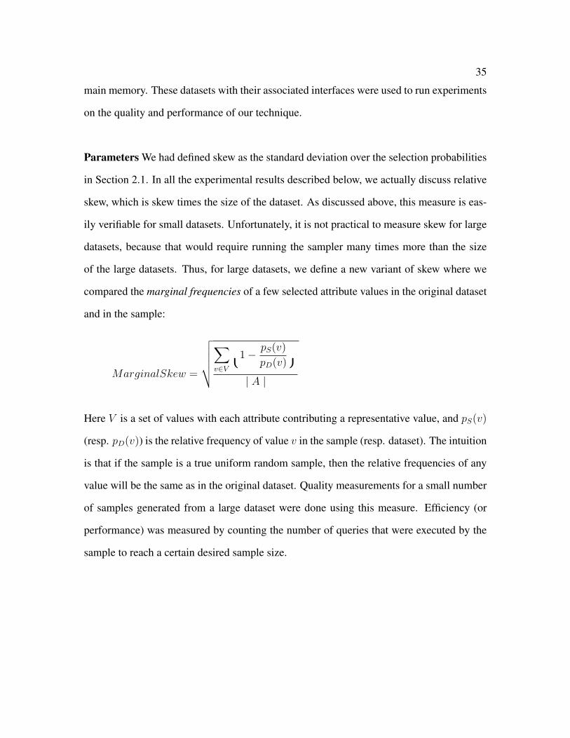
35
main memory. These datasets with their associated interfaces were used to run experiments
on the quality and performance of our technique.
Parameters We had defined skew as the standard deviation over the selection probabilities
in Section 2.1. In all the experimental results described below, we actually discuss relative
skew, which is skew times the size of the dataset. As discussed above, this measure is eas-
ily verifiable for small datasets. Unfortunately, it is not practical to measure skew for large
datasets, because that would require running the sampler many times more than the size
of the large datasets. Thus, for large datasets, we define a new variant of skew where we
compared the marginal frequencies of a few selected attribute values in the original dataset
and in the sample:
MarginalSkew =
√√√√√∑v∈V1− pS(v)
pD(v)
| A |
Here V is a set of values with each attribute contributing a representative value, and pS(v)
(resp. pD(v)) is the relative frequency of value v in the sample (resp. dataset). The intuition
is that if the sample is a true uniform random sample, then the relative frequencies of any
value will be the same as in the original dataset. Quality measurements for a small number
of samples generated from a large dataset were done using this measure. Efficiency (or
performance) was measured by counting the number of queries that were executed by the
sample to reach a certain desired sample size.
36
2.6.1 Experiments on Quality
2.6.1.1 Small Databases
The HIDDEN-DB-SAMPLER was first run on the small datasets to generate a very
large number of samples (around 300,000 samples were collected from the 500 tuple
datasets). Two types of experiments were run here. First, we considered fixed ordering
of the attributes in our datasets. We tried out several fixed orderings. Next, a random
ordering was used for selecting attributes at every level in the walk. Next the idea of ac-
ceptance/rejection sampling was introduced. We begin by using the best value of the path
that corresponds to the longest walk on the query space to accept tuples. Since a very large
number walk are run for a small dataset, we could find the depth of the longest walk. The
scaling factor C was then introduced. C was varied starting from the value corresponding
to the longest walk and then progressively increased till we reached a point where the im-
pact of C became ineffective and all tuples that were reached by the walks were getting
accepted.
Figure 2.6 shows the results of these experiments. We observed that the random
ordering of attributes does much better than any of the fixed orderings that we tried. This
corroborates our previous analysis on the effectiveness of random ordering to improve qual-
ity. Moreover, for all cases as C was increased the value of skew got larger. This indicates
the tradeoff in terms of skew while estimating C. Finally, the algorithm produced smaller
skew in the case of p = 0.5 compared to the dataset with p = 0.3. (The theoretical skew
for p = 0.5 should be zero, but the non-zero skew that was observed was an artifact of
the sampling process). Figures 2.7 and 2.8 shows similar behavior for mixed data and
correlated data.

37
638
Figure 2.6. Effect of Scaling Constant C on Skew for small datasets.
638
Figure 2.7. Effect of Scaling Constant C on Skew for Mixed Data.
638
Figure 2.8. Effect of C on skew for Correlated data.

38
638
Figure 2.9. Marginal Skew v/s C for synthetic large data.
2.6.1.2 Small Databases
We ran our experiments on synthetic large databases. In this scenario we limited
our random walks to collect 5000 samples. Marginal Skew was used to measure quality.
Marginal frequencies over all the 1 values of the attributes were collected in both the sample
as well as the dataset. Figure 2.9 (p = 0.3) represents the change in marginal skew for
various values of the scaling constant C, for random ordering and a specific fixed ordering.
As C increases, the marginal skew increases for both fixed and randomly ordered attributes
with random ordering producing better results compared to any fixed ordering that we tried.
We observe a similar trend as in small datasets. In contrast to these Boolean scenarios, the
quality results from our experiments on the real world categorical database indicate lower
marginal skews for the fixed order of attributes from (smallest domains to largest domains).
In the categorical scenario, most of the attributes have small domains, and only very few
have large domains. Thus, most of the walks proceed almost to the bottom of the tree since
most of the small domain values have numerous representative tuples.
39
638
Figure 2.10. Marginal Skew based measure for real large data.
639
Figure 2.11. Performance of HIDDEN-DB-SAMPLER for a top-1 query interface.
2.6.2 Experiments on Performance
2.6.2.1 Small Databases
We measure performance as the amount of work done with respect to the number
of queries issued to the number of samples retrieved. This metric is used over all our
performance experiments. Figure 2.12 indicates the queries versus sample size tradeoffs
for a small mixed dataset. This experiment shows that the performance of fixed ordering
is dependent on the specific ordering used (sometimes it performs better and sometimes
worse w.r.t. random ordering). Figure 2.13 indicates the increase in efficiency of our
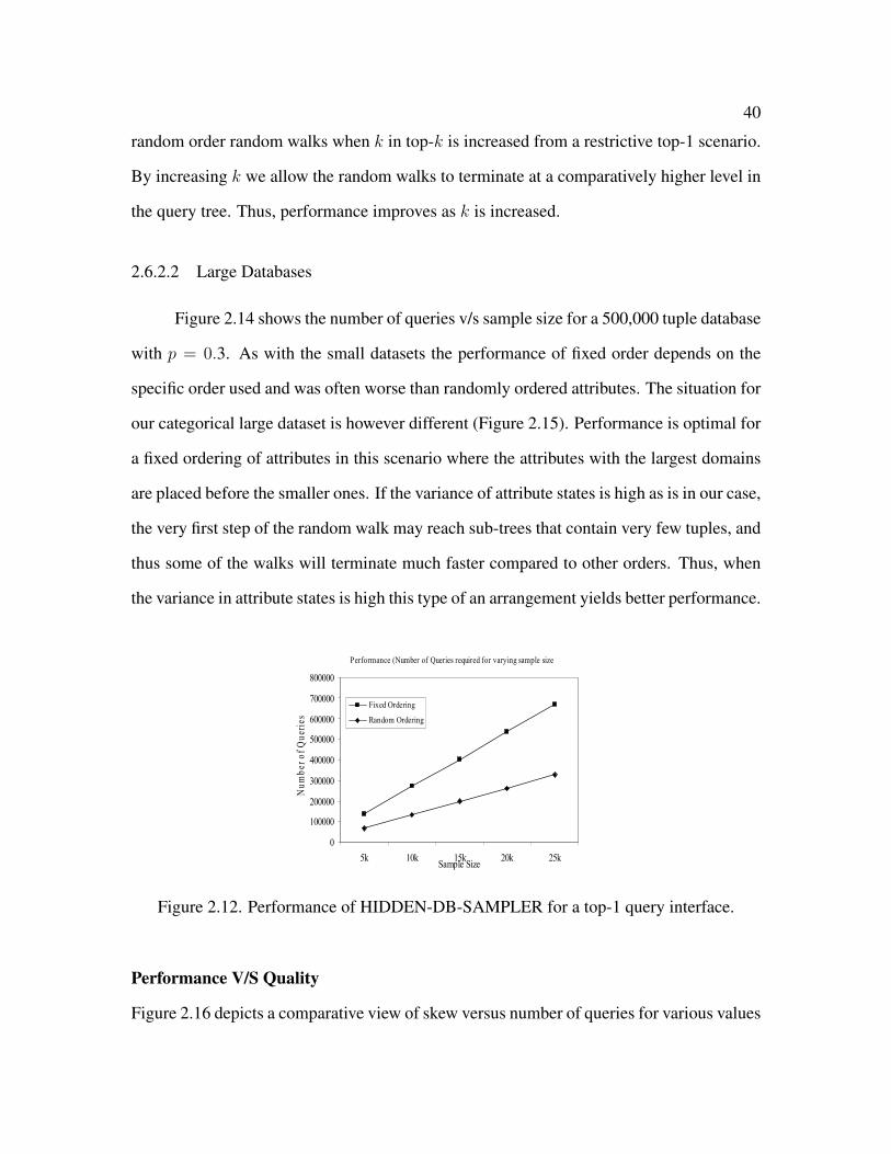
40
random order random walks when k in top-k is increased from a restrictive top-1 scenario.
By increasing k we allow the random walks to terminate at a comparatively higher level in
the query tree. Thus, performance improves as k is increased.
2.6.2.2 Large Databases
Figure 2.14 shows the number of queries v/s sample size for a 500,000 tuple database
with p = 0.3. As with the small datasets the performance of fixed order depends on the
specific order used and was often worse than randomly ordered attributes. The situation for
our categorical large dataset is however different (Figure 2.15). Performance is optimal for
a fixed ordering of attributes in this scenario where the attributes with the largest domains
are placed before the smaller ones. If the variance of attribute states is high as is in our case,
the very first step of the random walk may reach sub-trees that contain very few tuples, and
thus some of the walks will terminate much faster compared to other orders. Thus, when
the variance in attribute states is high this type of an arrangement yields better performance.
639
Figure 2.12. Performance of HIDDEN-DB-SAMPLER for a top-1 query interface.
Performance V/S Quality
Figure 2.16 depicts a comparative view of skew versus number of queries for various values
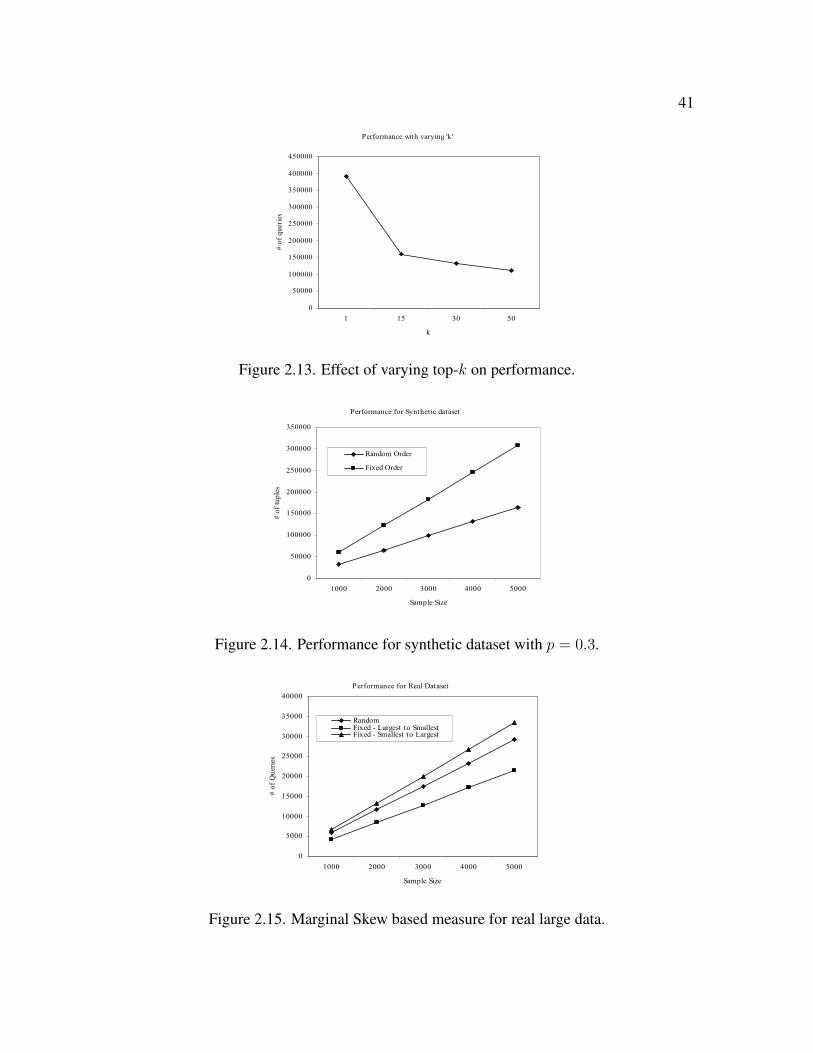
41
639
Figure 2.13. Effect of varying top-k on performance.
639
Figure 2.14. Performance for synthetic dataset with p = 0.3.
639
Figure 2.15. Marginal Skew based measure for real large data.
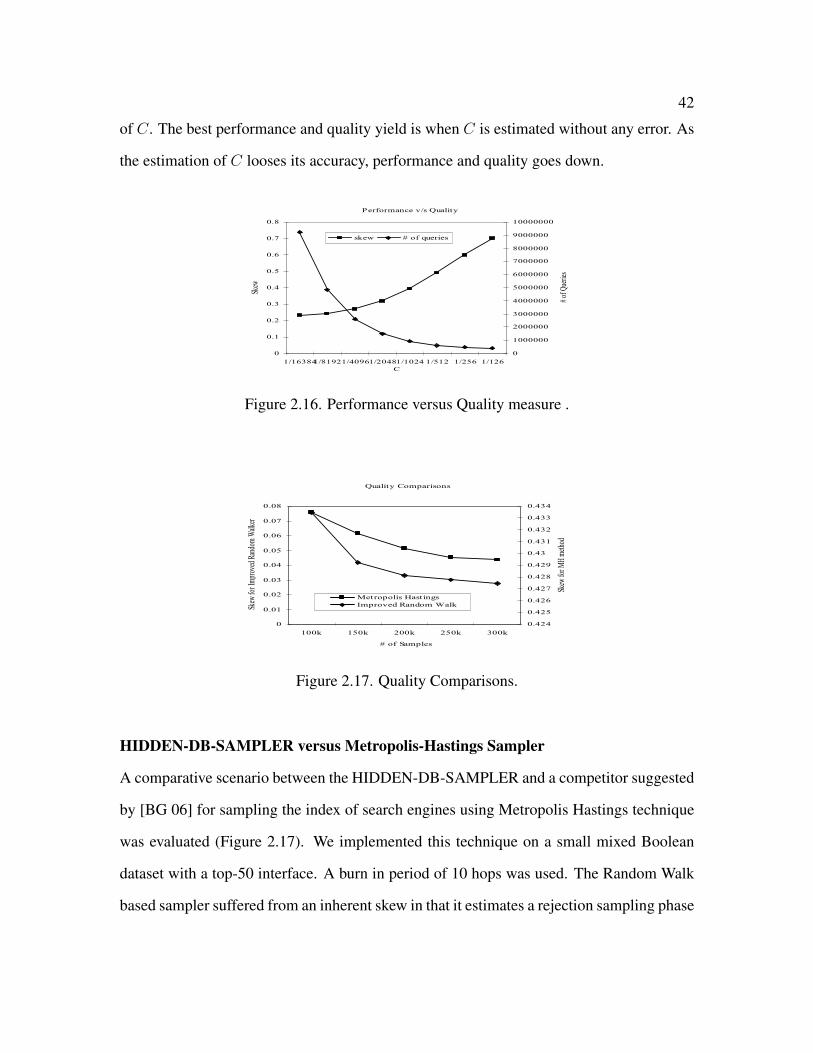
42
of C. The best performance and quality yield is when C is estimated without any error. As
the estimation of C looses its accuracy, performance and quality goes down.
640
Figure 2.16. Performance versus Quality measure .
640
Figure 2.17. Quality Comparisons.
HIDDEN-DB-SAMPLER versus Metropolis-Hastings Sampler
A comparative scenario between the HIDDEN-DB-SAMPLER and a competitor suggested
by [BG 06] for sampling the index of search engines using Metropolis Hastings technique
was evaluated (Figure 2.17). We implemented this technique on a small mixed Boolean
dataset with a top-50 interface. A burn in period of 10 hops was used. The Random Walk
based sampler suffered from an inherent skew in that it estimates a rejection sampling phase

43
on the basis of the number of queries that it can form of a single document (our equivalent
to a tuple). However, this approach does not work well for the hidden database model since
unlike the document model; the space of queries does not differ for individual tuples in the
database.
2.7 Conclusion
In this work we initiate an investigation of the problem of random sampling of hidden
databases on the web. We propose random walk schemes over the query space provided
by the interface to sample such databases. A major contribution of this work is also a
theoretical analysis of the quantitative impact of our ideas on improving efficiency and
quality of the resultant samples. We also describe a comprehensive set of experiments that
demonstrate the effectiveness of our sampling approach.

CHAPTER 3
LEVERAGINING COUNT INFORMATION IN SAMPLINGHIDDEN DATABASES
3.1 Introduction
3.1.1 Hidden Databases
A large portion of data available on the web is present in the so called “deep web”.
The deep web consists of private or hidden databases that lie behind form-like query inter-
faces. These query interfaces allow external users to browse these databases in a controlled
manner. Typically users provide inputs in the form interface which are then translated into
SQL queries for execution and the results provided to the user on the browser.
We focus on two of the simplest and most widely prevalent kind of query interfaces.
The first kind of interfaces allows users to specify range conditions on various attributes
- however, instead of returning all satisfying tuples, such interfaces restrict the returned
results to only a few (e.g., top-k) tuples, sorted by a suitable ranking function. Along with
these returned tuples, the interface may also alert the user if there was an “overflow”, i.e., if
there were other tuples besides the top-k that also satisfied the query conditions but were not
returned. We refer to such interfaces as TOP-k-ALERT interfaces. Examples include MSN
Stock Screener ( http://moneycentral.msn.com/investor/finder/customstocksdl.asp) which
has k = 25 and Microsoft Solution Finder (https://solutionfinder.microsoft.com/Solutions/-
SolutionsDirectory.aspx?mode=search) which has k = 500. The second kind interfaces
that we consider are similar to the above, except that instead of simply alerting the user of
an overflow, they provide a count of the total number of tuples in the database that satisfy
the query condition. We refer to such interfaces as TOP-k-COUNT interfaces. An example
44
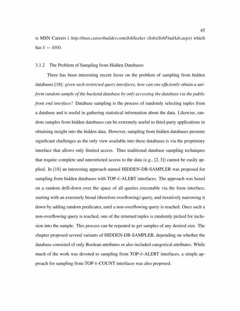
45
is MSN Careers ( http://msn.careerbuilder.com/JobSeeker /Jobs/JobFindAdv.aspx) which
has k = 4000.
3.1.2 The Problem of Sampling from Hidden Databases
There has been interesting recent focus on the problem of sampling from hidden
databases [18]: given such restricted query interfaces, how can one efficiently obtain a uni-
form random sample of the backend database by only accessing the database via the public
front end interface? Database sampling is the process of randomly selecting tuples from
a database and is useful in gathering statistical information about the data. Likewise, ran-
dom samples from hidden databases can be extremely useful to third-party applications in
obtaining insight into the hidden data. However, sampling from hidden databases presents
significant challenges as the only view available into these databases is via the proprietary
interface that allows only limited access. Thus traditional database sampling techniques
that require complete and unrestricted access to the data (e.g., [2, 3]) cannot be easily ap-
plied. In [18] an interesting approach named HIDDEN-DB-SAMPLER was proposed for
sampling from hidden databases with TOP-k-ALERT interfaces. The approach was based
on a random drill-down over the space of all queries executable via the form interface,
starting with an extremely broad (therefore overflowing) query, and iteratively narrowing it
down by adding random predicates, until a non-overflowing query is reached. Once such a
non-overflowing query is reached, one of the returned tuples is randomly picked for inclu-
sion into the sample. This process can be repeated to get samples of any desired size. The
chapter proposed several variants of HIDDEN-DB-SAMPLER, depending on whether the
database consisted of only Boolean attributes or also included categorical attributes. While
much of the work was devoted to sampling from TOP-k-ALERT interfaces, a simple ap-
proach for sampling from TOP-k-COUNT interfaces was also proposed.

46
3.1.3 Outline of Technical Results
In this chapter we revisit the hidden database sampling problem, and present vastly
superior sampling techniques than those proposed in our preliminary work [18]. Unlike
our earlier work, our main focus here is on the TOP-k-COUNT interface. However, we
also show how a novel hybrid technique can be utilized to also extend our techniques to
TOP-k-ALERT interfaces. We briefly describe our new contributions below.
There are two main objectives that any hidden database sampling algorithm should
seek to achieve:
• Sample bias: Due to the restricted nature of the interface, it is challenging to pro-
duce samples that are truly uniform random samples. Consequently, the task is to
produce samples that have small bias, i.e., samples that deviate as little as possible
from uniform.
• Efficiency: We measure efficiency of the sampling process by the number of queries
that need to be executed via the interface in order to collect a sample of a desired size.
The task is to design an efficient sampling procedure that executes as few queries as
possible.
Our Algorithm for TOP-k-COUNT Interfaces: We first discuss our results for TOP-k-
COUNT interfaces. As was briefly described in [18], it is fairly straightforward to design a
random drill-down procedure that produces samples without any bias. However, the proce-
dure suffers from poor efficiency - it has to execute an inordinate number of queries before
obtaining reasonable sized samples. In the current chapter we have carefully investigated
this problem, and have designed COUNT-DECISION-TREE, a vastly more efficient algo-
rithm. This is one of the principal results of our work.
The new procedure COUNT-DECISION-TREE is based on two main ideas. The
first idea is to continuously log the query history while the sampling is in progress - i.e.,
47
record (as materialized views) all executed queries and their returned counts. We then
design a sampling procedure that tries to leverage the query history as much as possible,
where in preparing the next query to execute, preference is given to queries that already
appear in the query history, thereby replacing a costly query execution with a fast local
look-up at the client’s end. In fact, utilization of query history offers opportunities of query
inference in addition to simple reuse - the former refers to queries that may not have been
directly executed in the past, but whose counts can be inferred from the ones that have
been executed. In the chapter, we carefully explore our idea of logging query history, and
provide both a theoretical analysis of the number of queries saved by this approach, as well
as substantial experimental evidence to corroborate our analytical findings.
The second idea is to generalize the notion of attribute ordering used in [18] to that
of a decision tree. In the earlier work, the random drill-down procedure was guided by an
ordering of the attributes, such that each new predicate selected for narrowing the query
involved a random value of the next attribute present in the attribute order. For the case of
TOP-k-COUNT interfaces, it was suggested that any specific attribute order was adequate
for obtaining unbiased samples. In the current chapter, we make non-trivial enhancements
to this simplistic scheme to obtain unbiased samples, but with significant performance im-
provements. Our new approach may be considered as the execution of multiple random
drill-down procedures (where each such procedure results in the selection of a random
sample tuple) except that we always adhere to following paths down a decision tree. In
this chapter, a decision tree over the database tuples is a tree where all internal nodes are
attributes, all leaf nodes are tuples, and each edge leading out of a node is labeled with a
unique value from that attribute’s domain, along with a transition probability proportional
to the number of leaf tuples that can be reached by following that edge. This transition
probability is used to select the edge during random drill-down. Each path from the root to
48
a leaf encounters a subset of the attributes in the interface, but the same attribute is never
repeated along a path.
Clearly the use of a decision tree is a generalization over using any fixed attribute
order - the latter essentially refers to a decision tree that has the same attributes at any given
level of the tree. More importantly, while any legitimate decision tree can be used to obtain
unbiased samples, the challenge is in designing a decision tree that achieves the maximum
efficiency. This problem is complicated by the fact that this tree cannot be created in its
entirety, as complete access to all database tuples is impractical; thus this tree has to be
built and used on-the-fly, i.e., while the sampling is in progress. Thus if we take a snapshot
at any time during the sampling process, we will essentially have created a partial decision
tree, with only a few paths extending all the way to the leaves (corresponding to those
tuples that have been included in the sample thus far).
Our investigations of such an optimal decision tree-based approach led to several
interesting technical results. A theoretical study revealed interesting connections with the
seemingly unrelated NP-hard problem of entity identification in the design of interactive
question-answering systems [19]. Thus we show that drawing samples in an optimal man-
ner using the decision tree approach is computationally intractable. However, our COUNT-
DECISION-TREE algorithm is based on a carefully designed heuristic for incrementally
building an efficient decision tree while the sampling is in progress, with the goal being
that the remaining samples can be obtained in as few queries as possible. This heuristic is
based on the online computation of a savings function that attempts to select new queries
that: (a) leverage the query history and try to reuse as many past queries as possible, and
(b) have the best chance of reaching a random tuple as quickly as possible. Although pri-
marily a heuristic, we are able to provide important analytical arguments as to why such
a heuristic is expected to do well. Our experiments corroborate our conceptual and ana-
lytical arguments to show that COUNT-DECISION-TREE is an order of magnitude more
49
efficient than the previous algorithm presented in [18] for drawing random samples from a
TOP-k-COUNT interface.
Our Algorithm for TOP-k-ALERT Interfaces: We next discuss our results for TOP-k-
ALERT interfaces. Unlike TOP-k-COUNT interfaces, it is quite difficult to draw a random
sample from a TOP-k-ALERT interface without introducing bias into the resultant sample.
In fact, bias and efficiency are contradictory goals, and the earlier algorithm HIDDEN-
DB-SAMPLER in [18] is actually a parameterized procedure which trades off bias against
efficiency. In the current chapter we propose a new parameterized procedure, ALERT-
HYBRID, for drawing random samples from a TOP-k-ALERT interface which is signif-
icantly better than HIDDEN-DB-SAMPLER. This is second main algorithm presented in
our work.
We provide a brief outline of the idea of ALERT-HYBRID. The algorithm consists
of two phases. The first phase consists of a drawing a fairly small random sample with very
small bias (henceforth called a pilot sample) using the earlier HIDDEN-DB-SAMPLER
algorithm. Then in the second phase, the remaining desired number of samples is drawn
from the alert interface, except that we use our COUNT-DECISION-TREE algorithm to
draw the remaining samples. Although the interface does not have the capability to provide
count information for queries, we use the pilot sample to estimate count information for
queries. This is done using standard approximate query processing techniques [7, 20, 21]
by executing each query locally on the pilot sample and appropriately scaling the result
to estimate the count for the entire database. Interestingly, the “hybrid” idea of using a
small amount of pilot samples to bootstrap COUNT-based sampling is inspired by similar
sampling approaches considered in other unrelated contexts [4, 22]. Because the counts
are only estimates, we are not able to completely remove bias from the resultant sample,
however our experiments show that ALERT-HYBRID is significantly better than HIDDEN-

50
DB-SAMPLER for drawing random samples from a TOP-k-ALERT interface - for the
same bias (same efficiency), it produces samples more efficiently (with less bias).
In summary, the main contributions of this chapter are:
• We revisit the problem of random sampling from hidden databases with proprietary
form interfaces.
• We present COUNT-DECISION-TREE, an efficient algorithm for drawing random
samples without bias from hidden databases with TOP-k-COUNT interfaces. The
algorithm is based on two ideas: (a) the use of query history, and (b) the use of a de-
cision tree. We provide several theoretical insights into the behavior and performance
of this algorithm.
• We present ALERT-HYBRID, an efficient algorithm for drawing random samples
with small bias from hidden databases with TOP-k-ALERT interfaces. The algo-
rithm is based on using a pilot sample to bootstrap the COUNT-DECISION-TREE
algorithm to draw the samples.
• We provide a thorough experimental study that demonstrates the significance of our
theoretical results and the superiority of our algorithms over previous efforts.
The rest of this chapter is organized as follows. We briefly review the existing sample
algorithms for hidden databases in Section 2. In Sections 3 and 4, we introduce our two
major algorithms, COUNT-DECISION-TREE and ALERT-HYBRID, respectively. Sec-
tion 5 presents the experimental results. Related work is reviewed in Section 6, followed
by final remarks in Section 7.

51
3.2 Preliminaries
3.2.1 Models of Hidden Databases
We restrict our discussion in this work to categorical data - we assume a simple dis-
cretization of numerical data to resemble categorical data. Apparently, different discretiza-
tion will lead to different performance of sampling. How to design an optimal discretization
scheme is left as an open problem.
Consider a hidden database tableD withm tuples t1, . . . , tm and n attributesA1, . . . , An
with respective domains Dom1, . . . , Domn. The table is only accessible to users through
a web interface. We assume a prototypical interface where users can query the database by
specifying values for a subset of attributes. Thus a user query QS is of the form:
SELECT ∗ FROM D WHERE Ai1 = vi1& . . .&Ais = vis ,
where vij is a value from Domij .
Let Sel(QS) be the set of tuples in D that satisfy QS . As is common with most
web interfaces, we shall assume that the query interface is restricted to only return k tuples,
where k m is a pre-determined small constant (such as 10 or 50). Thus, Sel(QS) will be
entirely returned only if |Sel(QS)| ≤ k. If the query is too broad (i.e., |Sel(QS)| > k), only
the top-k tuples in Sel(QS) will be selected according to a ranking function, and returned
as the query result. The interface will also notify the user that there is an overflow, i.e.,
that not all tuples satisfying QS can be returned. At the other extreme, if the query is too
specific and returns no tuple, we say that an underflow occurs. If there is neither overflow
nor underflow, we have a valid query result.
For the purpose of this chapter, we assume that a restrictive interface does not allow
the users to “scroll through” the complete answer Sel(QS) when an overflow occurs forQS .
Instead, the user must pose a new query by reformulating some of the search conditions.
We argue that this is a reasonable assumption because many real-world top-k interfaces

52
(e.g., Google) only allow “page turns” for limited (100) times before blocking a user by IP
address.
Based on the response provided by the interface when there was an overflow, we
classify the interfaces for hidden databases into two categories: TOP-k-ALERT and TOP-
k-COUNT. If the interface only issues a Boolean alert i.e., whether there were other tuples
besides the top-k that also satisfied the query conditions but were not returned, then the
interface is TOP-k-ALERT. If the interface also provides a count of the total number of
tuples in the database that satisfy the query condition, we call the interface as TOP-k-
COUNT.
3.2.2 A Running Example
Table 3.1 depicts a simple dataset which we will use as a running example throughout
this chapter. There are 8 tuples and 7 attributes, including 3 Boolean and 5 categorical with
domain size ranging from 4 to 8.
Table 3.1. Example: Input Table
A1 A2 A3 A4 A5 A6 A7
t1 0 0 0 0 0 0 0t2 0 1 0 0 2 0 1t3 1 0 0 1 1 0 2t4 1 0 1 1 2 0 3t5 2 1 0 0 2 1 4t6 2 1 0 1 2 2 5t7 3 1 1 1 3 3 6t8 4 0 1 1 3 0 7

53
3.2.3 Prior Sampling Algorithms
In this subsection we review three variants of HIDDEN-DB-SAMPLER, the sam-
pling algorithm presented in our earlier work [18] for obtaining random samples from hid-
den databases.
1. ALERT-ORDER: We first describe a variant that was designed for TOP-k-ALERT in-
terfaces (for the rest of this chapter we refer to this variant as ALERT-ORDER). Assume a
specific fixed ordering of all attributes, e.g. A1, . . . , An. Consider Figure 3.1 a) which rep-
resents an attribute-order tree over the database tuples, where all internal nodes at the ith
level are labeled by attribute Ai. Each internal node Ai has exactly |Domi| edges leading
out of it, labeled with values from Domi. Thus, each path from the root to a leaf rep-
resents a specific assignment of values to attributes, with the leaves representing possible
database tuples. Note that since some domain values may not lead to actual database tu-
ples, only some of the leaves representing actual database tuples are marked solid, while
the remaining leaves are marked empty.
The ALERT-ORDER sampler executes a random walk in this tree to obtain a random
sample tuple. To simplify the discussion, assume k = 1. Suppose we have reached the ith
level and the path thus far represents the query A1 = v1& . . .&Ai−1 = vi−1. The algorithm
selects one of the domain values of Ai uniformly at random, say vi, adds the condition
Ai = vi to the query, and executes it. If the outcome is an underflow (i.e., leads to an empty
leaf), we can immediately abort the random walk. If the outcome is a single valid tuple,
we can select that tuple into that sample. And only if the outcome is an overflow do we
proceed further down the tree.
This random walk may be repeated a number of times to obtain a sample (with re-
placement) of any desired size. One important point to note is that this method of sampling
introduces bias into the sample, as not all tuples are reached with the same probability.
54
Techniques such as acceptance/rejection sampling are further employed for reducing bias
(see [18] for further details).
For this scheme, clearly the order of the attributes can play an important role in the
efficiency of the sampling process. It was suggested in [18] that the attributes be ordered
from largest to smallest domain sizes.
2. ALERT-RANDOM: For the special case of Boolean data, since the domain sizes are
the same for all attributes, it was suggested that instead of using a specific fixed attribute
order, a fresh random ordering of attributes be used before every random walk. It was
shown that such a scheme helps reduce the bias more than any fixed order attribute scheme.
Henceforth we refer to this variant as ALERT-RANDOM.
3. COUNT-ORDER: We now turn our attention to TOP-k-COUNT interfaces. It was
pointed out in [18] that, when COUNT information is returned for each query, a random
walk scheme can be designed to generate completely unbiased samples. Thus, no bias
reduction techniques need to be used later. Henceforth we refer to this variant as COUNT-
ORDER. For a given node in the attribute-order tree, instead of choosing edges with uni-
form probability, COUNT-ORDER chooses an edge with probability proportional to the
COUNT of that edge (i.e., proportional to the number of actual tuples that can be reached
following that edge). For example, suppose we have reached the ith level and the path thus
far represents the query A1 = v1& . . .&Ai−1 = vi−1. Let the current attribute under con-
sideration, Ai, have |Domi| = bi edges labeled with values v1i , . . . , v
bii . Then, the random
walk follows edge vji (i.e., adds Ai = vji to the query) with probability equal to
P (vji ) =COUNT(A1 = v1, . . . , Ai−1 = vi−1, Ai = vji )
COUNT(A1 = v1, . . . , Ai−1 = vi−1).
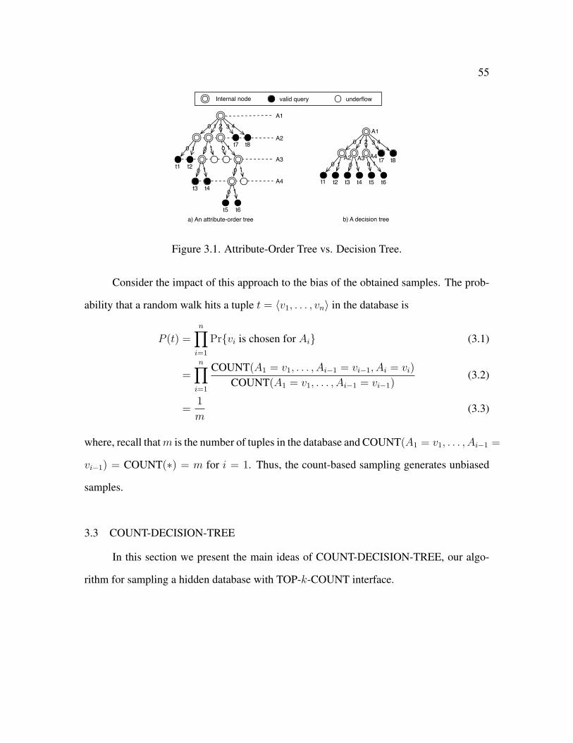
55
b) A decision tree
A1
A2 A3 A4
0 1 2 3 4
0 1 0 1 0 1
A10 1 2 3 4
0 1 0 1 0 1A2
A3
0 1 0 1
0 1A4
a) An attribute-order tree
t1 t2
t3 t4
t5 t6
t7 t8
t1 t2 t3 t4 t5 t6
t7 t8
valid queryInternal node underflow
Figure 3.1. Attribute-Order Tree vs. Decision Tree.
Consider the impact of this approach to the bias of the obtained samples. The prob-
ability that a random walk hits a tuple t = 〈v1, . . . , vn〉 in the database is
P (t) =n∏i=1
Prvi is chosen for Ai (3.1)
=n∏i=1
COUNT(A1 = v1, . . . , Ai−1 = vi−1, Ai = vi)
COUNT(A1 = v1, . . . , Ai−1 = vi−1)(3.2)
=1
m(3.3)
where, recall thatm is the number of tuples in the database and COUNT(A1 = v1, . . . , Ai−1 =
vi−1) = COUNT(∗) = m for i = 1. Thus, the count-based sampling generates unbiased
samples.
3.3 COUNT-DECISION-TREE
In this section we present the main ideas of COUNT-DECISION-TREE, our algo-
rithm for sampling a hidden database with TOP-k-COUNT interface.

56
3.3.1 Motivation
Although the simple COUNT-ORDER algorithm explained in Section 5.2 can gen-
erate unbiased samples, it also introduces a significant challenge, as the number of queries
required for sampling categorical databases may increase dramatically compared with both
TOP-k-ALERT algorithms. To understand this, consider a random walk from a node to one
of its b successors in the tree. In both TOP-k-ALERT algorithms, an edge is chosen uni-
formly at random from [1, b], and only one query corresponding to the chosen edge needs to
be issued. However in COUNT-ORDER, the counts of all edges must be first determined in
order to compute their respective transition probabilities, after which an edge is randomly
selected to follow. This requires b − 1 queries1. Thus, COUNT-ORDER may require a
large number of queries for sampling categorical databases, especially for attributes with
large domains.
The rest of this section is devoted to techniques for improving the efficiency of sam-
pling TOP-k-COUNT interfaces.
We first introduce a generalization of an attribute-order tree to a decision tree on
the hidden database. The key extension of a decision tree is that it allows each level of
the tree to contain different attributes. Figure 3.1 a) and b) illustrates both types of trees
for the database in Table 3.1 for the case k = 1. Random walks over decision trees are
likely to be more efficient than over attribute-order trees, as by leveraging the flexibility of
selecting multiple attributes for nodes at the same level, a compact decision tree features
a shorter depth and a smaller total number of possible queries. For the example in Fig-
ure 3.1, when one sample tuple needs to be collected, the decision tree provides a saving of
(1/4 × 1 + 1/4 × 2) = 3/4 queries in comparison with the attribute-order tree. We defer
a more thorough analysis of the advantages of decision trees over attribute-order trees to
Section 3.3.3.1The remaining count can be inferred from these b− 1 counts and the count of the current node.
57
Suppose we are given the structure of a decision tree over a hidden database - i.e., the
entire tree is available, barring the various COUNT information (or transition probabilities
associated with the edges). Algortihm 2 depicts a count-based sampling algorithm that
performs random walks on this decision tree to collect a sample with s tuples (in the figure
we use the notation |u| to refer to the count of node (or edge) u, i.e., the number of database
tuples below u in the tree). We would like to make several remarks regarding the algorithm.
First, this is of course a hypothetical scenario, as such a tree is not available for hidden
databases, and in fact has to be constructed on-the-fly (which will be discussed later in the
chapter). Second, queries corresponding to nodes in the upper level (e.g., root) of the tree
may be reused by many random walks, especially if s is large. This motivates us to consider
the impact of query history in Section 3.3.2. Third, no matter how the decision tree is
structured, the sampling algorithm always generates unbiased samples. Fourth, the number
of queries, however, may vary significantly between different structures. An interesting
challenge is to identify a structure which achieves the optimal efficiency. We will address
this challenge in Sections 3.3.3.
3.3.2 Improving Efficiency: Query History
We start our discussion on improving the efficiency of count-based sampling by a
simple strategy: take advantage of the query history. That is, the sampling algorithm
should only send to the hidden database “new” queries which have never been asked before
and cannot be inferred from the history. An example of inference is the computation of
COUNT(a1 = 1) from COUNT(∗) and COUNT(a1 = 0).
We discuss the impact of leveraging query history to improve sampling efficiency.
The following theorem provides a lower bound on the number of queries saved by consult-
ing the query history.

58
Algorithm 2 Sampling TOP-k-COUNT with a Given Decision Tree
Require: r: root node of the decision tree
1: for i = 1 to s do
2: Obtain the i-th sample as DT SAMP(r).
3: end for
4: function DT SAMP(u)
5: . Let u have b values v1, . . . , vb and edges u1, . . . , ub
6: Query b− 1 edges for counts of u1, . . . , ub.
7: Randomly pick j ∈ [1, b] s.t. Prj picked = |uj|/|u|.
8: if |uj| ≤ k then
9: return a random tuple from the answer to uj
10: else
11: return DT SAMP(uj).
12: end if
13: end function
Theorem 3.3.1. For the algorithm in Figure 2, the number of queries saved by consulting
the query history for obtaining s samples (s · k m) of a hidden database of size m is at
least
sQH > s ·(
(b− 1) · logb s− 2− b
b− 1
), (3.4)
where b (b ≥ 2) is the minimum domain size of an attribute.
We omit the proof due to space limitation. An observation from the theorem is
that the saving from history is significant when s is large. For example, obtaining 5, 000
samples from a Boolean database will lead to a saving of at least 41, 438 queries. For
a 100,000-tuple i.i.d. Boolean database where the 1’s and 0’s are uniformly distributed
with probability 0.5 each, it implies an expected saving of at least 49.90% when k = 1
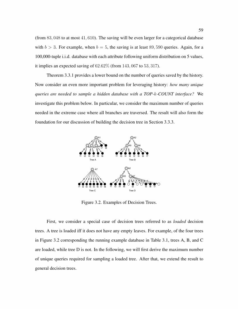
59
(from 83, 048 to at most 41, 610). The saving will be even larger for a categorical database
with b > 3. For example, when b = 5, the saving is at least 89, 590 queries. Again, for a
100,000-tuple i.i.d. database with each attribute following uniform distribution on 5 values,
it implies an expected saving of 62.62% (from 143, 067 to 53, 317).
Theorem 3.3.1 provides a lower bound on the number of queries saved by the history.
Now consider an even more important problem for leveraging history: how many unique
queries are needed to sample a hidden database with a TOP-k-COUNT interface? We
investigate this problem below. In particular, we consider the maximum number of queries
needed in the extreme case where all branches are traversed. The result will also form the
foundation for our discussion of building the decision tree in Section 3.3.3.
Tree A Tree B
Tree C
A2
A5 A6
A7
0 1 2 3 0 1 2 3
0 1
0 1 2 3 4 5 6 7
A2
A5 A7
0 1 2 3 0 1 2 3
0 1
4
Tree D
A1
A2 A3 A4
0 1 2 3 4
0 1 0 1 0 1
t1 t2 t3 t4 t5 t6
t7 t8
t1 t3 t4 t8 t2 t5 t6 t7
t1 t2 t3 t4 t5 t6 t7 t8 t1 t3 t4 t8 t5t2 t6 t7
5 6 7
Figure 3.2. Examples of Decision Trees.
First, we consider a special case of decision trees referred to as loaded decision
trees. A tree is loaded iff it does not have any empty leaves. For example, of the four trees
in Figure 3.2 corresponding the running example database in Table 3.1, trees A, B, and C
are loaded, while tree D is not. In the following, we will first derive the maximum number
of unique queries required for sampling a loaded tree. After that, we extend the result to
general decision trees.
60
Theorem 3.3.2. Given the structure of a loaded decision tree, the total number of unique
queries required for obtaining s samples through a TOP-k-COUNT interface is at most
m− 1.
Proof. Let |Li| and |Ωi| be the number of all (internal and leaf) nodes and internal nodes
in level i, respectively (root is level 1, let the maximum levels be h). Then, the maximum
number of queries issued for level i is |Li+1| − |Ωi| because each internal node has one
query saved through history inference. Thus, the maximum total number of queries issued
ish−1∑i=1
(|Li+1| − |Ωi|) =h∑i=1
|Li| −h−1∑i=1
|Ωi| − 1 = m− 1. (3.5)
This is due to two reasons. First,∑h
i=1 |Li|−∑h−1
i=1 |Ωi| is equal to the total number of leaf
nodes because all nodes in level h are leaves. Second, the number of leaves is m.
The theorem shows that given a loaded decision tree, the maximum number of unique
queries required for count-based sampling of the tree only depends on the number of tuples
in the database, and not by the number of attributes or their domain sizes. For example,
trees A, B and C in Figure 3.2 all have 7 unique queries for count-based sampling: Tree
A has 1 at the level 1 and 6 at level 2; Tree B has 4 at level 1 and 3 at level 2; while all 7
queries for Tree C are at the same level.
We now consider the extension to general decision trees. Again, we would like to
remark that in practice, we will not be provided with the structure of a decision tree; rather
queries must be issued to both construct the decision tree and sample from it. If a decision
tree is constructed without consulting the complete database, empty branches often occur
and the tree is usually not loaded. Thus, the sampling of a decision tree that has empty
leaves is arguably a more practical scenario.
Each edge leading to an empty leaf leads to one additional query, as we can observe
from tree D in Figure 3.2. To analyze the number of empty leaves, we consider an example

61
of m-tuple i.i.d. Boolean dataset studied in [18], where each attribute takes the value of
1 with probability p. Let L(m, k, p) be the expected number of empty leaves for such a
dataset. We have
L(0, k, p) = 1. (3.6)
L(1, k, p) = 0. (3.7)
. . .
L(k, k, p) = 0. (3.8)
L(m, k, p) =m∑i=0
(mi
)pi(1− p)m−i(L(i, k, p) + L(m− i, k, p)). (3.9)
Note that althoughL(m, k, p) appears in both the left and right side of (3.9), it can neverthe-
less be solved from the equation. Figure 3.3 depicts the relationship between the number
of empty leaves and the number of tuples when k = 1. The results are computed from
(3.6)-(3.9) using Matlab simulation. As we can see, L(m, p) and m roughly follow a linear
relationship. Based on (3.9) and Theorem 3.3.2, we have the following corollary.
Corollary 3.3.1. Given an i.i.d. Boolean dataset where each attribute takes the value of
1 with probability p, for all s ≥ 1, the total number of queries required for obtaining s
samples through a top-k interface with COUNT is at most m− 1 + L(m, k, p).
0 20 40 60 80 1000
50
100
150
200
Number of Tuples (m)
Num
ber
of E
mpt
y Le
aves
(L(
m, p
))
p = 0.125p = 0.250p = 0.333p = 0.500
Figure 3.3. The number of empty leaves vs. the number of tuples when k = 1.

62
3.3.3 Improving Efficiency: Constructing Decision Tree
3.3.3.1 Motivation and Hardness
Theorem 3.3.2 indicates that, if a very large number of samples need to be collected,
then every decision tree without empty leaves will have the same efficiency because the
total number of queries only depends on the size of the database. Nonetheless, the design
of the decision tree may play an important role in reality due to the following two reasons:
• Since the number of samples required in practice is usually much smaller than the
size of the database, many of the m − 1 queries may not be issued; thus different
decision trees may have different impact on efficiency.
• As we can see from Figure 3.3, the number of empty leaves may be significant,
especially when the attributes skew towards a few values.
We now discuss the design of an efficient decision tree, in particular the following
problem: Given s, the number of samples to be collected, design a decision tree with the
minimum sampling cost, i.e., the minimum expected number of queries required to collect
s unbiased samples.
Unfortunately, this problem is hard even if the decision tree can be constructed with
full access to the m tuples. Consider a special case of the problem when s = 1 and k = 1
for Boolean databases. The problem is essentially the same as computing a decision tree
with no empty leaves that has the minimum average path length from root to the leaves.
This is equivalent to a well-known problem of constructing an optimal decision tree for
the entity identification problem [19], for which the following hardness result is known
from [19]:
Theorem 3.3.3. (from Theorem 4.1 in [19]) When s = 1 and k = 1, it is NP-hard to
construct a decision tree over a Boolean database with the minimum sampling cost, or
even approximate it within a factor of Ω(logm).

63
3.3.3.2 Basic Ideas
Due to the hardness of the problem, we propose a heuristic greedy algorithm to
construct an efficient decision tree. We remind the reader that the tree cannot be created in
its entirety, as complete access to all database tuples is impractical; the tree has to be built
and used on-the-fly. At any time during the sampling process, we will essentially have
created a partial decision tree, with only a few paths extending all the way to the leaves
(corresponding to those tuples that have been included in the sample thus far).
We first discuss the intuition behind the algorithm: the saving and expense associated
with each node in the decision tree. For the ease of understanding, we restrict our attention
to k = 1 in the discussion of intuition, but will present the algorithm with arbitrary k.
Saving: Recall from the proof of Theorem 3.3.2 that, when k = 1, a decision tree without
empty branch requires exactly m − 1 total queries when the number of queries s → ∞.
Consider these as the baseline queries for the sampling process. As we mentioned above,
the actual number of queries varies from the baseline due to two possible reasons:
• When s is small, a subtree may never be encountered by a random walk. Note that a
never-encountered subtree with m tuples yields a reduction of m− 1 on the number
of queries. Let the total reduction be R(s).
• Each empty leaf leads to an increase of 1 on the number of queries. Let the total
increase be L.
Thus, the actual number of queries is m − 1 − (R(s) − L). We say that the decision tree
yields a saving of R(s)− L.
Note that unlike the number of baseline queries which is independent of the structure
of the decision tree, R(s)−L strongly depends on the tree structure. For example, consider
trees in Figure 3.2. Tree C offers no saving at all, because all possible queries will be issued
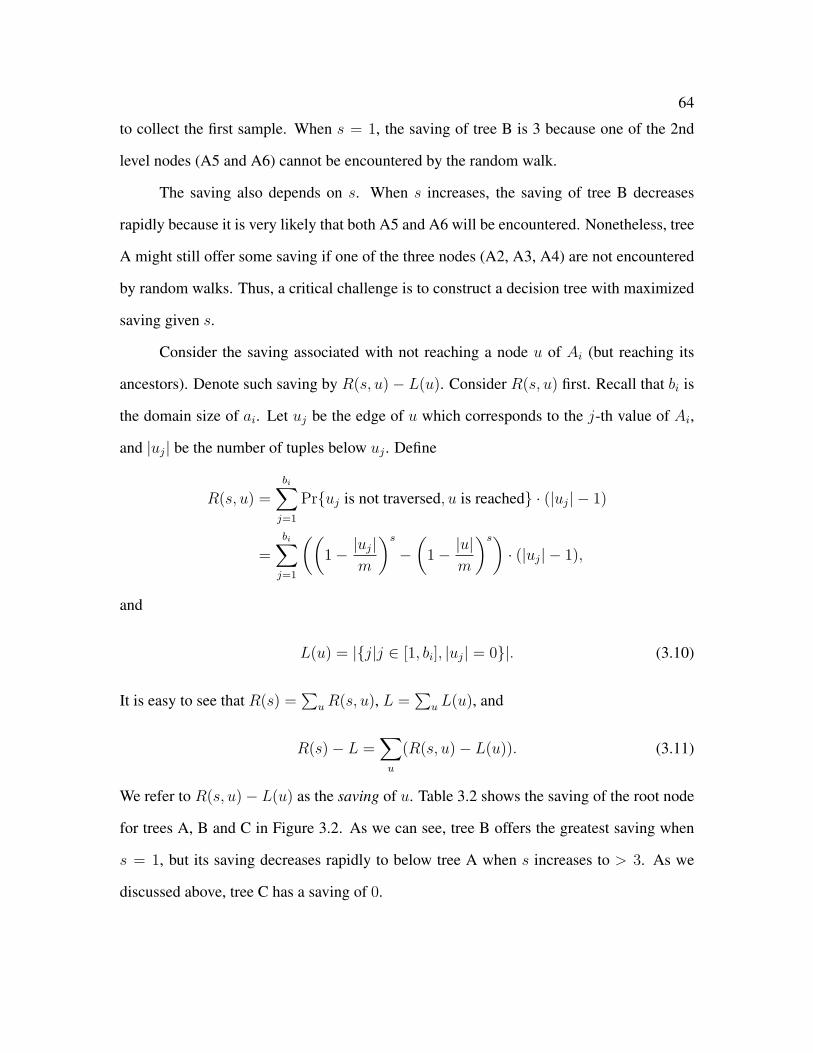
64
to collect the first sample. When s = 1, the saving of tree B is 3 because one of the 2nd
level nodes (A5 and A6) cannot be encountered by the random walk.
The saving also depends on s. When s increases, the saving of tree B decreases
rapidly because it is very likely that both A5 and A6 will be encountered. Nonetheless, tree
A might still offer some saving if one of the three nodes (A2, A3, A4) are not encountered
by random walks. Thus, a critical challenge is to construct a decision tree with maximized
saving given s.
Consider the saving associated with not reaching a node u of Ai (but reaching its
ancestors). Denote such saving by R(s, u)− L(u). Consider R(s, u) first. Recall that bi is
the domain size of ai. Let uj be the edge of u which corresponds to the j-th value of Ai,
and |uj| be the number of tuples below uj . Define
R(s, u) =
bi∑j=1
Pruj is not traversed, u is reached · (|uj| − 1)
=
bi∑j=1
((1− |uj|
m
)s−(
1− |u|m
)s)· (|uj| − 1),
and
L(u) = |j|j ∈ [1, bi], |uj| = 0|. (3.10)
It is easy to see that R(s) =∑
uR(s, u), L =∑
u L(u), and
R(s)− L =∑u
(R(s, u)− L(u)). (3.11)
We refer to R(s, u)− L(u) as the saving of u. Table 3.2 shows the saving of the root node
for trees A, B and C in Figure 3.2. As we can see, tree B offers the greatest saving when
s = 1, but its saving decreases rapidly to below tree A when s increases to > 3. As we
discussed above, tree C has a saving of 0.
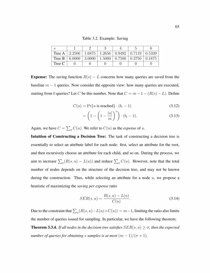
65
Table 3.2. Example: Saving
s 1 2 3 4 5 6Tree A 2.2500 1.6875 1.2656 0.9492 0.7119 0.5339Tree B 6.0000 3.0000 1.5000 0.7500 0.3750 0.1875Tree C 0 0 0 0 0 0
Expense: The saving function R(s) − L concerns how many queries are saved from the
baseline m− 1 queries. Now consider the opposite view: how many queries are executed,
starting from 0 queries? Let C be this number. Note that C = m− 1− (R(s)−L). Define
C(u) = Pru is reached · (bi − 1) (3.12)
=
(1−
(1− |u|
m
)s)· (bi − 1). (3.13)
Again, we have C =∑
uC(u). We refer to C(u) as the expense of u.
Intuition of Constructing a Decision Tree: The task of constructing a decision tree is
essentially to select an attribute label for each node: first, select an attribute for the root,
and then recursively choose an attribute for each child, and so on. During the process, we
aim to increase∑
u(R(s, u) − L(u)) and reduce∑
uC(u). However, note that the total
number of nodes depends on the structure of the decision tree, and may not be known
during the construction. Thus, while selecting an attribute for a node u, we propose a
heuristic of maximizing the saving per expense ratio
SER(s, u) =R(s, u)− L(u)
C(u). (3.14)
Due to the constraint that∑
u(R(s, u)−L(u)+C(u)) = m−1, limiting the ratio also limits
the number of queries issued for sampling. In particular, we have the following theorem:
Theorem 3.3.4. If all nodes in the decision tree satisfies SER(s, u) ≥ σ, then the expected
number of queries for obtaining s samples is at most (m− 1)/(σ + 1).
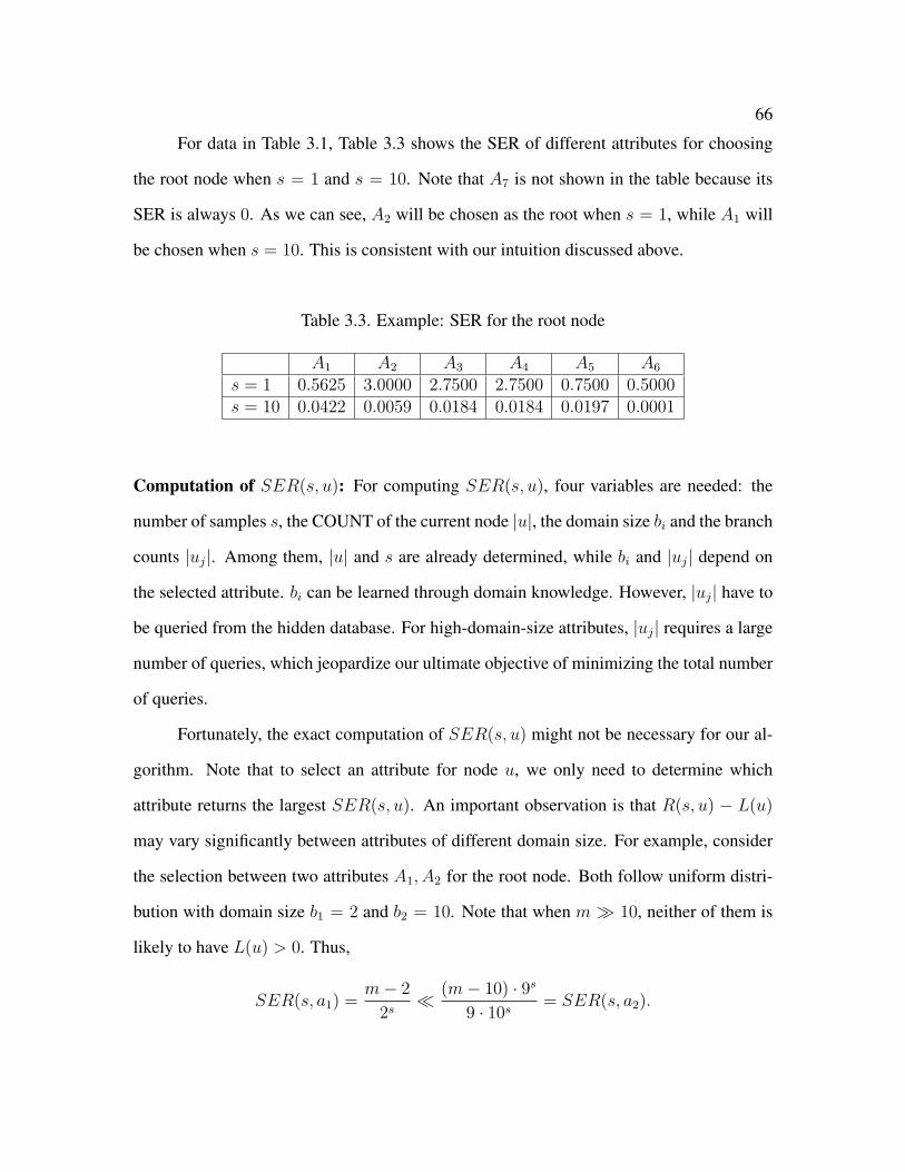
66
For data in Table 3.1, Table 3.3 shows the SER of different attributes for choosing
the root node when s = 1 and s = 10. Note that A7 is not shown in the table because its
SER is always 0. As we can see, A2 will be chosen as the root when s = 1, while A1 will
be chosen when s = 10. This is consistent with our intuition discussed above.
Table 3.3. Example: SER for the root node
A1 A2 A3 A4 A5 A6
s = 1 0.5625 3.0000 2.7500 2.7500 0.7500 0.5000s = 10 0.0422 0.0059 0.0184 0.0184 0.0197 0.0001
Computation of SER(s, u): For computing SER(s, u), four variables are needed: the
number of samples s, the COUNT of the current node |u|, the domain size bi and the branch
counts |uj|. Among them, |u| and s are already determined, while bi and |uj| depend on
the selected attribute. bi can be learned through domain knowledge. However, |uj| have to
be queried from the hidden database. For high-domain-size attributes, |uj| requires a large
number of queries, which jeopardize our ultimate objective of minimizing the total number
of queries.
Fortunately, the exact computation of SER(s, u) might not be necessary for our al-
gorithm. Note that to select an attribute for node u, we only need to determine which
attribute returns the largest SER(s, u). An important observation is that R(s, u) − L(u)
may vary significantly between attributes of different domain size. For example, consider
the selection between two attributes A1, A2 for the root node. Both follow uniform distri-
bution with domain size b1 = 2 and b2 = 10. Note that when m 10, neither of them is
likely to have L(u) > 0. Thus,
SER(s, a1) =m− 2
2s (m− 10) · 9s
9 · 10s= SER(s, a2).
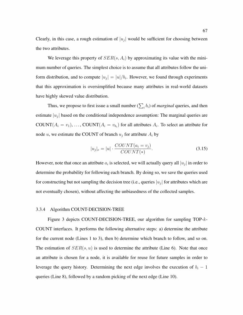
67
Clearly, in this case, a rough estimation of |uj| would be sufficient for choosing between
the two attributes.
We leverage this property of SER(s, Ai) by approximating its value with the mini-
mum number of queries. The simplest choice is to assume that all attributes follow the uni-
form distribution, and to compute |uj| = |u|/bi. However, we found through experiments
that this approximation is oversimplified because many attributes in real-world datasets
have highly skewed value distribution.
Thus, we propose to first issue a small number (∑
i bi) of marginal queries, and then
estimate |uj| based on the conditional independence assumption: The marginal queries are
COUNT(Ai = v1), . . . , COUNT(Ai = vbi) for all attributes Ai. To select an attribute for
node u, we estimate the COUNT of branch uj for attribute Ai by
|uj|e = |u| · COUNT (ai = vj)
COUNT (∗). (3.15)
However, note that once an attribute ai is selected, we will actually query all |uj| in order to
determine the probability for following each branch. By doing so, we save the queries used
for constructing but not sampling the decision tree (i.e., queries |uj| for attributes which are
not eventually chosen), without affecting the unbiasedness of the collected samples.
3.3.4 Algorithm COUNT-DECISION-TREE
Figure 3 depicts COUNT-DECISION-TREE, our algorithm for sampling TOP-k-
COUNT interfaces. It performs the following alternative steps: a) determine the attribute
for the current node (Lines 1 to 3), then b) determine which branch to follow, and so on.
The estimation of SER(s, u) is used to determine the attribute (Line 6). Note that once
an attribute is chosen for a node, it is available for reuse for future samples in order to
leverage the query history. Determining the next edge involves the execution of bi − 1
queries (Line 8), followed by a random picking of the next edge (Line 10).

68
Algorithm 3 COUNT-DECISION-TREERequire: Attr(·) = ∅ if not assigned
1: for i = 1 to s do
2: Obtain the i-th sample as DT SAMP(s− i+ 1, 〈〉).
3: end for
4: function DT SAMP(st, path)
5: if Attr(path) = φ then
6: Attr(path) = arg max((R(st, u, k)− L(u, k)) /C(u)).
7: end if
8: Query b− 1 branches. (Only issue those not in history)
9: Randomly pick j ∈ [1, b] s.t. Prj picked = |uj|/|u|.
10: if |uj| ≤ k then
11: return a random tuple from the answer to uj
12: else
13: return DT SAMP(st, path‖Attr(path) = vj).
14: end if
15: end function
COUNT-DECISION-TREE also extends the previous discussion by addressing the
cases with interface parameter k > 1. Clearly, the value of C(u) is unaffected. For com-
puting the saving R(s, u) − L(u), we define the number of baseline queries as m/k − 1.
Thus, the saving becomes
R(s, u, k) =
bi∑j=1
((1− |uj|
m
)s−(
1− |u|m
)s)·(|uj|k− 1
),
and
L(u, k) =∑
j|j∈[1,bi],|uj |<k
k − ujk
. (3.16)

69
3.4 ALERT-HYBRID
In this section, we present the main ideas behind ALERT-HYBRID, our new algo-
rithm for sampling hidden database behind a TOP-k-ALERT interface.
3.4.1 Basic Ideas
A major problem of ALERT-ORDER, the state-of-the-art algorithm for sampling
TOP-k-ALERT interfaces, is the bias of the collected samples. Since ALERT-ORDER
chooses each branch of a node with equal probability, those tuples on upper levels of the
tree (which require shorter walk from the root) are more likely to be sampled. Although
an acceptance-rejection module was introduced to reduce the bias [18], not many samples
can be rejected in order to maintain the efficiency of ALERT-ORDER. As a result, the
remaining bias may still be significant, as we will illustrate in the experiments.
On the other hand, the algorithms we just discussed for TOP-k-COUNT interfaces
generate no bias because each branch is chosen with probability proportional to its COUNT.
As a result, each tuple is sampled with equal probability. Clearly, the COUNT information
which is absent from TOP-k-ALERT interfaces can play an important role on reducing the
bias of collected samples.
Fortunately, the COUNT information is not completely out of reach in TOP-k-ALERT
interfaces. In particular, after a small number of samples are collected, the COUNT of cer-
tain queries may be estimated from the collected samples.
Thus, we propose ALERT-HYBRID, a two-phase procedure by which the sampler
first collects a small number (say s1) of pilot samples for COUNT estimations, and then
use the estimated COUNT to facilitate the collection of the remaining (much larger) s− s1
samples. The s1 samples can be simply collected by ALERT-ORDER, parameterized to
produce samples with small bias. The small bias in the s1 samples is desirable because
it helps in accurate COUNT estimations in the second phase. Although this requirement

70
makes the ALERT-ORDER procedure less efficient, the relatively small number of the pilot
samples required ensures that the cost of the first phase is a modest portion of the overall
sampling cost.
For the remaining s − s1 samples, note that we cannot directly use the COUNT-
DECISION-TREE algorithm because not all nodes can have COUNT accurately estimated
from a very small number (s1 m) of samples. Thus, we propose a hybrid approach
which integrates COUNT-based and ALERT-based sampling. In particular, after collect-
ing the s1 samples, we invoke the COUNT-DECISION-TREE algorithm until reaching a
node u with COUNT in the collected samples less than a threshold, say cS. At this node,
there are not enough collected samples to support a robust estimation of the probability
for following each edge. Thus, a natural choice is to switch to ALERT-based sampling.
In particular, ALERT-ORDER is called to collect a sample under node u. As we can see,
this hybrid approach starts with COUNT-based sampling at the upper levels of the tree, and
then switches to ALERT-based when there is not enough support from the collected sam-
ples. Initially, the switch from COUNT-based to ALERT-based sampling may occur early
at the upper levels. However, when more samples are collected (at the second phase), more
nodes will be able to support COUNT-based sampling, and thus the switch may occur later.
There are two important parameters in the algorithm: s1, the number of pilot samples
collected for initial count estimation, and cS, the count threshold for switching to ALERT-
ORDER. The setting of s1 influences the efficiency of ALERT-HYBRID for two reasons:
First, with a small s1, the constructed decision tree is unlikely to be optimal, and therefore
may require more queries in the second phase. Second, if s1 is too large, there will be a
large number of queries spent in collecting the pilot samples. Note that these queries are
unlikely to be reused in the second phase because COUNT-DECISION-TREE may use a
different tree from the attribute-order tree used by ALERT-ORDER in the first phase.
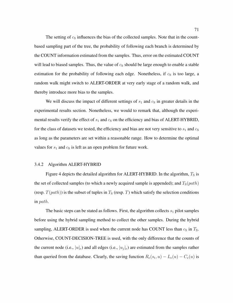
71
The setting of cS influences the bias of the collected samples. Note that in the count-
based sampling part of the tree, the probability of following each branch is determined by
the COUNT information estimated from the samples. Thus, error on the estimated COUNT
will lead to biased samples. Thus, the value of cS should be large enough to enable a stable
estimation for the probability of following each edge. Nonetheless, if cS is too large, a
random walk might switch to ALERT-ORDER at very early stage of a random walk, and
thereby introduce more bias to the samples.
We will discuss the impact of different settings of s1 and cS in greater details in the
experimental results section. Nonetheless, we would to remark that, although the experi-
mental results verify the effect of s1 and cS on the efficiency and bias of ALERT-HYBRID,
for the class of datasets we tested, the efficiency and bias are not very sensitive to s1 and cS
as long as the parameters are set within a reasonable range. How to determine the optimal
values for s1 and cS is left as an open problem for future work.
3.4.2 Algorithm ALERT-HYBRID
Figure 4 depicts the detailed algorithm for ALERT-HYBRID. In the algorithm, TS is
the set of collected samples (to which a newly acquired sample is appended); and TS(path)
(resp. T (path)) is the subset of tuples in TS (resp. T ) which satisfy the selection conditions
in path.
The basic steps can be stated as follows. First, the algorithm collects s1 pilot samples
before using the hybrid sampling method to collect the other samples. During the hybrid
sampling, ALERT-ORDER is used when the current node has COUNT less than cS in TS.
Otherwise, COUNT-DECISION-TREE is used, with the only difference that the counts of
the current node (i.e., |u|e) and all edges (i.e., |uj|e) are estimated from the samples rather
than queried from the database. Clearly, the saving function Re(st, u)− Le(u)− Ce(u) is
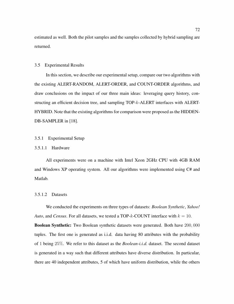
72
estimated as well. Both the pilot samples and the samples collected by hybrid sampling are
returned.
3.5 Experimental Results
In this section, we describe our experimental setup, compare our two algorithms with
the existing ALERT-RANDOM, ALERT-ORDER, and COUNT-ORDER algorithms, and
draw conclusions on the impact of our three main ideas: leveraging query history, con-
structing an efficient decision tree, and sampling TOP-k-ALERT interfaces with ALERT-
HYBRID. Note that the existing algorithms for comparison were proposed as the HIDDEN-
DB-SAMPLER in [18].
3.5.1 Experimental Setup
3.5.1.1 Hardware
All experiments were on a machine with Intel Xeon 2GHz CPU with 4GB RAM
and Windows XP operating system. All our algorithms were implemented using C# and
Matlab.
3.5.1.2 Datasets
We conducted the experiments on three types of datasets: Boolean Synthetic, Yahoo!
Auto, and Census. For all datasets, we tested a TOP-k-COUNT interface with k = 10.
Boolean Synthetic: Two Boolean synthetic datasets were generated. Both have 200, 000
tuples. The first one is generated as i.i.d. data having 80 attributes with the probability
of 1 being 25%. We refer to this dataset as the Boolean-i.i.d. dataset. The second dataset
is generated in a way such that different attributes have diverse distribution. In particular,
there are 40 independent attributes, 5 of which have uniform distribution, while the others

73
Algorithm 4 ALERT-HYBRID1: for i = 1 to s1 do
2: TS[i]← ALERT-ORDER(T ).
3: end for
4: for i = s1 to s do
5: TS[i]← HYBRID SAMP(s− i+ 1, 〈〉).
6: end for
7: function HYBRID SAMP(st, path)
8: if COUNT(TS(path)) < cS then
9: return ALERT-ORDER(T (path))
10: else if Attr(path) = φ then
11: Attr(path) = arg maxRe(st, u)− Le(u)− Ce(u).
12: end if
13: Randomly pick j ∈ [1, b] with P (j) = |uj|e/|u|e.
14: Query q = (path‖Attr(path) = vj).
15: if q is a valid query then
16: return a random tuple from the answer to q
17: else
18: return HYBRID SAMP(st, path‖Attr(path) = vj).
19: end if
20: end function

74
have the probability of 1 ranging from 1/160 to 35/160 with step of 1/160. We refer to
this dataset as the Boolean-mixed dataset.
Yahoo! Auto: The Yahoo! Auto dataset consists of data crawled from a real-world hidden
database at http://autos.yahoo.com/. In particular, it contains 15,211 used cars for sale in
the Dallas-Fort Worth metropolitan area. There are 32 Boolean attributes, such as A/C,
Power Locks, etc, and 6 categorical attributes, such as Make, Model, Color, etc. The
domain size of categorical attributes ranges from 5 to 447.
Census: The Census dataset consists of the 1990 US Census Adult data published on the
UCI Data Mining archive. After removing attributes with domain size greater than 100, the
dataset had 12 attributes and 32,561 tuples. It is instructive to note that the domain size of
the attributes of the underlying data is unbalanced in nature. The attribute with the highest
domain size has 92 categories and the lowest-domain-size attributes are Boolean.
3.5.1.3 Parameter Settings
The experiments involve five algorithms. Among them, ALERT-RANDOM and
COUNT-DECISION-TREE are parameter-less. ALERT-ORDER requires a parameter called
scaling factorC for the acceptance/rejection module, in order to tradeoff between efficiency
and bias. Following the heuristic in [18], for Boolean datasets, we set C = 1/2l where l
is the average length of random walks for collecting the samples. For categorical data, we
consider various values of C to tradeoff between efficiency and bias. COUNT-ORDER
requires input of an (arbitrary) attribute order. We randomly generate the order in our ex-
periments. Our ALERT-HYBRID approach requires two parameters: the number of pilot
samples s1 and the switching count threshold cS. We set s1 = 100 and cS = 10 by default,
but conducted experiments with various other combinations.

75
3.5.1.4 Performance Measures
For each algorithm, there are two performance measures: efficiency and bias. Effi-
ciency of a sampling algorithm was measured by counting the number of queries that were
executed to reach a certain desired sample size. To measure the bias of collected samples,
we use the same measure as [18] which compares the marginal frequencies of attribute
values in the original dataset and in the sample:
bias =
√√√√∑v∈V
(1− pS(v)
pD(v)
)2
|V |. (3.17)
Here V is a set of values with each attribute contributing one representative value, and pS(v)
(resp. pD(v)) is the relative frequency of value v in the sample (resp. dataset). The intuition
is that if the sample is unbiased uniform random sample, then the relative frequency of any
value will be the same as in the original dataset. However, note that even for uniform
random samples, this method of measuring bias will result in small but possibly non-zero
bias.
3.5.2 Comparison with Existing Algorithms
3.5.2.1 COUNT-DECISION-TREE
We compared the performance of COUNT-DECISION-TREE with three existing
algorithms: COUNT-ORDER, ALERT-ORDER, and ALERT-RANDOM (note: although
the latter two algorithms are designed for ALERT interfaces, they can sample from COUNT
interfaces by ignoring the returned counts).
For COUNT-ORDER, our direct competitor for COUNT interfaces, we conducted
the comparison on both Yahoo! Auto and Census datasets. The number of queries issued
are shown in Figures 3.4. Note that both algorithms generate unbiased samples. As we can
see, our algorithm requires orders of magnitude fewer queries than COUNT-ORDER.
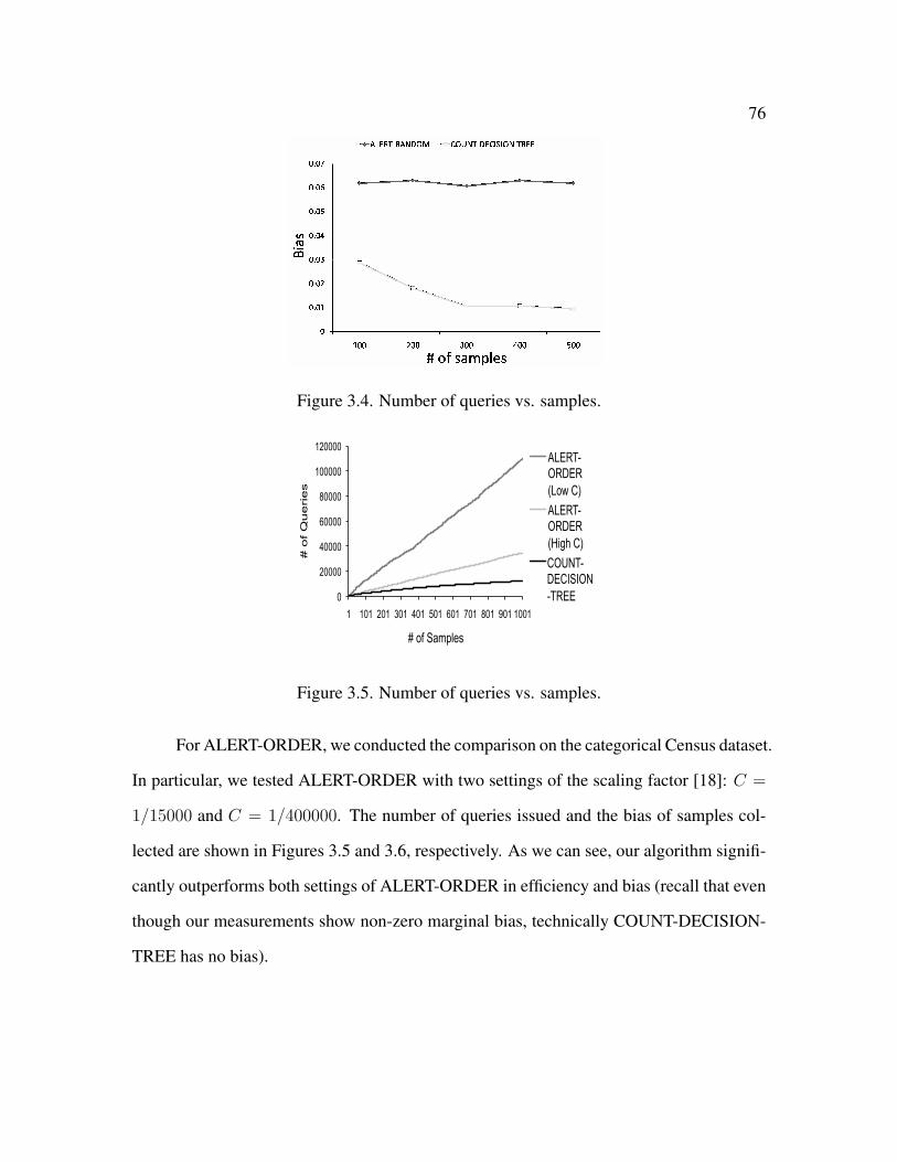
76
Figure 3.4. Number of queries vs. samples.
0
20000
40000
60000
80000
100000
120000
1 101 201 301 401 501 601 701 801 901 1001
# o
f Q
ueries
# of Samples
ALERT-ORDER (Low C)
ALERT-ORDER (High C)
COUNT-DECISION-TREE
Figure 3.5. Number of queries vs. samples.
For ALERT-ORDER, we conducted the comparison on the categorical Census dataset.
In particular, we tested ALERT-ORDER with two settings of the scaling factor [18]: C =
1/15000 and C = 1/400000. The number of queries issued and the bias of samples col-
lected are shown in Figures 3.5 and 3.6, respectively. As we can see, our algorithm signifi-
cantly outperforms both settings of ALERT-ORDER in efficiency and bias (recall that even
though our measurements show non-zero marginal bias, technically COUNT-DECISION-
TREE has no bias).
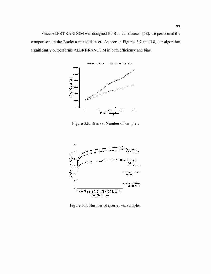
77
Since ALERT-RANDOM was designed for Boolean datasets [18], we performed the
comparison on the Boolean-mixed dataset. As seen in Figures 3.7 and 3.8, our algorithm
significantly outperforms ALERT-RANDOM in both efficiency and bias.
Figure 3.6. Bias vs. Number of samples.
Figure 3.7. Number of queries vs. samples.
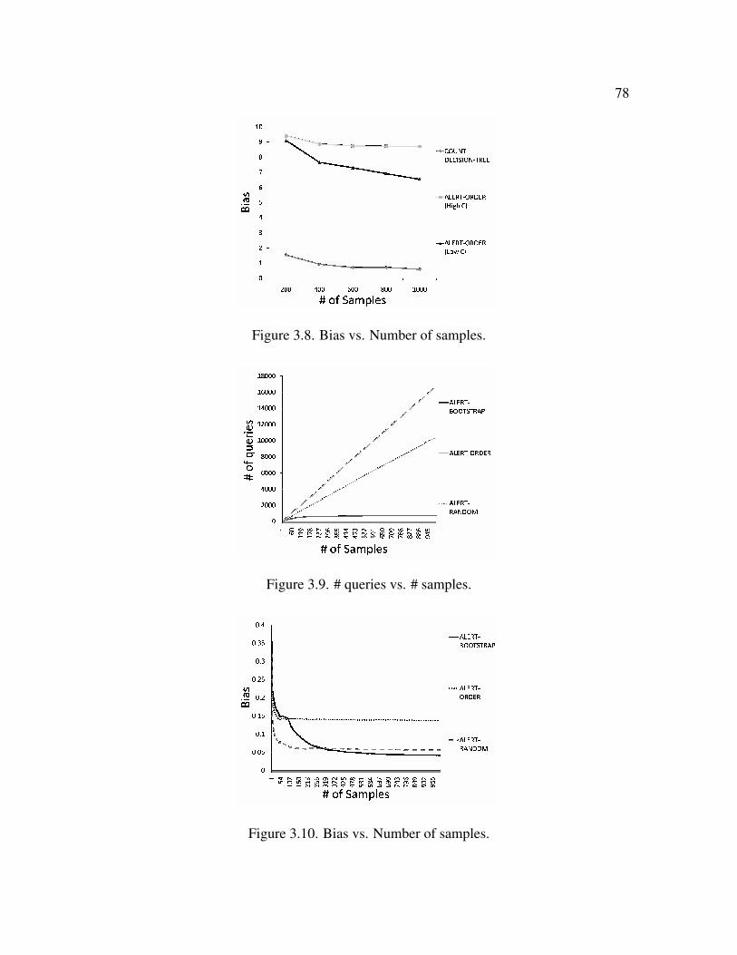
78
Figure 3.8. Bias vs. Number of samples.
Figure 3.9. # queries vs. # samples.
Figure 3.10. Bias vs. Number of samples.
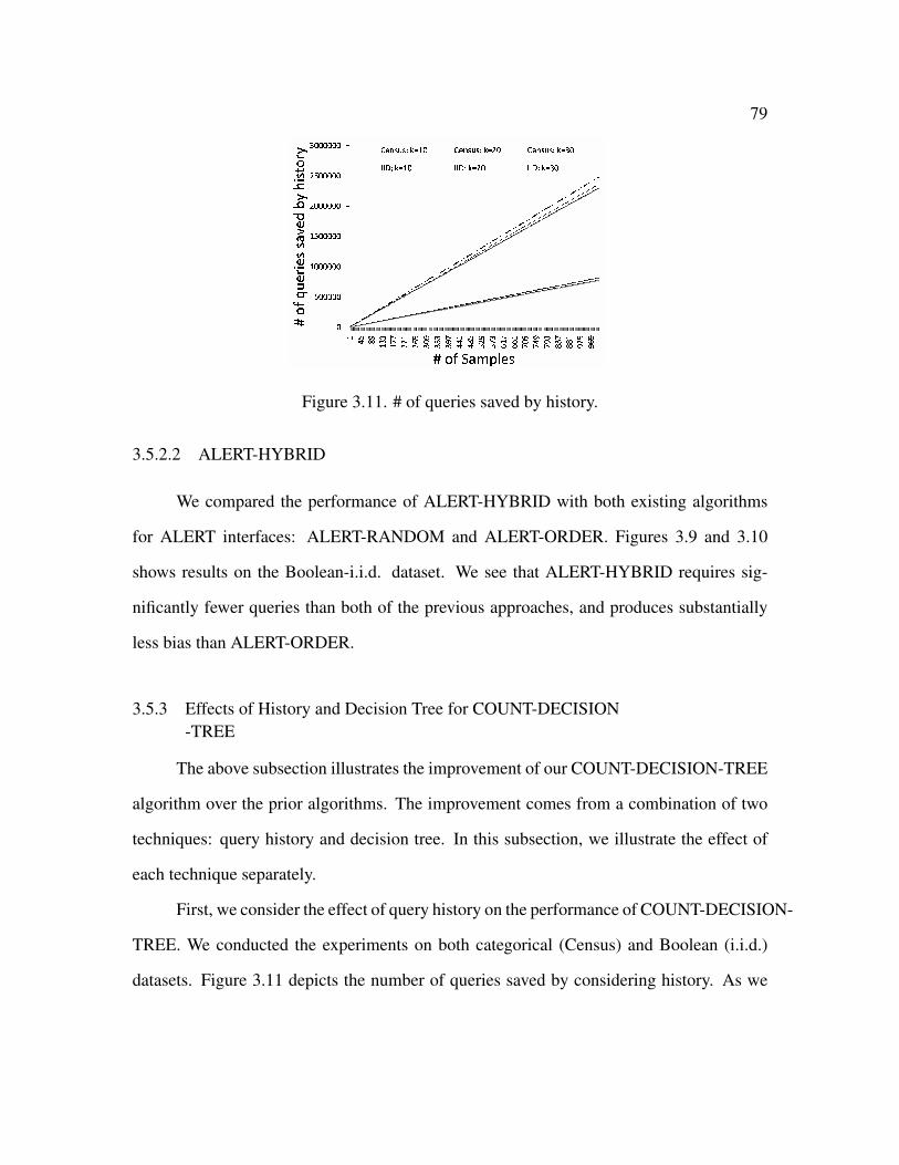
79
Figure 3.11. # of queries saved by history.
3.5.2.2 ALERT-HYBRID
We compared the performance of ALERT-HYBRID with both existing algorithms
for ALERT interfaces: ALERT-RANDOM and ALERT-ORDER. Figures 3.9 and 3.10
shows results on the Boolean-i.i.d. dataset. We see that ALERT-HYBRID requires sig-
nificantly fewer queries than both of the previous approaches, and produces substantially
less bias than ALERT-ORDER.
3.5.3 Effects of History and Decision Tree for COUNT-DECISION-TREE
The above subsection illustrates the improvement of our COUNT-DECISION-TREE
algorithm over the prior algorithms. The improvement comes from a combination of two
techniques: query history and decision tree. In this subsection, we illustrate the effect of
each technique separately.
First, we consider the effect of query history on the performance of COUNT-DECISION-
TREE. We conducted the experiments on both categorical (Census) and Boolean (i.i.d.)
datasets. Figure 3.11 depicts the number of queries saved by considering history. As we
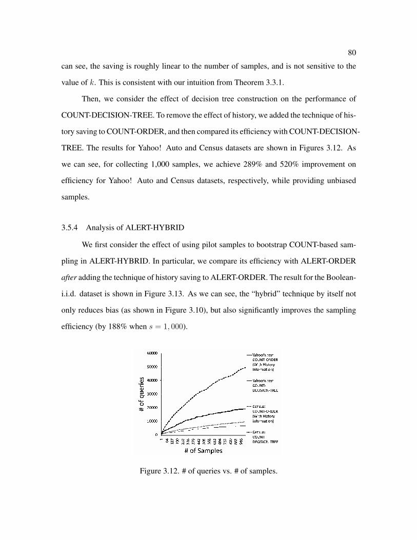
80
can see, the saving is roughly linear to the number of samples, and is not sensitive to the
value of k. This is consistent with our intuition from Theorem 3.3.1.
Then, we consider the effect of decision tree construction on the performance of
COUNT-DECISION-TREE. To remove the effect of history, we added the technique of his-
tory saving to COUNT-ORDER, and then compared its efficiency with COUNT-DECISION-
TREE. The results for Yahoo! Auto and Census datasets are shown in Figures 3.12. As
we can see, for collecting 1,000 samples, we achieve 289% and 520% improvement on
efficiency for Yahoo! Auto and Census datasets, respectively, while providing unbiased
samples.
3.5.4 Analysis of ALERT-HYBRID
We first consider the effect of using pilot samples to bootstrap COUNT-based sam-
pling in ALERT-HYBRID. In particular, we compare its efficiency with ALERT-ORDER
after adding the technique of history saving to ALERT-ORDER. The result for the Boolean-
i.i.d. dataset is shown in Figure 3.13. As we can see, the “hybrid” technique by itself not
only reduces bias (as shown in Figure 3.10), but also significantly improves the sampling
efficiency (by 188% when s = 1, 000).
Figure 3.12. # of queries vs. # of samples.
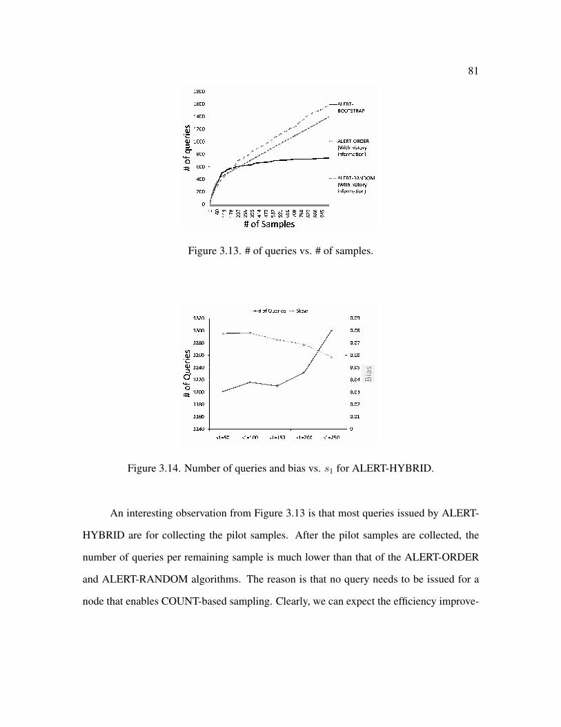
81
Figure 3.13. # of queries vs. # of samples.
Figure 3.14. Number of queries and bias vs. s1 for ALERT-HYBRID.
An interesting observation from Figure 3.13 is that most queries issued by ALERT-
HYBRID are for collecting the pilot samples. After the pilot samples are collected, the
number of queries per remaining sample is much lower than that of the ALERT-ORDER
and ALERT-RANDOM algorithms. The reason is that no query needs to be issued for a
node that enables COUNT-based sampling. Clearly, we can expect the efficiency improve-
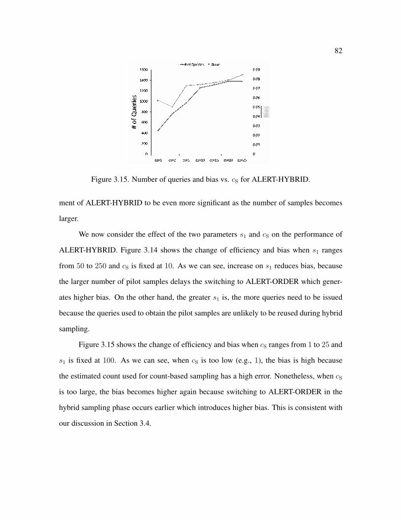
82
Figure 3.15. Number of queries and bias vs. cS for ALERT-HYBRID.
ment of ALERT-HYBRID to be even more significant as the number of samples becomes
larger.
We now consider the effect of the two parameters s1 and cS on the performance of
ALERT-HYBRID. Figure 3.14 shows the change of efficiency and bias when s1 ranges
from 50 to 250 and cS is fixed at 10. As we can see, increase on s1 reduces bias, because
the larger number of pilot samples delays the switching to ALERT-ORDER which gener-
ates higher bias. On the other hand, the greater s1 is, the more queries need to be issued
because the queries used to obtain the pilot samples are unlikely to be reused during hybrid
sampling.
Figure 3.15 shows the change of efficiency and bias when cS ranges from 1 to 25 and
s1 is fixed at 100. As we can see, when cS is too low (e.g., 1), the bias is high because
the estimated count used for count-based sampling has a high error. Nonetheless, when cS
is too large, the bias becomes higher again because switching to ALERT-ORDER in the
hybrid sampling phase occurs earlier which introduces higher bias. This is consistent with
our discussion in Section 3.4.

83
3.6 Related Work
Crawling and Sampling from Hidden Databases: There has been prior work on crawling
as well as sampling hidden databases using their public search interfaces. Several papers
have dealt with the problem of crawling and downloading information present in hidden
text based databases [8,23,24]. [17,25,26] deal with extracting data from structured hidden
databases. [27] and [28] use query based sampling methods to generate content summaries
with relative and absolute frequencies while [29, 30] uses two phase sampling method on
text based interfaces. On a related front [31, 32] discuss top-k processing which considers
sampling or distribution estimation over hidden sources. A closely related area of sampling
from a search engines index using a public interface has been addressed in [8] and more
recently [9, 33]. In [18] the authors have developed techniques for random sampling from
structured hidden databases leading to the HIDDEN-DB-SAMPLER algorithm. The hybrid
technique used in ALERT-HYBRID has also been used for other sampling applications
such as block-level sampling [4] and sampling peer-to-peer networks [22].
Approximate Query Processing and Database Sampling: Approximate query process-
ing (AQP) for decision support, especially sampling-based approaches for relational databases,
has been the subject of extensive recent research; e.g., see tutorials by Das [20] and Garo-
falakis et al [7], as well as the report [21] and the references therein.
3.7 Conclusion
In this chapter, we investigated techniques which leverage the COUNT information
to efficiently acquire unbiased samples of hidden databases. In particular, we proposed
the COUNT-DECISION-TREE algorithm based on two ideas: (a) the use of query history,
and (b) the construction and use of an efficient decision tree. We also discuss variants
for TOP-k-ALERT interfaces which do not provide COUNT information. In particular,

84
we presented ALERT-HYBRID based on using pilot samples to bootstrap the COUNT-
DECISION-TREE algorithm draw the samples. Our thorough experimental study demon-
strates the superiority of our sampling algorithms over the existing algorithms.
CHAPTER 4
TURBO-CHARGING HIDDEN DATABASE SAMPLERS WITHOVERFLOWING QUERIES AND SKEW REDUCTION
4.1 Introduction
In this chapter we consider the problem of random sampling over online hidden
databases. A hidden database, such as Google Base [34] and Yahoo! Auto [35], allows
external users to access its contents via a restricted form-like web interface. This restricted
query interface primarily allows users to execute search queries by selecting the desired
values for one or more attributes, e.g.,
SELECT * FROM D WHERE a1 = v1 AND a3 = v3
and the system responds by returning a few (e.g., top-k where k is a small constant such as
20 or 50) tuples that satisfy the selection conditions, sorted by a suitable scoring function.
Along with these returned tuples, the interface also usually alerts the user if there was an
“overflow”, i.e., if there are other tuples besides the top-k ones that also satisfy the query but
cannot be returned. The scoring function may be simple (e.g., based on a single attribute)
or complex (e.g., computed from multiple attributes), static (i.e., independent of the search
query) or dynamic, and may be known or unknown to the users.
Recently, there has been growing interest by third-party applications in obtaining
random samples of the data in online hidden databases [18, 36, 37]. Such samples can be
of great benefit to third-party applications, because various analytical tools can be enabled
from the sample. For example, statistical information about the data can be derived, such as
useful aggregates [18, 36]. A variety of sampling methods can be employed to produce the
random samples - e.g., simple random sampling, stratified sampling, etc. For the purpose
85
86
of this chapter, we focus on simple random sampling which selects each tuple with equal
probability. A justification for this choice is provided in Section 4.5. In the latter part of
this work, unless otherwise specified, our usage of term “sampling” refers specifically to
simple (uniform) random sampling.
Our previous work [36] shows that, for hidden databases which provide the actual
COUNT information (i.e., the total number of tuples that satisfy the given query) along with
the top-k returned tuples, uniform random sampling can be done very efficiently. While
a lot of hidden databases provide such COUNT information, numerous others do not or
provide notoriously inaccurate COUNT information (e.g., Google). For these COUNT-
less hidden databases, it has been challenging to develop effective sampling algorithms,
primarily because complete and unrestricted access to the data is disallowed. We focus
on the uniform random sampling of COUNT-less hidden databases in this chapter, and
summarize below the current state-of-the-art of such samplers.
4.1.1 Current State-of-the-Art Samplers
There are two main objectives that a sampling algorithm should seek to achieve:
• Efficiency: The efficiency of the sampling process is measured by the number of
queries that need to be executed via the web interface in order to collect a sample of
a desired size. The task is to design an efficient sampling procedure that executes as
few queries as possible.
• Minimizing Skew: Due to the restricted nature of the interface, it is challenging to
produce samples that are truly uniform random samples. Consequently, the task is
to produce samples that have small skew, i.e., the probability for each tuple to be
selected should deviate as little as possible from the uniform distribution.
A state-of-the-art sampler for hidden databases is the HIDDEN-DB-SAMPLER, pro-
posed in [18]. This approach is based on a random drill-down process of queries executable
87
via the form-like interface - it starts with an extremely broad (therefore overflowing) query,
and iteratively narrowing it down by adding random predicates, until a non-overflowing
query is reached. If such a query answer is not empty, one of the returned tuples is ran-
domly picked for inclusion into the sample (subject to a probabilistic rejection test to re-
duce skew). Otherwise, the drill-down process restarts from the extremely broad query.
This process can be repeated to get samples of any desired size.
However, HIDDEN-DB-SAMPLER and all other existing hidden database samplers
(i.e., COUNT-DECISION-TREE [36] and HYBRID-SAMPLER [36]) have a main defi-
ciency in that they ignore all overflowing queries. In the design of these samplers, tuples
returned as the result of an overflowing query are assumed to be useless for assembling
into a random sample because they have been selected not by a random procedure, but
preferentially based on the pre-determined scoring function. Thus, overflowing queries are
ignored in order to avoid favoring highly ranked tuples and thereby incurring high skew in
the retrieved sample. While not using overflowing queries is a simple solution to eliminate
the effect of scoring function on skew, it also significantly increases the number of queries
required for sampling, thus adversely impacting efficiency. For example, during the ran-
dom drill-down process, existing hidden database samplers have to execute a large number
of overflowing queries before they encounter a non-overflowing one.
4.1.2 Main Technical Contributions
In this chapter, one of our main contributions is to propose novel techniques that
leverage overflowing queries to turbo-charge the efficiency of samplers. Thus, overflow-
ing queries that were ignored by prior samplers can now be properly utilized during the
sampling process. In particular, we develop TURBO-DB-SAMPLER, a sampler for hid-
den databases that is an order of magnitude (10 times in our experiments) more efficient
than the existing HIDDEN-DB-SAMPLER. The main idea behind our approaches is the
88
novel concept of a designated query that maps each tuple in the database to a unique query
(whether overflowing or not) executable via the form-like interface, and a designation test
procedure that efficiently determines whether a query is designated for a tuple.
We also find that, for hidden databases with static scoring functions (i.e., which are
independent of the search queries), a simpler designation test is available which enables
the sampling efficiency to be further improved by a novel scheme called level-by-level
sampling. This scheme skips queries in the drill-down process whose results are not picked
for inclusion into the sample. With this scheme, we develop TURBO-DB-STATIC, an
algorithm that achieves an additional speedup factor of 2 for databases with static scoring
functions.
The second main contribution of our chapter is that our algorithms also significantly
reduces sampling skew. In particular, we propose a novel scheme of concatenating sam-
pling with crawling to reduce sampling skew. The basic idea is to switch to crawling from
the random drill-down process if we encounter a query which remains overflow after adding
a large number of predicates (i.e., a long overflowing query). The premise here is that a
long overflowing query is an indication of a dense cluster of data tuples - over which the
random drill-down technique produces an extremely high skew. The usage of crawling over
such dense clusters significantly reduces the sampling skew while maintaining a low query
cost because the number of queries needed for the crawling of such a cluster is linearly
bounded by the number of tuples matching the long overflowing query, which is usually
small. While this concatenated scheme is not able to completely remove skew, we show
that TURBO-DB-SAMPLER incurs orders of magnitude smaller skew than HIDDEN-DB-
SAMPLER and other state-of-the-art samplers.
The contributions of this chapter may be summarized as follows:

89
• We develop a novel technique of using designated queries and designation tests to
leverage overflowing queries and thereby dramatically improve the efficiency of sam-
pling.
• We develop a novel technique of concatenating sampling with crawling to signifi-
cantly reduce sampling skew.
• For hidden databases with static scoring functions, we develop a novel technique of
level-by-level sampling to further improve sampling efficiency substantially.
• For hidden databases with arbitrary scoring functions, we put together the first two
techniques to develop a generic TURBO-DB-SAMPLER which achieves a speedup
factor of more than 5 over HIDDEN-DB-SAMPLER [18].
• For hidden databases with static scoring functions, we put together all three tech-
niques to develop TURBO-DB-STATIC which further improves sampling efficiency
by a speedup factor of 2.
• We run extensive experiments to demonstrate the effectiveness of our proposed sam-
pling algorithms. In particular, we tested our results on both synthetic datasets and a
real-world dataset crawled from Yahoo! Auto [35]. The experimental results demon-
strate the superiority of our sampling algorithms over the previous efforts.
The rest of this chapter is organized as follows: We define the problem and briefly review
the existing samplers in Section 2. In Sections 3, we introduce TURBO-DB-SAMPLER,
our major sampling algorithm, and its two main ideas: leveraging overflowing queries with
designation tests, and reducing skew by concatenating sampling with crawling. In Section
4, we introduce TURBO-DB-STATIC, a sampling algorithm which leverages the static
scoring function to enable a more efficient designation test and a level-by-level sampling
scheme that further improves efficiency. We present related discussions in Section 5. Sec-
tion 6 shows the experimental results. Related work is reviewed in Section 7, followed by
final remarks in Section 8.

90
4.2 Preliminaries
In this section, we introduce a model of hidden databases, define the performance
measures for sampling over hidden databases, and review the state-of-the-art HIDDEN-
DB-SAMPLER.
4.2.1 Model of Hidden Databases
Hidden databases on the web receive queries from users through web forms. To
form a query, users are generally provided with drop down boxes, check boxes, text boxes
or other common HTML form elements. After a query is selected by the user, a request
is submitted and the hidden database system return tuples matching the user query. Large
databases generally restrict users access to top-k tuples which may be presented on one
pages or over multiple pages (accessed by page turns or clicking next at the bottom of the
results page). Below, we provide a simple formalization of this model.
Consider a hidden database table T with n tuples t1, . . . , tn and m attributes a1, . . . , am
which have respective domains of D1, . . . , Dm. We restrict our discussion in the most
part of this work to categorical data, and discuss the extension to numerical databases
in Section 4.5.2. We point out that a large number of hidden database systems can be
transformed into categorical data by applying simple transformations. As an example,
consider a price-range attribute which provides upper and lower bounds. This can be used
as a combination of discrete intervals with an upper and lower bound. Table 4.1 shows an
example with n = 4, m = 3 and Di = 0, 1 (i ∈ [1, 3]). Suppose k = 1 and the four
tuples ranked by score from high to low are t1, . . . , t4. This table will be used throughout
the chapter as a running example.
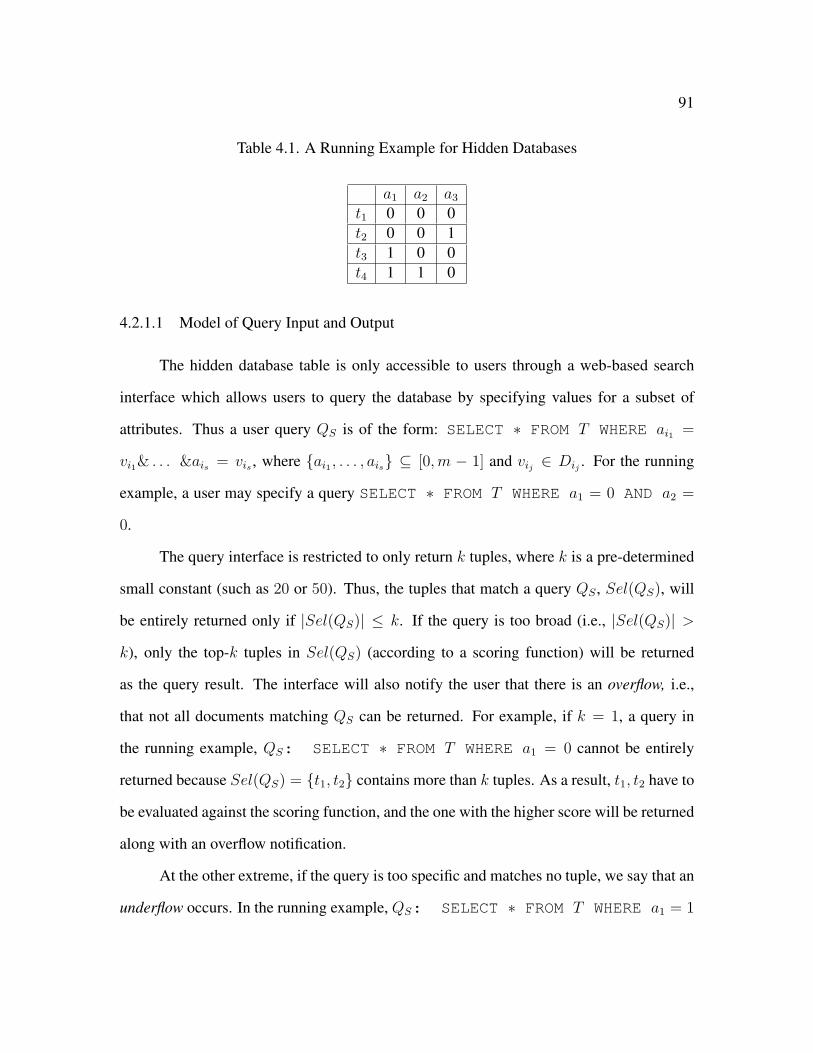
91
Table 4.1. A Running Example for Hidden Databases
a1 a2 a3
t1 0 0 0t2 0 0 1t3 1 0 0t4 1 1 0
4.2.1.1 Model of Query Input and Output
The hidden database table is only accessible to users through a web-based search
interface which allows users to query the database by specifying values for a subset of
attributes. Thus a user query QS is of the form: SELECT ∗ FROM T WHERE ai1 =
vi1& . . . &ais = vis , where ai1 , . . . , ais ⊆ [0,m − 1] and vij ∈ Dij . For the running
example, a user may specify a query SELECT ∗ FROM T WHERE a1 = 0 AND a2 =
0.
The query interface is restricted to only return k tuples, where k is a pre-determined
small constant (such as 20 or 50). Thus, the tuples that match a query QS , Sel(QS), will
be entirely returned only if |Sel(QS)| ≤ k. If the query is too broad (i.e., |Sel(QS)| >
k), only the top-k tuples in Sel(QS) (according to a scoring function) will be returned
as the query result. The interface will also notify the user that there is an overflow, i.e.,
that not all documents matching QS can be returned. For example, if k = 1, a query in
the running example, QS: SELECT ∗ FROM T WHERE a1 = 0 cannot be entirely
returned because Sel(QS) = t1, t2 contains more than k tuples. As a result, t1, t2 have to
be evaluated against the scoring function, and the one with the higher score will be returned
along with an overflow notification.
At the other extreme, if the query is too specific and matches no tuple, we say that an
underflow occurs. In the running example, QS: SELECT ∗ FROM T WHERE a1 = 1
92
AND a3 = 1 underflows. If there is neither overflow nor underflow, we have a valid query
result. An example of valid query is QS:SELECT ∗ FROM T WHERE a1 = 0 AND
a3 = 1 in the running example. In this chapter, we assume the query answering system to
be deterministic, i.e., the same query executed again will produce the same set of results.
For the purpose of this chapter, we assume that a restrictive interface does not allow
the users to “scroll through” the complete answer Sel(QS) when an overflow occurs for
QS . Instead, the user must pose a new query by reformulating the search conditions. We
argue that this is a reasonable assumption because many real-world top-k interfaces (e.g.,
Google Base [34], Yahoo Auto [35]) only allow “page turns” for limited (100) times.
Since the tuples returned by a query may not include tuples that match the query,
for the purpose of clarification, we distinguish the meaning of three verbs: match, return,
and draw, which are extensively used in the chapter. We say a tuple matches a query iff
the tuple is in the hidden database and satisfies the selection condition of the query. The
number of tuples that match a query may be greater than k. We say a tuple is returned by a
query iff the tuple is one of those that are actually displayed on the query output interface as
the response to that query. The number of tuples that a query can return is always smaller
than or equal to k. While a tuple returned by a query always matches the query, the reverse
is not always true. We say a tuple is drawn from a query during the sampling process iff
the sampler selects the tuple from the returned answer of the query, and then uses that tuple
as a sample tuple. A sample tuple drawn from a query must be returned by the query and
therefore matches the query. Again, the reverse is not always true.
4.2.1.2 Model of Scoring Function
There are two types of scoring functions for a hidden database: One is static in that
each tuple’s score is a function of the tuple value, and does not change with different user-
issued search queries. For example, a real estate database may score each tuple (i.e., house)

93
by its price (i.e., an attribute value), and only display the k cheapest houses. The scoring
function we use for the running example is also static. The other type of scoring function
is query-dependent and is a function of both the tuple value and the search query. For
example, the real estate database may score each tuple by price if price is not included in
the search conditions, or by the number of bedrooms if price is included. In this chapter,
unless otherwise specified (e.g., in Section 4.4 which focuses on static ranking functions),
we consider generic ranking functions which may be static or query-dependent.
4.2.2 Performance Measures
Recall from the introduction that our objective is to generate a uniform random sam-
ple over the hidden web database. Such a sampling algorithm should be measured in terms
of efficiency and skew which we formally define as follows.
• Efficiency: For a given (desired) sample size s, we measure the efficiency of a sam-
pler by the expected number of queries it issues to the form-like web interface in
order to obtain s sample tuples.
• Skew: We define the level of skew as the standard deviation of the probability for a
tuple to be sampled. i.e.,
γ =
√√√√ 1
n·
n∑i=1
(Prti is chosen as the sample − 1
n
)2
(4.1)
We observe later that the above measures tradeoff against each other. The parameter of our
system enables the user to strike the right balance according to their specific needs.
4.2.3 HIDDEN-DB-SAMPLER
We now review HIDDEN-DB-SAMPLER, the sampling algorithm presented in our
earlier work [18] for obtaining random samples from hidden databases. Consider a tree
constructed from an arbitrary order of all attributes, say a1, . . . , am. Let the root be the
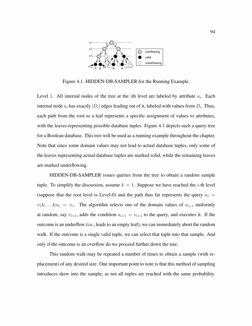
94
valid
overflowing
underflowing
t1 t4t3t2
a1
a2
a3
0 1
Figure 4.1. HIDDEN-DB-SAMPLER for the Running Example.
Level 1. All internal nodes of the tree at the ith level are labeled by attribute ai. Each
internal node ai has exactly |Di| edges leading out of it, labeled with values fromDi. Thus,
each path from the root to a leaf represents a specific assignment of values to attributes,
with the leaves representing possible database tuples. Figure 4.1 depicts such a query tree
for a Boolean database. This tree will be used as a running example throughout the chapter.
Note that since some domain values may not lead to actual database tuples, only some of
the leaves representing actual database tuples are marked solid, while the remaining leaves
are marked underflowing.
HIDDEN-DB-SAMPLER issues queries from the tree to obtain a random sample
tuple. To simplify the discussion, assume k = 1. Suppose we have reached the i-th level
(suppose that the root level is Level-0) and the path thus far represents the query a1 =
v1& . . .&ai = vi.. The algorithm selects one of the domain values of ai+1 uniformly
at random, say vi+1, adds the condition ai+1 = vi+1 to the query, and executes it. If the
outcome is an underflow (i.e., leads to an empty leaf), we can immediately abort the random
walk. If the outcome is a single valid tuple, we can select that tuple into that sample. And
only if the outcome is an overflow do we proceed further down the tree.
This random walk may be repeated a number of times to obtain a sample (with re-
placement) of any desired size. One important point to note is that this method of sampling
introduces skew into the sample, as not all tuples are reached with the same probability.
95
Techniques such as acceptance/rejection sampling are further employed for reducing skew
(see [18] for further details).
4.3 TURBO-DB-SAMPLER
In this section, we describe TURBO-DB-SAMPLER, our algorithm for sampling a
hidden database. TURBO-DB-SAMPLER features two main ideas: it leverages overflow-
ing queries to significantly improve the efficiency of sampling; and concatenate sampling
with crawling to substantially reduce the skew of samples. In the following, we first de-
velop two samplers: OVERFLOW-SAMPLER and CONCATENATE-SAMPLER with the
two respectively, and then combine them together to construct TURBO-DB-SAMPLER.
4.3.1 Improve Efficiency: Leverage Overflows
4.3.1.1 Basic Idea
We leverage overflowing queries by ignoring the overflowing flag and treating an
overflowing query in the same way as a valid query that returns k tuples. However, doing
so makes a tuple with a higher score to be returned by more queries, and to have a higher
probability of being selected into the sample. To eliminate such score-related skew, we
place a restriction on the selection of a tuple into the sample. In particular, we define one
designated query (in the set of all interface-executable queries) for each tuple in the hidden
database, and require each selected sample tuple to go through a designation test - i.e., we
enforce a rule that a tuple can be selected into the sample only if it is retrieved from the
result of its designated query. Note that the designated query for a tuple can be either valid
or overflowing.
To understand the effect of this change on hidden database sampling, let us first
investigate a simple application of it to the random drill-down process of HIDDEN-DB-

96
SAMPLER. At this moment, let us assume that the designation test can be done without
issuing any additional query to the web interface. We will discuss details about the cost of
designation test in the next step. There are two possible outcomes of this change for the
generation of one sample tuple:
• First, the random drill-down process might select a sample tuple from an overflow-
ing query, leading to an earlier termination of the random drill-down process. This
reduces the number of queries that need to be issued.
• However, depending on the definition of designated query, there might be a second
outcome where the sampler has to drill deeper down the tree than HIDDEN-DB-
SAMPLER if, according to the designated query definition, none of the overflowing
and valid queries issued on upper levels are the designated queries for the tuples they
return.
One can see from the two outcomes that the impact of this change on the efficiency
of sampling is determined by the definition of designated queries. Indeed, if the designated
query of a tuple is defined to be the highest-level valid query that returns the tuple, then
HIDDEN-DB-SAMPLER remains the same after applying the change because no over-
flowing query will serve as the designated query for a tuple anyway.
To improve sampling efficiency, we define the designated query of a tuple as follows:
Definition 4.3.1. For a given query tree, the designated query of a tuple t is the highest-
level query (valid or overflowing) that returns t. We denote the designated query by q(t).
Figure 4.2 shows the designated queries of all four tuples for the running example in
Table 4.1 (recall that k = 1 in the example). One can see from the figure that, compared
with HIDDEN-DB-SAMPLER, t1 and t3 may be retrieved by higher-level overflowing
queries. There are two important observations from this definition of designated queries:
• First, note that for a given tuple t, at any given level, there is at most one query
which returns t. Thus, the definition guarantees each tuple to have one and only one
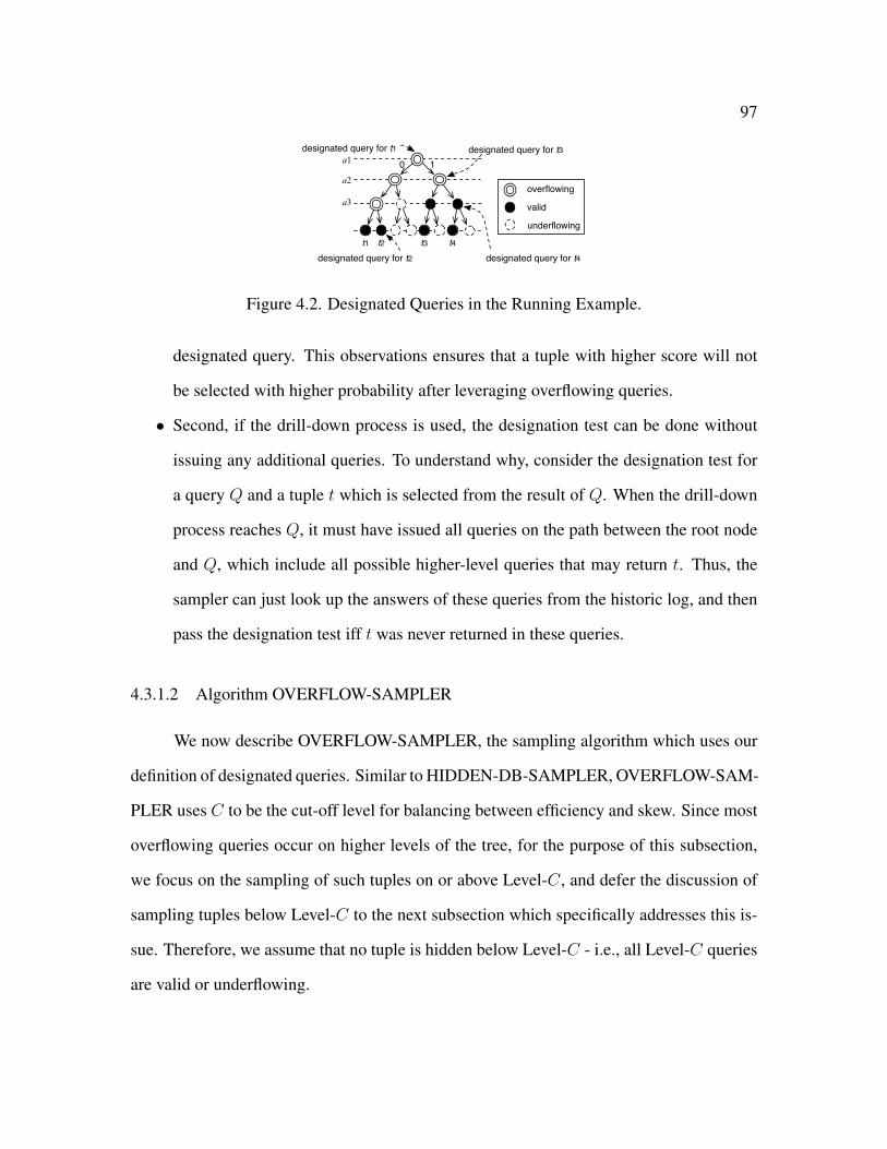
97
valid
overflowing
underflowing
t1
designated query for t1
t4designated query for t4
designated query for t3
t3t2designated query for t2
0 1a1
a2
a3
Figure 4.2. Designated Queries in the Running Example.
designated query. This observations ensures that a tuple with higher score will not
be selected with higher probability after leveraging overflowing queries.
• Second, if the drill-down process is used, the designation test can be done without
issuing any additional queries. To understand why, consider the designation test for
a query Q and a tuple t which is selected from the result of Q. When the drill-down
process reaches Q, it must have issued all queries on the path between the root node
and Q, which include all possible higher-level queries that may return t. Thus, the
sampler can just look up the answers of these queries from the historic log, and then
pass the designation test iff t was never returned in these queries.
4.3.1.2 Algorithm OVERFLOW-SAMPLER
We now describe OVERFLOW-SAMPLER, the sampling algorithm which uses our
definition of designated queries. Similar to HIDDEN-DB-SAMPLER, OVERFLOW-SAM-
PLER uses C to be the cut-off level for balancing between efficiency and skew. Since most
overflowing queries occur on higher levels of the tree, for the purpose of this subsection,
we focus on the sampling of such tuples on or above Level-C, and defer the discussion of
sampling tuples below Level-C to the next subsection which specifically addresses this is-
sue. Therefore, we assume that no tuple is hidden below Level-C - i.e., all Level-C queries
are valid or underflowing.

98
OVERFLOW-SAMPLER again uses a random drill-down process starting from the
root level of a given query tree. However, before drilling down the tree, the sampler first
determines whether the sample tuple can be drawn from the root query. In particular, it
randomly chooses a tuple from those returned by the root query, and selects it as a sample
with probability of
p0 =|d(Q0)|k · π(C)
, (4.2)
where |d(Q0)| is the number of tuples that have the root query as their designated query,
and function π(·) is defined as
π(i) =i∏
j=1
|Dj| (4.3)
which is the product of the domain size of attributes a1 to ai. Let π(0) = 1. For example,
the root query in our running example returns t1 with probability of 1/23. Note that accord-
ing to our definition of the designated query, a tuple has the root as its designated query
iff it is returned by the root query. As such, d(Q0) = |Q0|, the number of tuples returned
by Q0. Therefore, OVERFLOW-SAMPLER selects each tuple returned by the root with
probability of
1
|Q0|· p0 =
1
|Q0|· |Q0|k · π(C)
=1
k · π(C). (4.4)
If a sample tuple is not selected from the root and the root is overflowing, then
OVERFLOW-SAMPLER starts the random drill-down process. Note that if the root is
valid or underflowing, then no query with additional predicates can serve as the designated
query for any tuple. Thus, the sampling process has to restart in this case.
Different from HIDDEN-DB-SAMPLER, in the drill-down process, OVERFLOW-
SAMPLER follows each outgoing branch with different probability. The purpose of doing
so is to address the fact that tuples returned from upper levels of the tree may also satisfy
99
the outgoing branches, but will not be returned by any lower level queries. Therefore, these
tuples must be excluded from consideration in the computation of outgoing probabilities. In
particular, OVERFLOW-SAMPLER follows an outgoing branch ai = vi (of a Level-(i−1)
node Qi−1) with probability of
βi(vi) =π(i− 1)
π(i)· k · π(C)− |f(Qi−1, v)| · π(i)
k · π(C)− |f(Qi−1)| · π(i− 1), (4.5)
where f(Qi−1) is the set of tuples returned byQ0, . . . , Qi−1 which satisfyQi−1, and f(Qi−1, vi)
is the subset of f(Qi−1) which further satisfies ai = vi. In the running example, we have
β0(0) = (1/2) · (23 − 2)/(23 − 1) = 3/7 and β0(1) = (1/2) · 23/(23 − 1) = 4/7. Thus,
the sampler follows the left and right branches of the root node with probability of 3/7 and
4/7, respectively. This is consistent with the intuition that, since the tuple returned by the
root “belongs to” the left branch, the drill-down process should turn to the left with lower
probability.
During the drill down process, after issuing each query, the sampler again needs to
determine whether the sample tuple can be drawn from the results. Consider such a process
for a Level-i query Qi. Let the list of queries issued so far by the drill down process be
Q0, . . . , Qi−1, at levels 0 to i− 1, respectively. The sampler first computes d(Qi) as
d(Qi) = Qi\(Q0 ∪ · · · ∪Qi−1). (4.6)
For instance, in the running example, query with predicates (a1 = 0)&(a2 = 0) has d(Q) =
t1\t1 = ∅. If d(Qi) is not empty, the sampler randomly draws a tuple from d(Qi) and
selects it as a sample with probability of
pi =|d(Qi)|
k · π(C) · (∏i−1
j=1 βj(vj)) ·∏i−1
j=1(1− pj). (4.7)
We can derive the value of pi from this iterative formula and the value of p0 in (4.2):
pi =|d(Qi)| · π(i)
k · π(C)− |f(Qi−1, vi)| · π(i). (4.8)

100
In the running example, when query (a1 = 1) is issued, the sampler has probability of
21/(23 − 0) = 1/4 to select t3 as the sample. Note that there is always pi ≤ 1. To
understand why, note that pi increases monotonically with i. When i = C, we have
pC =|d(QC)|
k − |f(QC−1, vC)|, (4.9)
Since d(QC) and f(QC−1, vC) are mutually exclusive sets of tuples that satisfy QC , ac-
cording to our assumption for all Level-C queries to be valid or underflowing, there must
be |d(QC)|+ |f(QC−1, vC)| ≤ k. Therefore, pC ≤ 1.
From the definition of pi, one can derive that the probability for a tuple with desig-
nated query Qi to be selected as a sample is(i∏
j=1
βj(vj)
)·
(i−1∏j=0
(1− pj)
)· 1
|d(Qj)|· pi =
1
k · π(C)(4.10)
which is constant across all levels. Again, if no sample is drawn and Qi overflows, the
drill down process continues to deeper levels. Otherwise, the sampler either terminates (if
enough sample has been collected) or restarts from the root.
Algorithm 5 depicts the pseudocode for OVERFLOW-SAMPLER. For setting the
value of the parameter C, we follow the heuristic rule in [18] that C be set as the average
depth of a random walk. In the running example, this leads to an assignment of C =
(0 + 1 + 2 + 3)/4 = 1.5. Note that in practice, a sampler has no prior knowledge of
the average depth. Nonetheless, as discussed in [18], the value of C can be determined
adaptively during the sampling process because the average depth can be learned as more
and more random walks are accomplished.
4.3.1.3 Analysis of Improvement on Efficiency
We now discuss the efficiency comparison between OVERFLOW-SAMPLER and
HIDDEN-DB-SAMPLER. First, one can observe that, to achieve the same level of skew,

101
Algorithm 5 OVERFLOW-SAMPLER for Levels 1 to CRequire: C, a pre-determined cut-off level
1: Q← SELECT * FROM D, prod← 1, i← 0.
2: Issue query Q, Compute d(Q).
3: p← |d(Q)| · π(i)/(k · π(C) · prod).
4: Randomly generate r ∈ (0, 1) according to uniform distribution.
5: if r ≤ p then
6: Randomly choose a tuple from d(Q) as sample. exit.
7: end if
8: if Q overflows then
9: prod← prod · (1− p). i← i+ 1.
10: Randomly generate v ∈ Di. Add predicate ai = v to Q.
11: Goto 2
12: else
13: Goto 1
14: end if
the number of queries required by OVERFLOW-SAMPLER never exceeds that of HIDDEN-
DB-SAMPLER. To understand why, consider the execution of both samplers with the
same value of C over the same hidden database. As we have shown, for both algorithms,
a random drill-down process draws each tuple on or above Level-C with probability of
1/(k · π(C)). However, for any tuple, the number of queries (i.e., levels to step down)
required by OVERFLOW-SAMPLER to draw the tuple is always smaller than or equal to
that of HIDDEN-DB-SAMPLER. Thus, OVERFLOW-SAMPLER can only improve the
efficiency of sampling for a given level of skew.

102
In the following, we quantitatively analyze the efficiency improvement provided by
OVERFLOW-SAMPLER. Since OVERFLOW-SAMPLER is only used for sampling tu-
ples on or above Level-C, the ratio of improvement depends on the value of C. As previ-
ously discussed, we set the value of C to be the average depth of a random walk for both
algorithms. Similar theorems can be derived for other settings of C.
Theorem 4.3.1. For a given query tree with uO overflowing nodes, n tuples, and a top-k
interface, the ratio between the query cost of HIDDEN-DB-SAMPLER and OVERFLOW-
SAMPLER on obtaining one sample tuple is
E(cost of HIDDEN-DB-SAMPLER)
E(cost of OVERFLOW-SAMPLER)≥ 2k·uO/n. (4.11)
We omit the proof due to space limitation. The theorem follows directly from the
following observation: If a tuple appears in d overflowing queries, then the random walk
to reach this tuple in HIDDEN-DB-SAMPLER is d levels longer than in OVERFLOW-
SAMPLER. Thus, on average the length of a random walk that draws a sample tuple in
OVERFLOW-SAMPLER is k · uO/n shorter than that in HIDDEN-DB-SAMPLER. In
the running example, such average length is (0 + 1 + 2 + 3)/4 = 1.5 for OVERFLOW-
SAMPLER and (2 + 2 + 3 + 3)/4 = 2.5 for HIDDEN-DB-SAMPLER, leading to a differ-
ence of exactly k · uO/n = 1 · 4/4 = 1. Since each attribute has at least two values, 2k·uO/n
serves as a lower bound for the improvement ratio.
The theorem indicates that OVERFLOW-SAMPLER can achieve a significant im-
provement ratio in practice. For example, consider a 50-attribute, 10, 000-tuple, Boolean
i.i.d dataset with probability of 1 being 0.1 for each attribute and k = 1. There are an
expected number of 31, 176.95 overflowing queries in the query tree. According to the
theorem, by leveraging overflowing queries one can reduce the expected query cost by a
factor of at least 8.68.
103
4.3.2 Reduce skew: Concatenate with Crawling
4.3.2.1 Basic Idea
As we mentioned in the previous subsection, both HIDDEN-DB-SAMPLER and
OVERFLOW-SAMPLER can produce unbiased samples if all Level-C queries are valid.
Thus, sampling skew is caused by the different selection probability of tuples with desig-
nated queries below the cutoff Level-C. For example, if a tuple is only returned by a leaf-
level query but not higher-level ones (e.g., due to the tuple’s low score), then HIDDEN-
DB-SAMPLER selects this tuple with probability only π(C)/π(m) ≤ 1/2m−C times of
that for a tuple returned on or above Level-C.
To reduce the skew for sampling these low-level tuples, our main idea is to concate-
nate sampling with crawling on levels below Level-C. In particular, the sampling of tuples
below Level-C starts when OVERFLOW-SAMPLER reaches an overflowing query Q at
Level-C but could not select a sample from it (due to rejection sampling in Line 5 of Algo-
rithm 5). Instead of further conducting the random walk to drill below Level-C, we switch
to the crawling of the subtree of Q, and compute Ω(Q), the set of all tuples in the database
that match Q. Then, we randomly choose a tuple from Ω(Q) and return it as a sample after
a rejection sampling step which will be discussed in detail later. The crawling process can
be performed as a depth-first search of the subtree with root beingQ. The depth-first search
backtracks from a node if the node is already valid or underflowing.
The concatenation of sampling with crawling has two main implications on the per-
formance of sampling:
• The concatenated process substantially reduces the skew of selection probability for
tuples below Level-C. Unlike in HIDDEN-DB-SAMPLER where a tuple’s selection
probability decreases exponentially with its level index below Level-C, the concate-
nation idea ensures equal selection probability for all (lower-level) tuples in the sub-
104
tree of an overflowing Level-C node. As we shall show at the end of this subsection,
the difference between the selection probability of different tuples is substantially
reduced with the concatenated process.
• The effect of crawling on sampling efficiency is insignificant for practical databases.
The crawling of a subtree in which nT tuples have designated queries below Level
C requires O(nT) queries. In the theoretical worst case, the subtree may contain as
many as nT = max(n−k, k ·π(m)/π(C)−k) tuples which leads to an unacceptably
large query cost. Nonetheless, we argue that this case is extremely unlikely to occur
in practice because it indicates that attributes a1, . . . , aC (in the upper levels) are
incapable of distinguishing tuples, and should be excluded from the form-like web
interface. For real-world datasets, when C is reasonably large (e.g., k · π(C) ≈ n),
the number of tuples in each subtree should be fairly small.
4.3.2.2 Algorithm CONCATENATE-SAMPLER
We now describe the detailed design of CONCATENATE-SAMPLER, our algorithm
for sampling tuples with designated queries below Level-C by concatenating sampling with
crawling.
Recall from the above subsection that, when all Level-C queries are valid or under-
flowing, a random drill-down process of OVERFLOW-SAMPLER selects each tuple with
probability ζ = 1/(k · π(C)). When there exists tuples below Level-C (i.e., there exists
Level-C overflowing queries), however, it is no longer possible to always select each tu-
ple with probability of 1/(k · π(C)). To understand why, consider an extreme case where
all Level-C queries overflow. In this case, the number of tuples n > k · π(C), making it
impossible to select each tuple with probability of 1/(k · π(C)).

105
Thus, in order to support the sampling of tuples below Level-C, we have to decrease
the value of ζ . In particular, we consider a new (target) selection probability
ζI =1
(k + n0) · π(C), (4.12)
where n0 is the maximum number of tuples that match a Level-C overflowing query. Al-
though the sampler has no prior knowledge of n0, it can learn it adaptively when more
Level-C subtrees are crawled. The adaption of OVERFLOW-SAMPLER to this new se-
lection probability can be easily done by replacing k in Algorithm 5 with k + n0. Thus, in
the following, we focus on the sampling of tuples with designated queries below Level-C
with selection probability as close to ζI as possible (i.e., to achieve minimum skew).
Algorithm 6 CONCATENATE-SAMPLER for Levels C + 1 to m1: Crawl the subtree of Q. Suppose that nT tuples with designated queries below Level
C are collected.
2: With probability of nT/n0, return a tuple randomly chosen from the nT tuples.
3: Update the value of n0 if necessary.
Let QC be a Level-C overflowing query. After adapting OVERFLOW-SAMPLER
to the new ζI, a tuple randomly drawn from the returned result of QC is selected as a
sample with probability of pC = |d(Qi)|/(k + n0 − |f(QC−1, vC)|). If it is not selected as
a sample, our CONCATENATE-SAMPLER will be invoked with probability of n0/(k +
n0−|f(QC)|). This way, givenQC , the overall probability for a random-drill down process
to switch to the crawling of the subtree of QC is n0/((k + n0) · π(C)).
Once the CONCATENATE-SAMPLER is invoked, we crawl the subtree of QC and
randomly draw from the crawling result a tuple t with designated query below Level C.
Suppose that the subtree includes nT such tuples. Then, with probability of max(nT, n0)/n0,

106
we select t as a sample tuple. Otherwise, CONCATENATE-SAMPLER is aborted and
OVERFLOW-SAMPLER restarts from the root level.
Algorithm 6 depicts pseudocode of CONCATENATE-SAMPLER.
4.3.2.3 Analysis of Reduction on Skew
We now discuss the skew comparison between CONCATENATE-SAMPLER and
HIDDEN-DB-SAMPLER. One can observe that CONCATENATE-SAMPLER can still be
skewed - if an overflowing query at Level C has a subtree with size more than (the current
value of) n0, then tuples with designated queries in this tree will be sampled with lower
probability than the others. In particular, a tuple in a nT-tuple subtree will be selected with
probability min(1, n0/nT) times of that for a tuple on or above Level C.
However, as we argued in the beginning of this subsection, with a reasonable value
of C (e.g., π(C) ≈ n), we expect nT ≤ n0 to hold true for most subtrees. Even when
nT > n0, the ratio between the highest and lowest selection probability for different tuples
is at most n/n0, which in many cases is still much smaller than the π(m)/π(C) ratio for
HIDDEN-DB-SAMPLER, because for most hidden databases the size of the database n is
orders of magnitude smaller than the space of all possible tuple values (π(m)).
The following theorem further investigates the skew comparison for an i.i.d. Boolean
dataset with probability of 1 being 0.5 and k = 1.
Theorem 4.3.2. When 2C n and m is sufficiently large, the level of skew of HIDDEN-
DB-SAMPLER γH and that of TURBO-DB-SAMPLER γT satisfies
γT
γH
< 2C/2+1 ·(n− 1
2C
)n0/2
(4.13)
which is much smaller than 1 given a reasonably large n0.
We omit the proof due to space limitation. One can see from the theorem that the
sample skew is significantly smaller in CONCATENATE-SAMPLER than HIDDEN-DB-
107
SAMPLER. For example, given a Boolean database with 10, 000 tuples, 100 attributes, and
C = 20, when n0 = 5, CONCATENATE-SAMPLER has a skew of 0.018 times that of
TURBO-DB-SAMPLER. The skew ratio will further reduce for a larger value of n0.
Since the adoption of CONCATENATE-SAMPLER also incurs query cost on the
crawling of low-level tuples, we analyze the expected query cost incurred by CONCATEN-
ATE-SAMPLER. In particular, we integrate the lower-level sampling of CONCATENATE-
SAMPLER with the higher-level sampling of HIDDEN-DB-SAMPLER, and then compare
it with a pure HIDDEN-DB-SAMPLER which uses the random walk theme throughout all
levels. The comparison is analyzed in the following theorem.
Theorem 4.3.3. If n and m are sufficiently large, when a Level-C subtree contains at most
n0 tuples, to achieve the same level of skew, the ratio between the query cost of HIDDEN-
DB-SAMPLER and CONCATENATE-SAMPLER on obtaining one sample is
E(cost of HIDDEN-DB-SAMPLER)
E(cost of CONCATENATE-SAMPLER)
≥ n0 · π(C) · k(k + n0) · π(C) + n0 · n/2
(4.14)
Again, we omit the proof due to space limitation. One can see from the theorem
that despite of requiring the crawling of a subtree, CONCATENATE-SAMPLER actually
requires substantially fewer queries than HIDDEN-DB-SAMPLER to achieve the same
level of skew. In the above Boolean database example with n = 10, 000,m = 100, and
C = 20, when n0 = 5, the theorem indicates that the cost of HIDDEN-DB-SAMPLER is
at least 16.60 times that of CONCATENATE-SAMPLER.

108
4.3.3 Algorithm TURBO-DB-SAMPLER
Algorithm 7 depicts the pseudocode for TURBO-DB-SAMPLER.
Algorithm 7 TURBO-DB-SAMPLERRequire: Parameters C and n0 set adaptively during sampling
1: Q← SELECT * FROM D, prod← 1, i← 0.
2: Issue query Q, Compute d(Q).
3: p← |d(Q)| · π(i)/((k + n0) · π(C) · prod).
4: Randomly generate r ∈ (0, 1).
5: if r ≤ p then
6: Randomly choose a tuple from d(Q) as sample. exit.
7: end if
8: if Q overflows then
9: prod← prod · (1− p). i← i+ 1.
10: Randomly generate v ∈ Di. Add predicate ai = v to Q.
11: Goto 2 if i ≤ C, Goto 15 otherwise.
12: else
13: Goto 1
14: end if
15: Crawl the subtree of Q. Suppose that nT tuples with designated queries below Level
C are collected.
16: With probability of nT/n0, return a tuple randomly chosen from the nT tuples.
109
4.4 Turbo-Charging Samplers for Static scoring Functions
In this section, we describe TURBO-DB-STATIC, our algorithm for sampling a hid-
den database with a static scoring function. TURBO-DB-STATIC integrates the two ideas
we discussed for TURBO-DB-SAMPLER (i.e., leveraging overflows and concatenating
sampling with crawling), as well as a third idea of level-by-level sampling which is en-
abled by a unique property of static scoring functions and is capable of further improving
the efficiency of sampling. We discuss this idea in this section.
4.4.1 Improve Efficiency: Level-by-Level Sampling
4.4.1.1 Basic Idea
We first describe the basic idea of level-by-level sampling, and then explain why it
only applies to hidden databases with static scoring functions.
Similar to OVERFLOW-SAMPLER, the objective of level-by-level sampling is to
further improve the efficiency for sampling tuples with designated queries on or above the
cutoff level C. For sampling these tuples, both OVERFLOW-SAMPLER and HIDDEN-
DB-SAMPLER perform random walks and terminates a random walk when (1) one of the
tuples the current query returns is selected as a sample, and/or (2) the random walk reaches
a valid or underflowing query. However, such a technique has the following efficiency
problem: Almost all top-level queries will be issued because every random walk initiates
from there. Although the number of these queries is small in comparison with the total
number of possible queries and/or the size of the database, the cost of issuing them may
be significant for drawing a small number of samples. Nonetheless, we argue that issuing
these top-level queries are hardly useful for sampling due to the following two reasons:
110
• Tuples with top-level designated queries form only a very small fraction of the database.
Thus, these top-level queries have slim chances of actually contributing a sample tu-
ple drawn from their returned answers.
• The role of top-level queries on the “early termination” of a random walk is also
doubtful: Unless a database is extremely skewed, it is unlikely that these high-level
queries can be underflowing or valid.
To address this problem, the main idea of level-by-level sampling is to perform the
sampling successively for each level of the query tree, with the order downward from the
root, and to issue a growing number of queries per level during the step-down process. If
a query Q is not underflowing, we perform designation tests to find the set of tuples with
designated queries being Q, and then randomly choose a tuple t from these tuples. We
select t as a sample after subjecting it to a rejection sampling test. The sampling process
terminates when a sample tuple is selected. If no tuple is chosen on or above Level C,
we randomly choose an overflowing query from Level-C and execute CONCATENATE-
SAMPLER over it. If CONCATENATE-SAMPLER cannot select a sample (i.e., due to
rejection sampling based on the subtree size), we again randomly choose a Level-C over-
flowing query and repeatedly execute CONCATENATE-SAMPLER until a sample tuple is
selected.
As we shall show in the detailed algorithm, level-by-level sampling has two main
features that contribute to the improvement of sampling efficiency:
• Level-by-level sampling issues top-level queries with extremely small probability
due to their unlikeliness of being selected to contribute a sample tuple.
• Unlike the random walk process which often aborts without returning a sample, level-
by-level sampling always return a sample from each step-down process.
Finally, note that level-by-level sampling only applies to static scoring functions due
to the requirement of designation test. Unlike OVERFLOW-SAMPLER, level-by-level
111
sampling does not have a drill-down process. Therefore, when a query Q is issued, queries
on the path between the root and Q may not have been issued before. As a result, the des-
ignation test cannot be performed based on the historic query answers as in OVERFLOW-
SAMPLER. A simple method to perform this test is to actually issue every query on the
path. However, doing so leads to significant query cost and is contradictory to our idea of
avoid issuing top-level queries.
On the other hand, it is possible to perform the designation test efficiently when the
hidden database has a static scoring function. In this case, only a single query needs to
be issued for designation test: To check whether a given query Q is the designated query
of a tuple t that it returns, we only need to check whether the parent of Q returns t. If
it does not, then Q is the designated query of t, and vice versa. In the running example,
to determine whether (a1 = 1)&(a2 = 1) is the designated query for t4, we only need to
judge whether query a1 = 1 returns t4, and do not need to issue the root query. In general,
the reason is that if t is not returned by the parent query, it certainly cannot be returned by
upper-level queries due to the static nature of the scoring function. Therefore, t must have
Q as its designated query.
4.4.1.2 Algorithm LEVEL-SAMPLER
Algorithm 8 depicts LEVEL-SAMPLER, our baseline algorithm for level-by-level
sampling. The following discussion consists of two parts: First, we make a few remarks on
applying LEVEL-SAMPLER in practice. Then, we show that it samples each tuple with
designated queries on or above Level C with equal probability.
One can see from Algorithm 8 that LEVEL-SAMPLER requires the knowledge of
n, the number of tuples in the database. We argue that such knowledge is usually available
in practice, as many hidden database providers publicize their database size as an adver-
tisement for usability. If the knowledge of n is not available, an upper-bound estimate of

112
it can be used. In this case, all tuples with designated query on or above Level C will still
be sampled with equal probability, but the probability will be different from those tuples
below LevelC. Nonetheless, we shall demonstrate in the experimental results that the skew
is extremely small even with an inaccurate estimation of n, and much smaller than the skew
of the existing algorithms.
Another note of caution from Algorithm 8 is that the cutoff level C must be cho-
sen such that k · π(C) ≤ n. Since we would like to sample as many tuples by LEVEL-
SAMPLER as possible, to avoid the skew of CONCATENATE-SAMPLER, a natural choice
is to set C to be the maximum value that satisfies k · π(C) ≤ n. In Section 4.4.2, we shall
show how the value of C can be further increased by pruning the query tree.
Algorithm 8 LEVEL-SAMPLER for Levels 1 to C1: h = 0.
2: With probability of (1− k · π(h)/n), Goto 8. Otherwise, randomly choose a query Q
from Level-h.
3: Goto 10 if Q is empty. Otherwise randomly pick a tuple t from the result of Q.
4: Generate r ∈ (0, 1) uniformly at random.
5: if r ≤ |Q|/k and Q is the designated query for t then
6: return t as sample and exit.
7: else if r ≤ |Q|/k and Q is not the designated query for t then
8: With probability of k · π(h)/n, Goto 2.
9: end if
10: if h ≤ C − 1 then
11: Set h = h+ 1, goto 2
12: else exit
13: end if
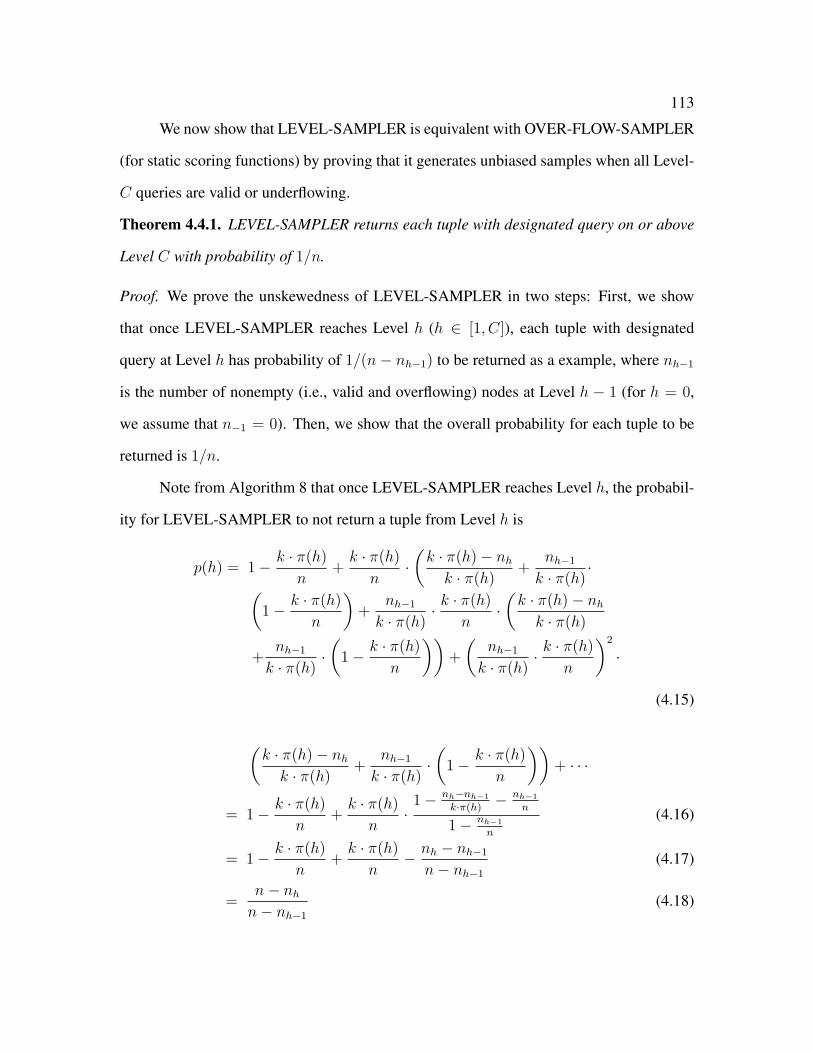
113
We now show that LEVEL-SAMPLER is equivalent with OVER-FLOW-SAMPLER
(for static scoring functions) by proving that it generates unbiased samples when all Level-
C queries are valid or underflowing.
Theorem 4.4.1. LEVEL-SAMPLER returns each tuple with designated query on or above
Level C with probability of 1/n.
Proof. We prove the unskewedness of LEVEL-SAMPLER in two steps: First, we show
that once LEVEL-SAMPLER reaches Level h (h ∈ [1, C]), each tuple with designated
query at Level h has probability of 1/(n− nh−1) to be returned as a example, where nh−1
is the number of nonempty (i.e., valid and overflowing) nodes at Level h − 1 (for h = 0,
we assume that n−1 = 0). Then, we show that the overall probability for each tuple to be
returned is 1/n.
Note from Algorithm 8 that once LEVEL-SAMPLER reaches Level h, the probabil-
ity for LEVEL-SAMPLER to not return a tuple from Level h is
p(h) = 1− k · π(h)
n+k · π(h)
n·(k · π(h)− nhk · π(h)
+nh−1
k · π(h)·(
1− k · π(h)
n
)+
nh−1
k · π(h)· k · π(h)
n·(k · π(h)− nhk · π(h)
+nh−1
k · π(h)·(
1− k · π(h)
n
))+
(nh−1
k · π(h)· k · π(h)
n
)2
·
(4.15)
(k · π(h)− nhk · π(h)
+nh−1
k · π(h)·(
1− k · π(h)
n
))+ · · ·
= 1− k · π(h)
n+k · π(h)
n·
1− nh−nh−1
k·π(h)− nh−1
n
1− nh−1
n
(4.16)
= 1− k · π(h)
n+k · π(h)
n− nh − nh−1
n− nh−1
(4.17)
=n− nhn− nh−1
(4.18)

114
When the algorithm does return a tuple from Level h, it is easy to verify that all tuples with
designated query at Level h are returned with equal probability. Note that since k = 1,
the number of tuples with designated query at Level h is nh − nh−1. Thus, once LEVEL-
SAMPLER reaches Level h, the probability for each tuple at Level h to be returned is
(1− p(h))/(nh − nh−1) = 1/(n− nh−1).
Since LEVEL-SAMPLER reaches Level h iff it cannot retrieve the sample from
Levels 0 to h − 1, for a given tuple with designated query at Level h, the probability for
LEVEL-SAMPLER to select the tuple as a sample is(h−1∏i=1
(1− xi
n− ni−1
))· 1
n− nh−1
=1
n(4.19)
The derivation is due to the fact that n−ni = n−ni−1−xi. Thus, the algorithm generates
unskewed simple random samples from tuples with designated queries at Levels 1 toC.
4.4.1.3 Analysis of Improvement on Efficiency
Let π−1(i) be the maximum value of x that satisfies pi(x) ≤ i. The following the-
orem shows that LEVEL-SAMPLER is significantly more efficient than HIDDEN-DB-
SAMPLER and OVERFLOW-SAMPLER on sampling tuples with designated queries on
or above Level C.
Theorem 4.4.2. The expected number of queries issued by LEVEL-SAMPLER to sample
each Level-C-retrievable tuple with probability of 1/n is
E(Cost of LEVEL-SAMPLER) ≤h∑i=0
2i+1
n≤ 4 (4.20)
Such expected number for HIDDEN-DB-SAMPLER and OVERFLOW-SAMPLER is at least
π−1(n/k)− 1.
We omit the proof due to space limitation. Note that the upper bound derived for
LEVEL-SAMPLER holds on arbitrary distribution of tuples.
115
4.4.2 Algorithm TURBO-DB-STATIC
Algorithm 9 depicts TURBO-DB-STATIC, an integration of all three ideas - lever-
aging overflowing queries, concatenating sampling with sampling, and level-by=level sam-
pling. In the algorithm,
ρ(j, i) = k ·i−1∏b=j
|Db| (4.21)
where |Db| is the domain size of Attribute ab. For a Boolean database, ρ(j, i) = k · 2i−j .
Recall from Section 5.2 that a0, . . . , am−1 are the attributes. card(q) is the number of tuples
returned by q. Root is Level 0. n0 is the pre-determined threshold for crawling. One can
see that the algorithm utilizes the two efficiency-improving strategies, query-tree pruning
and breath-first sampling:
Query-Tree Pruning: The simplest way to obtain the answer to a query is to issue the
query (through the web interface), as is done in Algorithm 9. TURBO-DB-SAMPLER
improves sampling efficiency by sending a query to the hidden database only if the query
cannot be inferred from the historic query answers. For example, if a historic query returns
valid or underflow, then no successor of the query needs to be issued, because its answer
can be readily inferred from the historic query answer (by matching the returned tuples with
the new query’s search conditions). This strategy can be considered as pruning the query
tree based on historic queries - the subtree of any issued underflowing and valid queries
can be removed from the tree because the corresponding queries need not to be issued in
the future.
Breath-First Sampling: TURBO-DB-SAMPLER also improves efficiency by performing
breath-first search for the s samples to be collected i.e., for each given level h, execute
LEVEL-SAMPLER for all of the s samples which have not been returned from higher
levels. The premise of this idea is that one would prefer issuing higher-level queries first,
in order to prune the search space for lower-level queries and to increase the cutoff level C.
116
4.5 Discussions
4.5.1 Uniform Random Sampling vs Weighted and StratifiedSampling
As we mentioned in the introduction, traditional database sampling can be done in a
variety of ways besides uniform random sampling. Two popular techniques are stratified
sampling and weighted sampling. In this subsection, we discuss our choice of uniform
random sampling for hidden databases.
A unique challenge to hidden database sampling is the lack of access to the popula-
tion being sampled. This presents a significant obstacle to stratified sampling, because it
has to (1) select an appropriate stratification variable which partitions all tuples into rela-
tively homogeneous subgroups, and (2) determine the size of each subgroup. While these
two tasks can be easily done for a traditional database [38], it is not immediately clear how
they can be accomplished for a hidden database without incurring significant query cost.
Another possible way to sampling hidden database is weighted sampling. Such a
scheme has been proposed for sampling search engines [39] to estimate aggregate query
answers. Adapted to hidden database sampling, it works as follows: instead of performing
rejection sampling on a tuple before selecting it as a sample, this scheme always selects
such a tuple while associating it with a weight computed from the probability that such a
tuple is selected. For example, consider a hidden database with k = 1000 and two attributes
a1, a2. There are 1000 tuples with a1 = 0 and 1 with a1 = 1. If we adapt HIDDEN-DB-
SAMPLER to the weighted sampling scheme, the tuples with a1 = 0 will be assigned a
weight of w0 = 2000/1001 while the tuple with a1 = 1 has weight of w1 = 2/1001. This
way, ∀i ∈ 0, 1,
Pra tuple with a = i is selected · w0 =1
1001. (4.22)
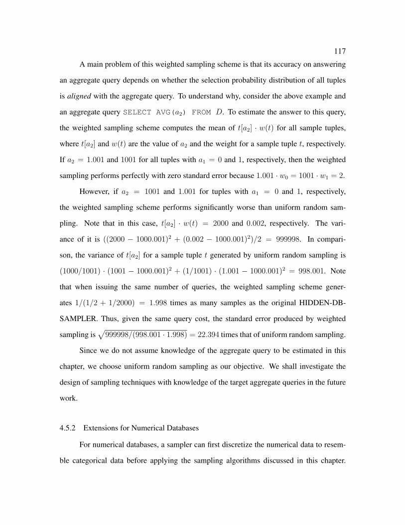
117
A main problem of this weighted sampling scheme is that its accuracy on answering
an aggregate query depends on whether the selection probability distribution of all tuples
is aligned with the aggregate query. To understand why, consider the above example and
an aggregate query SELECT AVG(a2) FROM D. To estimate the answer to this query,
the weighted sampling scheme computes the mean of t[a2] · w(t) for all sample tuples,
where t[a2] and w(t) are the value of a2 and the weight for a sample tuple t, respectively.
If a2 = 1.001 and 1001 for all tuples with a1 = 0 and 1, respectively, then the weighted
sampling performs perfectly with zero standard error because 1.001 · w0 = 1001 · w1 = 2.
However, if a2 = 1001 and 1.001 for tuples with a1 = 0 and 1, respectively,
the weighted sampling scheme performs significantly worse than uniform random sam-
pling. Note that in this case, t[a2] · w(t) = 2000 and 0.002, respectively. The vari-
ance of it is ((2000 − 1000.001)2 + (0.002 − 1000.001)2)/2 = 999998. In compari-
son, the variance of t[a2] for a sample tuple t generated by uniform random sampling is
(1000/1001) · (1001 − 1000.001)2 + (1/1001) · (1.001 − 1000.001)2 = 998.001. Note
that when issuing the same number of queries, the weighted sampling scheme gener-
ates 1/(1/2 + 1/2000) = 1.998 times as many samples as the original HIDDEN-DB-
SAMPLER. Thus, given the same query cost, the standard error produced by weighted
sampling is√
999998/(998.001 · 1.998) = 22.394 times that of uniform random sampling.
Since we do not assume knowledge of the aggregate query to be estimated in this
chapter, we choose uniform random sampling as our objective. We shall investigate the
design of sampling techniques with knowledge of the target aggregate queries in the future
work.
4.5.2 Extensions for Numerical Databases
For numerical databases, a sampler can first discretize the numerical data to resem-
ble categorical data before applying the sampling algorithms discussed in this chapter.

118
However, different discretization techniques have different impact on the performance of
sampling. Given our preference of minimizing n0 to reduce the quest cost, a equal-size
discretization might be preferred. Nonetheless, how to determine the optimal number of
intervals and choose an optimal discretization scheme is left as an open problem.
4.6 Experimental Results
In this section, we describe our experimental setup and compare our TURBO-DB-
SAMPLER and TURBO-DB-STATIC with the exiting HIDDEN-DB-SAMPLER [18] and
HYBRID-SAMPLER algorithms [36].
4.6.1 Experimental Setup
Hardware: All experiments were on a machine with Intel Xeon 2GHz CPU with 4GB
RAM and Windows XP operating system. The sampling algorithms were implemented
using C# and Matlab.
Yahoo! Auto Dataset: The Yahoo! Auto dataset consists of data crawled from a real-world
hidden database at http://autos.yahoo.com/. In particular, it contains 200,000 used cars for
sale in the Dallas-Fort Worth metropolitan area. There are 32 Boolean attributes, such as
A/C, Power Locks, etc, and 6 categorical attributes, such as Make, Model, Color, etc. The
domain size of categorical attributes ranges from 5 to 447.
System Implementation: We set k = 100. Since the database query processing technique
is relatively deterministic, we implemented our own in-memory database engine using Mat-
lab. All tuples are ranked lexicographically.
Parameter Settings: The experiments involve four algorithms: HIDDEN-DB-SAMPLER
[18], HYBRID-SAMPLER [36], as well as TURBO-DB-SAMPLER and TURBO-DB-
STATIC introduced in this chapter. TURBO-DB-SAMPLER and TURBO-DB-STATIC
require one parameter: the cutoff level C for switching from sampling to crawling. We

119
conducted experiments with various values of C ranging from 5 to 15. HIDDEN-DB-
SAMPLER also requires the cut-off level C as a parameter to balance between efficiency
and skew. Following the heuristic in [18], we set C for HIDDEN-DB-SAMPLER to be the
average length of random walks that reach a valid query. HYBRID-SAMPLER requires
two parameters: the number of pilot samples s1 and the switching count threshold cS. We
set s1 = 20 and cS = 5.
Performance Measures: For each algorithm, there are two performance measures: effi-
ciency and skew. Efficiency of a sampling algorithm was measured by counting the number
of unique queries that were executed to reach a certain desired sample size. For measur-
ing the skew of collected samples, there has not been a widely accepted measure. Thus,
we follow the same measure as [18] which compares the marginal frequencies of attribute
values in the original dataset and in the sample:
skew =
√√√√∑v∈V
(1− pS(v)
pD(v)
)2
|V |. (4.23)
Here V is a set of values with each attribute contributing one representative value, and pS(v)
(resp. pD(v)) is the relative frequency of value v in the sample (resp. dataset). Again, even
unskewed samples may have small but possibly non-zero value of the measure.
4.6.2 Comparison with State-of-The-Art Samplers
We tested TURBO-DB-SAMPLER and TURBO-DB-STATIC on the Yahoo! Auto
dataset and compared them against HIDDEN-DB-SAMPLER and HYBRID-SAMPLER
in terms of the tradeoff between efficiency and skew. Figure 4.3 depicts the results. For
TURBO-DB-SAMPLER, we set C to be the average length from the root to the designated
query of a tuple. For TURBO-DB-STATIC, we setC to be the maximum value that satisfies
the requirement of k ·π(C) ≤ n. The different points in the figure are generated by varying
the number of sample tuples to be collected between 1 and 500. One can see from the
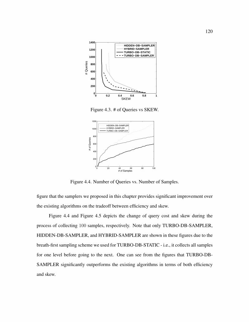
120
0 0.2 0.4 0.6 0.8 10
200
400
600
800
1000
1200
1400
# Q
uerie
s
SKEW
HIDDEN−DB−SAMPLERHYBRID−SAMPLERTURBO−DB−STATICTURBO−DB−SAMPLER
Figure 4.3. # of Queries vs SKEW.
0 20 40 60 80 1000
200
400
600
800
1000
1200
# of Samples
# of
Que
ries
HIDDEN−DB−SAMPLERHYBRID−SAMPLERTURBO−DB−SAMPLER
Figure 4.4. Number of Queries vs. Number of Samples.
figure that the samplers we proposed in this chapter provides significant improvement over
the existing algorithms on the tradeoff between efficiency and skew.
Figure 4.4 and Figure 4.5 depicts the change of query cost and skew during the
process of collecting 100 samples, respectively. Note that only TURBO-DB-SAMPLER,
HIDDEN-DB-SAMPLER, and HYBRID-SAMPLER are shown in these figures due to the
breath-first sampling scheme we used for TURBO-DB-STATIC - i.e., it collects all samples
for one level before going to the next. One can see from the figures that TURBO-DB-
SAMPLER significantly outperforms the existing algorithms in terms of both efficiency
and skew.

121
20 40 60 80 100
0.1
0.15
0.2
0.25
# Samples
SK
EW
HIDDEN−DB−SAMPLERHYBRID−SAMPLERTURB−DB−SAMPLER
Figure 4.5. Level of Skew vs. Number of Samples.
7 8 9 10 11 12 13 14 15
100
200
300
400
500
Que
ries
C7 8 9 10 11 12 13 14 15
0.1
0.15
0.2
0.25
# Sk
ew
Figure 4.6. Change of C for TURBO-DB-SAMPLER.
5 6 7 8 9 100
1000
2000
Que
ries
C5 6 7 8 9 10
0
0.1
0.2
# S
kew
Figure 4.7. Change of C for TURBO-DB-STATIC.
122
4.6.3 Evaluation of Parameter Settings
We now investigate the change of efficiency and skew of our algorithms with the cut-
off level parameter C. Figure 4.6 depicts the change of query cost and skew for TURBO-
DB-SAMPLER to collect 100 samples when C varies between 7 and 15. One can see
that while the skew is reduced when C increases, the number of queries remain roughly
constant for different values of C. This is because with a larger C, while the OVERFLOW-
SAMPLER part of TURBO-DB-SAMPLER needs to issue more queries due to the re-
duced acceptance probability, the CONCATENATE-SAMPLER part, however, requires
fewer queries because the subtree that needs to be crawled becomes smaller.
Figure 4.7 depicts the change of query cost and skew for TURBO-DB-STATIC to
collect 100 samples when C varies between 5 and 10 (the maximum value allowed by the
algorithm requirement of k ·π(C) ≤ n). One can see that unlike TURBO-DB-SAMPLER,
a larger value of C reduces both skew and query cost for TURBO-DB-STATIC. This is
because when C is too small (e.g., 5 or 6 in our dataset), the query cost is dominated
by crawling, the cost of which can be significantly reduced with a larger C. The value
assignment of C we suggested in the chapter is 10 for this dataset which, as one can see
from the figure, achieves a fairly good tradeoff between efficiency and skew.
4.7 Related Work
Crawling and Sampling from Hidden Databases: There has been prior work on crawl-
ing as well as sampling hidden databases using their public search interfaces. [17, 25, 26]
deal with extracting data from structured hidden databases. [27] and [28] use query based
sampling methods to generate content summaries with relative and absolute frequencies
while [29, 30] uses two phase sampling method on text based interfaces. On a related
front [31, 32] discuss top-k processing which considers sampling or distribution estima-
123
tion over hidden sources. A closely related area of sampling from a search engines in-
dex using a public interface has been addressed in [8] and more recently [9, 33]. In [18]
and [36] the authors have developed techniques for random sampling from structured hid-
den databases leading to the HIDDEN-DB-SAMPLER, COUNT-BASED-SAMPLER, and
HYBRID-SAMPLER algorithms.
Approximate Query Processing and Database Sampling: Approximate query process-
ing (AQP) for decision support, especially sampling-based approaches for relational databa-
ses, has been the subject of extensive recent research; e.g., see tutorials by Das [20] and
Garofalakis et al [7], as well as [21] and the references therein.
4.8 Conclusion
In this paper, we investigated techniques which leverage overflowing queries to ef-
ficiently sample a hidden database. In particular, we proposed TURBO-DB-SAMPLER
which significantly improves sampling efficiency while allowing much smaller skew than
state-of-the-art samplers. We also proposed TURBO-DB-STATIC, an algorithm that achieves
additional speedup for databases with static scoring functions. Our thorough experimental
study demonstrates the superiority of our sampling algorithms over the existing algorithms.

124
Algorithm 9 TURBO-DB-STATIC1: Set h = 0. Λ(i) = ρ(0, i) for i ∈ [0,m− 1]. W [i] = ∅ for i ∈ [1, s].
2: for all i ∈ [1, s] with W [i] = ∅ do
3: With probability of 1− Λ(h)/n, Goto 16 for the next loop.
4: Randomly choose a query q from Level h. With probability of card(q)/k, ran-
domly pick a tuple from the result of q as t.
5: if a valid or underflowing ancestor of q was issued then
6: Goto 4 if t = ∅.
7: else if q is valid or underflowing then
8: for i = h+ 1 to m do Λ(i) = Λ(i)− ρ(h, i) + card(q)
9: end if
10: if t 6= ∅ then
11: Issue query P (q), the parent of q.
12: if t ∈ P (q) then with probability of Λ(h)/n, Goto 4.
13: else Set W [i] = t.
14: end if
15: end if
16: end for
17: if Λ(h+ 1) ≤ n then
18: Set h = h+ 1, Goto 2
19: end if //below switch to CONCATENATE-SAMPLER
20: Randomly select an overflowing query q from Level h.
21: Crawl the subtree of q with nT tuples below Level h.
22: With probability of nT/n0, return a tuple chosen uniformly at random from the nT
tuples, otherwise Goto 20.

CHAPTER 5
UNBIASED ESTIMATION OF SIZE AND OTHER AGGREGATES OVERHIDDEN DATABASES
5.1 Introduction
In this chapter, we develop novel techniques to answer various types of aggregate
queries, such as database size, over hidden web databases. Our techniques are efficient and
provide estimates with small error. Most importantly, our estimations are unbiased, which
none of the existing non-crawling techniques can achieve.
Hidden databases: Hidden databases are widely prevalent on the web. They feature re-
strictive form-like interfaces which allow users to form a search query by specifying the
desired values for one or a few attributes, and the system returns a small number of tuples
satisfying the user-specified selection conditions. Due to limitations of a web interface,
the number of returned tuples is usually restricted by a top-k constraint - when more than
k tuples in the database match the specified condition, only k of them are preferentially
selected by a ranking function and returned to the user.
Problem Definition: The problem we consider in this chapter is how to use the web inter-
face to estimate the size and other aggregates of a hidden database:
• Estimating the number of tuples in a hidden database is by itself an important problem.
Many hidden databases today advertise their (large) sizes on public venues to attract
customers. However, the accuracy of such a published size is not (yet) verifiable, and
sometimes doubtful, as the hidden database owners have the incentive to exaggerate
their sizes to attract access. Furthermore, many hidden databases, such as the job-
125
126
hunting monster.com, do not publicize their total sizes, while such information can be
useful to the general public as an economic indicator for monitoring job growth.
• More generally, the ability to approximately answer aggregate queries can enable a
wide range of third-party data analytics applications over hidden databases. For ex-
ample, aggregates may reveal the quality, freshness, content bias and size of a hidden
database, and can be used by third-party applications to preferentially select a hidden
database with the best quality over other hidden databases.
Challenges: A simple approach to obtain the size of a hidden database is to crawl all tuples
and then count them. A number of techniques have been proposed for the crawling of
hidden databases [25,26,40]. This approach, however, requires an extremely large amount
of queries to be issued through the web interface. Such a high query cost is infeasible in
practice because most hidden databases impose a per-user/IP limit on the number of queries
one can issue. For example, Yahoo! Auto, a popular hidden database, has a limit of 1,000
queries per IP address per day.
Capture-recapture is another approach extensively studied in the field of statistics for
population size estimation [41], and has been recently used to estimate the size of a search
engine’s corpus [42–44]. This approach is built upon the sampling of a population, and es-
timates the population size according to the recaptures counts of entities being sampled. In
particular, for a population of m entities, the capture-recapture approach requires a sample
of size Ω(√m) to form a reasonable estimation.
However, applying capture-recapture over the existing sampling techniques for hid-
den databases leads to two problems, on estimation error and query cost, respectively. First,
127
the estimations generated this way are biased and may have high variance1. Not only is the
capture-recapture approach in general known to produce biased estimations with high vari-
ance for large populations [41], but all underlying sampling techniques in the literature for
hidden databases are also biased with the bias unknown [18, 36]2. For many data analytics
applications (e.g., to fairly compare the hidden database size of competing providers), how-
ever, the unbiasedness of an estimator is a requirement that cannot be waived. In addition,
the estimation variance must be clearly understood and minimized to derive a meaning-
ful confidence interval for the estimation. This cannot be achieved by directly applying
capture-recapture over existing hidden database sampling techniques.
Furthermore, to enable an accurate estimation, capture-recapture requires an intoler-
ably large number of queries to be issued. This is due to a distinct challenge for sampling
hidden databases, i.e., the significant difference between the size of the database and the
set of all possible queries [18, 36]. Such a drastic difference stands in contrast to sampling
a search engine’s corpus, for which a common assumption is the existence of a (reasonably
small) pool of queries that recall almost all documents [8, 9, 39]. Due to such drastic dif-
ference, each of the Ω(√m) sample tuples requires a small but non-negligible number of
queries to generate. As a result, the capture-recapture approach requires a very large query
cost over hidden databases which renders it impractical.
Similar to the challenges for estimating the hidden database size, significant obstacles
are present for estimating aggregates over a hidden database. The existing sampling-based
techniques are not designed to answer aggregate queries, but to sample all tuples with equal
1A random estimator θ for an aggregate θ is considered to be biased if E[θ] 6= θ. The mean
squared error of the estimator is defined as E[(θ − θ)2], which is the same as the variance of θ for
an unbiased estimator. It is usually desirable for estimators to be unbiased and have small variance.2Excluded from consideration here are sampling techniques designed under the assumption that
the hidden database truthfully disclose its size e.g., [36].

128
probability. Thus, while these techniques may support an estimation of AVG queries, they
cannot answer SUM or COUNT queries. Furthermore, even when the precise database size
is given, one still cannot generate unbiased estimates from these techniques because the
sampling is performed with a biased selection probability distribution over all tuples, and
moreover the bias is unknown.
Outline of Technical Results: In this chapter we initiate a study of estimating, without
bias, the size and other aggregates over a hidden database. For size estimation, our main
result is HD-UNBIASED-SIZE, an unbiased estimator with provably bounded variance.
For estimating other aggregates, we extend HD-UNBIASED-SIZE to HD-UNBIASED-
AGG which produces unbiased estimations for aggregate queries.
HD-UNBIASED-SIZE is based on performing random walks over the query space,
by starting with a query with very broad selection conditions, and drilling down by adding
random conjunctive constraints to the selection condition, until the query selects at most k
tuples. It features three key ideas: backtracking, weight adjustment, and divide-&-conquer.
Backtracking enables the unbiasedness of estimation. Weight adjustment and divide-&-
conquer both reduce the estimation variance, with divide-&-conquer delivering the most
significant reduction for real-world hidden databases.
Backtracking applies when the random walk hits an empty query. Instead of com-
pletely restarting the walk, we backtrack to the previous query and attempt adding another
constraint, in order to ensure that each trial of the random walk ends with a non-empty
query. The key implication of backtracking is that it enables the precise computation of the
selection probability for the returned tuples. As a result, HD-UNBIASED-SIZE is capable
of generating an unbiased estimation for the database size.
We note that there is a key difference between backtracking-enabled random walks
and the existing sampling techniques over hidden databases. The existing techniques aim
129
to produce uniform random samples but eventually fall short with unknown bias. In com-
parison, our random walk intentionally produces biased samples, but the bias of the sample
is precisely known. As a result, our estimation technique is capable of completely cor-
recting the sampling bias and producing unbiased estimations of database size and other
aggregates.
While a backtracking-enabled random walk produces no bias, the variance of its esti-
mation may be large when the underlying data distribution is highly skewed. The objective
of weight adjustment is to reduce the estimation variance by “aligning” the selection prob-
ability of tuples in the database to the distribution of measure attribute (to be aggregated).
For our purpose of estimating the database size, the measure attribute distribution is uni-
form (i.e., 1 for each tuple). Thus, we adjust the transitional probability in the random walk
based on the density distribution of “pilot” samples collected so far. After weight adjust-
ment, each random walk produces an unbiased estimate with gradually reduced variance.
While weight adjustment has the estimation variance converging to 0, the conver-
gence process may be slow for a database that is much smaller than its domain size (i.e.,
the set of all possible tuples). Divide-&-conquer is proposed to address this problem by
carefully partitioning the database domain into a large number of subdomains, such that
the vast majority of tuples belong to a small number of subdomains. Then, we perform ran-
dom walks over certain subdomains and combine the results for estimation of the database
size. The reduced size mismatch between the (sub-) query space and the database signif-
icantly reduces the final estimation variance, while only a small number of subdomains
need to be measured, leading to very small increase on query cost.
A major contribution of this chapter is also a theoretical analysis of the quantita-
tive impact of the above ideas on reducing variance. We also describe a comprehensive
set of experiments that demonstrate the effectiveness of HD-UNBIASED-SIZE and HD-
UNBIASED-AGG over both synthetic and real-world datasets, including experiments of

130
directly applying these algorithms over the web interface of a popular hidden database
websites, Yahoo! Auto.
In summary, the main contributions of this chapter are as follows:
• We initiate the study of unbiased estimation of the size and other aggregates over a
hidden database through its restrictive web interface.
• We propose a backtracking-enabled random walk technique to estimate hidden database
size and other aggregates without bias. To the best of our knowledge, this is the first
time an aggregate can be estimated without bias over a hidden database.
• We also propose two other techniques, weight adjustment and divide-&-conquer, to
reduce the estimation variance.
• We combine the three techniques to produce HD-UNBIASED-SIZE, an efficient and
unbiased estimator for the hidden database size. Similarly, we propose HD-UNBIASED-
AGG which supports various aggregate functions and selection conditions.
• We provide a thorough theoretical analysis and experimental studies that demonstrate
the effectiveness of our proposed approach over real-world hidden databases.
Chapter Organization: The rest of this chapter is organized as follows. In Section 2
we introduce preliminaries and discuss simple but ineffective algorithms for aggregate
estimation over hidden databases. Sections 3 and 4 are devoted to the development of
HD-UNBIASED-SIZE, focusing on achieving unbiasedness and reducing variance, respec-
tively. In Section 5 we discuss the parameter settings for HD-UNBIASED-SIZE and extend
it to HD-UNBIASED-AGG. Section 6 contains a detailed experimental evaluation of our
proposed approaches. Section 7 discusses related work, followed by conclusion in Section
8.
131
5.2 Preliminaries
5.2.1 Models of Hidden Databases
We restrict our discussion in this chapter to categorical data - we assume that numer-
ical data can be appropriately discretized to resemble categorical data, and exclude tuples
with null values from consideration. Consider a hidden database table D with m tuples
t1, . . . , tm and n attributes A1, . . . , An. We assume no duplicate tuple exists in D. Let
Dom(·) be a function that returns the domain of one or more attributes. As such, Dom(Ai)
represents the domain of Ai, and Dom(Ai, Aj) represents the Cartesian product of the do-
mains of Ai and Aj . |Dom(Ai)| represents the cardinality of Dom(Ai), i.e., the number of
possible values of Ai.
The table is only accessible to users through a web-based interface. We assume a
prototypical interface where users can query the database by specifying values for a subset
of attributes. Thus a user query q is of the form:
SELECT ∗ FROM D WHERE Ai1 = vi1& . . .&Ais = vis ,
where vij is a value from Domij .
Let Sel(q) be the set of tuples in D that satisfy q. As is common with most web
interfaces, we shall assume that the query interface is restricted to only return k tuples,
where k m is a pre-determined small constant (such as 10 or 50). Thus, Sel(q) will
be entirely returned iff |Sel(q)| ≤ k. If the query is too broad (i.e., |Sel(q)| > k), only
the top-k tuples in Sel(q) will be selected according to a ranking function, and returned as
the query result. The interface will also notify the user that there is an overflow, i.e., that
not all tuples satisfying q can be returned. At the other extreme, if the query is too specific
and returns no tuple, we say that an underflow occurs - i.e., the query is empty. If there is
neither overflow nor underflow, we have a valid query result. Without causing confusion,

132
we also use q to represent the set of tuples returned by q. Note that the number of returned
tuples |q| = min(k, |Sel(q)|).
For the purpose of this chapter, we assume that a restrictive interface does not allow
users to “scroll through” the complete answer Sel(q) when q overflows. Instead, the user
must pose a new query by reformulating some of the search conditions. This is a reason-
able assumption because many real-world top-k interfaces (e.g., Google) only allow “page
turns” for limited (e.g., 100) times.
A running example: Table 5.1 depicts a simple table which we shall use as a running
example throughout this chapter. There are m = 6 tuples and n = 5 attributes, including
four Boolean (A1, . . . , A4) and one categorical (A5 ∈ [1, 5], only 1 and 3 appear in the
table).
Table 5.1. Example: Input Table
A1 A2 A3 A4 A5
t1 0 0 0 0 1t2 0 0 0 1 1t3 0 0 1 0 1t4 0 1 1 1 1t5 1 1 1 0 3t6 1 1 1 1 1
5.2.2 Performance Measures
We consider the estimation of aggregate queries with conjunctive conditions of the
form SELECT AGGR(Aj) FROM D WHERE Ai1 = vi1& . . .&Ais = vis where AGGR
is the aggregate function. For example, such an aggregate query might be the number of
tuples in the database which we focus on for most part of the chapter. It may also be the
133
SUM of prices for all inventory cars of a car dealership’s hidden database (i.e., the inventory
balance).
An aggregate estimation algorithm for hidden databases should be measured in terms
of estimation accuracy and query efficiency:
• Estimation Accuracy: The mean squared error of an estimator is a composition of
its bias and variance. Consider an estimator θ for an aggregate θ. Then MSE(θ) =
E[(θ−θ)2] = E[(θ−E(θ))2]+(E[θ]−θ)2 = Var(θ) + Bias2(θ), whereE[·] represents
expected value. The task is to design unbiased estimators with minimum variance.
• Query Efficiency: Many hidden databases impose limits on the number of queries
from a user. The task is to minimize the number of queries issued through the web
interface to achieve a given level of estimation accuracy.
5.2.3 Simple Aggregate-Estimation Algorithms
BRUTE-FORCE-SAMPLER: This algorithm randomly composes a fully-specified query
A1 = v1, . . . , An = vn by generating each vi from Dom(Ai) uniformly at random. There
are two possible outcomes: either underflow or valid. After repeating this process for h
times, let hV be the number of tuples found. Then, one can estimate the database table
size as m = |Dom(A1, . . . , An)| · hV/h. It is easy to see that this process will produce
an unbiased estimate. Other aggregates can be estimated without bias in a similar way.
However, BRUTE-FORCE-SAMPLER is extremely inefficient because the probability for
a fully-specified query to return valid is extremely small (i.e., m |Dom(A1, . . . , An)|)
[18].
CAPTURE-&-RECAPTURE: The Lincoln-Petersen model [45] is a well-known capture-
&-recapture estimator for the size of a closed population. Consider the case where we
collect two samples, C1 and C2, of a hidden database. The Lincoln-Peterson estimator
gives m = |C1| · |C2|/|C1 ∩ C2| where |Ci| is the number of tuples in Ci and |C1 ∩ C2|

134
is the number of tuples that appear in both samples. The estimation tends to be positively
biased [41]. One can see that the estimator only works when each sample includes (at least)
Ω(√m) tuples, which leads to an extremely expensive process for hidden databases.
5.2.4 Hidden Database Sampling
The basic idea behind the HIDDEN-DB-SAMPLER [18] and its extension HYBRID-
SAMPLER [36] is to perform a random drill-down starting with extremely broad (and thus
overflowing) queries, and iteratively narrowing it down by adding randomly selected pred-
icates, until a valid query is reached. In particular, consider a Boolean database. The
sampler starts with query SELECT * FROM D. If the query overflows, it is expanded by
adding a randomly selected predicate on a1 (either “a1 = 0” or “a1 = 1”). If the expanded
query still overflows, we further expand it by adding random predicates for a2, . . . , an
respectively one at a time. This random walk process leads us to either a valid or an under-
flowing query. If it reaches an underflow, we restart the random walk. If the process reaches
a valid query, we randomly choose a returned tuple and include it in the sample. Since this
random walk process more likely chooses tuples returned by “short” valid queries, we have
to apply rejection sampling at the end of the random walk. In particular, a sample tuple is
rejected with probability 1 − C/2h, where C is a pre-determined parameter and h is the
number of predicates in the query from which the tuple is retrieved.
5.3 Unbiasedness for Size Estimation
In this section, we develop the main ideas that enable the unbiasedness of estimation
for the size of a hidden database.
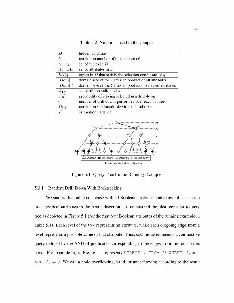
135
Table 5.2. Notations used in the Chapter
D hidden databasek maximum number of tuples returnedt1....tm set of tuples in DA1....An set of attributes in DSel(q) tuples in D that satisfy the selection conditions of q|Dom| domain size of the Cartesian product of all attributes|Dom(·)| domain size of the Cartesian product of selected attributesΩTV set of all top-valid nodesp(q) probability of q being selected in a drill downr number of drill downs performed over each subtreeDUB maximum subdomain size for each subtrees2 estimation variance
A1
A2
A3
A4
q2
q1
q3
q4
T
T
TT TT
T : Top-valid query: Valid query : Underflow: Overflow
q'2
q'1
t1 t2 t3 t4 t5 t6
0 1
0 1
0 1 0 1
0 1 0 1 0 1 0 1 0 1 0 1 0 1 10
0 10 1
0 1
branches initially chosen at random
Figure 5.1. Query Tree for the Running Example.
5.3.1 Random Drill-Down With Backtracking
We start with a hidden database with all Boolean attributes, and extend this scenario
to categorical attributes in the next subsection. To understand the idea, consider a query
tree as depicted in Figure 5.1 (for the first four Boolean attributes of the running example in
Table 5.1). Each level of the tree represents an attribute, while each outgoing edge from a
level represents a possible value of that attribute. Thus, each node represents a conjunctive
query defined by the AND of predicates corresponding to the edges from the root to this
node. For example, q2 in Figure 5.1 represents SELECT * FROM D WHERE A1 = 1
AND A2 = 0. We call a node overflowing, valid, or underflowing according to the result

136
of its corresponding query. Figure 5.1 shows the class of each node when k = 1. We also
introduce the definition of a top-valid node:
Definition 5.3.1. [Top-Valid Query] Given a query tree, a valid query is top-valid iff its
parent is overflowing.
All top-valid queries in Figure 5.1 are marked with symbol T. One can see from
this definition that each tuple belong to one and only one top-valid node. For example,
Figure 5.1 has 6 top-valid queries corresponding to 6 tuples as k = 1.
The main process of BOOL-UNBIASED-SIZE is a random procedure which sam-
ples top-valid nodes with certain probability distribution. If we know the probability p(q)
for each top-valid node q to be chosen, then for any sample node q, we can generate an
unbiased estimation for the database size as |q|/p(q), where |q| is the number of tuples
returned by q.
Following this basic idea, BOOL-UNBIASED-SIZE consists of two steps: The first
is a random drill-down process over the query tree to sample a top-valid node. The second is
to compute p(q) for the sampled node. The entire process can be repeated for multiple times
to reduce the variance of estimation. Both steps may require queries to be issued through
the interface of the hidden database. We describe the two steps respectively as follows,
with the pseudocode summarized in Figure 10. Note that the two steps are interleaved in
the pseudocode.
The random drill-down process starts from the root node. We choose a branch uni-
formly at random and issue the corresponding query q. There are three possible outcomes:
• If q overflows, we further drill down the tree by selecting each branch of q with equal
probability.
• If q is valid, i.e., it returns |q| (1 ≤ |q| ≤ k) tuples without an overflow flag, then we
conclude the random walk.

137
Algorithm 10 BOOL-UNBIASED-SIZE
1: q ← root node. p← 1. i← 1.
2: Randomly generate v ∈ 0, 1.
3: Issue q′ ← q ∧ (Ai = v). . for Step 1 (random drill-down)
4: if q′ underflows then
5: q ← q ∧ (Ai = 1− v). Goto 2. . Backtracking
6: else if q′ overflows then
7: Issue q ∧ (Ai = 1− v). . for Step 2 (computing p(q))
8: if q ∧ (Ai = 1− v) is nonempty then
9: p← p/2. . Update p(q)
10: end if
11: q ← q′. i← i+ 1. Goto 2.
12: end if
13: return m← |q|/p. . Return an estimation for database size
• If q underflows, then we backtrack by considering q′, the sibling of q - i.e., the node
that shares the same parent with q. For example, the sibling of q2 in Figure 5.1 is
q′2. Note that the parent of q must be overflowing because otherwise the drill-down
process will terminate before reaching q. Thus, q′ must overflow. We randomly
choose a branch coming out of q′ and follow it to further drill down the tree.
One can see that a drill-down process always terminates with a top-valid node. An
example of a random drill-down is shown in Figure 5.1 with bold edges representing the
branches that were initially chosen at random. In this example, backtracking happens when
q2 was chosen - since q2 overflows, we backtrack and continue drilling down from its sib-
ling node q′2. Note that with backtracking, a top-valid node like q4 may be reached under

138
multiple possibilities of the initially chosen branches. For example, when q1, q′2, q3, q4 were
initially chosen, q4 would also be reached by the drill-down.
We now consider the second step which computes p(q). Note that there is a unique
path from the root node to a top-valid node q - for a random drill-down to reach q, although
edges on this path might not be initially chosen, they must be finally followed (after back-
tracking). For example, such a path for q4 in Figure 5.1 goes through q1, q′2, q3 in order. For
each edge of the path, there are only two possible scenarios for choosing between the edge
and its sibling (from which the drill-down must choose one to follow):
• Scenario I: Both branches are non-underflowing. In this case, each branch is chosen
with 50% probability. The selection between q1 and q′1 in Figure 5.1 is an example of
this scenario.
• Scenario II: One branch is overflowing while the other is underflowing. In this case,
the overflowing branch will always be chosen. The selection between q2 and q′2 in
Figure 5.1 is an example of this scenario, and q′2 is always chosen.
In order to compute p(q), we must know which scenario occurs for each level from
the root to q. This may or may not require additional queries to be issued. In particular, no
additional query is needed for the last level before reaching q, as Scenario 1 always occurs
there. No query is needed for levels when backtracking applies either, because one branch
must underflow. However, for any other level, we must issue the sibling query to determine
the correct scenario. Consider the bold edges in Figure 5.1. Since q1 was selected during
random drill-down, we do not know whether q′1 is underflowing (Scenario I) or not (II).
Thus, we must now issue q′1 to determine which scenario actually occurred.
After learning the number of occurrences for Scenarios I and II, we can then compute
p(q). For a query q with h predicates, let h1 and h − h1 be the number of occurrences for
Scenario I and II, respectively. We have p(q) = 1/2h1 . For example, q4 in Figure 5.1 has
h1 = 2 (i.e., while issuing q1 and q4) and p(q) = 1/4, leading to an estimation of |q|/p(q) =

139
4. Note that this estimation is an instantiation of the Horvitz-Thompson Estimator [46]. The
following theorem shows its unbiasedness:
Theorem 5.3.1. [Estimate (un-)Biasness] The estimate generated by the drill-down pro-
cess is unbiased, i.e., its expected value taken over the randomness of q is
E
[|q|p(q)
]= m. (5.1)
Proof. Let ΩTV be the set of all top-valid nodes in the tree. Since each tuple belongs to
one and only one top-valid node, we have∑
q∈ΩTV|q| = m. Since the random drill-down
process always terminates on a top-valid query,
E
[|q|p(q)
]=∑q∈ΩTV
p(q) · |q|p(q)
= m
5.3.2 Smart Backtracking for Categorical Data
We now discuss how to apply unbiased size estimation to a categorical database. Two
changes are required:
• First, Boolean attributes ensure that the sibling of an underflowing node always over-
flow. There is no such guarantee for categorical databases. Thus, to successfully
backtrack from an underflowing branch, we must find one of its sibling branches
that returns non-empty and count the number of such non-empty siblings (in order
to compute p(q)). Note that a non-empty branch always exists given an overflow-
ing parent node. A simple backtracking approach is to query all branches to find
the (COUNT of) non-empty ones, and then randomly choose a non-empty branch to
follow.
• The other change required is the computation of p(q). If the above-mentioned simple
backtracking is used, the computation of p(q) becomes p(q) = 1/∏h−1
i=1 ci, where

140
ci is the number of non-underflowing branches for the i-th predicate en route to the
top-valid query q.
The two changes for categorical databases do not affect the unbiasedness of the es-
timation as the proof of Theorem 5.3.1 remains unchanged. These changes, however, do
affect the query cost of the drill-down process. In particular, if the above simple back-
tracking technique is used, we must issue queries corresponding to all branches to find the
number of non-empty ones, leading to a high query cost for large-fanout attributes.
To reduce such a high query cost, we develop smart backtracking which aims to
avoid testing all branches of a high fanout attribute. Consider a categorical attributeAi with
possible values v1, . . . , vw (w = |Dom(Ai)|). Assume a total order of the values which can
be arbitrarily assigned for cardinal or ordinal attributes. In the following, we describe the
random drill-down and the computation of p(q) with smart backtracking, respectively.
To choose a branch of Ai for further drill down, we first randomly choose a branch
vj . Backtracking is required if vj underflows. With smart backtracking, we test the right-
side neighbors of vj (in a circular fashion), i.e., v(j mod w)+1, v((j+1) mod w)+1, etc, in order
until finding one that does not underflow, and follow that branch for further drill down.
Figure 6.3 (a) demonstrates the branches for the categorical attribute A5 in the running
example with w = 5. To backtrack from q4, we test q5 and then q1. Since q1 returns
nonempty, we follow branch q1 for further drill-down.
A5
q1 q2 q3 q4 q5 q1 q2 q3 q4 q5
queries issued
branch to follow
queries not issued(a) (b)
Figure 5.2. An Example of Smart Backtracking.

141
We now consider the computation of p(q). With the new strategy, the probability
for choosing a non-empty branch vj is (wU(j) + 1)/w, where wU(j) is the number of
consecutive underflowing branches immediately preceding vj (again in a circular fashion).
For example, in Figure 6.3, q1 and q5 have wU = 2 and 1, respectively. To compute wU(j),
we need to issue queries corresponding to the left-side neighbors of vj , i.e., v((j−2) mod w)+1,
v(j−3) mod w+1 etc, in order until finding a non-empty branch. Then, we learn wU(j) and is
able to compute the probability of following vj . Figure 6.3 (a) and (b) shows the queries
one needs to issue after committing to branch q1 and q3, respectively.
With smart backtracking, for a given node, the expected number of branches one
need to test is
QC = 1 +w∑j=1
(wU(j) + 1)2
w, (5.2)
where wU(j) = −1 if vj is an empty branch. For example, QC = 3.6 for A5 in Fig-
ure 6.3. For attributes with larger fanouts, smart backtracking may reduce the query cost
more significantly.
5.3.3 Discussion
5.3.3.1 Comparison with Prior Samplers
To illustrate the effectiveness of our backtracking-enabled random drill-down ap-
proach, we compare it with two prior algorithms discussed in the preliminary section:
BRUTE-FORCE-SAMPLER which also generates unbiased size estimations, and HIDDEN-
DB-SAMPLER which can be used with CAPTURE-&-RECAPTURE to produce biased
size estimations.
Comparison with BRUTE-FORCE-SAMPLER: Both our random drill-down technique
and BRUTE-FORCE-SAMPLER use a random process to select valid queries for estimat-
ing the size of a hidden database. The key difference is the success probability of such a

142
random process. As we discussed in Section 5.2, BRUTE-FORCE-SAMPLER has an ex-
tremely low success rate because the database size is usually orders of magnitude smaller
than the query space. Our approach, on the other hand, guarantees to find one (top-)valid
query in every trial of the random walk, thanks to a combination of random drill-down
and backtracking techniques. Such a difference on the success rate leads to a dramatic
difference on the query cost. For example, consider a Boolean database with m tuples, n
attributes, and k = 1. While BRUTE-FORCE-SAMPLER requires an average of 2n/m
queries to find a valid query and produce an estimate, we require at most n queries (i.e., the
longest possible drill-down) to do so.
Comparison with HIDDEN-DB-SAMPLER: There are two key differences between the
random drill-down process in our approach and that in HIDDEN-DB-SAMPLER [18]. The
first is our introduction of backtracking. With HIDDEN-DB-SAMPLER, the random drill-
down process incurs an “early termination” (i.e., restarts from the root) if it reaches an
underflowing node. As a result, one has to know the probability of early termination pE in
order to compute the probability of reaching a query q with h predicates:
p(q) =1
(1− pE) ·∏h
i=1 |Dom(Ai)|(5.3)
Unfortunately, it is extremely difficult to approximate pE to the degree that supports
an accurate estimation of p(q). The reason is that (1− pE) ≈ 0 for many hidden databases,
especially categorical ones with large fan-out attributes, whose sizes are order of magnitude
smaller than the domain of all possible values. As a result, an extremely large number of
random drill-downs must be taken before p(q) can be accurately estimated - which makes
HIDDEN-DB-SAMPLER impossible to use for estimating the database size. Our tech-
nique, on the other hand, introduces backtracking to ensure that no random drill-down ter-
minates without reaching a valid query, thereby enabling the precise computation of p(q).
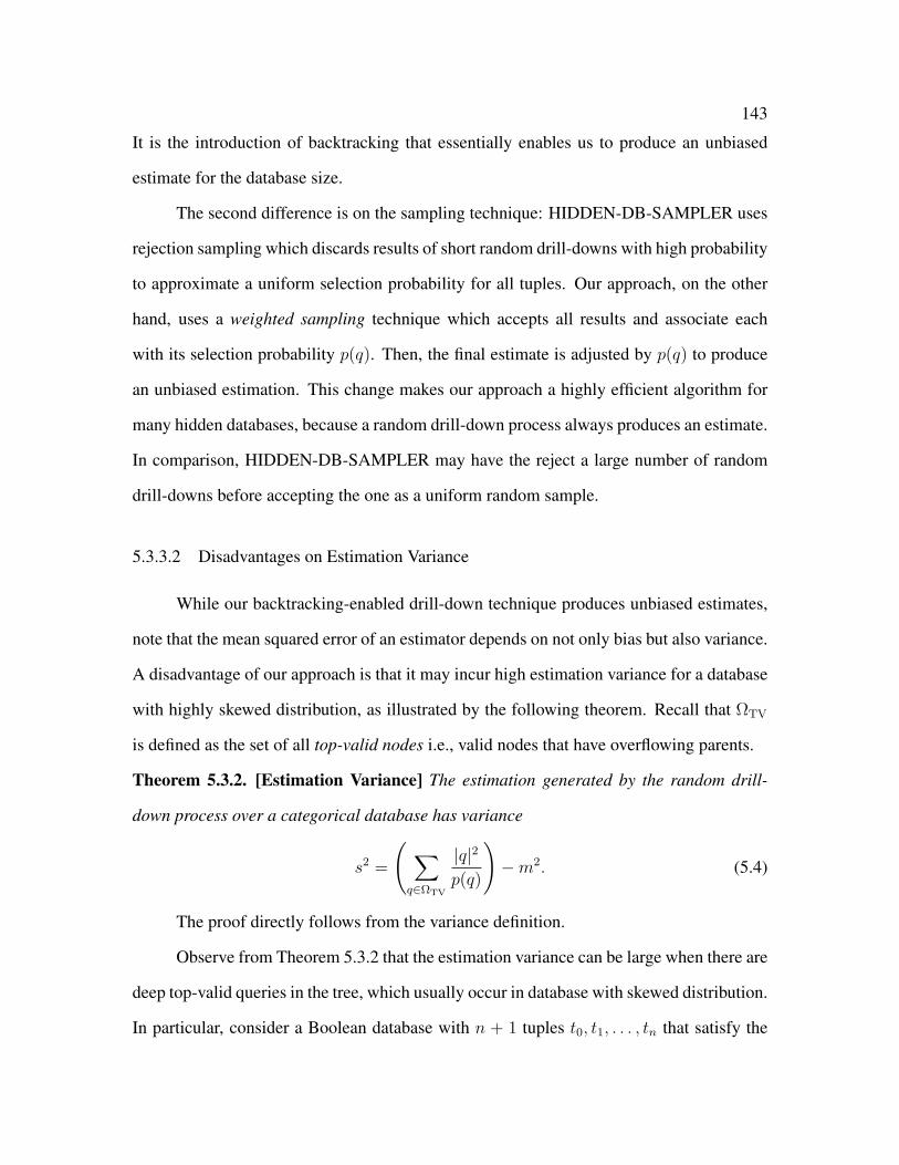
143
It is the introduction of backtracking that essentially enables us to produce an unbiased
estimate for the database size.
The second difference is on the sampling technique: HIDDEN-DB-SAMPLER uses
rejection sampling which discards results of short random drill-downs with high probability
to approximate a uniform selection probability for all tuples. Our approach, on the other
hand, uses a weighted sampling technique which accepts all results and associate each
with its selection probability p(q). Then, the final estimate is adjusted by p(q) to produce
an unbiased estimation. This change makes our approach a highly efficient algorithm for
many hidden databases, because a random drill-down process always produces an estimate.
In comparison, HIDDEN-DB-SAMPLER may have the reject a large number of random
drill-downs before accepting the one as a uniform random sample.
5.3.3.2 Disadvantages on Estimation Variance
While our backtracking-enabled drill-down technique produces unbiased estimates,
note that the mean squared error of an estimator depends on not only bias but also variance.
A disadvantage of our approach is that it may incur high estimation variance for a database
with highly skewed distribution, as illustrated by the following theorem. Recall that ΩTV
is defined as the set of all top-valid nodes i.e., valid nodes that have overflowing parents.
Theorem 5.3.2. [Estimation Variance] The estimation generated by the random drill-
down process over a categorical database has variance
s2 =
( ∑q∈ΩTV
|q|2
p(q)
)−m2. (5.4)
The proof directly follows from the variance definition.
Observe from Theorem 5.3.2 that the estimation variance can be large when there are
deep top-valid queries in the tree, which usually occur in database with skewed distribution.
In particular, consider a Boolean database with n + 1 tuples t0, t1, . . . , tn that satisfy the
144
following condition: For any ti (i ∈ [1, n]), ti has the opposite values as t0 on attributes
an−i+1, . . . , an, and the same values on all other attributes i.e., ∀j ∈ [1, n − i], t0[aj] =
ti[aj], ∀j ∈ [n − i + 1, n], t0[aj] = 1 − ti[aj]. Figure 6.4 illustrates this scenario when
k = 1. Note that all underflowing branches are omitted in the figure.
...
t1t0 t2 tn-1 tn
......
...
Figure 5.3. A Worst-Case Scenario.
One can see that, when k = 1, there are two n-predicate queries (e.g., t0 and t1) in
the tree that both are top-valid queries. Note that the value of p(q) for these two queries are
1/2n. Thus, the variance is at least s2 > 2n+1 −m2. Since the domain size is usually order
of magnitude larger than the database size i.e., 2n m, the variance can remain extremely
large even after a substantial number of random drill-downs. For example, if the database
has 40-attribute and one million tuples, at least 1012 random drill-downs are required to
reduce the variance to m2, which still leads to significant error. The following corollary
illustrates the generic case for categorical databases with an arbitrary k.
Corollary 5.3.1. [Worst-Case Estimate Variance for BOOL-UNBIASED-SIZE] The
worst-case estimate variance for an n-attribute, m-tuple hidden database with a top-k
interface satisfies
s2 > k2 ·
(n−1∏i=1
|Dom(Ai)|
)−m2. (5.5)
Due to space limitations, we do not include the proof of the corollary. Note that
this corollary shows a probabilistic lower bound which still assumes the randomness of
the drill-down process (i.e., it considers the worst-case database instance, not the worst-
case random walk). One can see from the corollary that the variance may be even more

145
significant in the generic case, because the variance increases linearly with k2. The next
section is an effort dedicated to reduce the estimation variance.
5.4 Variance Reduction
In this section, we describe two ideas to reduce the estimation variance: weight ad-
justment and divide-&-conquer.
5.4.1 Weight Adjustment
Weight adjustment is a popular technique for variance reduction in sampling tradi-
tional databases. In this subsection, we describe how weight adjustment can be applied over
hidden databases3. In particular, we show that while weight reduction in general reduces
estimation variance, the remaining variance is still significant for certain hidden databases
with highly skewed distributions.
5.4.1.1 Main Idea
The random drill-down process in BOOL-UNBIASED-SIZE essentially performs a
sampling process over all top-valid nodes of the hidden database, with varying selection
probability for different nodes. As any weighted-sampling estimator, the estimation vari-
ance is determined by the alignment between the selection probability distribution and the
3Note that while the COUNT-based sampling part of the ALERT-HYBRID algorithm [36] can
also be considered weighted sampling, the key difference between ALERT-HYBRID and the tech-
nique discussed here is how the weights are computed are the implications of imperfectly estimated
weights. In ALERT-HYBRID, the weights are estimated based on a small pool of pilot sample tu-
ples, and estimation errors on weights lead to biased samples [36]. Here, the weights are determined
by COUNT estimations from prior drill downs, and imperfectly estimated weights do not affect the
unbiasedness of BOOL-UNBIASED-SIZE.

146
distribution of the measure attribute (i.e., the attribute to be aggregated). For our purpose,
the measure aggregate is |q|, the size of a top-valid node. With BOOL-UNBIASED-SIZE,
the selection probability for q is p(q), which is generally independent of its measure at-
tribute |q|. Thus, in some cases, the selection probability may be perfectly aligned with the
measure attribute. For example, when k = 1 and all top-valid nodes have exactly log2m
predicates, we have p(q) = 1/m and 0 variance according to Theorem 5.3.2. Nonetheless,
there are also cases where these two distributions are badly misaligned which lead to an
extremely large variance. An example of such a case was depicted in Figure 6.4 - where
certain top-valid nodes reside on the leaf level, much deeper than other top-valid nodes.
The main idea of weight adjustment is to adjust the probability for following each
branch (and thereby change the eventual selection probability for top-valid nodes), so as to
better align the selection probability distribution p(q) with the distribution of |q|. The ideal
objective is to achieve the perfect alignment with 0 variance - i.e., each top-valid node q
has p(q) = |q|/m. Of course, such a perfect alignment is not possible without complete
knowledge of the measure attribute distribution. However, prior “pilot” samples can help
in estimating this distribution, as we shall discuss as follows.
To understand how to approximate this perfect alignment from the pilot samples,
consider a node qP with w branches qC1, . . ., qCw. Each branch qCi defines a subset of the
database DCi consisting of all tuples that have corresponding top-valid nodes “under” qCi.
That is, all tuples in DCi match the selection conditions of qCi. For example, in Figure 5.1,
t1, . . . , t4 are under q′1 while t5 and t6 are under q1. The optimal alignment is to select each
branch qCi with probability proportional to the size of its corresponding sub-database i.e.,
|DCi|. For example, in the running example depicted in Figure 5.1, q′1 and q1 should be
chosen with probability 4/6 and 2/6, respectively.
If the precise size of DCi is known for every branch, then the probability for each
top-valid node q to be picked up is p(q) = |q|/m, which leads to a perfect alignment that
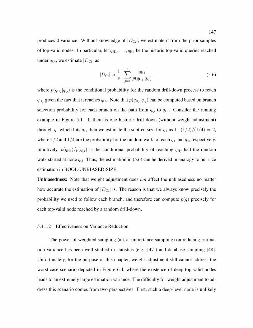
147
produces 0 variance. Without knowledge of |DCi|, we estimate it from the prior samples
of top-valid nodes. In particular, let qH1, . . . , qHs be the historic top-valid queries reached
under qCi, we estimate |DCi| as
|DCi| ≈1
s·
s∑j=1
|qHj|p(qHj|qij)
, (5.6)
where p(qHj|qij) is the conditional probability for the random drill-down process to reach
qHj given the fact that it reaches qCi. Note that p(qHj|qij) can be computed based on branch
selection probability for each branch on the path from qij to qCi. Consider the running
example in Figure 5.1. If there is one historic drill down (without weight adjustment)
through q1 which hits q4, then we estimate the subtree size for q1 as 1 · (1/2)/(1/4) = 2,
where 1/2 and 1/4 are the probability for the random walk to reach q1 and q4, respectively.
Intuitively, p(qHj)/p(qij) is the conditional probability of reaching qHj had the random
walk started at node qij . Thus, the estimation in (5.6) can be derived in analogy to our size
estimation in BOOL-UNBIASED-SIZE.
Unbiasedness: Note that weight adjustment does not affect the unbiasedness no matter
how accurate the estimation of |DCi| is. The reason is that we always know precisely the
probability we used to follow each branch, and therefore can compute p(q) precisely for
each top-valid node reached by a random drill-down.
5.4.1.2 Effectiveness on Variance Reduction
The power of weighted sampling (a.k.a. importance sampling) on reducing estima-
tion variance has been well studied in statistics (e.g., [47]) and database sampling [48].
Unfortunately, for the purpose of this chapter, weight adjustment still cannot address the
worst-case scenario depicted in Figure 6.4, where the existence of deep top-valid nodes
leads to an extremely large estimation variance. The difficulty for weight adjustment to ad-
dress this scenario comes from two perspectives: First, such a deep-level node is unlikely

148
to be reached by a historic drill-down, leading to low probability of applying the weight
adjustment in the first place. Second, even with historic trials hitting the node, the relative
error is likely to be high for estimating the size of a small subtree.
Corollary 5.4.1. [Worst-Case Estimate Variance with Weight Adjustment] For an n-
attribute, m-tuple hidden database, after r random drill-downs, the worst-case estimation
variance generated by the random-drill down with weight adjustment satisfies
s2 ≥ 2n−log2 r ·mn− log2 r + 1
−m2. (5.7)
The corollary shows the worst-case scenario still generates unacceptably high vari-
ance even after applying weight adjustment. Note that it is again a probabilistic lower
bound which assumes the randomness of the drill-down process. According to Corol-
lary 5.4.1, for a 40-attribute 100, 000-tuple database, s2 ≥ 354.29 · m2 even after 1, 000
random drill-downs have been performed.
5.4.2 Divide-&-Conquer
We now describe the idea for divide-&-conquer, a variance reduction technique
which is independent of weight adjustment but can be used in combination with it. As
mentioned in the introduction, divide-&-conquer provides the most significant variance
reduction especially for the worst-case scenarios.
5.4.2.1 Motivation and Technical Challenge
Our discussions for Corollary 5.3.1 and 5.4.1 indicate deep top-valid nodes as the
main source of high variance before and after weight adjustment, respectively. More fun-
damentally, the cause for the existence of deep top-valid queries lies on the significant
difference between the database size m and the domain size |Dom|. To understand why,
consider the case where k = 1. A deepest (i.e., leaf-level) top-valid query returns |Dom| as

149
the estimation, while the actual size is m. The following theorem further formalizes such a
fundamental cause of high variance:
Theorem 5.4.1. [Upper Bound on Estimation Variance] When k = 1, the estimation
variance of a random drill down satisfies
s2 ≤ m2 ·(|Dom|m
− 1
). (5.8)
The theorem shows a large value of |Dom|/m as a cause of high estimation variance
of HD-UNBIASED. The main motivation for divide-&-conquer is to partition the originally
large domain into smaller, mutually exclusive, subdomains so as to reduce |Dom| for the
subdomains. Note that the partitioning strategy must be carefully designed somwill not be
significantly reduced. To understand why, consider an otherwise simple strategy of dividing
the domain randomly into b mutually exclusive subdomains, using HD-UNBIASED-SIZE
to estimate each, and take the sum as the total size estimation. This partitioning strategy
reduces |Dom| and m with the same ratio b, leaving |Dom|/m unchanged. As a result,
according to Theorem 5.4.1, the total estimation variance is only reduced by a factor of
b, which is offset by the additional queries required for executing HD-UNBIASED-SIZE
over the b subdomains.
One can see that, to solve this problem, the domain must be partitioned in a way
such that while the number of subdomains may be large (such that each subdomain can be
small), the vast majority of tuples appear in only a small number of subdomains. Then, for
these subdomains, the ratio of subdomain size over the number of tuples in the subdomain
is small, allowing a reduced estimation variance for the total database size. Note that the
other sparsely packed subdomains will not adversely affect the estimation variance to a
significant degree because of the limited number of tuples contained in the subdomains.

150
A1
A2
A3
A4
T1
T2T3 T4
T5
n0
n0
qA qB
qC
t1 t2 t3 t4 t5 t6
Figure 5.4. An Example of Tree-based Partitioning.
5.4.2.2 Main Idea
To gather most tuples into a few small subdomains, we propose a query-tree-based
recursive partitioning of the domain. We start with Boolean databases and then extend the
results to categorical data at the end of this subsection. Consider the tree shown in Fig-
ure 5.1 which is also depicted in Figure 5.4. Originally, the domain includes the entire tree
which includes a top-valid node for each tuple. We partition the domain into subdomains
corresponding to subtrees with n0 levels. Figure 5.4 depicts an example of such a partition
with n0 = 3. Consider the root to be the first level. The partition generates one subtree
from the first to the n0-th level, 2n0−1 subtrees from the n0-th to the (2n0− 1)-th level, etc.
For example, T1 in Figure 5.4 is the 1-to-3 level subtree, and T2, . . . , T5 are the four 3-to-5
level subtrees. Note that the root node of a (i ·n0− i+1)-to-(i ·n0− i+n0)-th level subtree
is also a bottom-level node of a (i · n0 − 2i+ 1)-to-(i · n0 − 2i+ n0)-th level subtree. For
example, the root node of T2 is a leaf-level node of T1 in Figure 5.4. A tuple is included in a
subtree iff its corresponding top-valid node is a non-root node of the subtree. For example,
in Figure 5.4, t1 and t4 are included in T2 and T3, respectively. One can see that each tuple
belongs to one and only one subtree. Thus, the subtrees form a mutually exclusive partition
of the original domain.

151
With the subtree partitioning strategy, our size estimation algorithm can be stated
as the following recursive procedure: We start with the top-most subtree (e.g., T1 in Fig-
ure 5.4) and start to perform the random drill-down process over the subtree. In particular,
we perform r random drill-downs where r is a pre-determined parameter, the setting of
which will be discussed in Section 5.5. Note that each random drill-down may terminate
at two types of nodes: a top-valid node or a bottom-level overflowing node of the subtree,
which we refer to as a bottom-overflow node.
For each top-valid node qTV which terminates a random drill-down of the top-most
subtree, we compute δ(qTV) = r · p(qTV), where p(qTV), as defined in Section 5.3, is the
probability for a random drill-down to reach qTV. Intuitively, r · p(qTV) is the expected
number of random drill-downs that will terminate at qTV. For example, in Figure 5.4, with
r = 2 random drill-downs per subtree, we have δ(qB) = 2 · (1/4) = 1/2. Note that when
r = 1, δ(qTV) = p(qTV).
For each bottom-overflow node qBO which terminates a random drill-down of the
top-most subtree, we perform the random drill-down process over the subtree with root of
qBO, again with r drill-downs. This recursive process continues until no bottom-overflow
node is discovered. For a top-valid node q′TV captured in a subtree with root of qR, we
compute
δ(q′TV) = r · p(q′TV) · δ(qR), (5.9)
where p(q′TV) is the probability for a random drill-down over the subtree (of qR) to reach
q′TV, and δ(·) for a bottom-overflow node qR is defined in the same way as for a top-
valid node in (5.9). Again, δ(q′TV) is intuitively the expected number of drill-downs that
terminate at q′TV. For example, in Figure 5.4 with r = 2, we have δ(qA) = 1/2 and
δ(qC) = 2 · (1/2) · (1/2) = 1/2. Note that when r = 1, there is δ(q) = p(q) for all nodes

152
in all subtrees, essentially reverting the random drill-down process to the state without
divide-&-conquer.
Let QTV be the set of top-valid nodes captured by the random drill-downs over all
subtrees. We estimate the database size as
m =∑q∈QTV
|q|δ(q)
. (5.10)
The unbiasedness of this estimator follows from Theorem 5.3.1.
For categorical data, the only change required is the depth of each subtree. Instead of
having n0 levels for all subtrees, we maintain a (approximately) constant domain size for
each subtree. As a result, a categorical subtree could be shallow or deep depending on the
fan-outs of attributes involved. In particular, we set DUB as an upper bound on the domain
size (DUB ≥ maxi |Dom(Ai)|). Each subtree should have the maximum number of levels
without exceeding DUB. In the running example, if A1, . . . , A5 is the attribute order and
DUB = 10, then Levels 1-4 (i.e., A1, A2, A3 with domain size of 23 = 8) and 4-6 (i.e.,
A4, A5 with domain size of 2 × 5 = 10) become the two layers of subtrees. One can see
that the unbiasedness is unaffected by the change.
5.4.2.3 Effectiveness on Variance Reduction
Divide-&-conquer is effective on reducing the estimation variance because it pro-
vides a significantly better alignment between the selection probability distribution for top-
valid nodes and the measure attribute distribution. To understand why, consider a Boolean
database with k = 1 and two top-valid nodes q and q′, at the second level (i.e., as a child of
the root) and the bottom-level (i.e., n+1-th level), respectively. Without divide-&-conquer,
at the first drill-down, q has selection probability of 1/2 while q′ may have selection proba-
bility as small as p(q′) = 1/2n. This forms a striking contrast with the uniform distribution
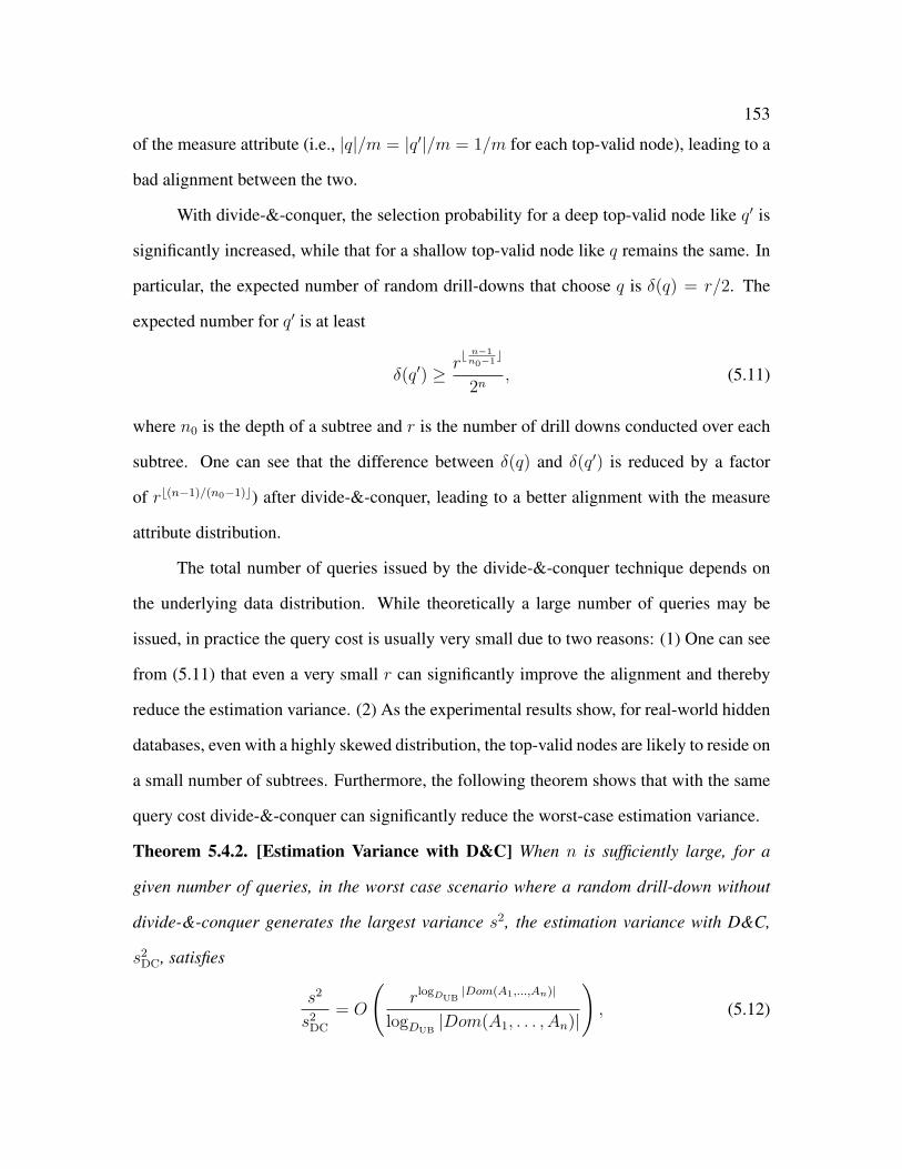
153
of the measure attribute (i.e., |q|/m = |q′|/m = 1/m for each top-valid node), leading to a
bad alignment between the two.
With divide-&-conquer, the selection probability for a deep top-valid node like q′ is
significantly increased, while that for a shallow top-valid node like q remains the same. In
particular, the expected number of random drill-downs that choose q is δ(q) = r/2. The
expected number for q′ is at least
δ(q′) ≥ rb n−1
n0−1c
2n, (5.11)
where n0 is the depth of a subtree and r is the number of drill downs conducted over each
subtree. One can see that the difference between δ(q) and δ(q′) is reduced by a factor
of rb(n−1)/(n0−1)c) after divide-&-conquer, leading to a better alignment with the measure
attribute distribution.
The total number of queries issued by the divide-&-conquer technique depends on
the underlying data distribution. While theoretically a large number of queries may be
issued, in practice the query cost is usually very small due to two reasons: (1) One can see
from (5.11) that even a very small r can significantly improve the alignment and thereby
reduce the estimation variance. (2) As the experimental results show, for real-world hidden
databases, even with a highly skewed distribution, the top-valid nodes are likely to reside on
a small number of subtrees. Furthermore, the following theorem shows that with the same
query cost divide-&-conquer can significantly reduce the worst-case estimation variance.
Theorem 5.4.2. [Estimation Variance with D&C] When n is sufficiently large, for a
given number of queries, in the worst case scenario where a random drill-down without
divide-&-conquer generates the largest variance s2, the estimation variance with D&C,
s2DC, satisfies
s2
s2DC
= O
(rlogDUB
|Dom(A1,...,An)|
logDUB|Dom(A1, . . . , An)|
), (5.12)
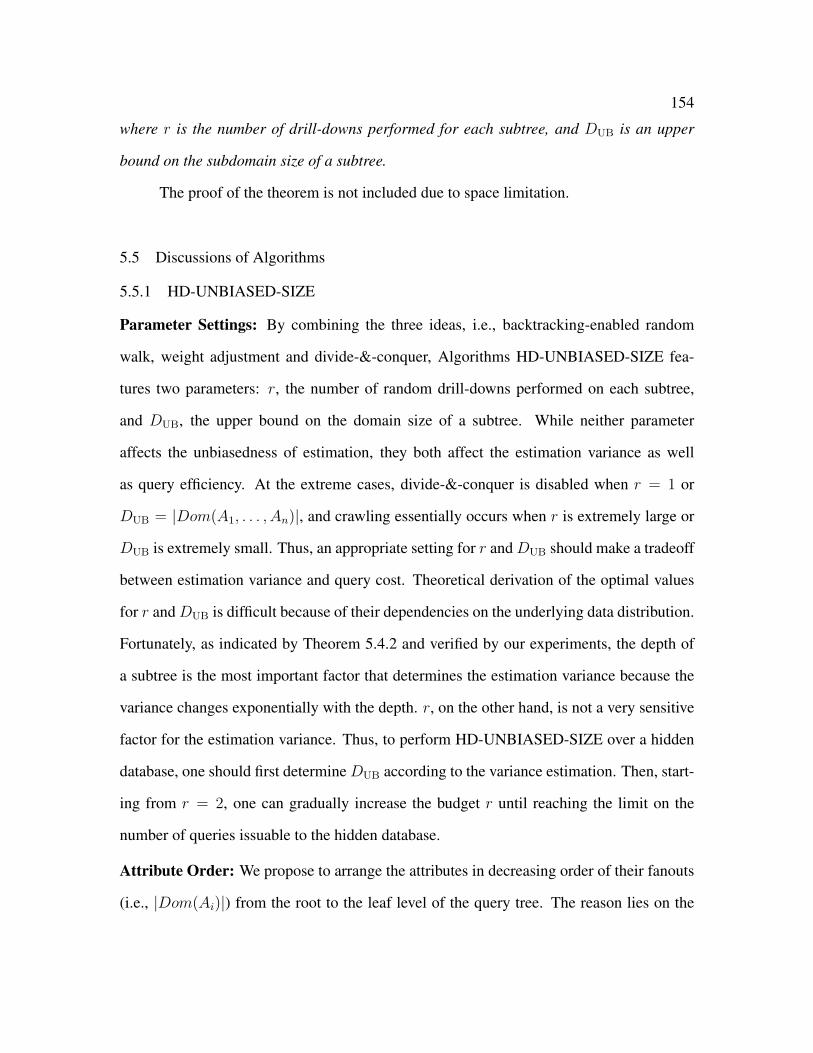
154
where r is the number of drill-downs performed for each subtree, and DUB is an upper
bound on the subdomain size of a subtree.
The proof of the theorem is not included due to space limitation.
5.5 Discussions of Algorithms
5.5.1 HD-UNBIASED-SIZE
Parameter Settings: By combining the three ideas, i.e., backtracking-enabled random
walk, weight adjustment and divide-&-conquer, Algorithms HD-UNBIASED-SIZE fea-
tures two parameters: r, the number of random drill-downs performed on each subtree,
and DUB, the upper bound on the domain size of a subtree. While neither parameter
affects the unbiasedness of estimation, they both affect the estimation variance as well
as query efficiency. At the extreme cases, divide-&-conquer is disabled when r = 1 or
DUB = |Dom(A1, . . . , An)|, and crawling essentially occurs when r is extremely large or
DUB is extremely small. Thus, an appropriate setting for r andDUB should make a tradeoff
between estimation variance and query cost. Theoretical derivation of the optimal values
for r andDUB is difficult because of their dependencies on the underlying data distribution.
Fortunately, as indicated by Theorem 5.4.2 and verified by our experiments, the depth of
a subtree is the most important factor that determines the estimation variance because the
variance changes exponentially with the depth. r, on the other hand, is not a very sensitive
factor for the estimation variance. Thus, to perform HD-UNBIASED-SIZE over a hidden
database, one should first determine DUB according to the variance estimation. Then, start-
ing from r = 2, one can gradually increase the budget r until reaching the limit on the
number of queries issuable to the hidden database.
Attribute Order: We propose to arrange the attributes in decreasing order of their fanouts
(i.e., |Dom(Ai)|) from the root to the leaf level of the query tree. The reason lies on the

155
query cost with smart backtracking. Recall from Section 5.3.2 that, with smart tracking, the
expected number of branches one need to test for a given node is QC = 1+∑w
j=1(wU(j)+
1)2/w, where wU(j) is the number of underflowing branches immediately preceding the
j-th branch. One can see that wU(j) is in general minimized when a high fanout attribute is
placed at the top levels of the tree. Thus, the overall query cost will be reduced by sorting
all attributes from largest to smallest domains.
5.5.2 HD-UNBIASED-AGG
In this section we discuss HD-UNBIASED-AGG, by extending HD-UNBIASED-
SIZE to answer SUM and AVG aggregate queries, as well as queries with selection condi-
tions. While our sampler provides unbiased estimates of SUM queries, we point out that it
cannot provide unbiased estimations of AVG queries.
For answering SUM and AVG queries: The same random drill-down process can be
used to generate unbiased estimate for SUM queries. There is only a slight change on
computing the estimation. Consider a SUM query SELECT SUM(Ai) FROM D. For a
random drill-down process (with divide-&-conquer), an unbiased estimator for the SUM
query is
∑q∈qTV
∑t∈q
t[Ai]
δ(q), (5.13)
where∑
t∈q t[Ai] is the sum of attribute values Ai for all tuples in q, and QTV is the set of
top-valid nodes captured by the random drill-downs over all subtrees.
However, note that the random drill-down process cannot be used as an unbiased
estimator for AVG queries. The direct division of the unbiased SUM and COUNT estima-
tors lead to a biased AVG estimator. This is consistent with the observation in [18] that it
is extremely difficult to generate unbiased AVG estimations without issuing a very large
number of queries (e.g., by using BRUTE-FORCE-SAMPLER).

156
For answering queries with selection conditions: Our previous discussions have been
focused on queries that select all tuples in the database. The random drill-down approach
can also generate unbiased SUM and COUNT estimates for queries with conjunctive selec-
tion conditions. In particular, a conjunctive query can be considered as selecting a subtree
which is defined with a subset of attributes (as levels) and, for each attribute involved, a
subset of its values (as branches). The random drill-down approach can be applied to the
subtree directly to generate unbiased estimations.
5.6 Experiments and Results
In this section, we describe our experimental setup and present the experimental
results. We carry out empirical studies to demonstrate the superiority of HD-UNBIASED-
SIZE and HD-UNBIASED-AGG over BRUTE-FORCE-SAMPLER and CAPTURE-&-
RECAP-TURE discussed in Section 5.2. We also draw conclusions on the individual im-
pact of weight adjustment and divide-&-conquer on reducing the estimation variance.
5.6.1 Experimental Setup
1) Hardware and Platform: All our experiments were performed on a 1.99 Ghz
Intel Xeon machine with 4 GB of RAM. The HD-UNBIASED-SIZE and HD-UNBIASED-
AGG algorithms was implemented in MATLAB for testing offline datasets, and PHP for
executions over the real Yahoo! Auto website.
2) Data Sets: Recall that we proposed three algorithms in the chapter: BOOL-
UNBIASED-SIZE, which applies only to Boolean data, and HD-UNBIASED-SIZE/AQP
which apply to both Boolean and categorical data. To test their performance, we consider
both Boolean and categorical datasets. To properly evaluate the accuracy of the estimations,
we need to know the ground truth on the aggregates being estimated. Thus, we perform
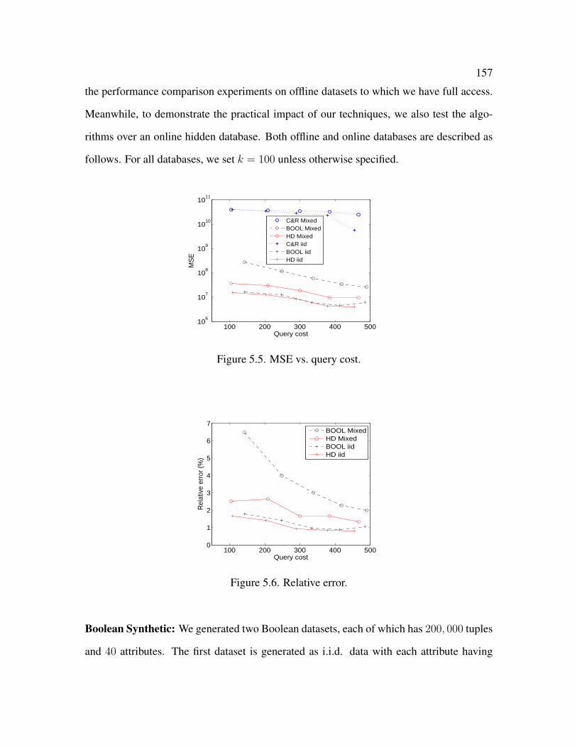
157
the performance comparison experiments on offline datasets to which we have full access.
Meanwhile, to demonstrate the practical impact of our techniques, we also test the algo-
rithms over an online hidden database. Both offline and online databases are described as
follows. For all databases, we set k = 100 unless otherwise specified.
100 200 300 400 50010
6
107
108
109
1010
1011
Query cost
MS
E
C&R MixedBOOL MixedHD MixedC&R iidBOOL iidHD iid
Figure 5.5. MSE vs. query cost.
100 200 300 400 5000
1
2
3
4
5
6
7
Query cost
Rel
ativ
e er
ror (
%)
BOOL MixedHD MixedBOOL iidHD iid
Figure 5.6. Relative error.
Boolean Synthetic: We generated two Boolean datasets, each of which has 200, 000 tuples
and 40 attributes. The first dataset is generated as i.i.d. data with each attribute having
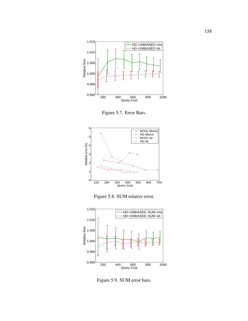
158
200 400 600 800 10000.990
0.995
1.000
1.005
1.010
1.015
Query Cost
Rel
ativ
e S
ize
HD−UNBIASED−mixHD−UNBIASED−iid
Figure 5.7. Error Bars.
100 200 300 400 500 600 7000
1
2
3
4
5
6
Query Cost
Rel
ativ
e er
ror (
%)
BOOL MixedHD MixedBOOL iidHD iid
Figure 5.8. SUM relative error.
200 400 600 800 10000.990
0.995
1.000
1.005
1.010
1.015
Query Cost
Rel
ativ
e S
ize
HD−UNBIASED−SUM−mixHD−UNBIASED−SUM−iid
Figure 5.9. SUM error bars.
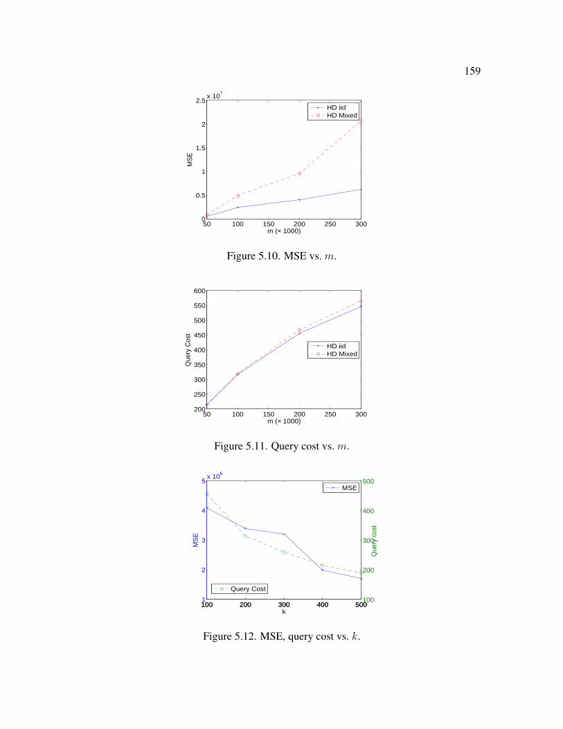
159
50 100 150 200 250 3000
0.5
1
1.5
2
2.5x 10
7
m (× 1000)
MS
E
HD iidHD Mixed
Figure 5.10. MSE vs. m.
50 100 150 200 250 300200
250
300
350
400
450
500
550
600
m (× 1000)
Que
ry C
ost
HD iidHD Mixed
Figure 5.11. Query cost vs. m.
100 200 300 400 5001
2
3
4
5x 10
6
MS
E
MSE
100 200 300 400 500100
200
300
400
500
Que
ry c
ost
k
Query Cost
Figure 5.12. MSE, query cost vs. k.

160
probability of p = 0.5 to be 1. We refer to this dataset as the Bool-iid dataset. The second
dataset is generated in a way such that different attributes have different distribution. In
particular, there are 40 independent attributes. 5 have probability of p = 0.5 to be 1, while
the others have the probability of 1 ranging from 1/70 to 35/70 with step of 1/70. One
can see that this dataset features a skewed distribution. We refer to it as the Boolean-mixed
dataset.
Offline Yahoo! Auto: The offline Yahoo! Auto dataset consists of data crawled from the
Yahoo! Auto website http://autos.yahoo.com/, a real-world hidden database, in 2007. In
particular, the original crawled dataset contains 15, 211 used cars for sale in the Dallas-
Fort Worth metropolitan area. We enlarged the dataset to 188, 790 tuples by following the
original distribution of the small dataset, in order to better test the ability of our algorithms
over large databases. In particular, the DBGen synthetic data generator [49] was used.
There are a total of 38 attributes including 32 Boolean ones, such as A/C, POWER LOCKS,
etc, and 6 categorical attributes, such as MAKE, MODEL, COLOR, etc. The domain sizes
of categorical attributes range from 5 to 16.
Online Yahoo! Auto: We also tested our algorithms over the real-world web interface
of Yahoo! Auto, a popular hidden database. In particular, we issue queries through the ad-
vanced used car search interface available at http://autos.yahoo.com/listings/
advanced_search. A specific requirement of this webpage is that either MAKE/MODEL
or ZIP CODE must be specified for a query to be processed. To address this requirement,
we place the MAKE/MODEL attribute at the top of our query tree and issue every query
with its value specified.
3) Aggregate Estimation Algorithms: We tested three algorithms in this chapter:
BOOL-UNBIASED-SIZE, HD-UNBIASED-SIZE, and HD-UNBIASED-AGG. BOOL-U-
NBIASED-SIZE is parameter-less, while both HD-UNBIASED-SIZE and HD-UNBIA-
SED-AGG feature two parameters: r, the number of drill-downs performed over each sub-

161
tree, and DUB, the maximum subdomain size for each subtree. We tested our algorithms
with various parameter settings to illustrate how r and DUB can be properly set in practice.
We also tested two baseline aggregate-estimation algorithms discussed in Section 5.2:
BRUTE-FORCE-SAMPLER [18] and the use of CAPTURE-&-RECAPTURE with HIDD-
EN-DB-SAMPLER [18]. BRUTE-FORCE-SAMPLER cannot return any result during our
test of issuing 100, 000 queries, because of the drastic difference between the size of the
database and set of all possible tuples. Thus, we compared the performance of our algo-
rithms with CAPTURE-&-RECAPTURE in the experimental results.
4) Performance Measures: For query cost, we focus on the number of queries issued
through the web interface of the hidden database. For estimation accuracy, we tested three
measures: (1) the mean squared error (MSE), (2) the relative error (i.e., |θ − θ|/θ for
an estimator θ of aggregate θ), and (3) error bars (indicating one standard deviation of
uncertainty).
5.6.2 Experimental Results
We compared the performance of HD-UNBIASED-SIZE, BOOL-UNBIASED-SIZE
and CAPTURE-&-RECAPTURE over a Boolean database. For HD-UNBIASED-SIZE,
we set parameters r = 4 and DUB = 25. Figure 5.5 depicts the tradeoff between MSE and
query cost for the three algorithms for BOOLEAN-iid and BOOLEAN-mixed datasets.
One can see from the figure that for both datasets, BOOL-UNBIASED-SIZE and HD-
UNBIASED-SIZE generates orders of magnitude smaller MSE than CAPTURE-&-RECA-
PTURE. Compared with BOOL-UNBIASED-SIZE, HD-UNBIASED-SIZE is capable of
further reducing the MSE by up to an order of magnitude (for BOOLEAN-MIXED) thanks
to the integration of weight adjustment and divide-&-conquer, the individual effect of each
will be discussed later in this section.

162
Another observation from Figure 5.5 is that the MSE for Boolean-mixed is higher
than that for Boolean-iid. This is consistent with our discussions in Section 5.3.3.2 which
show that the MSE is higher over a skewed data distribution, like that of BOOLEAN-
Mixed.
To provide an intuitive demonstration of the estimation accuracy, Figure 5.6 de-
picts the tradeoff between relative error and query cost for the three algorithms under the
same settings as Figure 5.5. Figure 5.7 further shows the error bars for HD-UNBIASED-
SIZE. One can see that both BOOL-UNBIASED-SIZE and HD-UNBIASED-SIZE are ca-
pable of producing smaller than 2% relative error for both datasets with fewer than 500
queries. In particular, all error bars of HD-UNBIASED-SIZE are within the range of 99%-
101.5%. This shows that our algorithm is capable of producing accurate estimates even
for a database with skewed underlying distribution, like Boolean-Mixed. Figures 5.8 and
5.9 depict the performance of HD-UNBIASED-SUM over the SUM of a randomly chosen
attribute. The observations are similar to the COUNT case.
We tested HD-UNBIASED-SIZE with varying database size m. Figures 5.10 and
5.11 depict the change of MSE and query cost, respectively, when m varies from 50, 000
to 300, 000. The parameters are r = 4 and DUB = 16. One can see from the figure that
the MSE increases (approximately) linearly with the database size. This is consistent with
our theoretical analysis in Theorem 5.4.1. The query cost also increases linearly with m,
showing the scalability of our algorithm to large databases. One can observe from the
figures that while the increase of query cost with m is always equal for Boolean-iid and
Boolean-Mixed, the difference between their MSE become larger when m increases. This
is because the larger the Boolean-Mixed database is, the “more skewed” its distribution on
the query tree will be, leading to a larger estimation variance.
To study how the value of k for the top-k interface affects the performance of our
algorithm, we tested HD-UNBIASED-SIZE with k ranging from 100 to 500. The changes
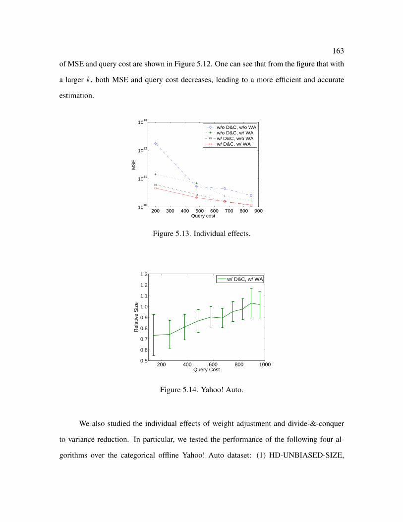
163
of MSE and query cost are shown in Figure 5.12. One can see that from the figure that with
a larger k, both MSE and query cost decreases, leading to a more efficient and accurate
estimation.
200 300 400 500 600 700 800 90010
10
1011
1012
1013
Query cost
MS
E
w/o D&C, w/o WAw/o D&C, w/ WAw/ D&C, w/o WAw/ D&C, w/ WA
Figure 5.13. Individual effects.
200 400 600 800 10000.5
0.6
0.7
0.8
0.9
1.0
1.1
1.2
1.3
Query Cost
Rel
ativ
e S
ize
w/ D&C, w/ WA
Figure 5.14. Yahoo! Auto.
We also studied the individual effects of weight adjustment and divide-&-conquer
to variance reduction. In particular, we tested the performance of the following four al-
gorithms over the categorical offline Yahoo! Auto dataset: (1) HD-UNBIASED-SIZE,
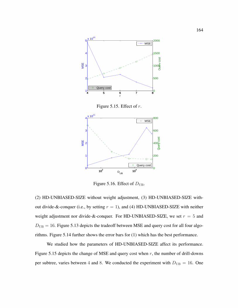
164
4 5 6 7 81
2
3
4
5x 10
10
MS
E
MSE
4 5 6 7 80
500
1000
1500
2000
Que
ry c
ost
r
Query cost
Figure 5.15. Effect of r.
102
104
0
1
2
3
4x 10
11
MS
E
MSE
102
104
0
200
400
600
800
Que
ry c
ost
DUB
Query cost
Figure 5.16. Effect of DUB.
(2) HD-UNBIASED-SIZE without weight adjustment, (3) HD-UNBIASED-SIZE with-
out divide-&-conquer (i.e., by setting r = 1), and (4) HD-UNBIASED-SIZE with neither
weight adjustment nor divide-&-conquer. For HD-UNBIASED-SIZE, we set r = 5 and
DUB = 16. Figure 5.13 depicts the tradeoff between MSE and query cost for all four algo-
rithms. Figure 5.14 further shows the error bars for (1) which has the best performance.
We studied how the parameters of HD-UNBIASED-SIZE affect its performance.
Figure 5.15 depicts the change of MSE and query cost when r, the number of drill-downs
per subtree, varies between 4 and 8. We conducted the experiment with DUB = 16. One

165
can see that the larger r is, the more queries will be issued, and the smaller the estimation
variance will be. This is consistent with our intuitive discussions in Section 5.5.1.
Figure 5.16 shows the change of MSE and query cost when DUB varies between 16
and 104544 (the domain size of the database). The experiment was conducted when r = 5.
One can see from the figure that the larger DUB is, the fewer queries need to be issued, but
the MSE will increase correspondingly.
We also tested the impact of r on the tradeoff between MSE and query cost. In par-
ticular, we setDUB = 16. For each value of r, we repeat the execution of HD-UNBIASED-
SIZE for certain number of times to reach a similar query cost. Then, we compute MSE
based on the average of the estimations from the repeated runs. The results are as follows.
Table 5.3. MSE vs Query Cost
r 3 4 5 6 7 8Query Cost 440 466 494 373 473 607MSE (×1010) 4.53 4.84 4.29 4.83 4.66 3.53
One can see that the tradeoff between MSE and query cost is not sensitive to the
value of r. This verifies our discussions in Section 5.5.1 for the setting of r.
Finally, we tested HD-UNBIASED-SIZE and HD-UNBIASED-AGG over the real-
world web interface of Yahoo! Auto. Note that Yahoo! enforces a limit on the frequency of
queries issued from an IP address. This prevents us from issuing a large number of queries
for the experiments. In particular, we conducted 10 executions of HD-UNBIASED-SIZE to
estimate the number of Toyota Corollas in the database (issuing an average of 193 queries
per execution). The parameters are set as r = 30, DUB = 126. Figure 5.17 shows the
estimations generated after each round of execution. One can see from the figure that our
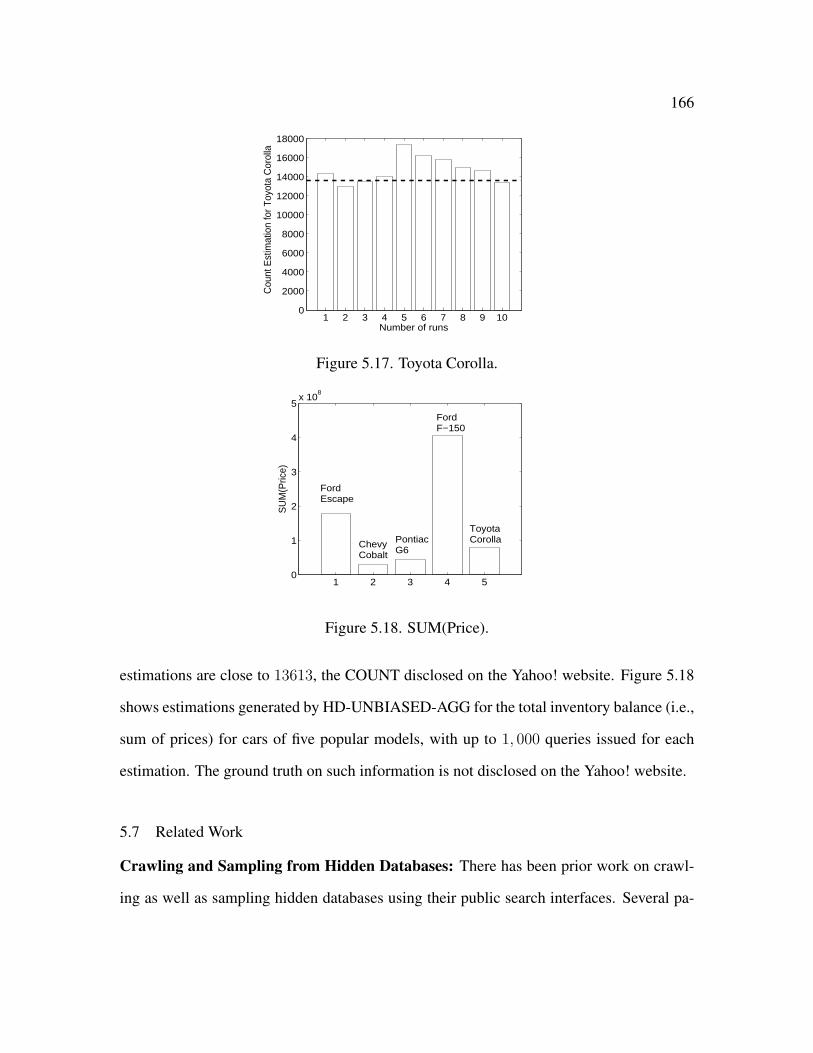
166
1 2 3 4 5 6 7 8 9 100
2000
4000
6000
8000
10000
12000
14000
16000
18000
Number of runs
Cou
nt E
stim
atio
n fo
r Toy
ota
Cor
olla
Figure 5.17. Toyota Corolla.
1 2 3 4 50
1
2
3
4
5x 10
8
SU
M(P
rice)
FordEscape
ChevyCobalt
PontiacG6
FordF−150
ToyotaCorolla
Figure 5.18. SUM(Price).
estimations are close to 13613, the COUNT disclosed on the Yahoo! website. Figure 5.18
shows estimations generated by HD-UNBIASED-AGG for the total inventory balance (i.e.,
sum of prices) for cars of five popular models, with up to 1, 000 queries issued for each
estimation. The ground truth on such information is not disclosed on the Yahoo! website.
5.7 Related Work
Crawling and Sampling from Hidden Databases: There has been prior work on crawl-
ing as well as sampling hidden databases using their public search interfaces. Several pa-

167
pers have dealt with the problem of crawling and downloading information present in hid-
den text based databases [8, 23, 24]. [25, 26, 40] deal with extracting data from structured
hidden databases. [27] and [28] use query based sampling methods to generate content
summaries with relative and absolute word frequencies while [29,30] uses two phase sam-
pling method on text based interfaces. [31, 32] discuss top-k processing which considers
sampling or distribution estimation over hidden sources. In [18, 36] techniques have been
developed for random sampling from structured hidden databases leading to the HIDDEN-
DB-SAMPLER algorithm. Techniques to thwart such sampling attempts have been devel-
oped in [37].
Sampling and Size Estimation for Search Engine’s Corpse: The increase in popularity
of search engines has motivated the research community to develop techniques to discover
its contents. [42, 50] studied the estimation by capture-recapture method to identify the in-
dex size of a search engine. [9] employed Monte Carlo methods to generate a near-uniform
sampling from the search engine’s corpus, while taking into consideration the degrees of
documents and cardinalities of queries. With approximate document degrees, techniques
for measuring search engine metrics were proposed in [39]. Sampling online suggestion
text databases were discussed in [51] to significantly improve the service quality of search
engines and to study users’ search patterns.
5.8 Conclusion
In this chapter we have initiated an investigation of the unbiased estimation of the
size and other aggregates over hidden web databases through its restrictive web interface.
We proposed backtrack-enabled random walk schemes over the query space to produce
unbiased estimates for SUM and COUNT queries, including the database size. We also
proposed two ideas, weight adjustment and capture-&-recapture, to reduce the estimation
variance. We provided theoretical analysis for estimation accuracy and query cost of the

168
proposed ideas. We also described a comprehensive set of experiments that demonstrate
the effectiveness of our approach over synthetic and real-world hidden databases.

CHAPTER 6
PRIVACY PRESERVATION OF AGGREGATES IN HIDDEN DATABASES:WHY AND HOW?
6.1 Introduction
Databases with public web-based search interfaces are available for many govern-
ment, scientific, and health-care websites as well as for many commercial sites. Such sites
are part of the much talked about hidden web and contain a lot of valuable information.
These sites provide controlled access to their databases through their search interfaces.
The simplest and most widely prevalent kind of search interface over such databases al-
lows users to specify selection conditions (point or range queries) on a number of attributes
and the system returns the tuples that satisfy the selection conditions. Sometimes the re-
turned results may be restricted to a few (e.g., top-k) tuples, sorted by one or more ranking
functions predetermined by the hidden web site. To illustrate the scenario let us consider
the following examples.
Example 1:An auto dealer’s web form lets a user choose from a set of attributes e.g.,
manufacturer, car type, mileage, age, price, engine type, etc. The top-k answers, sorted
according to a ranking function such as price, are presented to the user, where k is a small
constant such as 10.
Example 2:An airline company’s flight search form lets a user search for a flight by spec-
ifying a set of attributes such as departure and destination cities, date, number of stops,
carrier, and cabin preferences. The top-k flights, sorted according to a ranking function
such as price, are presented.
In this paper, our key observation is that there is a large class of such websites where
169

170
individual result tuples from search queries are public information and raise no privacy
concerns (e.g., availability of a specific model of car, schedule for a specific flight). How-
ever, such sites would like to suppress inference of aggregate information. In Example 1,
while the auto dealer wishes to allow potential car buyers to search its database, it would
not like to make public information that enables competitors to infer its inventory, e.g.,
that a certain popular car has been in short supply at the dealership in recent weeks. If the
competitors were able to infer such aggregate information, then this would allow them to
take advantage of the low inventory by a multitude of tactics (e.g., stock that vehicle, make
appropriate adjustments to price).
Likewise in Example 2, an airline company would not wish to reveal information that en-
ables terrorists to predict which flights, on what dates, are more likely to be relatively
empty. In recent hijackings such as 9/11 and Russian aircraft bombing of 2004, terrorists’
tactics are believed to be to hijack relatively empty flights because there would be less re-
sistance from occupants. If terrorists are able to infer aggregate information such as Friday
afternoon flights from Washington DC to Denver are emptier than others on average, they
could leverage this information to plan their attacks.
Of course, extremely broad aggregate information is usually well known and publicly avail-
able - e.g., that family sedans are more common than sports cars, or that flights are usually
empty on Christmas Day. It is the inferences of relatively fine-grained aggregates as il-
lustrated by the examples above that need to be protected against, as the impact of such
inference can range from being merely disadvantageous to the data publisher to posing
serious security threats to society at large. Also, aggregates collected from human efforts
(through domain knowledge) do not provide any form of statistical guarantees, which may
be particularly relevant for fine-grained aggregates.
It is important to recognize that our scenario of Privacy Preservation of Aggregates is in
sharp contrast to the traditional privacy scenarios, where the individual information needs
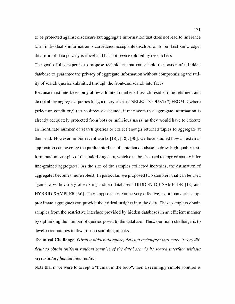
171
to be protected against disclosure but aggregate information that does not lead to inference
to an individual’s information is considered acceptable disclosure. To our best knowledge,
this form of data privacy is novel and has not been explored by researchers.
The goal of this paper is to propose techniques that can enable the owner of a hidden
database to guarantee the privacy of aggregate information without compromising the util-
ity of search queries submitted through the front-end search interfaces.
Because most interfaces only allow a limited number of search results to be returned, and
do not allow aggregate queries (e.g., a query such as “SELECT COUNT(*) FROM D where
¡selection-condition¿”) to be directly executed, it may seem that aggregate information is
already adequately protected from bots or malicious users, as they would have to execute
an inordinate number of search queries to collect enough returned tuples to aggregate at
their end. However, in our recent works [18], [18], [36], we have studied how an external
application can leverage the public interface of a hidden database to draw high quality uni-
form random samples of the underlying data, which can then be used to approximately infer
fine-grained aggregates. As the size of the samples collected increases, the estimation of
aggregates becomes more robust. In particular, we proposed two samplers that can be used
against a wide variety of existing hidden databases: HIDDEN-DB-SAMPLER [18] and
HYBRID-SAMPLER [36]. These approaches can be very effective, as in many cases, ap-
proximate aggregates can provide the critical insights into the data. These samplers obtain
samples from the restrictive interface provided by hidden databases in an efficient manner
by optimizing the number of queries posed to the database. Thus, our main challenge is to
develop techniques to thwart such sampling attacks.
Technical Challenge: Given a hidden database, develop techniques that make it very dif-
ficult to obtain uniform random samples of the database via its search interface without
necessitating human intervention.
Note that if we were to accept a “human in the loop“, then a seemingly simple solution is
172
to embed into the search interface a human-readable machine-unrecognizable image called
CAPTCHA [52], and to require each user to provide a correct CAPTCHA solution before
executing every search query. This strategy is used in a number of real-world websites .
Nonetheless, a key limitation of this approach is that it eliminates the possibility of any au-
tomated access, including legitimate ones such as third-party web services, over the hidden
database. Such limitation is becoming increasingly problematic with the growing popular-
ity mash-up web applications.
Thus, we aspire to develop techniques that allow search queries issued by bona fide users,
both human as well as third-party web applications, but at the same time make it very dif-
ficult for adversaries including automated bots by forcing them to execute an inordinate
number of search queries before they can obtain a small random sample of the database.
While there has been significant recent work in the areas of privacy preserving data min-
ing [53–55], data publishing [56], OLAP [57], and information sharing [58], these tech-
niques are inadequate for our purposes. Unlike our scenario, these techniques are appropri-
ate where the privacy of the individual needs to be preserved - e.g., in a medical database,
it is acceptable to reveal that the number of HIV patients is 30% more than cancer patients,
but not acceptable to reveal that a particular patient has HIV. Tuplewise privacy preservation
techniques such as encryption [58], data perturbation [53] and generalization methods [56]
cannot be used in our framework either as obfuscating individual data tuples is not an op-
tion since tuples need to be made visible to normal search users. The well-studied online
query auditing [59], which answers or denies a query based on the user’s query history, is
also not applicable in our scenario as these websites provide public interfaces and cannot
monitor individual users’ history of past queries.
Our Approach: In this paper we present novel techniques for protecting aggregates over
hidden databases. We propose a privacy-preserving algorithm called COUNTER-SAMPLER,
which can be used to defend against all possible sampling attacks. The key idea used in
173
COUNTER-SAMPLER is to insert into the hidden database a small number of carefully
constructed dummies tuples, i.e., tuples that do not exist in the original hidden database
but are composed of legitimate attribute values.
The reasons why dummy tuples can be effective at defending against sampling attacks are
subtle - we defer a detailed discussion for later in the paper, but provide brief intuition here.
Our approach builds on the observation that all existing sampling attacks retrieve uniform
random sample from tuples returned by queries that select at most k tuples each (where k
is a small constant such as 10 or 100), because otherwise the search on the hidden database
will return only the top-k tuples sorted by ranking functions unknown to the sampler, and
hence cannot be assumed to be random. In other words, we target a common character-
istic of samplers to find ”valid“ search queries that neither ”overflow“ (i.e., do not have
broad conditions that select more than k tuples) nor ”underflow” (i.e., do not have narrow
conditions that select no tuple). Thus, the key idea of COUNTER-SAMPLER is to care-
fully construct and insert dummy tuples into the database such that most valid (and some
underflowing) queries are converted to overflowing queries, thus significantly decreasing
the proportion of valid queries within the space of all possible search queries. As a result,
any sampler which generates samples from valid queries has to execute a huge number of
queries before it encounters enough valid queries be able to generate a uniform random
sample. Of course, the presence of dummy tuples presents an inconvenience to normal
search users or applications, which have to now distinguish the real tuples from the dummy
tuples in the returned results of any search query. How to distinguish dummy tuples from
real tuples is discussed later in the paper. Nevertheless, to reduce such inconveniences,
our objective is to minimize the number of inserted dummy tuples while providing the de-
sired privacy guarantees. Our analytical as well as experimental results show that only a
small number of dummy tuples are usually inserted by COUNTER-SAMPLER to provide
adequate privacy guarantees.
174
Summary of Contributions:
• We define the novel problem of Privacy Preservation of Aggregates in Hidden Databases.
• We develop COUNTER-SAMPLER, a privacy-preserving algorithm that inserts dummy
tuples to prevent the efficient sampling of hidden databases.
• We provide theoretical analysis on the privacy guarantee for sensitive aggregates
provided by COUNTER-SAMPLER.
• We describe a comprehensive set of experiments that demonstrate the effectiveness
of COUNTER-SAMPLER. Although it is universally effective against all possible
sampling attacks, we demonstrate its effectiveness against the state-of-the-art sam-
pling algorithms, HIDDEN-DB-SAMPLER [18] and HYBRID-SAMPLER [36].
6.2 Preliminaries
6.2.1 Hidden Databases
In most of this paper, we restrict discussions to categorical data - we discuss exten-
sions to numerical data later. Consider a hidden database tableD withm tuples t1, ..., tm on
N attributes a1, ..., aN . The table is only accessible through a web-based interface where
users can issue queries that specify values for a subset of the attributes, say a1, ..., an. We
refer to such queries as the search queries, which are of the form: QS: SELECT * FROM
D WHERE ac1 = vc1 AND ... AND acu = vcu, where vc1, ..., vcu are from the do-
mains of ac1, ..., acu ∈ a1, ..., an, respectively.
Let Sel(QS) be the set of tuples in D that satisfy QS . As is common with most web inter-
faces, we assume that the query interface is restricted to only return up to k tuples, where
k << m is a pre-determined small constant. If the query is too broad (i.e., |Sel(QS)| > k),
only the top − k tuples in Sel(QS) will be selected according to a ranking function, and
returned as the query result. The interface will also notify the user that there is an overflow.
175
At the other extreme, if the query is too specific and returns no tuple, we say that an under-
flow occurs. If there is neither an overflow nor an underflow, we have a valid query result.
In this paper, we assume that the interface does not allow a user to “scroll through” the
complete answer Sel(QS) when an overflow occurs. We argue that this is a reasonable as-
sumption because many real-world top-k interfaces only allow a limited number of “page
turns”. Google, for example, only allows 100 page turns (10 results per page) per query.
This essentially makes Google a top-1000 interface in our model.
6.2.2 Privacy Requirements
Consider aggregate queries of the form: SELECT AGGR(∗) FROM D WHERE
ac1=vc1 AND ... AND acu = vcu, where AGGR(.) is an aggregate function such as
COUNT, SUM, etc, and vc1, ..., vcu are from the domains of ac1, ..., acu, respectively. Let
Res(QA) be the result of such an aggregate query. As discussed earlier, due to privacy con-
cerns the owner of a hidden database may consider certain aggregate queries to be sensitive
and would not willingly disclose their results.
To quantify privacy protection, we first define the notion of disclosure. Similar to the pri-
vacy models for individual data tuples [59], we can define the exact and partial disclosure
of aggregates. Exact disclosure occurs when a user learns the exact answer to an aggregate
query. Exact disclosure is a special case of partial disclosure; the latter occurs when there
is a significant change between a user’s prior and posterior confidence about the range of a
sensitive query answer.
In this paper we consider the (broader) partial disclosure notion because approximate an-
swers are often adequate for aggregate queries. Carrying the same spirit in the privacy-
game notion for individual data tuples [60], we define the following (ε, δ)-privacy game
between a user and the hidden database owner for a sensitive aggregate query QA:
• The owner chooses its defensive scheme.

176
• The user issues search queries and analyzes their results to try and estimateRes(QA).
• The user wins if ∃x such that the user has confidence > δ that Res(QA) [x, x + ε].
Otherwise, the user loses.
Based on the (ε, δ)-game notion, we define the privacy requirement for a hidden
database as follows:
Definition 2.1: We say that a defensive scheme achieves (ε, δ, p)-privacy guarantee for QA
iff for any user, PrA wins (ε, δ)-privacy game for QA ≤ p.
The probability is taken over the (possible) randomness in both the defensive scheme and
the attacking strategy. Note that if a defensive scheme achieves (ε, δ, p)-privacy guarantee,
then no user can win a (ε0, δ0)-privacy game with probability of p0 if ε0 ≤ ε, δ0 ≥ δ, and
p0 ≥ p. Thus, the greater ε or the smaller δ and p are, the more protection a (ε, δ, p)-privacy
guarantee provides.
6.2.3 Attack: Cost and Strategies
A user cannot directly execute aggregate queries. Instead, it must issue search queries
and infer sensitive aggregates from the returned results. There may be an access fee for
search queries over a proprietary hidden database. Even for hidden databases with pub-
licly available interfaces, the server usually limits the number of queries a user can issue
before blocking the user’s account or IP address (e.g., Google SOAP Search API enforces
a limit of 1,000 queries per day [61]). Thus, we define the attacking-cost limit umax as
the maximum number of search queries that a user can issue. Such limits make it unre-
alistic for an attacker to completely crawl a large hidden database. However, as recent
research [18, 36][DDM07, DZD09] has shown, such databases are vulnerable to sampling
attacks, which are based on the generation of uniform random samples (with replacement)
from the database and the approximate estimation of sensitive aggregates from the samples.

177
6.2.4 Defense: Dummy Insertion
We study the strategy of inserting dummy tuples to defend against sampling attacks.
To enable a bona fide search user to distinguish real tuples from dummies, we propose
to accompany each returned tuple with a CAPTCHA flag indicating whether it is real or
dummy. Unlike the CAPTCHA challenge discussed in earlier, our scheme applies to a
large class of third-party applications such as meta-search engines . In particular, a meta-
search engine queries several hidden databases based on a search condition specified by
an end-user, and then returns the union of all returned tuples after (re-)sorting or filtering.
In the process, it treats all tuples in the same manner regardless of real or dummy. The
engine does not parse any CAPTCHA itself, and instead simply forwards the tuples with
the CAPTCHA flags they receive from the hidden database to end-users.
An important note of caution is that the attribute values of a dummy tuple may allow an
adversary to identify it as a dummy, essentially incapacitating the CAPTCHA flag. In
particular, an adversary may identify a dummy tuple by checking whether its attribute val-
ues violate constraints obtained by the adversary through external knowledge (e.g., that the
airline in Example 2 does not operate any flight out of Seattle, WA). A solution to this prob-
lem requires the proper modeling of external knowledge, which we will leave as an open
problem. In this paper, we assume that there exists a dummy-generating oracle DUMMY-
ORACLE(m0, C) which generates dummy tuples that (1) satisfy the search condition C,
and (2) cannot be identified as a dummy by the adversary. The oracle terminates when ei-
ther no more tuples satisfying the above conditions can be generated, or m0 dummy tuples
have been generated, whichever occurs first.
The objective of defense is to protect sensitive aggregates while maintaining the utility of
search queries to normal users. We measure the (loss of) utility by the number of inserted
dummy tuples: more dummy tuples increases inconvenience for normal users and hence
reduces utility . The problem studied for the remainder of this paper is formally defined as

178
follows:
Problem: Given the attacking-cost limit and a set of sensitive aggregate queries, the ob-
jective of dummy insertion is to achieve(ε, δ, p)-guarantee for each aggregate query while
minimizing the number of inserted dummy tuples.
6.3 COUNTER-SAMPLER
In this section, we present the detailed algorithm of COUNTER-SAMPLER and
analyze its performance.
6.3.1 Algorithm COUTER-SAMPLER
Algorithm COUNTER-SAMPLER consists of two steps: d-level packing (Lines 1-6)
and b-neighbor insertion (Lines 7-15). The subroutine DUMMY-ORACLE was discussed
earlier. Lines 1-6 ensure that no (d-1)-predicate (or shorter) query will underflow, while
Lines 7-15 ensure that no (b-1)-predicate (or shorter) query will be valid. Thus, Algorithm
COUNTER-SAMPLER achieves d-level packing and b-neighbor insertion.
Note that while COUNTER-SAMPLER does not require the hidden database D to be
Boolean, for ease of discussion our following analysis will be restricted to Boolean databases.
We will discuss categorical and numerical databases later. Also, for this moment, we as-
sume b and d are parameters set by the hidden database owner. How they should be deter-
mined will be discussed later.
6.3.2 Privacy Guarantee
To provide a privacy guarantee against any sampler that aims to draw uniform ran-
dom samples from the hidden database, we will first prove a lower bound on the expected
number of search queries required for a sampler to find s uniform random sample tuples
over a Boolean hidden database. Based on the bound, we will derive a (ε, δ, p)-privacy

179
Algorithm 11 COUNTER-SAMPLER(b, d, k)
1: . Start of d-level packing
2: for each set S of d− 1 attributes do
3: KS = Cartesian product of domains of attributes in S
4: DS = SELECT S FROM D
5: for each tuple t in SELECT * FROM KS −DS do
6: C = ∧ai∈S(ai = t[ai])
7: D = D ∪DUMMY −ORACLE(k + 1, C)
8: end for
9: end for
10: . Start of b-neighbor insertion
11: DDUMMY = φ
12: for each set S of b− 1 attributes do
13: DS = SELECT S FROM D
14: NS = SELECT S, COUNT(*) FROM D ∪ DUMMY GROUP BY S HAVING
COUNT(*) > k
15: for each tuple t in SELECT * FROM DS - NS[S] do
16: C = ∧ai∈S(ai = t[ai])
17: c = SELECT COUNT(*) FROM D ∪ DDUMMY WHERE C
18: DDUMMY = DDUMMY ∪ DUMMY-ORACLE(k + 1− c, C)
19: end for
20: end for
21: D = D ∪ DDUMMY
180
guarantee achieved by COUNTER-SAMPLER.
Before formally presenting the results, we would like to point out that although Algorithm
COUNTER-SAMPLER is quite intuitive, the theoretical analysis is quite challenging and
consequently the derived bounds are rather loose. We also point out that the results address
the class of samplers that use finding valid queries as a part of their sampling strategy.
Our goal of presenting these analytical results is not to promote the tightness of bounds,
but to demonstrate the versatility of COUNTER-SAMPLER in defending against any arbi-
trary sampler. However, as our experiments show, the actual performance is much better in
practice.
Lemma 6.3.1. For a Boolean hidden database with m tuples, after COUNTER-SAMPLER
has been executed with parameters b and d such that 4s(b−d)(d+1) ≤ 3d andm ≤ 2d−1,
any sampler needs at least an expected number of 4s(b − d)/3 search queries to find s
uniform random sample tuples over the database.
Due to space limitation, we omit the proof, and the full details are available at [62].
Interestingly, the bound is decreasing with d, which seems to suggest that d-level packing
is hurting the defense. However, this is not true because, in order for the lemma to hold, d
must be large enough to satisfy the two conditions in the lemma. The reason why the bound
decreases with d is because a “smart” sampler (which may be aware of the COUNTER-
SAMPLER algorithm and hence knows b and d) does not need to issue any queries with
fewer than d-predicates. Based on the lemma, the following Theorem 4.2 provides privacy
guarantees for sensitive COUNT aggregate queries. Recall from earlier that the attacking-
cost limit umax is the maximum number of search queries that an adversary can issue.
Theorem 6.3.1. For a Boolean hidden database with m tuples, when all samplers have an
attacking-cost limit umax, for any COUNT query with answer in [x, y], the hidden database
owner achieves (ε, δ,50%)-privacy guarantee if COUNTER-SAMPLER has been executed
with parameters b and d which satisfy:

181
(a) d ≥ lgm+ 1 and 3d−1/(d+ 1) ≥ umax
(b) b ≥ d+ (3εumax/(32min(x(m− x), y(m− y))(erf−1(δ))2)
The details of the proof are available in [62], but in brief, Conditions (a) and (b)
directly follow from Lemma 6.3.1 and a lower bound on the number of samples required
to win a (ε, δ)-privacy game, which can be derived via standard sampling theory. The the-
orem can be easily extended to other types of aggregates (e.g., SUM) by making proper
assumptions on the distribution of the measure attribute.
Theorem 4.2 provides guidelines on the parameter settings for b and d. In particular, Con-
ditions (a) and (b) imply lower bounds on d and b, respectively. Note that the smaller b or
d is, the fewer dummy tuples are required. Thus, to achieve a (ε, δ, 50%)-privacy guaran-
tee, for a given attacking-cost limit umax, we should first set d to be the minimum value
that satisfies Condition (a), and then compute b as the minimum value that satisfies Condi-
tion (b). Ideally, we can follow these settings to make Algorithm COUNTER-SAMPLER
parameter-less. Nonetheless, as discussed earlier, this theorem only provides necessary
but not sufficient conditions for (ε, δ, 50%)-privacy guarantee. In practice, other (tighter)
bounds on the b and d suffice, as we will demonstrate in the experimental results.
An interesting observation is that Condition (b) depends on the range[x, y] of COUNT
query answers. In particular, for given values of umax, b, d, and δ, the value of ε is maxi-
mized when x = y = m/2. This shows that COUNTER-SAMPLER provides the strongest
privacy guarantee when a COUNT query is neither too broad nor too narrow. This is con-
sistent with our objective of protecting fine-grained aggregates.
It is important to note that the privacy guarantee holds for all COUNT queries against pos-
sible sampling algorithms. This renders inference-based attacks that try to infer aggregates
by combining answers of two or more non-sensitive queries, useless.

182
6.3.3 Number of Inserted Dummy Tuples
The privacy guarantee derived above is independent of the interface parameter k.
The number of inserted dummy tuples however, depends on k because, intuitively, for a
larger k more dummy tuples are required for making underflowing or valid queries over-
flow. The number of inserted dummy tuples also depends on the original data distribution.
For example, when the data is densely distributed into a few clusters, b-neighbor insertion
requires much fewer dummy tuples than when all attributes are i.i.d. with uniform distri-
bution. For d-level packing, the i.i.d. case requires much fewer dummy tuples than when
the data is highly skewed (e.g., all attributes have probability of 99% to be 1). Because of
this dependency, we will not attempt a theoretical analysis of the number of dummy tuples
inserted, and instead present a thorough experimental evaluation.
6.3.4 Efficiency and Implementation Issues
Given b and d, the time complexity of COUNTER-SAMPLER isO(nCd?1∗max(2d,m)+
nCb?1 ∗m), where n is the number of (searchable) attributes and m is the number of tuples.
The efficiency is usually not a concern because (1) COUNTER-SAMPLER only needs to
be executed once as a pre-processing step for a static database, and (2) n is usually quite
small for a hidden database with web interface. However, COUNTER-SAMPLER can
be slow when n is large. To address this problem, we present RANDOM-COUNTER-
SAMPLER, a randomized version which replaces the enumeration of all (d− 1) or (b− 1)
attribute sets by checking such attribute sets at random.
Since the dummy tuples inserted for one attribute set may also overflow queries cor-
responding to other attribute sets, the number of dummy tuples required for the not-yet-
chosen attribute sets decreases quickly. We terminate the process when no dummy tuple is
inserted for h consecutive iterations. Thus, even when n is large, RANDOM-COUNTER-
SAMPER is able to terminate quickly with a small probability of error.
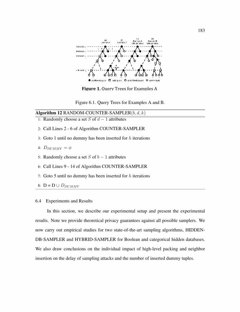
183
Figure1.QueryTreesforExamplesA
andB
Figure 6.1. Query Trees for Examples A and B.
Algorithm 12 RANDOM-COUNTER-SAMPLER(b, d, k)
1: Randomly choose a set S of d− 1 attributes
2: Call Lines 2 - 6 of Algorithm COUNTER-SAMPLER
3: Goto 1 until no dummy has been inserted for h iterations
4: DDUMMY = φ
5: Randomly choose a set S of b− 1 attributes
6: Call Lines 9 - 14 of Algorithm COUNTER-SAMPLER
7: Goto 5 until no dummy has been inserted for h iterations
8: D = D ∪ DDUMMY
6.4 Experiments and Results
In this section, we describe our experimental setup and present the experimental
results. Note we provide theoretical privacy guarantees against all possible samplers. We
now carry out empirical studies for two state-of-the-art sampling algorithms, HIDDEN-
DB-SAMPLER and HYBRID-SAMPLER for Boolean and categorical hidden databases.
We also draw conclusions on the individual impact of high-level packing and neighbor
insertion on the delay of sampling attacks and the number of inserted dummy tuples.

184
6.4.1 Experimental Setup
1. Hardware and Platform: All our experiments were performed on a 1.99 Ghz In-
tel Xeon machine with 4 GB of RAM. The COUNTER-SAMPLER algorithm was
implemented in MATLAB. We set h = 40 for the randomized version.
2. Data Sets: HIDDEN-DB-SAMPLER recommends different strategies for Boolean
and categorical databases (with random order of attributes for the former and fixed
order for the latter). Thus, we consider both Boolean and categorical datasets. Note
that in order to apply COUNTER-SAMPLER, these datasets are offline ones to which
we have full access.
Boolean Synthetic: We generated two Boolean datasets, each of which has 100,000
tuples and 30 attributes. The first dataset is generated as i.i.d. data with each attribute
having probability of p = 0.3 to be 1. We refer to this dataset as the Bool-0.3 dataset.
The second dataset is generated in a way such that different attributes have different
distribution. In particular, there are 30 independent attributes, 5 have probability of
p = 0.5 to be 1, 10 have p = 0.3, the other 10 have p = 0.1. We refer to this dataset
as the Bool-mixed dataset. Categorical Census: The Census dataset consists of the
1990 US Census Adult data published on the UCI Data Mining archive [63]. After
removing attributes with domain size greater than 100, the dataset had 12 attributes
and 32,561 tuples. It is instructive to note that the domain size of the attributes of the
underlying data is unbalanced in nature. The attribute with the highest domain size
has 92 categories and the lowest-domain-size attributes are Boolean.
3. Sampling Algorithms: We tested two state-of-the-art sampling algorithms for hid-
den databases: HIDDEN-DB-SAMPLER [18] and HYBRID-SAMPLER [36].
HIDDEN-DB-SAMPLER has two variations, HIDDEN-DB-RANDOM and HIDDE-
N-DB-FIXED, which use random and fixed order of attributes, respectively. HIDDEN-
DB-RANDOM can only be applied to Boolean data, while HIDDEN-DB-FIXED
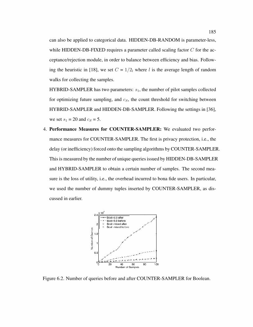
185
can also be applied to categorical data. HIDDEN-DB-RANDOM is parameter-less,
while HIDDEN-DB-FIXED requires a parameter called scaling factor C for the ac-
ceptance/rejection module, in order to balance between efficiency and bias. Follow-
ing the heuristic in [18], we set C = 1/2l where l is the average length of random
walks for collecting the samples.
HYBRID-SAMPLER has two parameters: s1, the number of pilot samples collected
for optimizing future sampling, and cS , the count threshold for switching between
HYBRID-SAMPLER and HIDDEN-DB-SAMPLER. Following the settings in [36],
we set s1 = 20 and cS = 5.
4. Performance Measures for COUNTER-SAMPLER: We evaluated two perfor-
mance measures for COUNTER-SAMPLER. The first is privacy protection, i.e., the
delay (or inefficiency) forced onto the sampling algorithms by COUNTER-SAMPLER.
This is measured by the number of unique queries issued by HIDDEN-DB-SAMPLER
and HYBRID-SAMPLER to obtain a certain number of samples. The second mea-
sure is the loss of utility, i.e., the overhead incurred to bona fide users. In particular,
we used the number of dummy tuples inserted by COUNTER-SAMPLER, as dis-
cussed in earlier.
Figure 6.2. Number of queries before and after COUNTER-SAMPLER for Boolean.

186
Figure 6.3. Delay of sampling vs. Percentage of dummy tuples.
Figure 6.4. Number of queries before and after COUNTER-SAMPLER for Census.
6.4.2 Effectiveness of COUNTER-SAMPLER
HIDDEN-DB-RANDOM: Since HIDDEN-DB-RANDOM only supports Boolean data,
we tested the effectiveness of COUNTER-SAMPLER on defending against HIDDEN-
DB-RANDOM over the two Boolean synthetic datasets. We first applied COUNTER-
SAMPLER with a fixed pair of parameters b = 10 (for b-neighbor insertion) and d = 6
(for d-level packing) when k = 1. In this case, COUNTER-SAMPLER inserts 29218 and
32717 dummy tuples for the Bool-0.3 and Bool-mixed datasets, respectively, leading to a

187
Figure 6.5. Delay of sampling vs. number of dummy tuples.
proportion of 22.6% and 24.7% tuples of the final database being dummies. Figure 6.2
depicts the number of queries required by HIDDEN-DB-RANDOM to obtain 1 to 100
samples before and after COUNTER-SAMPLER is used. One can see from the figure that
for both datasets, COUNTER-SAMPLER significantly increases the number of queries
HIDDEN-DB-RANDOM has to issue. For example, to draw 100 samples from the Bool-
mixed dataset, HIDDEN-DB-RANDOM requires only 1987 queries before COUNTER-
SAMPLER is applied, but 23751 queries afterwards.
We also tested the tradeoff between the delay of HIDDEN-DB-RANDOM and the number
of dummy tuples inserted by COUNTER-SAMPLER. To do so, we set d = 5 and vary b
between 10, 12, and 15. Again, k = 1. Figure 6.3 depicts relationship between the per-
centage of dummy tuples in the final database and the average number of queries required
by HIDDEN-DB-RANDOM to obtain a sample during the process of drawing 50 samples.
One can see from the figure that the sampler can be delayed by orders of magnitude with a
moderate number of dummy tuples. For example, HIDDEN-DB-SAMPLER requires over
700 times more queries when there are 43.7% dummy tuples in the dummy-inserted ver-
sion of the Bool-mixed dataset.
HIDDEN-DB-FIXED: In [18], HIDDEN-DB-FIXED is recommended over HIDDEN-

188
DB-RANDOM for categorical data as it generally yields a smaller bias in the samples.
Thus, we tested the effectiveness of COUNTER-SAMPLER in defending against HIDDEN-
DB-FIXED over the Census dataset. We set k = 10 by default unless otherwise noted.
Similar to the experiments on Boolean synthetic datasets, we first applied COUNTER-
SAMPLER with a fixed pair of parameters cd = 50 (for high-level packing) and cb = 500
(for neighbor insertion). In this case, COUNTER-SAMPLER inserts 10697 dummy tu-
ples, leading to a proportion of 24.7% tuples of the final database being dummies. Fig-
ure 6.4 depicts the number of queries required by HIDDEN-DB-FIXED to obtain 1 to 100
samples before and after COUNTER-SAMPLER is used. One can see from the figure
that COUNTER-SAMPLER significantly increases the number of queries HIDDEN-DB-
FIXED needs to issue. For example, to obtain 30 samples, HIDDEN-DB-FIXED needs
only 277 queries before COUNTER-SAMPLER is applied, but 1423 queries afterwards.
We again tested the relationship between the delay of HIDDEN-DB-FIXED and the num-
ber of inserted dummy tuples. To do so, we set cd = 100 and varied cb between 500, 1000,
and 1500. Figure 6.5 depicts the results. As we can see, COUNTER-SAMPLER delays
HIDDEN-DB-FIXED by more than ten-fold, from 6.41 to 69.07 queries per sample, when
53.4% tuples of the final database are dummies.
We also tested COUNTER-SAMPLER with varying cd. Figure 6.6 shows the number of
queries required by HIDDEN-DB-FIXED for each sample (while drawing 100 samples)
when cd varies from 0 to 300. One can observe from the figure a pattern that holds for all
three cases of cb = 500, 1000, and 1500: when cd increases, the number of queries required
by HIDDEN-DB-FIXED first increases, and then decreases. This verifies what is indicated
by our theoretical results in Lemma 4.1 and Theorem 4.2: once the value of d (resp. cd)
used by high-level packing reaches a threshold, the further increase of d (resp. cd) can only
reduce, and not improve, the protection provided by COUNTER-SAMPLER.
We tested COUNTER-SAMPLER with varying database sizes. In particular, we con-

189
structed 10 databases with 10,000 to 100,000 tuples by sampling with replacement from
the Census dataset. Then, we applied COUNTER-SAMPLER with cb = 500 and cd = 50
to all of them. Figure 6.7 shows the percentage of dummy tuples in the dummy-inserted
databases. One can see that this percentage decreases rapidly when k increases. For exam-
ple, the percentage is 49.11% for the 10,000-tuple database but only 5.77% for the 100,000-
tuple database. Meanwhile, the privacy protection provided by COUNTER-SAMPLER re-
mains effective, as demonstrated in Figure 6.8.
We also studied the impact of the interface parameter k on COUNTER-SAMPLER. In par-
ticular, we tested cases where k ranges from 10 to 50. To highlight the change of sampling
efficiency with k, we used the case where k = 10 as the baseline scenario, and calculated
the relative number of queries required by HIDDEN-DB-FIXED for other values of k (for
collecting the same number (100) of samples). Figure 6.9 shows the results before and
after COUNTER-SAMPLER with cb = 500 and cd = 50 is applied. One can see from the
figure that without COUNTER-SAMPLER, the number of queries required by HIDDEN-
DB-FIXED decreases rapidly with increasing k. After COUNTER-SAMPLER is applied,
however, the number of queries remains stable for all values of k. This is consistent with the
fact that our privacy guarantees derived in Lemma 6.3.1 and Theorem 6.3.1 are independent
of the value of k.
Figure 6.6. Delay of sampling vs. cd for high-level packing.
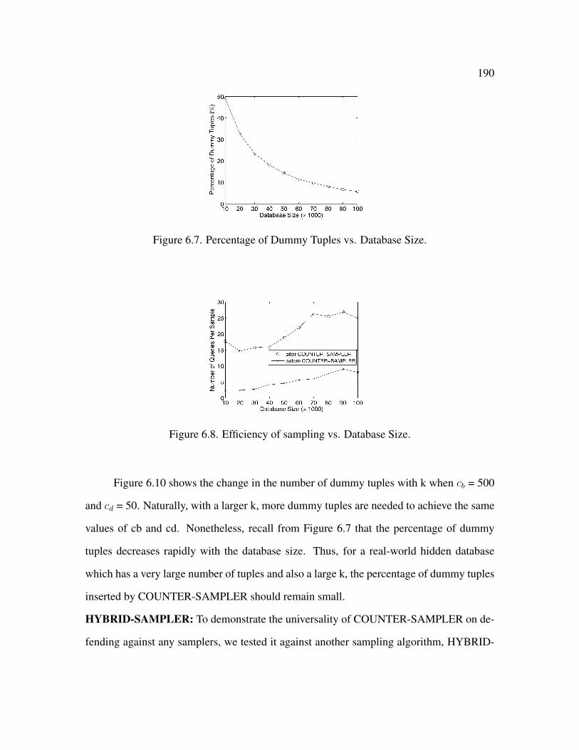
190
Figure 6.7. Percentage of Dummy Tuples vs. Database Size.
Figure 6.8. Efficiency of sampling vs. Database Size.
Figure 6.10 shows the change in the number of dummy tuples with k when cb = 500
and cd = 50. Naturally, with a larger k, more dummy tuples are needed to achieve the same
values of cb and cd. Nonetheless, recall from Figure 6.7 that the percentage of dummy
tuples decreases rapidly with the database size. Thus, for a real-world hidden database
which has a very large number of tuples and also a large k, the percentage of dummy tuples
inserted by COUNTER-SAMPLER should remain small.
HYBRID-SAMPLER: To demonstrate the universality of COUNTER-SAMPLER on de-
fending against any samplers, we tested it against another sampling algorithm, HYBRID-
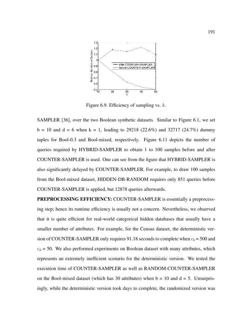
191
Figure 6.9. Efficiency of sampling vs. k.
SAMPLER [36], over the two Boolean synthetic datasets. Similar to Figure 6.1, we set
b = 10 and d = 6 when k = 1, leading to 29218 (22.6%) and 32717 (24.7%) dummy
tuples for Bool-0.3 and Bool-mixed, respectively. Figure 6.11 depicts the number of
queries required by HYBRID-SAMPLER to obtain 1 to 100 samples before and after
COUNTER-SAMPLER is used. One can see from the figure that HYBRID-SAMPLER is
also significantly delayed by COUNTER-SAMPLER. For example, to draw 100 samples
from the Bool-mixed dataset, HIDDEN-DB-RANDOM requires only 851 queries before
COUNTER-SAMPLER is applied, but 12878 queries afterwards.
PREPROCESSING EFFICIENCY: COUNTER-SAMPLER is essentially a preprocess-
ing step; hence its runtime efficiency is usually not a concern. Nevertheless, we observed
that it is quite efficient for real-world categorical hidden databases that usually have a
smaller number of attributes. For example, for the Census dataset, the deterministic ver-
sion of COUNTER-SAMPLER only requires 91.18 seconds to complete when cb = 500 and
cd = 50. We also performed experiments on Boolean dataset with many attributes, which
represents an extremely inefficient scenario for the deterministic version. We tested the
execution time of COUNTER-SAMPLER as well as RANDOM-COUNTER-SAMPLER
on the Bool-mixed dataset (which has 30 attributes) when b = 10 and d = 5. Unsurpris-
ingly, while the deterministic version took days to complete, the randomized version was
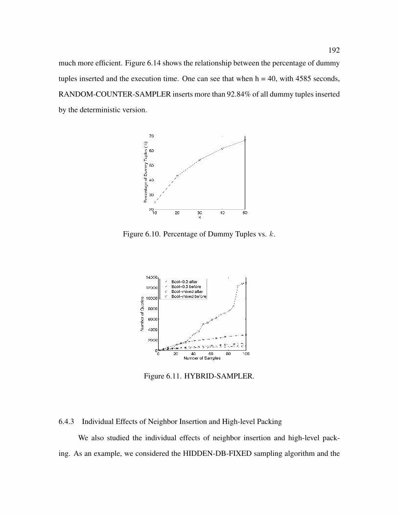
192
much more efficient. Figure 6.14 shows the relationship between the percentage of dummy
tuples inserted and the execution time. One can see that when h = 40, with 4585 seconds,
RANDOM-COUNTER-SAMPLER inserts more than 92.84% of all dummy tuples inserted
by the deterministic version.
Figure 6.10. Percentage of Dummy Tuples vs. k.
Figure 6.11. HYBRID-SAMPLER.
6.4.3 Individual Effects of Neighbor Insertion and High-level Packing
We also studied the individual effects of neighbor insertion and high-level pack-
ing. As an example, we considered the HIDDEN-DB-FIXED sampling algorithm and the
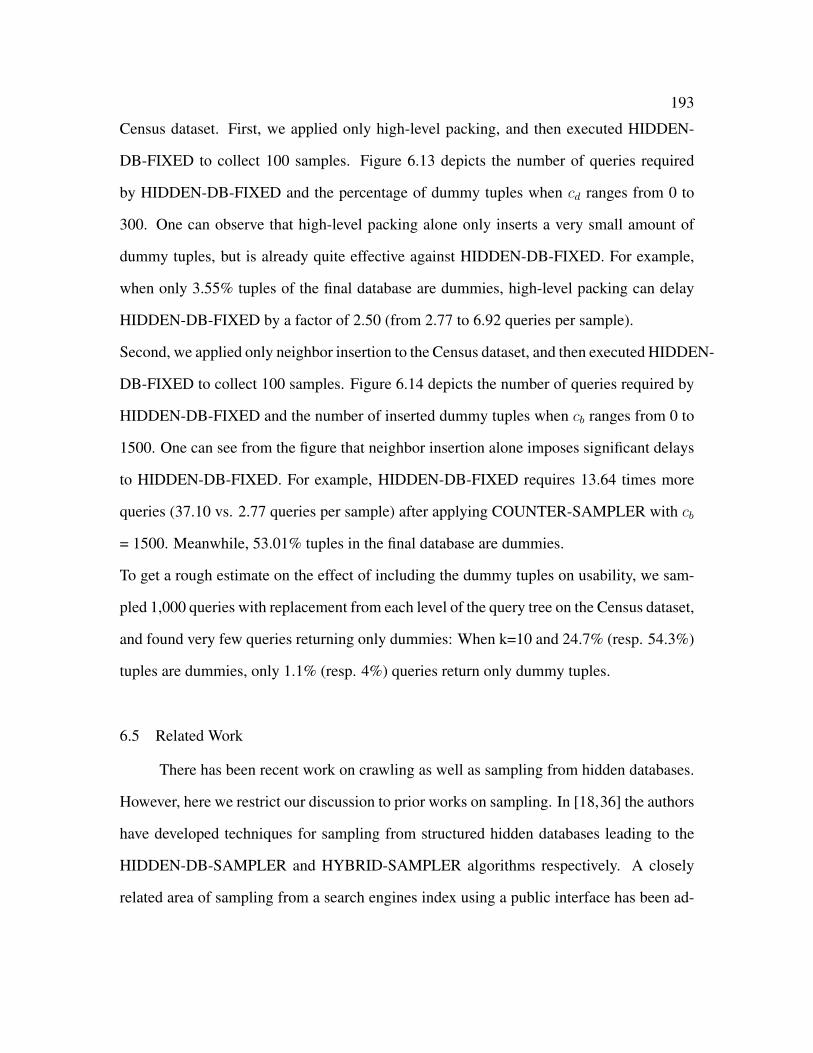
193
Census dataset. First, we applied only high-level packing, and then executed HIDDEN-
DB-FIXED to collect 100 samples. Figure 6.13 depicts the number of queries required
by HIDDEN-DB-FIXED and the percentage of dummy tuples when cd ranges from 0 to
300. One can observe that high-level packing alone only inserts a very small amount of
dummy tuples, but is already quite effective against HIDDEN-DB-FIXED. For example,
when only 3.55% tuples of the final database are dummies, high-level packing can delay
HIDDEN-DB-FIXED by a factor of 2.50 (from 2.77 to 6.92 queries per sample).
Second, we applied only neighbor insertion to the Census dataset, and then executed HIDDEN-
DB-FIXED to collect 100 samples. Figure 6.14 depicts the number of queries required by
HIDDEN-DB-FIXED and the number of inserted dummy tuples when cb ranges from 0 to
1500. One can see from the figure that neighbor insertion alone imposes significant delays
to HIDDEN-DB-FIXED. For example, HIDDEN-DB-FIXED requires 13.64 times more
queries (37.10 vs. 2.77 queries per sample) after applying COUNTER-SAMPLER with cb
= 1500. Meanwhile, 53.01% tuples in the final database are dummies.
To get a rough estimate on the effect of including the dummy tuples on usability, we sam-
pled 1,000 queries with replacement from each level of the query tree on the Census dataset,
and found very few queries returning only dummies: When k=10 and 24.7% (resp. 54.3%)
tuples are dummies, only 1.1% (resp. 4%) queries return only dummy tuples.
6.5 Related Work
There has been recent work on crawling as well as sampling from hidden databases.
However, here we restrict our discussion to prior works on sampling. In [18,36] the authors
have developed techniques for sampling from structured hidden databases leading to the
HIDDEN-DB-SAMPLER and HYBRID-SAMPLER algorithms respectively. A closely
related area of sampling from a search engines index using a public interface has been ad-
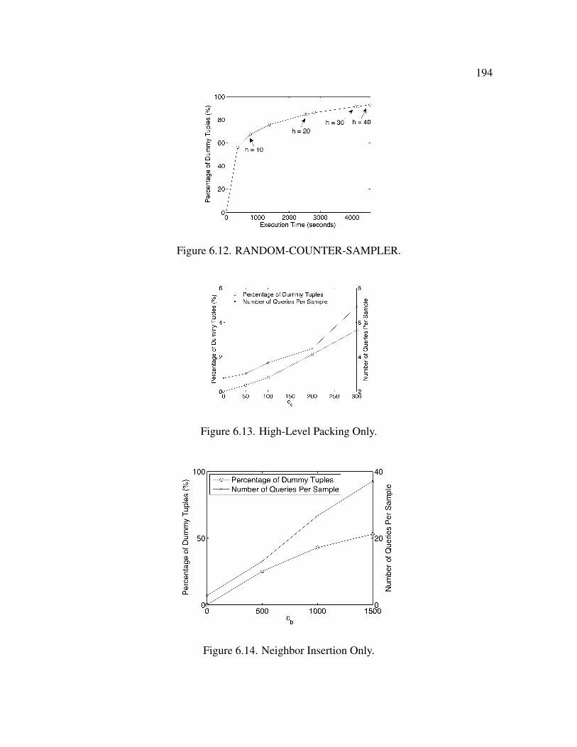
194
Figure 6.12. RANDOM-COUNTER-SAMPLER.
Figure 6.13. High-Level Packing Only.
Figure 6.14. Neighbor Insertion Only.
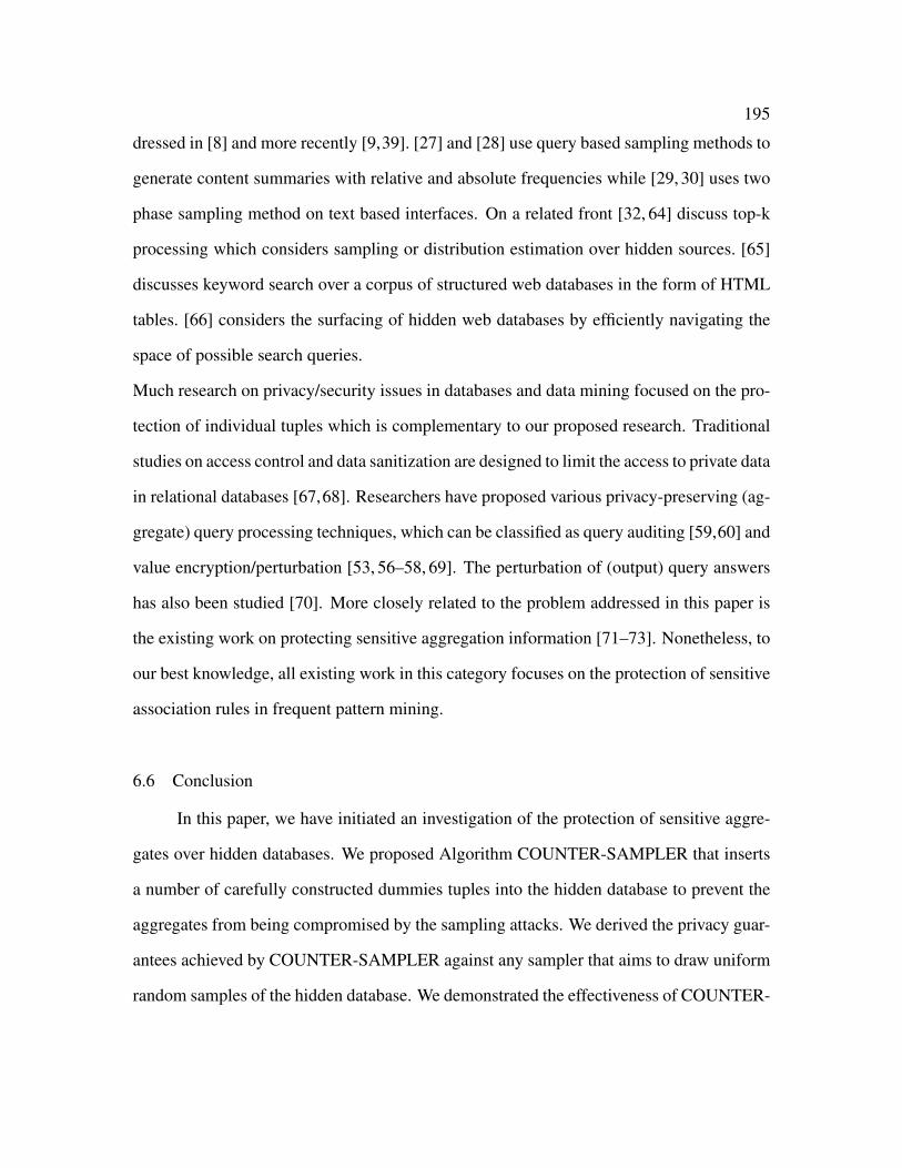
195
dressed in [8] and more recently [9,39]. [27] and [28] use query based sampling methods to
generate content summaries with relative and absolute frequencies while [29, 30] uses two
phase sampling method on text based interfaces. On a related front [32, 64] discuss top-k
processing which considers sampling or distribution estimation over hidden sources. [65]
discusses keyword search over a corpus of structured web databases in the form of HTML
tables. [66] considers the surfacing of hidden web databases by efficiently navigating the
space of possible search queries.
Much research on privacy/security issues in databases and data mining focused on the pro-
tection of individual tuples which is complementary to our proposed research. Traditional
studies on access control and data sanitization are designed to limit the access to private data
in relational databases [67,68]. Researchers have proposed various privacy-preserving (ag-
gregate) query processing techniques, which can be classified as query auditing [59,60] and
value encryption/perturbation [53, 56–58, 69]. The perturbation of (output) query answers
has also been studied [70]. More closely related to the problem addressed in this paper is
the existing work on protecting sensitive aggregation information [71–73]. Nonetheless, to
our best knowledge, all existing work in this category focuses on the protection of sensitive
association rules in frequent pattern mining.
6.6 Conclusion
In this paper, we have initiated an investigation of the protection of sensitive aggre-
gates over hidden databases. We proposed Algorithm COUNTER-SAMPLER that inserts
a number of carefully constructed dummies tuples into the hidden database to prevent the
aggregates from being compromised by the sampling attacks. We derived the privacy guar-
antees achieved by COUNTER-SAMPLER against any sampler that aims to draw uniform
random samples of the hidden database. We demonstrated the effectiveness of COUNTER-

196
SAMPLER against the state-of-the-art sampling algorithms [18,36][DDM07, DZD09]. We
performed a comprehensive set of experiments to illustrate the effectiveness of or algo-
rithm.
Our investigation is preliminary and many extensions are possible. For example, we fo-
cused on the dummy tuple insertion paradigm in this paper. In the future work, we shall in-
vestigate other defensive paradigms, such as the integration of dummy insertion and query
auditing, for protecting sensitive aggregates. We shall also investigate the techniques for the
protection of sensitive aggregates against adversaries holding external knowledge about the
underlying data distribution. Scenarios where hidden database interfaces return COUNT
results [36] also need to be explored. Another interesting future direction is the investiga-
tion of dynamic hidden databases and their impact on aggregates protection.
REFERENCES
[1] M. Bergman, “The deep web: Surfacing hidden value,” Journal of Electronic Pub-
lishing, vol. 7, no. 1, pp. 07–01, 2001.
[2] F. Olken and D. Rotem, “Random sampling from databases - a survey,” Statistics &
Computing, vol. 5, no. 1, pp. 25–42, 1995.
[3] J. S. Vitter, “Random sampling with a reservoir,” ACM Transactions on Mathematical
Software, vol. 11, no. 1, pp. 37–57, 1985.
[4] S. Chaudhuri, G. Das, and U. Srivastava, “Effective use of block-level sampling in
statistics estimation,” in SIGMOD, 2004.
[5] P. Haas and C. Konig, “A bi-level Bernoulli scheme for database sampling,” in Pro-
ceedings of the 2004 ACM SIGMOD international conference on Management of
data. ACM New York, NY, USA, 2004, pp. 275–286.
[6] G. Piatetsky-Shapiro and C. Connell, “Accurate estimation of the number of tuples
satisfying a condition,” ACM SIGMOD Record, vol. 14, no. 2, pp. 256–276, 1984.
[7] M. N. Garofalakis and P. B. Gibbons, “Approximate query processing: Taming the
terabytes,” in VLDB, 2001.
[8] K. Bharat and A. Broder, “A technique for measuring the relative size and overlap of
public web search engines,” in WWW, 1998.
[9] Z. Bar-Yossef and M. Gurevich, “Random sampling from a search engine’s index,” in
WWW, 2006.
[10] N. Metropolis, A. Rosenbluth, M. Rosenbluth, A. Teller, E. Teller, et al., “Equation
of state calculations by fast computing machines,” The journal of chemical physics,
vol. 21, no. 6, p. 1087, 1953.
197
198
[11] W. Hastings, “Monte Carlo sampling methods using Markov chains and their appli-
cations,” Biometrika, vol. 57, no. 1, pp. 97–109, 1970.
[12] J. von Neumann, “Various techniques for use in connection with random digits. In
von Neumann’s Collected Works, volume 5,” 1963.
[13] P. Ipeirotis, L. Gravano, and M. Sahami, “Probe, count, and classify: categorizing
hidden web databases,” in Proceedings of the 2001 ACM SIGMOD international con-
ference on Management of data. ACM New York, NY, USA, 2001, pp. 67–78.
[14] S. Lawrence and L. Giles, “Accessibility and distribution of information on the Web,”
Nature, vol. 400, no. 6740, pp. 107–109, 1999.
[15] S. Lawrence and C. Giles, “Searching the world wide web,” Science, vol. 280, no.
5360, p. 98, 1998.
[16] J. Callan, M. Connell, and A. Du, “Automatic discovery of language models for text
databases,” ACM SIGMOD Record, vol. 28, no. 2, pp. 479–490, 1999.
[17] S. Raghavan and H. Garcia-Molina, “Crawling the hidden web,” in VLDB, 2001.
[18] A. Dasgupta, G. Das, and H. Mannila, “A random walk approach to sampling hidden
databases,” in SIGMOD, 2007.
[19] V. T. Chakaravarthy, V. Pandit, S. Roy, P. Awasthi, and M. Mohania, “Decision trees
for entity identification: approximation algorithms and hardness results,” in PODS,
2007, pp. 53–62.
[20] G. Das, “Survey of approximate query processing techniques (tutorial),” in SSDBM,
2003.
[21] D. Barbara, W. DuMouchel, C. Faloutsos, P. J. Haas, J. M. Hellerstein, Y. E. Ioannidis,
H. V. Jagadish, T. Johnson, R. T. Ng, V. Poosala, K. A. Ross, and K. C. Sevcik, “The
new jersey data reduction report,” IEEE Data Engineering Bulletin, vol. 20, no. 4, pp.
3–45, 1997.
199
[22] B. Arai, G. Das, D. Gunopulos, and V. Kalogeraki, “Efficient approximate query
processing in peer-to-peer networks,” TKDE, vol. 19, no. 7, pp. 919–933, 2007.
[23] E. Agichtein, P. G. Ipeirotis, and L. Gravano, “Modeling query-based access to text
databases,” in WebDB, 2003.
[24] A. Ntoulas, P. Zerfos, and J. Cho, “Downloading textual hidden web content through
keyword queries,” in JCDL, 2005.
[25] S. W. Liddle, D. W. Embley, D. T. Scott, and S. H. Yau, “Extracting data behind web
forms,” in ER (Workshops), 2002.
[26] M. Alvarez, J. Raposo, A. Pan, F. Cacheda, F. Bellas, and V. Carneiro, “Crawling the
content hidden behind web forms,” in ICCSA, 2007.
[27] J. P. Callan and M. E. Connell, “Query-based sampling of text databases,” ACM Trans-
actions on Information Systems, vol. 19, no. 2, pp. 97–130, 2001.
[28] L. G. Panagiotis G. Ipeirotis, “Distributed search over the hidden web: Hierarchical
database sampling and selection,” in VLDB, 2002.
[29] Y.-L. Hedley, M. Younas, A. E. James, and M. Sanderson, “A two-phase sampling
technique for information extraction from hidden web databases,” in WIDM, 2004.
[30] ——, “Sampling, information extraction and summarisation of hidden web
databases,” Data and Knowledge Engineering, vol. 59, no. 2, pp. 213–230, 2006.
[31] K. C.-C. Chang and S. won Hwang, “Minimal probing: supporting expensive predi-
cates for top-k queries,” in SIGMOD, 2002.
[32] N. Bruno, L. Gravano, and A. Marian, “Evaluating top-k queries over web-accessible
databases,” in ICDE, 2002.
[33] L. Barbosa and J. Freire, “Siphoning hidden-web data through keyword-based inter-
faces,” in SBBD, 2004.
[34] Google Base, “http://base.google.com.”
[35] Yahoo! Auto, “http://auto.yahoo.com.”
200
[36] A. Dasgupta, N. Zhang, and G. Das, “Leveraging count information in sampling hid-
den databases,” in ICDE, 2009.
[37] A. Dasgupta, N. Zhang, G. Das, and S. Chaudhuri, “Privacy preservation of aggre-
gates in hidden databases: Why and how?” in SIGMOD, 2009.
[38] S. Chaudhuri, G. Das, and V. Narasayya, “Optimized stratified sampling for approxi-
mate query processing,” TODS, vol. 32, no. 2, 2007.
[39] Z. Bar-Yossef and M. Gurevich, “Efficient search engine measurements,” in WWW,
2007.
[40] S. Raghavan and H. Garcia-Molina, “Crawling the hidden web,” in VLDB, 2001.
[41] S. C. Amstrup, B. F. J. Manly, and T. L. McDonald, Handbook of capture-recapture
analysis. Princeton University Press, 2005.
[42] M. Shokouhi, J. Zobel, F. Scholer, and S. Tahaghoghi, “Capturing collection size for
distributed non-cooperative retrieval,” in SIGIR, 2006.
[43] A. Broder, M. Fontura, V. Josifovski, R. Kumar, R. Motwani, S. U. Nabar, R. Pani-
grahy, A. Tomkins, and Y. Xu, “Estimating corpus size via queries,” in CIKM, 2006.
[44] J. Lu, “Efficient estimation of the size of text deep web data source,” in CIKM, 2008.
[45] G. A. F. Seber, The estimation of animal abundance and related parameters. New
York: MacMillan Press, 1982.
[46] D. Horvitz and D. Thompson, “A generalization of sampling without replacement
from a finite universe,” Journal of the American Statistical Association, vol. 47, pp.
663–685, 1952.
[47] B. Ripley, Stochastic Simulation. New York: Wiley & Sons, 1987.
[48] B. Babcock, S. Chaudhuri, and G. Das, “Dynamic sample selection for approximate
query processing,” in SIGMOD, 2003.
[49] J. Gray, P. Sundaresan, S. Englert, K. Baclawski, and P. J. Weinberger, “Quickly
generating billion-record synthetic databases,” in SIGMOD, 1994.
201
[50] Y. C. Liu, K. and W. Meng, “Discovering the representative of a search engine,” in
CIKM, 2002.
[51] Z. Bar-Yossef and M. Gurevich, “Mining search engine query logs via suggestion
sampling,” in VLDB, 2008.
[52] J. Elson, J. Douceur, J. Howell, and J. Saul, “Asirra: a captcha that exploits interest-
aligned manual image categorization,” in Proc. of ACM CCS, 2007, pp. 366–374.
[53] R. Agrawal and R. Srikant, “Privacy-preserving data mining,” ACM Sigmod Record,
vol. 29, no. 2, pp. 439–450, 2000.
[54] C. Clifton, M. Kantarcioglu, J. Vaidya, X. Lin, and M. Zhu, “Tools for privacy pre-
serving distributed data mining,” ACM SIGKDD Explorations Newsletter, vol. 4,
no. 2, pp. 28–34, 2002.
[55] N. Zhang and W. Zhao, “Privacy-preserving data mining systems,” Computer, vol. 40,
no. 4, pp. 52–58, 2007.
[56] L. Sweeney et al., “k-anonymity: A model for protecting privacy,” International Jour-
nal of Uncertainty Fuzziness and Knowledge Based Systems, vol. 10, no. 5, pp. 557–
570, 2002.
[57] R. Agrawal, R. Srikant, and D. Thomas, “Privacy preserving OLAP,” in SIGMOD
Conference. Citeseer, 2005, pp. 251–262.
[58] R. Agrawal, A. Evfimievski, and R. Srikant, “Information sharing across private
databases,” in Proceedings of the 2003 ACM SIGMOD international conference on
Management of data. ACM, 2003, pp. 86–97.
[59] S. Nabar, B. Marthi, K. Kenthapadi, N. Mishra, and R. Motwani, “Towards robustness
in query auditing,” in Proceedings of the 32nd international conference on Very large
data bases. VLDB Endowment, 2006, p. 162.
202
[60] K. Kenthapadi, N. Mishra, and K. Nissim, “Simulatable auditing,” in Proceedings
of the twenty-fourth ACM SIGMOD-SIGACT-SIGART symposium on Principles of
database systems. ACM, 2005, p. 127.
[61] Google, “http://code.google.com/apis/soapsearch/api faq.html.”
[62] A. Dasgupta, N. Zhang, G. Das, and S. Chaudhuri, “Privacy preservation of aggre-
gates in hidden databases: why and how?” Technical Report TR-GWU-CS-09-001,
George Washington University, Tech. Rep., 2009.
[63] S. Hettich and S. D. Bay, “The uci kdd archive [http://kdd.ics.uci.edu],” Irvine, CA.
University of California, Department of Information and Computer Science, Tech.
Rep., 1999.
[64] K. Chang and S. Hwang, “Minimal probing: supporting expensive predicates for top-
k queries,” in Proceedings of the 2002 ACM SIGMOD international conference on
Management of data. ACM, 2002, p. 357.
[65] M. Cafarella, A. Halevy, D. Wang, E. Wu, and Y. Zhang, “Webtables: Exploring the
power of tables on the web,” Proceedings of the VLDB Endowment, vol. 1, no. 1, pp.
538–549, 2008.
[66] J. Madhavan, D. Ko, Ł. Kot, V. Ganapathy, A. Rasmussen, and A. Halevy, “Google’s
deep web crawl,” Proceedings of the VLDB Endowment archive, vol. 1, no. 2, pp.
1241–1252, 2008.
[67] S. Jajodia, P. Samarati, M. Sapino, and V. Subrahmanian, “Flexible support for multi-
ple access control policies,” ACM Transactions on Database Systems (TODS), vol. 26,
no. 2, pp. 214–260, 2001.
[68] R. Sandhu, E. Coyne, H. Feinstein, and C. Youman, “Role-based access control mod-
els,” Computer, vol. 29, no. 2, pp. 38–47, 1996.
203
[69] A. Machanavajjhala, D. Kifer, J. Gehrke, and M. Venkitasubramaniam, “l-diversity:
Privacy beyond k-anonymity,” ACM Transactions on Knowledge Discovery from Data
(TKDD), vol. 1, no. 1, p. 3, 2007.
[70] C. Dwork, F. McSherry, K. Nissim, and A. Smith, “Calibrating noise to sensitivity in
private data analysis,” Theory of Cryptography, pp. 265–284, 2006.
[71] M. Atallah, A. Elmagarmid, M. Ibrahim, E. Bertino, and V. Verykios, “Disclosure
limitation of sensitive rules,” in kdex. Published by the IEEE Computer Society,
1999, p. 45.
[72] A. Gkoulalas-Divanis and V. Verykios, “An integer programming approach for fre-
quent itemset hiding,” in Proceedings of the 15th ACM international conference on
Information and knowledge management. ACM, 2006, p. 757.
[73] V. Verykios, A. Elmagarmid, E. Bertino, Y. Saygin, and E. Dasseni, “Association rule
hiding,” IEEE Transactions on Knowledge and Data Engineering, vol. 16, no. 4, pp.
434–447, 2004.

BIOGRAPHICAL STATEMENT
Arjun Dasgupta was born in Calcutta, India, in 1982. He received his Bachelors in
Engineering (Computer Science) degree from Anna University, Chennai, in 2005 and his
M.S. (Computer Science) from The University of Texas at Arlington in 2007.
His current research interest is in Information Retrieval from Hidden Databases and
Web, Data Mining, Social Networks and Graph Theory.
204