forest analytics with r
TRANSCRIPT

For a complete list of titles published in this series, go to www.springer.com/series/6991
Use R!Series EditorsRobert Gentleman Kurt Hornik Giovanni Parmigiani

Paradis: Analysis of Phylogenetics and Evolution with R
Hahne/Huber/Gentleman/Falcon: Bioconductor Case Studies
Sarkar: Lattice: Multivariate Data Visualization with RSpector: Data Manipulation with R
Use R!
and GGobi
Claude:Morphometrics with R
Peng/Dominici: Statistical Methods for Environmental Epidemiology with R:
Bivand/Pebesma/Gomez-Rubio: Applied Spatial Data Analysis with R
Nason: Wavelet Methods in Statistics with R
A Case Study in Air Pollution and Health
´Albert: Bayesian Computation with R
Cook/Swayne: Interactive and Dynamic Graphics for Data Analysis: With R
editionPfaff: Analysis of Integrated and Cointegrated Time Series with R, 2nd

1 C
Andrew P. Robinson • Jeff D. Hamann
Forest Analytics with R
An Introduction

ISBN 978-1-4419-7761-8 e-ISBN 978-1-4419-7762-5DOI 10.1007/978-1-4419-7762-5Springer New York Dordrecht Heidelberg London
© Springer Science+Business Media, LLC 2011All rights reserved. This work may not be translated or copied in whole or in part without the written permission of the publisher (Springer Science+Business Media, LLC, 233 Spring Street, New York, NY 10013, USA), except for brief excerpts in connection with reviews or scholarly analysis. Use in connec-tion with any form of information storage and retrieval, electronic adaptation, computer software, or by similar or dissimilar methodology now known or hereafter developed is forbidden.The use in this publication of trade names, trademarks, service marks, and similar terms, even if they are not identified as such, is not to be taken as an expression of opinion as to whether or not they are subject to proprietary rights.
Printed on acid-free paper
Springer is part of Springer Science+Business Media (www.springer.com)
Andrew P. RobinsonDept. Mathematics and StatisticsUniversity of MelbourneParkville 3010 [email protected]
Jeff D. HamannForest Informatics, Inc.PO Box 142197339-1421 Corvallis [email protected]
Series Editors:Robert GentlemanProgram in Computational BiologyDivision of Public Health SciencesFred Hutchinson Cancer Research Center1100 Fairview Avenue, N. M2-B876Seattle,Washington 98109USA
Kurt HornikDepartment of Statistik and MathematikWirtschaftsuniversität Wien Augasse 2-6A-1090 WienAustria
Giovanni ParmigianiThe Sidney Kimmel ComprehensiveCancer Center at Johns Hopkins University550 North BroadwayBaltimore, MD 21205-2011USA

This book is dedicated to Grace, Felix, and M’Liss,(and Henry and Yohan)
with grateful thanks for inspiration and patience.

Preface
R is an open-source and free software environment for statistical computingand graphics. R compiles and runs on a wide variety of UNIX platforms(e.g., GNU/Linux and FreeBSD), Windows, and Mac OSX. Since the late1990s, R has been developed by hundreds of contributors and new capabilitiesare added each month. The software is gaining popularity because: 1) it isplatform independent, 2) it is free, and 3) the source code is freely availableand can be inspected to determine exactly what R is doing.
Our objectives for this book are to 1) demonstrate the use of R as a solidplatform upon which forestry analysts can develop repeatable and clearlydocumented methods; 2) provide guidance in the broad area of data handlingand analysis for forest and natural resources analytics; and 3) to use R tosolve problems we face each day as forest data analysts.
This book is intended for two broad audiences: students, researchers, andsoftware people who commonly handle forestry data; and forestry practition-ers who need to develop actionable solutions to common operational, tactical,and strategic problems. We often mention better and more complete treat-ments of specific subject material for further reference (e.g., forest sampling,spatial statistics, or operations research).
We hope that this book will serve as a field manual for practicing forest an-alysts, managers, and researchers. We hope that it will be dog-eared, defaced,coffee/tea-stained, and sticky-noted to near destruction. We hope the readerwill engage in the exercises, scrutinize its contents, forgive our weaknesses,possibly and carefully absorb suggestions, and constructively criticize.
Acknowledgments
This book would not have been possible without the patient and generousassistance of many people. We first thank all the authors of the literaturewe cite, who were willing to publish their data as part of their research.
vii

viii Preface
These data are often our only link between repeatable research and anecdotalopinion.
We thank Valerie LeMay and Timothy Gregoire for their kind contributionof tree measurement data and for their encouragement and leadership inthe field. We thank Boris Zeide for his generous contribution of the vonGuttenberg data. We thank Don Wallace and Bruce Alber for supplyingan interesting dataset to demonstrate the data management, plotting, andfile functions in Chapter 2. We thank the Oregon State University Collegeof Forestry Research Forests web site for posting a publicly available forestinventory for Chapters 2 and 4. Without those data, many of the examplesand topics in this book would have to have been performed using simulateddata and frankly would have been much less interesting. We thank MartinRitchie for providing data, funding, and snippets of code once lost and foundagain during the development of the rconifers package, used in Chapter 8. Wethank David Hann for, years ago, providing an original copy of the manuscriptthat we used to generate the shared library example (chambers-1980.so) inChapter 8 (Chambers, 1980).
We have received considerable constructive criticism via the review pro-cess, only some of which we can source. We especially thank John Kershawfor generous and detailed comments on Chapter 3, Jeff Gove for his supportand useful commentary on Chapter 5, and David Ratkowsky and GrahamHepworth for their thoughtful and thought-provoking comments on Chap-ters 6 and 7, respectively. Numerous other useful comments were made byanonymous reviewers. The collection of review comments improved the bookimmeasurably.
We thank R Core, the R community, and all the package authors and main-tainers we have come to rely upon. Specifically, we thank the following people,in no particular order: David B. Dahl (xtable); Lopaka Lee (R-GLPK); An-drew Makhorin (GLPK); Roger Bivand (maptools); Deepayan Sarkar (lat-tice); Hadley Wickham (ggplot2); Brian Ripley (MASS, class, boot); JosePinheiro and Douglas Bates (nlme); Frank Harrell (Hmisc); Alvaro Novo andJoe Schafer (norm); Greg Warnes (gmodels et al.); Reinhard Furrer, DouglasNychka, and Stephen Sain (fields); Thomas Lumley (survey); and NicholasJ. Lewin-Koh and Roger Bivand (maptools).
We thank John Kimmel, our managing editor at Springer, for showing in-credible patience and Hal Henglein, our copy editor, for keeping us consistent.
AR wishes to thank Mark Burgman for providing space to finish this bookwithin a packed ACERA calendar, and for his substantial support and guid-ance. AR also wishes to thank Geoff Wood, Brian Turner, Alan Ek, andAlbert Stage for their kindness and intellectual support along the way.
JH wishes to thank Martin Ritchie, David Marshall, Kevin Boston, andJohn Sessions for their support along the way.
Finally, we wish to thank our wives, children, and friends for cheerfulperseverance and support in the face of a task that seemed at times like alittle slice of Sisyphus.

Preface ix
Melbourne and Corvallis Andrew Robinson
August 16, 2010 Jeff D. Hamann

Contents
Preface . . . . . . . . . . . . . . . . . . . . . . . . . . . . . . . . . . . . . . . . . . . . . . . . . . . . . . . vii
Part I Introduction and Data Management
1 Introduction . . . . . . . . . . . . . . . . . . . . . . . . . . . . . . . . . . . . . . . . . . . . . . 31.1 This Book . . . . . . . . . . . . . . . . . . . . . . . . . . . . . . . . . . . . . . . . . . . . . 5
1.1.1 Topics Covered in This Book . . . . . . . . . . . . . . . . . . . . . . 51.1.2 Conventions Used in This Book . . . . . . . . . . . . . . . . . . . . 61.1.3 The Production of the Book . . . . . . . . . . . . . . . . . . . . . . . 6
1.2 Software . . . . . . . . . . . . . . . . . . . . . . . . . . . . . . . . . . . . . . . . . . . . . . 71.2.1 Communicating with R . . . . . . . . . . . . . . . . . . . . . . . . . . . 71.2.2 Getting Help . . . . . . . . . . . . . . . . . . . . . . . . . . . . . . . . . . . . 91.2.3 Using Scripts . . . . . . . . . . . . . . . . . . . . . . . . . . . . . . . . . . . . 111.2.4 Extending R . . . . . . . . . . . . . . . . . . . . . . . . . . . . . . . . . . . . . 121.2.5 Programming Suggestions . . . . . . . . . . . . . . . . . . . . . . . . . 131.2.6 Programming Conventions . . . . . . . . . . . . . . . . . . . . . . . . . 141.2.7 Speaking Other Languages . . . . . . . . . . . . . . . . . . . . . . . . 15
1.3 Notes about Data Analysis . . . . . . . . . . . . . . . . . . . . . . . . . . . . . . 16
2 Forest Data Management . . . . . . . . . . . . . . . . . . . . . . . . . . . . . . . . . 192.1 Basic Concepts . . . . . . . . . . . . . . . . . . . . . . . . . . . . . . . . . . . . . . . . . 192.2 File Functions . . . . . . . . . . . . . . . . . . . . . . . . . . . . . . . . . . . . . . . . . . 20
2.2.1 Text Files . . . . . . . . . . . . . . . . . . . . . . . . . . . . . . . . . . . . . . . 202.2.2 Spreadsheets . . . . . . . . . . . . . . . . . . . . . . . . . . . . . . . . . . . . . 252.2.3 Using SQL in R . . . . . . . . . . . . . . . . . . . . . . . . . . . . . . . . . . 262.2.4 The foreign Package . . . . . . . . . . . . . . . . . . . . . . . . . . . . . . 262.2.5 Geographic Data . . . . . . . . . . . . . . . . . . . . . . . . . . . . . . . . . 282.2.6 Other Data Formats . . . . . . . . . . . . . . . . . . . . . . . . . . . . . . 29
2.3 Data Management Functions . . . . . . . . . . . . . . . . . . . . . . . . . . . . . 302.3.1 Herbicide Trial Data . . . . . . . . . . . . . . . . . . . . . . . . . . . . . . 312.3.2 Simple Error Checking . . . . . . . . . . . . . . . . . . . . . . . . . . . . 33
xi
xii Contents
2.3.3 Graphical error checking . . . . . . . . . . . . . . . . . . . . . . . . . . 342.3.4 Data Structure Functions . . . . . . . . . . . . . . . . . . . . . . . . . . 37
2.4 Examples . . . . . . . . . . . . . . . . . . . . . . . . . . . . . . . . . . . . . . . . . . . . . . 432.4.1 Upper Flat Creek in the UIEF . . . . . . . . . . . . . . . . . . . . . 432.4.2 Sweetgum Stem Profiles . . . . . . . . . . . . . . . . . . . . . . . . . . . 462.4.3 FIA Data . . . . . . . . . . . . . . . . . . . . . . . . . . . . . . . . . . . . . . . 512.4.4 Norway Spruce Profiles . . . . . . . . . . . . . . . . . . . . . . . . . . . 522.4.5 Grand Fir Profiles . . . . . . . . . . . . . . . . . . . . . . . . . . . . . . . . 532.4.6 McDonald–Dunn Research Forest . . . . . . . . . . . . . . . . . . 552.4.7 Priest River Experimental Forest . . . . . . . . . . . . . . . . . . . 612.4.8 Leuschner . . . . . . . . . . . . . . . . . . . . . . . . . . . . . . . . . . . . . . . 72
2.5 Summary . . . . . . . . . . . . . . . . . . . . . . . . . . . . . . . . . . . . . . . . . . . . . . 72
Part II Sampling and Mapping
3 Data Analysis for Common Inventory Methods . . . . . . . . . . . 753.1 Introduction . . . . . . . . . . . . . . . . . . . . . . . . . . . . . . . . . . . . . . . . . . . 75
3.1.1 Infrastructure . . . . . . . . . . . . . . . . . . . . . . . . . . . . . . . . . . . . 763.1.2 Example Datasets . . . . . . . . . . . . . . . . . . . . . . . . . . . . . . . . 77
3.2 Estimate Computation . . . . . . . . . . . . . . . . . . . . . . . . . . . . . . . . . . 773.2.1 Sampling Distribution . . . . . . . . . . . . . . . . . . . . . . . . . . . . 773.2.2 Intervals from Large-Sample Theory . . . . . . . . . . . . . . . . 803.2.3 Intervals from Linearization . . . . . . . . . . . . . . . . . . . . . . . 813.2.4 Intervals from the Jackknife . . . . . . . . . . . . . . . . . . . . . . . 823.2.5 Intervals from the Bootstrap . . . . . . . . . . . . . . . . . . . . . . . 843.2.6 A Simulation Study . . . . . . . . . . . . . . . . . . . . . . . . . . . . . . 92
3.3 Single-Level Sampling . . . . . . . . . . . . . . . . . . . . . . . . . . . . . . . . . . . 943.3.1 Simple Random Sampling . . . . . . . . . . . . . . . . . . . . . . . . . 943.3.2 Systematic Sampling . . . . . . . . . . . . . . . . . . . . . . . . . . . . . . 96
3.4 Hierarchical Sampling . . . . . . . . . . . . . . . . . . . . . . . . . . . . . . . . . . . 973.4.1 Cluster Sampling . . . . . . . . . . . . . . . . . . . . . . . . . . . . . . . . . 973.4.2 Two-Stage Sampling . . . . . . . . . . . . . . . . . . . . . . . . . . . . . . 100
3.5 Using Auxiliary Information . . . . . . . . . . . . . . . . . . . . . . . . . . . . . 1043.5.1 Stratified Sampling . . . . . . . . . . . . . . . . . . . . . . . . . . . . . . . 1043.5.2 Ratio Estimation . . . . . . . . . . . . . . . . . . . . . . . . . . . . . . . . . 1063.5.3 Regression Estimation . . . . . . . . . . . . . . . . . . . . . . . . . . . . 1093.5.4 3P Sampling . . . . . . . . . . . . . . . . . . . . . . . . . . . . . . . . . . . . . 1113.5.5 VBAR . . . . . . . . . . . . . . . . . . . . . . . . . . . . . . . . . . . . . . . . . . 113
3.6 Summary . . . . . . . . . . . . . . . . . . . . . . . . . . . . . . . . . . . . . . . . . . . . . . 114
4 Imputation and Interpolation . . . . . . . . . . . . . . . . . . . . . . . . . . . . . 1174.1 Introduction . . . . . . . . . . . . . . . . . . . . . . . . . . . . . . . . . . . . . . . . . . . 1174.2 Imputation . . . . . . . . . . . . . . . . . . . . . . . . . . . . . . . . . . . . . . . . . . . . 118
4.2.1 Examining Missingness Patterns . . . . . . . . . . . . . . . . . . . 1184.2.2 Methods for Imputing Missing Data . . . . . . . . . . . . . . . . 125
Contents xiii
4.2.3 Nearest-Neighbor Imputation . . . . . . . . . . . . . . . . . . . . . . 1264.2.4 Expectation-Maximization Imputation . . . . . . . . . . . . . . 1314.2.5 Comparing Results . . . . . . . . . . . . . . . . . . . . . . . . . . . . . . . 133
4.3 Interpolation . . . . . . . . . . . . . . . . . . . . . . . . . . . . . . . . . . . . . . . . . . . 1354.3.1 Methods of Interpolation . . . . . . . . . . . . . . . . . . . . . . . . . . 1364.3.2 Ordinary Kriging . . . . . . . . . . . . . . . . . . . . . . . . . . . . . . . . . 1384.3.3 Semi-variogram Estimation . . . . . . . . . . . . . . . . . . . . . . . . 1414.3.4 Prediction . . . . . . . . . . . . . . . . . . . . . . . . . . . . . . . . . . . . . . . 145
4.4 Summary . . . . . . . . . . . . . . . . . . . . . . . . . . . . . . . . . . . . . . . . . . . . . . 148
Part III Allometry and Fitting Models
5 Fitting Dimensional Distributions . . . . . . . . . . . . . . . . . . . . . . . . 1555.1 Diameter Distribution . . . . . . . . . . . . . . . . . . . . . . . . . . . . . . . . . . . 1565.2 Non-parametric Representation . . . . . . . . . . . . . . . . . . . . . . . . . . 1575.3 Parametric Representation . . . . . . . . . . . . . . . . . . . . . . . . . . . . . . . 158
5.3.1 Parameter Estimation. . . . . . . . . . . . . . . . . . . . . . . . . . . . . 1585.3.2 Some Models of Choice . . . . . . . . . . . . . . . . . . . . . . . . . . . 1645.3.3 Profiling . . . . . . . . . . . . . . . . . . . . . . . . . . . . . . . . . . . . . . . . 1685.3.4 Sampling Weights . . . . . . . . . . . . . . . . . . . . . . . . . . . . . . . . 172
6 Linear and Non-linear Modeling . . . . . . . . . . . . . . . . . . . . . . . . . . 1756.1 Linear Regression . . . . . . . . . . . . . . . . . . . . . . . . . . . . . . . . . . . . . . 175
6.1.1 Example . . . . . . . . . . . . . . . . . . . . . . . . . . . . . . . . . . . . . . . . 1786.1.2 Thinking about the Problem . . . . . . . . . . . . . . . . . . . . . . . 1806.1.3 Fitting the Model . . . . . . . . . . . . . . . . . . . . . . . . . . . . . . . . 1806.1.4 Assumptions and Diagnostics . . . . . . . . . . . . . . . . . . . . . . 1816.1.5 Examining the Model . . . . . . . . . . . . . . . . . . . . . . . . . . . . . 1856.1.6 Using the Model . . . . . . . . . . . . . . . . . . . . . . . . . . . . . . . . . 1886.1.7 Testing Effects . . . . . . . . . . . . . . . . . . . . . . . . . . . . . . . . . . . 1926.1.8 Transformations . . . . . . . . . . . . . . . . . . . . . . . . . . . . . . . . . . 1956.1.9 Weights . . . . . . . . . . . . . . . . . . . . . . . . . . . . . . . . . . . . . . . . . 1956.1.10 Generalized Least-Squares Models . . . . . . . . . . . . . . . . . . 197
6.2 Non-linear Regression . . . . . . . . . . . . . . . . . . . . . . . . . . . . . . . . . . . 1996.2.1 Example . . . . . . . . . . . . . . . . . . . . . . . . . . . . . . . . . . . . . . . . 2006.2.2 Thinking about the Problem . . . . . . . . . . . . . . . . . . . . . . . 2006.2.3 Fitting the Model . . . . . . . . . . . . . . . . . . . . . . . . . . . . . . . . 2026.2.4 Assumptions and Diagnostics . . . . . . . . . . . . . . . . . . . . . . 2036.2.5 Examining the Model . . . . . . . . . . . . . . . . . . . . . . . . . . . . . 2076.2.6 Using the Model . . . . . . . . . . . . . . . . . . . . . . . . . . . . . . . . . 2106.2.7 Testing Effects . . . . . . . . . . . . . . . . . . . . . . . . . . . . . . . . . . . 2106.2.8 Generalized Non-linear Least-Squares Models . . . . . . . . 2126.2.9 Self-starting Functions . . . . . . . . . . . . . . . . . . . . . . . . . . . . 213
6.3 Back to Maximum Likelihood . . . . . . . . . . . . . . . . . . . . . . . . . . . . 2146.3.1 Linear Regression . . . . . . . . . . . . . . . . . . . . . . . . . . . . . . . . 215
xiv Contents
6.3.2 Non-linear Regression . . . . . . . . . . . . . . . . . . . . . . . . . . . . . 2166.3.3 Heavy-Tailed Residuals . . . . . . . . . . . . . . . . . . . . . . . . . . . 217
7 Fitting Linear Hierarchical Models . . . . . . . . . . . . . . . . . . . . . . . 2197.1 Introduction . . . . . . . . . . . . . . . . . . . . . . . . . . . . . . . . . . . . . . . . . . . 219
7.1.1 Effects . . . . . . . . . . . . . . . . . . . . . . . . . . . . . . . . . . . . . . . . . . 2207.1.2 Model Construction . . . . . . . . . . . . . . . . . . . . . . . . . . . . . . 2237.1.3 Solving a Dilemma . . . . . . . . . . . . . . . . . . . . . . . . . . . . . . . 2257.1.4 Decomposition . . . . . . . . . . . . . . . . . . . . . . . . . . . . . . . . . . . 226
7.2 Linear Mixed-Effects Models . . . . . . . . . . . . . . . . . . . . . . . . . . . . . 2277.2.1 A Simple Example . . . . . . . . . . . . . . . . . . . . . . . . . . . . . . . . 227
7.3 Case Study: Height and Diameter Model . . . . . . . . . . . . . . . . . . 2337.3.1 Height vs. Diameter . . . . . . . . . . . . . . . . . . . . . . . . . . . . . . 2347.3.2 Use More Data . . . . . . . . . . . . . . . . . . . . . . . . . . . . . . . . . . . 2437.3.3 Adding Fixed Effects . . . . . . . . . . . . . . . . . . . . . . . . . . . . . 2547.3.4 The Model . . . . . . . . . . . . . . . . . . . . . . . . . . . . . . . . . . . . . . 256
7.4 Model Wrangling . . . . . . . . . . . . . . . . . . . . . . . . . . . . . . . . . . . . . . . 2597.4.1 Monitor . . . . . . . . . . . . . . . . . . . . . . . . . . . . . . . . . . . . . . . . . 2607.4.2 Meddle . . . . . . . . . . . . . . . . . . . . . . . . . . . . . . . . . . . . . . . . . 2607.4.3 Modify . . . . . . . . . . . . . . . . . . . . . . . . . . . . . . . . . . . . . . . . . . 2607.4.4 Compromise . . . . . . . . . . . . . . . . . . . . . . . . . . . . . . . . . . . . . 261
7.5 The Deep End . . . . . . . . . . . . . . . . . . . . . . . . . . . . . . . . . . . . . . . . . 2617.5.1 Maximum Likelihood . . . . . . . . . . . . . . . . . . . . . . . . . . . . . 2627.5.2 Restricted Maximum Likelihood . . . . . . . . . . . . . . . . . . . . 263
7.6 Non-linear Mixed-Effects Models . . . . . . . . . . . . . . . . . . . . . . . . . 2647.6.1 Hierarchical Approach . . . . . . . . . . . . . . . . . . . . . . . . . . . . 269
7.7 Further Reading . . . . . . . . . . . . . . . . . . . . . . . . . . . . . . . . . . . . . . . . 273
Part IV Simulation and Optimization
8 Simulations . . . . . . . . . . . . . . . . . . . . . . . . . . . . . . . . . . . . . . . . . . . . . . . 2778.1 Generating Simulations . . . . . . . . . . . . . . . . . . . . . . . . . . . . . . . . . 278
8.1.1 Simulating Young Stands . . . . . . . . . . . . . . . . . . . . . . . . . . 2798.1.2 Simulating Established Stands . . . . . . . . . . . . . . . . . . . . . 284
8.2 Generating Volumes . . . . . . . . . . . . . . . . . . . . . . . . . . . . . . . . . . . . 2908.2.1 The Taper Function . . . . . . . . . . . . . . . . . . . . . . . . . . . . . . 2918.2.2 Computing Merchantable Height . . . . . . . . . . . . . . . . . . . 2918.2.3 Summarizing Log Volumes by Grade . . . . . . . . . . . . . . . . 2938.2.4 Young-Stand Volumes . . . . . . . . . . . . . . . . . . . . . . . . . . . . . 2958.2.5 Established-Stand Volumes . . . . . . . . . . . . . . . . . . . . . . . . 296
8.3 Merging Yield Streams . . . . . . . . . . . . . . . . . . . . . . . . . . . . . . . . . . 2998.4 Examining Results . . . . . . . . . . . . . . . . . . . . . . . . . . . . . . . . . . . . . . 299
8.4.1 Volume Distribution . . . . . . . . . . . . . . . . . . . . . . . . . . . . . . 3028.4.2 Mean Annual Increment . . . . . . . . . . . . . . . . . . . . . . . . . . . 304
8.5 Exporting Yields . . . . . . . . . . . . . . . . . . . . . . . . . . . . . . . . . . . . . . . 305

Contents xv
8.6 Summary . . . . . . . . . . . . . . . . . . . . . . . . . . . . . . . . . . . . . . . . . . . . . . 305
9 Forest Estate Planning and Optimization . . . . . . . . . . . . . . . . . 3079.1 Introduction . . . . . . . . . . . . . . . . . . . . . . . . . . . . . . . . . . . . . . . . . . . 3079.2 Problem Formulation . . . . . . . . . . . . . . . . . . . . . . . . . . . . . . . . . . . 3089.3 Strict Area Harvest Schedule . . . . . . . . . . . . . . . . . . . . . . . . . . . . . 309
9.3.1 Objective Function . . . . . . . . . . . . . . . . . . . . . . . . . . . . . . . 3109.3.2 Adding Columns . . . . . . . . . . . . . . . . . . . . . . . . . . . . . . . . . 3109.3.3 Naming Columns . . . . . . . . . . . . . . . . . . . . . . . . . . . . . . . . . 3119.3.4 Bounding Columns . . . . . . . . . . . . . . . . . . . . . . . . . . . . . . . 3129.3.5 Setting Objective Coefficients . . . . . . . . . . . . . . . . . . . . . . 3129.3.6 Adding Constraints . . . . . . . . . . . . . . . . . . . . . . . . . . . . . . . 3129.3.7 Solving . . . . . . . . . . . . . . . . . . . . . . . . . . . . . . . . . . . . . . . . . 3169.3.8 Results . . . . . . . . . . . . . . . . . . . . . . . . . . . . . . . . . . . . . . . . . 3179.3.9 Archiving Problems . . . . . . . . . . . . . . . . . . . . . . . . . . . . . . . 3229.3.10 Cleanup . . . . . . . . . . . . . . . . . . . . . . . . . . . . . . . . . . . . . . . . . 322
9.4 Summary . . . . . . . . . . . . . . . . . . . . . . . . . . . . . . . . . . . . . . . . . . . . . . 323
References . . . . . . . . . . . . . . . . . . . . . . . . . . . . . . . . . . . . . . . . . . . . . . . . . . . . 325
Index . . . . . . . . . . . . . . . . . . . . . . . . . . . . . . . . . . . . . . . . . . . . . . . . . . . . . . . . . 335

Part I
Introduction and Data Management

Chapter 1
Introduction
Forestry has offered a fertile environment for data analysts to operate insince forest measurements began. Forestry datasets are typically voluminous,hierarchical, messy, multi-faceted, and expensive. The challenges that forestmanagers face are complex, and the costs of poor decisions can be high. Onthe other hand, often, but not always, decisions are made over long timeframes, and there is time for considered data analysis. Forestry data analystsare fortunate to work in a space in which the data and the resources areusually sufficient to do something that is more useful than doing nothing.
Forestry has a wide range of datasets and questions in which statistics,econometrics, and applied mathematics tools can all play a constructive role.The challenge for the data analyst is to find the best match between the data,the question, and the tools. The match depends on the context. A model ordataset that perfectly suits one application may be quite inappropriate foranother. The same model or dataset may be just the best that can be doneat the time, and reluctantly accepted. The analyst must be pragmatic.
This need for pragmatism must cut across received dogma from statisticsand other fields. For example, in Chapters 6 and 7 we spend considerabletime scrutinizing graphical diagnostics to learn more about the intersectionsbetween particular models and the data to which we have fit them, as en-capsulated in the model assumptions. The importance of the fidelity of thematch between the assumptions and the diagnostics depends entirely on con-text. We can learn more about the data and can possibly improve the model,but at some point the analysis finishes and the action begins. To be clear:sometimes you have to make the decision in front of you using the data andthe model that you have rather than the data and the model that you wishyou had. Go ahead.
This book develops and demonstrates solutions to common forestry data-handling and analysis challenges. We draw upon solutions from applied statis-tics, forest biometrics, and operations research. Most of these solutions havealready been suggested and applied in forestry literature; our goal is to surveythem, and demonstrate an approach to resolving them using R (Ihaka and
3A. P. Robinson, J. D. Hamann, Forest Analytics with R, Use R!,DOI 10.1007/978-1-4419-7762-5_1, © Springer Science+Business Media, LLC 2011

4 1 Introduction
Gentleman, 1996). R is an open-source, GNU-licensed statistical program-ming language that has interpreters for several computing platforms, notablyUnix, Windows, and Mac OSX, in 32 bit and 64 bit versions (R DevelopmentCore Team, 2010). R is free, flexible, and powerful, and rapidly making in-roads into various aspects of statistical endeavor, including those relevant toforestry.
Forestry datasets are usually collected and managed according to lo-cal or organizational customs. Sometimes these customs are documented.Datasets may be censored, analyses chaotic, vocabularies inchoate, and pro-cesses more often breached than observed. The data analyst must respondflexibly and creatively, document processes, and leave an unambiguous ana-lytical trail. Analyses should be scripted, and scripts should be documented,time-stamped, and carefully archived. It is in these contingencies that R canshine most brightly. As we will see in Chapter 2, R provides a suite of data-reading and data-handling tools that can be combined to handle pretty muchany data-preparation challenge.
A cornucopia of analytical strategies is coupled to this plethora of data.R encompasses a considerable range of statistical and mathematical tools byitself, and with its extension packages, written by the R community, its reachwidens further. The count of such packages, at the time of writing, is in themultiple thousands. The quality of these packages, in terms of the matchbetween what they say and what they do, is not guaranteed. Some packagesare used and scrutinized daily by hundreds of individuals. Some packages aredeveloped in passing, contributed to the community, and rarely dusted off.Although there has been discussion of the development of a systematic reviewfacility or the tracking of usage statistics, these have not yet been developed.The analyst must consider the source carefully.
The challenge of real-world data analysis can be divided into substantialparts. In an ideal situation, these challenges are met sequentially. More often,iteration, if not outright back-tracking, is necessary. The parts are:
1. Abstraction: the art of translation of a practical question into a model.This process is interactive and relies at least as much upon communicationskills and sensitivity as it does statistical ability.
2. Data collection: from the field, the filing cabinet, the hard drive, or theInternet, find the data that are most likely to satisfy the model as itpertains to the practical question, within the time and effort that aredictated by the available budget.
3. Modeling: find the best match between the model and the data that areavailable, in the context of the question that the model represents.
4. Conclusion: stop modeling. Identify the model flaws rigorously and moveon.
5. Communication: translate the results and the model flaws back to theanswer to the practical question and the caveats with which it must beinterpreted.

1.1 This Book 5
Regardless of the platform used for analysis, the development of carefullydocumented scripts will inevitably save anguish and time, sooner or later.
1.1 This Book
The objectives of this book are to 1) demonstrate the use of R as a solidplatform upon which forestry analysts can develop repeatable and literateprogramming methods; 2) provide guidance in the broad area of data handlingand analysis for forest and natural resources analytics; and 3) to use R tosolve problems we face each day as forest data analysts.
This book is intended for two broad audiences: 1) students, researchers,and software people who commonly handle forestry data; and 2) forestry prac-titioners who need to develop actionable solutions to common operational,tactical, and strategic problems.
At times, our citations may appear excessive, and at other times lacking.We shamelessly mix units and nomenclature. The focus of this book is topresent R as an analytical tool for manipulating data, performing analysis,and generating useful outputs. We mention, where appropriate, better andmore complete treatments of the subject material, and assume the readereither has access to these standard texts or understands the details behindthe subject matter.
In each chapter, we present one or more analysis problems and at least onesolution. Our solutions are not necessarily the most efficient for the problemat hand. We encourage the reader to examine the problem in a variety of waysand develop alternative solutions. In each chapter, we also present a number ofquestions that are important for many analysis tasks and attempt to providegood templates for providing objective, unbiased, and useful answers.
1.1.1 Topics Covered in This Book
Four major subject areas are covered in this text. Part I includes this intro-duction and a chapter presenting the fundamental processes of data ingestion,data manipulation, and performance of basic procedures to examine forest,forestry, and forestry-related data.
In Part II, we present the processing of sample surveys, and imputationmethods. In Chapter 3, we cover the analysis of forest sample surveys, intervalestimation methods, single-level sampling, hierarchical sampling, and samplesusing auxiliary information. In Chapter 4, we cover mapping, imputation, andprediction of spatial data using nearest-neighbor, expectation maximization,and kriging methods to generate a complete dataset for a forest landscapewhen we begin with incomplete or missing data.
6 1 Introduction
In Part III, we present more sophisticated tools for examining allometricrelationships, fitting dimensional distributions, and linear and non-linear hier-archical models. In Chapter 5, we fit diameter distributions using parametricand non-parametric representations. In Chapter 6, we fit linear and non-linearregression models. In Chapter 7, we present methods for model construc-tion using maximum likelihood, linear mixed-effects models, and non-linearmixed-effects models.
In Part IV, we present techniques for simulation and optimization in forestenvironments. In Chapter 8, we shift focus to methods to generate simula-tions for disparate forest models using C and FORTRAN code. In Chapter 9,we present and solve a well-known linear forest estate planning and optimiza-tion problem to determine the wood flow for a strict area harvest schedule(Leuschner, 1990).
1.1.2 Conventions Used in This Book
This book contains numerous equations, examples of source code, computeroutput, and citations. The format for the computer inputs and outputs in thisbook is as follows: 1) names of files, objects, and functions used within thetext are in courier font; 2) package names are in plain text; 3) R code thatyou type at the command line is in slanted courier font; and 4) outputthat comes out of R is in courier font. For example, a simple R session wouldlook like (startup message omitted):
> a <- rnorm(1000)
> b <- mean(a)
> b
[1] -0.01262165
where a and b are objects of type vector and scalar; rnorm and mean arefunctions that return objects, respectively.
1.1.3 The Production of the Book
This book was produced by the authors using LATEX and the Sweave functionin R, and was compiled under a variety of platforms. At times, both authorshave used the Windows, FreeBSD, and Mac OSX operating systems, includ-ing both 32 bit and 64 bit versions. While we make no guarantees that thesescripts will work on other platforms, we encourage readers to report theirresults.

1.2 Software 7
1.2 Software
As well as demonstrating forest analytics, another aim of this book is toenable the reader to quickly get started in using these methods via R. The Rsoftware is compiled for numerous platforms and can be freely obtained fromthe Comprehensive R Archive Network at http://cran-r.project.org.
1.2.1 Communicating with R
R is, at its most basic level, a command-line language, meaning that weinteract with R by typing sequences of commands at its prompt. The defaultprompt, which means that R is ready to receive an instruction, looks likethis:
>
Sometimes input to R will be longer than one line. In these circumstances,R will change the prompt to let you know that it expects a continuation ofprevious input. By default, this is the plus sign:
+
A common trap that starting R users fall into is to fail to notice whichprompt is being provided. If you get a + when you expect a >, then R is stillwaiting for input to complete. This completion could require the balancing ofparentheses, or quotes, for example. If you get lost, then cancel out and startagain. Canceling out is a platform-specific operation; for example, in Unix,hitting Ctrl-C does the trick, whereas in Windows there is a big red buttonto click using the mouse.
We type commands at the prompt, and if R understands them, then itcarries them out and returns the result. For example,
> 1 + 2
[1] 3
If the command does not explicitly require feedback, then R will not provideit. Thus, if we were to wish to save the result of the preceding arithmetic asan object, called a.out, then we might type
> a.out <- 1 + 2
and no output is returned. <- is the assignment operator. This is how we tell Rto create (or recreate) the object named a.out. Note that R is case-sensitive.
One convenient way to gather sequences of commands together in R is towrite them as a function. For example, the following function evaluates thepreceding arithmetic expression and provides a cheery message:

8 1 Introduction
> hi.there <- function() {
+ a.out <- 1 + 2
+ cat("Hello World!\n")
+ return(a.out)
+ }
Some points need elaboration: the call to function creates a new object thatis stored in random-access computer memory (RAM). The object is calledhi.there, and it contains the function that we have defined. We call thefunction as follows.
> hi.there()
Hello World!
[1] 3
If we wanted to write a more general function, for example one that wouldadd 1 to an arbitrary number, we would include an argument to pass thearbitrary number to the function, as follows.
> hi.there <- function(arbitrary.number) {
+ a.out <- 1 + arbitrary.number
+ cat("Hello World!\n")
+ return(a.out)
+ }
> hi.there(pi)
Hello World!
[1] 4.141593
We can feed a sequence of R commands to the command line using thesource function. The source function accepts as its first argument the nameof a file that contains the R commands to be executed.
The code that we executed above created objects inside R. These objectsare stored in RAM in a container referred to as the workspace. We can identifythe objects in our workspace using the ls function:
> ls()
[1] "a" "a.out" "b" "hi.there"
and delete any of them using the rm function:
> rm(a.out)
> ls()
[1] "a" "b" "hi.there"

1.2 Software 9
Unless we take steps to explicitly save the objects, or the workspace thatcontains them, they will be lost when the R session finishes. See the helpinformation about the save and save.image functions for more information.We can delete all the objects in the workspace using
> rm(list = ls())
This line of code shows us that R will allow us to nest statements seamlessly.Here, the output of the call to ls is being used as the list argument for thefunction rm.
When we move objects from the workspace to the hard drive or back, aswe do in the next chapter, we need to tell R in which directory to look forfiles or to which directory to save files. If we do not tell R what directoryto use, it will use a default directory, called the working directory. We cansee what the working directory is by using the getwd function and set theworking directory by using the setwd function.
In addition to the command line, R has graphical user interfaces in varyingstates of sophistication. Adoption of one of these interfaces can simplify thechallenge of learning R.
1.2.2 Getting Help
There are four main sources of assistance: the internal help files, the R man-uals, the R-help community’s archive, and the R-help community itself.
1.2.2.1 Getting Help Locally
While working through this book, it is likely that you will find commands thatare used in example code that have been inadequately explained or perhapsignored completely. When you find such commands, you should read aboutthem using the help function, which has ? as a prefix-style shortcut. We canget help on commands this way; for example
> ?mean
> help(mean)
This approach is useful so long as we know the name of the command thatwe wish to use. If we only know some relevant words, then we can use thehelp.search function.
> help.search("quartile")
The output from this command is long. We have to read through all thedescriptions of the functions that correspond to this call until we find the onethat seems to be the best match with what we want.

10 1 Introduction
...
stats::qqnorm Quantile-Quantile Plots
stats::quantile Sample Quantiles
survey::svykm Estimate survival function.
...
Now we can try help(quantile). It also tells us that the quantile functionis in the stats package. It doesn’t tell us that the stats package is alreadyloaded, but it is.
We have found that the best way to learn to use the functions is to tryout the examples that usually appear at the end of the help information. Formost help files, we can just copy those example commands, paste them to theconsole, and see what happens. The commands can then be altered to suitour needs. Furthermore, these examples are often miniature data analysesand provide pointers to other useful functions that we can try. Finally,
> example(gstat)
and
> demo(graphics)
are useful for running examples from packages.We can also access the files that are installed with R using a web browser.
Again inside R, run the following command:
> help.start()
This function opens a browser (or a window inside an existing browser) intowhich help results will be sent and within which you can then point, click,and search for keywords. You may need to set the default browser, dependingon your operating system. That would be done by, for example,
> options(browser="firefox")
The page that is opened in the browser window also provides hyperlinkedaccess to R’s manuals, which provide a great deal of very useful information.The manuals are constantly under development, so it is worth checking backregularly. The options function allows you to change much of R’s defaultbehavior. Use help to learn more about it.
1.2.2.2 Getting Help Remotely
There is a thriving community of programmers and users who will be happyto answer carefully worded questions and, in fact, may well have alreadydone so. Questions and answers can be easily found from inside R using thefollowing commands:
1.2 Software 11
> RSiteSearch("lme4 p-value", restrict = "Rhelp08")
> RSiteSearch("{logistic regression}") # matches exact phrase
If you don’t find an answer after a solid search, then you should considerasking the community by using the R-help email list. There is a posting guideto help you write questions that are most likely to obtain useful answers —it is essential reading! Point your browser to http://www.r-project.org/
posting-guide.html for further guidance.One point that we emphasize is that a question is much easier to answer
when the motivation can be reproduced. Therefore, if at all possible, includeminimal, commented, executable R code that demonstrates the phenomenonof interest.
Details on joining the email list group can be found at https://stat.
ethz.ch/mailman/listinfo/r-help. You may like to consider the digestoption; emails arrive at a rate of up to 100 per day.
1.2.3 Using Scripts
Using R effectively virtually demands that we write scripts. We save thescripts to a known directory and then either copy and paste them into the Rconsole or read them in using one of the following commands:
> source(file = "C://path/to/scripts/file.R", echo = TRUE)
> source(file = "../scripts/file.R", echo = TRUE)
> source("file.R", echo=TRUE) # If file.R is in
# the working directory (q.v.)
Note the use of forward slashes to separate the directories. Also, the di-rectory names are case sensitive and are permitted to contain blank spaces.
A key element of good script writing is commentary. In R, the commentsymbol is the # symbol. Everything on a line after a # is ignored. Someeditors will tab comments based on the number of #s used.
Instructions can be delimited by line feeds or semicolons. R is syntacti-cally aware, so if you insert a return before your parentheses or brackets arebalanced, it will politely wait for the rest of the statement.
Script writing is a very powerful collaborative tool. It’s very nice to be ableto send your code and a raw data file to a cooperator and know that theycan just source the code and run your analysis on their machine. Writingreadable, well-commented scripts is a really good habit to get into early; itmakes life much easier in the future. Large projects are vastly simplified byrigorous script writing.

12 1 Introduction
1.2.4 Extending R
We need to distinguish between the R software application and its packages.When the R application is run, it automatically provides access to a sub-stantial range of functionality. For example, we can compute the mean of asequence of numbers using the mean function.
> mean(c(1, 2, 3))
[1] 2
However, still more functions are available to R within packages that areinstalled by default but not automatically attached to R’s search path. Toaccess these packages, we use the library or require functions. As a modestexample, in order to be able to use the boot function for bootstrapping, wemust first run
> library(boot)
We can obtain a list of the packages that are directly available via the librarycommand using the installed.packages function.
In addition to these installed packages, R also provides access to packagesthat have been written by members of the community. These packages aremade available on the CRAN web site, mirrors of which are available inmany countries. In order to obtain a list of the packages that are available fordownload and installation, use the available.packages function. To installone, use the install.packages function.
We have written an R package called FAwR (Forest Analytics with R)that includes the functions and data for this book.
CRAN also offers Task Views, which present collections of packages thatsupport a particular theme. For example, the CRAN Task View for spatialdata1 is an excellent source of options for data and algorithms for spatialdata, and the CRAN Task View for Environmetrics2 is an excellent source forecological and environmental data. We check the CRAN Task Views regularlyand suggest you do, too.
We often use packages that act as an interface to other libraries (for ex-ample, GLPK). We refer to the functions as wrapper functions, as the goalis to simply pass arguments into the underlying application programminginterface (API). For example, in Chapter 9, we use glpk wrapper functionssuch as lpx_set_mat_row, which stores, or replaces, the contents of the i -throw of the constraint matrix of the specified problem object. As you mayfind in the R documentation, this function is simply a wrapper for the glpk
function, which is written in C.
1 http://cran.r-project.org/web/views/Spatial.html2 http://cran.r-project.org/web/views/Environmetrics.html
1.2 Software 13
void glp_set_mat_row(glp_prob *lp,
int i,
int len,
const int ind[],
const double val[]);
where the column indices and numerical values of new row elements mustbe placed in locations ind[1], . . . , ind[len] and val[1], . . . , val[len],respectively. For most if not all of these cases, we refer the reader to theoriginal documents (e.g., Makhorin (2009) for the GLPK API).
1.2.5 Programming Suggestions
Generic programming skills are as useful in coding with R as anywhere else.Wherever possible, examine the results of your code, possibly using summarystatistics, to ensure that it has done what you intended. Keep backups of yourscripts and datasets. Work with the raw data as it came to you, as much aspossible, and execute the necessary cleaning and corrections inside R. Thisensures that, when the time comes to share your work, you need only passon the data as it came to you and one or more R scripts.
We prefer to start with an empty workspace to ensure that no lurkingobjects can affect code execution. Emptying the workspace is easiest via
> rm(list = ls())
Of course, these checking steps may later be omitted during automationif that proves clumsy.
For reporting, we have found that the most reliable rounding is done bythe sprintf function because it retains trailing zeros; for example,
> sprintf("%.1f", 3.01)
[1] "3.0"
We find that debugging R code is greatly eased by keeping in mind R’sobject orientation. We do not go into this aspect of R in any great detailexcept to mention that if R code is not doing what we expect it to, we oftenfind that it is because the class of the object is not as we expect. We canlearn the class of any object by using the class function:
> class(mean)
[1] "function"
> class(c(1, 2, 3))
[1] "numeric"

14 1 Introduction
> class(mean(c(1, 2, 3)))
[1] "numeric"
R will often refuse to carry out operations that are inappropriate to the classof the object. This is a feature, not a bug! For example,
> not.really.numeric <- c("1", "2", "3")
> class(not.really.numeric)
[1] "character"
> mean(not.really.numeric)
[1] NA
Here we can fix the problem by setting the class using one of several ap-proaches.
> not.really.numeric <- as.numeric(not.really.numeric)
> class(not.really.numeric)
[1] "numeric"
> mean(not.really.numeric)
[1] 2
The second strategy in the debugger’s kit is to examine the object. Oftenthe contents or the structure of the object will provide us a hint that ourexpectations are not being met. Sometimes this realization will lead directlyto the solution to our problem. The most useful function in this instance isstr, which reports the object’s class, its dimensions if appropriate, and aportion of the contents.
> str(not.really.numeric)
num [1:3] 1 2 3
We cannot emphasize enough that the use of str, class, and the relatedfunctions dim, head, and tail has led directly to solving problems that couldotherwise have taken hours of debugging.
For debugging in more complicated scenarios, for example within func-tions, we use browser.
1.2.6 Programming Conventions
There are many different ways to do things in R. There are no official conven-tions on how the language should be used, but the following thoughts mayprove useful in communicating with long-time R users.

1.2 Software 15
1. Although the equals sign “=” does work for assignment, it is also used forother things, for example in identifying values for arguments. The arrow“<-” is only used for assignment. We use the arrow for assignment, ratherthan the equals sign. Others use the equals sign.
2. Spaces are cheap. Use spaces liberally between arguments and betweenobjects and arithmetic operators.
3. Call your objects useful names. Don’t call your model model or yourdataframe data.
4. You can terminate your lines with semicolons, but most programmers donot do so.
For example, the following code is hard to read and understand. We don’tknow what role the constant is playing, and the text is dense.
> constant=3.2808399;
> x=x*constant;
The following code is easier to read and understand. The identities (andthe units) of the variables and the constant are obvious from our naming con-vention. The equations are spaced so that the distinction between operatorsand variables is easily seen.
> feet_per_meter <- 3.2808399
> heights_m <- heights_ft * feet_per_meter
When we return to this code years later, it will be obvious what we didand why we were doing it.
1.2.7 Speaking Other Languages
For processes that take a long time, it may be useful to convert R codeinto other languages (e.g., C, C++, and FORTRAN) or use other system-accessible tools (glpk, GRASS, or PostgreSQL). We use C or FORTRANwhen it seems that our R code will take too long to execute.
For example, in Chapter 8, we build and use a shared library to performforest simulation for established stands to demonstrate the process. Whilewe use a relatively simple model and a shared library does not appear to berequired for our task, we demonstrate all necessary steps required to producea shared library should the need arise.
Switching and blending languages can make a substantial difference to theoverall time taken for a project but has to be balanced against the necessaryinvestment of writing and debugging in another language.
The basic steps that we follow are:
� Write a draft solution in R, and try it out.

16 1 Introduction
� Identify the bottlenecks using the Rprof function.� Write C and FORTRAN functions to replace the computational bottle-
necks.� Compile the functions into a shared library.� Attach the library to an R session.� Call the functions when needed.
Note that a constraint in working with FORTRAN is that R can only callFORTRAN subroutines, not functions, and so we must generate wrappersfor each of the FORTRAN functions that we wish to call.
Direct access to operating system functions is available via the R system
function. Judicious use of system provides the ability for R to directly over-see the execution of other software on your computer. Personally, we haveused system at various times to manipulate text files, organize input files,execute simulation runs of an external forest growth simulator (specifically,ORGANON), build our own shared library (chapters-1980.so), solve largelinear programming problems, and set up the output files for subsequent im-port and analysis by R and other software.
Other approaches are offered by the inline and Rcpp packages.
1.3 Notes about Data Analysis
The following collection of aphorisms covers ideas that we wish we’d heardearlier, opinions that we wish we’d held earlier, and points for discussionwhen data analysis seems thornier than it should.
� Find the solution to the simplest possible version of the problem in frontof you. Add complexity as you have to.
� Every serious data analysis has multiple phases. Specific problems can behandled in more than one phase of the analysis. Picking the best phase inwhich to handle each problem is an art.
� The first time you ever submit a statistical report is nerve-wracking. Don’tbe afraid to start, and don’t be afraid to finish (Schabenberger and Pierce,2002).
� Data can be cheap or expensive. Examine the trade-offs. Select your datawisely.
� Time is often more expensive than computers, hard drives, and memory.Think carefully about the overall investment of time, machines, and cre-ative capital.
� Find the right questions. Traditional statistics provide one perspective.Operations research provides another. Depending on the question, theremay not be one best tool for the challenges that you face. Dogmatism willimpede your progress.

1.3 Notes about Data Analysis 17
� Keep aware of the options. Build a satisfactory solution by moving fromfamiliar to unfamiliar territory. Use your background knowledge to con-struct increasingly more appropriate models. Learn more about the dataas the models develop.
� Don’t fit a model for your project merely because it is the new thing.� Fit new models to old projects. Always benefit from your investment of
what you’ve already learned. Use your prior knowledge (about techniquesand datasets) as leverage.
� Borrow concepts from other fields to help you examine frameworks forformulating problems (graph theory, sampling, optimization).
� To paraphrase a quote about writing: “There is no good analysis, onlygood re-analysis.”
Chapter 2
Forest Data Management
2.1 Basic Concepts
Proper data management techniques are essential to ensuring flexible andefficient forest resource analysis options. However, little systematic attentionhas yet been paid to the tools and protocols that are necessary to providerobust and convenient access to data. There exists an overwhelming varietyof candidate tools and file formats. This wealth of choices offers the chance tofind a solution that best fits an organization’s needs. Unfortunately, this samewealth can create problems for interoperability and communication amongtools and can create confusion and mistakes and ultimately lead to poordecisions.
For example, many optimization programs use matrix generators to createa file that is then read into another program that solves linear or mixedinteger programs. These outputs are then reformatted to conform to somestandard organizational report format, which might or might not includegraphical displays. The solution from the linear programming software is thentransferred to yet another application, which is used for report generation.Those results can then be output to any number of formats or programs suchas web browsers, geographic information systems (GIS) applications, or somecombination thereof. At each step in transferring and reformatting data, theprobability of introducing process errors increases. Performing analysis withina single system can greatly reduce these errors and enhance the analysisprocess by simplifying data management tasks.
Although it is not necessarily suitable at all scales for all operations, R pro-vides functionality that will allow for the integration of many, and sometimesall, of these different tasks. However, none of these tasks can be accomplishedwith poor or improper data management techniques. This chapter will focuson those functions within R that read and write files commonly found inforest resource databases, will introduce some basic data-manipulation func-tions, and will briefly present some of its graphical capabilities. These fea-
19A. P. Robinson, J. D. Hamann, Forest Analytics with R, Use R!,DOI 10.1007/978-1-4419-7762-5_2, © Springer Science+Business Media, LLC 2011

20 2 Forest Data Management
tures, combined with some simple creativity, can create an effective analyticaltoolbox.
2.2 File Functions
We use the function list.files to report the files that are available in theworking directory. To learn what files are available in some other directory,pass the absolute or the relative directory location as an argument. If therelative location is used, it should be located relative to the working directory.
2.2.1 Text Files
The ability to read and write plain text files is critical because text filesare very commonly used for storing and communicating data. Most publiclyavailable growth and yield models use plain text files for input and output, asdo many landscape-level database systems and cruise compilers. Furthermore,text files can be straightforwardly managed in version control software (CVSand Subversion) to allow users to track all the changes in data over thelifetime of a project. Text files can be easily transferred through email andFTP programs, and are easily reformatted and displayed in any number ofprograms. Finally, text files are also in human-readable form, making themideal for archival purposes.
Unfortunately, text files provide limited flexibility for moving large amountsof data because of the need to convert values into their machine representa-tions, storage and retrieval efficiency, and rounding problems. The additionaltime required for conversion can be considerable for large datasets.
To read text files into R, use the read.table command. For example, toimport a comma-separated values (CSV, usually with suffix “.csv”) file thatcontains row names in the first column, use
> fia.plots <- read.table("../../data/fia_plots.csv", sep = ",",
+ header = TRUE, row.names = 1)
The default action of the read.table command is to convert characterfields into factors. If you want the characters to remain as characters, thenprovide as.is = TRUE in the argument list. This inclusion is handy for whenyou are importing files that contain comments.
A refined version of the read.table function, called read.csv, can alsobe used to read CSV files. The only difference between the two functionsis that the default arguments for read.csv are designed to simplify readingCSV files. Note that here we will use relative directory paths; absolute paths
2.2 File Functions 21
are also supported. Also note that the directories are delimited by forwardslashes, even in the Microsoft Windows environment.
> fia.plots <- read.csv("../../data/fia_plots.csv")
The object that is returned by the read family of functions is a data frameobject. For example,
> class(fia.plots)
[1] "data.frame"
The data frame is one of the fundamental data structures within R and willappear frequently in the functions we will use throughout this book.
The command that we use to save an R table or table-like object to a textfile is almost identical to the read.table function. To write a data frameobject to a text file called fia-plots.csv, we use
> write.table(fia.plots, file = "fia-plots.csv")
The names of these two functions are slightly misleading since the functionscan read and write data structures other than tables.
The read.fwf function reads data in fixed-width format. This is useful for,among other tasks, reading data that have been formatted for applicationswritten in FORTRAN. The read.fwf function accepts an argument thatreports the width of individual data fields. The widths argument accepts aninteger vector of fixed-width field lengths or a list of integer vectors givingwidths for multi-line records.
For example, to read a Forest Vegetation Simulator (FVS, see Wykoffet al., 1982) input tree file
1 1 161PP 54.4 165 8
1 2 161DF 16.4 101 8
2 1 01WF 36.3 171 7
2 2 161PP 35.6 131 5
...
3 44 161IC 5.5 45 7
3 45 161IC 10.8 53 7
4 1 161DF 14.6 91 8
4 2 161WF 9.6 83 9
4 3 161PP 46.8 159 6
4 4 161M 8.2 61 6
using the format defined at the FVS web site, we can use the read.fwf
function as follows:
22 2 Forest Data Management
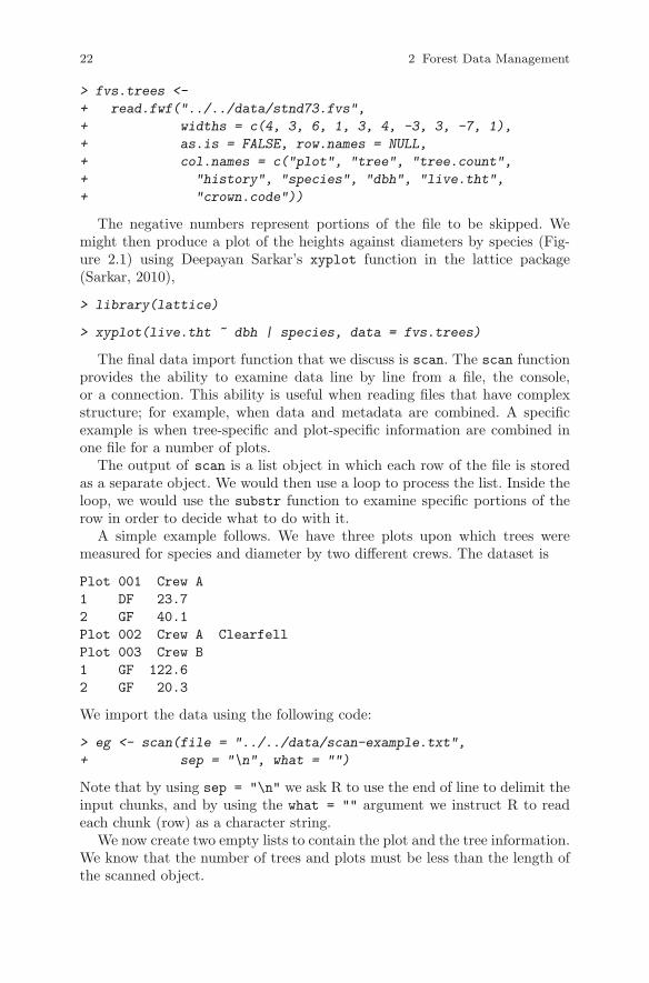
> fvs.trees <-
+ read.fwf("../../data/stnd73.fvs",
+ widths = c(4, 3, 6, 1, 3, 4, -3, 3, -7, 1),
+ as.is = FALSE, row.names = NULL,
+ col.names = c("plot", "tree", "tree.count",
+ "history", "species", "dbh", "live.tht",
+ "crown.code"))
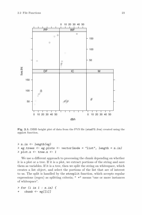
The negative numbers represent portions of the file to be skipped. Wemight then produce a plot of the heights against diameters by species (Fig-ure 2.1) using Deepayan Sarkar’s xyplot function in the lattice package(Sarkar, 2010),
> library(lattice)
> xyplot(live.tht ~ dbh | species, data = fvs.trees)
The final data import function that we discuss is scan. The scan functionprovides the ability to examine data line by line from a file, the console,or a connection. This ability is useful when reading files that have complexstructure; for example, when data and metadata are combined. A specificexample is when tree-specific and plot-specific information are combined inone file for a number of plots.
The output of scan is a list object in which each row of the file is storedas a separate object. We would then use a loop to process the list. Inside theloop, we would use the substr function to examine specific portions of therow in order to decide what to do with it.
A simple example follows. We have three plots upon which trees weremeasured for species and diameter by two different crews. The dataset is
Plot 001 Crew A
1 DF 23.7
2 GF 40.1
Plot 002 Crew A Clearfell
Plot 003 Crew B
1 GF 122.6
2 GF 20.3
We import the data using the following code:
> eg <- scan(file = "../../data/scan-example.txt",
+ sep = "\n", what = "")
Note that by using sep = "\n" we ask R to use the end of line to delimit theinput chunks, and by using the what = "" argument we instruct R to readeach chunk (row) as a character string.
We now create two empty lists to contain the plot and the tree information.We know that the number of trees and plots must be less than the length ofthe scanned object.
2.2 File Functions 23
dbh
live.
tht
50
100
150
0 10 20 30 40 50
●●●●
●
●●
●
●●
●
●
●
●
●
●
DF
●●●
●●
●●●●
●●●●●●●
●●●
●
IC
0 10 20 30 40 50
●●●●●
M
●
●
●
●
PP
0 10 20 30 40 50
50
100
150
●
●
●●
●
●●●
●
●●
●
WF
Fig. 2.1: DBH–height plot of data from the FVS file (stnd73.fvs) created using thexyplot function.
> n.in <- length(eg)
> eg.trees <- eg.plots <- vector(mode = "list", length = n.in)
> plot.n <- tree.n <- 1
We use a different approach to processing the chunk depending on whetherit is a plot or a tree. If it is a plot, we extract portions of the string and savethem as variables. If it is a tree, then we split the string on whitespace, whichcreates a list object, and select the portions of the list that are of interestto us. The split is handled by the strsplit function, which accepts regularexpressions (regex) as splitting criteria; " +" means “one or more instancesof whitespace”.
> for (i in 1 : n.in) {
+ chunk <- eg[[i]]

24 2 Forest Data Management
+ if (substr(chunk, 1, 4) == "Plot") {
+ plot.id <- as.numeric(substr(chunk, 6, 9))
+ crew.id <- substr(chunk, 16, 16)
+ comments <- ifelse(nchar(chunk) > 17,
+ substr(chunk, 17, nchar(chunk)),
+ "")
+ eg.plots[[plot.n]] <-
+ list(plot.id, crew.id, comments)
+ plot.n <- plot.n + 1
+ } else {
+ tree <- strsplit(chunk, " +")[[1]]
+ tree.id <- as.character(tree[1])
+ species <- as.character(tree[2])
+ dbh.cm <- as.numeric(tree[3])
+ eg.trees[[tree.n]] <-
+ list(plot.id, tree.id, species, dbh.cm)
+ tree.n <- tree.n + 1
+ }
+ }
Also, the plot identification for the tree record is retained from the mostrecent iteration of processing the plot information. We conclude by forming,naming, and examining the plot and tree objects. We form the objects fromthe lists using the do.call and rbind functions.
> eg.plots <- as.data.frame(do.call(rbind, eg.plots))
> names(eg.plots) <- c("plot", "crew", "comments")
> eg.plots
plot crew comments
1 1 A
2 2 A Clearfell
3 3 B
> eg.trees <- as.data.frame(do.call(rbind, eg.trees))
> names(eg.trees) <- c("plot", "tree", "species", "dbh.cm")
> eg.trees
plot tree species dbh.cm
1 1 1 DF 23.7
2 1 2 GF 40.1
3 3 1 GF 122.6
4 3 2 GF 20.3
Our example code is quite inefficient. For example, we could handle theconversions of the data types outside the loops. However, it will suffice forthe purposes of demonstrating the processing steps.
2.2 File Functions 25
The scan function is very powerful and flexible, and our example hasbarely scratched the surface of its use. For example, much larger files can behandled by using the skip and nlines arguments.
Next we examine reading the second most common data format used inforest resource analysis: spreadsheets.
2.2.2 Spreadsheets
In forestry, as in most fields, spreadsheets are extremely common as data stor-age and communication devices. However, there are shortcomings that limitthe spreadsheet’s utility for these purposes. Most spreadsheet applicationscannot separate the data from the analysis routines and formulas, so thatperforming a new analysis requires an entirely new spreadsheet, which mayinvolve cutting and pasting cell formulas, etc. Some spreadsheets can containmany subsheets, and the subsheets can all contain inter-connected formulas,macros, and so on. Not all programs can read multiple-sheeted spreadsheets,and some applications may be confused by other contents within the file. Mostspreadsheet programs are not platform independent, which makes them diffi-cult to use in a distributed environment or a web-based setting. Finally, somespreadsheets are encoded in proprietary formats that encrypt the data andany associated analysis unnecessarily.
For these reasons, we recommend that spreadsheets not be used for main-taining data. While spreadsheets have their place for simple data-editing tasksand for prototyping analysis methods, we advocate that the storage and man-agement of data be in text files for small projects and in formal databasesfor large projects. The data should be extracted from the file or the databaseusing sequences of commands that are recorded in documented scripts. Werecommend that data be stored in a relational database management system(RDMS) such as PostgreSQL, MySQL, Microsoft Access, or Oracle, and thatthe RODBC package (Section 2.2.3) be used for data retrieval and updates.
In some circumstances, there may be no way to avoid the use of spread-sheets for data storage. If so, Windows users can use odbcConnectExcel inthe RODBC package, originally developed by Michael Lapsley and now main-tained by Brian Ripley (Ripley and Lapsley, 2009). The odbcConnectExcel
function can select and extract rows and columns from any of the sheetsin an Excel spreadsheet file. This approach allows data importation into R,but it does not impede or interrupt the disparate, or incongruous, data cyclepresent in many organizations (Brackett, 2000).

26 2 Forest Data Management
2.2.3 Using SQL in R
The Structured Query Language (SQL) is a standard language for writingcommands that can be used to access data within RDMS such as Oracle, Mi-crosoft SQL Server, and PostgreSQL (Kline and Kline, 2001). Using an RDMSwith SQL for data storage and retrieval provides efficient, straightforward,and consistent interface to data in both simple or complex arrangements.
For example, suppose we have a table in a database named plots. Usingone of the database accessibility packages such as RODBC, RPostgreSQL, orRMySQL to access the data stored within the RDMS, the SQL select stringto select and retrieve all the data associated with the plots table would be thesame. Using the RPostgreSQL package (Prayaga et al., 2009), for example,the resulting code snippet to retrieve data from the plots table would looklike
> library(RPostgreSQL)
> drv <- dbDriver("PostgreSQL")
> con <- dbConnect(drv,
+ dbname="forestco",
+ user="hamannj",
+ host="localhost")
> sql.command <-
+ sprintf( "select * from plots where plottype = �fixed�;" )
> rs <- dbSendQuery(con, statement = sql.command )
> fixed.plots <- fetch(rs, n = -1)
> dbDisconnect(con)
where the resulting object from the fetch function, fixed.plots, containsa data frame object that contains all plots where the plottype is fixed.
In this book, however, we do not present data access methods for rela-tional databases using SQL since tasks commonly associated with databasesuse large datasets, and project management with large datasets is beyond thescope of this book. For more complete descriptions and examples of accessingan RDMS, see any number of database access libraries, e.g., RODBC, RPost-greSQL, and RMySQL (James and DebRoy, 2009) and the R-data documentthat comes with the R documentation.
2.2.4 The foreign Package
R provides a package called foreign to read and write files in formats thatare used by other software tools (R core members et al., 2010). The foreignpackage is a collection of file translation functions that can be used to readand write various file formats of common statistical and database applica-

2.2 File Functions 27
tions. Table 2.1 presents the functions for reading and writing data currentlyavailable in the foreign package.
Table 2.1: A list of functions available for reading and writing common file formats.
Function Purpose
data.restore Read an S3 binary filelookup.xport Look up information on a SAS XPORT format libraryread.dbf Read a DBF fileread.dta Read Stata binary filesread.epiinfo Read Epi Info data filesread.mtp Read a Minitab Portable Worksheetread.octave Read Octave text data filesread.S Read an S3 binary Fileread.spss Read an SPSS data fileread.ssd Obtain a data frame from a SAS permanent dataset via read.xportread.systat Obtain a data frame from a Systat fileread.xport Read a SAS XPORT format librarywrite.dbf Write a DBF filewrite.dta Write files in Stata binary formatwrite.foreign Write text files and code to read them
Most of the functions in the foreign package are simple to use. For example,the code to read a dBase-formatted file (e.g., stands.dbf) using the foreignpackage is
> library(foreign)
> stands <- read.dbf("../../data/stands.dbf")
As before, it is useful to immediately examine the imported object. Welearn something about the object by using the names function (we would alsouse str, but doing so here is a poor use of paper!).
> names(stands)
[1] "SP_ID" "AREA" "PERIMETER" "STANDID"
[5] "ALLOCATION" "TAGE" "BHAGE" "DF_SITE"
[9] "TOTHT" "CUBVOL_AC" "TPA" "QMD"
[13] "BA"
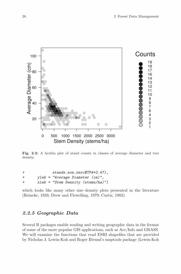
We can then plot the count of stands in hexagonal bins of quadratic meandiameter and tree counts per hectare using the plot and the hexbin func-tions, the latter from the hexbin package (Carr et al., 2010) (Figure 2.2).
> stands.non.zero <- stands[stands$QMD > 0,]
> plot(hexbin(stands.non.zero$QMD*2.54 ~
28 2 Forest Data Management
0 500 1000 1500 2000 2500 3000
20
40
60
80
100
Stem Density (stems/ha)
Ave
rage
Dia
met
er (
cm)
12346789101112131416171819
Counts
Fig. 2.2: A hexbin plot of stand counts in classes of average diameter and treedensity.
+ stands.non.zero$TPA*2.47),
+ ylab = "Average Diameter (cm)",
+ xlab = "Stem Density (stems/ha)")
which looks like many other size–density plots presented in the literature(Reineke, 1933; Drew and Flewelling, 1979; Curtis, 1982).
2.2.5 Geographic Data
Several R packages enable reading and writing geographic data in the formatof some of the more popular GIS applications, such as Arc/Info and GRASS.We will examine the functions that read ESRI shapefiles that are providedby Nicholas J. Lewin-Koh and Roger Bivand’s maptools package (Lewin-Koh

2.2 File Functions 29
and Bivand, 2010). Packages to read and write other GIS file formats can befound at CRAN.
Shapefiles can contain information about many individual polygons. If theshapefiles are relatively small and only consist of a few hundred polygons, thenR is suitable for making thematic maps, performing analyses, and storing andupdating data within the shapefiles. However, R should not be considered asubstitute for a fully featured GIS.
We begin by loading a shapefile of the forest inventory that is made avail-able by Oregon State University1. (stands.shp). First, we start by loadingthe package and reading the shapefile using the readShapePoly command
> library(maptools)
> stands <- readShapePoly("../../data/stands.shp")
The total area, in acres, is
> sum( stands$AREA ) / 43560.0
[1] 11994.71
and the number of stands is
> nrow(stands)
[1] 510
We use the names function to obtain the names of the attributes:
> names(stands)
[1] "SP_ID" "AREA" "PERIMETER" "STANDID"
[5] "ALLOCATION" "TAGE" "BHAGE" "DF_SITE"
[9] "TOTHT" "CUBVOL_AC" "TPA" "QMD"
[13] "BA"
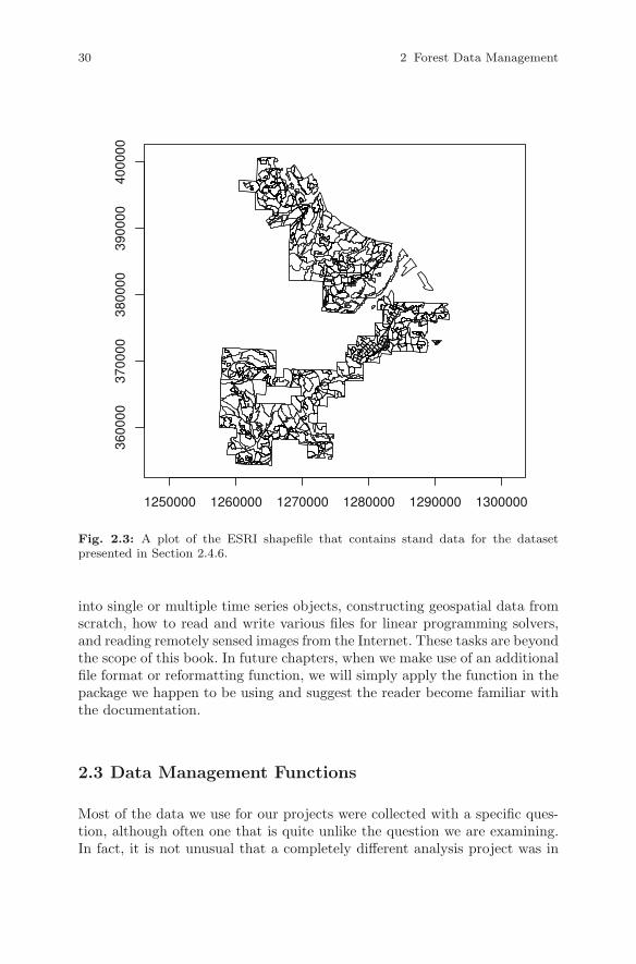
Then, we can use the plot command to produce a simple map such asthat shown in Figure 2.3
> plot(stands, axes = TRUE)
2.2.6 Other Data Formats
The set of functions we presented in the previous sections was not exhaustivebut covers the bulk of the formats in which forestry data tend to be stored.There are additional file management topics such as how to format a file
1 These data can be found at http://www.cof.orst.edu/cf/gis/.
30 2 Forest Data Management
1250000 1260000 1270000 1280000 1290000 1300000
3600
0037
0000
3800
0039
0000
4000
00
Fig. 2.3: A plot of the ESRI shapefile that contains stand data for the datasetpresented in Section 2.4.6.
into single or multiple time series objects, constructing geospatial data fromscratch, how to read and write various files for linear programming solvers,and reading remotely sensed images from the Internet. These tasks are beyondthe scope of this book. In future chapters, when we make use of an additionalfile format or reformatting function, we will simply apply the function in thepackage we happen to be using and suggest the reader become familiar withthe documentation.
2.3 Data Management Functions
Most of the data we use for our projects were collected with a specific ques-tion, although often one that is quite unlike the question we are examining.In fact, it is not unusual that a completely different analysis project was in
2.3 Data Management Functions 31
mind when the data that we must use were originally collected. Most likely,the data were collected under less than ideal conditions and without clearprotocols. Each analysis project usually requires that some effort be spent onreformatting and checking data. This section is designed to introduce readersto a few data manipulation and management functions in R. At the timeof writing, the authors have, between them, about 40 years of experience inhandling forestry data and have never worked with a dataset that did notdemand some level of scrutiny for structure and cleanliness.
2.3.1 Herbicide Trial Data
The herbdata dataset started as a herbicide trial. The plots were installedduring the 1994 planting season in southwestern Washington by Don Wal-lace and Bruce Alber. Three replications of 20 seedlings were planted in twoblocks. The two blocks were a control block and a block treated with 220ml per hectare of Oust herbicide (DuPont, 2005). The plots were then mea-sured over the next ten years. At each observation, the basal diameter, totalheight, and condition of the stem were recorded. When the stems reachedbreast height (1.37 m in the United States), the breast height diameter wasalso recorded. An indicator variable was used to record if the stem was deador alive. If the stem was dead, the observations were recorded as NA. Recallthat to read in the data from a text file, we use the read.table function
> herbdata <- read.table("../../data/herbdata.txt",
+ header = TRUE, sep = ",")
and to make sure we have suitable data by printing the first five rows of datausing the str function.
> str(herbdata)
�data.frame�: 960 obs. of 8 variables:
$ treat : Factor w/ 2 levels "CONTROL","OUST": 1 1 ...
$ rep : Factor w/ 3 levels "A","B","C": 1 1 ...
$ tree : int 1 1 ...
$ date : Factor w/ 8 levels "10/7/1996 0:00:00",..: 1 2 ...
$ isalive: int 1 1 ...
$ height : num 31 59 ...
$ dia : num 6.5 9 ...
$ dbh : num 0 0 ...
The measurement dates, but not the measurement times, were recorded forthe observations. So, we can use the strptime function to reformat the dates,thus removing the time portion of the date (otherwise when we plot the databy date, the times will be printed as YYYY-MM-DD 0:00:00) and storing
32 2 Forest Data Management
the resulting objects using a special object class that represents temporaldata, POSIXct.
> herbdata$date <- as.POSIXct(strptime(herbdata$date,
+ "%m/%d/%Y"))
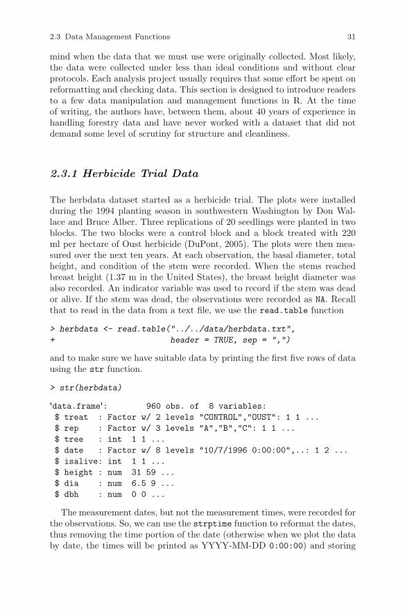
We can then plot the data (Figure 2.4) using the coplot function, whichcreates conditioning plots:
> coplot(height ~ dia | treat * rep, type = "p",
+ data = herbdata[herbdata$isalive == 1,],
+ ylab = "Height (cm)", xlab = "Basal Diameter (mm)")
●●
●●●●●
●
●●
●
● ●●
●
●
●●
●
●
●
●
●
●
●●
●
●
●
●●
●
●●
●
●
●
●
●
●
●
●
●
●
●
●
●
●
●●
●
●
●
●
●
●
●
●
●
●
●
●
●
●
●●
●
●
●
●●
●
●●
●●●
●●
●
●●
●●
●●
●
●
●
●
●
●
●
● ●
●
●●● ●●●●●
●●
●
●●
●
●
●
●●●
●●●● ●
●●
●
●
●
●
● ●
●●
●●
●
●
●
●
●●
●
●
●●
●
●
●●
●
●
●●
●
●
●
●
●
●
●
●
●
●
040
080
012
00
●
●
●
●
●
●●
●
●
●
●
●
●
●
●
●
●
●
●
●
●
●
●
●
●
●
●
●
●
● ●
●
●●
●
●
●
● ●
●
●
●
●
●
●
●●
●
●●
●
●
●
●
●
●
●●
●
●
●
●
●
●
●●
●
●
●
●
●
●
●●
●
●
●
●
●
●
●●
●
●
●
●
●
●
●●
●
●
●
●●
●
●●
●
●
●
●
●
●
●
●
●
●
●
●
●
●
●
●
●
●
●
● ●
●
●
●
●
●
●
●●
●
●●
●●
●
●
●
●
●●
●
●
●
●
●
●
●
●
●
●●
● ●
●
●
●
●
●
●
●●
●
0 100 200 300 400
●
●
●
●
●
● ●
●
●●
●
●
●
●
●
●
●●
●
●
●
●
●●
●●
●
●●
● ●
●
●
●
●
●
●
●●
●
●●
●
●
●
●
●
●
●●
●●
●
●●
●
●●
●●
●
●
●
●
●●
●●
●
●
●
●
●●
●
●●
●●
●
●●
●
●
●●
●●
●●
●
●
●
●
●
●
●●●●●●
●●
●●
●●
●
●●
●
●●
●
●
●
●●
●
●●●
●
●●
●
●
●
●●
●
●
●
●
●
●
●
●
●
●
●
●●
●
●●
●
●
●
●
●●
●●
●
●
●●
●
●
●
●
●
●
●
●
●
●
●●
●
●
●
●
●
●
●
●
●
●
●
●
●
●
●●
●
●
●
●
●●
● ●
●
●
●
●
●
●
●●
●
●
●
●●
●
●●
●
●
●●
●
●
●●
●
●
●
●
●
●
●●
●
●
●
● ●
●
●●
●
●
●
● ●
●
●
●
●
●
●
●
●
●
●●
●
●
●
●
●●
●● ●
●
●
●
●
●
●
●
●
●
●
●●
●
●
●
●
●
●
●●
●
●
●
●
●
●
● ●
●
●●●
●
●
●
● ●
●●
●
●
●●
●
●
●●
●
●
●
●●
●
040
080
012
00
●
●
●
●
●
● ●
●
●●
●
●
●
●
●
●
●●
●
●●
●
●
●
●
●
●
●
●
●
●●
●
●
●●
●
●
●
●
●
●
●
●
●
●
●●
●
●●
●●●●●●
●●
●
●
●
●●
●
●●
●
●
●
●●
●
●●
●
●
●
●●
●
●●
●
●
●
●●
●
●●
●
●
●
●
●
●
●●
●
●
●
●
●
●
●●●
●
●
●●
●
●
●●●
●
●
●
●
●
●●
●●
●
●●
●
0 100 200 300 400
040
080
012
00
●●
●
●
●
●
●
●
●
●
●
●
●
●
●
●
●
●
●
●
●
●●
●
●●
●
●
●
●
●
●
●
●
●
●
●
●●
●
●
●
●
●
●
●
●
●
●●
●
●
●
●
●
●
●●
●
●
●
● ●
●
●
●
●
●
● ● ●
●
●
●
●
●●
●
●
●
●
●
●
●
●
●
●
●
●
●
●
●
●
●●
●
●●
●
●
●
●●
●
●●
●
●
●
●●
●
●
●
●
●
●
●●
●
●
●
●
●
●
● ●
●
●
●
●
●
●
●
●
●
●●
●
●●
●
●
●
●
●
●●
●
●
●
●
●●
●
●
●
●
●
●
Basal Diameter (mm)
Hei
ght (
cm)
CONTROL
OUST
Given : treat
A
B
C
Giv
en :
rep
Fig. 2.4: A conditioning plot of the observations in the herbdata data frame.
2.3 Data Management Functions 33
Something looks suspicious in the figure. The cloud on the right side of thecontrol plot in the B replication looks out of place. We suspect measurementor process error in the data, and we should investigate further, as follows.
2.3.2 Simple Error Checking
Making use of simple tables and graphics to check for outliers and invalidvalues in datasets is common practice. To produce a summary of the variablesin a data frame object, use the summary function:
> summary(herbdata)
treat rep tree
CONTROL:480 A:320 Min. : 1.00
OUST :480 B:320 1st Qu.:15.75
C:320 Median :30.50
Mean :30.50
3rd Qu.:45.25
Max. :60.00
date isalive height
Min. :1996-10-07 00:00:00 Min. :0.0000 Min. : 15.0
1st Qu.:1999-03-09 18:45:00 1st Qu.:1.0000 1st Qu.: 193.0
Median :2001-10-03 23:30:00 Median :1.0000 Median : 449.9
Mean :2001-04-30 11:37:30 Mean :0.9615 Mean : 472.1
3rd Qu.:2003-04-04 05:15:00 3rd Qu.:1.0000 3rd Qu.: 693.4
Max. :2005-08-23 00:00:00 Max. :1.0000 Max. :1280.2
NAs : 37.0
dia dbh
Min. : 0.00 Min. : 0.00
1st Qu.: 36.75 1st Qu.: 0.00
Median : 82.00 Median : 22.00
Mean : 95.12 Mean : 52.96
3rd Qu.:138.50 3rd Qu.: 98.00
Max. :439.42 Max. :342.90
NAs : 37.00 NAs : 37.00
We see that some of the observations contain NA values, which signifymissing values. Other than that, nothing immediately appears to be wrongwith the data. We display the first few observations to assess whether or notthe other observations in those rows that include NA entries are correct:
> head(herbdata[is.na(herbdata$height),])
treat rep tree date isalive height dia dbh
282 CONTROL B 36 1997-11-11 0 NA NA NA

34 2 Forest Data Management
283 CONTROL B 36 1999-08-18 0 NA NA NA
284 CONTROL B 36 2001-02-07 0 NA NA NA
285 CONTROL B 36 2002-05-31 0 NA NA NA
286 CONTROL B 36 2002-11-26 0 NA NA NA
287 CONTROL B 36 2004-04-26 0 NA NA NA
We suspect that the trees with missing measurements are those trees thatare not alive (isalive = 0). This conjecture can be verified by counting therows that have missing values anywhere for each value of isalive, as follows.
> table(complete.cases(herbdata), herbdata$isalive)
0 1
FALSE 37 0
TRUE 0 923
As we suspected, the rows that contain missing values, which correspond tothe complete.cases function returning FALSE, are all dead trees. To com-plete our scrutiny, in the following section we will visually inspect the rela-tionships among the variables.
2.3.3 Graphical error checking
Graphical error-checking methods are straightforward using basic plottingfunctions. As we saw in Figure 2.4, graphical error checking provided quickidentification for the suspect observations using a conditioning plot (Cham-bers, 1991; Cleveland, 1993).
We created a conditioning plot by plotting the height–diameter scatter-plots, conditioned on treatment and replication (Figure 2.4). Inspection ofFigure 2.4 reveals outliers in the B replication of the control group. In orderto focus on these outliers we now need to produce a conditioning plot bymeasurement date (Figure 2.5):
> coplot(height ~ dia | treat * factor(date),
+ data = herbdata[herbdata$isalive == 1,],
+ type = "p",
+ ylab = "Height (cm)",
+ xlab = "Basal Diameter (mm)")
We can see that the measurements taken on 2004-04-26 contain the sus-picious observations. We can conveniently narrow in on those observationsusing index operators. To get the correct levels of the factors, use the levelsfunction, which returns the values of the levels of its argument.
> levels(herbdata$treat)
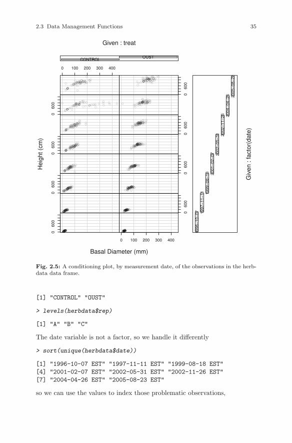
2.3 Data Management Functions 35
●●●●●●●●●●●●
●●●
●●●●●●●●●●●●●●●●●●●●
●●●●●●●●●●●●●
●●●●●●●●●●0
600
●●●●●●●●●●
●●●●●●●●●●●●●●●●●●●●●●●●●●●●●●●●●●●●●●●●●●●●●●●●●●
0 100 200 300 400
●●●●●●●●●
●●
●
●●
●●●●●●
●●
●●●●●●●●●●
●●●●● ●●●
●●●●●
●●
●●●●●●●●●●●●●●●●
●●
●●●●●●●●
●●●●●●●●●●●●
● ●●● ●●●●●●●●● ●●●●●●●●●●●●●●
●●
● 060
0●
●●●● ●●
●●
●●
●
●
●
●
●●●●●●
●●
●●●●●●●●●
●
●●●●●
●
●
●●
●●●
●
●●●●●●●
●●
060
0
●●● ●●●●
●●
●●●
●●●●
●●
●●●●●
●●
● ●●●●● ●●
●
●●●
●
●●●●● ●
●●
●●●●● ●●●●●●
●●
●
●
●●●●
●
●●●
●●
●
●
●
●
●●●●●
●
●●
●●●●●●●●●
●
●●●●●
●
●
●●
●
●●
●
●●●●●●●
●●
●●● ●●● ●●●
●●●
●●
●●
●
●●●
●●●
●
●● ●●●●● ●●
●●●●
●
●●●●● ●●
●●●●●●●●●●●
●●
●●
060
0
●
●●●●
●●
●●
●●
●
●
●
●
●●●●●
●
●●
●●
●●●●● ●●
●
● ●●
●●
●
●
●●
●
●
●
●
●●● ●
● ●●●●
060
0
●●●●●● ●
●●
●●●
●
●●●
●
●●
●● ● ●
●●
●●●
●●● ●●
●
●●
●
●
●●●●●
●●
● ●●●●●● ●●●
●●
●●
●
●
●
●●●
●
●●
●
●●
●
●
●
●
●●
●●
●●
●●
●●●●●●●●●
●
●●●
●●
●
●
●●
●
●
●
●
●●● ●
● ●
●●●
●●●● ●● ●
●●
●
●●●
●●●
●
●●
●
●● ●
●●●●
●●●●
●●●
●●●
●●●●● ●
●●
● ●●●●●●●●
● ●●
●●
●
060
0
●
●●
●● ●●
●●
●●
●
●
●
●
●●
●●
● ●●
●
●
●●●● ●●
●●
●
● ●●
● ●●●
●●
●
●●
●
●●
●●● ●
●●●
060
0 ●●●● ●● ●
●● ●●●
●
●●●
●
● ●
●●● ●
●
●●●
●●
● ●
●●
●
●
●●
●
●●●
●●
●●● ●● ●
●●●●●
● ●●●
●
●
●
●●●● ●●
●●
●●
●
●
●
●
●●●●
● ●●
●
●●●
●●●●●
●
●
●●●●
●●
●
●●
●
● ●
●
●●● ●● ●●●●
0 100 200 300 400
●●● ●
●● ●
●●
●●●●
●
●●
●● ●
●● ●●
● ●●●
●●● ●
● ●●
●
●●
●
●●●
●●
●●●
●● ●
●●
●●● ●
●●●
●
●
060
0
Basal Diameter (mm)
Hei
ght (
cm)
CONTROL OUST
Given : treat
1996
−10
−07 19
97−
11−
11 1999
−08
−18 20
01−
02−
07 2002
−05
−31 20
02−
11−
26 2004
−04
−26 20
05−
08−
23
Giv
en :
fact
or(d
ate)
Fig. 2.5: A conditioning plot, by measurement date, of the observations in the herb-data data frame.
[1] "CONTROL" "OUST"
> levels(herbdata$rep)
[1] "A" "B" "C"
The date variable is not a factor, so we handle it differently
> sort(unique(herbdata$date))
[1] "1996-10-07 EST" "1997-11-11 EST" "1999-08-18 EST"
[4] "2001-02-07 EST" "2002-05-31 EST" "2002-11-26 EST"
[7] "2004-04-26 EST" "2005-08-23 EST"
so we can use the values to index those problematic observations,
36 2 Forest Data Management
> bad.index <- herbdata$treat == levels(herbdata$treat)[1] &
+ herbdata$rep == levels(herbdata$rep)[2] &
+ herbdata$date == sort(unique(herbdata$date))[7]
> bad.data <- herbdata[bad.index,]
treat rep tree date isalive height dia dbh
167 CONTROL B 21 2004-04-26 1 734.56 439.42 342.90
175 CONTROL B 22 2004-04-26 1 637.03 259.08 187.96
183 CONTROL B 23 2004-04-26 1 883.92 330.20 266.70
191 CONTROL B 24 2004-04-26 1 478.53 269.24 157.48
199 CONTROL B 25 2004-04-26 1 646.17 233.68 165.10
207 CONTROL B 26 2004-04-26 1 612.64 218.44 147.32
...
treat rep tree date isalive height dia dbh
279 CONTROL B 35 2004-04-26 1 697.99 381.00 213.36
287 CONTROL B 36 2004-04-26 0 NA NA NA
295 CONTROL B 37 2004-04-26 1 615.69 332.74 231.14
303 CONTROL B 38 2004-04-26 1 774.19 330.20 279.40
311 CONTROL B 39 2004-04-26 1 792.48 375.92 330.20
319 CONTROL B 40 2004-04-26 1 762.00 0.00 203.20
A subsequent telephone call revealed the error in our data handling. Inthis case, the field crew had used a different device to measure the stemson 2004-04-26. During our unit conversion process, the value was incorrectlyconverted from imperial units to metric units. The values should have beendivided by 2.54. We can use the index values again to correct the problemwith the following commands:
> herbdata$dia[bad.index] <- herbdata$dia[bad.index] / 2.54
Note that we have to correct the breast-height diameter as well:
> herbdata$dbh[bad.index] <- herbdata$dbh[bad.index] / 2.54
These data-cleaning commands represent important intelligence about thedata handling. It is very important that the newly cleaned data object notbe saved back over the original dataset. Instead, either the data should bekept as they are and the code that was used to clean the data should berun routinely when the data are used, or a new version of the data, time-stamped, should be saved, and the differences between the original and thecleaned data should be carefully documented in a data dictionary or journal,which should be readily available with the dataset.
Now that the data have been corrected, we may want to revisit our originalplots using coplot or Deepayan Sarkar’s lattice functions to generate theconditioning plot again, verify our results, and continue with our analysis.

2.3 Data Management Functions 37
2.3.4 Data Structure Functions
Although we may be able to simply pass an unaltered data frame object toother functions for sample processing, model development, or optimization,we may want to change the structure of the data frame object to facilitatespecific programming needs. The main functions for data manipulation arethe split, aggregate, and merge functions.
The first of these functions that we examine is the split function, whichdivides a data frame (or any vector) into a list of the groups, distinguishedby corresponding with common values of some categorical variable. A list isa specific class of R object that is a collection of objects that can be unalike.The reverse operation can be performed by the unsplit function.
Imagine that we want to find out how many trees we have in each of thetreatments of the herbdata object. Using the split function, we can splitthe data frame into a list of data frames where the name of each treatmentis now the item in the list,
> split.herb <- split(herbdata, herbdata$treat)
> class(split.herb)
[1] "list"
> names(split.herb)
[1] "CONTROL" "OUST"
> nrow(split.herb$CONTROL)
[1] 480
> nrow(split.herb$OUST)
[1] 480
We can also check the names of the members,
> names(split.herb$CONTROL)
[1] "treat" "rep" "tree" "date" "isalive" "height"
[7] "dia" "dbh"
A more compact way to obtain the row count information is to use thepowerful lapply function, which applies its second argument as a functionto each of the items in the list that is identified as its first argument; forexample
> lapply(split.herb, nrow)
38 2 Forest Data Management
$CONTROL
[1] 480
$OUST
[1] 480
The lapply(X, FUN, ...) function returns a list of the same length as X.Using the newly split data frame, which is stored as a list, we can writefor loops to process our data or continue to manipulate our data frame forprocessing using the core data management functions.
For simplicity’s sake, we examine a reduced data frame, including onlycolumns 1 (treatment), 2 (replication), 6 (height), and 7 (basal diameter),and print some basic summaries using the lapply function:
> herbdata.short <- herbdata[,c(1,2,6,7)]
> split.herb.short <- split(herbdata.short, herbdata$treat)
> lapply(split.herb.short, summary)
$CONTROL
treat rep height dia
CONTROL:480 A:160 Min. : 15.0 Min. : 0.00
OUST : 0 B:160 1st Qu.: 175.6 1st Qu.: 26.75
C:160 Median : 391.4 Median : 62.00
Mean : 413.4 Mean : 69.55
3rd Qu.: 615.7 3rd Qu.:102.00
Max. :1219.2 Max. :228.60
NAs : 37.0 NAs : 37.00
$OUST
treat rep height dia
CONTROL: 0 A:160 Min. : 42.0 Min. : 10.0
OUST :480 B:160 1st Qu.: 212.6 1st Qu.: 51.0
C:160 Median : 530.4 Median :109.0
Mean : 526.2 Mean :112.6
3rd Qu.: 762.0 3rd Qu.:159.0
Max. :1280.2 Max. :298.4
The aggregate function is useful for collapsing data into forms familiar toforesters such as stand tables, log-stock tables, and species-level summaries.For example, we might want to know the diameter distribution of the treesby treatment, ignoring the replications, for the herbicide trial data for thelatest sample date. We can combine all three functions in conjunction withthe ability to select a subset of the measurements by date. We check whatdates we have to choose from by printing the unique values, sorted:
> sort(unique(herbdata$date))
2.3 Data Management Functions 39
[1] "1996-10-07 EST" "1997-11-11 EST" "1999-08-18 EST"
[4] "2001-02-07 EST" "2002-05-31 EST" "2002-11-26 EST"
[7] "2004-04-26 EST" "2005-08-23 EST"
To generate our summaries, we select and split only the last measurement:
> herbdata.shorter <-
+ herbdata[herbdata$date == max(herbdata$date), c(1,2,6,8)]
> split.herb.shorter <-
+ split(herbdata.shorter, herbdata.shorter$treat)
We can now classify the trees by diameter class. We bind that columnto a temporary data frame to facilitate the process. We can then use theaggregate function to generate totals for each of the treatments by diameterclass:
> rt <- cbind(herbdata.shorter,
+ dc = cut(herbdata.shorter$dbh,
+ breaks = c(0, 50, 100, 150, 200, 300, 400, 999),
+ labels = c("000--050", "050--100", "100--150",
+ "150--200", "200--300", "300--400","400+")))
> st <- aggregate(x = list(basal.area = pi/(4*10^2) * rt$dbh^2,
+ tht = rt$height,
+ stems = rep(1, nrow(rt))),
+ by = list(treat = rt$treat,
+ diac = rt$dc),
+ FUN = sum)
> st
treat diac basal.area tht stems
1 CONTROL 000--050 27.61556 2255.52 5
2 CONTROL 050--100 993.34934 13441.68 18
3 OUST 050--100 73.16856 883.92 1
4 CONTROL 100--150 3028.48926 21244.56 26
5 OUST 100--150 2439.45448 17465.04 18
6 CONTROL 150--200 1404.13710 6035.04 6
7 OUST 150--200 9093.28375 40660.32 39
8 OUST 200--300 681.82558 2529.84 2
From our results, we can see that the total height value is a sum of allthe heights. We really wanted the mean height for the treatment, so we canuse the assignment operator (<-) to reassign the tht variable to the correctvalue, now expressed in meters, and print the results again:
> st$tht <- st$tht / st$stems / 100
> st
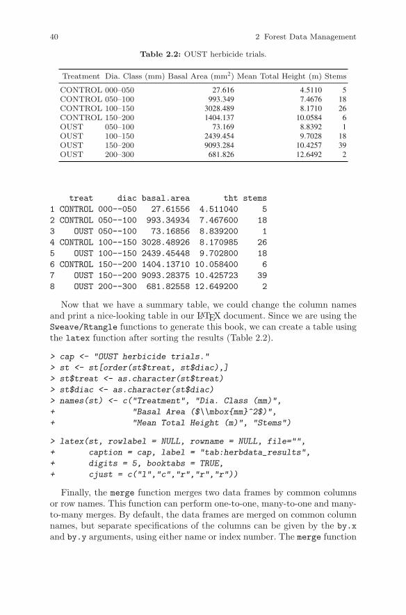
40 2 Forest Data Management
Table 2.2: OUST herbicide trials.
Treatment Dia. Class (mm) Basal Area (mm2) Mean Total Height (m) Stems
CONTROL 000–050 27.616 4.5110 5CONTROL 050–100 993.349 7.4676 18CONTROL 100–150 3028.489 8.1710 26CONTROL 150–200 1404.137 10.0584 6OUST 050–100 73.169 8.8392 1OUST 100–150 2439.454 9.7028 18OUST 150–200 9093.284 10.4257 39OUST 200–300 681.826 12.6492 2
treat diac basal.area tht stems
1 CONTROL 000--050 27.61556 4.511040 5
2 CONTROL 050--100 993.34934 7.467600 18
3 OUST 050--100 73.16856 8.839200 1
4 CONTROL 100--150 3028.48926 8.170985 26
5 OUST 100--150 2439.45448 9.702800 18
6 CONTROL 150--200 1404.13710 10.058400 6
7 OUST 150--200 9093.28375 10.425723 39
8 OUST 200--300 681.82558 12.649200 2
Now that we have a summary table, we could change the column namesand print a nice-looking table in our LATEX document. Since we are using theSweave/Rtangle functions to generate this book, we can create a table usingthe latex function after sorting the results (Table 2.2).
> cap <- "OUST herbicide trials."
> st <- st[order(st$treat, st$diac),]
> st$treat <- as.character(st$treat)
> st$diac <- as.character(st$diac)
> names(st) <- c("Treatment", "Dia. Class (mm)",
+ "Basal Area ($\\mbox{mm}^2$)",
+ "Mean Total Height (m)", "Stems")
> latex(st, rowlabel = NULL, rowname = NULL, file="",
+ caption = cap, label = "tab:herbdata_results",
+ digits = 5, booktabs = TRUE,
+ cjust = c("l","c","r","r","r"))
Finally, the merge function merges two data frames by common columnsor row names. This function can perform one-to-one, many-to-one and many-to-many merges. By default, the data frames are merged on common columnnames, but separate specifications of the columns can be given by the by.x
and by.y arguments, using either name or index number. The merge function
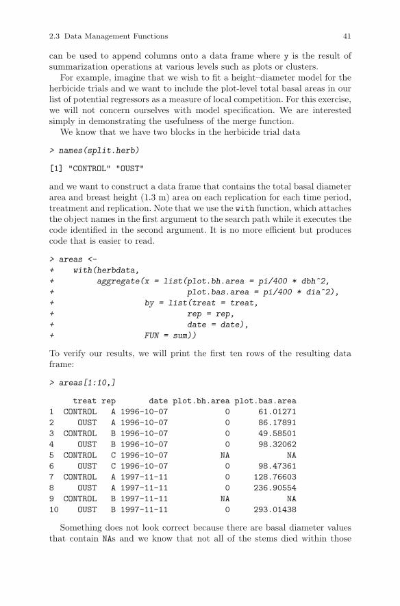
2.3 Data Management Functions 41
can be used to append columns onto a data frame where y is the result ofsummarization operations at various levels such as plots or clusters.
For example, imagine that we wish to fit a height–diameter model for theherbicide trials and we want to include the plot-level total basal areas in ourlist of potential regressors as a measure of local competition. For this exercise,we will not concern ourselves with model specification. We are interestedsimply in demonstrating the usefulness of the merge function.
We know that we have two blocks in the herbicide trial data
> names(split.herb)
[1] "CONTROL" "OUST"
and we want to construct a data frame that contains the total basal diameterarea and breast height (1.3 m) area on each replication for each time period,treatment and replication. Note that we use the with function, which attachesthe object names in the first argument to the search path while it executes thecode identified in the second argument. It is no more efficient but producescode that is easier to read.
> areas <-
+ with(herbdata,
+ aggregate(x = list(plot.bh.area = pi/400 * dbh^2,
+ plot.bas.area = pi/400 * dia^2),
+ by = list(treat = treat,
+ rep = rep,
+ date = date),
+ FUN = sum))
To verify our results, we will print the first ten rows of the resulting dataframe:
> areas[1:10,]
treat rep date plot.bh.area plot.bas.area
1 CONTROL A 1996-10-07 0 61.01271
2 OUST A 1996-10-07 0 86.17891
3 CONTROL B 1996-10-07 0 49.58501
4 OUST B 1996-10-07 0 98.32062
5 CONTROL C 1996-10-07 NA NA
6 OUST C 1996-10-07 0 98.47361
7 CONTROL A 1997-11-11 0 128.76603
8 OUST A 1997-11-11 0 236.90554
9 CONTROL B 1997-11-11 NA NA
10 OUST B 1997-11-11 0 293.01438
Something does not look correct because there are basal diameter valuesthat contain NAs and we know that not all of the stems died within those
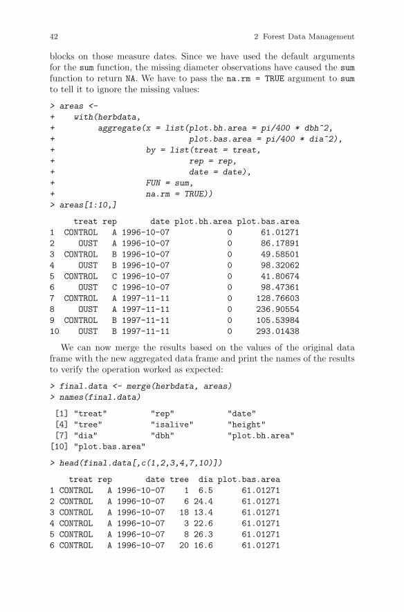
42 2 Forest Data Management
blocks on those measure dates. Since we have used the default argumentsfor the sum function, the missing diameter observations have caused the sumfunction to return NA. We have to pass the na.rm = TRUE argument to sum
to tell it to ignore the missing values:
> areas <-
+ with(herbdata,
+ aggregate(x = list(plot.bh.area = pi/400 * dbh^2,
+ plot.bas.area = pi/400 * dia^2),
+ by = list(treat = treat,
+ rep = rep,
+ date = date),
+ FUN = sum,
+ na.rm = TRUE))
> areas[1:10,]
treat rep date plot.bh.area plot.bas.area
1 CONTROL A 1996-10-07 0 61.01271
2 OUST A 1996-10-07 0 86.17891
3 CONTROL B 1996-10-07 0 49.58501
4 OUST B 1996-10-07 0 98.32062
5 CONTROL C 1996-10-07 0 41.80674
6 OUST C 1996-10-07 0 98.47361
7 CONTROL A 1997-11-11 0 128.76603
8 OUST A 1997-11-11 0 236.90554
9 CONTROL B 1997-11-11 0 105.53984
10 OUST B 1997-11-11 0 293.01438
We can now merge the results based on the values of the original dataframe with the new aggregated data frame and print the names of the resultsto verify the operation worked as expected:
> final.data <- merge(herbdata, areas)
> names(final.data)
[1] "treat" "rep" "date"
[4] "tree" "isalive" "height"
[7] "dia" "dbh" "plot.bh.area"
[10] "plot.bas.area"
> head(final.data[,c(1,2,3,4,7,10)])
treat rep date tree dia plot.bas.area
1 CONTROL A 1996-10-07 1 6.5 61.01271
2 CONTROL A 1996-10-07 6 24.4 61.01271
3 CONTROL A 1996-10-07 18 13.4 61.01271
4 CONTROL A 1996-10-07 3 22.6 61.01271
5 CONTROL A 1996-10-07 8 26.3 61.01271
6 CONTROL A 1996-10-07 20 16.6 61.01271

2.4 Examples 43
We can use this dataset to fit our model. We cover the use of R for hierarchicalregression in Chapter 7.
2.4 Examples
We now demonstrate the tools and principles that were developed in the pre-ceding sections to read and scrutinize a number of forestry-related databasesthat will be used in subsequent chapters of the book.
One operation that we will continuously rely upon is the identification ofthe counts of missing values in the variables of the datasets. We have writtenan R function to compactly report this information as follows.
> show.cols.with.na <- function(x) {
+ ## First, check that object is a data frame
+ if (class(x) != "data.frame")
+ stop("x must be a data frame.\n")
+ ## Count the missing values by column.
+ missing.by.column <- colSums(is.na(x))
+ ## Are any missing?
+ if (sum(missing.by.column) == 0) {
+ cat("No missing values.\n")
+ } else {
+ ## Only return columns with missing values.
+ missing <- which(missing.by.column > 0)
+ return(missing.by.column[missing])
+ }
+ }
This function will report the number of missing observations by variable foronly those variables that have missing values.
2.4.1 Upper Flat Creek in the UIEF
In the summer of 1991, a stand examination was made of the Upper FlatCreek unit of the University of Idaho Experimental Forest (UIEF). A squaregrid of 144 plots was laid out, with north–south inter-plot distance of 134.11m and east–west inter-plot distance of 167.64 m. A 7.0 m2/ha BAF variable-radius plot was installed at each plot location. Every tree in the plot wasmeasured for species and diameter at 1.37 m (dbh), recorded in mm. A sub-sample of trees was measured for height, recorded in dm, although it is nolonger known how this subsample was selected. The area of the stand was323.8 ha.
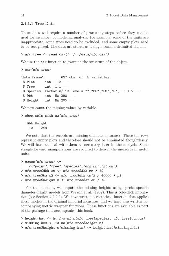
44 2 Forest Data Management
2.4.1.1 Tree Data
These data will require a number of processing steps before they can beused for inventory or modeling analysis. For example, some of the units areinappropriate, some trees need to be excluded, and some empty plots needto be recognized. The data are stored as a single comma-delimited flat file.
> ufc.tree <- read.csv("../../data/ufc.csv")
We use the str function to examine the structure of the object.
> str(ufc.tree)
�data.frame�: 637 obs. of 5 variables:
$ Plot : int 1 2 ...
$ Tree : int 1 1 ...
$ Species: Factor w/ 13 levels "","DF","ES","F",..: 1 2 ...
$ Dbh : int NA 390 ...
$ Height : int NA 205 ...
We now count the missing values by variable.
> show.cols.with.na(ufc.tree)
Dbh Height
10 248
We note that ten records are missing diameter measures. These ten rowsrepresent empty plots and therefore should not be eliminated thoughtlessly.We will have to deal with them as necessary later in the analysis. Somestraightforward manipulations are required to deliver the measures in usefulunits.
> names(ufc.tree) <-
+ c("point","tree","species","dbh.mm","ht.dm")
> ufc.tree$dbh.cm <- ufc.tree$dbh.mm / 10
> ufc.tree$ba.m2 <- ufc.tree$dbh.cm^2 / 40000 * pi
> ufc.tree$height.m <- ufc.tree$ht.dm / 10
For the moment, we impute the missing heights using species-specificdiameter–height models from Wykoff et al. (1982). This is cold-deck imputa-tion (see Section 4.2.2.2). We have written a vectorized function that appliesthese models in the original imperial measures, and we have also written ac-companying metric wrapper functions. These functions are available as partof the package that accompanies this book.
> height.hat <- ht.fvs.ni.m(ufc.tree$species, ufc.tree$dbh.cm)
> missing.hts <- is.na(ufc.tree$height.m)
> ufc.tree$height.m[missing.hts] <- height.hat[missing.hts]

2.4 Examples 45
We estimate tree-level merchantable volumes using functions provided byWykoff et al. (1982). Again, we have written a vectorized function that appliesthese models in the original imperial measures and accompanying metricwrapper functions.
> ufc.tree$vol.m3 <-
+ with(ufc.tree, vol.fvs.ni.m3(species, dbh.cm, height.m))
2.4.1.2 Plot-Level Data
We now create an object that summarizes the plot-level information. In orderto process the tree-level data, we need to invoke some elements of the design.The tree factor is the design basal area factor (BAF) divided by the tree-levelbasal area, and the tree-level volume per unit area is the product of the tree-level volume and the tree factor, as above. We can proceed with the aggregatecommand as there are no empty subsets, although there are some that havemissing values. We allow for these in the sum command by appending theflag: na.rm = TRUE. That flag is then passed by aggregate to the functionthat it calls.
> ufc.baf.met <- 7
> ufc.tree$tf.ha <- ufc.baf.met / ufc.tree$ba.m2
> ufc.tree$vol.m3.ha <- ufc.tree$vol.m3 * ufc.tree$tf.ha
> ufc.SyRS.data <-
+ aggregate(x = list(vol.m3.ha = ufc.tree$vol.m3.ha),
+ by = list(point = ufc.tree$point),
+ FUN = sum,
+ na.rm = TRUE)
> ufc.SyRS.data$weight <- 1
> str(ufc.SyRS.data)
�data.frame�: 144 obs. of 3 variables:
$ point : int 1 2 3 4 5 6 7 8 9 10 ...
$ vol.m3.ha: num 0 63.4 204.6 296.8 309.6 ...
$ weight : num 1 1 1 1 1 1 1 1 1 1 ...
Note that R automatically recycled the 1 that we assigned to the weightvariable in the ufc.SyRS.data data object until it had the same length asthe other variables contained in that object.
We now have a point-level dataset with the necessary design informationand a variable of interest. We named the object ufc.SyRS.data to reflect thefact that the inventory was performed using a systematic random sample,about which more can be found in Section 3.3.2. The spatial structure of thedesign is reported in the next section.
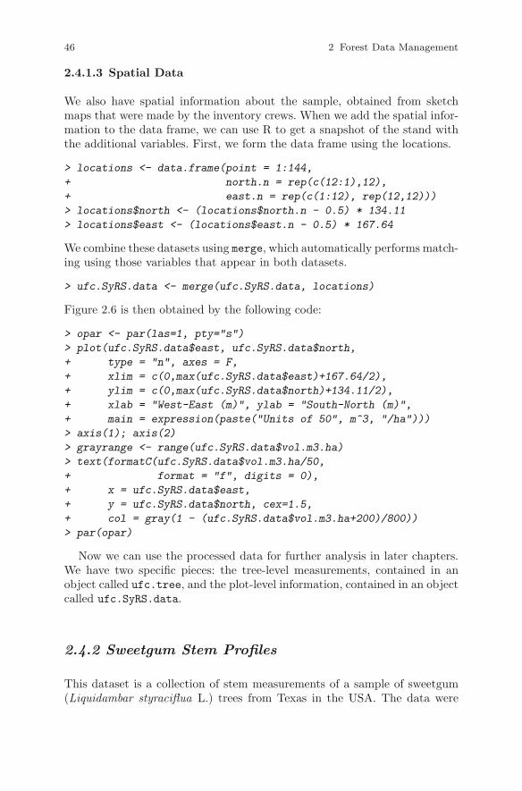
46 2 Forest Data Management
2.4.1.3 Spatial Data
We also have spatial information about the sample, obtained from sketchmaps that were made by the inventory crews. When we add the spatial infor-mation to the data frame, we can use R to get a snapshot of the stand withthe additional variables. First, we form the data frame using the locations.
> locations <- data.frame(point = 1:144,
+ north.n = rep(c(12:1),12),
+ east.n = rep(c(1:12), rep(12,12)))
> locations$north <- (locations$north.n - 0.5) * 134.11
> locations$east <- (locations$east.n - 0.5) * 167.64
We combine these datasets using merge, which automatically performs match-ing using those variables that appear in both datasets.
> ufc.SyRS.data <- merge(ufc.SyRS.data, locations)
Figure 2.6 is then obtained by the following code:
> opar <- par(las=1, pty="s")
> plot(ufc.SyRS.data$east, ufc.SyRS.data$north,
+ type = "n", axes = F,
+ xlim = c(0,max(ufc.SyRS.data$east)+167.64/2),
+ ylim = c(0,max(ufc.SyRS.data$north)+134.11/2),
+ xlab = "West-East (m)", ylab = "South-North (m)",
+ main = expression(paste("Units of 50", m^3, "/ha")))
> axis(1); axis(2)
> grayrange <- range(ufc.SyRS.data$vol.m3.ha)
> text(formatC(ufc.SyRS.data$vol.m3.ha/50,
+ format = "f", digits = 0),
+ x = ufc.SyRS.data$east,
+ y = ufc.SyRS.data$north, cex=1.5,
+ col = gray(1 - (ufc.SyRS.data$vol.m3.ha+200)/800))
> par(opar)
Now we can use the processed data for further analysis in later chapters.We have two specific pieces: the tree-level measurements, contained in anobject called ufc.tree, and the plot-level information, contained in an objectcalled ufc.SyRS.data.
2.4.2 Sweetgum Stem Profiles
This dataset is a collection of stem measurements of a sample of sweetgum(Liquidambar styraciflua L.) trees from Texas in the USA. The data were
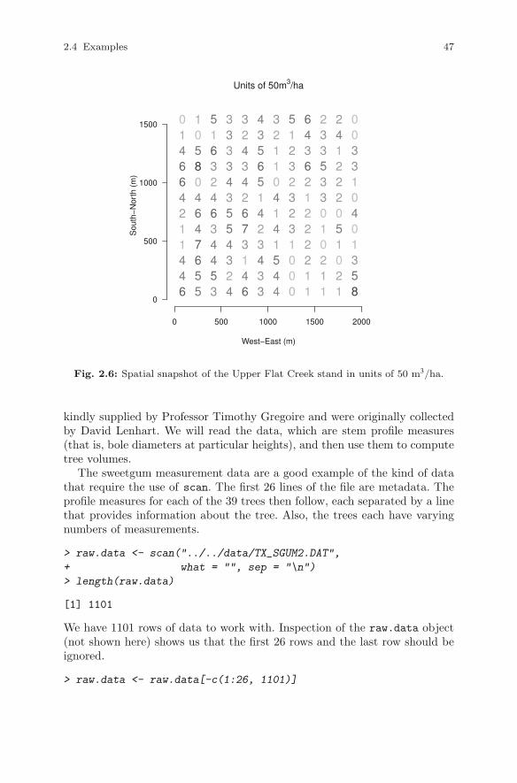
2.4 Examples 47
Units of 50m3/ha
West−East (m)
Sou
th−
Nor
th (
m)
0 500 1000 1500 2000
0
500
1000
1500 014664211446
105804647655
516324634453
333343554324
324342673146
435651423433
321104141544
512323231000
643621222211
233533010211
241222051021
003310401358
Fig. 2.6: Spatial snapshot of the Upper Flat Creek stand in units of 50 m3/ha.
kindly supplied by Professor Timothy Gregoire and were originally collectedby David Lenhart. We will read the data, which are stem profile measures(that is, bole diameters at particular heights), and then use them to computetree volumes.
The sweetgum measurement data are a good example of the kind of datathat require the use of scan. The first 26 lines of the file are metadata. Theprofile measures for each of the 39 trees then follow, each separated by a linethat provides information about the tree. Also, the trees each have varyingnumbers of measurements.
> raw.data <- scan("../../data/TX_SGUM2.DAT",
+ what = "", sep = "\n")
> length(raw.data)
[1] 1101
We have 1101 rows of data to work with. Inspection of the raw.data object(not shown here) shows us that the first 26 rows and the last row should beignored.
> raw.data <- raw.data[-c(1:26, 1101)]

48 2 Forest Data Management
We need to compare the metadata for the trees to be sure that we understandthem and their structure. After examining the file, we see that each tree isconsistently identified with the label SWEETGUM. We identify and examinethese rows using the grep function in the following code (results not shown).
> metadata <- grep("SWEETGUM", raw.data)
> cbind(metadata, raw.data[metadata])
This exercise shows us that the plot ID is incomplete for two of the trees.We fix them with educated guesses as follows. The substr function is verypowerful: it can be used to report and to alter portions of a string.
> substr(raw.data[627], 1, 1) <- "4"
> substr(raw.data[910], 1, 1) <- "5"
As is usually true with R, there are numerous ways to process the data.Here we will use brute force to associate plot and tree identifiers with thestem measures. We do this in a loop: every line that is not tree metadata hasthe first ten characters of the previous line prefixed to it using paste. We canthen use these values to merge the tree data and the stem data.
> for (i in 1:length(raw.data)) {
+ if(substr(raw.data[i], 57, 64) != "SWEETGUM")
+ raw.data[i] <- paste(substr(raw.data[i - 1], 1, 10),
+ raw.data[i], sep="")
+ }
This quick and dirty solution guarantees that the stem measures are now allassociated with the tree data that precede them in the file. We can now extractthe tree and section data using the search that we had already performed.
> tree.data <- raw.data[metadata]
> length(tree.data)
[1] 39
> sections.data <- raw.data[-metadata]
> length(sections.data)
[1] 1035
The variables of interest to us can be extracted directly from these two ob-jects.
> sweetgum <-
+ data.frame(plot = factor(substr(tree.data, 1, 5)),
+ tree = substr(tree.data, 6, 10),
+ dbh.in = substr(tree.data, 21, 26),
+ stump.ht.ft = substr(tree.data, 27, 32),

2.4 Examples 49
+ height.ft = substr(tree.data, 39, 44))
> sections <-
+ data.frame(plot = factor(substr(sections.data, 1, 5)),
+ tree = substr(sections.data, 6, 10),
+ meas.ln.ft = substr(sections.data, 11, 16),
+ meas.dob.in = substr(sections.data, 20, 25),
+ meas.dib.in = substr(sections.data, 26, 31))
We should check the data classes before continuing. We use sapply to easilyapply the class function to each column in the data frames.
> sapply(sweetgum, class)
plot tree dbh.in stump.ht.ft height.ft
"factor" "factor" "factor" "factor" "factor"
> sapply(sections, class)
plot tree meas.ln.ft meas.dob.in meas.dib.in
"factor" "factor" "factor" "factor" "factor"
The data are not yet of the appropriate class. We have to convert them.A single loop will suffice.
> for (i in 3:5) {
+ sweetgum[,i] <- as.numeric(as.character(sweetgum[,i]))
+ sections[,i] <- as.numeric(as.character(sections[,i]))
+ }
We next merge the two data frame objects. R will automatically use thevariables that are common to the data frames.
> all.meas <- merge(sweetgum, sections, all = TRUE)
> dim(all.meas)
[1] 1035 8
> names(all.meas)
[1] "plot" "tree" "dbh.in" "stump.ht.ft"
[5] "height.ft" "meas.ln.ft" "meas.dob.in" "meas.dib.in"
We now need to convert the data to metric measures for the section data andthe tree-level data.
> all.meas$meas.ht.ft <- with(all.meas,
+ meas.ln.ft + stump.ht.ft)
> all.meas$meas.ht.m <- all.meas$meas.ht.ft / 3.2808399
> all.meas$meas.dob.cm <- all.meas$meas.dob.in * 2.54
> sweetgum$height.m <- sweetgum$height.ft / 3.2808399
> sweetgum$dbh.cm <- sweetgum$dbh.in * 2.54

50 2 Forest Data Management
Finally, we are in a position to compute the volumes of the trees. We treatthe trees as geometric solids and integrate their sectional areas along theirlength. We use a function for this task. This function accepts the diametersand the heights at which they are measured, along with tree height and lowerlimit for volume. It constructs a spline model of the radius as a function ofmeasurement height. Finally, it computes the sectional area from the out-put of the spline function evaluated at arbitrary heights and integrates thatquantity along the length of the stem. The argument that supplies the radiusis constrained to be non-negative using the parallel maximum function pmax
> spline.vol.m3 <- function(hts.m,
+ ds.cm,
+ max.ht.m,
+ min.ht.m = 0) {
+ rs.cm <- c(ds.cm[order(hts.m)] / 2, 0)
+ hts.m <- c(hts.m[order(hts.m)], max.ht.m)
+ taper <- splinefun(hts.m, rs.cm)
+ volume <- integrate(f = function(x)
+ pi * (taper(pmax(x,0))/100)^2,
+ lower = min.ht.m,
+ upper = max.ht.m)$value
+ return(volume)
+ }
We apply this function to the section data and the tree data using the pow-erful mapply function, along with split.
> sweetgum$vol.m3 <-
+ mapply(spline.vol.m3,
+ hts.m = split(all.meas$meas.ht.m, all.meas$tree),
+ ds.cm = split(all.meas$meas.dob.cm, all.meas$tree),
+ max.ht.m = as.list(sweetgum$height.m),
+ min.ht.m = 0.3)
We conclude by checking that the volumes are commensurate with ourexpectations by comparing the predicted volumes with those of a second-degree paraboloid with the same height and breast-height cross-sectional area(Figure 2.7).
> par(las = 1)
> plot(sweetgum$vol.m3,
+ (sweetgum$dbh.cm/200)^2 * pi * sweetgum$height.m / 2,
+ ylab = expression(paste("Second-degree paraboloid volume (",
+ m^3, ")", sep="")),
+ xlab = expression(paste("Integrated spline volume (",
+ m^3, ")", sep="")))
> abline(0, 1, col="darkgrey")
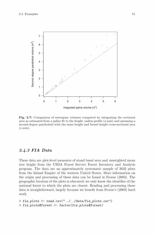
2.4 Examples 51
●
●
●
●
●
●
●
●
●
●
●
●
●
●
●●
●
●
●
●
●
●
●
●
● ●
●
●
●
●
●
●
●
●●
●
●
●
●
0 1 2 3 4 5 6
0
1
2
3
4
5
6
7
Integrated spline volume (m3)
Sec
ond−
degr
ee p
arab
oloi
d vo
lum
e (m
3 )
Fig. 2.7: Comparison of sweetgum volumes computed by integrating the sectionalarea as estimated from a spline fit to the height–radius profile (x-axis) and assuming asecond-degree paraboloid with the same height and breast-height cross-sectional area(y-axis).
2.4.3 FIA Data
These data are plot-level measures of stand basal area and unweighted meantree height from the USDA Forest Service Forest Inventory and Analysisprogram. The data are an approximately systematic sample of 2632 plotsfrom the Inland Empire of the western United States. More information onthe origin and processing of these data can be found in Froese (2003). Thegeographic location of the plots is obscured; we only know the identifier of thenational forest to which the plots are closest. Reading and processing thesedata is straightforward, largely because we benefit from Froese’s (2003) hardwork.
> fia.plots <- read.csv("../../data/fia_plots.csv")
> fia.plots$forest <- factor(fia.plots$forest)
52 2 Forest Data Management
> fia.plots$ba.m2.ha <- fia.plots$ba * 2.47105381 / 10.7639104
> fia.plots$ht.m <- fia.plots$ht * 0.3048
2.4.4 Norway Spruce Profiles
The Norway spruce (Picea abies [L.] Karst) data are tree data originallyreported in von Guttenberg (1915) and kindly provided to us by ProfessorBoris Zeide. The dataset comprises measures taken on 107 average-size treesfrom seven locations that encompassed five different sites. These data aremore fully documented in Zeide (1993).
We read the comma-delimited file, convert the variable names to be alllowercase, change one of them, and examine the resulting object.
> gutten <- read.csv("../../data/gutten.csv")
> names(gutten) <- tolower(names(gutten))
> names(gutten)[names(gutten)=="diameter"] <- "dbh.cm"
> str(gutten)
�data.frame�: 1287 obs. of 8 variables:
$ site : int 1 1 1 1 1 1 1 1 ...
$ location: int 1 1 1 1 1 1 1 1 ...
$ tree : int 1 1 1 1 1 1 1 1 ...
$ age.base: int 10 20 30 40 50 60 70 80 ...
$ height : num 1.2 4.2 9.3 14.9 19.7 23 25.8 27.4 ...
$ dbh.cm : num NA 4.6 10.2 14.9 18.3 20.7 22.6 24.1 ...
$ volume : num 0.3 5 38 123 263 400 555 688 ...
$ age.bh : num NA 9.67 19.67 29.67 ...
It would be useful to ensure that we have a unique tree identifier.
> gutten$site <- factor(gutten$site)
> gutten$location <- factor(gutten$location)
> gutten$tree.ID <- with(gutten, interaction(location, tree))
We can now count the trees within site and location classes by reducingthe first three columns of the data frame to their unique components andtabulating them. We use the unique function. Here we count trees by locationand then by location and site.
> with(unique(gutten[,c("site","location","tree.ID")]),
+ table(location))
location
1 2 3 4 5 6 7
15 2 13 10 46 11 10

2.4 Examples 53
> with(unique(gutten[,c("site","location","tree.ID")]),
+ table(location, site))
site
location 1 2 3 4 5
1 6 4 5 0 0
2 2 0 0 0 0
3 7 4 2 0 0
4 3 2 2 0 3
5 3 19 7 15 2
6 0 7 2 2 0
7 0 1 2 4 3
There seems to be substantial imbalance in the tree counts in the differentlocations — ranging from two at location 2 to 46 at location 5. Next, wecheck whether any observations contain missing values.
> show.cols.with.na(gutten)
dbh.cm volume age.bh
87 6 87
The 87 measures with missing diameter and age at breast height were eachpresumably taken while the tree height was less than or equal to 1.3 m. We cancheck this conjecture by asking R to report the maximum height associatedwith all the tree measures that have missing diameters. We identify the valuesthat are missing by using the is.na function.
> max(gutten$height[is.na(gutten$dbh.cm)])
[1] 1.3
Our conjecture seems reasonable. We will exclude these measures from thedata for the purposes of modeling.
> gutten <- gutten[!is.na(gutten$dbh.cm),]
These data are subsequently used in Sections 6.2 and 7.6.
2.4.5 Grand Fir Profiles
The grand fir (Abies grandis (Dougl.) Lindl.) data were provided to us by Dr.Albert Stage. To give a brief synopsis of the design, a sample of 66 trees wasselected in national forests around northern and central Idaho. According toStage (pers. comm., 2003), the trees were selected purposively rather thanrandomly. Stage (1963) noted that the selected trees “. . . appeared to havebeen dominant throughout their lives” and “. . . showed no visible evidence
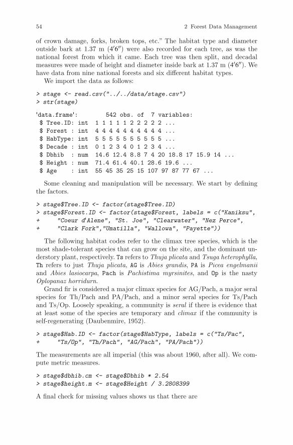
54 2 Forest Data Management
of crown damage, forks, broken tops, etc.” The habitat type and diameteroutside bark at 1.37 m (4′6′′) were also recorded for each tree, as was thenational forest from which it came. Each tree was then split, and decadalmeasures were made of height and diameter inside bark at 1.37 m (4′6′′). Wehave data from nine national forests and six different habitat types.
We import the data as follows:
> stage <- read.csv("../../data/stage.csv")
> str(stage)
�data.frame�: 542 obs. of 7 variables:
$ Tree.ID: int 1 1 1 1 1 2 2 2 2 2 ...
$ Forest : int 4 4 4 4 4 4 4 4 4 4 ...
$ HabType: int 5 5 5 5 5 5 5 5 5 5 ...
$ Decade : int 0 1 2 3 4 0 1 2 3 4 ...
$ Dbhib : num 14.6 12.4 8.8 7 4 20 18.8 17 15.9 14 ...
$ Height : num 71.4 61.4 40.1 28.6 19.6 ...
$ Age : int 55 45 35 25 15 107 97 87 77 67 ...
Some cleaning and manipulation will be necessary. We start by definingthe factors.
> stage$Tree.ID <- factor(stage$Tree.ID)
> stage$Forest.ID <- factor(stage$Forest, labels = c("Kaniksu",
+ "Coeur d�Alene", "St. Joe", "Clearwater", "Nez Perce",
+ "Clark Fork","Umatilla", "Wallowa", "Payette"))
The following habitat codes refer to the climax tree species, which is themost shade-tolerant species that can grow on the site, and the dominant un-derstory plant, respectively. Ts refers to Thuja plicata and Tsuga heterophylla,Th refers to just Thuja plicata, AG is Abies grandis, PA is Picea engelmanii
and Abies lasiocarpa, Pach is Pachistima myrsinites, and Op is the nastyOplopanaz horridurn.
Grand fir is considered a major climax species for AG/Pach, a major seralspecies for Th/Pach and PA/Pach, and a minor seral species for Ts/Pachand Ts/Op. Loosely speaking, a community is seral if there is evidence thatat least some of the species are temporary and climax if the community isself-regenerating (Daubenmire, 1952).
> stage$Hab.ID <- factor(stage$HabType, labels = c("Ts/Pac",
+ "Ts/Op", "Th/Pach", "AG/Pach", "PA/Pach"))
The measurements are all imperial (this was about 1960, after all). We com-pute metric measures.
> stage$dbhib.cm <- stage$Dbhib * 2.54
> stage$height.m <- stage$Height / 3.2808399
A final check for missing values shows us that there are

2.4 Examples 55
> show.cols.with.na(stage)
No missing values.
2.4.6 McDonald–Dunn Research Forest
The McDonald–Dunn Research Forest is located near Oregon State Univer-sity in Corvallis, Oregon. The forest is approximately 4856 hectares (11995acres) and is actively managed for student instruction, revenue, research, andrecreation.
The forest has been divided into areas of homogeneity (stands), representedby polygons, and each polygon has been designated for one of the objectivesabove. The data2 comprise two spatial datasets: stand polygons with plotlocations, and a tabular dataset consisting of field samples, which are treemeasurements. To simplify our presentation, we use a derived dataset thatcontains fewer attributes.
2.4.6.1 Stand Data
The stand polygon data are stored in an ESRI3 shapefile, which can be readin using the readShapePoly function of the maptools package.
> stands <- readShapePoly("../../data/stands.shp",
+ verbose=FALSE)
> names(stands)
[1] "SP_ID" "AREA" "PERIMETER" "STANDID"
[5] "ALLOCATION" "TAGE" "BHAGE" "DF_SITE"
[9] "TOTHT" "CUBVOL_AC" "TPA" "QMD"
[13] "BA"
The readShapePoly function reads data from a polygon shapefile into aSpatialPolygonsDataFrame object. The data can be accessed using the $
operator (e.g., stands$TAGE) or coerced into a non-spatial data frame usingthe as.data.frame function. For other geometry types, other functions areavailable (e.g., ?readShapeLines and ?readShapePoints).
To examine the attribute data for stands, use the names function.
> names(stands)
[1] "SP_ID" "AREA" "PERIMETER" "STANDID"
[5] "ALLOCATION" "TAGE" "BHAGE" "DF_SITE"
2 Available at http://www.cof.orst.edu/cf/forests/mcdonald/.3 Environmental Systems Research Institute, Inc.

56 2 Forest Data Management
[9] "TOTHT" "CUBVOL_AC" "TPA" "QMD"
[13] "BA"
The names function reveals that the data contain a few geometric at-tributes (AREA and PERIMETER, in feet), a stand identifier (STANDID), theland classification (ALLOCATION), total age (TAGE), breast-height age (BHAGE),a site productivity measure for Douglas-fir (DF_SITE) (Bruce, 1981), averageheight of the 40 tallest stems per acre (TOTHT), an estimate of the current vol-ume per acre (CUBVOL_AC), current stocking in trees per acre (TPA), quadraticstand diameter (QMD), and total stand basal area (BA) for each stand polygon.Some of the attributes contain NA (signifying that attributes are missing) andwill need to be either ignored or imputed.
To plot the SpatialPolygonsDataFrame object, with unique shadings forthe different stand allocations (stands$ALLOCATION), use a gradient in grayscale (?gray) to represent the forest allocation (see Figure 2.8).
2.4.6.2 Plot Data
The plot data, read in using the readShapePoints function,
> plots <- readShapePoints("../../data/plots.shp")
contains a plot identifier (plots$UNIPLOT) and plot locations stored as co-ordinates (plots$coords.x1 and plots$coords.x2). The plot locations canbe easily added to the existing plot using the plot function with the add =
TRUE argument,
> plot(plots, add=TRUE, pch=46)
> lev <- as.numeric(stands$ALLOCATION)
> fgs <- gray(length(levels(stands$ALLOCATION)):1 / 3)
> plot(stands,
+ col=fgs[lev],
+ add=FALSE,
+ axes=TRUE)
> title(paste("McDonald-Dunn Research Forest",
+ "Stand Boundaries and Plot Locations",
+ sep = "\n"))
> legend(1280000, 365000,
+ levels(stands$ALLOCATION)[3:1],
+ fill = fgs[3:1],
+ cex = 0.7,
+ title = "Land Allocations")
> plot(plots, add=TRUE, pch=46)

2.4 Examples 57
1260000 1270000 1280000 1290000
3500
0036
0000
3700
0038
0000
3900
0040
0000
McDonald−Dunn Research ForestStand Boundaries and Plot Locations
Land Allocations
researchold growthforest
Fig. 2.8: The Oregon State University research forest. The polygons are shadedaccording to management allocation (stands$ALLOCATION), and plot locations arerepresented as points.
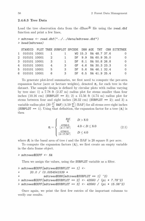
58 2 Forest Data Management
2.4.6.3 Tree Data
Load the tree observation data from the dBase� file using the read.dbf
function and print a few lines,
> mdtrees <- read.dbf("../../data/mdtrees.dbf")
> head(mdtrees)
STANDID PLOT TREE SUBPLOT SPCODE DBH AGE THT CBH SITETREE
1 010101 10001 1 1 WO 15.3 NA 48.7 37.6 0
2 010101 10001 2 1 DF 9.9 NA 60.9 35.0 0
3 010101 10001 3 1 DF 8.1 NA 50.8 26.8 0
4 010101 10001 4 3 GF 4.6 NA 30.3 23.3 0
5 010101 10001 5 3 DF 5.6 NA 46.1 32.4 0
6 010101 10001 6 3 DF 6.5 NA 41.9 25.4 0
To generate plot-level summaries, we first need to compute the per-areaexpansion factor (acre or hectare weights), denoted πi, for each tree in thedataset. The sample design is defined by circular plots with radius varyingby tree size: 1) a 7.78 ft (2.37 m) radius plot for stems smaller than fourinches (10.16 cm) (SUBPLOT == 3); 2) a 15.56 ft (4.74 m) radius plot forstems between four and eight inches (20.32 cm) (SUBPLOT == 2); and 3) a
variable radius plot (20 f t2
acBAF) (4.59 m2
ha) BAF) for all stems over eight inches
(SUBPLOT == 1). Using that definition, the expansion factor for a tree (πi) isthen
πi =
⎧⎪⎪⎪⎨⎪⎪⎪⎩
BAFBi
D > 8.0
43560.0(π×7.782)
4.0 < D ≤ 8.0
43560.0(π×15.562)
D ≤ 4.0
(2.1)
where Bi is the basal area of tree i and the BAF is 20 square ft per acre.To compute the expansion factors (πi), we first create an empty variable
in the data frame object.
> mdtrees$EXPF <- NA
Then we assign the values, using the SUBPLOT variable as a filter.
> mdtrees$EXPF[mdtrees$SUBPLOT == 1] <-
+ 20.0 / (0.0054541539 *
+ mdtrees$DBH[mdtrees$SUBPLOT == 1] ^2)
> mdtrees$EXPF[mdtrees$SUBPLOT == 2] <- 43560 / (pi * 7.78^2)
> mdtrees$EXPF[mdtrees$SUBPLOT == 3] <- 43560 / (pi * 15.56^2)
Once again, we print the first few entries of the important columns toverify our results.
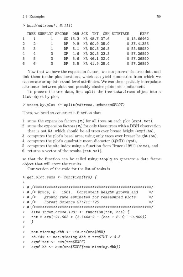
2.4 Examples 59
> head(mdtrees[, 3:11])
TREE SUBPLOT SPCODE DBH AGE THT CBH SITETREE EXPF
1 1 1 WO 15.3 NA 48.7 37.6 0 15.66462
2 2 1 DF 9.9 NA 60.9 35.0 0 37.41383
3 3 1 DF 8.1 NA 50.8 26.8 0 55.88980
4 4 3 GF 4.6 NA 30.3 23.3 0 57.26890
5 5 3 DF 5.6 NA 46.1 32.4 0 57.26890
6 6 3 DF 6.5 NA 41.9 25.4 0 57.26890
Now that we have the expansion factors, we can process the tree data andlink them to the plot locations, which can yield summaries from which wecan create or update stand-level attributes. We can then spatially interpolateattributes between plots and possibly cluster plots into similar sets.
To process the tree data, first split the tree data.frame object into alist object by plot,
> trees.by.plot <- split(mdtrees, mdtrees$PLOT)
Then, we need to construct a function that
1. sums the expansion factors (πi) for all trees on each plot (expf.tot),2. sums the expansion factors (πi) for only those trees with a DBH observation
that is not NA, which should be all trees over breast height (expf.ha),3. computes the plot’s basal area, using only trees over breast height (ba),4. computes the plot’s quadratic mean diameter (QMD) (qmd),5. computes the site index using a function from Bruce (1981) (site), and6. returns a vector of the results (ret.val),
so that the function can be called using sapply to generate a data frameobject that will store the results.
Our version of the code for the list of tasks is
> get.plot.sums <- function(trs) {
+
+ # /******************************************************/
+ # /* Bruce, D. 1981. Consistent height-growth and */
+ # /* growth-rate estimates for remeasured plots. */
+ # /* Forest Science 27:711-725. */
+ # /******************************************************/
+ site.index.bruce.1981 <- function(tht, bha) {
+ tht * exp(-21.663 * (3.744e-2 - (bha + 8.0)^ -0.809))
+ }
+
+ not.missing.dbh <- !is.na(trs$DBH)
+ bh.idx <- not.missing.dbh & trs$THT > 4.5
+ expf.tot <- sum(trs$EXPF)
+ expf.bh <- sum(trs$EXPF[not.missing.dbh])

60 2 Forest Data Management
+ ba <- sum(0.0054541539 * trs$DBH[not.missing.dbh] ^ 2 *
+ trs$EXPF[not.missing.dbh])
+ qmd <- sqrt(ba / expf.bh / 0.0054541539)
+ s.trs <- trs[trs$SITETREE == 1 & trs$SPCODE == "DF" &
+ !is.na(trs$THT),]
+ nst <- nrow(s.trs)
+ site.bar <-
+ ifelse(nst > 0,
+ weighted.mean(site.index.bruce.1981(s.trs$THT,
+ s.trs$AGE),
+ s.trs$EXPF),
+ NA)
+ return(c(nrow(trs), expf.bh, expf.tot,
+ ba, qmd, nst, site.bar))
+ }
To generate the summaries, call the sapply function, and transpose andcoerce the results from sapply call
> plot.sums <-
+ data.frame(t(sapply(trees.by.plot, get.plot.sums)))
so that each row in plot.sums contains the plot-level summaries, computedin the get.plot.sums function.
The current column names are meaningless, as they have been automat-ically generated. Also, the plot identifier needs to be appended to our dataframe. Therefore we use the names from the split operation with the namesof the variables from the get.plot.sums function,
> plot.sums$id <- as.numeric(names(trees.by.plot))
> names(plot.sums) <- c("trees","expf.bh","expf.tot",
+ "ba","qmd","nst","site","id")
> print(head(plot.sums), digits=3)
trees expf.bh expf.tot ba qmd nst site id
10001 20 1368.9 2972 134.449 4.244 0 NA 10001
10002 7 1030.8 1260 26.828 2.184 0 NA 10002
10003 2 286.3 286 15.955 3.196 0 NA 10003
10005 4 35.2 722 20.000 10.200 0 NA 10005
10006 3 458.2 687 0.562 0.474 0 NA 10006
10017 8 145.4 145 158.519 14.140 1 117 10017
The next step is to merge the plot summary data (plot.sums) with theplot.centers to create a single data frame object, making sure to preserveempty plots, using the argument all = TRUE.
> plot.id <- as.numeric(as.character(plots$UNIPLOT))
> plot.centers <- data.frame(cbind(coordinates(plots), plot.id))
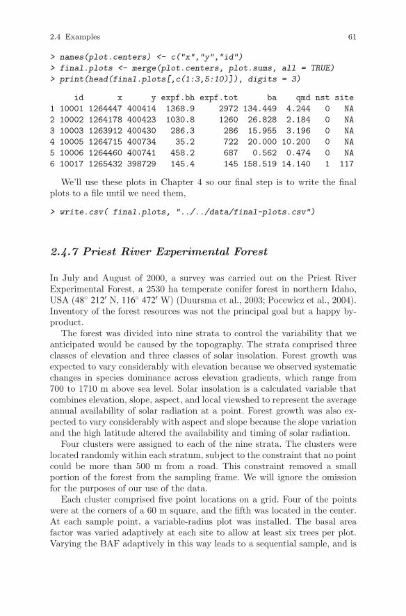
2.4 Examples 61
> names(plot.centers) <- c("x","y","id")
> final.plots <- merge(plot.centers, plot.sums, all = TRUE)
> print(head(final.plots[,c(1:3,5:10)]), digits = 3)
id x y expf.bh expf.tot ba qmd nst site
1 10001 1264447 400414 1368.9 2972 134.449 4.244 0 NA
2 10002 1264178 400423 1030.8 1260 26.828 2.184 0 NA
3 10003 1263912 400430 286.3 286 15.955 3.196 0 NA
4 10005 1264715 400734 35.2 722 20.000 10.200 0 NA
5 10006 1264460 400741 458.2 687 0.562 0.474 0 NA
6 10017 1265432 398729 145.4 145 158.519 14.140 1 117
We’ll use these plots in Chapter 4 so our final step is to write the finalplots to a file until we need them,
> write.csv( final.plots, "../../data/final-plots.csv")
2.4.7 Priest River Experimental Forest
In July and August of 2000, a survey was carried out on the Priest RiverExperimental Forest, a 2530 ha temperate conifer forest in northern Idaho,USA (48◦ 212′ N, 116◦ 472′ W) (Duursma et al., 2003; Pocewicz et al., 2004).Inventory of the forest resources was not the principal goal but a happy by-product.
The forest was divided into nine strata to control the variability that weanticipated would be caused by the topography. The strata comprised threeclasses of elevation and three classes of solar insolation. Forest growth wasexpected to vary considerably with elevation because we observed systematicchanges in species dominance across elevation gradients, which range from700 to 1710 m above sea level. Solar insolation is a calculated variable thatcombines elevation, slope, aspect, and local viewshed to represent the averageannual availability of solar radiation at a point. Forest growth was also ex-pected to vary considerably with aspect and slope because the slope variationand the high latitude altered the availability and timing of solar radiation.
Four clusters were assigned to each of the nine strata. The clusters werelocated randomly within each stratum, subject to the constraint that no pointcould be more than 500 m from a road. This constraint removed a smallportion of the forest from the sampling frame. We will ignore the omissionfor the purposes of our use of the data.
Each cluster comprised five point locations on a grid. Four of the pointswere at the corners of a 60 m square, and the fifth was located in the center.At each sample point, a variable-radius plot was installed. The basal areafactor was varied adaptively at each site to allow at least six trees per plot.Varying the BAF adaptively in this way leads to a sequential sample, and is
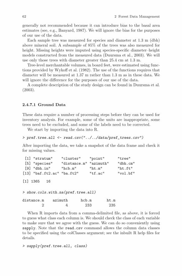
62 2 Forest Data Management
generally not recommended because it can introduce bias to the basal areaestimates (see, e.g., Banyard, 1987). We will ignore the bias for the purposesof our use of the data.
Each sample tree was measured for species and diameter at 1.3 m (dbh)above mineral soil. A subsample of 85% of the trees was also measured forheight. Missing heights were imputed using species-specific diameter–heightmodels constructed from the measured data (Duursma et al., 2003). We willuse only those trees with diameter greater than 25.4 cm at 1.3 m.
Tree-level merchantable volumes, in board feet, were estimated using func-tions provided by Wykoff et al. (1982). The use of the functions requires thatdiameter will be measured at 1.37 m rather than 1.3 m as in these data. Wewill ignore the difference for the purposes of our use of the data.
A complete description of the study design can be found in Duursma et al.(2003).
2.4.7.1 Ground Data
These data require a number of processing steps before they can be used forinventory analysis. For example, some of the units are inappropriate, sometrees need to be excluded, and some of the labels need to be corrected.
We start by importing the data into R.
> pref.tree.all <- read.csv("../../data/pref_trees.csv")
After importing the data, we take a snapshot of the data frame and check itfor missing values.
[1] "stratum" "cluster" "point" "tree"
[5] "species" "distance.m" "azimuth" "dbh.cm"
[9] "dbh.in" "hcb.m" "ht.m" "ht.ft"
[13] "baf.ft2.ac" "ba.ft2" "tf.ac" "vol.bf"
[1] 1365 16
> show.cols.with.na(pref.tree.all)
distance.m azimuth hcb.m ht.m
2 4 233 235
When R imports data from a comma-delimited file, as above, it is forcedto guess what class each column is. We should check the class of each variableto make sure that we agree with the guess. We can do so conveniently usingsapply. Note that the read.csv command allows the column data classesto be specified using the colClasses argument; see the inbuilt R help files fordetails.
> sapply(pref.tree.all, class)
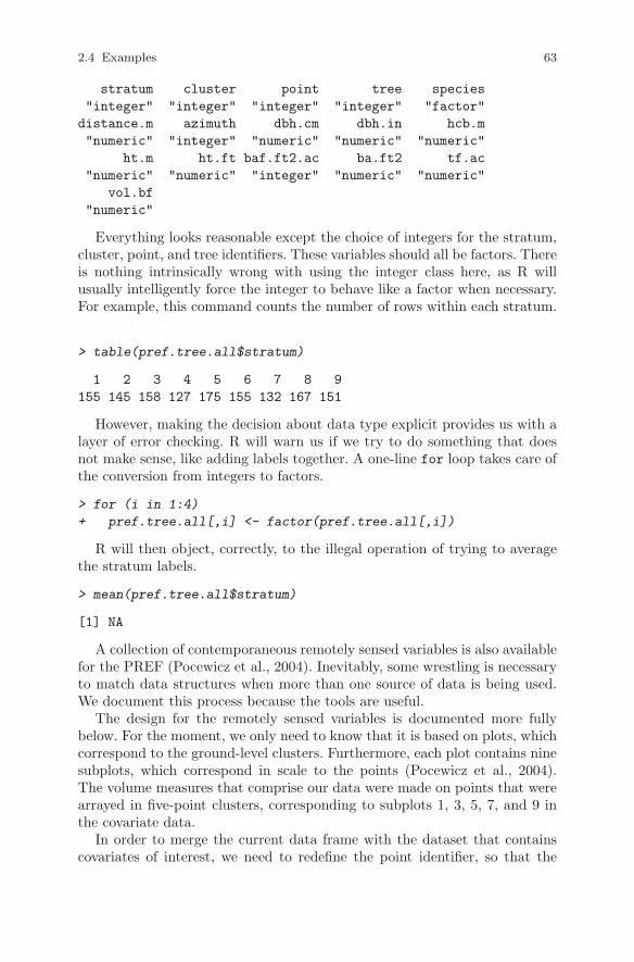
2.4 Examples 63
stratum cluster point tree species
"integer" "integer" "integer" "integer" "factor"
distance.m azimuth dbh.cm dbh.in hcb.m
"numeric" "integer" "numeric" "numeric" "numeric"
ht.m ht.ft baf.ft2.ac ba.ft2 tf.ac
"numeric" "numeric" "integer" "numeric" "numeric"
vol.bf
"numeric"
Everything looks reasonable except the choice of integers for the stratum,cluster, point, and tree identifiers. These variables should all be factors. Thereis nothing intrinsically wrong with using the integer class here, as R willusually intelligently force the integer to behave like a factor when necessary.For example, this command counts the number of rows within each stratum.
> table(pref.tree.all$stratum)
1 2 3 4 5 6 7 8 9
155 145 158 127 175 155 132 167 151
However, making the decision about data type explicit provides us with alayer of error checking. R will warn us if we try to do something that doesnot make sense, like adding labels together. A one-line for loop takes care ofthe conversion from integers to factors.
> for (i in 1:4)
+ pref.tree.all[,i] <- factor(pref.tree.all[,i])
R will then object, correctly, to the illegal operation of trying to averagethe stratum labels.
> mean(pref.tree.all$stratum)
[1] NA
A collection of contemporaneous remotely sensed variables is also availablefor the PREF (Pocewicz et al., 2004). Inevitably, some wrestling is necessaryto match data structures when more than one source of data is being used.We document this process because the tools are useful.
The design for the remotely sensed variables is documented more fullybelow. For the moment, we only need to know that it is based on plots, whichcorrespond to the ground-level clusters. Furthermore, each plot contains ninesubplots, which correspond in scale to the points (Pocewicz et al., 2004).The volume measures that comprise our data were made on points that werearrayed in five-point clusters, corresponding to subplots 1, 3, 5, 7, and 9 inthe covariate data.
In order to merge the current data frame with the dataset that containscovariates of interest, we need to redefine the point identifier, so that the
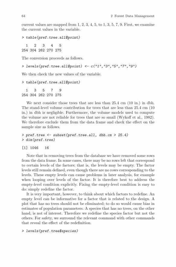
64 2 Forest Data Management
current values are mapped from 1, 2, 3, 4, 5, to 1, 3, 5, 7, 9. First, we examinethe current values in the variable.
> table(pref.tree.all$point)
1 2 3 4 5
254 304 262 270 275
The conversion proceeds as follows.
> levels(pref.tree.all$point) <- c("1","3","5","7","9")
We then check the new values of the variable.
> table(pref.tree.all$point)
1 3 5 7 9
254 304 262 270 275
We next consider those trees that are less than 25.4 cm (10 in.) in dbh.The stand-level volume contribution for trees that are less than 25.4 cm (10in.) in dbh is negligible. Furthermore, the volume models used to computethe volume are not reliable for trees that are so small (Wykoff et al., 1982).We therefore exclude them from the data frame and check the effect on thesample size as follows.
> pref.tree <- subset(pref.tree.all, dbh.cm > 25.4)
> dim(pref.tree)
[1] 1046 16
Note that in removing trees from the database we have removed some rowsfrom the data frame. In some cases, there may be no rows left that correspondto certain levels of the factors; that is, the levels may be empty. The factorlevels still remain defined, even though there are no rows corresponding to thelevels. These empty levels can cause problems in later analysis, for examplewhen looping over levels of the factor. It is therefore best to address theempty-level condition explicitly. Fixing the empty-level condition is easy todo: simply redefine the factor.
It is very important, however, to think about which factors to redefine. Anempty level can be informative for a factor that is related to the design. Aplot that has no trees should not be eliminated; to do so would cause bias inestimates of population parameters. A species that has no trees, on the otherhand, is not of interest. Therefore we redefine the species factor but not theothers. For safety, we surround the relevant command with other commandsthat reveal the effect of the redefinition.
> levels(pref.tree$species)
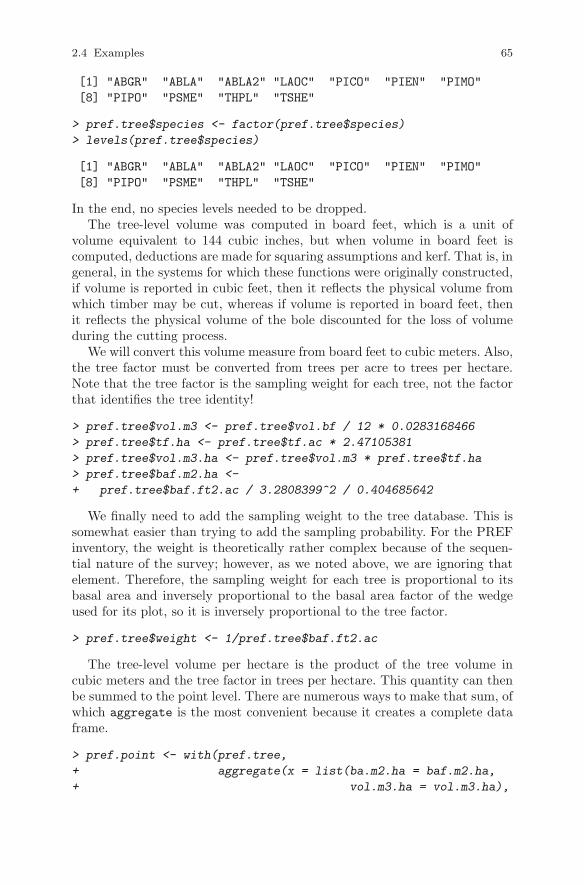
2.4 Examples 65
[1] "ABGR" "ABLA" "ABLA2" "LAOC" "PICO" "PIEN" "PIMO"
[8] "PIPO" "PSME" "THPL" "TSHE"
> pref.tree$species <- factor(pref.tree$species)
> levels(pref.tree$species)
[1] "ABGR" "ABLA" "ABLA2" "LAOC" "PICO" "PIEN" "PIMO"
[8] "PIPO" "PSME" "THPL" "TSHE"
In the end, no species levels needed to be dropped.The tree-level volume was computed in board feet, which is a unit of
volume equivalent to 144 cubic inches, but when volume in board feet iscomputed, deductions are made for squaring assumptions and kerf. That is, ingeneral, in the systems for which these functions were originally constructed,if volume is reported in cubic feet, then it reflects the physical volume fromwhich timber may be cut, whereas if volume is reported in board feet, thenit reflects the physical volume of the bole discounted for the loss of volumeduring the cutting process.
We will convert this volume measure from board feet to cubic meters. Also,the tree factor must be converted from trees per acre to trees per hectare.Note that the tree factor is the sampling weight for each tree, not the factorthat identifies the tree identity!
> pref.tree$vol.m3 <- pref.tree$vol.bf / 12 * 0.0283168466
> pref.tree$tf.ha <- pref.tree$tf.ac * 2.47105381
> pref.tree$vol.m3.ha <- pref.tree$vol.m3 * pref.tree$tf.ha
> pref.tree$baf.m2.ha <-
+ pref.tree$baf.ft2.ac / 3.2808399^2 / 0.404685642
We finally need to add the sampling weight to the tree database. This issomewhat easier than trying to add the sampling probability. For the PREFinventory, the weight is theoretically rather complex because of the sequen-tial nature of the survey; however, as we noted above, we are ignoring thatelement. Therefore, the sampling weight for each tree is proportional to itsbasal area and inversely proportional to the basal area factor of the wedgeused for its plot, so it is inversely proportional to the tree factor.
> pref.tree$weight <- 1/pref.tree$baf.ft2.ac
The tree-level volume per hectare is the product of the tree volume incubic meters and the tree factor in trees per hectare. This quantity can thenbe summed to the point level. There are numerous ways to make that sum, ofwhich aggregate is the most convenient because it creates a complete dataframe.
> pref.point <- with(pref.tree,
+ aggregate(x = list(ba.m2.ha = baf.m2.ha,
+ vol.m3.ha = vol.m3.ha),

66 2 Forest Data Management
+ by = list(stratum = stratum,
+ cluster = cluster,
+ point = point),
+ FUN = sum))
We should examine the new object to ensure that it matches our expecta-tions. For example, we expect each of the nine strata to contain 20 points.
> table(pref.point$stratum)
1 2 3 4 5 6 7 8 9
18 14 20 16 19 20 20 20 18
This summary shows a problem: several strata are missing points. Theaggregate function drops indicators for the empty points. At the time ofwriting, there is no way to instruct aggregate to keep the empty levels,although there may well be in the future. Regardless, we can take the oppor-tunity to demonstrate more data manipulation commands. As always, thereare several options for proceeding.
We will create a new data frame that reflects the structure of the design,using the expand.grid function, and merge it with this dataset. Note that thecluster identifier crosses stratum boundaries, instead of being nested insidethe strata, so we will add the stratum identifier to our new data frame aftercreating it.
> design.point <-
+ expand.grid(cluster = levels(pref.tree.all$cluster),
+ point = levels(pref.tree.all$point))
> str(design.point)
�data.frame�: 180 obs. of 2 variables:
$ cluster: Factor w/ 36 levels "1","4","5","6",..: 1 2 ...
$ point : Factor w/ 5 levels "1","3","5","7",..: 1 1 ...
- attr(*, "out.attrs")=List of 2
..$ dim : Named int 36 5
.. ..- attr(*, "names")= chr "cluster" ...
..$ dimnames:List of 2
.. ..$ cluster: chr "cluster=1" ...
.. ..$ point : chr "point=1" ...
This new data frame comprises 36 plots of five clusters for a total length of180. Next we need to construct a data frame that contains the cluster and thestratum identifiers for all the clusters, including the empty ones. We couldcreate such a document in a spreadsheet and read it in. We prefer to reducethe number of steps needed to analyze the data by creating the needed objectin R. Here, we do this by extracting the cluster and stratum columns fromthe original dataset, removing all the missing values, and then removing allthe duplicate rows, as follows.

2.4 Examples 67
> design.cluster <-
+ unique(pref.tree.all[, c("cluster","stratum")])
> str(design.cluster)
�data.frame�: 36 obs. of 2 variables:
$ cluster: Factor w/ 36 levels "1","4","5","6",..: 1 7 ...
$ stratum: Factor w/ 9 levels "1","2","3","4",..: 1 2 ...
The merging operation requires the merge command. This operation is bestmonitored, and an easy way to monitor it is to use dim commands before andafterward. When reusing an object name, we should check the effect of ourmerge command on a test data frame first, so we do not have to recreatethe original if we make a mistake. And, we often do. Also, it is important toensure that the factors for merging are appropriately defined before merging.Failure to do so can lead to errors that are difficult to detect, and may onlyshow up much later in the analysis or, worse, go undetected.
> dim(design.point)
[1] 180 2
> dim(design.cluster)
[1] 36 2
> test <- merge(x = design.point,
+ y = design.cluster,
+ all = TRUE)
> dim(test)
[1] 180 3
> head(test)
cluster point stratum
1 1 1 1
2 1 7 1
3 1 9 1
4 1 5 1
5 1 3 1
6 10 1 2
This seems to have worked just fine. We can now merge the volumes.
> design.point <- test
> dim(design.point)
[1] 180 3
> dim(pref.point)
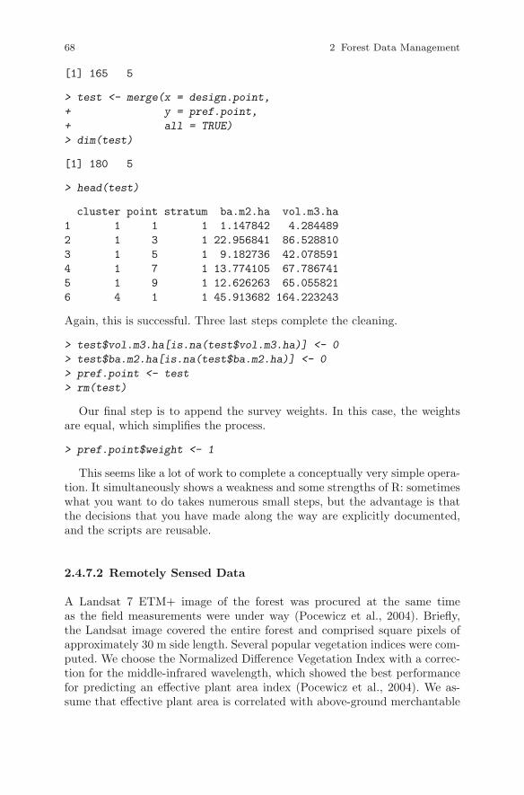
68 2 Forest Data Management
[1] 165 5
> test <- merge(x = design.point,
+ y = pref.point,
+ all = TRUE)
> dim(test)
[1] 180 5
> head(test)
cluster point stratum ba.m2.ha vol.m3.ha
1 1 1 1 1.147842 4.284489
2 1 3 1 22.956841 86.528810
3 1 5 1 9.182736 42.078591
4 1 7 1 13.774105 67.786741
5 1 9 1 12.626263 65.055821
6 4 1 1 45.913682 164.223243
Again, this is successful. Three last steps complete the cleaning.
> test$vol.m3.ha[is.na(test$vol.m3.ha)] <- 0
> test$ba.m2.ha[is.na(test$ba.m2.ha)] <- 0
> pref.point <- test
> rm(test)
Our final step is to append the survey weights. In this case, the weightsare equal, which simplifies the process.
> pref.point$weight <- 1
This seems like a lot of work to complete a conceptually very simple opera-tion. It simultaneously shows a weakness and some strengths of R: sometimeswhat you want to do takes numerous small steps, but the advantage is thatthe decisions that you have made along the way are explicitly documented,and the scripts are reusable.
2.4.7.2 Remotely Sensed Data
A Landsat 7 ETM+ image of the forest was procured at the same timeas the field measurements were under way (Pocewicz et al., 2004). Briefly,the Landsat image covered the entire forest and comprised square pixels ofapproximately 30 m side length. Several popular vegetation indices were com-puted. We choose the Normalized Difference Vegetation Index with a correc-tion for the middle-infrared wavelength, which showed the best performancefor predicting an effective plant area index (Pocewicz et al., 2004). We as-sume that effective plant area is correlated with above-ground merchantable

2.4 Examples 69
tree volume. Full information on the processing steps applied can be foundin Pocewicz et al. (2004) and Landsat Project Science Office (2005).
We now access two relevant comma-delimited datasets. The pixel datasetcontains the corrected, pixel-level response values for the coverage of thePREF.4 The subplot dataset contains field and remote measurements for thepoints. The remotely sensed covariates are taken from the pixels in the pixeldatabase that were closest in location to the field points.
> pref.pixel <- read.csv("../../data/pref_pixels.csv")
> names(pref.pixel)
[1] "num" "utme" "utmn" "lai.rs"
[5] "ndvi" "mir" "slope" "cti"
[9] "elev" "inso" "ndvic" "mirc.1"
[13] "mirc.2" "mirc.amy" "mirc.check" "mirc.pref"
> dim(pref.pixel)
[1] 28102 16
> pref.pixel[1:5, c(1:5,11)]
num utme utmn lai.rs ndvi ndvic
1 1 510731.2 5353596 5.870416 0.8032642 0.7116639
2 2 510731.2 5353626 5.229210 0.7827569 0.6076666
3 3 510731.2 5353656 5.900865 0.7757183 0.6872592
4 4 510731.2 5353566 4.912140 0.7921855 0.6149861
5 5 510731.2 5353686 6.003587 0.7757183 0.6872592
> show.cols.with.na(pref.pixel)
No missing values.
> sapply(pref.pixel, class)
num utme utmn lai.rs ndvi
"integer" "numeric" "numeric" "numeric" "numeric"
mir slope cti elev inso
"integer" "numeric" "numeric" "numeric" "integer"
ndvic mirc.1 mirc.2 mirc.amy mirc.check
"numeric" "numeric" "numeric" "numeric" "numeric"
mirc.pref
"numeric"
The pixel-level dataset seems fine.
> pref.subplot <- read.csv("../../data/pref_subplots.csv")
> names(pref.subplot)
4 Landsat imagery courtesy of NASA Goddard Space Flight Center and U.S. Geo-logical Survey.

70 2 Forest Data Management
[1] "plot" "subplot" "point"
[4] "scale" "utme" "utmn"
[7] "slope" "wetind" "elevclass"
[10] "insoclass" "elev1" "elevsq1"
[13] "inso1" "insosq1" "LAIbeer2total"
[16] "LAIbeer2can" "acblue" "acgreen"
[19] "acred" "acnir" "acmir1"
[22] "acmir2" "acndvi" "acndviC"
[25] "acsr" "acsrC" "acvegind"
[28] "acsavi" "acsarvi2" "acslavi"
[31] "acinfrared" "acbrightness" "acgreenness"
[34] "acwetness" "MIRc"
> dim(pref.subplot)
[1] 324 35
> pref.subplot[1:5, c(1:3, 5:6, 24)]
plot subplot point utme utmn acndviC
1 1 1 a 515397 5357562 0.3328538
2 1 2 a 515397 5357592 0.7114403
3 1 3 a 515397 5357622 0.7114403
4 1 4 a 515427 5357622 0.7396296
5 1 5 a 515457 5357622 0.6101370
> show.cols.with.na(pref.subplot)
No missing values.
> sapply(pref.subplot, class)[1:4]
plot subplot point scale
"integer" "integer" "factor" "factor"
> pref.subplot$plot <- factor(pref.subplot$plot)
> pref.subplot$subplot <- factor(pref.subplot$subplot)
The subplot-level dataset also seems fine. The merge command blendsour existing point-level information with the new subplot-level information.Again, we surround our merge with dim statements to monitor the process.
> dim(pref.point)
[1] 180 6
> dim(pref.subplot[,c("plot","subplot","acndviC")])
[1] 324 3

2.4 Examples 71
> pref.point.cov <-
+ merge(x = pref.point,
+ y = pref.subplot[,c("plot","subplot","acndviC")],
+ all.x = TRUE, all.y = FALSE,
+ by.x = c("cluster","point"),
+ by.y = c("plot","subplot"))
> head(pref.point.cov)
cluster point stratum ba.m2.ha vol.m3.ha weight acndviC
1 1 1 1 1.147842 4.284489 1 0.3328538
2 1 3 1 22.956841 86.528810 1 0.7114403
3 1 5 1 9.182736 42.078591 1 0.6101370
4 1 7 1 13.774105 67.786741 1 0.6126499
5 1 9 1 12.626263 65.055821 1 0.8090011
6 10 1 2 4.591368 16.293566 1 0.5550567
> dim(pref.point.cov)
[1] 180 7
> show.cols.with.na(pref.point.cov)
No missing values.
We now have a point-level dataset with the necessary design information,a variable of interest, and an auxiliary variable.
We note that there is a mismatch between the scales of the two sets ofmeasurements. The Landsat data comprise the average spectral responsesacross 30 meter pixels. The ground measurements represent points on thelandscape, ideally in the center of the pixel but most likely not. There alsomay be errors of registration; that is, the points and the pixels might not lineup as we would hope. These types of errors are likely to occur in large-scaleinventories. We will deal with this mismatch by defining the sampling unit asthe 30 meter area represented by each Landsat pixel. The point-level volumemeasurements are then a subsample of the volume per hectare within thepixel. Understood this way, the design is a two-stage–two-phase sample, withauxiliary information on the primary sampling unit (PSU) and the variable ofinterest on the secondary sampling unit (SSU), of which there is only one perPSU. Sarndal et al. (1992) devote a section to this problem. We will ignore itbecause the within-PSU variation is impossible to assess with only one SSU,and we believe that it is likely to make only a negligible contribution anyway(see Section 3.4.2.1).

72 2 Forest Data Management
2.4.8 Leuschner
For our forest-planning example, we have used the data presented in Leuschner(1990, see Tables 3.1 and 3.2) and Curtis et al. (1982). The data, originallyfrom DFSIM simulations, was adapted and used to demonstrate forest plan-ning and regulation techniques by Leuschner (1990; see Tables 3.1 and 3.2).
For this book, we have entered the values into a text file that can be readinto R using the read.table function
> leusch.ylds <- read.table("../../data/leuschner.txt",
+ header = TRUE)
where the resulting leusch.ylds object contains four columns: 1) the standidentifier (stand), 2) the planning period (per), 3) the age of the stand inperiod per, and 4) the yield (volume), in thousands of cubic feet per acre, ifwe harvest stand stand in period per.
In these data, there are eight stands and the problem is to schedule theharvest of the forest over six periods to create a fully regulated forest. Theareas of the stands are presented in Chapter 9, where we use these data todemonstrate using R for forest activity scheduling.
2.5 Summary
We have briefly covered many of the basic data management and manipula-tion functions within the context of data conversion, error checking, gener-ating summaries and plots. The tools that R contains for data manipulation(keyword ‘manip’) are numerous, and we have only scratched the surface.Some of the documentation is extensively detailed, and reading it may seemlaborious. It is well worth the effort.
In the next chapter, we will start processing data from forest samples anddiscuss some sampling design topics.

Part II
Sampling and Mapping

Chapter 3
Data Analysis for Common InventoryMethods
3.1 Introduction
This chapter covers the analysis of sample surveys in the context of naturalresources inventories, with a particular focus on forest inventories. Our goal istwofold: to provide coverage that is relevant to the efficient analysis of samplesurvey data using R, and to demonstrate the data manipulation techniquesintroduced in Chapter 2. We also provide scripts and commentary for theanalysis of sampling designs that are commonly used in natural resourceinventories.
We include only as much background material as necessary to motivateour analysis. More thorough expositions on various elements of sampling the-ory are available elsewhere (see, e.g., Cochran, 1977; Sarndal et al., 1992;Schreuder et al., 1993). Also, our survey of inventory designs is limited byspace and variation. We focus on those designs that permit us to present thekey elements of analysis in R rather than trying to be exhaustive in scope.
We draw heavily on several third-party packages. Notably, Thomas Lum-ley’s survey package provides most of the necessary sampling estimation tools(Lumley, 2004, 2010), and Angelo Canty’s boot package, maintained by BrianRipley, provides useful tools for bootstrapping (Davison and Hinkley, 1997;Canty and Ripley, 2010). We include our own R code where it seems useful.The code we present is not necessarily optimal for our immediate purpose;there are many ways to proceed using R, and the palette of options increasesevery month. We intend that the data-processing sections serve two purposes:first, to demonstrate how to achieve simple but important goals in the pro-cessing of natural resources inventory data, and second, to demonstrate someof the flexibility and power of the R language.
We next introduce some useful vocabulary and examples for sample sur-veys in the context of forest inventories. We then identify three exampledatasets that we will use to demonstrate the steps necessary for point andinterval estimation from sample surveys. In Section 3.2, we introduce inter-
75A. P. Robinson, J. D. Hamann, Forest Analytics with R, Use R!,DOI 10.1007/978-1-4419-7762-5_3, © Springer Science+Business Media, LLC 2011

76 3 Data Analysis for Common Inventory Methods
val computation and demonstrate three methods for their estimation. Thefollowing sections detail the use of R for single-level sampling (Section 3.3),hierarchical sampling (Section 3.4), and sampling with auxiliary information(Section 3.5).
3.1.1 Infrastructure
We briefly introduce some useful vocabulary and examples for sample surveysin the context of forest inventories.
The population is the entity for which one wishes to estimate quantities ofinterest. The population comprises sampling units and is in a sense co-definedwith the sampling unit. It must be possible to represent the population by aframe. An example of a population is the Priest River Experimental Forest(PREF).
A frame is a list of units of the population that is established to facilitatethe selection of a random sample from the population. A frame for the PREFmight be a map with a grid drawn upon it.
The sampling unit is the unit that we select from the population to makemeasurements upon. A sampling unit for the PREF might be a fixed areawithin the forest of size, say, 0.1 ha.
The sample is the collection of sampling units that are measured.The variables of interest are the quantities that are measured on the sam-
pling units about which we wish to make estimates.A statistic is an arithmetical function of data that reduces it to a summary.
Example statistics are the total, the mean, and the standard deviation.The parameters are the population-level statistics of the variables of inter-
est.The sampling distribution is the distribution of values that could possibly
be taken by a statistic that is computed using a sample of data taken from apopulation.
Sometimes we will also measure auxiliary information, which is informa-tion that is in some way related to the variable of interest and is available forall or most of the units in the population.
For example, we may wish to estimate the population total (a parameter)of the volume of merchantable timber (variable of interest) on PREF. We takea map of the PREF, divided into a 0.1 ha grid (the frame), and randomlynominate a collection of 100 grid spaces (plots) to locate and measure (theseplots are the sample). Upon each plot we measure the volume of the trees(the variable of interest). We may have soil, elevation, and aspect measures forthe entire forest (auxiliary information). We can estimate the population totalusing a statistic that is calculated from the variables of interest as measuredon the sample. We will use an assumption about the sampling distribution

3.2 Estimate Computation 77
of the sample statistic to estimate the confidence interval of the estimate ofthe population parameter.
3.1.2 Example Datasets
We adopt three datasets for our examples. In each case, we report the sampledesign that was used without necessarily making any recommendations as tothe appropriateness of the design for other purposes. In order to use theseexample datasets in this chapter, it was necessary to simplify or ignore ele-ments of the actual design. We will document the necessary simplificationswhen they are applied. The datasets are the UFC data (Section 2.4.1), thePREF data (Section 2.4.7), and the FIA data (Section 2.4.3).
3.2 Estimate Computation
An estimate of a population parameter is more useful when it is accompaniedby an estimate of its certainty. Two measures of certainty that are commonlycomputed are the standard error and the confidence interval.
Confidence intervals can be computed in several ways. Here we will coverclassical large-sample theory, jackknife, and bootstrap methods. We reviewthe principles of the sampling distribution in order to set the scene for devel-opment of the interval estimates.
3.2.1 Sampling Distribution
Given an assumed sampling distribution of a statistic, our goal is to identifyan interval of that distribution that contains a suitable proportion of thesampling distribution, for example 95%. We need to estimate the shape ofthe distribution to be able to identify the interval that contains a suitableproportion. Each of the three strategies that we demonstrate for computingthe interval uses a different approach to solving this problem.
For reference, the confidence interval for the population mean can be ex-pressed as
μ ± sμ × tn−11−α/2
(3.1)
where μ is an estimate of the population mean (often the sample mean), sμ isan estimate of the standard error of the estimate of the population mean, and

78 3 Data Analysis for Common Inventory Methods
tn−11−α/2
is a quantile from Student’s t-distribution. The following approaches
can be applied.
1. Large-sample theory invokes the Central Limit Theorem and Slutsky’sTheorem to permit the assumption that the sampling distribution of themean is Student’s t. The quantiles of Student’s t are used with the sample-based estimate of standard error sμ to compute a confidence interval, asper equation (3.1). See Section 3.2.2.
2. When no reasonable closed-form estimate for the standard error can befound (e.g., for the ratio of means estimator) approximations may be used.A popular example is the Taylor-series linearization, which expands thefunction of the estimators into an infinite series and ignores all termsbeyond the linear approximation (see, e.g., Sarndal et al., 1992, p. 172).We cover linearization in Section 3.2.3.
3. Use of the jackknife allows us to replace the analytical estimate of thestandard error sμ in equation (3.1) with a resampling-based estimate. Thisapproach is useful when no reasonable closed-form estimate for the stan-dard error can be found (e.g., for the ratio of means estimator). Use ofthe jackknife requires the assumption that the sampling distribution benormal, or at the very least symmetric. See Section 3.2.4.
4. The bootstrap generates an estimate of the shape of the sampling distri-bution directly by resampling from the observed sample, and computingthe statistic of interest, many times. See Section 3.2.5. The bootstrap canbe used in one of two ways, each of which has numerous variations.
a. Bootstrap-based estimates of the standard error sμ can be used to re-place the usual sample-based estimate in equation (3.1) when no rea-sonable closed-form estimate of the standard error is known (e.g., forthe ratio of means estimator).
b. Bootstrap-based estimates of the confidence interval can be used insteadof the usual formula (3.1) if there is doubt about the shape of thesampling distribution.
Among these options, if there is a closed-form equation for the standarderror of the parameter of interest and the sampling distribution of the pa-rameter of interest can be reasonably expected to be normal (or at leastsymmetric), then approach 1 is reasonable. If there is no closed-form equa-tion for the standard error of the parameter of interest but the samplingdistribution of the parameter of interest can be reasonably expected to benormal (or at least symmetric), then estimating the standard error sμ us-ing approach 3 or 4a is reasonable. If there is doubt about the shape of thesampling distribution, then approach 4b is best, but careful use of 4a is stillpossible (see Section 3.2.5.2).
There is no definitive answer as to whetherthe jackknife or the bootstrap isbetter for estimating the standard error of an estimate. Schreuder et al. (1993)summarized a collection of studies that used forestry data and addressed

3.2 Estimate Computation 79
common forestry concerns, and their conclusions depended heavily on thesample design.
In practical terms, the jackknife requires considerably less computationtime than the bootstrap, and is probably computationally more stable, be-cause the jackknife resamples are most likely more similar to the originalsample than are the bootstrap samples. All else being equal, if an estima-tor can be computed for a sample then it is more likley that it can also becomputed for a jackknife sample than for a bootstrap sample. These obser-vations suggest that, unless there is a strong reason to do otherwise, usingthe jackknife is a reasonable strategy.
Several books have been written that compare the traditional, jackknife,and bootstrap estimates for various purposes using simulations and asymp-totic theory. For example, Shao and Tu (1995) develop and compare therates of convergence of various estimators and report simulation studies. Theauthors focus on sample surveys, as well as more general applications, anddemonstrate that for sample surveys the jackknife and the linearization esti-mators have the best performance (Shao and Tu, 1995, pp. 252–256). Manly(1997) compared the coverage rates and accuracy from a simulation studyfor estimating a confidence interval for the standard deviation of a sample ofsize 20 generated from an exponentially distributed population. The small-sample properties of the compared estimators performed poorly, but such acase seems more extreme than those typically faced in natural resources in-ventories, for which larger samples and relatively straightforward functionsof the mean will be more common.
Overall, the jackknife estimator has no asymptotic advantage over the lin-earization estimator (Shao and Tu, 1995, p. 262). Lumley noted that the lin-earization estimates “...are approximately unbiased but may be quite variableand as a result tend to lead to confidence intervals that are too short in smallsamples” (Lumley, 2004, p. 4). However, Shao and Tu (1995) present simula-tion results that suggest that the linearization estimator can be more (nega-tively) biased and less variable than the jackknife estimator (Table 2.1, p.32)in small samples.
Other approximations are plausible, and may become more popular. Sad-dlepoint approximations are more complicated functions of the sample statis-tics that provide more accurate approximations to the distribution and there-fore are more likely to be accurate at a given sample size. Readable exposi-tions can be found in Reid (1988) and Goutis and Casella (1999). A forestinventory application is reported in Magnussen (2001) and an examinationof the use of the approximation in ratio and regression estimation in Aghoet al. (2005).
Higher-order asymptotics also provide opportunities for improvement (see,e.g., Reid and Fraser, 2000; Reid, 2003). The“higher-order” label refers to theinclusion of terms in the approximations that are higher than linear order,which results in a faster convergence rate of the estimators. Again, the resultis to provide estimators with better asymptotic properties than the existing
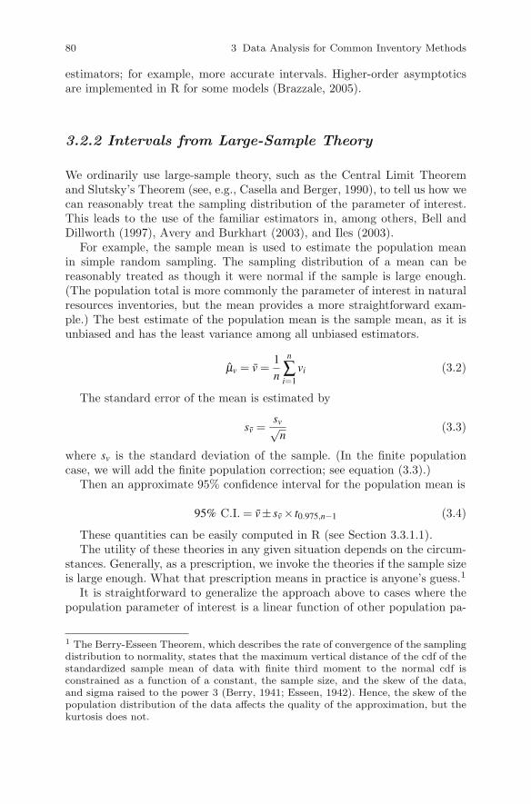
80 3 Data Analysis for Common Inventory Methods
estimators; for example, more accurate intervals. Higher-order asymptoticsare implemented in R for some models (Brazzale, 2005).
3.2.2 Intervals from Large-Sample Theory
We ordinarily use large-sample theory, such as the Central Limit Theoremand Slutsky’s Theorem (see, e.g., Casella and Berger, 1990), to tell us how wecan reasonably treat the sampling distribution of the parameter of interest.This leads to the use of the familiar estimators in, among others, Bell andDillworth (1997), Avery and Burkhart (2003), and Iles (2003).
For example, the sample mean is used to estimate the population meanin simple random sampling. The sampling distribution of a mean can bereasonably treated as though it were normal if the sample is large enough.(The population total is more commonly the parameter of interest in naturalresources inventories, but the mean provides a more straightforward exam-ple.) The best estimate of the population mean is the sample mean, as it isunbiased and has the least variance among all unbiased estimators.
μv = v =1
n
n
∑i=1
vi (3.2)
The standard error of the mean is estimated by
sv =sv√
n(3.3)
where sv is the standard deviation of the sample. (In the finite populationcase, we will add the finite population correction; see equation (3.3).)
Then an approximate 95% confidence interval for the population mean is
95% C.I. = v± sv × t0.975,n−1 (3.4)
These quantities can be easily computed in R (see Section 3.3.1.1).The utility of these theories in any given situation depends on the circum-
stances. Generally, as a prescription, we invoke the theories if the sample sizeis large enough. What that prescription means in practice is anyone’s guess.1
It is straightforward to generalize the approach above to cases where thepopulation parameter of interest is a linear function of other population pa-
1 The Berry-Esseen Theorem, which describes the rate of convergence of the samplingdistribution to normality, states that the maximum vertical distance of the cdf of thestandardized sample mean of data with finite third moment to the normal cdf isconstrained as a function of a constant, the sample size, and the skew of the data,and sigma raised to the power 3 (Berry, 1941; Esseen, 1942). Hence, the skew of thepopulation distribution of the data affects the quality of the approximation, but thekurtosis does not.
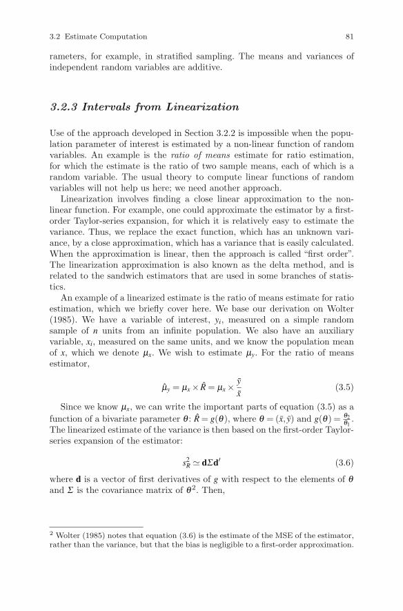
3.2 Estimate Computation 81
rameters, for example, in stratified sampling. The means and variances ofindependent random variables are additive.
3.2.3 Intervals from Linearization
Use of the approach developed in Section 3.2.2 is impossible when the popu-lation parameter of interest is estimated by a non-linear function of randomvariables. An example is the ratio of means estimate for ratio estimation,for which the estimate is the ratio of two sample means, each of which is arandom variable. The usual theory to compute linear functions of randomvariables will not help us here; we need another approach.
Linearization involves finding a close linear approximation to the non-linear function. For example, one could approximate the estimator by a first-order Taylor-series expansion, for which it is relatively easy to estimate thevariance. Thus, we replace the exact function, which has an unknown vari-ance, by a close approximation, which has a variance that is easily calculated.When the approximation is linear, then the approach is called “first order”.The linearization approximation is also known as the delta method, and isrelated to the sandwich estimators that are used in some branches of statis-tics.
An example of a linearized estimate is the ratio of means estimate for ratioestimation, which we briefly cover here. We base our derivation on Wolter(1985). We have a variable of interest, yi, measured on a simple randomsample of n units from an infinite population. We also have an auxiliaryvariable, xi, measured on the same units, and we know the population meanof x, which we denote μx. We wish to estimate μy. For the ratio of meansestimator,
μy = μx × R = μx × y
x(3.5)
Since we know μx, we can write the important parts of equation (3.5) as a
function of a bivariate parameter θ : R = g(θ), where θ = (x, y) and g(θ) = θ2θ1.
The linearized estimate of the variance is then based on the first-order Taylor-series expansion of the estimator:
s2R � dΣd′ (3.6)
where d is a vector of first derivatives of g with respect to the elements of θand Σ is the covariance matrix of θ2. Then,
2 Wolter (1985) notes that equation (3.6) is the estimate of the MSE of the estimator,rather than the variance, but that the bias is negligible to a first-order approximation.
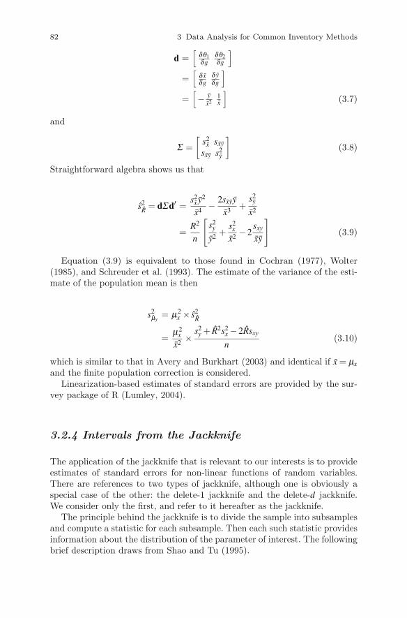
82 3 Data Analysis for Common Inventory Methods
d =[
δθ1δg
δθ2δg
]=[
δ xδg
δ yδg
]=[− y
x21x
](3.7)
and
Σ =
[s2
x sxy
sxy s2y
](3.8)
Straightforward algebra shows us that
s2R= dΣd′ =
s2x y2
x4− 2sxyy
x3+
s2y
x2
=R2
n
[s2
y
y2+
s2x
x2−2
sxy
xy
](3.9)
Equation (3.9) is equivalent to those found in Cochran (1977), Wolter(1985), and Schreuder et al. (1993). The estimate of the variance of the esti-mate of the population mean is then
s2μy
= μ2x × s2
R
=μ2
x
x2× s2
y + R2s2x −2Rsxy
n(3.10)
which is similar to that in Avery and Burkhart (2003) and identical if x = μx
and the finite population correction is considered.Linearization-based estimates of standard errors are provided by the sur-
vey package of R (Lumley, 2004).
3.2.4 Intervals from the Jackknife
The application of the jackknife that is relevant to our interests is to provideestimates of standard errors for non-linear functions of random variables.There are references to two types of jackknife, although one is obviously aspecial case of the other: the delete-1 jackknife and the delete-d jackknife.We consider only the first, and refer to it hereafter as the jackknife.
The principle behind the jackknife is to divide the sample into subsamplesand compute a statistic for each subsample. Then each such statistic providesinformation about the distribution of the parameter of interest. The followingbrief description draws from Shao and Tu (1995).

3.2 Estimate Computation 83
Assume that g is a possibly biased estimator of a parameter of interest θ ,where g is a function of the data from a sample of size n. Let g−i denote thesame function, computed on the same sample, but with the i-th observationremoved and the sample size reduced to n−1. Then g and each of the g−i areall valid, possibly biased, estimators of θ .
Now define each of n pseudovalues as follows. The i-th pseudovalue, gi, is
gi = n×g− (n−1)×g−i (3.11)
Each pseudovalue is now an estimate of θ . Also note that each pseudovalueis, loosely speaking, the difference between the function g applied to tworelated samples. Therefore a portion of the bias in g will be canceled out inthe gi and any estimates that are calculated from them.
Tukey (1958) asserted that these pseudovalues could be treated as thoughthey were independent and identically distributed. Furthermore, each pseu-dovalue has a variance approximately equal to n×σ2
g , where σ2g is the variance
of g. If this is true, then we can estimate θ by the mean of the pseudovalues,and the standard error of the estimate of θ will be the standard error of thatmean. That is,
θ jack =1
n
n
∑i=1
gi (3.12)
s2θ jack
=1
n(n−1)
n
∑i=1
(gi − θ jack
)2(3.13)
This estimator θ jack will have less bias than g, and the estimate of thestandard error can be computed easily for arbitrary functions.
Jackknife-based estimates of standard errors are provided by the surveypackage of R (Lumley, 2004). In cluster and multi-stage designs the jackknifevariance is computed by jackknifing the highest-stage units only.
3.2.4.1 A Brief History of the Jackknife
The origin of the jackknife is curiously unsettled. There seems little doubtthat it was suggested originally by Maurice Quenouille as a tool for bias re-duction. Casella and Berger (1990, p. 341) and Cochran (1977, p. 178) refer toQuenouille (1956), as does Tukey (1958). Efron and Tibshirani (1993, p. 133)say that Quenouille proposed it in the mid-1950s but later cite Quenouille(1949a), as do Davison and Hinkley (1997, p. 59) and Shao and Tu (1995, p.4). Sarndal et al. (1992, p. 437) and Schreuder et al. (1993, p. 102) both citeQuenouille (1949b) and Quenouille (1956). Quenouille (1956, p. 358) doescite Quenouille (1949a) as referring to a special case of the principle. To us,Quenouille (1956) seems to be the clearest starting point.
84 3 Data Analysis for Common Inventory Methods
Most authors then cite Tukey (1958) as providing the original suggestionfor variance estimation, although the citation is only to an abstract of apreliminary report presented at an April 1958 meeting of the Institute ofMathematical Statistics. Tukey cites Quenouille (1956) as suggesting the useof the tool to reduce bias, and Jones (1956) for the idea of using subsamplesof the sample in general.
To round out our historical exegesis, the earliest explicit reference to thename “jackknife” that we can find in a peer-reviewed publication is eitherBrillinger (1964) or Miller (1964). David (1995) cites Miller (1964) as beingthe earliest peer-reviewed reference. We note that both articles were in thelast edition for 1964 of each journal, Miller’s being in December, and thatMiller cites Brillinger, but as being“soon to appear”. Concerning the questionabout lineage above, Brillinger cites Quenouille (1956), Tukey (1958), and a1959 unpublished manuscript by Tukey,3 and Miller cites Quenouille (1949a)and a 1962 unpublished manuscript by Tukey.4 Only the latter seems to beamong the published collection of Tukey’s papers (Jones, 1986).
3.2.5 Intervals from the Bootstrap
The history of the bootstrap is much easier to trace than that for the jack-knife: it was introduced by Efron (1979). We focus here on the non-parametricbootstrap.
The bootstrap can be used to obtain an estimate of the empirical samplingdistribution of many useful statistics and functions of statistics. The estimateof the empirical sampling distribution can be examined directly for quantitiesof interest, such as standard errors, or confidence intervals of parameters ofinterest.
An important caveat is that the bootstrap can ameliorate some of theproblems associated with inference from small samples but will not eliminatethem. The bootstrap relies upon its own large-sample theory, and it has itsown strengths and weaknesses. Published theoretical examinations suggestthat in specific situations the convergence of the bootstrap large-sample the-ory is faster than in the classical large-sample theory (Hall, 1992; Shao andTu, 1995). Consequently, it is important to recognize that clever use of thebootstrap can lead to estimators with significantly better properties thannaive use of the bootstrap.
A good, basic introduction to and description of the bootstrap can be foundin Efron and Tibshirani (1993). For further reading, we suggest Davison andHinkley (1997) and Manly (1997). More advanced expositions can be foundin Hall (1992) and Shao and Tu (1995).
3 Tukey, J. 1959. Approximate confidence limits for most estimates. Unpublishedmanuscript.4 Tukey, J. 1962. Data analysis and behavioral science. Unpublished manuscript.
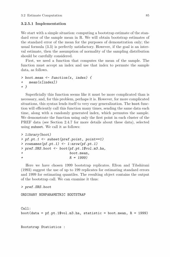
3.2 Estimate Computation 85
3.2.5.1 Implementation
We start with a simple situation: computing a bootstrap estimate of the stan-dard error of the sample mean in R. We will obtain bootstrap estimates ofthe standard error of the mean for the purposes of demonstration only; theusual formula (3.3) is perfectly satisfactory. However, if the goal is an inter-val estimate, then the assumption of normality of the sampling distributionshould be carefully considered.
First, we need a function that computes the mean of the sample. Thefunction must accept an index and use that index to permute the sampledata, as follows.
> boot.mean <- function(x, index) {
+ mean(x[index])
+ }
Superficially this function seems like it must be more complicated than isnecessary, and, for this problem, perhaps it is. However, for more complicatedsituations, this syntax lends itself to very easy generalization. The boot func-tion will efficiently call this function many times, sending the same data eachtime, along with a randomly generated index, which permutes the sample.We demonstrate the function using only the first point in each cluster of thePREF data (see Section 2.4.7 for more details about these data), selectedusing subset. We call it as follows:
> library(boot)
> pf.pt.1 <- subset(pref.point, point==1)
> rownames(pf.pt.1) <- 1:nrow(pf.pt.1)
> pref.SRS.boot <- boot(pf.pt.1$vol.m3.ha,
+ boot.mean,
+ R = 1999)
Here we have chosen 1999 bootstrap replicates. Efron and Tibshirani(1993) suggest the use of up to 199 replicates for estimating standard errorsand 1999 for estimating quantiles. The resulting object contains the outputof the bootstrap call. We can examine it thus:
> pref.SRS.boot
ORDINARY NONPARAMETRIC BOOTSTRAP
Call:
boot(data = pf.pt.1$vol.m3.ha, statistic = boot.mean, R = 1999)
Bootstrap Statistics :
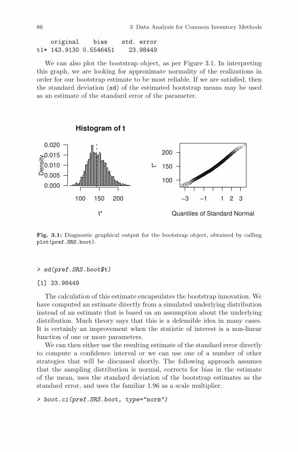
86 3 Data Analysis for Common Inventory Methods
original bias std. error
t1* 143.9130 0.5546451 23.98449
We can also plot the bootstrap object, as per Figure 3.1. In interpretingthis graph, we are looking for approximate normality of the realizations inorder for our bootstrap estimate to be most reliable. If we are satisfied, thenthe standard deviation (sd) of the estimated bootstrap means may be usedas an estimate of the standard error of the parameter.
Histogram of t
t*
Den
sity
100 150 200
0.000
0.005
0.010
0.015
0.020
●●●●●●●●●●●●●●●●
●●●●●●●●●●●●●●●●●●●●●●●●●●●●●●●●●●●●●●●●●●●●●●●●
●●●●●●●●●●●●●●●●●●●●●●●●●●●●●●●●●●●●●●●●●●●●●●●●●●●●●●●●●●●●●●●●●●●●●●●●●●●●●●●●●●●●●●●●●●●●●●●●●●●●●●●●●●●●●●●●●●●●●●●●●●●●●●
●●●●●●●●●●●●●●●●●●●●●●●●●●●●●●●●●●●●●●●●●●●●●●●●●●●●●●●●●●●●●●●●●●●●●●●●●●●●●●●●●●●●●●●●●●●●●●●●●●●●●●●●●●●●●●●●●●●●●●●●●●●●●●●●●●●●●●●●●●●●●●●●●●●●●●●●●●●●●●●●●●●●●●●●●●●●●●●●●●●●●●●●●●●●●●●●●●●●●●●●●●●●●●●●●●●●●●●●●●●●●●●●●●●●●●●●●●●●●●
●●●●●●●●●●●●●●●●●●●●●●●●●●●●●●●●●●●●●●●●●●●●●●●●●●●●●●●●●●●●●●●●●●●●●●●●●●●●●●●●●●●●●●●●●●●●●●●●●●●●●●●●●●●●●●●●●●●●●●●●●●●●●●●●●●●●●●●●●●●●●●●●●●●●●●●●●●●●●●●●●●●●●●●●●●●●●●●●●●●●●●●●●●●●●●●●●●●●●●●●●●●●●●●●●●●●●●●●●●●●●●●●●●●●●●●●●●●●●●●●●●●●●●●●●●●●●●●●●●●●●●●●●●●●●●●●●●●●●●●●●●●●●●●●●●●●●●●●●●●●●●●●●●●●●●●●●●●●●●●●●●●●●●●●●●●●●●●●●●●●●●●●●●●●●●●●●●●●
●●●●●●●●●●●●●●●●●●●●●●●●●●●●●●●●●●●●●●●●●●●●●●●●●●●●●●●●●●●●●●●●●●●●●●●●●●●●●●●●●●●●●●●●●●●●●●●●●●●●●●●●●●●●●●●●●●●●●●●●●●●●●●●●●●●●●●●●●●●●●●●●●●●●●●●●●●●●●●●●●●●●●●●●●●●●●●●●●●●●●●●●●●●●●●●●●●●●●●●●●●●●●●●●●●●●●●●●●●●●●●●●●●●●●●●●●●●●●●●●●●●●●●●●●●●●●●●●●●●●●●●●●●●●●●●●●●●●●●●●●●●●●●●●●●●●●●●●●●●●●●●●●●●●●●●●●●●●●●●●●●●●●●●●●●●●●●●●●●●●●●●●●●●●●●●●●●●●●●●●●●●●●●●●●●●●●●●●●●●●●●●●●●●●●●●●●●●●●●●●●●●●●●●●●●●●●●●●●●●●●●●●●●●●●●●●●●●●●●●●●●●●●●●●●●●●●●●●●●●●●●●●●●●●●●●●●●●●●●●●●●●●●●●●●●●●●●●●●●●●●●●●●●●●●●●●●●●●●●●●●●●●●●●●●●●●●●●●●●●●●●●●●●●●●●●●●●●●●●●●●●●●●●●●●●●●●●●●●●●●●●●●●●●●●●●●●●●●●●●●●●●●●●●●●●●●●●●●●●●●●●●●●●●●●●●●●●●●●●●●●●●●●●●●●●●●●●●●●●●●●●●●●●●●●●●●●●●●●●●●●●●●●●●●●●●●●●●●●●●●●●●●●●●●●●●●●●●●●●●●●●●●●●●●●●●●●●●●●●●●●●●●●●●●●●●●●●●●●●●●●●●●●●●●●●●●●●●●●●●●●●●●●●●●●●●●●●●●●●●●●●●●●●●●●●●●●●●●●●●●●●●●●●●●●●●●●●●●●●●●●●●●●●●●●●●●●●●●●●●●●●●●●●●●●●●●●●●●●●●●●●●●●●●●●●●●●●●●●●●●●●●●●●●●●●●●●●●●●●●●●●●●●●●●●●●●●●●●●●●●●●●●●●●●●●●●●●●●●●●●●●●●●●●●●●●●●●●●●●●●●●●●●●●●●●●●●●●●●●●●●●●●●●●●●●●●●●●●●●●●●●●●●●●●●●●●●●●●●●●●●●●●●●●●●●●●●●●●●●●●●●●●●●●●●●●●●●●●●●●●●●●●●●●●●●●●●●●●●●●●●●●●●●●●●●●●●●●●●●●●●●●●●●●●●●●●●●●●●●●●●●●●●●●●●●●●●●●●●●●●●●●●●●●●●●●●●●●●●●●●●●●●●●●●●●●●●●●●●●●●●●●●●●●
●●●●●●●●
−3 −1 1 2 3
100
150
200
Quantiles of Standard Normal
t*
Fig. 3.1: Diagnostic graphical output for the bootstrap object, obtained by callingplot(pref.SRS.boot).
> sd(pref.SRS.boot$t)
[1] 23.98449
The calculation of this estimate encapsulates the bootstrap innovation. Wehave computed an estimate directly from a simulated underlying distributioninstead of an estimate that is based on an assumption about the underlyingdistribution. Much theory says that this is a defensible idea in many cases.It is certainly an improvement when the statistic of interest is a non-linearfunction of one or more parameters.
We can then either use the resulting estimate of the standard error directlyto compute a confidence interval or we can use one of a number of otherstrategies that will be discussed shortly. The following approach assumesthat the sampling distribution is normal, corrects for bias in the estimateof the mean, uses the standard deviation of the bootstrap estimates as thestandard error, and uses the familiar 1.96 as a scale multiplier.
> boot.ci(pref.SRS.boot, type="norm")
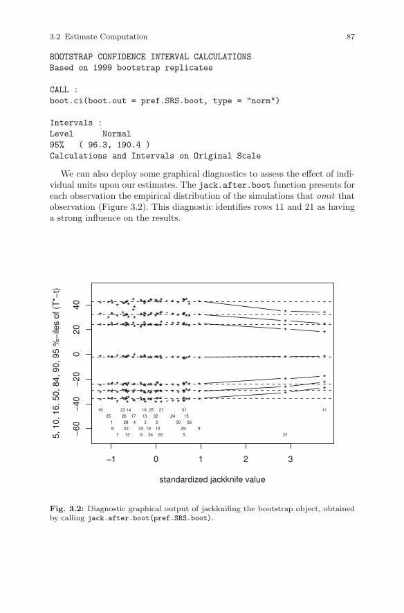
3.2 Estimate Computation 87
BOOTSTRAP CONFIDENCE INTERVAL CALCULATIONS
Based on 1999 bootstrap replicates
CALL :
boot.ci(boot.out = pref.SRS.boot, type = "norm")
Intervals :
Level Normal
95% ( 96.3, 190.4 )
Calculations and Intervals on Original Scale
We can also deploy some graphical diagnostics to assess the effect of indi-vidual units upon our estimates. The jack.after.boot function presents foreach observation the empirical distribution of the simulations that omit thatobservation (Figure 3.2). This diagnostic identifies rows 11 and 21 as havinga strong influence on the results.
−1 0 1 2 3
−60
−40
−20
020
40
standardized jackknife value
5, 1
0, 1
6, 5
0, 8
4, 9
0, 9
5 %
−ile
s of
(T
*−t)
* *** * ****** ** ******** ***** * * ***** ** ** *** * ****** ** ******** ***** * * ***** * * ** *** * ****** ** ******** ***** * * ***** ** *
* *** * ****** ** ******** ***** * * ***** * * *
* *** * ****** ** ******** ***** * * ***** ** *
* *** * ******** ******** ***** * * ***** *
* *
* *** * ****** **
******** ***** * * ***** ** *
19 23 14 16 25 27 31 1135 26 17 13 32 24 15
1 28 4 3 2 30 36
8 22 33 18 10 29 9
7 12 6 34 20 5 21
Fig. 3.2: Diagnostic graphical output of jackknifing the bootstrap object, obtainedby calling jack.after.boot(pref.SRS.boot).
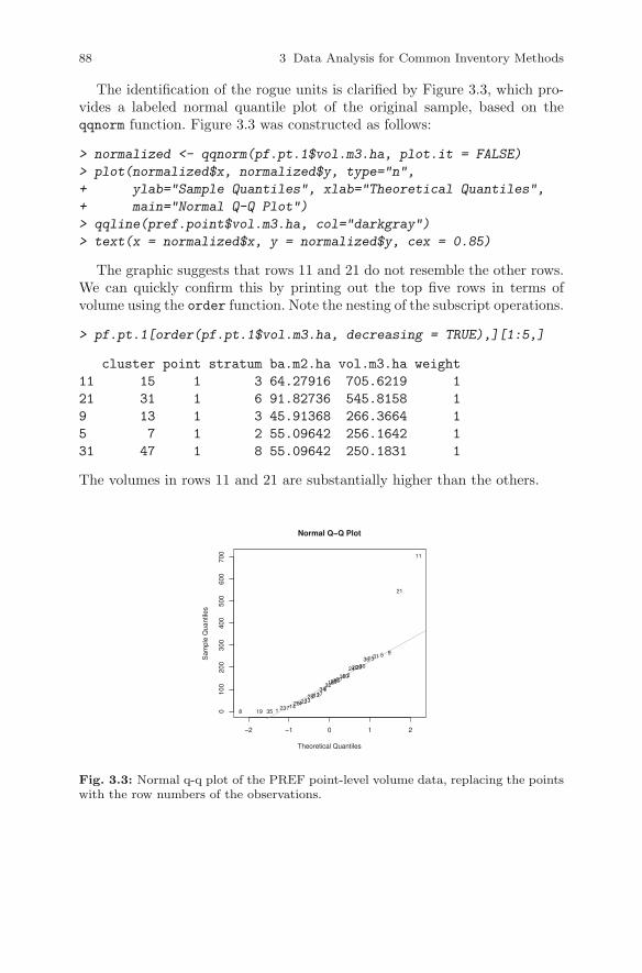
88 3 Data Analysis for Common Inventory Methods
The identification of the rogue units is clarified by Figure 3.3, which pro-vides a labeled normal quantile plot of the original sample, based on theqqnorm function. Figure 3.3 was constructed as follows:
> normalized <- qqnorm(pf.pt.1$vol.m3.ha, plot.it = FALSE)
> plot(normalized$x, normalized$y, type="n",
+ ylab="Sample Quantiles", xlab="Theoretical Quantiles",
+ main="Normal Q-Q Plot")
> qqline(pref.point$vol.m3.ha, col="darkgray")
> text(x = normalized$x, y = normalized$y, cex = 0.85)
The graphic suggests that rows 11 and 21 do not resemble the other rows.We can quickly confirm this by printing out the top five rows in terms ofvolume using the order function. Note the nesting of the subscript operations.
> pf.pt.1[order(pf.pt.1$vol.m3.ha, decreasing = TRUE),][1:5,]
cluster point stratum ba.m2.ha vol.m3.ha weight
11 15 1 3 64.27916 705.6219 1
21 31 1 6 91.82736 545.8158 1
9 13 1 3 45.91368 266.3664 1
5 7 1 2 55.09642 256.1642 1
31 47 1 8 55.09642 250.1831 1
The volumes in rows 11 and 21 are substantially higher than the others.
−2 −1 0 1 2
010
020
030
040
050
060
070
0
Normal Q−Q Plot
Theoretical Quantiles
Sam
ple
Qua
ntile
s
1
2
34
5
6
78
9
10
11
1213
14
15
16
17
18
19
20
21
2223
24
25
26
27
28
2930
31
3233
34
35
36
Fig. 3.3: Normal q-q plot of the PREF point-level volume data, replacing the pointswith the row numbers of the observations.
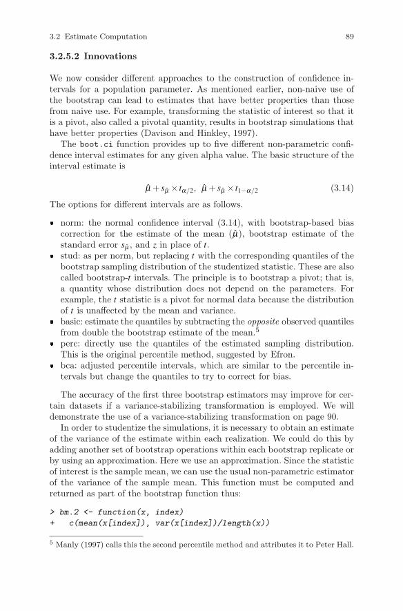
3.2 Estimate Computation 89
3.2.5.2 Innovations
We now consider different approaches to the construction of confidence in-tervals for a population parameter. As mentioned earlier, non-naive use ofthe bootstrap can lead to estimates that have better properties than thosefrom naive use. For example, transforming the statistic of interest so that itis a pivot, also called a pivotal quantity, results in bootstrap simulations thathave better properties (Davison and Hinkley, 1997).
The boot.ci function provides up to five different non-parametric confi-dence interval estimates for any given alpha value. The basic structure of theinterval estimate is
μ + sμ × tα/2, μ + sμ × t1−α/2 (3.14)
The options for different intervals are as follows.
� norm: the normal confidence interval (3.14), with bootstrap-based biascorrection for the estimate of the mean (μ), bootstrap estimate of thestandard error sμ , and z in place of t.
� stud: as per norm, but replacing t with the corresponding quantiles of thebootstrap sampling distribution of the studentized statistic. These are alsocalled bootstrap-t intervals. The principle is to bootstrap a pivot; that is,a quantity whose distribution does not depend on the parameters. Forexample, the t statistic is a pivot for normal data because the distributionof t is unaffected by the mean and variance.
� basic: estimate the quantiles by subtracting the opposite observed quantilesfrom double the bootstrap estimate of the mean.5
� perc: directly use the quantiles of the estimated sampling distribution.This is the original percentile method, suggested by Efron.
� bca: adjusted percentile intervals, which are similar to the percentile in-tervals but change the quantiles to try to correct for bias.
The accuracy of the first three bootstrap estimators may improve for cer-tain datasets if a variance-stabilizing transformation is employed. We willdemonstrate the use of a variance-stabilizing transformation on page 90.
In order to studentize the simulations, it is necessary to obtain an estimateof the variance of the estimate within each realization. We could do this byadding another set of bootstrap operations within each bootstrap replicate orby using an approximation. Here we use an approximation. Since the statisticof interest is the sample mean, we can use the usual non-parametric estimatorof the variance of the sample mean. This function must be computed andreturned as part of the bootstrap function thus:
> bm.2 <- function(x, index)
+ c(mean(x[index]), var(x[index])/length(x))
5 Manly (1997) calls this the second percentile method and attributes it to Peter Hall.
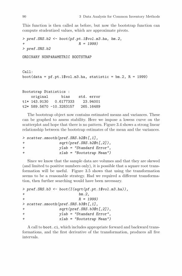
90 3 Data Analysis for Common Inventory Methods
This function is then called as before, but now the bootstrap function cancompute studentized values, which are approximate pivots.
> pref.SRS.b2 <- boot(pf.pt.1$vol.m3.ha, bm.2,
+ R = 1999)
> pref.SRS.b2
ORDINARY NONPARAMETRIC BOOTSTRAP
Call:
boot(data = pf.pt.1$vol.m3.ha, statistic = bm.2, R = 1999)
Bootstrap Statistics :
original bias std. error
t1* 143.9130 0.6177333 23.94001
t2* 589.5670 -10.3283157 265.16489
The bootstrap object now contains estimated means and variances. Thesecan be graphed to assess stability. Here we impose a lowess curve on thescatterplot and hope that there is no pattern. Figure 3.4 shows a strong linearrelationship between the bootstrap estimates of the mean and the variances.
> scatter.smooth(pref.SRS.b2$t[,1],
+ sqrt(pref.SRS.b2$t[,2]),
+ ylab = "Standard Error",
+ xlab = "Bootstrap Mean")
Since we know that the sample data are volumes and that they are skewed(and limited to positive numbers only), it is possible that a square root trans-formation will be useful. Figure 3.5 shows that using the transformationseems to be a reasonable strategy. Had we required a different transforma-tion, then further searching would have been necessary.
> pref.SRS.b3 <- boot(I(sqrt(pf.pt.1$vol.m3.ha)),
+ bm.2,
+ R = 1999)
> scatter.smooth(pref.SRS.b3$t[,1],
+ sqrt(pref.SRS.b3$t[,2]),
+ ylab = "Standard Error",
+ xlab = "Bootstrap Mean")
A call to boot.ci, which includes appropriate forward and backward trans-formations, and the first derivative of the transformation, produces all fiveintervals.
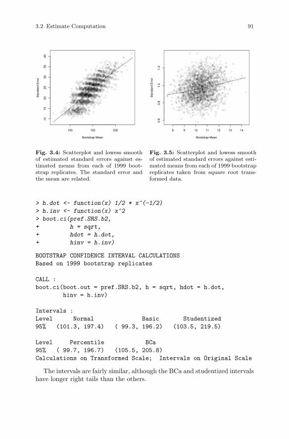
3.2 Estimate Computation 91
●
●
●
●
●
●
●
●
●
●
●
●
●
●
●
●
●
●
●
●
●
●●
●
●
●
●
●
●
●
●
●
●●
●●
●
●
●●●
●
●
●
●
●
●●
●
●
●
●
●
●
●
●
●
●●
●
●
●
●
●
●
●
●
●
●
●
●
●
●
●
●
●● ●
●
●
●●
●
●
●
●
●
●
●
●●
●
●
●●
●
●
●
●
●
●
●
●
●
●
●
●
●
●
●
●
● ●
●
●
●
●
●●
●
●●
●
●
●
●
●
●
●
●
●
●●
●
●
●
●
●
●
●
●
●
●
●
●
●
●
●
●
●
●
●
●
●
●
●
●
●
●
●
●
● ●
●●
●
●
●
●
●
●
●
●
●
●●
●
●
●
● ●
●
●
●
●
●
●
●
●
●
● ●
●
●
●
●
●●
●
●
●
●
●
●
●
●
●
●●
●
●
●
●
●●●
●
●
●
●
●
●
● ●
●
●
● ●
●
●
●
●
●
●
●
●
●
●
●
●
●
●
●
●
●
●
●
●
●
●
●
●
●
●
●
●
●
● ●
●
●
●
●
●
●
●
●
●
●
●
●
●
●
●●
●
●
●
●
●●
●
●
●
●
●
●
●
●
●
●
●
●
●
●
●
●
●●
●●
●
●
●
●
●
●
●●
●
●●
●
●
●●
●
●
●
●●
●
●
●
●
●
●
●●●
●
●
●
●
●
●
●
●●
●
●
●
●
●
●
●
●
●
●
●
●
●
●●
●
● ●●
●
●
●
●
●
●
●
●
●
●
●
●
●
●
●
●
●
●
●
●
●
●
●
●
●
●
●
●
●
●
●
●
●
●
●
●
●
●
●
●
●●
●
●
●
●
●
●
●
●
●
●
●
●
●
●
●
●
●
●
●
●
●
●
●
●
●
●
●
●
●
● ●
●
●
●
●
●
●
●●
●
●
●
●
●
●
●
●
●
●
●
●
●
●●
●
●
●
●
●
●
●
●
●
●
●
●
●
●
●
●
●
●
●
●
●
●
●
●
●
●
●
●●●
●
●
●
●
●
●
●
●
●
●
●
●
●
●
●
●
●
●
●
●
●
●
●
●
●
●
●
●
●
●
●
●
●
●
●
●
●
●
●
●●
●
●
●
●
●
●●
●
●
●
●
●
●
●
●
●
●
●
●
●
●
●
●
● ●
●
●
●
●
●
●
●
●
●
●
●
●
●
●
●
●
●
●
●
●
●
●
●
●
●
●
●
●
●
●
●
●
●
●
●
●
●
●
●
●
●
●
●
●
●
●
●
●
●
●●
●
●
●
●
●
●
●
●
●
●
●
●
●
●
●
●
●
●
●
●
●
●
●
●
●●
●
●
●
●
●
●
●
●
●
●
●
●
●
●
●
●
●
●●
●
●
●
●
●
●●
●
●
●
●
●
●
●
●
●
●
●
●
●
●
●●
●
●
●
●
●
●
●
●
●
●
●
●
●
●
●
●
●
●
●
●
●
●
●
●
●
●
●
●
●
●
●
●
●
●
●
●
●
●
●
●
●
●
●
●
●
●
●
●
●
●
●
●
●
●
●
●
●
●
●
●
●
●
●
●
●
●
●
●
●
●●
●
●
●
●
●●
●
●
●
●
●
●●
●
●
●
●
●
●
●
●
●
●
●
●
●
●
●
●
●
●
●
●
●
●
● ●
●
●
●
●●
●
●
●
●
●
●
●
●
●
●
●
●●
●
●
●
●
●
● ●
●
●
●
●
●
●
●
●
●
●
●
●
●
●
●
●
●
●
●
●
●
●
●
●
●
●
●
●
●
●
●
●
●
●●
●
●
●
●
●
●
●
●
●
●
●
●
●
●
●
●
●
●
●
●
●
●
●
●
●
●
●
●
●
●●
●
●
●
●
●
●
●●
●
●
●
●
●
●
●
●
●
●
●
●
●●
●
●
●
●
●
●
●
●
●
●
●
●
●
●
●
●
●
●
●
●
●
●
●
●
●
●
●
●
●
●
●
●
●
●
●
●
●
●
●
●
●
●
●
●
●
●●
●
●
●
●
●
●
●
●
●
●
●
●
●
●
●
●
●
●
●
●
●
●
●
●
●
●
●
●
●
●
●
●
●
●
●
●
●
●
●
●
●
●
●
●
●
●
●
●
●
●
●
●
●
●
●●
●
●
●
●
●
●
●
●
●
●
●
●
●
●
●
●
●
●●
●●
●
●
●
●
●
●
●
●
●
●
●
●
●●
●
●
●
●
●
●
●●
●
●
●
●
●
●
●
●
●
●
●
●
●
●
●
●
●
●
●
●
●
●
●
●●●
●
●
●●
●
●
●
●●
●●
●
●
●
●
●
●
●
●
●
●
●
●
●
●
●
●
●
●
●
●
● ●
●
●
●
●
●
●
●
●
●
●
●
●
●
●
●
●
●
●
●
●
●
●
●
●
●
●
●
●●
●
●
●
●
●
●
●
●
●
●
●
●
●
●
●
●●
●
●
●
●
● ●
●
●
●
●
●
●
●
●
●
●
●
●
●
●
●
● ●
●
●
●
●
●
●●
●
●
●
●
●
●
●
●
●
●
●
●
●
●
●
●
●
●
●
●
●
●
●
●
●
●
●
●
●
●
●
● ●
●
●
●
●●
●
●
● ●
●
●
●
●
●
●
●●
●
●
●
●
●
●
●
●
●
●
●
●
●
●
●
●
●
●
●
●
●
●
●
●
● ●
●
●
●
●
●
●
●
●
●
●
●
●
●
●
●
●
●
●
●
●
●
●
●
●
●
●
●
●
●
●
●
●
●
●
●
●
●
●
●
●
●
●
●
●
●●
●
●
●
●
●●
●
●
●
●
●
●
●
●
●
●
●
●
●
● ●
●
●
●
●
●
●
●
●
●
●
●
●
●
●●
●
●
●
●
●
●
●
●
●
●
●
●
●
●
●
●
●
●
●
●
●
●●
●
●
●
●
●
●
●
●
●
●●
●
●
●
●
●
●
●
●●
●
●
● ●
●
●
●
●
●
●
●
●
●
●
●
●●
●
●
●
●
●
●
●
●
●
●
●
●
●
●
●
●
●●
●
●
●
●
●
●
●
● ●
●
●
●
●
●●
●
●●
●
●
●
●
●
●
● ●
●
●
●
●●
●
●
●
●
●
●
●
●
●
●
●
●
●
●
●●
●
●
●
●
●
●
●
●
●
●
●
●
●
●
●
●
●
●
●
●●
●
●
●
●
●
●
●
●
●
●
●
●
●
●
●
●
●●
●
●
●
●
●
●
●●
●
●●
●
●
●
●
●
●
●
●
●●
●
●
●
●
●
●
●
●●
●
●
●
●
●
●
●
●
●
●
●
●
●
●
●
●
●
●
●
●
●
●
●
●
●
●
●
●
●
●
●
●
●
●
●
●●
●● ●
●
●
●
●
●
●
●
●●
●
●
●
●
●
●
●
●
●
●
●
●
●
●
●
●
●
●
●
●
●
●
●
●
●
●
●
●
●
●
●
●
●
●●
●
●●
●
●
●
●
●
●
●
●
●
●
●
●
●
●
●
●
●
●
●
●
●
●
●
●
●
●
●
●
●
●
●
●
●
●
●
●
●
●
●
●
●
●
●
●
●
●
●
●
●
●
●
●
●
●
●
●
●
●
●
●
●
●
●
●
●
●
●
●
●
●
●●
●
●
●●
●
●●
●
●
●
●
●
●
●
●
●●
●
●
●
●
●
●
●
●
●
●
●
●
●
●
●●
●
●
●
●
●
●
●
●
●
●
●
●
●
●
●
●
●
●
●
●
●
●
●
● ●
●
●
●
●
●●
●
●
●
●
●
●●
●
●
●
●
●●
●
●
●
●
●
●
●
●
●
●
●
●
●
●
●
●
● ●
●
●
●
●
●
●
●
●
●
●
●
●
●
●
●●
●●
●
●
●
●
●
●
●
●
●●
●
●
●
●
●
●
● ●
●
●
●
●
●
●
●●
●
●
●
●
●
●
●
●
●
●
●
●
●
●
●
●
●
●
●
●
●
●
●
●
●
●
●
●
●
●
●
●
●
●
●
●
●
●
●
●
●
●
● ●
●
●
●
●
●
●
●
●
●
● ●
●
●
●
●
●
●●
●
●
●●
●
●
●
●
●
●
●
●
●
●
●
●
●
●
●
●
●
●
●
●
●
●
●
●
●
●
●
●
●
●
●●
●
●
●●
●
●
●
●
●
●
●
●
●
●
●
●
●
●
●
●
●
●
●
●
●
●
●
●
●
●
●
●
●
●
●
●
●
●
●
●
●●
●
●
●
●
●●
●
●
●
●
●
●
●
●
●
●
●
●
●
●●
●
●
●
●
●
●
●
●
●●
●
●
●
●
●●
●
100 150 200
1015
2025
3035
40
Bootstrap Mean
Sta
ndar
d E
rror
Fig. 3.4: Scatterplot and lowess smoothof estimated standard errors against es-timated means from each of 1999 boot-strap replicates. The standard error andthe mean are related.
●
●
●
●
●
●
●
●● ●
●
●
●●
●
●
●
●
●
●
●
●
●
●
●
●
●
●●
●
●
●
●
●
●
●
●
●
●
●
●
●
●
●
●
●
●
●
●
●
●
●
●
●
●
●
●
●
●
●
●
●
●
●
●
●
●
●
●
●
●
●●
●
●●
●
●
●
●
●
●
●
●●
●
●
●
●
●
●
●
●
● ●
●
●
●
●
●
●
●
●
●
●
●
●
●
●
●
●
●
●
●
●
●
●
●
●●
●
●
●
●
● ●
●
●
●
●
●
●
●
●●
●
●
●
●
●
●
●
●
●
●
●
●
●
●
● ●
●
●
●
●
●
●
●●
●
●
●
●
●
●
●
●
●
●
●
●
●
●
●●
●
●
●
●
●●
●
●●
●
●●
●
●
●
●
●
●
●
●
●
●●
●
●
●●
●
●
●
●●
●
●
●
●
●●
● ●
●
●
●
●
●
●
●
●
●
●
●
●
●
●
●
●
●●
●
●
●
●
●●
●
●●
●
●
●
●
●
●
●
●
●
●
●
●
●
●
●
●
●
●
●
●
●
●
●
●●
●
●●
●●
●
●
●
●
●
●
●
●
●
●
●
●
●
●●
●
●
●
●
●●
●
●
●
●
●
●
●
●
●
●
●
●
●
●
●
●●
● ●
●
●
●
●
●
●
●
●
●
●●
●
●●
●●
●
●
●
● ●
●
●
●
●
●
●
●
●
●●
●
●
●
●
●
●
●
●
●
●
●
●
●●
●●
●
●
●
●
● ●
●
●
●
●
●
●
●
●
●
●
●
●
●
●
●
● ●
●
●
●
●
●
●
●
●
●
●
●
●
●
●
●
●
●
●
●
●
●
●
●
●
●
●
●
●
●
●
●
●
●
●
●
●
●
●
●
●
●
●
●
●●
●
●
●
●●
●●
●
●
●
●
●
●
●
●
●
●
●
●
●
●
●
●
●
● ●●
●
●
●
●●
●
●
●
●
●
●
●
●
●
●
●
●●
●
●
●
●
●
●
●●
●
●
●
●
●
●
● ●
●●
●
●
●
●
●
●
●
●
●
●
●
●
●
●
●
●
●
●●
●
●
●
●
●
●●
●
●
●
●
●
●
●
●
●
●
●
●
●
●
●
●
●
●●
●●
●●
●●
●
●
●
●
●
●
●
●
●
● ●
●
●
●
●
●
●
●
●
● ●
●
●
●
●
●
●
●
●
●
●
●
●
●
●
●
●
●
●
●
●
●
●
●
●
●
●
●
●
●
●
●
●
●
●
●●
●
●
●
●
●
●
●
●
●
●
● ●
●
●
●
●
●
●
●
●
●
●
●
●
●
●
●
●
●
●
●
●
●
●
●
●
●
●
●●
●
●
●
●
●
●
●
●
●
●
●
●
●
●
●
●
●
●
● ●●
●
●
●
●
●
●
●●
●
●
●
●
●
● ●
●
●
●
●
●
●●
●
●
●
●
●
●
●●
●
●
●
●
●
●
●
●●
●
●
●
●
●
●
●
●
●
●
●
●
●
●
●
●
●●
●
●
●
●
●
●
●
●
●
●
●
●
●
●
●
●
●
●
●
●
●●
●
●
●
●
●
●●
●
●
●
●
●
●
●
●
●
●
●
●
●
●
●
●
●
●
●
●
●
●
●
● ●
●●
●
●
●
●
●
●
●
●
●
●
●●
●
●
●
●
●
●
●
●
●
●
●●
●
●
●
●
●
●
●
●
●
●
●
●
●
●
●
●
●
●
●
●
●
●●
●
●
●
●
●
●
●
●
●
●
●
●
●
●
●●
●
●
●
●
●
●
●
●
●
●
●
●
●
●
●
●
●
●
●
●
●
●
●
●
●●
● ●
●
●
●
●
●
●
●
●
●
●
●
●
●
●
●
●
●
●
●
●
●
●
●
●
●●
●
●
●
●
●
●
●
●
●
●
●
●●
●
●
●
●
●●
● ●
●
●
●
●
●
●
●
●
●
●
●
●
●
●
●
●
●
●
●
●
●
●
●
●
●
●
●
●
●
●
●
●
●
●
●
●
●
●
●
●
●
●
●
●●
●
●
●
●
●
●●
●
●
●
●
●
●
●
●
●
●
●
●
●
●
●
●
●
●
●
●
●
●
●
●
●●
●
●●
●
●
●
●
●
●
●
●
●
●
●
●
●
●
●
●
●
●
●
●
●
●
●
●
●
●
●
●
●
●
●
●
●
●
●
●
●
●
●
●●
●
●
●
●
●
●
●
●
●
●
●
●
●
●
●
●
●
●
● ●
●
●
●
●
●
●
●
●●
●
●
●
●
●
●
●
●
●
●
●
●
●
●●
●
●
●
●
●
●
●
●
●
●
●
●
●
●●
●
●
●
●
●
●
●
●
●
●
●
●
●
●
●
●
●
●
●
●
●●
●
●
●
●
●
●
●
●
●
●
●
●
●
●
●
●
●
●
●
●
●
●
●
●●
●
●
●
●
●
●
●
●
●
●
●
●
●
●
●
●
●
●
●
●
●
●
●●
●
●
●
●
●
●
●
●
●
●
●
●
●
●
●
●
●
●
●
●
●
●
●
●
●
●
●
●
●
●
●
●
●
●
●
●
●
●
●
●
●
●
●
●
●
●
●
●
●
●
●
●
●
●
●
●
●
●●
●
●
●
●
●
●
●●
●
●
●
●
●
●
●
●
●
●
●
●
●
●
●
●
●
●
●
●
●
●
●
●
●
●
●
●
●
●
●
●
●
●
●
●
●
●
●
●●
●
●
●
●
●
●
●
● ●
●
●
●
●
●
●
●
●
●
●
●
●
●
●
●
●
●
●
●
●
●
●
●
●
●
●
●
●
●
●
●
●
●
●
●
●
●
●
● ●
●
●
●
●
●
●
●
●
●
●
●
●
●
●
●
●
●
●
●
●
●
●
●
●
●
●
●
●
●
●
●
●
●
●
●
●
●●
●
●● ●
●
●
●
●●
●●
●●
●
●
●
●
●
●
●
●
●
●
●
●
●
●
●
●
●
●
●
●
●
●
●
●
●
●
●
●●
●
●
●
●
●
●
●
●●
●
●
●
●
●●
●
●
●
●
●●●
●
●●
●
●
●
●
●
●
●
●
●
●
●
●
●
●
●
●
●
●●
●
●●
●
●
●
●
●
●
●
●
●
●
●
●
●
●
●
●
●
●
●
●
●
●
●
●
●
●
●
●
●
●
●
●
●
●
●●
●
●●
●
●
●
●
●
● ●●
●
●
●
●
●●
●
●
●
●
●
●
●●
●
●
●
●
●
●
●
●
●
●
●
●
●
●
●
●
●
●
●
●
●●
●
●
●
●
●
●
●
●
●
●
●
●
●
●
●
●
●
●
●
●
●
●
●
●
●
●●
●●
●
●
●
●
●
●
●
●
●
●
●●
●
●
●
● ●
●
●
●
●●
●
●
●
●
●
●
●
●
●
●
●
●●
●
●
●
●
●
●
●
●
●●
●
●
●
●
●
●
●
●
●
●
●
●
●
●
●
● ●
●
●●
●
●
●●
●
●
●
●
●
●
●
●
●
●
●
●
●
●
●
●
●
●
●
●
●
●
●
●
●
●
●●
●
●
●
●
●●
●
●
● ●
●
●
●
●●
●
●
●
●
●
●
●
●
●
●
●
●
●
●
●
●
●
●
●
●
●
●
●
●
●
●
●
●
●
●
●
●
●
●
●●
●
●
●
●
●
●
●
●
●
●
●
●
●
●
●
●
●
●
●
●
●
●
●
●
●
●
●
●
●
●
●
●
●
●
●
●
●
●●
●
●
●●
●
●●
●
●
●
●
●
●
●
●
●●
●
●
●●
●
●
●
●
●
●
●
●
●
●
●
●
●
●
●
●
●
●
●
●
●
●
●
●
●
●
●
●
●
●
●
●
●
●
●
●
●
●
●
●
●
●
●
●
●
●
●
●
●
●
●
●
●
●
●
●
●
●
●
●
●
●
●
●
●
●
●
●
●
●
●
●
●
●
●
●
●
●
●
●
●●
●
●●
●
●
●●
●
●
●
●
● ●
●
●
●
●
●
●●
●
●
●
●
●
●
●
●
●
●
●
●
●
●
●
●
●●
●
●
●
●
●
●●
●
●
●
●
●
●
●●
●●
●
●
●
●
●
●
●
●
●
●
●
●
● ●
●
●
●
●
●
●
●
●
●●
●
●
●
●
●
●
●
●
●
●
●
●
●
●
●
●
●
●●
●
●
●
●
●
●
●
●
●
●
●
●
●
●
●
●
●
●
●
●
●
●
●
●
●
●
●
●
●
●
●●
●
●
●
●
● ●
●
●
●
●
●
●
●
●
●
●
●
●
●
●
●
8 9 10 11 12 13 14
0.6
0.8
1.0
1.2
Bootstrap Mean
Sta
ndar
d E
rror
Fig. 3.5: Scatterplot and lowess smoothof estimated standard errors against esti-mated means from each of 1999 bootstrapreplicates taken from square root trans-formed data.
> h.dot <- function(x) 1/2 * x^(-1/2)
> h.inv <- function(x) x^2
> boot.ci(pref.SRS.b2,
+ h = sqrt,
+ hdot = h.dot,
+ hinv = h.inv)
BOOTSTRAP CONFIDENCE INTERVAL CALCULATIONS
Based on 1999 bootstrap replicates
CALL :
boot.ci(boot.out = pref.SRS.b2, h = sqrt, hdot = h.dot,
hinv = h.inv)
Intervals :
Level Normal Basic Studentized
95% (101.3, 197.4) ( 99.3, 196.2) (103.5, 219.5)
Level Percentile BCa
95% ( 99.7, 196.7) (105.5, 205.8)
Calculations on Transformed Scale; Intervals on Original Scale
The intervals are fairly similar, although the BCa and studentized intervalshave longer right tails than the others.
92 3 Data Analysis for Common Inventory Methods
It is presently unclear which of these intervals is the best to use. Davisonand Hinkley (1997) recommend studentized intervals applied to data thathave been transformed to stabilize variance.
We next report the results of a simulation study using a large-scale sampleof forest inventory data as a population.
3.2.6 A Simulation Study
The best way to assess the different interval-generating strategies is to com-pare them in known situations on the basis of their realized coverage ratesand relative lengths. Such a comparison requires complete knowledge of thetarget population and is rarely possible in a practical setting.
An alternative is to use ideal target populations; for example, the normal,the exponential, etc. The challenge is to find the subtle balance betweenreliably generating the natural patterns that provide realism and includingsufficient randomness to provide a challenging test for the tool in question.
A slightly messier alternative is to obtain large databases that are withinthe scope of interest, treat the databases as the population of interest, andsimulate the process of sampling. We report such an exercise in this sectionusing the FIA data presented in Section 2.4.3.
Here we apply the ratio of means estimator, with the unweighted treeheight as the auxiliary variable. This scenario is reasonable because treeheights have been successfully measured from aerial photographs and willbecome increasingly attractive as a source of auxiliary information with theintroduction of remote measurement tools such as LIDAR. The relationshipbetween height and basal area in our data is well suited to the use of theratio of means estimator, being approximately linear, increasing in variancewith height, and plausibly intersecting the origin (not shown here).
Each subpopulation was sampled randomly with replacement 2000 times,and the resultant sample data were used to estimate the mean stand basalarea and a 95% confidence interval. We then counted whether the true valuefor the subpopulation was above, below, or within the confidence interval.The sample sizes used were 16, 32, 64, 96, and 128.
The average coverage rate is summarized by estimator and sample size inFigure 3.6.
> xyplot(contained ~ n | interval,
+ xlab = "Sample size (n)",
+ ylab = "Realized Coverage Rate",
+ panel = function(x, y) {
+ panel.xyplot(x, y, type="l")
+ panel.abline(h = 0.95, col = "darkgrey")
+ },
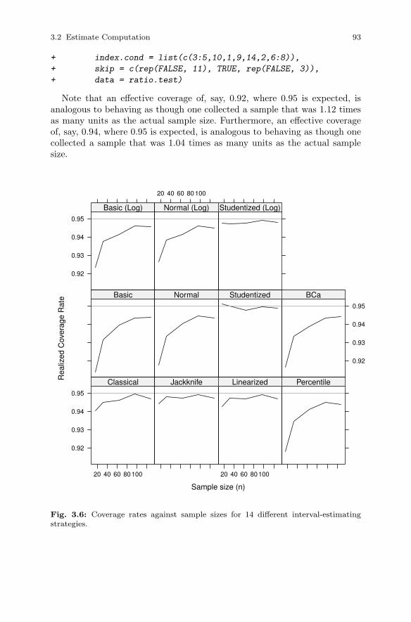
3.2 Estimate Computation 93
+ index.cond = list(c(3:5,10,1,9,14,2,6:8)),
+ skip = c(rep(FALSE, 11), TRUE, rep(FALSE, 3)),
+ data = ratio.test)
Note that an effective coverage of, say, 0.92, where 0.95 is expected, isanalogous to behaving as though one collected a sample that was 1.12 timesas many units as the actual sample size. Furthermore, an effective coverageof, say, 0.94, where 0.95 is expected, is analogous to behaving as though onecollected a sample that was 1.04 times as many units as the actual samplesize.
Sample size (n)
Rea
lized
Cov
erag
e R
ate
0.92
0.93
0.94
0.95
20 40 60 80 100
Classical Jackknife
20 40 60 80 100
Linearized Percentile
Basic Normal Studentized
0.92
0.93
0.94
0.95
BCa
0.92
0.93
0.94
0.95
Basic (Log)
20 40 60 80 100
Normal (Log) Studentized (Log)
Fig. 3.6: Coverage rates against sample sizes for 14 different interval-estimatingstrategies.
94 3 Data Analysis for Common Inventory Methods
Our results suggest that the coverage rate is reasonable for the classi-cal, jackknife, and linearized estimators. The eight different bootstrap in-tervals performed poorly unless the sample was studentized or the samplesize was sufficiently large, in which case it performed well. It is noteworthythat although bootstrapping the transformed data worked better than theuntransformed data, studentizing was much more successful. Given that thelinearization and jackknife tools are already available in R via the surveypackage, they seem suitable for our purposes.
Further examination of the results when categorized by nearest nationalforest did not reveal any important variation from these conclusions.
3.3 Single-Level Sampling
3.3.1 Simple Random Sampling
Simple random sampling involves the selection of a sample of known size n
in such a way that every possible permutation of n sampling units has anequal and known probability of being selected. This approach is uncommonin natural resources inventories. It does, however, present a straightforwardstarting point for analysis.
3.3.1.1 Analysis for Simple Random Sampling
Assume that we have selected a simple random sample of n plots from aframe of N plot labels that completely represent a small forest stand. Wemeasured the above-ground volume of the trees of each plot i, vi m
2ha−1. Wewish to estimate the population total and a 95% confidence interval of thevolume of the stand. For example, we have 180 observations of point-levelabove-ground volume in units of m3ha−1 from the PREF dataset. We shallassume that these points represent a simple random sample.
We will obtain our estimate of the total by multiplying an estimate of themean volume per hectare with the known size of the stand, in hectares. Thesample mean of a simple random sample is a design-unbiased estimate of thepopulation mean,
v =1
n
n
∑i=1
vi (3.15)
The standard error is estimated using equation (3.3)
sv =sv√
n×√
1− n
N(3.16)
3.3 Single-Level Sampling 95
where sv is the standard deviation of the sample and the quantity√
1− nN
is referred to as the finite population correction (FPC). The 95% confidenceinterval is then
95% C.I. = g± sg × t0.975,n−1 (3.17)
These computations can be done most efficiently in R via the survey package.The data are in a data frame called pref.point, and the variable of inter-
est is volume, reported in cubic meters per hectare, vol.m3.ha. We begin bydeclaring a survey object, which contains design information as well as thesurvey data. The required id argument identifies any hierarchical clustering,and the required id argument identifies the relative probability of selectionof the sample units.
> library(survey)
> pref.SRS <- svydesign(id = ~1,
+ data = pref.point,
+ weight = pref.point$weight)
We note that the svydesign function requires a weight argument, whichreports the sampling probability or the sampling weight of the observations.If a weight is not provided, then svydesign will issue a warning and assumeequal weights. We now compute the estimate of the mean and its standarderror as follows.
> svymean(~vol.m3.ha, pref.SRS)
mean SE
vol.m3.ha 141.62 8.8959
However, for simple random sampling, it is almost as easy to code theanalysis manually.
> (SRS.v.hat <- mean(pref.point$vol.m3.ha))
[1] 141.6188
> SRS.n <- length(pref.point$vol.m3.ha)
> (SRS.v.se <- sd(pref.point$vol.m3.ha) / sqrt(SRS.n))
[1] 8.895931
> SRS.v.hat + SRS.v.se * qt(0.975, df = SRS.n - 1) * c(-1, 1)
[1] 124.0644 159.1732
The estimate of the total, and an appropriate confidence interval, can thenbe found by multiplying the estimate and confidence interval of the mean bythe known forest area (2530 ha for PREF).
96 3 Data Analysis for Common Inventory Methods
3.3.2 Systematic Sampling
Systematic sampling involves imposing a grid of sampling points with a oneor more dimensions upon the population, preferably with random start andorientation. Generally speaking, systematic sampling provides good coverageof the population. An important exception is if one suspects that there iscyclic behavior in the population, in which case a systematic sample shouldnot be used. An extreme example of such a spatial pattern is a plantationthat has had different site preparations for different rows; for example, asmight arise after slash mounding.
3.3.2.1 Analysis for Systematic Sampling
The Upper Flat Creek data are a systematic sample of 144 variable-radiusplots. See Section 2.4.1 for a more detailed description of the sample designand the data collection methodology.
Estimating the population mean or total follows the same approach forsystematic sampling as used for simple random sampling. We include thecode here merely to set the scene for estimation of the standard error of theestimate.
> (SyRS.v.hat <- mean(ufc.SyRS.data$vol.m3.ha))
[1] 148.1544
Estimating the standard error is a little more complex for systematic ran-dom sampling because, in a design-based setting, the standard error is usuallycomputed using the randomization distribution, and there is only one inde-pendent sample from that distribution. It is common that, for the purposesof variance estimation, samples from systematic random sampling are treatedas though they were simple random samples. If the plot locations are known,or at least the order of the plot measurement is known, then better estimatesof the variance are available.
Wolter (1985) provides an extensive discussion of eight distinct candidates,of which we select one that was also recommended by Schreuder et al. (1993)for use when nothing is known about the spatial structure of the population.The survey package does not currently support the use of spatial informationfor variance estimation in this way.
σy =
√(1− n
N
) 1
2n(n−1)
n
∑i=2
(yi − yi−1)2 (3.18)
We omit the finite population correction because the sample units werepoints, not plots.
3.4 Hierarchical Sampling 97
> SyRS.v.n <- length(ufc.SyRS.data$vol.m3.ha)
> vol.first.diffs <- ufc.SyRS.data$vol.m3.ha[1:(SyRS.v.n-1)] -
+ ufc.SyRS.data$vol.m3.ha[2:SyRS.v.n]
> SyRS.v.se <- sqrt(1 / (2 * SyRS.v.n * (SyRS.v.n - 1)) *
+ sum(vol.first.diffs^2))
> SyRS.v.se
[1] 6.581681
The 95% confidence interval follows from the simple random sampling case.Had this sample been treated as a simple random sample, then the standarderror would have been estimated as
> sd(ufc.SyRS.data$vol.m3.ha) / sqrt(SyRS.v.n)
[1] 8.106629
3.4 Hierarchical Sampling
Hierarchical sampling involves the selection of sets of sampling units, andpossibly subsampling within those sets. Hierarchical sampling is less efficientthan simple random sampling with the same number of sampling units. How-ever, the inclusion in the budget of other elements of inventory, such as traveltime, can make single-level sampling more expensive per unit of standarderror. Furthermore, there are circumstances when it is impossible or pro-hibitively expensive to obtain a list of the sampling units in the populationbut easier or cheaper to obtain a list of clusters.
3.4.1 Cluster Sampling
Cluster sampling is a specific kind of hierarchical sampling in which sets ofsampling units are selected and measured. As noted above, cluster samplingcan be used to save on inventory costs, but it may also be used if a list ofclusters is available but a sampling frame for the population is not. Clus-ter sampling can be considered as a special case of two-stage sampling (seeSection 3.4.2), in which all of the secondary sampling units in each selectedprimary sampling unit are measured.
3.4.1.1 Analysis for Cluster Sampling
We have selected a simple random sample of n clusters from a frame of N
clusters of plots, representing our population of interest. Each sampled cluster

98 3 Data Analysis for Common Inventory Methods
contained mi plots, and we measured the volume for each plot, vi. We wish toestimate the population total for the tree volume, τv, and a 95% confidenceinterval.
This is a cluster sample because the variable of interest is a plot-levelcharacteristic, but the selection strategy uses only clusters of plots. Call thetotal of the measures in the i-th cluster ti, so ti is the sum of the plot volumeswithin cluster i. Denote the average number of plots per sampled cluster as m.
For the PREF data, we have 36 clusters of five plots each. The data arecontained in the pref.point object, the selection weight is in the weight
variable, the cluster identifier is in the cluster variable, and the variable ofinterest is vol.m3.ha.
The estimate is
vc =∑
ni=1 ti
∑ni=1 mi
(3.19)
In the survey package of R, the design is expressed by
> pref.CS <- svydesign(id = ~cluster,
+ data = pref.point,
+ weight = pref.point$weight)
and the estimate is
> svymean( ~ vol.m3.ha, pref.CS)
mean SE
vol.m3.ha 141.62 14.636
The variance of the estimator is the variance of the cluster means weightedby the number of units in each cluster,
s2vc=
N −n
N
1
n
1
n−1
n
∑i=1
m2i
m2
(ti
mi
− vc
)2
(3.20)
We can easily compute both these classical estimates manually. The codethat follows is intended to show the process rather than maximize the effi-ciency of the computation.
> v.clust <-
+ aggregate(x = list(vol.m3.ha = pref.point$vol.m3.ha),
+ by = list(cluster = pref.point$cluster),
+ FUN = sum)
> v.clust$count <- table(pref.point$cluster)
> n.clusters <- length(v.clust$count)
> (v.bar.c <- sum(v.clust$vol.m3.ha) / sum(v.clust$count))
[1] 141.6188

3.4 Hierarchical Sampling 99
> (se.v.bar.c <-
+ sqrt(sum(v.clust$count^2 / mean(v.clust$count)^2 *
+ (v.clust$vol.m3.ha / v.clust$count -
+ v.bar.c)^2) / n.clusters / (n.clusters - 1)))
[1] 14.63561
When the clusters each have an identical number of sampling units, m, thevariance estimate simplifies to
s2vc=
N −n
N
1
n
1
n−1
n
∑i=1
( ti
m− vc
)2
(3.21)
For the purposes of setting a confidence interval, we either need to pindown a reference distribution or apply the bootstrap. An exact referencedistribution is difficult to pin down for cluster sampling. In practice, thefollowing simplification is used:
95% C.I. = vc ± svc ×2 (3.22)
If we wish to use the bootstrap for this problem, then we should probablybootstrap the clusters only (Davison and Hinkley, 1997, p. 101). Based onour experience in Section 3.2.6, we will studentize the bootstrap variable. Thecode for the mean and standard deviation can be used as above.
> boot.mean.cluster <- function(v.clust, index) {
+ v.clust <- v.clust[index,]
+ v.bar.c <- sum(v.clust$vol.m3.ha) / sum(v.clust$count)
+ c(v.bar.c,
+ sum(v.clust$count^2 / mean(v.clust$count)^2 *
+ (v.clust$vol.m3.ha / v.clust$count -
+ v.bar.c)^2) / n.clusters / (n.clusters - 1))
+ }
> pref.cluster.boot <- boot(v.clust,
+ boot.mean.cluster,
+ R = 1999)
> pref.cluster.boot
ORDINARY NONPARAMETRIC BOOTSTRAP
Call:
boot(data = v.clust, statistic = boot.mean.cluster, R = 1999)
Bootstrap Statistics :
original bias std. error
100 3 Data Analysis for Common Inventory Methods
t1* 141.6188 -0.1852036 14.45360
t2* 214.2011 -7.5990225 60.49281
> boot.ci(pref.cluster.boot, type = "stud")
BOOTSTRAP CONFIDENCE INTERVAL CALCULATIONS
Based on 1999 bootstrap replicates
CALL :
boot.ci(boot.out = pref.cluster.boot, type = "stud")
Intervals :
Level Studentized
95% (115.4, 177.2)
Calculations and Intervals on Original Scale
These are only slightly different from the classical approach as in equation(3.22):
> v.bar.c + c(-1, 1) * 2 * se.v.bar.c
[1] 112.3476 170.8900
3.4.2 Two-Stage Sampling
Two-stage sampling is similar to cluster sampling in that the units upon whichthe measurements are made are selected in groups, or clusters. However,the clusters are now referred to as primary sampling units (PSUs), and thesampling units within the clusters are called secondary sampling units (SSUs).Instead of measuring every sampling unit within the cluster, we now samplethem. Here we will assume that sampling is with equal probability amongthe PSUs and SSUs and that the PSUs are all the same size.
3.4.2.1 Analysis for Two-Stage Sampling
We have collected a simple random sample of n = 36 primary sampling units(plots) from a frame of N labels of plots, representing our population. Eachpotential plot was a 90 m horizontal square projected onto the landscape, soapproximately 3124 sampling units are possible in the 2530 ha.
There are Mi secondary sampling units, for example points, on each se-lected plot, of which we have measured mi for volume vi j. We wish to estimatethe population mean and a 95% confidence interval. To keep the algebra sim-ple, we will assume that the same number of points is measured in each plot;
3.4 Hierarchical Sampling 101
i.e., that mi = m. Also note that for variable-radius plot sampling, M = ∞, sowe will use a very small second-stage FPC weight.
The estimate is
vts =∑
ni=1 ∑
mj=1 vi j
n×m(3.23)
The analysis of such data in R is straightforward. We now declare twolayers of hierarchy in our sampling units and proceed as before. We also adda variable to the dataset as the FPC for the PSU. The design is expressed asfollows.
> pref.2SS <- svydesign(id = ~cluster + point,
+ fpc = ~rep(36/3124, nrow(pref.point)) +
+ rep(0.000001, nrow(pref.point)),
+ weight = pref.point$weight,
+ data = pref.point)
To obtain the estimates, we use
> svymean(~vol.m3.ha, pref.2SS, na.rm = TRUE)
mean SE
vol.m3.ha 141.62 14.569
This estimate is practically identical to that from cluster sampling.The standard error of the mean is marginally more complex than for cluster
sampling. The development is similar to that of analysis of variance in that theestimate of the standard error is the weighted sum of estimates of variances ofthe different levels of units. Each sampling book we referred to had a slightlydifferent exposition of the variance; we found Cochran (1977) the clearest.Let f1 = n/N and f2 = m/M. Then
s2vts
=1− f1
ns2
1 +f1(1− f2)
mns2
2 (3.24)
where s21 is the variance of the means of the PSUs and s2
2 is the variance ofthe SSUs within the PSUs.
s21 =
1
n−1
n
∑i=1
(vi− =v)2 (3.25)
s22 =
1
n(m−1)
n
∑i=1
mi
∑j=1
(vi j − vi)2 (3.26)
Note that equation (3.25) is just the variance of the PSU means and equa-tion (3.26) is the within-PSU variance. Computation proceeds as follows.
> v.2SS <-
+ aggregate(x = list(vol.m3.ha.bar = pref.point$vol.m3.ha),
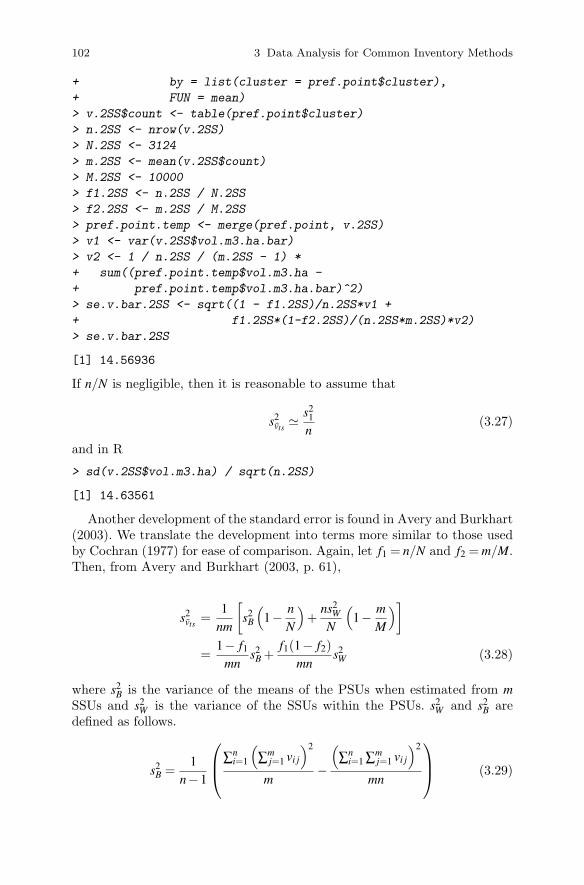
102 3 Data Analysis for Common Inventory Methods
+ by = list(cluster = pref.point$cluster),
+ FUN = mean)
> v.2SS$count <- table(pref.point$cluster)
> n.2SS <- nrow(v.2SS)
> N.2SS <- 3124
> m.2SS <- mean(v.2SS$count)
> M.2SS <- 10000
> f1.2SS <- n.2SS / N.2SS
> f2.2SS <- m.2SS / M.2SS
> pref.point.temp <- merge(pref.point, v.2SS)
> v1 <- var(v.2SS$vol.m3.ha.bar)
> v2 <- 1 / n.2SS / (m.2SS - 1) *
+ sum((pref.point.temp$vol.m3.ha -
+ pref.point.temp$vol.m3.ha.bar)^2)
> se.v.bar.2SS <- sqrt((1 - f1.2SS)/n.2SS*v1 +
+ f1.2SS*(1-f2.2SS)/(n.2SS*m.2SS)*v2)
> se.v.bar.2SS
[1] 14.56936
If n/N is negligible, then it is reasonable to assume that
s2vts
� s21
n(3.27)
and in R
> sd(v.2SS$vol.m3.ha) / sqrt(n.2SS)
[1] 14.63561
Another development of the standard error is found in Avery and Burkhart(2003). We translate the development into terms more similar to those usedby Cochran (1977) for ease of comparison. Again, let f1 = n/N and f2 = m/M.Then, from Avery and Burkhart (2003, p. 61),
s2vts
=1
nm
[s2
B
(1− n
N
)+
ns2W
N
(1− m
M
)]
=1− f1
mns2
B +f1(1− f2)
mns2W (3.28)
where s2B is the variance of the means of the PSUs when estimated from m
SSUs and s2W is the variance of the SSUs within the PSUs. s2
W and s2B are
defined as follows.
s2B =
1
n−1
⎛⎜⎝∑
ni=1
(∑
mj=1 vi j
)2
m−
(∑
ni=1 ∑
mj=1 vi j
)2
mn
⎞⎟⎠ (3.29)
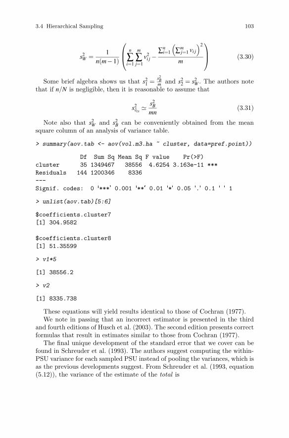
3.4 Hierarchical Sampling 103
s2W =
1
n(m−1)
⎛⎜⎝ n
∑i=1
m
∑j=1
v2i j −
∑ni=1
(∑
mj=1 vi j
)2
m
⎞⎟⎠ (3.30)
Some brief algebra shows us that s21 =
s2B
mand s2
2 = s2W . The authors note
that if n/N is negligible, then it is reasonable to assume that
s2vts
� s2B
mn(3.31)
Note also that s2W and s2
B can be conveniently obtained from the meansquare column of an analysis of variance table.
> summary(aov.tab <- aov(vol.m3.ha ~ cluster, data=pref.point))
Df Sum Sq Mean Sq F value Pr(>F)
cluster 35 1349467 38556 4.6254 3.163e-11 ***
Residuals 144 1200346 8336
---
Signif. codes: 0 �***� 0.001 �**� 0.01 �*� 0.05 �.� 0.1 � � 1
> unlist(aov.tab)[5:6]
$coefficients.cluster7
[1] 304.9582
$coefficients.cluster8
[1] 51.35599
> v1*5
[1] 38556.2
> v2
[1] 8335.738
These equations will yield results identical to those of Cochran (1977).We note in passing that an incorrect estimator is presented in the third
and fourth editions of Husch et al. (2003). The second edition presents correctformulas that result in estimates similar to those from Cochran (1977).
The final unique development of the standard error that we cover can befound in Schreuder et al. (1993). The authors suggest computing the within-PSU variance for each sampled PSU instead of pooling the variances, which isas the previous developments suggest. From Schreuder et al. (1993, equation(5.12)), the variance of the estimate of the total is

104 3 Data Analysis for Common Inventory Methods
s2Vts
= N2M2a(1− f )
s2B
n+
N
n
n
∑i=1
M2i (1− fi)
s2Wi
mi
(3.32)
where f = n/N, fi =mi/Mi, Ma =∑Ni=1 Mi/N, mi is the number of SSUs selected
in PSU i, and s2Wi is the variance within PSU i. Also, the authors’ label for
our equation (3.25) is s2b instead of s2
1.Substituting terms that we have used above, and assuming that the same
number of SSUs is sampled in each PSU, the variance of the estimate of themean is
s2vts
= (1− f1)s2
1
n+
f1(1− f2)
n2
n
∑i=1
s2Wi
m(3.33)
which, if we assume s2Wi = s2
W , is identical to (3.24).
3.5 Using Auxiliary Information
The efficiency of estimation from sampling can be greatly enhanced by theuse of auxiliary information. Auxiliary information is some kind of knowledgeabout the sampling units that is related to the variable of interest and thatis known for all of the units in the population, or at least the populationparameters are known. Auxiliary information can be used for the design of asample (as per stratification, Section 3.5.1) or for the estimation (as per ratioand regression estimation, Sections 3.5.2 and 3.5.3, respectively).
3.5.1 Stratified Sampling
Stratification enables us to control variation. To stratify, we divide the popu-lation into discrete, non-overlapping subpopulations using an auxiliary vari-able. We then sample within each subpopulation without reference to theother subpopulations. That is, the sampling is carried out independently.
Stratification controls variation by allowing us to calculate separate statis-tics for things that we think will differ, a priori. We then compute population-level estimates by taking weighted averages of these stratum-level statistics.In this way, the variation between the subpopulations does not enter theuncertainty of the estimate.
We can stratify using a discrete or a continuous auxiliary variable. Oncewe have stratified, we do not use the auxiliary variable further unless weexplicitly involve it by means of a more advanced estimation technique. Instratification, the auxiliary variable only affects the design. Once we have thedesign, it plays no further role.
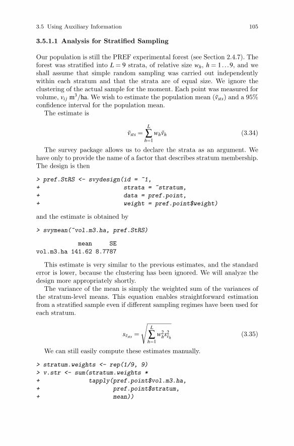
3.5 Using Auxiliary Information 105
3.5.1.1 Analysis for Stratified Sampling
Our population is still the PREF experimental forest (see Section 2.4.7). Theforest was stratified into L = 9 strata, of relative size wh, h = 1 . . .9, and weshall assume that simple random sampling was carried out independentlywithin each stratum and that the strata are of equal size. We ignore theclustering of the actual sample for the moment. Each point was measured forvolume, vi j m3/ha. We wish to estimate the population mean (vsts) and a 95%confidence interval for the population mean.
The estimate is
vsts =L
∑h=1
whvh (3.34)
The survey package allows us to declare the strata as an argument. Wehave only to provide the name of a factor that describes stratum membership.The design is then
> pref.StRS <- svydesign(id = ~1,
+ strata = ~stratum,
+ data = pref.point,
+ weight = pref.point$weight)
and the estimate is obtained by
> svymean(~vol.m3.ha, pref.StRS)
mean SE
vol.m3.ha 141.62 8.7787
This estimate is very similar to the previous estimates, and the standarderror is lower, because the clustering has been ignored. We will analyze thedesign more appropriately shortly.
The variance of the mean is simply the weighted sum of the variances ofthe stratum-level means. This equation enables straightforward estimationfrom a stratified sample even if different sampling regimes have been used foreach stratum.
svsts =
√L
∑h=1
w2hs2
vh(3.35)
We can still easily compute these estimates manually.
> stratum.weights <- rep(1/9, 9)
> v.str <- sum(stratum.weights *
+ tapply(pref.point$vol.m3.ha,
+ pref.point$stratum,
+ mean))
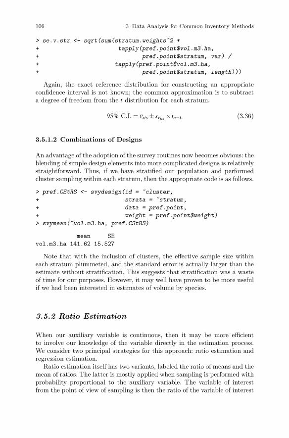
106 3 Data Analysis for Common Inventory Methods
> se.v.str <- sqrt(sum(stratum.weights^2 *
+ tapply(pref.point$vol.m3.ha,
+ pref.point$stratum, var) /
+ tapply(pref.point$vol.m3.ha,
+ pref.point$stratum, length)))
Again, the exact reference distribution for constructing an appropriateconfidence interval is not known; the common approximation is to subtracta degree of freedom from the t distribution for each stratum.
95% C.I. = vsts ± svsts × tn−L (3.36)
3.5.1.2 Combinations of Designs
An advantage of the adoption of the survey routines now becomes obvious: theblending of simple design elements into more complicated designs is relativelystraightforward. Thus, if we have stratified our population and performedcluster sampling within each stratum, then the appropriate code is as follows.
> pref.CStRS <- svydesign(id = ~cluster,
+ strata = ~stratum,
+ data = pref.point,
+ weight = pref.point$weight)
> svymean(~vol.m3.ha, pref.CStRS)
mean SE
vol.m3.ha 141.62 15.527
Note that with the inclusion of clusters, the effective sample size withineach stratum plummeted, and the standard error is actually larger than theestimate without stratification. This suggests that stratification was a wasteof time for our purposes. However, it may well have proven to be more usefulif we had been interested in estimates of volume by species.
3.5.2 Ratio Estimation
When our auxiliary variable is continuous, then it may be more efficientto involve our knowledge of the variable directly in the estimation process.We consider two principal strategies for this approach: ratio estimation andregression estimation.
Ratio estimation itself has two variants, labeled the ratio of means and themean of ratios. The latter is mostly applied when sampling is performed withprobability proportional to the auxiliary variable. The variable of interestfrom the point of view of sampling is then the ratio of the variable of interest

3.5 Using Auxiliary Information 107
and the auxiliary variable, and computation proceeds according to variableprobability sampling.
Here we focus on the ratio of means case. Ratio of means estimation isappropriate if we are reasonably certain that the relationship between thevariable of interest and the auxiliary variable is linear and passes through theorigin and that the variance of the variable of interest is roughly proportionalto the value of the auxiliary variable.
This case provides the simplest interesting challenge to the sampler, as thepopulation parameter of interest is a non-linear function of two statistics. Aswe have discussed earlier in the context of interval estimation, estimating thevariance is complicated.
3.5.2.1 Analysis for Ratio Estimation
Continuing the analysis of the PREF inventory data, we now introduce theremotely sensed auxiliary variable, which is the atmospherically correctedNormalized Difference Vegetation Index (NDVI), adjusted using the mid-infrared band. This variable is available for every 30 m by 30 m pixel ofthe forest and can be expected to be fairly well correlated with the per-unitvolume. As previously, the use of the survey package simplifies the analysisconsiderably.
As noted earlier in the chapter, the following two equations provide theusual estimate of the population mean of the variable of interest and anestimate of its standard error. Initially, we will ignore some of the importantelements of the PREF design: the clustering and the stratification.
μy = μx × y
x(3.37)
s2μy
=μ2
x
x2× s2
y + R2s2x −2Rsxy
n(3.38)
We register the design as follows
> pref.SRSc <- svydesign(id = ~1,
+ data = pref.point.cov,
+ weight = pref.point$weight)
Then the analysis is performed by
> volume.over.acndviC <- svyratio(numerator = ~vol.m3.ha,
+ denominator = ~acndviC,
+ design = pref.SRSc)
> predict(volume.over.acndviC, mean(pref.pixel$ndvic))
$total
acndviC

108 3 Data Analysis for Common Inventory Methods
vol.m3.ha 139.5000
$se
acndviC
vol.m3.ha 8.317442
We can easily reproduce these straightforward results using our own code tocheck our understanding.
> ratio.hat <- sum(pref.point.cov$vol.m3.ha) /
+ sum(pref.point.cov$acndviC)
> RatE.v.hat <- mean(pref.pixel$ndvic) * ratio.hat
> RatE.v.hat
[1] 139.5000
> RatE.v.hat.se <-
+ sqrt((mean(pref.pixel$ndvic))^2 /
+ (mean(pref.point.cov$acndviC))^2 *
+ (var(pref.point.cov$vol.m3.ha) +
+ ratio.hat^2 * var(pref.point.cov$acndviC) -
+ 2 * ratio.hat * cov(pref.point.cov$acndviC,
+ pref.point.cov$vol.m3.ha)) /
+ nrow(pref.point.cov))
> RatE.v.hat.se
[1] 8.317442
The results of the simulation study reported in Section 3.2.6 suggest thatthe use of the jackknife or the linearized estimates of the standard error,along with the t quantile that is appropriate for the desired coverage, mayprovide a reasonable confidence interval.
3.5.2.2 Combinations of Designs
As before, the use of the survey package permits the straightforward exten-sion of these simple design elements into a more complex whole. Here weinclude the design elements of stratification and clustering as well as theratio estimation in our analysis. The design is
> pref.CStRSc <- svydesign(id = ~cluster+point,
+ strata = ~stratum,
+ data = pref.point.cov,
+ weight = pref.point$weight)
and the analysis requires the following code:
3.5 Using Auxiliary Information 109
> v.over.a.CStRSc <- svyratio(numerator = ~vol.m3.ha,
+ denominator = ~acndviC,
+ design=pref.CStRSc)
> predict(v.over.a.CStRSc, mean(pref.pixel$ndvic))
$total
acndviC
vol.m3.ha 139.5000
$se
acndviC
vol.m3.ha 13.77745
This analysis is closest to being the most appropriate analysis for the originaldesign.
3.5.3 Regression Estimation
In the more general case when we are uncertain as to the nature of the re-lationship between the variable of interest and the auxiliary variable, specifi-cally the form of the conditional mean and variance, we can apply regressionestimation.
3.5.3.1 Analysis for Regression Estimation
Continuing the analysis of the PREF inventory data, we again use the re-motely sensed auxiliary variable, which is the atmospherically corrected Nor-malized Difference Vegetation Index, adjusted using the mid-infrared band.This variable is available for every 30 m by 30 m pixel of the forest and canbe expected to be fairly well correlated with the per-unit volume. Again, theuse of the survey package simplifies the analysis considerably.
The following four equations provide the usual estimate of the populationmean of the variable of interest and an estimate of its standard error. Initiallywe again ignore the important elements of the PREF design: the clusteringand the stratification.
The regression-based estimate of the mean of the variable of interest, y, is
ylr = y+ β1 × (X − x) (3.39)
where x is the mean of the auxiliary variable for the sample X is the (known)mean of the auxiliary variable for the population, and
β1 =sxy
s2x
(3.40)

110 3 Data Analysis for Common Inventory Methods
The standard error is estimated as follows:
sy|x =
√n−1
n−2
(s2
y −s2
xy
s2x
)(3.41)
sylr= sy|x ×
√(1
n+
(n−1)(X − x)2
s2x
)×(
1− n
N
)(3.42)
These estimates are computed in R using the following code:
> volume.against.acndviC <- svyglm(vol.m3.ha ~ acndviC,
+ design = pref.SRSc)
We now rely on another package, gmodels (Warnes, 2010), to provide uswith appropriate predictions and standard errors. We will use the estimablefunction for this purpose. This very useful function will compute estimates,standard errors, confidence intervals, and hypothesis tests for arbitrary linearcombinations of parameters from a wide variety of model types, includingmixed-effects models. We load the package using the library function.
> library(gmodels)
We then invoke the estimable function as follows.
> estimable(volume.against.acndviC,
+ conf.int = 0.95,
+ cm = rbind(total=c(1, mean(pref.pixel$ndvic))))
Estimate Std. Error t value DF Pr(>|t|) Lower.CI
total 139.3812 8.34162 16.70913 178 0 122.9200
Upper.CI
total 155.8424
3.5.3.2 Combinations of Designs
Again we can draw upon the survey package to provide us with a general yetstraightforward solution that is appropriate for the full PREF design.
> pref.CStRSc <- svydesign(id = ~cluster+point,
+ strata = ~stratum,
+ weight = pref.point$weight,
+ data = pref.point.cov)
> v.against.a.CStRSc <- svyglm(vol.m3.ha ~ acndviC,
+ design = pref.CStRSc)
> estimable(v.against.a.CStRSc,
+ conf.int = 0.95,
+ cm = rbind(total = c(1, mean(pref.pixel$ndvic))))
3.5 Using Auxiliary Information 111
Estimate Std. Error t value DF Pr(>|t|) Lower.CI
total 139.3812 13.66037 10.20332 26 1.391884e-10 111.3019
Upper.CI
total 167.4605
Note that the acknowledgment of the clustering of sampling units hasinflated the estimate of the standard error considerably.
3.5.4 3P Sampling
3P sampling, also called Poisson sampling (see, e.g., Schreuder et al., 1993),is a system that involves guessing the variable of interest before measuringit, and using the guesses as auxiliary information.
3.5.4.1 Analysis for 3P Sampling
We have a population of N trees, and we wish to estimate the total volume.We have guessed the population size N and generated N random numbers,qi, uniformly distributed from 0 to qmax. qmax corresponds to the estimatedtotal divided by the desired sample size.
We visited each of the trees and guessed the volume in cubic meters, xi.If qi < xi, we measured the tree accurately for volume yi. The guesses sum toXt for the whole population. We wish to estimate the population total and a95% confidence interval.
For the purposes of demonstration, we will use the PREF tree databaseas our population. The variable of interest is now volume in cubic meters,vol.m3. We set up the sample as follows. We believe that the tree count in thepopulation is 1000, and we wish to accurately measure, say, 20 trees. Further,we shall guess that the volume of all the trees in the forest is, say, 1000 m3.Then we generate 1000 random numbers between 0 and 1000/20 = 50.
> q.max <- 1000/20
> PPP.rand <- q.max * runif(1200)
The guesses can be simulated by either adding a random variable to ormultiplying a random variable by the known values. All kinds of scenarioscan be compared. The authors are notoriously poor at guessing tree volumes,so for the purpose of generating realistic data to demonstrate the technique,
> PPP.guesses <- pref.tree$vol.m3 *
+ rnorm(n = nrow(pref.tree), mean = 1.05, sd = 0.15) +
+ rnorm(n = nrow(pref.tree), mean = -0.05, sd = 0.05)
We then choose the sample using one of numerous possible approaches.
112 3 Data Analysis for Common Inventory Methods
> PPP.sample <-
+ PPP.rand[seq(1,length(PPP.guesses))] < PPP.guesses
> PPP.trees <-
+ data.frame(vol.m3 = pref.tree$vol.m3[PPP.sample],
+ guess.m3 = PPP.guesses[PPP.sample])
The estimate is then
Y3P∗ = Xt × 1
n×(
n
∑i=1
ri
)(3.43)
ri =yi
xi
(3.44)
and in R
> (PPP.hat.1 <- sum(PPP.guesses) / sum(PPP.sample) *
+ sum(PPP.trees$vol.m3 / PPP.trees$guess.m3))
[1] 1217.149
An alternative estimator with slightly better properties, in that it correctssomewhat for the randomness of the sample size (Schreuder et al., 1993), is
Y3P =1
n× Xt
qmax
× Y3P∗ (3.45)
In R,
> (PPP.hat.2 <- PPP.hat.1 *
+ sum(PPP.guesses) / q.max / sum(PPP.sample))
[1] 905.2569
The actual value is known to be
> sum(pref.tree$vol.m3)
[1] 1185.261
The standard error of the estimate also has numerous incarnations. Asimple version is
sY3P= Xt × sr (3.46)
> se.PPP.hat <- sd(PPP.trees$vol.m3 / PPP.trees$guess.m3) /
+ sqrt(sum(PPP.sample)) * sum(PPP.guesses)
> se.PPP.hat
[1] 44.86651
3.5 Using Auxiliary Information 113
As with other complicated sampling routines, the reference value for thesampling distribution of the statistic is not known. The usual approximationis used,
95% C.I. = Y3P ±2× sY3P(3.47)
3.5.5 VBAR
VBAR stands for variable-basal area ratio. It is an efficient way to gatherdimensional information on trees in a stand. It is most often applied usingvariable-radius plots, but there is no reason that it could not be applied withfixed-area plots.
The idea behind VBAR is to use many cheap basal area plots to cover thespatial variation and a smaller number of more expensive plots to establish arelationship between the basal area and the variable of interest. The two bestreferences for this technique are Bell and Dillworth (1997) and Iles (2003).
VBAR was originally coined as volume-basal area ratio, but it has since(rightly) been pointed out that the technique can be used for measuring mostanything, as long as it is likely to be related to basal area at the point level, bysome kind of ratio. It is formally known as two-phase sampling in statisticalliterature.
3.5.5.1 Analysis for VBAR
We have installed n1 variable-radius plots. In each one, we only counted thetrees. Among these plots, we took a subsample of measure plots, upon whichwe ended up measuring n2 trees for basal area gi and volume vi. We wish toestimate the population total and a 95% confidence interval.
We can easily alter the PREF database to demonstrate the use of VBAR.We have already computed the basal area and volume from each plot, so wejust need to choose a sample of the plot numbers. We shall take a sample of30 volume plots.
> vbar.sample <- sample(1:dim(pref.point)[1], size=30)
> vbar.points <- pref.point[vbar.sample,]
> vbar.points <- vbar.points[vbar.points$ba.m2.ha > 0,]
> vbar.points$ratio <- vbar.points$vol.m3.ha /
+ vbar.points$ba.m2.ha
Empty plots should be eliminated from the sample for the purposes ofcomputing the ratio and its standard error. Note that this is a rare occasionwhen ignoring measured plots is reasonable. Our rationale is that 0/0 is un-defined. Also note that this strategy effectively makes the sample size for the

114 3 Data Analysis for Common Inventory Methods
ratio a random variable, which, if correctly accounted for, will complicate theanalysis. We ignore that element of the analysis here. Probably the simplestapproach to accommodating this element of the design would require use ofthe bootstrap.
The estimate is
vV BAR = g× v/g (3.48)
> (v.hat.vbar <-
+ mean(pref.point$ba.m2.ha) * mean(vbar.points$ratio))
[1] 138.6455
The units are, as before, m3/ha.The estimation of standard error follows principles laid out in Goodman
(1960),
sv% =√
s2g% + s2
v/g%− s2
g% × s2v/g%
(3.49)
Here sv% is the ratio of the standard error of the volume and the meanvolume, s2
g% is the square of the ratio of the standard error of the basal area
and the mean basal area, and s2v/g%
is the square of the ratio of the standard
error of the ratios and the mean ratio,
svV BAR= vV BAR × sv% (3.50)
> s.bar.g.perc.2 <- (sd(pref.point$ba.m2.ha) /
+ sqrt(length(pref.point$ba.m2.ha)) /
+ mean(pref.point$ba.m2.ha))^2
> s.bar.r.perc.2 <- (sd(vbar.points$ratio) /
+ sqrt(length(vbar.points$ratio)) /
+ mean(vbar.points$ratio))^2
> s.bar.v.perc <- sqrt(s.bar.g.perc.2 + s.bar.r.perc.2 -
+ s.bar.g.perc.2 * s.bar.r.perc.2)
> s.bar.v <- s.bar.v.perc * v.hat.vbar
> s.bar.v
[1] 9.71663
The confidence interval again uses 2 as the approximate quantile of thesampling distribution.
3.6 Summary
This chapter gives a brief presentation of the tools available for sample pro-cessing and confidence interval estimation. We chose to focus on the oper-

3.6 Summary 115
ations required for the various sampling designs normally found in forestinventories, but the reader should be aware that these methods can apply toany situation where these sampling designs are applicable.

Chapter 4
Imputation and Interpolation
4.1 Introduction
In Chapter 3, we presented methods to process samples, estimate param-eters, and construct confidence intervals for design-based inference. In thischapter, we present model-based imputation (to fill in missing values) andinterpolation (for predicting values at unsampled locations) methods to gen-erate complete datasets so that 1) we have no missing values in our analysisdataset or so that 2) we have complete coverage using predicted values atunsampled locations for some variable of interest.
In Section 4.2, we impute missing values for the stands data frame object.We use definitions consistent with those presented by Little and Rubin (2002)and define imputation as any process that replaces missing values (NA) withother predicted or observed values. We first examine the stands data todetermine if any data are missing. Then, we examine missingness patterns todetermine if the missingness has a simple spatial pattern. We then presenta few methods to impute missing values in Section 4.2.2. In Sections 4.2.3and 4.2.4, we impute missing values using the nearest-neighbor (NN) andthe expectation-maximization (EM) algorithms. Finally, in Section 4.2.5, webriefly examine and compare the two results against the original data for asingle site productivity variable, specifically site index (Bruce, 1981).
In Section 4.3, we then interpolate site index using the processed plots andtree data frame objects from Section 2.4.6. In Section 4.3.1, we present a fewinterpolation methods. In Section 4.3.2, we answer a few critical questions,select one interpolation method (specifically, kriging) and briefly present thetheory. In Section 4.3.3, we estimate the variogram used in Section 4.3.4,where we finally predict site index over a finite region.
117A. P. Robinson, J. D. Hamann, Forest Analytics with R, Use R!,DOI 10.1007/978-1-4419-7762-5_4, © Springer Science+Business Media, LLC 2011
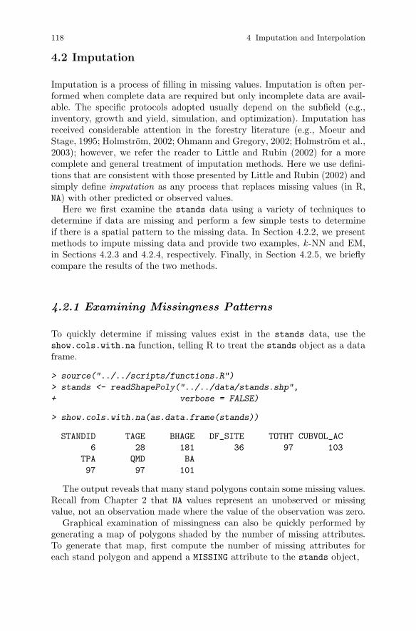
118 4 Imputation and Interpolation
4.2 Imputation
Imputation is a process of filling in missing values. Imputation is often per-formed when complete data are required but only incomplete data are avail-able. The specific protocols adopted usually depend on the subfield (e.g.,inventory, growth and yield, simulation, and optimization). Imputation hasreceived considerable attention in the forestry literature (e.g., Moeur andStage, 1995; Holmstrom, 2002; Ohmann and Gregory, 2002; Holmstrom et al.,2003); however, we refer the reader to Little and Rubin (2002) for a morecomplete and general treatment of imputation methods. Here we use defini-tions that are consistent with those presented by Little and Rubin (2002) andsimply define imputation as any process that replaces missing values (in R,NA) with other predicted or observed values.
Here we first examine the stands data using a variety of techniques todetermine if data are missing and perform a few simple tests to determineif there is a spatial pattern to the missing data. In Section 4.2.2, we presentmethods to impute missing data and provide two examples, k -NN and EM,in Sections 4.2.3 and 4.2.4, respectively. Finally, in Section 4.2.5, we brieflycompare the results of the two methods.
4.2.1 Examining Missingness Patterns
To quickly determine if missing values exist in the stands data, use theshow.cols.with.na function, telling R to treat the stands object as a dataframe.
> source("../../scripts/functions.R")
> stands <- readShapePoly("../../data/stands.shp",
+ verbose = FALSE)
> show.cols.with.na(as.data.frame(stands))
STANDID TAGE BHAGE DF_SITE TOTHT CUBVOL_AC
6 28 181 36 97 103
TPA QMD BA
97 97 101
The output reveals that many stand polygons contain some missing values.Recall from Chapter 2 that NA values represent an unobserved or missingvalue, not an observation made where the value of the observation was zero.
Graphical examination of missingness can also be quickly performed bygenerating a map of polygons shaded by the number of missing attributes.To generate that map, first compute the number of missing attributes foreach stand polygon and append a MISSING attribute to the stands object,
4.2 Imputation 119
> stands.frame <- as.data.frame(stands)
> stands.frame$MISSING <- rowSums(is.na(stands.frame))
The stands object now contains stands$MISSING, which reports the num-ber of missing attributes for each stand polygon. Next, create a color rampfrom the number of unique values of the MISSING attribute:
> brks <- sort(unique(stands.frame$MISSING))
> colors <- gray(length(brks):1 / (length(brks)))
Finally, plot the stands, add a title, and include a legend to produce Fig-ure 4.1.
> plot(stands,
+ col = colors[findInterval(stands.frame$MISSING,
+ brks, all.inside = TRUE)],
+ forcefill = FALSE,
+ axes = TRUE)
> title(main="Attribute Missingness by Polygon")
> legend(1280000, 365000, brks, fill = colors, cex = 0.7,
+ ncol = 3, title = "# of Missing Attributes")
Figure 4.1 reveals a potential pattern in which missingness might be moreprominent in the northern portion of the landscape than in the southern part.If the headquarters is located at or near the southern portion of the forest, forexample, a lengthy drive might explain the pattern where the stands in thenorth portion of the forest might be sampled less frequently or have fewermeasurements taken on fewer variables. Regardless of the mechanism thatcreated the differences in missingness, the summaries presented above andFigure 4.1 show that 1) data are missing in the stands object; 2) some standpolygons have more missing attributes than others; and 3) there may be aspatial pattern; with more missing values in the north than in the south.
While this quick analysis cannot tell us for certain that there is a patternto the missingness, missing data problems can be more formally expressed sothat more sophisticated techniques can be applied to construct a completedataset.
Let Y denote the n×m random matrix that represents the complete datamatrix of n rows (observations) and m columns (variables) and follows amultivariate density function f (y;θ), where y is a particular realization ofthe random variable Y (complete data) and θ is a parameter vector thatdefines the distribution of y. Also, Y can be partitioned into a matrix of thenon-missing observations Y o
i j and missing observations Y mi j .
To describe missingness, let M ∈ (0,1) be a random indicator matrix thatrepresents the missingness of the data for the i-th observation on the j-thvariable. When yi j is missing, Mi j = 1; otherwise, Mi j = 0. The realization ofM, m, shows the pattern of missing values of y, a realization of Y that followsf (y;φ), where f (y;φ) defines the pattern of missing data m. The primary
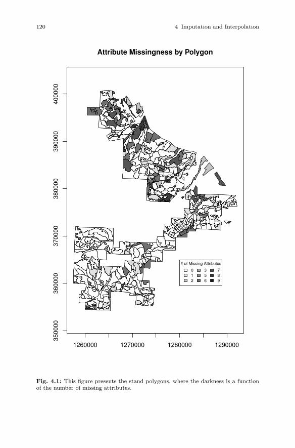
120 4 Imputation and Interpolation
1260000 1270000 1280000 1290000
3500
0036
0000
3700
0038
0000
3900
0040
0000
Attribute Missingness by Polygon
# of Missing Attributes
012
356
789
Fig. 4.1: This figure presents the stand polygons, where the darkness is a functionof the number of missing attributes.
4.2 Imputation 121
objective in most imputation problems is to describe f (y;φ) sufficiently sothat all pertinent missing values can be imputed to construct a completedataset.
Often, the indicator matrix M can be described by answering a few im-portant contextual questions, such as:
1. What were/are the sampling design, plot design, and sampling frequency?2. Is there any information about censoring observations in the field manuals
or protocol documents?
Once these types of questions have been addressed, it is then possibleto more rigorously examine the data for patterns of missingness using thetechniques described by Little and Rubin (2002). Formally, the challenge isto determine the values for θ that best define f , so you can say with somecertainty whether the data are missing with any detectable pattern, or if thepattern is indeed random. Here we do not make an attempt to determine thedistinct missingness mechanism, and instead focus on the examination of m
itself.First, we examine m by simply printing out the unique binary combinations
of m in the data. Since there are 13 columns in the stands dataset, there are8192 possible (213) missingness patterns.
To create a simple table to examine row-wise summaries for m, use thena.pattern function provided in the Hmisc package,
> nap <- na.pattern(stands.frame)
The na.pattern function provides a summary of the row-wise vectors form. Since printing the resulting object by itself is difficult to read, coercingthe resulting object into a matrix and then printing the results to obtain amore presentable pattern yields
> as.matrix(nap)
[,1]
00000000000000 324
00000000000010 2
00000000111110 1
00000001111110 2
00000010000000 68
00000010000010 1
00000010010000 5
00000010111110 61
00000011000000 6
00000011000010 1
00000011111110 11
00000110000000 1
00000110010000 1
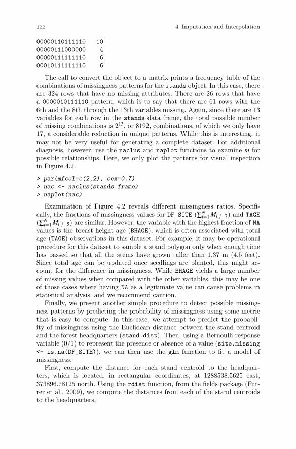
122 4 Imputation and Interpolation
00000110111110 10
00000111000000 4
00000111111110 6
00010111111110 6
The call to convert the object to a matrix prints a frequency table of thecombinations of missingness patterns for the stands object. In this case, thereare 324 rows that have no missing attributes. There are 26 rows that havea 0000010111110 pattern, which is to say that there are 61 rows with the6th and the 8th through the 13th variables missing. Again, since there are 13variables for each row in the stands data frame, the total possible numberof missing combinations is 213, or 8192, combinations, of which we only have17, a considerable reduction in unique patterns. While this is interesting, itmay not be very useful for generating a complete dataset. For additionaldiagnosis, however, use the naclus and naplot functions to examine m forpossible relationships. Here, we only plot the patterns for visual inspectionin Figure 4.2.
> par(mfcol=c(2,2), cex=0.7)
> nac <- naclus(stands.frame)
> naplot(nac)
Examination of Figure 4.2 reveals different missingness ratios. Specifi-cally, the fractions of missingness values for DF_SITE (∑N
i=1 Mi, j=7) and TAGE
(∑Ni=1 Mi, j=5) are similar. However, the variable with the highest fraction of NA
values is the breast-height age (BHAGE), which is often associated with totalage (TAGE) observations in this dataset. For example, it may be operationalprocedure for this dataset to sample a stand polygon only when enough timehas passed so that all the stems have grown taller than 1.37 m (4.5 feet).Since total age can be updated once seedlings are planted, this might ac-count for the difference in missingness. While BHAGE yields a large numberof missing values when compared with the other variables, this may be oneof those cases where having NA as a legitimate value can cause problems instatistical analysis, and we recommend caution.
Finally, we present another simple procedure to detect possible missing-ness patterns by predicting the probability of missingness using some metricthat is easy to compute. In this case, we attempt to predict the probabil-ity of missingness using the Euclidean distance between the stand centroidand the forest headquarters (stand.dist). Then, using a Bernoulli responsevariable (0/1) to represent the presence or absence of a value (site.missing<- is.na(DF_SITE)), we can then use the glm function to fit a model ofmissingness.
First, compute the distance for each stand centroid to the headquar-ters, which is located, in rectangular coordinates, at 1288538.5625 east,373896.78125 north. Using the rdist function, from the fields package (Fur-rer et al., 2009), we compute the distances from each of the stand centroidsto the headquarters,
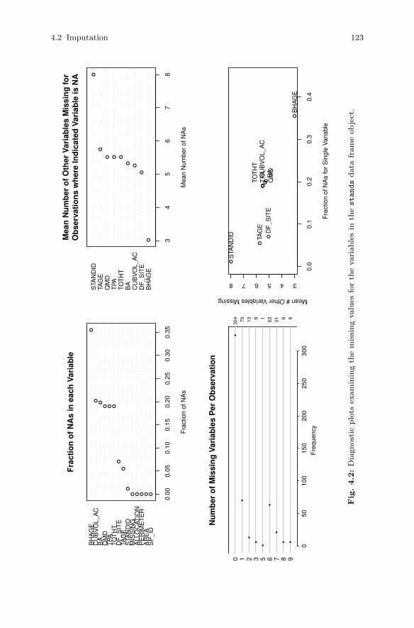
4.2 Imputation 123
SP
_ID
AR
EA
PE
RIM
ET
ER
ALL
OC
ATIO
NM
ISS
ING
STA
ND
IDTA
GE
DF
_SIT
ETO
TH
TT
PAQ
MD
BA
CU
BV
OL_
AC
BH
AG
E
●●●●●
●
●
●
●●●
●
●
●
0.00
0.05
0.10
0.15
0.20
0.25
0.30
0.35
Fra
ctio
n o
f N
As
in e
ach
Var
iab
le
Fra
ctio
n of
NA
s
Nu
mb
er o
f M
issi
ng
Var
iab
les
Per
Ob
serv
atio
n
Fre
quen
cy
050
100
150
200
250
300
●
●
●
●
●
●
●
● ●
324 70
13
6
1
63
21
6
6
0
1
2
3
5
6
7
8
9
BH
AG
ED
F_S
ITE
CU
BV
OL_
AC
BA
TOT
HT
TPA
QM
DTA
GE
STA
ND
ID
●
●
●
●
●●●
●
●
34
56
78
Mea
n N
um
ber
of
Oth
er V
aria
ble
s M
issi
ng
for
Ob
serv
atio
ns
wh
ere
Ind
icat
ed V
aria
ble
is N
A
Mea
n N
umbe
r of
NA
s
●
●
●
●
●●
●●●
0.0
0.1
0.2
0.3
0.4
345678
Fra
ctio
n of
NA
s fo
r S
ingl
e V
aria
ble
Mean # Other Variables Missing
STA
ND
ID TAG
E
BH
AG
E
DF
_SIT
E
TOT
HT
TPA
QM
DC
UB
VO
L_A
CB
A
Fig.4.2:Diagnostic
plots
examiningth
emissingvalues
forth
evariablesin
thestandsdata
frameobject.
124 4 Imputation and Interpolation
> hq <- c(1288538.5625,373896.78125)
> centers <- coordinates(stands)
> stand.dist <- rdist(t(c(1288538.5625,373896.78125)), centers)
Then, we define a vector where the entries are NA if the site index is missingusing the is.na function:
> site.na <- as.numeric(is.na(stands.frame$DF_SITE))
Finally, fit a binomial model using the glm function:
> gfit.site <- glm(site.na ~ c(stand.dist),
+ family = "binomial")
> summary(gfit.site)
Call:
glm(formula = site.na ~ c(stand.dist), family = "binomial")
Deviance Residuals:
Min 1Q Median 3Q Max
-0.4511 -0.4126 -0.3764 -0.3389 2.4567
Coefficients:
Estimate Std. Error z value Pr(>|z|)
(Intercept) -3.015e+00 4.315e-01 -6.986 2.83e-12 ***
c(stand.dist) 2.145e-05 1.865e-05 1.150 0.25
---
Signif. codes: 0 �***� 0.001 �**� 0.01 �*� 0.05 �.� 0.1 � � 1
(Dispersion parameter for binomial family taken to be 1)
Null deviance: 260.26 on 509 degrees of freedom
Residual deviance: 258.91 on 508 degrees of freedom
AIC: 262.91
Number of Fisher Scoring iterations: 5
The resulting p-value of 0.25 for the predictor variable suggests that thereis little correlation between the distance of the stand centroid to the head-quarters and the probability of the DF_SITE observation being missing. Itseems that distance from the office is not a good predictor of missingnesshere.
We could continue to examine the dataset with more sophisticated toolsand plots, but, in practice, the determination of the mechanism, and themethod used to correct for it, is at the discretion of the analyst and judgmentwill dictate the final determination once our attempt to document the searchfor a missingness pattern is complete.
4.2 Imputation 125
4.2.2 Methods for Imputing Missing Data
Now that we have determined that some data are missing, we present a fewmethods for imputation. Little and Rubin (2002) grouped the methods forimputing unobserved variables into three categories: 1) weighting procedures;2) imputation-based procedures; and 3) model-based procedures. We brieflypresent them in the next few sections.
4.2.2.1 Weighting Procedures
When the sample selection is based on unequal probabilities of inclusion (sam-ple weights), as described by Horvitz and Thompson (1952), then weightingprocedures can adjust the weights used to compute various estimators (Littleand Rubin, 2002, Chapter 3).
For relatively small amounts of missing data, weighting procedures thatare based on completely recorded units (that is, with no missing values) canyield sufficient results. They can yield biased results and may not be veryefficient when making inferences to subpopulations such as stands or strata(Little and Rubin, 2002, Chapter 3). In the current example, we believe wehave sufficiently large numbers of missing observations in the stands objectto give us biased results if we were to apply these methods. We do not presentthem here.
4.2.2.2 Imputation-Based Procedures
Imputation-based methods include those methods most commonly used inforestry, such as k-nearest neighbor (k-NN) and most similar neighbor (MSN)(Moeur and Stage, 1995), as well as less sophisticated methods such as mean
and regression imputation methods . The mean imputation method simplyreplaces the missing attributes with the mean of the sampled attributes. Theregression imputation method estimates unsampled attributes from sampledattributes using regression techniques (Little and Rubin, 2002, Chapter 1).These hot-deck methods of imputation are covered more completely elsewhere(e.g., by Venables and Ripley, 2002) and are not presented further here.
Alternatively, cold-deck methods assign values based on a constant valuefrom an external source rather than from samples of the observed data. Forexample, in landscape-planning projects, regeneration stands might not havean adequate sample to make inference for the entire population over the spanof the planning horizon. A decision is made to assign all unsampled standsthat are under some arbitrary age a set of values that is “representative” ofyoung stands across the landscape. This method ignores the consequencesof imputation, such as bias, and is discouraged when unbiased results aredesired (Little and Rubin, 2002, Chapter 4).

126 4 Imputation and Interpolation
Finally, the nearest-neighbor methods are those for which unsampled mea-sures are assigned values from nearby sampled attributes using a variety ofstatistical distances (Bishop, 2006, see, e.g., Chapter 2). We present our firstimputation method, the k-NN method, in Section 4.2.3.
4.2.2.3 Model-Based Procedures
Model-based procedures are methods that make inferences upon the distri-bution of the data under a specific model. These methods include maximum-likelihood estimation (MLE) , expectation-maximization (EM), and Markovchain Monte Carlo (MCMC) methods (Little and Rubin, 2002; Madras, 2002;Kuroda, 2004). These methods offer great flexibility, as the imputation proce-dures can include models of the covariance structure of the data themselves.Also, the underlying model assumptions can be assessed, and the model subse-quently improved, based on standard statistical diagnostics. There are meth-ods for continuous values, categories, and censored data. We present the EMapproach to imputation in Section 4.2.4.
4.2.3 Nearest-Neighbor Imputation
Nearest-neighbor methods for imputation of attributes in forest inventoriesare common in forest resource analysis. The method and various forms of ithave been used to impute stand-level attributes (Moeur and Stage, 1995),plot-level attributes (Holmstrom et al., 2003), basal-area diameter distribu-tions (Haara et al., 1997), and tree lists (Korhonen and Kangas, 1997).
Numerous R packages provide nearest-neighbor methods for continuousand categorical data; for example: the class (Venables and Ripley, 2002) andknncat packages (Buttrey, 2008); weighted k -nn, for example the kknn pack-age (Schliep and Hechenbichler, 2009); and generic nearest-neighbor methodsfor missing observations, for example the class package (Venables and Rip-ley, 2002). Crookston and Finley’s yaImpute package includes many methodsthat are commonly found in the forest inventory analysis, such as the gra-dient nearest-neighbor (GNN, Ohmann and Gregory, 2002), Most SimilarNeighbor (MSN, Moeur and Stage, 1995), and the random forest methodBreiman (2001a).
Here we will use the simplest of the nearest-neighbor methods, k -nn im-putation. The k -nn method is a kernel density estimation method that iscommonly used to impute missing values where the value of k dictates thenumber of nearest neighbors, in statistical distance, to the observed data inany given row of the dataset (Bishop, 2006, Chapter 2). The method is non-parametric in the sense that it does not assume any underlying distribution.The lack of a distributional assumption is an advantage, as the distributional

4.2 Imputation 127
form of variables of interest is often influenced by factors such as marketconditions (for example, sales, exchanges, and depletions) and disturbancepatterns (such as fire, insects, and disease). It is often difficult to find a dis-tributional form that is sufficiently flexible to match these contingencies.
Nearest-neighbor methods require training and target datasets. The train-ing dataset comprises the data for which we have all the necessary attributes.The target dataset is the dataset for which we have some, but not all, of thevalues. The task then is to find which data in the training data are closest tothe target data, using the attributes that are common to both datasets, andassign those values that are missing from the training dataset.
Normally, we would begin by obtaining our training data from those rowsin the inventory that contain all of the attributes. Since there is a possibilitythat there are rows with all nine attributes missing, we shall include thecentroid of the stand polygon so that we can assign the geographically, notstatistically, closest stand if we have no other attributes to compare. Forthis example, location is the only variable that is available for every polygonregardless of missingness.
We already know from the MISSING variable how many attributes aremissing from each row of the stands object. We select those rows from stands
that have no missing values as our training dataset,
> centers <- coordinates(stands)
> stands.frame <- as.data.frame(stands)
> stands.frame$x.ctr <- centers[,1]
> stands.frame$y.ctr <- centers[,2]
> stands.frame$MISSING <- rowSums(is.na(stands.frame))
> training.stands <- subset(stands.frame, MISSING == 0)
> nrow(training.stands)
[1] 324
The remainder of the rows contain various missing attributes. Assign thoserows to a variable named target.stands,
> target.stands <- subset(stands.frame, MISSING > 0)
> nrow(target.stands)
[1] 186
Recall from Chapter 2 that stands contains 510 polygons and in Sec-tion 4.2.1 we partitioned stands into target and training rows to representrows with and without missing data, respectively. From the output above, thenumber of rows with and without missing data are 324 and 186, respectively,and the sum of the two equals the total number of rows in the stands object.
Next, create the training and target objects and include the coordinatesof the centroid for each of the sampled stands
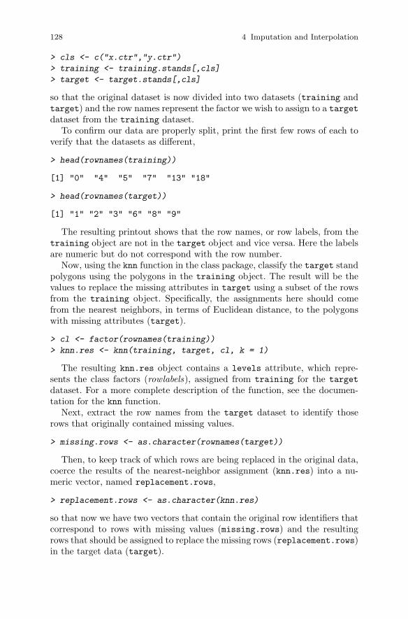
128 4 Imputation and Interpolation
> cls <- c("x.ctr","y.ctr")
> training <- training.stands[,cls]
> target <- target.stands[,cls]
so that the original dataset is now divided into two datasets (training andtarget) and the row names represent the factor we wish to assign to a targetdataset from the training dataset.
To confirm our data are properly split, print the first few rows of each toverify that the datasets as different,
> head(rownames(training))
[1] "0" "4" "5" "7" "13" "18"
> head(rownames(target))
[1] "1" "2" "3" "6" "8" "9"
The resulting printout shows that the row names, or row labels, from thetraining object are not in the target object and vice versa. Here the labelsare numeric but do not correspond with the row number.
Now, using the knn function in the class package, classify the target standpolygons using the polygons in the training object. The result will be thevalues to replace the missing attributes in target using a subset of the rowsfrom the training object. Specifically, the assignments here should comefrom the nearest neighbors, in terms of Euclidean distance, to the polygonswith missing attributes (target).
> cl <- factor(rownames(training))
> knn.res <- knn(training, target, cl, k = 1)
The resulting knn.res object contains a levels attribute, which repre-sents the class factors (rowlabels), assigned from training for the target
dataset. For a more complete description of the function, see the documen-tation for the knn function.
Next, extract the row names from the target dataset to identify thoserows that originally contained missing values.
> missing.rows <- as.character(rownames(target))
Then, to keep track of which rows are being replaced in the original data,coerce the results of the nearest-neighbor assignment (knn.res) into a nu-meric vector, named replacement.rows,
> replacement.rows <- as.character(knn.res)
so that now we have two vectors that contain the original row identifiers thatcorrespond to rows with missing values (missing.rows) and the resultingrows that should be assigned to replace the missing rows (replacement.rows)in the target data (target).
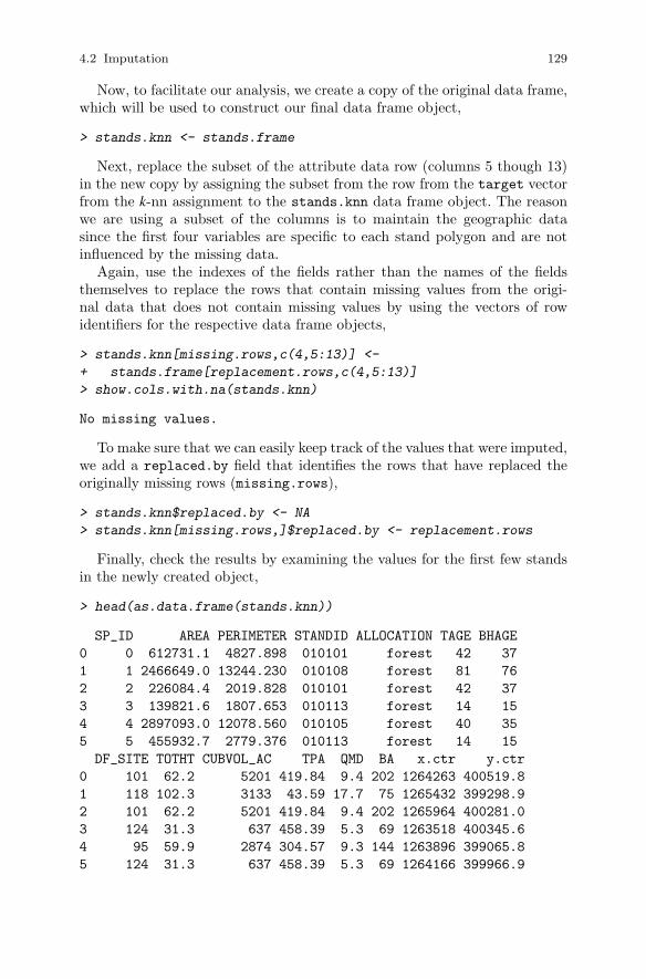
4.2 Imputation 129
Now, to facilitate our analysis, we create a copy of the original data frame,which will be used to construct our final data frame object,
> stands.knn <- stands.frame
Next, replace the subset of the attribute data row (columns 5 though 13)in the new copy by assigning the subset from the row from the target vectorfrom the k-nn assignment to the stands.knn data frame object. The reasonwe are using a subset of the columns is to maintain the geographic datasince the first four variables are specific to each stand polygon and are notinfluenced by the missing data.
Again, use the indexes of the fields rather than the names of the fieldsthemselves to replace the rows that contain missing values from the origi-nal data that does not contain missing values by using the vectors of rowidentifiers for the respective data frame objects,
> stands.knn[missing.rows,c(4,5:13)] <-
+ stands.frame[replacement.rows,c(4,5:13)]
> show.cols.with.na(stands.knn)
No missing values.
To make sure that we can easily keep track of the values that were imputed,we add a replaced.by field that identifies the rows that have replaced theoriginally missing rows (missing.rows),
> stands.knn$replaced.by <- NA
> stands.knn[missing.rows,]$replaced.by <- replacement.rows
Finally, check the results by examining the values for the first few standsin the newly created object,
> head(as.data.frame(stands.knn))
SP_ID AREA PERIMETER STANDID ALLOCATION TAGE BHAGE
0 0 612731.1 4827.898 010101 forest 42 37
1 1 2466649.0 13244.230 010108 forest 81 76
2 2 226084.4 2019.828 010101 forest 42 37
3 3 139821.6 1807.653 010113 forest 14 15
4 4 2897093.0 12078.560 010105 forest 40 35
5 5 455932.7 2779.376 010113 forest 14 15
DF_SITE TOTHT CUBVOL_AC TPA QMD BA x.ctr y.ctr
0 101 62.2 5201 419.84 9.4 202 1264263 400519.8
1 118 102.3 3133 43.59 17.7 75 1265432 399298.9
2 101 62.2 5201 419.84 9.4 202 1265964 400281.0
3 124 31.3 637 458.39 5.3 69 1263518 400345.6
4 95 59.9 2874 304.57 9.3 144 1263896 399065.8
5 124 31.3 637 458.39 5.3 69 1264166 399966.9
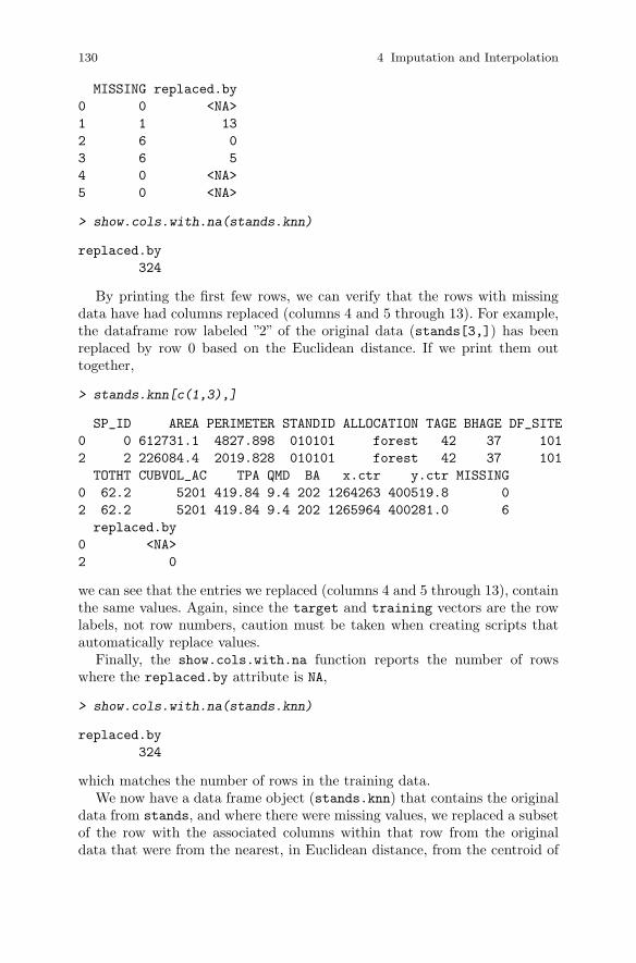
130 4 Imputation and Interpolation
MISSING replaced.by
0 0 <NA>
1 1 13
2 6 0
3 6 5
4 0 <NA>
5 0 <NA>
> show.cols.with.na(stands.knn)
replaced.by
324
By printing the first few rows, we can verify that the rows with missingdata have had columns replaced (columns 4 and 5 through 13). For example,the dataframe row labeled ”2” of the original data (stands[3,]) has beenreplaced by row 0 based on the Euclidean distance. If we print them outtogether,
> stands.knn[c(1,3),]
SP_ID AREA PERIMETER STANDID ALLOCATION TAGE BHAGE DF_SITE
0 0 612731.1 4827.898 010101 forest 42 37 101
2 2 226084.4 2019.828 010101 forest 42 37 101
TOTHT CUBVOL_AC TPA QMD BA x.ctr y.ctr MISSING
0 62.2 5201 419.84 9.4 202 1264263 400519.8 0
2 62.2 5201 419.84 9.4 202 1265964 400281.0 6
replaced.by
0 <NA>
2 0
we can see that the entries we replaced (columns 4 and 5 through 13), containthe same values. Again, since the target and training vectors are the rowlabels, not row numbers, caution must be taken when creating scripts thatautomatically replace values.
Finally, the show.cols.with.na function reports the number of rowswhere the replaced.by attribute is NA,
> show.cols.with.na(stands.knn)
replaced.by
324
which matches the number of rows in the training data.We now have a data frame object (stands.knn) that contains the original
data from stands, and where there were missing values, we replaced a subsetof the row with the associated columns within that row from the originaldata that were from the nearest, in Euclidean distance, from the centroid of
4.2 Imputation 131
the stand. Ultimately we now have a data frame object that does not containmissing values.
To apply k -nn in this context, we have invoked some useful simplifications:
1. We ignored the fact that some of the attributes were more complete thanothers.
2. We also ignored the fact that the distribution of the missing attributesmight not have been equal, although the frequency of the missing at-tributes was roughly equal for many of the missing values.
3. We replaced the entire row when at least one attribute was missing, notindividual fields based on additional information.
With those simplifications, we have generated imputed values similar tothose of our observations, where there were no negative values, no extremelylarge values, and the distributions of the combined imputed and observedvalues were similar to the observed values alone. This may not always be thecase.
Nearest-neighbor classification methods are useful for determining whichcategory a new observation belongs to, but the methods require that theentire training set be stored, which can lead to excessive computational times(Bishop, 2006, Chapter 2). Another drawback is that the methods rely onselecting and computing a weighted combination of the observations ratherthan making assumptions of the underlying distributions of the missing andobserved data.
Yet another problem with our specific method of using the closest neighboris that there might be large contrasts in adjacent cover types when adjacencyis defined by the Euclidean distance and nothing more. For example, if wehad a stand polygon with no measurements, it is possible that the stand wasrecently harvested and could be surrounded by either much older stands ormuch younger stands. In either case, since we are not including informationon the distribution of the surrounding stands, our imputed values may notreflect the true distribution of the current vegetation.
A better method would allow us to control the classification process inde-pendently of the size of the training data while maintaining the ability to es-timate complex densities. For that, we turn to the expectation-maximization(EM) algorithm.
4.2.4 Expectation-Maximization Imputation
The Expectation-Maximization (EM) algorithm iteratively computes the ex-pected values for missing observations by repeatedly updating maximum-likelihood parameter estimates and imputing expected values until conver-gence is achieved. It has been applied to maximum likelihood estimation(Little and Rubin, 2002), latent structure models (McLachlan and Krishnan,

132 4 Imputation and Interpolation
2008), neural network learning (Bishop, 2006, Chapter 9), and Gibbs sam-pling (Watanabe and Yamaguchi, 2004, Chapter 4). For a more completepresentation, we refer the reader to Dempster et al. (1977). Watanabe andYamaguchi (2004) and McLachlan and Krishnan (2008) also provide a thor-ough introduction, related models, and extensions to the algorithm.
Briefly, the algorithm iterates over two steps (Little and Rubin, 2002, seeChapter 8):
1. E-step: Find the conditional expectation of the missing data from theobserved data and current estimates of the parameters and substitute theexpectations back into the missing data.
2. M-step: Perform maximum-likelihood estimation of the parameters as ifthere were no missing data.
Imputation using the EM algorithm can be accomplished using the normpackage (Novo and Schafer, 2002) if we are willing to assume that our dataare distributed as multivariate normal. To use R for imputing missing valuesusing the EM algorithm, first use the prelim.norm function,
> cls <- c(5:12)
> sd <- as.matrix(as.data.frame(stands[,cls]))
> psd <- prelim.norm(sd)
This function performs preliminary bookkeeping functions (e.g., sorting,centering, and scaling) on the input data, and the output object (psd) is anintermediate object, so for brevity we do not present the details here. Formore complete details, see the documentation provided with the package.
Next, call the em.norm function to compute the maximum-likelihood esti-mates on the psd matrix and assign the results to a variable called thetahat,
> thetahat <- em.norm(psd, showits=FALSE) #compute mle
where thetahat contains a vector that represents the maximum-likelihoodestimates of the normal parameters that are not in the original scales.
To extract the estimates, covariances, and correlations from thetahat inthe original scales, call the getparam.norm function,
> em.params <- getparam.norm(psd, thetahat, corr=TRUE)
which extracts the information of interest. Here we extract only the mean(em.params$mu),
> names(em.params)
[1] "mu" "sdv" "r"
> em.params$mu
[1] 0.00000 58.05591 53.21879 115.85964 69.26065
[6] 5890.92943 241.54077 12.42562
4.2 Imputation 133
Finally, to obtain our imputed values, we seed the random number generator,
> rngseed(1234567) #set random number generator seed
make a copy of the original data as we did for the stands.knn object,
> stands.em <- as.data.frame(stands)
and use the imp.norm function to impute the missing values
> stands.em[,cls] <- imp.norm(psd, thetahat, sd)
using the cls to index the columns to be replaced.
> show.cols.with.na(stands.em)
STANDID BA
6 101
Once again, we now have a complete dataset that contains no missingvalues. The imp.norm function returns a matrix of the same form as theinput matrix (psd) but with all missing values filled in with simulated valuesdrawn from their predictive distribution given the observed data (sd) andthe specified parameter (thetahat).
A print of the summaries (from summary(stands.em)) shows a few neg-ative values for fields that are not normally negative (specifically, QMD, TPA,and BA). This reveals that the method can produce values beyond the rangeof the original data, which in some cases is unacceptable. In the next section,we compare our results for a single metric (site index) and examine somedifferences between the two methods.
4.2.5 Comparing Results
Comparing results for imputation methods can include numerous metrics(Dempster et al., 1977). Here we compare the results graphically to simplifyour presentation. Specifically, we generate a plot of the distributions for theoriginal data and the distributions of the two imputation methods we tried(see Figure 4.3) and discuss them briefly.
First, construct the individual data frame objects,
> knn.frame <- data.frame(site = stands.knn$DF_SITE,
+ method = "KNN")
> em.frame <- data.frame(site = stands.em$DF_SITE,
+ method = "EM")
> obs.frame <-
+ data.frame(site = subset(stands.frame,
+ MISSING == 0)$DF_SITE,
+ method = "OBS")
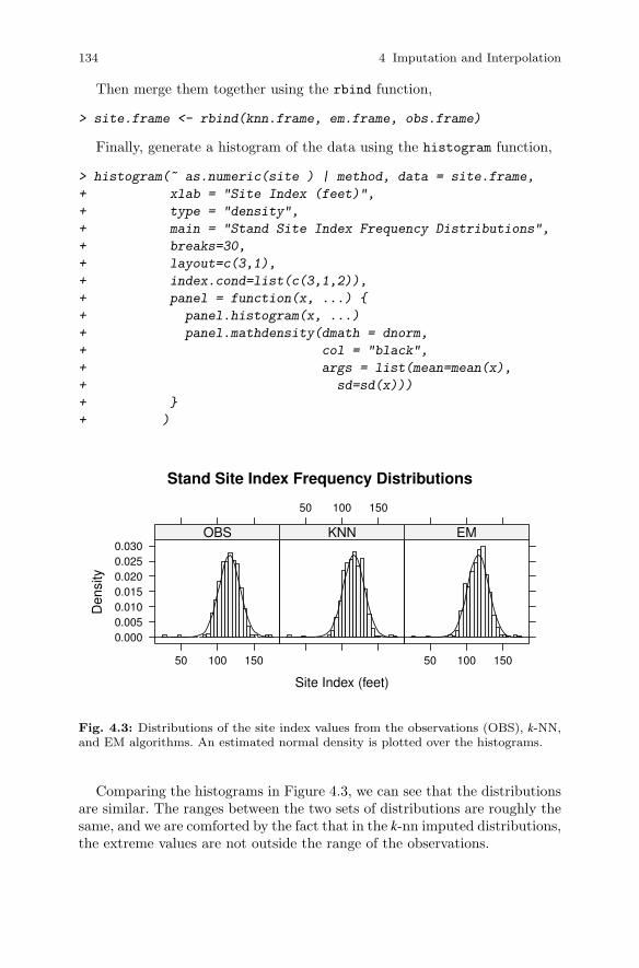
134 4 Imputation and Interpolation
Then merge them together using the rbind function,
> site.frame <- rbind(knn.frame, em.frame, obs.frame)
Finally, generate a histogram of the data using the histogram function,
> histogram(~ as.numeric(site ) | method, data = site.frame,
+ xlab = "Site Index (feet)",
+ type = "density",
+ main = "Stand Site Index Frequency Distributions",
+ breaks=30,
+ layout=c(3,1),
+ index.cond=list(c(3,1,2)),
+ panel = function(x, ...) {
+ panel.histogram(x, ...)
+ panel.mathdensity(dmath = dnorm,
+ col = "black",
+ args = list(mean=mean(x),
+ sd=sd(x)))
+ }
+ )
Stand Site Index Frequency Distributions
Site Index (feet)
Den
sity
0.0000.0050.0100.0150.0200.0250.030
50 100 150
OBS
50 100 150
KNN
50 100 150
EM
Fig. 4.3: Distributions of the site index values from the observations (OBS), k-NN,and EM algorithms. An estimated normal density is plotted over the histograms.
Comparing the histograms in Figure 4.3, we can see that the distributionsare similar. The ranges between the two sets of distributions are roughly thesame, and we are comforted by the fact that in the k-nn imputed distributions,the extreme values are not outside the range of the observations.
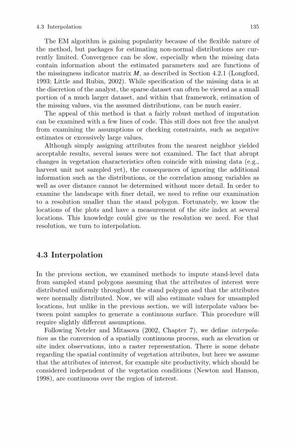
4.3 Interpolation 135
The EM algorithm is gaining popularity because of the flexible nature ofthe method, but packages for estimating non-normal distributions are cur-rently limited. Convergence can be slow, especially when the missing datacontain information about the estimated parameters and are functions ofthe missingness indicator matrix M, as described in Section 4.2.1 (Longford,1993; Little and Rubin, 2002). While specification of the missing data is atthe discretion of the analyst, the sparse dataset can often be viewed as a smallportion of a much larger dataset, and within that framework, estimation ofthe missing values, via the assumed distributions, can be much easier.
The appeal of this method is that a fairly robust method of imputationcan be examined with a few lines of code. This still does not free the analystfrom examining the assumptions or checking constraints, such as negativeestimates or excessively large values.
Although simply assigning attributes from the nearest neighbor yieldedacceptable results, several issues were not examined. The fact that abruptchanges in vegetation characteristics often coincide with missing data (e.g.,harvest unit not sampled yet), the consequences of ignoring the additionalinformation such as the distributions, or the correlation among variables aswell as over distance cannot be determined without more detail. In order toexamine the landscape with finer detail, we need to refine our examinationto a resolution smaller than the stand polygon. Fortunately, we know thelocations of the plots and have a measurement of the site index at severallocations. This knowledge could give us the resolution we need. For thatresolution, we turn to interpolation.
4.3 Interpolation
In the previous section, we examined methods to impute stand-level datafrom sampled stand polygons assuming that the attributes of interest weredistributed uniformly throughout the stand polygon and that the attributeswere normally distributed. Now, we will also estimate values for unsampledlocations, but unlike in the previous section, we will interpolate values be-tween point samples to generate a continuous surface. This procedure willrequire slightly different assumptions.
Following Neteler and Mitasova (2002, Chapter 7), we define interpola-
tion as the conversion of a spatially continuous process, such as elevation orsite index observations, into a raster representation. There is some debateregarding the spatial continuity of vegetation attributes, but here we assumethat the attributes of interest, for example site productivity, which should beconsidered independent of the vegetation conditions (Newton and Hanson,1998), are continuous over the region of interest.

136 4 Imputation and Interpolation
4.3.1 Methods of Interpolation
There are numerous methods for interpolating values at unsampled loca-tions, including point interpolation, inverse distance methods, and minimum-variance methods. Point estimation methods can be classified into polygo-nal and triangular interpolation methods. The relative performance of thesemethods can vary depending on the estimation criteria (Isaaks and Srivas-tava, 1989). These methods are relatively simple and are thoroughly pre-sented within other references (Okabe et al., 2000; Cressie, 1993), so we donot present them here.
Instead, we focus on minimum-variance methods. These methods are de-signed to yield the best estimates under one particular statistical criterion:unbiased estimates with minimum error variance. To begin, we need to ad-dress the following questions to provide key contextual information:
� Are we interested in global or local estimates?� Are we interested in population parameters, such as mean and variance,
or do we want the complete distribution of values?� What is the support? Do we want point values or estimates over larger
areas such as polygons?
For global estimates, all of the sample values and locations are used forprediction. Global estimates are typically used for estimating the distributionof attributes over the region of interest and can be greatly influenced by clus-tering (Isaaks and Srivastava, 1989) . For local estimates, only those pointsnear the point of interest are used for estimation. As with global estimates,local estimates are also influenced by clustering, but local estimation meth-ods account for both the distance of sample points to estimation locationsand possible redundancy among samples.
Historically, forest inventories have been focused on global estimation byattempting to answer such questions as “How much volume does a forestcontain?” or “How many trees are in a given area?” Site-specific informationis also becoming important. Both types of estimation are influenced by thenumber and location of samples within a given area, and much work has beendone to examine the influence of plot location on both global estimation andlocal estimation (de Gruijter et al., 2006, Chapters 6 and 8 respectively).
Once we have decided whether we are interested in obtaining global orlocal estimates, we then need to determine whether we are interested in es-timating parameters of a distribution or the distribution itself. The mean isthe most commonly estimated parameter (Isaaks and Srivastava, 1989). Ifestimation of an entire distribution is of interest, then both parametric andnon-parametric methods are available. Parametric methods make assump-tions about the underlying distribution of the data, but the assumptions canbe difficult to verify and may not be appropriate for many types of situationswhere the surface is neither smooth nor continuous. Non-parametric methodsdo not make those assumptions but require interpolation between points on

4.3 Interpolation 137
the cumulative histogram. Should we need to extrapolate beyond the data,the results can be invalid.
Then we need to determine if we are interested in predicting values at in-dividual points across the entire region or in smaller subregions such as standor harvest polygons rather than individual points. The support, or spatialcontinuity , is important, as it determines the appropriate prediction meth-ods depending on our desire to predict point, line, area, or volume estimates.The support acts as a smoothing filter depending on the size of the area beingestimated and the density of the sample data (Goovaerts, 1997, Chapter 5)and (Isaaks and Srivastava, 1989, Chapter 19).
For this section, we will examine one of the most basic types of interpo-lation commonly used for point support. There are numerous methods thatcan be used for all types of support, but it is beyond the scope of this bookto cover all of the possibilities.
Here we are interested in estimating the mean site index at unsampledpoint locations over the entire landscape. The data, from Chapter 2, includesthe final.plots dataframe,
> final.plots <- read.csv("../../data/final-plots.csv" )
To begin, we examine the distribution of the site index plots using a basichistogram and normal q-q plot,
> opar <- par(mfcol = c(1,2), las = 1, cex.axis = 0.70)
> site.plots <- subset(final.plots, !is.na(site))
> hist(site.plots$site, xlim = c(0,220), ylim = c(0,0.025),
+ freq = FALSE, main = "Histogram", xlab = "Site Index",
+ breaks = 30)
> qqnorm(site.plots$site, pch=46)
> qqline(site.plots$site, lty=1, col="grey", pch=46)
Judging from the histogram and normal quantile-quantile plots in Fig-ure 4.4, the distribution of the site index is fairly close to normal, whichwould lead us to conclude that using one of the parametric methods mightyield satisfactory results.
Some of the nomenclature associated with the various interpolation meth-ods can cause confusion. Schabenberger and Pierce (2002, Table 9.3) presenta useful table of the various features of kriging systems in relation to the un-derlying assumptions. Here, we need to estimate the site index at any point ina finite region where the mean over the entire region is unknown. Their tablesuggests that a parametric method for point estimation known as ordinarykriging meets our requirements.
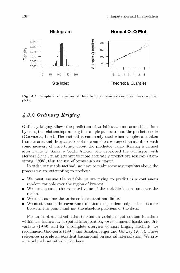
138 4 Imputation and Interpolation
Histogram
Site Index
Den
sity
0 50 100 150 200
0.000
0.005
0.010
0.015
0.020
0.025
−3 −2 −1 0 1 2 3
50
100
150
200
Normal Q−Q Plot
Theoretical Quantiles
Sam
ple
Qua
ntile
sFig. 4.4: Graphical summaries of the site index observations from the site indexplots.
4.3.2 Ordinary Kriging
Ordinary kriging allows the prediction of variables at unmeasured locationsby using the relationships among the sample points around the prediction site(Goovaerts, 1997). The method is commonly used when samples are takenfrom an area and the goal is to obtain complete coverage of an attribute withsome measure of uncertainty about the predicted value. Kriging is namedafter Danie G. Krige, a South African who developed the technique, withHerbert Sichel, in an attempt to more accurately predict ore reserves (Arm-strong, 1998), thus the use of terms such as nugget.
In order to use this method, we have to make some assumptions about theprocess we are attempting to predict :
� We must assume the variable we are trying to predict is a continuousrandom variable over the region of interest.
� We must assume the expected value of the variable is constant over theregion.
� We must assume the variance is constant and finite.� We must assume the covariance function is dependent only on the distance
between two points and not the absolute positions of the data.
For an excellent introduction to random variables and random functionswithin the framework of spatial interpolation, we recommend Isaaks and Sri-vastava (1989), and for a complete overview of most kriging methods, werecommend Goovaerts (1997) and Schabenberger and Gotway (2005). Thesereferences provide an excellent background on spatial interpolation. We pro-vide only a brief introduction here.

4.3 Interpolation 139
4.3.2.1 Theory
Ordinary kriging is a best linear unbiased estimator (BLUE) because theestimates are weighted linear combinations of the data that have the smallestpossible variance among all possible linear combinations of the data (Isaaksand Srivastava, 1989). The estimator is unbiased because the mean residualerror is zero, and it minimizes the variance of the errors. In order to achieveBLUE, we have to develop a model to describe our data and select weightsto apply to our random function model that ensure that the error variance
σ2r = σ2 +
n
∑i=1
n
∑j=1
wiw jCi j −2n
∑j=1
wiCi0 (4.1)
is minimized subject to the unbiasedness constraint ∑ni=1 wi = 1. C is a model
of the covariance (Isaaks and Srivastava, 1989, Chapter 12). Since we needto constrain the solution to equation (4.1), a system of n+ 1 equations canbe expressed more compactly in matrix notation as⎡
⎢⎢⎢⎣C11 . . . C1n 1...
. . ....
...
Cn1 . . . Cnn 1
1 . . . 1 0
⎤⎥⎥⎥⎦⎡⎢⎢⎢⎣
w1
...wn
μ
⎤⎥⎥⎥⎦=
⎡⎢⎢⎢⎣
C10
...
Cn0
1
⎤⎥⎥⎥⎦ (4.2)
or more simply
Cw = D (4.3)
where w is a vector of weights, C is the covariance matrix of the observations,and D is the vector of the covariances at the points themselves; that is,C(h) = 0, where h is the distance between sample points. This generates asystem of n+ 1 equations that can be easily solved for C−1 to obtain thekriging weights w
w = C−1D (4.4)
where the resulting values for w produce the unbiased estimates with theminimum error variance for equation (4.1). Finally, the resulting estimate(v0) can then be calculated as
v0 =n
∑i=1
wivi (4.5)
and the resulting minimized estimation variance (σ2r ) is
σ2r = σ2 −
n
∑i=1
wiCi0 +μ (4.6)
140 4 Imputation and Interpolation
It should be noted here that the use of the system of equations we havepresented requires some caveats and observations.
First, since we will need to predict values (v0) that are at distances thatare not found in the distance matrix, we must construct a function of thedistance between points to describe the relationship among the attributesof interest. This relationship C(h) represents the statistical distances amongthe sample points separated by a distance h. Thus when two points are verysimilar, the values of Ci j will be large compared with the other entries of thematrix.
Second, there is no guarantee that a C−1 exists that yields a unique so-lution to our system of equations. We can check for the positive definitecondition (x′Ax > 0;A,x ∈ C
n) using any number of methods, such as deter-mining whether all of the eigenvalues are greater than zero. In most cases, wedo not need to worry about this condition, as we will almost always fit ourspatial relationships with positive definite functions, such as the exponentialfunction presented in equation (4.7).
Third, the predictor is an exact interpolator, meaning the predictions ex-actly match the measured values at locations where measurements have beenmade and the corresponding estimation variance is zero (Journel and Hui-jbregts, 1978).
Last, the matrix D is not necessarily the spatial distance from the samplepoints to the location we are estimating but rather the statistical distance.The combination of these two matrices (C and D) accounts for the two mostimportant aspects of spatial estimation: clustering of the data values (C−1)and the statistical distances (D) between them (Isaaks and Srivastava, 1989).
In order to compute the kriging weights, we must first decide on a randomfunction, C(h), that will represent the spatial relationship of our data.
4.3.2.2 Descriptions of Spatial Correlation
In order to obtain the unbiased estimate of the random function C(h) withthe minimum error variance, we need to define the spatial relationship forour random function model. This relationship is usually defined as a modelof the covariance structure of the distance between sample locations anddata with some unexplainable variation (nugget). We use this model to de-scribe the variation of our random function model. The covariance model isoften a combination of two models (Armstrong, 1998). For example, whenthe exponential model exp(−h
a) is combined with the nugget model (c0), the
covariances form the function
C(h) =
{c0 + c1 if h = 0
c1 exp(−ha) if h > 0
(4.7)
4.3 Interpolation 141
which can also be expressed as a semi-variogram
γ(h) =
{0 if h = 0
c0 + c1(1− exp(ha) if h > 0
(4.8)
where c0 + c1 = σ2 and h is the distance between two points. The c0 and c1
parameters have special interpretations:
1. c0 describes that part of the variance that cannot be accounted for inthe smallest sampling distance between two points. This is known as thenugget effect.
2. a is known as the range. The range is that distance at which the varianceis considered constant and the distance between points will not accountfor the variation. It can be considered the horizon at which no changes invariation can be detected.
3. The sum of c0 + c1 is known as the sill, which represents the variance ofthe random variables.
In fact, the covariance function is directly related to the semi-variogram inthat one can be expressed as a variation of the other (Isaaks and Srivastava,1989; Goovaerts, 1997; Pebesma, 2004). It can also be shown that the totalvariance (σ2
r ) for an ordinary kriging system can be decomposed as
σ2r = σ2 +
σ2
n(4.9)
where σ2 is the variance of the random variables and σ2
nis the variance of
the unknown mean. Closer examination shows us that the addition of extrasamples (increasing n) only reduces the uncertainty about the unknown meanand not the variance introduced by the random variables in our randomfunction.
There are many semi-variogram model forms. The gstat package providesinfrastructure to list and examine different forms (Pebesma, 2004). A list ofpossible semi-variogram models can be obtained using the vgm function withno arguments, and a convenient trellis plot of the semi-variogram models canbe generated using the show.vgms function.
Since we wish to predict values and their accompanying confidence inter-vals, our first task is to develop the covariance (semi-variogram) model forthe plot summary data we developed in Chapter 2.
4.3.3 Semi-variogram Estimation
Much has been written on the subject of fitting semi-variograms (Cressie,1993, Chapter 2). Armstrong (1998) provides three reasons that least-squaresmethods often fail when fitting semi-variogram models:

142 4 Imputation and Interpolation
1. The function must be positive definite; otherwise mean-squared errors ofprediction may be negative.
2. Least-squares fitting assumes all sample points are independent observa-tions.
3. Semi-variogram behavior close to the origin is unknown, yet it is vital, andleast-squares methods cannot take this into account.
The gstat package provides several methods to estimate parameters forsemi-variogram models and uses iteratively reweighted least squares (Cressie,1993, Chapter 2) by default (Pebesma, 2004). The package also provides amethod for fitting the semi-variogram using restricted maximum-likelihood(REML) estimation, although Pebesma (2004) suggests that REML may beslow for moderate to large datasets (that is, having more than 100 observa-tions). We will use the default settings.
To estimate the semi-variogram for our site index data, we first obtain theplots that have a site index observation by constructing a data frame objectthat contains the non-missing site index values.
> site.plots <- subset(final.plots, !is.na(site))
We then build a model of the semi-variogram using the variogram andfit.variogram functions and fit.
> site.var <- gstat::variogram(site ~ 1,
+ locations = ~x+y,
+ data = site.plots,
+ width = 50,
+ cutoff = 3000)
> site.model <-
+ fit.variogram(site.var,
+ vgm(1000, "Exp", 1000, nugget = 0))
Here we have used the scope operator (::) to let R know that we wish touse the variogram function provided by the gstat package and not the oneprovided by the spatial package (Venables and Ripley, 2002).
We then print the results of our model:
> site.model
model psill range
1 Nug 129.1209 0.0000
2 Exp 172.6557 952.9546
The sum-of-squares value for the fitted model can be obtained using theattributes function.
> attributes(site.model)$SSErr
[1] 14.51226
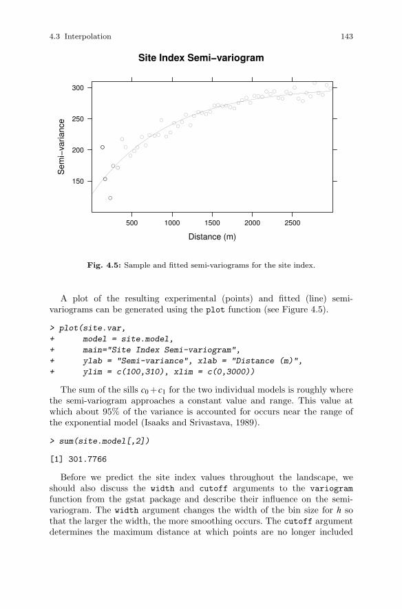
4.3 Interpolation 143
Site Index Semi−variogram
Distance (m)
Sem
i−va
rianc
e
150
200
250
300
500 1000 1500 2000 2500
●
●
●
●●
●
●
●
●●
●
●
● ●●
●
●●
●●
●
●
●
●●●●
●
●●●●●●
●●
●
●
●●●
●●
●
●●
●●
●
●●
●●
●
●●
●●
Fig. 4.5: Sample and fitted semi-variograms for the site index.
A plot of the resulting experimental (points) and fitted (line) semi-variograms can be generated using the plot function (see Figure 4.5).
> plot(site.var,
+ model = site.model,
+ main="Site Index Semi-variogram",
+ ylab = "Semi-variance", xlab = "Distance (m)",
+ ylim = c(100,310), xlim = c(0,3000))
The sum of the sills c0 +c1 for the two individual models is roughly wherethe semi-variogram approaches a constant value and range. This value atwhich about 95% of the variance is accounted for occurs near the range ofthe exponential model (Isaaks and Srivastava, 1989).
> sum(site.model[,2])
[1] 301.7766
Before we predict the site index values throughout the landscape, weshould also discuss the width and cutoff arguments to the variogram
function from the gstat package and describe their influence on the semi-variogram. The width argument changes the width of the bin size for h sothat the larger the width, the more smoothing occurs. The cutoff argumentdetermines the maximum distance at which points are no longer included
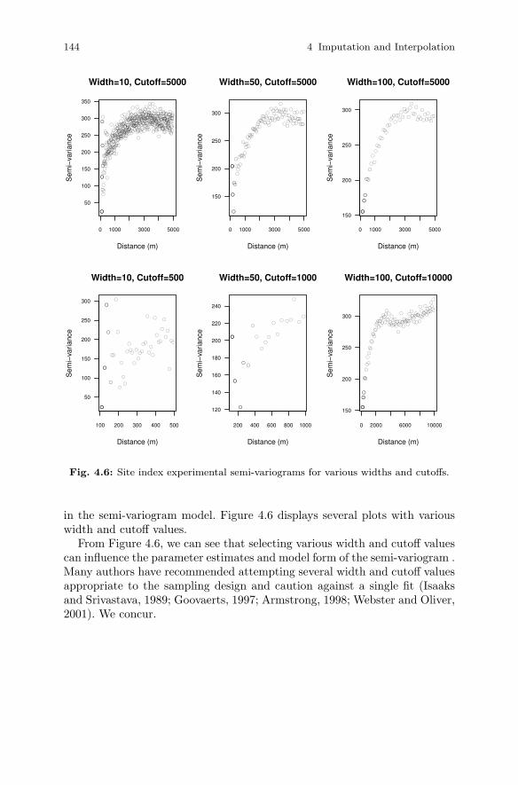
144 4 Imputation and Interpolation
●
●
●
●
●
●●
●
●
●
●
●
●
●
●
●●
●
●
●
●●
●●
●
●
●
●
●
●
●●
●
●
●
●
●
●●
●
●
●
●●●●●
●●
●
●●
●
●●●
●
●
●●
●●
●
●
●
●
●
●
●
●
●●
●●
●●●
●●
●
●
●●●●
●●
●
●●
●
●
●
●
●
●●
●
●●
●
●
●
●●
●
●
●●
●
●
●●
●
●
●
●
●
●●
●
●●
●
●
●●
●
●●●●
●
●
●
●
●●
●
●
●●●●
●●
●
●●●
●●●
●
●●
●
●
●
●
●
●●
●
●
●●●
●
●
●
●
●
●
●
●
●
●●●●
●
●●
●
●
●
●●●●
●●●
●
●
●
●
●
●
●
●
●
●●
●●●●●
●●
●
●
●
●
●
●
●
●●●
●
●●●
●●
●●
●
●●
●●
●●
●●
●
●●●
●
●
●●
●
●
●
●●
●
●●●
●
●
●●●
●●
●
●●
●●●
●
●
●●
●●●●
●●
●
●●●
●
●
●●
●●●
●
●
●●
●
●●
●
●
●
●
●●
●
●
●
●
●
●
●
●●
●
●
●
●
●●
●●
●
●
●
●●
●
●●
●
●
●
●
●
●
●●●●
●●●
●
●
●●●
●●●●
●
●
●
●
●●●
●●
●
●●●●
●●
●●●
●
●
●
●
●
●
●
●
●
●
●
●●
●●●
●
●
●
●●●
●●
●
●
●
●●
●
●
●
●
●●
●
●
●●●
●
●
●
●
●
●●●●
●●●
●
●
●
●●●●
●
●●●●
●
●●
●
●●
●●
●
●
●●●
●
●●●●●
●●●
●●●●
●
●
●●
●●
●
●
●●●
●●●●
●●
●
●
●
●●●
●
●
●●●
●●
0 1000 3000 5000
50
100
150
200
250
300
350
Width=10, Cutoff=5000
Distance (m)
Sem
i−va
rianc
e
●
●
●
●●
●
●
●
●●
●
●
●●●
●
●●
●●●
●
●
●●●●●
●●●●●●
●●●
●
●●●
●●●
●●
●●
●
●●
●●
●
●●
●●
●
●
●
●
●●
●●
●
●
●●
●
●
●●
●
●
●
●●●
●
●●
●●
●
●
●
●
●●●●
●
●
●●
●
0 1000 3000 5000
150
200
250
300
Width=50, Cutoff=5000
Distance (m)
Sem
i−va
rianc
e
●
●
●
●●
●
●
●
●
●
●●
●●
●●●
●●
●●●
●
●●
●
●
●
●●●
●
●●
●●
●
●●●
●
●
●
●
●
●●
●●
0 1000 3000 5000
150
200
250
300
Width=100, Cutoff=5000
Distance (m)
Sem
i−va
rianc
e
●
●
●
●
●
●●
●
●
●
●
●
●
●
●
●●
●
●
●
●●
●●
●
●
●
●
●
●
●●
●
●
●
●
●
●●
100 200 300 400 500
50
100
150
200
250
300
Width=10, Cutoff=500
Distance (m)
Sem
i−va
rianc
e
●
●
●
●●
●
●
●
●
●
●
●
● ●●
●
●
●
200 400 600 800 1000
120
140
160
180
200
220
240
Width=50, Cutoff=1000
Distance (m)
Sem
i−va
rianc
e
●
●
●
●●
●
●
●
●
●
●●
●●
●●●
●●
●●●
●
●●●
●
●
●●●
●
●●
●●
●
●●●
●
●
●
●
●
●●●●
●
●●●
●
●●●
●●●●●●●
●
●●
●
●●●
●
●●
●
●●●
●
●
●
●
●●●●
●
●●
●●●●●
●●●
●
●
0 2000 6000 10000
150
200
250
300
Width=100, Cutoff=10000
Distance (m)
Sem
i−va
rianc
e
Fig. 4.6: Site index experimental semi-variograms for various widths and cutoffs.
in the semi-variogram model. Figure 4.6 displays several plots with variouswidth and cutoff values.
From Figure 4.6, we can see that selecting various width and cutoff valuescan influence the parameter estimates and model form of the semi-variogram .Many authors have recommended attempting several width and cutoff valuesappropriate to the sampling design and caution against a single fit (Isaaksand Srivastava, 1989; Goovaerts, 1997; Armstrong, 1998; Webster and Oliver,2001). We concur.
4.3 Interpolation 145
4.3.4 Prediction
Upon visual inspection, our semi-variogram model seems to fit the data sat-isfactorily. Now we can estimate the site index and accompanying varianceestimates throughout the entire forest, but first we need to generate a pre-diction grid and clip the points outside our region using the inside.owin
function.First, read the geometry from the boundary file (boundary.shp),
> bdry2 <- readShapePoly("../../data/boundary.shp")
Then, using the fortify function in the ggplot2 package, we gener-ate a region to define the forest boundary using the boundary attribute(FORBNDRY_),
> dum <- fortify(bdry2, region = "FORBNDRY_")
> summary(dum)
long lat order
Min. :1257463 Min. :354303 Min. : 1.0
1st Qu.:1267739 1st Qu.:368686 1st Qu.: 345.5
Median :1272965 Median :379267 Median : 690.0
Mean :1274130 Mean :379745 Mean : 690.0
3rd Qu.:1280129 3rd Qu.:391242 3rd Qu.:1034.5
Max. :1292129 Max. :400783 Max. :1379.0
hole piece group id
Mode :logical 1:1329 2.1: 50 Length:1379
FALSE:1329 2: 50 3.1:1279 Class :character
TRUE :50 3.2: 50 Mode :character
NA�s :0
From the output of the summary function, we have three polygons (group)defining the forest boundary: two that define the boundary going clockwiseand one to define the hole in the southern portion of the forest.
To generate our boundary, we must manually extract the polygons’ pieces,using array indices and our familiarity with the data, and generate a list ofpoints from the inner and outer pieces that can then be used to define anowin object, using the poly constructor argument (owin(poly))
> dum2 <- dum[dum$id == 3,]
> outer <- dum2[dum2$piece == 1,]
> inner <- dum2[dum2$piece == 2,]
Next, construct a list object that contains the pairs of vertices for theboundary
> bdry.poly <- vector(2, mode="list")
> bdry.poly[[1]] <-
146 4 Imputation and Interpolation
+ list(x = outer[(nrow(outer)-1):1,]$long,
+ y = outer[(nrow(outer)-1):1,]$lat)
> bdry.poly[[2]] <-
+ list(x = inner[(nrow(inner)-1):1,]$long,
+ y = inner[(nrow(inner)-1):1,]$lat)
and then generate the owin object, using the forest polygon boundary wejust created,
> bdry.owin <- owin(poly=bdry.poly)
Checking 2 polygons...1, [Checking polygon with 1278 edges...]
2.
done.
Checking for cross-intersection between 2 polygons...1.
done.
> grid <- gridcentres(bdry.owin, 200, 200)
The owin function requires that the polygon that defines the window thatwill be applied masks out unwanted points in our prediction grid. The indicesare reversed because the vertices for the outer boundaries must be listedcounter-clockwise. The vertices for the holes must be listed clockwise. Theobject grid now contains a prediction grid bounded by the bounding box ofthe window defined by bdry.owin.
Next, reduce the prediction grid by only including those points within thepolygonal boundary, defined by the bdry.owin object,
> ok <- inside.owin(grid$x, grid$y, bdry.owin)
> pred.grid <- data.frame(x=grid$x[ok], y=grid$y[ok])
Then, to predict the site index estimates at the new prediction locationsusing the model we developed previously,
> sample.site.plots <- sample(1:nrow(site.plots), 1000 )
> site.pred <- krige(formula = site ~ 1,
+ locations = ~ x + y,
+ data = site.plots[sample.site.plots,],
+ model = site.model,
+ newdata = pred.grid)
[using ordinary kriging]
We can see from printing the first few rows of the resulting predictions(site.pred) that our values appear in the range of the distribution presentedin Figure 4.7.
> head(site.pred)
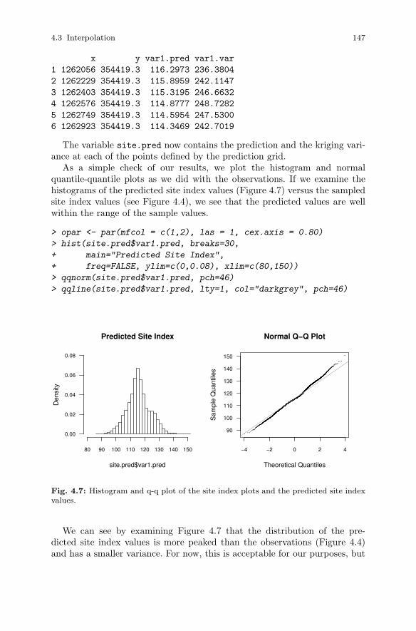
4.3 Interpolation 147
x y var1.pred var1.var
1 1262056 354419.3 116.2973 236.3804
2 1262229 354419.3 115.8959 242.1147
3 1262403 354419.3 115.3195 246.6632
4 1262576 354419.3 114.8777 248.7282
5 1262749 354419.3 114.5954 247.5300
6 1262923 354419.3 114.3469 242.7019
The variable site.pred now contains the prediction and the kriging vari-ance at each of the points defined by the prediction grid.
As a simple check of our results, we plot the histogram and normalquantile-quantile plots as we did with the observations. If we examine thehistograms of the predicted site index values (Figure 4.7) versus the sampledsite index values (see Figure 4.4), we see that the predicted values are wellwithin the range of the sample values.
> opar <- par(mfcol = c(1,2), las = 1, cex.axis = 0.80)
> hist(site.pred$var1.pred, breaks=30,
+ main="Predicted Site Index",
+ freq=FALSE, ylim=c(0,0.08), xlim=c(80,150))
> qqnorm(site.pred$var1.pred, pch=46)
> qqline(site.pred$var1.pred, lty=1, col="darkgrey", pch=46)
Predicted Site Index
site.pred$var1.pred
Den
sity
80 90 100 110 120 130 140 150
0.00
0.02
0.04
0.06
0.08
−4 −2 0 2 4
90
100
110
120
130
140
150
Normal Q−Q Plot
Theoretical Quantiles
Sam
ple
Qua
ntile
s
Fig. 4.7: Histogram and q-q plot of the site index plots and the predicted site indexvalues.
We can see by examining Figure 4.7 that the distribution of the pre-dicted site index values is more peaked than the observations (Figure 4.4)and has a smaller variance. For now, this is acceptable for our purposes, but
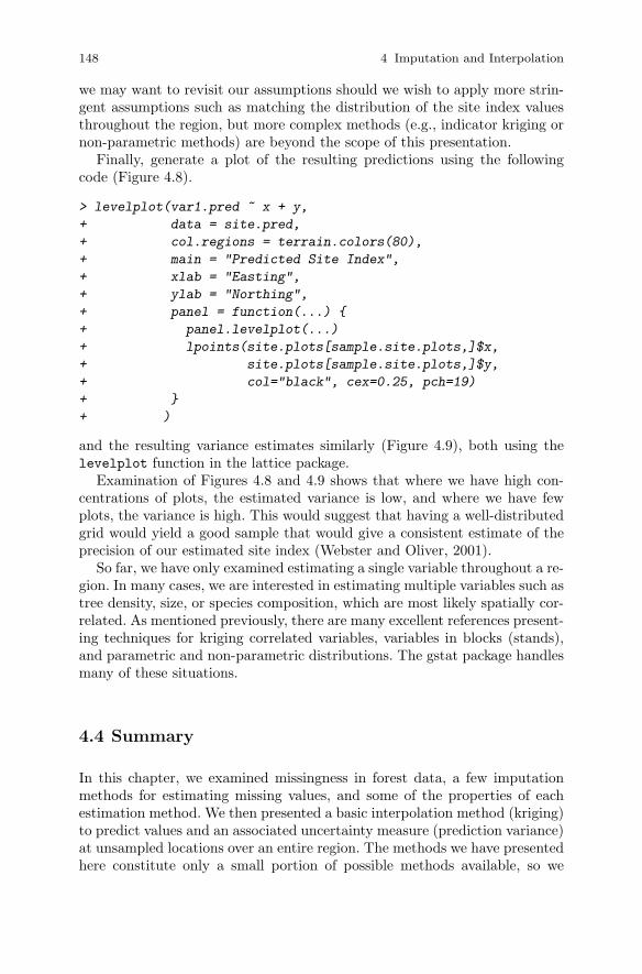
148 4 Imputation and Interpolation
we may want to revisit our assumptions should we wish to apply more strin-gent assumptions such as matching the distribution of the site index valuesthroughout the region, but more complex methods (e.g., indicator kriging ornon-parametric methods) are beyond the scope of this presentation.
Finally, generate a plot of the resulting predictions using the followingcode (Figure 4.8).
> levelplot(var1.pred ~ x + y,
+ data = site.pred,
+ col.regions = terrain.colors(80),
+ main = "Predicted Site Index",
+ xlab = "Easting",
+ ylab = "Northing",
+ panel = function(...) {
+ panel.levelplot(...)
+ lpoints(site.plots[sample.site.plots,]$x,
+ site.plots[sample.site.plots,]$y,
+ col="black", cex=0.25, pch=19)
+ }
+ )
and the resulting variance estimates similarly (Figure 4.9), both using thelevelplot function in the lattice package.
Examination of Figures 4.8 and 4.9 shows that where we have high con-centrations of plots, the estimated variance is low, and where we have fewplots, the variance is high. This would suggest that having a well-distributedgrid would yield a good sample that would give a consistent estimate of theprecision of our estimated site index (Webster and Oliver, 2001).
So far, we have only examined estimating a single variable throughout a re-gion. In many cases, we are interested in estimating multiple variables such astree density, size, or species composition, which are most likely spatially cor-related. As mentioned previously, there are many excellent references present-ing techniques for kriging correlated variables, variables in blocks (stands),and parametric and non-parametric distributions. The gstat package handlesmany of these situations.
4.4 Summary
In this chapter, we examined missingness in forest data, a few imputationmethods for estimating missing values, and some of the properties of eachestimation method. We then presented a basic interpolation method (kriging)to predict values and an associated uncertainty measure (prediction variance)at unsampled locations over an entire region. The methods we have presentedhere constitute only a small portion of possible methods available, so we
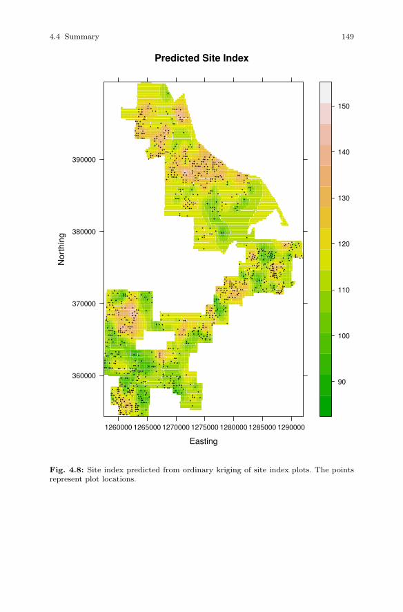
4.4 Summary 149
Predicted Site Index
Easting
Nor
thin
g
360000
370000
380000
390000
1260000 1265000 1270000 1275000 1280000 1285000 1290000
●
●
●
●
●
●
●
●
●
●
●
●
●
●
●
●
●
●
●
●
●
●
●
●
●
●
●
●
●
●
●
●
●
●
●
●
●
●
●
●
●
●
●
●
●
●
●
●
●
●
●
●
●
●
●
●
●
●
●
●
●
●
●
●
●
●
●
●
●
●
●
●
●
●
●
●
●
●
●
●
●●
●
●
●
●
●
●
●
●
●
●
●
●
●
●
●
●
●
●
●
●
●
●
●
●
●
●
●
●
●
●
●
●
●
●
●
●
●
●
●
●
●
●
●
●
●
●
●
●
●
●
●
●
●
●
●
●
●
●
●
●
●
●
●
●
●
●
●●
●
●
●
●
●
●
●
●
●
●
●
●
●
●
●
●
●
●
●
●
●
●
●
●
●
●
●
●
●
●
●
●
●
●
●
●
●
●
●
●
●
●
●
●
●
●
●
●
●
●●
●
●
●
●
●
●
●
●
●
●
●
●
●
●
●
●
●
●
●
●
●
●
●
●
●
●
●
●
●
●
●
●
●
●
●
●
●
●
●
●
●
●
●
●
●
●
●
●
●
●
●
●
●
●
●
●
●
●
●
●
●
●
●
●
●
●
●
●
●
●
●
●
●
●
●
●
●
●
●
●
●
●
●
●
●
●
●
●
●
●
●
●
●
●
●
●
●
●
●
●
●
●
●
●
●
●
●
●
●
●
●
●
●
●
●
●
●
●
●
●
●
●
●
●
●
●
●
●
●
●
●
●
●
●
●
●
●
●
●
●
●
●
●
●
●
●
●
●
●
●
●
●
●
●
●
●
●
●
●
●
●
●
●
●
●
●
●
●
●
●
●
●
●
●
●
●
●
●
●
●
●
●
●
●
●
●
●
●
●
●
●
●
●
●
●
●
●
●
●
●●
●
●
●
●
●
●
●
●
●
●
●
●
●
●
●
●
●
●
●
●
●
●
●
●
●
●
●
●
●
●
●
●
●
●
●
●
●
●
●
●
●
●
●
●
●
●
●
●
●
●
●
●
●
●
●
●
●
●
●
●
●
●
●
●
●
●
●
●
●
●
●
●
●
●
●
●
●
●
●
●
●
●
●
●
●
●
●
●
●
●
●
●
●
●
●
●
●
●
●
●
●
●
●
●
●
●
●
●
●
●
●
●
●
●
●
●
●
●
●
●
●
●
●
●
●
●
●
●
●
●
●
●
●
●
●
●
●
●
●
●
●
●
●
●
●
●
●
●
●
●
●
●
●
●
●
●
●
●
●●
●
●
●
●
●
●
●
●
●
●
●
●
●
●
●
●
●
●
●
●
●
●
●
●
●
●
●
●
●
●
●
●
●
●
●
●
●
●
●
●
●
●
●
●
●
●
●
●
●
●●
●
●
●
●
●
●
●
●
●
●
●
●
●
●
●
●
●
●
●
●
●
●
●
●
●
●
●
●
●
●
●
●
●
●
●
●
●
●
●
●
●
●
●
●
●
●
●
●
●
●
●
●
●
●
●
●
●
●
●
●
●
●
●
●
●
●
●
●
●
●
●
●
●
●
●
●
●
●
●
●
●
●
●
●
●
●
●
●
●
●
●
●
●
●
●
●
●
●
●
●
●
●
●
●
●
●
●
●
●
●
●
●
●
●
●
●
● ●
●
●
●
●
●
●
●
●
●
●
●
●
●
●
●
●
●
●
●
●
●
●
●
●
●
●
●
●
●
●
●
●
●
●
●
●
●
●
●
●
●
●
●
●
●
●
●
●
●
●
●
●
●
●
●
●
●
●
●
●
●
●
●
●
●
●
●
●
●
●
●
●
●
●
●
●
●
●
●
●
●
●
●
●
●
●
●
●
●
●
●
●
●
●
90
100
110
120
130
140
150
Fig. 4.8: Site index predicted from ordinary kriging of site index plots. The pointsrepresent plot locations.
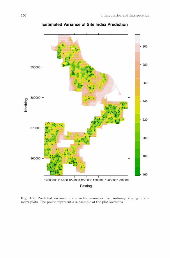
150 4 Imputation and Interpolation
Estimated Variance of Site Index Prediction
Easting
Nor
thin
g
360000
370000
380000
390000
1260000 1265000 1270000 1275000 1280000 1285000 1290000
●
●
●
●
●
●
●
●
●
●
●
●
●
●
●
●
●
●
●
●
●
●
●
●
●
●
●
●
●
●
●
●
●
●
●
●
●
●
●
●
●
●
●
●
●
●
●
●
●
●
●
●
●
●
●
●
●
●
●
●
●
●
●
●
●
●
●
●
●
●
●
●
●
●
●
●
●
●
●
●
●●
●
●
●
●
●
●
●
●
●
●
●
●
●
●
●
●
●
●
●
●
●
●
●
●
●
●
●
●
●
●
●
●
●
●
●
●
●
●
●
●
●
●
●
●
●
●
●
●
●
●
●
●
●
●
●
●
●
●
●
●
●
●
●
●
●
●
●●
●
●
●
●
●
●
●
●
●
●
●
●
●
●
●
●
●
●
●
●
●
●
●
●
●
●
●
●
●
●
●
●
●
●
●
●
●
●
●
●
●
●
●
●
●
●
●
●
●
●●
●
●
●
●
●
●
●
●
●
●
●
●
●
●
●
●
●
●
●
●
●
●
●
●
●
●
●
●
●
●
●
●
●
●
●
●
●
●
●
●
●
●
●
●
●
●
●
●
●
●
●
●
●
●
●
●
●
●
●
●
●
●
●
●
●
●
●
●
●
●
●
●
●
●
●
●
●
●
●
●
●
●
●
●
●
●
●
●
●
●
●
●
●
●
●
●
●
●
●
●
●
●
●
●
●
●
●
●
●
●
●
●
●
●
●
●
●
●
●
●
●
●
●
●
●
●
●
●
●
●
●
●
●
●
●
●
●
●
●
●
●
●
●
●
●
●
●
●
●
●
●
●
●
●
●
●
●
●
●
●
●
●
●
●
●
●
●
●
●
●
●
●
●
●●
●
●
●
●
●
●
●
●
●
●
●
●
●
●
●
●
●
●
●
●
●
●
●
●
●
●
●
●
●
●
●
●
●
●
●
●
●
●
●
●
●
●
●
●
●
●
●
●
●
●
●
●
●
●
●
●
●
●
●
●
●
●
●
●
●
●
●
●
●
●
●
●
●
●
●
●
●
●
●
●
●
●
●
●
●
●
●
●
●
●
●
●
●
●
●
●
●
●
●
●
●
●
●
●
●
●
●
●
●
●
●
●
●
●
●
●
●
●
●
●
●
●
●
●
●
●
●
●
●
●
●
●
●
●
●
●
●
●
●
●
●
●
●
●
●
●
●
●
●
●
●
●
●
●
●
●
●
●
●
●
●
●
●
●
●
●
●
●
●
●
●
●
●
●
●
●
●
●
●
●
●
●
●
●
●
●
●
●
●
●
●
●
●
●
●
●
●
●
●
●●
●
●
●
●
●
●
●
●
●
●
●
●
●
●
●
●
●
●
●
●
●
●
●
●
●
●
●
●
●
●
●
●
●
●
●
●
●
●
●
●
●
●
●
●
●
●
●
●
●
●
●
●
●
●
●
●
●
●
●
●
●
●
●
●
●
●
●
●
●
●
●
●
●
●
●
●
●
●
●
●
●
●
●
●
●
●
●
●
●
●
●
●
●
●
●
●
●
●
●
●
●
●
●
●
●
●
●
●
●
●
●
●
●
●
●
●
●
●
●
●
●
●
●
●
●
●
●
●
●
●
●
●
●
●
●
●
●
●
●
●
●
●
●
●
●
●
●
●
●
●
●
●
●
●
●
●
●
●
●●
●
●
●
●
●
●
●
●
●
●
●
●
●
●
●
●
●
●
●
●
●
●
●
●
●
●
●
●
●
●
●
●
●
●
●
●
●
●
●
●
●
●
●
●
●
●
●
●
●
●●
●
●
●
●
●
●
●
●
●
●
●
●
●
●
●
●
●
●
●
●
●
●
●
●
●
●
●
●
●
●
●
●
●
●
●
●
●
●
●
●
●
●
●
●
●
●
●
●
●
●
●
●
●
●
●
●
●
●
●
●
●
●
●
●
●
●
●
●
●
●
●
●
●
●
●
●
●
●
●
●
●
●
●
●
●
●
●
●
●
●
●
●
●
●
●
●
●
●
●
●
●
●
●
●
●
●
●
●
●
●
●
●
●
●
●
●
● ●
●
●
●
●
●
●
●
●
●
●
●
●
●
●
●
●
●
●
●
●
●
●
●
●
●
●
●
●
●
●
●
●
●
●
●
●
●
●
●
●
●
●
●
●
●
●
●
●
●
●
●
●
●
●
●
●
●
●
●
●
●
●
●
●
●
●
●
●
●
●
●
●
●
●
●
●
●
●
●
●
●
●
●
●
●
●
●
●
●
●
●
●
●
●
160
180
200
220
240
260
280
300
Fig. 4.9: Predicted variance of site index estimates from ordinary kriging of siteindex plots. The points represent a subsample of the plot locations.

4.4 Summary 151
encourage the reader to search the documentation for additional methodsthat might be more appropriate for any given situation.

Part III
Allometry and Fitting Models

Chapter 5
Fitting Dimensional Distributions
This chapter focuses on the use of statistical tools for fitting models to di-mensional data that represent a sample of trees. Here, we consider the mod-els, theory, and tools for one-dimensional data, such as diameter distribu-tions. Two-dimensional data, such as the classical allometric relationships,and multi-dimensional data, which require systems of equations, are handledin a later chapter.
Our goal is to reduce the information about a sample of n observations toas compact and simple a representation as possible while retaining as muchinformation about the underlying population as we can.
The representation of the sample that we choose may require the assump-tion of a particular model form, for example the Weibull or beta probabilitydensity functions, or a family of model forms, such as the Johnson familyof distribution functions. Using a model provides several benefits. A modelsimplifies communication of the outcome because the outcome can be sum-marized by the estimates of the parameters of the model. Also, if comparablemodel forms are used, the parametric approach facilitates straightforwardconnection or comparison with historical theory or results.
The analyst may prefer to represent the data without relying on havingto choose a particular functional form, instead using one of a number of non-parametric representations. These so-called non-parametric approaches aremore flexible and allow for a wider range of possible densities, including, forexample, densities that are bimodal.
It is important to recognize that, since the 1980s, the major differencesbetween parametric and non-parametric models have been in ease of com-munication and portability. Given an appropriate computing platform, it isjust as easy to obtain a prediction of a non-parametric distribution at anynumber of points as it is a parametric distribution (see, e.g., Borders et al.,1987).
We focus on diameter distributions, but the principles still hold and thetools work for the distribution of any other measures.
155A. P. Robinson, J. D. Hamann, Forest Analytics with R, Use R!,DOI 10.1007/978-1-4419-7762-5_5, © Springer Science+Business Media, LLC 2011

156 5 Fitting Dimensional Distributions
5.1 Diameter Distribution
A diameter distribution is a histogram of the tree-level dbh measurements.The bin widths and bin starting point that are used to construct the his-togram are chosen subjectively and are usually chosen to simplify the inter-pretation rather than to optimally capture the shape of the distribution. Itis well known that the estimate of the shape of the diameter distributioncan be strongly affected by the choice of these parameters (see, e.g., Scott,1985). In forestry, the width and starting point are most commonly set byconvention; for example, a popular configuration is bins that have a width of5 cm (alternatively, 2 inches), starting at 0 cm.
Diameter distributions are important tools in forest resource management.The interpretation of diameter distributions will affect silvicultural decisions,such as when to thin and how much to thin, as well as harvesting decisions,such as where and when to harvest and what kinds of equipment will benecessary. Diameter distributions are also used as inputs to growth modelsand sometimes are the subject of growth modeling themselves. Consequently,information about the diameter distribution for a forest stand as it is andas it may be in the future is very useful for forest management. Clutteret al. (1983), Borders et al. (1987), Vanclay (1994), and Avery and Burkhart(2003) provide useful overviews of the uses and interpretation of diameterdistributions in forest management.
Invariably the diameter distribution is computed from a sample of trees,rather than the population. Often the sample of trees is arranged in plots,which may muddy the interpretation of the sample-based diameter distribu-tion as an estimate of the population diameter distribution (Garcıa, 1992).Trees might compete against their closest neighbors, which may induce nega-tive correlation in dimensions among the proximate trees. Also, local growthpatterns could reflect positive correlation due to micro-site variability. Theseconcerns about representativeness and independence of the sample data aremost likely impossible to resolve with the usual forest inventory data and areconsequently ignored in the modeling phase. However, interpretation of theoutcomes can be softened.
From the point of view of the biometrician, the two primary goals for theestimation of a diameter distribution from a sample are prediction in time andin space, and probably both. The spatial goal is to use the sample diameterdistributions to represent the size class densities of the population from whichthe sample was taken. The temporal goal is to project the current diameterdistribution forward in time, contingent on some management decision. Inorder to achieve these tasks efficiently, the distribution is summarized bystatistics, and the statistics are projected in time and/or space. The statisticsmay be parameters of a chosen distribution, such as the Weibull, or they maybe quantiles of the sample. The projections are often supported by auxiliaryinformation, such as site class, stem density, or age class. Simplified, thesequence of steps is:
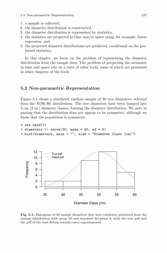
5.2 Non-parametric Representation 157
1. a sample is collected,2. the diameter distribution is constructed,3. the diameter distribution is represented by statistics,4. the statistics are projected in time and/or space using, for example, linear
regression, and5. the projected diameter distributions are predicted, conditional on the pro-
jected statistics.
In this chapter, we focus on the problem of representing the diameterdistribution from the sample data. The problem of projecting the estimatesin time and space rely on a suite of other tools, some of which are presentedin other chapters of the book.
5.2 Non-parametric Representation
Figure 5.1 shows a simulated random sample of 30 tree diameters, selectedfrom the N(50,36) distribution. The tree diameters have been lumped into5 cm (2 in.) diameter classes, forming the diameter distribution. We note inpassing that the distribution does not appear to be symmetric, although weknow that the population is symmetric.
> set.seed(1)
> diameters <- rnorm(30, mean = 50, sd = 6)
> hist(diameters, main = "", xlab = "Diameter Class (cm)")
Diameter Class (cm)
Fre
quen
cy
35 40 45 50 55 60
0
2
4
6
8
10
12True pdfFitted pdf
Fig. 5.1: Histogram of 30 sample diameters that were randomly generated from thenormal distribution with mean 50 and standard deviation 6, with the true pdf andthe pdf of the best-fitting normal curve superimposed.
158 5 Fitting Dimensional Distributions
The sample diameter distribution can be interrogated directly for quan-tities of interest. For example, the percentile method due to Borders et al.(1987) represents the distribution using a collection of quantiles. The usualempirical quantiles can be obtained from the sample using the quantile func-tion, although the 0 and 100% quantiles require the min and max functions,respectively.
> min(diameters)
[1] 36.7118
> quantile(diameters, p = (5 + (0:9) * 10) / 100 )
5% 15% 25% 35% 45% 55% 65%
39.46411 45.48462 47.39024 49.67330 50.48011 52.32096 53.37517
75% 85% 95%
54.25220 55.30858 58.02619
> max(diameters)
[1] 59.57168
5.3 Parametric Representation
Sometimes we prefer to make an assumption about the shape of the underly-ing density. Here, we will proceed under the assumption that the population isnormally distributed. This is a fairly unusual assumption for fitting diameterdistributions; we make it here to simplify this introductory material.
The normal distribution is completely determined by two parameters,mean and variance; that is, if you know the mean and variance of data thatare normally distributed, then you know everything about the distributionof those data. Therefore, in order to obtain all possible information from asample about a normally distributed population, all we need to estimate arethe mean and variance.
We often prefer to think about the standard deviation rather than thevariance because the standard deviation is in the same units as the data, asis the mean. Doing so allows us to think about the spread of the data in unitsthat have a natural interpretation.
5.3.1 Parameter Estimation
We now present a number of approaches to the challenge of estimating theparameters of the distribution given data. We develop these estimators for

5.3 Parametric Representation 159
the relatively familiar normal pdf before introducing the more popular pdfsthat are used for diameter distribution modeling.
5.3.1.1 Plug-in Principle
One intuitively satisfying way of estimating the mean and standard deviationis to calculate the sample mean and the sample standard deviation and usethose values to estimate the population parameters. This is called the plug-inprinciple (PP),
μPP = x; σPP =
√1
n−1
n
∑i=1
(xi − x)2
The sample mean is known to be an unbiased estimator of the populationmean. Furthermore, it can be shown that, in terms of estimator variance,the sample mean is as good as the best possible unbiased estimator for thepopulation mean; specifically, the variance of the sample mean is the same asthe Cramer–Rao lower bound, which is a theoretical lower limit on how smallthe variance of an estimator can possibly be (see, e.g., Casella and Berger,1990).
The sample standard deviation is a biased estimator of the populationstandard deviation. The bias in the estimate can be demonstrated by recog-nizing that the sample variance is an unbiased estimator of the populationvariance and the standard deviation is a curvilinear function of the variance,and applying Jensen’s Inequality (Jensen, 1906).
So, the PP estimators of the mean and standard deviation of the popula-tion are:
> (x.bar.pp <- mean(diameters))
[1] 50.49475
> (s.x.pp <- sd(diameters))
[1] 5.544725
At this point, we have a model of the diameter distribution. The modelform was selected based on an assumption about the distribution of the un-derlying population and parameterized using a sample of data. We can nowuse this model to speculate, for example, what is the most common diam-eter in the population. Also, if we know how many stems we have in thepopulation, then we can estimate the number in each size class.
We can superimpose the estimated population distribution over the his-togram of the data using the following code (Figure 5.1).
> curve(dnorm(x, x.bar.pp, s.x.pp) * length(diameters) * s.x.pp,
+ add = TRUE,
+ col = "darkgrey")
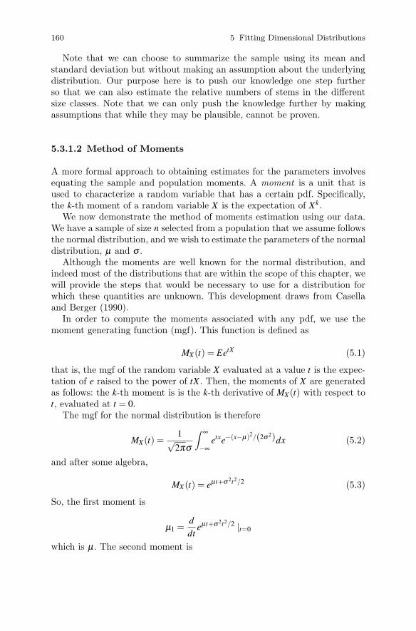
160 5 Fitting Dimensional Distributions
Note that we can choose to summarize the sample using its mean andstandard deviation but without making an assumption about the underlyingdistribution. Our purpose here is to push our knowledge one step furtherso that we can also estimate the relative numbers of stems in the differentsize classes. Note that we can only push the knowledge further by makingassumptions that while they may be plausible, cannot be proven.
5.3.1.2 Method of Moments
A more formal approach to obtaining estimates for the parameters involvesequating the sample and population moments. A moment is a unit that isused to characterize a random variable that has a certain pdf. Specifically,the k-th moment of a random variable X is the expectation of Xk.
We now demonstrate the method of moments estimation using our data.We have a sample of size n selected from a population that we assume followsthe normal distribution, and we wish to estimate the parameters of the normaldistribution, μ and σ .
Although the moments are well known for the normal distribution, andindeed most of the distributions that are within the scope of this chapter, wewill provide the steps that would be necessary to use for a distribution forwhich these quantities are unknown. This development draws from Casellaand Berger (1990).
In order to compute the moments associated with any pdf, we use themoment generating function (mgf). This function is defined as
MX (t) = EetX (5.1)
that is, the mgf of the random variable X evaluated at a value t is the expec-tation of e raised to the power of tX . Then, the moments of X are generatedas follows: the k-th moment is is the k-th derivative of MX (t) with respect tot, evaluated at t = 0.
The mgf for the normal distribution is therefore
MX (t) =1√
2πσ
∫ ∞
−∞etxe−(x−μ)2/(2σ2)dx (5.2)
and after some algebra,
MX (t) = eμt+σ2t2/2 (5.3)
So, the first moment is
μ1 =d
dteμt+σ2t2/2 |t=0
which is μ. The second moment is
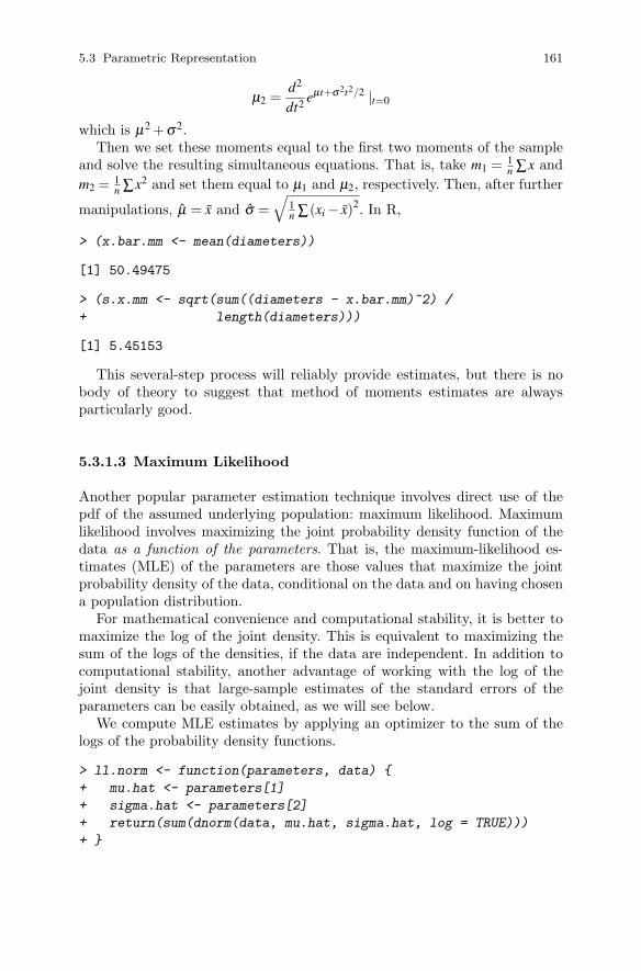
5.3 Parametric Representation 161
μ2 =d2
dt2eμt+σ2t2/2 |t=0
which is μ2 +σ2.Then we set these moments equal to the first two moments of the sample
and solve the resulting simultaneous equations. That is, take m1 =1n ∑x and
m2 =1n ∑x2 and set them equal to μ1 and μ2, respectively. Then, after further
manipulations, μ = x and σ =√
1n ∑(xi − x)2. In R,
> (x.bar.mm <- mean(diameters))
[1] 50.49475
> (s.x.mm <- sqrt(sum((diameters - x.bar.mm)^2) /
+ length(diameters)))
[1] 5.45153
This several-step process will reliably provide estimates, but there is nobody of theory to suggest that method of moments estimates are alwaysparticularly good.
5.3.1.3 Maximum Likelihood
Another popular parameter estimation technique involves direct use of thepdf of the assumed underlying population: maximum likelihood. Maximumlikelihood involves maximizing the joint probability density function of thedata as a function of the parameters. That is, the maximum-likelihood es-timates (MLE) of the parameters are those values that maximize the jointprobability density of the data, conditional on the data and on having chosena population distribution.
For mathematical convenience and computational stability, it is better tomaximize the log of the joint density. This is equivalent to maximizing thesum of the logs of the densities, if the data are independent. In addition tocomputational stability, another advantage of working with the log of thejoint density is that large-sample estimates of the standard errors of theparameters can be easily obtained, as we will see below.
We compute MLE estimates by applying an optimizer to the sum of thelogs of the probability density functions.
> ll.norm <- function(parameters, data) {
+ mu.hat <- parameters[1]
+ sigma.hat <- parameters[2]
+ return(sum(dnorm(data, mu.hat, sigma.hat, log = TRUE)))
+ }
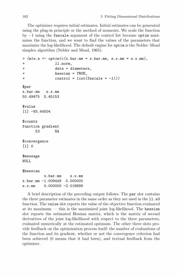
162 5 Fitting Dimensional Distributions
The optimizer requires initial estimates. Initial estimates can be generatedusing the plug-in principle or the method of moments. We scale the functionby −1 using the fnscale argument of the control list because optim mini-mizes the function, and we want to find the values of the parameters thatmaximize the log-likelihood. The default engine for optim is the Nelder–Meadsimplex algorithm (Nelder and Mead, 1965).
> (mle.n <- optim(c(x.bar.mm = x.bar.mm, s.x.mm = s.x.mm),
+ ll.norm,
+ data = diameters,
+ hessian = TRUE,
+ control = list(fnscale = -1)))
$par
x.bar.mm s.x.mm
50.49475 5.45153
$value
[1] -93.44504
$counts
function gradient
53 NA
$convergence
[1] 0
$message
NULL
$hessian
x.bar.mm s.x.mm
x.bar.mm -1.009449 0.000000
s.x.mm 0.000000 -2.018899
A brief description of the preceding output follows. The par slot containsthe three parameter estimates in the same order as they are used in the ll.w3function. The value slot reports the value of the objective function evaluatedat its maximum — this is the maximized joint log-likelihood. The hessian
slot reports the estimated Hessian matrix, which is the matrix of secondderivatives of the joint log-likelihood with respect to the three parameters,evaluated numerically at the estimated optimum. The other three slots pro-vide feedback on the optimization process itself: the number of evaluations ofthe function and its gradient, whether or not the convergence criterion hadbeen achieved (0 means that it had been), and textual feedback from theoptimizer.
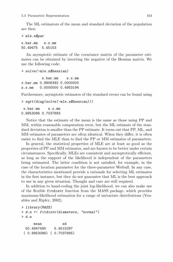
5.3 Parametric Representation 163
The ML estimators of the mean and standard deviation of the populationare then
> mle.n$par
x.bar.mm s.x.mm
50.49475 5.45153
An asymptotic estimate of the covariance matrix of the parameter esti-mates can be obtained by inverting the negative of the Hessian matrix. Weuse the following code:
> solve(-mle.n$hessian)
x.bar.mm s.x.mm
x.bar.mm 0.9906392 0.0000000
s.x.mm 0.0000000 0.4953194
Furthermore, asymptotic estimates of the standard errors can be found using
> sqrt(diag(solve(-mle.n$hessian)))
x.bar.mm s.x.mm
0.9953086 0.7037893
Notice that the estimate of the mean is the same as those using PP andMM, within reasonable computation error, but the ML estimate of the stan-dard deviation is smaller than the PP estimate. It turns out that PP, ML, andMM estimates of parameters are often identical. When they differ, it is ofteneasier to find the MLE than to find the PP or MM estimates of parameters.
In general, the statistical properties of MLE are at least as good as theproperties of PP and MM estimates, and are known to be better under certaincircumstances. Specifically, MLEs are consistent and asymptotically efficient,as long as the support of the likelihood is independent of the parametersbeing estimated. The latter condition is not satisfied, for example, in thecase of the location parameter for the three-parameter Weibull. In any case,the characteristics mentioned provide a rationale for selecting ML estimatesin the first instance, but they do not guarantee that ML is the best approachto use in any given situation. Thought and care are still required.
In addition to hand-coding the joint log-likelihood, we can also make useof the flexible fitdistr function from the MASS package, which providesmaximum-likelihood estimation for a range of univariate distributions (Ven-ables and Ripley, 2002).
> library(MASS)
> d.n <- fitdistr(diameters, "normal")
> d.n
mean sd
50.4947490 5.4515297
( 0.9953086) ( 0.7037895)
164 5 Fitting Dimensional Distributions
5.3.2 Some Models of Choice
Numerous distribution families have been proposed to match diameter dis-tributions; for example, the exponential distribution, the two- and three-parameter Weibull distributions (Bailey and Dell, 1973), and Johnson’s SB
(Hafley and Schreuder, 1977), among many others. Some of these distribu-tions are easy to parameterize; others are more difficult.
We start with the two-parameter Weibull distribution. The Weibull dis-tribution originated in the statistical analysis of failure rates and is popularin the statistical analysis of survival data. The interested reader can learnmore from Johnson et al. (1994). The two-parameter Weibull can be fit to adataset in a number of ways; we use the fitdistr function again.
> d.w2 <- fitdistr(diameters, "weibull")
> d.w2
shape scale
11.5600440 52.8091906
( 1.6694364) ( 0.8766854)
Now we want to compare the two distribution fits; that is, compare the fitof the two-parameter Weibull against the fit of the normal distribution. Thepdfs both have the same number of parameters, so a direct comparison of thelog-likelihoods will yield the same outcome as a comparison of AIC would.
> logLik(d.n)
�log Lik.� -93.44504 (df=2)
> logLik(d.w2)
�log Lik.� -91.75936 (df=2)
These results suggest that the two-parameter Weibull distribution is aslightly better fit to our data than the normal distribution.
The three-parameter Weibull distribution is an extension of the two-parameter Weibull that provides for a shift in location. The three-parameterWeibull distribution is useful when the mass of points is known to be remotefrom zero, which is often the case with tree dimension measurements. Thepdf of the three-parameter Weibull distribution is
fX (x | α,β ,γ) =γ
β
(x−α
β
)γ−1
exp
(−(
x−α
β
)γ)(5.4)
with β > 0, γ > 0, and −∞ < α < ∞. And, in R, we can use the followingfunction:
> dweibull3 <- function(x, gamma, beta, alpha) {
+ (gamma/beta)*((x - alpha)/beta)^(gamma - 1) *
5.3 Parametric Representation 165
+ (exp(-((x - alpha)/beta)^gamma))
+ }
So the joint log-likelihood for an independent sample from the three-parameter Weibull distribution is, ready for optim,
> ll.w3 <- function(p, data)
+ sum(log(dweibull3(data, p[1], p[2], p[3])))
Note that we have separated the steps of computing the pdf and takingits log for clarity. Using a function that computed the log of the densitydirectly would be more efficient and more stable for operational uses. Densityfunctions that are provided in R, for example dnorm, offer the option ofreturning the log of the density value directly. Doing so is recommendedwhen the log of the density is of interest, such as in this case, because iteliminates redundant steps; note, for example, that among other things weare taking the log of the exponential raised to the power −((x−α)/β )γ .
A challenge in fitting this distribution is that the location parameter αlimits the domain of the random variable. Maximum-likelihood inference isproblematic for such models because the likelihood is undefined across a setof the real numbers that is determined by the data. Furthermore, estimatesof such parameters that arise from ML procedures no longer necessarily havethe desirable characteristics of consistency and asymptotic efficiency (Casellaand Berger, 1990).
From the point of view of parameter estimation, the troublesome portionof the pdf is (x−α)γ , which is
� undefined if α > x and γ is not an integer,� negative if α > x and γ is an odd integer, and� increasing as α increases in absolute value for α outside the range of x if
γ is an even integer.
Fortunately, the optimization algorithms are reasonably robust againstthese difficulties and will recover gracefully if they find themselves arrivingin areas of the parameter space for which the function is undefined. Theonly requirement is that the starting values be chosen in such a way that thefunction can be evaluated. For example, upon application to our data and thethree-parameter Weibull log-likelihood, the Nelder–Mead algorithm reportsconvergence and provides plausible parameter estimates.
> mle.w3.nm <- optim(c(gamma = 1, beta = 5, alpha = 10),
+ ll.w3,
+ data = diameters,
+ hessian = TRUE,
+ control = list(fnscale = -1))
> mle.w3.nm$par
166 5 Fitting Dimensional Distributions
gamma beta alpha
6.843394 32.530438 20.122516
The log-likelihood, evaluated at its maximum, is
> mle.w3.nm$value
[1] -91.99055
We can obtain asymptotic estimates of the standard errors from the resultusing code similar to that which we have used previously.
> sqrt(diag(solve(-mle.w3.nm$hessian)))
gamma beta alpha
3.796482 16.293066 16.079340
Different optimization engines may well yield different estimates of theparameters. For example, the optimization method due to Broyden, Fletcher,Goldfarb, and Shanno (see, e.g., Nocedal and Wright, 2006) fails to convergeafter (the default) 100 iterations, and when more iterations are requested,using the maxit option in the control argument, the solution is differentfrom that offered by Nelder–Mead.
> mle.w3.bfgs <- optim( c(gamma = 1, beta = 5, alpha = 10),
+ ll.w3,
+ method = "BFGS",
+ data = diameters,
+ hessian = TRUE,
+ control = list(fnscale = -1,
+ maxit = 1000))
> mle.w3.bfgs$value
[1] -91.75805
> mle.w3.bfgs$par
gamma beta alpha
11.6698254 53.2463892 -0.4232776
> (mle.w3.bfgs.se <- sqrt(diag(solve(-mle.w3.bfgs$hessian))))
gamma beta alpha
13.15200 57.46787 57.22259
These results leave the analyst in somewhat of a dilemma. The outcome offitting the pdf seems to depend on the optimization engine that has been cho-sen. And, if the parameter estimates from BFGS are used as a starting pointfor the Nelder–Mead, then different estimates again are obtained (results notshown here). However, reference to the estimated standard errors suggests
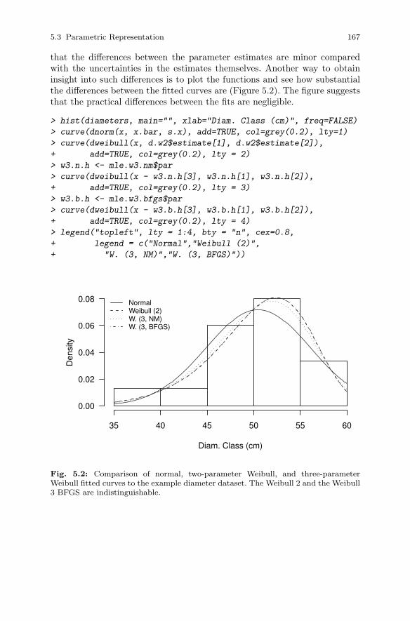
5.3 Parametric Representation 167
that the differences between the parameter estimates are minor comparedwith the uncertainties in the estimates themselves. Another way to obtaininsight into such differences is to plot the functions and see how substantialthe differences between the fitted curves are (Figure 5.2). The figure suggeststhat the practical differences between the fits are negligible.
> hist(diameters, main="", xlab="Diam. Class (cm)", freq=FALSE)
> curve(dnorm(x, x.bar, s.x), add=TRUE, col=grey(0.2), lty=1)
> curve(dweibull(x, d.w2$estimate[1], d.w2$estimate[2]),
+ add=TRUE, col=grey(0.2), lty = 2)
> w3.n.h <- mle.w3.nm$par
> curve(dweibull(x - w3.n.h[3], w3.n.h[1], w3.n.h[2]),
+ add=TRUE, col=grey(0.2), lty = 3)
> w3.b.h <- mle.w3.bfgs$par
> curve(dweibull(x - w3.b.h[3], w3.b.h[1], w3.b.h[2]),
+ add=TRUE, col=grey(0.2), lty = 4)
> legend("topleft", lty = 1:4, bty = "n", cex=0.8,
+ legend = c("Normal","Weibull (2)",
+ "W. (3, NM)","W. (3, BFGS)"))
Diam. Class (cm)
Den
sity
35 40 45 50 55 60
0.00
0.02
0.04
0.06
0.08 NormalWeibull (2)W. (3, NM)W. (3, BFGS)
Fig. 5.2: Comparison of normal, two-parameter Weibull, and three-parameterWeibull fitted curves to the example diameter dataset. The Weibull 2 and the Weibull3 BFGS are indistinguishable.
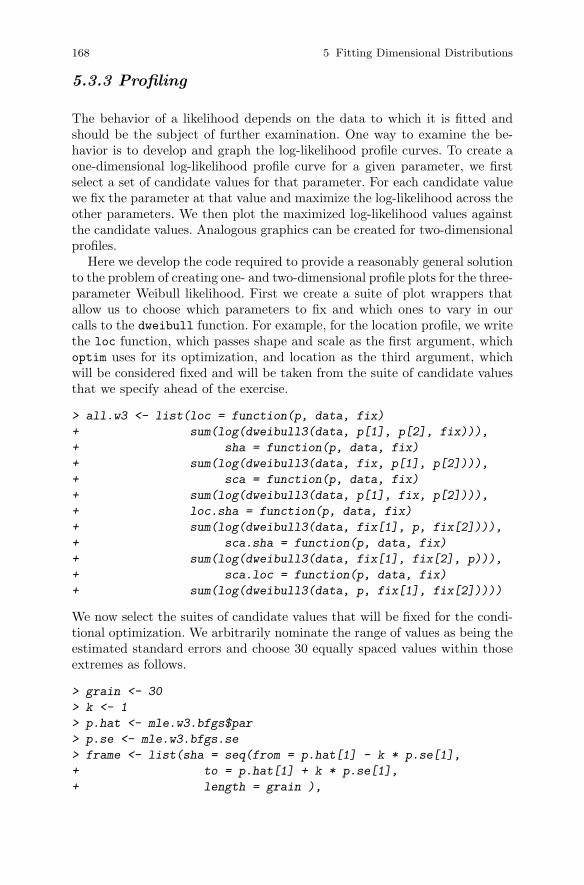
168 5 Fitting Dimensional Distributions
5.3.3 Profiling
The behavior of a likelihood depends on the data to which it is fitted andshould be the subject of further examination. One way to examine the be-havior is to develop and graph the log-likelihood profile curves. To create aone-dimensional log-likelihood profile curve for a given parameter, we firstselect a set of candidate values for that parameter. For each candidate valuewe fix the parameter at that value and maximize the log-likelihood across theother parameters. We then plot the maximized log-likelihood values againstthe candidate values. Analogous graphics can be created for two-dimensionalprofiles.
Here we develop the code required to provide a reasonably general solutionto the problem of creating one- and two-dimensional profile plots for the three-parameter Weibull likelihood. First we create a suite of plot wrappers thatallow us to choose which parameters to fix and which ones to vary in ourcalls to the dweibull function. For example, for the location profile, we writethe loc function, which passes shape and scale as the first argument, whichoptim uses for its optimization, and location as the third argument, whichwill be considered fixed and will be taken from the suite of candidate valuesthat we specify ahead of the exercise.
> all.w3 <- list(loc = function(p, data, fix)
+ sum(log(dweibull3(data, p[1], p[2], fix))),
+ sha = function(p, data, fix)
+ sum(log(dweibull3(data, fix, p[1], p[2]))),
+ sca = function(p, data, fix)
+ sum(log(dweibull3(data, p[1], fix, p[2]))),
+ loc.sha = function(p, data, fix)
+ sum(log(dweibull3(data, fix[1], p, fix[2]))),
+ sca.sha = function(p, data, fix)
+ sum(log(dweibull3(data, fix[1], fix[2], p))),
+ sca.loc = function(p, data, fix)
+ sum(log(dweibull3(data, p, fix[1], fix[2]))))
We now select the suites of candidate values that will be fixed for the condi-tional optimization. We arbitrarily nominate the range of values as being theestimated standard errors and choose 30 equally spaced values within thoseextremes as follows.
> grain <- 30
> k <- 1
> p.hat <- mle.w3.bfgs$par
> p.se <- mle.w3.bfgs.se
> frame <- list(sha = seq(from = p.hat[1] - k * p.se[1],
+ to = p.hat[1] + k * p.se[1],
+ length = grain ),
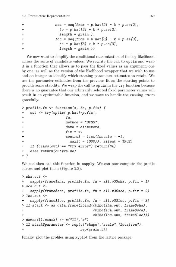
5.3 Parametric Representation 169
+ sca = seq(from = p.hat[2] - k * p.se[2],
+ to = p.hat[2] + k * p.se[2],
+ length = grain ),
+ loc = seq(from = p.hat[3] - k * p.se[3],
+ to = p.hat[3] + k * p.se[3],
+ length = grain ))
We now want to simplify the conditional maximization of the log-likelihoodacross the suite of candidate values. We rewrite the call to optim and wrapit in a function that allows us to pass the fixed values as an argument, oneby one, as well as the version of the likelihood wrapper that we wish to useand an integer to identify which starting parameter estimates to retain. Weuse the parameter estimates from the previous fit as the starting points toprovide some stability. We wrap the call to optim in the try function becausethere is no guarantee that our arbitrarily selected fixed parameter values willresult in an optimizable function, and we want to handle the ensuing errorsgracefully.
> profile.fn <- function(x, fn, p.fix) {
+ out <- try(optim( p.hat[-p.fix],
+ fn,
+ method = "BFGS",
+ data = diameters,
+ fix = x,
+ control = list(fnscale = -1,
+ maxit = 1000)), silent = TRUE)
+ if (class(out) == "try-error") return(NA)
+ else return(out$value)
+ }
We can then call this function in sapply. We can now compute the profilecurves and plot them (Figure 5.3).
> sha.out <-
+ sapply(frame$sha, profile.fn, fn = all.w3$sha, p.fix = 1)
> sca.out <-
+ sapply(frame$sca, profile.fn, fn = all.w3$sca, p.fix = 2)
> loc.out <-
+ sapply(frame$loc, profile.fn, fn = all.w3$loc, p.fix = 3)
> ll.stack <- as.data.frame(rbind(cbind(sha.out, frame$sha),
+ cbind(sca.out, frame$sca),
+ cbind(loc.out, frame$loc)))
> names(ll.stack) <- c("ll","x")
> ll.stack$parameter <- rep(c("shape","scale","location"),
+ rep(grain,3))
Finally, plot the profiles using xyplot from the lattice package.
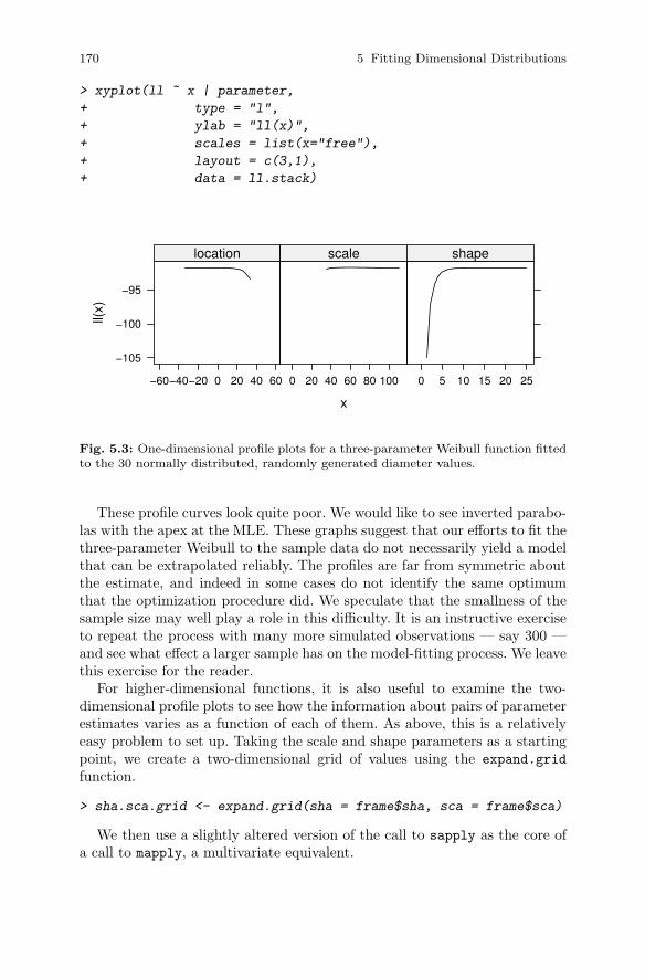
170 5 Fitting Dimensional Distributions
> xyplot(ll ~ x | parameter,
+ type = "l",
+ ylab = "ll(x)",
+ scales = list(x="free"),
+ layout = c(3,1),
+ data = ll.stack)
x
ll(x)
−105
−100
−95
−60−40−20 0 20 40 60
location
0 20 40 60 80 100
scale
0 5 10 15 20 25
shape
Fig. 5.3: One-dimensional profile plots for a three-parameter Weibull function fittedto the 30 normally distributed, randomly generated diameter values.
These profile curves look quite poor. We would like to see inverted parabo-las with the apex at the MLE. These graphs suggest that our efforts to fit thethree-parameter Weibull to the sample data do not necessarily yield a modelthat can be extrapolated reliably. The profiles are far from symmetric aboutthe estimate, and indeed in some cases do not identify the same optimumthat the optimization procedure did. We speculate that the smallness of thesample size may well play a role in this difficulty. It is an instructive exerciseto repeat the process with many more simulated observations — say 300 —and see what effect a larger sample has on the model-fitting process. We leavethis exercise for the reader.
For higher-dimensional functions, it is also useful to examine the two-dimensional profile plots to see how the information about pairs of parameterestimates varies as a function of each of them. As above, this is a relativelyeasy problem to set up. Taking the scale and shape parameters as a startingpoint, we create a two-dimensional grid of values using the expand.grid
function.
> sha.sca.grid <- expand.grid(sha = frame$sha, sca = frame$sca)
We then use a slightly altered version of the call to sapply as the core ofa call to mapply, a multivariate equivalent.
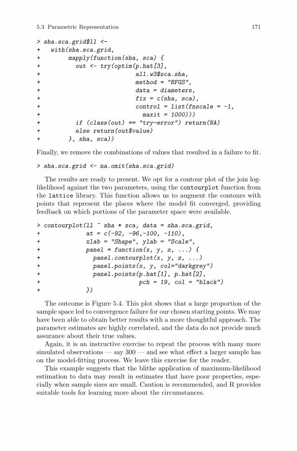
5.3 Parametric Representation 171
> sha.sca.grid$ll <-
+ with(sha.sca.grid,
+ mapply(function(sha, sca) {
+ out <- try(optim(p.hat[3],
+ all.w3$sca.sha,
+ method = "BFGS",
+ data = diameters,
+ fix = c(sha, sca),
+ control = list(fnscale = -1,
+ maxit = 1000)))
+ if (class(out) == "try-error") return(NA)
+ else return(out$value)
+ }, sha, sca))
Finally, we remove the combinations of values that resulted in a failure to fit.
> sha.sca.grid <- na.omit(sha.sca.grid)
The results are ready to present. We opt for a contour plot of the join log-likelihood against the two parameters, using the contourplot function fromthe lattice library. This function allows us to augment the contours withpoints that represent the places where the model fit converged, providingfeedback on which portions of the parameter space were available.
> contourplot(ll ~ sha * sca, data = sha.sca.grid,
+ at = c(-92, -96,-100, -110),
+ xlab = "Shape", ylab = "Scale",
+ panel = function(x, y, z, ...) {
+ panel.contourplot(x, y, z, ...)
+ panel.points(x, y, col="darkgrey")
+ panel.points(p.hat[1], p.hat[2],
+ pch = 19, col = "black")
+ })
The outcome is Figure 5.4. This plot shows that a large proportion of thesample space led to convergence failure for our chosen starting points. We mayhave been able to obtain better results with a more thoughtful approach. Theparameter estimates are highly correlated, and the data do not provide muchassurance about their true values.
Again, it is an instructive exercise to repeat the process with many moresimulated observations — say 300 — and see what effect a larger sample hason the model-fitting process. We leave this exercise for the reader.
This example suggests that the blithe application of maximum-likelihoodestimation to data may result in estimates that have poor properties, espe-cially when sample sizes are small. Caution is recommended, and R providessuitable tools for learning more about the circumstances.
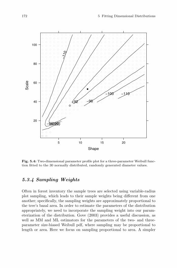
172 5 Fitting Dimensional Distributions
Shape
Sca
le
20
40
60
80
100
5 10 15 20
−92
−96
−96
−100
−100
−110
−110
−110
● ●
● ● ●
● ● ● ●
● ● ● ● ●
● ● ● ● ● ●
● ● ● ● ● ● ●
● ● ● ● ● ● ● ●
● ● ● ● ● ● ● ● ● ●
● ● ● ● ● ● ● ● ● ● ● ● ●
● ● ● ● ● ● ● ● ● ● ● ● ● ● ● ●
● ● ● ● ● ● ● ● ● ● ● ● ● ● ● ● ● ● ● ● ● ●
● ● ● ● ● ● ● ● ● ● ● ● ● ● ● ● ● ● ● ● ● ● ● ● ● ● ●
● ● ● ● ● ● ● ● ● ● ● ● ● ● ● ● ● ● ● ● ● ● ● ● ● ● ●
● ● ● ● ● ● ● ● ● ● ● ● ● ● ● ● ● ● ● ● ● ● ● ● ● ● ●
● ● ● ● ● ● ● ● ● ● ● ● ● ● ● ● ● ● ● ● ● ● ● ● ● ● ●
● ● ● ● ● ● ● ● ● ● ● ● ● ● ● ● ● ● ● ● ● ● ● ● ● ● ●
● ● ● ● ● ● ● ● ● ● ● ● ● ● ● ● ● ● ● ● ● ● ● ● ● ● ●
● ● ● ● ● ● ● ● ● ● ● ● ● ● ● ● ● ● ● ● ● ● ● ● ● ● ●
● ● ● ● ● ● ● ● ● ● ● ● ● ● ● ● ● ● ● ● ● ● ● ● ● ● ●
● ● ● ● ● ● ● ● ● ● ● ● ● ● ● ● ● ● ● ● ● ● ● ● ● ● ●
● ● ● ● ● ● ● ● ● ● ● ● ● ● ● ● ● ● ● ● ● ● ● ● ● ● ●
● ● ● ● ● ● ● ● ● ● ● ● ● ● ● ● ● ● ● ● ● ● ● ● ● ● ●
● ● ● ● ● ● ● ● ● ● ● ● ● ● ● ● ● ● ● ● ● ● ● ● ● ● ●
● ● ● ● ● ● ● ● ● ● ● ● ● ● ● ● ● ● ● ● ● ● ● ● ● ● ●
● ● ● ● ● ● ● ● ● ● ● ● ● ● ● ● ● ● ● ● ● ● ● ● ● ● ●
● ● ● ● ● ● ● ● ● ● ● ● ● ● ● ● ● ● ● ● ● ● ● ● ● ● ●
● ● ● ● ● ● ● ● ● ● ● ● ● ● ● ● ● ● ● ● ● ● ● ● ● ● ●
● ● ● ● ● ● ● ● ● ● ● ● ● ● ● ● ● ● ● ● ● ● ● ● ● ● ●
●
Fig. 5.4: Two-dimensional parameter profile plot for a three-parameter Weibull func-tion fitted to the 30 normally distributed, randomly generated diameter values.
5.3.4 Sampling Weights
Often in forest inventory the sample trees are selected using variable-radiusplot sampling, which leads to their sample weights being different from oneanother; specifically, the sampling weights are approximately proportional tothe tree’s basal area. In order to estimate the parameters of the distributionappropriately, we need to incorporate the sampling weight into our param-eterization of the distribution. Gove (2003) provides a useful discussion, aswell as MM and ML estimators for the parameters of the two- and three-parameter size-biased Weibull pdf, where sampling may be proportional tolength or area. Here we focus on sampling proportional to area. A simpler

5.3 Parametric Representation 173
correction is used for length-biased sampling; see Gove (2003) for furtherdetails.
The alterations that are necessary to make the joint log-likelihood suitablefor area-biased estimation are as follows. We compute a correction to the log-likelihood that allows for the fact that the observations have been drawnwith variable probability. This correction is the following function of theparameters for area-biased sampling (equation (2), Gove, 2003):
μ ′2 = β 2Γ (2/γ +1)+2αβΓ (1/γ +1)+α2 (5.5)
> ll.w3.sb2 <- function(p, data) {
+ gam <- p[1]
+ bet <- p[2]
+ alp <- p[3]
+ mu.prime.2 <- bet^2 * gamma(2/gam + 1) +
+ 2 * bet * gamma(1/gam + 1) * alp + alp^2
+ sum(log(dweibull3(data, gam, bet, alp))) -
+ log(mu.prime.2) * length(data)
+ }
We can now use optim to maximize the joint log-likelihood as we havebefore, and can furthermore obtain asymptotic estimates of the standarderrors of the parameter estimates.
> mle.w3.sb2 <- optim( c(gamma = 1, beta = 5, alpha = 0),
+ ll.w3.sb2,
+ method = "BFGS",
+ data = diameters,
+ hessian = TRUE,
+ control = list(fnscale = -1,
+ maxit = 1000))
The function converges, providing the following estimates:
> mle.w3.sb2$par
gamma beta alpha
13.67537 68.21522 -16.45170
> sqrt(diag(solve(-mle.w3.sb2$hessian)))
gamma beta alpha
20.10398 100.20780 100.04163
The estimated standard errors for the parameter estimates are quite largerelative to the estimates themselves. The overarching message from the statis-tics would appear to be that fitting a three-parameter Weibull function tothese diameters is a fairly perilous prospect.
Chapter 6
Linear and Non-linear Modeling
This chapter describes some of the tools that are available in R for fitting cer-tain kinds of conditional distributions; that is, constructing models to predictthe behavior of one random variable given that the value of another one ormore is known. Examples of such models in forestry include height–diametermodels, diameter–volume models, and so on. Such models are of interest fortwo reasons: in order to make predictions and in order to estimate and inter-pret the parameters that describe the relationship. For example, a scientistmight wish to know whether or not coring trees affects their growth and mor-tality, and how much; this problem is more naturally an interpretation andestimation problem. Alternatively, a manager might wish to predict heightsfor some trees for which only diameters and species are known; this problemis a prediction problem. The intended application of the model intimatelyaffects the fitting process. Breiman (2001b) and the discussions that followare excellent reading on this topic.
6.1 Linear Regression
There are many excellent references that describe the theory and practice oflinear regression. Here we will provide enough information to motivate ourexample and provide context for the analysis. For further reading, we suggestDraper and Smith (1998), Harrell (2001), Weisberg (2005), and Gelman andHill (2007).
Broadly speaking, a goal of regression is to make a statement about thedistribution of the response variable Y conditional on the values of predictorvariable(s) X having some known value(s), F (Y | X1, . . . ,Xp).
Usually we are interested only in the conditional mean and the conditionalvariance, and we ignore the higher-order moments such as the skew. Evidenceof residual skew or kurtosis in the data, conditional on the model, is takenas a sign of poor model choice, and ameliorative action is usually taken, such
175A. P. Robinson, J. D. Hamann, Forest Analytics with R, Use R!,DOI 10.1007/978-1-4419-7762-5_6, © Springer Science+Business Media, LLC 2011
176 6 Linear and Non-linear Modeling
as deploying a generalized linear model or making a transformation of theresponse variable.
Furthermore, in performing, for example, ordinary least-squares linear re-gression, we will assume that the conditional distribution of Y given X isnormal. The mean and variance are (jointly) a sufficient statistic for the nor-mal distribution, and other moments are known and fixed. If this assumptionis untenable, then some alternative approach must be found, which we willtouch upon later.
So, we can simplify the expression of our model as
yi = f (xi;βββ )+ εi
where f is a known function of known predictor variables x and some unknownparameters βββ . For linear regression, we write
yi = β0 +β1x1i + . . .+βpxpi + εi
That is, the β s are the gradients, or (partial) first derivatives, of the rela-tionship between y and the xs. f is encapsulated by two model statements,
E (Y | X1, . . . ,Xp) = β0 +p
∑j=1
β jx ji
and
Var(Y | X1, . . . ,Xp) = σ2
This model is called a linear model because it is linear in the predictors.Formally, a linear model is one for which none of the first derivatives of themean function with respect to each of the parameters contain any of theparameters. Hence the linearity in the model label refers to the parameters,not to the predictor variables.
Our goal is to find the best estimates of the β s and σ . We have to providesome structure in order to do so. First, we have to choose what is meantby best and develop an objective function that reflects the definition. Forexample, we might say that we would like the estimates of the β s to be thosethat minimize the sum of the squared residuals. This particular strategy isknown as least-squares estimation, also referred to as L2 minimization.
Other objective functions are possible and may be more appropriate. Wenote in passing that the sum of absolute values of the deviations is an L1
criterion and the maximum of the absolute deviations is an L∞ criterion.Least-squares estimation has some pleasant properties that are not immedi-ately obvious, not least among which is that the sums of squares of variousportions of the model are additive.
We can construct these estimates using one of numerous methods. To mini-mize the least-squares objective function, we could use brute force (numericalminimization, using for example the Gauss–Newton algorithm) or, more ele-
6.1 Linear Regression 177
gantly, we could differentiate the sum of squared residuals with regard to theβ s, set these derivatives to 0, and solve the resulting system of simultaneousequations, called the normal equations. Neither of these approaches is takenby R because neither is necessarily numerically stable or efficient; by defaultR uses QR-decomposition (Chambers and Hastie, 1992, Section 4.4.2).
It turns out that the least-squares parameter estimates are unbiased (see,among many others, Weisberg, 2005), although we did not specify that theyhad to be. Furthermore, the Gauss–Markov Theorem (see, among many oth-ers, Casella and Berger, 1990) establishes that among all linear unbiasedestimates the least-squares estimates have the lowest possible variance; thatis, they are the most efficient. So, the least-squares estimates are referred toas BLUEs, that is, Best Linear Unbiased Estimates.
However, if the population from which the residuals are sampled is nor-mally distributed, then other useful facts hold. First, the least-squares esti-mates are also normally distributed, which greatly simplifies the problem ofcreating and interpreting interval estimates of the parameters. Second, theleast-squares estimates are now the minimum-variance estimates among allpossible unbiased estimators, not just the linear ones. Such estimates arecalled minimum-variance unbiased estimators (MVUEs). These latter pointsprovide us motivation to check the assumption of the normality of the resid-uals; if the regression assumptions are satisfied, then our model has betterstatistical properties than if they are not satisfied. We may be able to ob-tain unbiased estimates that have as low a variance as least-squares estimatesusing some other algorithm, but not unbiased estimates that have lower vari-ance.
Forming interval estimates and performing hypothesis tests on the popu-lation parameters both require an estimate of the conditional variance, σ2.This term can be estimated using the variance of the residuals. However,the model assumes that the variance is constant. There are many ways thatthis assumption could fail to be true, but in practice we really only worryabout one way: if the variance seems to change systematically with any ofthe available predictor variables. If the variance changes systematically with avariable, then we have to ask whether or not the interval estimates or the out-comes of tests that we compute might change depending on X . That wouldbe an unsatisfactory outcome. Hence we check the assumption of constantvariance and take action if the assumption seems unreasonable. For example,we may elect to use generalized linear modeling, or we may transform theresponse variable, or use weighted least squares, or even try to model thevariance explicitly, if we have enough data and sufficient motivation.
A further concern in estimating the residual variance is that we need tobe sure that the data are valued appropriately; that is, the observations tellus as much about the system as we hope they do. A key way in which thisassumption can fail to be true is if the population from which the residualsare sampled has correlation structure, a situation that is usually informallyreferred to as having correlated residuals. Although that seems like it might
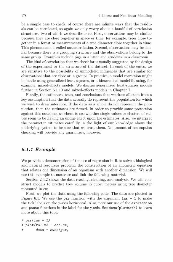
178 6 Linear and Non-linear Modeling
be a simple case to check, of course there are infinite ways that the residu-als can be correlated, so again we only worry about a handful of correlationstructures, two of which we describe here. First, observations may be similarbecause they are close together in space or time; for example, trees close to-gether in a forest or measurements of a tree diameter close together in time.This phenomenon is called autocorrelation. Second, observations may be sim-ilar because there is a grouping structure and the observations belong to thesame group. Examples include pigs in a litter and students in a classroom.
The kind of correlation that we check for is usually suggested by the designof the experiment or the structure of the dataset. In each of the cases, weare sensitive to the possibility of unmodeled influences that are similar forobservations that are close or in groups. In practice, a model correction mightbe made using generalized least squares, or a hierarchical model fit using, forexample, mixed-effects models. We discuss generalized least-squares modelsfurther in Section 6.1.10 and mixed-effects models in Chapter 7.
Finally, the estimates, tests, and conclusions that we draw all stem from akey assumption that the data actually do represent the population for whichwe wish to draw inference. If the data as a whole do not represent the pop-ulation, then the estimates are flawed. In order to provide some protectionagainst this outcome, we check to see whether single values or clusters of val-ues seem to be having an undue effect upon the estimates. Also, we interpretthe parameter estimates carefully in the light of our knowledge about theunderlying system to be sure that we trust them. No amount of assumptionchecking will provide any guarantees, however.
6.1.1 Example
We provide a demonstration of the use of regression in R to solve a biologicaland natural resources problem: the construction of an allometric equationthat relates one dimension of an organism with another dimension. We willuse this example to motivate and link the following material.
Section 2.4.2 shows the data reading, cleaning, and analysis. We will con-struct models to predict tree volume in cubic meters using tree diametermeasured in cm.
First, we plot the data using the following code. The data are plotted inFigure 6.1. We use the par function with the argument las = 1 to makethe tick labels on the y-axis horizontal. Also, note our use of the expressionand paste functions in the label for the y-axis. See demo(plotmath) to learnmore about this topic.
> par(las = 1)
> plot(vol.m3 ~ dbh.cm,
+ data = sweetgum,
6.1 Linear Regression 179
+ xlab = "Diameter (cm)",
+ ylab = expression(paste("Volume (", m^3, ")")))
●
●
●
●
●●
●
●
●
●
●
●
●
●
●●
●
●
●
●
●
●
●
●
●
●
●
●
●
●
●
●
●
●●
●
●
●
●
20 30 40 50 60 70
0
1
2
3
4
5
6
Diameter (cm)
Vol
ume
(m3 )
Fig. 6.1: Scatterplot of volume against diameter for sweetgum data.
It is tempting at this point to immediately start thinking of ways thatthe linear regression could fail and to try to identify the assumptions thatare likely to be contradicted. Some analysts may even begin with favoredtransformations of the response variable. We try to avoid transformation if atall possible. First, it is unusual, although not impossible, for transformationto preserve the meaning of the model. That is, we mind the fact that themodel can play an important role as a mathematical representation of thesystem that is being modeled. Transformation may result in a model withbetter statistical properties but lacking the meaning inherent in the originalmodel. Second, transformation may not be necessary, depending on the modelbeing fitted and the dataset. Fitting models is inexpensive, and much can belearned about the data and model from fitting the basic models to the rawdata and examining them. Also, it may well be that the base model and theraw data combine in an acceptable way. So, we avoid tempting pre-emptivemeasures. However, fitting models should not be used as a substitute forthinking about the problem.
180 6 Linear and Non-linear Modeling
6.1.2 Thinking about the Problem
We need to identify the scope of applications that the model will be used for.In some settings, the scope of applications will be known, at least approxi-mately, before the data are collected. Often the scope will change, or not befully formulated before modeling begins, and compromises will be called for.
Here, we wish to be able to predict an unobserved volume conditional ona known diameter,
vi = β0 +β1 ×di + εi (6.1)
We would like to make an interval prediction and would like this intervalprediction to have good statistical properties. For example, we would likeour interval to be wide enough that it covers the true value with specifiedconfidence but be no wider than it really needs to be. We would like ourestimators to be unbiased. We would like our estimators to make as efficientuse of the data as possible, meaning that they should have minimum varianceamong the class of unbiased estimators. To support our stated preferences,we will make the following assumptions:
1. the linear model captures the relationship,2. εi are independent,3. εi have constant variance,4. εi are normally distributed, and5. the sample represents the population from which it was drawn.
The scope of applications of the model is important to know because itaffects what compromises we are willing to make in the modeling process,which in turn affects how important the different model assumptions are. Asnoted above, two fairly distinct applications for models are the prediction offuture values and the estimation of population or process parameters. Anyapplication that requires knowledge of the distribution of the estimator, suchas hypothesis testing and interval estimation, will demand that the assump-tions about constant variance and normal residuals be satisfied to some degreeunless the analyst wishes to fall back on large-sample theory. Applicationsthat merely require point estimates will not be so stringent.
6.1.3 Fitting the Model
The lm function is used to fit least-squares regression.
> sweetgum.lm.d <- lm(vol.m3 ~ dbh.cm, data=sweetgum)
6.1 Linear Regression 181
This code fits the model vi = β0 +β1 × di + εi. Note that we did not specifythe intercept term; R includes it by default. To remove the intercept fromthe model, we would instead write vol.m3 ~ dbh.cm - 1.
6.1.4 Assumptions and Diagnostics
We noted above that, in order for our estimators to have good statisticalproperties, we need several assumptions to be true. Each desirable propertycan be connected to one or more assumptions. Not all properties are necessaryto use the model; therefore, some assumptions will be less important thanothers, depending upon the application.
There is no way to know whether these assumptions are true, but it ispossible to determine whether or not the assumptions are reasonable by us-ing graphical diagnostics. Checking assumptions in this way distinguishes astatistical analysis from the mathematical operation of just minimizing anobjective function.
The default graphical display, which is created by the plot function whenan object of class lm is passed as its first argument, produces four plots, andtwo others can be obtained by using the which argument (Figure 6.2). Opin-ions vary among statisticians as to the utility and necessity of the followinggraphics. We find them useful. We obtain the diagnostics using the followingcode. Note the use of par to set up a 2×2 matrix of plots with appropriatelysized margins.
> par(mfrow = c(2, 2), mar=c(4, 4, 3, 1), las = 1)
> plot(sweetgum.lm.d)
The default graphical representation of the model provides plots of themodel residuals, scaled and manipulated in various ways as described below.Smooth lines are superimposed to aid interpretation; however, in cases wherethe sample size is small, these smooth lines can overemphasize departuresfrom acceptable patterns, so they should not be overinterpreted. As a remedy,R will allow the plot function to pass those arguments that should be passedto the functions that it calls. Hence, a less wiggly set of smooth lines can beobtained by including, say, span = 2 in the call to plot. Also, keep in mindthat unstandardized residuals will have non-constant variances by design.
We interpret these diagnostic graphics as follows.
� The top-left panel shows a plot of the residuals against the fitted values,with a smooth curve superimposed. Here we are looking for evidence ofcurvature and outliers. Our plot shows curvature, which we are concernedabout, but no points that are particularly unlike the others. Curvature inthis plot is of concern because it suggests possibly substantial local bias inthe model. Also, curvature contradicts the first assumption above. These
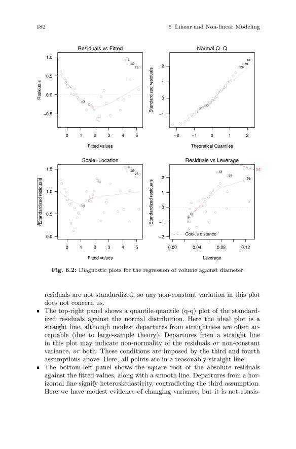
182 6 Linear and Non-linear Modeling
0 1 2 3 4 5
−0.5
0.0
0.5
1.0
Fitted values
Res
idua
ls
●
●
●
●
●
●
●
●
● ●
●
●
●
●
●
●
●
●
●
●
●
●
●
●
●
●
●
●
●
●
●
●
●
●●
●
●
●
●
Residuals vs Fitted
1339
26
●
●
●
●
●
●
●
●
●●
●
●
●
●
●
●
●
●
●
●
●
●
●
●
●
●
●
●
●
●
●
●
●
●●
●
●
●
●
−2 −1 0 1 2
−1
0
1
2
Theoretical QuantilesS
tand
ardi
zed
resi
dual
s
Normal Q−Q
1339
26
0 1 2 3 4 5
0.0
0.5
1.0
1.5
Fitted values
Sta
ndar
dize
d re
sidu
als
●
●●
●
●●
●
●
●●
●
●
●
●●
●
●
●
●
●
●
●
●
●
●
●
●
●
●
●
●
●
●
●●
●
●
●
●
Scale−Location13
3926
0.00 0.04 0.08 0.12
−2
−1
0
1
2
Leverage
Sta
ndar
dize
d re
sidu
als
●
●
●
●
●
●
●
●
●●
●
●
●
●
●
●
●
●
●
●
●
●
●
●
●
●
●
●
●
●
●
●
●
●●
●
●
●
●
Cook's distance
0.5
Residuals vs Leverage
26
1339
Fig. 6.2: Diagnostic plots for the regression of volume against diameter.
residuals are not standardized, so any non-constant variation in this plotdoes not concern us.
� The top-right panel shows a quantile-quantile (q-q) plot of the standard-ized residuals against the normal distribution. Here the ideal plot is astraight line, although modest departures from straightness are often ac-ceptable (due to large-sample theory). Departures from a straight linein this plot may indicate non-normality of the residuals or non-constantvariance, or both. These conditions are imposed by the third and fourthassumptions above. Here, all points are in a reasonably straight line.
� The bottom-left panel shows the square root of the absolute residualsagainst the fitted values, along with a smooth line. Departures from a hor-izontal line signify heteroskedasticity, contradicting the third assumption.Here we have modest evidence of changing variance, but it is not consis-

6.1 Linear Regression 183
tent. Interpretation of this graph will be complicated by variability in themean of the residuals, which we clearly observe in the top-left panel.
� The bottom-right panel shows a plot of the leverage of the observa-tions against the standardized residuals. These are the two componentsof Cook’s distance, which is a statistic that reports the overall effect onthe parameter estimates of each of the observations (Cook, 1977). So faras observations are concerned, being a large residual or a high leveragepoint alone is no guarantee of having a substantial impact on the param-eter estimates. A reasonably well accepted rule of thumb is that Cook’sdistances greater than 1 should attract our attention. Contours of thesedistances1 at 0.5 and 1.0 are added to the graph by default to assist suchan interpretation. This plot provides us with some information about thefifth assumption above. Here we see no evidence to suggest that morethan one population has been sampled or that the population that hasbeen sampled is unduly heterogeneous.
Interpretation of diagnostics is as much an art as it is a science. On av-erage, our experience is that more experienced data analysts tend to be lessconcerned than less experienced analysts about deviation from the strict ex-pectations. Whether this greater relaxation reflects experience or fatigue re-mains a point of conjecture. However, training one’s eye is instructive andeasy: generate a clutch of diagnostic plots, for example q-q plots, on datagenerated randomly under the null hypothesis.2
R does not automatically provide diagnostics that are relevant to testingthe assumption of independence. If we suspect that residual dependence isa possibility, then we would fit a model that accommodates it and examineestimates of its magnitude. For example, we might check for clustering byfitting a mixed-effects model and estimating the intra-class correlation (seep. 241) and check autocorrelation by fitting a generalized least-squares modelwith an autocorrelation function using the gls function of the nlme package(see Section 6.1.10).
Overall, the panels show worrying curvature. We will now quash our evilthoughts about transformations. In fact, it is natural to think of the followingallometric function in the context of predicting volume from diameter:
yi = β0xβ1i × εi (6.2)
It is easy to fit something like this model, although with additive instead ofmultiplicative errors, as a non-linear least-squares model (see Section 6.2.9).For the moment, we take log transformations of the response and the predictorvariables and use those as the predictor and response variables for a new linearmodel.
1 These contours should probably be referred to as isoCooks.2 For example, par(mfrow=c(4,4)); for (i in 1:16) qqnorm(rnorm(20)).
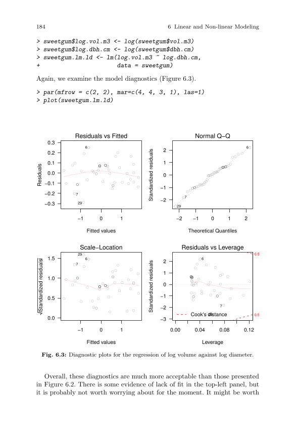
184 6 Linear and Non-linear Modeling
> sweetgum$log.vol.m3 <- log(sweetgum$vol.m3)
> sweetgum$log.dbh.cm <- log(sweetgum$dbh.cm)
> sweetgum.lm.ld <- lm(log.vol.m3 ~ log.dbh.cm,
+ data = sweetgum)
Again, we examine the model diagnostics (Figure 6.3).
> par(mfrow = c(2, 2), mar=c(4, 4, 3, 1), las=1)
> plot(sweetgum.lm.ld)
−1 0 1
−0.3
−0.2
−0.1
0.0
0.1
0.2
0.3
Fitted values
Res
idua
ls ● ●
● ●
●
●
●
●
●
●
●
● ●
●
●
●
●
●
●
●
●
●●
●●
●
●
●
●
●●
●
●
●
● ●
●
●
●
Residuals vs Fitted
29
6
7
●●
●●
●
●
●
●
●
●
●
●●
●
●
●
●
●
●
●
●
●●
●●
●
●
●
●
●●
●
●
●
●●
●
●
●
−2 −1 0 1 2
−2
−1
0
1
2
Theoretical Quantiles
Sta
ndar
dize
d re
sidu
als
Normal Q−Q
29
6
7
−1 0 1
0.0
0.5
1.0
1.5
Fitted values
Sta
ndar
dize
d re
sidu
als
●●
●●
●
●
●
●
●
●
●
● ●
●
●
●
●
●
●
●
●
●●
●●
●
●
●
●
●●
●
●
●
● ●
●
●
●
Scale−Location29
6
7
0.00 0.04 0.08 0.12
−3
−2
−1
0
1
2
Leverage
Sta
ndar
dize
d re
sidu
als
●●
●●
●
●
●
●
●
●
●
● ●
●
●
●
●
●
●
●
●
●●
●●
●
●
●
●
●●
●
●
●
●●
●
●
●
Cook's distance 0.5
0.5
Residuals vs Leverage
29
7
6
Fig. 6.3: Diagnostic plots for the regression of log volume against log diameter.
Overall, these diagnostics are much more acceptable than those presentedin Figure 6.2. There is some evidence of lack of fit in the top-left panel, butit is probably not worth worrying about for the moment. It might be worth
6.1 Linear Regression 185
experimenting with a few other terms in the model to see if the lack of fitcan be ironed out, but to do so here is beyond the scope of this chapter.
6.1.5 Examining the Model
Having satisfied ourselves that the model is at least reasonable, by using theregression diagnostics, we can examine parameter estimates and summarystatistics. The summary function reports a number of useful statistics. Wedissect it as follows.
> summary(sweetgum.lm.ld)
First, the fitted model call is identified. This identification may seem redun-dant, but it is useful when the model is more complex and has been specifiedusing some of the convenient shortcuts that are available.
Call:
lm(formula = log.vol.m3 ~ log.dbh.cm, data = sweetgum)
The distribution of the residuals is then summarized by the minimum, max-imum, median, and two quartiles. Ideally the distribution will be symmetric.
Residuals:
Min 1Q Median 3Q Max
-0.286306 -0.089245 0.008477 0.071497 0.249096
A regression table is presented, including the parameter estimates, their es-timated standard errors, the t-statistic for the two-sided null hypothesis thatthe population or process parameter is actually 0, and the p-value appropriateto that same test.
Coefficients:
Estimate Std. Error t value Pr(>|t|)
(Intercept) -7.80452 0.14542 -53.67 <2e-16 ***
log.dbh.cm 2.22675 0.04023 55.35 <2e-16 ***
---
Signif. codes: 0 �***� 0.001 �**� 0.01 �*� 0.05 �.� 0.1 � � 1
Finally, some summary statistics of the model fit are presented: the estimatedstandard deviation of the errors, the multiple and adjusted R-squared values,and the F-statistics and associated p-value for the null hypothesis that themodel is no better than the sample mean of the response variable.
Residual standard error: 0.1163 on 37 degrees of freedom
Multiple R-squared: 0.9881, Adjusted R-squared: 0.9877
F-statistic: 3063 on 1 and 37 DF, p-value: < 2.2e-16
186 6 Linear and Non-linear Modeling
An informal way to assess the usefulness of the model is to compare themarginal and conditional variabilities of the response variable — e.g., comparethe standard deviation of the response variable with the standard deviation ofthe residuals. Here there is a big difference between the marginal variability,which is 1.05 (units are logm3), and the conditional variability, which is 0.12(units are logm3). The model appears to be a useful one. A formal comparisonwould require the use of cross-validation or a similar strategy (see, e.g., Hastieet al., 2009).
We can obtain interval estimates of the model parameters in several ways.For example, we can compute estimates directly from a portion of the outputof the summary statement. Here we capture the output as an object, convertit to a data frame, and then manipulate it to obtain an interval estimate forthe slope.
> reg.table <- as.data.frame(coef(summary(sweetgum.lm.ld)))
> reg.table$Estimate[2] +
+ reg.table$�Std. Error�[2] *
+ qt(c(0.025, 0.975), summary(sweetgum.lm.ld)$df[2])
[1] 2.145230 2.308270
The same quantities can be more easily obtained using the confint function:
> confint(sweetgum.lm.ld)
2.5 % 97.5 %
(Intercept) -8.099178 -7.509869
log.dbh.cm 2.145230 2.308270
In order to interpret the interval estimates appropriately, it is essentialthat we check the assumptions that underpin them. Specifically, the intervalestimates are made conditional on the assumption that the sampling distribu-tion of the parameter estimate is normal with mean equal to the populationparameter and constant variance. For this to be true, we need the assump-tions 1–5 listed on p. 180 to be true or that the sample size be sufficientlylarge that the Central Limit Theorem can be invoked in place of assumption 4. These assumptions are assessed using the graphical diagnostics presentedin Figure 6.2 as well as our knowledge about the system or process that thedata represent and our knowledge of the protocols by which the data werecollected.
More general manipulation of the parameter estimates is also possible. Al-though it seems cumbersome, the estimable function of the gmodels packageprovides great flexibility in that it constructs point and interval estimates forarbitrary linear combinations of the parameter estimates for a wide range ofdifferent model objects (Warnes, 2010). The function requires a specificationof the linear combinations of interest, but the specification can be in one of a

6.1 Linear Regression 187
number of formats. Here we opt for a matrix with named rows and truncatethe output. See the estimable help file for more information.
> library(gmodels)
> estimable(sweetgum.lm.ld,
+ rbind(Intercept = c(1,0),
+ Slope = c(0,1)),
+ conf.int = 0.95)[,c(1,2,4,6,7)]
Estimate Std. Error DF Lower.CI Upper.CI
Intercept -7.804523 0.14542291 37 -8.099178 -7.509869
Slope 2.226750 0.04023317 37 2.145230 2.308270
We now diverge from the example to discuss elements of R that are sug-gested by the preceding code. Readers that are uninterested in the internalsof R should skip to the next section.
We can identify some of the object classes that have a correspondingestimable method via the methods function.
> methods(estimable)
[1] estimable.default* estimable.mer* estimable.mlm*
Non-visible functions are asterisked
However, the list is not definitive because the default function may handlea wide range of object types. What do we do? The next step would be toexamine the source code of the default method by printing it,
> estimable.default
Error in eval(expr, envir, enclos) : object �estimable.default�
not found
but the code seems to be hidden. Therefore we call on the getAnywhere
function with success.
> getAnywhere(estimable.default)
A single object matching �estimable.default� was found
It was found in the following places
registered S3 method for estimable from namespace gmodels
namespace:gmodels
with value
function (obj, cm, beta0, conf.int = NULL, show.beta0,
joint.test = FALSE, ...)
And, scrolling down through the code, we find the list of classes that thefunction is used for.
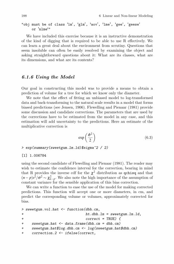
188 6 Linear and Non-linear Modeling
"obj must be of class �lm�, �glm�, �aov�, �lme�, �gee�, �geese�
or �nlme�"
We have included this exercise because it is an instructive demonstrationof the kind of digging that is required to be able to use R effectively. Wecan learn a great deal about the environment from scrutiny. Questions thatseem insoluble can often be easily resolved by examining the object andasking straightforward questions about it: What are its classes, what areits dimensions, and what are its contents?
6.1.6 Using the Model
Our goal in constructing this model was to provide a means to obtain aprediction of volume for a tree for which we know only the diameter.
We note that the effect of fitting an unbiased model to log-transformeddata and back-transforming to the natural scale results in a model that formsbiased predictions (see Jensen, 1906). Flewelling and Pienaar (1981) providesome discussion and candidate corrections. The parameters that are used bythe corrections have to be estimated from the model in any case, and thisestimation will add uncertainty to the predictions. Here an estimate of themultiplicative correction is
exp
(σ2
2
)(6.3)
> exp(summary(sweetgum.lm.ld)$sigma^2 / 2)
[1] 1.006784
using the second candidate of Flewelling and Pienaar (1981). The reader maywish to estimate the confidence interval for the correction, bearing in mindthat R provides the inverse cdf for the χ2 distribution as qchisq and that(n− p)s2/σ2 ∼ χ2
n−p. We also note the high importance of the assumption ofconstant variance for the sensible application of this bias correction.
We can write a function to ease the use of the model for making correctedpredictions. This function will accept one or more diameters, in cm, andpredict the corresponding volume or volumes, approximately corrected forbias.
> sweetgum.vol.hat <- function(dbh.cm,
+ ht.dbh.lm = sweetgum.lm.ld,
+ correct = TRUE) {
+ sweetgum.hat <- data.frame(dbh.cm = dbh.cm)
+ sweetgum.hat$log.dbh.cm <- log(sweetgum.hat$dbh.cm)
+ correction.2 <- ifelse(correct,

6.1 Linear Regression 189
+ exp(summary(ht.dbh.lm)$sigma^2 / 2),
+ 1)
+ sweetgum.hat$vol.m3 <-
+ exp(predict(ht.dbh.lm, newdata = sweetgum.hat)) *
+ correction.2
+ return(sweetgum.hat$vol.m3)
+ }
We can then use the function
> sweetgum.vol.hat(10, sweetgum.lm.ld)
[1] 0.06921896
as inputs, as well as single values. Such code is called vectorized and willexecute much more quickly than an equivalent operation within a loop.
> sweetgum.vol.hat(c(10,12), sweetgum.lm.ld)
[1] 0.06921896 0.10388239
We can also omit the correction to see how large it is for these trees.
> sweetgum.vol.hat(c(10,12), sweetgum.lm.ld, correct = FALSE)
[1] 0.06875256 0.10318242
We note in passing that we could simplify the use of the function even fur-ther by omitting the second argument and identifying our lm object directlyin the predict function. R would search the environment that has been cre-ated by the function for the object and upon failing to find it would searchthe parent environment from which the function was called. R would find theobject there and either use that object (if no changes are being made) or acopy of it if changes are to be made. This nested search path provides anexample of lexical scoping. Lexical scoping permits complicated sets of op-erations to be expressed and performed very easily. However, lexical scopingcontains traps for the unwary; it is easy to perform operations on the wrongobject.
Figure 6.4 presents a view of the data and the model. It replicates Fig-ure 6.1 and adds the fitted line by using the curve function.
> par(las = 1)
> plot(vol.m3 ~ dbh.cm,
+ data = sweetgum,
+ xlab = "Diameter (cm)",
+ ylab = expression(paste("Volume (", m^3, ")")))
> curve(sweetgum.vol.hat, from=0, to=100, add=TRUE)

190 6 Linear and Non-linear Modeling
●
●
●
●
●●
●
●
●
●
●
●
●
●
●●
●
●
●
●
●
●
●
●
●
●
●
●
●
●
●
●
●
●●
●
●
●
●
20 30 40 50 60 70
0
1
2
3
4
5
6
Diameter (cm)
Vol
ume
(m3 )
Fig. 6.4: Scatterplot of volume against diameter for sweetgum data with fitted modelsuperimposed.
In order for curve to work, we needed to be sure that all arguments forsweetgum.vol.hat other than the first were provided default values in thefunction definition. Default values are provided to the function using thefollowing protocol in the declaration: argument = default.
We can use the predict function to obtain prediction intervals for valuesof interest of the predictor variables. For example,
> exp(predict(sweetgum.lm.ld,
+ newdata = data.frame(log.dbh.cm = log(c(10, 20))),
+ interval = "prediction"))
fit lwr upr
1 0.06875256 0.05298514 0.08921207
2 0.32181591 0.25229082 0.41050038
These estimates are not corrected for bias, although extending the functionabove to provide bias-corrected interval estimates is a straightforward exer-cise.
We now take another brief detour into the workings of R. Again, we directthe disinterested reader to the end of the section.
Model interrogation is enriched if we take advantage of the fact that themodel that we have fitted is an object and the summary of that model fit isa different object. The following discussion pertains to S3 classes. Completecoverage of R’s facilities for object-oriented programming, including S3 andS4 classes, is beyond the scope of this book.

6.1 Linear Regression 191
> names(sweetgum.lm.ld)
[1] "coefficients" "residuals" "effects"
[4] "rank" "fitted.values" "assign"
[7] "qr" "df.residual" "xlevels"
[10] "call" "terms" "model"
> names(summary(sweetgum.lm.ld))
[1] "call" "terms" "residuals"
[4] "coefficients" "aliased" "sigma"
[7] "df" "r.squared" "adj.r.squared"
[10] "fstatistic" "cov.unscaled"
The reader may also wish to try the str function on these two objects.Some high-level functions, called methods, exist to enable the reliable ex-
traction of model information, for example, the residuals and fitted func-tions are methods that will extract the residuals and the fitted values, re-spectively.
We can learn what methods are available for our object as follows: firstidentify the class of the object, and then call the methods function using theclass as the argument. Here we print only the first few.
> class(sweetgum.lm.ld)
[1] "lm"
> head(methods(class = class(sweetgum.lm.ld)))
[1] "BIC.lm" "add1.lm" "addterm.lm" "alias.lm"
[5] "anova.lm" "attrassign.lm"
We can also extract or otherwise manipulate the attributes of some objectsby means of the $ sign:
> sweetgum.lm.ld$call
lm(formula = log.vol.m3 ~ log.dbh.cm, data = sweetgum)
> summary(sweetgum.lm.ld)$sigma
[1] 0.1162833
Generally, code authors prefer that attributes be extracted using custom-written extractor functions. An example extractor function to extract theestimate of the standard deviation of the residuals might look like this:
> sigma <- function(x) {
+ if (class(x) == "lm") {
+ return(summary(x)$sigma)
+ } else {
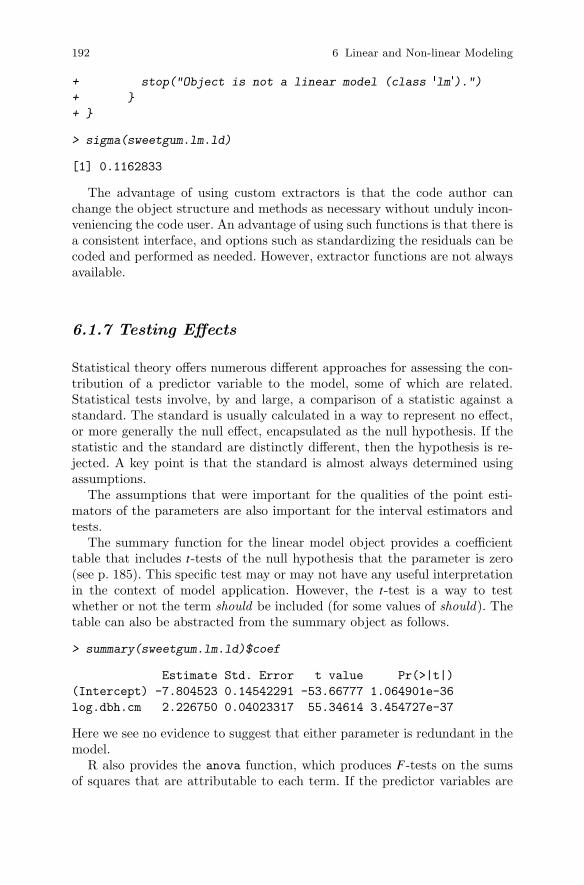
192 6 Linear and Non-linear Modeling
+ stop("Object is not a linear model (class �lm�).")
+ }
+ }
> sigma(sweetgum.lm.ld)
[1] 0.1162833
The advantage of using custom extractors is that the code author canchange the object structure and methods as necessary without unduly incon-veniencing the code user. An advantage of using such functions is that there isa consistent interface, and options such as standardizing the residuals can becoded and performed as needed. However, extractor functions are not alwaysavailable.
6.1.7 Testing Effects
Statistical theory offers numerous different approaches for assessing the con-tribution of a predictor variable to the model, some of which are related.Statistical tests involve, by and large, a comparison of a statistic against astandard. The standard is usually calculated in a way to represent no effect,or more generally the null effect, encapsulated as the null hypothesis. If thestatistic and the standard are distinctly different, then the hypothesis is re-jected. A key point is that the standard is almost always determined usingassumptions.
The assumptions that were important for the qualities of the point esti-mators of the parameters are also important for the interval estimators andtests.
The summary function for the linear model object provides a coefficienttable that includes t-tests of the null hypothesis that the parameter is zero(see p. 185). This specific test may or may not have any useful interpretationin the context of model application. However, the t-test is a way to testwhether or not the term should be included (for some values of should). Thetable can also be abstracted from the summary object as follows.
> summary(sweetgum.lm.ld)$coef
Estimate Std. Error t value Pr(>|t|)
(Intercept) -7.804523 0.14542291 -53.66777 1.064901e-36
log.dbh.cm 2.226750 0.04023317 55.34614 3.454727e-37
Here we see no evidence to suggest that either parameter is redundant in themodel.
R also provides the anova function, which produces F-tests on the sumsof squares that are attributable to each term. If the predictor variables are
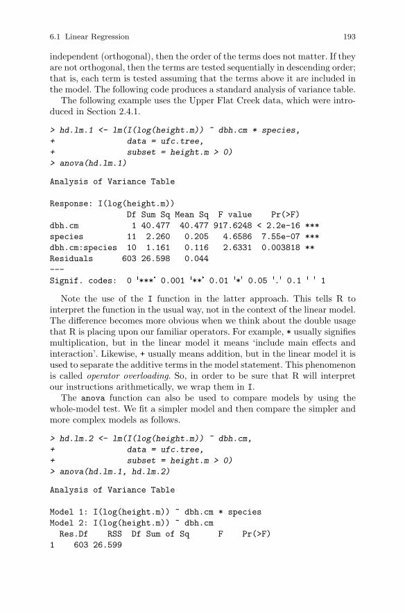
6.1 Linear Regression 193
independent (orthogonal), then the order of the terms does not matter. If theyare not orthogonal, then the terms are tested sequentially in descending order;that is, each term is tested assuming that the terms above it are included inthe model. The following code produces a standard analysis of variance table.
The following example uses the Upper Flat Creek data, which were intro-duced in Section 2.4.1.
> hd.lm.1 <- lm(I(log(height.m)) ~ dbh.cm * species,
+ data = ufc.tree,
+ subset = height.m > 0)
> anova(hd.lm.1)
Analysis of Variance Table
Response: I(log(height.m))
Df Sum Sq Mean Sq F value Pr(>F)
dbh.cm 1 40.477 40.477 917.6248 < 2.2e-16 ***
species 11 2.260 0.205 4.6586 7.55e-07 ***
dbh.cm:species 10 1.161 0.116 2.6331 0.003818 **
Residuals 603 26.598 0.044
---
Signif. codes: 0 �***� 0.001 �**� 0.01 �*� 0.05 �.� 0.1 � � 1
Note the use of the I function in the latter approach. This tells R tointerpret the function in the usual way, not in the context of the linear model.The difference becomes more obvious when we think about the double usagethat R is placing upon our familiar operators. For example, * usually signifiesmultiplication, but in the linear model it means ‘include main effects andinteraction’. Likewise, + usually means addition, but in the linear model it isused to separate the additive terms in the model statement. This phenomenonis called operator overloading. So, in order to be sure that R will interpretour instructions arithmetically, we wrap them in I.
The anova function can also be used to compare models by using thewhole-model test. We fit a simpler model and then compare the simpler andmore complex models as follows.
> hd.lm.2 <- lm(I(log(height.m)) ~ dbh.cm,
+ data = ufc.tree,
+ subset = height.m > 0)
> anova(hd.lm.1, hd.lm.2)
Analysis of Variance Table
Model 1: I(log(height.m)) ~ dbh.cm * species
Model 2: I(log(height.m)) ~ dbh.cm
Res.Df RSS Df Sum of Sq F Pr(>F)
1 603 26.599
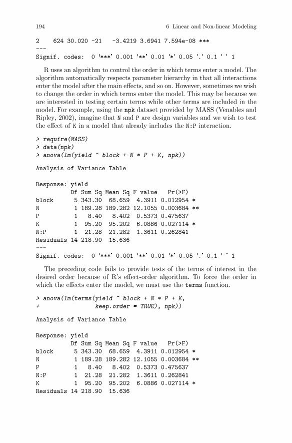
194 6 Linear and Non-linear Modeling
2 624 30.020 -21 -3.4219 3.6941 7.594e-08 ***
---
Signif. codes: 0 �***� 0.001 �**� 0.01 �*� 0.05 �.� 0.1 � � 1
R uses an algorithm to control the order in which terms enter a model. Thealgorithm automatically respects parameter hierarchy in that all interactionsenter the model after the main effects, and so on. However, sometimes we wishto change the order in which terms enter the model. This may be because weare interested in testing certain terms while other terms are included in themodel. For example, using the npk dataset provided by MASS (Venables andRipley, 2002), imagine that N and P are design variables and we wish to testthe effect of K in a model that already includes the N:P interaction.
> require(MASS)
> data(npk)
> anova(lm(yield ~ block + N * P + K, npk))
Analysis of Variance Table
Response: yield
Df Sum Sq Mean Sq F value Pr(>F)
block 5 343.30 68.659 4.3911 0.012954 *
N 1 189.28 189.282 12.1055 0.003684 **
P 1 8.40 8.402 0.5373 0.475637
K 1 95.20 95.202 6.0886 0.027114 *
N:P 1 21.28 21.282 1.3611 0.262841
Residuals 14 218.90 15.636
---
Signif. codes: 0 �***� 0.001 �**� 0.01 �*� 0.05 �.� 0.1 � � 1
The preceding code fails to provide tests of the terms of interest in thedesired order because of R’s effect-order algorithm. To force the order inwhich the effects enter the model, we must use the terms function.
> anova(lm(terms(yield ~ block + N * P + K,
+ keep.order = TRUE), npk))
Analysis of Variance Table
Response: yield
Df Sum Sq Mean Sq F value Pr(>F)
block 5 343.30 68.659 4.3911 0.012954 *
N 1 189.28 189.282 12.1055 0.003684 **
P 1 8.40 8.402 0.5373 0.475637
N:P 1 21.28 21.282 1.3611 0.262841
K 1 95.20 95.202 6.0886 0.027114 *
Residuals 14 218.90 15.636
6.1 Linear Regression 195
---
Signif. codes: 0 �***� 0.001 �**� 0.01 �*� 0.05 �.� 0.1 � � 1
Happily, we learn that the order of the terms makes no difference to ourinference in this case. A balanced dataset is a wonderful thing!
6.1.8 Transformations
Sometimes the modeler has biological or statistical reasons to change thenature of the data that are being modeled. Such transformations can be doneeither by creating a new variable in the data frame with the appropriatefunction or by making the transformation inside the call to the model.
> ufc.tree$log.height.m <- log(ufc.tree$height.m)
> hd.lm.4a <- lm(log.height.m ~ dbh.cm * species,
+ data = ufc.tree,
+ subset = height.m > 0)
> hd.lm.4b <- lm(I(log(height.m)) ~ dbh.cm * species,
+ data = ufc.tree,
+ subset=height.m > 0)
Transformation can be very useful, but it is not without cost. We believethat if possible it is best to work in the units that will make the most senseto the person who uses the model. Of course, it is possible to back-transformarbitrarily, and correct for bias, but why do so if it is unnecessary? Thereare certainly circumstances where transformation is called for, but often amore appropriate and satisfying strategy is available, whether that be fittinga generalized linear model or an additive model or performing a small MonteCarlo experiment on the residuals and placing trust in the Central LimitTheorem.
6.1.9 Weights
We have been analyzing the UFC data assuming that each observation isequally informative about the population. However, although the sample treesmay be considered a random sample, they are not selected with equal prob-ability, and furthermore they are clustered in location because they wereselected using a variable-radius plot sample. How much difference to the pa-rameter estimates does this sample design make? Here we will assess the effectof the sample weights. We will examine tools that more formally illuminatethe effect of clustering upon our parameter estimates in the next chapter.

196 6 Linear and Non-linear Modeling
Recall that, in a variable-radius plot, the probability of selection of a treeis proportional to its basal area. We can fit a model that accommodates thiseffect as follows.
> hd.lm.5 <- lm(height.m ~ dbh.cm * species,
+ weights = dbh.cm^-2,
+ data = ufc.tree)
Now we may wish to know what effect this change of weights has on ourparameter estimates. To pull out estimates of each slope and intercept, wecan use the estimable function provided in the gmodels package, but formodels that have only one categorical predictor variable, there is a hack, asimpler way to obtain them. We refit the models with the intercept and, ifnecessary, the slope explicitly removed from the model statement. That is,
> unweighted <-
+ coef(lm(height.m ~ dbh.cm * species - 1 - dbh.cm,
+ data = ufc.tree))
> weighted <-
+ coef(lm(height.m ~ dbh.cm * species - 1 - dbh.cm,
+ weights = dbh.cm^-2, data = ufc.tree))
Note that altering the model in this way (that is, fitting the model withthe intercept omitted) distorts the meaning of much of the summary output,so we advocate its use only for expediting the extraction of specific parameterestimates.
We can now plot these estimates in various more or less informative ways.The following code constructs Figure 6.5, which provides a compact graphi-cal summary of the effects of weighting. We use the text function to placesymbols and the abline function to provide an x = y line for the purposes ofcomparison.
> intercepts <- 1:10; slopes <- 11:20
> par(mfrow = c(1,2), las = 1, mar = c(4,4,3,1))
> plot(unweighted[intercepts], weighted[intercepts],
+ main = "Intercepts", type = "n",
+ xlab = "Unweighted", ylab = "Weighted")
> abline(0, 1, col="darkgrey")
> text(unweighted[intercepts], weighted[intercepts],
+ levels(ufc.tree$species))
> plot(unweighted[slopes], weighted[slopes],
+ main = "Slopes", type = "n",
+ xlab = "Unweighted", ylab = "Weighted")
> abline(0, 1, col = "darkgrey")
> text(unweighted[slopes], weighted[slopes],
+ levels(ufc.tree$species))
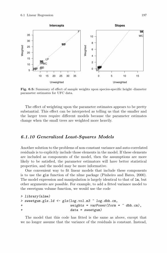
6.1 Linear Regression 197
10 15 20 25 30 35
5
10
15
20
25
30
35
Intercepts
Unweighted
Wei
ghte
d
DF
ES
F
FG
GF
HW
LP
PP SF
WCWL
WP
0 5 10 15
0
2
4
6
8
10
Slopes
UnweightedW
eigh
ted
DF
ESFGFHWLPPPSF
WC
WL
WP
Fig. 6.5: Summary of effect of sample weights upon species-specific height–diameterparameter estimates for UFC data.
The effect of weighting upon the parameter estimates appears to be prettysubstantial. This effect can be interpreted as telling us that the smaller andthe larger trees require different models because the parameter estimateschange when the small trees are weighted more heavily.
6.1.10 Generalized Least-Squares Models
Another solution to the problems of non-constant variance and auto-correlatedresiduals is to explicitly include those elements in the model. If these elementsare included as components of the model, then the assumptions are morelikely to be satisfied, the parameter estimators will have better statisticalproperties, and the model may be more informative.
One convenient way to fit linear models that include these componentsis to use the gls function of the nlme package (Pinheiro and Bates, 2000).The model expression and manipulation is largely identical to that of lm, butother arguments are possible. For example, to add a fitted variance model tothe sweetgum volume function, we would use the code
> library(nlme)
> sweetgum.gls.ld <- gls(log.vol.m3 ~ log.dbh.cm,
+ weights = varPower(form = ~ dbh.cm),
+ data = sweetgum)
The model that this code has fitted is the same as above, except thatwe no longer assume that the variance of the residuals is constant. Instead,
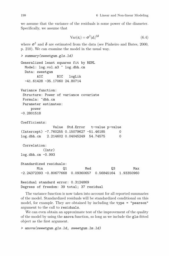
198 6 Linear and Non-linear Modeling
we assume that the variance of the residuals is some power of the diameter.Specifically, we assume that
Var(εi) = σ2|di|2δ (6.4)
where σ2 and δ are estimated from the data (see Pinheiro and Bates, 2000,p. 210). We can examine the model in the usual way.
> summary(sweetgum.gls.ld)
Generalized least squares fit by REML
Model: log.vol.m3 ~ log.dbh.cm
Data: sweetgum
AIC BIC logLik
-41.61428 -35.17060 24.80714
Variance function:
Structure: Power of variance covariate
Formula: ~dbh.cm
Parameter estimates:
power
-0.2801518
Coefficients:
Value Std.Error t-value p-value
(Intercept) -7.760255 0.15079627 -51.46185 0
log.dbh.cm 2.214602 0.04045249 54.74575 0
Correlation:
(Intr)
log.dbh.cm -0.993
Standardized residuals:
Min Q1 Med Q3 Max
-2.24372393 -0.80677668 0.09360657 0.56845164 1.93350960
Residual standard error: 0.3124869
Degrees of freedom: 39 total; 37 residual
The variance function is now taken into account for all reported summariesof the model. Standardized residuals will be standardized conditional on thismodel, for example. They are obtained by including the type = "pearson"
argument to the call to residuals.We can even obtain an approximate test of the improvement of the quality
of the model by using the anova function, so long as we include the gls-fittedobject as the first argument.
> anova(sweetgum.gls.ld, sweetgum.lm.ld)

6.2 Non-linear Regression 199
Model df AIC BIC logLik Test
sweetgum.gls.ld 1 4 -41.61428 -35.17060 24.80714
sweetgum.lm.ld 2 3 -42.44004 -37.60728 24.22002 1 vs 2
L.Ratio p-value
sweetgum.gls.ld
sweetgum.lm.ld 1.174237 0.2785
The p-value above suggests poor support in the data for the inclusion ofa variance function that depends on the predictor variable.
The gls class has a number of useful methods. Use
> methods(class = "gls")
to discover them. Pinheiro and Bates (2000) is essential reading.
6.2 Non-linear Regression
One of the unsatisfying characteristics of linear models is that we are con-strained in how the parameters and coefficients can interact. We have hadto ensure that the normal equations, which are the first derivatives of theobjective function with respect to the coefficients, were independent of thecoefficients. This constraint has precluded us from using a wealth of biolog-ically realistic model forms. There have also been advantages: we have beenguaranteed that any inference has been exact, conditional on the assumptionsand the model, and that fitting has required one step only and no startingvalues. However, it is arguably better to get an approximate answer to ameaningful question than to get an exact answer to an approximation to ameaningful question.3
With non-linear model fitting, we can deploy classes of models that donot have such a restriction. This broader stance allows us to choose modelforms that we feel genuinely represent the underlying processes in some way,which in turn allows us to think about the fitting process in more than purelyempirical ways.
As before, we do not present the theory here, as that has been covered moreeffectively elsewhere. Recommended reading includes Ratkowsky (1983), Gal-lant (1987), Bates and Watts (1988), Schabenberger and Pierce (2002), andSeber and Wild (2003).
Examples of non-linear models that might be relevant in forestry and nat-ural resources include:
� change-point models� plateau models� allometric models
3 This quotation is a first-order approximation to Tukey (1962).

200 6 Linear and Non-linear Modeling
� growth models
Schabenberger and Pierce (2002) charge that researchers tend to avoidnon-linear models because of discomfort with the messiness of implementa-tion. The messiness is unavoidable; however, non-linear models are parsimo-nious, incorporate limits, and can be parameterized so that parameters willhave a direct interpretation.
We consider non-linear models with one continuous predictor. We write
yi = f (xi,β )+ εi (6.5)
where β is a p+1-length vector of parameters; e.g., β = (β0,β1, . . . ,βp)′.
This model statement is sufficient to find least-squares estimates: we simplyneed to find those values of β that minimize the sum of squared deviationsbetween the observed yi and the fitted yi. Furthermore, the least-squaresestimates of the parameters are asymptotically normally distributed if thefollowing assumptions hold:
1. Var(εi) = σ2, a constant.2. εi are independent.3. εi are normally distributed.
As in the linear model case, each of the assumptions play different rolesand are of varying importance depending on the purpose to which the modelwill be put. Note that the assumption of zero mean for the errors depends onwhether or not an additive constant is included in f .
6.2.1 Example
As in the previous section, we will motivate non-linear modeling via an exam-ple. Our data are Norway spruce measurements drawn from von Guttenberg(1915), kindly provided to us by Professor Boris Zeide. Our goal is, in thefirst instance, to construct a model that predicts tree diameter as a functionof age. The data import and cleaning are documented in Section 2.4.4.
6.2.2 Thinking about the Problem
We start with a plot of the trajectories of diameter growth. The followingcode uses Hadley Wickham’s qplot function from the ggplot2 package in R,documented in Wickham (2009), to produce Figure 6.6.
> library(ggplot2)
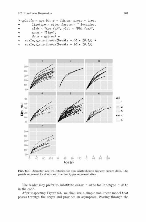
6.2 Non-linear Regression 201
> qplot(x = age.bh, y = dbh.cm, group = tree,
+ linetype = site, facets = ~ location,
+ xlab = "Age (y)", ylab = "Dbh (cm)",
+ geom = "line",
+ data = gutten) +
+ scale_x_continuous(breaks = 40 * (0:3)) +
+ scale_y_continuous(breaks = 10 * (0:5))
Age (y)
Dbh
(cm
)
0
10
20
30
40
50
0
10
20
30
40
50
0
10
20
30
40
50
1
4
7
0 40 80 120
2
5
0 40 80 120
3
6
0 40 80 120
site
1
2
3
4
5
Fig. 6.6: Diameter–age trajectories for von Guttenberg’s Norway spruce data. Thepanels represent locations and the line types represent sites.
The reader may prefer to substitute color = site for linetype = site
in the code.After inspecting Figure 6.6, we shall use a simple non-linear model that
passes through the origin and provides an asymptote. Passing through the
202 6 Linear and Non-linear Modeling
origin is reasonable as a starting point because, by definition, dbh is non-zeroonly after age at breast height is non-zero. That may prove to be an uglyconstraint, however. A candidate model is then
yi = φ1 ×[
1− exp
(−xi log2
φ2
)]+ εi (6.6)
where φ1 is the fixed, unknown asymptote and φ2 is the fixed, unknown timeuntil the tree reaches half its predicted maximum size (see Pinheiro and Bates,2000, who use a different parameterization). Note that the model omits anadditive constant, so we can’t expect the residuals to have zero mean and wemay take substantial deviation of the residuals from zero mean to be evidenceof lack of fit.
6.2.3 Fitting the Model
Fitting non-linear models is an iterative procedure; in order to calculate esti-mates of the parameters, we need to have existing estimates. So, we require astarting point for the estimates, a numerical rule for updating the estimates,and a stopping rule.
The principle of least squares still underpins parameter estimation: wewish to minimize the sum of squares of deviations between the observationsand the predictions. That is, we want to find the value θ that minimizes
S(θ) =n
∑i=1
(yi − f (xi,β ))2
Two parameter-estimation strategies are popular: Gauss–Newton andNewton–Raphson. The differences between the two are important: the Gauss–Newton algorithm requires the calculation of first derivatives, and the Newton–Raphson requires the calculation of first and second derivatives. If the resid-uals are small, then the Gauss–Newton algorithm will converge more rapidlythan Newton–Raphson, but if the residuals are large, then it may not convergeat all. R’s non-linear model fitting function, nls, uses the Gauss–Newton al-gorithm by default.
In order to fit a non-linear model, we generally need to construct our ownnon-linear model function. We can do this simply by constructing a functionthat produces the appropriate predictions given the inputs. However, fittingthe model turns out to be more efficient if we can also pass the first andmaybe second derivatives to the function as well. Writing a function to passthe predictions and the derivatives is simplified by using the deriv function.NB: R provides some simple prepackaged models, about which we will learnmore later.

6.2 Non-linear Regression 203
Our use of deriv() requires three things: a statement of the function, avector of parameter names for which derivatives are required, and the tem-plate of the function call.
> dbh.growth <-
+ deriv(~ asymptote * (1 - exp(-log(2)/scale * x)),
+ c("asymptote","scale"),
+ function(x, asymptote, scale){},
+ hessian = TRUE)
The Hessian is the matrix of estimated second partial derivatives. We askedfor the Hessian to be returned as well because it will be used later in diagnosticcode that determines the curvature of the model.
Having written the non-linear model as a function, we should try it out.We select a handy tree:
> handy.tree <- subset(gutten, tree.ID == "1.1")
In a departure from our earlier chapters, we also need to guess the startingestimates for the parameters. Here we will use the highest value as an estimateof the asymptote and guess that the tree reaches about half its maximumdiameter in about 30 years.
> max(handy.tree$dbh.cm, na.rm=TRUE)
[1] 29
Then the model is fit using nls, as per the following code. Note the in-clusion of the argument na.action = na.exclude to tell R how to handlemissing values: we are asking R to take the missing values out of the dataprior to fitting but also to pad its observation-level statistics, such as fittedvalues and residuals, so that they are of the same length as the original data.We will need this facility in the construction of Figure 6.7.
> handy.nls <-
+ nls(dbh.cm ~ dbh.growth(age.bh, asymptote, scale),
+ start = list(asymptote = 29, scale = 10),
+ na.action = na.exclude,
+ data = handy.tree)
6.2.4 Assumptions and Diagnostics
We now need to assess the model assumptions in the light of the fit of themodel to the data. Some background will help us to understand the impor-tance of these assumptions.
204 6 Linear and Non-linear Modeling
Geometry provides a convenient way to think about least-squares linear re-gression. Briefly, the response variable is an n-dimensional vector in n-space.The predictor variables are used to form a p-dimensional surface, specifi-cally a hyperplane, in the n-space. Then, the model predictions are the p-dimensional vector within the p-dimensional hyperplane that is closest tothe n-dimensional vector in n-space. That p-dimensional vector is found byprojecting the n-dimensional vector into the p-dimensional hyperplane. Theparameter estimates are then the coordinates of that p-dimensional vector.
In non-linear least squares, the least-squares geometric principles are as-sumed to hold locally, but they are known to hold only approximately. Thequality of the information about the model fit depends on how close to linearthe model is, for the data, in the region of the optimum.
First, there is no guarantee that the surface that is formed by the pre-dictor variables is flat, or the multi-dimensional equivalent of flat. This lackof flatness is because the values of the parameters affect the shape of themodel; that is, the normal equations are not independent of the parameters.Therefore projection will not find the nearest point; the location upon thehyperplane of the nearest point to the n-vector must be found iteratively. Theassumption of local flatness is referred to as the planar assumption (Seberand Wild, 2003, p. 134) and is estimated using the intrinsic curvature.
Second, there is no guarantee that the surface thus formed has well-behaved coordinates; that is, coordinates that map to straight, parallel,equidistant lines. The scale may change along one direction or another, thecoordinates might be curved, and the inter-coordinate distance may vary. Theassumption of locally well-behaved coordinates is called the uniform coordi-
nate assumption (Seber and Wild, 2003, p. 135), and is estimated using theparameter-effects curvature.
We will refer to these assumptions jointly as the local-linearity assump-tions.
The MASS package in R (Venables and Ripley, 2002) provides code thatcan be used to compute the intrinsic and the parameter-effects curvatures fora given model, so long as the model function can provide the Hessian. Thecode, which we invoke after loading the MASS package, is
> rms.curv(handy.nls)
Parameter effects: c^theta x sqrt(F) = 0.096
Intrinsic: c^iota x sqrt(F) = 0.0246
The value 0.3 has been suggested as a soft cutoff for the point at whichthe curvature becomes unacceptable for the planar assumption and the uni-form coordinate assumption. Both assumptions seem to be reasonable for thismodel and these data.
As a side note, we also fit the model represented in equation (6.6) usingthe parameterization suggested in Pinheiro and Bates (2000),
6.2 Non-linear Regression 205
yi = φ1 × [1− exp(−exp(φ2)xi)]+ εi (6.7)
An advantage of that parameterization is that the effect of scale is con-strained to be positive, so the process of estimation may be more stable. Thisstrategy is also useful for constraining estimates of parameters that havebiological constraints. We obtained the following curvature estimates:
Parameter effects: c^theta x sqrt(F) = 0.1818
Intrinsic: c^iota x sqrt(F) = 0.0246
Note that the intrinsic curvature is unchanged. That is, our efforts left thefundamental shape of the surface upon which we were projecting unchanged.However, the parameter-effects curvature has doubled, suggesting that theassumption of uniform coordinates for the Pinheiro and Bates (2000) param-eterization does not hold as well for these data as the assumption for theprevious parameterization. For further reading, see Ratkowsky (1983), Chap-ter 7 of Bates and Watts (1988), and Section 5.7.1 of Schabenberger andPierce (2002).
The intrinsic curvature also affects the nature of the residuals in that inthe presence of substantial intrinsic curvature the residuals may have non-zero means, non-unit variances, and negative correlation with the responsevariable (Seber and Wild, 2003, p. 179). Note that
> mean(residuals(handy.nls), na.rm=TRUE)
[1] -0.06936603
Therefore residual diagnostics should be interpreted carefully in the lightof the estimate of the intrinsic curvature. That said, there seems to be noreason to omit the diagnostics in this case. We provide several in Figure 6.7,which is created using the following code:
> par(mfrow=c(1,3), mar=c(4,4,2,1), las=1)
> plot(fitted(handy.nls), residuals(handy.nls, type="pearson"),
+ xlab = "Fitted Values", ylab = "Standardized Residuals")
> abline(h=0, col="red")
> qqnorm(residuals(handy.nls, type="pearson"))
> qqline(residuals(handy.nls, type="pearson"))
> plot(fitted(handy.nls), handy.tree$dbh.cm,
+ xlab = "Fitted Values", ylab = "Observed Values")
> abline(0, 1, col="red")
The left frame is a plot of the standardized residuals against the fittedvalues, with a y = 0 line imposed. As with OLS regression, we want to see noparticular pattern and no influential outliers. Here we seem to see a distinctkink — a systematic lack of fit in the trajectory. The center panel is a q-q plotof the residuals against the normal distribution. We prefer to see the pointsmatching the line, and apart from one point, the match seems reasonable.
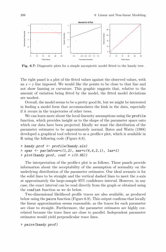
206 6 Linear and Non-linear Modeling
●
●
●
●
●
●
●
●
●
●
●
●
●
5 10 15 20 25 30
−2
−1
0
1
Fitted Values
Sta
ndar
dize
d R
esid
uals
●
●
●
●
●
●
●
●
●
●
●
●
●
−1.5 −0.5 0.0 0.5 1.0 1.5
−2
−1
0
1
Normal Q−Q Plot
Theoretical Quantiles
Sam
ple
Qua
ntile
s
●
●
●
●
●
●
●
●
●
●
●●
●
5 10 15 20 25 30
5
10
15
20
25
Fitted Values
Obs
erve
d V
alue
s
Fig. 6.7: Diagnostic plots for a simple asymptotic model fitted to the handy tree.
The right panel is a plot of the fitted values against the observed values, withan x = y line imposed. We would like the points to be close to that line andnot show fanning or curvature. This graphic suggests that, relative to theamount of variation being fitted by the model, the fitted model deviationsare modest.
Overall, the model seems to be a pretty good fit, but we might be interestedin finding a model form that accommodates the kink in the data, especiallyif it recurs in the trajectories of other trees.
We can learn more about the local-linearity assumptions using the profilefunction, which provides insight as to the shape of the parameter space ontowhich our data have been projected. Ideally we want the distribution of theparameter estimates to be approximately normal. Bates and Watts (1988)developed a graphical tool referred to as a profile-t plot, which is available inR using the following code (Figure 6.8).
> handy.prof <- profile(handy.nls)
> opar <- par(mfrow=c(1,2), mar=c(4,4,2,1), las=1)
> plot(handy.prof, conf = c(0.95))
The interpretation of the profile-t plot is as follows. These panels provideinformation about the acceptability of the assumption of normality on theunderlying distribution of the parameter estimates. Our ideal scenario is forthe solid lines to be straight and the vertical dashed lines to meet the x-axisat approximately the large-sample 95% confidence interval. However, in anycase, the exact interval can be read directly from the graph or obtained usingthe confint function as we do below.
Two-dimensional likelihood profile traces are also available, as producedbelow using the pairs function (Figure 6.9). This output confirms that locallythe linear approximation seems reasonable, as the traces for each parameterare close to straight. Furthermore, the parameter estimates are highly cor-related because the trace lines are close to parallel. Independent parameterestimates would yield perpendicular trace lines.
> pairs(handy.prof)
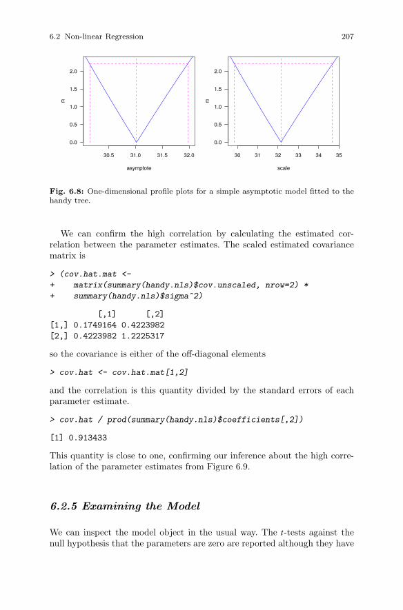
6.2 Non-linear Regression 207
30.5 31.0 31.5 32.0
0.0
0.5
1.0
1.5
2.0
asymptote
τ
30 31 32 33 34 35
0.0
0.5
1.0
1.5
2.0
scale
τ
Fig. 6.8: One-dimensional profile plots for a simple asymptotic model fitted to thehandy tree.
We can confirm the high correlation by calculating the estimated cor-relation between the parameter estimates. The scaled estimated covariancematrix is
> (cov.hat.mat <-
+ matrix(summary(handy.nls)$cov.unscaled, nrow=2) *
+ summary(handy.nls)$sigma^2)
[,1] [,2]
[1,] 0.1749164 0.4223982
[2,] 0.4223982 1.2225317
so the covariance is either of the off-diagonal elements
> cov.hat <- cov.hat.mat[1,2]
and the correlation is this quantity divided by the standard errors of eachparameter estimate.
> cov.hat / prod(summary(handy.nls)$coefficients[,2])
[1] 0.913433
This quantity is close to one, confirming our inference about the high corre-lation of the parameter estimates from Figure 6.9.
6.2.5 Examining the Model
We can inspect the model object in the usual way. The t-tests against thenull hypothesis that the parameters are zero are reported although they have
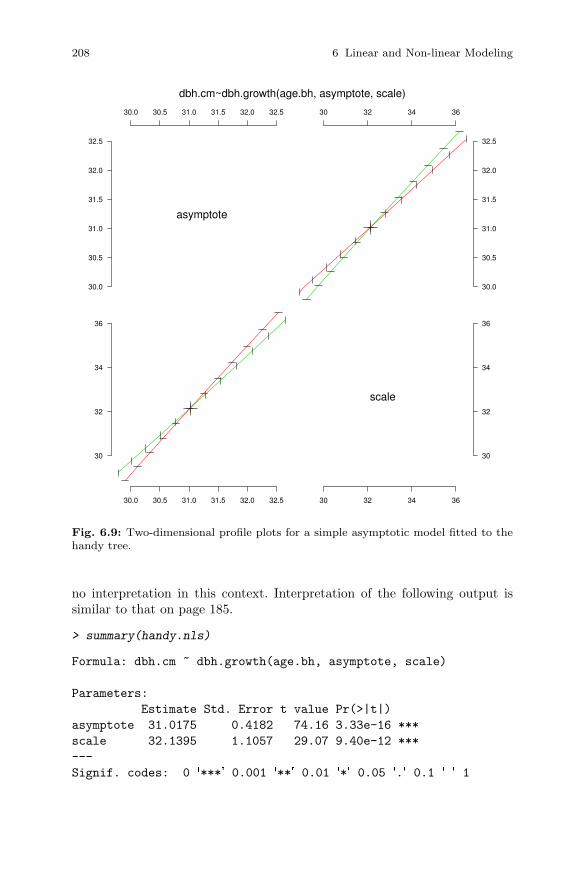
208 6 Linear and Non-linear Modeling
dbh.cm~dbh.growth(age.bh, asymptote, scale)
asymptote
30.0
30.5
31.0
31.5
32.0
32.5
30.0 30.5 31.0 31.5 32.0 32.5 30 32 34 36
30.0
30.5
31.0
31.5
32.0
32.5
30.0 30.5 31.0 31.5 32.0 32.5
30
32
34
36
scale
30 32 34 36
30
32
34
36
Fig. 6.9: Two-dimensional profile plots for a simple asymptotic model fitted to thehandy tree.
no interpretation in this context. Interpretation of the following output issimilar to that on page 185.
> summary(handy.nls)
Formula: dbh.cm ~ dbh.growth(age.bh, asymptote, scale)
Parameters:
Estimate Std. Error t value Pr(>|t|)
asymptote 31.0175 0.4182 74.16 3.33e-16 ***
scale 32.1395 1.1057 29.07 9.40e-12 ***
---
Signif. codes: 0 �***� 0.001 �**� 0.01 �*� 0.05 �.� 0.1 � � 1

6.2 Non-linear Regression 209
Residual standard error: 0.4507 on 11 degrees of freedom
Number of iterations to convergence: 5
Achieved convergence tolerance: 6.62e-06
Apart from the fact that we can’t guarantee to have found a global mini-mum, the reported estimates are the least-squares estimates. We should trya range of other starting points to be sure that the final estimates are robustto the initial estimates.
We can compute the approximate large-sample interval estimates using
> (my.t <- qt(0.975, summary(handy.nls)$df[2]))
[1] 2.200985
> coef(summary(handy.nls))[,1:2] %*%
+ matrix(c(1,-my.t,1,my.t), nrow=2)
[,1] [,2]
asymptote 30.09697 31.93801
scale 29.70590 34.57308
and extract the exact marginal profiled versions using
> confint(handy.prof)
2.5% 97.5%
asymptote 30.14710 31.97636
scale 29.84986 34.67562
These estimates are very similar, which confirms the outcomes of our diag-nostics. But, the data appear to have a modest kink that our model failed tocapture. This might be true just of this tree, a subset of the trees, or all thetrees. We are naturally curious, but understandably reluctant to go throughthe same process for every tree. We will need some more powerful tools, towhich we will return in Section 7.6.
Finally, we can obtain an estimate of the root-mean-squared error of theresiduals using confint
> sqrt(sum(residuals(handy.nls)^2, na.rm=TRUE) /
+ summary(handy.nls)$df[2])
[1] 0.4507378
and compare it with the standard deviation of the data,
> sd(handy.tree$dbh.cm, na.rm=TRUE)
[1] 7.640395
which provides a loose indication of the predictive quality of the model. Amore formal comparison requires the use of a cross-validation mechanism.
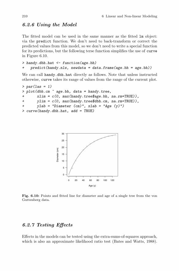
210 6 Linear and Non-linear Modeling
6.2.6 Using the Model
The fitted model can be used in the same manner as the fitted lm object:via the predict function. We don’t need to back-transform or correct thepredicted values from this model, so we don’t need to write a special functionfor its predictions, but the following terse function simplifies the use of curvein Figure 6.10.
> handy.dbh.hat <- function(age.bh)
+ predict(handy.nls, newdata = data.frame(age.bh = age.bh))
We can call handy.dbh.hat directly as follows. Note that unless instructedotherwise, curve takes its range of values from the range of the current plot.
> par(las = 1)
> plot(dbh.cm ~ age.bh, data = handy.tree,
+ xlim = c(0, max(handy.tree$age.bh, na.rm=TRUE)),
+ ylim = c(0, max(handy.tree$dbh.cm, na.rm=TRUE)),
+ ylab = "Diameter (cm)", xlab = "Age (y)")
> curve(handy.dbh.hat, add = TRUE)
●
●
●
●
●
●
●
●
●●
●●
●
0 20 40 60 80 100 120
0
5
10
15
20
25
30
Age (y)
Dia
met
er (
cm)
Fig. 6.10: Points and fitted line for diameter and age of a single tree from the vonGuttenberg data.
6.2.7 Testing Effects
Effects in the models can be tested using the extra-sums-of-squares approach,which is also an approximate likelihood ratio test (Bates and Watts, 1988).
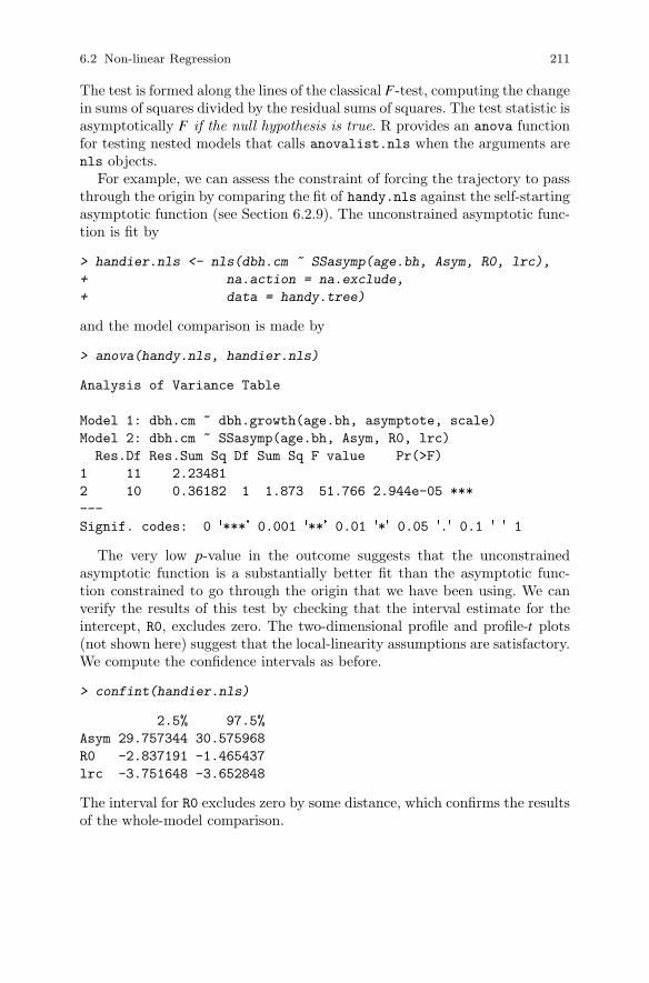
6.2 Non-linear Regression 211
The test is formed along the lines of the classical F-test, computing the changein sums of squares divided by the residual sums of squares. The test statistic isasymptotically F if the null hypothesis is true. R provides an anova functionfor testing nested models that calls anovalist.nls when the arguments arenls objects.
For example, we can assess the constraint of forcing the trajectory to passthrough the origin by comparing the fit of handy.nls against the self-startingasymptotic function (see Section 6.2.9). The unconstrained asymptotic func-tion is fit by
> handier.nls <- nls(dbh.cm ~ SSasymp(age.bh, Asym, R0, lrc),
+ na.action = na.exclude,
+ data = handy.tree)
and the model comparison is made by
> anova(handy.nls, handier.nls)
Analysis of Variance Table
Model 1: dbh.cm ~ dbh.growth(age.bh, asymptote, scale)
Model 2: dbh.cm ~ SSasymp(age.bh, Asym, R0, lrc)
Res.Df Res.Sum Sq Df Sum Sq F value Pr(>F)
1 11 2.23481
2 10 0.36182 1 1.873 51.766 2.944e-05 ***
---
Signif. codes: 0 �***� 0.001 �**� 0.01 �*� 0.05 �.� 0.1 � � 1
The very low p-value in the outcome suggests that the unconstrainedasymptotic function is a substantially better fit than the asymptotic func-tion constrained to go through the origin that we have been using. We canverify the results of this test by checking that the interval estimate for theintercept, R0, excludes zero. The two-dimensional profile and profile-t plots(not shown here) suggest that the local-linearity assumptions are satisfactory.We compute the confidence intervals as before.
> confint(handier.nls)
2.5% 97.5%
Asym 29.757344 30.575968
R0 -2.837191 -1.465437
lrc -3.751648 -3.652848
The interval for R0 excludes zero by some distance, which confirms the resultsof the whole-model comparison.
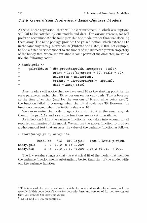
212 6 Linear and Non-linear Modeling
6.2.8 Generalized Non-linear Least-Squares Models
As with linear regression, there will be circumstances in which assumptionswill fail to be satisfied by our models and data. For various reasons, we willprefer to accommodate the failings within the model rather than transformingthem away. The nlme package provides the gnls function, which extends nlsin the same way that gls extends lm (Pinheiro and Bates, 2000). For example,to add a fitted variance model to the model of the diameter growth trajectoryof the handy tree, where the variance is some power of the diameter, we woulduse the following code4:
> handy.gnls <-
+ gnls(dbh.cm ~ dbh.growth(age.bh, asymptote, scale),
+ start = list(asymptote = 30, scale = 10),
+ na.action = na.exclude,
+ weights = varPower(form = ~age.bh),
+ data = handy.tree)
Alert readers will notice that we have used 10 as the starting point for thescale parameter rather than 30, as per our earlier call to nls. This is because,at the time of writing (and for the versions of R and nlme being used5),the function failed to converge when the initial scale was 30. However, thefunction converged when the initial value was 10.
We can examine the model diagnostics and output in the usual way, al-though the profile and rms.curv functions are as yet unavailable.
As in Section 6.1.10, the variance function is now taken into account for allreported summaries of the model. We can use the anova function to producea whole-model test that assesses the value of the variance function as follows.
> anova(handy.gnls, handy.nls)
Model df AIC BIC logLik Test L.Ratio p-value
handy.gnls 1 4 -12.0 -9.75 10.005
handy.nls 2 3 20.0 21.70 -7.001 1 vs 2 34.011 <.0001
The low p-value suggests that the statistical fit of the model that includesthe variance function seems substantially better than that of the model with-out the variance function.
4 This is one of the rare occasions in which the code that we developed was platform-specific. If this code doesn’t work for your platform and version of R, then we suggestthat you change the starting values.5 2.11.1 and 3.1-96, respectively.

6.2 Non-linear Regression 213
6.2.9 Self-starting Functions
A handful of popular non-linear modeling functions have been retooled in Rto provide their own starting values. These are called self-starting functionsand are distinguished by having their names begin with the letters SS. Thisinformation is enough to be able to identify the functions in help, as typing?SS and then TAB will provide a list of all such functions at the commandprompt.6
We now take another brief detour into searching for R objects. We canalso find all instances of these functions in the entire search path using theapropos function.
> apropos("^SS")
[1] "SSD" "SSasymp" "SSasympOff" "SSasympOrig"
[5] "SSbiexp" "SSfol" "SSfpl" "SSgompertz"
[9] "SSlogis" "SSmicmen" "SSweibull"
Note the use of the exponent symbol ^ to alert R that the string SS shouldstart the object name. This symbol is an integral part of the so-called regularexpressions (regex), which provide a very powerful and flexible framework forsearching text strings.
It is possible that the returned objects are not all of the right class. Wecan filter all the objects in the search path by class using the following code:
> apropos("^SS")[sapply(apropos("^SS"),
+ function(x) {
+ "selfStart" %in%
+ class(eval(parse(text = x)))}) ]
[1] "SSasymp" "SSasympOff" "SSasympOrig" "SSbiexp"
[5] "SSfol" "SSfpl" "SSgompertz" "SSlogis"
[9] "SSmicmen" "SSweibull"
NB: We can see how many objects R has in the search path using
> length(apropos("."))
[1] 4212
If the existing collection of self-starting functions is inadequate for ourpurposes, then we can write our own. For example, we could create anSSallometric function. R provides a selfStart function for this purpose.We need to provide a function for fitting, a function for determining initialestimates, and the names of the parameters. The function to fit will be
6 This is true for all the versions of R that we use.

214 6 Linear and Non-linear Modeling
> allometric <- deriv(~ alpha * x^beta, c("alpha", "beta"),
+ function(x, alpha, beta){},
+ hessian = TRUE)
and the function for obtaining initial estimates is
> allometric.init <- function (mCall, data, LHS) {
+ xy <- data.frame(sortedXyData(mCall[["x"]], LHS, data))
+ if (nrow(xy) < 3)
+ stop("Too few observations to fit allometric function")
+ pars <- as.vector(coef(lm(I(log(y)) ~ I(log(x)),
+ data = xy)))
+ pars[1] <- exp(pars[1])
+ names(pars) <- mCall[c("alpha", "beta")]
+ return(pars)
+ }
We then call
> SSallometric <- selfStart(allometric,
+ allometric.init,
+ c("alpha", "beta"))
This function then works as follows.
> nls(vol.m3 ~ SSallometric(dbh.cm, alpha, beta),
+ data = sweetgum)
Nonlinear regression model
model: vol.m3 ~ SSallometric(dbh.cm, alpha, beta)
data: sweetgum
alpha beta
0.0006338 2.1160953
residual sum-of-squares: 2.278
Number of iterations to convergence: 5
Achieved convergence tolerance: 3.696e-06
6.3 Back to Maximum Likelihood
In Section 5.3.1.3, we demonstrated the use of maximum likelihood (ML)for estimating the parameters of the Weibull distribution for tree diameters.One of the advantages of ML is its flexibility. For example, we can replaceany parameter in the likelihood with a function of other parameters, perhapsincluding predictor variables. We need to be careful about adding complex-ity; the ML estimates can become correspondingly harder to find, and poor

6.3 Back to Maximum Likelihood 215
choices of parameterization may really make a difference to the quality andease of fitting of the model.
6.3.1 Linear Regression
In Section 6.1.3, we fit a linear model to predict log volume from log diameterof the sweetgum trees. We know that the parameter estimates that arise fromleast-squares estimation are the same as those that arise from maximum-likelihood estimation if the residuals are normally distributed. The followingcode fits the same regression model using maximum likelihood and providesestimates of the parameters and their asymptotic standard errors.
First, we write a function that computes the conditional, joint log-likelihoodof the data. The observations are assumed to be conditionally normal. Wesum the logs of the pdfs of the normal distribution evaluated at the observeddata as a function of the parameter estimates.
> normal.ll <- function(parameters, x, y) {
+ sum(dnorm(y,
+ parameters[1] + parameters[2] * x,
+ parameters[3],
+ log = TRUE))
+ }
We then maximize this function using optim.
> good.fit <- optim(c(intercept = 1, slope = 1, sigma = 1),
+ normal.ll,
+ hessian = TRUE,
+ control = list(fnscale = -1),
+ x = sweetgum$log.dbh.cm,
+ y = sweetgum$log.vol.m3)
We can now extract the maximum-likelihood parameter estimates from thereturned object.
> good.fit$par
intercept slope sigma
-7.8050519 2.2268877 0.1132759
The (asymptotic) estimates of the standard errors are then
> sqrt(diag(solve(-good.fit$hessian)))
intercept slope sigma
0.14166190 0.03919263 0.01282375

216 6 Linear and Non-linear Modeling
These estimates are close to those reported previously, allowing for numericalerror, although the estimate of the variance differs, as we would expect.
A disadvantage of taking this approach to fitting the linear model is thatit is cumbersome to generalize in certain ways. For example, if we now wishedto fit a unique slope and intercept for each species, we’d have to write thatrequirement into the objective function explicitly, whereas when we use lm
we just add the species term to the model specification (see Section 6.1.9 foran example).
6.3.2 Non-linear Regression
A corresponding advantage is that other types of generalizations are easy.For example, we can also fit a non-linear model simply by changing the meanfunction.
> normal.ll.nl <- function(parameters, x, y) {
+ sum( dnorm(y,
+ parameters[1] * x ^ parameters[2],
+ parameters[3],
+ log = TRUE ))
+ }
We maximize this function using optim:
> good.fit <- optim(c(intercept = 1, slope = 1, sigma = 1),
+ normal.ll.nl,
+ hessian = TRUE,
+ control = list(fnscale = -1),
+ x = sweetgum$dbh.cm,
+ y = sweetgum$vol.m3)
The MLEs are then
> good.fit$par
intercept slope sigma
0.0006654548 2.1041851701 0.2411616481
The (asymptotic) estimates of the standard errors are
> sqrt(diag(solve(-good.fit$hessian)))
intercept slope sigma
0.0001729483 0.0629433124 0.0272184407
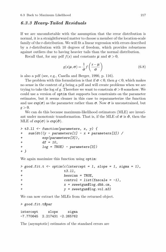
6.3 Back to Maximum Likelihood 217
6.3.3 Heavy-Tailed Residuals
If we are uncomfortable with the assumption that the error distribution isnormal, it is a straightforward matter to choose a member of the location-scalefamily of the t-distribution. We will fit a linear regression with errors describedby a t-distribution with 10 degrees of freedom, which provides robustnessagainst outliers due to having heavier tails than the normal distribution.
Recall that, for any pdf f (x) and constants μ and σ > 0,
g(x|μ,σ) =1
σf
(x−μ
σ
)(6.8)
is also a pdf (see, e.g., Casella and Berger, 1990, p. 116).The problem with this formulation is that if σ < 0, then g< 0, which makes
no sense in the context of g being a pdf and will create problems when we aretrying to take the log of g. Therefore we want to constrain σ > 0 somehow. Wecould use a version of optim that supports box constraints on the parameterestimates, but it seems cleaner in this case to reparameterize the functionand use exp(σ) as the parameter rather than σ . Now σ is unconstrained, butg > 0.
We can do this because maximum-likelihood estimators (MLE) are invari-ant under monotonic transformation. That is, if the MLE of σ is σ , then theMLE of exp(σ) is exp(σ).
> t3.ll <- function(parameters, x, y) {
+ sum(dt((y - parameters[1] - x * parameters[2]) /
+ exp(parameters[3]),
+ df = 10,
+ log = TRUE) - parameters[3])
+ }
We again maximize this function using optim:
> good.fit.t <- optim(c(intercept = 1, slope = 1, sigma = 1),
+ t3.ll,
+ hessian = TRUE,
+ control = list(fnscale = -1),
+ x = sweetgum$log.dbh.cm,
+ y = sweetgum$log.vol.m3)
We can now extract the MLEs from the returned object.
> good.fit.t$par
intercept slope sigma
-7.770645 2.217431 -2.265762
The (asymptotic) estimates of the standard errors are

218 6 Linear and Non-linear Modeling
> sqrt(diag(solve(-good.fit.t$hessian)))
intercept slope sigma
0.14326083 0.03943311 0.12799391
The interpretation of the parameters μ and σ is left to the analyst. Don’tforget that the variance of the tν is ν
ν−2 (Casella and Berger, 1990), so thereported scale parameter should not be directly interpreted as the antilog ofthe conditional standard deviation of the data. The conditional estimate ofthe standard deviation of the data would be
> exp(good.fit.t$par[3]) * sqrt(10 / (10 - 2))
sigma
0.1159971
All these parameter estimators are maximum-likelihood estimators, con-ditional on the model, and therefore are asymptotically normal, efficient es-timators, if the model is sufficiently flexible to capture the true relationshipand if the assumptions hold.

Chapter 7
Fitting Linear Hierarchical Models
7.1 Introduction
We now shift to the analysis of hierarchical data using mixed-effects mod-els. These models are a natural match for many problems that occur com-monly in natural resources. A number of the tools that we discuss in thischapter are extensively documented in Pinheiro and Bates (2000), and ourgoal is to complement that resource, not replace it. Although we focus onmixed-effects models, other solutions are possible. For example, stochasticdifferential equations have also seen success in forestry (Garcıa, 1983), andgeneralized estimating equations may also be useful.
Recall that for fitting a linear regression using the least-squares or maximum-likelihood techniques, it was necessary to make some assumptions about thenature of the residuals or, equivalently, about the distribution of the responsevariable conditional on the predictor variables. The level of detail of the as-sumptions depended upon the applications of the model. For direct intervalestimation of model parameters, it was necessary to assume that the residualswere
1. independent,2. identically distributed, and3. normally distributed.
It was also necessary to assume that the nature of the relationship betweenthe response and the predictors was accurately captured by the model form.An assumption of constant variance (homoskedasticity) is implied by the“identically distributed” assumption (point 2 above).
If these assumptions are defensible, then model interpretation proceedswithout complications and with a degree of comfort. However, more oftenthan not, we will know that the assumptions are not true. This knowledgeis common in natural resources data collections because the data may havea temporal structure, a spatial structure, or a hierarchical structure, or all
219A. P. Robinson, J. D. Hamann, Forest Analytics with R, Use R!,DOI 10.1007/978-1-4419-7762-5_7, © Springer Science+Business Media, LLC 2011
220 7 Fitting Linear Hierarchical Models
three.1 That structure may or may not be relevant to the scientific question,but it is very relevant to the assumptions that are necessary for data analysisand modeling.
Numerous strategies are available for modeling when the standard assump-tions are unsatisfied. It may well be justifiable in some circumstances to ignorethe problem altogether, depending on the application to which the model willbe put. We do not advocate ignoring the problem in general.
Mixed-effects models contain both fixed and random effects. The modelstructure is usually suggested by the underlying design or structure of thedata. An oversimplified but useful position is that random effects are sug-gested by the design of a study and fixed effects are suggested by the hy-potheses. This position is not always true.
7.1.1 Effects
“Effects” is the label for predictor variables in a linear or non-linear model.The use of the label seems to be a hangover from experimental design andno longer really suits the application, but inertia prevents change.
The distinction between fixed and random effects can be confusing. “Ran-dom” and “fixed” are not normally held to be antonyms, or even mutuallyexclusive, except by sheer force of habit. Why not use “stochastic” and “de-terministic”? Or “sample” and “population”? Or “local” and “global”? Suchlabels would provide clearer links to alternative strategies, such as stochas-tic differential equations. However, in order to maintain a clear connectionwith our source material, we shall continue to use these labels, although theyappear to be both fixed, in the sense that they do not change, and random,in the sense that they lack a clear connection to their interpretation in thiscontext.
In order to be used in a mixed-effects model, an effect has to be clas-sified as either fixed or random. There are different ways to look at whichof these two labels is best for an effect. This decision is important becausethe assigned label affects the data analysis and the conclusions that can bedrawn. Modelers may disagree on whether effects should be fixed or random,and a predictor variable can switch from one type to the other depending oncircumstances.
In some published analyses, an effect may appear to be both fixed andrandom in a model, for example the subplot treatment effect in the split-plot design of Pinheiro and Bates (2000), but this is merely a matter ofconvenience. The fixed effect that represents the treatment is numericallyidentical to the random effect that represents the subplot, so the same variablecan be used for both roles.
1 “The first law of ecology is that everything is related to everything else” (Commoner,1971).

7.1 Introduction 221
Statisticians have not agreed on a strategy for assigning the fixed andrandom roles (see, e.g., Gelman, 2005, and discussion). Some analysts claimthat it depends entirely on the desired inference and some that it dependsentirely on the design. In an ideal world, of course, the inference and thedesign are unambiguously linked. This scenario is rare in our experience.
As the statistical tools that are used to analyze such data become moresophisticated, and models that were previously unthinkable become main-stream, the inadequacies of old vocabularies become increasingly obvious.Vocabularies can affect the way we think about a problem, and inadequatevocabularies may impede progress. Robinson (1991) is excellent reading.
7.1.1.1 Fixed Effects
Fixed effects are generally held to be purposively selected, and the estimatesof the levels represent only themselves. For example, if we have a fixed effectcalled sex with levels female and male, the statistics that we collect for levelfemale refer only to sampling units in the population that belong to theclass with level female. They are not intended to represent other, possiblebut unsampled, levels of sex.
In a designed experiment context, fixed effects represent the treatments,or interventions. Imagine that you have carried out an experiment and areconsidering repeating it. If for the experiment to be repeated it would benecessary to purposively produce the exact same levels, or even a subset ofthe same levels, of an experimental effect, then the effect is fixed in the design.
However, some effects that might vary upon remeasurement may also beconsidered fixed. An example is when the predictor variable in a regression ismeasured but not set. If we are interested in constructing a height–diameterequation for a particular forest and we randomly sample trees, then the di-ameter is usually held to be a fixed effect, even though a new sample wouldyield a new set of diameters. This is because the diameter of a tree has to beknown in order to use the model to predict the tree’s height.
Alternatively, one might say that a fixed effect is simply one for which theestimates of location (as opposed to measures of scale) are of primary inter-est. In the case of the height–diameter equation above, interest would lie inestimating the parameters that describe the relationship between height anddiameter, as opposed to merely estimating the strength of the relationship.
Another alternative is that one might say that a fixed effect is one that theanalyst wishes to condition on, for whatever reason. This pragmatic definitionspeaks to what we want to do with the variable rather than where it camefrom. That is, we classify the variable by what inference we would like todraw for it rather than how it appeared in the sample design. Hopefully, thesample design reflects the intended purpose for the variable in any case.

222 7 Fitting Linear Hierarchical Models
7.1.1.2 Random Effects
Random effects are those whose levels are supposedly sampled randomly froma range of possible levels. For example, if we have a random effect calledforest, comprising two randomly selected forests that are represented bylevels 1 and 2, then the statistics that we collect for levels 1 and 2 are intendedto represent all possible levels (that is, forests) in the population from whichthe sample of forests was selected.
Generally, although not always, when effects are considered random, it isof interest to draw conclusions from the results of the sample of levels to thebroader population of levels. That is, the levels are assumed to be collectivelyrepresentative of a broader class of potential levels about which we wish tosay something. In the case of the forest random effect, we might wish tomake inference about the population of forests from which our sample hasbeen drawn.
Alternatively, one might say that a random effect is simply one for whichthe estimates of location are not of primary interest. We might be less in-terested in the individual values of forest 1 and forest 2, for example, thanwhat they can tell us about the distribution — mostly the spread — of thepopulation of forests as a whole.
Another alternative is that one might say that a random effect is one thatthe analyst wishes to marginalize, for whatever reason. Again, this pragmaticdefinition speaks to what we want to do with the variable rather than whereit came from.
In a designed experiment context, random effects represent the experimen-tal material; that is, they identify the replication. Generally, blocks, plots, andsubplots are held to be random effects.
Some authors infer from this definition of the random effect that an effectcan only be random if its levels are known to be a simple random samplefrom a population of possible levels. We believe that this requirement is toostringent. For our purposes, an effect can be a random effect if the modelerreasonably believes the levels are representative of the population for whichinference will be drawn. One way to be sure of this condition is to randomlysample the levels from the population of interest, but it is clear that otherkinds of sample designs should also be acceptable.
7.1.1.3 Mixed-up Effects
Some variables do not lend themselves to easy classification, and either knowl-edge of the process or an epistemological slant is required. Such variables arecommon in natural resources. For example, if an experiment that we feel islikely to be affected by climate is repeated over a number of years, would year
be a fixed or a random effect? It is not a random sample of possible years,but the same years would not recur if the experiment were repeated. Per-

7.1 Introduction 223
haps year might be included as a continuous fixed effect and as a categoricalrandom effect. Likewise, there is ambiguity in classifying the replication ofan experiment at known locations: some would claim that these should be afixed effect, others that they represent environmental variation, and thereforethey can be considered a random effect.
Furthermore, it may be necessary to consider as fixed effects that wouldotherwise be considered random, if they have only a small number of levels.Random effects are used to estimate variance components, which we describelater, and the variance components are used in inference about other termsin the model. If a variance component is poorly estimated, the effects on therest of the model can be substantial. For example, if an experiment were splitacross two forests, it might seem most sensible for the forest factor to be arandom effect in order that it not be necessary to condition upon the forestfor model use. On the other hand, the model might be much easier to fit, andmight make more sense, if the forest factor is included as a fixed effect.
7.1.2 Model Construction
The process of model construction for mixed-effects models is much morecomplicated than the construction of fixed-effects models. We have to bal-ance different approaches and assumptions, each of which carries differentimplications for the model and its utility. If we think about the process of fit-ting an ordinary regression as being like a flow chart in two dimensions, thenadding random effects adds a third dimension to the flow chart altogether.This additional complication is magnified by the plethora of fitting tools thatcan be used to fit mixed-effects models, each of which provides different func-tions. Therefore it is very important to plan the approach carefully beforebeginning.
The key point to remember is that you should be prepared to take timeover this process. All the fancy graphics and scripts will amount to nothing ifthey are used without careful reflection. It could be argued that the increasingefficiency of model-fitting software is deleterious to the practice of statisticsif it tempts the analyst to fit more models and think less about them.
The number of potential strategies is almost as varied as the number ofmodels we can fit. Here is one that we will rely on in our further examples.
1. Choose the minimal set of fixed and random effects for the model. Specif-ically:
a. Identify the random effects that must be included. These effects shouldbe such that if they are not in the model, then the model will notadequately reflect the experimental or sample design.
b. Identify the fixed effects that must be included. These effects should besuch that if they are not in the model, then the model has no meaning.

224 7 Fitting Linear Hierarchical Models
If the data are from a designed experiment, then include all the fixedeffects that will be necessary to test the hypotheses of interest.
This is the baseline model to which others will be compared.2. Fit this model to the data using tools discussed in this chapter, and check
the assumption diagnostics. Iterate through the process of refining andimproving the representation of the random effects, including considerationof
a. a heteroskedastic variance structure (several candidates),b. a correlation structure (several candidates), andc. extra random effects (e.g., random slopes).
3. When the diagnostics suggest that the fit is reasonable, consider addingmore fixed effects. At each step, re-examine the diagnostics to be sure thatany estimates that you will use to assess the fixed effects are based on agood match between the data, model, and assumptions.
We note in passing that often the software that we use to fit models con-strains the range of models that can be fit with finite effort.
A further layer of complexity is that it may well be that some importantassumptions cannot be met in the absence of certain fixed effects or randomeffects. That is, a satisfactory resolution of step 3 above may never be achievedbecause the key fixed effects are missing. In this case, a certain amount ofiteration is inevitable and careful record-keeping is essential. And compromisemight be necessary.
The roles of the fixed and the random effects are distinct in the tools thatwe will describe. Fixed effects explain variation. Random effects organize the
unexplained variation. The careless analysis of certain experimental designsmay result in error. Be sure to check whether the between-block variation isbeing used according to the experimental design.
At the end of the model-fitting process, you will have a model that maysuperficially seem worse than a simple linear regression by most metrics ofmodel quality, for example residual variance. Adding random effects may addinformation, and may improve diagnostic compatibility, but does not explainmore variation!
The bottom line is that the goal of the analyst is to find the simplest modelthat satisfies the necessary model assumptions and answers the questionsof interest. It is tempting to go hunting for more complex random effectsstructures, which may provide a higher maximum likelihood, but if the simplemodel satisfies the assumptions and answers the questions, then trying tomaximize the likelihood further may not bear fruit. Schabenberger and Pierce(2002) provide some wonderfully practical advice: “Don’t be afraid to start,and don’t be afraid to finish”.

7.1 Introduction 225
7.1.3 Solving a Dilemma
We approach the advantages to modeling that are offered by mixed-effectsmodels through a simple example. Imagine that we are interested in con-structing a height–diameter relationship using two randomly selected plotsin a forest and that we have measured three trees on each plot. It turns outthat on the plots the growing conditions are quite different, leading to a sys-tematic but unexpected difference between the height–diameter relationshipson each. We plot the data in Figure 7.1 using the following code:
> trees <- data.frame(plot=factor(c(1, 1, 1, 2, 2, 2)),
+ dbh.cm=c(30, 32, 35, 30, 33, 35),
+ ht.m=c(25, 30, 40, 30, 40, 50))
> plot(trees$dbh.cm, trees$ht.m, pch=c(1, 19)[trees$plot],
+ xlab="Diameter (cm)", ylab="Height (m)")
> abline(lm(ht.m ~ dbh.cm, data=trees), col="darkgrey")
If we fit a simple regression to the trees, then we obtain a residual/fittedvalue plot as displayed in Figure 7.2.
> case.model.1 <- lm(ht.m ~ dbh.cm, data=trees)
> plot(fitted(case.model.1), residuals(case.model.1),
+ ylab = "Residuals", xlab = "Fitted Values",
+ pch = c(1, 19)[trees$plot])
> abline(h = 0, col = "darkgrey")
If we fit a simple regression to the trees with an intercept for each plot,then we obtain a residual/fitted value plot as displayed in Figure 7.3.
> case.model.2 <- lm(ht.m ~ dbh.cm*plot, data=trees)
> plot(fitted(case.model.2), residuals(case.model.2),
+ ylab = "Residuals", xlab = "Fitted Values",
+ pch = c(1, 19)[trees$plot])
> abline(h = 0, col = "darkgrey")
Figures 7.1–7.3 show the analyst’s dilemma. The residuals in Figure 7.2clearly show a correlation structure within the plots; the plot conditions dic-tate that all the trees in the plot will have the same sign of residual. Thisphenomenon is not seen in Figure 7.3. However, the model described by Fig-ure 7.3 has limited utility because in order to use it for an unmeasured treewe have to nominate whether the unmeasured tree belongs to plot 1 or plot2. If the tree belongs to neither plot, which is true of all of the unmeasuredtrees, then the model can make no prediction. So, the dilemma is that wecan construct a useless model that satisfies the regression assumptions or auseful model that definitely does not.
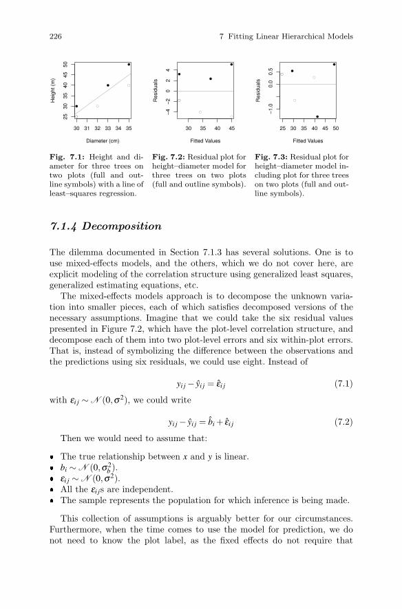
226 7 Fitting Linear Hierarchical Models
●
●
●
●
●
●
30 31 32 33 34 35
2530
3540
4550
Diameter (cm)
Hei
ght (
m)
Fig. 7.1: Height and di-ameter for three trees ontwo plots (full and out-line symbols) with a line ofleast–squares regression.
●
●
●
●
●
●
30 35 40 45
−4
−2
02
4
Fitted Values
Res
idua
lsFig. 7.2: Residual plot forheight–diameter model forthree trees on two plots(full and outline symbols).
●
●
●
●
●
●
25 30 35 40 45 50
−1.
00.
00.
5
Fitted Values
Res
idua
ls
Fig. 7.3: Residual plot forheight–diameter model in-cluding plot for three treeson two plots (full and out-line symbols).
7.1.4 Decomposition
The dilemma documented in Section 7.1.3 has several solutions. One is touse mixed-effects models, and the others, which we do not cover here, areexplicit modeling of the correlation structure using generalized least squares,generalized estimating equations, etc.
The mixed-effects models approach is to decompose the unknown varia-tion into smaller pieces, each of which satisfies decomposed versions of thenecessary assumptions. Imagine that we could take the six residual valuespresented in Figure 7.2, which have the plot-level correlation structure, anddecompose each of them into two plot-level errors and six within-plot errors.That is, instead of symbolizing the difference between the observations andthe predictions using six residuals, we could use eight. Instead of
yi j − yi j = εi j (7.1)
with εi j ∼ N (0,σ2), we could write
yi j − yi j = bi + εi j (7.2)
Then we would need to assume that:
� The true relationship between x and y is linear.� bi ∼ N (0,σ2
b ).� εi j ∼ N (0,σ2).� All the εi js are independent.� The sample represents the population for which inference is being made.
This collection of assumptions is arguably better for our circumstances.Furthermore, when the time comes to use the model for prediction, we donot need to know the plot label, as the fixed effects do not require that

7.2 Linear Mixed-Effects Models 227
we know it. The plot-to-plot variation is represented by σ2b and no longer
creates a correlation structure within the residuals. Also, although it seemsodd to use eight quantities to represent six unknowns, the fact that we putconstraints on them (for example, zero mean) means that the quantities canbe estimated, although they do not need to be estimated in order to fit themodel.
We now have two unknown variances in our model. These variances aregenerally referred to as variance components, inasmuch as they represent thesources of variation that contribute to the errors in the model.
This example illustrates the use of random effects. Random effects donot explain variation. Explaining variation is the role of the fixed effects.Random effects organize variation, or enforce a more complex structure uponit, in such a way that a match is possible between the model assumptionsand the diagnostics. We would expect the overall uncertainty, measured asroot-mean-squared error, to increase any time we estimate parameters for amodel using any way other than by least squares.
7.2 Linear Mixed-Effects Models
Now we use a simple example as a basis for walking through the code to fitmixed-effects models in R.
7.2.1 A Simple Example
We start with a very simple and abstract example. Our goal is to constructa model to predict y from a continuous predictor variable x and a categoricalpredictor variable called group. First we generate a simple dataset.
> example <- data.frame(y = c(4.2, 4.8, 5.8, 1.2, 10.1,
+ 14.9, 15.9, 13.1),
+ x = c(1, 2, 3, 4, 1, 2, 3, 4),
+ group = factor(c(1, 1, 1, 1,
+ 2, 2, 2, 2)))
Now, we have to load the package that holds the mixed-effects code, nlme(Pinheiro and Bates, 2000).
> library(nlme)
Next, we plot the data (Figure 7.4).
> par(las=1, mar=c(4,4,1,1))
> colours <- c("red", "blue")
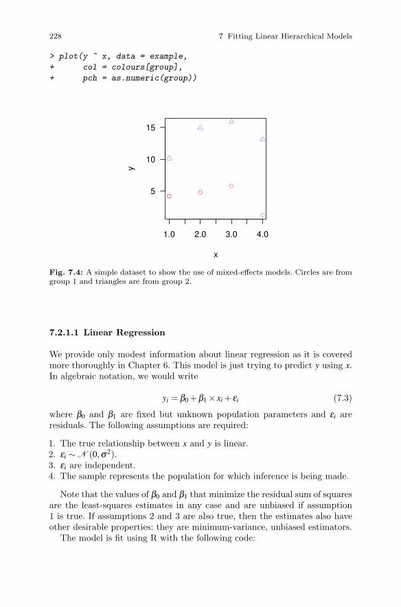
228 7 Fitting Linear Hierarchical Models
> plot(y ~ x, data = example,
+ col = colours[group],
+ pch = as.numeric(group))
●●
●
●
1.0 2.0 3.0 4.0
5
10
15
x
y
Fig. 7.4: A simple dataset to show the use of mixed-effects models. Circles are fromgroup 1 and triangles are from group 2.
7.2.1.1 Linear Regression
We provide only modest information about linear regression as it is coveredmore thoroughly in Chapter 6. This model is just trying to predict y using x.In algebraic notation, we would write
yi = β0 +β1 × xi + εi (7.3)
where β0 and β1 are fixed but unknown population parameters and εi areresiduals. The following assumptions are required:
1. The true relationship between x and y is linear.2. εi ∼ N (0,σ2).3. εi are independent.4. The sample represents the population for which inference is being made.
Note that the values of β0 and β1 that minimize the residual sum of squaresare the least-squares estimates in any case and are unbiased if assumption1 is true. If assumptions 2 and 3 are also true, then the estimates also haveother desirable properties: they are minimum-variance, unbiased estimators.
The model is fit using R with the following code:
7.2 Linear Mixed-Effects Models 229
> basic.1 <- lm(y ~ x, data=example)
We can examine estimates from the model via:
> coef(summary(basic.1))
Estimate Std. Error t value Pr(>|t|)
(Intercept) 8.5 5.142956 1.65274590 0.1494694
x 0.1 1.877942 0.05324978 0.9592616
Next, we let each group have its own intercept. In algebra,
yi = β01 +β02 ×gi +β1 × xi + εi (7.4)
where β01, β02, and β1 are fixed but unknown population parameters, gi isan indicator variable with value 0 for group 1 and 1 for group 2, and εi areresiduals. Note that in accordance with R’s convention, β01 is the coefficientrepresenting the intercept for the first group and β02 is the coefficient rep-resenting the difference between the intercepts for the first and the secondgroups. The same assumptions are required as for model (7.3).
The model is fit using R with the following code:
> basic.2 <- lm(y ~ x + group, data=example)
Now we let each group have its own intercept and slope.
yi = β01 +β02 ×gi +(β11 +β12 ×gi)× xi + εi (7.5)
where β01, β02, β12, and β12 are fixed but unknown population parameters,gi is an indicator variable with value 0 for group 1 and 1 for group 2, and theεi are the errors. The same assumptions are required as for model (7.3).
The model is fit using R with the following code:
> basic.3 <- lm(y ~ x * group, data=example)
7.2.1.2 Mixed Effects
In order to analyze the data using a mixed-effects model, some preparationis advantageous. It will help to convert the data to a grouped object — aspecial kind of data frame that supports special nlme commands. The groupwill hereby be a random effect. Constructing a groupedData object is notessential, but it enables functionality later on. For example, we will be ableto use augPred, as seen in Figure 7.5, below.
> example.mixed <- groupedData(y ~ x | group, data=example)
Now we fit the basic mixed-effects model that allows the intercepts to varyrandomly between the groups. This is analogous to the situation described inthe previous section. We will add a subscript for clarity. The model form is

230 7 Fitting Linear Hierarchical Models
yi j = β0 +b0i +β1 × xi j + εi j (7.6)
where β0 and β1 are fixed but unknown population parameters, the b0i arethe two group-specific random intercepts, and εi j are residuals. The followingassumptions are required:
� The true relationship between x and y is linear.� b0i ∼ N (0,σ2
b0).
� εi j ∼ N (0,σ2).� The b0i and the εi j are all independent.� The samples represent the populations from which they were drawn.
The model is fit using R with the following code:
> basic.4 <- lme(y ~ x,
+ random = ~1 | group,
+ data = example.mixed)
The random syntax can be a little confusing. Here we are instructing R tolet each group have its own random intercept. If we wanted to let each grouphave its own slope and intercept, we would write random = ~x | group. Ifwe wanted to let each group have its own slope but only a common intercept,we would write random = ~x - 1 | group. We can also write the model inlist form, that is, random = list(group = ~ 1).
We can examine the model in a useful graphic called an augmented pre-
diction plot. This plot provides a scatterplot of the data, with a unique panelfor each group, and a fitted line that represents the model predictions (Fig-ure 7.5). We should also check the regression diagnostics that are relevant toour assumptions, but we have so few data here that the diagnostics are notinstructive. We will develop these ideas further during the case study thatfollows.
> plot(augPred(basic.4))
If we are satisfied with the model diagnostics, then we can examine thestructure of the model, including the estimates, using the summary function.The summary function presents a collection of useful information about themodel. Here we report the default structure for a summary.lme object; thatis, the object produced when the summary function is called on an object oftype lme.
> summary(basic.4)
First, the data.frame object is identified and fit statistics are reported,including Akaike’s information criterion, Schwartz’s Bayesian information cri-terion, and the log-likelihood.

7.2 Linear Mixed-Effects Models 231
x
y
5
10
15
1.0 1.5 2.0 2.5 3.0 3.5 4.0
●
●
●
●
1
1.0 1.5 2.0 2.5 3.0 3.5 4.0
●
●
●
●
2
Fig. 7.5: An augmented plot of the basic mixed-effects model with random interceptsfit to the sample dataset.
Linear mixed-effects model fit by REML
Data: example.mixed
AIC BIC logLik
43.74387 42.91091 -17.87193
The random-effects structure is then described, and estimates are providedfor the variance components. Here we have an intercept for each group forwhich the standard deviation is reported as well as the standard deviation ofthe residuals within each group.
Random effects:
Formula: ~1 | group
(Intercept) Residual
StdDev: 6.600769 2.493992
The fixed effects structure is described next in a standard t-table arrange-ment. Estimated correlations between the fixed effects follow.
Fixed effects: y ~ x
Value Std.Error DF t-value p-value
(Intercept) 8.5 5.142963 5 1.6527437 0.1593
x 0.1 0.788670 5 0.1267958 0.9040
Correlation:
(Intr)
x -0.383
The distribution of the within-group residuals, also called the innermost
residuals in the context of strictly hierarchical models by Pinheiro and Bates(2000), is then described.

232 7 Fitting Linear Hierarchical Models
Standardized Within-Group Residuals:
Min Q1 Med Q3 Max
-1.2484738 -0.4255493 0.1749470 0.6387985 1.0078956
Finally, the hierarchical structure of the model and data is presented.
Number of Observations: 8
Number of Groups: 2
7.2.1.3 Mixed Effects, Unique Variances
Next we shall allow the residuals within each group to have their own vari-ances. The model form will be the same as in equation (7.6), but the assump-tions will be different. Now we will need to assume that the residuals εi j fromeach group have their own distributions. That is:
� The true relationship between x and y is linear.� b0i ∼ N (0,σ2
b1).
� ε1 j ∼ N (0,σ2b01).
� ε2 j ∼ N (0,σ2b02).
� The b0i and the εi j are all independent.� The samples represent the populations from which they were drawn.
The model is fitted using R with the following code:
> basic.5 <- lme(y ~ x, random = ~1 | group,
+ weights = varIdent(form = ~1 | group),
+ data = example.mixed)
The summary output is essentially identical to the previous output instructure, with the addition of a new section that summarizes the newlyadded variance model. Here we show only the new portion.
> summary(basic.5)
Variance function:
Structure: Different standard deviations per stratum
Formula: ~1 | group
Parameter estimates:
1 2
1.000000 1.327843
We see that the standard deviation of the first group has been set to 1 andthe standard deviation of the other groups is presented as a ratio relative togroup 1.
7.3 Case Study: Height and Diameter Model 233
7.2.1.4 Mixed Effects, Unique Variances, Autocorrelation
Finally, we allow for simple temporal autocorrelation within each group. Wewill specify a one-step autocorrelation that specifies that the correlation be-tween any pair of residuals is a function of their distance apart in time (orspace). Again, the model form will be the same as in equation (7.6), but theassumptions will be different. Now, we will need to assume that:
� The true relationship between x and y is linear.� b0i ∼ N (0,σ2
b1).
� ε1 j ∼ N (0,σ2b01).
� ε2 j ∼ N (0,σ2b02).
� Corr(εab,εac) = ρ |c−b|.� The b0i and the εi j are all independent otherwise.� The samples represent the populations from which they were drawn.
The model is fit using R with the following code:
> basic.6 <- lme(y ~ x, random = ~1 | group,
+ weights = varIdent(form = ~1 | group),
+ correlation = corAR1(),
+ data = example.mixed)
The summary output is again essentially identical to the previous outputin structure, with the addition of a new section that summarizes the newlyadded correlation model. Here we show only the new portion.
> summary(basic.6)
Correlation Structure: AR(1)
Formula: ~1 | group
Parameter estimate(s):
Phi
0.8107325
The model estimates the first-order autocorrelation between the residualswithin the groups as 0.81, which is quite high.
Any or all of the innovations that we added to the model in the recentfitting exercise might be necessary to achieve a suitable model fit.
7.3 Case Study: Height and Diameter Model
We now use a real dataset to demonstrate the construction of mixed-effectsmodels. Section 2.4.5 summarizes the data entry and processing. Briefly, asample of 66 trees was purposively selected in national forests around north-ern and central Idaho. The habitat type and diameter at 1.37 m (4′6′′) were
234 7 Fitting Linear Hierarchical Models
also recorded for each tree, as was the national forest from which it came.Each tree was then split, and decadal measures were made of height and di-ameter inside bark at 1.37 m (4′6′′). We have data from nine national forestsand six different habitat types.
> names(stage)
[1] "Tree.ID" "Forest" "HabType" "Decade" "Dbhib"
[6] "Height" "Age" "Forest.ID" "Hab.ID" "dbhib.cm"
[11] "height.m"
> dim(stage)
[1] 542 11
7.3.1 Height vs. Diameter
The prediction of height from diameter provides useful and inexpensiveinformation. It may be that the height vs. diameter relationship differsamong habitat types, climate zones, or tree ages. We shall examine theheight/diameter model of the trees using a mixed-effects model. We’ll startwith a simple case, using only the oldest measurement from each tree.
> stage.old <- stage[stage$Decade == 0, ]
Note that this code actually drops a tree from our dataset because thattree lacks a measurement at decade 0, but we can afford to let it go for thepurposes of this demonstration.
Based on our knowledge of the locations of national forests, it seems rea-sonable to believe that there will be similarities between trees that grow inthe same forest relative to the overall population of trees. That is, a randomlyselected pair of trees from the same forest are more likely to be similar to oneanother than a randomly selected pair of trees from the whole population,which includes all the different forests. However, we would like to create amodel that does not need to rely on knowing the national forest; that is, amodel that can plausibly be used for trees in other forests. The followingapproach is acceptable as long as we are willing to believe that the sample oftrees that we are using is representative of the conditions for which we wishto apply the model. In the absence of other information, this decision is ajudgment call. We assume it for the moment.
So, based on the information above, national forest will be a random effectand habitat type will be a fixed effect, the inclusion of which we will test for.That is, we wish to construct a model that can be used for any forest, and thatmight be more accurate if used correctly within a named national forest, andprovides unique estimates for habitat type. We can later ask how useful the

7.3 Case Study: Height and Diameter Model 235
knowledge of habitat type is and whether we want to include it in the model.So, we’ll have two random effects: national forest and tree within nationalforest. We have one baseline fixed effect, diameter at breast height insidebark, with two potential additions, age and habitat type. The lowest-levelsampling unit will be the tree, nested within national forest.
As noted earlier, it is convenient to provide a basic groupedData structureto R. The structure will help R create useful graphical diagnostics later inthe analysis.
> stage.old <- groupedData(height.m ~ dbhib.cm | Forest.ID,
+ data = stage.old)
Now, we look to our model. An algebraic expression of the model is
yi j = β0 +b0i +β1 × xi j + εi j (7.7)
where yi j is the height of tree j in forest i and xi j is the diameter of the sametree. β0 and β1 are fixed but unknown parameters, and b0i are the forest-specific random and unknown intercepts. Later we might see if the slope alsovaries with forest. So, in matrix form from Laird and Ware (1982), the modelis
Y = Xβββ +Zb+ εεε
b ∼ N (0,D)
εεε ∼ N (0,R)
where Y is the column of tree heights and X is the column of diametersbound with a column of 1s for the intercept. β will be a vector of parameterestimates. Z will be a matrix of 0s and 1s to allocate the observations todifferent forests. b will be a vector of means for the forests and trees withinforests. Finally, we will let D be a 9 × 9 identity matrix multiplied by aconstant σ2
h , as there are nine national forests, and R be a 66× 66 identitymatrix multiplied by a constant σ2, as there are 66 trees.
NB: D and R are covariance matrices constructed using a small number ofparameters. The structure of D and R is suggested by what is known aboutthe data and can be tested by comparing nested models.
The key assumptions that we’re making for our model are that:
1. The model structure is correctly specified.2. The random effects are normally distributed.3. The innermost residuals are normally distributed.4. The innermost residuals are homoskedastic within and across the groups.5. The innermost residuals are independent within the groups.6. The sample represents the population for which inference is being made.

236 7 Fitting Linear Hierarchical Models
It is timely to introduce some useful nomenclature. For hierarchical models,there is more than one level of fitted values and residuals. Pinheiro and Bates(2000) adopt the following labels: the outermost residuals and fitted valuesare conditional only on the fixed effects, the innermost residuals and fittedvalues are conditional on the fixed and all the random effects, and there areas many levels between these extremes as necessary. So, in a two-level modellike this one:
� The outermost residuals are the residuals that are computed from theoutermost fitted values, which are computed using only the fixed effects.Let’s refer to them as r0.
r0 = yi j − β0 − β1 × xi j (7.8)
� The innermost residuals are the residuals that are computed from theinnermost fitted values, which are computed from the fixed effects and therandom effects. We shall refer to them as r1.
r1 = yi j − β0 − b0i − β1 × xi j (7.9)
Note that in the more general case of mixed-effects models with crossedrandom effects, the labels “innermost” and “outermost” are not likely to beuseful.
The linear mixed-effects apparatus also provides us with three kinds ofinnermost and outermost residuals:
1. response residuals, simply the difference between the observation and theprediction;
2. Pearson residuals, which are the response residuals scaled by dividing bytheir estimated standard deviation; and
3. normalized residuals, which are the Pearson residuals pre-multiplied by theinverse square root of the estimated correlation matrix from the model.
In the model specification, we are not making any assumptions about theoutermost residuals. However, they are useful for summarizing the elementsof model performance. We fit a model to the measurements taken at the latestpoint for each tree as follows. First, we construct the groupedData object.
> stage.old <- groupedData(height.m ~ dbhib.cm | Forest.ID,
+ data = stage[stage$Decade == 0,])
Our model is then fit using the following code:
> hd.lme.1 <- lme(height.m ~ dbhib.cm,
+ random = ~1 | Forest.ID,
+ data = stage.old)
We next construct diagnostic graphs to check our assumptions. Note thatin some cases the assumptions are stated in an unhelpfully broad fashion.

7.3 Case Study: Height and Diameter Model 237
Therefore the sensible strategy is to check for the conditions that can beinterpreted in the context of the design, the data, and the incumbent model.For example, there are infinite ways that the innermost residuals could failto have constant variance. We should ask: What are the important ways?The situation that is most likely to lead to problems is if the variance ofthe residuals is a function of some effect, whether that be a fixed effect or arandom effect.
Rather than trust our ability to anticipate what the programmers meantby the labels that they use, etc, we prefer to know what goes into each ofour plots. The best way to do that is to put it there ourselves. To examineeach of the assumptions in turn, we have constructed the following suite ofgraphics. These are presented in Figure 7.6.
1. A plot of the outermost fitted values against the observed values of theresponse variable. This graph allows an overall summary of the explanatorypower of the model.
> scatter.smooth(fitted(hd.lme.1, level=0),
+ stage.old$height.m,
+ xlab = "Fitted Values (height, m.)",
+ ylab = "Observed Values (height, m.)",
+ main = "Model Structure (I)")
> abline(0, 1, col = "blue")
The important questions to ask are:
a. How much of the variation is explained by the fixed effects?b. How much of the variation remains?c. Is there evidence of lack of fit anywhere in particular?
2. A plot of the innermost fitted values against the innermost Pearson residu-als. This graph allows a check of the assumption of correct model structure.
> scatter.smooth(fitted(hd.lme.1),
+ residuals(hd.lme.1, type="pearson"),
+ main = "Model Structure (II)",
+ xlab = "Fitted Values",
+ ylab = "Innermost Residuals")
> abline(h = 0, col = "red")
The important questions to ask are:
a. Is there curvature? If so, then perhaps the fixed effects could be aug-mented or improved. There might be an interaction missing, or perhapsa predictor should be quadratic.
b. Do the residuals fan out? If so, then the variance function for the modelcould be inadequate. Consider modeling the change in variance explic-itly. Or, if this is coupled with curvature and a biological explanation,a transformation might be useful.
238 7 Fitting Linear Hierarchical Models
c. Are any outliers evident? If so, then they should be checked and theirinfluence on the model assessed by refitting the model without them.
3. A q-q plot of the estimated random effects to check whether they are nor-mally distributed with constant variance. Note that interpretation of theq-q plot is sensitive to the assumption of constant variance, so violationsof this diagnostic could be due to non-normality or heteroskedasticity.
> ref.forest <- ranef(hd.lme.1)[[1]]
> ref.var.forest <-
+ tapply(residuals(hd.lme.1, type="pearson", level=1),
+ stage.old$Forest.ID, var)
> qqnorm(ref.forest, main="Q-Q Norm: Forest Random Effects")
> qqline(ref.forest, col="red")
The important questions to ask are:
a. Do the points follow a straight line, or do they exhibit patterns thatcan be translated as skewness or kurtosis? If the latter, then the vari-ance function for the model could be inadequate. Consider modeling thechange in variance explicitly. Also, a transformation may be required,but care should be taken. Perhaps large-sample theory can be invoked.
b. Are any outliers evident? See possible actions in part 2c above. Theidentification of outlying groups can be particularly informative.
4. A q-q plot of the Pearson residuals to check whether they are normallydistributed with constant variance.
> qqnorm(residuals(hd.lme.1, type="pearson"),
+ main="Q-Q Normal - Residuals")
> qqline(residuals(hd.lme.1, type="pearson"), col="red")
The important questions to ask are:
a. Do the points follow a straight line, or do they exhibit skewness orkurtosis? See possible actions in part 3a above.
b. Are any outliers evident? See possible actions in part 2c above.
5. A notched boxplot of the innermost Pearson residuals by the groupingvariable to see what the within-group distribution looks like.
> boxplot(residuals(hd.lme.1, type = "pearson", level = 1) ~
+ stage.old$Forest.ID,
+ ylab = "Innermost Residuals",
+ xlab = "National Forest",
+ notch = TRUE,
+ varwidth = TRUE,
+ at = rank(ref.forest))
> axis(3, labels = format(ref.forest, dig=2),
7.3 Case Study: Height and Diameter Model 239
+ cex.axis = 0.8, at = rank(ref.forest))
> abline(h = 0, col = "darkgreen")
The important questions to ask are:
a. Do the notches intersect 0? If not, then the relevant groups should bechecked and their effect on the model fit examined by deleting them.
b. Is there a trend between the medians of the within-group residuals andthe estimated random effect? If so, then the random effect may be ex-plaining some variation that could be explained by a fixed effect.
6. A scatterplot of the variance of the Pearson residuals within the forestagainst the forest random effect.
> plot(ref.forest, ref.var.forest,
+ xlab = "Forest Random Effect",
+ ylab = "Variance of within-Forest Residuals")
> abline(lm(ref.var.forest ~ ref.forest), col="purple")
a. Is there a distinct positive or negative trend? If so, then careful thoughtabout the variance model might be beneficial.
Of course, there is no need to pack all the graphical diagnostics into onefigure. We cross-reference the list against Figure 7.6. In fact, all of theseresidual diagnostics look good for the model that we have fit.
The next important question is whether there are any outliers or high-influence points. In a case like this, it is relatively easy to see from the diag-nostics that no point is likely to dominate the fit in this way. However, a moreformal examination of the question may be valuable. There is considerablepeer-reviewed development of the problem of outlier and influence detectionin mixed-effects models, reaching back at least to Christensen et al. (1992).Schabenberger (2005) provides an overview of the extensive offerings avail-able in SAS, none of which are presently available in R packages as far aswe know. Demidenko (2004) and Demidenko and Stukel (2005) also suggestsome alternatives.
It is worth recalling that much of the outlier-detecting apparatus focuseson efficiently assessing the effect of individual observations on the model.Therefore, if the fitting process is reasonably quick and the analyst is pa-tient, it is straightforward to custom-build influence diagnostics that focusspecifically upon the parameter estimates or tests of interest. The simpleststrategy is to refit the model, dropping each observation or group one byone and collecting the results in a vector for further analysis. This is easilyhandled by using the update() function, and we do not cover it here.
We will accept the model as it stands for the moment and go on to examinethe model summary. We divide the summary into pieces here to explain itsstructure and content.
> summary(hd.lme.1)
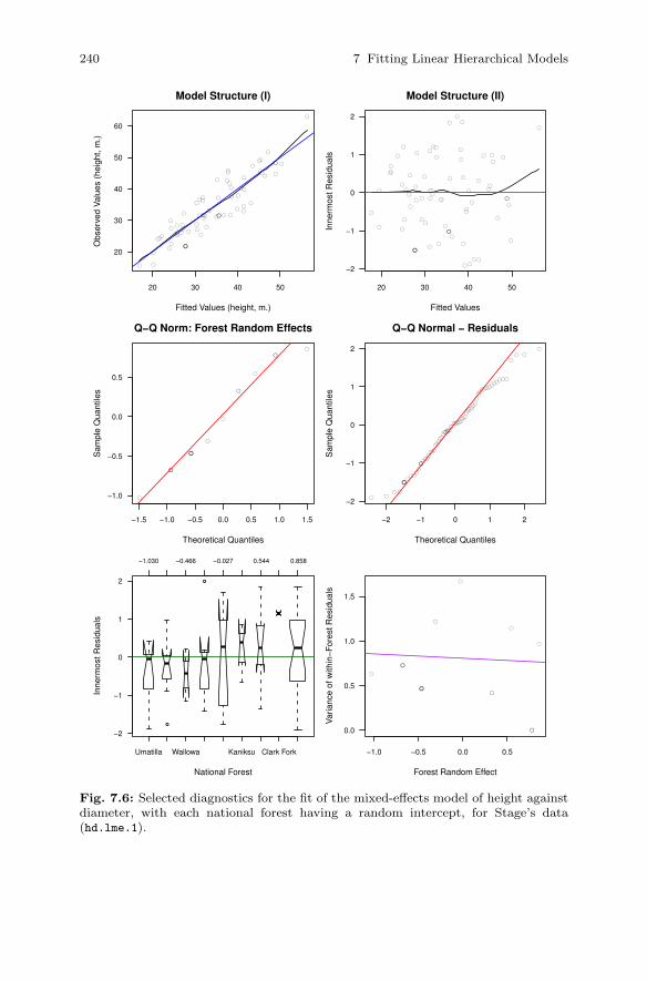
240 7 Fitting Linear Hierarchical Models
●
●
●
●
●
●
●
●
●●
●
●
●
●
●
●●
●
●
●
●
●
●
●
●
●
●●
●
●
●
●
●
●●
●
●
●
●
●●
●
●
●
●
●
●
●
●
●
●
●
●
●
●
●●
●
●
●
●
●
●
●
●
20 30 40 50
20
30
40
50
60
Model Structure (I)
Fitted Values (height, m.)
Obs
erve
d V
alue
s (h
eigh
t, m
.)
●
●
●●
●
● ●
●●
●
●
●
●
●
●
●
●
●
●
●
●
●
●
●
●
●
●
●
●
●
●
●
●
●
●
●
●
●
●
●
●
●
●
●
●
●
●
●
●
●
●
●
●●
●
●
●
●
●
●
●
●
●
●
●
20 30 40 50
−2
−1
0
1
2
Model Structure (II)
Fitted Values
Inne
rmos
t Res
idua
ls
●
●
●
●
●
●
●
●
●
−1.5 −1.0 −0.5 0.0 0.5 1.0 1.5
−1.0
−0.5
0.0
0.5
Q−Q Norm: Forest Random Effects
Theoretical Quantiles
Sam
ple
Qua
ntile
s
●
●
●●
●
●●
●●
●
●
●
●
●
●
●
●
●
●
●
●
●
●
●
●
●
●
●
●
●
●
●
●
●
●
●
●
●
●
●
●
●
●
●
●
●
●
●
●
●
●
●
●●
●
●
●
●
●
●
●
●
●
●
●
−2 −1 0 1 2
−2
−1
0
1
2
Q−Q Normal − Residuals
Theoretical Quantiles
Sam
ple
Qua
ntile
s
●
●
Umatilla Wallowa Kaniksu Clark Fork
−2
−1
0
1
2
National Forest
Inne
rmos
t Res
idua
ls
−1.030 −0.466 −0.027 0.544 0.858
●
●
●
●
●
●
●
●
●
−1.0 −0.5 0.0 0.5
0.0
0.5
1.0
1.5
Forest Random Effect
Var
ianc
e of
with
in−
For
est R
esid
uals
Fig. 7.6: Selected diagnostics for the fit of the mixed-effects model of height againstdiameter, with each national forest having a random intercept, for Stage’s data(hd.lme.1).

7.3 Case Study: Height and Diameter Model 241
1. Linear mixed-effects model fit by REML
Data: stage.old
AIC BIC logLik
376.6805 385.2530 -184.3403
Here we have the overall metrics of model fit, including the log-likelihood(recall that this is the quantity that we are maximizing to make the fit)and the AIC and BIC statistics. The fixed effects are profiled out of thelog-likelihood, so that the log-likelihood is a function only of the data andtwo parameters: σ2
h and σ2. We are not comparing these statistics withanything, so they do not offer direct interpretation here.
2. Random effects:
Formula: ~1 | Forest.ID
(Intercept) Residual
StdDev: 1.151405 3.937486
The formula reminds us of what we asked for: that the forest be a randomeffect and that a unique intercept be fit for each level of forest. The squareroots of the estimates of the two parameters are also here. These quantitiesare measured in meters. That is, the standard deviation of the variationbetween the forest mean heights is 1.15 m and that of the tree heightswithin the forests is 3.94 m.
3. Another metric of model quality is RMSE, which is the estimate of thestandard deviation of the response residuals conditional on only the fixedeffects. Note that 3.94 is not the RMSE but it is instead an estimate ofthe standard deviation of the response residuals conditional on the fixedand the random effects. Obtaining the RMSE is relatively easy becausethe random effects and the residuals are assumed to be independent.
RMSE =√
σ2h +σ2 = 4.1
The last metric of model quality we can get here is the intra-class correla-tion. This is the variance of the random effect divided by the sum of thevariances of the random effects and the residuals
ρ =σ2
h
σ2h +σ2
= 0.0788
so about 7.9% of the variation in height (that is not explained by diameter)is explained by national forest. This is a small quantity and implies thatthe systematic differences between tree heights in the different forests aresmall once the tree diameter has been taken into account.
4. Fixed effects: height.m ~ dbhib.cm
Value Std.Error DF t-value p-value
(Intercept) 6.58239 1.7763571 55 3.705556 5e-04
dbhib.cm 0.57036 0.0335347 55 17.008062 0e+00

242 7 Fitting Linear Hierarchical Models
Now we have a reminder of the fixed-effects model and the estimates ofthe fixed effects. We have several columns:
a. the value of the estimate,b. its standard error,c. the degrees of freedom,d. the t-value associated with the significance test of the null hypothesis
that the estimate is 0 against the two-tailed alternative that it is not 0,which is meaningless for this particular model, and
e. the p-value associated with that meaningless test.
5. Correlation:
(Intr)
dbhib.cm -0.931
This is the correlation matrix for the estimates of the fixed effects. It isestimated from the design matrix. This comes from the covariance matrixof the fixed effects, which can be estimated by (X′V−1X)−1. Here the cor-relation is high and negative, which in our case is simply a consequence ofnot centering the data before fitting the model. The high negative corre-lation is to be expected and is not of great diagnostic importance in thiscase.
6. Standardized Within-Group Residuals:
Min Q1 Med Q3 Max
-1.91215622 -0.70233393 0.04308139 0.81189065 1.99133843
This segment reports distributional information about the within-groupresiduals. We should be asking ourselves: Are they symmetric? Are thereegregious outliers? We can compare these values to what we know of thestandard normal distribution, for which the median should be about 0, thefirst quartile at −0.674, and the third quartile at 0.674.
7. Number of Observations: 65
Number of Groups: 9
And finally, we have confirmation that we have the correct number ofobservations and groups. This is a useful conclusion to draw; it comfortsus that we fit the model that we thought we had!
A set of sequential tests of the model’s fixed effects can be had from
> anova(hd.lme.1)
numDF denDF F-value p-value
(Intercept) 1 55 2848.4436 <.0001
dbhib.cm 1 55 289.2742 <.0001
Pinheiro and Bates (2000) recommend that these tests be used in pref-erence to whole-model tests and Wald tests, which are reported in item 4above. It is worth noting at this point that the question of testing in the

7.3 Case Study: Height and Diameter Model 243
more general case of models with crossed random effects is not satisfactorilyresolved. The anova.lme function, that is, the version of anova that is usedwhen the first argument is of class lme, also has a type argument, for which“marginal” is an option and that defaults to “sequential”.
7.3.2 Use More Data
We now treat the grand fir height/diameter data from Stage (1963) in adifferent way. We have numerous measurements of height and diameter foreach tree. It seems wasteful to use only the oldest observation.
We still assume that the national forests represent different purposivelyselected sources of climatic variation and that habitat type represents a ran-domly selected treatment of environment (it is probably not true, but weassume that it is). This is like a randomized block design, where the blocksand the treatment effects are crossed. This time we are interested in usingall of the data. Previously we took only the first measurement. How will themodel change? We begin by setting up the data in a groupedData object.
> stage <- groupedData(height.m ~ dbhib.cm | Forest.ID/Tree.ID,
+ data = stage)
We say that, based on the information above, national forest will be arandom effect and habitat type a candidate fixed effect. So, we will haveone to three fixed effects; dbhib, age, and habitat, and two random effects;forest and tree within forest. The response variable will still be the heightmeasurement. There will be numerous height measurements within each tree,separated by time. There will be numerous trees measured within each forest,separated by space. We assume, for the moment, that the measurements areconditionally independent within the tree. This means that we are assumingthat the innermost residuals from the model that we have just described willbe independent of one another. This assumption is definitely not true, andwill be revisited. Now, we look to our model.
yi jk = β0 +b0i +b0i j +β1 × xi jk + εi jk (7.10)
where yi jk is the height of tree j in forest i at measurement k and xi jk is thediameter of the same tree. β0 and β1 are fixed but unknown parameters, b0i
are the forest-specific random and unknown intercepts, and b0i j are the tree-specific random and unknown intercepts. Later we might see if the slope alsovaries with forest. So, in matrix form, we have

244 7 Fitting Linear Hierarchical Models
Y = Xβββ +Zb+ εεε
b ∼ N (0,D)
εεε ∼ N (0,R)
where
� Y is the vector of height measurements. The basic unit of Y will be ameasurement within a tree within a forest. It has 542 observations.
� X is a matrix of 0s, 1s, and diameters to allocate the observations todifferent tree diameters at the time of measurement.
� β is a vector of parameter estimates.� Z is a matrix of 0s and 1s to allocate the observations to different forests
and trees within forests.� b is a vector of means for the forests and the trees.� D is a block diagonal matrix that comprises two portions: a 9×9 identity
matrix multiplied by a constant σ 2f and then a square matrix for each
forest, which is a diagonal matrix with variances on the diagonals.� R is a 542×542 identity matrix multiplied by a constant σ2.
This model is fitted using the following code:
> hd.lme.3 <- lme(height.m ~ dbhib.cm,
+ random = ~1 | Forest.ID/Tree.ID,
+ data = stage)
The key assumptions that we’re making are that:
1. The model structure is correctly specified.2. The tree and forest random effects are normally distributed.3. The tree random effects are homoskedastic within the forest random ef-
fects.4. The innermost residuals are normally distributed.5. The innermost residuals are homoskedastic within and across the tree ran-
dom effects.6. The innermost residuals are independent within the trees.7. The samples represent the populations from which they were drawn.
We again construct diagnostic graphs to check these assumptions. To ex-amine each of the assumptions in turn, we have constructed the earlier suiteof graphics along with some supplementary graphs. The extra graphs are:
1. An extra q-q plot of the tree-level random effects to check whether theyare normally distributed with constant variance.
a. Do the points follow a straight line, or do they exhibit skewness orkurtosis? If not, then careful thought about the variance model mightbe beneficial.

7.3 Case Study: Height and Diameter Model 245
b. Are any outliers evident? If so, they should be checked and their effecton the model fit examined by their deletion.
2. A notched boxplot of the tree-level random effects by the grouping variableto see what the within-group distribution looks like.
a. Do the notches intersect 0? If not, then the relevant groups should bechecked and the effect of their deletion on the model fit examined.
b. Is there a trend between the medians of the within-group residuals andthe estimated random effect? If so, then the random effect may be ex-plaining some variation that could be explained by a fixed effect.
c. Do any of the random effects stand out as being wildly different? If so,they should be checked and the effect of their deletion on the model fitexamined.
3. A scatterplot of the variance of the tree-level random effects within theforest against the forest random effect.
a. Is there a distinct positive or negative trend? If so, then careful thoughtabout the variance model might be beneficial.
b. Do any of the random effects stand out as being wildly different? If so,they should be checked and the effect of their deletion on the model fitexamined.
4. An autocorrelation plot of the within-tree errors.
a. Is there evidence of substantial autocorrelation? If so, then the modelshould be extended to cover that possibility, as documented below.
As a rule of thumb, we will need about four plots plus three for eachrandom effect. Cross-reference these against Figures 7.7–7.9. Each graphicshould ideally be examined separately in its own frame. The code follows.
> opar <- par(mfrow = c(1, 3), mar = c(4, 4, 3, 1), las = 1,
+ cex.axis = 0.9)
> plot(fitted(hd.lme.3, level=0), stage$height.m,
+ xlab = "Fitted Values", ylab = "Observed Values",
+ main = "Model Structure (I)")
> abline(0, 1, col = "gray")
> scatter.smooth(fitted(hd.lme.3),
+ residuals(hd.lme.3, type="pearson"),
+ main = "Model Structure (II)",
+ xlab = "Fitted Values",
+ ylab = "Innermost Residuals")
> abline(h = 0, col = "gray")
> acf.resid <- ACF(hd.lme.3, resType = "normal")
> plot(acf.resid$lag[acf.resid$lag < 10.5],
+ acf.resid$ACF[acf.resid$lag < 10.5],
+ type="b", main="Autocorrelation",
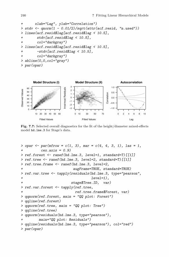
246 7 Fitting Linear Hierarchical Models
+ xlab="Lag", ylab="Correlation")
> stdv <- qnorm(1 - 0.01/2)/sqrt(attr(acf.resid, "n.used"))
> lines(acf.resid$lag[acf.resid$lag < 10.5],
+ stdv[acf.resid$lag < 10.5],
+ col="darkgray")
> lines(acf.resid$lag[acf.resid$lag < 10.5],
+ -stdv[acf.resid$lag < 10.5],
+ col="darkgray")
> abline(0,0,col="gray")
> par(opar)
●●
●●
●
●●
●●●
●
●●
●
●
●
●●
●●
●●
●●
●
●
●
●●
●●
●
●
●●
●
●
●
●
●●
●●
●●
●●
●
●
●
●●
●●
●
●
●
●●
●●●●●●
●
●●
●●
●●
●
●
●●
●
●●
●
●
●
●●
●
●●
●●
●
●●●●●
●●●●
●
●
●
●
●
●
●
●●
●●
●●
●●
●●
●●
●●
●
●●
●
●
●
●
●
●
●
●
●
●
●
●
●●
●●
●●
●●
●
●
●
●
●●
●●
●●
●●
●
●
●
●
●
●
●
●
●
●
●
●
●
●
●
●
●
●
●
●
●
●
●
●●
●
●
●
●●
●●
●●
●●
●
●
●
●
●
●
●
●
●●
●●
●
●
●
●●
●●
●
●
●●
●
●
●●●
●●
●
●●
●
●
●
●
●
●
●●
●
●●
●
●
●
●
●
●●
●
●
●●
●●
●●
●●
●●
●
●
●
●●
●
●●●
●
●
●
●●
●
●
●
●
●●
●●
●●
●
●
●
●
●●
●
●
●
●
●●
●
●
●
●
●●
●
●
●
●
●●
●●
●
●
●
●●
●●
●●
●●
●●
●
●●
●
●
●
●
●
●●
●
●
●
●
●
●
●
●
●●
●●
●●●●
●●
●
●
●
●
●
●●
●
●
●
●
●●
●●
●●
●
●●
●
●
●
●
●●
●
●
●
●●
●●
●●
●
●●
●
●
●
●
●●
●●
●●●
●●●
●●
●
●
●
●●
●
●
●
●
●●
●●
●
●
●
●
●
●●
●●
●●
●●
●
●
●●
●
●●
●●
●
●
●
●
●●
●●
●
●●
●
●●
●●
●
●●
●
●
●
●●
●
●
●
●
●●
●
●
●
●●
●●
●
●
●●
●●
●●●
●
●
●
●
●
●
●●
●
●
●
●
●
●
●
●
●
●
●●
●●
●
●
●●
●●
●
●●
●●
●
●
●
●
●
●
●
●●
●
●●
●●
●
●
●
●
●●
●●●
●●●
●
●
●
10 20 30 40 50 60
0
10
20
30
40
50
60
Model Structure (I)
Fitted Values
Obs
erve
d V
alue
s
●●
●●
●●
●●
●
●●
●
●
●● ●
●●●●
●●
●●
●
●
●
●●●
●●
●
●
●
●
●●●
●● ●
●
●
●
●
●●
●
●
●
●
●
●
●
●
●●●●●
●
●
●
●●
●
●
●●
●
●●
●●
●●
●●●●
●●
●
●
●
●●
●
●
●
●
●
●
●●
●
●●
●●
●
●
●
●
●●
●●●●
●
●●●
●
●●
●●●
●
●●
●●
●
●
●
●
●
●●
●
●
●
●●●
●●●●
●●
●
●
●●
●
●●
●
●
●
●●
●
●
●
●●
●
●
●
●
●
●●
●●
●●
●
●
●
●●
●
●
●●
●
●●
●●
●
●
●●
●
●
●
●●
●
●●
●
●●●
●
●●
●●
●
●●
●
●
●
●●
●●●
●●
●●
●
●
●●
●●
●
●
●
●
●
●
●
●●
●●
●●●
●
●
●
●●●
●●
●●
●●
●●
●●
●
●
●●
●●●
●●
●●
●
●●
●
●
●
●●●
●●
●
●●●
●
●
●●
●
●
●
●
●
●●
●
●
●●
●●●●●
●
●
●●●
●
●
●
●
●●
●
●
●●
●
●
●
●
●
●●
●●
●
●●
●
●●
●●
●●●●
●
●
●
●
●●
●
●
●
●
●
●
●●
●
●●
●
●
●
●●
●●
●
●
●●
●
●
●●●●
●●
●●
●●
●●●●
●
●
●
●
●●●●
●●●●
●●
●
●
●
●●
●●
●●
●●
●●●●
●●
●
●●
●
●●●
●
●
●
●
●
●●
●
●
●
●
●
●
●
●
●●●
●
●
●●●
●●●
●●
●
●
●
●●
●●
●●
●●
●●
●
●
●●●
●
●●
●●
●●
●
●
●
●
●●●
●
●
●●
●●
●
●●
●●
●
●
●●
●
●●●
●
●
●●●
●●
●
●
●●●
●●
●
●
●
●
●●●
●●
●
●●●
●
●
●●
●
●
●
●
●
●
●
●
●
0 10 30 50 70
−3
−2
−1
0
1
2
3
Model Structure (II)
Fitted Values
Inne
rmos
t Res
idua
ls ●
●
●
●
●
●
●● ●
●
●
0 2 4 6 8 10
−1.0
−0.5
0.0
0.5
1.0
Autocorrelation
Lag
Cor
rela
tion
Fig. 7.7: Selected overall diagnostics for the fit of the height/diameter mixed-effectsmodel hd.lme.3 for Stage’s data.
> opar <- par(mfrow = c(1, 3), mar = c(4, 4, 3, 1), las = 1,
+ cex.axis = 0.9)
> ref.forest <- ranef(hd.lme.3, level=1, standard=T)[[1]]
> ref.tree <- ranef(hd.lme.3, level=2, standard=T)[[1]]
> ref.tree.frame <- ranef(hd.lme.3, level=2,
+ augFrame=TRUE, standard=TRUE)
> ref.var.tree <- tapply(residuals(hd.lme.3, type="pearson",
+ level=1),
+ stage$Tree.ID, var)
> ref.var.forest <- tapply(ref.tree,
+ ref.tree.frame$Forest, var)
> qqnorm(ref.forest, main = "QQ plot: Forest")
> qqline(ref.forest)
> qqnorm(ref.tree, main = "QQ plot: Tree")
> qqline(ref.tree)
> qqnorm(residuals(hd.lme.3, type="pearson"),
+ main="QQ plot: Residuals")
> qqline(residuals(hd.lme.3, type="pearson"), col="red")
> par(opar)
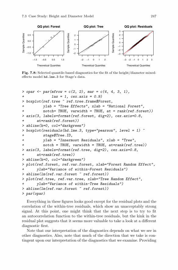
7.3 Case Study: Height and Diameter Model 247
●
●
●
●
●
●
●
●
●
−1.5 −0.5 0.5 1.5
−1.0
−0.5
0.0
0.5
QQ plot: Forest
Theoretical Quantiles
Sam
ple
Qua
ntile
s
●●
●
●
●
●
●
●
●
●
●
●●
●
●
●
●
●●●
●
●
●
●
●
●
●
●
●●
●
●
●●
●
●
●
●
●
●
●
●
●
●●
●
●●
●
●●
●
●
●●
●
●
●
●●
●
●
●
●●
●
−2 −1 0 1 2
−2
−1
0
1
2
QQ plot: Tree
Theoretical QuantilesS
ampl
e Q
uant
iles
●●
●●
●●
●●
●
●●
●
●
●●●
●●●●
●●
●●
●
●
●
●●●
●●
●
●
●
●
●●●
●●●●
●
●
●
●●
●
●
●
●
●
●
●
●
●●●●●●
●
●
●●
●
●
●●
●
●●
●●
●●
●●●●
●●
●
●
●
●●
●
●
●
●
●
●
●●
●
●●
●●
●
●
●
●
●●
●●●●
●
●●●
●
●●
●●●
●
●●
●●
●
●
●
●
●
●●
●
●
●
●●●
●●●●
●●
●
●
●●
●
●●
●
●
●
●●
●
●
●
●●
●
●
●
●
●
●●
●●
●●
●
●
●
●●
●
●
●●
●
●●
●●
●
●
●●
●
●
●
●●
●
●●
●
●●●
●
●●
●●
●
●●
●
●
●
●●
●●●●
●●
●
●
●
●●
●●
●
●
●
●
●
●
●
●●
●●
●●●
●
●
●
●●●
●●
●●
●●
●●
●●
●
●
●●
●●●●●
●●
●
●●
●
●
●
●●●
●●
●
●●●
●
●
●●
●
●
●
●
●
●●
●
●
●●
●●●●●
●
●
●●●
●
●
●
●
●●
●
●
●●
●
●
●
●
●
●●
●●
●
●●
●
●●
●●
●●●●
●
●
●
●
●●
●
●
●
●
●
●
●●●
●●
●
●
●
●●
●●
●
●
●●
●
●
●●●●
●●
●●
●●
●●●●
●
●
●
●
●●●●
●●●●
●●
●
●
●
●●
●●
●●
●●
●●●●
●●
●
●●●
●●●
●
●
●
●
●
●●
●
●
●
●
●
●
●
●
●●●
●
●
●●●
●●●
●●
●
●
●
●●
●●
●●
●●
●●
●
●
●●●
●
●●
●●
●●
●
●
●
●
●●●
●
●
●●
●●
●
●●
●●
●
●
●●
●
●●●
●
●
●●●
●●
●
●
●●●
●●
●
●
●
●
●●●
●●
●
●●●
●
●
●●
●
●
●
●
●
●
●
●
●
−3 −2 −1 0 1 2 3
−3
−2
−1
0
1
2
3
QQ plot: Residuals
Theoretical Quantiles
Sam
ple
Qua
ntile
s
Fig. 7.8: Selected quantile-based diagnostics for the fit of the height/diameter mixed-effects model hd.lme.3 for Stage’s data.
> opar <- par(mfrow = c(2, 2), mar = c(4, 4, 3, 1),
+ las = 1, cex.axis = 0.9)
> boxplot(ref.tree ~ ref.tree.frame$Forest,
+ ylab = "Tree Effects", xlab = "National Forest",
+ notch= TRUE, varwidth = TRUE, at = rank(ref.forest))
> axis(3, labels=format(ref.forest, dig=2), cex.axis=0.8,
+ at=rank(ref.forest))
> abline(h=0, col="darkgreen")
> boxplot(residuals(hd.lme.3, type="pearson", level = 1) ~
+ stage$Tree.ID,
+ ylab = "Innermost Residuals", xlab = "Tree",
+ notch = TRUE, varwidth = TRUE, at=rank(ref.tree))
> axis(3, labels=format(ref.tree, dig=2), cex.axis=0.8,
+ at=rank(ref.tree))
> abline(h=0, col="darkgreen")
> plot(ref.forest, ref.var.forest, xlab="Forest Random Effect",
+ ylab="Variance of within-Forest Residuals")
> abline(lm(ref.var.forest ~ ref.forest))
> plot(ref.tree, ref.var.tree, xlab="Tree Random Effect",
+ ylab="Variance of within-Tree Residuals")
> abline(lm(ref.var.forest ~ ref.forest))
> par(opar)
Everything in these figures looks good except for the residual plots and thecorrelation of the within-tree residuals, which show an unacceptably strongsignal. At this point, one might think that the next step is to try to fitan autocorrelation function to the within-tree residuals, but the kink in theresidual plot suggests that it seems more valuable to take a look at a differentdiagnostic first.
Note that our interpretation of the diagnostics depends on what we see inother diagnostics. Also, note that much of the direction that we take is con-tingent upon our interpretation of the diagnostics that we examine. Providing
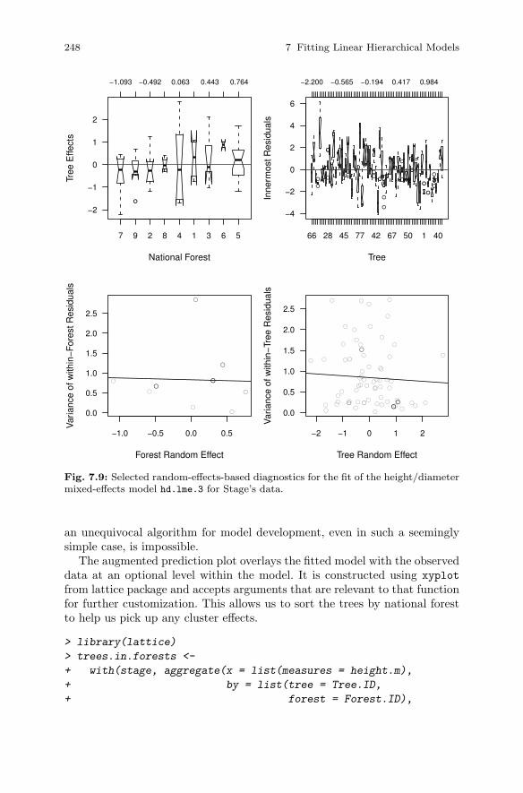
248 7 Fitting Linear Hierarchical Models
●
7 9 2 8 4 1 3 6 5
−2
−1
0
1
2
National Forest
Tree
Effe
cts
−1.093 −0.492 0.063 0.443 0.764
●●
●
●●
● ●
●
●
●
●
●
●●
●
●
●
66 28 45 77 42 67 50 1 40
−4
−2
0
2
4
6
TreeIn
nerm
ost R
esid
uals
−2.200 −0.565 −0.194 0.417 0.984
●
●
●
●
●
●
●
●
●
−1.0 −0.5 0.0 0.5
0.0
0.5
1.0
1.5
2.0
2.5
Forest Random Effect
Var
ianc
e of
with
in−
For
est R
esid
uals
●●
●
● ●
●
●
●
●
● ●
●
●
●
●
●
●
●
●
● ●
●●
●
●
●
●
●
●
●
●
●●
●
●
●
●
●
●
●
●●
●
●
●
●
●
●●
●
●
●
●
●
●●
●
● ●
●
●
●
●
●
●
●
−2 −1 0 1 2
0.0
0.5
1.0
1.5
2.0
2.5
Tree Random Effect
Var
ianc
e of
with
in−
Tree
Res
idua
ls
Fig. 7.9: Selected random-effects-based diagnostics for the fit of the height/diametermixed-effects model hd.lme.3 for Stage’s data.
an unequivocal algorithm for model development, even in such a seeminglysimple case, is impossible.
The augmented prediction plot overlays the fitted model with the observeddata at an optional level within the model. It is constructed using xyplot
from lattice package and accepts arguments that are relevant to that functionfor further customization. This allows us to sort the trees by national forestto help us pick up any cluster effects.
> library(lattice)
> trees.in.forests <-
+ with(stage, aggregate(x = list(measures = height.m),
+ by = list(tree = Tree.ID,
+ forest = Forest.ID),

7.3 Case Study: Height and Diameter Model 249
+ FUN = length))
> panel.order <-
+ rank(as.numeric(as.character(trees.in.forests$tree)))
> plot(augPred(hd.lme.3),
+ index.cond = list(panel.order),
+ strip = strip.custom(par.strip.text = list(cex = 0.5)))
The augmented prediction plot (Figure 7.10) shows that a number of thetrees have curvature in the relationship between height and diameter thatthe model fails to pick up, whereas others seem quite linear. It also showsthat the omission of a random slope appears to create problematic lack offit. Finally, there does not appear to be any particular pattern among theforests.
At this point, we have several options, each of which potentially leads todifferent resolutions of our problem or, more likely, to several further prob-lems. How we proceed depends on our goal. We can
1. add a quadratic fixed effect;2. add a quadratic random effect;3. add quadratic fixed and random effects;4. correct the model by including within-tree correlation; and5. switch to non-linear mixed-effects models and use a more appropriate func-
tional form.
Since we do not believe that the true relationship between height and di-ameter could reasonably be a straight line, we add a fixed quadratic diametereffect and a random diameter effect, by tree, and see how things go. We willshow only a sample of the diagnostic graphs here.
> hd.lme.4 <- lme(height.m ~ dbhib.cm + I(dbhib.cm^2),
+ random = list( ~ 1 | Forest.ID,
+ ~ dbhib.cm | Tree.ID),
+ control = lmeControl(maxIter = 500,
+ msMaxIter = 500),
+ data = stage)
Note the splitting of the random-effects statement into a list in order topermit different inclusions at different levels of the hierarchy. During theprocess of writing this text, we tried various more detailed arrangements,but the more complex models failed to converge for these data. Also note ourinvocation of the control = lmeControl argument in the function call. Thisargument is an essential element of the model-fitter’s toolbox, and we delayits discussion until Section 7.4. We present the first set of relevant diagnosticsin Figure 7.11.
> opar <- par(mfrow = c(1, 3), mar = c(4, 4, 3, 1), las = 1,
+ cex.axis = 0.9)
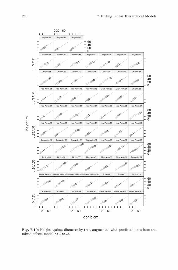
250 7 Fitting Linear Hierarchical Models
dbhib.cm
heig
ht.m
0204060
0 20 60
●●●●●●●
●●
Kaniksu/6
●●●●●●
●
Kaniksu/7
0 20 60
●●●
●●
●●
Kaniksu/34
●●●●●●●●●
●●●●
Kaniksu/65
0 20 60
●●●●●●●●●●●
Coeur d'Alene/11
●●●●●●●●●
Coeur d'Alene/12
0 20 60
●●●●●
●●●
Coeur d'Alene/13
●●●●●●●●●●
Coeur d'Alene/19
●●●
●●
●●
Coeur d'Alene/33
●●●●●●
●
Coeur d'Alene/38
●●●●●
●●●
Coeur d'Alene/39
●●●●●●
●●
St. Joe/4
●●
●●●●
St. Joe/5
0204060
●●●●●
St. Joe/15
0204060
●●●●●
●●
St. Joe/60
●●●●●●●●●
●●
●●
St. Joe/61
●●●●●●●
●●●●
St. Joe/77
●●●●●
Clearwater/1
●●●●●●●●●●
Clearwater/2
●●●●●●●●●●
●●
Clearwater/3
●●●●●●●●●●●●
Clearwater/17
●●
●●
Clearwater/18
●●●●●●●●●●●
●
Clearwater/30
●●●●●●●●●●
●●
●
Clearwater/31
●●●●●●●●●●
●●
●
Clearwater/59
●●●●●●●●●●●
●
Nez Perce/28
●●●●
●●
●
Nez Perce/29
0204060
●●
●●
Nez Perce/32
0204060
●●●●
●
Nez Perce/35
●●●●
Nez Perce/36
●●●●●●●●●
●●●
Nez Perce/37
●●●●●●●●
Nez Perce/40
●●●●●●●●●●
Nez Perce/48
●●●●●
●●●
Nez Perce/49
●●
●●
Nez Perce/50
●●●●●●
Nez Perce/51
●●●●●●●●●●●
Nez Perce/52
●●●●●●●
●●●
Nez Perce/53
●●●
●●●
Nez Perce/54
●●●
●●
Nez Perce/55
●●
●●●
Nez Perce/56
0204060
●●●●●●●●●●●
●●
Nez Perce/57
0204060
●●●
●●●
Nez Perce/58
●●●
●●
●
Nez Perce/74
●●●●●●
Nez Perce/75
●●●●●
Nez Perce/76
●●●●●●●●●●
●●●
Clark Fork/62
●●●●●●
●●●
Clark Fork/64
●●●●●●
Umatilla/63
●●●●●
●●●
●●
Umatilla/68
●●●●
●●
Umatilla/69
●●●
●●
Umatilla/70
●●●●●●●●●●
Umatilla/71
●●●●●●
●●
●●●
Umatilla/72
●●●
●
Umatilla/73
0204060
●●●●●●●●●●●
Umatilla/84
0204060
●●●●●●
●●
Wallowa/66
●●●●●●●●
Wallowa/67
●●●●●●●●●
●●
Wallowa/85
●●●●
●●
●●
Payette/41
●●●
●●●
●●
Payette/42
●●●●●●
Payette/43
●●●●●●●●●●●
Payette/44
●●●●●
●●●●
Payette/45
0 20 60
●●●●
Payette/46
0204060
●●
●●
Payette/47
Fig. 7.10: Height against diameter by tree, augmented with predicted lines from themixed-effects model hd.lme.3.
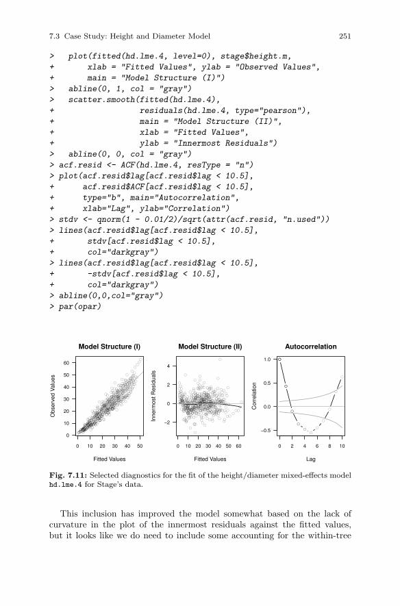
7.3 Case Study: Height and Diameter Model 251
> plot(fitted(hd.lme.4, level=0), stage$height.m,
+ xlab = "Fitted Values", ylab = "Observed Values",
+ main = "Model Structure (I)")
> abline(0, 1, col = "gray")
> scatter.smooth(fitted(hd.lme.4),
+ residuals(hd.lme.4, type="pearson"),
+ main = "Model Structure (II)",
+ xlab = "Fitted Values",
+ ylab = "Innermost Residuals")
> abline(0, 0, col = "gray")
> acf.resid <- ACF(hd.lme.4, resType = "n")
> plot(acf.resid$lag[acf.resid$lag < 10.5],
+ acf.resid$ACF[acf.resid$lag < 10.5],
+ type="b", main="Autocorrelation",
+ xlab="Lag", ylab="Correlation")
> stdv <- qnorm(1 - 0.01/2)/sqrt(attr(acf.resid, "n.used"))
> lines(acf.resid$lag[acf.resid$lag < 10.5],
+ stdv[acf.resid$lag < 10.5],
+ col="darkgray")
> lines(acf.resid$lag[acf.resid$lag < 10.5],
+ -stdv[acf.resid$lag < 10.5],
+ col="darkgray")
> abline(0,0,col="gray")
> par(opar)
●
●
●
●
●
●
●
●●
●
●
●●
●
●
●
●●
●●
●●
●●
●
●
●
●●
●●
●
●
●
●
●
●
●
●
●
●
●
●
●●
●
●
●
●
●
●
●
●
●
●
●
●
●●
●●
●●●
●
●
●
●
●●
●●
●
●
●
●
●
●●
●
●
●
●
●●
●
●
●
●
●
●●
●●
●
●●
●●
●
●
●
●
●
●
●
●●
●●
●●
●●
●
●
●●
●●
●
●●
●
●
●
●
●
●
●
●
●
●
●
●
●●
●●
●
●●
●
●
●
●
●
●●
●●
●
●
●
●
●
●
●
●
●
●
●
●
●
●
●
●
●
●
●
●
●
●
●
●
●
●
●
●
●
●
●
●
●
●
●
●
●●
●●
●
●
●
●
●
●
●
●
●●
●
●
●
●
●
●
●
●●
●
●
●●
●
●
●●
●
●
●●
●
●
●
●
●
●
●
●
●
●
●
●●
●
●
●
●
●
●
●
●
●
●●
●●
●
●
●
●●
●●
●
●
●●
●
●●●
●
●
●
●●
●
●
●
●
●●
●●
●
●
●
●
●
●
●
●
●
●
●
●
●●
●
●
●
●
●
●●
●
●
●
●●
●●
●
●
●
●
●
●
●
●●
●●
●
●
●
●
●●
●
●
●
●
●
●
●
●
●
●
●
●
●
●
●
●
●
●
●●
●
●●
●
●
●
●
●
●
●
●
●
●
●
●
●●
●●
●
●
●
●●
●
●
●
●
●
●
●
●
●
●
●
●●
●●
●
●
●
●
●
●
●
●
●
●●
●●
●●
●●
●
●
●
●
●
●
●
●
●
●
●
●
●
●●
●
●
●
●
●
●●
●●
●●
●
●
●
●
●
●●
●
●
●●
●
●
●
●
●●
●
●
●
●
●●
●●
●
●
●
●●
●
●
●
●
●
●
●
●
●
●●
●
●
●
●●
●
●
●
●
●
●
●●
●●
●●
●
●
●
●
●
●
●
●
●
●
●
●
●
●
●
●
●
●
●
●
●
●
●
●
●
●
●
●
●●
●
●
●
●
●
●
●
●
●
●
●●
●●
●●
●
●
●
●
●●
●●●
●●
●
●
●
●
0 10 20 30 40 50
0
10
20
30
40
50
60
Model Structure (I)
Fitted Values
Obs
erve
d V
alue
s
●●
●
●
●
●
●
●●
●
●
●
●
●
●
●
●
●
●
●●
●●●●
●
●
●
●●
●●
●
●
●
●
●●
●●
●
●
●●
●
●
●●
●
●
●●
●
●
●
●
●
●●
●●●
●
●
●●
●
●
●●●
●
●
●●
●●
●●●
●
●●
●
●
●
●
●
●●●●●●●
●
●
●●●
●
●
●●
●
●
●●
●
●●
●
●
●●
●
●
●
●●
●
●
●
●
●
●
●
● ●
●
●
●
●
●
●
●●●●
●●
●●
●
●●
●
●
●
●●
●
●
●
●
●●
●
●
●
●
●
●
●
●
●
●
●
●
●
●
●
●
●
●
●●
●
●
●
●
●●
●●
●●
●
●
●
●
●
●
●
●
●
●●
● ●●
●
●
●
●●
●
●
●
●
●
●
●
●
●●
●
●
●●●●
●
●
●
●●
●
●
●
●●
●
●
●
●
●
●●●
●
●
●●
●
●
●
●
●
●
●
●
●
●
●
●
●
●●
●
●
●
●
●
●●
●
●
●
●
●● ●●
●
●
●●
●
●●
●
●
●
●●
●
●
●
● ●●
●●
●●
●
●
●
●●
●
●●●
●
●
●
●
●
●
●
●
●●
●
●
●
●
●
●●
●
●●
●
●●
●
●
●
●
●
●
●
●
●
●
●
●
●●●
●
●
●●
●
●●
●
●
●
●●
●
●●
●
●
●
●●
●
●●
●
●
●
●●●
●
●
●
● ●●
●
●●
●●●●●
●
●
●
●●●
●●
●●
●
●
●
●●
●
●
●
●●●
●
●
●
●●
●
●
●
●●●
●●
●●●
●
●
●
●
●
●
●
●
●●
●
●
●
●
●
●
●●
●
●
●
●
●
●
●●
●
●
●
●
●●
●
●●
●
●●
●●
●
●
●
●
●
●
●●
●
●●
●●
●
●
●
●
●
●
●
●
●●
●●
●●
●●
●
●
●●
●
●
●
●●●●
●
●
●●●
●
●
●
●●
●●
●
●
●
●
●
●
●
●
●●
●
●
●●
●
●
●●●●
●
●
●
●
●
●
●
0 10 20 30 40 50 60
−2
0
2
4
Model Structure (II)
Fitted Values
Inne
rmos
t Res
idua
ls
●
●
●
●
●
●
●
●
●
●
●
0 2 4 6 8 10
−0.5
0.0
0.5
1.0
Autocorrelation
Lag
Cor
rela
tion
Fig. 7.11: Selected diagnostics for the fit of the height/diameter mixed-effects modelhd.lme.4 for Stage’s data.
This inclusion has improved the model somewhat based on the lack ofcurvature in the plot of the innermost residuals against the fitted values,but it looks like we do need to include some accounting for the within-tree
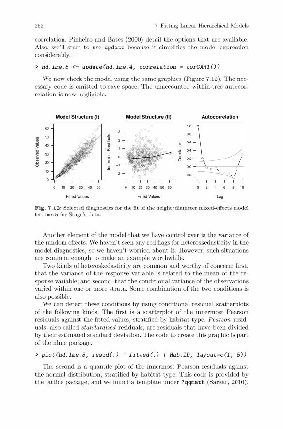
252 7 Fitting Linear Hierarchical Models
correlation. Pinheiro and Bates (2000) detail the options that are available.Also, we’ll start to use update because it simplifies the model expressionconsiderably.
> hd.lme.5 <- update(hd.lme.4, correlation = corCAR1())
We now check the model using the same graphics (Figure 7.12). The nec-essary code is omitted to save space. The unaccounted within-tree autocor-relation is now negligible.
●
●
●
●
●
●
●
●●
●
●
●●
●
●
●
●●
●●
●●
●●
●
●
●
●●
●●
●
●
●
●
●
●
●
●
●
●
●
●
●●
●
●
●
●
●
●
●
●
●
●
●
●
●●
●●
●●●
●
●
●
●
●●
●●
●
●
●
●
●
●●
●
●
●
●
●●
●
●
●
●
●
●●
●●
●
●●
●●
●
●
●
●
●
●
●
●●
●●
●●
●●
●
●
●●
●●
●
●●
●
●
●
●
●
●
●
●
●
●
●
●
●●
●●
●
●●
●
●
●
●
●
●●
●●
●
●
●
●
●
●
●
●
●
●
●
●
●
●
●
●
●
●
●
●
●
●
●
●
●
●
●
●
●
●
●
●
●
●
●
●
●●
●●
●
●
●
●
●
●
●
●
●●
●
●
●
●
●
●
●
●●
●
●
●●
●
●
●●
●
●
●●
●
●
●
●
●
●
●
●
●
●
●
●●
●
●
●
●
●
●
●
●
●
●●
●●
●
●
●
●●
●●
●
●
●●
●
●●●
●
●
●
●●
●
●
●
●
●●
●●
●
●
●
●
●
●
●
●
●
●
●
●
●●
●
●
●
●
●
●●
●
●
●
●●
●●
●
●
●
●
●
●
●
●●
●●
●
●
●
●
●●
●
●
●
●
●
●
●
●
●
●
●
●
●
●
●
●
●
●
●●
●
●●
●
●
●
●
●
●
●
●
●
●
●
●
●●
●●
●
●
●
●●
●
●
●
●
●
●
●
●
●
●
●
●●
●●
●
●
●
●
●
●
●
●
●
●●
●●
●●
●●
●
●
●
●
●
●
●
●
●
●
●
●
●
●●
●
●
●
●
●
●●
●●
●●
●
●
●
●
●
●●
●
●
●●
●
●
●
●
●●
●
●
●
●
●●
●●
●
●
●
●●
●
●
●
●
●
●
●
●
●
●●
●
●
●
●●
●
●
●
●
●
●
●●
●●
●●
●
●
●
●
●
●
●
●
●
●
●
●
●
●
●
●
●
●
●
●
●
●
●
●
●
●
●
●
●●
●
●
●
●
●
●
●
●
●
●
●●
●●
●●
●
●
●
●
●●
●●●
●●
●
●
●
●
0 10 20 30 40 50
0
10
20
30
40
50
60
Model Structure (I)
Fitted Values
Obs
erve
d V
alue
s
●●
●●
●
●
●
●●
●
●
●
●
●
●
●
●
●
●
●●
●●●●
●
●
●●●
●●
●
●
●●
●●
●●● ●
●
●
●
●
●●
●
● ●●
●
●
●
●
●
●●●●●
●
●
●●
●●
●●●
●
●
●●
●●
●●●
●
●●
●
●
●
●
●
●●
●●●●
●●
●
●●●
●
●
●
●
●
●
●●●
●●
●
●
●●
●
●
●
●●
●
●
●
●
●
●
●
●
●
●
●
●
●
●
●
●●●●
●●
●●
●
●●●
●●●
●●
●
●
●
●
●●
●
●
●
●
●
●
●
●
●
●
●
●
●
●
●
●
●
●●
●
●
●
●●
●
●●
●● ●
●
●●
●
●
●
●●
●●
●
●●
●
●
●
●●
●
●
●
●
●
●
●
●
●●
●●
●●●●●
●
●
●●
●●
●
●●
●
●
●
●
●
●
●●
●●
●●
●
●●
●
●
●●
●
●
●●
●●
●●
●
●
●
●
●
●●
●
●
●
●
●●
●●
●
●
●●●
●●
● ●●
●●
●
●
●
●
●●
●
●●
●
●
●
●●
●●●●●
●
●
●●
●
●
●
●
●●●
●
●
●
●
●
●
●
●
●●
● ●
●
●
●
●
●
●
●
●
●
●
●
●●
●●
●
●
●●
●
●● ●
●
●
●●
●●●
●
●
●
●●
●
●●
●
●
●
●●●
●●
●
●
●●
●
●●
●●
●
●●●●
●
●●●●
●●●
●
●
●
●●
●●
●
●●●
●
●
●
●●●
●
●
●● ●●
●●●
●●
●
●
●
●
●
●
●
●●
●
●
●
●●
●
●●
●
●
●
●
●
●
●●●
●
●
●
●●
●
●●
●
●●
●
●●
●
●
●
●
●
●●
●
●●
●●
● ●
●
●
●●
●
●
●●●
●●●
●●
●
●
●●
●
●
●
●●●●
●
●
●●●
●
●
●
●●
●●
●
●
●
●
●
●●●
●●
●
●●●
●
●
●●●●
●
●
●
●
●
●
●
0 10 20 30 40 50 60
−2
−1
0
1
2
3
Model Structure (II)
Fitted Values
Inne
rmos
t Res
idua
ls
●
●
●●
●
● ● ●
●
●
●
0 2 4 6 8 10
−0.2
0.0
0.2
0.4
0.6
0.8
1.0
Autocorrelation
Lag
Cor
rela
tion
Fig. 7.12: Selected diagnostics for the fit of the height/diameter mixed-effects modelhd.lme.5 for Stage’s data.
Another element of the model that we have control over is the variance ofthe random effects. We haven’t seen any red flags for heteroskedasticity in themodel diagnostics, so we haven’t worried about it. However, such situationsare common enough to make an example worthwhile.
Two kinds of heteroskedasticity are common and worthy of concern: first,that the variance of the response variable is related to the mean of the re-sponse variable; and second, that the conditional variance of the observationsvaried within one or more strata. Some combination of the two conditions isalso possible.
We can detect these conditions by using conditional residual scatterplotsof the following kinds. The first is a scatterplot of the innermost Pearsonresiduals against the fitted values, stratified by habitat type. Pearson resid-uals, also called standardized residuals, are residuals that have been dividedby their estimated standard deviation. The code to create this graphic is partof the nlme package.
> plot(hd.lme.5, resid(.) ~ fitted(.) | Hab.ID, layout=c(1, 5))
The second is a quantile plot of the innermost Pearson residuals againstthe normal distribution, stratified by habitat type. This code is provided bythe lattice package, and we found a template under ?qqmath (Sarkar, 2010).
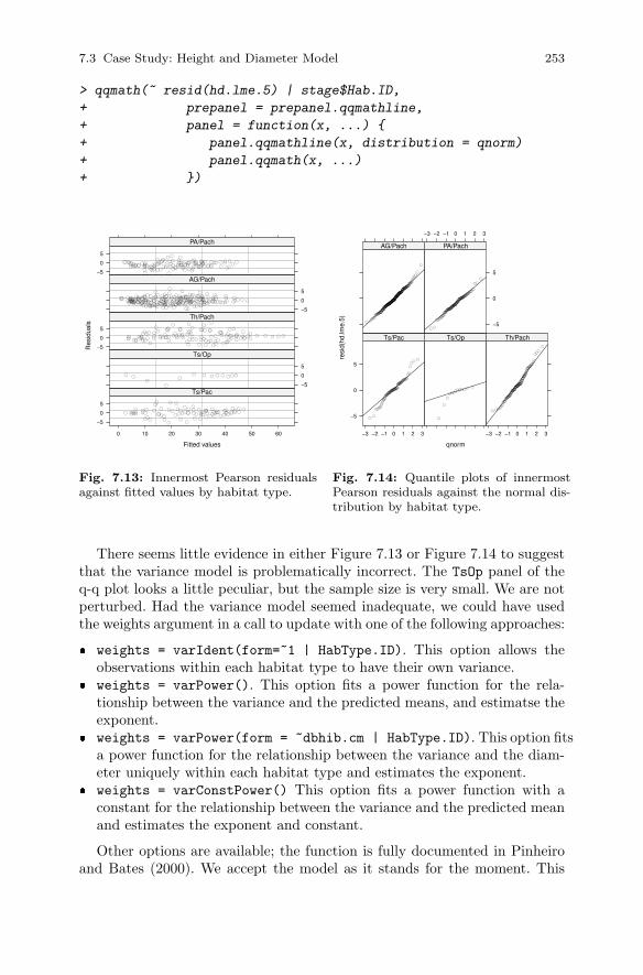
7.3 Case Study: Height and Diameter Model 253
> qqmath(~ resid(hd.lme.5) | stage$Hab.ID,
+ prepanel = prepanel.qqmathline,
+ panel = function(x, ...) {
+ panel.qqmathline(x, distribution = qnorm)
+ panel.qqmath(x, ...)
+ })
Fitted values
Res
idua
ls
−5
0
5
0 10 20 30 40 50 60
●●●●●●●
● ●●●●●● ●●●
●●
●●
●● ●●
●●
●●
● ●●
●●● ●●●●●
●●●●●●
●●●●
●●
●●
●●
●●●
●●●●●
●●●●●●●
●
●●●●●
●●●●
Ts/Pac−5
0
5
●●●●●●●●●
●
●●
●
Ts/Op−5
0
5 ●
●●
●●●●●●●●
●
●●●●●●●
●●●●●●●
●●
●●
●●●●●●
●●●
●
●●
●●
●●
●●●●●●●●●
●●●● ●●●●●
●●
●●●●
●
●
●●
●●
●●●●●● ●●
●
●●
●●●
●●●●●
●●●
●●
●●
●●●●●●
●●●
Th/Pach−5
0
5
●●●●●●●
●●●●
●●●●●●●●●
●●●●●●
●
●●
●●●●
●●●● ●●
●●●●
●●●●●●
●●●●●
●● ●●●●●●●● ●
●●
●●●●●
●●
●●●●
●●●●●●●
●●●●
●●●●
●●
●●
● ●●●● ●
●●● ●●●●
●●●●●● ●●●●
●
●●●
●●●●●●
●●●●
●
●●●
●●
●●●●●● ●●●
●
●●
●● ●●●●●
●●●
●●●●●
●
●●●
●●
●●●
●●●●●
● ●●●
●●●●●●●● ●●●●
●●●●
●● ●●●●●
●
●●●●● ●●●●●
●●
●●
●●
AG/Pach−5
0
5
●●●●
●●
●●●●
●
●●
●●
●●
●●●
●●
●●●
●●
●●
●●●●
●● ●●
●
●●● ●●●●●●
●●
●● ●
●●●●●
●●
●●●
●● ●
●●
●●●
●●●●●●● ●●●●●●●●
●●
●●● ●●●●●
●●●
●●
●●●●●●
●●●●
●●
PA/Pach
Fig. 7.13: Innermost Pearson residualsagainst fitted values by habitat type.
qnorm
resi
d(hd
.lme.
5)
−5
0
5
−3 −2 −1 0 1 2 3
●●
●●●●●●●●●●●●●●●●●●●●●●●●●●●●●●●●●●
●●●●●●●●●●●●●●●●
●●●●●●●●●●●
●●●●●●●●●
●●●●●
●
●●
●
Ts/Pac
●
●
●
●●●●●●●●●
●
Ts/Op
−3 −2 −1 0 1 2 3
● ●●●●●●●●●●
●●●●●●●●●●●●●●●●●●●●●●●●●●●●●●●●●●●●●●●●●●●●●●●
●●●●●●●●●●●●●●●●●●●●●●●●●●●●●●●●●●●●●●●●●●●●
●●●●●
●●●
●
Th/Pach
● ●●●●
●●●●●●●●●
●●●●●●●●●●●●●●●●●●●●●●●●●●●●●●●●●●●●●●●●●●●●●●●●●●●●●●
●●●●●●●●●●●●●●●●●●●●●●●●●●●●●●●●●●●●●●●●●●●●●●●●●●●●●●●●●●●●●●●●●●●●●●●●●●●●●●●●●●●●●●●●●●●●●●●●●●●●●●●●●
●●●●●●●●●●●●●●●●●●●●●●●●●●●●●●●●●●●
●●●●●●●●●●●●●●●
●
●
AG/Pach
−3 −2 −1 0 1 2 3
−5
0
5
● ●
●●●●●
●●●●●●●●●●●●●●●●●●●●●●●●●●●●
●●●●●●●●●●●●●●●●●●●●●●●●●●●●●●●●●●●●●●●●●●●●●●●●●
●●●●●●●●●●●●
●●●●●●●●
●●●●●
●●
●
PA/Pach
Fig. 7.14: Quantile plots of innermostPearson residuals against the normal dis-tribution by habitat type.
There seems little evidence in either Figure 7.13 or Figure 7.14 to suggestthat the variance model is problematically incorrect. The TsOp panel of theq-q plot looks a little peculiar, but the sample size is very small. We are notperturbed. Had the variance model seemed inadequate, we could have usedthe weights argument in a call to update with one of the following approaches:
� weights = varIdent(form=~1 | HabType.ID). This option allows theobservations within each habitat type to have their own variance.
� weights = varPower(). This option fits a power function for the rela-tionship between the variance and the predicted means, and estimatse theexponent.
� weights = varPower(form = ~dbhib.cm | HabType.ID). This option fitsa power function for the relationship between the variance and the diam-eter uniquely within each habitat type and estimates the exponent.
� weights = varConstPower() This option fits a power function with aconstant for the relationship between the variance and the predicted meanand estimates the exponent and constant.
Other options are available; the function is fully documented in Pinheiroand Bates (2000). We accept the model as it stands for the moment. This
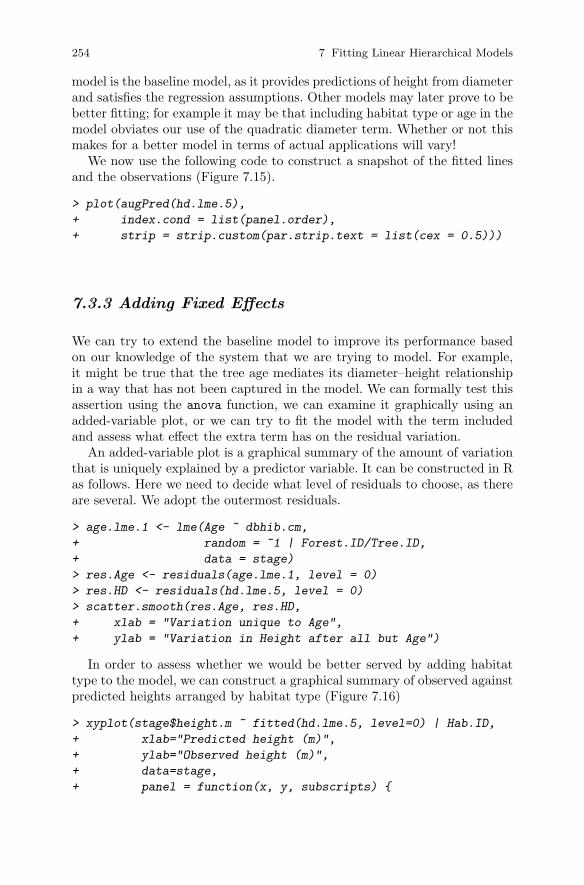
254 7 Fitting Linear Hierarchical Models
model is the baseline model, as it provides predictions of height from diameterand satisfies the regression assumptions. Other models may later prove to bebetter fitting; for example it may be that including habitat type or age in themodel obviates our use of the quadratic diameter term. Whether or not thismakes for a better model in terms of actual applications will vary!
We now use the following code to construct a snapshot of the fitted linesand the observations (Figure 7.15).
> plot(augPred(hd.lme.5),
+ index.cond = list(panel.order),
+ strip = strip.custom(par.strip.text = list(cex = 0.5)))
7.3.3 Adding Fixed Effects
We can try to extend the baseline model to improve its performance basedon our knowledge of the system that we are trying to model. For example,it might be true that the tree age mediates its diameter–height relationshipin a way that has not been captured in the model. We can formally test thisassertion using the anova function, we can examine it graphically using anadded-variable plot, or we can try to fit the model with the term includedand assess what effect the extra term has on the residual variation.
An added-variable plot is a graphical summary of the amount of variationthat is uniquely explained by a predictor variable. It can be constructed in Ras follows. Here we need to decide what level of residuals to choose, as thereare several. We adopt the outermost residuals.
> age.lme.1 <- lme(Age ~ dbhib.cm,
+ random = ~1 | Forest.ID/Tree.ID,
+ data = stage)
> res.Age <- residuals(age.lme.1, level = 0)
> res.HD <- residuals(hd.lme.5, level = 0)
> scatter.smooth(res.Age, res.HD,
+ xlab = "Variation unique to Age",
+ ylab = "Variation in Height after all but Age")
In order to assess whether we would be better served by adding habitattype to the model, we can construct a graphical summary of observed againstpredicted heights arranged by habitat type (Figure 7.16)
> xyplot(stage$height.m ~ fitted(hd.lme.5, level=0) | Hab.ID,
+ xlab="Predicted height (m)",
+ ylab="Observed height (m)",
+ data=stage,
+ panel = function(x, y, subscripts) {
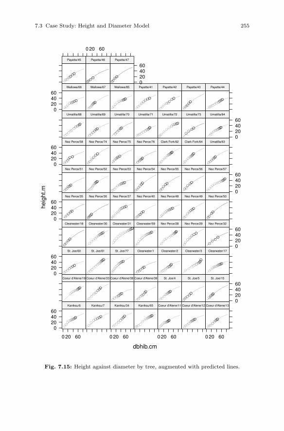
7.3 Case Study: Height and Diameter Model 255
dbhib.cm
heig
ht.m
0204060
0 20 60
●●●●●●●
●●
Kaniksu/6
●●●●●
●●
Kaniksu/7
0 20 60
●●●
●●
●●
Kaniksu/34
●●●●●●●●●
●●●●
Kaniksu/65
0 20 60
●●●●●●●●●●●
Coeur d'Alene/11
●●●●●●
●●●
Coeur d'Alene/12
0 20 60
●●●●
●●●●
Coeur d'Alene/13
●●●●●●●●●●
Coeur d'Alene/19
●●●
●●
●●
Coeur d'Alene/33
●●●●●●
●
Coeur d'Alene/38
●●●●●
●●●
Coeur d'Alene/39
●●●●●●
●●
St. Joe/4
●●
●●●●
St. Joe/5
0204060
●●●●●
St. Joe/150
204060
●●●●
●●●
St. Joe/60
●●●●●●●●●
●●
●●
St. Joe/61
●●●●●●●
●●
●●
St. Joe/77
●●●●●
Clearwater/1
●●●●●●●●●●
Clearwater/2
●●●●●●●●●●
●●
Clearwater/3
●●●●●●●●●●●
●
Clearwater/17
●●
●●
Clearwater/18
●●●●●●●●●
●●
●
Clearwater/30
●●●●●●●●●
●●
●●
Clearwater/31
●●●●●●●●●
●●
●●
Clearwater/59
●●●●●●●
●●●●
●
Nez Perce/28
●●
●●
●●
●
Nez Perce/29
0204060
●●
●●
Nez Perce/320
204060
●●●
●●
Nez Perce/35
●●●●
Nez Perce/36
●●●●●●●●●
●●●
Nez Perce/37
●●●●●●●●
Nez Perce/40
●●●●●●●●●
●
Nez Perce/48
●●●●●
●●●
Nez Perce/49
●●
●●
Nez Perce/50
●●●●●●
Nez Perce/51
●●●●●●●●●●●
Nez Perce/52
●●●●●●●
●●●
Nez Perce/53
●●●
●●●
Nez Perce/54
●●●
●●
Nez Perce/55
●●
●●●
Nez Perce/56
0204060
●●●●●●●●●●
●●
●
Nez Perce/570
204060
●●●
●●●
Nez Perce/58
●●
●●
●●
Nez Perce/74
●●●●●●
Nez Perce/75
●●●●●
Nez Perce/76
●●●●●●●●●●
●●
●
Clark Fork/62
●●●●●●
●●
●
Clark Fork/64
●●●●
●●
Umatilla/63
●●●●●
●●●
●●
Umatilla/68
●●●
●●
●
Umatilla/69
●●●
●●
Umatilla/70
●●●●●●●●●●
Umatilla/71
●●●●●●
●●
●●●
Umatilla/72
●●
●●
Umatilla/73
0204060
●●●●●●●●●
●●
Umatilla/840
204060
●●●●●●
●●
Wallowa/66
●●●●●●●●
Wallowa/67
●●●●●●●●●
●●
Wallowa/85
●●●●
●●
●●
Payette/41
●●●
●●●
●●
Payette/42
●●
●●●●
Payette/43
●●●●●●●●●●●
Payette/44
●●
●●●●●●●
Payette/45
0 20 60
●●
●●
Payette/46
0204060
●●
●●
Payette/47
Fig. 7.15: Height against diameter by tree, augmented with predicted lines.
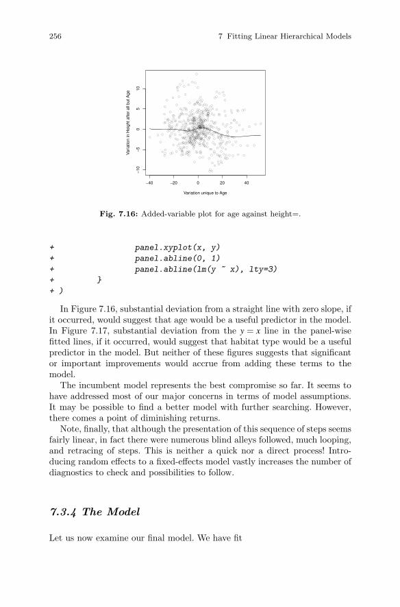
256 7 Fitting Linear Hierarchical Models
●
● ●●
●
●
●
●●
●●
●
●
●
●
●
●
●
●●●
●●
●●
●
●
●●
●
●●
●
●
●
●
●●
●●●
●
●
●
●
●
●●
●
●
●●
●
●
●
●
●
●●●●●
●
●
●●
●●
●●
●
●●
●●
●●
●●●
●
● ●
●
●
●
●
●
●●
●●
●●
●●
●
●●
●●●
●
●
●
●
●●●
●●
●
●●●
●
●
●
●●
●
●●
●
●●
●
●
●●
●
● ●
●
●
●●●●●●
●●
●
● ● ●
●
●
●●
●
●●
●
● ●
●
●
●
●
●
● ●
●
●
●
● ●
●
●
●
●
●
●
●
●
●
●
●
●●
●
●●
●●
●
●
●●
●
●
●
●●
●●
●
●
●●
●
●
●
●
●
●
●
●
●
●
●
●
●●
●
●
●●●●●
●
●
● ●
●●
●●
●
●
●
●
●
●
●
●●
●●
●
●
●●●
●●
●●
●
●
●
●
●●
●●
●
●
●
●
●
●
●
●
●●
●
●
● ●●
●
●
●●
●●●
●
●●●●
●
●●
●
●
●
●
●
●●
●
●●
●
●●●●
●
●
●
●●●
●
●
●
●
●●
●
●●
●
●
●
●
●
●●
●
●●
●
●
●
●
●
●
●
●
●
●
●●
●●
●
●
●●
●
●●
●
●
●
●●
●
●●●
●
●●●
●
●●
●
●
●
●
●
●● ●
●
●
●●
●
●●
●●
●
●
●●
●
●
●●
●
●●●●●
●
●
●
●●
●●
●●●
●
●
●
●●●
●
●●
●
●●●
●●●
●
●
●
●
●
●
●
●
●●
●
●
●●●
●
●●
●
●
●
●
●
●
●● ●
●
●
●
●●
●●●
●
● ●
●
●●
●
●
●
●
●
●●
●
●
●
●
●
●
●●
●
●
●
●●
● ●●
●
● ●
●●
● ●
●
●
●●
●
●●●●
●
●
●●●
●
●
●
●●
●
●●
●
●
●
●
●●●●●
●
●●
●
●
●
●●●
●
●
●
●
●
●
●
●
−40 −20 0 20 40
−10
−5
05
10
Variation unique to Age
Var
iatio
n in
Hei
ght a
fter
all b
ut A
ge
Fig. 7.16: Added-variable plot for age against height=.
+ panel.xyplot(x, y)
+ panel.abline(0, 1)
+ panel.abline(lm(y ~ x), lty=3)
+ }
+ )
In Figure 7.16, substantial deviation from a straight line with zero slope, ifit occurred, would suggest that age would be a useful predictor in the model.In Figure 7.17, substantial deviation from the y = x line in the panel-wisefitted lines, if it occurred, would suggest that habitat type would be a usefulpredictor in the model. But neither of these figures suggests that significantor important improvements would accrue from adding these terms to themodel.
The incumbent model represents the best compromise so far. It seems tohave addressed most of our major concerns in terms of model assumptions.It may be possible to find a better model with further searching. However,there comes a point of diminishing returns.
Note, finally, that although the presentation of this sequence of steps seemsfairly linear, in fact there were numerous blind alleys followed, much looping,and retracing of steps. This is neither a quick nor a direct process! Intro-ducing random effects to a fixed-effects model vastly increases the number ofdiagnostics to check and possibilities to follow.
7.3.4 The Model
Let us now examine our final model. We have fit
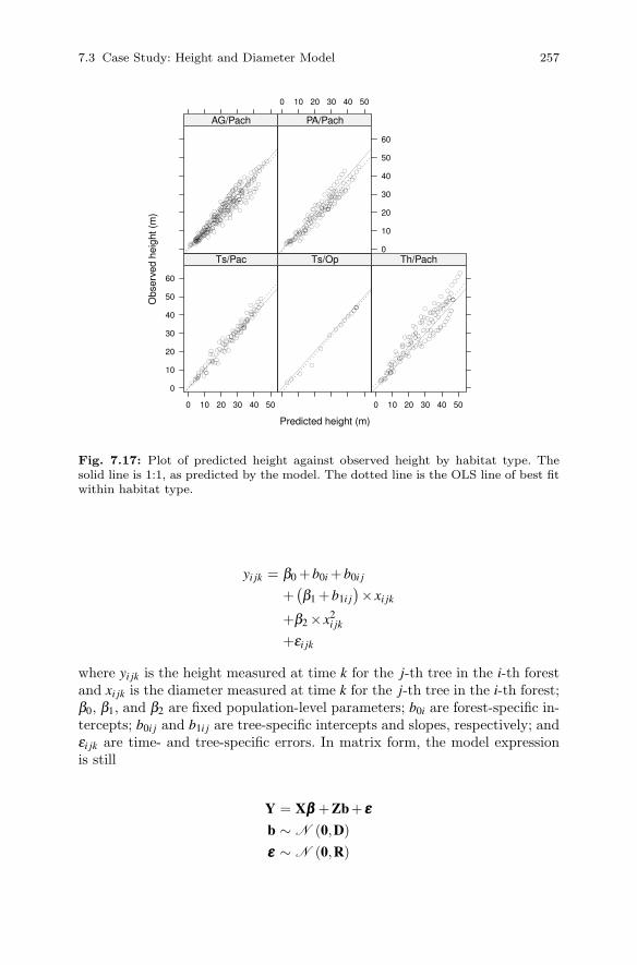
7.3 Case Study: Height and Diameter Model 257
Predicted height (m)
Obs
erve
d he
ight
(m
)
0
10
20
30
40
50
60
0 10 20 30 40 50
●●
●●
●
●
●
●
●
●
●
●
●
●
●●
●●
●●
●
●
●
●
●
●●
●
●
●
●
●
●
●
●
●●
●●
●●
●●
●
●
●
●
●
●
●
●
●
●
●
●
●
●
●
●
●●
●●
●
●●
●
●
●
●
●
●
●
●
●●
●
●
●
●
●
Ts/Pac
●●
●●
●●
●
●
●
●
●
●●
Ts/Op
0 10 20 30 40 50
●
●●
●●
●●
●●
●
●
●
●●
●●
●
●●
●●●
●
●
●
●
●
●
●●
●●
●
●●
●
●
●
●
●
●
●
●
●
●
●
●
●●
●●
●●
●
●
●
●
●
●
●●
●●
●
●
●
●
●
●
●
●
●
●
●
●
●
●
●
●
●
●
●
●
●
●
●
●
●●
●●
●
●●
●●
●
●
●
●
●●
●
●●
●
●
●
●
●
●
Th/Pach
●●
●●
●●●
●
●
●
●
●●
●●
●
●
●
●
●
●●
●
●
●
●●
●
●
●
●
●
●
●
●
●
●
●●
●●
●
●
●
●
●
●
●
●
●●
●●
●
●
●
●
●
●●
●
●●
●
●
●
●
●
●
●
●
●
●
●
●
●
●
●
●●
●●
●
●
●
●●
●●
●
●
●●
●
●●●
●
●
●
●●
●
●
●
●
●●
●●
●
●
●
●
●
●
●
●
●
●
●
●
●●
●●
●●
●
●
●
●
●
●
●
●
●
●
●
●
●
●
●
●
●
●
●
●●
●●
●
●
●
●●
●
●
●
●●
●
●●
●
●
●
●●
●
●
●
●●
●
●
●
●
●
●
●●
●●
●●
●
●
●
●
●
●
●
●
●
●
●
●
●
●
●
●
●
●
●
●
●
●
●
●
●
●
●
●
●●
●●●
●●
●
●
●
●
AG/Pach
0 10 20 30 40 50
0
10
20
30
40
50
60
●
●
●
●
●
●
●
●●
●
●
●●
●
●
●
●
●●
●
●
●●
●
●
●
●●
●
●
●
●
●
●
●
●
●●
●
●
●
●●
●●
●
●
●
●
●●
●●
●●
●
●●
●
●
●
●
●
●
●
●
●
●
●
●
●
●
●
●
●
●
●
●●
●●
●●
●●
●
●
●
●
●
●
●
●
●
●
●
●●
●
●
●
●
●●
●●
●●
●
●
●
●
PA/Pach
Fig. 7.17: Plot of predicted height against observed height by habitat type. Thesolid line is 1:1, as predicted by the model. The dotted line is the OLS line of best fitwithin habitat type.
yi jk = β0 +b0i +b0i j
+(β1 +b1i j
)× xi jk
+β2 × x2i jk
+εi jk
where yi jk is the height measured at time k for the j-th tree in the i-th forestand xi jk is the diameter measured at time k for the j-th tree in the i-th forest;β0, β1, and β2 are fixed population-level parameters; b0i are forest-specific in-tercepts; b0i j and b1i j are tree-specific intercepts and slopes, respectively; andεi jk are time- and tree-specific errors. In matrix form, the model expressionis still
Y = Xβββ +Zb+ εεε
b ∼ N (0,D)
εεε ∼ N (0,R)

258 7 Fitting Linear Hierarchical Models
The structure is as follows:
� Y is the vector of height measurements. It has 542 observations.� X is a 542×3 matrix of 1s, diameters, and squared diameters.� β is a vector of length three: it has an intercept, a slope for the linear
diameter term, and a slope for the quadratic diameter term.� Z is a 542×141 unit brute. See below.� b is a vector of intercepts and slopes for diameter and diameter squared
for each forest, and then for each tree. It will be 9 + 132 = 141 elementslong. See below. The predictions can be obtained using ranef(hd.lme.5).
� D is a block diagonal matrix comprising a 9× 9 matrix followed by 662×2 identical matrices. Each matrix will express the covariance betweenthe random effects within forest or within tree. See below.
� R is a 542×542 symmetric matrix for which the off diagonals are 0 betweentrees and a geometrically decreasing function of the inter-measurementtime distance within trees.
7.3.4.1 More on Z
Recall that the role of Z is to allocate the random effects to the appropriateelement. This allocation can be somewhat complicated. Our Z can be dividedinto two distinct sections: a 542×9 matrix Zf associated with the forest-leveleffects and a 542× 132 matrix Zt associated with the tree-level effects. Inmatrix nomenclature,
Z = [Zf | Zt] (7.11)
Now, Zf allocates the random intercept to each observation from eachforest. There are nine forests, so any given row of Zf will contain eight zerosand a 1. Similarly, Zt allocates an intercept and slope to each observationfrom each tree. There are 66 trees, so any given row of Zt will contain 195zeros, a 1, and the corresponding dbhib.
7.3.4.2 More on b
The purpose of b is to contain all the predicted random effects. Thus it will be141 units long, which corresponds to 1 unit for each level of forest (intercept)and 2 units for each level of tree (intercept, slope for diameter).
b = (b f 1,b f 20, . . . ,bt10,bt1d ,bt20,bt2d , . . .)′ (7.12)
The combination of b and Z serves to allocate each random effect to theappropriate unit and measurement.
7.4 Model Wrangling 259
7.3.4.3 More on D
Finally, D dictates the relationships between the different random effectswithin the levels of forest and tree. We have assumed that the random effectswill be independent between habitat types and trees. So, there are only twosubmatrices to this matrix, called Df and Dt.
Df =[σ2
b f 0
](7.13)
Dt =
[σ2
bt0 σbt0d
σbt0d σ2btd
](7.14)
Then the structure of D is simply nine repetitions of Df laid on a diagonalline followed by 66 repetitions of Dt laid on the same diagonal and zeroseverywhere else.
7.4 Model Wrangling
We observed earlier that the use of the control argument was a key toolfor the modeler. This element can introduce a little culture shock. Havingcome from traditions of model fitting for which exact solutions were easilyobtained and convergence was unequivocal, it was surprising, not to say dis-heartening, for us to find that algorithms sometimes quit before they achievedconvergence. Probably we are displaying our naivete.
The statistical models that we have been discussing in this chapter do nothave exact solutions. Accordingly, we have to try to maximize the likelihood,for example, by iterative means. It is necessary and correct that the authorsof the code we use will have put in checks to halt the code in situations wherethey deem continuing to be unprofitable.
In any case, bitter experience and ruthless experimentation have taught usthat the code authors do not necessarily have exactly our problem in mindwhen they are choosing the default parameters for their software. In suchcases, it is necessary to roll up our sleeves and plunge our arms into the organsof our analysis. Most of the fitting tools that we use have control argumentsthat will report or modify the process of model fitting. Experimenting withthem will often lead to model configurations that fit reliably.
In short, don’t be reluctant to experiment. Any or all of the followingstrategies might be necessary to achieve a satisfactory fit of your model toyour data.

260 7 Fitting Linear Hierarchical Models
7.4.1 Monitor
In order to be better informed about the progress of model fitting, we use themsVerbose argument. It provides a brief updating description of the progressof the model fit. It will also point out problems along the way, which helpthe user decide what is the best thing to do next.
7.4.2 Meddle
This strategy involves adjusting the fitting tool.If the model is failing to converge, then often all that is required is an
increase in the number of allowable iterations. The mixed-effects model fittingalgorithm in lme uses a hybrid optimization scheme that starts with the EMalgorithm and then changes to Newton–Raphson (Pinheiro and Bates, 2000,p. 80). The latter algorithm is implemented with two loops, so we have threeiteration caps. We have found that increasing both maxIter and msMaxIter
is a useful strategy. If we are feeling patient, we will increase them to about10000 and monitor the process to see if the algorithm still wishes to search.We have occasionally seen iteration counts in excess of 8000 for models thatsubsequently converged.
We have also had success with changing the optimization algorithm. Thatis, models that have failed to converge with nlminb, by getting caught in asingular non-convergence, have converged successfully using Nelder-Mead inoptim. The default is to use nlminb, but it may be worth switching to optim,and within optim choosing between Nelder-Mead and BFGS. Each of thesealgorithms has different properties and different strengths and weaknesses.Any might lead more reliably to a satisfactory solution.
7.4.3 Modify
This strategy involves changing the relationship between the model and thedata.
A number of the model components permit the specification of a startingpoint. For example, if we provide the corAR1 function with a suitable num-ber, then the algorithm will use that number as a starting point. Specifyingthis value can help the algorithm converge speedily or at all. Experimentingwith subsets of the full model to try to find suitable starting points can beprofitable; for example, if one has a correlation model and a variance model.
We can also think about how the elements in the data might be interactingwith the model. Is the dataset unbalanced or does it contain outliers, or is ittoo small? Any of these conditions can cause problems for fitting algorithms.

7.5 The Deep End 261
Examining the data before fitting any model is standard practice. Be preparedto temporarily delete data points, or temporarily augment underrepresentedportions, in order to provide a reasonable set of starting values to thosefunctions that accept them.
7.4.4 Compromise
Sometimes a model involves a complicated hierarchy of random effects. It isworth asking whether or not such depth is warranted and whether a superfi-cially more complex but simpler model might suffice. The case study in thischapter serves as a good example: although model fit benefited by allowingeach individual tree to have a random slope, there was no need to allow eachnational forest to have a random slope. Including a slope for each forest madethe model unnecessarily complicated and also made fitting the model muchharder. Specifying the smaller model was a little less elegant, however.
Finally, sometimes no matter what exigencies we try, a model will notconverge. There is a point in every analysis where we must decide to cutour losses and go with the model we have. If we know that the model hasshortcomings, then it is our responsibility to draw attention to those short-comings. For example, if we are convinced that there is serial autocorrelationin our residuals but cannot achieve a reasonable fit using the available re-sources, then providing a diagnostic plot of that autocorrelation is essential.Furthermore, it is important to comment on the likely effect of the modelshortcoming upon inference and prediction. If we are fortunate enough to beable to fit a simpler model that does include autocorrelation, for example,we might demonstrate what effect the inclusion of that portion of the modelhas upon our conclusions. We would do this by fitting three models: the com-plex model, the simple model with the autocorrelation, and the simple modelwithout the autocorrelation. If the difference between the latter two models ismodest, then we have some modest degree of indirect evidence that perhapsour conclusions will be robust to misspecification of the complex model. It isnot ideal, but we must be pragmatic.
7.5 The Deep End
We will now provide some mathematical motivation for the fitting strategiesthat we showcased in the previous section. There are numerous different rep-resentations of the linear mixed-effects model. We adopt that suggested byLaird and Ware (1982):
262 7 Fitting Linear Hierarchical Models
Y = Xβββ +Zb+ εεε
b ∼ N (0,D)
εεε ∼ N (0,R)
Here Y and X are the response variable and the design matrix, respectively,and D and R are variance–covariance matrices that are preferably constructedusing a small number of parameters, which will be estimated from the data.That is, despite their apparent complexity, they are motivated by a handfulof parameters, such as σ 2
b01, σ2b02, and σ2
b1, as above.
7.5.1 Maximum Likelihood
Recall that the principle behind maximum likelihood was to find the set ofparameter estimates that were best supported by the data. This began bywriting down the conditional distribution of the observations. For example,the pdf for a single observation from the normal distribution is
f(yi | μ,σ2
)=
1√2πσ
e−(yi−μ)2
2σ2
So a vector of observations Y is distributed according to Yd= N(μ,V), and
f (Y | μ,V) =|V|− 1
2
(2π)n2
e−12 (Y−μ)′V−1(Y−μ)
Now if we are interested in predicting Y using some linear predictors X , wemight claim that the expectation of Y is equal to some linear combination ofthe Xs. So in terms of the linear model Y = Xβ , the conditional joint densityis
f (Y | X,β ,V) =|V|− 1
2
(2π)n2
e−12 (Y−Xβ )′V−1(Y−Xβ )
Reversing the conditioning and taking logarithms yields the log-likelihood:
L (β ,V | Y,X) =−1
2ln(|V|)− n
2ln(2π)− 1
2(Y−Xβ )′ V−1 (Y−Xβ )
Notice that the parameters we are interested in, β and V, are now embeddedin the likelihood. Solving for those parameters requires maximizing the like-lihood. Assume that we know V. Then, to find β , we take the derivative ofL (β ,V | y,X) with regard to β :
7.5 The Deep End 263
dL
dβ=
d
dβ
[−1
2(y−Xβ )′ V−1 (y−Xβ )
]This formulation leads, as we’ve seen earlier, to
βMLE =(X′V−1X
)−1X′V−1Y
but this can only be solved if we know V! Since we do not know V, we haveto maximize the likelihood as follows. First, substitute
(X′V−1X)−1X′V−1Y
for β in the likelihood. That is, remove all the instances of β , and replacethem with this statement. By this means, β is profiled out of the likelihood.The likelihood is now only a function of the data and the covariance matrixV . This covariance matrix is itself a function of the covariance matrices ofthe random effects, which are structures that involve hopefully only a fewunknown parameters and are organized by the model assumptions.
We maximize the resulting log-likelihood in order to estimate V , and thenwe calculate the estimates of the fixed effects via
βMLE =(X′V−1X
)−1X′V−1Y (7.15)
After some algebra, which is well documented in, for example, Schabenbergerand Pierce (2002), we also get the best linear unbiased predictors (BLUPs)of the random effects,
bMLE = DZ′V(
Y−Xβ)
(7.16)
where D is the covariance matrix of the random effects.
7.5.2 Restricted Maximum Likelihood
Maximum-likelihood estimators of covariance parameters are usually nega-tively biased. Restricted or residual maximum likelihood will penalize thevariance estimates based on the model size and is therefore preferred formixed-effects models. REML-based estimates are not unbiased, except undercertain circumstances, but they are expected to be less biased than maximum-likelihood estimates. See Demidenko (2004) for a useful discussion.
Instead of maximizing the conditional joint likelihood of Y, we do so foran (almost) arbitrary linear transformation of Y, which we shall denote K. Itis almost arbitrary inasmuch as there are only two constraints: K must havefull column rank, or else we would be creating observations out of thin air,and K must be chosen so that E[K′Y] = 0.

264 7 Fitting Linear Hierarchical Models
The easiest way to guarantee that these hold is to ensure that K′X = 0 andthat K has no more than n− p independent columns, where p is the numberof independent parameters in the model. This removes the fixed effects fromconsideration and in so doing also penalizes the estimation for model size. So,the likelihood is restricted by the fixed effects being set to 0, thus the namerestricted maximum likelihood.
So, briefly, REML involves applying ML but replacing Y with KY, X with0, Z with K′Z, and V with K′VK. Pawitan (2001) and Lee et al. (2006) showthat the REML estimation procedure can be derived as maximization of amodified profiled likelihood.
7.6 Non-linear Mixed-Effects Models
In Section 6.2.3, we fit a nice non-linear model to a single tree. It would begood to be able to fit the same model to a collection of trees with minimalfuss. The nlme package again provides us with a way forward. First, we canuse the groupedData structure to simplify the problem of fitting a model tomany trees, and secondly, we can use a so-called self-starting function, whichprovides its own starting values for any data that are presented to it. Thisself-starting function is one of the packaged functions mentioned earlier, andits adoption simplifies our approach considerably.
Our data are Norway spruce measurements drawn from von Guttenberg(1915), kindly provided to us by Professor Boris Zeide. Our goal in the firstinstance is to construct a model that predicts tree diameter as a function ofage. The data import and cleaning are documented in Section 2.4.4.
The lattice package provides us with an easy way to plot the data (Fig-ure 7.18). Note that these are not particularly large trees!
> library(lattice)
> xyplot(dbh.cm ~ age.bh | tree.ID, type="l", data=gutten)
> library(nlme)
> gutten.d <- groupedData(dbh.cm ~ age.bh | tree.ID,
+ data = gutten)
The relevant self-starting function is called SSasympOrig.
> gutten.nlsList <-
+ nlsList(dbh.cm ~ SSasympOrig(age.bh, asymptote, scale),
+ data = gutten.d)
We are now in a position to speculate as to whether or not the kink thatwe observed in the residuals for tree 1.1 is repeated in the other trees (Fig-ure 7.19). Figure 7.19 is created using the following code.

7.6 Non-linear Mixed-Effects Models 265
age.bh
dbh.
cm
01020304050
0 50 100
1.1 2.1
0 50 100
3.1 4.1
0 50 100
5.1 7.1
0 50 100
1.2 2.2
0 50 100
3.2 4.2
0 50 100
5.2
6.2 1.3 3.3 4.3 5.3 6.3 1.4 3.4 4.4 5.4
01020304050
6.40
1020304050
3.5 4.5 6.5 1.6 3.6 4.6 5.6 6.6 7.6 1.7 3.7
4.7 5.7 6.7 1.8 3.8 4.8 5.8 6.8 1.9 4.9
01020304050
5.90
1020304050
6.9 1.10 3.10 4.10 5.10 6.10 7.10 1.11 3.11 5.11 6.11
7.11 1.12 3.12 5.12 6.12 7.12 1.13 3.13 5.13 7.13
01020304050
1.140
1020304050
3.14 5.14 7.14 1.15 5.15 7.15 1.16 5.17 5.18 5.19 5.20
7.20 5.21 7.21 5.22 5.23 5.24 5.25 5.26 5.27 5.28
01020304050
5.290
1020304050
5.30 5.31 5.32 5.33 5.34 5.35 5.36 5.37 5.38 5.39 5.40
5.41
0 50 100
5.42 5.43
0 50 100
5.44 5.45
0 50 100
5.46 5.47
0 50 100
01020304050
5.48
Fig. 7.18: Tree diameter data from von Guttenberg.
> plot(gutten.nlsList,
+ residuals(., type="pearson") ~ fitted(.) | tree.ID)
These results suggest that there certainly is a systematic lack of fit across theboard. We may need to adopt a more flexible function.
We could print out all the parameter estimates but it is more useful toconstruct a graphical summary, using the following commands (Figure 7.20).
> plot(intervals(gutten.nlsList), layout=c(2,1))
Note that the intervals are based on large-sample theory.We can extract and manipulate the coefficient estimates with a little bit of
digging. The digging follows, and may be skipped. First we try to find whatfunctions are available to manipulate objects that have the same class as theobject that we have just created.

266 7 Fitting Linear Hierarchical Models
Fitted values
Sta
ndar
dize
d re
sidu
als
−2−1
012
010 30 50
●
●
●●●●●●
5.32
●●●
●●●●
●●●
5.36
010 30 50
●
●
●●
●
●●●●●●
5.33
●
●●●
●●●●●
●
●
7.12
010 30 50
●●●●●●
●
●
●●
●●
7.20
●
●●●●
●●
7.11
010 30 50
●
●●
●●●
●●●●●●●●
5.40●●
●
●●
●
●
●●
●
●
●●●
5.44
010 30 50
●●
●
●
●
●●●
●
●
5.34
●●
●
●●●●●●●●●●
7.21
010 30 50
●
●
●●
●●●●
5.1
●
●
●●●
●●●
6.2●●
●
●●●●●●●●●●
4.8
●
●
●●
●●●
●
6.9
●
●
●
●●
●●●
●
●●
4.3
●
●
●
●
●
●●●
6.3
●
●
●●
●●●●●
●
5.20
●●●●●
●
●●
●●
●
5.38
●
●●●
●●●
●
5.9
●
●●●●●●●●●
●
7.13
●
●●
●
●
●
●
●
●●●●
5.37
−2−1012
●
●●
●●●●●
●
●
●
7.1−2−1
012
●
●
●
●●●●●
5.7
●
●●
●
●●
●
4.1
●
●●●
●●●
●
5.6
●
●
●
●
●
●●
●●
5.10
●
●●●
●●●●
●●●
7.14
●
●
●
●●
●
●
4.2
●
●●●
●●●●●●
●●
●●
5.41
●●
●
●
●
●
●●
5.3
●
●
●
●●
●●●
●
●●●
●
●
1.14
●
●
●●
●●
●●●●●●
●●
5.42
●
●●
●●●●
●
●
5.12
●●
●
●●●
●●
●
5.11
●
●
●
●●●
●
6.6 6.5
●●
●●
●●●
5.2
●●●●●●●
●
●●●●
●
●
5.45●
●●●●●●●●
●
6.10●
●
●●
●●●
●●
●
●
●●●
1.8
●
●●●
●●
●●●●●●
●
●
5.46
●
●
●
●
●●
●●●●
5.35
●●
●●●●
●●●●
3.14
−2−1012
●
●
●●●●●●●●
5.18−2−1
012
●
●
●●
●
3.2
●
●
●●
●
3.1
●
●
●
●●●
●●
●●●
●
●●
5.29
●
●●
●
●
●●●●●●●●●
5.48
●
●
●●●●●●●●●●●
1.1
●
●
●●
●
●
●
3.3
●
●
●
●
●●●●●●●
5.17
●●●●●●●●●●●●
●
●
5.23●
●
●
●●●●●●●●
3.13
●
●
●
●●
●●
●
3.4
●●
●●
●●
●
●
6.4
●
●●●
●
●●
●
●
6.8
●
●
●●
●
●●
●
●●
●●●
●
1.15
●
●●●●
●
●●
●
4.5
●●
●●
●
●●●
●●
5.15
●●●
●●●
●●●●●●●●
6.11●●
●●●●●●●
●●
●
●
5.43
●
●
●
●●●●●●●●●●
●
6.12
●
●
●
●
●●●●
●●●●
●●
5.30
●●
●●
●●●●
●●
6.7
●
●
●
●●
●●
●
●●
●●●
4.9
−2−1012
●●
●●
●●
●
●
●●●
4.4−2−1
012
●
●●●
●●●●
●
●
●
7.15
●
●
●●
●●●●
●
●
●
5.39
●●
●●
●●●●
5.4
●●
●
●●●●●
5.13
●
●●
●
●●●●
5.8
●
●●
●●●●●●
●
3.8
●●●●
●●●●●
●●●●
5.28
●
●●
●●●●●
●
●
●
5.19
●●●
●●
●●●●
●●●●●
7.10
●
●
●●●●
●
●●
●●
●●
5.27
●●
●●
●
●●
●●●
3.5
●
●
●●●
●●●●
●●
●
5.21
●
●●
●
●●●●●
●●
●
●
4.10
● ●●
●
●
●●●
●
●
3.6
●
●
●
●●●●●●●
5.14
●
●
●
●●●●●●●
3.7
●●●●
●●●●●●●●
●
●
1.9●
●
●
●
●
●●●●●●●●●
●
5.26●
●●
●●●●
●●●●●
●
●
5.47
●●
●●
●●●
●●●
●
●●
●
1.16
●
●
●
●●
●
●●●●
4.6
−2−1012
●
●
●●
●●●●●●●
●●●
1.12−2−1
012
●●
●●●●●
●●●●
●
●
●
1.13
●
●●●●●●
●●●●●
●
●
1.10●
●
●
●●●●
●
●●●
3.10
●
●
●
●
●●
●
●●●●●●
●
5.31
●
●
●●●
●●●●●●●●●●
1.6
●
●●
●●
●●●●
●
●●
3.11
●●
●
●●
●●
●●●●
●
●
●
5.24
●
●●●●●●●●●
●
●
●
1.2
●
●●●
●●●
●●●●
●
●
●
1.3
●
●
●●●●●●●●●●
●
●
7.6
●●
●●
●●●●
●●●●
5.22
●●
●
●
●
●
●●●●●
●●●
1.11
010 30 50
●
●●
●
●●●●●●
●
●
●
4.7
●
●●●
●●●●●●●
●●
●
2.2
010 30 50
●
●●
●●
●●●●●
●●●
●
2.1
●
●
●
●●
●●●●●●●
●
●
●
1.7
010 30 50
●
●
●
●
●●●●●●●●
3.12
●
●
●●
●●●●
●●●●●
●●
5.25
010 30 50
−2−1012
●●
●●
●●●●●
●●
●
●
1.4
Fig. 7.19: Plot of residuals against fitted values from non-linear models as fit to eachtree.
> methods(class=class(gutten.nlsList))
[1] formula.nlsList* nlme.nlsList summary.nlsList*
[4] update.nlsList*
Non-visible functions are asterisked
A summary method is available. Let’s find out what functions are available tomanipulate summary objects.
> methods(class=class(summary(gutten.nlsList)))
[1] coef.summary.nlsList*
Non-visible functions are asterisked

7.6 Non-linear Mixed-Effects Models 267
tree
.ID
5.325.365.337.127.207.115.405.445.347.215.16.24.86.94.36.3
5.205.385.9
7.135.377.15.74.15.6
5.107.144.2
5.415.3
1.145.425.125.116.66.55.2
5.456.101.8
5.465.353.145.183.23.1
5.295.481.13.3
5.175.233.133.46.46.8
1.154.5
5.156.115.436.125.306.74.94.4
7.155.395.4
5.135.83.8
5.285.197.105.273.5
5.214.103.6
5.143.71.9
5.265.471.164.6
1.121.131.103.105.311.6
3.115.241.21.37.6
5.221.114.72.22.11.7
3.125.251.4
20 40 60 80 100
||
||||
|||||||||||||
||
|||||
||
||||
|||
|||
||
||
||||
||
||
||
||||
||
||
||
||
||
||
||
||
||
||
||
|||
||
||
|||
||
||
||
|||
||
||||
||
|
||
||
||
||||
|||
|||
||
||
||
||
||
||
||
||
|||
||
|||
||
||
||
||
||
||
|||
||
||
||
||
||
||
||
||
||
||
||
||
||
||
||
|||
||
||
||
|||
||
|||
||
||
||
||
||
|||
||
||
|||
||
||
||
||
||
||
||
||
|||
||
|||
||
||
||
||
||
||
|||
||
||
||
||
||
||
||
||
||
||
||
||
||
||
||
|||
||
||
||
|||
||
|||
||
||
asymptote
−6.0 −5.5 −5.0 −4.5 −4.0 −3.5 −3.0
||
||
||
||
||
||
||
||
||
||
||
||
||
||
||
||
||
|
|||
||
||
||
||
||
|||
||
||
||
|||
||
||
||
||
||
||
||
||
||
||
||
||
||
||
||
||
||
||
||
||
||
||
||
||
||
||
||
||
||
||
||
||
||
||
||
||
||
||
||
||
|
||
||
||
||
||
||
||
||
||
||
||
|||
||
||
||
||
||
||
||
||
||
||
||
||
|||
||
||
|||
||
||
||
||
||
||
||
||
||
||
||
||
|||
||
||
||
||
|||
||
||
||
||
|
||
||
||
|||
||
||
|||
||
||
||
|||
||
|||
||
||
||
||
||
||
||
||
||
||
||
||
||
|||
||
||
||
||
||
||
scale
Fig. 7.20: Interval plot for diameter prediction model fitted to the von Guttenbergdata.
A coef method is available. What does its output look like?
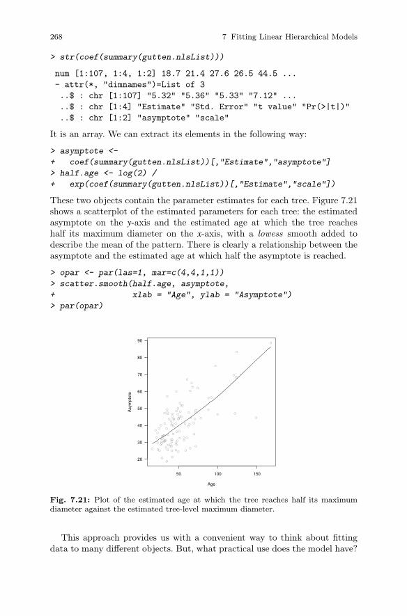
268 7 Fitting Linear Hierarchical Models
> str(coef(summary(gutten.nlsList)))
num [1:107, 1:4, 1:2] 18.7 21.4 27.6 26.5 44.5 ...
- attr(*, "dimnames")=List of 3
..$ : chr [1:107] "5.32" "5.36" "5.33" "7.12" ...
..$ : chr [1:4] "Estimate" "Std. Error" "t value" "Pr(>|t|)"
..$ : chr [1:2] "asymptote" "scale"
It is an array. We can extract its elements in the following way:
> asymptote <-
+ coef(summary(gutten.nlsList))[,"Estimate","asymptote"]
> half.age <- log(2) /
+ exp(coef(summary(gutten.nlsList))[,"Estimate","scale"])
These two objects contain the parameter estimates for each tree. Figure 7.21shows a scatterplot of the estimated parameters for each tree: the estimatedasymptote on the y-axis and the estimated age at which the tree reacheshalf its maximum diameter on the x-axis, with a lowess smooth added todescribe the mean of the pattern. There is clearly a relationship between theasymptote and the estimated age at which half the asymptote is reached.
> opar <- par(las=1, mar=c(4,4,1,1))
> scatter.smooth(half.age, asymptote,
+ xlab = "Age", ylab = "Asymptote")
> par(opar)
●
●
●●
●
●
●
●●●
●
● ●
●
●●
●●
●
●
●
●
●
●●●
●
●
●
●
●●
●
●●
●●
●
● ●
●
●
●
●
●
●
●●
●
●
●
●
●
●●
●
●
●
●
●
●
●
●
●
●
●
●
●
●
●
●
●
●
●
●
●
●
●
●
●
●
●
●
●●
●
●●●
●
●
●
●
●
●
●
●
●
●
●
●●
●
●
●
●
50 100 150
20
30
40
50
60
70
80
90
Age
Asy
mpt
ote
Fig. 7.21: Plot of the estimated age at which the tree reaches half its maximumdiameter against the estimated tree-level maximum diameter.
This approach provides us with a convenient way to think about fittingdata to many different objects. But, what practical use does the model have?

7.6 Non-linear Mixed-Effects Models 269
Not much. This model is analogous to the linear model that includes oneintercept for each plot: the model assumptions are (probably) satisfied, butthe model isn’t really useful. We need a way to tie all these little modelstogether. Hence, we adopt a hierarchical approach.
7.6.1 Hierarchical Approach
We now focus on fitting the same kinds of models to hierarchical data. Thisdirection produces simplifications and complications, but sadly more of thelatter than the former.
We use the non-linear mixed-effects model that generalizes the Pinheiroand Bates (2000) parameterization of our earlier non-linear model (equa-tion (6.6)). We will start with allowing each tree to have a random asymptoteand scale. That is, for diameter measure t in tree i,
yit = (φ1 +φi1)× [1− exp(−exp((φ2 +φi2)x))]+ εit (7.17)
where φ1 is the fixed, unknown asymptote and φ2 is the fixed, unknown scale,and [
φi1
φi2
]∼ N
([0
0
],
[σ 2
1 σ12
σ12 σ22
])(7.18)
The process of fitting and critiquing these models is well documented inPinheiro and Bates (2000). Given that we have already used nlsList, theeasiest approach both from the point of view of typing and of having sensiblestarting points is to use gutten.nlsList as the starting point for the model:
> gutten.nlme.0 <- nlme(gutten.nlsList)
If we wanted to construct this model from scratch, then we would need todo this:
> gutten.nlme.0 <-
+ nlme(dbh.cm ~ SSasympOrig(age.bh, asymptote, scale),
+ fixed = asymptote + scale ~ 1,
+ random = asymptote + scale ~ 1,
+ start = c(asymptote = 50, scale = -5),
+ data = gutten.d)
Note that as of the current version2 we do need to include the estimatedstarting values.
As with the linear mixed-effects models, we have a wide array of differ-ent diagnostic plots that we can deploy, and the functions to obtain those
2 nlme 3.1-96 on R 2.11.1.
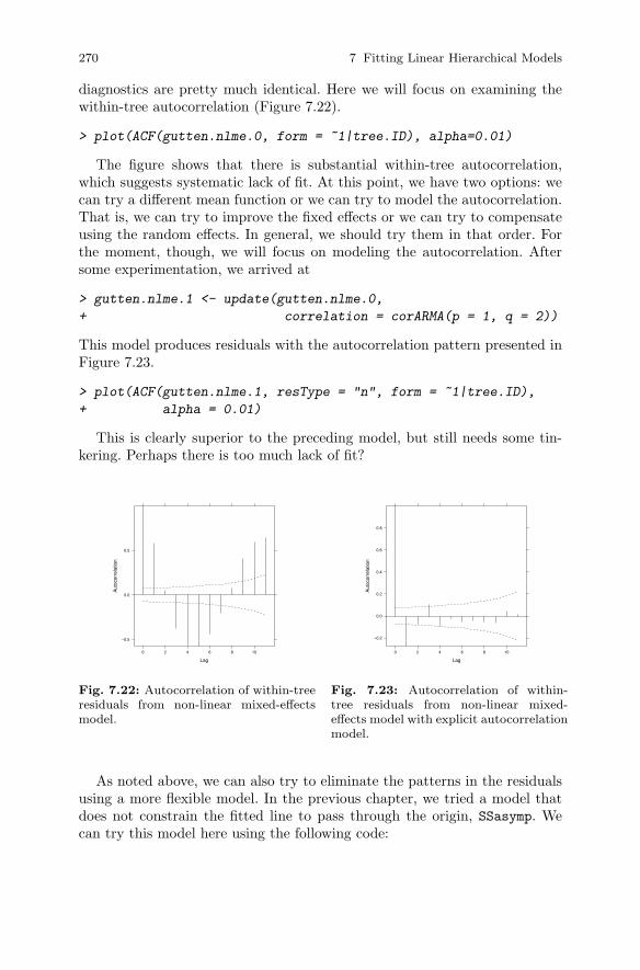
270 7 Fitting Linear Hierarchical Models
diagnostics are pretty much identical. Here we will focus on examining thewithin-tree autocorrelation (Figure 7.22).
> plot(ACF(gutten.nlme.0, form = ~1|tree.ID), alpha=0.01)
The figure shows that there is substantial within-tree autocorrelation,which suggests systematic lack of fit. At this point, we have two options: wecan try a different mean function or we can try to model the autocorrelation.That is, we can try to improve the fixed effects or we can try to compensateusing the random effects. In general, we should try them in that order. Forthe moment, though, we will focus on modeling the autocorrelation. Aftersome experimentation, we arrived at
> gutten.nlme.1 <- update(gutten.nlme.0,
+ correlation = corARMA(p = 1, q = 2))
This model produces residuals with the autocorrelation pattern presented inFigure 7.23.
> plot(ACF(gutten.nlme.1, resType = "n", form = ~1|tree.ID),
+ alpha = 0.01)
This is clearly superior to the preceding model, but still needs some tin-kering. Perhaps there is too much lack of fit?
Lag
Aut
ocor
rela
tion
−0.5
0.0
0.5
0 2 4 6 8 10
Fig. 7.22: Autocorrelation of within-treeresiduals from non-linear mixed-effectsmodel.
Lag
Aut
ocor
rela
tion
−0.2
0.0
0.2
0.4
0.6
0.8
0 2 4 6 8 10
Fig. 7.23: Autocorrelation of within-tree residuals from non-linear mixed-effects model with explicit autocorrelationmodel.
As noted above, we can also try to eliminate the patterns in the residualsusing a more flexible model. In the previous chapter, we tried a model thatdoes not constrain the fitted line to pass through the origin, SSasymp. Wecan try this model here using the following code:

7.6 Non-linear Mixed-Effects Models 271
> gutten.nlme.2 <-
+ nlme(dbh.cm ~ SSasymp(age.bh, asymptote, scale, R0),
+ fixed = asymptote + scale + R0 ~ 1,
+ random = asymptote + scale + R0 ~ 1,
+ start = c(asymptote = 40, scale = -0.07, R0 = -4),
+ data = gutten.d)
We had to try numerous different starting points before this model wouldconverge. For example,
1. with c(asymptote=50, scale=-5, R0=1), the error was “system is com-putationally singular”,
2. with c(asymptote=50, scale=-5, R0=-10), the error was “step halvingfactor reduced below minimum in PNLS step”,
3. with c(asymptote=50, scale=-5, R0=-1), the model converged but tookseveral minutes, and
4. with c(asymptote=40, scale=-0.07, R0=-4), the model converged withina few seconds.
We can compare the models using whole-model tests in the anova function.The test statistics should be regarded as only approximate. Here we see someevidence to suggest that the constraint leads to a worse-fitting model.
> anova(gutten.nlme.0, gutten.nlme.2)
Model df AIC BIC logLik Test
gutten.nlme.0 1 6 3627.763 3658.304 -1807.882
gutten.nlme.2 2 10 3473.265 3524.166 -1726.632 1 vs 2
L.Ratio p-value
gutten.nlme.0
gutten.nlme.2 162.4983 <.0001
A graphical comparison provides a useful addition. Because we constructedthese models from a groupedData object, we can use the augmented predic-tion plots as a very useful summary of the model’s behavior. This graphic ispresented in Figure 7.24, and shows that the differences between the modelsdoes not appear to be substantial.
> plot(comparePred(gutten.nlme.0, gutten.nlme.2))
We can get the approximate 95% confidence intervals of the estimates fromthe following call:
> intervals(gutten.nlme.1)
Approximate 95% confidence intervals
Fixed effects:
lower est. upper

272 7 Fitting Linear Hierarchical Models
age.bh
dbh.
cm
02040
0 50 100
●●●●●●●●
5.32
●●●●●●●●●●
5.36
0 50 100
●●●●●●●●●●●
5.33
●●●●●●●●●●●
7.12
0 50 100
●●●●●●●●●●●●
7.20
●●●●●●●
7.11
0 50 100
●●●●●●●●●●●●●●
5.40
●●●●●●●●●●●●●●
5.44
0 50 100
●●●●●●●●●●
5.34
●●●●●●●●●●●●●
7.21
0 50 100
●●●●●●●●
5.1●●●●●●●●
6.2
●●●●●●●●●●●●●
4.8
●●●●●●●●
6.9
●●●●●●●●●●●
4.3
●●●●●●●●
6.3
●●●●●●●●●●
5.20
●●●●●●●●●●●
5.38
●●●●●●●●
5.9
●●●●●●●●●●●
7.13
●●●●●●●●●●●●
5.37
02040
●●●●●●●●●●●
7.10
2040
●●●●●●●●
5.7
●●●●●●●
4.1
●●●●●●●●
5.6
●●●●●●●●●
5.10
●●●●●●●●●●●
7.14
●●●●●●●
4.2
●●●●●●●●●●●●●●
5.41
●●●●●●●●
5.3
●●●●●●●●●●●●●●
1.14
●●●●●●●●●●●●●●
5.42
●
●●●●●●●●
5.12●●●●●●●●●
5.11
●●●●●●●
6.6
●●●●●●
6.5
●●●●●●●
5.2
●●●●●●●●●●●●●●
5.45
●●●●●●●●●●
6.10
●●●●●●●●●●●●●●
1.8
●●●●●●●●●●●●●●
5.46
●●●
●●●●●●●
5.35
●●●●●●●●●●
3.14
02040
●●●●●●●●●●
5.180
2040
●●●●●
3.2
●●●●●
3.1
●●●●●●●●●●●●●●
5.29
●●●●●●●●●●●●●●
5.48
●●●●●●●●●●●●●
1.1
●●●●●●●
3.3
●●●●●●●●●●●
5.17
●●●●●●●●●●●●●●
5.23
●●●●●●●●●●●
3.13
●●●●●●●●
3.4
●●●●●●●●
6.4
●●●●●●●●●
6.8
●●●●●●●●●●●●●●
1.15
●●●●●●●●●
4.5
●●●●●●●●●●
5.15
●●●●●●●●●●●●●●
6.11
●●●●●●●●●●●●●
5.43
●●●●●●●●●●●●●●
6.12
●●●●●●●●●●●●●●
5.30
●
●●●●●●●●●
6.7
●●●●●●●●●●●●●
4.9
02040
●●●●●●●●●●●
4.40
2040
●●●●●●●●●●●
7.15
●●●●●●●●●●●
5.39
●●●●●●●●
5.4
●●●●●●●●
5.13
●
●●●●●●●
5.8
●●●●●●●●●●
3.8
●●●●●●●●●●●●●
5.28
●
●●●●●●●●●●
5.19
●●●●●●●●●●●●●●
7.10
●●●●●●●●●●●●●
5.27
●●●●●●●●●●
3.5
●●●●●●●●●●●●
5.21
●●●●●●●●●●●●●
4.10
●●●●●●●●●●
3.6
●●●●●●●●●●
5.14
●●●●●●●●●●
3.7
●●●●
●●●●●●●●●●
1.9
●●●●●●●●●●●●●●●
5.26
●●●●●●●●●●●●●●
5.47
●●●●●●●●●●●●●●
1.16
●●●●●●●●●●
4.6
02040
●●●●●●●●●●●●●●
1.120
2040
●●●●●●●●●●●●●●
1.13
●●●●●●●●●●●●●●
1.10
●●●●●●●●●●●
3.10
●●●●●●●●●●●●●●
5.31
●
●●●●●●●●●●●●●●
1.6
●●●●●●●●●●●●
3.11
●●●●●●●●●●●●●●
5.24
●●●●●●●●●●●●●
1.2
●●●●●●●●●●●●●●
1.3
●●●●●●●●●●●●●●
7.6
●●●●●●●●●●●●
5.22
●●●●
●●●●●●●●●●
1.11
0 50 100
●●●●●●●●●●●●●
4.7
●
●●●●●●●●●●●●●
2.2
0 50 100
●
●●●●●●●●●●●●●
2.1
●
●●●●●●●●●●●●●●
1.7
0 50 100
●●●●●●●●●●●●
3.12
●●●●●●●●●●●●●●●
5.25
0 50 100
02040
●
●
●●●●●●●●●●●
1.4
gutten.nlme.0 gutten.nlme.2
Fig. 7.24: Diameter data from von Guttenberg with both origin-constrained andunconstrained asymptotic models fitted. Here the tree-level models (equation (7.17))are plotted.
asymptote 36.477392 38.649203 40.821014
scale -4.203253 -4.119008 -4.034763
attr(,"label")
[1] "Fixed effects:"
Random Effects:
Level: tree.ID
lower est. upper
sd(asymptote) 8.9042315 10.5142706 12.4154325
sd(scale) 0.3232857 0.3855331 0.4597661
cor(asymptote,scale) -0.6726260 -0.5225912 -0.3312863

7.7 Further Reading 273
Correlation structure:
lower est. upper
Phi1 0.7549473 0.8217214 0.8716312
Theta1 0.2940804 0.4007537 0.5090448
Theta2 0.5607426 0.6827465 0.7757331
attr(,"label")
[1] "Correlation structure:"
Within-group standard error:
lower est. upper
1.291170 1.524274 1.799463
7.7 Further Reading
The book that documents the fitting tools that we have used for this chapter,Pinheiro and Bates (2000), should be considered essential reading for anyonewanting to use the code. The authors describe the theory, the algorithms, andmost of the options, and provide substantial examples for using the code.We have also found Schabenberger and Pierce (2002), Demidenko (2004),Fitzmaurice et al. (2004), Wood (2006), Lee et al. (2006), and Gelman andHill (2007) to be very useful. Venables and Ripley (2002) also provides someadvice and examples.

Part IV
Simulation and Optimization
Chapter 8
Simulations
In this chapter, we use R to generate, examine, detect, and illuminate sim-ulated yield tables, projections, or sets of possible future forest conditions.Our objectives are to 1) cover the major topics and tasks required to generateforest forecasts; 2) compare some common metrics from the resulting simu-lations; and 3) examine and present potential shortcomings and remedies forthe methods presented. Our motivation is to generate simulations and combi-nations of simulations that can be 1) examined quickly for anomalies; 2) easilyqueried to answer specific questions; and 3) efficiently exported into other ap-plications like harvest scheduling and transportation applications (Weintrauband Navon, 1976) or ecological community analysis (Oksanen et al., 2010),or linked to a geospatial database (Prayaga et al., 2009).
We tackle a specific and common problem in forest growth simulationin which more than one growth and dynamics model is needed in order toprovide forecasts but those models are not commensurate, meaning that thephysical scale of the unit of simulation between the models differs. Here weuse the individual-tree young-stand simulator rconifers (Ritchie and Hamann,2006, 2008) and construct a stand-level, established-stand simulator using theequations presented by Chambers (1980). The jurisdiction of the young-standsimulator presented here is normally for plantations below 25 years of age.The jurisdiction for the established-stand simulator is considered to be noyounger than 30 years. This gap, or in some cases overlap, is not unusual,and it has been expected that a smooth transition between the young-standsimulator and the established-stand simulator would occur at about the timeof crown closure. Here we will focus on the challenges that are introduced byour attempts to use projections from these two models jointly and ignore theminutiae of the individual jurisdictions of the respective models.
The chapter is structured as follows. In Section 8.1, we provide a briefpresentation of rconifers and construct the established-stand simulator us-ing Chambers (1980). In Section 8.2, we then determine volume and volumedistributions using the taper function developed by Kozak et al. (1968) andindividual tree records. In Section 8.3, we merge the results from our two
277A. P. Robinson, J. D. Hamann, Forest Analytics with R, Use R!,DOI 10.1007/978-1-4419-7762-5_8, © Springer Science+Business Media, LLC 2011
278 8 Simulations
models into a single data frame object. We use that object to examine thefollowing questions in Section 8.4: 1) What, if anything, happens to the pre-dicted maximum mean annual increment when we merge the results frommultiple models (e.g., linear combination of the results)? 2) What, if any-thing, happens to the distribution of log product volumes when the resultsare merged to create a single prediction? Finally, in Section 8.5, we export thepredicted yields to a database using the Structured Query Language (SQL)to allow our results to be used conveniently in other software.
8.1 Generating Simulations
The simulation of forest growth and dynamics is a complicated and multi-facted undertaking. Depending on the objectives, forest simulation may re-quire multiple software tools (e.g., SAS, PostgreSQL, Python), several sim-ulators and models (e.g., CONIFERS, ORGANON, ZELIG), and sometimesa handful of supporting model components (e.g., taper functions, wildlifehabitat models, and fuel loading models). Coordinating and linking thesedisparate tools is a substantial challenge.
Few forest simulation models have been developed within R, although thereare some tools for simulating ecological phenomena (see, e.g., Oksanen et al.,2010). We must construct our own tools to achieve our objectives. Here weuse two different and non-commensurate models that have different modelarchitectures: 1) rconifers, a young-stand and single-plant model developedby Hamann and Ritchie (2009); and 2) the normal yield tables developed byChambers (1980) for stand-level projection of established stands.
We start by generating model forecasts given 1) some initial set of condi-tions; 2) a set of possible management decisions (e.g., harvest, thin, and donothing); and 3) a list of the required outputs (e.g., reports, maps, and files).The process, presented in Algorithm 1, comprises the steps that are used togenerate the required outputs: age, volume, and volume distribution by loggrade. For this simple example, the process is: 1) project the initial plant listone year, then 2) compute the volume and volume distribution by log grade,then 3) compute the summary statistics for all necessary metrics of interest,and finally 4) repeat the process until the end of the planning horizon. Theseprocedures are the major focus of this section. In Sections 8.2 and 8.3, weexamine and address potential problems.
The final step is to plot graphs, generate maps, and write reports. Weassume that each project will have a unique set of metrics, constraints, andobjectives, so here we focus on only three outputs for simplicity: age, vol-ume, and volume distribution by log grade. For more complicated simulationprojects, the list of inputs, management decisions, and outputs can be exten-sive.
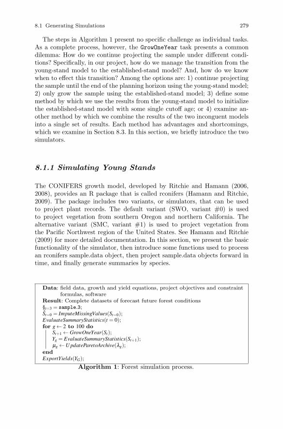
8.1 Generating Simulations 279
The steps in Algorithm 1 present no specific challenge as individual tasks.As a complete process, however, the GrowOneYear task presents a commondilemma: How do we continue projecting the sample under different condi-tions? Specifically, in our project, how do we manage the transition from theyoung-stand model to the established-stand model? And, how do we knowwhen to effect this transition? Among the options are: 1) continue projectingthe sample until the end of the planning horizon using the young-stand model;2) only grow the sample using the established-stand model; 3) define somemethod by which we use the results from the young-stand model to initializethe established-stand model with some single cutoff age; or 4) examine an-other method by which we combine the results of the two inconguent modelsinto a single set of results. Each method has advantages and shortcomings,which we examine in Section 8.3. In this section, we briefly introduce the twosimulators.
8.1.1 Simulating Young Stands
The CONIFERS growth model, developed by Ritchie and Hamann (2006,2008), provides an R package that is called rconifers (Hamann and Ritchie,2009). The package includes two variants, or simulators, that can be usedto project plant records. The default variant (SWO, variant #0) is usedto project vegetation from southern Oregon and northern California. Thealternative variant (SMC, variant #1) is used to project vegetation fromthe Pacific Northwest region of the United States. See Hamann and Ritchie(2009) for more detailed documentation. In this section, we present the basicfunctionality of the simulator, then introduce some functions used to processan rconifers sample.data object, then project sample.data objects forward intime, and finally generate summaries by species.
Data: field data, growth and yield equations, project objectives and constraintformulas, software
Result: Complete datasets of forecast future forest conditions§t=3 = sample.3;St=0 = ImputeMissingValues(St=0);EvaluateSummaryStatistics(t = 0);for g ← 2 to 100 do
St+1 ← GrowOneYear(St);Yg = EvaluateSummaryStatistics(St+1);μg ←U pdateParetoArchive(λg);
end
ExportYields(YG);
Algorithm 1: Forest simulation process.

280 8 Simulations
8.1.1.1 Loading the rconifers Package
We assume that the rconifers package is installed, for example using
> install.packages("rconifers")
We load the CONIFERS model using the library function and set the speciesmap to the variant that we wish to use. Here we use variant 1.
> library(rconifers)
Initialized 19 functional species coefficients for variant # 0
coefficients version is 4.120000
> set.species.map(set.variant(1))
Initialized 3 functional species coefficients for variant # 1
coefficients version is 4.120000
The species map object, called smc, contains settings for three functionalspecies-level coefficients that can be controlled by the user. We can examineit as follows.
> dim(smc)
[1] 3 13
> names(smc)
[1] "idx" "code" "fsp"
[4] "name" "organon" "cactos"
[7] "fvs" "endemic.mort" "max.sdi"
[10] "browse.damage" "mechanical.damage" "genetic.worth.h"
[13] "genetic.worth.d"
> head(smc)
idx code fsp name organon cactos fvs
1 0 CV 0 Competing Vegetation 0 0
2 1 DF 1 Douglas fir 202 4 DF
3 2 NS 2 Non Stocked 0 0
endemic.mort max.sdi browse.damage mechanical.damage
1 0.002 0 0 0
2 0.002 450 0 0
3 0.000 0 0 0
genetic.worth.h genetic.worth.d
1 0 0
2 0 0
3 0 0

8.1 Generating Simulations 281
or by using the str function.Each functional species code is used to map an actual species into the co-
efficient array for each variant. We use the term functional species to describea group species of that behave similarly to one another in the growth model.The data frame object smc also contains a text species code that can be usedin data recorder files. The species map also includes elements for mortalitycontrols like endemic mortality (smc$endemic.mort), maximum stand den-sity index values (smc$max.sdi Reineke, 1933), and values that can be usedto control height growth like mechanical damage (smc$mechanical.damage)or damage caused by animal browsing (smc$browse.damage).
8.1.1.2 Creating and Using a sample.data Object
The rconifers package provides a specific class for storing the data to beused for simulation: a sample.data object. A sample.data object must con-tain at least two data frame objects: one to define plot-level attributes(called sample.data$plots) and one to define the tree records (calledsample.data$plants). In additon to the data frame objects, the sample.dataobject must also include an age (called sample.data$age) and a parameter(called sample.data$x0) that defines the intercept term for a stand den-sity trajectory (Reineke, 1933; Hann and Wang, 1990). Most of the rconifersfunctions operate directly upon sample.data objects.
First, load the plot and plant data frame objects from the package.
> data(plots.smc)
> data(plants.smc)
Next, create a list that contains the plots, plants, and initial age, andassign the resulting list a sample.data class,
> sample.3 <- list(plots = plots.smc,
+ plants = plants.smc,
+ age = 3,
+ x0 = 0.0)
> class(sample.3) <- "sample.data"
Now we can call many of the functions in rconifers directly upon the sample.3object. For example, to generate a set of species-level summaries, we use thesummary function.
> summary(sample.3)
sample contains 18 plots records
sample contains 58 plant records
age = 3
x0 = 0

282 8 Simulations
max sdi = 450
qmd tht ba expf
DF 0.578505 5.76724 0.456331 322.222
The summary function calls the sp.sums function, which generates a dataframe object for which each row contains the summaries for a different speciesin the plant list. This data frame can also include non-tree species. Thesummary function also presents the sample.data$age and sample.data$x0
variables.
8.1.1.3 Generating Young-Stand Simulations
We use the project function to project for a sample.data object. Here, wegrow the sample.3 sample.data object forward in time for 10 years, andsimply print out the projected summary, using the summary function,
> summary(sample.3)
sample contains 18 plots records
sample contains 58 plant records
age = 3
x0 = 0
max sdi = 450
qmd tht ba expf
DF 0.578505 5.76724 0.456331 322.222
> sample.25 <- project(sample.3,
+ 22,
+ control = list(rand.err = 0,
+ rand.seed = 0,
+ endemic.mort = 0,
+ sdi.mort = 0))
> summary(sample.25)
sample contains 18 plots records
sample contains 58 plant records
age = 25
x0 = 0
max sdi = 450
qmd tht ba expf
DF 8.59453 65.5306 129.815 322.222
Here the output includes the number of total plot records, the total numberof plant records in the sample, the total age, the maximum stand density in-dex (max.sdi, see Hann and Wang, 1990), the initial value at which max.sdi
crossed the line of imminent mortality (Reineke, 1933), x0, and the outputfrom the sp.sums function.
8.1 Generating Simulations 283
The project function includes a control argument that can be used tofine-tune the behavior of the function, and thus the simulator. rand.err is aflag to indicate that a normally distributed random number should be addedto the height growth of the plant (rand.err = 1). rand.seed sets the initialvalue for the random number generator and only needs to be called once atthe beginning of the simulation for each sample you want to project. If youneed to repeat the randomness pattern, you need to reseed the random num-ber generator with the same seed before projecting the sample. The valueis not a switch; it requires an integer value to set the random number gen-erator (see ?set.seed). The endemic.mort argument is used to toggle thebackground mortality in the model applied to each growth cycle. Finally, thesdi.mortality switch is used to control additional mortality using the standdensity index, defined by Reineke (1933). This last component of mortalityis independent of the endemic mortality in the simulator. The influence ofspecific arguments is covered more completely in the package documentation(Ritchie and Hamann, 2006, 2008; Hamann and Ritchie, 2009).
As we described in Section 8.1, we ultimately want to compare simulations,given the same initial conditions. For example, in the following simulationrun we assume that no vegetation control will be applied, and we generatesimulations using a set of for loops to project a sample.data object for 100years.
> res.v <- vector(length = 98, mode = "list")
> s0 <- sample.3
> res.v[[1]] <- data.frame(age = s0$age, sp.sums(s0)["DF",])
> ## grow from age 3 to age 100 (97 more years)
> for(m in 1:97) {
+ ## project s0 in one year intervals
+ s1 <- project(s0, 1, control = list(rand.err = 0,
+ rand.seed = 0,
+ endemic.mort = 1,
+ sdi.mort = 1))
+ res.v[[m+1]] <- data.frame(age = s1$age,
+ sp.sums(s1)["DF",])
+ s0 <- s1
+ }
> res.v <- do.call(rbind, res.v)
> res <- res.v
In this example, the plant list in the sample s0 includes only Douglas-fir(Pseudotsuga menzesii Mirb. Franco), and so we can use the index operatorto extract only the Douglas-fir results from the summaries generated by thesp.sums function (here sp.sums(s1)["DF",]). The process, as outlined inSection 8.1, is to assume that sample.3 represents the initial conditions,compute the initial condition summary statistics, and then project s0 forwardin time 1 year where the results are stored in s1. The process is repeated
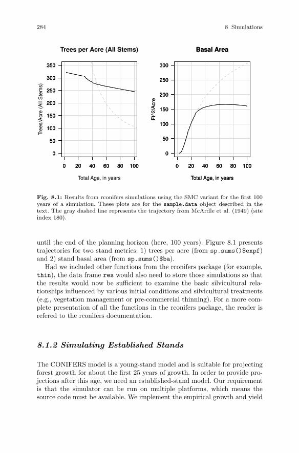
284 8 Simulations
0 20 40 60 80 100
0
50
100
150
200
250
300
350
Trees per Acre (All Stems)
Total Age, in years
Tree
s/A
cre
(All
Ste
ms)
0 20 40 60 80 100
0
50
100
150
200
250
300
350
0 20 40 60 80 100
0
50
100
150
200
250
300
350
0 20 40 60 80 100
0
50
100
150
200
250
300
Basal Area
Total Age, in years
Ft^
2/A
cre
0 20 40 60 80 100
0
50
100
150
200
250
300
Basal Area
Total Age, in years
Ft^
2/A
cre
0 20 40 60 80 100
0
50
100
150
200
250
300
Fig. 8.1: Results from rconifers simulations using the SMC variant for the first 100years of a simulation. These plots are for the sample.data object described in thetext. The gray dashed line represents the trajectory from McArdle et al. (1949) (siteindex 180).
until the end of the planning horizon (here, 100 years). Figure 8.1 presentstrajectories for two stand metrics: 1) trees per acre (from sp.sums()$expf)and 2) stand basal area (from sp.sums()$ba).
Had we included other functions from the rconifers package (for example,thin), the data frame res would also need to store those simulations so thatthe results would now be sufficient to examine the basic silvicultural rela-tionships influenced by various initial conditions and silvicultural treatments(e.g., vegetation management or pre-commercial thinning). For a more com-plete presentation of all the functions in the rconifers package, the reader isrefered to the rconifers documentation.
8.1.2 Simulating Established Stands
The CONIFERS model is a young-stand model and is suitable for projectingforest growth for about the first 25 years of growth. In order to provide pro-jections after this age, we need an established-stand model. Our requirementis that the simulator can be run on multiple platforms, which means thesource code must be available. We implement the empirical growth and yield

8.1 Generating Simulations 285
tables for the Douglas-fir zone in Washington State developed by Chambers(1980). This approach allows us to provide a useful example of 1) building amodel using external C or FORTRAN source code; 2) using that model fromwithin R; and finally 3) integrating that model into our current project tocreate a uniform, and thus useful, stream of data.
The model developed by Chambers (1980) contains equations for predict-ing normal1 basal area (nba), trees per acre for trees 7 inches and larger(tpa.7.plus), average stand diameter (qmd), and stand mean height for trees5 inches and larger (smh). The model also includes equations for cubic footvolume, Scribner volume to a 6 inch top, Scribner volume in 16 foot logs, andScribner volume in 32 foot logs using a tariff system. However, since rconifersdoes not provide volumes and we may want to compute volumes to someother specification, we defer volume determination until Section 8.2. In thissection, we briefly present a subset of the source code, compile the source codefor use within R, and finally load, attach, and call the functions to generatea data frame commensurate with the resulting data frame in Section 8.1.1.3.
8.1.2.1 Source Code
The files chambers-1980.h, chambers-1980.c, and chambers-1980.r con-tain equations and functions that define the growth and yield characteristicsfor the Douglas-fir (Pseudotsuga menzesii Mirb. Franco) zone in WashingtonState as defined in Chambers (1980). The header file (chambers-1980.h) de-fines the functions presented in the implementation file (chambers-1980.c),and we provide a set of R wrapper functions (chambers-1980.r).
In this section, we demonstrate the procedures for calling external func-tions using the equation to predict stand mean height (Chambers, 1980, Table16), expressed as
H = 2202.75000
+205.41618× (log(Abh ×S))2
−1323.88477× (log(Abh ×S))
−0.00671×A2bh
−383.35889× 1
Abh
where H is the predicted stand mean height for trees 5.0 inches and larger,Abh is the age at breast height, S is the site index, defined by King (1966),and log is the base 10 logarithm.
1 Normal is defined here informally as meaning typical or average for a large popula-tion of sampled stands.
286 8 Simulations
The C function chambers_1980_stand_mean_height is defined in the filechambers-1980.h as
void chambers_1980_stand_mean_height(
double *site_index,
double *total_age,
double *stand_mean_height);
and the C implementation for the function is in the file chambers-1980.c as
void chambers_1980_stand_mean_height(
double *site_index,
double *total_age,
double *stand_mean_height)
{
double ret_val;
double bha;
bha = chambers_1980_breast_height_age(site_index,
total_age);
if(bha < 1.0)
{
bha = 1.0;
}
ret_val = 2202.75000
+ 205.41618 * pow(log10(bha * (*site_index)), 2.0)
- 1323.88477 * log10(bha * (*site_index))
- 0.00671 * bha * bha
- 383.35889 * (1.0 / bha);
if(ret_val <= 0.0)
{
ret_val = 0.0;
}
*stand_mean_height = ret_val;
}
The function chambers_1980_breast_height_age, which is called fromwithin the chambers_1980_stand_mean_height function, is also found inthe file chambers-1980.c.
The function is called using three arguments: *site_index, *total_age,and *stand_mean_height. The first two arguments are the predictor vari-ables. The last argument is a pointer to where the results are stored. Allthree arguments are pointers to variables of type double (that is, these argu-ments are passed by reference). At the time of this writing, all arguments toexternal functions or subroutines are passed by reference. A table of variabletypes is presented in Table 8.1.

8.1 Generating Simulations 287
Table 8.1: Foreign language data types.
R storage mode C type FORTRAN type
logical int * INTEGER
integer int * INTEGER
double double * DOUBLE PRECISION
complex Rcomplex * DOUBLE COMPLEX
character char ** CHARACTER*255
raw unsigned char * none
8.1.2.2 Compile, Attach, Call, and Wrap External Code
The final step in the process of calling external source code is to 1) compile
the source code into a shared library; 2) attach the resulting shared libraryto your current R process; 3) call the external code using one of the R func-tions for calling external libraries; and optionally 4) wrap the R externalcalling functions into a wrapper function of your own. The following codeassumes that appropriate command-line tools are available to build R and Rextensions.
Compile
Since the files chambers-1980.h and chambers-1980.c define and containthe functions themselves, we only need to issue a single command, from theoperating system command prompt (here, $) to compile the shared library,
$ R CMD SHLIB chambers-1980.c
which will compile and link the code into a shared library chambers-1980.so(chambers-1980.dll in Windows). The call will present reasonably helpful er-ror messages if necessary.
Attach
To attach the shared library and access the functions in the current R process,use the dyn.load function at the R prompt,
> dyn.load("chambers-1980.so")
upon which, unless something goes wrong, you should recieve no error mes-sage and be returned directly to the R command prompt.

288 8 Simulations
Call
To call the function chambers_1980_stand_mean_height, which is writtenin C, we must use either of R’s .C or .Call function, passing the argumentsto the function as well,
> site.index <- 120.0
> total.age <- 60
> .C("chambers_1980_stand_mean_height",
+ as.double(site.index),
+ as.double(total.age),
+ smh = as.double(0))$smh
[1] 112.9387
which returns the correct value but looks cumbersome.
Wrap
For simplicity, we wrap the .C function call within a more accessible-lookingR function called chambers.1980.smh,
> chambers.1980.smh <- function(site.index,total.age) {
+ ret.val <- .C("chambers_1980_stand_mean_height",
+ as.double(site.index),
+ as.double(total.age),
+ smh = as.double(0))$smh
+ ret.val
+ }
which provides an easier interface to the original function and returns thevalue of interest.
Finally, to verfiy the wrapper function is working properly, simply call theR wrapper function chambers.1980.smh,
> chambers.1980.smh(120.0, 60.0)
[1] 112.9387
which matches the results presented in the original publication for a standwith a 50 year site index of 120 feet at age 60 (Chambers, 1980, Table 16).
In all, there are about 14 functions defined in chambers-1980.h andchambers-1980.c that need .C wrappers. We provide a set of wrapper func-tions so, to conserve space, the functions can be loaded by sourcing the file
> source("chambers-1980.r")
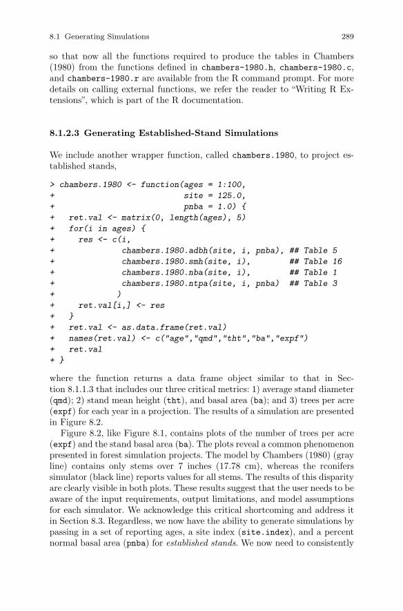
8.1 Generating Simulations 289
so that now all the functions required to produce the tables in Chambers(1980) from the functions defined in chambers-1980.h, chambers-1980.c,and chambers-1980.r are available from the R command prompt. For moredetails on calling external functions, we refer the reader to “Writing R Ex-tensions”, which is part of the R documentation.
8.1.2.3 Generating Established-Stand Simulations
We include another wrapper function, called chambers.1980, to project es-tablished stands,
> chambers.1980 <- function(ages = 1:100,
+ site = 125.0,
+ pnba = 1.0) {
+ ret.val <- matrix(0, length(ages), 5)
+ for(i in ages) {
+ res <- c(i,
+ chambers.1980.adbh(site, i, pnba), ## Table 5
+ chambers.1980.smh(site, i), ## Table 16
+ chambers.1980.nba(site, i), ## Table 1
+ chambers.1980.ntpa(site, i, pnba) ## Table 3
+ )
+ ret.val[i,] <- res
+ }
+ ret.val <- as.data.frame(ret.val)
+ names(ret.val) <- c("age","qmd","tht","ba","expf")
+ ret.val
+ }
where the function returns a data frame object similar to that in Sec-tion 8.1.1.3 that includes our three critical metrics: 1) average stand diameter(qmd); 2) stand mean height (tht), and basal area (ba); and 3) trees per acre(expf) for each year in a projection. The results of a simulation are presentedin Figure 8.2.
Figure 8.2, like Figure 8.1, contains plots of the number of trees per acre(expf) and the stand basal area (ba). The plots reveal a common phenomenonpresented in forest simulation projects. The model by Chambers (1980) (grayline) contains only stems over 7 inches (17.78 cm), whereas the rconiferssimulator (black line) reports values for all stems. The results of this disparityare clearly visible in both plots. These results suggest that the user needs to beaware of the input requirements, output limitations, and model assumptionsfor each simulator. We acknowledge this critical shortcoming and address itin Section 8.3. Regardless, we now have the ability to generate simulations bypassing in a set of reporting ages, a site index (site.index), and a percentnormal basal area (pnba) for established stands. We now need to consistently
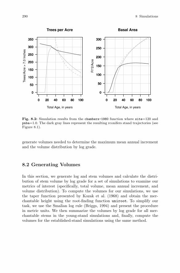
290 8 Simulations
0 20 40 60 80 100
0
50
100
150
200
250
300
350
Trees per Acre
Total Age, in years
Tree
s/A
cre
> 7
.0 In
ches
0 20 40 60 80 100
0
50
100
150
200
250
300
350
0 20 40 60 80 100
0
50
100
150
200
250
300
350
0 20 40 60 80 100
0
50
100
150
200
250
300
Basal Area
Total Age, in years
Ft^
2/A
cre
0 20 40 60 80 100
0
50
100
150
200
250
300
0 20 40 60 80 100
0
50
100
150
200
250
300
Fig. 8.2: Simulation results from the chambers-1980 function where site=120 andpnba=1.0. The dark gray lines represent the resulting rconifers stand trajectories (seeFigure 8.1).
generate volumes needed to determine the maximum mean annual incrementand the volume distribution by log grade.
8.2 Generating Volumes
In this section, we generate log and stem volumes and calculate the distri-bution of stem volume by log grade for a set of simulations to examine ourmetrics of interest (specifically, total volume, mean annual increment, andvolume distribution). To compute the volumes for our simulations, we usethe taper function presented by Kozak et al. (1968) and obtain the mer-chantable height using the root-finding function uniroot. To simplify ourtask, we use the Smalian log rule (Briggs, 1994) and present the procedurein metric units. We then summarize the volumes by log grade for all mer-chantable stems in the young-stand simulations and, finally, compute thevolumes for the established-stand simulations using the same method.

8.2 Generating Volumes 291
8.2.1 The Taper Function
The taper equation for Douglas-fir, developed by Kozak (1988), can be usedto provide 1) predictions of inside diameter at any point on the stem; 2) esti-mates of total volume; 3) estimates of merchantable volume and merchantableheight to any top diameter and from any stump height; and 4) estimates ofindividual log volumes. The taper equation function is
di = a0Da1aD2 Xb1Z2+b2 ln(Z+0.001)+b3
√Z+b4 expZ+b5(
DH ) (8.1)
where X = (1−√hi/H)(1−√p), D is the diameter at breast height (1.3 m), H
is the total stem height, p = 0.25, Z = hiH, and hi is the height above ground on
the stem at which we want to determine di, the diameter inside bark, ln is thenatural logarithm, and a0, a1, a2, b1, b2, b3, b4, b5 are estimated coefficients(Kozak, 1988).
Equation (8.1) can be written as a vectorized R function,
> bcmof.diDBH <- function(dbh, tht, cr, hi) {
+ p <- 0.25
+ dib <- 1.02453 * dbh^0.88809 * 1.00035^dbh
+ X <- (1.0 - sqrt(hi / tht)) / (1.0 - sqrt(p))
+ Z = hi / tht
+ a = 0.95086 * Z * Z;
+ b = -0.18090 * log(Z + 0.001);
+ c = 0.61407 * sqrt(Z) + -0.35105 * exp(Z);
+ d = 0.05686 * (dbh / tht);
+ retval <- (dib * X^(a + b + c + d))
+ retval[tht < hi] <- 0
+ retval
+ }
where arguments for the function are dbh, tht, cr, and hi, which represent thediameter at breast height (1.3 m), the total stem height, the crown ratio, andthe height at which we want to determine di, respectively. An example profilewhere dbh = 45 cm, tht = 27 m, and cr = 0.6 is displayed in Figure 8.3.
8.2.2 Computing Merchantable Height
To determine the height above the base of the stem at which we cannot makecuts (the merchantable limits), we need a function that will cross the x-axisat the merchantable height of the stem. A simple method to accomplish thisis to subtract the merchantable diameter (md) from the diameter inside bark(diDBH)

292 8 Simulations
> merch.height.func <- function(hi, dbh, tht, cr, md) {
+ dib <- bcmof.diDBH(dbh, tht, cr, hi)
+ diff <- dib - md
+ diff
+ }
so that when diDBH is less that md, the function crosses the x-axis; that is,the root of equation (8.1).
We pass the merch.height.func function to the uniroot function to ob-tain the merchantable height of the stem,
> mh <- uniroot(merch.height.func,
+ c(0, 27),
+ dbh = 45.0,
+ tht = 27,
+ cr = 0.60,
+ md = 10.0)
> mh
$root
[1] 23.34488
$f.root
[1] 1.584768e-06
$iter
[1] 5
$estim.prec
[1] 6.103516e-05
where the arguments of the uniroot function include the limits of eval-uation (c(0,27)) and any necessary arguments to pass through to themerch.height.func function (here dbh, tht, cr, and md).
The results of the uniroot function show that it took five iterations to ar-rive at the root (iter), which occurred at 23.34488 meters above the ground.To be precise, for the inputs we provided, the location of the root occuredat 23.34488 and the taper function actually evaluates to 0.000002 (a zero, orroot) at that value. The estimated precision after five iterations was 0.00006.Should we require greater precision, we can alter the tol and maxiter argu-ments to our satisfaction.
Finally, to verify the results, we can pass the resulting uniroot mh$root
value back into the taper function to verify that we get the same value forthe minimum merchantable diameter inside bark of 10.0 cm,
> min.dib.check <- bcmof.diDBH(45, 27, 0.60, mh$root)
> min.dib.check
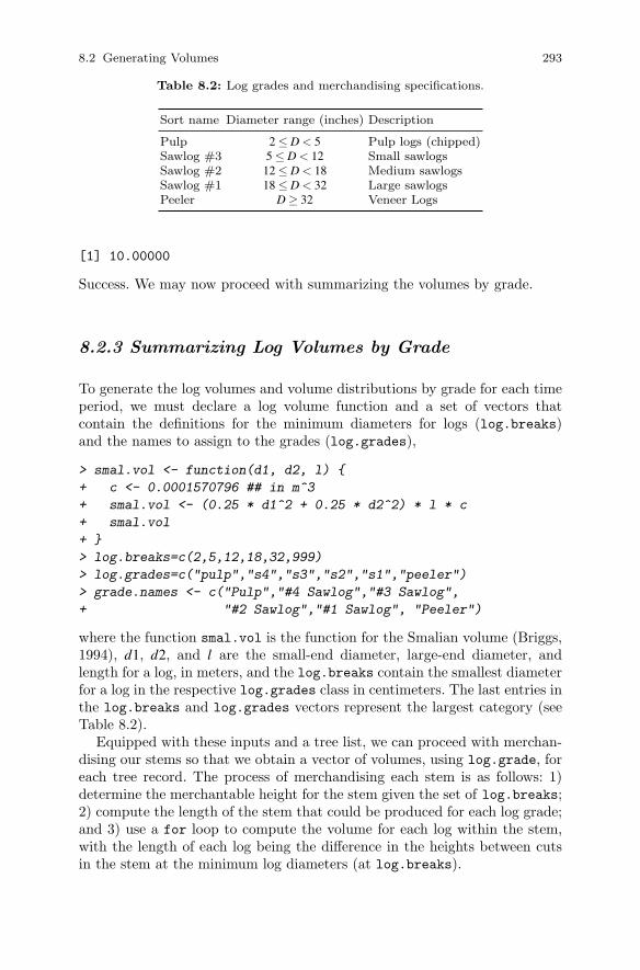
8.2 Generating Volumes 293
Table 8.2: Log grades and merchandising specifications.
Sort name Diameter range (inches) Description
Pulp 2 ≤ D < 5 Pulp logs (chipped)Sawlog #3 5 ≤ D < 12 Small sawlogsSawlog #2 12 ≤ D < 18 Medium sawlogsSawlog #1 18 ≤ D < 32 Large sawlogsPeeler D ≥ 32 Veneer Logs
[1] 10.00000
Success. We may now proceed with summarizing the volumes by grade.
8.2.3 Summarizing Log Volumes by Grade
To generate the log volumes and volume distributions by grade for each timeperiod, we must declare a log volume function and a set of vectors thatcontain the definitions for the minimum diameters for logs (log.breaks)and the names to assign to the grades (log.grades),
> smal.vol <- function(d1, d2, l) {
+ c <- 0.0001570796 ## in m^3
+ smal.vol <- (0.25 * d1^2 + 0.25 * d2^2) * l * c
+ smal.vol
+ }
> log.breaks=c(2,5,12,18,32,999)
> log.grades=c("pulp","s4","s3","s2","s1","peeler")
> grade.names <- c("Pulp","#4 Sawlog","#3 Sawlog",
+ "#2 Sawlog","#1 Sawlog", "Peeler")
where the function smal.vol is the function for the Smalian volume (Briggs,1994), d1, d2, and l are the small-end diameter, large-end diameter, andlength for a log, in meters, and the log.breaks contain the smallest diameterfor a log in the respective log.grades class in centimeters. The last entries inthe log.breaks and log.grades vectors represent the largest category (seeTable 8.2).
Equipped with these inputs and a tree list, we can proceed with merchan-dising our stems so that we obtain a vector of volumes, using log.grade, foreach tree record. The process of merchandising each stem is as follows: 1)determine the merchantable height for the stem given the set of log.breaks;2) compute the length of the stem that could be produced for each log grade;and 3) use a for loop to compute the volume for each log within the stem,with the length of each log being the difference in the heights between cutsin the stem at the minimum log diameters (at log.breaks).

294 8 Simulations
First, we create a vector to store the merchantable heights for each of thelog.breaks. Then, we loop over the log.breaks vector to determine whereto make the cuts in the stem so that the stem is cut into lengths that representthe longest possible log for each log grade,
> mh.bks <- rep(0, length(log.breaks))
> for(i in 1:length(log.breaks)) {
+ dbh <- 45.0; tht <- 27; cr <- 0.60
+ if(log.breaks[i] <= bcmof.diDBH(dbh, tht, cr, 0.0)) {
+ mh <- uniroot(merch.height.func,
+ c(0, tht),
+ dbh = dbh,
+ tht = tht,
+ cr = 0.60,
+ md = log.breaks[i])
+ mh.bks[i] <- mh$root
+ } else {
+ mh.bks[i] <- 0.0
+ }
+ }
The resulting vector (mh.bks) contains the heights at which the stem canno longer be merchandised into the associated log.break entry. For example,the first entry in the merchantable height breaks (that is, mh.bks[1]), whichis
> log.breaks
[1] 2 5 12 18 32 999
> mh.bks
[1] 26.497448 25.405561 22.451219 19.407203 4.588263 0.000000
means that the longest log that can be cut from the stem while maintain-ing a small-end diameter larger than 2 cm is 26.49745 m above the ground.Subsequently, the maximum length that can be cut from the stem for a 5 cmlog is 25.40556 m. Thus, the length of the top log is the difference betweenthe two lengths, 1.09189 m, so that the top log has a small-end diameter(sed) of 2 cm, a large end diameter of 5 cm, and a length of 1.09189 m. TheSmalian volume given those dimensions is in cubic meters. Since the processof iterating over tree records can be lengthy, we provide a function calledgenerate.log.vols so that given a sample.data object and a vector of min-imum log diameters (log.breaks), the generate.log.vols function returnsa data frame that contains the original tree list, with volumes, by log.grade,appended as columns. The function can be used to compute volumes for bothyoung-stand and older-stand model results.
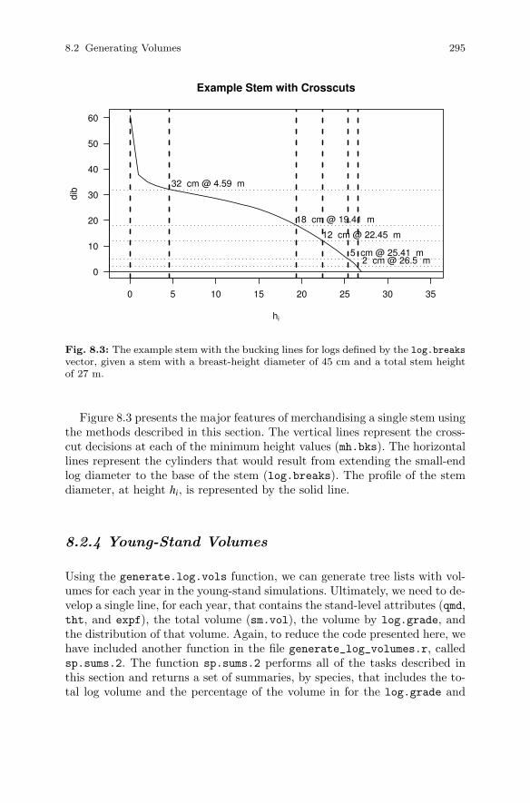
8.2 Generating Volumes 295
0 5 10 15 20 25 30 35
0
10
20
30
40
50
60
Example Stem with Crosscuts
hi
dib
2 cm @ 26.5 m5 cm @ 25.41 m
12 cm @ 22.45 m
18 cm @ 19.41 m
32 cm @ 4.59 m
Fig. 8.3: The example stem with the bucking lines for logs defined by the log.breaksvector, given a stem with a breast-height diameter of 45 cm and a total stem heightof 27 m.
Figure 8.3 presents the major features of merchandising a single stem usingthe methods described in this section. The vertical lines represent the cross-cut decisions at each of the minimum height values (mh.bks). The horizontallines represent the cylinders that would result from extending the small-endlog diameter to the base of the stem (log.breaks). The profile of the stemdiameter, at height hi, is represented by the solid line.
8.2.4 Young-Stand Volumes
Using the generate.log.vols function, we can generate tree lists with vol-umes for each year in the young-stand simulations. Ultimately, we need to de-velop a single line, for each year, that contains the stand-level attributes (qmd,tht, and expf), the total volume (sm.vol), the volume by log.grade, andthe distribution of that volume. Again, to reduce the code presented here, wehave included another function in the file generate_log_volumes.r, calledsp.sums.2. The function sp.sums.2 performs all of the tasks described inthis section and returns a set of summaries, by species, that includes the to-tal log volume and the percentage of the volume in for the log.grade and
296 8 Simulations
log.breaks vectors. For example, to obtain the volumes for the young-standsimulation from Section 8.1.1.3 (that is, sample.25),
> ## the log.breaks are in cm
> sp2 <- sp.sums.2(sample.25, log.breaks/2.54, log.grades)
> sp2[,c("sm.vol", log.grades)]
sm.vol pulp s4 s3 s2 s1
DF 3647.269 1.380405 21.88773 463.9883 1826.207 1321.220
peeler
DF 12.58429
The resulting data frame object contains the quadratic mean diameter(qmd), the mean total height weighted by the stem’s expansion factor (expf),the total basal area (ba), the total number of stems per acre (expf), the totalnumber of stems per acre over 7 inches (expf.7.plus to compare our resultsagainst the Chambers (1980) model), the total Smalian log volume (sm.vol),a vector of Smalian volumes by log.grade, and a vector of proportions forthe log volume (log.grades) for each species in sample.25. Here we onlypresent the total volume and the volumes in each of the log.grades.
8.2.5 Established-Stand Volumes
To generate established-stand volumes using the function sp.sums.2, weneed to create a temporary sample.data object from the results of thechambers.1980 function. The output from the established-stand simulatoris a vector of attributes for any given age, so we can either 1) determinethe volume from a single set of observations (that is, summary statistics likeqmd and tht) or 2) generate a set of stem observations (a tree list) from thepopulation of stems described by the summary statistics. We present bothmethods in this section.
8.2.5.1 From Summary Statistics
The first method is the simplest. Here we construct a single stem from thestand summary statistics from the established-stand simulator. For exam-ple, to determine the volumes for an established-stand simulation at age50 years (e.g., site = 120, pnba = 1.0, age = 50), we first generate theestablished-stand simulation using the chambers.1980 function. Then, wecreate an rconifers plot and plant data frame objects and, finally, an rconiferssample.data object,
> ch <- chambers.1980(ages = 1:200, site = 120, pnba = 1.0)
> ch.stem <- data.frame(plot = 1,
8.2 Generating Volumes 297
+ sp.code = "DF",
+ d6 = NA,
+ dbh = ch[50,]$qmd,
+ tht = ch[50,]$tht,
+ cr = 0.6,
+ n.stems = 1,
+ expf = ch[50,]$expf,
+ crown.width = NA,
+ errors = 0)
> ch.plot <- data.frame(plot = 1,
+ elevation = NA,
+ slope = NA,
+ aspect = NA,
+ whc = NA,
+ map = NA,
+ si30 = 120)
> ch.50 <- list(plots = ch.plot, plants = ch.stem, age = 50)
> class(ch.50) <- "sample.data"
> sh2 <- sp.sums.2(ch.50, log.breaks, log.grades)
> sh2[,c("qmd","ba","expf","sm.vol",log.grades)]
qmd ba expf sm.vol pulp s4 s3
DF 12.13548 207.8756 258.7996 9032.07 22.49502 360.6965 8481.45
s2 s1 peeler
DF 167.4276 0 0
Note that the volumes are generated from a single representative stem forthe stand.
8.2.5.2 From Tree Lists
There are many techniques for generating tree lists. Here we generate a nor-mal distribution of diameters. Using the normal function, and choosing year50, we generate round(ch[50,]$tpa) realizations from an assumed normalpopulation of stem sizes,
> dia.obs <- rnorm(n = round(ch[50,]$expf)*10,
+ mean = ch[50,]$qmd,
+ sd = 0.20*ch[50,]$qmd)
where mean is the quadratic mean of the tree diameters, sd is the standarddeviation of the population which we assume is 20% of qmd , and ch[50,] isthe data for the 50th year in the simulation. To increase the number of stemsin our sample, say to generate a smoother distribution of stems, we wouldgenerate ten times the number of stem observations and divide the expansion
298 8 Simulations
factor for each entry by ten to obtain the correct total number of stems perunit area.
To construct the tree list, we include a set of values for the heights. Herewe use the equation to predict total height given DBH, presented by Hanuset al. (1999), to generate the heights for each of the diameter realizations,and assume a crown ratio of 40% (that is, cr = 0.40) and a single plotrepresenting the sample,
> ## generate the plant records
> plant.obs <- data.frame(plot = 1,
+ sp.code = "DF",
+ d6 = NA,
+ dbh = dia.obs,
+ tht = 4.5 + exp(7.262195456 +
+ -5.899759104 *
+ dia.obs^-0.287207389),
+ cr = 0.40,
+ n.stems = 1,
+ expf = 1/10,
+ crown.width = NA)
> plot.obs <- data.frame(plot = 1,
+ elevation = 1000,
+ slope = 0,
+ aspect = 0,
+ whc = NA,
+ map = NA,
+ si30 = 85.0)
> ch.50 <- list(plots = plot.obs,
+ plants = plant.obs,
+ age = ch[50,]$age,
+ x0 = NA)
> class(ch.50) <- "sample.data"
Finally, we can use the modified function sp.sums.2 to obtain the metricsof interest:
> sh2 <- sp.sums.2(ch.50, log.breaks, log.grades)
> sh2[, c("qmd", "ba", "expf", "sm.vol", log.grades)]
qmd ba expf sm.vol pulp s4 s3
DF 12.43444 218.4129 259 7868.594 20.05454 328.2135 6692.396
s2 s1 peeler
DF 819.5235 8.406364 0
methods, as in Section 8.2.4.Finally, when we no longer need the chambers-1980.so shared library, we
unload the library using the dyn.unload function,
8.4 Examining Results 299
> dyn.unload("chambers-1980.so")
8.3 Merging Yield Streams
For each of the two models, we can now produce data frame objects thatcontain projected summaries that include volumes and volume distributionsfor each of the log grades. Before we can examine our results, however, wemust address the dilemma presented in Section 8.1.2.3. We need to providea smooth transition between young-stand and established-stand simulations.Here our solution is to construct a linear combination similar to that pre-sented by Wykoff et al. (1982), which creates results so that values from theyoung-stand simulations are used at young ages followed by some mixture ofthe two, and then, as the simulation progresses, the established-stand modeldefines the characteristics of the stand.
A linear combination of the values from the two data frames for eachsimulator can be expressed as
Sα,t = α(t)Sy,t +(1−α(t))Se,t (8.2)
where Sα,t is the linear combination of Sy,t , the young-stand simulation vari-able at time t, Se,t , the established-stand simulation variable at time t, andα(t) is defined by
α(t) =
⎧⎪⎨⎪⎩
1 for 1 < t < 20t−tste−ts
for 20 ≤ t ≤ 40
0 for t ≥ 40
(8.3)
where ts = 20 is the starting age at which the transition between the two mod-els begins and te = 40 is the end of the transition period. Here, when t < 20,the young-stand model defines the yields. When t > 40, the established-standmodel defines the yields. For example, at age 35, the value of the statistic isa linear combination of 25% young-stand model and 75% established-standmodel. For other situtations, the starting and ending values of the transitionperiod may be substantially different. This method should not be applied toordinal or categorical data.
8.4 Examining Results
Figure 8.4 presents a comparison of the results for the individual models.The results for the stems per acre (expf) and basal area (ba) appear com-mensurate with the results from McArdle et al. (1949). The trajectories formean stand height (tht) and, as a result, volume (sm.vol) appear patho-
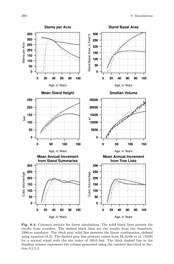
300 8 Simulations
0 20 40 60 80 100
0
50
100
150
200
250
300
350
Stems per Acre
Age, in Years
Ste
ms
per
Acr
e
0 20 40 60 80 100
0
50
100
150
200
250
300
350
0 20 40 60 80 100
0
50
100
150
200
250
300
350
0 20 40 60 80 100
0
50
100
150
200
250
300
350
0 20 40 60 80 100
0
50
100
150
200
250
300
Stand Basal Area
Age, in YearsS
tand
Bas
al A
rea,
in F
eet^
2
0 20 40 60 80 100
0
50
100
150
200
250
300
0 20 40 60 80 100
0
50
100
150
200
250
300
0 20 40 60 80 100
0
50
100
150
200
250
300
0 50 100 150
0
50
100
150
200
250
Mean Stand Height
Age, in Years
feet
0 50 100 150
0
50
100
150
200
250
0 50 100 150
0
50
100
150
200
250
0 50 100 150
0
50
100
150
200
250
0 50 100 150
0
5000
10000
15000
20000
25000
Smalian Volume
Age, in Years
ft3
0 50 100 150
0
5000
10000
15000
20000
25000
0 50 100 150
0
5000
10000
15000
20000
25000
0 50 100 150
0
5000
10000
15000
20000
25000
0 20 40 60 80 100
0
50
100
150
200
250
300
Mean Annual Incrementfrom Stand Summaries
Age, in Years
Cub
ic V
olum
e/A
ge
0 20 40 60 80 100
0
50
100
150
200
250
300
0 20 40 60 80 100
0
50
100
150
200
250
300
0 20 40 60 80 100
0
50
100
150
200
250
300
0 20 40 60 80 100
0
50
100
150
200
250
300
Mean Annual Incrementfrom Tree Lists
Age, in Years
Cub
ic V
olum
e/A
ge
0 20 40 60 80 100
0
50
100
150
200
250
300
0 20 40 60 80 100
0
50
100
150
200
250
300
0 20 40 60 80 100
0
50
100
150
200
250
300
Fig. 8.4: Common metrics for forest simulations. The solid black lines present theresults from rconifers. The dashed black lines are the results from the chambers-1980.so simulator. The thick gray solid line presents the linear combination, definedusing equation (8.2). The dashed gray line presents values from McArdle et al. (1949)for a normal stand with the site index of 180.0 feet. The thick dashed line in theSmalian volume represents the volume generated using the method described in Sec-tion 8.2.5.2.
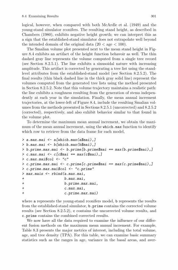
8.4 Examining Results 301
logical, however, when compared with both McArdle et al. (1949) and theyoung-stand simulator rconifers. The resulting stand height, as described inChambers (1980), exhibits negative height growth; we can interpret this asa sign that the established-stand simulator does not extrapolate well beyondthe intended domain of the original data (20 < age < 100).
The Smalian volume plot presented next to the mean stand height in Fig-ure 8.4 exhibits an artifact of the height function behavoir as well. The thindashed gray line represents the volume computed from a single tree record(see Section 8.2.5.1). The line exhibits a sinusoidal nature with increasingamplitude. This artifact is corrected by generating a tree list using the stand-level attributes from the established-stand model (see Section 8.2.5.2). Thefinal results (thin black dashed line in the thick gray solid line) represent thevolumes computed from the generated tree lists using the method presentedin Section 8.2.5.2. Note that this volume trajectory maintains a realistic path:the line exhibits a roughness resulting from the generation of stems indepen-dently at each year in the simulation. Finally, the mean annual incrementtrajectories, at the lower-left of Figure 8.4, include the resulting Smalian vol-umes from the methods presented in Sections 8.2.5.1 (uncorrected) and 8.2.5.2(corrected), respectively, and also exhibit behavior similar to that found inthe volume plot.
To determine the maximum mean annual increment, we obtain the maxi-mum of the mean annual increment, using the which.max function to identifywhich row to retrieve from the data frame for each model,
> a.max.mai <- a[which.max(a$mai),]
> b.max.mai <- b[which.max(b$mai),]
> b.prime.max.mai <- b.prime[b.prime$mai == max(b.prime$mai),]
> c.max.mai <- c[c$mai == max(c$mai),]
> c.max.mai$col <- "c"
> c.prime.max.mai <- c.prime[c.prime$mai == max(c.prime$mai),]
> c.prime.max.mai$col <- "c.prime"
> max.mais <- rbind(a.max.mai,
+ b.max.mai,
+ b.prime.max.mai,
+ c.max.mai,
+ c.prime.max.mai)
where a represents the young-stand rconifers model, b represents the resultsfrom the established-stand simulator, b.prime contains the corrected volumeresults (see Section 8.2.5.2), c contains the uncorrected volume results, andc.prime contains the combined corrected results.
We now have all the data required to examine the influence of our differ-ent fusion methods on the maximum mean annual increment. For example,Table 8.3 presents the major metrics of interest, including the total volume,age, and tree density (TPA). For this table, we can examine basic summarystatistics such as the ranges in age, variance in the basal areas, and aver-
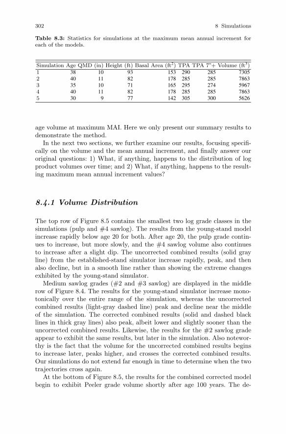
302 8 Simulations
Table 8.3: Statistics for simulations at the maximum mean annual increment foreach of the models.
Simulation Age QMD (in) Height (ft) Basal Area (ft2) TPA TPA 7”+ Volume (ft3)1 38 10 93 153 290 285 73052 40 11 82 178 285 285 78633 35 10 71 165 295 274 59674 40 11 82 178 285 285 78635 30 9 77 142 305 300 5626
age volume at maximum MAI. Here we only present our summary results todemonstrate the method.
In the next two sections, we further examine our results, focusing specifi-cally on the volume and the mean annual increment, and finally answer ouroriginal questions: 1) What, if anything, happens to the distribution of logproduct volumes over time; and 2) What, if anything, happens to the result-ing maximum mean annual increment values?
8.4.1 Volume Distribution
The top row of Figure 8.5 contains the smallest two log grade classes in thesimulations (pulp and #4 sawlog). The results from the young-stand modelincrease rapidly below age 20 for both. After age 20, the pulp grade contin-ues to increase, but more slowly, and the #4 sawlog volume also continuesto increase after a slight dip. The uncorrected combined results (solid grayline) from the established-stand simulator increase rapidly, peak, and thenalso decline, but in a smooth line rather than showing the extreme changesexhibited by the young-stand simulator.
Medium sawlog grades (#2 and #3 sawlog) are displayed in the middlerow of Figure 8.4. The results for the young-stand simulator increase mono-tonically over the entire range of the simulation, whereas the uncorrectedcombined results (light-gray dashed line) peak and decline near the middleof the simulation. The corrected combined results (solid and dashed blacklines in thick gray lines) also peak, albeit lower and slightly sooner than theuncorrected combined results. Likewise, the results for the #2 sawlog gradeappear to exhibit the same results, but later in the simulation. Also notewor-thy is the fact that the volume for the uncorrected combined results beginsto increase later, peaks higher, and crosses the corrected combined results.Our simulations do not extend far enough in time to determine when the twotrajectories cross again.
At the bottom of Figure 8.5, the results for the combined corrected modelbegin to exhibit Peeler grade volume shortly after age 100 years. The de-
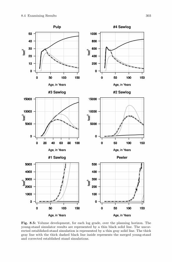
8.4 Examining Results 303
0 50 100 150
0
10
20
30
40
50
Pulp
Age, in Years
feet
3
0 50 100 150
0
10
20
30
40
50
0 50 100 150
0
10
20
30
40
50
Age, in Years
feet
3
0 50 100 150
0
10
20
30
40
50
0 50 100 150
0
10
20
30
40
50
0 50 100 150
0
200
400
600
800
1000
#4 Sawlog
Age, in Years
feet
3
0 50 100 150
0
200
400
600
800
1000
0 50 100 150
0
200
400
600
800
1000
Age, in Years
feet
3
0 50 100 150
0
200
400
600
800
1000
0 50 100 150
0
200
400
600
800
1000
0 20 40 60 80 100
0
5000
10000
15000
#3 Sawlog
Age, in Years
feet
3
0 20 40 60 80 100
0
5000
10000
15000
0 20 40 60 80 100
0
5000
10000
15000
Age, in Years
feet
3
0 20 40 60 80 100
0
5000
10000
15000
0 20 40 60 80 100
0
5000
10000
15000
0 50 100 150
0
5000
10000
15000
#2 Sawlog
Age, in Years
feet
3
0 50 100 150
0
5000
10000
15000
0 50 100 150
0
5000
10000
15000
Age, in Years
feet
3
0 50 100 150
0
5000
10000
15000
0 50 100 150
0
5000
10000
15000
0 50 100 150
0
1000
2000
3000
4000
5000
#1 Sawlog
Age, in Years
feet
3
0 50 100 150
0
1000
2000
3000
4000
5000
0 50 100 150
0
1000
2000
3000
4000
5000
Age, in Years
feet
3
0 50 100 150
0
1000
2000
3000
4000
5000
0 50 100 150
0
1000
2000
3000
4000
5000
0 50 100 150
0
100
200
300
400
500
Peeler
Age, in Years
feet
3
0 50 100 150
0
100
200
300
400
500
0 50 100 150
0
100
200
300
400
500
Age, in Years
feet
3
0 50 100 150
0
100
200
300
400
500
0 50 100 150
0
100
200
300
400
500
Fig. 8.5: Volume development, for each log grade, over the planning horizon. Theyoung-stand simulator results are represented by a thin black solid line. The uncor-rected established-stand simulation is represented by a thin gray solid line. The thickgray line with the thick dashed black line inside represents the merged young-standand corrected established stand simulations.
304 8 Simulations
velopment of #1 Sawlog volume follows a similar pattern, with the standage around 60 years for the corrected combined results (black dashed lineinside thick gray solid line), followed 20 years later by accumlated volume inthe uncorrected combined results. When we examine ages above our originalrange (150 years), only then do any of the simulators produce volumes in thelargest class.
The patterns and resulting conclusions we can infer from Figure 8.5, sim-ilar to those in Figure 8.4, are that 1) the method used to merge modelscan greatly influence the behavoir of the resulting combination; 2) the result-ing simulations, and resulting combinations, may exhibit behavoir similar topublished results (Chambers, 1980); and 3) producing results using a smallsample (Chambers uncorrected) can lead to peculiar behavoir, and the deci-sions resulting from those simulations should be viewed critically.
8.4.2 Mean Annual Increment
Table 8.4: Volume metrics for simulations at maximum mean annual increment.
Model Age Pulp #4 Sawlog #3 Sawlog #2 Sawlog #1 Sawlog Peeler Total MAI1 38 31 560 6599 115 0.000 0 7305 1922 40 24 397 7438 3 0.000 0 7863 1973 35 24 431 5421 91 0.003 0 5967 1704 40 24 397 7438 3 0.000 0 7863 1975 30 29 559 4986 52 0.000 0 5626 188
Mean annual increment, which determines the biological rotation age inmany forests (Leuschner, 1990; Davis et al., 2001), can be greatly influencedby the results of the growth and yield models used to compute the volumesover time. Table 8.4 presents the age, the Smalian volumes (see Section 8.2)by log.grade, and the mean annual increment at the age when maximummean increment occurs. This is the time point that corresponds with thehighest average yield. It is important to note that Table 8.4 represents onlya single moment in time: when the mean annual increment is maximum.
The range in values in projected MAI, from a low of 5966.92 ft3 to a highof 7863.18 ft3, is reasonably compact. Conversely, the range in ages when themaximum occurs is considerable when compared with the values themselves.The ages range from a low of 35.00 ft3 to a high of 40.00 ft3. This rangemay have a considerable effect on the projections of forest- or landscape-levelservices.
8.6 Summary 305
8.5 Exporting Yields
To export the results from the simulations (res$rconfiers) into a databaseprogram, we could use an SQL file. First, we would construct a loop to gen-erate SQL INSERT commands and then write the results to a file namedsmc-yields.sql:
> hres <- res$rconifers
> names(hres)[3] <- "rx"
> sql.file <- file("smc-yields.sql", "w")
> sql.columns <- names(hres)
> for(i in 1:nrow(hres)) {
+ sql.command <-
+ sprintf("insert into results (%s) values (%s);",
+ paste(as.vector(sql.columns), collapse=","),
+ paste(hres[i,], collapse=","))
+ cat(sql.command, file = sql.file, sep = "\n")
+
+ }
> close(sql.file)
8.6 Summary
Forest simulation is a complex subject. Depending on the level of resolutionrequired in the analysis (tree, stand, or forest), the process may be as simpleas a single equation (model component) or require the development of ashared library or simulation package (chambers-1980.so and rconifers) andinclude multiple software packages (R and SQL), which could include usingthe system function to run command-line applications (FVS, ORGANON,CACTOS).
In this chapter, we used R to generate simulated yield tables, projections,or sets of possible future forest conditions that could be analyzed within R orexported to other packages (for example, a harvest scheduler). Our methods,while basic, provide a starting place for more complex analysis techniques.
Chapter 9
Forest Estate Planning and Optimization
9.1 Introduction
So far, we have developed procedures for processing field data, producingcomplete inventories, and generating forecasts of future forest conditions. Inthis chapter, we use R to solve a forest estate planning problem assuming wealready have a sufficient inventory to describe the forest. Here we present andsolve a linear programming (LP) problem that was originally presented byLeuschner (1990, see Chapter 4). The objective is to determine the harvestschedule for a classical method of forest regulation, the strict area harvestschedule. Strict area control is an indirect method of controlling the amountof forest produced in each cutting period. To achieve our objective, we usethe glpk package (Lee and Luangkesorn, 2010), which is the R interface toAndrew Makhorin’s GNU linear programing kit (GLPK) (Makhorin, 2009).
This problem provides a gentle introduction to mathematical program-ming that does not require extensive background development. There areother types of harvest schedules, model formulations, and constraints thatcan be applied to develop more interesting problems, but they are beyond thescope of this book. For more complete presentations of forest estate planningproblems, we recommend Leuschner (1990), Ronnqvist (2003), and Bettingeret al. (2009).
The chapter is structured as follows. In Section 9.2, we briefly present abasic formulation framework. In Section 9.3, we present the tasks that arerequired to translate the model formulation into the components that arerequired to solve the formulation, namely 1) generating the decision variablecolumns, 2) the objective function coefficients, 3) row constraints, and 4)forest-level row constraints. In Section 9.3.7, we then obtain a solution giventhe developed model. Then, in Section 9.3.8, we extract the solution, decodethe decision variables, compute forest-level metrics, and examine importantfeatures of the solution. Finally, we generate a machine-readable archive ofthe problem in Section 9.3.9.
307A. P. Robinson, J. D. Hamann, Forest Analytics with R, Use R!,DOI 10.1007/978-1-4419-7762-5_9, © Springer Science+Business Media, LLC 2011
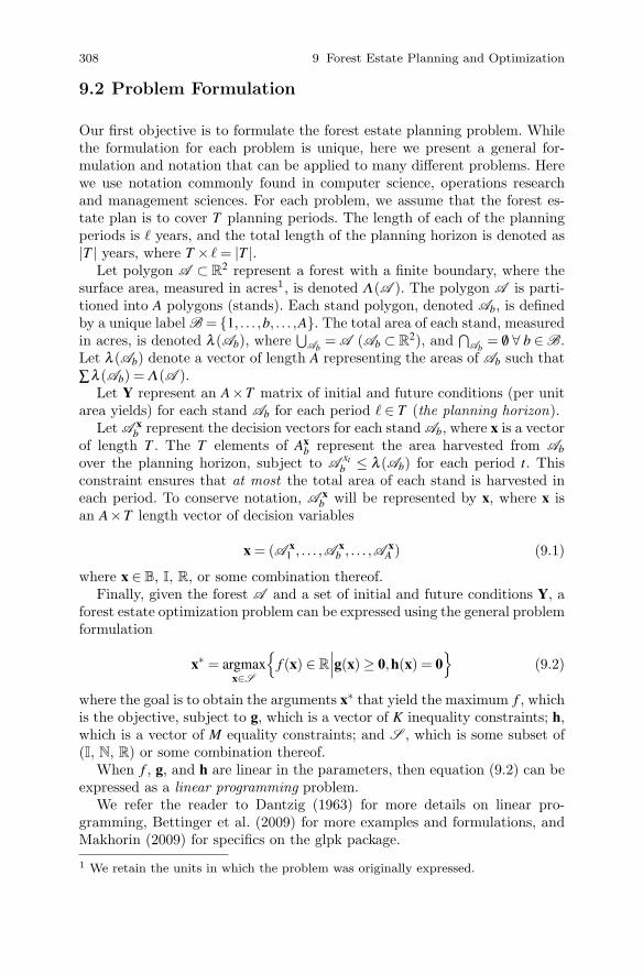
308 9 Forest Estate Planning and Optimization
9.2 Problem Formulation
Our first objective is to formulate the forest estate planning problem. Whilethe formulation for each problem is unique, here we present a general for-mulation and notation that can be applied to many different problems. Herewe use notation commonly found in computer science, operations researchand management sciences. For each problem, we assume that the forest es-tate plan is to cover T planning periods. The length of each of the planningperiods is � years, and the total length of the planning horizon is denoted as|T | years, where T × �= |T |.
Let polygon A ⊂ R2 represent a forest with a finite boundary, where the
surface area, measured in acres1, is denoted Λ(A ). The polygon A is parti-tioned into A polygons (stands). Each stand polygon, denoted Ab, is definedby a unique label B = {1, . . . ,b, . . . ,A}. The total area of each stand, measuredin acres, is denoted λ (Ab), where
⋃Ab
= A (Ab ⊂ R2), and
⋂Ab
= /0 ∀ b ∈ B.Let λ (Ab) denote a vector of length A representing the areas of Ab such that
∑λ (Ab) = Λ(A ).Let Y represent an A×T matrix of initial and future conditions (per unit
area yields) for each stand Ab for each period � ∈ T (the planning horizon).Let A x
b represent the decision vectors for each stand Ab, where x is a vectorof length T . The T elements of Ax
b represent the area harvested from Ab
over the planning horizon, subject to Axt
b ≤ λ (Ab) for each period t. Thisconstraint ensures that at most the total area of each stand is harvested ineach period. To conserve notation, A x
b will be represented by x, where x isan A×T length vector of decision variables
x = (A x1 , . . . ,A
xb , . . . ,A
xA ) (9.1)
where x ∈ B, I, R, or some combination thereof.Finally, given the forest A and a set of initial and future conditions Y, a
forest estate optimization problem can be expressed using the general problemformulation
x∗ = argmaxx∈S
{f (x) ∈ R
∣∣∣g(x)≥ 0,h(x) = 0}
(9.2)
where the goal is to obtain the arguments x∗ that yield the maximum f , whichis the objective, subject to g, which is a vector of K inequality constraints; h,which is a vector of M equality constraints; and S , which is some subset of(I, N, R) or some combination thereof.
When f , g, and h are linear in the parameters, then equation (9.2) can beexpressed as a linear programming problem.
We refer the reader to Dantzig (1963) for more details on linear pro-gramming, Bettinger et al. (2009) for more examples and formulations, andMakhorin (2009) for specifics on the glpk package.
1 We retain the units in which the problem was originally expressed.

9.3 Strict Area Harvest Schedule 309
9.3 Strict Area Harvest Schedule
For this problem, our objective is to generate a solution for a strict areaharvest schedule that maximizes the total woodflow of A over a planninghorizon of six 10 year periods (T = 6, � = 10, |T |= 60 years) subject to someset of physical and policy constraints. Specifically, suppose that we have aforest with a finite boundary, denoted A , and the function for the surfacearea, denoted λ (A ), returns 84000 acres. Also, A is partitioned into eightstand polygons (so A = 8), where the areas of the stands are
λ (Ab) = (5000,5000,5000,5000,30000,20000,12000,2000)
Since these values are relatively easy to keep track of using atomic objects,we begin by simply assigning them to individual variable names,
> A <- 8 # A
> T <- 6 # T
> l <- 10 # \ell
> P <- T * l # |T|
> ## \lambda(\mathcal{A}_{b})
> stand.acres <- c(5000,5000,5000,5000,30000,20000,12000,2000)
For this example, we will use the published yields from the original problemas presented by Leuschner (1990, see Chapter 4, Table 4.2). Here we haveentered the values into a text file (located at ../../data/leuschner.txt),which can be read in using the read.table function,
> leusch.ylds <- read.table("../../data/leuschner.txt",
+ header = TRUE)
where the resulting leusch.ylds object contains four columns: 1) the standidentifier (stand is the label for Ab); 2) the planning period (per); 3) the ageof the stand (Aa
b = age); and 4) the yield (volume) (A vb = vol) in thousands
of cubic feet per acre if we harvest stand Ab in period t.To solve this problem, we need to generate the 14×48 detached coefficient
matrix that stores the coefficients for the problem. The results matrix shouldhave a set of eight rows that define the area constraints, a set of six rows thatdefine the policy constraints, and 48 columns for the decision variables.
To generate all the required components to solve this problem, we firstneed to load the glpk package and create a glpk problem object,
> library(glpk)
> leusch.lp <- lpx_create_prob()
Next, we assign a symbolic name to the problem object:
> lpx_set_prob_name(leusch.lp, "leuschner")

310 9 Forest Estate Planning and Optimization
By default, glpk will minimize the objective function. Since we want tomaximize the objective function (equivalently, −min(− f )), we need to callthe lpx_set_obj_dir function to change the direction of optimization,
> lpx_set_obj_dir(leusch.lp, LPX_MAX)
where GLP_MAX indicates maximization.The glpk problem object we have now created (called leusch.lp) is the
object that stores the information about the optimization problem in memoryand allows us to pass information to the glpk library directly, and almost allfunctions in the glpk package require it.
9.3.1 Objective Function
For this problem, the objective is to maximize the total yield
f = Avt
b ∀ t ∈ T,b ∈ B (9.3)
where the objective function (total yield) f is the sum of the product yieldsfrom stand A v
b , harvested in period t, over the entire forest A . In this prob-lem, the vector of yields for each stand (A v
b ) is known exactly (that is, non-stochastic), so the only decision variables required (A x
b ) represent the numberof acres to harvest in Ab in period t (Marti, 2005).
In the following sections, we add columns, give them names, and placebounds on the columns.
9.3.2 Adding Columns
To add columns (decision variables) to the newly created problem object, wenow use the lpx_add_cols function. For this problem, the length of x is 48,and so we need to add 48 columns to hold the 8 stand polygons × 6 harvestperiods:
> lpx_add_cols(leusch.lp, nrow( leusch.ylds ))
[1] 1
where the 1 is the response from the glpk library. In this case, it is the ordinalnumber of the first new column added to the problem object.
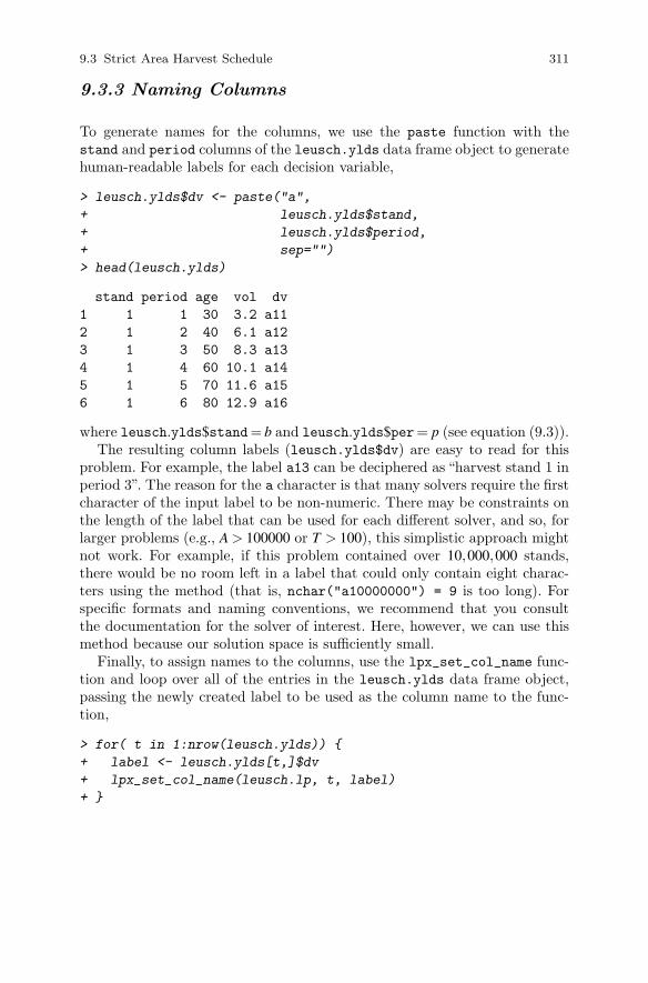
9.3 Strict Area Harvest Schedule 311
9.3.3 Naming Columns
To generate names for the columns, we use the paste function with thestand and period columns of the leusch.ylds data frame object to generatehuman-readable labels for each decision variable,
> leusch.ylds$dv <- paste("a",
+ leusch.ylds$stand,
+ leusch.ylds$period,
+ sep="")
> head(leusch.ylds)
stand period age vol dv
1 1 1 30 3.2 a11
2 1 2 40 6.1 a12
3 1 3 50 8.3 a13
4 1 4 60 10.1 a14
5 1 5 70 11.6 a15
6 1 6 80 12.9 a16
where leusch.ylds$stand= b and leusch.ylds$per= p (see equation (9.3)).The resulting column labels (leusch.ylds$dv) are easy to read for this
problem. For example, the label a13 can be deciphered as “harvest stand 1 inperiod 3”. The reason for the a character is that many solvers require the firstcharacter of the input label to be non-numeric. There may be constraints onthe length of the label that can be used for each different solver, and so, forlarger problems (e.g., A > 100000 or T > 100), this simplistic approach mightnot work. For example, if this problem contained over 10,000,000 stands,there would be no room left in a label that could only contain eight charac-ters using the method (that is, nchar("a10000000") = 9 is too long). Forspecific formats and naming conventions, we recommend that you consultthe documentation for the solver of interest. Here, however, we can use thismethod because our solution space is sufficiently small.
Finally, to assign names to the columns, use the lpx_set_col_name func-tion and loop over all of the entries in the leusch.ylds data frame object,passing the newly created label to be used as the column name to the func-tion,
> for( t in 1:nrow(leusch.ylds)) {
+ label <- leusch.ylds[t,]$dv
+ lpx_set_col_name(leusch.lp, t, label)
+ }
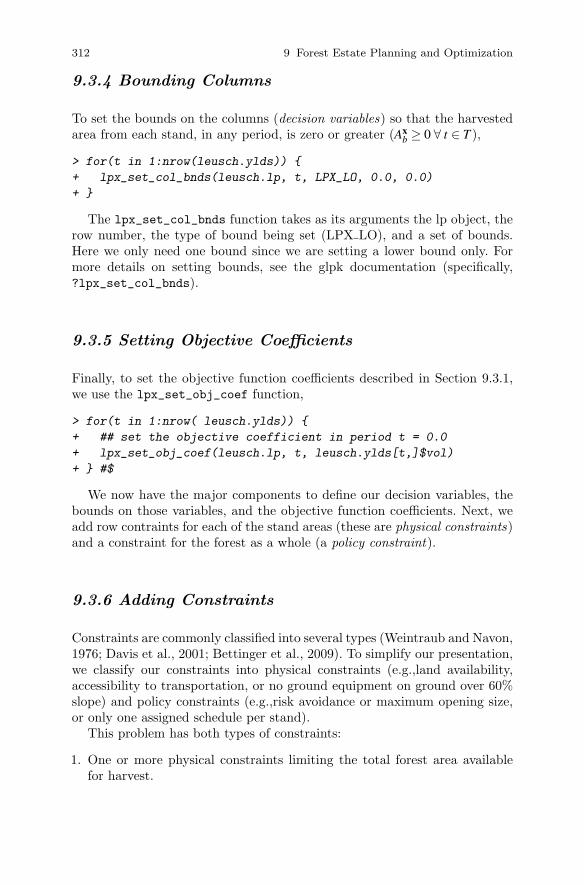
312 9 Forest Estate Planning and Optimization
9.3.4 Bounding Columns
To set the bounds on the columns (decision variables) so that the harvestedarea from each stand, in any period, is zero or greater (Ax
b ≥ 0 ∀ t ∈ T ),
> for(t in 1:nrow(leusch.ylds)) {
+ lpx_set_col_bnds(leusch.lp, t, LPX_LO, 0.0, 0.0)
+ }
The lpx_set_col_bnds function takes as its arguments the lp object, therow number, the type of bound being set (LPX LO), and a set of bounds.Here we only need one bound since we are setting a lower bound only. Formore details on setting bounds, see the glpk documentation (specifically,?lpx_set_col_bnds).
9.3.5 Setting Objective Coefficients
Finally, to set the objective function coefficients described in Section 9.3.1,we use the lpx_set_obj_coef function,
> for(t in 1:nrow( leusch.ylds)) {
+ ## set the objective coefficient in period t = 0.0
+ lpx_set_obj_coef(leusch.lp, t, leusch.ylds[t,]$vol)
+ } #$
We now have the major components to define our decision variables, thebounds on those variables, and the objective function coefficients. Next, weadd row contraints for each of the stand areas (these are physical constraints)and a constraint for the forest as a whole (a policy constraint).
9.3.6 Adding Constraints
Constraints are commonly classified into several types (Weintraub and Navon,1976; Davis et al., 2001; Bettinger et al., 2009). To simplify our presentation,we classify our constraints into physical constraints (e.g.,land availability,accessibility to transportation, or no ground equipment on ground over 60%slope) and policy constraints (e.g.,risk avoidance or maximum opening size,or only one assigned schedule per stand).
This problem has both types of constraints:
1. One or more physical constraints limiting the total forest area availablefor harvest.

9.3 Strict Area Harvest Schedule 313
2. A policy constraint to control cutting so that the acres harvested over allperiods must equal the total acres of the forest (i.e., strict area control).
Since the goal is to turn the current forest A into a well-regulated forest,where an equal area will be harvested in each period, we need to include twophysical constraints,
1. stand total area constraints and2. total harvest area constraints
so that we can generate the final volume flow policy constraints. We first addthe rows for each stand area and then add the constraints for the strict areacontrol.
9.3.6.1 Stand Area Constraints
An unconstrained problem might harvest an infinite number of acres in eachperiod, but since the total number of acres available for harvest in any periodis limited to the total area of the forest (Λ(A) = 84000), we must constrainthe total harvested area to be no larger than the total forest area (84000acres). Mathematically, this constraint is expressed as
∑t
Axt
b ≤ λ (Ab) ∀ b ∈ B (9.4)
where Axt
b is the total available acres in stand b harvested in period t, andλ (Ab) is the total available acres in stand b.
Since each stand may be harvested in more than one period, we mustensure that the total area that is harvested is no larger than the total standarea over all periods. To accomplish that, we must add a set of rows for eachperiod in the planning horizon and include a sum of all the acres harvestedfor each stand over all periods.
First, add the constraint rows, using the lpx_add_rows function to createa row for each stand,
> lpx_add_rows(leusch.lp, length(stand.acres))
[1] 1
Create a matrix to contain sets of coefficients for each row, using I ⊗ 1,where I is an A× A matrix, 1 is a column vector of length P (number of
periods), and ⊗ is the Kronecker product,
> acre.consts <- t( kronecker(diag(length(stand.acres)),
+ as.matrix( rep(1,6))))
The result is an 8 × 48 matrix called acre.consts. Now set the rownames, bounds, and row matrix coefficients for Ab using lpx_set_row_name,lpx_set_row_bounds, and lpx_set_mat_row, respectively.

314 9 Forest Estate Planning and Optimization
To do that, we create a for loop as we did for the columns in Section 9.3.6,generate the entries for the row, and finally set the row name, bounds, andcoefficients. Here we perform all three functions at the same time rather thancreating a loop for each operation as we did previously.
First, we create a variable to store the coefficient values for this portion ofthe detached coefficients matrix. The variable, val, is a vector of ones thatholds the coefficients
> val <- rep(1, 6) # this is the value of the constraint
Then, we loop over the stands to create the row coefficients for the numberof acres harvested over the six periods. Since we can create all six entries foreach of the six columns that need to be set for each row, we create a vectorthat will contain the column index (idx) by creating a loop within the outerloop, to generate the values for idx, and then perform the row operations,
> ## loop over the stands to generate
> ## the idx is the index for the set of rows
> ## we are trying to set the coefficients for
> for(i in 1:length(stand.acres)) {
+
+ idx <- rep(0, 6) # this is the index of the col coeffs
+
+ ## manually create the index using id
+ ## and assign row i, column j stored as idx[id]
+ id <- 1
+ for(j in 1:ncol(acre.consts)) {
+ if(acre.consts[i,j] != 0.0) {
+ idx[id] <- j
+ id <- id + 1
+ }
+ }
+
+ ## now, perform all three tasks within the same loop
+ ## set the constraint row name
+ lpx_set_row_name(leusch.lp, i, paste("s", i, sep=""))
+
+ ## set the upper bound on the acres for this stand
+ ## to make sure no more than stand.acres[i] are cut
+ lpx_set_row_bnds(leusch.lp, i, LPX_UP, 0.0,
+ stand.acres[i])
+
+ ## set matrix row coefficients (?glp_set_mat_row)
+ ## idx = ???, row index = i, val = vector of 1�s
+ lpx_set_mat_row(leusch.lp, i, length(val), idx, val)
+ }
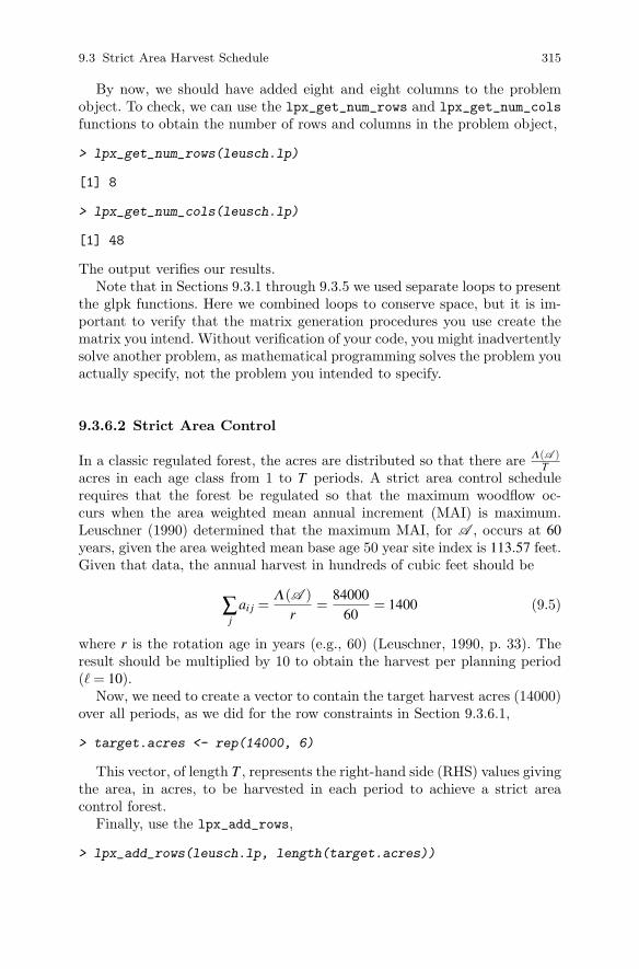
9.3 Strict Area Harvest Schedule 315
By now, we should have added eight and eight columns to the problemobject. To check, we can use the lpx_get_num_rows and lpx_get_num_cols
functions to obtain the number of rows and columns in the problem object,
> lpx_get_num_rows(leusch.lp)
[1] 8
> lpx_get_num_cols(leusch.lp)
[1] 48
The output verifies our results.Note that in Sections 9.3.1 through 9.3.5 we used separate loops to present
the glpk functions. Here we combined loops to conserve space, but it is im-portant to verify that the matrix generation procedures you use create thematrix you intend. Without verification of your code, you might inadvertentlysolve another problem, as mathematical programming solves the problem youactually specify, not the problem you intended to specify.
9.3.6.2 Strict Area Control
In a classic regulated forest, the acres are distributed so that there are Λ(A )T
acres in each age class from 1 to T periods. A strict area control schedulerequires that the forest be regulated so that the maximum woodflow oc-curs when the area weighted mean annual increment (MAI) is maximum.Leuschner (1990) determined that the maximum MAI, for A , occurs at 60
years, given the area weighted mean base age 50 year site index is 113.57 feet.Given that data, the annual harvest in hundreds of cubic feet should be
∑j
ai j =Λ(A )
r=
84000
60= 1400 (9.5)
where r is the rotation age in years (e.g., 60) (Leuschner, 1990, p. 33). Theresult should be multiplied by 10 to obtain the harvest per planning period(�= 10).
Now, we need to create a vector to contain the target harvest acres (14000)over all periods, as we did for the row constraints in Section 9.3.6.1,
> target.acres <- rep(14000, 6)
This vector, of length T , represents the right-hand side (RHS) values givingthe area, in acres, to be harvested in each period to achieve a strict areacontrol forest.
Finally, use the lpx_add_rows,
> lpx_add_rows(leusch.lp, length(target.acres))

316 9 Forest Estate Planning and Optimization
[1] 9
to add the T rows to the leusch.lp problem object. The function returnsthe first index of the new row set.
Next, add the strict area control constraints, as was done in Section 9.3.6.1,
> val <- rep(1,8) ## a vector of 8 ones.
> for(i in 1:length(target.acres)) {
+ idx <-
+ as.numeric(rownames(subset(leusch.ylds, period == i)))
+ lpx_set_row_name(leusch.lp,
+ i + length(stand.acres),
+ paste("tac", i, sep="" ))
+ lpx_set_row_bnds(leusch.lp,
+ i + length(stand.acres),
+ LPX_FX,
+ target.acres[i],
+ target.acres[i])
+ lpx_set_mat_row(leusch.lp,
+ i + length(stand.acres),
+ length(val),
+ idx,
+ val)
+ }
We should now have added a total of 14 rows and 14 columns to theproblem object. Recall from Section 9.3.6.1 that we added only eight rows.Here we added an additional six rows to represent the constraints on the totalacres cut (tac) in each of the six periods.
Again, using the lpx_get_num_rows and lpx_get_num_cols functions toretrieve the number of rows and columns in the problem object,
> lpx_get_num_rows(leusch.lp)
[1] 14
> lpx_get_num_cols(leusch.lp)
[1] 48
This again verifies our results, and we now have a completed glpk problemobject that contains all the components of our forest planning problem.
9.3.7 Solving
functionNow we can solve the linear program by calling the lpx_simplex function:

9.3 Strict Area Harvest Schedule 317
> lpx_simplex(leusch.lp)
0: objval = 0.0000000e+00 infeas = 1.0000e+00 (0)
13: objval = 1.1584000e+06 infeas = 0.0000e+00 (1)
* 13: objval = 1.1584000e+06 infeas = 0.0000e+00 (1)
* 25: objval = 1.2246000e+06 infeas = 0.0000e+00 (1)
OPTIMAL SOLUTION FOUND
[1] 200
The lpx_simplex function is the wrapper function for the GLPK APIglp_simplex routine, a driver to the glpk solver that uses the simplexmethod. This function retrieves problem data from the specified problemobject, calls the glpk solver to solve the problem instance, and stores re-sults of computations back into the problem object. Fortunately, this solutionmatches the solution reported by Leuschner (1990).
9.3.8 Results
In this section, we 1) obtain the value of the objective function, 2) decode thedecision variables (column activities), 3) confirm that our solution achieves astrict area policy (equation (9.5)), 4) compute and plot the resulting wood-flow, and 5) examine shadow prices, reduced costs, and binding constraints.To conserve space, we include two functions that can be used to obtain row(get.row.report) and column (get.col.report) information from the lin-ear programming object. See the provided script schedpak.r for these func-tions.
9.3.8.1 Objective Function
To extract the value of the objective function, use the get_obj_val function,
> leusch.obj <- lpx_get_obj_val(leusch.lp)
> leusch.obj
[1] 1224600
The resulting object, leusch.obj, is the value of equation 9.3 at its max-imum. Therefore the optimal set of harvest decisions yields a total volume of1224600 ×103ft3.
It would also be nice to have some report on the quality of the solutionhere as well (e.g., the Karush-Kuhn-Tucker (KKT) conditions (Karush, 1939;Kuhn and Tucker, 1951; Press et al., 2007)). The KKT general optimalityconditions are necessary and sufficient conditions for the decision variables(x) to be optimal and are often used to report the quality of the solution for
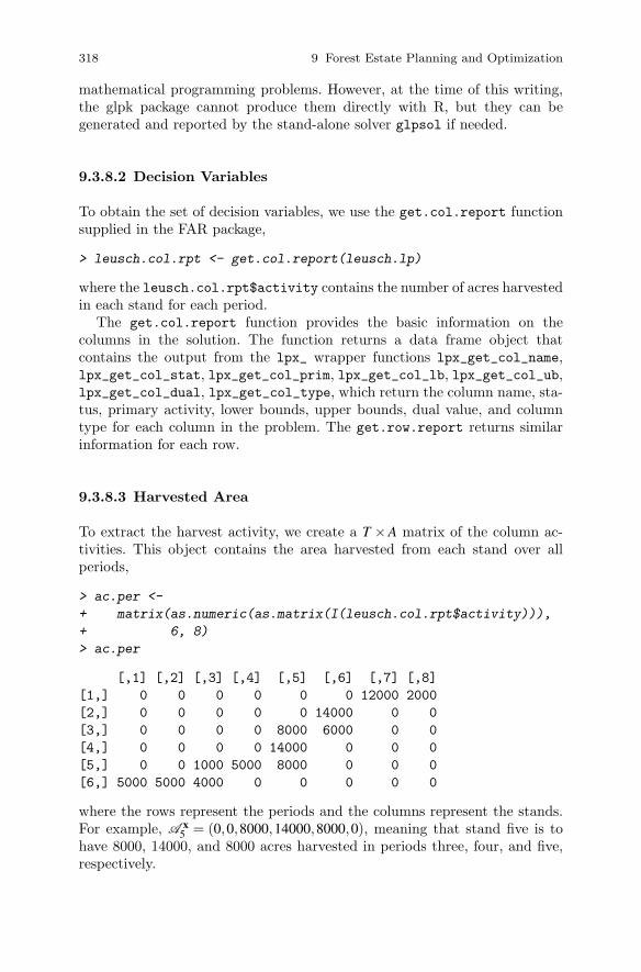
318 9 Forest Estate Planning and Optimization
mathematical programming problems. However, at the time of this writing,the glpk package cannot produce them directly with R, but they can begenerated and reported by the stand-alone solver glpsol if needed.
9.3.8.2 Decision Variables
To obtain the set of decision variables, we use the get.col.report functionsupplied in the FAR package,
> leusch.col.rpt <- get.col.report(leusch.lp)
where the leusch.col.rpt$activity contains the number of acres harvestedin each stand for each period.
The get.col.report function provides the basic information on thecolumns in the solution. The function returns a data frame object thatcontains the output from the lpx_ wrapper functions lpx_get_col_name,lpx_get_col_stat, lpx_get_col_prim, lpx_get_col_lb, lpx_get_col_ub,lpx_get_col_dual, lpx_get_col_type, which return the column name, sta-tus, primary activity, lower bounds, upper bounds, dual value, and columntype for each column in the problem. The get.row.report returns similarinformation for each row.
9.3.8.3 Harvested Area
To extract the harvest activity, we create a T ×A matrix of the column ac-tivities. This object contains the area harvested from each stand over allperiods,
> ac.per <-
+ matrix(as.numeric(as.matrix(I(leusch.col.rpt$activity))),
+ 6, 8)
> ac.per
[,1] [,2] [,3] [,4] [,5] [,6] [,7] [,8]
[1,] 0 0 0 0 0 0 12000 2000
[2,] 0 0 0 0 0 14000 0 0
[3,] 0 0 0 0 8000 6000 0 0
[4,] 0 0 0 0 14000 0 0 0
[5,] 0 0 1000 5000 8000 0 0 0
[6,] 5000 5000 4000 0 0 0 0 0
where the rows represent the periods and the columns represent the stands.For example, A x
5 = (0,0,8000,14000,8000,0), meaning that stand five is tohave 8000, 14000, and 8000 acres harvested in periods three, four, and five,respectively.
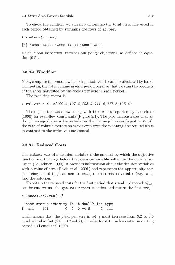
9.3 Strict Area Harvest Schedule 319
To check the solution, we can now determine the total acres harvested ineach period obtained by summing the rows of ac.per,
> rowSums(ac.per)
[1] 14000 14000 14000 14000 14000 14000
which, upon inspection, matches our policy objectives, as defined in equa-tion (9.5).
9.3.8.4 Woodflow
Next, compute the woodflow in each period, which can be calculated by hand.Computing the total volume in each period requires that we sum the productsof the acres harvested by the yields per acre in each period.
The resulting vector is
> vol.cut.a <- c(199.4,197.4,203.4,211.4,217.6,195.4)
Then, plot the woodflow along with the results reported by Leuschner(1990) for even-flow constraints (Figure 9.1). The plot demonstrates that al-though an equal area is harvested over the planning horizon (equation (9.5)),the rate of volume extraction is not even over the planning horizon, which isin contrast to the strict volume control.
9.3.8.5 Reduced Costs
The reduced cost of a decision variable is the amount by which the objectivefunction must change before that decision variable will enter the optimal so-lution (Leuschner, 1990). It provides information about the decision variableswith a value of zero (Davis et al., 2001) and represents the opportunity costof forcing a unit (e.g., an acre of Ab=1) of the decision variable (e.g., a11)into the solution.
To obtain the reduced costs for the first period that stand 1, denoted Ab=1,can be cut, we use the get.col.report function and return the first row,
> leusch.col.rpt[1,]
name status activity lb ub dual b_ind type
1 a11 141 0 0 0 -4.8 0 111
which means that the yield per acre in Ab=1 must increase from 3.2 to 8.0hundred cubic feet (8.0 = 3.2+4.8), in order for it to be harvested in cuttingperiod 1 (Leuschner, 1990).
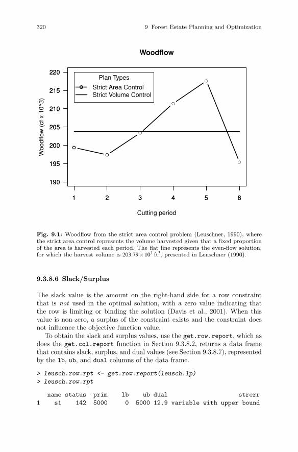
320 9 Forest Estate Planning and Optimization
●
●
●
●
●
●
1 2 3 4 5 6
190
195
200
205
210
215
220
Woodflow
Cutting period
Woo
dflo
w (
cf x
10^
3)
1 2 3 4 5 6
190
195
200
205
210
215
220
●
Plan Types
Strict Area ControlStrict Volume Control
Fig. 9.1: Woodflow from the strict area control problem (Leuschner, 1990), wherethe strict area control represents the volume harvested given that a fixed proportionof the area is harvested each period. The flat line represents the even-flow solution,for which the harvest volume is 203.79×103 ft3, presented in Leuschner (1990).
9.3.8.6 Slack/Surplus
The slack value is the amount on the right-hand side for a row constraintthat is not used in the optimal solution, with a zero value indicating thatthe row is limiting or binding the solution (Davis et al., 2001). When thisvalue is non-zero, a surplus of the constraint exists and the constraint doesnot influence the objective function value.
To obtain the slack and surplus values, use the get.row.report, which asdoes the get.col.report function in Section 9.3.8.2, returns a data framethat contains slack, surplus, and dual values (see Section 9.3.8.7), representedby the lb, ub, and dual columns of the data frame.
> leusch.row.rpt <- get.row.report(leusch.lp)
> leusch.row.rpt
name status prim lb ub dual strerr
1 s1 142 5000 0 5000 12.9 variable with upper bound

9.3 Strict Area Harvest Schedule 321
2 s2 142 5000 0 5000 14.1 variable with upper bound
3 s3 142 5000 0 5000 15.1 variable with upper bound
4 s4 142 5000 0 5000 16.1 variable with upper bound
5 s5 142 30000 0 30000 17 variable with upper bound
6 s6 142 20000 0 20000 18 variable with upper bound
7 s7 142 12000 0 12000 19 variable with upper bound
8 s8 142 2000 0 2000 20 variable with upper bound
9 tac1 144 14000 14000 14000 -4.9 fixed variable
10 tac2 144 14000 14000 14000 -3.9 fixed variable
11 tac3 144 14000 14000 14000 -2.9 fixed variable
12 tac4 144 14000 14000 14000 -1.9 fixed variable
13 tac5 144 14000 14000 14000 -1 fixed variable
14 tac6 140 14000 14000 14000 0 fixed variable
From the printout, it appears that all stands have a zero upper bound forthe slack/surplus entries for the rows that define total possible areas thatcan be harvested in each stand. Recall that in this case we used an equalityconstraint so that all of the land was harvested (that is, a strict area controlschedule), so all of the slack variables for stand acres should be zero.
9.3.8.7 Shadow Prices
The shadow, or dual, price is the maximum amount the objective functionwould change if one more unit of a constraint were included (Davis et al., 2001,Chapter 6). In this case, the shadow price would represent our willingness topay for the ability to harvest an additional acre of land.
For example, there are physical constraints that limit the amount of landavailable to the current landscape (84000 acres total, eight stands). What ifanother acre of A1, or something very close to it, were available for harvest?The shadow price would tell us how much an additional acre of land wouldneed to be worth in order to increase the objective function by including thatone additional acre.
To obtain the shadow prices, examine the column labeled dual in the out-put of the get.row.report function. We print the first row, which representsthe total land in A1,
> leusch.row.rpt[1,]
name status prim lb ub dual strerr
1 s1 142 5000 0 5000 12.9 variable with upper bound
The resulting value for leusch.row.rpt$dual is 12.9, which means that aone acre increase in A1 harvested in the first period will increase the objectivefunction by 12.9 ×103ft3.

322 9 Forest Estate Planning and Optimization
9.3.9 Archiving Problems
We have now formulated, generated, and solved the strict area schedule prob-lem, and we now need to create a machine-readable archive of our model andsolution. The glpk package has functions that can be used to archive prob-lems, solve previously archived problems using glpk, and translate archivedproblems between solver formats like CPLEX (CPLEX Optimization Inc.,2003) and MathProg, which is a subset of AMPL (Fourer et al., 2003).
To archive the leuschner problem object, save the problem object to yourhard drive as an MPS file
> lpx_write_mps(leusch.lp, "leuschner.mps")
lpx_write_mps: writing problem data to �leuschner.mps�...
[1] 0
functionor as a file that can be read by CPLEX (Figure 9.2)
> lpx_write_cpxlp(leusch.lp, "leuschner.xlp")
lpx_write_cpxlp: writing problem data to �leuschner.xlp�...
[1] 0
functionwhich matches the example presented by Leuschner (1990, see Table 4.3).
The resulting files (leuschner.mps and leuschner.xlp) can then be im-ported and solved from many solvers. For example, to solve and generate amachine-readable solution file for the same problem using the command-linesolver glpsol, use
$ glpsol --cpxlp leuschner.xlp -w leuschner.sln
9.3.10 Cleanup
Our final step is to make sure that we free up the memory allocated for theproblem by using the lpx_delete_prob function
> lpx_delete_prob(leusch.lp)
> leusch.lp
<pointer: 0x0>
which deletes the data associated with the problem object and sets an internalpointer to null (0x0).
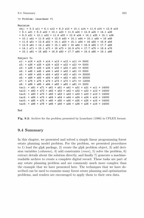
9.4 Summary 323
\* Problem: leuschner *\
Maximize
obj: + 3.2 a11 + 6.1 a12 + 8.3 a13 + 10.1 a14 + 11.6 a15 + 12.9 a16
+ 6.1 a21 + 8.3 a22 + 10.1 a23 + 11.6 a24 + 12.9 a25 + 14.1 a26
+ 8.3 a31 + 10.1 a32 + 11.6 a33 + 12.9 a34 + 14.1 a35 + 15.1 a36
+ 10.1 a41 + 11.6 a42 + 12.6 a43 + 14.1 a44 + 15.1 a45 + 16 a46
+ 11.6 a51 + 12.6 a52 + 14.1 a53 + 15.1 a54 + 16 a55 + 16.9 a56
+ 12.9 a61 + 14.1 a62 + 15.1 a63 + 16 a64 + 16.9 a65 + 17.7 a66
+ 14.1 a71 + 15.1 a72 + 16 a73 + 16.9 a74 + 17.7 a75 + 18.4 a76
+ 15.1 a81 + 16 a82 + 16.9 a83 + 17.7 a84 + 18.4 a85 + 19.1 a86
Subject To
s1: + a16 + a15 + a14 + a13 + a12 + a11 <= 5000
s2: + a26 + a25 + a24 + a23 + a22 + a21 <= 5000
s3: + a36 + a35 + a34 + a33 + a32 + a31 <= 5000
s4: + a46 + a45 + a44 + a43 + a42 + a41 <= 5000
s5: + a56 + a55 + a54 + a53 + a52 + a51 <= 30000
s6: + a66 + a65 + a64 + a63 + a62 + a61 <= 20000
s7: + a76 + a75 + a74 + a73 + a72 + a71 <= 12000
s8: + a86 + a85 + a84 + a83 + a82 + a81 <= 2000
tac1: + a81 + a71 + a61 + a51 + a41 + a31 + a21 + a11 = 14000
tac2: + a82 + a72 + a62 + a52 + a42 + a32 + a22 + a12 = 14000
tac3: + a83 + a73 + a63 + a53 + a43 + a33 + a23 + a13 = 14000
tac4: + a84 + a74 + a64 + a54 + a44 + a34 + a24 + a14 = 14000
tac5: + a85 + a75 + a65 + a55 + a45 + a35 + a25 + a15 = 14000
tac6: + a86 + a76 + a66 + a56 + a46 + a36 + a26 + a16 = 14000
End
Fig. 9.2: Archive for the problem presented by Leuschner (1990) in CPLEX format.
9.4 Summary
In this chapter, we presented and solved a simple linear programming forestestate planning model problem. For the problem, we presented proceduresto 1) load the glpk package, 2) create the glpk problem object, 3) add deci-sion variables (columns), 4) add constraints (rows), 5) solve the problem, 6)extract details about the solution directly, and finally 7) generate a machine-readable archive to create a complete digital record. These tasks are part ofany estate planning problem and are commonly much more complex thanthe example that we have presented here. The techniques that we have de-scribed can be used to examine many forest estate planning and optimizationproblems, and readers are encouraged to apply them to their own data.
References
Agho, K., Dai, W., Robinson, J., 2005. Empirical saddlepoint approximationsof the Studentized ratio and regression estimates for finite populations.Statistics and Probability Letters 71 (3), 237–247.
Armstrong, M., 1998. Basic Linear Geostatistics. Springer-Verlag, Berlin.Avery, T. E., Burkhart, H. E., 2003. Forest Measurements, 5th Ed. McGraw–Hill, New York.
Bailey, R. L., Dell, T. R., 1973. Quantifying diameter distributions with theWeibull function. Forest Science 19, 97–104.
Banyard, S. G., 1987. Point sampling using constant tallies is biased: a trop-ical rainforest case study. Commonwealth Forestry Review 66, 161–163.
Bates, D. M., Watts, D. G., 1988. Nonlinear Regression Analysis and ItsApplications. Wiley, New York.
Bell, J. F., Dillworth, J. R., 1997. Log Scaling and Timber Cruising. JohnBell and Associates, Inc., P.O. Box 1538, Corvallis, Oregon 97339, 444 pp.
Berry, A. C., 1941. The accuracy of the Gaussian approximation to the sum ofindependent variates. Transactions of the American Mathematical Society49 (1), 122–136.
Bettinger, P., Boston, K., Siry, J. P., Grebner, D. L., 2009. Forest Manage-ment and Planning. Elsevier, New York.
Bishop, C. M., 2006. Pattern Recognition and Machine Learning (InformationScience and Statistics). Springer-Verlag, New York.
Borders, B., Souter, R., Bailey, R., Ware, K., 1987. Percentile-based distri-butions characterize forest stand tables. Forest Science 33 (2), 570–576.
Brackett, M. H., 2000. Data Resource Quality: Turning Bad Habits into GoodPractices. Addison-Wesley information technology series. Addison-Wesley,Reading, MA.
Brazzale, A. R., 2005. hoa: An R package bundle for higher order likelihoodinference. R News 5 (1).
Breiman, L., 2001a. Random forests. Machine Learning 45 (1), 5–32.Breiman, L., 2001b. Statistical modeling: the two cultures. Statistical Science16 (3), 199–231.
325A. P. Robinson, J. D. Hamann, Forest Analytics with R, Use R!,DOI 10.1007/978-1-4419-7762-5, © Springer Science+Business Media, LLC 2011

326 References
Briggs, D., 1994. Forest Products Measures and Conversion Factors: WithSpecial Emphasis on the U.S. Pacific Northwest. Tech. Rep. ContributionNo. 75, College of Forest Resources, University of Washington, Institute ofForest Resources.
Brillinger, D. R., 1964. The asymptotic behaviour of Tukey’s general methodof setting approximate confidence limits (the jackknife) when applied tomaximum likelihood estimates. Revue de l’Institut International de Statis-tique 32 (3), 202–206.
Bruce, D., 1981. Consistent height-growth and growth rate estimates for re-measured plots. Forest Science 27, 711–725.
Buttrey, S., 2008. knncat: Nearest-neighbor classification with categoricalvariables. R package version 1.1.11.
Canty, A., Ripley, B., 2010. boot: Bootstrap R (S-Plus) functions. R packageversion 1.2-42.
Carr, D., Lewin-Koh, N., Maechler, M., 2010. hexbin: Hexagonal binningroutines. R package version 1.22.0.
Casella, G., Berger, R. L., 1990. Statistical Inference. Duxbury Press, Bel-mont, CA.
Chambers, C. J., 1980. Empirical Growth and Yield Tables for the Douglas-firZone. Report 41, Department of Natural Resources, Olympia, WA.
Chambers, J. M., 1991. Data for models. In: Chambers, J. M., Hastie, T. J.(Eds.), Statistical Models in S. CRC Press, Inc., Boca Raton, FL.
Chambers, J. M., Hastie, T. J., 1992. Statistical Models in S. Chapman andHall, London.
Christensen, R., Pearson, L. M., Johnson, W., 1992. Case-deletion diagnosticsfor mixed models. Technometrics 34 (1), 38–45.
Cleveland, W. S., 1993. Visualizing Data. Hobart Press, Lafayette, IN.Clutter, J. L., Fortson, J. C., Pienaar, L. V., Brister, G. H., Bailey, R. L.,1983. Timber Management: A Quantitative Approach. Krieger PublishingCompany, Malabar, FL.
Cochran, W. G., 1977. Sampling techniques. John Wiley and Sons, New York.Commoner, B., 1971. The Closing Circle: Nature, Man, and Technology.Knopf, New York.
Cook, R. D., 1977. Detection of influential observations in linear regression.Technometrics 19, 15–18.
CPLEX Optimization Inc., 2003. CPLEX Linear Optimizer and Mixed Inte-ger Optimizer. Incline Village, NV.
Cressie, N. A. C., 1993. Statistics for Spatial Data, Revised Edition. JohnWiley and Sons, Inc., New York.
Curtis, R. O., 1982. A simple index for stand density. Forest Science 28 (1),92–94.
Curtis, R. O., Clendenen, G. W., Reukema, D. L., DeMars, D. J., 1982. Yieldtables for managed stands of coast Douglas-fir. General Technical ReportPNW-135, Pacific Northwest Forest and Range Experiment Station, ForestService, U.S. Department of Agriculture, Portland, Oregon.

References 327
Dantzig, G. B., 1963. Linear Programming and Extensions. Princeton Uni-versity Press, Princeton, NJ.
Daubenmire, R., 1952. Forest vegetation of Northern Idaho and adjacentWashington, and its bearing on concepts of vegetation classification. Eco-logical Monographs 22, 301–330.
David, H. A., 1995. First (?) occurrence of common terms in mathematicalstatistics. American Statistician 49 (2), 121–133.
Davis, L. S., Johnson, K. N., Bettinger, P. S., Howard, T. E., 2001. For-est Management, 4th Edition. McGraw-Hill Series in Forest Resources.McGraw-Hill, New York.
Davison, A. C., Hinkley, D. V., 1997. Bootstrap Methods and Their Appli-cation. Cambridge University Press, Cambridge.
de Gruijter, J. J., Brus, D. J., Bierkins, M. F. P., Knotters, M., 2006. Samplingfor Natural Resource Monitoring. Springer-Verlag.
Demidenko, E., 2004. Mixed Models: Theory and Applications. John Wileyand Sons, Hoboken, NJ.
Demidenko, E., Stukel, T. A., 2005. Influence analysis for linear mixed-effectsmodels. Statistics in Medicine 24, 893–909.
Dempster, A. P., Laird, N. M., Rubin, D. B., 1977. Maximum likelihoodfrom incomplete data via the EM algorithm (with discussion). Journal ofthe Royal Statistical Society (B) 39 (1), 1–38.
Draper, N. R., Smith, H., 1998. Applied Regression Analysis, 3rd Edition.Jonh Wiley and Sons, New York.
Drew, T. J., Flewelling, J. W., 1979. Stand density management: an alterna-tive approach and its application to Douglas-fir plantations. Forest Science25 (3), 518–532.
DuPont, 2005. DuPont Oust� Extra. Material Safety Data Sheet,http://msds.dupont.com/msds/pdfs/EN/PEN_09004a2f8061d37c.pdf,Accessed February 8, 2006.
Duursma, R., Marshall, J. D., Robinson, A. P., 2003. Leaf area index inferredfrom solar beam transmission in mixed conifer forests on complex terrain.Agricultural and Forest Meteorology 118, 221–236.
Efron, B., 1979. Bootstrap methods: Another look at the jackknife. The An-nals of Statistics 7 (1), 1–26.
Efron, B., Tibshirani, R. J., 1993. An Introduction to the Bootstrap. No. 57in Monographs on Statistics and Applied Probability. Chapman and Hall,New York.
Esseen, C.-G., 1942. On the Liapunoff limit of error in the theory of proba-bility. Arkiv for matematik, astronomi och fysik A28, 1–19.
Fitzmaurice, G., Laird, N., Ware, J., 2004. Applied Longitudinal Analysis.Wiley–Interscience, New York.
Flewelling, J. W., Pienaar, L. V., 1981. Multiplicative Regression with Log-normal Errors. Forest Science 27 (2), 281–289.
Fourer, R., Gay, D. M., Kernighan, B. W., 2003. AMPL: A model-ing language for mathematical programming, 2nd Edition. Thomson,

328 References
Toronto, Canada, first chapter, software, and other material available athttp://www.ampl.com.
Froese, R. E., 2003. Re-engineering the Prognosis basal area increment modelfor the Inland Empire. Ph.D. thesis, University of Idaho.
Furrer, R., Nychka, D., Sain, S., 2009. fields: Tools for spatial data. R packageversion 6.01.
Gallant, A. R., 1987. Nonlinear Statistical Models. John Wiley & Sons, NewYork.
Garcıa, O., 1983. A stochastic differential equation model for the heightgrowth of forest stands. Biometrics 39 (4), 1059–1072.
Garcıa, O., 1992. What is a diameter distribution? In: Minowa, M., Tsuyuki,S. (Eds.), Proceedings of the Symposium on Integrated Forest ManagementInformation Systems. Japan Society of Forest Planning Press, Tokyo, pp.11–29.
Gelman, A., 2005. Analysis of variance — why it is more important thanever. The Annals of Statistics 33, 1–31.
Gelman, A., Hill, J., 2007. Data Analysis Using Regression and Multi-level/Hierarchical Models. Cambridge University Press, Cambridge.
Goodman, L. A., 1960. On the exact variance of products. Journal of theAmerican Statistical Association 55, 708–713.
Goovaerts, P., 1997. Geostatistics for Natural Resources Evaluation. AppliedGeostatistics Series. Oxford University Press, New York, New York.
Goutis, C., Casella, G., 1999. Explaining the saddlepoint approximation.American Statistician 53 (3), 216–224.
Gove, J. H., 2003. Moment and maximum likelihood estimators for Weibulldistributions under length- and area-biased sampling. Environmental andEcological Statistics 10, 455–467.
Haara, A., Maltamo, M., Tokola, T., 1997. K-nearest-neighbor method forestimating basal-area diameter distribution. Scandinavian Journal of ForestResearch 12, 200–208.
Hafley, W. L., Schreuder, H. T., 1977. Statistical distributions for fittingdiameter and height data in even-aged stands. Canadian Journal of ForestResearch 7, 481–487.
Hall, P., 1992. The Bootstrap and Edgeworth Expansion. Springer-Verlag,New York.
Hamann, J. D., Ritchie, M. W., 2009. rconifers: R interface to the CONIFERSforest growth model. R package version 1.0.0.
Hann, D. W., Wang, C. H., 1990. Mortality equations for individual trees insouthwest Oregon. Tech. Rep. Research Bulletin 67, Oregon State Univer-sity, Forest Research Laboratory, Corvallis, OR.
Hanus, M. L., Marshall, D. D., Hann, D. W., 1999. Height–diameter equationsfor six species in the coastal regions of the Pacific Northwest. Research Con-tribution 25, Forest Research Laboratory, Oregon State University, Corval-lis, OR.
References 329
Harrell, F. E., 2001. Regression Modeling Strategies: With Applications toLinear Models, Logistic Regression and Survival Analysis. Springer, NewYork.
Hastie, T., Tibshirani, R., Friedman, J., 2009. The Elements of StatisticalLearning: Data Mining, Inference, and Prediction, 2nd Edition. Springer,New York.
Holmstrom, H., 2002. Estimation of single-tree characteristics using the knnmethod and plotwise aerial photograph interpretations. Forest Ecology andManagement 167, 303–314.
Holmstrom, H., Kallur, H., Støahl, G., 2003. Cost-plus-loss analyses of forestinventory strategies based on kNN-assigned reference sample plot data.Silva Fennica 37 (3), 381–398.
Horvitz, D., Thompson, D., 1952. A generalization of sampling without re-placement from a finite population. Journal of the American StatisticalAssociation 47, 89–96.
Husch, B., Beers, T., Kershaw Jr., J., 2003. Forest Mensuration. John Wileyand Sons, Hoboken, NJ.
Ihaka, R., Gentleman, R., 1996. R: A language for data analysis and graphics.Journal of Computational and Graphical Statistics 5 (3), 299–314.
Iles, K., 2003. A Sampler of Inventory Topics. K. Iles and Associates, Inc.,Nanaimo.
Isaaks, E. H., Srivastava, R. M., 1989. An Introduction to Applied Geostatis-tics. Oxford University Press, Inc., New York.
James, D. A., DebRoy, S., 2009. RMySQL: R interface to the MySQLdatabase. R package version 0.7-4.
Jensen, J. L., 1906. Sur les fonctions convexes et les inegualites entre lesvaleurs moyennes. Acta Mathematica 30, 175–193 (in French).
Johnson, N. L., Kotz, S., Balakrishnan, N., 1994. Continuous univariate dis-tributions, 2nd Edition. Wiley–Interscience, New York.
Jones, H. L., 1956. Investigating the properties of a sample mean by employ-ing random subsample means. Journal of the American Statistical Associ-ation 51, 54–83.
Jones, L. V. (Ed.), 1986. Data analysis and behavioral science or learningto bear the quantitative man’s burden by shunning badmandments. TheCollected Works of John W. Tukey, Philosophy and Principles of DataAnalysis 1949–1964, Volume III. Chapman and Hall/CRC, Boca Raton,FL., pp. 187–390.
Journel, A., Huijbregts, C., 1978. Mining Geostatistics. Academic Press, Lon-don.
Karush, W., 1939. Minima of functions of several variables with inequalities asside constraints. Master’s thesis, Department of Mathematics, Universityof Chicago.
King, J. E., 1966. Site index curves for douglas-fir in the pacific northwest.Weyerhaeuser Forestry Paper 8, Weyerhaeuser Co. Centralia, WA.

330 References
Kline, K., Kline, D., 2001. SQL in a Nutshell. O’Reilly & Associates, Inc.,Sebastapol, CA.
Korhonen, K., Kangas, A., 1997. Application of nearest-neighbor regressionfor generating sample tree information. Scandinavian Journal of ForestResearch 12, 97–101.
Kozak, A., 1988. A variable-exponent taper equation. Canadian Journal ofForest Research 18, 1363–1368.
Kozak, A., Munro, D. D., Smith, J., 1968. Taper functions and thier appli-cation in forest inventory. Forestry Chronicle 45, 278–283.
Kuhn, H. W., Tucker, A. W., 1951. Nonlinear programming. In: Neyman, J.(Ed.), Proceedings of the Second Berkeley Symposium on MathematicalStatistics and Probability, Berkeley, 1950. University of California Press,Berkeley, CA., pp. 481–492, reprinted in: Readings in Mathematical Eco-nomics, Vol 1, Value Theory, (P. Newman, Ed.), The Johns Hopkins Uni-versity Press, Baltimore, 1968, pp. 3–14.
Kuroda, M., 2004. Markov Chain Monte Carlo. In: Watanabe, M., Yam-aguchi, K. (Eds.), The EM Algorithm and Related Statistical Models. Mar-cel Dekker, Inc., New York, Chapter 9.
Laird, N. M., Ware, J. H., 1982. Random-effects models for longitudinal data.Biometrics 38, 963–974.
Landsat Project Science Office, 2005. The Landsat-7 science data user’s hand-book [online]. Landsat Project Science Office, NASA Goddard Space FlightCenter, Greenbelt, MD, http://ltpwww.gsfc.nasa.gov/IAS/handbook/handbook_toc.html. Accessed December 28, 2005.
Lee, L., Luangkesorn, L., 2010. glpk: GNU linear programming kit. R packageversion 4.8-0.5.
Lee, Y., Nelder, J. A., Pawitan, Y., 2006. Generalized Linear Modelswith Random Effects: Unified Analysis via H-likelihood. Chapman andHall/CRC, Boca Raton, FL.
Leuschner, W. A., 1990. Forest Regulation, Harvest Scheduling, and PlanningTechniques. John Wiley and Sons, Inc., New York.
Lewin-Koh, N. J., Bivand, R., 2010. maptools: Tools for reading and handlingspatial objects. R package version 0.7-34.
Little, R. J. A., Rubin, D. B., 2002. Statistical Analysis with Missing Data.John Wiley and Sons, Inc., New York.
Longford, N. R., 1993. Random Coefficient Models. No. 11 in Oxford Statis-tical Science Series. Oxford University Press, Inc., New York.
Lumley, T., 2004. Analysis of complex survey samples. Journal of StatisticalSoftware 9 (8), 1–19.
Lumley, T., 2010. survey: Analysis of complex survey samples. R packageversion 3.22-1.
Madras, N., 2002. Lectures on Monte Carlo Methods. No. 16 in Fields Insti-tute Monographs. American Mathematical Society, Providence, RI.
References 331
Magnussen, S., 2001. Saddlepoint approximations for statistical inference ofPPP sample estimates. Scandinavian Journal of Forest Research 16 (2),180–192.
Makhorin, A., 2009. GNU linear programming kit, version 4.9. GNU SoftwareFoundation, http://www.gnu.org/software/glpk/glpk.html.
Manly, B. F., 1997. Randomization, Bootstrap, and Monte Carlo Methods inBiology, 2nd Edition. Chapman and Hall, London.
Marti, K., 2005. Stochastic Optimization Methods. Springer, New York.McArdle, R. E., Meyer, W. H., Bruce, D., 1949. The yield of Douglas-fir in thePacific Northwest. Technical Bulletin No. 201, United States Departmentof Agriculture, Washington, D.C.
McLachlan, G. J., Krishnan, T., 2008. The EM Algorithm and Extensions.John Wiley & Sons, Inc., Hoboken, NJ.
Miller, Jr., R. G., 1964. A trustworthy jackknife. The Annals of MathematicalStatistics 35 (4), 1594–1605.
Moeur, M., Stage, A. R., 1995. Most similar neighbor: An improved samplinginference procedure for natural resource planning. Forest Science 41 (2),337–359.
Nelder, J. A., Mead, R., 1965. A simplex algorithm for function minimization.Computer Journal 7, 308–313.
Neteler, M., Mitasova, H., 2002. Open Source GIS: A GRASS GIS approach.Kluwer Academic Publishers, Dordrecht.
Newton, M., Hanson, T. J., 1998. Bias in site estimation from early compe-tition. In: 19th Forest Vegetation Management Conference. Redding, CA.,pp. 78–84.
Nocedal, J., Wright, S. J., 2006. Numerical Optimization, 2nd Edition.Springer-Verlag, New York.
Novo, A. A., Schafer, J. L., 2002. norm: Analysis of multivariate normaldatasets with missing values. R package version 1.0-9.
Ohmann, J. L., Gregory, M. J., 2002. Predictive mapping of forest composi-tion and structure with direct gradient analysis and nearest-neighbor im-putation in coastal Oregon, USA. Canadian Journal of Forest Research32 (4), 725–741.
Okabe, A., Boots, B., Sugihara, K., Chiu, S. N., 2000. Spatial Tessellations:Concepts and Applications of Voronoi Diagrams, 2nd Edition. John Wileyand Sons, Inc., New York.
Oksanen, J., Blanchet, F. G., Kindt, R., Legendre, P., O’Hara, R. B., Simp-son, G. L., Solymos, P., Stevens, M. H. H., Wagner, H., 2010. vegan: Com-munity Ecology Package. R package version 1.17-2.
Pawitan, Y., 2001. In All Likelihood: Statistical Modelling and Inference Us-ing Likelihood. Clarendon Press, Oxford.
Pebesma, E. J., 2004. Multivariable geostatistics in S: the gstat package.Computers & Geosciences 30 (7), 683–691.
Pinheiro, J. C., Bates, D. M., 2000. Mixed-effects models in S and Splus.Springer-Verlag, New York.
332 References
Pocewicz, A. L., Gessler, P., Robinson, A. P., 2004. The relationship betweeneffective plant area index and landsat spectral response across elevation,solar insolation, and spatial scales in a northern Idaho forest. CanadianJournal of Forest Research 34, 465–480.
Prayaga, S. K., Eddelbuettel, D., Tiffin, N., Conway, J., 2009. RPostgreSQL:R interface to the PostgreSQL database system. R package version 0.1-6.
Press, W. H., Flannery, B. P., Teukolsky, S. A., Vetterling, W. T., 2007. Nu-merical Recipes: The Art of Scientific Computing, 3rd Edition. CambridgeUniversity Press, Cambridge.
Quenouille, M. H., 1949a. Approximate tests of correlation in time-series.Journal of the Royal Statistical Society Series B 11, 68–84.
Quenouille, M. H., 1949b. Problems in plane sampling. Annals of Mathemat-ical Statistics 20, 355–375.
Quenouille, M. H., 1956. Notes on bias in estimation. Biometrika 43, 353–360.R core members, DebRoy, S., Bivand, R., et al., 2010. foreign: Read DataStored by Minitab, S, SAS, SPSS, Stata, Systat, dBase, . . . . R packageversion 0.8-40.
R Development Core Team, 2010. R: A Language and Environment for Sta-tistical Computing. R Foundation for Statistical Computing, Vienna.
Ratkowsky, D. A., 1983. Nonlinear Regression Modeling: A Unified Practi-cal Approach. Vol. 48 of Statistics, Textbooks and Monographs. MarcelDekker, Inc., New York.
Reid, N., 1988. Saddlepoint methods and statistical inference. Statistical Sci-ence 3, 213–238.
Reid, N., 2003. Asymptotics and the theory of inference. Annals of Statistics31 (6), 1695–1731.
Reid, N., Fraser, D. A. S., 2000. Higher-order asymptotics: costs and bene-fits. In: Rao, C. R., Szekely, G. J. (Eds.), Statistics for the 21st Century:Methodologies for Applications of the Future. Marcel Dekker, Inc., NewYork, pp. 351–365.
Reineke, L. H., 1933. Perfecting a stand-density index for even-aged forests.Journal of Agricultural Research 46 (7), 627–638.
Ripley, B., Lapsley, M., 2009. RODBC: ODBC database access. R packageversion 1.3-1.
Ritchie, M. W., Hamann, J. D., 2006. Modeling dynamics of competing veg-etation in young conifer plantations of northern California and southernOregon, USA. Canadian Journal of Forest Research 36 (10), 2523–2532.
Ritchie, M. W., Hamann, J. D., 2008. Individual-tree height-, diameter- andcrown-width increment equations for young Douglas-fir plantations. NewForests 35 (2), 173–186.
Robinson, G. K., 1991. That BLUP is a good thing: the estimation of randomeffects. Statistical Science 6 (1), 15–32.
Ronnqvist, M., 2003. Optimization in forestry. Mathematical Programming97 (1), 267–284.
Sarkar, D., 2010. lattice: Lattice Graphics. R package version 0.18-8.
References 333
Sarndal, C.-E., Swensson, B., Wretman, J., 1992. Model Assisted Survey Sam-pling. Springer-Verlag, New York, 694 p.
Schabenberger, O., 2005. Mixed model influence diagnostics. In: SUGI 29.Paper 189-29, SAS Institute.
Schabenberger, O., Gotway, C., 2005. Statistical Methods for Spatial DataAnalysis. Chapman & Hall/CRC, Boca Raton, 488 p.
Schabenberger, O., Pierce, F. J., 2002. Contemporary statistical models forthe plant and soil sciences. CRC Press, Boca Raton, FL.
Schliep, K., Hechenbichler, K., 2009. kknn: Weighted k-nearest neighbors. Rpackage version 1.0-7.
Schreuder, H. T., Gregoire, T. G., Wood, G. B., 1993. Sampling methods formultiresource forest inventory. John Wiley & Sons, Inc., New York.
Scott, D. W., 1985. Average shifted histograms: effective nonparametric den-sity estimators in several dimensions. Annals of Statistics 13 (3), 1024–1040.
Seber, G., Wild, C., 2003. Nonlinear Regression. John Wiley & Sons, Inc.,New York.
Shao, J., Tu, D., 1995. The Jacknife and Bootstrap. Springer, New York.Stage, A. R., 1963. A mathematical approach to polymorphic site index curvesfor Grand fir. Forest Science 9 (2), 167–180.
Tukey, J., 1962. The future of data analysis. Annals of Mathematical Statis-tics 33, 1–67.
Tukey, J. W., 1958. Bias and confidence in not-quite large samples (abstractof preliminary report). Annals of Mathematical Statistics 29, 614.
Vanclay, J. K., 1994. Modelling Forest Growth and Yield: Applications toMixed Tropical Forests. CAB International, Oxon.
Venables, W. N., Ripley, B. D., 2002. Modern Applied Statistics with S. 4thEdition. Springer, New York.
von Guttenberg, A. R., 1915. Growth and yield of spruce in Hochgebirge.Franz Deuticke, Vienna (in German).
Warnes, G. R., 2010. gmodels: Various R programming tools for model fitting.R package version 2.15.0.
Watanabe, M., Yamaguchi, K. (Eds.), 2004. The EM Algorithm and RelatedStatistical Models. Marcel Dekker, Inc., New York.
Webster, R., Oliver, M., 2001. Geostatistics for Environmental Scientists.John Wiley & Sons, Inc., Chichester.
Weintraub, A., Navon, D., 1976. A forest management planning model in-tegrating silvicultural and transportation activities. Management Science22 (12), 1299–1309.
Weisberg, S., 2005. Applied Linear Regression, 3rd Edition. Wiley–Interscience, New York, 310 p.
Wickham, H., 2009. ggplot2: Elegant Graphics for Data Analysis. Springer,New York.
Wolter, K. M., 1985. Introduction to Variance Estimation. Springer-Verlag,New York.

334 References
Wood, S. N., 2006. Generalized Additive Models: An Introduction with R.Chapman and Hall/CRC, Boca Raton, FL.
Wykoff, W. R., Crookston, N. L., Stage, A. R., 1982. User’s Guide to theStand Prognosis Model. GTR-INT 133, USDA Forest Service, Ogden, UT.
Zeide, B., 1993. Analysis of growth equations. Forest Science 39 (3), 549–616.
Index
Symbols
$ 191
A
abline 196aggregate 38, 45, 65analysis parts 4anova 192, 198, 211apropos 213assumptions 192
linear regression 180checking 181constant variance 177independence 178representativeness 178
non-linear regression 200, 204checking 205
attributes 191auxiliary information 76
B
boot 85bootstrap interval estimates 89
C
cbind 48Central Limit Theorem 186, 195class 13, 21, 49, 62code, vectorized 189color ramp 119column bounds 312column labels 311command prompt 287
command-line toolsglpsol 322
complete vs incomplete data 119complete.cases 34confidence interval 78confint 186, 209constraints 307
even-flow 319physicalaccessibility 312land availability 312
policymaximum opening size 312risk avoidance 312
stand area constraints 313contextual information 136Cook’s distance 183coplot 34covariance matrix 139CRAN 7, 12curve 190, 210cutting period 307
D
dataFIA 92PREF 85UFC 96
data dictionary 36data management 19debugging 13decision variables 307decision vector 308delta method 81deriv 202detached coefficient matrix 309
335A. P. Robinson, J. D. Hamann, Forest Analytics with R, Use R!,DOI 10.1007/978-1-4419-7762-5, © Springer Science+Business Media, LLC 2011
336 Index
diagnostic interpretation 183dim 62, 67do.call 24
E
environment 189estimable 110, 186estimates
point vs. interval 180expand.grid 66expansion factor 58expectation-maximization (EM) 126,
131external functions 286external code
.Call 288
.C 288
.FORTRAN 288
F
factorempty levels 64
factor 63for 63forest regulation 307forest activity scheduling 72forest estate planning 308forest planning 72Forest Vegetation Simulator 21frame 76fully regulated forest 72function 7
read.table 309bootstrap mean 85wrapper 12
functions, FARget.col.report 318get.plot.sums 59get.row.report 318ht.fvs.ni.m 44show.cols.with.na 43, 44, 53, 54, 62spline.vol.m3 50sweetgum.vol.hat 188vol.fvs.ni.m3 44SSallometric 213
functions, glpklpx_simplex 316lpx_write_cpxlp 322lpx_write_mps 322
G
get.col.report 318
get.plot.sums 59get.row.report 318getAnywhere 187ggplot2
fortify 145gls 197gnls 212graphical examination 118grep 48
H
harvest schedule 309head 33help
getting better 11help 9Hessian 203hexbin 27
I
I 193ifelse 188imputation 118
cold-deck 44, 125hot-deck 125methods 125model-based 126
integrate 50interpolation 135
global estimates 136local estimates 136
is.na 53
J
jack.after.boot 87
K
k-Nearest Neighbor (k-NN) 125
L
Landsat 68lapply 37latex 40least-squares estimation 176levels 34, 64lexical scoping 189linear programming 308linear combinations 299linear regression 180
geometry 203interval estimates 186
Index 337
via maximum likelihood 215list 37list.files 20lm 180ls 8
M
map 118mapply 50Markov-chain Monte Carlo (MCMC)
126mathematical programming 307matrix generation 309max 53, 203maximum likelihood 131maximum-likelihood estimation (MLE)
126mean annual increment 304mean imputation 125merge 40, 46, 49, 60, 67, 70methods 187, 191, 199Microsoft SQL Server 26missing values 33missing attributes 118missing data mechanism 121missing data patterns 121missing data problems 119missing values 118model
assumptions 3diagnostics 3volume–diameter 178
model utility 186Most Similar Neighbor (MSN) 125
N
NA 33, 118names 27, 29, 55, 62, 190Nearest-neighbor imputation 126nls 203non-linear regression 199
geometry 204interval estimates 209reparameterized 204, 217via maximum likelihood 216
non-parametric imputation 126non-stochastic yields 310normal equations 177nrow 29
O
object-oriented programming 190
objective function coefficients 312objective function 307
dual price 321shadow price 321
operator overloading. 193optim 215options 10Oracle 26order 50, 88ordinary kriging 138
assumptions 138exact interpolator 140system of equations 139
P
package 4, 12class 128ggplot2 200glpk 307, 308gmodels 186maptools 28MASS 194nlme 197rconifers 279
pairs 207par 178, 181parameter hierarchy 194parameter estimates
linear regression 185parameters 76paste 48, 311planning horizon 308, 309planning period 72plot 27, 29, 178, 181pmax 50policy constraints 309population 76PostgreSQL 26predict 188, 190, 210problem archives 322profile 206profile-t plot 206prompt 7
Q
qplot 200qqnorm 88
R
random number generator 283random number seed 283raster representation 135rbind 24
338 Index
read.csv 20, 44, 52, 54, 62read.dbf 27, 58read.fwf 21read.table 20readShapePoints function, 56readShapePoly 55recycling 45reduced costs 319regression imputation 125regression table 185regular expressions 23, 213relational database management system
(RDMS) 25remotely sensed data 63residuals 198restricted maximum likelihood (REML)
estimation 142rm 8rms.curv 204rounding 13row constraints
slack/surplus 320RSiteSearch 10
S
S3 classes 190sample 76sampling distribution 76sampling unit 76sapply 49, 60, 62scan 22, 47scripts 4sd 86selfStart 213semi-variogram 141
bin width 144cutoff values 144
shapefile 29shared library 287show.cols.with.na 43, 44, 53, 54, 62simulation 277
control argument 283animal damage 281calling external functions 285compiling source code 285computing volumes 290taper functions 291
empirical growth and yield tables285
endemic mortality 281established stands 284external code.Call 288
attach 287call 288compile 287wrapper function(s) 288
functional species 281generating 278initial conditions 283maximum stand density index 281mechanical damage 281model forecasts 278shared library 287source code 285header file 285implementation file 285
species map 280young stands 279
simulationssubroutines 286
sort 38source 8, 11sp
owin 145spatial continuity 135
support 137spline fitting 50spline.vol.m3 50splinefun 50split 37, 50spreadsheets 25sprintf 13SSallometric 213standard error 77statistic 76str 14, 31, 44strict area control 307strict area control 309, 315strict volume control 319strptime 31strsplit 23Structured Query Language 26subset 64, 85, 203substr 22, 48sum 42summary 33, 185, 192, 208system 16
T
table 34, 63tables, construction 40target data 127Taylor-series expansion 81temporal data 32
POSIXct 32

Index 339
terms 194text 196total yield 310training data 127transformation 179, 183, 195
bias correction 188
U
unique 52, 66unsplit 37
V
variable names 311variables of interest 76variance modeling 198
variance-stabilizing transformation 90vectorized code 189volume
board feet 65
W
with 41, 52working directory 9workspace 8
emptying 13write.table 21
X
xyplot 22