Edited by:

Donald M. Anderson, Siobhan F.E. Boerlage, Mike B. Dixon

Harmful Algal Blooms (HABs)and Desalination: A Guide to

Impacts, Monitoring, and Management

Manuals and Guides 78

UNESCO

Manuals and Guides 78 Intergovernmental Oceanographic Commission

Harmful Algal Blooms (HABs) and Desalination: A

Guide to Impacts, Monitoring and Management

Edited by:

Donald M. Anderson* Biology Department, Woods Hole Oceanographic Institution

Woods Hole, MA 02543 USA

Siobhan F. E. Boerlage Boerlage Consulting

Gold Coast, Queensland, Australia

Mike B. Dixon MDD Consulting, Kensington

Calgary, Alberta, Canada

*Corresponding Author’s email: danderson@whoi.edu

UNESCO 2017

IOC Manuals and Guides, 78 Paris, October 2017

English only The preparation of this manual was supported by the U.S. Agency for International Development (USAID) through a contract to the Middle East Desalination Research Center (MEDRC). Additional support for publishing came from the Intergovernmental Oceanographic Commission (IOC) of UNESCO. The Manual was prepared with support from multiple programs and agencies, including the United States Agency for International Development, the Middle East Desalination Research Center, and the Intergovernmental Oceanographic Commission. Neither these sponsors nor the editors and contributing authors guarantee the accuracy or completeness of any information published herein, and neither these sponsors nor the editors and contributing authors shall be responsible for any errors, omissions, or damages arising out of the use of this information. This work is published with the understanding that the sponsors, editors, and contributing authors are supplying information but are not attempting to render engineering or other professional services. If such services are required, the assistance of appropriate professionals should be sought. Furthermore, the sponsors, editors, and authors do not endorse any products or commercial services mentioned in the text.

The designations employed and the presentation of the material in this publication do not imply the expression of any opinion whatsoever on the part of the Secretariats of UNESCO and IOC concerning the legal status of any country or territory, or its authorities, or concerning the delimitation of the frontiers of any country or territory.

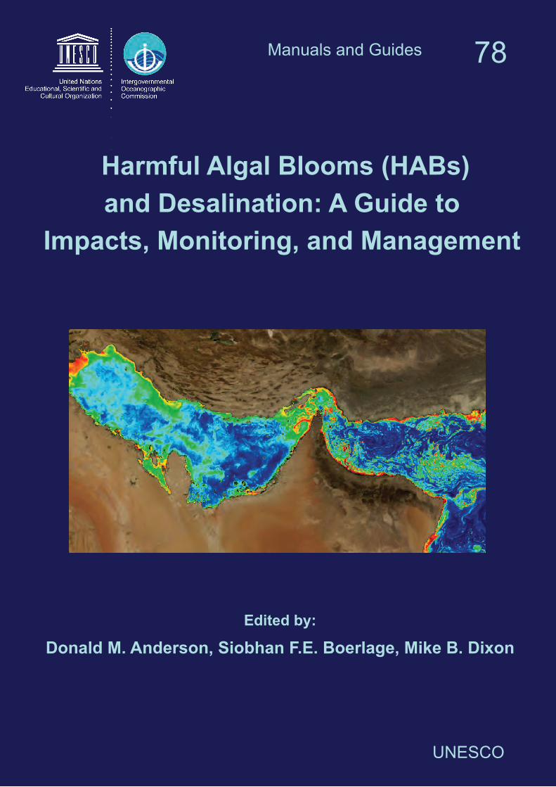
For bibliographic purposes this document should be cited as follows: Anderson D. M., S. F. E. Boerlage, M. B. Dixon (Eds), Harmful Algal Blooms (HABs) and Desalination: A Guide to Impacts, Monitoring and Management. Paris, Intergovernmental Oceanographic Commission of UNESCO, 2017. 539 pp. (IOC Manuals and Guides No.78.) (English.) (IOC/2017/MG/78). Cover photo: Chlorophyll concentrations captured by the MODIS Aqua sensor (NASA) from February 6, 2016, showing typical bloom patterns for the Arabian Gulf, Sea of Oman region, with low chlorophyll (dark blue) away from the coasts and high chlorophyll (orange and red) in complex patches and filaments, particularly around the Arabian Peninsula. The patterns are caused by surface transport and concentration of a harmful Cochlodinium bloom that is widely dispersed in response to surface currents and eddies. (Courtesy of R. Kudela, University of California, Santa Cruz and the National Aeronautics and Space Administration (NASA). Back cover photo: Foaming observed in the rapid mix basins during pretreatment at Tampa Bay Seawater Desalination Plant during an algal bloom event (Courtesy of Nikolay Voutchkov, Water Globe Consultants, LLC 2009). First published in 2017 by the United Nations Educational, Scientific, and Cultural Organization 7, Place de Fontenoy, 75732 Paris 07 SP © UNESCO 2017 Printed in Denmark

3

FOREWORD Coastal development is progressing at a rapid pace and coastal populations are increasingly vulnerable to sea-level rise, tsunamis, coastal erosion, storms, and other adverse environmental phenomena. One of the objectives of the Intergovernmental Oceanographic Commission of UNESCO (IOC) is to facilitate safety and security of people in the coastal zone and at sea. For example, the IOC operates a quasi-global tsunami warning system and strives to enable efficient coastal zone management that is fully informed of all major coastal risks.

In a number of coastal countries with dry climates, the demands for food and water are to a significant extent supported by seawater desalination activities. One marine hazard that is a threat to the large and rapidly expanding desalination industry is harmful algal blooms (HABs). The harm comes in part from algal production of neurotoxins as well as bad taste and odor and skin-irritating compounds that may persist in the treated water. Another major concern is the organic material produced by some algal blooms, as these compounds can clog intake filters and foul membrane surfaces, greatly compromising plant operations. Expansion of harmful algal events is inevitable given global trends in population, agriculture, development and climate. With the already observed increase in the number of toxic and harmful blooms, the resulting economic losses, the types of resources affected, and the number of toxins and toxic species reported, HAB problems can only be expected to increase.

For more than 20 years IOC has offered leadership in capacity building and international research cooperation in relation to harmful algae. The overall goal of the IOC Harmful Algal Bloom Programme is to foster the effective management of, and scientific research on, HABs in order to understand their causes, predict their occurrences, and mitigate their effects. The programme activities include provision of information and expertise, training, and research to improve understanding of harmful algae ecology. The design of efficient and effective HAB monitoring programmes can minimize the impacts of HABs on drinking water and seafood quality, thereby protecting public health and resources.

Despite the overall progress of HAB research, desalination plant operators and those who design plants or advise plant managers have thus far had very little information and guidance on how to manage and mitigate the effects of harmful algae on desalination operations. To meet their needs, the Intergovernmental Panel on Harmful Algal Blooms (IPHAB) established an international Task Team to address the effects of harmful algae on desalination. The group was heavily involved in the organization of two major conferences on the subject and was successful in reaching out to the expert community. The time has now come to combine experience and publish this book: Harmful Algal Blooms (HABs) and Desalination: A Guide to Impacts, Monitoring and Management. The IOC is pleased to be a co-sponsor of this important effort and hopes this Guide can help address the practical issues that harmful algae pose to desalination. At the same time the need for continuing targeted research in this topic area must also be stressed. Improved HAB forecasts for desalination plants will rely on improved coastal models, in combination with in situ observations that can detect and quantify HAB cells and toxins, or satellite remote sensing data to characterize the spatial extent and density of the blooms. A collaborative program can be envisioned involving multiple desalination plants with the aim of transitioning pilot HAB forecasting systems (like those described in this Guide) into operational systems.

Vladimir Ryabinin Executive Secretary, IOC

4

Acknowledgements The Editors would like to thank the following people who assisted in the preparation of this manual. These include: Shannon McCarthy for her efforts to initiate and obtain funding for this project, Kevin Price for his administrative work, Karen Steidinger for reviewing the algal species descriptions, Judy Kleindinst for major editorial and layout support, and Henrik Enevoldsen for publication assistance.

5

PREFACE Arid countries throughout the world are heavily reliant on seawater desalination for their supply of drinking and municipal water. The desalination industry is large and rapidly growing, approaching more than 20,000 plants operating or contracted in greater than 150 countries worldwide and capacity projected to grow at a rate of 12% per year for the next several decades (http://www.desaldata.com; 2016). Desalination plants are broadly distributed worldwide, with a large and growing capacity in what will be referred to as the “Gulf” region throughout this manual. Here the Gulf refers to the shallow body of water bounded in the southwest by the Arabian Peninsula and Iran to the northeast. The Gulf is linked with the Arabian Sea by the Strait of Hormuz and the Gulf of Oman to the east and extends to the Shatt al-Arab river delta at its western end. One of the operational challenges facing the industry is also expanding globally – the phenomena termed harmful algal blooms or HABs. Blooms are cell proliferations caused by the growth and accumulation of individual algal species; they occur in virtually all bodies of water. The algae, which can be either microscopic or macroscopic (e.g., seaweeds) are the base of the marine food web, and produce roughly half of the oxygen we breathe. Most of the thousands of species of algae are beneficial to humans and the environment, but there are a small number (several hundred) that cause HABs. This number is vague because the harm caused by HABs is diverse and affects many different sectors of society (see Chapter 1).

HABs are generally considered in two groups. One contains the species that produce potent toxins (Chapter 2) that can cause a wide range of impacts to marine resources, including mass mortalities of fish, shellfish, seabirds, marine mammals, and various other organisms, as well as illness and death in humans and other consumers of fish or shellfish that have accumulated the algal toxins during feeding. The second category is represented by species that produce dense blooms - often termed high biomass blooms because of the large number of cells. Cells can reach concentrations sufficient to make the water appear red (hence the common term “red tide”), though brown, green and golden blooms are also observed, while many blooms are not visible. In this manual, we define toxic algae as those that produce potent toxins (poisonous substances produced within living cells or organisms), e.g., saxitoxin. These can cause illness or mortality in humans as well as marine life through either direct exposure to the toxin or ingestion of bioaccumulated toxin in higher trophic levels e.g. shellfish. Non-toxic HABs can cause damage to ecosystems and commercial facilities such as desalination plants, sometimes because of the biomass of the accumulated algae, and in other cases due to the release of compounds that are not toxins (e.g., reactive oxygen species, mucilage) but that can still be lethal to marine animals or cause disruptions of other types. Both toxic and non-toxic HABs represent potential threats to seawater desalination facilities. Although toxins are typically removed very well by reverse osmosis and thermal desalination processes (see Chapter 10), algal toxins represent a potential health risk if they are present in sufficiently high concentrations in the seawater and if they break through the desalination process. It is therefore important for operators to be aware when toxic blooms are near their plants so they can ensure that the removal has indeed occurred (Chapter 3). High biomass blooms pose a different type of threat, as the resulting particulate and dissolved organic material can accelerate clogging of media filters or contribute to (bio)fouling of pretreatment and RO membranes which may lead to a loss of production.

Impacts of HABs on desalination facilities are thus a significant and growing problem, made worse by the lack of knowledge of this phenomena among plant operators, managers,

6

engineers, and others involved in the industry, including regulatory agencies. Recognizing this problem, the Middle East Desalination Research Center (MEDRC) and the UNESCO Intergovernmental Oceanographic Commission (IOC) organized a conference in 2012 in Muscat, Oman, to bring HAB researchers and desalination professionals together to exchange knowledge and discuss the scale of the problem and strategies for addressing it. One of the recommendations of that meeting was that a “guidance manual” be prepared to provide information to desalination plant operators and others in the industry about HABs, their impacts, and the strategies that could be used to mitigate those impacts. With support from the US Agency for International Development (USAID) and the IOC Intergovernmental Panel for Harmful Algal Blooms (IPHAB), an editorial team was assembled and potential authors contacted. For the first time, HAB scientists worked closely with desalination professionals to write chapters that were scientifically rigorous yet practical in nature – all focused on HABs and desalination. During the planning of this manual, it became clear from an informal survey of the desalination industry that generally, HAB problems are far more significant for seawater reverse osmosis (SWRO) plants than for those that use thermal desalination. Both types of processes are very effective in removing HAB toxins (Chapter 10), but the SWRO plants are far more susceptible to clogging of pretreatment granular media filters and fouling of membranes by algal organic matter and particulate biomass. Accordingly, the focus of this book is on SWRO, with only occasional reference to thermal processes. Likewise, emphasis has been placed on seawater HABs, with reference to estuarine and brackish-water HABs only when practices from those types of waters can be informative or illustrative.

A brief synopsis of the book follows. Chapter 1 provides a broad overview of HAB phenomena, including their impacts, the spatial and temporal nature of their blooms, common causative species, trends in occurrence, and general aspects of bloom dynamics in coastal waters. Chapter 2 describes the metabolites of HAB cells, including toxins, taste and odor compounds. Methods for analyses are presented there, supplemented by detailed methodological descriptions of rapid toxin screening methods in Appendix 2. As discussed in Chapters 8 and 10, thermal and SWRO operations are highly effective in the removal of HAB toxins, but plant personnel should have the capability to screen for these toxins in raw and treated water to ensure that this removal has been effective. This would be critical, for example, if the public or the press were aware of a toxic HAB in the vicinity of a desalination plant intake and asked for proof that their drinking water is safe. Currently, most desalination plants do not collect data on seawater outside their plants, so they are generally unaware of the presence (now or anticipated) of a potentially disruptive HAB. Chapter 3 provides practical information on the approaches to implementing an observing system for HABs, describing sampling methods and measurement options that can be tailored to available resources and the nature of the HAB threat in a given area. Appendix 4 provides more details on methods used to count and identify HAB cells during this process. All are based on direct water sampling, but it is also possible to observe HABs from space – particularly the high biomass events. Chapter 4 describes how satellite remote sensing can be used to detect booms. The common sources of imagery (free over the Internet) are presented, as well as descriptions of the software (also free) that can be used to analyze the satellite data. It is relatively easy and highly informative for plant personnel to use this approach to better understand what is in the seawater outside their plants. The cover of this guide provides a graphic example of the incredible scale and resolution of this observational approach.

Chapter 5 discusses typical water quality parameters that are measured online or in feedwater samples at desalination plants that could be used to detect blooms at the intake or evaluate process efficiency in removing algal particulates and organics. Emerging parameters that also

7

show promise are examined to provide a resource for plant personnel. Chapter 6 looks at desalination seawater intakes that are the first point of control in minimizing the ingress of algae into the plant. A brief overview of siting considerations that may ultimately drive the location of an intake is also provided.

One question asked frequently of HAB scientists is whether the blooms can be controlled or suppressed in a manner analogous to the treatment of insects or other agricultural pests on land. This has proven to be an exceedingly difficult challenge for the HAB scientific and management community, given the dynamic nature of HABs in coastal waters, their large spatial extent, and concerns about the environmental impacts of bloom control methods. Chapter 7 presents a summary of the approaches to bloom prevention and control that have been developed, and discusses whether these are feasible or realistic in the context of an individual desalination plant.

Chapter 8 describes management strategies for HABs and risk assessment, including Hazard Analysis Critical Control Point (HACCP) and Alert Level Framework procedures. Once a HAB is detected, a wide range of approaches can be used to address the problems posed by the dissolved toxins associated with those blooms. Chapter 9 presents many of these pretreatment strategies and discusses their use in removing algal organic matter and particulates to prevent filter clogging and membrane fouling. This is necessary to maintain effective plant operation and avoid serious operational challenges for the reverse osmosis step. The chapter covers common pretreatments such as chlorination/dechlorination, coagulation, dissolved air flotation, granular media filtration, ultrafiltration, and cartridge filtration, in addition to discussing issues experienced due to the inefficiencies of each pretreatment on reverse osmosis. Chapter 10 then addresses the important issue of HAB toxin removal during pretreatment and desalination, and describes laboratory and pilot-scale studies that address that issue. Finally, Chapter 11 provides a series of case studies describing individual HAB events at desalination plants throughout the world, detailing the types of impacts and the strategies that were used to combat them. These studies should be of great interest to other operators as they encounter similar challenges. The manual concludes with a series of appendices that provide images and short descriptions of common HAB species (Appendix 1), rapid screening methods for HAB toxins (Appendix 2), methods to measure transparent exopolymer particles (TEP) and their precursors (Appendix 3), methods to enumerate algal cells (Appendix 4), and reverse osmosis autopsy and cleaning methods (Appendix 5).

Compilation of this manual was a major undertaking, requiring the cooperation of scientists and engineers from multiple disciplines, including a number where interactions have been rare in the past. We hope the accumulated material proves useful, and plan to keep this document updated through time and readily available through the Internet. The Editors welcome questions, comments, and suggestions that can make this compilation more useful and accurate.

Donald M. Anderson Woods Hole Oceanographic Institution

Siobhan F.E. Boerlage Boerlage Consulting

Mike B. Dixon MDD Consulting

9

Table of Contents

Foreword 3 Acknowledgements 4 Preface 5 Contributing Authors and Affiliations 13

Chapter 1. Harmful algal blooms Donald M. Anderson 1.1 Algal blooms 17 1.2 Harmful or toxic bloom species 20 1.3 Algal cell characteristics 22 1.4 Trends and species dispersal 32 1.5 Growth features, bloom mechanisms 34 1.6 Summary 41 1.7 References 42

Chapter 2. Algal issues in seawater desalination Philipp Hess, Loreen O. Villacorte, Mike B. Dixon, Siobhan F.E. Boerlage, Donald M. Anderson, Maria D. Kennedy and Jan C. Schippers 2.1 Introduction 53 2.2 Algal organic matter (AOM) and membrane fouling 53 2.3 Algal issues in thermal desalination plants 63 2.4 Marine and freshwater toxins 63 2.5 Taste and odor compounds 71 2.6 Detection techniques 71 2.7 Gaps and perspectives on analytical techniques 75 2.8 References 76 Chapter 3. Designing an observing system for early detection of harmful algal blooms Bengt Karlson, Clarissa R. Anderson, Kathryn J. Coyne, Kevin G. Sellner, and Donald M. Anderson

3.1 Introduction 89 3.2 Designing an observation system 90 3.3 Background information 90 3.4 Identifying existing infrastructure 93 3.5 Sampling methods 93 3.6 Identification and enumeration of HAB organisms 102 3.7 Satellite remote sensing 108 3.8 Transport and delivery of harmful algal blooms 108 3.9 Distributing warnings and information 110 3.10 Data storage and distribution 112

3.11 Facilities, equipment, and personnel 112 3.12 Summary 114 3.13 References 115 Chapter 4. Acquisition and analysis of remote sensing imagery of harmful algal blooms Raphael M. Kudela, Richard P. Stumpf, and Peter Petrov

4.1 Introduction 119 4.2 Availability of data and software 121

10

4.3 Internet access to imagery 121 4.4 Software for processing satellite data 123 4.5 Algorithms used to detect blooms 124 4.6 Examples of algorithms 127 4.7 Summary for end-users 128 4.8 Useful links to satellite based ocean color data 130 4.9 References 130

Chapter 5. Harmful algal bloom-related water quality monitoring for desalination design and operation Siobhan F.E. Boerlage, Loreen O.Villacorte, Lauren Weinrich, S. Assiyeh Alizadeh Tabatabai, Maria D. Kennedy, and Jan C. Schippers

5.1 Intake feedwater characterization and water quality monitoring 133 5.2 Suitability of conventional online water quality parameters to detect HABs 134 5.3 Overview of parameters to determine organic matter 136 5.4 Measuring biofouling potential 147 5.5 Fouling indices to measure particulate fouling potential 153 5.6 Summary 162 5.7 References 164

Chapter 6. Seawater intake considerations to mitigate harmful algal bloom impacts Siobhan F.E. Boerlage, Thomas M. Missimer, Thomas M. Pankratz, and Donald M. Anderson

6.1 Introduction 169 6.2 Intake options for SWRO desalination plants 171 6.3 Surface intake and screen options 172 6.4 Subsurface intake options 181 6.4 Siting of desalination seawater intakes 197 6.5 Summary 199 6.6 References 200

Chapter 7. Bloom prevention and control Clarissa R. Anderson, Kevin G. Sellner, and Donald M. Anderson

7.1 Introduction 205 7.2 Bloom prevention 207 7.3 Bloom control 209 7.4 Summary 214 7.5 References 215

Chapter 8. World Health Organization and international guidelines for toxin control, harmful algal bloom management, and response planning Alex Soltani, Phillip Hess, Mike B. Dixon, Siobhan F.E. Boerlage, Donald M. Anderson, Gayle Newcombe, Jenny House, Lionel Ho, Peter Baker, and Michael Burch

8.1 Guidelines and standards 223 8.2 Using guideline values 228 8.3 Australian drinking water guidelines regarding multiple treatment barriers 228 8.4 Risk assessment for the presence of HABs 230 8.5 Alert level frameworks 240 8.6 Summary 247 8.7 References 247

11

Chapter 9. Algal biomass pretreatment in seawater reverse osmosis Mike B. Dixon, Siobhan F.E. Boerlage, Nikolay Voutchkov, Rita Henderson, Mark Wilf, Ivan Zhu, S. Assiyeh Alizadeh Tabatabai, Tony Amato, Adhika Resosudarmo, Graeme K. Pearce, Maria Kennedy, Jan C. Schippers, and Harvey Winters

9.1 Introduction 252 9.2 Chlorination in SWRO 252 9.3 Dechlorination in SWRO 257 9.4 Coagulation for DAF, DMF and UF pretreatment 257 9.5 DAF pretreatment for SWRO 272 9.6 Granular media filtration 278 9.7 Microscreens for membrane pretreatment 287 9.8 Microfiltration/ ultrafiltration 290 9.9 Cartridge filters for reverse osmosis pretreatment 297 9.10 Reverse osmosis 299 9.11 Summary of biomass removal in SWRO 307 9.12 References 308

Chapter 10. Removal of algal toxins and taste and odor compounds during desalination Mike B. Dixon, Siobhan F.E. Boerlage, Holly Churman, Lisa Henthorne, and Donald M. Anderson

10.1 Introduction 315 10.2 Chlorination 316 10.3 Dissolved air flotation (DAF) 317 10.4 Granular media filters 317 10.5 Ultrafiltration/microfiltration 318 10.6 Reverse osmosis 320 10.7 Sludge treatment and backwash disposal 324 10.8 Toxin removal in thermal desalination plants 324 10.9 Chlorination prior to the distribution system 327 10.10 Summary 328 10.11 References 329

Chapter 11. Case histories for harmful algal blooms in desalination Siobhan F.E. Boerlage, Mike B. Dixon, and Donald M. Anderson

11.1 Introduction 333 11.2 Fujairah 2, United Arab Emirates – Effects of harmful algal blooms on plant operations in 2008 and 2013 - Herve Faujour, Cyril de

Vomecourt, and Jérôme Leparc 347 349 11.3 Sohar, Oman – Harmful algal bloom impact on membrane pre- treatment: challenges and solutions - Abdullah Said Al-Sadi and Khurram Shahid 355 11.4 Barka 1, Oman - The impact of harmful algal blooms on the performance stability of UF pretreatment - Graeme K. Pearce 367 11.5 Shuwaikh, Kuwait – Harmful algal bloom cell removal using dissolved air flotation: pilot and laboratory studies - Robert Wiley, Mike Dixon, and Siobhan F. E. Boerlage 383

12

11.6 La Chimba, Antofagasta, Chile – Oxygen depletion and hydrogen sulfide gas mitigation due to harmful algal blooms - Walter Cerda Acuña, Carlos

Jorquera Gonzalez, and Victor Gutierrez Aqueveque 391 11.7 Mejillones, Chile – Operation of the ultrafiltration system during harmful algal blooms at the Gas Atacama SWRO plant - Frans Knops and Alejandro Sturnilio 399 11.8 Antofagasta, Chile - Abengoa water micro/ultrafiltration pretreatment pilot plant - Francisco Javier Bernaola, Israel Amores, Miguel Ramón, Raquel Serrano and Juan Arévalo 409 11.9 Tampa Bay, Florida (USA) – Non-toxic algal blooms and operation of the

SWRO plant detailing monitoring program for blooms - Lauren Weinrich 417 11.10 Jacobahaven, The Netherlands – Ultrafiltration for SWRO pretreatment: A

demonstration plant - Rinnert Schurer, Loreen O. Villacorte, Jan C. Schippers, and Maria D. Kennedy 425 11.11 Barcelona, Spain - SWRO demonstration plant: DAF/DMF versus DAF/UF - Joan Llorens, Andrea R. Guastalli and Sylvie Baig 439 11.12 Gold Coast, Queensland, Australia - Deep water intake limits Trichodesmium ingress - Dianne L. Turner, Siobhan F. E. Boerlage and Scott Murphy 447 11.13 Berlin, Germany – akvola: An integrated DAF-UF pilot - Johanna Ludwig and Matan Beery 459

Appendix 1. Algal species potentially harmful to desalination operations David G. Borkman and Donald M. Anderson 465 Appendix 2. Rapid screening methods for harmful algal bloom toxins Donald M. Anderson, Maurice Laycock, and Fernando Rubio 485 Appendix 3. Methods for measuring transparent exopolymer particles and their precursors in seawater Loreen O. Villacorte, Jan C. Schippers, and Maria D. Kennedy 501 Appendix 4. Preservatives and methods for algal cell enumeration Donald M. Anderson and Bengt Karlson 509 Appendix 5. Autopsy and cleaning of reverse osmosis elements affected by harmful algal bloom-contaminated seawater

Nuria Peña, Steve Chesters, Mike Dixon, and Siobhan F. E. Boerlage 519 Index 527

13

Contributing Authors and Affiliations

Abdullah Said Al-Sadi Majis Industrial Services, Sohar, Oman E-mail: abdullah.al-sadi@miscoman.com

Tony Amato Water2Water Consulting, England, UK E-mail: water2water@btinternet.com

Israel Amores Abengoa, Spain E-mail: israel.amores.bautista@gmail.com

Clarissa R. Anderson University of California, Santa Cruz, Santa Cruz, CA, USA E-mail: clrander@ucsc.edu

Donald M. Anderson Biology Department, Woods Hole Oceanographic Institution, Woods Hole, MA USA E-mail: danderson@whoi.edu

Juan Arévalo Abengoa, Spain E-mail: arevalo.vilches@gmail.com

Sylvie Baig Degrémont SA, Rueil-Malmaison Cedex, France E-mail: Sylvie.baig@degremont.com

Peter Baker South Australian Water Corporation, Adelaide, South Australia, 5000 Water Research Australia, Adelaide, South Australia, 5000 E-mail: peter.baker@sawater.com.au

Matan Beery akvola Technologies, Berlin, Germany E-mail: beery@akvola.com

Francisco Javier Bernaola Abengoa, Spain E-mail: patxobernaola@yahoo.com

David G. Borkman Pausacaco Plankton, Saunderstown, RI USA E-mail: David.Borkman@dem.ri.gov

Siobhan F.E. Boerlage Boerlage Consulting, Gold Coast, Queensland, Australia E-mail: desal@boerlageconsulting.com

Michael Burch South Australian Water Corporation, Adelaide, South Australia, 5000 Water Research Australia, Adelaide, South Australia, 5000 E-mail: mike.burch@sawater.com.au

Walter Cerda Acuña Aguas Antofagasta, Anofagasta, Chile E-mail: wcerda@aguasantofagasta.cl

Steve Chesters Genesys International, Cheshire, United Kingdom E-mail: schesters@genesysro.com

Holly Churman Water Standard, Houston, TX, USA E-mail: hchurman@waterstandard.com

14

Kathyrn J. Coyne University of Delaware, Lewes, DE, USA E-mail: kcoyne@udel.edu

Cyril de Vomecourt Veolia Middle East, Dubai, United Arab Emirates E-mail: Cyril.devomecourt@veolia.com

Mike B. Dixon MDD Consulting, Kensington, Calgary, Alberta, Canada E-mail: mikedixondesalination@gmail.com

Herve Faujour Veolia Middle East, Dubai, United Arab Emirates E-mail: herve.faujour@veolia.com

Andrea R. Guastalli University of Barcelona, Barcelona, Spain E-mail: guastalli.a@gmail.com

Victor Gutierrez Aqueveque Aguas Antofagasta, Anofagasta, Chile E-mail: vgutierrez@aguasantofagasta.cl

Rita Henderson School of Chemical Engineering, The University of New South Wales, Australia E-mail: r.henderson@unsw.edu.au

Lisa Henthorne Water Standard, Houston, TX, USA E-mail: lhenthorne@waterstandard.com

Philipp Hess IFREMER, Laboratoire Phycotoxines, 44311 Nantes, France E-mail: Philipp.Hess@ifremer.fr

Lionel Ho South Australian Water Corporation, Adelaide, South Australia, 5000 Water Research Australia, Adelaide, South Australia, 5000 E-mail: lionel.ho@sawater.com.au

Jenny House South Australian Water Corporation, Adelaide, South Australia, 5000 Water Research Australia, Adelaide, South Australia, 5000 E-mail: jenny.house@sawater.com.au

Carlos Jorquera Gonzalez Aguas Antofagasta, Anofagasta, Chile E-mail: cjorquera@aguasantofagasta.cl

Bengt Karlson Swedish Meteorological and Hydrological Institute, Gothenberg, Sweden E-mail: Bengt.Karlson@smhi.se

Maria D. Kennedy UNESCO-IHE Institute for Water Education, Delft, The Netherlands E-mail: m.kennedy@un-ihe.org

Frans Knops X-Flow BV / Pentair Water Process Technology BV, Enschede, the Netherlands E-mail: Frans.knops@pentair.com

Raphael M. Kudela University of California, Santa Cruz, Santa Cruz, CA USA E-mail: kudela@ucsc.edu

15

Maurice Laycock Scotia Rapid Testing Ltd, Chester Basin, Nova Scotia, Canada E-mail: mlaycock@bellaliant.net

Jérôme Leparc Veolia Recherche and Innovation, Maisons Laffitte, France E-mail: jerome.leparc@veolia.com

Joan Llorens University of Barcelona, Barcelona, Spain E-mail: jllorensl@ub.edu

Johanna Ludwig akvola Technologies, Berlin, Germany E-mail: ludwig@akvola.com

Thomas M. Missimer Florida Gulf Coast University, Fort Myers, FL USA E-mail: tmissimer@fgcu.edu

Scott Murphy Veoila Australia and New Zealand, Gold Cost, Australia E-mail: scott.murphy@veolia.com.au

Gayle Newcombe South Australian Water Corporation, Adelaide, South Australia, 5000 Water Research Australia, Adelaide, South Australia, 5000 E-mail: gayle.newcombe@sawater.com.au

Thomas M. Pankratz Water Desalination Report, Houston, TX USA E-mail: tp@globalwaterintel.com

Graeme K. Pearce Membrane Consultancy Associates Ltd, Reading, UK E-mail: graemekpearce@btinternet.com

Nuria Peña Genesys Membrane Products, S.L. Spain E-mail: npena@genesysro.com

Peter Petrov Kuwait Institute for Scientific Research (KISR) E-mail: ppetrov@kisr.edu.kw

Miguel Ramón Abengoa, Spain E-mail: mramonmuro@gmail.com

Adhikara Resosudarmo The University of New South Wales, Australia E-mail: adhikara.resosudarmo@student.unsw.edu.au

Fernando Rubio Abraxis LLC, Warminster, PA USA E-mail: frubio@abraxiskits.com

Jan C. Schippers UNESCO-IHE Institute for Water Education, Delft, The Netherlands E-mail: jancschippers@gmail.com

Rinnert Schurer Evides Water Company, Rotterdam, the Netherlands E-mail: r.schurer@evides.nl

Kevin G. Sellner Chesapeake Research Consortium, Edgewater, MD, USA E-mail: sellnerk@si.edu

16

Raquel Serrano Abengoa, Spain E-mail: raquelserrano@hotmail.com

Khurram Shahid Water Solutions International Ltd, Gatwick, England E-mail: kshahid@waterwastewater.uk

Alex Soltani Alex Soltani Consulting, Calgary, Alberta, Canada

E-mail: alexander.soltani@outlook.com Richard P. Stumpf

National Oceanographic and Atmospheric Administration, Silver Spring, MD USA E-mail: Richard.Stumpf@noaa.gov

Alejandro Sturniolo RWL Water Unitek, Mar del Plata, Argentina E-mail:asturniolo@rwlwater.com

S. Assiyeh Alizadeh Tabatabai UNESCO-IHE Institute for Water Education, Delft, The Netherlands E-mail: assiyeh.alizadeh@gmail.com

Dianne L. Turner Veoila Australia and New Zealand, Gold Cost, Australia E-mail: dianne.turner@veolia.com.au

Loreen O. Villacorte GRUNDFOS Holding A/S, Bjerringbro, Denmark (current affiliation) E-mail: lvillacorte@grundfos.com

Nikolay Voutchkov Water Globe Consulting, Winter Springs, FL, USA E-mail: nvoutchkov@water-g.com

Lauren Weinrich American Water, Voorhees, NJ USA E-mail: Lauren.Weinrich@amwater.com

Robert Wiley Leopold, a Xylem Brand, Zelienople, PA, USA E-mail: Bob.Wiley.III@xyleminc.com

Mark Wilf Mark Wilf Consulting, San Diego, CA, USA E-mail: Mark.Wilf@rotechnology.net

Harvey Winters Fairleigh Dickinson University, Teaneck, NJ USA E-mail: harvey@fdu.edu

Ivan Zhu Leopold, a Xylem Brand, Zelienople, PA USA E-mail: ivan.zhu@evoqua.com

Harmful algal blooms

17

1! HARMFUL ALGAL BLOOMS

Donald M. Anderson1 1Woods Hole Oceanographic Institution, Woods Hole, MA USA

!

1.1! Algal blooms ........................................................................................................................................... 17!1.2! Harmful or toxic bloom species .............................................................................................................. 20!1.3! Algal cell characteristics ......................................................................................................................... 22!

1.3.1! Toxins .............................................................................................................................................. 22!1.3.2! Cell size ........................................................................................................................................... 25!1.3.3! Cell wall coverings and surface charge ........................................................................................... 25!1.3.4! Life histories .................................................................................................................................... 31!

1.4! Trends and species dispersal ................................................................................................................... 32!1.5! Growth features, bloom mechanisms ...................................................................................................... 34!

1.5.1! Scale of blooms ............................................................................................................................... 34!1.5.2! Cell growth ...................................................................................................................................... 35!1.5.3! Bloom dynamics and coastal oceanography .................................................................................... 36!1.5.4! Bloom initiation ............................................................................................................................... 36!1.5.5! Bloom transport ............................................................................................................................... 36!1.5.6! Fronts ............................................................................................................................................... 37!1.5.7! Upwelling systems ........................................................................................................................... 38!1.5.8! Alongshore transport ....................................................................................................................... 38!1.5.9! Vertical distributions ....................................................................................................................... 39!

1.6! Summary ................................................................................................................................................. 41!1.7! References ............................................................................................................................................... 42!

1.1! ALGAL BLOOMS Oceans and freshwater rivers, lakes, and streams teem with microscopic plants called algae that capture the sun’s energy with their pigments and grow and proliferate in illuminated surface waters, typically through simple cell division. These increases in abundance over background levels are termed “blooms”, analogous to the growth and flourishing of terrestrial plants. Many algal species are non-motile and thus their distributions are simply determined by the movements of water. Even species that swim are not powerful enough to control their location in most situations, so they too are generally dominated by the motion of waves, currents, and tides (though the combination of swimming behaviour and water movement can lead to dense cell aggregations and other spatial features (see section 1.5.3.6)). The microscopic algae are called phytoplankton (drifting, single celled plants), to be distinguished from their close relatives, the multi-cellular macroalgae or seaweeds. Algae of both types are critical to life on earth, as they produce half of the oxygen we breathe and represent the base of the aquatic food chain that provides substantial food for human society. Among the many thousands of species of microalgae are a few hundred that cause harm in various ways. Potentially harmful species are found in multiple phytoplankton groups. Many are eukaryotes, (i.e., organisms with a nucleus and other organelles enclosed within membranes) such as dinoflagellates, raphidophytes, diatoms, euglenophytes, cryptophytes, haptophytes, pelagophytes, and chlorophytes. Some are prokaryotes, (i.e., single-celled organisms such as cyanobacteria that lack a membrane-bound nucleus or other organelle). While dinoflagellates comprise the majority of toxic harmful algal bloom (HAB) species in the marine environment where seawater reverse osmosis (SWRO) plants are located, many of the toxic species that pose a threat to drinking water supply in fresh- or brackish-water systems are cyanobacteria.

Harmful algal blooms

18

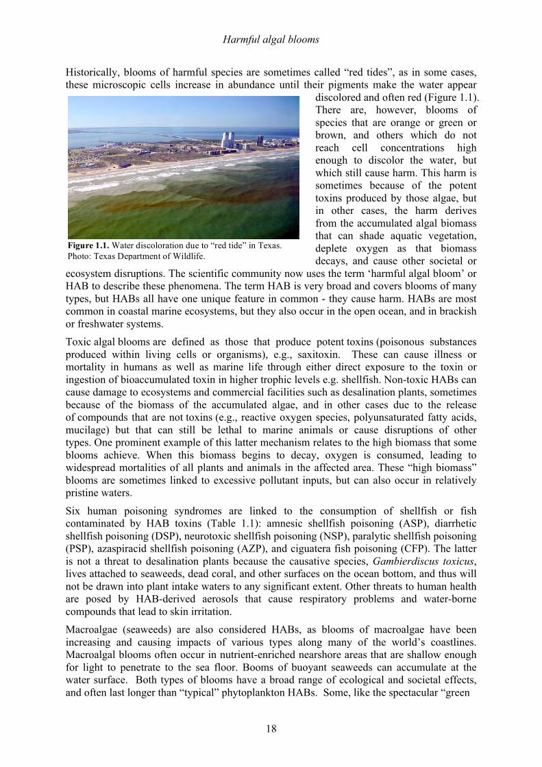
Historically, blooms of harmful species are sometimes called “red tides”, as in some cases, these microscopic cells increase in abundance until their pigments make the water appear

discolored and often red (Figure 1.1). There are, however, blooms of species that are orange or green or brown, and others which do not reach cell concentrations high enough to discolor the water, but which still cause harm. This harm is sometimes because of the potent toxins produced by those algae, but in other cases, the harm derives from the accumulated algal biomass that can shade aquatic vegetation, deplete oxygen as that biomass decays, and cause other societal or

ecosystem disruptions. The scientific community now uses the term ‘harmful algal bloom’ or HAB to describe these phenomena. The term HAB is very broad and covers blooms of many types, but HABs all have one unique feature in common - they cause harm. HABs are most common in coastal marine ecosystems, but they also occur in the open ocean, and in brackish or freshwater systems. Toxic algal blooms are defined as those that produce potent toxins (poisonous substances produced within living cells or organisms), e.g., saxitoxin. These can cause illness or mortality in humans as well as marine life through either direct exposure to the toxin or ingestion of bioaccumulated toxin in higher trophic levels e.g. shellfish. Non-toxic HABs can cause damage to ecosystems and commercial facilities such as desalination plants, sometimes because of the biomass of the accumulated algae, and in other cases due to the release of compounds that are not toxins (e.g., reactive oxygen species, polyunsaturated fatty acids, mucilage) but that can still be lethal to marine animals or cause disruptions of other types. One prominent example of this latter mechanism relates to the high biomass that some blooms achieve. When this biomass begins to decay, oxygen is consumed, leading to widespread mortalities of all plants and animals in the affected area. These “high biomass” blooms are sometimes linked to excessive pollutant inputs, but can also occur in relatively pristine waters.

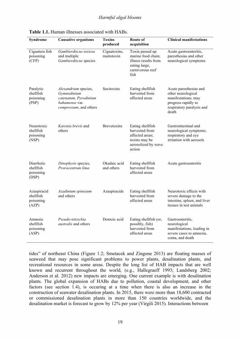
Six human poisoning syndromes are linked to the consumption of shellfish or fish contaminated by HAB toxins (Table 1.1): amnesic shellfish poisoning (ASP), diarrhetic shellfish poisoning (DSP), neurotoxic shellfish poisoning (NSP), paralytic shellfish poisoning (PSP), azaspiracid shellfish poisoning (AZP), and ciguatera fish poisoning (CFP). The latter is not a threat to desalination plants because the causative species, Gambierdiscus toxicus, lives attached to seaweeds, dead coral, and other surfaces on the ocean bottom, and thus will not be drawn into plant intake waters to any significant extent. Other threats to human health are posed by HAB-derived aerosols that cause respiratory problems and water-borne compounds that lead to skin irritation. Macroalgae (seaweeds) are also considered HABs, as blooms of macroalgae have been increasing and causing impacts of various types along many of the world’s coastlines. Macroalgal blooms often occur in nutrient-enriched nearshore areas that are shallow enough for light to penetrate to the sea floor. Booms of buoyant seaweeds can accumulate at the water surface. Both types of blooms have a broad range of ecological and societal effects, and often last longer than “typical” phytoplankton HABs. Some, like the spectacular “green

Figure 1.1. Water discoloration due to “red tide” in Texas. Photo: Texas Department of Wildlife.

Harmful algal blooms

19

Table 1.1. Human illnesses associated with HABs. Syndrome Causative organisms Toxins

produced Route of acquisition

Clinical manifestations

Ciguatera fish poisoning (CFP)

Gambierdiscus toxicus and multiple Gambierdiscus species

Ciguatoxins, maitotoxin

Toxin passed up marine food chain; illness results from eating large, carnivorous reef fish

Acute gastroenteritis, paresthesias and other neurological symptoms

Paralytic shellfish poisoning (PSP)

Alexandrium species, Gymnodinium catenatum, Pyrodinium bahamense var. compressum, and others

Saxitoxins Eating shellfish harvested from affected areas

Acute paresthesias and other neurological manifestations; may progress rapidly to respiratory paralysis and death

Neurotoxic shellfish poisoning (NSP)

Karenia brevis and others

Brevetoxins Eating shellfish harvested from affected areas; toxins may be aerosolized by wave action

Gastrointestinal and neurological symptoms; respiratory and eye irritation with aerosols

Diarrhetic shellfish poisoning (DSP)

Dinophysis species; Prorocentrum lima

Okadaic acid and others

Eating shellfish harvested from affected areas

Acute gastroenteritis

Azaspiracid shellfish poisoning (AZP)

Azadinium spinosum and others

Azaspiracids Eating shellfish harvested from affected areas

Neurotoxic effects with severe damage to the intestine, spleen, and liver tissues in test animals

Amnesic shellfish poisoning (ASP)

Pseudo-nitzschia australis and others

Domoic acid Eating shellfish (or, possibly, fish) harvested from affected areas

Gastroenteritis, neurological manifestations, leading in severe cases to amnesia, coma, and death

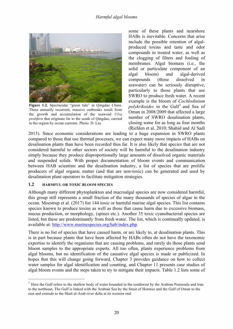
tides” of northeast China (Figure 1.2; Smetacek and Zingone 2013) are floating masses of seaweed that may pose significant problems to power plants, desalination plants, and recreational resources in some areas. Despite the long list of HAB impacts that are well known and recurrent throughout the world, (e.g., Hallegraeff 1993; Landsberg 2002; Anderson et al. 2012) new impacts are emerging. One current example is with desalination plants. The global expansion of HABs due to pollution, coastal development, and other factors (see section 1.4), is occuring at a time when there is also an increase in the construction of seawater desalination plants. In 2015, there were more than 18,600 contracted or commissioned desalination plants in more than 150 countries worldwide, and the desalination market is forecast to grow by 12% per year (Virgili 2015). Interactions between

Harmful algal blooms

20

some of these plants and nearshore HABs is inevitable. Concerns that arise include the possible retention of algal-produced toxins and taste and odor compounds in treated water, as well as the clogging of filters and fouling of membranes. Algal biomass (i.e., the solid or particulate component of an algal bloom) and algal-derived compounds (those dissolved in seawater) can be seriously disruptive, particularly to those plants that use SWRO to produce fresh water. A recent example is the bloom of Cochlodinium polykrikoides in the Gulf1 and Sea of Oman in 2008/2009 that affected a large number of SWRO desalination plants, closing some for as long as four months (Richlen et al. 2010; Shahid and Al Sadi

2015). Since economic considerations are leading to a huge expansion in SWRO plants compared to those that use thermal processes, we can expect many more impacts of HABs on desalination plants than have been recorded thus far. It is also likely that species that are not considered harmful to other sectors of society will be harmful to the desalination industry simply because they produce disproportionally large amounts of dissolved organic materials and suspended solids. With proper documentation of bloom events and communication between HAB scientists and the desalination industry, a list of species that are prolific producers of algal organic matter (and that are non-toxic) can be generated and used by desalination plant operators to facilitate mitigation strategies.

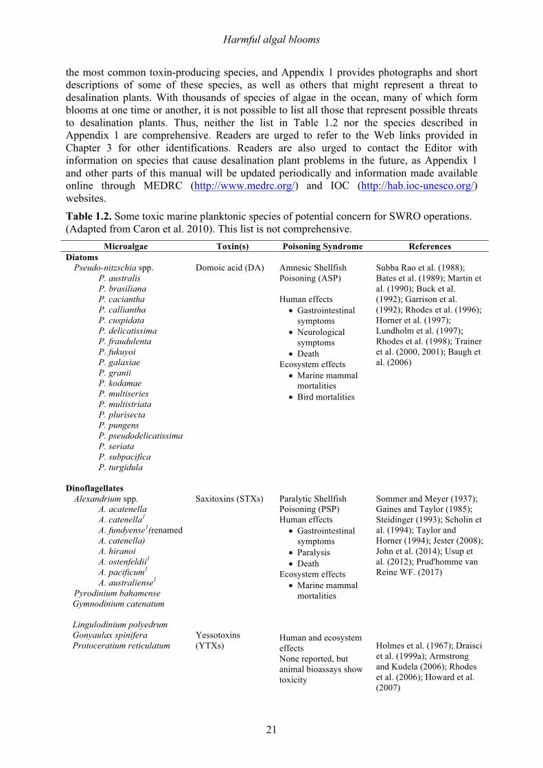
1.2! HARMFUL OR TOXIC BLOOM SPECIES Although many different phytoplankton and macroalgal species are now considered harmful, this group still represents a small fraction of the many thousands of species of algae in the ocean. Moestrup et al. (2017) list 144 toxic or harmful marine algal species. This list contains species known to produce toxins as well as those that cause harm due to excessive biomass, mucus production, or morphology, (spines etc.). Another 35 toxic cyanobacterial species are listed, but these are predominantly from fresh water. The list, which is continually updated, is available at: http://www.marinespecies.org/hab/index.php.

There is no list of species that have caused harm, or are likely to, at desalination plants. This is in part because plants that have been affected by HABs often do not have the taxonomic expertise to identify the organisms that are causing problems, and rarely do those plants send bloom samples to the appropriate experts. All too often, plants experience problems from algal blooms, but no identification of the causative algal species is made or publicized. In hopes that this will change going forward, Chapter 3 provides guidance on how to collect water samples for algal identification and counting, and Chapter 11 presents case studies of algal bloom events and the steps taken to try to mitigate their impacts. Table 1.2 lists some of

1 Here the Gulf refers to the shallow body of water bounded in the southwest by the Arabian Peninsula and Iran to the northeast. The Gulf is linked with the Arabian Sea by the Strait of Hormuz and the Gulf of Oman to the east and extends to the Shatt al-Arab river delta at its western end.

Figure 1.2. Spectacular “green tide” in Qingdao China. These annually recurrent, massive outbreaks result from the growth and accumulation of the seaweed Ulva prolifera that originate far to the south of Qingdao, carried to the region by ocean currents. Photo: D. Liu.

Harmful algal blooms

21

the most common toxin-producing species, and Appendix 1 provides photographs and short descriptions of some of these species, as well as others that might represent a threat to desalination plants. With thousands of species of algae in the ocean, many of which form blooms at one time or another, it is not possible to list all those that represent possible threats to desalination plants. Thus, neither the list in Table 1.2 nor the species described in Appendix 1 are comprehensive. Readers are urged to refer to the Web links provided in Chapter 3 for other identifications. Readers are also urged to contact the Editor with information on species that cause desalination plant problems in the future, as Appendix 1 and other parts of this manual will be updated periodically and information made available online through MEDRC (http://www.medrc.org/) and IOC (http://hab.ioc-unesco.org/) websites. Table 1.2. Some toxic marine planktonic species of potential concern for SWRO operations. (Adapted from Caron et al. 2010). This list is not comprehensive.

Microalgae Toxin(s) Poisoning Syndrome References Diatoms

Pseudo-nitzschia spp. P. australis P. brasiliana P. caciantha P. calliantha P. cuspidata P. delicatissima P. fraudulenta P. fukuyoi P. galaxiae P. granii P. kodamae P. multiseries P. multistriata P. plurisecta P. pungens P. pseudodelicatissima P. seriata P. subpacifica P. turgidula

Domoic acid (DA)

Amnesic Shellfish Poisoning (ASP) Human effects •!Gastrointestinal

symptoms •!Neurological

symptoms •!Death

Ecosystem effects •!Marine mammal

mortalities •!Bird mortalities

Subba Rao et al. (1988); Bates et al. (1989); Martin et al. (1990); Buck et al. (1992); Garrison et al. (1992); Rhodes et al. (1996); Horner et al. (1997); Lundholm et al. (1997); Rhodes et al. (1998); Trainer et al. (2000, 2001); Baugh et al. (2006)

Dinoflagellates Alexandrium spp.

A. acatenella

A. catenella1 A. fundyense1(renamed A. catenella) A. hiranoi A. ostenfeldii1 A. pacificum1 A. australiense1

Pyrodinium bahamense Gymnodinium catenatum Lingulodinium polyedrum Gonyaulax spinifera Protoceratium reticulatum

Saxitoxins (STXs) Yessotoxins (YTXs)

Paralytic Shellfish Poisoning (PSP) Human effects •!Gastrointestinal

symptoms •! Paralysis •!Death

Ecosystem effects •!Marine mammal

mortalities Human and ecosystem effects None reported, but animal bioassays show toxicity

Sommer and Meyer (1937); Gaines and Taylor (1985); Steidinger (1993); Scholin et al. (1994); Taylor and Horner (1994); Jester (2008); John et al. (2014); Usup et al. (2012); Prud'homme van Reine WF. (2017) Holmes et al. (1967); Draisci et al. (1999a); Armstrong and Kudela (2006); Rhodes et al. (2006); Howard et al. (2007)

Harmful algal blooms

22

Table 1.2. (Continued)

Microalgae Toxin(s) Poisoning Syndrome

References

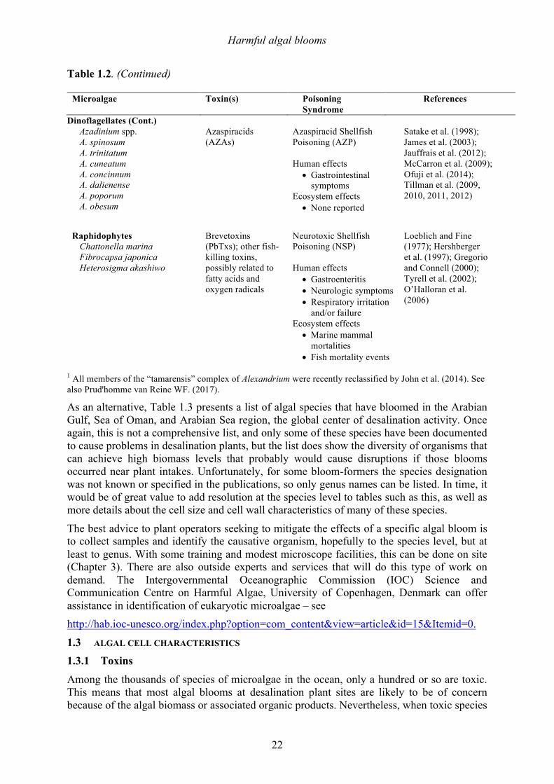
Dinoflagellates (Cont.) Azadinium spp. A. spinosum A. trinitatum A. cuneatum A. concinnum A. dalienense A. poporum A. obesum

Azaspiracids (AZAs)

Azaspiracid Shellfish Poisoning (AZP) Human effects •!Gastrointestinal

symptoms Ecosystem effects •!None reported

Satake et al. (1998); James et al. (2003); Jauffrais et al. (2012); McCarron et al. (2009); Ofuji et al. (2014); Tillman et al. (2009, 2010, 2011, 2012)

Raphidophytes Chattonella marina Fibrocapsa japonica Heterosigma akashiwo

Brevetoxins (PbTxs); other fish-killing toxins, possibly related to fatty acids and oxygen radicals

Neurotoxic Shellfish Poisoning (NSP) Human effects •!Gastroenteritis •!Neurologic symptoms •!Respiratory irritation

and/or failure Ecosystem effects •!Marine mammal

mortalities •! Fish mortality events

Loeblich and Fine (1977); Hershberger et al. (1997); Gregorio and Connell (2000); Tyrell et al. (2002); O’Halloran et al. (2006)

1 All members of the “tamarensis” complex of Alexandrium were recently reclassified by John et al. (2014). See also Prud'homme van Reine WF. (2017). As an alternative, Table 1.3 presents a list of algal species that have bloomed in the Arabian Gulf, Sea of Oman, and Arabian Sea region, the global center of desalination activity. Once again, this is not a comprehensive list, and only some of these species have been documented to cause problems in desalination plants, but the list does show the diversity of organisms that can achieve high biomass levels that probably would cause disruptions if those blooms occurred near plant intakes. Unfortunately, for some bloom-formers the species designation was not known or specified in the publications, so only genus names can be listed. In time, it would be of great value to add resolution at the species level to tables such as this, as well as more details about the cell size and cell wall characteristics of many of these species.

The best advice to plant operators seeking to mitigate the effects of a specific algal bloom is to collect samples and identify the causative organism, hopefully to the species level, but at least to genus. With some training and modest microscope facilities, this can be done on site (Chapter 3). There are also outside experts and services that will do this type of work on demand. The Intergovernmental Oceanographic Commission (IOC) Science and Communication Centre on Harmful Algae, University of Copenhagen, Denmark can offer assistance in identification of eukaryotic microalgae – see http://hab.ioc-unesco.org/index.php?option=com_content&view=article&id=15&Itemid=0.

1.3! ALGAL CELL CHARACTERISTICS 1.3.1! Toxins Among the thousands of species of microalgae in the ocean, only a hundred or so are toxic. This means that most algal blooms at desalination plant sites are likely to be of concern because of the algal biomass or associated organic products. Nevertheless, when toxic species

Harmful algal blooms

23

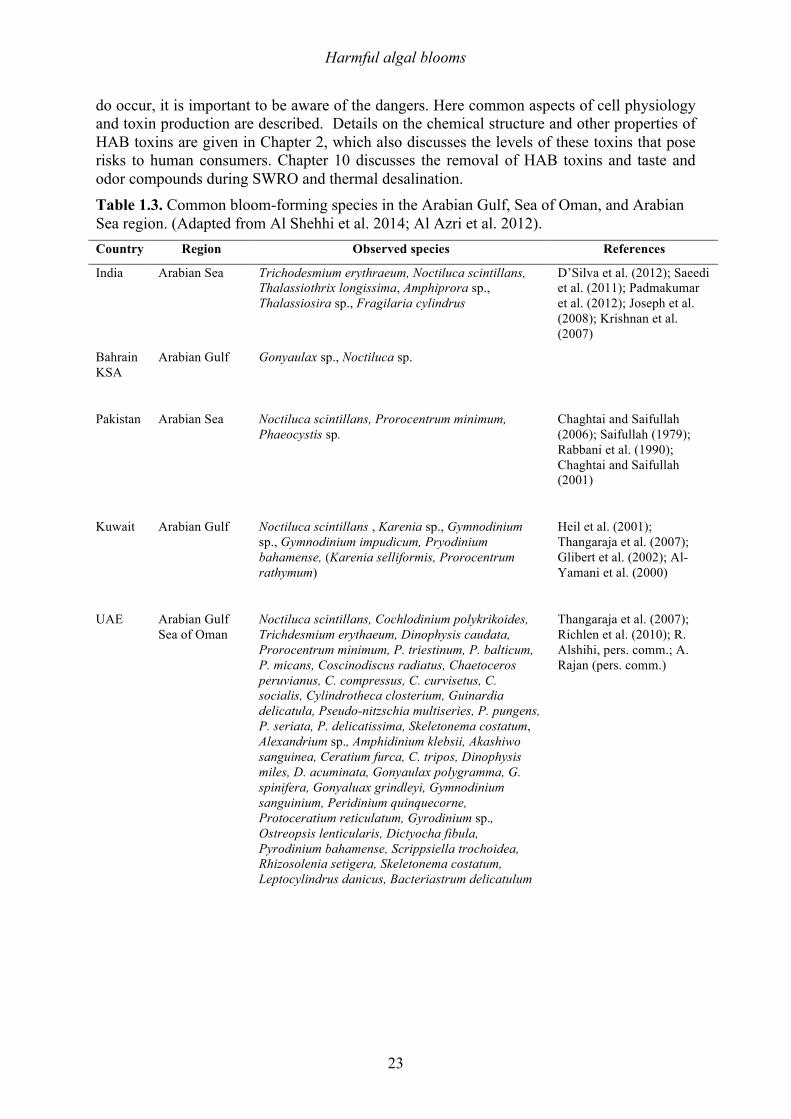
do occur, it is important to be aware of the dangers. Here common aspects of cell physiology and toxin production are described. Details on the chemical structure and other properties of HAB toxins are given in Chapter 2, which also discusses the levels of these toxins that pose risks to human consumers. Chapter 10 discusses the removal of HAB toxins and taste and odor compounds during SWRO and thermal desalination. Table 1.3. Common bloom-forming species in the Arabian Gulf, Sea of Oman, and Arabian Sea region. (Adapted from Al Shehhi et al. 2014; Al Azri et al. 2012). Country Region Observed species References

India Arabian Sea Trichodesmium erythraeum, Noctiluca scintillans, Thalassiothrix longissima, Amphiprora sp., Thalassiosira sp., Fragilaria cylindrus

D’Silva et al. (2012); Saeedi et al. (2011); Padmakumar et al. (2012); Joseph et al. (2008); Krishnan et al. (2007)

Bahrain KSA

Arabian Gulf Gonyaulax sp., Noctiluca sp.

Pakistan Arabian Sea Noctiluca scintillans, Prorocentrum minimum, Phaeocystis sp.

Chaghtai and Saifullah (2006); Saifullah (1979); Rabbani et al. (1990); Chaghtai and Saifullah (2001)

Kuwait Arabian Gulf Noctiluca scintillans , Karenia sp., Gymnodinium sp., Gymnodinium impudicum, Pryodinium bahamense, (Karenia selliformis, Prorocentrum rathymum)

Heil et al. (2001); Thangaraja et al. (2007); Glibert et al. (2002); Al-Yamani et al. (2000)

UAE

Arabian Gulf Sea of Oman

Noctiluca scintillans, Cochlodinium polykrikoides, Trichdesmium erythaeum, Dinophysis caudata, Prorocentrum minimum, P. triestinum, P. balticum, P. micans, Coscinodiscus radiatus, Chaetoceros peruvianus, C. compressus, C. curvisetus, C. socialis, Cylindrotheca closterium, Guinardia delicatula, Pseudo-nitzschia multiseries, P. pungens, P. seriata, P. delicatissima, Skeletonema costatum, Alexandrium sp., Amphidinium klebsii, Akashiwo sanguinea, Ceratium furca, C. tripos, Dinophysis miles, D. acuminata, Gonyaulax polygramma, G. spinifera, Gonyaluax grindleyi, Gymnodinium sanguinium, Peridinium quinquecorne, Protoceratium reticulatum, Gyrodinium sp., Ostreopsis lenticularis, Dictyocha fibula, Pyrodinium bahamense, Scrippsiella trochoidea, Rhizosolenia setigera, Skeletonema costatum, Leptocylindrus danicus, Bacteriastrum delicatulum

Thangaraja et al. (2007); Richlen et al. (2010); R. Alshihi, pers. comm.; A. Rajan (pers. comm.)

Harmful algal blooms

24

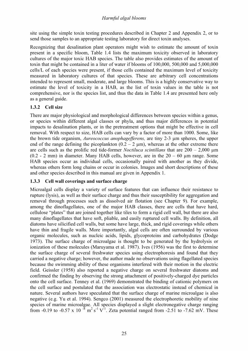
Table 1.3. (Continued) Country Region Observed species References

Oman Qatar

Arabian Sea, Sea of Oman Arabian Gulf

Phaeocystis globosa, Nitzschia longissima,, Navicula directa, Rhizosolenia spp., Chaetoceros didymus, Noctiluca scintillans, Gymnodinium sp., Karenia sp., Dinophysis sp., Trichodesmium sp., Coscinodiscus sp., Ceratium furca, Prorocentrum arabianum, Prorocentrum minimum, Gymnodinium breve Pseudo-nitzschia spp., Alexandrium spp., Pyrodinium bahamense Alexandrium sp., Dinophysis sp., Pseudo-nitzschia sp., Gymnodinium breve

Madhupratap et al. (2000); Thangaraja et al (2007); Morton et al. (2002); Al Azri et al. (2012); Tang et al. (2002); Al-Busaidi et al. (2008); Al Gheilani et al. (2011); Saeedi et al. (2011) Al-Ansi et al. (2002)

Iran

Arabian Gulf Karenia spp, Cochlodinium polykrikoides, Trichodesmium sp., Noctiluca scintillans, Navicula sp.

Thangaraja et al. (2007); Fatemi et al. (2012)

___________________________________________________________________________

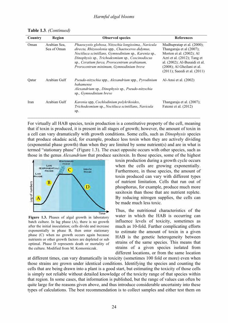
For virtually all HAB species, toxin production is a constitutive property of the cell, meaning that if toxin is produced, it is present in all stages of growth; however, the amount of toxin in a cell can vary dramatically with growth conditions. Some cells, such as Dinophysis species that produce okadaic acid, for example, produce less toxin when they are actively dividing (exponential phase growth) than when they are limited by some nutrient(s) and are in what is termed “stationary phase” (Figure 1.3). The exact opposite occurs with other species, such as those in the genus Alexandrium that produce saxitoxin. In those species, some of the highest

toxin production during a growth cycle occurs when the cells are growing exponentially. Furthermore, in those species, the amount of toxin produced can vary with different types of nutrient limitation. Cells that run out of phosphorus, for example, produce much more saxitoxin than those that are nutrient replete. By reducing nitrogen supplies, the cells can be made much less toxic.

Thus, the nutritional characteristics of the water in which the HAB is occurring can influence levels of toxicity, sometimes as much as 10-fold. Further complicating efforts to estimate the amount of toxin in a given HAB is the genetic heterogeneity between strains of the same species. This means that strains of a given species isolated from different locations, or from the same location

at different times, can vary dramatically in toxicity (sometimes 100 fold or more) even when those strains are grown under identical conditions. Identifying the species and counting the cells that are being drawn into a plant is a good start, but estimating the toxicity of those cells is simply not reliable without detailed knowledge of the toxicity range of that species within that region. In some cases, that information is published, but the range of values can often be quite large for the reasons given above, and thus introduce considerable uncertainty into these types of calculations. The best recommendation is to collect samples and either test them on

Figure 1.3. Phases of algal growth in laboratory batch culture. In lag phase (A), there is no growth after the initial inoculation; cells divide and increase exponentially in phase B, then enter stationary phase (C) when no growth occurs again because nutrients or other growth factors are depleted or sub optimal. Phase D represents death or mortality of the culture. Modified from M. Komorniczak.

Harmful algal blooms

25

site using the simple toxin testing procedures described in Chapter 2 and Appendix 2, or to send those samples to an appropriate testing laboratory for direct toxin analyses.

Recognizing that desalination plant operators might wish to estimate the amount of toxin present in a specific bloom, Table 1.4 lists the maximum toxicity observed in laboratory cultures of the major toxic HAB species. The table also provides estimates of the amount of toxin that might be contained in a liter of water if blooms of 100,000, 500,000 and 5,000,000 cells/L of each species were present, if those cells contained the maximum level of toxicity measured in laboratory cultures of that species. These are arbitrary cell concentrations intended to represent small, moderate, and large blooms. This is a highly conservative way to estimate the level of toxicity in a HAB, as the list of toxin values in the table is not comprehensive, nor is the species list, and thus the data in Table 1.4 are presented here only as a general guide.

1.3.2! Cell size There are major physiological and morphological differences between species within a genus, or species within different algal classes or phyla, and thus major differences in potential impacts to desalination plants, or in the pretreatment options that might be effective in cell removal. With respect to size, HAB cells can vary by a factor of more than 1000. Some, like the brown tide organism, Aureococcus anophagefferens, are tiny 2-3 µm spheres, the upper end of the range defining the picoplankton (0.2 – 2 µm), whereas at the other extreme there are cells such as the prolific red tide-former Noctiluca scintillans that are 200 – 2,000 µm (0.2 - 2 mm) in diameter. Many HAB cells, however, are in the 20 – 60 µm range. Some HAB species occur as individual cells, occasionally paired with another as they divide, whereas others form long chains or occur in colonies. Images and short descriptions of these and other species described in this manual are given in Appendix 1.

1.3.3! Cell wall coverings and surface charge Microalgal cells display a variety of surface features that can influence their resistance to rupture (lysis), as well as their surface charge and thus their susceptibility for aggregation and removal through processes such as dissolved air flotation (see Chapter 9). For example, among the dinoflagellates, one of the major HAB classes, there are cells that have hard, cellulose “plates” that are joined together like tiles to form a rigid cell wall, but there are also many dinoflagellates that have soft, pliable, and easily ruptured cell walls. By definition, all diatoms have silicified cell walls, but some have large, thick, and rigid coverings while others have thin and fragile walls. More importantly, algal cells are often surrounded by various organic molecules, such as nucleic acids, lipids, glycoproteins and carbohydrates (Dodge 1973). The surface charge of microalgae is thought to be generated by the hydrolysis or ionization of these molecules (Maruyama et al. 1987). Ives (1956) was the first to determine the surface charge of several freshwater species using electrophoresis and found that they carried a negative charge; however, the author made no observations using flagellated species because the swimming ability of these organisms interfered with their motion in the electric field. Geissler (1958) also reported a negative charge on several freshwater diatoms and confirmed the finding by observing the strong attachment of positively-charged dye particles onto the cell surface. Tenney et al. (1969) demonstrated the binding of cationic polymers on the cell surface and postulated that the association was electrostatic instead of chemical in nature. Several authors have speculated that the surface charge of marine microalgae is also negative (e.g. Yu et al. 1994). Sengco (2001) measured the electrophoretic mobility of nine species of marine microalgae. All species displayed a slight electronegative charge ranging from -0.19 to -0.57 x 10 -8 m2 s-1 V-1. Zeta potential ranged from -2.51 to -7.62 mV. These

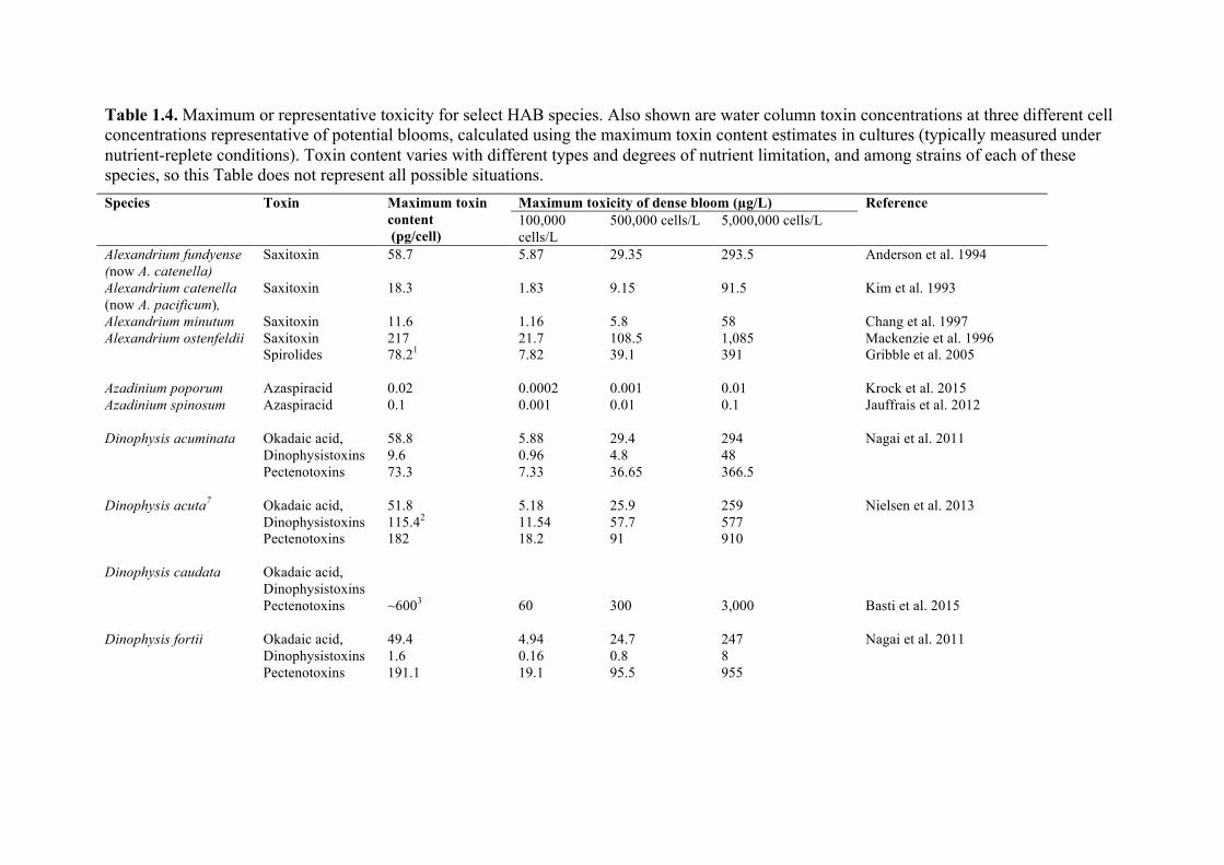
Table 1.4. Maximum or representative toxicity for select HAB species. Also shown are water column toxin concentrations at three different cell concentrations representative of potential blooms, calculated using the maximum toxin content estimates in cultures (typically measured under nutrient-replete conditions). Toxin content varies with different types and degrees of nutrient limitation, and among strains of each of these species, so this Table does not represent all possible situations. Species Toxin Maximum toxin

content (pg/cell)

Maximum toxicity of dense bloom (µg/L) Reference 100,000 cells/L

500,000 cells/L 5,000,000 cells/L

Alexandrium fundyense (now A. catenella)

Saxitoxin 58.7 5.87 29.35 293.5 Anderson et al. 1994

Alexandrium catenella (now A. pacificum),

Saxitoxin 18.3 1.83 9.15 91.5

Kim et al. 1993

Alexandrium minutum Saxitoxin 11.6 1.16 5.8 58 Chang et al. 1997 Alexandrium ostenfeldii Saxitoxin

Spirolides 217 78.21

21.7 7.82

108.5 39.1

1,085 391

Mackenzie et al. 1996 Gribble et al. 2005

Azadinium poporum Azadinium spinosum

Azaspiracid Azaspiracid

0.02 0.1

0.0002 0.001

0.001 0.01

0.01 0.1

Krock et al. 2015 Jauffrais et al. 2012

Dinophysis acuminata Okadaic acid,

Dinophysistoxins Pectenotoxins

58.8 9.6 73.3

5.88 0.96 7.33

29.4 4.8 36.65

294 48 366.5

Nagai et al. 2011

Dinophysis acuta7 Okadaic acid,

Dinophysistoxins Pectenotoxins

51.8 115.42

182

5.18 11.54 18.2

25.9 57.7 91

259 577 910

Nielsen et al. 2013

Dinophysis caudata Okadaic acid,

Dinophysistoxins Pectenotoxins

~6003

60

300

3,000

Basti et al. 2015

Dinophysis fortii Okadaic acid,

Dinophysistoxins Pectenotoxins

49.4 1.6 191.1

4.94 0.16 19.1

24.7 0.8 95.5

247 8 955

Nagai et al. 2011

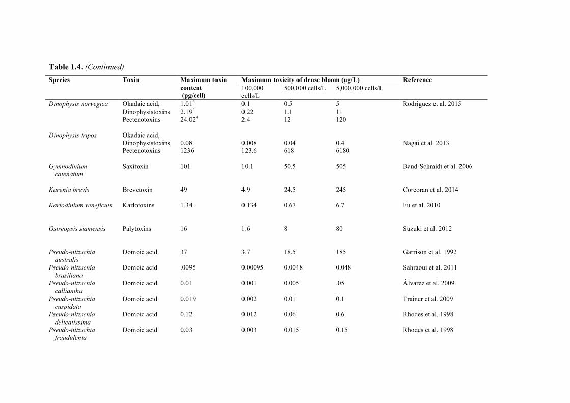
Table 1.4. (Continued) Species Toxin Maximum toxin

content (pg/cell)

Maximum toxicity of dense bloom (µg/L) Reference 100,000 cells/L

500,000 cells/L 5,000,000 cells/L

Dinophysis norvegica Okadaic acid, Dinophysistoxins Pectenotoxins

1.014 2.194 24.024

0.1 0.22 2.4

0.5 1.1 12

5 11 120

Rodriguez et al. 2015

Dinophysis tripos Okadaic acid,

Dinophysistoxins Pectenotoxins

0.08 1236

0.008 123.6

0.04 618

0.4 6180

Nagai et al. 2013

Gymnodinium

catenatum Saxitoxin 101 10.1 50.5 505 Band-Schmidt et al. 2006

Karenia brevis Brevetoxin 49 4.9 24.5 245 Corcoran et al. 2014 Karlodinium veneficum Karlotoxins 1.34

0.134

0.67

6.7

Fu et al. 2010

Ostreopsis siamensis Palytoxins 16

1.6 8 80 Suzuki et al. 2012

Pseudo-nitzschia

australis Domoic acid 37 3.7 18.5 185 Garrison et al. 1992

Pseudo-nitzschia brasiliana

Domoic acid .0095 0.00095 0.0048 0.048 Sahraoui et al. 2011

Pseudo-nitzschia calliantha

Domoic acid 0.01 0.001 0.005 .05 Álvarez et al. 2009

Pseudo-nitzschia cuspidata

Domoic acid 0.019 0.002 0.01 0.1 Trainer et al. 2009

Pseudo-nitzschia delicatissima

Domoic acid 0.12 0.012 0.06 0.6 Rhodes et al. 1998

Pseudo-nitzschia fraudulenta

Domoic acid 0.03 0.003 0.015 0.15 Rhodes et al. 1998

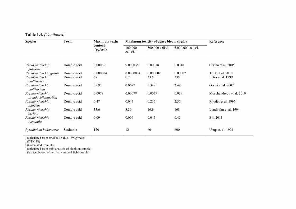
Table 1.4. (Continued) Species Toxin Maximum toxin

content (pg/cell)

Maximum toxicity of dense bloom (µg/L) Reference

100,000 cells/L

500,000 cells/L 5,000,000 cells/L

Pseudo-nitzschia

galaxiae Domoic acid 0.00036 0.000036 0.00018 0.0018 Cerino et al. 2005

Pseudo-nitzschia granii Domoic acid 0.000004 0.0000004 0.000002 0.00002 Trick et al. 2010 Pseudo-nitzschia

multiseries Domoic acid 67 6.7 33.5 335 Bates et al. 1999

Pseudo-nitzschia multistriata

Domoic acid 0.697 0.0697 0.349 3.49 Orsini et al. 2002

Pseudo-nitzschia pseudodelicatissima

Domoic acid 0.0078 0.00078 0.0039 0.039 Moschandreou et al. 2010

Pseudo-nitzschia pungens

Domoic acid 0.47 0.047 0.235 2.35 Rhodes et al. 1996

Pseudo-nitzschia seriata

Domoic acid 33.6 3.36 16.8 168 Lundholm et al. 1994

Pseudo-nitzschia turgidula

Domoic acid 0.09 0.009 0.045 0.45

Bill 2011

Pyrodinium bahamense Saxitoxin 120 12 60 600 Usup et. al. 1994 1 (calculated from fmol/cell value - 692g/mole) 2 (DTX-1b) 3 (Calculated from plot) 4 (calculated from bulk analysis of plankton sample) 5 (lab incubation of nutrient enriched field sample)

Chapter 1 – Harmful algal blooms

29

data confirm the prediction that marine algal species, including the dinoflagellates, possess negative surface charges like their freshwater counterparts (Maruyama et al. 1987; Shirota 1989; Yu et al. 1994). The magnitude of these charges was, however, small compared to freshwater algae, as Ives (1956) reported a range of zeta potential between -7.6 mV to -11.6 mV at pH values from 7.2 to 8.8 in freshwater, while the values reported by Sengco (2001) ranged from -2.5 to -7.7 mV. Zhu et al. (2014) measured the zeta potential of the dinoflagellate Prorocentrum minimum to be about -4 mV at a moderate cell concentration. A few of the species listed in Table 1.3 are worth highlighting because of the scale of their impacts, or their prevalence in regions with significant desalination capacity, or simply because they are prolific bloom formers. One of the most significant is Cochlodinium polykrikoides, the organism that disrupted desalination operations at many plants in the Arabian Gulf and Sea of Oman in 2008 and 2009 (Richlen et al. 2010; Shahid and Al Sadi 2015). First described from Puerto Rico in the Caribbean by Margalef (1961), the geographic distribution of C. polykrikoides is widespread, and populations have been documented in tropical and warm-temperate waters around the world, including the Caribbean Sea, eastern and western Pacific Ocean, the eastern Atlantic Ocean, Indian Ocean, and Mediterranean Sea (see Kudela et al. 2008; Matsuoka et al. 2008). This species has been spreading globally in recent years and thus represents a significant threat to desalination operations worldwide.

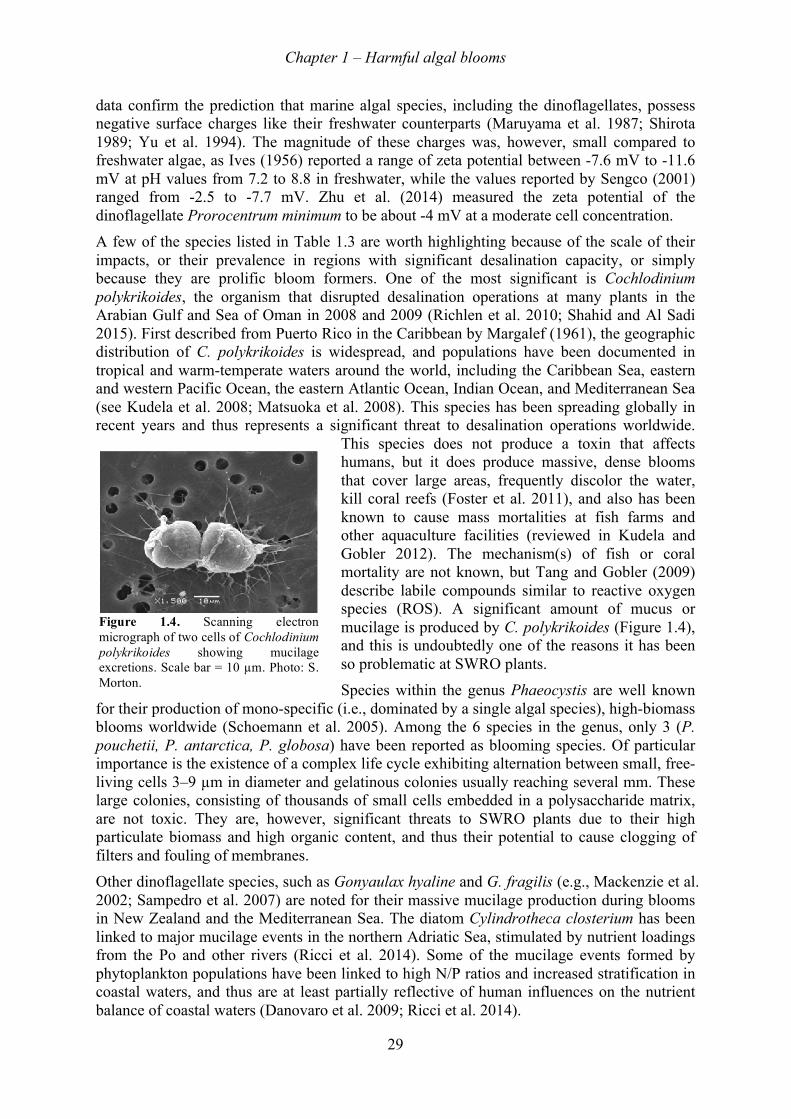
This species does not produce a toxin that affects humans, but it does produce massive, dense blooms that cover large areas, frequently discolor the water, kill coral reefs (Foster et al. 2011), and also has been known to cause mass mortalities at fish farms and other aquaculture facilities (reviewed in Kudela and Gobler 2012). The mechanism(s) of fish or coral mortality are not known, but Tang and Gobler (2009) describe labile compounds similar to reactive oxygen species (ROS). A significant amount of mucus or mucilage is produced by C. polykrikoides (Figure 1.4), and this is undoubtedly one of the reasons it has been so problematic at SWRO plants. Species within the genus Phaeocystis are well known

for their production of mono-specific (i.e., dominated by a single algal species), high-biomass blooms worldwide (Schoemann et al. 2005). Among the 6 species in the genus, only 3 (P. pouchetii, P. antarctica, P. globosa) have been reported as blooming species. Of particular importance is the existence of a complex life cycle exhibiting alternation between small, free-living cells 3–9 µm in diameter and gelatinous colonies usually reaching several mm. These large colonies, consisting of thousands of small cells embedded in a polysaccharide matrix, are not toxic. They are, however, significant threats to SWRO plants due to their high particulate biomass and high organic content, and thus their potential to cause clogging of filters and fouling of membranes. Other dinoflagellate species, such as Gonyaulax hyaline and G. fragilis (e.g., Mackenzie et al. 2002; Sampedro et al. 2007) are noted for their massive mucilage production during blooms in New Zealand and the Mediterranean Sea. The diatom Cylindrotheca closterium has been linked to major mucilage events in the northern Adriatic Sea, stimulated by nutrient loadings from the Po and other rivers (Ricci et al. 2014). Some of the mucilage events formed by phytoplankton populations have been linked to high N/P ratios and increased stratification in coastal waters, and thus are at least partially reflective of human influences on the nutrient balance of coastal waters (Danovaro et al. 2009; Ricci et al. 2014).

Figure 1.4. Scanning electron micrograph of two cells of Cochlodinium polykrikoides showing mucilage excretions. Scale bar = 10 µm. Photo: S. Morton.

Chapter 1 – Harmful algal blooms

30

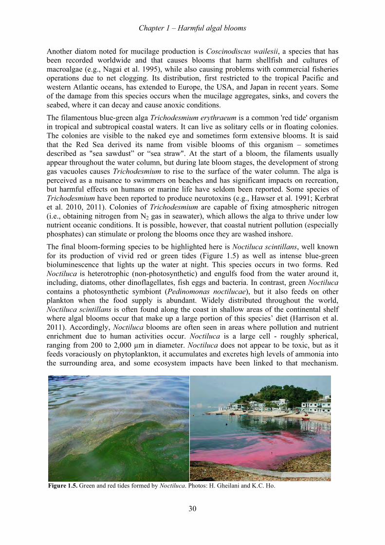
Another diatom noted for mucilage production is Coscinodiscus wailesii, a species that has been recorded worldwide and that causes blooms that harm shellfish and cultures of macroalgae (e.g., Nagai et al. 1995), while also causing problems with commercial fisheries operations due to net clogging. Its distribution, first restricted to the tropical Pacific and western Atlantic oceans, has extended to Europe, the USA, and Japan in recent years. Some of the damage from this species occurs when the mucilage aggregates, sinks, and covers the seabed, where it can decay and cause anoxic conditions. The filamentous blue-green alga Trichodesmium erythraeum is a common 'red tide' organism in tropical and subtropical coastal waters. It can live as solitary cells or in floating colonies. The colonies are visible to the naked eye and sometimes form extensive blooms. It is said that the Red Sea derived its name from visible blooms of this organism – sometimes described as "sea sawdust” or “sea straw". At the start of a bloom, the filaments usually appear throughout the water column, but during late bloom stages, the development of strong gas vacuoles causes Trichodesmium to rise to the surface of the water column. The alga is perceived as a nuisance to swimmers on beaches and has significant impacts on recreation, but harmful effects on humans or marine life have seldom been reported. Some species of Trichodesmium have been reported to produce neurotoxins (e.g., Hawser et al. 1991; Kerbrat et al. 2010, 2011). Colonies of Trichodesmium are capable of fixing atmospheric nitrogen (i.e., obtaining nitrogen from N2 gas in seawater), which allows the alga to thrive under low nutrient oceanic conditions. It is possible, however, that coastal nutrient pollution (especially phosphates) can stimulate or prolong the blooms once they are washed inshore. The final bloom-forming species to be highlighted here is Noctiluca scintillans, well known for its production of vivid red or green tides (Figure 1.5) as well as intense blue-green bioluminescence that lights up the water at night. This species occurs in two forms. Red Noctiluca is heterotrophic (non-photosynthetic) and engulfs food from the water around it, including, diatoms, other dinoflagellates, fish eggs and bacteria. In contrast, green Noctiluca contains a photosynthetic symbiont (Pedinomonas noctilucae), but it also feeds on other plankton when the food supply is abundant. Widely distributed throughout the world, Noctiluca scintillans is often found along the coast in shallow areas of the continental shelf where algal blooms occur that make up a large portion of this species’ diet (Harrison et al. 2011). Accordingly, Noctiluca blooms are often seen in areas where pollution and nutrient enrichment due to human activities occur. Noctiluca is a large cell - roughly spherical, ranging from 200 to 2,000 µm in diameter. Noctiluca does not appear to be toxic, but as it feeds voraciously on phytoplankton, it accumulates and excretes high levels of ammonia into the surrounding area, and some ecosystem impacts have been linked to that mechanism.

Figure 1.5. Green and red tides formed by Noctiluca. Photos: H. Gheilani and K.C. Ho.

Chapter 1 – Harmful algal blooms

31

Some report ammonia concentrations as high as 250 µg/L during Noctiluca blooms (G. Hallegraeff, pers. comm.). This characteristic should be of interest to the desalination industry because shock chlorination of water containing high levels of ammonia can lead to production of the highly potent carcinogen N-nitrosodimethylamine (NDMA) (e.g., Mitch and Sedlak 2002). Current NDMA guidelines for drinking waters are as low as 10 ng/L.

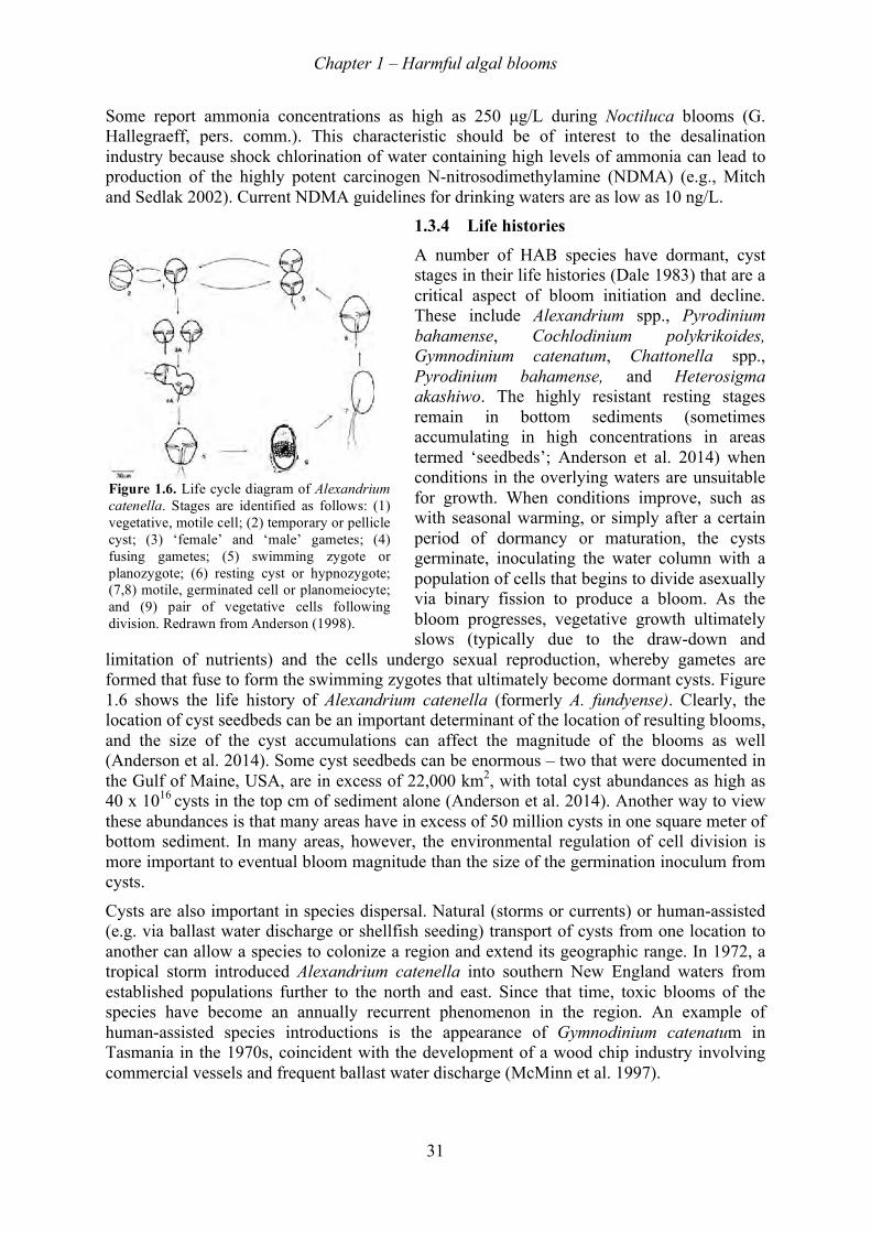
1.3.4! Life histories A number of HAB species have dormant, cyst stages in their life histories (Dale 1983) that are a critical aspect of bloom initiation and decline. These include Alexandrium spp., Pyrodinium bahamense, Cochlodinium polykrikoides, Gymnodinium catenatum, Chattonella spp., Pyrodinium bahamense, and Heterosigma akashiwo. The highly resistant resting stages remain in bottom sediments (sometimes accumulating in high concentrations in areas termed ‘seedbeds’; Anderson et al. 2014) when conditions in the overlying waters are unsuitable for growth. When conditions improve, such as with seasonal warming, or simply after a certain period of dormancy or maturation, the cysts germinate, inoculating the water column with a population of cells that begins to divide asexually via binary fission to produce a bloom. As the bloom progresses, vegetative growth ultimately slows (typically due to the draw-down and

limitation of nutrients) and the cells undergo sexual reproduction, whereby gametes are formed that fuse to form the swimming zygotes that ultimately become dormant cysts. Figure 1.6 shows the life history of Alexandrium catenella (formerly A. fundyense). Clearly, the location of cyst seedbeds can be an important determinant of the location of resulting blooms, and the size of the cyst accumulations can affect the magnitude of the blooms as well (Anderson et al. 2014). Some cyst seedbeds can be enormous – two that were documented in the Gulf of Maine, USA, are in excess of 22,000 km2, with total cyst abundances as high as 40 x 1016 cysts in the top cm of sediment alone (Anderson et al. 2014). Another way to view these abundances is that many areas have in excess of 50 million cysts in one square meter of bottom sediment. In many areas, however, the environmental regulation of cell division is more important to eventual bloom magnitude than the size of the germination inoculum from cysts.

Cysts are also important in species dispersal. Natural (storms or currents) or human-assisted (e.g. via ballast water discharge or shellfish seeding) transport of cysts from one location to another can allow a species to colonize a region and extend its geographic range. In 1972, a tropical storm introduced Alexandrium catenella into southern New England waters from established populations further to the north and east. Since that time, toxic blooms of the species have become an annually recurrent phenomenon in the region. An example of human-assisted species introductions is the appearance of Gymnodinium catenatum in Tasmania in the 1970s, coincident with the development of a wood chip industry involving commercial vessels and frequent ballast water discharge (McMinn et al. 1997).

Figure 1.6. Life cycle diagram of Alexandrium catenella. Stages are identified as follows: (1) vegetative, motile cell; (2) temporary or pellicle cyst; (3) ‘female’ and ‘male’ gametes; (4) fusing gametes; (5) swimming zygote or planozygote; (6) resting cyst or hypnozygote; (7,8) motile, germinated cell or planomeiocyte; and (9) pair of vegetative cells following division. Redrawn from Anderson (1998).

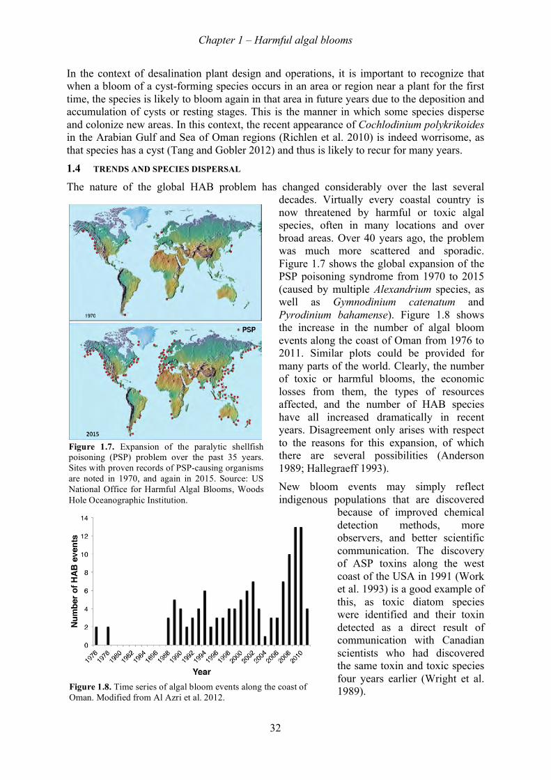
Chapter 1 – Harmful algal blooms

32

In the context of desalination plant design and operations, it is important to recognize that when a bloom of a cyst-forming species occurs in an area or region near a plant for the first time, the species is likely to bloom again in that area in future years due to the deposition and accumulation of cysts or resting stages. This is the manner in which some species disperse and colonize new areas. In this context, the recent appearance of Cochlodinium polykrikoides in the Arabian Gulf and Sea of Oman regions (Richlen et al. 2010) is indeed worrisome, as that species has a cyst (Tang and Gobler 2012) and thus is likely to recur for many years. 1.4! TRENDS AND SPECIES DISPERSAL The nature of the global HAB problem has changed considerably over the last several

decades. Virtually every coastal country is now threatened by harmful or toxic algal species, often in many locations and over broad areas. Over 40 years ago, the problem was much more scattered and sporadic. Figure 1.7 shows the global expansion of the PSP poisoning syndrome from 1970 to 2015 (caused by multiple Alexandrium species, as well as Gymnodinium catenatum and Pyrodinium bahamense). Figure 1.8 shows the increase in the number of algal bloom events along the coast of Oman from 1976 to 2011. Similar plots could be provided for many parts of the world. Clearly, the number of toxic or harmful blooms, the economic losses from them, the types of resources affected, and the number of HAB species have all increased dramatically in recent years. Disagreement only arises with respect to the reasons for this expansion, of which there are several possibilities (Anderson 1989; Hallegraeff 1993). New bloom events may simply reflect indigenous populations that are discovered

because of improved chemical detection methods, more observers, and better scientific communication. The discovery of ASP toxins along the west coast of the USA in 1991 (Work et al. 1993) is a good example of this, as toxic diatom species were identified and their toxin detected as a direct result of communication with Canadian scientists who had discovered the same toxin and toxic species four years earlier (Wright et al. 1989).

Figure 1.8. Time series of algal bloom events along the coast of Oman. Modified from Al Azri et al. 2012.

Figure 1.7. Expansion of the paralytic shellfish poisoning (PSP) problem over the past 35 years. Sites with proven records of PSP-causing organisms are noted in 1970, and again in 2015. Source: US National Office for Harmful Algal Blooms, Woods Hole Oceanographic Institution.

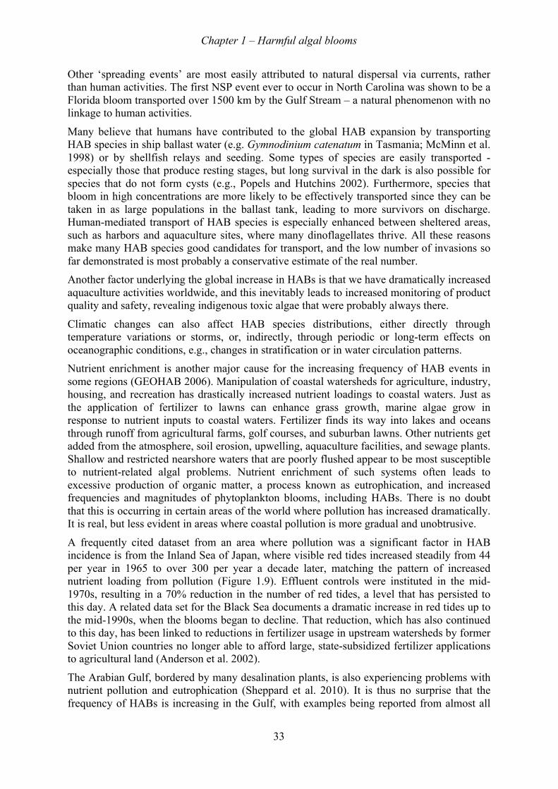
Chapter 1 – Harmful algal blooms

33

Other ‘spreading events’ are most easily attributed to natural dispersal via currents, rather than human activities. The first NSP event ever to occur in North Carolina was shown to be a Florida bloom transported over 1500 km by the Gulf Stream – a natural phenomenon with no linkage to human activities.

Many believe that humans have contributed to the global HAB expansion by transporting HAB species in ship ballast water (e.g. Gymnodinium catenatum in Tasmania; McMinn et al. 1998) or by shellfish relays and seeding. Some types of species are easily transported - especially those that produce resting stages, but long survival in the dark is also possible for species that do not form cysts (e.g., Popels and Hutchins 2002). Furthermore, species that bloom in high concentrations are more likely to be effectively transported since they can be taken in as large populations in the ballast tank, leading to more survivors on discharge. Human-mediated transport of HAB species is especially enhanced between sheltered areas, such as harbors and aquaculture sites, where many dinoflagellates thrive. All these reasons make many HAB species good candidates for transport, and the low number of invasions so far demonstrated is most probably a conservative estimate of the real number. Another factor underlying the global increase in HABs is that we have dramatically increased aquaculture activities worldwide, and this inevitably leads to increased monitoring of product quality and safety, revealing indigenous toxic algae that were probably always there.

Climatic changes can also affect HAB species distributions, either directly through temperature variations or storms, or, indirectly, through periodic or long-term effects on oceanographic conditions, e.g., changes in stratification or in water circulation patterns. Nutrient enrichment is another major cause for the increasing frequency of HAB events in some regions (GEOHAB 2006). Manipulation of coastal watersheds for agriculture, industry, housing, and recreation has drastically increased nutrient loadings to coastal waters. Just as the application of fertilizer to lawns can enhance grass growth, marine algae grow in response to nutrient inputs to coastal waters. Fertilizer finds its way into lakes and oceans through runoff from agricultural farms, golf courses, and suburban lawns. Other nutrients get added from the atmosphere, soil erosion, upwelling, aquaculture facilities, and sewage plants. Shallow and restricted nearshore waters that are poorly flushed appear to be most susceptible to nutrient-related algal problems. Nutrient enrichment of such systems often leads to excessive production of organic matter, a process known as eutrophication, and increased frequencies and magnitudes of phytoplankton blooms, including HABs. There is no doubt that this is occurring in certain areas of the world where pollution has increased dramatically. It is real, but less evident in areas where coastal pollution is more gradual and unobtrusive.

A frequently cited dataset from an area where pollution was a significant factor in HAB incidence is from the Inland Sea of Japan, where visible red tides increased steadily from 44 per year in 1965 to over 300 per year a decade later, matching the pattern of increased nutrient loading from pollution (Figure 1.9). Effluent controls were instituted in the mid-1970s, resulting in a 70% reduction in the number of red tides, a level that has persisted to this day. A related data set for the Black Sea documents a dramatic increase in red tides up to the mid-1990s, when the blooms began to decline. That reduction, which has also continued to this day, has been linked to reductions in fertilizer usage in upstream watersheds by former Soviet Union countries no longer able to afford large, state-subsidized fertilizer applications to agricultural land (Anderson et al. 2002).

The Arabian Gulf, bordered by many desalination plants, is also experiencing problems with nutrient pollution and eutrophication (Sheppard et al. 2010). It is thus no surprise that the frequency of HABs is increasing in the Gulf, with examples being reported from almost all

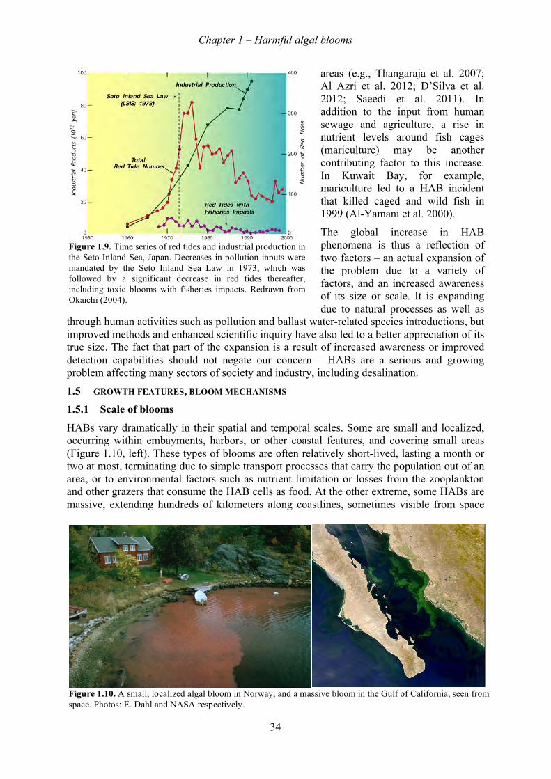
Chapter 1 – Harmful algal blooms

34

areas (e.g., Thangaraja et al. 2007; Al Azri et al. 2012; D’Silva et al. 2012; Saeedi et al. 2011). In addition to the input from human sewage and agriculture, a rise in nutrient levels around fish cages (mariculture) may be another contributing factor to this increase. In Kuwait Bay, for example, mariculture led to a HAB incident that killed caged and wild fish in 1999 (Al-Yamani et al. 2000).

The global increase in HAB phenomena is thus a reflection of two factors – an actual expansion of the problem due to a variety of factors, and an increased awareness of its size or scale. It is expanding due to natural processes as well as

through human activities such as pollution and ballast water-related species introductions, but improved methods and enhanced scientific inquiry have also led to a better appreciation of its true size. The fact that part of the expansion is a result of increased awareness or improved detection capabilities should not negate our concern – HABs are a serious and growing problem affecting many sectors of society and industry, including desalination.

1.5! GROWTH FEATURES, BLOOM MECHANISMS 1.5.1! Scale of blooms HABs vary dramatically in their spatial and temporal scales. Some are small and localized, occurring within embayments, harbors, or other coastal features, and covering small areas (Figure 1.10, left). These types of blooms are often relatively short-lived, lasting a month or two at most, terminating due to simple transport processes that carry the population out of an area, or to environmental factors such as nutrient limitation or losses from the zooplankton and other grazers that consume the HAB cells as food. At the other extreme, some HABs are massive, extending hundreds of kilometers along coastlines, sometimes visible from space

Figure 1.9. Time series of red tides and industrial production in the Seto Inland Sea, Japan. Decreases in pollution inputs were mandated by the Seto Inland Sea Law in 1973, which was followed by a significant decrease in red tides thereafter, including toxic blooms with fisheries impacts. Redrawn from Okaichi (2004).

Figure 1.10. A small, localized algal bloom in Norway, and a massive bloom in the Gulf of California, seen from space. Photos: E. Dahl and NASA respectively.

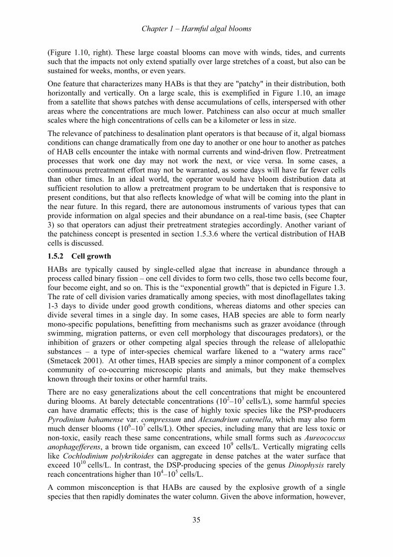
Chapter 1 – Harmful algal blooms

35

(Figure 1.10, right). These large coastal blooms can move with winds, tides, and currents such that the impacts not only extend spatially over large stretches of a coast, but also can be sustained for weeks, months, or even years. One feature that characterizes many HABs is that they are "patchy" in their distribution, both horizontally and vertically. On a large scale, this is exemplified in Figure 1.10, an image from a satellite that shows patches with dense accumulations of cells, interspersed with other areas where the concentrations are much lower. Patchiness can also occur at much smaller scales where the high concentrations of cells can be a kilometer or less in size.

The relevance of patchiness to desalination plant operators is that because of it, algal biomass conditions can change dramatically from one day to another or one hour to another as patches of HAB cells encounter the intake with normal currents and wind-driven flow. Pretreatment processes that work one day may not work the next, or vice versa. In some cases, a continuous pretreatment effort may not be warranted, as some days will have far fewer cells than other times. In an ideal world, the operator would have bloom distribution data at sufficient resolution to allow a pretreatment program to be undertaken that is responsive to present conditions, but that also reflects knowledge of what will be coming into the plant in the near future. In this regard, there are autonomous instruments of various types that can provide information on algal species and their abundance on a real-time basis, (see Chapter 3) so that operators can adjust their pretreatment strategies accordingly. Another variant of the patchiness concept is presented in section 1.5.3.6 where the vertical distribution of HAB cells is discussed. 1.5.2! Cell growth HABs are typically caused by single-celled algae that increase in abundance through a process called binary fission – one cell divides to form two cells, those two cells become four, four become eight, and so on. This is the “exponential growth” that is depicted in Figure 1.3. The rate of cell division varies dramatically among species, with most dinoflagellates taking 1-3 days to divide under good growth conditions, whereas diatoms and other species can divide several times in a single day. In some cases, HAB species are able to form nearly mono-specific populations, benefitting from mechanisms such as grazer avoidance (through swimming, migration patterns, or even cell morphology that discourages predators), or the inhibition of grazers or other competing algal species through the release of allelopathic substances – a type of inter-species chemical warfare likened to a “watery arms race” (Smetacek 2001). At other times, HAB species are simply a minor component of a complex community of co-occurring microscopic plants and animals, but they make themselves known through their toxins or other harmful traits. There are no easy generalizations about the cell concentrations that might be encountered during blooms. At barely detectable concentrations (102–103 cells/L), some harmful species can have dramatic effects; this is the case of highly toxic species like the PSP-producers Pyrodinium bahamense var. compressum and Alexandrium catenella, which may also form much denser blooms (106–107 cells/L). Other species, including many that are less toxic or non-toxic, easily reach these same concentrations, while small forms such as Aureococcus anophagefferens, a brown tide organism, can exceed 109 cells/L. Vertically migrating cells like Cochlodinium polykrikoides can aggregate in dense patches at the water surface that exceed 1010 cells/L. In contrast, the DSP-producing species of the genus Dinophysis rarely reach concentrations higher than 104–105 cells/L. A common misconception is that HABs are caused by the explosive growth of a single species that then rapidly dominates the water column. Given the above information, however,

Chapter 1 – Harmful algal blooms

36

it should be clear that it is only necessary to have conditions that favor the growth of a moderately large population of a given species and the proper hydrographic and meteorological conditions to permit the accumulation of those cells. In other words, coupled with normal or average growth rates, winds, tides, currents, fronts, and other hydrographic features can combine with organism behavior (e.g., vertical migration) to create discrete “patches” of cells (blooms) at all scales.

1.5.3! Bloom dynamics and coastal oceanography Though the number of HAB species is only a small fraction of the many algal species in the ocean, their diversity in terms of shape (morphology), physiology, and ecology is very large. In effect, there are hundreds of common HAB species and they differ in their growth characteristics and in the types of blooms they cause and the waters they inhabit. Given this diversity of species and habitats in which they occur, there exist few unifying principles that explain bloom dynamics in all habitats. A few common processes and mechanisms for bloom development and accumulation are highlighted below.

1.5.4! Bloom initiation HABs can be initiated from cells present at low concentrations, sometimes persisting in the background for months or years before a bloom develops (the “hidden flora” concept). Other

HABs are delivered to a location by tides and currents (see below). Still other HABs are initiated from resting cysts (Figure 1.11) that germinate from bottom sediments, significantly impacting many aspects of HAB phenomena. In those instances, cyst or spore germination provides the inoculum for blooms, and the transformation back to the resting state can remove substantial numbers of vegetative cells from the population and act as a major factor in bloom decline. Cysts are also important for population dispersal, including through ballast water transfer. They permit a species to survive through adverse conditions, and since sexuality is typically required for their formation, they facilitate genetic recombination. They can even be major sources of toxin to shellfish and other benthic animals.

1.5.5! Bloom transport Once a population is established, its geographic extent and biomass are affected by physical controls such as the transport and accumulation of cells in response to water flows (e.g., Franks and Anderson 1992), by the swimming behavior of organisms (Kamykowski 1995) and by the maintenance of suitable environmental conditions (including temperature and salinity, stratification, irradiance, and nutrient supply). These factors all interact to determine the timing, location, and ultimate biomass achieved by the bloom, as well as its impacts.

Physical processes that are likely to influence the population dynamics of HAB species are operative over a broad range of spatial and temporal scales. Large-scale circulation patterns (Figure 1.10) affect the distribution of water masses and their associated HABs. Some HABs are delivered into a specific region via advection (transport) after developing elsewhere. In

Figure 1.11. Satellite image of sea surface temperature, showing the warm Gulf Stream (blue) off the coast of North Carolina, USA. Several filaments of the Gulf Stream extend toward shore. These carried a toxic population of Karenia brevis that originated in the Gulf of Mexico, >1500 km away. Photo: NASA.

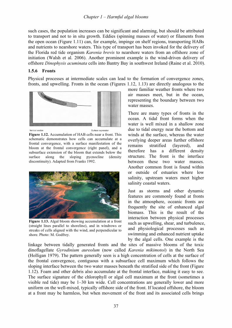
Chapter 1 – Harmful algal blooms

37

such cases, the population increases can be significant and alarming, but should be attributed to transport and not to in situ growth. Eddies (spinning masses of water) or filaments from the open ocean (Figure 1.11) can, for example, impinge on shelf regions, transporting HABs and nutrients to nearshore waters. This type of transport has been invoked for the delivery of the Florida red tide organism Karenia brevis to nearshore waters from an offshore zone of initiation (Walsh et al. 2006). Another prominent example is the wind-driven delivery of offshore Dinophysis acuminata cells into Bantry Bay in southwest Ireland (Raine et al. 2010). 1.5.6! Fronts Physical processes at intermediate scales can lead to the formation of convergence zones, fronts, and upwelling. Fronts in the ocean (Figures 1.12, 1.13) are directly analogous to the

more familiar weather fronts where two air masses meet, but in the ocean, representing the boundary between two water masses.

There are many types of fronts in the ocean. A tidal front forms when the water is well mixed in a shallow zone due to tidal energy near the bottom and winds at the surface, whereas the water overlying deeper areas further offshore remains stratified (layered), and therefore has a different density structure. The front is the interface between these two water masses. Another common front is found within or outside of estuaries where low salinity, upstream waters meet higher salinity coastal waters.

Just as storms and other dynamic features are commonly found at fronts in the atmosphere, oceanic fronts are frequently the site of enhanced algal biomass. This is the result of the interaction between physical processes such as upwelling, shear, and turbulence, and physiological processes such as swimming and enhanced nutrient uptake by the algal cells. One example is the

linkage between tidally generated fronts and the sites of massive blooms of the toxic dinoflagellate Gyrodinium aureolum (now called Karenia mikimotoi) in the North Sea (Holligan 1979). The pattern generally seen is a high concentration of cells at the surface of the frontal convergence, contiguous with a subsurface cell maximum which follows the sloping interface between the two water masses beneath the stratified side of the front (Figure 1.12). Foam and other debris also accumulate at the frontal interface, making it easy to see. The surface signature of the chlorophyll or algal cell maximum at the front (sometimes a visible red tide) may be 1–30 km wide. Cell concentrations are generally lower and more uniform on the well-mixed, typically offshore side of the front. If located offshore, the bloom at a front may be harmless, but when movement of the front and its associated cells brings

Figure 1.12. Accumulation of HAB cells near a front. This schematic demonstrates how cells can accumulate at a frontal convergence, with a surface manifestation of the bloom at the frontal convergence (right panel), and a subsurface extension of the bloom that extends below the surface along the sloping pycnocline (density discontinuity). Adapted from Franks 1992.

Figure 1.13. Algal bloom showing accumulation at a front (straight lines parallel to shoreline), and in windrows or streaks of cells aligned with the wind, and perpendicular to shore. Photo: M. Godfrey.

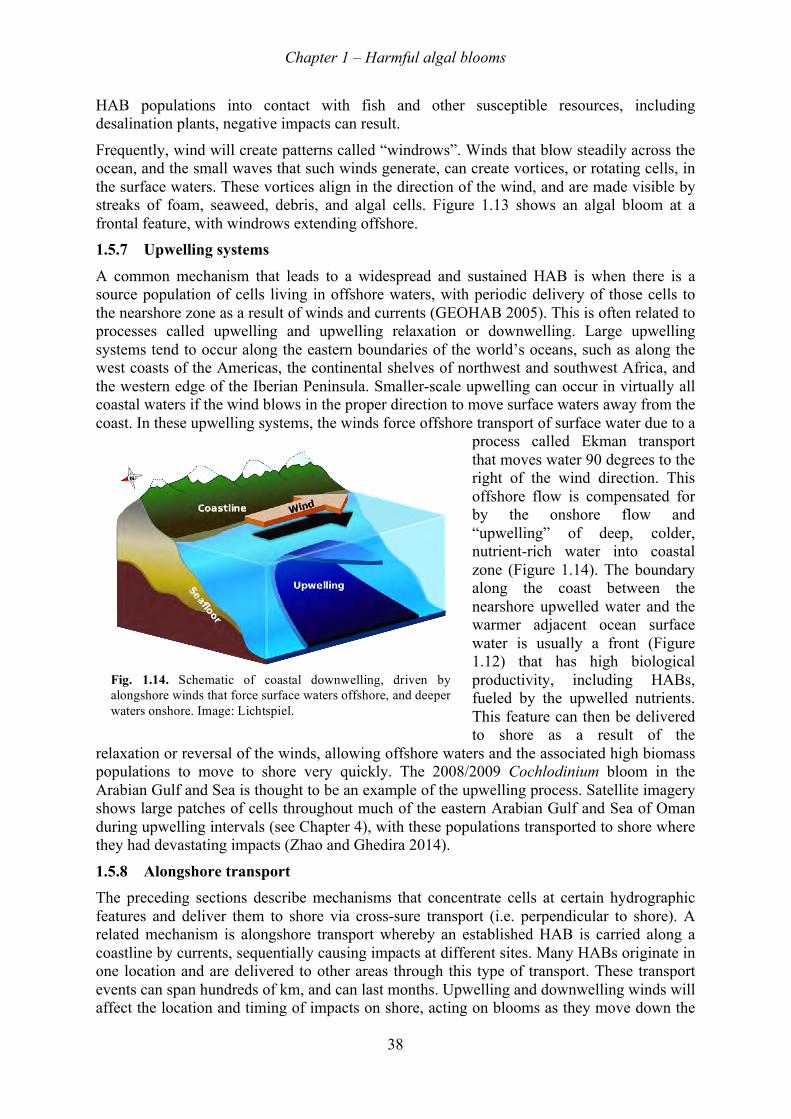
Chapter 1 – Harmful algal blooms

38

HAB populations into contact with fish and other susceptible resources, including desalination plants, negative impacts can result.

Frequently, wind will create patterns called “windrows”. Winds that blow steadily across the ocean, and the small waves that such winds generate, can create vortices, or rotating cells, in the surface waters. These vortices align in the direction of the wind, and are made visible by streaks of foam, seaweed, debris, and algal cells. Figure 1.13 shows an algal bloom at a frontal feature, with windrows extending offshore. 1.5.7! Upwelling systems A common mechanism that leads to a widespread and sustained HAB is when there is a source population of cells living in offshore waters, with periodic delivery of those cells to the nearshore zone as a result of winds and currents (GEOHAB 2005). This is often related to processes called upwelling and upwelling relaxation or downwelling. Large upwelling systems tend to occur along the eastern boundaries of the world’s oceans, such as along the west coasts of the Americas, the continental shelves of northwest and southwest Africa, and the western edge of the Iberian Peninsula. Smaller-scale upwelling can occur in virtually all coastal waters if the wind blows in the proper direction to move surface waters away from the coast. In these upwelling systems, the winds force offshore transport of surface water due to a

process called Ekman transport that moves water 90 degrees to the right of the wind direction. This offshore flow is compensated for by the onshore flow and “upwelling” of deep, colder, nutrient-rich water into coastal zone (Figure 1.14). The boundary along the coast between the nearshore upwelled water and the warmer adjacent ocean surface water is usually a front (Figure 1.12) that has high biological productivity, including HABs, fueled by the upwelled nutrients. This feature can then be delivered to shore as a result of the

relaxation or reversal of the winds, allowing offshore waters and the associated high biomass populations to move to shore very quickly. The 2008/2009 Cochlodinium bloom in the Arabian Gulf and Sea is thought to be an example of the upwelling process. Satellite imagery shows large patches of cells throughout much of the eastern Arabian Gulf and Sea of Oman during upwelling intervals (see Chapter 4), with these populations transported to shore where they had devastating impacts (Zhao and Ghedira 2014).

1.5.8! Alongshore transport The preceding sections describe mechanisms that concentrate cells at certain hydrographic features and deliver them to shore via cross-sure transport (i.e. perpendicular to shore). A related mechanism is alongshore transport whereby an established HAB is carried along a coastline by currents, sequentially causing impacts at different sites. Many HABs originate in one location and are delivered to other areas through this type of transport. These transport events can span hundreds of km, and can last months. Upwelling and downwelling winds will affect the location and timing of impacts on shore, acting on blooms as they move down the

Fig. 1.14. Schematic of coastal downwelling, driven by alongshore winds that force surface waters offshore, and deeper waters onshore. Image: Lichtspiel.

Chapter 1 – Harmful algal blooms

39

coast. The appearance of HABs can be sudden and unexpected at times, and in some of these instances, alongshore transport is the explanation. Operators should learn the nature of the transport pathways in the vicinity of their plant intakes to better anticipate and respond to HABs of this type.

An example of this type of transport is found with blooms of the PSP-toxin producing Alexandrium catenella in the Gulf of Maine (USA). In that region, the bloom populations are found within a low-salinity coastal current that travels along the coast (Franks and Anderson 1992). This water mass provides a suitable growth habitat for the Alexandrium cells as its southerly transport is regulated by river runoff, Coriolis forces (due to the Earth’s rotation), wind stress and other large-scale hydrographic forcings. Of these factors, wind appears to be particularly important in determining transport variability in surface waters. Downwelling-favorable winds (from the north or northeast) compress the plume against the coast and accelerate it alongshore, while an upwelling favorable wind (from the south) thins the low-salinity surface plume as it is moved offshore. Upwelling winds also retard the southward progression of the plume and its associated cells. In the downwelling case, the bloom would progress rapidly down the coast, whereas with upwelling, the bloom would move more slowly. The general velocity of alongshore transport of this bloom and Alexandrium cells during downwelling is roughly 0.2 m/s, or 17 km/d or 120 km in a week.

1.5.9! Vertical distributions An important feature of some HAB events, particularly in the context of desalination, is that the algal cells are often not uniformly distributed in the vertical direction (GEOHAB 2008). Typically, the “water column” in nearshore waters has a stratified structure whereby there is a surface layer that is warmer or fresher, and thus more buoyant than deeper waters. That layer is often stirred by winds, and is thus termed the "mixed layer". Algal cells and other constituents of the plankton that are non-motile are distributed uniformly through the mixed layer. Species that swim, however, such as many HAB species, can override that random mixing process and form aggregations at specific depths – sometimes at the surface, sometimes deeper. In some instances, these subsurface layers of cells do not move vertically because they are linked to some feature, such as the interface or density discontinuity between the mixed layer and the deeper waters (called the pycnocline) below which nutrients are typically higher than in the surface. Cells residing at that location would have ready access to high nutrients. For example, off the French coast, a thin layer of dinoflagellates, including the HAB species Dinophysis acuminata, is frequently observed in the proximity of the pycnocline (Gentien et al. 1995). Thin, subsurface layers have been observed at scales as small as 10 cm in the vertical and as large as 10 km in the horizontal. Some subsurface cell aggregations do move up and down, typically on a daily basis, due to a process called diel vertical migration. These migrating populations often reside in surface waters during the day to harvest the sunlight for photosynthesis, and then swim to the pycnocline and below to take up nutrients at night. This strategy can explain how dense accumulations of cells can appear in surface waters that are devoid of nutrients and which would seem to be incapable of supporting such apparent, prolific growth. In truth, the growth is not rapid; the cells are aggregating, not growing fast. This behavior also explains the disappearance, and the reappearance of cells or surface bloom patches on a daily basis. Typically, vertical movement down to 10, 15 or even 20 m have been observed, depending on the organism and depth of the mixed layer or water column. An example of the extent and timing of vertical movement is seen in Park et al. (2001) who observed the behaviour of Cochlodinium polykrikoides, the same species that caused desalination plant disruptions in 2008 and 2009 in the Arabian Gulf and Sea of Oman regions (Richlen et al. 2010; Shahid and

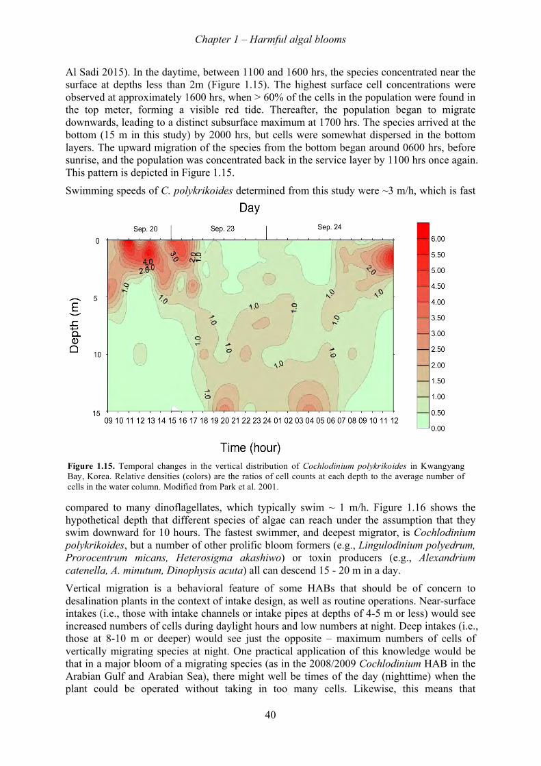
Chapter 1 – Harmful algal blooms

40

Al Sadi 2015). In the daytime, between 1100 and 1600 hrs, the species concentrated near the surface at depths less than 2m (Figure 1.15). The highest surface cell concentrations were observed at approximately 1600 hrs, when > 60% of the cells in the population were found in the top meter, forming a visible red tide. Thereafter, the population began to migrate downwards, leading to a distinct subsurface maximum at 1700 hrs. The species arrived at the bottom (15 m in this study) by 2000 hrs, but cells were somewhat dispersed in the bottom layers. The upward migration of the species from the bottom began around 0600 hrs, before sunrise, and the population was concentrated back in the service layer by 1100 hrs once again. This pattern is depicted in Figure 1.15. Swimming speeds of C. polykrikoides determined from this study were ~3 m/h, which is fast

compared to many dinoflagellates, which typically swim ~ 1 m/h. Figure 1.16 shows the hypothetical depth that different species of algae can reach under the assumption that they swim downward for 10 hours. The fastest swimmer, and deepest migrator, is Cochlodinium polykrikoides, but a number of other prolific bloom formers (e.g., Lingulodinium polyedrum, Prorocentrum micans, Heterosigma akashiwo) or toxin producers (e.g., Alexandrium catenella, A. minutum, Dinophysis acuta) all can descend 15 - 20 m in a day. Vertical migration is a behavioral feature of some HABs that should be of concern to desalination plants in the context of intake design, as well as routine operations. Near-surface intakes (i.e., those with intake channels or intake pipes at depths of 4-5 m or less) would see increased numbers of cells during daylight hours and low numbers at night. Deep intakes (i.e., those at 8-10 m or deeper) would see just the opposite – maximum numbers of cells of vertically migrating species at night. One practical application of this knowledge would be that in a major bloom of a migrating species (as in the 2008/2009 Cochlodinium HAB in the Arabian Gulf and Arabian Sea), there might well be times of the day (nighttime) when the plant could be operated without taking in too many cells. Likewise, this means that

Figure 1.15. Temporal changes in the vertical distribution of Cochlodinium polykrikoides in Kwangyang Bay, Korea. Relative densities (colors) are the ratios of cell counts at each depth to the average number of cells in the water column. Modified from Park et al. 2001.

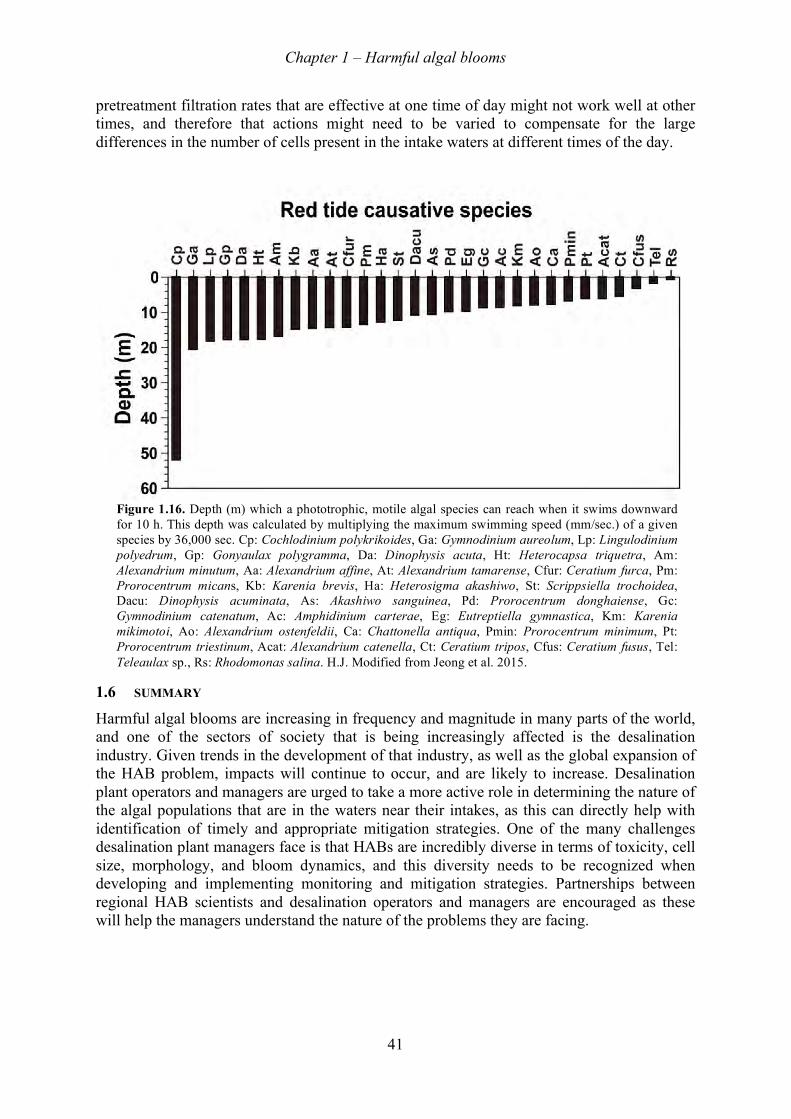
Chapter 1 – Harmful algal blooms

41

pretreatment filtration rates that are effective at one time of day might not work well at other times, and therefore that actions might need to be varied to compensate for the large differences in the number of cells present in the intake waters at different times of the day.

1.6! SUMMARY Harmful algal blooms are increasing in frequency and magnitude in many parts of the world, and one of the sectors of society that is being increasingly affected is the desalination industry. Given trends in the development of that industry, as well as the global expansion of the HAB problem, impacts will continue to occur, and are likely to increase. Desalination plant operators and managers are urged to take a more active role in determining the nature of the algal populations that are in the waters near their intakes, as this can directly help with identification of timely and appropriate mitigation strategies. One of the many challenges desalination plant managers face is that HABs are incredibly diverse in terms of toxicity, cell size, morphology, and bloom dynamics, and this diversity needs to be recognized when developing and implementing monitoring and mitigation strategies. Partnerships between regional HAB scientists and desalination operators and managers are encouraged as these will help the managers understand the nature of the problems they are facing.

Figure 1.16. Depth (m) which a phototrophic, motile algal species can reach when it swims downward for 10 h. This depth was calculated by multiplying the maximum swimming speed (mm/sec.) of a given species by 36,000 sec. Cp: Cochlodinium polykrikoides, Ga: Gymnodinium aureolum, Lp: Lingulodinium polyedrum, Gp: Gonyaulax polygramma, Da: Dinophysis acuta, Ht: Heterocapsa triquetra, Am: Alexandrium minutum, Aa: Alexandrium affine, At: Alexandrium tamarense, Cfur: Ceratium furca, Pm: Prorocentrum micans, Kb: Karenia brevis, Ha: Heterosigma akashiwo, St: Scrippsiella trochoidea, Dacu: Dinophysis acuminata, As: Akashiwo sanguinea, Pd: Prorocentrum donghaiense, Gc: Gymnodinium catenatum, Ac: Amphidinium carterae, Eg: Eutreptiella gymnastica, Km: Karenia mikimotoi, Ao: Alexandrium ostenfeldii, Ca: Chattonella antiqua, Pmin: Prorocentrum minimum, Pt: Prorocentrum triestinum, Acat: Alexandrium catenella, Ct: Ceratium tripos, Cfus: Ceratium fusus, Tel: Teleaulax sp., Rs: Rhodomonas salina. H.J. Modified from Jeong et al. 2015.

Chapter 1 – Harmful algal blooms

42

1.7! REFERENCES Al-Ansi, M. A., Abdel-Moati, M. A. R., Al-Ansari, I. S., 2002. Causes of fish mortality along

the Qatari waters (Arabian Gulf). International Journal of Environmental Studies. 59(1), 59–71.

Al-Azri, A., Piontkovski, S., Al-Hashmi, K., Al-Gheilani, H., Al-Habsi, H., Al-Khusaibi, S., and Al-Azri, N. 2012. The occurrence of algal blooms in Omani coastal waters. Aquatic Ecosystem Health and Management 15 (supplement 1), 56-63.

Al-Busaidi, S. S., Al-Rashdi, K. M., Al-Gheilani, H. M., and Amer, S. 2008. Hydrographical observations during a red tide with fish mortalities at Masirah Island, Oman. . Agricultural and Marine Sciences 13, 63–72.

Al-Gheilani, H. M., Matsuoka, K., Al-Kindi, A. Y., Amer, S., and Waring, C. 2011. Fish kill incidents and harmful algal blooms in Omani waters. Sultan Qaboos University Research Journal-Agricultural and Marine Sciences 16, 23-33.

Al Shehhi, M. R., Gherboudj, I. and Ghedira, H. 2014. An overview of historical harmful algae blooms outbreaks in the Arabian Seas. Marine Pollution Bulletin 86(1), 314-324.

Al-Yamani, F., Al-Ghunaim, D. V., Subba R. N., Khan, M., Al-Ghool, M., Muruppel, S., and Al-Qatma, L. M. 2000. Fish Kills, Red Tides, and Kuwait’s Marine Environment. Kuwait Institute for Scientific Research, Kuwait. 202 pp.

Álvarez, G., Uribe, E., Quijano-Scheggia, S., López-Rivera, A., Mariño, C., and Blanco, J. 2009. Domoic acid production by Pseudo-nitzschia australis and Pseudo-nitzschia calliantha isolated from North Chile. Harmful Algae 8(6), 938-945.

Anderson, D. M. 1989. Toxic algal blooms and red tides: a global perspective. In: T. Okaichi, D. M. Anderson, and T. Nemoto (Eds.), Red Tides: Biology, Environmental Science and Toxicology. pp. 11-16. Elsevier.

Anderson, D. M. 1998. Physiology and bloom dynamics of toxic Alexandrium species, with emphasis on life cycle transitions. NATO ASI Series G Ecological Sciences 41, 29-48.

Anderson, D. M., Glibert, P. M., and Burkholder, J. M. 2002. Harmful algal blooms and eutrophication: nutrient sources, composition, and consequences. Estuaries 25(4), 704-726.

Anderson, D. M., Kulis, D. M., Doucette, G. J., Gallagher, J. C., and Balech, E. 1994. Biogeography of toxic dinoflagellates in the genus Alexandrium from the northeastern United States and Canada. Marine Biology 120(3), 467-478.

Anderson, D. M., Keafer, B. A., Kleindinst, J. L., McGillicuddy Jr, D. J., Martin, J. L., Norton, K., Pilskaln, C. H., Smith, J. L., Sherwood, C. R., and Butman, B. 2014. Alexandrium fundyense cysts in the Gulf of Maine: Long-term time series of abundance and distribution, and linkages to past and future blooms. Deep-Sea Research Part II 103, 6-26.

Armstrong, M. and Kudela, R. 2006. Evaluation of California isolates of Lingulodinium polyedrum for the production of yessotoxin. African Journal of Marine Science 28 (2), 399–401.

Chapter 1 – Harmful algal blooms

43

Band-Schmidt, C., Bustillos-Guzmán, J., Morquecho, L., Gárate-Lizárraga, I., Alonso Rodríguez, R., Reyes-Salinas, A., and Luckas, B. 2006. Variations of PSP toxin profiles during different growth phases in Gymnodinium catenatum (Dinophyceae) strains isolated from three locations in the Gulf of California, Mexico. Journal of Phycology 42(4), 757-768.

Basti, L., Uchida, H., Matsushima, R., Watanabe, R., Suzuki, T., Yamatogi, T., and Nagai, S. 2015. Influence of temperature on growth and production of Pectenotoxin-2 by a monoclonal culture of Dinophysis caudata. Marine Drugs 13(12), 7124-7137.

Bates, S. S., Bird, C. J., Defreitas, A. S. W., Foxall, R., Gilgan, M., Hanic, L. A., Johnson, G. R., McCulloch, A. W., Dodense, P., Pocklington, R., Quilliam, M. A., Sim, P. G., Smith, J. C., Rao, D. V. S., Todd, C. D., Walter, J. A., and Wright, J. L. C. 1989. Pennate diatom Nitzschia pungens as the primary source of domoic acid, a toxin in shellfish from eastern Prince Edwards Island, Canada. Canadian Journal of Fisheries and Aquatic Sciences 46(7), 1203–1215.

Bates, S. S., Hiltz, M. F., and Leger, C. 1999. Domoic acid toxicity of large new cells of Pseudo-nitzschia multiseries resulting from sexual reproduction. Canadian translations of fisheries and aquatic sciences/Traductions canadiennes en sciences halieutiques et aquatiques. Ottawa ON, (2261), 21-26.

Baugh, K. A., Bush, J. M., Bill, B. D., Lefebvre, K. A., and Trainer, V. L. 2006. Estimates of specific toxicity in several Pseudo-nitzschia species from the Washington coast, based on culture and field studies. African Journal of Marine Science 28(2), 403–407.

Bill, B. D. 2011. Carbon and nitrogen uptake of toxigenic diatoms: Pseudo-nitzschia australis and Pseudo-nitzschia turgidula. Ph.D. thesis, San Francisco State University, San Francisco CA USA.

Buck, K. R., Uttal-Cooke, L., Pilskaln, C. H., Roelke, D. L., Villac, M. C., Fryxell, G. A., Cifuentes, L., and Chavez, F. P. 1992. Autecology of the diatom Pseudo-nitzschia australis, a domoic acid producer, from Monterey Bay, California. Marine Ecology Progress Series 84(3), 293–302.

Caron, D. A., Garneau, M. È., Seubert, E., Howard, M. D., Darjany, L., Schnetzer, A., Cetinić, I., Filteau, G., Lauri, P., Jones, B. and Trussell, S. 2010. Harmful algae and their potential impacts on desalination operations off southern California. Water Research 44(2), 385-416.

Cerino, F., Orsini, L., Sarno, D., Dell’Aversano, C., Tartaglione, L., and Zingone, A. 2005. The alternation of different morphotypes in the seasonal cycle of the toxic diatom Pseudo-nitzschia galaxiae. Harmful Algae 4(1), 33-48.

Chaghtai, F. and Saifullah, S. M. 2001. Harmful algal bloom (HAB) organisms of the north Arabian sea bordering Pakistan. Pakistan Journal of Botany 33, 69–75.

Chaghtai, F. and Saifullah, S. 2006. On the occurrence of green Noctiluca scintillans blooms in coastal waters of Pakistan, North Arabian Sea. Pakistan Journal of Botany 38, 893-898.

Chang, F. H., Anderson, D. M., Kulis, D. M., and Till, D. G. 1997. Toxin production of Alexandrium minutum (Dinophyceae) from the Bay of Plenty, New Zealand. Toxicon 35(3), 393-409.

Chapter 1 – Harmful algal blooms

44

Corcoran, A. A., Richardson, B., and Flewelling, L. J. 2014. Effects of nutrient-limiting supply ratios on toxin content of Karenia brevis grown in continuous culture. Harmful Algae 39, 334-341.

D’Silva, M. S., Anil, A. C., Naik, R. K., D’Costa, P. M. 2012. Algal blooms: a perspective from the coasts of India. Natural Hazards 63, 1225–1253.

Dale, B. 1983. Dinoflagellate resting cysts: “benthic plankton”. Survival strategies of the algae. 69-136.

Danovaro, R., Umani, S. F. and Pusceddu, A. 2009. Climate change and the potential spreading of marine mucilage and microbial pathogens in the Mediterranean Sea. PLoS One 4(9), e7006.

Dodge, J. D. 1973. The Fine Structure of Algal Cells. Academic Press, London. pp. 21-50. Draisci, R., Ferretti, E., Palleschi, L., Marchiafava, C., Poletti, R., Milandri, A., Ceredi, A.,

and Pompei, M., 1999. High levels of yessotoxin in mussels and presence of yessotoxin and homoyessotoxin in dinoflagellates of the Adriatic Sea. Toxicon 37, 1187–1193.

Fatemi, S. M. R, Nabavis, M. B., Vosoghi, G., Fallahi, M., and Mohammadi, M. 2012. The relation between environmental parameters of Hormuzgan coastline in Persian Gulf and occurrence of the first harmful algal bloom of Cochlodinium polykrikoides (Gymnodiniaceae). Iranian Journal of Fisheries Sciences 11(3), 475-489.

Foster, K. A., Foster, G., Tourenq, C., and Shuriqi, M. K. 2011. Shifts in coral community structures following cyclone and red tide disturbances within the Gulf of Oman (United Arab Emirates). Marine Biology 158, 955–968.

Franks, P. J. S. 1992. Sink or swim: Accumulation of biomass at fronts. Marine Ecology Progress Series. 82(1), 1-12.

Franks, P. J. S. and Anderson, D. M. 1992. Alongshore transport of a toxic phytoplankton bloom in a buoyancy current: Alexandrium tamarense in the Gulf of Maine. Marine Biology 112, 153-164.

Fu, F. X., Place, A. R., Garcia, N. S., and Hutchins, D. A. 2010. CO2 and phosphate availability control the toxicity of the harmful bloom dinoflagellate Karlodinium veneficum. Aquatic Microbial Ecology 59(1), 55-65.

Gaines, G., and Taylor, F. J. R., 1985. An exploratory analysis of PSP patterns in British Columbia: 1942–1984. In: Anderson, D.M., White, A.W., Baden, D.G. (Eds.), Toxic dinoflagellates. Elsevier Science, New York, pp. 439–444.

Garrison, D.L., Conrad, S.M., Eilers, P.P., and Waldron, E.M. 1992. Confirmation domoic acid production by Pseudonitzchia australis (Bacillariophyceae) cultures. Journal of Phycology 28(5): 604-607.

Geissler, U. 1958. Das Membranpotential einiger Diatomeen und seine Bedeutung fuer die lebende Kieselalganzelle. Mikroskopie 13, 145-172.

GEOHAB. 2005. Global Ecology and Oceanography of Harmful Algal Blooms, GEOHAB Core Research Project: HABs in Upwelling Systems. G. Pitcher, T. Moita, V. Trainer, R. Kudela, P. Figueiras, T. Probyn (Eds.) IOC and SCOR, Paris and Baltimore. 82 pp.

GEOHAB. 2006. Oceanography of Harmful Algal Blooms, Harmful Algal Blooms in Eutrophic Systems. P. Glibert (Ed.) IOC and SCOR, Paris and Baltimore. 74 pp.

Chapter 1 – Harmful algal blooms

45

Glibert, P. M., Landsberg, J. H., Evans, J. J., Al-Sawari, M. A., Faraj, M., Al-Jarallah, M. A., Haywood, A., Ibrahem, S., Klesius, P., Powell, K., and Shoemaker, C. 2002. A fish kill of massive proportion in Kuwait Bay, Arabian Gulf, 2001: the roles of bacterial disease, harmful algae, and eutrophication. Harmful Algae 1, 215–231.

Gribble, K. E., Keafer, B. A, Quilliam, M. A., Cembella, A. D., Kulis, D. M., Manahan, A., and Anderson, D. M. 2005. Distribution and toxicity of Alexandrium ostenfeldii (Dinophyceae) in the Gulf of Maine, USA. Deep Sea Research Part II 52(19), 2745-2763.

Gregorio, D. E. and Connell, L. 2000. Range of Heterosigma akashiwo (Raphidophyceae) expanded to include California, USA. In: Ninth International Conference on Harmful Algal Blooms, Tasmania, Australia (abstract).

Hallegraeff, G. M. 1993. A review of harmful algal blooms and their apparent global increase. Phycologia 32(2), 79-99.

Harrison, P. J., Furuya, K., Glibert, P. M., Xu, J., Liu, H. B., Yin, K., Lee, J. H. W., Anderson, D. M., Gowen, R., Al-Azri, A. R. and Ho, A. Y. T. 2011. Geographical distribution of red and green Noctiluca scintillans. Chinese Journal of Oceanology and Limnology 29(4), 807-831.

Hawser, S. P., Codd, G. A., Capone, D. G., and Carpenter, E. J. 1991. A neurotoxic factor associated with the bloom-forming cyanobacterium Trichodesmium. Toxicon 29(3), 277-278.

Heil, C. A., Glibert, P. M., Al-Sarawl, M. A., Faraj, M., Behbehani, M., and Husain, M. 2001. First record of a fish-killing Gymnodinium sp. bloom in Kuwait Bay, Arabian Sea: chronology and potential causes. Marine Ecology Progress Series 214, 15–23.

Hershberger, P. K., Rensel, J. E., Postel, J. R., and Taub, F.B. 1997. Heterosigma bloom and associated fish kill. Harmful Algae News 16(1), 4.

Holligan, P. M. 1979. Dinoflagellate blooms associated with tidal fronts around the British Isles. In Toxic Dinoflagellate Blooms: Developments in Marine Biology. D. L. Taylor and H. H. Seliger (Eds.) pp 249-256. Elsevier, New York.

Holmes, R. W., Williams, P. M., and Eppley, R. W. 1967. Red water in La Jolla, 1964–1966. Limnology and Oceanography 12(3), 503–512.

Horner, R. A., Garrison, D. L., and Plumley, F. G. 1997. Harmful algal blooms and red tide problems on the U.S. west coast. Limnology and Oceanography 42(2), 1076–1088.

Howard, M. D. A., Cochlan, W. P., Ladizinsky, N., and Kudela, R. M. 2007. Nitrogenous preference of toxigenic Pseudo-nitzschia australis (Bacillariophyceae) from field and laboratory experiments. Harmful Algae 6(2), 206–217.

Ives, K. J. 1956. Electrokinetic phenomena of planktonic algae. Proceedings of the Society for Water Treatment and Examination 5, 41-58.

James, K. J., Sierra, M. D., Lehane, M., Brana, M. A, and Furey, A. 2003. Detection of five new hydroxyl analogues of azaspiracids in shellfish using multiple tandem mass spectrometry. Toxicon 41(3), 277–283.

Jauffrais, T., Kilcoyne, J., Sechet, V., Herrenknecht, C., Truquet, P., Herve, F., Berard, J. B., Nulty, C., Taylor, S., Tillman, U., Miles, C. O., and Hess, P. 2012. Production and isolation of Azaspiracid-1 and -2 from Azadinium spinosum culture in pilot scale photobioreactors. Marine Drugs 10(12), 1360–1382.

Chapter 1 – Harmful algal blooms

46

Jeong, H. J., Lim, A. S., Franks, P. J., Lee, K. H., Kim, J. H., Kang, N. S., Lee, M. J., Jang, S. H., Lee, S. Y., Yoon, E. Y., Park, J. Y., Yoo, Y. D., Seong, K. A., Kwon, J. E., and Jang, T. Y. 2015. A hierarchy of conceptual models of red-tide generation: nutrition, behavior, and biological interactions. Harmful Algae 47, 97-115.

Jester, R. 2008. An investigation into the prevalence of Alexandrium derived toxins in marine food webs. Ph.D., University of California, Santa Cruz, Santa Cruz, 116 pp.

John, U., Litaker, R. W., Montresor, M., Murray, S., Brosnahan, M. L., and Anderson, D. M. 2014. Formal revision of the Alexandrium tamarense species complex (Dinophyceae) taxonomy: the introduction of five species with emphasis on molecular-based (rDNA) classification. Protist 165, 779-804.

Joseph, T., Shaiju, P., Laluraj, C. M., Balachandran, K. K., Nair, M., George, R., Nair, K. K., Sahayak, S., and Prabhakaran, M. P. 2008. Nutrient environment of red tide-infested waters off south-west coast of India. Environmental Monitoring and Assessment 143, 355–361.

Kamykowski, D. 1995. Trajectories of autotrophic marine dinoflagellates. Journal of Phycology 31(2), 200-208.

Kerbrat, A. S., Amzil, Z., Pawlowiez, R., Golubic, S., Sibat, M., Darius, H. T., Chinain, M. and Laurent, D. 2011. First evidence of palytoxin and 42-hydroxy-palytoxin in the marine cyanobacterium Trichodesmium. Marine Drugs 9(4), 543-560.

Kerbrat, A. S., Darius, H. T., Pauillac, S., Chinain, M., and Laurent, D. 2010. Detection of ciguatoxin-like and paralysing toxins in Trichodesmium spp. from New Caledonia lagoon. Marine Pollution Bulletin 61(7), 360-366.

Kim, C. H., Sako, Y., and Ishida, Y. 1993. Comparison of toxin composition between populations of Alexandrium spp. from geographically distant areas. Nippon Suisan Gakkaishi 59, 641–646.

Krishnan, A. A., Krishnakumar, P. K., and Rajagopalan, M. 2007. Trichodesmium erythraeum (Ehrenberg) bloom along the southwest coast of India (Arabian Sea) and its impact on trace metal concentrations in seawater. Estuarine, Coastal and Shelf Science 71, 641–646.

Krock, B., Tillmann, U., Potvin, E., Jeong, H. J., Drebing, W., Kilcoyne, J., Al-Jorani, A., Twiner, M. J, Göthel, Q., and Köck, M. 2015. Structure elucidation and in vitro toxicity of new Azaspiracids isolated from the marine dinoflagellate Azadinium poporum. Marine Drugs 13(11), 6687-6702.

Kudela, R. M. and Gobler, C. J. 2012. Harmful dinoflagellate blooms caused by Cochlodinium sp.: Global expansion and ecological strategies facilitating bloom formation. Harmful Algae 14, 71-86.

Kudela, R., Ryan, J., Blakely, M., Lane, J., Peterson, T. 2008. Linking the physiology and ecology of Cochlodinium to better understand harmful algal bloom events: a comparative approach. Harmful Algae 7, 278–292.

Loeblich III, A. R. and Fine, K. E. 1977. Marine chloromonads: More widely distributed in neritic environments than previously thought. Proceedings of the Biological Society of Washington 90(2), 388–399.

Chapter 1 – Harmful algal blooms

47

Lundholm, N., Skov, J., Pocklington, R., and Moestrup, O. 1994. Domoic acid, the toxic amino acid responsible for amnesic shellfish poisoning, now in Pseudonitzschia seriata (Bacillariophyceae) in Europe. Phycologia 33(6), 475-478.

Lundholm, N., Skov, J., Pocklington, R., and Moestrup, O. 1997. Studies on the marine planktonic diatom Pseudo-nitzschia. 2. Autecology of P. pseudodelicatissima based on isolates from Danish coastal waters. Phycologia 36, 381–388.

Mackenzie, L., White, D., Oshima, Y., and Kapa, J. 1996. The resting cyst and toxicity of Alexandrium ostenfeldii (Dinophyceae) in New Zealand. Phycologia 35(2), 148-155.

MacKenzie, L., Sims, I., Beuzenberg, V. and Gillespie, P. 2002. Mass accumulation of mucilage caused by dinoflagellate polysaccharide exudates in Tasman Bay, New Zealand. Harmful Algae, 1(1), 69-83.

Madhupratap, M., Sawant, S., and Gauns, M. 2000. A first report on a bloom of the marine prymnesiophycean, Phaeocystis globosa from the Arabian Sea. Oceanologica Acta 23(1), 83–90.

Margalef, R. 1961. Hidrografia y fitoplancton de un area marina de la costa meridional de Puerto Rico. Investigación pesquera 18, 76–78.

Martin, J. L., Haya, K., Burridge, L. E., and Wildish, D. J. 1990. Nitzschia pseudodelicatissima - a source of domoic acid in the Bay of Fundy, eastern Canada. Marine Ecology Progress Series 67(2), 177–182.

Maruyama, T., Yamada, R., Usui, K., Suzuki, H. and Yoshida, T. 1987. Removal of marine red tide plankton with acid-treated clay. Nippon Suisan Gakkaishi, 53(10), 1811-1819.

Matsuoka, K., Iwataki, M., and Kawami, H. 2008. Morphology and taxonomy of chainforming species of the genus Cochlodinium (Dinophyceae). Harmful Algae 7, 261–270.

McCarron, P., Kilcoyne, J., Miles, C. O., and Hess, P. 2009. Formation of Azaspiracids-3, -4, -6, and -9 via decarboxylation of carboxyazaspiracid metabolites from shellfish. Journal of Agricultural and Food Chemistry 57(1), 160–169.

McMinn, A., Hallegraeff, G. M., Thomson, P., Jenkinson, A., and Heijnis, H. 1997. Cyst and radionucleotide evidence for the recent introduction of the toxic dinoflagellate Gymnodinium catenatum into Tasmanian waters. Marine Ecology Progress Series 161, 165-172.

Mitch, W. A. and Sedlak, D. L. 2002. Formation of N-nitrosodimethylamine (NDMA) from dimethylamine during chlorination. Environmental Science and Technology 36(4), 588-595.

Moestrup, O., Akselmann, R., Fraga, S., Hansen, G., Hoppenrath, M., Iwataki, M., Komarek, J., Larsen, J., Lundholm, N., and Zingone, A. (Eds.) 2017. IOC-UNESCO Taxonomic Reference List of Harmful Micro Algae.

Morton, S. L., Faust, M. A., Fairey, E. I., and Moeller, P. D. R. 2002. Morphology and toxicology of Prorocentrum arabianum sp. nov., (Dinophyceae) a toxic planktonic dinoflagellate from the Gulf of Oman, Arabian Sea. Harmful Algae 1(4), 393–400.

Moschandreou, K. K., Papaefthimiou, D., Katikou, P., Kalopesa, E., Panou, A., and Nikolaidis, G. 2010. Morphology, phylogeny and toxin analysis of Pseudo-nitzschia pseudodelicatissima (Bacillariophyceae) isolated from the Thermaikos Gulf, Greece. Phycologia 49(3), 260-273.

Chapter 1 – Harmful algal blooms

48

Nagai, S., Hori, Y., Manabe, T., and Imai, I. 1995. Morphology and rejuvenation of Coscinodiscus wailesii Gran (Bacillariophyceae) resting cells found in bottom sediments of Harima-Nada, Seto Inland Sea. Bulletin of the Japanese Society of Scientific Fisheries 61, 179-185.

Nagai, S., Suzuki, T., and Kamiyama, T. 2013. Successful cultivation of the toxic dinoflagellate Dinophysis tripos (Dinophyceae). Plankton and Benthos Research 8(4), 171-177.

Nagai, S., Suzuki, T., Nishikawa, T., and Kamiyama, T. 2011. Differences in the production and excretion kinetics of okadaic acid, dinophysistoxin-1, and pectenotoxin-2 between cultures of Dinophysis acuminata and Dinophysis fortii isolated from western Japan. Journal of Phycology 47(6), 1326-1337.

Nielsen, L. T., Krock, B., and Hansen, P. J. 2013. Production and excretion of okadaic acid, pectenotoxin-2 and a novel dinophysistoxin from the DSP-causing marine dinoflagellate Dinophysis acuta–effects of light, food availability and growth phase. Harmful Algae 23, 34-45.

Ofuji, K., Satake, M., McMahon, T., James, K. J., Naoki, H., Oshima, Y., and Yasumoto, T. 2014. Structures of azaspiracid analogs, azaspiracid-4 and azaspiracid-5, causative toxins of azaspiracid poisoning in Europe. Bioscience, Biotechnology and Biochemistry 65(3), 740–742.

O’Halloran, C., Silver, M., Holman, T., and Scholin, C. 2006. Heterosigma akashiwo in central California waters. Harmful Algae 5 (2), 124–132.

Okaichi, T. 2004. Red tide phenomena. In: Okaichi, T. (Ed.), Red Tides, Kluwer Academic Publishers, London, pp. 7-60.

Orsini, L., Sarno, D., Procaccini, G., Poletti, R., Dahlmann, J., and Montresor, M. 2002. Toxic Pseudo-nitzschia multistriata (Bacillariophyceae) from the Gulf of Naples: morphology, toxin analysis and phylogenetic relationships with other Pseudo-nitzschia species. European Journal of Phycology 37(2), 247-257.

Padmakumar, K. B., Menon, N. R., and Sanjeevan, V. N. 2012. Is occurrence of harmful algal blooms in the exclusive economic zone of India on the rise? International Journal of Oceanography.

Park, J., Jeong, M., Lee, J., Cho, K. J, and Kwon, O. S. 2001. Diurnal vertical migration of a harmful dinoflagellate, Cochlodinium polykrikoides (Dinophyceae) during a red tide in coastal waters of Namhae Island, Korea. Phycologia 40, 292–297.

Popels, L. C., and Hutchins, D. A. 2002. Factors affecting dark survival of the brown tide alga Aureococcus anophagefferens (Pelagophyceae). Journal of Phycology 38(4), 738-744.

Prud'homme van Reine, W. F. 2017. Report of the Nomenclature Committee for Algae: 16 – On proposals to amend the Code. Taxon 6 (1): 197-8.

Rabbani, M. M., Rehman, A. U., and Harms, C. E. 1990. Mass mortality of fishes caused by dinoflagellate bloom in Gwadar Bay, southwestern Pakistan. In: Graneli, E., Sundström, B., Edler, L., and Anderson, D. M. (Eds.), Toxic Marine Phytoplankton. Elsevier Science Publishing, New York, US, pp. 209–2014.

Chapter 1 – Harmful algal blooms

49

Raine, R., McDermott, G., Silke, J., Lyons, K., Nolan, G. and Cusack, C. 2010. A simple short range model for the prediction of harmful algal events in the bays of southwestern Ireland. Journal of Marine Systems 83(3), 150-157.

Rhodes, L., McNabb, P., de Salas, M., Briggs, L., Beuzenberg, V., and Gladstone, M. 2006. Yessotoxin production by Gonyaulax spinifera. Harmful Algae 5 (2), 148–155.

Rhodes, L., Scholin, C., and Garthwaite, I. 1998. Pseudo-nitzschia in New Zealand and the role of DNA probes and immunoassays in refining marine biotoxin monitoring programmes. Natural Toxins 6(3-4), 105-111.

Rhodes, L., White, D., Syhre, M., and Atkinson, M. 1996. Pseudo-nitzschia species isolated from New Zealand coastal waters: domoic acid production in vitro and links with shellfish toxicity. T. Yasumoto, Y. Oshima, Y. Fukuyo (Eds.), Harmful and Toxic Algal Blooms, Intergov. Oceanogr. Comm. UNESCO, Paris, pp. 155–158.

Ricci, F., Penna, N., Capellacci, S., and Penna, A. 2014. Potential environmental factors influencing mucilage formation in the northern Adriatic Sea. Chemical Ecology 30, 364–375.

Richlen, M. L., Morton, S. L., Jamali, E. A., Rajan, A., and Anderson, D. M. 2010. The catastrophic 2008–2009 red tide in the Arabian gulf region, with observations on the identification and phylogeny of the fish-killing dinoflagellate Cochlodinium polykrikoides. Harmful Algae 9, 163–172.

Rodríguez, L. P., González, V., Martínez, A., Paz, B., Lago, J., Cordeiro, V., Blanco, L., Vieites, J. M. and Cabado, A. G. 2015. Occurrence of lipophilic marine toxins in shellfish from Galicia (NW of Spain) and synergies among them. Marine Drugs, 13(4), 1666-1687.

Saeedi, H., Kamrani, E., and Matsuoka, K. 2011. Catastrophic impact of red tides of Cochlodinium polykrikoides on the razor clam Solen dactylus in coastal waters of the Northern Persian Gulf. Journal of the Persian Gulf 2(6), 13–20.

Sahraoui, I., Bates, S. S., Bouchouicha, D., Hadj Mabrouk, H., and Sakka Hlaili, A. 2011. Toxicity of Pseudo-nitzschia populations in Bizerte Lagoon, Tunisia, southwest Mediterranean, and first report of domoic acid production by P.brasiliana. Diatom Research 26, 293–303.

Saifullah, S. M. 1979. Occurrence of dinoflagellates and distribution of chlorophyll A on Pakistan shelf. In: Taylor, D. L. and Seliger, H. H. (Eds.), Toxic Dinoflagellate Blooms. Elsevier, North Holland, New York, pp. 203–208.

Sampedro, N., Arin, L., Quijano, S., Rene, A., and Camp, J. 2007. Mucilage event associated with Gonyaulax fragilis in NW Mediterranean Sea. Harmful Algae News 33, 10-11.

Satake, M., Ofuji, K., Naoki, H., James, K. J., Furey, A., McMachon, T., Silke, J., and Yasumoto, T. 1998. Azaspiracid, a new marine toxin having unique spiro ring assemblies, isolated from Irish mussels, Mytilus edulis. Journal of the American Chemical Society 12(38), 9967–9968.

Schoemann, V., Bequevort, S., Stefels, J., Rousseau, V., and Lancelot, C. 2005. Phaeocystis blooms in the global ocean and their controlling mechanisms: a review. Journal of Sea Research 53(1), 43-66.

Chapter 1 – Harmful algal blooms

50

Scholin, C. A., Herzog, M., Sogin, M., Anderson, D. M., 1994. Identification of group-and strain-specific genetic markers for globally distributed Alexandrium (Dinophyceae). Part II. Sequence analysis of a fragment of the LSU rRNA gene. Journal of Phycology 30(6), 999–1011.

Sengco, M. R. 2001. The aggregation of clay minerals and marine microalgal cells: physicochemical theory and implications for controlling harmful algal blooms. Ph.D. Dissertation, Massachusetts Institute of Technology/Woods Hole Oceanographic Institution Joint Program in Oceanography, 237 pp.

Shahid, K., and Al Sadi, A. 2015. Algae: a tide of trouble. Desalination and Water Reuse, May-June, 35-37.

Sheppard, C., Al-Husiani, M., Al-Jamali, F., Al-Yamani, F., Baldwin, R., Bishop, J., Benzoni, F., Dutrieux, E., Dulvy, N. K., Durvasula, S. R. V. and Jones, D. A. 2010. The Gulf: a young sea in decline. Marine Pollution Bulletin 60(1), 13-38.

Shirota, A. 1989. Red tide problem and countermeasures (2). International Journal of Fisheries and Aquatic Studies, 195-223.

Smetacek, V. 2001. A watery arms race. Nature 411(6839), 745-745.

Smetacek, V. and Zingone, A. 2013. Green and golden seaweed tides on the rise. Nature, 504(7478), 84.

Sommer, H. and Meyer, K.F. 1937. Paralytic shellfish poisoning. Archives of Pathology 24, 560–598.

Steidinger, K. A. 1993. Some taxonomic and biologic aspects of toxic dinoflagellates. In: Falconer, I. (Ed.), Algal Toxins in Seafood and Drinking Water. Academic Press, London, pp. 1–28.

Subba Rao, D. V., Quilliam, M. A., and Pocklington, R. 1988. Domoic acid – a neurotoxic amino acid produced by the marine diatom Nitzschia pungens in culture. Canadian Journal of Fisheries and Aquatic Sciences 45(12), 2076–2079.

Suzuki, T., Watanabe, R., Uchida, H., Matsushima, R., Nagai, H., Yasumoto, T., Yoshimatsu, T., Sato, S. and Adachi, M. 2012. LC-MS/MS analysis of novel ovatoxin isomers in several Ostreopsis strains collected in Japan. Harmful Algae 20, 81-91.

Tang, D. L., Kawamura, H., and Luis, A. J. 2002. Short-term variability of phytoplankton blooms associated with a cold eddy in the northwestern Arabian Sea. Remote Sensing of Environment 81, 82–89.

Tang, Y. Z. and Gobler, C. J. 2009. Characterization of the toxicity of Cochlodinium polykrikoides isolates from Northeast US estuaries to finfish and shellfish. Harmful Algae 8(3), 454-462.

Tang, Y. Z. and Gobler, C. J. 2012. The toxic dinoflagellate Cochlodinium polykrikoides (Dinophyceae) produces resting cysts. Harmful Algae 20, 71-80.

Taylor, F. J. R. and Horner, R. A. 1994. Red tides and other problems with harmful algal blooms in Pacific Northwest coastal waters. In: Review of the Marine Environment and Biota of Strait of Georgia, Puget Sound and Juan de Fuca Strait. Canadian Fisheries and Aquatic Science Technical Report 1948, pp. 175–186.

Tenny, M. W., Echelberger, W. F., Schuessler, R. G., and Pavoni, J. L. 1969. Algal flocculation with synthetic organic polyelectrolytes. Applied Microbiology 18, 965-971.

Chapter 1 – Harmful algal blooms

51

Thangaraja, M., Al-Aisry, A., Al-Kharusi, L., 2007. Harmful algal blooms and their impacts in the middle and outer ROPME sea area. International Journal of Oceans and Oceanography 2, 85– 98.

Tillman, U., Elbrachter, M., John, U., and Krock, B. 2011. A new non-toxic species in the dinoflagellate genus Azadinium: A. poporum sp. nov. European Journal of Phycology 46, 74–87.

Tillman, U., Elbrachter, M., John, U., Krock, B., and Cembella, A. D. 2010. Azadinium obesum (Dinophyceae), a new nontoxic species in the genus that can produce azaspiracid toxins. Phycologia 49, 169–182.

Tillmann, U., Elbrachter, M., Krock, B., John, U., and Cembella, A. D. 2009. Azadinium spinosum gen. et sp. nov. (Dinophyceae) identified as a primary producer of azaspiracid toxins. European Journal of Phycology 44, 63–79.

Tillman, U., Soehner, S., Nezan, E., and Krock, B. 2012. First record of the genus Azadinium (Dinophyceae) from the Shetland Islands, including the description of Azadinium polongum sp. nov. Harmful Algae 20, 142–155.

Trainer, V. L., Adams, N. G., Bill, B. D., Stehr, C. M., Wekell, J. C., Moeller, P., Busman, M., and Woodruff, D. 2000. Domoic acid production near California coastal upwelling zones, June 1998. Limnology and Oceanography 45(8), 1818–1833.

Trainer, V. L., Adams, N. G., and Wekell, J. C. 2001. Domoic acid producing Pseudo-nitzschia species off the U.S. west coast associated with toxification events. In: Hallegraeff, G. M., Blackburn, S. I., Bolch, C. J., and Lewis, R. J. (Eds.), Harmful Algal Bloom 2000. Intergovernmental Oceanographic Commission of UNESCO, Paris, pp. 46–49.

Trainer, V. L., Hickey, B. M., Lessard, E. J., Cochlan, W. P., Trick, C. G., Wells, M. L., MacFadyen, A. and Moore, S. K. 2009. Variability of Pseudo‐nitzschia and domoic acid in the Juan de Fuca eddy region and its adjacent shelves. Limnology and Oceanography 54(1), 289-308.

Trick, C. G., Bill, B. D., Cochlan, W. P., Wells, M. L., Trainer, V. L., and Pickell, L. D. 2010. Iron enrichment stimulates toxic diatom production in high-nitrate, low-chlorophyll areas. Proceedings of the National Academy of Sciences 107(13), 5887-5892.

Tyrell, J. V., Connell, L. B., and Scholin, C. A. 2002. Monitoring for Heterosigma akashiwo using a sandwich hybridization assay. Harmful Algae 1(2), 205–214.

Usup, G., Ahmad, A., Matsuoka, K., Lim, P. T, and Leaw, C. P. 2012. Biology, ecology and bloom dynamics of the toxic marine dinoflagellate Pyrodinium bahamense. Harmful Algae 14, 301-312.

Usup, G., Kulis, D. M., and Anderson, D. M. 1994. Growth and toxin production of the toxic dinoflagellate Pyrodinium bahamense var. compressum in laboratory cultures. Natural Toxins 2(5), 254-262.

Virgili, F. 2015. GWI Q4 desalination market review and forecast points to some improvement in contracted capacity. pp. 12, 13: IDA News Nov./Dec. 2015. International Desalination Association.

Chapter 1 – Harmful algal blooms

52

Walsh, J. J., Joliff, J. K., Darrow, B. P., Lenes, J. M., Milroy, S. P., Dieterie, D. A., Chen, F. R., Vargo, G. A., Weisburg, H. R., Fanning, K. A., Muller-Karger, F. E., Whitledge, T. E., Stockwell, D. A., Tomas, C. R., Villareal, T. A., Jochens, A. E. 2006. Red tides in the Gulf of Mexico: where, when and why? Journal of Geophysical Research C11003, 1-46.

Work, T. M., Barr, B., Beale, A. M., Fritz, L., Quilliam, M. A., and Wright, J. L. 1993. Epidemiology of domoic acid poisoning in brown pelicans (Pelecanus occidentalis) and Brandt's cormorants (Phalacrocorax penicillatus) in California. Journal of Zoo and Wildlife Medicine, 54-62.

Wright, J. L. C., Boyd, R. K., De Freitas, A. S. W., Falk, M., Foxall, R. A., Jamieson, W. D., Laycock, M. V., McCulloch, A. W., McInnes, A. G., Odense, P., Pathak, V. P., Quilliam, M. A., Ragan, M. A., Sim, P. G., Thibault, P., Walter, J. A., Gilgan, M., Richard, D. J. A., and Dewar, D. 1989. Identification of domoic acid, a neuroexcitatory amino acid, in toxic mussels from eastern Prince Edward Island. Canadian Journal of Chemistry 67, 481-490.

Yu, Z., Zou, J., and Ma, X. 1994. Applications of clays to removal of red tide organisms I. Coagulation of red tide organisms with clays. Chinese Journal of Oceanology and Limnology 12(3), 193-200.

Zhao, J. and Ghedira, H. 2014. Monitoring red tide with satellite imagery and numerical models: a case study in the Arabian Gulf. Marine Pollution Bulletin 79(1), 305-313.

Zhu, I. X., Bates, B. J. and Anderson, D. M. 2014. Removal of Prorocentrum minimum from seawater using dissolved air flotation. Journal of Applied Water Engineering and Research 2(1), 47-56.

Algal issues in seawater desalination

53

2 ALGAL ISSUES IN SEAWATER DESALINATION

Philipp Hess1, Loreen O. Villacorte2,3, Mike B. Dixon4, Siobhan F.E. Boerlage5, Donald M. Anderson6, Maria D. Kennedy2, and Jan C. Schippers2

1IFREMER, Laboratoire Phycotoxines, 44311 Nantes, France 2IHE-Delft Institute for Water Education, Delft, The Netherlands

3GRUNDFOS Holding A/S, Bjerringbro, Denmark (current affiliation) 4MDD Consulting, Kensington, Calgary, Alberta, Canada 5Boerlage Consulting, Gold Coast, Queensland, Australia

6Biology Department, Woods Hole Oceanographic Institution, Woods Hole, MA 02543 USA

2.1 Introduction ............................................................................................................................................. 53 2.2 Algal organic matter (AOM) and membrane fouling .............................................................................. 53

2.2.1 AOM release and composition ........................................................................................................ 54 2.2.2 AOM classification .......................................................................................................................... 54 2.2.3 Transparent Exopolymer Particles (TEP) ........................................................................................ 56 2.2.4 Fouling issues in SWRO plant during HAB events ........................................................................ 57

2.2.4.1 Biofouling in SWRO due to AOM deposition ........................................................................ 58 2.2.4.2 Particulate/Organic fouling of MF/UF during HABs .............................................................. 59

2.2.5 Summary and outlook ...................................................................................................................... 62 2.3 Algal issues in thermal desalination plants ............................................................................................. 63 2.4 Marine and freshwater toxins .................................................................................................................. 63

2.4.1 Background ...................................................................................................................................... 63 2.4.2 Chemistry and source organisms ..................................................................................................... 64

2.5 Taste and odor compounds ...................................................................................................................... 71 2.6 Detection techniques ............................................................................................................................... 71

2.6.1 Geosmin and methylisoborneol ....................................................................................................... 72 2.6.2 Cylindrospermopsin ........................................................................................................................ 73 2.6.3 Saxitoxins and tetrodotoxins ........................................................................................................... 73 2.6.4 Domoic acid ..................................................................................................................................... 73 2.6.5 Microcystins and nodularin ............................................................................................................. 73 2.6.6 Azaspiracids, brevetoxins, ciguatoxins, cyclic imines, okadaic acid and dinophysistoxins ........... 75

2.7 Gaps and perspectives on analytical techniques ..................................................................................... 75 2.8 References ............................................................................................................................................... 76

2.1 INTRODUCTION

Once harmful algal blooms (HABs) reach a desalination plant, they can cause significant operational issues and potential health concerns for consumers. These issues stem from two factors – first, the algal cells produce organic matter that can cause filter clogging and membrane fouling, and secondly, some cells produce toxic substances or taste and odor compounds. This chapter first explains the mechanisms for cellular release of organic matter, the types of matter that are produced, and the relative contribution of each type of matter to fouling mechanisms. It then describes the wide range of toxins that are produced by HABs, their mode of toxicity, and analytical methods for detecting them. While taste and odor compounds are non-toxic, they are included in this chapter as they can create customer perception issues and distrust in the water supply system.

2.2 ALGAL ORGANIC MATTER (AOM) AND MEMBRANE FOULING Natural organic matter in seawater is comprised of a diverse mixture of particulate, colloidal and dissolved organic substances which may originate from autochthonous (local) and allochthonous (external) sources. Algal blooms are believed to be responsible for about half of the autochthonous organic matter input to the earth’s oceans (Field et al. 1998). These

Algal issues in seawater desalination

54

algal-derived substances are collectively known as algal (or algogenic) organic matter (AOM). AOM can cause (directly or indirectly) operational problems in membrane-based desalination plants, affecting both the pretreatment processes and reverse osmosis membrane units. This section reviews the latest knowledge on the occurrence, composition, and characteristics of AOM from the perspective of seawater desalination. 2.2.1 AOM release and composition

Algal blooms are often responsible for the highest annual pulses of natural organic matter in seawater. A spike (>50% increase) in total organic carbon (TOC) concentration has been recorded in coastal seawater during algal blooms (e.g., Petry et al. 2007); however, AOM produced during algal blooms may vary substantially in terms of concentration, composition and characteristics, depending on the causative species and environmental conditions. AOM is generally released into seawater through metabolic excretion of active algal cells or through autolysis of damaged or dying cells. Active cells may excrete AOM in response to low-nutrient stress, unfavorable environmental conditions (e.g., light, pH and temperature) or invasion by bacteria or viruses (Leppard 1993). Several species of algae may also release AOM even under fairly favorable conditions (Fogg 1983).

Excessive production of AOM due to depletion of specific nutrients (e.g., phosphorus (P), nitrogen (N) and silicon (Si)) and pathogen invasion have been linked to the occurrence of marine mucilage (Mingazzini and Thake 1995). This phenomenon is characterized by the appearance of a sporadic but massive accumulation of gelatinous material at and below the water surface. Severe mucilage events occasionally occur in the North Sea, Adriatic Sea, and other parts of the Mediterranean Sea, and undoubtedly elsewhere in the world as well, though unreported. The proliferation of smaller mucilaginous aggregates known as “marine snow” has been reported in most oceanic and marine systems.

Specific conditions at the seawater intake and through the pretreatment processes may also induce further release of AOM. For instance, the addition of oxidizing or biocidal agents such as chlorine has been shown to cause damage to algal cell walls and membranes, resulting in the release of intracellular AOM (Daly et al. 2007). Moreover, exposure to hydrodynamic shear stress (e.g., valves and pumps) may cause breakage of soft-walled algal cells, releasing AOM which is normally stored inside the cells (Ladner et al. 2010; Voutchkov 2010).

The chemical composition of AOM usually includes proteins, polysaccharides, nucleic acids, lipids and other dissolved organic substances (Fogg 1983). For some algae, particularly diatoms such as Chaetoceros affinis, extracellular polysaccharides may comprise up to 90% of AOM released (Myklestad 1995). A major fraction of AOM is very sticky and is thought to cause operational issues in SWRO plants during blooms (Villacorte et al. 2015a). These substances are widely known as transparent exopolymer particles or TEPs (see Section 2.3.3 and Appendix 3). 2.2.2 AOM classification

Based on the mechanism of release by algae, AOM can be classified into two major groups, namely: (1) extracellular organic matter (EOM) - organic substances released through metabolic activity of algae, and (2) intracellular organic matter (IOM) - substances released through autolysis and/or during the process of cell decay. EOM substances can be either dis-

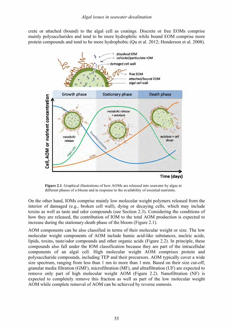
Algal issues in seawater desalination

55

crete or attached (bound) to the algal cell as coatings. Discrete or free EOMs comprise mainly polysaccharides and tend to be more hydrophilic while bound EOM comprise more protein compounds and tend to be more hydrophobic (Qu et al. 2012; Henderson et al. 2008).

On the other hand, IOMs comprise mainly low molecular weight polymers released from the interior of damaged (e.g., broken cell wall), dying or decaying cells, which may include toxins as well as taste and odor compounds (see Section 2.3). Considering the conditions of how they are released, the contribution of IOM to the total AOM production is expected to increase during the stationary-death phase of the bloom (Figure 2.1). AOM components can be also classified in terms of their molecular weight or size. The low molecular weight components of AOM include humic acid-like substances, nucleic acids, lipids, toxins, taste/odor compounds and other organic acids (Figure 2.2). In principle, these compounds also fall under the IOM classification because they are part of the intracellular components of an algal cell. High molecular weight AOM comprises protein and polysaccharide compounds, including TEP and their precursors. AOM typically cover a wide size spectrum, ranging from less than 1 nm to more than 1 mm. Based on their size cut-off, granular media filtration (GMF), microfiltration (MF), and ultrafiltration (UF) are expected to remove only part of high molecular weight AOM (Figure 2.2). Nanofiltration (NF) is expected to completely remove this fraction as well as part of the low molecular weight AOM while complete removal of AOM can be achieved by reverse osmosis.

Figure 2.1. Graphical illustrations of how AOMs are released into seawater by algae at different phases of a bloom and in response to the availability of essential nutrients.

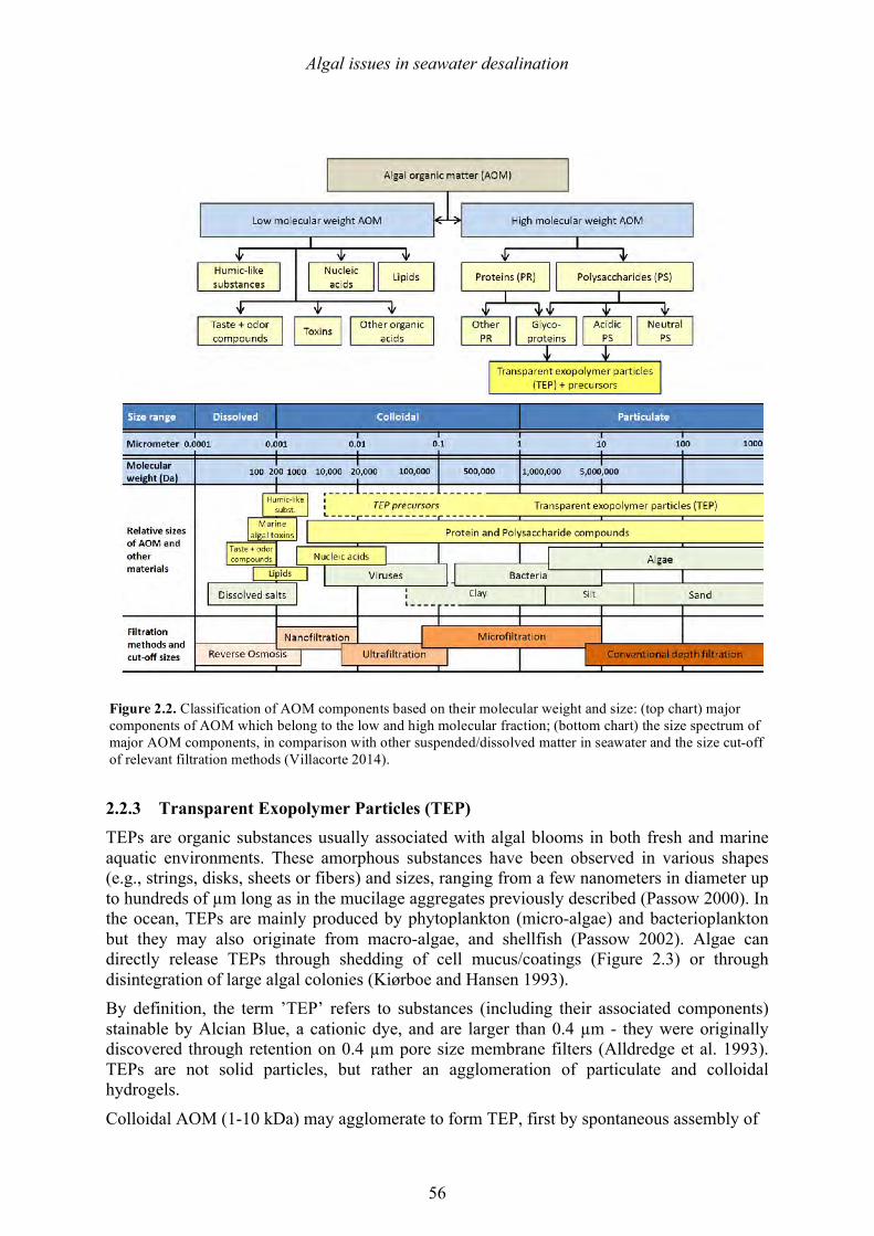
Algal issues in seawater desalination

56

2.2.3 Transparent Exopolymer Particles (TEP) TEPs are organic substances usually associated with algal blooms in both fresh and marine aquatic environments. These amorphous substances have been observed in various shapes (e.g., strings, disks, sheets or fibers) and sizes, ranging from a few nanometers in diameter up to hundreds of µm long as in the mucilage aggregates previously described (Passow 2000). In the ocean, TEPs are mainly produced by phytoplankton (micro-algae) and bacterioplankton but they may also originate from macro-algae, and shellfish (Passow 2002). Algae can directly release TEPs through shedding of cell mucus/coatings (Figure 2.3) or through disintegration of large algal colonies (Kiørboe and Hansen 1993). By definition, the term ’TEP’ refers to substances (including their associated components) stainable by Alcian Blue, a cationic dye, and are larger than 0.4 µm - they were originally discovered through retention on 0.4 µm pore size membrane filters (Alldredge et al. 1993). TEPs are not solid particles, but rather an agglomeration of particulate and colloidal hydrogels.

Colloidal AOM (1-10 kDa) may agglomerate to form TEP, first by spontaneous assembly of

Figure 2.2. Classification of AOM components based on their molecular weight and size: (top chart) major components of AOM which belong to the low and high molecular fraction; (bottom chart) the size spectrum of major AOM components, in comparison with other suspended/dissolved matter in seawater and the size cut-off of relevant filtration methods (Villacorte 2014).

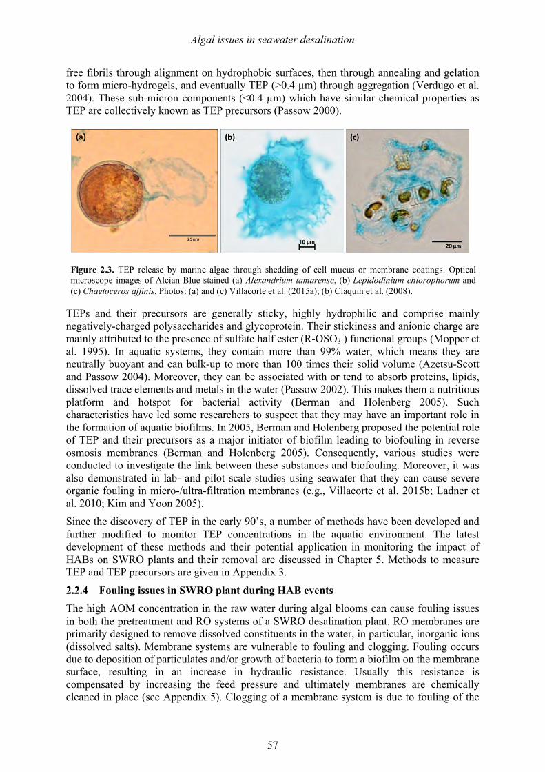
Algal issues in seawater desalination

57

free fibrils through alignment on hydrophobic surfaces, then through annealing and gelation to form micro-hydrogels, and eventually TEP (>0.4 µm) through aggregation (Verdugo et al. 2004). These sub-micron components (<0.4 µm) which have similar chemical properties as TEP are collectively known as TEP precursors (Passow 2000).

TEPs and their precursors are generally sticky, highly hydrophilic and comprise mainly negatively-charged polysaccharides and glycoprotein. Their stickiness and anionic charge are mainly attributed to the presence of sulfate half ester (R-OSO3-) functional groups (Mopper et al. 1995). In aquatic systems, they contain more than 99% water, which means they are neutrally buoyant and can bulk-up to more than 100 times their solid volume (Azetsu-Scott and Passow 2004). Moreover, they can be associated with or tend to absorb proteins, lipids, dissolved trace elements and metals in the water (Passow 2002). This makes them a nutritious platform and hotspot for bacterial activity (Berman and Holenberg 2005). Such characteristics have led some researchers to suspect that they may have an important role in the formation of aquatic biofilms. In 2005, Berman and Holenberg proposed the potential role of TEP and their precursors as a major initiator of biofilm leading to biofouling in reverse osmosis membranes (Berman and Holenberg 2005). Consequently, various studies were conducted to investigate the link between these substances and biofouling. Moreover, it was also demonstrated in lab- and pilot scale studies using seawater that they can cause severe organic fouling in micro-/ultra-filtration membranes (e.g., Villacorte et al. 2015b; Ladner et al. 2010; Kim and Yoon 2005). Since the discovery of TEP in the early 90’s, a number of methods have been developed and further modified to monitor TEP concentrations in the aquatic environment. The latest development of these methods and their potential application in monitoring the impact of HABs on SWRO plants and their removal are discussed in Chapter 5. Methods to measure TEP and TEP precursors are given in Appendix 3.

2.2.4 Fouling issues in SWRO plant during HAB events The high AOM concentration in the raw water during algal blooms can cause fouling issues in both the pretreatment and RO systems of a SWRO desalination plant. RO membranes are primarily designed to remove dissolved constituents in the water, in particular, inorganic ions (dissolved salts). Membrane systems are vulnerable to fouling and clogging. Fouling occurs due to deposition of particulates and/or growth of bacteria to form a biofilm on the membrane surface, resulting in an increase in hydraulic resistance. Usually this resistance is compensated by increasing the feed pressure and ultimately membranes are chemically cleaned in place (see Appendix 5). Clogging of a membrane system is due to fouling of the

Figure 2.3. TEP release by marine algae through shedding of cell mucus or membrane coatings. Optical microscope images of Alcian Blue stained (a) Alexandrium tamarense, (b) Lepidodinium chlorophorum and (c) Chaetoceros affinis. Photos: (a) and (c) Villacorte et al. (2015a); (b) Claquin et al. (2008).

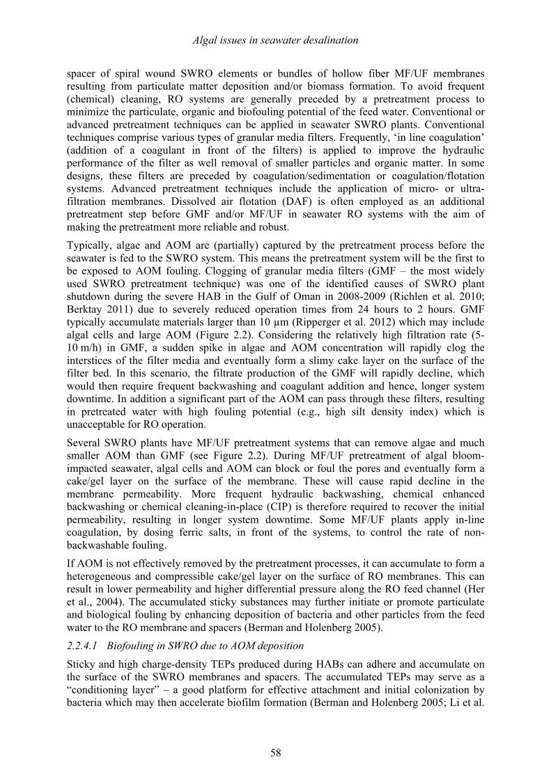
Algal issues in seawater desalination

58

spacer of spiral wound SWRO elements or bundles of hollow fiber MF/UF membranes resulting from particulate matter deposition and/or biomass formation. To avoid frequent (chemical) cleaning, RO systems are generally preceded by a pretreatment process to minimize the particulate, organic and biofouling potential of the feed water. Conventional or advanced pretreatment techniques can be applied in seawater SWRO plants. Conventional techniques comprise various types of granular media filters. Frequently, ‘in line coagulation’ (addition of a coagulant in front of the filters) is applied to improve the hydraulic performance of the filter as well removal of smaller particles and organic matter. In some designs, these filters are preceded by coagulation/sedimentation or coagulation/flotation systems. Advanced pretreatment techniques include the application of micro- or ultra-filtration membranes. Dissolved air flotation (DAF) is often employed as an additional pretreatment step before GMF and/or MF/UF in seawater RO systems with the aim of making the pretreatment more reliable and robust. Typically, algae and AOM are (partially) captured by the pretreatment process before the seawater is fed to the SWRO system. This means the pretreatment system will be the first to be exposed to AOM fouling. Clogging of granular media filters (GMF – the most widely used SWRO pretreatment technique) was one of the identified causes of SWRO plant shutdown during the severe HAB in the Gulf of Oman in 2008-2009 (Richlen et al. 2010; Berktay 2011) due to severely reduced operation times from 24 hours to 2 hours. GMF typically accumulate materials larger than 10 µm (Ripperger et al. 2012) which may include algal cells and large AOM (Figure 2.2). Considering the relatively high filtration rate (5-10 m/h) in GMF, a sudden spike in algae and AOM concentration will rapidly clog the interstices of the filter media and eventually form a slimy cake layer on the surface of the filter bed. In this scenario, the filtrate production of the GMF will rapidly decline, which would then require frequent backwashing and coagulant addition and hence, longer system downtime. In addition a significant part of the AOM can pass through these filters, resulting in pretreated water with high fouling potential (e.g., high silt density index) which is unacceptable for RO operation.

Several SWRO plants have MF/UF pretreatment systems that can remove algae and much smaller AOM than GMF (see Figure 2.2). During MF/UF pretreatment of algal bloom-impacted seawater, algal cells and AOM can block or foul the pores and eventually form a cake/gel layer on the surface of the membrane. These will cause rapid decline in the membrane permeability. More frequent hydraulic backwashing, chemical enhanced backwashing or chemical cleaning-in-place (CIP) is therefore required to recover the initial permeability, resulting in longer system downtime. Some MF/UF plants apply in-line coagulation, by dosing ferric salts, in front of the systems, to control the rate of non-backwashable fouling. If AOM is not effectively removed by the pretreatment processes, it can accumulate to form a heterogeneous and compressible cake/gel layer on the surface of RO membranes. This can result in lower permeability and higher differential pressure along the RO feed channel (Her et al., 2004). The accumulated sticky substances may further initiate or promote particulate and biological fouling by enhancing deposition of bacteria and other particles from the feed water to the RO membrane and spacers (Berman and Holenberg 2005). 2.2.4.1 Biofouling in SWRO due to AOM deposition

Sticky and high charge-density TEPs produced during HABs can adhere and accumulate on the surface of the SWRO membranes and spacers. The accumulated TEPs may serve as a “conditioning layer” – a good platform for effective attachment and initial colonization by bacteria which may then accelerate biofilm formation (Berman and Holenberg 2005; Li et al.

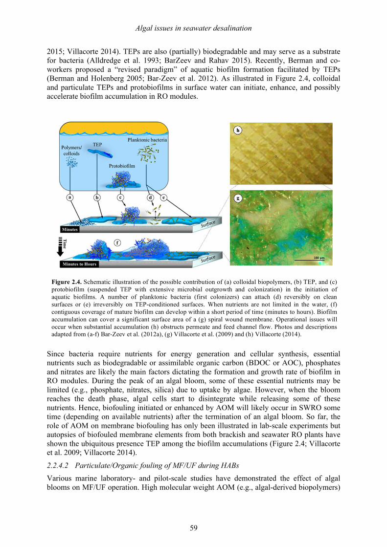
Algal issues in seawater desalination

59

2015; Villacorte 2014). TEPs are also (partially) biodegradable and may serve as a substrate for bacteria (Alldredge et al. 1993; BarZeev and Rahav 2015). Recently, Berman and co-workers proposed a “revised paradigm” of aquatic biofilm formation facilitated by TEPs (Berman and Holenberg 2005; Bar-Zeev et al. 2012). As illustrated in Figure 2.4, colloidal and particulate TEPs and protobiofilms in surface water can initiate, enhance, and possibly accelerate biofilm accumulation in RO modules.

Since bacteria require nutrients for energy generation and cellular synthesis, essential nutrients such as biodegradable or assimilable organic carbon (BDOC or AOC), phosphates and nitrates are likely the main factors dictating the formation and growth rate of biofilm in RO modules. During the peak of an algal bloom, some of these essential nutrients may be limited (e.g., phosphate, nitrates, silica) due to uptake by algae. However, when the bloom reaches the death phase, algal cells start to disintegrate while releasing some of these nutrients. Hence, biofouling initiated or enhanced by AOM will likely occur in SWRO some time (depending on available nutrients) after the termination of an algal bloom. So far, the role of AOM on membrane biofouling has only been illustrated in lab-scale experiments but autopsies of biofouled membrane elements from both brackish and seawater RO plants have shown the ubiquitous presence TEP among the biofilm accumulations (Figure 2.4; Villacorte et al. 2009; Villacorte 2014).

2.2.4.2 Particulate/Organic fouling of MF/UF during HABs Various marine laboratory- and pilot-scale studies have demonstrated the effect of algal blooms on MF/UF operation. High molecular weight AOM (e.g., algal-derived biopolymers)

Figure 2.4. Schematic illustration of the possible contribution of (a) colloidal biopolymers, (b) TEP, and (c) protobiofilm (suspended TEP with extensive microbial outgrowth and colonization) in the initiation of aquatic biofilms. A number of planktonic bacteria (first colonizers) can attach (d) reversibly on clean surfaces or (e) irreversibly on TEP-conditioned surfaces. When nutrients are not limited in the water, (f) contiguous coverage of mature biofilm can develop within a short period of time (minutes to hours). Biofilm accumulation can cover a significant surface area of a (g) spiral wound membrane. Operational issues will occur when substantial accumulation (h) obstructs permeate and feed channel flow. Photos and descriptions adapted from (a-f) Bar-Zeev et al. (2012a), (g) Villacorte et al. (2009) and (h) Villacorte (2014).

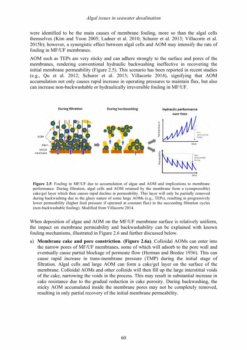
Algal issues in seawater desalination

60

were identified to be the main causes of membrane fouling, more so than the algal cells themselves (Kim and Yoon 2005; Ladner et al. 2010; Schurer et al. 2013; Villacorte et al. 2015b); however, a synergistic effect between algal cells and AOM may intensify the rate of fouling in MF/UF membranes.

AOM such as TEPs are very sticky and can adhere strongly to the surface and pores of the membranes, rendering conventional hydraulic backwashing ineffective in recovering the initial membrane permeability (Figure 2.5). This scenario has been reported in recent studies (e.g., Qu et al. 2012; Schurer et al. 2013; Villacorte 2014), signifying that AOM accumulation not only causes rapid increase in operating pressures to maintain flux, but also can increase non-backwashable or hydraulically irreversible fouling in MF/UF.

When deposition of algae and AOM on the MF/UF membrane surface is relatively uniform, the impact on membrane permeability and backwashability can be explained with known fouling mechanisms, illustrated in Figure 2.6 and further discussed below. a) Membrane cake and pore constriction. (Figure 2.6a). Colloidal AOMs can enter into

the narrow pores of MF/UF membranes, some of which will adsorb to the pore wall and eventually cause partial blockage of permeate flow (Herman and Bredee 1936). This can cause rapid increase in trans-membrane pressure (TMP) during the initial stage of filtration. Algal cells and large AOM can form a cake/gel layer on the surface of the membrane. Colloidal AOMs and other colloids will then fill up the large interstitial voids of the cake, narrowing the voids in the process. This may result in substantial increase in cake resistance due to the gradual reduction in cake porosity. During backwashing, the sticky AOM accumulated inside the membrane pores may not be completely removed, resulting in only partial recovery of the initial membrane permeability.

Figure 2.5: Fouling in MF/UF due to accumulation of algae and AOM and implications to membrane performance. During filtration, algal cells and AOM retained by the membrane form a (compressible) cake/gel layer which then causes rapid decline in permeability. This layer will only be partially removed during backwashing due to the gluey nature of some large AOMs (e.g., TEPs), resulting in progressively lower permeability (higher feed pressure if operated at constant flux) in the succeeding filtration cycles (non-backwashable fouling). Modified from Villacorte 2014.

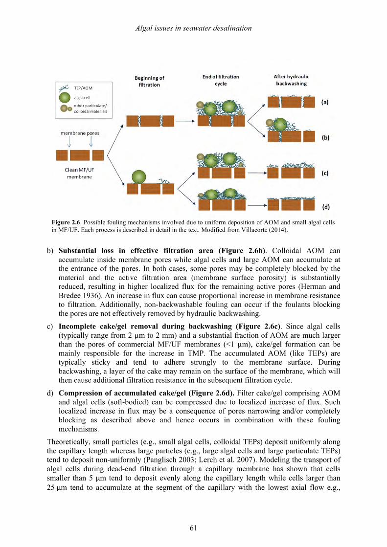
Algal issues in seawater desalination

61

b) Substantial loss in effective filtration area (Figure 2.6b). Colloidal AOM can

accumulate inside membrane pores while algal cells and large AOM can accumulate at the entrance of the pores. In both cases, some pores may be completely blocked by the material and the active filtration area (membrane surface porosity) is substantially reduced, resulting in higher localized flux for the remaining active pores (Herman and Bredee 1936). An increase in flux can cause proportional increase in membrane resistance to filtration. Additionally, non-backwashable fouling can occur if the foulants blocking the pores are not effectively removed by hydraulic backwashing.

c) Incomplete cake/gel removal during backwashing (Figure 2.6c). Since algal cells (typically range from 2 µm to 2 mm) and a substantial fraction of AOM are much larger than the pores of commercial MF/UF membranes (<1 µm), cake/gel formation can be mainly responsible for the increase in TMP. The accumulated AOM (like TEPs) are typically sticky and tend to adhere strongly to the membrane surface. During backwashing, a layer of the cake may remain on the surface of the membrane, which will then cause additional filtration resistance in the subsequent filtration cycle.

d) Compression of accumulated cake/gel (Figure 2.6d). Filter cake/gel comprising AOM and algal cells (soft-bodied) can be compressed due to localized increase of flux. Such localized increase in flux may be a consequence of pores narrowing and/or completely blocking as described above and hence occurs in combination with these fouling mechanisms.

Theoretically, small particles (e.g., small algal cells, colloidal TEPs) deposit uniformly along the capillary length whereas large particles (e.g., large algal cells and large particulate TEPs) tend to deposit non-uniformly (Panglisch 2003; Lerch et al. 2007). Modeling the transport of algal cells during dead-end filtration through a capillary membrane has shown that cells smaller than 5 μm tend to deposit evenly along the capillary length while cells larger than 25 μm tend to accumulate at the segment of the capillary with the lowest axial flow e.g.,

Figure 2.6. Possible fouling mechanisms involved due to uniform deposition of AOM and small algal cells in MF/UF. Each process is described in detail in the text. Modified from Villacorte (2014).

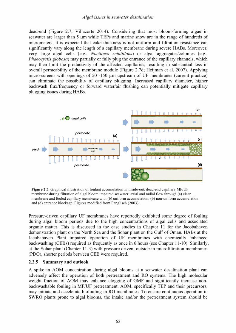
Algal issues in seawater desalination

62

dead-end (Figure 2.7; Villacorte 2014). Considering that most bloom-forming algae in seawater are larger than 5 μm while TEPs and marine snow are in the range of hundreds of micrometers, it is expected that cake thickness is not uniform and filtration resistance can significantly vary along the length of a capillary membrane during severe HABs. Moreover, very large algal cells (e.g., Noctiluca scintillans) or algal aggregates/colonies (e.g., Phaeocystis globosa) may partially or fully plug the entrance of the capillary channels, which may then limit the productivity of the affected capillaries, resulting in substantial loss in overall permeability of the membrane module (Figure 2.7d; Heijman et al. 2007). Applying micro-screens with openings of 50 -150 µm upstream of UF membranes (current practice) can eliminate the possibility of capillary plugging. Increased capillary diameter, higher backwash flux/frequency or forward water/air flushing can potentially mitigate capillary plugging issues during HABs.

Pressure-driven capillary UF membranes have reportedly exhibited some degree of fouling during algal bloom periods due to the high concentrations of algal cells and associated organic matter. This is discussed in the case studies in Chapter 11 for the Jacobahaven demonstration plant on the North Sea and the Sohar plant on the Gulf of Oman. HABs at the Jacobahaven Plant impaired operation of UF membranes with chemically enhanced backwashing (CEBs) required as frequently as once in 6 hours (see Chapter 11-10). Similarly, at the Sohar plant (Chapter 11-3) with pressure driven, outside-in microfiltration membranes (PDO), shorter periods between CEB were required.

2.2.5 Summary and outlook A spike in AOM concentration during algal blooms at a seawater desalination plant can adversely affect the operation of both pretreatment and RO systems. The high molecular weight fraction of AOM may enhance clogging of GMF and significantly increase non-backwashable fouling in MF/UF pretreatment. AOM, specifically TEP and their precursors, may initiate and accelerate biofouling in RO membranes. To ensure continuous operation in SWRO plants prone to algal blooms, the intake and/or the pretreatment system should be

Figure 2.7. Graphical illustration of foulant accumulation in inside-out, dead-end capillary MF/UF membrane during filtration of algal bloom impaired seawater: axial and radial flow through (a) clean membrane and fouled capillary membrane with (b) uniform accumulation, (b) non-uniform accumulation and (d) entrance blockage. Figures modified from Panglisch (2003).

Algal issues in seawater desalination

63

reliable and robust to ensure continuous operation at design capacity and to minimize breakthrough of AOM to the downstream SWRO system. It is also advantageous to have monitoring instruments that can detect algal biomass (and algal species known to produce TEP and other organic material in high quantities) and alert operators that intervention or oversight is needed. 2.3 ALGAL ISSUES IN THERMAL DESALINATION PLANTS

Multi stage flash (MSF) and multi effect distillation (MED) are the most commonly employed methods to desalinate seawater for municipal use and for drinking water supply in the Middle East. MSF and MED thermal desalination account for 60% of the total seawater desalinated capacity in the region (20 Mm3/d) (DesalData 2015). Thermal desalination plants have been known to be impacted by blinding of intake screens by seaweed (macroalgae) but generally are very forgiving of source water quality (Boerlage and Nada 2014). Unlike SWRO desalination plants, phytoplankton blooms seldom affect thermal desalination plants. During the prolonged 2008 algal bloom in the Gulf, the high concentration of the marine dinoflagellate Cochlodinium polykrikoides had limited impact on thermal plants. At Fujairah 1 in the UAE, the MSF plants continued to operate without issue while the SWRO desalination plant had to be shut down for more than one week. A minor shut down of thermal desalination plants did occur in Sharjah, UAE (less than 24 hours) due to odor issues associated with the product water. This was overcome through increased chlorination. Another thermal desalination plant (MED) at Kish Island in Iran reported a higher seawater pH during the bloom which required additional treatment measures to prevent alkaline scaling during this period.

2.4 MARINE AND FRESHWATER TOXINS 2.4.1 Background

Marine and cyanobacterial toxins have been identified globally in various coastal environments. Most of these toxins have been identified due to (i) poisoning events following the consumption of fish or shellfish or (ii) harmful effects through direct contact or exposure to aerosols. Therefore, the risks classically described for these compounds mostly relate to acute toxicity. However, acute poisoning from toxins following the consumption of desalinated drinking water has not yet been reported globally. The absence of such reports may relate to the absence of actual poisoning events or may reflect the typically experienced under-reporting of such events. In view of the risks these toxins pose, this section describes HAB toxins, their pharmacological activity, and methods of analysis. Risk assessment is presented in Chapter 8.

The following toxin groups have been identified for inclusion into this section: anatoxins (ATXs), azapiracids (AZAs), ß-methylamino alanine (BMAA), brevetoxins (BTXs), ciguatoxins (CTXs), cyclic imines (gymnodimines (GYM), spirolides (SPX), pinnatoxin (PnTX)), domoic acid (DA), microcystins (MCs), nodularins (NODs), okadaic acid and analogues (OA), palytoxins (PLTXs) incl. ovatoxins (OvTXs), saxitoxins (STXs), tetrodotoxins (TTXs) and trichotoxins (TRXs). Additional to this group of toxins are two taste and odor compounds, methyl isoborneol (MIB) and geosmin (GSM) that are non toxic, but can be a source of customer complaints. Geosmin is included in the information below in order of increasing molecular weight. Removal of these toxins is discussed in Chapter 10 with practical cases from the laboratory and full-scale plants. Note that not all of these toxins are direct threats to desalination plants, but all are presented here for completeness. For each toxin group there is a short description of the chemical nature of the compound and the

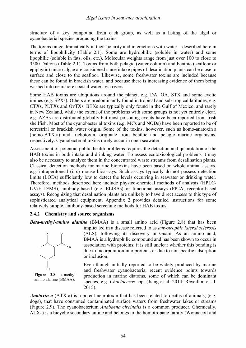
Algal issues in seawater desalination

64

structure of a key compound from each group, as well as a listing of the algal or cyanobacterial species producing the toxins.

The toxins range dramatically in their polarity and interactions with water – described here in terms of lipophilicity (Table 2.1). Some are hydrophilic (soluble in water) and some lipophilic (soluble in fats, oils, etc.). Molecular weights range from just over 100 to close to 3500 Daltons (Table 2.1). Toxins from both pelagic (water column) and benthic (seafloor or epiphytic) micro-algae are considered since intake pipes of desalination plants can be close to surface and close to the seafloor. Likewise, some freshwater toxins are included because these can be found in brackish water, and because there is increasing evidence of them being washed into nearshore coastal waters via rivers.

Some HAB toxins are ubiquitous around the planet, e.g. DA, OA, STX and some cyclic imines (e.g. SPXs). Others are predominantly found in tropical and sub-tropical latitudes, e.g. CTXs, PLTXs and OvTXs. BTXs are typically only found in the Gulf of Mexico, and rarely in New Zealand, while the extent of the problems with some groups is not yet entirely clear, e.g. AZAs are distributed globally but most poisoning events have been reported from Irish shellfish. Most of the cyanobacterial toxins (e.g. MCs and NODs) have been reported to be of terrestrial or brackish water origin. Some of the toxins, however, such as homo-anatoxin a (homo-ATX-a) and trichotoxin, originate from benthic and pelagic marine organisms, respectively. Cyanobacterial toxins rarely occur in open seawater. Assessment of potential public health problems requires the detection and quantitation of the HAB toxins in both intake and drinking water. To assess ecotoxicological problems it may also be necessary to analyze them in the concentrated waste streams from desalination plants. Classical detection methods for marine biotoxins have been based on whole animal assays, e.g. intraperitoneal (i.p.) mouse bioassays. Such assays typically do not possess detection limits (LODs) sufficiently low to detect the levels occurring in seawater or drinking water. Therefore, methods described here include physico-chemical methods of analysis (HPLC-UV/FLD/MS), antibody-based (e.g. ELISAs) or functional assays (PP2A, receptor-based assays). Recognizing that desalination plants are unlikely to have direct access to this type of sophisticated analytical equipment, Appendix 2 provides detailed instructions for some relatively simple, antibody-based screening methods for HAB toxins.

2.4.2 Chemistry and source organisms Beta-methyl-amino alanine (BMAA) is a small amino acid (Figure 2.8) that has been

implicated in a disease referred to as amyotrophic lateral sclerosis (ALS), following its discovery in Guam. As an amino acid, BMAA is a hydrophilic compound and has been shown to occur in association with proteins; it is still unclear whether this bonding is due to incorporation into proteins or due to nonspecific adsorption or inclusion.

Even though initially reported to be widely produced by marine and freshwater cyanobacteria, recent evidence points towards production in marine diatoms, some of which can be dominant species, e.g. Chaetoceros spp. (Jiang et al. 2014; Réveillon et al. 2015).

Anatoxin-a (ATX-a) is a potent neurotoxin that has been related to deaths of animals, (e.g. dogs), that have consumed contaminated surface waters from freshwater lakes or streams (Figure 2.9). The cyanobacterium Anabaena circinalis is a common producer. Chemically, ATX-a is a bicyclic secondary amine and belongs to the homotropane family (Wonnacott and

Figure 2.8. ß-methyl-amino alanine (BMAA).

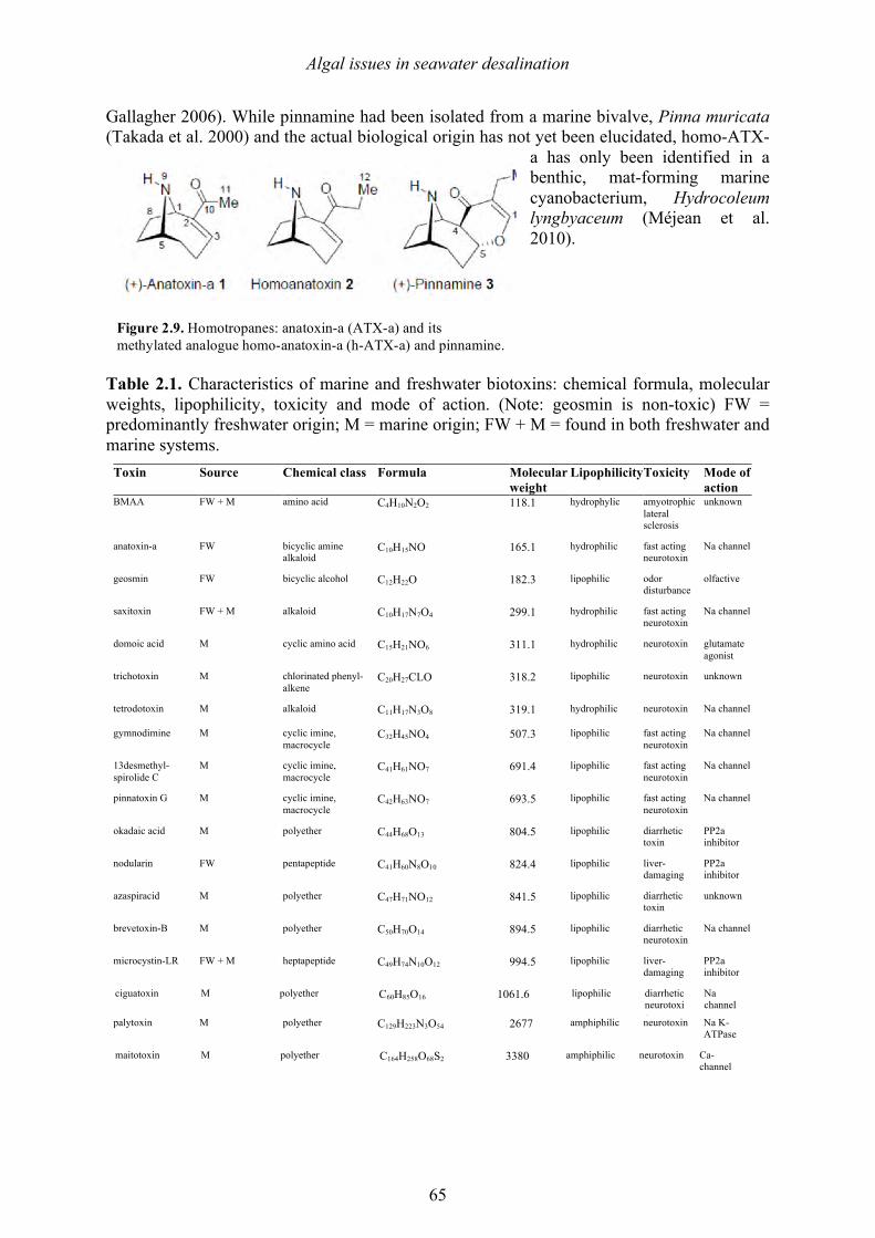
Algal issues in seawater desalination

65

Gallagher 2006). While pinnamine had been isolated from a marine bivalve, Pinna muricata (Takada et al. 2000) and the actual biological origin has not yet been elucidated, homo-ATX-

a has only been identified in a benthic, mat-forming marine cyanobacterium, Hydrocoleum lyngbyaceum (Méjean et al. 2010).

Table 2.1. Characteristics of marine and freshwater biotoxins: chemical formula, molecular weights, lipophilicity, toxicity and mode of action. (Note: geosmin is non-toxic) FW = predominantly freshwater origin; M = marine origin; FW + M = found in both freshwater and marine systems.

Toxin Source Chemical class Formula Molecular weight

Lipophilicity Toxicity Mode of action

BMAA FW + M amino acid C4H10N2O2 118.1 hydrophylic amyotrophic lateral sclerosis

unknown

anatoxin-a FW bicyclic amine alkaloid

C10H15NO 165.1 hydrophilic fast acting neurotoxin

Na channel

geosmin FW bicyclic alcohol C12H22O 182.3 lipophilic odor disturbance

olfactive

saxitoxin FW + M alkaloid C10H17N7O4 299.1 hydrophilic fast acting neurotoxin

Na channel

domoic acid M cyclic amino acid C15H21NO6 311.1 hydrophilic neurotoxin glutamate agonist

trichotoxin M chlorinated phenyl-alkene

C20H27CLO 318.2 lipophilic neurotoxin unknown

tetrodotoxin M alkaloid C11H17N3O8 319.1 hydrophilic neurotoxin Na channel

gymnodimine M cyclic imine, macrocycle

C32H45NO4 507.3 lipophilic fast acting neurotoxin

Na channel

13desmethyl-spirolide C

M cyclic imine, macrocycle

C41H61NO7 691.4 lipophilic fast acting neurotoxin

Na channel

pinnatoxin G M cyclic imine, macrocycle

C42H63NO7 693.5 lipophilic fast acting neurotoxin

Na channel

okadaic acid M polyether C44H68O13 804.5 lipophilic diarrhetic toxin

PP2a inhibitor

nodularin FW pentapeptide C41H60N8O10 824.4 lipophilic liver-damaging

PP2a inhibitor

azaspiracid M polyether C47H71NO12 841.5 lipophilic diarrhetic toxin

unknown

brevetoxin-B M polyether C50H70O14 894.5 lipophilic diarrhetic neurotoxin

Na channel

microcystin-LR FW + M heptapeptide C49H74N10O12 994.5 lipophilic liver-damaging

PP2a inhibitor

ciguatoxin M polyether C60H85O16 1061.6 lipophilic diarrhetic neurotoxin

Na channel

palytoxin M polyether C129H223N3O54 2677 amphiphilic neurotoxin Na K-ATPase

maitotoxin M polyether C164H258O68S2 3380 amphiphilic neurotoxin Ca-channel

Figure 2.9. Homotropanes: anatoxin-a (ATX-a) and its methylated analogue homo-anatoxin-a (h-ATX-a) and pinnamine.

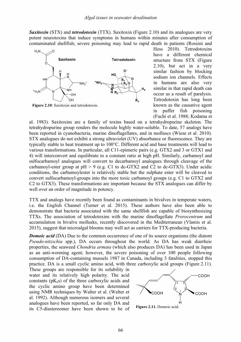
Algal issues in seawater desalination

66

Saxitoxin (STX) and tetrodotoxin (TTX). Saxitoxin (Figure 2.10) and its analogues are very potent neurotoxins that induce symptoms in humans within minutes after consumption of contaminated shellfish; severe poisoning may lead to rapid death in patients (Rossini and

Hess 2010). Tetrodotoxins have a different chemical structure from STX (Figure 2.10), but act in a very similar fashion by blocking sodium ion channels. Effects in humans are also very similar in that rapid death can occur as a result of paralysis. Tetrodotoxin has long been known as the causative agent in puffer fish poisoning (Fuchi et al. 1988; Kodama et

al. 1983). Saxitoxins are a family of toxins based on a tetrahydropurine skeleton. The tetrahydropurine group renders the molecule highly water-soluble. To date, 57 analogs have been reported in cyanobacteria, marine dinoflagellates, and in molluscs (Wiese et al. 2010). STX analogues do not exhibit a strong ultraviolet (UV) absorbance or fluorescence. They are typically stable to heat treatment up to 100°C. Different acid and base treatments will lead to various transformations. In particular, all C11-epimeric pairs (e.g. GTX2 and 3 or GTX1 and 4) will interconvert and equilibrate to a constant ratio at high pH. Similarly, carbamoyl and sulfocarbamoyl analogues will convert to decarbamoyl analogues through cleavage of the carbamoyl-ester group at pH > 9 (e.g. C1 to dc-GTX2 and C2 to dc-GTX3). Under acidic conditions, the carbamoylester is relatively stable but the sulphate ester will be cleaved to convert sulfocarbamoyl-groups into the more toxic carbamoyl groups (e.g. C1 to GTX2 and C2 to GTX3). These transformations are important because the STX analogues can differ by well over an order of magnitude in potency.

TTX and analogs have recently been found as contaminants in bivalves in temperate waters, i.e. the English Channel (Turner et al. 2015). These authors have also been able to demonstrate that bacteria associated with the same shellfish are capable of biosynthesizing TTXs. The association of tetrodotoxins with the marine dinoflagellate Prorocentrum and accumulation in bivalve mollusks, recently discovered in the Mediterranean (Vlamis et al. 2015), suggest that microalgal blooms may well act as carriers for TTX-producing bacteria. Domoic acid (DA) Due to the common occurrence of one of its source organisms (the diatom Pseudo-nitzschia spp.), DA occurs throughout the world. As DA has weak diarrheic properties, the seaweed Chondria armata (which also produces DA) has been used in Japan as an anti-worming agent; however, the severe poisoning of over 100 people following consumption of DA-containing mussels 1987 in Canada, including 3 fatalities, stopped this practice. DA is a small cyclic amino acid, with three carboxylic acid groups (Figure 2.11). These groups are responsible for its solubility in water and its relatively high polarity. The acid constants (pKas) of the three carboxylic acids and the cyclic amino group have been determined using NMR techniques by Walter et al. (Walter et al. 1992). Although numerous isomers and several analogues have been reported, so far only DA and its C5-diastereomer have been shown to be of

Figure 2.10: Saxitoxin and tetrodotoxin.

Figure 2.11. Domoic acid.

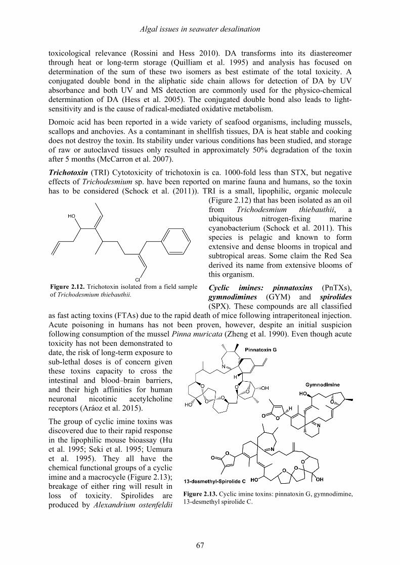
Algal issues in seawater desalination

67

toxicological relevance (Rossini and Hess 2010). DA transforms into its diastereomer through heat or long-term storage (Quilliam et al. 1995) and analysis has focused on determination of the sum of these two isomers as best estimate of the total toxicity. A conjugated double bond in the aliphatic side chain allows for detection of DA by UV absorbance and both UV and MS detection are commonly used for the physico-chemical determination of DA (Hess et al. 2005). The conjugated double bond also leads to light-sensitivity and is the cause of radical-mediated oxidative metabolism. Domoic acid has been reported in a wide variety of seafood organisms, including mussels, scallops and anchovies. As a contaminant in shellfish tissues, DA is heat stable and cooking does not destroy the toxin. Its stability under various conditions has been studied, and storage of raw or autoclaved tissues only resulted in approximately 50% degradation of the toxin after 5 months (McCarron et al. 2007).

Trichotoxin (TRI) Cytotoxicity of trichotoxin is ca. 1000-fold less than STX, but negative effects of Trichodesmium sp. have been reported on marine fauna and humans, so the toxin has to be considered (Schock et al. (2011)). TRI is a small, lipophilic, organic molecule

(Figure 2.12) that has been isolated as an oil from Trichodesmium thiebauthii, a ubiquitous nitrogen-fixing marine cyanobacterium (Schock et al. 2011). This species is pelagic and known to form extensive and dense blooms in tropical and subtropical areas. Some claim the Red Sea derived its name from extensive blooms of this organism.

Cyclic imines: pinnatoxins (PnTXs), gymnodimines (GYM) and spirolides (SPX). These compounds are all classified

as fast acting toxins (FTAs) due to the rapid death of mice following intraperitoneal injection. Acute poisoning in humans has not been proven, however, despite an initial suspicion following consumption of the mussel Pinna muricata (Zheng et al. 1990). Even though acute toxicity has not been demonstrated to date, the risk of long-term exposure to sub-lethal doses is of concern given these toxins capacity to cross the intestinal and blood–brain barriers, and their high affinities for human neuronal nicotinic acetylcholine receptors (Aráoz et al. 2015).

The group of cyclic imine toxins was discovered due to their rapid response in the lipophilic mouse bioassay (Hu et al. 1995; Seki et al. 1995; Uemura et al. 1995). They all have the chemical functional groups of a cyclic imine and a macrocycle (Figure 2.13); breakage of either ring will result in loss of toxicity. Spirolides are produced by Alexandrium ostenfeldii

Figure 2.12. Trichotoxin isolated from a field sample of Trichodesmium thiebauthii.

Figure 2.13. Cyclic imine toxins: pinnatoxin G, gymnodimine, 13-desmethyl spirolide C.

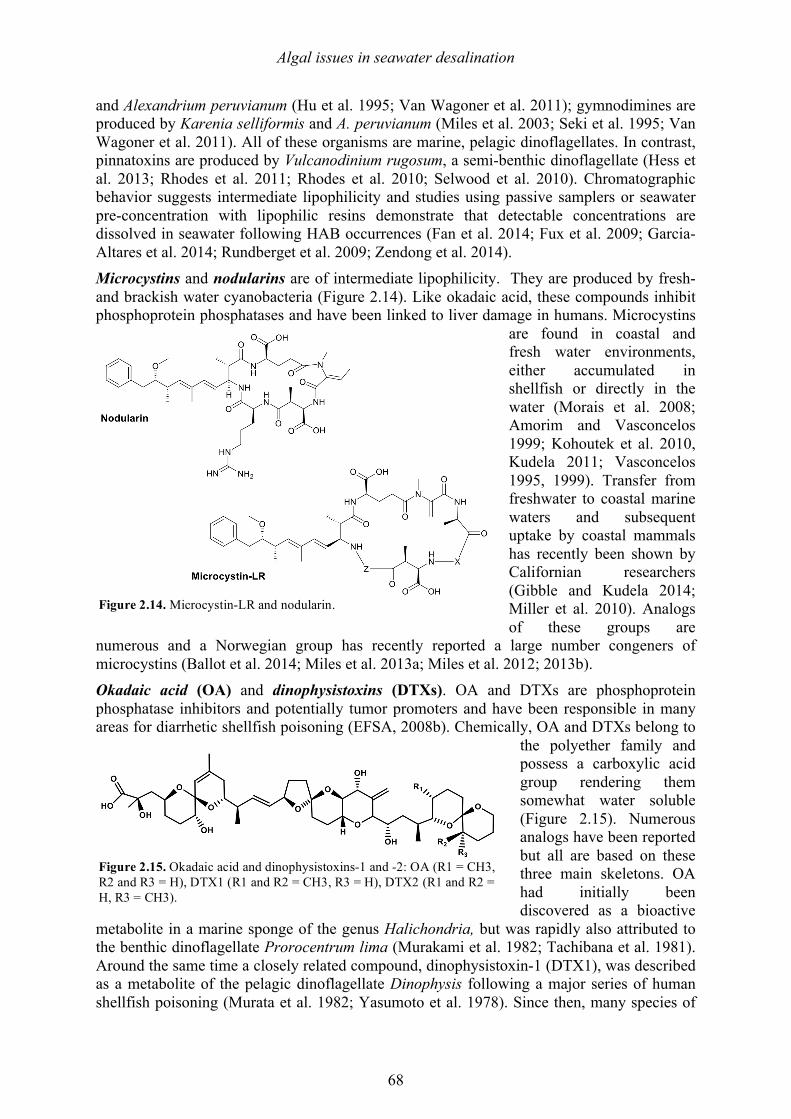
Algal issues in seawater desalination

68

and Alexandrium peruvianum (Hu et al. 1995; Van Wagoner et al. 2011); gymnodimines are produced by Karenia selliformis and A. peruvianum (Miles et al. 2003; Seki et al. 1995; Van Wagoner et al. 2011). All of these organisms are marine, pelagic dinoflagellates. In contrast, pinnatoxins are produced by Vulcanodinium rugosum, a semi-benthic dinoflagellate (Hess et al. 2013; Rhodes et al. 2011; Rhodes et al. 2010; Selwood et al. 2010). Chromatographic behavior suggests intermediate lipophilicity and studies using passive samplers or seawater pre-concentration with lipophilic resins demonstrate that detectable concentrations are dissolved in seawater following HAB occurrences (Fan et al. 2014; Fux et al. 2009; Garcia-Altares et al. 2014; Rundberget et al. 2009; Zendong et al. 2014). Microcystins and nodularins are of intermediate lipophilicity. They are produced by fresh- and brackish water cyanobacteria (Figure 2.14). Like okadaic acid, these compounds inhibit phosphoprotein phosphatases and have been linked to liver damage in humans. Microcystins

are found in coastal and fresh water environments, either accumulated in shellfish or directly in the water (Morais et al. 2008; Amorim and Vasconcelos 1999; Kohoutek et al. 2010, Kudela 2011; Vasconcelos 1995, 1999). Transfer from freshwater to coastal marine waters and subsequent uptake by coastal mammals has recently been shown by Californian researchers (Gibble and Kudela 2014; Miller et al. 2010). Analogs of these groups are

numerous and a Norwegian group has recently reported a large number congeners of microcystins (Ballot et al. 2014; Miles et al. 2013a; Miles et al. 2012; 2013b). Okadaic acid (OA) and dinophysistoxins (DTXs). OA and DTXs are phosphoprotein phosphatase inhibitors and potentially tumor promoters and have been responsible in many areas for diarrhetic shellfish poisoning (EFSA, 2008b). Chemically, OA and DTXs belong to

the polyether family and possess a carboxylic acid group rendering them somewhat water soluble (Figure 2.15). Numerous analogs have been reported but all are based on these three main skeletons. OA had initially been discovered as a bioactive

metabolite in a marine sponge of the genus Halichondria, but was rapidly also attributed to the benthic dinoflagellate Prorocentrum lima (Murakami et al. 1982; Tachibana et al. 1981). Around the same time a closely related compound, dinophysistoxin-1 (DTX1), was described as a metabolite of the pelagic dinoflagellate Dinophysis following a major series of human shellfish poisoning (Murata et al. 1982; Yasumoto et al. 1978). Since then, many species of

Figure 2.14. Microcystin-LR and nodularin.

Figure 2.15. Okadaic acid and dinophysistoxins-1 and -2: OA (R1 = CH3, R2 and R3 = H), DTX1 (R1 and R2 = CH3, R3 = H), DTX2 (R1 and R2 = H, R3 = CH3).

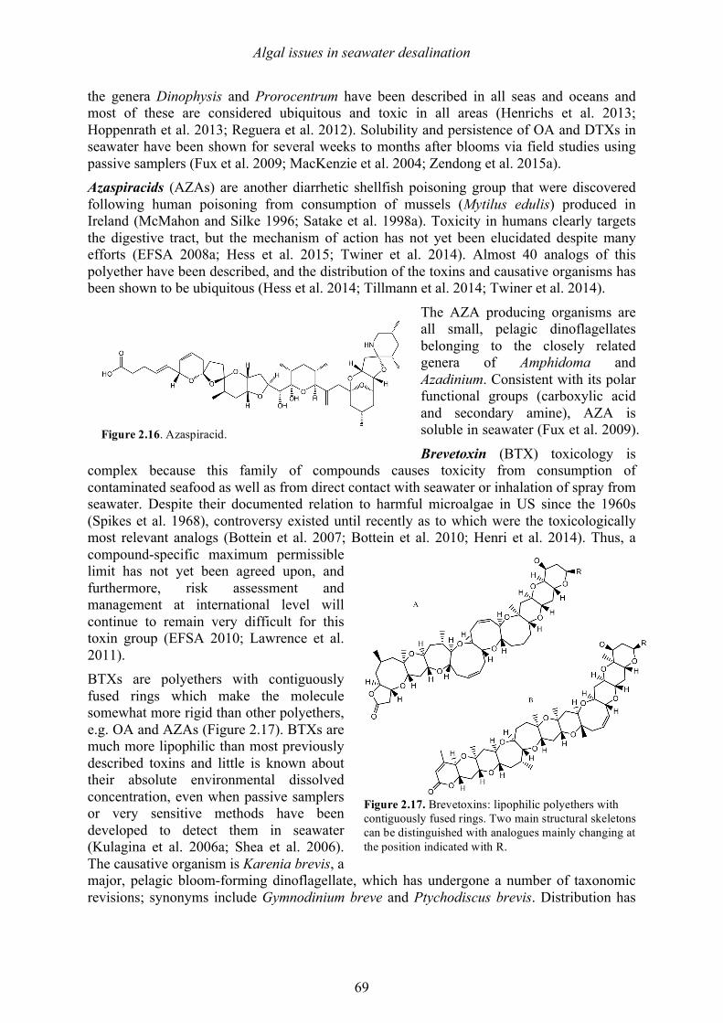
Algal issues in seawater desalination

69

the genera Dinophysis and Prorocentrum have been described in all seas and oceans and most of these are considered ubiquitous and toxic in all areas (Henrichs et al. 2013; Hoppenrath et al. 2013; Reguera et al. 2012). Solubility and persistence of OA and DTXs in seawater have been shown for several weeks to months after blooms via field studies using passive samplers (Fux et al. 2009; MacKenzie et al. 2004; Zendong et al. 2015a). Azaspiracids (AZAs) are another diarrhetic shellfish poisoning group that were discovered following human poisoning from consumption of mussels (Mytilus edulis) produced in Ireland (McMahon and Silke 1996; Satake et al. 1998a). Toxicity in humans clearly targets the digestive tract, but the mechanism of action has not yet been elucidated despite many efforts (EFSA 2008a; Hess et al. 2015; Twiner et al. 2014). Almost 40 analogs of this polyether have been described, and the distribution of the toxins and causative organisms has been shown to be ubiquitous (Hess et al. 2014; Tillmann et al. 2014; Twiner et al. 2014).

The AZA producing organisms are all small, pelagic dinoflagellates belonging to the closely related genera of Amphidoma and Azadinium. Consistent with its polar functional groups (carboxylic acid and secondary amine), AZA is soluble in seawater (Fux et al. 2009).

Brevetoxin (BTX) toxicology is complex because this family of compounds causes toxicity from consumption of contaminated seafood as well as from direct contact with seawater or inhalation of spray from seawater. Despite their documented relation to harmful microalgae in US since the 1960s (Spikes et al. 1968), controversy existed until recently as to which were the toxicologically most relevant analogs (Bottein et al. 2007; Bottein et al. 2010; Henri et al. 2014). Thus, a compound-specific maximum permissible limit has not yet been agreed upon, and furthermore, risk assessment and management at international level will continue to remain very difficult for this toxin group (EFSA 2010; Lawrence et al. 2011). BTXs are polyethers with contiguously fused rings which make the molecule somewhat more rigid than other polyethers, e.g. OA and AZAs (Figure 2.17). BTXs are much more lipophilic than most previously described toxins and little is known about their absolute environmental dissolved concentration, even when passive samplers or very sensitive methods have been developed to detect them in seawater (Kulagina et al. 2006a; Shea et al. 2006). The causative organism is Karenia brevis, a major, pelagic bloom-forming dinoflagellate, which has undergone a number of taxonomic revisions; synonyms include Gymnodinium breve and Ptychodiscus brevis. Distribution has

Figure 2.17. Brevetoxins: lipophilic polyethers with contiguously fused rings. Two main structural skeletons can be distinguished with analogues mainly changing at the position indicated with R.

Figure 2.16. Azaspiracid.

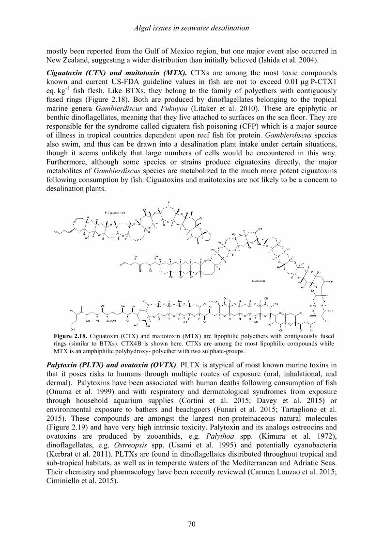
Algal issues in seawater desalination

70

mostly been reported from the Gulf of Mexico region, but one major event also occurred in New Zealand, suggesting a wider distribution than initially believed (Ishida et al. 2004).

Ciguatoxin (CTX) and maitotoxin (MTX). CTXs are among the most toxic compounds known and current US-FDA guideline values in fish are not to exceed 0.01 µg P-CTX1 eq. kg-1 fish flesh. Like BTXs, they belong to the family of polyethers with contiguously fused rings (Figure 2.18). Both are produced by dinoflagellates belonging to the tropical marine genera Gambierdiscus and Fukuyoa (Litaker et al. 2010). These are epiphytic or benthic dinoflagellates, meaning that they live attached to surfaces on the sea floor. They are responsible for the syndrome called ciguatera fish poisoning (CFP) which is a major source of illness in tropical countries dependent upon reef fish for protein. Gambierdiscus species also swim, and thus can be drawn into a desalination plant intake under certain situations, though it seems unlikely that large numbers of cells would be encountered in this way. Furthermore, although some species or strains produce ciguatoxins directly, the major metabolites of Gambierdiscus species are metabolized to the much more potent ciguatoxins following consumption by fish. Ciguatoxins and maitotoxins are not likely to be a concern to desalination plants.

Palytoxin (PLTX) and ovatoxin (OVTX). PLTX is atypical of most known marine toxins in that it poses risks to humans through multiple routes of exposure (oral, inhalational, and dermal). Palytoxins have been associated with human deaths following consumption of fish (Onuma et al. 1999) and with respiratory and dermatological syndromes from exposure through household aquarium supplies (Cortini et al. 2015; Davey et al. 2015) or environmental exposure to bathers and beachgoers (Funari et al. 2015; Tartaglione et al. 2015). These compounds are amongst the largest non-proteinaceous natural molecules (Figure 2.19) and have very high intrinsic toxicity. Palytoxin and its analogs ostreocins and ovatoxins are produced by zooanthids, e.g. Palythoa spp. (Kimura et al. 1972), dinoflagellates, e.g. Ostreopsis spp. (Usami et al. 1995) and potentially cyanobacteria (Kerbrat et al. 2011). PLTXs are found in dinoflagellates distributed throughout tropical and sub-tropical habitats, as well as in temperate waters of the Mediterranean and Adriatic Seas. Their chemistry and pharmacology have been recently reviewed (Carmen Louzao et al. 2015; Ciminiello et al. 2015).

Figure 2.18. Ciguatoxin (CTX) and maitotoxin (MTX) are lipophilic polyethers with contiguously fused rings (similar to BTXs). CTX4B is shown here. CTXs are among the most lipophilic compounds while MTX is an amphiphilic polyhydroxy- polyether with two sulphate-groups.

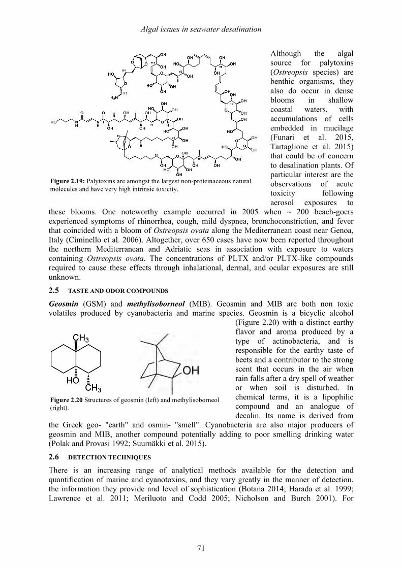
Algal issues in seawater desalination

71

Although the algal source for palytoxins (Ostreopsis species) are benthic organisms, they also do occur in dense blooms in shallow coastal waters, with accumulations of cells embedded in mucilage (Funari et al. 2015, Tartaglione et al. 2015) that could be of concern to desalination plants. Of particular interest are the observations of acute toxicity following aerosol exposures to

these blooms. One noteworthy example occurred in 2005 when ~ 200 beach-goers experienced symptoms of rhinorrhea, cough, mild dyspnea, bronchoconstriction, and fever that coincided with a bloom of Ostreopsis ovata along the Mediterranean coast near Genoa, Italy (Ciminello et al. 2006). Altogether, over 650 cases have now been reported throughout the northern Mediterranean and Adriatic seas in association with exposure to waters containing Ostreopsis ovata. The concentrations of PLTX and/or PLTX-like compounds required to cause these effects through inhalational, dermal, and ocular exposures are still unknown. 2.5 TASTE AND ODOR COMPOUNDS

Geosmin (GSM) and methylisoborneol (MIB). Geosmin and MIB are both non toxic volatiles produced by cyanobacteria and marine species. Geosmin is a bicyclic alcohol

(Figure 2.20) with a distinct earthy flavor and aroma produced by a type of actinobacteria, and is responsible for the earthy taste of beets and a contributor to the strong scent that occurs in the air when rain falls after a dry spell of weather or when soil is disturbed. In chemical terms, it is a lipophilic compound and an analogue of decalin. Its name is derived from

the Greek geo- "earth" and osmin- "smell". Cyanobacteria are also major producers of geosmin and MIB, another compound potentially adding to poor smelling drinking water (Polak and Provasi 1992; Suurnäkki et al. 2015).

2.6 DETECTION TECHNIQUES There is an increasing range of analytical methods available for the detection and quantification of marine and cyanotoxins, and they vary greatly in the manner of detection, the information they provide and level of sophistication (Botana 2014; Harada et al. 1999; Lawrence et al. 2011; Meriluoto and Codd 2005; Nicholson and Burch 2001). For

Figure 2.19: Palytoxins are amongst the largest non-proteinaceous natural molecules and have very high intrinsic toxicity.

Figure 2.20 Structures of geosmin (left) and methylisoborneol (right).

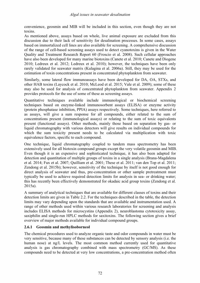
Algal issues in seawater desalination

72

convenience, geosmin and MIB will be included in this section, even though they are not toxins. As mentioned above, assays based on whole, live animal exposure are excluded from this discussion due to their lack of sensitivity for desalination processes. In some cases, assays based on immortalized cell lines are also available for screening. A comprehensive discussion of the range of cell-based screening assays used to detect cyanotoxins is given in the Water Quality and Treatment Research Report 60 (Froscio et al. 2008). Such cellular approaches have also been developed for many marine biotoxins (Canete et al. 2010; Canete and Diogene 2010; Ledreux et al. 2012; Ledreux et al. 2010); however, the techniques have been only rarely validated for seawater matrix (Kulagina et al. 2006a). Still, they may be used for the estimation of toxin concentrations present in concentrated phytoplankton from seawater. Similarly, some lateral flow immunoassays have been developed for DA, OA, STXs, and other HAB toxins (Laycock et al. 2010; McLeod et al. 2015; Vale et al. 2009); some of these may also be used for analysis of concentrated phytoplankton from seawater. Appendix 2 provides protocols for the use of some of these as screening assays. Quantitative techniques available include immunological or biochemical screening techniques based on enzyme-linked immunosorbent assays (ELISA) or enzyme activity (protein phosphatase inhibition, PPIA) assays respectively. Some techniques, here referred to as assays, will give a sum response for all compounds, either related to the sum of concentrations present (immunological assays) or relating to the sum of toxic equivalents present (functional assays). Other methods, mainly those based on separation by gas- or liquid chromatography with various detectors will give results on individual compounds for which the sum toxicity present needs to be calculated via multiplication with toxic equivalence factors, specific to each compound.

One technique, liquid chromatography coupled to tandem mass spectrometry has been extensively used for all biotoxin compound groups except the very volatile geosmin and MIB. Even though it is an expensive and sophisticated technique, it has also been adapted for detection and quantitation of multiple groups of toxins in a single analysis (Brana-Magdalena et al. 2014; Fux et al. 2007; Quilliam et al. 2001; These et al. 2011; van den Top et al. 2011; Zendong et al. 2015b); however, sensitivity of the technique by itself is not good enough for direct analysis of seawater and thus, pre-concentration or other sample pretreatment must typically be used to achieve required detection limits for analysis in sea- or drinking water; this has recently been effectively demonstrated for okadaic acid group toxins (Zendong et al. 2015a).

A summary of analytical techniques that are available for different classes of toxins and their detection limits are given in Table 2.2. For the techniques described in the table, the detection limits may vary depending upon the standards that are available and instrumentation used. A range of other methods used within various research laboratories for screening and analysis includes ELISA methods for microcystins (Appendix 2), neuroblastoma cytotoxicity assay, saxiphilin and single-run HPLC methods for saxitoxins. The following section gives a brief overview of major methods available for individual compound groups. 2.6.1 Geosmin and methylisoborneol

The chemical procedures used to analyze organic taste and odor compounds in water must be very sensitive, because many of these substances can be detected by sensory analysis (i.e. the human nose) at ng/L levels. The most common method currently used for quantitative analysis is gas chromatography combined with mass spectrometry (GC/MS). As these compounds need to be detected at very low concentrations, a pre-concentration method often

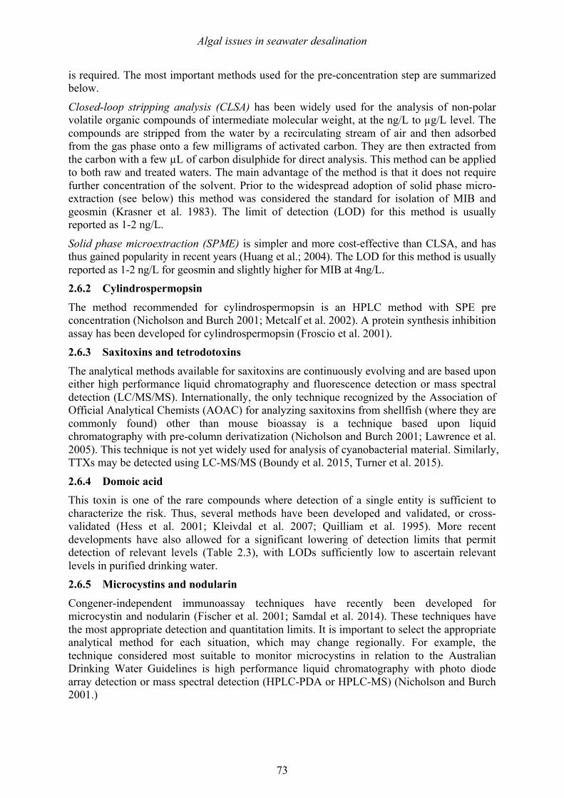
Algal issues in seawater desalination

73

is required. The most important methods used for the pre-concentration step are summarized below.

Closed-loop stripping analysis (CLSA) has been widely used for the analysis of non-polar volatile organic compounds of intermediate molecular weight, at the ng/L to µg/L level. The compounds are stripped from the water by a recirculating stream of air and then adsorbed from the gas phase onto a few milligrams of activated carbon. They are then extracted from the carbon with a few µL of carbon disulphide for direct analysis. This method can be applied to both raw and treated waters. The main advantage of the method is that it does not require further concentration of the solvent. Prior to the widespread adoption of solid phase micro-extraction (see below) this method was considered the standard for isolation of MIB and geosmin (Krasner et al. 1983). The limit of detection (LOD) for this method is usually reported as 1-2 ng/L.

Solid phase microextraction (SPME) is simpler and more cost-effective than CLSA, and has thus gained popularity in recent years (Huang et al.; 2004). The LOD for this method is usually reported as 1-2 ng/L for geosmin and slightly higher for MIB at 4ng/L. 2.6.2 Cylindrospermopsin

The method recommended for cylindrospermopsin is an HPLC method with SPE pre concentration (Nicholson and Burch 2001; Metcalf et al. 2002). A protein synthesis inhibition assay has been developed for cylindrospermopsin (Froscio et al. 2001). 2.6.3 Saxitoxins and tetrodotoxins

The analytical methods available for saxitoxins are continuously evolving and are based upon either high performance liquid chromatography and fluorescence detection or mass spectral detection (LC/MS/MS). Internationally, the only technique recognized by the Association of Official Analytical Chemists (AOAC) for analyzing saxitoxins from shellfish (where they are commonly found) other than mouse bioassay is a technique based upon liquid chromatography with pre-column derivatization (Nicholson and Burch 2001; Lawrence et al. 2005). This technique is not yet widely used for analysis of cyanobacterial material. Similarly, TTXs may be detected using LC-MS/MS (Boundy et al. 2015, Turner et al. 2015).

2.6.4 Domoic acid This toxin is one of the rare compounds where detection of a single entity is sufficient to characterize the risk. Thus, several methods have been developed and validated, or cross-validated (Hess et al. 2001; Kleivdal et al. 2007; Quilliam et al. 1995). More recent developments have also allowed for a significant lowering of detection limits that permit detection of relevant levels (Table 2.3), with LODs sufficiently low to ascertain relevant levels in purified drinking water. 2.6.5 Microcystins and nodularin

Congener-independent immunoassay techniques have recently been developed for microcystin and nodularin (Fischer et al. 2001; Samdal et al. 2014). These techniques have the most appropriate detection and quantitation limits. It is important to select the appropriate analytical method for each situation, which may change regionally. For example, the technique considered most suitable to monitor microcystins in relation to the Australian Drinking Water Guidelines is high performance liquid chromatography with photo diode array detection or mass spectral detection (HPLC-PDA or HPLC-MS) (Nicholson and Burch 2001.)

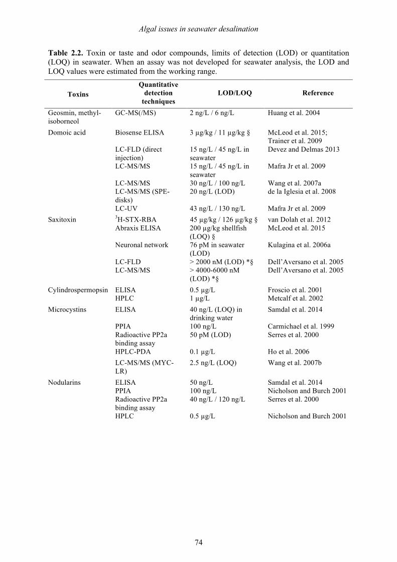
Algal issues in seawater desalination

74

Table 2.2. Toxin or taste and odor compounds, limits of detection (LOD) or quantitation (LOQ) in seawater. When an assay was not developed for seawater analysis, the LOD and LOQ values were estimated from the working range.

Toxins Quantitative

detection techniques

LOD/LOQ Reference

Geosmin, methyl-isoborneol

GC-MS(/MS) 2 ng/L / 6 ng/L Huang et al. 2004

Domoic acid Biosense ELISA 3 µg/kg / 11 µg/kg §

McLeod et al. 2015; Trainer et al. 2009

LC-FLD (direct injection)

15 ng/L / 45 ng/L in seawater

Devez and Delmas 2013

LC-MS/MS 15 ng/L / 45 ng/L in seawater

Mafra Jr et al. 2009

LC-MS/MS 30 ng/L / 100 ng/L Wang et al. 2007a LC-MS/MS (SPE-

disks) 20 ng/L (LOD) de la Iglesia et al. 2008

LC-UV 43 ng/L / 130 ng/L Mafra Jr et al. 2009 Saxitoxin 3H-STX-RBA 45 µg/kg / 126 µg/kg § van Dolah et al. 2012 Abraxis ELISA 200 µg/kg shellfish

(LOQ) § McLeod et al. 2015

Neuronal network 76 pM in seawater (LOD)

Kulagina et al. 2006a

LC-FLD > 2000 nM (LOD) *§ Dell’Aversano et al. 2005 LC-MS/MS > 4000-6000 nM

(LOD) *§ Dell’Aversano et al. 2005

Cylindrospermopsin ELISA 0.5 µg/L Froscio et al. 2001 HPLC 1 µg/L Metcalf et al. 2002 Microcystins ELISA 40 ng/L (LOQ) in

drinking water Samdal et al. 2014

PPIA 100 ng/L Carmichael et al. 1999 Radioactive PP2a

binding assay 50 pM (LOD) Serres et al. 2000

HPLC-PDA LC-MS/MS (MYC-LR)

0.1 µg/L 2.5 ng/L (LOQ)

Ho et al. 2006 Wang et al. 2007b

Nodularins ELISA 50 ng/L Samdal et al. 2014 PPIA 100 ng/L Nicholson and Burch 2001 Radioactive PP2a

binding assay 40 ng/L / 120 ng/L Serres et al. 2000

HPLC 0.5 µg/L Nicholson and Burch 2001

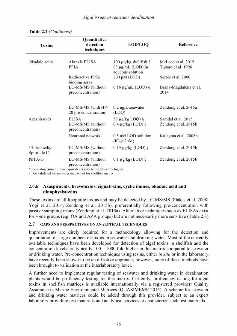
Algal issues in seawater desalination

75

Table 2.2 (Continued)

Toxins Quantitative

detection techniques

LOD/LOQ Reference

Okadaic acids Abraxis ELISA 100 µg/kg shellfish § McLeod et al. 2015

PPIA 63 pg/mL (LOD) in aqueous solution

Tubaro et al. 1996

Radioactive PP2a binding assay

200 pM (LOD) Serres et al. 2000

LC-MS/MS (without preconcentration)

0.16 ng/mL (LOD) § Brana-Magdalena et al. 2014

LC-MS/MS (with HP-20 pre-concentration)

0.2 ng/L seawater (LOQ)

Zendong et al. 2015a

Azaspiracids ELISA 57 µg/kg LOQ) § Samdal et al. 2015 LC-MS/MS (without

preconcentration) 0.4 µg/kg (LOD) § Zendong et al. 2015b

Neuronal network 0.5 nM LOD solution (IC50=2nM)

Kulagina et al. 2006b

13-desmethyl Spirolide C

LC-MS/MS (without preconcentration)

0.15 µg/kg (LOD) § Zendong et al. 2015b

PnTX-G LC-MS/MS (without preconcentration)

0.1 µg/kg (LOD) § Zendong et al. 2015b

*Per analog (sum of toxic equivalents may be significantly higher) § Not validated for seawater matrix but for shellfish matrix 2.6.6 Azaspiracids, brevetoxins, ciguatoxins, cyclic imines, okadaic acid and

dinophysistoxins These toxins are all lipophilic toxins and may be detected by LC-MS/MS (Plakas et al. 2008; Yogi et al. 2014, Zendong et al. 2015b), preferentially following pre-concentration with passive sampling resins (Zendong et al. 2015a). Alternative techniques such as ELISAs exist for some groups (e.g. OA and AZA groups) but are not necessarily more sensitive (Table 2.3). 2.7 GAPS AND PERSPECTIVES ON ANALYTICAL TECHNIQUES

Improvements are direly required for a methodology allowing for the detection and quantitation of large numbers of toxins in seawater and drinking water. Most of the currently available techniques have been developed for detection of algal toxins in shellfish and the concentration levels are typically 100 – 1000 fold higher in this matrix compared to seawater or drinking water. Pre-concentration techniques using resins, either in situ or in the laboratory, have recently been shown to be an effective approach; however, none of these methods have been brought to validation at the interlaboratory level. A further need to implement regular testing of seawater and drinking water in desalination plants would be proficiency testing for this matrix. Currently, proficiency testing for algal toxins in shellfish matrices is available internationally via a registered provider: Quality Assurance in Marine Environmental Matrices (QUASIMEME 2015). A scheme for seawater and drinking water matrices could be added through this provider, subject to an expert laboratory providing test materials and analytical services to characterize such test materials.

Algal issues in seawater desalination

76

A promising area that is developing rapidly is the application of molecular techniques (quantitative PCR) for determination of genes for toxin production. Among the algal toxins from diatoms and dinoflagellates, this approach has only been applied to STX thus far, as the toxin-producing genes are not known for most of the other toxins. Still, this approach will only apply to detection of toxin-producing algae, not the toxins themselves. 2.8 REFERENCES Alldredge, A. L., Passow, U., and Logan, B. E. 1993. The abundance and significance of a

class of large, transparent organic particles in the ocean. Deep-Sea Research I: 40, 1131–1140.

Amorim, Á. And Vasconcelos, V. 1999. Dynamics of microcystins in the mussel Mytilus galloprovincialis. Toxicon 37, 1041-1052.

Aráoz, R., Hess, P., Pelissier, F., Benoit, E., Servent, D., Zakarian, A., and Molgó, J. 2015. Cyclic imine toxins: From shellfish poisoning to neuroscience: The case of acyl derivatives. Biochemical Pharmacology 97, 622.

Azetsu-Scott, K. and Passow, U. 2004. Ascending marine particles: Significance of transparent exopolymer particles (TEP) in the upper ocean. Limnology and Oceanography 49(3), 741-748.

Ballot, A., Sandvik, M., Rundberget, T., Botha, C. J., and Miles, C. O. 2014. Diversity of cyanobacteria and cyanotoxins in Hartbeespoort Dam, South Africa. Marine and Freshwater Research 65, 175-189.

Bar-Zeev, E., Berman-Frank, I., Girshevitz, O., and Berman, T. 2012. Revised paradigm of aquatic biofilm formation facilitated by microgel transparent exopolymer particles. Proceedings of the National Academy of Sciences 109(23), 9119-9124.

Bar-Zeev, E. and Rahav E. 2015. Microbial metabolism of transparent exopolymer particles during the summer months along a eutrophic estuary system. Frontiers in Microbiology 6:403. doi: 10.3389/fmicb.2015.00403.

Berktay, A. 2011. Environmental approach and influence of red tide to desalination process in the middle-east region. International Journal of Chemical and Environmental Engineering 2(3), 183-188.

Berman, T. and Holenberg, M. 2005. Don't fall foul of biofilm through high TEP levels. Filtration & Separation 42(4), 30-32.

Botana, L.M. 2014. Seafood and Freshwater toxins: pharmacology, physiology, and detection. Third Edition. CRC Press, Boca Raton, FL, USA.

Boerlage, S. F. E. and Nada, N. 2014. Algal toxin removal in seawater desalination processes, In Proceedings of European Desalination Society, Cyprus.

Bottein, M.-Y. D., Fuquay, J. M., Munday, R., Selwood, A. I., van Ginkel, R., Miles, C. O., Loader, J. I., Wilkins, A. L., and Ramsdell, J. S. 2010. Bioassay methods for detection of N-palmitoylbrevetoxin-B2 (BTX-B4). Toxicon 55, 497-506.

Bottein, M.-Y. D, Wang, Z., and Ramsdell, J. S. 2007. Intrinsic potency of synthetically prepared brevetoxin cysteine metabolites BTX-B2 and desoxyBTX-B2. Toxicon 50, 825-834.

Algal issues in seawater desalination

77

Boundy, M. J., Selwood, A. I., Harwood, D. T., McNabb, P. S., and Turner, A. D. 2015. Development of a sensitive and selective liquid chromatography–mass spectrometry method for high throughput analysis of paralytic shellfish toxins using graphitised carbon solid phase extraction. Journal of Chromatography A 1387, 1-12.

Brana-Magdalena, A., Leao-Martins, J. M., Glauner, T., Gago-Martinez, A. 2014. Intralaboratory validation of a fast and sensitive UHPLC/MS/MS method with fast polarity switching for the analysis of lipophilic shellfish toxins. Journal of AOAC International 97, 285-292.

Canete, E., Campas, M., de la Iglesia, P., and Diogene, J. 2010. NG108-15 cell-based and protein phosphatase inhibition assays as alternative semiquantitative tools for the screening of lipophilic toxins in mussels. Okadaic acid detection. Toxicology in Vitro 24, 611-619.

Canete, E., Diogene, J. 2010. Improvements in the use of neuroblastoma x glioma hybrid cells (NG108-15) for the toxic effect quantification of marine toxins. Toxicon 55, 381-389.

Carmen Louzao, M., Fraga, M., and Vilariño, N. 2015. Pharmacology of palytoxins and ostreocins, Phycotoxins. John Wiley & Sons, Ltd, pp. 113-135.

Carmichael, W. W. and An, J. 1999. Using an enzyme linked immunosorbent assay (ELISA) and a protein phosphatase inhibition assay (PPIA) for the detection of microcystins and nodularins. Journal of Natural Toxins 7: 377-385 .

Ciminiello, P., Dell'Aversano, C., Fattorusso, E., Forino, M., Magno, G. S., Tartaglione, L., Grillo, C., and Melchiorre, N. 2006. The Genoa 2005 outbreak. Determination of putative palytoxin in Mediterranean Ostreopsis ovata by a new liquid chromatography tandem mass spectrometry method. Analytical Chemistry, 78(17), 6153-6159.

Ciminiello, P., Dell'Aversano, C., and Forino, M. 2015. Chemistry of palytoxin and its analogues, Phycotoxins. John Wiley & Sons, Ltd, pp. 85-111.

Claquin, P., Probert, I., Lefebvre, S., AND Veron, B. 2008. Effects of temperature on photosynthetic parameters and TEP production in eight species of marine microalgae. Aquatic Microbial Ecology 51, 1-11.

Cortini, E., Lonati, D., Petrolini, V. M., Giampreti, A., Tubaro, A., and Locatelli, C. A. 2015. Dangerous palytoxin exposure after boiling coral. Clinical Toxicology 53, 339-339.

Daly, R., Ho, L., and Brookes, J. 2007. Effect of chlorination on Microcystis aeruginosa cell integrity and subsequent Microcystin release and degradation. Environmental Science and Technology 41, 4447-4453.

Davey, M. P., McKeown, N., and Hendrickson, R. 2015. Palytoxin yoxicity in a coral enthusiast and his family from unmanipulated coral. Clinical Toxicology 53, 776-777.

de la Iglesia, P., Giménez, G., and Diogène, J. 2008. Determination of dissolved domoic acid in seawater with reversed-phase extraction disks and rapid resolution liquid chromatography tandem mass spectrometry with head-column trapping. Journal of Chromatography A 1215, 116-124.

Dell’Aversano, C., Hess, P., and Quilliam, M. A. 2005. Hydrophilic interaction liquid chromatography–mass spectrometry for the analysis of paralytic shellfish poisoning (PSP) toxins. Journal of Chromatography A 1081, 190-201.

DesalData, 2015. https://www.desaldata.com/, accessed 3 November 2015.

Algal issues in seawater desalination

78

Devez, A. and Delmas, D. 2013. Selective liquid chromatographic determination of trace domoic acid in seawater and phytoplankton: improvement using the o-phthaldialdehyde/9-fluorenylmethylchloroformate derivatization. Limnology and Oceanography: Methods 11, 327-336.

EFSA, 2008a. Marine biotoxins in shellfish - Azaspiracid group, Scientific Opinion of the Panel on Contaminants in the Food chain, adopted on 9 June 2008. EFSA Journal 723, 1-52.

EFSA, 2008b. Marine biotoxins in shellfish - Okadaic Acid and analogues, Scientific Opinion of the Panel on Contaminants in the Food chain, adopted on 27 November 2007. EFSA Journal 589, 1-62.

EFSA, 2010. Marine biotoxins in shellfish - Emerging Toxins: Brevetoxin-group, Scientific Opinion of the Panel on Contaminants in the Food chain; adopted on 5 July 2010. EFSA Journal 8, 1-29.

Fan, L., Sun, G., Qiu, J., Ma, Q., Hess, P., and Li, A. 2014. Effect of seawater salinity on pore-size distribution on a poly(styrene)-based HP20 resin and its adsorption of diarrhetic shellfish toxins. Journal of Chromatography A 1373, 1-8.

Field, C. B., Behrenfeld, M. J., Randerson, J. T., and Falkowski, P. 1998. Primary production of the biosphere: Integrating terrestrial and oceanic components. Science 281, 237-240.

Fischer, W. J., Garthwaite, I., Miles, C. O., Ross, K. M., Aggen, J. B., Chamberlin, A. R., Towers, N. R., Dietrich, and D. R. 2001. Congener-independent immunoassay for microcystins and nodularins. Environmental Science and Technology 35, 4849-4856.

Fogg, G. E. 1983. The ecological significance of extracellular products of phytoplankton photosynthesis. Botanica Marina 26, 3–14.

Froscio, S., Fanok, S., King, B., and Humpage, A. R. 2008. Screening assays for water-borne toxicants research report 60. CRC for Water Quality and Treatment.

Froscio, S. M., Humpage, A. R., Burcham, P. C. and Falconer, I. R. 2001. Cell-free protein synthesis inhibition assay for the cyanobacterial toxin cylindrospermopsin. Environmental Toxicology 16: 408–412.

Fuchi, Y., Morisaki, S., Nagata, T., Shimazaki, K., Noguchi, T., Ohtomo, N., and Hashimoto, K. 1988. Determination of tetrodotoxin in puffer fish and shellfish by high performance liquid chromatography. Shokuhin Eiseigaku Zasshi 29, 306-312.

Funari, E., Manganelli, M., and Testai, E. 2015. Ostreospis cf. ovata blooms in coastal water: Italian guidelines to assess and manage the risk associated to bathing waters and recreational activities. Harmful Algae 50, 45-56.

Fux, E., Biré, R., and Hess, P. 2009. Comparative accumulation and composition of lipophilic marine biotoxins in passive samplers and in mussels (M. edulis) on the West Coast of Ireland. Harmful Algae 8, 523-537.

Fux, E., McMillan, D., Biré, R., and Hess, P. 2007. Development of an ultra-performance liquid chromatography-mass spectrometry method for the detection of lipophilic marine toxins. Journal of Chromatography A 1157, 273-280.

Garcia-Altares, M., Casanova, A., Bane, V., Diogene, J., Furey, A., and de la Iglesia, P. 2014. Confirmation of pinnatoxins and spirolides in shellfish and passive samplers from catalonia (Spain) by liquid chromatography coupled with triple quadrupole and high-resolution hybrid tandem mass spectrometry. Marine Drugs 12, 3706-3732.

Algal issues in seawater desalination

79

Gibble, C. M. and Kudela, R. M. 2014. Detection of persistent microcystin toxins at the land–sea interface in Monterey Bay, California. Harmful Algae 39, 146-153.

Harada, K. I., Kondo, F., and Lawton, L. 1999. Toxic cyanobacteria in water. A guide to their public health consequences, monitoring and management, in: Chorus, I., Bartram, J. (Eds.). World Health Organisation, pp. 369-405.

Heijman, S. G. J., Vantieghem, M., Raktoe, S., Verberk, J. Q. J. C., and van Dijk, J. C. 2007. Blocking of capillaries as fouling mechanism for dead-end ultrafiltration. Journal of Membrane Science, 287(1), 119-125.

Henderson, R. K., Baker, A., Parsons, S. A., and Jefferson, B. 2008. Characterisation of algogenic organic matter extracted from cyanobacteria, green algae and diatoms. Water Research 42:3435-3445.

Henri, J., Leighfield, T. A., Lanceleur, R., Huguet, A., Ramsdell, J. S., and Fessard, V. 2014. Permeability of dihydro- and cysteine-brevetoxin metabolites across a Caco-2 cell monolayer. Harmful Algae 32, 22-26.

Henrichs, D. W., Scott, P. S., Steidinger, K. A., Errera, R. M., Abraham, A., and Campbell, L. 2013. Morphology and Phylogeny of Prorocentrum texanum sp nov (Dinophyceae): A new toxic dinoflagellate from the Gulf of Mexico coastal waters exhibiting two distinct morphologies. Journal of Phycology 49, 143-155.

Her, N., Amy, G., Park, H.-R., and Song, M. 2004. Characterizing algogenic organic matter (AOM) and evaluating associated NF membrane fouling. Water Research 38, 1427–1438.

Herman, P.H., Bredee, H.L. 1936. Principles of the mathematical treatment of constant pressure filtration. Journal of the Society of Chemical Industry 1-4.

Hess, P., Abadie, E., Herve, F., Berteaux, T., Sechet, V., Araoz, R., Molgo, J., Zakarian, A., Sibat, M., Rundberget, T., Miles, C. O., and Amzil, Z. 2013. Pinnatoxin G is responsible for atypical toxicity in mussels (Mytilus galloprovincialis) and clams (Venerupis decussata) from Ingril, a French Mediterranean lagoon. Toxicon 75, 16-26.

Hess, P., Gallacher, S., Bates, L. A., Brown, N., and Quilliam, M. A. 2001. Determination and confirmation of the amnesic shellfish poisoning toxin, domoic acid, in shellfish from Scotland by liquid chromatography and mass spectrometry. Journal of the AOAC International 84, 1657-1667.

Hess, P., McCarron, P., Krock, B., Kilcoyne, J., and Miles, C. O. 2014. Azaspiracids: Chemistry, Biosynthesis, Metabolism, and Detection, Seafood and Freshwater Toxins. CRC Press, Boca Raton, Florida, USA, pp. 799-822.

Hess, P., Stobo, L. A., Brown, N, A., McEvoy, J. D. G., Kennedy, G., Young, P. B., Slattery, D., McGovern, E., McMahon, T., and Gallacher. S. 2005. LC-UV and LC-MS methods for the determination of domoic acid. Trends in Analytical Chemistry 24, 358-367.

Hess, P., Twiner, M., Kilcoyne, J., and Sosa, S. 2015. Azaspiracid Toxins: Toxicological Profile, in: Gopalakrishnakone, P., Haddad Jr, V., Kem, W.R., Tubaro, A., Kim, E. (Eds.), Marine and Freshwater Toxins. Springer Netherlands, pp. 1-19.

Ho, L., Onstad, G., von Gunten, U., Rinck-Pfeiffer, S., Craig, K., and Newcombe, G. 2006. Differences in the chlorine reactivity of four microcystin analogues, Water Research 40(6), 1200-1209.

Algal issues in seawater desalination

80

Hoppenrath, M., Chomérat, N., Horiguchi, T., Schweikert, M., Nagahama, Y., and Murray, S. 2013. Taxonomy and phylogeny of the benthic Prorocentrum species (Dinophyceae)—A proposal and review. Harmful Algae 27, 1-28.

Hu, T., Curtis, J. M., Oshima, Y., Quilliam, M. A., Walter, J. A., Watson-Whright, W. M., and Wright, J. L. C. 1995. Spirolides B and D, two novel macrocycles isolated from the digestive glands of shellfish. Journal of the Chemical Society, Chemical Communications, 2159-2161.

Huang, Y., Ortiz, L., Garcia, J., Aguirre, P., Mujeriego, R., and Bayona, J. M. 2004. Use of headspace solid-phase microextraction to characterize odour compounds in subsurface flow constructed wetland for wastewater treatment. Water Science and Technology 49, 89-98.

Ishida, H., Nozawa, A., Nukaya, H., Rhodes, L., McNabb, P., Holland, P. T., and Tsuji, K. 2004. Confirmation of brevetoxin metabolism in cockle, Austrovenus stutchburyi, and greenshell mussel, Perna canaliculus, associated with New Zealand neurotoxic shellfish poisoning, by controlled exposure to Karenia brevis culture. Toxicon 43, 701-712.

Jiang, L. Y., Eriksson, J., Lage, S., Jonasson, S., Shams, S., Mehine, M., Ilag, L. L., and Rasmussen, U. 2014. Diatoms: A novel source for the neurotoxin BMAA in aquatic environments. PLoS One 9.

Kerbrat, A. S., Amzil, Z., Pawlowiez, R., Golubic, S., Sibat, M., Darius, H. T., Chinain, M., and Laurent, D. 2011. First evidence of palytoxin and 42-hydroxy-palytoxin in the marine cyanobacterium Trichodesmium. Marine Drugs 9, 543-560.

Kim, S. H. and Yoon, J. S. 2005. Optimization of microfiltration for seawater suffering from red-tide contamination. Desalination 182(1–3), 315–321.

Kimura, S., Hashimoto, Y., and Yamazato, K. 1972. Toxicity of the zoanthid Palythoa tuberculosa. Toxicon 10, 611.

Kiørboe, T. and Hansen, J. L. 1993. Phytoplankton aggregate formation: Observations of patterns and mechanisms of cell sticking and the significance of exopolymeric material. Journal of Plankton Research, 15(9), 993-1018.

Kleivdal, H., Kristiansen, S. I., Nilsen, M. V., Goksoyr, A., Briggs, L., Holland, P., and McNabb, P. 2007. Determination of domoic acid toxins in shellfish by Biosense ASP ELISA - A direct competitive enzyme-linked immunosorbent assay: Collaborative study. Journal of the AOAC International 90, 1011-1027.

Kodama, M., Ogata, T., Noguchi, T., Maruyama, J., and Hashimoto, K. 1983. Occurrence of saxitoxin and other toxins in the liver of the pufferfish Takifugu pardalis. Toxicon 21, 897-900.

Kohoutek, J., Maršálek, B., and Bláha, L. 2010. Evaluation of the novel passive sampler for cyanobacterial toxins microcystins under various conditions including field sampling. Analytical and Bioanalytical Chemistry 397, 823-828.

Krasner, S. W., Hwang, C. J., and McGuire, M. J. 1983. A standard method for quantification of earthy-musty odorants in water, sediments, and algal cultures. Water Science and Technology 15, 127-138.

Kudela, R. M. 2011. Characterization and deployment of Solid Phase Adsorption Toxin Tracking (SPATT) resin for monitoring of microcystins in fresh and saltwater. Harmful Algae 11, 117-125.

Algal issues in seawater desalination

81

Kulagina, N. V., Mikulski, C. M., Gray, S., Ma, W., Doucette, G. J., Ramsdell, J. S., and Pancrazio, J. J. 2006a. Detection of marine toxins, brevetoxin-3 and saxitoxin, in seawater using neuronal networks. Environmental Sciemce amd Technology 40, 578-583.

Kulagina, N. V., Twiner M. J., Hess, P., McMahon, T., Satake, M., Yasumoto, T., Ramsdell, J. S., Doucette, G. J., Ma, W., and O'Shaughnessy, T. J. 2006b. Azaspiracid-1 inhibits bioelectrical activity of spinal cord neuronal networks. Toxicon 47, 766-773.

Ladner, D. A., Vardon, D. R., and Clark, M. M. 2010. Effects of shear on microfiltration and ultrafiltration fouling by marine bloom-forming algae. Journal of Membrane Science 356, 33-43.

Lawrence, J., Loreal, H., Toyofuku, H., Hess, P., Iddya, K., and Ababouch, L. 2011. Assessment and management of biotoxin risks in bivalve molluscs. FAO Fisheries and Aquaculture Technical Paper No. 551, 337 pages.

Lawrence, J. F., Niedzwiadek, B., and Ménard, C. 2005. Quantitative determination of paralytic shellfish poisoning toxins in shellfish using prechromatographic oxidation and liquid chromatography with fluorescence detection: Collaborative study. Journal of the AOAC International 88, 1714-1732.

Laycock, M. V., Anderson, D. M., Naar, J., Goodman, A., Easy, D. J., Donovan, M. A., Li, A. F., Quilliam, M. A., Al Jamali, E., and Alshihi, R. 2012. Laboratory desalination experiments with some algal toxins. Desalination 293, 1-6.

Laycock, M. V., Donovan, M. A., and Easy, D. J. 2010. Sensitivity of lateral flow tests to mixtures of saxitoxins and applications to shellfish and phytoplankton monitoring. Toxicon 55, 597-605.

Ledreux, A., Serandour, A. L., Morin, B., Derick, S., Lanceleur, R., Hamlaoui, S., Furger, C., Bire, R., Krys, S., Fessard, V., Troussellier, M., and Bernard, C. 2012. Collaborative study for the detection of toxic compounds in shellfish extracts using cell-based assays. Part II: application to shellfish extracts spiked with lipophilic marine toxins. Analytical and Bioanalytical Chemistry 403, 1995-2007.

Ledreux, A., Thomazeau, S., Catherine, A., Duval, C., Yepremian, C., Marie, A., and Bernard, C. 2010. Evidence for saxitoxins production by the cyanobacterium Aphanizomenon gracile in a French recreational water body. Harmful Algae 10, 88-97.

Leppard, G. G. 1993. Organic flocs in surface waters: their native state and aggregation behavior in relation to contaminant dispersion. In: Rao, S.S. Lewis (Ed.), Particulate Matter and Aquatic Contaminants, Boca Raton, FL, pp. 169– 195.

Lerch, A., Uhl, W., and Gimbel, R. 2007. CFD modelling of floc transport and coating layer build-up in single UF/MF membrane capillaries driven in inside-out mode. Water Science and Technology: Water Supply 7(4), 37-47.

Li, S., Winters, H., Villacorte, L. O., Ekowati, Y., Abdul-Hamid, E., Kennedy, M. D., and Amy, G. L. 2015. Compositional similarities and differences between Transparent Exopolymer Particles (TEP) from two Marine Bacteria and two Marine Algae: Significance to Surface Biofouling. Marine Chemistry 174, 131–140.

Litaker, R. W., Vandersea, M. W., Faust, M. A., Kibler, S. R., Nau, A. W., Holland, W. C., Chinain, M., Holmes, M. J., and Tester, P. A. 2010. Global distribution of ciguatera causing dinoflagellates in the genus Gambierdiscus. Toxicon, 56(5), pp.711-730.

Algal issues in seawater desalination

82

MacKenzie, L., Beuzenberg, V., Holland, P., McNabb, P., and Selwood, A. 2004. Solid phase adsorption toxin tracking (SPATT): a new monitoring tool that simulates the biotoxin contamination of filter feeding bivalves. Toxicon 44, 901-918.

Mafra, Jr, L. L., Léger, C., Bates, S. S., and Quilliam, M. A. 2009. Analysis of trace levels of domoic acid in seawater and plankton by liquid chromatography without derivatization, using UV or mass spectrometry detection. Journal of Chromatography A 1216, 6003-6011.

McCarron, P., Burrell, S., and Hess, P. 2007. Effect of addition of antibiotics and an antioxidant on the stability of tissue reference materials for domoic acid, the amnesic shellfish poison. Analytical and Bioanalytical Chemistry 387, 2495-2502.

McLeod, C., Burrell, S., and Holland, P. 2015. Review of the currently available field methods for detection of marine biotoxins in shellfish flesh. Report FS102086 UK-FSA Crown Copyright, website access.

McMahon, T. and Silke, J. 1996. West coast of Ireland; winter toxicity of unknown aetiology in mussels. Harmful Algae News 14, 2.

Méjean, A., Peyraud-Thomas, C., Kerbrat, A. S., Golubic, S., Pauillac, S., Chinain, M., and Laurent, D. 2010. First identification of the neurotoxin homoanatoxin-a from mats of Hydrocoleum lyngbyaceum (marine cyanobacterium) possibly linked to giant clam poisoning in New Caledonia. Toxicon 56, 829-835.

Meriluoto, J., and Codd, G. A. 2005. Toxic cyanobacterial monitoring and cyanotoxin analysis. Åbo Akademi University Press, Turku, Finland.

Metcalf, J. S., Beattie, K. A., Saker, M. L., and Codd, G. A. 2002 Effects of organic solvents on the high performance liquid chromatographic analysis of the cyanobacterial toxin cylindrospermopsin and its recovery from environmental eutrophic waters by solid phase extraction. FEMS Microbiology Letters 216(2), 159.

Miles, C. O., Sandvik, M., Haande, S., Nonga, H., and Ballot, A. 2013a. LC-MS analysis with thiol derivatization to differentiate [Dhb(7)]- from [Mdha(7)]-Microcystins: Analysis of cyanobacterial blooms, planktothrix cultures and european crayfish from Lake Steinsfjorden, Norway. Environmental Science and Technology 47, 4080-4087.

Miles, C. O., Sandvik, M., Nonga, H. E., Rundberget, T., Wilkins, A. L., Rise, F., Ballot, and A. 2012. Thiol derivatization for LC-MS identification of Microcystins in complex matrices. Environmental Science and Technology 46, 8937-8944.

Miles, C. O., Sandvik, M., Nonga, H. E., Rundberget, T., Wilkins, A. L., Rise, F., and Ballot, A. 2013b. Identification of microcystins in a Lake Victoria cyanobacterial bloom using LC–MS with thiol derivatization. Toxicon 70, 21-31.

Miles, C. O., Wilkins, A. L., Stirling, D. J., and MacKenzie, A. L. 2003. Gymnodimine C, an isomer of gymnodimine B, from Karenia selliformis. Jouranl of Agricultural and Food Chemistry 51, 4838-4840.

Miller, M. A., Kudela, R. M., Mekebri, A., Crane, D., Oates, S. C., Tinker, M. T., Staedler, M., Miller, W. A., Toy-Choutka, S., Dominik, C., Hardin, D., Langlois, G. W., Murray, M., Ward, K., and Jessup, D. A. 2010. Evidence for a novel marine harmful algal bloom: cyanotoxin (Microcystin) transfer from land to sea otters. PLoS One 5, e12576.

Mingazzini, M. and Thake, B. 1995. Summary and conclusions of the workshop on marine mucilages in the Adriatic Sea and elsewhere. Science of the Total Environment, 165:9-14.

Algal issues in seawater desalination

83

Mopper, K., Zhou, J., Sri Ramana, K., Passow, U., Dam, H. G., and Drapeau, D. T. 1995. The role of surface-active carbohydrates in the flocculation of a diatom bloom in a mesocosm. Deep-Sea Research Part II, 42(1), 47-73.

Morais, J., Augusto, M., Carvalho, A. P., Vale, M., and Vasconcelos, V. M. 2008. Cyanobacteria hepatotoxins, microcystins: bioavailability in contaminated mussels exposed to different environmental conditions. European Food Research and Technology 227, 949-952.

Murakami, Y., Oshima, Y., and Yasumoto, T. 1982. Identification of okadaic acid as a toxic component of a marine dinoflagellate Prorocentrum lima. Nippon Suisan Gakkaishi 48, 69-72.

Murata, M., Shimatani, M., Sugitani, H., and Oshima, Y. T. Y. 1982. Isolation and structural elucidation of the causative toxin of the diarrhetic shellfish poisoning. Bulletin of the Japanese Society for the Science of Fish 48, 549-552.

Myklestad, S. M. 1995. Release of extracellular products by phytoplankton with special emphasis on polysaccharides. Science of the Total Environment 165, 155-164.

Nicholson, B. and Burch, M. 2001. Evaluation of analytical methods for the detection and quantification of cyanotoxins in relation to Australian drinking water guidelines. NHMRC, Water Services Association of Australia and the Cooperative Research Centre for Water Quality and Treatment report, National Health and Medical Research Council of Australia, Canberra, Australia.

Onuma, Y., Satake, M., Ukena, T., Roux, J., Chanteau, S., Rasolofonirina, N., Ratsimaloto, M., Naoki, H., and Yasumoto, T. 1999. Identification of putative palytoxin as the cause of clupeotoxism. Toxicon 37, 55-65.

Panglisch, S. 2003. Formation and prevention of hardly removable particle layers in inside-out capillary membranes operating in dead-end mode. Water Science and Technology: Water Supply 3 (5-6), 117-124.

Passow, U. 2000. Formation of transparent exopolymer particles (TEP) from dissolved precursor material. Marine Ecology Progress Series 192, 1-11.

Passow, U. 2002. Transparent exopolymer particles (TEP) in aquatic environments. Progress in Oceanography 55(3), 287-333.

Petry, M., Sanz, M. A., Langlais, C., Bonnelye, V., Durand, J.-P., Guevara, D., Nardes, W. M., and Saemi, C. H. 2007. The El Coloso (Chile) reverse osmosis plant. Desalination 203(1-3), 141-152.

Plakas, S. M., Jester, E. L. E., El Said, K. R., Granade, H. R., Abraham, A., Dickey, R. W., Scott, P. S., Flewelling, L. J., Henry, M. S., Blum, P., and Pierce, R. H. 2008. Monitoring of brevetoxins in the Karenia brevis bloom-exposed Eastern oyster (Crassostrea virginica). Toxicon 52, 32-38.

Polak, E. H. and Provasi, J. 1992. Odor sensitivity to geosmin enantiomers. Chemical Senses 17, 23-26.

Qu, F., Liang, H., He, J., Ma, J., Wang, Z., Yu, H., and Li, G. 2012. Characterization of dissolved extracellular organic matter (dEOM) and bound extracellular organic matter (bEOM) of Microcystis aeruginosa and their impacts on UF membrane fouling. Water Research 46, 2881-2890.

QUASIMEME, 2015. http://www.quasimeme.org/,. website accessed 31 December 2015.

Algal issues in seawater desalination

84

Quilliam, M. A., Hess, P., and Dell'Aversano, C. 2001. Recent developments in the analysis of phycotoxins by liquid chromatography-mass spectrometry, Mycotoxins and Phycotoxins in Perspective at the Turn of the Century, pp. 383-391.

Quilliam, M. A., Xie, M., and Hardstaff, W. R. 1995. A rapid extraction and cleanup procedure for the liquid chromatographic determination of domoic acid in unsalted seafood. Journal of AOAC International 78, 543-554.

Reguera, B., Velo-Suárez, L., Raine, R., and Park, M. G. 2012. Harmful Dinophysis species: A review. Harmful Algae 14, 87-106.

Réveillon, D., Abadie, E., Séchet, V., Masseret, E., Hess, P., and Amzil, Z. 2015. β-N-methylamino-l-alanine (BMAA) and isomers: Distribution in different food web compartments of Thau lagoon, French Mediterranean Sea. Marine Environmental Research 110, 8-18.

Rhodes, L., Smith, K., Selwood, A. I., McNabb, P., Molenaar, S., Munday, R., Wilkinson, C., and Hallegraeff, G. M. 2011. Production of pinnatoxins E, F and G by scrippsielloid dinoflagellates isolated from Franklin Harbour, South Australia. New Zealand Journal of Marine and Freshwater Research 45, 703-709.

Rhodes, L., Smith, K., Selwood, A. I., McNabb, P., van Ginkel, R., Holland, P. T., and Munday, R. 2010. Production of pinnatoxins by a peridinoid dinoflagellate isolated from Northland, New Zealand. Harmful Algae 9, 384-389.

Richlen, M. L., Morton, S. L., Jamali, E. A., Rajan, A., and Anderson, D. M. 2010. The catastrophic 2008–2009 red tide in the Arabian Gulf region, with observations on the identification and phylogeny of the fish-killing dinoflagellate Cochlodinium polykrikoides. Harmful Algae 9(2), pp.163-172.

Ripperger, S., Gösele, W., and Alt, C. 2012. Filtration, 1. Fundamentals. Ullmann's Encyclopedia of Industrial Chemistry. pp. 677–709.

Rossini, G. P. and Hess, P. 2010. Phycotoxins: chemistry, mechanisms of action and shellfish poisoning. Exs 100, 65-122.

Rundberget, T., Gustad, E., Samdal, I. A., Sandvik, M., and Miles, C. O. 2009. A convenient and cost-effective method for monitoring marine algal toxins with passive samplers. Toxicon 53, 543-550.

Samdal, I. A., Ballot, A., Lovberg, K. E., Miles, C. O. 2014. Multihapten approach leading to a sensitive ELISA with broad cross-reactivity to microcystins and nodularin. Environmental Science and Technology 48, 8035-8043.

Samdal, I. A., Lovberg, K. E., Briggs, L. R., Kilcoyne, J., Xu, J., Forsyth, C. J., and Miles, C. O. 2015. Development of an ELISA for the Detection of Azaspiracids. Journal of Agriculture and Food Chemistry 63, 7855-7861.

Satake, M., Ofuji, K., James, K., Furey, A., and Yasumoto, T. 1998a. New toxic event caused by Irish mussels, in: Reguera, B., Blanco, J., Fernandez, M.L., Wyatt, T. (Eds.), Harmful Algae. Xunta de Galicia and Intergovernmental Oceanographic Commission of UNESCO pp. 468-469.

Schock, T. B., Huncik, K., Beauchesne, K. R., Villareal, T. A., and Moeller, P. D. R. 2011. Identification of Trichotoxin, a novel chlorinated compound associated with the bloom forming cyanobacterium, Trichodesmium thiebautii. Environmental Science and Technology 45, 7503-7509.

Algal issues in seawater desalination

85

Schurer, R., Tabatabai, A., Villacorte, L., Schippers, J. C., and Kennedy, M. D. 2013. Three years operational experience with ultrafiltration as SWRO pretreatment during algal bloom. Desalination and Water Treatment 51 (4-6), 1034-1042.

Seki, T., Satake, M., MacKenzie, A. L., Kaspar, H. F., and Yasumoto, T. 1995. Gymnodimine, a new marine toxin of unprecedented structure isolated from New Zealand oysters and the dinoflagellate, Gymnodinium sp. Tetrahedron Letters 36, 7093-7096.

Selwood, A. I., Miles, C. O., Wilkins, A. L., van Ginkel, R., Munday, R., Rise, F., and McNabb, P. 2010. Isolation, structural determination and acute toxicity of pinnatoxins E, F and G. Journal of Agriculture and Food Chemistry 58, 6532-6542.

Serres, M. H., Fladmark, K. E., and Doskeland, S.O. 2000. An ultrasensitive competitive binding assay for the detection of toxins affecting protein phosphatases. Toxicon 38, 347-360.

Shea, D., Tester, P., Cohen, J., Kibler, S., and Varnam, S. 2006. Accumulation of brevetoxins by passive sampling devices. African Journal of Marine Science 28, 379-381.

Spikes, J. J., Ray, S. M., Aldrich, D. V., Nash, J. B. 1968. Toxicity variations of Gymnodinium breve cultures. Toxicon 5, 171-174.

Suurnäkki, S., Gomez-Saez, G. V., Rantala-Ylinen, A., Jokela, J., Fewer, D. P., and Sivonen, K. 2015. Identification of geosmin and 2-methylisoborneol in cyanobacteria and molecular detection methods for the producers of these compounds. Water Research 68, 56-66.

Tachibana, K., Scheuer, P. J., Tsukitani, Y., Kikuchi, H., Van Engen, D., Clardy, J., Gopichand, Y., and Schmitz, F. J. 1981. Okadaic acid, a cytotoxic polyether from two marine sponges of the genus Halichondria. Journal of the American Chemical Society 103, 2469-2471.

Takada, N., Iwatsuki, M., Suenaga, K., and Uemura, D. 2000. Pinnamine, an alkaloidal marine toxin, isolated from Pinna muricata. Tetrahedron Letters 41, 6425-6428.

Tartaglione, L., Dell’Aversano, C., Mazzeo, A., Forino, M., Wieringa, A., and Ciminiello, P. 2015. Determination of palytoxins in soft coral and seawater from a home aquarium. comparison between Palythoa- and Ostreopsis-related inhalatory poisonings. Environmental Science and Technology 50(2):1023-30.

These, A., Klemm, C., Nausch, I., and Uhlig, S. 2011. Results of a European interlaboratory method validation study for the quantitative determination of lipophilic marine biotoxins in raw and cooked shellfish based on high-performance liquid chromatography–tandem mass spectrometry. Part I: collaborative study. Analytical and Bioanalytical Chemistry 399, 1245-1256.

Tillmann, U., Salas, R., Jauffrais, T., Hess, P., and Silke, J. 2014. AZA: The producing organisms - Biology and trophic transfer, in: Botana., L.M. (Ed.), Seafood and Freshwater Toxins. CRC Press, Boca Raton, Florida, USA, pp. 773-798.

Trainer, V. L., Wells, M. L., Cochlan, W. P., Trick, C. G., Bill, B. D., Baugh, K. A., Beall, B. F., Herndon, J., and Lundholm, N. 2009. An ecological study of a massive bloom of toxigenic Pseudo-nitzschia cuspidata off the Washington state coast. Limnology and Oceanography 54, 1461-1474.

Algal issues in seawater desalination

86

Tubaro, A., Florio, C., Luxich, E., Sosa, S., DellaLoggia, R., and Yasumoto, T. 1996. A protein phosphatase 2A inhibition assay for a fast and sensitive assessment of okadaic acid contamination in mussels. Toxicon 34, 743-752.

Turner, A. D., Powell, A., Schofield, A., Lees, D. N., and Baker-Austin, C. 2015. Detection of the pufferfish toxin tetrodotoxin in European bivalves, England, 2013 to 2014. Eurosurveillance 20, 2-8.

Twiner, M.J., Hess, P., and Doucette, G. J. 2014. Azaspiracids: Toxicology, Pharmacologiy, and Risk Assessment, Seafood and Freshwater Toxins. CRC Press, Boca Raton, Florida, USA, pp. 823-856.

Uemura, D., Chou, T., Haino, T., Nagatsu, A., Fukuzawa, S., Zheng, S., and Chen, H. 1995. Pinnatoxin A: a toxic amphoteric macrocycle from the Okinawan bivalve Pinna muricata. Journal of the American Chemical Society 117, 1155-1156.

Usami, M., Satake, M., Ishida, S., Inoue, A., Kan, Y., and Yasumoto, T. 1995. Palytoxin analogs from the dinoflagellate Ostreopsis siamensis. Journal of the American Chemical Society 117, 5389-5390.

Vale, P., Gomes, S. S., Lameiras, J., Rodrigues, S. M., Botelho, M. J., and Laycock, M. V. 2009. Assessment of a new lateral flow immunochromatographic (LFIC) assay for the okadaic acid group of toxins using naturally contaminated bivalve shellfish from the Portuguese coast. Food Additives and Contaminants Part A-Chem. 26, 214-220.

van den Top, H. J., Gerssen, A., McCarron, P., and van Egmond, H. P. 2011. Quantitative determination of marine lipophilic toxins in mussels, oysters and cockles using liquid chromatography-mass spectrometry: inter-laboratory validation study. Food Addit Contam Part A Chem Anal Control Expo Risk Assess 28, 1745-1757.

van Dolah F. M., Fire S. E., Leighfield T. A., Mikulski C. M., and Doucette G. J. 2012. Determination of paralytic shellfish toxins in shellfish by receptor binding assay: collaborative study. Journal of AOAC Internationa. 95, 795-812.

Van Wagoner, R. M., Misner, I., Tomas, C., and Wright, J. L. C. 2011. Occurrence of 12-methylgymnodimine in a spirolide-producing dinoflagellate Alexandrium peruvianum and the biogenetic implications. Tetrahedron Letters 52, 4243-4246.

Vasconcelos, V. M., 1995. Uptake and depuration of the heptapeptide toxin microcystin-LR in Mytilus galloprovincialis. Aquatic Toxicology 32, 227-237.

Vasconcelos, V. M. 1999. Cyanobacterial toxins in Portugal: effects on aquatic animals and risk for human health. Brazilian Journal of Medical and Biological Research 32, 249-254.

Verdugo, P., Alldredge, A. L., Azam, F., Kirchman, D. L., Passow, U., and Santschi, P. H. 2004. The oceanic gel phase: a bridge in the DOM–POM continuum. Marine Chemistry 92, 67-85.

Villacorte, L. O. 2014. Algal blooms and membrane-based desalination technology. ISBN 978-1-138-02626-1, CRC Press/Balkema, Leiden.

Villacorte, L. O., Ekowati, Y., Neu, T. R., Kleijn, J. M., Winters, H., Amy, G., Schippers J. C., and Kennedy M. D. 2015a. Characterisation of algal organic matter produced by bloom forming marine and freshwater algae. Water Research 73, 216–230.

Algal issues in seawater desalination

87

Villacorte, L. O., Ekowati, Y., Winters, H., Amy, G., Schippers, J. C., and Kennedy, M. D. 2015b. MF/UF rejection and fouling potential of algal organic matter from bloom-forming marine and freshwater algae. Desalination 367, 1-10.

Villacorte, L. O., Kennedy, M. D., Amy, G. L., and Schippers, J. C. 2009. The fate of Transparent Exopolymer Particles (TEP) in integrated membrane systems: Removal through pretreatment processes and deposition on reverse osmosis membranes. Water Research 43 (20), 5039-5052.

Voutchkov, N. 2010. Considerations for selection of seawater filtration pretreatment system. Desalination 261 (3), 354-364.

Vlamis, A., Katikou, P., Rodriguez, I., Rey, V., Alfonso, A., Papazachariou, A., Zacharaki, T., Botana, A. M., and Botana, L. M. 2015. First detection of Tetrodotoxin in greek shellfish by UPLC-MS/MS potentially linked to the presence of the dinoflagellate Prorocentrum minimum. Toxins 7, 1779-1807.

Walter, J. A., Leek, D. M., and Falk, M. 1992. NMR study of the protonation of domoic acid. Canadian Journal of Chemistry 70, 1156-1161.

Wang, Z., King, K. L., Ramsdell, J. S., and Doucette, G. J. 2007a. Determination of domoic acid in seawater and phytoplankton by liquid chromatography-tandem mass spectrometry. Journal of Chromatography A 1163, 169-176.

Wang, J., Pang, X., Ge, F., and Ma, Z. 2007b. An ultra-performance liquid chromatography–tandem mass spectrometry method for determination of microcystins occurrence in surface water in Zhejiang Province, China. Toxicon 49, 1120-1128.

Wiese, M., D'Agostino, P. M., Mihali, T. K., Moffitt, M. C., and Neilan, B. A. 2010. Neurotoxic alkaloids: Saxitoxin and its analogs. Marine Drugs 8, 2185-2211.

Wonnacott, S. and Gallagher, T. 2006. The chemistry and pharmacology of anatoxin-a and related homotropanes with respect to nicotinic acetylcholine receptors. Marine Drugs 4, 228-254.

Yasumoto, T., Oshima, Y., and Yamaguchi, M. 1978. Occurrence of a new type of shellfish poisoning in the Tohoku district. Bulletin of the Japanese Society for the Science of Fish, 1249-1255.

Yogi, K., Sakugawa, S., Oshiro, N., Ikehara, T., Sugiyama, K., and Yasumoto, T. 2014. Determination of toxins involved in ciguatera fish poisoning in the Pacific by LC/MS. Journal of AOAC International 97, 398-403.

Zendong, Z., Abadie, E., Mazzeo, A., Hervé, F., Herrenknecht, C., Amzil, Z., Dell’Aversano, C., and Hess, P. 2015a. Determination of the concentration of dissolved lipophilic algal toxins in seawater using pre-concentration with HP-20 resin and LC-MS/MS detection, in: MacKenzie, L. (Ed.), 16th International Conference on Harmful Algae 27th-31st October 2014. Cawthron Institute, Nelson, New Zealand and International Society for the Study of Harmful Algae, Wellington, New Zealand.

Zendong, Z., Herrenknecht, C., Abadie, E., Brissard, C., Tixier, C., Mondeguer, F., Séchet, V., Amzil, Z., and Hess, P. 2014. Extended evaluation of polymeric and lipophilic sorbents for passive sampling of marine toxins. Toxicon 91, 57-68.

Algal issues in seawater desalination

88

Zendong, Z., McCarron, P., Herrenknecht, C., Sibat, M., Amzil, Z., Cole, R. B., and Hess, P. 2015b. High resolution mass spectrometry for quantitative analysis and untargeted screening of algal toxins in mussels and passive samplers. Journal of Chromatography A 1416, 10-21.

Zheng, S. Z., Huang, F. L., Chen, S. C., Tan, X. F., Zuo, J. B., Peng, J., Xie, R. W. 1990. The isolation and bioactivities of pinnatoxin. Chinese Journal of Marine Drugs 33, 33-35.

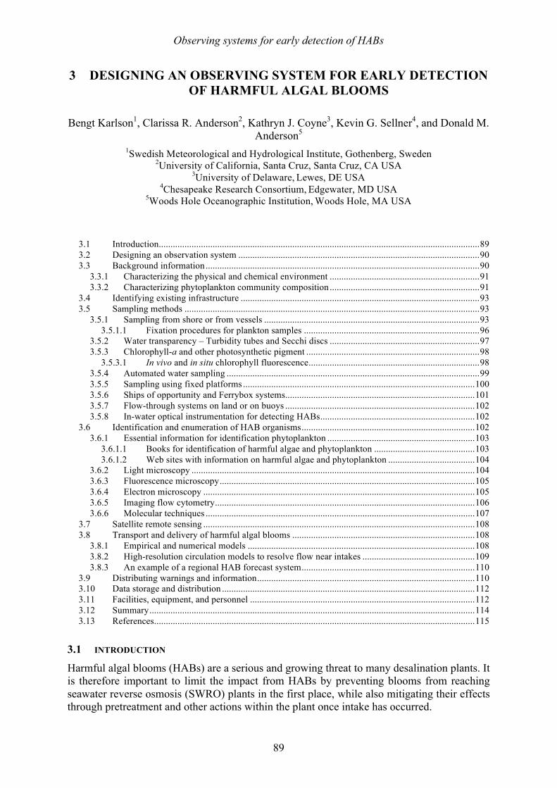
Observing systems for early detection of HABs

89

3 DESIGNING AN OBSERVING SYSTEM FOR EARLY DETECTION OF HARMFUL ALGAL BLOOMS

Bengt Karlson1, Clarissa R. Anderson2, Kathryn J. Coyne3, Kevin G. Sellner4, and Donald M. Anderson5

1Swedish Meteorological and Hydrological Institute, Gothenberg, Sweden 2University of California, Santa Cruz, Santa Cruz, CA USA

3University of Delaware, Lewes, DE USA 4Chesapeake Research Consortium, Edgewater, MD USA

5Woods Hole Oceanographic Institution, Woods Hole, MA USA

3.1 Introduction ......................................................................................................................................... 89 3.2 Designing an observation system ....................................................................................................... 90 3.3 Background information ..................................................................................................................... 90

3.3.1 Characterizing the physical and chemical environment ................................................................ 91 3.3.2 Characterizing phytoplankton community composition ................................................................ 91

3.4 Identifying existing infrastructure ...................................................................................................... 93 3.5 Sampling methods .............................................................................................................................. 93

3.5.1 Sampling from shore or from vessels ............................................................................................ 93 3.5.1.1 Fixation procedures for plankton samples ........................................................................... 96

3.5.2 Water transparency – Turbidity tubes and Secchi discs ................................................................ 97 3.5.3 Chlorophyll-a and other photosynthetic pigment .......................................................................... 98

3.5.3.1 In vivo and in situ chlorophyll fluorescence ......................................................................... 98 3.5.4 Automated water sampling ............................................................................................................ 99 3.5.5 Sampling using fixed platforms ................................................................................................... 100 3.5.6 Ships of opportunity and Ferrybox systems ................................................................................. 101 3.5.7 Flow-through systems on land or on buoys ................................................................................. 102 3.5.8 In-water optical instrumentation for detecting HABs .................................................................. 102

3.6 Identification and enumeration of HAB organisms .......................................................................... 102 3.6.1 Essential information for identification phytoplankton ............................................................... 103

3.6.1.1 Books for identification of harmful algae and phytoplankton ........................................... 103 3.6.1.2 Web sites with information on harmful algae and phytoplankton ..................................... 104

3.6.2 Light microscopy ......................................................................................................................... 104 3.6.3 Fluorescence microscopy ............................................................................................................. 105 3.6.4 Electron microscopy .................................................................................................................... 105 3.6.5 Imaging flow cytometry ............................................................................................................... 106 3.6.6 Molecular techniques ................................................................................................................... 107

3.7 Satellite remote sensing .................................................................................................................... 108 3.8 Transport and delivery of harmful algal blooms .............................................................................. 108

3.8.1 Empirical and numerical models ................................................................................................. 108 3.8.2 High-resolution circulation models to resolve flow near intakes ................................................ 109 3.8.3 An example of a regional HAB forecast system .......................................................................... 110

3.9 Distributing warnings and information ............................................................................................. 110 3.10 Data storage and distribution ............................................................................................................ 112 3.11 Facilities, equipment, and personnel ................................................................................................ 112 3.12 Summary ........................................................................................................................................... 114 3.13 References ......................................................................................................................................... 115

3.1 INTRODUCTION

Harmful algal blooms (HABs) are a serious and growing threat to many desalination plants. It is therefore important to limit the impact from HABs by preventing blooms from reaching seawater reverse osmosis (SWRO) plants in the first place, while also mitigating their effects through pretreatment and other actions within the plant once intake has occurred.

Observing systems for early detection of HABs

90

In this chapter, traditional and emerging technologies in the field of HAB detection and monitoring are summarized. Also advice on designing “observing systems” for early detection or characterization of algal blooms is provided. These systems will vary dramatically in terms of the number of parameters to be measured, the number of stations, frequency of sampling and instruments used - all determined by desalination plant budgets and personnel skills, the nature of the HAB threat for a given plant or region, and other such considerations. An observing system might be as simple as visual observations of the color or nature of the intake water, or as complex as a moored array of autonomous sensors outside the plant, or weekly surveys from small vessels to determine what algal species and blooms are in the intake area or surrounding waters, and thus likely to impact the plant.

There are a number of factors that complicate the design of an observing system. One is the diversity of HAB species. Potentially harmful phytoplankton are found in many groups (mainly eukaryotes) such as dinoflagellates, raphidophytes, diatoms, euglenophytes, cryptophytes, haptophytes, pelagophytes, and chlorophytes (see Chapter 1), but prokaryotes, (cyanobacteria) are also a concern. While dinoflagellates comprise the majority of toxic HAB species in the marine environment where desalination plants are located, many of the toxic species that pose a threat to drinking water supply in fresh- or brackish-water systems are cyanobacteria.

A second factor is that phytoplankton distribution in the sea is not uniform vertically or horizontally in space or in time. This is termed “patchiness” and results from the interaction between physical and biological processes. Examples are presented later in this chapter. The simultaneous use of multiple monitoring methods is therefore often necessary to characterize the species composition and extent of blooms, but even then, a full picture of the distribution of a HAB may not be achievable.

3.2 DESIGNING AN OBSERVATION SYSTEM In the context of providing observations of the water and plankton that can guide desalination operations and plant siting, a HAB observing system can be very informative in many locations. The main goal of such a system is to provide information for actions (rapid response) to avoid or minimize operational disruptions and damage to desalination plants. Prior to the design and construction of a plant, a HAB observing system can be used to gather information on the nature and function of the regional oceanographic system, its role in HAB occurrence, and the historical patterns and extent of HAB events. This can be used to provide input on where to place, and how to design, water intake systems, as well as highlighting the types of pretreatment equipment that might be needed in order to minimize damage from HABs during operation. Figures 3.1 – 3.3 show some features to be considered in this regard. 3.3 BACKGROUND INFORMATION

To design an observation system, it is necessary to gather background information on the occurrence of harmful algae in relation to local physical and chemical conditions. Existing information should be used when possible (likely from monitoring programs run by government, industry, or academic institutions), but often a pilot study may be required. A physical oceanographic model describing regional hydrodynamics surrounding the desalination facility would be a valued asset to any observing system. These are often developed by universities and other academic institutes, as well as government agencies, and are sometimes utilized in studies of brine dispersion and recirculation during plant design. Models in HAB monitoring and management are discussed in section 3.8.1.

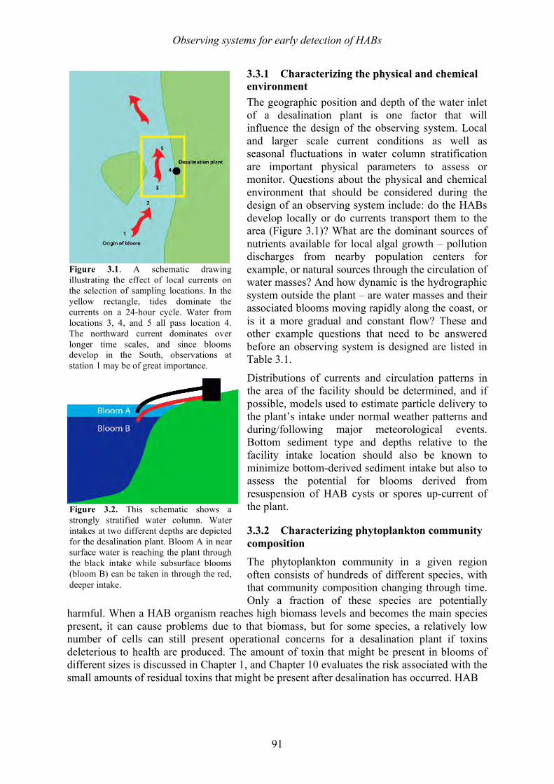
Observing systems for early detection of HABs

91

3.3.1 Characterizing the physical and chemical environment The geographic position and depth of the water inlet of a desalination plant is one factor that will influence the design of the observing system. Local and larger scale current conditions as well as seasonal fluctuations in water column stratification are important physical parameters to assess or monitor. Questions about the physical and chemical environment that should be considered during the design of an observing system include: do the HABs develop locally or do currents transport them to the area (Figure 3.1)? What are the dominant sources of nutrients available for local algal growth – pollution discharges from nearby population centers for example, or natural sources through the circulation of water masses? And how dynamic is the hydrographic system outside the plant – are water masses and their associated blooms moving rapidly along the coast, or is it a more gradual and constant flow? These and other example questions that need to be answered before an observing system is designed are listed in Table 3.1.

Distributions of currents and circulation patterns in the area of the facility should be determined, and if possible, models used to estimate particle delivery to the plant’s intake under normal weather patterns and during/following major meteorological events. Bottom sediment type and depths relative to the facility intake location should also be known to minimize bottom-derived sediment intake but also to assess the potential for blooms derived from resuspension of HAB cysts or spores up-current of the plant.

3.3.2 Characterizing phytoplankton community composition The phytoplankton community in a given region often consists of hundreds of different species, with that community composition changing through time. Only a fraction of these species are potentially

harmful. When a HAB organism reaches high biomass levels and becomes the main species present, it can cause problems due to that biomass, but for some species, a relatively low number of cells can still present operational concerns for a desalination plant if toxins deleterious to health are produced. The amount of toxin that might be present in blooms of different sizes is discussed in Chapter 1, and Chapter 10 evaluates the risk associated with the small amounts of residual toxins that might be present after desalination has occurred. HAB

Figure 3.1. A schematic drawing illustrating the effect of local currents on the selection of sampling locations. In the yellow rectangle, tides dominate the currents on a 24-hour cycle. Water from locations 3, 4, and 5 all pass location 4. The northward current dominates over longer time scales, and since blooms develop in the South, observations at station 1 may be of great importance.

Figure 3.2. This schematic shows a strongly stratified water column. Water intakes at two different depths are depicted for the desalination plant. Bloom A in near surface water is reaching the plant through the black intake while subsurface blooms (bloom B) can be taken in through the red, deeper intake.

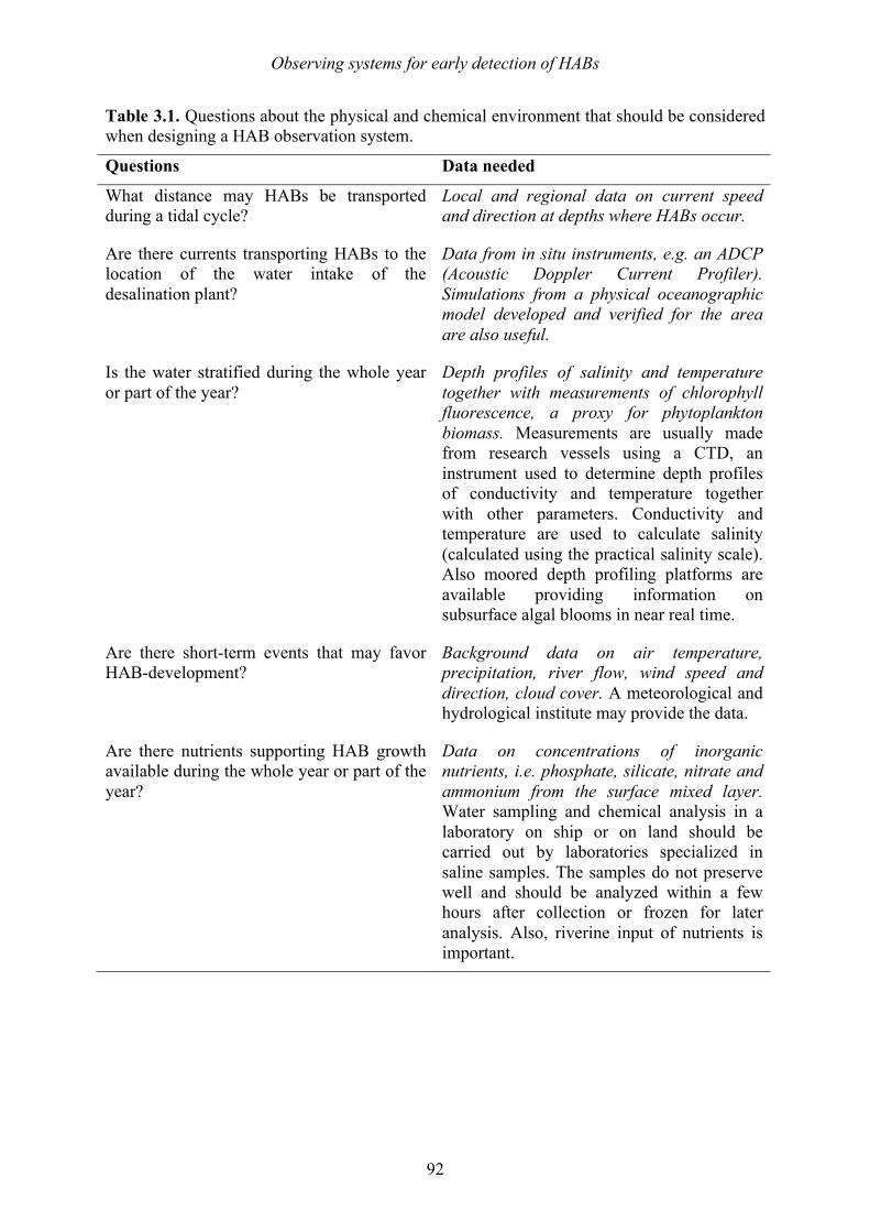
Observing systems for early detection of HABs

92

Table 3.1. Questions about the physical and chemical environment that should be considered when designing a HAB observation system.

Questions Data needed

What distance may HABs be transported during a tidal cycle?

Are there currents transporting HABs to the location of the water intake of the desalination plant?

Local and regional data on current speed and direction at depths where HABs occur.

Data from in situ instruments, e.g. an ADCP (Acoustic Doppler Current Profiler). Simulations from a physical oceanographic model developed and verified for the area are also useful.

Is the water stratified during the whole year or part of the year?

Depth profiles of salinity and temperature together with measurements of chlorophyll fluorescence, a proxy for phytoplankton biomass. Measurements are usually made from research vessels using a CTD, an instrument used to determine depth profiles of conductivity and temperature together with other parameters. Conductivity and temperature are used to calculate salinity (calculated using the practical salinity scale). Also moored depth profiling platforms are available providing information on subsurface algal blooms in near real time.

Are there short-term events that may favor HAB-development?

Background data on air temperature, precipitation, river flow, wind speed and direction, cloud cover. A meteorological and hydrological institute may provide the data.

Are there nutrients supporting HAB growth available during the whole year or part of the year?

Data on concentrations of inorganic nutrients, i.e. phosphate, silicate, nitrate and ammonium from the surface mixed layer. Water sampling and chemical analysis in a laboratory on ship or on land should be carried out by laboratories specialized in saline samples. The samples do not preserve well and should be analyzed within a few hours after collection or frozen for later analysis. Also, riverine input of nutrients is important.

Observing systems for early detection of HABs

93

toxins are sufficiently well removed that toxins in treated water should not be a concern, but they are an operational issue that should be identified and monitored when such a threat is present.

Since many of the non-harmful and harmful algal species are similar in appearance (morphology) it is necessary to have trained personnel identifying the organisms. Semi-automated systems exist, as described below, but staff or outside experts with knowledge of the instruments and phytoplankton taxonomy are needed to set up the systems and evaluate the results. Other information on the local phytoplankton community can often be obtained from existing monitoring programs in a region, perhaps conducted by a state, province, or municipality. Some of the questions and required data relative to phytoplankton population dynamics are listed in Table 3.2.

3.4 IDENTIFYING EXISTING INFRASTRUCTURE In many cases, existing sampling infrastructure may be used when setting up a HAB observation system. An oceanographic laboratory with facilities for working with phytoplankton nearby the sampling sites is ideal. If there are already on-going marine monitoring programs, they can be adapted to undertake HAB work. Ships of opportunity, e.g. ferries, with a stable timetable, may be

used for automated sampling. It is useful to investigate if there are buoys or permanent structures (e.g. pilings) in the area that can be used for mounting automated sensors and water sampling devices. Although existing buoys may not be available for mounting sensors and water sampling devices, colocation of HAB buoys is useful to avoid problems with fishing and traffic of merchant vessels. These approaches are described in more detail below. 3.5 SAMPLING METHODS

3.5.1 Sampling from shore or from vessels The most basic sampling procedure for observing algal bloom species that cause problems for desalinations plants is to collect a water sample and analyze it with a microscope. This can complement online, continuous analyses, such as chlorophyll fluorescence, discussed below. The recommended frequency for sampling is once per week, as phytoplankton can grow and accumulate very rapidly (some can double their cell concentrations in a day or less). If resources are limited, bi-weekly sampling can provide reasonable protection. The number of sampling locations and the depth of sampling will depend on the local conditions and available funding and staff. One approach is to sample at the seawater intake, but that gives little advance notice or information about the geographic extent of the bloom. At the other extreme, ship-based surveys can be conducted, covering an area several km or more from the intake. During a HAB event, increased sampling frequency and spatial coverage can be very informative, as it can reveal the spatial extent of a bloom, its vertical distribution, and other factors that can help the plant anticipate future impacts and potential treatments.

Nearshore samples can be taken from land, but the sampling point must be before the waves break. A jetty, dock, or other extended feature can be used for that purpose. Both dedicated ships, i.e. research vessels, and other boats may be used. Ships should be of a size suitable for

Figure 3.3. Typical vertical distribution of algae in the water column. The graph illustrates a common vertical distribution with a sub-surface maximum of chloro-phyll or phytoplankton biomass (often 10-20 m deep), which may move vertically to the surface and back (termed migration), depending on the day-night cycle. Water sampling and automated observations should account for this heterogeneity.

Observing systems for early detection of HABs

94

work in rough weather and have room for both the crew and technical personnel. For this type of nearshore sampling, the ships should be fitted with CTD (conductivity, temperature, depth profilers) or other such devices to measure water column structure. The CTD should include a sensor for chlorophyll fluorescence if possible (see Table 3.1). A laboratory area on the ship is important for filtering of samples and other activities.

Table 3.2. Questions regarding HAB species and bloom dynamics that need to be addressed when designing an observation system. Some of the information is likely available in other institutions and should be explored prior to initiating the observing system. Question Data needed

Which HAB species occur in the area? What is the temporal and spatial distribution of HAB species? Do HABs develop upstream of the desalination plant? During what time of year do the HABs occur? What is the background composition of the phytoplankton community in the area?

Abundance and distribution of phytoplankton, in general, and of HAB species, in particular. Frequent (e.g. weekly) water sampling and microscopy-based analyses of the samples by skilled personnel. In addition, automated analyses using imaging flow cytometry and/or genetic methods can be useful. Surveys including water sampling at multiple locations are needed to document the spatial distribution of HAB species. Data on current speed and direction support the design of the surveys.

What are the ecological and bloom dynamics of the local HAB species? Can the HAB species regulate their position in the water column? What is the growth rate of the HAB species?

Long-term observations and experimental work are needed to characterize the ecology of HAB species. This may be outside the scope of the observation system, but some observations (e.g., vertical swimming behavior) are relatively simple to make, and are important for minimizing HAB intake.

Do the HAB-species produce resting stages? What is the distribution of these?

Resting stages (cysts or spores) should be documented from observations or the scientific literature. If a common HAB-organism in the region produces resting stages, a distributional survey may be useful, as this can guide understanding of the timing and location of blooms.

Do the HAB species produce toxins that may cause health problems for humans?

Toxins produced by the species in the area. Field samples of phytoplankton should be analyzed for toxin content using methods described in Chapter 2. Once the local HAB species are identified, known toxin profiles are likely available in the scientific literature.

Are there local nutrients to support HABs? Concentrations of inorganic nutrients (see Table 1). This information can help explain the frequency and size of HABs in the area.

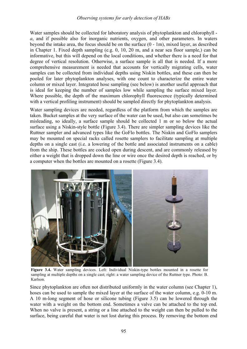
Observing systems for early detection of HABs

95

Water samples should be collected for laboratory analysis of phytoplankton and chlorophyll -a, and if possible also for inorganic nutrients, oxygen, and other parameters. In waters beyond the intake area, the focus should be on the surface (0 - 1m), mixed layer, as described in Chapter 1. Fixed depth sampling (e.g. 0, 10, 20 m, and a near sea floor sample,) can be informative, but this will depend on the local conditions, and whether there is a need for that degree of vertical resolution. Otherwise, a surface sample is all that is needed. If a more comprehensive measurement is needed that accounts for vertically migrating cells, water samples can be collected from individual depths using Niskin bottles, and these can then be pooled for later phytoplankton analyses, with one count to characterize the entire water column or mixed layer. Integrated hose sampling (see below) is another useful approach that is ideal for keeping the number of samples low while sampling the surface mixed layer. Where possible, the depth of the maximum chlorophyll fluorescence (typically determined with a vertical profiling instrument) should be sampled directly for phytoplankton analysis. Water sampling devices are needed, regardless of the platform from which the samples are taken. Bucket samples at the very surface of the water can be used, but also can sometimes be misleading, so ideally, a surface sample should be collected 1 m or so below the actual surface using a Niskin-style bottle (Figure 3.4). There are simpler sampling devices like the Ruttner sampler and advanced types like the GoFlo bottles. The Niskin and GoFlo samplers may be mounted on special racks called rosette samplers to facilitate sampling at multiple depths on a single cast (i.e. a lowering of the bottle and associated instruments on a cable) from the ship. These bottles are cocked open during descent, and are commonly released by either a weight that is dropped down the line or wire once the desired depth is reached, or by a computer when the bottles are mounted on a rosette (Figure 3.4).

Since phytoplankton are often not distributed uniformly in the water column (see Chapter 1), hoses can be used to sample the mixed layer at the surface of the water column, e.g. 0-10 m. A 10 m-long segment of hose or silicone tubing (Figure 3.5) can be lowered through the water with a weight on the bottom end. Sometimes a valve can be attached to the top end. When no valve is present, a string or a line attached to the weight can then be pulled to the surface, being careful that water is not lost during this process. By removing the bottom end

Figure 3.4. Water sampling devices. Left: Individual Niskin-type bottles mounted in a rosette for sampling at multiple depths on a single cast; right: a water sampling device of the Ruttner type. Photo: B. Karlson.

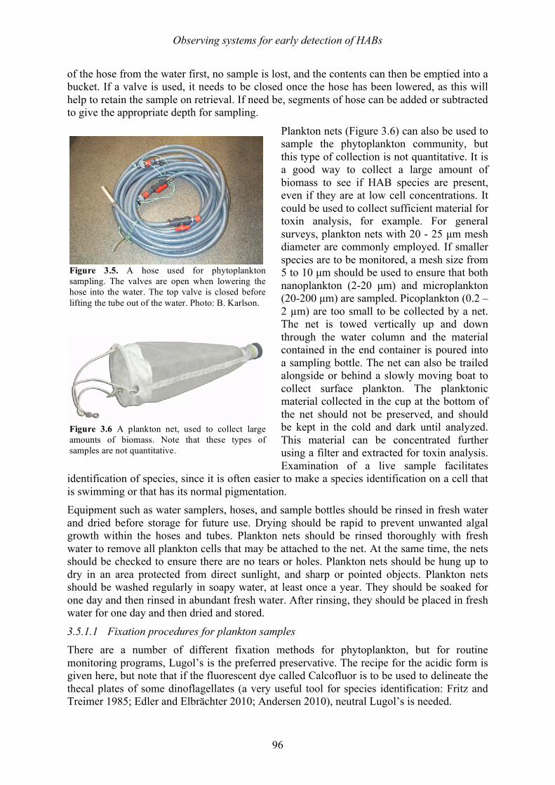
Observing systems for early detection of HABs

96

of the hose from the water first, no sample is lost, and the contents can then be emptied into a bucket. If a valve is used, it needs to be closed once the hose has been lowered, as this will help to retain the sample on retrieval. If need be, segments of hose can be added or subtracted to give the appropriate depth for sampling.

Plankton nets (Figure 3.6) can also be used to sample the phytoplankton community, but this type of collection is not quantitative. It is a good way to collect a large amount of biomass to see if HAB species are present, even if they are at low cell concentrations. It could be used to collect sufficient material for toxin analysis, for example. For general surveys, plankton nets with 20 - 25 µm mesh diameter are commonly employed. If smaller species are to be monitored, a mesh size from 5 to 10 µm should be used to ensure that both nanoplankton (2-20 µm) and microplankton (20-200 µm) are sampled. Picoplankton (0.2 – 2 µm) are too small to be collected by a net. The net is towed vertically up and down through the water column and the material contained in the end container is poured into a sampling bottle. The net can also be trailed alongside or behind a slowly moving boat to collect surface plankton. The planktonic material collected in the cup at the bottom of the net should not be preserved, and should be kept in the cold and dark until analyzed. This material can be concentrated further using a filter and extracted for toxin analysis. Examination of a live sample facilitates

identification of species, since it is often easier to make a species identification on a cell that is swimming or that has its normal pigmentation. Equipment such as water samplers, hoses, and sample bottles should be rinsed in fresh water and dried before storage for future use. Drying should be rapid to prevent unwanted algal growth within the hoses and tubes. Plankton nets should be rinsed thoroughly with fresh water to remove all plankton cells that may be attached to the net. At the same time, the nets should be checked to ensure there are no tears or holes. Plankton nets should be hung up to dry in an area protected from direct sunlight, and sharp or pointed objects. Plankton nets should be washed regularly in soapy water, at least once a year. They should be soaked for one day and then rinsed in abundant fresh water. After rinsing, they should be placed in fresh water for one day and then dried and stored.

3.5.1.1 Fixation procedures for plankton samples There are a number of different fixation methods for phytoplankton, but for routine monitoring programs, Lugol’s is the preferred preservative. The recipe for the acidic form is given here, but note that if the fluorescent dye called Calcofluor is to be used to delineate the thecal plates of some dinoflagellates (a very useful tool for species identification: Fritz and Treimer 1985; Edler and Elbrächter 2010; Andersen 2010), neutral Lugol’s is needed.

Figure 3.5. A hose used for phytoplankton sampling. The valves are open when lowering the hose into the water. The top valve is closed before lifting the tube out of the water. Photo: B. Karlson.

Figure 3.6 A plankton net, used to collect large amounts of biomass. Note that these types of samples are not quantitative.

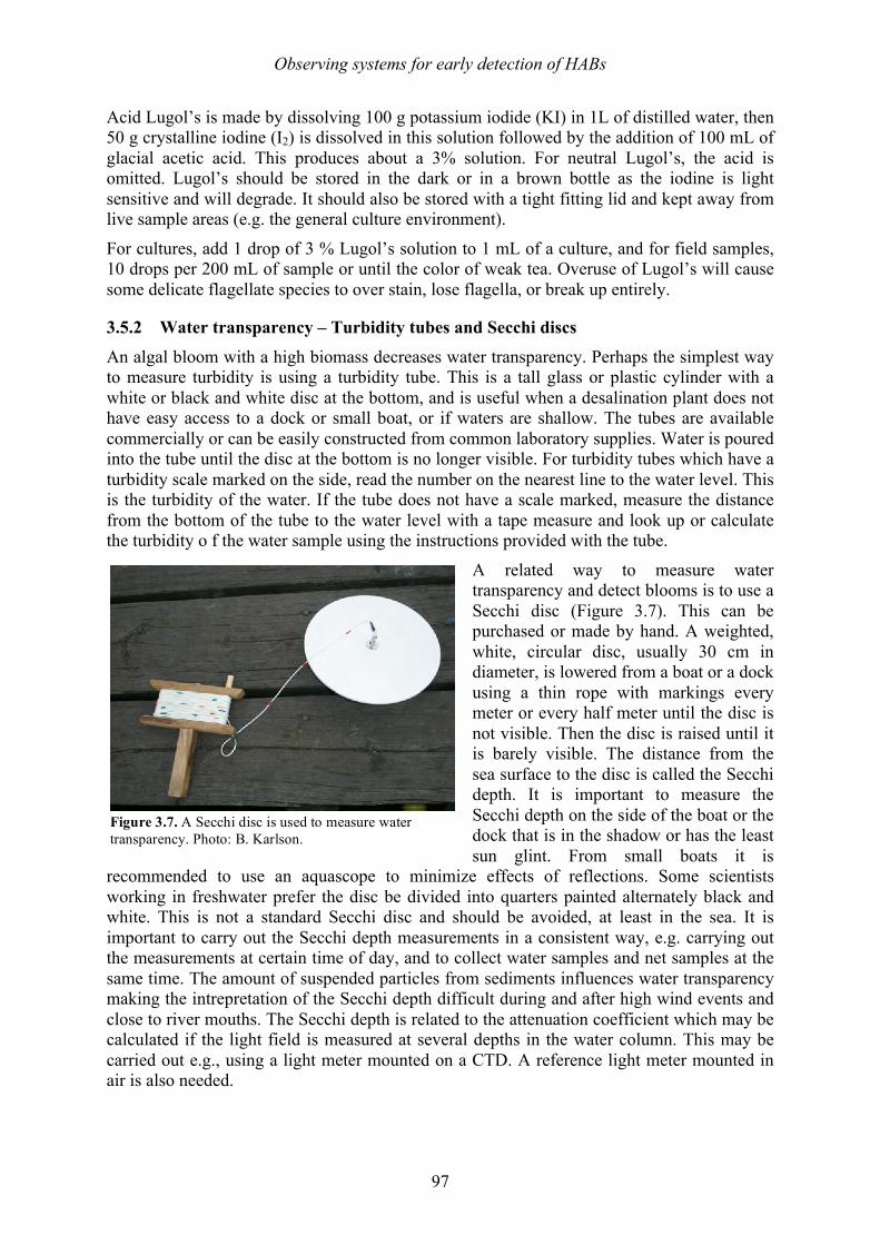
Observing systems for early detection of HABs

97

Acid Lugol’s is made by dissolving 100 g potassium iodide (KI) in 1L of distilled water, then 50 g crystalline iodine (I2) is dissolved in this solution followed by the addition of 100 mL of glacial acetic acid. This produces about a 3% solution. For neutral Lugol’s, the acid is omitted. Lugol’s should be stored in the dark or in a brown bottle as the iodine is light sensitive and will degrade. It should also be stored with a tight fitting lid and kept away from live sample areas (e.g. the general culture environment).

For cultures, add 1 drop of 3 % Lugol’s solution to 1 mL of a culture, and for field samples, 10 drops per 200 mL of sample or until the color of weak tea. Overuse of Lugol’s will cause some delicate flagellate species to over stain, lose flagella, or break up entirely.

3.5.2 Water transparency – Turbidity tubes and Secchi discs

An algal bloom with a high biomass decreases water transparency. Perhaps the simplest way to measure turbidity is using a turbidity tube. This is a tall glass or plastic cylinder with a white or black and white disc at the bottom, and is useful when a desalination plant does not have easy access to a dock or small boat, or if waters are shallow. The tubes are available commercially or can be easily constructed from common laboratory supplies. Water is poured into the tube until the disc at the bottom is no longer visible. For turbidity tubes which have a turbidity scale marked on the side, read the number on the nearest line to the water level. This is the turbidity of the water. If the tube does not have a scale marked, measure the distance from the bottom of the tube to the water level with a tape measure and look up or calculate the turbidity o f the water sample using the instructions provided with the tube.

A related way to measure water transparency and detect blooms is to use a Secchi disc (Figure 3.7). This can be purchased or made by hand. A weighted, white, circular disc, usually 30 cm in diameter, is lowered from a boat or a dock using a thin rope with markings every meter or every half meter until the disc is not visible. Then the disc is raised until it is barely visible. The distance from the sea surface to the disc is called the Secchi depth. It is important to measure the Secchi depth on the side of the boat or the dock that is in the shadow or has the least sun glint. From small boats it is

recommended to use an aquascope to minimize effects of reflections. Some scientists working in freshwater prefer the disc be divided into quarters painted alternately black and white. This is not a standard Secchi disc and should be avoided, at least in the sea. It is important to carry out the Secchi depth measurements in a consistent way, e.g. carrying out the measurements at certain time of day, and to collect water samples and net samples at the same time. The amount of suspended particles from sediments influences water transparency making the intrepretation of the Secchi depth difficult during and after high wind events and close to river mouths. The Secchi depth is related to the attenuation coefficient which may be calculated if the light field is measured at several depths in the water column. This may be carried out e.g., using a light meter mounted on a CTD. A reference light meter mounted in air is also needed.

Figure 3.7. A Secchi disc is used to measure water transparency. Photo: B. Karlson.

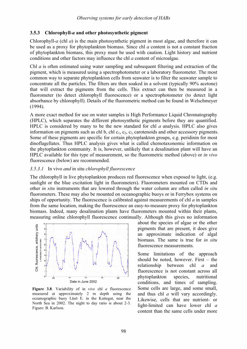
Observing systems for early detection of HABs

98

3.5.3 Chlorophyll-a and other photosynthetic pigment

Chlorophyll-a (chl a) is the main photosynthetic pigment in most algae, and therefore it can be used as a proxy for phytoplankton biomass. Since chl a content is not a constant fraction of phytoplankton biomass, this proxy must be used with caution. Light history and nutrient conditions and other factors may influence the chl a content of microalgae. Chl a is often estimated using water sampling and subsequent filtering and extraction of the pigment, which is measured using a spectrophotometer or a laboratory fluorometer. The most common way to separate phytoplankton cells from seawater is to filter the seawater sample to concentrate all the particles. The filters are then soaked in a solvent (typically 90% acetone) that will extract the pigments from the cells. This extract can then be measured in a fluorometer (to detect chlorophyll fluorescence) or a spectrophotometer (to detect light absorbance by chlorophyll). Details of the fluorometric method can be found in Welschmeyer (1994). A more exact method for use on water samples is High Performance Liquid Chromatography (HPLC), which separates the different photosynthetic pigments before they are quantified. HPLC is considered by many to be the new standard for chl a analysis. HPLC also gives information on pigments such as chl b, chl c1, c2, c3, carotenoids and other accessory pigments. Some of these pigments are specific for certain phytoplankton groups, e.g. peridinin for most dinoflagellates. Thus HPLC analysis gives what is called chemotaxonomic information on the phytoplankton community. It is, however, unlikely that a desalination plant will have an HPLC available for this type of measurement, so the fluorometric method (above) or in vivo fluorescence (below) are recommended. 3.5.3.1 In vivo and in situ chlorophyll fluorescence The chlorophyll in live phytoplankton produces red fluorescence when exposed to light, (e.g. sunlight or the blue excitation light in fluorometers). Fluorometers mounted on CTDs and other in situ instruments that are lowered through the water column are often called in situ fluorometers. These may also be mounted on oceanographic buoys or in Ferrybox systems on ships of opportunity. The fluorescence is calibrated against measurements of chl a in samples from the same location, making the fluorescence an easy-to-measure proxy for phytoplankton biomass. Indeed, many desalination plants have fluorometers mounted within their plants, measuring online chlorophyll fluorescence continually. Although this gives no information

about the species of algae or the other pigments that are present, it does give an approximate indication of algal biomass. The same is true for in situ fluorescence measurements.

Some limitations of the approach should be noted, however. First – the relationship between chl a and fluorescence is not constant across all phytoplankton species, nutritional conditions, and times of sampling. Some cells are large, and some small, and thus chl a will vary accordingly. Likewise, cells that are nutrient- or light-limited can have lower chl a content than the same cells under more

Figure 3.8. Variability of in vivo chl a fluorescence measured at approximately 2 m depth using the oceanographic buoy Läsö E. in the Kattegat, near the North Sea in 2002. The night to day ratio is about 2-3. Figure: B. Karlson.

Date in June 2002

Chl. fluorescence, arbitrary units

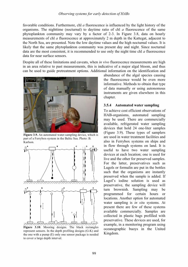
Observing systems for early detection of HABs

99

favorable conditions. Furthermore, chl a fluorescence is influenced by the light history of the organisms. The nighttime (nocturnal) to daytime ratio of chl a fluorescence of the same phytoplankton community may vary by a factor of 2-3. In Figure 3.8, data on hourly measurements of chl a fluorescence at approximately 2 m depth in the Kattegat, adjacent to the North Sea, are presented. Note the low daytime values and the high nocturnal values. It is likely that the same phytoplankton community was present day and night. Since nocturnal data are the most consistent, it is recommended to use only the night time chl a fluorescence data for near surface sensors.

Despite all of these limitations and caveats, when in vivo fluorescence measurements are high in an area relative to past measurements, this is indicative of a major algal bloom, and thus can be used to guide pretreatment options. Additional information on the identification and

abundance of the algal species causing the fluorescence would be even more informative. Methods to obtain that type of data manually or using autonomous instruments are given elsewhere in this chapter.

3.5.4 Automated water sampling To achieve cost efficient observations of HAB-organisms, automated sampling may be used. There are commercially available, refrigerated water sampling devices that hold 24 one-liter samples (Figure 3.9). These types of samplers are used in water treatment facilities and also in Ferrybox systems on ships and in flow through systems on land. It is useful to have two water sampling devices at each location; one is used for live and the other for preserved samples. For the latter, preservatives such as Lugols or formalin are put in the bottles such that the organisms are instantly preserved when the sample is added. If Lugol’s iodine solution is used as preservative, the sampling device will turn brownish. Sampling may be programmed for certain hours or locations. Another option for automated water sampling is in situ systems. At present there are few of these systems available commercially. Samples are collected in plastic bags prefilled with preservative. These devices are used, for example, in a monitoring program using oceanographic buoys in the United Kingdom.

Figure 3.9. An automated water-sampling device, which is part of a Ferrybox-system in the Baltic Sea. Photo: B. Karlson.

Figure 3.10. Mooring designs. The black rectangles represent sensors. In the depth profiling designs (G-K) and the one with a pump (E) only one sensor package is needed to cover a large depth interval.

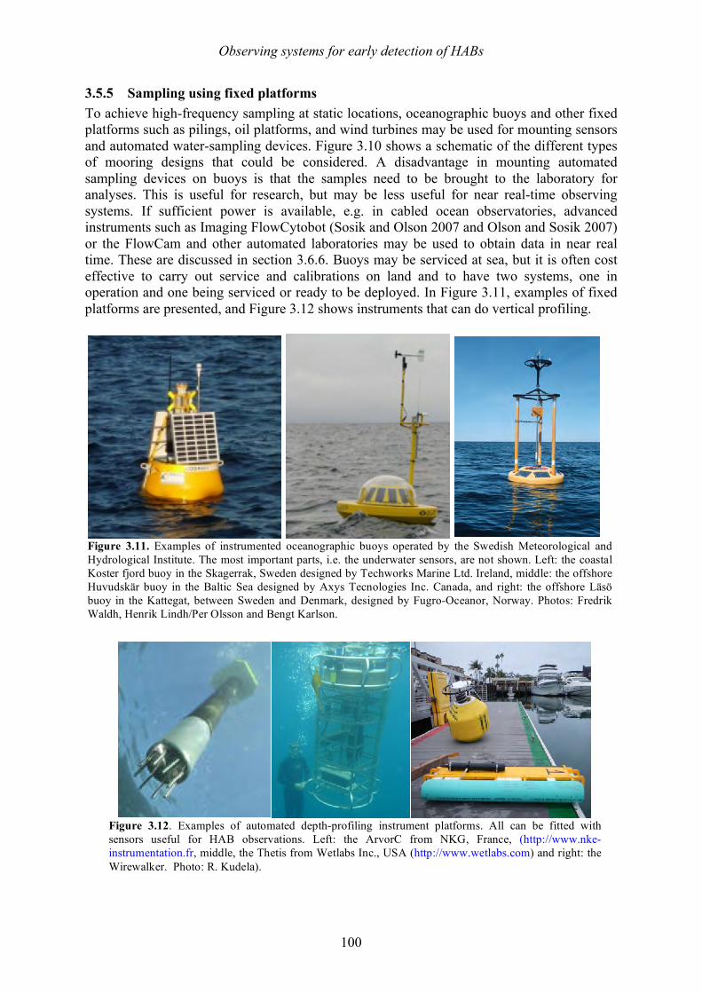
Observing systems for early detection of HABs

100

3.5.5 Sampling using fixed platforms To achieve high-frequency sampling at static locations, oceanographic buoys and other fixed platforms such as pilings, oil platforms, and wind turbines may be used for mounting sensors and automated water-sampling devices. Figure 3.10 shows a schematic of the different types of mooring designs that could be considered. A disadvantage in mounting automated sampling devices on buoys is that the samples need to be brought to the laboratory for analyses. This is useful for research, but may be less useful for near real-time observing systems. If sufficient power is available, e.g. in cabled ocean observatories, advanced instruments such as Imaging FlowCytobot (Sosik and Olson 2007 and Olson and Sosik 2007) or the FlowCam and other automated laboratories may be used to obtain data in near real time. These are discussed in section 3.6.6. Buoys may be serviced at sea, but it is often cost effective to carry out service and calibrations on land and to have two systems, one in operation and one being serviced or ready to be deployed. In Figure 3.11, examples of fixed platforms are presented, and Figure 3.12 shows instruments that can do vertical profiling.

Figure 3.11. Examples of instrumented oceanographic buoys operated by the Swedish Meteorological and Hydrological Institute. The most important parts, i.e. the underwater sensors, are not shown. Left: the coastal Koster fjord buoy in the Skagerrak, Sweden designed by Techworks Marine Ltd. Ireland, middle: the offshore Huvudskär buoy in the Baltic Sea designed by Axys Tecnologies Inc. Canada, and right: the offshore Läsö buoy in the Kattegat, between Sweden and Denmark, designed by Fugro-Oceanor, Norway. Photos: Fredrik Waldh, Henrik Lindh/Per Olsson and Bengt Karlson.

Figure 3.12. Examples of automated depth-profiling instrument platforms. All can be fitted with sensors useful for HAB observations. Left: the ArvorC from NKG, France, (http://www.nke-instrumentation.fr, middle, the Thetis from Wetlabs Inc., USA (http://www.wetlabs.com) and right: the Wirewalker. Photo: R. Kudela).

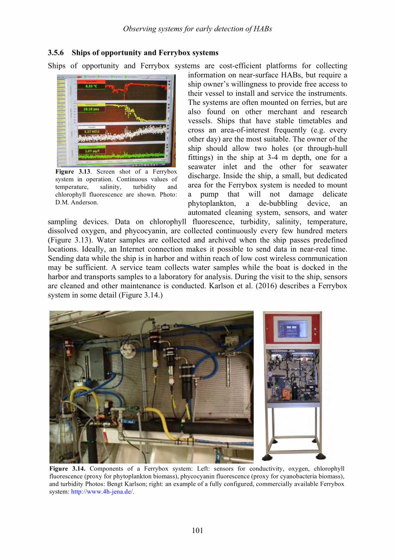
Observing systems for early detection of HABs

101

3.5.6 Ships of opportunity and Ferrybox systems Ships of opportunity and Ferrybox systems are cost-efficient platforms for collecting

information on near-surface HABs, but require a ship owner’s willingness to provide free access to their vessel to install and service the instruments. The systems are often mounted on ferries, but are also found on other merchant and research vessels. Ships that have stable timetables and cross an area-of-interest frequently (e.g. every other day) are the most suitable. The owner of the ship should allow two holes (or through-hull fittings) in the ship at 3-4 m depth, one for a seawater inlet and the other for seawater discharge. Inside the ship, a small, but dedicated area for the Ferrybox system is needed to mount a pump that will not damage delicate phytoplankton, a de-bubbling device, an automated cleaning system, sensors, and water

sampling devices. Data on chlorophyll fluorescence, turbidity, salinity, temperature, dissolved oxygen, and phycocyanin, are collected continuously every few hundred meters (Figure 3.13). Water samples are collected and archived when the ship passes predefined locations. Ideally, an Internet connection makes it possible to send data in near-real time. Sending data while the ship is in harbor and within reach of low cost wireless communication may be sufficient. A service team collects water samples while the boat is docked in the harbor and transports samples to a laboratory for analysis. During the visit to the ship, sensors are cleaned and other maintenance is conducted. Karlson et al. (2016) describes a Ferrybox system in some detail (Figure 3.14.)

Figure 3.14. Components of a Ferrybox system: Left: sensors for conductivity, oxygen, chlorophyll fluorescence (proxy for phytoplankton biomass), phycocyanin fluorescence (proxy for cyanobacteria biomass), and turbidity Photos: Bengt Karlson; right: an example of a fully configured, commercially available Ferrybox system: http://www.4h-jena.de/.

Figure 3.13. Screen shot of a Ferrybox system in operation. Continuous values of temperature, salinity, turbidity and chlorophyll fluorescence are shown. Photo: D.M. Anderson.

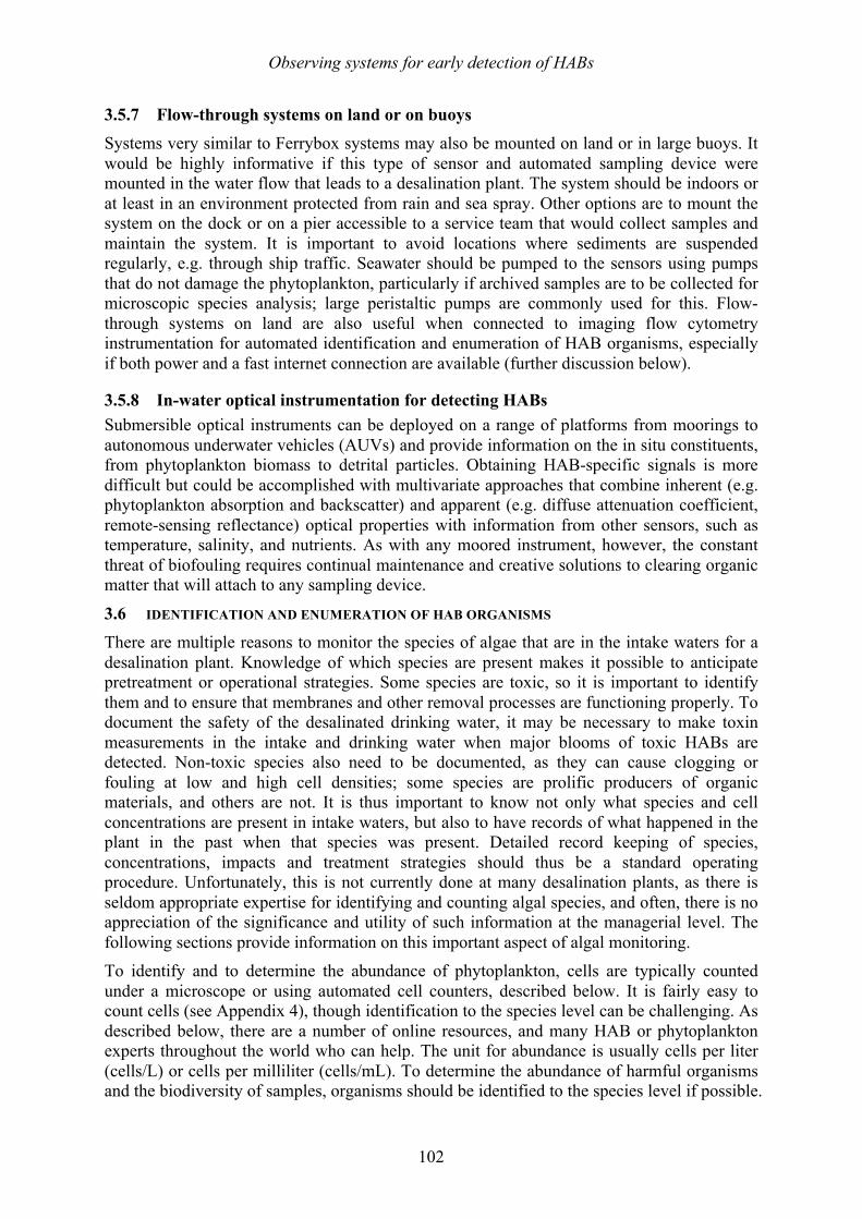
Observing systems for early detection of HABs

102

3.5.7 Flow-through systems on land or on buoys Systems very similar to Ferrybox systems may also be mounted on land or in large buoys. It would be highly informative if this type of sensor and automated sampling device were mounted in the water flow that leads to a desalination plant. The system should be indoors or at least in an environment protected from rain and sea spray. Other options are to mount the system on the dock or on a pier accessible to a service team that would collect samples and maintain the system. It is important to avoid locations where sediments are suspended regularly, e.g. through ship traffic. Seawater should be pumped to the sensors using pumps that do not damage the phytoplankton, particularly if archived samples are to be collected for microscopic species analysis; large peristaltic pumps are commonly used for this. Flow-through systems on land are also useful when connected to imaging flow cytometry instrumentation for automated identification and enumeration of HAB organisms, especially if both power and a fast internet connection are available (further discussion below).

3.5.8 In-water optical instrumentation for detecting HABs Submersible optical instruments can be deployed on a range of platforms from moorings to autonomous underwater vehicles (AUVs) and provide information on the in situ constituents, from phytoplankton biomass to detrital particles. Obtaining HAB-specific signals is more difficult but could be accomplished with multivariate approaches that combine inherent (e.g. phytoplankton absorption and backscatter) and apparent (e.g. diffuse attenuation coefficient, remote-sensing reflectance) optical properties with information from other sensors, such as temperature, salinity, and nutrients. As with any moored instrument, however, the constant threat of biofouling requires continual maintenance and creative solutions to clearing organic matter that will attach to any sampling device.

3.6 IDENTIFICATION AND ENUMERATION OF HAB ORGANISMS There are multiple reasons to monitor the species of algae that are in the intake waters for a desalination plant. Knowledge of which species are present makes it possible to anticipate pretreatment or operational strategies. Some species are toxic, so it is important to identify them and to ensure that membranes and other removal processes are functioning properly. To document the safety of the desalinated drinking water, it may be necessary to make toxin measurements in the intake and drinking water when major blooms of toxic HABs are detected. Non-toxic species also need to be documented, as they can cause clogging or fouling at low and high cell densities; some species are prolific producers of organic materials, and others are not. It is thus important to know not only what species and cell concentrations are present in intake waters, but also to have records of what happened in the plant in the past when that species was present. Detailed record keeping of species, concentrations, impacts and treatment strategies should thus be a standard operating procedure. Unfortunately, this is not currently done at many desalination plants, as there is seldom appropriate expertise for identifying and counting algal species, and often, there is no appreciation of the significance and utility of such information at the managerial level. The following sections provide information on this important aspect of algal monitoring. To identify and to determine the abundance of phytoplankton, cells are typically counted under a microscope or using automated cell counters, described below. It is fairly easy to count cells (see Appendix 4), though identification to the species level can be challenging. As described below, there are a number of online resources, and many HAB or phytoplankton experts throughout the world who can help. The unit for abundance is usually cells per liter (cells/L) or cells per milliliter (cells/mL). To determine the abundance of harmful organisms and the biodiversity of samples, organisms should be identified to the species level if possible.

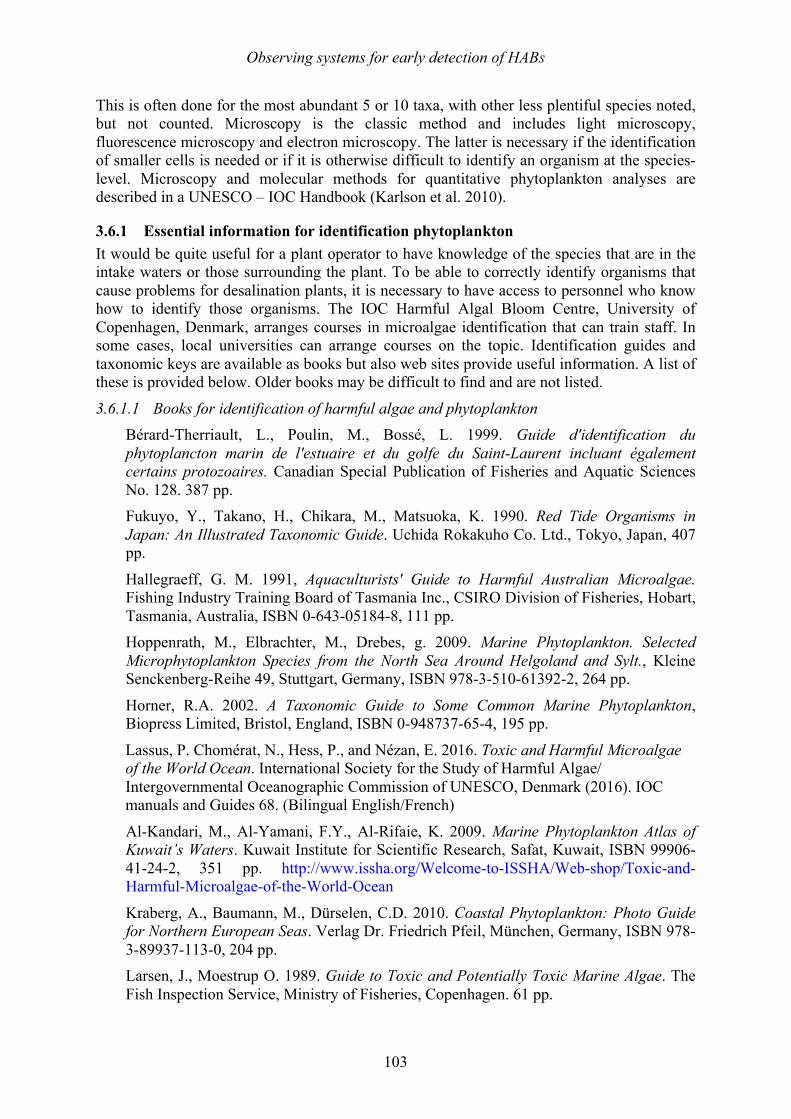
Observing systems for early detection of HABs

103

This is often done for the most abundant 5 or 10 taxa, with other less plentiful species noted, but not counted. Microscopy is the classic method and includes light microscopy, fluorescence microscopy and electron microscopy. The latter is necessary if the identification of smaller cells is needed or if it is otherwise difficult to identify an organism at the species-level. Microscopy and molecular methods for quantitative phytoplankton analyses are described in a UNESCO – IOC Handbook (Karlson et al. 2010).

3.6.1 Essential information for identification phytoplankton It would be quite useful for a plant operator to have knowledge of the species that are in the intake waters or those surrounding the plant. To be able to correctly identify organisms that cause problems for desalination plants, it is necessary to have access to personnel who know how to identify those organisms. The IOC Harmful Algal Bloom Centre, University of Copenhagen, Denmark, arranges courses in microalgae identification that can train staff. In some cases, local universities can arrange courses on the topic. Identification guides and taxonomic keys are available as books but also web sites provide useful information. A list of these is provided below. Older books may be difficult to find and are not listed.

3.6.1.1 Books for identification of harmful algae and phytoplankton Bérard-Therriault, L., Poulin, M., Bossé, L. 1999. Guide d'identification du phytoplancton marin de l'estuaire et du golfe du Saint-Laurent incluant également certains protozoaires. Canadian Special Publication of Fisheries and Aquatic Sciences No. 128. 387 pp. Fukuyo, Y., Takano, H., Chikara, M., Matsuoka, K. 1990. Red Tide Organisms in Japan: An Illustrated Taxonomic Guide. Uchida Rokakuho Co. Ltd., Tokyo, Japan, 407 pp.

Hallegraeff, G. M. 1991, Aquaculturists' Guide to Harmful Australian Microalgae. Fishing Industry Training Board of Tasmania Inc., CSIRO Division of Fisheries, Hobart, Tasmania, Australia, ISBN 0-643-05184-8, 111 pp. Hoppenrath, M., Elbrachter, M., Drebes, g. 2009. Marine Phytoplankton. Selected Microphytoplankton Species from the North Sea Around Helgoland and Sylt., Kleine Senckenberg-Reihe 49, Stuttgart, Germany, ISBN 978-3-510-61392-2, 264 pp.

Horner, R.A. 2002. A Taxonomic Guide to Some Common Marine Phytoplankton, Biopress Limited, Bristol, England, ISBN 0-948737-65-4, 195 pp.

Lassus, P. Chomérat, N., Hess, P., and Nézan, E. 2016. Toxic and Harmful Microalgae of the World Ocean. International Society for the Study of Harmful Algae/ Intergovernmental Oceanographic Commission of UNESCO, Denmark (2016). IOC manuals and Guides 68. (Bilingual English/French) Al-Kandari, M., Al-Yamani, F.Y., Al-Rifaie, K. 2009. Marine Phytoplankton Atlas of Kuwait’s Waters. Kuwait Institute for Scientific Research, Safat, Kuwait, ISBN 99906-41-24-2, 351 pp. http://www.issha.org/Welcome-to-ISSHA/Web-shop/Toxic-and-Harmful-Microalgae-of-the-World-Ocean

Kraberg, A., Baumann, M., Dürselen, C.D. 2010. Coastal Phytoplankton: Photo Guide for Northern European Seas. Verlag Dr. Friedrich Pfeil, München, Germany, ISBN 978-3-89937-113-0, 204 pp. Larsen, J., Moestrup O. 1989. Guide to Toxic and Potentially Toxic Marine Algae. The Fish Inspection Service, Ministry of Fisheries, Copenhagen. 61 pp.

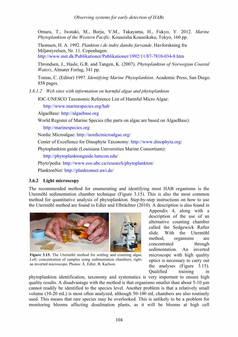
Observing systems for early detection of HABs

104

Omura, T., Iwataki, M., Borja, V.M., Takayama, H., Fukyo, Y. 2012. Marine Phytoplankton of the Western Pacific. Kouseisha Kouseikaku, Tokyo, 160 pp.

Thomsen, H. A. 1992. Plankton i de indre danske farvande. Havforskning fra Miljøstyrelsen, Nr. 11. Copenhagen. http://www.mst.dk/Publikationer/Publikationer/1992/11/87-7810-034-8.htm Throndsen, J., Hasle, G.R. and Tangen, K. (2007). Phytoplankton of Norwegian Coastal Waters, Almater Forlag, 341 pp. Tomas, C. (Editor) 1997. Identifying Marine Phytoplankton. Academic Press, San Diego. 858 pages.

3.6.1.2 Web sites with information on harmful algae and phytoplankton

IOC-UNESCO Taxonomic Reference List of Harmful Micro Algae: http://www.marinespecies.org/hab

AlgaeBase: http://algaebase.org World Register of Marine Species (the parts on algae are based on AlgaeBase):

http://marinespecies.org Nordic Microalgae: http://nordicmicroalgae.org/ Center of Excellence for Dinophyte Taxonomy: http://www.dinophyta.org/ Phytoplankton guide (Louisiana Universities Marine Consortium):

http://phytoplanktonguide.lumcon.edu/ Phyto'pedia: http://www.eos.ubc.ca/research/phytoplankton/ PlanktonNet: http://planktonnet.awi.de/

3.6.2 Light microscopy

The recommended method for enumerating and identifying most HAB organisms is the Utermöhl sedimentation chamber technique (Figure 3.15). This is also the most common method for quantitative analysis of phytoplankton. Step-by-step instructions on how to use the Utermöhl method are found in Edler and Elbrächter (2010). A description is also found in

Appendix 4, along with a description of the use of an alternative counting chamber called the Sedgewick Rafter slide. With the Utermöhl method, organisms are concentrated through sedimentation. An inverted microscope with high quality optics is necessary to carry out the analyses (Figure 3.15). Qualified training in

phytoplankton identification, taxonomy and systematics is very important to ensure high quality results. A disadvantage with the method is that organisms smaller than about 5-10 µm cannot readily be identified to the species level. Another problem is that a relatively small volume (10-20 mL) is most often analyzed, although 50-100 mL chambers are also routinely used. This means that rare species may be overlooked. This is unlikely to be a problem for monitoring blooms affecting desalination plants, as it will be blooms at high cell

Figure 3.15. The Utermöhl method for settling and counting algae. Left: concentration of samples using sedimentation chambers; right: an inverted microscope. Photos: Å. Edler, B. Karlson.

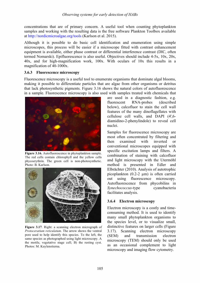
Observing systems for early detection of HABs

105

concentrations that are of primary concern. A useful tool when counting phytoplankton samples and working with the resulting data is the free software Plankton Toolbox available at http://nordicmicroalgae.org/tools (Karlson et al. 2015). Although it is possible to do basic cell identification and enumeration using simple microscopes, this process will be easier if a microscope fitted with contrast enhancement equipment is available, either phase contrast or differential interference contrast (DIC, often termed Nomarski). Epifluorescence is also useful. Objectives should include 4-5x, 10x, 20x, 40x, and for high-magnification work, 100x. With oculars of 10x this results in a magnification of 40-1000x. 3.6.3 Fluorescence microscopy

Fluorescence microscopy is a useful tool to enumerate organisms that dominate algal blooms, making it possible to differentiate particles that are algae from other organisms or detritus that lack photosynthetic pigments. Figure 3.16 shows the natural colors of autofluorescence in a sample. Fluorescence microscopy is also used with samples treated with chemicals that

are used in a diagnostic fashion, e.g. fluorescent RNA-probes (described below), calcofluor to stain the cell wall features of the many dinoflagellates with cellulose cell walls, and DAPI (4',6-diamidino-2-phenylindole) to reveal cell nuclei. Samples for fluorescence microscopy are most often concentrated by filtering and then examined with inverted or conventional microscopes equipped with specific excitation lamps and filters. A combination of staining with calcofluor and light microscopy with the Utermöhl method is presented in Edler and Elbrächter (2010). Analysis of autotrophic picoplankton (0.2-2 µm) is often carried out using fluorescence microscopy. Autofluorescence from phycobilins in Synechococcus-type cyanobacteria facilitates analysis.

3.6.4 Electron microscopy

Electron microscopy is a costly and time-consuming method. It is used to identify many small phytoplankton organisms to the species level, or to visualize small, distinctive features on larger cells (Figure 3.17). Scanning electron microscopy (SEM) and transmission electron microscopy (TEM) should only be used as an occasional complement to light microscopy and imaging flow cytometry.

Figure 3.16. Autofluorescence in phytoplankton sample. The red cells contain chlorophyll and the yellow cells phycoerythrin. The green cell is non-photosynthetic. Photo: B. Karlson.

Figure 3.17. Right: a scanning electron micrograph of Protoceratium reticulatum. The arrow shows the ventral pore used to help identify this species. To the left, the same species as photographed using light microscopy. A the motile, vegetative stage cell; B) the resting cyst. Photos: M. Kuylenstierna.

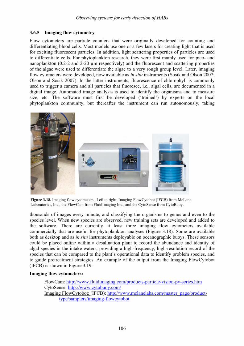
Observing systems for early detection of HABs

106

3.6.5 Imaging flow cytometry Flow cytometers are particle counters that were originally developed for counting and differentiating blood cells. Most models use one or a few lasers for creating light that is used for exciting fluorescent particles. In addition, light scattering properties of particles are used to differentiate cells. For phytoplankton research, they were first mainly used for pico- and nanoplankton (0.2-2 and 2-20 µm respectively) and the fluorescent and scattering properties of the algae were used to differentiate the algae to a very rough group level. Later, imaging flow cytometers were developed, now available as in situ instruments (Sosik and Olson 2007; Olson and Sosik 2007). In the latter instruments, fluorescence of chlorophyll is commonly used to trigger a camera and all particles that fluoresce, i.e., algal cells, are documented in a digital image. Automated image analysis is used to identify the organisms and to measure size, etc. The software must first be developed (‘trained’) by experts on the local phytoplankton community, but thereafter the instrument can run autonomously, taking

thousands of images every minute, and classifying the organisms to genus and even to the species level. When new species are observed, new training sets are developed and added to the software. There are currently at least three imaging flow cytometers available commercially that are useful for phytoplankton analyses (Figure 3.18). Some are available both as desktop and as in situ instruments deployable on oceanographic buoys. These sensors could be placed online within a desalination plant to record the abundance and identity of algal species in the intake waters, providing a high-frequency, high-resolution record of the species that can be compared to the plant’s operational data to identify problem species, and to guide pretreatment strategies. An example of the output from the Imaging FlowCytobot (IFCB) is shown in Figure 3.19. Imaging flow cytometers:

FlowCam: http://www.fluidimaging.com/products-particle-vision-pv-series.htm CytoSense: http://www.cytobuoy.com/ Imaging FlowCytobot: (IFCB): http://www.mclanelabs.com/master_page/product-

type/samplers/imaging-flowcytobot

Figure 3.18. Imaging flow cytometers. Left to right: Imaging FlowCytobot (IFCB) from McLane Laboratories, Inc., the FlowCam from FluidImaging Inc., and the CytoSense from CytoBuoy.

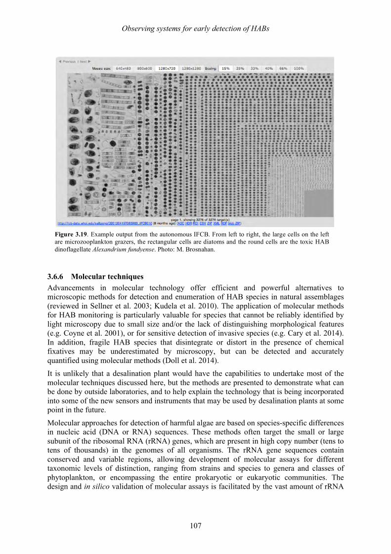
Observing systems for early detection of HABs

107

3.6.6 Molecular techniques Advancements in molecular technology offer efficient and powerful alternatives to microscopic methods for detection and enumeration of HAB species in natural assemblages (reviewed in Sellner et al. 2003; Kudela et al. 2010). The application of molecular methods for HAB monitoring is particularly valuable for species that cannot be reliably identified by light microscopy due to small size and/or the lack of distinguishing morphological features (e.g. Coyne et al. 2001), or for sensitive detection of invasive species (e.g. Cary et al. 2014). In addition, fragile HAB species that disintegrate or distort in the presence of chemical fixatives may be underestimated by microscopy, but can be detected and accurately quantified using molecular methods (Doll et al. 2014). It is unlikely that a desalination plant would have the capabilities to undertake most of the molecular techniques discussed here, but the methods are presented to demonstrate what can be done by outside laboratories, and to help explain the technology that is being incorporated into some of the new sensors and instruments that may be used by desalination plants at some point in the future.

Molecular approaches for detection of harmful algae are based on species-specific differences in nucleic acid (DNA or RNA) sequences. These methods often target the small or large subunit of the ribosomal RNA (rRNA) genes, which are present in high copy number (tens to tens of thousands) in the genomes of all organisms. The rRNA gene sequences contain conserved and variable regions, allowing development of molecular assays for different taxonomic levels of distinction, ranging from strains and species to genera and classes of phytoplankton, or encompassing the entire prokaryotic or eukaryotic communities. The design and in silico validation of molecular assays is facilitated by the vast amount of rRNA

Figure 3.19. Example output from the autonomous IFCB. From left to right, the large cells on the left are microzooplankton grazers, the rectangular cells are diatoms and the round cells are the toxic HAB dinoflagellate Alexandrium fundyense. Photo: M. Brosnahan.

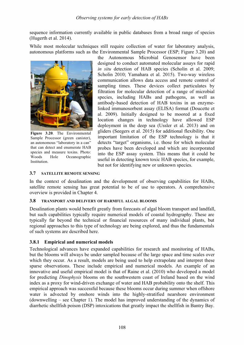
Observing systems for early detection of HABs

108

sequence information currently available in public databases from a broad range of species (Hugerth et al. 2014).

While most molecular techniques still require collection of water for laboratory analysis, autonomous platforms such as the Environmental Sample Processor (ESP; Figure 3.20) and

the Autonomous Microbial Genosensor have been designed to conduct automated molecular assays for rapid in situ detection of HAB species (Scholin et al. 2009; Scholin 2010; Yamahara et al. 2015). Two-way wireless communication allows data access and remote control of sampling times. These devices collect particulates by filtration for molecular detection of a range of microbial species, including HABs and pathogens, as well as antibody-based detection of HAB toxins in an enzyme-linked immunosorbent assay (ELISA) format (Doucette et al. 2009). Initially designed to be moored at a fixed location changes in technology have allowed ESP deployment in the deep sea (Ussler et al. 2013) and on gliders (Seegers et al. 2015) for additional flexibility. One important limitation of the ESP technology is that it detects “target” organisms, i.e. those for which molecular probes have been developed and which are incorporated into the ESP assay system. This means that it could be useful in detecting known toxic HAB species, for example, but not for identifying new or unknown species.

3.7 SATELLITE REMOTE SENSING In the context of desalination and the development of observing capabilities for HABs, satellite remote sensing has great potential to be of use to operators. A comprehensive overview is provided in Chapter 4.

3.8 TRANSPORT AND DELIVERY OF HARMFUL ALGAL BLOOMS Desalination plants would benefit greatly from forecasts of algal bloom transport and landfall, but such capabilities typically require numerical models of coastal hydrography. These are typically far beyond the technical or financial resources of many individual plants, but regional approaches to this type of technology are being explored, and thus the fundamentals of such systems are described here.

3.8.1 Empirical and numerical models Technological advances have expanded capabilities for research and monitoring of HABs, but the blooms will always be under sampled because of the large space and time scales over which they occur. As a result, models are being used to help extrapolate and interpret these sparse observations. These include empirical and numerical models. An example of an innovative and useful empirical model is that of Raine et al. (2010) who developed a model for predicting Dinophysis blooms on the southwestern coast of Ireland based on the wind index as a proxy for wind-driven exchange of water and HAB probability onto the shelf. This empirical approach was successful because these blooms occur during summer when offshore water is advected by onshore winds into the highly-stratified nearshore environment (downwelling – see Chapter 1). The model has improved understanding of the dynamics of diarrhetic shellfish poison (DSP) intoxications that greatly impact the shellfish in Bantry Bay.

Figure 3.20. The Environmental Sample Processor (green canister), an autonomous “laboratory in a can” that can detect and enumerate HAB species and measure toxins. Photo: Woods Hole Oceanographic Institution.

Observing systems for early detection of HABs

109

Hydrodynamic circulation models are commonly used to track and visualize bloom formation and duration as well as to understand the physical processes controlling phytoplankton bloom dynamics. Models with varying levels of sophistication have been developed. Some are purely three-dimensional physical models capable of resolving hydrography, and into which HAB cells can be introduced as passive particles. In the event that a particular HAB can be identified through detection methods discussed above, algorithms can be used to predict its trajectory and map the bloom using Lagrangian Particle Transport (LPT). This can be coupled to either a 2D or 3D circulation model. LPT is widely used in oil spill tracking and studies of fish or shellfish larval transport and is now seeing growing popularity for HAB risk management. LPT can be a powerful tool for estimating the timing and spatial impact of HAB landfall because many blooms originate offshore and are moved into the regions where most intakes to desalination plants would be located (either surface or subsurface). This is the approach used in a HAB forecasting system developed for Karenia brevis blooms in the Gulf of Mexico in which HAB forecasts are made twice weekly during bloom events (Stumpf et al. 2009). Blooms are detected using SeaWiFS and MODIS imagery, and bloom transport is then predicted using hydrographic modeling with passive particle transport. Vélo-Suarez et al. (2010) determined the physical processes responsible for the demise of a Dinophysis acuminata bloom, illustrating the importance of retention-dispersion patterns driven by the physics of the bay. Another study used a combination of models to track particles and identify the dominant sites of discharge along the Saudi Coast of the Red Sea (Zhan et al. 2015). This had direct implications to blooms as well as sediment transport. In each of these cases, particle transport models provided crucial spatial information about bloom or sediment transport that could potentially serve as an early warning to desalination plants.

The next step in sophistication and complexity is to couple a detailed biological submodel (one that incorporates cyst germination, cell growth, nutrient uptake, mortality and swimming behavior) to a hydrographic model, as has been done for Alexandrium dynamics in the Gulf of Maine region in the US (McGillicuddy et al. 2005; He et al. 2008). This level of modeling is species-specific, and not generally appropriate for desalination plants, however, at least at this point in time.

An alternative but practical approach to biophysical modeling blends empirical and dynamic methods to leverage the power of both simple and complex modeling approaches. In California, where seawater desalination plants already exist and are being revitalized or built for the first time, there is a great need to understand toxin production and transport of HABs nearshore. To this end, a HAB forecasting system has been developed to predict domoic acid-producing Pseudo-nitzschia blooms from empirical HAB models that are computed routinely in near real-time from satellite ocean color parameters and physical output (salinity and temperature) in a physical oceanographic model (Anderson et al. under review).

3.8.2 High-resolution circulation models to resolve flow near intakes High-resolution hydrodynamic models for studying physical features ~10-50 km in size, such as eddies, plumes and fronts, are becoming more accessible as technological advances reduce computing times and costs. Many of these models were initially developed to study patterns of fish larval recruitment or runoff close to shore. Models with a degree of physical complexity are useful for determining the initiation and termination of eddies and their movement near intake systems. Additional complexity in the form of coupled biological/ecosystem models provides specific guidance on where nutrient loading is highest in order to better inform the placement of intakes, initial design strategies or early warning of

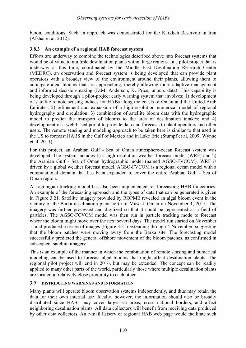
Observing systems for early detection of HABs

110

bloom conditions. Such an approach was demonstrated for the Karkheh Reservoir in Iran (Afshar et al. 2012).

3.8.3 An example of a regional HAB forecast system Efforts are underway to combine the technologies described above into forecast systems that would be of value to multiple desalination plants within large regions. In a pilot project that is underway at this time, coordinated by the Middle East Desalination Research Center (MEDRC), an observation and forecast system is being developed that can provide plant operators with a broader view of the environment around their plants, allowing them to anticipate algal blooms that are approaching, thereby allowing more adaptive management and informed decision-making (D.M. Anderson, K. Price, unpub. data). This capability is being developed through a pilot-project early warning system that involves: 1) development of satellite remote sensing indices for HABs along the coasts of Oman and the United Arab Emirates; 2) refinement and expansion of a high-resolution numerical model of regional hydrography and circulation; 3) combination of satellite bloom data with the hydrographic model to predict the transport of blooms to the area of desalination intakes; and 4) development of a web-based portal to provide data and forecasts to plant operators and other users. The remote sensing and modeling approach to be taken here is similar to that used in the US to forecast HABS in the Gulf of Mexico and in Lake Erie (Stumpf et al. 2009; Wynne et al. 2011).

For this project, an Arabian Gulf - Sea of Oman atmosphere-ocean forecast system was developed. The system includes 1) a high-resolution weather forecast model (WRF) and 2) the Arabian Gulf - Sea of Oman hydrographic model (named AGSO-FVCOM). WRF is driven by a global weather forecast model. AGSO-FVCOM is a regional ocean model with a computational domain that has been expanded to cover the entire Arabian Gulf - Sea of Oman region.

A Lagrangian tracking model has also been implemented for forecasting HAB trajectories. An example of the forecasting approach and the types of data that can be generated is given in Figure 3.21. Satellite imagery provided by ROPME revealed an algal bloom event in the vicinity of the Barka desalination plant north of Muscat, Oman on November 1, 2015. The imagery was further processed and digitized so that it could be represented as a field of particles. The AGSO-FCVOM model was then run in particle tracking mode to forecast where the bloom might move over the next several days. The model run started on November 1, and produced a series of images (Figure 3.21) extending through 4 November, suggesting that the bloom patches were moving away from the Barka site. The forecasting model successfully predicted the general offshore movement of the bloom patches, as confirmed in subsequent satellite imagery. This is an example of the manner in which the combination of remote sensing and numerical modeling can be used to forecast algal blooms that might affect desalination plants. The regional pilot project will end in 2016, but may be extended. The concept can be readily applied to many other parts of the world, particularly those where multiple desalination plants are located in relatively close proximity to each other.

3.9 DISTRIBUTING WARNINGS AND INFORMATION Many plants will operate bloom observation systems independently, and thus may retain the data for their own internal use. Ideally, however, the information should also be broadly distributed since HABs may cover large sea areas, cross national borders, and affect neighboring desalination plants. All data collectors will benefit from receiving data produced by other data collectors. An e-mail listserv or regional HAB web page would facilitate such

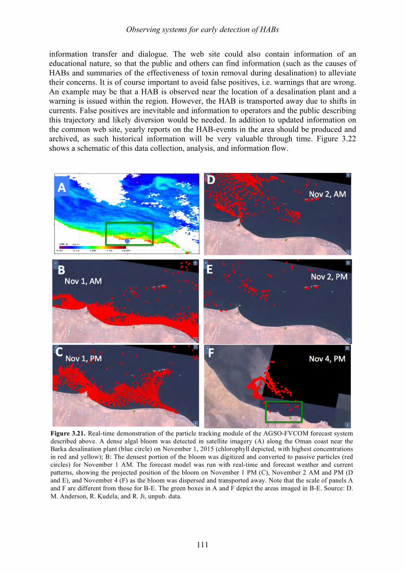
Observing systems for early detection of HABs

111

information transfer and dialogue. The web site could also contain information of an educational nature, so that the public and others can find information (such as the causes of HABs and summaries of the effectiveness of toxin removal during desalination) to alleviate their concerns. It is of course important to avoid false positives, i.e. warnings that are wrong. An example may be that a HAB is observed near the location of a desalination plant and a warning is issued within the region. However, the HAB is transported away due to shifts in currents. False positives are inevitable and information to operators and the public describing this trajectory and likely diversion would be needed. In addition to updated information on the common web site, yearly reports on the HAB-events in the area should be produced and archived, as such historical information will be very valuable through time. Figure 3.22 shows a schematic of this data collection, analysis, and information flow.

Figure 3.21. Real-time demonstration of the particle tracking module of the AGSO-FVCOM forecast system described above. A dense algal bloom was detected in satellite imagery (A) along the Oman coast near the Barka desalination plant (blue circle) on November 1, 2015 (chlorophyll depicted, with highest concentrations in red and yellow); B: The densest portion of the bloom was digitized and converted to passive particles (red circles) for November 1 AM. The forecast model was run with real-time and forecast weather and current patterns, showing the projected position of the bloom on November 1 PM (C), November 2 AM and PM (D and E), and November 4 (F) as the bloom was dispersed and transported away. Note that the scale of panels A and F are different from those for B-E. The green boxes in A and F depict the areas imaged in B-E. Source: D. M. Anderson, R. Kudela, and R. Ji, unpub. data.

Observing systems for early detection of HABs

112

3.10 DATA STORAGE AND DISTRIBUTION All data produced should be stored and their quality controlled. Ideally, the data should be made available freely to the scientific community. The UNESCO-IOC-Global Ocean Observing System (GOOS) and its regional organizations provide an umbrella-organization for this. IOC is the Intergovernmental Oceanographic Commission; it supports the Harmful Algal Event Database (http://haedat.iode.org) and the International Oceanographic Data and Information Exchange (IODE, http://iode.org). ICES (www.ices.dk) provides a system for handling quantitative physical, chemical, and biological data (including phytoplankton) for the North Atlantic. Similar systems exist or are being set up for other areas. 3.11 FACILITIES, EQUIPMENT, AND PERSONNEL

Facilities and equipment needed for a HAB-observation system are listed in Table 3.3, with some suggested priorities. However, facilities and priorities will vary dramatically among plants, depending upon available resources and the magnitude of the perceived HAB threat. The number of personnel involved in HAB observing efforts will vary dramatically among desalination plants, as this once again will be determined by the nature of the HAB threat as well as the funding resources available. In some cases, existing staff can be assigned additional duties to undertake the sampling and analyses after adequate training. In others, a single individual might be assigned HAB monitoring responsibilities, with the mandate to draw upon additional plant personnel when more hands are needed. Local or international HAB experts (e.g. taxonomy, bloom dynamics, HAB observing systems, remote sensing, toxin analysis) should be identified and their contact details kept in a suitable archive so they can be of assistance in training or during outbreaks.

Figure 3.22. Illustration of flow of information from data sources to end users, national and international databases.

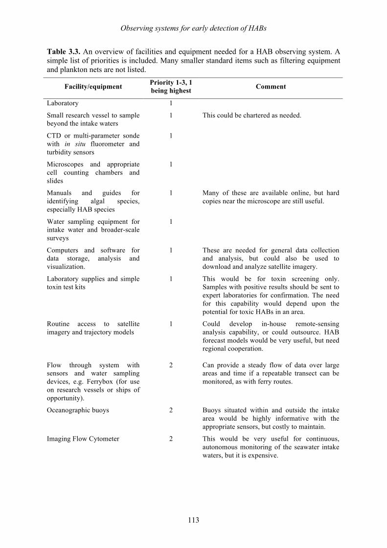
Observing systems for early detection of HABs

113

Table 3.3. An overview of facilities and equipment needed for a HAB observing system. A simple list of priorities is included. Many smaller standard items such as filtering equipment and plankton nets are not listed.

Facility/equipment Priority 1-3, 1 being highest Comment

Laboratory 1

Small research vessel to sample beyond the intake waters

1 This could be chartered as needed.

CTD or multi-parameter sonde with in situ fluorometer and turbidity sensors

1

Microscopes and appropriate cell counting chambers and slides

1

Manuals and guides for identifying algal species, especially HAB species

1 Many of these are available online, but hard copies near the microscope are still useful.

Water sampling equipment for intake water and broader-scale surveys

1

Computers and software for data storage, analysis and visualization.

1 These are needed for general data collection and analysis, but could also be used to download and analyze satellite imagery.

Laboratory supplies and simple toxin test kits

1 This would be for toxin screening only. Samples with positive results should be sent to expert laboratories for confirmation. The need for this capability would depend upon the potential for toxic HABs in an area.

Routine access to satellite imagery and trajectory models

1 Could develop in-house remote-sensing analysis capability, or could outsource. HAB forecast models would be very useful, but need regional cooperation.

Flow through system with sensors and water sampling devices, e.g. Ferrybox (for use on research vessels or ships of opportunity).

2 Can provide a steady flow of data over large areas and time if a repeatable transect can be monitored, as with ferry routes.

Oceanographic buoys 2 Buoys situated within and outside the intake area would be highly informative with the appropriate sensors, but costly to maintain.

Imaging Flow Cytometer 2 This would be very useful for continuous, autonomous monitoring of the seawater intake waters, but it is expensive.

Observing systems for early detection of HABs

114

Table 3.3. (Continued)

Facility/equipment Priority 1-3, 1 being highest

Comment

Equipment and supplies (or service) for analyzing TEP and other organic molecules (Appendix 3)

2 These are useful measurements, especially when paired with phytoplankton counts in the intake water – helps to specify the species and cell concentrations that disrupt operations or that require specific pretreatments.

Equipment (or a service) for analyses of algal toxins (LC-MS)

3 This should be a low priority unless there is a significant risk for biotoxin contamination of water used for human consumption. These types of analyses are typically outsourced.

Equipment (or a service) for analyses of inorganic nutrients

3 This provides useful information relevant to HAB bloom growth and persistence, but typically are outsourced.

Electron microscope 3 This is a low priority and should be available at local universities.

3.12 SUMMARY There are numerous techniques to detect HABs in order to react in time to minimize their effects on desalination plants. To accomplish this goal, local and regional monitoring of phytoplankton composition and biomass are needed. To carry out such monitoring, a combination of methods is recommended. A comprehensive monitoring program might include:

1. Long-term funding and staffing commitments 2. Appropriate facilities and equipment in the form of laboratory, shiptime, sampling

equipment, microscope, analysis instruments 3. Frequent water sampling near or at the desalination plant. This could include:

a. Manual sampling in water flowing into the plant or sampling from ships and boats in nearby waters.

b. Automated sampling in water flowing into a plant or on fixed platforms or ships of opportunity outside the intake.

c. Analysis of the composition and biomass of the phytoplankton by microscopy and/or imaging flow cytometry. Molecular techniques or SEM may be considered to complement the other methods when high-level species identification is needed.

d. Continuous online analysis of chlorophyll-a, as a proxy for phytoplankton biomass

4. Automated measurements of in-water bio-optical and physical parameters, e.g. chlorophyll fluorescence, temperature and salinity, from fixed platforms such as moorings or by using Ferrybox systems. Biofouling of sensors must be considered when deciding frequency of service.

5. The use of ocean color data from satellite remote sensing. Algorithms for chlorophyll-a, a proxy for phytoplankton biomass, are useful and there are also algorithms for detecting certain phytoplankton groups in high biomass algal blooms.

6. The use of physical oceanographic models, verified for the geographic area in focus, to produce forecasts regarding advection of HABs.

Observing systems for early detection of HABs

115

7. Quality control and storage of data as well as distribution of data to regional and global data centers.

8. Interpretation of data and visualization of results. 9. Information officers who distribute warnings and information.

If funding is limited, regular water sampling using water bottles and plankton nets with subsequent microscope analysis of the HAB-species should be conducted. In addition, water transparency or turbidity should be measured using a Secchi disk or turbidity tube. This probably requires a part-time technician and linkages to a phytoplankton identification expert. However, such a low cost approach would miss many blooms and be very dependent on the availability of the key staff. In practice such a system could benefit from a larger regional program that detects and forecasts HABs within a region (using remote sensing and numerical modeling, for example), with minimal staffing at each desalination plant to respond to advancing HABs.

3.13 REFERENCES Afshar, A., Saadatpour, M., and Marino, M. A. 2012. Development of a complex system

dynamic eutrophication model: application to Karkheh reservoir. Environmental Engineering Science 29, 373–385.

Andersen, P. 2010. Filtering – calcofluor staining – quantitative epifluorescence microscopy for phytoplankton analysis. in: Microscopic and molecular methods for quantitative phytoplankton analysis, Eds. Karlson, B., Cusack, C. and Bresnan, E. Intergovernmental Oceanographic Commission Manual and Guides 55, 31-35.

Anderson, C. R., Kudela, R. M., Kahru, M., Chao, Y., Rosenfeld, L. K., Bahr, F. L., Anderson, D. M., and Norris, T. A. Accepted for publication. Towards an operational HAB forecast system for California. Harmful Algae.

Bosch van Drakestein, F. G. 2014. Modeling of tides and spreading of saline water in the Arabian Gulf and in the coastal area of Abu Dhabi with a flexible mesh model. Master thesis 67 pp.

Cary, S. C., Coyne, K. J., Rueckert, A., Wood, S. A., Kelly, S., Gemmill, C. E. C., Vieglais, C., and Hicks, B. J. 2014. Development and validation of a quantitative PCR assay for the early detection and monitoring of the invasive diatom Didymosphenia geminata. Harmful Algae 36, 63–70.

Coyne, K. J., Hutchins, D. A., Hare, C. E., and Cary, S. C. 2001. Assessing temporal and spatial variability in Pfiesteria piscicida distributions using molecular probing techniques. Aquatic Microbial Ecology 24, 275–285.

Doll, C., Main, C. R., Bianco, C., Coyne, K. J., and Greenfield, D. I. 2014. Comparison of sandwich hybridization assay and quantitative PCR for the quantification of live and preserved cultures of Heterosigma akashiwo (Raphidophyceae). Limnology and Oceanography - Methods 12, 232–245.

Doucette, G. J., Mikulski, C. M., Jones, K. L., King, K. L., Greenfield, D. I., Marin, R., Jensen, S., Roman, B., Elliott, C. T., and Scholin, C. A. 2009. Remote, subsurface detection of the algal toxin domoic acid onboard the Environmental Sample Processor: assay development and field trials. Harmful Algae 8, 880–888.

Observing systems for early detection of HABs

116

Edler, L. and Elbrächter, M. 2010. The Utermöhl method for quantitative phytoplankton analysis. in: Microscopic and molecular methods for quantitative phytoplankton analysis, Eds. Karlson, B., Cusack, C., and Bresnan, E. Intergovernmental Oceanographic Commission Manual and Guides 55, 13-20.

Fritz, L. and Triemer, R. E. 1985. A rapid simple technique utilizing Calcofluor White M2R for the visualization of dinoflagellate thecal plates. Journal of Phycology 21, 662-664.

He, R., McGillicuddy, D. J., Keafer, B. A., and Anderson, D. M. 2008. Historic 2005 toxic bloom of Alexandrium fundyense in the western Gulf of Maine: 2. Coupled biophysical numerical modeling. Journal of Geophysical Research: Oceans 113, 1978–2012.

Hugerth, L. W., Muller, E. E., Hu, Y. O., Lebrun, L. A., Roume, H., Lundin, D., Wilmes, P., and Andersson, A. F. 2014. Systematic design of 18S rRNA gene primers for determining eukaryotic diversity in microbial consortia. PLoS One 9: e95567.

Karlson, B., Cusack, C., and Bresnan, E. (editors) 2010. Microscopic and molecular methods for quantitative phytoplankton analysis. Paris, UNESCO. IOC Manuals and Guides 55, 110 pages. http://hab.ioc-unesco.org/index.php?option=com_oe&task=viewDocumentRecord&docID=5440

Karlson, B., Godhe, A., Cusack, C., and Bresnan, B. 2010. Overview of methods for quantitative phytoplankton analysis in: Microscopic and molecular methods for quantitative phytoplankton analysis, Eds. Karlson, B., Cusack, C., and Bresnan, E. Intergovernmental Oceanographic Commission Manual and Guides 55, pp 5-12.

Karlson, B., Andreasson, A., Johansen, M., Mohlin, M., Skjevik, A-T., and Strömberg, P. 2015. Plankton Toolbox – open source software making it easier to work with plankton data, A. Lincoln MacKenzie [Ed]. Marine and Freshwater Harmful Algae 2014. Proceedings of the 16th International Conference on Harmful Algae. Cawthron Institute, Nelson, New Zealand and the International Society for the Study of Harmful Algae (ISSHA), pp 194-197.

Karlson, B., Andersson, L. S., Kaitala, S., Kronsell, J., Mohlin, M., Seppälä, J., and Wranne, A. W. 2016. Oceanographic variability in near surface waters of the Baltic Sea and the Kattegat – a comparison of Ferrybox data vs. monitoring data from research vessels. Journal of Marine Systems 162, 98–111.

Kudela, R. M., Howard, M., Jenkins, B. D., Miller, P. E., and Smith, G., J. 2010. Using the molecular toolbox to compare harmful algal blooms in upwelling systems. Progress in Oceanography 85, 108–121.

McGillicuddy, Jr., D. J., Anderson, D. M., Lynch, D. R., and Townsend, D. W. 2005. Mechanisms regulating large-scale seasonal fluctuations in Alexandrium fundyense populations in the Gulf of Maine: Results from a physical-biological model. Deep-Sea Res. II 52, 2698–2714.

Olson, R. J., and Sosik, H. M. 2007. A submersible imaging in flow instrument to analyze nano and microplankton: Imaging FlowCytobot. Limnology and Oceanography - Methods 5, 195–203.

Raine, R., McDermott, G., Silke, J., Lyons, K., and Nolan, G. 2010. A simple short range model for the prediction of harmful algal events in the bays of southwestern Ireland. Journal of Marine Systems 83, 150-157.

Observing systems for early detection of HABs

117

Scholin, C. A. 2010. What are“ ecogenomic sensors?” A review and thoughts for the future. Ocean Science 6, 51–60.

Scholin, C., Doucette, G., Jensen, S., Roman, B., Pargett, D., Marin III, R., Preston, C., Jones, W., Feldman, J., and Everlove, C. 2009. Remote detection of marine microbes, small invertebrates, harmful algae, and biotoxins using the environmental sample processor (ESP). Oceanography 22, 158-167.

Seegers, B. N., Birch, J. M., Marin, R., Scholin, C. A., Caron, D. A., Seubert, E. L., Howard, M. D., Robertson, G. L., and Jones, B. H. 2015. Subsurface seeding of surface harmful algal blooms observed through the integration of autonomous gliders, moored environmental sample processors, and satellite remote sensing in southern California. Limnology and Oceanography 60, 754–764.

Sellner, K. G., Doucette, G. J., and Kirkpatrick, G. J. 2003. Harmful algal blooms: causes, impacts and detection. Journal of Industrial Microbiology and Biotechnology 30, 383–406.

Sosik, H. M. and Olson, R. J. 2007. Automated taxonomic classification of phytoplankton sampled with imaging in flow cytometry. Limnology and Oceanography - Methods 5, 204–216.

Stumpf, R. P., Tomlinson, M. C., Calkins, J. A., Kirkpatrick, B., Nierenberg, K., Currier, R., and Wynne, T. T. 2009. Skill assessment for an operational algal bloom forecast system. Journal of Marine Systems 76, 151-161.

Ussler, W., Preston, C., Tavormina, P., Pargett, D., Jensen, S., Roman, B., Marin, R., Shah, S. R., Girguis, P. R., Birch, J. M., Orphan, V., and Scholin, C. 2013. Autonomous application of Quantitative PCR in the deep sea: In situ surveys of aerobic methanotrophs using the deep-sea Environmental Sample Processor. Environmental Science and Technology 47, 9339-9346.

Velo-Suárez, L., Reguera, B., González-Gil, S., Lunven, M., Lazure, P., Nézan, E., and Gentien, P. 2010. Application of a 3D Lagrangian model to explain the decline of a Dinophysis acuminata bloom in the Bay of Biscay. Journal of Marine Systems 83, 242–252.

Welschmeyer, N. A. 1994. Fluorometric analysis of chlorophyll a in the presence of chlorophyll b and pheopigments. Limnology and Oceanography 39(8), 1985-1992.

Wynne, T. T., Stumpf, R. P., Tomlinson, M. C., Schwab, D. J., Watabayashi, G. Y., and Christensen, J. D. 2011. Estimating cyanobacterial bloom transport by coupling remotely sensed imagery and a hydrodynamic model. Ecological Applications 2, 2709-2721.

Yamahara, K. M., Demir-Hilton, E., Preston, C. M., Marin, R., Pargett, D., Roman, B., Jensen, S., Birch, J. M., Boehm, A. B., and Scholin, C. A. 2015. Simultaneous monitoring of faecal indicators and harmful algae using an in-situ autonomous sensor. Letters in Applied Microbiology 61, 130–138.

Zhan, P., Yao, F., Kartadikaria, A. R., Viswanadhapalli, Y., Gopalakrishnan, G., and Hoteit, I. 2015. Far-field ocean conditions and concentrate discharges modeling along the Saudi Coast of the Red Sea. In: Intakes and Outfalls for Seawater Reverse-Osmosis Desalination Facilities, Springer. pp. 501–520.

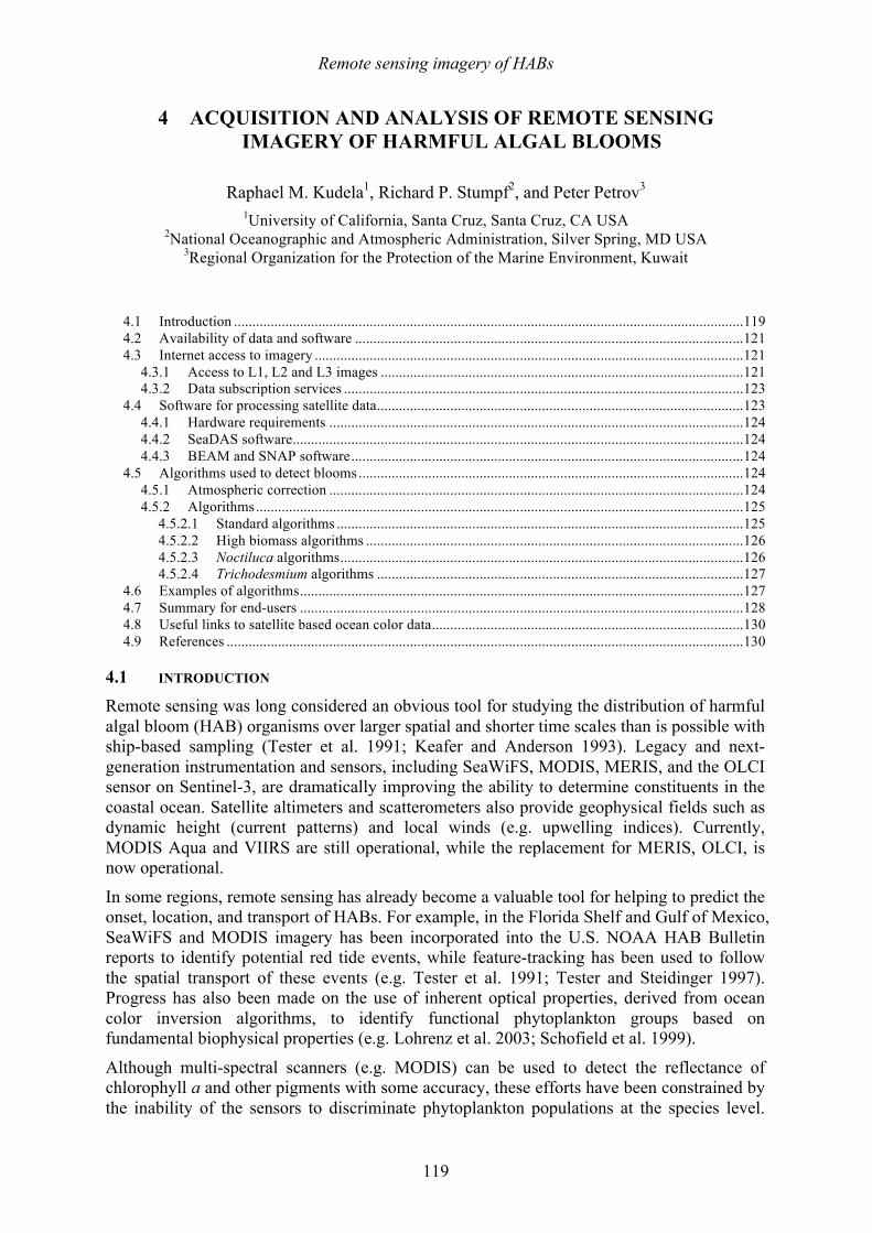
Remote sensing imagery of HABs

119

4 ACQUISITION AND ANALYSIS OF REMOTE SENSING IMAGERY OF HARMFUL ALGAL BLOOMS

Raphael M. Kudela1, Richard P. Stumpf2, and Peter Petrov3 1University of California, Santa Cruz, Santa Cruz, CA USA

2National Oceanographic and Atmospheric Administration, Silver Spring, MD USA 3Regional Organization for the Protection of the Marine Environment, Kuwait

4.1 Introduction ........................................................................................................................................... 119 4.2 Availability of data and software .......................................................................................................... 121 4.3 Internet access to imagery ..................................................................................................................... 121

4.3.1 Access to L1, L2 and L3 images ................................................................................................... 121 4.3.2 Data subscription services ............................................................................................................. 123

4.4 Software for processing satellite data .................................................................................................... 123 4.4.1 Hardware requirements ................................................................................................................. 124 4.4.2 SeaDAS software ........................................................................................................................... 124 4.4.3 BEAM and SNAP software ........................................................................................................... 124

4.5 Algorithms used to detect blooms ......................................................................................................... 124 4.5.1 Atmospheric correction ................................................................................................................. 124 4.5.2 Algorithms ..................................................................................................................................... 125

4.5.2.1 Standard algorithms ............................................................................................................... 125 4.5.2.2 High biomass algorithms ....................................................................................................... 126 4.5.2.3 Noctiluca algorithms .............................................................................................................. 126 4.5.2.4 Trichodesmium algorithms .................................................................................................... 127

4.6 Examples of algorithms ......................................................................................................................... 127 4.7 Summary for end-users ......................................................................................................................... 128 4.8 Useful links to satellite based ocean color data ..................................................................................... 130 4.9 References ............................................................................................................................................. 130

4.1 INTRODUCTION Remote sensing was long considered an obvious tool for studying the distribution of harmful algal bloom (HAB) organisms over larger spatial and shorter time scales than is possible with ship-based sampling (Tester et al. 1991; Keafer and Anderson 1993). Legacy and next-generation instrumentation and sensors, including SeaWiFS, MODIS, MERIS, and the OLCI sensor on Sentinel-3, are dramatically improving the ability to determine constituents in the coastal ocean. Satellite altimeters and scatterometers also provide geophysical fields such as dynamic height (current patterns) and local winds (e.g. upwelling indices). Currently, MODIS Aqua and VIIRS are still operational, while the replacement for MERIS, OLCI, is now operational.

In some regions, remote sensing has already become a valuable tool for helping to predict the onset, location, and transport of HABs. For example, in the Florida Shelf and Gulf of Mexico, SeaWiFS and MODIS imagery has been incorporated into the U.S. NOAA HAB Bulletin reports to identify potential red tide events, while feature-tracking has been used to follow the spatial transport of these events (e.g. Tester et al. 1991; Tester and Steidinger 1997). Progress has also been made on the use of inherent optical properties, derived from ocean color inversion algorithms, to identify functional phytoplankton groups based on fundamental biophysical properties (e.g. Lohrenz et al. 2003; Schofield et al. 1999).

Although multi-spectral scanners (e.g. MODIS) can be used to detect the reflectance of chlorophyll a and other pigments with some accuracy, these efforts have been constrained by the inability of the sensors to discriminate phytoplankton populations at the species level.

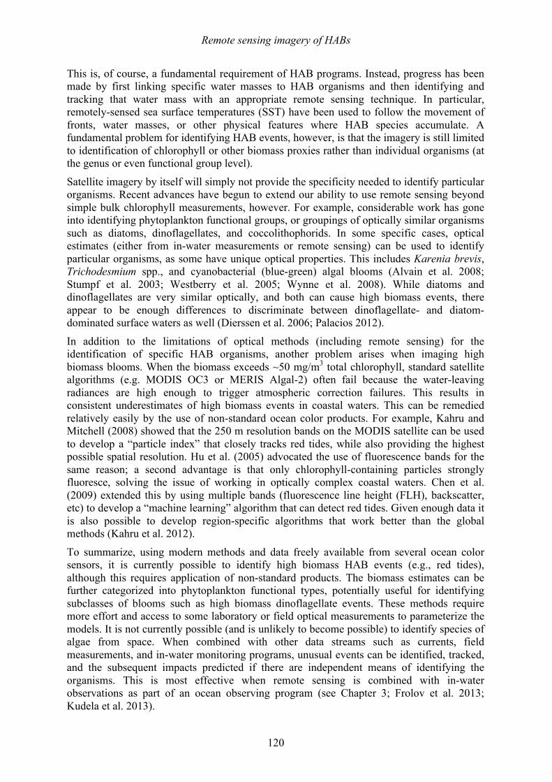
Remote sensing imagery of HABs

120

This is, of course, a fundamental requirement of HAB programs. Instead, progress has been made by first linking specific water masses to HAB organisms and then identifying and tracking that water mass with an appropriate remote sensing technique. In particular, remotely-sensed sea surface temperatures (SST) have been used to follow the movement of fronts, water masses, or other physical features where HAB species accumulate. A fundamental problem for identifying HAB events, however, is that the imagery is still limited to identification of chlorophyll or other biomass proxies rather than individual organisms (at the genus or even functional group level).

Satellite imagery by itself will simply not provide the specificity needed to identify particular organisms. Recent advances have begun to extend our ability to use remote sensing beyond simple bulk chlorophyll measurements, however. For example, considerable work has gone into identifying phytoplankton functional groups, or groupings of optically similar organisms such as diatoms, dinoflagellates, and coccolithophorids. In some specific cases, optical estimates (either from in-water measurements or remote sensing) can be used to identify particular organisms, as some have unique optical properties. This includes Karenia brevis, Trichodesmium spp., and cyanobacterial (blue-green) algal blooms (Alvain et al. 2008; Stumpf et al. 2003; Westberry et al. 2005; Wynne et al. 2008). While diatoms and dinoflagellates are very similar optically, and both can cause high biomass events, there appear to be enough differences to discriminate between dinoflagellate- and diatom-dominated surface waters as well (Dierssen et al. 2006; Palacios 2012).

In addition to the limitations of optical methods (including remote sensing) for the identification of specific HAB organisms, another problem arises when imaging high biomass blooms. When the biomass exceeds ~50 mg/m3 total chlorophyll, standard satellite algorithms (e.g. MODIS OC3 or MERIS Algal-2) often fail because the water-leaving radiances are high enough to trigger atmospheric correction failures. This results in consistent underestimates of high biomass events in coastal waters. This can be remedied relatively easily by the use of non-standard ocean color products. For example, Kahru and Mitchell (2008) showed that the 250 m resolution bands on the MODIS satellite can be used to develop a “particle index” that closely tracks red tides, while also providing the highest possible spatial resolution. Hu et al. (2005) advocated the use of fluorescence bands for the same reason; a second advantage is that only chlorophyll-containing particles strongly fluoresce, solving the issue of working in optically complex coastal waters. Chen et al. (2009) extended this by using multiple bands (fluorescence line height (FLH), backscatter, etc) to develop a “machine learning” algorithm that can detect red tides. Given enough data it is also possible to develop region-specific algorithms that work better than the global methods (Kahru et al. 2012).

To summarize, using modern methods and data freely available from several ocean color sensors, it is currently possible to identify high biomass HAB events (e.g., red tides), although this requires application of non-standard products. The biomass estimates can be further categorized into phytoplankton functional types, potentially useful for identifying subclasses of blooms such as high biomass dinoflagellate events. These methods require more effort and access to some laboratory or field optical measurements to parameterize the models. It is not currently possible (and is unlikely to become possible) to identify species of algae from space. When combined with other data streams such as currents, field measurements, and in-water monitoring programs, unusual events can be identified, tracked, and the subsequent impacts predicted if there are independent means of identifying the organisms. This is most effective when remote sensing is combined with in-water observations as part of an ocean observing program (see Chapter 3; Frolov et al. 2013; Kudela et al. 2013).

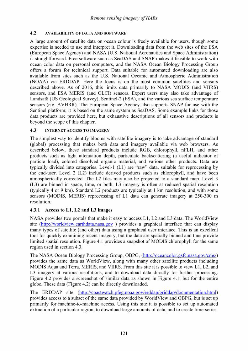
Remote sensing imagery of HABs

121

4.2 AVAILABILITY OF DATA AND SOFTWARE A large amount of satellite data on ocean colour is freely available for users, though some expertise is needed to use and interpret it. Downloading data from the web sites of the ESA (European Space Agency) and NASA (U.S. National Aeronautics and Space Administration) is straightforward. Free software such as SeaDAS and SNAP makes it feasible to work with ocean color data on personal computers, and the NASA Ocean Biology Processing Group offers a forum for technical support. Data suitable for automated downloading are also available from sites such as the U.S. National Oceanic and Atmospheric Administration (NOAA) via ERDDAP. Here the focus is on the most common satellites and sensors described above. As of 2016, this limits data primarily to NASA MODIS (and VIIRS) sensors, and ESA MERIS (and OLCI) sensors. Expert users may also take advantage of Landsat8 (US Geological Survey), Sentinel-2 (ESA), and the various sea surface temperature sensors (e.g. AVHRR). The European Space Agency also supports SNAP for use with the Sentinel platform; it is based on the same system as SeaDAS. Some example links for those data products are provided here, but exhaustive descriptions of all sensors and products is beyond the scope of this chapter.

4.3 INTERNET ACCESS TO IMAGERY The simplest way to identify blooms with satellite imagery is to take advantage of standard (global) processing that makes both data and imagery available via web browsers. As described below, these standard products include RGB, chlorophyll, nFLH, and other products such as light attenuation depth, particulate backscattering (a useful indicator of particle load), colored dissolved organic material, and various other products. Data are typically divided into categories. Level-1 (L1) are “raw” data, suitable for reprocessing by the end-user. Level 2 (L2) include derived products such as chlorophyll, and have been atmospherically corrected. The L2 files may also be projected to a standard map. Level 3 (L3) are binned in space, time, or both. L3 imagery is often at reduced spatial resolution (typically 4 or 9 km). Standard L2 products are typically at 1 km resolution, and with some sensors (MODIS, MERIS) reprocessing of L1 data can generate imagery at 250-300 m resolution. 4.3.1 Access to L1, L2 and L3 images

NASA provides two portals that make it easy to access L1, L2 and L3 data. The WorldView site (http://worldview.earthdata.nasa.gov ) provides a graphical interface that can display many types of satellite (and other) data using a graphical user interface. This is an excellent tool for quickly examining recent imagery, but the data are spatially binned and thus provide limited spatial resolution. Figure 4.1 provides a snapshot of MODIS chlorophyll for the same region used in section 4.3.

The NASA Ocean Biology Processing Group, OBPG, (http://oceancolor.gsfc.nasa.gov/cms/) provides the same data as WorldView, along with many other satellite products including MODIS Aqua and Terra, MERIS, and VIIRS. From this site it is possible to view L1, L2, and L3 imagery at various resolutions, and to download data directly for further processing. Figure 4.2 provides a screenshot of similar data as shown in Figure 4.1, but for the entire globe. These data (Figure 4.2) can be directly downloaded.

The ERDDAP site (http://coastwatch.pfeg.noaa.gov/erddap/griddap/documentation.html) provides access to a subset of the same data provided by WorldView and OBPG, but is set up primarily for machine-to-machine access. Using this site it is possible to set up automated extraction of a particular region, to download large amounts of data, and to create time-series.

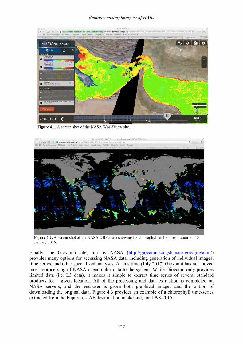
Remote sensing imagery of HABs

122

Finally, the Giovanni site, run by NASA (http://giovanni.sci.gsfc.nasa.gov/giovanni/) provides many options for accessing NASA data, including generation of individual images, time-series, and other specialized analyses. At this time (July 2017) Giovanni has not moved most reprocessing of NASA ocean color data to the system. While Giovanni only provides limited data (i.e. L3 data), it makes it simple to extract time series of several standard products for a given location. All of the processing and data extraction is completed on NASA servers, and the end-user is given both graphical images and the option of downloading the original data. Figure 4.3 provides an example of a chlorophyll time-series extracted from the Fujairah, UAE desalination intake site, for 1998-2015.

Figure 4.1. A screen shot of the NASA WorldView site.

Figure 4.2. A screen shot of the NASA OBPG site showing L3 chlorophyll at 4 km resolution for 15 January 2016.

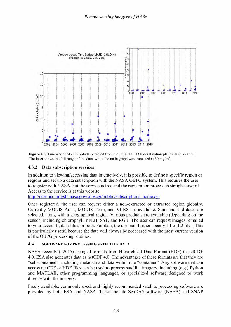
Remote sensing imagery of HABs

123

4.3.2 Data subscription services

In addition to viewing/accessing data interactively, it is possible to define a specific region or regions and set up a data subscription with the NASA OBPG system. This requires the user to register with NASA, but the service is free and the registration process is straightforward. Access to the service is at this website: http://oceancolor.gsfc.nasa.gov/sdpscgi/public/subscriptions_home.cgi Once registered, the user can request either a non-extracted or extracted region globally. Currently MODIS Aqua, MODIS Terra, and VIIRS are available. Start and end dates are selected, along with a geographical region. Various products are available (depending on the sensor) including chlorophyll, nFLH, SST, and RGB. The user can request images (emailed to your account), data files, or both. For data, the user can further specify L1 or L2 files. This is particularly useful because the data will always be processed with the most current version of the OBPG processing routines.

4.4 SOFTWARE FOR PROCESSING SATELLITE DATA NASA recently (~2015) changed formats from Hierarchical Data Format (HDF) to netCDF 4.0. ESA also generates data as netCDF 4.0. The advantages of these formats are that they are “self-contained”, including metadata and data within one “container”. Any software that can access netCDF or HDF files can be used to process satellite imagery, including (e.g.) Python and MATLAB, other programming languages, or specialized software designed to work directly with the imagery. Freely available, commonly used, and highly recommended satellite processing software are provided by both ESA and NASA. These include SeaDAS software (NASA) and SNAP

Figure 4.3. Time-series of chlorophyll extracted from the Fujairah, UAE desalination plant intake location. The inset shows the full range of the data, while the main graph was truncated at 30 mg/m3.

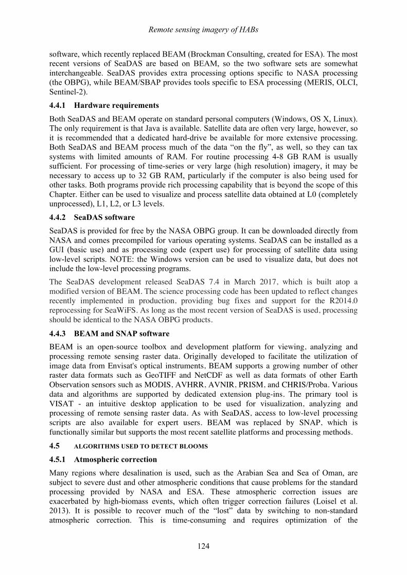
Remote sensing imagery of HABs

124

software, which recently replaced BEAM (Brockman Consulting, created for ESA). The most recent versions of SeaDAS are based on BEAM, so the two software sets are somewhat interchangeable. SeaDAS provides extra processing options specific to NASA processing (the OBPG), while BEAM/SBAP provides tools specific to ESA processing (MERIS, OLCI, Sentinel-2). 4.4.1 Hardware requirements

Both SeaDAS and BEAM operate on standard personal computers (Windows, OS X, Linux). The only requirement is that Java is available. Satellite data are often very large, however, so it is recommended that a dedicated hard-drive be available for more extensive processing. Both SeaDAS and BEAM process much of the data “on the fly”, as well, so they can tax systems with limited amounts of RAM. For routine processing 4-8 GB RAM is usually sufficient. For processing of time-series or very large (high resolution) imagery, it may be necessary to access up to 32 GB RAM, particularly if the computer is also being used for other tasks. Both programs provide rich processing capability that is beyond the scope of this Chapter. Either can be used to visualize and process satellite data obtained at L0 (completely unprocessed), L1, L2, or L3 levels.

4.4.2 SeaDAS software SeaDAS is provided for free by the NASA OBPG group. It can be downloaded directly from NASA and comes precompiled for various operating systems. SeaDAS can be installed as a GUI (basic use) and as processing code (expert use) for processing of satellite data using low-level scripts. NOTE: the Windows version can be used to visualize data, but does not include the low-level processing programs. The SeaDAS development released SeaDAS 7.4 in March 2017, which is built atop a modified version of BEAM. The science processing code has been updated to reflect changes recently implemented in production, providing bug fixes and support for the R2014.0 reprocessing for SeaWiFS. As long as the most recent version of SeaDAS is used, processing should be identical to the NASA OBPG products.

4.4.3 BEAM and SNAP software BEAM is an open-source toolbox and development platform for viewing, analyzing and processing remote sensing raster data. Originally developed to facilitate the utilization of image data from Envisat's optical instruments, BEAM supports a growing number of other raster data formats such as GeoTIFF and NetCDF as well as data formats of other Earth Observation sensors such as MODIS, AVHRR, AVNIR, PRISM, and CHRIS/Proba. Various data and algorithms are supported by dedicated extension plug-ins. The primary tool is VISAT - an intuitive desktop application to be used for visualization, analyzing and processing of remote sensing raster data. As with SeaDAS, access to low-level processing scripts are also available for expert users. BEAM was replaced by SNAP, which is functionally similar but supports the most recent satellite platforms and processing methods. 4.5 ALGORITHMS USED TO DETECT BLOOMS

4.5.1 Atmospheric correction Many regions where desalination is used, such as the Arabian Sea and Sea of Oman, are subject to severe dust and other atmospheric conditions that cause problems for the standard processing provided by NASA and ESA. These atmospheric correction issues are exacerbated by high-biomass events, which often trigger correction failures (Loisel et al. 2013). It is possible to recover much of the “lost” data by switching to non-standard atmospheric correction. This is time-consuming and requires optimization of the

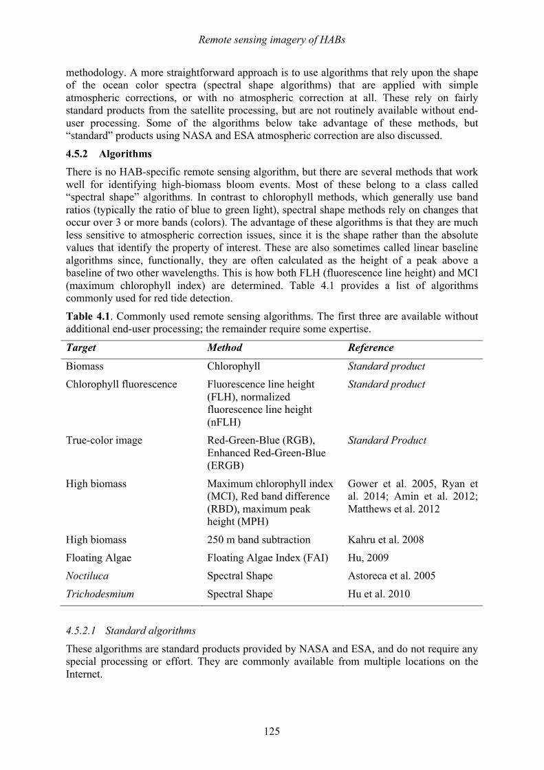
Remote sensing imagery of HABs

125

methodology. A more straightforward approach is to use algorithms that rely upon the shape of the ocean color spectra (spectral shape algorithms) that are applied with simple atmospheric corrections, or with no atmospheric correction at all. These rely on fairly standard products from the satellite processing, but are not routinely available without end-user processing. Some of the algorithms below take advantage of these methods, but “standard” products using NASA and ESA atmospheric correction are also discussed.

4.5.2 Algorithms There is no HAB-specific remote sensing algorithm, but there are several methods that work well for identifying high-biomass bloom events. Most of these belong to a class called “spectral shape” algorithms. In contrast to chlorophyll methods, which generally use band ratios (typically the ratio of blue to green light), spectral shape methods rely on changes that occur over 3 or more bands (colors). The advantage of these algorithms is that they are much less sensitive to atmospheric correction issues, since it is the shape rather than the absolute values that identify the property of interest. These are also sometimes called linear baseline algorithms since, functionally, they are often calculated as the height of a peak above a baseline of two other wavelengths. This is how both FLH (fluorescence line height) and MCI (maximum chlorophyll index) are determined. Table 4.1 provides a list of algorithms commonly used for red tide detection.

Table 4.1. Commonly used remote sensing algorithms. The first three are available without additional end-user processing; the remainder require some expertise.

Target Method Reference

Biomass Chlorophyll Standard product Chlorophyll fluorescence Fluorescence line height

(FLH), normalized fluorescence line height (nFLH)

Standard product

True-color image Red-Green-Blue (RGB), Enhanced Red-Green-Blue (ERGB)

Standard Product

High biomass Maximum chlorophyll index (MCI), Red band difference (RBD), maximum peak height (MPH)

Gower et al. 2005, Ryan et al. 2014; Amin et al. 2012; Matthews et al. 2012

High biomass 250 m band subtraction Kahru et al. 2008 Floating Algae Floating Algae Index (FAI) Hu, 2009 Noctiluca Spectral Shape Astoreca et al. 2005

Trichodesmium Spectral Shape Hu et al. 2010

4.5.2.1 Standard algorithms

These algorithms are standard products provided by NASA and ESA, and do not require any special processing or effort. They are commonly available from multiple locations on the Internet.

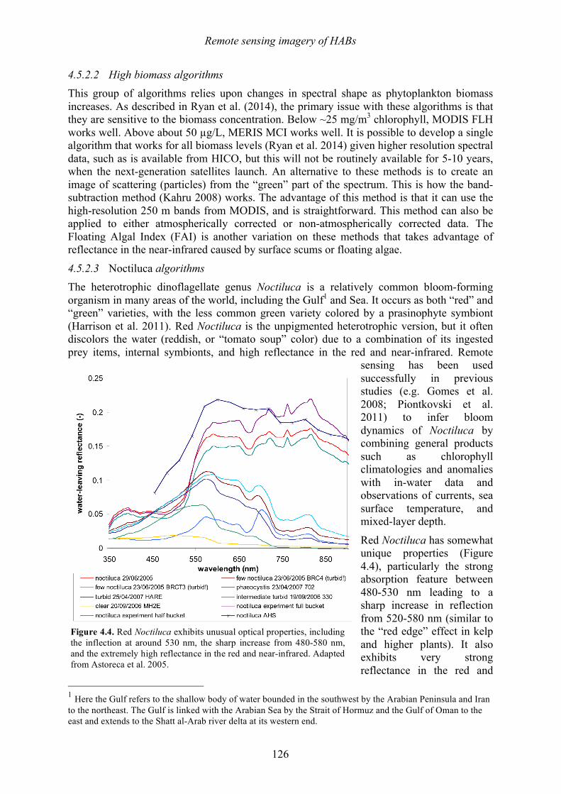
Remote sensing imagery of HABs

126

4.5.2.2 High biomass algorithms This group of algorithms relies upon changes in spectral shape as phytoplankton biomass increases. As described in Ryan et al. (2014), the primary issue with these algorithms is that they are sensitive to the biomass concentration. Below ~25 mg/m3 chlorophyll, MODIS FLH works well. Above about 50 µg/L, MERIS MCI works well. It is possible to develop a single algorithm that works for all biomass levels (Ryan et al. 2014) given higher resolution spectral data, such as is available from HICO, but this will not be routinely available for 5-10 years, when the next-generation satellites launch. An alternative to these methods is to create an image of scattering (particles) from the “green” part of the spectrum. This is how the band-subtraction method (Kahru 2008) works. The advantage of this method is that it can use the high-resolution 250 m bands from MODIS, and is straightforward. This method can also be applied to either atmospherically corrected or non-atmospherically corrected data. The Floating Algal Index (FAI) is another variation on these methods that takes advantage of reflectance in the near-infrared caused by surface scums or floating algae.

4.5.2.3 Noctiluca algorithms The heterotrophic dinoflagellate genus Noctiluca is a relatively common bloom-forming organism in many areas of the world, including the Gulf1 and Sea. It occurs as both “red” and “green” varieties, with the less common green variety colored by a prasinophyte symbiont (Harrison et al. 2011). Red Noctiluca is the unpigmented heterotrophic version, but it often discolors the water (reddish, or “tomato soup” color) due to a combination of its ingested prey items, internal symbionts, and high reflectance in the red and near-infrared. Remote

sensing has been used successfully in previous studies (e.g. Gomes et al. 2008; Piontkovski et al. 2011) to infer bloom dynamics of Noctiluca by combining general products such as chlorophyll climatologies and anomalies with in-water data and observations of currents, sea surface temperature, and mixed-layer depth.

Red Noctiluca has somewhat unique properties (Figure 4.4), particularly the strong absorption feature between 480-530 nm leading to a sharp increase in reflection from 520-580 nm (similar to the “red edge” effect in kelp and higher plants). It also exhibits very strong reflectance in the red and

1 Here the Gulf refers to the shallow body of water bounded in the southwest by the Arabian Peninsula and Iran to the northeast. The Gulf is linked with the Arabian Sea by the Strait of Hormuz and the Gulf of Oman to the east and extends to the Shatt al-Arab river delta at its western end.

Figure 4.4. Red Noctiluca exhibits unusual optical properties, including the inflection at around 530 nm, the sharp increase from 480-580 nm, and the extremely high reflectance in the red and near-infrared. Adapted from Astoreca et al. 2005.

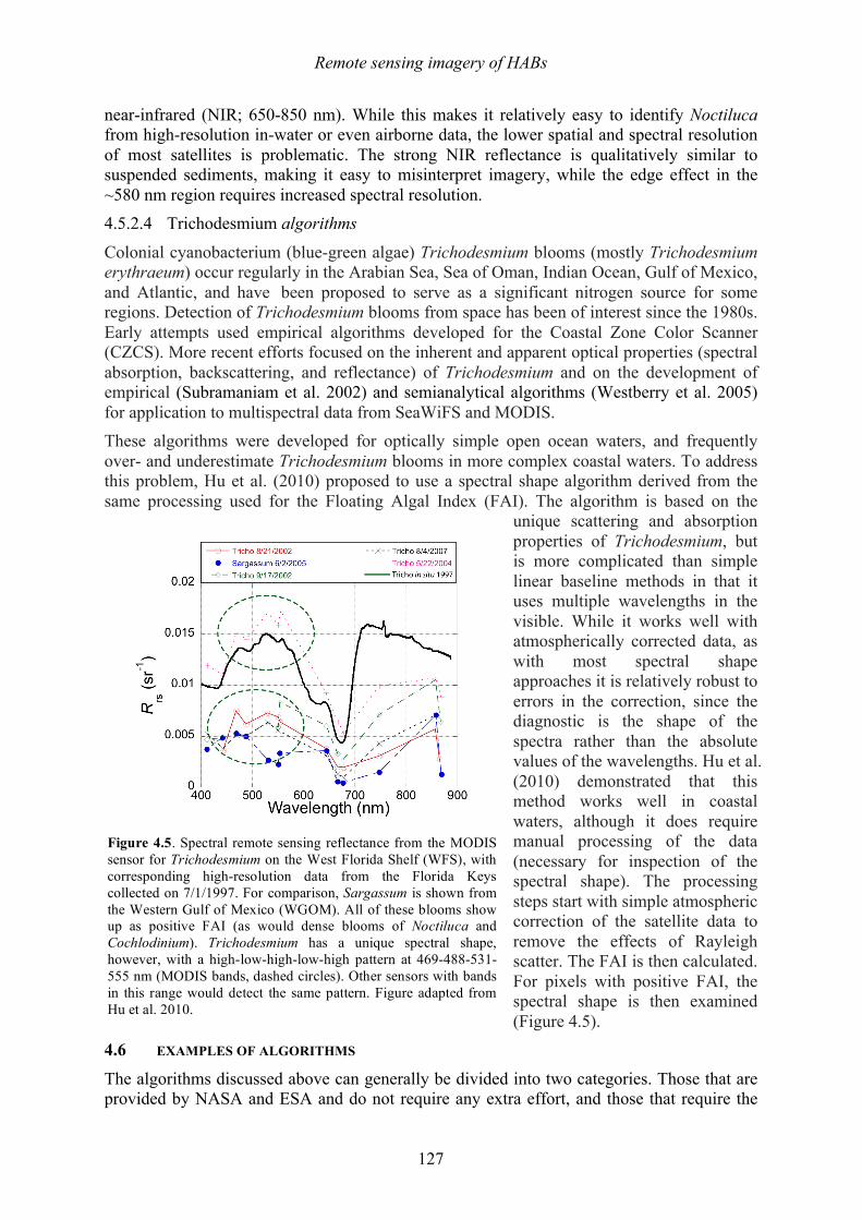
Remote sensing imagery of HABs

127

near-infrared (NIR; 650-850 nm). While this makes it relatively easy to identify Noctiluca from high-resolution in-water or even airborne data, the lower spatial and spectral resolution of most satellites is problematic. The strong NIR reflectance is qualitatively similar to suspended sediments, making it easy to misinterpret imagery, while the edge effect in the ~580 nm region requires increased spectral resolution. 4.5.2.4 Trichodesmium algorithms

Colonial cyanobacterium (blue-green algae) Trichodesmium blooms (mostly Trichodesmium erythraeum) occur regularly in the Arabian Sea, Sea of Oman, Indian Ocean, Gulf of Mexico, and Atlantic, and have been proposed to serve as a significant nitrogen source for some regions. Detection of Trichodesmium blooms from space has been of interest since the 1980s. Early attempts used empirical algorithms developed for the Coastal Zone Color Scanner (CZCS). More recent efforts focused on the inherent and apparent optical properties (spectral absorption, backscattering, and reflectance) of Trichodesmium and on the development of empirical (Subramaniam et al. 2002) and semianalytical algorithms (Westberry et al. 2005) for application to multispectral data from SeaWiFS and MODIS. These algorithms were developed for optically simple open ocean waters, and frequently over- and underestimate Trichodesmium blooms in more complex coastal waters. To address this problem, Hu et al. (2010) proposed to use a spectral shape algorithm derived from the same processing used for the Floating Algal Index (FAI). The algorithm is based on the

unique scattering and absorption properties of Trichodesmium, but is more complicated than simple linear baseline methods in that it uses multiple wavelengths in the visible. While it works well with atmospherically corrected data, as with most spectral shape approaches it is relatively robust to errors in the correction, since the diagnostic is the shape of the spectra rather than the absolute values of the wavelengths. Hu et al. (2010) demonstrated that this method works well in coastal waters, although it does require manual processing of the data (necessary for inspection of the spectral shape). The processing steps start with simple atmospheric correction of the satellite data to remove the effects of Rayleigh scatter. The FAI is then calculated. For pixels with positive FAI, the spectral shape is then examined (Figure 4.5).

4.6 EXAMPLES OF ALGORITHMS

The algorithms discussed above can generally be divided into two categories. Those that are provided by NASA and ESA and do not require any extra effort, and those that require the

Figure 4.5. Spectral remote sensing reflectance from the MODIS sensor for Trichodesmium on the West Florida Shelf (WFS), with corresponding high-resolution data from the Florida Keys collected on 7/1/1997. For comparison, Sargassum is shown from the Western Gulf of Mexico (WGOM). All of these blooms show up as positive FAI (as would dense blooms of Noctiluca and Cochlodinium). Trichodesmium has a unique spectral shape, however, with a high-low-high-low-high pattern at 469-488-531-555 nm (MODIS bands, dashed circles). Other sensors with bands in this range would detect the same pattern. Figure adapted from Hu et al. 2010.

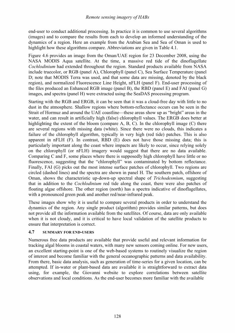
Remote sensing imagery of HABs

128

end-user to conduct additional processing. In practice it is common to use several algorithms (images) and to compare the results from each to develop an informed understanding of the dynamics of a region. Here an example from the Arabian Sea and Sea of Oman is used to highlight how these algorithms compare. Abbreviations are given in Table 4.1.

Figure 4.6 provides an image from the Oman/UAE region for 23 December 2008, using the NASA MODIS Aqua satellite. At the time, a massive red tide of the dinoflagellate Cochlodinium had extended throughout the region. Standard products available from NASA include truecolor, or RGB (panel A), Chlorophyll (panel C), Sea Surface Temperature (panel D; note that MODIS Terra was used, and that some data are missing, denoted by the black region), and normalized Fluorescence Line Height, nFLH (panel F). End-user processing of the files produced an Enhanced RGB image (panel B), the RBD (panel E) and FAI (panel G) images, and spectra (panel H) were extracted using the SeaDAS processing program.

Starting with the RGB and ERGB, it can be seen that it was a cloud-free day with little to no dust in the atmosphere. Shallow regions where bottom-reflectance occurs can be seen in the Strait of Hormuz and around the UAE coastline—these areas show up as “bright” areas in the water, and can result in artificially high (false) chlorophyll values. The ERGB does better at highlighting the extent of the bloom (compare A, B, C). In the chlorophyll image (C) there are several regions with missing data (white). Since there were no clouds, this indicates a failure of the chlorophyll algorithm, typically in very high (red tide) patches. This is also apparent in nFLH (F). In contrast, RBD (E) does not have those missing data; this is particularly important along the coast where impacts are likely to occur, since relying solely on the chlorophyll (or nFLH) imagery would suggest that there are no data available. Comparing C and F, some places where there is supposedly high chlorophyll have little or no fluorescence, suggesting that the “chlorophyll” was contaminated by bottom reflectance. Finally, FAI (G) picks out the most intense surface patches of chlorophyll. Two regions are circled (dashed lines) and the spectra are shown in panel H. The southern patch, offshore of Oman, shows the characteristic up-down-up spectral shape of Trichodesmium, suggesting that in addition to the Cochlodinium red tide along the coast, there were also patches of floating algae offshore. The other region (north) has a spectra indicative of dinoflagellates, with a pronounced green peak and another red/near-infrared peak.

These images show why it is useful to compare several products in order to understand the dynamics of the region. Any single product (algorithm) provides similar patterns, but does not provide all the information available from the satellites. Of course, data are only available when it is not cloudy, and it is critical to have local validation of the satellite products to ensure that interpretation is correct. 4.7 SUMMARY FOR END-USERS

Numerous free data products are available that provide useful and relevant information for tracking algal blooms in coastal waters, with many new sensors coming online. For new users, an excellent starting-point is one of the web-based systems to routinely visualize the region of interest and become familiar with the general oceanographic patterns and data availability. From there, basic data analysis, such as generation of time-series for a given location, can be attempted. If in-water or plant-based data are available it is straightforward to extract data using, for example, the Giovanni website to explore correlations between satellite observations and local conditions. As the end-user becomes more familiar with the available

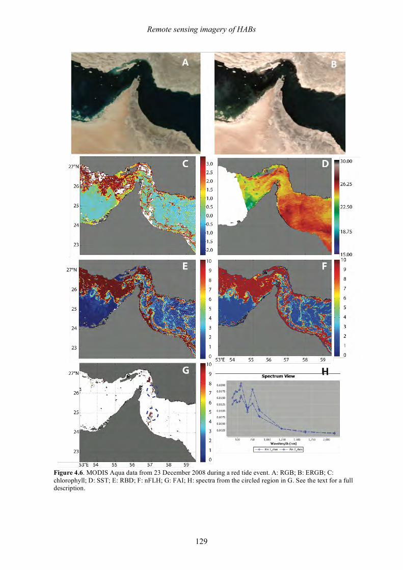
Remote sensing imagery of HABs

129

Figure 4.6. MODIS Aqua data from 23 December 2008 during a red tide event. A: RGB; B: ERGB; C: chlorophyll; D: SST; E: RBD; F: nFLH; G: FAI; H: spectra from the circled region in G. See the text for a full description.

Remote sensing imagery of HABs

130

data and limitations, the final step is to acquire and process data directly, using either standard algorithms, or taking advantage of the tools available in both SeaDAS and BEAM for non-standard algorithms. An excellent resource for this last step are self-guided tutorials available online (https://www.youtube.com/results?search_query=seadas). At the time of publication, the main satellite processing tools (SeaDAS, BEAM, SNAP) are all based on the same underlying computer code, so an end-user familiar with SeaDAS will quickly be able to use any of these packages. With the basic information provided in this chapter, an end-user can quickly progress from casual use of satellite images to routine production of regionally-adjusted datasets suitable for research and monitoring. 4.8 USEFUL LINKS TO SATELLITE BASED OCEAN COLOR DATA

General European Space Agency: http://sentinel.copernicus.eu

NASA: http://oceancolor.gsfc.nasa.gov/cms/ USGS: http://earthexplorer.usgs.gov

Data Access NASA WorldView: https://worldview.earthdata.nasa.gov

NASA Ocean Biology Processing Group: http://oceancolor.gsfc.nasa.gov NASA Data Subscriptions: http://oceancolor.gsfc.nasa.gov/sdpscgi/public/subscriptions_home.cgi Old Giovanni Site: http://gdata1.sci.gsfc.nasa.gov/daac-bin/G3/gui.cgi?instance_id=ocean_8day New Giovanni Site: http://giovanni.sci.gsfc.nasa.gov/giovanni/

NOAA ERDDAP: http://coastwatch.pfeg.noaa.gov/erddap/griddap/documentation.html

SST and other Data Visualization: http://podaac-tools.jpl.nasa.gov/soto-2d/soto.html?layers[]=jpl_ourocean_l4___sst___36000_x_18000___daynight&date=2016-01-11 SST Data: https://podaac.jpl.nasa.gov/GHRSST

Software NASA SeaDAS: http://seadas.gsfc.nasa.gov

ESA BEAM: http://www.brockmann-consult.de/cms/web/beam/ ESA SNAP: http://step.esa.int/main/toolboxes/snap/

4.9 REFERENCES Alvain, S., Moulin, C., Dandoneau, Y., and Loisel, H. 2008. Seasonal distribution and

succession of dominant phytoplankton groups in the global ocean: A satellite view. Global Biogeochemical Cycles, 22: GB3001.

Amin R., Zhou J., Gilerson A., Gross B., Moshary F., and Ahmed, S. 2012. Novel optical techniques for detecting and classifying toxic dinoflagellate Karenia brevis blooms using satellite imagery. Optics Express, 17: 9126-9144.

Remote sensing imagery of HABs

131

Astoreca, R., Rousseau, V., Parent, J.-Y., Lancelot, C., Ruddick, K., and Van Mol, B. 2005. Optical properties of algal blooms in an eutrophicated coastal area and its relevance to remote sensing. Proc. SPIE 5885, doi:10.1117/12.615160.

Chen, W. W., Hall, L. O., Goldgof, D. B., Soto, I. M., and Hu, C. 2009 Automatic red tide detection from MODIS satellite images. Proceedings of the 2009 IEEE International Conference on Systems, Man and Cybernetics, 1864-1868.

Dierssen, H., Kudela, R., Ryan, J., and Zimmerman, R. 2006. Red and black tides: Quantitative analysis of water-leaving radiance and perceived color for phytoplankton, colored dissolved organic matter, and suspended sediments. Limnology and Oceanography 51, 2646-2659

Frolov, S., Kudela, R. M., and Bellingham, J. G. 2013. Monitoring of harmful algal blooms in the era of diminishing resources: A case study of the U.S. West Coast. Harmful Algae, 21-22, 1-12.

Gomes, H. R., Goes, J. I., Prabhu Matondkar, S. G., Garab, S. G., Al-Azri, A. R. N., and Thoppil, P. G. 2008. Blooms of Noctiluca miliaris in the Arabian Sea—An in situ and satellite study. Deep-Sea Research 55, 751-765.

Gower, J., King, S., Borstad, G., and Brown, L. 2005. Detection of intense plankton blooms using the 709 nm band of the MERIS imaging spectrometer. International Journal of Remote Sensing, 26, 2005-2012.

Harrison, P. J., Furuya, K., Glibert, P. M., Xu, J., Liu, H. B., Yin, K., Lee, J. H. W., Anderson, D. M., Gowen, R., Al-Azri, A. R., and Ho, A. Y. T. 2011. Geographical distribution of red and green Noctiluca scintillans. Chinese Journal of Oceanology and Limnology 29, 807-831.

Hu, C., Muller-Karger, F. E., Taylor, C. J., Carder, K. L., Kelble, C., Johns, E., and Heil, C. A. 2005. Red tide detection and tracing using MODIS fluorescence data: A regional example in SW Florida coastal waters. Remote Sensing of Environment 97, 311-321.

Hu, C. 2009. A novel ocean color index to detect floating algae in the global oceans. Remote Sensing Environment 113, 2118-2129.

Hu, C., Cannizzaro, J., Carder, K. L., Muller-Karger, F. E., and Hardy, R. 2010. Remote detection of Trichodesmium blooms in optically complex coastal waters: Examples with MODIS full-spectral data. Remote Sensing of Environment 114, 2048-2058.

Kahru, M., and Mitchell, B. 2008. Ocean color reveals increased blooms in various parts of the world. EOS 89:170-171.

Kahru, M., Kudela, R. M., di Lorenzo, E., Manzano-Sarabia, M., and Mitchell, B. G. 2012. Trends in the surface chlorophyll of the California Current: Merging data from multiple ocean color satellites. Deep-Sea Research II 77-80, 89-98.

Keafer, B. A., and Anderson, D. M. 1993. Use of remotely-sensed sea surface temperatures in studies of Alexandrium tamarense bloom dynamics. In: Smayda, T. J., Shimizu, Y. (eds) Toxic phytoplankton blooms in the sea. Elsevier Science, Amsterdam, pp 763-768.

Kudela, R. M., Frolov, S. A., Anderson, C. R., and Bellingham, J. G.. 2013. Leveraging ocean observatories to monitor and forecast harmful algal blooms: A case study of the U.S. West Coast. IOOS Summit. Available at http://www.iooc.us/summit/white-paper-submissions/community-white-paper-submissions/

Remote sensing imagery of HABs

132

Lohrenz, S. E., Weidemann, A.D., and Tuel, M. 2003. Phytoplankton spectral absorption as influenced by community size structure and pigment composition. Journal of Plankton Research 25(1), 35-61.

Loisel, H., Vantrepotte, V., Jamet, C., and Dat, D. N. 2013. Challenges and new advances in ocean color remote sensing of coastal waters. In: Topics in Oceanography, E Zmbbianchi (Ed.), InTech.

Matthews, M.W., Berard, S., and Robertson, L. 2012. An algorithm for detecting trophic status (chlorophyll-a), cyanobacterial-dominance, surface scums and floating vegetation in inland and coastal waters. Remote Sensing of Environment, 124, 637-652.

Palacios, S. L. 2012. Identifying and tracking evolving water masses in optically complex aquatic environments. Ph.D. Thesis, University of California, Santa Cruz, 207 pp.

Piontkovski, S., Al-Azri, A., and Al-Hashmi, K. 2011. Seasonal and interannual variability of chlorophyll-a in the Gulf of Oman compared to the open Arabian Sea regions. International Journal of Remote Sensing 32, 7703-7715.

Ryan, J. P., Davis, C. O., Tufillaro, N. B., Kudela, R. M., and Gao, B.-C. 2014. Application of the hyperspectral imager for the coastal ocean to phytoplankton ecology studies in Monterey Bay, California. Remote Sensing 6, 1007-1025.

Schofield, O., Grzymski, J., Bissett, W. P., Kirkpatrick, G. J., Millie, D. F., Moline, M., and Roesler, C. S. 1999. Optical monitoring and forecasting systems for harmful algal blooms: possibility or pipe dream? Journal of Phycology, 35(6), 1477-1496.

Stumpf, R. P., Culver, M. E., Tester, P. A., Tomlinson, M., Kirkpatrick, G. J., Pederson, B. A., Truby, E., Ransibrahmanakul, V., and Soracco, M. 2003. Monitoring Karenia brevis blooms in the Gulf of Mexico using satellite ocean color imagery and other data. Harmful Algae 2, 147-160.

Subramaniam, A., Brown, C. W., Hood, R. R., Carpenter, E. J., and Capone, D. G. 2002. Detection of Trichodesmium blooms in SeaWiFS imagery. Deep-Sea Research II 49, 107-121.

Tester, P. A., and Steidinger, K. A. 1997. Gymnodinium breve red tide blooms: Initiation, transport, and consequences of surface circulation. Limnology and Oceanography 42,1039-1051.

Tester, P. A., Stumpf, R. P., Vukovich, F. M., Fowler, P. K., and Turner, J. T.1991. An expatriate red tide bloom: Transport, distribution, and persistence. Limnology and Oceanography 36, 1053-1061.

Westberry, T. K., Siegel, D. A., and Subramaniam, A. 2005. An improved bio-optical model for the remote sensing of Trichodesmium spp. blooms. Journal of Geophysical Research 110: C06012.

Wynne, T. T., Stumpf, R. P., Tomlinson, M. C., Warner, R. A., Tester, P. A., Dyble, J., and Fahnenstiel, G. L. 2008. Relating spectral shape to cyanobacterial blooms in the Laurentian Great Lakes. International Journal of Remote Sensing 29, 3665-3772.

HAB-related monitoring for desalination design and operation

133

5! HARMFUL ALGAL BLOOM-RELATED WATER QUALITY MONITORING FOR DESALINATION DESIGN AND OPERATION

!Siobhan F.E. Boerlage1, Loreen O. Villacorte2,3, Lauren Weinrich4, S. Assiyeh Alizadeh

Tabatabai2,, Maria D. Kennedy2, and Jan C. Schippers2 1Boerlage Consulting, Gold Coast, Queensland, Australia

2UNESCO-IHE Delft Institute for Water Education, Delft, The Netherlands 3GRUNDFOS Holding A/S, Bjerringbro, Denmark (current affiliation)

4American Water, Voorhees, NJ USA

!5.1! Intake feedwater characterization and water quality monitoring .......................................................... 133!5.2! Suitability of conventional online water quality parameters to detect HABs ....................................... 134!

5.2.1! Temperature ................................................................................................................................... 135!5.2.2! Salinity (conductivity) ................................................................................................................... 135!5.2.3! pH .................................................................................................................................................. 135!5.2.4! Dissolved oxygen .......................................................................................................................... 135!5.2.5! Turbidity ........................................................................................................................................ 136!

5.3! Overview of parameters to determine organic matter ........................................................................... 136!5.3.1! Advanced methods to determine algal organic matter .................................................................. 142!

5.3.1.1! Liquid chromatography – organic carbon detection (LC-OCD) ........................................... 142!5.3.1.2! Transparent exopolymer particles (TEP) ............................................................................... 145!

5.4! Measuring biofouling potential ............................................................................................................. 147!5.4.1! Assimilable organic carbon ........................................................................................................... 148!5.4.2! Membrane fouling simulator ......................................................................................................... 152!

5.5! Fouling indices to measure particulate fouling potential ...................................................................... 153!5.5.1! Silt Density Index .......................................................................................................................... 153!5.5.2! Modified Fouling Indices .............................................................................................................. 158!

5.5.2.1! Modified Fouling Index-0.45 ................................................................................................. 158!5.5.2.2! Modified Fouling Index-UF .................................................................................................. 159!

5.6! Summary ............................................................................................................................................... 162!5.7! References ............................................................................................................................................. 164!

5.1! INTAKE FEEDWATER CHARACTERIZATION AND WATER QUALITY MONITORING Characterization of the raw seawater at plant intakes and monitoring to detect poor water quality events including harmful algal blooms (HABs) is critical throughout the lifetime of a desalination plant. HABs can result in a substantial increase in the organic and solids load in the seawater feed to be treated at a desalination plant. This may result in an increase in the clogging of granular media filters and accelerated particulate and/or (bio)fouling of pretreatment and reverse osmosis membranes (see Chapter 2). Other feedwater quality changes may be observed during or following a HAB event, such as a reduction in dissolved oxygen levels and continued high concentration of organics due to decomposition of algal matter by bacteria when the algal bloom degrades. Seawater in areas that are prone to algal blooms or silt inflow etc. may require additional pretreatment if events are frequent and/or of long duration (Chapter 9). Depending on the project structure and site, an extensive seawater quality assessment study may be conducted prior to plant design to provide the raw seawater quality design envelope, select pretreatment and/or to obtain environmental permits. The study may include a review of historical seawater quality such as the frequency and severity of algal blooms, hydrodynamic conditions at the intake area and consider diffuse and point pollution sources

HAB-related monitoring for desalination design and operation

134

around the intake area which may impact water quality (e.g., ballast water exchange in port areas that may promote HABs).

Subsequently, during plant operation, water quality monitoring of the intake feedwater (online or through sampling) is essential for process control and contractual purposes to:

•! confirm the influent seawater is within the raw water design envelope in which case the plant is required to meet production and product water quality specifications;

•! allow analysis of data relative to baseline data collected prior to design to identify seasonal or diurnal trends and to detect poor water quality events such as HABs;

•! optimize pretreatment processes in response to a deterioration in feedwater quality due to events such as a HAB in order to maintain production and water quality targets; and

•! allow the operational performance of downstream plant unit processes to be assessed against the intake values e.g. dissolved air flotation (DAF), granular media filtration (GMF), seawater reverse osmosis (SWRO), residual handling.

During a HAB event, desalination plant operators require methods to measure the concentration of algae and algal organic matter (AOM), its fouling constituents, and any increases in membrane fouling potential and other HAB associated water quality changes in the raw water and treatment process streams. This allows operators to respond to a bloom in a timely manner to optimize plant operation to avoid disruption to supply.

This chapter examines the ability of conventional water quality parameters routinely used in desalination feedwater monitoring during design, piloting, and SWRO plant operation to detect HABs and characterize water quality during a bloom. Although the focus is on water quality parameters monitored at the intake, key parameters commonly used within SWRO desalination plants to assess the reduction in the particulate fouling potential (i.e. the Silt Density Index (SDI)) and organic load of the raw water (e.g. total organic carbon) through pretreatment are discussed. More sophisticated and lesser known techniques that are under development to directly measure AOM or assess the biofouling and/or particulate fouling potential of feedwater are presented to provide an overview to plant operators when evaluating additional tests during a HAB event. Applications of these techniques are presented to illustrate their use. Methods which directly identify the presence of HAB species in the seawater feed through algal cell identification and enumeration or an increase in algal productivity (such as chlorophyll-a measurements or advance warning through remote sensing) are discussed in Chapters 3 and 4, respectively. 5.2! SUITABILITY OF CONVENTIONAL ONLINE WATER QUALITY PARAMETERS TO DETECT

HABS Online instrumentation typically installed at a SWRO desalination plant intake to continuously monitor feedwater quality may include temperature, conductivity, dissolved oxygen (DO), pH, turbidity, residual chlorine and dissolved hydrocarbons. These online parameters can be monitored, trended and viewed in the control room to assess raw feedwater quality and the impact of water quality changes on the efficiency of unit processes such as pretreatment and desalination. None of the aforementioned parameters are specific to algal blooms. Changes in the core physiochemical parameters monitored (temperature, conductivity, DO, pH, and turbidity) can be caused by other factors such as pollution events and/or marine hydrodynamics, thus the interpretation of these water quality variables can be

HAB-related monitoring for desalination design and operation

135

complex. At best they can indirectly indicate conditions that favor a bloom, the presence of algal blooms, or associated with the termination of a bloom, such as DO depletion as discussed below. 5.2.1! Temperature Temperature, a key desalination water quality process parameter, is trended at almost all desalination plants. Some algal species are known to bloom under specific ranges of temperature, e.g., Trichodesmium, commonly responsible for red tide outbreaks in the Gulf, favors seawater temperatures ranging from 20 – 34˚C (Thangaraja et al. 2007 cited in Zhao and Ghedira 2014). Alternatively, changes in temperature may indicate downwelling or upwelling events that can bring nutrients or established blooms to the plant intake.

5.2.2! Salinity (conductivity) Salinity at plant intakes is typically calculated from online conductivity measurements using a correlation of total dissolved solids (TDS) and conductivity.1 Many algal species have a broad tolerance for salinity, particularly those endemic to estuarine regions. Nevertheless, there are salinity ranges that are optimal for a HAB, as well as those that are too high or low for rapid growth. A particular salinity range in combination with temperature may promote growth of a specific bloom-forming algal species or break the dormancy of an algal cyst (Chapter 1). Alternatively, a change in salinity outside the tolerance range of an algal species may result in the termination of a HAB or changes in the species assemblage in a bloom community. Hence, monitoring changes in salinity and temperature at a plant intake may be useful where an algal blooming species routinely occurs. 5.2.3! pH Monitoring of pH to detect blooms is complex and typically not useful for the purposes of detecting or characterizing HABs. The pH of seawater is around 8.2 and does not normally vary substantially due to the vast buffering capacity of the seawater bicarbonate-carbonate system. As a result of estuarine input, however, pH may increase or decrease depending on the salinity and evaporative effects on the estuary. Dense algal blooms in shallow coastal areas with limited tidal exchange may also cause a local pH change – leading to both increases and decreases in pH. As algae consume carbon dioxide during photosynthesis during daylight hours, removing it from the water, less carbonic acid dissociates and a pH rise can occur. During the night, when there is no photosynthesis, CO2 is released by respiring cells, leading to a decrease in pH. When the bloom ends and the algal biomass degrades, CO2 is again released and pH decreases. Diurnal changes in pH may subsequently occur due to bacterial decomposition and aerobic respiration.

5.2.4! Dissolved oxygen As with pH, diurnal changes in online DO may also reflect algal photosynthesis and respiration as well as tidal exchange, which can replenish DO levels. Elevated DO may be observed in the photic zone (or sunlight zone) through photosynthesis. In contrast, a rapid decrease in DO may occur in stratified coastal water due to the respiratory activity of a bloom, or to bacterial decomposition of algal biomass as blooms age and decay, sinking to the seabed and sometimes leading to hypoxic conditions (<0.5 mg/L) or even anoxia. Hence, a decline in online DO may be observed depending on the depth of the intake, and DO trends may be used to indicate a HAB. Anoxic events due to DO depletion were observed at the La Chimba SWRO desalination plant, leading to the presence of hydrogen sulphide in the 1 Caution should be taken when comparing this salinity with that measured by conductivity, temperature, and depth (CTD) sensors at sea which calculate salinity using the Practical Salinity Scale (Boerlage 2012).

HAB-related monitoring for desalination design and operation

136

feedwater due to the proliferation of sulphate-reducing bacteria that prolifereate under low DO conditions (see Chapter 11, section 11.6). Low DO can also be caused by pollution events and therefore needs to be assessed in conjunction with other water quality testing such as SDI, total organic carbon, and cell counts.

5.2.5! Turbidity Turbidity, based on the amount of visible light (400 – 700 nm) scattered by particles in solution, generally increases with a greater load of suspended solids. While turbidity provides some information on particle concentration and water clarity 2 , measurements can be inaccurate at both high and low levels. Scattered light is the aggregate response for all particles; the physical properties of particles such as color, shape, size distribution and numbers all affect the light scattering properties of a solution. When particles are in the wavelength range of visible light, turbidity is at a maximum (Edzwald and Tobiason 2011). In contrast, turbidity meters have been reported to be insensitive to small colloidal particles - particles with a diameter less than half the wavelength of visible light (0.2 µm) will not produce significant scatter (Kremen and Tanner 1998). Therefore, turbidity will decrease for smaller particles due to poor light scattering, while if the total particle mass remains constant, turbidity will also decrease for larger particles due to the decreased number or concentration (Edzwald and Tobiason 2011). Moreover, as noted by Tabatabai (2014a), transparent exopolymer particles (TEP), a component of AOM, do not absorb visible light. In some cases, high chlorophyll correlates well with high turbidity, but this is not always the case, as suspended materials like sand or clay will have similar light-scattering properties as algal cells. Turbidity is thus only a general indicator of algal blooms and cannot be relied upon to detect a bloom or an increase in particles associated with a bloom. Other confirmatory measures are needed such as those provided by chlorophyll sensors, or through direct cell counts. 5.3! OVERVIEW OF PARAMETERS TO DETERMINE ORGANIC MATTER Total organic carbon (TOC) and dissolved organic carbon (DOC) are common measures of the concentration of organics at desalination plant intakes and are used to assess the efficiency of pretreatment processes in removing organics. Ultraviolet absorption at 254 nm (UV254) and the related specific ultraviolet absorbance (SUVA) are used to a lesser extent. The maximum, average, or median concentration of these parameters may be provided as part of the raw seawater design envelope to characterize the organic load in the seawater to be desalinated. Standards from ASTM International and Standard Methods for the Examination of Water and Wastewater (APHA 2012) are often recommended by membrane manufacturers for the analysis of these aforementioned parameters. In addition, these protocols may be specified in design and/or operation and maintenance (O&M) contracts for analysis of the saline feed and desalination process streams (see Table 5.1). In general, these parameters can be quickly and reliably determined by laboratories experienced in the analysis of saline matrices with some parameters determined by on site laboratories. These parameters are routinely measured on a weekly or monthly basis at the seawater intake depending on the site (e.g. to monitor the potential for HABs and/or pollution or to check the feedwater is within design specifications). Monitoring may also occur upstream and downstream of pretreatment processes to assess performance or in the RO feedwater for compliance with membrane guarantees. The

2 Secchi disks - another method to measure water clarity are discussed in Chapter 3.

HAB-related monitoring for desalination design and operation

137

frequency of monitoring may increase when a bloom event is forecast or during a bloom to adjust operating parameters for process steps accordingly.

The aforementioned techniques measure aggregate organic matter and therefore provide no specific information as to the composition or concentration of potential AOM foulants produced during an algal bloom. TOC measures both organic matter derived from natural processes such as HABs, bacteria, riverine flushing or through direct anthropogenic input. Therefore, spikes in feedwater TOC may be due to an algal bloom and/or pollution or other events. Moreover, increases in TOC are not always observed during a bloom event. Feedwater TOC increased significantly in the Red Sea off the coast of Saudi Arabia during an algal bloom (pers. com. N. Nada) and also in the source seawater during testing of Long Beach Water Department’s demonstration seabed infiltration gallery during blooms (see Chapter 6 Section 6.4.1.6). Yet, in other cases, TOC has not significantly increased during a bloom. The latter may be attributed to underestimating TOC if floatable organics are not captured during sampling or sample homogenization (Table 5.1). Measuring TOC removal to assess the efficiency of pretreatment processes is also inaccurate due to the difficulties in measuring low-level TOC residuals in seawater process streams. In high temperature catalytic oxidation measurement of organic carbon in seawater, the high salt concentration (in the range of 30,000 to 45,000 mg/L) compared to a few mg/L of organic carbon, results in low accuracy and high limits of detection for TOC measurements. Consequently, TOC results are often interpreted in conjunction with chlorophyll-a and algal counts (where available) and other more standard plant water quality monitoring parameters such as SDI, turbidity, total suspended solids, and DO to assess the occurrence of algal blooms in the intake water.

Although, UV254 and TOC can be determined online, these instruments are not frequently installed at SWRO plants. As with TOC, UV254 is an aggregate parameter, but only for selected organic constituents such as lignin, humic acids, and various aromatic compounds which strongly absorb UV radiation (APHA 5910B). SUVA, the quotient of UV254 and DOC, provides an indication of dissolved natural organic matter measured by UV254 compared to the overall dissolved organic concentration and can be used to indicate whether the dissolved organic matter is primarily derived from natural processes occurring at the intake rather than anthropogenic sources. Algal organic matter may contain some UV-absorbing compounds, but their proportion among AOM components significantly varies among species releasing them. Moreover, carbohydrates (i.e., polysaccharides produced by algae and marine bacteria) do not absorb UV (APHA 5910B) and therefore UV254 cannot be relied upon to monitor or measure AOM in the raw water or treatment process streams.

More sophisticated techniques to characterize the composition and concentration of AOM in seawater have been developed or are under development such as liquid chromatography - organic carbon detection (LC-OCD) to determine biopolymers or measurement of TEP, (compounds demonstrated to promote fouling in SWRO and ultrafiltration (UF) – see Chapter 2) and other AOM components as shown in Figure 5.1. While these methods offer more targeted information (and higher sensitivity) of AOM constituents and potential foulants in a feedwater, the degree of difficulty and cost in determining them is correspondingly higher. As yet, samples need to be sent to specialized laboratories with experience in determining these parameters, which are limited in number, resulting in delays to obtain results. Hence, at present they cannot be employed directly as a trigger to alert a plant of a bloom in the incoming feedwater or to adjust process parameters during plant operation. Nonetheless, these parameters are expected to be a key factor in developing an understanding in controlling AOM fouling in seawater UF and RO systems as they allow quantification of specific foulant components of AOM not detectable by standard monitoring parameters, including those components which are likely to cause membrane fouling.

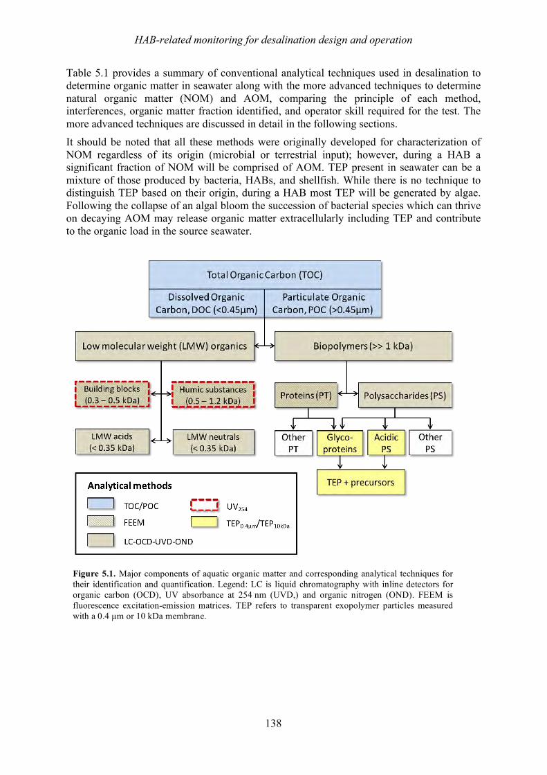
HAB-related monitoring for desalination design and operation

138

Table 5.1 provides a summary of conventional analytical techniques used in desalination to determine organic matter in seawater along with the more advanced techniques to determine natural organic matter (NOM) and AOM, comparing the principle of each method, interferences, organic matter fraction identified, and operator skill required for the test. The more advanced techniques are discussed in detail in the following sections. It should be noted that all these methods were originally developed for characterization of NOM regardless of its origin (microbial or terrestrial input); however, during a HAB a significant fraction of NOM will be comprised of AOM. TEP present in seawater can be a mixture of those produced by bacteria, HABs, and shellfish. While there is no technique to distinguish TEP based on their origin, during a HAB most TEP will be generated by algae. Following the collapse of an algal bloom the succession of bacterial species which can thrive on decaying AOM may release organic matter extracellularly including TEP and contribute to the organic load in the source seawater.

Figure 5.1. Major components of aquatic organic matter and corresponding analytical techniques for their identification and quantification. Legend: LC is liquid chromatography with inline detectors for organic carbon (OCD), UV absorbance at 254 nm (UVD,) and organic nitrogen (OND). FEEM is fluorescence excitation-emission matrices. TEP refers to transparent exopolymer particles measured with a 0.4 µm or 10 kDa membrane.

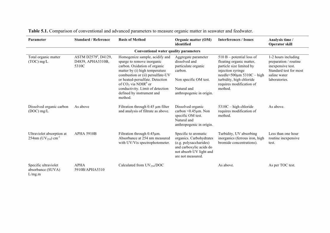
Table 5.1. Comparison of conventional and advanced parameters to measure organic matter in seawater and feedwater.

Parameter Standard / Reference Basis of Method Organic matter (OM) identified

Interferences / Issues Analysis time / Operator skill

Conventional water quality parameters Total organic matter (TOC) mg/L

ASTM D2579a, D4129, D4839, APHA5310B, 5310C

Homogenize sample, acidify and sparge to remove inorganic carbon. Oxidation of organic matter by (i) high temperature combustion or (ii) persulfate-UV or heated-persulfate. Detection of CO2 via NDIRb or conductivity. Limit of detection defined by instrument and method.

Aggregate parameter dissolved and particulate organic carbon. Non specific OM test. Natural and anthropogenic in origin.

510 B – potential loss of floating organic matter, particle size limited by injection syringe needle≈500µm 5310C – high turbidity, high chloride requires modification of method.

1-2 hours including preparation / routine inexpensive test. Standard test for most saline water laboratories.

Dissolved organic carbon (DOC) mg/L

As above Filtration through 0.45 µm filter and analysis of filtrate as above.

Dissolved organic carbon <0.45µm. Non specific OM test. Natural and anthropogenic in origin.

5310C – high chloride requires modification of method.

As above.

Ultraviolet absorption at 254nm (UV254) cm-1

APHA 5910B Filtration through 0.45µm. Absorbance at 254 nm measured with UV/Vis spectrophotometer.

Specific to aromatic organics. Carbohydrates (e.g. polysaccharides) and carboxylic acids do not absorb UV light and are not measured.

Turbidity, UV absorbing inorganics (ferrous iron, high bromide concentrations).

Less than one hour routine inexpensive test.

Specific ultraviolet absorbance (SUVA) L/mg.m

APHA 5910B/APHA5310

Calculated from UV254/DOC As above. As per TOC test.

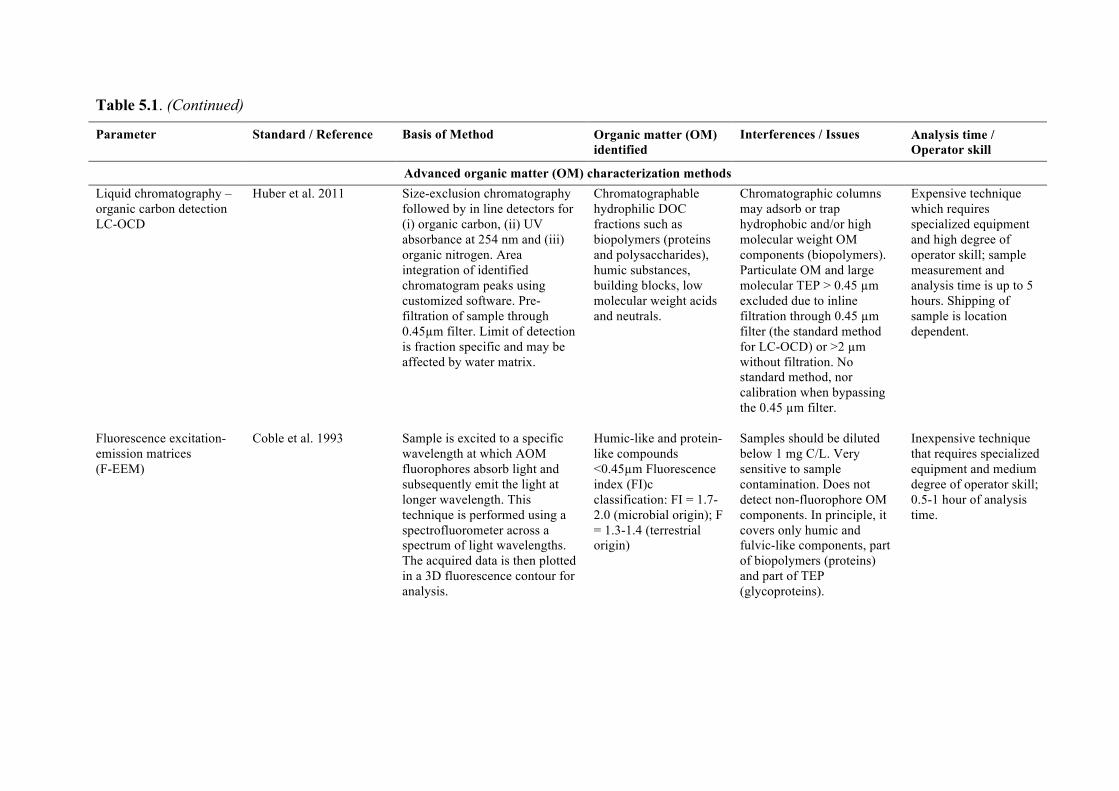
Table 5.1. (Continued)

Parameter Standard / Reference Basis of Method Organic matter (OM) identified

Interferences / Issues Analysis time / Operator skill

Advanced organic matter (OM) characterization methods Liquid chromatography – organic carbon detection LC-OCD

Huber et al. 2011 Size-exclusion chromatography followed by in line detectors for (i) organic carbon, (ii) UV absorbance at 254 nm and (iii) organic nitrogen. Area integration of identified chromatogram peaks using customized software. Pre-filtration of sample through 0.45µm filter. Limit of detection is fraction specific and may be affected by water matrix.

Chromatographable hydrophilic DOC fractions such as biopolymers (proteins and polysaccharides), humic substances, building blocks, low molecular weight acids and neutrals.

Chromatographic columns may adsorb or trap hydrophobic and/or high molecular weight OM components (biopolymers). Particulate OM and large molecular TEP > 0.45 µm excluded due to inline filtration through 0.45 µm filter (the standard method for LC-OCD) or >2 µm without filtration. No standard method, nor calibration when bypassing the 0.45 µm filter.

Expensive technique which requires specialized equipment and high degree of operator skill; sample measurement and analysis time is up to 5 hours. Shipping of sample is location dependent.

Fluorescence excitation-emission matrices (F-EEM)

Coble et al. 1993 Sample is excited to a specific wavelength at which AOM fluorophores absorb light and subsequently emit the light at longer wavelength. This technique is performed using a spectrofluorometer across a spectrum of light wavelengths. The acquired data is then plotted in a 3D fluorescence contour for analysis.

Humic-like and protein-like compounds <0.45µm Fluorescence index (FI)c classification: FI = 1.7-2.0 (microbial origin); F = 1.3-1.4 (terrestrial origin)

Samples should be diluted below 1 mg C/L. Very sensitive to sample contamination. Does not detect non-fluorophore OM components. In principle, it covers only humic and fulvic-like components, part of biopolymers (proteins) and part of TEP (glycoproteins).

Inexpensive technique that requires specialized equipment and medium degree of operator skill; 0.5-1 hour of analysis time.

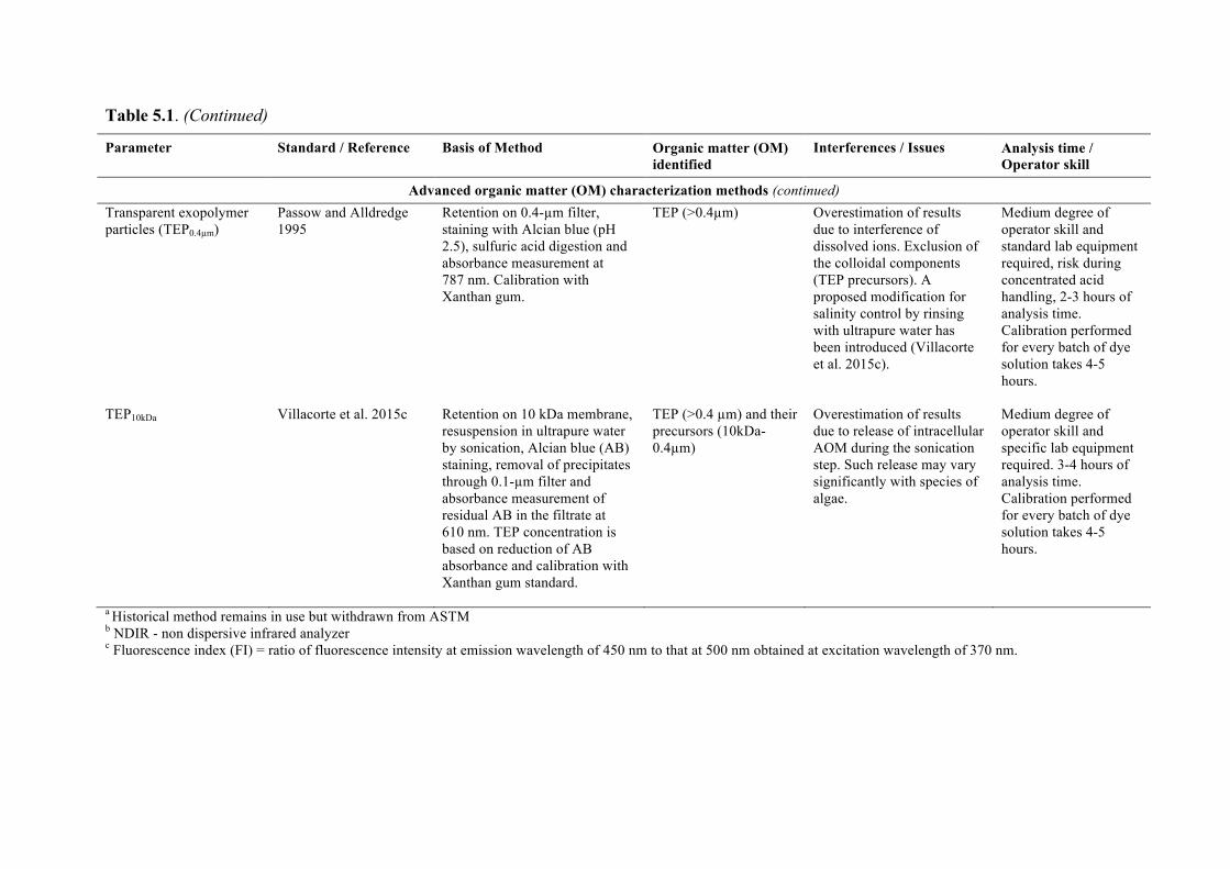
Table 5.1. (Continued)

Parameter Standard / Reference Basis of Method Organic matter (OM) identified

Interferences / Issues Analysis time / Operator skill

Advanced organic matter (OM) characterization methods (continued) Transparent exopolymer particles (TEP0.4µm)

Passow and Alldredge 1995

Retention on 0.4-µm filter, staining with Alcian blue (pH 2.5), sulfuric acid digestion and absorbance measurement at 787 nm. Calibration with Xanthan gum.

TEP (>0.4µm)

Overestimation of results due to interference of dissolved ions. Exclusion of the colloidal components (TEP precursors). A proposed modification for salinity control by rinsing with ultrapure water has been introduced (Villacorte et al. 2015c).

Medium degree of operator skill and standard lab equipment required, risk during concentrated acid handling, 2-3 hours of analysis time. Calibration performed for every batch of dye solution takes 4-5 hours.

TEP10kDa Villacorte et al. 2015c Retention on 10 kDa membrane, resuspension in ultrapure water by sonication, Alcian blue (AB) staining, removal of precipitates through 0.1-µm filter and absorbance measurement of residual AB in the filtrate at 610 nm. TEP concentration is based on reduction of AB absorbance and calibration with Xanthan gum standard.

TEP (>0.4 µm) and their precursors (10kDa-0.4µm)

Overestimation of results due to release of intracellular AOM during the sonication step. Such release may vary significantly with species of algae.

Medium degree of operator skill and specific lab equipment required. 3-4 hours of analysis time. Calibration performed for every batch of dye solution takes 4-5 hours.

a Historical method remains in use but withdrawn from ASTM b NDIR - non dispersive infrared analyzer c Fluorescence index (FI) = ratio of fluorescence intensity at emission wavelength of 450 nm to that at 500 nm obtained at excitation wavelength of 370 nm.

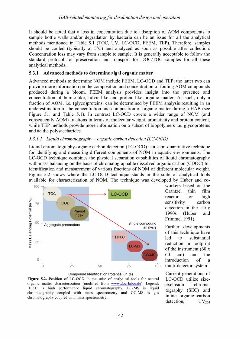
HAB-related monitoring for desalination design and operation

142

It should be noted that a loss in concentration due to adsorption of AOM components to sample bottle walls and/or degradation by bacteria can be an issue for all the analytical methods mentioned in Table 5.1 (TOC, UV, LC-OCD, FEEM, TEP). Therefore, samples should be cooled (typically at 5oC) and analyzed as soon as possible after collection. Concentration loss may vary from sample to sample. It is generally acceptable to follow the standard protocol for preservation and transport for DOC/TOC samples for all these analytical methods. 5.3.1! Advanced methods to determine algal organic matter

Advanced methods to determine NOM include FEEM, LC-OCD and TEP; the latter two can provide more information on the composition and concentration of fouling AOM compounds produced during a bloom. FEEM analysis provides insight into the presence and concentration of humic-like, fulvic-like and protein-like organic matter. As such, only a fraction of AOM, i.e. (glyco)proteins, can be determined by FEEM analysis resulting in an underestimation of the concentration and composition of organic matter during a HAB (see Figure 5.1 and Table 5.1). In contrast LC-OCD covers a wider range of NOM (and consequently AOM) fractions in terms of molecular weight, aromaticity and protein content, while TEP methods provide more information on a subset of biopolymers i.e. glycoproteins and acidic polysaccharides.

5.3.1.1! Liquid chromatography – organic carbon detection (LC-OCD) Liquid chromatography-organic carbon detection (LC-OCD) is a semi-quantitative technique for identifying and measuring different components of NOM in aquatic environments. The LC-OCD technique combines the physical separation capabilities of liquid chromatography with mass balancing on the basis of chromatographable dissolved organic carbon (CDOC) for identification and measurement of various fractions of NOM of different molecular weight. Figure 5.2 shows where the LC-OCD technique stands in the suite of analytical tools available for characterization of NOM. The technique was developed by Huber and co-

workers based on the Gräntzel thin film reactor for high sensitivity carbon detection in the early 1990s (Huber and Frimmel 1991). Further developments of this technique have led to substantial reduction in footprint of the instrument (60 x 60 cm) and the introduction of a multi-detector system. Current generations of LC-OCD utilize size-exclusion chroma- tography (SEC) and inline organic carbon detection, UV254

!

TOC

COD

Phenol!index

!

GC0MS

LC0MS

HPLC

Aggregate!parameters Single!compound!analysis

LC0OCD

0

25

50

75

100

0 25 50 75 100

Mass!Balancing!Potential!(in!%)

Compound!Identification!Potential!(in!%) Figure 5.2. Position of LC-OCD in the suite of analytical tools for natural organic matter characterization (modified from www.doc-labor.de). Legend: HPLC is high performance liquid chromatography, LC-MS is liquid chromatography coupled with mass spectrometry and GC-MS is gas chromatography coupled with mass spectrometry.

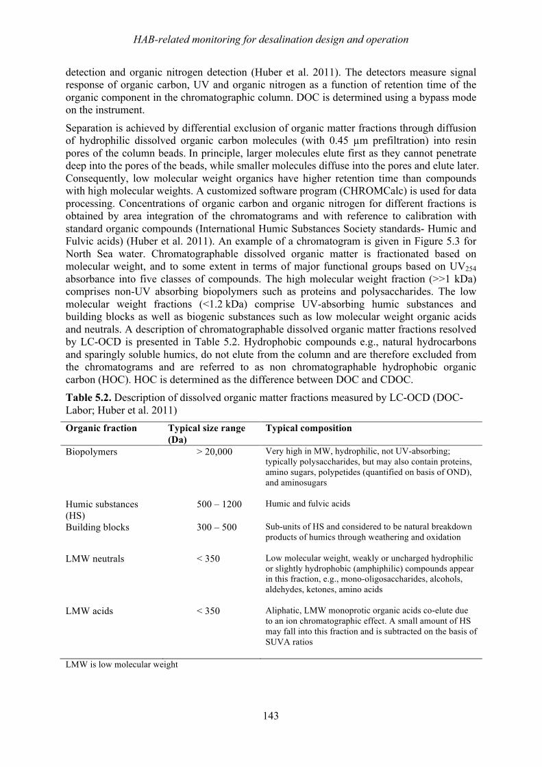
HAB-related monitoring for desalination design and operation

143

detection and organic nitrogen detection (Huber et al. 2011). The detectors measure signal response of organic carbon, UV and organic nitrogen as a function of retention time of the organic component in the chromatographic column. DOC is determined using a bypass mode on the instrument.

Separation is achieved by differential exclusion of organic matter fractions through diffusion of hydrophilic dissolved organic carbon molecules (with 0.45 µm prefiltration) into resin pores of the column beads. In principle, larger molecules elute first as they cannot penetrate deep into the pores of the beads, while smaller molecules diffuse into the pores and elute later. Consequently, low molecular weight organics have higher retention time than compounds with high molecular weights. A customized software program (CHROMCalc) is used for data processing. Concentrations of organic carbon and organic nitrogen for different fractions is obtained by area integration of the chromatograms and with reference to calibration with standard organic compounds (International Humic Substances Society standards- Humic and Fulvic acids) (Huber et al. 2011). An example of a chromatogram is given in Figure 5.3 for North Sea water. Chromatographable dissolved organic matter is fractionated based on molecular weight, and to some extent in terms of major functional groups based on UV254 absorbance into five classes of compounds. The high molecular weight fraction (>>1 kDa) comprises non-UV absorbing biopolymers such as proteins and polysaccharides. The low molecular weight fractions (<1.2 kDa) comprise UV-absorbing humic substances and building blocks as well as biogenic substances such as low molecular weight organic acids and neutrals. A description of chromatographable dissolved organic matter fractions resolved by LC-OCD is presented in Table 5.2. Hydrophobic compounds e.g., natural hydrocarbons and sparingly soluble humics, do not elute from the column and are therefore excluded from the chromatograms and are referred to as non chromatographable hydrophobic organic carbon (HOC). HOC is determined as the difference between DOC and CDOC. Table 5.2. Description of dissolved organic matter fractions measured by LC-OCD (DOC-Labor; Huber et al. 2011) Organic fraction Typical size range

(Da) Typical composition

Biopolymers > 20,000 Very high in MW, hydrophilic, not UV-absorbing; typically polysaccharides, but may also contain proteins, amino sugars, polypetides (quantified on basis of OND), and aminosugars

Humic substances (HS)

500 – 1200 Humic and fulvic acids

Building blocks 300 – 500 Sub-units of HS and considered to be natural breakdown products of humics through weathering and oxidation

LMW neutrals < 350 Low molecular weight, weakly or uncharged hydrophilic or slightly hydrophobic (amphiphilic) compounds appear in this fraction, e.g., mono-oligosaccharides, alcohols, aldehydes, ketones, amino acids

LMW acids < 350 Aliphatic, LMW monoprotic organic acids co-elute due to an ion chromatographic effect. A small amount of HS may fall into this fraction and is subtracted on the basis of SUVA ratios

LMW is low molecular weight

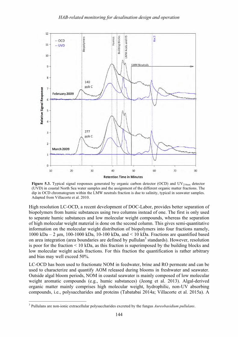
HAB-related monitoring for desalination design and operation

144

High resolution LC-OCD, a recent development of DOC-Labor, provides better separation of biopolymers from humic substances using two columns instead of one. The first is only used to separate humic substances and low molecular weight compounds, whereas the separation of high molecular weight material is done on the second column. This gives semi-quantitative information on the molecular weight distribution of biopolymers into four fractions namely, 1000 kDa – 2 µm, 100-1000 kDa, 10-100 kDa, and < 10 kDa. Fractions are quantified based on area integration (area boundaries are defined by pullulan3 standards). However, resolution is poor for the fraction < 10 kDa, as this fraction is superimposed by the building blocks and low molecular weight acids fractions. For this fraction the quantification is rather arbitrary and bias may well exceed 50%.

LC-OCD has been used to fractionate NOM in feedwater, brine and RO permeate and can be used to characterize and quantify AOM released during blooms in freshwater and seawater. Outside algal bloom periods, NOM in coastal seawater is mainly composed of low molecular weight aromatic compounds (e.g., humic substances) (Jeong et al. 2013). Algal-derived organic matter mainly comprises high molecular weight, hydrophilic, non-UV absorbing compounds, i.e., polysaccharides and proteins (Tabatabai 2014a; Villacorte et al. 2015a). A

3 Pullulans are non-ionic extracellular polysaccharides excreted by the fungus Aureobasidium pullulans.

Figure 5.3. Typical signal responses generated by organic carbon detector (OCD) and UV254nm detector (UVD) in coastal North Sea water samples and the assignment of the different organic matter fractions. The dip in OCD chromatogram within the LMW neutrals fraction is due to salinity, typical in seawater samples. Adapted from Villacorte et al. 2010.

HAB-related monitoring for desalination design and operation

145

substantial increase in the biopolymer fraction is observed during severe algal blooms as shown in Figure 5.3 where an increase in biopolymer concentration was observed; from 140 ppb C in February 2009 outside of a bloom to 277 ppb C during a spring bloom in March 2009. Considering that high molecular weight AOM has been shown to cause irreversible fouling of low pressure membranes (microfiltration and ultrafiltration) and is likely to deposit and/or accumulate on SWRO membranes, monitoring the biopolymer fraction of organic matter in seawater is a promising indicator of organic and biological fouling potential of algal bloom-impacted waters.

The amount of proteins and polysaccharides in algal biopolymers can be estimated using LC-OCD. The organic carbon concentration of protein can be estimated based on the organic nitrogen content of the biopolymer fraction. Protein concentration is calculated by assuming that all organic nitrogen detected by the organic nitrogen detector between 25 and 42 minutes retention time are bound to proteinaceous compounds. Typically, proteins contain 14.5 - 17.5% nitrogen and 49.7 - 55.3 % carbon (Rouwenhorst et al. 1991). Hence, the C:N ratio of the protein fraction of biopolymers can be estimated as 3:1. The estimated protein concentration in mg C/L is calculated by multiplying the organic nitrogen concentration (in mg N/L) by 3. From there, the polysaccharide concentration is calculated by subtracting the organic carbon concentration of protein from that of the biopolymer concentration.

Since AOM may comprise large macromolecules (e.g., TEPs), LC-OCD analyses should be preferably performed without 0.45 µm inline filtration of samples – a standard pretreatment protocol for LC-OCD analysis (Villacorte et al. 2015b): however, removing the pretreatment step has been shown to cause clogging issues in the size exclusion columns. The theoretical maximum size when performing chromatography without sample pre-filtration is 2 µm, which is based on the pore size of the frit at the column entrance (S. Huber pers. com.).

5.3.1.2! Transparent exopolymer particles (TEP) Since the discovery of TEPs more than two decades ago, various quantification methods have been developed, all of which are based on staining with cationic Alcian blue (AB) dye. This particular dye is known to be highly selective and forms insoluble complexes with TEP that cannot be easily reversed by subsequent treatment. In aqueous solutions without extra electrolytes, AB specifically binds with functional components such as acidic polysaccharides, glycoproteins and proteoglycans, resulting in the formation of neutral precipitates (Ramus 1977). AB does not react with nucleic acids and neutral biopolymers. The staining ability of AB depends on the type and density of anionic functional groups associated with TEP in the sample and to a large extent on the pH and ionic strength of the sample solution (Horobin 1988). In high ionic strength solutions, AB molecules spontaneously precipitate due to interactions with dissolved salts resulting in the formation of flocs not associated with TEP. This is considered the main drawback of the application of AB staining for TEP measurements in seawater. To minimize measurement artifacts due to coagulation, AB staining solutions should always be pre-filtered and should not be directly applied to solutions with high salinity.

So far, five methods have been developed to quantify TEP and their precursors. The first TEP method is based on optical microscopic enumeration. This method provides useful information on the size-frequency distribution of TEP in seawater (Alldredge et al. 1993), but it is laborious, complicated, time consuming and is not always feasible, especially for samples with low concentration and smaller size range (<2 µm) of TEP. All the succeeding methods based on semi-quantitative spectrophotometric techniques were able to address these issues. The method by Passow and Alldredge (1995), referred hereafter as TEP0.4µm, has been widely used in various scientific investigations, but additional time-consuming pretreatment

HAB-related monitoring for desalination design and operation

146

techniques (e.g., bubble adsorption, laminar shear) are needed to measure TEP precursors (Zhou et al. 1998; Passow 2000). Further modification of this method using smaller pore size filters (e.g., TEP0.1µm or TEP0.05µm) was later introduced to measure part of the TEP precursors (Villacorte et al. 2009; 2010). The alternative methods introduced by Arruda-Fatibello et al. (2004) and Thornton et al. (2007) are capable of measuring both TEP and their precursors in one single analysis; however, the former is only applicable in freshwater samples while the latter requires a dialysis step (performed for a couple of days) for saline samples. Furthermore, the method introduced by Thornton et al. (2007) is only accurate for samples with high concentration of TEP and their precursors. The latest method, referred hereafter as TEP10kDa, developed by Villacorte et al. (2015c) specifically for desalination applications aims to address the major practical issues associated with the previous methods (e.g., salinity, exclusion of TEP precursors), but also allows measurement of low concentration of TEP through the introduction of a concentration step (i.e., filtration through 10 kDa membrane). As such, it allows analyses of samples with a wide range of TEP + precursors concentrations (down to <0.1 mg Xeq/L) in seawater. In principle, this method also enables size fractionation of TEPs in seawater by making use of membranes with different pore sizes during the extraction step. As discussed above, some of the TEP methods may not be suitable for seawater application due to potential artefacts formed with high salinity. Although TEP has been identified as a likely cause or initiator of biofouling in SWRO membranes during algal blooms (See Chapter 2), TEP monitoring is still not widely conducted in SWRO plants. Nevertheless, as TEP is gaining increasing attention in this regard, there is a clear need for a reliable method to measure these substances in seawater. The two methods considered to be most feasible for SWRO applications (i.e., TEP0.4μm, TEP10kDa) are described in detail in Appendix 3.

From the perspective of HAB monitoring in SWRO plants, the TEP10kDa method is complimentary to the more established and widely accepted TEP0.4µm method. TEP0.4µm measures TEP while TEP10kDa can measure both TEP and most (if not all) of their precursors. TEP0.4µm is a more rapid and less laborious method than TEP10kDa, which means it is ideal for routine or high frequency TEP monitoring in intake seawater. This was demonstrated in the Jacobahaven demonstration plant in the Netherlands where TEP0.4µm was monitored for three years and a correlation between TEP and fouling rates in the UF pretreatment system was observed (see Chapter 11.10 Table 11.10.4). To assess the removal of TEP and their precursors over the treatment processes, TEP10kDa measurement is more appropriate because it covers the wider size spectrum of TEP. This was illustrated when both TEP0.4µm and TEP10kDa testing was conducted along with biopolymer measurements (LC-OCD analysis) during a summer algal bloom (dominated by green algae) at a low salinity lake water desalination plant with extensive pretreatment. Measurements were taken of the raw water at the intake and after various pretreatment processes, microstrainer, coagulation, sedimentation and rapid sand filtration, granular activated carbon filtration and ultrafiltration and in the RO permeate. The concentration of TEP10kDa was very high during the bloom in the raw lake water (see Figure 5.4) demonstrating that the test could be used to detect a HAB while quantifying the fouling AOM component in the bloom. Furthermore, the results illustrate the importance of measuring both TEP and their precursors when evaluating the efficiency of the pretreatment systems in removing algal-derived foulants from the RO feedwater. It revealed that TEP precursors were the dominant fraction as compared to TEP. While coagulation-sedimentation-sand filtration proved successful in almost completely removing the large TEP (TEP0.4μm) component, TEP precursors (TEP10kDa) and smaller biopolymers remained in the water. A substantial fraction of TEP precursors and

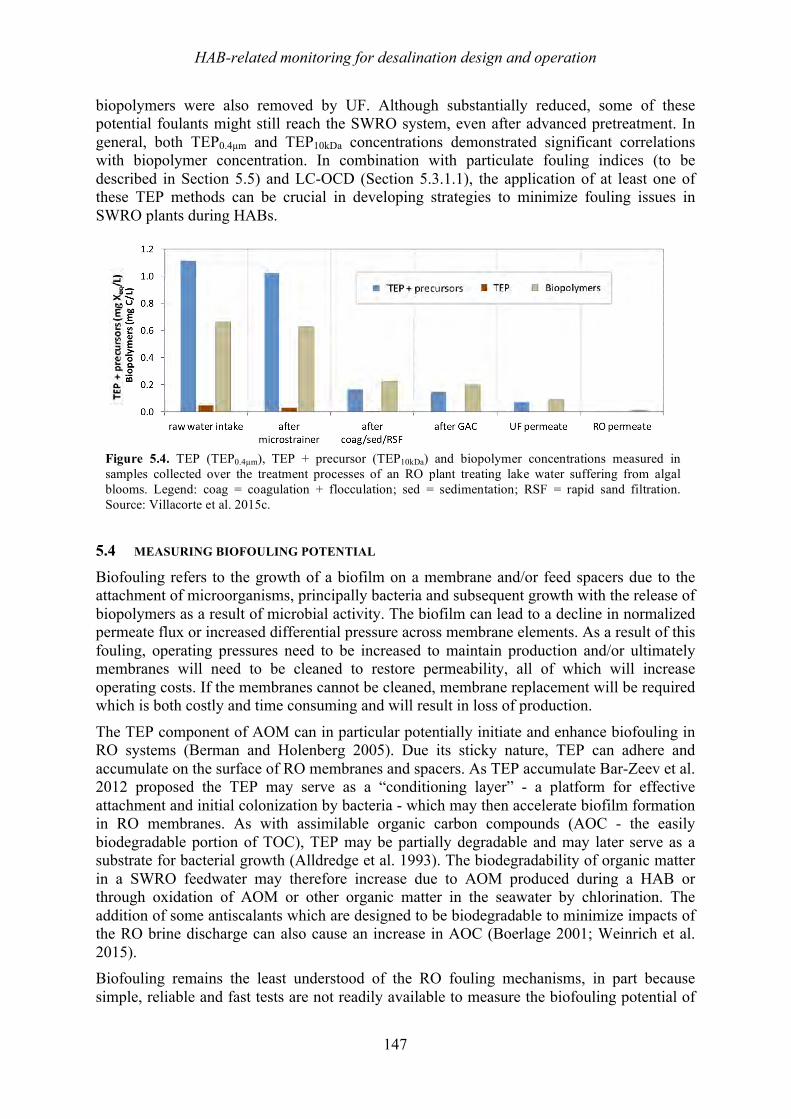
HAB-related monitoring for desalination design and operation

147

biopolymers were also removed by UF. Although substantially reduced, some of these potential foulants might still reach the SWRO system, even after advanced pretreatment. In general, both TEP0.4µm and TEP10kDa concentrations demonstrated significant correlations with biopolymer concentration. In combination with particulate fouling indices (to be described in Section 5.5) and LC-OCD (Section 5.3.1.1), the application of at least one of these TEP methods can be crucial in developing strategies to minimize fouling issues in SWRO plants during HABs.""""""""

5.4! MEASURING BIOFOULING POTENTIAL

Biofouling refers to the growth of a biofilm on a membrane and/or feed spacers due to the attachment of microorganisms, principally bacteria and subsequent growth with the release of biopolymers as a result of microbial activity. The biofilm can lead to a decline in normalized permeate flux or increased differential pressure across membrane elements. As a result of this fouling, operating pressures need to be increased to maintain production and/or ultimately membranes will need to be cleaned to restore permeability, all of which will increase operating costs. If the membranes cannot be cleaned, membrane replacement will be required which is both costly and time consuming and will result in loss of production.

The TEP component of AOM can in particular potentially initiate and enhance biofouling in RO systems (Berman and Holenberg 2005). Due its sticky nature, TEP can adhere and accumulate on the surface of RO membranes and spacers. As TEP accumulate Bar-Zeev et al. 2012 proposed the TEP may serve as a “conditioning layer” - a platform for effective attachment and initial colonization by bacteria - which may then accelerate biofilm formation in RO membranes. As with assimilable organic carbon compounds (AOC - the easily biodegradable portion of TOC), TEP may be partially degradable and may later serve as a substrate for bacterial growth (Alldredge et al. 1993). The biodegradability of organic matter in a SWRO feedwater may therefore increase due to AOM produced during a HAB or through oxidation of AOM or other organic matter in the seawater by chlorination. The addition of some antiscalants which are designed to be biodegradable to minimize impacts of the RO brine discharge can also cause an increase in AOC (Boerlage 2001; Weinrich et al. 2015). Biofouling remains the least understood of the RO fouling mechanisms, in part because simple, reliable and fast tests are not readily available to measure the biofouling potential of

Figure 5.4. TEP (TEP0.4µm), TEP + precursor (TEP10kDa) and biopolymer concentrations measured in samples collected over the treatment processes of an RO plant treating lake water suffering from algal blooms. Legend: coag = coagulation + flocculation; sed = sedimentation; RSF = rapid sand filtration. Source: Villacorte et al. 2015c.

HAB-related monitoring for desalination design and operation

148

RO feedwater (Schneider et al. 2012). Tests to determine the biofouling potential could be used to assess the increase in the biofouling potential of seawater from AOM and the efficiency of pretreatment to reduce it. For instance, the presence of trace AOCs in seawater can promote biofouling so by measuring AOC treatment plant operators would gain insight for managing pretreatment in terms of biofouling potential (Weinrich et al. 2016). To support this effort, an AOC test specifically for seawater was developed and later used for monitoring pretreatment effects on biofouling potential in full scale RO systems with both subsurface (beach well) and open intake seawater feed (Schneider et al. 2012; Weinrich et al. 2015). Only limited data are available for the correlation between growth potential levels and biofouling rate in full scale plants during algal blooms. This is mainly due to the relatively recent development of appropriate AOC assays for use in seawater studies. Moreover these tests require sophisticated equipment and are not currently deployed as an online test which could offer immediate results. In order to gain an understanding of the fouling potential of a feedwater without using a bioassay such as the AOC test, the Membrane Fouling Simulator (MFS) test was developed (Vrouwenvelder et al. 2006). In this test, fouling in a spiral wound element is simulated and monitored by the development of the head loss across the spacer. The AOC and MFS tests are discussed further below. 5.4.1! Assimilable organic carbon

5.4.1.1 AOC method development A test was developed to determine the biofilm regrowth formation potential of drinking water in water distribution networks according to the growth response of a bacterial inoculum to the amount of easily assimilable organic carbon (AOC) (van der Kooij 1978; van der Kooij et al. 1982). Initially, the test was based on the growth of the bacterial Pseudomonas fluorescence strain P17 in a sample with the AOC concentration expressed as µg acetate-C/L, since the test is calibrated with sodium acetate solutions of different concentrations. The strain P. fluorescence P17 is capable of utilizing a variety of easily biodegradable compounds. As some compounds formed by oxidation in the water treatment process such as ozonation cannot be degraded by P17, the Spirilium spp. strain NOX was added to the inoculum (van der Kooij et al. 1982) and more recently, a special test making use of Flavobacterium johnsoniae has been developed to take into account less biodegradable organic compounds e.g. biopolymers (Sack et al. 2011). Further improvements to the AOC test include increasing the incubation test temperature from 15°C to 25°C and the inoculum from 500 to 104 CFU/mL (LeChevallier et al. 1993). Both of these adjustments reduced the time for the culture to reach stationary phase which was generally between two to four days. Other attempts to simplify the method used adenosine triphosphate (ATP) instead of determining plate counts (LeChevallier et al. 1993), but problems with commercial ATP measurement reagents discouraged adoption of this technique (Haddix et al. 2003). Nonetheless, both plate count and ATP methods are complex requiring weeks of turnaround time before results are available. In addition, the methods are costly because of the technical labor involved in assaying ATP levels from filter-concentrated cells or in spread plating samples and determining plate CFU counts. A novel approach to simplify the method was achieved by producing bioluminescent strains of P-17 and NOX test bacteria through mutagenesis with luxCDABE operon fusion and inducible transposons (Haddix et al. 2004), and that method was further developed to include the use of a high sensitivity 96-microtiter plate luminometer (Weinrich et al. 2009). Using luminescence for bacterial growth estimation instead of the traditional plate counts reduces labor for preparing media and turnaround time to two days, which was an improvement on traditional methods taking three weeks or more. Moreover, the method provides information

HAB-related monitoring for desalination design and operation

149

regarding the kinetics of substrate utilization as well as the AOC concentration, in acetate carbon equivalent units which is consistent with previous methods. The bioluminescent fresh water method has been used for numerous projects that investigate biological filtration effectiveness and distribution system biological stability in both drinking water and reclaimed water matrices (Evans et al. 2013, Weinrich et al. 2010). Evaluations conducted previously indicate that the genetically modified P17 and NOX-strains tolerate salinity up to 5,000 mg/L TDS in the freshwater bioluminescent-AOC test, and are therefore not useful for seawater monitoring. Researchers have been developing methods for seawater application to address the need for managing biofouling and mitigating its costly consequences. The following sections describe tests suitable for seawater desalination plants.

5.4.1.2 Seawater AOC tests An AOC test for seawater is used to assess the microbial growth potential in SWRO plants. Since P17 and NOX strains cannot survive in water with salinity greater than that of reclaimed water or brackish water (<5,000 mg/L TDS), luminescence assays have been developed using Vibrio bacteria. The genus Vibrio contains biofilm-forming species that have been detected on a biologically-fouled SWRO membrane (Zhang et al. 2011). Weinrich et al. (2011) developed a seawater AOC test using a naturally occurring bioluminescent marine organism, Vibrio harveyi (ATCC®, 700106™). The V. harveyi seawater AOC is applicable to salinities between 20,000 – 35,000 mg/L TDS but has been applied in seawater with higher salinity from the Gulf and the Gulf of Oman. Briefly, the seawater AOC test consists of inoculating the sample with V. harveyi (from an overnight culture prepared at 30˚C). The inoculated samples are then transferred to a 96-well microtiter plate and a sensitive microtiter plate-luminometer is programmed to read the plate every two to four hours. The growth profile is monitored until the stationary phase (Nmax) in which all substrate has been consumed by the test bacteria. The rate of utilization (µmax) can be determined using Monod kinetics. Typically, the test duration with V. harveyi is about one day. Maximum luminescence measured at the stationary phase is converted into an AOC concentration with a 10 – 500 µg-C/L standard curve of acetate carbon equivalents. A full description is published in Weinrich et al. 2011, and Schneider et al. 2012. The AOC test for V. harveyi in seawater has been applied to monitor biofouling potential at bench scale and full scale SWRO plants for pretreatment monitoring, (Section 5.4.1.3) as well as in HAB events (see Chapter 11 Section 11.9).

Another AOC test based on the direct measurement of bioluminescence using Vibrio fisheri MJ-1 was developed by Jeong et al. (2013) and is reported to estimate the AOC concentration within one hour. It is similar to the V. harveyi test described above but estimates AOC concentration with a 10 – 100 µg-C standard curve of glucose for V. fischeri. Recent research studies have been published using this method for monitoring AOC removal in SWRO pretreatment using granular activated carbon deep bed filtration (Jeong et al. 2013), and submerged membrane adsorption bioreactors which were operated with 2.4 – 8.0 g of powdered activated carbon per cubic meter of seawater (Jeong et al. 2014). The latter was shown to reduce biofouling for SWRO by adsorption and biodegradation of AOC and low molecular weight organic matter.

While these bioluminescence AOC tests using specific bacteria are faster, they may not measure high molecular weight biopolymers generated during a HAB. Vibrio harveyi utilizes compounds in the 100 - 350 Da range including disaccharides trehalose and cellobiose (Baumann et al. 1984) and low molecular weight monosaccharides, amino and carboxylic acids, alcohols and aldehydes (Weinrich et al. 2011). Biopolymers have much higher molecular weights and have been defined by size exclusion to be greater than 1 kDa (see

HAB-related monitoring for desalination design and operation

150

Figure 5.1) and in the range of 10 kDa defined by the TEP10kDa method or 20 kDa (Huber et al., 2011 in LC-OCD). Under the conditions defined in the seawater AOC test, the test organism is unlikely to assimilate high molecular weight biopolymers. Specifically for SWRO treatment, biopolymers create conditions that enable bacterial attachment and increase biofouling potential. Therefore, knowing the AOC concentration would provide guidance on whether nutrients are present for the bacteria to proliferate and lead to biological fouling. The luminescent AOC tests also require equipment that may not be typically used in a water quality lab and would need to be purchased, such as a luminometer for measuring bacterial growth, a water bath for temperature control, and an autoclave for sterilizing media. Consumables for the test such as test tubes, microtiter plates, and filters are inexpensive. Glassware used for AOC tests must be carefully prepared to minimize cross contamination of trace amounts of organic carbon. Alternatively, glassware is commercially available that claims to be AOC-free. Bacterial contamination is also a concern for AOC assays; however, salinity conditions in the seawater test would deter contamination from bacteria common in the human environment that are not halophilic or halotolerant. Assay samples should be analyzed as soon as possible after collection because of the highly biodegradable nature of the organic matter to be measured. If samples are to be shipped to the laboratory, then they should be cooled and shipped on ice overnight to inhibit biological activity in the sample during transit.

5.4.1.3 Application of seawater AOC test Recently, the biofouling potential in numerous full-scale SWRO plants worldwide and extensively at the Tampa Bay Seawater Desalination Plant (TBSDP) was examined using the V. harveyi seawater AOC method. The AOC test was also used to assess feedwater quality to the plant, the impacts of pretreatment, and the biofouling potential in the SWRO feed. The first study was at TBSDP when a non-toxic HAB contributed to periodic operational challenges. AOC at TBSDP has been investigated during normal operation and during a period of algal growth. The plant experienced foaming in the pretreatment basins, shortened diatomaceous earth (precoat) run times and reduced production capacity. The algal species Ceratium furca and Phaeocystis sp. were found in filter backwash media and were thought to contribute to the operational issues. At the same time, TOC was 7.6 mg/L at the plant influent and average AOC (from three consecutive days) was 360 ± 180 µg acetate C per L. AOC was also measured after chlorine dioxide treatment and increased by 65% compared to the raw water. TOC levels in TBSDP raw water were generally between 4-6 mg/L at the intake and are variable. During normal operation, AOC has been determined to be less than 30 µg/L (Weinrich et al. 2015) and up to 225 µg/L (Schneider et al. 2012). While the AOC test may not measure high molecular weight biopolymers as discussed earlier, the AOC increase may have occurred through shear of algal cells and release of low molecular weight AOM or from bacterial oxidation of organic matter into easily biodegradable low molecular weight compounds. In this case, the AOC test may measure the additional nutrients during a HAB which can be utilized by bacteria in a biofilm on the RO membrane. The results are further discussed in Chapter 11 Section 11.9.2. The plant has demonstrated AOC removal by the diatomaceous earth filters in the same studies. In another study, plant personnel at the Al Zawrah plant in UAE described evidence of an algal bloom in May 2012 when the raw water pH decreased from the pH 8.1, normally observed, to pH 7.5. This was accompanied by elevated organic matter measured in the raw water as AOC (220 µg/L) and TOC (2.9 mg/L). During two other sampling events with reportedly normal conditions, the concentration of organics in the raw seawater was below

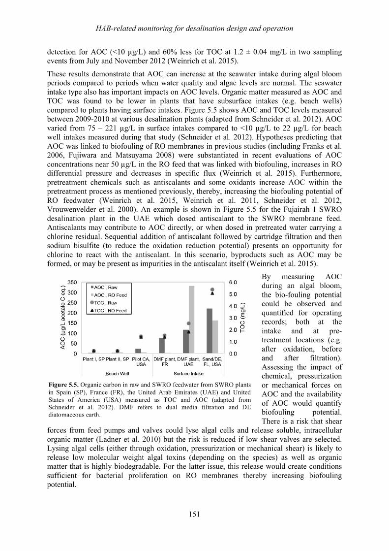
HAB-related monitoring for desalination design and operation

151

detection for AOC (<10 µg/L) and 60% less for TOC at 1.2 ± 0.04 mg/L in two sampling events from July and November 2012 (Weinrich et al. 2015).

These results demonstrate that AOC can increase at the seawater intake during algal bloom periods compared to periods when water quality and algae levels are normal. The seawater intake type also has important impacts on AOC levels. Organic matter measured as AOC and TOC was found to be lower in plants that have subsurface intakes (e.g. beach wells) compared to plants having surface intakes. Figure 5.5 shows AOC and TOC levels measured between 2009-2010 at various desalination plants (adapted from Schneider et al. 2012). AOC varied from 75 – 221 µg/L in surface intakes compared to <10 µg/L to 22 µg/L for beach well intakes measured during that study (Schneider et al. 2012). Hypotheses predicting that AOC was linked to biofouling of RO membranes in previous studies (including Franks et al. 2006, Fujiwara and Matsuyama 2008) were substantiated in recent evaluations of AOC concentrations near 50 µg/L in the RO feed that was linked with biofouling, increases in RO differential pressure and decreases in specific flux (Weinrich et al. 2015). Furthermore, pretreatment chemicals such as antiscalants and some oxidants increase AOC within the pretreatment process as mentioned previously, thereby, increasing the biofouling potential of RO feedwater (Weinrich et al. 2015, Weinrich et al. 2011, Schneider et al. 2012, Vrouwenvelder et al. 2000). An example is shown in Figure 5.5 for the Fujairah 1 SWRO desalination plant in the UAE which dosed antiscalant to the SWRO membrane feed. Antiscalants may contribute to AOC directly, or when dosed in pretreated water carrying a chlorine residual. Sequential addition of antiscalant followed by cartridge filtration and then sodium bisulfite (to reduce the oxidation reduction potential) presents an opportunity for chlorine to react with the antiscalant. In this scenario, byproducts such as AOC may be formed, or may be present as impurities in the antiscalant itself (Weinrich et al. 2015).

By measuring AOC during an algal bloom, the bio-fouling potential could be observed and quantified for operating records; both at the intake and at pre-treatment locations (e.g. after oxidation, before and after filtration). Assessing the impact of chemical, pressurization or mechanical forces on AOC and the availability of AOC would quantify biofouling potential. There is a risk that shear

forces from feed pumps and valves could lyse algal cells and release soluble, intracellular organic matter (Ladner et al. 2010) but the risk is reduced if low shear valves are selected. Lysing algal cells (either through oxidation, pressurization or mechanical shear) is likely to release low molecular weight algal toxins (depending on the species) as well as organic matter that is highly biodegradable. For the latter issue, this release would create conditions sufficient for bacterial proliferation on RO membranes thereby increasing biofouling potential.

Figure 5.5. Organic carbon in raw and SWRO feedwater from SWRO plants in Spain (SP), France (FR), the United Arab Emirates (UAE) and United States of America (USA) measured as TOC and AOC (adapted from Schneider et al. 2012). DMF refers to dual media filtration and DE diatomaceous earth.

HAB-related monitoring for desalination design and operation

152

HABs would be best managed by SWRO plants that can effectively minimize nutrients during routine (non-HAB) operations. Nutrient limitation begins with identifying nutrient sources by testing antiscalants and other dechlorinating chemicals for impurities such as AOC or phosphate. While costly capital improvements could be an option (e.g. changing the intake source, installation of granular media filters and coagulation, conversion to biological filtration), modifying the chlorination strategy may be an effective solution for reducing biodegradable byproducts and bacterial growth. Plant operators need more specific water quality information for pretreatment optimization and biofouling reduction outside of typical bulk organic measurements or SDI. Monitoring AOC regularly and balancing pretreatment may be one solution; another would be sidestream piloting using the Membrane Fouling Simulator Test (see section 5.4.2). Granular media-based biological filtration is generally effective in drinking water applications and could be an option for SWRO as discussed in Chapter 9.6. Limiting AOC and removing it during pretreatment through biodegradation mechanisms on filter media and by coagulation would lower the biofouling potential of the RO feedwater carried to RO membranes. Removing this source of biological fouling material, measured as AOC, would reduce the potential for microbial growth or at least delay it on the RO membranes and associated operational impacts of biological fouling. Future work needed at SWRO plants would be to identify the increase of AOC caused by blooms of specific algal species in order to gain an understanding of their contribution to biofouling potential. 5.4.2! Membrane fouling simulator

Biofouling in spiral wound RO elements usually manifests in increasing head loss across the spacer. In full scale plants, the head loss across the first stage is commonly monitored with pressure sensors, since biofouling tends to occur primarily in the first 10 to 20 cm of the first element. It is possible to monitor the head loss across the first element in order to modify the pretreatment process and as a criterion for chemical cleaning. In pilot tests, monitoring the increase of differential pressure along the feed channel over time as an index is very useful in testing different pretreatment schemes and conditions. It is, however, very costly due to the length of operations and/or the need for several pilot plants. For this reason the MFS was developed (Vrouwenvelder et al. 2006). In a MFS, biofouling along the feed channel is simulated. This device is constructed of two stainless steel plates containing sample coupons of membrane, feed and product spacer. It is equipped with connectors for feed and brine flow and sometimes for product flow as well. Head loss development is accurately monitored using pressure sensors. Villacorte (2014) demonstrated, by making use of the MFS, that AOM produced by laboratory cultivated marine algae (Chaetoceros affinis in synthetic seawater) accelerated biofilm growth and resulted in a rapid increase in the feed channel pressure drop. The tests were performed by running two MFS in parallel, one initially with a RO membrane slightly pre-fouled with AOM and another one with a clean membrane (control). Both MFS were fed with 100,000 cells/L of marine bacteria Vibrio harveyi for about 24 hours and then fed with synthetic seawater spiked with dissolved nutrients (0.1 mg acetate-C/L, 0.02 mg N/L and 0.01 P/L) for 10 to 21 days. An exponential increase of pressure drop was observed for MFS pre-fouled with AOM with up to 1000% increase in only a span of 6 days. In comparison, the control membrane only showed 250% increase in a span of 17 days. While the MFS allows the biofouling potential of feedwater to be measured quite accurately it remains a lengthy test. Therefore, the development of quick AOC tests that incorporate biopolymers into the AOC measurements would be of great value to plant operators to optimize pretreatment during a HAB.

HAB-related monitoring for desalination design and operation

153

5.5! FOULING INDICES TO MEASURE PARTICULATE FOULING POTENTIAL The deposition of algal particulates (e.g. TEP and TEP precursors) on RO membranes during a bloom, along with inorganic and organic colloids, bacteria and other materials, can lead to a decline in normalized permeate flux and an increase in head loss across spacers (or membrane bundles). This type of fouling, often referred to as particulate fouling, may exacerbate other types of fouling (e.g. biofouling). Reliable methods to predict the particulate fouling potential of feedwater are important in preventing and diagnosing fouling at the design stage and for monitoring pre-treatment performance during full-scale plant operation. Turbidity and the Silt Density Index (SDI) are universally applied for this purpose as they often form the basis of RO membrane guarantees. Turbidity however, like particle counting, can only indicate the concentration or mass of particles in feedwater, but provides no information on the resistance of these particles when they deposit on a membrane. Similarly, measurements of total suspended solids (TSS), while important for solids loading in design and operation, will not provide any information on particulate fouling.

Fouling indices, of which the Silt Density Index is the most commonly used in practice, are designed as quick filtration tests to simulate RO membrane fouling and thereby, determine the particulate fouling propensity of a feedwater. The lesser known Modified Fouling Indices (MFI) are increasingly applied, in particular in research projects, pilot and lab/bench scale studies. While both indices are not specific for algal-related particulate material, an increase in the values above background may occur due to HABs at the intake. Table 5.3 provides a summary of the SDI and MFI indices, comparing the principle of each method, interferences, particulate fraction identified and operator skill required for the test. The fundamental background of the SDI and MFI fouling indices is provided in subsequent sections. Applications of the indices in measuring algal-laden feedwater are given to illustrate advantages and limitations of these indices. The performance of parameters such as turbidity and chlorophyll-a to compliment and interpret SDI measured at the seawater intake are also discussed. 5.5.1! Silt Density Index

The SDI, developed by the Du Pont Company at the request of the Bureau of Reclamation (Du Pont 1972), has been universally applied in the desalination industry for the last 40 years to assess the particulate fouling tendency of feedwater. ASTM International standardized the test protocol in 1995 as ASTM D4189, reapproving it most recently in 2014 (ASTM D4189-07(2014)). The SDI test consists of passing a feedwater through a 0.45µm microfiltration membrane in dead-end flow at a constant pressure (207 kPa) and determining the membrane filter-plugging rate. The SDIT 4is calculated from Equation 1.

(1)

where ti is the time to collect an initial sample (normally 500 ml) filtered through the membrane, tT is the time taken to collect a second sample after a total elapsed filtration time (T) of 5, 10 or 15 minutes, and %PF is the percentage plugging factor. The ASTM specifies the %PF should not exceed 75% when conducting the test. If so, the SDI should be 4 The SDI means the percentage flux decline per minute. Dimensions of the SDI test are %/min; by convention the SDI is commonly reported as dimensionless.

T

100 tt - 1

T

%PF (%/min) SDI T

i

T

!"

#$%

&

==

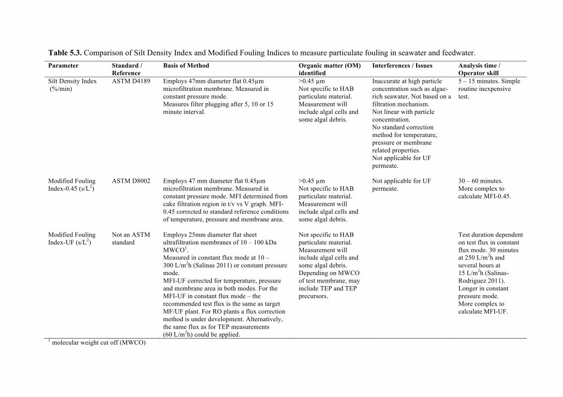
Table 5.3. Comparison of Silt Density Index and Modified Fouling Indices to measure particulate fouling in seawater and feedwater. Parameter Standard /

Reference Basis of Method Organic matter (OM)

identified Interferences / Issues Analysis time /

Operator skill Silt Density Index (%/min)

ASTM D4189 Employs 47mm diameter flat 0.45µm microfiltration membrane. Measured in constant pressure mode. Measures filter plugging after 5, 10 or 15 minute interval.

>0.45 µm Not specific to HAB particulate material. Measurement will include algal cells and some algal debris.

Inaccurate at high particle concentration such as algae-rich seawater. Not based on a filtration mechanism. Not linear with particle concentration. No standard correction method for temperature, pressure or membrane related properties. Not applicable for UF permeate.

5 – 15 minutes. Simple routine inexpensive test.

Modified Fouling Index-0.45 (s/L2)

ASTM D8002 Employs 47 mm diameter flat 0.45µm microfiltration membrane. Measured in constant pressure mode. MFI determined from cake filtration region in t/v vs V graph. MFI-0.45 corrected to standard reference conditions of temperature, pressure and membrane area.

>0.45 µm Not specific to HAB particulate material. Measurement will include algal cells and some algal debris.

Not applicable for UF permeate.

30 – 60 minutes. More complex to calculate MFI-0.45.

Modified Fouling Index-UF (s/L2)

Not an ASTM standard

Employs 25mm diameter flat sheet ultrafiltration membranes of 10 – 100 kDa MWCO1. Measured in constant flux mode at 10 – 300 L/m2h (Salinas 2011) or constant pressure mode. MFI-UF corrected for temperature, pressure and membrane area in both modes. For the MFI-UF in constant flux mode – the recommended test flux is the same as target MF/UF plant. For RO plants a flux correction method is under development. Alternatively, the same flux as for TEP measurements (60 L/m2h) could be applied.

Not specific to HAB particulate material. Measurement will include algal cells and some algal debris. Depending on MWCO of test membrane, may include TEP and TEP precursors.

Test duration dependent on test flux in constant flux mode. 30 minutes at 250 L/m2h and several hours at 15 L/m2h (Salinas-Rodriguez 2011). Longer in constant pressure mode. More complex to calculate MFI-UF.

1 molecular weight cut off (MWCO)

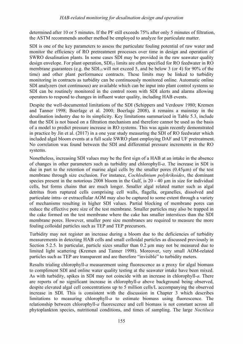
HAB-related monitoring for desalination design and operation

155

determined after 10 or 5 minutes. If the PF still exceeds 75% after only 5 minutes of filtration, the ASTM recommends another method be employed to analyze for particulate matter.

SDI is one of the key parameters to assess the particulate fouling potential of raw water and monitor the efficiency of RO pretreatment processes over time in design and operation of SWRO desalination plants. In some cases SDI may be provided in the raw seawater quality design envelope. For plant operation, SDI15 limits are often specified for RO feedwater in RO membrane guarantees (e.g. the SDI15 will not exceed 5, and be below 3 (or 4) for 90% of the time) and other plant performance contracts. These limits may be linked to turbidity monitoring in contracts as turbidity can be continuously monitored online. Automatic online SDI analyzers (not continuous) are available which can be input into plant control systems so SDI can be routinely monitored in the control room with SDI alerts and alarms allowing operators to respond to changes in influent water quality, including HAB events.

Despite the well-documented limitations of the SDI (Schippers and Verdouw 1980; Kremen and Tanner 1998; Boerlage et al. 2000; Boerlage 2008), it remains a mainstay in the desalination industry due to its simplicity. Key limitations summarized in Table 5.3, include that the SDI is not based on a filtration mechanism and therefore cannot be used as the basis of a model to predict pressure increase in RO systems. This was again recently demonstrated in practice by Jin et al. (2017) in a one year study measuring the SDI of RO feedwater which included algal bloom events at a full scale SWRO plant employing DAF and UF pretreatment. No correlation was found between the SDI and differential pressure increments in the RO systems. Nonetheless, increasing SDI values may be the first sign of a HAB at an intake in the absence of changes in other parameters such as turbidity and chlorophyll-a. The increase in SDI is due in part to the retention of marine algal cells by the smaller pores (0.45µm) of the test membrane through size exclusion. For instance, Cochlodinium polykrikoides, the dominant species present in the notorious 2008 bloom in the Gulf, is 20 - 40 µm in size for individual cells, but forms chains that are much longer. Smaller algal related matter such as algal detritus from ruptured cells comprising cell walls, flagella, organelles, dissolved and particulate intra- or extracellular AOM may also be captured to some extent through a variety of mechanisms resulting in higher SDI values. Partial blocking of membrane pores can reduce the effective pore size of the test membrane. Smaller particles may also be trapped in the cake formed on the test membrane where the cake has smaller interstices than the SDI membrane pores. However, smaller pore size membranes are required to measure the more fouling colloidal particles such as TEP and TEP precursors.

Turbidity may not register an increase during a bloom due to the deficiencies of turbidity measurements in detecting HAB cells and small colloidal particles as discussed previously in Section 5.2.5. In particular, particle sizes smaller than 0.2 µm may not be measured due to limited light scattering (Kremen and Tanner 1998). Moreover, very small AOM-related particles such as TEP are transparent and are therefore “invisible” to turbidity meters. Results trialing chlorophyll-a measurement using fluorescence as a proxy for algal biomass to compliment SDI and online water quality testing at the seawater intake have been mixed. As with turbidity, spikes in SDI may not coincide with an increase in chlorophyll-a. There are reports of no significant increase in chlorophyll-a above background being observed, despite elevated algal cell concentrations up to 5 million cells/L accompanying the observed increase in SDI. This is consistent with the discussion in Chapter 3 which describes limitations to measuring chlorophyll-a to estimate biomass using fluorescence. The relationship between chlorophyll-a fluorescence and cell biomass is not constant across all phytoplankton species, nutritional conditions, and times of sampling. The large Noctiluca

HAB-related monitoring for desalination design and operation

156

scintillans dinoflagellate is a notable example; it ranges up to 2 mm in size and while it releases ammonia into seawater and therefore can be harmful, it lacks chloroplasts and therefore its chlorophyll content is low (Pool et al. 2015). In this instance, SDI may increase along with ammonia concentrations (if measured) in the intake seawater, while chlorophyll would show no change. Other factors influencing chlorophyll-a include nutrients, and light history, with limitations often resulting in lower chlorophyll-a content than the same cells under more favorable conditions (see Chapter 3). If chlorophyll-a is measured then it is recommended that only the night time data be used, as nocturnal chlorophyll-a fluorescence is more consistent. Other options that could be used in conjunction with SDI are regular microscopic examination and counting of cells, or some of the newer automated phytoplankton-identifying instruments, such as the Imaging FlowCytobot or FlowCam (see Chapter 3). They can also be automated, and provide more information about species and cell numbers. Routine, online use of these automated biosensors would allow operators to generate a long-term, high-resolution database of algal species and concentrations that are associated with plant disruptions, and an associated record of which pretreatment strategies worked or failed.

Visual examination of the SDI test membrane may provide additional information on feedwater constituents and indicate changes in quality such as an unusual color of the deposit on the SDI membrane e.g. a red filter deposit from red blooming algae. Closer examination of membranes by electron microscopy may be used in combination with algal counting to identify species or bloom types. This is illustrated in electron micrographs of SDI test membranes of raw water off the coast of Chile where diatoms and coccoliths are visible in Figure 5.6 (left) and an intact coccolithopore (Emiliania huxleyi) cell in Figure 5.6 (right) (Petry et al. 2007).

Severe HAB events can significantly increase the fouling potential of seawater at open intakes due to the increase in algal biomass to the point that the SDI may not be measurable due to rapid plugging of the SDI test membrane. During the prolonged 2008 HAB event in the Gulf, algal cell counts of 11 to 21 million cells/L were recorded in surface waters near Fujairah (Richlen et al. 2010). As a result, TSS increased to 30 mg/L on occasion, compared to the median TSS of 5 mg/L; the SDI test was not informative, as it is limited to low fouling feedwater. Despite the ASTM recommendation that the SDI is only employed for low turbidity water (< 1 NTU) and for water that will not result in a %PF of > 75%, these guidelines are widely ignored in practice. Furthermore, raw seawater SDI5 values often

Figure 5.6. Electron microscopy of SDI test membranes showing the presence of algae and algal particulate debris (left) and close up (right) of a coccolithopore cell. Photo: Petry 2007.

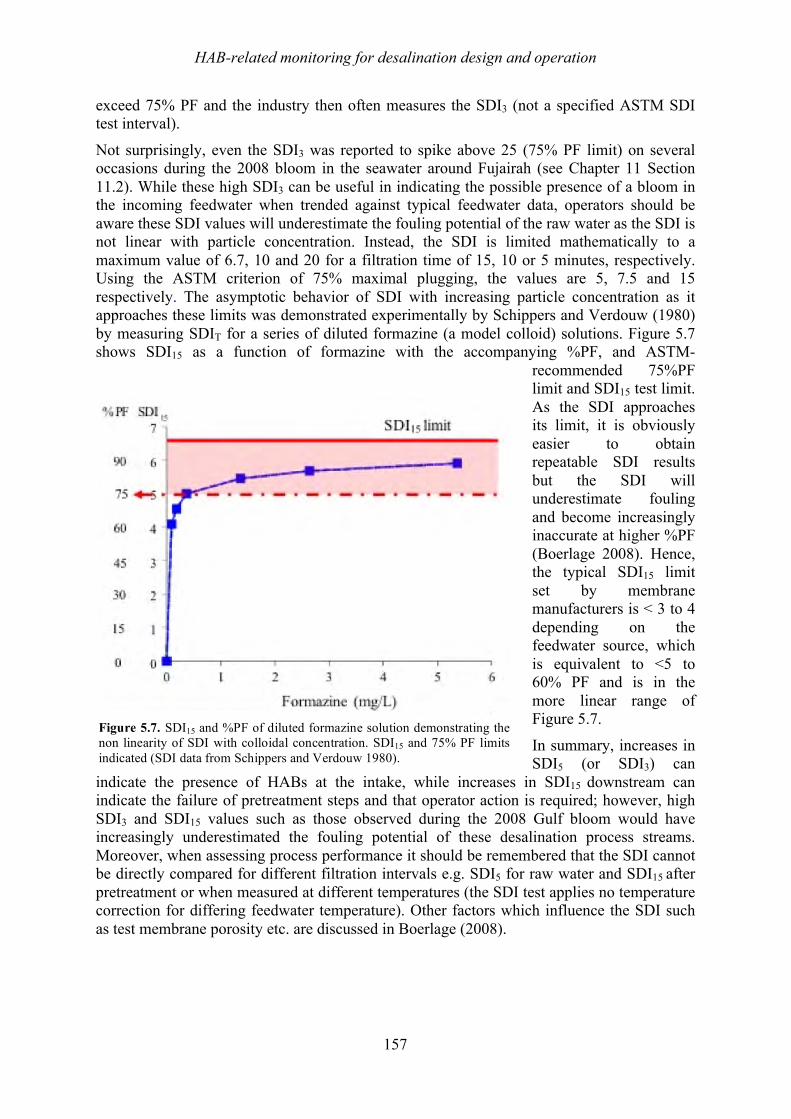
HAB-related monitoring for desalination design and operation

157

exceed 75% PF and the industry then often measures the SDI3 (not a specified ASTM SDI test interval).

Not surprisingly, even the SDI3 was reported to spike above 25 (75% PF limit) on several occasions during the 2008 bloom in the seawater around Fujairah (see Chapter 11 Section 11.2). While these high SDI3 can be useful in indicating the possible presence of a bloom in the incoming feedwater when trended against typical feedwater data, operators should be aware these SDI values will underestimate the fouling potential of the raw water as the SDI is not linear with particle concentration. Instead, the SDI is limited mathematically to a maximum value of 6.7, 10 and 20 for a filtration time of 15, 10 or 5 minutes, respectively. Using the ASTM criterion of 75% maximal plugging, the values are 5, 7.5 and 15 respectively. The asymptotic behavior of SDI with increasing particle concentration as it approaches these limits was demonstrated experimentally by Schippers and Verdouw (1980) by measuring SDIT for a series of diluted formazine (a model colloid) solutions. Figure 5.7 shows SDI15 as a function of formazine with the accompanying %PF, and ASTM-

recommended 75%PF limit and SDI15 test limit. As the SDI approaches its limit, it is obviously easier to obtain repeatable SDI results but the SDI will underestimate fouling and become increasingly inaccurate at higher %PF (Boerlage 2008). Hence, the typical SDI15 limit set by membrane manufacturers is < 3 to 4 depending on the feedwater source, which is equivalent to <5 to 60% PF and is in the more linear range of Figure 5.7.

In summary, increases in SDI5 (or SDI3) can

indicate the presence of HABs at the intake, while increases in SDI15 downstream can indicate the failure of pretreatment steps and that operator action is required; however, high SDI3 and SDI15 values such as those observed during the 2008 Gulf bloom would have increasingly underestimated the fouling potential of these desalination process streams. Moreover, when assessing process performance it should be remembered that the SDI cannot be directly compared for different filtration intervals e.g. SDI5 for raw water and SDI15 after pretreatment or when measured at different temperatures (the SDI test applies no temperature correction for differing feedwater temperature). Other factors which influence the SDI such as test membrane porosity etc. are discussed in Boerlage (2008).

Figure 5.7. SDI15 and %PF of diluted formazine solution demonstrating the non linearity of SDI with colloidal concentration. SDI15 and 75% PF limits indicated (SDI data from Schippers and Verdouw 1980).

HAB-related monitoring for desalination design and operation

158

5.5.2! Modified Fouling Indices

5.5.2.1! Modified Fouling Index-0.45 The MFI-0.45 was developed by Schippers to overcome the limitations of the SDI (Schippers and Verdouw 1980) and thus has the potential to be of value in detecting a HAB at an intake and optimizing the efficiency of pretreatment processes. The MFI-0.45 has recently been approved by ASTM International as a standard (D8002-15) to indicate the fouling potential of feedwater due to particular matter. Automatic analyzers are commercially available that can simultaneously measure MFI-0.45 and SDI online, but they are not as widely used as the SDI analyzers. Unlike the SDI, the MFI-0.45 is based on a filtration mechanism (cake filtration) and is linear with particle concentration. As with the SDI, the MFI-0.45 is determined in dead-end flow under constant pressure using similar equipment as the SDI. The MFI-0.45 is determined in a plot of t/V vs V (where V is filtrate volume and t filtration time) from the gradient of the linear region of minimum slope where cake filtration occurs (refer to Schippers and Verdouw 1980 for more information). Schippers defined the MFI at reference pressure and temperature values of 2 bar (ΔPo) and 20°C (η20°), respectively and for the area of the 0.45 µm membrane (Ao=13.8×10-4 m2). Incorporating the Carman-Kozeny relationship for idealized spherical particles to calculate the specific resistance of the cake deposited on the MFI-0.45 membrane yields the following equation for the MFI-0.45 at standard reference conditions:

(2)

where (Cb) is the concentration of particles in the feedwater, (ρp) is the density of particles forming the cake, (ε) cake porosity and (dp) particle diameter. From this equation the pronounced effect of decreasing particle size in increasing the MFI can be seen.

The MFI can be used as an index to characterize the fouling potential of a feedwater containing particles, as it is a function of the dimension and nature of the particles forming a cake on the membrane, and is directly correlated to particle concentration in a feedwater. For feedwater containing algae, the MFI-0.45 could provide information about the difference in net fouling potential (cake permeability) due to differing algal cell size (dp) and cell abundance (Cb) of bloom species that can vary significantly. For instance, two algal bloom-forming species found in the Gulf and Gulf of Oman are Cochlodinium polykrikoides (with a size range of 20 – 40 µm and a maximum abundance up to 20 million cells/L in the 2008 HAB) compared to the much larger Noctiluca scintillans dinoflagellate which formed less dense blooms with only up to 68,500 cells/L measured during HAB events in the Gulf (Al Shehhi et al. 2014). The MFI-0.45 is expected to be higher for the smaller Cochlodinium polykrikoides as the MFI is inversely proportional to particle diameter squared (see equation 2). A clear advantage of the MFI-0.45 is that it could be used to measure the fouling potential of low and high fouling feedwater and therefore assess the efficiency of pretreatment processes during a HAB. Data available from the Jacobahaven SWRO demonstration plant (see Case Study 11.10 for more information), where both the MFI-0.45 and SDI15 were measured during an algal bloom pre- and post-UF are shown in Figure 5.8 (from Al Hadidi 2011). Both

( )2

0o32

b20

A P

C - 190

!=

"#

"$

pp

C

dMFI

!

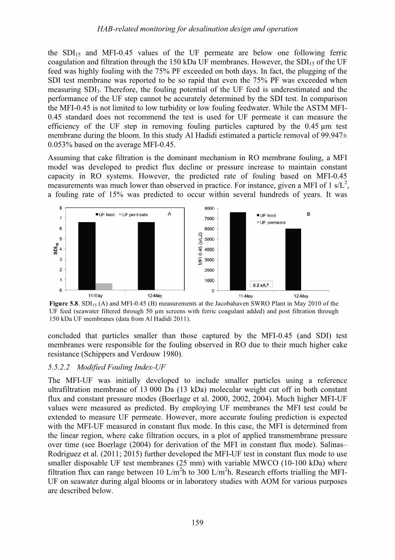
HAB-related monitoring for desalination design and operation

159

the SDI15 and MFI-0.45 values of the UF permeate are below one following ferric coagulation and filtration through the 150 kDa UF membranes. However, the SDI15 of the UF feed was highly fouling with the 75% PF exceeded on both days. In fact, the plugging of the SDI test membrane was reported to be so rapid that even the 75% PF was exceeded when measuring SDI3.!Therefore, the fouling potential of the UF feed is underestimated and the performance of the UF step cannot be accurately determined by the SDI test. In comparison the MFI-0.45 is not limited to low turbidity or low fouling feedwater. While the ASTM MFI-0.45 standard does not recommend the test is used for UF permeate it can measure the efficiency of the UF step in removing fouling particles captured by the 0.45 µm test membrane during the bloom. In this study Al Hadidi estimated a particle removal of 99.947± 0.053% based on the average MFI-0.45. Assuming that cake filtration is the dominant mechanism in RO membrane fouling, a MFI model was developed to predict flux decline or pressure increase to maintain constant capacity in RO systems. However, the predicted rate of fouling based on MFI-0.45 measurements was much lower than observed in practice. For instance, given a MFI of 1 s/L2, a fouling rate of 15% was predicted to occur within several hundreds of years. It was

concluded that particles smaller than those captured by the MFI-0.45 (and SDI) test membranes were responsible for the fouling observed in RO due to their much higher cake resistance (Schippers and Verdouw 1980). 5.5.2.2! Modified Fouling Index-UF The MFI-UF was initially developed to include smaller particles using a reference ultrafiltration membrane of 13 000 Da (13 kDa) molecular weight cut off in both constant flux and constant pressure modes (Boerlage et al. 2000, 2002, 2004). Much higher MFI-UF values were measured as predicted. By employing UF membranes the MFI test could be extended to measure UF permeate. However, more accurate fouling prediction is expected with the MFI-UF measured in constant flux mode. In this case, the MFI is determined from the linear region, where cake filtration occurs, in a plot of applied transmembrane pressure over time (see Boerlage (2004) for derivation of the MFI in constant flux mode). Salinas–Rodriguez et al. (2011; 2015) further developed the MFI-UF test in constant flux mode to use smaller disposable UF test membranes (25 mm) with variable MWCO (10-100 kDa) where filtration flux can range between 10 L/m2h to 300 L/m2h. Research efforts trialling the MFI-UF on seawater during algal blooms or in laboratory studies with AOM for various purposes are described below.

Figure 5.8. SDI15 (A) and MFI-0.45 (B) measurements at the Jacobahaven SWRO Plant in May 2010 of the UF feed (seawater filtered through 50 µm screens with ferric coagulant added) and post filtration through 150 kDa UF membranes (data from Al Hadidi 2011).

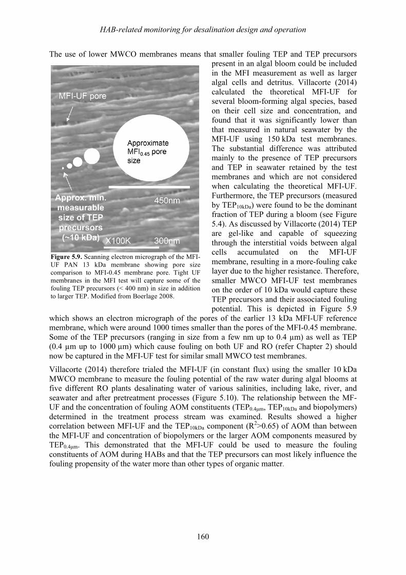
HAB-related monitoring for desalination design and operation

160

The use of lower MWCO membranes means that smaller fouling TEP and TEP precursors present in an algal bloom could be included in the MFI measurement as well as larger algal cells and detritus. Villacorte (2014) calculated the theoretical MFI-UF for several bloom-forming algal species, based on their cell size and concentration, and found that it was significantly lower than that measured in natural seawater by the MFI-UF using 150 kDa test membranes. The substantial difference was attributed mainly to the presence of TEP precursors and TEP in seawater retained by the test membranes and which are not considered when calculating the theoretical MFI-UF. Furthermore, the TEP precursors (measured by TEP10kDa) were found to be the dominant fraction of TEP during a bloom (see Figure 5.4). As discussed by Villacorte (2014) TEP are gel-like and capable of squeezing through the interstitial voids between algal cells accumulated on the MFI-UF membrane, resulting in a more-fouling cake layer due to the higher resistance. Therefore, smaller MWCO MFI-UF test membranes on the order of 10 kDa would capture these TEP precursors and their associated fouling potential. This is depicted in Figure 5.9

which shows an electron micrograph of the pores of the earlier 13 kDa MFI-UF reference membrane, which were around 1000 times smaller than the pores of the MFI-0.45 membrane. Some of the TEP precursors (ranging in size from a few nm up to 0.4 µm) as well as TEP (0.4 µm up to 1000 µm) which cause fouling on both UF and RO (refer Chapter 2) should now be captured in the MFI-UF test for similar small MWCO test membranes. Villacorte (2014) therefore trialed the MFI-UF (in constant flux) using the smaller 10 kDa MWCO membrane to measure the fouling potential of the raw water during algal blooms at five different RO plants desalinating water of various salinities, including lake, river, and seawater and after pretreatment processes (Figure 5.10). The relationship between the MF-UF and the concentration of fouling AOM constituents (TEP0.4µm, TEP10kDa and biopolymers) determined in the treatment process stream was examined. Results showed a higher correlation between MFI-UF and the TEP10kDa component (R2>0.65) of AOM than between the MFI-UF and concentration of biopolymers or the larger AOM components measured by TEP0.4µm. This demonstrated that the MFI-UF could be used to measure the fouling constituents of AOM during HABs and that the TEP precursors can most likely influence the fouling propensity of the water more than other types of organic matter.

Figure 5.9. Scanning electron micrograph of the MFI-UF PAN 13 kDa membrane showing pore size comparison to MFI-0.45 membrane pore. Tight UF membranes in the MFI test will capture some of the fouling TEP precursors (< 400 nm) in size in addition to larger TEP. Modified from Boerlage 2008.

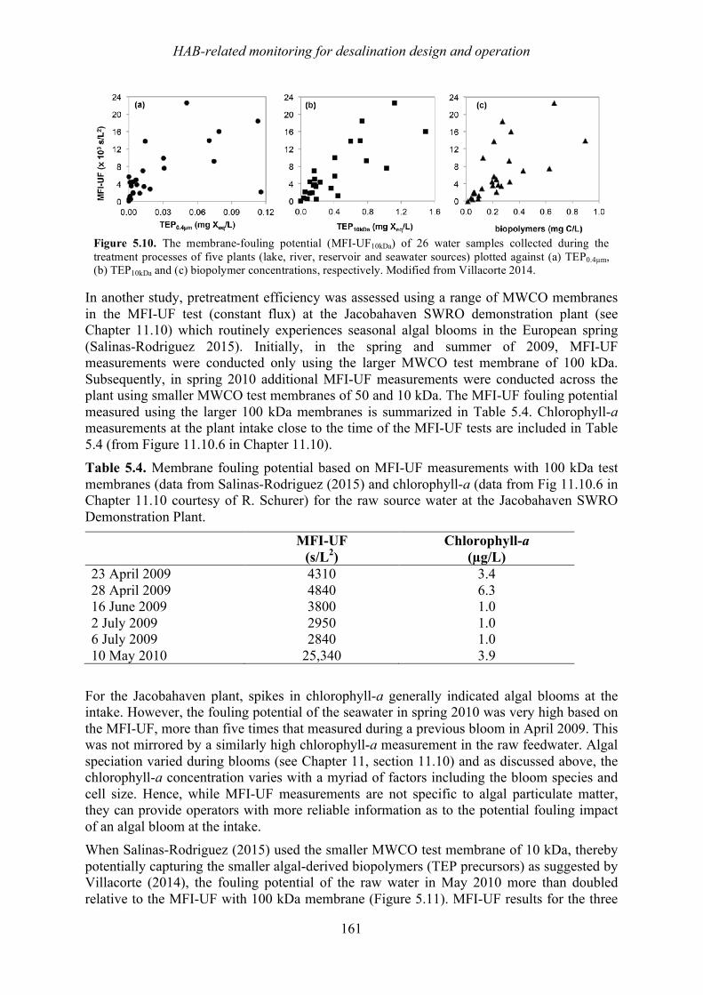
HAB-related monitoring for desalination design and operation

161

In another study, pretreatment efficiency was assessed using a range of MWCO membranes in the MFI-UF test (constant flux) at the Jacobahaven SWRO demonstration plant (see Chapter 11.10) which routinely experiences seasonal algal blooms in the European spring (Salinas-Rodriguez 2015). Initially, in the spring and summer of 2009, MFI-UF measurements were conducted only using the larger MWCO test membrane of 100 kDa. Subsequently, in spring 2010 additional MFI-UF measurements were conducted across the plant using smaller MWCO test membranes of 50 and 10 kDa. The MFI-UF fouling potential measured using the larger 100 kDa membranes is summarized in Table 5.4. Chlorophyll-a measurements at the plant intake close to the time of the MFI-UF tests are included in Table 5.4 (from Figure 11.10.6 in Chapter 11.10). Table 5.4. Membrane fouling potential based on MFI-UF measurements with 100 kDa test membranes (data from Salinas-Rodriguez (2015) and chlorophyll-a (data from Fig 11.10.6 in Chapter 11.10 courtesy of R. Schurer) for the raw source water at the Jacobahaven SWRO Demonstration Plant.

MFI-UF (s/L2)

Chlorophyll-a (µg/L)

23 April 2009 4310 3.4 28 April 2009 4840 6.3 16 June 2009 3800 1.0 2 July 2009 2950 1.0 6 July 2009 2840 1.0 10 May 2010 25,340 3.9

For the Jacobahaven plant, spikes in chlorophyll-a generally indicated algal blooms at the intake. However, the fouling potential of the seawater in spring 2010 was very high based on the MFI-UF, more than five times that measured during a previous bloom in April 2009. This was not mirrored by a similarly high chlorophyll-a measurement in the raw feedwater. Algal speciation varied during blooms (see Chapter 11, section 11.10) and as discussed above, the chlorophyll-a concentration varies with a myriad of factors including the bloom species and cell size. Hence, while MFI-UF measurements are not specific to algal particulate matter, they can provide operators with more reliable information as to the potential fouling impact of an algal bloom at the intake. When Salinas-Rodriguez (2015) used the smaller MWCO test membrane of 10 kDa, thereby potentially capturing the smaller algal-derived biopolymers (TEP precursors) as suggested by Villacorte (2014), the fouling potential of the raw water in May 2010 more than doubled relative to the MFI-UF with 100 kDa membrane (Figure 5.11). MFI-UF results for the three

Figure 5.10. The membrane-fouling potential (MFI-UF10kDa) of 26 water samples collected during the treatment processes of five plants (lake, river, reservoir and seawater sources) plotted against (a) TEP0.4µm, (b) TEP10kDa and (c) biopolymer concentrations, respectively. Modified from Villacorte 2014.

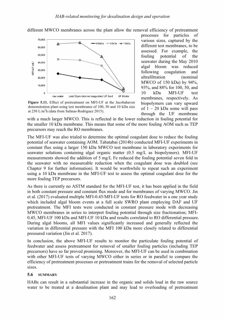
HAB-related monitoring for desalination design and operation

162

different MWCO membranes across the plant allow the removal efficiency of pretreatment processes for particles of various sizes, captured by the different test membranes, to be assessed. For example, the fouling potential of the seawater during the May 2010 algal bloom was reduced following coagulation and ultrafiltration (nominal MWCO of 150 kDa) by 94%, 93%, and 88% for 100, 50, and 10 kDa MFI-UF test membranes, respectively. As biopolymers can vary upward of 1 – 20 kDa some will pass through the UF membrane

with a much larger MWCO. This is reflected in the lower reduction in fouling potential for the smaller 10 kDa membrane. This means that some of the more fouling AOM such as TEP precursors may reach the RO membranes.

The MFI-UF was also trialed to determine the optimal coagulant dose to reduce the fouling potential of seawater containing AOM. Tabatabai (2014b) conducted MFI-UF experiments in constant flux using a larger 150 kDa MWCO test membrane in laboratory experiments for seawater solutions containing algal organic matter (0.5 mg/L as biopolymers). MFI-UF measurements showed the addition of 5 mg/L Fe reduced the fouling potential seven fold in the seawater with no measureable reduction when the coagulant dose was doubled (see Chapter 9 for further information). It would be worthwhile to repeat such an experiment using a 10 kDa membrane in the MFI-UF test to assess the optimal coagulant dose for the more fouling TEP precursors. As there is currently no ASTM standard for the MFI-UF test, it has been applied in the field in both constant pressure and constant flux mode and for membranes of varying MWCO. Jin et al. (2017) evaluated multiple MFI-0.45/MFI-UF tests for RO feedwater in a one year study which included algal bloom events at a full scale SWRO plant employing DAF and UF pretreatment. The MFI tests were conducted in constant pressure mode with decreasing MWCO membranes in series to interpret fouling potential through size fractionation; MFI-0.45, MFI-UF 100 kDa and MFI-UF 10 kDa and results correlated to RO differential pressure. During algal blooms, all MFI values significantly increased and generally reflected the variation in differential pressure with the MFI 100 kDa more closely related to differential pressured variation (Jin et al. 2017). In conclusion, the above MFI-UF results to monitor the particulate fouling potential of feedwater and assess pretreatment for removal of smaller fouling particles (including TEP precursors) have so far proved promising. Moreover, the MFI-UF can be used in combination with other MFI-UF tests of varying MWCO either in series or in parallel to compare the efficiency of pretreatment processes or pretreatment trains for the removal of selected particle sizes. 5.6! SUMMARY

HABs can result in a substantial increase in the organic and solids load in the raw source water to be treated at a desalination plant and may lead to overloading of pretreatment

Figure 5.11. Effect of pretreatment on MFI-UF at the Jacobahaven demonstration plant using test membranes of 100, 50 and 10 kDa size at 250 L/m2h (data from Salinas-Rodriguez 2015).

HAB-related monitoring for desalination design and operation

163

systems and membrane fouling. SWRO designers and operators therefore require methods to determine the concentration of AOM, its fouling constituents, and any increases in the particulate and biofouling fouling potential or other HAB-associated water quality changes. Such methods allow HABs to be monitored and detected in the raw water so that treatment processes can be optimized during a bloom event to maintain plant production and water quality targets.

Temperature, conductivity, pH and turbidity are often continuously monitored at plant intakes, in addition to analysis of SDI, TOC and TSS to characterize feedwater quality. None of the conventional online parameters can definitively detect HABs as they are not specific to algal blooms. Changes can be caused by other factors such as pollution events and/or marine hydrodynamics. The interpretation of a water quality variable can thus be complex. Nonetheless, these measurements may indicate conditions that promote a bloom, such as temperature and salinity or indirect impacts from HABs such as low DO following decomposition of a dense bloom. In conjunction with other conventional water quality tests such as SDI, the standard online water quality parameters can be useful in indicating a deterioration in feedwater quality due to HAB events, and can provide timely and valuable information that action is required. Measuring TOC to detect AOM and for process control is generally unreliable. Spikes in TOC may be derived from both natural processes such as HABs and/or through anthropogenic input. Measuring TOC removal to assess the efficiency of pretreatment processes is also inaccurate due to the difficulties in measuring low level TOC residuals in seawater process streams. Of the conventional water quality parameters used in desalination, the SDI, despite its well known limitations, has proven useful in detecting algal blooms at the intake compared to other parameters including turbidity and chlorophyll-a (determined via fluorescence). Notwithstanding, care should be taken in interpreting results, as the SDI test was not designed for high fouling feedwater such as algae-laden seawater. As a result, it can underestimate the fouling potential of feedwater. Moreover, it does not include the smaller, more fouling AOM produced during a bloom.

Recently, more sophisticated tests have been developed to determine constituents of AOM which may better indicate the biofouling and particulate fouling potential of seawater and process streams during a bloom. Villacorte (2014) demonstrated that algal-derived TEP and biopolymers can promote fouling of both pretreatment and SWRO membranes and developed tests to measure the concentration of larger TEP (TEP0.4μm) and smaller TEP precursors (TEP10kDa) in seawater. Applications of both tests showed the smaller and more fouling TEP precursors dominated AOM during a bloom and allowed the differences in the efficiency of pretreatment in removing these algal-derived foulants to be distinguished. For instance, UF was found to be superior in removing TEP precursors in comparison to conventional coagulation-sedimentation-sand filtration. AOM generated during a HAB may lead to an increase in the biodegradability of organic matter in seawater and serve as a substrate for bacterial growth causing biofouling. A recently developed AOC test, based on luminescence, to measure the biofouling potential of seawater using Vibrio harveyi which utilizes low molecular weight organics, demonstrated an increase in AOC during a HAB event compared to normal operating conditions. Other AOC tests are under development to incorporate high molecular weight organic compounds such as biopolymers generated during a bloom. As with AOC, the determination of TEP and the MFI-UF have both proven valuable in laboratory and field trials. They offer distinct advantages over the SDI. The MFI-UF has been applied to optimize coagulant dose to reduce the fouling potential of feedwater containing AOM and to investigate pretreatment efficiency

HAB-related monitoring for desalination design and operation

164

during a bloom. Promising results were found when using a 10 kDa membrane in the MFI-UF test. A high correlation was found between the MFI-UF and TEP10kDa, indicating the MFI-UF10kDa could be used to investigate the fouling potential of feedwater containing the smaller high fouling TEP precursors across a plant during a bloom.

While the AOC, TEP and MFI-UF tests offer more targeted information on AOM constituents and the potential biofouling and particulate fouling potential of a feedwater during a bloom than conventional parameters used in the industry, the degree of difficulty in determining them is correspondingly higher. The tests require skilled analysts and specialized equipment. At present, TEP, AOC and MFI-UF cannot be directly employed as a trigger to alert a plant of a bloom in the incoming feedwater or to adjust process parameters during plant operation. Nonetheless, these parameters are expected to be key factors in developing our understanding of AOM fouling in seawater UF and RO systems, and therefore in efforts to control them. 5.7! REFERENCES

Al-Hadidi, A. M. M. 2011. Limitations, Improvements, Alternatives for the Silt Density Index, Enschede, Gildeprint Drukkerijen.

Al Shehhi, M. R., Gherboudj, I. and Ghedira, H. 2014. An overview of historical harmful algae blooms outbreaks in the Arabian Seas. Marine Pollution Bulletin 86(1), 314-324.

Alldredge, A. L., Passow, U., and Logan, B. E. 1993. The abundance and significance of a class of large, transparent organic particles in the ocean. Deep Sea Research Part I: Oceanographic Research Papers 40(6), 1131-1140.

Arruda-Fatibello, S. H. S., Henriques-Vieira, A. A., and Fatibello-Filho, O. 2004. A rapid spectrophotometric method for the determination of transparent exopolymer particles (TEP) in freshwater. Talanta 62(1), 81-85.

APHA. 2012. Standard methods for the examination of water and wastewater, 21st edition. American Public Health Association, Washington, D.C.

ASTM D2579-93e1, Standard Test Method for Total Organic Carbon in Water (Withdrawn 2002), ASTM International, West Conshohocken, PA.

ASTM D4129-05(2013), Standard Test Method for Total and Organic Carbon in Water by High Temperature Oxidation and by Coulometric Detection, ASTM International, West Conshohocken, PA.

ASTM D4189-07(2014), Standard Test Method for Silt Density Index (SDI) of Water, ASTM International, West Conshohocken, PA.

ASTM D4839-03(2011), Standard Test Method for Total Carbon and Organic Carbon in Water by Ultraviolet, or Persulfate Oxidation, or Both, and Infrared Detection, ASTM International, West Conshohocken, PA.

ASTM D8002-15e1 (2015), Standard Test Method for Modified Fouling Index (MFI-0.45) of Water, ASTM International, West Conshohocken, PA.

Bar-Zeev, E., Berman-Frank, I., Girshevitz, O., and Berman, T. 2012. Revised paradigm of aquatic biofilm formation facilitated by microgel transparent exopolymer particles. Proceedings of the National Academy of Sciences 109(23), 9119-9124.

Baumann, P., Furniss, A. L., and Lee, J. V. 1984. Genus I, Vibrio pacini 1854, 411 AL. In: Krieg, N. R. and Holt, J. G. (eds) Bergey’s Manual of Systematic Bacteriology, Vol. 1. Baltimore, Williams & Wilkins, p. 518-538.

HAB-related monitoring for desalination design and operation

165

Berman, T., and Holenberg, M. 2005. Don't fall foul of biofilm through high TEP levels. Filtration and Separation 42, 30-32.

Boerlage, S. F. E. 2001. Scaling and particulate fouling in membrane filtration systems. Swets & Zeitlinger Publishers, Lisse: pp. 242.

Boerlage, S. F. E. 2008 Understanding the Silt Density Index and Modified Fouling Indices (MFI0.45 and MFI-UF). Desalination and Water Reuse Quarterly, May –June, 12-21.

Boerlage, S. F. E. 2012. Measuring salinity and TDS of seawater and brine for process and environmental monitoring—which one, when? Desalination and Water Treatment 42(1-3), 222-230.

Boerlage, S. F. E, Kennedy, M., Aniye, M., Abogrean, E., El-Hodali, D., Tarawneh, Z., and Schippers, J. 2000. Modified Fouling Index - ultrafiltration to compare pretreatment processes of reverse osmosis feedwater. Desalination 131, 201-214.

Boerlage, S. F. E., Kennedy, M., Aniye, M., Tarawneh, Z., Schippers, J. 2004. The Modified Fouling Index-ultrafiltration in constant flux mode. Desalination 161, 103-113.

Boerlage, S. F., Kennedy, M. D., Dickson, M. R., El-Hodali, D. E. and Schippers, J. C. 2002. The modified fouling index using ultrafiltration membranes (MFI-UF): characterisation, filtration mechanisms and proposed reference membrane. Journal of Membrane Science, 197(1), pp.1-21.

Coble, P. G., Schultz, C. A. and Mopper, K. 1993. Fluorescence contouring analysis of DOC intercalibration experiment samples: a comparison of techniques. Marine Chemistry 41(1-3), 173-178.

Du Pont Permasep Issued in 1972 in Technical Bulletin 300 Standard Millipore Test for Determining Fouling Characteristics of Permeator Feed Supply.

Edzwald, J. K., and Tobiason, J. E. 2011. Chapter 3. Chemical Principles, Source Water Composition, and Watershed Protection, In: Water Quality and Treatment: A Handbook on Drinking Water, 6th edition. J. K. Edzwald, (Ed). American Water Works Association, McGraw-Hill.

Evans, P. J., Smith, J. L., LeChevallier, M. W., Schneider, O. D., Weinrich, L. A., and Jjemba, P. K. 2013. A Monitoring and Control Toolbox for Biological Filtration. Water Research Foundation: Denver, CO. pp.1-92.

Franks, R., Wilf, M., Voutchkov, N., Murkute, P., and Kizer, J. 2006. A pilot study using seawater reverse osmosis membranes in combination with various pretreatments to meet the challenges of Pacific seawater desalination. http://hydranautics.com/docs/papers/NewFolder/APILOTSTUDYUSINGSEAWATERREVERSEOSMOSISMEMBRANES.pdf. (Accessed 6 July 16).

Fujiwara, N., and Matsuyama, H. 2008. Elimination of biological fouling in seawater reverse osmosis desalination plants. Desalination 227, 295–305.

Haddix, P. L., Shaw, N. J., and LeChevallier, M. W. 2003. Development of a simple assay. American Water, Voorhees, NJ.

Haddix, P. L., Shaw, N. J., and LeChevallier, M. W. 2004. Characterization of bioluminescent derivatives of assimilable organic carbon test bacteria. Applied and Environmental Microbiology 70, 850–854.

Horobin, R. W. 1988. Understanding histochemistry: Selection, evaluation and design of biological stains. Wiley, New York:

HAB-related monitoring for desalination design and operation

166

Huber, S. A., and Frimmel, F. H. 1991. Flow injection analysis of organic and inorganic carbon in the low-ppb range. Analytical Chemistry 63, 2122-2130.

Huber, S. A. 2009. Personal Communication. Huber S. A., Balz A., Abert, M., and Pronk, W. 2011. Characterisation of aquatic humic and

non-humic matter with size-exclusion chromatography – organic carbon detection – organic nitrogen detection (LC-OCD-OND). Water Research 45(2), 879-885.

Jeong, S., Naidu, G., Vigneswaran, S., Ma, C. H., and Rice, S. A. 2013. A rapid bioluminescence-based test of assimilable organic carbon for seawater. Desalination 317, 160-165.

Jeong, S., Rice, S. A., and Vigneswaran, S. 2014. Long-term effect on membrane fouling in a new membrane bioreactor as a pretreatment to seawater desalination. Bioresource Technology 165, 60-68.

Jin, Y., Lee, H., Jin, Y. O. and Hong, S., 2017. Application of multiple modified fouling index (MFI) measurements at full-scale SWRO plant. Desalination 407, 24-32.

Kremen, S. S. and Tanner, M. 1998. Silt density indices (SDI), percent plugging factor (% PF): their relation to actual foulant deposition. Desalination 119(1), 259-262.

Ladner, D. A., Vardon, D. R., and Clark, M. M. 2010. Effects of shear on microfiltration and ultrafiltration fouling by marine bloom-forming algae. Journal of Membrane Science 356(1), 33-43.

LeChevallier, M. W., Shaw, N. E., Kaplan, L. A., and Bott, T. L. 1993. Development of a rapid assimilable organic carbon method for water. Applied and Environmental Microbiology 59, 1526–1531.

Nada, N., Personal Communication, 2012. Passow, U. and Alldredge, A.L. 1995. A dye-binding assay for the spectrophotometric

measurement of Transparent Exopolymer Particles (TEP). Limnology and Oceanography 40(7), 1326-1335.

Passow, U. 2000. Formation of transparent exopolymer particles (TEP) from dissolved precursor material. Marine Ecology Progress Series 192, 1-11.

Petry, M., Sanz, M. A., Langlais, C., Bonnelye, V., Durand, J. P., Guevara, D., Nardes, W. M. and Saemi, C. H. 2007. The El Coloso (Chile) reverse osmosis plant. Desalination 203(1-3), 141-152.

Pool, S. S., Krembs, C., Bos, J., and Sackmann, B. 2015. Physical, Chemical, and Biological Conditions during Noctiluca Blooms in an Urban Fjord, Puget Sound, https://fortress.wa.gov/ecy/publications/SummaryPages/1503040.html. (Accessed July 2016).

Ramus, J. 1977. Alcian Blue: A quantitative aqueous assay for algal acid and sulfated polysaccharides. Journal of Phycology 13, 345-348.

Richlen, M. L., Morton, S. L., Jamali, E. A., Rajan, A., and Anderson, D. M. 2010. The catastrophic 2008-2009 red tide in the Gulf region, with observations on the identification and phylogeny of the fish-killing dinoflagellate Cochlodinium polykrikoides. Harmful Algae 9, 163-172.

HAB-related monitoring for desalination design and operation

167

Rouwenhorst, R. J., Jzn, J. F., Scheffers, A., and van Dijken, J. P. 1991. Determination of protein concentration by total organic carbon analysis. Journal of Biochemical and Biophysical Methods 22, 119-128.

Sack, E. L., van der Wielen, P. W., and van der Kooij, D. 2011. Flavobacterium johnsoniae as a model organism for characterizing biopolymer utilization in oligotrophic freshwater environments. Applied and Environmental Microbiology 77(19), 6931-6938.

Salinas-Rodriguez, S. G. 2011. Particulate and organic matter fouling of SWRO systems: characterization, modelling and applications. Doctoral dissertation, UNESCO-IHE/TUDelft, Delft.

Salinas-Rodriguez, S. G., Amy, G. L., Schippers, J. C., and Kennedy, M. D. 2015. The Modified Fouling Index Ultrafiltration constant flux for assessing particulate/colloidal fouling of RO systems. Desalination 365, 79-91.

Schippers, J. C., and Verdouw, J. 1980. The Modified Fouling Index, a method of determining the fouling characteristics of water. Desalination 32, 137-148.

Schneider, O. D., Giraldo, E., Weinrich, L., Salinas, S., and Kennedy, M. 2012. Investigation of Organic Matter Removal in Saline Waters by Pretreament. Water Research Foundation: Denver, CO.

Tabatabai, S. A. A. 2014a. Coagulation and Ultrafiltration in Seawater Reverse Osmosis Pretreatment UNESCO-IHE/TU Delft, Delft.

Tabatabai, S. A. A., Schippers, J. C., and Kennedy, M. D. 2014b. Effect of coagulation on fouling potential and removal of algal organic matter in ultrafiltration pretreatment to seawater reverse osmosis. Water Research 59, 283-294.

Thangaraja, M., Al-Aisry, A. and Al-Kharusi, L. 2007. Harmful algal blooms and their impacts in the middle and outer ROPME sea area. International Journal of Oceans and Oceanography, 2(1), pp.85-98.

Thornton, D. C. O., Fejes, E. M., Dimarco, S. F., and Clancy, K. M. 2007. Measurement of acid polysaccharides (APS) in marine and freshwater samples using alcian blue. Limnology and Oceanography: Methods 5, 73–87.

Van der Kooi, D. 1978. The occurrence of Pseudomonas spp. in surface water and in tap water as determined on citrate media. Antonie van Leeuwenhoek, Journal Microbiology. 43(2), 187-197.

Van der Kooij, D., Visser, A., and Hijnen, W. A. M. 1982. Determining the concentration of easily assimilable organic carbon in drinking water. Journal American Water Works Association 74, 540-545.

Villacorte, L. O. 2014. Algal blooms and membrane-based desalination technology. PhD Thesis UNESCO-IHE/TUDelft, ISBN 978-1-138-02626-1, CRC Press/Balkema, Leiden.

Villacorte, L. O., Ekowati, Y., Neu, T. R., Kleijn, J. M., Winters, H., Amy, G., Schippers, J. C. and Kennedy, M. D. 2015a. Characterisation of algal organic matter produced by bloom forming marine and freshwater algae. Water Research 73, 216–230.

Villacorte, L. O., Ekowati, Y., Winters, H., Amy, G., Schippers, J. C., and Kennedy, M. D. 2015b. MF/UF rejection and fouling potential of algal organic matter from bloom-forming marine and freshwater algae. Desalination 367, 1-10.

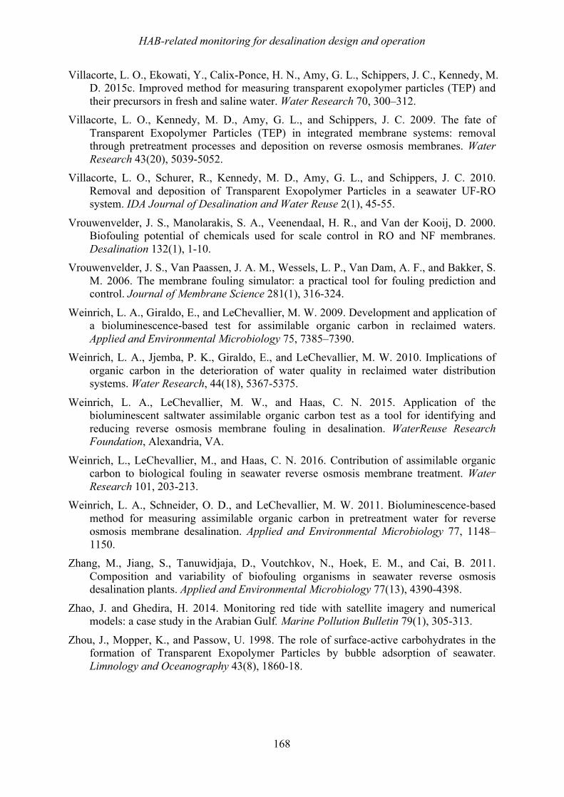
HAB-related monitoring for desalination design and operation

168

Villacorte, L. O., Ekowati, Y., Calix-Ponce, H. N., Amy, G. L., Schippers, J. C., Kennedy, M. D. 2015c. Improved method for measuring transparent exopolymer particles (TEP) and their precursors in fresh and saline water. Water Research 70, 300–312.

Villacorte, L. O., Kennedy, M. D., Amy, G. L., and Schippers, J. C. 2009. The fate of Transparent Exopolymer Particles (TEP) in integrated membrane systems: removal through pretreatment processes and deposition on reverse osmosis membranes. Water Research 43(20), 5039-5052.

Villacorte, L. O., Schurer, R., Kennedy, M. D., Amy, G. L., and Schippers, J. C. 2010. Removal and deposition of Transparent Exopolymer Particles in a seawater UF-RO system. IDA Journal of Desalination and Water Reuse 2(1), 45-55.

Vrouwenvelder, J. S., Manolarakis, S. A., Veenendaal, H. R., and Van der Kooij, D. 2000. Biofouling potential of chemicals used for scale control in RO and NF membranes. Desalination 132(1), 1-10.

Vrouwenvelder, J. S., Van Paassen, J. A. M., Wessels, L. P., Van Dam, A. F., and Bakker, S. M. 2006. The membrane fouling simulator: a practical tool for fouling prediction and control. Journal of Membrane Science 281(1), 316-324.

Weinrich, L. A., Giraldo, E., and LeChevallier, M. W. 2009. Development and application of a bioluminescence-based test for assimilable organic carbon in reclaimed waters. Applied and Environmental Microbiology 75, 7385–7390.

Weinrich, L. A., Jjemba, P. K., Giraldo, E., and LeChevallier, M. W. 2010. Implications of organic carbon in the deterioration of water quality in reclaimed water distribution systems. Water Research, 44(18), 5367-5375.

Weinrich, L. A., LeChevallier, M. W., and Haas, C. N. 2015. Application of the bioluminescent saltwater assimilable organic carbon test as a tool for identifying and reducing reverse osmosis membrane fouling in desalination. WaterReuse Research Foundation, Alexandria, VA.

Weinrich, L., LeChevallier, M., and Haas, C. N. 2016. Contribution of assimilable organic carbon to biological fouling in seawater reverse osmosis membrane treatment. Water Research 101, 203-213.

Weinrich, L. A., Schneider, O. D., and LeChevallier, M. W. 2011. Bioluminescence-based method for measuring assimilable organic carbon in pretreatment water for reverse osmosis membrane desalination. Applied and Environmental Microbiology 77, 1148–1150.

Zhang, M., Jiang, S., Tanuwidjaja, D., Voutchkov, N., Hoek, E. M., and Cai, B. 2011. Composition and variability of biofouling organisms in seawater reverse osmosis desalination plants. Applied and Environmental Microbiology 77(13), 4390-4398.

Zhao, J. and Ghedira, H. 2014. Monitoring red tide with satellite imagery and numerical models: a case study in the Arabian Gulf. Marine Pollution Bulletin 79(1), 305-313.

Zhou, J., Mopper, K., and Passow, U. 1998. The role of surface-active carbohydrates in the formation of Transparent Exopolymer Particles by bubble adsorption of seawater. Limnology and Oceanography 43(8), 1860-18.

Seawater intake considerations to mitigate HAB impacts

169

6 SEAWATER INTAKE CONSIDERATIONS TO MITIGATE HARMFUL ALGAL BLOOM IMPACTS

Siobhan F.E. Boerlage1, Thomas M. Missimer2, Thomas M. Pankratz3, and Donald M. Anderson4

1Boerlage Consulting, Gold Coast, Queensland, Australia 2Florida Gulf Coast University, Fort Myers, Florida 33965-6565 USA

3Water Desalination Report, Houston, TX, USA

4 Woods Hole Oceanographic Institution, Woods Hole, MA 02543 USA

6.1 Introduction ........................................................................................................................................... 169 6.2 Intake options for SWRO desalination plants ....................................................................................... 171 6.3 Surface intake and screen options ......................................................................................................... 172

6.3.1 Onshore and offshore intake screening ......................................................................................... 173 6.3.1.1 Traveling Water Screens ........................................................................................................ 174 6.3.1.2 Rotating Drum Screens .......................................................................................................... 174 6.3.1.3 Velocity Caps ......................................................................................................................... 175 6.3.1.4 Passive Screens ...................................................................................................................... 175 6.3.1.5 Intake Head ............................................................................................................................ 176

6.3.2 Surface intake strategies to minimize harmful algal bloom (HAB) impacts ................................. 176 6.3.3 Deep-water intakes ........................................................................................................................ 178

6.4 Subsurface intake options ...................................................................................................................... 181 6.4.1 Description of intake types with example installations ................................................................. 184

6.4.1.1 Conventional vertical wells ................................................................................................... 184 6.4.1.2 Collector or Ranney Wells ..................................................................................................... 187 6.4.1.3 Angle wells ............................................................................................................................ 188 6.4.1.4 Horizontal wells (HDD) ........................................................................................................ 188 6.4.1.5 Beach gallery systems ............................................................................................................ 189 6.4.1.6 Offshore or seabed gallery systems ....................................................................................... 190 6.4.1.7 New subsurface intake designs .............................................................................................. 192

6.4.2 Subsurface intake performance for algae and NOM removal ....................................................... 193 6.4.3 Planning of desalination plants with subsurface intakes ............................................................... 194

6.5 Siting of desalination seawater intakes ................................................................................................. 197 6.6 Summary ............................................................................................................................................... 199 6.7 References ............................................................................................................................................. 200

6.1 INTRODUCTION Seawater intakes are a key element in the design, construction and success of desalination plants. Various intake options exist and are generally classified based on their abstraction depth. Surface ocean intakes abstract seawater from the top of the water column or at depth, while subsurface1 intakes are embedded in the seabed or beach, thereby pre-filtering the abstracted seawater. Location, intake type and depth are important determinants of water quality. Intakes are also the first point of control in minimizing the ingress of algae into a plant or where algal impacts first manifest.

Originally the more robust thermal desalination processes dominated the desalination market where feedwater quality was not the primary driver in determining intake type or location. Instead, feedwater supply was critical, as thermal plants were configured as cogeneration power/desalination plants with common intakes with large volume requirements to generate 1 Note that ‘subsurface’ in this context differs from common oceanographic usage, in which the term refers to waters just below the air/water interface.

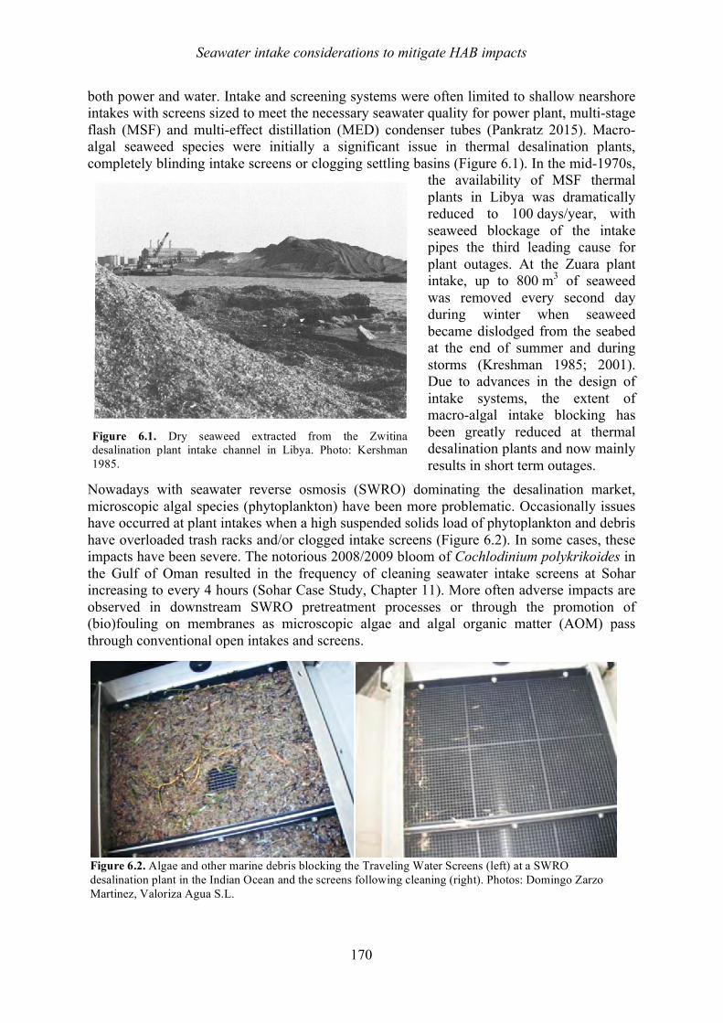
Seawater intake considerations to mitigate HAB impacts

170

both power and water. Intake and screening systems were often limited to shallow nearshore intakes with screens sized to meet the necessary seawater quality for power plant, multi-stage flash (MSF) and multi-effect distillation (MED) condenser tubes (Pankratz 2015). Macro-algal seaweed species were initially a significant issue in thermal desalination plants, completely blinding intake screens or clogging settling basins (Figure 6.1). In the mid-1970s,

the availability of MSF thermal plants in Libya was dramatically reduced to 100 days/year, with seaweed blockage of the intake pipes the third leading cause for plant outages. At the Zuara plant intake, up to 800 m3 of seaweed was removed every second day during winter when seaweed became dislodged from the seabed at the end of summer and during storms (Kreshman 1985; 2001). Due to advances in the design of intake systems, the extent of macro-algal intake blocking has been greatly reduced at thermal desalination plants and now mainly results in short term outages.

Nowadays with seawater reverse osmosis (SWRO) dominating the desalination market, microscopic algal species (phytoplankton) have been more problematic. Occasionally issues have occurred at plant intakes when a high suspended solids load of phytoplankton and debris have overloaded trash racks and/or clogged intake screens (Figure 6.2). In some cases, these impacts have been severe. The notorious 2008/2009 bloom of Cochlodinium polykrikoides in the Gulf of Oman resulted in the frequency of cleaning seawater intake screens at Sohar increasing to every 4 hours (Sohar Case Study, Chapter 11). More often adverse impacts are observed in downstream SWRO pretreatment processes or through the promotion of (bio)fouling on membranes as microscopic algae and algal organic matter (AOM) pass through conventional open intakes and screens.

Figure 6.1. Dry seaweed extracted from the Zwitina desalination plant intake channel in Libya. Photo: Kershman 1985.

Figure 6.2. Algae and other marine debris blocking the Traveling Water Screens (left) at a SWRO desalination plant in the Indian Ocean and the screens following cleaning (right). Photos: Domingo Zarzo Martinez, Valoriza Agua S.L.

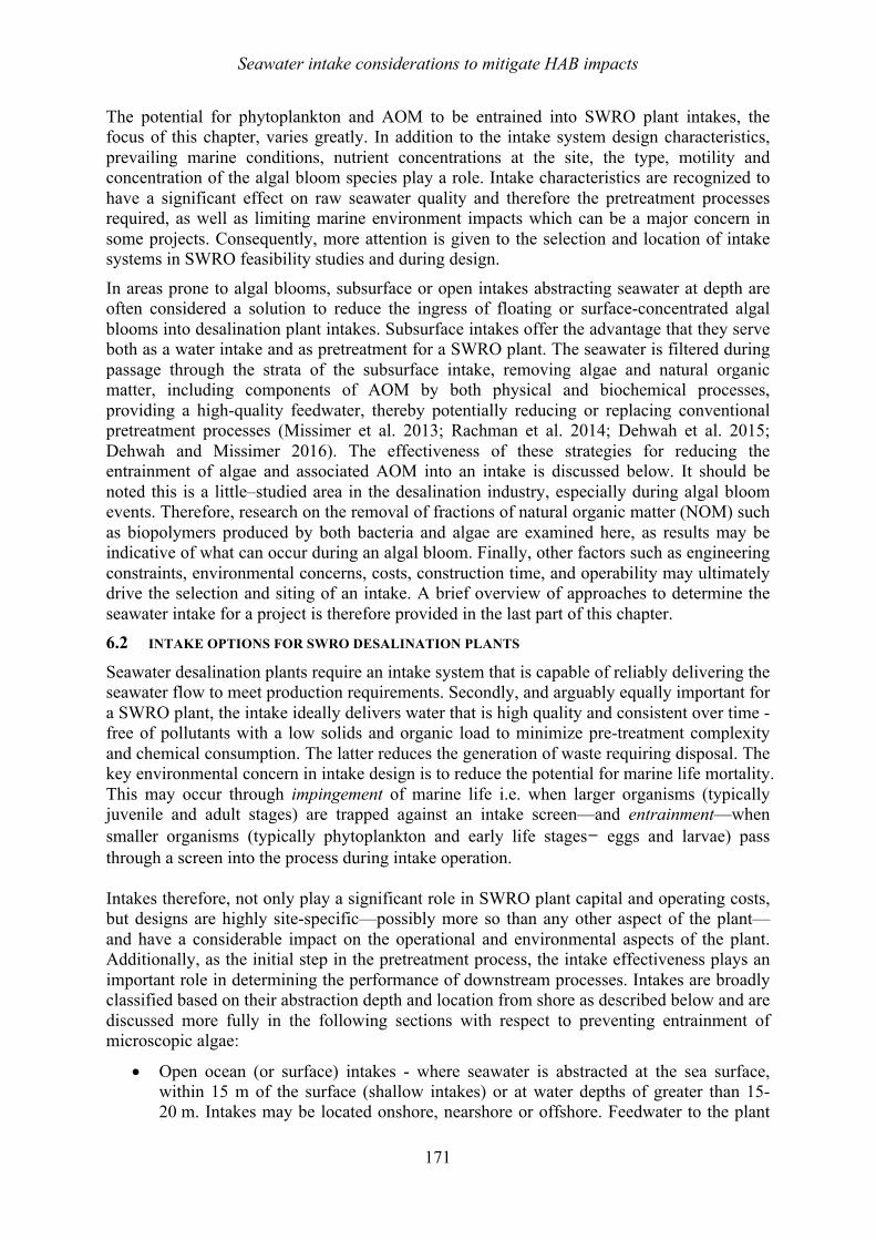
Seawater intake considerations to mitigate HAB impacts

171

The potential for phytoplankton and AOM to be entrained into SWRO plant intakes, the focus of this chapter, varies greatly. In addition to the intake system design characteristics, prevailing marine conditions, nutrient concentrations at the site, the type, motility and concentration of the algal bloom species play a role. Intake characteristics are recognized to have a significant effect on raw seawater quality and therefore the pretreatment processes required, as well as limiting marine environment impacts which can be a major concern in some projects. Consequently, more attention is given to the selection and location of intake systems in SWRO feasibility studies and during design.

In areas prone to algal blooms, subsurface or open intakes abstracting seawater at depth are often considered a solution to reduce the ingress of floating or surface-concentrated algal blooms into desalination plant intakes. Subsurface intakes offer the advantage that they serve both as a water intake and as pretreatment for a SWRO plant. The seawater is filtered during passage through the strata of the subsurface intake, removing algae and natural organic matter, including components of AOM by both physical and biochemical processes, providing a high-quality feedwater, thereby potentially reducing or replacing conventional pretreatment processes (Missimer et al. 2013; Rachman et al. 2014; Dehwah et al. 2015; Dehwah and Missimer 2016). The effectiveness of these strategies for reducing the entrainment of algae and associated AOM into an intake is discussed below. It should be noted this is a little–studied area in the desalination industry, especially during algal bloom events. Therefore, research on the removal of fractions of natural organic matter (NOM) such as biopolymers produced by both bacteria and algae are examined here, as results may be indicative of what can occur during an algal bloom. Finally, other factors such as engineering constraints, environmental concerns, costs, construction time, and operability may ultimately drive the selection and siting of an intake. A brief overview of approaches to determine the seawater intake for a project is therefore provided in the last part of this chapter. 6.2 INTAKE OPTIONS FOR SWRO DESALINATION PLANTS

Seawater desalination plants require an intake system that is capable of reliably delivering the seawater flow to meet production requirements. Secondly, and arguably equally important for a SWRO plant, the intake ideally delivers water that is high quality and consistent over time - free of pollutants with a low solids and organic load to minimize pre-treatment complexity and chemical consumption. The latter reduces the generation of waste requiring disposal. The key environmental concern in intake design is to reduce the potential for marine life mortality. This may occur through impingement of marine life i.e. when larger organisms (typically juvenile and adult stages) are trapped against an intake screen—and entrainment—when smaller organisms (typically phytoplankton and early life stages— eggs and larvae) pass through a screen into the process during intake operation. Intakes therefore, not only play a significant role in SWRO plant capital and operating costs, but designs are highly site-specific—possibly more so than any other aspect of the plant—and have a considerable impact on the operational and environmental aspects of the plant. Additionally, as the initial step in the pretreatment process, the intake effectiveness plays an important role in determining the performance of downstream processes. Intakes are broadly classified based on their abstraction depth and location from shore as described below and are discussed more fully in the following sections with respect to preventing entrainment of microscopic algae:

• Open ocean (or surface) intakes - where seawater is abstracted at the sea surface, within 15 m of the surface (shallow intakes) or at water depths of greater than 15- 20 m. Intakes may be located onshore, nearshore or offshore. Feedwater to the plant

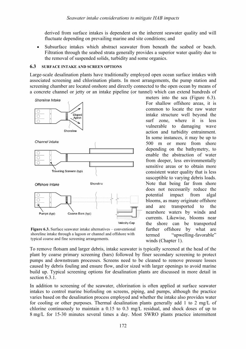
Seawater intake considerations to mitigate HAB impacts

172

derived from surface intakes is dependent on the inherent seawater quality and will fluctuate depending on prevailing marine and site conditions; and

• Subsurface intakes which abstract seawater from beneath the seabed or beach. Filtration through the seabed strata generally provides a superior water quality due to the removal of suspended solids, turbidity and some organics.

6.3 SURFACE INTAKE AND SCREEN OPTIONS

Large-scale desalination plants have traditionally employed open ocean surface intakes with associated screening and chlorination plants. In most arrangements, the pump station and screening chamber are located onshore and directly connected to the open ocean by means of a concrete channel or jetty or an intake pipeline (or tunnel) which can extend hundreds of

meters into the sea (Figure 6.3). For shallow offshore areas, it is common to locate the raw water intake structure well beyond the surf zone, where it is less vulnerable to damaging wave action and turbidity entrainment. In some instances, it may be up to 500 m or more from shore depending on the bathymetry, to enable the abstraction of water from deeper, less environmentally sensitive areas or to obtain more consistent water quality that is less susceptible to varying debris loads. Note that being far from shore does not necessarily reduce the potential impact from algal blooms, as many originate offshore and are transported to the nearshore waters by winds and currents. Likewise, blooms near the shore can be transported further offshore by what are termed “upwelling-favorable” winds (Chapter 1).

To remove flotsam and larger debris, intake seawater is typically screened at the head of the plant by coarse primary screening (bars) followed by finer secondary screening to protect pumps and downstream processes. Screens need to be cleaned to remove pressure losses caused by debris fouling and ensure flow, and/or sized with larger openings to avoid marine build up. Typical screening options for desalination plants are discussed in more detail in section 6.3.1.

In addition to screening of the seawater, chlorination is often applied at surface seawater intakes to control marine biofouling on screens, piping, and pumps, although the practice varies based on the desalination process employed and whether the intake also provides water for cooling or other purposes. Thermal desalination plants generally add 1 to 2 mg/L of chlorine continuously to maintain a 0.15 to 0.3 mg/L residual, and shock doses of up to 8 mg/L for 15-30 minutes several times a day. Most SWRO plants practice intermittent

Figure 6.3. Surface seawater intake alternatives – conventional shoreline intake through a lagoon or channel and offshore with typical coarse and fine screening arrangements.

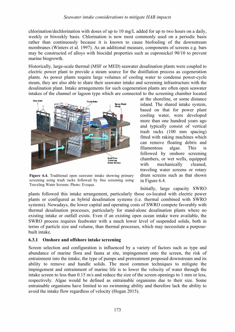
Seawater intake considerations to mitigate HAB impacts

173

chlorination/dechlorination with doses of up to 10 mg/L added for up to two hours on a daily, weekly or biweekly basis. Chlorination is now most commonly used on a periodic basis rather than continuously because it is known to cause biofouling of the downstream membranes (Winters et al. 1997). As an additional measure, components of screens e.g. bars may be constructed of alloys with biocidal properties such as cupronickel 90/10 to prevent marine biogrowth.

Historically, large-scale thermal (MSF or MED) seawater desalination plants were coupled to electric power plant to provide a steam source for the distillation process as cogeneration plants. As power plants require large volumes of cooling water to condense power-cycle steam, they are also able to share their seawater intake and screening infrastructure with the desalination plant. Intake arrangements for such cogeneration plants are often open seawater intakes of the channel or lagoon type which are connected to the screening chamber located

at the shoreline, or some distance inland. The shared intake system, based on that for power plant cooling water, were developed more than one hundred years ago and typically consist of vertical trash racks (100 mm spacing) fitted with raking machines which can remove floating debris and filamentous algae. This is followed by onshore screening chambers, or wet wells, equipped with mechanically cleaned, traveling water screens or rotary drum screens such as that shown in Figure 6.4.

Initially, large capacity SWRO plants followed this intake arrangement, particularly those co-located with electric power plants or configured as hybrid desalination systems (i.e. thermal combined with SWRO systems). Nowadays, the lower capital and operating costs of SWRO compete favorably with thermal desalination processes, particularly for stand-alone desalination plants where no existing intake or outfall exists. Even if an existing open ocean intake were available, the SWRO process requires feedwater with a much lower level of suspended solids, both in terms of particle size and volume, than thermal processes, which may necessitate a purpose-built intake. 6.3.1 Onshore and offshore intake screening

Screen selection and configuration is influenced by a variety of factors such as type and abundance of marine flora and fauna at site, impingement onto the screen, the risk of entrainment into the intake, the type of pumps and pretreatment proposed downstream and its ability to remove and handle solids. The most common techniques to mitigate the impingement and entrainment of marine life is to lower the velocity of water through the intake screen to less than 0.15 m/s and reduce the size of the screen openings to 1 mm or less, respectively. Algae would be defined as entrainable organisms due to their size. Some entrainable organisms have limited to no swimming ability and therefore lack the ability to avoid the intake flow regardless of velocity (Hogan 2015).

Figure 6.4. Traditional open seawater intake showing primary screening using trash racks followed by fine screening using Traveling Water Screens. Photo: Evoqua.

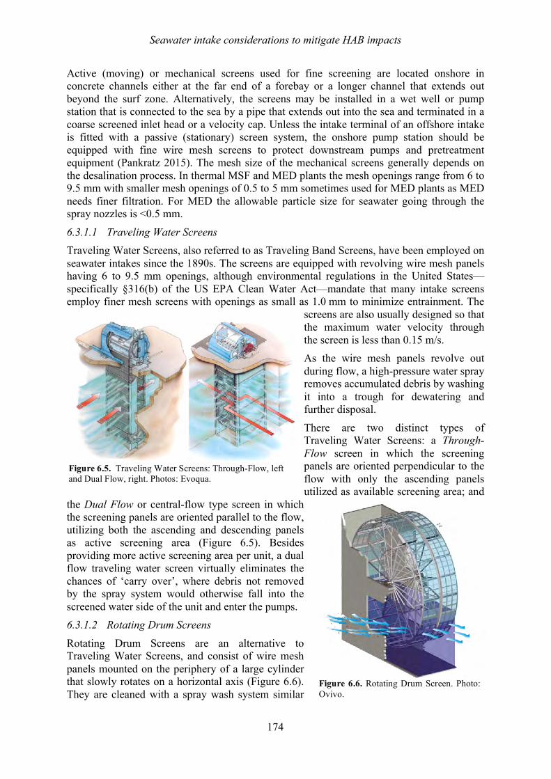
Seawater intake considerations to mitigate HAB impacts

174

Active (moving) or mechanical screens used for fine screening are located onshore in concrete channels either at the far end of a forebay or a longer channel that extends out beyond the surf zone. Alternatively, the screens may be installed in a wet well or pump station that is connected to the sea by a pipe that extends out into the sea and terminated in a coarse screened inlet head or a velocity cap. Unless the intake terminal of an offshore intake is fitted with a passive (stationary) screen system, the onshore pump station should be equipped with fine wire mesh screens to protect downstream pumps and pretreatment equipment (Pankratz 2015). The mesh size of the mechanical screens generally depends on the desalination process. In thermal MSF and MED plants the mesh openings range from 6 to 9.5 mm with smaller mesh openings of 0.5 to 5 mm sometimes used for MED plants as MED needs finer filtration. For MED the allowable particle size for seawater going through the spray nozzles is <0.5 mm.

6.3.1.1 Traveling Water Screens Traveling Water Screens, also referred to as Traveling Band Screens, have been employed on seawater intakes since the 1890s. The screens are equipped with revolving wire mesh panels having 6 to 9.5 mm openings, although environmental regulations in the United States—specifically §316(b) of the US EPA Clean Water Act—mandate that many intake screens employ finer mesh screens with openings as small as 1.0 mm to minimize entrainment. The

screens are also usually designed so that the maximum water velocity through the screen is less than 0.15 m/s. As the wire mesh panels revolve out during flow, a high-pressure water spray removes accumulated debris by washing it into a trough for dewatering and further disposal.

There are two distinct types of Traveling Water Screens: a Through-Flow screen in which the screening panels are oriented perpendicular to the flow with only the ascending panels utilized as available screening area; and

the Dual Flow or central-flow type screen in which the screening panels are oriented parallel to the flow, utilizing both the ascending and descending panels as active screening area (Figure 6.5). Besides providing more active screening area per unit, a dual flow traveling water screen virtually eliminates the chances of ‘carry over’, where debris not removed by the spray system would otherwise fall into the screened water side of the unit and enter the pumps. 6.3.1.2 Rotating Drum Screens

Rotating Drum Screens are an alternative to Traveling Water Screens, and consist of wire mesh panels mounted on the periphery of a large cylinder that slowly rotates on a horizontal axis (Figure 6.6). They are cleaned with a spray wash system similar

Figure 6.5. Traveling Water Screens: Through-Flow, left and Dual Flow, right. Photos: Evoqua.

Figure 6.6. Rotating Drum Screen. Photo: Ovivo.

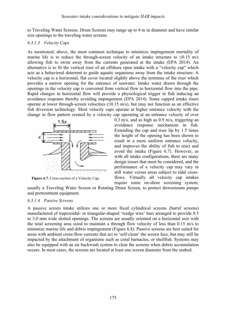
Seawater intake considerations to mitigate HAB impacts

175

to Traveling Water Screens. Drum Screens may range up to 4 m in diameter and have similar size openings to the traveling water screens.

6.3.1.3 Velocity Caps

As mentioned, above, the most common technique to minimize impingement mortality of marine life is to reduce the through-screen velocity of an intake structure to ≤0.15 m/s allowing fish to swim away from the currents generated at the intake (EPA 2014). An alternative is to fit the vertical riser of an offshore open intake with a “velocity cap” which acts as a behavioral deterrent to guide aquatic organisms away from the intake structure. A velocity cap is a horizontal, flat cover located slightly above the terminus of the riser which provides a narrow opening for the entrance of seawater. Intake water drawn through the openings in the velocity cap is converted from vertical flow to horizontal flow into the pipe. Rapid changes in horizontal flow will provide a physiological trigger in fish inducing an avoidance response thereby avoiding impingement (EPA 2014). Some capped intake risers operate at lower through-screen velocities (≤0.15 m/s), but may not function as an effective fish diversion technology. Most velocity caps operate at higher entrance velocity with the change in flow pattern created by a velocity cap operating at an entrance velocity of over

0.3 m/s, and as high as 0.9 m/s, triggering an avoidance response mechanism in fish. Extending the cap and riser lip by 1.5 times the height of the opening has been shown to result in a more uniform entrance velocity, and improves the ability of fish to react and avoid the intake (Figure 6.7). However, as with all intake configurations, there are many design issues that must be considered, and the performance of a velocity cap may vary in still water versus areas subject to tidal cross-flows. Virtually all velocity cap intakes require some on-shore screening system,

usually a Traveling Water Screen or Rotating Drum Screen, to protect downstream pumps and pretreatment equipment. 6.3.1.4 Passive Screens

A passive screen intake utilizes one or more fixed cylindrical screens (barrel screens) manufactured of trapezoidal- or triangular-shaped ‘wedge wire’ bars arranged to provide 0.5 to 3.0 mm wide slotted openings. The screens are usually oriented on a horizontal axis with the total screening area sized to maintain a through flow velocity of less than 0.15 m/s to minimize marine life and debris impingement (Figure 6.8). Passive screens are best suited for areas with ambient cross-flow currents that act to ‘self-clean’ the screen face, but may still be impacted by the attachment of organisms such as coral barnacles, or shellfish. Systems may also be equipped with an air backwash system to clear the screens when debris accumulation occurs. In most cases, the screens are located at least one screen diameter from the seabed.

Figure 6.7. Cross-section of a Velocity Cap.

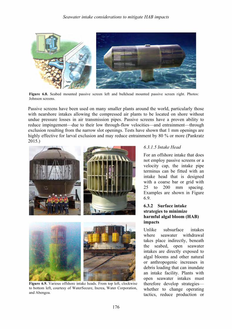
Seawater intake considerations to mitigate HAB impacts

176

Passive screens have been used on many smaller plants around the world, particularly those with nearshore intakes allowing the compressed air plants to be located on shore without undue pressure losses in air transmission pipes. Passive screens have a proven ability to reduce impingement—due to their low through-flow velocities—and entrainment—through exclusion resulting from the narrow slot openings. Tests have shown that 1 mm openings are highly effective for larval exclusion and may reduce entrainment by 80 % or more (Pankratz 2015.)

6.3.1.5 Intake Head

For an offshore intake that does not employ passive screens or a velocity cap, the intake pipe terminus can be fitted with an intake head that is designed with a coarse bar or grid with 25 to 200 mm spacing. Examples are shown in Figure 6.9. 6.3.2 Surface intake strategies to minimize harmful algal bloom (HAB) impacts Unlike subsurface intakes where seawater withdrawal takes place indirectly, beneath the seabed, open seawater intakes are directly exposed to algal blooms and other natural or anthropogenic increases in debris loading that can inundate an intake facility. Plants with open seawater intakes must therefore develop strategies—whether to change operating tactics, reduce production or

Figure 6.9. Various offshore intake heads. From top left, clockwise to bottom left, courtesy of WaterSecure, Increa, Water Corporation, and Abengoa.

Figure 6.8. Seabed mounted passive screen left and bulkhead mounted passive screen right. Photos: Johnson screens.

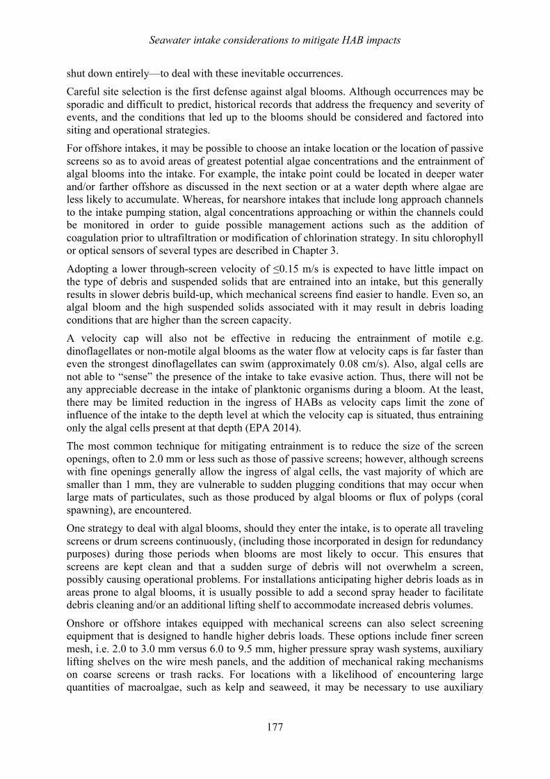
Seawater intake considerations to mitigate HAB impacts

177

shut down entirely—to deal with these inevitable occurrences. Careful site selection is the first defense against algal blooms. Although occurrences may be sporadic and difficult to predict, historical records that address the frequency and severity of events, and the conditions that led up to the blooms should be considered and factored into siting and operational strategies. For offshore intakes, it may be possible to choose an intake location or the location of passive screens so as to avoid areas of greatest potential algae concentrations and the entrainment of algal blooms into the intake. For example, the intake point could be located in deeper water and/or farther offshore as discussed in the next section or at a water depth where algae are less likely to accumulate. Whereas, for nearshore intakes that include long approach channels to the intake pumping station, algal concentrations approaching or within the channels could be monitored in order to guide possible management actions such as the addition of coagulation prior to ultrafiltration or modification of chlorination strategy. In situ chlorophyll or optical sensors of several types are described in Chapter 3.

Adopting a lower through-screen velocity of ≤0.15 m/s is expected to have little impact on the type of debris and suspended solids that are entrained into an intake, but this generally results in slower debris build-up, which mechanical screens find easier to handle. Even so, an algal bloom and the high suspended solids associated with it may result in debris loading conditions that are higher than the screen capacity. A velocity cap will also not be effective in reducing the entrainment of motile e.g. dinoflagellates or non-motile algal blooms as the water flow at velocity caps is far faster than even the strongest dinoflagellates can swim (approximately 0.08 cm/s). Also, algal cells are not able to “sense” the presence of the intake to take evasive action. Thus, there will not be any appreciable decrease in the intake of planktonic organisms during a bloom. At the least, there may be limited reduction in the ingress of HABs as velocity caps limit the zone of influence of the intake to the depth level at which the velocity cap is situated, thus entraining only the algal cells present at that depth (EPA 2014). The most common technique for mitigating entrainment is to reduce the size of the screen openings, often to 2.0 mm or less such as those of passive screens; however, although screens with fine openings generally allow the ingress of algal cells, the vast majority of which are smaller than 1 mm, they are vulnerable to sudden plugging conditions that may occur when large mats of particulates, such as those produced by algal blooms or flux of polyps (coral spawning), are encountered. One strategy to deal with algal blooms, should they enter the intake, is to operate all traveling screens or drum screens continuously, (including those incorporated in design for redundancy purposes) during those periods when blooms are most likely to occur. This ensures that screens are kept clean and that a sudden surge of debris will not overwhelm a screen, possibly causing operational problems. For installations anticipating higher debris loads as in areas prone to algal blooms, it is usually possible to add a second spray header to facilitate debris cleaning and/or an additional lifting shelf to accommodate increased debris volumes.

Onshore or offshore intakes equipped with mechanical screens can also select screening equipment that is designed to handle higher debris loads. These options include finer screen mesh, i.e. 2.0 to 3.0 mm versus 6.0 to 9.5 mm, higher pressure spray wash systems, auxiliary lifting shelves on the wire mesh panels, and the addition of mechanical raking mechanisms on coarse screens or trash racks. For locations with a likelihood of encountering large quantities of macroalgae, such as kelp and seaweed, it may be necessary to use auxiliary

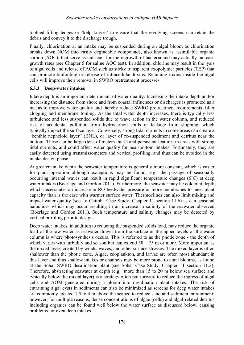
Seawater intake considerations to mitigate HAB impacts

178

toothed lifting ledges or ‘kelp knives’ to ensure that the revolving screens can retain the debris and convey it to the discharge trough.

Finally, chlorination at an intake may be suspended during an algal bloom as chlorination breaks down NOM into easily degradable compounds, also known as assimilable organic carbon (AOC), that serve as nutrients for the regrowth of bacteria and may actually increase growth rates (see Chapter 5 for saline AOC test). In addition, chlorine may result in the lysis of algal cells and release of AOM such as sticky transparent exopolymer particles (TEP) that can promote biofouling or release of intracellular toxins. Retaining toxins inside the algal cells will improve their removal in SWRO pretreatment processes. 6.3.3 Deep-water intakes

Intake depth is an important determinant of water quality. Increasing the intake depth and/or increasing the distance from shore and from coastal influences or discharges is promoted as a means to improve water quality and thereby reduce SWRO pretreatment requirements, filter clogging and membrane fouling. As the total water depth increases, there is typically less turbulence and less suspended solids due to wave action in the water column, and reduced risk of accidental pollution from hydrocarbon spills or leakage from shipping, which typically impact the surface layer. Conversely, strong tidal currents in some areas can create a “benthic nepheloid layer” (BNL), or layer of re-suspended sediment and detritus near the bottom. These can be large (tens of meters thick) and persistent features in areas with strong tidal currents, and could affect water quality for near-bottom intakes. Fortunately, they are easily detected using transmissometers and vertical profiling, and thus can be avoided in the intake design phase.

At greater intake depth the seawater temperature is generally more constant, which is easier for plant operation although exceptions may be found, e.g., the passage of seasonally occurring internal waves can result in rapid significant temperature changes (6˚C) at deep water intakes (Boerlage and Gordon 2011). Furthermore, the seawater may be colder at depth, which necessitates an increase in RO feedwater pressure or more membranes to meet plant capacity than is the case with warmer surface water. Thermoclines can also limit mixing and impact water quality (see La Chimba Case Study, Chapter 11 section 11.6) as can seasonal haloclines which may occur resulting in an increase in salinity of the seawater observed (Boerlage and Gordon 2011). Such temperature and salinity changes may be detected by vertical profiling prior to design.

Deep water intakes, in addition to reducing the suspended solids load, may reduce the organic load of the raw water as seawater drawn from the surface or the upper levels of the water column is where photosynthesis occurs. This is referred to as the photic zone - the depth of which varies with turbidity and season but can extend 50 – 75 m or more. More important is the mixed layer, created by winds, waves, and other surface stresses. The mixed layer is often shallower than the photic zone. Algae, zooplankton, and larvae are often most abundant in this layer and thus shallow intakes or channels may be more prone to algal blooms, as found at the Sohar SWRO desalination plant (see Sohar Case Study, Chapter 11 section 11.2). Therefore, abstracting seawater at depth (e.g. more than 15 to 20 m below sea surface and typically below the mixed layer) is a strategy often put forward to reduce the ingress of algal cells and AOM generated during a bloom into desalination plant intakes. The risk of entraining algal cysts in sediments can also be minimized as screens for deep water intakes are commonly located 1.5 to 4 m above the seabed to reduce sand and sediment entrainment; however, for multiple reasons, dense concentrations of algae (cells) and algal-related detritus including organics can be found well below the water surface as discussed below, causing problems for even deep intakes.

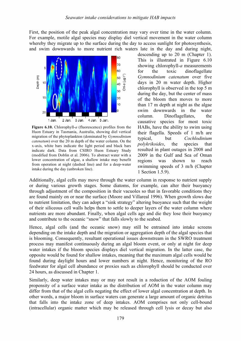
Seawater intake considerations to mitigate HAB impacts

179

First, the position of the peak algal concentration may vary over time in the water column. For example, motile algal species may display diel vertical movement in the water column whereby they migrate up to the surface during the day to access sunlight for photosynthesis, and swim downwards to more nutrient rich waters late in the day and during night,

descending up to 20 m (Chapter 1). This is illustrated in Figure 6.10 showing chlorophyll-a measurements for the toxic dinoflagellate Gymnodinium catenatum over five days in 20 m water depth. Higher chlorophyll is observed in the top 5 m during the day, but the center of mass of the bloom then moves to more than 17 m depth at night as the algae swim downwards in the water column. Dinoflagellates, the causative species for most toxic HABs, have the ability to swim using their flagella. Speeds of 1 m/h are typical, but Cochlodinium polykrikoides, the species that resulted in plant outages in 2008 and 2009 in the Gulf and Sea of Oman regions was shown to reach swimming speeds of 3 m/h (Chapter 1 Section 1.5.9).

Additionally, algal cells may move through the water column in response to nutrient supply or during various growth stages. Some diatoms, for example, can alter their buoyancy through adjustment of the composition in their vacuoles so that in favorable conditions they are found mainly on or near the surface (Moore and Villareal 1996). When growth slows due to nutrient limitation, they can adopt a “sink strategy” altering buoyance such that the weight of their siliceous cell walls helps them to settle to deeper layers of the water column where nutrients are more abundant. Finally, when algal cells age and die they lose their buoyancy and contribute to the oceanic “snow” that falls slowly to the seabed.

Hence, algal cells (and the oceanic snow) may still be entrained into intake screens depending on the intake depth and the migration or aggregation depth of the algal species that is blooming. Consequently, resultant operational issues downstream in the SWRO treatment process may manifest continuously during an algal bloom event, or only at night for deep water intakes if the bloom species displays diel vertical migration. In the latter case, the opposite would be found for shallow intakes, meaning that the maximum algal cells would be found during daylight hours and lower numbers at night. Hence, monitoring of the RO feedwater for algal cell abundance or proxies such as chlorophyll should be conducted over 24 hours, as discussed in Chapter 1. Similarly, deep water intakes may or may not result in a reduction of the AOM fouling propensity of a surface water intake as the distribution of AOM in the water column may differ from that of the algal cells negating the effect of lower algal concentration at depth. In other words, a major bloom in surface waters can generate a large amount of organic detritus that falls into the intake zone of deep intakes. AOM comprises not only cell-bound (intracellular) organic matter which may be released through cell lysis or decay but also

Figure 6.10. Chlorophyll-a (fluorescence) profiles from the Huon Estuary in Tasmania, Australia, showing diel vertical migration of the phytoplankton (dominated by Gymnodinium catenatum) over the 20 m depth of the water column. On the x-axis, white bars indicate the light period and black bars indicate dark. Data from CSIRO Huon Estuary Study (modified from Doblin et al. 2006). To abstract water with a lower concentration of algae, a shallow intake may benefit from operation at night (dashed line) and for a deep-water intake during the day (unbroken line).

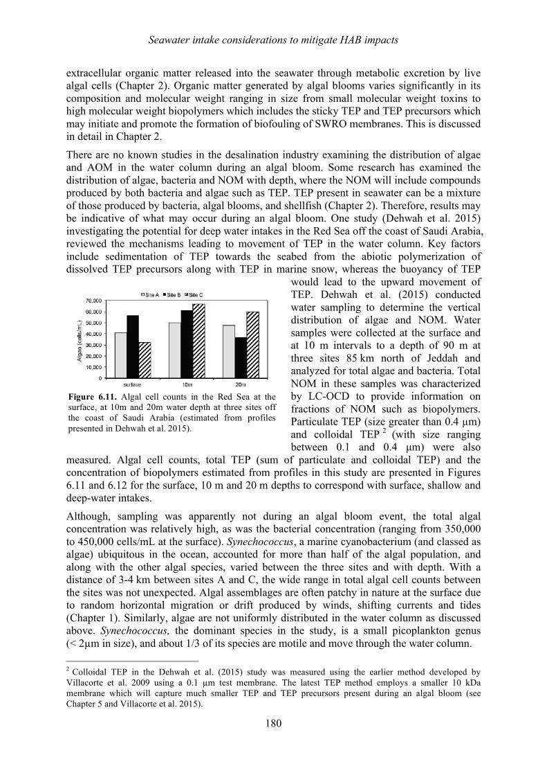
Seawater intake considerations to mitigate HAB impacts

180

extracellular organic matter released into the seawater through metabolic excretion by live algal cells (Chapter 2). Organic matter generated by algal blooms varies significantly in its composition and molecular weight ranging in size from small molecular weight toxins to high molecular weight biopolymers which includes the sticky TEP and TEP precursors which may initiate and promote the formation of biofouling of SWRO membranes. This is discussed in detail in Chapter 2.

There are no known studies in the desalination industry examining the distribution of algae and AOM in the water column during an algal bloom. Some research has examined the distribution of algae, bacteria and NOM with depth, where the NOM will include compounds produced by both bacteria and algae such as TEP. TEP present in seawater can be a mixture of those produced by bacteria, algal blooms, and shellfish (Chapter 2). Therefore, results may be indicative of what may occur during an algal bloom. One study (Dehwah et al. 2015) investigating the potential for deep water intakes in the Red Sea off the coast of Saudi Arabia, reviewed the mechanisms leading to movement of TEP in the water column. Key factors include sedimentation of TEP towards the seabed from the abiotic polymerization of dissolved TEP precursors along with TEP in marine snow, whereas the buoyancy of TEP

would lead to the upward movement of TEP. Dehwah et al. (2015) conducted water sampling to determine the vertical distribution of algae and NOM. Water samples were collected at the surface and at 10 m intervals to a depth of 90 m at three sites 85 km north of Jeddah and analyzed for total algae and bacteria. Total NOM in these samples was characterized by LC-OCD to provide information on fractions of NOM such as biopolymers. Particulate TEP (size greater than 0.4 µm) and colloidal TEP 2 (with size ranging between 0.1 and 0.4 µm) were also

measured. Algal cell counts, total TEP (sum of particulate and colloidal TEP) and the concentration of biopolymers estimated from profiles in this study are presented in Figures 6.11 and 6.12 for the surface, 10 m and 20 m depths to correspond with surface, shallow and deep-water intakes.

Although, sampling was apparently not during an algal bloom event, the total algal concentration was relatively high, as was the bacterial concentration (ranging from 350,000 to 450,000 cells/mL at the surface). Synechococcus, a marine cyanobacterium (and classed as algae) ubiquitous in the ocean, accounted for more than half of the algal population, and along with the other algal species, varied between the three sites and with depth. With a distance of 3-4 km between sites A and C, the wide range in total algal cell counts between the sites was not unexpected. Algal assemblages are often patchy in nature at the surface due to random horizontal migration or drift produced by winds, shifting currents and tides (Chapter 1). Similarly, algae are not uniformly distributed in the water column as discussed above. Synechococcus, the dominant species in the study, is a small picoplankton genus (< 2µm in size), and about 1/3 of its species are motile and move through the water column. 2 Colloidal TEP in the Dehwah et al. (2015) study was measured using the earlier method developed by Villacorte et al. 2009 using a 0.1 µm test membrane. The latest TEP method employs a smaller 10 kDa membrane which will capture much smaller TEP and TEP precursors present during an algal bloom (see Chapter 5 and Villacorte et al. 2015).

Figure 6.11. Algal cell counts in the Red Sea at the surface, at 10m and 20m water depth at three sites off the coast of Saudi Arabia (estimated from profiles presented in Dehwah et al. 2015).

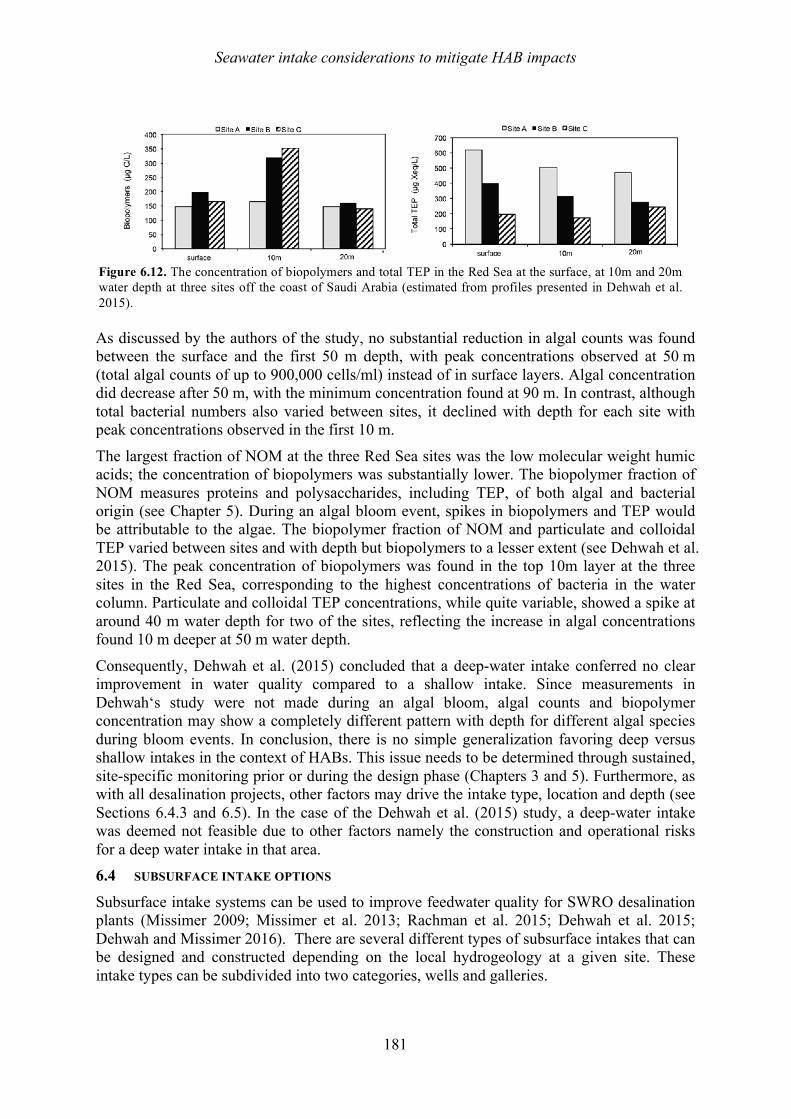
Seawater intake considerations to mitigate HAB impacts

181

As discussed by the authors of the study, no substantial reduction in algal counts was found between the surface and the first 50 m depth, with peak concentrations observed at 50 m (total algal counts of up to 900,000 cells/ml) instead of in surface layers. Algal concentration did decrease after 50 m, with the minimum concentration found at 90 m. In contrast, although total bacterial numbers also varied between sites, it declined with depth for each site with peak concentrations observed in the first 10 m.

The largest fraction of NOM at the three Red Sea sites was the low molecular weight humic acids; the concentration of biopolymers was substantially lower. The biopolymer fraction of NOM measures proteins and polysaccharides, including TEP, of both algal and bacterial origin (see Chapter 5). During an algal bloom event, spikes in biopolymers and TEP would be attributable to the algae. The biopolymer fraction of NOM and particulate and colloidal TEP varied between sites and with depth but biopolymers to a lesser extent (see Dehwah et al. 2015). The peak concentration of biopolymers was found in the top 10m layer at the three sites in the Red Sea, corresponding to the highest concentrations of bacteria in the water column. Particulate and colloidal TEP concentrations, while quite variable, showed a spike at around 40 m water depth for two of the sites, reflecting the increase in algal concentrations found 10 m deeper at 50 m water depth.

Consequently, Dehwah et al. (2015) concluded that a deep-water intake conferred no clear improvement in water quality compared to a shallow intake. Since measurements in Dehwah‘s study were not made during an algal bloom, algal counts and biopolymer concentration may show a completely different pattern with depth for different algal species during bloom events. In conclusion, there is no simple generalization favoring deep versus shallow intakes in the context of HABs. This issue needs to be determined through sustained, site-specific monitoring prior or during the design phase (Chapters 3 and 5). Furthermore, as with all desalination projects, other factors may drive the intake type, location and depth (see Sections 6.4.3 and 6.5). In the case of the Dehwah et al. (2015) study, a deep-water intake was deemed not feasible due to other factors namely the construction and operational risks for a deep water intake in that area. 6.4 SUBSURFACE INTAKE OPTIONS

Subsurface intake systems can be used to improve feedwater quality for SWRO desalination plants (Missimer 2009; Missimer et al. 2013; Rachman et al. 2015; Dehwah et al. 2015; Dehwah and Missimer 2016). There are several different types of subsurface intakes that can be designed and constructed depending on the local hydrogeology at a given site. These intake types can be subdivided into two categories, wells and galleries.

Figure 6.12. The concentration of biopolymers and total TEP in the Red Sea at the surface, at 10m and 20m water depth at three sites off the coast of Saudi Arabia (estimated from profiles presented in Dehwah et al. 2015).

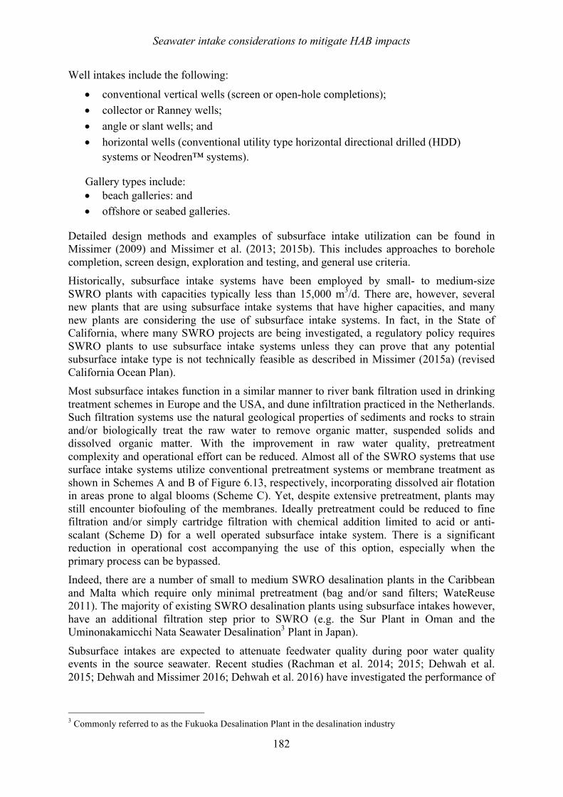
Seawater intake considerations to mitigate HAB impacts

182

Well intakes include the following:

• conventional vertical wells (screen or open-hole completions); • collector or Ranney wells; • angle or slant wells; and • horizontal wells (conventional utility type horizontal directional drilled (HDD)

systems or Neodren™ systems).

Gallery types include: • beach galleries: and • offshore or seabed galleries.

Detailed design methods and examples of subsurface intake utilization can be found in Missimer (2009) and Missimer et al. (2013; 2015b). This includes approaches to borehole completion, screen design, exploration and testing, and general use criteria. Historically, subsurface intake systems have been employed by small- to medium-size SWRO plants with capacities typically less than 15,000 m3/d. There are, however, several new plants that are using subsurface intake systems that have higher capacities, and many new plants are considering the use of subsurface intake systems. In fact, in the State of California, where many SWRO projects are being investigated, a regulatory policy requires SWRO plants to use subsurface intake systems unless they can prove that any potential subsurface intake type is not technically feasible as described in Missimer (2015a) (revised California Ocean Plan). Most subsurface intakes function in a similar manner to river bank filtration used in drinking treatment schemes in Europe and the USA, and dune infiltration practiced in the Netherlands. Such filtration systems use the natural geological properties of sediments and rocks to strain and/or biologically treat the raw water to remove organic matter, suspended solids and dissolved organic matter. With the improvement in raw water quality, pretreatment complexity and operational effort can be reduced. Almost all of the SWRO systems that use surface intake systems utilize conventional pretreatment systems or membrane treatment as shown in Schemes A and B of Figure 6.13, respectively, incorporating dissolved air flotation in areas prone to algal blooms (Scheme C). Yet, despite extensive pretreatment, plants may still encounter biofouling of the membranes. Ideally pretreatment could be reduced to fine filtration and/or simply cartridge filtration with chemical addition limited to acid or anti-scalant (Scheme D) for a well operated subsurface intake system. There is a significant reduction in operational cost accompanying the use of this option, especially when the primary process can be bypassed. Indeed, there are a number of small to medium SWRO desalination plants in the Caribbean and Malta which require only minimal pretreatment (bag and/or sand filters; WateReuse 2011). The majority of existing SWRO desalination plants using subsurface intakes however, have an additional filtration step prior to SWRO (e.g. the Sur Plant in Oman and the Uminonakamicchi Nata Seawater Desalination3 Plant in Japan).

Subsurface intakes are expected to attenuate feedwater quality during poor water quality events in the source seawater. Recent studies (Rachman et al. 2014; 2015; Dehwah et al. 2015; Dehwah and Missimer 2016; Dehwah et al. 2016) have investigated the performance of

3 Commonly referred to as the Fukuoka Desalination Plant in the desalination industry

Seawater intake considerations to mitigate HAB impacts

183

subsurface intake systems for the removal of natural particulate and dissolved organic matter, such as algae, bacteria, various fractions of NOM and TEP and found them to successfully remove these completely or a large degree, as discussed further in the following sections. This is very important to SWRO plants that are located in regions subject to periodic bloom events. SWRO plants have a history of operational problems or shut-downs during severe blooms (Berktay 2011). Subsurface intake systems can continue to operate during algal blooms depending on the intake type and duration of the event. While no literature has been published for the operation of subsurface intake systems during major algal blooms, well intakes located in area with frequent blooms have been operated during events with no reported shutdown such as the Sur plant in Oman. Subsurface intakes can be used to provide feedwater for virtually any capacity SWRO system with significant savings achieved in terms of operating costs, which can be reduced by 5 to 35% (Missimer et al. 2013).

Potential cost reductions include:

• Lower capital costs for pretreatment processes due to improved raw water quality; • Reduction in permitting costs, especially the investigation of impingement and

entrainment impacts; • Elimination of chlorine and coagulant usage translating to a reduction in operating

costs; • Reduction in costs associated with waste disposal e.g. elimination of marine debris

disposal from traveling screens and reduction in sludge generated during coagulation; and

• Continuity of supply to meet contract targets.

Figure 6.13. SWRO pretreatment schemes for conventional surface-water intake systems with the goal of using alternative “d” with a subsurface intake system.

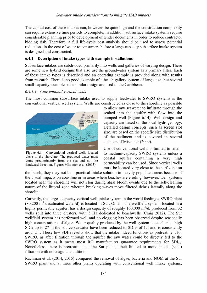
Seawater intake considerations to mitigate HAB impacts

184

The capital cost of these intakes can, however, be quite high and the construction complexity can require extensive time periods to complete. In addition, subsurface intake systems require considerable planning prior to development of tender documents in order to reduce contractor bidding risk. Therefore, a full life-cycle cost analysis should be used to assess potential reductions in the cost of water to consumers before a large-capacity subsurface intake system is designed and constructed.

6.4.1 Description of intake types with example installations Subsurface intakes are subdivided primarily into wells and galleries of varying design. There are some new hybrid designs that also use the groundwater system as a primary filter. Each of these intake types is described and an operating example is provided along with results from research. There is no good example of a beach gallery system of large size, but several small-capacity examples of a similar design are used in the Caribbean.

6.4.1.1 Conventional vertical wells The most common subsurface intake used to supply feedwater to SWRO systems is the conventional vertical well system. Wells are constructed as close to the shoreline as possible

to allow raw seawater to infiltrate through the seabed into the aquifer with flow into the pumped well (Figure 6.14). Well design and capacity are based on the local hydrogeology. Detailed design concepts, such as screen slot size, are based on the specific size distribution of the sediment and is covered in several chapters of Missimer (2009). Use of conventional wells is limited to small- to medium-capacity SWRO systems unless a coastal aquifer containing a very high permeability can be used. Since vertical wells must be located very close to the surf zone on

the beach, they may not be a practical intake solution in heavily populated areas because of the visual impacts on coastline or in areas where beaches are eroding; however, well systems located near the shoreline will not clog during algal bloom events due to the self-cleaning nature of the littoral zone wherein breaking waves move filtered debris laterally along the shoreline. Currently, the largest capacity vertical well intake system in the world feeding a SWRO plant (80,200 m3 desalinated water/d) is located in Sur, Oman. The wellfield system, located in a highly permeable aquifer, has a design capacity of roughly 160,000 m3/d, produced from 32 wells split into three clusters, with 5 Ha dedicated to beachwells (Craig 2012). The Sur wellfield system has performed well and no clogging has been observed despite seasonally high concentrations of algae. Water quality produced by the well system is excellent – high SDI3 up to 27 in the source seawater have been reduced to SDI15 of 1.4 and is consistently around 1. These low SDI15 results show that the intake indeed functions as pretreatment for SWRO, as after filtration through the aquifer the raw water could be directly fed to the SWRO system as it meets most RO manufacturer guarantee requirements for SDI15. Nonetheless, there is pretreatment at the Sur plant, albeit limited to mono media (sand) filtration with no coagulant addition. Rachman et al. (2014, 2015) compared the removal of algae, bacteria and NOM at the Sur SWRO plant and at three other plants operating with conventional well intake systems;

Figure 6.14. Conventional vertical wells located close to the shoreline. The produced water must come predominantly from the sea and not the landward direction. Figure: Missimer et al. (2013).

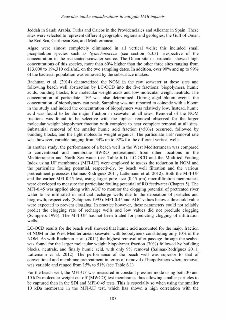
Seawater intake considerations to mitigate HAB impacts

185

Jeddah in Saudi Arabia, Turks and Caicos in the Providenciales and Alicante in Spain. These sites were selected to represent different geographic regions and geologies; the Gulf of Oman, the Red Sea, Caribbean Sea, and Mediterranean. Algae were almost completely eliminated in all vertical wells; this included small picoplankton species such as Synechococcus (see section 6.3.3) irrespective of the concentration in the associated seawater source. The Oman site in particular showed high concentrations of this species, more than 80% higher than the other three sites ranging from 113,000 to 194,310 cells/mL on the two sampling dates. In addition, over 90% and up to 99% of the bacterial population was removed by the subsurface intakes. Rachman et al. (2014) characterized the NOM in the raw seawater at these sites and following beach well abstraction by LC-OCD into the five fractions: biopolymers, humic acids, building blocks, low molecular weight acids and low molecular weight neutrals. The concentration of particulate TEP was also determined. During algal bloom events, the concentration of biopolymers can peak. Sampling was not reported to coincide with a bloom in the study and indeed the concentration of biopolymers was relatively low. Instead, humic acid was found to be the major fraction in seawater at all sites. Removal of the NOM fractions was found to be selective with the highest removal observed for the larger molecular weight biopolymer fraction with complete to near complete removal at all sites. Substantial removal of the smaller humic acid fraction (>50%) occurred, followed by building blocks, and the light molecular weight organics. The particulate TEP removal rate was, however, variable ranging from 34% up to 92% for the different vertical wells. In another study, the performance of a beach well in the West Mediterranean was compared to conventional and membrane SWRO pretreatment from other locations in the Mediterranean and North Sea water (see Table 6.1). LC-OCD and the Modified Fouling Index using UF membranes (MFI-UF) were employed to assess the reduction in NOM and the particulate fouling potential, respectively, by beach well filtration and the various pretreatment processes (Salinas-Rodríguez 2011; Lattemann et al. 2012). Both the MFI-UF and the earlier MFI-0.45 test, using larger pore size (0.45 µm) microfiltration membranes, were developed to measure the particulate fouling potential of RO feedwater (Chapter 5). The MFI-0.45 was applied along with AOC to monitor the clogging potential of pretreated river water to be infiltrated in artificial recharge wells due to the deposition of particles and biogrowth, respectively (Schippers 1995). MFI-0.45 and AOC values below a threshold value were expected to prevent clogging. In practice however, these parameters could not reliably predict the clogging rate of recharge wells and low values did not preclude clogging (Schippers 1995). The MFI-UF has not been trialed for predicting clogging of infiltration wells.

LC-OCD results for the beach well showed that humic acid accounted for the major fraction of NOM in the West Mediterranean seawater with biopolymers constituting only 10% of the NOM. As with Rachman et al. (2014) the highest removal after passage through the seabed was found for the larger molecular weight biopolymer fraction (70%) followed by building blocks, neutrals, and finally humic acid, with only 9% removal (Salinas-Rodríguez 2011; Lattemann et al. 2012). The performance of the beach well was superior to that of conventional and membrane pretreatment in terms of removal of biopolymers where removal was variable and ranged from 15% to 51% (see Table 6.1).

For the beach well, the MFI-UF was measured in constant pressure mode using both 30 and 10 kDa molecular weight cut off (MWCO) test membranes thus allowing smaller particles to be captured than in the SDI and MFI-0.45 tests. This is especially so when using the smaller 10 kDa membrane in the MFI-UF test, which has shown a high correlation with the

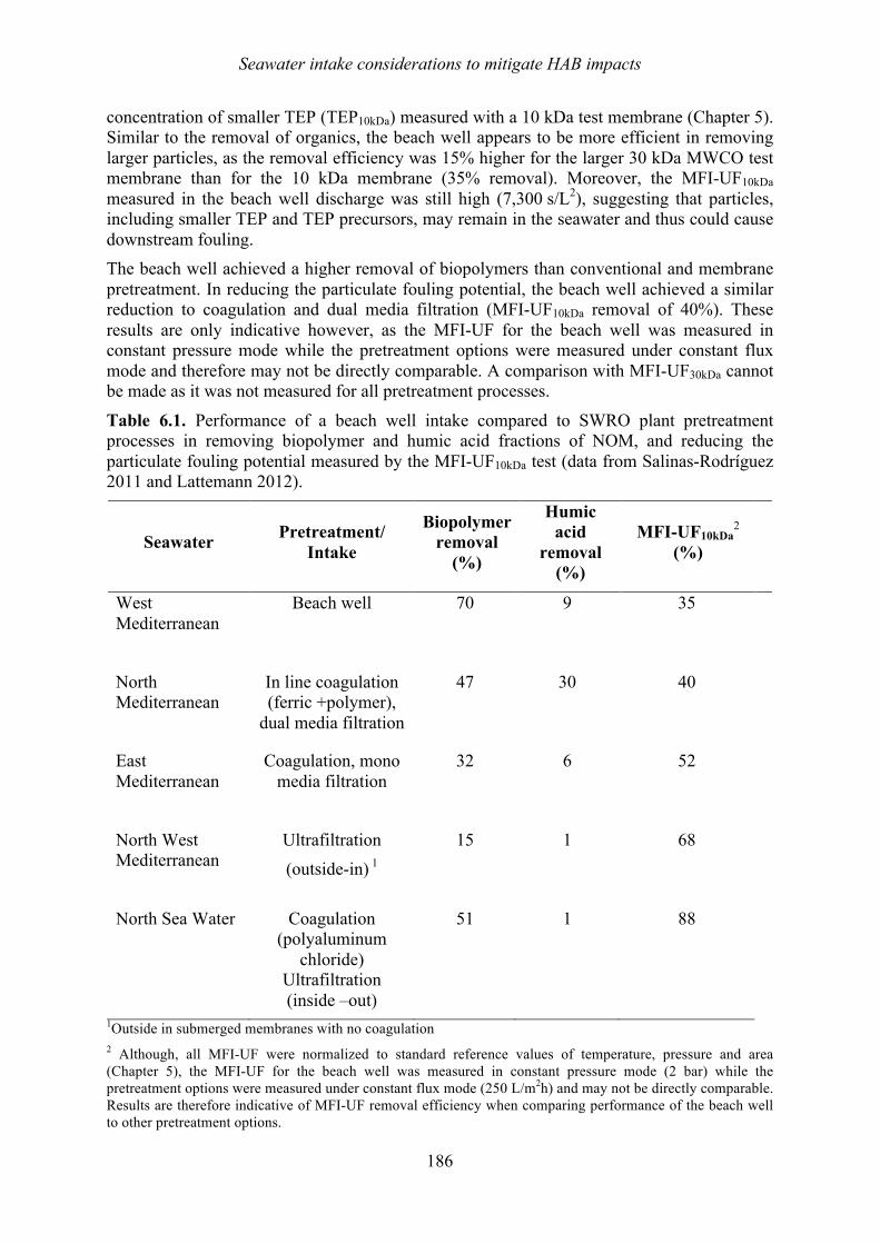
Seawater intake considerations to mitigate HAB impacts

186

concentration of smaller TEP (TEP10kDa) measured with a 10 kDa test membrane (Chapter 5). Similar to the removal of organics, the beach well appears to be more efficient in removing larger particles, as the removal efficiency was 15% higher for the larger 30 kDa MWCO test membrane than for the 10 kDa membrane (35% removal). Moreover, the MFI-UF10kDa measured in the beach well discharge was still high (7,300 s/L2), suggesting that particles, including smaller TEP and TEP precursors, may remain in the seawater and thus could cause downstream fouling. The beach well achieved a higher removal of biopolymers than conventional and membrane pretreatment. In reducing the particulate fouling potential, the beach well achieved a similar reduction to coagulation and dual media filtration (MFI-UF10kDa removal of 40%). These results are only indicative however, as the MFI-UF for the beach well was measured in constant pressure mode while the pretreatment options were measured under constant flux mode and therefore may not be directly comparable. A comparison with MFI-UF30kDa cannot be made as it was not measured for all pretreatment processes.

Table 6.1. Performance of a beach well intake compared to SWRO plant pretreatment processes in removing biopolymer and humic acid fractions of NOM, and reducing the particulate fouling potential measured by the MFI-UF10kDa test (data from Salinas-Rodríguez 2011 and Lattemann 2012).

Seawater Pretreatment/ Intake

Biopolymer removal

(%)

Humic acid

removal (%)

MFI-UF10kDa2

(%)

West Mediterranean

Beach well 70 9 35

North Mediterranean

In line coagulation (ferric +polymer),

dual media filtration

47 30 40

East Mediterranean

Coagulation, mono media filtration

32 6 52

North West Mediterranean

Ultrafiltration (outside-in) 1

15 1 68

North Sea Water Coagulation (polyaluminum

chloride) Ultrafiltration (inside –out)

51 1 88

1Outside in submerged membranes with no coagulation 2 Although, all MFI-UF were normalized to standard reference values of temperature, pressure and area (Chapter 5), the MFI-UF for the beach well was measured in constant pressure mode (2 bar) while the pretreatment options were measured under constant flux mode (250 L/m2h) and may not be directly comparable. Results are therefore indicative of MFI-UF removal efficiency when comparing performance of the beach well to other pretreatment options.

Seawater intake considerations to mitigate HAB impacts

187

As expected, ultrafiltration with or without coagulation yielded the largest reduction in particulate fouling potential (68 to 88%) due to smaller membrane pore sizes than the interstices in dual media filtration or the seabed strata. The results presented in Lattemann et

al. (2012) while promising in terms of biopolymer removal by beach well filtration, are limited and indicative only for the MFI-UF results and warrant further investigation. The aforementioned studies show that vertical wells reduce the biopolymer fraction of NOM (which includes TEP that can promote biofouling of membranes), in addition to bacteria, algae, and particulate matter. A typical removal percentage for well intakes is 100% for algae and over 90% for bacteria (Figure 6.15). Biopolymer removal ranged from 70% (Table 6.1) up to nearly 100% in some cases (Figure 6.16). The degree of treatment provided within a well intake system is based upon a number of factors including the flow path length time, the type of geological media, the hydraulic retention time, the biochemical activity in the aquifer, and the local composition of the seawater. Rachman et al. (2014) found that the geological characteristics of the site and

aquifer type (the Oman and the Turks and Caicos aquifers are limestone, while the Jeddah system is siliciclastic) did not have a direct correlation to the removal rate of the organic substances. Instead the flow path length and hydraulic retention time had a greater impact on organic matter removal efficiency compared to the geology of the aquifer or specifically, lithology. Therefore, a careful balance must be achieved wherein the wells are located close enough to the shoreline to have most of the recharge from the sea, but sufficiently far away to remove a significant percentage of the organic matter. 6.4.1.2 Collector or Ranney Wells

A collector well (Ranney well) is a specialized well type with a high unit production capacity compared to most wells. It contains a central caisson with a diameter ranging from ~ 2 to 4 m and a series of horizontal laterals to collect water from the penetrated aquifer (Figure 6.17). Collector wells are commonly used to tap gravel units within aquifers underlying river systems in the Midwest region of the United States and other geographic areas. These wells can have capacities of over 51,400 m3/d (Missimer 1997; Missimer et al. 2013. There are a

Figure 6.15. Comparison of bacterial concentrations in surface seawater and well discharges for a SWRO plant with a groundwater flow path averaging about 100 m. Figure: Rachman et al. 2014.

Figure 6.16. Comparison of NOM fraction for surface seawater and well discharges for a SWRO plant in Jeddah in Saudi Arabia with a groundwater flow path of about 200m. Note that the reduction of the biopolymer fraction, which contain sticky polysaccharides and proteins is nearly 100% at this location. Modified from Dehwah and Missimer 2016.

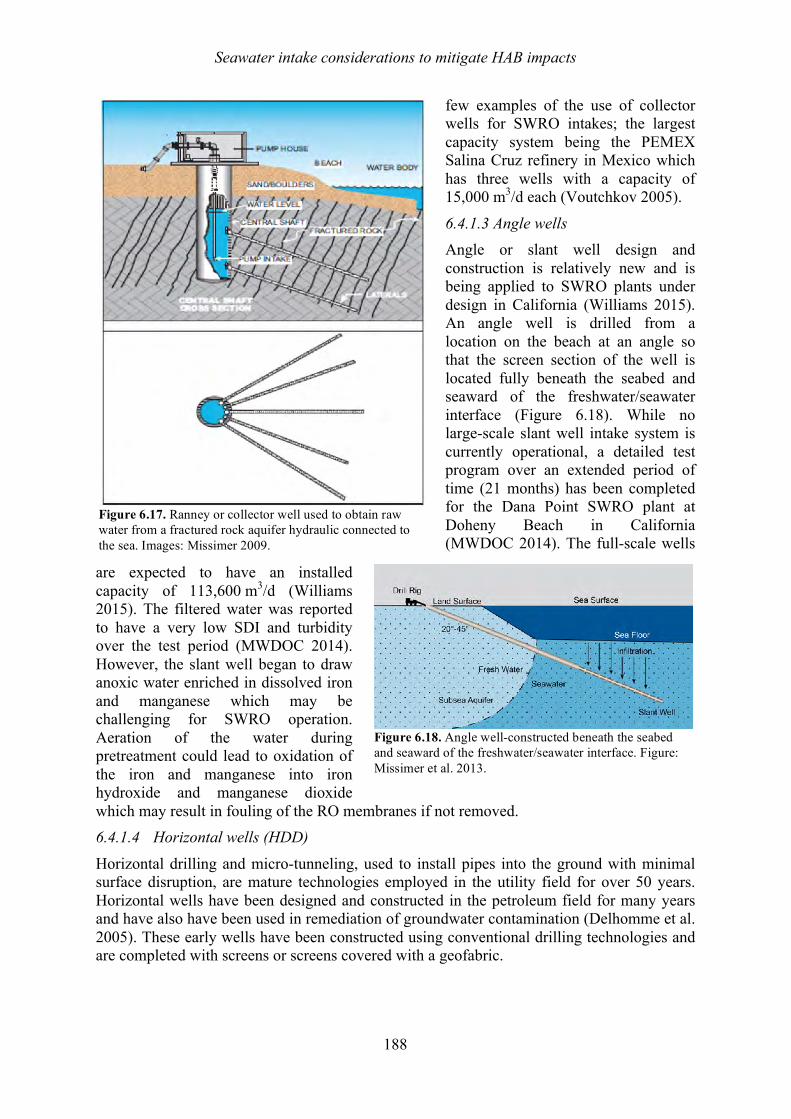
Seawater intake considerations to mitigate HAB impacts

188

few examples of the use of collector wells for SWRO intakes; the largest capacity system being the PEMEX Salina Cruz refinery in Mexico which has three wells with a capacity of 15,000 m3/d each (Voutchkov 2005).

6.4.1.3 Angle wells Angle or slant well design and construction is relatively new and is being applied to SWRO plants under design in California (Williams 2015). An angle well is drilled from a location on the beach at an angle so that the screen section of the well is located fully beneath the seabed and seaward of the freshwater/seawater interface (Figure 6.18). While no large-scale slant well intake system is currently operational, a detailed test program over an extended period of time (21 months) has been completed for the Dana Point SWRO plant at Doheny Beach in California (MWDOC 2014). The full-scale wells

are expected to have an installed capacity of 113,600 m3/d (Williams 2015). The filtered water was reported to have a very low SDI and turbidity over the test period (MWDOC 2014). However, the slant well began to draw anoxic water enriched in dissolved iron and manganese which may be challenging for SWRO operation. Aeration of the water during pretreatment could lead to oxidation of the iron and manganese into iron hydroxide and manganese dioxide which may result in fouling of the RO membranes if not removed. 6.4.1.4 Horizontal wells (HDD)

Horizontal drilling and micro-tunneling, used to install pipes into the ground with minimal surface disruption, are mature technologies employed in the utility field for over 50 years. Horizontal wells have been designed and constructed in the petroleum field for many years and have also have been used in remediation of groundwater contamination (Delhomme et al. 2005). These early wells have been constructed using conventional drilling technologies and are completed with screens or screens covered with a geofabric.

Figure 6.18. Angle well-constructed beneath the seabed and seaward of the freshwater/seawater interface. Figure: Missimer et al. 2013.

Figure 6.17. Ranney or collector well used to obtain raw water from a fractured rock aquifer hydraulic connected to the sea. Images: Missimer 2009.

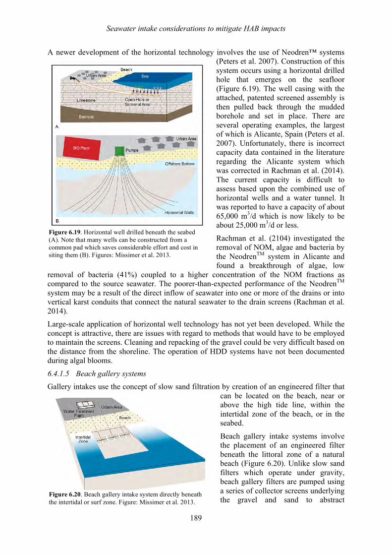
Seawater intake considerations to mitigate HAB impacts

189

A newer development of the horizontal technology involves the use of Neodren™ systems (Peters et al. 2007). Construction of this system occurs using a horizontal drilled hole that emerges on the seafloor (Figure 6.19). The well casing with the attached, patented screened assembly is then pulled back through the mudded borehole and set in place. There are several operating examples, the largest of which is Alicante, Spain (Peters et al. 2007). Unfortunately, there is incorrect capacity data contained in the literature regarding the Alicante system which was corrected in Rachman et al. (2014). The current capacity is difficult to assess based upon the combined use of horizontal wells and a water tunnel. It was reported to have a capacity of about 65,000 m3/d which is now likely to be about 25,000 m3/d or less.

Rachman et al. (2104) investigated the removal of NOM, algae and bacteria by the NeodrenTM system in Alicante and found a breakthrough of algae, low

removal of bacteria (41%) coupled to a higher concentration of the NOM fractions as compared to the source seawater. The poorer-than-expected performance of the NeodrenTM system may be a result of the direct inflow of seawater into one or more of the drains or into vertical karst conduits that connect the natural seawater to the drain screens (Rachman et al. 2014). Large-scale application of horizontal well technology has not yet been developed. While the concept is attractive, there are issues with regard to methods that would have to be employed to maintain the screens. Cleaning and repacking of the gravel could be very difficult based on the distance from the shoreline. The operation of HDD systems have not been documented during algal blooms.

6.4.1.5 Beach gallery systems Gallery intakes use the concept of slow sand filtration by creation of an engineered filter that

can be located on the beach, near or above the high tide line, within the intertidal zone of the beach, or in the seabed.

Beach gallery intake systems involve the placement of an engineered filter beneath the littoral zone of a natural beach (Figure 6.20). Unlike slow sand filters which operate under gravity, beach gallery filters are pumped using a series of collector screens underlying the gravel and sand to abstract

Figure 6.20. Beach gallery intake system directly beneath the intertidal or surf zone. Figure: Missimer et al. 2013.

Figure 6.19. Horizontal well drilled beneath the seabed (A). Note that many wells can be constructed from a common pad which saves considerable effort and cost in siting them (B). Figures: Missimer et al. 2013.

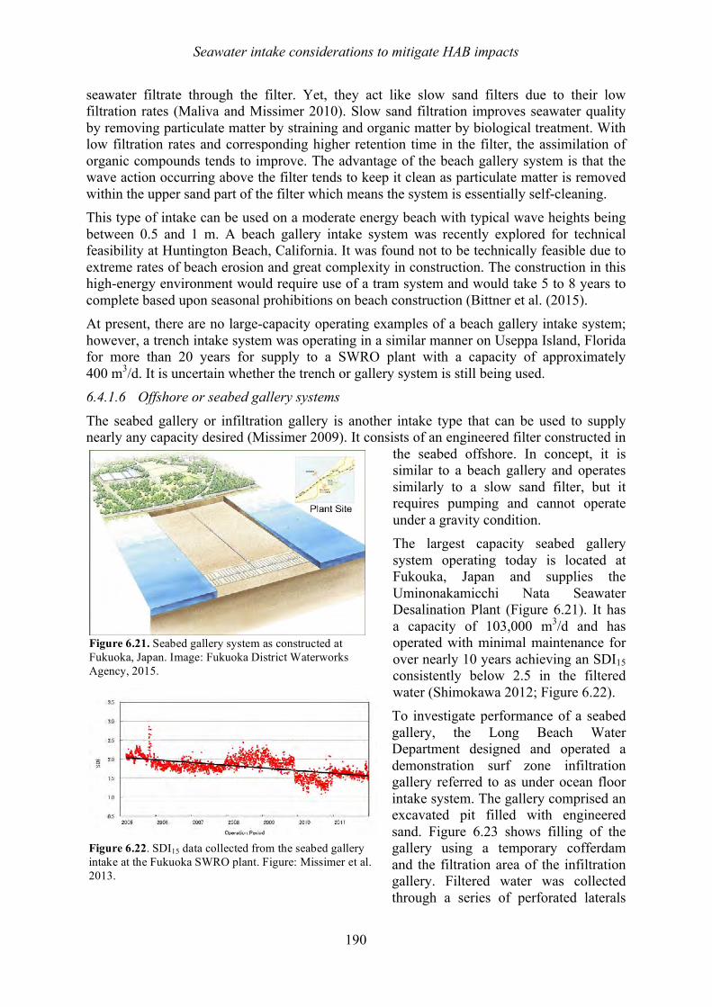
Seawater intake considerations to mitigate HAB impacts

190

seawater filtrate through the filter. Yet, they act like slow sand filters due to their low filtration rates (Maliva and Missimer 2010). Slow sand filtration improves seawater quality by removing particulate matter by straining and organic matter by biological treatment. With low filtration rates and corresponding higher retention time in the filter, the assimilation of organic compounds tends to improve. The advantage of the beach gallery system is that the wave action occurring above the filter tends to keep it clean as particulate matter is removed within the upper sand part of the filter which means the system is essentially self-cleaning. This type of intake can be used on a moderate energy beach with typical wave heights being between 0.5 and 1 m. A beach gallery intake system was recently explored for technical feasibility at Huntington Beach, California. It was found not to be technically feasible due to extreme rates of beach erosion and great complexity in construction. The construction in this high-energy environment would require use of a tram system and would take 5 to 8 years to complete based upon seasonal prohibitions on beach construction (Bittner et al. (2015). At present, there are no large-capacity operating examples of a beach gallery intake system; however, a trench intake system was operating in a similar manner on Useppa Island, Florida for more than 20 years for supply to a SWRO plant with a capacity of approximately 400 m3/d. It is uncertain whether the trench or gallery system is still being used. 6.4.1.6 Offshore or seabed gallery systems

The seabed gallery or infiltration gallery is another intake type that can be used to supply nearly any capacity desired (Missimer 2009). It consists of an engineered filter constructed in

the seabed offshore. In concept, it is similar to a beach gallery and operates similarly to a slow sand filter, but it requires pumping and cannot operate under a gravity condition. The largest capacity seabed gallery system operating today is located at Fukouka, Japan and supplies the Uminonakamicchi Nata Seawater Desalination Plant (Figure 6.21). It has a capacity of 103,000 m3/d and has operated with minimal maintenance for over nearly 10 years achieving an SDI15 consistently below 2.5 in the filtered water (Shimokawa 2012; Figure 6.22). To investigate performance of a seabed gallery, the Long Beach Water Department designed and operated a demonstration surf zone infiltration gallery referred to as under ocean floor intake system. The gallery comprised an excavated pit filled with engineered sand. Figure 6.23 shows filling of the gallery using a temporary cofferdam and the filtration area of the infiltration gallery. Filtered water was collected through a series of perforated laterals

Figure 6.21. Seabed gallery system as constructed at Fukuoka, Japan. Image: Fukuoka District Waterworks Agency, 2015.

Figure 6.22. SDI15 data collected from the seabed gallery intake at the Fukuoka SWRO plant. Figure: Missimer et al. 2013.

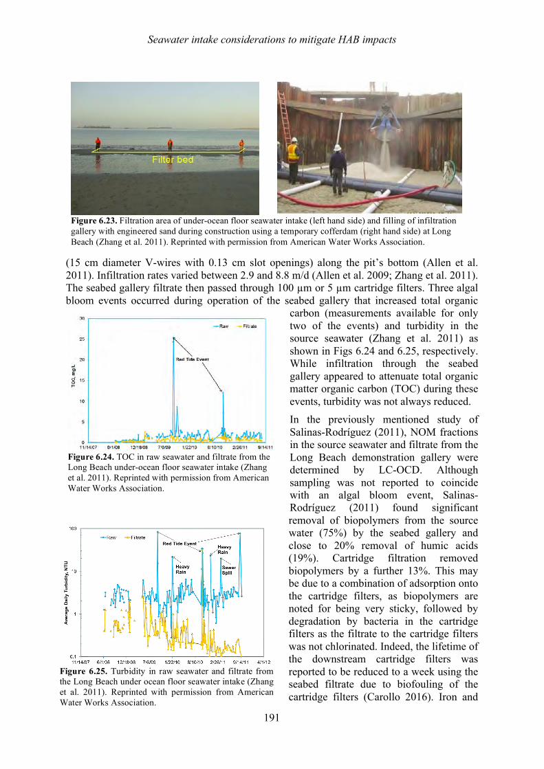
Seawater intake considerations to mitigate HAB impacts

191

(15 cm diameter V-wires with 0.13 cm slot openings) along the pit’s bottom (Allen et al. 2011). Infiltration rates varied between 2.9 and 8.8 m/d (Allen et al. 2009; Zhang et al. 2011). The seabed gallery filtrate then passed through 100 µm or 5 µm cartridge filters. Three algal bloom events occurred during operation of the seabed gallery that increased total organic

carbon (measurements available for only two of the events) and turbidity in the source seawater (Zhang et al. 2011) as shown in Figs 6.24 and 6.25, respectively. While infiltration through the seabed gallery appeared to attenuate total organic matter organic carbon (TOC) during these events, turbidity was not always reduced. In the previously mentioned study of Salinas-Rodríguez (2011), NOM fractions in the source seawater and filtrate from the Long Beach demonstration gallery were determined by LC-OCD. Although sampling was not reported to coincide with an algal bloom event, Salinas-Rodríguez (2011) found significant removal of biopolymers from the source water (75%) by the seabed gallery and close to 20% removal of humic acids (19%). Cartridge filtration removed biopolymers by a further 13%. This may be due to a combination of adsorption onto the cartridge filters, as biopolymers are noted for being very sticky, followed by degradation by bacteria in the cartridge filters as the filtrate to the cartridge filters was not chlorinated. Indeed, the lifetime of the downstream cartridge filters was reported to be reduced to a week using the seabed filtrate due to biofouling of the cartridge filters (Carollo 2016). Iron and

Figure 6.23. Filtration area of under-ocean floor seawater intake (left hand side) and filling of infiltration gallery with engineered sand during construction using a temporary cofferdam (right hand side) at Long Beach (Zhang et al. 2011). Reprinted with permission from American Water Works Association.

Figure 6.25. Turbidity in raw seawater and filtrate from the Long Beach under ocean floor seawater intake (Zhang et al. 2011). Reprinted with permission from American Water Works Association.

Figure 6.24. TOC in raw seawater and filtrate from the Long Beach under-ocean floor seawater intake (Zhang et al. 2011). Reprinted with permission from American Water Works Association.

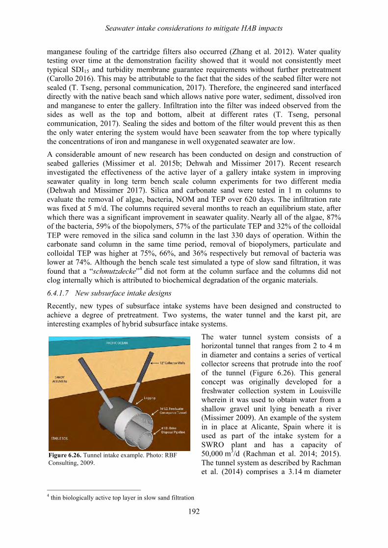
Seawater intake considerations to mitigate HAB impacts

192

manganese fouling of the cartridge filters also occurred (Zhang et al. 2012). Water quality testing over time at the demonstration facility showed that it would not consistently meet typical SDI15 and turbidity membrane guarantee requirements without further pretreatment (Carollo 2016). This may be attributable to the fact that the sides of the seabed filter were not sealed (T. Tseng, personal communication, 2017). Therefore, the engineered sand interfaced directly with the native beach sand which allows native pore water, sediment, dissolved iron and manganese to enter the gallery. Infiltration into the filter was indeed observed from the sides as well as the top and bottom, albeit at different rates (T. Tseng, personal communication, 2017). Sealing the sides and bottom of the filter would prevent this as then the only water entering the system would have been seawater from the top where typically the concentrations of iron and manganese in well oxygenated seawater are low. A considerable amount of new research has been conducted on design and construction of seabed galleries (Missimer et al. 2015b; Dehwah and Missimer 2017). Recent research investigated the effectiveness of the active layer of a gallery intake system in improving seawater quality in long term bench scale column experiments for two different media (Dehwah and Missimer 2017). Silica and carbonate sand were tested in 1 m columns to evaluate the removal of algae, bacteria, NOM and TEP over 620 days. The infiltration rate was fixed at 5 m/d. The columns required several months to reach an equilibrium state, after which there was a significant improvement in seawater quality. Nearly all of the algae, 87% of the bacteria, 59% of the biopolymers, 57% of the particulate TEP and 32% of the colloidal TEP were removed in the silica sand column in the last 330 days of operation. Within the carbonate sand column in the same time period, removal of biopolymers, particulate and colloidal TEP was higher at 75%, 66%, and 36% respectively but removal of bacteria was lower at 74%. Although the bench scale test simulated a type of slow sand filtration, it was found that a “schmutzdecke”4 did not form at the column surface and the columns did not clog internally which is attributed to biochemical degradation of the organic materials.

6.4.1.7 New subsurface intake designs Recently, new types of subsurface intake systems have been designed and constructed to achieve a degree of pretreatment. Two systems, the water tunnel and the karst pit, are interesting examples of hybrid subsurface intake systems.

The water tunnel system consists of a horizontal tunnel that ranges from 2 to 4 m in diameter and contains a series of vertical collector screens that protrude into the roof of the tunnel (Figure 6.26). This general concept was originally developed for a freshwater collection system in Louisville wherein it was used to obtain water from a shallow gravel unit lying beneath a river (Missimer 2009). An example of the system in in place at Alicante, Spain where it is used as part of the intake system for a SWRO plant and has a capacity of 50,000 m3/d (Rachman et al. 2014; 2015). The tunnel system as described by Rachman et al. (2014) comprises a 3.14 m diameter

4 thin biologically active top layer in slow sand filtration

Figure 6.26. Tunnel intake example. Photo: RBF Consulting, 2009.

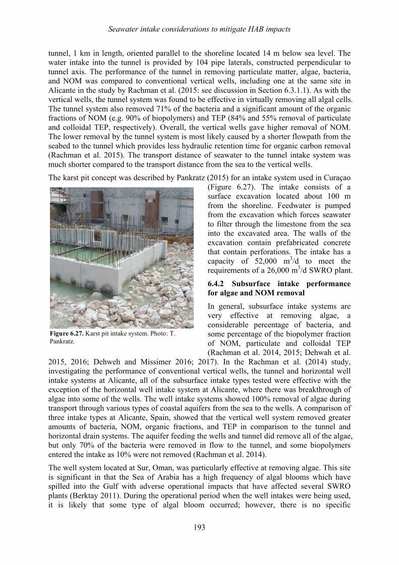
Seawater intake considerations to mitigate HAB impacts

193

tunnel, 1 km in length, oriented parallel to the shoreline located 14 m below sea level. The water intake into the tunnel is provided by 104 pipe laterals, constructed perpendicular to tunnel axis. The performance of the tunnel in removing particulate matter, algae, bacteria, and NOM was compared to conventional vertical wells, including one at the same site in Alicante in the study by Rachman et al. (2015: see discussion in Section 6.3.1.1). As with the vertical wells, the tunnel system was found to be effective in virtually removing all algal cells. The tunnel system also removed 71% of the bacteria and a significant amount of the organic fractions of NOM (e.g. 90% of biopolymers) and TEP (84% and 55% removal of particulate and colloidal TEP, respectively). Overall, the vertical wells gave higher removal of NOM. The lower removal by the tunnel system is most likely caused by a shorter flowpath from the seabed to the tunnel which provides less hydraulic retention time for organic carbon removal (Rachman et al. 2015). The transport distance of seawater to the tunnel intake system was much shorter compared to the transport distance from the sea to the vertical wells. The karst pit concept was described by Pankratz (2015) for an intake system used in Curaçao

(Figure 6.27). The intake consists of a surface excavation located about 100 m from the shoreline. Feedwater is pumped from the excavation which forces seawater to filter through the limestone from the sea into the excavated area. The walls of the excavation contain prefabricated concrete that contain perforations. The intake has a capacity of 52,000 m3/d to meet the requirements of a 26,000 m3/d SWRO plant.

6.4.2 Subsurface intake performance for algae and NOM removal

In general, subsurface intake systems are very effective at removing algae, a considerable percentage of bacteria, and some percentage of the biopolymer fraction of NOM, particulate and colloidal TEP (Rachman et al. 2014, 2015; Dehwah et al.

2015, 2016; Dehweh and Missimer 2016; 2017). In the Rachman et al. (2014) study, investigating the performance of conventional vertical wells, the tunnel and horizontal well intake systems at Alicante, all of the subsurface intake types tested were effective with the exception of the horizontal well intake system at Alicante, where there was breakthrough of algae into some of the wells. The well intake systems showed 100% removal of algae during transport through various types of coastal aquifers from the sea to the wells. A comparison of three intake types at Alicante, Spain, showed that the vertical well system removed greater amounts of bacteria, NOM, organic fractions, and TEP in comparison to the tunnel and horizontal drain systems. The aquifer feeding the wells and tunnel did remove all of the algae, but only 70% of the bacteria were removed in flow to the tunnel, and some biopolymers entered the intake as 10% were not removed (Rachman et al. 2014). The well system located at Sur, Oman, was particularly effective at removing algae. This site is significant in that the Sea of Arabia has a high frequency of algal blooms which have spilled into the Gulf with adverse operational impacts that have affected several SWRO plants (Berktay 2011). During the operational period when the well intakes were being used, it is likely that some type of algal bloom occurred; however, there is no specific

Figure 6.27. Karst pit intake system. Photo: T. Pankratz.

Seawater intake considerations to mitigate HAB impacts

194

documentation concerning the algal concentrations occurring and any changes in the algae occurrence within the production wells during a bloom. Based on the distances of the wells from the sea ranging from 30 to 250 m and the flow path length through the aquifer, it is highly unlikely that algae could actually enter the production wells, even during a bloom. In addition, the removal of algae, biopolymers and TEP should reduce the biofouling potential of a feedwater during a bloom event.

A considerable amount of research has been completed recently on the development of gallery intake systems that can be used to produce a sufficient supply of feedwater even for the largest SWRO plants (Missimer et al. 2015a; Dehwah and Missimer 2017). The seabed gallery, in particular, appears to have the greatest potential number of applications. This system operates similarly to a slow sand filter in which the seawater is filtered through an engineering system with a hydraulic retention time of 6 to 8 hours. Experiments conducted on the use of a slow sand filter as pretreatment for SWRO plants showed no penetration of algae through the system and a very high rate of kainic acid removal which was used as an algal toxin surrogate (Desormeaux et al. 2009). This research can be used as a proxy for the operation of a seabed gallery system and will likely function in the same manner, although no seabed gallery system has been operated throughout a major, high-biomass algal bloom, so the need for additional on-land pretreatment of the gallery effluent is still open to question.

The processes of particulate and dissolved organics removal are similar to those occurring during slow sand filtration with the exception that no biologically active “schmutzdecke” layer forms during filtration at the sediment-water interface i.e. on the top surface of the filter (Dehwah and Missimer 2017). Instead, all of the particulate organics and suspended sediments are strained during transport and accumulate within the aquifer or upper 1 m of a seabed filter. No reported clogging has been reported despite operation of wells and seabed filters for up to 30 years (in the case of wells). Therefore, within groundwater systems, it is assumed that biochemical processes are active in reducing particulate organics into dissolved forms that move through the aquifer. This is suggested in some recently collected data by increases in the concentration of light molecular weight neutrals in the well discharges (Dehwah and Missimer 2017). Within seabed filters, the upper layer of the filter undergoes bioturbation whereby organisms that derive nutrition from the sediments such as polychaete worms and some molluscs assimilate organic material and small particulates, leaving beneath rigid fecal pellets that act hydraulically similar to sand grains. The deposit feeders act to prevent the building of a biological clogging layer at the sediment–water interface. Removal of biopolymers and other fractions of NOM are likely caused by a variety of physical (straining and adsorption) and biochemical breakdown processes (bacterial and geochemical). Additional research is being conducted on these mechanisms in column and larger scale experiments. 6.4.3 Planning of desalination plants with subsurface intakes

While subsurface intakes offer many advantages for SWRO plants in areas prone to blooms they are not always feasible. Use of a particular type of subsurface intake is dependent on the hydrogeologic and marine conditions of a specific site. In addition, local infrastructure also plays an important role in the choice of intake type that can be used (e.g., availability of specialized construction equipment, electric power availability to pipe and pump the raw seawater). Since the use of subsurface intakes is related to the site-specific conditions, the specification of an intake type requires planning and a certain level of pre-tender field investigation.

It is prudent to perform feasibility level investigations of the coastal area in regions that are planning use of a subsurface intake system to supply SWRO plants. Dehwah et al. (2014)

Seawater intake considerations to mitigate HAB impacts

195

developed a coastal geomorphological mapping system that can be used for screening purposes to assess which types of intakes can be used. The method considers both field conditions and the capacity of the plant being considered for the Red Sea shoreline of Saudi Arabia. The factors considered and areas mapped are shown in Table 6.2. The relationship between the mapped coastline and the feasibility of using a specific intake type are given in Table 6.3. Table 6.2. Geomorphological classifications of the Red Sea coastline (Dehwah et al. 2014). A. Sandy Beaches

A1 - Sandy beach with corresponding nearshore sand or slightly muddy sand, coral reef complex offshore A2 - Sandy beaches, restricted, with no reef A3 - Offshore island with nearshore sandy sediments and reef

B. Rocky shorelines B1 - Limestone rocky shoreline with corresponding nearshore sand, and offshore coral reef complex B2 - Limestone rocky shoreline with nearshore muddy sediments B3 - Limestone rocky shoreline, nearshore deep water, no reef B4 - Rocky headland with offshore rocky bottom, no reef B5 - Rocky shoreline, wadi1 sediments nearshore, offshore reef

C. Wadi 1intersections C1 - Wadi sediments (boulders, pebble, and gravel)at shoreline, variable sand, gravel and mud offshore with no reef C2 - Wadi shoreline sediments, nearshore marine hard ground, minor nearshore sand , coral reef offshore

D. Sabkha2, lagoons, and mangrove D1 - Coastal sabkha shoreline and nearshore muddy sediments D2 - Muddy shoreline with lagoonal muddy sediments, nearshore sand and offshore reef complex D3 - Muddy shoreline /lagoon/ supra-tidal sabkha with no reef complex D4 - Mangrove shoreline with nearshore muddy sediments

E. Others E1 - Shoreline reef complex dropping to deep water in the nearshore off-reef area E2 - Artificial channels or urban shoreline with artificially filled nearshore dropping to deep water nearshore E3 - Natural channel

1Wadi- an ephemeral stream that flows only during flood conditions in arid regions 2Sabkha -a supra-tidal to intertidal area wherein seawater is trapped during storms or high-tide events and the trapped water evaporates to produce hypersaline conditions (salinity often over 250,000 mg/L), commonly with the precipitation of evaporite minerals occurring on the Sabhka plain.

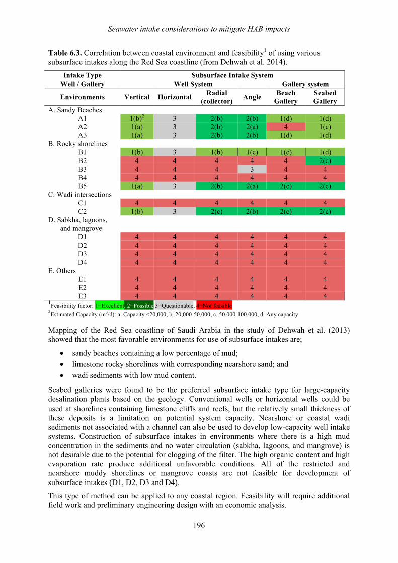
Seawater intake considerations to mitigate HAB impacts

196

Table 6.3. Correlation between coastal environment and feasibility1 of using various subsurface intakes along the Red Sea coastline (from Dehwah et al. 2014).

Intake Type Subsurface Intake System Well / Gallery Well System Gallery system

Environments Vertical Horizontal Radial (collector) Angle Beach

Gallery Seabed Gallery

A. Sandy Beaches A1 1(b)2 3 2(b) 2(b) 1(d) 1(d) A2 1(a) 3 2(b) 2(a) 4 1(c) A3 1(a) 3 2(b) 2(b) 1(d) 1(d)

B. Rocky shorelines B1 1(b) 3 1(b) 1(c) 1(c) 1(d) B2 4 4 4 4 4 2(c) B3 4 4 4 3 4 4 B4 4 4 4 4 4 4 B5 1(a) 3 2(b) 2(a) 2(c) 2(c)

C. Wadi intersections C1 4 4 4 4 4 4 C2 1(b) 3 2(c) 2(b) 2(c) 2(c)

D. Sabkha, lagoons, and mangrove

D1 4 4 4 4 4 4 D2 4 4 4 4 4 4 D3 4 4 4 4 4 4 D4 4 4 4 4 4 4

E. Others E1 4 4 4 4 4 4 E2 4 4 4 4 4 4 E3 4 4 4 4 4 4

1Feasibility factor: 1=Excellent, 2=Possible 3=Questionable, 4=Not feasible 2Estimated Capacity (m3/d): a. Capacity <20,000, b. 20,000-50,000, c. 50,000-100,000, d. Any capacity Mapping of the Red Sea coastline of Saudi Arabia in the study of Dehwah et al. (2013) showed that the most favorable environments for use of subsurface intakes are;

• sandy beaches containing a low percentage of mud; • limestone rocky shorelines with corresponding nearshore sand; and • wadi sediments with low mud content.

Seabed galleries were found to be the preferred subsurface intake type for large-capacity desalination plants based on the geology. Conventional wells or horizontal wells could be used at shorelines containing limestone cliffs and reefs, but the relatively small thickness of these deposits is a limitation on potential system capacity. Nearshore or coastal wadi sediments not associated with a channel can also be used to develop low-capacity well intake systems. Construction of subsurface intakes in environments where there is a high mud concentration in the sediments and no water circulation (sabkha, lagoons, and mangrove) is not desirable due to the potential for clogging of the filter. The high organic content and high evaporation rate produce additional unfavorable conditions. All of the restricted and nearshore muddy shorelines or mangrove coasts are not feasible for development of subsurface intakes (D1, D2, D3 and D4). This type of method can be applied to any coastal region. Feasibility will require additional field work and preliminary engineering design with an economic analysis.

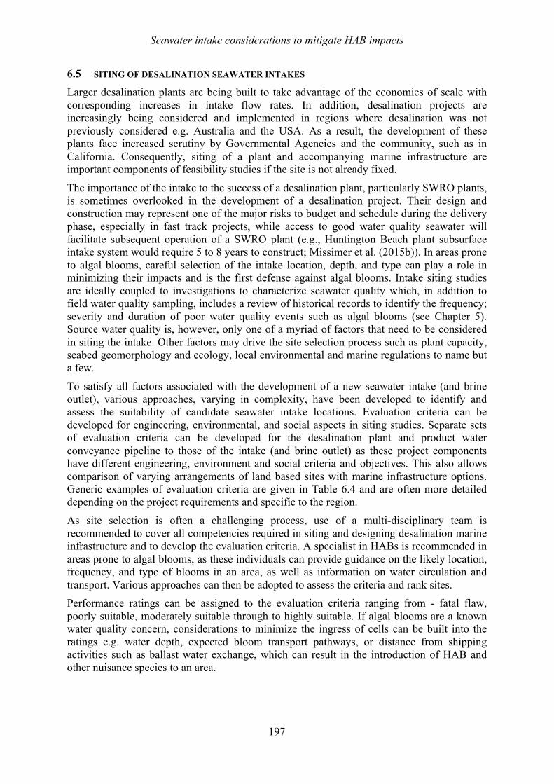
Seawater intake considerations to mitigate HAB impacts

197

6.5 SITING OF DESALINATION SEAWATER INTAKES Larger desalination plants are being built to take advantage of the economies of scale with corresponding increases in intake flow rates. In addition, desalination projects are increasingly being considered and implemented in regions where desalination was not previously considered e.g. Australia and the USA. As a result, the development of these plants face increased scrutiny by Governmental Agencies and the community, such as in California. Consequently, siting of a plant and accompanying marine infrastructure are important components of feasibility studies if the site is not already fixed.

The importance of the intake to the success of a desalination plant, particularly SWRO plants, is sometimes overlooked in the development of a desalination project. Their design and construction may represent one of the major risks to budget and schedule during the delivery phase, especially in fast track projects, while access to good water quality seawater will facilitate subsequent operation of a SWRO plant (e.g., Huntington Beach plant subsurface intake system would require 5 to 8 years to construct; Missimer et al. (2015b)). In areas prone to algal blooms, careful selection of the intake location, depth, and type can play a role in minimizing their impacts and is the first defense against algal blooms. Intake siting studies are ideally coupled to investigations to characterize seawater quality which, in addition to field water quality sampling, includes a review of historical records to identify the frequency; severity and duration of poor water quality events such as algal blooms (see Chapter 5). Source water quality is, however, only one of a myriad of factors that need to be considered in siting the intake. Other factors may drive the site selection process such as plant capacity, seabed geomorphology and ecology, local environmental and marine regulations to name but a few. To satisfy all factors associated with the development of a new seawater intake (and brine outlet), various approaches, varying in complexity, have been developed to identify and assess the suitability of candidate seawater intake locations. Evaluation criteria can be developed for engineering, environmental, and social aspects in siting studies. Separate sets of evaluation criteria can be developed for the desalination plant and product water conveyance pipeline to those of the intake (and brine outlet) as these project components have different engineering, environment and social criteria and objectives. This also allows comparison of varying arrangements of land based sites with marine infrastructure options. Generic examples of evaluation criteria are given in Table 6.4 and are often more detailed depending on the project requirements and specific to the region. As site selection is often a challenging process, use of a multi-disciplinary team is recommended to cover all competencies required in siting and designing desalination marine infrastructure and to develop the evaluation criteria. A specialist in HABs is recommended in areas prone to algal blooms, as these individuals can provide guidance on the likely location, frequency, and type of blooms in an area, as well as information on water circulation and transport. Various approaches can then be adopted to assess the criteria and rank sites. Performance ratings can be assigned to the evaluation criteria ranging from - fatal flaw, poorly suitable, moderately suitable through to highly suitable. If algal blooms are a known water quality concern, considerations to minimize the ingress of cells can be built into the ratings e.g. water depth, expected bloom transport pathways, or distance from shipping activities such as ballast water exchange, which can result in the introduction of HAB and other nuisance species to an area.

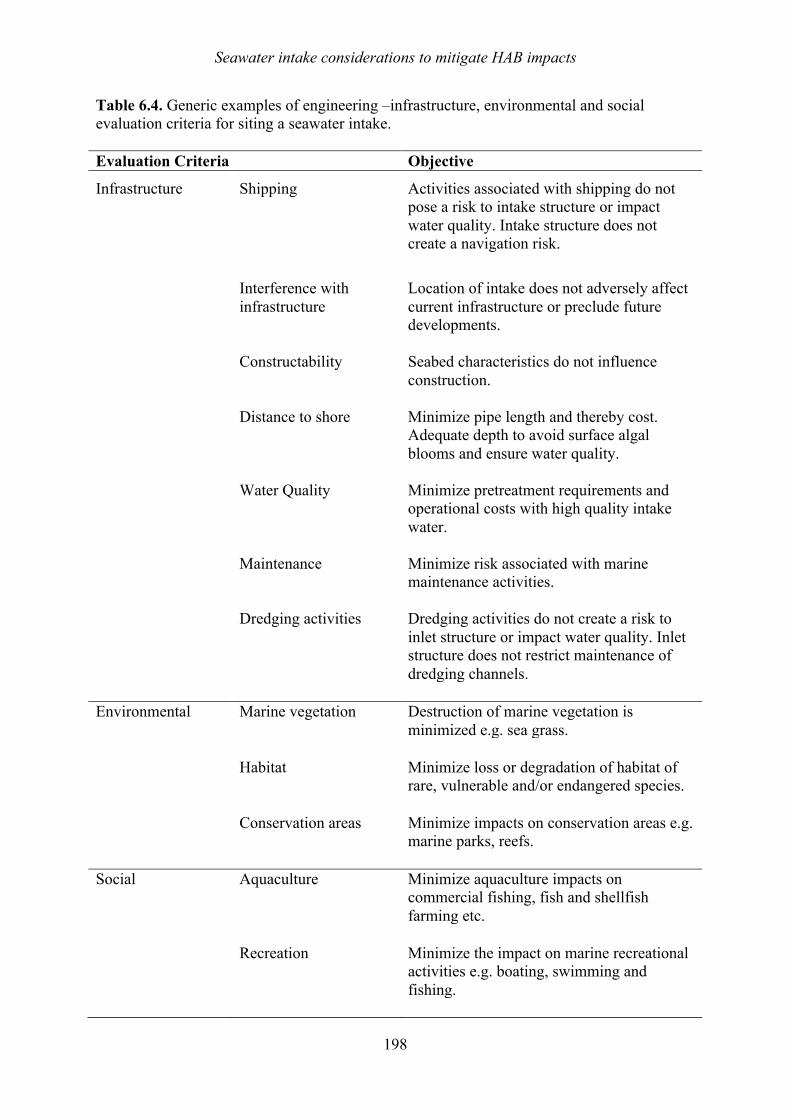
Seawater intake considerations to mitigate HAB impacts

198

Table 6.4. Generic examples of engineering –infrastructure, environmental and social evaluation criteria for siting a seawater intake. Evaluation Criteria Objective

Infrastructure Shipping Activities associated with shipping do not pose a risk to intake structure or impact water quality. Intake structure does not create a navigation risk.

Interference with

infrastructure Location of intake does not adversely affect current infrastructure or preclude future developments.

Constructability Seabed characteristics do not influence construction.

Distance to shore Minimize pipe length and thereby cost. Adequate depth to avoid surface algal blooms and ensure water quality.

Water Quality Minimize pretreatment requirements and

operational costs with high quality intake water.

Maintenance Minimize risk associated with marine maintenance activities.

Dredging activities Dredging activities do not create a risk to inlet structure or impact water quality. Inlet structure does not restrict maintenance of dredging channels.

Environmental Marine vegetation Destruction of marine vegetation is

minimized e.g. sea grass. Habitat Minimize loss or degradation of habitat of

rare, vulnerable and/or endangered species. Conservation areas Minimize impacts on conservation areas e.g.

marine parks, reefs. Social Aquaculture Minimize aquaculture impacts on

commercial fishing, fish and shellfish farming etc.

Recreation

Minimize the impact on marine recreational activities e.g. boating, swimming and fishing.

Seawater intake considerations to mitigate HAB impacts

199

For instance, locating the seawater intake within 150 m of a shipping lane may be deemed a fatal flaw by the team. Similarly, geomorphological environments that preclude the development of a subsurface intake and only allow the option of a surface intake e.g. rocky shorelines could be rated as poorly suitable (see geomorphological mapping system in Section 6.4.3). Overall, performance ratings allow a comparative assessment of sites.

More sophisticated approaches may use a Multi Criteria Analysis (MCA) approach, whereby the relative importance of each criterion within a set of environmental, social, and engineering criteria is compared to other criteria, weighted and ranked, e.g. water quality may be ranked first amongst the engineering criteria, especially if HABs are known to be a persistent issue. Thereafter, the MCA can be linked to a Geographic Information System (GIS) modelling and analysis platform to overlay geographic data sets to represent each of the evaluation criteria. The GIS models can then be used to compile scores across all the evaluation criteria and identify areas that are more suitable for the location of a seawater intake. While these approaches aim to provide a balanced approach, some subjectivity is unavoidable by the team with some criteria not directly measureable. Instead the experience of the team is relied upon. Moreover, this technique can be limited by the accuracy and currency of data sets used coupled to the fact that not all critical aspects that determine suitability can be represented in a geographic format. Hence, results need to be verified and validated with ground-truthing of sites.

While financial criteria may not be directly included in MCA, some criteria (e.g. engineering) will require financial considerations of some aspects to weight the criteria. The final decision on siting of marine infrastructure will be based on capital expenditure estimates plus operation and maintenance expenditures at suitable sites plus constructability, permitting requirements, construction and delivery schedules. MCA has proven useful in selecting the location, depth and type of intake for SWRO desalination plants. One such plant is the Gold Coast Desalination Plant which selected a deep water intake (20 m), 1.5 km off shore based on a MCA, considering factors such as; cost, risk, scheduled delivery window, environmental impact, community disruption, visual amenity in addition to water quality (algal blooms were known to occur). The deep water intake has been successful in providing good water quality and preventing the ingress of Trichodesmium blooms which are the most frequent blooms found in the area (see Gold Coast Case Study, Chapter 11). 6.6 SUMMARY

Intake channels and screens of surface intakes can be impacted by macroalgal (seaweed) blooms, with the potential loss of plant availability whereas the impact of blooms of smaller phytoplankton species at the intake is rare. Instead the microscopic algae generally pass through intake screens, impacting downstream processes in SWRO plants. There are limited opportunities to minimize the ingress of such blooms into a plant. Careful selection of the location and depth of a surface intake are important considerations in areas prone to algal blooms or the use of a subsurface intake. Offshore velocity caps, commonly used for open-ocean intakes on large-capacity stand-alone SWRO plants, have been proven successful in decreasing marine life impingement. They will not however, directly reduce entrainment of free floating algae or motile algae as they cannot detect the change in flow direction or swim away fast enough to avoid entrainment. Velocity caps can reduce the likelihood of entrainment if they are located in an unproductive area, or one with a lower number of drifting organisms. In addition, they could limit the zone of

Seawater intake considerations to mitigate HAB impacts

200

influence of the intake to the depth level at which the velocity cap is situated, thereby entraining only the algae and other plankton present at that depth.

Deep water open ocean intakes may be successful in avoiding some bloom-forming species, but some species are motile or display diel vertical migration so that they move within the water column and are not found solely within the surface, mixed layer. In the case of diel vertical migration, a SWRO plant with a deep-water intake could change to intermittent operation during a bloom, albeit reducing production, – operating during the daylight when algae are more likely to be found at the surface. By the same reasoning, shallow intakes may benefit from operating at night. However, the distribution of AOM may not reflect the distribution of algal cells, as AOM can be extracellular and detrital in form, sinking to the seabed or rising to the surface. Once algal cells are entrained into a plant, chlorination at the intake could be suspended during a bloom event to limit the increase of AOC generated through oxidation of organic matter, lysis of algal cells and release of AOM to reduce downstream fouling and retain toxins intracellularly.

In addition to providing feedwater to a plant, subsurface intakes can act as an engineered pretreatment step, performing similar to, or surpassing conventional or membrane pretreatment to eliminate algae, a high percentage of bacteria, and a significant percentage of natural organic matter (dissolved and colloidal), in particular sticky biopolymers from the source seawater which can include AOM. Depending on the local hydrogeology and the concentration of algae and duration of an algal bloom event, it is likely that most of the subsurface intake systems would allow a SWRO plant to operate continuously during a bloom without interruption. There is however a shortage of literature of SWRO plants operating during a bloom examining the removal of algae and AOM. Finally, intake type and location may be dictated by other project constraints such as environmental regulations, budget or schedule. Various approaches can be used to balance all competing factors in siting the intake for a SWRO desalination plant such as multi-criteria analysis wherein considerations to minimize the ingress of algal blooms could be incorporated.

6.7 REFERENCES Allen, J., Cheng, R., Tseng, T., and Wattier, K. 2009. Update for the pilot and demonstration-

scale research evaluation of under-ocean floor seawater intake and discharge. Proceedings of the AWWA Membrane Technology Conference, Memphis, Tennessee.

Allen, J. B., Cheng, R. C., Tseng, T. J. and Wattier, K. L., 2011. Update Evaluation of Under-Ocean Floor Seawater Intake and Discharge. IDA Journal of Desalination and Water Reuse 3(1), 19-25.

Boerlage, S. and Gordon, H. 2011. Assessing diffuser performance and discharge footprint for the Gold Coast Desalination Plant. In: Proceedings of IDA World Congress, Perth, Western Australia.

Berktay, A. 2011. Environmental approach and influence of red tide to desalination process in the Middle East region. International Journal of Chemical and Environmental Engineering 2(3), 183-188.

Bittner, R., Clements, J., Dale, L., Lee, S., Kavanaugh, M., and Missimer, T. M. 2015. Phase 2 report: Feasibility of subsurface intake designs for the proposed Poseidon water desalination facility at Huntington Beach, California: Independent Scientific Advisory Panel, California Coastal Commission and Poseidon Resources (Surfside) LLC Final Report.

Seawater intake considerations to mitigate HAB impacts

201

Carollo Consulting. 2016. Subsurface Desalination intake feasibility study. Technical Memorandum No. 3 Basis of Design and initial screening 2016 Consultant’s report to City of Santa Barbara, 338 pp.

Craig, K. 2012. Gold Coast, Sydney and Sur Desalination Plant Intake Overview. National Centre of Excellence in Desalination. International Desalination Intakes and Outfalls Workshop Proceedings. Adelaide, South Australia.

Dehwah, A. H., Al-Mashharawi, S., and Missimer, T. M. 2014. Mapping to assess feasibility of using subsurface intakes for SWRO, Red Sea coast of Saudi Arabia. Desalination and Water Treatment 52(13-15), 2351-2361.

Dehwah, A. H. A., Al-Mashharawi, S., Ng, K. C., and Missimer, T. M. 2016. Aquifer treatment of seawater to remove natural organic matter before desalination. Groundwater DOI:10.111/gwat.12476.

Dehwah, A. H. A., Li, S., Al-Mashharawi, S., Winters, H., and Missimer, T. M. 2015. Changes in feedwater organic matter concentrations based on intake type and pretreatment processes at SWRO facilities, Red Sea, Saudi Arabia. Desalination 360, 19-27.

Dehwah, A. H. A. and Missimer, T. M. 2016. Subsurface intake systems: Green choice for improving feed water quality at SWRO plants, Jeddah, Saudi Arabia. Desalination, 88: 216-224. Dehwah, A.H., Al-Mashharawi, S., and Missimer, T.M. 2014. Mapping to assess feasibility of using subsurface intakes for SWRO, Red Sea coast of Saudi Arabia. Desalination and Water Treatment 52(13-15), 2351-2361.

Dehwah, A. H. A. and Missimer, T. M. 2017. Seabed gallery investigation of the water pretreatment effectiveness of the active layer using a long-term column experiment, Water Research 121, 95-108.

Delhomme, J.-P., Labregre, D., Rogala, J.–P., Mccann, D. 2005. Horizontal wells: A solution for desalination feedwater intake and brine disposal. Proceedings, International Desalination Association World Congress on Desalination and Water Reuse. Singapore.

Desormeaux, E. D., Meyerhofer, P. F., and Luckenbach, H. 2009. Results from nine investigations assessing Pacific Ocean seawater desalination in Santa Cruz, California. In: Proceedings of the International Desalination Association World Congress on Desalination and Water Reuse, Atlantis, The Palm, Dubai, UAE: 7-12.

Doblin, M. A., Thompson, P. A., Revill, A. T., Butler, E. C., Blackburn, S. I., and Hallegraeff, G. M. 2006. Vertical migration of the toxic dinoflagellate Gymnodinium catenatum under different concentrations of nutrients and humic substances in culture. Harmful Algae 5(6), 665-677.

EPA (United States Environmental Protection Agency) 2014. National pollutant discharge elimination system—Final regulations to establish requirements for cooling water intake structures at existing facilities and amend requirements at phase I facilities; Final Rule. Federal Register 79(158).

Fukuoka District Waterworks Agency. 2015 Uminonakamichi Nata Seawater Desalination Plant.

Kreshman, S. A. 1985. Seawater intakes for desalination plants in Libya. Desalination 55, 493-502.

Seawater intake considerations to mitigate HAB impacts

202

Kreshman, S. A. 2001. 25 years of experience in operating thermal desalination plants. Desalination 136(1), 141-145.

Hogan, T. W. 2015. Impingement and Entrainment at SWRO Desalination Facility Intakes. Chapter 4. In: T. M. Missimer, B. Jones, and R. G. Maliva (Eds.). Intakes and outfalls for seawater reverse osmosis desalination facilities: Innovations and environmental impacts. Springer International Publishing: p. 57-78.

Lattemann, S., Rodriguez, S. G. S., Kennedy, M. D., Schippers, J. C., and Amy, G. L. 2012. Environmental and performance aspects of pretreatment and desalination technologies. Advances in Water Desalination 79-195.

Maliva, R. G., and Missimer, T. M. 2010. Self-cleaning beach gallery design for seawater desalination plants. Desalination and Water Treatment 13(1-3), 88-95.

Missimer, T.M. 1997. Technical evaluation of Ranney collectors for raw water supply to seawater reverse osmosis treatment facilities. In: Proceedings, International Desalination Association World Congress on Desalination and Water Reuse. Vol. 1. Madrid, Spain: 439-454.

Missimer, T. M. (with contributions by Ian Watson, Robert G. Maliva, and Tom Pankratz). 2009. Water supply development, aquifer storage, and concentrate disposal for membrane water treatment facilities, 2nd edition: Methods in Water Resources Evaluation Series No. 1. Schlumberger Water Services. Houston, Texas: 390 p.

Missimer, T. M. 2016. The California Ocean Plan: Does it eliminate the development of large-capacity SWRO plants in California. In Proceedings of the American Membrane Technology Conference & Exposition. San Antonio, Texas: 17 pp.

Missimer, T. M., Dehwah, A. H., Lujan, L., Mantilla, D., and Al-Mashharawi, S. 2015a. Feasibility and Design of Seabed Gallery Intake Systems Along the Red Sea Coast of Saudi Arabia with Discussion of Design Criteria and Methods Chapter 11. In: T. M. Missimer, B. Jones, and R.G. Maliva (Eds.). Intakes and outfalls for seawater reverse osmosis desalination facilities: Innovations and environmental impacts. Springer International Publishing: p. 215-250.

Missimer, T. M., Ghaffour, N., Dehwah, A. H., Rachman, R., Maliva, R. G., and Amy, G. 2013. Subsurface intakes for seawater reverse osmosis facilities: Capacity limitation, water quality improvement, and economics. Desalination 322, 37-51.

Missimer, T. M., Jones, B., and Maliva, R. G. 2015b. Intakes and Outfalls for Seawater Reverse-Osmosis Desalination Facilities. Springer, New York: 544 pp.

Moore, J. K., and Villareal, T. A. 1996. Buoyancy and growth characteristics of three positively buoyant marine diatoms. Marine Ecology Progress Series 132, 203–213.

Municipal Water District of Orange County January 2014. Final Summary Report Doheny Ocean Desalination Project Phase 3 Investigation Extended Pumping and Pilot Plant Test Regional Watershed and Groundwater Modeling Full Scale Project Conceptual Assessment.

Pankratz, T. 2015. Overview of Intake Systems for Seawater Reverse Osmosis Facilities. Chapter 1. In: T. M. Missimer, B. Jones, and R.G. Maliva (Eds.). Intakes and outfalls for seawater reverse osmosis desalination facilities: Innovations and environmental impacts. Springer International Publishing: p. 3-17.

Seawater intake considerations to mitigate HAB impacts

203

Peters, T., Pintó, D., and Pintó, E. 2007. Improved seawater intake and pre-treatment system based on Neodren technology. Desalination 203(1), 134-140.

Rachman, R., Dehwah, A. H., Li, S., Winters, H., Al-Mashharawi, S., and Missimer, T. M. 2015. Effects of well intake systems on removal of algae, bacteria, and natural organic matter. Chapter 6. In: T. M. Missimer, B. Jones, and R. G. Maliva (Eds.). Intakes and outfalls for seawater reverse osmosis desalination facilities: Innovations and environmental impacts Springer International Publishing: p. 163-193.

Rachman, R. M., Li, S., and Missimer, T. M. 2014. SWRO feed water quality improvement using subsurface intakes in Oman, Spain, Turks and Caicos Islands, and Saudi Arabia. Desalination 351, 88-100.

RBF Consulting. 2009. Camp Pendleton desalination project feasibility study (California). Consultant’s report to San Diego County Water Authority.

Salinas-Rodríguez Rodriguez, S. G. 2011. Particulate and organic matter fouling of SWRO systems: Characterization, modelling and applications. Delft: CRC Press/Balkema. ISBN:9780415620925.

Schippers, J. C., Verdouw, J. and Zweere, G. J. 1995. Predicting the clogging rate of artificial recharge wells. Journal of Water Supply Research and Technology-Aqua, 44(1), 18-28.

Shimokawa, A. 2012. Fukuoka District desalination system with some unique methods. National Centre of Excellence in Desalination, International Desalination Intakes and Outfalls Workshop Proceedings. Adelaide, South Australia.

Villacorte, L.O., Ekowati, Y., Calix-Ponce, H. N, Schippers, J. C., Amy, G. L., and Kennedy, M. D. 2015. Improved method for measuring transparent exopolymer particles (TEP) and their precursors in fresh and saline water. Water Research 70, 300-312.

Villacorte, L. O., Kennedy, M. D., Amy, G. L. and Schippers, J. C. 2009. Measuring transparent exopolymer particles (TEP) as indicator of the (bio) fouling potential of RO feed water. Desalination and Water Treatment 5(1-3), 207-212.

Voutchkov, N. 2005. Thorough study is key to large beach-well intakes. Desalination and Water Reuse Quarterly 17(1), 16-20.

WateReuse Association. 2011. Desalination Plant Intakes: Impingement and Entrainment Impacts and Solutions. WateReuse Association White Paper.

Williams, D. E. 2015. Slant well intake systems: Design and construction. Chapter 13. In: T. M. Missimer, B. Jones, and R. G. Maliva (Eds.). Intakes and outfalls for seawater reverse osmosis desalination facilities: Innovations and environmental impacts. Springer, International Publishing: p. 275-320.

Winters, H. 1997. Twenty years experience in seawater reverse osmosis and how chemicals in pretreatment affect fouling of membranes. Desalination 110(1-2), 93-98.

Zhang, Y., Tseng, T. J., Andrews-Tate, C., Cheng, R. C., and Wattier, K. L. 2012. LBWD’s Experience with Subsurface Intake as Pretreatment for Seawater Desalination. Water Quality Technology Conference Toronto, ON, Canada.

Zhang, Y., Tseng, T. J., Cheng, R. C., and Wattier, K. L. 2011 Water Quality Impacted by External Events in the Demonstration-Scale Under-Ocean Floor Seawater Intake System Presented at Water Quality Technology Conference; Phoenix, Ariz. Reprinted with permission from American Water Works Association.

Bloom prevention and control

205

7 BLOOM PREVENTION AND CONTROL

Clarissa R. Anderson1, Kevin G. Sellner2, and Donald M. Anderson3 1University of California, Santa Cruz, Santa Cruz, CA USA

2Chesapeake Research Consortium, Edgewater MD USA 3Woods Hole Oceanographic Institution, Woods Hole MA USA

7.1 Introduction ........................................................................................................................................... 205 7.2 Bloom prevention .................................................................................................................................. 207

7.2.1 Nutrient load reduction .................................................................................................................. 207 7.2.2 Nutrient load .................................................................................................................................. 207 7.2.3 Hydraulics ..................................................................................................................................... 208 7.2.4 Mixing/destratification .................................................................................................................. 208

7.3 Bloom control ........................................................................................................................................ 209 7.3.1 Barley straw ................................................................................................................................... 209 7.3.2 Flocculation ................................................................................................................................... 209 7.3.3 Miscellaneous ................................................................................................................................ 211 7.3.4 Chemical additions ........................................................................................................................ 211

7.3.4.1 Copper sulfate ........................................................................................................................ 211 7.3.4.2 Hydrogen peroxide ................................................................................................................ 211 7.3.4.3 Sulfuric acid ........................................................................................................................... 212 7.3.4.4 Potassium permanganate ....................................................................................................... 212 7.3.4.5 Chlorination ........................................................................................................................... 212

7.3.5 Biological additions ....................................................................................................................... 212 7.3.5.1 Microbes ................................................................................................................................ 212 7.3.5.2 Competitors ............................................................................................................................ 213 7.3.5.3 Grazers and trophic cascades ................................................................................................. 214

7.3.6 Combined methods/redundancy .................................................................................................... 214 7.4 Summary ............................................................................................................................................... 214 7.5 References ............................................................................................................................................. 215

7.1 INTRODUCTION Harmful algal blooms (HABs) are a serious and growing problem to many sectors of society, including the desalination industry. The many problems that HABs present for seawater reverse osmosis (SWRO) desalination plants include: 1) the production of dangerous toxins that have the potential to contaminate treated water; 2) high algal biomass that clogs intake filters; and 3) contributing to biofouling of equipment and SWRO membranes.

It is important to limit the impact from HABs by preventing blooms from reaching SWRO plants in the first place, while also reducing their effects in the event that ingress to the plant has occurred. Many of the management actions taken to respond to HABs can be termed mitigation – i.e., dealing with an existing or ongoing bloom, and taking whatever steps are necessary or possible to reduce negative impacts. Mitigation strategies can be classified into two categories, precautionary impact preventions and bloom controls (Kim 2006; Anderson 2004). Precautionary impact preventions refer to monitoring, predictive, and emergent actions - essentially actions taken to keep HABs from happening or from directly impacting a particular resource. Several problems are immediately apparent in this regard. For one, we do not have all of the knowledge we need about why HABs form in many areas, so it is obviously difficult to regulate or control those factors. This argues for substantial and sustained research on all aspects of HABs, including their ecology, physiology, and oceanography. All too often managers and agency officials view these topics as fundamental

Bloom prevention and control

206

or basic science issues that have little direct practical utility, but in reality, such knowledge is essential for the design and implementation of effective prevention strategies.

Another problem that arises with the concept of HAB prevention is that even if certain environmental factors are known to influence the population dynamics of a specific HAB organism, there are limitations on what can feasibly be done to modify or control those factors. It might be known that a particular HAB is strongly influenced by the outflow of a river system – that it is associated with a buoyant coastal current, for example - but are unlikely to be able to justify the alteration of that river flow solely on the basis of HAB prevention. As discussed below, it is nevertheless important to factor the possible impacts on HABs into large-scale policy decisions on such topics as pollution reductions or alterations in freshwater flows in response to agricultural and drinking water demands. Obvious examples of impact prevention in the context of desalination are pretreatment strategies that remove cells and the organic compounds they produce. These are described in Chapter 9. In effect, these strategies are used to cope with HABs and to manage around them. The question often arises, however, as to whether it is possible to be more pro-active. Can something be done about blooms before they happen, or can something be done to destroy or suppress them while they are occurring? These questions highlight the “control” aspects of HAB management.

Bloom control is both challenging and controversial. The concept refers to actions taken to suppress or destroy HABs, intervening directly in the bloom process. Curtailing or suppressing the duration and magnitude of a HAB through physical, chemical, or biological intervention are potential approaches, but this is one area where HAB science is rudimentary and slow moving. Anderson (1997) highlighted the slow research progress on bloom control, in contrast to aggressive policies to control pests and nuisance species in terrestrial agriculture. A number of reasons were listed for the reticence or reluctance of scientists and managers to explore and implement control strategies. These include:

• HABs are complex phenomena in highly dynamic environments. Many are large, covering thousands of km2. Control strategies would be massively expensive and logistically challenging.

• HABs are caused by algae from many phylogenetic clades (see Chapter 1), including eukaryotes (armored and unarmored dinoflagellates, raphidophytes and diatoms, euglenophytes, cryptophytes, haptophytes, pelagophytes, and chlorophytes) and microbial prokaryotes (cyanobacteria that occur in both marine and freshwater systems). Given this biodiversity, no single strategy or approach to bloom control or suppression will apply to all harmful algae.

• HAB phenomena remain poorly understood, i.e.,“we can’t control what we don’t understand”.

• Few, if any, countries have government agencies with the mandate to conduct research or to implement strategies to control marine “pests”.

• The solutions may cause more damages than do the HAB problem being treated. Each of these arguments has a counter argument, as discussed in Anderson (2004), but the bottom line is that progress on bloom control has been slow, with advances being made by only a few countries. The challenge is even more significant when viewed in the context of a desalination plant. In the discussion that follows, traditional and emerging technologies in the field of HAB mitigation and control are summarized in the context of their applicability to HAB risk management at SWRO desalination plants. In doing this, it is recognized that desalination plants are unlikely to undertake any large-scale bloom control or suppression strategies outside their plants, given the cost, logistics, and uncertainty of such efforts. It may

Bloom prevention and control

207

be that bloom control would be considered at a small scale within an embayment or intake lagoon, and thus it is important to know the various approaches that have been attempted in different systems. This will also help operators address a very common question from the public, or from plant management – “Is there anything we can do to control or stop this bloom before it enters the plant?” 7.2 BLOOM PREVENTION

7.2.1 Nutrient load reduction For many HABs, particularly those caused by freshwater or brackish water cyanobacteria or nearshore or estuarine dinoflagellates, the reduction of nutrient inputs is an appropriate strategy for preventing and/or limiting bloom magnitude. In the context of a desalination plant, it is obviously not feasible for a plant to alter regional nutrient inputs. If HAB problems persist in an area, the plant can, however, join with other advocates of pollution controls to help reduce the nutrient loadings which often favor HAB development (Anderson et al. 2002; Heisler et al. 2008).

7.2.2 Nutrient load An example of major intervention in manipulating nutrient loads to coastal waters is the brackish Baltic Sea. The Baltic has a long and on-going history of hypoxia and fish kills associated with cyanobacterial blooms, such as Nodularia spumigena (Zillén et al. 2008). Agriculture is the largest source of nitrogen entering the Baltic, but point source discharge of sewage makes up a significant fraction of the load. To respond to these inputs, Sweden has adaptively managed sewage outflow by intermittently releasing more N into surrounding waters when there is a high risk of encouraging potentially toxic blooms of cyanobacteria species, some that are N2-fixers (i.e., the cells use elemental nitrogen from the atmosphere to form nitrate and thereby grow in waters that have low N:P ratios). If additional N is supplied to the system, however, they are less likely to bloom (Elmgren and Larsson 2001). After the Helsinki Convention of 1974, these Baltic blooms have been largely controlled by heavy restrictions on land-based nutrient pollutants. A second example is from Lake Erie, the shallowest, warmest, and most human-impacted of the Laurentian Great Lakes in North America. While not a coastal system, its large size and far-reaching impacts make it a good case study for marine HAB control in the context of desalination plants. The predominant bloom species in this region is Microcystis aeruginosa, a cyanobacterium that produces the hepatotoxin, microcystin. Importantly, and with direct relevance to desalination, this freshwater toxin is now a known contaminant of coastal marine waters as well due to its ability to move unaltered from watersheds to the ocean (Miller et al. 2010). Phosphorus abatement strategies in the late 1970s successfully suppressed blooms of cyanobacteria in Lake Erie, but only until 1995 when an invasion of foreign mussels (Dreissena polymorpha and D. bugensis, zebra and quagga mussels, respectively) opened an ecological niche for Microcystis by selectively feeding on its competitors (Budd et al. 2001; Juhel et al. 2006). As a result, a water treatment plant in Ohio, USA detected microcystin at concentrations more than threefold higher than the WHO threshold of 1.0 part per billion (ppb) in drinking water. This forced a shutdown of the municipal water supply (Henry 2013), an event that was repeated in Toledo, Ohio in 2014 affecting nearly 500,000 people (Nelson 2015). Adaptive control of N and P akin to strategies in the Baltic Sea may be an effective way to limit M. aeruginosa blooms in freshwater systems where drinking water is either directly filtered or where adjacent coastal regions/SWRO plants may be affected by the toxin. Ultimately, reductions in nitrogen and phosphorus must be considered as freshwater, brackish,

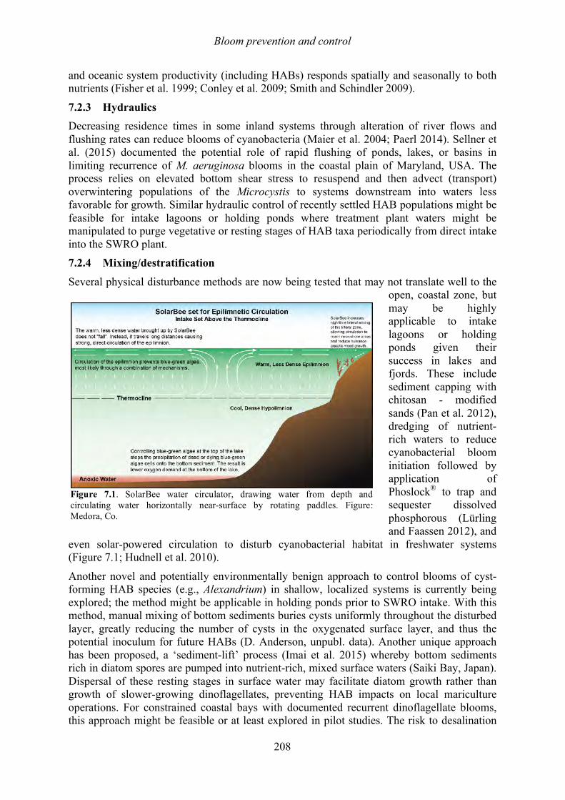
Bloom prevention and control

208

and oceanic system productivity (including HABs) responds spatially and seasonally to both nutrients (Fisher et al. 1999; Conley et al. 2009; Smith and Schindler 2009).

7.2.3 Hydraulics Decreasing residence times in some inland systems through alteration of river flows and flushing rates can reduce blooms of cyanobacteria (Maier et al. 2004; Paerl 2014). Sellner et al. (2015) documented the potential role of rapid flushing of ponds, lakes, or basins in limiting recurrence of M. aeruginosa blooms in the coastal plain of Maryland, USA. The process relies on elevated bottom shear stress to resuspend and then advect (transport) overwintering populations of the Microcystis to systems downstream into waters less favorable for growth. Similar hydraulic control of recently settled HAB populations might be feasible for intake lagoons or holding ponds where treatment plant waters might be manipulated to purge vegetative or resting stages of HAB taxa periodically from direct intake into the SWRO plant. 7.2.4 Mixing/destratification

Several physical disturbance methods are now being tested that may not translate well to the open, coastal zone, but may be highly applicable to intake lagoons or holding ponds given their success in lakes and fjords. These include sediment capping with chitosan - modified sands (Pan et al. 2012), dredging of nutrient-rich waters to reduce cyanobacterial bloom initiation followed by application of Phoslock® to trap and sequester dissolved phosphorous (Lürling and Faassen 2012), and

even solar-powered circulation to disturb cyanobacterial habitat in freshwater systems (Figure 7.1; Hudnell et al. 2010).

Another novel and potentially environmentally benign approach to control blooms of cyst-forming HAB species (e.g., Alexandrium) in shallow, localized systems is currently being explored; the method might be applicable in holding ponds prior to SWRO intake. With this method, manual mixing of bottom sediments buries cysts uniformly throughout the disturbed layer, greatly reducing the number of cysts in the oxygenated surface layer, and thus the potential inoculum for future HABs (D. Anderson, unpubl. data). Another unique approach has been proposed, a ‘sediment-lift’ process (Imai et al. 2015) whereby bottom sediments rich in diatom spores are pumped into nutrient-rich, mixed surface waters (Saiki Bay, Japan). Dispersal of these resting stages in surface water may facilitate diatom growth rather than growth of slower-growing dinoflagellates, preventing HAB impacts on local mariculture operations. For constrained coastal bays with documented recurrent dinoflagellate blooms, this approach might be feasible or at least explored in pilot studies. The risk to desalination

Figure 7.1. SolarBee water circulator, drawing water from depth and circulating water horizontally near-surface by rotating paddles. Figure: Medora, Co.

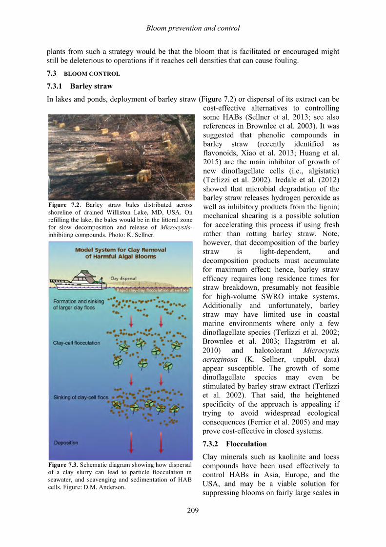
Bloom prevention and control

209

plants from such a strategy would be that the bloom that is facilitated or encouraged might still be deleterious to operations if it reaches cell densities that can cause fouling.

7.3 BLOOM CONTROL 7.3.1 Barley straw

In lakes and ponds, deployment of barley straw (Figure 7.2) or dispersal of its extract can be cost-effective alternatives to controlling some HABs (Sellner et al. 2013; see also references in Brownlee et al. 2003). It was suggested that phenolic compounds in barley straw (recently identified as flavonoids, Xiao et al. 2013; Huang et al. 2015) are the main inhibitor of growth of new dinoflagellate cells (i.e., algistatic) (Terlizzi et al. 2002). Iredale et al. (2012) showed that microbial degradation of the barley straw releases hydrogen peroxide as well as inhibitory products from the lignin; mechanical shearing is a possible solution for accelerating this process if using fresh rather than rotting barley straw. Note, however, that decomposition of the barley straw is light-dependent, and decomposition products must accumulate for maximum effect; hence, barley straw efficacy requires long residence times for straw breakdown, presumably not feasible for high-volume SWRO intake systems. Additionally and unfortunately, barley straw may have limited use in coastal marine environments where only a few dinoflagellate species (Terlizzi et al. 2002; Brownlee et al. 2003; Hagström et al. 2010) and halotolerant Microcystis aeruginosa (K. Sellner, unpubl. data) appear susceptible. The growth of some dinoflagellate species may even be stimulated by barley straw extract (Terlizzi et al. 2002). That said, the heightened specificity of the approach is appealing if trying to avoid widespread ecological consequences (Ferrier et al. 2005) and may prove cost-effective in closed systems.

7.3.2 Flocculation Clay minerals such as kaolinite and loess compounds have been used effectively to control HABs in Asia, Europe, and the USA, and may be a viable solution for suppressing blooms on fairly large scales in

Figure 7.2. Barley straw bales distributed across shoreline of drained Williston Lake, MD, USA. On refilling the lake, the bales would be in the littoral zone for slow decomposition and release of Microcystis-inhibiting compounds. Photo: K. Sellner.

Figure 7.3. Schematic diagram showing how dispersal of a clay slurry can lead to particle flocculation in seawater, and scavenging and sedimentation of HAB cells. Figure: D.M. Anderson.

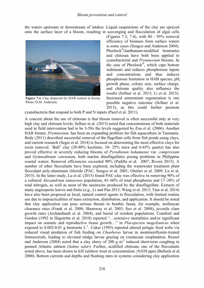
Bloom prevention and control

210

the waters upstream or downstream of intakes. Liquid suspensions of the clay are sprayed onto the surface layer of a bloom, resulting in scavenging and flocculation of algal cells

(Figures 7.3, 7.4), with 80 - 95% removal efficiency of biomass from surface waters in some cases (Sengco and Anderson 2004). Phoslock®(lanthanum-modified bentonite) and chitosan have both been applied to cyanobacterial and Prymnesium blooms. In the case of Phoslock®, which caps bottom sediments and reduces phosphorous inputs and concentrations and thus induces phosphorous limitation in HAB species, pH, growth phase, colony size, surface charge, and chitosan quality also influence the results (Sellner et al. 2013; Li et al. 2015). Increased ammonium regeneration is one possible negative outcome (Sellner et al. 2013), as this could further promote

cyanobacteria that respond to both P and N inputs (Paerl et al. 2011). A concern about the use of chitosan is that bloom removal is often successful only at very high clay and chitosan levels; Sellner et al. (2013) noted that concentrations of both materials used in field intervention had to be 3-50x the levels suggested by Zou et al. (2006). Another HAB former, Prymnesium, has been an expanding problem for fish aquaculture in Tasmania. Body (2011) described successful removal of the flagellate cells from fish ponds using clays, and current research (Seger et al. 2014) is focused on determining the most effective clays for toxin removal. ‘Ball’ clay (20-80% kaolinite, 10- 25% mica and 6-65% quartz) has also proved effective in severely reducing blooms of Pyrodinium bahamense var. compressum and Gymnodinium catenatum, both marine dinoflagellates posing problems in Philippine coastal waters. Removal efficiencies exceeded 90% (Padilla et al. 2007; Rivera 2015). A number of other flocculants have been explored, including the wastewater treatment plant flocculant poly-aluminum chloride (PAC, Sengco et al. 2001; Ghafari et al. 2009; Lu et al. 2015). In the latter study, Lu et al. (2015) found PAC-clay was effective in removing 90% of a cultured Alexandrium tamarense population, 43–60% of total phosphorus and 17–30% of total nitrogen, as well as most of the saxitoxins produced by the dinoflagellate. Extracts of many angiosperm leaves and fruits (e.g., Li and Pan 2013; Wang et al. 2013; Tian et al. 2014) have also been proposed as local, natural control agents in flocculation, with limited routine use due to impracticalities of mass extraction, distribution, and application. It should be noted that clay application can pose serious threats to benthic fauna, for example, molluscan clearance rates (Frank et al. 2000; Shumway et al. 2003; Seo et al. 2008), juvenile clam growth rates (Archambault et al. 2004), and burial of resident populations. Cranford and Gordon (1992 in Hagström et al. 2010) reported “…extensive mortalities and/or significant impact on somatic and reproductive tissue growth…” in Placopecten magellanicus when exposed to 0.002-0.01 g bentonite L-1. Cuker (1993) reported altered pelagic food webs via reduced visual predation of fish feeding on Chaoborus larvae in montmorillonite-treated limnocorrals, leading to elevated midge larvae grazing on crustacean zooplankton. Rensel and Anderson (2004) noted that a clay slurry of 200 g m-2 induced short-term coughing in penned Atlantic salmon (Salmo salar). Further, acidified chitosan, one of the flocculants noted above, has been shown to kill rainbow trout at concentration >0.038 ppm (Bullock et al. 2000). Bottom currents and depths and flushing rates in systems considering clay application

Figure 7.4. Clay dispersal for HAB control in Korea. Photo: D.M. Anderson.

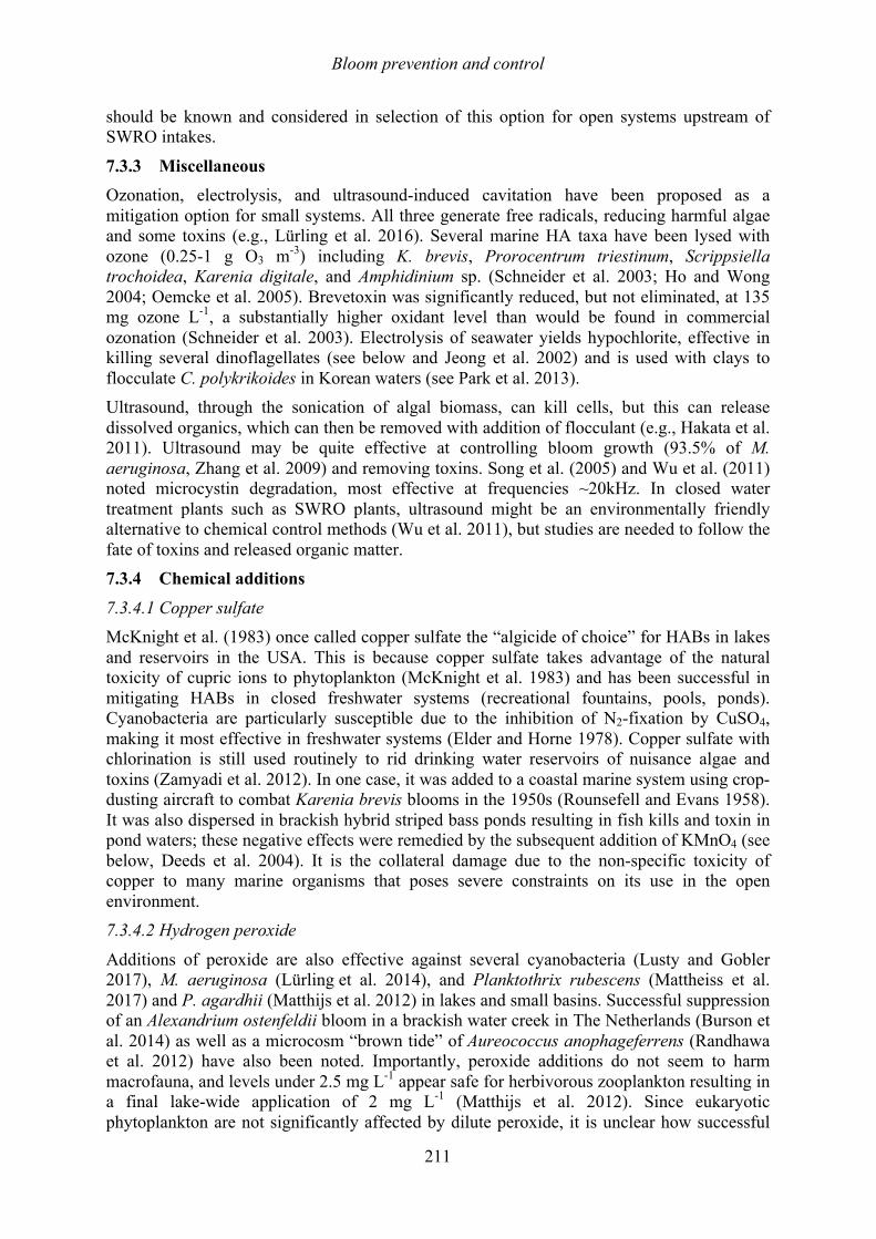
Bloom prevention and control

211

should be known and considered in selection of this option for open systems upstream of SWRO intakes.

7.3.3 Miscellaneous Ozonation, electrolysis, and ultrasound-induced cavitation have been proposed as a mitigation option for small systems. All three generate free radicals, reducing harmful algae and some toxins (e.g., Lürling et al. 2016). Several marine HA taxa have been lysed with ozone (0.25-1 g O3 m-3) including K. brevis, Prorocentrum triestinum, Scrippsiella trochoidea, Karenia digitale, and Amphidinium sp. (Schneider et al. 2003; Ho and Wong 2004; Oemcke et al. 2005). Brevetoxin was significantly reduced, but not eliminated, at 135 mg ozone L-1, a substantially higher oxidant level than would be found in commercial ozonation (Schneider et al. 2003). Electrolysis of seawater yields hypochlorite, effective in killing several dinoflagellates (see below and Jeong et al. 2002) and is used with clays to flocculate C. polykrikoides in Korean waters (see Park et al. 2013). Ultrasound, through the sonication of algal biomass, can kill cells, but this can release dissolved organics, which can then be removed with addition of flocculant (e.g., Hakata et al. 2011). Ultrasound may be quite effective at controlling bloom growth (93.5% of M. aeruginosa, Zhang et al. 2009) and removing toxins. Song et al. (2005) and Wu et al. (2011) noted microcystin degradation, most effective at frequencies ~20kHz. In closed water treatment plants such as SWRO plants, ultrasound might be an environmentally friendly alternative to chemical control methods (Wu et al. 2011), but studies are needed to follow the fate of toxins and released organic matter. 7.3.4 Chemical additions

7.3.4.1 Copper sulfate McKnight et al. (1983) once called copper sulfate the “algicide of choice” for HABs in lakes and reservoirs in the USA. This is because copper sulfate takes advantage of the natural toxicity of cupric ions to phytoplankton (McKnight et al. 1983) and has been successful in mitigating HABs in closed freshwater systems (recreational fountains, pools, ponds). Cyanobacteria are particularly susceptible due to the inhibition of N2-fixation by CuSO4, making it most effective in freshwater systems (Elder and Horne 1978). Copper sulfate with chlorination is still used routinely to rid drinking water reservoirs of nuisance algae and toxins (Zamyadi et al. 2012). In one case, it was added to a coastal marine system using crop-dusting aircraft to combat Karenia brevis blooms in the 1950s (Rounsefell and Evans 1958). It was also dispersed in brackish hybrid striped bass ponds resulting in fish kills and toxin in pond waters; these negative effects were remedied by the subsequent addition of KMnO4 (see below, Deeds et al. 2004). It is the collateral damage due to the non-specific toxicity of copper to many marine organisms that poses severe constraints on its use in the open environment. 7.3.4.2 Hydrogen peroxide

Additions of peroxide are also effective against several cyanobacteria (Lusty and Gobler 2017), M. aeruginosa (Lürling et al. 2014), and Planktothrix rubescens (Mattheiss et al. 2017) and P. agardhii (Matthijs et al. 2012) in lakes and small basins. Successful suppression of an Alexandrium ostenfeldii bloom in a brackish water creek in The Netherlands (Burson et al. 2014) as well as a microcosm “brown tide” of Aureococcus anophageferrens (Randhawa et al. 2012) have also been noted. Importantly, peroxide additions do not seem to harm macrofauna, and levels under 2.5 mg L-1 appear safe for herbivorous zooplankton resulting in a final lake-wide application of 2 mg L-1 (Matthijs et al. 2012). Since eukaryotic phytoplankton are not significantly affected by dilute peroxide, it is unclear how successful

Bloom prevention and control

212

this approach would be in coastal applications where the dominant HAB species are not cyanobacteria. Higher concentrations would be harmful to all marine life, and as a result, peroxide treatment is limited due to cost and hazardous chemical permitting (particularly in the USA).

7.3.4.3 Sulfuric acid Acid rain, volcanic activity, and mining are known sources of sulfuric acid to aquatic systems and have been shown to be detrimental to phytoplankton populations via overall acidification of surface waters (Geller et al. 1998). Enclosure experiments with toxic Prymnesium parvum demonstrated the inhibitory effect of lowered pH on bloom development and toxin (prymnesins) production after the addition of 0.1 N sulfuric acid (Prosser et al. 2012). Place (A. Place, unpubl. data) has examined the effects of sulfuric acid additions to reduce pH of surface waters surrounding local HABs temporarily, thereby increasing phytoplankton susceptibility to flocculation and settling to the bottom. 7.3.4.4 Potassium permanganate

Potassium permanganate has been employed in wastewater treatment plants for decades as a potent oxidizing agent to reduce biological and chemical oxygen demands in effluents (reviewed by Scott and Ollis 1995). Use in the natural environment is a concern due to its generic ability to oxidize all organic matter, i.e., HAB cells and all other biota. It has, however, been used to control Karlodinium veneficum (an ichthyotoxin-producing dinoflagellate) and its toxin in brackish hybrid striped bass ponds in Eastern Maryland, USA (Deeds et al. 2004). In another spring-fed pond, near-bottom cold water anatoxin-producing Planktothrix prolifera populations were effectively removed or severely reduced with bottom water KMnO4 additions, thereby freeing the pond of detectable toxin, with only low cell abundances (K. Sellner, unpubl. data) and no apparent impact on metazoans in the system. The P. prolifera population has since been found at bloom levels under ice seven years post-treatment.

7.3.4.5 Chlorination Chlorination, through addition of NaOCl or other chloride compounds, is commonly used to remove cyanobacteria and cyanotoxins from drinking water supplies, with the degree of toxin degradation being toxin-specific (Zamyadi et al. 2012). Following experimental work with electrolysis of seawater (yielding hypochlorite) and several marine dinoflagellates (Gymnodinium catenatum, Cochlodinium polykrikoides, Akashiwo sanguinea, Lingulodinium polyedrum, Prorocentrum micans, Alexandrium affine, and Gymnodinium impudicum), Jeong et al. (2002) suggested effective NaOCl doses of 300-500 ppb for 10 min or 200-400 ppb for 1 h could minimize HAB exposures; however, free radicals may stress other biota in the system (Brungs 1973). Chlorination to eliminate HAB toxins is discussed in Chapter 2.

7.3.5 Biological additions 7.3.5.1 Microbes

Viral and bacterially induced lysis (cell breakdown) are natural processes that regulate phytoplankton communities and carbon flux (e.g., Fuhrman and Azam 1980; Salomon and Imai 2006). Making use of this natural pathogenicity seems like a logical, cost-effective solution to HAB control; however, the scientific community is skeptical of experiments that introduce foreign, potentially invasive species, or have the potential to restructure natural assemblages in an ecosystem irreversibly (Sanders et al. 2003; Secord 2003). Despite the many laboratory studies demonstrating the harmful effects of heterotrophic bacteria on algal species, Mayali and Azam (2004) argue that most field studies have failed to show

Bloom prevention and control

213

conclusively the causal relationship between the decline of a bloom in natural ecosystems and the behavior of an introduced algicidal bacterium. Another major issue is that the conversion from laboratory conditions to the natural environment is inherently complex given the flexibility of predator-prey dynamics mediated by the presence or absence of other algal species (Mayali and Azam 2004). There are at least two studies indicating the benefit of natural plant-associated bacteria in reducing HABs. Imai et al. (2012) and Onishi et al. (2014; Figure 1.6) noted lytic bacteria for M. aeruginosa as well as H. akashiwo and Alexandrium tamarense in submersed angiosperms and macroalgae, respectively, indicating potential natural control in several Japanese bays (see Imai et al. 2014) and Puget Sound (Inaba et al. 2015).

HAB parasites are increasingly studied as bloom control agents, with Amoebophyra spp. the most well-documented natural dinoflagellate control. The seminal work by Coats and colleagues (e.g., Coats 1999) has stimulated other research, resulting in the identification of several taxon-specific parasites that some suggest could be applied routinely to nearshore zones where host dinoflagellates might be increasing, detected through satellite or other remote detection systems (see Chapter 4). Jeong et al. (2003) have proposed using heterotrophic dinoflagellates for control of natural HABs. Routine use of most biological agents seems impractical at this time due to the costs associated with maintenance of the parasite in culture, mass cultivation, manpower, and the diversity of HABs that could frequent an area.

Although not identified for marine species, chytrid fungi have been shown to infect a wide variety of phytoplankton in freshwater lakes, and while not necessarily host-specific, they appear to prefer larger phytoplankton species (Kagami et al. 2007). These eukaryotic parasites are ubiquitous in coastal marshes, and so far, only two genera of infecting fungi have been studied for marine taxa (diatoms only), with little known regarding the magnitude of their pathogenicity (Park et al. 2004). Interestingly, the major eukaryotic parasites infecting marine dinoflagellates are other dinoflagellates (rather than fungi), such as Amoebophyra spp. mentioned above. Jia et al. (2010) examined the effect of “white rot fungus” (Trichaptum abietinum), a non-aquatic, wood-decay fungus often used to degrade industrial pollutants, on several cyanobacterial cultures. Not only were the cultures destroyed within 48 h, but it appeared that the fungus actively preyed on the algal cells and did not seem to discriminate between species. Even more tantalizing is the complete degradation after 12 h of microcystin in test M. aeruginosa cultures inoculated with mycelial pellicles. It is important to note that white rot fungus has not been applied to larger reservoirs or drinking water systems nor evaluated for environmental safety (Jia et al. 2012), although it has been used to increase barley straw decomposition and inhibition of the cyanobacterium (Sellner et al. 2015). 7.3.5.2 Competitors

Biological diversity may also be an important factor for keeping HAB species from gaining dominance. Cardinale (2011) demonstrated that more diverse communities are naturally buffered against nutrient enrichment relative to less diverse communities due to the enhanced niche partitioning by benthic diatoms which increased nitrogen uptake. The promotion of higher algal biodiversity and habitat preservation may thus be one method for facilitating greater nutrient uptake capacity, particularly in protected environments where physical advection processes do not dominate phytoplankton turnover rates. Allelopathic interactions (e.g., Pratt 1966; Tang and Gobler 2011; Lim et al. 2014; Tang et al. 2014) introduced when algae exude dissolved secondary metabolites (sometimes phycotoxins) into the environment are an indicator of inter-specific competition for limiting resources (Graneli and Hansen

Bloom prevention and control

214

2006). It may also be that as species diversity increases, the ability of a given toxic species to dominate its competitors is suppressed by the wider array of competitive strategies present in the community. As marine ecosystem models become more sophisticated and include realistic phytoplankton biodiversity (Follows et al. 2007; Goebel et al. 2010), varying management strategies can be assessed in relation to the physical environment, community composition, competitive interactions, and nutrient dynamics.

7.3.5.3 Grazers and trophic cascades Algal proliferation is heavily regulated by grazing pressure from zooplankton, with grazing and trophic cascades representing an often overlooked component of bloom development and persistence (e.g., Verity and Smetacek 1996; Gobler et al. 2002; Turner and Graneli 2006; Smayda 2008). There is evidence that eutrophication (i.e., nutrient enrichment) exerts an indirect effect on zooplankton grazing efficiency. At higher nutrient levels, phytoplankton are no longer suppressed by grazers (Kemp et al. 2001) and actually increase the production of grazing deterrents (Mitra and Flynn 2006), a positive feedback that intensifies negative impacts of HABs (Sunda et al. 2006). This idea of indirect effects is also consistent with a simulation study by Daskalov (2002) who found that the increase in algal blooms in the Black Sea was the result of intense overfishing of top predators, such as cetaceans and large migratory fish. The overfishing resulted in decreased predator control of planktivorous fish, thereby depleting zooplankton stocks and allowing phytoplankton to flourish. This ‘trophic cascade’ was assisted by anthropogenic eutrophication that significantly relieved resource limitation from the bottom-up (Daskalov 2002) and likely further suppressed grazing. Another simulation study (Walsh et al. 2011) used a coupled physical-biological model of the Chukchi/Beaufort Seas to illustrate that “fishing down of the food web” (sensu Pauly et al. 1998) and increased eutrophication in a scenario similar to that of the Black Sea supports hypotheses of a regime shift favoring N2-fixers and HAB-forming dinoflagellates like the saxitoxin-producing Alexandrium tamarense. Ultimately, the solution to this ecologically complex interplay is similar to that discussed in Section 7.2.1, whereby reduction in nutrient loads not only provides bottom-up regulation of blooms, but can lead to unexpected consequences for other ecosystem components essential to bloom control. 7.3.6 Combined methods/redundancy

There are some examples of combinations of multiple interventions in bloom control. Sellner et al. (2015) document the combined effects of hydraulic flushing and barley straw additions in limiting growth of M. aeruginosa and toxin accumulation in a freshwater lake in Maryland, USA. Flocculation, sedimentation, capping of bottom sediments, and additions of toxin-utilizing Pseudomonas sp. in bloom control have been suggested for blooms of M. aeruginosa in China (Li et al. 2015). As noted above, seawater electrolysis followed by clay flocculation is an effective removal strategy for C. polykrikoides populations that threaten fish pen mariculture in Korean (Park et al. 2013). Practical use of approaches like these near SWRO intakes remains to be determined. 7.4 SUMMARY

There are numerous techniques to prevent and control HABs, though many remain experimental or are practical only on a small scale. Most preventative measures involve factors beyond the control of desalination plant operators, such as nutrient reduction from regional watersheds or other point and non-point sources of nutrient discharge to the coastal zone that can stimulate HABs. The increasing development of desalination plants should serve to provide pressure on governmental entities (or favor government-private partnerships) responsible for monitoring and controlling nutrient pollution given the need for safe, clean

Bloom prevention and control

215

drinking water. As covered in Chapter 3, monitoring methods that include satellite-based bloom detection, and advanced models of HAB initiation and transport provide early warning of delivery of potential toxins or bloom biomass to a plant’s intake system. While these monitoring and modeling programs require significant financial investment to develop and maintain, they allow operators to prepare for HAB events and potentially adjust intake operations and plant pre-treatment technologies accordingly.

Fortunately, options remain for the control of HABs that have already entered a desalination plant, and these are described in detail in Chapter 9. For plants with holding ponds or reservoirs, intervening with physical disturbance techniques, oxidizing compounds (H2O2, KMnO4) or clay minerals to remove HAB particles via flocculation are possibilities. Care must be taken, however, as some turn particulate algal biomass (which is relatively easy to remove with pretreatment) into dissolved organic compounds, which are much harder to remove. Other post-intake technologies for SWRO include the application of copper sulfate (cell lysis but little toxin degradation) followed by, or by themselves, the use of techniques that generate oxidizing conditions (again peroxide or permanganate as well as chlorination, electrolysis, ozonation, perhaps ultrasound), but post-treatment of these waters might be required to mitigate possible damage to plant membranes. High costs will likely prohibit the frequent use of these methods for mitigation, but several could also be considered as options for minimizing HAB entry into a desalination plant, particularly in the case of methods that are applicable to coastal environments or embayments, such as hydrogen peroxide application or electrolysis-clay addition. The majority of methods suggested in this chapter, however, are meant to give desalination operators an understanding of the challenges associated with HAB prevention and control. Many are not practical, given desalination–specific factors such as the high-volume intake requirements of plants, but others may be of use, and may contribute to a suite of adaptive strategies to mitigate HAB impacts on desalination operations.

7.5 REFERENCES Anderson, D. M. 1997. Turning back the harmful red tide. Nature 388, 513-514.

Anderson, D. M. 2004. Prevention, control and mitigation of harmful algal blooms: Multiple approaches to HAB management. Hall, S., Etheridge, S., Anderson, D., Kleindinst, J., Zhu, M., and Zou, Y. (Eds.), Harmful Algae Management and Mitigation, Asia-Pacific Economic Cooperation (Singapore): APEC Publication #204-MR-04.2. pp. 123-130.

Anderson, D. M., Glibert, P. M., and Burkholder, J. M. 2002. Harmful algal blooms and eutrophication: Nutrient sources, composition, and consequences. Estuaries 25, 704–726.

Archambault, M. C., Bricelj, V. M., Grant, J., and Anderson, D. M. 2004. Effects of suspended and sedimented clays on juvenile hard clams, Mercenaria mercenaria, within the context of harmful algal bloom mitigation. Marine Biology 144, 553-565.

Body, A. 2011. Stable pond blooms through phosphate and pH control. Infofish International 1/2011, 22-25.

Brownlee, E. F., Sellner, S. G., and Sellner, K. G. 2003. Effects of barley straw (Hordeum vulgare) on freshwater and brackish phytoplankton and cyanobacteria. Journal of Applied Phycology 15, 525–531.

Brungs, W. A. 1973. Effects of residual chlorine on aquatic life. Journal of the Water Pollution Control Federation 45, 2180-2193.

Bloom prevention and control

216

Budd, J. W., Drummer, T. D., Nalepa, T. F., and Fahnenstiel, G. L. 2001. Remote sensing of biotic effects: Zebra mussels (Dreissena polymorpha) influence on water clarity in Saginaw Bay, Lake Huron. Limnology and Oceanography 46(2), 213-223.

Bullock, G., Blazer, V., Tsukuda, S., and S. Summerfelt. 2000. Toxicity of acidified chitosan for cultured rainbow trout (Oncorhynchus mykiss). Aquaculture 185, 273-280.

Burson, A., Matthijs, H. C., de Bruijne, W., Talens, R., Hoogenboom, R., Gerssen, A., Visser, P. M., Stomp, M., Steur, K., and van Scheppingen, Y. 2014. Termination of a toxic Alexandrium bloom with hydrogen peroxide. Harmful Algae 31: 125–135.

Cardinale, B. J. 2011. Biodiversity improves water quality through niche partitioning. Nature 472, 86–89.

Coats, D. W. 1999. Parasitic life styles of marine dinoflagellates. Journal of Eukaryote Microbiology 46, 402-409.

Conley, D. J., Paerl, H. W., Howarth, R. W., Boesch, D. F., Seitzinger, S. P., Havens, K. E., Lancelot, C., and Likens, G. E. 2009. Controlling eutrophication: Nitrogen and phosphorus. Science 323, 1014-1015.

Cuker, B. E. 1993. Suspended clays alter trophic interactions in the plankton. Ecology 74, 944-953.

Daskalov, G. M. 2002. Overfishing drives a trophic cascade in the Black Sea. Marine Ecology Progress Series 225, 53–63.

Deeds, J. R., Mazzaccaro, A. P., Terlizzi, D. E., and Place, A. R. 2004. Treatment options for the control of an ichthyotoxic dinoflagellate in an estuarine aquaculture facility: A case study. Hall, S., Anderson, D., Kleindinst, J., Zhu, M., and Zou, Y. (Eds.), Proceedings of the Second International Conference on Harmful Algae Management and Mitigation, Asia-Pacific Economic Cooperation, APEC Publ. #204-MR-04.2, Singapore, pp. 177-181.

Elder, J. F., and Horne, A. J. 1978. Copper cycles and CuSO4 algicidal capacity in two California lakes. Environmental Management 2, 17–30.

Elmgren, R., and Larsson, U. 2001. Nitrogen and the Baltic Sea: managing nitrogen in relation to phosphorus. The Scientific World Journal 1, 371–377.

Ferrier, M. D., Butler, B. R., Terlizzi, D. E., and Lacouture, R. V. 2005. The effects of barley straw (Hordeum vulgare) on the growth of freshwater algae. Bioresource Technology 96, 1788–1795.

Fisher, T. R., Gustafson, A. B., Sellner, K., Lacouture, R., Haas, L. W., Wetzel, R. L., Magnien, R., Everitt, D., Michaels, B., and Karrh, R. 1999. Spatial and temporal variation of resource limitation in Chesapeake Bay. Marine Biology 133, 763-778.

Follows, M. J., Dutkiewicz, S., Grant, S., and Chisholm, S. W. 2007. Emergent biogeography of microbial communities in a model ocean. Science 315, 1843–1846.

Frank, D., Ewert, L., Shumway, S., and Ward, J. E. 2000. Effect of clay suspensions on clearance rates in three species of benthic invertebrates. Journal of Shellfish Research 19, 663.

Fuhrman, J. A., and Azam, F. 1980. Bacterioplankton secondary production estimates for coastal waters of British Columbia, Antarctica, and California. Applied and Environmental Microbiology 39, 1085–1095.

Bloom prevention and control

217

Geller, W., Klapper, H., and Schultze, M. 1998. Natural and anthropogenic sulfuric acidification of lakes. Geller, W., Klapper, H., and Salomons, W. (Eds.), Acidic Mining Lakes. Springer, Berlin Heidelberg, pp. 3–14.

Ghafari, S., Aziz, H. A., Isa, M. H., and Zinatizadeh, A. A. 2009. Application of response surface methodology (RSM) to optimize coagulation–flocculation treatment of leachate using poly-aluminum chloride (PAC) and alum. Journal of Hazardous Materials 163, 650–656.

Gobler, C. J., Renaghan, M. J., and Buck, N. J. 2002. Impacts of nutrients and grazing mortality on the abundance of Aureococcus anophagefferens during a New York brown tide bloom. Limnology and Oceanography 47, 129–141.

Goebel, N. L., Edwards, C. A., Zehr, J. P., and Follows, M. J. 2010. An emergent community ecosystem model applied to the California Current System. Journal of Marine Systems 83, 221–241.

Graneli, E., and Hansen, P. J. 2006. Allelopathy in harmful algae: A mechanism to compete for resources? Granéli, E. and Turner, J. T. (Eds.), Ecology of Harmful Algae, Springer. pp. 189–201.

Hagström, J. A., Sengco, M. R., and Villareal, T. A. 2010. Potential methods for managing Prymnesium parvum blooms and toxicity, with emphasis on clay and barley straw: a review. Journal of the American Water Resources Association 46, 187–198.

Hakata, Y., Roddick, F., and Fan, L. 2011. Impact of ultrasonic pre-treatment on the microfiltration of a biologically treated municipal effluent. Desalination 283, 75–79.

Heisler, J., Glibert, P., Burkholder, J., Anderson, D., Cochlan, W., Dennison, W., Dortch, Q., Gobler, C., Heil, C., Humphries, E., Lewitus, A., Magnien, R., Marshall, H., Sellner, K., Stockwell, D., Stoecker, D., and Suddleson, M. 2008. Eutrophication and harmful algal blooms: A scientific consensus. Harmful Algae 8, 3-13.

Henry, T. 2013. Carrol Township’s scare with toxin a “wake-up call.” Toledo Blade 15.

Ho, K. C. and Wong, Y. K. 2004. A study on the effectiveness of using ozone to mitigate harmful algal blooms. Hall, S., Anderson, D., Kleindinst, J., Zhu, M., and Zou, Y. (Eds.), Proceedings of the Second International Conference on Harmful Algae Management and Mitigation, Asia-Pacific Economic Cooperation, APEC Publ. #204-MR-04.2, Singapore, pp. 185-188.

Huang, H., Xiao, X., Ghadouani, A., Wu, J., Nie, Z., Peng, C., Xu, X., and Shi, J. 2015. Effects of natural flavonoids on photosynthetic activity and cell integrity in Microcystis aeruginosa. Toxins 7, 66-80.

Hudnell, H. K., Jones, C., Labisi, B., Lucero, V., Hill, D. R., and Eilers, J. 2010. Freshwater harmful algal bloom (FHAB) suppression with solar powered circulation (SPC). Harmful Algae 9, 208–217.

Imai, I., Imai, Y., Toda, T., Noda, M., and Miyamura, K. 2015. Manipulating phytoplankton flora to harmless diatoms through germination of resting stage cells by sediment-lift to euphotic layer in coastal sea. Proceedings of the 16th International Conference on Harmful Algae, Abstract and presentation, Wellington, NZ.

Bloom prevention and control

218

Imai, I., Shimada, H., Shinada, A., Baba, K., Kanamori, M., Sato, M., Kuwahara, Y., Miyoshi, K., Tada, M., Hirano, K., Miyazono, A., and Itakura, S. 2014. Prediction of toxic algal bloom occurrences and adaptation to toxic blooms to minimize economic loss to the scallop aquaculture industry in Hokkaido, Japan. Trainer, V.L. and Yoshida, T. (Eds.). Proceedings of a Workshop on Economic Impacts of Harmful Algal Blooms on Fisheries and Aquaculture, PICES Scientific Report Number. 47, pp. 7-16.

Imai, Y., Ohgi, K., Mizuhara, S., Yamaguchi, A., and Kaerlyama, M. 2012. Experimental study on control of Microcystis aeruginosa bloom by using of microorganisms in waters of a reed community and a water plant zone. Abstract and presentation, 15th International Conference on Harmful Algae, Gyeongnam, Korea.

Inaba, N., Onishi, Y., Ishii, K., Trainer, V. L., Wylie-Echeverria, S., Hatch, M. B. A., and Imai, I. 2015. High density of algicidal and growth-inibiting bacteria against harmful algal species detected from seagrass and macroalgae in Puget Sound. Abstract and presentation, 16th International Conference on Harmful Algae, Wellington, NZ.

Iredale, R. S., McDonald, A. T., and Adams, D. G. 2012. A series of experiments aimed at clarifying the mode of action of barley straw in cyanobacterial growth control. Water Research 46, 6095–6103.

Jeong, H. J., Kim, J. S., Yoo, Y. D., Kim, S. T., Kim, T. H., Park, M. G., Lee, C. H., Seong, K. A., Rang, N. S., and Shim, J. H. 2003. Feeding by the heterotrophic dinoflagellate Oxyrrhis marina on the red-tide raphidophyte Heterosigma akashiwo: A potential biological method to control red tides using mass-cultured grazers. Journal of Eukaryotic Microbiology 50, 274-282.

Jeong, H. J., Kim, H. R., Kwang, I. K., Kwang, Y. K., Park, K. H., Seong, T. K., Yoo, Y. D., Song, J. Y., Kim, J. S., Seong, K. A., Pae, W. H. S. E., Lee, C. H., Huh, M. D., and Lee, S. H. 2002. NaOCl produced by electrolysis of natural seawater as a potential method to control marine red-tide dinoflagellates. Phycologia 41, 643-656.

Jia, Y., Han, G., Wang, C., Guo, P., Jiang, W., Li, X., and Tian, X. 2010. The efficacy and mechanisms of fungal suppression of freshwater harmful algal bloom species. Journal of Hazardous Materials 183, 176–181.

Jia, Y., Du, J., Song, F., Zhao, G., and Tian, X. 2012. A fungus capable of degrading microcystin-LR in the algal culture of Microcystis aeruginosa PCC7806. Applied Biochemistry and Biotechnology 166, 987–996.

Juhel, G., Davenport, J., O’Halloran, J., Culloty, S. C., O’Riordan, R. M., James, K. F., Furey, A., and Allis, O. 2006. Impacts of microcystins on the feeding behaviour and energy balance of zebra mussels, Dreissena polymorpha: A bioenergetics approach. Aquatic Toxicology 79, 391–400.

Kagami, M., de Bruin, A., Ibelings, B. W., and Van Donk, E. 2007. Parasitic chytrids: their effects on phytoplankton communities and food-web dynamics. Hydrobiologia 578, 113–129.

Kemp, W. M., Brooks, M. T., and Hood, R. R. 2001. Nutrient enrichment, habitat variability and trophic transfer efficiency in simple models of pelagic ecosystems. Marine Ecology Progress Series 223, 73–87.

Kim, H. G. 2006. Mitigation and controls of HABs. Granéli, E. and Turner, J.T. (Eds.), Ecology of Harmful Algae, Springer. pp. 327–338.

Bloom prevention and control

219

Li, L. and Pan, G. 2013. A universal method for flocculating harmful algal blooms in marine and fresh waters using modified sand. Environmental Science and Technology 47, 4555–4562.

Li, L., Zhang, H., and Pan, G. 2015. Influence of zeta potential on the flocculation of cyanobacteria cells using chitosan modified soil. Journal of Environmental Sciences 28, 47–53.

Lim, A. S., Jeong, H. J., Jang, T. Y., Jang, S. H., and Franks, P. J. 2014. Inhibition of growth rate and swimming speed of the harmful dinoflagellate Cochlodinium polykrikoides by diatoms: Implications for red tide formation. Harmful Algae 37, 53–61.

Lu, G., Song, X., Yu, Z., Cao, X., and Yuan, Y. 2015. Environmental effects of modified clay flocculation on Alexandrium tamarense and paralytic shellfish poisoning toxins (PSTs). Chemosphere 127, 188–194.

Lürling, M. and Faassen, E. J. 2012. Controlling toxic cyanobacteria: Effects of dredging and phosphorus-binding clay on cyanobacteria and microcystins. Water Research 46, 1447–1459.

Lürling, M., Meng, D., and Faassen, E. J. 2014. Effects of hydrogen peroxide and ultrasound on biomass reduction and toxin release in the cyanobacterium, Microcystis aeruginosa. Toxins 6, 3260-3280.

Lürling, M., Waajen, G., and de Senerpont Domis, L. N. 2016. Evaluation of several end-of-pipe measures proposed to control cyanobacteria. Aquatic Ecology 50, 499-519.

Maier, H. R., Kingston, G. B., Clark, T., Frazer, A., and Sanderson, A. 2004. Risk-based approach for assessing the effectiveness of flow management in controlling cyanobacterial blooms in rivers. River Research Applications 20, 459-471.

Mattheiss, J., Sellner, K. G., and Ferrier, D. 2017. Lake Anita Louise Peroxide Treatment Summary – December 2016. CCWS Contribution #17-01, Center for Coastal and Watershed Studies, Hood College, Frederick, MD. 9 pp.

Matthijs, H. C., Visser, P. M., Reeze, B., Meeuse, J., Slot, P. C., Wijn, G., Talens, R., and Huisman, J. 2012. Selective suppression of harmful cyanobacteria in an entire lake with hydrogen peroxide. Water Research 46, 1460–1472.

Mayali, X., and Azam, F. 2004. Algicidal bacteria in the sea and their impact on algal blooms. Journal of Eukaryotic Microbiology 51, 139–144.

McKnight, D. M., Chisholm, S. W., and Harleman, D. R. 1983. CuSO4 treatment of nuisance algal blooms in drinking water reservoirs. Environmental Management 7, 311–320.

Miller, M. A., Kudela, R. M., Mekebri, A., Crane, D., Oates, S. C., Tinker, M. T., Staedler, M., Miller, W. A., Toy-Choutka, S., and Dominik, C. 2010. Evidence for a novel marine harmful algal bloom: cyanotoxin (microcystin) transfer from land to sea otters. PLoS One, 5: e12576.

Mitra, A., and Flynn, K. J. 2006. Promotion of harmful algal blooms by zooplankton predatory activity. Biology Letters 2, 194–197.

Nelson, L. A. 2015. Community assessment for public health emergency response (CASPER) following detection of microcystin toxin in a municipal water system, Ohio, September 2014. Proceedings of the 2015 CSTE Annual Conference. Cste.

Bloom prevention and control

220

Oemcke, D. J. and Van Leeuwen, J. H. 2005. Ozonation of the marine dinoflagellate alga Amphidinium sp.—implications for ballast water disinfection. Water Research 39, 5119–5125.

Onishi, Y., Mohri, Y., Tuji, A., Ohgi, K., Yamaguchi, A., and Imai, I. 2014. The seagrass Zostera marina harbors growth inhibiting bacteria against the toxic dinoflagellate Alexandrium tamarense. Fisheries Science 80, 353–362.

Padilla, L., San Diego-McGlone, M. L., and Azanza, R. 2007. Preliminary results on the use of clay to control Pyrodinium bloom-a mitigation strategy. Science Diliman 18(1), 35-42.

Paerl, H. W. 2014. Mitigating harmful cyanobacterial blooms in a human- and climatically-impacted world. Life 4, 988-1012.

Paerl, H. W., Hall, N. S., and Calandrino, E. S. 2011. Controlling harmful cyanobacterial blooms in a world experiencing anthropogenic and climatic-induced change. Science of the Total Environment 409, 1739–1745.

Pan, G., Dai, L., Li, L., He, L., Li, H., Bi, L., and Gulati, R. D. 2012. Reducing the recruitment of sedimented algae and nutrient release into the overlying water using modified soil/sand flocculation-capping in eutrophic lakes. Environmental Science and Technology 46, 5077–5084.

Park, M. G., Yih, W., and Coats, D. W. 2004. Parasites and phytoplankton, with special emphasis on dinoflagellate infections. Journal of Eukaryotic Microbiology 51, 145–155.

Park, T. G.,Lim, W. A., Park, Y. T., Lee, C. K., and Jeong, H. J. 2013. Economic impact, management and mitigation of red tides in Korea. Harmful Algae 30S, S131-S143.

Pauly, D., Christensen, V., Dalsgaard, J., Froese, R., and Torres, F. 1998. Fishing down marine food webs. Science 279, 860–863.

Pratt, D. M. 1966. Competition between Skeletonema costatum and Olisthodiscus luteus in Narragansett Bay and in culture. Limnology and Oceanography 11, 447–455.

Prosser, K. N., Valenti, T. W., Hayden, N. J., Neisch, M. T., Hewitt, N. C., Umphres, G. D., Gable, G. M., Grover, J. P., Roelke, D. L., and Brooks, B. W. 2012. Low pH pre-empts bloom development of a toxic haptophyte. Harmful Algae 20, 156–164.

Randhawa, V., Thakkar, M., and Wei, L. 2012. Applicability of hydrogen peroxide in brown tide control - culture and microcosm studies. PLOS One https://doi.org/10.1371/journal.pone.0047844

Rensel, J. E. J. and Anderson, D. M. 2004. Effects of phosphatic clay dispersal at two divergent sites in Puget Sound, Washington. In: Steidinger, K.A., Landsberg, J.H., Tomas, C.R., and Vargo, G.A. (Eds.), Harmful Algae 2002. Florida Fish and Wildlife Conservation Commission, Florida Institute of Oceanography and Intergovernmental Ocenographic Commission of UNESCO, St. Petersburg Beach, Florida, pp. 522-524.

Rivera, P. P. L. 2015. Removal of harmful algal bloom (HAB)-forming organisms using ball clay: Factors and effects of clay addition. University of Philippines. pp. 101.

Rounsefell, G. A., and Evans, J. E. 1958. Large-scale experimental test of copper sulfate as a control for the Florida red tide. U.S. Fish and Wildlife Service Special Scientific Report.

Salomon, P. S. and Imai, I. 2006. Pathogens of harmful microalgae. Granéli, E. and Turner, J.T. (Eds.), Ecology of Harmful Algae, Springer. pp. 271–282.

Bloom prevention and control

221

Sanders, N. J., Gotelli, N. J., Heller, N. E., and Gordon, D. M. 2003. Community disassembly by an invasive species. Proceedings of the National Academy of Sciences USA, 100, 2474–2477.

Schneider, K. R., Pierce, R. H., and Rodrick, G. E. 2003. The degradation of Karenia brevis toxins utilizing ozonated seawater. Harmful Algae 2, 101-107.

Scott, J. P. and Ollis, D. F. 1995. Integration of chemical and biological oxidation processes for water treatment: review and recommendations. Environmental Progress 14, 88–103.

Secord, D. 2003. Biological control of marine invasive species: cautionary tales and land-based lessons. Biological Invasions 5, 117–131.

Seger, A., Body, A., and Hallegraeff, G. M. 2014. Exploration of Phoslock™ clay in mitigating Prymnesium parvum fish-killing algal blooms in aquaculture ponds. Proceedings of the 15th International Conference on Harmful Algae, Changwon, South Korea, October.

Sellner, K. G., Place, A. R., Paolisso, M., Gao, Y., Williams, E. and VanDolah, F. M. 2013. Options in mitigating cyanobacterial blooms. Proceedings of the 7th U.S. Harmful Algal Bloom Symposium, Abstract and presentation.

Sellner, K. G., Place, A. R., Williams, E., Gao, Y., VanDolah, E., Paolisso, M., Bowers, H. A., and Roche, S. 2015. Hydraulics and barley straw (Hordeum vulgare) as effective treatment options for a cyanotoxin-impacted lake. L. MacKenzie (Ed.), Proceedings of the 16th International Conference on Harmful Algae, Cawthron Institute and International Society for the Study of Harmful Algae, Vawthron, NZ. pp. 218-221.

Sengco, M. R., Li, A., Tugend, K., Kulis, D., and Anderson, D. M. 2001. Removal of red-and brown-tide cells using clay flocculation. I. Laboratory culture experiments with Gymnodinium breve and Aureococcus anophagefferens. Marine Ecology Progress Series 210, 41–53.

Sengco, M. R., and Anderson, D. M. 2004. Controlling harmful algal blooms through clay flocculation1. Journal of Eukaryotic Microbiology 51, 169–172.

Seo, K. S., Lee, C. K., Park, Y. T., and Lee, Y. 2008. Effect of yellow clay on respiration and phytoplankton uptake of bivalves. Fisheries Science 74, 120-127.

Shumway, S. E., Frank, D. M., Ewart, L. M., and Ward, L. E. 2003. Effect of yellow loess on clearance rate in seven species of benthic, filter-feeding invertebrates. Aquaculture Research 34, 1391-1402.

Smayda, T. J. 2008. Complexity in the eutrophication–harmful algal bloom relationship, with comment on the importance of grazing. Harmful Algae 8, 140–151.

Smith, V. H. and Schindler, D. W. 2009. Eutrophication science: where do we go from here? Trends in Ecology & Evolution 24, 201–207.

Song, W., Teshiba, T., Rein, K., and O'Shea, K. E. 2005. Ultrasonically induced degradation and detoxification of microcystin-LR (cyanobacterial toxin). Environmental Science and Technology 39, 6300–6305.

Sunda, W. G., Granéli, E., and Gobler, C. J. 2006. Positive feedback and the development and persistence of ecosystem disruptive algal blooms. Journal of Phycology 42, 963–974.

Tang, Y. Z., and Gobler, C. J. 2011. The green macroalga, Ulva lactuca, inhibits the growth of seven common harmful algal bloom species via allelopathy. Harmful Algae 10, 480–488.

Bloom prevention and control

222

Tang, Y. Z., Kang, Y., Berry, D., and Gobler, C. J. 2014. The ability of the red macroalga, Porphyra purpurea (Rhodophyceae) to inhibit the proliferation of seven common harmful microalgae. Journal of Applied Phycology 27, 531–544.

Terlizzi, D. E., Ferrier, M. D., Armbrester, E. A., and Anlauf, K. A. 2002. Inhibition of dinoflagellate growth by extracts of barley straw (Hordeum vulgare). Journal of Applied Phycology 14, 275–280.

Tian, F., Zhou, J., Sun, Z., Cai, Z., Xu, N., An, M., and Duan, S. 2014. Inhibitory effects of Chinese traditional herbs and herb-modified clays on the growth of harmful algae, Phaeocystis globosa and Prorocentrum donghaiense. Harmful Algae 37, 153–159.

Turner, J. T. and Granéli, E. 2006. “Top-down” predation control on marine harmful algae, Granéli, E. and Turner, J.T. (Eds.), Ecology of Harmful Algae, Springer. pp. 355–366.

Verity, P. G., and Smetacek, V. 1996. Organism life cycles, predation, and the structure of marine pelagic ecosystems. Marine Ecology Progress Series 130, 277–293.

Walsh, J. J., Dieterle, D. A., Chen, F. R., Lenes, J. M., Maslowski, W., Cassano, J. J., Whitledge, T. E., Stockwell, D., Flint, M., and Sukhanova, I. N. 2011. Trophic cascades and future harmful algal blooms within ice-free Arctic Seas north of Bering Strait: A simulation analysis. Progress in Oceanography 91, 312–343.

Wang, L., Liang, W., Yu, J., Liang, Z., Ruan, L., and Zhang, Y. 2013. Flocculation of Microcystis aeruginosa using modified larch tannin. Environmental Science and Technology 47, 5771–5777.

Wu, X., Joyce, E. M., and Mason, T. J. 2011. The effects of ultrasound on cyanobacteria. Harmful Algae 10, 738–743.

Xiao, X., Huang, H., Ge, Z., Rounge, T. B., Shi, J., Xu, X., Li, R., and Chen, Y. 2013. A pair of chiral flavonolignans as novel anti-cyanobacterial allelochemicals derived from barley straw (Hordeum vulgare): Characterization and comparison of their anti-cyanobacterial activities. Environmental Microbiology doi:10.1111/1462-2920.12226.

Zamyadi, A., MacLeod, S. L., Fan, Y., McQuaid, N., Dorner, S., Sauvé, S., and Prévost, M. 2012. Toxic cyanobacterial breakthrough and accumulation in a drinking water plant: A monitoring and treatment challenge. Water Research 46, 1511–1523.

Zhang, G., Zhang, P., and Fan, M. 2009. Ultrasound-enhanced coagulation for Microcystis aeruginosa removal. Ultrasonics Sonochemistry 16, 334–338.

Zillén, L., Conley, D. J., Andrén, T., Andrén, E., and Björck, S. 2008. Past occurrences of hypoxia in the Baltic Sea and the role of climate variability, environmental change and human impact. Earth Science Reviews 91, 77–92.

Zou, H., Pan, G., Chen, H., and Yuan, X. 2006. Removal of cyanobacteria blooms in Taihu Lake using local soils. II. Effective removal of Microcystis aeruginosa using local soils and sediments modified by chitosan. Environmental Pollution 141, 201-205.

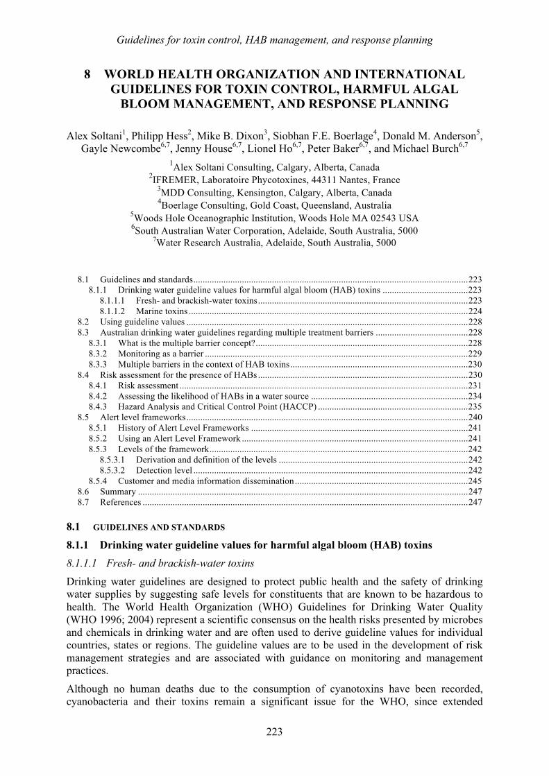
Guidelines for toxin control, HAB management, and response planning

223

8! WORLD HEALTH ORGANIZATION AND INTERNATIONAL GUIDELINES FOR TOXIN CONTROL, HARMFUL ALGAL

BLOOM MANAGEMENT, AND RESPONSE PLANNING Alex Soltani1, Philipp Hess2, Mike B. Dixon3, Siobhan F.E. Boerlage4, Donald M. Anderson5,

Gayle Newcombe6,7, Jenny House6,7, Lionel Ho6,7, Peter Baker6,7, and Michael Burch6,7 1Alex Soltani Consulting, Calgary, Alberta, Canada

2IFREMER, Laboratoire Phycotoxines, 44311 Nantes, France

3MDD Consulting, Kensington, Calgary, Alberta, Canada 4Boerlage Consulting, Gold Coast, Queensland, Australia

5Woods Hole Oceanographic Institution, Woods Hole MA 02543 USA 6South Australian Water Corporation, Adelaide, South Australia, 5000

7Water Research Australia, Adelaide, South Australia, 5000 !

8.1! Guidelines and standards ....................................................................................................................... 223!8.1.1! Drinking water guideline values for harmful algal bloom (HAB) toxins ..................................... 223!

8.1.1.1! Fresh- and brackish-water toxins ........................................................................................... 223!8.1.1.2! Marine toxins ......................................................................................................................... 224!

8.2! Using guideline values .......................................................................................................................... 228!8.3! Australian drinking water guidelines regarding multiple treatment barriers ........................................ 228!

8.3.1! What is the multiple barrier concept? ............................................................................................ 228!8.3.2! Monitoring as a barrier .................................................................................................................. 229!8.3.3! Multiple barriers in the context of HAB toxins ............................................................................. 230!

8.4! Risk assessment for the presence of HABs ........................................................................................... 230!8.4.1! Risk assessment ............................................................................................................................. 231!8.4.2! Assessing the likelihood of HABs in a water source .................................................................... 234!8.4.3! Hazard Analysis and Critical Control Point (HACCP) ................................................................. 235!

8.5! Alert level frameworks .......................................................................................................................... 240!8.5.1! History of Alert Level Frameworks .............................................................................................. 241!8.5.2! Using an Alert Level Framework .................................................................................................. 241!8.5.3! Levels of the framework ................................................................................................................ 242!

8.5.3.1! Derivation and definition of the levels .................................................................................. 242!8.5.3.2! Detection level ....................................................................................................................... 242!

8.5.4! Customer and media information dissemination ........................................................................... 245!8.6! Summary ............................................................................................................................................... 247!8.7! References ............................................................................................................................................. 247!

8.1! GUIDELINES AND STANDARDS 8.1.1 Drinking water guideline values for harmful algal bloom (HAB) toxins 8.1.1.1! Fresh- and brackish-water toxins

Drinking water guidelines are designed to protect public health and the safety of drinking water supplies by suggesting safe levels for constituents that are known to be hazardous to health. The World Health Organization (WHO) Guidelines for Drinking Water Quality (WHO 1996; 2004) represent a scientific consensus on the health risks presented by microbes and chemicals in drinking water and are often used to derive guideline values for individual countries, states or regions. The guideline values are to be used in the development of risk management strategies and are associated with guidance on monitoring and management practices.

Although no human deaths due to the consumption of cyanotoxins have been recorded, cyanobacteria and their toxins remain a significant issue for the WHO, since extended

Guidelines for toxin control, HAB management, and response planning

224

exposure may cause gastroenteritis, among other more serious health impacts (NHMRC/NRMMC 2011). In addition, cyanotoxins are suspected to have resulted in fatalities when introduced into the human body through routes other than ingestion, such as through the use of toxin-containing water for renal dialysis (Jochimsen et al. 1998).

Motivated by growing concern over the presence of cyanotoxins in drinking water, the WHO published an addendum to its Guidelines for Drinking Water Quality in 1998, which included a guideline value for microcystin-LR (MCLR), an acutely toxic cyanotoxin (WHO, 1998). The health-based guideline value for total (i.e., free plus cell-bound) concentration of MCLR was set at 1 µg/L; however, the WHO emphasizes that the guideline value is only provisional, since it only pertains to MCLR, and since the toxicity data for other cyanotoxins are still being collected (WHO, 2004). According to the WHO, not enough data exist to allow guideline values for other cyanotoxins to be developed (WHO 2004).

Concern over drinking water contamination by cyanotoxins has also grown among national regulatory bodies, due to the increasing impact of anthropogenic activity on water resources, as well as the improvement of analytical methods identifying and measuring cyanotoxins. For example, Australian drinking water authorities have set a guideline value of 1.3 µg/L for microcystins, expressed as MCLR. New Zealand has developed maximum allowable values (MAVs) for several cyanotoxins, including anatoxin and anatoxin-A, cylindrospermopsin, microcystins, nodularin, and saxitoxins. The US Environmental Protection Agency, on the other hand, has yet to set any firm, enforceable maximum contaminant levels (MCLs) for cyanobacterial toxins, and has only added cyanobacteria and their toxins to its candidate contaminant list (CCL), which prioritizes contaminants for setting MCLs. In Canada, a maximum acceptable concentration (MAC) of 1.5 μg/L has been developed for cyanobacterial toxins, expressed as MCLR. Canada’s guideline was derived using tolerable daily intake (TDI) values, determined using no-observed adverse effect levels (NOAEL), which are based on human or animal toxicity studies. Brazil has developed guidelines for three cyanobacterial toxins (microcystins, saxitoxins, and cylindrospermopsin), with guideline values being set as 1.0 μg/L, 3.0" μg/L, and 15" μg/L, respectively. Several other countries, however, still rely on the WHO provisional guideline of 1"μg/L MCLR.

A comprehensive summary of international guideline values for cyanobacterial toxins from various countries worldwide are summarized in Table 8.1.

8.1.1.2! Marine toxins

No toxin guidelines currently exist for drinking water produced specifically from the seawater that has been affected by HABs such as dinoflagellates and diatoms. As a result, operators must look to existing guidelines for drinking water produced from fresh water sources. In order to build knowledge of the potential for future guidelines, this chapter discusses the existing guidelines internationally for cyanobacterial toxins from fresh water. The WHO has a guideline specifically for microcystin-LR (1.0µg/L), a common analogue of microcystin, a toxin produced by several species of cyanobacteria. Other guidelines around the world (Table 8.1) have been determined in part by using this guidance. Relevant for seawater desalination are the guidelines for saxitoxin set by New Zealand (1.0 µg/L) and Brazil (3.0 µg/L). Outside the saxitoxin (STX) family, no guidelines exist as yet for other

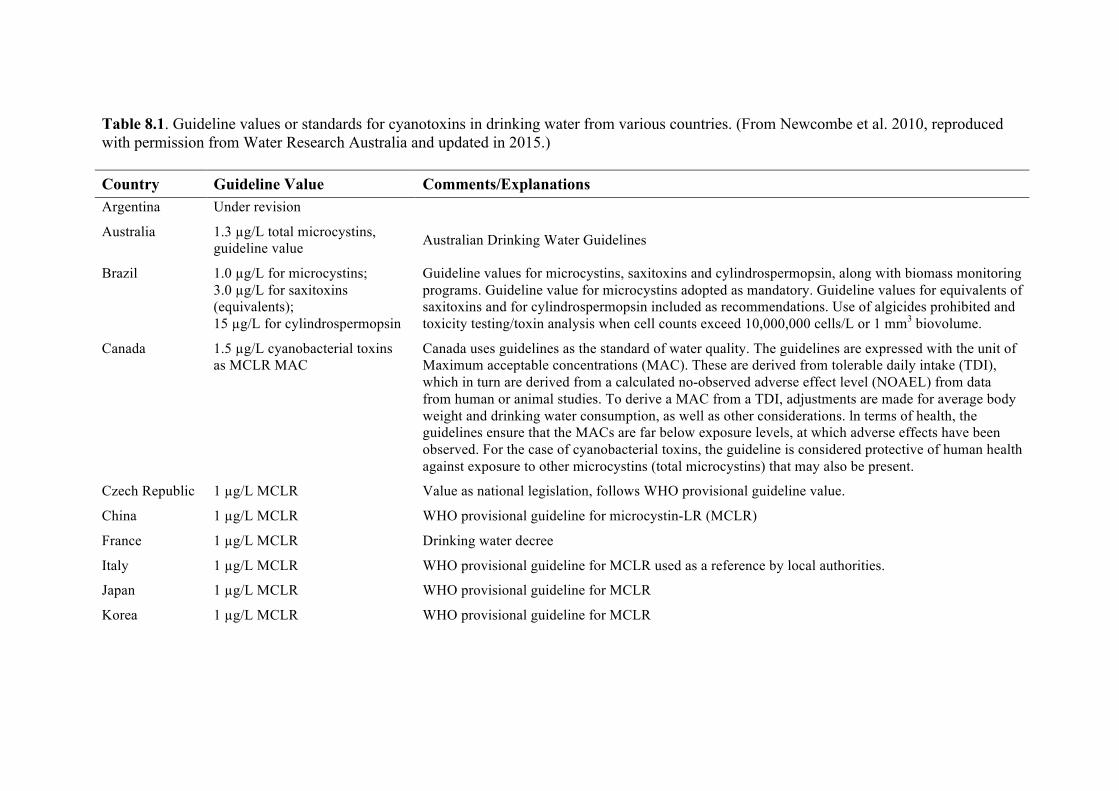
Table 8.1. Guideline values or standards for cyanotoxins in drinking water from various countries. (From Newcombe et al. 2010, reproduced with permission from Water Research Australia and updated in 2015.)!

Country Guideline Value Comments/Explanations Argentina Under revision

Australia 1.3 µg/L total microcystins,

guideline value Australian Drinking Water Guidelines

Brazil 1.0 µg/L for microcystins; 3.0 µg/L for saxitoxins (equivalents); 15 µg/L for cylindrospermopsin

Guideline values for microcystins, saxitoxins and cylindrospermopsin, along with biomass monitoring programs. Guideline value for microcystins adopted as mandatory. Guideline values for equivalents of saxitoxins and for cylindrospermopsin included as recommendations. Use of algicides prohibited and toxicity testing/toxin analysis when cell counts exceed 10,000,000 cells/L or 1 mm3 biovolume.

Canada 1.5 µg/L cyanobacterial toxins as MCLR MAC

Canada uses guidelines as the standard of water quality. The guidelines are expressed with the unit of Maximum acceptable concentrations (MAC). These are derived from tolerable daily intake (TDI), which in turn are derived from a calculated no-observed adverse effect level (NOAEL) from data from human or animal studies. To derive a MAC from a TDI, adjustments are made for average body weight and drinking water consumption, as well as other considerations. ln terms of health, the guidelines ensure that the MACs are far below exposure levels, at which adverse effects have been observed. For the case of cyanobacterial toxins, the guideline is considered protective of human health against exposure to other microcystins (total microcystins) that may also be present.

Czech Republic 1 µg/L MCLR Value as national legislation, follows WHO provisional guideline value.

China 1 µg/L MCLR WHO provisional guideline for microcystin-LR (MCLR)

France 1 µg/L MCLR Drinking water decree

Italy 1 µg/L MCLR WHO provisional guideline for MCLR used as a reference by local authorities.

Japan 1 µg/L MCLR WHO provisional guideline for MCLR

Korea 1 µg/L MCLR WHO provisional guideline for MCLR

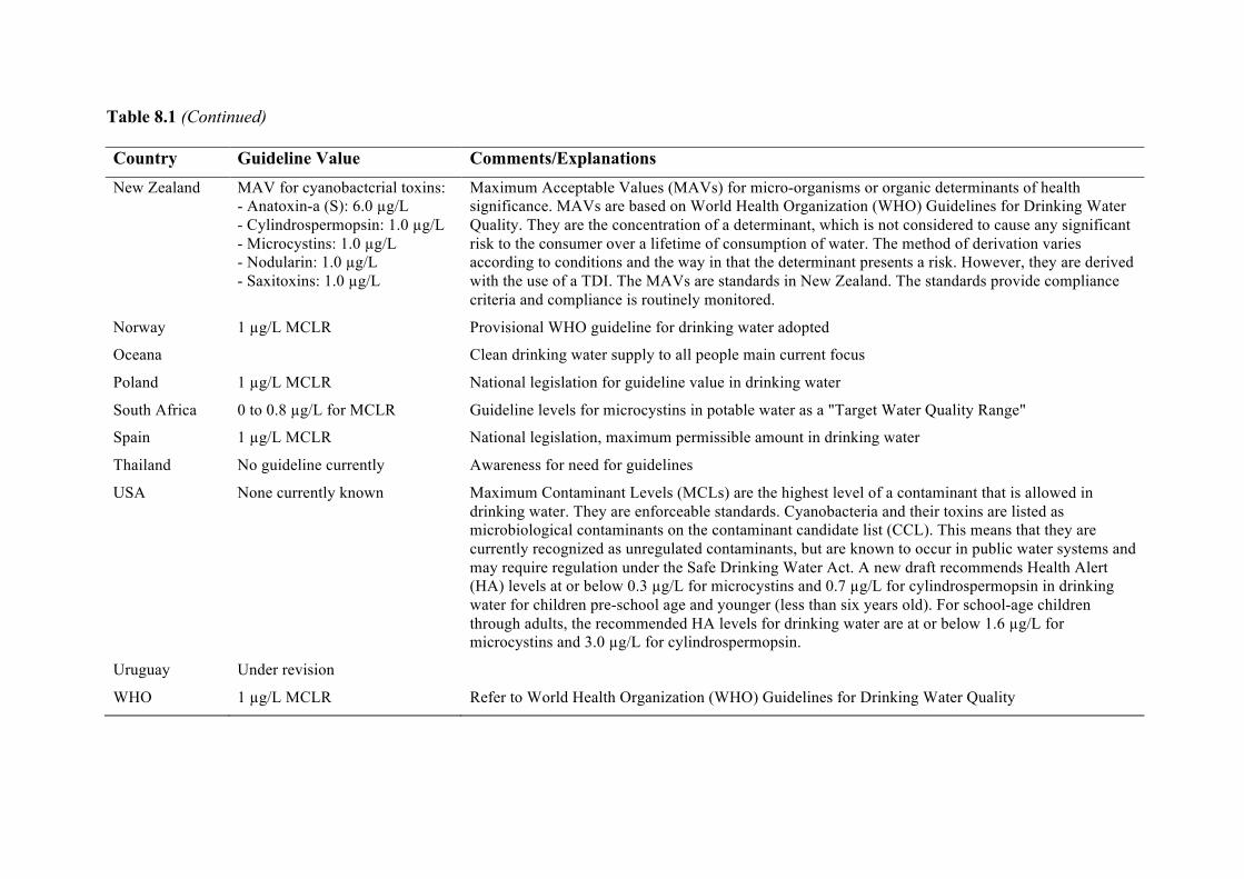
Table 8.1 (Continued) Country Guideline Value Comments/Explanations

New Zealand MAV for cyanobactcrial toxins: - Anatoxin-a (S): 6.0 µg/L - Cylindrospermopsin: 1.0 µg/L - Microcystins: 1.0 µg/L - Nodularin: 1.0 µg/L - Saxitoxins: 1.0 µg/L

Maximum Acceptable Values (MAVs) for micro-organisms or organic determinants of health significance. MAVs are based on World Health Organization (WHO) Guidelines for Drinking Water Quality. They are the concentration of a determinant, which is not considered to cause any significant risk to the consumer over a lifetime of consumption of water. The method of derivation varies according to conditions and the way in that the determinant presents a risk. However, they are derived with the use of a TDI. The MAVs are standards in New Zealand. The standards provide compliance criteria and compliance is routinely monitored.

Norway 1 µg/L MCLR Provisional WHO guideline for drinking water adopted

Oceana Clean drinking water supply to all people main current focus

Poland 1 µg/L MCLR National legislation for guideline value in drinking water

South Africa 0 to 0.8 µg/L for MCLR Guideline levels for microcystins in potable water as a "Target Water Quality Range"

Spain 1 µg/L MCLR National legislation, maximum permissible amount in drinking water

Thailand No guideline currently Awareness for need for guidelines

USA None currently known Maximum Contaminant Levels (MCLs) are the highest level of a contaminant that is allowed in drinking water. They are enforceable standards. Cyanobacteria and their toxins are listed as microbiological contaminants on the contaminant candidate list (CCL). This means that they are currently recognized as unregulated contaminants, but are known to occur in public water systems and may require regulation under the Safe Drinking Water Act. A new draft recommends Health Alert (HA) levels at or below 0.3 µg/L for microcystins and 0.7 µg/L for cylindrospermopsin in drinking water for children pre-school age and younger (less than six years old). For school-age children through adults, the recommended HA levels for drinking water are at or below 1.6 µg/L for microcystins and 3.0 µg/L for cylindrospermopsin.

Uruguay Under revision

WHO 1 µg/L MCLR Refer to World Health Organization (WHO) Guidelines for Drinking Water Quality

Guidelines for toxin control, HAB management, and response planning

227

commonly found seawater HAB toxins, such as the brevetoxins (BTX), okadaic acid (OA), and domoic acid (DA).

Some guidelines, such as the Australian Drinking Water Guidelines (ADWG) provide information and recommendations for several individual classes of toxins, but not necessarily a specific concentration of toxin. In this case microcystins, nodularin, saxitoxins, and cylindrospermopsin (NHMRC/NRMMC 2011). In the Australian case, a guideline value has been recommended only for total microcystins. The guideline recommends that the concentration of total microcystins in drinking water in Australia should not exceed 1.3 µg/L. No guideline values could be set for concentrations of nodularin, saxitoxins, or cylindrospermopsin in Australia due to the lack of adequate data. In relation to lipopolysaccharides (LPS) produced by cyanobacteria, there is currently insufficient information to carry out a critical assessment on occurrence and significance of LPS and so no fact sheet has been produced. The most recent review of the ADWG has now led to the recommendation that, although the strength of data is insufficient to establish a guideline value for cylindrospermopsin in drinking water, a range of information can be used to develop a ‘Health Alert’ value for cylindrospermopsin of 1 µg/L. The data used to develop this health alert came from a range of Australian toxicological studies, one of which provided sub-chronic oral doses of the toxin to mice and demonstrated responses to the toxins after an extended trial of 11 weeks (Humpage and Falconer 2002). The recommendation of a health alert acknowledges that health authorities should be notified if blooms of Cylindrospermopsis raciborskii or other producers of this toxin are present in water supplies. Given that data pertinent to drinking water produced from the sea are very rare, it will take some time to establish guidelines for desalination. The process of establishing ‘Health Alert’ values could also be applied to relevant common seawater toxins or toxin families such as the brevetoxins, saxitoxins, okadaic acid, and domoic acid. Further considerations to assist in establishing meaningful guidelines for HAB toxins in seawater desalination are the guidelines promulgated for shellfish harvesting based on acute toxicity following ingestion. Guidelines for toxins derived from marine HABs exist in Australia, New Zealand, and many other countries. The former are described by the Australian and New Zealand Food Authorities (ANZFA) (Todd 2011). ANZFA sets the following guideline values: paralytic shellfish poisoning (PSP or the saxitoxin family) 80 μg/100 g of edible shellfish, amnesic shellfish poisoning (ASP or domoic acid) 20 ppm, and diarrhetic shellfish poisoning (DSP okadaic acid and other toxins) 20 μg/100 g (Discussed further in Chapter 2). Although it is difficult to apply the latter values to drinking water, one could consider the minimum mass of shellfish consumed in a meal, and then compare that with a minimum volume of water consumed. For example, considering PSP, consuming a minimum of 10 g of shellfish would correspond to ingestion of 8 µg of saxitoxin. If one were to consume 100 mL of water containing the same 8 µg of saxitoxin, this would correspond to a concentration of 80 µg/L: however, guidelines for saxitoxins worldwide range from 1.0 to 3.0 µg/L, which suggests that it is far more prudent to work to these lower values when producing drinking water. The oral LD50 for humans is 5.7 µg/kg, so the average 80 kg person would need to ingest 456 µg of saxitoxin for the dose to be fatal. One would need to drink 5.7 L of water if guidelines for drinking water were based on shellfish guidelines or 456 L of water at the New Zealand drinking water guideline. Considering that small children are more susceptible to the toxin, as well as the fact that illness is common at far lower saxitoxin doses, 1.0 µg/L is a far more reliable guideline.

Guidelines for toxin control, HAB management, and response planning

228

8.2! USING GUIDELINE VALUES The guideline value is important for water supply authorities, as this value sets the concentration of toxin that is tolerable in drinking water, i.e. “at the tap”. For example, ADWG for cyanobacterial toxins in fresh or brackish waters are not mandatory standards; however, they provide a basis for determining the quality of water to be supplied to consumers in all parts of Australia. In this circumstance the guideline level is effectively a recommendation from the health authorities, although this situation is changing with the introduction of more prescriptive drinking water standards in some jurisdictions. For some water authorities in Australia the guidelines/standards become part of the de facto contractual standards. They are therefore required to comply with the guideline values as part of their standards of service. For other countries the guideline level can be a standard that must be met and compliance monitoring may be required. 8.3! AUSTRALIAN DRINKING WATER GUIDELINES REGARDING MULTIPLE TREATMENT

BARRIERS 8.3.1 What is the multiple barrier concept? In the absence of guideline values for HAB toxins internationally, the best method for ensuring that toxin does not enter the drinking water distribution system is by employing the multiple barrier approach to treatment, which is well described in the Australian Drinking Water Guidelines (NHMRC/NRMMC 2011). The concept, which is widely recognized as the most effective approach for producing safe drinking water, aims to improve a water treatment train’s reliability by employing multiple treatment processes in series. Providing multiple treatment processes, or barriers, ensures that when one process fails or partially fails, the performance reduction can be compensated for by other processes in the treatment train. Ideally, all treatment barriers should be operating effectively to ensure that a water treatment plant is performing optimally. Since it is likely that individual barriers are not effective 100 percent of the time, however (NHMRC/NRMMC 2011), employing multiple barriers against contaminants ensures that produced drinking water remains of a high quality, even if one of the treatment barriers becomes compromised. In addition, using multiple barriers expands the range of contaminants removed by a water treatment train, also referred to as robustness, since individual barriers typically target different groups of contaminants (Crittenden et al, 2005). The number of barriers required, as well as the types of barriers employed, depend largely on how acute the source water contaminants are, with more acute contaminants requiring more barriers (Crittenden et al. 2005). In addition, understanding both the challenges that contaminants may present, as well as any vulnerabilities associated with the treatment barriers, plays an important role in barrier selection (NHMRC/NRMMC 2011).

Although the multiple barrier concept places a great deal of emphasis on treatment processes, other barriers that help ensure safe drinking water are equally important, such as source water selection and protection, as well as safe water transportation and storage (Bixio and Wintgens 2006). ADWGs recognize the importance of these barriers, stressing that “understanding a water supply system from catchment to consumer, how it works, and its vulnerabilities to failure” are an integral part of the multiple barrier concept (NHMRC/NRMMC 2011). Furthermore, ADWGs highlight the importance of including “mechanisms or fail-safes to accommodate inevitable human errors without allowing major failures to occur” when applying the multiple barrier concept (NHMRC/NRMMC 2011).

Guidelines for toxin control, HAB management, and response planning

229

Seawater reverse osmosis (SWRO) plants are inherently a multi barrier treatment process for certain feedwater contaminants. As discussed in Chapter 9, pre-treatment processes provide an added barrier for toxin removal in addition to the core reverse osmosis (RO) treatment. This allows intracellular toxin removal upstream of the RO step and thus less dependence on this process as a sole toxin removal mechanism. In addition, many plants that commonly experience HAB blooms are in the Gulf and have a full or partial second pass. Chlorination of treated waters in the distribution system provides an added barrier for some toxins such as saxitoxin (Laycock et al. 2012).

8.3.2 Monitoring as a barrier Once barriers are in place to protect public health, regulatory bodies need to ensure that those barriers are performing effectively. To this end, ADWGs identify drinking water quality monitoring as the ultimate test to confirm whether employed treatment barriers, or other preventative measures, are effectively protecting the public from consuming unsafe drinking water (NHMRC/NRMMC 2011). Additionally, ADWGs emphasize that drinking water quality monitoring should be performed on a frequent basis, so as to identify the failure of any treatment processes, or other measures, in a timely manner (NHMRC/NRMMC 2011).

In addition to monitoring drinking water quality, operational monitoring of treatment processes plays an important role in ensuring that safe water is delivered to consumers (refer to Section 8.4.3 below – HACCP). According to ADWGs, operational monitoring aims to ensure that all existing treatment barriers, and other water safety measures, are performing as desired (NHMRC/NRMMC 2011). For example, monitoring of RO permeate for conductivity can be used as a surrogate for failure of the RO (see Chapter 10). As with drinking water quality monitoring, operational monitoring should be performed regularly so that any detected process deficiencies can be corrected promptly. To this end, continuous, online monitoring is the most desirable form of operational monitoring, and should be implemented wherever practical (NHMRC/NRMMC 2011). This ensures that ineffective treatment barriers, such as a damaged membrane, can be recognized and addressed immediately, preventing unsafe drinking water from reaching the public. In the event of an emergency, such as the discovery of a ‘bloom’ event in the source water, monitoring frequency should be increased to ensure that barriers are effectively protecting consumers.

Validation monitoring is also vital to protecting the public from consuming unsafe drinking water. Unlike operational monitoring, validation monitoring aims to assess newly added treatment barriers, and ensure that they are performing effectively. For example, if a new activated carbon column were to be added to a water treatment train, the column’s effluent would need to be tested to confirm whether or not contaminants, such as toxins, are continually removed over time. Validation monitoring is particularly important when adding treatment processes that have not been implemented onsite previously, and have not been tested by the manufacturer (NHMRC/NRMMC 2011). In such cases, validation monitoring gives plant operators a chance to verify any assumptions regarding process performance, and to ensure that all desired contaminants are effectively removed. Where a treatment process has been tested by the manufacturer (i.e., pre-validated), validation monitoring should still be performed; however, the treatment process need not necessarily be tested before it is brought online in the water treatment plant, assuming that onsite water characteristics are not substantially different from those used in manufacturer testing (NHMRC/NRMMC 2011).

All forms of monitoring play a significant role in managing risk in a waters supply system. As a result, a monitoring strategy requires careful consideration of numerous factors, including which variables should be monitored, what data should be collected, and how collected data should be used to mitigate risk (NHMRC/NRMMC 2011). Furthermore, it is

Guidelines for toxin control, HAB management, and response planning

230

important that a monitoring strategy be developed with mechanisms in place to incorporate monitoring information into decision-making processes affecting the water supply system (NHMRC/NRMMC 2011). Finally, for all forms of monitoring, it is essential that monitoring data are compiled, analyzed, and reported in a timely manner to ensure that corrective measures can be taken before unsafe drinking water is delivered to the public (NHMRC/NRMMC 2011).

In summary, by checking that all treatment processes and other barriers are performing effectively, monitoring in and of itself represents an additional barrier, preventing unsafe drinking water from reaching consumers. Effective implementation of the multiple barrier concept thus requires integrating an effective monitoring program with a reliable, robust treatment train, along with sufficient preventative measures. 8.3.3 Multiple barriers in the context of HAB toxins Employing multiple barriers against HAB toxins is a high priority, particularly due to their acute toxicity. Such barriers can be comprised of a wide range of treatment processes, preventative measures, and monitoring strategies. In terms of treatment barriers, numerous processes have been developed to remove HAB biomass and their toxins from drinking water (Chapters 9,10). These aim to remove HAB cells (which can include cell-bound toxins), and can also remove dissolved (i.e., extracellular) toxins, depending on the treatment technology considered. For example, treatment using coagulation and dual media filtration removes a significant portion of cell-bound toxins from drinking water (Hrudey et al. 1999). Dissolved toxins, on the other hand, are not effectively removed using pre-treatment processes and are better targeted using reverse osmosis, oxidants, such as chlorine for some toxins, or activated carbon adsorption (Hrudey et al. 1999; Laycock et al. 2012). Where multiple treatment processes are employed, process interactions must be considered, since upstream treatment processes may result in cell damage, which leads to significantly higher levels of dissolved toxins. For example, chlorination of the intake will result in cell lysis and therefore higher concentration of dissolved toxins. Therefore, treatment processes leading to cell damage are not recommended unless a subsequent process is included to remove dissolved toxins (Newcombe et al. 2010). A comprehensive monitoring strategy serves as the final barrier between HAB toxins and consumers. Monitoring toxins can, however, be challenging, since instrument-based analytical methods used to measure toxins are time expensive and consuming, required limits of detection are extremely low, and analytical standards used to quantify many toxins are lacking (WHO 2004). Consequently, analyzing toxins using sophisticated instruments such as liquid chromatography/mass spectroscopy (LC/MS) and high performance liquid chromatography (HPLC) is not likely for routine monitoring in desalination plants. On the other hand, source water monitoring using rapid screening methods for toxins (see Appendix 2) presents a practical alternative. Steps might include visually checking source water for indications that a HAB has occurred or may be imminent, or sampling of source waters to screen for potentially toxic or harmful species (Chapter 3).

8.4! RISK ASSESSMENT FOR THE PRESENCE OF HABS Risk assessment is the process of using available information to predict how often identified hazards or events may occur and the magnitude of their consequences. Risk can be assessed at two levels: maximum risk in the absence of preventative measures and residual risk after consideration of existing preventative measures (Nadebaum et al. 2004).

Guidelines for toxin control, HAB management, and response planning

231

8.4.1 Risk assessment Formal risk assessment is often carried out under the auspices of official government agencies. Such risk assessment also typically draws on knowledge from a group of scientists, including chemists, toxicologists and statisticians. Risk evaluation is considered an iterative process and includes the following steps:

(i)! Public call for data (ii)! Hazard identification (iii)! Exposure assessment (iv)! Hazard characterization (v)! Review of the status of detection and quantification methods (vi)! Review of toxicological and epidemiological data (vii)! Risk characterization (viii)! Recommendations for management and monitoring

In the case of new or emerging risks, it is common that an initial risk assessment is carried out, leading to a provisional management procedure. After some time, the effectiveness of this procedure is then reviewed and, possibly in combination with new toxicology and occurrence data, a new management procedure or trigger level may be put in place. Thus, risk assessment should be considered to be an iterative process.

Based on previous risk assessments and current knowledge of HAB occurrence, it is clear that algal toxins should be considered as an identified hazard in drinking water derived from seawater (Caron et al. 2010; Laycock et al. 2012; Boerlage and Nada, 2014; Berdalet et al. 2015). Thus, the main objective of this section is to discuss potential exposure and assess risk.

For several toxin groups described above, such risk assessments have been carried out by the European Food Safety Authority (EFSA 2008a, b, 2009a, b, c, d, e, f, g, 2010a, b, c, d; EFSA (EFSA Panel on Biological Hazards (BIOHAZ) 2012; FSAI 2006; Lawrence et al. 2011), in particular for exposure through the consumption of bivalve molluscs. Note that some discrepancies between current legislation and risk evaluation for several toxins groups in shellfish have been established in recent risk evaluation exercises by EFSA, as shown in the summary report (Table 8.2). For drinking water, so far only microcystin-LR has been formalized and regulated as a hazard by WHO (2004). This guide has also established 2 L as a maximum quantity of water that can be consumed as one portion in a day. The maximum amount of a toxin or contaminant that a human may be exposed to without ill effects is referred to as the ARfD. ARfDs or safe doses have only been established for four marine toxins (saxitoxin, domoic acid, okadaic acid, and azaspiracids by EFSA) and for microcystin-LR (indirectly by WHO). Table 8.2 shows the current European Union (EU) limits for selected algal toxins in shellfish meat, ARfD and recommended maximum levels based on a representative portion of shellfish consumed. As not many reports are available for the occurrence of toxins in seawater, it was not possible to make probabilistic exposure assessments, so worst case assumptions of these five toxin groups used for assessment are provided here. The data used were collated from laboratory culture data on toxic HAB species described in Chapter 1, as well as from the studies described in Chapter 10 showing 99% rejection of dissolved toxins. The rationale for this approach is given below. To assess risk, the amount of toxin that might be retained in treated water needs to be compared to the ARfD or safe dose values. The two components to be considered in this regard are the extracellular and intracellular toxins. Some studies report measurements of both categories of toxin in seawater, but most do not. For saxitoxin, a very polar compound,

Guidelines for toxin control, HAB management, and response planning

232

extracellular levels ranged from 12 to 31 µg/L in Alexandrium cultures studied by Lefebvre et al. (2008), who also reported a maximum extracellular STX level of 0.8 µg/L during an Alexandrium bloom in the field. Previous culture studies of cyanobacteria and dinoflagellates have reported extracellular STX levels of 50 to 75 µg/L (Hsieh et al. 2000; Velzeboer et al. 2001). For domoic acid, a toxin actively excreted by diatoms, a dissolved concentration of 3.3 µg/L has been reported (Liefer et al. 2013; Trainer et al. 2009), but much higher levels have also been observed. Kudela (pers. comm.) measured total and extracellular concentrations of 100 and 50 µg/L domoic acid respectively during a massive Pseudo-nitzschia bloom along the US west coast in 2014. Half of the measured toxin was extracellular. One study estimated extracellular okadaic acid concentrations during blooms of 0.2 µg/L (Takahashi et al. 2007), whereas another study measured only low background levels of okadaic acid in a coastal lagoon (Zendong et al. 2015). In contrast, Smith et al. (2012) reported that 60% of the okadaic acid produced by Dinophysis cultures was extracellular. Microcystin concentrations from terrestrial runoff in coastal water have been recently estimated to be around 1.4 µg/L (Kudela 2011; Miller et al. 2010). These are just a few of the many studies that report toxicity values for HAB species cultures or for natural waters during blooms, and clearly there are many differences in the amounts of toxin that might be in intra- versus extracellular form. Given the large variability in these published data from different locations and conditions, the toxicity differences between strains of a given species, the variation in toxicity that occurs with different forms of nutrient limitation or environmental stress, and the different levels of population biomass achieved under varying growth conditions (see Chapter 1), simplifying assumptions are needed to constrain HAB risk assessments. Here a hypothetical approach is taken, in which laboratory-derived cellular toxicity data for the most toxic species producing the major HAB toxins are attributed to a dense bloom of those species. In Chapter 1 (Table 1.4), these calculations were performed for three possible bloom types – 100,000, 500,000, and 5,000,000 cells/L, representing moderate, large, and extreme HABs for most species. For this conservative analysis, the extreme bloom level is used to estimate maximum exposure levels and safety factors for treated water. For a bloom of this size, the highest calculated total toxin levels for saxitoxin, domoic acid, okadaic acid, and azaspiracid are 600, 335, 294, and 0.1 µg/L respectively (calculated in Chapter 2). Chapters 2, 9, and 10 discuss the relative ease of removal of intracellular versus extracellular toxins. A variety of pretreatment steps like ultrafiltration and dissolved air flotation (DAF) will remove cells, and thus intracellular toxins, but they are not very effective in removing the dissolved or extracellular fractions. It is clear that on occasion, 50% or more of the toxin produced by HABs can be extracellular, and to this, one would add the toxin that is released by physical and chemical processes during pretreatment. Again, in order to err on the conservative side, it will be assumed that 100% of the toxin from a bloom of 5,000,000 cells/L will be dissolved and will reach RO membranes, where 99% removal will occur in a single pass. Results are tabulated in Table 8.3. A similar calculation could be made for thermal desalination systems, in which most cases there is no pretreatment and HAB cells will be degraded by temperature and pressure, releasing toxin (Boerlage and Nada 2014). A toxin removal of 99% in thermal systems could also be assumed for this calculation (toxin removal efficiencies are discussed in Chapter 10).

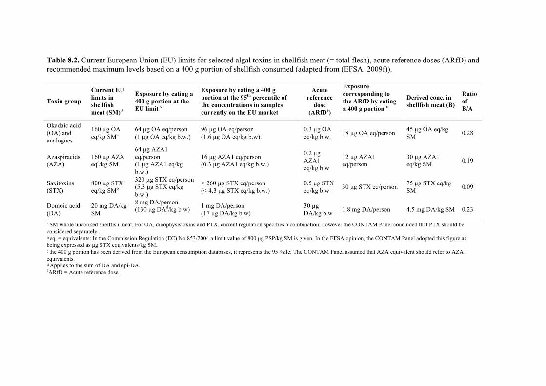
Table 8.2. Current European Union (EU) limits for selected algal toxins in shellfish meat (= total flesh), acute reference doses (ARfD) and recommended maximum levels based on a 400 g portion of shellfish consumed (adapted from (EFSA, 2009f)).

Toxin group

Current EU limits in shellfish meat (SM) a

Exposure by eating a 400 g portion at the EU limit c

Exposure by eating a 400 g portion at the 95th percentile of the concentrations in samples currently on the EU market

Acute reference

dose (ARfDe)

Exposure corresponding to the ARfD by eating a 400 g portion c

Derived conc. in shellfish meat (B)

Ratioof B/A

Okadaic acid (OA) and analogues

160 µg OA eq/kg SMa

64 µg OA eq/person (1 µg OA eq/kg b.w.)

96 µg OA eq/person (1.6 µg OA eq/kg b.w).

0.3 µg OA eq/kg b.w. 18 µg OA eq/person 45 µg OA eq/kg

SM 0.28

Azaspiracids (AZA)

160 µg AZA eqc/kg SM

64 µg AZA1 eq/person (1 µg AZA1 eq/kg b.w.)

16 µg AZA1 eq/person (0.3 µg AZA1 eq/kg b.w.)

0.2 µg AZA1 eq/kg b.w

12 µg AZA1 eq/person

30 µg AZA1 eq/kg SM 0.19

Saxitoxins (STX)

800 µg STX eq/kg SMb

320 µg STX eq/person (5.3 µg STX eq/kg b.w.)

< 260 µg STX eq/person (< 4.3 µg STX eq/kg b.w.)

0.5 µg STX eq/kg b.w 30 µg STX eq/person 75 µg STX eq/kg

SM 0.09

Domoic acid (DA)

20 mg DA/kg SM

8 mg DA/person (130 µg DAd/kg b.w)

1 mg DA/person (17 µg DA/kg b.w)

30 µg DA/kg b.w 1.8 mg DA/person 4.5 mg DA/kg SM 0.23

a"SM whole uncooked shellfish meat, For OA, dinophysistoxins and PTX, current regulation specifies a combination; however the CONTAM Panel concluded that PTX should be considered separately."b"eq. = equivalents: In the Commission Regulation (EC) No 853/2004 a limit value of 800 µg PSP/kg SM is given. In the EFSA opinion, the CONTAM Panel adopted this figure as being expressed as µg STX equivalents/kg SM. c"the 400 g portion has been derived from the European consumption databases, it represents the 95 %ile; The CONTAM Panel assumed that AZA equivalent should refer to AZA1 equivalents."d"Applies to the sum of DA and epi-DA."eARfD = Acute reference dose"

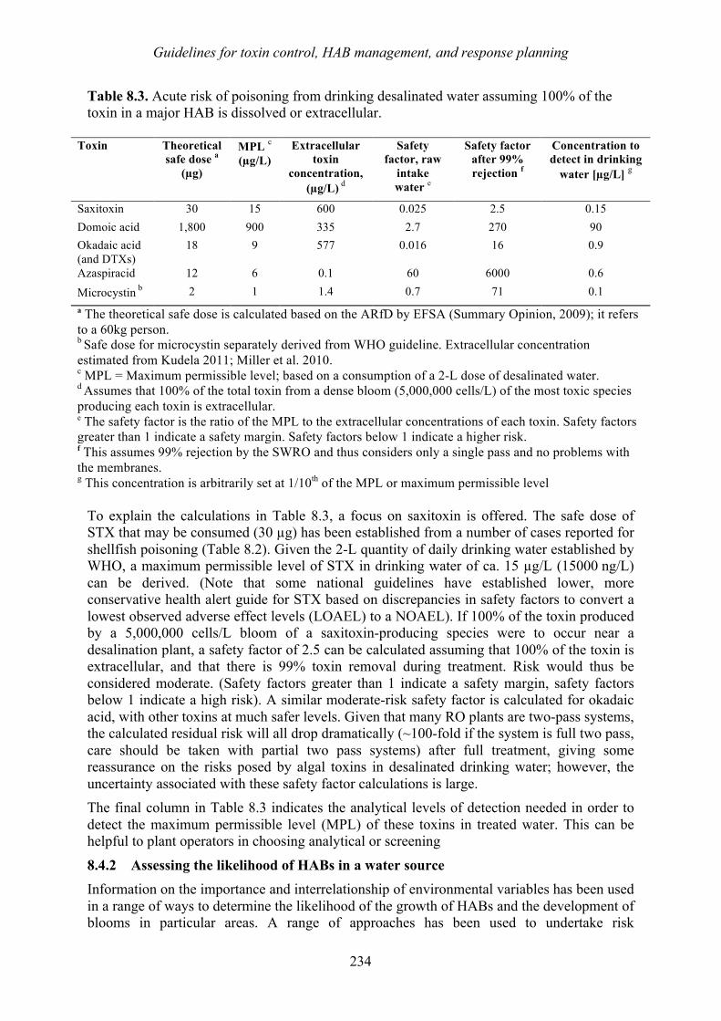
Guidelines for toxin control, HAB management, and response planning

234

Table 8.3. Acute risk of poisoning from drinking desalinated water assuming 100% of the toxin in a major HAB is dissolved or extracellular.

Toxin Theoretical safe dose a

(µg)

MPL c (µg/L)

Extracellular toxin

concentration, (µg/L) d

Safety factor, raw

intake water e

Safety factor after 99% rejection f

Concentration to detect in drinking

water [µg/L] g

Saxitoxin 30 15 600 0.025 2.5 0.15 Domoic acid 1,800 900 335 2.7 270 90 Okadaic acid (and DTXs)

18 9 577 0.016 16 0.9

Azaspiracid 12 6 0.1 60 6000 0.6 Microcystin b 2 1 1.4 0.7 71 0.1 a The theoretical safe dose is calculated based on the ARfD by EFSA (Summary Opinion, 2009); it refers to a 60kg person. b Safe dose for microcystin separately derived from WHO guideline. Extracellular concentration estimated from Kudela 2011; Miller et al. 2010. c MPL = Maximum permissible level; based on a consumption of a 2-L dose of desalinated water. d Assumes that 100% of the total toxin from a dense bloom (5,000,000 cells/L) of the most toxic species producing each toxin is extracellular. e The safety factor is the ratio of the MPL to the extracellular concentrations of each toxin. Safety factors greater than 1 indicate a safety margin. Safety factors below 1 indicate a higher risk. f This assumes 99% rejection by the SWRO and thus considers only a single pass and no problems with the membranes. g This concentration is arbitrarily set at 1/10th of the MPL or maximum permissible level

To explain the calculations in Table 8.3, a focus on saxitoxin is offered. The safe dose of STX that may be consumed (30 µg) has been established from a number of cases reported for shellfish poisoning (Table 8.2). Given the 2-L quantity of daily drinking water established by WHO, a maximum permissible level of STX in drinking water of ca. 15 µg/L (15000 ng/L) can be derived. (Note that some national guidelines have established lower, more conservative health alert guide for STX based on discrepancies in safety factors to convert a lowest observed adverse effect levels (LOAEL) to a NOAEL). If 100% of the toxin produced by a 5,000,000 cells/L bloom of a saxitoxin-producing species were to occur near a desalination plant, a safety factor of 2.5 can be calculated assuming that 100% of the toxin is extracellular, and that there is 99% toxin removal during treatment. Risk would thus be considered moderate. (Safety factors greater than 1 indicate a safety margin, safety factors below 1 indicate a high risk). A similar moderate-risk safety factor is calculated for okadaic acid, with other toxins at much safer levels. Given that many RO plants are two-pass systems, the calculated residual risk will all drop dramatically (~100-fold if the system is full two pass, care should be taken with partial two pass systems) after full treatment, giving some reassurance on the risks posed by algal toxins in desalinated drinking water; however, the uncertainty associated with these safety factor calculations is large. The final column in Table 8.3 indicates the analytical levels of detection needed in order to detect the maximum permissible level (MPL) of these toxins in treated water. This can be helpful to plant operators in choosing analytical or screening

8.4.2 Assessing the likelihood of HABs in a water source Information on the importance and interrelationship of environmental variables has been used in a range of ways to determine the likelihood of the growth of HABs and the development of blooms in particular areas. A range of approaches has been used to undertake risk

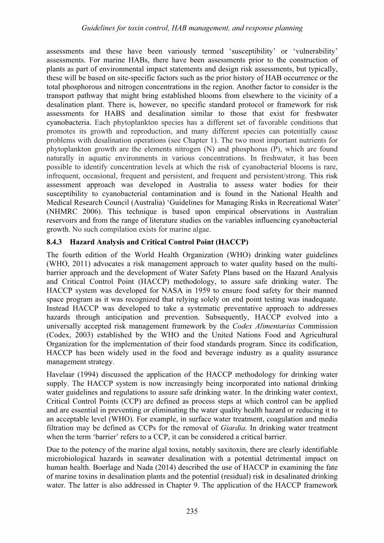
Guidelines for toxin control, HAB management, and response planning

235

assessments and these have been variously termed ‘susceptibility’ or ‘vulnerability’ assessments. For marine HABs, there have been assessments prior to the construction of plants as part of environmental impact statements and design risk assessments, but typically, these will be based on site-specific factors such as the prior history of HAB occurrence or the total phosphorous and nitrogen concentrations in the region. Another factor to consider is the transport pathway that might bring established blooms from elsewhere to the vicinity of a desalination plant. There is, however, no specific standard protocol or framework for risk assessments for HABS and desalination similar to those that exist for freshwater cyanobacteria. Each phytoplankton species has a different set of favorable conditions that promotes its growth and reproduction, and many different species can potentially cause problems with desalination operations (see Chapter 1). The two most important nutrients for phytoplankton growth are the elements nitrogen (N) and phosphorus (P), which are found naturally in aquatic environments in various concentrations. In freshwater, it has been possible to identify concentration levels at which the risk of cyanobacterial blooms is rare, infrequent, occasional, frequent and persistent, and frequent and persistent/strong. This risk assessment approach was developed in Australia to assess water bodies for their susceptibility to cyanobacterial contamination and is found in the National Health and Medical Research Council (Australia) ‘Guidelines for Managing Risks in Recreational Water’ (NHMRC 2006). This technique is based upon empirical observations in Australian reservoirs and from the range of literature studies on the variables influencing cyanobacterial growth. No such compilation exists for marine algae. 8.4.3 Hazard Analysis and Critical Control Point (HACCP) The fourth edition of the World Health Organization (WHO) drinking water guidelines (WHO, 2011) advocates a risk management approach to water quality based on the multi- barrier approach and the development of Water Safety Plans based on the Hazard Analysis and Critical Control Point (HACCP) methodology, to assure safe drinking water. The HACCP system was developed for NASA in 1959 to ensure food safety for their manned space program as it was recognized that relying solely on end point testing was inadequate. Instead HACCP was developed to take a systematic preventative approach to addresses hazards through anticipation and prevention. Subsequently, HACCP evolved into a universally accepted risk management framework by the Codex Alimentarius Commission (Codex, 2003) established by the WHO and the United Nations Food and Agricultural Organization for the implementation of their food standards program. Since its codification, HACCP has been widely used in the food and beverage industry as a quality assurance management strategy. Havelaar (1994) discussed the application of the HACCP methodology for drinking water supply. The HACCP system is now increasingly being incorporated into national drinking water guidelines and regulations to assure safe drinking water. In the drinking water context, Critical Control Points (CCP) are defined as process steps at which control can be applied and are essential in preventing or eliminating the water quality health hazard or reducing it to an acceptable level (WHO). For example, in surface water treatment, coagulation and media filtration may be defined as CCPs for the removal of Giardia. In drinking water treatment when the term ‘barrier’ refers to a CCP, it can be considered a critical barrier. Due to the potency of the marine algal toxins, notably saxitoxin, there are clearly identifiable microbiological hazards in seawater desalination with a potential detrimental impact on human health. Boerlage and Nada (2014) described the use of HACCP in examining the fate of marine toxins in desalination plants and the potential (residual) risk in desalinated drinking water. The latter is also addressed in Chapter 9. The application of the HACCP framework

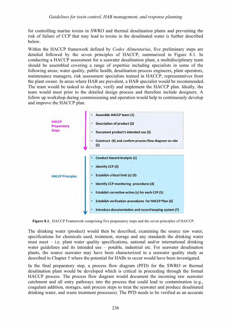
Guidelines for toxin control, HAB management, and response planning

236

for controlling marine toxins in SWRO and thermal desalination plants and preventing the risk of failure of CCP that may lead to toxins in the desalinated water is further described below. Within the HACCP framework defined by Codex Alimentarius, five preliminary steps are detailed followed by the seven principles of HACCP, summarized in Figure 8.1. In conducting a HACCP assessment for a seawater desalination plant, a multidisciplinary team should be assembled covering a range of expertise including specialists in some of the following areas; water quality, public health, desalination process engineers, plant operators, maintenance managers, risk assessment specialists trained in HACCP, representatives from the plant owner. In areas where HAB are prevalent, a HAB specialist would be recommended. The team would be tasked to develop, verify and implement the HACCP plan. Ideally, the team would meet prior to the detailed design process and therefore include designers. A follow up workshop during commissioning and operation would help to continuously develop and improve the HACCP plan.

The drinking water (product) would then be described, examining the source raw water, specifications for chemicals used, treatment, storage and any standards the drinking water must meet – i.e. plant water quality specifications, national and/or international drinking water guidelines and its intended use – potable, industrial etc. For seawater desalination plants, the source seawater may have been characterized in a seawater quality study as described in Chapter 5 where the potential for HABs to occur would have been investigated. In the final preparatory step, a process flow diagram (PFD) for the SWRO or thermal desalination plant would be developed which is critical in proceeding through the formal HACCP process. The process flow diagram would document the incoming raw seawater catchment and all entry pathways into the process that could lead to contamination (e.g., coagulant addition, storages, unit process steps to treat the seawater and produce desalinated drinking water, and waste treatment processes). The PFD needs to be verified as an accurate

Figure 8.1. HACCP Framework comprising five preparatory steps and the seven principles of HACCP.

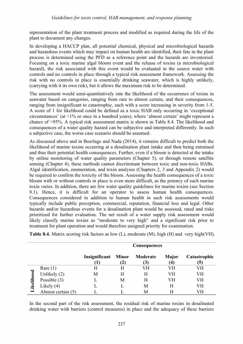
Guidelines for toxin control, HAB management, and response planning

237

representation of the plant treatment process and modified as required during the life of the plant to document any changes.

In developing a HACCP plan, all potential chemical, physical and microbiological hazards and hazardous events which may impact on human health are identified, their fate in the plant process is determined using the PFD as a reference point and the hazards are inventoried. Focusing on a toxic marine algal bloom event and the release of toxins (a microbiological hazard), the risk associated with this event would be evaluated in the source water with controls and no controls in place through a typical risk assessment framework. Assessing the risk with no controls in place is essentially drinking seawater, which is highly unlikely, (carrying with it its own risk), but it allows the maximum risk to be determined.

The assessment would semi-quantitatively rate the likelihood of the occurrence of toxins in seawater based on categories, ranging from rare to almost certain, and their consequences, ranging from insignificant to catastrophic, each with a score increasing in severity from 1-5. A score of 1 for likelihood could be defined as a toxic HAB only occurring in ‘exceptional circumstances’ (at <1% or once in a hundred years), where ‘almost certain’ might represent a chance of >95%. A typical risk assessment matrix is shown in Table 8.4. The likelihood and consequences of a water quality hazard can be subjective and interpreted differently. In such a subjective case, the worse case scenario should be assumed.

As discussed above and in Boerlage and Nada (2014), it remains difficult to predict both the likelihood of marine toxins occurring at a desalination plant intake and then being entrained and thus their potential health consequences. Further, even if a bloom is detected at the intake by online monitoring of water quality parameters (Chapter 5), or through remote satellite sensing (Chapter 4), these methods cannot discriminate between toxic and non-toxic HABs. Algal identification, enumeration, and toxin analyses (Chapters 2, 3 and Appendix 2) would be required to confirm the toxicity of the bloom. Assessing the health consequences of a toxic bloom with or without controls in place is even more difficult, as the potency of each marine toxin varies. In addition, there are few water quality guidelines for marine toxins (see Section 8.1). Hence, it is difficult for an operator to assess human health consequences. Consequences considered in addition to human health in such risk assessments would typically include public perception, commercial, reputation, financial loss and legal. Other hazards and/or hazardous events for a desalination plant would be assessed, rated and risks prioritized for further evaluation. The net result of a water supply risk assessment would likely classify marine toxins as “moderate to very high” and a significant risk prior to treatment for plant operation and would therefore assigned priority for examination.

Table 8.4. Matrix scoring risk factors as low (L), moderate (M), high (H) and very high(VH). Consequences

Insignificant

(1)

Minor

(2)

Moderate

(3)

Major

(4)

Catastrophic

(5)

Lik

elih

ood Rare (1) H H VH VH VH

Unlikely (2) M H H VH VH Possible (3) L M H VH VH Likely (4) L L M H VH Almost certain (5) L L M H VH

In the second part of the risk assessment, the residual risk of marine toxins in desalinated drinking water with barriers (control measures) in place and the adequacy of these barriers

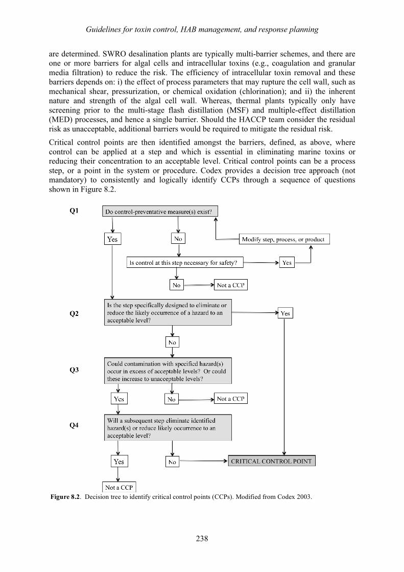
Guidelines for toxin control, HAB management, and response planning

238

are determined. SWRO desalination plants are typically multi-barrier schemes, and there are one or more barriers for algal cells and intracellular toxins (e.g., coagulation and granular media filtration) to reduce the risk. The efficiency of intracellular toxin removal and these barriers depends on: i) the effect of process parameters that may rupture the cell wall, such as mechanical shear, pressurization, or chemical oxidation (chlorination); and ii) the inherent nature and strength of the algal cell wall. Whereas, thermal plants typically only have screening prior to the multi-stage flash distillation (MSF) and multiple-effect distillation (MED) processes, and hence a single barrier. Should the HACCP team consider the residual risk as unacceptable, additional barriers would be required to mitigate the residual risk. Critical control points are then identified amongst the barriers, defined, as above, where control can be applied at a step and which is essential in eliminating marine toxins or reducing their concentration to an acceptable level. Critical control points can be a process step, or a point in the system or procedure. Codex provides a decision tree approach (not mandatory) to consistently and logically identify CCPs through a sequence of questions shown in Figure 8.2.

Figure 8.2. Decision tree to identify critical control points (CCPs). Modified from Codex 2003.

Guidelines for toxin control, HAB management, and response planning

239

None of the pretreatment barriers in a typical SWRO desalination plant scheme (i.e., conventional pretreatment coagulation and flocculation, granular media filtration followed by cartridge filtration or ultrafiltration membrane pretreatment) would be deemed as critical control points when answering the four questions in the Codex decision tree. While these barriers may remove intact algal cells (and thus the intracellular toxins), none would act as a reliable barrier to remove extracellular algal toxins, nor meet the definition of a CCP.

Hence, following the decision tree approach, the RO step is the first critical control point in SWRO plants for removal of extracellular algal toxins. If a SWRO desalination plant operates a second-pass brackish water RO system to desalinate the water further, then this would be classed as the second critical control point. Similarly, for MSF and MED desalination plants, the thermal desalination step would be the critical control point to prevent algal toxins from contaminating drinking water.

Once CCPs have been determined, the HACCP framework requires the establishment of critical limits and monitoring to assess whether the CCPS are under control. Critical limits are defined as criteria that separate acceptability from unacceptability (i.e., safe and unsafe operating conditions at a CCP). Maintaining operation within the critical limits demonstrates a CCP is working and ensures safe drinking water. Breaches in a critical limit allow failures of a CCP to be detected which would result in an increase in the residual risk and trigger documented corrective actions, operating procedures etc. to bring the CCP back under control. Alerts can be set which are more conservative than critical limits, thereby allowing a timely response to rectify deviations prior to the critical limit being breached. Ideally, monitoring of the CCP and its critical limits should be continuous, using online measurements to allow monitoring of the CCP in real time and a rapid response by the duty operator in the control room. Further, parameters tending towards loss of control can be detected and provide an accurate record for verification. Ensuring the integrity of both SWRO membranes and thermal desalination processes using critical control points is paramount for the removal of marine toxins. Integrity loss for SWRO membranes may occur due to membrane failure, defective interconnections, O-rings, etc. Membrane integrity would be continuously monitored in SWRO plants by conductivity as a surrogate for salinity to detect any leakage. Alert and critical limits, based on conductivity would be defined specific to a plant, its design, level of instrumentation and treated water storage. For example for a single pass system treating salinity of 35, an alert may be triggered when the conductivity of the RO permeate from a single RO train exceeds 400 µS/cm for more than 2 hours and an alarm when the combined RO permeate conductivity from several trains exceeds 400 µS/cm for more than 2 hours. Similarly, in MSF and MED systems direct carry over from the seawater to the distillate must be limited to the greatest extent possible. Seawater and potential algal toxin carry over may occur due to possible joint leakage or tube failure allowing bypassing of the separation process or the displacement of demister pads (used to separate the entrained brine liquid droplets entrained with the vapor and to allow the vapor to pass through the mesh). The integrity of the tubes and joints can be checked and confirmed by hydro testing; however, failures are readily identified by rapid increases in distillate conductivity as the rejection of salts was demonstrated to be similar to marine toxins in the work of Laycock et al. (2012). Should the conductivity increase in either a SWRO desalination or thermal plant approach, the alert, or critical limits, documented corrective actions would be taken in line with the fifth principle of the HACCP framework. Corrective actions would be established aimed at identifying and eliminating the cause of the deviation in conductivity to bring the CCP back under control. No unsafe desalinated water would be delivered should the CCP be out of

Guidelines for toxin control, HAB management, and response planning

240

control. With duty operators appropriately trained in HACCP, the processes and instruments would be directed to documented operating procedures associated with each alert and alarm. For a SWRO plant, corrective measures could include verification that RO permeate conductivity instruments were reading accurately using a handheld conductivity meter. Corrective measures could also include checking differential pressure, recovery and normalized flows. Should the conductivity reading be correct then conductivity profiling of RO modules may be amongst the corrective measures outlined and/or the RO permeate could be rejected and isolated and the RO train could be shut down. In the case of a prolonged HAB event, the alert and alarm levels could be reduced further to ensure a higher salt removal efficiency and corresponding removal of toxins. Corrective actions and reporting of CCP alarms may be integrated into the plant’s incident and response plans. The penultimate HACCP principle is to establish procedures to verify the HACCP system is working effectively. This encompasses a range of tools from internal and external auditing of procedures by qualified third parties, routine calibration checks of online CCP instrumentation (conductivity), operational checks, random sampling and analysis, recording CCP deviations, corrective actions, and follow up actions (Codex 2003).

The final HACCP principle requires accurate record keeping of HACCP documentation sufficient to verify that the HACCP controls are in place and being maintained. These include recording a hazard register, the risk assessment, determination of CCP, CCP monitoring activities, deviations, and associated corrective actions such as verification procedures performed and importantly modifications to the HACCP plan (Codex 2003). The HACCP plan would be integrated into the plant’s operating systems.

8.5! ALERT LEVEL FRAMEWORKS An ‘Alert Level Framework’ (ALF) is a monitoring and action sequence that operators can use for a graduated response to the onset and progress of HABs in a seawater source. All HABs should be treated with caution until the absence of toxicity in the treated water is confirmed, or advice based upon past local knowledge indicates the absence of hazard. The ALF described here is a generic model; however, it is possible to translate the format for monitoring and management of HABs in waters used for other purposes such as recreation and agriculture. The level thresholds, indicators, and actions for each specific area or plant would be different and would need to be developed based upon appropriate local guidelines and risk assessment procedures. The following framework acts as an example and basis for further development by specific plant operations staff. The ALF is a situation assessment tool based upon data from cell counts and other observations that can be used in conjunction with the relevant drinking water guidelines for toxins to assess the potential hazard from a bloom. The rationale for the use of cell counts to prompt management actions is that, for most practical purposes, cell counting is the fastest and most relevant way to detect algal-related water quality problems (Chapter 3). This is because cell counting is not too difficult for plant staff to undertake, and provides relatively rapid and cost-effective information. By contrast, reliable biotoxin testing is still sufficiently complex such that most desalination plants will not have a local capability. If samples are sent out for analyses, there can also be a slow turn-around time for results. Note, however, that highly sensitive antibody-based kits are now available for many of the algal toxins (see Appendix 2), so it is possible to do preliminary screening on site at a plant, with samples showing positive results being sent off site to qualified analytical facilities for confirmation. The cell counts are regarded as an indicator or "surrogate" for a potential toxin or organic/fouling hazard. They do not replace toxin or organic carbon analyses, which are

Guidelines for toxin control, HAB management, and response planning

241

required for health risk assessment or for pre-treatment decisions, but rather are used as relatively conservative triggers in the management plan. The counts can be used to prompt toxin or biomass screening, which can then be assessed to determine the hazard and risk to plant operations. Cell counts are directly useful for determining the optimal operation of the plant and for implementing mitigation strategies to accommodate the higher volumes of biomass. If recorded properly and archived, they also provide useful information to guide future operational decisions on pretreatment strategies. The framework given below is developed from the perspective of the plant operator. The circumstances and operational alternatives for use with the ALF will vary depending upon the source of supply and water treatment barriers available. The associated monitoring program for HABs will also be site- and season-specific. Further, the monitoring program will depend upon the level of expertise of the operators, and on the degree of access to cell counting, toxicity testing and analytical capacity for toxins, organic exudates, and other parameters. The progress through this sequence, particularly in relation to consultation and warnings, will vary depending upon the water source parameters such as the arrangement of the intake. 8.5.1! History of Alert Level Frameworks The concept of the ALF was first developed for algal management in South Australia in 1991, and modified and adopted nationally in 1992. It was subsequently adopted and used internationally by the WHO as a model system for response to cyanobacterial blooms (Bartram et al. 1999), and has been adapted by other users to incorporate recreational and agricultural waters. The ALF given here is an updated version of the earlier Australian model which now references the Australian Drinking Water Guidelines for microcystin toxins in particular (NHMRC/NRMMC 2011). In this Chapter, the ALF concept has been adapted for use in seawater desalination systems and has been expanded to consider biomass as well as toxin. The generic Alert Level Framework described here was originally developed for tracking populations of potentially toxic Microcystis aeruginosa using cell counts as a surrogate for the toxin hazard. The use of ALFs in seawater desalination is a potential management tool, but requires optimization to be plant specific.

8.5.2 Using an Alert Level Framework The ALF follows the development of a potentially toxic or disruptive HAB through a monitoring program with associated actions in four stages called Alert Levels. The actions accompanying each level include additional sampling and testing, operational interventions, consultation with health authorities and other agencies, and customer and media releases. The sequence of Alert Levels is based upon initial detection of HAB cells at the Detection Level, progressing to moderate HAB numbers at Level 1, where notification, operational readiness, additional sampling, and assessment of toxicity may occur. For the next stage at Level 2, the higher cell numbers can indicate the potential for the occurrence of toxins above guideline concentrations (or potential guideline values). Alert Level 2 represents the point where the operators may decide to take further action regarding operations within the plant to deal with biomass. This would follow a full health assessment and depend upon circumstances such as availability and performance of water treatment, consumption patterns, etc. It is possible of course that an operator may decide to issue advice or a notice at cell numbers lower than that equivalent to the guideline. The sequence can also continue to escalate to Alert Level 3 for very high biomass in the seawater. This level represents the situation where the potential risk of toxin in the seawater is significantly increased and treatment processes may break down due to heavy biomass loads. Alert Level 1 and 2 ideally require an assessment of toxicity and toxins in the seawater and assessment of both the drinking water and the performance of the treatment system for toxin removal.

Guidelines for toxin control, HAB management, and response planning

242

8.5.3 Levels of the framework 8.5.3.1 Derivation and definition of the levels

Cell toxin quotas in natural populations will be highly variable and the relationship between toxin concentrations and cell numbers will not necessarily be valid for different species or populations (see Chapter 1, Table 1.4); however, the cell number assumptions below are regarded as reasonable for the purpose of preliminary hazard assessment in the absence of toxin testing. 8.5.3.2!Detection level

This level encompasses the early stages of bloom development, where HABs are first detected at low levels in raw water samples. The cell numbers for this level are somewhat arbitrary, and as an example may be ~ 100,000 cells/L. Taste and odors may become detectable in the supply, although this does not necessarily indicate the presence of toxic HABs. If a routine monitoring program is not in place, this is the appropriate time to collect and deliver samples to a laboratory for confirmation of the presence of HABs. If there is no routine program the recommendation for monitoring is to commence weekly sampling and cell counts at representative locations in the water body. The presence of low population densities of HABs could still mean there is the potential for the formation of localized surface scums or subsurface accumulations, and operators should regularly inspect intake areas visually, or if not possible, inspect shoreline areas for scums or discoloured water.

Alert Level 1 Alert Level 1 represents the level at which the HAB population has become established, and localized high numbers may occur. An example threshold for this level might be a cell number of 1,000,000 cells/L.

The definition for Level 1 is relatively conservative and has been chosen to indicate a point that represents a cell density providing a buffer, or time margin, of a few days before the guideline for toxin concentration in raw water might be exceeded (i.e. Level 2 conditions). This is based upon a population doubling rate of 4 days.

Alert Level 1 may require notification and consultation with health authorities and other agencies for ongoing assessment of the status of the bloom. Although contact with health authorities is recommended when this level is reached, it may not be required on a weekly basis if local conditions deem this unnecessary. For instance, if the dominant algal species present is not known to be a problem based on prior testing and experience, this alert level can be adjusted to suit the local situation.

The requirement for toxicity assessment at this level will depend upon advice and discussion with health authorities. It will also depend upon circumstances such as: whether the HAB is a known toxic species, cell concentrations that might be dangerous (see Table 8.3), past history of toxicity, nature of the supply and associated water treatment, local sensitivity in relation to this supply, or other factors. This consultation should be initiated as early as possible and continue after the results of toxicity testing and toxin analyses become available. The water (if a potentially toxic species is present) should be sampled to establish the extent of the spread and patchiness of the bloom. Special samples (concentrated surface layers and/or plankton net tow samples representative of the raw water intake) should be

Guidelines for toxin control, HAB management, and response planning

243

collected and used for rapid toxin screening (Appendix 3), and/or dispatched for toxicity testing or toxin analysis.

In consideration of biomass, this level may warrant operational actions such as analysis of the pre-treatment performance or re-commissioning of the DAF system if this has previously been bypassed. Operators should be made aware of the situation and discussion regarding changes to pre-treatment made. Shock chlorination of the intake should be suspended where possible. Other plant-specific actions should be discussed that pertain to a readiness to act rapidly if Alert Levels escalate.

Alert Level 2 Alert Level 2 is the next stage at slightly higher cell numbers of potentially toxic HABs. The threshold for Level 2 (in the absence of toxin information) is cell numbers and/or biovolume that could indicate the potential for a toxin hazard at or above the guideline level in the seawater if the population was highly toxic, and all toxins were released from the cells and pre-treatment is ineffective for their removal. Some guideline values for this determination are given in Table 8.3. This level is characterised in general terms by an established bloom with moderately high numbers showing a trend upwards over several successive samples at sampling frequencies of at least twice per week. The HAB population is likely to have developed to the extent that localised surface discoloration may be observed, though this does not always happen.

An example threshold for this level might be a cell number of 2,000,000 cells/L. Alert Level 2 represents the point where the operators and health authorities may need to monitor the product water for relevant toxins to ensure toxin-free water is being delivered to customers. It is also possible that an operator may decide to issue advice or a notice at cell numbers lower than these thresholds, taking into account public safety. It may be acceptable to continue to supply drinking water from the seawater even with a positive toxicity result, dependent upon a risk assessment by the health authorities that may recommend specific action to protect more susceptible population groups. As the removal of toxin should be in excess of 99% using RO, some health authorities may consider allowing continuation of supply. During this stage, direct toxin measurements are critical for the decision process, emphasizing the needs to develop a capability for reliable toxin screening by plant staff (Appendix 2), and to identify outside laboratories that can rapidly do toxin analyses. When considering the effect of biomass on the plant, the operational interventions at this level are the same as those for Alert Level 1, with the addition of some minor changes to operating parameters, such as backwash frequency of DMF and UF units. Diurnal operation of the intake (off during the day and on at night) may provide some amount of protection from the bloom, depending on the depth of the intake, and the swimming or surface aggregation behavior of the HAB species (Chapters 1 and 6). Operation conditions should be discussed to allow for changes, but have some operational capacity in reserve to allow for Alert Level 3.

Alert Level 3 The cell number for Level 3 represents a minimum cell number that could produce ten times as much toxin as any international guidelines. This describes an established toxic bloom with high cell numbers and possibly localised surface accumulations. The sampling program outside the plant (Chapter 3) will have indicated that the bloom is

Guidelines for toxin control, HAB management, and response planning

244

widespread with no indication of a HAB population in decline in the short term. Conditions in Level 3 are indicative of a significant increase in the risk of adverse human health effects if water is treated by an ineffective pretreatment system. An example threshold definition for Alert Level 3 is cell numbers of > 5,000,000 cells/L.

The cell count at Level 3 can be a trigger for the immediate notification of health authorities, but this would only be in a situation where this has not occurred earlier (at Level 1 or 2). This would occur where there was no prior information from an ongoing monitoring program, treatment is limited, or its performance for toxin removal is untested. This could be a scenario where a one-off sample or result is the initial discovery of a major bloom in the source water. By definition, the circumstances for Level 3 are that there is potential for adverse public health outcomes if these high numbers are present in the source water or supply. When combined with failures of the treatment system, a single pass RO system or thermal system, the population sensitivity, and public water consumption patterns, a Level 3 incident has potential for serious public health issues. High cell numbers also mean there is potential for much higher localised concentrations, i.e. surface accumulations. Depending upon the position of the intake, this could then mean that very high cell numbers could be entering the supply for short periods and this may not be captured by the monitoring program.

In consideration of biomass removal, the full extent of the operational plan for HAB mitigation should be deployed at this point. At the selected cell concentration for Level 3, diurnal operation of the intake may no longer provide protection for the plant, again, depending on the vertical migration behavior of the HAB species. Shock chlorination should definitely be ceased, DAF should be fully operational where installed, and jar tests undertaken to establish conditions for maximum cell removal without damage to algae cells. If ultrafiltration is available, the backwash strategy should be reviewed and pre-coagulation used if possible to maximize time between backwashes, avoid algal organic material seeding biofouling on the RO, and to avoid irreversible fouling. If lower fluxes can be used by operating more UF units in parallel, this should be undertaken. Jar testing for GMF pre-coagulation should be undertaken and filter rates revised. Continual analysis of RO normalized permeate flux, normalized salt passage and differential pressure should be undertaken. The product water should be continually monitored at this Alert Level for the specific toxins to confirm their removal in the interest of public health. In the unlikely event that seawater treatment barriers simultaneously fail and toxin removal is unsatisfactory, toxins present in the product water at concentrations significantly above suggested guidelines for Level 3 may result in the activation of a contingency water supply plan that is appropriate for the operator and the system. This may involve switching to an alternative drinking water supply for human consumption, or in some circumstances the delivery of safe drinking water to consumers by tanker or in bottles. More extensive media releases and provision of appropriate advice via direct contact with customers may be necessary. Where advice is provided to the public because of a toxin hazard to human health it may be appropriate to indicate that the water would be suitable for purposes such as washing, laundry, toilet flushing. Complete shutdown of a public drinking water supply because of a toxin hazard in source water is not likely to be justified since potential hazards from disruption of supply (public hygiene and fire-fighting, etc.) are likely to be worse than the toxin hazard.

Monitoring of the bloom in the intake and in coastal waters adjacent to the plant should continue, to determine when it is in decline, so that normal operation and supply can be

Guidelines for toxin control, HAB management, and response planning

245

resumed. Given the patchiness in marine HAB populations, monitoring at daily or every other day intervals is sometimes warranted. Experience suggests that the cell concentrations and thus the toxicity of a HAB population can change dramatically from day to day, but it will likely take a week or two, and sometimes more to dissipate completely. The sequence of actions at Level 3 should follow through to deactivation of an emergency with advice and media releases to confirm the decline of a bloom. It is possible that the collapse of a bloom, or management action such as flushing and control of surface accumulations, could lead to a rapid decline from Level 3 back to Level 1 or beyond. Likewise, the sequence might escalate rapidly, bypassing Level 1 and 2, if adequate monitoring and early warning information is not available. The collapse of a bloom may be associated with the release of dissolved toxin into the water and the length of time for toxins to degrade is variable. Generally, times to avoid toxin contamination can vary from a minimum of several days to weeks depending upon the toxin and the seawater.

A summary of Alert Level Frameworks is provided in Figure 8.3.

8.5.4 Customer and media information dissemination Providing information to consumers and the media is an important aspect of managing water quality problems associated with HABs. Information should be prompt and concise with details regarding reasons for changes to supply and explanation for any differences in water quality. It is important for all of the companies and agencies involved to provide coordinated and consistent advice. It is also useful to have guidance from a HAB expert, in order to address questions about the distribution and longevity of the bloom, or of the symptoms associated with consumption of certain of the toxins.

The Alert Level Framework suggests a number of points where media releases could be issued. These are in situations where consumers may experience changes in water quality, e.g. due to changes in source water quality, switching to another source water, changes in treatment, implementation of a contingency plan, or warning notices for recreational use of the source water. It is always advisable to have a single, well-informed individual as the spokesperson for the event. When too many people offer guidance to the media, the situation can become confusing and inaccurate guidance released. The approach to release information will depend on the nature of the supply and the problem. For example, for SWRO plants with two passes and thus sophisticated multi-barrier treatment infrastructure, it may not ever be necessary to advise consumers, as water quality changes will not be evident in the product water. In those cases, however, it is important for the plant to be aware of the algal bloom situation in the event that the public, government officials, or journalists inquire about the safety of the drinking water after learning of the presence of a dangerous HAB through other impacts (e.g., dead fish, poisonous shellfish). It is far better for plant management to be able to say that they are aware of the situation and that tests have been run to assure water quality, rather than to be ignorant of the situation and presume that the RO and pretreatment processes are being effective. In circumstances with simple pre-treatment and a single pass RO, as is often the case with low salinity feedwaters, or if the bloom occurs in a multiple-use water resource (for instance those also used for recreation), it is important to inform consumers of the extent of the problem as part of the management strategy.

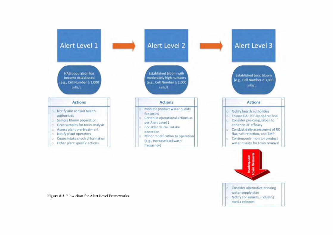
Figure 8.3. Flow chart for Alert Level Frameworks.

Guidelines for toxin control, HAB management, and response planning

247

8.6! SUMMARY This chapter has presented information regarding the risks presented by HAB toxins and how designers and operators could use tools to consider these risks and mitigate them appropriately. Many guidelines exist globally for HAB toxins in drinking water, although few countries have guidelines that consider seawater toxins, apart from New Zealand and Brazil that have guidelines for saxitoxin. To ensure complete removal of HAB toxins to a safe level in a desalination plant, designers can consider the multi barrier concept to mitigate the risk of unit process failure and toxin release into the distribution system. Risk assessments for HAB toxins can be undertaken by several methods, one of which is the HACCP process. This chapter also considered a practical assessment of toxin risks, calculating the residual risk after treatment for several common seawater toxins. Finally, this chapter describes an Alert Level Framework tool that can be used by operators to make rapid and effective decisions on how to operate a plant during a HAB bloom according to cellular concentrations in the seawater and thus react in an appropriate manner. By considering risks and mitigation options using the tools presented here, designers and operators can keep drinking water supplies safe and protect public health during toxic HABs. 8.7! REFERENCES Bartram, J., Burch, M., Falconer, I. R., Jones, G., and Kuiper-Goodman, T. 1999. Chapter 6:

Situation Assessment, Planning and Management. In I. Chorus & J. Bartram (Eds.), Toxic Cyanobacteria in Water: A Guide to Their Public Health Consequences, Monitoring and Management. London: E & F Spon.

Berdalet, E., Fleming, L. E., Gowen, R., Davidson, K., Hess, P., Backer, L. C., Moore, S. K., Hoagland, P., and Enevoldsen, H. 2015. Marine harmful algal blooms, human health and wellbeing: challenges and opportunities in the 21st century. Journal of the Marine Biological Association of the United Kingdom FirstView, 1-31.

Bixio, D., and Wintgens, T. 2006. Water Reuse System Management Manual: AQUAREC: Office for Official Publications of the European Communities.

Boerlage, S. F. E. and Nada, N. 2014. Algal toxin removal in seawater desalination processes, In Proceedings of European Desalination Society, Cyprus.

Caron, D. A., Garneau, M. È., Seubert, E., Howard, M. D., Darjany, L., Schnetzer, A., Cetinić, I., Filteau, G., Lauri, P., Jones, B., and Trussell, S. 2010. Harmful algae and their potential impacts on desalination operations off southern California. Water Research 44, 385-416.

Codex Alimentarius. (2003) http://www.fao.org/fao-who-codexalimentarius/standards/list-of-standards/en/?provide=standards&orderField=fullReference&sort=asc&num1=CAC/RCP, World Health Organization and Food Administration Organization of the United Nations.

Crittenden, J. C., Trussell, R. R., Hand, D. W., Howe, K. J., and Tchobanoglous, G. 2005. Water Treatment: Principles and Design (Second ed.): Wiley.

EFSA. 2008a. Marine biotoxins in shellfish - Azaspiracid group, Scientific Opinion of the Panel on Contaminants in the Food chain, adopted on 9 June 2008. EFSA Journal 723, 1-52.

Guidelines for toxin control, HAB management, and response planning

248

EFSA. 2008b. Marine biotoxins in shellfish - Okadaic Acid and analogues, Scientific Opinion of the Panel on Contaminants in the Food chain, adopted on 27 November 2007. EFSA Journal 589, 1-62.

EFSA. 2009a. Influence of processing on the levels of lipophilic marine biotoxins in bivalve molluscs, Statement of the Panel on Contaminants in the Food Chain (Question No EFSA-Q-2009-00203), Adopted on 25 March 2009. EFSA Journal 1016, 1-10.

EFSA. 2009b. Marine biotoxins in shellfish - Domoic acid group, Scientific Opinion of the Panel on Contaminants in the Food chain; adopted on 2 July 2009. EFSA Journal 1181, 1-61.

EFSA. 2009c. Marine biotoxins in shellfish - Palytoxin Group, Scientific Opinion of the Panel on Contaminants in the Food chain; adopted on 13 August 2009. EFSA Journal 7, 1-38.

EFSA. 2009d. Marine biotoxins in shellfish - Pectenotoxin group, Scientific Opinion of the Panel on Contaminants in the Food chain; adopted on 27 May 2009. EFSA Journal 1109, 1-47.

EFSA. 2009e. Marine biotoxins in shellfish - Saxitoxin group; Scientific Opinion of the Panel on Contaminants in the Food Chain, Adopted on 25 March 2009. EFSA Journal 1019, 1-76.

EFSA. 2009f. Marine biotoxins in shellfish - Summary Opinion, Scientific Opinion of the Panel on Contaminants in the Food chain; adopted on 13 August 2009. EFSA Journal 1306, 1-23.

EFSA. 2009g. Marine biotoxins in shellfish - Yessotoxin group, Scientific Opinion of the Panel on Contaminants in the Food chain, adopted on the 2 December 2008. EFSA Journal 907, 1-62.

EFSA. 2010a. Marine biotoxins in shellfish - Cyclic Imines (spirolides, gymnodimines, pinnatoxins and pteriatoxins), Scientific Opinion of the Panel on Contaminants in the Food chain; adopted on 5 July 2010. EFSA Journal 8, 1-39.

EFSA. 2010b. Marine biotoxins in shellfish - Emerging Toxins: Brevetoxin-group, Scientific Opinion of the Panel on Contaminants in the Food chain; adopted on 5 July 2010. EFSA Journal 8, 1-29.

EFSA. 2010c. Marine biotoxins in shellfish - Emerging Toxins: Ciguatoxin-group, Scientific Opinion of the Panel on Contaminants in the Food chain; adopted on 18 May 2010. EFSA Journal 8, 1-38.

EFSA. 2010d. Statement on further elaboration on consumption figure of 400 g shellfish meat on the basis of new consumption data, EFSA Panel on contaminants in the food chain.; adopted on 31 July 2010. EFSA Journal 8, 1-20.

EFSA (EFSA Panel on Biological Hazards (BIOHAZ), E.P.o.C.i.t.F.C.C. 2012. Scientific Opinion on the minimum hygiene criteria to be applied to clean seawater and on the public health risks and hygiene criteria for bottled seawater intended for domestic use. EFSA Journal 10, 2613 [2685 pages].

FSAI. 2006. Risk Assessment of Azaspiracids (AZAs) in Shellfish. A Report of the Scientific Committee of the Food Safety Authority of Ireland (FSAI) August 2006, 39 pages.

Havelaar, A. H. 1994. Application of HACCP to drinking water supply. Food Control 5, 142-152.

Guidelines for toxin control, HAB management, and response planning

249

Hrudey, S., Burch, M., Drikas, M., and Ross, G. 1999. Chapter 9: Remedial Measures. In I. Chorus & J. Bartram (Eds.), Toxic Cyanobacteria in Water: A Guide to Their Public Health Consequences, Monitoring and Management. London: E & F Spon.

Hsieh, D., Huxtable, S., and Chang, G. 2000. Total production of C1/C2 by Alexandrium tamarense. In Proceedings from the Ninth International Conference on Harmful Algal Blooms; Hallegraeff, G., Ed.; University of Tasmania: Hobart, Tasmania.

Humpage, A. R., and Falconer, I. R. 2002. Oral Toxicity of Cylindrospermopsin: No Observed Adverse Effect Level Determination in Swiss Albino Mice: CRC for Water Quality and Treatment Research Report #13.

Jochimsen, E. M., Carmichael, W. W., An, J., Cardo, D. M., Cookson, S. T., Holmes, C. E. and Barreto, V. S. T. 1998. Liver failure and death after exposure to microcystins at a hemodialysis center in Brazil. New England Journal of Medicine, 338(13), 873-878.

Kudela, R. M., 2011. Characterization and deployment of Solid Phase Adsorption Toxin Tracking (SPATT) resin for monitoring of microcystins in fresh and saltwater. Harmful Algae 11, 117-125.

Laycock, M. V., Anderson, D. M., Naar, J., Goodman, A., Easy, D. J., Donovan, M. A., Li, A. F., Quilliam, M. A., Al Jamali, E., and Alshihi, R. 2012. Laboratory desalination experiments with some algal toxins. Desalination 293, 1-6.

Lawrence, J., Loreal, H., Toyofuku, H., Hess, P., Iddya, K., and Ababouch, L. 2011. Assessment and management of biotoxin risks in bivalve molluscs. FAO Fisheries and Aquaculture Technical Paper No. 551, 337 pages.

Lefebvre, K. A., Bill, B. D., Erickson, A., Baugh, K. A., O'Rourke, L., Costa, P. R., Nance, S., Trainer, V. L. 2008. Characterization of intracellular and extracellular saxitoxin levels in both field and cultured Alexandrium spp. samples from Sequim Bay, Washington. Marine Drugs 6, 103-116.

Liefer, J. D., Robertson, A., MacIntyre, H. L., Smith, W. L., Dorsey, C. P., 2013. Characterization of a toxic Pseudo-nitzschia spp. bloom in the Northern Gulf of Mexico associated with domoic acid accumulation in fish. Harmful Algae 26, 20-32.

Miller, M. A., Kudela, R. M., Mekebri, A., Crane, D., Oates, S. C., Tinker, M. T., Staedler, M., Miller, W. A., Toy-Choutka, S., Dominik, C., Hardin, D., Langlois, G. W., Murray, M., Ward, K., Jessup, D.A. 2010. Evidence for a novel marine harmful algal bloom: Cyanotoxin (microcystin) transfer from land to sea otters. PLoS One 5, e12576.

Nadebaum, P., Chapman, M., Morden, R., and Rizak, S. 2004. A Guide to Hazard Identification and Risk Assessment for Drinking Water Supplies: CRC for Water Quality and Treatment Research Report #11.

Newcombe, G., House, J., Ho, L., Baker, P., and Burch, M. 2010. Management Strategies for Cyanobacteria (Blue-Green Algae): A Guide for Water Utilities: Cooperative Research Centre for Water Quality and Treatment Research Report #74.

NHMRC. 2006. Guidelines for Managing Risks in Recreational Water. Canberra: National Health and Medical Research Council.

NHMRC/NRMMC. 2011. Australian Drinking Water Guidelines Paper 6: National Water Quality Management Strategy. Canberra: National Health and Medical Research Council / National Resource Management Ministerial Council.

Guidelines for toxin control, HAB management, and response planning

250

Smith, J. L., Tong, M., Fux, E., and Anderson D. M. 2012. Toxin production, retention, and extracellular release by Dinophysis acuminate during extended stationary phase and culture decline. Harmful Algae 19, 125–132.

Takahashi, E., Yu, Q., Eaglesham, G., Connell, D. W., McBroom, J., Costanzo, S., and Shaw, G. R. 2007. Occurrence and seasonal variations of algal toxins in water, phytoplankton and shellfish from North Stradbroke Island, Queensland, Australia. Marine Environmental Research 64, 429-442.

Todd, K. 2011. Australian Marine Biotoxin Management Plan for Shellfish Farming: Cawthorn Report #645.

Trainer, V. L., Wells, M. L., Cochlan, W. P., Trick, C. G., Bill, B. D., Baugh, K. A., Beall, B. F., Herndon, J., and Lundholm, N. 2009. An ecological study of a massive bloom of toxigenic Pseudo-nitzschia cuspidata off the Washington State coast. Limnology and Oceanography 54, 1461-1474.

Velzeboer, R. M. A., Bater, P. D., and Rositano, J. 2001. Saxitoxins associated with the growth of the cyanobacterium Anabaena circinalis (Nostocales, Cyanophyta) under varying sources and concentrations of nitrogen. Phycologia 40, 305-312.

WHO. 1996. Guidelines for Drinking Water Quality: Health Criteria and Other Supporting Information (Vol. 2). Geneva: World Health Organization.

WHO. 1998. Guidelines for Drinking Water Quality: Health Criteria and Other Supporting Information - Addendum (Vol. 2). Geneva: World Health Organization.

WHO. 2004. Guidelines for Drinking Water Quality: Recommendations (Vol. 1). Geneva: World Health Organization.

WHO. 2011. Guidelines for Drinking Water Quality, Fouth Edition. Geneva: World Health Organization.

Zendong, Z., Abadie, E., Mazzeo, A., Hervé, F., Herrenknecht, C., Amzil, Z., Dell’Aversano, C., and Hess, P. 2015. Determination of the concentration of dissolved lipophilic algal toxins in seawater using pre-concentration with HP-20 resin and LC-MS/MS detection, in: MacKenzie, L. (Ed.), 16th International Conference on Harmful Algae 27th-31st October 2014. Cawthron Institute, Nelson, New Zealand and International Society for the Study of Harmful Algae, Wellington, New Zealand.

Algal biomass pretreatment in SWRO

251

9 ALGAL BIOMASS PRETREATMENT IN SEAWATER REVERSE OSMOSIS

Mike B. Dixon1, Siobhan F.E. Boerlage2, Nikolay Voutchkov3, Rita Henderson4, Mark Wilf5, Ivan Zhu6, S. Assiyeh Alizadeh Tabatabai7, Tony Amato8, Adhikara Resosudarmo4, Graeme

K. Pearce9, Maria Kennedy7, Jan C. Schippers7, and Harvey Winters10 1MDD Consulting, Kensington, Calgary, Alberta, Canada 2Boerlage Consulting, Gold Coast, Queensland, Australia 3Water Globe Consultants, Winter Springs, Florida, USA

4School of Chemical Engineering, The University of New South Wales, Australia 5Mark Wilf Consulting, San Diego, California, USA

6Leopold, a Xylem Brand, Zelienople, Pennsylvania, USA 7UNESCO-IHE Delft Institute for Water Education, Delft, The Netherlands

8Water2Water Consulting, England, UK 9Membrane Consultancy Associates Ltd, Reading, UK

10Fairleigh Dickinson University, Teaneck, New Jersey, USA

9.1 Introduction ....................................................................................................................................... 252 9.2 Chlorination in SWRO ..................................................................................................................... 252

9.2.1 Overview ...................................................................................................................................... 252 9.2.2 Chlorination during a HAB .......................................................................................................... 254 9.2.3 Summary ...................................................................................................................................... 257

9.3 Dechlorination in SWRO .................................................................................................................. 257 9.4 Coagulation for DAF, GMF, and UF pretreatment .......................................................................... 257

9.4.1 Overview ...................................................................................................................................... 257 9.4.2 Type of coagulation feed systems ................................................................................................ 260 9.4.3 Coagulation operational considerations ....................................................................................... 262 9.4.4 Coagulation and flocculation for DAF pretreatment ................................................................... 264 9.4.5 Coagulation for GMF pretreatment ............................................................................................. 265 9.4.6 Coagulation for MF/UF pretreatment .......................................................................................... 266

9.5 DAF pretreatment for SWRO ........................................................................................................... 272 9.5.1 Overview ...................................................................................................................................... 272 9.5.2 Fundamental principles of DAF ................................................................................................... 274 9.5.3 Process design of DAF systems ................................................................................................... 275 9.5.4 DAF in SWRO pretreatment for removal of marine algae .......................................................... 277 9.5.5 Optimization of process parameters for marine HABs ................................................................ 277 9.5.6 Summary ...................................................................................................................................... 278

9.6 Granular media filtration .................................................................................................................. 278 9.6.1 Overview ...................................................................................................................................... 278 9.6.2 The filter operation cycle ............................................................................................................. 279 9.6.3 Single and two-stage filtration ..................................................................................................... 281 9.6.4 Gravity filters ............................................................................................................................... 282 9.6.5 Pressure filters ............................................................................................................................... 284 9.6.6 GMF filter performance ............................................................................................................... 286

9.7 Microscreens for membrane pretreatment ........................................................................................ 287 9.7.1 Overview ...................................................................................................................................... 287 9.7.2 Types and configurations ............................................................................................................. 287 9.7.3 Algal bloom-related challenges ................................................................................................... 288 9.7.4 Summary ...................................................................................................................................... 290

9.8 Microfiltration/ ultrafiltration ........................................................................................................... 290 9.8.1 Overview ...................................................................................................................................... 290 9.8.2 MF/UF filtration modes ............................................................................................................... 290 9.8.3 Fouling of MF/UF during algal blooms ....................................................................................... 292 9.8.4 Removal of HAB cells using MF/UF .......................................................................................... 293 9.8.5 Summary ...................................................................................................................................... 296

Algal biomass pretreatment in SWRO

252

9.9 Cartridge filters for reverse osmosis pretreatment ............................................................................ 297 9.9.1 Overview ...................................................................................................................................... 297 9.9.2 Types and configurations ............................................................................................................. 297 9.9.3 Algal-bloom related challenges ................................................................................................... 298

9.10 Reverse osmosis ................................................................................................................................ 299 9.10.1 Overview ................................................................................................................................. 299 9.10.2 Raw water quality and pretreatment requirements for SWRO ............................................... 299 9.10.3 Effect of algal blooms on SWRO operation ........................................................................... 301 9.10.4 Ferric coagulant SWRO fouling during algal bloom events ................................................... 301 9.10.5 SWRO Biofouling during and following algal bloom events ................................................. 302 9.10.6 SWRO operational strategies during a bloom ......................................................................... 306 9.10.7 Membrane cleaning ................................................................................................................. 306 9.10.8 Summary ................................................................................................................................. 307

9.11 Summary of biomass removal in SWRO .......................................................................................... 307 9.12 References ......................................................................................................................................... 308

9.1 INTRODUCTION Harmful algal blooms (HABs) can result in a substantial increase in the organic and solids load in the seawater feed to be treated at a desalination plant. In this chapter, the removal of this material is addressed in the context of the multi-barrier treatment process for seawater reverse osmosis (SWRO) as presented in Chapter 8 on risk management for HAB events. While this chapter covers removal of non-toxic material, Chapter 10 builds upon these principles and discusses the mechanisms and effectiveness for each barrier with respect to toxin removal. This chapter covers only the main barriers used in the SWRO desalination plants for HAB bloom risk mitigation, though the authors acknowledge that other niche treatment barriers exist in SWRO systems. The treatment processes discussed here are chlorination and dechlorination, dissolved air flotation (DAF), granular media filtration (GMF), microscreens for microfiltration/ultrafiltration (MF/UF), MF/UF itself, cartridge filtration and SWRO. Coagulation is discussed in general terms and then more specifically for DAF, GMF, and MF/UF pretreatments. Each treatment process is broken down into a discussion of how the process works and then how HAB cells affect the process operation. Importantly, the chapter deals with how upstream actions can detrimentally affect downstream treatment processes with respect to algal blooms. In particular, this chapter discusses removal mechanisms for algal organic matter (AOM) and how operational actions can prevent detrimental effects of AOM. As discussed in Chapter 2, the chemical composition of AOM usually includes proteins, polysaccharides, nucleic acids, lipids, and other dissolved organic substances. AOM compounds typically cover a wide size spectrum, ranging from less than 1 nm to more than 1 mm. Based on their size cut-off, GMF and MF/UF are expected to remove only part of high molecular weight AOM (as shown in Chapter 2, Figure 2.2). SWRO is expected to achieve complete removal of AOM, but will suffer from fouling issues if AOM is not removed upstream. 9.2 CHLORINATION IN SWRO

9.2.1 Overview The disinfection properties of chlorine have been known for many years and routine use of chlorine in water treatment processes began in the early 1900s; however, in the last decade water chlorination has received criticism due to its production of disinfection byproducts.

In order to prevent marine growth, such as molluscs, in seawater intakes for both SWRO and thermal plants, biocides such as chlorine, ozone, potassium permanganate, and hydrogen peroxide can be used. The most widely used among them is chlorine, usually applied in one

Algal biomass pretreatment in SWRO

253

of three forms: 1) chlorine gas; 2) calcium hypochlorite; and 3) sodium hypochlorite, with the latter being the most typical (Bahamdan et al. 1999).

Chlorination in SWRO desalination plants is typically applied either at regular intervals (intermittent/shock chlorination) or continuously (rare) and dosed at the intake structure with additional dosing points downstream to maintain the required chlorine residual. Residual concentration of chlorine in the feedwater is typically kept at 0.2 - 4 mg/L (Agus et al. 2009). For intermittent chlorination, the duration of the dose may last from 30 to 90 minutes and is typically undertaken every 1 to 2 weeks at a random time (Ferguson et al. 2011). Often this is undertaken more frequently, up to daily. The continuous chlorination method has suffered from criticism that it causes biofouling of the reverse osmosis (RO) process unit. Appelgate et al. (1989) reported that chlorine degrades humic acids and high molecular weight compounds present in coastal seawater to smaller molecules that can be assimilated by bacteria. The chlorine suppresses bacterial activity, but when the sodium metabisulfite (SMBS) is added to remove chlorine prior to the RO, the surviving bacteria quickly take advantage of the nutrients generated by the degradation of larger molecules and enter into a cycle of enhanced growth. The significant increase in the biomass of bacteria after dechlorination causes slime development of biofilm on the surfaces of pipes and RO membranes (Winters 1995). To overcome the problem, alternate disinfectants have been used such as chlorine dioxide, chloramine and copper sulfate (Winters and Isquith 1995) although these have not been widely adopted. Plants that practice continuous chlorination now typically use very low doses (0.1 to 0.3 mg/L). Shock chlorination, also referred to as intermittent chlorination, is undertaken to control growth of marine life on pipelines and equipment that are constantly in contact with seawater. Both continuous and shock chlorination inhibit but do not fully prevent the growth of marine life so the presence of common oceanic foulants such as molluscan shells and barnacle deposits is unavoidable. The growth rate can be controlled to manageable levels, however. The effectiveness of shock chlorination can also be limited by the withdrawal of marine creatures into their protective shells and their re-emergence when chlorine has dissipated, especially when chlorine addition is undertaken at regular times rather than random intervals. Shock chlorination of seawater collected by open ocean intakes will result in an increased load of particulates on all solid removal processes due to the varied size range of solids introduced. The suspended solids will be in the micron size range, such as finer silts through to larger particles such as molluscan shells, byssal threads, and smaller debris like molluscan tissues and larvae. The impact on a membrane filtration system can be minimized by installing strainers or disk filters that would remove the bulk of the solids load created by the chlorination process (Ferguson et al. 2011).

As an alternative to using chlorine, a low dose of chlorine dioxide can be compatible with polyamide RO membranes, under certain conditions and to a certain extent. When generating chlorine dioxide onsite, it can be contaminated with chlorine and thus dechlorination is still necessary (Dow Water and Process Solutions 2015).

Intake chlorination can also produce carcinogenic compounds like trihalomethanes and haloacetic acids, as well as other inorganic disinfection byproducts (DBPs) such as chlorite, chlorate, bromate, and nitrogenous DBPs (N-DBPs). The latter generally form in much smaller amounts than chlorinated DBPs, but have been a growing concern over the past decade because of their greater health risk. High levels of nitrogen-containing compounds in AOM, which increases dramatically during a bloom, can lead to the formation of significant quantities of N-DBPs (Le Roux et al. 2015).

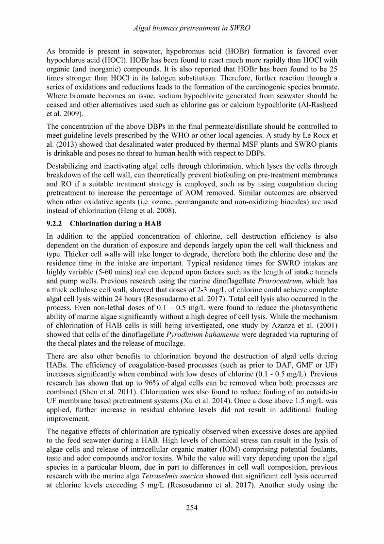
Algal biomass pretreatment in SWRO

254

As bromide is present in seawater, hypobromus acid (HOBr) formation is favored over hypochlorus acid (HOCl). HOBr has been found to react much more rapidly than HOCl with organic (and inorganic) compounds. It is also reported that HOBr has been found to be 25 times stronger than HOCl in its halogen substitution. Therefore, further reaction through a series of oxidations and reductions leads to the formation of the carcinogenic species bromate. Where bromate becomes an issue, sodium hypochlorite generated from seawater should be ceased and other alternatives used such as chlorine gas or calcium hypochlorite (Al-Rasheed et al. 2009).

The concentration of the above DBPs in the final permeate/distillate should be controlled to meet guideline levels prescribed by the WHO or other local agencies. A study by Le Roux et al. (2013) showed that desalinated water produced by thermal MSF plants and SWRO plants is drinkable and poses no threat to human health with respect to DBPs.

Destabilizing and inactivating algal cells through chlorination, which lyses the cells through breakdown of the cell wall, can theoretically prevent biofouling on pre-treatment membranes and RO if a suitable treatment strategy is employed, such as by using coagulation during pretreatment to increase the percentage of AOM removed. Similar outcomes are observed when other oxidative agents (i.e. ozone, permanganate and non-oxidizing biocides) are used instead of chlorination (Heng et al. 2008).

9.2.2 Chlorination during a HAB In addition to the applied concentration of chlorine, cell destruction efficiency is also dependent on the duration of exposure and depends largely upon the cell wall thickness and type. Thicker cell walls will take longer to degrade, therefore both the chlorine dose and the residence time in the intake are important. Typical residence times for SWRO intakes are highly variable (5-60 mins) and can depend upon factors such as the length of intake tunnels and pump wells. Previous research using the marine dinoflagellate Prorocentrum, which has a thick cellulose cell wall, showed that doses of 2-3 mg/L of chlorine could achieve complete algal cell lysis within 24 hours (Resosudarmo et al. 2017). Total cell lysis also occurred in the process. Even non-lethal doses of 0.1 – 0.5 mg/L were found to reduce the photosynthetic ability of marine algae significantly without a high degree of cell lysis. While the mechanism of chlorination of HAB cells is still being investigated, one study by Azanza et al. (2001) showed that cells of the dinoflagellate Pyrodinium bahamense were degraded via rupturing of the thecal plates and the release of mucilage.

There are also other benefits to chlorination beyond the destruction of algal cells during HABs. The efficiency of coagulation-based processes (such as prior to DAF, GMF or UF) increases significantly when combined with low doses of chlorine (0.1 - 0.5 mg/L). Previous research has shown that up to 96% of algal cells can be removed when both processes are combined (Shen et al. 2011). Chlorination was also found to reduce fouling of an outside-in UF membrane based pretreatment systems (Xu et al. 2014). Once a dose above 1.5 mg/L was applied, further increase in residual chlorine levels did not result in additional fouling improvement.

The negative effects of chlorination are typically observed when excessive doses are applied to the feed seawater during a HAB. High levels of chemical stress can result in the lysis of algae cells and release of intracellular organic matter (IOM) comprising potential foulants, taste and odor compounds and/or toxins. While the value will vary depending upon the algal species in a particular bloom, due in part to differences in cell wall composition, previous research with the marine alga Tetraselmis suecica showed that significant cell lysis occurred at chlorine levels exceeding 5 mg/L (Resosudarmo et al. 2017). Another study using the

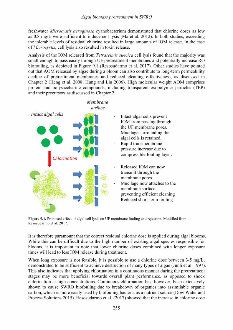
Algal biomass pretreatment in SWRO

255

freshwater Microcystis aeruginosa cyanobacterium demonstrated that chlorine doses as low as 0.8 mg/L were sufficient to induce cell lysis (Ma et al. 2012). In both studies, exceeding the tolerable levels of residual chlorine resulted in large amounts of IOM release. In the case of Microcystis, cell lysis also resulted in toxin release.

Analysis of the IOM released from Tetraselmis suecica cell lysis found that the majority was small enough to pass easily through UF pretreatment membranes and potentially increase RO biofouling, as depicted in Figure 9.1 (Resosudarmo et al. 2017). Other studies have pointed out that AOM released by algae during a bloom can also contribute to long-term permeability decline of pretreatment membranes and reduced cleaning effectiveness, as discussed in Chapter 2 (Heng et al. 2008; Hung and Liu 2006). High molecular weight AOM comprises protein and polysaccharide compounds, including transparent exopolymer particles (TEP) and their precursors as discussed in Chapter 2.

Figure 9.1. Proposed effect of algal cell lysis on UF membrane fouling and rejection. Modified from Resosudarmo et al. 2017.

It is therefore paramount that the correct residual chlorine dose is applied during algal blooms. While this can be difficult due to the high number of existing algal species responsible for blooms, it is important to note that lower chlorine doses combined with longer exposure times will lead to less IOM release during treatment.

When long exposure is not feasible, it is possible to use a chlorine dose between 3-5 mg/L, demonstrated to be sufficient to achieve destruction of many types of algae (Junli et al. 1997). This also indicates that applying chlorination in a continuous manner during the pretreatment stages may be more beneficial towards overall plant performance, as opposed to shock chlorination at high concentrations. Continuous chlorination has, however, been extensively shown to cause SWRO biofouling due to breakdown of organics into assimilable organic carbon, which is more easily used by biofouling bacteria as a nutrient source (Dow Water and Process Solutions 2015). Resosudarmo et al. (2017) showed that the increase in chlorine dose

-­‐ Intact algal cells prevent IOM from passing through the UF membrane pores.

-­‐ Mucilage surrounding the algal cells is retained.

-­‐ Rapid transmembrane pressure increase due to compressible fouling layer.

-­‐ Released IOM can now transmit through the membrane pores.

-­‐ Mucilage now attaches to the membrane surface, preventing efficient cleaning

-­‐ Reduced short-term fouling

Chlorination

Intact algal cells

Membrane surface

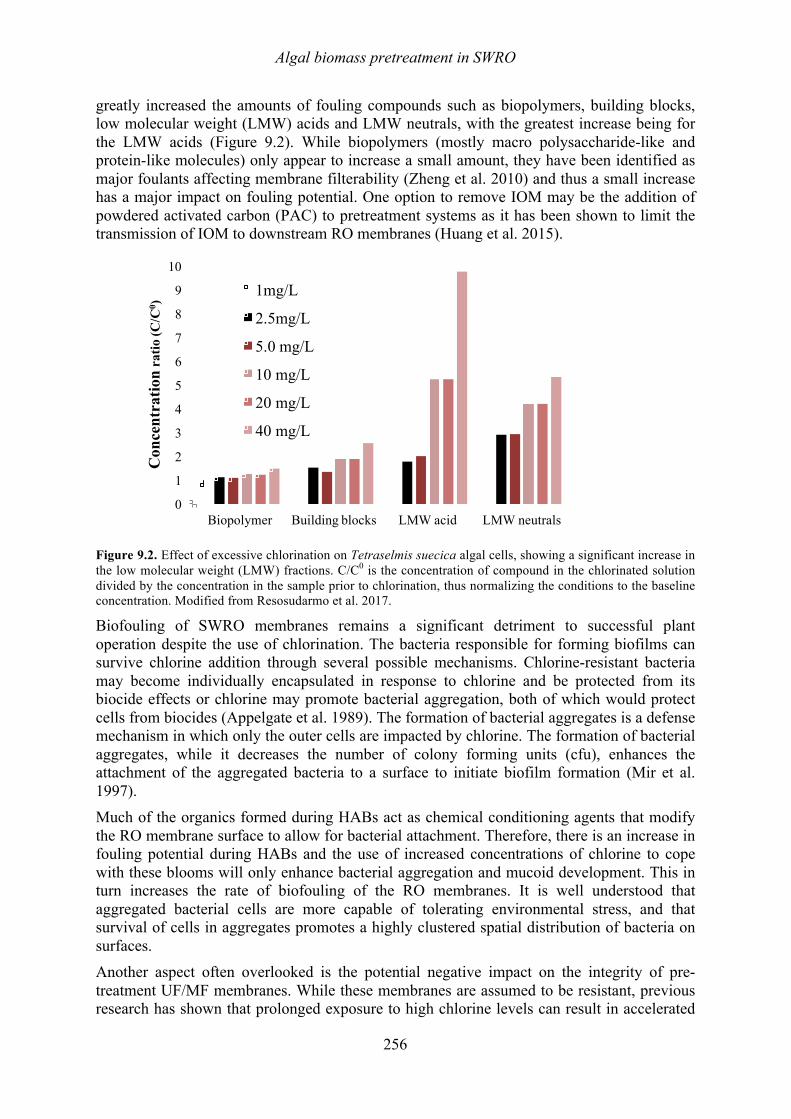
Algal biomass pretreatment in SWRO

256

greatly increased the amounts of fouling compounds such as biopolymers, building blocks, low molecular weight (LMW) acids and LMW neutrals, with the greatest increase being for the LMW acids (Figure 9.2). While biopolymers (mostly macro polysaccharide-like and protein-like molecules) only appear to increase a small amount, they have been identified as major foulants affecting membrane filterability (Zheng et al. 2010) and thus a small increase has a major impact on fouling potential. One option to remove IOM may be the addition of powdered activated carbon (PAC) to pretreatment systems as it has been shown to limit the transmission of IOM to downstream RO membranes (Huang et al. 2015).

Figure 9.2. Effect of excessive chlorination on Tetraselmis suecica algal cells, showing a significant increase in the low molecular weight (LMW) fractions. C/C0 is the concentration of compound in the chlorinated solution divided by the concentration in the sample prior to chlorination, thus normalizing the conditions to the baseline concentration. Modified from Resosudarmo et al. 2017.

Biofouling of SWRO membranes remains a significant detriment to successful plant operation despite the use of chlorination. The bacteria responsible for forming biofilms can survive chlorine addition through several possible mechanisms. Chlorine-resistant bacteria may become individually encapsulated in response to chlorine and be protected from its biocide effects or chlorine may promote bacterial aggregation, both of which would protect cells from biocides (Appelgate et al. 1989). The formation of bacterial aggregates is a defense mechanism in which only the outer cells are impacted by chlorine. The formation of bacterial aggregates, while it decreases the number of colony forming units (cfu), enhances the attachment of the aggregated bacteria to a surface to initiate biofilm formation (Mir et al. 1997). Much of the organics formed during HABs act as chemical conditioning agents that modify the RO membrane surface to allow for bacterial attachment. Therefore, there is an increase in fouling potential during HABs and the use of increased concentrations of chlorine to cope with these blooms will only enhance bacterial aggregation and mucoid development. This in turn increases the rate of biofouling of the RO membranes. It is well understood that aggregated bacterial cells are more capable of tolerating environmental stress, and that survival of cells in aggregates promotes a highly clustered spatial distribution of bacteria on surfaces. Another aspect often overlooked is the potential negative impact on the integrity of pre-treatment UF/MF membranes. While these membranes are assumed to be resistant, previous research has shown that prolonged exposure to high chlorine levels can result in accelerated

0

1

2

3

4

5

6

7

8

9

10

Biopolymer Building blocks LMW acid LMW neutrals

Con

cent

ratio

nra

tio (C

/C0 )

1mg/L

2.5mg/L

5.0 mg/L

10 mg/L

20 mg/L

40 mg/L

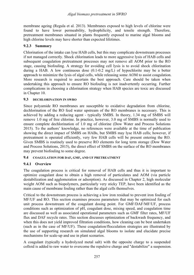
Algal biomass pretreatment in SWRO

257

membrane ageing (Regula et al. 2013). Membranes exposed to high levels of chlorine were found to have lower permeability, hydrophilicity, and tensile strength. Therefore, pretreatment membranes situated in plants frequently exposed to marine algal blooms and high chlorine levels may have shorter than expected lifetimes.

9.2.3 Summary Chlorination of the intake can lyse HAB cells, but this may complicate downstream processes if not managed correctly. Shock chlorination leads to more aggressive lysis of HAB cells and subsequent coagulation pretreatment processes may not remove all AOM prior to the RO stage, causing biofouling. A strategy for avoiding cell lysis is to avoid shock chlorination during a HAB. A low continuous dose (0.1-0.2 mg/L) of hypochlorite may be a better approach to minimize the lysis of algal cells, while releasing some AOM to assist coagulation. More research is required to ascertain the best approach. Care should be taken when undertaking this approach to ensure RO biofouling is not inadvertently occurring. Further complications in choosing a chlorination strategy when HAB species are toxic are discussed in Chapter 10. 9.3 DECHLORINATION IN SWRO

Since polyamide RO membranes are susceptible to oxidative degradation from chlorine, dechlorination of the RO feed water upstream of the RO membranes is necessary. This is achieved by adding a reducing agent - typically SMBS. In theory, 1.34 mg of SMBS will remove 1.0 mg of free chlorine. In practice, however, 3.0 mg of SMBS is normally used to ensure complete dechlorination of 1.0 mg of chlorine (Dow Water and Process Solutions 2015). To the authors’ knowledge, no references were available at the time of publication showing the direct impact of SMBS on HABs, but SMBS may lyse HAB cells; however, if pretreatment is operated efficiently, very few HAB cells will be present entering the RO. Given SMBS is routinely used to preserve RO elements for long term storage (Dow Water and Process Solutions, 2015), the direct effect of SMBS on the surface of the RO membranes may prevent biofouling to some degree. 9.4 COAGULATION FOR DAF, GMF, AND UF PRETREATMENT

9.4.1 Overview The coagulation process is critical for removal of HAB cells and thus it is important to optimize coagulant dose to obtain a high removal of particulates and AOM (via particle destabilization and agglomeration or adsorption). As discussed in Chapter 2, high molecular weight AOM such as biopolymers, particularly very sticky TEP, have been identified as the main cause of membrane fouling rather than the algal cells themselves.

Critical to the downstream process is achieving a low iron residual to prevent iron fouling of MF/UF and RO. This section examines process parameters that may be optimized for each unit process downstream of the coagulant dosing point. For GMF/DAF/MF/UF, process conditions such as optimization of pH, coagulant dose, mixing speed, and coagulation time are discussed as well as associated operational parameters such as GMF filter rates, MF/UF flux and DAF recycle rates. This section discusses optimization of backwash frequency, and when this does not yield improved filtration conditions, how cleaning can be best undertaken (such as in the case of MF/UF). These coagulation/flocculation strategies are illustrated by the use of supporting research on simulated algal blooms to isolate and elucidate precise mechanisms for scale-up and use in plant scenarios.

A coagulant (typically a hydrolyzed metal salt) with the opposite charge to a suspended colloid is added to raw water to overcome the repulsive charge and "destabilize" a suspension.

Algal biomass pretreatment in SWRO

258

In a colloidal suspension, particles will settle very slowly or not at all because the particles carry the same surface charges that mutually repel each other; the coagulant accelerates this particle settling process by neutralizing particle charge. For example, when colloidal particles in source seawater typically are negatively charged, ferric chloride is added as a coagulant to create positively charged ions (specifically cationic ferric chloride hydrolysis products), which attract and ultimately neutralize the charge of the seawater’s suspended solid particles. Once the repulsive charges are neutralized, the van der Waals force agglomerates the particles and form micro floc. Conversely, flocculation involves the process of clumping the small, destabilized micro flocs together into larger aggregates so that they can be more easily separated from the water. Flocculation is a physical process and does not involve the neutralization of charge. Coagulation may be used in conjunction with flocculation to assist with suspended solids separation.

Ferric salts, ferric chloride, and ferric sulfate, are the best choice for seawater coagulation (Edzwald and Haarhoff 2011). When ferric chloride is introduced in the seawater, both of them form ferric hydroxide, which is a large, positively charged molecule that attracts and coagulates predominantly negatively charged seawater suspended solids particles. While aluminum sulfate and polyaluminum chlorides (PACls) have been studied extensively at laboratory and pilot-scale in seawater RO pretreatment (Gabelich et al. 2006), they are not used in full-scale applications, primarily due to the relatively high solubility of aluminum, which may result in carryover and accumulation on RO membranes leading to aluminum hydroxide fouling (Gabelich et al. 2005). Ferric chloride is less soluble over a wider pH range, resulting in lower residual dissolved iron in RO feed water and less fouling problems. Further, ferric hydroxide has a high ratio of cationic charge to total mass (Jamaly et al. 2014) that makes hydrolysis products more reactive and adsorptive with emulsified and semi-emulsified organic matter; e.g. oil and grease, natural and synthetic organic matter. The settled sludge volume of the ferric hydroxide formed from ferric chloride is reportedly 30–60% that of sulfate based coagulants (e.g. Fe2(SO4)3). Additionally, the sludge developed from ferric chloride is generally much more dewaterable (CWT 2004).

The most important process parameters for coagulation are mixing intensity (G), flocculation shear rate (product of mixing intensity and time, G x t), pH, and temperature. Camp and Stein (1943) developed the basic theory of power input for mixing and defined G as the mean velocity gradient, which is proportional to the square root of power dissipated per unit volume of liquid. Upon coagulant addition, hydrolysis is instantaneous and the reactions that lead to the formation of ferric hydroxide occur in the order of seconds. As such, mixing has to ensure that the coagulant is fully dispersed within the liquid in the shortest time possible. Flocculation occurs by particle collision through thermally induced Brownian motion, stirring, or differential settling. Notably, coagulation is electric-force driven attraction of the negatively charged particles of the source water by the positively charged molecules of the coagulant, (which in the case of ferric salts is a trivalent metal salt), which neutralizes the charge of suspended, colloidal, and dissolved materials so these solids no longer repulse each other and subsequently are removed by aggregation followed by sedimentation or flotation. The mechanisms of destabilization for the negative particle charge of the suspended solids naturally occurring in seawater were summarized previously by Crittenden et al. (2012):

1) compression of the electrical double layer; 2) adsorption and charge neutralization; 3) adsorption and inter-particle bridging; and 4) enmeshment in a precipitate or “sweep floc”.

Algal biomass pretreatment in SWRO

259

It is unlikely that significant changes in ionic strength would occur due to coagulant addition. Therefore, the compression of the double layer should not be the dominant mechanism in the coagulation process, especially for seawater coagulation. Adsorption and inter-particle bridging usually happen when nonionic polymers and high-molecular-weight polymers are added. In the latter two mechanisms, surface charge plays an important role in dictating the speed and effectiveness of the formation of larger particles. The speed and effectiveness of the second mechanism – formation of larger particles by physical contact (enmesh/catch or sweep flocculation) –depends mainly on the number of particles in the source water (i.e., the turbidity/total suspended solids (TSS), concentration of the seawater) and their nature (Edzward and Haarhoff 2011). The dose of coagulant is determined by the content of solids in the source water, the electrical charge of the solid particles, and desired removal, the concentration of algae and particles, in addition to temperature, pH, alkalinity, and salinity, and other factors. In general, the higher the negative electrical charge of the particles in the source water and the less algae the seawater contains, the lower the coagulant dose needed. In addition, the higher the content of mineral particles in the seawater (i.e. the higher the turbidity/TSS concentration) the more coagulant will be needed to engage these particles in the formation of larger flocs.

If the source water particles have a strong negative charge, the dominating mechanism for large floc formation is electric attraction – therefore, relatively low doses of coagulant could achieve high coagulation effect. If the source particles do not have a strong charge, then the dose of coagulant will mainly be driven by the content of mineral suspended solids and natural organic matter (NOM) in the source water and the time the source water particles and coagulant will have to get in physical contact with each other – i.e. to collide with each other and stick together to form a larger floc. Recent research suggests that the dominant mechanism for coagulation of the marine dinoflagellate Prorocentrum minimum was through sweeping flocs, with charge neutralization constituting a critical step (Zhu et al. 2014). Therefore, operators often incorrectly assume that if they add more coagulant to poorly coagulating waters (i.e. waters containing particles with low or non-existent negative charge) they will improve the coagulation and filtration process.

During hydrolysis of salts, a complex of polynuclear, positively charged species are formed in a matter of seconds. During flocculation, colloidal particles and some fraction of dissolved AOM may attach to the floc body, and are eventually retained in downstream DAF, GMF, and UF processes.

Coagulation and flocculation are critical for DAF, GMF, and UF. During the DAF process, compressed air is introduced into a recycle stream of clarified water, is dissolved, and subsequently generates 10–100 µm bubbles when released through dispersion headers into a DAF tank. Coagulated particles, such as algae, attach to the bubbles and float to the top of the water column where they are mechanically or hydraulically removed. Two other removal mechanisms are adsorption, where the particles stick to the media surface, and biological removal, where soluble contaminants are removed through biological metabolism. GMF typically accumulates materials larger than 10 µm (Ripperger et al. 2012), which may include algal cells and large AOM (See Chapter 2, Figure 2.2). Since the size of some algae in seawater can be smaller than this threshold, coagulation to increase algal cell size is of critical importance to improve the removal efficiency of GMF. Unlike GMF, UF removes particles through physical straining only.

Coagulant addition is accomplished ahead of the SWRO pretreatment sedimentation tanks, dissolved air flotation units, GMF or MF/UF. The optimum coagulant dose is pH dependent

Algal biomass pretreatment in SWRO

260

and should be established on site through jar or pilot testing to provide site-specific conditions that will be encountered during plant operation. Practical experience indicates that the optimum pH for coagulation of particles in saline waters is highly temperature dependent. As the temperature decreases, the optimum pH for coagulation increases and vice versa. For example, the optimum pH for a temperature of 10oC is 8.2, while for source water temperature of 35oC, the optimum pH decreases down to 7.4 (Edzwald and Haarhoff 2012). Other factors influencing pH adjustment are salinity and alkalinity. The acidity constants K1sw and K2sw of carbonic acid are a function of salinity and temperature. For example, K1sw for seawater salinity of 35,000 ppm is 10-5.99 at 10°C, and 10-5.76 at 35°C. These differ greatly from fresh water constants (ionic strength approaching 0 M), which are 10-6.46 and 10-6.34. Seawater alkalinity is mainly contributed by carbonate and bicarbonate in addition to borate.

The mechanisms proposed for coagulation of NOM are a chemical phase change or precipitation by complexation with soluble metal species for pH < 6 and adsorption to and/or enmeshment in metal hydroxide precipitates for pH > 6 (Dennett et al. 1996). In seawater, dissolved metal speciation is affected by the high ionic strength, and optimum pH values for organic matter complexation are higher than those reported in freshwater (Duan et al. 2002; Edzwald and Haarhoff 2011). For lower temperature seawater (< 20°C), coagulation pH of 6.5 - 7 should be effective to maximize the availability of Fe(OH)2

+; however, Henderson et al. (2008a) demonstrated that AOM is characteristically different from NOM and therefore existing knowledge on NOM coagulation may not be adequate to explain on AOM fouling potential and removal in UF systems.

The formation of agglomerates in part comes about due to the negative charges (that naturally occur on the surfaces of particles, including algae, in the untreated water) becoming overcome by the addition of coagulants and sometimes polymers that neutralize surface charges, encouraging closer contact and subsequent agglomeration. Similarly, colloidal and dissolved organic matter, such as that produced by algae, can interact with coagulants, undergoing a phase change as they grow to form larger particles. In freshwater, both ferric and alum coagulants are commonly applied due to the production of positively-charged hydrolysis products (Duan and Gregory 2003); however, in seawater applications, ferric salts are the coagulant of choice as previously discussed (Edzwald and Haahoff 2011). Hence, much of the research conducted to date has focused on ferric chloride, although other ferric coagulants have been considered. Algal cells are covered with AOM produced during metabolic activities. The charge of those molecules is likely influenced by H+/OH− ions, providing opportunities to use pH adjustment to control coagulation and optimize coagulant doses. Since cells are negatively charged, adding hydrogen ions may neutralize the negatively charged functional groups (e.g. phosphate and carboxyl). At pH lower than 5.5, cells can lyse under stress, releasing intracellular substances that may not be fully removed by downstream pretreatment and may contribute to RO membrane fouling (Zhu et al. 2014).

9.4.2 Type of coagulation feed systems Chemical conditioning of the source seawater includes three key components: chemical feed system, coagulation, and flocculation tanks. The purpose of coagulation tanks is to achieve accelerated mixing of the coagulant with the source water and to neutralize the electric charge of the source water particles and colloids. Subsequent agglomeration of the coagulated particles into larger and easy to remove flocs is completed in flocculation tanks.

While coagulation is a relatively rapid chemical reaction, flocculation is much slower sand typically requires longer contact time and mixing conditions. Therefore, coagulation and

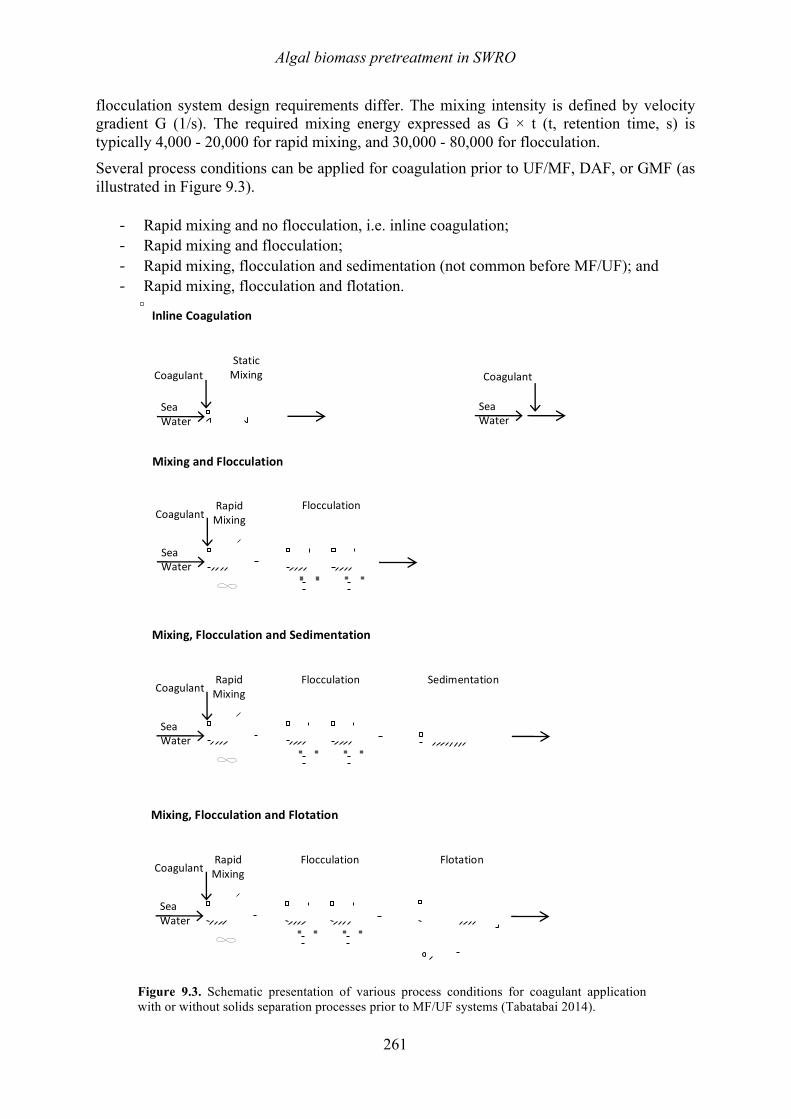
Algal biomass pretreatment in SWRO

261

flocculation system design requirements differ. The mixing intensity is defined by velocity gradient G (1/s). The required mixing energy expressed as G × t (t, retention time, s) is typically 4,000 - 20,000 for rapid mixing, and 30,000 - 80,000 for flocculation. Several process conditions can be applied for coagulation prior to UF/MF, DAF, or GMF (as illustrated in Figure 9.3).

-­‐‑ Rapid mixing and no flocculation, i.e. inline coagulation; -­‐‑ Rapid mixing and flocculation; -­‐‑ Rapid mixing, flocculation and sedimentation (not common before MF/UF); and -­‐‑ Rapid mixing, flocculation and flotation.

Figure 9.3. Schematic presentation of various process conditions for coagulant application with or without solids separation processes prior to MF/UF systems (Tabatabai 2014).

Inline Coagulation

Mixing and Flocculation

Mixing, Flocculation and Sedimentation

Sea Water

Static Mixing Coagulant

Sea Water

Coagulant

Sea Water

Rapid Mixing

Flocculation Coagulant

Mixing, Flocculation and Flotation

Sea Water

Rapid Mixing

Flocculation Coagulant

Flotation

Sea Water

Rapid Mixing

Flocculation Coagulant

Sedimentation

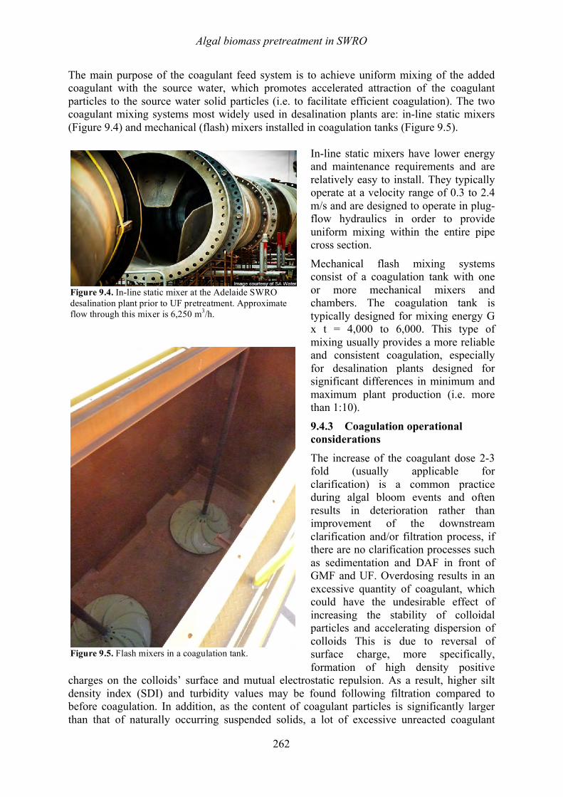
Algal biomass pretreatment in SWRO

262

The main purpose of the coagulant feed system is to achieve uniform mixing of the added coagulant with the source water, which promotes accelerated attraction of the coagulant particles to the source water solid particles (i.e. to facilitate efficient coagulation). The two coagulant mixing systems most widely used in desalination plants are: in-line static mixers (Figure 9.4) and mechanical (flash) mixers installed in coagulation tanks (Figure 9.5).

In-line static mixers have lower energy and maintenance requirements and are relatively easy to install. They typically operate at a velocity range of 0.3 to 2.4 m/s and are designed to operate in plug-flow hydraulics in order to provide uniform mixing within the entire pipe cross section.

Mechanical flash mixing systems consist of a coagulation tank with one or more mechanical mixers and chambers. The coagulation tank is typically designed for mixing energy G x t = 4,000 to 6,000. This type of mixing usually provides a more reliable and consistent coagulation, especially for desalination plants designed for significant differences in minimum and maximum plant production (i.e. more than 1:10).

9.4.3 Coagulation operational considerations

The increase of the coagulant dose 2-3 fold (usually applicable for clarification) is a common practice during algal bloom events and often results in deterioration rather than improvement of the downstream clarification and/or filtration process, if there are no clarification processes such as sedimentation and DAF in front of GMF and UF. Overdosing results in an excessive quantity of coagulant, which could have the undesirable effect of increasing the stability of colloidal particles and accelerating dispersion of colloids This is due to reversal of surface charge, more specifically, formation of high density positive

charges on the colloids’ surface and mutual electrostatic repulsion. As a result, higher silt density index (SDI) and turbidity values may be found following filtration compared to before coagulation. In addition, as the content of coagulant particles is significantly larger than that of naturally occurring suspended solids, a lot of excessive unreacted coagulant

Figure 9.4. In-line static mixer at the Adelaide SWRO desalination plant prior to UF pretreatment. Approximate flow through this mixer is 6,250 m3/h.

Figure 9.5. Flash mixers in a coagulation tank.

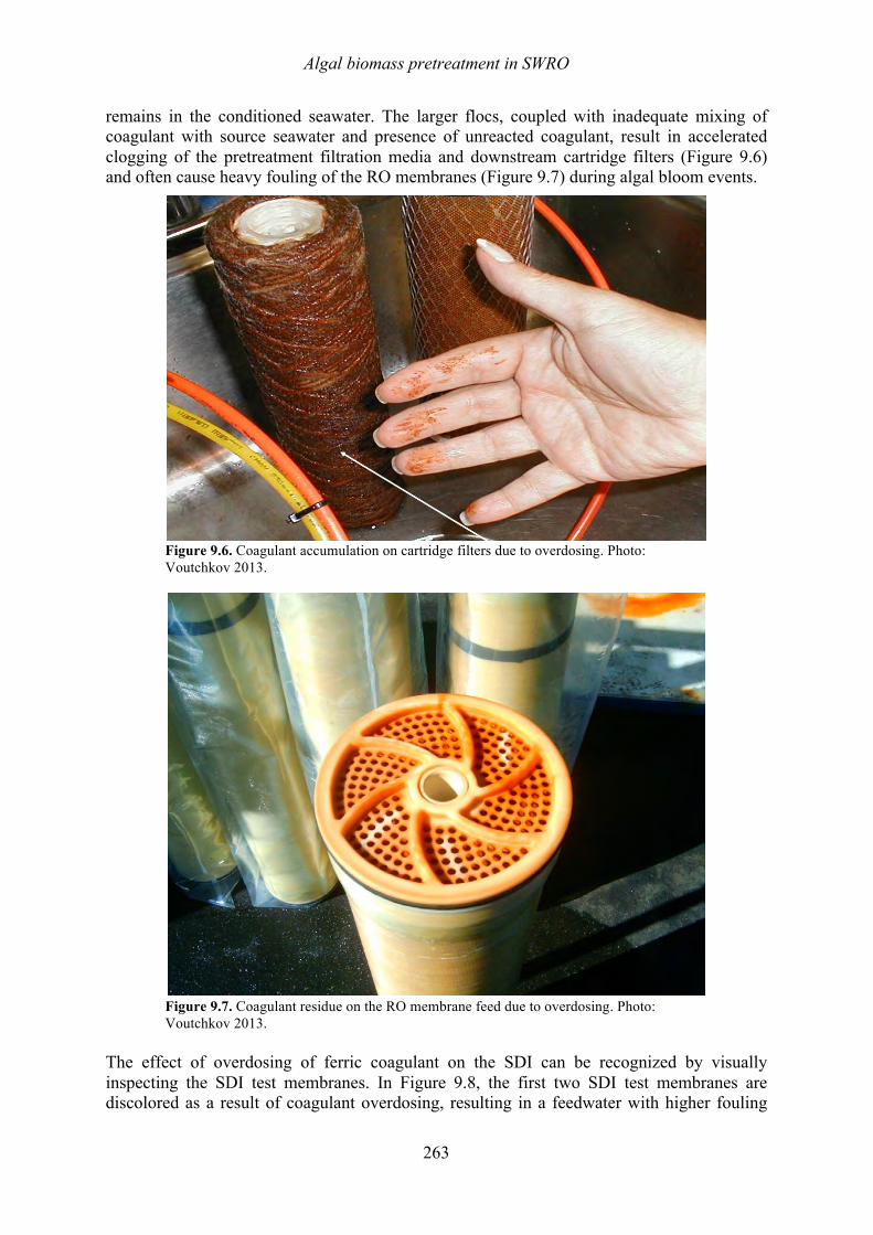
Algal biomass pretreatment in SWRO

263

remains in the conditioned seawater. The larger flocs, coupled with inadequate mixing of coagulant with source seawater and presence of unreacted coagulant, result in accelerated clogging of the pretreatment filtration media and downstream cartridge filters (Figure 9.6) and often cause heavy fouling of the RO membranes (Figure 9.7) during algal bloom events.

Figure 9.6. Coagulant accumulation on cartridge filters due to overdosing. Photo: Voutchkov 2013.

Figure 9.7. Coagulant residue on the RO membrane feed due to overdosing. Photo: Voutchkov 2013.

The effect of overdosing of ferric coagulant on the SDI can be recognized by visually inspecting the SDI test membranes. In Figure 9.8, the first two SDI test membranes are discolored as a result of coagulant overdosing, resulting in a feedwater with higher fouling

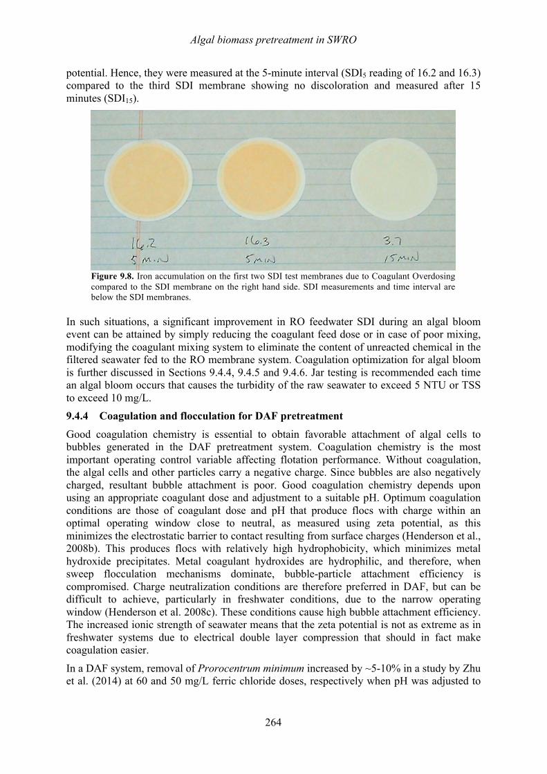
Algal biomass pretreatment in SWRO

264

potential. Hence, they were measured at the 5-minute interval (SDI5 reading of 16.2 and 16.3) compared to the third SDI membrane showing no discoloration and measured after 15 minutes (SDI15).

Figure 9.8. Iron accumulation on the first two SDI test membranes due to Coagulant Overdosing compared to the SDI membrane on the right hand side. SDI measurements and time interval are below the SDI membranes.

In such situations, a significant improvement in RO feedwater SDI during an algal bloom event can be attained by simply reducing the coagulant feed dose or in case of poor mixing, modifying the coagulant mixing system to eliminate the content of unreacted chemical in the filtered seawater fed to the RO membrane system. Coagulation optimization for algal bloom is further discussed in Sections 9.4.4, 9.4.5 and 9.4.6. Jar testing is recommended each time an algal bloom occurs that causes the turbidity of the raw seawater to exceed 5 NTU or TSS to exceed 10 mg/L. 9.4.4 Coagulation and flocculation for DAF pretreatment

Good coagulation chemistry is essential to obtain favorable attachment of algal cells to bubbles generated in the DAF pretreatment system. Coagulation chemistry is the most important operating control variable affecting flotation performance. Without coagulation, the algal cells and other particles carry a negative charge. Since bubbles are also negatively charged, resultant bubble attachment is poor. Good coagulation chemistry depends upon using an appropriate coagulant dose and adjustment to a suitable pH. Optimum coagulation conditions are those of coagulant dose and pH that produce flocs with charge within an optimal operating window close to neutral, as measured using zeta potential, as this minimizes the electrostatic barrier to contact resulting from surface charges (Henderson et al., 2008b). This produces flocs with relatively high hydrophobicity, which minimizes metal hydroxide precipitates. Metal coagulant hydroxides are hydrophilic, and therefore, when sweep flocculation mechanisms dominate, bubble-particle attachment efficiency is compromised. Charge neutralization conditions are therefore preferred in DAF, but can be difficult to achieve, particularly in freshwater conditions, due to the narrow operating window (Henderson et al. 2008c). These conditions cause high bubble attachment efficiency. The increased ionic strength of seawater means that the zeta potential is not as extreme as in freshwater systems due to electrical double layer compression that should in fact make coagulation easier.

In a DAF system, removal of Prorocentrum minimum increased by ~5-10% in a study by Zhu et al. (2014) at 60 and 50 mg/L ferric chloride doses, respectively when pH was adjusted to

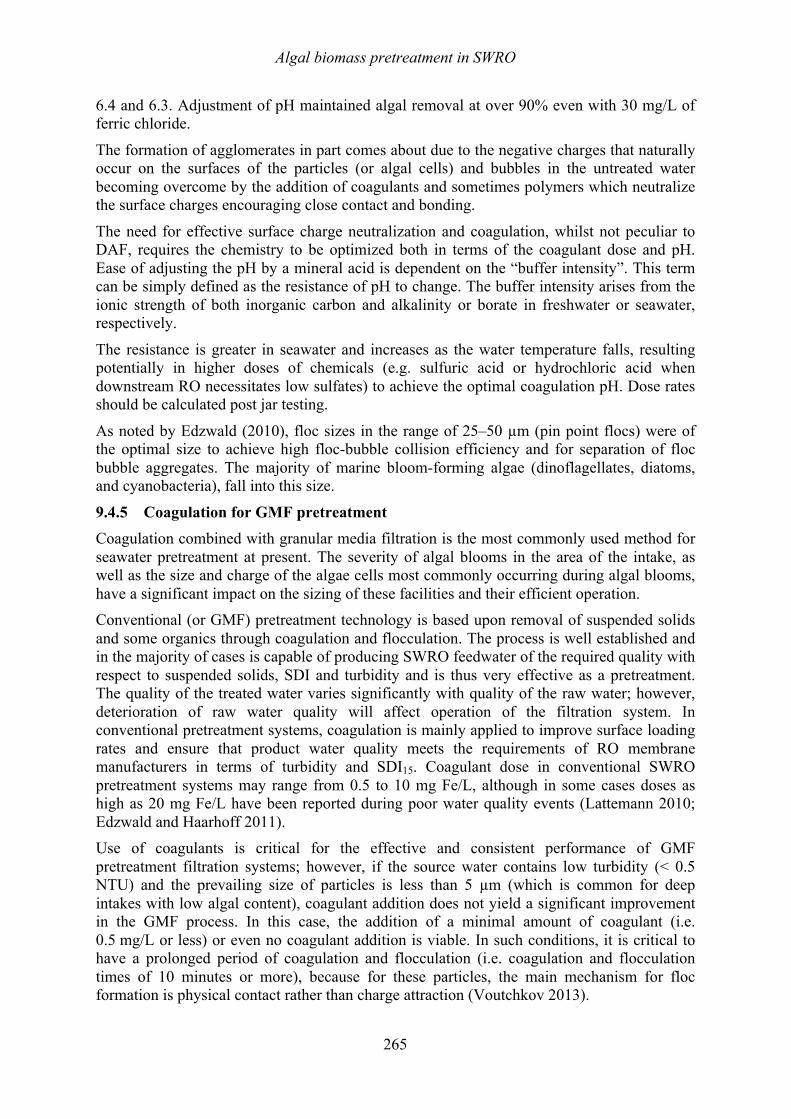
Algal biomass pretreatment in SWRO

265

6.4 and 6.3. Adjustment of pH maintained algal removal at over 90% even with 30 mg/L of ferric chloride.

The formation of agglomerates in part comes about due to the negative charges that naturally occur on the surfaces of the particles (or algal cells) and bubbles in the untreated water becoming overcome by the addition of coagulants and sometimes polymers which neutralize the surface charges encouraging close contact and bonding.

The need for effective surface charge neutralization and coagulation, whilst not peculiar to DAF, requires the chemistry to be optimized both in terms of the coagulant dose and pH. Ease of adjusting the pH by a mineral acid is dependent on the “buffer intensity”. This term can be simply defined as the resistance of pH to change. The buffer intensity arises from the ionic strength of both inorganic carbon and alkalinity or borate in freshwater or seawater, respectively.

The resistance is greater in seawater and increases as the water temperature falls, resulting potentially in higher doses of chemicals (e.g. sulfuric acid or hydrochloric acid when downstream RO necessitates low sulfates) to achieve the optimal coagulation pH. Dose rates should be calculated post jar testing.

As noted by Edzwald (2010), floc sizes in the range of 25–50 µm (pin point flocs) were of the optimal size to achieve high floc-bubble collision efficiency and for separation of floc bubble aggregates. The majority of marine bloom-forming algae (dinoflagellates, diatoms, and cyanobacteria), fall into this size.

9.4.5 Coagulation for GMF pretreatment Coagulation combined with granular media filtration is the most commonly used method for seawater pretreatment at present. The severity of algal blooms in the area of the intake, as well as the size and charge of the algae cells most commonly occurring during algal blooms, have a significant impact on the sizing of these facilities and their efficient operation. Conventional (or GMF) pretreatment technology is based upon removal of suspended solids and some organics through coagulation and flocculation. The process is well established and in the majority of cases is capable of producing SWRO feedwater of the required quality with respect to suspended solids, SDI and turbidity and is thus very effective as a pretreatment. The quality of the treated water varies significantly with quality of the raw water; however, deterioration of raw water quality will affect operation of the filtration system. In conventional pretreatment systems, coagulation is mainly applied to improve surface loading rates and ensure that product water quality meets the requirements of RO membrane manufacturers in terms of turbidity and SDI15. Coagulant dose in conventional SWRO pretreatment systems may range from 0.5 to 10 mg Fe/L, although in some cases doses as high as 20 mg Fe/L have been reported during poor water quality events (Lattemann 2010; Edzwald and Haarhoff 2011). Use of coagulants is critical for the effective and consistent performance of GMF pretreatment filtration systems; however, if the source water contains low turbidity (< 0.5 NTU) and the prevailing size of particles is less than 5 µm (which is common for deep intakes with low algal content), coagulant addition does not yield a significant improvement in the GMF process. In this case, the addition of a minimal amount of coagulant (i.e. 0.5 mg/L or less) or even no coagulant addition is viable. In such conditions, it is critical to have a prolonged period of coagulation and flocculation (i.e. coagulation and flocculation times of 10 minutes or more), because for these particles, the main mechanism for floc formation is physical contact rather than charge attraction (Voutchkov 2013).

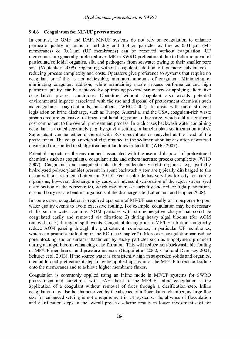
Algal biomass pretreatment in SWRO

266

9.4.6 Coagulation for MF/UF pretreatment In contrast, to GMF and DAF, MF/UF systems do not rely on coagulation to enhance permeate quality in terms of turbidity and SDI as particles as fine as 0.04 µm (MF membranes) or 0.01 µm (UF membranes) can be removed without coagulation. UF membranes are generally preferred over MF in SWRO pretreatment due to better removal of particulate/colloidal organics, silt, and pathogens from seawater owing to their smaller pore size (Voutchkov 2009). Operating without coagulant addition offers many advantages – reducing process complexity and costs. Operators give preference to systems that require no coagulant or if this is not achievable, minimum amounts of coagulant. Minimizing or eliminating coagulant addition, while maintaining stable process performance and high permeate quality, can be achieved by optimizing process parameters or applying alternative coagulation process conditions. Operating without coagulant also avoids potential environmental impacts associated with the use and disposal of pretreatment chemicals such as coagulants, coagulant aids, and others. (WHO 2007). In areas with more stringent legislation on brine discharge, such as Europe, Australia, and the USA, coagulant-rich waste streams require extensive treatment and handling prior to discharge, which add a significant cost component to the overall pretreatment process. In such cases backwash water containing coagulant is treated separately (e.g. by gravity settling in lamella plate sedimentation tanks). Supernatant can be either disposed with RO concentrate or recycled at the head of the pretreatment. The coagulant-rich sludge retained in the sedimentation tank is often dewatered onsite and transported to sludge treatment facilities or landfills (WHO 2007). Potential impacts on the environment associated with the use and disposal of pretreatment chemicals such as coagulants, coagulant aids, and others increase process complexity (WHO 2007). Coagulants and coagulant aids (high molecular weight organics, e.g. partially hydrolyzed polyacrylamide) present in spent backwash water are typically discharged to the ocean without treatment (Lattemann 2010). Ferric chloride has very low toxicity for marine organisms; however, discharge may cause an intense discoloration of the reject stream (red discoloration of the concentrate), which may increase turbidity and reduce light penetration, or could bury sessile benthic organisms at the discharge site (Lattemann and Höpner 2008). In some cases, coagulation is required upstream of MF/UF seasonally or in response to poor water quality events to avoid excessive fouling. For example, coagulation may be necessary if the source water contains NOM particles with strong negative charge that could be coagulated easily and removed via filtration; 2) during heavy algal blooms (for AOM removal); or 3) during oil spill events. Coagulant dosing prior to MF/UF filtration can greatly reduce AOM passing through the pretreatment membranes, in particular UF membranes, which can promote biofouling in the RO (see Chapter 2). Moreover, coagulation can reduce pore blocking and/or surface attachment by sticky particles such as biopolymers produced during an algal bloom, enhancing cake filtration. This will reduce non-backwashable fouling of MF/UF membranes and pressure increase (Guigui et al. 2002; Choi and Dempsey 2004; Schurer et al. 2013). If the source water is consistently high in suspended solids and organics, then additional pretreatment steps may be applied upstream of the MF/UF to reduce loading onto the membranes and to achieve higher membrane fluxes.

Coagulation is commonly applied using an inline mode in MF/UF systems for SWRO pretreatment and sometimes with DAF ahead of the MF/UF. Inline coagulation is the application of a coagulant without removal of flocs through a clarification step. Inline coagulation may also be characterized by the absence of a flocculation chamber, as large floc size for enhanced settling is not a requirement in UF systems. The absence of flocculation and clarification steps in the overall process scheme results in lower investment cost for

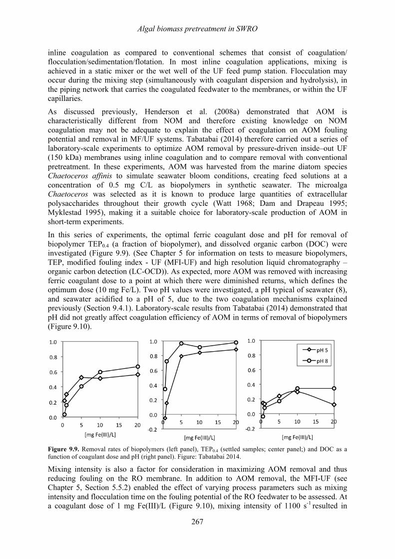
Algal biomass pretreatment in SWRO

267

inline coagulation as compared to conventional schemes that consist of coagulation/ flocculation/sedimentation/flotation. In most inline coagulation applications, mixing is achieved in a static mixer or the wet well of the UF feed pump station. Flocculation may occur during the mixing step (simultaneously with coagulant dispersion and hydrolysis), in the piping network that carries the coagulated feedwater to the membranes, or within the UF capillaries.

As discussed previously, Henderson et al. (2008a) demonstrated that AOM is characteristically different from NOM and therefore existing knowledge on NOM coagulation may not be adequate to explain the effect of coagulation on AOM fouling potential and removal in MF/UF systems. Tabatabai (2014) therefore carried out a series of laboratory-scale experiments to optimize AOM removal by pressure-driven inside–out UF (150 kDa) membranes using inline coagulation and to compare removal with conventional pretreatment. In these experiments, AOM was harvested from the marine diatom species Chaetoceros affinis to simulate seawater bloom conditions, creating feed solutions at a concentration of 0.5 mg C/L as biopolymers in synthetic seawater. The microalga Chaetoceros was selected as it is known to produce large quantities of extracellular polysaccharides throughout their growth cycle (Watt 1968; Dam and Drapeau 1995; Myklestad 1995), making it a suitable choice for laboratory-scale production of AOM in short-term experiments. In this series of experiments, the optimal ferric coagulant dose and pH for removal of biopolymer TEP0.4 (a fraction of biopolymer), and dissolved organic carbon (DOC) were investigated (Figure 9.9). (See Chapter 5 for information on tests to measure biopolymers, TEP, modified fouling index - UF (MFI-UF) and high resolution liquid chromatography – organic carbon detection (LC-OCD)). As expected, more AOM was removed with increasing ferric coagulant dose to a point at which there were diminished returns, which defines the optimum dose (10 mg Fe/L). Two pH values were investigated, a pH typical of seawater (8), and seawater acidified to a pH of 5, due to the two coagulation mechanisms explained previously (Section 9.4.1). Laboratory-scale results from Tabatabai (2014) demonstrated that pH did not greatly affect coagulation efficiency of AOM in terms of removal of biopolymers (Figure 9.10).

Figure 9.9. Removal rates of biopolymers (left panel), TEP0.4 (settled samples; center panel;) and DOC as a function of coagulant dose and pH (right panel). Figure: Tabatabai 2014.

Mixing intensity is also a factor for consideration in maximizing AOM removal and thus reducing fouling on the RO membrane. In addition to AOM removal, the MFI-UF (see Chapter 5, Section 5.5.2) enabled the effect of varying process parameters such as mixing intensity and flocculation time on the fouling potential of the RO feedwater to be assessed. At a coagulant dose of 1 mg Fe(III)/L (Figure 9.10), mixing intensity of 1100 s-1 resulted in

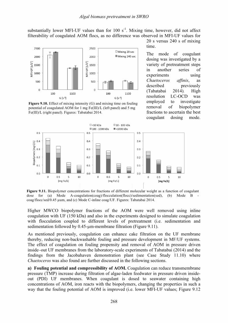
Algal biomass pretreatment in SWRO

268

substantially lower MFI-UF values than for 100 s-1. Mixing time, however, did not affect filterability of coagulated AOM flocs, as no difference was observed in MFI-UF values for

20 s versus 240 s of mixing time.

The mode of coagulant dosing was investigated by a variety of pretreatment steps in another series of experiments using Chaetoceros affinis, as described previously (Tabatabai 2014). High resolution LC-OCD was employed to investigate removal of biopolymer fractions to ascertain the best coagulant dosing mode.

Higher MWCO biopolymer fractions of the AOM were well removed using inline coagulation with UF (150 kDa) and also in the experiments designed to simulate coagulation with flocculation coupled to different levels of pretreatment (i.e. sedimentation and sedimentation followed by 0.45-µm-membrane filtration (Figure 9.11). As mentioned previously, coagulation can enhance cake filtration on the UF membrane thereby, reducing non-backwashable fouling and pressure development in MF/UF systems. The effect of coagulation on fouling propensity and removal of AOM in pressure driven inside–out UF membranes from the laboratory-scale experiments of Tabatabai (2014) and the findings from the Jacobahaven demonstration plant (see Case Study 11.10) where Chaetoceros was also found are further discussed in the following sections. a) Fouling potential and compressibility of AOM. Coagulation can reduce transmembrane pressure (TMP) increase during filtration of algae-laden feedwater in pressure driven inside-out (PDI) UF membranes. When coagulant is dosed to seawater containing high concentrations of AOM, iron reacts with the biopolymers, changing the properties in such a way that the fouling potential of AOM is improved (i.e. lower MFI-UF values; Figure 9.12

Figure 9.10. Effect of mixing intensity (G) and mixing time on fouling potential of coagulated AOM for 1 mg Fe(III)/L (left panel) and 5 mg Fe(III)/L (right panel). Figures: Tabatabai 2014.

Figure 9.11. Biopolymer concentrations for fractions of different molecular weight as a function of coagulant dose for (a) Mode A-coagulation(coag)/flocculation(flocc)/sedimentation(sed), (b) Mode B - coag/flocc/sed/0.45 µum, and (c) Mode C-inline coag/UF. Figures: Tabatabai 2014.

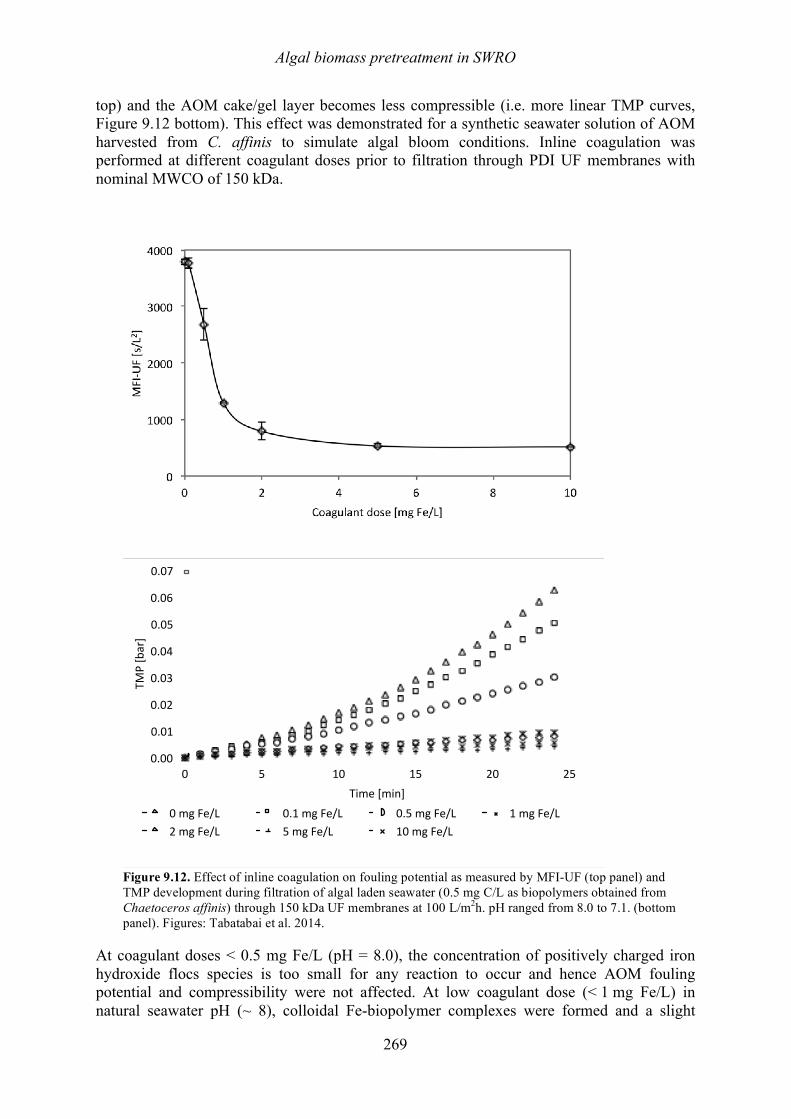
Algal biomass pretreatment in SWRO

269

top) and the AOM cake/gel layer becomes less compressible (i.e. more linear TMP curves, Figure 9.12 bottom). This effect was demonstrated for a synthetic seawater solution of AOM harvested from C. affinis to simulate algal bloom conditions. Inline coagulation was performed at different coagulant doses prior to filtration through PDI UF membranes with nominal MWCO of 150 kDa.

At coagulant doses < 0.5 mg Fe/L (pH = 8.0), the concentration of positively charged iron hydroxide flocs species is too small for any reaction to occur and hence AOM fouling potential and compressibility were not affected. At low coagulant dose (< 1 mg Fe/L) in natural seawater pH (~ 8), colloidal Fe-biopolymer complexes were formed and a slight

Figure 9.12. Effect of inline coagulation on fouling potential as measured by MFI-UF (top panel) and TMP development during filtration of algal laden seawater (0.5 mg C/L as biopolymers obtained from Chaetoceros affinis) through 150 kDa UF membranes at 100 L/m2h. pH ranged from 8.0 to 7.1. (bottom panel). Figures: Tabatabai et al. 2014.

0.00#

0.01#

0.02#

0.03#

0.04#

0.05#

0.06#

0.07#

0# 5# 10# 15# 20# 25#

TMP#[bar]#

Time#[min]#0#mg#Fe/L# 0.1#mg#Fe/L# 0.5#mg#Fe/L# 1#mg#Fe/L#2#mg#Fe/L# 5#mg#Fe/L# 10#mg#Fe/L#

(b)#

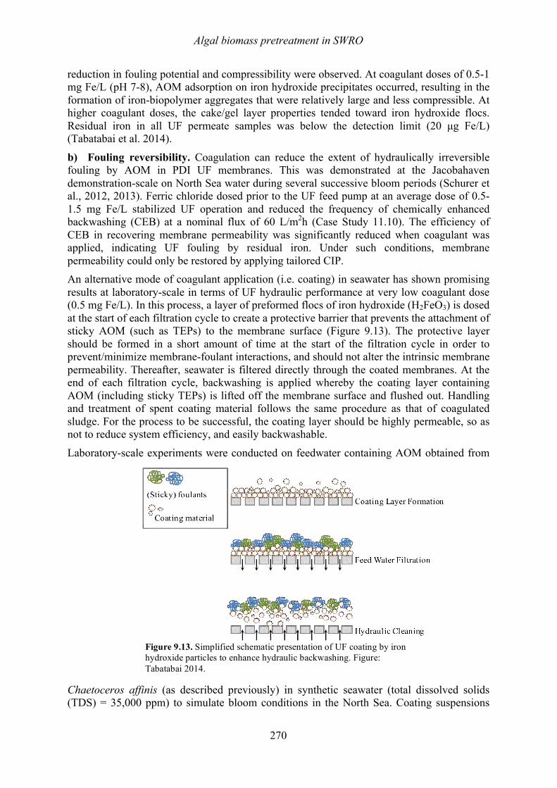
Algal biomass pretreatment in SWRO

270

reduction in fouling potential and compressibility were observed. At coagulant doses of 0.5-1 mg Fe/L (pH 7-8), AOM adsorption on iron hydroxide precipitates occurred, resulting in the formation of iron-biopolymer aggregates that were relatively large and less compressible. At higher coagulant doses, the cake/gel layer properties tended toward iron hydroxide flocs. Residual iron in all UF permeate samples was below the detection limit (20 µg Fe/L) (Tabatabai et al. 2014).

b) Fouling reversibility. Coagulation can reduce the extent of hydraulically irreversible fouling by AOM in PDI UF membranes. This was demonstrated at the Jacobahaven demonstration-scale on North Sea water during several successive bloom periods (Schurer et al., 2012, 2013). Ferric chloride dosed prior to the UF feed pump at an average dose of 0.5-1.5 mg Fe/L stabilized UF operation and reduced the frequency of chemically enhanced backwashing (CEB) at a nominal flux of 60 L/m2h (Case Study 11.10). The efficiency of CEB in recovering membrane permeability was significantly reduced when coagulant was applied, indicating UF fouling by residual iron. Under such conditions, membrane permeability could only be restored by applying tailored CIP. An alternative mode of coagulant application (i.e. coating) in seawater has shown promising results at laboratory-scale in terms of UF hydraulic performance at very low coagulant dose (0.5 mg Fe/L). In this process, a layer of preformed flocs of iron hydroxide (H2FeO3) is dosed at the start of each filtration cycle to create a protective barrier that prevents the attachment of sticky AOM (such as TEPs) to the membrane surface (Figure 9.13). The protective layer should be formed in a short amount of time at the start of the filtration cycle in order to prevent/minimize membrane-foulant interactions, and should not alter the intrinsic membrane permeability. Thereafter, seawater is filtered directly through the coated membranes. At the end of each filtration cycle, backwashing is applied whereby the coating layer containing AOM (including sticky TEPs) is lifted off the membrane surface and flushed out. Handling and treatment of spent coating material follows the same procedure as that of coagulated sludge. For the process to be successful, the coating layer should be highly permeable, so as not to reduce system efficiency, and easily backwashable.

Laboratory-scale experiments were conducted on feedwater containing AOM obtained from

Chaetoceros affinis (as described previously) in synthetic seawater (total dissolved solids (TDS) = 35,000 ppm) to simulate bloom conditions in the North Sea. Coating suspensions

Figure 9.13. Simplified schematic presentation of UF coating by iron hydroxide particles to enhance hydraulic backwashing. Figure: Tabatabai 2014.

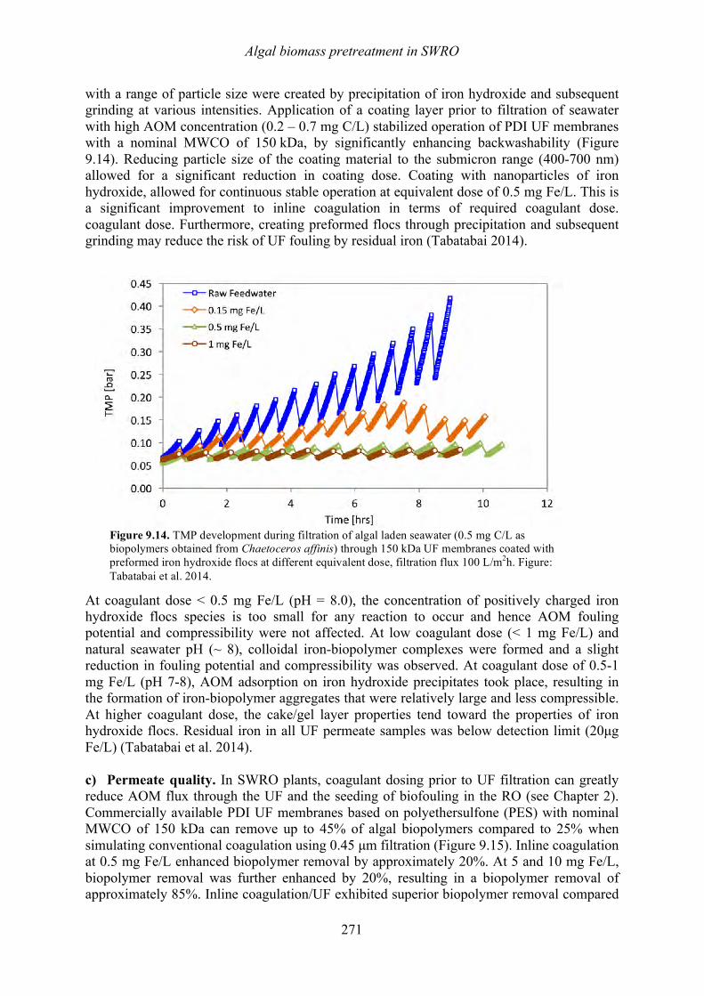
Algal biomass pretreatment in SWRO

271

with a range of particle size were created by precipitation of iron hydroxide and subsequent grinding at various intensities. Application of a coating layer prior to filtration of seawater with high AOM concentration (0.2 – 0.7 mg C/L) stabilized operation of PDI UF membranes with a nominal MWCO of 150 kDa, by significantly enhancing backwashability (Figure 9.14). Reducing particle size of the coating material to the submicron range (400-700 nm) allowed for a significant reduction in coating dose. Coating with nanoparticles of iron hydroxide, allowed for continuous stable operation at equivalent dose of 0.5 mg Fe/L. This is a significant improvement to inline coagulation in terms of required coagulant dose. coagulant dose. Furthermore, creating preformed flocs through precipitation and subsequent grinding may reduce the risk of UF fouling by residual iron (Tabatabai 2014).

At coagulant dose < 0.5 mg Fe/L (pH = 8.0), the concentration of positively charged iron hydroxide flocs species is too small for any reaction to occur and hence AOM fouling potential and compressibility were not affected. At low coagulant dose (< 1 mg Fe/L) and natural seawater pH (~ 8), colloidal iron-biopolymer complexes were formed and a slight reduction in fouling potential and compressibility was observed. At coagulant dose of 0.5-1 mg Fe/L (pH 7-8), AOM adsorption on iron hydroxide precipitates took place, resulting in the formation of iron-biopolymer aggregates that were relatively large and less compressible. At higher coagulant dose, the cake/gel layer properties tend toward the properties of iron hydroxide flocs. Residual iron in all UF permeate samples was below detection limit (20µg Fe/L) (Tabatabai et al. 2014). c) Permeate quality. In SWRO plants, coagulant dosing prior to UF filtration can greatly reduce AOM flux through the UF and the seeding of biofouling in the RO (see Chapter 2). Commercially available PDI UF membranes based on polyethersulfone (PES) with nominal MWCO of 150 kDa can remove up to 45% of algal biopolymers compared to 25% when simulating conventional coagulation using 0.45 µm filtration (Figure 9.15). Inline coagulation at 0.5 mg Fe/L enhanced biopolymer removal by approximately 20%. At 5 and 10 mg Fe/L, biopolymer removal was further enhanced by 20%, resulting in a biopolymer removal of approximately 85%. Inline coagulation/UF exhibited superior biopolymer removal compared

Figure 9.14. TMP development during filtration of algal laden seawater (0.5 mg C/L as biopolymers obtained from Chaetoceros affinis) through 150 kDa UF membranes coated with preformed iron hydroxide flocs at different equivalent dose, filtration flux 100 L/m2h. Figure: Tabatabai et al. 2014.

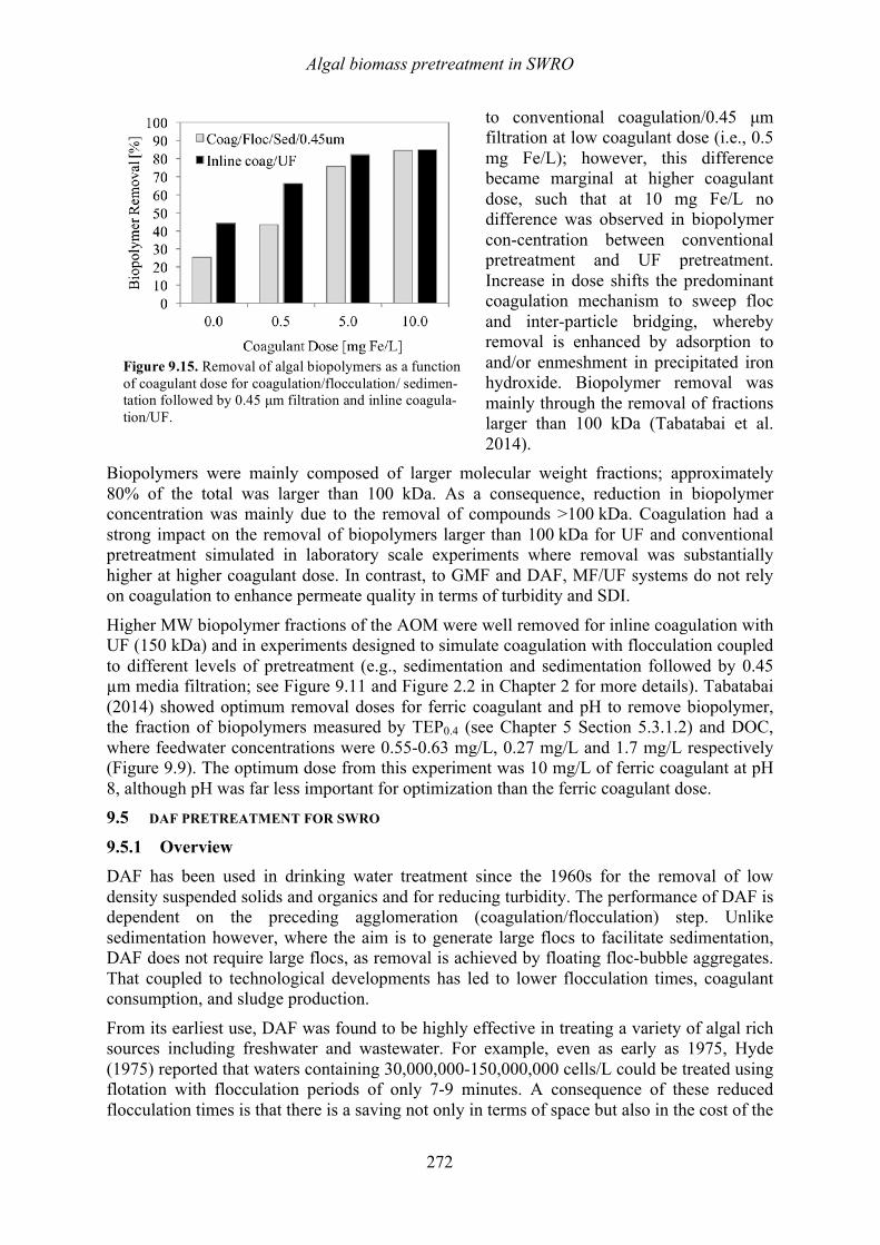
Algal biomass pretreatment in SWRO

272

to conventional coagulation/0.45 µm filtration at low coagulant dose (i.e., 0.5 mg Fe/L); however, this difference became marginal at higher coagulant dose, such that at 10 mg Fe/L no difference was observed in biopolymer con-centration between conventional pretreatment and UF pretreatment. Increase in dose shifts the predominant coagulation mechanism to sweep floc and inter-particle bridging, whereby removal is enhanced by adsorption to and/or enmeshment in precipitated iron hydroxide. Biopolymer removal was mainly through the removal of fractions larger than 100 kDa (Tabatabai et al. 2014).

Biopolymers were mainly composed of larger molecular weight fractions; approximately 80% of the total was larger than 100 kDa. As a consequence, reduction in biopolymer concentration was mainly due to the removal of compounds >100 kDa. Coagulation had a strong impact on the removal of biopolymers larger than 100 kDa for UF and conventional pretreatment simulated in laboratory scale experiments where removal was substantially higher at higher coagulant dose. In contrast, to GMF and DAF, MF/UF systems do not rely on coagulation to enhance permeate quality in terms of turbidity and SDI.

Higher MW biopolymer fractions of the AOM were well removed for inline coagulation with UF (150 kDa) and in experiments designed to simulate coagulation with flocculation coupled to different levels of pretreatment (e.g., sedimentation and sedimentation followed by 0.45 µm media filtration; see Figure 9.11 and Figure 2.2 in Chapter 2 for more details). Tabatabai (2014) showed optimum removal doses for ferric coagulant and pH to remove biopolymer, the fraction of biopolymers measured by TEP0.4 (see Chapter 5 Section 5.3.1.2) and DOC, where feedwater concentrations were 0.55-0.63 mg/L, 0.27 mg/L and 1.7 mg/L respectively (Figure 9.9). The optimum dose from this experiment was 10 mg/L of ferric coagulant at pH 8, although pH was far less important for optimization than the ferric coagulant dose. 9.5 DAF PRETREATMENT FOR SWRO

9.5.1 Overview DAF has been used in drinking water treatment since the 1960s for the removal of low density suspended solids and organics and for reducing turbidity. The performance of DAF is dependent on the preceding agglomeration (coagulation/flocculation) step. Unlike sedimentation however, where the aim is to generate large flocs to facilitate sedimentation, DAF does not require large flocs, as removal is achieved by floating floc-bubble aggregates. That coupled to technological developments has led to lower flocculation times, coagulant consumption, and sludge production.

From its earliest use, DAF was found to be highly effective in treating a variety of algal rich sources including freshwater and wastewater. For example, even as early as 1975, Hyde (1975) reported that waters containing 30,000,000-150,000,000 cells/L could be treated using flotation with flocculation periods of only 7-9 minutes. A consequence of these reduced flocculation times is that there is a saving not only in terms of space but also in the cost of the

Figure 9.15. Removal of algal biopolymers as a function of coagulant dose for coagulation/flocculation/ sedimen-tation followed by 0.45 µm filtration and inline coagula-tion/UF.

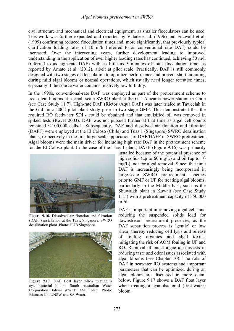
Algal biomass pretreatment in SWRO

273

civil structure and mechanical and electrical equipment, as smaller flocculators can be used. This work was further expanded and reported by Valade et al. (1996) and Edzwald et al. (1999) confirming reduced flocculation times and, more significantly, that previously typical clarification loading rates of 10 m/h (referred to as conventional rate DAF) could be increased. Over the intervening years, further development leading to improved understanding in the application of ever higher loading rates has continued, achieving 50 m/h (referred to as high-rate DAF) with as little as 5 minutes of total flocculation time, as reported by Amato et al. (2012), albeit at pilot scale. Practically, DAF is still commonly designed with two stages of flocculation to optimize performance and prevent short circuiting during mild algal blooms or normal operations, which usually need longer retention times, especially if the source water contains relatively low turbidity. In the 1990s, conventional-rate DAF was employed as part of the pretreatment scheme to treat algal blooms at a small scale SWRO plant at the Gas Atacama power station in Chile (see Case Study 11.7). High-rate DAF (Rictor /Aqua DAF) was later trialed at Taweelah in the Gulf in a 2002 pilot plant study prior to two stage GMF. This demonstrated that the required RO feedwater SDI15 could be obtained and that emulsified oil was removed in spiked tests (Rovel 2003). DAF was not pursued further at that time as algal cell counts remained < 100,000 cells/L. Subsequently, DAF and dissolved air flotation and filtration (DAFF) were employed at the El Coloso (Chile) and Tuas 1 (Singapore) SWRO desalination plants, respectively in the first large-scale applications of DAF/DAFF in SWRO pretreatment. Algal blooms were the main driver for including high rate DAF in the pretreatment scheme for the El Coloso plant. In the case of the Tuas 1 plant, DAFF (Figure 9.16) was primarily

installed because of the potential presence of high solids (up to 60 mg/L) and oil (up to 10 mg/L), not for algal removal. Since, that time DAF is increasingly being incorporated in large-scale SWRO pretreatment schemes prior to GMF or UF for treating algal blooms, particularly in the Middle East, such as the Shuwaikh plant in Kuwait (see Case Study 11.5) with a pretreatment capacity of 350,000 m3/d.

DAF is important in removing algal cells and reducing the suspended solids load for downstream pretreatment processes, as the DAF separation process is ‘gentle’ or low shear, thereby reducing cell lysis and release of fouling organics and algal toxins, mitigating the risk of AOM fouling in UF and RO. Removal of intact algae also assists in reducing taste and odor issues associated with algal blooms (see Chapter 10). The role of DAF in seawater RO systems and important parameters that can be optimized during an algal bloom are discussed in more detail below. Figure 9.17 shows a DAF float layer when treating a cyanobacterial (freshwater) bloom.

Figure 9.16. Dissolved air flotation and filtration (DAFF) installation at the Tuas, Singapore, SWRO desalination plant. Photo: PUB Singapore.

Figure 9.17. DAF float layer when treating a cyanobacterial bloom. South Australian Water Corporation Bolivar WWTP DAFF plant. Photo: Biomass lab, UNSW and SA Water.

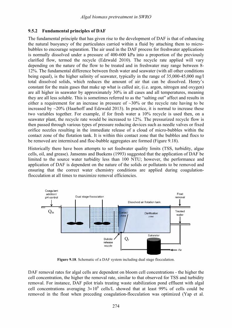
Algal biomass pretreatment in SWRO

274

9.5.2 Fundamental principles of DAF The fundamental principle that has given rise to the development of DAF is that of enhancing the natural buoyancy of the particulates carried within a fluid by attaching them to micro-bubbles to encourage separation. The air used in the DAF process for freshwater applications is normally dissolved under a pressure of 400-600 kPa into a proportion of the previously clarified flow, termed the recycle (Edzwald 2010). The recycle rate applied will vary depending on the nature of the flow to be treated and in freshwater may range between 8-12%. The fundamental difference between fresh water and seawater (with all other conditions being equal), is the higher salinity of seawater, typically in the range of 35,000-45,000 mg/l total dissolved solids, which reduces the amount of air that can be dissolved. Henry’s constant for the main gases that make up what is called air, (i.e. argon, nitrogen and oxygen) are all higher in seawater by approximately 30% in all cases and all temperatures, meaning they are all less soluble. This is sometimes referred to as the “salting out” affect and results in either a requirement for an increase in pressure of ~30% or the recycle rate having to be increased by ~20% (Haarhoff and Edzwald 2013). In practice, it is normal to increase these two variables together. For example, if for fresh water a 10% recycle is used then, on a seawater plant, the recycle rate would be increased to 12%. The pressurized recycle flow is then passed through various types of pressure reducing devices such as needle valves or fixed orifice nozzles resulting in the immediate release of a cloud of micro-bubbles within the contact zone of the flotation tank. It is within this contact zone that the bubbles and flocs to be removed are intermixed and floc-bubble aggregates are formed (Figure 9.18). Historically there have been attempts to set feedwater quality limits (TSS, turbidity, algae cells, oil, and grease). Jansenns and Buekens (1993) suggested that the application of DAF be limited to the source water turbidity less than 100 NTU; however, the performance and application of DAF is dependent on the nature of the solids or pollutants to be removed and ensuring that the correct water chemistry conditions are applied during coagulation-flocculation at all times to maximize removal efficiencies.

Figure 9.18. Schematic of a DAF system including dual stage flocculation.

DAF removal rates for algal cells are dependent on bloom cell concentrations - the higher the cell concentration, the higher the removal rate, similar to that observed for TSS and turbidity removal. For instance, DAF pilot trials treating waste stabilization pond effluent with algal cell concentrations averaging 3´108 cells/L showed that at least 99% of cells could be removed in the float when preceding coagulation-flocculation was optimized (Yap et al.

Qin

Qr

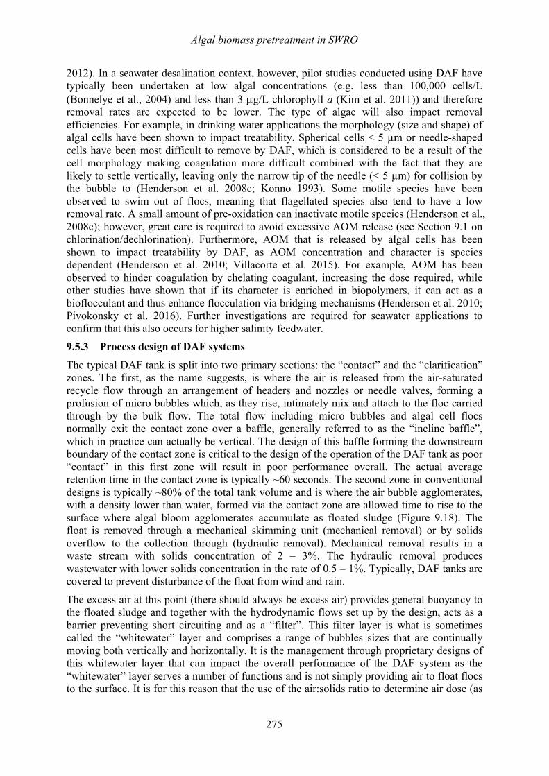
Algal biomass pretreatment in SWRO

275

2012). In a seawater desalination context, however, pilot studies conducted using DAF have typically been undertaken at low algal concentrations (e.g. less than 100,000 cells/L (Bonnelye et al., 2004) and less than 3 µg/L chlorophyll a (Kim et al. 2011)) and therefore removal rates are expected to be lower. The type of algae will also impact removal efficiencies. For example, in drinking water applications the morphology (size and shape) of algal cells have been shown to impact treatability. Spherical cells < 5 µm or needle-shaped cells have been most difficult to remove by DAF, which is considered to be a result of the cell morphology making coagulation more difficult combined with the fact that they are likely to settle vertically, leaving only the narrow tip of the needle (< 5 µm) for collision by the bubble to (Henderson et al. 2008c; Konno 1993). Some motile species have been observed to swim out of flocs, meaning that flagellated species also tend to have a low removal rate. A small amount of pre-oxidation can inactivate motile species (Henderson et al., 2008c); however, great care is required to avoid excessive AOM release (see Section 9.1 on chlorination/dechlorination). Furthermore, AOM that is released by algal cells has been shown to impact treatability by DAF, as AOM concentration and character is species dependent (Henderson et al. 2010; Villacorte et al. 2015). For example, AOM has been observed to hinder coagulation by chelating coagulant, increasing the dose required, while other studies have shown that if its character is enriched in biopolymers, it can act as a bioflocculant and thus enhance flocculation via bridging mechanisms (Henderson et al. 2010; Pivokonsky et al. 2016). Further investigations are required for seawater applications to confirm that this also occurs for higher salinity feedwater. 9.5.3 Process design of DAF systems

The typical DAF tank is split into two primary sections: the “contact” and the “clarification” zones. The first, as the name suggests, is where the air is released from the air-saturated recycle flow through an arrangement of headers and nozzles or needle valves, forming a profusion of micro bubbles which, as they rise, intimately mix and attach to the floc carried through by the bulk flow. The total flow including micro bubbles and algal cell flocs normally exit the contact zone over a baffle, generally referred to as the “incline baffle”, which in practice can actually be vertical. The design of this baffle forming the downstream boundary of the contact zone is critical to the design of the operation of the DAF tank as poor “contact” in this first zone will result in poor performance overall. The actual average retention time in the contact zone is typically ~60 seconds. The second zone in conventional designs is typically ~80% of the total tank volume and is where the air bubble agglomerates, with a density lower than water, formed via the contact zone are allowed time to rise to the surface where algal bloom agglomerates accumulate as floated sludge (Figure 9.18). The float is removed through a mechanical skimming unit (mechanical removal) or by solids overflow to the collection through (hydraulic removal). Mechanical removal results in a waste stream with solids concentration of 2 – 3%. The hydraulic removal produces wastewater with lower solids concentration in the rate of 0.5 – 1%. Typically, DAF tanks are covered to prevent disturbance of the float from wind and rain.

The excess air at this point (there should always be excess air) provides general buoyancy to the floated sludge and together with the hydrodynamic flows set up by the design, acts as a barrier preventing short circuiting and as a “filter”. This filter layer is what is sometimes called the “whitewater” layer and comprises a range of bubbles sizes that are continually moving both vertically and horizontally. It is the management through proprietary designs of this whitewater layer that can impact the overall performance of the DAF system as the “whitewater” layer serves a number of functions and is not simply providing air to float flocs to the surface. It is for this reason that the use of the air:solids ratio to determine air dose (as

Algal biomass pretreatment in SWRO

276

used in sludge thickening applications) is not appropriate for seawater conditions, a TSS of several hundred is considered very high for SWRO pretreatment applications.

The size of bubbles regarded as ideal for freshwater DAF applications have traditionally been in the range of 10-100 µm with most having sizes of 40-80 µm (Edzwald 2010). This appears to be the case for desalination applications as Kim et al. (2011) also reported bubble sizes in the range of 10-100 µm when using seawater. It was reported that the mean bubble size in saline water was smaller than that in fresh water because of such factors as higher surface tension, higher ionic strength, and higher density of seawater (Besson and Guiraud 2012). The concentration of air bubbles (bubble density) will vary depending on a number of factors including sizes. These factors can include, but not be limited to, the recycle rate (that can vary typically in the range of 6-20% on a volumetric basis), recycle pressure, the saturator efficiency and temperature. However, for a typical system delivering the equivalent of ~8 g air/m3 of throughput, the number of bubbles can be in the range of 1.8 – 2.5 x 105/mL. Smaller bubbles in seawater DAF systems may slightly offset the negative effects of salinity on the air demand. The smaller the bubble size (and the lower the water temperature), the slower the rise rate of the bubble, and thus, a larger flotation tank is required to allow bubbles to reach the surface (Gregory et al. 1999). There are various DAF designs on the market and these range from what some may describe as horizontal, where the flow enters at one end (Figure 9.18) or from the center, and then flows along the tank length or radius to the outlet normally via an underflow baffle or a series of collector pipes. An alternative to this approach is combined dual media gravity filters with DAF which include the proprietary systems such as CoCo™ and Enflo-Filt™ or generic type called stack DAF, in-filter DAF or DAFF (Figure 9.19). These systems offer the end-user the advantage of space savings; however, the operation of the DAF in terms of loading rate is restricted by the limits placed on the filter and the physical property of an air bubble. Air bubbles with average diameters of 40-60 µm would have a rise rate in the range of 3-7 m/h,

respectively (with large bubbles of 100 µm reaching rise rates of 20 m/h). This means that the higher net flotation rates now being utilized in high-rate DAF of 30-50 m/h cannot be used because of the problems associated with air being drawn into the filter bed causing air blinding. There is also the lack of available hydraulic driving head required for flow to pass through the filter to match the higher DAF rates. Moreover, the whole system (including the flotation cell) will need to be taken offline for 15 to 20 minutes during a filter backwash event. When no bloom, oil, or grease are present in the feedwater, some systems provide pipework to bypass the DAF. Some DAFF systems will operate in direct filter mode when blooms are not present.

Figure 9.19. Combined DAF clarifier and granular media filter.

Algal biomass pretreatment in SWRO

277

The typical frequency of float removal tends to be site specific ranging from continuous to intermittent. This is true regardless of whether the sludge removal method is mechanical or hydraulic. The resulting sludge from the DAF tank can be dewatered and thickened separately but is generally mixed with the settled GMF or UF backwash water before thickening and dewatering by centrifuge or plate press. The clarified water following sludge treatment is typically returned to sea with the SWRO brine.

When designing a DAF system according to hydraulic loading, the influent flow is considered as the upstream flocculation system and excludes recycle flow. The tank area can then be designed according to the preferred hydraulic loading rate. The area calculated is that of the contact and clarification zones, whereby the velocity of the water flowing towards the base of the tank must be less than the rising velocity of floc-bubble aggregates to ensure separation (Edzwald et al., 2010). The area of the adjacent contact zone must be designed to ensure a residence time of 1-2.5 minutes. It is not always clear whether the hydraulic loading rate reported is for the clarification zone only.

9.5.4 DAF in SWRO pretreatment for removal of marine algae A study by Haarhoff and Edzwald (2013), examining the differences in the application of DAF in seawater compared to freshwater, found that contact and separations zones were not significantly different. The largest difference was due to the lower solubility of air in seawater compared to freshwater. The dynamic viscosity, density and surface tension are all higher in seawater and though these differences are small at +8%, +3% and +1% respectively at a salinity of 35 g/kg and temperature of 20 °C (Haarhoff and Edzwald 2013) as viscosity cannot be ignored when designs are proposed where the operational load is high, i.e. typically ≥ 20 m/h. The reason why viscosity cannot be ignored at these elevated levels is because of the additional drag on the floc-bubble aggregates and the overall supporting whitewater layer as described by Amato et al. (2012). This ultimately impacts on the tank design, particularly in terms of its overall depth, which needs to be slightly deeper when considering the treatment of seawater. This will not always be necessary and will depend upon other factors such as the method used to draw off the subnatant and any water quality requirements imposed on the DAF product flow. At a minimum, an additional 30 cm of tank depth might be needed, as reported by Amato et al. (2012).

The percentage removal of algae in fresh water applications is typically 90-99% (Yap et al. 2012; Zhu et al. 2014) while practical experience shows that when used for seawater pretreatment, DAF systems usually yield significantly lower algal removal rates – 40 to 50% (Voutchkov 2013). Actual removal can be as low as 40%; however, as it is dependent on the cell concentration in the feed, the type and size of algal cells, and phase of growth (lag, exponential or stationary phase), due to differing amounts of AOM in solution (Henderson et al. 2008b). Oil and grease removal are difficult to quantify because of the three states in which it may be found, i.e. suspended (easy), emulsified, and dissolved (both more difficult). Therefore, in the case of oil, any removal rates need quantification by jar testing. Efficiency of turbidity reduction is a very poor parameter as it is not unusual to have higher turbidities post DAF than what may have been found in the raw. True turbidity removal efficiency can only be reported when the feed to the DAF is measured after flocculation.

9.5.5 Optimization of process parameters for marine HABs While removal of algal cells via DAF is important during a bloom, operators must also consider the presence of associated AOM that may also deteriorate the water quality. This AOM may interfere with coagulation or reach downstream RO membranes and cause biofouling. It is therefore important that coagulation conditions are optimized, not just for

Algal biomass pretreatment in SWRO

278

cell removal, but also for simultaneous AOM removal. Application of coagulation-flocculation-DAF to remove AOM of larger molecular size (e.g., biopolymers and humic-type substances), in combination with biofiltration in GMF will maximize organic matter removal to protect the downstream SWRO membranes from accelerated biofouling (Shutova et al. 2016; Naidu et al. 2013). (This is discussed further in Chapter 2 and Section 9.4). 9.5.6 Summary

DAF is useful in removing algal cells and reducing the suspended solids load for downstream pretreatment, as the process is ‘gentle’ or low shear, preventing cell lysis and release of fouling organics and algal toxins, thereby reducing the risk of AOM fouling of UF and RO membranes. Practical full-scale experience to date with using DAF for pretreatment of seawater is very limited and have shown a wide range of algal removal efficiency; however, with optimization, DAF can be very effective as an SWRO pre-treatment, removing up to 99% of cells when preceding coagulation-flocculation is optimized. This removal efficiency depends on many factors – one of the key factors is the content of suspended solids in the source water. Designers of DAF for seawater plants should take care to consider salt water-specific parameters such as the “salting out” affect that results in either a requirement for an increase in pressure (~30%) or recycle rate (~20%). If the DAF is only operational periodically, operators could consider bringing the DAF online while cell counts are low so that the plant is fully operational when counts increase. This argues for plankton monitoring in the vicinity of the plant (Chapter 3) and within the plant (Chapter 5) so that effective actions can be taken sufficiently early to minimize clogging and fouling.

9.6 GRANULAR MEDIA FILTRATION

9.6.1 Overview Conventional pretreatment using coagulation, flocculation, and filtration through granular media is the most commonly used source water pretreatment process for SWRO desalination plants today (other than cartridge filtration). This process includes filtration of the source seawater through one or more layers of granular media (e.g. anthracite coal, silica sand, garnet).

In the GMF process, suspended solids are removed through attachment to the filtration media particles and through blockage/capture by the filtration cake. Organics may be removed by biofiltration occurring in the filter (e.g., the utilization and breakdown of organic materials by microbes). The preferred process of filtration is capture of suspended solids with bed penetration (depth filtration) as opposed to surface filtration, since the latter results in a significantly faster increase of pressure loss and therefore shorter filter runs. During algal bloom events, coagulant overdosing may occur as described in Section 9.4.3 resulting in accumulation of large flocs at the filter surface, blinding the filter bed if the blooms are very intense.

Conventional filters used in SWRO pretreatment are typically rapid dual-media (anthracite and sand) filters (DMF) in a single-stage configuration; however, in some cases where the source water contains high levels of organics (total organic carbon (TOC) > 6 mg/L) and suspended solids (monthly average turbidity > 20 NTU/TSS > 30 mg/L), two-stage filtration systems are applied to achieve desired SDI levels. Under this configuration, the first filtration stage is mainly designed to remove macroalgae, solids, and organics that are present in suspended form. Often when a plant is subject to HABs, coagulation is employed in the first stage filtration. The second-stage filters are configured to retain fine solids (including HAB cells) and silt, and to remove a portion (20 to 50 %) of the soluble organics contained in the saline water by biofiltration.

Algal biomass pretreatment in SWRO

279

Depending on the driving force for water filtration, GMF systems are classified as gravity or pressure filters. The main differences between the two are the head required to convey the water through the media bed, the filtration rate, and the type of vessel used to contain the filter media. Because of the high cost of constructing large pressure vessels with proper wetted surfaces for corrosion resistance, pressure filters are typically used for small and medium size capacity SWRO plants. Gravity pretreatment filters are used for both small and large SWRO desalination plants. 9.6.2 The filter operation cycle

GMF is a cyclical process, which incorporates two sequential modes of operation: 1) source water processing (filtration) mode; and 2) filter media backwash mode. During the filtration cycle the water moves in the direction of decreasing size gradation of the media and solids in the water are retained on and around the media grains.

As the feed water is filtered through the media, the content of solids and silt in this water decreases. Well-operating filters typically remove 90 to 99 % of the solids and silt in the source seawater (to an approximate size of 10 µm). Some of the marine microorganisms in the source water are also retained on the filter media forming biofilm around the filtration media granules. These microorganisms may consume a portion of the dissolved AOM from the source seawater such as biopolymers and TEP through biofiltration. The organic load removal efficiency of the filters is a function of four main factors: media depth, surface loading rate, coagulant concentration, and temperature. Removal of organics by the filters increases with depth and temperature and with the decrease of the filter-loading rate. The solids retained in the pore volume between the filter grains reduce this volume over time and create hydraulic losses through the filter media (filter bed resistance). Most filters used in SWRO pretreatment operate at constant filtration rate, which means that the feed pressure of these filters increases over the filtration cycle to compensate for the head losses in the filter bed caused by accumulation of solids. Once the filter media head losses reach a certain preset maximum level, the filter is taken out of service and media backwash is activated. Deeper filters or larger surface area have larger capacity to retain solids and therefore, usually have longer filtration cycles. Typical parameters used to monitor pretreatment GMF performance are SDI, turbidity, TOC and iron. Usually, turbidity of the feed and filtered seawater is measured continuously with online turbidity meters. For larger plants SDI15 of the filtered water may also be measured on line. The measurement frequency of TOC may be increased during an algal bloom event, especially when TOC exceeds 2 mg/L, chlorophyll a increases over 1 µg/L and/or algal counts exceed one or two million cells/L. Usually, if TOC, chlorophyll a or algal counts are below these levels, the algal bloom is not expected to have a major impact on pretreatment system operation and RO fouling. If these source water quality parameters exceed the above-mentioned thresholds, usually plant operators institute algal bloom mitigation strategies such as increasing the dose of coagulant fed to the source seawater, increasing acid addition in order to decrease pH, and thereby enhance algal removal, and/or decrease surface loading rate to enhance filter retention time and encourage biofiltration. (Note, however, that cell counts can be deceiving – one million cells of a small species will constitute a much lower cell volume or biomass than the same number of a larger species. Ideally, operators need to learn the species and cell concentrations of those species that cause problems, and the pretreatment strategies that were effective for those conditions. Simply stated - not all algal blooms are the same, so local experience needs to be documented and applied.

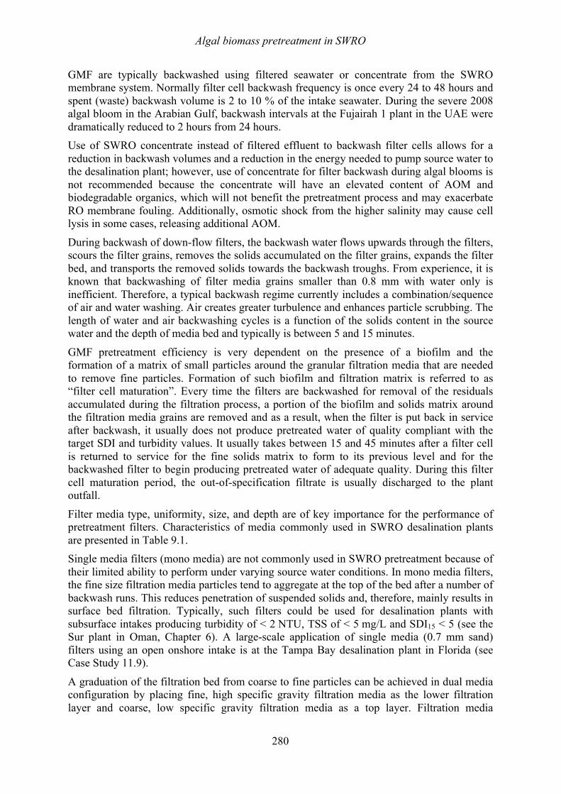
Algal biomass pretreatment in SWRO

280

GMF are typically backwashed using filtered seawater or concentrate from the SWRO membrane system. Normally filter cell backwash frequency is once every 24 to 48 hours and spent (waste) backwash volume is 2 to 10 % of the intake seawater. During the severe 2008 algal bloom in the Arabian Gulf, backwash intervals at the Fujairah 1 plant in the UAE were dramatically reduced to 2 hours from 24 hours. Use of SWRO concentrate instead of filtered effluent to backwash filter cells allows for a reduction in backwash volumes and a reduction in the energy needed to pump source water to the desalination plant; however, use of concentrate for filter backwash during algal blooms is not recommended because the concentrate will have an elevated content of AOM and biodegradable organics, which will not benefit the pretreatment process and may exacerbate RO membrane fouling. Additionally, osmotic shock from the higher salinity may cause cell lysis in some cases, releasing additional AOM.

During backwash of down-flow filters, the backwash water flows upwards through the filters, scours the filter grains, removes the solids accumulated on the filter grains, expands the filter bed, and transports the removed solids towards the backwash troughs. From experience, it is known that backwashing of filter media grains smaller than 0.8 mm with water only is inefficient. Therefore, a typical backwash regime currently includes a combination/sequence of air and water washing. Air creates greater turbulence and enhances particle scrubbing. The length of water and air backwashing cycles is a function of the solids content in the source water and the depth of media bed and typically is between 5 and 15 minutes.

GMF pretreatment efficiency is very dependent on the presence of a biofilm and the formation of a matrix of small particles around the granular filtration media that are needed to remove fine particles. Formation of such biofilm and filtration matrix is referred to as “filter cell maturation”. Every time the filters are backwashed for removal of the residuals accumulated during the filtration process, a portion of the biofilm and solids matrix around the filtration media grains are removed and as a result, when the filter is put back in service after backwash, it usually does not produce pretreated water of quality compliant with the target SDI and turbidity values. It usually takes between 15 and 45 minutes after a filter cell is returned to service for the fine solids matrix to form to its previous level and for the backwashed filter to begin producing pretreated water of adequate quality. During this filter cell maturation period, the out-of-specification filtrate is usually discharged to the plant outfall.

Filter media type, uniformity, size, and depth are of key importance for the performance of pretreatment filters. Characteristics of media commonly used in SWRO desalination plants are presented in Table 9.1. Single media filters (mono media) are not commonly used in SWRO pretreatment because of their limited ability to perform under varying source water conditions. In mono media filters, the fine size filtration media particles tend to aggregate at the top of the bed after a number of backwash runs. This reduces penetration of suspended solids and, therefore, mainly results in surface bed filtration. Typically, such filters could be used for desalination plants with subsurface intakes producing turbidity of < 2 NTU, TSS of < 5 mg/L and SDI15 < 5 (see the Sur plant in Oman, Chapter 6). A large-scale application of single media (0.7 mm sand) filters using an open onshore intake is at the Tampa Bay desalination plant in Florida (see Case Study 11.9).

A graduation of the filtration bed from coarse to fine particles can be achieved in dual media configuration by placing fine, high specific gravity filtration media as the lower filtration layer and coarse, low specific gravity filtration media as a top layer. Filtration media

Algal biomass pretreatment in SWRO

281

selection that provides coarse to fine filtration bed configuration includes 0.4 to 1 m anthracite or pumice as a top layer and 0.4 to 2.0 m of silica sand as a bottom filtration layer. DMF is the most commonly used GMF in SWRO plants worldwide. Deep DMF are often used if the desalination plant filtration system is designed to achieve enhanced removal of soluble organics from source water by biofiltration. In this case, the depth of the anthracite level is enhanced to between 1.5 and 1.8 m. In comparison to mono media filters, DMF systems operate at higher filtration rates, have longer filter run times, and produce less backwash water.

Tri-media filters are not commonly used in SWRO pretreatment and are primarily used for capturing small-size phytoplankton and fine silt that cannot be well retained by the top two layers in DMF. Tri-media filters typically comprise 0.45 to 0.6 m of anthracite as the top layer, which retains large-size algae (i.e. algae over 100 µm), 0.2 to 0.4 m of sand as a middle layer to remove medium-size algae (20 to 100 µm) and 0.10 to 0.15 m of garnet or limonite as the bottom layer. The third (garnet or limonite) layer of filtration is usually used only if the source water contains a large amount of very fine silt or the source water intake experiences algal blooms dominated by small algae (0.2 to 2 µm).

Since the cost of filter cells increases with depth, often instead of a deep, single tri-media gravity filter, a combination of coarser media (anthracite-sand) gravity filter followed by a pressure filter containing finer (sand and garnet) is used. Most filters used in seawater pretreatment are down-flow filters. This flow direction allows large algal particles to be retained at the top of the filter media and removed with the backwash water with minimum breakage and release of organics. If upflow filtration is used, algae contained in the source water are pressed against the filter media and unwanted dissolved organics such as algal biopolymers may be released from the broken algal cells into the filtered water, which is undesirable as it can exacerbate biofouling of the downstream SWRO membranes.

Table 9.1. Typical media characteristics for GMF used in SWRO plants.

Media Type Typical Effective Grain Size - mm

Specific Density tons/m3

Pumice 0.8 – 2.0 1.2 Anthracite 0.8 – 2.0 1.4 – 1.7 Silica Sand 0.4 – 0.8 2.60 – 2.65 Garnet 0.2 – 0.6 3.50 – 4.30

9.6.3 Single and two-stage filtration Two-stage filtration is typically used when the source water contains high levels of turbidity (usually above 20 NTU) and organics (TOC > 6 mg/L) for long periods of time (i.e., weeks/month). Such conditions occur in desalination plant intake areas exposed to prolonged red-tide events (which sometimes could last for several months) or in river estuaries, which are exposed to an elevated turbidity levels occurring during the wet-season of the year.

Two stage filtration systems typically consist of coarse (roughing) filters and fine (polishing) filters operated in series. Usually the first stage filter is a mono-media type (i.e., coarse sand or anthracite) or dual media while the second stage filter is configured as a DMF with design criteria described in the previous section. The first (coarse-media) filter typically removes 60 to 80% of the total amount of solids contained in the source water and is designed to retain all large debris and floating algal biomass. The second stage filter removes over 99% of the

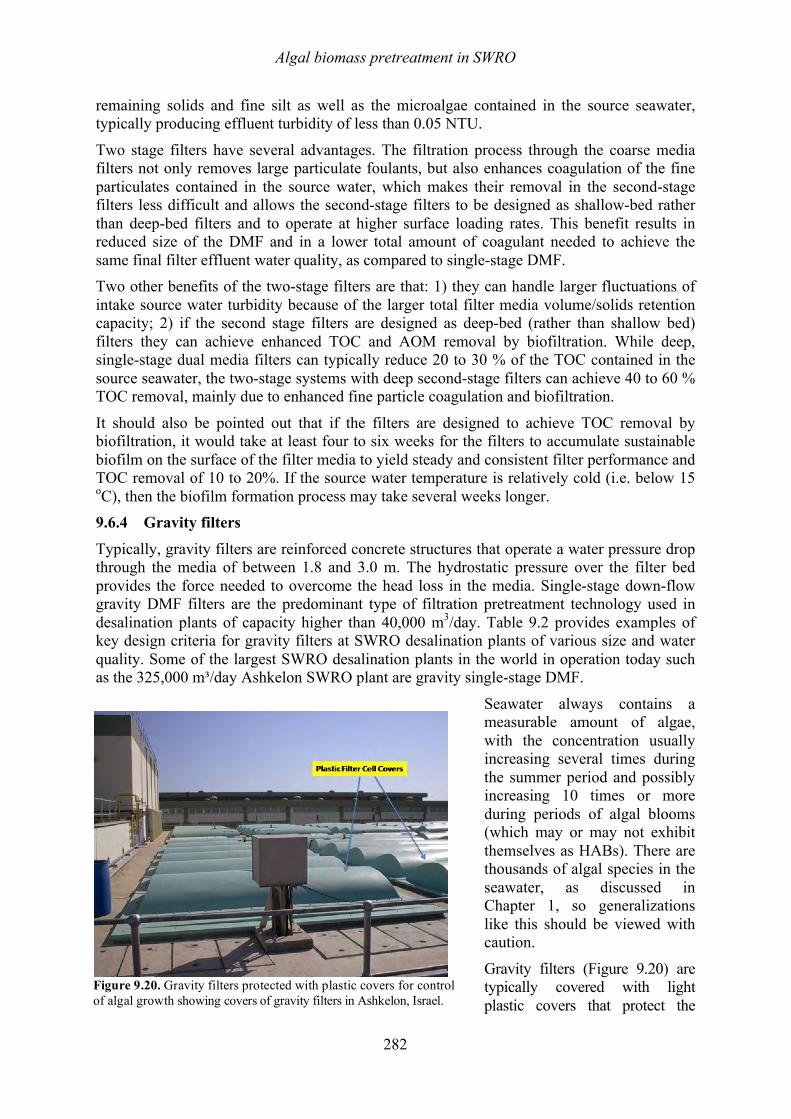
Algal biomass pretreatment in SWRO

282

remaining solids and fine silt as well as the microalgae contained in the source seawater, typically producing effluent turbidity of less than 0.05 NTU.

Two stage filters have several advantages. The filtration process through the coarse media filters not only removes large particulate foulants, but also enhances coagulation of the fine particulates contained in the source water, which makes their removal in the second-stage filters less difficult and allows the second-stage filters to be designed as shallow-bed rather than deep-bed filters and to operate at higher surface loading rates. This benefit results in reduced size of the DMF and in a lower total amount of coagulant needed to achieve the same final filter effluent water quality, as compared to single-stage DMF. Two other benefits of the two-stage filters are that: 1) they can handle larger fluctuations of intake source water turbidity because of the larger total filter media volume/solids retention capacity; 2) if the second stage filters are designed as deep-bed (rather than shallow bed) filters they can achieve enhanced TOC and AOM removal by biofiltration. While deep, single-stage dual media filters can typically reduce 20 to 30 % of the TOC contained in the source seawater, the two-stage systems with deep second-stage filters can achieve 40 to 60 % TOC removal, mainly due to enhanced fine particle coagulation and biofiltration.

It should also be pointed out that if the filters are designed to achieve TOC removal by biofiltration, it would take at least four to six weeks for the filters to accumulate sustainable biofilm on the surface of the filter media to yield steady and consistent filter performance and TOC removal of 10 to 20%. If the source water temperature is relatively cold (i.e. below 15 oC), then the biofilm formation process may take several weeks longer. 9.6.4 Gravity filters

Typically, gravity filters are reinforced concrete structures that operate a water pressure drop through the media of between 1.8 and 3.0 m. The hydrostatic pressure over the filter bed provides the force needed to overcome the head loss in the media. Single-stage down-flow gravity DMF filters are the predominant type of filtration pretreatment technology used in desalination plants of capacity higher than 40,000 m3/day. Table 9.2 provides examples of key design criteria for gravity filters at SWRO desalination plants of various size and water quality. Some of the largest SWRO desalination plants in the world in operation today such as the 325,000 m³/day Ashkelon SWRO plant are gravity single-stage DMF.

Seawater always contains a measurable amount of algae, with the concentration usually increasing several times during the summer period and possibly increasing 10 times or more during periods of algal blooms (which may or may not exhibit themselves as HABs). There are thousands of algal species in the seawater, as discussed in Chapter 1, so generalizations like this should be viewed with caution.

Gravity filters (Figure 9.20) are typically covered with light plastic covers that protect the

Figure 9.20. Gravity filters protected with plastic covers for control of algal growth showing covers of gravity filters in Ashkelon, Israel.

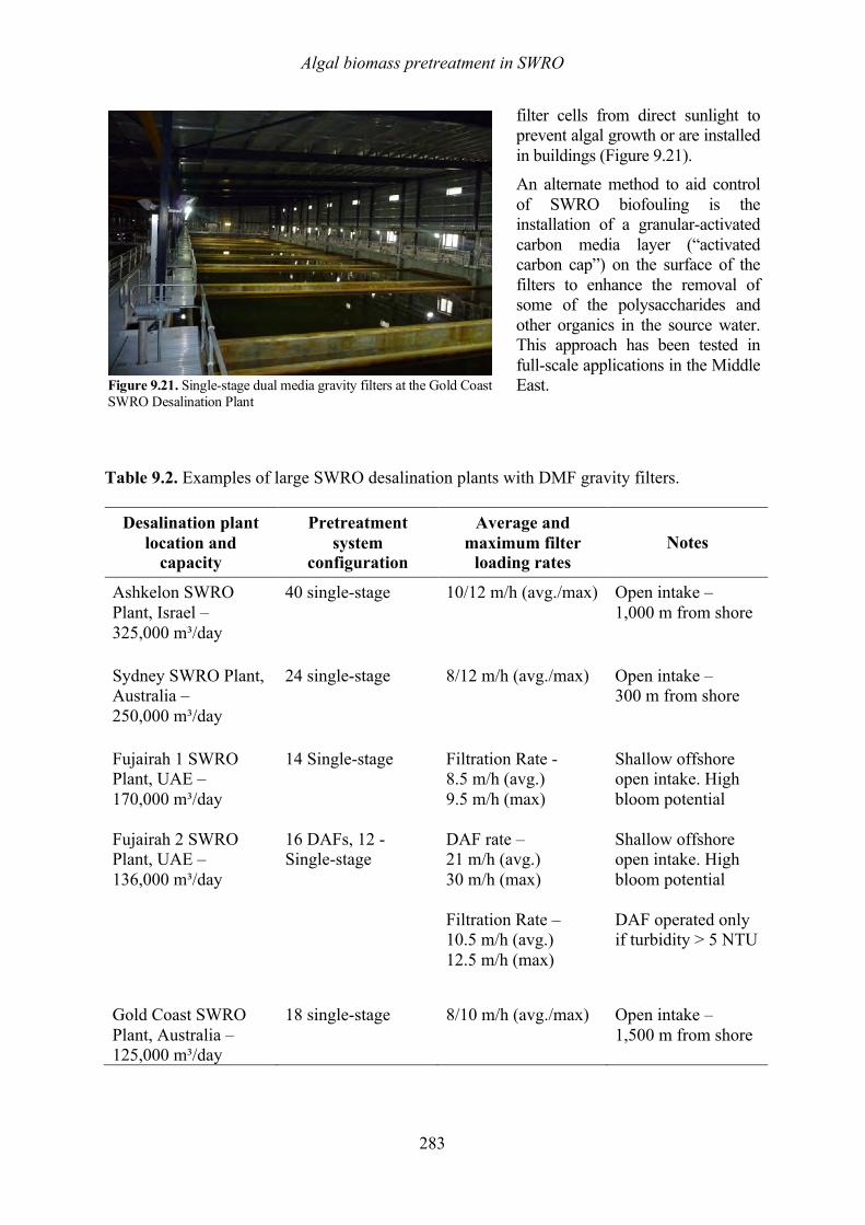
Algal biomass pretreatment in SWRO

283

filter cells from direct sunlight to prevent algal growth or are installed in buildings (Figure 9.21). An alternate method to aid control of SWRO biofouling is the installation of a granular-activated carbon media layer (“activated carbon cap”) on the surface of the filters to enhance the removal of some of the polysaccharides and other organics in the source water. This approach has been tested in full-scale applications in the Middle East.

Table 9.2. Examples of large SWRO desalination plants with DMF gravity filters.

Desalination plant location and

capacity

Pretreatment system

configuration

Average and maximum filter

loading rates Notes

Ashkelon SWRO Plant, Israel – 325,000 m³/day

40 single-stage

10/12 m/h (avg./max)

Open intake – 1,000 m from shore

Sydney SWRO Plant, Australia – 250,000 m³/day

24 single-stage

8/12 m/h (avg./max)

Open intake – 300 m from shore

Fujairah 1 SWRO Plant, UAE – 170,000 m³/day

14 Single-stage

Filtration Rate - 8.5 m/h (avg.) 9.5 m/h (max)

Shallow offshore open intake. High bloom potential

Fujairah 2 SWRO Plant, UAE – 136,000 m³/day

16 DAFs, 12 -Single-stage

DAF rate – 21 m/h (avg.) 30 m/h (max) Filtration Rate – 10.5 m/h (avg.) 12.5 m/h (max)

Shallow offshore open intake. High bloom potential DAF operated only if turbidity > 5 NTU

Gold Coast SWRO Plant, Australia – 125,000 m³/day

18 single-stage

8/10 m/h (avg./max)

Open intake – 1,500 m from shore

Figure 9.21. Single-stage dual media gravity filters at the Gold Coast SWRO Desalination Plant

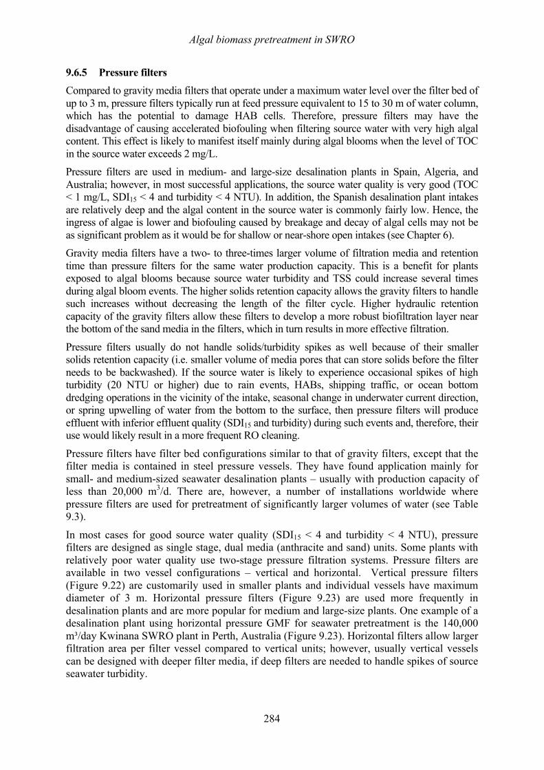
Algal biomass pretreatment in SWRO

284

9.6.5 Pressure filters Compared to gravity media filters that operate under a maximum water level over the filter bed of up to 3 m, pressure filters typically run at feed pressure equivalent to 15 to 30 m of water column, which has the potential to damage HAB cells. Therefore, pressure filters may have the disadvantage of causing accelerated biofouling when filtering source water with very high algal content. This effect is likely to manifest itself mainly during algal blooms when the level of TOC in the source water exceeds 2 mg/L. Pressure filters are used in medium- and large-size desalination plants in Spain, Algeria, and Australia; however, in most successful applications, the source water quality is very good (TOC < 1 mg/L, SDI15 < 4 and turbidity < 4 NTU). In addition, the Spanish desalination plant intakes are relatively deep and the algal content in the source water is commonly fairly low. Hence, the ingress of algae is lower and biofouling caused by breakage and decay of algal cells may not be as significant problem as it would be for shallow or near-shore open intakes (see Chapter 6). Gravity media filters have a two- to three-times larger volume of filtration media and retention time than pressure filters for the same water production capacity. This is a benefit for plants exposed to algal blooms because source water turbidity and TSS could increase several times during algal bloom events. The higher solids retention capacity allows the gravity filters to handle such increases without decreasing the length of the filter cycle. Higher hydraulic retention capacity of the gravity filters allow these filters to develop a more robust biofiltration layer near the bottom of the sand media in the filters, which in turn results in more effective filtration.

Pressure filters usually do not handle solids/turbidity spikes as well because of their smaller solids retention capacity (i.e. smaller volume of media pores that can store solids before the filter needs to be backwashed). If the source water is likely to experience occasional spikes of high turbidity (20 NTU or higher) due to rain events, HABs, shipping traffic, or ocean bottom dredging operations in the vicinity of the intake, seasonal change in underwater current direction, or spring upwelling of water from the bottom to the surface, then pressure filters will produce effluent with inferior effluent quality (SDI15 and turbidity) during such events and, therefore, their use would likely result in a more frequent RO cleaning.

Pressure filters have filter bed configurations similar to that of gravity filters, except that the filter media is contained in steel pressure vessels. They have found application mainly for small- and medium-sized seawater desalination plants – usually with production capacity of less than 20,000 m3/d. There are, however, a number of installations worldwide where pressure filters are used for pretreatment of significantly larger volumes of water (see Table 9.3).

In most cases for good source water quality (SDI15 < 4 and turbidity < 4 NTU), pressure filters are designed as single stage, dual media (anthracite and sand) units. Some plants with relatively poor water quality use two-stage pressure filtration systems. Pressure filters are available in two vessel configurations – vertical and horizontal. Vertical pressure filters (Figure 9.22) are customarily used in smaller plants and individual vessels have maximum diameter of 3 m. Horizontal pressure filters (Figure 9.23) are used more frequently in desalination plants and are more popular for medium and large-size plants. One example of a desalination plant using horizontal pressure GMF for seawater pretreatment is the 140,000 m³/day Kwinana SWRO plant in Perth, Australia (Figure 9.23). Horizontal filters allow larger filtration area per filter vessel compared to vertical units; however, usually vertical vessels can be designed with deeper filter media, if deep filters are needed to handle spikes of source seawater turbidity.

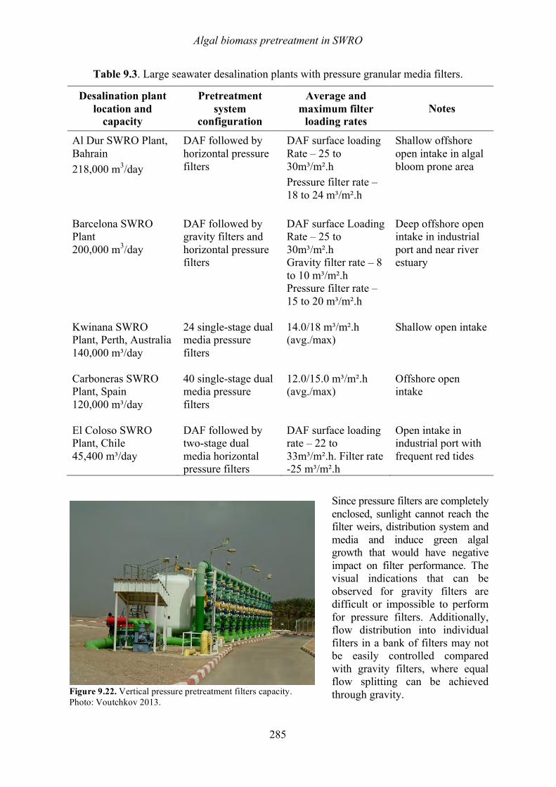
Algal biomass pretreatment in SWRO

285

Table 9.3. Large seawater desalination plants with pressure granular media filters.

Desalination plant location and

capacity

Pretreatment system

configuration

Average and maximum filter

loading rates Notes

Al Dur SWRO Plant, Bahrain 218,000 m3/day

DAF followed by horizontal pressure filters

DAF surface loading Rate – 25 to 30m³/m².h Pressure filter rate – 18 to 24 m³/m².h

Shallow offshore open intake in algal bloom prone area

Barcelona SWRO Plant 200,000 m3/day

DAF followed by gravity filters and horizontal pressure filters

DAF surface Loading Rate – 25 to 30m³/m².h Gravity filter rate – 8 to 10 m³/m².h Pressure filter rate – 15 to 20 m³/m².h

Deep offshore open intake in industrial port and near river estuary

Kwinana SWRO Plant, Perth, Australia 140,000 m³/day

24 single-stage dual media pressure filters

14.0/18 m³/m².h (avg./max)

Shallow open intake

Carboneras SWRO Plant, Spain 120,000 m³/day

40 single-stage dual media pressure filters

12.0/15.0 m³/m².h (avg./max)

Offshore open intake

El Coloso SWRO Plant, Chile 45,400 m³/day

DAF followed by two-stage dual media horizontal pressure filters

DAF surface loading rate – 22 to 33m³/m².h. Filter rate -25 m³/m².h

Open intake in industrial port with frequent red tides

Since pressure filters are completely enclosed, sunlight cannot reach the filter weirs, distribution system and media and induce green algal growth that would have negative impact on filter performance. The visual indications that can be observed for gravity filters are difficult or impossible to perform for pressure filters. Additionally, flow distribution into individual filters in a bank of filters may not be easily controlled compared with gravity filters, where equal flow splitting can be achieved through gravity.

Figure 9.22. Vertical pressure pretreatment filters capacity. Photo: Voutchkov 2013.

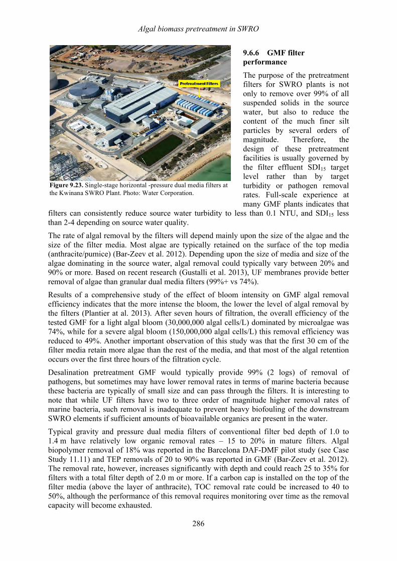
Algal biomass pretreatment in SWRO

286

9.6.6 GMF filter performance

The purpose of the pretreatment filters for SWRO plants is not only to remove over 99% of all suspended solids in the source water, but also to reduce the content of the much finer silt particles by several orders of magnitude. Therefore, the design of these pretreatment facilities is usually governed by the filter effluent SDI15 target level rather than by target turbidity or pathogen removal rates. Full-scale experience at many GMF plants indicates that

filters can consistently reduce source water turbidity to less than 0.1 NTU, and SDI15 less than 2-4 depending on source water quality. The rate of algal removal by the filters will depend mainly upon the size of the algae and the size of the filter media. Most algae are typically retained on the surface of the top media (anthracite/pumice) (Bar-Zeev et al. 2012). Depending upon the size of media and size of the algae dominating in the source water, algal removal could typically vary between 20% and 90% or more. Based on recent research (Gustalli et al. 2013), UF membranes provide better removal of algae than granular dual media filters (99%+ vs 74%). Results of a comprehensive study of the effect of bloom intensity on GMF algal removal efficiency indicates that the more intense the bloom, the lower the level of algal removal by the filters (Plantier at al. 2013). After seven hours of filtration, the overall efficiency of the tested GMF for a light algal bloom (30,000,000 algal cells/L) dominated by microalgae was 74%, while for a severe algal bloom (150,000,000 algal cells/L) this removal efficiency was reduced to 49%. Another important observation of this study was that the first 30 cm of the filter media retain more algae than the rest of the media, and that most of the algal retention occurs over the first three hours of the filtration cycle. Desalination pretreatment GMF would typically provide 99% (2 logs) of removal of pathogens, but sometimes may have lower removal rates in terms of marine bacteria because these bacteria are typically of small size and can pass through the filters. It is interesting to note that while UF filters have two to three order of magnitude higher removal rates of marine bacteria, such removal is inadequate to prevent heavy biofouling of the downstream SWRO elements if sufficient amounts of bioavailable organics are present in the water. Typical gravity and pressure dual media filters of conventional filter bed depth of 1.0 to 1.4 m have relatively low organic removal rates – 15 to 20% in mature filters. Algal biopolymer removal of 18% was reported in the Barcelona DAF-DMF pilot study (see Case Study 11.11) and TEP removals of 20 to 90% was reported in GMF (Bar-Zeev et al. 2012). The removal rate, however, increases significantly with depth and could reach 25 to 35% for filters with a total filter depth of 2.0 m or more. If a carbon cap is installed on the top of the filter media (above the layer of anthracite), TOC removal rate could be increased to 40 to 50%, although the performance of this removal requires monitoring over time as the removal capacity will become exhausted.

Figure 9.23. Single-stage horizontal -pressure dual media filters at the Kwinana SWRO Plant. Photo: Water Corporation.

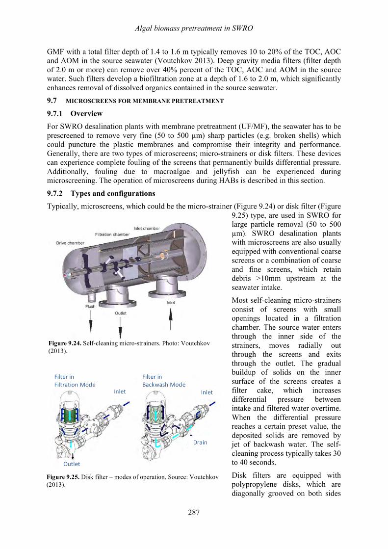
Algal biomass pretreatment in SWRO

287

GMF with a total filter depth of 1.4 to 1.6 m typically removes 10 to 20% of the TOC, AOC and AOM in the source seawater (Voutchkov 2013). Deep gravity media filters (filter depth of 2.0 m or more) can remove over 40% percent of the TOC, AOC and AOM in the source water. Such filters develop a biofiltration zone at a depth of 1.6 to 2.0 m, which significantly enhances removal of dissolved organics contained in the source seawater. 9.7 MICROSCREENS FOR MEMBRANE PRETREATMENT

9.7.1 Overview For SWRO desalination plants with membrane pretreatment (UF/MF), the seawater has to be prescreened to remove very fine (50 to 500 µm) sharp particles (e.g. broken shells) which could puncture the plastic membranes and compromise their integrity and performance. Generally, there are two types of microscreens; micro-strainers or disk filters. These devices can experience complete fouling of the screens that permanently builds differential pressure. Additionally, fouling due to macroalgae and jellyfish can be experienced during microscreening. The operation of microscreens during HABs is described in this section.

9.7.2 Types and configurations Typically, microscreens, which could be the micro-strainer (Figure 9.24) or disk filter (Figure

9.25) type, are used in SWRO for large particle removal (50 to 500 µm). SWRO desalination plants with microscreens are also usually equipped with conventional coarse screens or a combination of coarse and fine screens, which retain debris >10mm upstream at the seawater intake. Most self-cleaning micro-strainers consist of screens with small openings located in a filtration chamber. The source water enters through the inner side of the strainers, moves radially out through the screens and exits through the outlet. The gradual buildup of solids on the inner surface of the screens creates a filter cake, which increases differential pressure between intake and filtered water overtime. When the differential pressure reaches a certain preset value, the deposited solids are removed by jet of backwash water. The self-cleaning process typically takes 30 to 40 seconds.

Disk filters are equipped with polypropylene disks, which are diagonally grooved on both sides

Figure 9.24. Self-cleaning micro-strainers. Photo: Voutchkov (2013).

Figure 9.25. Disk filter – modes of operation. Source: Voutchkov (2013).

Filter in Filtration Mode

Outlet

Filter in Backwash Mode

Inlet Inlet

Drain

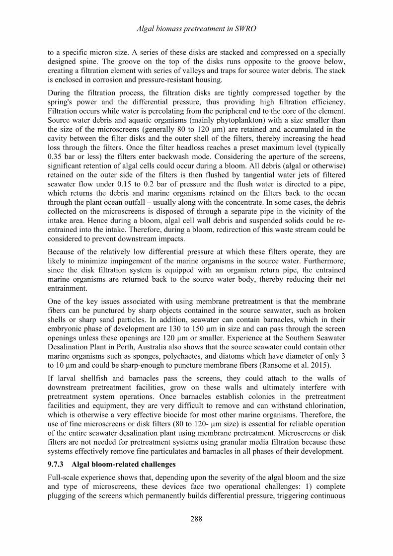
Algal biomass pretreatment in SWRO

288

to a specific micron size. A series of these disks are stacked and compressed on a specially designed spine. The groove on the top of the disks runs opposite to the groove below, creating a filtration element with series of valleys and traps for source water debris. The stack is enclosed in corrosion and pressure-resistant housing.

During the filtration process, the filtration disks are tightly compressed together by the spring's power and the differential pressure, thus providing high filtration efficiency. Filtration occurs while water is percolating from the peripheral end to the core of the element. Source water debris and aquatic organisms (mainly phytoplankton) with a size smaller than the size of the microscreens (generally 80 to 120 µm) are retained and accumulated in the cavity between the filter disks and the outer shell of the filters, thereby increasing the head loss through the filters. Once the filter headloss reaches a preset maximum level (typically 0.35 bar or less) the filters enter backwash mode. Considering the aperture of the screens, significant retention of algal cells could occur during a bloom. All debris (algal or otherwise) retained on the outer side of the filters is then flushed by tangential water jets of filtered seawater flow under 0.15 to 0.2 bar of pressure and the flush water is directed to a pipe, which returns the debris and marine organisms retained on the filters back to the ocean through the plant ocean outfall – usually along with the concentrate. In some cases, the debris collected on the microscreens is disposed of through a separate pipe in the vicinity of the intake area. Hence during a bloom, algal cell wall debris and suspended solids could be re-entrained into the intake. Therefore, during a bloom, redirection of this waste stream could be considered to prevent downstream impacts. Because of the relatively low differential pressure at which these filters operate, they are likely to minimize impingement of the marine organisms in the source water. Furthermore, since the disk filtration system is equipped with an organism return pipe, the entrained marine organisms are returned back to the source water body, thereby reducing their net entrainment.

One of the key issues associated with using membrane pretreatment is that the membrane fibers can be punctured by sharp objects contained in the source seawater, such as broken shells or sharp sand particles. In addition, seawater can contain barnacles, which in their embryonic phase of development are 130 to 150 µm in size and can pass through the screen openings unless these openings are 120 µm or smaller. Experience at the Southern Seawater Desalination Plant in Perth, Australia also shows that the source seawater could contain other marine organisms such as sponges, polychaetes, and diatoms which have diameter of only 3 to 10 µm and could be sharp-enough to puncture membrane fibers (Ransome et al. 2015).

If larval shellfish and barnacles pass the screens, they could attach to the walls of downstream pretreatment facilities, grow on these walls and ultimately interfere with pretreatment system operations. Once barnacles establish colonies in the pretreatment facilities and equipment, they are very difficult to remove and can withstand chlorination, which is otherwise a very effective biocide for most other marine organisms. Therefore, the use of fine microscreens or disk filters (80 to 120- µm size) is essential for reliable operation of the entire seawater desalination plant using membrane pretreatment. Microscreens or disk filters are not needed for pretreatment systems using granular media filtration because these systems effectively remove fine particulates and barnacles in all phases of their development. 9.7.3 Algal bloom-related challenges

Full-scale experience shows that, depending upon the severity of the algal bloom and the size and type of microscreens, these devices face two operational challenges: 1) complete plugging of the screens which permanently builds differential pressure, triggering continuous

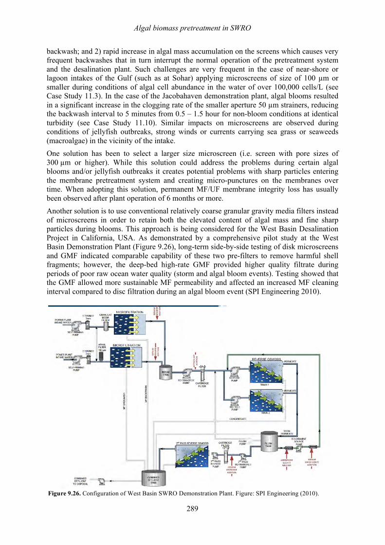
Algal biomass pretreatment in SWRO

289

backwash; and 2) rapid increase in algal mass accumulation on the screens which causes very frequent backwashes that in turn interrupt the normal operation of the pretreatment system and the desalination plant. Such challenges are very frequent in the case of near-shore or lagoon intakes of the Gulf (such as at Sohar) applying microscreens of size of 100 µm or smaller during conditions of algal cell abundance in the water of over 100,000 cells/L (see Case Study 11.3). In the case of the Jacobahaven demonstration plant, algal blooms resulted in a significant increase in the clogging rate of the smaller aperture 50 µm strainers, reducing the backwash interval to 5 minutes from 0.5 – 1.5 hour for non-bloom conditions at identical turbidity (see Case Study 11.10). Similar impacts on microscreens are observed during conditions of jellyfish outbreaks, strong winds or currents carrying sea grass or seaweeds (macroalgae) in the vicinity of the intake. One solution has been to select a larger size microscreen (i.e. screen with pore sizes of 300 µm or higher). While this solution could address the problems during certain algal blooms and/or jellyfish outbreaks it creates potential problems with sharp particles entering the membrane pretreatment system and creating micro-punctures on the membranes over time. When adopting this solution, permanent MF/UF membrane integrity loss has usually been observed after plant operation of 6 months or more. Another solution is to use conventional relatively coarse granular gravity media filters instead of microscreens in order to retain both the elevated content of algal mass and fine sharp particles during blooms. This approach is being considered for the West Basin Desalination Project in California, USA. As demonstrated by a comprehensive pilot study at the West Basin Demonstration Plant (Figure 9.26), long-term side-by-side testing of disk microscreens and GMF indicated comparable capability of these two pre-filters to remove harmful shell fragments; however, the deep-bed high-rate GMF provided higher quality filtrate during periods of poor raw ocean water quality (storm and algal bloom events). Testing showed that the GMF allowed more sustainable MF permeability and affected an increased MF cleaning interval compared to disc filtration during an algal bloom event (SPI Engineering 2010).

Figure 9.26. Configuration of West Basin SWRO Demonstration Plant. Figure: SPI Engineering (2010).

Algal biomass pretreatment in SWRO

290

In order for microscreens to successfully handle conditions of high algal cell concentrations, jellyfish outbreaks or sea grass plugging, they need to have an effective focused auto-backwash system that maximizes the backwashing velocity across the strainer face with moving nozzles that operate over the strainer surface (Figure 9.24) or a variable area mesh that opens up on backwashing. For example, at the Southern Seawater Desalination Plant in Perth, Australia the original conventional microscreens had to be replaced by screens with a focused auto-backwash system to address operational challenges of intense screen plugging due to large quantity of macroalgal sea grass fragments carried to the intake via underwater currents (Ransome et al. 2015). A microsreening technology that has potential to handle severe algal bloom conditions is microfiber filtration (Eshel et al. 2013). Microfiber filters consist of cartridges with multilayer textile threads, usually with pore sizes of 2 to 20 µm. While their ability to retain algae, organic matter and mineral solids is comparable to cartridge filters, they have the benefit that they can be backwashed automatically, similar to conventional microscreens. Full-scale test experiments of this technology on freshwater during algal bloom conditions in a lake have showed significant reductions in TEP (mean 47±21%), chlorophyll (mean 90±6%), total suspended solids (67±7%), turbidity (89±5%), and particles larger in size than 3 µm (93±4%). Such systems have not yet found full-scale implementation for seawater screening. 9.7.4 Summary

Fouling of microscreens due to HABs cause two main operational challenges: 1) complete plugging of the microscreens which permanently builds differential pressure triggering continuous backwash; and 2) rapid increase in algal mass accumulation on the screens which causes frequent backwashes that in turn interrupt the normal operation of the pretreatment system and the desalination plant. Monitoring of the time between backwashes in microscreen systems is therefore an important consideration during bloom periods.

9.8 MICROFILTRATION/ ULTRAFILTRATION 9.8.1 Overview

MF/UF membranes have been tested and applied as pretreatment for SWRO membranes for more than a decade (Wolf et al. 2005; Halpern et al. 2005). MF/UF membranes offer several advantages over GMF in SWRO pretreatment, namely, smaller footprint, consistently high permeate quality in terms of SDI, higher retention of organic macromolecules (including some AOM), lower overall chemical consumption (Wilf and Schierach 2001; Pearce 2010). Although, MF and UF are both applied in SWRO, UF is often employed due to its smaller pore size and better removal of particulate/colloidal organics, silt, and pathogens from seawater (Voutchkov 2009).

9.8.2 MF/UF filtration modes In contrast to RO membranes that operate in cross flow, MF/UF membranes are typically operated in dead-end mode in two main configurations based on feed flow direction; PDI, and pressure driven outside-in (PDO). MF/UF membranes in outside-in configuration may also be operated in vacuum driven (submerged) mode, which are commonly polyvinyledene fluoride (PVDF). PDI membranes are generally based on polyethersulphone (PES) and blends thereof, although some PDI membranes based on cellulose triacetate and polysulphone are also available in the market (Pearce 2007). In PDI filtration, feedwater enters through the inside of the element and permeate is collected from the outside of the capillaries. Hydraulic cleaning (or backwash) is performed by reversing the flow, whereby product water flows through the membranes from the outside of the capillary, physically

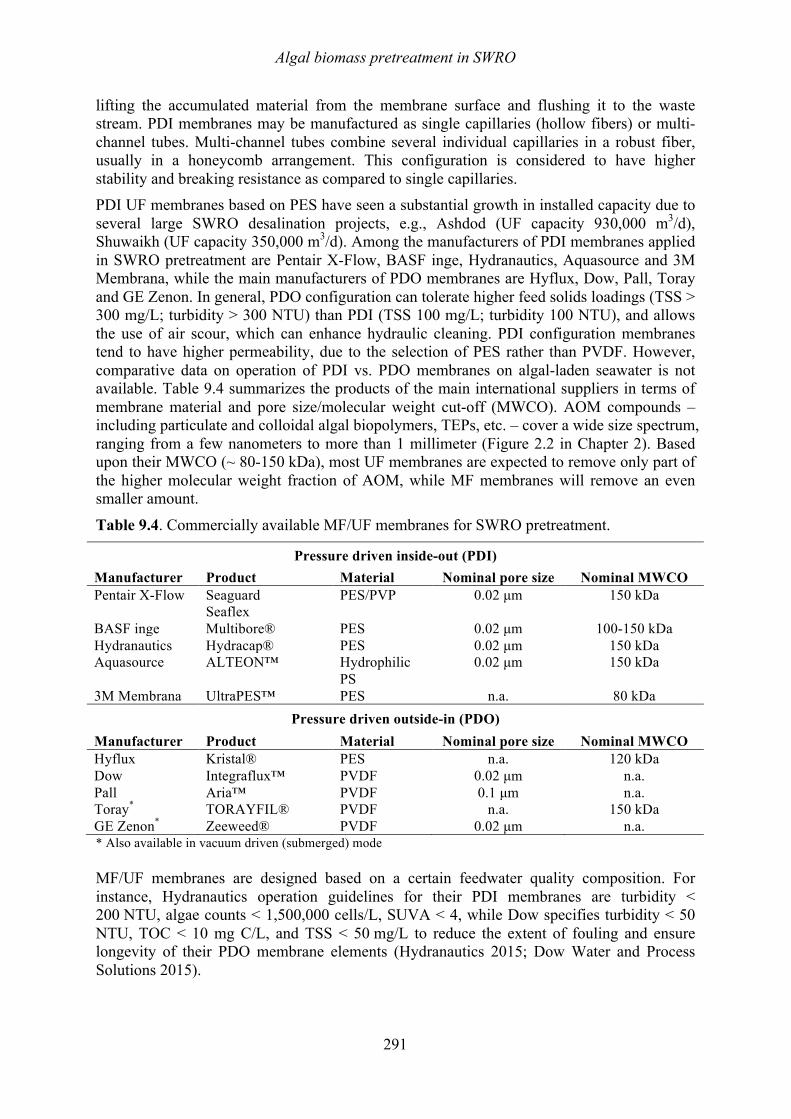
Algal biomass pretreatment in SWRO

291

lifting the accumulated material from the membrane surface and flushing it to the waste stream. PDI membranes may be manufactured as single capillaries (hollow fibers) or multi-channel tubes. Multi-channel tubes combine several individual capillaries in a robust fiber, usually in a honeycomb arrangement. This configuration is considered to have higher stability and breaking resistance as compared to single capillaries. PDI UF membranes based on PES have seen a substantial growth in installed capacity due to several large SWRO desalination projects, e.g., Ashdod (UF capacity 930,000 m3/d), Shuwaikh (UF capacity 350,000 m3/d). Among the manufacturers of PDI membranes applied in SWRO pretreatment are Pentair X-Flow, BASF inge, Hydranautics, Aquasource and 3M Membrana, while the main manufacturers of PDO membranes are Hyflux, Dow, Pall, Toray and GE Zenon. In general, PDO configuration can tolerate higher feed solids loadings (TSS > 300 mg/L; turbidity > 300 NTU) than PDI (TSS 100 mg/L; turbidity 100 NTU), and allows the use of air scour, which can enhance hydraulic cleaning. PDI configuration membranes tend to have higher permeability, due to the selection of PES rather than PVDF. However, comparative data on operation of PDI vs. PDO membranes on algal-laden seawater is not available. Table 9.4 summarizes the products of the main international suppliers in terms of membrane material and pore size/molecular weight cut-off (MWCO). AOM compounds – including particulate and colloidal algal biopolymers, TEPs, etc. – cover a wide size spectrum, ranging from a few nanometers to more than 1 millimeter (Figure 2.2 in Chapter 2). Based upon their MWCO (~ 80-150 kDa), most UF membranes are expected to remove only part of the higher molecular weight fraction of AOM, while MF membranes will remove an even smaller amount.

Table 9.4. Commercially available MF/UF membranes for SWRO pretreatment.

Pressure driven inside-out (PDI) Manufacturer Product Material Nominal pore size Nominal MWCO Pentair X-Flow Seaguard

Seaflex PES/PVP 0.02 µm 150 kDa

BASF inge Multibore® PES 0.02 µm 100-150 kDa Hydranautics Hydracap® PES 0.02 µm 150 kDa Aquasource ALTEON™ Hydrophilic

PS 0.02 µm 150 kDa

3M Membrana UltraPES™ PES n.a. 80 kDa Pressure driven outside-in (PDO)

Manufacturer Product Material Nominal pore size Nominal MWCO Hyflux Kristal® PES n.a. 120 kDa Dow Integraflux™ PVDF 0.02 µm n.a. Pall Aria™ PVDF 0.1 µm n.a. Toray* TORAYFIL® PVDF n.a. 150 kDa GE Zenon* Zeeweed® PVDF 0.02 µm n.a. * Also available in vacuum driven (submerged) mode

MF/UF membranes are designed based on a certain feedwater quality composition. For instance, Hydranautics operation guidelines for their PDI membranes are turbidity < 200 NTU, algae counts < 1,500,000 cells/L, SUVA < 4, while Dow specifies turbidity < 50 NTU, TOC < 10 mg C/L, and TSS < 50 mg/L to reduce the extent of fouling and ensure longevity of their PDO membrane elements (Hydranautics 2015; Dow Water and Process Solutions 2015).

Algal biomass pretreatment in SWRO

292

9.8.3 Fouling of MF/UF during algal blooms PDI and PDO membranes have reportedly exhibited some degree of fouling during bloom periods due to high concentrations of algal cells and associated organics. The accumulation of AOM and algal particulates on the surface and/or within the pores of MF/UF membranes leads to a loss in membrane performance. As discussed in Chapter 2, high molecular weight AOM such as biopolymers, particularly the very sticky TEP, have been identified as the main cause of membrane fouling rather than the algal cells themselves. Most MF/UF membrane plants are operated in constant flux mode to a flux set point to meet RO feedwater requirements. In constant flux filtration, fouling is observed as an increase in TMP through time, resulting in higher pumping requirements to maintain constant filtration flow. This may impact the efficiency of membrane cleaning. In general, MF/UF membrane fouling phenomena are a function of feedwater quality, membrane properties and operational conditions (e.g., filtration flux) and may be classified as:

- Hydraulically reversible or back-washable fouling (permeability is restored with hydraulic cleaning with air and water);

- Hydraulically irreversible or non-backwashable fouling (permeability cannot be restored with hydraulic cleaning alone and CEB may be required); and

- Chemically irreversible fouling (permeability cannot be restored with CEB and/or chemical cleaning in place (CIP))

AOM accumulation can cause a rapid increase in TMP and/or can increase non-backwashable fouling in MF/UF. The impact of AOM on MF/UF membrane permeability and backwashability can be explained using classic blocking and cake mechanisms as described in Chapter 2 (see Section 2.4.4.2). Control of fouling that may occur during a HAB can be achieved by optimizing operational conditions and cleaning procedures (Murrer and Rosberg 1998; Brehant et al. 2002; Zhang et al. 2006; Ma et al. 2007; Bu-Rashid and Czolkoss 2007; Di Profio et al. 2011; Schurer et al. 2012) or by feedwater conditioning. Operating MF/UF membranes at a lower flux can reduce the extent of backwashable and non-backwashable fouling. Filtration flux affects the characteristics of the AOM cake/gel layer formed on the membrane surface; layers formed at low flux exhibit lower resistance to filtration and are less compressible than those formed at higher flux values (Salinas Rodriguez et al. 2012; Tabatabai et al. 2014). The downside of lowering filtration flux is that proportionally higher membrane surface area is required to meet production capacity, resulting in a larger plant footprint and higher CAPEX. This can be balanced in part by an increase in operational flexibility to allow backwash while maintaining capacity. During HAB events, cleaning procedures can be tailored to control fouling in membrane pretreatment. Optimizing the frequency, duration and intensity of hydraulic cleaning regimes, the type and concentration of cleaning chemicals, the sequence in which they are applied, and the duration of soaking and rinsing steps can enhance permeability recovery and fouling control. Optimum conditions for cleaning are site and event specific and membrane manufacturer guidelines on cleaning regimes during HAB events are currently not available. Alternatively, feedwater conditioning (e.g. with coagulation) can be undertaken to reduce the extent of back-washable and non-back-washable fouling in MF/UF systems. Experience in PDI UF operation in SWRO pretreatment has shown that other than for algal bloom events, coagulation is generally not required to stabilize UF hydraulic performance (Schurer et al. 2013), even during storms with turbidity peaks as high as 50 NTU (see Case Study 11.10). Most importantly, operating at lowered filtration flux of approximately 60 L/m2h on North

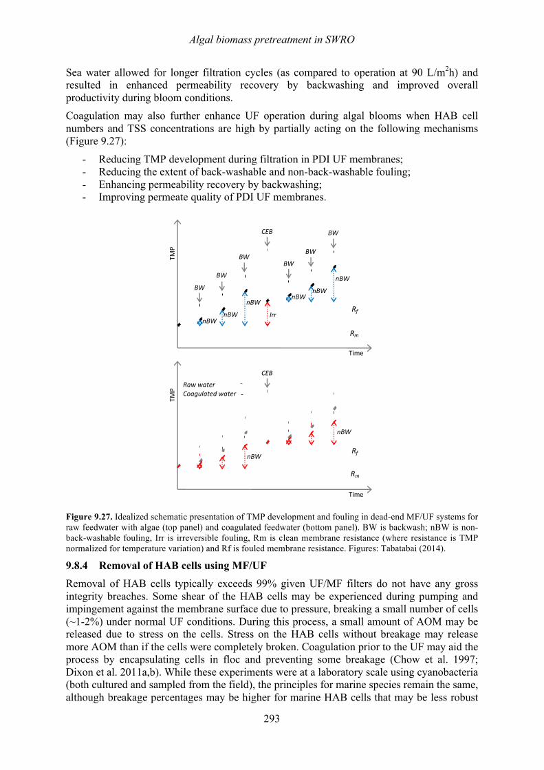
Algal biomass pretreatment in SWRO

293

Sea water allowed for longer filtration cycles (as compared to operation at 90 L/m2h) and resulted in enhanced permeability recovery by backwashing and improved overall productivity during bloom conditions. Coagulation may also further enhance UF operation during algal blooms when HAB cell numbers and TSS concentrations are high by partially acting on the following mechanisms (Figure 9.27):

- Reducing TMP development during filtration in PDI UF membranes; - Reducing the extent of back-washable and non-back-washable fouling; - Enhancing permeability recovery by backwashing; - Improving permeate quality of PDI UF membranes.

Figure 9.27. Idealized schematic presentation of TMP development and fouling in dead-end MF/UF systems for raw feedwater with algae (top panel) and coagulated feedwater (bottom panel). BW is backwash; nBW is non-back-washable fouling, Irr is irreversible fouling, Rm is clean membrane resistance (where resistance is TMP normalized for temperature variation) and Rf is fouled membrane resistance. Figures: Tabatabai (2014).

9.8.4 Removal of HAB cells using MF/UF Removal of HAB cells typically exceeds 99% given UF/MF filters do not have any gross integrity breaches. Some shear of the HAB cells may be experienced during pumping and impingement against the membrane surface due to pressure, breaking a small number of cells (~1-2%) under normal UF conditions. During this process, a small amount of AOM may be released due to stress on the cells. Stress on the HAB cells without breakage may release more AOM than if the cells were completely broken. Coagulation prior to the UF may aid the process by encapsulating cells in floc and preventing some breakage (Chow et al. 1997; Dixon et al. 2011a,b). While these experiments were at a laboratory scale using cyanobacteria (both cultured and sampled from the field), the principles for marine species remain the same, although breakage percentages may be higher for marine HAB cells that may be less robust

Irr

TMP

Time

CEB

nBW

nBW nBW

BW

BW

BW

Rf

nBW

nBW nBW

BW

BW

BW

Rm

TMP

Time

CEB

nBW

nBW

Rm

Rf

Raw water Coagulated water

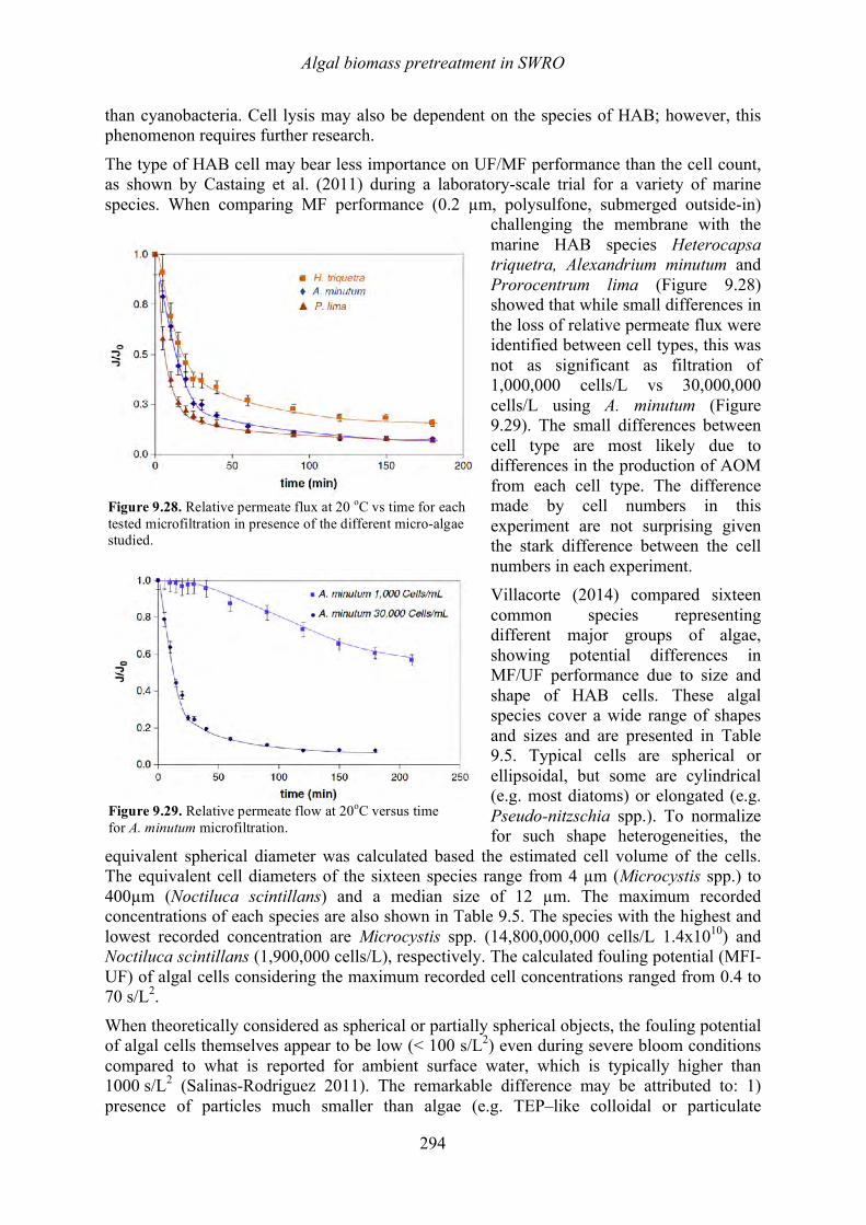
Algal biomass pretreatment in SWRO

294

than cyanobacteria. Cell lysis may also be dependent on the species of HAB; however, this phenomenon requires further research.

The type of HAB cell may bear less importance on UF/MF performance than the cell count, as shown by Castaing et al. (2011) during a laboratory-scale trial for a variety of marine species. When comparing MF performance (0.2 µm, polysulfone, submerged outside-in)

challenging the membrane with the marine HAB species Heterocapsa triquetra, Alexandrium minutum and Prorocentrum lima (Figure 9.28) showed that while small differences in the loss of relative permeate flux were identified between cell types, this was not as significant as filtration of 1,000,000 cells/L vs 30,000,000 cells/L using A. minutum (Figure 9.29). The small differences between cell type are most likely due to differences in the production of AOM from each cell type. The difference made by cell numbers in this experiment are not surprising given the stark difference between the cell numbers in each experiment. Villacorte (2014) compared sixteen common species representing different major groups of algae, showing potential differences in MF/UF performance due to size and shape of HAB cells. These algal species cover a wide range of shapes and sizes and are presented in Table 9.5. Typical cells are spherical or ellipsoidal, but some are cylindrical (e.g. most diatoms) or elongated (e.g. Pseudo-nitzschia spp.). To normalize for such shape heterogeneities, the

equivalent spherical diameter was calculated based the estimated cell volume of the cells. The equivalent cell diameters of the sixteen species range from 4 µm (Microcystis spp.) to 400µm (Noctiluca scintillans) and a median size of 12 µm. The maximum recorded concentrations of each species are also shown in Table 9.5. The species with the highest and lowest recorded concentration are Microcystis spp. (14,800,000,000 cells/L 1.4x1010) and Noctiluca scintillans (1,900,000 cells/L), respectively. The calculated fouling potential (MFI-UF) of algal cells considering the maximum recorded cell concentrations ranged from 0.4 to 70 s/L2.

When theoretically considered as spherical or partially spherical objects, the fouling potential of algal cells themselves appear to be low (< 100 s/L2) even during severe bloom conditions compared to what is reported for ambient surface water, which is typically higher than 1000 s/L2 (Salinas-Rodriguez 2011). The remarkable difference may be attributed to: 1) presence of particles much smaller than algae (e.g. TEP–like colloidal or particulate

Figure 9.28. Relative permeate flux at 20 oC vs time for each tested microfiltration in presence of the different micro-algae studied.

Figure 9.29. Relative permeate flow at 20oC versus time for A. minutum microfiltration.

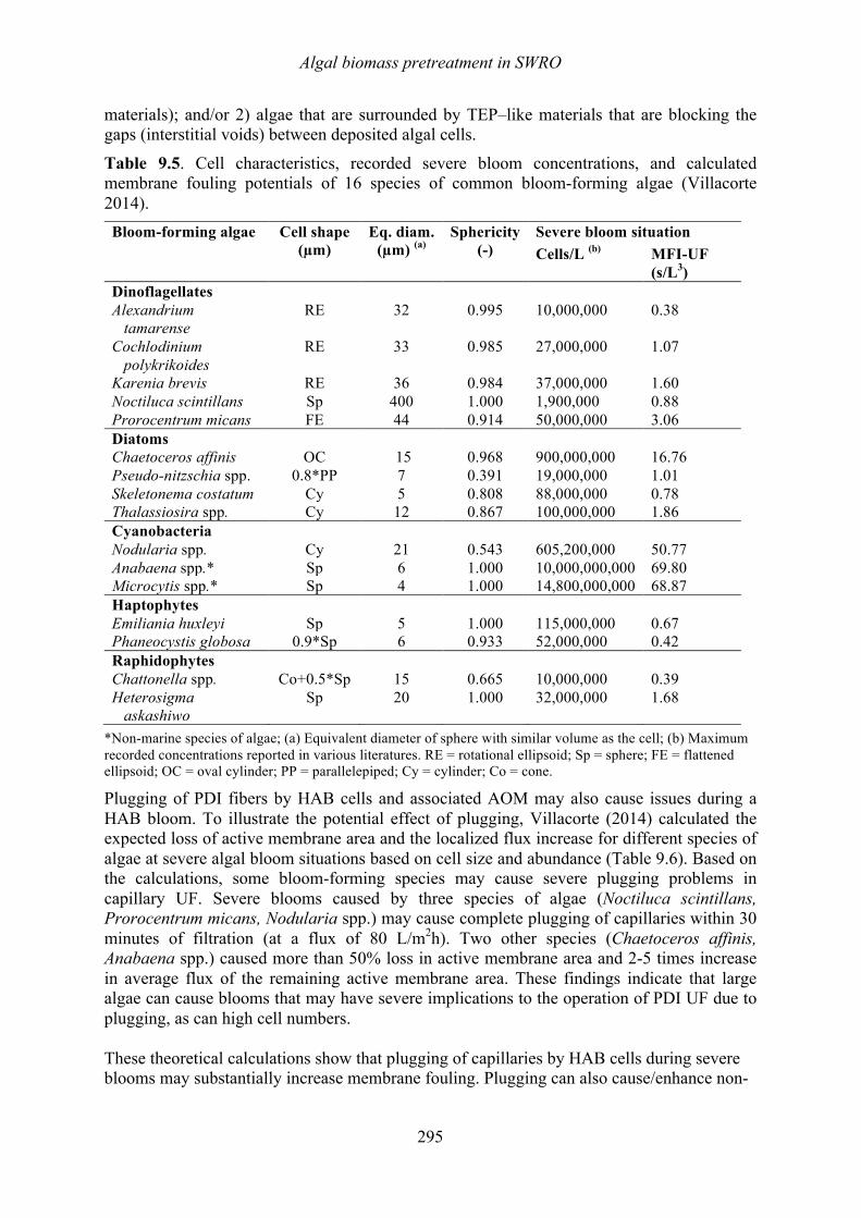
Algal biomass pretreatment in SWRO

295

materials); and/or 2) algae that are surrounded by TEP–like materials that are blocking the gaps (interstitial voids) between deposited algal cells.

Table 9.5. Cell characteristics, recorded severe bloom concentrations, and calculated membrane fouling potentials of 16 species of common bloom-forming algae (Villacorte 2014). Bloom-forming algae Cell shape

(µm) Eq. diam.

(µm) (a) Sphericity

(-) Severe bloom situation Cells/L (b) MFI-UF

(s/L3) Dinoflagellates Alexandrium tamarense

RE 32 0.995 10,000,000 0.38

Cochlodinium polykrikoides

RE 33 0.985 27,000,000 1.07

Karenia brevis RE 36 0.984 37,000,000 1.60 Noctiluca scintillans Sp 400 1.000 1,900,000 0.88 Prorocentrum micans FE 44 0.914 50,000,000 3.06 Diatoms Chaetoceros affinis OC 15 0.968 900,000,000 16.76 Pseudo-nitzschia spp. 0.8*PP 7 0.391 19,000,000 1.01 Skeletonema costatum Cy 5 0.808 88,000,000 0.78 Thalassiosira spp. Cy 12 0.867 100,000,000 1.86 Cyanobacteria Nodularia spp. Cy 21 0.543 605,200,000 50.77 Anabaena spp.* Sp 6 1.000 10,000,000,000 69.80 Microcytis spp.* Sp 4 1.000 14,800,000,000 68.87 Haptophytes Emiliania huxleyi Sp 5 1.000 115,000,000 0.67 Phaneocystis globosa 0.9*Sp 6 0.933 52,000,000 0.42 Raphidophytes Chattonella spp. Co+0.5*Sp 15 0.665 10,000,000 0.39 Heterosigma askashiwo

Sp 20 1.000 32,000,000 1.68

*Non-marine species of algae; (a) Equivalent diameter of sphere with similar volume as the cell; (b) Maximum recorded concentrations reported in various literatures. RE = rotational ellipsoid; Sp = sphere; FE = flattened ellipsoid; OC = oval cylinder; PP = parallelepiped; Cy = cylinder; Co = cone.

Plugging of PDI fibers by HAB cells and associated AOM may also cause issues during a HAB bloom. To illustrate the potential effect of plugging, Villacorte (2014) calculated the expected loss of active membrane area and the localized flux increase for different species of algae at severe algal bloom situations based on cell size and abundance (Table 9.6). Based on the calculations, some bloom-forming species may cause severe plugging problems in capillary UF. Severe blooms caused by three species of algae (Noctiluca scintillans, Prorocentrum micans, Nodularia spp.) may cause complete plugging of capillaries within 30 minutes of filtration (at a flux of 80 L/m2h). Two other species (Chaetoceros affinis, Anabaena spp.) caused more than 50% loss in active membrane area and 2-5 times increase in average flux of the remaining active membrane area. These findings indicate that large algae can cause blooms that may have severe implications to the operation of PDI UF due to plugging, as can high cell numbers. These theoretical calculations show that plugging of capillaries by HAB cells during severe blooms may substantially increase membrane fouling. Plugging can also cause/enhance non-

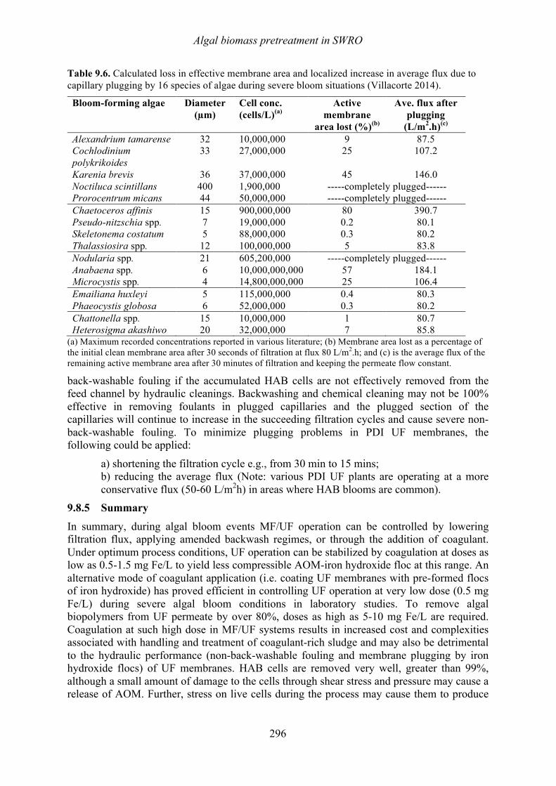
Algal biomass pretreatment in SWRO

296

Table 9.6. Calculated loss in effective membrane area and localized increase in average flux due to capillary plugging by 16 species of algae during severe bloom situations (Villacorte 2014).

Bloom-forming algae Diameter (µm)

Cell conc. (cells/L)(a)

Active membrane

area lost (%)(b)

Ave. flux after plugging

(L/m2.h)(c) Alexandrium tamarense 32 10,000,000 9 87.5 Cochlodinium polykrikoides

33 27,000,000 25 107.2

Karenia brevis 36 37,000,000 45 146.0 Noctiluca scintillans 400 1,900,000 -----completely plugged------ Prorocentrum micans 44 50,000,000 -----completely plugged------ Chaetoceros affinis 15 900,000,000 80 390.7 Pseudo-nitzschia spp. 7 19,000,000 0.2 80.1 Skeletonema costatum 5 88,000,000 0.3 80.2 Thalassiosira spp. 12 100,000,000 5 83.8 Nodularia spp. 21 605,200,000 -----completely plugged------ Anabaena spp. 6 10,000,000,000 57 184.1 Microcystis spp. 4 14,800,000,000 25 106.4 Emailiana huxleyi 5 115,000,000 0.4 80.3 Phaeocystis globosa 6 52,000,000 0.3 80.2 Chattonella spp. 15 10,000,000 1 80.7 Heterosigma akashiwo 20 32,000,000 7 85.8

(a) Maximum recorded concentrations reported in various literature; (b) Membrane area lost as a percentage of the initial clean membrane area after 30 seconds of filtration at flux 80 L/m2.h; and (c) is the average flux of the remaining active membrane area after 30 minutes of filtration and keeping the permeate flow constant.

back-washable fouling if the accumulated HAB cells are not effectively removed from the feed channel by hydraulic cleanings. Backwashing and chemical cleaning may not be 100% effective in removing foulants in plugged capillaries and the plugged section of the capillaries will continue to increase in the succeeding filtration cycles and cause severe non-back-washable fouling. To minimize plugging problems in PDI UF membranes, the following could be applied:

a) shortening the filtration cycle e.g., from 30 min to 15 mins; b) reducing the average flux (Note: various PDI UF plants are operating at a more conservative flux (50-60 L/m2h) in areas where HAB blooms are common).

9.8.5 Summary

In summary, during algal bloom events MF/UF operation can be controlled by lowering filtration flux, applying amended backwash regimes, or through the addition of coagulant. Under optimum process conditions, UF operation can be stabilized by coagulation at doses as low as 0.5-1.5 mg Fe/L to yield less compressible AOM-iron hydroxide floc at this range. An alternative mode of coagulant application (i.e. coating UF membranes with pre-formed flocs of iron hydroxide) has proved efficient in controlling UF operation at very low dose (0.5 mg Fe/L) during severe algal bloom conditions in laboratory studies. To remove algal biopolymers from UF permeate by over 80%, doses as high as 5-10 mg Fe/L are required. Coagulation at such high dose in MF/UF systems results in increased cost and complexities associated with handling and treatment of coagulant-rich sludge and may also be detrimental to the hydraulic performance (non-back-washable fouling and membrane plugging by iron hydroxide flocs) of UF membranes. HAB cells are removed very well, greater than 99%, although a small amount of damage to the cells through shear stress and pressure may cause a release of AOM. Further, stress on live cells during the process may cause them to produce

Algal biomass pretreatment in SWRO

297

more AOM. Some difference between removal of different cell types has been apparent, particularly for larger cells such as Noctiluca, that can cause plugging of PDI UF fibers.

9.9 CARTRIDGE FILTERS FOR REVERSE OSMOSIS PRETREATMENT 9.9.1 Overview

Cartridge filters are a protection measure for SWRO membranes, pumps, and energy recovery devices. The main purpose they serve is to capture particulates in the pretreated source water that may have passed through the upstream pretreatment systems. During a bloom, cellular material should have been removed prior to the cartridge filters so in most cases an increase in differential pressure should not be due to cells. More likely, AOM can build up on the cartridge filters and cause biofouling. Buildup of iron residuals can also occur on cartridge filters. This section describes operation of cartridge filters during a bloom and the subsequent challenges.

9.9.2 Types and configurations Cartridge filters are fine micro-filters of nominal size of 1 to 25 µm made of thin plastic fibers (typically polypropylene) which are wound around a central tube to form standard size

cartridges (Figure 9.30). Often they are the only screening device between the intake wells and the SWRO system with well intakes producing high quality source water. Although wound (spun) polypropylene cartridges are most commonly used for seawater (and brackish water) applications, other types, such as melt-blown or pleated cartridges of other materials have also found application. Standard

cartridge filters for RO desalination plants are typically 101.6 to 1,524 cm long and are installed in horizontal or vertical pressure vessels (filter housings). Cartridges are rated for removal of particle sizes of 1, 2, 5, 10, and 25 µm, with the most frequently used size being 5 µm. Cartridge filters are typically installed downstream of the pretreatment to capture fine sand, particles and silt that could be contained in the pretreated seawater following GMF. When the source seawater is of very high quality (SDI15 < 2) and does not need particulate removal by filtration prior to desalination, cartridge filters are used as the only pretreatment device, which in this case serves as a barrier to capture fine silt and particulates that could occasionally enter the source water during the start up on intake well pumps or due to equipment/piping failure.

The main function of cartridge filters is to protect the downstream SWRO membranes, high-pressure pumps and energy recovery devices from damage, not to provide removal of large amount of particulate foulants from the source seawater. A typical indication of whether the pretreatment system of a given desalination plant operates properly is the seawater SDI reduction through the cartridge filters. If the pretreatment system performs well, then the SDI of the source water upstream and downstream of the cartridge filters is approximately the same.

Figure 9.30. Cartridge filters installed in horizontal vessel.

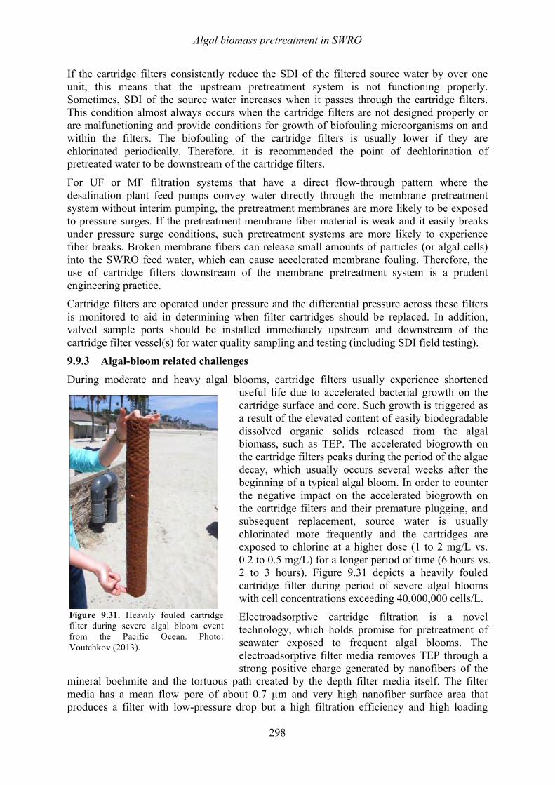
Algal biomass pretreatment in SWRO

298

If the cartridge filters consistently reduce the SDI of the filtered source water by over one unit, this means that the upstream pretreatment system is not functioning properly. Sometimes, SDI of the source water increases when it passes through the cartridge filters. This condition almost always occurs when the cartridge filters are not designed properly or are malfunctioning and provide conditions for growth of biofouling microorganisms on and within the filters. The biofouling of the cartridge filters is usually lower if they are chlorinated periodically. Therefore, it is recommended the point of dechlorination of pretreated water to be downstream of the cartridge filters.

For UF or MF filtration systems that have a direct flow-through pattern where the desalination plant feed pumps convey water directly through the membrane pretreatment system without interim pumping, the pretreatment membranes are more likely to be exposed to pressure surges. If the pretreatment membrane fiber material is weak and it easily breaks under pressure surge conditions, such pretreatment systems are more likely to experience fiber breaks. Broken membrane fibers can release small amounts of particles (or algal cells) into the SWRO feed water, which can cause accelerated membrane fouling. Therefore, the use of cartridge filters downstream of the membrane pretreatment system is a prudent engineering practice. Cartridge filters are operated under pressure and the differential pressure across these filters is monitored to aid in determining when filter cartridges should be replaced. In addition, valved sample ports should be installed immediately upstream and downstream of the cartridge filter vessel(s) for water quality sampling and testing (including SDI field testing). 9.9.3 Algal-bloom related challenges

During moderate and heavy algal blooms, cartridge filters usually experience shortened useful life due to accelerated bacterial growth on the cartridge surface and core. Such growth is triggered as a result of the elevated content of easily biodegradable dissolved organic solids released from the algal biomass, such as TEP. The accelerated biogrowth on the cartridge filters peaks during the period of the algae decay, which usually occurs several weeks after the beginning of a typical algal bloom. In order to counter the negative impact on the accelerated biogrowth on the cartridge filters and their premature plugging, and subsequent replacement, source water is usually chlorinated more frequently and the cartridges are exposed to chlorine at a higher dose (1 to 2 mg/L vs. 0.2 to 0.5 mg/L) for a longer period of time (6 hours vs. 2 to 3 hours). Figure 9.31 depicts a heavily fouled cartridge filter during period of severe algal blooms with cell concentrations exceeding 40,000,000 cells/L.

Electroadsorptive cartridge filtration is a novel technology, which holds promise for pretreatment of seawater exposed to frequent algal blooms. The electroadsorptive filter media removes TEP through a strong positive charge generated by nanofibers of the

mineral boehmite and the tortuous path created by the depth filter media itself. The filter media has a mean flow pore of about 0.7 µm and very high nanofiber surface area that produces a filter with low-pressure drop but a high filtration efficiency and high loading

Figure 9.31. Heavily fouled cartridge filter during severe algal bloom event from the Pacific Ocean. Photo: Voutchkov (2013).

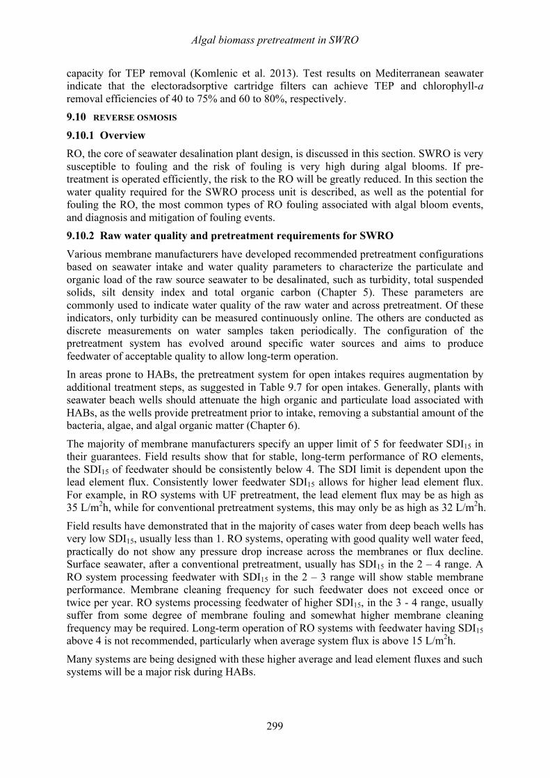
Algal biomass pretreatment in SWRO

299

capacity for TEP removal (Komlenic et al. 2013). Test results on Mediterranean seawater indicate that the electoradsorptive cartridge filters can achieve TEP and chlorophyll-a removal efficiencies of 40 to 75% and 60 to 80%, respectively. 9.10 REVERSE OSMOSIS

9.10.1 Overview RO, the core of seawater desalination plant design, is discussed in this section. SWRO is very susceptible to fouling and the risk of fouling is very high during algal blooms. If pre-treatment is operated efficiently, the risk to the RO will be greatly reduced. In this section the water quality required for the SWRO process unit is described, as well as the potential for fouling the RO, the most common types of RO fouling associated with algal bloom events, and diagnosis and mitigation of fouling events. 9.10.2 Raw water quality and pretreatment requirements for SWRO

Various membrane manufacturers have developed recommended pretreatment configurations based on seawater intake and water quality parameters to characterize the particulate and organic load of the raw source seawater to be desalinated, such as turbidity, total suspended solids, silt density index and total organic carbon (Chapter 5). These parameters are commonly used to indicate water quality of the raw water and across pretreatment. Of these indicators, only turbidity can be measured continuously online. The others are conducted as discrete measurements on water samples taken periodically. The configuration of the pretreatment system has evolved around specific water sources and aims to produce feedwater of acceptable quality to allow long-term operation. In areas prone to HABs, the pretreatment system for open intakes requires augmentation by additional treatment steps, as suggested in Table 9.7 for open intakes. Generally, plants with seawater beach wells should attenuate the high organic and particulate load associated with HABs, as the wells provide pretreatment prior to intake, removing a substantial amount of the bacteria, algae, and algal organic matter (Chapter 6).

The majority of membrane manufacturers specify an upper limit of 5 for feedwater SDI15 in their guarantees. Field results show that for stable, long-term performance of RO elements, the SDI15 of feedwater should be consistently below 4. The SDI limit is dependent upon the lead element flux. Consistently lower feedwater SDI15 allows for higher lead element flux. For example, in RO systems with UF pretreatment, the lead element flux may be as high as 35 L/m2h, while for conventional pretreatment systems, this may only be as high as 32 L/m2h.

Field results have demonstrated that in the majority of cases water from deep beach wells has very low SDI15, usually less than 1. RO systems, operating with good quality well water feed, practically do not show any pressure drop increase across the membranes or flux decline. Surface seawater, after a conventional pretreatment, usually has SDI15 in the 2 – 4 range. A RO system processing feedwater with SDI15 in the 2 – 3 range will show stable membrane performance. Membrane cleaning frequency for such feedwater does not exceed once or twice per year. RO systems processing feedwater of higher SDI15, in the 3 - 4 range, usually suffer from some degree of membrane fouling and somewhat higher membrane cleaning frequency may be required. Long-term operation of RO systems with feedwater having SDI15 above 4 is not recommended, particularly when average system flux is above 15 L/m2h.

Many systems are being designed with these higher average and lead element fluxes and such systems will be a major risk during HABs.

Algal biomass pretreatment in SWRO

300

Table 9.7. Recommended configuration of pretreatment system according to raw water quality (Hydranautics 2015).

Water source Water quality parameters

Configuration of pretreatment system Comments

Seawater beach well Turbidity < 0.2 NTU TSS < 2 mg/L SDI15 < 1.0

Cartridge filtration If seawater is under influence of brackish water, acidification, and scale inhibitor may be required

Seawater beach well Turbidity > 0.2 NTU TSS > 2 mg/L SDI15 > 1.0

Sand filtration Cartridge filtration

If seawater is under influence of brackish water, acidification, and scale inhibitor may be required

Seawater open intake Turbidity < 5 NTU TSS < 5 mg/L TOC < 2 mg/L

Acidification Coagulation + flocculation Single stage granular dual media filtration

Short excursion of turbidity up to 20 NTU is possible for few days in year

Seawater open intake Turbidity < 5 NTU TSS < 5 mg/L TOC < 2 mg/L

Membrane filtration Short excursion of turbidity up to 20 NTU is possible for few days in year

Seawater open intake Turbidity 5 -20 NTU TSS > 5 mg/L TOC > 2 mg/L

Acidification Coagulation + flocculation Two stage granular dual media filtration

Short excursion of turbidity up to 30 NTU is possible for few days in year

Seawater open intake Turbidity 5 -20 NTU TSS > 5 mg/L TOC > 2 mg/L

Acidification Coagulation + flocculation Membrane filtration

Short excursion of turbidity up to 30 NTU is possible for few days in year

Seawater open intake Turbidity > 20 – 30 NTU TSS > 5 mg/L TOC > 2 mg/L

Settling clarification Coagulation + flocculation Single stage granular dual media filtration

Suspended solids mainly inorganic particles(silt)

Seawater open intake Turbidity > 20 – 30 NTU TSS > 5 mg/L TOC > 2 mg/L

Settling clarification Coagulation + flocculation Membrane filtration

Suspended solids mainly inorganic particles(silt

Seawater open intake Turbidity > 20 - 30 NTU TSS > 5 mg/L TOC > 2 mg/L

DAF Coagulation + flocculation Single stage granular dual media filtration

Suspended solids mainly organic and biological particles(algae)

Seawater open intake Turbidity > 20 - 30 NTU TSS > 5 mg/L TOC > 2 mg/L

DAF Coagulation + flocculation Membrane filtration

Suspended solids mainly organic and biological particles(algae)

Algal biomass pretreatment in SWRO

301

Media filtration and membrane filtration are well understood. The prevention of biofilms was misunderstood in the past as discussed in the chlorination-dechlorination section of this Chapter. Recently most of the SWRO plants either eliminated the chlorination – dechlorination process completely or apply shock chlorination.

Another alternative for AOM reduction is addition of activated carbon (Huang et al. 2015) to absorb organics, although this is seldom practiced. A PAC system exists at the Adelaide Desalination Plant in Australia, where PAC can be dosed before and after the disk filters and PAC is removed by the UF, but no serious algal blooms have occurred at that plant to warrant use of the PAC system. Its primary use is for hydrocarbon removal. 9.10.3 Effect of algal blooms on SWRO operation

Algal blooms may result in deterioration of raw water quality depending on the density of the bloom and associated organics (intracellular or extracellular) or indirectly through a reduction in oxygen as algae die off. This may be detected through raw water monitoring of SDI, turbidity, TOC, and AOM such as TEP (see Chapter 5). An additional indicator that may be specifically associated with an algal bloom event is an increase in the concentration of chlorophyll-a, thus alerting RO operators of the potential for a fouling event. Chlorophyll background levels are generally specific for different regions and might be in the range of 1-5 µg/L. During a HAB bloom chlorophyll may increase significantly, reaching as high as 120 µg/L (Desormeaux et al. 2009; Franks et al. 2006). Some blooms will produce other algal pigments and thus less chlorophyll-a, and thus may not be detected by chlorophyll sensors (see Chapters 3 and 5). During the HAB period, seawater drawn into the pretreatment system contains much higher concentrations of suspended particulate matter, which significantly increases the solids load in the influent to the filtration system (either media or membrane filtration). The result is a need to increase frequency of backwashing, backwash volume, backwash time and air scour time, which in turn reduces the yield of the pretreatment system and thus the flow to the RO trains. Another problem can be an increased concentration of dissolved organic carbon (or algal organic matter, AOM), which can easily pass the pre-treatment process. This can contribute to an increase in biofouling of RO membrane elements, resulting in an increase in differential pressure.

Alternatively, impacts may manifest in the RO due to fouling if pretreatment does not mitigate the increases in these parameters. SWRO systems with poorly optimized pretreatment may experience a rapid rate of differential pressure increase, due to particulate fouling and biofouling during or following a bloom event (Franks et al. 2006; Unni et al. 2011). 9.10.4 Ferric coagulant SWRO fouling during algal bloom events

When coagulation/flocculation is employed as a part of a seawater feed pretreatment scheme, it is important to dose the coagulant at a rate that will not result in filter breakthrough. While aluminum and ferric salts will both foul the RO process by a similar mechanism, only ferric is discussed as the most commonly used coagulant in SWRO (see Section 9.4.1). Ferric coagulant that will pass the filtration step and reach the membrane elements will result in iron hydroxide fouling of membrane elements (Figure 9.32). Ferric coagulant fouling can be diagnosed in the plant through a rapid increase in differential pressure, a rapid increase in normalized feed pressure and a rapid increase in normalized salt passage (normalization of RO plant data is discussed in ASTM method D4516 (ASTM, 2010) and requires diligent collection of plant data to be of use when diagnosing fouling). This trend is well described in Hydranautics Technical Bulletin, TSB-107, Table 1 (Hydranuatics, 2015).

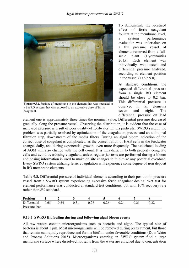
Algal biomass pretreatment in SWRO

302

To demonstrate the localized effect of ferric coagulant foulant at the membrane level, a system performance evaluation was undertaken on a full pressure vessel of elements removed from a full-scale plant (Hydranautics 2015). Each element was individually wet tested and differential pressure analyzed, according to element position in the vessel (Table 9.8). At standard conditions, the expected differential pressure from a single RO element should be close to 0.2 bar. This differential pressure is observed in tail elements seven and eight. The differential pressure on lead

element one is approximately three times the nominal value. Differential pressure decreased gradually along the pressure vessel. Observing the distribution, it is evident that the case of increased pressure is result of poor quality of feedwater. In this particular SWRO system, the problem was partially resolved by optimization of the coagulation process and an additional filtration step, downstream of the media filters. During an algal bloom, selection of the correct dose of coagulant is complicated, as the concentration of HAB cells in the feedwater changes daily, and during exponential growth, even more frequently. The associated loading of AOM will also change with the cell count. It is thus difficult to both properly coagulate cells and avoid overdosing coagulant, unless regular jar tests are performed during a bloom and dosing information is used to make on site changes to minimize any potential overdose. Every SWRO system utilizing ferric coagulation will experience some degree of iron deposit in RO membrane elements. Table 9.8. Differential pressure of individual elements according to their position in pressure vessel from a SWRO system experiencing excessive ferric coagulant dosing. Wet test for element performance was conducted at standard test conditions, but with 10% recovery rate rather than 8% standard.

Position 1 2 3 4 5 6 7 8 Differential Pressure, bar

0.65 0.34 0.31 0.28 0.26 0.24 0.21 0.22

9.10.5 SWRO Biofouling during and following algal bloom events

All raw waters contain microorganisms such as bacteria and algae. The typical size of bacteria is about 1 µm. Most microorganisms will be removed during pretreatment, but those that remain can rapidly reproduce and form a biofilm under favorable conditions (Dow Water and Process Solutions 2015). Microorganisms entering an SWRO system find a large membrane surface where dissolved nutrients from the water are enriched due to concentration

Figure 9.32. Surface of membrane in the element that was operated in a SWRO system that was exposed to an excessive dose of ferric coagulant.

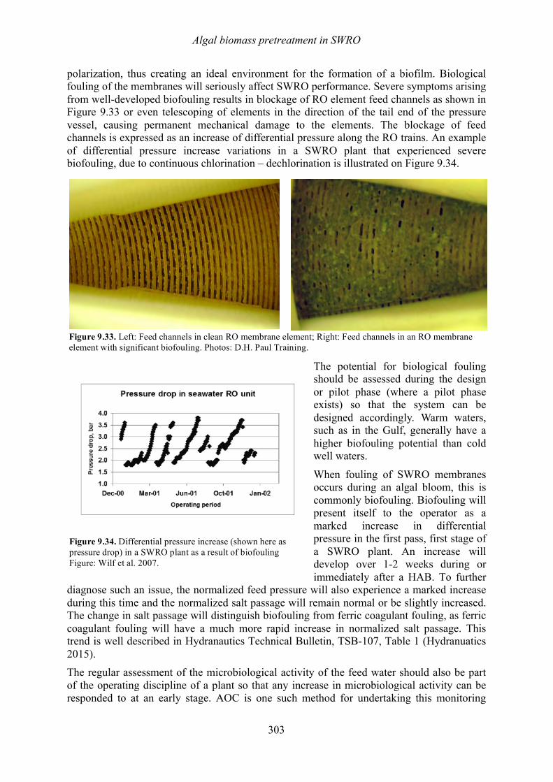
Algal biomass pretreatment in SWRO

303

polarization, thus creating an ideal environment for the formation of a biofilm. Biological fouling of the membranes will seriously affect SWRO performance. Severe symptoms arising from well-developed biofouling results in blockage of RO element feed channels as shown in Figure 9.33 or even telescoping of elements in the direction of the tail end of the pressure vessel, causing permanent mechanical damage to the elements. The blockage of feed channels is expressed as an increase of differential pressure along the RO trains. An example of differential pressure increase variations in a SWRO plant that experienced severe biofouling, due to continuous chlorination – dechlorination is illustrated on Figure 9.34.

The potential for biological fouling should be assessed during the design or pilot phase (where a pilot phase exists) so that the system can be designed accordingly. Warm waters, such as in the Gulf, generally have a higher biofouling potential than cold well waters.

When fouling of SWRO membranes occurs during an algal bloom, this is commonly biofouling. Biofouling will present itself to the operator as a marked increase in differential pressure in the first pass, first stage of a SWRO plant. An increase will develop over 1-2 weeks during or immediately after a HAB. To further

diagnose such an issue, the normalized feed pressure will also experience a marked increase during this time and the normalized salt passage will remain normal or be slightly increased. The change in salt passage will distinguish biofouling from ferric coagulant fouling, as ferric coagulant fouling will have a much more rapid increase in normalized salt passage. This trend is well described in Hydranautics Technical Bulletin, TSB-107, Table 1 (Hydranuatics 2015). The regular assessment of the microbiological activity of the feed water should also be part of the operating discipline of a plant so that any increase in microbiological activity can be responded to at an early stage. AOC is one such method for undertaking this monitoring

Figure 9.33. Left: Feed channels in clean RO membrane element; Right: Feed channels in an RO membrane element with significant biofouling. Photos: D.H. Paul Training.

Figure 9.34. Differential pressure increase (shown here as pressure drop) in a SWRO plant as a result of biofouling Figure: Wilf et al. 2007.

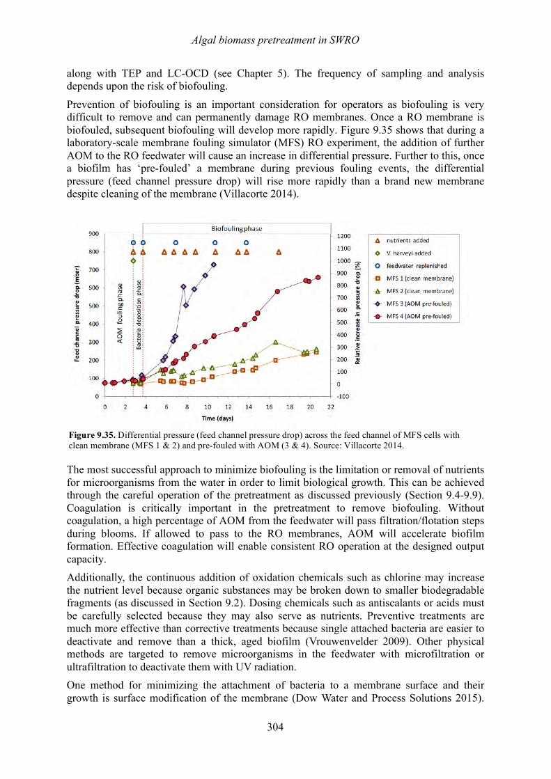
Algal biomass pretreatment in SWRO

304

along with TEP and LC-OCD (see Chapter 5). The frequency of sampling and analysis depends upon the risk of biofouling.

Prevention of biofouling is an important consideration for operators as biofouling is very difficult to remove and can permanently damage RO membranes. Once a RO membrane is biofouled, subsequent biofouling will develop more rapidly. Figure 9.35 shows that during a laboratory-scale membrane fouling simulator (MFS) RO experiment, the addition of further AOM to the RO feedwater will cause an increase in differential pressure. Further to this, once a biofilm has ‘pre-fouled’ a membrane during previous fouling events, the differential pressure (feed channel pressure drop) will rise more rapidly than a brand new membrane despite cleaning of the membrane (Villacorte 2014).

The most successful approach to minimize biofouling is the limitation or removal of nutrients for microorganisms from the water in order to limit biological growth. This can be achieved through the careful operation of the pretreatment as discussed previously (Section 9.4-9.9). Coagulation is critically important in the pretreatment to remove biofouling. Without coagulation, a high percentage of AOM from the feedwater will pass filtration/flotation steps during blooms. If allowed to pass to the RO membranes, AOM will accelerate biofilm formation. Effective coagulation will enable consistent RO operation at the designed output capacity. Additionally, the continuous addition of oxidation chemicals such as chlorine may increase the nutrient level because organic substances may be broken down to smaller biodegradable fragments (as discussed in Section 9.2). Dosing chemicals such as antiscalants or acids must be carefully selected because they may also serve as nutrients. Preventive treatments are much more effective than corrective treatments because single attached bacteria are easier to deactivate and remove than a thick, aged biofilm (Vrouwenvelder 2009). Other physical methods are targeted to remove microorganisms in the feedwater with microfiltration or ultrafiltration to deactivate them with UV radiation. One method for minimizing the attachment of bacteria to a membrane surface and their growth is surface modification of the membrane (Dow Water and Process Solutions 2015).

Figure 9.35. Differential pressure (feed channel pressure drop) across the feed channel of MFS cells with clean membrane (MFS 1 & 2) and pre-fouled with AOM (3 & 4). Source: Villacorte 2014.

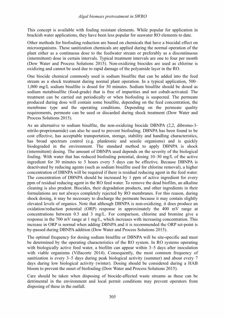
Algal biomass pretreatment in SWRO

305

This concept is available with fouling resistant elements. While popular for application in brackish water applications, they have been less popular for seawater RO elements to date.

Other methods for biofouling reduction are based on chemicals that have a biocidal effect on microorganisms. These sanitization chemicals are applied during the normal operation of the plant either as a continuous dose to the feedwater stream or preferably as a discontinuous (intermittent) dose in certain intervals. Typical treatment intervals are one to four per month (Dow Water and Process Solutions 2015). Non-oxidizing biocides are used as chlorine is oxidizing and cannot be used due to rapid damage of the polyamide layer in the RO.

One biocide chemical commonly used is sodium bisulfite that can be added into the feed stream as a shock treatment during normal plant operation. In a typical application, 500–1,000 mg/L sodium bisulfite is dosed for 30 minutes. Sodium bisulfite should be dosed as sodium metabisulfite (food-grade) that is free of impurities and not cobalt-activated. The treatment can be carried out periodically or when biofouling is suspected. The permeate produced during dose will contain some bisulfite, depending on the feed concentration, the membrane type and the operating conditions. Depending on the permeate quality requirements, permeate can be used or discarded during shock treatment (Dow Water and Process Solutions 2015). As an alternative to sodium bisulfite, the non-oxidizing biocide DBNPA (2,2, dibromo-3-nitrilo-proprionamide) can also be used to prevent biofouling. DBNPA has been found to be cost effective, has acceptable transportation, storage, stability and handling characteristics, has broad spectrum control (e.g. planktonic and sessile organisms) and is quickly biodegraded in the environment. The standard method to apply DBNPA is shock (intermittent) dosing. The amount of DBNPA used depends on the severity of the biological fouling. With water that has reduced biofouling potential, dosing 10–30 mg/L of the active ingredient for 30 minutes to 3 hours every 5 days can be effective. Because DBNPA is deactivated by reducing agents (such as sodium bisulfite used for chlorine removal), a higher concentration of DBNPA will be required if there is residual reducing agent in the feed water. The concentration of DBNPA should be increased by 1 ppm of active ingredient for every ppm of residual reducing agent in the RO feed water. To remove the dead biofilm, an alkaline cleaning is also prudent. Biocides, their degradation products, and other ingredients in their formulations are not always completely rejected by RO membranes. For this reason, during shock dosing, it may be necessary to discharge the permeate because it may contain slightly elevated levels of organics. Note that although DBNPA is non-oxidizing, it does produce an oxidation/reduction potential (ORP) response in approximately the 400 mV range at concentrations between 0.5 and 3 mg/L. For comparison, chlorine and bromine give a response in the 700 mV range at 1 mg/L, which increases with increasing concentration. This increase in ORP is normal when adding DBNPA and it is recommended the ORP set-point is by-passed during DBNPA addition (Dow Water and Process Solutions 2015).

The optimal frequency for dosing sodium bisulfite or DBNPA will be site-specific and must be determined by the operating characteristics of the RO system. In RO systems operating with biologically active feed water, a biofilm can appear within 3–5 days after inoculation with viable organisms (Villacorte 2014). Consequently, the most common frequency of sanitization is every 3–5 days during peak biological activity (summer) and about every 7 days during low biological activity (winter). Dosing should be considered during a HAB bloom to prevent the onset of biofouling (Dow Water and Process Solutions 2015). Care should be taken when disposing of biocide-affected waste streams as these can be detrimental in the environment and local permit conditions may prevent operators from disposing of these in the outfall.

Algal biomass pretreatment in SWRO

306

9.10.6 SWRO operational strategies during a bloom At low algal concentrations, the RO system will most likely continue to operate, with no system changes. Sometimes at moderate algae concentrations, the RO will operate at reduced capacity, due to lower output of the feedwater from the pretreatment system. At severe algal concentrations, operators may consider shutting down the RO to avoid severe (and somewhat irreversible) fouling of membrane elements.

Optimization of pretreatment may be the best strategy for maximizing SWRO efficiency during a bloom. Media filtration and membrane filtration optimization are discussed earlier in this Chapter (Section 9.6 and 9.8). Coagulation should be considered, as without coagulation, a high percentage of AOM from the feedwater will pass the pretreatment during the HAB blooms (Section 9.5). If allowed to pass to the RO membranes, AOM will accelerate biofilm formation. Acceleration of biofouling is also attributed to chlorination-dechlorination, as discussed in the chlorination-dechlorination section of this Chapter (9.2 and 9.3). Most SWRO plants either eliminate the chlorination – dechlorination process completely or apply shock chlorination. Shock chlorination should be reconsidered or modified during a bloom. Non-oxidizing biocide dosing to the RO could also be considered during a bloom period (e.g., DBNPA). While RO operating conditions can be slightly changed during a bloom, the design envelope to produce the required amount of permeate at an acceptable quality is usually set precisely during the design process. When flux is lowered in an SWRO train, the permeate salinity increases, therefore lowering flux too much may result in permeate water that is out of TDS specification. In places where a boron specification for the permeate quality is low (e.g. 0.5mg/L), lowering the permeate flux may quickly produce an unacceptable permeate boron concentration. While some plants may be able to deal with this issue through a second pass design, others may not have this flexibility. Lowering recovery may slightly improve permeate quality and at the same time decrease the lead element flux to alleviate some fouling trends. This will result in higher pumping pressures and thus more energy to produce the same amount of water; however, the minor impact on lead element flux experienced when lowering recovery may not be sufficient to significantly alleviate the effects of fouling. While flux and recovery could be lowered to avoid some fouling during an algal bloom, a better result may be obtained by optimizing the pretreatment to yield better removal of AOM. 9.10.7 Membrane cleaning

Maintenance chemical cleaning for iron removal, applied periodically, will restore membrane performance to clean membrane conditions. The common cleaning procedure for iron removal (in the absence or organics) is recirculation of citric acid solution at a concentration of about 2%.

The cleaning applied for biofouling consists of high pH flushing combined with prolonged soaking. RO cleaning is discussed in greater detail in Appendix 5. A biofilm is difficult to remove because it protects its microorganisms against the action of shear forces and biocide chemicals. In addition, if not completely removed, remaining parts of a biofilm (in the form of AOM) lead to accelerated biofouling (Villacorte 2014). Once an element has biofouled once, it can be difficult to prevent further occurrences. Biological fouling prevention is therefore a major objective of the pretreatment process. The common cleaning procedure for biofouling removal is recirculation of an alkaline cleaning solution at pH 12. In extreme cases, a biocide can be used (Appendix 5). When iron fouling is combined with biofouling, the removal of foulant from the membrane is difficult and restoration of performance much less effective. In such cases, the cleaning

Algal biomass pretreatment in SWRO

307

procedure consists of alternate steps of high pH (organics removal) and low pH (iron removal) cleaning. In extreme cases, a biocide can be used between the high pH and low pH step. To adequately restore RO system performance, in the case of mixed iron – biofouling, the cause of biofouling has to be addressed and eliminated (Appendix 5).

9.10.8 Summary SWRO is very susceptible to fouling, particularly from overdosing ferric coagulants and through biofouling. During HABs, this risk is very high as it is difficult to predict the precise dose of ferric coagulant on any given day of a bloom, and AOM released from HAB cells can pass the pretreatment process and promote biofouling; however, if pre-treatment is operated efficiently, the risk to the RO will be greatly reduced in all but the most severe HABs. Cleaning of the RO after ferric coagulant fouling is not difficult, but cleaning of biofouled elements can be a challenge owing to the sticky nature of the biofilm. Other than optimization of the pre-treatment, only a minor amount of adjustment can be made to the lower flux and lower recovery of a SWRO process unit to prevent fouling from HAB AOM due to tight design parameters to achieve acceptable permeate quality. 9.11 SUMMARY OF BIOMASS REMOVAL IN SWRO

This chapter presents the most common treatment methods used in SWRO systems and discussed the impacts of a non-toxic HAB on plant operations. A summary of a broad set of industry knowledge on the matter is summarized, giving guidance to designers and operators alike. The following major concepts are discussed:

• Avoiding chlorination-dechlorination during a bloom will help to prevent downstream fouling. While chlorination will destroy HAB cells, broken cells will release AOM, causing downstream fouling (Section 9.2 and 9.3). The AOM is more important in terms of negative impacts than the intact cells, which are more easily removed during pretreatment.

• DAF is a good choice for cell removal in areas likely to experience heavy algal blooms, as it lifts and removes cells from the seawater in a relatively gentle manner (Section 9.5).

• GMF (Section 9.6) and UF (Section 9.8) can deal with cell removal in lighter blooms, but using a DAF upstream for heavy blooms is prudent.

• Coagulation assists all three pretreatments (DAF, GMF, and UF) and acts to remove AOM more effectively than the pretreatments alone. Less AOM in the pretreated water is also an important objective to alleviate SWRO fouling (Section 9.4).

• Microstrainers can foul with algal material and may have shorter cycle times during a bloom (Section 9.7).

• Cartridge filters are installed to protect the SWRO. These will most likely foul during or following a bloom and require regular replacement during longer more intense blooms (Section 9.9).

• There is little an operator can do to adjust the SWRO flux and recovery. A better strategy may be to focus on getting the pretreatment working efficiently and, consequently, the SWRO will operate more effectively. SWRO fouling from excess ferric coagulant and biofouling may still be an issue during intense blooms and may require focused cleaning after a bloom (Section 9.10).

Algal biomass pretreatment in SWRO

308

9.12 REFERENCES Agus, E., Voutchkov, N., and Sedlak, D. L. 2009. Disinfection by-products and their

potential impact on the quality of water produced by desalination systems: a literature review. Desalination 237(1-3), 214-237.

Al-Rasheed, R., Althobity, E., Al-Sulami, S., and Al-Ruwished, A. 2009. Influence of Different Disinfection Methods on the Presence of Bromate and Chlorate in the Product Water of Seawater Desalination Plants. Proceedings of the International Desalination Association World Congress, Dubai, UAE.

Amato, T., Nattress, J., and Mackay, D. 2012. Seawater v. Surface Water Treatment Applying Enflo-DAFTM Technology. Proceeding of the American Water Works Association Water Quality Technology Conference, Toronto, Ontario, Canada.

Appelgate, L., Erkembrecher Jr., C. and Winters, H. (1989) New chloramine process to control aftergrowth and biofouling in Permasep B-10 RO surface seawater plants, Desalination 74, 59-72.

Bahamdan, T., Al Mobayed, A., and Ehsan, A. 1999. Prevention of biofouling of seawater systems – a case study. Proceedings of the International Desalination Association World Congress, San Diego, California.

Bar-Zeev, E., Belkin, N., Liberman, B., Berman, T., and Berman-Frank, I. 2012. Rapid sand filtration pretreatment for SWRO: Microbial Maturation Dynamics and Filtration Efficiency of Organic Matter, Desalination 286, 120-130.

Besson, A. and Guiraud, P. 2012. Characterization of bubbles produced by dissolved air flotation in saline water. Proceedings of the International Water Association Flotation Conference. Oct 29 - Nov 1. New York City, New York.

Bonnelye, V., Sanz, M. A., Durand, J-P., Plasse, L., Gueguen, F., and Mazounie, P. 2004. Reverse osmosis on open intake seawater: pre-treatment strategy. Desalination 167, 191-200.

Brehant, A., Bonnelye, V., and Perez, M. 2002. Comparison of MF/UF pretreatment with conventional filtration prior to RO membranes for surface seawater desalination. Desalination 144, 353-360.

Bu-Rashid, K. A. and Czolkoss, W. 2007. Pilot tests of Multibore UF membrane at Addur SWRO desalination plant, Bahrain. Desalination 203(1-3), 229-242.

Camp, T. R. and Stein, P. C. 1943. Velocity gradients and internal work in fluid motion. Journal of the Boston Society of Civil Engineers 30, 219-237.

Castaing, J. B., Mass. A., Sechet, V., Sabiri, N.-E., Ponti, M., Haure, J., and Jaouen, P. 2011. Immersed hollow fibres microfiltration (MF) for removing undesirable micro-algae and protecting semi-closed aquaculture basins, Desalination 276, 386–396.

Huang, W., Chu, H., Dong, B., Hu, M., and Yu, Y. 2015. A membrane combined process to cope with algae blooms in water. Desalination 355, 99–109.

Choi, K. Y. and Dempsey, B. A. 2004. Inline coagulation with low pressure membrane filtration. Water Research 38, 4271-4281.

Chow, C. W. K., Panglish, S., House, J., Drikas, M., Burch, M. D., and Gimbel, R. 1997. A study of membrane filtration for the removal of cyanobacterial cells. Journal of Water Supply: Research and Technology 46(6), 324-334.

Algal biomass pretreatment in SWRO

309

Crittenden, J. C., Trussell, R. R., Hand, D. W., Howe, K. J., Tchobanoglous, G., and Borchardt, J. H. 2012. MWH’s water treatment principles and design. Hoboken (NJ), Wiley: 1920 p.

Dennett, K. E., Amirtharajah, A., Moran, T. F., and Gould, J. P. 1996. Coagulation: its effect on organic matter. Journal of the American Water Works Association 84(4), 129-142.

Desormeaux, E., Meyerhofer, P. F., and Luckenbach H. 2009. Results from Nine Investigations Assessing Pacific Ocean Seawater Desalination in Santa Cruz, California, Proceeding of the IDA World Congress, Atlantis, The Palm – Dubai, UAE.

Di Profio, G., Ji, X., Curcio, E., and Drioli, E. 2011. Submerged hollow fiber ultrafiltration as seawater pretreatment in the logic of integrated membrane desalination systems. Desalination 269 (1-3), 128-135.

Dixon, M. B., Richard, Y., Ho, L., Chow, C. W. K., O’Neill, B. K., and Newcombe, G. 2011a. Integrated membrane systems incorporating coagulation, activated carbon and ultrafiltration for the removal of toxic cyanobacterial metabolites from Anabaena circinalis. Water Science and Technology 63(7), 1405-1411.

Dixon, M. B., Richard, Y., Ho, L., Chow, C. W. K., O’Neill, B. K., and Newcombe, G. 2011b. A coagulation - powdered activated carbon - ultrafiltration multiple barrier approach for removing toxins from two Australian cyanobacterial blooms. Journal of Hazardous Materials 186(2-3), 1553-1559.

Dow Water and Process Solutions. 2015. Reverse Osmosis Technical Manual, http://msdssearch.dow.com/PublishedLiteratureDOWCOM/dh_08db/0901b803808db77d.pdf?filepath=liquidseps/pdfs/noreg/609-00071.pdf&fromPage=GetDoc, Accessed online, November 2015.

Duan, J., Graham, N. J. D., and Wilson, F. 2002. Coagulation of humic acid by ferric chloride in saline (marine) water conditions. Water Science and Technology 47(1), 41-48.

Duan, J. and Gregory, J. 2003. Coagulation by hydrolyzing metal salts. Advances in Colloid and Interface Science 100-102, 475-502.

Edzwald, J. K., Tobiason, J. E., Amato, T., and Maggi, L. J. 1999. Integrating high rate dissolved air flotation technology into plant design, Journal of American Water Works Association 91(12), 41-53.

Edzwald, J. K. 2010. Dissolved air flotation and me. Water Research 44, 2077-2106. Edzwald, J. K. and Haarhoff, J. 2011. Seawater pretreatment for reverse osmosis: chemistry,

contaminants, and coagulation, Water Research 45, 5428–5440. Edzwald, J. K. and Haarhoff, J. 2012. Dissolved Air Flotation for Water Clarification.

American Water Works Association and McGraw-Hill: 352 p. Eshel, G., Elifantz, H., Nuriel, S., Holenberg, M., and Berman T. 2013. Microfiber filtration

of lake water: impacts on TEP removal and biofouling development. Desalination and Water Treatment 51, 1043-1049.

Ferguson, M., Towndrow, S., Broom, G., Jovanoski, M., Boardman, B., and Sibma, S. 2011. Southern seawater microfiltration pilot plant trial – the impacts of shock chlorination. Proceedings of the International Desalination Association World Congress, Perth, Australia.

Algal biomass pretreatment in SWRO

310

Franks, R., Wilf, M., Voutchkov, N., Murkute, P., and Kizer, J. 2006. A Pilot Study Using Seawater Reverse Osmosis Membranes In Combination With Various Pretreatments To Meet The Challenges Of Pacific Seawater Desalination, Proceeding of the AMTA Biennial Conference.

Gabelich, C. J., Chen, W. R., Yun, T. I., Coffey, B. M., and Suffet, I. H. 2005. The role of dissolved aluminum in silica chemistry for membrane processes. Desalination 180(1-3), 307-319.

Gabelich, C. J., Ishida, K. P., Gerringer, F. W., Evangelista, R., Kalyan, M., and Suffet, I. H. 2006. Control of residual aluminum from conventional treatment to improve reverse osmosis performance. Desalination 190(1-3), 147-160.

Gregory, R., Zabel, T. F., and Edzwald, J. K. 1999. Sedimentation and Flotation. Chapter 7. In: Water Quality & Treatment: A Handbook of Community Water Supply. (Letterman, R.D., Ed). AWWA 5th Ed. McGraw-Hill. New York: 509 p.

Guigui, C., Rouch, J. C., Durand-Bourlier, L., Bonnelye, V., and Aptel, P. 2002. Impact of coagulation conditions on the inline coagulation/UF process for drinking water production. Desalination 147, 95-100.

Gustalli, A., Simon, F. X., Penru, Y., de Kirchove, A., Llorens, J., and Baig, S. 2013. Comparison of DMF and UF pretreatments for particulate material and dissolved organic matter removal in SWRO desalination. Desalination 322, 144-150.

Haarhoff, J. and Edzwald, J. K. 2013. Adapting dissolved air flotation for the clarification of seawater. Desalination 311, 90–94.

Halpern, D.F., Mcardle, J., and Antrim, B. 2005. UF pretreatment for SWRO: pilot studies. Desalination 182, 323-332.

Henderson, R. K., Baker, A., Parsons, S. A., and Jefferson, B. 2008a. Characterisation of algogenic organic matter extracted from cyanobacteria, green algae and diatoms. Water Research 42, 3435-3445.

Henderson, R. K., Parsons, S. A., and Jefferson, B. 2008b. Successful removal of algae through the control of zeta potential. Separation Science and Technolog 43(7), 1653-1666.

Henderson, R. K., Parsons, S. A., and Jefferson, B. 2008c. The impact of algal properties and pre-oxidation on solid-liquid separation of algae. Water Research 42, 1827-1845.

Henderson, R. K., Parsons, S. A., and Jefferson, B. 2010. The impact of differing cell and algogenic organic matter (AOM) characteristics on the coagulation and flotation of algae. Water Research 44(12), 3617-3624.

Heng, L., Yanling, Y., Weijia, G., Xing, L., and Guibai, L. 2008. Effect of pretreatment by permanganate/chlorine on algae fouling control for ultrafiltration (UF) membrane system. Desalination 222(1-3), 74-80.

Hung, M. T. and Liu, J. C. 2006. Microfiltration for separation of green algae from water. Colloids and Surfaces B: Biointerfaces 51(2), 157-164.

Huang, W., Chu, H., Dong, B., Hu, M., and Yu, Y. 2015. A membrane combined process to cope with algae blooms in water. Desalination 355, 99-109.

Hyde, R. A. 1975. Water Clarification by Flotation – 4 Technical Report No.TR13, Medmenham, England Water Research Centre.

Algal biomass pretreatment in SWRO

311

Hydranautics. 2015. www.membranes.com. Accessed 1 November 2015. Jamaly, S., Darwish, N. N., Ahmed, I., and Hasan, S. W. 2014. A short review on reverse

osmosis pretreatment technologies. Desalination 354, 30–38. Jansenns, J. and Buekens, A. 1993. Assessment of process selection for particle removal in

surface water treatment. Aqua 42(5), 279-288. Junli, H., Li, W., Nenqi, R., Li, L. X., Fun, S. R., and Guanle, Y. 1997. Disinfection effect of

chlorine dioxide on viruses, algae and animal planktons in water. Water Research 31(3), 455-460.

Kim, S-H., Min, C.-S., and Lee, S. 2011. Application of dissolved air flotation as pretreatment of seawater desalination. Desalination and Water Treatment 33, 261-266.

Komlenic, R., Berman, T., Brant, J. A., Dorr, B., El-Azizi, I., and Mowers, H. 2013. Removal of polysaccharide foulants from reverse osmosis feedwater using electroadsorptive cartridge filters. Desalination and Water Treatment 51, 1050-1056.

Konno, H. 1993. Settling and coagulation of slender type diatoms. Water Science and Technology 27(11), 231–240.

Lattemann, S. 2010. Development of an environmental impact assessment and decision support system for seawater desalination plants. Doctoral dissertation, UNESCO-IHE/TUDelft, Delft.

Lattemann, S. and Höpner, T. 2008. Environmental impact and impact assessment of seawater desalination. Desalination 220, 1-15.

Le Roux, J., Croue, J-P., and Nada, N. 2013. Tracing disinfection byproducts in desalination plants. Proceedings of the International Desalination Association World Congress, Tianjin, China.

Le Roux, J., Nihemaiti, M., and Croué, J-P. 2015. The role of aromatic precursors in the formation of haloacetamides by chloramination of dissolved organic matter. Water Research 88, 371-379.

Ma, M., Liu, R., Liu, H., and Qu, J. 2012. Chlorination of Microcystis aeruginosa suspension: cell lysis, toxin release and degradation. Journal of Hazardous Materials, 217-218, 279-285.

Ma, W., Zhao, Y., and Wang, L. 2007. The pretreatment with enhanced coagulation and a UF membrane for seawater desalination with reverse osmosis. Desalination 203(1-3), 256-259.

Mir, J., Morato, J., and Ribas, F. 1997. Resistance to chlorine of freshwater bacterial strains. Journal of Applied Microbiology 82, 7-18.

Murrer, J. and Rosberg, R. 1998. Desalting of seawater using UF and RO – results of a pilot study. Desalination 118(1-3), 1-4.

Myklestad, S. 1995. Release of extracellular products by phytoplankton with special emphasis on polysaccharides. Science of the Total Environment 165, 155-164.

Naidu, G., Jeong, S., Vigneswaran, S., and Rice, S. A. 2013. Microbial activity in biofilter used as a pretreatment for seawater desalination. Desalination 309, 254–260.

Pearce, G. K. 2007. Introduction to membranes: manufacturers’ comparison: part 1. Filtration+Separation, 44(8), 36-38.

Algal biomass pretreatment in SWRO

312

Pearce, G. K. 2010. SWRO pre-treatment: markets and experience. Filtration+Separation, 47(4), 30-33.

Pivokonsky, M., Naceradska, J., Kopecka, I., Baresova, M., Jefferson, B., Li, X., and Henderson, R. K. 2016. The impact of algogenic organic matter on water treatment plant operation and water quality: a review. Critical Reviews in Environmental Science and Technology 46(4), 291-335.

Plantier, S., Castaing, J. B., Sabiri, N. E., Masse, A., Jaouen, P., and Pontie, M. 2013. Performance of sand filter in removal of algal bloom for SWRO pretreatment. Desalination and Water Treatment 51, 1838-1846.

Ransome, T., Ferguson, M., de Miguel, A., and Sibma, S. 2015. Operation of Large Scale RO plant with Ultrafiltration Pretreatment: Challenges in Early Operation. Proceedings of the IDA World Congress on Desalination and Water Reuse, San Diego, CA.

Regula, C., Carretier, E., Wyart, Y., Sergent, M., Gésan-Guizioud, G., Ferry, D., Vincent, A., Boudot, D., and Moulin, P. 2013. Ageing of ultrafiltration membranes in contact with sodium hypochlorite and commercial oxidant: experimental designs as a new ageing protocol. Separation and Purification Technology 103, 119-138.

Resosudarmo, A., Nappa, L., Ye, Y., Le-Clech, P., and Chen, V. 2017. Effect of physical and chemical stress on ultrafiltration membrane performance during marine algal blooms. Separation Science and Technology 52, 364 – 373.

Ripperger, S., Gösele, W., and Alt, C. 2012. Filtration, 1. Fundamentals. In: Ullmann's Encyclopedia of Industrial Chemistry. Wiley-VCH Verlag GmbH & Co. KGaA, Weinheim, Germany: pp. 677–709.

Rovel, J. M. 2003. Why a SWRO in Taweelah? - Pilot plant results demonstrating feasibility and performance of SWRO on Gulf water. Proceedings of International Desalination Association World Congress, Nassau, Bahamas.

Salinas Rodriguez, S. G. 2011. Particulate and Organic Matter Fouling of Seawater Reverse Osmosis Systems: Characterization, Modelling and Applications. Thesis dissertation, UNESCO-IHE/TUDelft, ISBN 978-0-415-62092-5, CRC Press/Balkema, Leiden.

Salinas Rodriguez, S. G., Kennedy, M. D., Amy, G. L., and Schippers, J. C. 2012. Flux dependency of particulate/colloidal fouling in seawater reverse osmosis systems. Desalination and Water Treatment 42, 155-162.

Schurer, R., Janssen, A., Villacorte, L. O., and Kennedy, M. D. 2012. Performance of ultrafiltration and coagulation in an UF-RO seawater desalination demonstration plant. Desalination and Water Treatment 42(1-3), 57-64.

Schurer, R., Tabatabai, A., Schippers, J. C., and Kennedy, M. D. 2013. Three years operational experience with ultrafiltration as SWRO pre-treatment during algal bloom. Desalination and Water Treatment 51(4-6), 1034-1042.

Shen, Q., Zhu, J., Cheng, L., Zhang, J., Zhang, Z., and Xu, X. 2011. Enhanced algae removal by drinking water treatment of chlorination coupled with coagulation. Desalination 271, 236-240.

Shutova, Y., Karna, B., Hambly, A. C., Lau, B., Henderson, R. K., and Le-Clech, P. 2016. Enhancing organic matter removal in desalination pretreatment systems by application of dissolved air flotation. Desalination 318, 12-21.

Algal biomass pretreatment in SWRO

313

SPI Engineering. 2010. West Basin Municipal Water District, Ocean Water Desalination Pilot Program, Final Comprehensive Report 2002 – 2009, September 2, 2010.

Tabatabai, S. A. A. 2014. Coagulation and Ultrafiltration in Seawater Reverse Osmosis Pretreatment. Doctoral dissertation, UNESCO-IHE/TU Delft, ISBN 978-1-138-02686-5, CRC Press/Balkema, Leiden.

Tabatabai, S. A. A., Schippers, J. C., and Kennedy, M. D. 2014. Effect of coagulation on fouling potential and removal of algal organic matter in ultrafiltration pretreatment to seawater reverse osmosis. Water Research 59, 283-294.

Unni, S., Gorenflo, A., Al Suwaidi, E., Al Mulla, M., and Scott K. 2011. Two Year Operational Experience Of SWRO Membrane With Arabian Gulf And Gulf Of Oman Water. Proceedings of the IDA World Congress, Perth, Western Australia.

Valade, M. T., Edzwald, J. K., Tobiason, J. E., Dahlquist, J., Hedberg, T., and Amato, T. 1996. Particle Removal by Flotation and Filtration: Pretreatment Effects. Journal of American Water Works Association 88(12), 35-47.

Villacorte, L. O. 2014. Algal blooms and membrane-based desalination technology. Doctoral dissertation. UNESCO-IHE/TUDelft, ISBN 978-1-138-02626-1. CRC Press/Balkema, Leiden.

Villacorte, L. O., Ekowati, Y., Neu, T. R., Klein, J. M., Winters, H., Amy, G., Schippers, J. C., and Kennedy, M. D. 2015. Characterisation of algal organic matter produced by bloom-forming marine and freshwater algae. Water Research 73, 216-230.

Voutchkov, N. 2009. SWRO pretreatment systems: choosing between conventional and membrane filtration. Filtration+Separation 46(1), 5-8.

Voutchkov, N. 2013. Desalination Engineering - Planning and Design. McGraw-Hill, New York: 637 p.

Vrouwenvelder, J. S. 2009. Biofouling of spiral wound membrane systems. Doctoral dissertation. Delft University of Technology, Delft, The Netherlands. ISBN: 978-90-814743-1-3, Ipskamp Drukkers, Enschede, The Netherlands.

WHO. 2007. Desalination for Safe Water Supply, Guidance for the Health and Environmental Aspects Applicable to Desalination. World Health Organization (WHO), Geneva: 161 p.

Wilf, M. and Schierach, M. K. 2001. Improved performance and cost reduction of RO seawater systems using UF pretreatment. Desalination 135, 61-68.

Wilf, M., Awerbuch, L., Bartels, C., Mickley, M., Pearce, G., and Voutchkov, N. 2007. The Guidebook to Membrane Desalination Technology: Reverse Osmosis, Nanofiltration And Hybrid Systems Process Design, Applications And Economics. Rehovot: Balaban Publishers: 524 p.

Winters, H. 1995. Biofouling: Its history and how it affects today's Desalination industry. Proceedings of the International Desalination Association World Congress, Abu Dhabi, UAE.

Winters, H. and Isquith, I. 1995. A Critical Evaluation of Pretreatment to Control Fouling in Open Seawater Reverse Osmosis - Has it been a success? Proceedings of the International Desalination Association World Congress, Abu Dhabi, UAE.

Wolf, P. H., Siverns, S., and Monti, S. 2005. UF membranes for RO desalination pretreatment. Desalination 182, 293-300.

Algal biomass pretreatment in SWRO

314

Xu, H., Chen, W., Xiao, H., and Hu, X. 2014. Stability of an ultrafiltration system for drinking water treatment, using chlorine for fouling control. Desalination 336(1), 187-195.

Yap, R. K., Holmes, M., Peirson, W., Whittaker, M., Stuetz, R., Jefferson, B., and Henderson, R. 2012. Optimising dissolved air flotation/filtration treatment of algae-laden lagoon effluent using surface charge: a Bolivar treatment plant case study. Water Science and Technology 66(8), 1684-1690.

Zhang, J. D., Liu, Y. W., Gao, S. M., Li, C. Z., Zhang, F., Zen, H. M., and Ye, C. S. 2006. Pilot testing of outside-in UF pretreatment prior to RO for high turbidity seawater desalination. Desalination 189(1-3), 269-277.

Zheng, X., Ernst, M., Huck, P. M., and Jekel, M. 2010. Biopolymer fouling in dead-end ultrafiltration of treated domestic wastewater. Water Research 44, 5212-5221.

Zhu, I. X., Bates, B. J., and Anderson, D. M. 2014. Removal of Prorocentrum minimum from seawater using dissolved air flotation. Journal of Applied Water Engineering and Research 2(1), 1-10.

Removal of algal toxins and taste and odor compounds

315

10 REMOVAL OF ALGAL TOXINS AND TASTE AND ODOR COMPOUNDS DURING DESALINATION

Mike B. Dixon1, Siobhan F.E. Boerlage2, Holly Churman3, Lisa Henthorne3, and Donald M.

Anderson4 1MDD Consulting, Kensington, Calgary, Alberta, Canada 2Boerlage Consulting, Gold Coast, Queensland, Australia

3Water Standard, Houston, Texas, USA 4Woods Hole Oceanographic Institution,Woods Hole MA USA

10.1 Introduction ......................................................................................................................................... 315 10.2 Chlorination ......................................................................................................................................... 316 10.3 Dissolved air flotation (DAF) ............................................................................................................. 317 10.4 Granular media filters .......................................................................................................................... 317 10.5 Ultrafiltration/microfiltration .............................................................................................................. 318 10.6 Reverse osmosis .................................................................................................................................. 320 10.7 Sludge treatment and backwash disposal ............................................................................................ 324 10.8 Toxin removal in thermal desalination plants ..................................................................................... 324

10.8.1 Chemical and physical properties of marine HAB toxins ........................................................... 325 10.8.2 Toxin barriers in thermal desalination plants .............................................................................. 325

10.9 Chlorination prior to the distribution system ...................................................................................... 327 10.10 Summary ........................................................................................................................................... 328 10.11 References ......................................................................................................................................... 329

10.1 INTRODUCTION A major challenge in desalination is the removal of harmful algal bloom (HAB) toxins and taste and odor compounds (hereafter referred to as algal metabolites) using common treatment techniques. Removal of other compounds such as polysaccharides, proteins or transparent exopolymer particles (TEP) are discussed in Chapter 2. Taste and odor compounds are materials produced during a HAB that are not detrimental to human health, but cause customer dissatisfaction and often a misconception that the drinking water is not suitable for consumption. Toxins are detrimental to human health and are discussed in Chapter 2. Here the objective is to assess each process unit in a common desalination treatment train, both for SWRO and thermal desalination, and address how each is best optimized to act as a barrier to these specific algal metabolites. Where treatment techniques in seawater applications exist, these have been referenced and used as examples. As little documentation exists on removal of algal metabolites from seawater blooms, fresh water algal species are referred to whenever needed. This information is relevant in understanding the removal mechanisms that are possible. For clarity, these are denoted for each example. Algal metabolites can be either intracellular or extracellular. Many algal species have high percentages of intracellular metabolites, such as Microcystis (freshwater) in which the toxin microcystin can be up to 98% intracellular (Chow et al. 1997). Lefebvre et al. (2008) showed an approximate 81% intracellular saxitoxin (STX)-equivalent concentration for an Alexandrium (seawater) bloom, although further data are needed to confirm this observation. STX-eq (or STX-equivalents) is a measure of total toxicity due to all saxitoxin analogues in a particular solution. In contrast, Smith et al. (2012) report that 60% of the okadaic acid produced by Dinophysis cultures was extracellular, while Kudela (pers. comm.) reported total and extracellular concentrations of 100 and 50 µg/L domoic acid respectively during a massive bloom of Pseudo-nitzschia along the US west coast in 2014. Extracellular

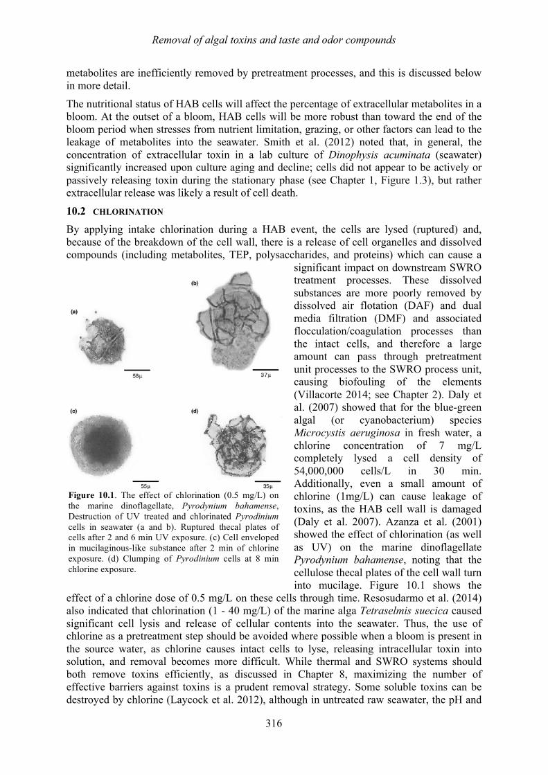
Removal of algal toxins and taste and odor compounds

316

metabolites are inefficiently removed by pretreatment processes, and this is discussed below in more detail.

The nutritional status of HAB cells will affect the percentage of extracellular metabolites in a bloom. At the outset of a bloom, HAB cells will be more robust than toward the end of the bloom period when stresses from nutrient limitation, grazing, or other factors can lead to the leakage of metabolites into the seawater. Smith et al. (2012) noted that, in general, the concentration of extracellular toxin in a lab culture of Dinophysis acuminata (seawater) significantly increased upon culture aging and decline; cells did not appear to be actively or passively releasing toxin during the stationary phase (see Chapter 1, Figure 1.3), but rather extracellular release was likely a result of cell death.

10.2 CHLORINATION By applying intake chlorination during a HAB event, the cells are lysed (ruptured) and, because of the breakdown of the cell wall, there is a release of cell organelles and dissolved compounds (including metabolites, TEP, polysaccharides, and proteins) which can cause a

significant impact on downstream SWRO treatment processes. These dissolved substances are more poorly removed by dissolved air flotation (DAF) and dual media filtration (DMF) and associated flocculation/coagulation processes than the intact cells, and therefore a large amount can pass through pretreatment unit processes to the SWRO process unit, causing biofouling of the elements (Villacorte 2014; see Chapter 2). Daly et al. (2007) showed that for the blue-green algal (or cyanobacterium) species Microcystis aeruginosa in fresh water, a chlorine concentration of 7 mg/L completely lysed a cell density of 54,000,000 cells/L in 30 min. Additionally, even a small amount of chlorine (1mg/L) can cause leakage of toxins, as the HAB cell wall is damaged (Daly et al. 2007). Azanza et al. (2001) showed the effect of chlorination (as well as UV) on the marine dinoflagellate Pyrodynium bahamense, noting that the cellulose thecal plates of the cell wall turn into mucilage. Figure 10.1 shows the

effect of a chlorine dose of 0.5 mg/L on these cells through time. Resosudarmo et al. (2014) also indicated that chlorination (1 - 40 mg/L) of the marine alga Tetraselmis suecica caused significant cell lysis and release of cellular contents into the seawater. Thus, the use of chlorine as a pretreatment step should be avoided where possible when a bloom is present in the source water, as chlorine causes intact cells to lyse, releasing intracellular toxin into solution, and removal becomes more difficult. While thermal and SWRO systems should both remove toxins efficiently, as discussed in Chapter 8, maximizing the number of effective barriers against toxins is a prudent removal strategy. Some soluble toxins can be destroyed by chlorine (Laycock et al. 2012), although in untreated raw seawater, the pH and

Figure 10.1. The effect of chlorination (0.5 mg/L) on the marine dinoflagellate, Pyrodynium bahamense, Destruction of UV treated and chlorinated Pyrodinium cells in seawater (a and b). Ruptured thecal plates of cells after 2 and 6 min UV exposure. (c) Cell enveloped in mucilaginous-like substance after 2 min of chlorine exposure. (d) Clumping of Pyrodinium cells at 8 min chlorine exposure.

Removal of algal toxins and taste and odor compounds

317

chlorine demand may reduce the effectiveness of this reaction and therefore it cannot be relied upon as a viable treatment option (Daly et al. 2007; Boerlage and Nada 2014). Laycock et al. (2012) demonstrated that saxitoxin, domoic acid, and okadaic acid in synthetic seawater were completely destroyed by exposure to 10 ppm hypochlorite at 37 °C for 10 min, whereas brevetoxin was unaffected. While these operating conditions are extreme within desalination plants, it demonstrates possibilities for further investigations. Equipment warranties may need review to ensure that maximum allowable chlorine expose is not exceeded. By avoiding the use of chlorination at the intake, cell lysis can be avoided and therefore algal metabolites can be kept intracellular and more easily removed by downstream processes. During the majority of the bloom, SWRO pretreatment processes should then remove intracellular metabolites efficiently, but as a bloom dies and the metabolites become extracellular, pretreatment will become less efficient for metabolite removal and downstream processes (such as SWRO and product water chlorination) will become the relevant treatment methods for toxin removal. Taste and odor compounds MIB and geosmin are not denatured by chlorine. 10.3 DISSOLVED AIR FLOTATION (DAF)

As mentioned in Chapter 9, DAF will remove cells by floating them to the surface of the DAF tank. Due to the very low shear forces and encapsulation of the HAB cells with coagulant (if used to aid flotation), cells are not lysed and are floated, unharmed, to the surface of the DAF tank (Zhu and Bates 2012; Zhu et al. 2014). As the unharmed cells are skimmed from the surface of the tank, the intracellular metabolites will be removed from the treated water. When the HAB species has a high percentage of intracellular metabolites, the majority will be removed by this step (Teixeira and Rosa 2006, 2007; Teixeira et al. 2010). This metabolite removal technique is practiced at the freshwater Myponga WTP in South Australia, which is regularly challenged with concentrated cyanobacteria that are successfully removed using dissolved air flotation and filtration (DAFF; Qian et al. 2014).

In the DAF process, seawater HAB cell removal is expected to be >75% (Zhu and Bates 2012; Zhu et al. 2014). DAF removal of cells has been studied by many groups previously as detailed in Chapter 9, but cell counts were often either relatively low (less than 1,000,000 cells/L), or counts were not undertaken; however, several studies have incorporated cell counting in their research programs. Wiley et al. (2014) showed that when a bloom consisted of 100,000,000 cells/L of the marine green alga Tetraselmis, the removal by DAF was as high as 97%. Zhu et al. (2014) showed that DAF could remove >90% of the marine dinoflagellate Prorocentrum minimum.

SWRO desalination plants that incorporate DAF specifically designed for algal removal will also be a barrier for intracellular metabolites, which may be as high as 97% of the total in a HAB. Removal is clearly dependent on the intracellular toxin percentage, and that can vary with the physiological status of the cells, as well as the pretreatment strategies (e.g., chlorination). Brevetoxin is hydrophobic and accumulates in bubbles, therefore some of this toxin may be removed during DAF (Boerlage and Nada 2014). Pierce et al. (2004) reported that adding a slurry of natural clay at the rate of 0.25 g/L removed 97% of brevetoxins associated with live marine Karenia brevis (intracellular toxins) from seawater. 10.4 GRANULAR MEDIA FILTERS

GMF, a conventional filtration method, will remove HAB cells by trapping them between the sand granules while the clean water passes out the bottom of the filter. Gravity GMF can achieve around 90% removal of algal cells (Chapter 9), and thus intracellular metabolites will

Removal of algal toxins and taste and odor compounds

318

be removed to the same percentage (Desormeaux et al. 2009). HAB cell removal has been shown to be between 75 and 97% for pressurized GMF, thus metabolite removal percentage is similar when comparing the same cell types (Desormeaux et al. 2011). Similar to the DAF discussion above, coagulation will aid removal of HAB cells and ensure that those cells remain unharmed by the filtration process as they are encapsulated inside flocs (Dixon et al. 2011b, c). Studies by Velzeboer et al. (1995), Chow et al. (1998, 1999), Dixon et al. (2012) and Drikas et al. (2001) have shown that alum and ferric coagulation/flocculation (with flash mixing at 200rpm) do not compromise the membrane integrity of cyanobacterial cells; if this is borne out with marine HAB species, the process would not cause extracellular metabolite release. As mentioned above, removal of toxin will be maximized if the metabolite remains intracellular, as extracellular metabolites will be poorly removed by both coagulation and GMF. To maximize the effectiveness of the multi-barrier treatment approach, care should be taken to restart the GMF filter properly after a backwash to ensure that a concentrated portion of extracellular metabolite is not sent downstream (see Chapter 9). In some cases, a biofilm forms in the GMF with bacteria specific for biodegradation of extracellular toxins and taste and odor compounds. Studies at the Morgan Water Treatment Plant (WTP) in South Australia show the biodegradation of geosmin, affording a 70% removal (McDowall 2008) in a GMF. 10.5 ULTRAFILTRATION/MICROFILTRATION

Ultrafiltration/microfiltration (hereafter referred to as UF) will remove intracellular metabolites reliably, but not extracellular metabolites. There are many mechanisms for metabolite removal in UF processes such as those illustrated in Figure 10.2 (Schäfer et al. 2011), but the only ongoing reliable method is by size exclusion of the HAB cells and subsequent intracellular toxin removal. In some cases there may be some incidental absorption of extracellular metabolites onto the UF membrane fibers, but they will become quickly saturated (Dixon et al. 2011a) and therefore this removal method is not operationally reliable. Desormeaux et al. (2009) also observed this phenomenon for extracellular toxin removal, seeing a removal of 9-28% of a 100% extracellular domoic acid surrogate using two different pilot UF systems. Additionally, extracellular metabolites can be removed by foulant-toxin interaction (Figure 10.2); however, a large amount of foulant is required for any efficiency of the process and there is an inherent inefficiency during backwashing, when the foulant is mostly removed from the UF membrane. In one example case in South Australia at the freshwater Cowirra UF Plant on the Murray River, more algal metabolite was removed than expected for a PVDF UF membrane due to absorption by the foulants on the surface of the UF membrane (Newcombe 2011). While regular removal of the extracellular algal metabolites 2-methyl isoborneol (MIB) and geosmin (GSM) is less than 20%, during a serious fouling episode, removal of GSM was 40-60%. This was due to unusually high DOC concentrations in the raw water, a side effect of the conclusion to the Australian drought and referred to as a ‘black water’ event. DOC was 10mg/L or greater. While this shows that removal mechanisms other than size exclusion of cells are possible, they cannot be relied upon consistently as a treatment barrier for extracellular metabolites. Many UF operators have concerns that cells can be broken by shear or pressurization during normal UF operation. With UF filtration, shear will only cause minor cell lysis in regular operating conditions. In a study by Ladner (2009), shear was maximized by repeatedly running water through a needle valve with a small aperture (power density was 4x1010 W/m3).

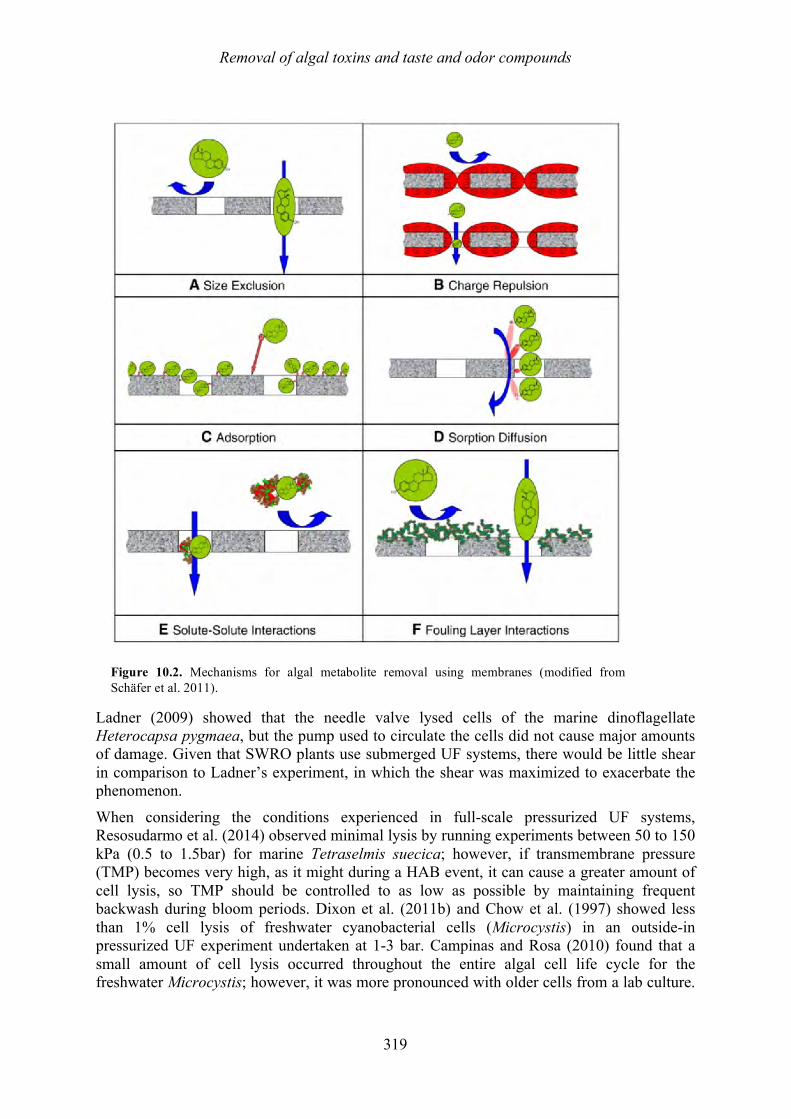
Removal of algal toxins and taste and odor compounds

319

Ladner (2009) showed that the needle valve lysed cells of the marine dinoflagellate Heterocapsa pygmaea, but the pump used to circulate the cells did not cause major amounts of damage. Given that SWRO plants use submerged UF systems, there would be little shear in comparison to Ladner’s experiment, in which the shear was maximized to exacerbate the phenomenon.

When considering the conditions experienced in full-scale pressurized UF systems, Resosudarmo et al. (2014) observed minimal lysis by running experiments between 50 to 150 kPa (0.5 to 1.5bar) for marine Tetraselmis suecica; however, if transmembrane pressure (TMP) becomes very high, as it might during a HAB event, it can cause a greater amount of cell lysis, so TMP should be controlled to as low as possible by maintaining frequent backwash during bloom periods. Dixon et al. (2011b) and Chow et al. (1997) showed less than 1% cell lysis of freshwater cyanobacterial cells (Microcystis) in an outside-in pressurized UF experiment undertaken at 1-3 bar. Campinas and Rosa (2010) found that a small amount of cell lysis occurred throughout the entire algal cell life cycle for the freshwater Microcystis; however, it was more pronounced with older cells from a lab culture.

Figure 10.2. Mechanisms for algal metabolite removal using membranes (modified from Schäfer et al. 2011).

Removal of algal toxins and taste and odor compounds

320

Dixon et al. (2011c) undertook UF experiments using flocculation/coagulation and found that encapsulation within floc protect the cell from damage.

Dixon et al. (2011b, c) showed excellent saxitoxin removal using a pressurized outside-in UF system and by keeping toxin intracellular. In one experiment, Dixon et al. (2011c) found that total saxitoxin concentrations (intracellular and extracellular combined) from the freshwater cyanobacterium Anabaena circinalis were 2.2 – 2.7 µg/L STX-eq in the feed water to a UF membrane laboratory system, of which 31–38% was extracellular (0.7–0.8 µg/L STX-eq). Results showed that when using alum coagulant, up to 68% removal of total saxitoxin was achieved in the membrane tank as intact A. circinalis cells were removed via coagulation prior to contact with the UF membrane. The majority of saxitoxin that was not removed was extracellular. Extracellular saxitoxin (STX-eq) removal by the UF membrane itself (without the effect of coagulation) was less than 20%.

Thus in UF, if TMP is minimized, intracellular metabolite removal will be maximized. Use of a coagulant can aid cellular removal and help keep toxin intracellular, while keeping TMP lower than if the coagulant was not used. 10.6 REVERSE OSMOSIS

If the pretreatment process performs properly, then a very small number of HAB cells should be present entering the RO treatment step. Therefore intracellular metabolite removal is no longer relevant and the RO mechanism is used to remove extracellular metabolites. Additionally, if the pretreatment process is optimized, there should be minimal extracellular metabolite concentration at the entry to the RO. RO is an excellent barrier for removing extracellular metabolites and the removal mechanism is the same as for removal of ‘organic micropollutants’ such as personal care products and pharmaceuticals, which has been well studied in Europe and North America (Bellona et al. 2004; Verliefde et al. 2007, 2009; Schoonenberg Kegel et al. 2010). Metabolite removal is governed by the properties of the RO (or in some cases nanofiltration (NF)) membrane and the properties of the specific metabolite itself. Bellona et al. (2004) reported that in estimating the rejection of a solute by high pressure membranes (RO, NF), properties such as molecular weight cut-off (MWCO), desalting degree, porosity, membrane morphology, and hydrophobicity of the membrane, and the molecular weight, molecular size, charge, and hydrophobicity of the solute as well as the feedwater chemistry must all be considered. A complete understanding of the solute and membrane characteristics that influence rejection could lay the foundation for a modeling approach capable of predicting the fate of specific compounds during high pressure membrane applications.

Given these mechanisms, if a metabolite is larger in molecular weight than approximately 200-300 Da (as a guide), then there will be excellent removal of the metabolite using RO. Molecules 50-200 Da are more difficult to remove by RO. While the MWCO of RO is theoretically approximately 100 Da (Dixon et al. 2012), the charge of the molecule becomes more important for the 50-200 Da molecular weight range. If the molecule is negatively charged, then the molecule will be repelled from the negatively charged RO surface. If the molecule is positively charged, then it will be attracted to the surface of the membrane and might be sorbed into the polyamide and pass into the permeate (Bellona et al. 2004; Verliefde et al. 2007, 2009; Schoonenberg Kegel et al. 2010). Fortunately, the most common HAB toxins are above 200 Da as discussed in Chapter 2. Common toxins such as domoic acid and brevetoxin are far larger than saxitoxin in MW and molecular size and will be well removed by size exclusion. Desormeaux et al. (2009) undertook a pilot study in Monterey Bay, California, and due to a lack of a natural HAB,

Removal of algal toxins and taste and odor compounds

321

kainic acid was selected as a toxin surrogate to spike into the treatment system as it has a similar chemical structure to domoic acid, but is non-toxic. Kainic acid is a natural marine acid contained in some species of seaweed and is a commonly used surrogate for domoic acid. Dissolved kainic acid was spiked at concentrations 100 - 1,000 times greater than observed during blooms of domoic acid-producing algae. Removal of the toxin surrogate was greater than 99.5% for two different RO pilot systems, with a detection limit of 0.6 µg/L in seawater and 0.017 µg/L in the RO product water. Seubert et al. (2012) undertook bench-scale RO experiments to explore the potential of extracellular algal toxins contaminating RO product waters. Concentrations exceeding maximal values previously reported during natural blooms were used in the laboratory experiments, with treatments comprised of 50 µg/L of domoic acid, 2 µg/L of saxitoxin and 20 µg/L of brevetoxin. None of the algal toxins used in the bench-scale RO experiments were detectable in the desalinated product water. In the same study by Seubert et al. (2012) monitoring for intracellular and extracellular concentrations of domoic acid and saxitoxin within the intake and RO treated water from a pilot RO desalination plant in El Segundo, California was conducted from 2005 to 2009. During the five-year monitoring period, domoic acid and saxitoxin were detected sporadically in the intake waters but never in the RO treated water. Another relevant study is that of Laycock et al. (2012) in which a small laboratory-scale RO device was used to study HAB toxin removal. Starting with 10.3 µg/mL of saxitoxin, 17.2 µg/mL of domoic acid, and 0.4 and 0.9 µg/mL of okadaic acid and brevetoxin respectively, removal was 99.4, 99.0, 99.7 and 99.9 %, respectively. While only a single pass through an RO membrane, the results are consistent with previous studies mentioned above.

Given that the only existing relevant water quality guidelines relating to algal toxins (Brazil and New Zealand) are in the range of 0.2 to 3 µg/L for saxitoxin and a worst case scenario bloom may contain up to 600 ug/L of extracellular toxin (Chapter 8, Table 8.3), 99% membrane removal can be an adequate treatment barrier for HAB toxins, depending on local guideline concentrations. With the relatively low molecular weights of saxitoxin and domoic acid (299 and 311 Da, respectively) and their hydrophilic nature, they are the most likely of the common HAB toxins to pass through RO, as their molecular weights are the closest of any HAB toxin to the theoretical MWCO of a RO membrane (~100Da). Brevetoxin (895 Da) and okadaic acid (805 Da) are approximately eight times the MWCO of a RO membrane and will therefore be easily removed. Despite saxitoxin being a smaller molecule, a study by Dixon (2014) showed that saxitoxin and its congeners were removed to 99% or greater by a tight nanofiltration membrane with a MWCO of ~100 Da (Table 10.1). The saxitoxin analogues STX, GTX 3 and 4, and C1 and 2 were removed to greater than 99% by both NF membranes. In parallel studies by Dixon et al. (2010, 2011a), it was shown that both SWRO and BWRO membranes always removed toxin more efficiently than nanofiltration membranes for toxins similar to saxitoxin in charge and size, such as cylindrospermopsin. One can thus expect RO to remove saxitoxin just as well as this particular NF membrane. This saxitoxin removal information correlates well with the work undertaken by Seubert et al. (2012). Dixon (2014) also showed that the smaller molecular weight non-toxic taste and odor compounds MIB and geosmin were removed less efficiently than for saxitoxin (71-94%) owing to their smaller molecular weight and size (168 and 182 Da respectively) (Table 10.1). Given a heavily concentrated HAB producing MIB or geosmin, if the pretreatment system completely fails and all the MIB and geosmin is extracellular, then a small amount of material may pass into the product water. Given the non-toxic nature of taste and odor compounds, the worst-case scenario would be customer complaints, but no risk to public health exists.

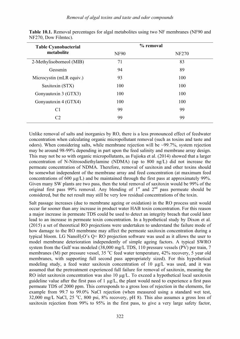
Removal of algal toxins and taste and odor compounds

322

Table 10.1. Removal percentages for algal metabolites using two NF membranes (NF90 and NF270, Dow Filmtec).

Table Cyanobacterial metabolite

% removal

NF90 NF270

2-Methylisoborneol (MIB) 71 83

Geosmin 94 89 Microcystin (mLR equiv.) 93 100

Saxitoxin (STX) 100 100 Gonyautoxin 3 (GTX3) 100 100

Gonyautoxin 4 (GTX4) 100 100 C1 99 99

C2 99 99

Unlike removal of salts and inorganics by RO, there is a less pronounced effect of feedwater concentration when calculating organic micropollutant removal (such as toxins and taste and odors). When considering salts, while membrane rejection will be ~99.7%, system rejection may be around 98-99% depending in part upon the feed salinity and membrane array design. This may not be so with organic micropollutants, as Fujioka et al. (2014) showed that a larger concentration of N-Nitrosodiethylamine (NDMA) (up to 800 ng/L) did not increase the permeate concentration of NDMA. Therefore, removal of saxitoxin and other toxins should be somewhat independent of the membrane array and feed concentration (at maximum feed concentrations of 600 µg/L) and be maintained through the first pass at approximately 99%. Given many SW plants are two pass, then the total removal of saxitoxin would be 99% of the original first pass 99% removal. Any blending of 1st and 2nd pass permeate should be considered, but the net result may still be very low residual concentrations of the toxin.

Salt passage increases (due to membrane ageing or oxidation) in the RO process unit would occur far sooner than any increase in product water HAB toxin concentration. For this reason a major increase in permeate TDS could be used to detect an integrity breach that could later lead to an increase in permeate toxin concentration. In a hypothetical study by Dixon et al. (2015) a set of theoretical RO projections were undertaken to understand the failure mode of how damage to the RO membrane may affect the permeate saxitoxin concentration during a typical bloom. LG NanoH2O’s Q+ RO projection software was used as it allows the user to model membrane deterioration independently of simple ageing factors. A typical SWRO system from the Gulf was modeled (38,000 mg/L TDS, 110 pressure vessels (PV) per train, 7 membranes (M) per pressure vessel, 35 oC feed water temperature, 42% recovery, 5 year old membranes, with supporting full second pass appropriately sized). For this hypothetical modeling study, a feed water saxitoxin concentration of 10 µg/L was used, and it was assumed that the pretreatment experienced full failure for removal of saxitoxin, meaning the RO inlet saxitoxin concentration was also 10 µg/L. To exceed a hypothetical local saxitoxin guideline value after the first pass of 1 µg/L, the plant would need to experience a first pass permeate TDS of 2000 ppm. This corresponds to a gross loss of rejection in the elements, for example from 99.7 to 99.0% NaCl rejection (when measured using a standard wet test, 32,000 mg/L NaCl, 25 oC, 800 psi, 8% recovery, pH 8). This also assumes a gross loss of saxitoxin rejection from 99% to 95% in the first pass, to give a very large safety factor,

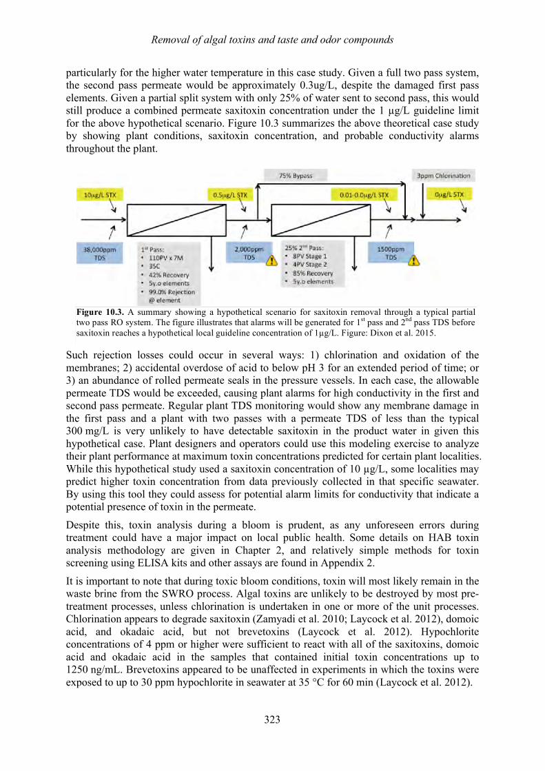
Removal of algal toxins and taste and odor compounds

323

particularly for the higher water temperature in this case study. Given a full two pass system, the second pass permeate would be approximately 0.3ug/L, despite the damaged first pass elements. Given a partial split system with only 25% of water sent to second pass, this would still produce a combined permeate saxitoxin concentration under the 1 µg/L guideline limit for the above hypothetical scenario. Figure 10.3 summarizes the above theoretical case study by showing plant conditions, saxitoxin concentration, and probable conductivity alarms throughout the plant.

Such rejection losses could occur in several ways: 1) chlorination and oxidation of the membranes; 2) accidental overdose of acid to below pH 3 for an extended period of time; or 3) an abundance of rolled permeate seals in the pressure vessels. In each case, the allowable permeate TDS would be exceeded, causing plant alarms for high conductivity in the first and second pass permeate. Regular plant TDS monitoring would show any membrane damage in the first pass and a plant with two passes with a permeate TDS of less than the typical 300 mg/L is very unlikely to have detectable saxitoxin in the product water in given this hypothetical case. Plant designers and operators could use this modeling exercise to analyze their plant performance at maximum toxin concentrations predicted for certain plant localities. While this hypothetical study used a saxitoxin concentration of 10 µg/L, some localities may predict higher toxin concentration from data previously collected in that specific seawater. By using this tool they could assess for potential alarm limits for conductivity that indicate a potential presence of toxin in the permeate.

Despite this, toxin analysis during a bloom is prudent, as any unforeseen errors during treatment could have a major impact on local public health. Some details on HAB toxin analysis methodology are given in Chapter 2, and relatively simple methods for toxin screening using ELISA kits and other assays are found in Appendix 2.

It is important to note that during toxic bloom conditions, toxin will most likely remain in the waste brine from the SWRO process. Algal toxins are unlikely to be destroyed by most pre-treatment processes, unless chlorination is undertaken in one or more of the unit processes. Chlorination appears to degrade saxitoxin (Zamyadi et al. 2010; Laycock et al. 2012), domoic acid, and okadaic acid, but not brevetoxins (Laycock et al. 2012). Hypochlorite concentrations of 4 ppm or higher were sufficient to react with all of the saxitoxins, domoic acid and okadaic acid in the samples that contained initial toxin concentrations up to 1250 ng/mL. Brevetoxins appeared to be unaffected in experiments in which the toxins were exposed to up to 30 ppm hypochlorite in seawater at 35 °C for 60 min (Laycock et al. 2012).

Figure 10.3. A summary showing a hypothetical scenario for saxitoxin removal through a typical partial two pass RO system. The figure illustrates that alarms will be generated for 1st pass and 2nd pass TDS before saxitoxin reaches a hypothetical local guideline concentration of 1µg/L. Figure: Dixon et al. 2015.

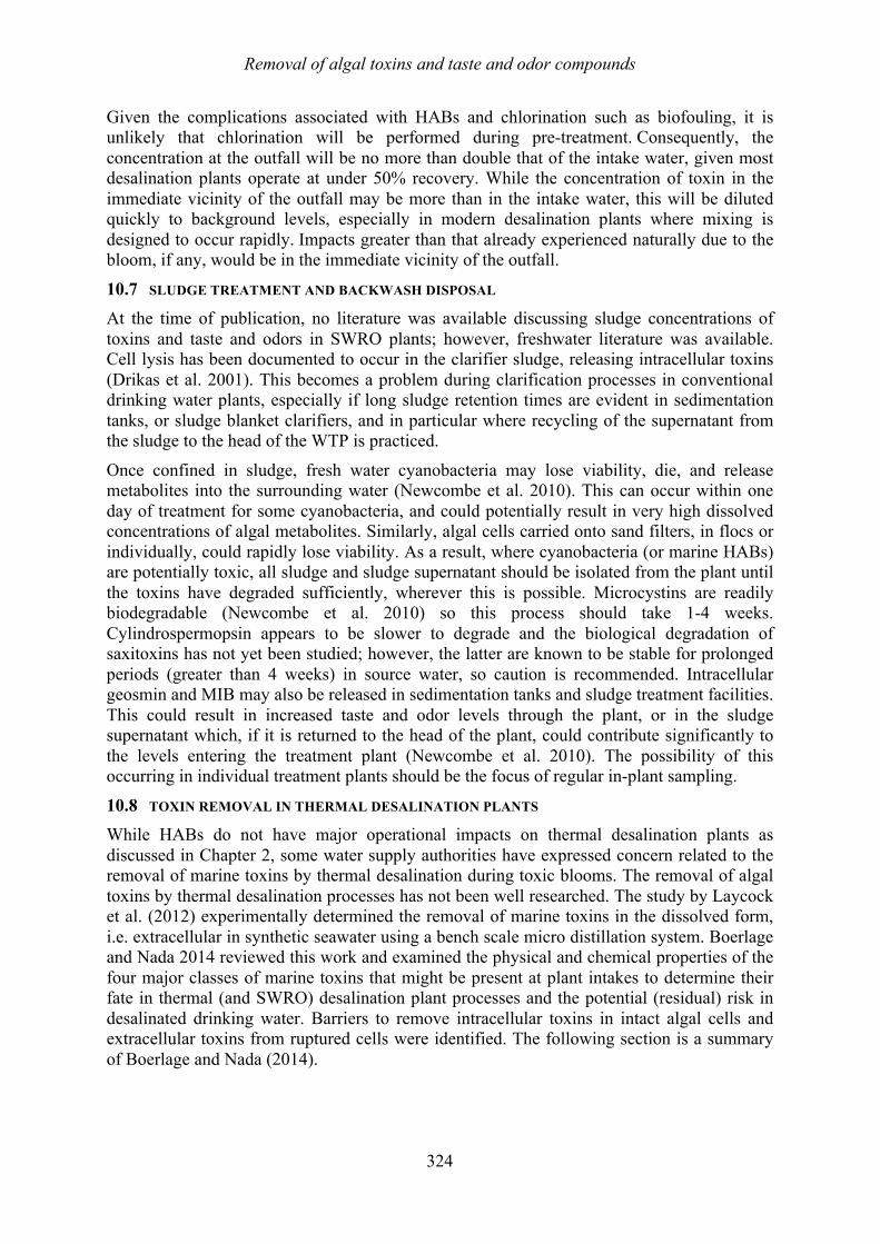
Removal of algal toxins and taste and odor compounds

324

Given the complications associated with HABs and chlorination such as biofouling, it is unlikely that chlorination will be performed during pre-treatment. Consequently, the concentration at the outfall will be no more than double that of the intake water, given most desalination plants operate at under 50% recovery. While the concentration of toxin in the immediate vicinity of the outfall may be more than in the intake water, this will be diluted quickly to background levels, especially in modern desalination plants where mixing is designed to occur rapidly. Impacts greater than that already experienced naturally due to the bloom, if any, would be in the immediate vicinity of the outfall.

10.7 SLUDGE TREATMENT AND BACKWASH DISPOSAL At the time of publication, no literature was available discussing sludge concentrations of toxins and taste and odors in SWRO plants; however, freshwater literature was available. Cell lysis has been documented to occur in the clarifier sludge, releasing intracellular toxins (Drikas et al. 2001). This becomes a problem during clarification processes in conventional drinking water plants, especially if long sludge retention times are evident in sedimentation tanks, or sludge blanket clarifiers, and in particular where recycling of the supernatant from the sludge to the head of the WTP is practiced.

Once confined in sludge, fresh water cyanobacteria may lose viability, die, and release metabolites into the surrounding water (Newcombe et al. 2010). This can occur within one day of treatment for some cyanobacteria, and could potentially result in very high dissolved concentrations of algal metabolites. Similarly, algal cells carried onto sand filters, in flocs or individually, could rapidly lose viability. As a result, where cyanobacteria (or marine HABs) are potentially toxic, all sludge and sludge supernatant should be isolated from the plant until the toxins have degraded sufficiently, wherever this is possible. Microcystins are readily biodegradable (Newcombe et al. 2010) so this process should take 1-4 weeks. Cylindrospermopsin appears to be slower to degrade and the biological degradation of saxitoxins has not yet been studied; however, the latter are known to be stable for prolonged periods (greater than 4 weeks) in source water, so caution is recommended. Intracellular geosmin and MIB may also be released in sedimentation tanks and sludge treatment facilities. This could result in increased taste and odor levels through the plant, or in the sludge supernatant which, if it is returned to the head of the plant, could contribute significantly to the levels entering the treatment plant (Newcombe et al. 2010). The possibility of this occurring in individual treatment plants should be the focus of regular in-plant sampling.

10.8 TOXIN REMOVAL IN THERMAL DESALINATION PLANTS While HABs do not have major operational impacts on thermal desalination plants as discussed in Chapter 2, some water supply authorities have expressed concern related to the removal of marine toxins by thermal desalination during toxic blooms. The removal of algal toxins by thermal desalination processes has not been well researched. The study by Laycock et al. (2012) experimentally determined the removal of marine toxins in the dissolved form, i.e. extracellular in synthetic seawater using a bench scale micro distillation system. Boerlage and Nada 2014 reviewed this work and examined the physical and chemical properties of the four major classes of marine toxins that might be present at plant intakes to determine their fate in thermal (and SWRO) desalination plant processes and the potential (residual) risk in desalinated drinking water. Barriers to remove intracellular toxins in intact algal cells and extracellular toxins from ruptured cells were identified. The following section is a summary of Boerlage and Nada (2014).

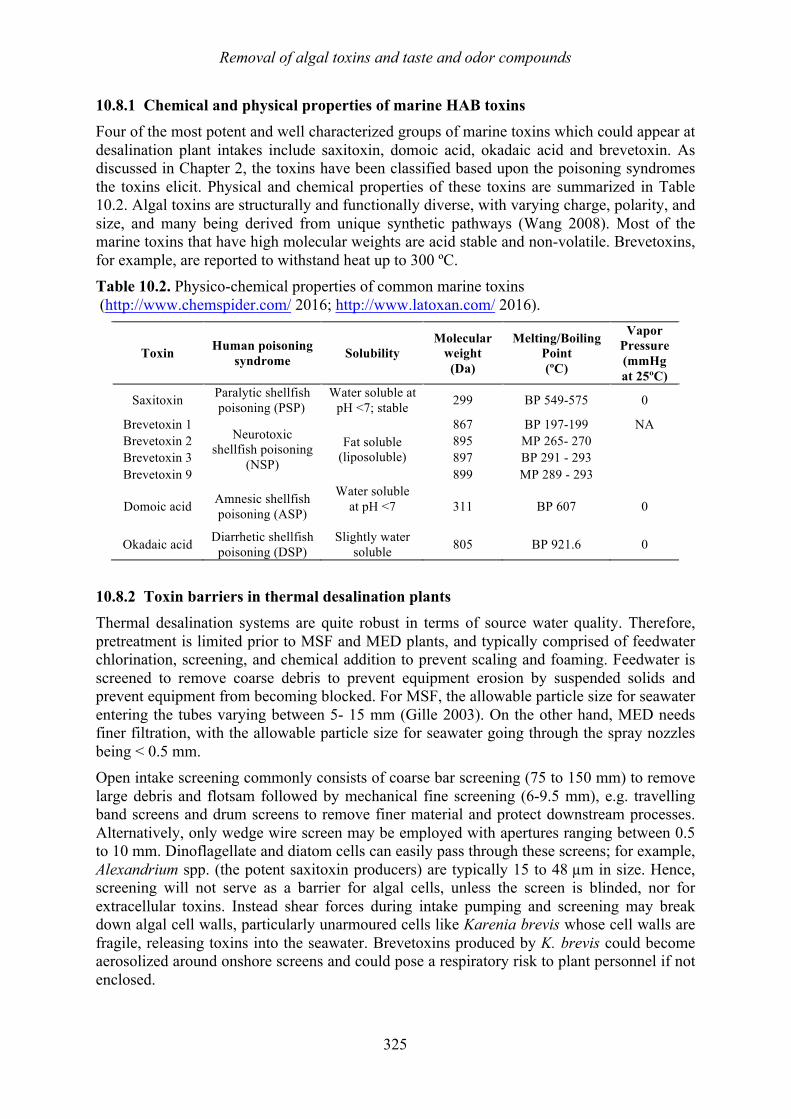
Removal of algal toxins and taste and odor compounds

325

10.8.1 Chemical and physical properties of marine HAB toxins Four of the most potent and well characterized groups of marine toxins which could appear at desalination plant intakes include saxitoxin, domoic acid, okadaic acid and brevetoxin. As discussed in Chapter 2, the toxins have been classified based upon the poisoning syndromes the toxins elicit. Physical and chemical properties of these toxins are summarized in Table 10.2. Algal toxins are structurally and functionally diverse, with varying charge, polarity, and size, and many being derived from unique synthetic pathways (Wang 2008). Most of the marine toxins that have high molecular weights are acid stable and non-volatile. Brevetoxins, for example, are reported to withstand heat up to 300 ºC. Table 10.2. Physico-chemical properties of common marine toxins (http://www.chemspider.com/ 2016; http://www.latoxan.com/ 2016).

Toxin Human poisoning syndrome Solubility

Molecular weight (Da)

Melting/Boiling Point (ºC)

Vapor Pressure (mmHg at 25ºC)

Saxitoxin Paralytic shellfish poisoning (PSP)

Water soluble at pH <7; stable 299 BP 549-575 0

Brevetoxin 1 Neurotoxic

shellfish poisoning (NSP)

Fat soluble (liposoluble)

867 BP 197-199 NA Brevetoxin 2 895 MP 265- 270 Brevetoxin 3 897 BP 291 - 293 Brevetoxin 9 899 MP 289 - 293

Domoic acid Amnesic shellfish poisoning (ASP)

Water soluble at pH <7

311 BP 607 0

Okadaic acid Diarrhetic shellfish poisoning (DSP)

Slightly water soluble 805 BP 921.6 0

10.8.2 Toxin barriers in thermal desalination plants Thermal desalination systems are quite robust in terms of source water quality. Therefore, pretreatment is limited prior to MSF and MED plants, and typically comprised of feedwater chlorination, screening, and chemical addition to prevent scaling and foaming. Feedwater is screened to remove coarse debris to prevent equipment erosion by suspended solids and prevent equipment from becoming blocked. For MSF, the allowable particle size for seawater entering the tubes varying between 5- 15 mm (Gille 2003). On the other hand, MED needs finer filtration, with the allowable particle size for seawater going through the spray nozzles being < 0.5 mm. Open intake screening commonly consists of coarse bar screening (75 to 150 mm) to remove large debris and flotsam followed by mechanical fine screening (6-9.5 mm), e.g. travelling band screens and drum screens to remove finer material and protect downstream processes. Alternatively, only wedge wire screen may be employed with apertures ranging between 0.5 to 10 mm. Dinoflagellate and diatom cells can easily pass through these screens; for example, Alexandrium spp. (the potent saxitoxin producers) are typically 15 to 48 µm in size. Hence, screening will not serve as a barrier for algal cells, unless the screen is blinded, nor for extracellular toxins. Instead shear forces during intake pumping and screening may break down algal cell walls, particularly unarmoured cells like Karenia brevis whose cell walls are fragile, releasing toxins into the seawater. Brevetoxins produced by K. brevis could become aerosolized around onshore screens and could pose a respiratory risk to plant personnel if not enclosed.

Removal of algal toxins and taste and odor compounds

326

Chemical conditioning is utilized in thermal desalination in two treatment streams: the seawater cooling water component and the seawater makeup water (used within the desalination process). An oxidizing agent (usually chlorine) or biocide is continuously added to the cooling water to prevent marine fouling, while antiscalants are continuously dosed to prevent scaling on the heat exchanger surfaces. In addition, antifoaming agents are continuously added to thermal process to prevent foaming in the deaerator and flash chambers. Neither the antifoaming chemicals (polypropylene/polyethylene oxide, isopropanol) nor the antiscalant (commonly polyacrylactes, polycarboxylic acids) are expected to assist in removal of algal cells or detoxification of extracellular toxins. Antiscalants are designed to modify crystal formation and disperse scaling ions and not oxidize organic matter. Antifoam agents may have an effect on organic compounds associated with algal blooms, but are not expected to degrade the toxin itself.

Most thermal desalination plants practice continuous chlorination at the seawater intake to provide a residual chlorine concentration of approximately 0.15 – 0.3 mg/L to prevent fouling marine growth in piping and biofilm formation on heat exchange surfaces. Chlorination has also been proven to detoxify some marine toxins, with domoic acid the most sensitive to chlorine - requiring only 1 ppm hypochlorite. Exposure to ≥ 4 ppm hypochlorite for 10 min at 37 ºC completely destroyed saxitoxin and okadic acid (Laycock et al. 2012); however, brevetoxin (3 and 300 µg/L concentration) was unaffected by exposure to hypochlorite up to 30 ppm for one hour. Hence, chlorination is not a barrier for all marine toxins. The experiments of Laycock et al. (2012) were in synthetic seawater with toxins isolated from laboratory cultures. In practice the higher organics present during a bloom will exert a chlorine demand, thereby reducing the efficiency of toxin degradation by chlorination, potentially rendering it impractical as a degradation strategy. It is unlikely that continuous chlorination of intake seawater can be applied at 4 ppm hypochlorite in thermal desalination plants. In addition to increasing chemical consumption costs, the higher concentration of chlorine will have a deleterious effect on the venting system and plant corrosion and the guarantee values of various equipment may be exceeded. Finally, as discussed earlier in this chapter, chlorine can result in the lysis of algal cells, thereby releasing intracellular toxins into solution. Hence, chlorination should be avoided during a HAB when possible.

In thermal desalination systems, volatile and semi-volatile organics with boiling points lower than water’s boiling point may carry over in the steam to contaminate the distillate and therefore are vented out in the process. It is often assumed that high molecular weight organics with high boiling points will remain in the brine, but this can sometimes be erroneous. This is because the evaporation of organics from seawater and their condensation into distillates is governed by a multitude of factors such as the temperature and pressure of the MSF stage or MED effect and the concentration, vapor pressure, latent heat of condensation of the individual compounds (Kutty et al. 1994).

The four major toxins presented in Table 10.2 are all reported to be heat stable, have low vapor pressures, and are non volatile. The boiling points of saxitoxins, domoic acid, and okadaic acid are significantly higher than water (at atmospheric pressure). Similarly, the boiling point of brevetoxin is higher than that of water. These factors would suggest that the toxins will not carry over in thermal desalination systems or co-distill, but instead will remain in the flashing brine.

The results of Laycock et al. (2012) support high removal of toxins in the MSF and MED desalination processes. The maximum temperature in that study was 104 ºC which is approaching the top brine temperature of MSF (90 to 112 °C), but above MED (60 and 64°C). Three of the toxins, at unusually high test concentrations for the marine environment,

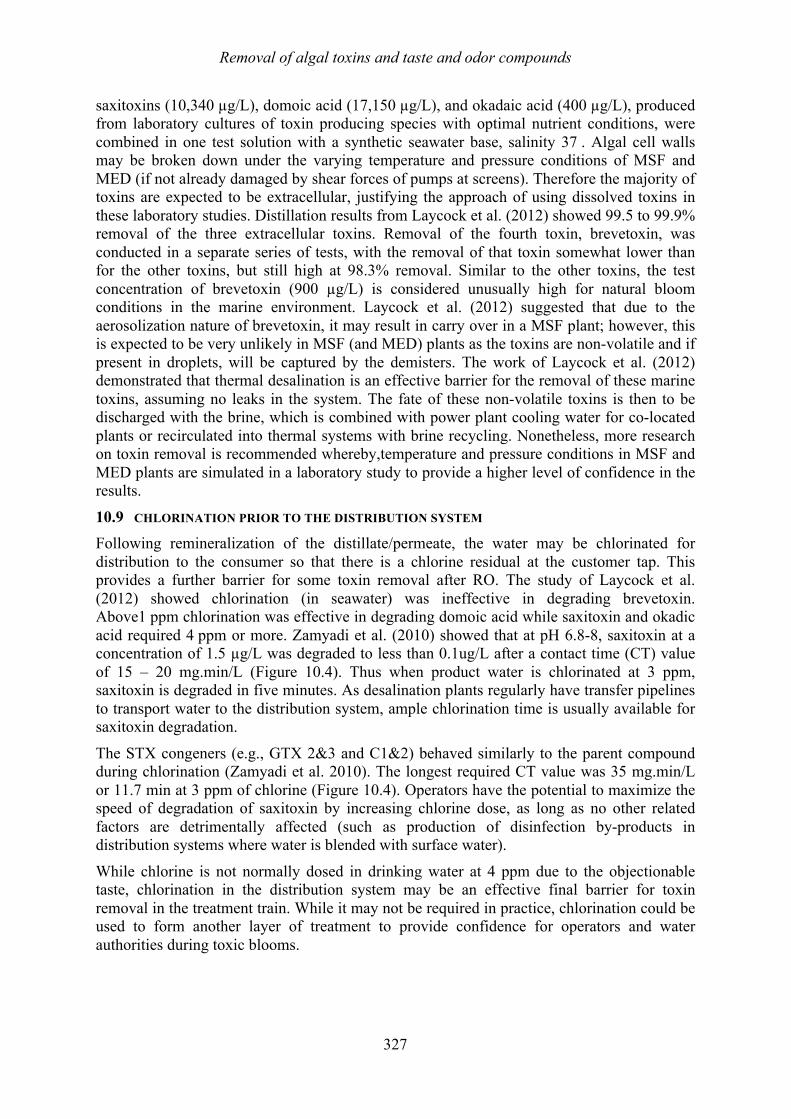
Removal of algal toxins and taste and odor compounds

327

saxitoxins (10,340 µg/L), domoic acid (17,150 µg/L), and okadaic acid (400 µg/L), produced from laboratory cultures of toxin producing species with optimal nutrient conditions, were combined in one test solution with a synthetic seawater base, salinity 37 . Algal cell walls may be broken down under the varying temperature and pressure conditions of MSF and MED (if not already damaged by shear forces of pumps at screens). Therefore the majority of toxins are expected to be extracellular, justifying the approach of using dissolved toxins in these laboratory studies. Distillation results from Laycock et al. (2012) showed 99.5 to 99.9% removal of the three extracellular toxins. Removal of the fourth toxin, brevetoxin, was conducted in a separate series of tests, with the removal of that toxin somewhat lower than for the other toxins, but still high at 98.3% removal. Similar to the other toxins, the test concentration of brevetoxin (900 µg/L) is considered unusually high for natural bloom conditions in the marine environment. Laycock et al. (2012) suggested that due to the aerosolization nature of brevetoxin, it may result in carry over in a MSF plant; however, this is expected to be very unlikely in MSF (and MED) plants as the toxins are non-volatile and if present in droplets, will be captured by the demisters. The work of Laycock et al. (2012) demonstrated that thermal desalination is an effective barrier for the removal of these marine toxins, assuming no leaks in the system. The fate of these non-volatile toxins is then to be discharged with the brine, which is combined with power plant cooling water for co-located plants or recirculated into thermal systems with brine recycling. Nonetheless, more research on toxin removal is recommended whereby,temperature and pressure conditions in MSF and MED plants are simulated in a laboratory study to provide a higher level of confidence in the results.

10.9 CHLORINATION PRIOR TO THE DISTRIBUTION SYSTEM Following remineralization of the distillate/permeate, the water may be chlorinated for distribution to the consumer so that there is a chlorine residual at the customer tap. This provides a further barrier for some toxin removal after RO. The study of Laycock et al. (2012) showed chlorination (in seawater) was ineffective in degrading brevetoxin. Above1 ppm chlorination was effective in degrading domoic acid while saxitoxin and okadic acid required 4 ppm or more. Zamyadi et al. (2010) showed that at pH 6.8-8, saxitoxin at a concentration of 1.5 µg/L was degraded to less than 0.1ug/L after a contact time (CT) value of 15 – 20 mg.min/L (Figure 10.4). Thus when product water is chlorinated at 3 ppm, saxitoxin is degraded in five minutes. As desalination plants regularly have transfer pipelines to transport water to the distribution system, ample chlorination time is usually available for saxitoxin degradation.

The STX congeners (e.g., GTX 2&3 and C1&2) behaved similarly to the parent compound during chlorination (Zamyadi et al. 2010). The longest required CT value was 35 mg.min/L or 11.7 min at 3 ppm of chlorine (Figure 10.4). Operators have the potential to maximize the speed of degradation of saxitoxin by increasing chlorine dose, as long as no other related factors are detrimentally affected (such as production of disinfection by-products in distribution systems where water is blended with surface water).

While chlorine is not normally dosed in drinking water at 4 ppm due to the objectionable taste, chlorination in the distribution system may be an effective final barrier for toxin removal in the treatment train. While it may not be required in practice, chlorination could be used to form another layer of treatment to provide confidence for operators and water authorities during toxic blooms.

Removal of algal toxins and taste and odor compounds

328

Taste and odor compounds like geosmin are not degraded by chlorination. Geosmin is very well detected by smell and taste, at around 10 ng/L, but is not toxic. It is therefore regularly detected by customers of river and reservoir water. It will be removed moderately well by RO

(80-95%) (Dixon et al. 2010, 2011a) and more so by a full two pass RO. Typical bloom concentration in river and reservoir sources can be as high as 100 ng/L. The instrument detection limit for GC/MS is 4 ng/L and a full two pass system will approximately produce a permeate concentration of this value given a worst-case scenario, if geosmin is allowed to stay intracellular for best removal during pretreatment.

Operators may consider chlorination experiments on remineralized distillate/permeate to see whether chlorination is effective in fresh water and whether a lower dose than that used by Laycock et al. (2012) might be effective in degrading saxitoxin and okadic acid. As degradation of toxins is pH dependent, this would need to be investigated in these experiments. Given the current status of research on the effect of chlorination in degrading marine toxins, further work is clearly required for greater confidence in chlorination as a final barrier to all common HAB toxins. 10.10 SUMMARY

This chapter describes the process steps within SWRO and thermal desalination that specifically remove HAB toxin and taste and odor compounds and the limitations of each process step. The general principle for HAB toxin and taste and odor compound removal is to ensure toxin remains intracellular to maximize the removal efficiency of each pretreatment step. By avoiding chlorination of the intake or any shock chlorinations during a HAB bloom, cells will not be ruptured and release toxin. In SWRO plants, extracellular toxin is difficult for the downstream processes to remove, apart from the RO process. DAF will effectively remove intact cells to approximately greater than 90%, thus removing intracellular toxin along with the cells. GMF will remove similar percentages of intracellular toxins to DAF.

Figure 10.4. Toxin oxidation in Myponga Reservoir water at pH 8 with 3 mg/L (solid line) chlorine dose (a) STX, (b) GTX2 (c) GTX3 (d) C1 and (e) C2. (Dashed line represents chlorination at 2 mg/L) (modified from Zamyadi et al. 2010)

Removal of algal toxins and taste and odor compounds

329

UF/MF will remove greater than 99% of HAB cells and associated intracellular toxins, although some minor leakage of toxins from the cells may occur due to shear and pressure in the unit process. RO is the major toxin removal step and removes greater than 99% of extracellular toxin. A two pass system will remove another 99% of the remaining 1% extracellular toxin, although operators should take care to assess a partial split two pass system. Taste and odor compounds are difficult to remove when extracellular. Should off taste and odor occur with the HAB bloom, pretreatment will remove intracellular compounds to greater than 90% (similar to removal of toxins), while each full RO pass will remove 60-80% of the extracellular taste and odor. Chlorination will not remove taste and odor compounds. As common HAB tase and odor compounds can be detected at around 10ng/L, single pass RO systems may experience customer complaints. Any sludge produced from pretreatment will still contain toxin and care must be taken when considering any supernatant return to the plant or disposal of the sludge. Removal of toxins from thermal systems should be in the order of 99%, and toxin should exit the plant in the brine. As an additional barrier to toxin removal, some toxins are denatured by chlorination, for example saxitoxin (STX) will be removed with a CT of 15 µg.min/L. Thus the inherent multiple barrier approach to seawater desalination systems creates an effective removal system for HAB toxin with built in redundancy.

10.11 REFERENCES Azanza, M. P. V., Azanza, R. V., Gedaria, A. I., Sententa, H. G., and Idjao, M. V. 2001.

Decimal reduction times of Pyrodinium bahamense var. compressum and Escherichia coli in chlorine- and ultraviolet-treated seawater. Letters in Applied Microbiology 33(5), 371-376.

Bellona, C., Drewes, J. E., Xu, P., and Amy, G. 2004. Factor affecting the rejection of during NF/RO treatment - a literature review. Water Research 38, 2795-2809.

Boerlage, S. F. E., and Nada, N. 2014. Algal toxin removal in seawater desalination processes, In: Proceedings of European Desalination Society, Cyprus.

Campinas, M., and Rosa, M. J. 2010. Evaluation of cyanobacterial cells removal and lysis by ultrafiltration. Separation and Purification Technology 70, 345-353.

Chemspider. 2016. www.chemspider.com. Royal Society of Chemistry, Accessed 13 Feb 2016.

Chow, C. W. K., Drikas, M., House, J., Burch, M. D., and Velzeboer, R. M. A. 1999. The impact of conventional water treatment processes on cells of the cyanobacterium Microcystis aeruginosa. Water Research 33(15), 3253–3262.

Chow, C.W.K., House, J., Velzeboer, R.M.A., 1998. The effect of ferric chloride flocculation on cyanobacterial cells. Water Research 32, 808–814.

Chow, C. W. K., Panglish, S., House, J., Drikas, M., Burch, M. D., and Gimbel, R. 1997. A study of membrane filtration for the removal of cyanobacterial cells. Aqua, 46(6), 324–334.

Daly, R. I., Ho, L., and Brookes, J. D. 2007. Effect of chlorination on Microcystis aeruginosa cell integrity and subsequent microcystin release and degradation. Environmental Science and Technology 41(12), 4447-4453.

DesalData. 2015. Worldwide desalination inventory (MS Excel Format), downloaded from DesalData.com (GWI/IDA) 2015.

Removal of algal toxins and taste and odor compounds

330

Desormeaux, E. D., Meyerhofer, P. F., and Luckenbach, H. 2009. Results from nine investigations assessing Pacific Ocean seawater desalination in Santa Cruz, California. Proceedings of the IDA World Congress, Dubai, UAE, November 2009.

Desormeaux, E. D., Meyerhofer, P. F., Luckenbach, H., and Kudela, R. M. 2011. Pilot-testing multiple pretreatment systems for seawater desalination. IDA Journal of Desalination and Reuse 3(1), 42-52.

Dixon, M. B. 2014. Removal of toxin and taste & odor compounds using membranes and associated processes. Proceedings of the Middle East Desalination Research Centre’s HABs and Desalination workshop, Muscat, Oman, April 2014.

Dixon, M. B., Churman, H., and Henthorne, L. 2015. Harmful algae blooms and desalination: a cells journey from sea to SWRO. Proceedings of the IDA World Congress, San Diego, California, Sept 2015.

Dixon, M. B., Falconet, C., Ho, L., Chow, C. W. K., O’Neil, B., and Newcombe, G. 2010. Nanofiltration for the removal of algal metabolites and the effects of fouling. Water Science and Technology 61, 1189–1199.

Dixon, M. B., Falconet, C., Ho, L., Chow, C. W. K., O’Neil, B. and Newcombe, G. 2011a. Removal of cyanobacterial metabolites by nanofiltration from two treated waters. Journal of Hazardous Materials 188(1), 288–295.

Dixon M. B., Ho, L., Chow, C., Newcombe, G., Croue, J-P., Buisson, H., Cigana, J., and Treuger, R. 2012. Water Research Foundation Report #4016: Evaluation of integrated membranes for taste and odour and algal toxin control, Published by Water Research Foundation, Denver, Colorado, USA.

Dixon, M. B., Richard, Y., Ho, L., Chow, C. W. K., O’Neil, B. and Newcombe, G. 2011b. A coagulation-powdered activated carbon-ultrafiltration – Multiple barrier approach for removing toxins from two Australian cyanobacterial blooms. Journal of Hazardous Materials 186(2), 1553–1559.

Dixon, M. B., Richard, Y., Ho, L., Chow, C. W. K., O’Neil, B., and Newcombe, G. 2011c. Integrated membrane systems incorporating coagulation, activated carbon and ultrafiltration for the removal of toxic cyanobacterial metabolites from Anabaena circinalis. Water Science and Technology 63(7), 1405-1411.

Drikas, M., Chow, C. W. K., House, J. and Burch, M. D. 2001. Using coagulation, flocculation, and settling to remove toxic cyanobacteria. Journal American Water Works Association 93, 100–111.

Fujioka, T., Tu, K. L., Khan, S. J., McDonald, J. A., Roux, A., Poussade, Y., Drewes, J. E., and Nghiem. L .D. 2014. Rejection of small solutes by reverse osmosis membranes for water reuse applications: a pilot-scale study. Desalination 350, 28-34.

Gille, D. 2003. Seawater intakes for desalination plants. Desalination 156(1), 249-256. Kutty P. C. M., Nomani, A. A. and Thankachan,T. S. 1994. Carry over of some high

molecular weight organics from seawater to MSF distillates SWCC RDC 25 Technical Report.

Ladner, D. A. 2009. Effects of bloom-forming algae on fouling of integrated membrane systems in seawater desalination. PhD dissertation, University of Illinois at Urbana-Champaign.

Removal of algal toxins and taste and odor compounds

331

Laycock, M. V., Anderson, D. M., Naar, J., Goodman, A., Easy, D. J., Donovan, M. A., Li, A., Quilliam, M. A., Al Jamali, E., and Alshihi, R. 2012. Laboratory desalination experiments with some algal toxins. Desalination 293, 1-6.

Lefebvre, K. A., Bill, B. D., Costa, P. R., Nance, S., Erickson, A., Trainer, V. L., and Baugh, K. A. 2008. Characterization of intracellular and extracellular saxitoxin levels in both field and cultured Alexandrium spp. samples from Sequim Bay, Washington. Marine Drugs 6(2), 103-116.

McDowall, B. 2008. Removal of geosmin and 2-methylisoborneol from drinking water through biologically active sand filters. PhD Thesis, The University of Adelaide.

Newcombe, G. 2011. Personal Communication.

Newcombe, G., House, J., Ho, L., Baker, P., and Burch, M. 2010. Management strategies for cyanobacteria (blue-greenalgae): a guide for water utilities: cooperative research centre for water quality and treatment research report #74.

Pierce, R. H., Henry, M. S., Higham, C. J., Blum, P., Sengco, M. R. and Anderson, D. M. 2004. Removal of harmful algal cells (Karenia brevis) and toxins from seawater culture by clay flocculation. Harmful Algae 3(2), 141–148.

Qian, F., Dixon, D. R., Newcombe, G., Ho, L., Dreyfus, J. and Scales, P. J. 2014. The effect of pH on the release of metabolites by cyanobacteria in conventional water treatment processes. Harmful Algae 39, 253-258.

Resosudarmo, A. Ye, Y. Le-Clech, P.. amd Chen, V. 2014. UF pretreatment for desalination during algal blooms: Negative effects of stress and benefits of hybridised systems. Proceedings of the HABs and Desalination Worksop, Muscat, Oman April 2014.

Schaefer, A., Akanyeti, I., and Semiao, A. J. C. 2011. Micropollutant sorption to membrane polymers: A review of mechanisms for estrogens. Advances in Colloid and Interface Science 164(1–2), 100-117.

Schoonenberg Kegel, F., Rietman, B. M., and Verliefde, A. R. D. 2010. Reverse osmosis followed by activated carbon filtration for efficient removal of organic micropollutants from river bank filtrate. Water Science and Technology 61(10), 2603-2610.

Seubert, E. L., Trussell, S., Eagleton, J., Schnetzer, A., Cetinic, I., Lauri, P., Jones, B. H., and Caron, D. A. 2012. Algal toxins and reverse osmosis desalination operations: laboratory bench testing and field monitoring of domoic acid, saxitoxin, brevetoxin and okadaic acid. Water Research 46(19), 6563-6573.

Smith, J. L., Tong, M., Fux, E., and Anderson D. M. 2012. Toxin production, retention, and extracellular release by Dinophysis acuminate during extended stationary phase and culture decline. Harmful Algae 19, 125–132.

Teixeira, M. R., Sousa, V., and Rosa, M. J. 2010. Investigating dissolved air flotation performance with cyanobacterial cells and filaments. Water Research 44(11), 3337-3344.

Teixeira, M. R. and Rosa, M. J. 2006. Comparing dissolved air flotation and conventional sedimentation to remove cyanobacterial cells of Microcystis aeruginosa. Part I: The key operating conditions. Separation and Purification Technology 52(1), 84-94.

Teixeira, M. R. and Rosa, M. J. 2007. Comparing dissolved air flotation and conventional sedimentation to remove cyanobacterial cells of Microcystis aeruginosa. Part II. The effect of water background organics. Separation and Purification Technology 53(1), 126-134.

Removal of algal toxins and taste and odor compounds

332

Verliefde, A. R. D., Cornelissen, E. R., Amy, G., Van der Bruggen, B., and Van Dijk, H. 2007. Priority organic micropollutants in water sources in Flanders and the Netherlands and assessment of removal possibilities with nanofiltration. Environmental Pollution 146(1), 281-289.

Verliefde, A. R. D., Cornelissen, E. R., Heijman, S. G. J., Verberk, J. Q. J. C. and Amy, G. L. 2009. Construction and validation of a full-scale model for rejection of organic micropollutants by NF membranes. Journal of Membrane Science 339(1), 10-20.

Velzeboer, R., Drikas, M., Donati, C., Burch, M., and Steffensen, D. 1995. Release of geosmin by Anabaena circinalis following treatment with aluminium sulphate. Water Science and Technology 31, 187–194.

Villacorte, L. O. Algal Blooms and Membrane Based Desalination Technology, UNESCO-IHE PhD Thesis Dissertation, May 20 2014.

Wiley, R. 2014. Proceeding of the American Membrane Technology Membrane Technology Conference, March 2014, Las Vegas, NV.

Wang D.-Z. 2008. Neurotoxins from marine dinoflagellates: a brief review. Marine Drugs 6(2): 349-371.

www.latoxan.com. Natural Active ingredients, Accessed 13 Feb 2016. Zamyadi, A., Ho, L., Newcombe, G., Daly, R. I., Burch, M., and Baker, P. 2010. Release and

oxidation of cell-bound saxitoxins during chlorination of Anabaena circinalis cells. Environmental Science and Technology 44(23), 9055-61.

Zhu, I. X. and Bates, B. 2012. Seawater desalination pretreatment for harmful algae blooms using dissolved air flotation. IDA Journal of Desalination and Water Reuse 4(1), 34-37.

Zhu, I. X., Bates, B. J. and Anderson, D. M. 2014. Removal of Prorocentrum minimum from seawater using dissolved air flotation. Journal of Applied Water Engineering and Research 2(1), 47-56.

Case histories for HABs in desalination

333

11 CASE HISTORIES FOR HARMFUL ALGAL BLOOMS IN DESALINATION

Siobhan F.E. Boerlage1, Mike B. Dixon2 and Donald M. Anderson3 1 Boerlage Consulting, Gold Coast, Queensland, Australia

2 MDD Consulting, Kensington, Calgary, Alberta, Canada 3Woods Hole Oceanographic Institution, Woods Hole, MA USA

11.1 Introduction ........................................................................................................................................... 333 11.2 Fujairah 2, United Arab Emirates – Effects of harmful algal blooms on plant operations in 2008 and 2013 ....................................................................................................................................... 347 11.3 Sohar, Oman – Harmful algal bloom impact on membrane pretreatment: challenges and solutions ... 355 11.4 Barka 1, Oman - The impact of harmful algal blooms on the performance stability of UF

pretreatment ........................................................................................................................................... 367 11.5 Shuwaikh, Kuwait – Harmful algal bloom cell removal using dissolved air flotation: pilot and laboratory studies ................................................................................................................... 383 11.6 La Chimba, Antofagasta, Chile – Oxygen depletion and hydrogen sulfide gas mitigation due to harmful algal blooms ............................................................................................................................. 391 11.7 Mejillones, Chile – Operation of the ultrafiltration system during harmful algal blooms at the Gas Atacama SWRO plant .............................................................................................................. 399 11.8 Antofagasta, Chile - Abengoa water micro/ultrafiltration pretreatment pilot plant .............................. 409 11.9 Tampa Bay, Florida (USA) – Non-toxic algal blooms and operation of the SWRO plant detailing monitoring program for blooms ............................................................................................. 417 11.10 Jacobahaven, The Netherlands – Ultrafiltration for SWRO pretreatment: a demonstration plant ........ 425 11.11 Barcelona, Spain – SWRO demonstration plant: DAF/DMF versus DAF/UF ..................................... 439 11.12 Gold Coast, Queensland, Australia - Deep water intake limits Trichodesmium ingress ....................... 447 11.13 Berlin, Germany – akvola: An integrated DAF-UF pilot ...................................................................... 459

11.1 INTRODUCTION Algae have long been an issue impacting desalination plant operation in areas prone to algal blooms or where macroalgae (seaweeds) and detritus became dislodged from the seabed. Previously and still today, operators and designers may elect to turn down production or shut down SWRO plants, if contract obligations allow, when blooms are infrequent or of short duration. Alternatively, in areas subject to frequent and prolonged blooms, additional pretreatment such as conventional dissolved air flotation (DAF), hitherto designed for brackish water applications, began to be employed as early as 1995. The unprecedented 2008/2009 bloom of Cochlodinium polykrikoides in the Gulf of Oman and the Gulf1, brought algal blooms to the fore in the desalination industry. SWRO plant shutdowns were up to four months long as pretreatment processes struggled to remove the increased biomass and produce the required RO feedwater quality. Apart from a few exceptions, thermal desalination plants continued to operate without major issue throughout the bloom, as phytoplankton blooms generally pass through intake screens and thermal processes are very forgiving of source water quality. This was demonstrated at the Fujairah 1 hybrid desalination plant where the multi-stage flash (MSF) plant operated throughout the bloom while the adjacent SWRO plant was shut down.

1 Here the Gulf refers to the shallow body of water bounded in the southwest by the Arabian Peninsula and Iran to the northeast. The Gulf is linked with the Arabian Sea by the Strait of Hormuz and the Gulf of Oman to the east and extends to the Shatt al-Arab river delta at its western end.

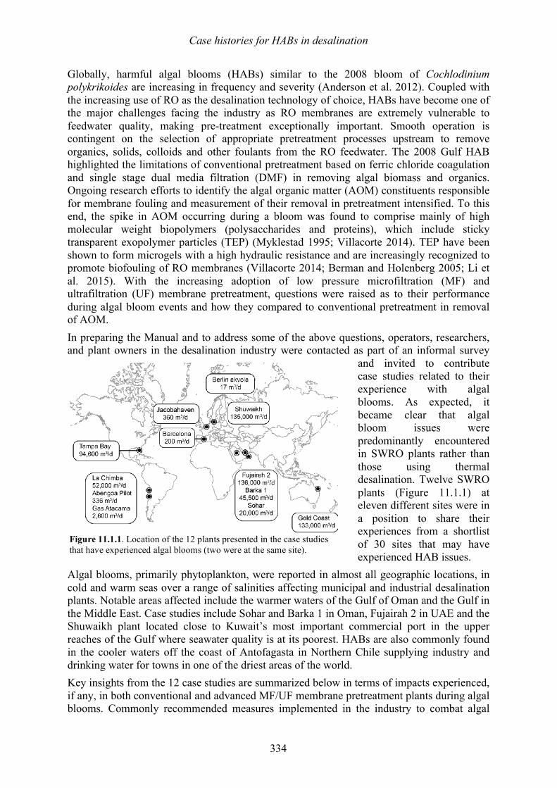
Case histories for HABs in desalination

334

Globally, harmful algal blooms (HABs) similar to the 2008 bloom of Cochlodinium polykrikoides are increasing in frequency and severity (Anderson et al. 2012). Coupled with the increasing use of RO as the desalination technology of choice, HABs have become one of the major challenges facing the industry as RO membranes are extremely vulnerable to feedwater quality, making pre-treatment exceptionally important. Smooth operation is contingent on the selection of appropriate pretreatment processes upstream to remove organics, solids, colloids and other foulants from the RO feedwater. The 2008 Gulf HAB highlighted the limitations of conventional pretreatment based on ferric chloride coagulation and single stage dual media filtration (DMF) in removing algal biomass and organics. Ongoing research efforts to identify the algal organic matter (AOM) constituents responsible for membrane fouling and measurement of their removal in pretreatment intensified. To this end, the spike in AOM occurring during a bloom was found to comprise mainly of high molecular weight biopolymers (polysaccharides and proteins), which include sticky transparent exopolymer particles (TEP) (Myklestad 1995; Villacorte 2014). TEP have been shown to form microgels with a high hydraulic resistance and are increasingly recognized to promote biofouling of RO membranes (Villacorte 2014; Berman and Holenberg 2005; Li et al. 2015). With the increasing adoption of low pressure microfiltration (MF) and ultrafiltration (UF) membrane pretreatment, questions were raised as to their performance during algal bloom events and how they compared to conventional pretreatment in removal of AOM. In preparing the Manual and to address some of the above questions, operators, researchers, and plant owners in the desalination industry were contacted as part of an informal survey

and invited to contribute case studies related to their experience with algal blooms. As expected, it became clear that algal bloom issues were predominantly encountered in SWRO plants rather than those using thermal desalination. Twelve SWRO plants (Figure 11.1.1) at eleven different sites were in a position to share their experiences from a shortlist of 30 sites that may have experienced HAB issues.

Algal blooms, primarily phytoplankton, were reported in almost all geographic locations, in cold and warm seas over a range of salinities affecting municipal and industrial desalination plants. Notable areas affected include the warmer waters of the Gulf of Oman and the Gulf in the Middle East. Case studies include Sohar and Barka 1 in Oman, Fujairah 2 in UAE and the Shuwaikh plant located close to Kuwait’s most important commercial port in the upper reaches of the Gulf where seawater quality is at its poorest. HABs are also commonly found in the cooler waters off the coast of Antofagasta in Northern Chile supplying industry and drinking water for towns in one of the driest areas of the world. Key insights from the 12 case studies are summarized below in terms of impacts experienced, if any, in both conventional and advanced MF/UF membrane pretreatment plants during algal blooms. Commonly recommended measures implemented in the industry to combat algal

Figure 11.1.1. Location of the 12 plants presented in the case studies that have experienced algal blooms (two were at the same site).

Case histories for HABs in desalination

335

blooms are discussed in relation to the case studies mitigation strategies, and lessons learned. This encompasses measures adopted during design and/or during plant operation, e.g. deep-water intakes (Gold Coast), and DAF (Fujairah 2, Shuwaikh) and/or direct MF/UF filtration (Jacobahaven, Sohar), or subsequently enacted in response to HAB events (La Chimba).

11.1.1 Algal-related impacts in desalination HABs pose two main operational risks in desalination, namely safety of the drinking water produced (which relates to the toxicity of the bloom) and security of supply (Boerlage and Nada 2014). HABs are broadly classified as toxic or non-toxic. Toxic algal blooms produce potent toxins, causing illness or mortality in humans, fish, marine mammals, and other marine life through either the direct exposure to the toxin or ingestion of bioaccumulated toxin in higher trophic levels e.g. shellfish consumption. In desalination, marine algal toxins represent a potential health risk to the safety of desalinated drinking water if present in sufficiently high concentrations in the seawater and they breakthrough through the desalination process. Non-toxic HABs can cause damage to ecosystems, fisheries resources, recreational areas, and commercial facilities such as desalination plants, sometimes because of the biomass of the accumulated algae, and in other cases due to the release of compounds that are not toxins (i.e., reactive oxygen species, polyunsaturated fatty acids, organic matter, mucilage) that can be lethal to marine animals or that can cause disruptions of other types. In desalination, these blooms represent an operational risk to plants, threatening water supply security through unplanned outages, and loss of production at any point in the process from blinding of intakes (less common) through to failure of pretreatment unit processes and/or the RO system itself. Such blooms can have massive financial impacts. Huge economic losses were reported, for example, at Oman’s Sohar Industrial Port Area (SIPA), which supplies desalinated water and seawater cooling water to industrial customers. The non-toxic bloom of Cochlodinium polykrikoides in 2008/2009 resulted in an increase in the frequency of cleaning seawater intake screens from every 12 hours to every 4 hours and an inability to maintain the required free residual chlorine. The independent SWRO plant operated by the Sohar Refinery at SIPA shut down for four months and required 100% membrane replacement due to severe biofouling. A myriad of HAB impacts in desalination were identified in the cases studies. Some are easily identified with most posing a risk to the security of desalinated water supply as in general, the causative species of the HAB, where identified, were non-toxic. Other impacts were more obscure and relate more to the perception that desalinated drinking water may be unsafe (e.g., malodorous) or even to the perceived environmental impacts of brine during an algal bloom event. Perceived impacts associated with safety of drinking water may follow the decay of an algal bloom. In 2011, the La Chimba plant, supplying 60% of Antofagasta’s drinking water, detected hydrogen sulfide at the seawater intake. The seawater, abstracted from a deep water intake, had become hypoxic (DO<0.5 mg/l) due to the decay of an intense bloom of Prorocentrum micans made worse by thermoclines that restricted mixing and movement of water in the bay. Under these conditions, sulfate reducing bacteria (SRB) flourished and hydrogen sulfide was generated. While the inhalation of hydrogen sulfide in air is well known to be extremely toxic, there are no data on the human health effects of ingesting water that contains hydrogen sulfide (NHMRC/NRMMC 2011). Instead, impacts are mainly related to the foul smell of rotting eggs, with hydrogen sulfide having a very low taste and odor threshold in water, estimated to be as low as 0.05 mg/l (WHO 2011). As a gas, hydrogen sulfide can readily pass through RO membranes resulting in customer complaints and/or the

Case histories for HABs in desalination

336

perception that water produced following a HAB is unsafe. Alternatively, oxidation of hydrogen sulfide could lead to elemental sulfur which has a detrimental effect on membranes. The plant owner therefore quickly enacted a raft of measures to remove H2S from the product water. Another atypical issue encountered during an algal bloom event was that a desalination plant was thought to be the cause of a dark plume in the seawater in an area renowned for its beaches and recreational fishing. A vast Trichodesmium bloom occurred in the area of the brine outlet (and intake) during commissioning of the Gold Coast plant which led a member of the public to complain to the local Environmental Protection Agency (EPA) of a dark plume emanating from the brine outlet. The bloom was, in fact, demonstrated to frequently occur naturally in the area (prior to the construction of the plant) and shown not to be entrained in the plant intake. If it was entrained, the solids associated with the high concentration of algal cells would be removed during residual treatment and not be returned to sea. Hence, no plume would be evident from the brine outfall. Nonetheless, this demonstrates potential community perception issues associated with algal bloom events in desalination. The more typical algal-related issues in SWRO desalination arising from the high biomass and organics accompanying non-toxic HABs are well known in the desalination industry. High biomass blooms can increase suspended solids beyond design thresholds, overloading conventional granular media filters (GMF) and resulting in rapid filter clogging. If the coagulation dose becomes prohibitively high in response to a bloom, surface clogging of the media may occur, severely limiting filtration capacity. Downstream this may lead to more frequent cartridge filter replacement and cleaning of the RO membranes due to a higher iron residual and higher concentration of colloids and AOM remaining in the RO feedwater. At worst, plant production is lost due to frequent media backwashing and short filter runs, and conventional pretreatment may fail to produce water to meet RO guidelines. Plants are then forced to void warranties and continue operating or shut down to avoid the risk of irreversible RO membrane fouling. In the latter case, they may also incur cost penalties associated with loss of production. Conventional pretreatment was employed in 5 of the 12 case studies (Tampa Bay, Gold Coast, Barcelona, Atacama Plant 1, Fujairah 2). Shorter filter runs were observed for the diatomaceous earth filters at Tampa Bay during algal blooms, along with foaming. No negative impacts were observed in the gravity DMF at the Gold Coast plant as the deep water intake limited ingress of the most frequently occurring algal bloom. The same was true at Fujairah 2, which employs additional solids removal through an upstream DAF. Similarly, HAB impacts are found in microfiltration or ultrafiltration which was the predominant pretreatment choice in the case studies. This involved a variety of membrane materials and pore sizes either in the pressurised inside-out or outside-in flow configuration. Here impacts were as expected and included blocking of strainers due to higher solids loading and increases in transmembrane pressure (TMP) in order to maintain a constant permeate flux as pretreatment membranes fouled. Backwashing and chemically enhanced backwashing (CEB) intervals were severely shortened in some cases and less effective than in non-bloom conditions, with a marked membrane permeability decrease over time. Additional cleaning-in-place (CIP) to recover initial permeability was required in some cases (Sohar, Barka 1, Antofagasta, Jacobahaven). Biofouling of the SWRO membranes was noted at the Sohar plant during algal bloom events in 2013 (and earlier in 2008 at the Sohar Refinery SWRO plant as mentioned above), which uses direct MF membrane pretreatment without coagulation. Additional RO membrane cleaning was also required at the SWRO plant at Atacama using conventional pretreament but the nature of fouling was not identified. Pretreatment was effective during algal bloom

Case histories for HABs in desalination

337

events for most of the remaining case studies with no additional cleaning reported for the SWRO or fouling was not directly attributed to algal blooms. RO fouling is typically complex with more than one type of fouling occurring and may be the synergistic effect of operating conditions prior, during or after a bloom e.g. overdosing of ferric coagulants causing iron fouling along with biofouling during or following the termination of the bloom. 11.1.2 Algal bloom mitigation and lessons learned

11.1.2.1 Characterization of seawater quality and piloting Ideally, prior to SWRO plant design, seawater quality is thoroughly characterized through a long-term monitoring study (see section 11.1.2.1.1 for parameters) to assist in selecting an intake site and pretreatment processes from which the plant footprint and layout can be estimated. This should be coupled to a review of historical records to determine factors that impact on water quality such as the frequency and severity of algal blooms. Hydrodynamic conditions at the intake area should also be considered, such as the presence of thermoclines or upwelling that may promote HABs. Monitoring methods and approaches are covered in detail in Chapters 3 and 5. It should be noted that water quality can vary in a region or be strongly influenced by intake design. The importance of having data specific to a site cannot be understated, as highlighted by the Sohar case study in Oman. Sohar’s SWRO plant based its design for a direct MF membrane pretreatment system on blooms with a maximum duration of one month once a year and on process data (e.g. MF flux) from a similar plant operating for 5 years located on the Duqum Coast of Oman. Instead of one month, the plant encountered a prolonged bloom of six months during plant commissioning and extremely poor water quality exacerbated by its shallow lagoon intake system. The plant experienced a multitude of issues including clogging of the intake screen, partially clogged self-cleaning strainers, high TMP on the MF system, biofouling of the SWRO, and ultimately loss of production and supply for downstream industrial users. Short-term mitigation measures to maintain supply included lowering MF flux and renting containerized MF-RO plants to compensate for the applied drop in production. A one-year feedwater characterization study for design was recommended following their experience. Pilot plant trials are often employed in addition to, or instead of, a seawater quality assessment study and are a useful tool offering many benefits for process design optimization, leading to successful long term operation of the full scale plant. Ideally, MF/UF can be operated at high flux and without the addition of coagulant, thereby avoiding capital and operating costs associated with chemical storage, residual handling and treatment for coagulated solids. In practice, MF/UF cannot always achieve high fluxes during challenging water quality conditions such as HABs or storms where the solids and/or organic feedwater load increase. Piloting can therefore assist in determining whether solids removal by clarification or flotation is required prior to conventional or membrane pretreatment. Should no bloom occur during piloting, plants can be challenged through the addition of cultivated algae to the raw water (see section 11.5). Process parameters can also be optimized such as the fluxes that can be achieved on MF/UF with or without coagulation, efficacy of mechanical (hydraulic backwash, air scour) cleaning frequency and duration of CEB or CIP to maintain production targets (Sohar, Barka 1, Antofagasta, Jacobahaven). This information is often critical in preventing over-capitalization of pretreatment facilities if coagulation is incorporated for MF/UF pretreatment or upstream clarification or flotation. Moreover, these facilities may only be required for a short period each year. Alternatively, pretreatment requirements may be underestimated or key process parameters overly ambitious, potentially leading to loss of production and severe disruptions to drinking or industrial water supply.

Case histories for HABs in desalination

338

Four of the case studies directly relate to piloting pretreatment options and process optimization during algal blooms; Abengoa, Jacobahaven, Barcelona, and the akvola pilots. Pilot or lab studies were also used to support pretreatment plant design for many of the full-scale plants reported in this paper. Sohar’s rental containerized plant, following significant HAB events, acted as a pilot plant to determine long-term mitigation strategies so that the existing plant could be redesigned to operate through such prolonged algal blooms.

11.1.2.1.1 Water quality parameters for HAB monitoring in design and operation Methods to measure AOM, its fouling constituents, and their impact on membrane fouling potential (organic, particulate and/or biofouling) are important to detect blooms and assess pretreatment efficiency. Monitoring efforts also need to continue following the collapse of an algal bloom. The succession of bacterial species which can thrive on decaying AOM may release organic matter extracellularly including TEP which can contribute to fouling.

Conventional water quality parameters typically included in monitoring programs to provide an indication of the increase in organics, solids, and fouling potential include: TOC, DOC, TSS, turbidity, SDI, and DO. Monitoring of the same parameters for process control during plant operation as during the design phase provides continuity so operational data can be compared with baseline data. Although, the aforementioned parameters are not specific to algal blooms, changes may indicate their presence, e.g. increase in TSS (Abengoa pilot plant), or indirect impacts from HABs such as low DO following decomposition of a dense bloom (La Chimba plant). Despite the well-known limitations of the SDI (Schippers and Verdouw 1980; Kremen and Tanner 1998; Boerlage et al. 2000; Boerlage 2008), it has proven useful in detecting algal blooms at the intake compared to other parameters including turbidity and chlorophyll-a (determined via fluorescence). Elevated SDI at the intake corresponded to algal bloom events as seen at Fujairah 2, Barka 1, Sohar and Gas Atacama plants. Care should be taken however, in interpreting results. Often the SDI was measured at intervals not recommended by the ASTM standard, e.g. SDI3 and even SDI1. The SDI test was not designed to measure high fouling feedwater such as algal-laden seawater nor for UF permeate where UF have smaller pores than that of the SDI membrane. SDI results will underestimate the fouling potential of feedwater during a bloom as it does not capture small particles responsible for fouling including TEP precursors and the SDI is not linear with particle concentration. Moreover, when assessing process performance, SDI cannot be directly compared for different filtration intervals, e.g. SDI5 for raw water and SDI15 after pretreatment, or when measured at different temperatures (Boerlage 2008).

Measuring TOC to detect AOM in the source seawater and for process control is generally unreliable. TOC (and DOC) measure bulk organic matter and therefore provide no information as to the composition or concentration of potential AOM foulants produced during an algal bloom. While TOC increases in the source seawater were found at Fujairah 2, Sohar, and Tampa Bay, this is not always true. Measuring TOC removal to assess pretreatment efficiency processes and as a process trigger is also inaccurate due to the difficulties in measuring low-level TOC residuals in saline process streams (as discussed in the Fujairah 2 case study).

SDI and TOC are often interpreted in conjunction with other parameters which directly identify the presence of algal species in the source water through algal cell identification and enumeration or an increase in algal productivity or advance warning through remote sensing. Algal counts were reported at 10 of the plants, but the dominant species were not always identified. Although cell counting can be automated using new biosensors if conducted on

Case histories for HABs in desalination

339

discrete samples at external laboratories, this can result in prohibitively long turnaround times and therefore cannot be used as an alert to trigger process adjustment, as discussed for Fujairah 2. Identification of the algal species, size, and toxicity is important for plant operation and process control, but must be done on discrete samples by experienced personnel. Published and online taxonomic guides listed in the Manual can be of great value, but trained personnel are needed to insure consistency through time.

Chlorophyll-a measurements were reported at 6 plants with La Chimba obtaining chlorophyll-a data from satellite images provided by NPOES and MODIS satellites. Results from chlorophyll-a data using fluorescence measurements at the seawater intake are not always a reliable indicator of the severity of a bloom nor are the instruments easy to maintain. The relationship between chlorophyll-a fluorescence and cell biomass is not constant across all phytoplankton species, nutritional conditions, and times of sampling. Some species have a low content of chlorophyll despite their size e.g. Noctiluca scintillans which ranges up to 2 mm in size. Other factors influencing chlorophyll-a include nutrients and light history, with limitations often resulting in lower chlorophyll-a content than the same cells under more favorable conditions. This may explain why chlorophyll-a readings were very low at Barka 1 (species not identified), yet operational issues were observed, while Tampa Bay (Ceratium furca and Phaocystis) and the Jacobahaven plant (Phaeocystes, Chaetoceros) reported much higher chlorophyll-a values at times of operational difficulties. Similarly, Fujairah 2 reported no particular trends in chlorophyll-a concentrations during a bloom. Satellite-derived chlorophyll-a in conjunction with information on prevailing currents has been used as an early warning system by desalination plants to track algal blooms approaching plant intakes. La Chimba in Chile used the Bricker et al. (Bricker et al. 2003) eutrophication status classification based on chlorophyll-a levels from satellite images to assess the risk for algal blooms during the summer months. For the 2013 bloom, water in Antofagasta Bay was classed as hyper-eutrophication (chlorophyll-a > 60 µg/L). Recently, more sophisticated tests have been developed to determine constituents of AOM which may better indicate the biofouling and particulate fouling potential of seawater and process streams during a bloom. Villacorte (2014) demonstrated that biopolymers and TEP can promote fouling of both pretreatment and SWRO membranes. Monitoring of biopolymer and TEP concentrations during a bloom would therefore be informative. Biopolymers can be determined by liquid chromatography - organic carbon detection (LC-OCD). LC-OCD fractionates natural organic matter (NOM), primarily by size and also by ion interaction and hydrophobic interaction. Fractions vary from larger biopolymers (> 20,000 Da) of which TEP is a component, to low molecular weight compounds (< 350 Da). In a LC-OCD chromatogram, a spike in biopolymers is observed during an algal bloom. Two methods have been developed to determine fractions of TEP in seawater (Villacorte 2014). TEP0.4µm measures larger TEP (>0.4 µm) while TEP10kDa includes both TEP and most of the smaller TEP precursors. TEP precursors dominate AOM during a bloom, therefore, applying both tests allow the differences in pretreatment removal efficiency for these algal-derived foulants to be distinguished (Villacorte 2014); however, the degree of difficulty and cost in determining them is correspondingly higher. As samples need to be sent to specialized laboratories, delays in obtaining the results mean these parameters cannot be employed to alert a plant of a bloom or to adjust process parameters during plant operation. Consequently, only a few plants used these tests. The Barcelona and Jacobahaven plants both used LC-OCD to examine the performance of pretreatment steps to remove biopolymers. TEP0.4µm was also monitored for three years at the Jacobahaven plant and a correlation between TEP and fouling rates in the UF pretreatment system was observed.

Case histories for HABs in desalination

340

A method to determine assimilable organic carbon (AOC) based on luminescence using Vibrio harveyi has also been developed to indicate the biofouling potential of the source seawater and process streams (Weinrich et al. 2011). The saline AOC test was trialed at the Tampa Bay plant to monitor pretreatment. High levels of AOC were measured in the source seawater during a bloom that further increased following chlorine dioxide prechlorination which may be due to oxidation of organic matter. The AOC was greatly reduced by bioactivity in the subsequent sand filtration step (LeChevallier 2014; Tampa Bay Case Study).

Finally, there are improved methods to measure particulate fouling which can be used during a bloom. The Modified Fouling Indices (MFI), developed to address the limitations of the SDI, comprise the MFI-0.45 (an ASTM standard) and the MFI-UF using ultrafiltration membranes (Schippers and Verdouw 1980; Boerlage et al. 2000; Salinas-Rodriguez 2011). The MFI-UF with smaller pore size membranes can measure UF permeate unlike the SDI and MFI-0.45. Both MFI tests are normalized to reference temperature, area and pressure values and can measure high fouling feedwater. Therefore, MFI can be compared and pretreatment efficiencies can be determined. When using a 10 kDa membrane in the MFI-UF test, a high correlation was found between MFI-UF and TEP10kDa, measurements (Villacorte 2014). This indicates the MFI-UF could be used to investigate the fouling potential of feedwater containing the smaller high fouling TEP precursors across a plant during a bloom. Of the twelve case studies, only the Jacobahaven plant employed the MFI-UF where it was used to measure pretreatment efficiency. 11.1.2.2 Intake depth and location

Careful selection of intake type, depth, and location, is often considered the first defense in preventing the entrainment of algal blooms into a plant coupled to a comprehensive investigation of seawater quality and site conditions as discussed above. Subsurface intakes are one option to reduce the ingress of algal cells and associated AOM into a plant; however, subsurface intakes are not feasible for all sites and were not covered in the case studies, though chapter 6 covers intake designs in detail. Most large scale SWRO plants use an open ocean (or surface) intake. Abstracting water at depth is often promoted as a means to prevent entrainment of algae into desalination plants with open intakes. Indeed, the deep water (20 m water depth) intake option selected for the Gold Coast plant appears to be successful in providing good water quality and preventing the ingress of dense floating mats of Trichodesmium erythraeum, the most frequent algal bloom observed in that region. Limited ingress of Colpomenia, a macroalgae typically attached to rocks, has occurred. This is most likely not as a result of a bloom but through dislodgment with wind and waves breaking it into flakes which may then have become entrained into the intake. The success of deep water intakes depends on the bloom-forming species. Some are motile or display diel vertical migration so that they move within the water column and are not found solely within the surface, mixed layer. Indeed, they can be at the surface during the daytime, and at 10 or even 20 m depths at night. Moreover, the distribution of AOM may not reflect the distribution of algal cells in the water column, as AOM can be extracellular and detrital in form, sinking to the seabed or rising to the surface. Hence, a deep-water intake can assist in limiting ingress of some algal blooms, but is no guarantee in preventing all algae and AOM as seen in various SWRO desalination plants in Chile.

The La Chimba and Gas Atacama plants, located 50 km apart, abstract seawater from the sheltered bays of Moreno and Mejillones, respectively, using a deep (25 m) and shallow (5m) intake. Both plants entrain algae into the intake. Abengoa’s pilot plant employed the La Chimba intake and measured a significant increase in algal concentration, suspended solids

Case histories for HABs in desalination

341

and organics during bloom events. TEP was found to increase five-fold to 3500 µg x-eq/L and suspended solids increased to 40 mg/L on average and up to 76 mg/L. The deep-water intake did not therefore prevent algal bloom and AOM from being entrained into the intake. Moreover, thermoclines in the Moreno Bay led to SRB and the generation of H2S issues at the La Chimba plant as discussed above. Further up the coast, the shallow intake of the Gas Atacama is less likely to suffer from hypoxic events as at La Chimba, but directly from algae and AOM. 11.1.2.3 Chlorination

Chlorine lyses algal and bacterial cells and oxidizes high molecular weight organics into biodegradable low molecular weight compounds which are more easily metabolized by biofouling bacteria. Some of the organic compounds released or formed may adsorb onto MF/UF pretreatment membranes or pass through to the RO system, increasing fouling and biofouling of the RO membranes. Hence, the SWRO industry moved from continuous to shock dosing of chlorine. During an algal bloom, chlorination at the intake could be suspended to limit lysis of algal cells and release of fouling AOM and toxins (if it is a toxin-producing bloom).

The small Jacobahaven demonstration plant (360 m3/d) avoided chlorination to prevent the formation of chlorination byproducts by pigging their intake lines (once every 2 weeks), which would be infeasible for large full scale plants. Yet, it still suffered from AOM fouling of the UF membranes. Although, the intake at the Fujairah 2 hybrid plant was switched from continuous to shock dosing during studies of HABs at the SWRO plant, it is difficult to show direct data from their case study to demonstrate that the plant reduced algal lysis. Shuwaikh, Gas Atacama and Gold Cost practice shock chlorination. Some plants continue to practice continuous chlorination such as Barka 1 and Sohar. Sohar intends to change to shock chlorination, but has issues due to other co-located industries that require chlorinated seawater. La Chimba can continuously chlorinate, but doesn’t use the system. At Tampa Bay, continuous chlorination is practiced at two locations; chlorine dioxide at the intake and hypochlorite prior to the coagulation mixing basins. A 65% increase in the AOC during algal blooms was found following disinfection with chlorine dioxide compared to the raw water at the plant intake. Increases in AOC have been observed following disinfection with chlorine dioxide (Haas et al. 2015). Increases in AOC may lead to increased biofouling potential and may be directly linked to HABs.

11.1.2.4 Dissolved air flotation DAF is generally thought to be one of the leading approaches to mitigate algal-related issues in downstream processes. However, DAF can be an expensive addition to a plant if it is only required to remove algae and blooms are not severe or frequent. A disadvantage of operating DAF in bypass mode is that it needs to be brought online prior to the bloom, which is often difficult to time correctly. The advantage of DAF is that the algal cells will be gently lifted by air bubbles, minimizing damage to cells or release of AOM. Successful performance of DAF is contingent on optimized coagulation flocculation to promote attachment of algal cells to the micro-bubbles generated in DAF. In general, cell removal is higher for more dense blooms.

DAF was utilized in five of the twelve case studies, Shuwaikh, Fujairah 2, Gas Atacama, Barcelona and akvola. Two of these cases (Shuwaikh and Fujairah 2) require DAF for other problems besides HABs, such as very high turbidity, suspended solids, and hydrocarbons. At Gas Atacama, a conventional DAF+DMF system ran side-by-side with a UF system. The DAF+DMF encountered significant operational issues: high coagulant dose (25 ppm),

Case histories for HABs in desalination

342

increased SWRO membrane cleaning and cartridge filter replacement, and eventually premature SWRO membrane replacement. The alternative system that employed UF did not require cartridge filter replacement or SWRO membrane cleaning even when challenged by HAB events; however, it should be noted that the DAF+DMF plant is approximately 20 years old and employs older designs for DAF and SWRO. The Shuwaikh plant uses high rate Leopold Clari- DAF before autostrainers and UF (pressurized inside out). The DAF uses ferric chloride and sulfuric acid. The system maintained full capacity during a bloom after optimization of coagulant and acid dose. DAF pilot studies conducted on Antofagasta Bay reported in the Shuwaikh case study showed greater than 95% removal for varying species of algae.

At Fujairah 2, Spidflow® DAF is utilized in line with DMF. Ferric chloride average dose rate during blooms in 2011-2012 was < 20 ppm and in 2013 <15 ppm. Fujairah 2 has provision in the DAF for acid dosing, but this was only used in commissioning and has provision for polymer dosing, but this has never been used. A DAF pilot plant operated throughout the 2008/2009 Cochlodinium bloom and the full-scale plant operated through a 2013 bloom. The Barcelona pilot operated a parallel trial of DAF followed by (i) conventional DMF or (ii) pressurized outside-in UF. The combination of DAF followed by UF gave superior removal of biopolymers (41%) compared to only 18% for DAF and conventional DMF pretreatment. The ferric chloride coagulant dose for the Barcelona DAF pilot study was low being 0-6 mg/L and acid and coagulant aid were not found to be crucial in optimizing DAF performance. Algal cell removal averaged at 75% and up to 87%. 11.1.2.5 Microfiltration/Ultrafiltration

Microfiltration and ultrafiltration were commonly used for treatment of algal rich water, with eight of the twelve plants employing advanced membrane pretreatment: Sohar, Barka 1, Shuwaikh, Gas Atacama, Abengoa pilot, Jacobahaven, Barcelona and akvola. Due to the pore size of MF/UF membranes, cell removal is generally 99-100% and cells only pass the MF/UF through broken fibers (Dixon et al. 2011). Most of the plants employed ultrafiltration which will achieve a higher removal of AOM and particulates due to their smaller membrane pores (or MWCO rating) than microfiltration with larger pores. As fouling biopolymers and TEP precursors range upwards of 20,000 Da in molecular weight and a few nm in size, respectively, ultrafiltration membranes (with a typical MWCO of 100,000 – 150,000 Da) will not remove them completely. Coagulation, albeit at a lower dose than for DMF, is therefore practiced to remove dissolved AOM, improve removal of biopolymers and TEP, and the filterability of the cake deposited on UF membranes. Several of these plants used DAF in combination with UF in order to reduce the suspended solids and organics loading on the membranes: Shuwaikh, Barcelona and akvola. The akvola pilot plant is a single unit combined DAF+UF system employing ceramic membranes. Several operating techniques to prevent hydraulically irreversible fouling are available to allow UF plants to continue operations during an algal bloom. The following were used in the case studies: reducing flux (4 plants), recirculating flow (1 plant), use of coagulation involving optimizing the dose or switching on coagulation in response to blooms (3 plants), decreasing backwashing intervals (2 plants), increased CEB frequency (5 plants) and CIP (3 plants). The specific actions taken at each plant to maintain membrane performance are described in more detail in the following paragraphs.

Case histories for HABs in desalination

343

At the Sohar plant which employs direct MF filtration, immediate short-term mitigation measures included reducing the MF flux from 100 L/m2h maximum to 60-73 L/m2h. The operators also reduced backwash cycle time, increased CEB frequency, and optimized cleaning strategies using chlorine and caustic (twice/day) and acid cleans (every 3 days). Coagulation will be incorporated into pretreatment as part of long term bloom mitigation measures to improve removal of AOM.

At Barka 1, the plant experienced significant UF fouling yielding a permeability drop of 100 L/m2hbar during light to moderate blooms. The plant maintained flux without coagulation by reducing the CEB design interval from 18 hours to 12-15 hours to delay the CIP to greater than once in 180 days. In the case of a more significant bloom, the plant could reduce flux or turn on coagulation. The Gas Atacama UF plant maintained operation during blooms as coagulation is employed at the plant (maximum 2 ppm). The Abengoa pilot plant experienced a rapid increase in TMP during their bloom and responded first by reducing the CEB interval from 30 to 7-8 hours, using hypochlorite and caustic for CEB cleaning, with the pH increased from 9 (normal pH) to 12 during blooms. Later, mitigation included reducing flux (16%), which allowed CEB to be conducted every 26 hours. Unlike most other UF plants, no coagulation was utilized. The UF membranes were operated with increased recirculation flow allowing scouring of the membrane. While the UF plant usually achieves 96% recovery, during the bloom, recovery dropped to 80% due to the reduction in flux while maintaining backwash frequency. Jacobahaven (a demonstration plant) allowed for maximum flexibility in operation. Rapid fouling of UF coincided with high chlorophyll-a, TEP and algal counts. CEB decreased to every 6-12 hours while in non-bloom conditions, CEB was typically every 24 hours, and as infrequent as once every 2 weeks. Modification of the backwash interval gave limited improvement and increased backwash volume to 20%. Similarly, modification of CEB conditions and frequency was ineffective. Flux reduction did not yield a satisfactory CEB interval. Coagulation was effective but CEB remained ineffective during coagulation and HABs, requiring a CIP. At Barcelona, no impacts were noted with algal cell counts up to 1.2 million/L. Both conventional and membrane pretreatment performed well; however, UF gave better performance with respect to SDI15, turbidity, algal cell, and biopolymer removal.

11.1.2.6 Dual media filtration/Granular media filtration While DMF is a common pretreatment practice, only four of the case studies employed DMF as part of their pretreatment. These were Fujairah 2, Gas Atacama, Barcelona and the Gold Coast. While DMF has been proven as an effective HAB removal method, giving between 20 and 90% removal in several cases (Gustalli et al. 2013), in this study little cell removal data was corroborated.

No negative impacts were observed in the gravity DMF at the Gold Coast plant as the deep water intake limited ingress of the most frequently occurring algal bloom. Hence, no cell removal data were recorded. Anecdotally, no increased DMF clogging was experienced during blooms with ferric sulfate (13 mg/L) coagulation and DMF. Similarly, no impacts were reported at Fujairah 2 and the Barcelona pilot plant, which employ additional solids removal through an upstream DAF.

At Barcelona cell removal with DMF was 74% and removal of biopolymers was 18% for DAF and DMF. As Barcelona was a side-by-side pilot plant, it showed DAF+UF cell

Case histories for HABs in desalination

344

removal (100%) was superior to DAF+DMF. Likewise, biopolymer removal was 41% versus 18%.

11.1.3 Summary The twelve case studies present an array of mitigation strategies for operating in algal-rich seawater from around the globe including deep water intakes, DAF, conventional and advanced pretreatment with or without coagulation. A myriad of impacts, algal water quality monitoring and detection techniques and management practices are described in the case studies. In many cases, the observations collected from plant operations as part of the Manual development validate some of the key perceptions held by our industry about how to manage operations during HABs. For example:

• Careful, informed site analysis with a focus on the potential for different types of algal blooms can be a cost-effective strategy that minimizes future pretreatment needs;

• Long-term monitoring programs to characterize seawater quality should be conducted at the plant intake site. This should include a review of historical records examining the frequency and severity of algal blooms (if available);

• Piloting at site is recommended with challenge testing using cultivated algae if no blooms occur;

• Conventional parameters such as the SDI have proven useful in detecting blooms at an intake. Care needs to be taken with the SDI as it will underestimate the fouling potential of feedwater, especially during algal blooms;

• Parameters have been developed to monitor AOM constituents and the increase in (bio)fouling potential of seawater during a bloom e.g. biopolymer concentration by LC-OCD, TEP10kDa, MFI-UF using a 10 kDa test membrane and the AOC luminescence test using Vibrio harveyi. These tests can be used to assess and optimize pretreatment during a bloom. While promising, the degree of difficulty and cost in determining them is correspondingly higher. As yet, these parameters cannot be employed to alert a plant to a bloom or to adjust process parameters during plant operation;

• Deep-water open ocean intakes may be successful in avoiding some bloom-forming species, but some species are motile or display diel vertical migration so that they move 10 m or more daily within the water column. Moreover, the distribution of AOM may not reflect the distribution of algal cells in the water column. Deep water intakes are thus not guaranteed to prevent the ingress of algae and AOM into a plant;

• Avoiding chlorination-dechlorination during a bloom will help to prevent downstream fouling as fouling AOM will be retained intercellularly along with toxins and less assimilable organic carbon is generated through oxidation of organic matter;

• Coagulation is important for all three pretreatments (DAF, UF, and DMF) and acts to remove AOM more effectively than these pretreatment processes alone. Less AOM in the pretreated water will help to alleviate SWRO fouling;

• DAF is a good choice for cell removal in areas predicted to experience heavy blooms, as it removes cells by floatation, minimizing cell rupture;

• DMF or UF alone can accomplish cell removal and some dissolved AOM (if coagulation is used for UF) for light algal blooms, but using a DAF upstream is prudent for heavy blooms; and

• The combination of DAF and UF is increasingly being applied in the industry, when applied in bypass mode, care needs to be taken to bring the DAF online in time.

Case histories for HABs in desalination

345

11.1.4. References Anderson, D. M., Cembella, A. D., and Hallegraeff, G. M. 2012. Progress in understanding

harmful algal blooms: paradigm shifts and new technologies for research, monitoring, and management. Annual Review of Marine Science 4, 143-176.

Berman, T. and Holenberg, M. 2005. Don't fall foul of biofilm through high TEP levels. Filtration and Separation 42(4), 30-32.

Boerlage, S. F. E. 2008. Understanding the Silt Density Index and Modified Fouling Indices (MFI0.45 and MFI-UF). Desalination and Water Reuse Quarterly May –June, 12-21.

Boerlage, S. F. E, Kennedy, M., Aniye, M., Abogrean, E., El-Hodali, D., Tarawneh, Z., and Schippers, J. 2000. Modified Fouling Index - ultrafiltration to compare pretreatment processes of reverse osmosis feedwater. Desalination 131, 201-214.

Boerlage, S. F. E. and Nada N. 2014. Algal toxin removal in seawater desalination processes. In: Proceedings of European Desalination Society, Cyprus.

Bricker, S. B., Ferreira, J. G., and Simas, T. 2003. An integrated methodology for assessment of estuarine trophic status. Ecological Modelling 169(1), 39–60.

Dixon, M. B., Richard, Y., Ho, L., Chow, C. W. K., O’Neill, B. K., and Newcombe, G. 2011. A coagulation - powdered activated carbon - ultrafiltration multiple barrier approach for removing toxins from two Australian cyanobacterial blooms. Journal of Hazardous Materials 186(2-3), 1553-1559.

Gustalli, A., Simon, F. X., Penru, Y., de Kirchove, A, Llorens, J., and Baig, S. 2013. Comparison of DMF and UF pretreatments for particulate material and dissolved organic matter removal in SWRO desalination. Desalination 322, 144-150.

Haas, C. N., LeChevallier, M. W., and Weinrich, L. A. 2015. Application of the Bioluminescent Saltwater Assimilable Organic Carbon Test as a Tool for Identifying and Reducing Reverse-Osmosis Membrane Fouling in Desalination. Alexandria: Water Environment & Reuse Foundation. Project 11-07.

Kremen, S. S., and Tanner, M. 1998. Silt density indices (SDI), percent plugging factor (% PF): their relation to actual foulant deposition. Desalination 119(1), 259-262.

LeChevallier M. W. 2014. Measurement of biostability and impacts on water treatment in the US. In: Microbial Growth in Drinking-Water Supplies Problems, Causes, Control and Research Needs. IWA Publishing.

Li, S., Winters, H., Villacorte, L. O., Ekowati Y., Abdul-Hamid. E., Kennedy, M. D., and Amy, G. L. 2015. Compositional similarities and differences between Transparent Exopolymer Particles (TEP) from two marine bacteria and two marine algae: significance to surface biofouling. Marine Chemistry 174, 131–140.

Myklestad, S. M. 1995. Release of extracellular products by phytoplankton with special emphasis on polysaccharides. Science of the Total Environment 165, 155-164.

NHMRC/NRMMC. 2011. Australian Drinking Water Guidelines Paper 6: National Water Quality Management Strategy. Canberra: National Health and Medical Research Council / National Resource Management Ministerial Council.

Salinas-Rodriguez, S. G. 2011. Particulate and organic matter fouling of SWRO systems: characterization, modelling and applications. Doctoral dissertation, UNESCO-IHE/TUDelft, Delft.

Case histories for HABs in desalination

346

Schippers, J. C. and Verdouw, J. 1980. The Modified Fouling Index, a method of determining the fouling characteristics of water. Desalination 32, 137-148.

Villacorte, L. O. 2014. Algal blooms and membrane-based desalination technology. CRC Press/Balkema, Leiden: 200 p.

Weinrich, L. A., Schneider, O. D., and LeChevallier, M. W. 2011. Bioluminescence-based method for measuring assimilable organic carbon in pretreatment water for reverse osmosis membrane desalination. Applied and Environmental Microbiology 77, 1148–1150.

WHO. 2011. Guidelines for Drinking Water Quality, Fouth Edition. Geneva: World Health Organization, 564 p.

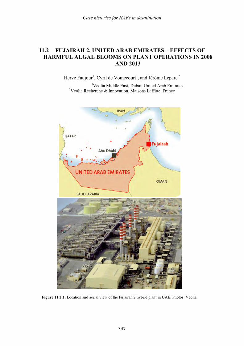
Case histories for HABs in desalination

347

11.2 FUJAIRAH 2, UNITED ARAB EMIRATES – EFFECTS OF

HARMFUL ALGAL BLOOMS ON PLANT OPERATIONS IN 2008 AND 2013

Herve Faujour1, Cyril de Vomecourt1, and Jérôme Leparc 2

1Veolia Middle East, Dubai, United Arab Emirates 2Veolia Recherche & Innovation, Maisons Laffitte, France

Figure 11.2.1. Location and aerial view of the Fujairah 2 hybrid plant in UAE. Photos: Veolia.

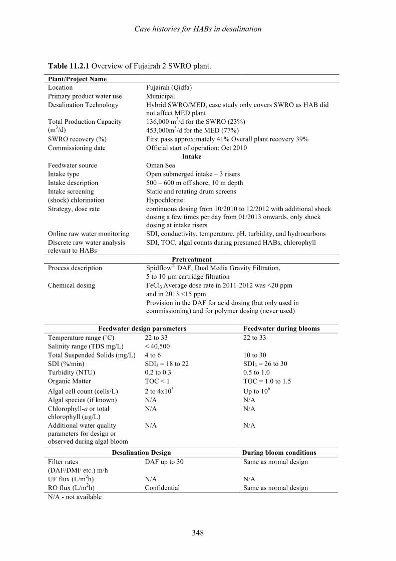
Case histories for HABs in desalination

348

Table 11.2.1 Overview of Fujairah 2 SWRO plant. Plant/Project Name Location Fujairah (Qidfa) Primary product water use Municipal Desalination Technology Hybrid SWRO/MED, case study only covers SWRO as HAB did

not affect MED plant Total Production Capacity (m3/d)

136,000 m3/d for the SWRO (23%) 453,000m3/d for the MED (77%)

SWRO recovery (%) First pass approximately 41% Overall plant recovery 39% Commissioning date Official start of operation: Oct 2010

Intake Feedwater source Oman Sea Intake type Open submerged intake – 3 risers Intake description 500 – 600 m off shore, 10 m depth Intake screening Static and rotating drum screens (shock) chlorination Strategy, dose rate

Hypochlorite: continuous dosing from 10/2010 to 12/2012 with additional shock dosing a few times per day from 01/2013 onwards, only shock dosing at intake risers

Online raw water monitoring SDI, conductivity, temperature, pH, turbidity, and hydrocarbons Discrete raw water analysis relevant to HABs

SDI, TOC, algal counts during presumed HABs, chlorophyll

Pretreatment Process description Spidflow® DAF, Dual Media Gravity Filtration,

5 to 10 µm cartridge filtration Chemical dosing FeCl3 Average dose rate in 2011-2012 was <20 ppm

and in 2013 <15 ppm Provision in the DAF for acid dosing (but only used in commissioning) and for polymer dosing (never used)

Feedwater design parameters Feedwater during blooms

Temperature range (˚C) 22 to 33 22 to 33 Salinity range (TDS mg/L) < 40,500 Total Suspended Solids (mg/L) 4 to 6 10 to 30 SDI (%/min) SDI3 = 18 to 22 SDI3 = 26 to 30 Turbidity (NTU) 0.2 to 0.3 0.5 to 1.0 Organic Matter TOC < 1 TOC = 1.0 to 1.5 Algal cell count (cells/L) 2 to 4x105 Up to 106 Algal species (if known) N/A N/A Chlorophyll-a or total chlorophyll (µg/L)

N/A N/A

Additional water quality parameters for design or observed during algal bloom

N/A N/A

Desalination Design During bloom conditions Filter rates (DAF/DMF etc.) m/h

DAF up to 30 Same as normal design

UF flux (L/m2h) N/A N/A RO flux (L/m2h) Confidential Same as normal design N/A - not available

Case histories for HABs in desalination

349

11.2.1 Introduction High demographic growth in the United Arab Emirates (UAE) in recent years has resulted in a higher demand for drinking water and power. In order to satisfy the growing demand, the Fujairah 2 Independent Water and Power Plant (IWPP) was launched by the Emirate of Abu Dhabi for completion during 2010. The location of this new plant was immediately next to the existing Fujairah 1 IWPP in the Emirate of Fujairah on the Gulf of Oman (Figure 11.2.1).

Until recently, the Fujairah 2 IWPP was the largest hybrid desalination plant in the world with a combined net design capacity of 590,000 m3/d linked to a power plant with a 2,000 MW/d net design capacity. Desalinated water is produced by a Seawater Reverse Osmosis (SWRO) plant and a Multi-Effect Distillation plant (MED).

In recent years, the unwelcome phenomenon of harmful algal blooms (HABs) have been experienced in the Gulf of Oman along the coasts of the UAE and Oman. Impacts had been devastating, particularly during a 2008/2009 HAB event which caused the shutdown of many SWRO plants due to the inability of conventional pretreatment processes to deal with the high concentrations of algae, and an associated increase in suspended solids and dissolved organics. The Fujairah pilot plant, which incorporated dissolved air flotation (DAF) as a pretreatment strategy, continued to operate during that bloom. Effective pretreatment process performance is paramount for any SWRO plant, as feedwater quality needs to meet the generally stringent O&M contractual specification. Veolia meets the very stringent SWRO plant availability requirement of Fujairah 2 of 98%. In order to achieve such availability with challenging raw water quality, the Veolia SPIDFLOW® Dissolved Air Flotation process has been included in the pretreatment with the aim of mitigating algal blooms/red tide events in particular and ensuring a superior and highly consistent water quality.

11.2.2 Plant overview 11.2.2.1 SWRO desalination plant

A shared seawater intake supplies seawater to the power plant as well as the MED thermal and SWRO desalination plants with a common remineralization section where MED distillate and SWRO permeate are blended and remineralized. The Fujairah 2 RO plant process configuration comprises the SPIDFLOW® DAF units (16) with coagulation/flocculation, rapid gravity dual media filters (12), cartridge filtration (16), first pass Reverse Osmosis (10) and partial second pass Reverse Osmosis (2) with the second pass to achieve boron removal (Figure 11.2.2). During the first five years of operation, two distinctly different intake chlorination strategies were employed. These had potential effects on general treatment process performance and water quality. During the first 27 months of operation, continuous intake chlorination was practiced plus an extra “shock-chlorination” every 6 – 8 hours, which could reach up to 2.5 mg/L. Since January 2013, shock or intermediate intake chlorination has been practiced at various frequencies and concentrations. Residual Cl2 was monitored upstream of the RO, and when detected, was neutralized with sodium bisulfite (SBS) injection in the suction of the HP pump. Provision was made for polymer and acid dosing to reach an optimum pH for coagulation, but experience from the five previous years showed that the efficiency of FeCl3 alone is sufficient.

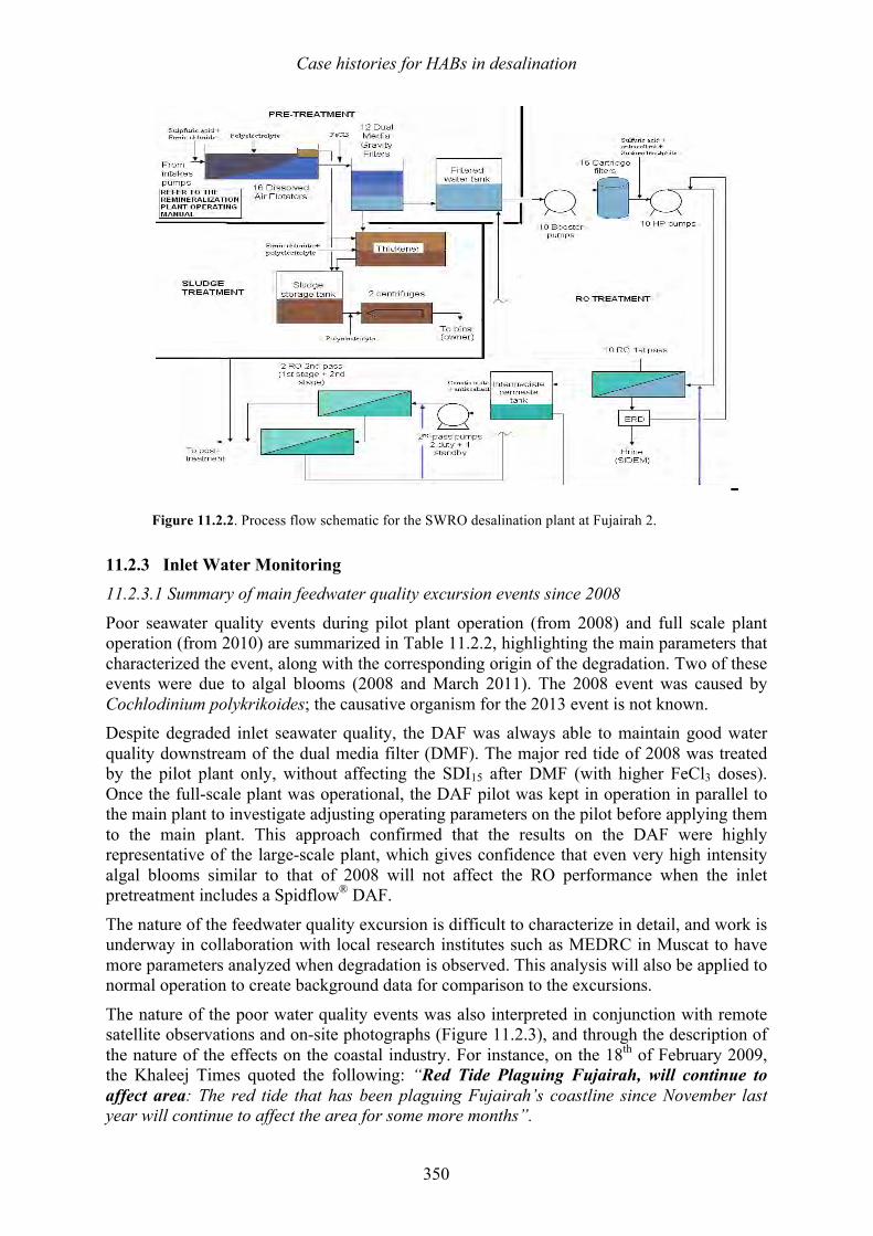
Case histories for HABs in desalination

350

Figure 11.2.2. Process flow schematic for the SWRO desalination plant at Fujairah 2.

11.2.3 Inlet Water Monitoring 11.2.3.1 Summary of main feedwater quality excursion events since 2008

Poor seawater quality events during pilot plant operation (from 2008) and full scale plant operation (from 2010) are summarized in Table 11.2.2, highlighting the main parameters that characterized the event, along with the corresponding origin of the degradation. Two of these events were due to algal blooms (2008 and March 2011). The 2008 event was caused by Cochlodinium polykrikoides; the causative organism for the 2013 event is not known. Despite degraded inlet seawater quality, the DAF was always able to maintain good water quality downstream of the dual media filter (DMF). The major red tide of 2008 was treated by the pilot plant only, without affecting the SDI15 after DMF (with higher FeCl3 doses). Once the full-scale plant was operational, the DAF pilot was kept in operation in parallel to the main plant to investigate adjusting operating parameters on the pilot before applying them to the main plant. This approach confirmed that the results on the DAF were highly representative of the large-scale plant, which gives confidence that even very high intensity algal blooms similar to that of 2008 will not affect the RO performance when the inlet pretreatment includes a Spidflow® DAF.

The nature of the feedwater quality excursion is difficult to characterize in detail, and work is underway in collaboration with local research institutes such as MEDRC in Muscat to have more parameters analyzed when degradation is observed. This analysis will also be applied to normal operation to create background data for comparison to the excursions.

The nature of the poor water quality events was also interpreted in conjunction with remote satellite observations and on-site photographs (Figure 11.2.3), and through the description of the nature of the effects on the coastal industry. For instance, on the 18th of February 2009, the Khaleej Times quoted the following: “Red Tide Plaguing Fujairah, will continue to affect area: The red tide that has been plaguing Fujairah’s coastline since November last year will continue to affect the area for some more months”.

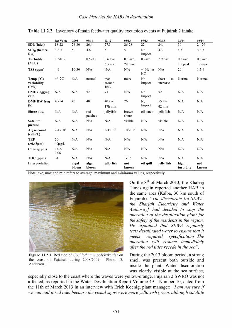
Case histories for HABs in desalination

351

Table 11.2.2. Inventory of main feedwater quality excursion events at Fujairah 2 intake. Ref Value 2008 03/11 03/12 03/13 07/13 09/13 02/14 10/14 SDI3 (inlet) 18-22 26-30 26.4 27.3 26-28 22 24.4 30 24-29 SDI15 (before RO)

3-3.5 5 4.8 5 5 No Impact

4.3 4.5 < 3.5

Turbidity (NTU)

0.2-0.3 0.5-0.8 0.6 ave 6.5 max

0.3 ave 29 max

0.2ave 2.9max 0.5 ave 1.5 peak

0.3 ave 13 max

TSS (ppm) 4-6 10-30 N/A N/A N/A +10% in HC

N/A 20 1.5-9

Temp (oC) variability (D/N)

+/- 2C N/A normal max around 16/3

more No Impact

Start to increase

Normal Normal

DMF clogging rate

N/A N/A x2 x3 N/A No Impact

x2 N/A N/A

DMF BW freq (h)

40-54 40 40 40 ave 17h min

26 No Impact

55 ave 42 min

N/A N/A

Shore obs. N/A N/A red patches

jellyfish brown shore

oil patch jellyfish N/A N/A

Satellite picture

N/A N/A N/A N/A visible N/A visible N/A N/A

Algae count (cells/L)

2-4x105 N/A N/A 3-4x105 105-106 N/A N/A N/A N/A

TEP (>0.45µm)

20-40µg/L

N/A N/A N/A N/A N/A N/A N/A N/A

Chl-a (µg/L) 0.02-0.06

N/A N/A N/A N/A N/A N/A N/A N/A

TOC (ppm) ~1 N/A N/A N/A 1-1.5 N/A N/A N/A N/A Interpretation algal

bloom algal bloom

jelly fish not known

oil spill jelly fish high turbidity

not known

Note: ave, max and min refers to average, maximum and minimum values, respectively

On the 8th of March 2013, the Khaleej Times again reported another HAB in the same area (Kalba, 30 km south of Fujairah). “The directorate [of SEWA, the Sharjah Electricity and Water Authority] had decided to stop the operation of the desalination plant for the safety of the residents in the region. He explained that SEWA regularly tests desalinated water to ensure that it meets required specifications. The operation will resume immediately after the red tides recede in the sea”.

During the 2013 bloom period, a strong smell was present both outside and inside the plant. Water discoloration was clearly visible at the sea surface,

especially close to the coast where the waves were yellow-orange. Fujairah 2 SWRO was not affected, as reported in the Water Desalination Report Volume 49 – Number 10, dated from the 11th of March 2013 in an interview with Erich Koenig, plant manager: “I am not sure if we can call it red tide, because the visual signs were more yellowish green, although satellite

Figure 11.2.3. Red tide of Cochlodinium polykrikoides on the coast of Fujairah during 2008/2009. Photo: D. Anderson.

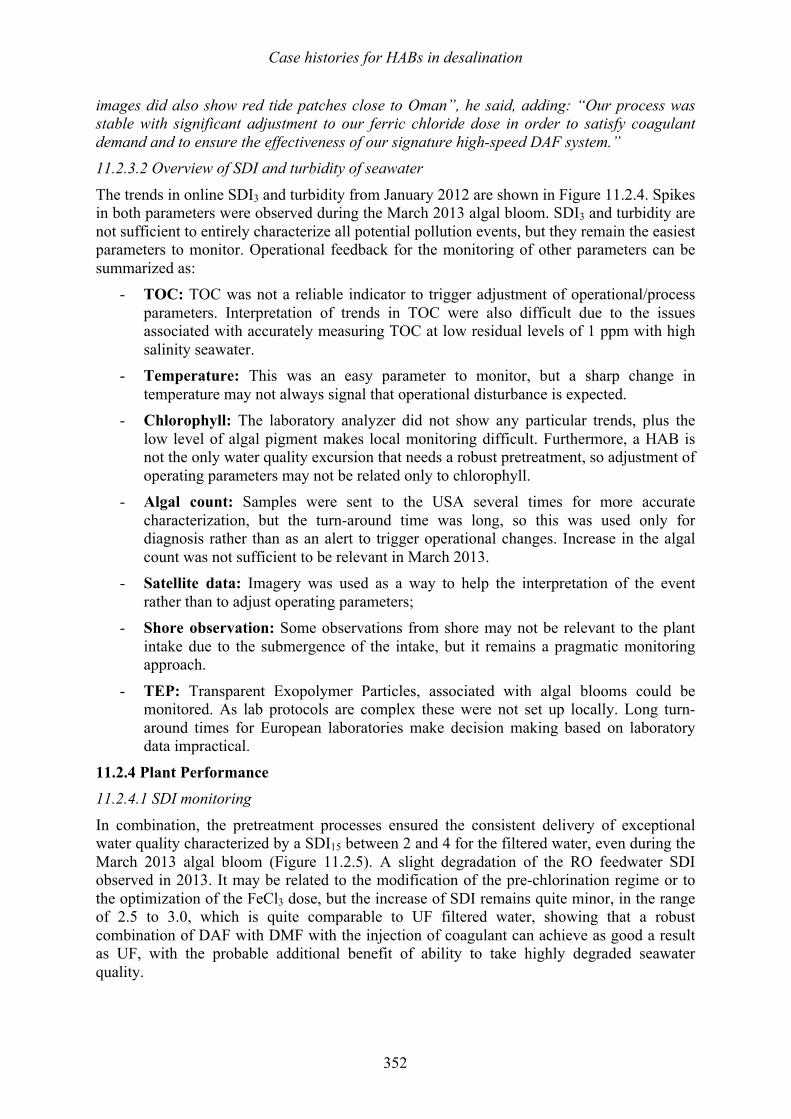
Case histories for HABs in desalination

352

images did also show red tide patches close to Oman”, he said, adding: “Our process was stable with significant adjustment to our ferric chloride dose in order to satisfy coagulant demand and to ensure the effectiveness of our signature high-speed DAF system.” 11.2.3.2 Overview of SDI and turbidity of seawater

The trends in online SDI3 and turbidity from January 2012 are shown in Figure 11.2.4. Spikes in both parameters were observed during the March 2013 algal bloom. SDI3 and turbidity are not sufficient to entirely characterize all potential pollution events, but they remain the easiest parameters to monitor. Operational feedback for the monitoring of other parameters can be summarized as:

- TOC: TOC was not a reliable indicator to trigger adjustment of operational/process parameters. Interpretation of trends in TOC were also difficult due to the issues associated with accurately measuring TOC at low residual levels of 1 ppm with high salinity seawater.

- Temperature: This was an easy parameter to monitor, but a sharp change in temperature may not always signal that operational disturbance is expected.

- Chlorophyll: The laboratory analyzer did not show any particular trends, plus the low level of algal pigment makes local monitoring difficult. Furthermore, a HAB is not the only water quality excursion that needs a robust pretreatment, so adjustment of operating parameters may not be related only to chlorophyll.

- Algal count: Samples were sent to the USA several times for more accurate characterization, but the turn-around time was long, so this was used only for diagnosis rather than as an alert to trigger operational changes. Increase in the algal count was not sufficient to be relevant in March 2013.

- Satellite data: Imagery was used as a way to help the interpretation of the event rather than to adjust operating parameters;

- Shore observation: Some observations from shore may not be relevant to the plant intake due to the submergence of the intake, but it remains a pragmatic monitoring approach.

- TEP: Transparent Exopolymer Particles, associated with algal blooms could be monitored. As lab protocols are complex these were not set up locally. Long turn-around times for European laboratories make decision making based on laboratory data impractical.

11.2.4 Plant Performance 11.2.4.1 SDI monitoring

In combination, the pretreatment processes ensured the consistent delivery of exceptional water quality characterized by a SDI15 between 2 and 4 for the filtered water, even during the March 2013 algal bloom (Figure 11.2.5). A slight degradation of the RO feedwater SDI observed in 2013. It may be related to the modification of the pre-chlorination regime or to the optimization of the FeCl3 dose, but the increase of SDI remains quite minor, in the range of 2.5 to 3.0, which is quite comparable to UF filtered water, showing that a robust combination of DAF with DMF with the injection of coagulant can achieve as good a result as UF, with the probable additional benefit of ability to take highly degraded seawater quality.

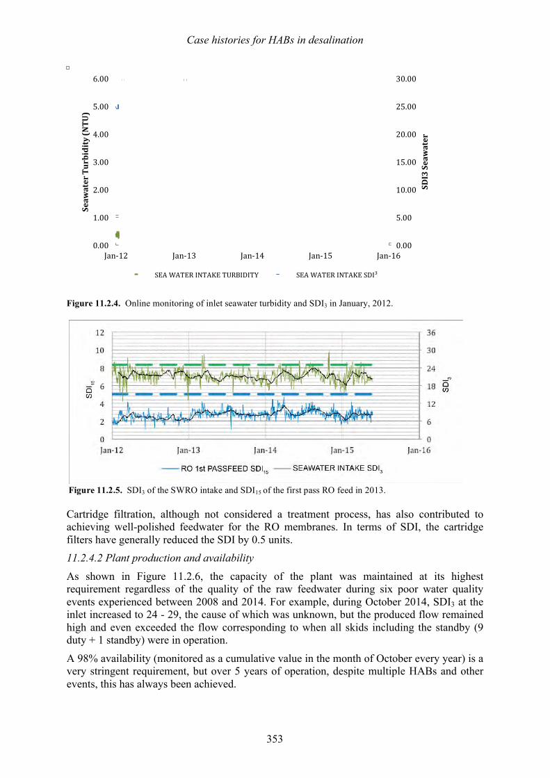
Case histories for HABs in desalination

353

Figure 11.2.4. Online monitoring of inlet seawater turbidity and SDI3 in January, 2012.

Cartridge filtration, although not considered a treatment process, has also contributed to achieving well-polished feedwater for the RO membranes. In terms of SDI, the cartridge filters have generally reduced the SDI by 0.5 units. 11.2.4.2 Plant production and availability

As shown in Figure 11.2.6, the capacity of the plant was maintained at its highest requirement regardless of the quality of the raw feedwater during six poor water quality events experienced between 2008 and 2014. For example, during October 2014, SDI3 at the inlet increased to 24 - 29, the cause of which was unknown, but the produced flow remained high and even exceeded the flow corresponding to when all skids including the standby (9 duty + 1 standby) were in operation.

A 98% availability (monitored as a cumulative value in the month of October every year) is a very stringent requirement, but over 5 years of operation, despite multiple HABs and other events, this has always been achieved.

0.00

5.00

10.00

15.00

20.00

25.00

30.00

0.00

1.00

2.00

3.00

4.00

5.00

6.00

Jan-­‐‑12 Jan-­‐‑13 Jan-­‐‑14 Jan-­‐‑15 Jan-­‐‑16

SDI3 Seawater

Seawater Turbidity (NTU)

SEA WATER INTAKE TURBIDITY SEA WATER INTAKE SDI³

Figure 11.2.5. SDI3 of the SWRO intake and SDI15 of the first pass RO feed in 2013.

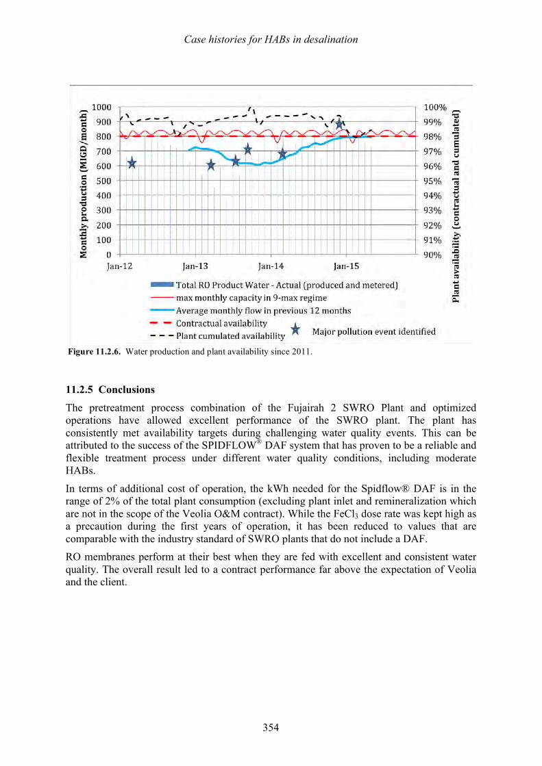
Case histories for HABs in desalination

354

11.2.5 Conclusions

The pretreatment process combination of the Fujairah 2 SWRO Plant and optimized operations have allowed excellent performance of the SWRO plant. The plant has consistently met availability targets during challenging water quality events. This can be attributed to the success of the SPIDFLOW® DAF system that has proven to be a reliable and flexible treatment process under different water quality conditions, including moderate HABs.

In terms of additional cost of operation, the kWh needed for the Spidflow® DAF is in the range of 2% of the total plant consumption (excluding plant inlet and remineralization which are not in the scope of the Veolia O&M contract). While the FeCl3 dose rate was kept high as a precaution during the first years of operation, it has been reduced to values that are comparable with the industry standard of SWRO plants that do not include a DAF. RO membranes perform at their best when they are fed with excellent and consistent water quality. The overall result led to a contract performance far above the expectation of Veolia and the client.

Figure 11.2.6. Water production and plant availability since 2011.

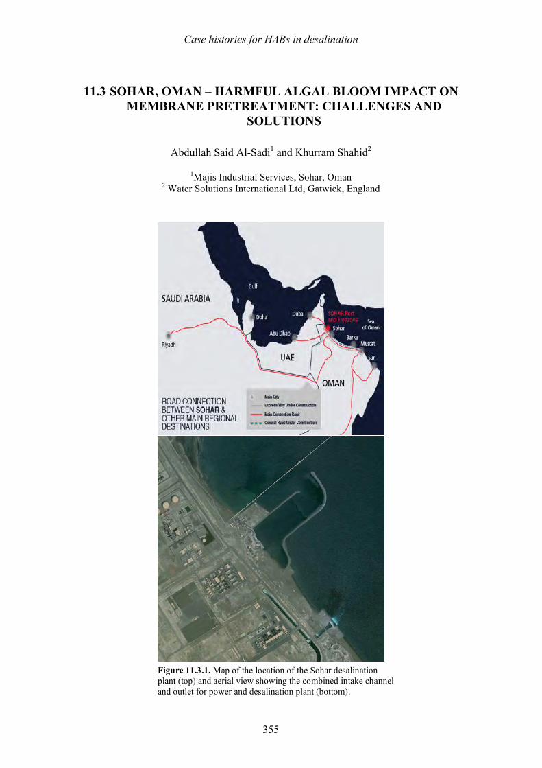
Case histories for HABs in desalination

355

11.3 SOHAR, OMAN – HARMFUL ALGAL BLOOM IMPACT ON MEMBRANE PRETREATMENT: CHALLENGES AND

SOLUTIONS

Abdullah Said Al-Sadi1 and Khurram Shahid2

1Majis Industrial Services, Sohar, Oman 2 Water Solutions International Ltd, Gatwick, England

Figure 11.3.1. Map of the location of the Sohar desalination plant (top) and aerial view showing the combined intake channel and outlet for power and desalination plant (bottom).

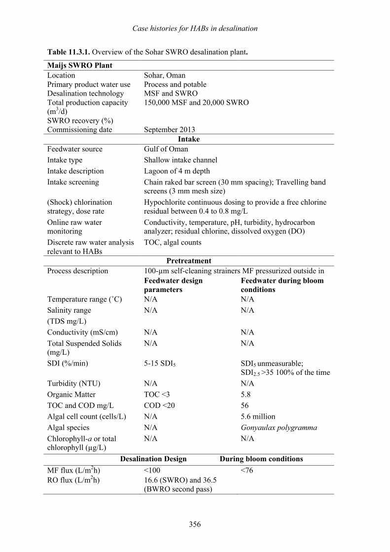
Case histories for HABs in desalination

356

Table 11.3.1. Overview of the Sohar SWRO desalination plant.

Maijs SWRO Plant Location Sohar, Oman Primary product water use Process and potable Desalination technology MSF and SWRO Total production capacity (m3/d)

150,000 MSF and 20,000 SWRO

SWRO recovery (%) Commissioning date September 2013

Intake Feedwater source Gulf of Oman Intake type Shallow intake channel Intake description Lagoon of 4 m depth Intake screening Chain raked bar screen (30 mm spacing); Travelling band

screens (3 mm mesh size) (Shock) chlorination strategy, dose rate

Hypochlorite continuous dosing to provide a free chlorine residual between 0.4 to 0.8 mg/L

Online raw water monitoring

Conductivity, temperature, pH, turbidity, hydrocarbon analyzer; residual chlorine, dissolved oxygen (DO)

Discrete raw water analysis relevant to HABs

TOC, algal counts

Pretreatment Process description 100-µm self-cleaning strainers MF pressurized outside in Feedwater design

parameters Feedwater during bloom conditions

Temperature range (˚C) N/A N/A Salinity range (TDS mg/L)

N/A N/A

Conductivity (mS/cm) N/A N/A Total Suspended Solids (mg/L)

N/A N/A

SDI (%/min) 5-15 SDI5 SDI5 unmeasurable; SDI2.5 >35 100% of the time

Turbidity (NTU) N/A N/A Organic Matter TOC and COD mg/L

TOC <3 COD <20

5.8 56

Algal cell count (cells/L) N/A 5.6 million Algal species N/A Gonyaulax polygramma Chlorophyll-a or total chlorophyll (µg/L)

N/A N/A

Desalination Design During bloom conditions MF flux (L/m2h) <100 <76 RO flux (L/m2h) 16.6 (SWRO) and 36.5

(BWRO second pass)

Case histories for HABs in desalination

357

11.3.1 Introduction The Oman Sohar Industrial Port Area (SIPA) is home to major petrochemical, iron and steel, methanol, and fertilizer plants, as well as three power stations. Since its inception in 2006 it has drawn some US$ 15 billion in investment and holds a strategic place in the future development of Oman. As the sole water services provider at SIPA, Majis Industrial Services (Majis) has a significant role in the economy of the Sultanate. Majis provides seawater for cooling as well as high-quality desalinated water for process water applications, as well as potable water and wastewater collection, treatment, and re-use for irrigation. After the completion of its second seawater pumping station, the cooling water pumping facility with a capacity of almost 700,000 m3/h will be one of the largest in the Middle East. Some of the industries at SIPA have their own treatment plants to produce process and boiler water using this seawater. The plant comprises a 585MW combined-cycle, gas-fired power plant and a 170,000 m3/d desalination plant located in the Sohar Industrial Port area in the North Al Batinah region of the Sultanate of Oman (Figure 11.3.1). The desalination plant comprises four conventional Multi Stage Flash (MSF) units and a SWRO system. The 20,000 m3/d SWRO plant is unique in nature by using direct membrane filtration, not conventional pretreatment. The raw water originating from an open intake is pumped directly through the microfiltration (MF) membrane filtration system, then directly to the RO units without a break tank. The characteristics of the SWRO plant are given in Table 11.3.1. HABs have been observed in the Sohar Region since 1970s, but presumably occurred long before that. Majis started its operations at SIPA in 2006-2007, and since 2008 has kept a record of algal bloom events. In 2008-2009 a severe red tide of Cochlodinium polykrikoides disrupted operations at SIPA resulting in huge economic loss. Sohar Refinery shut down its own SWRO plant and intake screens required cleaning every 4 hours instead of every 12. In 2011 and 2013 green algal blooms also impacted SIPA operations. In September 2013, when the RO plant was ready for commissioning, the seawater conditions were very challenging with very high levels of SDI2.5 >35, and high algal bloom cell concentrations > 5.8 million cells/L. This prolonged HAB event lasted almost six months during which the installations had to be commissioned, the feedwater consistently having the same high level of SDI.

11.3.2 System description The screened and continuously chlorinated seawater is supplied from the Seawater Intake Pumping Station (SWIPS I). The SWIPS I has an open intake and the water comes from a shallow lagoon of 4 m depth which provides an ideal environment for algal blooms (Figure 11.3.1). The SWRO plant consists of MF pretreatment (with no coagulation or chemical injection prior) followed by five SWRO trains, each having a capacity of 4,000 m3/d. Two trains are dedicated for process water and the other three for potable water. A diagram of the 20,000 m3/d MF plant is provided in Figure 11.3.2. The microfiltration (MF) system uses Pall Microza UNA-620A, high crystalline PVDF Membranes, with < 0.1 µm pore size, and an outside-inside filtration mode. The first-pass SWRO system consists of a combination Hydranautics membrane, SWC5max/SWC6max at train 1 and 2 and SWC4max/SWC5max at train 3, 4 and 5. The second pass BWRO trains consist of ESPA2-LD/Hydranautics. The average membrane flux for the SWRO and BWRO systems is 16.6 L/m2h and 36.5 L/m2h, respectively.

The 20,000 m3/d plant, was designed for standard seawater quality conditions where the duration of any red tide or algal bloom events were expected to last for two to a maximum of

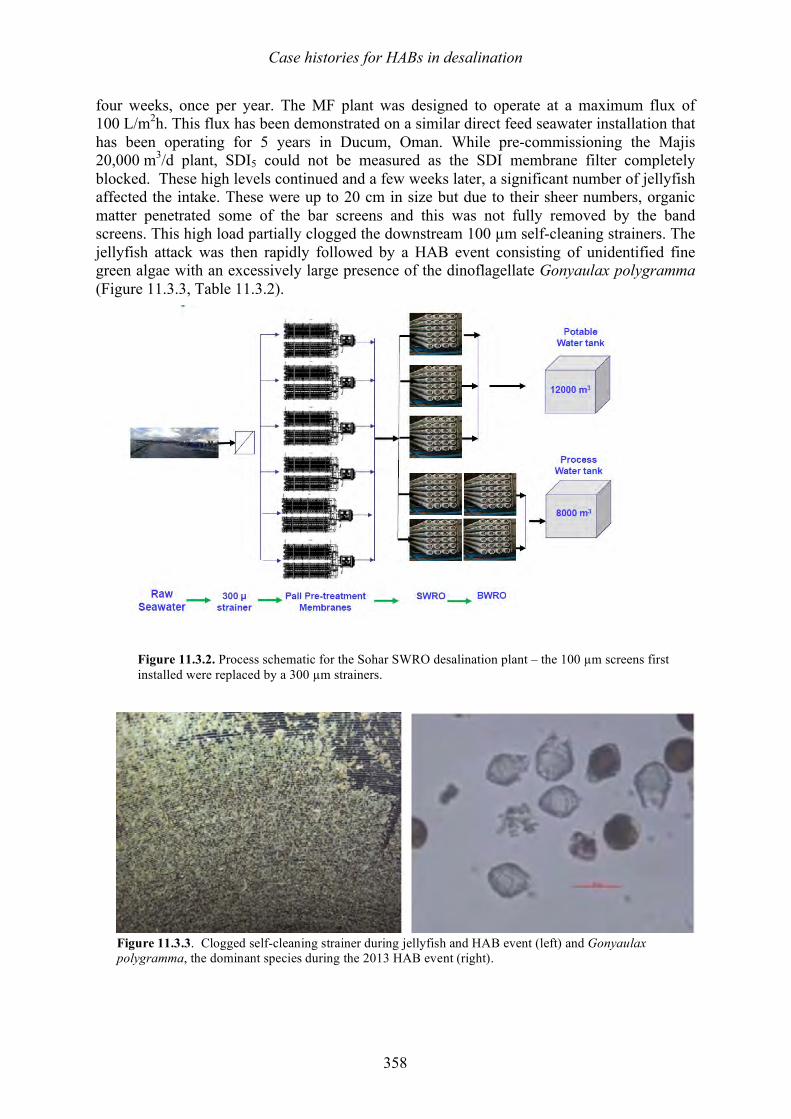
Case histories for HABs in desalination

358

four weeks, once per year. The MF plant was designed to operate at a maximum flux of 100 L/m2h. This flux has been demonstrated on a similar direct feed seawater installation that has been operating for 5 years in Ducum, Oman. While pre-commissioning the Majis 20,000 m3/d plant, SDI5 could not be measured as the SDI membrane filter completely blocked. These high levels continued and a few weeks later, a significant number of jellyfish affected the intake. These were up to 20 cm in size but due to their sheer numbers, organic matter penetrated some of the bar screens and this was not fully removed by the band screens. This high load partially clogged the downstream 100 µm self-cleaning strainers. The jellyfish attack was then rapidly followed by a HAB event consisting of unidentified fine green algae with an excessively large presence of the dinoflagellate Gonyaulax polygramma (Figure 11.3.3, Table 11.3.2).

Figure 11.3.2. Process schematic for the Sohar SWRO desalination plant – the 100 µm screens first installed were replaced by a 300 µm strainers.

Figure 11.3.3. Clogged self-cleaning strainer during jellyfish and HAB event (left) and Gonyaulax polygramma, the dominant species during the 2013 HAB event (right).

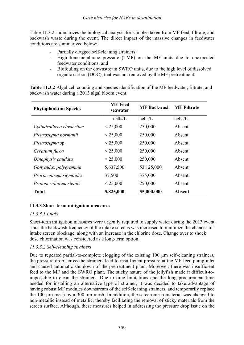
Case histories for HABs in desalination

359

Table 11.3.2 summarizes the biological analysis for samples taken from MF feed, filtrate, and backwash waste during the event. The direct impact of the massive changes in feedwater conditions are summarized below:

- Partially clogged self-cleaning strainers; - High transmembrane pressure (TMP) on the MF units due to unexpected

feedwater conditions; and - Biofouling on the downstream SWRO units, due to the high level of dissolved

organic carbon (DOC), that was not removed by the MF pretreatment.

Table 11.3.2 Algal cell counting and species identification of the MF feedwater, filtrate, and backwash water during a 2013 algal bloom event.

Phytoplankton Species MF Feed seawater MF Backwash MF Filtrate

cells/L cells/L cells/L Cylindrotheca closterium < 25,000 250,000 Absent

Pleurosigma normanii < 25,000 250,000 Absent Pleurosigma sp. < 25,000 250,000 Absent Ceratium furca < 25,000 250,000 Absent

Dinophysis caudata < 25,000 250,000 Absent Gonyaulax polygramma 5,637,500 53,125,000 Absent

Prorocentrum sigmoides 37,500 375,000 Absent Protoperidinium steinii < 25,000 250,000 Absent

Total 5,825,000 55,000,000 Absent

11.3.3 Short-term mitigation measures

11.3.3.1 Intake Short-term mitigation measures were urgently required to supply water during the 2013 event. Thus the backwash frequency of the intake screens was increased to minimize the chances of intake screen blockage, along with an increase in the chlorine dose. Change over to shock dose chlorination was considered as a long-term option. 11.3.3.2 Self-cleaning strainers

Due to repeated partial-to-complete clogging of the existing 100 µm self-cleaning strainers, the pressure drop across the strainers lead to insufficient pressure at the MF feed pump inlet and caused automatic shutdown of the pretreatment plant. Moreover, there was insufficient feed to the MF and the SWRO plant. The sticky nature of the jellyfish made it difficult-to-impossible to clean the strainers. Due to time limitations and the long procurement time needed for installing an alternative type of strainer, it was decided to take advantage of having robust MF modules downstream of the self-cleaning strainers, and temporarily replace the 100 µm mesh by a 300 µm mesh. In addition, the screen mesh material was changed to non-metallic instead of metallic, thereby facilitating the removal of sticky materials from the screen surface. Although, these measures helped in addressing the pressure drop issue on the

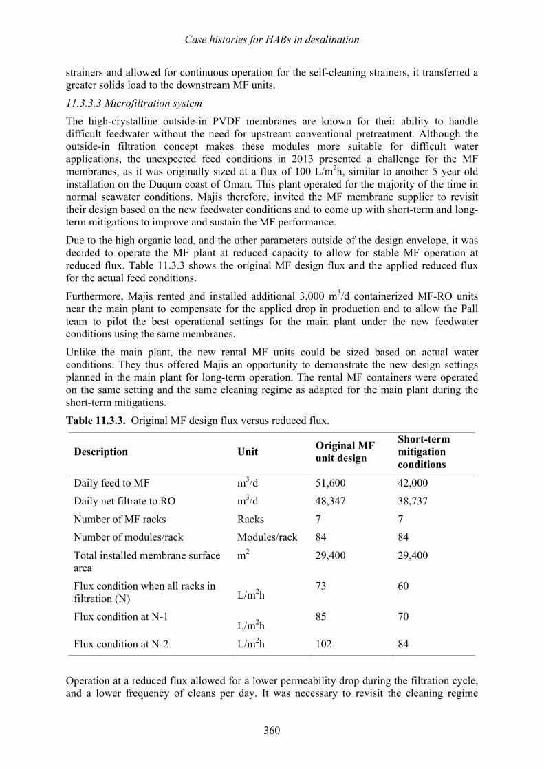
Case histories for HABs in desalination

360

strainers and allowed for continuous operation for the self-cleaning strainers, it transferred a greater solids load to the downstream MF units.

11.3.3.3 Microfiltration system The high-crystalline outside-in PVDF membranes are known for their ability to handle difficult feedwater without the need for upstream conventional pretreatment. Although the outside-in filtration concept makes these modules more suitable for difficult water applications, the unexpected feed conditions in 2013 presented a challenge for the MF membranes, as it was originally sized at a flux of 100 L/m2h, similar to another 5 year old installation on the Duqum coast of Oman. This plant operated for the majority of the time in normal seawater conditions. Majis therefore, invited the MF membrane supplier to revisit their design based on the new feedwater conditions and to come up with short-term and long-term mitigations to improve and sustain the MF performance.

Due to the high organic load, and the other parameters outside of the design envelope, it was decided to operate the MF plant at reduced capacity to allow for stable MF operation at reduced flux. Table 11.3.3 shows the original MF design flux and the applied reduced flux for the actual feed conditions.

Furthermore, Majis rented and installed additional 3,000 m3/d containerized MF-RO units near the main plant to compensate for the applied drop in production and to allow the Pall team to pilot the best operational settings for the main plant under the new feedwater conditions using the same membranes.

Unlike the main plant, the new rental MF units could be sized based on actual water conditions. They thus offered Majis an opportunity to demonstrate the new design settings planned in the main plant for long-term operation. The rental MF containers were operated on the same setting and the same cleaning regime as adapted for the main plant during the short-term mitigations. Table 11.3.3. Original MF design flux versus reduced flux.

Description Unit Original MF unit design

Short-term mitigation conditions

Daily feed to MF m3/d 51,600 42,000 Daily net filtrate to RO m3/d 48,347 38,737

Number of MF racks Racks 7 7 Number of modules/rack Modules/rack 84 84

Total installed membrane surface area

m2 29,400 29,400

Flux condition when all racks in filtration (N) L/m2h

73 60

Flux condition at N-1 L/m2h

85 70

Flux condition at N-2 L/m2h 102 84

Operation at a reduced flux allowed for a lower permeability drop during the filtration cycle, and a lower frequency of cleans per day. It was necessary to revisit the cleaning regime

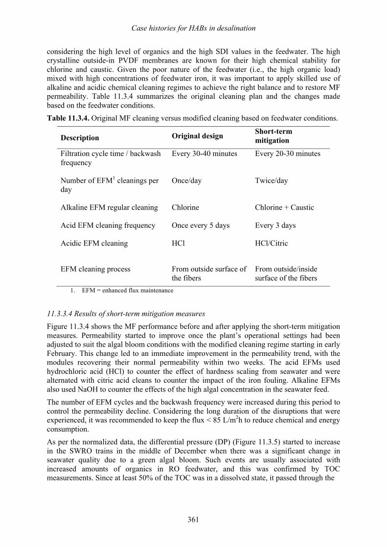
Case histories for HABs in desalination

361

considering the high level of organics and the high SDI values in the feedwater. The high crystalline outside-in PVDF membranes are known for their high chemical stability for chlorine and caustic. Given the poor nature of the feedwater (i.e., the high organic load) mixed with high concentrations of feedwater iron, it was important to apply skilled use of alkaline and acidic chemical cleaning regimes to achieve the right balance and to restore MF permeability. Table 11.3.4 summarizes the original cleaning plan and the changes made based on the feedwater conditions. Table 11.3.4. Original MF cleaning versus modified cleaning based on feedwater conditions.

Description Original design Short-term mitigation

Filtration cycle time / backwash frequency

Every 30-40 minutes Every 20-30 minutes

Number of EFM1 cleanings per day

Once/day Twice/day

Alkaline EFM regular cleaning

Chlorine Chlorine + Caustic

Acid EFM cleaning frequency

Once every 5 days Every 3 days

Acidic EFM cleaning HCl HCl/Citric

EFM cleaning process From outside surface of

the fibers From outside/inside surface of the fibers

1. EFM = enhanced flux maintenance 11.3.3.4 Results of short-term mitigation measures Figure 11.3.4 shows the MF performance before and after applying the short-term mitigation measures. Permeability started to improve once the plant’s operational settings had been adjusted to suit the algal bloom conditions with the modified cleaning regime starting in early February. This change led to an immediate improvement in the permeability trend, with the modules recovering their normal permeability within two weeks. The acid EFMs used hydrochloric acid (HCl) to counter the effect of hardness scaling from seawater and were alternated with citric acid cleans to counter the impact of the iron fouling. Alkaline EFMs also used NaOH to counter the effects of the high algal concentration in the seawater feed. The number of EFM cycles and the backwash frequency were increased during this period to control the permeability decline. Considering the long duration of the disruptions that were experienced, it was recommended to keep the flux < 85 L/m2h to reduce chemical and energy consumption. As per the normalized data, the differential pressure (DP) (Figure 11.3.5) started to increase in the SWRO trains in the middle of December when there was a significant change in seawater quality due to a green algal bloom. Such events are usually associated with increased amounts of organics in RO feedwater, and this was confirmed by TOC measurements. Since at least 50% of the TOC was in a dissolved state, it passed through the

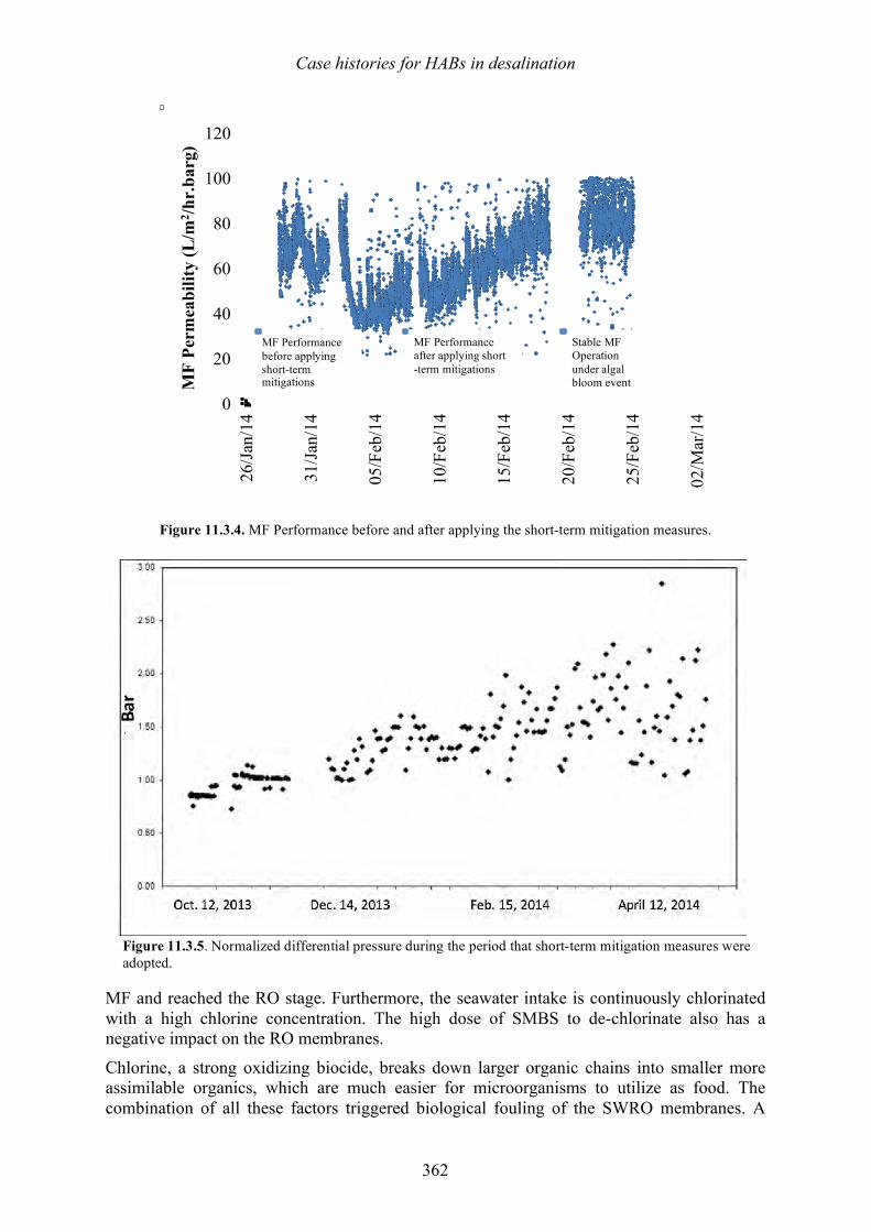
Case histories for HABs in desalination

362

Figure 11.3.4. MF Performance before and after applying the short-term mitigation measures.

MF and reached the RO stage. Furthermore, the seawater intake is continuously chlorinated with a high chlorine concentration. The high dose of SMBS to de-chlorinate also has a negative impact on the RO membranes.

Chlorine, a strong oxidizing biocide, breaks down larger organic chains into smaller more assimilable organics, which are much easier for microorganisms to utilize as food. The combination of all these factors triggered biological fouling of the SWRO membranes. A

0

20

40

60

80

100

120

26/J

an/1

4

31/J

an/1

4

05/F

eb/1

4

10/F

eb/1

4

15/F

eb/1

4

20/F

eb/1

4

25/F

eb/1

4

02/M

ar/1

4

MF Performance after applying short -term mitigations

Stable MF Operationunder algal bloom eventM

F Pe

rmea

bilit

y (L

/m2 /h

r.ba

rg)

MF Performance before applying short-term mitigations

Figure 11.3.5. Normalized differential pressure during the period that short-term mitigation measures were adopted.

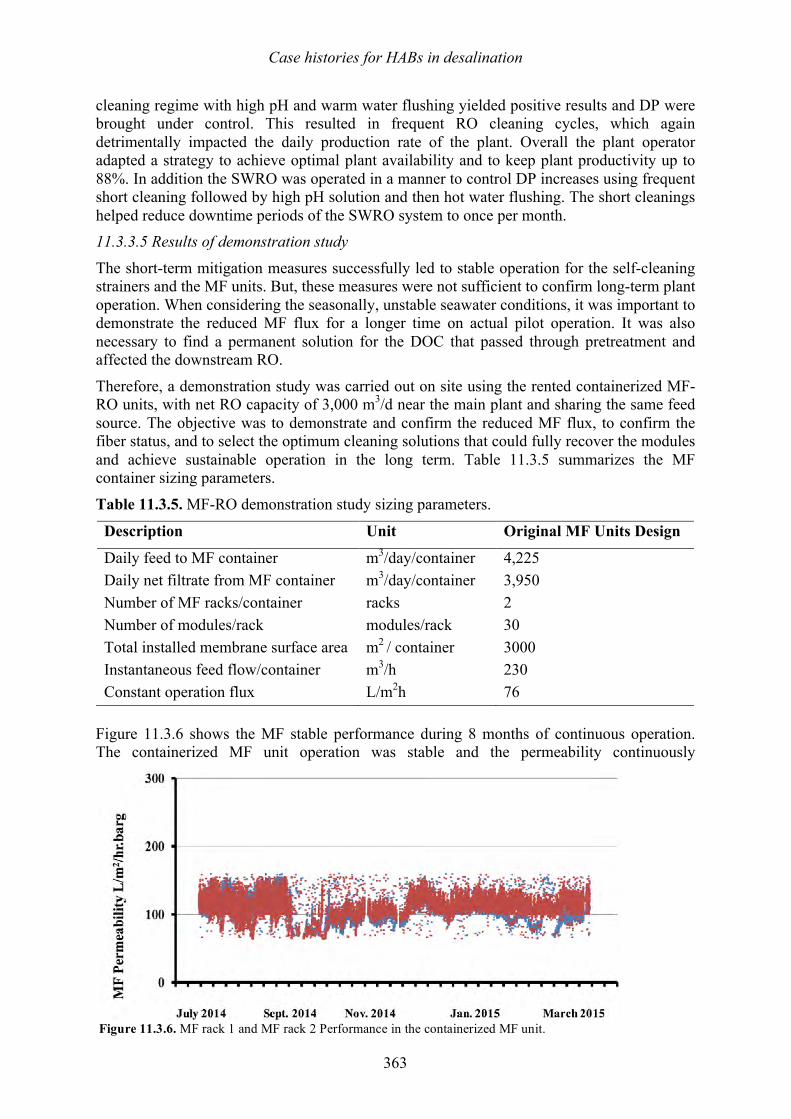
Case histories for HABs in desalination

363

cleaning regime with high pH and warm water flushing yielded positive results and DP were brought under control. This resulted in frequent RO cleaning cycles, which again detrimentally impacted the daily production rate of the plant. Overall the plant operator adapted a strategy to achieve optimal plant availability and to keep plant productivity up to 88%. In addition the SWRO was operated in a manner to control DP increases using frequent short cleaning followed by high pH solution and then hot water flushing. The short cleanings helped reduce downtime periods of the SWRO system to once per month. 11.3.3.5 Results of demonstration study

The short-term mitigation measures successfully led to stable operation for the self-cleaning strainers and the MF units. But, these measures were not sufficient to confirm long-term plant operation. When considering the seasonally, unstable seawater conditions, it was important to demonstrate the reduced MF flux for a longer time on actual pilot operation. It was also necessary to find a permanent solution for the DOC that passed through pretreatment and affected the downstream RO.

Therefore, a demonstration study was carried out on site using the rented containerized MF-RO units, with net RO capacity of 3,000 m3/d near the main plant and sharing the same feed source. The objective was to demonstrate and confirm the reduced MF flux, to confirm the fiber status, and to select the optimum cleaning solutions that could fully recover the modules and achieve sustainable operation in the long term. Table 11.3.5 summarizes the MF container sizing parameters.

Table 11.3.5. MF-RO demonstration study sizing parameters.

Description Unit Original MF Units Design

Daily feed to MF container m3/day/container 4,225 Daily net filtrate from MF container m3/day/container 3,950 Number of MF racks/container racks 2 Number of modules/rack modules/rack 30 Total installed membrane surface area m2 / container 3000 Instantaneous feed flow/container m3/h 230 Constant operation flux L/m2h 76

Figure 11.3.6 shows the MF stable performance during 8 months of continuous operation. The containerized MF unit operation was stable and the permeability continuously

Figure 11.3.6. MF rack 1 and MF rack 2 Performance in the containerized MF unit.

Case histories for HABs in desalination

364

maintained above 100 L/m2h.bar, except for a few days during an algal bloom event that repeated again in September 2014.

11.3.4 Long-term mitigation measures With a strategic view on the desalination business of Majis, it has been decided to replace continuous chlorination with shock chlorination. This will be challenging, as the Majis intake system serves various types of industries that are dependent on the chlorine level at their heat exchangers. For the removal of DOC, it is important to use coagulation upstream of the MF system to remove dissolved organics that are currently fouling the RO membranes. Either a direct coagulation before the MF units will be applied in the existing plant, or during phase 2 of plant expansion, a common gravity filter stage with coagulation dose could be installed preceding the new RO system. This would be located upstream of the MF system to cover both phase 1 and phase 2. The self-cleaning filters will be expanded by adding an extra two units, and the drum screens’ pore size will be reduced back to 100 µm from 300 µm. This increase in the screen area will allow for continuous supply and the use of non-metallic parts instead of the metallic screens that have enhanced the removal of sticky materials from the screen surface. Based on the research study, operation under a relaxed flux range of < 76 L/m2h showed very stable operation for the MF containerised units. The same flux was used as the maximum MF flux for long term mitigation of poor feedwater in the main plant. Extra membrane surface area will be added to allow full production at the reduced flux. Table 11.3.6 summarizes design changes for long-term mitigation of algal blooms.

The frequency of HCl cleaning will be increased as will the use of citric acid in addition to HCl. Alkaline cleaning will use a mixture of chlorine and caustic soda (Table 11.3.7). The use of direct coagulation is one of the options proposed for removing dissolved organics. Table 11.3.6. Planned design changes at Majis.

Description Unit Original MF unit design

Long-term mitigation

Daily feed to MF m3/d 51,600 58,500 Daily net filtrate to RO m3/d 48,347 54,800 Number of MF racks Racks 7 9 Number of modules/rack modules/rack 84 96 Total installed membrane surface area

m2 29,400 43,200

Flux condition when all racks in filtration (N) L/m2h

73 56

Flux condition with N-1 L/m2h

85 63

Flux condition with N-2 L/m2h

102 72.5

Since the pretreatment system has been modified, the RO system performance is expected to improve. There is also a plan for reducing the flux rate on the SWRO from 16.6 L/m2h to 14 L/m2h by adding extra RO membranes. With the use of coagulation in front of the MF units, the majority of DOC should be removed, and this will further achieve better results in the RO system.

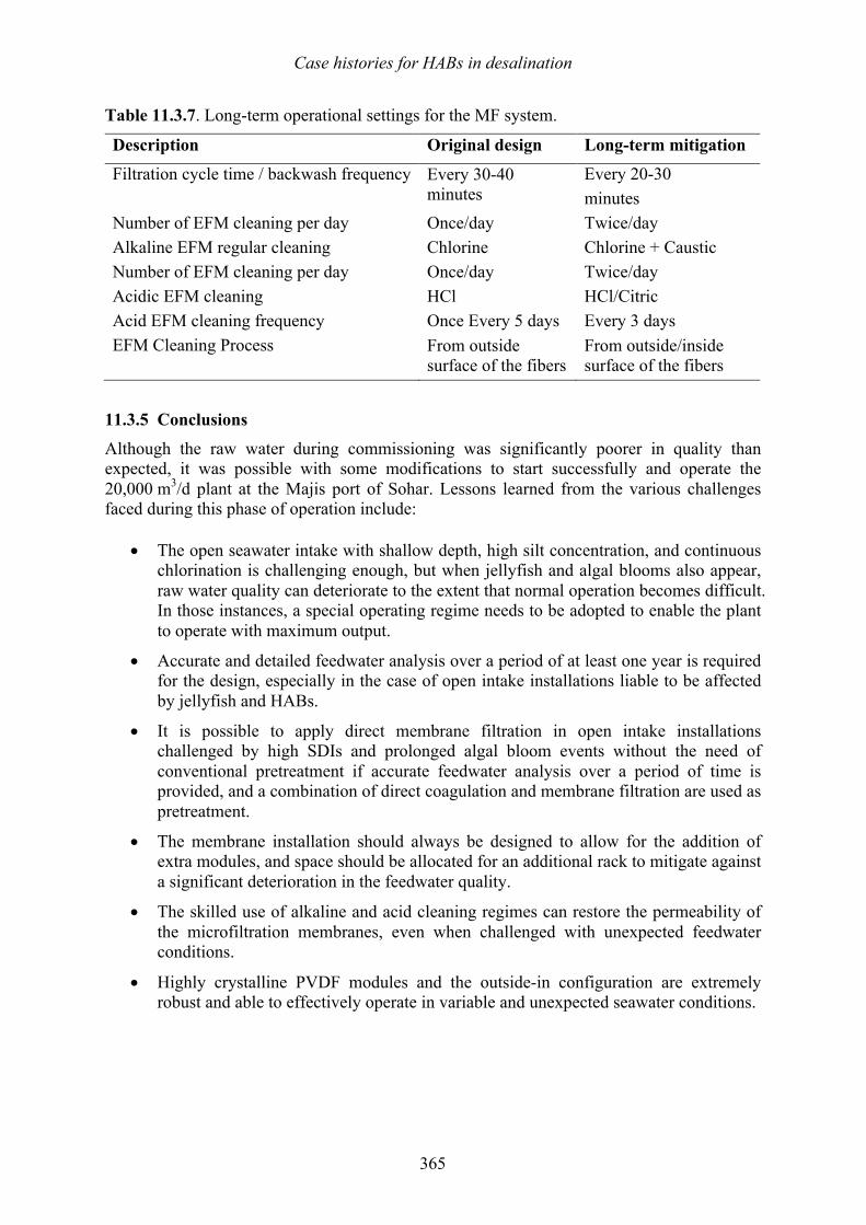
Case histories for HABs in desalination

365

Table 11.3.7. Long-term operational settings for the MF system.

Description Original design Long-term mitigation

Filtration cycle time / backwash frequency Every 30-40 minutes

Every 20-30 minutes

Number of EFM cleaning per day Once/day Twice/day Alkaline EFM regular cleaning Chlorine Chlorine + Caustic Number of EFM cleaning per day Once/day Twice/day Acidic EFM cleaning HCl HCl/Citric Acid EFM cleaning frequency Once Every 5 days Every 3 days EFM Cleaning Process From outside

surface of the fibers From outside/inside surface of the fibers

11.3.5 Conclusions

Although the raw water during commissioning was significantly poorer in quality than expected, it was possible with some modifications to start successfully and operate the 20,000 m3/d plant at the Majis port of Sohar. Lessons learned from the various challenges faced during this phase of operation include:

• The open seawater intake with shallow depth, high silt concentration, and continuous chlorination is challenging enough, but when jellyfish and algal blooms also appear, raw water quality can deteriorate to the extent that normal operation becomes difficult. In those instances, a special operating regime needs to be adopted to enable the plant to operate with maximum output.

• Accurate and detailed feedwater analysis over a period of at least one year is required for the design, especially in the case of open intake installations liable to be affected by jellyfish and HABs.

• It is possible to apply direct membrane filtration in open intake installations challenged by high SDIs and prolonged algal bloom events without the need of conventional pretreatment if accurate feedwater analysis over a period of time is provided, and a combination of direct coagulation and membrane filtration are used as pretreatment.

• The membrane installation should always be designed to allow for the addition of extra modules, and space should be allocated for an additional rack to mitigate against a significant deterioration in the feedwater quality.

• The skilled use of alkaline and acid cleaning regimes can restore the permeability of the microfiltration membranes, even when challenged with unexpected feedwater conditions.

• Highly crystalline PVDF modules and the outside-in configuration are extremely robust and able to effectively operate in variable and unexpected seawater conditions.

Case histories for HABs in desalination

366

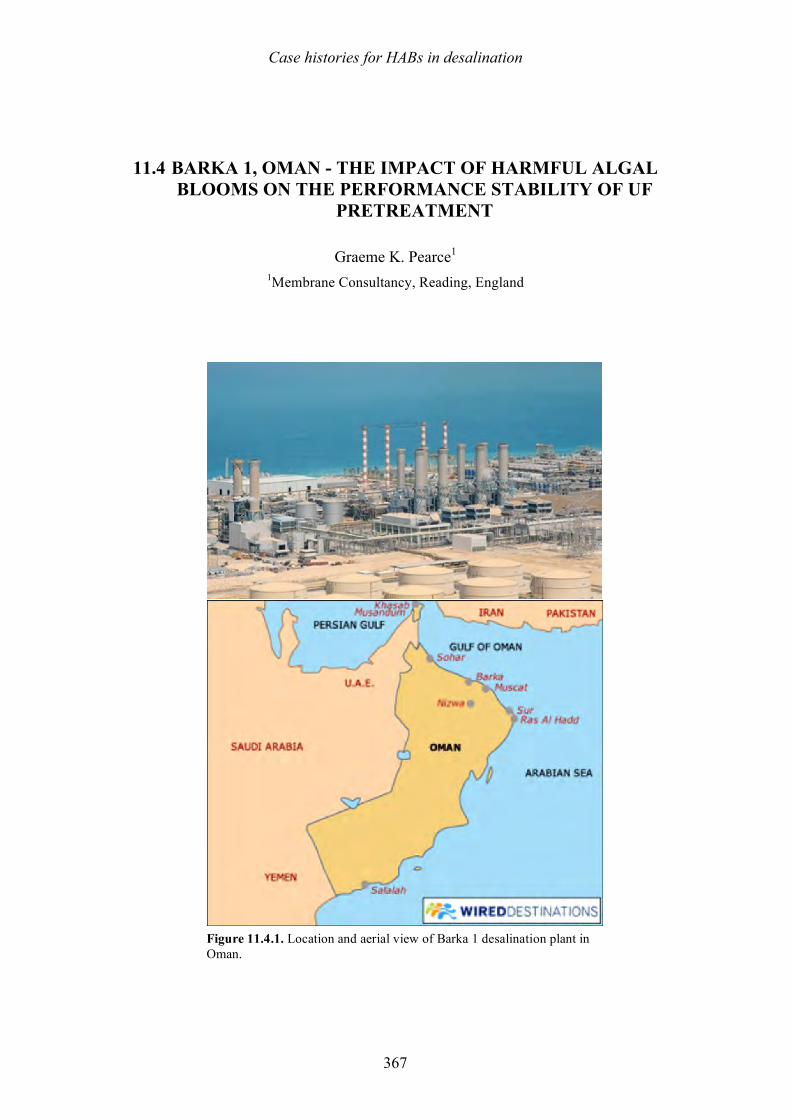
Case histories for HABs in desalination

367

11.4 BARKA 1, OMAN - THE IMPACT OF HARMFUL ALGAL

BLOOMS ON THE PERFORMANCE STABILITY OF UF PRETREATMENT

Graeme K. Pearce1

1Membrane Consultancy, Reading, England

Figure 11.4.1. Location and aerial view of Barka 1 desalination plant in Oman.

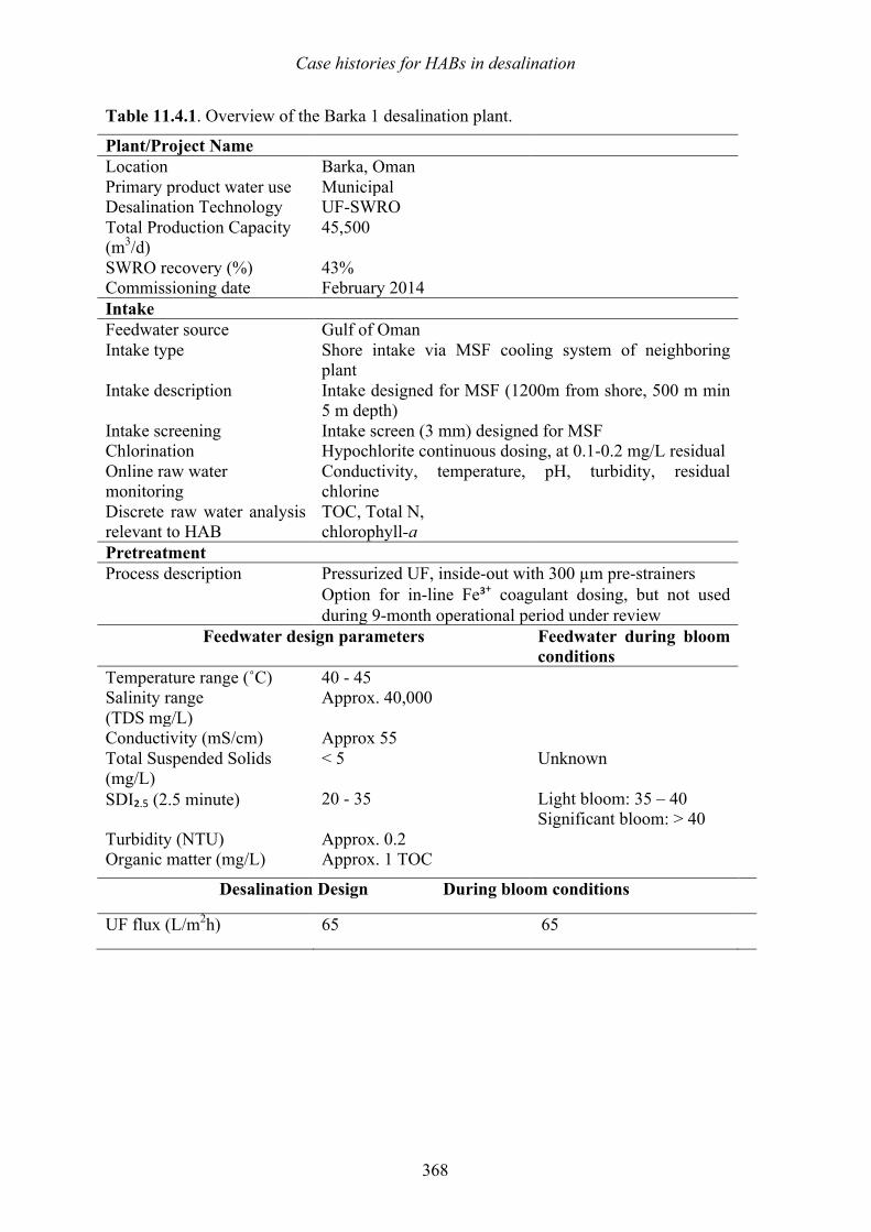
Case histories for HABs in desalination

368

Table 11.4.1. Overview of the Barka 1 desalination plant.

Plant/Project Name Location Barka, Oman Primary product water use Municipal Desalination Technology UF-SWRO Total Production Capacity (m3/d)

45,500

SWRO recovery (%) 43% Commissioning date February 2014 Intake Feedwater source Gulf of Oman Intake type Shore intake via MSF cooling system of neighboring

plant Intake description Intake designed for MSF (1200m from shore, 500 m min

5 m depth) Intake screening Intake screen (3 mm) designed for MSF Chlorination Hypochlorite continuous dosing, at 0.1-0.2 mg/L residual Online raw water monitoring

Conductivity, temperature, pH, turbidity, residual chlorine

Discrete raw water analysis relevant to HAB

TOC, Total N, chlorophyll-a

Pretreatment Process description Pressurized UF, inside-out with 300 µm pre-strainers Option for in-line Fe³+ coagulant dosing, but not used

during 9-month operational period under review Feedwater design parameters Feedwater during bloom

conditions Temperature range (˚C) 40 - 45 Salinity range (TDS mg/L)

Approx. 40,000

Conductivity (mS/cm) Approx 55 Total Suspended Solids (mg/L)

< 5 Unknown

SDI₂.5 (2.5 minute) 20 - 35 Light bloom: 35 – 40 Significant bloom: > 40

Turbidity (NTU) Approx. 0.2 Organic matter (mg/L) Approx. 1 TOC

Desalination Design During bloom conditions

UF flux (L/m2h) 65 65 65

Case histories for HABs in desalination

369

11.4.1 Introduction The original desalination and power plant at the industrial port city of Barka was based around a 91,000 m3/d multi-stage flash (MSF) thermal desalination unit. Barka is located 60 km north east of Oman’s capital, Muscat, and draws its feedwater from the Gulf of Oman as shown in Figure 11.4.1. In 2012, the plant operator, ACWA Power Barka won a contract from the government agency Oman Power and Water Procurement (OPWP) for expansion of the facility with a 45,500 m3/d seawater RO (SWRO) unit. The contract to build this first phase expansion plant, subsequently referred to as Barka 1, was awarded to Abeinsa. The contractor, a wholly owned subsidiary of the Spanish EPC Abengoa, is experienced in UF-SWRO design and operation including with feedwater that are prone to algal bloom (Bernaola 2012). Commissioning for Barka 1 started in September 2013 with continuous operation in February 2014. In 2015, a second phase expansion for a further 57,000 m3/d, known as Barka 2, was also brought online.

The Barka 1 plant uses an open intake seawater feed without any pretreatment by clarification or flotation. Before arriving at the RO desalination plant, the feedwater passes through the heat exchangers of a condensing system providing cooling water for the MSF facility. The plant has a provision for in-line coagulant dosing which was intended for periods of poor feedwater quality, but for the period of review in this case study, this dosing facility has not been used.

Details of the algal species at Barka during the period of this investigation were not determined directly. The HAB and red tide causing species commonly found in these areas are: Noctiluca scintillans, Dinophysis spp., Gonyaulax sp., Trichodesmium sp., and Ceratium spp. of which the dinoflagellate, N. scintillans is a major species that produces red tide blooms yearly (Thangaraja et al. 2007). More recently, 24 algal species have been identified in these waters (Al-Azri 2014) with relatively abundant concentrations of the dinoflagellates Prorocentrum minimum and Cochlodinium polykrikoides being reported for the first time. The pretreatment system at Barka 1 utilizes Pentair-Xflow UF. The Xflow membranes are made from polyethersulfone (PES) and have a nominal 0.02 µm pore size rating. The membranes operate with an inside-out feed flow configuration, with four 1.5 m elements mounted in a 6 m horizontal pressure vessel. This case study focuses on the performance stability of the UF system during a 9-month period which took place 5 months after continuous operation commenced in February 2014. This ensured that initial conditioning of the membrane was completed and effective chemical cleaning procedures were established. The period under review started in July 2014 and finished in April 2015 and was assessed through the monitoring of permeability trends for three months at the start of the review period and comparing these trends with the three months at the end of the period.

11.4.2 Plant overview A simplified block flow diagram for the Barka 1 desalination plant is shown in Figure 11.4.2. The seawater feed is taken from an open intake 1200m from shore at a depth of 5 m below the lowest tide level. Following 3-mm screens, the seawater is used as cooling water for the neighboring MSF desalination plant, which increases the temperature by 9 ºC. The feedwater is chlorinated with a 2 ppm free chlorine dose prior to the MSF, but by the time it reaches the membrane units, the chlorine residual has reduced to around 0.2 ppm. The desalination plant feedwater is filtered by 300 µm strainers before passing through the eight UF units. There is an option for in-line coagulant dosing, but this was not employed during the nine-month period of evaluation described in this case study. The UF is connected directly to the RO

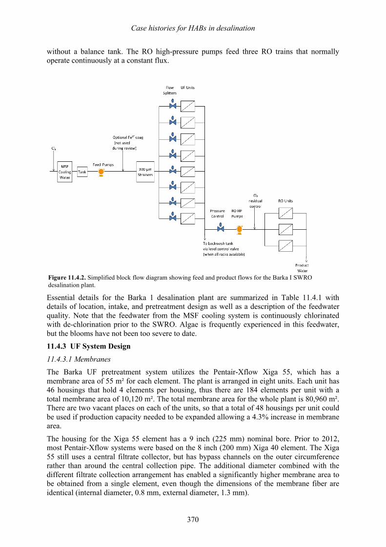
Case histories for HABs in desalination

370

without a balance tank. The RO high-pressure pumps feed three RO trains that normally operate continuously at a constant flux.

Essential details for the Barka 1 desalination plant are summarized in Table 11.4.1 with details of location, intake, and pretreatment design as well as a description of the feedwater quality. Note that the feedwater from the MSF cooling system is continuously chlorinated with de-chlorination prior to the SWRO. Algae is frequently experienced in this feedwater, but the blooms have not been too severe to date. 11.4.3 UF System Design

11.4.3.1 Membranes The Barka UF pretreatment system utilizes the Pentair-Xflow Xiga 55, which has a membrane area of 55 m² for each element. The plant is arranged in eight units. Each unit has 46 housings that hold 4 elements per housing, thus there are 184 elements per unit with a total membrane area of 10,120 m². The total membrane area for the whole plant is 80,960 m². There are two vacant places on each of the units, so that a total of 48 housings per unit could be used if production capacity needed to be expanded allowing a 4.3% increase in membrane area.

The housing for the Xiga 55 element has a 9 inch (225 mm) nominal bore. Prior to 2012, most Pentair-Xflow systems were based on the 8 inch (200 mm) Xiga 40 element. The Xiga 55 still uses a central filtrate collector, but has bypass channels on the outer circumference rather than around the central collection pipe. The additional diameter combined with the different filtrate collection arrangement has enabled a significantly higher membrane area to be obtained from a single element, even though the dimensions of the membrane fiber are identical (internal diameter, 0.8 mm, external diameter, 1.3 mm).

Figure 11.4.2. Simplified block flow diagram showing feed and product flows for the Barka I SWRO desalination plant.

Case histories for HABs in desalination

371

11.4.3.2 In-line design The UF is connected directly to the RO in a direct-coupled design that eliminates the break tank between UF and RO systems. Pentair-Xflow is a strong proponent of the in-line UF-RO system design, especially for large scale seawater duties. The control system provides a constant inlet pressure to the RO feed pump at approximately 2 bar. Eliminating the RO feedwater tank reduces space and cost for the system and saves energy. Of arguably greater significance, the intermediate tank can promote biofouling, and so by eliminating it from the flowsheet, the operational stability of the RO can be improved and chemical cleaning frequency reduced (Pearce 2013; Knops 2014). In-line designs need to employ a significant number of units to ensure that flow can be kept reasonably constant. In order to minimize fouling it is preferable to keep flux variation within 10% of the average if possible (+/- 15% maximum), or alternatively the average flux should be reduced by a few percent (Pearce 2015). In the Barka 1 design, the flux selected is moderate and the flux variation for the in-line design has been optimized such that the variation falls within the 10-15% guideline. Accelerated fouling would therefore not be expected, and as will be seen from the results review in section 11.3.4, has not been observed. 11.4.3.3 Flux

For a plant without flux variation, it would be expected that 70 L/m2h would be a suitable design flux for the Pentair-Xflow membrane on seawater from the Gulf based on comparison with other plants. The Barka 1 plant has been designed to operate at an average UF flux of around 65 L/m2h, but with a modest degree of flux variation. Flux varies during the filtration cycle (time between backwash) between 60 and 70 L/m2h, with occasional short-lived excursions down to 55 L/m2h and up to 75 L/m2h. Fine-tuning the process cycle has minimized the flux variation. At the design flux, the filtration cycle time is approximately 50 minutes, but this cycle time may extend at lower flux.

When a unit is taken off-line for backwash, the remaining units increase their flow in proportion causing an increase of flux over the average for when all 8 units are available, that is, from around 62 L/m2h with 8 units in filtration, to about 70 L/m2h when one unit is in backwash. The filtration cycle takes about one minute. At the same time, some filtrate is taken from the manifold to replenish the backwash tank. The replenishment rate has been optimized to ensure that there is no adverse effect on flux variation.

11.4.3.4 Temperature correction Warm feedwater temperatures increase clean water permeability. For example, an elevation of 9 oC above ambient should increase permeability by 30%. Furthermore, the elevated temperatures would reduce lumen length pressure drop as well as pressure drop in the shell, resulting in improved hydrodynamic efficiency of the module. The benefit at 70 L/m2h would, however, be minimal since hydrodynamic stress at this moderate flux is relatively low. Furthermore, the benefit of elevated temperature for a real feedwater is observed to be significantly less than the 30% permeability improvement indicated above. For seawater from the Gulf, fluxes are determined as much by the concentration of particles in the lumen as by the permeability across the membrane. Any increase in flux would increase the particle concentration in the lumen and at the membrane surface thereby increasing the fouling rate. Thus in these circumstances, elevated temperature would have no significant benefit. This assumption is reinforced by the practical observation that there does not appear to be a

Case histories for HABs in desalination

372

benefit from high temperature operation for other power plant cooling water desalination systems.

11.4.4 UF system performance 11.4.4.1 Expected permeability

A typical Pentair-Xflow membrane has a permeability of 400-500 L/m2h.bar during early operation on a surface water feed at 20oC (for example during take-over testing). Generally, the membrane would stabilize after the first month at 300-400 L/m2h.bar, depending on feedwater quality, and this would be expected to represent an initial baseline.

Seawater feeds may have lower permeabilities than for surface waters at the same temperature since the viscosity and density are both higher. Permeability is also strongly affected by foulants and the adsorption of organics, especially algae and algal derivatives. A higher temperature would decrease viscosity, which would give an increase in permeability.

For the Gulf water feedwater at Barka, taking account of the effects described above, it would be expected that the baseline permeability after the initial operating period should be around 350-400 L/m2h.bar, depending on local feedwater quality characteristics. Permeability reported in subsequent sections shows that the Barka 1 plant has been able to achieve the expected permeability level. 11.4.4.2 Use of chemical cleaning to maintain permeability

Performance stability is maintained by conducting a chemical enhanced backwash (CEB) on a regular basis. Under normal circumstances with good quality feedwater, the CEB would be scheduled once every 23 or 24 backwash cycles, equivalent to an interval of around 18 hours between consecutive CEB’s (which is the period referred to in this review as a CEB cycle). If feedwater quality deteriorates, for example due to an algal bloom, or permeability drops for some other reason, the CEB is performed more frequently, perhaps after 12 or 15 hours. The change of CEB frequency is initiated manually. If there is a long-term deterioration in CEB, a Clean-In-Place (CIP) is performed. The CIP is more effective than CEB since the contact time is longer and the chemicals may be recirculated. The longer CIP downtime would mean that recovery and hence output would be reduced if conducted too frequently, so it is beneficial to make the interval between CIP as long as possible with a target of at least 6 months. It is therefore important for the CEB to recover a high proportion of the permeability lost during the course of a CEB cycle. 360 CEB cycles have been performed in the period of this review. The following time periods have been evaluated which used the full design flux at a consistent level:

1. Period 1: CEB cycles 8 to 119 during 10 July to 7 October 2014; and 2. Period 2: CEB cycles 201 to 360 during 1 January to 27 April 2015

Prior to cycle 8, flux varied. No data were evaluated for cycles 120 to 200 in the last quarter of 2014, but the plant appeared to operate in a stable fashion at this time. The starting permeability at the beginning of Period 2 was fully satisfactory and in line with expectations for this type of operational plant with membranes in good condition.

The analysis focuses on the performance of unit 7 since this unit was found to have average performance, although, variation between units was found to be almost negligible.

Case histories for HABs in desalination

373

11.4.4.3 Permeability trends during period 1 Figure 11.4.3 shows the permeability trend data for Period 1, CEB cycles 8 to 119, together with the CEB cycle time on the right-hand axis.

Figure 11.4.3. Permeability at start and end of CEB cycle for cycles 8-119

The chart shows the loss of permeability during the course of a CEB cycle was significant at around 100-150 L/m2h.bar, and that the CEB was reasonably effective at recovering the permeability (Figure 11.4.3). The CEB was not fully effective, and there was a gradual loss of permeability with time. The loss reduced slightly in the later cycles and showed a response to external factors.

At the beginning of CEB cycle 8, the initial permeability was fully satisfactory. The chart shows the trend lines for start and end permeability. The two trend lines gradually converge, indicating that the rate of fouling was falling, and this issue will be discussed in more detail below. The slope can be used to predict the requirement for CIP and quantify the CIP interval and this will be discussed below. For a given flux, permeability is affected by the following control variables:

• Filtration cycle time • CEB interval • Feedwater quality

The loss of permeability in a single filtration cycle was approximately 5 L/m2h.bar per cycle. A series of 24 cycles would therefore lead to a permeability loss of approximately 120 L/m2h.bar. In reviewing the data, there has not been an opportunity to examine the effect of changing the filtration cycle time, since this value is linked to the flux, and only increased if the flux reduced. It is possible that the rate of fouling could be reduced slightly by reducing the filtration cycle time from the standard interval of 50 minutes. This action would not be recommended, since recovery would fall significantly. The first of the three parameters is therefore not a control variable as far as the operator is concerned.

Case histories for HABs in desalination

374

The second factor listed is the interval between CEB. Although normally set at one CEB every 23 or 24 backwash cycles (equivalent to a time interval of 18 hours), the interval can be reduced as shown by the green triangles in Figure 11.4.3. The final operational factor affecting performance is the feedwater quality. The main parameter that appears to correlate with permeability is the chlorophyll concentration. Typical concentrations vary between 0.02 and 0.04 µg/L, but minor excursions to 0.1 µg/L do not appear to cause the UF system any problems and appear to indicate a normal non-problematic seawater quality. A moderate algal bloom event between cycles 40 and 60 (mid to late August 2014) had a significant effect on permeability, but the plant managed to maintain flux and recovered without any intervention other than a reduction in the CEB cycle time. For a more significant algal bloom, it might be necessary to reduce flux or possibly consider coagulant dosing.

Figure 11.4.3 shows that increasing CEB frequency from once in 18 hours to once in 15 hours or 12 hours during a period of high algae between cycles 40 and 60 enabled the plant to cope with the challenging conditions. Although permeability dropped during this period by around 100 L/m2h.bar, the plant recovered without having to reduce the flux. Permeability then recovered to a level only marginally below the original level once feedwater quality returned to normal conditions.

Note that the CEB cycle time remained slightly below the original level between cycles 60 and 80, which appeared to arrest the rate of decline slightly. The situation was made more complicated by the fact that there was a sticking valve on unit 7 at around cycle 75, that is, during the 2nd week of September. The result of this was that CEB was not fully effective during this period and permeability temporarily declined. After the problem was resolved, the plant returned to previous levels without any further intervention, again underlining the fact that the operational regime was sufficiently robust for performance to recover after a minor upset.

11.4.4.4 Permeability Trends after One Year of Operation Figure 11.4.4 shows permeability trends for cycles 201 to 360. The figure shows that the starting permeability in cycle 201 was similar to the starting permeability at cycle 119, thus the gradual decline discussed in the previous section had been arrested. The difference between the start and end permeability from cycle 201 onwards is normally around 100 L/m2h.bar or just over which is similar to or slightly less than in cycle 119.

The initial permeability did not decline further between cycles 119 and 201 because of the use of a slightly shorter CEB cycle time, i.e., CEB frequency increased. Shortening CEB cycle time reduces the loss of permeability in the course of a CEB cycle. For cycles from 201 onwards, CEB cycle time was 12 - 15 hours as opposed to 18 hours previously. The higher frequency was implemented in response to the poor feedwater quality from an algal bloom that began in December and continued for much of January through April. Increasing CEB frequency made the start permeability more stable. This has the effect of lengthening the CIP interval and will be quantified in section 11.4.4.7.

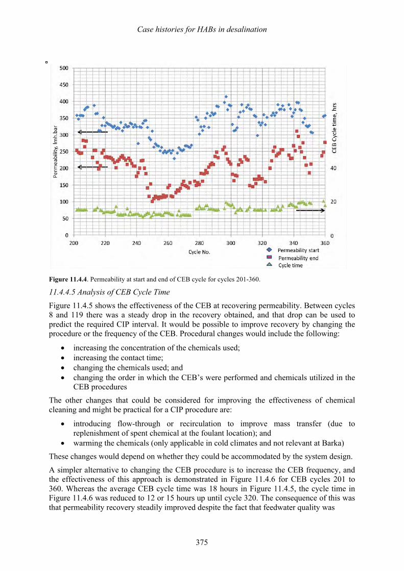
Case histories for HABs in desalination

375

Figure 11.4.4. Permeability at start and end of CEB cycle for cycles 201-360.

11.4.4.5 Analysis of CEB Cycle Time

Figure 11.4.5 shows the effectiveness of the CEB at recovering permeability. Between cycles 8 and 119 there was a steady drop in the recovery obtained, and that drop can be used to predict the required CIP interval. It would be possible to improve recovery by changing the procedure or the frequency of the CEB. Procedural changes would include the following:

• increasing the concentration of the chemicals used; • increasing the contact time; • changing the chemicals used; and • changing the order in which the CEB’s were performed and chemicals utilized in the

CEB procedures The other changes that could be considered for improving the effectiveness of chemical cleaning and might be practical for a CIP procedure are:

• introducing flow-through or recirculation to improve mass transfer (due to replenishment of spent chemical at the foulant location); and

• warming the chemicals (only applicable in cold climates and not relevant at Barka) These changes would depend on whether they could be accommodated by the system design.

A simpler alternative to changing the CEB procedure is to increase the CEB frequency, and the effectiveness of this approach is demonstrated in Figure 11.4.6 for CEB cycles 201 to 360. Whereas the average CEB cycle time was 18 hours in Figure 11.4.5, the cycle time in Figure 11.4.6 was reduced to 12 or 15 hours up until cycle 320. The consequence of this was that permeability recovery steadily improved despite the fact that feedwater quality was

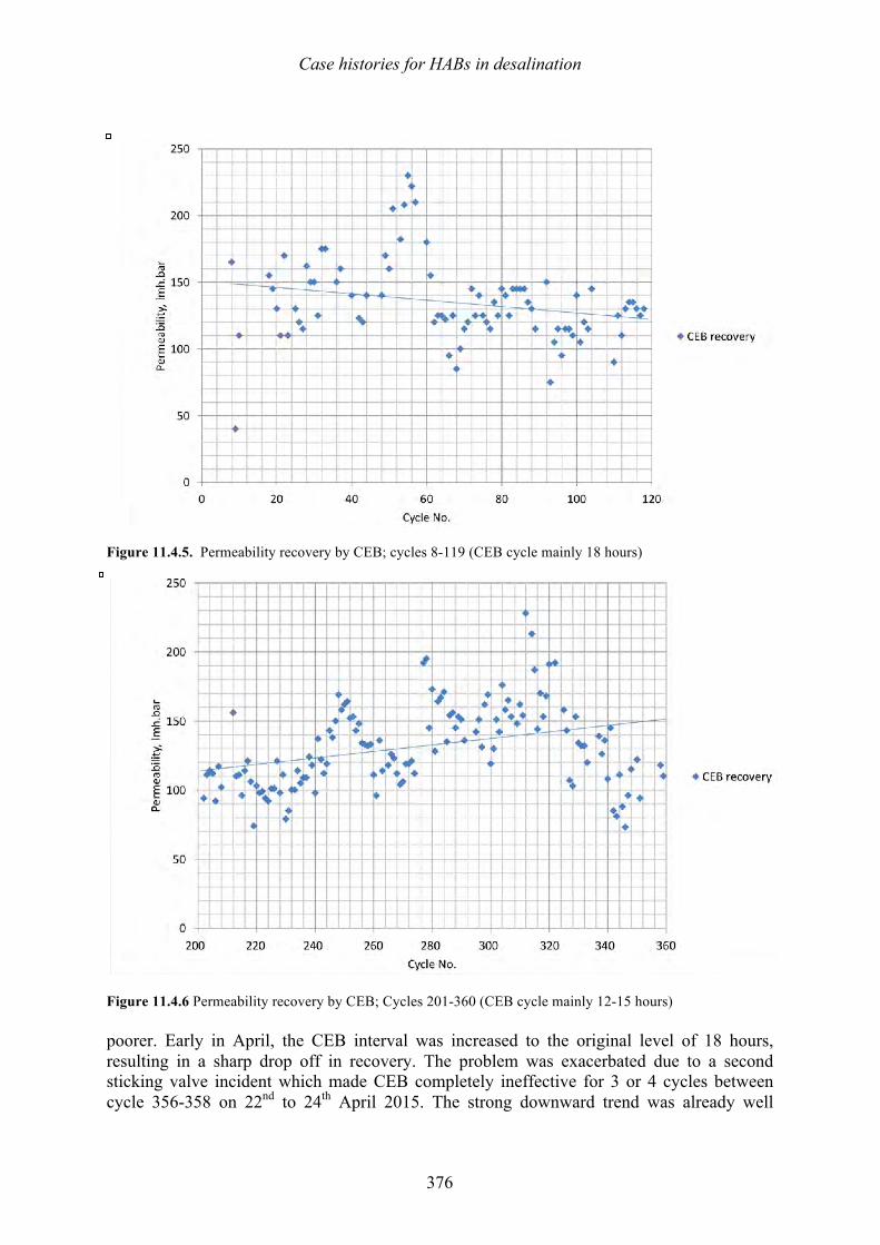
Case histories for HABs in desalination

376

Figure 11.4.5. Permeability recovery by CEB; cycles 8-119 (CEB cycle mainly 18 hours)

Figure 11.4.6 Permeability recovery by CEB; Cycles 201-360 (CEB cycle mainly 12-15 hours) poorer. Early in April, the CEB interval was increased to the original level of 18 hours, resulting in a sharp drop off in recovery. The problem was exacerbated due to a second sticking valve incident which made CEB completely ineffective for 3 or 4 cycles between cycle 356-358 on 22nd to 24th April 2015. The strong downward trend was already well

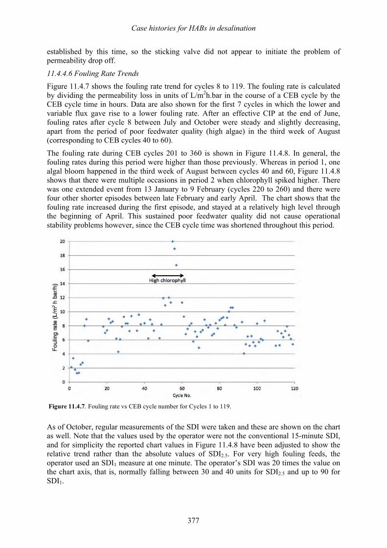
Case histories for HABs in desalination

377

established by this time, so the sticking valve did not appear to initiate the problem of permeability drop off.

11.4.4.6 Fouling Rate Trends Figure 11.4.7 shows the fouling rate trend for cycles 8 to 119. The fouling rate is calculated by dividing the permeability loss in units of L/m2h.bar in the course of a CEB cycle by the CEB cycle time in hours. Data are also shown for the first 7 cycles in which the lower and variable flux gave rise to a lower fouling rate. After an effective CIP at the end of June, fouling rates after cycle 8 between July and October were steady and slightly decreasing, apart from the period of poor feedwater quality (high algae) in the third week of August (corresponding to CEB cycles 40 to 60).

The fouling rate during CEB cycles 201 to 360 is shown in Figure 11.4.8. In general, the fouling rates during this period were higher than those previously. Whereas in period 1, one algal bloom happened in the third week of August between cycles 40 and 60, Figure 11.4.8 shows that there were multiple occasions in period 2 when chlorophyll spiked higher. There was one extended event from 13 January to 9 February (cycles 220 to 260) and there were four other shorter episodes between late February and early April. The chart shows that the fouling rate increased during the first episode, and stayed at a relatively high level through the beginning of April. This sustained poor feedwater quality did not cause operational stability problems however, since the CEB cycle time was shortened throughout this period.

As of October, regular measurements of the SDI were taken and these are shown on the chart as well. Note that the values used by the operator were not the conventional 15-minute SDI, and for simplicity the reported chart values in Figure 11.4.8 have been adjusted to show the relative trend rather than the absolute values of SDI2.5. For very high fouling feeds, the operator used an SDI1 measure at one minute. The operator’s SDI was 20 times the value on the chart axis, that is, normally falling between 30 and 40 units for SDI2.5 and up to 90 for SDI1.

Figure 11.4.7. Fouling rate vs CEB cycle number for Cycles 1 to 119.

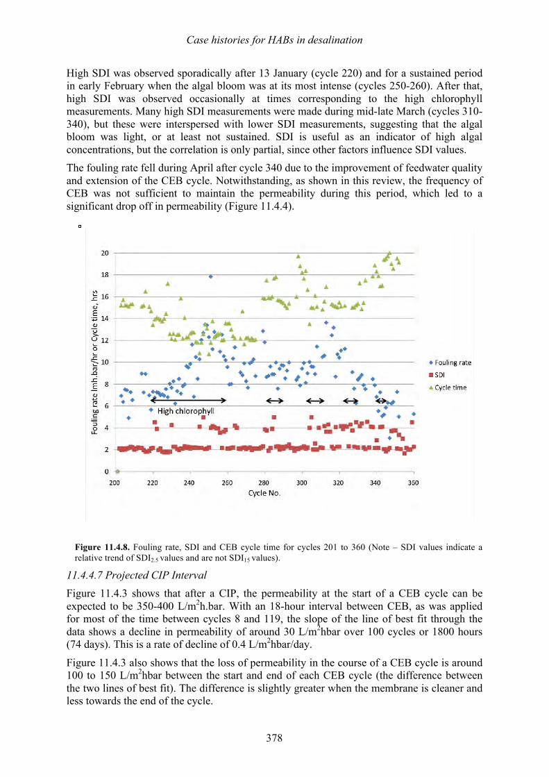
Case histories for HABs in desalination

378

High SDI was observed sporadically after 13 January (cycle 220) and for a sustained period in early February when the algal bloom was at its most intense (cycles 250-260). After that, high SDI was observed occasionally at times corresponding to the high chlorophyll measurements. Many high SDI measurements were made during mid-late March (cycles 310-340), but these were interspersed with lower SDI measurements, suggesting that the algal bloom was light, or at least not sustained. SDI is useful as an indicator of high algal concentrations, but the correlation is only partial, since other factors influence SDI values. The fouling rate fell during April after cycle 340 due to the improvement of feedwater quality and extension of the CEB cycle. Notwithstanding, as shown in this review, the frequency of CEB was not sufficient to maintain the permeability during this period, which led to a significant drop off in permeability (Figure 11.4.4).

Figure 11.4.8. Fouling rate, SDI and CEB cycle time for cycles 201 to 360 (Note – SDI values indicate a relative trend of SDI2.5 values and are not SDI15 values).

11.4.4.7 Projected CIP Interval Figure 11.4.3 shows that after a CIP, the permeability at the start of a CEB cycle can be expected to be 350-400 L/m2h.bar. With an 18-hour interval between CEB, as was applied for most of the time between cycles 8 and 119, the slope of the line of best fit through the data shows a decline in permeability of around 30 L/m2hbar over 100 cycles or 1800 hours (74 days). This is a rate of decline of 0.4 L/m2hbar/day.

Figure 11.4.3 also shows that the loss of permeability in the course of a CEB cycle is around 100 to 150 L/m2hbar between the start and end of each CEB cycle (the difference between the two lines of best fit). The difference is slightly greater when the membrane is cleaner and less towards the end of the cycle.

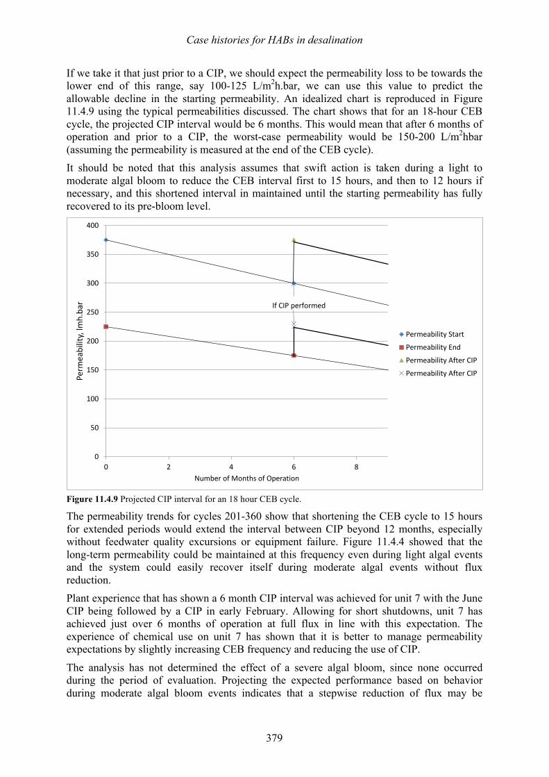
Case histories for HABs in desalination

379

If we take it that just prior to a CIP, we should expect the permeability loss to be towards the lower end of this range, say 100-125 L/m2h.bar, we can use this value to predict the allowable decline in the starting permeability. An idealized chart is reproduced in Figure 11.4.9 using the typical permeabilities discussed. The chart shows that for an 18-hour CEB cycle, the projected CIP interval would be 6 months. This would mean that after 6 months of operation and prior to a CIP, the worst-case permeability would be 150-200 L/m2hbar (assuming the permeability is measured at the end of the CEB cycle). It should be noted that this analysis assumes that swift action is taken during a light to moderate algal bloom to reduce the CEB interval first to 15 hours, and then to 12 hours if necessary, and this shortened interval in maintained until the starting permeability has fully recovered to its pre-bloom level.

Figure 11.4.9 Projected CIP interval for an 18 hour CEB cycle.

The permeability trends for cycles 201-360 show that shortening the CEB cycle to 15 hours for extended periods would extend the interval between CIP beyond 12 months, especially without feedwater quality excursions or equipment failure. Figure 11.4.4 showed that the long-term permeability could be maintained at this frequency even during light algal events and the system could easily recover itself during moderate algal events without flux reduction. Plant experience that has shown a 6 month CIP interval was achieved for unit 7 with the June CIP being followed by a CIP in early February. Allowing for short shutdowns, unit 7 has achieved just over 6 months of operation at full flux in line with this expectation. The experience of chemical use on unit 7 has shown that it is better to manage permeability expectations by slightly increasing CEB frequency and reducing the use of CIP.

The analysis has not determined the effect of a severe algal bloom, since none occurred during the period of evaluation. Projecting the expected performance based on behavior during moderate algal bloom events indicates that a stepwise reduction of flux may be

0

50

100

150

200

250

300

350

400

0 2 4 6 8

Perm

eability, lm

h.bar

Number of Months of Operation

Permeability Start

Permeability End

Permeability After CIP

Permeability After CIP

If CIP performed

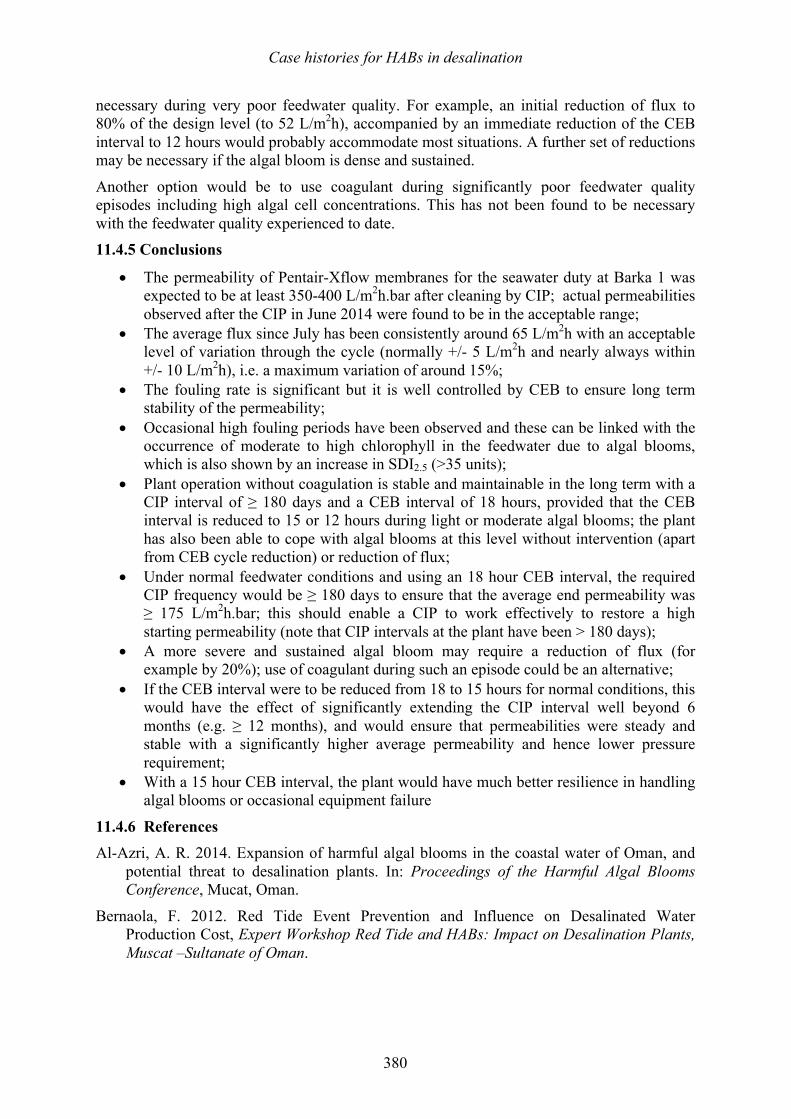
Case histories for HABs in desalination

380

necessary during very poor feedwater quality. For example, an initial reduction of flux to 80% of the design level (to 52 L/m2h), accompanied by an immediate reduction of the CEB interval to 12 hours would probably accommodate most situations. A further set of reductions may be necessary if the algal bloom is dense and sustained.

Another option would be to use coagulant during significantly poor feedwater quality episodes including high algal cell concentrations. This has not been found to be necessary with the feedwater quality experienced to date. 11.4.5 Conclusions

• The permeability of Pentair-Xflow membranes for the seawater duty at Barka 1 was expected to be at least 350-400 L/m2h.bar after cleaning by CIP; actual permeabilities observed after the CIP in June 2014 were found to be in the acceptable range;

• The average flux since July has been consistently around 65 L/m2h with an acceptable level of variation through the cycle (normally +/- 5 L/m2h and nearly always within +/- 10 L/m2h), i.e. a maximum variation of around 15%;

• The fouling rate is significant but it is well controlled by CEB to ensure long term stability of the permeability;

• Occasional high fouling periods have been observed and these can be linked with the occurrence of moderate to high chlorophyll in the feedwater due to algal blooms, which is also shown by an increase in SDI2.5 (>35 units);

• Plant operation without coagulation is stable and maintainable in the long term with a CIP interval of ≥ 180 days and a CEB interval of 18 hours, provided that the CEB interval is reduced to 15 or 12 hours during light or moderate algal blooms; the plant has also been able to cope with algal blooms at this level without intervention (apart from CEB cycle reduction) or reduction of flux;

• Under normal feedwater conditions and using an 18 hour CEB interval, the required CIP frequency would be ≥ 180 days to ensure that the average end permeability was ≥ 175 L/m2h.bar; this should enable a CIP to work effectively to restore a high starting permeability (note that CIP intervals at the plant have been > 180 days);

• A more severe and sustained algal bloom may require a reduction of flux (for example by 20%); use of coagulant during such an episode could be an alternative;

• If the CEB interval were to be reduced from 18 to 15 hours for normal conditions, this would have the effect of significantly extending the CIP interval well beyond 6 months (e.g. ≥ 12 months), and would ensure that permeabilities were steady and stable with a significantly higher average permeability and hence lower pressure requirement;

• With a 15 hour CEB interval, the plant would have much better resilience in handling algal blooms or occasional equipment failure

11.4.6 References Al-Azri, A. R. 2014. Expansion of harmful algal blooms in the coastal water of Oman, and

potential threat to desalination plants. In: Proceedings of the Harmful Algal Blooms Conference, Mucat, Oman.

Bernaola, F. 2012. Red Tide Event Prevention and Influence on Desalinated Water Production Cost, Expert Workshop Red Tide and HABs: Impact on Desalination Plants, Muscat –Sultanate of Oman.

Case histories for HABs in desalination

381

Knops, F. N. M. 2014. Reducing SWRO life cycle costs by direct coupling of UF and SWRO Systems. In: Proceedings European Desalination Society Conference, Limmasol, Cyprus.

Pearce, G. K. 2013. The Potential Advantages of Direct Coupled UF System Designs for Bio-Fouling Control in Pre-treatment of Seawater RO Systems. In: Proceedings International Desalination Association Conference, Tianjin, China.

Pearce, G. K. 2015. How Much Flux Variation Can We Allow in UF System Design; Striking the Right Balance between Performance Stability and Cost Minimization. In: Proceedings American Membrane Technology Association Membrane Technology Conference, Orlando, Florida, USA.

Thangaraja, M., Al-Aisry, A., and Al-Kharusi, L. 2007. Harmful algal blooms and their impacts in the middle and outer ROPME sea area. International Journal of Oceans and Oceanography 2(1), 85-98.

Case histories for HABs in desalination

382

Case histories for HABs in desalination

383

11.5 SHUWAIKH, KUWAIT – HARMFUL ALGAL BLOOM CELL REMOVAL USING DISSOLVED AIR FLOTATION: PILOT AND

LABORATORY STUDIES

Robert Wiley1, Mike Dixon2 and Siobhan F. E. Boerlage3 1Leopold, a Xylem Brand, Zelienople, PA, USA

2MDD Consulting, Kensington, Calagry, Alberta, Canada 3 Boerlage Consulting, Gold Coast, Queensland, Australia

Figure 11.5.1. Location of the Shuwaikh, SWRO Plant in Kuwait (top). Algal (species unidentified) bloom near intake (middle). DAF Float during the bloom (bottom).

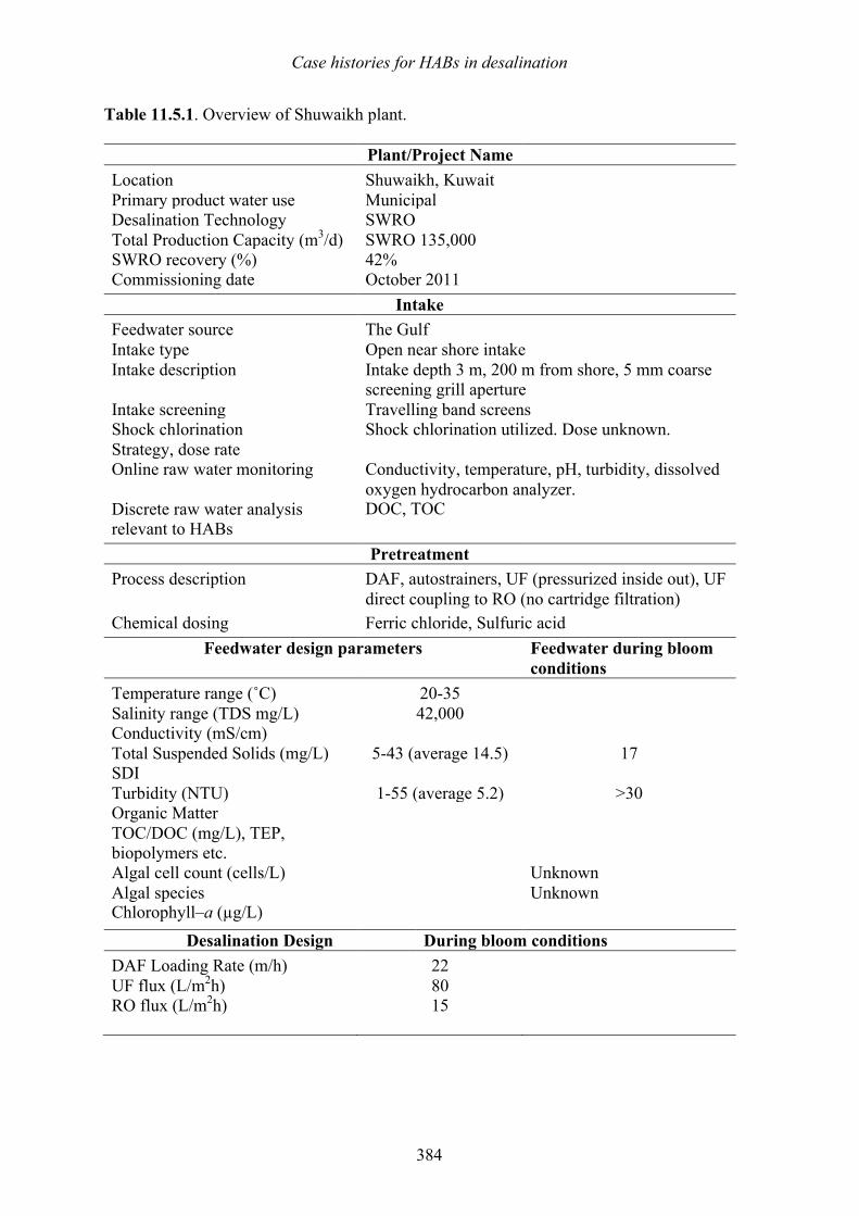
Case histories for HABs in desalination

384

Table 11.5.1. Overview of Shuwaikh plant.

Plant/Project Name Location Shuwaikh, Kuwait Primary product water use Municipal Desalination Technology SWRO Total Production Capacity (m3/d) SWRO 135,000 SWRO recovery (%) 42% Commissioning date October 2011

Intake Feedwater source The Gulf Intake type Open near shore intake Intake description Intake depth 3 m, 200 m from shore, 5 mm coarse

screening grill aperture Intake screening Travelling band screens Shock chlorination Strategy, dose rate

Shock chlorination utilized. Dose unknown.

Online raw water monitoring Conductivity, temperature, pH, turbidity, dissolved oxygen hydrocarbon analyzer.

Discrete raw water analysis relevant to HABs

DOC, TOC

Pretreatment Process description

DAF, autostrainers, UF (pressurized inside out), UF direct coupling to RO (no cartridge filtration)

Chemical dosing Ferric chloride, Sulfuric acid Feedwater design parameters Feedwater during bloom

conditions Temperature range (˚C) 20-35 Salinity range (TDS mg/L) 42,000 Conductivity (mS/cm) Total Suspended Solids (mg/L) 5-43 (average 14.5) 17 SDI Turbidity (NTU) 1-55 (average 5.2) >30 Organic Matter TOC/DOC (mg/L), TEP, biopolymers etc.

Algal cell count (cells/L) Unknown Algal species Unknown Chlorophyll–a (µg/L)

Desalination Design During bloom conditions DAF Loading Rate (m/h) 22 UF flux (L/m2h) 80 RO flux (L/m2h) 15

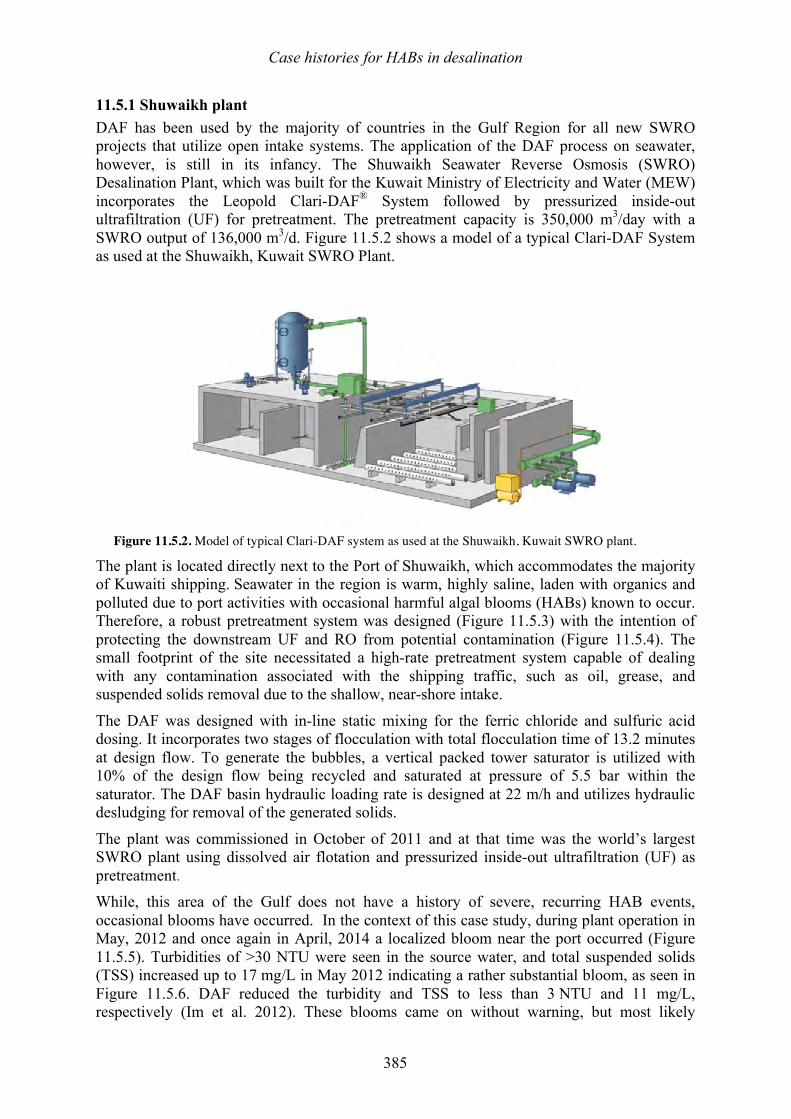
Case histories for HABs in desalination

385

11.5.1 Shuwaikh plant DAF has been used by the majority of countries in the Gulf Region for all new SWRO projects that utilize open intake systems. The application of the DAF process on seawater, however, is still in its infancy. The Shuwaikh Seawater Reverse Osmosis (SWRO) Desalination Plant, which was built for the Kuwait Ministry of Electricity and Water (MEW) incorporates the Leopold Clari-DAF® System followed by pressurized inside-out ultrafiltration (UF) for pretreatment. The pretreatment capacity is 350,000 m3/day with a SWRO output of 136,000 m3/d. Figure 11.5.2 shows a model of a typical Clari-DAF System as used at the Shuwaikh, Kuwait SWRO Plant.

Figure 11.5.2. Model of typical Clari-DAF system as used at the Shuwaikh, Kuwait SWRO plant.

The plant is located directly next to the Port of Shuwaikh, which accommodates the majority of Kuwaiti shipping. Seawater in the region is warm, highly saline, laden with organics and polluted due to port activities with occasional harmful algal blooms (HABs) known to occur. Therefore, a robust pretreatment system was designed (Figure 11.5.3) with the intention of protecting the downstream UF and RO from potential contamination (Figure 11.5.4). The small footprint of the site necessitated a high-rate pretreatment system capable of dealing with any contamination associated with the shipping traffic, such as oil, grease, and suspended solids removal due to the shallow, near-shore intake.

The DAF was designed with in-line static mixing for the ferric chloride and sulfuric acid dosing. It incorporates two stages of flocculation with total flocculation time of 13.2 minutes at design flow. To generate the bubbles, a vertical packed tower saturator is utilized with 10% of the design flow being recycled and saturated at pressure of 5.5 bar within the saturator. The DAF basin hydraulic loading rate is designed at 22 m/h and utilizes hydraulic desludging for removal of the generated solids.

The plant was commissioned in October of 2011 and at that time was the world’s largest SWRO plant using dissolved air flotation and pressurized inside-out ultrafiltration (UF) as pretreatment. While, this area of the Gulf does not have a history of severe, recurring HAB events, occasional blooms have occurred. In the context of this case study, during plant operation in May, 2012 and once again in April, 2014 a localized bloom near the port occurred (Figure 11.5.5). Turbidities of >30 NTU were seen in the source water, and total suspended solids (TSS) increased up to 17 mg/L in May 2012 indicating a rather substantial bloom, as seen in Figure 11.5.6. DAF reduced the turbidity and TSS to less than 3 NTU and 11 mg/L, respectively (Im et al. 2012). These blooms came on without warning, but most likely

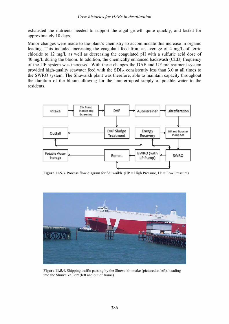
Case histories for HABs in desalination

386

exhausted the nutrients needed to support the algal growth quite quickly, and lasted for approximately 10 days.

Minor changes were made to the plant’s chemistry to accommodate this increase in organic loading. This included increasing the coagulant feed from an average of 4 mg/L of ferric chloride to 12 mg/L as well as decreasing the coagulated pH with a sulfuric acid dose of 40 mg/L during the bloom. In addition, the chemically enhanced backwash (CEB) frequency of the UF system was increased. With these changes the DAF and UF pretreatment system provided high-quality seawater feed with the SDI15 consistently less than 3.0 at all times to the SWRO system. The Shuwaikh plant was therefore, able to maintain capacity throughout the duration of the bloom allowing for the uninterrupted supply of potable water to the residents.

Figure 11.5.3. Process flow diagram for Shuwaikh. (HP = High Pressure, LP = Low Pressure).

Figure 11.5.4. Shipping traffic passing by the Shuwaikh intake (pictured at left), heading into the Shuwaikh Port (left and out of frame).

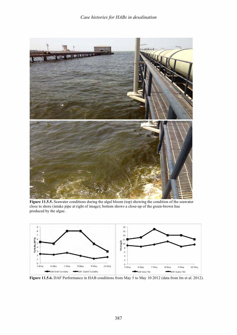
Case histories for HABs in desalination

387

Figure 11.5.5. Seawater conditions during the algal bloom (top) showing the condition of the seawater close to shore (intake pipe at right of image); bottom shows a close-up of the green-brown hue produced by the algae.

Figure 11.5.6. DAF Performance in HAB conditions from May 5 to May 10 2012 (data from Im et al. 2012).

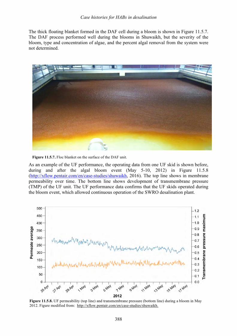
Case histories for HABs in desalination

388

The thick floating blanket formed in the DAF cell during a bloom is shown in Figure 11.5.7. The DAF process performed well during the blooms in Shuwaikh, but the severity of the bloom, type and concentration of algae, and the percent algal removal from the system were not determined.

Figure 11.5.7. Floc blanket on the surface of the DAF unit.

As an example of the UF performance, the operating data from one UF skid is shown before, during and after the algal bloom event (May 5-10, 2012) in Figure 11.5.8 (http://xflow.pentair.com/en/case-studies/shuwaikh, 2016). The top line shows in membrane permeability over time. The bottom line shows development of transmembrane pressure (TMP) of the UF unit. The UF performance data confirms that the UF skids operated during the bloom event, which allowed continuous operation of the SWRO desalination plant.

Figure 11.5.8. UF permeability (top line) and transmembrane pressure (bottom line) during a bloom in May 2012. Figure modified from: http://xflow.pentair.com/en/case-studies/shuwaikh.

Case histories for HABs in desalination

389

11.5.2 Laboratory and Pilot Scale DAF Testing To confirm the performance of the full-scale DAF system during a HAB event, multiple HAB species were cultivated at Woods Hole Oceanographic Institution for DAF bench scale testing. These species included Cochlodinium polykrikoides, the algal species that caused the 2008 - 2009 bloom in the Gulf. Different coagulation techniques were investigated to help lower the high charge-neutralization demand of the algal cells. The most promising techniques found to date are oxidation with sodium hypochlorite (typically less than 1 mg/L) and adjustment of the pH prior to coagulation. These techniques lowered the coagulant demand while improving cell removal by a few percentage points. Following laboratory bench tests, the process was tested on a naturally occurring Cochlodinium bloom in Buzzards Bay, MA in 2011 (14,000 cells/mL), with over 99% of the algae removed with the DAF process. The most interesting pilot study conducted to date was a simulated algal challenge test conducted for the Fujairah I expansion in Fujairah, UAE. To demonstrate the effectiveness of the DAF design which now feeds the existing Fujairah I filtration system and the ongoing expansion of the plant, a pilot study with up to 100,000 cells/mL in the source water was required as part of the contract. To accomplish this test with an algal concentration approximately 4-5 times that present in the 2008- 2009 Gulf bloom, a cultivated alga was utilized. The DAF pilot consistently removed over 95% of the algal cells and at times exceeded 99% removal, as seen in Figure 11.5.9. The DAF pilot was followed by a gravity media filtration pilot which utilized the current Fujairah I plant’s media profile. Interestingly when the algae was introduced to the DAF system, the downstream filtration system Silt Density Index (SDI) actually improved and filter head loss accumulation decreased. This is most likely due to the algae acting as a sweep floc to incorporate colloidal material in the source water.

Figure 11.5.9. Samples of feedwater (left) and DAF-treated water (right) from the challenge test at the Fujairah I pilot plant using cultured algae.

Case histories for HABs in desalination

390

Several pilots have also been conducted on naturally occurring blooms including a pilot at the University of Texas Marine Science Institute at Port Aransas, Texas during a bloom of Karenia brevis. Also a pilot study was conducted in Antofagasta Bay in Chile which experiences a prolonged HAB event yearly, lasting at times up to 3 to 4 months due to the bay’s currents which serve to feed nutrients to the algae continually over the summer months. This prolonged bloom tends to support the growth of many algal species. The results from each of the pilot tests on the different species of algae all showed greater than 95% removal, suggesting that DAF would be equally effective on differing strains of algae and should be considered a robust process for pretreatment around the world when an uninterrupted supply from open intake systems needs to be assured.

11.5.3 Conclusions DAF effectively removed cells during a HAB bloom in Kuwait, producing a stable and dense floc blanket and effectively removed elevated levels of TSS and turbidity. The UF performed well during the bloom, with no TMP spikes during this period. After optimization of the ferric chloride dose, the DAF and UF pretreatment system provided high-quality seawater feed with the SDI15 consistently less than 3.0 at all times to the SWRO system.

The DAF-UF pretreatment system at the Shuwaikh Desalination Plant provided a very stable and effective system for providing RO feedwater during a HAB bloom. The DAF system has also been tested and its effectiveness demonstrated through pilot studies on multiple other HAB species in the laboratory and the field.

11.5.4 References

Im, J., Park, K., and Yim, W. 2012. Doosan as Pioneer in Supplying and Operating Large-scale RO Desalination Plant at Shuwaikh on Coast of Kuwait. In: Proceedings of the International Water Association World Water Congress & Exhibition, Busan, South Korea.

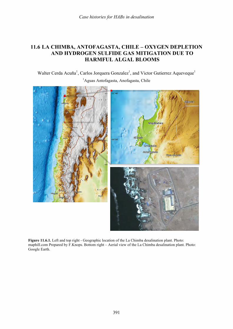
Case histories for HABs in desalination

391

11.6 LA CHIMBA, ANTOFAGASTA, CHILE – OXYGEN DEPLETION AND HYDROGEN SULFIDE GAS MITIGATION DUE TO

HARMFUL ALGAL BLOOMS

Walter Cerda Acuña1, Carlos Jorquera Gonzalez1, and Victor Gutierrez Aqueveque1 1Aguas Antofagasta, Anofagasta, Chile

Figure 11.6.1. Left and top right - Geographic location of the La Chimba desalination plant. Photo: maphill.com Prepared by F.Knops. Bottom right – Aerial view of the La Chimba desalination plant. Photo: Google Earth.

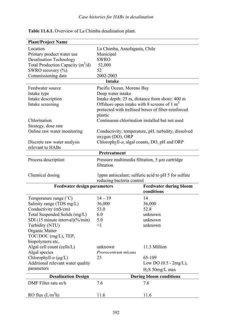
Case histories for HABs in desalination

392

Table 11.6.1. Overview of La Chimba desalination plant. Plant/Project Name Location La Chimba, Antofagasta, Chile Primary product water use Municipal Desalination Technology SWRO Total Production Capacity (m3/d) 52,000 SWRO recovery (%) 52 Commissioning date 2002-2003

Intake Feedwater source Pacific Ocean, Moreno Bay Intake type Deep water intake Intake description Intake depth: 25 m, distance from shore: 400 m Intake screening Offshore open intake with 8 screens of 1 m2

protected with trellised boxes of fiber-reinforced plastic

Chlorination Strategy, dose rate

Continuous chlorination installed but not used

Online raw water monitoring Conductivity, temperature, pH, turbidity, dissolved oxygen (DO), ORP

Discrete raw water analysis relevant to HABs

Chlorophyll-a, algal counts, DO, pH and ORP

Pretreatment Process description Pressure multimedia filtration, 5 µm cartridge

filtration

Chemical dosing 1ppm antiscalant; sulfuric acid to pH 5 for sulfate reducing bacteria control

Feedwater design parameters Feedwater during bloom conditions

Temperature range (˚C) 14 – 19 14 Salinity range (TDS mg/L) 36,000 36,000 Conductivity (mS/cm) 53.0 52.8 Total Suspended Solids (mg/L) 6.0 unknown SDI (15 minute interval)(%/min) 5.0 unknown Turbidity (NTU) <1 unknown Organic Matter TOC/DOC (mg/L), TEP, biopolymers etc.

Algal cell count (cells/L) unknown 11.3 Million Algal species Prorocentrum micans Chlorophyll-a (µg/L) 23 65-109 Additional relevant water quality parameters

Low DO (0.5 - 2mg/L), H2S 50mg/L max

Desalination Design During bloom conditions DMF Filter rate m/h

7.6 7.6

RO flux (L/m2h) 11.6 11.6

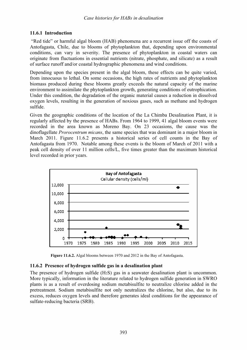
Case histories for HABs in desalination

393

11.6.1 Introduction “Red tide” or harmful algal bloom (HAB) phenomena are a recurrent issue off the coasts of Antofagasta, Chile, due to blooms of phytoplankton that, depending upon environmental conditions, can vary in severity. The presence of phytoplankton in coastal waters can originate from fluctuations in essential nutrients (nitrate, phosphate, and silicate) as a result of surface runoff and/or coastal hydrographic phenomena and wind conditions.

Depending upon the species present in the algal bloom, these effects can be quite varied, from innocuous to lethal. On some occasions, the high rates of nutrients and phytoplankton biomass produced during these blooms greatly exceeds the natural capacity of the marine environment to assimilate the phytoplankton growth, generating conditions of eutrophication. Under this condition, the degradation of the organic material causes a reduction in dissolved oxygen levels, resulting in the generation of noxious gases, such as methane and hydrogen sulfide. Given the geographic conditions of the location of the La Chimba Desalination Plant, it is regularly affected by the presence of HABs. From 1964 to 1999, 41 algal bloom events were recorded in the area known as Moreno Bay. On 23 occasions, the cause was the dinoflagellate Prorocentrum micans, the same species that was dominant in a major bloom in March 2011. Figure 11.6.2 presents a historical series of cell counts in the Bay of Antofagasta from 1970. Notable among these events is the bloom of March of 2011 with a peak cell density of over 11 million cells/L, five times greater than the maximum historical level recorded in prior years.

Figure 11.6.2. Algal blooms between 1970 and 2012 in the Bay of Antofagasta.

11.6.2 Presence of hydrogen sulfide gas in a desalination plant The presence of hydrogen sulfide (H2S) gas in a seawater desalination plant is uncommon. More typically, information in the literature related to hydrogen sulfide generation in SWRO plants is as a result of overdosing sodium metabisulfite to neutralize chlorine added in the pretreatment. Sodium metabisulfite not only neutralizes the chlorine, but also, due to its excess, reduces oxygen levels and therefore generates ideal conditions for the appearance of sulfate-reducing bacteria (SRB).

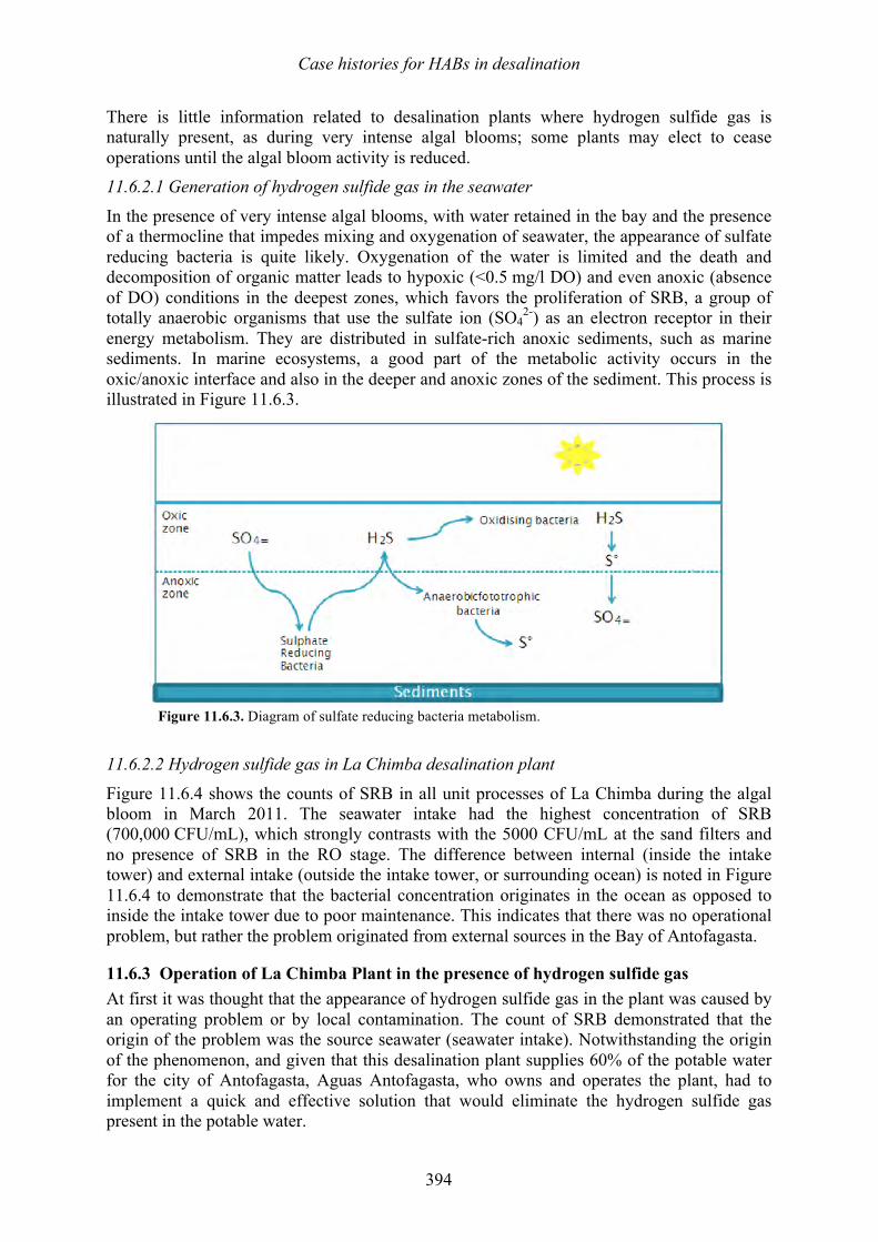
Case histories for HABs in desalination

394

There is little information related to desalination plants where hydrogen sulfide gas is naturally present, as during very intense algal blooms; some plants may elect to cease operations until the algal bloom activity is reduced. 11.6.2.1 Generation of hydrogen sulfide gas in the seawater

In the presence of very intense algal blooms, with water retained in the bay and the presence of a thermocline that impedes mixing and oxygenation of seawater, the appearance of sulfate reducing bacteria is quite likely. Oxygenation of the water is limited and the death and decomposition of organic matter leads to hypoxic (<0.5 mg/l DO) and even anoxic (absence of DO) conditions in the deepest zones, which favors the proliferation of SRB, a group of totally anaerobic organisms that use the sulfate ion (SO4

2-) as an electron receptor in their energy metabolism. They are distributed in sulfate-rich anoxic sediments, such as marine sediments. In marine ecosystems, a good part of the metabolic activity occurs in the oxic/anoxic interface and also in the deeper and anoxic zones of the sediment. This process is illustrated in Figure 11.6.3.

Figure 11.6.3. Diagram of sulfate reducing bacteria metabolism. 11.6.2.2 Hydrogen sulfide gas in La Chimba desalination plant

Figure 11.6.4 shows the counts of SRB in all unit processes of La Chimba during the algal bloom in March 2011. The seawater intake had the highest concentration of SRB (700,000 CFU/mL), which strongly contrasts with the 5000 CFU/mL at the sand filters and no presence of SRB in the RO stage. The difference between internal (inside the intake tower) and external intake (outside the intake tower, or surrounding ocean) is noted in Figure 11.6.4 to demonstrate that the bacterial concentration originates in the ocean as opposed to inside the intake tower due to poor maintenance. This indicates that there was no operational problem, but rather the problem originated from external sources in the Bay of Antofagasta.

11.6.3 Operation of La Chimba Plant in the presence of hydrogen sulfide gas At first it was thought that the appearance of hydrogen sulfide gas in the plant was caused by an operating problem or by local contamination. The count of SRB demonstrated that the origin of the problem was the source seawater (seawater intake). Notwithstanding the origin of the phenomenon, and given that this desalination plant supplies 60% of the potable water for the city of Antofagasta, Aguas Antofagasta, who owns and operates the plant, had to implement a quick and effective solution that would eliminate the hydrogen sulfide gas present in the potable water.

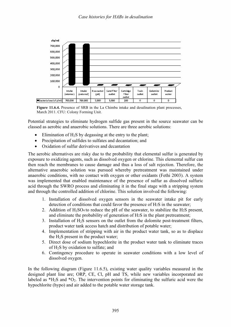
Case histories for HABs in desalination

395

Figure 11.6.4. Presence of SRB in the La Chimba intake and desalination plant processes, March 2011. CFU: Colony Forming Unit.

Potential strategies to eliminate hydrogen sulfide gas present in the source seawater can be classed as aerobic and anaerobic solutions. There are three aerobic solutions:

• Elimination of H2S by degassing at the entry to the plant; • Precipitation of sulfides to sulfates and decantation; and • Oxidation of sulfur derivatives and decantation

The aerobic alternatives are risky due to the probability that elemental sulfur is generated by exposure to oxidizing agents, such as dissolved oxygen or chlorine. This elemental sulfur can then reach the membranes to cause damage and thus a loss of salt rejection. Therefore, the alternative anaerobic solution was pursued whereby pretreatment was maintained under anaerobic conditions, with no contact with oxygen or other oxidants (Fethi 2003). A system was implemented that enabled maintenance of the presence of sulfur as dissolved sulfuric acid through the SWRO process and eliminating it in the final stage with a stripping system and through the controlled addition of chlorine. This solution involved the following:

1. Installation of dissolved oxygen sensors in the seawater intake pit for early detection of conditions that could favor the presence of H2S in the seawater;

2. Addition of H2SO4 to reduce the pH of the seawater, to stabilize the H2S present, and eliminate the probability of generation of H2S in the plant pretreatment;

3. Installation of H2S sensors on the outlet from the dolomite post-treatment filters, product water tank access hatch and distribution of potable water;

4. Implementation of stripping with air in the product water tank, so as to displace the H2S present in the product water;

5. Direct dose of sodium hypochlorite in the product water tank to eliminate traces of H2S by oxidation to sulfate; and

6. Contingency procedure to operate in seawater conditions with a low level of dissolved oxygen.

In the following diagram (Figure 11.6.5), existing water quality variables measured in the designed plant line are; ORP, CE, Cl, pH and TS, while new variables incorporated are labeled as *H2S and *O2. The intervention points for eliminating the sulfuric acid were the hypochlorite (hypo) and air added to the potable water storage tank.

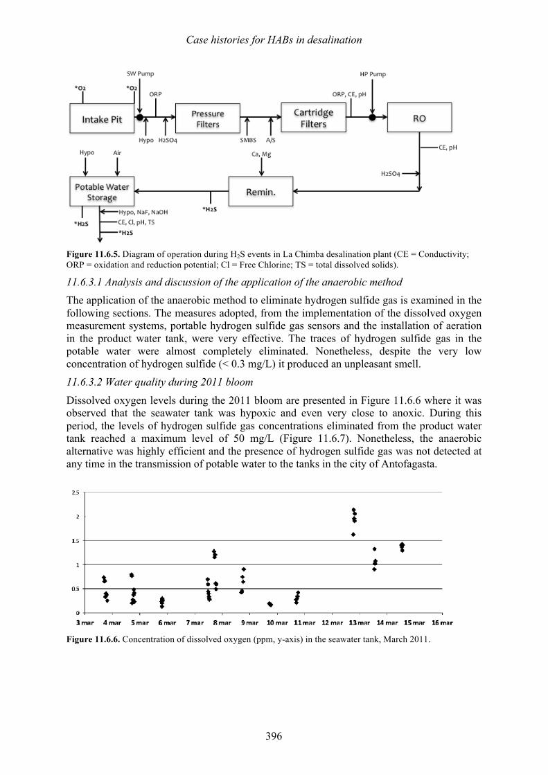
Case histories for HABs in desalination

396

Figure 11.6.5. Diagram of operation during H2S events in La Chimba desalination plant (CE = Conductivity; ORP = oxidation and reduction potential; Cl = Free Chlorine; TS = total dissolved solids).

11.6.3.1 Analysis and discussion of the application of the anaerobic method The application of the anaerobic method to eliminate hydrogen sulfide gas is examined in the following sections. The measures adopted, from the implementation of the dissolved oxygen measurement systems, portable hydrogen sulfide gas sensors and the installation of aeration in the product water tank, were very effective. The traces of hydrogen sulfide gas in the potable water were almost completely eliminated. Nonetheless, despite the very low concentration of hydrogen sulfide (< 0.3 mg/L) it produced an unpleasant smell. 11.6.3.2 Water quality during 2011 bloom

Dissolved oxygen levels during the 2011 bloom are presented in Figure 11.6.6 where it was observed that the seawater tank was hypoxic and even very close to anoxic. During this period, the levels of hydrogen sulfide gas concentrations eliminated from the product water tank reached a maximum level of 50 mg/L (Figure 11.6.7). Nonetheless, the anaerobic alternative was highly efficient and the presence of hydrogen sulfide gas was not detected at any time in the transmission of potable water to the tanks in the city of Antofagasta.

Figure 11.6.6. Concentration of dissolved oxygen (ppm, y-axis) in the seawater tank, March 2011.

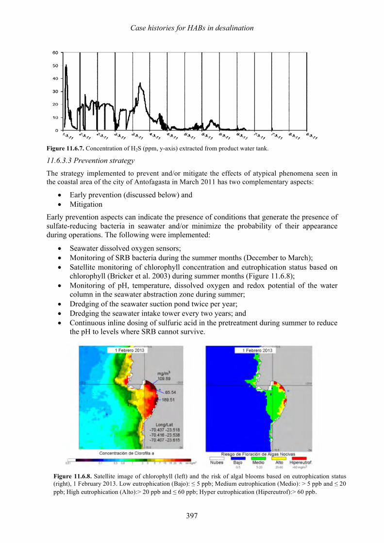
Case histories for HABs in desalination

397

Figure 11.6.7. Concentration of H2S (ppm, y-axis) extracted from product water tank.

11.6.3.3 Prevention strategy The strategy implemented to prevent and/or mitigate the effects of atypical phenomena seen in the coastal area of the city of Antofagasta in March 2011 has two complementary aspects:

• Early prevention (discussed below) and • Mitigation

Early prevention aspects can indicate the presence of conditions that generate the presence of sulfate-reducing bacteria in seawater and/or minimize the probability of their appearance during operations. The following were implemented:

• Seawater dissolved oxygen sensors; • Monitoring of SRB bacteria during the summer months (December to March); • Satellite monitoring of chlorophyll concentration and eutrophication status based on

chlorophyll (Bricker et al. 2003) during summer months (Figure 11.6.8); • Monitoring of pH, temperature, dissolved oxygen and redox potential of the water

column in the seawater abstraction zone during summer; • Dredging of the seawater suction pond twice per year; • Dredging the seawater intake tower every two years; and • Continuous inline dosing of sulfuric acid in the pretreatment during summer to reduce

the pH to levels where SRB cannot survive.

Figure 11.6.8. Satellite image of chlorophyll (left) and the risk of algal blooms based on eutrophication status (right), 1 February 2013. Low eutrophication (Bajo): ≤ 5 ppb; Medium eutrophication (Medio): > 5 ppb and ≤ 20 ppb; High eutrophication (Alto):> 20 ppb and ≤ 60 ppb; Hyper eutrophication (Hipereutrof):> 60 ppb.

Case histories for HABs in desalination

398

In terms of mitigation, when dissolved oxygen concentrations <2 mg/L are detected, operational procedures are activated based on the anaerobic solution described above, with additional actions that minimize the production of H2S gas. These actions are as follows:

• Dosing sulfuric acid prior to the multimedia filters to lower pH to 4 - 5. Growth of SRB bacteria is prevented in multimedia and cartridge filters and/or RO membranes;

• Activate the aeration system in the product water tank to strip out H2S; and • Dosing sodium hypochlorite directly to the product water tank, transforming the

traces of H2S into sulfates.

Additional actions:

• Permanently washing the multimedia filters (even when the pressure differential is low) to remove biological matter and reduce the probability of its decomposition;

• Change out of filter cartridges when differential pressure is >0.7 kg/cm2; • Maintain a minimum level of water in the product water tank, equivalent to 90% of its

total capacity, so the reaction of the H2S with air is effective; • Monitoring of pH, odor and dissolved oxygen in all stages of the process, to detect,

the sources of generation of H2S gas (if possible); and • Hourly monitoring of the product water quality for pH, residual chlorine, turbidity,

odor (by observation), taste and H2S.

11.6.4 Conclusions

• Red tide is a recurrent phenomenon on the coast of Antofagasta; however, the episode in March 2011 was the most intense recorded to date, leading to a major problem with hypoxia and H2S gas.

• The anaerobic solution described above was successful. During the bloom, DO in the seawater was at hypoxic levels until mid-March 2011, with the presence of H2S, but La Chimba was able to operate with no impacts on potable water quality.

• The measures adopted, from the implementation of DO measurement systems, portable H2S gas sensors, and the installation of aeration in the product water tank were effective. Other actions included dosing sulfuric acid prior to the multimedia filters to lower pH, and dosing sodium hypochlorite directly to the product water tank.

• The presence of H2S in seawater is an exceptional event; nevertheless, desalination plants that supply potable water to cities can have effective operating systems under these conditions.

• As it is very likely that this phenomenon will occur again, Aguas Antofagasta desalination plants have been equipped with instrumentation in anticipation of the presence of H2S in the source intake water.

• Monitoring of phytoplankton communities, bacteria, and the determination of chlorophyll in the seawater, especially in periods when red tides appear, are good approaches to detect the appearance of conditions that could favor the proliferation of sulfate reducing bacteria and thereby provide an early warning of this phenomenon.

11.6.5 References Bricker, S. B., Ferreira, J. G., and Simas, T. 2003. An integrated methodology for assessment

of estuarine trophic status. Ecological Modelling 169(1), 39–60. Fethi, K. 2003. The 15,000 m3/d RO Djerba Plant: Desalination of Brackish Water with a

High Hydrogen Sulfide Concentration. In: Proceedings of the International Desalination Association World Congress, The Bahamas.

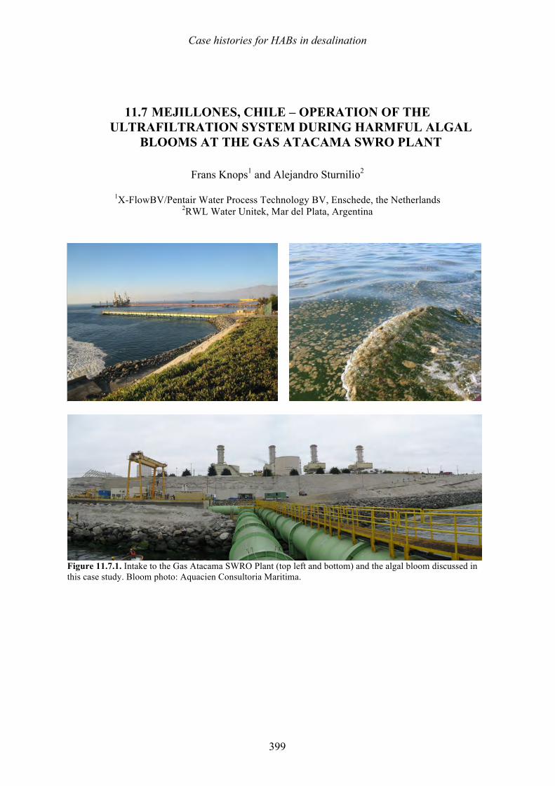
Case histories for HABs in desalination

399

11.7 MEJILLONES, CHILE – OPERATION OF THE ULTRAFILTRATION SYSTEM DURING HARMFUL ALGAL

BLOOMS AT THE GAS ATACAMA SWRO PLANT

Frans Knops1 and Alejandro Sturnilio2

1X-FlowBV/Pentair Water Process Technology BV, Enschede, the Netherlands 2RWL Water Unitek, Mar del Plata, Argentina

Figure 11.7.1. Intake to the Gas Atacama SWRO Plant (top left and bottom) and the algal bloom discussed in this case study. Bloom photo: Aquacien Consultoria Maritima.

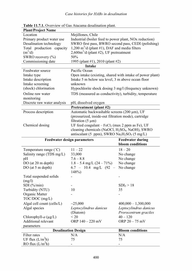
Case histories for HABs in desalination

400

Table 11.7.1. Overview of Gas Atacama desalination plant. Plant/Project Name Location Mejillones, Chile Primary product water use Industrial (boiler feed to power plant, NOx reduction) Desalination technology SWRO first pass, BWRO second pass, CEDI (polishing) Total production capacity (m3/d)

1,200 m3/d (plant #1), DAF and media filters 2,600m3/d (plant #2), UF pretreatment

SWRO recovery (%) 50% Commissioning date 1995 (plant #1), 2010 (plant #2)

Intake Feedwater source Pacific Ocean Intake type Open intake (existing, shared with intake of power plant) Intake description Intake 5 m below sea level, 3 m above ocean floor Intake screening unknown (shock) chlorination Hypochlorite shock dosing 3 mg/l (frequency unknown) Online raw water monitoring

TDS (measured as conductivity), turbidity, temperature

Discrete raw water analysis pH, dissolved oxygen Pretreatment (plant #2)

Process description

Automatic backwashable screens (200 µm), UF (pressurized, inside-out filtration mode), cartridge filtration (5 µm)

Chemical dosing UF feed coagulant – FeCl3 (max 2 ppm as Fe), UF cleaning chemicals (NaOCl, H2SO4, NaOH), SWRO antiscalant (5 ppm), SWRO Na2H2SO5 (5 mg/L)

Feedwater design parameters Feedwater during bloom conditions

Temperature range (˚C) 11 – 22 18 – 20 Salinity range (TDS mg/L) 33,000 No change pH 7.6 – 8.8 No change DO (at 20 m depth) 1.8 – 5.4 mg/L (24 – 71%) No change DO (at 5 m depth) 6.7 – 10.4 mg/L (92 –

148%) No change

Total suspended solids (mg/l)

- -

SDI (%/min) - SDI5 > 18 Turbidity (NTU) 10 35 Organic Matter TOC/DOC (mg/L)

- -

Algal cell count (cells/L) ~25,000 400,000 – 1,300,000 Algal species Leptocylindrus danicus

(Diatom) Leptocylindrus danicus Prorocentrum graciles

Chlorophyll-a (µg/L) < 20 40 – 120 Additional relevant parameters

ORP 140 – 220 mV ORP 20 – 75 mV

Desalination Design Bloom conditions Filter rates UF flux (L/m2h)

N/A 75

N/A 75

RO flux (L/m2h) - -

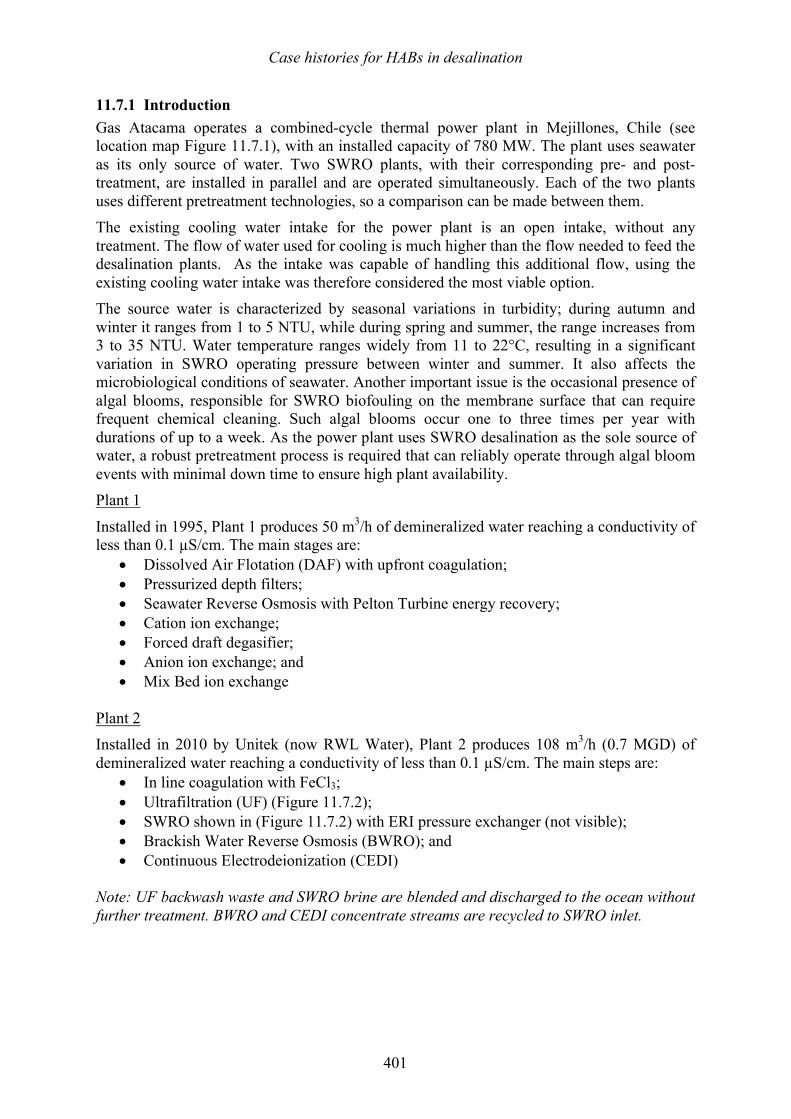
Case histories for HABs in desalination

401

11.7.1 Introduction Gas Atacama operates a combined-cycle thermal power plant in Mejillones, Chile (see location map Figure 11.7.1), with an installed capacity of 780 MW. The plant uses seawater as its only source of water. Two SWRO plants, with their corresponding pre- and post-treatment, are installed in parallel and are operated simultaneously. Each of the two plants uses different pretreatment technologies, so a comparison can be made between them. The existing cooling water intake for the power plant is an open intake, without any treatment. The flow of water used for cooling is much higher than the flow needed to feed the desalination plants. As the intake was capable of handling this additional flow, using the existing cooling water intake was therefore considered the most viable option. The source water is characterized by seasonal variations in turbidity; during autumn and winter it ranges from 1 to 5 NTU, while during spring and summer, the range increases from 3 to 35 NTU. Water temperature ranges widely from 11 to 22°C, resulting in a significant variation in SWRO operating pressure between winter and summer. It also affects the microbiological conditions of seawater. Another important issue is the occasional presence of algal blooms, responsible for SWRO biofouling on the membrane surface that can require frequent chemical cleaning. Such algal blooms occur one to three times per year with durations of up to a week. As the power plant uses SWRO desalination as the sole source of water, a robust pretreatment process is required that can reliably operate through algal bloom events with minimal down time to ensure high plant availability. Plant 1

Installed in 1995, Plant 1 produces 50 m3/h of demineralized water reaching a conductivity of less than 0.1 µS/cm. The main stages are:

• Dissolved Air Flotation (DAF) with upfront coagulation; • Pressurized depth filters; • Seawater Reverse Osmosis with Pelton Turbine energy recovery; • Cation ion exchange; • Forced draft degasifier; • Anion ion exchange; and • Mix Bed ion exchange

Plant 2 Installed in 2010 by Unitek (now RWL Water), Plant 2 produces 108 m3/h (0.7 MGD) of demineralized water reaching a conductivity of less than 0.1 µS/cm. The main steps are:

• In line coagulation with FeCl3; • Ultrafiltration (UF) (Figure 11.7.2); • SWRO shown in (Figure 11.7.2) with ERI pressure exchanger (not visible); • Brackish Water Reverse Osmosis (BWRO); and • Continuous Electrodeionization (CEDI)

Note: UF backwash waste and SWRO brine are blended and discharged to the ocean without further treatment. BWRO and CEDI concentrate streams are recycled to SWRO inlet.

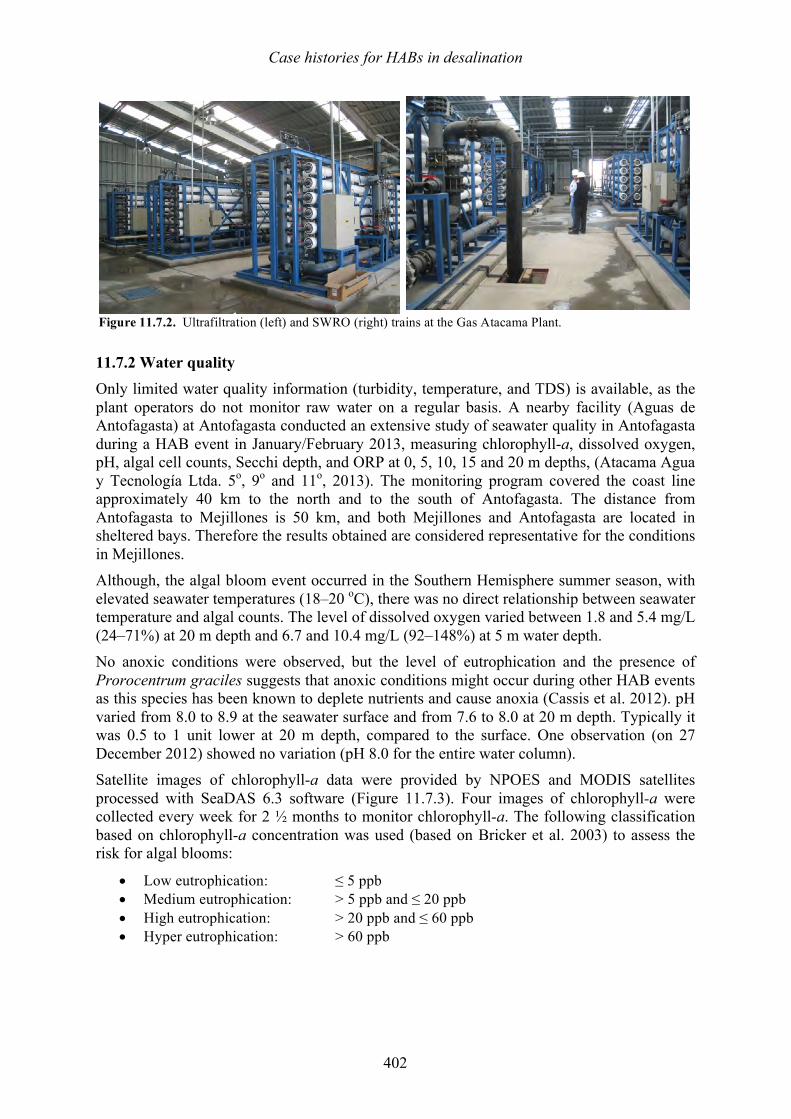
Case histories for HABs in desalination

402

11.7.2 Water quality Only limited water quality information (turbidity, temperature, and TDS) is available, as the plant operators do not monitor raw water on a regular basis. A nearby facility (Aguas de Antofagasta) at Antofagasta conducted an extensive study of seawater quality in Antofagasta during a HAB event in January/February 2013, measuring chlorophyll-a, dissolved oxygen, pH, algal cell counts, Secchi depth, and ORP at 0, 5, 10, 15 and 20 m depths, (Atacama Agua y Tecnología Ltda. 5o, 9o and 11o, 2013). The monitoring program covered the coast line approximately 40 km to the north and to the south of Antofagasta. The distance from Antofagasta to Mejillones is 50 km, and both Mejillones and Antofagasta are located in sheltered bays. Therefore the results obtained are considered representative for the conditions in Mejillones. Although, the algal bloom event occurred in the Southern Hemisphere summer season, with elevated seawater temperatures (18–20 oC), there was no direct relationship between seawater temperature and algal counts. The level of dissolved oxygen varied between 1.8 and 5.4 mg/L (24–71%) at 20 m depth and 6.7 and 10.4 mg/L (92–148%) at 5 m water depth. No anoxic conditions were observed, but the level of eutrophication and the presence of Prorocentrum graciles suggests that anoxic conditions might occur during other HAB events as this species has been known to deplete nutrients and cause anoxia (Cassis et al. 2012). pH varied from 8.0 to 8.9 at the seawater surface and from 7.6 to 8.0 at 20 m depth. Typically it was 0.5 to 1 unit lower at 20 m depth, compared to the surface. One observation (on 27 December 2012) showed no variation (pH 8.0 for the entire water column). Satellite images of chlorophyll-a data were provided by NPOES and MODIS satellites processed with SeaDAS 6.3 software (Figure 11.7.3). Four images of chlorophyll-a were collected every week for 2 ½ months to monitor chlorophyll-a. The following classification based on chlorophyll-a concentration was used (based on Bricker et al. 2003) to assess the risk for algal blooms:

• Low eutrophication: ≤ 5 ppb • Medium eutrophication: > 5 ppb and ≤ 20 ppb • High eutrophication: > 20 ppb and ≤ 60 ppb • Hyper eutrophication: > 60 ppb

Figure 11.7.2. Ultrafiltration (left) and SWRO (right) trains at the Gas Atacama Plant.

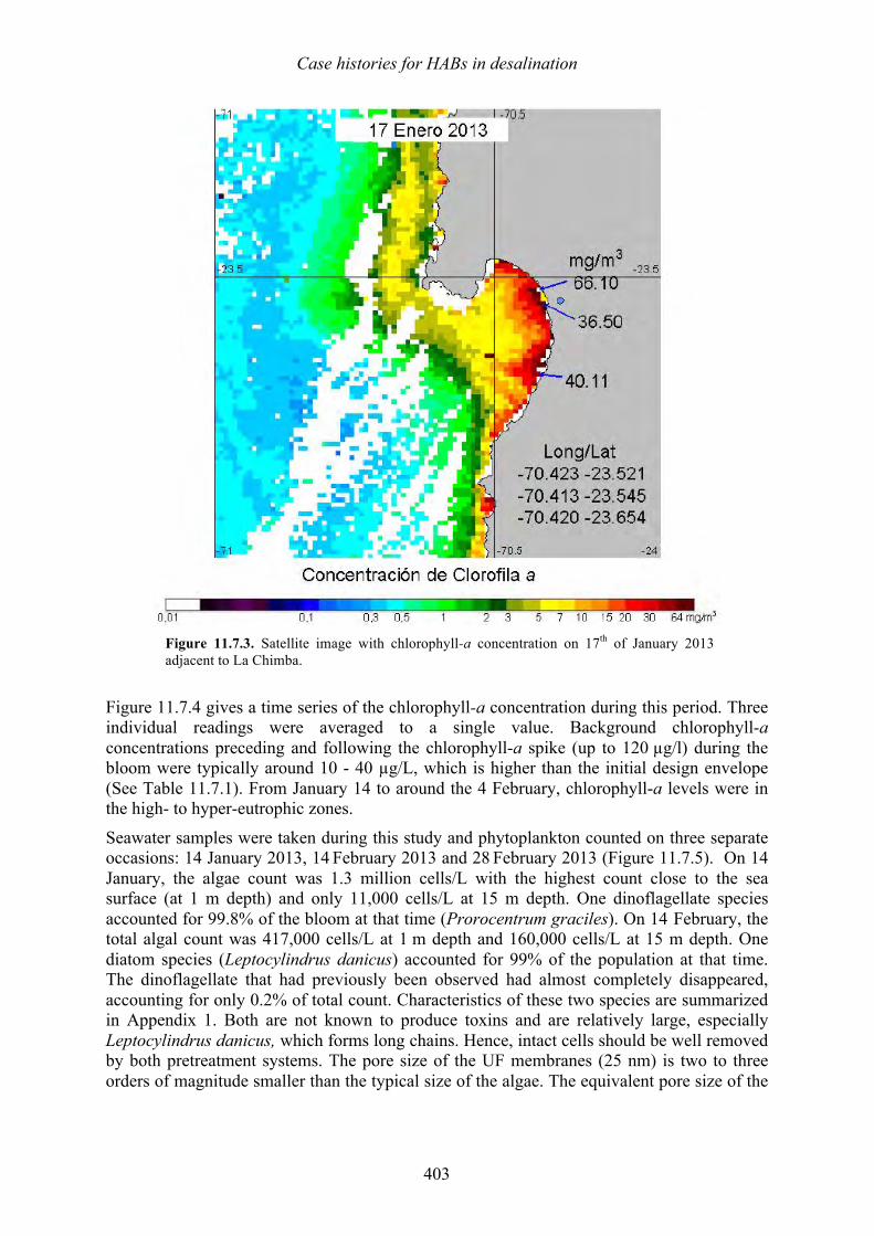
Case histories for HABs in desalination

403

Figure 11.7.3. Satellite image with chlorophyll-a concentration on 17th of January 2013 adjacent to La Chimba.

Figure 11.7.4 gives a time series of the chlorophyll-a concentration during this period. Three individual readings were averaged to a single value. Background chlorophyll-a concentrations preceding and following the chlorophyll-a spike (up to 120 µg/l) during the bloom were typically around 10 - 40 µg/L, which is higher than the initial design envelope (See Table 11.7.1). From January 14 to around the 4 February, chlorophyll-a levels were in the high- to hyper-eutrophic zones.

Seawater samples were taken during this study and phytoplankton counted on three separate occasions: 14 January 2013, 14 February 2013 and 28 February 2013 (Figure 11.7.5). On 14

January, the algae count was 1.3 million cells/L with the highest count close to the sea surface (at 1 m depth) and only 11,000 cells/L at 15 m depth. One dinoflagellate species accounted for 99.8% of the bloom at that time (Prorocentrum graciles). On 14 February, the total algal count was 417,000 cells/L at 1 m depth and 160,000 cells/L at 15 m depth. One diatom species (Leptocylindrus danicus) accounted for 99% of the population at that time. The dinoflagellate that had previously been observed had almost completely disappeared, accounting for only 0.2% of total count. Characteristics of these two species are summarized in Appendix 1. Both are not known to produce toxins and are relatively large, especially Leptocylindrus danicus, which forms long chains. Hence, intact cells should be well removed by both pretreatment systems. The pore size of the UF membranes (25 nm) is two to three orders of magnitude smaller than the typical size of the algae. The equivalent pore size of the

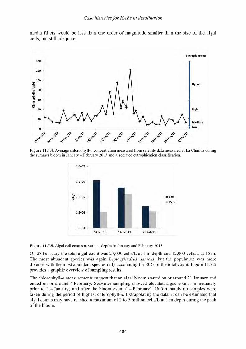
Case histories for HABs in desalination

404

media filters would be less than one order of magnitude smaller than the size of the algal cells, but still adequate.

Figure 11.7.4. Average chlorophyll-a concentration measured from satellite data measured at La Chimba during the summer bloom in January – February 2013 and associated eutrophication classification.

Figure 11.7.5. Algal cell counts at various depths in January and February 2013.

On 28 February the total algal count was 27,000 cells/L at 1 m depth and 12,000 cells/L at 15 m. The most abundant species was again Leptocylindrus danicus, but the population was more diverse, with the most abundant species only accounting for 80% of the total count. Figure 11.7.5 provides a graphic overview of sampling results. The chlorophyll-a measurements suggest that an algal bloom started on or around 21 January and ended on or around 4 February. Seawater sampling showed elevated algae counts immediately prior to (14 January) and after the bloom event (14 February). Unfortunately no samples were taken during the period of highest chlorophyll-a. Extrapolating the data, it can be estimated that algal counts may have reached a maximum of 2 to 5 million cells/L at 1 m depth during the peak of the bloom.

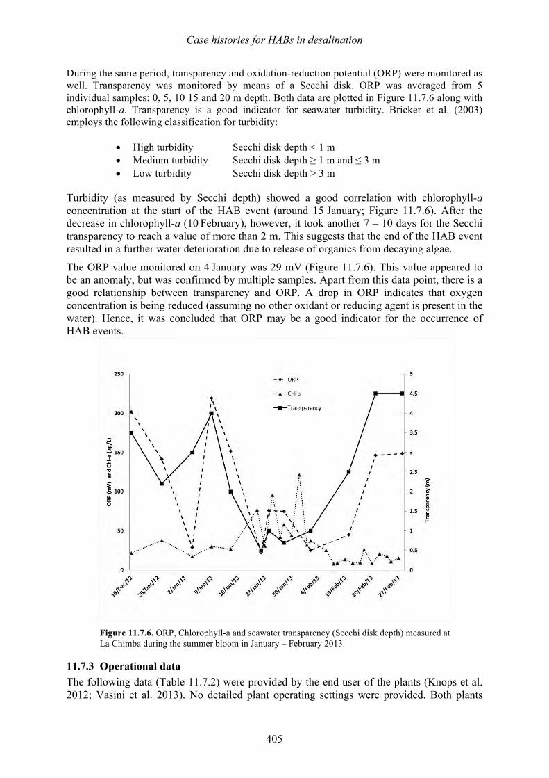
Case histories for HABs in desalination

405

During the same period, transparency and oxidation-reduction potential (ORP) were monitored as well. Transparency was monitored by means of a Secchi disk. ORP was averaged from 5 individual samples: 0, 5, 10 15 and 20 m depth. Both data are plotted in Figure 11.7.6 along with chlorophyll-a. Transparency is a good indicator for seawater turbidity. Bricker et al. (2003) employs the following classification for turbidity:

• High turbidity Secchi disk depth < 1 m • Medium turbidity Secchi disk depth ≥ 1 m and ≤ 3 m • Low turbidity Secchi disk depth > 3 m

Turbidity (as measured by Secchi depth) showed a good correlation with chlorophyll-a concentration at the start of the HAB event (around 15 January; Figure 11.7.6). After the decrease in chlorophyll-a (10 February), however, it took another 7 – 10 days for the Secchi transparency to reach a value of more than 2 m. This suggests that the end of the HAB event resulted in a further water deterioration due to release of organics from decaying algae.

The ORP value monitored on 4 January was 29 mV (Figure 11.7.6). This value appeared to be an anomaly, but was confirmed by multiple samples. Apart from this data point, there is a good relationship between transparency and ORP. A drop in ORP indicates that oxygen concentration is being reduced (assuming no other oxidant or reducing agent is present in the water). Hence, it was concluded that ORP may be a good indicator for the occurrence of HAB events.

Figure 11.7.6. ORP, Chlorophyll-a and seawater transparency (Secchi disk depth) measured at La Chimba during the summer bloom in January – February 2013.

11.7.3 Operational data The following data (Table 11.7.2) were provided by the end user of the plants (Knops et al. 2012; Vasini et al. 2013). No detailed plant operating settings were provided. Both plants

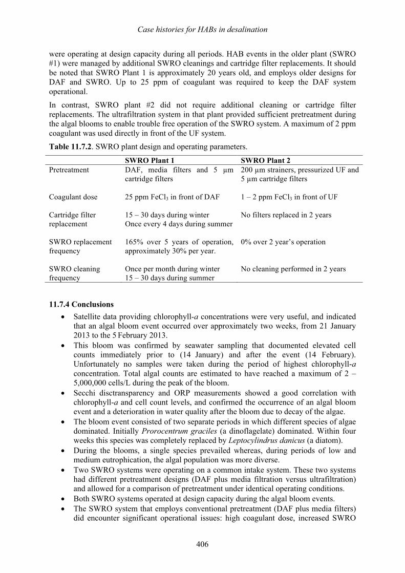
Case histories for HABs in desalination

406

were operating at design capacity during all periods. HAB events in the older plant (SWRO #1) were managed by additional SWRO cleanings and cartridge filter replacements. It should be noted that SWRO Plant 1 is approximately 20 years old, and employs older designs for DAF and SWRO. Up to 25 ppm of coagulant was required to keep the DAF system operational. In contrast, SWRO plant #2 did not require additional cleaning or cartridge filter replacements. The ultrafiltration system in that plant provided sufficient pretreatment during the algal blooms to enable trouble free operation of the SWRO system. A maximum of 2 ppm coagulant was used directly in front of the UF system. Table 11.7.2. SWRO plant design and operating parameters.

SWRO Plant 1 SWRO Plant 2 Pretreatment DAF, media filters and 5 µm

cartridge filters 200 µm strainers, pressurized UF and 5 µm cartridge filters

Coagulant dose 25 ppm FeCl3 in front of DAF 1 – 2 ppm FeCl3 in front of UF

Cartridge filter replacement

15 – 30 days during winter Once every 4 days during summer

No filters replaced in 2 years

SWRO replacement frequency

165% over 5 years of operation, approximately 30% per year.

0% over 2 year’s operation

SWRO cleaning frequency

Once per month during winter 15 – 30 days during summer

No cleaning performed in 2 years

11.7.4 Conclusions • Satellite data providing chlorophyll-a concentrations were very useful, and indicated

that an algal bloom event occurred over approximately two weeks, from 21 January 2013 to the 5 February 2013.

• This bloom was confirmed by seawater sampling that documented elevated cell counts immediately prior to (14 January) and after the event (14 February). Unfortunately no samples were taken during the period of highest chlorophyll-a concentration. Total algal counts are estimated to have reached a maximum of 2 – 5,000,000 cells/L during the peak of the bloom.

• Secchi disctransparency and ORP measurements showed a good correlation with chlorophyll-a and cell count levels, and confirmed the occurrence of an algal bloom event and a deterioration in water quality after the bloom due to decay of the algae.

• The bloom event consisted of two separate periods in which different species of algae dominated. Initially Prorocentrum graciles (a dinoflagelate) dominated. Within four weeks this species was completely replaced by Leptocylindrus danicus (a diatom).

• During the blooms, a single species prevailed whereas, during periods of low and medium eutrophication, the algal population was more diverse.

• Two SWRO systems were operating on a common intake system. These two systems had different pretreatment designs (DAF plus media filtration versus ultrafiltration) and allowed for a comparison of pretreatment under identical operating conditions.

• Both SWRO systems operated at design capacity during the algal bloom events. • The SWRO system that employs conventional pretreatment (DAF plus media filters)

did encounter significant operational issues: high coagulant dose, increased SWRO

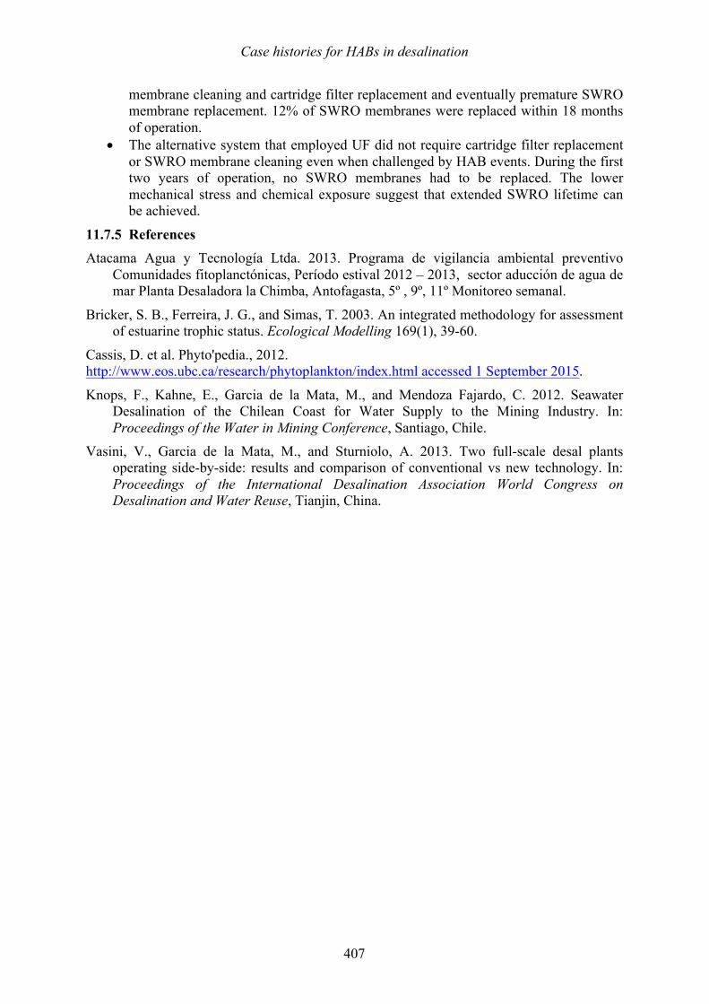
Case histories for HABs in desalination

407

membrane cleaning and cartridge filter replacement and eventually premature SWRO membrane replacement. 12% of SWRO membranes were replaced within 18 months of operation.

• The alternative system that employed UF did not require cartridge filter replacement or SWRO membrane cleaning even when challenged by HAB events. During the first two years of operation, no SWRO membranes had to be replaced. The lower mechanical stress and chemical exposure suggest that extended SWRO lifetime can be achieved.

11.7.5 References Atacama Agua y Tecnología Ltda. 2013. Programa de vigilancia ambiental preventivo

Comunidades fitoplanctónicas, Período estival 2012 – 2013, sector aducción de agua de mar Planta Desaladora la Chimba, Antofagasta, 5º , 9º, 11º Monitoreo semanal.

Bricker, S. B., Ferreira, J. G., and Simas, T. 2003. An integrated methodology for assessment of estuarine trophic status. Ecological Modelling 169(1), 39-60.

Cassis, D. et al. Phyto'pedia., 2012. http://www.eos.ubc.ca/research/phytoplankton/index.html accessed 1 September 2015.

Knops, F., Kahne, E., Garcia de la Mata, M., and Mendoza Fajardo, C. 2012. Seawater Desalination of the Chilean Coast for Water Supply to the Mining Industry. In: Proceedings of the Water in Mining Conference, Santiago, Chile.

Vasini, V., Garcia de la Mata, M., and Sturniolo, A. 2013. Two full-scale desal plants operating side-by-side: results and comparison of conventional vs new technology. In: Proceedings of the International Desalination Association World Congress on Desalination and Water Reuse, Tianjin, China.

Case histories for HABs in desalination

408

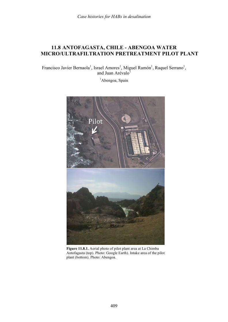
Case histories for HABs in desalination

409

11.8 ANTOFAGASTA, CHILE - ABENGOA WATER MICRO/ULTRAFILTRATION PRETREATMENT PILOT PLANT

Francisco Javier Bernaola1, Israel Amores1, Miguel Ramón1, Raquel Serrano1,

and Juan Arévalo1 1Abengoa, Spain

Figure 11.8.1. Aerial photo of pilot plant area at La Chimba Antofagasta (top). Photo: Google Earth). Intake area of the pilot plant (bottom). Photo: Abengoa.

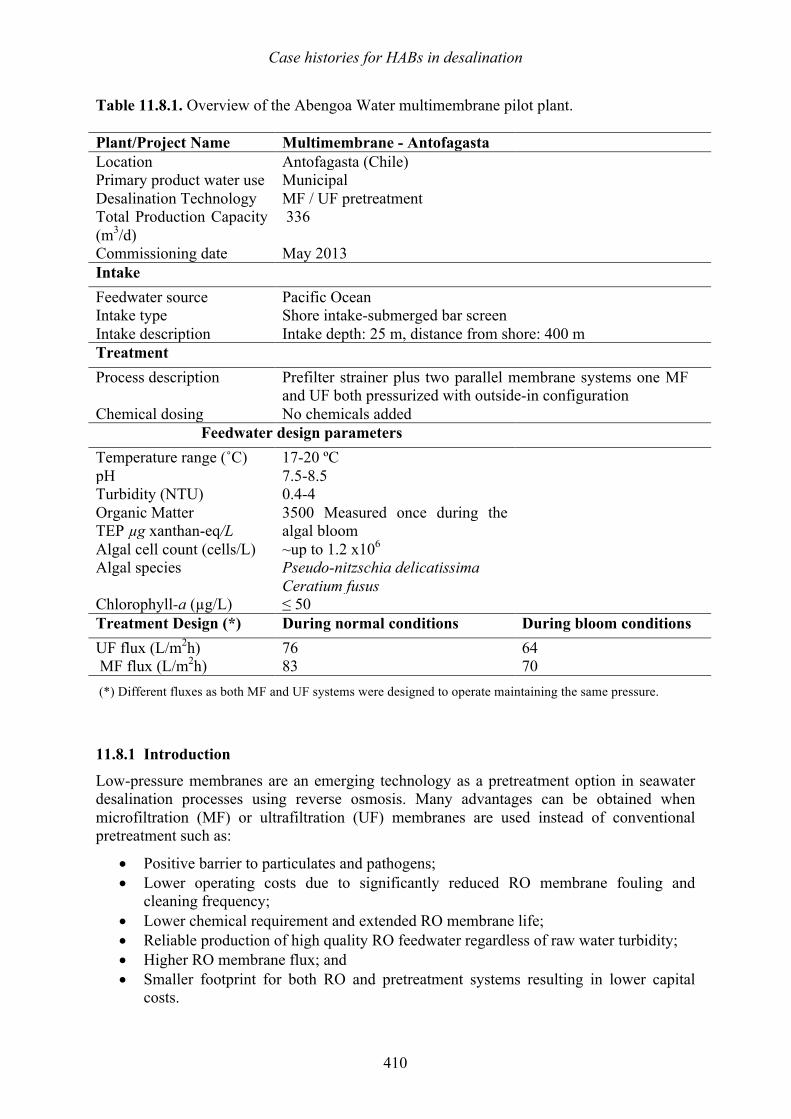
Case histories for HABs in desalination

410

Table 11.8.1. Overview of the Abengoa Water multimembrane pilot plant. Plant/Project Name Multimembrane - Antofagasta Location Antofagasta (Chile) Primary product water use Municipal Desalination Technology MF / UF pretreatment Total Production Capacity (m3/d)

336

Commissioning date May 2013 Intake Feedwater source Pacific Ocean Intake type Shore intake-submerged bar screen Intake description Intake depth: 25 m, distance from shore: 400 m Treatment Process description Prefilter strainer plus two parallel membrane systems one MF

and UF both pressurized with outside-in configuration Chemical dosing No chemicals added

Feedwater design parameters Temperature range (˚C) 17-20 ºC pH 7.5-8.5 Turbidity (NTU) 0.4-4 Organic Matter TEP µg xanthan-eq/L

3500 Measured once during the algal bloom

Algal cell count (cells/L) ~up to 1.2 x106 Algal species Pseudo-nitzschia delicatissima

Ceratium fusus

Chlorophyll-a (µg/L) ≤ 50 Treatment Design (*) During normal conditions During bloom conditions UF flux (L/m2h) 76 64 MF flux (L/m2h) 83 70 (*) Different fluxes as both MF and UF systems were designed to operate maintaining the same pressure. 11.8.1 Introduction

Low-pressure membranes are an emerging technology as a pretreatment option in seawater desalination processes using reverse osmosis. Many advantages can be obtained when microfiltration (MF) or ultrafiltration (UF) membranes are used instead of conventional pretreatment such as:

• Positive barrier to particulates and pathogens; • Lower operating costs due to significantly reduced RO membrane fouling and

cleaning frequency; • Lower chemical requirement and extended RO membrane life; • Reliable production of high quality RO feedwater regardless of raw water turbidity; • Higher RO membrane flux; and • Smaller footprint for both RO and pretreatment systems resulting in lower capital

costs.

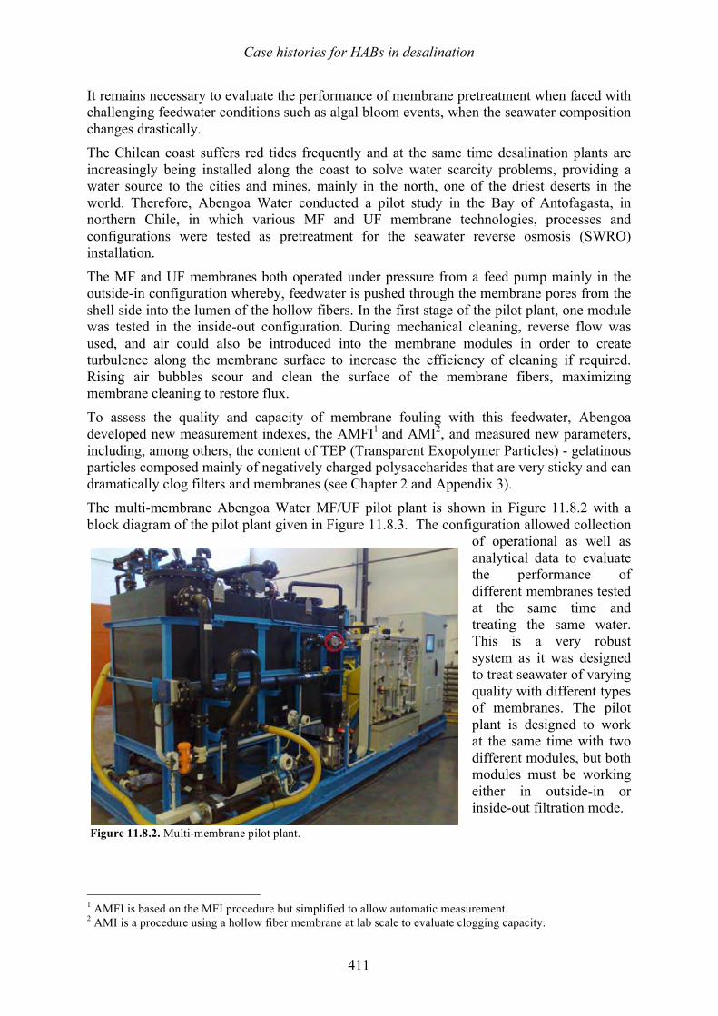
Case histories for HABs in desalination

411

It remains necessary to evaluate the performance of membrane pretreatment when faced with challenging feedwater conditions such as algal bloom events, when the seawater composition changes drastically. The Chilean coast suffers red tides frequently and at the same time desalination plants are increasingly being installed along the coast to solve water scarcity problems, providing a water source to the cities and mines, mainly in the north, one of the driest deserts in the world. Therefore, Abengoa Water conducted a pilot study in the Bay of Antofagasta, in northern Chile, in which various MF and UF membrane technologies, processes and configurations were tested as pretreatment for the seawater reverse osmosis (SWRO) installation.

The MF and UF membranes both operated under pressure from a feed pump mainly in the outside-in configuration whereby, feedwater is pushed through the membrane pores from the shell side into the lumen of the hollow fibers. In the first stage of the pilot plant, one module was tested in the inside-out configuration. During mechanical cleaning, reverse flow was used, and air could also be introduced into the membrane modules in order to create turbulence along the membrane surface to increase the efficiency of cleaning if required. Rising air bubbles scour and clean the surface of the membrane fibers, maximizing membrane cleaning to restore flux.

To assess the quality and capacity of membrane fouling with this feedwater, Abengoa developed new measurement indexes, the AMFI1 and AMI2, and measured new parameters, including, among others, the content of TEP (Transparent Exopolymer Particles) - gelatinous particles composed mainly of negatively charged polysaccharides that are very sticky and can dramatically clog filters and membranes (see Chapter 2 and Appendix 3). The multi-membrane Abengoa Water MF/UF pilot plant is shown in Figure 11.8.2 with a block diagram of the pilot plant given in Figure 11.8.3. The configuration allowed collection

of operational as well as analytical data to evaluate the performance of different membranes tested at the same time and treating the same water. This is a very robust system as it was designed to treat seawater of varying quality with different types of membranes. The pilot plant is designed to work at the same time with two different modules, but both modules must be working either in outside-in or inside-out filtration mode.

1 AMFI is based on the MFI procedure but simplified to allow automatic measurement. 2 AMI is a procedure using a hollow fiber membrane at lab scale to evaluate clogging capacity.

Figure 11.8.2. Multi-membrane pilot plant.

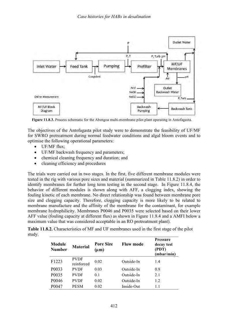
Case histories for HABs in desalination

412

The objectives of the Antofagasta pilot study were to demonstrate the feasibility of UF/MF for SWRO pretreatment during normal feedwater conditions and algal bloom events and to optimise the following operational parameters:

• UF/MF flux; • UF/MF backwash frequency and parameters; • chemical cleaning frequency and duration; and • cleaning efficiency and procedures

The trials were carried out in two stages. In the first, five different membrane modules were tested in the rig with various pore sizes and material (summarized in Table 11.8.2) in order to identify membranes for further long term testing in the second stage. In Figure 11.8.4, the behavior of different modules is shown along with AFF, a clogging index, showing the fouling kinetic of each membrane. No direct relationship was found between membrane pore size and clogging capacity. Therefore, clogging capacity is more likely to be related to membrane manufacture and the affinity of the membrane for the contaminant, for example membrane hydrophilicity. Membranes P0046 and P0035 were selected based on their lower AFF value (fouling capacity at different flux) as shown in Figure 11.8.4 and a AMFI below a maximum value that was considered acceptable in an RO pretreatment plant). Table 11.8.2. Characteristics of MF and UF membranes used in the first stage of the pilot study.

Module Number Material Pore Size

(µm) Flow mode

Pressure decay test (PDT) (mbar/min)

F1223 PVDF reinforced 0.02 Outside-In 1.4

P0033 PVDF 0.03 Outside-In 0.9 P0035 PVDF 0.1 Outside-In 2.1 P0046 PVDF 0.02 Outside-In 1.2 P0047 PESM 0.02 Inside-Out 1.1

Figure 11.8.3. Process schematic for the Abengoa multi-membrane pilot plant operating in Antofagasta.

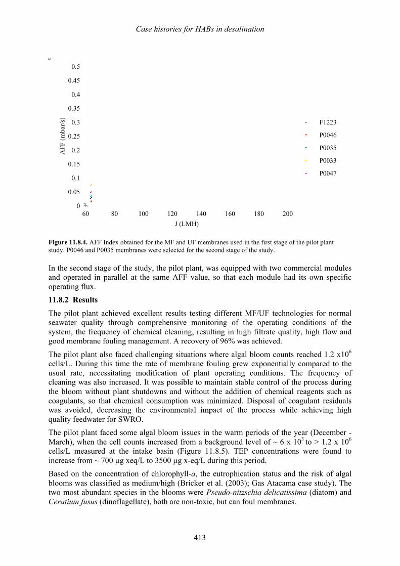
Case histories for HABs in desalination

413

Figure 11.8.4. AFF Index obtained for the MF and UF membranes used in the first stage of the pilot plant study. P0046 and P0035 membranes were selected for the second stage of the study. In the second stage of the study, the pilot plant, was equipped with two commercial modules and operated in parallel at the same AFF value, so that each module had its own specific operating flux. 11.8.2 Results

The pilot plant achieved excellent results testing different MF/UF technologies for normal seawater quality through comprehensive monitoring of the operating conditions of the system, the frequency of chemical cleaning, resulting in high filtrate quality, high flow and good membrane fouling management. A recovery of 96% was achieved.

The pilot plant also faced challenging situations where algal bloom counts reached 1.2 x106 cells/L. During this time the rate of membrane fouling grew exponentially compared to the usual rate, necessitating modification of plant operating conditions. The frequency of cleaning was also increased. It was possible to maintain stable control of the process during the bloom without plant shutdowns and without the addition of chemical reagents such as coagulants, so that chemical consumption was minimized. Disposal of coagulant residuals was avoided, decreasing the environmental impact of the process while achieving high quality feedwater for SWRO. The pilot plant faced some algal bloom issues in the warm periods of the year (December - March), when the cell counts increased from a background level of ~ 6 x 103 to > 1.2 x 106 cells/L measured at the intake basin (Figure 11.8.5). TEP concentrations were found to increase from ~ 700 µg xeq/L to 3500 µg x-eq/L during this period. Based on the concentration of chlorophyll-a, the eutrophication status and the risk of algal blooms was classified as medium/high (Bricker et al. (2003); Gas Atacama case study). The two most abundant species in the blooms were Pseudo-nitzschia delicatissima (diatom) and Ceratium fusus (dinoflagellate), both are non-toxic, but can foul membranes.

0

0.05

0.1

0.15

0.2

0.25

0.3

0.35

0.4

0.45

0.5

60 80 100 120 140 160 180 200

AFF

(mba

r/s)

J (LMH)

F1223

P0046

P0035

P0033

P0047

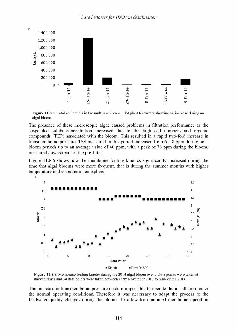
Case histories for HABs in desalination

414

Figure 11.8.5. Total cell counts in the multi-membrane pilot plant feedwater showing an increase during an algal bloom.

The presence of these microscopic algae caused problems in filtration performance as the suspended solids concentration increased due to the high cell numbers and organic compounds (TEP) associated with the bloom. This resulted in a rapid two-fold increase in transmembrane pressure. TSS measured in this period increased from 6 – 8 ppm during non-bloom periods up to an average value of 40 ppm, with a peak of 76 ppm during the bloom, measured downstream of the pre-filter. Figure 11.8.6 shows how the membrane fouling kinetics significantly increased during the time that algal blooms were more frequent, that is during the summer months with higher temperature in the southern hemisphere.

Figure 11.8.6. Membrane fouling kinetic during the 2014 algal bloom event. Data points were taken at uneven times and 34 data points were taken between early November 2013 to mid-March 2014.

This increase in transmembrane pressure made it impossible to operate the installation under the normal operating conditions. Therefore it was necessary to adapt the process to the feedwater quality changes during the bloom. To allow for continued membrane operation

0

200,000

400,000

600,000

800,000

1,000,000

1,200,000

1,400,000

1-­‐‑Jan-­‐‑14

15-­‐‑Jan-­‐‑14

21-­‐‑Jan-­‐‑14

29-­‐‑Jan-­‐‑14

5-­‐‑Feb-­‐‑14

12-­‐‑Feb-­‐‑14

19-­‐‑Feb-­‐‑14

Cells/L

0

0.5

1

1.5

2

2.5

3

3.5

4

4.5

0

0.5

1

1.5

2

2.5

3

3.5

4

0 5 10 15 20 25 30 35

Flow

(m3/h)

Kinetic

Data Point

Kinetic Flow (m3/h)

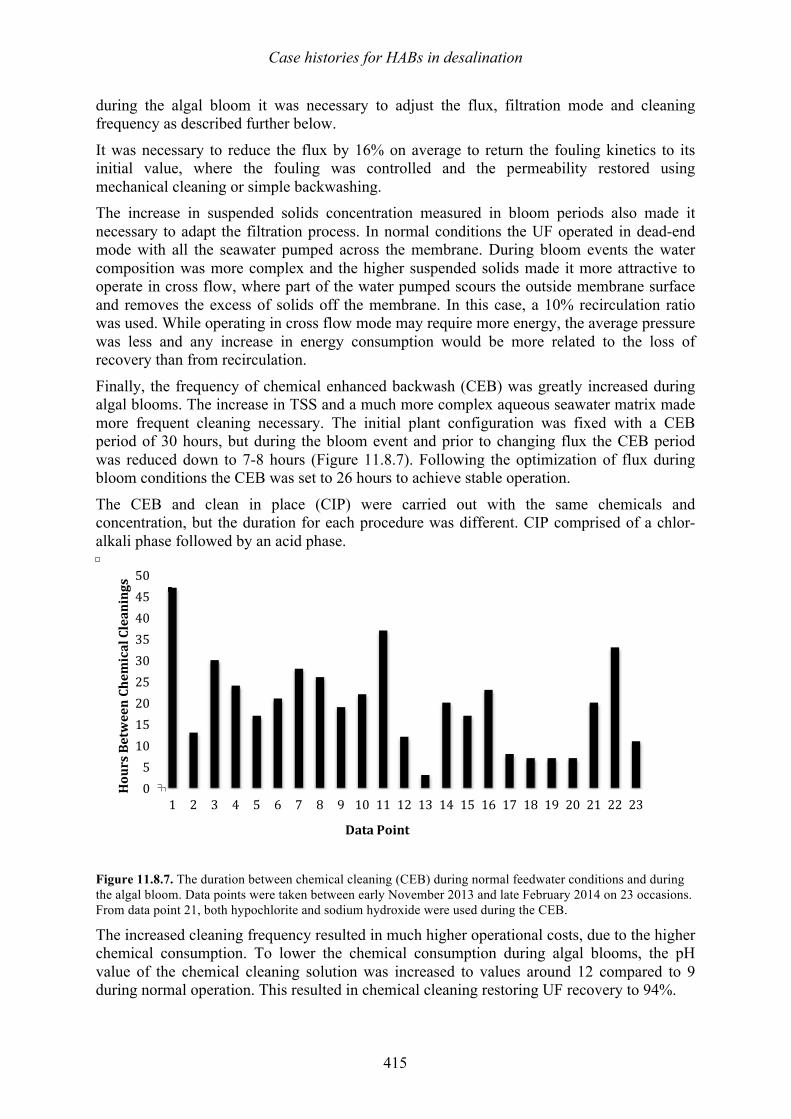
Case histories for HABs in desalination

415

during the algal bloom it was necessary to adjust the flux, filtration mode and cleaning frequency as described further below.

It was necessary to reduce the flux by 16% on average to return the fouling kinetics to its initial value, where the fouling was controlled and the permeability restored using mechanical cleaning or simple backwashing. The increase in suspended solids concentration measured in bloom periods also made it necessary to adapt the filtration process. In normal conditions the UF operated in dead-end mode with all the seawater pumped across the membrane. During bloom events the water composition was more complex and the higher suspended solids made it more attractive to operate in cross flow, where part of the water pumped scours the outside membrane surface and removes the excess of solids off the membrane. In this case, a 10% recirculation ratio was used. While operating in cross flow mode may require more energy, the average pressure was less and any increase in energy consumption would be more related to the loss of recovery than from recirculation.

Finally, the frequency of chemical enhanced backwash (CEB) was greatly increased during algal blooms. The increase in TSS and a much more complex aqueous seawater matrix made more frequent cleaning necessary. The initial plant configuration was fixed with a CEB period of 30 hours, but during the bloom event and prior to changing flux the CEB period was reduced down to 7-8 hours (Figure 11.8.7). Following the optimization of flux during bloom conditions the CEB was set to 26 hours to achieve stable operation.

The CEB and clean in place (CIP) were carried out with the same chemicals and concentration, but the duration for each procedure was different. CIP comprised of a chlor-alkali phase followed by an acid phase.

Figure 11.8.7. The duration between chemical cleaning (CEB) during normal feedwater conditions and during the algal bloom. Data points were taken between early November 2013 and late February 2014 on 23 occasions. From data point 21, both hypochlorite and sodium hydroxide were used during the CEB.

The increased cleaning frequency resulted in much higher operational costs, due to the higher chemical consumption. To lower the chemical consumption during algal blooms, the pH value of the chemical cleaning solution was increased to values around 12 compared to 9 during normal operation. This resulted in chemical cleaning restoring UF recovery to 94%.

05101520253035404550

1 2 3 4 5 6 7 8 9 10 11 12 13 14 15 16 17 18 19 20 21 22 23

Hours Between Chem

ical Cleanings

Data Point

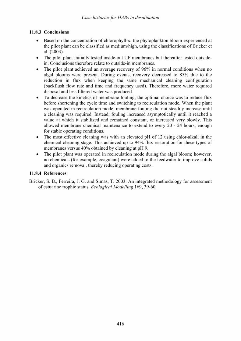
Case histories for HABs in desalination

416

11.8.3 Conclusions

• Based on the concentration of chlorophyll-a, the phytoplankton bloom experienced at the pilot plant can be classified as medium/high, using the classifications of Bricker et al. (2003).

• The pilot plant initially tested inside-out UF membranes but thereafter tested outside-in. Conclusions therefore relate to outside-in membranes.

• The pilot plant achieved an average recovery of 96% in normal conditions when no algal blooms were present. During events, recovery decreased to 85% due to the reduction in flux when keeping the same mechanical cleaning configuration (backflush flow rate and time and frequency used). Therefore, more water required disposal and less filtered water was produced.

• To decrease the kinetics of membrane fouling, the optimal choice was to reduce flux before shortening the cycle time and switching to recirculation mode. When the plant was operated in recirculation mode, membrane fouling did not steadily increase until a cleaning was required. Instead, fouling increased asymptotically until it reached a value at which it stabilized and remained constant, or increased very slowly. This allowed membrane chemical maintenance to extend to every 20 - 24 hours, enough for stable operating conditions.

• The most effective cleaning was with an elevated pH of 12 using chlor-alkali in the chemical cleaning stage. This achieved up to 94% flux restoration for these types of membranes versus 40% obtained by cleaning at pH 9.

• The pilot plant was operated in recirculation mode during the algal bloom; however, no chemicals (for example, coagulant) were added to the feedwater to improve solids and organics removal, thereby reducing operating costs.

11.8.4 References

Bricker, S. B., Ferreira, J. G. and Simas, T. 2003. An integrated methodology for assessment of estuarine trophic status. Ecological Modelling 169, 39-60.

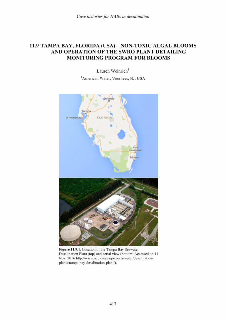
Case histories for HABs in desalination

417

11.9 TAMPA BAY, FLORIDA (USA) – NON-TOXIC ALGAL BLOOMS AND OPERATION OF THE SWRO PLANT DETAILING

MONITORING PROGRAM FOR BLOOMS

Lauren Weinrich1

1American Water, Voorhees, NJ, USA

Figure 11.9.1. Location of the Tampa Bay Seawater Desalination Plant (top) and aerial view (bottom; Accessed on 11 Nov. 2016 http://www.acciona.us/projects/water/desalination-plants/tampa-bay-desalination-plant/).

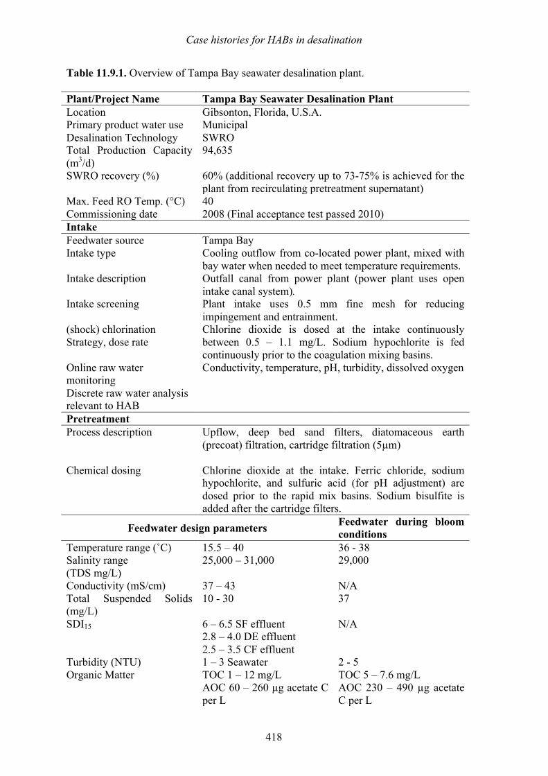
Case histories for HABs in desalination

418

Table 11.9.1. Overview of Tampa Bay seawater desalination plant. Plant/Project Name Tampa Bay Seawater Desalination Plant Location Gibsonton, Florida, U.S.A. Primary product water use Municipal Desalination Technology SWRO Total Production Capacity (m3/d)

94,635

SWRO recovery (%) 60% (additional recovery up to 73-75% is achieved for the plant from recirculating pretreatment supernatant)

Max. Feed RO Temp. (°C) 40 Commissioning date 2008 (Final acceptance test passed 2010) Intake Feedwater source Tampa Bay Intake type Cooling outflow from co-located power plant, mixed with

bay water when needed to meet temperature requirements. Intake description Outfall canal from power plant (power plant uses open

intake canal system). Intake screening Plant intake uses 0.5 mm fine mesh for reducing

impingement and entrainment. (shock) chlorination Strategy, dose rate

Chlorine dioxide is dosed at the intake continuously between 0.5 – 1.1 mg/L. Sodium hypochlorite is fed continuously prior to the coagulation mixing basins.

Online raw water monitoring

Conductivity, temperature, pH, turbidity, dissolved oxygen

Discrete raw water analysis relevant to HAB

Pretreatment Process description

Upflow, deep bed sand filters, diatomaceous earth (precoat) filtration, cartridge filtration (5µm)

Chemical dosing Chlorine dioxide at the intake. Ferric chloride, sodium hypochlorite, and sulfuric acid (for pH adjustment) are dosed prior to the rapid mix basins. Sodium bisulfite is added after the cartridge filters.

Feedwater design parameters Feedwater during bloom conditions

Temperature range (˚C) 15.5 – 40 36 - 38 Salinity range (TDS mg/L)

25,000 – 31,000 29,000

Conductivity (mS/cm) 37 – 43 N/A Total Suspended Solids (mg/L)

10 - 30 37

SDI15 6 – 6.5 SF effluent 2.8 – 4.0 DE effluent 2.5 – 3.5 CF effluent

N/A

Turbidity (NTU) 1 – 3 Seawater 2 - 5 Organic Matter TOC 1 – 12 mg/L

AOC 60 – 260 µg acetate C per L

TOC 5 – 7.6 mg/L AOC 230 – 490 µg acetate C per L

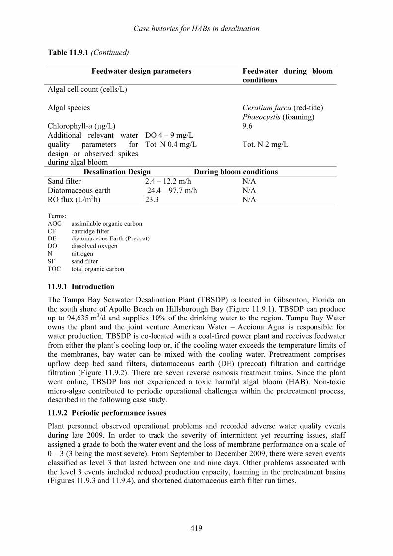
Case histories for HABs in desalination

419

Table 11.9.1 (Continued)

Feedwater design parameters Feedwater during bloom conditions

Algal cell count (cells/L)

Algal species Ceratium furca (red-tide) Phaeocystis (foaming)

Chlorophyll-a (µg/L) 9.6 Additional relevant water quality parameters for design or observed spikes during algal bloom

DO 4 – 9 mg/L Tot. N 0.4 mg/L

Tot. N 2 mg/L

Desalination Design During bloom conditions Sand filter 2.4 – 12.2 m/h N/A Diatomaceous earth 24.4 – 97.7 m/h N/A RO flux (L/m2h) 23.3 N/A Terms:

AOC assimilable organic carbon CF cartridge filter DE diatomaceous Earth (Precoat) DO dissolved oxygen N nitrogen SF sand filter TOC total organic carbon 11.9.1 Introduction The Tampa Bay Seawater Desalination Plant (TBSDP) is located in Gibsonton, Florida on the south shore of Apollo Beach on Hillsborough Bay (Figure 11.9.1). TBSDP can produce up to 94,635 m3/d and supplies 10% of the drinking water to the region. Tampa Bay Water owns the plant and the joint venture American Water – Acciona Agua is responsible for water production. TBSDP is co-located with a coal-fired power plant and receives feedwater from either the plant’s cooling loop or, if the cooling water exceeds the temperature limits of the membranes, bay water can be mixed with the cooling water. Pretreatment comprises upflow deep bed sand filters, diatomaceous earth (DE) (precoat) filtration and cartridge filtration (Figure 11.9.2). There are seven reverse osmosis treatment trains. Since the plant went online, TBSDP has not experienced a toxic harmful algal bloom (HAB). Non-toxic micro-algae contributed to periodic operational challenges within the pretreatment process, described in the following case study.

11.9.2 Periodic performance issues Plant personnel observed operational problems and recorded adverse water quality events during late 2009. In order to track the severity of intermittent yet recurring issues, staff assigned a grade to both the water event and the loss of membrane performance on a scale of 0 – 3 (3 being the most severe). From September to December 2009, there were seven events classified as level 3 that lasted between one and nine days. Other problems associated with the level 3 events included reduced production capacity, foaming in the pretreatment basins (Figures 11.9.3 and 11.9.4), and shortened diatomaceous earth filter run times.

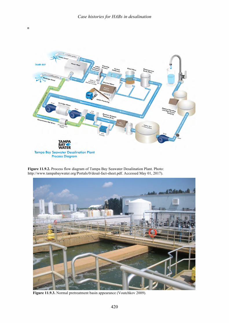
Case histories for HABs in desalination

420

Figure 11.9.2. Process flow diagram of Tampa Bay Seawater Desalination Plant. Photo: http://www.tampabaywater.org/Portals/0/desal-fact-sheet.pdf. Accessed May 01, 2017).

Figure 11.9.3. Normal pretreatment basin appearance (Voutchkov 2009).

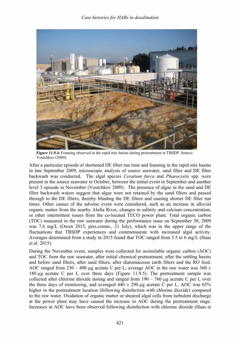
Case histories for HABs in desalination

421

Figure 11.9.4. Foaming observed in the rapid mix basins during pretreatment at TBSDP. Source: Voutchkov (2009).

After a particular episode of shortened DE filter run time and foaming in the rapid mix basins in late September 2009, microscopic analysis of source seawater, sand filter and DE filter backwash was conducted. The algal species Ceratium furca and Phaeocystis spp. were present in the source seawater in October, between the initial event in September and another level 3 episode in November (Voutchkov 2009). The presence of algae in the sand and DE filter backwash waters suggest that algae were not retained by the sand filters and passed through to the DE filters, thereby blinding the DE filters and causing shorter DE filter run times. Other causes of the adverse event were considered, such as an increase in alluvial organic matter from the nearby Alafia River, changes in salinity and calcium concentration, or other intermittent issues from the co-located TECO power plant. Total organic carbon (TOC) measured in the raw seawater during the performance issue on September 30, 2009 was 7.6 mg/L (Owen 2015, pers.comm., 21 July), which was in the upper range of the fluctuations that TBSDP experiences and commensurate with increased algal activity. Averages determined from a study in 2015 found that TOC ranged from 5.5 to 6 mg/L (Haas et al. 2015). During the November event, samples were collected for assimilable organic carbon (AOC) and TOC from the raw seawater, after initial chemical pretreatment, after the settling basins and before sand filters, after sand filters, after diatomaceous earth filters and the RO feed. AOC ranged from 230 – 490 µg acetate C per L; average AOC in the raw water was 360 ± 180 µg acetate C per L over three days (Figure 11.9.5). The pretreatment sample was collected after chlorine dioxide dosing and ranged from 190 – 760 µg acetate C per L over the three days of monitoring, and averaged 440 ± 290 µg acetate C per L. AOC was 65% higher in the pretreatment location (following disinfection with chlorine dioxide) compared to the raw water. Oxidation of organic matter or sheared algal cells from turbulent discharge at the power plant may have caused the increase in AOC during the pretreatment stage. Increases in AOC have been observed following disinfection with chlorine dioxide (Haas et

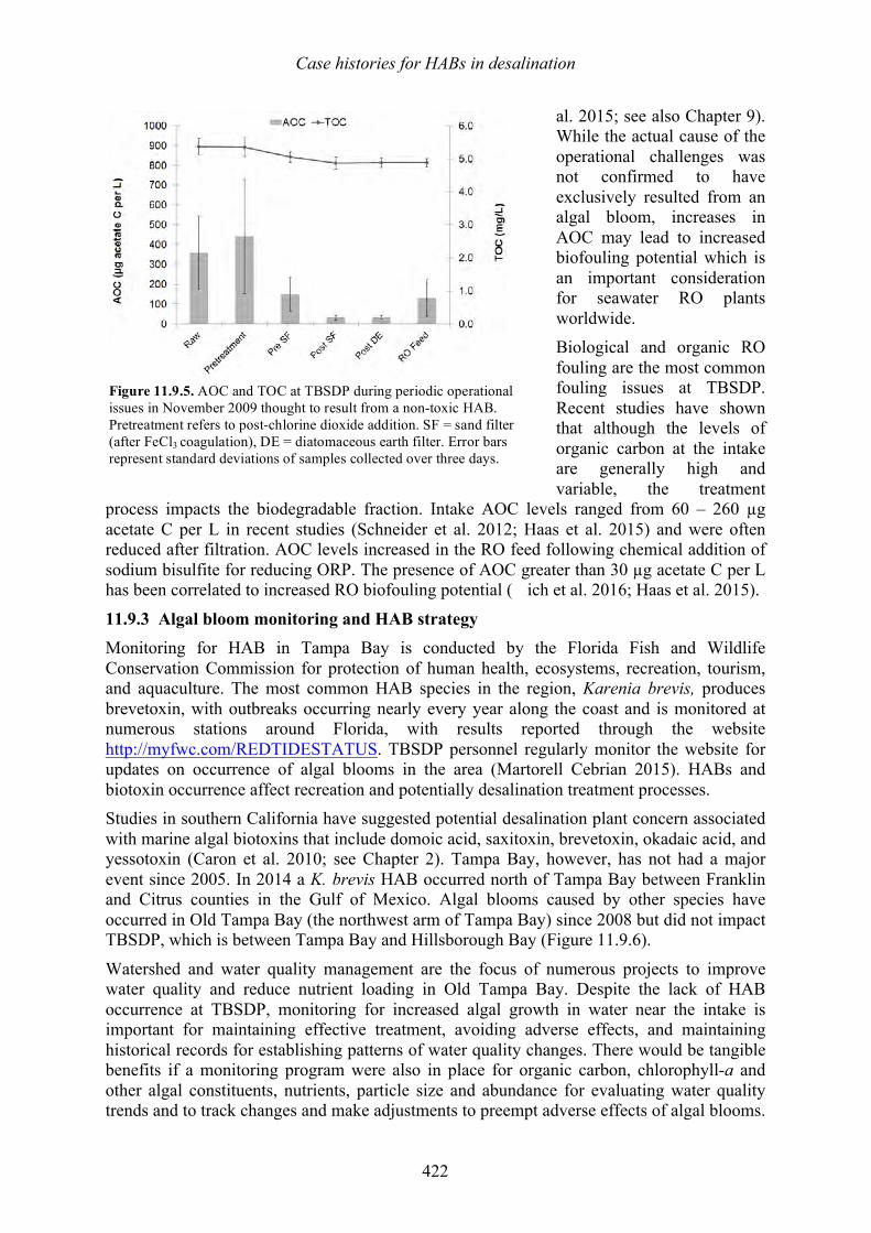
Case histories for HABs in desalination

422

al. 2015; see also Chapter 9). While the actual cause of the operational challenges was not confirmed to have exclusively resulted from an algal bloom, increases in AOC may lead to increased biofouling potential which is an important consideration for seawater RO plants worldwide. Biological and organic RO fouling are the most common fouling issues at TBSDP. Recent studies have shown that although the levels of organic carbon at the intake are generally high and variable, the treatment

process impacts the biodegradable fraction. Intake AOC levels ranged from 60 – 260 µg acetate C per L in recent studies (Schneider et al. 2012; Haas et al. 2015) and were often reduced after filtration. AOC levels increased in the RO feed following chemical addition of sodium bisulfite for reducing ORP. The presence of AOC greater than 30 µg acetate C per L has been correlated to increased RO biofouling potential ( ich et al. 2016; Haas et al. 2015).

11.9.3 Algal bloom monitoring and HAB strategy Monitoring for HAB in Tampa Bay is conducted by the Florida Fish and Wildlife Conservation Commission for protection of human health, ecosystems, recreation, tourism, and aquaculture. The most common HAB species in the region, Karenia brevis, produces brevetoxin, with outbreaks occurring nearly every year along the coast and is monitored at numerous stations around Florida, with results reported through the website http://myfwc.com/REDTIDESTATUS. TBSDP personnel regularly monitor the website for updates on occurrence of algal blooms in the area (Martorell Cebrian 2015). HABs and biotoxin occurrence affect recreation and potentially desalination treatment processes. Studies in southern California have suggested potential desalination plant concern associated with marine algal biotoxins that include domoic acid, saxitoxin, brevetoxin, okadaic acid, and yessotoxin (Caron et al. 2010; see Chapter 2). Tampa Bay, however, has not had a major event since 2005. In 2014 a K. brevis HAB occurred north of Tampa Bay between Franklin and Citrus counties in the Gulf of Mexico. Algal blooms caused by other species have occurred in Old Tampa Bay (the northwest arm of Tampa Bay) since 2008 but did not impact TBSDP, which is between Tampa Bay and Hillsborough Bay (Figure 11.9.6).

Watershed and water quality management are the focus of numerous projects to improve water quality and reduce nutrient loading in Old Tampa Bay. Despite the lack of HAB occurrence at TBSDP, monitoring for increased algal growth in water near the intake is important for maintaining effective treatment, avoiding adverse effects, and maintaining historical records for establishing patterns of water quality changes. There would be tangible benefits if a monitoring program were also in place for organic carbon, chlorophyll-a and other algal constituents, nutrients, particle size and abundance for evaluating water quality trends and to track changes and make adjustments to preempt adverse effects of algal blooms.

Figure 11.9.5. AOC and TOC at TBSDP during periodic operational issues in November 2009 thought to result from a non-toxic HAB. Pretreatment refers to post-chlorine dioxide addition. SF = sand filter (after FeCl3 coagulation), DE = diatomaceous earth filter. Error bars represent standard deviations of samples collected over three days.

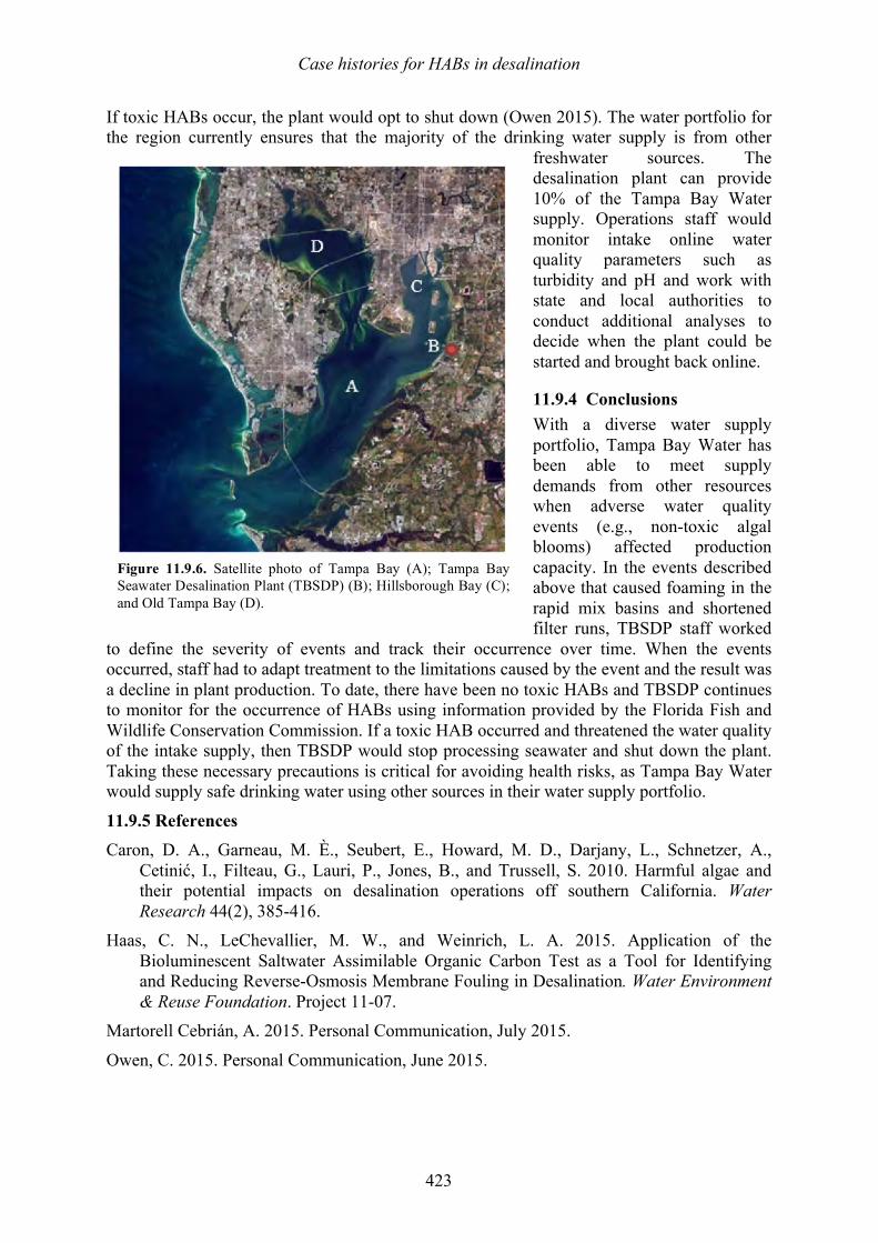
Case histories for HABs in desalination

423

If toxic HABs occur, the plant would opt to shut down (Owen 2015). The water portfolio for the region currently ensures that the majority of the drinking water supply is from other

freshwater sources. The desalination plant can provide 10% of the Tampa Bay Water supply. Operations staff would monitor intake online water quality parameters such as turbidity and pH and work with state and local authorities to conduct additional analyses to decide when the plant could be started and brought back online.

11.9.4 Conclusions With a diverse water supply portfolio, Tampa Bay Water has been able to meet supply demands from other resources when adverse water quality events (e.g., non-toxic algal blooms) affected production capacity. In the events described above that caused foaming in the rapid mix basins and shortened filter runs, TBSDP staff worked

to define the severity of events and track their occurrence over time. When the events occurred, staff had to adapt treatment to the limitations caused by the event and the result was a decline in plant production. To date, there have been no toxic HABs and TBSDP continues to monitor for the occurrence of HABs using information provided by the Florida Fish and Wildlife Conservation Commission. If a toxic HAB occurred and threatened the water quality of the intake supply, then TBSDP would stop processing seawater and shut down the plant. Taking these necessary precautions is critical for avoiding health risks, as Tampa Bay Water would supply safe drinking water using other sources in their water supply portfolio.

11.9.5 References Caron, D. A., Garneau, M. È., Seubert, E., Howard, M. D., Darjany, L., Schnetzer, A.,

Cetinić, I., Filteau, G., Lauri, P., Jones, B., and Trussell, S. 2010. Harmful algae and their potential impacts on desalination operations off southern California. Water Research 44(2), 385-416.

Haas, C. N., LeChevallier, M. W., and Weinrich, L. A. 2015. Application of the Bioluminescent Saltwater Assimilable Organic Carbon Test as a Tool for Identifying and Reducing Reverse-Osmosis Membrane Fouling in Desalination. Water Environment & Reuse Foundation. Project 11-07.

Martorell Cebrián, A. 2015. Personal Communication, July 2015.

Owen, C. 2015. Personal Communication, June 2015.

Figure 11.9.6. Satellite photo of Tampa Bay (A); Tampa Bay Seawater Desalination Plant (TBSDP) (B); Hillsborough Bay (C); and Old Tampa Bay (D).

Case histories for HABs in desalination

424

Schneider, O. D., Weinrich, L. A., Giraldo, E., Kennedy, M., and Salinas, S. 2012. Investigation of Organic Matter Removal in Saline Waters by Pretreatment. Water Research Foundation. Project 4280.

Voutchkov, N. 2009. Initial biofouling analysis. Water Globe Consulting Tech. Memo. Proj. No. 0007-2009-0001 on Nov. 5, 2009.

Weinrich, L., LeChevallier, M. and Haas, C. N. 2016. Contribution of assimilable organic carbon to biological fouling in seawater reverse osmosis membrane treatment. Water Research 101, 203-213.

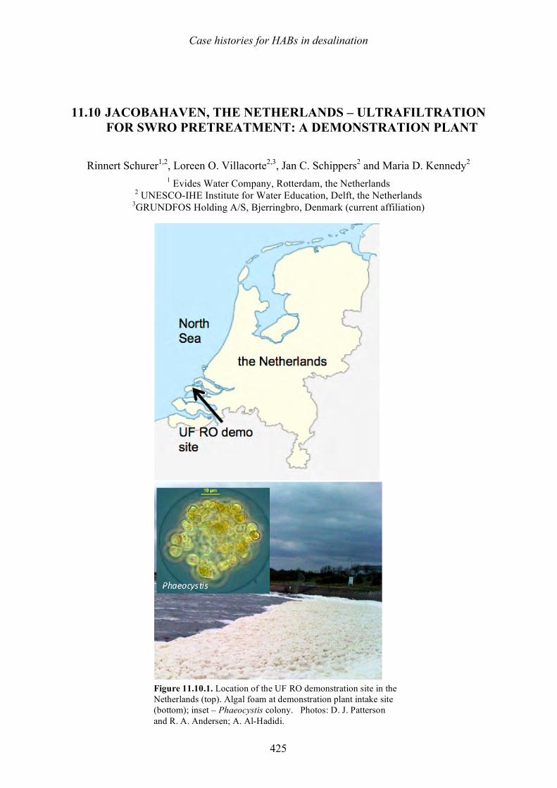
Case histories for HABs in desalination

425

11.10 JACOBAHAVEN, THE NETHERLANDS – ULTRAFILTRATION FOR SWRO PRETREATMENT: A DEMONSTRATION PLANT

Rinnert Schurer1,2, Loreen O. Villacorte2,3, Jan C. Schippers2 and Maria D. Kennedy2 1 Evides Water Company, Rotterdam, the Netherlands

2 UNESCO-IHE Institute for Water Education, Delft, the Netherlands 3GRUNDFOS Holding A/S, Bjerringbro, Denmark (current affiliation)

Figure 11.10.1. Location of the UF RO demonstration site in the Netherlands (top). Algal foam at demonstration plant intake site (bottom); inset – Phaeocystis colony. Photos: D. J. Patterson and R. A. Andersen; A. Al-Hadidi.

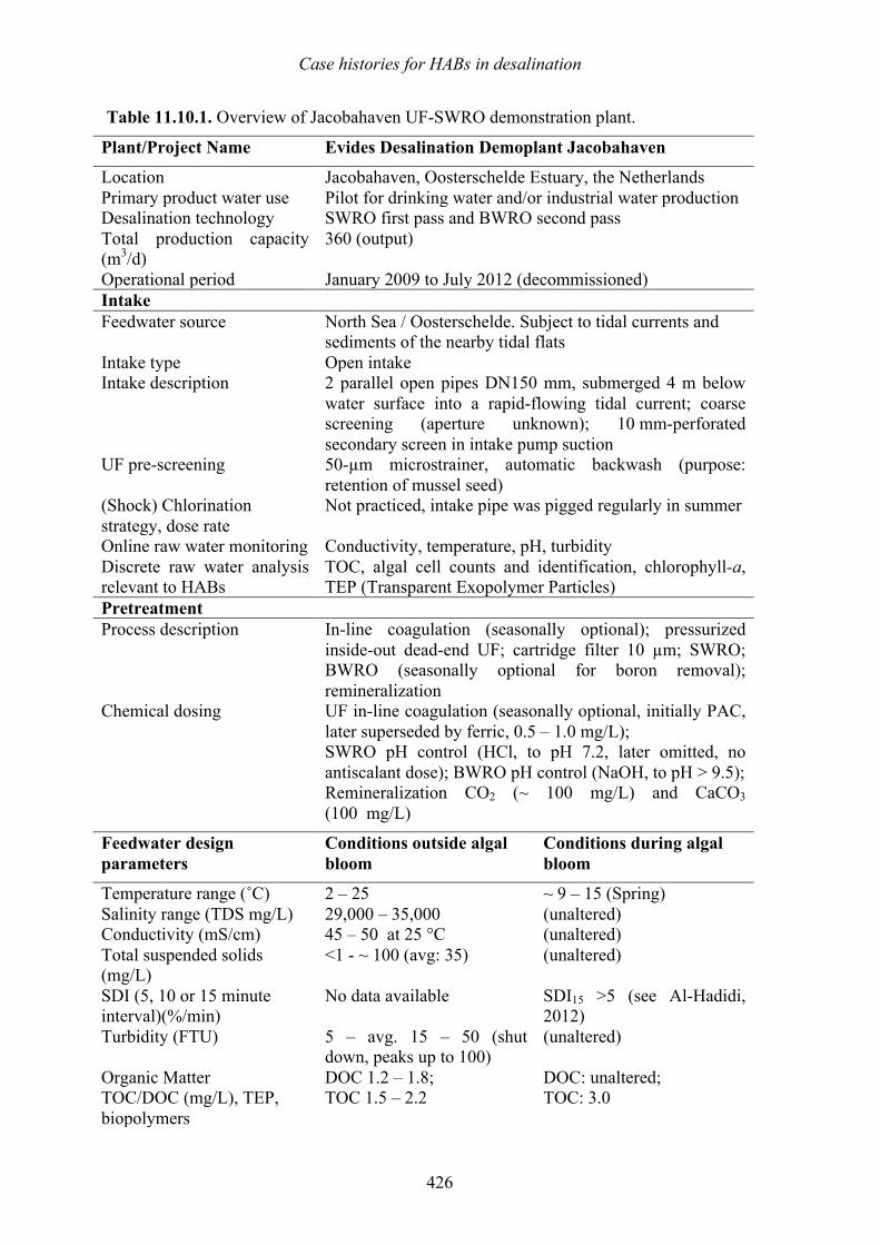
Case histories for HABs in desalination

426

Table 11.10.1. Overview of Jacobahaven UF-SWRO demonstration plant.

Plant/Project Name Evides Desalination Demoplant Jacobahaven

Location Jacobahaven, Oosterschelde Estuary, the Netherlands Primary product water use Pilot for drinking water and/or industrial water production Desalination technology SWRO first pass and BWRO second pass Total production capacity (m3/d)

360 (output)

Operational period January 2009 to July 2012 (decommissioned) Intake Feedwater source North Sea / Oosterschelde. Subject to tidal currents and

sediments of the nearby tidal flats Intake type Open intake Intake description 2 parallel open pipes DN150 mm, submerged 4 m below

water surface into a rapid-flowing tidal current; coarse screening (aperture unknown); 10 mm-perforated secondary screen in intake pump suction

UF pre-screening 50-µm microstrainer, automatic backwash (purpose: retention of mussel seed)

(Shock) Chlorination strategy, dose rate

Not practiced, intake pipe was pigged regularly in summer

Online raw water monitoring Conductivity, temperature, pH, turbidity Discrete raw water analysis relevant to HABs

TOC, algal cell counts and identification, chlorophyll-a, TEP (Transparent Exopolymer Particles)

Pretreatment Process description

In-line coagulation (seasonally optional); pressurized inside-out dead-end UF; cartridge filter 10 µm; SWRO; BWRO (seasonally optional for boron removal); remineralization

Chemical dosing UF in-line coagulation (seasonally optional, initially PAC, later superseded by ferric, 0.5 – 1.0 mg/L); SWRO pH control (HCl, to pH 7.2, later omitted, no antiscalant dose); BWRO pH control (NaOH, to pH > 9.5); Remineralization CO2 (~ 100 mg/L) and CaCO3 (100 mg/L)

Feedwater design parameters

Conditions outside algal bloom

Conditions during algal bloom

Temperature range (˚C) 2 – 25 ~ 9 – 15 (Spring) Salinity range (TDS mg/L) 29,000 – 35,000 (unaltered) Conductivity (mS/cm) 45 – 50 at 25 °C (unaltered) Total suspended solids (mg/L)

<1 - ~ 100 (avg: 35) (unaltered)

SDI (5, 10 or 15 minute interval)(%/min)

No data available SDI15 >5 (see Al-Hadidi, 2012)

Turbidity (FTU) 5 – avg. 15 – 50 (shut down, peaks up to 100)

(unaltered)

Organic Matter TOC/DOC (mg/L), TEP, biopolymers

DOC 1.2 – 1.8; TOC 1.5 – 2.2

DOC: unaltered; TOC: 3.0

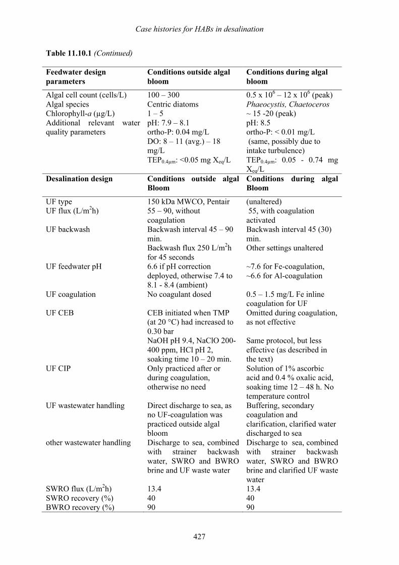
Case histories for HABs in desalination

427

Table 11.10.1 (Continued)

Feedwater design parameters

Conditions outside algal bloom

Conditions during algal bloom

Algal cell count (cells/L) 100 – 300 0.5 x 106 – 12 x 106 (peak) Algal species Centric diatoms Phaeocystis, Chaetoceros Chlorophyll-a (µg/L) 1 – 5 ~ 15 -20 (peak) Additional relevant water quality parameters

pH: 7.9 – 8.1 ortho-P: 0.04 mg/L DO: 8 – 11 (avg.) – 18 mg/L TEP0.4µm: <0.05 mg Xeq/L

pH: 8.5 ortho-P: < 0.01 mg/L (same, possibly due to intake turbulence) TEP0.4µm: 0.05 - 0.74 mg Xeq/L

Desalination design Conditions outside algal Bloom

Conditions during algal Bloom

UF type 150 kDa MWCO, Pentair (unaltered) UF flux (L/m2h) 55 – 90, without

coagulation 55, with coagulation activated

UF backwash Backwash interval 45 – 90 min. Backwash flux 250 L/m2h for 45 seconds

Backwash interval 45 (30) min. Other settings unaltered

UF feedwater pH 6.6 if pH correction deployed, otherwise 7.4 to 8.1 - 8.4 (ambient)

~7.6 for Fe-coagulation, ~6.6 for Al-coagulation

UF coagulation No coagulant dosed 0.5 – 1.5 mg/L Fe inline coagulation for UF

UF CEB CEB initiated when TMP (at 20 °C) had increased to 0.30 bar NaOH pH 9.4, NaClO 200-400 ppm, HCl pH 2, soaking time 10 – 20 min.

Omitted during coagulation, as not effective Same protocol, but less effective (as described in the text)

UF CIP Only practiced after or during coagulation, otherwise no need

Solution of 1% ascorbic acid and 0.4 % oxalic acid, soaking time 12 – 48 h. No temperature control

UF wastewater handling Direct discharge to sea, as no UF-coagulation was practiced outside algal bloom

Buffering, secondary coagulation and clarification, clarified water discharged to sea

other wastewater handling Discharge to sea, combined with strainer backwash water, SWRO and BWRO brine and UF waste water

Discharge to sea, combined with strainer backwash water, SWRO and BWRO brine and clarified UF waste water

SWRO flux (L/m2h) 13.4 13.4 SWRO recovery (%) 40 40 BWRO recovery (%) 90 90

Case histories for HABs in desalination

428

11.10.1 Introduction Evides Waterbedrijf, the South-Western Netherlands water supply company providing municipal drinking water, industrial water, as well as wastewater treatment services, owned and operated a UF-RO (Ultrafiltration – Reverse Osmosis) desalination plant on the Oosterschelde for demonstration and research purposes between 2009 and 2012. The overall aim of the project was to study desalination as one of the alternatives to the water resources already used by Evides (i.e., fresh surface water, ground water and infiltrated water), in the framework of the company’s efforts to safeguard water supply in the long term with respect to climate change. The desalination research was conducted under locally relevant conditions regarding water quality (seasonally variable) and temperature (seasonally low). The characteristics of the plant are given in Table 11.10.1. As the site featured an open intake, and raw water quality was variable, conditions were challenging for the downstream treatment processes. A major characteristic in this respect was the occurrence of seasonal algal blooms, which impacted the UF pretreatment in terms of fouling, necessitating the temporary application of in-line coagulation. To guide plant operation and design, a major objective was to gain an understanding of the following topics relative to the ultrafiltration pretreatment: • Seasonal variation in raw water quality, especially of parameters associated with algal

blooms, expected to be relevant for the strainer and UF treatment steps such as algal presence, associated algogenic organic components and nutrients;

• Impact of algal bloom-related raw water quality variations on UF permeability performance i.e., fouling, and its maintenance by means of hydraulic backwash, chemically enhanced backwash (CEB), and application of coagulant;

• Resultant UF permeate quality and SWRO membrane permeability. During the plant’s operation, ample data were collected; several scientific institutes conducted or participated in research at the site. A valuable dataset, experience, and lessons learned have therefore been acquired1. The dissemination of this material by means of the current Case Study aims to contribute to the ongoing improvement of operating standards in the desalination industry. 11.10.2 Feedwater intake

The demonstration plant feedwater was drawn from the Oosterschelde water body, close to the southern landfall of the identically-named storm surge barrier (Figure 11.10.2). This feed can be regarded as North Sea water in terms of salinity, temperature, and organic and inorganic constituents. Due to its geographical position, seasonal temperature variations were applicable. The intake was located at a site featuring highly turbulent conditions caused by tidal currents, hence stratification was absent. During stormy weather, severe turbidity peaks occurred, due to mobilization of sediments from the tidal flats in the Oosterschelde water body. If turbidity exceeded 50-75 FTU for more than several hours, the limited capacity of the strainer forced a plant shut down, which occurred two to four times a year.

A specific characteristic of the feedwater was the recurrence of seasonal algal blooms in Spring (April-May) every year, as described in Section 11.10.5. For further feedwater data, see Table 11.10.1.

1 For further literature specific for the current Case Study, the reader is also referred to Al-Hadidi et al. (2012); Villacorte (2014); Tabatabai (2014) and Schurer et al. (2012, 2013).

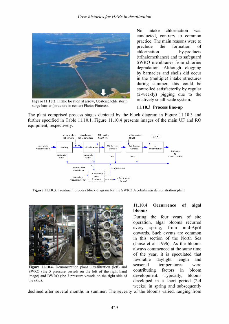
Case histories for HABs in desalination

429

No intake chlorination was conducted, contrary to common practice. The main reasons were to preclude the formation of chlorination by-products (trihalomethanes) and to safeguard SWRO membranes from chlorine degradation. Although clogging by barnacles and shells did occur in the (multiple) intake structures during summer, this could be controlled satisfactorily by regular (2-weekly) pigging due to the relatively small-scale system.

11.10.3 Process line-up The plant comprised process stages depicted by the block diagram in Figure 11.10.3 and further specified in Table 11.10.1. Figure 11.10.4 presents images of the main UF and RO equipment, respectively.

11.10.4 Occurrence of algal blooms During the four years of site operation, algal blooms recurred every spring, from mid-April onwards. Such events are common in this section of the North Sea (Janse et al. 1996). As the blooms always commenced at the same time of the year, it is speculated that favorable daylight length and seasonal temperatures were contributing factors in bloom development. Typically, blooms developed in a short period (2-4 weeks) in spring and subsequently

declined after several months in summer. The severity of the blooms varied, ranging from

Figure 11.10.4. Demonstration plant ultrafiltration (left) and SWRO (the 5 pressure vessels on the left of the right hand image) and BWRO (the 3 pressure vessels on the right side of the skid).

Figure 11.10.2. Intake location at arrow, Oosterschelde storm surge barrier (structure in center) Photo: Pinterest.

Figure 11.10.3. Treatment process block diagram for the SWRO Jacobahaven demonstration plant.

Case histories for HABs in desalination

430

peak levels of 12 million cells/L to a relatively subdued bloom in 2012 at 2 million cells/L (which could possibly be attributed to the cold and stormy weather conditions in that particular year). Algal speciation varied from year to year. Diatoms were generally present during each bloom (Chaetoceros, Thalassiosira), whereas Phaeocystis or Chrysochromulina prevailed only in some years (2010 and 2010 and 2011, respectively) during the four years of monitoring (Evides data). Example images of these species are given in Appendix 1. The prevalence of Phaeocystis caused noticeable foam formation as shown in Figures 11.10.1 and 11.10.5.

11.10.4.1 Associated raw water quality parameters

During algal blooms, levels of chlorophyll-a (Figure 11.10.6) and algal counts (Table 11.10.1) correspondingly spiked up to 20 µg/L and 10,000/mL, respectively. Interestingly, a measurable elevation of the pH (~0.5 pH above average) occurred during the algal bloom periods. In contrast, no deviation in dissolved oxygen was noted, possibly because of the highly turbulent conditions at the raw water intake site.

Also, in associated research work, the presence of TEP0.4µm was measured. TEP0.4µm levels fluctuated in rather close unison with chlorophyll-a levels, increasing 20 to 60-fold at the algal bloom peak (Villacorte 2014; Schurer et al. 2012), as shown in Section 11.10.6 – (Impact on UF). More data on TEP measurements are presented in Chapters 2 and 5 and the methods for TEP measurement are outlined in Appendix 4.

Figure 11.10.5 Foam formation at the intake site during Phaeocystis bloom occurrence.

Figure 11.10.6. Seasonal patterns of raw water temperature and algal-boom related parameters (chlorophyll, TEP0.4µm).

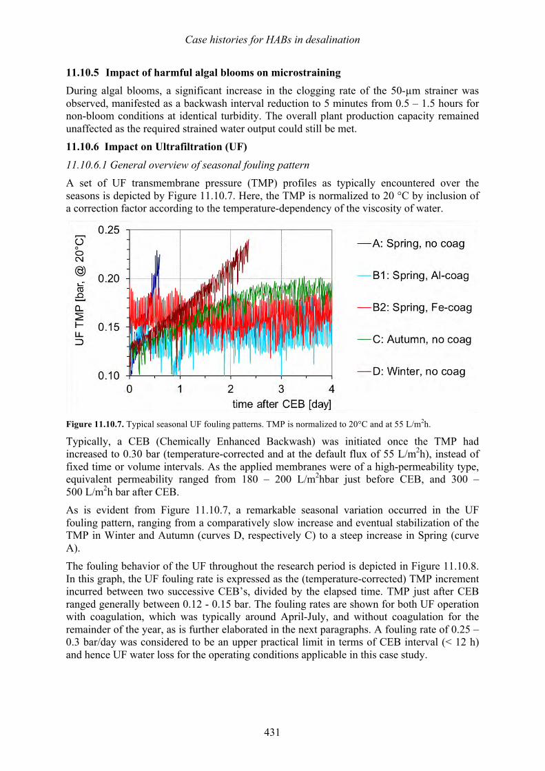
Case histories for HABs in desalination

431

11.10.5 Impact of harmful algal blooms on microstraining During algal blooms, a significant increase in the clogging rate of the 50-µm strainer was observed, manifested as a backwash interval reduction to 5 minutes from 0.5 – 1.5 hours for non-bloom conditions at identical turbidity. The overall plant production capacity remained unaffected as the required strained water output could still be met. 11.10.6 Impact on Ultrafiltration (UF)

11.10.6.1 General overview of seasonal fouling pattern A set of UF transmembrane pressure (TMP) profiles as typically encountered over the seasons is depicted by Figure 11.10.7. Here, the TMP is normalized to 20 °C by inclusion of a correction factor according to the temperature-dependency of the viscosity of water.

Figure 11.10.7. Typical seasonal UF fouling patterns. TMP is normalized to 20°C and at 55 L/m2h.

Typically, a CEB (Chemically Enhanced Backwash) was initiated once the TMP had increased to 0.30 bar (temperature-corrected and at the default flux of 55 L/m2h), instead of fixed time or volume intervals. As the applied membranes were of a high-permeability type, equivalent permeability ranged from 180 – 200 L/m2hbar just before CEB, and 300 – 500 L/m2h bar after CEB. As is evident from Figure 11.10.7, a remarkable seasonal variation occurred in the UF fouling pattern, ranging from a comparatively slow increase and eventual stabilization of the TMP in Winter and Autumn (curves D, respectively C) to a steep increase in Spring (curve A). The fouling behavior of the UF throughout the research period is depicted in Figure 11.10.8. In this graph, the UF fouling rate is expressed as the (temperature-corrected) TMP increment incurred between two successive CEB’s, divided by the elapsed time. TMP just after CEB ranged generally between 0.12 - 0.15 bar. The fouling rates are shown for both UF operation with coagulation, which was typically around April-July, and without coagulation for the remainder of the year, as is further elaborated in the next paragraphs. A fouling rate of 0.25 – 0.3 bar/day was considered to be an upper practical limit in terms of CEB interval (< 12 h) and hence UF water loss for the operating conditions applicable in this case study.

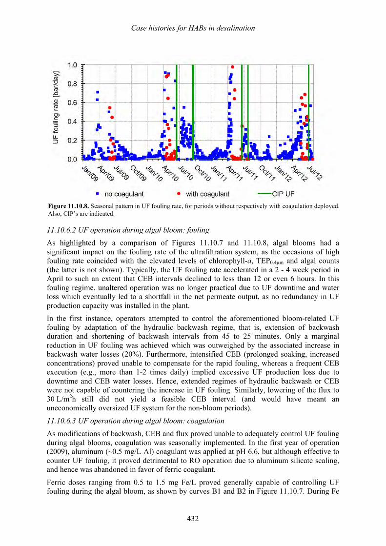
Case histories for HABs in desalination

432

11.10.6.2 UF operation during algal bloom: fouling As highlighted by a comparison of Figures 11.10.7 and 11.10.8, algal blooms had a significant impact on the fouling rate of the ultrafiltration system, as the occasions of high fouling rate coincided with the elevated levels of chlorophyll-a, TEP0.4µm and algal counts (the latter is not shown). Typically, the UF fouling rate accelerated in a 2 - 4 week period in April to such an extent that CEB intervals declined to less than 12 or even 6 hours. In this fouling regime, unaltered operation was no longer practical due to UF downtime and water loss which eventually led to a shortfall in the net permeate output, as no redundancy in UF production capacity was installed in the plant. In the first instance, operators attempted to control the aforementioned bloom-related UF fouling by adaptation of the hydraulic backwash regime, that is, extension of backwash duration and shortening of backwash intervals from 45 to 25 minutes. Only a marginal reduction in UF fouling was achieved which was outweighed by the associated increase in backwash water losses (20%). Furthermore, intensified CEB (prolonged soaking, increased concentrations) proved unable to compensate for the rapid fouling, whereas a frequent CEB execution (e.g., more than 1-2 times daily) implied excessive UF production loss due to downtime and CEB water losses. Hence, extended regimes of hydraulic backwash or CEB were not capable of countering the increase in UF fouling. Similarly, lowering of the flux to 30 L/m2h still did not yield a feasible CEB interval (and would have meant an uneconomically oversized UF system for the non-bloom periods).

11.10.6.3 UF operation during algal bloom: coagulation As modifications of backwash, CEB and flux proved unable to adequately control UF fouling during algal blooms, coagulation was seasonally implemented. In the first year of operation (2009), aluminum (~0.5 mg/L Al) coagulant was applied at pH 6.6, but although effective to counter UF fouling, it proved detrimental to RO operation due to aluminum silicate scaling, and hence was abandoned in favor of ferric coagulant.

Ferric doses ranging from 0.5 to 1.5 mg Fe/L proved generally capable of controlling UF fouling during the algal bloom, as shown by curves B1 and B2 in Figure 11.10.7. During Fe

Figure 11.10.8. Seasonal pattern in UF fouling rate, for periods without respectively with coagulation deployed. Also, CIP’s are indicated.

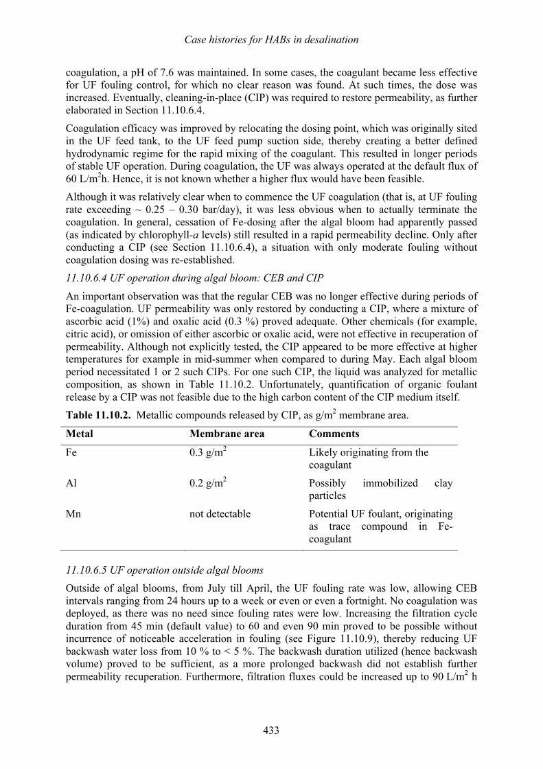
Case histories for HABs in desalination

433

coagulation, a pH of 7.6 was maintained. In some cases, the coagulant became less effective for UF fouling control, for which no clear reason was found. At such times, the dose was increased. Eventually, cleaning-in-place (CIP) was required to restore permeability, as further elaborated in Section 11.10.6.4.

Coagulation efficacy was improved by relocating the dosing point, which was originally sited in the UF feed tank, to the UF feed pump suction side, thereby creating a better defined hydrodynamic regime for the rapid mixing of the coagulant. This resulted in longer periods of stable UF operation. During coagulation, the UF was always operated at the default flux of 60 L/m2h. Hence, it is not known whether a higher flux would have been feasible. Although it was relatively clear when to commence the UF coagulation (that is, at UF fouling rate exceeding ~ 0.25 – 0.30 bar/day), it was less obvious when to actually terminate the coagulation. In general, cessation of Fe-dosing after the algal bloom had apparently passed (as indicated by chlorophyll-a levels) still resulted in a rapid permeability decline. Only after conducting a CIP (see Section 11.10.6.4), a situation with only moderate fouling without coagulation dosing was re-established. 11.10.6.4 UF operation during algal bloom: CEB and CIP

An important observation was that the regular CEB was no longer effective during periods of Fe-coagulation. UF permeability was only restored by conducting a CIP, where a mixture of ascorbic acid (1%) and oxalic acid (0.3 %) proved adequate. Other chemicals (for example, citric acid), or omission of either ascorbic or oxalic acid, were not effective in recuperation of permeability. Although not explicitly tested, the CIP appeared to be more effective at higher temperatures for example in mid-summer when compared to during May. Each algal bloom period necessitated 1 or 2 such CIPs. For one such CIP, the liquid was analyzed for metallic composition, as shown in Table 11.10.2. Unfortunately, quantification of organic foulant release by a CIP was not feasible due to the high carbon content of the CIP medium itself. Table 11.10.2. Metallic compounds released by CIP, as g/m2 membrane area.

Metal Membrane area Comments

Fe 0.3 g/m2 Likely originating from the coagulant

Al 0.2 g/m2 Possibly immobilized clay particles

Mn not detectable Potential UF foulant, originating as trace compound in Fe-coagulant

11.10.6.5 UF operation outside algal blooms Outside of algal blooms, from July till April, the UF fouling rate was low, allowing CEB intervals ranging from 24 hours up to a week or even or even a fortnight. No coagulation was deployed, as there was no need since fouling rates were low. Increasing the filtration cycle duration from 45 min (default value) to 60 and even 90 min proved to be possible without incurrence of noticeable acceleration in fouling (see Figure 11.10.9), thereby reducing UF backwash water loss from 10 % to < 5 %. The backwash duration utilized (hence backwash volume) proved to be sufficient, as a more prolonged backwash did not establish further permeability recuperation. Furthermore, filtration fluxes could be increased up to 90 L/m2 h

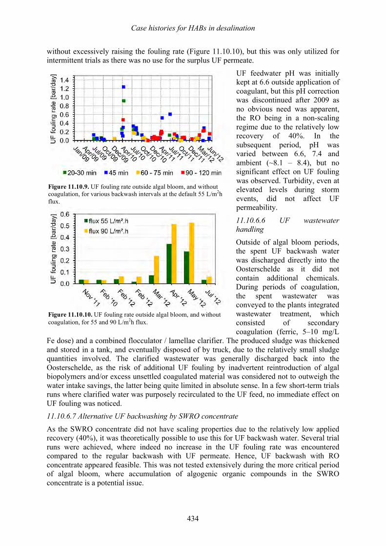
Case histories for HABs in desalination

434

without excessively raising the fouling rate (Figure 11.10.10), but this was only utilized for intermittent trials as there was no use for the surplus UF permeate.

UF feedwater pH was initially kept at 6.6 outside application of coagulant, but this pH correction was discontinued after 2009 as no obvious need was apparent, the RO being in a non-scaling regime due to the relatively low recovery of 40%. In the subsequent period, pH was varied between 6.6, 7.4 and ambient (~8.1 – 8.4), but no significant effect on UF fouling was observed. Turbidity, even at elevated levels during storm events, did not affect UF permeability.

11.10.6.6 UF wastewater handling

Outside of algal bloom periods, the spent UF backwash water was discharged directly into the Oosterschelde as it did not contain additional chemicals. During periods of coagulation, the spent wastewater was conveyed to the plants integrated wastewater treatment, which consisted of secondary coagulation (ferric, 5–10 mg/L

Fe dose) and a combined flocculator / lamellae clarifier. The produced sludge was thickened and stored in a tank, and eventually disposed of by truck, due to the relatively small sludge quantities involved. The clarified wastewater was generally discharged back into the Oosterschelde, as the risk of additional UF fouling by inadvertent reintroduction of algal biopolymers and/or excess unsettled coagulated material was considered not to outweigh the water intake savings, the latter being quite limited in absolute sense. In a few short-term trials runs where clarified water was purposely recirculated to the UF feed, no immediate effect on UF fouling was noticed. 11.10.6.7 Alternative UF backwashing by SWRO concentrate

As the SWRO concentrate did not have scaling properties due to the relatively low applied recovery (40%), it was theoretically possible to use this for UF backwash water. Several trial runs were achieved, where indeed no increase in the UF fouling rate was encountered compared to the regular backwash with UF permeate. Hence, UF backwash with RO concentrate appeared feasible. This was not tested extensively during the more critical period of algal bloom, where accumulation of algogenic organic compounds in the SWRO concentrate is a potential issue.

Figure 11.10.9. UF fouling rate outside algal bloom, and without coagulation, for various backwash intervals at the default 55 L/m2h flux.

Figure 11.10.10. UF fouling rate outside algal bloom, and without coagulation, for 55 and 90 L/m2h flux.

Case histories for HABs in desalination

435

11.10.6.8 UF permeate quality and membrane integrity Selected UF permeate quality data are presented by Table 11.10.3. Appropriate RO feedwater quality standards were met. Furthermore, UF integrity testing revealed that UF fiber breakage amounted to < 0.06 % over a period of 3.5 years of nearly continuous operation under periodically challenging conditions, attesting to the resilience of UF pretreatment in the retention of particulate and biomass matter in conjunction with the upstream-positioned microstrainer. Table 11.10.3. UF permeate quality data and reductions.

Parameter Result

Turbidity < 0.05 FTU Particle count reduction > 3.6 log for particles ≥ 0.5 µm

SDI15 < 2 (Al-Hadidi et al. 2012) Fe during coagulation < 0.05 µg/L (detection limit)

Biopolymer (LC-OCD) ~50 % reduction (Salinas Rodríguez 2011; Villacorte 2014)

TEP0.4µm < 0.01 mg Xeq/L (detection limit), equivalent reduction > 90% (Appendix 4; Villacorte 2014).

11.10.6.9 Further data on UF foulant levels

During an algal bloom period in May 2013, various parameters relevant to HABs were monitored at the same Oosterschelde site. Since operation of the demo-site UF unit was discontinued in July 2012, samples for the UF feed and UF permeate were collected from a smaller pilot UF unit (1” module) with similar membrane properties and operational settings as in the previous demo-site unit. On this occasion, the raw water recorded algal density was 6.25 x 106 cells/L and the chlorophyll-a concentration was 10.6 µg/L. Table 11.10.4 shows the comparison of the different parameters and their reduction over the pretreatment processes.

Table 11.10.4. Measured parameters for raw water, strained water and UF permeate during the 2013 algal bloom. Data from Villacorte et al. 2014.

Sampling point

MFI-UF10kDa

s/L2

TEP0.4 µm

(mg Xeq/L)

TEP10 kDa

(mg Xeq/L)

DOC

mg C/L

Bio-polymers

mg C/L

SUVA

L/(mg.m)

Raw water 16000 0.079 1.49 1.61 0.34 2.38

After strainer 9200 0.075 0.78 1.55 0.32 2.52

UF permeate* 1200 0.001 0.44 1.25 0.10 3.02

* The sample for UF permeate was collected from a 1” module size pilot system operated with the same feedwater, membrane type and hydraulic settings as the previous demonstration plant.

The strainer showed significant reduction of MFI-UF10kDa and TEP10kDa but no significant reduction of other parameters was observed. The UF demonstrated remarkable reduction in MFI-UF10kDa, TEP10kDa, TEP0.4µm and biopolymers. DOC was only slightly reduced mainly because the low molecular weight (<1 kDa) organic substances such as humic substances, building blocks, organic acids and organic neutrals, comprising about 80% of the DOC, are

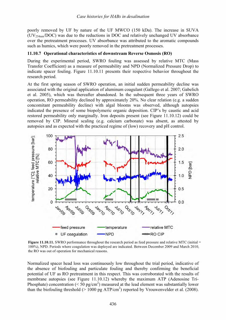
Case histories for HABs in desalination

436

poorly removed by UF by nature of the UF MWCO (150 kDa). The increase in SUVA (UV254nm/DOC) was due to the reductions in DOC and relatively unchanged UV absorbance over the pretreatment processes. UV absorbance was attributed to the aromatic compounds such as humics, which were poorly removed in the pretreatment processes.

11.10.7 Operational characteristics of downstream Reverse Osmosis (RO) During the experimental period, SWRO fouling was assessed by relative MTC (Mass Transfer Coefficient) as a measure of permeability and NPD (Normalized Pressure Drop) to indicate spacer fouling. Figure 11.10.11 presents their respective behavior throughout the research period. At the first spring season of SWRO operation, an initial sudden permeability decline was associated with the original application of aluminum coagulant (Gallego et al. 2007; Gabelich et al. 2005), which was thereafter abandoned. In the subsequent three years of SWRO operation, RO permeability declined by approximately 20%. No clear relation (e.g. a sudden concomitant permeability decline) with algal blooms was observed, although autopsies indicated the presence of some biopolymeric organic deposition. CIP’s by caustic and acid restored permeability only marginally. Iron deposits present (see Figure 11.10.12) could be removed by CIP. Mineral scaling (e.g. calcium carbonate) was absent, as attested by autopsies and as expected with the practiced regime of (low) recovery and pH control.

Normalized spacer head loss was continuously low throughout the trial period, indicative of the absence of biofouling and particulate fouling and thereby confirming the beneficial potential of UF as RO pretreatment in this respect. This was corroborated with the results of membrane autopsies (see Figure 11.10.12) whereby the maximum ATP (Adenosine Tri-Phosphate) concentration (< 50 pg/cm2) measured at the lead element was substantially lower than the biofouling threshold (> 1000 pg ATP/cm2) reported by Vrouwenvelder et al. (2008).

Figure 11.10.11. SWRO performance throughout the research period as feed pressure and relative MTC (initial = 100%), NPD. Periods where coagulation was deployed are indicated. Between December 2009 and March 2010, the RO was out of operation for mechanical reasons.

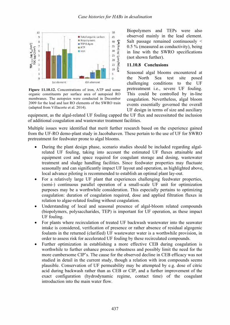
Case histories for HABs in desalination

437

Biopolymers and TEPs were also observed mainly in the lead element. Salt passage remained continuously < 0.5 % (measured as conductivity), being in line with the SWRO specifications (not shown further).

11.10.8 Conclusions Seasonal algal blooms encountered at the North Sea test site posed challenging conditions to the UF pretreatment i.e., severe UF fouling. This could be controlled by in-line coagulation. Nevertheless, algal bloom events essentially governed the overall UF design in terms of size and auxiliary

equipment, as the algal-related UF fouling capped the UF flux and necessitated the inclusion of additional coagulation and wastewater treatment facilities. Multiple issues were identified that merit further research based on the experience gained from the UF-RO demo-plant study in Jacobahaven. These pertain to the use of UF for SWRO pretreatment for feedwater prone to algal blooms.

• During the plant design phase, scenario studies should be included regarding algal-related UF fouling, taking into account the estimated UF fluxes attainable and equipment cost and space required for coagulant storage and dosing, wastewater treatment and sludge handling facilities. Since feedwater properties may fluctuate seasonally and can significantly impact UF layout and operation, as highlighted above, local advance piloting is recommended to establish an optimal plant lay-out.

• For a relatively large UF plant that experiences challenging feedwater properties, (semi-) continuous parallel operation of a small-scale UF unit for optimization purposes may be a worthwhile consideration. This especially pertains to optimizing coagulation: duration of coagulation required, dose and applied filtration fluxes in relation to algae-related fouling without coagulation.

• Understanding of local and seasonal presence of algal-bloom related compounds (biopolymers, polysaccharides, TEP) is important for UF operation, as these impact UF fouling.

• For plants where recirculation of treated UF backwash wastewater into the seawater intake is considered, verification of presence or rather absence of residual algogenic foulants in the returned (clarified) UF wastewater water is a worthwhile provision, in order to assess risk for accelerated UF fouling by these recirculated compounds.

• Further optimization in establishing a more effective CEB during coagulation is worthwhile to further enhance process robustness and possibly limit the need for the more cumbersome CIP’s. The cause for the observed decline in CEB efficacy was not studied in detail in the current study, though a relation with iron compounds seems plausible. Conservation of UF permeability may be attempted by e.g. dose of citric acid during backwash rather than as CEB or CIP, and a further improvement of the exact configuration (hydrodynamic regime, contact time) of the coagulant introduction into the main water flow.

Figure 11.10.12. Concentrations of iron, ATP and some organic constituents per surface area of autopsied RO membranes. The autopsies were conducted in December 2009 for the lead and last RO elements of the SWRO train (adapted from Villacorte et al. 2014).

Case histories for HABs in desalination

438

• Although it was not directly studied, UF CIP efficacy appeared to be enhanced by elevated ambient temperature, suggesting that a temperature-controlled CIP system could be worthwhile to shorten system downtime.

• Further study of the exact cause of the decline in SWRO MTC is recommended, by conducting more extensive membrane autopsies specifically aimed at determining the presence and identification of organic compounds.

11.10.10 References

Al-Hadidi, A. M. M., Kemperman, A. J. B., Schurer, R., Schippers, J. C., Wessling, M., and van der Meer, W. G. J. 2012. Using SDI, SDI+ and MFI to evaluate fouling in a UF/RO desalination plant. Desalination 285, 153-162.

Gabelich, C. J., Chen, W. R., Yun, T. I., and Coffey, B. M. 2005. The role of dissolved aluminum in silica chemistry for membrane processes. Desalination 180(1-3), 307-319.

Gallego, M. S. and Darton, M. E. G. 2007. Simple laboratory techniques improve the operation of RO pretreatment systems. In: Proceedings of the International Desalination Association World Congress, Maspalomas, Gran Canaria, Spain.

Janse, I., Van Rijssel, M., Gottschal, J. C., Lancelot, C., and Gieskes, W. W. 1996. Carbohydrates in the North Sea during spring blooms of Phaeocystis: a specific fingerprint. Aquatic Microbial Ecology 10(1), 97-103.

Salinas Rodriguez, S. G. 2011. Particulate and Organic matter fouling of seawater reverse osmosis systems. Thesis Dissertation, UNESCO-IHE / TU Delft PhD Thesis, CRC Press.

Schurer, R., Janssen, A., Villacorte, L., and Kennedy, M. 2012. Performance of ultrafiltration and coagulation in an UF-RO seawater desalination demonstration plant. Desalination and Water Treatment 42(1-3), 57-64.

Schurer, R., Tabatabai, A., Villacorte, L., Schippers, J. C., and Kennedy, M. D. 2013. Three years operational experience with ultrafiltration as SWRO pre-treatment during algal bloom. Desalination and Water Treatment 51(4-6), 1034-1042.

Tabatabai, S. A. A. 2014. Coagulation and Ultrafiltration in Seawater Reverse Osmosis Pretreatment. Dissertation, Unesco-IHE / TU Delft.

Villacorte, L. O. 2014. Algal Blooms and Membrane Based Desalination Technology. Thesis Dissertation, Unesco-IHE / TU Delft.

Vrouwenvelder, J. S., Manolarakis, S. A., Van der Hoek, J. P., Van Paassen, J. A. M., Van der Meer, W. G. J., Van Agtmaal, J. M. C., Prummel, H. D. M., Kruithof, J. C., and Van Loosdrecht, M. C. M. 2008. Quantitative biofouling diagnosis in full scale nanofiltration and reverse osmosis installations. Water Research 42(19), 4856-4868.

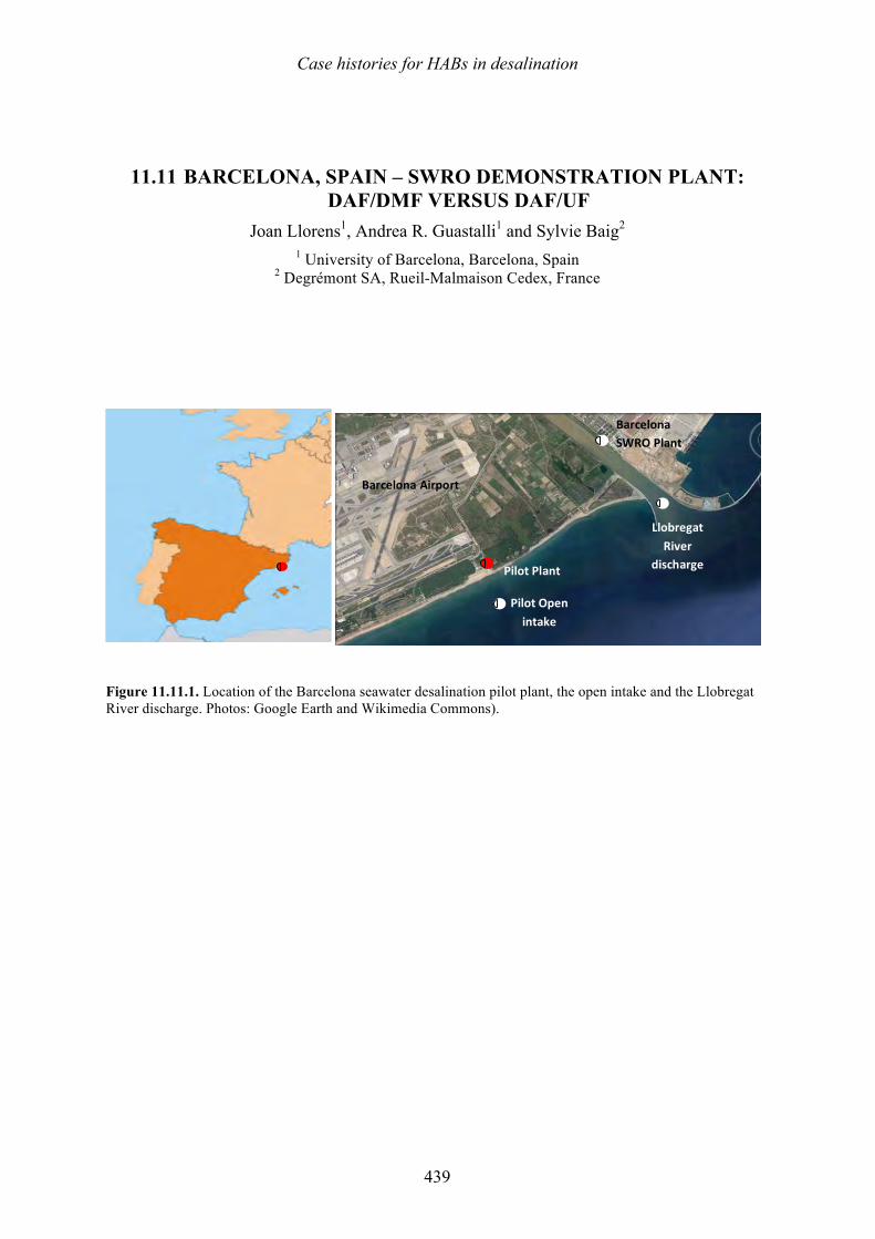
Case histories for HABs in desalination

439

11.11 BARCELONA, SPAIN – SWRO DEMONSTRATION PLANT: DAF/DMF VERSUS DAF/UF

Joan Llorens1, Andrea R. Guastalli1 and Sylvie Baig2 1 University of Barcelona, Barcelona, Spain

2 Degrémont SA, Rueil-Malmaison Cedex, France

Figure 11.11.1. Location of the Barcelona seawater desalination pilot plant, the open intake and the Llobregat River discharge. Photos: Google Earth and Wikimedia Commons).

Llobregat River

discharge Pilot Plant

Pilot Open intake

Barcelona Airport

Barcelona SWRO Plant

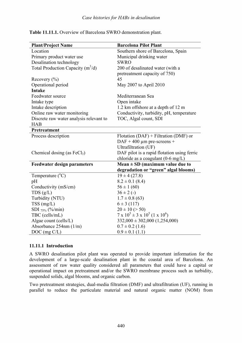
Case histories for HABs in desalination

440

Table 11.11.1. Overview of Barcelona SWRO demonstration plant. Plant/Project Name Barcelona Pilot Plant Location Southern shore of Barcelona, Spain Primary product water use Municipal drinking water Desalination technology SWRO Total Production Capacity (m3/d) 200 of desalinated water (with a

pretreatment capacity of 750) Recovery (%) 45 Operational period May 2007 to April 2010 Intake Feedwater source Mediterranean Sea Intake type Open intake Intake description 1.2 km offshore at a depth of 12 m Online raw water monitoring Conductivity, turbidity, pH, temperature Discrete raw water analysis relevant to HAB

TOC, Algal count, SDI

Pretreatment Process description Flotation (DAF) + Filtration (DMF) or

DAF + 400 µm pre-screens + Ultrafiltration (UF)

Chemical dosing (as FeCl3) DAF pilot is a rapid flotation using ferric chloride as a coagulant (0-6 mg/L)

Feedwater design parameters Mean ± SD (maximum value due to degradation or “green” algal blooms)

Temperature (oC) 19 ± 4 (27.8) pH 8.2 ± 0.1 (8.4) Conductivity (mS/cm) 56 ± 1 (60) TDS (g/L) 36 ± 2 (-) Turbidity (NTU) 1.7 ± 0.8 (63) TSS (mg/L) 6 ± 3 (117) SDI 75% (%/min) 20 ± 10 (> 50) TBC (cells/mL) 7 x 105 ± 3 x 105 (1 x 106) Algae count (cells/L) 332,000 ± 302,000 (1,254,000) Absorbance 254nm (1/m) 0.7 ± 0.2 (1.6) DOC (mg C/L) 0.9 ± 0.1 (1.1)

11.11.1 Introduction

A SWRO desalination pilot plant was operated to provide important information for the development of a large-scale desalination plant in the coastal area of Barcelona. An assessment of raw water quality considered all parameters that could have a capital or operational impact on pretreatment and/or the SWRO membrane process such as turbidity, suspended solids, algal blooms, and organic carbon. Two pretreatment strategies, dual-media filtration (DMF) and ultrafiltration (UF), running in parallel to reduce the particulate material and natural organic matter (NOM) from

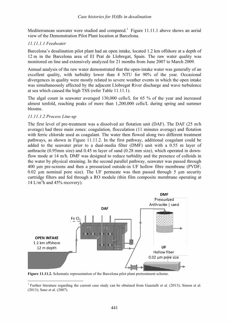
Case histories for HABs in desalination

441

Mediterranean seawater were studied and compared.1 Figure 11.11.1 above shows an aerial view of the Demonstration Pilot Plant location at Barcelona.

11.11.1.1 Feedwater Barcelona’s desalination pilot plant had an open intake, located 1.2 km offshore at a depth of 12 m in the Barcelona area of El Prat de Llobregat, Spain. The raw water quality was monitored on line and extensively analyzed for 21 months from June 2007 to March 2009.

Annual analysis of the raw water demonstrated that the open-intake water was generally of an excellent quality, with turbidity lower than 4 NTU for 90% of the year. Occasional divergences in quality were mostly related to severe weather events in which the open intake was simultaneously affected by the adjacent Llobregat River discharge and wave turbulence at sea which caused the high TSS (refer Table 11.11.1). The algal count in seawater averaged 130,000 cells/L for 65 % of the year and increased almost tenfold, reaching peaks of more than 1,200,000 cells/L during spring and summer blooms.

11.11.1.2 Process Line-up The first level of pre-treatment was a dissolved air flotation unit (DAF). The DAF (25 m/h average) had three main zones: coagulation, flocculation (11 minutes average) and flotation with ferric chloride used as coagulant. The water then flowed along two different treatment pathways, as shown in Figure 11.11.2. In the first pathway, additional coagulant could be added to the seawater prior to a dual-media filter (DMF) unit with a 0.55 m layer of anthracite (0.95mm size) and 0.45 m layer of sand (0.28 mm size), which operated in down-flow mode at 14 m/h. DMF was designed to reduce turbidity and the presence of colloids in the water by physical straining. In the second parallel pathway, seawater was passed through 400 µm pre-screens and then a pressurized outside-in UF hollow fibre membrane (PVDF; 0.02 µm nominal pore size). The UF permeate was then passed through 5 µm security cartridge filters and fed through a RO module (thin film composite membrane operating at 14 L/m2h and 45% recovery).

Figure 11.11.2. Schematic representation of the Barcelona pilot plant pretreatment scheme.

1 Further literature regarding the current case study can be obtained from Guastalli et al. (2013); Simon et al. (2013); Sanz et al. (2007).

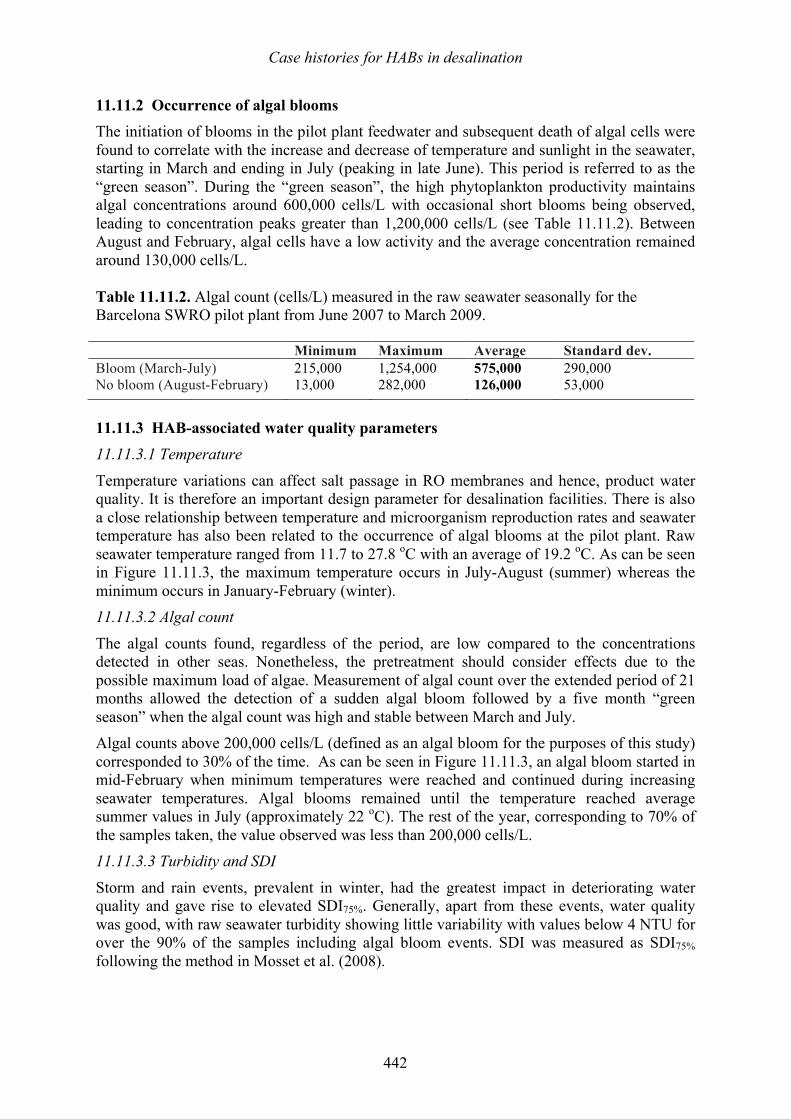
Case histories for HABs in desalination

442

11.11.2 Occurrence of algal blooms The initiation of blooms in the pilot plant feedwater and subsequent death of algal cells were found to correlate with the increase and decrease of temperature and sunlight in the seawater, starting in March and ending in July (peaking in late June). This period is referred to as the “green season”. During the “green season”, the high phytoplankton productivity maintains algal concentrations around 600,000 cells/L with occasional short blooms being observed, leading to concentration peaks greater than 1,200,000 cells/L (see Table 11.11.2). Between August and February, algal cells have a low activity and the average concentration remained around 130,000 cells/L. Table 11.11.2. Algal count (cells/L) measured in the raw seawater seasonally for the Barcelona SWRO pilot plant from June 2007 to March 2009. Minimum Maximum Average Standard dev. Bloom (March-July) 215,000 1,254,000 575,000 290,000 No bloom (August-February) 13,000 282,000 126,000 53,000

11.11.3 HAB-associated water quality parameters 11.11.3.1 Temperature

Temperature variations can affect salt passage in RO membranes and hence, product water quality. It is therefore an important design parameter for desalination facilities. There is also a close relationship between temperature and microorganism reproduction rates and seawater temperature has also been related to the occurrence of algal blooms at the pilot plant. Raw seawater temperature ranged from 11.7 to 27.8 oC with an average of 19.2 oC. As can be seen in Figure 11.11.3, the maximum temperature occurs in July-August (summer) whereas the minimum occurs in January-February (winter). 11.11.3.2 Algal count

The algal counts found, regardless of the period, are low compared to the concentrations detected in other seas. Nonetheless, the pretreatment should consider effects due to the possible maximum load of algae. Measurement of algal count over the extended period of 21 months allowed the detection of a sudden algal bloom followed by a five month “green season” when the algal count was high and stable between March and July. Algal counts above 200,000 cells/L (defined as an algal bloom for the purposes of this study) corresponded to 30% of the time. As can be seen in Figure 11.11.3, an algal bloom started in mid-February when minimum temperatures were reached and continued during increasing seawater temperatures. Algal blooms remained until the temperature reached average summer values in July (approximately 22 oC). The rest of the year, corresponding to 70% of the samples taken, the value observed was less than 200,000 cells/L. 11.11.3.3 Turbidity and SDI

Storm and rain events, prevalent in winter, had the greatest impact in deteriorating water quality and gave rise to elevated SDI75%. Generally, apart from these events, water quality was good, with raw seawater turbidity showing little variability with values below 4 NTU for over the 90% of the samples including algal bloom events. SDI was measured as SDI75% following the method in Mosset et al. (2008).

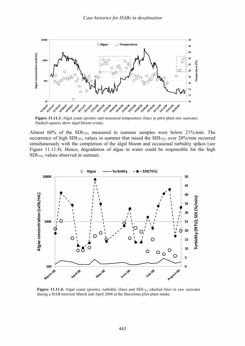
Case histories for HABs in desalination

443

Figure 11.11.3. Algal count (points) and measured temperature (line) in pilot plant raw seawater. Dashed squares show algal bloom events.

Almost 60% of the SDI75% measured in summer samples were below 21%/min. The occurrence of high SDI75% values in summer that raised the SDI75% over 20%/min occurred simultaneously with the completion of the algal bloom and occasional turbidity spikes (see Figure 11.11.4). Hence, degradation of algae in water could be responsible for the high SDI75% values observed in summer.

Figure 11.11.4. Algal count (points), turbidity (line) and SDI75% (dashed line) in raw seawater during a HAB between March and April 2008 at the Barcelona pilot plant intake.

10

100

1000

10000

01/06/07

01/07/07

31/07/07

30/08/07

29/09/07

29/10/07

28/11/07

28/12/07

27/01/08

26/02/08

27/03/08

26/04/08

26/05/08

25/06/08

25/07/08

24/08/08

23/09/08

23/10/08

22/11/08

22/12/08

21/01/09

20/02/09

Algae concen

tration (cell/mL)

10

12

14

16

18

20

22

24

26

28

30

Tempe

rature (ºC)

Algae Temperature

0

5

10

15

20

25

30

35

40

45

50

100

1000

10000

Turbidity

(NTU

); SD

I (%/m

in)

Algae concen

tration (cells/

mL)

Algae Turbidity SDI(75%)

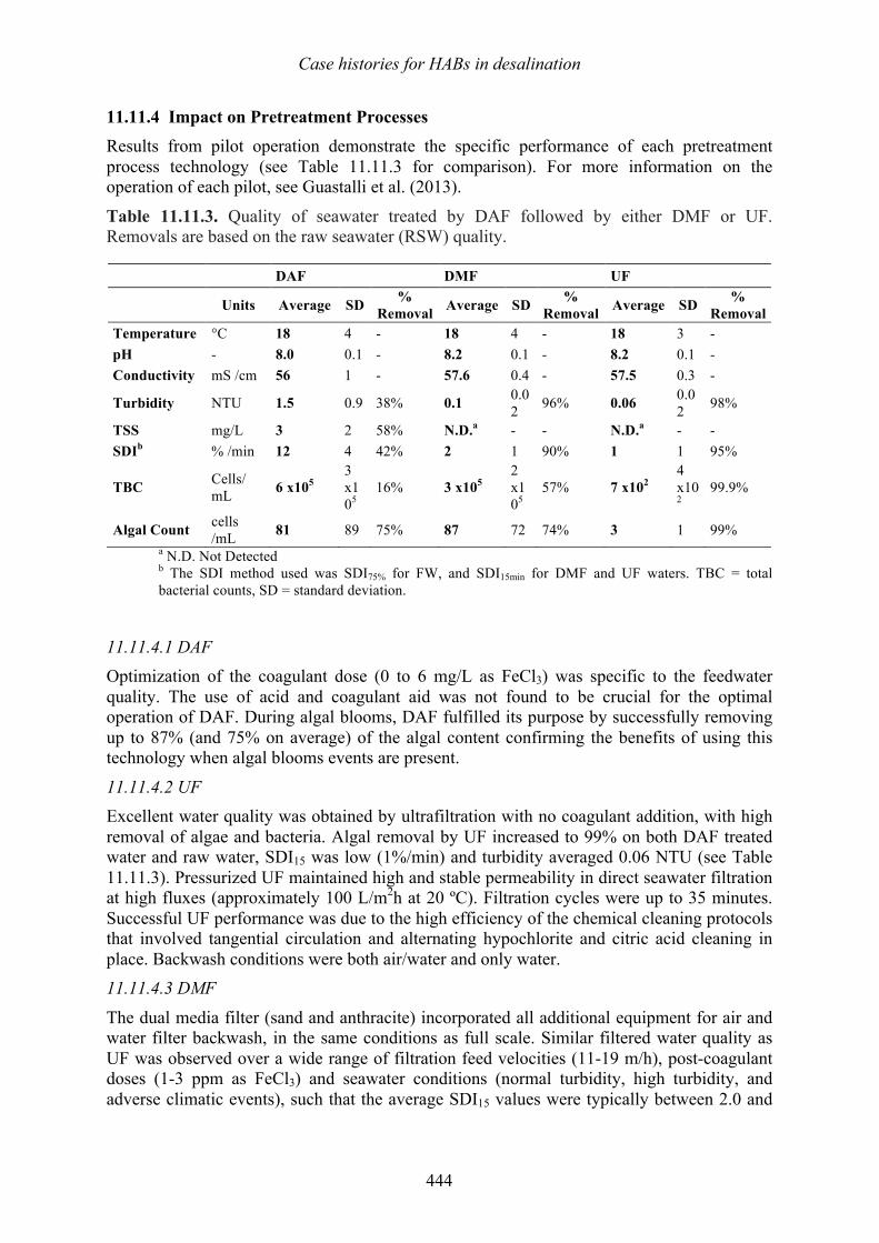
Case histories for HABs in desalination

444

11.11.4 Impact on Pretreatment Processes Results from pilot operation demonstrate the specific performance of each pretreatment process technology (see Table 11.11.3 for comparison). For more information on the operation of each pilot, see Guastalli et al. (2013).

Table 11.11.3. Quality of seawater treated by DAF followed by either DMF or UF. Removals are based on the raw seawater (RSW) quality. DAF DMF UF

Units Average SD % Removal Average SD %

Removal Average SD % Removal

Temperature °C 18 4 - 18 4 - 18 3 - pH - 8.0 0.1 - 8.2 0.1 - 8.2 0.1 - Conductivity mS /cm 56 1 - 57.6 0.4 - 57.5 0.3 -

Turbidity NTU 1.5 0.9 38% 0.1 0.02 96% 0.06 0.0

2 98%

TSS mg/L 3 2 58% N.D.a - - N.D.a - - SDIb % /min 12 4 42% 2 1 90% 1 1 95%

TBC Cells/ mL 6 x105

3 x105

16% 3 x105 2 x105

57% 7 x102 4 x102

99.9%

Algal Count cells /mL 81 89 75% 87 72 74% 3 1 99%

a N.D. Not Detected b The SDI method used was SDI75% for FW, and SDI15min for DMF and UF waters. TBC = total bacterial counts, SD = standard deviation.

11.11.4.1 DAF Optimization of the coagulant dose (0 to 6 mg/L as FeCl3) was specific to the feedwater quality. The use of acid and coagulant aid was not found to be crucial for the optimal operation of DAF. During algal blooms, DAF fulfilled its purpose by successfully removing up to 87% (and 75% on average) of the algal content confirming the benefits of using this technology when algal blooms events are present.

11.11.4.2 UF Excellent water quality was obtained by ultrafiltration with no coagulant addition, with high removal of algae and bacteria. Algal removal by UF increased to 99% on both DAF treated water and raw water, SDI15 was low (1%/min) and turbidity averaged 0.06 NTU (see Table 11.11.3). Pressurized UF maintained high and stable permeability in direct seawater filtration at high fluxes (approximately 100 L/m2h at 20 ºC). Filtration cycles were up to 35 minutes. Successful UF performance was due to the high efficiency of the chemical cleaning protocols that involved tangential circulation and alternating hypochlorite and citric acid cleaning in place. Backwash conditions were both air/water and only water. 11.11.4.3 DMF

The dual media filter (sand and anthracite) incorporated all additional equipment for air and water filter backwash, in the same conditions as full scale. Similar filtered water quality as UF was observed over a wide range of filtration feed velocities (11-19 m/h), post-coagulant doses (1-3 ppm as FeCl3) and seawater conditions (normal turbidity, high turbidity, and adverse climatic events), such that the average SDI15 values were typically between 2.0 and

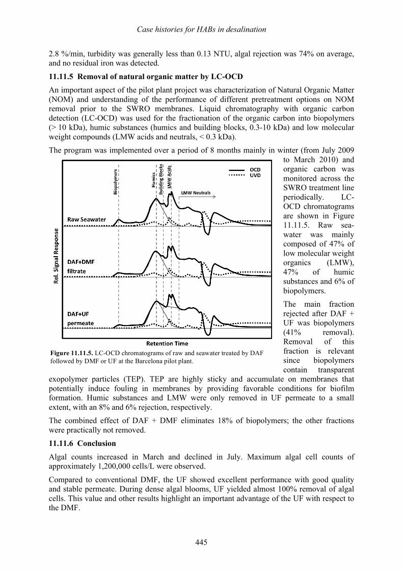
Case histories for HABs in desalination

445

2.8 %/min, turbidity was generally less than 0.13 NTU, algal rejection was 74% on average, and no residual iron was detected.

11.11.5 Removal of natural organic matter by LC-OCD An important aspect of the pilot plant project was characterization of Natural Organic Matter (NOM) and understanding of the performance of different pretreatment options on NOM removal prior to the SWRO membranes. Liquid chromatography with organic carbon detection (LC-OCD) was used for the fractionation of the organic carbon into biopolymers (> 10 kDa), humic substances (humics and building blocks, 0.3-10 kDa) and low molecular weight compounds (LMW acids and neutrals, < 0.3 kDa). The program was implemented over a period of 8 months mainly in winter (from July 2009

to March 2010) and organic carbon was monitored across the SWRO treatment line periodically. LC-OCD chromatograms are shown in Figure 11.11.5. Raw sea-water was mainly composed of 47% of low molecular weight organics (LMW), 47% of humic substances and 6% of biopolymers. The main fraction rejected after DAF + UF was biopolymers (41% removal). Removal of this fraction is relevant since biopolymers contain transparent

exopolymer particles (TEP). TEP are highly sticky and accumulate on membranes that potentially induce fouling in membranes by providing favorable conditions for biofilm formation. Humic substances and LMW were only removed in UF permeate to a small extent, with an 8% and 6% rejection, respectively. The combined effect of DAF + DMF eliminates 18% of biopolymers; the other fractions were practically not removed. 11.11.6 Conclusion

Algal counts increased in March and declined in July. Maximum algal cell counts of approximately 1,200,000 cells/L were observed.

Compared to conventional DMF, the UF showed excellent performance with good quality and stable permeate. During dense algal blooms, UF yielded almost 100% removal of algal cells. This value and other results highlight an important advantage of the UF with respect to the DMF.

Figure 11.11.5. LC-OCD chromatograms of raw and seawater treated by DAF followed by DMF or UF at the Barcelona pilot plant.

Case histories for HABs in desalination

446

Acknowledgment: The authors are grateful to CDTI (Spain) through the project CENIT-Sostaqua (CEN20071039).

11.11.7 References

Guastalli, A. R., Simon, F. X., Penru, Y., de Kerchove, A., Llorens, J., and Baig, S. 2013. Comparison of DMF and UF pretreatments for particulate material and dissolved organic matter removal in SWRO desalination, Desalination 322, 144-150.

Mosset, A., Bonnelye, V., Petry, M., and Sanz, M. A. 2008. The sensitivity of SDI analysis: from RO feedwater to raw water. Desalination 222, 17-23.

Sanz, M. A., Cremer, G., Beltran, F., Bonnelye, V., and Del Campo, I. 2007. Barcelona: 200,000 m3/day of Potable Water coming from Mediterranean Sea. In: Proceedings of the International Desalination Association World Congress, Maspalomas, Gran Canaria, Spain.

Simon, F. X., Penru, Y., Guastalli, A. R., Esplugas, S., Llorens, J., and Baig, S. 2013. NOM characterization by LC-OCD in a SWRO desalination line. Desalination and Water Treatment 51, 1776-1780.

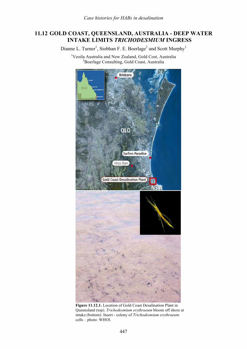
Case histories for HABs in desalination

447

11.12 GOLD COAST, QUEENSLAND, AUSTRALIA - DEEP WATER INTAKE LIMITS TRICHODESMIUM INGRESS

Dianne L. Turner1, Siobhan F. E. Boerlage2 and Scott Murphy1 1Veoila Australia and New Zealand, Gold Cost, Australia

2Boerlage Consulting, Gold Coast, Australia

Figure 11.12.1. Location of Gold Coast Desalination Plant in Queensland (top). Trichodesmium erythraeum bloom off shore at intake (bottom). Insert - colony of Trichodesmium erythraeum cells – photo: WHOI.

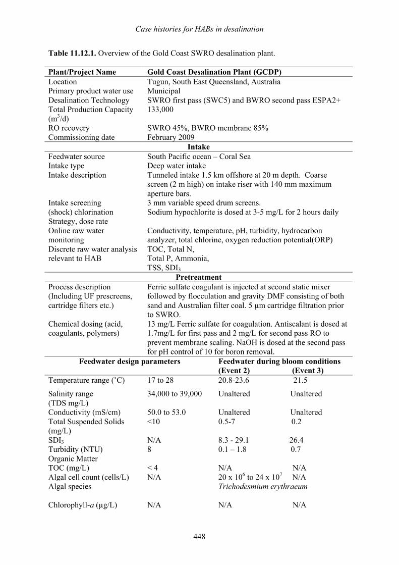
Case histories for HABs in desalination

448

Table 11.12.1. Overview of the Gold Coast SWRO desalination plant. Plant/Project Name Gold Coast Desalination Plant (GCDP) Location Tugun, South East Queensland, Australia Primary product water use Municipal Desalination Technology SWRO first pass (SWC5) and BWRO second pass ESPA2+ Total Production Capacity (m3/d)

133,000

RO recovery SWRO 45%, BWRO membrane 85% Commissioning date February 2009

Intake Feedwater source South Pacific ocean – Coral Sea Intake type Deep water intake Intake description Tunneled intake 1.5 km offshore at 20 m depth. Coarse

screen (2 m high) on intake riser with 140 mm maximum aperture bars.

Intake screening 3 mm variable speed drum screens. (shock) chlorination Strategy, dose rate

Sodium hypochlorite is dosed at 3-5 mg/L for 2 hours daily

Online raw water monitoring

Conductivity, temperature, pH, turbidity, hydrocarbon analyzer, total chlorine, oxygen reduction potential(ORP)

Discrete raw water analysis relevant to HAB

TOC, Total N, Total P, Ammonia, TSS, SDI3

Pretreatment Process description (Including UF prescreens, cartridge filters etc.)

Ferric sulfate coagulant is injected at second static mixer followed by flocculation and gravity DMF consisting of both sand and Australian filter coal. 5 µm cartridge filtration prior to SWRO.

Chemical dosing (acid, coagulants, polymers)

13 mg/L Ferric sulfate for coagulation. Antiscalant is dosed at 1.7mg/L for first pass and 2 mg/L for second pass RO to prevent membrane scaling. NaOH is dosed at the second pass for pH control of 10 for boron removal.

Feedwater design parameters Feedwater during bloom conditions (Event 2) (Event 3)

Temperature range (˚C) 17 to 28 20.8-23.6 21.5

Salinity range (TDS mg/L)

34,000 to 39,000 Unaltered Unaltered

Conductivity (mS/cm) 50.0 to 53.0 Unaltered Unaltered Total Suspended Solids (mg/L)

<10 0.5-7 0.2

SDI3 N/A 8.3 - 29.1 26.4 Turbidity (NTU) 8 0.1 – 1.8 0.7 Organic Matter TOC (mg/L)

< 4

N/A N/A

Algal cell count (cells/L) N/A 20 x 106 to 24 x 107 N/A Algal species Trichodesmium erythraeum

Chlorophyll-a (µg/L) N/A N/A N/A

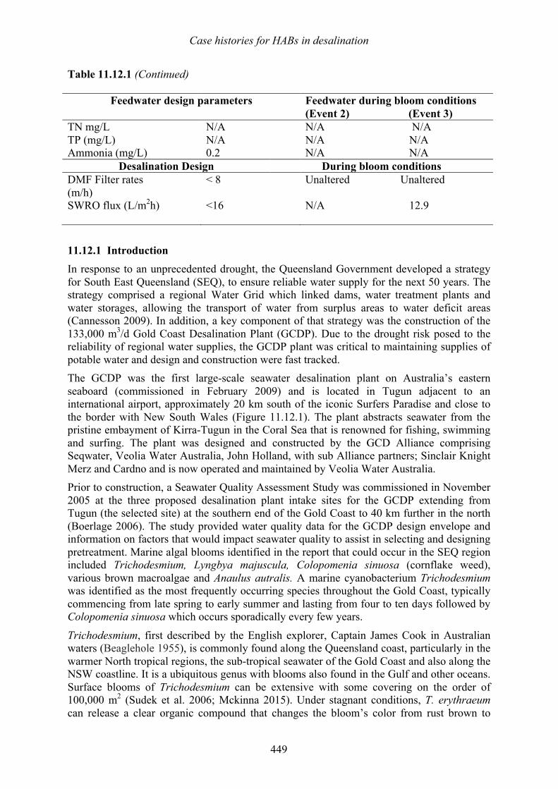
Case histories for HABs in desalination

449

Table 11.12.1 (Continued)

Feedwater design parameters Feedwater during bloom conditions (Event 2) (Event 3)

TN mg/L TP (mg/L) Ammonia (mg/L)

N/A N/A 0.2

N/A N/A N/A N/A N/A N/A

Desalination Design During bloom conditions DMF Filter rates (m/h)

< 8 Unaltered Unaltered

SWRO flux (L/m2h) <16 N/A 12.9

11.12.1 Introduction In response to an unprecedented drought, the Queensland Government developed a strategy for South East Queensland (SEQ), to ensure reliable water supply for the next 50 years. The strategy comprised a regional Water Grid which linked dams, water treatment plants and water storages, allowing the transport of water from surplus areas to water deficit areas (Cannesson 2009). In addition, a key component of that strategy was the construction of the 133,000 m3/d Gold Coast Desalination Plant (GCDP). Due to the drought risk posed to the reliability of regional water supplies, the GCDP plant was critical to maintaining supplies of potable water and design and construction were fast tracked. The GCDP was the first large-scale seawater desalination plant on Australia’s eastern seaboard (commissioned in February 2009) and is located in Tugun adjacent to an international airport, approximately 20 km south of the iconic Surfers Paradise and close to the border with New South Wales (Figure 11.12.1). The plant abstracts seawater from the pristine embayment of Kirra-Tugun in the Coral Sea that is renowned for fishing, swimming and surfing. The plant was designed and constructed by the GCD Alliance comprising Seqwater, Veolia Water Australia, John Holland, with sub Alliance partners; Sinclair Knight Merz and Cardno and is now operated and maintained by Veolia Water Australia. Prior to construction, a Seawater Quality Assessment Study was commissioned in November 2005 at the three proposed desalination plant intake sites for the GCDP extending from Tugun (the selected site) at the southern end of the Gold Coast to 40 km further in the north (Boerlage 2006). The study provided water quality data for the GCDP design envelope and information on factors that would impact seawater quality to assist in selecting and designing pretreatment. Marine algal blooms identified in the report that could occur in the SEQ region included Trichodesmium, Lyngbya majuscula, Colopomenia sinuosa (cornflake weed), various brown macroalgae and Anaulus autralis. A marine cyanobacterium Trichodesmium was identified as the most frequently occurring species throughout the Gold Coast, typically commencing from late spring to early summer and lasting from four to ten days followed by Colopomenia sinuosa which occurs sporadically every few years.

Trichodesmium, first described by the English explorer, Captain James Cook in Australian waters (Beaglehole 1955), is commonly found along the Queensland coast, particularly in the warmer North tropical regions, the sub-tropical seawater of the Gold Coast and also along the NSW coastline. It is a ubiquitous genus with blooms also found in the Gulf and other oceans. Surface blooms of Trichodesmium can be extensive with some covering on the order of 100,000 m2 (Sudek et al. 2006; Mckinna 2015). Under stagnant conditions, T. erythraeum can release a clear organic compound that changes the bloom’s color from rust brown to

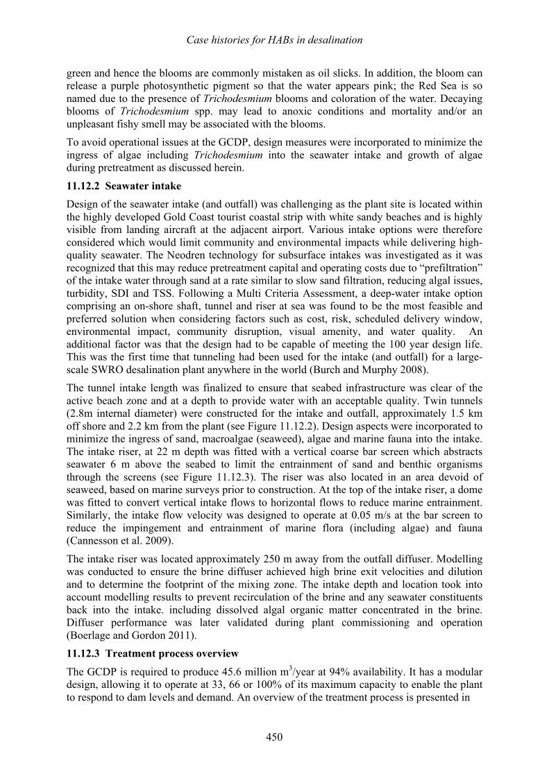
Case histories for HABs in desalination

450

green and hence the blooms are commonly mistaken as oil slicks. In addition, the bloom can release a purple photosynthetic pigment so that the water appears pink; the Red Sea is so named due to the presence of Trichodesmium blooms and coloration of the water. Decaying blooms of Trichodesmium spp. may lead to anoxic conditions and mortality and/or an unpleasant fishy smell may be associated with the blooms. To avoid operational issues at the GCDP, design measures were incorporated to minimize the ingress of algae including Trichodesmium into the seawater intake and growth of algae during pretreatment as discussed herein.

11.12.2 Seawater intake Design of the seawater intake (and outfall) was challenging as the plant site is located within the highly developed Gold Coast tourist coastal strip with white sandy beaches and is highly visible from landing aircraft at the adjacent airport. Various intake options were therefore considered which would limit community and environmental impacts while delivering high-quality seawater. The Neodren technology for subsurface intakes was investigated as it was recognized that this may reduce pretreatment capital and operating costs due to “prefiltration” of the intake water through sand at a rate similar to slow sand filtration, reducing algal issues, turbidity, SDI and TSS. Following a Multi Criteria Assessment, a deep-water intake option comprising an on-shore shaft, tunnel and riser at sea was found to be the most feasible and preferred solution when considering factors such as cost, risk, scheduled delivery window, environmental impact, community disruption, visual amenity, and water quality. An additional factor was that the design had to be capable of meeting the 100 year design life. This was the first time that tunneling had been used for the intake (and outfall) for a large-scale SWRO desalination plant anywhere in the world (Burch and Murphy 2008). The tunnel intake length was finalized to ensure that seabed infrastructure was clear of the active beach zone and at a depth to provide water with an acceptable quality. Twin tunnels (2.8m internal diameter) were constructed for the intake and outfall, approximately 1.5 km off shore and 2.2 km from the plant (see Figure 11.12.2). Design aspects were incorporated to minimize the ingress of sand, macroalgae (seaweed), algae and marine fauna into the intake. The intake riser, at 22 m depth was fitted with a vertical coarse bar screen which abstracts seawater 6 m above the seabed to limit the entrainment of sand and benthic organisms through the screens (see Figure 11.12.3). The riser was also located in an area devoid of seaweed, based on marine surveys prior to construction. At the top of the intake riser, a dome was fitted to convert vertical intake flows to horizontal flows to reduce marine entrainment. Similarly, the intake flow velocity was designed to operate at 0.05 m/s at the bar screen to reduce the impingement and entrainment of marine flora (including algae) and fauna (Cannesson et al. 2009).

The intake riser was located approximately 250 m away from the outfall diffuser. Modelling was conducted to ensure the brine diffuser achieved high brine exit velocities and dilution and to determine the footprint of the mixing zone. The intake depth and location took into account modelling results to prevent recirculation of the brine and any seawater constituents back into the intake. including dissolved algal organic matter concentrated in the brine. Diffuser performance was later validated during plant commissioning and operation (Boerlage and Gordon 2011). 11.12.3 Treatment process overview

The GCDP is required to produce 45.6 million m3/year at 94% availability. It has a modular design, allowing it to operate at 33, 66 or 100% of its maximum capacity to enable the plant to respond to dam levels and demand. An overview of the treatment process is presented in

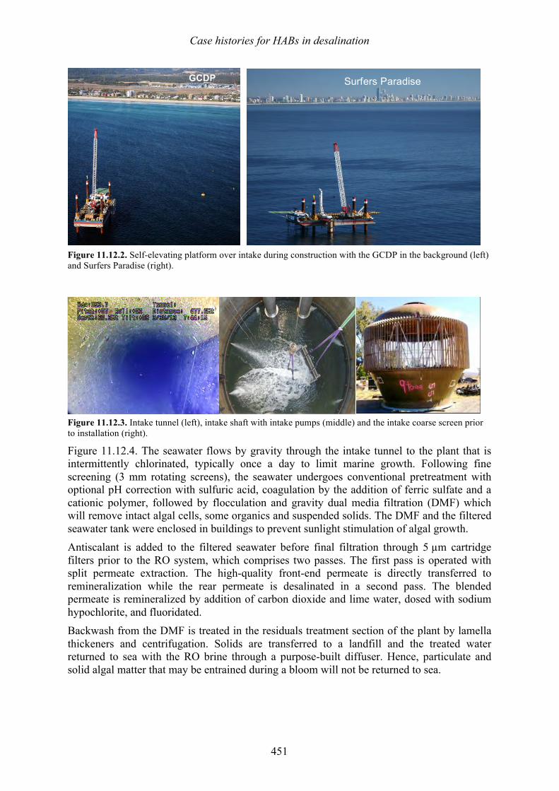
Case histories for HABs in desalination

451

Figure 11.12.2. Self-elevating platform over intake during construction with the GCDP in the background (left) and Surfers Paradise (right).

Figure 11.12.3. Intake tunnel (left), intake shaft with intake pumps (middle) and the intake coarse screen prior to installation (right).

Figure 11.12.4. The seawater flows by gravity through the intake tunnel to the plant that is intermittently chlorinated, typically once a day to limit marine growth. Following fine screening (3 mm rotating screens), the seawater undergoes conventional pretreatment with optional pH correction with sulfuric acid, coagulation by the addition of ferric sulfate and a cationic polymer, followed by flocculation and gravity dual media filtration (DMF) which will remove intact algal cells, some organics and suspended solids. The DMF and the filtered seawater tank were enclosed in buildings to prevent sunlight stimulation of algal growth. Antiscalant is added to the filtered seawater before final filtration through 5 µm cartridge filters prior to the RO system, which comprises two passes. The first pass is operated with split permeate extraction. The high-quality front-end permeate is directly transferred to remineralization while the rear permeate is desalinated in a second pass. The blended permeate is remineralized by addition of carbon dioxide and lime water, dosed with sodium hypochlorite, and fluoridated. Backwash from the DMF is treated in the residuals treatment section of the plant by lamella thickeners and centrifugation. Solids are transferred to a landfill and the treated water returned to sea with the RO brine through a purpose-built diffuser. Hence, particulate and solid algal matter that may be entrained during a bloom will not be returned to sea.

GCDP Surfers Paradise

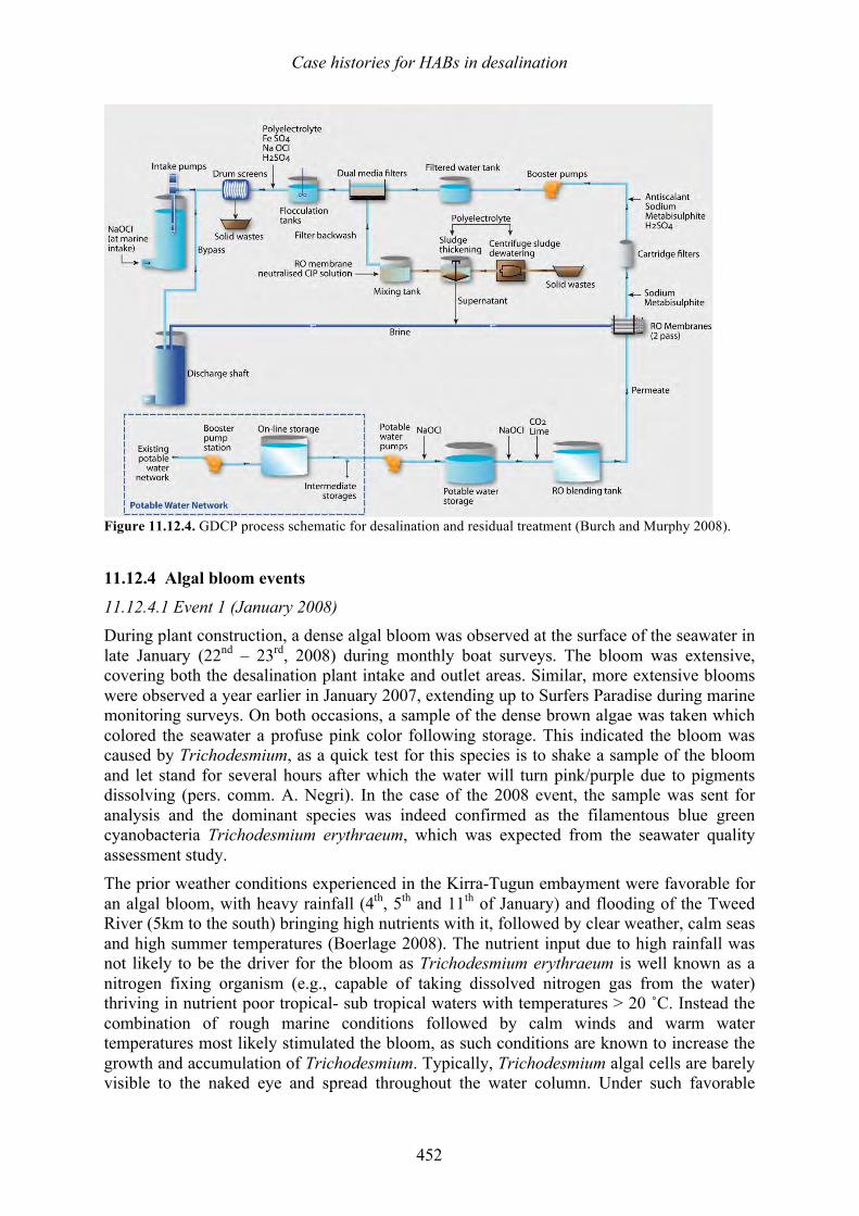
Case histories for HABs in desalination

452

Figure 11.12.4. GDCP process schematic for desalination and residual treatment (Burch and Murphy 2008).

11.12.4 Algal bloom events

11.12.4.1 Event 1 (January 2008) During plant construction, a dense algal bloom was observed at the surface of the seawater in late January (22nd – 23rd, 2008) during monthly boat surveys. The bloom was extensive, covering both the desalination plant intake and outlet areas. Similar, more extensive blooms were observed a year earlier in January 2007, extending up to Surfers Paradise during marine monitoring surveys. On both occasions, a sample of the dense brown algae was taken which colored the seawater a profuse pink color following storage. This indicated the bloom was caused by Trichodesmium, as a quick test for this species is to shake a sample of the bloom and let stand for several hours after which the water will turn pink/purple due to pigments dissolving (pers. comm. A. Negri). In the case of the 2008 event, the sample was sent for analysis and the dominant species was indeed confirmed as the filamentous blue green cyanobacteria Trichodesmium erythraeum, which was expected from the seawater quality assessment study. The prior weather conditions experienced in the Kirra-Tugun embayment were favorable for an algal bloom, with heavy rainfall (4th, 5th and 11th of January) and flooding of the Tweed River (5km to the south) bringing high nutrients with it, followed by clear weather, calm seas and high summer temperatures (Boerlage 2008). The nutrient input due to high rainfall was not likely to be the driver for the bloom as Trichodesmium erythraeum is well known as a nitrogen fixing organism (e.g., capable of taking dissolved nitrogen gas from the water) thriving in nutrient poor tropical- sub tropical waters with temperatures > 20 ˚C. Instead the combination of rough marine conditions followed by calm winds and warm water temperatures most likely stimulated the bloom, as such conditions are known to increase the growth and accumulation of Trichodesmium. Typically, Trichodesmium algal cells are barely visible to the naked eye and spread throughout the water column. Under such favorable

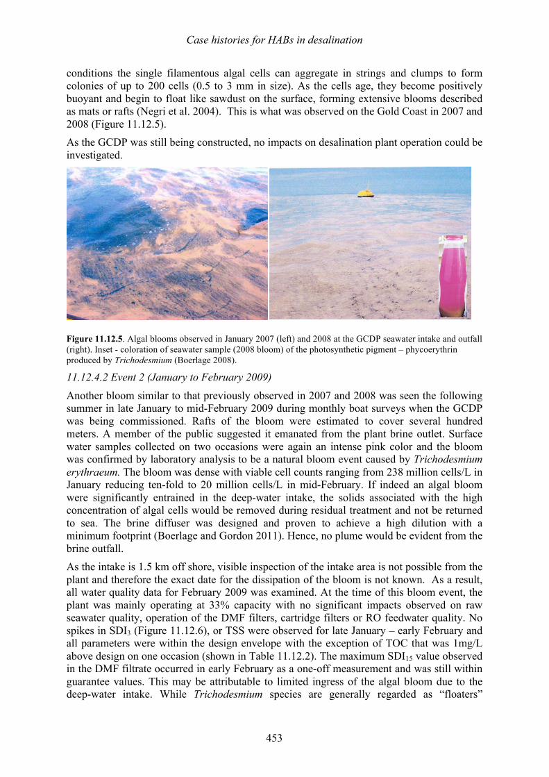
Case histories for HABs in desalination

453

conditions the single filamentous algal cells can aggregate in strings and clumps to form colonies of up to 200 cells (0.5 to 3 mm in size). As the cells age, they become positively buoyant and begin to float like sawdust on the surface, forming extensive blooms described as mats or rafts (Negri et al. 2004). This is what was observed on the Gold Coast in 2007 and 2008 (Figure 11.12.5). As the GCDP was still being constructed, no impacts on desalination plant operation could be investigated.

Figure 11.12.5. Algal blooms observed in January 2007 (left) and 2008 at the GCDP seawater intake and outfall (right). Inset - coloration of seawater sample (2008 bloom) of the photosynthetic pigment – phycoerythrin produced by Trichodesmium (Boerlage 2008).

11.12.4.2 Event 2 (January to February 2009)

Another bloom similar to that previously observed in 2007 and 2008 was seen the following summer in late January to mid-February 2009 during monthly boat surveys when the GCDP was being commissioned. Rafts of the bloom were estimated to cover several hundred meters. A member of the public suggested it emanated from the plant brine outlet. Surface water samples collected on two occasions were again an intense pink color and the bloom was confirmed by laboratory analysis to be a natural bloom event caused by Trichodesmium erythraeum. The bloom was dense with viable cell counts ranging from 238 million cells/L in January reducing ten-fold to 20 million cells/L in mid-February. If indeed an algal bloom were significantly entrained in the deep-water intake, the solids associated with the high concentration of algal cells would be removed during residual treatment and not be returned to sea. The brine diffuser was designed and proven to achieve a high dilution with a minimum footprint (Boerlage and Gordon 2011). Hence, no plume would be evident from the brine outfall. As the intake is 1.5 km off shore, visible inspection of the intake area is not possible from the plant and therefore the exact date for the dissipation of the bloom is not known. As a result, all water quality data for February 2009 was examined. At the time of this bloom event, the plant was mainly operating at 33% capacity with no significant impacts observed on raw seawater quality, operation of the DMF filters, cartridge filters or RO feedwater quality. No spikes in SDI3 (Figure 11.12.6), or TSS were observed for late January – early February and all parameters were within the design envelope with the exception of TOC that was 1mg/L above design on one occasion (shown in Table 11.12.2). The maximum SDI15 value observed in the DMF filtrate occurred in early February as a one-off measurement and was still within guarantee values. This may be attributable to limited ingress of the algal bloom due to the deep-water intake. While Trichodesmium species are generally regarded as “floaters”

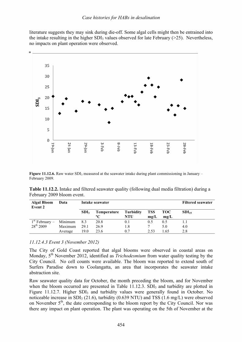
Case histories for HABs in desalination

454

literature suggests they may sink during die-off. Some algal cells might then be entrained into the intake resulting in the higher SDI3 values observed for late February (>25). Nevertheless, no impacts on plant operation were observed.

Figure 11.12.6. Raw water SDI3 measured at the seawater intake during plant commissioning in January – February 2009. Table 11.12.2. Intake and filtered seawater quality (following dual media filtration) during a February 2009 bloom event.

Algal Bloom Event 2

Data

Intake seawater Filtered seawater

SDI3 Temperature °C

Turbidity NTU

TSS mg/L

TOC mg/L

SDI15

1st February – 28th 2009

Minimum 8.3 20.8 0.1 0.5 0.5 1.1 Maximum 29.1 26.9 1.8 7 5.0 4.0 Average 19.0 23.6 0.7 2.53 1.65 2.8

11.12.4.3 Event 3 (November 2012)

The City of Gold Coast reported that algal blooms were observed in coastal areas on Monday, 5th November 2012, identified as Trichodesmium from water quality testing by the City Council. No cell counts were available. The bloom was reported to extend south of Surfers Paradise down to Coolangatta, an area that incorporates the seawater intake abstraction site. Raw seawater quality data for October, the month preceding the bloom, and for November when the bloom occurred are presented in Table 11.12.3. SDI3 and turbidity are plotted in Figure 11.12.7. Higher SDI3 and turbidity values were generally found in October. No noticeable increase in SDI3 (21.6), turbidity (0.639 NTU) and TSS (1.6 mg/L) were observed on November 5th, the date corresponding to the bloom report by the City Council. Nor was there any impact on plant operation. The plant was operating on the 5th of November at the

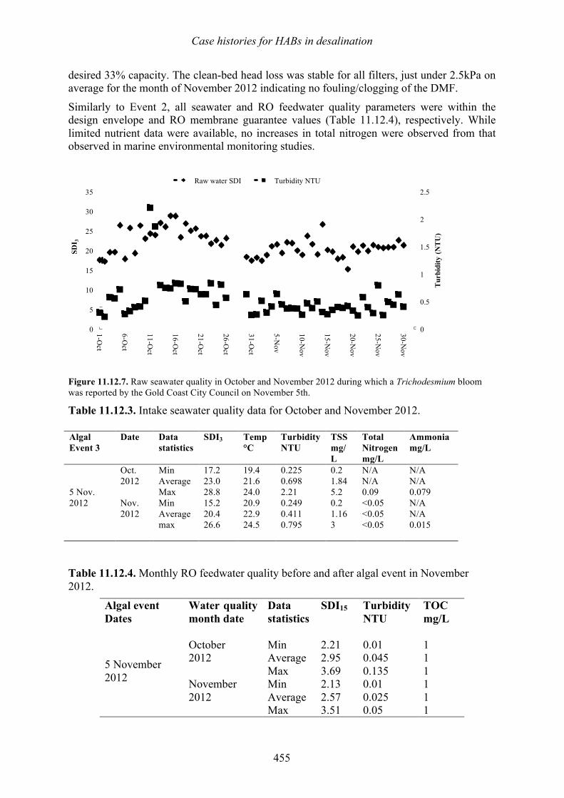
Case histories for HABs in desalination

455

desired 33% capacity. The clean-bed head loss was stable for all filters, just under 2.5kPa on average for the month of November 2012 indicating no fouling/clogging of the DMF.

Similarly to Event 2, all seawater and RO feedwater quality parameters were within the design envelope and RO membrane guarantee values (Table 11.12.4), respectively. While limited nutrient data were available, no increases in total nitrogen were observed from that observed in marine environmental monitoring studies.

Figure 11.12.7. Raw seawater quality in October and November 2012 during which a Trichodesmium bloom was reported by the Gold Coast City Council on November 5th.

Table 11.12.3. Intake seawater quality data for October and November 2012.

Table 11.12.4. Monthly RO feedwater quality before and after algal event in November 2012.

Algal event Dates

Water quality month date

Data statistics

SDI15

Turbidity NTU

TOC mg/L

5 November 2012

October 2012

Min 2.21 0.01 1 Average 2.95 0.045 1 Max 3.69 0.135 1

November 2012

Min 2.13 0.01 1 Average 2.57 0.025 1 Max 3.51 0.05 1

0

0.5

1

1.5

2

2.5

0

5

10

15

20

25

30

35

1-Oct

6-Oct

11-Oct

16-Oct

21-Oct

26-Oct

31-Oct

5-Nov

10-Nov

15-Nov

20-Nov

25-Nov

30-Nov

Tur

bidi

ty (N

TU

)

SDI 3

Raw water SDI Turbidity NTU

Algal Event 3

Date Data statistics

SDI3 Temp °C

Turbidity NTU

TSS mg/L

Total Nitrogen mg/L

Ammonia mg/L

5 Nov. 2012

Oct. 2012

Min 17.2 19.4 0.225 0.2 N/A N/A Average 23.0 21.6 0.698 1.84 N/A N/A Max 28.8 24.0 2.21 5.2 0.09 0.079

Nov. 2012

Min 15.2 20.9 0.249 0.2 <0.05 N/A Average 20.4 22.9 0.411 1.16 <0.05 N/A max 26.6 24.5 0.795 3 <0.05 0.015

Case histories for HABs in desalination

456

11.12.5 Long-term plant operation The GCDP plant has been in operation for more than seven years, with anecdotal reports of Trichodesmium blooms similar to algal events 1-3 described above occurring during the summer months when conditions are expected to promote blooms. In the absence of any observed impacts at the plant, algal blooms are likely to be unreported as the intake is 2.5 km from the plant and algae are not specifically monitored for by the GCDP.

Blooms of another marine algal species, Colpomenia sinuosa, have been detected sporadically, once in 2010 and again in 2014, through an increase in the mass of intake screenings. In the latter case, this resulted in the unusually high mass of screenings (approximately 400 kg). Colpomenia sinuosa, a globe-shaped brown macroalga, is much larger than Trichodesmium, ranging in size from 1 to 3 mm and up to 10 mm. It is found in intertidal areas growing on rocks or other algae. Colpomenia sinuosa is typically in the attached form, it becomes dislodged with wind and waves breaking into flakes and may then have become entrained into the intake.

In general, the depth of the intake and pretreatment design is believed to have largely mitigated algal bloom impacts, especially surface Trichodesmium blooms with limited ingress of Colpomenia. Water quality associated with algal blooms does not appear to have deteriorated - SDI3, TSS and TOC were within the range observed throughout the year. No operational issues were observed at the plant such as increased DMF clogging. No sudden increases in RO operating pressures due to biofilm or adsorptive organic fouling have been observed associated with the potential increase in organics from an algal bloom entrained at the seawater intake.

Membrane autopsies and the low cleaning frequency of the RO trains further support the contention that no organic fouling or significant biofouling has occurred during plant operation. Autopsies of a cartridge filter, first and second pass RO membranes in May of 2009 following algal event 2 showed no evidence of organic deposits or fouling with only minor inorganic deposits. Similar autopsies were conducted in August 2009, March 2010, August 2010 and April 2013. In general, visual inspection of lead membranes showed that the level of fouling was very light with only minor biofilm deposits present. The loss of ignition results indicated that the organics on the membrane were low.

Only limited CIP cleans of RO membranes have been carried out, which is attributed to the effectiveness of pretreatment coupled to good raw water quality. Clean in place have not been conducted in response to any fouling issues but rather as a trial run on a limited number of RO trains or as preventative cleans.

11.12.6 Conclusions Trichodesmium, the most frequent bloom-forming species in the region, occurred prior to operation of the GCDP and continues to occur during the summer months as a result of marine and meteorological conditions that promote the growth of this genus. Dense surface blooms have been extensive, covering the seawater intake and brine discharge area with a density of up to 238 million cells/L. Occasional blooms of Colpomenia have also occurred.

The deep water (20 m water depth) intake option selected for the GCDP appears to be successful in providing good water quality and preventing the ingress of Trichodesmium, which typically floats at the surface with limited ingress of Colpomenia. No increase in raw water TOC, TSS, SDI3 have been observed as a result of blooms. Membrane autopsies also show no organic or biofilm fouling due to the potential increase in organics associated with such dense blooms.

Case histories for HABs in desalination

457

11.12.7 References Beaglehole, J. C. 1955. The Journals of Captain James Cook on His Voyages of Discovery. I.

The Voyage of the Endeavour 1768–1771. Cambridge: Cambridge University Press. Boerlage, S. F. E. 2006. Seawater quality investigation at proposed desalination intake sites

Consultancy Report. Boerlage, S. F. E. 2008. Identification of marine algal bloom, Gold Coast Desalination

Alliance, Internal Memo. Boerlage, S. and Gordon, H. 2011. Assessing diffuser performance and discharge footprint

for the Gold Coast Desalination Plant. In: Proceedings of IDA World Congress, Perth, Western Australia.

Burch, R. and Murphy, S. 2008. Twin intake/outfall tunnels save space and environment. IDA Journal of Desalination and Water Reuse 18(2), 22-28.

Cannesson, N., Johnstone, P. M., Mitchell, M. A., and Boerlage, S. F. 2009. Minimizing community, environmental, and marine impacts at the Gold Coast Desalination Plant. IDA Journal of Desalination and Water Reuse 1(1), 74-87.

Negri, A. P., Bunter, O., Jones, B., and Llewellyn, L. 2004. Effects of the bloom-forming alga Trichodesmium erythraeum on the pearl oyster Pinctada maxima. Aquaculture 232(1), 91-102.

McKinna, L .I. 2015. Three decades of ocean-color remote-sensing Trichodesmium spp. in the World’s oceans: a review. Progress in Oceanography 131, 177-199.

Sudek, S., Haygood, M. G., Youssef, D. T., and Schmidt, E. W. 2006. Structure of trichamide, a cyclic peptide from the bloom-forming cyanobacterium Trichodesmium erythraeum, predicted from the genome sequence. Applied and Environmental Microbiology 72(6), 4382-4387.

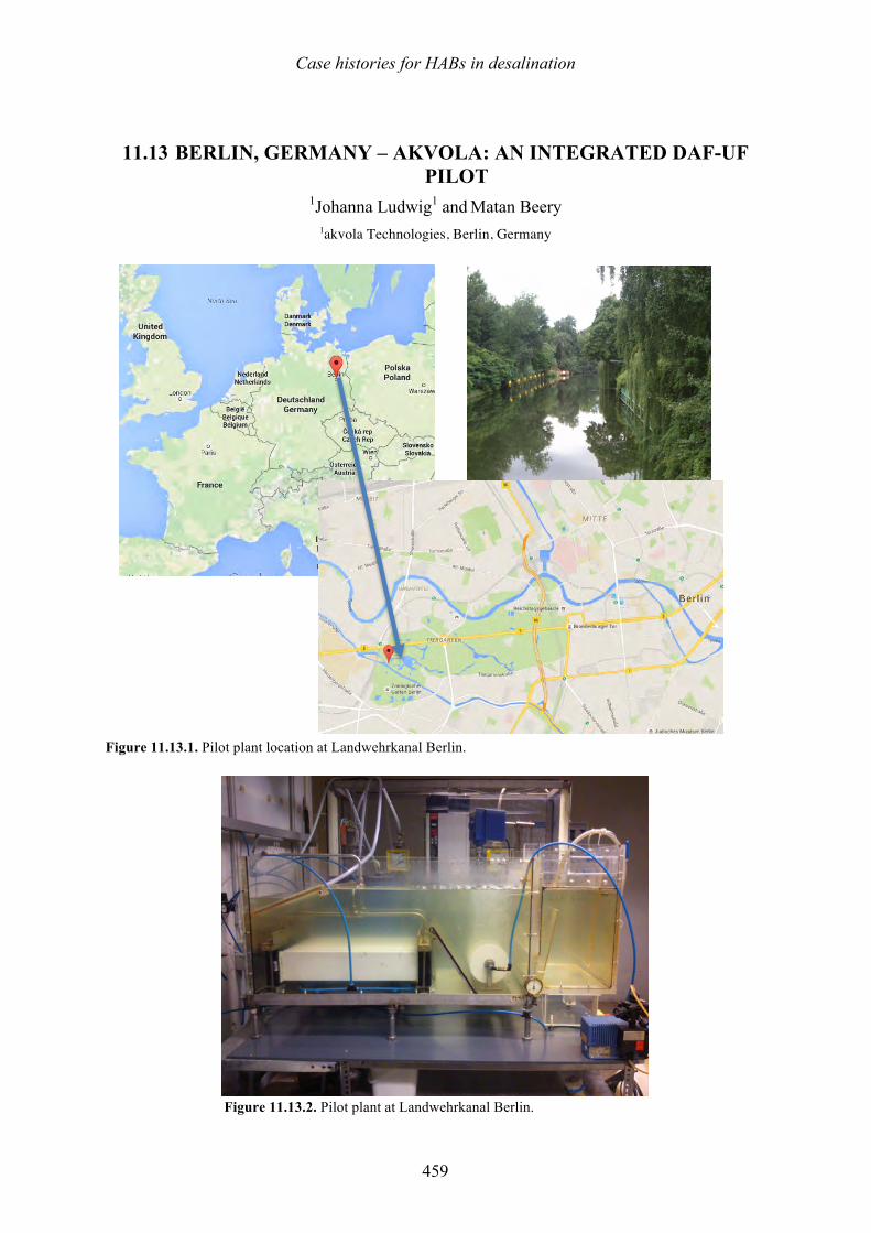
Case histories for HABs in desalination

459

11.13 BERLIN, GERMANY – AKVOLA: AN INTEGRATED DAF-UF PILOT

1Johanna Ludwig1 and Matan Beery 1akvola Technologies, Berlin, Germany

Figure 11.13.1. Pilot plant location at Landwehrkanal Berlin.

Figure 11.13.2. Pilot plant at Landwehrkanal Berlin.

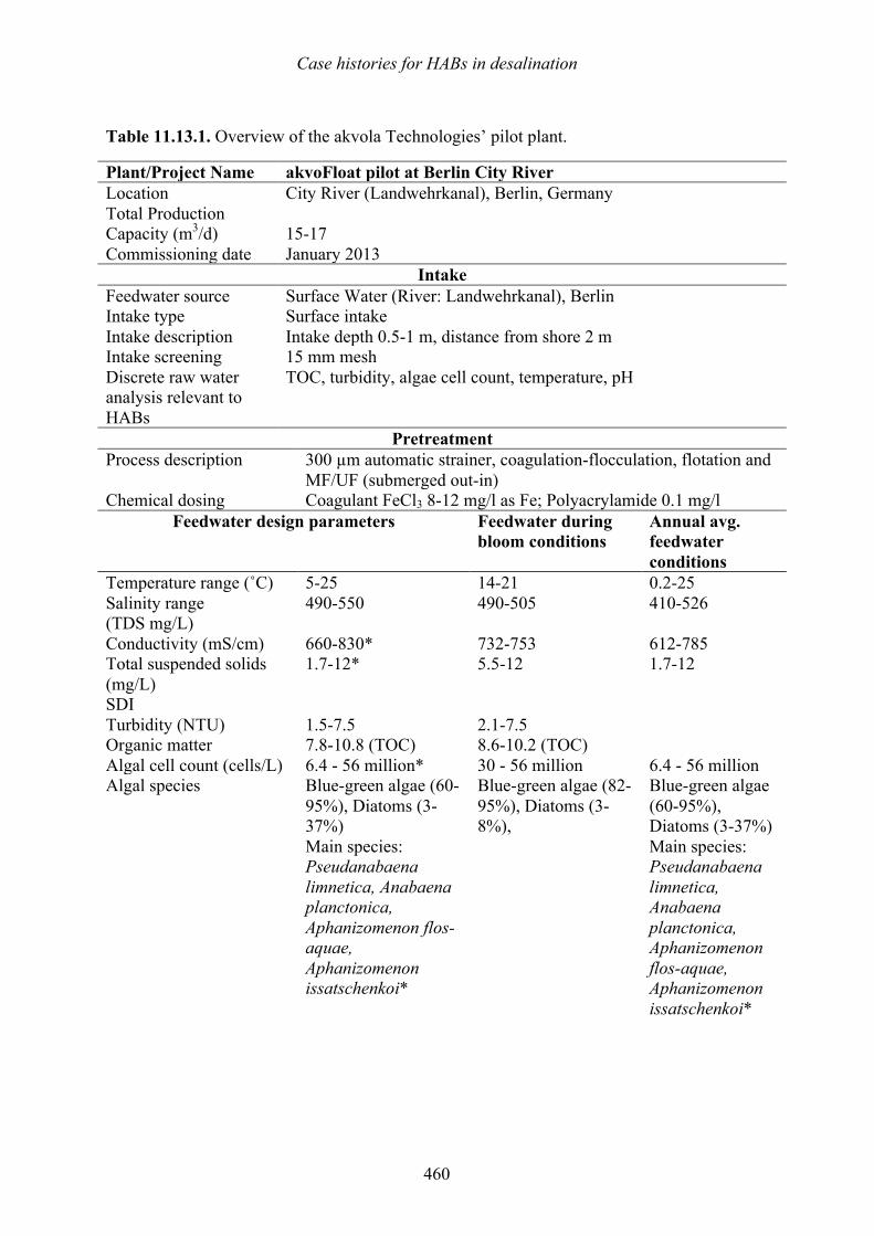
Case histories for HABs in desalination

460

Table 11.13.1. Overview of the akvola Technologies’ pilot plant.

Plant/Project Name akvoFloat pilot at Berlin City River Location City River (Landwehrkanal), Berlin, Germany Total Production Capacity (m3/d)

15-17

Commissioning date January 2013 Intake

Feedwater source Surface Water (River: Landwehrkanal), Berlin Intake type Surface intake Intake description Intake depth 0.5-1 m, distance from shore 2 m Intake screening 15 mm mesh Discrete raw water analysis relevant to HABs

TOC, turbidity, algae cell count, temperature, pH

Pretreatment Process description

300 µm automatic strainer, coagulation-flocculation, flotation and MF/UF (submerged out-in)

Chemical dosing Coagulant FeCl3 8-12 mg/l as Fe; Polyacrylamide 0.1 mg/l Feedwater design parameters Feedwater during

bloom conditions Annual avg. feedwater conditions

Temperature range (˚C) 5-25 14-21 0.2-25 Salinity range (TDS mg/L)

490-550 490-505 410-526

Conductivity (mS/cm) 660-830* 732-753 612-785 Total suspended solids (mg/L)

1.7-12* 5.5-12 1.7-12

SDI Turbidity (NTU) 1.5-7.5 2.1-7.5 Organic matter 7.8-10.8 (TOC) 8.6-10.2 (TOC) Algal cell count (cells/L) 6.4 - 56 million* 30 - 56 million 6.4 - 56 million Algal species Blue-green algae (60-

95%), Diatoms (3-37%) Main species: Pseudanabaena limnetica, Anabaena planctonica, Aphanizomenon flos-aquae, Aphanizomenon issatschenkoi*

Blue-green algae (82-95%), Diatoms (3-8%),

Blue-green algae (60-95%), Diatoms (3-37%) Main species: Pseudanabaena limnetica, Anabaena planctonica, Aphanizomenon flos-aquae, Aphanizomenon issatschenkoi*

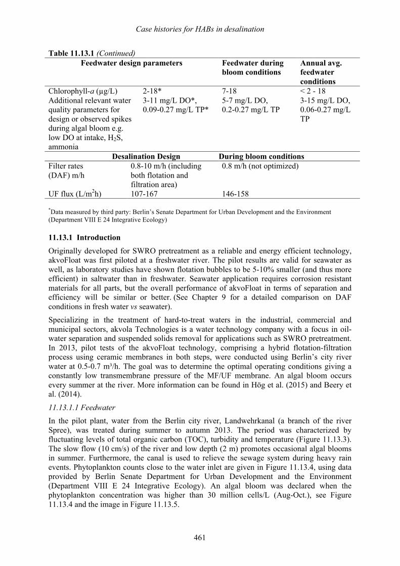
Case histories for HABs in desalination

461

Table 11.13.1 (Continued) Feedwater design parameters Feedwater during

bloom conditions Annual avg. feedwater conditions

Chlorophyll-a (µg/L) 2-18* 7-18 < 2 - 18 Additional relevant water quality parameters for design or observed spikes during algal bloom e.g. low DO at intake, H2S, ammonia

3-11 mg/L DO*, 0.09-0.27 mg/L TP*

5-7 mg/L DO, 0.2-0.27 mg/L TP

3-15 mg/L DO, 0.06-0.27 mg/L TP

Desalination Design During bloom conditions Filter rates (DAF) m/h

0.8-10 m/h (including both flotation and filtration area)

0.8 m/h (not optimized)

UF flux (L/m2h) 107-167 146-158 *Data measured by third party: Berlin’s Senate Department for Urban Development and the Environment (Department VIII E 24 Integrative Ecology) 11.13.1 Introduction

Originally developed for SWRO pretreatment as a reliable and energy efficient technology, akvoFloat was first piloted at a freshwater river. The pilot results are valid for seawater as well, as laboratory studies have shown flotation bubbles to be 5-10% smaller (and thus more efficient) in saltwater than in freshwater. Seawater application requires corrosion resistant materials for all parts, but the overall performance of akvoFloat in terms of separation and efficiency will be similar or better. (See Chapter 9 for a detailed comparison on DAF conditions in fresh water vs seawater). Specializing in the treatment of hard-to-treat waters in the industrial, commercial and municipal sectors, akvola Technologies is a water technology company with a focus in oil-water separation and suspended solids removal for applications such as SWRO pretreatment. In 2013, pilot tests of the akvoFloat technology, comprising a hybrid flotation-filtration process using ceramic membranes in both steps, were conducted using Berlin’s city river water at 0.5-0.7 m³/h. The goal was to determine the optimal operating conditions giving a constantly low transmembrane pressure of the MF/UF membrane. An algal bloom occurs every summer at the river. More information can be found in Hög et al. (2015) and Beery et al. (2014).

11.13.1.1 Feedwater In the pilot plant, water from the Berlin city river, Landwehrkanal (a branch of the river Spree), was treated during summer to autumn 2013. The period was characterized by fluctuating levels of total organic carbon (TOC), turbidity and temperature (Figure 11.13.3). The slow flow (10 cm/s) of the river and low depth (2 m) promotes occasional algal blooms in summer. Furthermore, the canal is used to relieve the sewage system during heavy rain events. Phytoplankton counts close to the water inlet are given in Figure 11.13.4, using data provided by Berlin Senate Department for Urban Development and the Environment (Department VIII E 24 Integrative Ecology). An algal bloom was declared when the phytoplankton concentration was higher than 30 million cells/L (Aug-Oct.), see Figure 11.13.4 and the image in Figure 11.13.5.

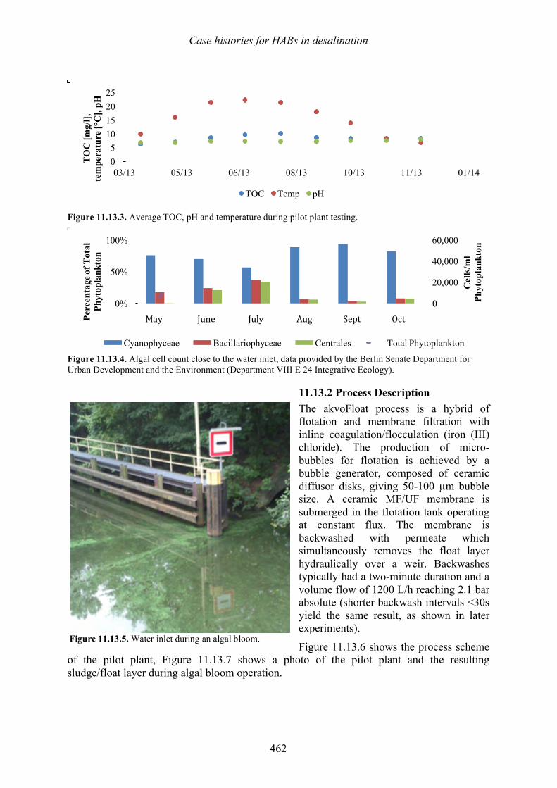
Case histories for HABs in desalination

462

Figure 11.13.3. Average TOC, pH and temperature during pilot plant testing.

Figure 11.13.4. Algal cell count close to the water inlet, data provided by the Berlin Senate Department for Urban Development and the Environment (Department VIII E 24 Integrative Ecology).

11.13.2 Process Description The akvoFloat process is a hybrid of flotation and membrane filtration with inline coagulation/flocculation (iron (III) chloride). The production of micro-bubbles for flotation is achieved by a bubble generator, composed of ceramic diffusor disks, giving 50-100 µm bubble size. A ceramic MF/UF membrane is submerged in the flotation tank operating at constant flux. The membrane is backwashed with permeate which simultaneously removes the float layer hydraulically over a weir. Backwashes typically had a two-minute duration and a volume flow of 1200 L/h reaching 2.1 bar absolute (shorter backwash intervals <30s yield the same result, as shown in later experiments).

Figure 11.13.6 shows the process scheme of the pilot plant, Figure 11.13.7 shows a photo of the pilot plant and the resulting sludge/float layer during algal bloom operation.

05

10152025

03/13 05/13 06/13 08/13 10/13 11/13 01/14

TO

C [m

g/l],

te

mpe

ratu

re [°

C],

pH

TOC Temp pH

0

20,000

40,000

60,000

0%

50%

100%

May June July Aug Sept Okt

Cel

ls/m

l Ph

ytop

lank

ton

Perc

enta

ge o

f Tot

al

Phyt

opla

nkto

n

Cyanophyceae Bacillariophyceae Centrales Total Phytoplankton

May June July Aug Sept Oct

Figure 11.13.5. Water inlet during an algal bloom.

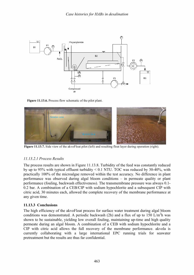
Case histories for HABs in desalination

463

11.13.2.1 Process Results

The process results are shown in Figure 11.13.8. Turbidity of the feed was constantly reduced by up to 95% with typical effluent turbidity < 0.1 NTU. TOC was reduced by 30-40%, with practically 100% of the microalgae removed within the test accuracy. No difference in plant performance was observed during algal bloom conditions – in permeate quality or plant performance (fouling, backwash effectiveness). The transmembrane pressure was always 0.1-0.2 bar. A combination of a CEB/CIP with sodium hypochlorite and a subsequent CIP with citric acid, 30 minutes each, allowed the complete recovery of the membrane performance at any given time.

11.13.3 Conclusions The high efficiency of the akvoFloat process for surface water treatment during algal bloom conditions was demonstrated. A periodic backwash (2h) and a flux of up to 150 L/m2h was shown to be sustainable, yielding low overall fouling, maintaining up-time and high quality permeate during an algal bloom. A combination of a CEB with sodium hypochlorite and a CIP with citric acid allows the full recovery of the membrane performance. akvola is currently collaborating with a large international EPC running trials for seawater pretreatment but the results are thus far confidential.

Figure 11.13.7. Side view of the akvoFloat pilot (left) and resulting float layer during operation (right).

Figure 11.13.6. Process flow schematic of the pilot plant.

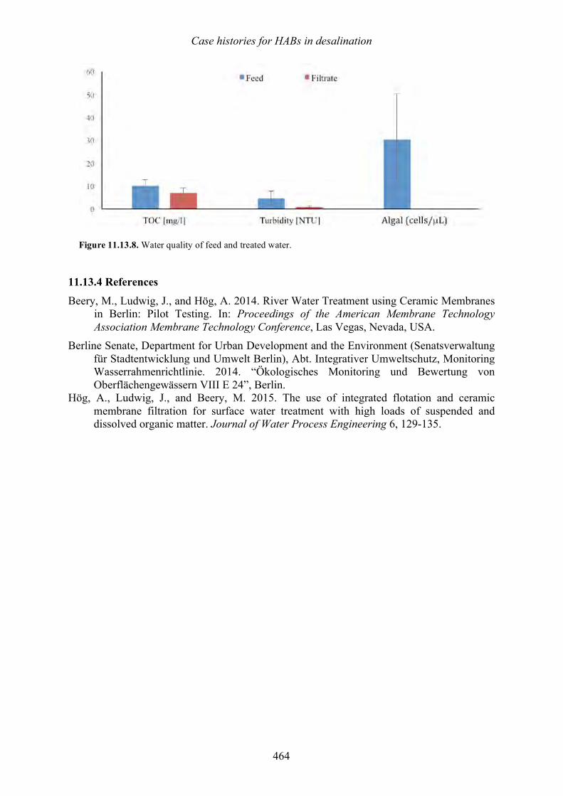
Case histories for HABs in desalination

464

11.13.4 References

Beery, M., Ludwig, J., and Hög, A. 2014. River Water Treatment using Ceramic Membranes in Berlin: Pilot Testing. In: Proceedings of the American Membrane Technology Association Membrane Technology Conference, Las Vegas, Nevada, USA.

Berline Senate, Department for Urban Development and the Environment (Senatsverwaltung für Stadtentwicklung und Umwelt Berlin), Abt. Integrativer Umweltschutz, Monitoring Wasserrahmenrichtlinie. 2014. “Ökologisches Monitoring und Bewertung von Oberflächengewässern VIII E 24”, Berlin.

Hög, A., Ludwig, J., and Beery, M. 2015. The use of integrated flotation and ceramic membrane filtration for surface water treatment with high loads of suspended and dissolved organic matter. Journal of Water Process Engineering 6, 129-135.

Figure 11.13.8. Water quality of feed and treated water.

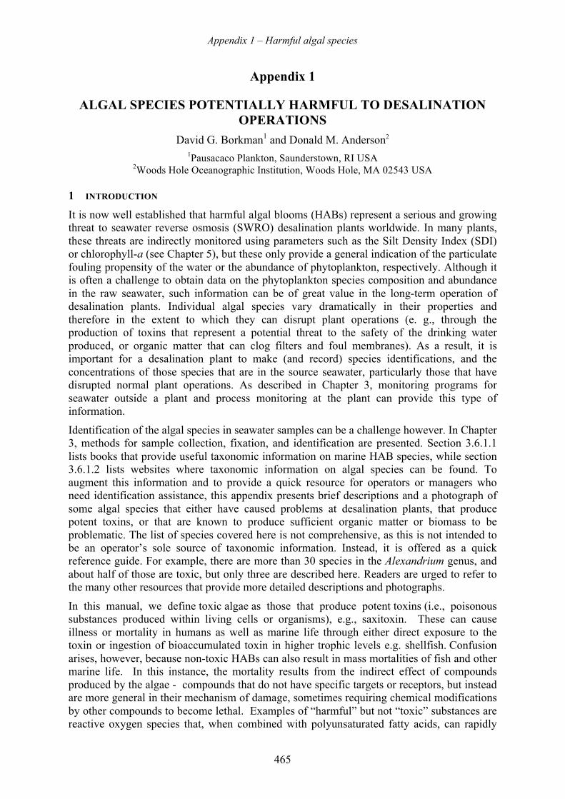
Appendix 1 – Harmful algal species

465

Appendix 1

ALGAL SPECIES POTENTIALLY HARMFUL TO DESALINATION OPERATIONS

David G. Borkman1 and Donald M. Anderson2 1Pausacaco Plankton, Saunderstown, RI USA

2Woods Hole Oceanographic Institution, Woods Hole, MA 02543 USA 1 INTRODUCTION

It is now well established that harmful algal blooms (HABs) represent a serious and growing threat to seawater reverse osmosis (SWRO) desalination plants worldwide. In many plants, these threats are indirectly monitored using parameters such as the Silt Density Index (SDI) or chlorophyll-a (see Chapter 5), but these only provide a general indication of the particulate fouling propensity of the water or the abundance of phytoplankton, respectively. Although it is often a challenge to obtain data on the phytoplankton species composition and abundance in the raw seawater, such information can be of great value in the long-term operation of desalination plants. Individual algal species vary dramatically in their properties and therefore in the extent to which they can disrupt plant operations (e. g., through the production of toxins that represent a potential threat to the safety of the drinking water produced, or organic matter that can clog filters and foul membranes). As a result, it is important for a desalination plant to make (and record) species identifications, and the concentrations of those species that are in the source seawater, particularly those that have disrupted normal plant operations. As described in Chapter 3, monitoring programs for seawater outside a plant and process monitoring at the plant can provide this type of information.

Identification of the algal species in seawater samples can be a challenge however. In Chapter 3, methods for sample collection, fixation, and identification are presented. Section 3.6.1.1 lists books that provide useful taxonomic information on marine HAB species, while section 3.6.1.2 lists websites where taxonomic information on algal species can be found. To augment this information and to provide a quick resource for operators or managers who need identification assistance, this appendix presents brief descriptions and a photograph of some algal species that either have caused problems at desalination plants, that produce potent toxins, or that are known to produce sufficient organic matter or biomass to be problematic. The list of species covered here is not comprehensive, as this is not intended to be an operator’s sole source of taxonomic information. Instead, it is offered as a quick reference guide. For example, there are more than 30 species in the Alexandrium genus, and about half of those are toxic, but only three are described here. Readers are urged to refer to the many other resources that provide more detailed descriptions and photographs.

In this manual, we define toxic algae as those that produce potent toxins (i.e., poisonous substances produced within living cells or organisms), e.g., saxitoxin. These can cause illness or mortality in humans as well as marine life through either direct exposure to the toxin or ingestion of bioaccumulated toxin in higher trophic levels e.g. shellfish. Confusion arises, however, because non-toxic HABs can also result in mass mortalities of fish and other marine life. In this instance, the mortality results from the indirect effect of compounds produced by the algae - compounds that do not have specific targets or receptors, but instead are more general in their mechanism of damage, sometimes requiring chemical modifications by other compounds to become lethal. Examples of “harmful” but not “toxic” substances are reactive oxygen species that, when combined with polyunsaturated fatty acids, can rapidly

Appendix 1 – Harmful algal species

466

kill fish and other animals. Another example is a proteinaceous compound produced by Akashiwo sanguinea that accumulates on bird feathers, causing a loss in natural water repellency and widespread mortality of affected animals. In this appendix, species that do not produce toxins but that do cause marine mortalities are termed “harmful”. The following glossary defines some of the taxonomic terminology used here.

Antapex – posterior-most (bottom) part of the cell body, excluding spines, lists and similar structures

Apex – anterior-most (top) part of the cell body

Areolate – ornamentation of the thecal plates that consists of depressions of variable depth and form

Cingulum – a furrow encircling the cell that contains the rotary flagellum Cyst – the diploid zygotic dormant state in the sexual life cycle; usually morphologically

dissimilar from the haploid motile stage; also called the ‘dinocyst’ or ‘hypnozygote’

Dorsal Side – back side of the cell, opposite of the front or ventral side where the sulcus is located

Epicone – the part of a dinoflagellate cell above the cingulum; usually refers to an ‘unarmored’ (lacking cellulose plates) cell; may also be known as the epitheca or episome

Epitheca – the part of a dinoflagellate cell above the cingulum; usually refers to a thecate (with cellulose plates) cell; may also be known as the epicone or episome

Flagellar Area – the vicinity of the origin of the two flagella

Hypocone – the part of a dinoflagellate cell below the cingulum; usually refers to an ‘unarmored’ (lacking cellulose plates) cell; may also be referred to as the hypotheca or hyposome

Hypotheca – the part of a dinoflagellate cell below the cingulum; usually refers to a thecate (with cellulose plates) cell; may also be referred to as the hypocone or hyposome

Lists – membranous extensions of the cingulum and/or sulcus that extend beyond the cell wall boundary

Pores – openings in the theca that can be involved in the extrusion of certain structures from the cell

Sulcus – a longitudinal furrow, often partially enclosing the propulsive flagellum Thecate – having a cell wall of cellulose plates which have special designations and

symbols according to their location on the cell

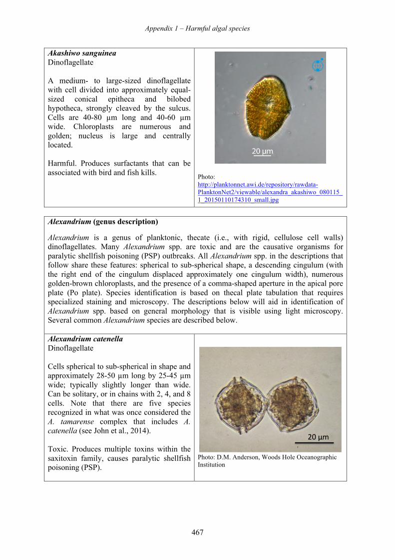
Appendix 1 – Harmful algal species

467

Akashiwo sanguinea Dinoflagellate A medium- to large-sized dinoflagellate with cell divided into approximately equal-sized conical epitheca and bilobed hypotheca, strongly cleaved by the sulcus. Cells are 40-80 µm long and 40-60 µm wide. Chloroplasts are numerous and golden; nucleus is large and centrally located. Harmful. Produces surfactants that can be associated with bird and fish kills.

Photo: http://planktonnet.awi.de/repository/rawdata-PlanktonNet2/viewable/alexandra_akashiwo_080115_1_20150110174310_small.jpg

Alexandrium (genus description)

Alexandrium is a genus of planktonic, thecate (i.e., with rigid, cellulose cell walls) dinoflagellates. Many Alexandrium spp. are toxic and are the causative organisms for paralytic shellfish poisoning (PSP) outbreaks. All Alexandrium spp. in the descriptions that follow share these features: spherical to sub-spherical shape, a descending cingulum (with the right end of the cingulum displaced approximately one cingulum width), numerous golden-brown chloroplasts, and the presence of a comma-shaped aperture in the apical pore plate (Po plate). Species identification is based on thecal plate tabulation that requires specialized staining and microscopy. The descriptions below will aid in identification of Alexandrium spp. based on general morphology that is visible using light microscopy. Several common Alexandrium species are described below.

Alexandrium catenella Dinoflagellate Cells spherical to sub-spherical in shape and approximately 28-50 µm long by 25-45 µm wide; typically slightly longer than wide. Can be solitary, or in chains with 2, 4, and 8 cells. Note that there are five species recognized in what was once considered the A. tamarense complex that includes A. catenella (see John et al., 2014). Toxic. Produces multiple toxins within the saxitoxin family, causes paralytic shellfish poisoning (PSP).

Photo: D.M. Anderson, Woods Hole Oceanographic Institution

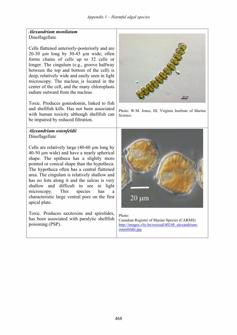
Appendix 1 – Harmful algal species

468

Alexandrium monilatum Dinoflagellate Cells flattened anteriorly-posteriorly and are 20-30 µm long by 30-45 µm wide; often forms chains of cells up to 32 cells or longer. The cingulum (e.g., groove halfway between the top and bottom of the cell) is deep, relatively wide and easily seen in light microscopy. The nucleus is located in the center of the cell, and the many chloroplasts radiate outward from the nucleus Toxic. Produces goniodomin, linked to fish and shellfish kills. Has not been associated with human toxicity although shellfish can be impaired by reduced filtration.

Photo: W.M. Jones, III, Virginia Institute of Marine Science.

Alexandrium ostenfeldii Dinoflagellate Cells are relatively large (40-60 µm long by 40-50 µm wide) and have a nearly spherical shape. The epitheca has a slightly more pointed or conical shape than the hypotheca. The hypotheca often has a central flattened area. The cingulum is relatively shallow and has no lists along it and the sulcus is very shallow and difficult to see in light microscopy. This species has a characteristic large ventral pore on the first apical plate. Toxic. Produces saxitoxins and spirolides, has been associated with paralytic shellfish poisoning (PSP).

Photo: Canadian Register of Marine Species (CARMS) http://images.vliz.be/resized/40248_alexandrium-ostenfeldii.jpg

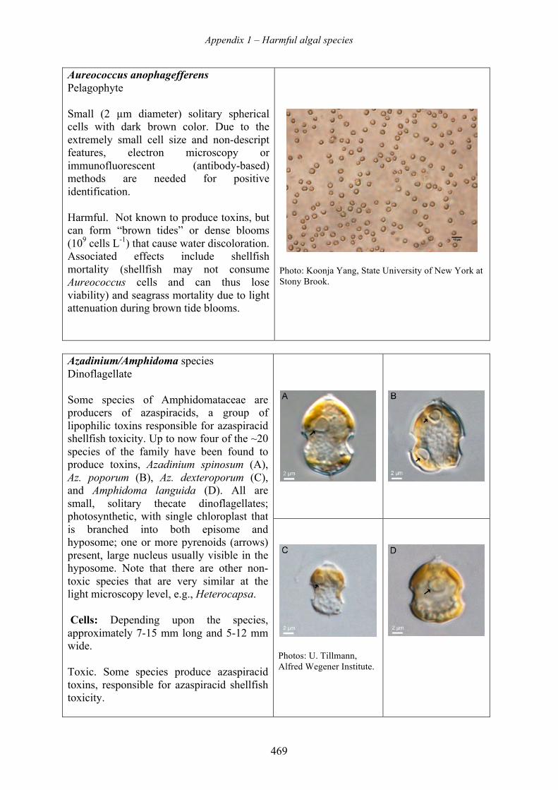
Appendix 1 – Harmful algal species

469

Aureococcus anophagefferens Pelagophyte Small (2 µm diameter) solitary spherical cells with dark brown color. Due to the extremely small cell size and non-descript features, electron microscopy or immunofluorescent (antibody-based) methods are needed for positive identification. Harmful. Not known to produce toxins, but can form “brown tides” or dense blooms (109 cells L-1) that cause water discoloration. Associated effects include shellfish mortality (shellfish may not consume Aureococcus cells and can thus lose viability) and seagrass mortality due to light attenuation during brown tide blooms.

Photo: Koonja Yang, State University of New York at Stony Brook.

Azadinium/Amphidoma species Dinoflagellate Some species of Amphidomataceae are producers of azaspiracids, a group of lipophilic toxins responsible for azaspiracid shellfish toxicity. Up to now four of the ~20 species of the family have been found to produce toxins, Azadinium spinosum (A), Az. poporum (B), Az. dexteroporum (C), and Amphidoma languida (D). All are small, solitary thecate dinoflagellates; photosynthetic, with single chloroplast that is branched into both episome and hyposome; one or more pyrenoids (arrows) present, large nucleus usually visible in the hyposome. Note that there are other non-toxic species that are very similar at the light microscopy level, e.g., Heterocapsa. Cells: Depending upon the species, approximately 7-15 mm long and 5-12 mm wide. Toxic. Some species produce azaspiracid toxins, responsible for azaspiracid shellfish toxicity.

Photos: U. Tillmann, Alfred Wegener Institute.

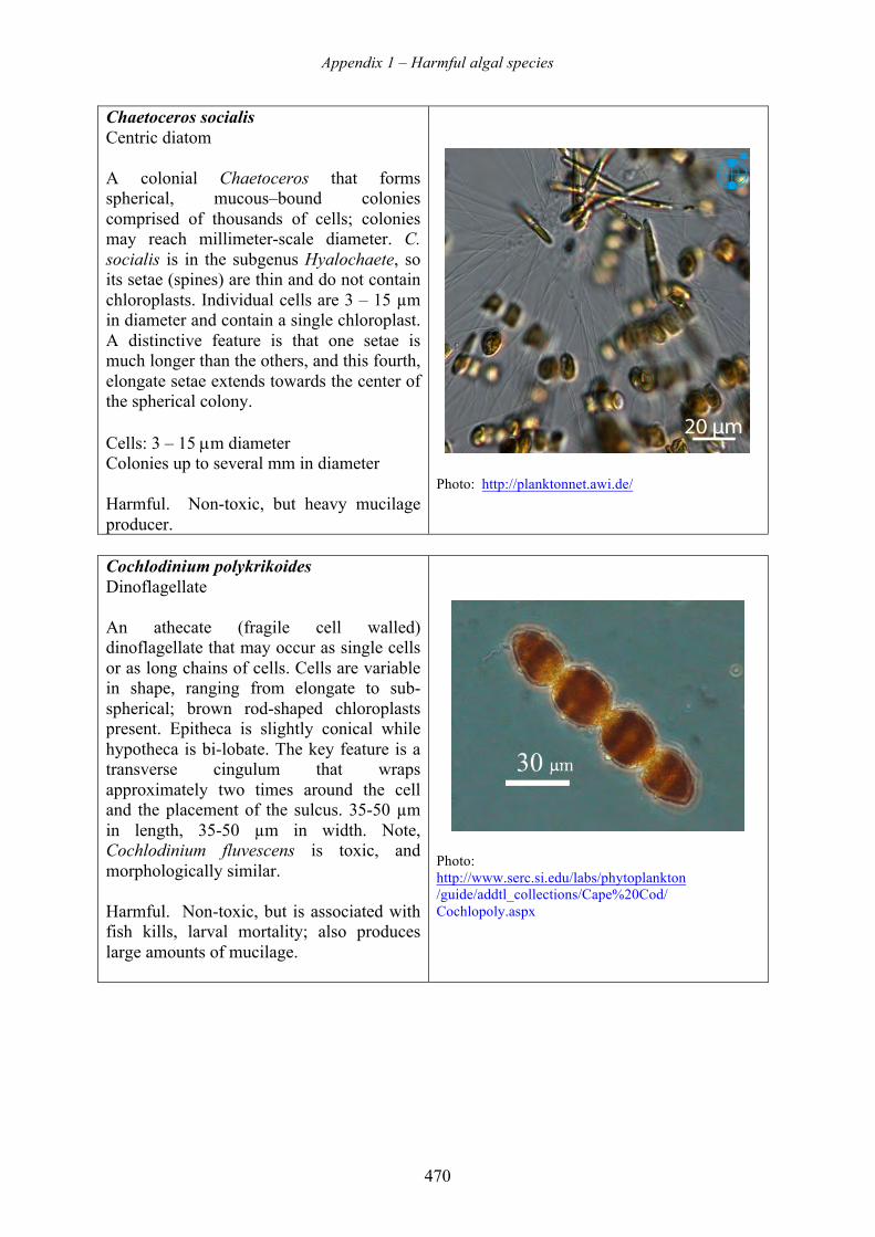
Appendix 1 – Harmful algal species

470

Chaetoceros socialis Centric diatom A colonial Chaetoceros that forms spherical, mucous–bound colonies comprised of thousands of cells; colonies may reach millimeter-scale diameter. C. socialis is in the subgenus Hyalochaete, so its setae (spines) are thin and do not contain chloroplasts. Individual cells are 3 – 15 µm in diameter and contain a single chloroplast. A distinctive feature is that one setae is much longer than the others, and this fourth, elongate setae extends towards the center of the spherical colony. Cells: 3 – 15 µm diameter Colonies up to several mm in diameter Harmful. Non-toxic, but heavy mucilage producer.

Photo: http://planktonnet.awi.de/

Cochlodinium polykrikoides Dinoflagellate An athecate (fragile cell walled) dinoflagellate that may occur as single cells or as long chains of cells. Cells are variable in shape, ranging from elongate to sub-spherical; brown rod-shaped chloroplasts present. Epitheca is slightly conical while hypotheca is bi-lobate. The key feature is a transverse cingulum that wraps approximately two times around the cell and the placement of the sulcus. 35-50 µm in length, 35-50 µm in width. Note, Cochlodinium fluvescens is toxic, and morphologically similar. Harmful. Non-toxic, but is associated with fish kills, larval mortality; also produces large amounts of mucilage.

Photo: http://www.serc.si.edu/labs/phytoplankton /guide/addtl_collections/Cape%20Cod/ Cochlopoly.aspx

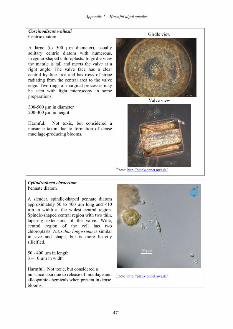
Appendix 1 – Harmful algal species

471

Coscinodiscus wailesii Centric diatom A large (to 500 µm diameter), usually solitary centric diatom with numerous, irregular-shaped chloroplasts. In girdle view the mantle is tall and meets the valve at a right angle. The valve face has a clear central hyaline area and has rows of striae radiating from the central area to the valve edge. Two rings of marginal processes may be seen with light microscopy in some preparations. 300-500 µm in diameter 200-400 µm in height Harmful. Not toxic, but considered a nuisance taxon due to formation of dense mucilage-producing blooms.

Girdle view

Valve view

Photo: http://planktonnet.awi.de/

Cylindrotheca closterium Pennate diatom A slender, spindle-shaped pennate diatom approximately 50 to 400 µm long and <10 µm in width at the widest central region. Spindle-shaped central region with two thin, tapering extensions of the valve. Wide, central region of the cell has two chloroplasts. Nitzschia longissima is similar in size and shape, but is more heavily silicified. 50 - 400 µm in length 3 – 10 µm in width Harmful. Not toxic, but considered a nuisance taxa due to release of mucilage and alleopathic chemicals when present in dense blooms.

Photo: http://planktonnet.awi.de/

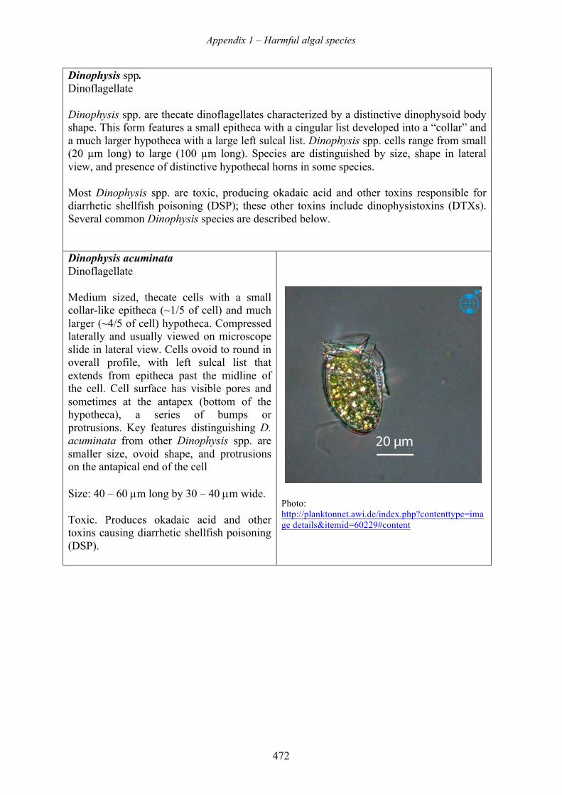
Appendix 1 – Harmful algal species

472

Dinophysis spp. Dinoflagellate Dinophysis spp. are thecate dinoflagellates characterized by a distinctive dinophysoid body shape. This form features a small epitheca with a cingular list developed into a “collar” and a much larger hypotheca with a large left sulcal list. Dinophysis spp. cells range from small (20 µm long) to large (100 µm long). Species are distinguished by size, shape in lateral view, and presence of distinctive hypothecal horns in some species. Most Dinophysis spp. are toxic, producing okadaic acid and other toxins responsible for diarrhetic shellfish poisoning (DSP); these other toxins include dinophysistoxins (DTXs). Several common Dinophysis species are described below.

Dinophysis acuminata Dinoflagellate Medium sized, thecate cells with a small collar-like epitheca (~1/5 of cell) and much larger (~4/5 of cell) hypotheca. Compressed laterally and usually viewed on microscope slide in lateral view. Cells ovoid to round in overall profile, with left sulcal list that extends from epitheca past the midline of the cell. Cell surface has visible pores and sometimes at the antapex (bottom of the hypotheca), a series of bumps or protrusions. Key features distinguishing D. acuminata from other Dinophysis spp. are smaller size, ovoid shape, and protrusions on the antapical end of the cell Size: 40 – 60 µm long by 30 – 40 µm wide. Toxic. Produces okadaic acid and other toxins causing diarrhetic shellfish poisoning (DSP).

Photo: http://planktonnet.awi.de/index.php?contenttype=image details&itemid=60229#content

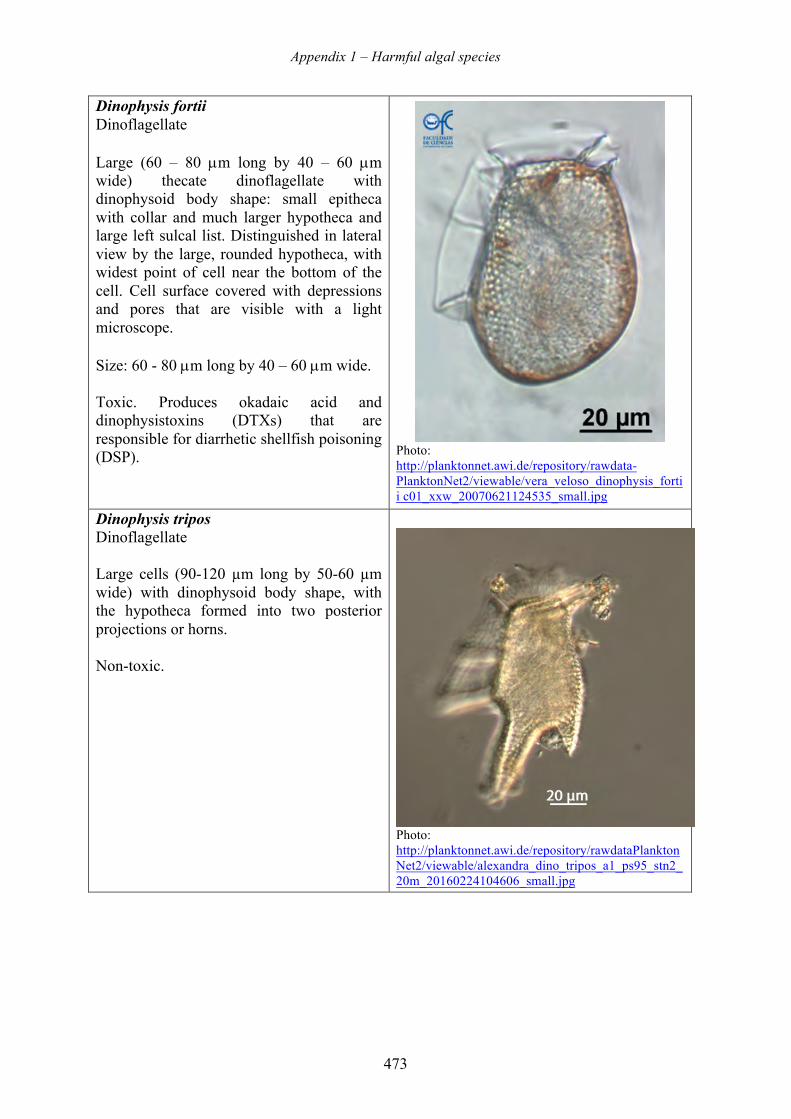
Appendix 1 – Harmful algal species

473

Dinophysis fortii Dinoflagellate Large (60 – 80 µm long by 40 – 60 µm wide) thecate dinoflagellate with dinophysoid body shape: small epitheca with collar and much larger hypotheca and large left sulcal list. Distinguished in lateral view by the large, rounded hypotheca, with widest point of cell near the bottom of the cell. Cell surface covered with depressions and pores that are visible with a light microscope. Size: 60 - 80 µm long by 40 – 60 µm wide. Toxic. Produces okadaic acid and dinophysistoxins (DTXs) that are responsible for diarrhetic shellfish poisoning (DSP).

Photo: http://planktonnet.awi.de/repository/rawdata-PlanktonNet2/viewable/vera_veloso_dinophysis_fortii c01_xxw_20070621124535_small.jpg

Dinophysis tripos Dinoflagellate Large cells (90-120 µm long by 50-60 µm wide) with dinophysoid body shape, with the hypotheca formed into two posterior projections or horns. Non-toxic.

Photo: http://planktonnet.awi.de/repository/rawdataPlanktonNet2/viewable/alexandra_dino_tripos_a1_ps95_stn2_20m_20160224104606_small.jpg

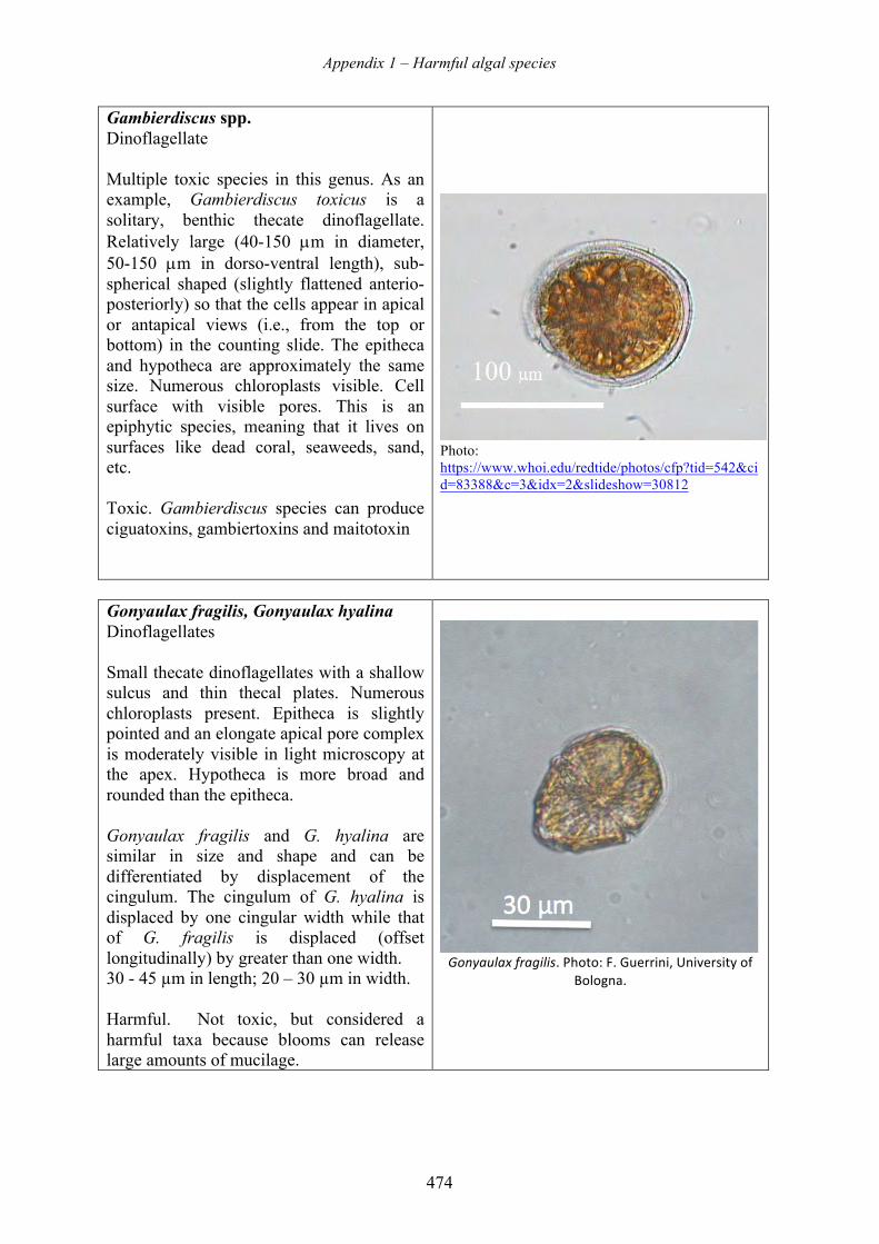
Appendix 1 – Harmful algal species

474

Gambierdiscus spp. Dinoflagellate Multiple toxic species in this genus. As an example, Gambierdiscus toxicus is a solitary, benthic thecate dinoflagellate. Relatively large (40-150 µm in diameter, 50-150 µm in dorso-ventral length), sub-spherical shaped (slightly flattened anterio-posteriorly) so that the cells appear in apical or antapical views (i.e., from the top or bottom) in the counting slide. The epitheca and hypotheca are approximately the same size. Numerous chloroplasts visible. Cell surface with visible pores. This is an epiphytic species, meaning that it lives on surfaces like dead coral, seaweeds, sand, etc. Toxic. Gambierdiscus species can produce ciguatoxins, gambiertoxins and maitotoxin

Photo: https://www.whoi.edu/redtide/photos/cfp?tid=542&cid=83388&c=3&idx=2&slideshow=30812

Gonyaulax fragilis, Gonyaulax hyalina Dinoflagellates Small thecate dinoflagellates with a shallow sulcus and thin thecal plates. Numerous chloroplasts present. Epitheca is slightly pointed and an elongate apical pore complex is moderately visible in light microscopy at the apex. Hypotheca is more broad and rounded than the epitheca. Gonyaulax fragilis and G. hyalina are similar in size and shape and can be differentiated by displacement of the cingulum. The cingulum of G. hyalina is displaced by one cingular width while that of G. fragilis is displaced (offset longitudinally) by greater than one width. 30 - 45 µm in length; 20 – 30 µm in width. Harmful. Not toxic, but considered a harmful taxa because blooms can release large amounts of mucilage.

Gonyaulax fragilis. Photo: F. Guerrini, University of

Bologna.

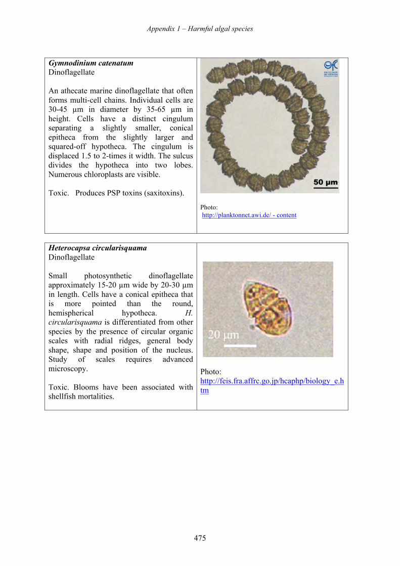
Appendix 1 – Harmful algal species

475

Gymnodinium catenatum Dinoflagellate An athecate marine dinoflagellate that often forms multi-cell chains. Individual cells are 30-45 µm in diameter by 35-65 µm in height. Cells have a distinct cingulum separating a slightly smaller, conical epitheca from the slightly larger and squared-off hypotheca. The cingulum is displaced 1.5 to 2-times it width. The sulcus divides the hypotheca into two lobes. Numerous chloroplasts are visible. Toxic. Produces PSP toxins (saxitoxins).

Photo: http://planktonnet.awi.de/ - content

Heterocapsa circularisquama Dinoflagellate Small photosynthetic dinoflagellate approximately 15-20 µm wide by 20-30 µm in length. Cells have a conical epitheca that is more pointed than the round, hemispherical hypotheca. H. circularisquama is differentiated from other species by the presence of circular organic scales with radial ridges, general body shape, shape and position of the nucleus. Study of scales requires advanced microscopy. Toxic. Blooms have been associated with shellfish mortalities.

Photo: http://feis.fra.affrc.go.jp/hcaphp/biology_e.htm

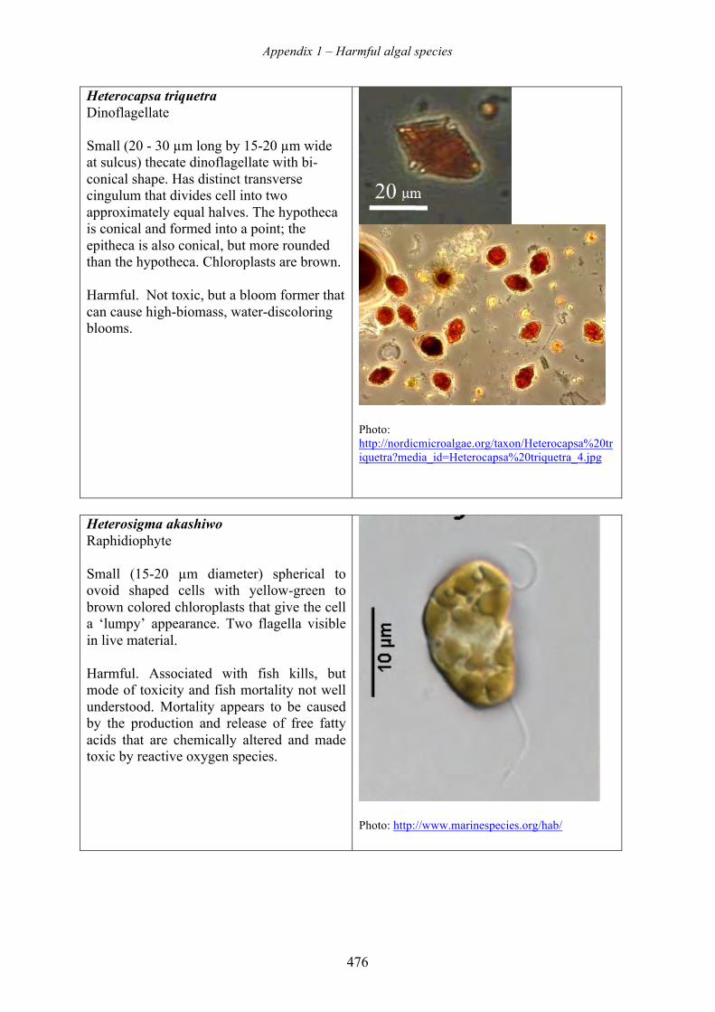
Appendix 1 – Harmful algal species

476

Heterocapsa triquetra Dinoflagellate Small (20 - 30 µm long by 15-20 µm wide at sulcus) thecate dinoflagellate with bi-conical shape. Has distinct transverse cingulum that divides cell into two approximately equal halves. The hypotheca is conical and formed into a point; the epitheca is also conical, but more rounded than the hypotheca. Chloroplasts are brown. Harmful. Not toxic, but a bloom former that can cause high-biomass, water-discoloring blooms.

Photo: http://nordicmicroalgae.org/taxon/Heterocapsa%20triquetra?media_id=Heterocapsa%20triquetra_4.jpg

Heterosigma akashiwo Raphidiophyte Small (15-20 µm diameter) spherical to ovoid shaped cells with yellow-green to brown colored chloroplasts that give the cell a ‘lumpy’ appearance. Two flagella visible in live material. Harmful. Associated with fish kills, but mode of toxicity and fish mortality not well understood. Mortality appears to be caused by the production and release of free fatty acids that are chemically altered and made toxic by reactive oxygen species.

Photo: http://www.marinespecies.org/hab/

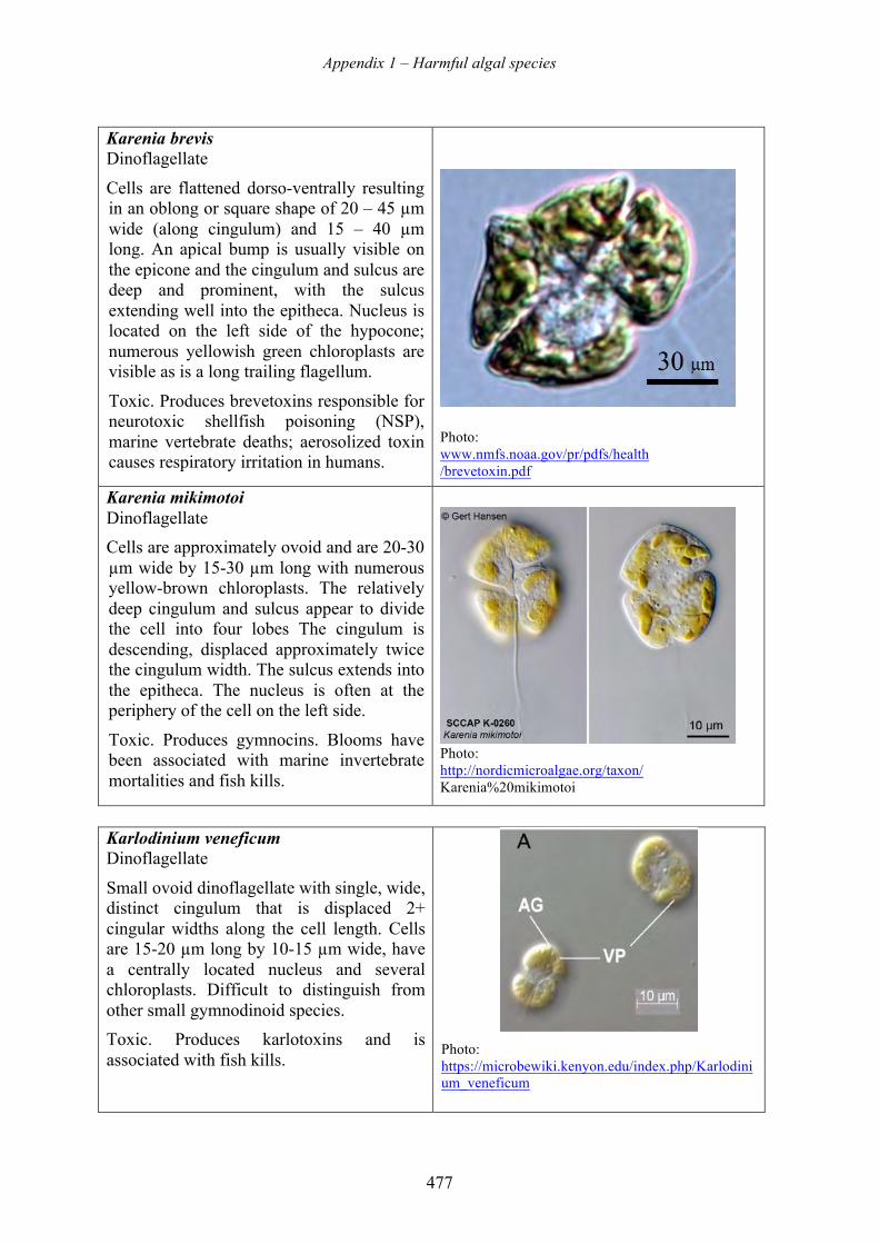
Appendix 1 – Harmful algal species

477

Karenia brevis Dinoflagellate

Cells are flattened dorso-ventrally resulting in an oblong or square shape of 20 – 45 µm wide (along cingulum) and 15 – 40 µm long. An apical bump is usually visible on the epicone and the cingulum and sulcus are deep and prominent, with the sulcus extending well into the epitheca. Nucleus is located on the left side of the hypocone; numerous yellowish green chloroplasts are visible as is a long trailing flagellum.

Toxic. Produces brevetoxins responsible for neurotoxic shellfish poisoning (NSP), marine vertebrate deaths; aerosolized toxin causes respiratory irritation in humans.

Photo: www.nmfs.noaa.gov/pr/pdfs/health /brevetoxin.pdf

Karenia mikimotoi Dinoflagellate Cells are approximately ovoid and are 20-30 µm wide by 15-30 µm long with numerous yellow-brown chloroplasts. The relatively deep cingulum and sulcus appear to divide the cell into four lobes The cingulum is descending, displaced approximately twice the cingulum width. The sulcus extends into the epitheca. The nucleus is often at the periphery of the cell on the left side.

Toxic. Produces gymnocins. Blooms have been associated with marine invertebrate mortalities and fish kills.

Photo: http://nordicmicroalgae.org/taxon/ Karenia%20mikimotoi

Karlodinium veneficum Dinoflagellate

Small ovoid dinoflagellate with single, wide, distinct cingulum that is displaced 2+ cingular widths along the cell length. Cells are 15-20 µm long by 10-15 µm wide, have a centrally located nucleus and several chloroplasts. Difficult to distinguish from other small gymnodinoid species. Toxic. Produces karlotoxins and is associated with fish kills.

Photo: https://microbewiki.kenyon.edu/index.php/Karlodinium_veneficum

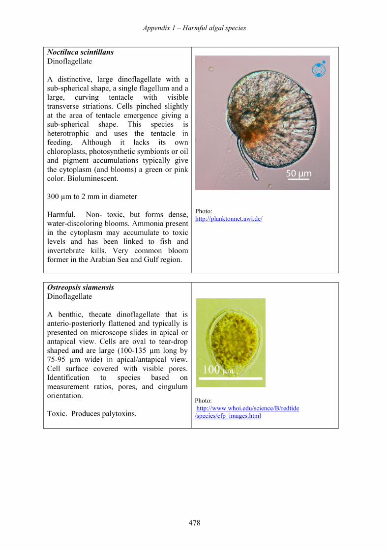
Appendix 1 – Harmful algal species

478

Noctiluca scintillans Dinoflagellate A distinctive, large dinoflagellate with a sub-spherical shape, a single flagellum and a large, curving tentacle with visible transverse striations. Cells pinched slightly at the area of tentacle emergence giving a sub-spherical shape. This species is heterotrophic and uses the tentacle in feeding. Although it lacks its own chloroplasts, photosynthetic symbionts or oil and pigment accumulations typically give the cytoplasm (and blooms) a green or pink color. Bioluminescent. 300 µm to 2 mm in diameter Harmful. Non- toxic, but forms dense, water-discoloring blooms. Ammonia present in the cytoplasm may accumulate to toxic levels and has been linked to fish and invertebrate kills. Very common bloom former in the Arabian Sea and Gulf region.

Photo: http://planktonnet.awi.de/

Ostreopsis siamensis Dinoflagellate A benthic, thecate dinoflagellate that is anterio-posteriorly flattened and typically is presented on microscope slides in apical or antapical view. Cells are oval to tear-drop shaped and are large (100-135 µm long by 75-95 µm wide) in apical/antapical view. Cell surface covered with visible pores. Identification to species based on measurement ratios, pores, and cingulum orientation. Toxic. Produces palytoxins.

Photo: http://www.whoi.edu/science/B/redtide /species/cfp_images.html

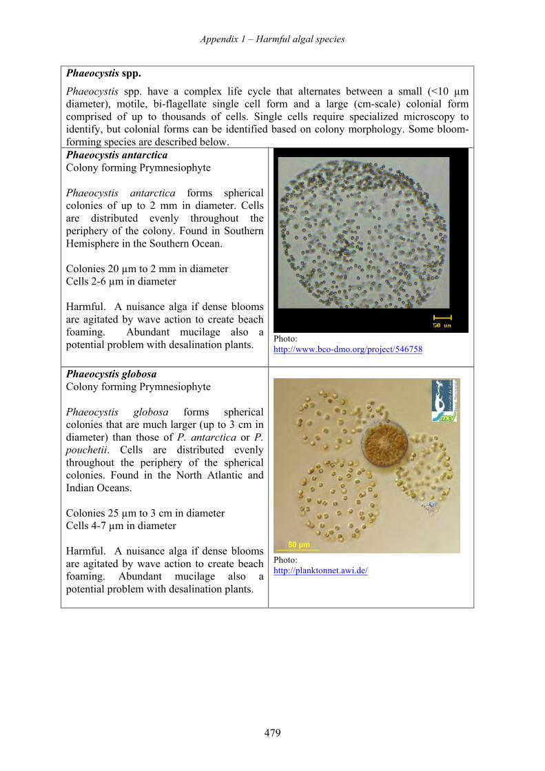
Appendix 1 – Harmful algal species

479

Phaeocystis spp.

Phaeocystis spp. have a complex life cycle that alternates between a small (<10 µm diameter), motile, bi-flagellate single cell form and a large (cm-scale) colonial form comprised of up to thousands of cells. Single cells require specialized microscopy to identify, but colonial forms can be identified based on colony morphology. Some bloom-forming species are described below. Phaeocystis antarctica Colony forming Prymnesiophyte Phaeocystis antarctica forms spherical colonies of up to 2 mm in diameter. Cells are distributed evenly throughout the periphery of the colony. Found in Southern Hemisphere in the Southern Ocean. Colonies 20 µm to 2 mm in diameter Cells 2-6 µm in diameter Harmful. A nuisance alga if dense blooms are agitated by wave action to create beach foaming. Abundant mucilage also a potential problem with desalination plants.

Photo: http://www.bco-dmo.org/project/546758

Phaeocystis globosa Colony forming Prymnesiophyte Phaeocystis globosa forms spherical colonies that are much larger (up to 3 cm in diameter) than those of P. antarctica or P. pouchetii. Cells are distributed evenly throughout the periphery of the spherical colonies. Found in the North Atlantic and Indian Oceans. Colonies 25 µm to 3 cm in diameter Cells 4-7 µm in diameter Harmful. A nuisance alga if dense blooms are agitated by wave action to create beach foaming. Abundant mucilage also a potential problem with desalination plants.

Photo: http://planktonnet.awi.de/

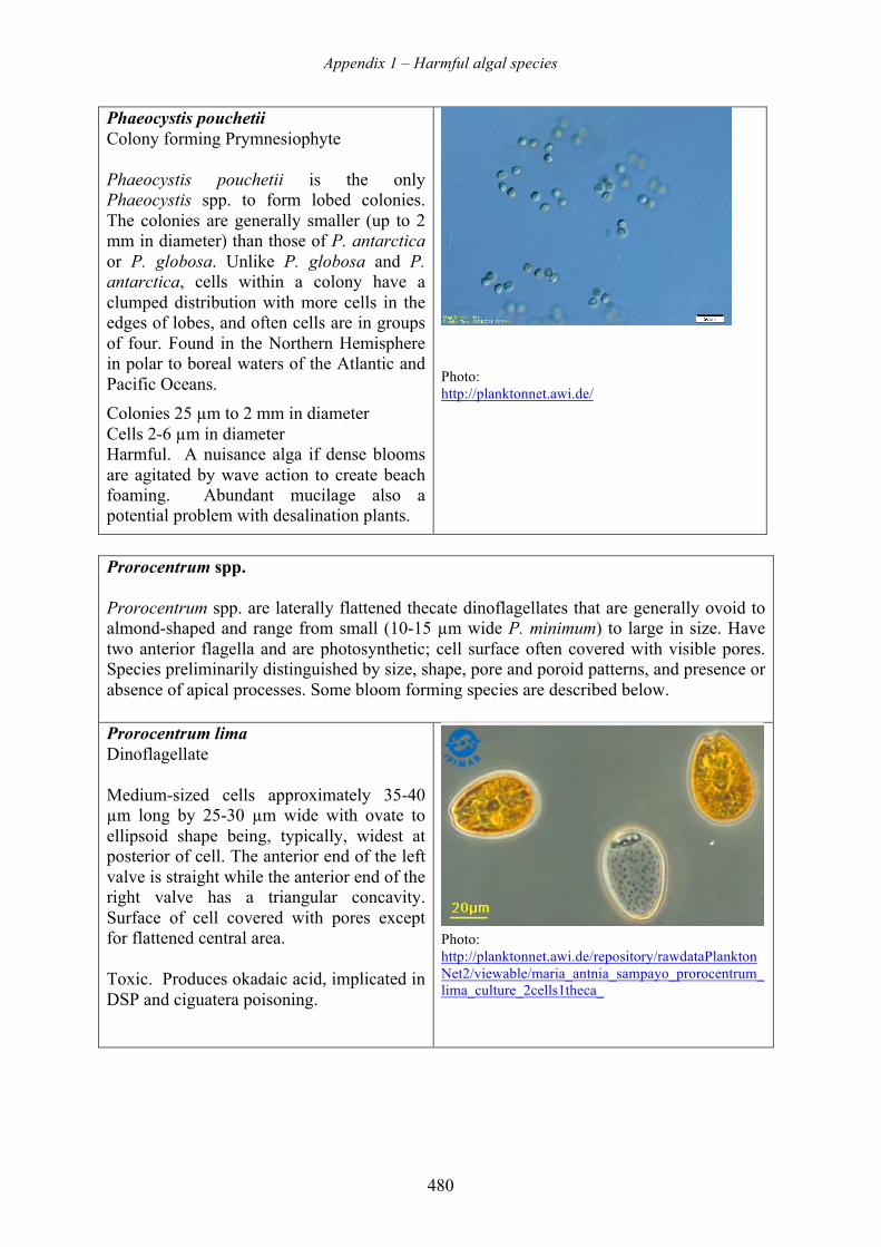
Appendix 1 – Harmful algal species

480

Phaeocystis pouchetii Colony forming Prymnesiophyte Phaeocystis pouchetii is the only Phaeocystis spp. to form lobed colonies. The colonies are generally smaller (up to 2 mm in diameter) than those of P. antarctica or P. globosa. Unlike P. globosa and P. antarctica, cells within a colony have a clumped distribution with more cells in the edges of lobes, and often cells are in groups of four. Found in the Northern Hemisphere in polar to boreal waters of the Atlantic and Pacific Oceans. Colonies 25 µm to 2 mm in diameter Cells 2-6 µm in diameter Harmful. A nuisance alga if dense blooms are agitated by wave action to create beach foaming. Abundant mucilage also a potential problem with desalination plants.

Photo: http://planktonnet.awi.de/

Prorocentrum spp. Prorocentrum spp. are laterally flattened thecate dinoflagellates that are generally ovoid to almond-shaped and range from small (10-15 µm wide P. minimum) to large in size. Have two anterior flagella and are photosynthetic; cell surface often covered with visible pores. Species preliminarily distinguished by size, shape, pore and poroid patterns, and presence or absence of apical processes. Some bloom forming species are described below.

Prorocentrum lima Dinoflagellate Medium-sized cells approximately 35-40 µm long by 25-30 µm wide with ovate to ellipsoid shape being, typically, widest at posterior of cell. The anterior end of the left valve is straight while the anterior end of the right valve has a triangular concavity. Surface of cell covered with pores except for flattened central area. Toxic. Produces okadaic acid, implicated in DSP and ciguatera poisoning.

Photo: http://planktonnet.awi.de/repository/rawdataPlanktonNet2/viewable/maria_antnia_sampayo_prorocentrum_lima_culture_2cells1theca_

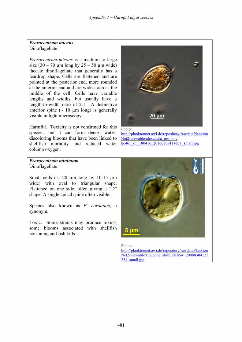
Appendix 1 – Harmful algal species

481

Prorocentrum micans Dinoflagellate Prorocentrum micans is a medium to large size (30 – 70 µm long by 25 – 50 µm wide) thecate dinoflagellate that generally has a teardrop shape. Cells are flattened and are pointed at the posterior end, more rounded at the anterior end and are widest across the middle of the cell. Cells have variable lengths and widths, but usually have a length-to-width ratio of 2:1. A distinctive anterior spine (~ 10 µm long) is generally visible in light microscopy. Harmful. Toxicity is not confirmed for this species, but it can form dense, water-discoloring blooms that have been linked to shellfish mortality and reduced water column oxygen.

Photo: http://planktonnet.awi.de/repository/rawdataPlanktonNet2/viewable/alexandra_pro_mic he461_e1_180416_20160509114831_small.jpg

Prorocentrum minimum Dinoflagellate Small cells (15-20 µm long by 10-15 µm wide) with oval to triangular shape. Flattened on one side, often giving a “D” shape. A single apical spine often visible. Species also known as P. cordatum, a synonym. Toxic. Some strains may produce toxins; some blooms associated with shellfish poisoning and fish kills.

Photo: http://planktonnet.awi.de/repository/rawdataPlanktonNet2/viewable/fjouenne_sbrbill0165w_20080304121251_small.jpg

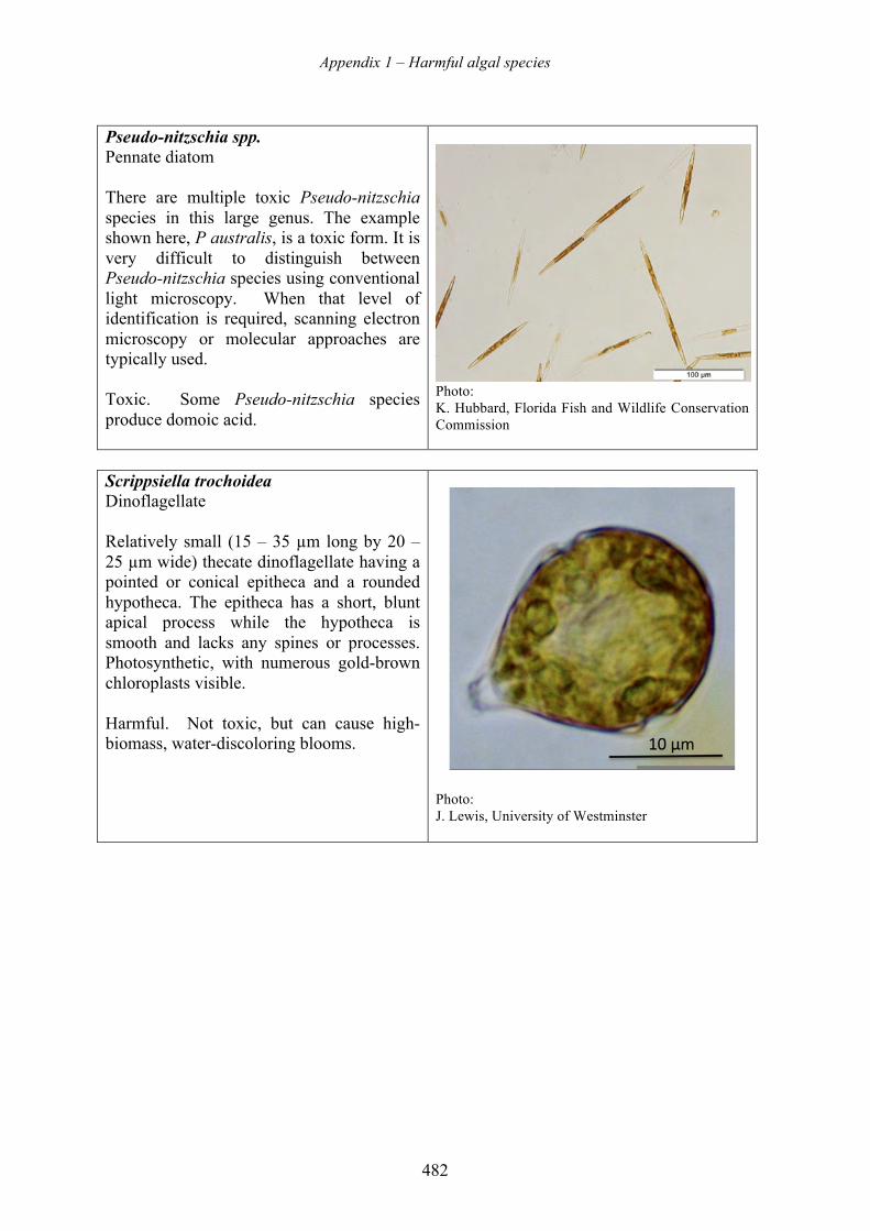
Appendix 1 – Harmful algal species

482

Pseudo-nitzschia spp. Pennate diatom There are multiple toxic Pseudo-nitzschia species in this large genus. The example shown here, P australis, is a toxic form. It is very difficult to distinguish between Pseudo-nitzschia species using conventional light microscopy. When that level of identification is required, scanning electron microscopy or molecular approaches are typically used. Toxic. Some Pseudo-nitzschia species produce domoic acid.

Photo: K. Hubbard, Florida Fish and Wildlife Conservation Commission

Scrippsiella trochoidea Dinoflagellate Relatively small (15 – 35 µm long by 20 – 25 µm wide) thecate dinoflagellate having a pointed or conical epitheca and a rounded hypotheca. The epitheca has a short, blunt apical process while the hypotheca is smooth and lacks any spines or processes. Photosynthetic, with numerous gold-brown chloroplasts visible. Harmful. Not toxic, but can cause high-biomass, water-discoloring blooms.

Photo: J. Lewis, University of Westminster

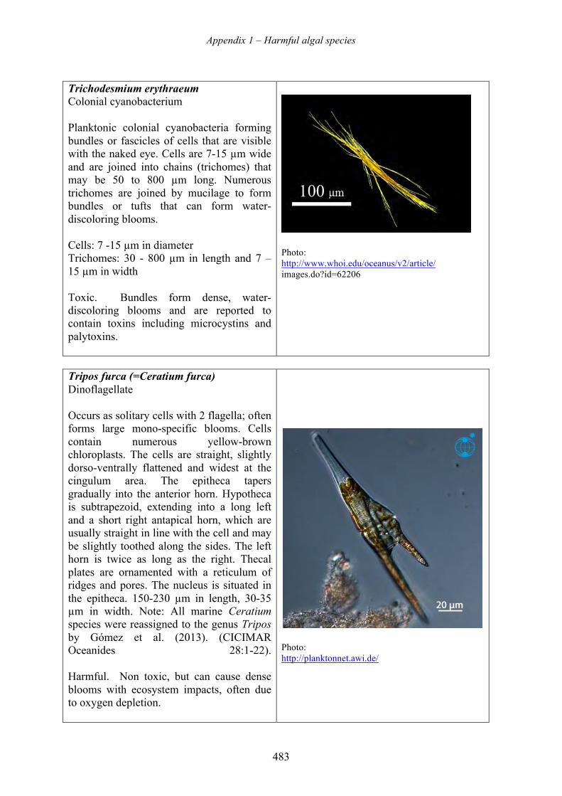
Appendix 1 – Harmful algal species

483

Trichodesmium erythraeum Colonial cyanobacterium Planktonic colonial cyanobacteria forming bundles or fascicles of cells that are visible with the naked eye. Cells are 7-15 µm wide and are joined into chains (trichomes) that may be 50 to 800 µm long. Numerous trichomes are joined by mucilage to form bundles or tufts that can form water-discoloring blooms. Cells: 7 -15 µm in diameter Trichomes: 30 - 800 µm in length and 7 – 15 µm in width Toxic. Bundles form dense, water-discoloring blooms and are reported to contain toxins including microcystins and palytoxins.

Photo: http://www.whoi.edu/oceanus/v2/article/ images.do?id=62206

Tripos furca (=Ceratium furca) Dinoflagellate Occurs as solitary cells with 2 flagella; often forms large mono-specific blooms. Cells contain numerous yellow-brown chloroplasts. The cells are straight, slightly dorso-ventrally flattened and widest at the cingulum area. The epitheca tapers gradually into the anterior horn. Hypotheca is subtrapezoid, extending into a long left and a short right antapical horn, which are usually straight in line with the cell and may be slightly toothed along the sides. The left horn is twice as long as the right. Thecal plates are ornamented with a reticulum of ridges and pores. The nucleus is situated in the epitheca. 150-230 µm in length, 30-35 µm in width. Note: All marine Ceratium species were reassigned to the genus Tripos by Gómez et al. (2013). (CICIMAR Oceanides 28:1-22). Harmful. Non toxic, but can cause dense blooms with ecosystem impacts, often due to oxygen depletion.

Photo: http://planktonnet.awi.de/

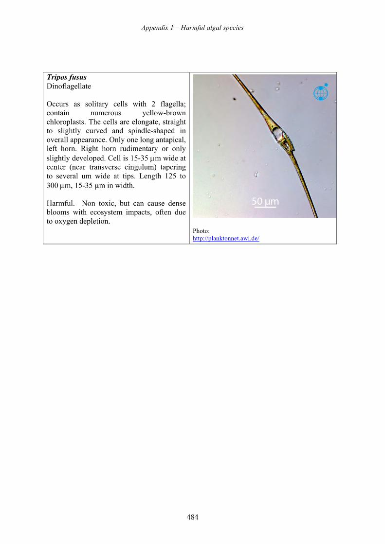
Appendix 1 – Harmful algal species

484

Tripos fusus Dinoflagellate Occurs as solitary cells with 2 flagella; contain numerous yellow-brown chloroplasts. The cells are elongate, straight to slightly curved and spindle-shaped in overall appearance. Only one long antapical, left horn. Right horn rudimentary or only slightly developed. Cell is 15-35 µm wide at center (near transverse cingulum) tapering to several um wide at tips. Length 125 to 300 µm, 15-35 µm in width. Harmful. Non toxic, but can cause dense blooms with ecosystem impacts, often due to oxygen depletion.

Photo: http://planktonnet.awi.de/

Appendix 2 – Rapid screening methods for HAB toxins

485

Appendix 2

RAPID SCREENING METHODS FOR HARMFUL ALGAL BLOOM TOXINS

Donald M. Anderson1, Maurice Laycock2, and Fernando Rubio3

1Woods Hole Oceanographic Institution, Woods Hole, MA USA

2Scotia Rapid Testing Ltd, Chester Basin, Nova Scotia Canada 3Abraxis LLC, Warminster, PA USA

1 Introduction .................................................................................................................................................485 2 ELISA methodology ...................................................................................................................................486

2.1 Abraxis ELISA kit for saxitoxin .........................................................................................................487 2.1.1 Principle .......................................................................................................................................487

2.2 Abraxis ADDA-DM ELISA kit for microcystins/nodularins .............................................................489 2.2.1 Principle .......................................................................................................................................489

2.3 Abraxis ELISA kit for Anatoxin-a (ATX) ..........................................................................................490 2.3.1 Principle .......................................................................................................................................490

2.4 Biosense ELISA Kit for Domoic acid (DA) .......................................................................................491 2.4.1 Principle .......................................................................................................................................491

3 Imunochromatographic or lateral flow format ............................................................................................492 3.1 The Scotia tests ....................................................................................................................................492

3.1.1 Principle .......................................................................................................................................492 3.2 Abraxis microcystins finished drinking water immunochromatographic tests ...................................494

3.2.2 Sample preparation methods .......................................................................................................494 3.2.2.1 Toxins from phytoplankton .................................................................................................495 3.2.2.2 Preparation of shellfish samples ..........................................................................................496

3.3 Obtaining quantitative data with Abraxis ELISA reader ....................................................................497 3.3.1 Essential steps to obtain data with the Abraxis + reader .............................................................497

4 Summary and conclusions ..........................................................................................................................499 5 References ...................................................................................................................................................499 1 INTRODUCTION

At the core of all national harmful algal bloom (HAB) programs are the monitoring programs needed to detect HAB toxins in shellfish, fish, water, or other resources sufficiently early to take management actions (Anderson et al. 2001). These programs measure toxins produced by multiple species of algae, with the methods used varying dramatically in scope and complexity due to the types of toxins that need to be detected, the nature of the affected resource, and regulatory requirements.

Some of the methods developed for analysis of shellfish tissues and algal blooms can be of direct use in desalination plants for analysis of toxins in water – both the raw, untreated water before desalination, and the treated, fresh water. A major concern, however, are the detection limits of the assays. All analytical methods have limits of detection (LODs) and the choice of a method should be consistent with potential bloom concentrations and possible toxin levels. With desalination plants, toxins need to be measured at exceedingly low levels in water, whereas shellfish concentrate toxins to much higher levels. A recent study summarized the epidemiological data for four common algal toxins (Laycock et al. 2010) and estimated the potential contamination of water that might enter a desalination plant during major blooms. The assessment was based on a hypothetical (and dense) bloom of toxic algae consisting of 107 cells/L with a toxin cell quota of 40 pg toxin/cell. If all of that toxin were released from the cells into the water, that would give a concentration in

Appendix 2 – Rapid screening methods for HAB toxins

486

seawater of 400 µg/L. An alternative approach to estimating the total amount of toxin present in a bloom is given in Chapter 1 (Table 1.4), where the amounts of toxin contained in hypothetical blooms of various common HAB species are presented. The values range from a few hundred to 1,000 µg/L. Given that 99% or more of a toxin is likely to be removed by thermal or reverse osmosis desalination (Chapter 10), the sensitivity of an analytical method must therefore be at least 0.1 – 1.0 µg/L or 0.1 – 1.0 ng/mL. Therefore, analysis of water samples for dissolved or particulate toxins (i.e., inside algal cells) will require high sensitivity methods, such as enzyme-linked immunosorbent assays (ELISAs). For example, the LOD for saxitoxin (STX) using the Abraxis STX ELISA kit is 0.02 ng/mL and there is similar sensitivity for domoic acid.

This appendix presents details on simple screening methods for HAB toxins. More complex analytical methods are described or cited in Chapter 2. The screening methods are presented here as a guide to desalination plant staff who wish to conduct on-site analyses. These analyses could be of raw intake water, treated water, or algal cell extracts from monitoring programs (Chapter 3). The example assays are restricted to four HAB toxins i.e., saxitoxins, domoic acid, microcystins/nodularins, and anatoxin-a. Although sample preparation procedures may differ for the other HAB toxins not include here, the commercial ELISA kit protocols are similar to each other. Sample preparation procedures, however, vary depending on solubility of the toxins, source (e.g., phytoplankton, shellfish, or cyanobacteria) and method of analysis. Sample preparation methods will be described in detail, as will procedures used to obtain samples. Methods of analysis other than ELISA are also presented.

Lateral flow tests (such as the Scotia tests) are described as simpler alternatives to the ELISA kits. The advantages and disadvantages of both tests will be discussed.

2 ELISA METHODOLOGY For the purpose of demonstrating antibody methods that are potentially useful for monitoring HAB toxins in water, four commercial ELISA kits are discussed here: saxitoxins (STXs), microcystins/nodularins (MCT/NOD), anatoxin-a (ATX) manufactured by Abraxis, and the domoic acid (DA), manufactured by Biosense Laboratories. Other kits are commercially available – these specific kits are presented as examples, not as endorsements.

Antibodies are especially useful for analysis of HAB toxins because of their high sensitivity and specificity. Since the introduction of the ELISA format in 1971 by Engvall and Perlmann (1971), this microtitre plate format has been used for thousands of clinical applications. For a review of ELISAs for shellfish toxins, see Usleber et al. (2001). Antibodies to the common HAB toxins are relatively easy to prepare using purified toxins conjugated to carrier proteins that are injected into rabbits or other animals from which crude serum can be used. Most other components for this technology are commercially available. Nevertheless, the basic ELISA requires a well-equipped laboratory and skill in performing the numerous steps involved. Equipment required includes a plate reader (Figure 1) and multi-channel pipettes.

There are several ELISA plate readers available commercially at a cost of approximately $10,000 (Figure 1). A plate reader also requires a computer to record and plot data. A simple reader is available from Abraxis for ~ $1,200 and is described below.

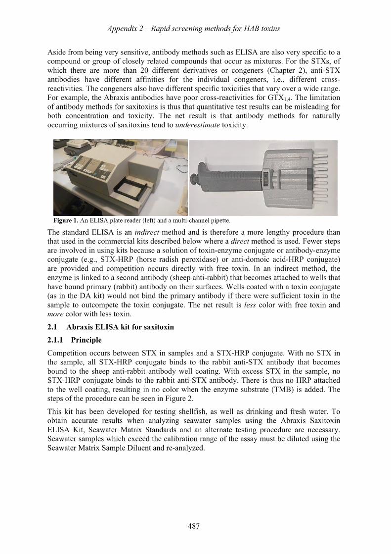
Appendix 2 – Rapid screening methods for HAB toxins

487

Aside from being very sensitive, antibody methods such as ELISA are also very specific to a compound or group of closely related compounds that occur as mixtures. For the STXs, of which there are more than 20 different derivatives or congeners (Chapter 2), anti-STX antibodies have different affinities for the individual congeners, i.e., different cross-reactivities. The congeners also have different specific toxicities that vary over a wide range. For example, the Abraxis antibodies have poor cross-reactivities for GTX1,4. The limitation of antibody methods for saxitoxins is thus that quantitative test results can be misleading for both concentration and toxicity. The net result is that antibody methods for naturally occurring mixtures of saxitoxins tend to underestimate toxicity.

The standard ELISA is an indirect method and is therefore a more lengthy procedure than that used in the commercial kits described below where a direct method is used. Fewer steps are involved in using kits because a solution of toxin-enzyme conjugate or antibody-enzyme conjugate (e.g., STX-HRP (horse radish peroxidase) or anti-domoic acid-HRP conjugate) are provided and competition occurs directly with free toxin. In an indirect method, the enzyme is linked to a second antibody (sheep anti-rabbit) that becomes attached to wells that have bound primary (rabbit) antibody on their surfaces. Wells coated with a toxin conjugate (as in the DA kit) would not bind the primary antibody if there were sufficient toxin in the sample to outcompete the toxin conjugate. The net result is less color with free toxin and more color with less toxin.

2.1 Abraxis ELISA kit for saxitoxin 2.1.1 Principle

Competition occurs between STX in samples and a STX-HRP conjugate. With no STX in the sample, all STX-HRP conjugate binds to the rabbit anti-STX antibody that becomes bound to the sheep anti-rabbit antibody well coating. With excess STX in the sample, no STX-HRP conjugate binds to the rabbit anti-STX antibody. There is thus no HRP attached to the well coating, resulting in no color when the enzyme substrate (TMB) is added. The steps of the procedure can be seen in Figure 2.

This kit has been developed for testing shellfish, as well as drinking and fresh water. To obtain accurate results when analyzing seawater samples using the Abraxis Saxitoxin ELISA Kit, Seawater Matrix Standards and an alternate testing procedure are necessary. Seawater samples which exceed the calibration range of the assay must be diluted using the Seawater Matrix Sample Diluent and re-analyzed.

Figure 1. An ELISA plate reader (left) and a multi-channel pipette.

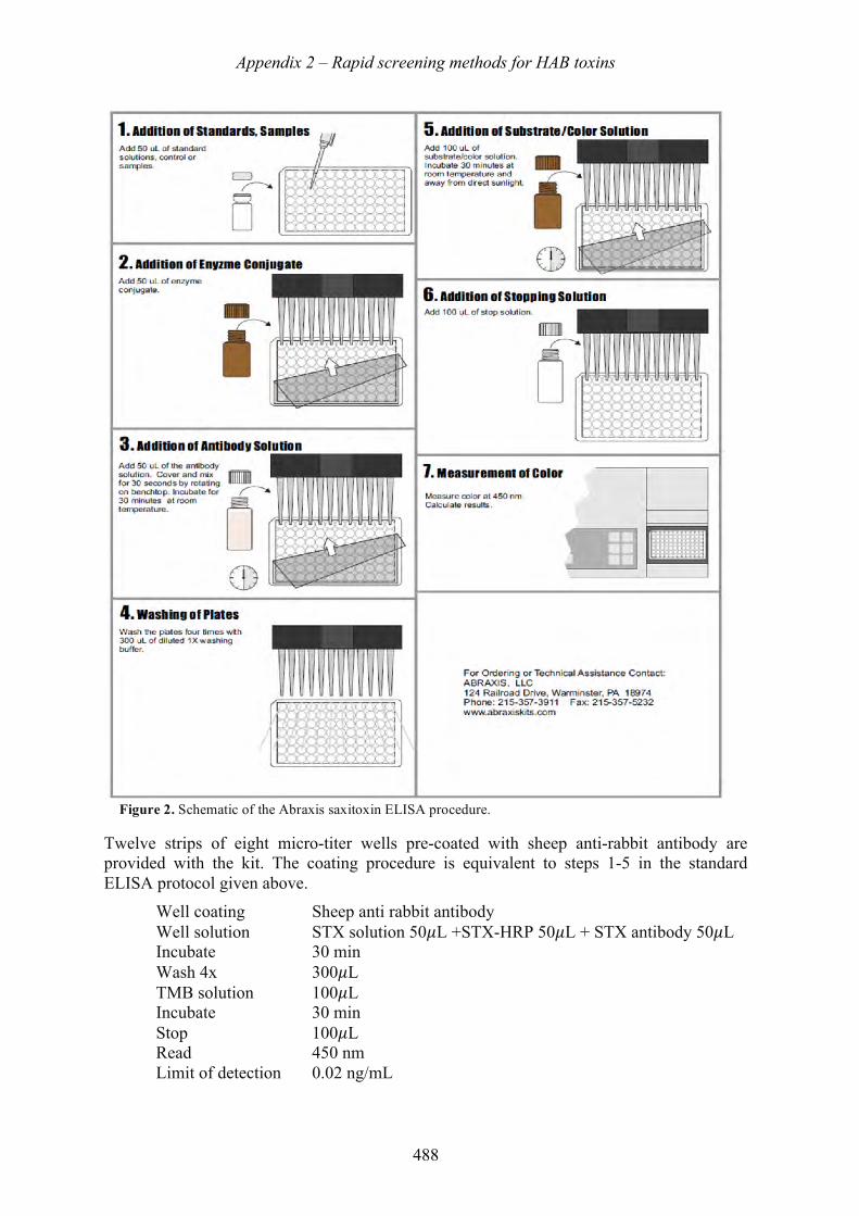
Appendix 2 – Rapid screening methods for HAB toxins

488

Twelve strips of eight micro-titer wells pre-coated with sheep anti-rabbit antibody are provided with the kit. The coating procedure is equivalent to steps 1-5 in the standard ELISA protocol given above.

Well coating Sheep anti rabbit antibody Well solution STX solution 50𝜇L +STX-HRP 50𝜇L + STX antibody 50𝜇L Incubate 30 min Wash 4x 300𝜇L TMB solution 100𝜇L Incubate 30 min Stop 100𝜇L Read 450 nm Limit of detection 0.02 ng/mL

Figure 2. Schematic of the Abraxis saxitoxin ELISA procedure.

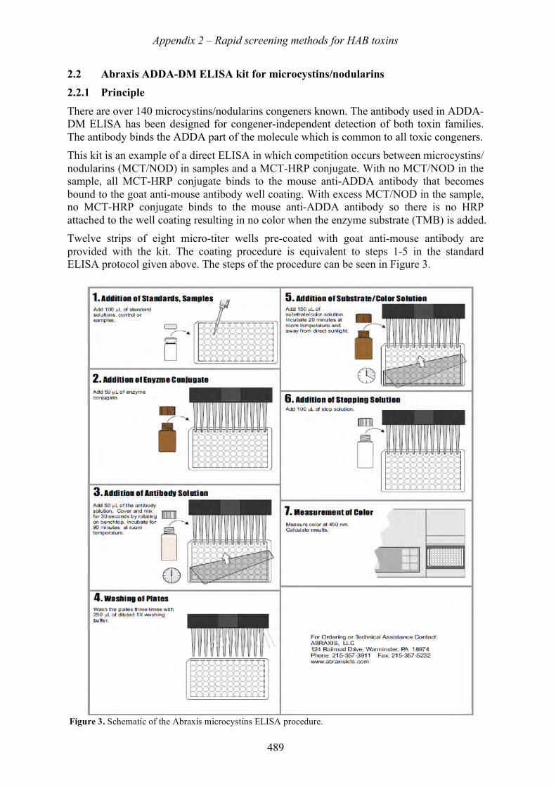
Appendix 2 – Rapid screening methods for HAB toxins

489

2.2 Abraxis ADDA-DM ELISA kit for microcystins/nodularins 2.2.1 Principle

There are over 140 microcystins/nodularins congeners known. The antibody used in ADDA-DM ELISA has been designed for congener-independent detection of both toxin families. The antibody binds the ADDA part of the molecule which is common to all toxic congeners. This kit is an example of a direct ELISA in which competition occurs between microcystins/ nodularins (MCT/NOD) in samples and a MCT-HRP conjugate. With no MCT/NOD in the sample, all MCT-HRP conjugate binds to the mouse anti-ADDA antibody that becomes bound to the goat anti-mouse antibody well coating. With excess MCT/NOD in the sample, no MCT-HRP conjugate binds to the mouse anti-ADDA antibody so there is no HRP attached to the well coating resulting in no color when the enzyme substrate (TMB) is added. Twelve strips of eight micro-titer wells pre-coated with goat anti-mouse antibody are provided with the kit. The coating procedure is equivalent to steps 1-5 in the standard ELISA protocol given above. The steps of the procedure can be seen in Figure 3.

Figure 3. Schematic of the Abraxis microcystins ELISA procedure.

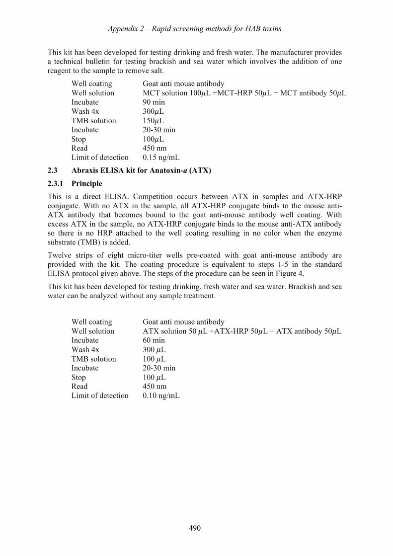
Appendix 2 – Rapid screening methods for HAB toxins

490

This kit has been developed for testing drinking and fresh water. The manufacturer provides a technical bulletin for testing brackish and sea water which involves the addition of one reagent to the sample to remove salt.

Well coating Goat anti mouse antibody Well solution MCT solution 100𝜇L +MCT-HRP 50𝜇L + MCT antibody 50𝜇L Incubate 90 min Wash 4x 300𝜇L TMB solution 150𝜇L Incubate 20-30 min Stop 100𝜇L Read 450 nm Limit of detection 0.15 ng/mL

2.3 Abraxis ELISA kit for Anatoxin-a (ATX)

2.3.1 Principle This is a direct ELISA. Competition occurs between ATX in samples and ATX-HRP conjugate. With no ATX in the sample, all ATX-HRP conjugate binds to the mouse anti-ATX antibody that becomes bound to the goat anti-mouse antibody well coating. With excess ATX in the sample, no ATX-HRP conjugate binds to the mouse anti-ATX antibody so there is no HRP attached to the well coating resulting in no color when the enzyme substrate (TMB) is added. Twelve strips of eight micro-titer wells pre-coated with goat anti-mouse antibody are provided with the kit. The coating procedure is equivalent to steps 1-5 in the standard ELISA protocol given above. The steps of the procedure can be seen in Figure 4.

This kit has been developed for testing drinking, fresh water and sea water. Brackish and sea water can be analyzed without any sample treatment.

Well coating Goat anti mouse antibody Well solution ATX solution 50 𝜇L +ATX-HRP 50𝜇L + ATX antibody 50𝜇L Incubate 60 min Wash 4x 300 𝜇L TMB solution 100 𝜇L Incubate 20-30 min Stop 100 𝜇L Read 450 nm Limit of detection 0.10 ng/mL

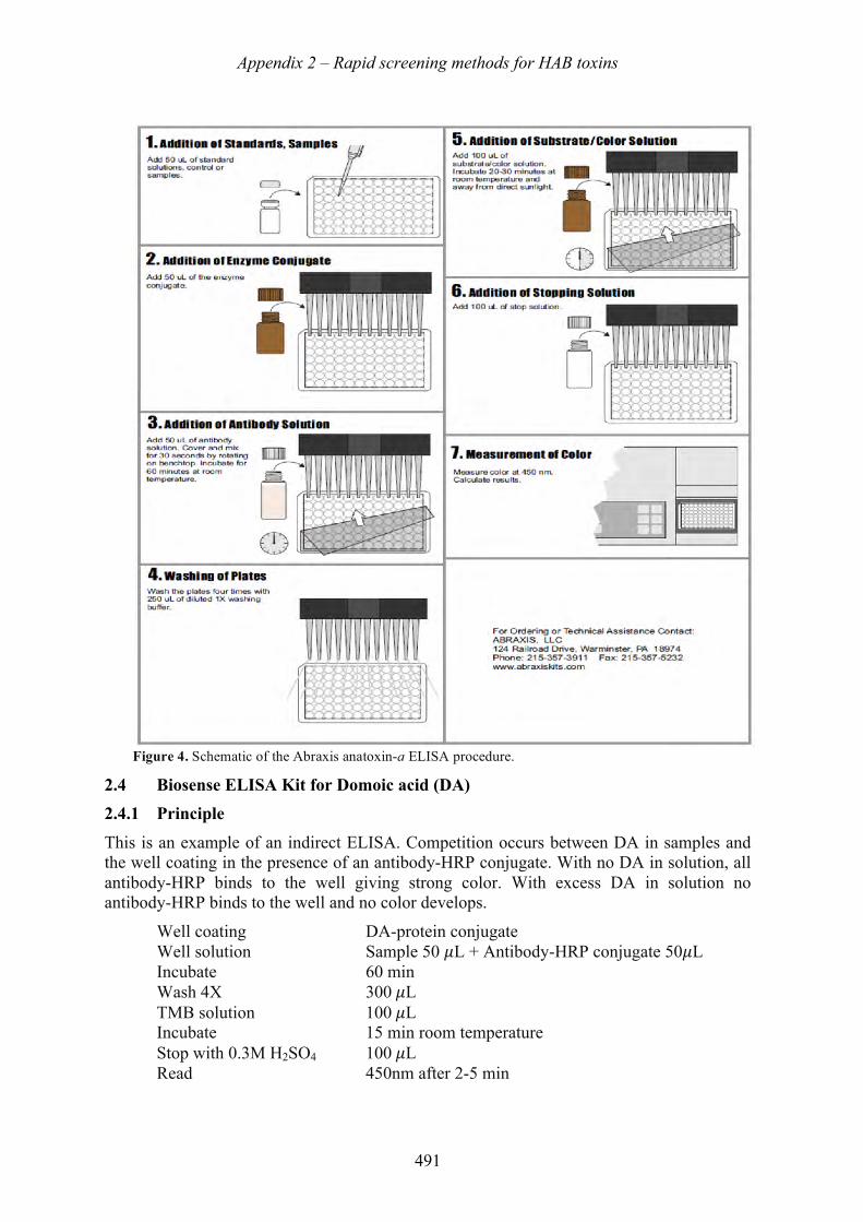
Appendix 2 – Rapid screening methods for HAB toxins

491

2.4 Biosense ELISA Kit for Domoic acid (DA) 2.4.1 Principle

This is an example of an indirect ELISA. Competition occurs between DA in samples and the well coating in the presence of an antibody-HRP conjugate. With no DA in solution, all antibody-HRP binds to the well giving strong color. With excess DA in solution no antibody-HRP binds to the well and no color develops.

Well coating DA-protein conjugate Well solution Sample 50 𝜇L + Antibody-HRP conjugate 50𝜇L Incubate 60 min Wash 4X 300 𝜇L TMB solution 100 𝜇L Incubate 15 min room temperature Stop with 0.3M H2SO4 100 𝜇L Read 450nm after 2-5 min

Figure 4. Schematic of the Abraxis anatoxin-a ELISA procedure.

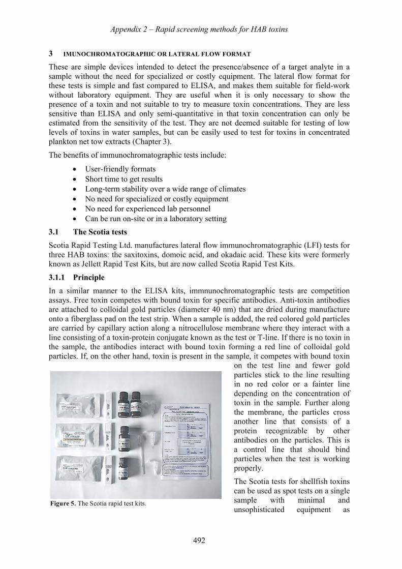
Appendix 2 – Rapid screening methods for HAB toxins

492

3 IMUNOCHROMATOGRAPHIC OR LATERAL FLOW FORMAT These are simple devices intended to detect the presence/absence of a target analyte in a sample without the need for specialized or costly equipment. The lateral flow format for these tests is simple and fast compared to ELISA, and makes them suitable for field-work without laboratory equipment. They are useful when it is only necessary to show the presence of a toxin and not suitable to try to measure toxin concentrations. They are less sensitive than ELISA and only semi-quantitative in that toxin concentration can only be estimated from the sensitivity of the test. They are not deemed suitable for testing of low levels of toxins in water samples, but can be easily used to test for toxins in concentrated plankton net tow extracts (Chapter 3).

The benefits of immunochromatographic tests include:

• User-friendly formats • Short time to get results • Long-term stability over a wide range of climates • No need for specialized or costly equipment • No need for experienced lab personnel • Can be run on-site or in a laboratory setting

3.1 The Scotia tests Scotia Rapid Testing Ltd. manufactures lateral flow immunochromatographic (LFI) tests for three HAB toxins: the saxitoxins, domoic acid, and okadaic acid. These kits were formerly known as Jellett Rapid Test Kits, but are now called Scotia Rapid Test Kits.

3.1.1 Principle In a similar manner to the ELISA kits, immnunochromatographic tests are competition assays. Free toxin competes with bound toxin for specific antibodies. Anti-toxin antibodies are attached to colloidal gold particles (diameter 40 nm) that are dried during manufacture onto a fiberglass pad on the test strip. When a sample is added, the red colored gold particles are carried by capillary action along a nitrocellulose membrane where they interact with a line consisting of a toxin-protein conjugate known as the test or T-line. If there is no toxin in the sample, the antibodies interact with bound toxin forming a red line of colloidal gold particles. If, on the other hand, toxin is present in the sample, it competes with bound toxin

on the test line and fewer gold particles stick to the line resulting in no red color or a fainter line depending on the concentration of toxin in the sample. Further along the membrane, the particles cross another line that consists of a protein recognizable by other antibodies on the particles. This is a control line that should bind particles when the test is working properly. The Scotia tests for shellfish toxins can be used as spot tests on a single sample with minimal and unsophisticated equipment as

Figure 5. The Scotia rapid test kits.

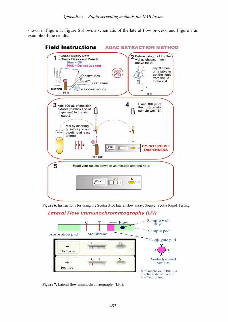
Appendix 2 – Rapid screening methods for HAB toxins

493

shown in Figure 5. Figure 6 shows a schematic of the lateral flow process, and Figure 7 an example of the results.

Figure 6. Instructions for using the Scotia STX lateral flow assay. Source: Scotia Rapid Testing.

Figure 7. Lateral flow immnochromatography (LFI).

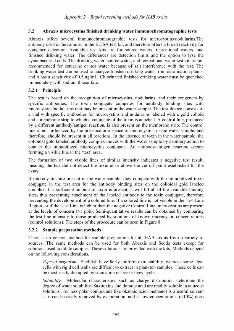
Appendix 2 – Rapid screening methods for HAB toxins

494

3.2 Abraxis microcystins finished drinking water immunochromatographic tests Abraxis offers several immunochromatographic tests for microcystins/nodularins.The antibody used is the same as in the ELISA test kit, and therefore offers a broad reactivity for congener detection. Available test kits are for source waters, recreational waters, and finished drinking water. The differences are detection limits and the option to lyse the cyanobacterial cells. The drinking water, source water, and recreational water test kit are not recommended for estuarine or sea water because of salt interference with the test. The drinking water test can be used to analyze finished drinking water from desalination plants, and it has a sensitivity of 0.5 ng/mL. Chlorinated finished drinking water must be quenched immediately with sodium thiosulfate.

3.2.1 Principle The test is based on the recognition of microcystins, nodularins, and their congeners by specific antibodies. The toxin conjugate competes for antibody binding sites with microcystins/nodularins that may be present in the water sample. The test device consists of a vial with specific antibodies for microcystins and nodularins labeled with a gold colloid and a membrane strip to which a conjugate of the toxin is attached. A control line, produced by a different antibody/antigen reaction, is also present on the membrane strip. The control line is not influenced by the presence or absence of microcystins in the water sample, and therefore, should be present in all reactions. In the absence of toxin in the water sample, the colloidal gold labeled antibody complex moves with the water sample by capillary action to contact the immobilized microcystins conjugate. An antibody-antigen reaction occurs forming a visible line in the ‘test’ area.

The formation of two visible lines of similar intensity indicates a negative test result, meaning the test did not detect the toxin at or above the cut-off point established for the assay. If microcystins are present in the water sample, they compete with the immobilized toxin conjugate in the test area for the antibody binding sites on the colloidal gold labeled complex. If a sufficient amount of toxin is present, it will fill all of the available binding sites, thus preventing attachment of the labeled antibody to the toxin conjugate, therefore preventing the development of a colored line. If a colored line is not visible in the Test Line Region, or if the Test Line is lighter than the negative Control Line, microcystins are present at the levels of concern (>1 ppb). Semi-quantitative results can be obtained by comparing the test line intensity to those produced by solutions of known microcystin concentrations (control solutions). The steps of the procedure can be seen in Figure 8.

3.2.2 Sample preparation methods There is no general method for sample preparation for all HAB toxins from a variety of sources. The same methods can be used for both Abraxis and Scotia tests except for solutions used to dilute samples. These solutions are provided with the kits. Methods depend on the following considerations.

Type of organism. Shellfish have fairly uniform extractability, whereas some algal cells with rigid cell walls are difficult to extract in plankton samples. These cells can be most easily disrupted by sonication or freeze-thaw cycles.

Solubility. Molecular characteristics such as charge distribution determine the degree of water solubility. Saxitoxins and domoic acid are readily soluble in aqueous solutions. For less polar compounds like okadaic acid, methanol is a useful solvent as it can be easily removed by evaporation, and at low concentrations (<10%) does

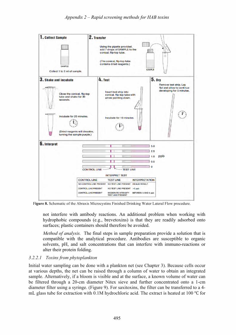
Appendix 2 – Rapid screening methods for HAB toxins

495

not interfere with antibody reactions. An additional problem when working with hydrophobic compounds (e.g., brevetoxins) is that they are readily adsorbed onto surfaces; plastic containers should therefore be avoided.

Method of analysis. The final steps in sample preparation provide a solution that is compatible with the analytical procedure. Antibodies are susceptible to organic solvents, pH, and salt concentrations that can interfere with immuno-reactions or alter their protein folding.

3.2.2.1 Toxins from phytoplankton Initial water sampling can be done with a plankton net (see Chapter 3). Because cells occur at various depths, the net can be raised through a column of water to obtain an integrated sample. Alternatively, if a bloom is visible and at the surface, a known volume of water can be filtered through a 20-cm diameter Nitex sieve and further concentrated onto a 1-cm diameter filter using a syringe. (Figure 9). For saxitoxins, the filter can be transferred to a 4-mL glass tube for extraction with 0.1M hydrochloric acid. The extract is heated at 100 for

Figure 8. Schematic of the Abraxis Microcystins Finished Drinking Water Lateral Flow procedure.

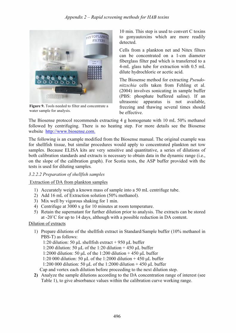
Appendix 2 – Rapid screening methods for HAB toxins

496

10 min. This step is used to convert C toxins to gonyautoxins which are more readily detected. Cells from a plankton net and Nitex filters can be concentrated on a 1-cm diameter fiberglass filter pad which is transferred to a 4-mL glass tube for extraction with 0.5 mL dilute hydrochloric or acetic acid.

The Biosense method for extracting Pseudo-nitzschia cells taken from Fehling et al. (2004) involves sonicating in sample buffer (PBS: phosphate buffered saline). If an ultrasonic apparatus is not available, freezing and thawing several times should be effective.

The Biosense protocol recommends extracting 4 g homogenate with 10 mL 50% methanol followed by centrifuging. There is no heating step. For more details see the Biosense website http://www.biosense.com.

The following is an example modified from the Biosense manual. The original example was for shellfish tissue, but similar procedures would apply to concentrated plankton net tow samples. Because ELISA kits are very sensitive and quantitative, a series of dilutions of both calibration standards and extracts is necessary to obtain data in the dynamic range (i.e., on the slope of the calibration graph). For Scotia tests, the ASP buffer provided with the tests is used for diluting samples.

3.2.2.2 Preparation of shellfish samples Extraction of DA from plankton samples

1) Accurately weigh a known mass of sample into a 50 mL centrifuge tube. 2) Add 16 mL of Extraction solution (50% methanol). 3) Mix well by vigorous shaking for 1 min. 4) Centrifuge at 3000 x g for 10 minutes at room temperature. 5) Retain the supernatant for further dilution prior to analysis. The extracts can be stored

at -20˚C for up to 14 days, although with a possible reduction in DA content. Dilution of extracts

1) Prepare dilutions of the shellfish extract in Standard/Sample buffer (10% methanol in PBS-T) as follows: 1:20 dilution: 50 µL shellfish extract + 950 µL buffer 1:200 dilution: 50 µL of the 1:20 dilution + 450 µL buffer 1:2000 dilution: 50 µL of the 1:200 dilution + 450 µL buffer 1:20 000 dilution: 50 µL of the 1:2000 dilution + 450 µL buffer 1:200 000 dilution: 50 µL of the 1:2000 dilution + 450 µL buffer

Cap and vortex each dilution before proceeding to the next dilution step. 2) Analyze the sample dilutions according to the DA concentration range of interest (see

Table 1), to give absorbance values within the calibration curve working range.

Figure 9. Tools needed to filter and concentrate a water sample for analysis.

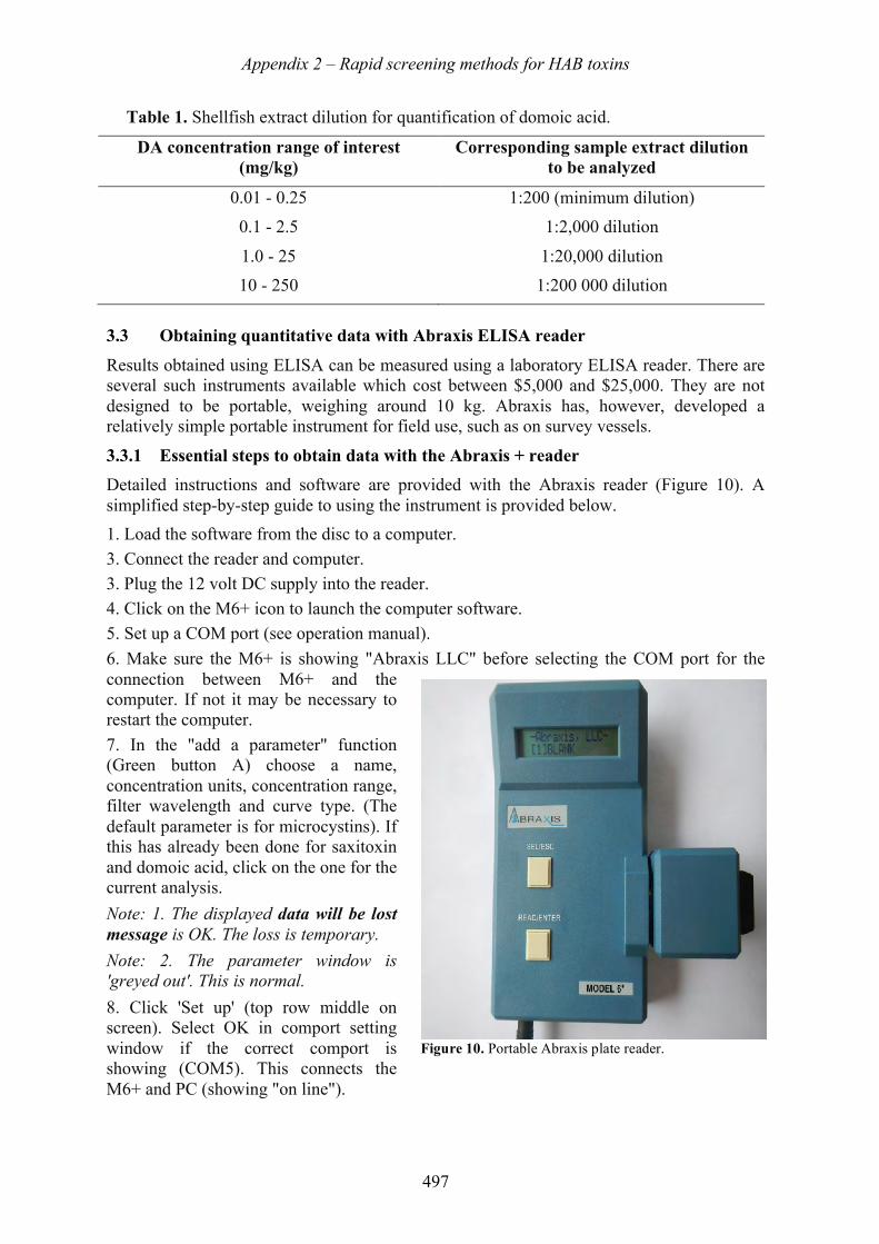
Appendix 2 – Rapid screening methods for HAB toxins

497

Table 1. Shellfish extract dilution for quantification of domoic acid.

DA concentration range of interest (mg/kg)

Corresponding sample extract dilution to be analyzed

0.01 - 0.25 0.1 - 2.5

1.0 - 25 10 - 250

1:200 (minimum dilution) 1:2,000 dilution

1:20,000 dilution 1:200 000 dilution

3.3 Obtaining quantitative data with Abraxis ELISA reader

Results obtained using ELISA can be measured using a laboratory ELISA reader. There are several such instruments available which cost between $5,000 and $25,000. They are not designed to be portable, weighing around 10 kg. Abraxis has, however, developed a relatively simple portable instrument for field use, such as on survey vessels.

3.3.1 Essential steps to obtain data with the Abraxis + reader Detailed instructions and software are provided with the Abraxis reader (Figure 10). A simplified step-by-step guide to using the instrument is provided below. 1. Load the software from the disc to a computer. 3. Connect the reader and computer. 3. Plug the 12 volt DC supply into the reader. 4. Click on the M6+ icon to launch the computer software. 5. Set up a COM port (see operation manual). 6. Make sure the M6+ is showing "Abraxis LLC" before selecting the COM port for the connection between M6+ and the computer. If not it may be necessary to restart the computer. 7. In the "add a parameter" function (Green button A) choose a name, concentration units, concentration range, filter wavelength and curve type. (The default parameter is for microcystins). If this has already been done for saxitoxin and domoic acid, click on the one for the current analysis. Note: 1. The displayed data will be lost message is OK. The loss is temporary. Note: 2. The parameter window is 'greyed out'. This is normal. 8. Click 'Set up' (top row middle on screen). Select OK in comport setting window if the correct comport is showing (COM5). This connects the M6+ and PC (showing "on line").

Figure 10. Portable Abraxis plate reader.

Appendix 2 – Rapid screening methods for HAB toxins

498

9. Click on the third green button (capture data) to take readings from a strip of wells. In the capture data window on the PC select "Clear sample data and get real time reading then OK. A blank must be taken at this stage. 10. The M6+ window should show: Abraxis LLC. If not, scroll round the options by pressing SEL/ESC several times until it appears. 11. Insert a strip with water (blank) in a well until it clicks into position in the light path then press READ/ENTER on the M6+. 12. The reading will be 0.000 ABS., then repeat before going to the next level 13. On M6+ press SEL/ESC twice to get to level [2] PARAMETER. Here the number of standards is shown, e.g. 6, but should correspond with those listed in the parameter with their respective concentrations. Press READ/ENTER to select the number of replicates. 14. In the screen on the M6+ the number of replicates can be selected. Unlike the number of standards which corresponds to the pre-determined PARAMETER any number of replicates can be chosen for the standards at this stage up to a maximum of 5 by pressing SEL/ESC repeatedly then press READ/ENTER. 15. Now the number of sample replicates can be chosen up to a maximum of 5 by pressing SEL/ESC repeatedly (usually 2). 16. Press SEL/ESC to get to level [3] STANDARD. Here the standards can be read. Press READ/ENTER to read the first Standard. The M6+ screen shows S1-1 Standard. Read Standard? Press READ/ENTER. The screen will show S1-1 and the absorbance (eg 0.528A). After S1-2 the PC screen will show the two values and the average. To move to standard number two press SEL/ESC. Move the strip to the next well and press READ/ENTER. Press SEL/ESC. The M6+ screen will ask if you want to continue. Press READ/ENTER to continue. 17. Move the strip of wells ahead after the replicates have been read for the standard. The readings and averages will appear on the PC screen under the Data tab. If they do not, repeat steps 9-17. After the second replicate of standard 6 the M6+ screen will show END. 18. To read the samples press SEL/ESC to go to level [4] SAMPLE. 19. Press READ/ENTER. M6+ screen shows T01-1 Sample and Read Sample? Press READ/ENTER repeatedly to read the replicates of the first sample. The PC screen will show the absorption values for each replicate and their average. 18. Continue through all samples, then click on the green button to stop reading. 19. To see the calibration graph and sample concentrations click on the quantitative tab to show the calibration graph and sample concentrations. 20. To print the quantitative results click File on the top line then print. If no printer is attached to the PC save as a pdf to an external memory (flash drive). 20. To save the data so that this existing calibration graph can be used for new samples without generating another graph each time samples are analyzed (and using up the limited number of wells) scroll up to [6] RS232 to PC in the M6+ window followed by READ/ENTER to M6 -OK->PC. Then capture data (third green button) by selecting upload batch data in the capture data window ("not clear sample data and get real-time reading" as before). Click OK in message window "Please load STD data". 21. Samples should be read using a calibration graph prepared at the same time. However, for approximate values calibration data in the memory can be used.

Appendix 2 – Rapid screening methods for HAB toxins

499

22. Select [6] RS232 to PC then enter to show M6->PC in the M6 window. Then Capture Data in the PC screen. 23. Select Upload batch data in the PC screen to show the data for calibration. 24. To read new samples using the uploaded calibration click on Capture Data button and select "Clear sample data and get real time reading, then OK. The sample data will be erased from the table under data in the PC screen. 25. Select [4] SAMPLE. The M6 screen will show "Rewrite Memory-are you sure? 26. Press read/enter on M6 and read the first new sample. If two replicates were chosen for samples - read again. 27. The new sample data will be shown in the Table in the Quantitative tab on the PC. 28. To save data after obtaining sample concentrations a. Under File select Load data b. Select the protocol, eg Saxitoxin c. Click on the data capture icon d. Select Real Time Reading e. Select Read Sample on M6+ f. Stop reading g. Save and give a new name 4 SUMMARY AND CONCLUSIONS

Desalination plants should establish a capability for screening samples for HAB toxins. This would not be a routine analysis, but instead an opportunistic approach triggered by identification of toxic cells in plankton samples, or other indications that toxic species are entering the plant. It is advisable for operators in areas subject to toxic HABs to have some lateral flow or ELISA kits on site, as it can take days or even weeks to get new kits during a crisis. ELISA kits are suitable for use when an estimate of toxin concentration is necessary. Lateral flow tests are more suitable than ELISA for routine monitoring of phytoplankton and shellfish extracts, but are not sensitive enough for water analysis, nor are they quantitative. If a positive result is indicated by the ELISA or the lateral flow tests, samples should be collected and evaluated with more sophisticated analytical instruments. A fully equipped analytical laboratory capable of measuring algal toxins is unrealistic at a desalination plant, but capabilities for HAB toxin analysis exist within many countries or regions at government agencies or universities. Operators should have contact details and sampling protocols prepared as part of their Alert Level Framework actions (Chapter 8) in the event that this type of external or outsourced analysis is required. Local or regional HAB experts should also be identified and contacted for guidance during potentially dangerous or damaging bloom events. 5 REFERENCES

Anderson, D. M., Andersen, P., Bricelj, V. M., Cullen, J. J., and Rensel, J. E. 2001. Monitoring and Management Strategies for Harmful Algal Blooms in Coastal Waters. Asia Pacific Economic Program, Singapore, and Intergovernmental Oceanographic Commission, Paris. 268 pp.

Engvall, E. and Perlmann, P. 1971. Enzyme-linked immunosorbent assay (ELISA) quantitative assay of immunoglobulin G. Immunochemistry 8(9), 871-874.

Appendix 2 – Rapid screening methods for HAB toxins

500

Fehling, J., Green, D. H., Davidson, K., Bolch, C. J., and Bates, S. S. 2004. Domoic acid production by Pseudo-nitzschia seriata (Bacillariophyceae) in Scottish waters. Journal of Phycology 40, 622-630.

Laycock, M. V., Donovan, M. A., and Easy, D. J. 2010. Sensitivity of lateral flow tests to mixtures of saxitoxins and applications to shellfish and phytoplankton monitoring. Toxicon 55, 597-605.

Usleber, E., Dietrich, R., Burk, C., Schneider, E., and Martlbauer, E. 2001. Immunoassay methods for paralytic shellfish poisoning toxins. Journal of AOAC International 84, 1649-1656.

Appendix 3 - Methods for measuring TEP and their precursors in seawater

501

Appendix 3

METHODS FOR MEASURING TRANSPARENT EXOPOLYMER PARTICLES AND THEIR PRECURSORS IN SEAWATER

Loreen O. Villacorte1,2, Jan C. Schippers1 and Maria D. Kennedy1

1UNESCO-IHE Delft Institute for Water Education, Delft, The Netherlands 2GRUNDFOS Holding A/S, Bjerringbro, Denmark (current affiliation)

1! Introduction ................................................................................................................................................... 501!2! TEP0.4µm method ............................................................................................................................................ 501!3! TEP10KDA method .......................................................................................................................................... 504!4! Storing water samples ................................................................................................................................... 507!5! References ..................................................................................................................................................... 507!

1! INTRODUCTION Transparent exopolymer particles (TEP) and their precursors produced by phyto-/bacterio-plankton in fresh and marine aquatic environments are increasingly considered as a major cause of organic/particulate fouling in MF/UF membranes and organic/particulate and biological fouling in SWRO membranes. The following sections comprise detailed descriptions of two methods for measuring transparent exopolymer particles in seawater, namely TEP0.4µm and TEP10kDa. The TEP0.4µm method measures transparent exopolymer particles retained by membrane filters having pores of 0.4 µm and conventionally known as TEP (Passow and Alldredge, 1995). The TEP10kDa method covers transparent exopolymer particles retained by membrane filters with molecular weight cut-off of 10 kDa. Consequently, this method covers both TEP and most (if not all) of their colloidal precursors. TEP0.4µm is a more rapid method than TEP10kDa and is recommended for routine TEP monitoring in untreated seawater. The TEP10kDa method is more time consuming, however, it gives much more information because it covers both TEP and their colloidal precursors. 2! TEP0.4µM METHOD The most widely used method for TEP, referred to here as TEP0.4µm, was developed in the mid-90s (Passow and Alldredge 1995). Recently, it was found that this method may overestimate TEP in seawater due to the reaction of Alcian blue (AB) with residual saline moisture on the filter (Villacorte 2014). To minimize this effect, Villacorte et al. (2015) proposed that the membrane with the retained TEPs be pre-rinsed with ultrapure water (UPW) before staining with AB. The modified procedure for measuring TEP0.4µm is illustrated in Figure 1 and is briefly described as follows: Preparation of Alcian blue dye solution

1.! The stock dye solution is prepared by dissolving 250 mg/L of Alcian blue in ultrapure water spiked with acetic acid to lower pH to 2.5. The prepared stock solution is stirred until most of the Alcian blue powder is dissolved (up to 18 hours). The working solution is prepared on the same day of analysis by filtering 20 mL of the stock solution through 0.05 µm polycarbonate (PC) membranes before staining. The remaining stock solution is stored in the dark at 4oC and a new stock solution should be prepared after 4 weeks.

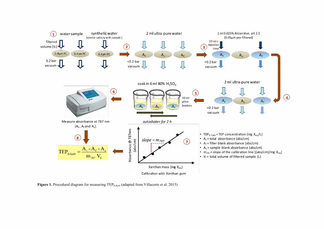
Figure 1. Procedural diagram for measuring TEP0.4µm (adapted from Villacorte et al. 2015)

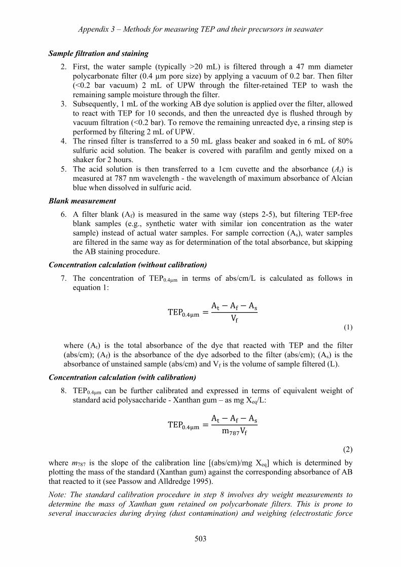
Appendix 3 – Methods for measuring TEP and their precursors in seawater

503

Sample filtration and staining

2.! First, the water sample (typically >20 mL) is filtered through a 47 mm diameter polycarbonate filter (0.4 µm pore size) by applying a vacuum of 0.2 bar. Then filter (<0.2 bar vacuum) 2 mL of UPW through the filter-retained TEP to wash the remaining sample moisture through the filter.

3.! Subsequently, 1 mL of the working AB dye solution is applied over the filter, allowed to react with TEP for 10 seconds, and then the unreacted dye is flushed through by vacuum filtration (<0.2 bar). To remove the remaining unreacted dye, a rinsing step is performed by filtering 2 mL of UPW.

4.! The rinsed filter is transferred to a 50 mL glass beaker and soaked in 6 mL of 80% sulfuric acid solution. The beaker is covered with parafilm and gently mixed on a shaker for 2 hours.

5.! The acid solution is then transferred to a 1cm cuvette and the absorbance (At) is measured at 787 nm wavelength - the wavelength of maximum absorbance of Alcian blue when dissolved in sulfuric acid.

Blank measurement

6.! A filter blank (Af) is measured in the same way (steps 2-5), but filtering TEP-free blank samples (e.g., synthetic water with similar ion concentration as the water sample) instead of actual water samples. For sample correction (As), water samples are filtered in the same way as for determination of the total absorbance, but skipping the AB staining procedure.

Concentration calculation (without calibration)

7.! The concentration of TEP0.4µm in terms of abs/cm/L is calculated as follows in equation 1:

TEP$.&'( = A+ − A- − A.V-

(1) where (At) is the total absorbance of the dye that reacted with TEP and the filter (abs/cm); (Af) is the absorbance of the dye adsorbed to the filter (abs/cm); (As) is the absorbance of unstained sample (abs/cm) and Vf is the volume of sample filtered (L).

Concentration calculation (with calibration)

8.! TEP0.4µm can be further calibrated and expressed in terms of equivalent weight of standard acid polysaccharide - Xanthan gum – as mg Xeq/L:

TEP$.&'( = A+ − A- − A.m121V-

(2)

where m787 is the slope of the calibration line [(abs/cm)/mg Xeq] which is determined by plotting the mass of the standard (Xanthan gum) against the corresponding absorbance of AB that reacted to it (see Passow and Alldredge 1995). Note: The standard calibration procedure in step 8 involves dry weight measurements to determine the mass of Xanthan gum retained on polycarbonate filters. This is prone to several inaccuracies during drying (dust contamination) and weighing (electrostatic force

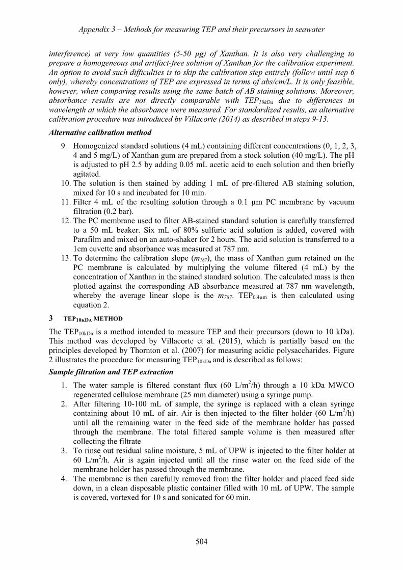
Appendix 3 – Methods for measuring TEP and their precursors in seawater

504

interference) at very low quantities (5-50 µg) of Xanthan. It is also very challenging to prepare a homogeneous and artifact-free solution of Xanthan for the calibration experiment. An option to avoid such difficulties is to skip the calibration step entirely (follow until step 6 only), whereby concentrations of TEP are expressed in terms of abs/cm/L. It is only feasible, however, when comparing results using the same batch of AB staining solutions. Moreover, absorbance results are not directly comparable with TEP10kDa due to differences in wavelength at which the absorbance were measured. For standardized results, an alternative calibration procedure was introduced by Villacorte (2014) as described in steps 9-13.

Alternative calibration method

9.! Homogenized standard solutions (4 mL) containing different concentrations (0, 1, 2, 3, 4 and 5 mg/L) of Xanthan gum are prepared from a stock solution (40 mg/L). The pH is adjusted to pH 2.5 by adding 0.05 mL acetic acid to each solution and then briefly agitated.

10.!The solution is then stained by adding 1 mL of pre-filtered AB staining solution, mixed for 10 s and incubated for 10 min.

11.!Filter 4 mL of the resulting solution through a 0.1 µm PC membrane by vacuum filtration (0.2 bar).

12.!The PC membrane used to filter AB-stained standard solution is carefully transferred to a 50 mL beaker. Six mL of 80% sulfuric acid solution is added, covered with Parafilm and mixed on an auto-shaker for 2 hours. The acid solution is transferred to a 1cm cuvette and absorbance was measured at 787 nm.

13.!To determine the calibration slope (m787), the mass of Xanthan gum retained on the PC membrane is calculated by multiplying the volume filtered (4 mL) by the concentration of Xanthan in the stained standard solution. The calculated mass is then plotted against the corresponding AB absorbance measured at 787 nm wavelength, whereby the average linear slope is the m787. TEP0.4µm is then calculated using equation 2.

3! TEP10KDA METHOD The TEP10kDa is a method intended to measure TEP and their precursors (down to 10 kDa). This method was developed by Villacorte et al. (2015), which is partially based on the principles developed by Thornton et al. (2007) for measuring acidic polysaccharides. Figure 2 illustrates the procedure for measuring TEP10kDa and is described as follows: Sample filtration and TEP extraction

1.! The water sample is filtered constant flux (60 L/m2/h) through a 10 kDa MWCO regenerated cellulose membrane (25 mm diameter) using a syringe pump.

2.! After filtering 10-100 mL of sample, the syringe is replaced with a clean syringe containing about 10 mL of air. Air is then injected to the filter holder (60 L/m2/h) until all the remaining water in the feed side of the membrane holder has passed through the membrane. The total filtered sample volume is then measured after collecting the filtrate

3.! To rinse out residual saline moisture, 5 mL of UPW is injected to the filter holder at 60 L/m2/h. Air is again injected until all the rinse water on the feed side of the membrane holder has passed through the membrane.

4.! The membrane is then carefully removed from the filter holder and placed feed side down, in a clean disposable plastic container filled with 10 mL of UPW. The sample is covered, vortexed for 10 s and sonicated for 60 min.

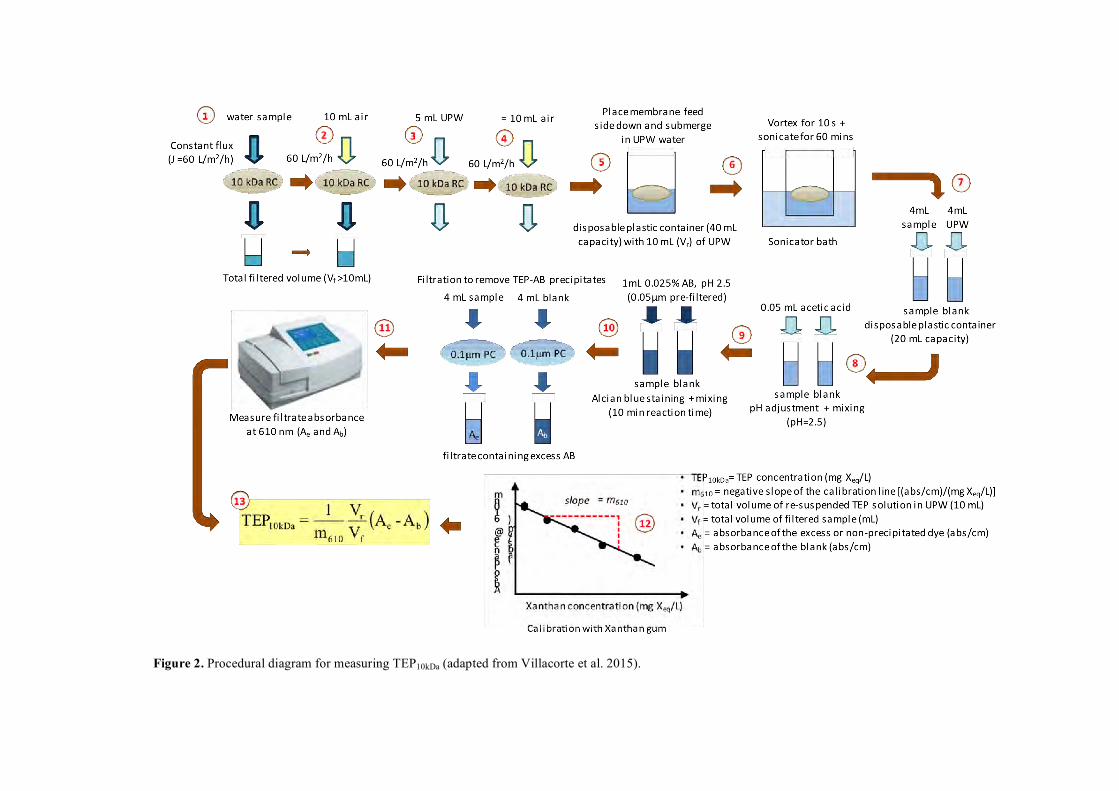
Figure 2. Procedural diagram for measuring TEP10kDa (adapted from Villacorte et al. 2015).

Appendix 3 - Methods for measuring TEP and their precursors in seawater

506

Staining and absorbance measurement

5.! Transfer 4 mL of the re-suspended TEP solution to a clean 20 mL disposable plastic container. To adjust the sample pH to 2.5, 0.05 mL of acetic acid solution is added to the solution.

6.! Add 1 mL of the working AB dye solution (for dye preparation see step 1 of TEP0.4µm method) to the sample, mix vigorously and leave to react for 10 min.

7.! Filter 4 mL sample of the TEP-AB solution through a 0.1 µm PC filter by vacuum filtration (<0.2 bar).

8.! The filtrate is collected in a plastic container (10 mL), transferred to a 1-cm cuvette and absorbance (Ae) at 610 nm wavelength - the wavelength of maximum absorbance (visible light range) of AB when dissolved in acetic acid solution - is measured with a spectrophotometer.

Blank measurement

9.! The blank absorbance (Ab) is measured to correct for the amount of stain adsorbed by the polycarbonate filter (0.1µm). This is performed following steps 5-8 but replacing the sample with UPW.

Concentration calculation (without calibration)

10.!The TEP10kDa concentration in absorbance per cm per liter of filter water (abs/cm/L) is calculated as follows:

TEP$%&'( =A+ − A-V/

(3)

where Ab is the absorbance of filtered blank (abs/cm), Ae is the absorbance of the excess or un-reacted dye (abs/cm) and Vf is the volume of filtered sample (mL).

Concentration calculation (with calibration)

11.!Alternatively, the TEP10kDa concentration can be calibrated and expressed in terms of mg Xanthan equivalent per litre (mg Xeq/L):

TEP$%&'( =1

12$%

V3V/

A- − A+

(4)

where m610 is the slope of the calibration curve [(abs/cm)/(mg Xeq/L)] and Vr is the total volume of the re-suspended TEP sample solution (i.e., 10 mL).

12.!For the calibration, standard solutions (4 mL) containing different concentrations (0, 1, 2, 3, 4 and 5 mg/L) of Xanthan gum are prepared from a homogenized stock solution. To adjust sample pH to 2.5, 0.05 mL acetic acid is added to each solution and then briefly agitated. The solution is then stained by adding 1 mL of pre-filtered AB staining solution, mixed for 10 seconds and incubated for 10 min.

13.!Filter 4 mL of the resulting solution through a 0.1 µm PC membrane by vacuum filtration (0.2 bar). The filtrate is collected, transferred to 1cm cuvette and absorbance is measured at 610 nm.

14.!The Xanthan concentration of the stained dye is plotted against the measured absorbance (excess dye absorbance) and the average linear slope is the m610. Since

Appendix 3 - Methods for measuring TEP and their precursors in seawater

507

concentration is inversely proportional to the excess dye absorbance, the calibration slope (m610) is always a negative value.

Note: The TEP10kDa concentration calculated using Eqn. 4 can be directly compared with TEP0.4µm calculated based on Eqn. 2 as both are calibrated with Xanthan gum standard. However, results for TEP10kDa calculated based on Eqn. 3 and TEP0.4µm calculated based on Eqn. 1 are not comparable as the absorbance values were measured at different wavelengths - 610nm and 787nm, respectively.

4! STORING WATER SAMPLES Storing samples for a period of time before analysis may lead to significant disparity between the measured and in-situ TEP concentration as a consequence of coagulation, bacterial release, bacterial degradation, adsorption on walls of sample bottles or a combination thereof. Bottle tests at 4oC temperature revealed that TEP0.4um concentration may increase over a period of time either due to coagulation of TEP precursors or through bacterial TEP release (Villacorte 2014). On the other hand, TEP10kDa concentration can rapidly decrease by up to 45% within the 3 days of storage resulting from either bacterial degradation or adsorption to walls of sample bottles (Villacorte 2014). Further investigations are still necessary to fully understand the mechanisms involved in the TEP loss or increase as well as to develop reliable measures to preserve TEP samples (e.g., sample bottle, freezing, preservative addition). It is therefore important that samples be analyzed immediately (within 24 hours) after sampling to obtain reliable TEP concentrations. For TEP10kDa, it is advisable to filter and then flush the sample immediately after sampling so the membrane can be kept at 4oC until analysis. 5! REFERENCES

Passow, U. and Alldredge, A. L. 1995. A dye-binding assay for the spectrophotometric measurement of transparent exopolymer particles (TEP). Limnology and Oceanography 40(7), 1326-1335.

Thornton, D. C. O., Fejes, E. M., Dimarco, S. F. and Clancy, K. M. 2007. Measurement of acid polysaccharides (APS) in marine and freshwater samples using alcian blue. Limnology and Oceanography: Methods 5, 73–87.

Villacorte, L. O. 2014. Algal blooms and membrane-based desalination technology. ISBN 978-1-138-02626-1, CRC Press/Balkema, Leiden.

Villacorte, L. O., Ekowati, Y., Calix-Ponce, H. N., Amy, G. L., Schippers, J. C., AND Kennedy, M. D. 2015. Improved method for measuring transparent exopolymer particles (TEP) and their precursors in fresh and saline water. Water Research 70 (1), 300–312.

Appendix 4 – Preservatives and methods for algal cell enumeration

509

Appendix 4

PRESERVATIVES AND METHODS FOR ALGAL CELL ENUMERATION

Donald M. Anderson1 and Bengt Karlson2 1Woods Hole Oceanographic Institution, Woods Hole MA USA

2Swedish Meteorological and Hydrological Institute, Gothenberg, Sweden

1 Introduction ................................................................................................................................................... 509 2 Miscellaneous supplies, recipes, and protocols ............................................................................................ 509

2.1 Preservatives .......................................................................................................................................... 509 2.1.1 Advantages of Lugol’s solution ..................................................................................................... 510 2.1.2 Advantages of formaldehyde ......................................................................................................... 510

2.2 Sample storage ...................................................................................................................................... 510 2.3 Settling chambers .................................................................................................................................. 510 2.4 Inverted microscope equipped with phase contrast and fluorescence ................................................... 511 2.5 Software that aids counting and data processing .................................................................................. 511 2.6 Manual cell counter ............................................................................................................................... 511 2.7 Qualification requirements for staff ...................................................................................................... 512 2.8 Assistance with species identification ................................................................................................... 512

3 Enumeration of phytoplankton using inverted microscopy (the utermöhl technique) .................................. 512 3.1 Equipment and reagents ........................................................................................................................ 512 3.2 Procedure ............................................................................................................................................... 512 3.3 Calculations ........................................................................................................................................... 515

4 Phytoplankton counting using a sedgewick rafter slide ................................................................................ 515 4.1 Procedure ............................................................................................................................................... 515

5 References ..................................................................................................................................................... 516

1 INTRODUCTION There are multiple ways to preserve phytoplankton samples and determine the algal species composition and abundance. This Appendix provides details on some of the most common methods. Additional relevant publications are included in Section 5, References. One of the most useful is Karlson et al. (2010), which can be downloaded at http://hab.ioc-unesco.org/index.php?option=com_oe&task=viewDocumentRecord&docID=5440. 2 MISCELLANEOUS SUPPLIES, RECIPES, AND PROTOCOLS 2.1 Preservatives

Lugol’s solution has proved to be a suitable preservative for many phytoplankton samples. The solution preserves the shape of the algal cells; for flagellated species, the flagella remain attached to the cells and the iodine staining of the algal cells gives a good contrast between the organisms and the background when using phase-contrast microscopy. For seawater samples, neutral or alkaline Lugol’s solution is most appropriate because calcareous flagellates (coccolithophorids) can comprise a considerable proportion of the algal biomass. If acidic Lugol’s solution is used, a parallel sample fixed in alkaline Lugol’s or with hexamine buffered formalin should be taken because the acid dissolves the calcareous casings (coccoliths) which are the basis for species determination of coccolithophorids. Diatoms, which have silicate cell walls, preserve well in acidic Lugols. In samples fixed with alkaline Lugol’s solution, fungal infections may occur, and for long-term storage, such samples should be post-fixed by adding a few drops of concentrated formalin solution. If the samples are to be stained with Calcofluor to enhance the pattern of cellulose plates on

Appendix 4 – Preservatives and methods for algal cell enumeration

510

armored dinoflagellates, it is an advantage to use neutral or basic Lugol’s solution or a buffered formaldehyde solution, because acid prevents staining of the cellulose.

If cells are rugged and do not distort, a 2-5% formaldehyde solution is generally used, working from a stock formalin sample (37% formaldehyde ) that is often acidified with acetic acid. Recipes for these fixatives follow:

Acidic Lugol’s solution: Potassium iodide (KI) 100 g, Distilled water 1000 mL, Iodine (I2) 50 g, Acetic acid glacial (100 % CH3COOH) 100 g, Neutral Lugol’s solution, Potassium iodide (KI) 100 g, Distilled water 1000 mL, Iodine (I2) 50 g.

Alkaline (basic) Lugol’s solution: Potassium iodide (KI) 100 g, Distilled water 1000 mL, Iodine (I2) 50 g, Sodium acetate (CH3COONa) 100 g.

Neutral, weakly basic formalin solution: Analytical quality formalin is diluted to 20 % (1 part concentrated solution to 1 part distilled water). 100 g hexamethylenetetramine (hexamine) C6H12N4 is added to 1 L of the 20 % formaldehyde solution. Acidic formalin: Equal amounts of analytical quality formalin (formaldehyde 37 %) and concentrated acetic acid are mixed.

2.1.1 Advantages of Lugol’s solution Lugol’s enters the cell more quickly than formaldehyde, leaving shock-sensitive organisms better preserved in the sample. The specific weight of organisms is increased by iodine, resulting in faster settling times. Detection of phytoplankton cells is made easier by the enhanced contrast between organisms and the surrounding fluid. The iodine stains starch, aiding recognition of those groups of algae (e.g. Chlorophyta) which use this as a storage compound.

2.1.2 Advantages of formaldehyde Formaldehyde is a good fixing and preserving agent for cells that have a relatively rigid cell wall, as the cell wall structures and other characteristics such as eye spots remain visible. When stored properly in appropriate bottles, samples will stay in good condition for many years without attention. Autofluorescence of chlorophyll-a, though decaying, remains intact for at least several days if the samples are stored in constant dark.

2.2 Sample storage Preserved phytoplankton samples should be stored in the dark at room temperature to prevent photo-oxidation. The maximum storage time for iodine (Lugols)-fixed samples that have been stored in a dark and cool place (1 to 5 °C) is 12 months. During this period, the samples should be checked every second month and topped up with Lugol’s solution if necessary (the sample should be golden brown in color, like tea). Reference material should be collected and stored in suitable separate sample bottles. For all phytoplankton samples to be stored for more than 3 to 4 months, dark glass bottles are the preferred container.

2.3 Settling chambers If an inverted microscope is to be used (which is highly recommended), consider purchasing the Hydrobios Combined Plate Chamber (Utermöhl-Chamber) set or the equivalent, with one cylinder each of 10, 50, and 100 mLs (Figure 1). Three cover plates are also needed. There

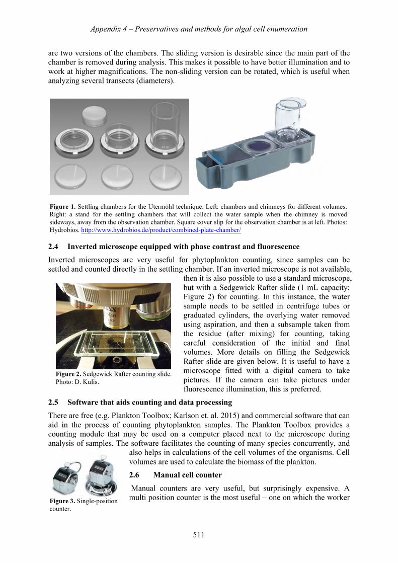
Appendix 4 – Preservatives and methods for algal cell enumeration

511

are two versions of the chambers. The sliding version is desirable since the main part of the chamber is removed during analysis. This makes it possible to have better illumination and to work at higher magnifications. The non-sliding version can be rotated, which is useful when analyzing several transects (diameters).

2.4 Inverted microscope equipped with phase contrast and fluorescence Inverted microscopes are very useful for phytoplankton counting, since samples can be settled and counted directly in the settling chamber. If an inverted microscope is not available,

then it is also possible to use a standard microscope, but with a Sedgewick Rafter slide (1 mL capacity; Figure 2) for counting. In this instance, the water sample needs to be settled in centrifuge tubes or graduated cylinders, the overlying water removed using aspiration, and then a subsample taken from the residue (after mixing) for counting, taking careful consideration of the initial and final volumes. More details on filling the Sedgewick Rafter slide are given below. It is useful to have a microscope fitted with a digital camera to take pictures. If the camera can take pictures under fluorescence illumination, this is preferred.

2.5 Software that aids counting and data processing There are free (e.g. Plankton Toolbox; Karlson et. al. 2015) and commercial software that can aid in the process of counting phytoplankton samples. The Plankton Toolbox provides a counting module that may be used on a computer placed next to the microscope during analysis of samples. The software facilitates the counting of many species concurrently, and

also helps in calculations of the cell volumes of the organisms. Cell volumes are used to calculate the biomass of the plankton. 2.6 Manual cell counter

Manual counters are very useful, but surprisingly expensive. A multi position counter is the most useful – one on which the worker

Figure 1. Settling chambers for the Utermöhl technique. Left: chambers and chimneys for different volumes. Right: a stand for the settling chambers that will collect the water sample when the chimney is moved sideways, away from the observation chamber. Square cover slip for the observation chamber is at left. Photos: Hydrobios. http://www.hydrobios.de/product/combined-plate-chamber/

Figure 2. Sedgewick Rafter counting slide. Photo: D. Kulis.

Figure 3. Single-position counter.

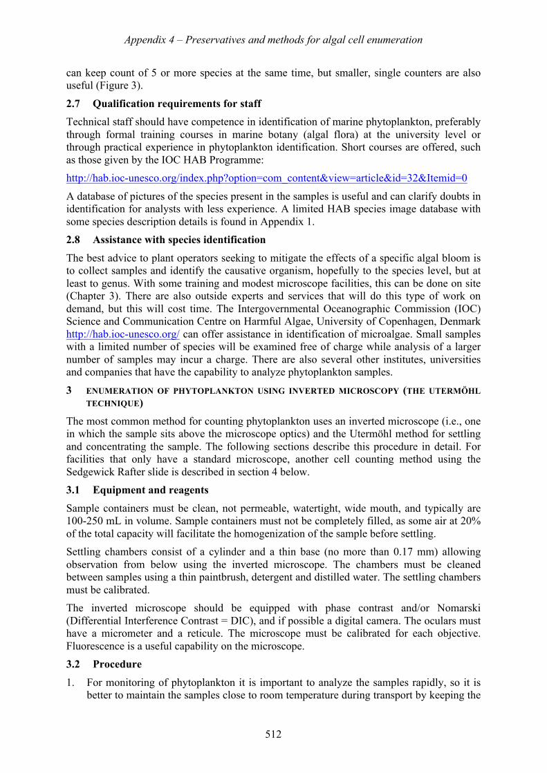
Appendix 4 – Preservatives and methods for algal cell enumeration

512

can keep count of 5 or more species at the same time, but smaller, single counters are also useful (Figure 3).

2.7 Qualification requirements for staff Technical staff should have competence in identification of marine phytoplankton, preferably through formal training courses in marine botany (algal flora) at the university level or through practical experience in phytoplankton identification. Short courses are offered, such as those given by the IOC HAB Programme: http://hab.ioc-unesco.org/index.php?option=com_content&view=article&id=32&Itemid=0

A database of pictures of the species present in the samples is useful and can clarify doubts in identification for analysts with less experience. A limited HAB species image database with some species description details is found in Appendix 1. 2.8 Assistance with species identification

The best advice to plant operators seeking to mitigate the effects of a specific algal bloom is to collect samples and identify the causative organism, hopefully to the species level, but at least to genus. With some training and modest microscope facilities, this can be done on site (Chapter 3). There are also outside experts and services that will do this type of work on demand, but this will cost time. The Intergovernmental Oceanographic Commission (IOC) Science and Communication Centre on Harmful Algae, University of Copenhagen, Denmark http://hab.ioc-unesco.org/ can offer assistance in identification of microalgae. Small samples with a limited number of species will be examined free of charge while analysis of a larger number of samples may incur a charge. There are also several other institutes, universities and companies that have the capability to analyze phytoplankton samples.

3 ENUMERATION OF PHYTOPLANKTON USING INVERTED MICROSCOPY (THE UTERMÖHL TECHNIQUE)

The most common method for counting phytoplankton uses an inverted microscope (i.e., one in which the sample sits above the microscope optics) and the Utermöhl method for settling and concentrating the sample. The following sections describe this procedure in detail. For facilities that only have a standard microscope, another cell counting method using the Sedgewick Rafter slide is described in section 4 below. 3.1 Equipment and reagents

Sample containers must be clean, not permeable, watertight, wide mouth, and typically are 100-250 mL in volume. Sample containers must not be completely filled, as some air at 20% of the total capacity will facilitate the homogenization of the sample before settling. Settling chambers consist of a cylinder and a thin base (no more than 0.17 mm) allowing observation from below using the inverted microscope. The chambers must be cleaned between samples using a thin paintbrush, detergent and distilled water. The settling chambers must be calibrated. The inverted microscope should be equipped with phase contrast and/or Nomarski (Differential Interference Contrast = DIC), and if possible a digital camera. The oculars must have a micrometer and a reticule. The microscope must be calibrated for each objective. Fluorescence is a useful capability on the microscope. 3.2 Procedure

1. For monitoring of phytoplankton it is important to analyze the samples rapidly, so it is better to maintain the samples close to room temperature during transport by keeping the

Appendix 4 – Preservatives and methods for algal cell enumeration

513

samples inside a cooler with cooling blocks. On arrival to the laboratory, the samples should be placed on the bench. A portion of the sample is saved for live examination and another portion preserved (if this was not done in the field) and either stored or settled. To demonstrate that the temperature in the room and the temperature in the sample are close, a thermometer for the air temperature in the laboratory and other thermometer to measure temperature in the water sample are used. In a notebook, records are kept of the code of the sample, the complete reference of the sample, the date and hour of settling, the number and volume of the settling chamber, temperature in the laboratory and in the sample, and the analyst who did the settling.

2. During sample storage, suspended particles settle out and (small) algae become indiscernible by incorporation in detritus aggregates or by adhesion to other large algal cells. Resuspension and separation of particles before settling them in the Utermöhl chamber can be achieved by shaking the sample as gently as possible. The method used for manual shaking should be described clearly in order to minimize differences between operators. A combination of alternating horizontally rolling and vertical turning upside down of the sample bottle for a specific number of times provides better mixing than straightforward shaking. The homogenization of the samples must be gentle, combining circular horizontal movements with vertical movements.

3. One subsample is maintained alive for in vivo examination and another is preserved in Lugols. Samples must be preserved as soon as possible after collection. Live samples must be observed within 36 h. Preserved samples must be stored in the dark; room temperature is appropriate if the analysis is done within 3 weeks. Otherwise, refrigerate at 4oC. Lugol’s- fixed samples can be stored for 1 year in the dark and at temperatures between 1-5ºC; for longer periods of storage it is necessary to add formaldehyde.

4. The volume of the settling chamber must be adapted to the type of waters to be analyzed: 100 mL for oligotrophic waters, 50 mL for mesotrophic, 5-25 mL for eutrophic. For nanoplankton and picoplankton the settling chambers of 100 mL are not adequate and require preconcentration. The settling chambers must be placed on a horizontal surface, all the chamber must be filled with the sample without air spaces, and the chamber must be closed using a glass cover. The bench must be free of vibrations. The recommended settling time depends on the volume (height) of the chamber, 48 h for 100 mL, 24 h for 50 mL, 12 h for 25 mL, 8 h for 10 mL, 3 h for 2 mL. After settling, the cylinder is displaced and a glass cover is placed on top of the chamber.

5. Preserved samples must be acclimated to the ambient temperature, homogenized and transferred directly from the container to the settling chamber. Temperature differences between sedimentation chamber and medium may produce convection currents that have differential effects on the settling of phytoplankton species, depending on their physical properties. Furthermore, bubbles may develop in relatively cold samples as the solubility of gases declines with the gradual rise of the temperature of the sample. When the temperature of the chamber is higher than that of the sub-sample, the larger and heavier particles tend to concentrate towards the chamber wall and the smallest particles more towards the center of the chamber. If the subsample has a higher temperature, the smallest particles collect near the chamber wall.

6. There are three counting strategies; the strategy to choose depends on the abundance and size of each species.

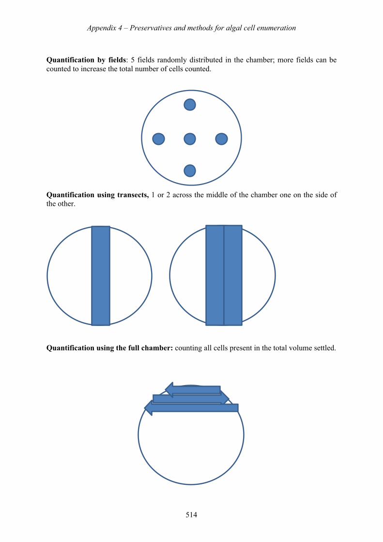
Appendix 4 – Preservatives and methods for algal cell enumeration

514

Quantification by fields: 5 fields randomly distributed in the chamber; more fields can be counted to increase the total number of cells counted.

Quantification using transects, 1 or 2 across the middle of the chamber one on the side of the other.

Quantification using the full chamber: counting all cells present in the total volume settled.

Appendix 4 – Preservatives and methods for algal cell enumeration

515

For the 3 strategies, it is necessary to define a normal procedure for the quantification of cells at the boundary of the field; for example, do not include cells lying across the top line and the left line but include the cells crossing the lower and the right lines of the reticule.

As a general rule, if a precision of 5% in the estimation of the mean number of cells per sample is required, then 400 objects should be counted. It makes no difference whether 10 fields are counted with 40 objects per field or 80 fields with just 5 objects. It is, however, sometimes difficult to count 400 cells, so in practice, the number of cells counted should be at least 50-100 cells in total for each dominant species. The area to be counted should be adjusted to reach this number of cells. For some species this will not be possible because they are in low density. In that case, the full chamber should be examined. 3.3 Calculations

The following equation related the number of cells per unt volume to the area examined:

N=avAdX

N is the number of cells per unit volume (e.g., cells/mL) X is the average number of cells per field, transect or full chamber A is the area of the chamber v is the volume of the chamber. If the result is in mL then we use mL, if the result is in L we will use L a is the area of the total field counted d is the dilution factor (when the sample is diluted)

Example of calculations for the case of counting 10 cells in a full chamber (area 529.13 mm2) after settling 50 mL.

N = 10 * 529.13 * 1 = 0.2 cells/mL = 200 cells/L 529.13 * 50 mL 4 PHYTOPLANKTON COUNTING USING A SEDGEWICK RAFTER SLIDE

For laboratories that do not have an inverted microscope, an alternative to the Utermohl’s technique is to use a Sedgewick Rafter slide (SRS) and a regular compound microscope (see sction 2.4). The Sedgewick Rafter slide holds exactly one mL. The thickness of the slide generally restricts magnification to 200X or lower.

4.1 Procedure The SRS without grid with cover glasses is available from Wildlife Supply Company, 95 Botsford Place, Buffalo NY 14216 (www.wildco.com ). Two styles are available – one without, and one with grids. The latter is useful if only a portion of the slide is to be counted. 1. The preserved sample can be counted directly if the cell concentrations are high enough,

or the sample can be concentrated by settling a known volume in a graduated cylinder for several days, with the settled material careful removed from the bottom with a pipette, and its volume measured.

2. Swirl the sample manually or with a mechanical agitator or vortexer to randomize the organisms.

Appendix 4 – Preservatives and methods for algal cell enumeration

516

3. Withdraw a 1.0 mL sample and dispense it into the SRS. This is best accomplished by rotating the cover slip so that it sits diagonally across the SRS such that small openings are in each diagonal corner. The sample is pipetted into one open corner, and air exits from the other opening. When the slide is full, straighten the cover slip so there are no more openings. Placement of the cover glass limits the volume to 1 mL.

4. The gridded SRS has 20 rows, 50 columns, and 1000 squares. Using a microscope magnification that allows the cells of interest to be easily identified, move the microscope stage laterally, counting cells within a gridded row. Repeat with a return transect across the slide, either directly below the first transect, or randomly – the latter if only a portion of the slide is to be scanned. Have a consistent policy for cells that fall on a line. For example, do not include cells lying across the top line, but do count those lying across the bottom line. Try to count 100 - 400 algal cells, and calculate cells/mL from that. For example, if you counted 150 cells in 8 rows, you have 150 * 20/8 = 375 cells/mL. This should be multiplied by the concentration factor determined from the settling step in # 1 above, if that was done.

5. Note that if you have a non-gridded SRS, you can still count less than the entire slide. Just move the microscope stage horizontally, counting all cells that are visible in the field of view, and then when the edge of the chamber is reached, slide the field of view vertically to a new, random position, and then scan horizontally to the opposite edge. Repeat with another random scan. Keep track of the number of horizontal scans until you have counted 100 – 400 cells of interest. You can then count how many horizontal scans there are along the vertical edge of the SRS, and use the same approach described above for the gridded SRS to calculate a cell concentration.

5 REFERENCES Edler, L. and Elbrächter, M. 2010. The Utermöhl method for quantitative phytoplankton

analysis. In: Microscopic and molecular methods for quantitative phytoplankton analysis, Eds. Karlson, B., Cusack, C. and Bresnan, E. Intergovernmental Oceanographic Commission Manual and guides, pp 13-20.

EN 15204. 2006. Water quality - Guidance standard on the enumeration of phytoplankton using inverted microscopy (Utermöhl technique).

Hallegraeff, G. M., Anderson D. M., and Cembella, A. D. 2003. Manual on Harmful Marine Microalgae UNESCO Publishing.Hasle, G. R. 1978. The inverted-microscope method, p. 88–96. In A. Sournia [ed.], Phytoplankton Manual. UNESCO.

Karlson, B., Andreasson, A., Johansen, M., Mohlin, M., Skjevik, A-T., and Strömberg, P. 2015. Plankton Toolbox – open source software making it easier to work with plankton data, Proceedings of the 16th International Conference on Harmful Algal Blooms, 27 Oct. to 1 November, 2014, Wellington, New Zealand.

Software available at http://nordicmicroalgae.org/tools Karlson, B., Cusack, C., and Bresnan, E. (Eds.) 2010. Microscopic and molecular methods

for quantitative phytoplankton analysis. Paris, UNESCO. (IOC Manuals and Guides, no. 55.). 110 pages. http://hab.ioc-unesco.org/index.php?option=com_oe&task=viewDocumentRecord&docID=5440

Appendix 4 – Preservatives and methods for algal cell enumeration

517

LeGresley, M., and McDermott, G. 2010. Counting chamber methods for quantitative phytoplankton analysis - haemocytometer, Palmer-Maloney cell and Sedgewick-Rafter cell. in: Microscopic and molecular methods for quantitative phytoplankton analysis, Eds. Karlson, B., Cusack, C. and Bresnan, E. Intergovernmental Oceanographic Commission Manual and guides, pp 25-30.

Moestrup, Ø., Akselman, R., Cronberg, G., Elbraechter, M., Fraga, S., Halim, Y., Hansen, G., Hoppenrath, M., Larsen, J., Lundholm, N., Nguyen, L. N., and Zingone, A. (Eds) 2016. IOC-UNESCO Taxonomic Reference List of Harmful Micro Algae. Available online at http://www.marinespecies.org/hab/

Utermöhl, H. 1958. Zur vervollkommnung der quantitativen phytoplankton-methodik. Mitt. int. Ver. theor. angew. Limnology 9, 1–38.

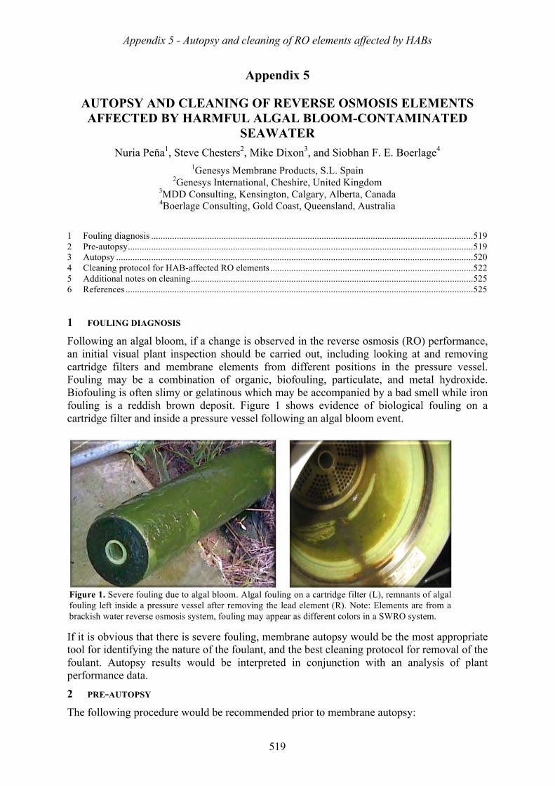
Appendix 5 - Autopsy and cleaning of RO elements affected by HABs

519

Appendix 5

AUTOPSY AND CLEANING OF REVERSE OSMOSIS ELEMENTS AFFECTED BY HARMFUL ALGAL BLOOM-CONTAMINATED

SEAWATER Nuria Peña1, Steve Chesters2, Mike Dixon3, and Siobhan F. E. Boerlage4

1Genesys Membrane Products, S.L. Spain 2Genesys International, Cheshire, United Kingdom

3MDD Consulting, Kensington, Calgary, Alberta, Canada 4Boerlage Consulting, Gold Coast, Queensland, Australia

1 Fouling diagnosis .......................................................................................................................................... 519 2 Pre-autopsy .................................................................................................................................................... 519 3 Autopsy ......................................................................................................................................................... 520 4 Cleaning protocol for HAB-affected RO elements ....................................................................................... 522 5 Additional notes on cleaning ......................................................................................................................... 525 6 References ..................................................................................................................................................... 525

1 FOULING DIAGNOSIS

Following an algal bloom, if a change is observed in the reverse osmosis (RO) performance, an initial visual plant inspection should be carried out, including looking at and removing cartridge filters and membrane elements from different positions in the pressure vessel. Fouling may be a combination of organic, biofouling, particulate, and metal hydroxide. Biofouling is often slimy or gelatinous which may be accompanied by a bad smell while iron fouling is a reddish brown deposit. Figure 1 shows evidence of biological fouling on a cartridge filter and inside a pressure vessel following an algal bloom event.

If it is obvious that there is severe fouling, membrane autopsy would be the most appropriate tool for identifying the nature of the foulant, and the best cleaning protocol for removal of the foulant. Autopsy results would be interpreted in conjunction with an analysis of plant performance data.

2 PRE-AUTOPSY The following procedure would be recommended prior to membrane autopsy:

Figure 1. Severe fouling due to algal bloom. Algal fouling on a cartridge filter (L), remnants of algal fouling left inside a pressure vessel after removing the lead element (R). Note: Elements are from a brackish water reverse osmosis system, fouling may appear as different colors in a SWRO system.

Appendix 5 - Autopsy and cleaning of RO elements affected by HABs

520

• The first element from the SWRO first pass should be chosen for autopsy, although best characterization of plant status would be obtained by autopsying elements from both the first and last positions of the pressure vessel. Note that for two-pass seawater desalination plants, it is unlikely that harmful algal bloom (HAB) fouling will be evident in the second pass, as low fouling permeate from the SWRO is the feedwater.

• Membrane elements should be wrapped in dark plastic and taped securely to ensure that water is retained within the element. This is necessary for accurate microbiological analysis and deposit characterization. Dry membrane elements yield unrepresentative samples that can give false results.

• Do not use any chemicals for membrane preservation before sample delivery. Otherwise, microbiological count results will not be representative.

• Membrane elements should be sent for autopsy the day of removal. If membrane(s) cannot be shipped immediately, store horizontally in a cool dark place. It is important to avoid light and high temperatures.

In addition to membrane elements, further samples could be analyzed for complementary information about the algal bloom:

• Water samples from different points in the pretreatment process;

• Silt density index (SDI) membrane discs from different points in the pretreatment process; and

• Cartridge filters 3 AUTOPSY

Autopsy involves different tests and analyses that should be carried out in order to obtain a final diagnosis. This process includes the following steps that should be followed during algal bloom events: External and internal inspection of membrane element

During the inspection, failure due to a significant presence of fouling would be verified. Fouling after an algal bloom would be expected to:

• Appear organic, with development of a biofilm on the RO membrane surface;

• Be a sticky deposit with a high content of water that would probably also adhere to the spacer material; and

• Exhibit different coloration depending upon the type of algal bloom and fouling content.

Analyses of foulant

• The LOI (loss on ignition) test is a common and widely used method to estimate the organic content of foulants. A very high organic matter content would be expected (>60%), although the high sodium chloride content in seawater systems could interfere with the measurement.

• Optical microscopy analysis for algae identification (see Chapter 3, Appendix 3). Analyses of foulant samples and membrane surface samples

• Scanning electronic microscopy with Energy Dispersive X-ray detection (SEM-EDX): with this analytical technique it is possible to get an elemental analysis of

Appendix 5 - Autopsy and cleaning of RO elements affected by HABs

521

fouling and inspection at very high magnifications. This method can assist in identifying colloidal, scaling, and metal hydroxide fouling, but cannot identify biofouling.

• Infrared spectroscopy (IR): This technique provides information related to the presence of specific functional groups and it is a very good tool for identification of organic components. For algal bloom fouling it would verify the presence of biopolymeric substances such as polysaccharides and proteins produced during an algal bloom.

• Liquid Chromatography - Organic Carbon - Organic Nitrogen Detection (LC-OCD-OND): a very accurate tool for the characterization of natural organic matter including biopolymers (see Chapter 5).

Analyses of foulant samples and membrane surface samples for Algal Organic Matter At present, there is no standard test protocol for determining Algal Organic Matter (AOM) deposits on RO membranes or spacers. HAB research studies have examined the accumulation of organic deposits using LC-OCD and staining of the membrane/spacer using Alcian blue in membrane autopsies (Villacorte 2014).

• TEP deposits can be identified by staining a sample of RO membranes and/or spacer with a solution of Alcian blue (see Appendix 3 for preparation) followed by rinsing with ultrapure water.

• The stained samples are then viewed by an optical microscope. The presence of a blue/green stained deposit is indicative of the presence of TEP. It cannot distinguish between TEP which may have originated from algae and/or bacteria in the feedwater or generated by biofilm growth in the membrane.

• For more quantitative information on the deposit on RO membranes/spacers following a HAB bloom, Villacorte (2014) submerged samples of membrane and spacer in a known quantity of ultrapure water and sonicated for 1 hour to extract the organic matter accumulated on the membrane.

• The extracted solutions can then be analyzed for TEP0.4µm and TEP10kDa (see Appendix 3) and natural organic matter such as biopolymer concentrations using LC-OCD as described above.

The identification of NOM constituents such as TEP could assist in determining the appropriate cleaning agent/chemical. Microbiological counts

• A very high presence of microorganisms would be expected in the biofilm on the membrane surface after an algal bloom.

• Characteristic microorganisms would be: bacteria (aerobic and anaerobic), moulds, and yeasts, etc. Results would be recorded as UFC/cm2.

Biocide tests

Based on microbiological counts, biocide tests would be carried out to determine the most suitable biocide for biofilm removal.

Sampling for membrane performance parameters and cleaning tests Once the nature of fouling has been identified, it is important to know the effect of the foulant on membrane performance. By working with membrane coupons on a flat sheet test

Appendix 5 - Autopsy and cleaning of RO elements affected by HABs

522

rig it is possible to examine the permeate flux and salt rejection conditions of a membrane after an algal bloom. If the membrane was not damaged during algal bloom operation and there is fouling present, a decrease in both permeate flux at constant applied pressure and salt rejection would be expected.

Different cleaning tests should be carried out in order to choose the most suitable cleaner and optimal cleaning conditions (e.g., concentration, contact time, temperature) as the incorrect cleaning agent may cause a further loss in membrane performance. Depending upon the results obtained during the biocide tests, an additional biocide step should be tested and included in the final cleaning protocol if appropriate. Integrity tests

An important impact of fouling on reverse osmosis membranes is the damage that can be caused on the polyamide layer and on their rejection capabilities (Peña et al. 2013). Therefore, integrity tests should be carried out in order to check if the polyamide layer has suffered irreversible damage during operation after fouling due to algal bloom. Considering the nature of fouling after an algal bloom, it is very common to observe increases in differential pressure that can produce physical damage on the membrane surface.

The methylene blue test would detect this kind of damage, staining damaged areas blue. Care should be taken not to scratch or damage the membrane during the autopsy process.

4 CLEANING PROTOCOL FOR HAB-AFFECTED RO ELEMENTS Before cleaning RO elements, operators are advised to review the technical manual, technical bulletins, or specification sheets for each element type used. Common manufacturers’ literature is below:

• Hydranautics: Foulants and Cleaning Procedures, TSB-107, http://www.membranes.com/docs/tsb/TSB107.pdf

• Dow Filmtec: Filmtec Reverse Osmosis Membranes Technical Manual, Section 6, page 121, http://www.dow.com/en-us/water-and-process-solutions/resources/resource-finder

• Toray: Operation, Maintenance and Handling Manual, TMM-300, 310, 320, 330, 340, 350, http://www.toraywater.com/knowledge/pdf/HandlingManual.pdf

While general cleaning solutions are presented below, specially formulated cleaners are available from RO chemical suppliers that are more effective than standard commodity chemicals. Globally there are many common RO cleaning chemical suppliers such as (but not limited to); Genesys, Avista, PWT Chemicals, Nalco, Alkema Solutions, GE, and BASF. It is very important always to follow membrane manufacturers’ guidelines. While most SWRO elements will tolerate pH 2 - 12, care should be taken as some RO membrane elements will only withstand high pH values for short periods of time (e.g. 30min) or may only withstand lower alkaline pH (e.g. pH 11.0). Cleaning fluid volume should be on the order of 35 - 40 liters per 8” element and made with permeate water (rather than feedwater).

Table 1 shows a common cleaning procedure for HAB-affected RO elements where organic, biological plus iron fouling, may occur. Ideally the clean should consist of a high pH clean to soften and remove organics, biofilm and algae (Step 1), followed by a biocide in extreme cases to kill these organisms (Step 2), Step 1 is repeated to remove dead organisms and the remainder of the organics, and finally a low pH acid clean (Step 4) to remove carbonates and iron and generally restore the membranes. In order to restore membrane plant performance as quickly as possible after an algal bloom event has fouled the membranes, proprietary cleaners

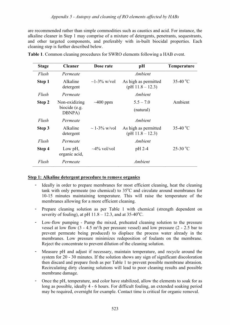
Appendix 5 - Autopsy and cleaning of RO elements affected by HABs

523

are recommended rather than simple commodities such as caustics and acid. For instance, the alkaline cleaner in Step 1 may comprise of a mixture of detergents, penetrants, sequestrants, and other targeted components, and preferably with in-built biocidal properties. Each cleaning step is further described below.

Table 1. Common cleaning procedures for SWRO elements following a HAB event.

Step 1: Alkaline detergent procedure to remove organics

-­ Ideally in order to prepare membranes for most efficient cleaning, heat the cleaning tank with only permeate (no chemical) to 35oC and circulate around membranes for 10-15 minutes maintaining temperature. This will raise the temperature of the membranes allowing for a more efficient cleaning.

-­ Prepare cleaning solution as per Table 1 with chemical (strength dependent on severity of fouling), at pH 11.8 – 12.3, and at 35-40oC.

-­ Low-flow pumping - Pump the mixed, preheated cleaning solution to the pressure vessel at low flow (3 - 4.5 m³/h per pressure vessel) and low pressure (2 - 2.5 bar to prevent permeate being produced) to displace the process water already in the membranes. Low pressure minimizes redeposition of foulants on the membrane. Reject the concentrate to prevent dilution of the cleaning solution.

-­ Measure pH and adjust if necessary, maintain temperature, and recycle around the system for 20 - 30 minutes. If the solution shows any sign of significant discoloration then discard and prepare fresh as per Table 1 to prevent possible membrane abrasion. Recirculating dirty cleaning solutions will lead to poor cleaning results and possible membrane damage.

-­ Once the pH, temperature, and color have stabilized, allow the elements to soak for as long as possible, ideally 4 - 6 hours. For difficult fouling, an extended soaking period may be required, overnight for example. Contact time is critical for organic removal.

Stage Cleaner Dose rate pH Temperature

Flush Permeate Ambient Step 1 Alkaline

detergent ~1-3% w/vol As high as permitted

(pH 11.8 – 12.3) 35-40 oC

Flush Permeate Ambient

Step 2 Non-oxidizing biocide (e.g.

DBNPA)

~400 ppm 5.5 – 7.0 (natural)

Ambient

Flush Permeate Ambient

Step 3 Alkaline detergent

~ 1-3% w/vol As high as permitted (pH 11.8 – 12.3)

35-40 oC

Flush Permeate Ambient Step 4 Low pH,

organic acid, ~4% vol/vol pH 2-4 25-30 oC

Flush Permeate Ambient

Appendix 5 - Autopsy and cleaning of RO elements affected by HABs

524

-­ High-flow pumping. Feed the cleaning solution at high flow rates (8 - 10.2 m3/h at 1.5 - 4.0 bar) for 30 - 60 minutes. The high flow rate flushes out the foulants removed from the membrane surface by the cleaning.

-­ Flush with good quality permeate to return to natural pH levels.

Step 2: Non-oxiding biocide to remove biofouling

-­ Prepare cleaning solution with non-oxidizing biocide.

-­ Low-flow pumping - Pump the mixed, preheated cleaning solution to the pressure vessel at low flow (3-4.5 m³/h per pressure vessel) and low pressure (2 - 2.5 bar to prevent permeate being produced) to displace the process water already in the membranes. Low pressure minimizes redeposition of foulants on the membrane. Reject the concentrate to prevent dilution of the cleaning solution.

-­ Measure pH and adjust if necessary, and recycle around the system for 20 minutes. If the solution shows any sign of significant discoloration then discard and prepare fresh as per above to prevent possible membrane abrasion. Recirculating dirty cleaning solutions will lead to poor cleaning results and possible membrane damage.

-­ Once the pH, temperature, and color have stabilized, allow the elements to soak for as long as possible. One hour should be sufficient unless biological fouling is very severe. For difficult fouling, an extended soaking period (several hours) may be required followed by further recirculation.

-­ High-flow pumping. Feed the cleaning solution at high flow rates (8 - 10.2 m3/h at 1.5 - 4.0 bar) for 30 - 60 minutes. The high flow rate flushes out the foulants removed from the membrane surface by the cleaning.

-­ Flush with good quality permeate to natural pH levels.

Step 3: Alkaline procedure (Repeat of Step 1)

Biocide application works best if applied between alkaline cleanings. The first alkaline application “softens” the fouling, allowing the biocide to penetrate and kill the microorganisms, and the second alkaline cleaning step optimizes their removal. Step 4: Low pH, organic acid procedure to remove iron hydroxide fouling

If iron hydroxide fouling is present in addition to biofouling:

-­ Ideally, in order to prepare membranes for most efficient cleaning, heat the cleaning tank with permeate only to 30oC and circulate around membranes for 10 - 15 minutes maintaining temperature, this will allow for more efficient cleaning.

-­ Prepare cleaning solution as per Table 1 with low pH, organic acid (such as citric acid), at around pH 2 - 4, and heat to 25-30oC

-­ Low-flow pumping. Pump the mixed, preheated cleaning solution to the vessel at low flow (3-4.5 m³/h per pressure vessel) and low pressure to displace the process water.

-­ Measure pH and adjust if necessary, maintain temperature and recycle around the system for 20-30 minutes. If the solution shows any sign of significant discoloration then discard and prepare fresh as per above to prevent possible membrane abrasion.

-­ Once the pH, temperature and color has stabilized allow the elements to soak for as long as possible ideally 2-4 hours. For difficult fouling an extended soaking period may be required, overnight for example.

Appendix 5 - Autopsy and cleaning of RO elements affected by HABs

525

-­ High-flow pumping. Feed the cleaning solution at high flow rates (8 - 10.2 m3/h at 1.5 - 4.0 bar) for 30-60 minutes. The high flow rate flushes out the foulants removed from the membrane surface by the cleaning.

-­ Flush with good quality permeate to return to natural pH levels.

5 ADDITIONAL NOTES ON CLEANING Always measure the pH during cleaning. If the pH increases more than 0.5 pH units during acid cleaning, more acid needs to be added. If the pH decreases more than 0.5 pH units during alkaline cleaning, more caustic needs to be added.

Long soak times should be broken up with short circulation periods. It is possible for the cleaning solution to become fully saturated and the foulants can deposit back onto the membrane surface. In addition, the temperature will decrease during this period, therefore the soaking becomes less effective. It is recommended to circulate the solution regularly in order to maintain the temperature (temperature should not drop more than 5°C) and add chemicals if the pH needs to be adjusted. Soaking times may be reduced if it is felt that no more deposits are being removed. Turbid or strong-colored cleaning solutions should be replaced with a freshly prepared solution to avoid recirculating foulants around the system causing membrane damage. 6 REFERENCES

Peña, N., Gallego, S., del Vigo, F. and Chesters, S. P. 2013. Evaluating impact of fouling on reverse osmosis membranes performance, Desalination and Water Treatment 51, 958-961.

Villacorte, L. O. 2014. Algal blooms and membrane-based desalination technology. Ph.D. thesis UNESCO-IHE/TUDelft, ISBN 978-1-138-02626-1, CRC Press/Balkema, Leiden.

527

INDEX

A

Abengoa pilot plant, 338, 343, 410Abraxis ELISA Kit for Anatoxin-a, 485, 490 Abraxis ELISA Kit for Saxitoxin, 485, 487 Abraxis ELISA Reader, 485, 497acidic formalin, 510acidic Lugol's solution, 509-510; see Lugol'sacidic polysaccharides, 504acoustic Doppler current profiler, 92; see

ADCPADCP, 92; see acoustic Doppler current

profilerADDA-DM ELISA kit for

Microcystins/Nodularins, 485, 489 adenosine tri-phosphate, 436; see ATPAkashiwo sanguinea, 466-467akvoFloat process, 462-463akvola pilot plant, 342, 460alcian blue, 141, 145, 166, 501, 503, 507Alert Level, 223, 240-247, 499Alexandrium catenella, 467Alexandrium fundyense, 26, 42Alexandrium minutum, 26, 40-41, 43Alexandrium monilatum, 468Alexandrium ostenfeldii, 468Alexandrium species, 19, 21, 24, 26, 32,

40-44, 46, 465, 467-468Alexandrium tamarense, 41, 44, 46algae identification, 465-483, 520algal counting, 338, 343, 348, 352, 356, 392,

402-404, 406, 430, 432, 440-445, 509,517; see cell counts; phytoplankton countingalgal metabolites, 53-75, 315, 317-318, 322,

324, 330; see metabolitesalgal organic matter, 53-62, 133-134, 137,

142, 162, 167, 252, 299, 301, 313, 334,450, 521; see AOM

algal-derived foulants, 146, 163alkaline cleaning, 364alkaline Lugol's, 509; see Lugol'salongshore transport, 17, 38-39, 44alum coagulant, 320amnesic shellfish poisoning, 18, 47; see ASPamorphous substances, 56

Amphidoma species, 469amyotrophic lateral sclerosis, 64Anabaena circinalis, 64anatoxin-a, 64-65, 87, 485-486, 490-491 angle wells, 169, 188anoxic events, 135antapex, 466, 472Antofagasta desalination plant (Chile),

409-416ANZFA, 227; see Australian and New

Zealand Food AuthoritiesAOC, 147-152, 163-164, 340-341, 344,

418-419, 421-422; see assimilable organiccarbon

AOM, 134, 136-138, 140-142, 144-148,150, 152, 155, 159-160, 162-164,252-255, 257, 259-260, 266-273, 275,277-280, 282, 287, 290-297, 301-302,304, 306-307, 310, 334, 336, 338-344,521; see algal organic matter

AOM adsorption, 270-271AOM components, 137, 142, 160, 252, 291AOM deposition, 53, 58apex, 466, 474Arabian Sea region, 22-23areolate, 466ArvorC, 100ASP, 18-19, 21, 32; see amnesic shellfish

poisoningASP toxins, 32assimilable organic carbon, 133, 147-148,

165-168, 340, 344-346, 419, 421, 423-424;see AOC

ASTM International, 136, 153, 158, 164 atmospheric correction, 119-120, 124-125 ATP, 436-437; see adenosine tri-phosphateATP methods, 148Aureococcus anophagefferens, 25, 35, 48, 469Australian and New Zealand Food

Authorities, 227; see ANZFAAustralian Drinking Water Guidelines, 223,

225, 227-228, 241, 249auto-backwash system, 290

528

INDEX

Autonomous Microbial Genosensor, 108 autonomous underwater vehicles, 102; see

AUVsAUVs, 102; see autonomous underwater

vehiclesAzadinium, 469AZAs, 63-64, 69; see azaspiracidazaspiracid, 53, 65, 69, 75, 78-79, 81, 84, 86;

see AZAsazaspiracid shellfish poisoning, 18; see AZPAZP, 18-19, 22; see azaspiracid shellfish

poisoning

Bbackwashing, 58, 60-62, 343bacterial decomposition, 135bacterial degradation, 507bacterial release, 507band-subtraction method, 126Barcelona SWRO demonstration plant,

439-446Barka 1 desalination plant, 367-382barley straw, 205, 209, 213-218, 221-222 beach gallery systems, 169, 182, 189BEAM Software, 119, 124, 130Berlin akvola pilot plant, 459-464beta-methyl-amino alanine, 64; see BMAAbiochemical screening, 72biocide tests, 521-522biofilms, 149, 256, 301biofiltration, 278-279, 281-282, 284, 287 biofouling, 53, 57-59, 62, 81; see fouling

issuesbiogenic substances, 143biological control, 221bioluminescence, 149, 166, 168biomass, 91-93, 96-98, 101-102, 114; see

phytoplankton biomassbiomass removal, 252, 307biopolymer concentration, 145, 147, 161 biopolymer fraction, 145biopolymer removal, 271-272, 286 biopolymers, 137, 140, 142-150, 152,

160-163, 256-257, 266-269, 271-272,275, 278-279, 281, 291-292, 296, 334,339, 342-343, 384, 392, 426, 434-435,437, 445

Biosense ELISA kit for Domoic Acid, 485, 491bloom control, 205-214

bloom development, 36bloom dynamics, 17, 36, 41-42, 51bloom initiation, 17, 31, 36bloom mechanisms, 17, 34bloom mitigation, 205-221, 337, 343bloom transport, 17, 36, 108-109, 117 BMAA, 63-65, 80, 84; see

beta-methyl-amino alaninebooks for identification of cells, 89, 103; see

taxonomic reference listsbrackish water applications, 333brackish water reverse osmosis, 401; see

BWRObrevetoxin, 53, 63, 65, 69, 75-76, 78-81, 83,

85, 248, 317, 320-321, 323, 325-327, 331;see BTX

BTX, 53, 63-65, 69-70, 75-76, 78-81, 83,85, 227, 248, 317, 320-321, 323, 325-327, 331; see brevetoxin

bubble size, 276BWRO, 356-357, 400-401, 426-427, 429,

448; see brackish water reverse osmosis

C

Calcofluor, 509calculated residual risk, 234Carman-Kozeny relationship, 158cartridge filters, 252, 263, 290, 297-299,

307, 311case histories, 333-463CCL, 224, 226; see contaminant candidate

listCEB, 62, 336-337, 342-343, 372-380, 386,

415, 427-428, 431-433, 437, 463; seechemical enhanced backwash

CEB cycle time, 373-375, 377-378CEB interval, 343, 373, 376, 379-380,

431-433CEDI, 400-401; see Continuous

Electrodeionizationcell biomass, 155cell counts, 225, 240-242, 509-518; see algal counting; phytoplankton countscell growth, 17, 35cell lysis, 254-257, 273, 278, 280, 294, 311 cell size, 17, 22, 25, 41cellular release of organic matter, 53Ceratium furca, 339, 359, 419, 421, 483;

see Tripos furcaCeratium fusus, 410, 413

529

INDEX

CFP, 18-19, 70; see ciguatera fish poisoningcfu, 256; see colony forming unitsChaetoceros, 54, 57, 267-271, 295-296, 470Chaetoceros affinis, 54, 57, 267-271,

295-296chemical additions, 205, 211chemical cleaning, 361, 369, 371-372, 375,

401, 412-413, 415-416, 444chemical composition of AOM, 54chemical enhanced backwash, 372, 415; see

CEBchl a, 98-99, 338-339, 343, 348, 352, 356,

368, 374, 377-378, 380, 384, 392,397-398, 400, 402-406, 410, 413, 416,419, 422, 426-427, 430, 432-433, 435,448, 461; see chlorophyll-a; chlorophyll

chlorination, 172-173, 177-178, 200, 205,210-212, 215, 217-218, 251-257, 275,288, 301, 303, 306-307, 309, 311-312,315-317, 323-329, 332, 341, 344,348-349, 352, 356, 359, 364-365, 368,370, 384, 392, 400, 418, 426, 429, 448

chlorination - dechlorination process, 301,306

chlorine dose, 316, 327-328chlorophyll, 98-99, 338-339, 343, 348, 352,

356, 368, 374, 377-378, 380, 384, 392,397-398, 400, 402-406, 410, 413, 416,419, 422, 426-427, 430, 432-433, 435,448, 461; see chlorophyll-a; chl-a

chlorophyll fluorescence, 89, 92-95, 98, 101,105-106, 111, 114, 117

chlorophyll-a, 89, 98-99, 114, 338-339, 343,348, 352, 356, 368, 374, 377-380, 384, 392, 397-406, 410, 413, 416, 419, 422, 426-427, 430, 432-433, 435, 448, 461; see chlorophyll; chl-a

chlorophytes, 17, 90ciguatera fish poisoning, 18, 70, 87; see CFPciguatoxin, 53, 63, 65, 70, 75; see CTXcingulum, 466-468, 470, 474-478, 483-484 CIP, 336-337, 342-343, 372-375, 377-380,

415, 427, 432-433, 436-438, 456, 463; seeClean-In-Place

circulation models, 89, 109Clean-In-Place, 372; see CIPcleaning solutions, 522-525closed-loop stripping analysis, 73; see CLSACLSA, 73; see closed-loop stripping analysiscoagulant, 252, 257-272, 275, 278-279, 282,

296, 301-303, 307coagulant addition, 258-259, 265-266 coagulant dose, 257, 259-260, 262, 264-265,

267-272coagulation, 251-252, 254, 257-262,

264-272, 274-275, 277-278, 282,292-293, 296, 300-302, 304, 306-313,334, 336-337, 341-345, 349, 357,364-365, 380, 389, 401, 418, 422,426-428, 431-438, 441, 448, 451, 460, 462

coagulation feed systems, 251, 260coastal oceanography, 17, 36 coccolithophorids, 509Cochlodinium polykrikoides, 23-24, 29,

31-32, 35, 39-41, 44, 48-50, 333-335,350-351,357, 369, 389, 470

colloidal biopolymers, 59colloidal Fe-biopolymer complexes, 269 colloidal hydrogels, 56colloidal suspension, 258colony forming units, 256; see cfuColpomenia sinuosa, 456commercial ELISA kit protocols, 486 competitive interactions, 213-214 comprehensive monitoring strategy, 230 conductivity, temperature, depth, 2, 94,

97-98, 113, 135; see CTDconservative flux, 296contaminant candidate list, 226; see CCLContinuous Electrodeionization, 401; see

CEDIcontrol variables, 373conventional plant water quality parameters,

134,139, 163copper sulfate, 205, 211, 215, 220; see

CuSO4

Coscinodiscus wailesii, 30, 48, 471counting strategies, 338, 343, 348, 352, 356,

392, 402-404, 406, 430, 432, 440-445,509, 517; see algal counting methods

criteria for siting, 198critical control points, 235, 238-239 cryptophytes, 17, 90CTD, 92, 94, 97-98, 113, 135; see

conductivity, temperature, depthCTX, 63-64, 70; see ciguatoxinCuSO4, 211, 216, 219; see copper sulfatecyanobacteria, 90, 101, 105cyanobacterial toxins, 63-64, 80, 86,

224-225, 228

530

INDEX

cyclic imine, 53, 63-65, 67, 75-76Cylindrospermopsin, 53, 73-74, 78, 82Cylindrospermopsis, 227Cylindrotheca closterium, 23, 29, 471cysts, 31-33, 36, 42, 44, 50, 466CytoSense, 106

D

DA, 63-64, 66-67, 72, 227, 485-487, 491,496-497; see domoic acid

DAF, 58, 134, 155, 162, 243, 251-252, 254,257, 259, 261-262, 264-266, 272-278,283, 285-286, 300, 307, 315-318, 328, 333, 335-336, 341-344, 348-350, 352,354, 383-390, 400-401, 406, 439-441,444-445, 459, 461; see dissolved airflotation

DAFF, 273, 276; see flotation and filtrationdata storage and distribution, 89, 112data subscription services, 119, 123DBPs, 253-254, 311; see disinfection

byproductsdechlorination, 173, 251-253, 257, 275, 298,

301, 303, 306-307deep water intakes, 178-180, 340-341, 344,

450, 453definition of the levels, 223, 242 destratification, 205, 208detection level, 223, 241-242detection techniques, 53, 71; see toxin

detectiondeterioration in feedwater quality, 134, 163 diarrhetic shellfish poisoning, 18, 227,

472-473; see DSPdiatoms, 17, 21, 25, 30, 35, 43, 90, 107, 224,

232, 325, 400, 403, 406, 413, 427, 430, 460

differential pressure, 361-362, 398 dinoflagellates, 17, 21-22, 25, 29-30, 33, 35,

39-40, 42, 44, 46, 49-50, 90, 96, 98, 105, 224, 232, 358, 369, 393, 403, 413

Dinophysis, 26-27, 35, 37, 39, 315-316, 331Dinophysis acuminata, 26, 37, 39, 41, 48,

472Dinophysis acuta, 40-41, 48Dinophysis blooms, 108Dinophysis fortii, 473Dinophysis tripos, 473dinophysistoxins, 53, 68, 75; see DTxsdisinfection byproducts, 252-253, 311; see

DBPs

disk filters, 253, 287-288, 301dissolved air flotation, 58, 134, 252, 259,

273, 308-312, 314-317, 331-333, 341,349, 383, 385, 401, 441; see DAF

dissolved organic carbon, 136, 139,142-143, 267, 301, 359; see DOC

dissolved oxygen, 133-135distribution of AOM, 179, 200diurnal changes in pH, 135; see pHDMF, 316, 333-334, 336, 341-345, 348,

350-352, 392, 439-441, 444-446,448-449, 451, 453, 455-456

DO depletion, 135DOC, 136-137, 139-140, 142-144, 165, 267,

272, 338, 359, 363-364, 384, 392, 400,426, 435-436, 440; see dissolved organiccarbon

domoic acid, 53, 63, 65-67, 73-74, 77-80,82, 84, 87, 227, 231-232, 234, 248-249, 315, 317-318, 320-321, 323, 325-327,331, 485-487, 491-492, 494, 497, 500; seeDA

domoic acid quantification, 497dorsal side, 466downwelling, 38-39, 108DSP, 18-19, 35, 48, 227, 472-473, 480; see

diarrhetic shellfish poisoningDSP-producing species, 35DTxs, 68-69; see dinophysistoxinsdual flow, 174dual media filter, 349-350, 444

EEkman transport, 38electrolysis, 211-212, 214-215, 218electron microscopy, 89, 103, 105ELISA format, 486ELISA methodology, 485-486ELISAs, 64, 72, 74-75, 77, 80, 84, 485-492,

494, 496-497, 499; see Enzyme-LinkedImmunosorbent Assays

empirical models, 108Environmental Protection Agency, 336; see

EPAEnvironmental Sample Processor, 108, 115,

117; see ESPenzyme substrate, 487, 489-490; see TMBEnzyme-Linked Immunosorbent Assays, 64,

72, 74-75, 77, 80, 84, 485-492, 494, 496-497, 499; see ELISAs

531

INDEX

EOM, 54-55EOM substances, 54EPA, 336; see Environmental Protection

Agencyepicone, 466, 477epidemiological data, 485epitheca, 466-468, 470, 472-477, 482-483 ERDDAP site, 121ESA, 121, 123-125, 127, 130; see European

Space AgencyESP, 108, 117; see Environmental Sample

Processoreuglenophytes, 17, 90European Space Agency, 121, 130; see ESAeutrophication, 214-217, 221excessive production of AOM, 54 extracellular levels, 232extracellular metabolites, 316, 318, 320; see

metabolitesextracellular polysaccharides, 54 extracellular saxitoxin, 320, 331extraction of DA, 496

F

FAI, 126-127; see floating algal indexferric coagulant, 252, 260, 263, 267, 272,

301-303, 307Ferrybox systems, 89, 98-99, 101-102, 114 filter grains, 279-280filter media backwash, 279filter media type, 280filtration cycle time, 361, 365, 371, 373 filtration cycles, 444filtration flux, 271, 292, 296first stage filter, 281fixatives, 509-517; see preservativesflagellar area, 466Floating Algal Index, 126-127; see FAIfloating blanket, 388flocculation, 205, 209-210, 212, 214-215,

217, 219-222, 251, 257-261, 264-268, 272-275, 277-278, 300-301

flotation and filtration, 273, 313; see DAFFFlowCam, 100, 106fluorescence, 509, 511-512fluorescence microscopy, 89, 103, 105 fluorometers, 98flux, 336-337, 342-343, 348, 356-358,

360-361, 363-364, 368, 370-374, 377, 379-381, 384, 392, 400, 410-413,415-416, 419, 427, 431-434, 437, 444,

449, 461-463forecast, 89, 108-111, 113-115, 117; see

HAB forecast systemsformaldehyde solution, 510foulant components of AOM, 137fouling, 334, 336-346, 361-362, 364, 371,

373, 377-378, 380, 410-416, 422-424,428, 431-434, 436-438, 445, 455-456, 463;see biofouling; fouling issues

fouling diagnosis, 519fouling indices, 133, 147, 153-154, 158, 165 fouling issues, 53, 57-62, 79, 81, 83, 87; see

biofoulingfouling organics, 273, 278fouling rate trends, 377fouling reversibility, 270fresh- and brackish-water toxins, 223 freshwater bioluminescent-AOC test, 149 freshwater biotoxins, 65fronts, 17, 36-37, 44-45FTAs, 67Fujairah pilot plant, 347-354

G

gallery types, 182Gambierdiscus spp, 474Gas Atacama desalination plant, 400Gas Atacama UF plant, 343GCDP, 336, 340, 343, 447-458; see Gold

Coast Desalination PlantGeographic Information System, 199; see

GISgeosmin, 53, 63, 65, 71-74, 83, 85, 317-318,

321-322, 324, 328, 331-332; see GSMgermination, 31, 36Giovanni site, 122, 130GIS, 199; see Geographic Information

SystemGMF, 55, 58, 62, 134, 251-252, 254, 257,

259, 261-262, 265-266, 272-273,277-281, 284, 286-287, 289-290, 297,307, 317-318, 328, 336; see granularmedia filters

GMF filter performance, 251, 286GMF filter rates, 257GoFlo bottles, 95Gold Coast Desalination Plant, 336, 340,

343, 447-458; see GCDPGonyaulax fragilis, 29, 49, 474Gonyaulax hyaline, 29granular media filters, 55, 58, 62, 134,

532

INDEX

251-252, 254, 257, 259, 261-262,265-266, 272-273, 277-281, 284,286-287, 289-290, 297, 307, 315,317-318, 328, 336; see GMF

granular media filtration, 55, 134, 251-252,265, 278, 288; see GMF

gravity DMF, 336, 343, 448gravity media filters, 251, 276, 282-285 grazers and trophic cascades, 205, 214green tide, 20, 30GSM, 53, 63, 65, 71-74, 83, 85, 317-318,

321-322, 324, 328, 331-332; see geosminguideline values, 223-225, 227-228, 241, 243 Gulf of Maine (USA), 39GYM, 63, 67-68; see gymnodiminesgymnodimines, 63, 67-68; see GYMGymnodinium breve, 69, 85Gymnodinium catenatum, 21, 31-33, 41, 43,

47, 475

H

H2S, 333, 335-336, 341, 391, 398, 461; seehydrogen sulfide

HAB buoys, 93HAB control, 205, 207, 210, 212HAB forecast systems, 15, 89, 108-111,

113-115, 117; see forecastHAB observing system, 89-117HAB prevention, 205-222HACCP, 223, 229, 235-240, 247-248; see

Hazard Analysis and Critical Control Point

haptophytes, 17, 90hardware requirements, 119, 124Hazard Analysis and Critical Control Point,

223, 229, 235-240, 247-248; see HACCPHCl, 361, 364-365, 426-427; see

hydrochloric acidHDD, 169, 182, 188-189; see horizontal

wellsHDF, 123; see Hierarchical Data FormatHeterocapsa circularisquama, 475Heterocapsa triquetra, 476Heterosigma akashiwo, 22, 31, 40-41, 45,

48, 51, 476Hierarchical Data Format, 123; see HDFhigh biomass algorithms, 119, 126high molecular weight AOM, 55, 59High Performance Liquid Chromatography,

72-74, 78, 98; see HPLC

highly crystalline PVDF modules, 365HOBr, 254; see hypobromus acidHOCl, 254; see hypochlorus acidhorizontal wells, 169, 182, 188-189, 196,

201; see HDDHPLC, 72-74, 78, 98; see High Performance

Liquid Chromatographyhuman illnesses, 19humic substances, 140, 143-144hybrid flotation-filtration, 461Hydrobios Combined Plate Chamber, 510;

see Utermöhl-Chamberhydrochloric acid, 361; see HClhydrogen peroxide, 205, 209, 211-212,

215-216, 219-220hydrogen sulfide, 333, 335-336, 341,

391-398, 461; see H2Shydrophobic compounds, 143hypobromus acid, 254; see HOBrhypochlorus acid, 254; see HOClhypocone, 466, 477hypotheca, 466-468, 470, 472-476, 482-483 hypoxic conditions, 135

I

identification and enumeration of HABorganisms, 89, 102, 465-483, 509-517; see algal counting methods

IFCB, 100, 106-107, 116; see ImagingFlowCytobot

Imaging FlowCytobot, 100, 106-107, 116;see IFCB

immunochromatographic tests, 485, 492, 494 in-line design, 371Independent Water and Power Plant, 349;

see IWPPIndian Ocean, 29infrared spectroscopy, 521; see IRinlet water monitoring, 350intake, 122-123, 133-137, 146, 148,

150-153, 155-158, 161, 163, 169-199,333, 335-341, 343-344, 348-349,351-353, 355-359, 362, 364-365,368-370, 383-387, 390, 392, 394-395,397-401, 406, 409-410, 413, 418,422-423, 425-430, 434, 437, 439-441,443, 447-457, 460-461

intake design, 169-199intake feedwater quality, 133-134intake siting, 91, 198integrated hose sampling, 95high transmembrane pressure, 359

533

INDEX

integrity tests, 522Intergovernmental Oceanographic

Commission, 21-22, 44, 47, 51, 512,516-517; see IOC

international guideline values, 224internet access to imagery, 119, 121 intracellular metabolites, 315, 317-318; see

metabolitesintracellular organic matter, 54-55, 254-256;

see IOMintracellular toxins, 231-232, 238-239 inverted microscope, 511IOC, 21-22, 44, 47, 51, 512, 516-517; see

Intergovernmental Oceanographic Commission

IOM, 54-55, 254-256; see intracellularorganic matter

IOM classification, 55IR, 521; see infrared spectroscopyiron hydroxide flocs, 269-271, 296IWPP, 349; see Independent Water and

Power Plant

JJacobahaven UF-SWRO demonstration

plant, 339-340, 425-438

KKarenia, 19, 23-24, 27, 36-37, 41, 44Karenia brevis, 19, 27, 36-37, 41, 44, 477Karenia mikimotoi, 477Karlodinium veneficum , 477Korea, 40, 48

L

La Chimba desalination plant (Chile), 335,338,341, 391-397

Lagrangian particle transport, 109; seeLPT

lateral flow format, 485, 492LC-OCD analysis, 145-146LC/MS, 230; see liquid

schromatography/mass spectroscopylevels of an alert framework, 223, 241-242 life history, 17, 31light microscopy, 89, 103-105, 107limit of detection, 74, 488, 490; see LODLingulodinium polyedrum, 21, 40-42lipophilic toxins, 75, 77, 86

lipopolysaccharides, 227; see LPSliquid chromatography/mass spectroscopy,

230; see LC/MSLMW, 256; see low molecular weightLOD, 64, 73-75, 485-486; see limit of

detectionLOI, 520; see loss on ignitionloss on ignition, 520; see LOIlow molecular weight, 256; see LMWlow-nutrient stress, 54LPS, 227; see lipopolysaccharidesLPT, 109; see Lagrangian particle transportLugol's, 509-510, 513; see acidic Lugol's

solution; alkaline Lugol's; Lugol's solutionLugol's solution, 509-510; see Lugol's

MMAC, 224-225; see maximum acceptable

concentrationsmacroalgae, 17-18, 30; see seaweedmaitotoxin, 65, 70; see MTXmanual cell counter, 511-512marine snow, 54, 62mass spectrometry, 72, 77-79, 82, 84-88mass transfer coefficient, 436; see MTCmaximum acceptable concentrations,

224-225; see MACmaximum contaminant levels, 224, 226; see

MCLsMCLR, 53, 63, 65, 68, 72-74, 76-80, 82-84,

86-87, 224-225, 231; see microcystinMCLs, 224, 226; see maximum contaminant

levelsmeasuring biofouling potential, 133, 147 MED, 63, 170, 173-174, 325, 327, 348-349 media information dissemination, 223, 245 Mediterranean Sea, 29, 44, 49Mejillones desalination plant (Chile),

399-408; see Gas Atacama Plantmembrane autopsy, 519-525membrane cake and pore constriction, 60 membrane cleaning, 252, 292, 299, 306 membrane fouling potential, 134, 161 Membrane Fouling Simulator, 133, 148,

152, 168, 304membrane integrity, 435MERIS, 119-121, 124, 126, 131metabolite removal, 317-320metabolites, 53-75, 315-318, 320, 322, 324,

330-331; see algal metabolites;

534

INDEX

extracellular metabolites; intracellularmetabolites

meteorological conditions, 36methods for measuring TEP, 501, 503-504,

506-507methylisoborneol, 53, 71-72, 85; see MIBMEW, 385; see Ministry of Electricity and

WaterMF design flux versus reduced flux, 360MF/UF pretreatment, 251-252, 266, 290,

308, 501MFI, 340, 344-345, 411, 435, 438MFI-UF, 133, 159, 251-252, 266, 290, 308,

501; see Modified Fouling Index-UFMFs, 53, 55, 58-62, 81, 87, 148, 152, 304,

334-337, 341-343, 356-365, 410-413,460-462; see microfiltration

MIB, 63, 71-73; see methylisoborneolmicrobes, 205, 212microbiological counts, 521microcystin, 53, 63, 65, 68, 72-74, 76-80,

82-84, 86-87, 224-225, 231; see MCLRMicrocystis, 207-209, 217-219, 222,

294, 296, 315-316, 319, 329, 331microfiltration, 53, 55, 58-62, 80-81, 87,

148, 152, 304, 334-337, 341-343,356-365, 410-413, 460-462; see MFs

microfiltration system, 360microfiltration/ultrafiltration, 342 microplankton, 96, 116microscopy, 89, 94, 103-105, 107, 114-115 migration, 35-36, 39-40, 48, 179, 200-201;

see vertical migrationMinistry of Electricity and Water, 385; see

MEWmitigation, 205-214mixing, 205, 208mixing intensity, 258, 261, 267-268Modified Fouling Index, 133, 153-154,

158-159, 164-167, 340, 344-345, 411,435, 438; see MFI

Modified Fouling Index-UF, 133, 159,251-252, 266, 290, 308, 501; see MFI-UF

MODIS, 119-121, 123-124, 126-129, 131 molecular weight cut-off, 320monitoring of phytoplankton, 512monitoring program design, 89-118MSF, 63, 170, 173-174, 325-327, 330, 333,

356-357, 368-370; see Multi Stage Flash

MTC, 436, 438; see mass transfer coefficientMTX, 70; see maitotoxinmucilage, 18, 29-30, 44, 47, 49mucilage events, 54multi effect distillation, 63; see MEDMulti Stage Flash, 63, 170, 173-174,

325-327, 330, 333, 356-357, 368-370; seeMSF

multi-spectral scanners, 119multiple barrier concept, 223, 228, 230

N

N-DBPs, 253; see nitrogenous DBPsN-Nitrosodiethylamine, 322; see NDMAnanofiltration, 55, 320-321, 330, 332; see

NF; NF membranesnanoplankton, 96, 106, 513NASA OBPG system, 123National Oceanic and Atmospheric

Administration, 119, 121, 130; see NOAAnatural organic matter, 169, 171, 178,

180-181, 183-187, 189, 191-194,200-201, 203, 339, 440, 445-446; seeNOM

NDMA, 322; see N-Nitrosodiethylamineneurotoxic shellfish poisoning, 18, 477; see

NSPNew Zealand, 29, 43, 47, 49NF, 55, 320-321, 330, 332; see nanofiltrationNF membranes, 55, 320-321, 330, 332; see

nanofiltrationNiskin bottle, 95nitrogenous DBPs, 253; see N-DBPsNMR techniques, 66no-observed adverse effect levels, 224; see

NOAELNOAA, 119, 121, 130; see National Oceanic

and Atmospheric AdministrationNOAEL, 224-225, 234; see no-observed

adverse effect levelsNoctiluca, 23-25, 30-31, 43, 45Noctiluca algorithms, 119, 126Noctiluca scintillans, 23-25, 30, 43, 45,

294-296, 339, 369, 478nodularin, 53, 63, 65, 68, 73-74, 77-78, 84 NOM, 169, 171, 178, 180-181, 183-187,

189, 191-194, 339, 440, 445-446; seenatural organic matter

non-oxidizing biocide, 254, 305, 524non-toxic HABs, 335-336, 419

535

INDEX

non-UV absorbing compounds, 144non-volatile toxins, 327normalized pressure drop, 436; see NPD NPD, 436; see normalized pressure drop NSP, 18-19, 22, 33, 477; see neurotoxic shellfish poisoning numerical models, 89, 108-111nutrient enrichment, 30, 33; see pollution nutrient source, 255nutrients, 24, 31, 33, 37-39

O

OA, 63-64, 68-69, 72, 75, 227OBPG, 121-124, 130; see Ocean Biology

Processing Groupobserving system for blooms, 89-114OCD, 133, 137-138, 140, 142-147, 150, 166;

see organic carbon detectionOcean Biology Processing Group, 121-124,

130; see OBPGokadaic acid, 53, 63, 65, 68, 72, 75, 77-78,

83, 85-86, 227, 231-232, 234, 248, 315, 317, 321, 323, 325-327, 331; see OA

OLCI sensor, 119Oman Power and Water Procurement, 369;

see OPWPON, 138, 140, 143, 145, 166; see organic

nitrogenOPWP, 369; see Oman Power and Water

Procurementorganic carbon detection, 133, 137, 140,

142, 166; see OCDorganic nitrogen, 138, 140, 143, 145, 166;

see ONORP, 392, 395-396, 400, 402, 405-406, 422,

448; see oxidation-reduction potentialOstreopsis ovata, 71, 77Ostreopsis siamensis, 478ovatoxins, 63-64, 70; see OvTXOvTX, 63-64, 70; see ovatoxinsoxidation-reduction potential; see ORPoxygen depletion, 333, 391ozonation, 211, 215, 220

PPAC, 256, 301; see powdered activated carbon PACls, 258; see polyaluminum chlorides palytoxin, 63, 65, 70-71, 77, 80, 83, 85-86; see PLTX paralytic shellfish poisoning, 18, 50, 227,

467; see PSPparticulate fouling potential, 133-134, 153,

155, 162-164particulate organic carbon, 134, 139; see

POCpassive screen intake, 175PDA, 73-74; see photo diode array detectionPDI, 268-271, 290-293, 295-297; see

pressure driven inside-outPDI membranes, 290-291PDI UF membranes, 269-271, 291, 293, 296PDO, 290-292; see pressure driven

outside-inpelagophytes, 17, 90permeate quality, 266, 271-272, 290, 293,

305-307PES, 369; see polyethersulfonepH, 132-135, 141, 145, 150, 163; see diurnal

changes in pHPhaeocystis antarctica, 479Phaeocystis globosa, 479Phaeocystis pouchetii, 480Phaeocystis spp, 421, 479-480phase contrast, 509, 511photic zone, 135photo diode array detection, 73; see PDAphotosynthetic pigments, 98, 105phycocyanin, 101phytoplankton, 17-18, 20, 29-30, 33, 44, 48,

50, 89-96, 98-99, 101-107, 109, 112,114-117

phytoplankton analysis, 95, 103, 106,115-116, 465-484, 509-518; see cellcounts; algal counting

phytoplankton biomass, 92-93, 98, 101-102,114; see biomass

phytoplankton counting, 509-518; see cellcounts

phytoplankton population dynamics, 93; seepopulation dynamics

phytoplankton samples, 509-512 phytoplankton taxonomy, 93; see taxonomypicoplankton, 513pilot Scale DAF Testing, 389pilot studies, 342, 347-354, 390, 409-416,

425-446, 459-464plankton net, 96, 113, 115Plankton Toolbox, 105, 116, 511, 516 planktonic bacteria, 59

536

INDEX

PLTX, 63-64, 70-71; see palytoxinPOC, 134, 139; see particulate organic

carbonpollution, 19, 30, 33-34, 42, 46, 50, 52, 134,

136, 163, 205-207, 214-215, 222; seeeutrophication

polyaluminum chlorides, 258; see PAClspolyethersulfone, 369; see PESpolysaccharide compounds, 55population dynamics, 93; see phytoplankton

population dynamicspotassium permanganate, 205, 212powdered activated carbon, 256, 309; see

PACPractical Salinity Scale, 135precautionary impact prevention, 205preservatives, 509-517; see fixativespressure driven inside-out, 268, 291; see PDIpressure driven outside-in, 290-291; see

PDOpressure filters, 251, 279, 284-285 pretreatment, 54, 58, 87, 133-134, 136-137,

145-152, 155-158, 160-163, 165-168,252-307, 333-334, 337, 344-345, 349,352, 435-436, 444

process line-up, 429, 441projected CIP interval, 378-379prokaryotes, 17, 90Prorocentrum, 254, 259, 264, 294-296, 314,

400, 402-403, 406, 410, 413, 480-481Prorocentrum graciles, 400, 402-403, 406Prorocentrum lima, 480Prorocentrum micans, 40-41, 481Prorocentrum minimum, 259, 264, 314, 481Pseudo-nitzschia, 19, 21, 23-24, 27-28,

42-43, 45, 47-49, 315, 410, 413, 482, 500Pseudo-nitzschia delicatissima, 410, 413PSP, 18-19, 21, 32, 35, 39, 43-44, 227,

467-468, 475; see paralytic shellfishpoisoning

PSP-toxin, 39Ptychodiscus brevis, 69; see Karenia brevis

Qquantification by fields, 514quantification using transects, 514

RRanney Wells, 169, 182, 187raphidophytes, 17, 22, 90

red Noctiluca, 30, 126Red Sea, 180-181, 185, 195-196, 201-202red tides, 18, 25, 30, 33-34, 37, 40, 42,

44-50, 52region-specific algorithms, 120remote sensing, 89, 108, 110, 112, 114-115,

117, 119-132; see satellite remote sensingremoval of marine algae, 251, 277residual handling, 134reverse osmosis, 33-337, 341, 348-354,

356-357, 360-364, 369-371, 381,384-385, 390, 392, 394, 398, 400, 410,412, 418-419, 421-422, 425, 446, 448,451, 453, 455-456, 519-525; see RO

risk assessmentmaximum risk, 230, 237residual risk, 230, 234, 237-239, 247

risk evaluationdetection and quantification methods, 231 exposure assessment, 231hazard characterization, 231hazard identification, 231, 249 management and monitoring, 231public call for data, 231risk characterization, 231toxicological and epidemiological data,

231RO, 333-337, 341, 348-354, 356-357,

360-364, 369-371, 381, 384-385, 390,392, 394, 398, 400, 410, 412, 418-419,421-422, 425, 428-429, 432, 434-438,441-442, 446, 448, 451, 453, 455-456,519-525; see reverse osmosis

RO feedwater, 136, 146, 148, 151-152, 155,162

RO membranes, 147, 151-153, 162rotating drum screens, 169, 174Ruttner sampler, 95

Ssalinity, 133, 135, 141, 144-146, 149-150, 160, 163, 165sampling methods, 89, 114satellite remote sensing, 89, 108, 110, 112, 114-115, 117, 119-132; see remote sensing saxitoxin, 64, 66-67, 74, 76, 224, 232, 234, 486-488, 493; see STX SBS, 349; see sodium bisulfite scale of blooms, 17, 34scanning electron microscopy, 105; see SEM

537

INDEX

scattered light, 136Scotia Rapid Test, 85-486, 492-494, 496Scrippsiella trochoidea, 482SDI, 134, 136-137, 152-153, 155-159,

163-164, 166, 262-266, 272, 278-280,290, 297-299, 301, 520; see Silt DensityIndex

Sea of Oman, 20, 22-24, 29, 32, 38-39sea sawdust, 30sea surface temperature, 120-121, 126, 128,

131; see SSTseabed gallery systems, 169, 182, 190, 192,

196SeaDAS, 119, 121, 123-124, 128, 130 seasonal fouling pattern, 431seawater quality, 334, 337, 340, 344, 350,

352, 357, 361, 374, 402, 413, 449,452-455, 457

seaweed, 17-20, 38, 50; see macroalgaeSeaWiFS, 119, 124, 127, 132Secchi disc, 89, 97Sedgewick Rafter slide, 509, 511-512, 515;

see SRSsedimentation chamber, 513self-cleaning strainers, 337, 356, 358-360,

363SEM, 105, 114; see scanning electron

microscopysemi-volatile organics, 326settling chambers, 509-513seven principles of HACCP, 236Sharjah Electricity, 351shear, 37ship-based sampling, 119shock chlorination, 243-244shore observation, 352short-term mitigation measures, 337, 343,

359, 361-363Shuwaikh Desalination Plant, 334, 342,

383-390Silt Density Index, 133-134, 153-154,

164-166, 262, 299, 520; see SDIsingle media filters, 280SIPA, 335, 357; see Sohar Industrial Port

Areasite selection, 177, 197sludge blanket clarifiers, 324sludge treatment, 315, 324sodium bisulfite, 349, 418, 422; see SBS

Sohar Industrial Port Area, 335, 357; see SIPA Sohar SWRO desalination plant, 355-356, 358solid phase microextraction, 73; see SPME species identification, 102-108, 465-484, 509, 512species identification assistance, 509, 512specific ultraviolet absorbance, 136; see SUVA SPME, 73; see solid phase microextraction SRB, 335, 341, 393-395, 397-398; see sulfate-reducing bacteria SRS, 515-516; see Sedgewick Rafter slide SST, 120, 123, 129-130; see sea surface temperature standard algorithms, 119, 125, 130STX, 64, 66-67, 74, 76, 224, 232, 234, 486-488, 493; see saxitoxin STX analogues, 66STX-equivalents, 315subsurface intakes, 169, 171-172, 176, 181-185, 194, 196, 200-203sulcus, 466-468, 470, 474-477sulfate-reducing bacteria, 136, 393, 397sulfuric acid, 205, 212surface charge, 17, 25, 29surface intake, 169, 172, 176, 182, 199SUVA, 136-137, 139, 143; see specific ultraviolet absorbance SWRO brine, 401SWRO elements, 522-523

T

Tampa Bay Seawater Desalination Plant,417-424; see TBSDP

taste and odor compounds, 53, 55, 63,71-72, 74

taxonomic reference lists, 104; see books foridentification

taxonomic terminology, 466taxonomy, 93, 104, 112; see phytoplankton

taxonomy; algae identificationTBSDP, 417, 424; see Tampa Bay Seawater

Desalination PlantTDS, 135, 149, 165; see total dissolved

solidstemperature, 120-121, 126, 128, 131,

133-135, 137, 139, 148, 150, 154,157-158, 163-164, 338, 340, 348, 352,356, 368-369, 371-372, 384, 392, 397,

538

INDEX

400-402, 410, 414, 418-419, 426-431,433, 438, 440, 442-444, 448, 452, 454, 460-462

TEP0.4µm, 501-504, 506-507TEP10kDa, 501, 504-507TEP methods, 142, 146-147TEP precursors, 57, 338-340, 342TEPs, 53-63, 76-77, 81, 83, 87, 133,

136-138, 140-142, 145-147, 153-155,160-166, 168, 255, 257, 267, 270, 279,286, 290-292, 294-295, 298-299, 301,304, 309, 315-316, 334, 338-343, 345,351-352, 384, 392, 410-411, 413-414,426, 430, 437, 445, 501, 503-507; see Transparent Exopolymer Particles

Tetraselmis suecica, 254-256tetrodotoxins, 53, 63, 65-66, 73, 78, 86-87;

see TTXthecate, 466-467, 469, 472-474, 476, 478,

480-482thermal desalination, 169-170, 172-173,

202, 315, 324-328TMB, 487-491; see enzyme substrateTMP, 268-269, 271, 292-293, 336-337, 343,

359, 388, 390, 427, 431; seetransmembrane pressure

TOC, 54, 136-137, 139, 142, 147, 150-151,163, 338, 348, 351-352, 356, 361, 368, 384, 392, 400, 418-419, 421-422, 426,440, 448, 453-456, 460-463; see totalorganic carbon

TOC measurements, 137total dissolved solids, 135; see TDStotal organic carbon, 54, 136-137, 139, 142,

147, 150-151, 163, 338, 348, 351-352,356, 361, 368, 384, 392, 400, 418-419, 421-422, 426, 440, 448; see TOC

total suspended solids, 137, 153; see TSStoxin detection, 32; see detection techniquestoxin guidelines, 223-247toxin measurement methods, 71-75, 485-500 toxin oxidation, 328toxin removal, 315-328toxin screening methods, 485-500 transmembrane pressure, 159, 255, 268, 319,

336, 359, 388, 414, 431, 461, 463; seeTMP

transmission electron microscopy, 105 Transparent Exopolymer Particles, 53-54, 56, 76, 81, 83, 87, 133, 136, 138, 145, 164, 166, 168, 255, 315, 334, 345, 352, 411,

426, 445, 501, 507; see TEPsTrichodesmium, 120, 125, 127-128, 131-132,

135, 333, 336, 340, 369, 447-450, 452-457Trichodesmium algorithms, 119, 127Trichodesmium erythraeum, 23, 30, 46, 340,

447-448, 452-453, 457, 483Trichodesmium thiebauthi, 67trichotoxin, 63-65, 67, 84Tripos furca, 483; see Ceratium furcaTripos fusus, 484TSS, 153, 156, 163, 293; see total suspended

solidsTTX, 66; see tetrodotoxinsturbidity, 133-134, 136-137, 139, 153,

155-156, 159, 163, 338, 341, 343, 348,351-353, 356, 368, 384-385, 390, 392,398, 400-402, 405, 410, 418, 423, 426,428, 431, 434-435, 440-445, 448, 450,454-455, 460-461, 463

turbulence, 37two-stage filtration, 251, 278, 281

U

UAE, 334, 347, 349, 389; see United ArabEmirates

UF, 53, 55, 58-62, 81, 83, 87, 133, 137,146-147, 154-155, 158-165, 167-168,318-320, 329, 331, 333-335, 337-345,348, 352, 367-372, 374, 381, 384-386,388, 390, 400-401, 403, 406-407,410-413, 415-416, 425-441, 444-446,448, 459-462; see ultrafiltration

UF backwash waste, 401UF backwashing by SWRO concentrate, 434 UF foulant levels, 435UF system design, 370, 381UF system performance, 372UF systems, 260-261, 266-268, 272,

292-293, 296, 318-319UF wastewater handling, 427, 434 ultrafiltration, 55, 58, 79, 81, 85, 137,

145-146, 154, 159, 162, 165-167, 315,318, 329-330, 333-334, 336, 340, 342,345, 385, 399, 401-402, 406, 409-410,425, 428-429, 431-432, 438, 440, 444; seeUF

ultrasound, 211, 215, 219, 222ultraviolet absorption, 136, 139United Arab Emirates, 333, 347, 349; see

UAE

539

INDEX

UPW, 501, 503-504, 506upwelling, 17, 33, 37-39, 44, 51, 116upwelling relaxation, 38Utermöhl method, 104-105, 116Utermöhl-Chamber, 510; see Hydrobios Combined Plate Chamber UV radiation, 137

V

velocity caps, 169, 175, 177, 199 vertical cell distributions, 17, 39, 93 vertical migration, 36, 39-40, 48, 179,

200-201; see migrationVibrio, 149, 152, 163-164Vulcanodinium rugosum, 68

Wwater quality monitoring, 133-162water quality parameters, 338, 423, 430, 442water sampling devices, 93, 95, 99, 101water supply system, 53water treatment plant, 317-318, 324; see WTP WHO, 223-226, 230-232, 234-235, 241, 247, 250; see World Health Organization windrows, 37-38Wirewalker, 100World Health Organization, 223, 226, 235, 247, 250; see WHO WTP, 317-318, 324; see water treatment plant

Xxanthan gum, 503-504, 506-507

Zzooanthids, 70

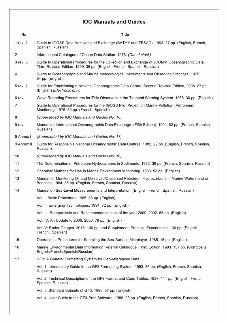
IOC Manuals and Guides

No. Title

1 rev. 2 Guide to IGOSS Data Archives and Exchange (BATHY and TESAC). 1993. 27 pp. (English, French, Spanish, Russian)

2 International Catalogue of Ocean Data Station. 1976. (Out of stock)

3 rev. 3 Guide to Operational Procedures for the Collection and Exchange of JCOMM Oceanographic Data. Third Revised Edition, 1999. 38 pp. (English, French, Spanish, Russian)

4 Guide to Oceanographic and Marine Meteorological Instruments and Observing Practices. 1975. 54 pp. (English)

5 rev. 2 Guide for Establishing a National Oceanographic Data Centre. Second Revised Edition, 2008. 27 pp. (English) (Electronic only)

6 rev. Wave Reporting Procedures for Tide Observers in the Tsunami Warning System. 1968. 30 pp. (English)

7 Guide to Operational Procedures for the IGOSS Pilot Project on Marine Pollution (Petroleum) Monitoring. 1976. 50 pp. (French, Spanish)

8 (Superseded by IOC Manuals and Guides No. 16)

9 rev. Manual on International Oceanographic Data Exchange. (Fifth Edition). 1991. 82 pp. (French, Spanish, Russian)

9 Annex I (Superseded by IOC Manuals and Guides No. 17)

9 Annex II Guide for Responsible National Oceanographic Data Centres. 1982. 29 pp. (English, French, Spanish, Russian)

10 (Superseded by IOC Manuals and Guides No. 16)

11 The Determination of Petroleum Hydrocarbons in Sediments. 1982. 38 pp. (French, Spanish, Russian)

12 Chemical Methods for Use in Marine Environment Monitoring. 1983. 53 pp. (English)

13 Manual for Monitoring Oil and Dissolved/Dispersed Petroleum Hydrocarbons in Marine Waters and on Beaches. 1984. 35 pp. (English, French, Spanish, Russian)

14 Manual on Sea-­Level Measurements and Interpretation. (English, French, Spanish, Russian)

Vol. I: Basic Procedure. 1985. 83 pp. (English)

Vol. II: Emerging Technologies. 1994. 72 pp. (English)

Vol. III: Reappraisals and Recommendations as of the year 2000. 2002. 55 pp. (English)

Vol. IV: An Update to 2006. 2006. 78 pp. (English)

Vol. V: Radar Gauges. 2016. 100 pp. and Supplement: Practical Experiences. 100 pp. (English, French,, Spanish)

15 Operational Procedures for Sampling the Sea-­Surface Microlayer. 1985. 15 pp. (English)

16 Marine Environmental Data Information Referral Catalogue. Third Edition. 1993. 157 pp. (Composite English/French/Spanish/Russian)

17 GF3: A General Formatting System for Geo-­referenced Data

Vol. 1: Introductory Guide to the GF3 Formatting System. 1993. 35 pp. (English, French, Spanish, Russian)

Vol. 2: Technical Description of the GF3 Format and Code Tables. 1987. 111 pp. (English, French, Spanish, Russian)

Vol. 3: Standard Subsets of GF3. 1996. 67 pp. (English)

Vol. 4: User Guide to the GF3-­Proc Software. 1989. 23 pp. (English, French, Spanish, Russian)

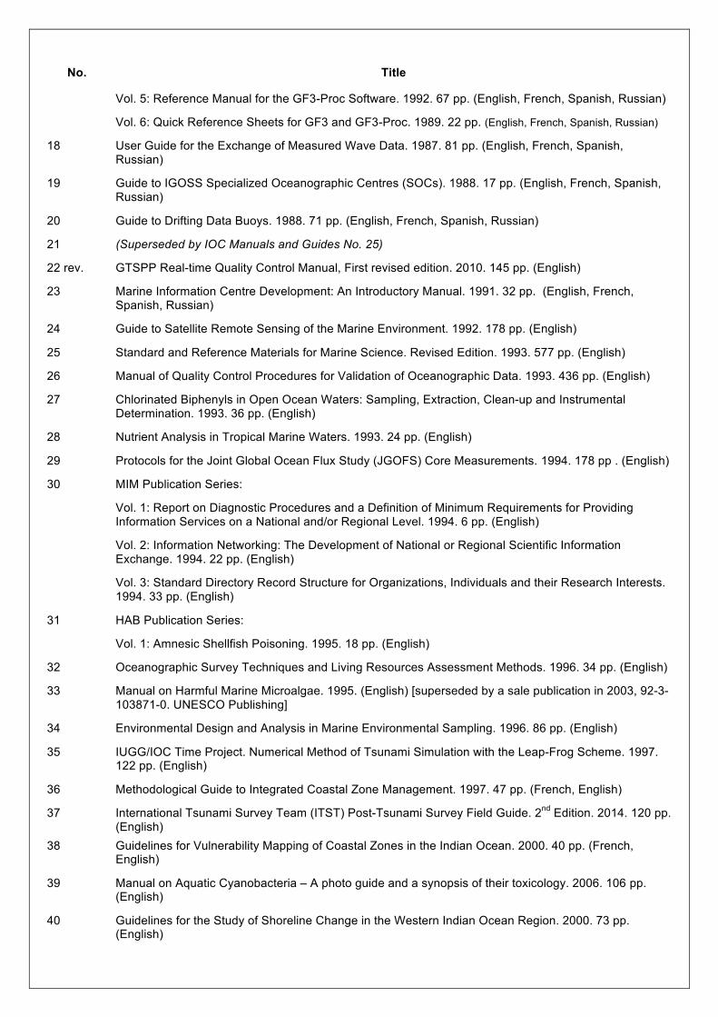
No. Title

Vol. 5: Reference Manual for the GF3-­Proc Software. 1992. 67 pp. (English, French, Spanish, Russian)

Vol. 6: Quick Reference Sheets for GF3 and GF3-­Proc. 1989. 22 pp. (English, French, Spanish, Russian)

18 User Guide for the Exchange of Measured Wave Data. 1987. 81 pp. (English, French, Spanish, Russian)

19 Guide to IGOSS Specialized Oceanographic Centres (SOCs). 1988. 17 pp. (English, French, Spanish, Russian)

20 Guide to Drifting Data Buoys. 1988. 71 pp. (English, French, Spanish, Russian)

21 (Superseded by IOC Manuals and Guides No. 25)

22 rev. GTSPP Real-­time Quality Control Manual, First revised edition. 2010. 145 pp. (English)

23 Marine Information Centre Development: An Introductory Manual. 1991. 32 pp. (English, French, Spanish, Russian)

24 Guide to Satellite Remote Sensing of the Marine Environment. 1992. 178 pp. (English)

25 Standard and Reference Materials for Marine Science. Revised Edition. 1993. 577 pp. (English)

26 Manual of Quality Control Procedures for Validation of Oceanographic Data. 1993. 436 pp. (English)

27 Chlorinated Biphenyls in Open Ocean Waters: Sampling, Extraction, Clean-­up and Instrumental Determination. 1993. 36 pp. (English)

28 Nutrient Analysis in Tropical Marine Waters. 1993. 24 pp. (English)

29 Protocols for the Joint Global Ocean Flux Study (JGOFS) Core Measurements. 1994. 178 pp . (English)

30 MIM Publication Series:

Vol. 1: Report on Diagnostic Procedures and a Definition of Minimum Requirements for Providing Information Services on a National and/or Regional Level. 1994. 6 pp. (English)

Vol. 2: Information Networking: The Development of National or Regional Scientific Information Exchange. 1994. 22 pp. (English)

Vol. 3: Standard Directory Record Structure for Organizations, Individuals and their Research Interests. 1994. 33 pp. (English)

31 HAB Publication Series:

Vol. 1: Amnesic Shellfish Poisoning. 1995. 18 pp. (English)

32 Oceanographic Survey Techniques and Living Resources Assessment Methods. 1996. 34 pp. (English)

33 Manual on Harmful Marine Microalgae. 1995. (English) [superseded by a sale publication in 2003, 92-­3-­103871-­0. UNESCO Publishing]

34 Environmental Design and Analysis in Marine Environmental Sampling. 1996. 86 pp. (English)

35 IUGG/IOC Time Project. Numerical Method of Tsunami Simulation with the Leap-­Frog Scheme. 1997. 122 pp. (English)

36 Methodological Guide to Integrated Coastal Zone Management. 1997. 47 pp. (French, English)

37 International Tsunami Survey Team (ITST) Post-­Tsunami Survey Field Guide. 2nd Edition. 2014. 120 pp. (English)

38 Guidelines for Vulnerability Mapping of Coastal Zones in the Indian Ocean. 2000. 40 pp. (French, English)

39 Manual on Aquatic Cyanobacteria – A photo guide and a synopsis of their toxicology. 2006. 106 pp. (English)

40 Guidelines for the Study of Shoreline Change in the Western Indian Ocean Region. 2000. 73 pp. (English)

No. Title

41 Potentially Harmful Marine Microalgae of the Western Indian Ocean Microalgues potentiellement nuisibles de l'océan Indien occidental. 2001. 104 pp. (English/French)

42 Des outils et des hommes pour une gestion intégrée des zones côtières -­ Guide méthodologique, vol.II/ Steps and Tools Towards Integrated Coastal Area Management – Methodological Guide, Vol. II. 2001. 64 pp. (French, English;; Spanish)

43 Black Sea Data Management Guide (Cancelled)

44 Submarine Groundwater Discharge in Coastal Areas – Management implications, measurements and effects. 2004. 35 pp. (English)

45 A Reference Guide on the Use of Indicators for Integrated Coastal Management. 2003. 127 pp. (English). ICAM Dossier No. 1

46 A Handbook for Measuring the Progress and Outcomes of Integrated Coastal and Ocean Management. 2006. iv + 215 pp. (English). ICAM Dossier No. 2

47 TsunamiTeacher – An information and resource toolkit building capacity to respond to tsunamis and mitigate their effects. 2006. DVD (English, Bahasa Indonesia, Bangladesh Bangla, French, Spanish, and Thai)

48 Visions for a Sea Change. Report of the first international workshop on marine spatial planning. 2007. 83 pp. (English). ICAM Dossier No. 4

49 Tsunami preparedness. Information guide for disaster planners. 2008. (English, French, Spanish)

50 Hazard Awareness and Risk Mitigation in Integrated Coastal Area Management. 2009. 141 pp. (English). ICAM Dossier No. 5

51 IOC Strategic Plan for Oceanographic Data and Information Management (2008–2011). 2008. 46 pp. (English)

52 Tsunami risk assessment and mitigation for the Indian Ocean;; knowing your tsunami risk – and what to do about it. 2009. 82 pp. (English)

53 Marine Spatial Planning. A Step-­by-­step Approach. 2009. 96 pp. (English;; Spanish). ICAM Dossier No. 6

54 Ocean Data Standards Series:

Vol. 1: Recommendation to Adopt ISO 3166-­1 and 3166-­3 Country Codes as the Standard for Identifying Countries in Oceanographic Data Exchange. 2010. 13 pp. (English)

Vol. 2: Recommendation to adopt ISO 8601:2004 as the standard for the representation of date and time in oceanographic data exchange. 2011. 17 pp. (English)

55 Microscopic and Molecular Methods for Quantitative Phytoplankton Analysis. 2010. 114 pp. (English)

56 The International Thermodynamic Equation of Seawater—2010: Calculation and Use of Thermodynamic Properties. 2010. 190 pp. (English)

57 Reducing and managing the risk of tsunamis. Guidance for National Civil Protection Agencies and Disaster Management Offices as Part of the Tsunami Early Warning and Mitigation System in the North-­eastern Atlantic, the Mediterranean and Connected Seas Region – NEAMTWS. 2011. 74 pp. (English)

58 How to Plan, Conduct, and Evaluate Tsunami Exercises / Directrices para planificar, realizar y evaluar ejercicios sobre tsunamis. 2012. 88 pp. (English, Spanish)

59 Guide for designing and implementing a plan to monitor toxin-­producing microalgae. Second Edition. 2016. 63 pp. (English, Spanish)

60 Global Temperature and Salinity Profile Programme (GTSPP) — Data user's manual, 1st Edition 2012. 2011. 48 pp. (English)

61 Coastal Management Approaches for Sea-­level related Hazards: Case-­studies and Good Practices. 2012. 45 pp. (English)

No. Title

62 Guide sur les options d’adaptation en zone côtières à l’attention des décideurs locaux – Aide à la prise de décision pour faire face aux changements côtiers en Afrique de l’Ouest / A Guide on adaptation options for local decision-­makers: guidance for decision making to cope with coastal changes in West Africa / Guia de opções de adaptação a atenção dos decisores locais: guia para tomada de decisões de forma a lidar com as mudanças costeiras na Africa Ocidental. 2012. 52 pp. (French, English, Portuguese). ICAM Dossier No. 7.

63 The IHO-­IOC General Bathymetric Chart of the Oceans (GEBCO) Cook Book. 2012. 221 pp. (English). Also IHO Publication B-­11

64 Ocean Data Publication Cookbook. 2013. 41 pp. (English)

65 Tsunami Preparedness Civil Protection: Good Practices Guide. 2013. 57 pp. (English)

66 IOC Strategic Plan for Oceanographic data and Information Management (2013-­2016). 2013. 54 pp. (English/French/Spanish/Russian)

67 IODE Quality Management Framework for National Oceanographic Data Centres (in preparation)

68 An Inventory of Toxic and Harmful Microalgae of the World Ocean (in preparation)

69 A Guide to Tsunamis for Hotels: Tsunami Evacuation Procedures (in preparation)

70 A guide to evaluating marine spatial plans. 2014. 96 pp. (English)

71 IOC Communication Strategy for Marine Information Management (2015-­2017). 2015

72 How to reduce coastal hazard risk in your community – A step-­by-­step approach. 2016

73 Guidelines for a Data Management Plan. 2016

74 Tsunami Ready Guidelines for the Caribbean and Adjacent Regions. 2016. (English/French/Spanish)

75 ICAN (International Coastal Atlas Network) -­ best practice guide to engage your CWA (Coastal Web Atlas) user community. 2016

76 Plans and Procedures for Tsunami Warning and Emergency Management – Guidance for countries in strengthening tsunami warning and emergency response through the development of Plans and Standard Operating Procedures for their warning and emergency management authorities. 2017

77 IOC Strategic Plan for Data and Information Management (2017-­2021). 2017

78 Harmful Algal Blooms (HABs) and Desalination: A Guide to Impacts, Monitoring and Management. 2017

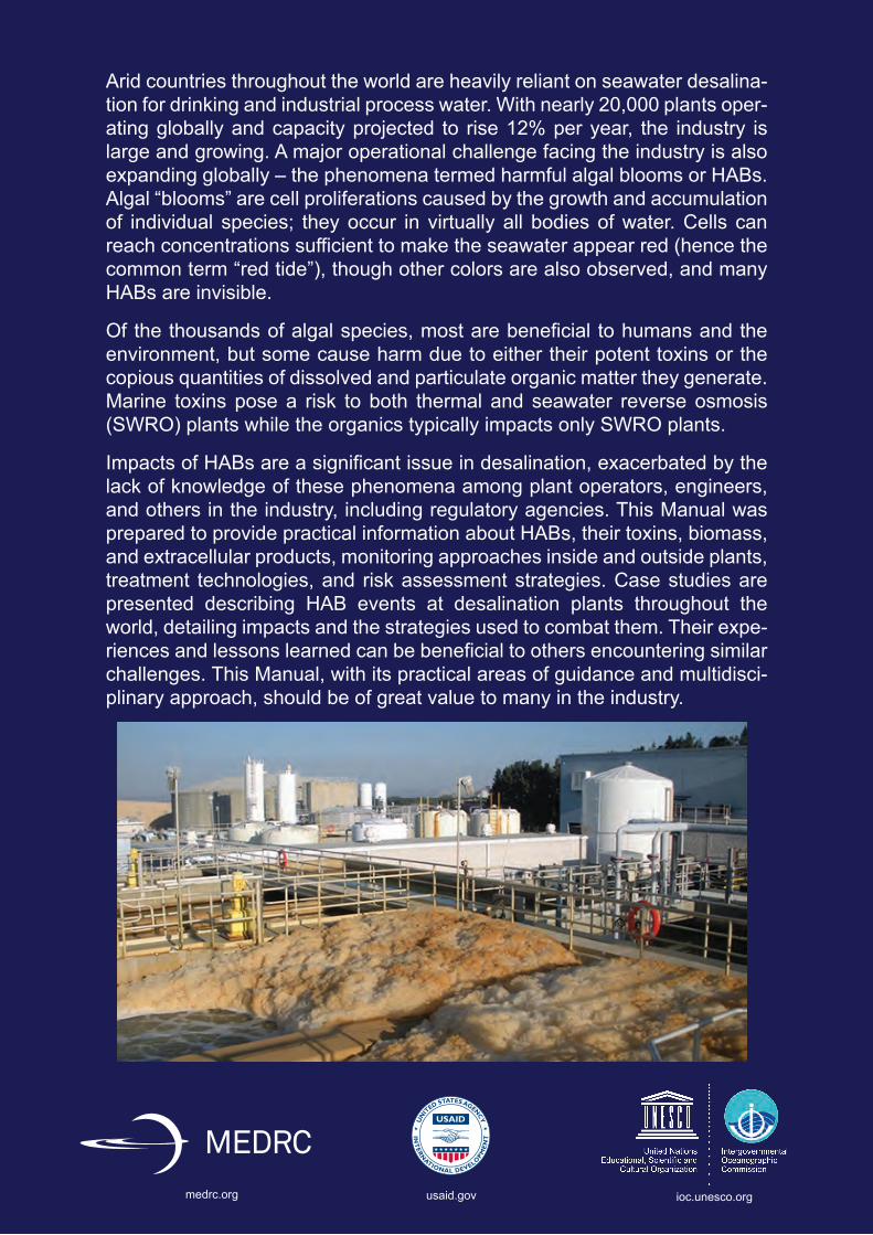
Arid countries throughout the world are heavily reliant on seawater desalina-tion for drinking and industrial process water. With nearly 20,000 plants oper-ating globally and capacity projected to rise 12% per year, the industry is large and growing. A major operational challenge facing the industry is also expanding globally – the phenomena termed harmful algal blooms or HABs. Algal “blooms” are cell proliferations caused by the growth and accumulation of individual species; they occur in virtually all bodies of water. Cells can reach concentrations sufficient to make the seawater appear red (hence the common term “red tide”), though other colors are also observed, and many HABs are invisible.

Of the thousands of algal species, most are beneficial to humans and the environment, but some cause harm due to either their potent toxins or the copious quantities of dissolved and particulate organic matter they generate. Marine toxins pose a risk to both thermal and seawater reverse osmosis (SWRO) plants while the organics typically impacts only SWRO plants.

Impacts of HABs are a significant issue in desalination, exacerbated by the lack of knowledge of these phenomena among plant operators, engineers, and others in the industry, including regulatory agencies. This Manual was prepared to provide practical information about HABs, their toxins, biomass, and extracellular products, monitoring approaches inside and outside plants, treatment technologies, and risk assessment strategies. Case studies are presented describing HAB events at desalination plants throughout the world, detailing impacts and the strategies used to combat them. Their expe-riences and lessons learned can be beneficial to others encountering similar challenges. This Manual, with its practical areas of guidance and multidisci-plinary approach, should be of great value to many in the industry.

ioc.unesco.orgmedrc.org usaid.gov