handouts dam 2015 2016
TRANSCRIPT

DATA ANALYSIS
for
MANAGERS
MScBA
Instituto Universitário de Lisboa (ISCTE-IUL)
JOSÉ DIAS [email protected]
2015/2016

i Contents
Contents
1 Math introductory concepts 11.1 The real numbers system . . . . . . . . . . . . . . . . . . . . . . . . . . . . . . . . . 11.2 The concept of sets . . . . . . . . . . . . . . . . . . . . . . . . . . . . . . . . . . . . 21.3 Relations and functions . . . . . . . . . . . . . . . . . . . . . . . . . . . . . . . . . . 3
1.3.1 Linear function . . . . . . . . . . . . . . . . . . . . . . . . . . . . . . . . . . 31.3.2 Exponential function . . . . . . . . . . . . . . . . . . . . . . . . . . . . . . . 41.3.3 Logarithmic function . . . . . . . . . . . . . . . . . . . . . . . . . . . . . . . 51.3.4 Functions of two or more independent variables . . . . . . . . . . . . . . . . 51.3.5 The concepts of derivative and elasticity . . . . . . . . . . . . . . . . . . . . 5
1.4 Matrices and vectors . . . . . . . . . . . . . . . . . . . . . . . . . . . . . . . . . . . 61.5 Descriptive statistics . . . . . . . . . . . . . . . . . . . . . . . . . . . . . . . . . . . 61.6 How to prepare a le for statistical analysis . . . . . . . . . . . . . . . . . . . . . . 71.7 Applications . . . . . . . . . . . . . . . . . . . . . . . . . . . . . . . . . . . . . . . . 9
1.7.1 Investment Bank 1 . . . . . . . . . . . . . . . . . . . . . . . . . . . . . . . . 91.7.2 Investment Bank 2 . . . . . . . . . . . . . . . . . . . . . . . . . . . . . . . . 91.7.3 Derivative and Elasticity . . . . . . . . . . . . . . . . . . . . . . . . . . . . . 91.7.4 Operations involving matrices . . . . . . . . . . . . . . . . . . . . . . . . . . 91.7.5 Descriptive statistics . . . . . . . . . . . . . . . . . . . . . . . . . . . . . . . 10
2 Statistical and distribution theory 112.1 Random variables . . . . . . . . . . . . . . . . . . . . . . . . . . . . . . . . . . . . . 11
2.1.1 Discrete random variables (drv) . . . . . . . . . . . . . . . . . . . . . . . . . 112.1.2 Continuous random variables (crv) . . . . . . . . . . . . . . . . . . . . . . . 122.1.3 Properties of the Expected value of a rv . . . . . . . . . . . . . . . . . . . . 132.1.4 The Correlation Coecient . . . . . . . . . . . . . . . . . . . . . . . . . . . 142.1.5 Properties of the Variance of a rv . . . . . . . . . . . . . . . . . . . . . . . . 142.1.6 Properties of the Covariance . . . . . . . . . . . . . . . . . . . . . . . . . . . 142.1.7 Moments of a rv . . . . . . . . . . . . . . . . . . . . . . . . . . . . . . . . . 142.1.8 Conditional distributions . . . . . . . . . . . . . . . . . . . . . . . . . . . . . 152.1.9 Independence and correlation . . . . . . . . . . . . . . . . . . . . . . . . . . 15
2.2 Estimation . . . . . . . . . . . . . . . . . . . . . . . . . . . . . . . . . . . . . . . . . 162.2.1 The properties of estimators . . . . . . . . . . . . . . . . . . . . . . . . . . . 16
2.3 Probability distributions . . . . . . . . . . . . . . . . . . . . . . . . . . . . . . . . . 172.3.1 Normal or Gaussian distribution . . . . . . . . . . . . . . . . . . . . . . . . . 172.3.2 The Chi-square distribution . . . . . . . . . . . . . . . . . . . . . . . . . . . 202.3.3 The Student's t distribution . . . . . . . . . . . . . . . . . . . . . . . . . . . 202.3.4 F distribution . . . . . . . . . . . . . . . . . . . . . . . . . . . . . . . . . . . 20
2.4 Applications . . . . . . . . . . . . . . . . . . . . . . . . . . . . . . . . . . . . . . . . 212.4.1 Probabilities . . . . . . . . . . . . . . . . . . . . . . . . . . . . . . . . . . . . 212.4.2 Discrete random variable . . . . . . . . . . . . . . . . . . . . . . . . . . . . . 212.4.3 Continuous random variable . . . . . . . . . . . . . . . . . . . . . . . . . . . 212.4.4 Normal distribution . . . . . . . . . . . . . . . . . . . . . . . . . . . . . . . . 22
José Dias Curto Data Analysis for Managers - MScBA
ii Contents
3 Statistical inference: a brief review 233.1 The Hypothesis Testing Methodology: a brief review . . . . . . . . . . . . . . . . . 233.2 Statistical Tests Applications . . . . . . . . . . . . . . . . . . . . . . . . . . . . . . 24
3.2.1 One sample t test . . . . . . . . . . . . . . . . . . . . . . . . . . . . . . . . . 243.2.2 One Sample Kolmogorov-Smirnov Test (nonparametric test) . . . . . . . . . 263.2.3 Characteristics and limitations of the Kolmogorov-Smirnov test . . . . . . . 263.2.4 Test statistic and signicance . . . . . . . . . . . . . . . . . . . . . . . . . . 263.2.5 Two independent samples . . . . . . . . . . . . . . . . . . . . . . . . . . . . 293.2.6 Analysis of Variance (ANOVA) . . . . . . . . . . . . . . . . . . . . . . . . . 31
4 Correlation and simple linear regression 354.1 Types of data . . . . . . . . . . . . . . . . . . . . . . . . . . . . . . . . . . . . . . . 354.2 Correlation Analysis . . . . . . . . . . . . . . . . . . . . . . . . . . . . . . . . . . . 364.3 Simple Regression Analysis . . . . . . . . . . . . . . . . . . . . . . . . . . . . . . . . 38
5 The multiple linear regression model (MLRM) 425.1 Assumptions of the MLRM . . . . . . . . . . . . . . . . . . . . . . . . . . . . . . . 425.2 Ordinary Least Squares Method (OLS) . . . . . . . . . . . . . . . . . . . . . . . . . 435.3 Properties of OLS estimators . . . . . . . . . . . . . . . . . . . . . . . . . . . . . . 445.4 Ohlson Empirical Application . . . . . . . . . . . . . . . . . . . . . . . . . . . . . . 45
5.4.1 Coecient of Determination: R-Square (Quadrado de R) . . . . . . . . . . . 465.4.2 The Standard Error of Regression (Erro-padrão da Regressão) . . . . . . . . 495.4.3 The Unstandardized Coecients . . . . . . . . . . . . . . . . . . . . . . . . . 495.4.4 The Standardized Coecients . . . . . . . . . . . . . . . . . . . . . . . . . . 495.4.5 F test . . . . . . . . . . . . . . . . . . . . . . . . . . . . . . . . . . . . . . . 515.4.6 t test . . . . . . . . . . . . . . . . . . . . . . . . . . . . . . . . . . . . . . . . 515.4.7 Information Criteria . . . . . . . . . . . . . . . . . . . . . . . . . . . . . . . 52
6 Assumptions of the MLRM: Normality and Multicollinearity 546.1 Normality Tests . . . . . . . . . . . . . . . . . . . . . . . . . . . . . . . . . . . . . . 54
6.1.1 Skewness and Kurtosis coecients . . . . . . . . . . . . . . . . . . . . . . . . 546.2 The Jarque-Bera (JB) Test . . . . . . . . . . . . . . . . . . . . . . . . . . . . . . . 566.3 The Kolmogorov-Smirnov (KS) Test . . . . . . . . . . . . . . . . . . . . . . . . . . 566.4 Cobb-Douglas Application . . . . . . . . . . . . . . . . . . . . . . . . . . . . . . . . 576.5 Multicollinearity Consequences . . . . . . . . . . . . . . . . . . . . . . . . . . . . . 596.6 Multicollinearity Diagnostic . . . . . . . . . . . . . . . . . . . . . . . . . . . . . . . 60
6.6.1 Tolerance and Variance Ination Factor . . . . . . . . . . . . . . . . . . . . . 606.6.2 Matrix Condition . . . . . . . . . . . . . . . . . . . . . . . . . . . . . . . . . 616.6.3 Variance Decomposition . . . . . . . . . . . . . . . . . . . . . . . . . . . . . 62
6.7 Solutions for Multicollinearity . . . . . . . . . . . . . . . . . . . . . . . . . . . . . . 626.8 Application: Electric Utility . . . . . . . . . . . . . . . . . . . . . . . . . . . . . . . 62
7 Assumptions of the MLRM: heteroskedasticity 657.1 The Generalized Least Squares (GLS) Method . . . . . . . . . . . . . . . . . . . . . 667.2 Heteroskedasticity . . . . . . . . . . . . . . . . . . . . . . . . . . . . . . . . . . . . . 68
José Dias Curto Data Analysis for Managers - MScBA

iii Contents
7.2.1 Detecting Heteroskedasticity . . . . . . . . . . . . . . . . . . . . . . . . . . . 697.2.2 Corrective Measures . . . . . . . . . . . . . . . . . . . . . . . . . . . . . . . 70
7.3 Applications . . . . . . . . . . . . . . . . . . . . . . . . . . . . . . . . . . . . . . . . 757.3.1 Income-Sales-Workforce . . . . . . . . . . . . . . . . . . . . . . . . . . . . . 757.3.2 Ohlson Model . . . . . . . . . . . . . . . . . . . . . . . . . . . . . . . . . . . 78
8 Assumptions of the MLRM: AUTOCORRELATION 848.1 The consequences of autocorrelation . . . . . . . . . . . . . . . . . . . . . . . . . . . 858.2 First order autocorrelation . . . . . . . . . . . . . . . . . . . . . . . . . . . . . . . . 858.3 How to detect the errors' autocorrelation . . . . . . . . . . . . . . . . . . . . . . . . 88
8.3.1 Graphical representation of residuals . . . . . . . . . . . . . . . . . . . . . . 888.3.2 Hypotheses Testing . . . . . . . . . . . . . . . . . . . . . . . . . . . . . . . . 88
8.4 Solutions for autocorrelation . . . . . . . . . . . . . . . . . . . . . . . . . . . . . . . 928.4.1 The Cochrane-Orcutt (CORC)(1949) iterative procedure . . . . . . . . . . . 928.4.2 The iterative procedure of Hildreth-Lu (HL) . . . . . . . . . . . . . . . . . . 938.4.3 Heteroskedasticity and Autocorrelation Consistent Estimators (HAC) . . . . 93
8.5 Application: GDP and PC (USA) . . . . . . . . . . . . . . . . . . . . . . . . . . . . 93
9 Models with Binary dependent variable: Logit and Probit 989.1 Application: Credit Scoring . . . . . . . . . . . . . . . . . . . . . . . . . . . . . . . 101
José Dias Curto Data Analysis for Managers - MScBA

1 1 Math introductory concepts
1 Math introductory concepts
The purpose of these rst two lectures is to present a brief review of math introductory conceptslike functions, derivative, elasticity, logarithm, etc.
1.1 The real numbers system
The real number system consists of rational and irrational numbers. These numbers may bepositive, zero, or negative. Real numbers may be represented by innite decimals, for example:
9.7243527 . . . ;2
3= 0.6666666 . . . ;
√3 = 1.73205 . . . ; π = 3.14159265 . . .
Natural numbers or Counting numbers: NThese are the numbers that we use to count:N = 1, 2, 3, 4, . . .
Whole numbers: N0
These are the natural numbers plus the number zero:N0 = 0, 1, 2, 3, 4, . . .
The Whole numbers set includes the Natural numbers set (or N is a subset of N0):
N ⊂ N0 or N0 ⊃ N.
Integers: ZThe expanded set of numbers that we get by including negative versions of the counting numbersis called the Integers:Z = . . . ,−4,−3,−2,−1, 0, 1, 2, 3, 4, . . .
N0 ⊂ Z or Z ⊃ N0.
Rational numbers: QA rational number is a number which can be expressed as a ratio of two integers. Non-integerrational numbers (commonly called fractions) are usually written as the vulgar fraction x
y, where
y cannot be zero (but x can). x is called the numerator, and y the denominator.
Q =
x
y, x ∈ Z, y ∈ Z, y 6= 0
where Z denotes the set of integers.
All integers can also be thought of as rational numbers, with a denominator 1:
5 =5
1;−15 =
−15
1.
This means that all the previous sets of numbers (Natural numbers, Whole numbers andIntegers) are subsets of the rational numbers:
N ⊂ N0 ⊂ Z ⊂ Q or Q ⊃ Z ⊃ N0 ⊃ N.
José Dias Curto Data Analysis for Managers - MScBA
2 1.2 The concept of sets
Irrational numbers: IQThese are the numbers that cannot be expressed as a ratio of two integers. The decimals neverrepeat or terminate (rational numbers always do one or the other). Perhaps the most well knownirrational numbers are π and
√2.
Real numbers: RThe real numbers set includes all the rational and irrational numbers. A real number may beexpressed by a point on the real line:
ExamplesConsider the following numbers:
3,−4.3,−7345.22, 1456, 67495.78, 0.25(1
4),√
3 = 1.73205080756
1. Classify each one of the numbers. For example, 3 is a natural number.
2. Is this sentence true: 3 is also a rational number but it is not an integer.
3. Propose a fraction to represent the number −4.3.
4. Suggest real situations where these numbers can be used. For example, 3 can be a family'snumber of children.
1.2 The concept of sets
A set is a collection of distinct objects and sets are one of the most fundamental concepts inmathematics. The sets can be represented in extension or in comprehension:
Extension:A = 5, 6, 7, 8, 9, 10
Comprehension:A = x : x is an integer bigger than 4 and lower than 11
N, N0, Z, Q, IQ and R are all examples of sets where the objects are numbers.
Operations involving setsConsider the sets A, B and C:
A = 1, 2, 3, 4, B = 3, 4, 5, 6, 7 and C = 1, 3, 4, 5, 6, 7
• The union of two sets A and B is the set of elements which are in A or in B or in both andit is denoted by A ∪ B:
A ∪B = 1, 2, 3, 4, 5, 6, 7
José Dias Curto Data Analysis for Managers - MScBA

3 1.3 Relations and functions
• The intersection of sets A and B is the set of all elements common to both A and B and itis denoted by A ∩ B:
A ∩B = 3, 4
• x ∈ A if x belongs to A. For example, 1 ∈ A.
• If B is a subset of C than B is included in C or C contains B:
B ⊂ C or C ⊃ B.
1.3 Relations and functions
In management and economics the quantitative phenomena are usually represented by variables:x, y, z and the mathematical functions are used to establish the relationship between those phe-nomena.
The mathematical concept of a function expresses the dependence between two quantities, oneof which is given (the independent variable, argument of the function, or its input) and the otheris the result (the dependent variable, value of the function, or output):
y = f(x),
where x is the independent variable and y is the dependent one.For example, if y = 2x and x = 4 then y = 8.
1.3.1 Linear function
A linear (strictly speaking, ane) function has the form:
y = f(x) = b+mx,
for two real numbers b and m, where b is the intercept and m is the slope.If y is a linear function its slope is always constant.
ProportionalityWe say that y is (directly) proportional to x if there is a nonzero constant k such that
y = kx,
where k is the constant of proportionality.Let the function g represent the yearly production of car brand A since 1990 (t=0):
y = g(t) = 10000 + 500t,
where 10000 represents the production in 1990 (at t=0) and the slope (500) tells us that theproduction increases by about 500 units per year. We say that g is an increasing function as theslope is positive.
José Dias Curto Data Analysis for Managers - MScBA

4 1.3 Relations and functions
VariationsLet ∆y and ∆x represent the absolute variation in y and x, respectively.
∆y = y2 − y1 and ∆x = x2 − x1,
where the absolute variation in y is always proportional to the absolute variation in x: ∆y = m∆xand the slope is given by m = ∆y
∆x. For example, if ∆t = 5, ∆y = 500× 5 = 2500.
The relative variations in y and x are given by ∆yy1
and ∆xx1, respectively. If the ratio between the
absolute variations is always constant and it is given by the slope, the ratio of relative variationsdepends on the x and y values.
The percentage variation (or the rate of change) is the product of 100 by the relative variation:100× ∆y
y1and 100× ∆x
x1.
Now you are able to answer to APPLICATION 1.7.1 (at the end of this section).
1.3.2 Exponential function
The common form of the exponential function is:
y = f(x) = abx,
where a is the value of y when x = 0, b is the base and x is the exponent. Special cases of theexponential function are:
• a = 1, y = bx;
• a = 1 and b = e, y = ex, where e is a mathematical constant, the base of the naturallogarithm, which equals approximately 2.718281828, and is also known as the Euler's number.
In this function, y increases (b > 1) or decreases (0 < b < 1) at the same rate. Let the relativevariation in y be:
y2 − y1
y1
=abx2 − abx1
abx1=bx2
bx1− 1 = bx2−x1 − 1.
If ∆x = x2 − x1 = 1, then the relative variation in y is given by:
b− 1
and the percentage variation in y is100× (b− 1)
which is constant.Go to APPLICATION 1.7.2.
José Dias Curto Data Analysis for Managers - MScBA

5 1.3 Relations and functions
1.3.3 Logarithmic function
The logarithm of a number x one base a (necessarily positive) is dened as the power y of whichmust be increased the base a to obtain that number: y = loga(x). For example, log2(16) = 4, as 4is the number that should powered 2 to aord 16: 24 = 16.
The logarithm of base e is referred to as the natural logarithm and is represented by ln(x) withno explicit reference to the base. In practice one can also use common logarithms, or logarithms ofbase 10, which are usually represented by log(x). The relationship between the natural logarithmand the logarithm of base 10 is given by:
ln(x) = 2.3026 log(x).
1.3.4 Functions of two or more independent variables
The functions can include more than one independent variable. The usual notation is:
y = f(x1, x2, x3)
and if there is a linear relationship between y and each one of the independent variables, then
y = b+m1x1 +m2x2 +m3x3.
In management and economics the models include usually more than one independent variable.Let yt represents the aggregate consumption of one country in year t, x1t and x2t represent the
interest rates and the GDP, respectively. A function can be used to determine the relationshipbetween the consumption and each one of these independent variables.
1.3.5 The concepts of derivative and elasticity
The derivative is a measurement of how a function changes when the values of their inputs change.Thus, the derivative is the marginal eect of x in y :
dy
dx= Lim
∆x→0
∆y
∆x.
The elasticity (that we represent by η) measures the percentage change in one variable thatresults from a 1% change in another variable. For example, if the price elasticity of demand is −5,when the price rises by 1%, quantity demanded might fall by 5%:
100× ∆yy
100× ∆xx
=∆y
y:
∆x
x=x
y× ∆y
∆x.
When ∆x→ 0, ∆y∆x
= dydx
and η = xy× dy
dx, or,
η =∆y
y:
∆x
x=x
y× ∆y
∆x=x
y× dy
dx.
Go to APPLICATION 1.7.3.
José Dias Curto Data Analysis for Managers - MScBA

6 1.4 Matrices and vectors
1.4 Matrices and vectors
Let m and n be two integer positive numbers. The matrix A is a table with m rows and n columnsand the cells are lled by scalars that usually are real numbers:
A = (aij) =
a11 a12 . . . a1n
a21 a22 . . . a2n...
.... . .
...am1 am2 . . . amn
, (1)
where i = 1, 2, . . . ,m and j = 1, 2, . . . , n.In the following matrix m = 2 and n = 3. The rows and the columns determine the dimension
of the matrix that is 2× 3.
A =
[3 4 62 5 8
].
A vector is a special matrix with just one row (row-vector) or one column (column-vector).The dimension is 1× n and m× 1, respectively.
There are special matrices students must know: Quadratic, Symmetric, Diagonal and Identity.Main operations involving matrices and vectors are: Product, Inverse, Transpose and Deter-
minant. The Excel functions to perform these operations are (in english): MMULT, MINVERSE,
TRANSPOSE, MDETERM.MATRIZ.MULT, MATRIZ.INVERSA, TRANSPOR, MATRIZ.DETERM (in portuguese). In order to
compute these functions,
1. Select the range where the output will appear (for example, if the result is a 4 × 4 matrixyou have to select an Excel range composed by 4 rows and 4 columns);
2. Introduce the function;
3. Press simultaneously the keys <Shift>+ <Ctrl>+<Enter> to get all the matrix elements. Ifyou press just <Enter> only the rst element of the matrix will appear.
Go to APPLICATION 1.7.4.
1.5 Descriptive statistics
Descriptive statistics are used to describe the basic features of the data. Together with simplegraphical analysis, they form the basics of every data quantitative analysis. Descriptive statisticsare usually divided in three main sets:
• Location measures
Central tendency (arithmetic mean, mode and median).The arithmetic mean is probably the most commonly used statistic to describing centraltendency:
X =
∑ni=1 Xi
n.
The median is the score found at the exact middle of the set of values. The mode is themost frequently occurring value in the set of scores.
José Dias Curto Data Analysis for Managers - MScBA

7 1.6 How to prepare a le for statistical analysis
Noncentral tendency (percentiles, deciles and quartiles).
• Dispersion measures (variance, standard deviation, interquartile range, mean absolute devi-ation and coecient of variation).
Variance: S2 =∑n
i=1(Xi−X)2
n;
Standard deviation: S =
√∑ni=1(Xi−X)
2
n;
Coecient of variation: CV = SX× 100.
• Asymmetry and Kurtosis measures.
1.6 How to prepare a le for statistical analysis
The common procedure is to prepare an Excel le with all the data and open it later in SPSS1 orEViews2. Suppose that you want to prepare a le with the information of 10 master students:
where gender 0 is male and gender 1 is female, pincome represents the monthly parents' income,city represents the city of origin, where 1 is Lisbon, 2 is Porto, 3 is Coimbra and 4 is Faro; andnally distance represents the time of travel between home and the university. As one can see,and when it is possible, we introduce numbers instead of labels: for example we couldintroduce male instead of 0! but it is more correct to introduce the number andassociate later the respective designation.
Once the EXCEL le is prepared you must save it. After that, it can be opened in SPSSthrough the usual procedure: File, Open, Data. The SPSS appearance must be:
1The SPSS can be downloaded free from https://dsi.iscte.pt/.2You can access the EVIEWS, in any room or lab, by checking on the Windows button and write:
\\aplicacoes.iul.intra
José Dias Curto Data Analysis for Managers - MScBA

8 1.6 How to prepare a le for statistical analysis
Now you can save the le in SPSS format: name.SAV. The next steps are:
1. Associate the labels Male and Female to the numbers 0 and 1 in the gender variable:
(1) Change from Data View to Variable View, (2) Check on the right dots . . . of None, (3)Introduce the value 0 and the label Male and (4) Check on the button Add. You can dothe same for Female. After this click OK and change again to Data View. If you selectView, Value Labels, the numbers are replaced by the labels introduced before. In spiteof this, the numbers 0 and 1 remain in the le.
2. Apply the same procedure for the variable City.
3. Change again from Data View to Variable View and introduce a longer designation for thevariable pincome: Monthly Parents Income. You have to introduce this on the column Labelon the right side of the variable pincome. Go to APPLICATION 1.7.5
José Dias Curto Data Analysis for Managers - MScBA

9 1.7 Applications
1.7 Applications
1.7.1 Investment Bank 1
The investment bank ALLMONEY has a nancial application with the following characteristics:
• Capital: 500000 euros;
• Duration: 4 years;
• Annual interest rate: 3%;
• Simple interests type;
Based on this information look for a linear function to compute the cumulative amount of capi-tal+interests for each year.
• Represent graphically the resulting function;
• Compute the rate of change in the amount of capital+interests for each year;
1.7.2 Investment Bank 2
Now assume that interests are compounding yearly.
1. Propose a (non-linear) function to compute the cumulative amount of capital+interests foreach year;
2. Compute the rate of change in the amount of capital+interests for each year;
1.7.3 Derivative and Elasticity
Consider the following linear function: y = 20 + 2x. Compute the derivative of y in relation to xand the elasticity of y in relation to x if x = 10.
1.7.4 Operations involving matrices
A company has 4 stores (Lisboa, Porto, Faro and Leiria) where it sells 4 products that we nameby RA, RB, RC and RD. Let the matrix A be composed by the quantities sold in each one of thestores in the last month.
A =
40 50 30 2520 15 60 8090 25 35 4045 30 55 45
If the vector of prices is represented by b,
b =
10152512
,José Dias Curto Data Analysis for Managers - MScBA

10 1.7 Applications
compute the amount of sales per store using the rules of matrices' product.If the company establishes as target the following vector of sales compute the corresponding
prices.
S =
3000400037003825
.1.7.5 Descriptive statistics
The Excel le international.xls includes the saving rate and the per-capita disposable income for50 countries.
1. Import the data from the Excel to the SPPS: FILE, OPEN, Data.
2. Compute and interpret the descriptive statistics for both variables: the saving rate and theper-capita disposable income,ANALYZE, DESCRIPTIVE STATISTICS, Frequencies.STATISTICS Percentile values (Quartiles and Percentiles: 43, 75, 80) Central Tendency(Mean, Median, Mode) Dispersion (Std. deviation, Variance, Minimum, Maximum).CHARTS Histogram with normal curve.
3. Based on the coecient of variation compare the two distributions in terms of dispersion.
REFERENCESChiang, Alpha C. (2005), Fundamental Methods of Mathematical Economics, 4th edition.McClave, James T., Benson, P. G. and Sincich, T. (2012), Statistics for Business and Economics,12th edition.
José Dias Curto Data Analysis for Managers - MScBA

11 2 Statistical and distribution theory
2 Statistical and distribution theory
In this lecture we refer the most important concepts related with probabilities, random variablesand theoretical distributions.
2.1 Random variables
A random variable is a variable that can takes dierent outcomes, each with a probability less thanor equal to 1. A random variable can be described by examining the process which generates itsvalues and this process is called probability distribution. A probability distribution lists all possiblevalues and the probability that each will occur.
ExampleConsider the coin random experiment. The outcomes are: Ω = F,C, where F denotes a cointoss of heads and C is a toss of tails. If the coin is fair and thrown randomly the probability ofheads will be 1
2: P (F ) = P (C) = 1
2. Let the random variable X be the Number of heads. Thus, X
can assume the values 1 and 0 with probability 12.
Based on this, we might dene a random variable as a function that assigns to each outcomeof a random experiment a real number:
F → 1 C → 0.
The random variables (rv) can be distinguished between discrete and continuous rv. A discreterandom variablemay take on only a nite or an innite but countable number of distinct values suchas 0, 1, 2, 3, 4, ... Discrete random variables are usually (but not necessarily) counts. Examples ofdiscrete random variables include the number of children in a family, the Friday night attendanceat a cinema, the number of patients in a doctor's surgery, the number of defective light bulbs in abox of ten.
A continuous random variable can take an innite number of dierent outcomes, for example,any value in the interval [0, 3]. In this case each individual outcome has a probability of zero.Continuous random variables are usually measurements. Examples include height, weight, theamount of sugar in an orange, the time required to run a mile.
2.1.1 Discrete random variables (drv)
If X is a drv then:
• The probability function, f(x) = P (X = x), has the following properties: f(x) ≥ 0 and∑f(x) = 1.
• The distribution function is given by: F (x) = P (X ≤ x).
• The expected value or mean of a drv, often denoted by µ, is dened as: µ = E(X) =∑ni=1 f(xi)xi. The expected value should be distinguished from the sample mean which is
denoted by X and it is the average of the outcomes obtained in a sample.
José Dias Curto Data Analysis for Managers - MScBA

12 2.1 Random variables
• The variance is a weighted average of the squares of the deviations of outcomes on X fromits expected value, with the corresponding probabilities of each outcome serving as weights.It is dened as: σ2 =
∑ni=1 f(xi) [xi − E(X)]2. The variance is in itself an expectation: σ2 =
E [X − E(X)]2. The positive square root of the variance is called the standard deviation.
Example of a drv
x 0 1 2 3 4 5
f(x) 0.15 0.30 0.25 0.15 0.10 0.05F (x) 0.15 0.45 0.70 0.85 0.95 1.00xf(x) 0.00 0.30 0.50 0.45 0.40 0.25E(X) 1.90x2 0 1 4 9 16 25
x2f(x) 0.00 0.30 1.00 1.35 1.60 1.25E(X2) 5.50
x− E(X) -1.90 -0.90 0.10 1.10 2.10 3.10(x− E(X))2 3.61 0.81 0.01 1.21 4.41 9.61
f(x)(x− E(X))2 0.54 0.24 0.00 0.18 0.44 0.48Var(X) 1.89
2.1.2 Continuous random variables (crv)
If Y is a crv then:
• We dene the probability density function (pdf)
f(y) ≥ 0 as P a ≤ Y ≤ b =∫ baf(y)dy.
In a graph P a ≤ Y ≤ b =∫ baf(y)dy is the area under the function f(y) between the points
a and b. Taking the integral of f(y) over all possible outcomes gives∫ +∞−∞ f(y)dy = 1.
• The cumulative density function (cdf) is dened asF (y) = P Y ≤ y =
∫ y−∞ f(u)du, such that f(y) = F ′(y) (the derivative). The cdf has the
property that 0 ≤ F (y) ≤ 1, and is monotonically increasing, i.e., F (y) ≥ F (x) if y > x.
• The expected value or mean is dened as µ = E(Y ) =∫ +∞−∞ yf(y)dy.
• The variance is given by σ2 = V ar(Y ) =∫ +∞−∞ [y − E(Y )]2f(y)dy. Or,
V ar(Y ) = E[(Y − µ)2
]= E
(Y 2 − 2Y µ+ µ2
)= E
(Y 2)−2µE(Y )+µ2 = E
(Y 2)−[E(Y )]2 .
José Dias Curto Data Analysis for Managers - MScBA

13 2.1 Random variables
Next gure shows pdf and cdf of a certain continuous variable
Example of a crvLet X be a crv with the following pdf: f(x) = 1
2x for 0 ≤ x ≤ 2 and f(x) = 0 for other x values.
The cdf is given by: F (x) =∫ x−∞ f(x)dx =
[x2
4
]x0
= x2
4for 0 ≤ x ≤ 2 and F (x) = 0 for other x
values.
The expected value of X is given by:
E(X) =∫ +∞−∞ xf(x)dx = 0 +
∫ 2
0xf(x)dx+ 0 =
[x3
6
]2
0= 8
6.
The variance results from:V ar(X) = E (X2)− [E(X)]2.
As E (X2) = 0 +∫ 2
0x2f(x)dx+ 0 =
[x4
8
]2
0= 2 then
V ar(X) = 2− 86
= 0.22(2)
2.1.3 Properties of the Expected value of a rv
Let X and Y be rv and k be a constant. Then,
• E(k) = k: the expected value of a constant is the constant.
• E(kX) = kE(X);
• E(X + Y ) = E(X) + E(Y );
• E(X − Y ) = E(X)− E(Y );
• E(XY ) = Cov (X, Y ) + E(X)E(Y ) or E(XY ) = E(X)E(Y ) if X and Y are uncorrelatedand Cov (X, Y ) = 0.
The covariance is a measure of the linear relationship between X and Y :Cov (X, Y ) = E [(X − µX) (Y − µY )]
• drv: Cov (X, Y ) =∑n
i=1
∑nj=1 (xi − µX) (yj − µY ) f(xi, yj);
• crv: Cov (X, Y ) =∫ +∞−∞
∫ +∞−∞ (x− µX) (y − µY ) f(x, y)dxdy.
José Dias Curto Data Analysis for Managers - MScBA

14 2.1 Random variables
2.1.4 The Correlation Coecient
The value of the covariance depends on the units in which X and Y are measured. As a result weuse the correlation coecient:
ρXY = −1 ≤ σXYσXσY
≤ +1,
where σXY is the covariance between X and Y , σX and σY represent the standard deviations ofX and Y , respectively.
Unlike covariance, the correlation coecient has been normalized and is scale-free. The value ofthe correlation coecient always lies between −1 and +1. A positive correlation indicates that thevariables tend to move in the same direction, while a negative value implies that they tend to movein opposite directions. A zero value means that variables are linearly independent (uncorrelated).
2.1.5 Properties of the Variance of a rv
Let X and Y be rv and k be a constant. Then,
• V ar(k) = 0.
• V ar(kX) = k2V ar(X);
• V ar(X ± Y ) = V ar(X) + V ar(Y )± 2Cov(X, Y );
2.1.6 Properties of the Covariance
When a, b, c and d are constants, it holds that
Cov(aX + b, cY + d) = acCov(X, Y ).
Further,Cov(aX + bY, Y ) = aCov(X, Y ) + bCov(Y, Y ) =
= aCov(X, Y ) + bV ar(Y ).
It also follows that two variables X and Y are perfectly correlated (ρXY = 1) if Y = kX for somenonzero value of k. If X and Y are correlated, the variance of a linear function of X and Y dependsupon their covariance. In particular,
V ar(aX + bY ) = a2V ar(X) + b2V ar(Y ) + 2Cov(X, Y ).
2.1.7 Moments of a rv
In most cases the distribution of a rv is not completely described by its mean and variance, andwe can dene the k-th central moment as
E[(X − µX)k
], k = 1, 2, 3, . . .
The variance is the second central moment.
José Dias Curto Data Analysis for Managers - MScBA

15 2.1 Random variables
In particular, the third central moment is a measure for skewness, where a value of 0 indicates asymmetric distribution, and the fourth central moment measures kurtosis. It is a measure of thethickness of the tails of the distribution.
2.1.8 Conditional distributions
A conditional distribution describes the distribution of a variable, say Y , given the outcome ofanother variable X. The conditional distribution is implied by the joint distribution of the twovariables. We dene
f(y|X = x) = f(y|x) =f(x, y)
f(x).
If X and Y are independent then
f(y|x) = f(y) and f(x, y) = f(y)f(x).
The conditional expectation and variance of Y given X = x are:
E(Y |X = x) = E(Y |x) =
∫yf(y|x)dy
V ar(Y |x) =
∫[y − E(Y/x)]2 f(y/x)dy.
andV ar(Y |x) = E
(Y 2/x
)− [E(Y |x)]2 .
It holds thatV ar(Y ) = Ex [V ar(Y |X)] + V arx [E(Y |X)] ,
where Ex and V arx denote the expected value and variance, respectively, based upon the marginaldistribution of X.
If Y is conditional mean independent of X it means that
E(Y |X) = E(Y ) = 0.
This is stronger than zero correlation because E(Y |X) = 0 implies that E(Y ) = 0.
2.1.9 Independence and correlation
If two variables X and Y are independent, the covariance between them is zero. However, theresults does not hold in the opposite direction. Two variables may have zero correlation, yet theremay be a dependence between the variables. The key is that covariance and correlation measurelinear dependence; the variables may be related nonlinearly yet have a zero covariance.
Consider the example where Y = X4 and the correlation between Y and X is null:
X -4 -3 -2 -1 0 1 2 3 4Y 256 81 16 1 0 1 16 81 256
José Dias Curto Data Analysis for Managers - MScBA

16 2.2 Estimation
2.2 Estimation
Means, variances and covariances can be measured with certainty only if we know all the possibleoutcomes, i.e., the population. Usually, however, we have only a sample of the population andthose measures have to be estimated. Finding the best estimator for any given sample is a com-plex issue but for the moment assume that the estimator of a parameter yields estimates closelyapproximating that parameter. We would like the estimator to be UNBIASED, i.e., the expectedvalue of the estimator is equal to the parameter itself. Unbiased estimators for:
• The mean: µ = X =∑n
i=1Xi
n;
• The variance: σ2 = S′2 =
∑ni=1(Xi−X)2
n−1;
• The covariance: σ2XY =
∑ni=1(Xi−X)(Yi−Y )
n−1;
• The correlation coecient: ρXY =∑n
i=1(Xi−X)(Yi−Y )√∑ni=1(Xi−X)2
∑ni=1(Yi−Y )2
.
2.2.1 The properties of estimators
Let θ and θ represent the parameter and the estimator, respectively. There are four properties ofestimators that are important:
• Lack of bias: θ is an unbiased estimator if the mean or expected value of θ is equal to the
true value: E(θ)
= θ.
• Eciency: θ is an ecient unbiased estimator if for a given sample size the variance of θ issmaller than the variance of any other unbiased estimators. One estimator is more ecientthan another if it has smaller variance.Thus θ1 is more ecient than θ2 if V ar(θ1) < V ar(θ2), assuming that θ1 and θ2 are bothunbiased.
José Dias Curto Data Analysis for Managers - MScBA

17 2.3 Probability distributions
• Minimum Mean Square Error (MSE): There are many circumstances in which one is forcedto trade o bias and variance of estimators. Sometimes an estimator with very low varianceand some bias may be more desirable than an unbiased estimator with high variance. Onecriterion is to minimize Mean Square Error which is dened as
MSE(θ) = E(θ − θ)2
or
MSE(θ) =[Bias(θ)
]2
+ V ar(θ).
When θ is unbiased, the Bias(θ) = E(θ)− θ = 0 and the MSE and variance of θ are equal.
• Large-sample or asymptotic properties: as the sample size increases we expect that θ ap-proaches θ. Thus, the probability that θ diers from θ becomes very small.
The probability limit of θ (plim θ) is dened as follows:plim θ is equal to θ if, as n goes to innity, the probability that |θ − θ| will be less than anarbitrary small positive number will approach 1:
limn→∞
P(|θ − θ| < δ
)= 1,
for any small positive δ.
Consistency property: θ is a consistent estimator of θ if the probability limit of θ is θ.In an alternative criterion the MSE of the estimator should approach zero as the sample sizeincreases. The MSE criterion implies that:
The estimator is unbiased asymptotically:
limn→∞
E(θ)
= θ,
The estimator is the most ecient asymptotically. Thus, the variance of the estimatorgoes to zero as the sample size gets very large:
limn→∞
V ar(θ)
= 0.
An estimator with a MSE that approaches zero will be a consistent estimator but the reverseneed not be true. However, in the most part of applications consistent estimators have MSEapproaching zero, and the two criteria are used interchangeably.
2.3 Probability distributions
2.3.1 Normal or Gaussian distribution
The normal distribution is a continuous symmetric distribution that can be fully described by itsmean and variance and we write
X ∼ N(µ, σ)
José Dias Curto Data Analysis for Managers - MScBA

18 2.3 Probability distributions
meaning that X is normally distributed with mean µ and variance σ2. The pdf is given by:
f(x) =1
σ√
2πexp
[−(x− µ)2
2σ2
]
Let Z = X−µσ
be the standardization of X, with mean 0 and standard deviation 1. The pdf of Z(the standard normal distribution) is given by:
f(z) =1√2π
exp
(−1
2z2
)
All normal density curves satisfy the following property which is often referred to as the Em-pirical Rule.
• 68.27% of the observations fall within 1 standard deviation of the mean:
P (µ− σ ≤ X ≤ µ+ σ) = 0.6827.
• 95.45% of the observations fall within 2 standard deviations of the mean
P (µ− 2σ ≤ X ≤ µ+ 2σ) = 0.9545.
• 99.73% of the observations fall within 3 standard deviations of the mean:
P (µ− 3σ ≤ X ≤ µ+ 3σ) = 0.9973.
As the normal distribution is fully described by its mean and variance, we need not worryabout other properties such as skewness and kurtosis.
A linear function of a normal variable is also normal. If X ∼ N(µ, σ2) then
(aX + b) ∼ N(aµ+ b, a2σ2).
José Dias Curto Data Analysis for Managers - MScBA

19 2.3 Probability distributions
The cdf of the normal distribution does not have a closed form. Thus
P (X ≤ x) = P
(X − µσ
≤ x− µσ
)= Φ
(x− µσ
)=
∫ (x−µ)/σ
−∞f(z)dz,
where Φ denotes the cdf of the standard normal distribution.The symmetry of the normal distribution implies that:
• Φ(z) = 1− Φ(−z);
• The third central moment of a normal distribution is zero:E[(X − µX)3] = 0.
It can be shown that the fourth central moment of the normal distribution is 3σ4:
E[(X − µX)4] = 3σ4.
The properties of the third and fourth central moments are used in tests against normality (theJarque-Bera test, for example).
More results related with the normal distribution:
• If two (or more) variables have a joint normal distribution, all marginal distributions andconditional distributions are also normal;
• The conditional expectation of one variable given the other(s) is a linear function (with anintercept term);
• If ρXY = 0 it follows that f(y|x) = f(y) so that f(x, y) = f(x)f(y) and X and Y areindependent. Thus, if X and Y have a joint normal distribution with zero correlation thenthey are automatically independent.
• A linear function of normal variables is also normal.If X ∼ N(µX , σ
2X) and Y ∼ N(µY , σ
2Y ) then
(aX + bY ) ∼ N(aµX + bµY , a
2σ2X + b2σ2
Y + 2abσXY).
The Central Limit TheoremIf the random variable X has mean µ and variance σ2 (whatever the distribution is), then thesampling distribution of X becomes approximately normal with mean µ and variance σ2/n as nincreases:
Xa∼ N(µ, σ/
√n).
José Dias Curto Data Analysis for Managers - MScBA

20 2.3 Probability distributions
2.3.2 The Chi-square distribution
The chi square is useful for testing hypothesis that deal with variances of random variables. IfX1, X2, . . . , XK is a set of independent standard normal variables it holds that
Y =K∑i=1
X2i ∼ χ2
K ,
Y has a chi square distribution with K degrees of freedom. If Y ∼ χ2K then E(Y ) = K and
V ar(X) = 2K.Let S2 be the sample variance of n observations drawn from a normal distribution with variance
σ2. Then, it can be shown that:(N − 1)S2
σ2χ2n−1.
The chi square starts at the origin, is skewed to the right and has a tail which extends innitelyfar to the right. The distribution becomes more and more symmetric as the number of degreesof freedom gets larger and when the degrees of freedom get very large, the chi square distributionapproximates the normal.
2.3.3 The Student's t distribution
IfX has a standard normal distribution, X ∼ N(0, 1) and Y ∼ χ2K and ifX and Y are independent,
then the ratio
t =X√YK
has a Student's t distribution with K degrees of freedom. Like the normal, the t is symmetric, andit approximates the normal for large sample sizes. For sample sizes of roughly 30 or less the t hasfatter tails than the normal distribution.
2.3.4 F distribution
The F distribution is the distribution of the ratio of two independent chi squared distributedvariables, divided by their respective degrees of freedom:
F =Y1/K1
Y2/K2
,
where Y1 ∼ χ2K1
and Y2 ∼ χ2K2.
When K1 = 1 the F distribution is just the square of a t distribution. If K2 is large thedistribution of
K1F =Y1
Y2/K2
is well approximated by a chi-squared distribution with K1 degrees of freedom. For large K2 thedenominator is thus negligible.
José Dias Curto Data Analysis for Managers - MScBA

21 2.4 Applications
2.4 Applications
2.4.1 Probabilities
Next table presents some information related with ISCTE-IUL master students:
NACIONALITYSEX Portuguese Non-Portuguese TotalMale 200 20 220Female 100 20 120Total 300 40 340
Dene the events related with each one of the cells in the table.Compute the probabilities that a student selected randomly will be:
1. Portuguese;
2. Non-Portuguese;
3. Male;
4. Female;
5. If a student is a female compute the probability that she will be Portuguese.
2.4.2 Discrete random variable
The probability function of points scored per match by a Portuguese football team is as follows:Points 0 1 3f(x) 0.1 25 0.65
1. Is it f(x) a probability function?
2. Interpret the values of the probability function.
3. Compute and represent graphically the distribution function.
4. What is the probability that points scored per match will be higher than 0?
5. Compute the mean and variance of points per match.
2.4.3 Continuous random variable
A random variable X has probability density function (pdf)
f(x) = kx2(1− x) if 0 ≤ x ≤ 1, 0 otherwise.
1. Determine k.
2. Find E(X) and V ar(X).
3. Show that the median m satises the equation 6m4 − 8m3 + 1 = 0.
José Dias Curto Data Analysis for Managers - MScBA

22 2.4 Applications
2.4.4 Normal distribution
Let X ∼ N(µ = 100, σ = 20). Answer to the following questions:
• Compute the following probabilities:P (X < 100), P (X < 65), P (75 < X < 120) and P (X > 130) based on Statistical Tablesand Excel functions.
• Compute x : P (X < x) = 0.975.
• Comment the following sentence: The tails of the normal distribution are thin.
• If Y ∼ N(µ = 80, σ = 40) and X is independent of Y , compute P (X + Y < 160).
REFERENCESPinto, J. C. and Curto, J. D. (2001), Estatística para economia e gestão, Ed. Sílabo.McClave, James T., Benson, P. G. and Sincich, T. (2012), Statistics for Business and Economics,12th edition.
José Dias Curto Data Analysis for Managers - MScBA

23 3 Statistical inference: a brief review
3 Statistical inference: a brief review
Statistical inference allows us to draw conclusions about the population from which the sample hasbeen collected. The main tools of statistical inference are the CONFIDENCE INTERVALS andHYPOTHESES TESTING. Students must be able to deduce and interpret a condence intervaland to formulate and decide on hypothesis testing.
3.1 The Hypothesis Testing Methodology: a brief review
Hypothesis testing is the use of statistics to determine the probability that a given hypothesis(involving parameters or not) is true. Hypothesis testing is sometimes called conrmatory dataanalysis, in contrast to exploratory data analysis. In statistics, a result is called statisticallysignicant if it is unlikely to have occurred by chance. The usual process of hypothesis testingconsists in four steps.
1. The rst step is to specify the null hypothesis (H0) and the alternative hypothesis (H1).Until further decision it is assumed that the null hypothesis is true. If the research concernswhether one production method is better than another, the null hypothesis would most likelybe that there is no dierence between the means of two methods (H0 : µ1 − µ2 = 0) andthe alternative hypothesis would be H1 : µ1 6= µ2. If the research concerned the correlationbetween two variables, the null hypothesis would state that there is no correlation (H0 : ρ = 0)and the alternative hypothesis would be H1 : ρ 6= 0.
2. Identify a test statistic that can be used to assess the truth of the null hypothesis. After all,we intend to investigate whether the sampling results are very or somewhat believable, giventhe conditions postulated in the null hypothesis. This likelihood is quantied in probabilisticterms. For that, it is necessary to know the distribution of the test to be used, which is nomore than a function of sample values.
3. The third step correponds to the determination of the Rejection (or Critical) region (RR)and the Non Rejection (or Acceptance) region (NRR). The critical region comprises a setof values that the test can take for which there is a small plausibility between the sampleinformation and what is postulated in H0, which consequently leads to the rejection of thenull hypothesis. The acceptance region is also formed by a set of values that the test cantake and if the test assumes one of these values the decision should be do not reject H0.
The critical region can be one of two types: unilateral and bilateral. For example, thehypothesis H0 : µ <= b/H1 : µ > b, referring to a right-sided critical region, and thehypotheses H0 : µ >= b/H1 : µ < b suggest a left-sided critical region. The critical regionbilaterally, results from a formulation of hypotheses such as: H0 : µ = b/H1 : µ 6= b.
Associated to the set of values on the critical region there is a probability mass that thesevalues can occur under conditions of H0. This portion of probability is called as signicancelevel (α). In general, the level of signicance more commonly used ranges between 0.01 and0.05, without having a scientic criterion for its determination. Therefore the analyst setsthis value taking into account his experience or the cost of making a bad decision.
If the test value falls in the critical region there is a statistical evidence to doubt aboutthe truth of H0, i.e., if the signicance level is 0.01, for example, it means that under the
José Dias Curto Data Analysis for Managers - MScBA

24 3.2 Statistical Tests Applications
conditions dictated by the null hypothesis, the probability to collect a random sample with acertain size and to obtain results that lead to a test value that belongs to the critical regionis only 0.01 a very low probability, meaning that this is a situation unlikely to occur thuswe are led to doubt seriously about the postulate under the null hypothesis and thereforereject this hypothesis.
4. Test value and decision making. In this step a sample is collected and we assess the plausibil-ity between the results obtained from the sample and what is stated in H0. This evaluationshould be based on the test value that would belong to one of the two predened regions -the critical or the acceptance regions. If the test value belongs to the rst one, the decisionshould be to reject H0; otherwise, if it is included in the other region, the decision should bedo not reject H0.
3.2 Statistical Tests Applications
3.2.1 One sample t test
Test the hypothesis that the parents monthly income is 3000 euros. Apply the methodologypresented before.
1. Hypotheses formulation:
H0 : µ = 3000
H1 : µ 6= 3000;
2. The statistic of the test:X − µ0
s′√n
∼ t(n−1),
where X is the sample mean, µ0 is the µ value under the null hypothesis, s′ is the standarddeviation of the sample income and n is the sample size.
3. Determination of the Rejection (or Critical (CR)) and Non Rejection (NRR) (or Acceptance(AR) regions considering a signicance level of 5%, α = 0.05:
4. Test value and decision making:
t =2888.29− 3000
1210.645√100
= −0.923.
José Dias Curto Data Analysis for Managers - MScBA

25 3.2 Statistical Tests Applications
Since the test value falls in the acceptance region, we do not reject the null hypothesis, giventhe sample and the signicance level.
The decision can be based on the probability associated with the test value. Assuming thatthe null hypothesis is true, what is the probability of observing a value for the test statisticthat is at least as extreme as the value that was actually observed? If the probability islower than or equal to the signicance level, then the null hypothesis is rejected; if theprobability is greater than the signicance level then the null hypothesis is not rejected. Ifthe null hypothesis is rejected, the outcome is said to be statistically signicant, if the nullhypothesis is not rejected then the outcome is said to be not statistically signicant.
In order to compute that probability we can use the EXCEL Student's t function:
= DISTT (0.923; 99; 2) = 0.358 (in Portuguese)
or= TDIST (0.923; 99; 2) = 0.358 (in English).
As the probability is greater than the signicance level (0.05) the null hypothesis is notrejected. Assuming that the null hypothesis is true, there is a high probability of observinga value of −0.923 for the test value.
Do the same test, but now refer directly to SPSS:
José Dias Curto Data Analysis for Managers - MScBA

26 3.2 Statistical Tests Applications
As you can see, the SPSS shows the test value (-0.923) and also the probability associated withit (0.358). Thus, you only need to compare the Sig. (2-tailed) with the signicance level that weconsider (0.05 in our application) in order to decide if we reject or not the null.
3.2.2 One Sample Kolmogorov-Smirnov Test (nonparametric test)
The one-sample Kolmogorov-Smirnov test (Kolmogorov, 1933; Smirnov, 1939) is the best knownsupremum goodness-of-t test for continuous variables due to its simplicity and intuition and it canbe used to test whether or not the sample data is consistent with a specied distribution function.
The K-S statistic examines the maximum vertical deviation between the empirical and thetheoretical distribution functions and is dened as:
D = sup−∞<x<∞
|Fn(x)− F0(x)| , (2)
where F0(x) is the theoretical cumulative distribution being tested which must be a continuousdistribution and it must be fully specied, i.e., the location, scale, and shape parameters cannotbe estimated from the data. The null hypothesis, and the distribution under test, is rejected forlarge values of D.
3.2.3 Characteristics and limitations of the Kolmogorov-Smirnov test
An attractive feature of this test is that the distribution of the K-S test statistic itself does notdepend on the underlying cumulative distribution function being tested. Another advantage isthat it is an exact test (for example, the chi-square goodness-of-t test depends on an adequatesample size for the approximations to be valid).
Despite these advantages, the K-S test has several drawbacks. First, it only applies to contin-uous distributions. Second, it tends to be more sensitive near the center of the distribution thanat the tails, which makes it more conservative. Finally, and perhaps the most serious limitation,the distribution under the null must be fully specied. That is, if location, scale, and shape pa-rameters are estimated from the data, the critical region of the K-S test is no longer valid. Dueto the rst two limitations, many analysts prefer to use the Anderson-Darling goodness-of-t testin the presence of heavy-tailed distributions. However, this test is only available for a few specicdistributions.
3.2.4 Test statistic and signicance
The table of critical values for D when testing continuous distributions with known parameters ispresented next.
José Dias Curto Data Analysis for Managers - MScBA

27 3.2 Statistical Tests Applications
Level of signicance (α)
n 0.20 0.15 0.10 0.05 0.01
1 0.900 0.925 0.950 0.975 0.995
2 0.684 0.726 0.776 0.842 0.929
3 0.565 0.597 0.642 0.708 0.828
4 0.494 0.525 0.564 0.624 0.733
5 0.446 0.474 0.510 0.565 0.669
6 0.410 0.436 0.470 0.521 0.618
7 0.381 0.405 0.438 0.486 0.577
8 0.358 0.381 0.411 0.457 0.543
9 0.339 0.360 0.388 0.432 0.514
10 0.322 0.342 0.368 0.410 0.490
11 0.307 0.326 0.352 0.391 0.468
12 0.295 0.313 0.338 0.375 0.450
13 0.284 0.302 0.325 0.361 0.433
14 0.274 0.292 0.314 0.349 0.418
15 0.266 0.283 0.304 0.338 0.404
16 0.258 0.274 0.295 0.328 0.392
17 0.250 0.266 0.286 0.318 0.381
18 0.244 0.259 0.278 0.309 0.371
19 0.237 0.252 0.272 0.301 0.363
20 0.231 0.246 0.264 0.294 0.356
25 0.210 0.220 0.240 0.270 0.320
30 0.190 0.200 0.220 0.240 0.290
35 0.180 0.190 0.210 0.230 0.270
over 35 1.07/√n 1.14/
√n 1.22/
√n 1.36/
√n 1.63/
√n
Two common but incorrect uses of these critical values occur 1) when they are used to evaluatet of discrete distributions with known parameters despite their continuous distributions purposeand 2) when the parameters are unknown and they have to be estimated from sample data. Inboth cases the incorrect critical values (based on the distribution of the test for known parameters)biases the test toward acceptance of the theoretical distribution under the null. Due to this lastissue, Lilliefors (1967) proposed the corrected critical values when the distribution parameters haveto be estimated.
We can proceed by testing the normality of the Parents Monthly Income computing theKolmogorov-Smirnov test (in SPSS) with critical values proposed by Lilliefors: Analyse, DescriptiveStatistics, Explore and next proceed as it is shown in the gure:
José Dias Curto Data Analysis for Managers - MScBA

28 3.2 Statistical Tests Applications
The obtained results are presented next:
As one can see, the SPSS also shows the Shapiro-Wilk normality test (it is more appropriate forsmall samples). In the null of the tests we assume that the Parents Monthly Income distributionis normal. As one can see, the signicance associated with the test values is lower than 0.05 inboth tests. Thus, based on this sample and the 0.05 signicance level, there is statistical evidenceto reject the normality of the variable.
José Dias Curto Data Analysis for Managers - MScBA

29 3.2 Statistical Tests Applications
3.2.5 Two independent samples
Suppose that we want to test if the means of parents' income are statistically dierent betweenmale and female students.
1. Hypotheses formulation:H0 : µ1 = µ2 or µ1 − µ2 = 0
H1 : µ1 6= µ2 or µ1 − µ2 6= 0,
where 1 and 2 represent male and female students, respectively.
2. The statistic of the test can assume three dierent forms:
(a) For two populations with normal distributions with known variances (σ21, σ
22), the statis-
tic of the test is:(X1 − X2)− (µ1 − µ2)√
σ21
n1+
σ22
n2
∼ N(0; 1);
(b) For two populations with normal distribution with unknown but equal variances,
(X1 − X2)− (µ1 − µ2)0√(n1−1)S′2
1 +(n2−1)S′22
n1+n2−2
√1n1
+ 1n2
∼ t(n1+n2−2)
(c) For two normal populations with unknown variances,
(X1 − X2)− (µ1 − µ2)0√S′21
n1+
S′22
n2
∼t(v),
where 1v
=(
c2
n1−1
)+[
(1−c)2n2−1
]and c =
(S′21
n1
)/[S′21
n1+
S′22
n2
].
For big samples, and even if the distributions are not normal,
(X1 − X2)− (µ1 − µ2)0√S′21
n1+
S′22
n2
a∼ N(0; 1).
In order to test the equality of variances (H0 : σ21 = σ2
2) we can perform the Levene's test:Analyse, Compare Means, Independent-Samples T Test,
José Dias Curto Data Analysis for Managers - MScBA

30 3.2 Statistical Tests Applications
The results are shown in step 4. As one can see, the probability associated with the Levene'stest is 0.000 (lower than 0.05). Thus we reject the null and we cannot assume that thevariances are equal. SPSS computes the statistics of the test (b) and (c) and we interpretthe test value in the rst or second row depending on the Levene's test decision. In our case,as we reject the null, we should interpret the test value in the second row which results fromthe statistic of the test (c), the one which has exactly a Student's t distribution in spite ofthe sample size.
3. Determination of the Rejection (CR) and Acceptance regions (AR) considering a signicancelevel of 5%, α = 0.05.
As 1v
=(
c2
n1−1
)+[
(1−c)2n2−1
]and c =
(S′21
n1
)/[S′21
n1+
S′22
n2
]then v = 94.990. Based on these
degrees of freedom, we can determine the critical values from the Student's t distribution byusing the EXCEL functions:
= INV T (0.05; 94.990) = 1.9855 (in Portuguese)
or= TINV (0.05; 94.990) = 1.9855 (in English).
Thus,CR =]−∞;−1.9855] ∪ [1.9855;−∞[ AR =]− 1.9855; 1.9855[.
4. Test value and decision making:
José Dias Curto Data Analysis for Managers - MScBA

31 3.2 Statistical Tests Applications
t =(1707.68− 3815.91)− 0√
453.8632
44+ 697.0992
56
= −18.24.
Since the test value falls in the rejection region, we reject the null hypothesis, given thesample and the signicance level. Thus, we can conclude that the income means dierenceis statistically signicant.
In order to compute the probability associated to the test value, we can use the EXCELStudent's t function:
= DISTT (18.24; 94.99; 2) = 0.000 (in Portuguese)
or= TDIST (18.24; 94.99; 2) = 0.000 (in English).
As the probability is lower than the signicance level (0.05), then the null hypothesis is re-jected. Assuming that the null hypothesis is true, there is a very low probability of observinga value of −18.24 for the test value.
3.2.6 Analysis of Variance (ANOVA)
The parametric ANALYSIS OF VARIANCE is an appropriate statistical procedure to test theequality of means (µ1, µ2, . . . , µk) of the same variable, named dependent variable (Y ), in two ormore populations and based on the same number of samples. The null hypothesis is the equalityof means:
H0 : µ1 = µ2 = . . . = µk,
and in the alternative hypothesis there are at least two populations in which the means are dierent:
H1 : µi 6= µj with i 6= j.
The hypothesis that the samples come from populations with the same mean, can be testedassuming the verication of the following conditions:
José Dias Curto Data Analysis for Managers - MScBA

32 3.2 Statistical Tests Applications
• The elements in the samples are randomly selected and the samples are independent of eachother;
• The dependent variable must be normally distributed in each population. This condition isnot mandatory when big samples are available;
• All populations have equal variances: σ2.
Starting from this last condition, the decision about the equality of means is based on thecomparison of two estimates for the variance of populations, an estimate that results from thevariation among sample means: S2
B and a second resulting from the variation of the dependentvariable within each group: S2
W .
σ21 = S2
B =
k∑j=1
nj(Yj − Y
)2
k − 1, σ2
2 = S2W =
k∑j=1
nj∑i=1
(Yji − Yj
)2
n− k,
Where:
• k is the number of samples or groups (each category of the explanatory variable denes agroup of observations);
• nj is the number of the dependent variable observations in the sample j;
• Yj is the mean of the dependent variable in the sample j;
• Yji is the observation i of the dependent variable in the sample j;
• Y is the overall mean of the dependent variable;
• n is the total number of observations (all samples):
If the k samples (groups) with nj (j = 1, . . . , k) observations were randomly collected from knormal populations with equal variance, and if the hypothesis of equal means is true, the ratiobetween the two estimators for the variance of the population has a F -Snedecor distribution withk − 1 and n − k degrees of freedom, i.e., the degrees of freedom associated with each of the twosample variances:
F =S2B
S2W
∼ F(k−1;n−k).
José Dias Curto Data Analysis for Managers - MScBA
33 3.2 Statistical Tests Applications
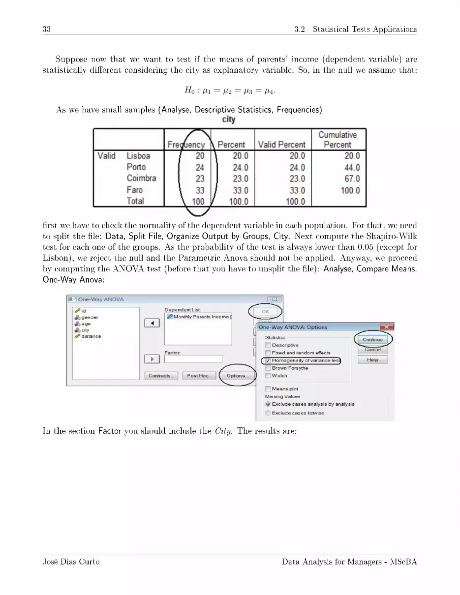
Suppose now that we want to test if the means of parents' income (dependent variable) arestatistically dierent considering the city as explanatory variable. So, in the null we assume that:
H0 : µ1 = µ2 = µ3 = µ4.
As we have small samples (Analyse, Descriptive Statistics, Frequencies)
rst we have to check the normality of the dependent variable in each population. For that, we needto split the le: Data, Split File, Organize Output by Groups, City. Next compute the Shapiro-Wilktest for each one of the groups. As the probability of the test is always lower than 0.05 (except forLisbon), we reject the null and the Parametric Anova should not be applied. Anyway, we proceedby computing the ANOVA test (before that you have to unsplit the le): Analyse, Compare Means,One-Way Anova:
In the section Factor you should include the City. The results are:
José Dias Curto Data Analysis for Managers - MScBA

34 3.2 Statistical Tests Applications
As the probability associated with the ANOVA F-test (0.768) is higher than 0.05, we don't rejectthe null and the equality of means can be assumed. However, as the normality assumption is re-jected and the sample size is small, this conclusion is statistically limited. In this case you shouldapply a nonparametric test.
REFERENCESPinto, J. C. and Curto, J. D. (2001), Estatística para economia e gestão, Ed. Sílabo.McClave, James T., Benson, P. G. and Sincich, T. (2012), Statistics for Business and Economics,12th edition.
José Dias Curto Data Analysis for Managers - MScBA

35 4 Correlation and simple linear regression
4 Correlation and simple linear regression
Correlation analysis can be used to quantify the linear association between two variables. Simplelinear regression is used to establish the linear relationship between a dependent and one explana-tory variable. Students must be able to interpret the scatter diagram, to compute and interpretthe linear correlation coecient and to estimate the parameters of the simple linear regressionmodel.
When quantitative variables are involved, the correlation and regression analyzes are suitableto quantify the relationship between those variables. The regression analysis is more complete andallows us to determine the equation that describes, in average terms, that relationship.
4.1 Types of data
The data that support correlation and regression analyzes can be classied into three categories:
• Data which describe the movement of a variable over time are called time-series data and maybe hourly, daily, weekly, monthly, quarterly or annual. In nance, time series observationscan also be recorded with elapsed time lower that one hour (the price of a stock ve-by-veminutes, for example);
• Data which describe the activities of individual persons, rms, or other units at a given pointin time are called cross-section data;
• Panel data, which combine time-series and cross-section data, may be used to study thebehavior of a group of rms over time.
Examples
• Time series dataXt The sales of EDP in the last 10 years, t = 1, 2, . . . 10.Xt The BCP quarterly income in the last 5 years, t = 1, 2, . . . 20.
• Cross section dataYi The sales of the Portuguese Stock Index listed rms in 2014,i = 1, 2, . . . , 20.Yi The stock prices of the NASDAQ listed rms at the end of 2014, i = 1, 2, . . . , 100.
• Panel dataZit The yearly closing price of PT, EDP, and BCP since 2000,i = 1, 2, 3 and t = 1, 2, . . . , 8.Zit The sales of the PSI20 listed rms in the last 10 years,i = 1, 2, . . . 20 and t = 1, 2, . . . , 10.
t, i and it are used to represent a particular observation from time-series, cross-section and pooleddata, respectively. We represent by T , n and nT the total of observations for each kind of data.
José Dias Curto Data Analysis for Managers - MScBA

36 4.2 Correlation Analysis
4.2 Correlation Analysis
The main tools from correlation analysis are: the scatter diagram, the covariance and the simplelinear correlation coecient. The scatter diagram is a graph, the sample covariance and linearcorrelation coecient are given by:
SXY = SY X =n∑i=1
(Xi − X
) (Yi − Y
)n− 1
,
−1 ≤ rXY = rY X = r =
n∑i=1
(Xi−X)(Yi−Y )
n−1√n∑
i=1(Xi−X)2
n−1
√n∑
i=1(Yi−Y )2
n−1
=SXYSXSY
≤ +1,
where n is the sample size, SXY is the sample covariance, rXY is the sample linear correlationcoecient, X and Y are the sample means and SX and SY are the sample standard deviations ofvariables X and Y , respectively.
Work le: Data1.xls. The le includes information about the stock market price (PRICE), theBook Value of Equity per share (BVEPS) and the Net Income per share (NIPS) of several Euro-pean rms.
1. Open the le in Excel;
2. To construct the scatter diagram between PRICE and BVEPS, select the rst 51 rows (in-cluding the name of the variables) and proceed as presented next: INSERT, Scatter.
The result must be the graph:
José Dias Curto Data Analysis for Managers - MScBA

37 4.2 Correlation Analysis
The scatter diagram suggests a positive linear association between PRICE and BVEPS: whenthe BVEPS increases/decreases the PRICE tends also to increase/decrease. They tend tomove in the same direction.
More: nonlinear relationship, negative linear association and no linear association.
3. To compute the covariance and the linear correlation coecient we can use the Excel func-tions: COVAR and CORREL. Introduce in the blank cells I1 and J1 the functions:
= COV AR(E2 : E51;F2 : F51)and = CORREL(E2 : E51;F2 : F51).
The results must be 117.79349 and 0.8134, respectively. The value of the linear correlationcoecient conrms the strong positive linear association between PRICE and BVEPS.
To test if the sample linear correlation coecient is statistically signicant, we can performthe following test: H0 : ρ = 0 against H1 : ρ 6= 0, where ρ is the population linear correlationcoecient. The statistic of the test is given by:
r√(1− r2)/(n− 2)
=r√n− 2√
1− r2∼ t(n−2).
This test is valid only if the variables are normally distributed and the samples are independent.When big samples are available, and despite the variables' distribution,
r√n− 2√
1− r2
a∼ N (0, 1) .
To test the signicance of the sample correlation coecient, open the le Data1.xls in SPSS.Then Analyse, Correlate, Bivariate. In the opened window proceed as follows:
José Dias Curto Data Analysis for Managers - MScBA

38 4.3 Simple Regression Analysis
The correlation coecient is also named by Pearson correlation coecient due to its author,the statistician Karl Pearson. The obtained results are summarized next:
The test value is given by:
t =0.8√
13371− 2√1− 0.82
= 154.1659
and the associated probability (Sig. (2-tailed)) is obtained from the Excel function
= DISTT (154.1659; 13369; 2) = 0.000 (in Portuguese)
or= TDIST (154.1659; 13369; 2) = 0.000 (in English).
Based on this signicance (0.000) we reject the null. Thus, we conclude that the sample linearcorrelation coecient between PRICE and BVEPS is statistically signicant, in accordance to thesample and the 5% signicance level.
4.3 Simple Regression Analysis
The equation for the simple linear regression model is given by:
Yi = β1 + β2X2i + εi
José Dias Curto Data Analysis for Managers - MScBA

39 4.3 Simple Regression Analysis
where Y is the dependent variable, β1 and β2 are the parameters or coecients of the model andε is the error term. If we exclude ε, we have the equation of a straight line.
The index i is used to represent a cross section data: information for dierent companiesreferred to a single period of time. See section 4.1 for more on types of data.
To obtain the equation that represents, in average terms, the relationship between PRICE andBVEPS we can do that directly on the scatter diagram. Go back to the Excel.
1. Check with the right button of the mouse in any point of the scatter diagram. In the openedwindow select Add Trend Line (Adicionar Linha de Tendência):
More: nonlinear relationships.
José Dias Curto Data Analysis for Managers - MScBA

40 4.3 Simple Regression Analysis
2. Next proceed as follows:
And the result must be:
You can use the mouse to move the equation for any position in the graph.
The equation of the straight line is given by:
Yi = 6.7232 + 1.2332Xi or P ricei = 6.7232 + 1.2332BV EPSi.
The hat means predicted instead of observed. In terms of the estimates for the parameters:
• 6.7232 is the expected value for the PRICE of a company if the BVEPS is 0. This interpre-tation makes sense only if there are companies with BV EPS = 0 in the sample.
• 1.2332 is the expected variation on price per unit change on BVEPS, ceteris paribus: if allthe rest remains constant.
José Dias Curto Data Analysis for Managers - MScBA

41 4.3 Simple Regression Analysis
The Excel presents also the R2, the Coecient of determination, and it represents the per-centage of the total variation of the dependent variable that is explained by the variation of theexplanatory variables in the sample. In the simple linear regression model, the coecient of de-termination is the square of the linear correlation coecient: R2 = 0.81342. Thus, on this sample,66% of the total variation on price is explained by the variation on BVEPS. This result conrmsthe strong linear association between PRICE and BVEPS.
REFERENCEWooldridge, Jerey M. (2015), Introductory Econometrics: A Modern Approach, South-Western,5th Edition
José Dias Curto Data Analysis for Managers - MScBA

42 5 The multiple linear regression model (MLRM)
5 The multiple linear regression model (MLRM)
Multiple linear regression is used to establish the linear relationship between a dependent and morethan one explanatory variables; it is a generalization of the simple model. Students must be ableto understand how the Ordinary Least Squares (OLS) method works, to compute and interpretthe R2, the adjusted R2, the standard error of the regression, the F -test, the t-tests and condenceintervals for the parameters.
The multiple linear regression model allows us to establish a linear relationship between adependent variable and more than one explanatory variables. The main purpose is to estimatehow the variation in each of the explanatory variables impacts on the dependent one. The equationof the model is given by (for cross section data):
Yi = β1 + β2X2i + . . . , βkXki + εi
The error term is included because we can not expect that changes in the explanatory variablesfully explain the variation in the dependent one. Therefore, the error term represents the variationin the dependent variable that is not associated, or does not result, from the variations in theexplanatory variables.
The number of parameters is k+1 including k coecients (βj) plus the variance of the errors: σ2ε .
The explanatory variables can be a linear (or a nonlinear) transformation of the other explanatoryvariables but the relationship between the dependent and the explanatory variables must be linearin the parameters βj.
The MLRM equation can be presented for each observation i:Y1 = β1 + β2X21 + β3X31 + . . .+ βkXk1 + ε1
Y2 = β1 + β2X22 + β3X32 + . . .+ βkXk2 + ε2
. . . . . . . . .Yn = β1 + β2X2n + β3X3n + . . .+ βkXkn + εn.
and it can be represented by using matrices and vectors:
y = Xβ + ε,
where:
y =
Y1
Y2...Yn
, X =
1 X21 X31 Xk1
1 X22 X32 Xk2...
......
...1 X2n X3n Xkn,
, β =
β1
β2...βk
, ε =
ε1
ε2...εn
.y and ε are n × 1 vectors, β is a k × 1 vector and X is a n × k matrix. Each X elementhas two indexes: the rst one refers to the column (variables) and the second one to the row (ob-servation). X2i, for example, represents the observation i for the explanatory variable X2. EachX column represents a vector with n observations for each of the explanatory variables.
5.1 Assumptions of the MLRM
The assumptions of the MLRM can be presented in terms of matrices and vectors:
1. The specication of the model is given by: y = Xβ + ε;
José Dias Curto Data Analysis for Managers - MScBA

43 5.2 Ordinary Least Squares Method (OLS)
2. E (ε) = 0;
3. The covariance matrix (ε) of the errors is given by: E (εε′) = σ2I (Homoskedasticity andNo Autocorrelation assumptions), where I is a n× n identity matrix:
E (εε′) =
E (ε2
1) E (ε1ε2) . . . E (ε1εn)E (ε2ε1) E (ε2
2) . . . E (ε2εn)...
......
...E (εnε1) E (εnε2) . . . E (ε2
n)
=
=
Var (ε1) Cov (ε1, ε2) . . . Cov (ε1, εn)
Cov (ε2, ε1) Var (ε2) . . . Cov (ε2, εn)...
......
...Cov (εn, ε1) Cov (εn, ε2) . . . Var (εn)
.Since Var (εi|X2, X3, ..., Xk) = σ2 and Cov (εi, εj) = E (εiεj) = 0 for i 6= j then,
E (εε′) = σ2I = σ2
1 0 . . . 00 1 . . . 0...
......
...0 0 . . . 1
;
4. The errors are normally distributed: ε ∼ (0, σ2I) ;
5. The X elements are non random and the rank of X is k, the number of X columns. If therank of matrix X is k, the explanatory variables are not perfectly correlated (No Multi-collinearity assumption). Thus, we can conclude that X′X is a regular symmetric matrixwhose determinant is dierent from 0;
6. E (X′ε) = 0, according to the last assumption and since that E (ε) = 0.
5.2 Ordinary Least Squares Method (OLS)
The objective of the Ordinary Least Squares method is to nd the estimator β that minimize theResidual Sum of Squares (RSS):
Min RSS =n∑i=1
e2i =
n∑i=1
ε2i = ε′ε = e′e,
where e is the vector of ordinary residuals: e = y − y and y = Xβ is the OLS estimator for themean of the vector y: Xβ.
To obtain the OLS estimators, we simplify rst the Residual Sum of Squares:
e′e =(y −Xβ
)′ (y −Xβ
)= y′y − β
′X′y − y′Xβ + β
′X′Xβ =
= y′y − 2β′X′y + β
′X′Xβ, (3)
Considering that:
José Dias Curto Data Analysis for Managers - MScBA

44 5.3 Properties of OLS estimators
• The transpose of the product of matrices is the product of transposes considering the inverse
order of the original product(Xβ)′
= β′X′,
• The transpose of a scalar is the scalar itself, y′Xβ =(y′Xβ
)′= β
′X′y.
The rst order conditions to minimize the RSS are:
∂RSS
∂β= −2X′y + 2X′Xβ = 0,
considering the derivative of a quadratic form:
∂(β′X′Xβ
)/∂β = 2X′Xβ.
Based on this it is possible to deduce the normal equations :
(X′X) β = X′y
and the vector of the Ordinary Least Squares estimators is given by:
β = (X′X)−1
(X′y) .
5.3 Properties of OLS estimators
If the assumptions of the MLRM hold, the OLS estimators β are the most ecient from the set ofthe linear unbiased estimators for β, i.e., they are the ones with the smallest (minimum) varianceand we conclude that OLS estimators are BLUE : Best Linear Unbiased Estimators (by theGauss-Markov theorem).
We show next that β is an unbiased estimator for β. As,
β = (X′X)−1
(X′Y) = (X′X)−1
X′ (Xβ + ε) =
= (X′X)−1
X′Xβ + (X′X)−1
X′ε = β + (X′X)−1
X′ε = β + Aε,
where A = (X′X)−1 X′ and, therefore,
E(β)
= β + AE (ε) = β.
The OLS estimators are normally distributed as β is a linear function of ε and, by assumption,ε has normal distribution.
Next we deduce the variances and covariances of the individual estimators βj:
var(β)
= E
[(β − β
)(β − β
)′]=
José Dias Curto Data Analysis for Managers - MScBA

45 5.4 Ohlson Empirical Application
=
var(β1
)cov
(β1, β2
). . . cov
(β1, βk
)cov
(β2, β1
)var(β2
). . . cov
(β2, βk
)...
......
...
cov(βk, β1
)cov
(βk, β2
). . . var
(βk
)
.Since that:
β = β + (X′X)−1 X′ε and β − β = (X′X)−1 X′ε then,
var(β)
= E
[(β − β
)(β − β
)′]= E
[(X′X)
−1X′εε′X (X′X)
−1]
=
= (X′X)−1
X′E (εε′) X (X′X)−1
= σ2 (X′X)−1.
Thus,
var(β)
= E
[(β − β
)(β − β
)′]= σ2 (X′X)
−1.
This is a k× k matrix where the sample variances of βj are in the main diagonal of the matrixand the covariances are out of that diagonal.
To compute the covariance matrix of the OLS estimators it becomes necessary to estimate thescalar σ2 and the usual estimator is the Mean Square Error (MSE):
s2 = σ2 =e′e
n− k,
which is an unbiased estimator for σ2εi. In conclusion:
• β = (X′X)−1 X′y,
• var(β)
= E[(β − β
)(β − β
)]= σ2 (X′X)−1 ,
• s2 = σ2 = e′en−k , where k is the number of coecients,
• β ∼ N[β, σ2 (X′X)−1] .
5.4 Ohlson Empirical Application
Let's consider the linear regression model where the PRICE is the dependent variable and theBVEPS and NIPS are the explanatory variables. This model is due to OHLSON (1995) and it iscommonly used in empirical accounting:
PRICEi = β1 + β2BV EPSi + β3NIPSi + εi.
1. Open the le Data1 in Excel;
José Dias Curto Data Analysis for Managers - MScBA

46 5.4 Ohlson Empirical Application
2. Select the worksheet FirmsPS2005 where a Portuguese and Spanish cross section data isconsidered.
3. To estimate the model select the menu DATA (DADOS) and the command Data Analysis(Análise de Dados). From the statistical options select Regression (Regressão). Next proceedas follows:
4. The results are presented next:
Next we interpret the results from the table.
5.4.1 Coecient of Determination: R-Square (Quadrado de R)
The total variation of the dependent variable can be broken down into two parts:
n∑i=1
(Yi − Y
)2
︸ ︷︷ ︸TSS
=n∑i=1
(Yi − Y
)2
+n∑i=1
(Yi − Yi
)2
+ 2n∑i=1
(Yi − Y
)(Yi − Yi
)=
José Dias Curto Data Analysis for Managers - MScBA

47 5.4 Ohlson Empirical Application
=n∑i=1
(Yi − Y
)2
︸ ︷︷ ︸ESS
+n∑i=1
(Yi − Yi
)2
︸ ︷︷ ︸RSS
,
since that:
n∑i=1
(Yi − Y
)(Yi − Yi
)=
n∑i=1
(Yi − Y
)ei =
n∑i=1
Yiei − Yn∑i=1
ei = 0.
Thus, we can conclude that:
n∑i=1
(Yi − Y
)2
︸ ︷︷ ︸TSS
=n∑i=1
(Yi − Y
)2
︸ ︷︷ ︸ESS
+n∑i=1
(Yi − Yi
)2
︸ ︷︷ ︸RSS
, (4)
where TSS, ESS and RSS stand for Total Sum of Squares (the total variation of the dependentvariable around the mean), Explained Sum of Squares (the total variation explained by the model)and Residual Sum of Squares (the unexplained variation of the dependent variable), respectively.
The coecient of determination (R2) quanties the percentage of the total variation of depen-dent variable (TSS) that is explained by the model considering the data in the sample and it worksas a goodness-of-t measure:
0 ≤ R2 =ESS
TSS= 1− RSS
TSS≤ 1.
In our application,
TSS = 38540.60265, ESS = 28357.00432 and RSS = 10183.59833.
Thus
R2 =28357.00432
38540.60265= 1− 10183.59833
38540.60265= 0.735770.
This result means that in the 2005 sample of Portuguese and Spanish companies, around 74%of the total variation on PRICE is explained by the variation on BVEPS and NIPS.
The Multiple Correlation Coecient (R Múltiplo) is the square root of the coecientof determination and represents the linear association of the dependent and all the explanatoryvariables.
In spite of its widespread use as goodness-of-t measure, there are two main problems relatedwith R2. First, when comparing dierent specications for the MLRM, the coecient of deter-mination is sensitive to the number of explanatory variables. The inclusion of new explanatoryvariables never decreases the R2 and the common is to increase it (the inclusion of new explanatoryvariables does not change the TSS value but probably increases the value of ESS and reduces theRSS value).
Second, when the intercept nullity restriction is imposed (β1 = 0), the R2 cannot be interpretedas it was done before. In this case the ratio between ESS and TSS cannot vary between 0 and 1and the traditional decomposition of the Total Sum of Squares is not true.
Thus, the rst one constitutes the major problem associated with the R2 as goodness-of-tmeasure because it takes no account the degrees of freedom associated with the TSS, RSS and
José Dias Curto Data Analysis for Managers - MScBA

48 5.4 Ohlson Empirical Application
ESS sum of squares. To face this, the variances instead of the variations are considered and theresult is the adjusted R2 (R2):
R2 = 1− V ar(ε)
V ar(Y )= 1−
n∑i=1
e2i
n−kn∑i=1
(Yi−Y )2
n−1
= 1− s2
s2Y
. (5)
The R2 compares the variance of residuals with the variance of dependent variable and repre-sents the proportion of the variance of the dependent variable that is explained by its relationshipwith the explanatory variables.
In the Ohlson model application, R2 = 0.73, meaning that when the relationship betweenPRICE and BVEPS, NIPS is established, it is possible to explain or eliminate 73% of the vari-ance of PRICE. The remainder 27% represents the part of the PRICE's variance that cannot beexplained/eliminated by the model.
In general, if R2 = 1 the variance of Y is fully explained/eliminated since the variance ofresiduals is equal to zero. If R2 = 0 the standard deviation of Y equals the standard error of theregression and the predicted values of Y are the sample mean.
Even if the RSS decreases (or remains constant) when new explanatory variables are added tothe model, it does not imply a decline on the variance of residuals. Thus, the goodness-of-t is nolonger dependent on the number of explanatory variables which are part of the model.
Based on the R2 denition presented above,
R2 = 1− RSS
TSS= 1−
n∑i=1
e2i
n∑i=1
(Yi − Y
)2= 1−
n∑i=1
e2i
n−kn∑
i=1(Yi−Y )
2
n−1
n− kn− 1
= 1− s2
s2Y
n− kn− 1
,
since s2
s2Y= 1− R2, we can derive the the formula that relates R2 and R2:
R2 = 1−(1− R2
) n− kn− 1
or R2 = 1− n− kn− 1
+ R2n− kn− 1
or
R2 = 1−(1−R2
) n− 1
n− k.
Based on this relationship we can conclude that:
• If k = 1, then R2 = R2;
• If k > 1, than R2 > R2;
• R2 can be negative. In this case the value of the coecient means that the model does notdescribe correctly the process that generated the data. If this is the case we assume zero forthe R2 value.
José Dias Curto Data Analysis for Managers - MScBA
49 5.4 Ohlson Empirical Application
5.4.2 The Standard Error of Regression (Erro-padrão da Regressão)
The standard error of regression is given by:
s =
√RSS
n− k=
√10183.59833
106− 3= 9.943
and represents the standard error of the residuals: the smaller the better is the t between theobserved and the estimated values of the dependent variable.
Sometimes the coecient of variation is computed to have an idea about the relative weight ofthe standard error of the regression on the mean of the dependent variable:
CV =9.943333782
17.06240566× 100 = 58.276%
meaning that the standard error of the regression represents around 58% of the mean of thedependent variable.
5.4.3 The Unstandardized Coecients
Slope coecients represent the expected change in the dependent variable for each unit changein the associated explanatory variable, assuming that all the other explanatory variables remainunchanged. Due to this they are also known as partial regression coecients. Based on estimatesfor the unstandardized coecients, the estimated equation is given by:
PRICEi = 3.31965432 + 9.789285753NIPSi + 0.218969462BV EPSi.
For example, the expected value for the PRICE of a company with BV EPS = 3.5 andNIPS =2.3 is given by:
PRICEi = 3.31965432 + 9.789285753× 2.3 + 0.218969462× 3.5 = 26.60
In terms of the estimates meaning:
• 3.31965432: this is the expected value for the PRICE of a company if the BVEPS and NIPSare 0. This interpretation makes sense only if there are companies with BV EPS = 0 andNIPS = 0 in the sample.
• 9.789285753: it is the expected variation on PRICE per unit change on NIPS, ceteris paribus:if all the rest remains constant.
• 0.218969462: it is the expected variation on PRICE per unit change on BVEPS, ceterisparibus: if all the rest remains constant.
5.4.4 The Standardized Coecients
If the explanatory variables are measured in dierent units, the estimated coecients can not becompared directly to assess the importance of each explanatory variable on the dependent one.For this to be possible, the standardized coecients should be estimate.
José Dias Curto Data Analysis for Managers - MScBA
50 5.4 Ohlson Empirical Application
The standardized coecients, also named beta coecients provide an indication of the relativeimportance of each of the explanatory variables in the model. In order to estimate the standardizedcoecients, all the variables are standardized rst before the OLS method application.
The standardization process unfolds in two steps. Firstly, variables are centered, subtractingthe average of the variable to each observation:
X∗j = Xj −Xj.
Then the scale of the original variable is changed, dividing the dierence by the standarddeviation of the variable:
xji =X∗jisXj
=Xji −Xj
sXj
.
The regression model in the standardized form is given by:
Yi − YsY
= β∗2X2i − X2
sX2
+ β∗3X3i − X3
sX3
+ . . .+ β∗kXki − Xk
sXk
+εi − εsε
.
Since that xki = Xki − Xk (centered variables) then:
yisY
= β∗2x2i
sX2
+ β∗3x3i
sX3
+ . . .+ β∗kxkisXk
+ ε∗i .
Multiplying both members of the last equation by sY results in:
yi = β∗2sYsX2
x2i + β∗3sYsX3
x3i + . . .+ β∗ksYsXk
xki + ε∗∗i .
Thus,
βj = β∗jsYsXj
or,
β∗j = βjsXj
sY. (6)
To estimate the standardized coecients in the OHLSON model application, you must computerst the standard deviation of each variable. You can use the Excel functions: STDEV (in En-glish) or DESVPAD (in Portuguese) to compute the standard deviations. Thus, the standardizedcoecients for:
• NIPS : β∗ = 9.789285753× 1.47959380219.15863666
= 0.756012381;
• BV EPS : β∗ = 0.218969462× 10.6804396819.15863666
= 0.122069757.
The standardized coecient of the intercept is undened, since the constant disappears asresult of the standardization process. In terms of meaning:
• 0.756012381: for the variation of one standard deviation in the NIPS, and assuming every-thing else constant, it is expected a variation of 0.756 standard deviations on PRICE.
José Dias Curto Data Analysis for Managers - MScBA

51 5.4 Ohlson Empirical Application
• 0.122069757: it is the expected variation on PRICE per unit change on BVEPS (both interms of standard deviations), ceteris paribus: if all the rest remains constant.
The higher the value of beta coecient the greater the impact of the explanatory variableon the dependent one. Thus, the NIPS is the explanatory variable with higher impact on thedependent one.
5.4.5 F test
The objective of the F test is to assess the overall statistical signicance of the linear regressionmodel. The F test, with k − 1 and n − k degrees of freedom, allows us to test if no explanatoryvariables contribute to explain the total variation of the dependent variable Y . The hypotheses ofthe test are:
H0 : β2 = β3 = . . . = βk = 0
H1 : ∃βj 6= 0
and the statistic of the test is
F =ESSk−1RSSn−k
=R2
k−1
1−R2
n−k
=R2 (n− k)
(1−R2) (k − 1)∼ F(k−1;n−k).
if the null hypothesis is true, the statistic of the test has an F -Snedecor distribution when theerrors are normally distributed.
The F test is also a signicance test of R2, i.e., testing the null hypothesis that all slope coe-cients are equal to zero is equivalent to test the null hypothesis that the coecient of determinationof the population is zero.
In the OHLSON model application the value of the F test is given by:
F =28357.004
210183.598
103
= 143.4056682.
As the associated signicance (1.70652E−30) is lower than 0.05 (the default signicance level) wereject the null and we conclude that, based on the sample, there is at least one estimated coecientthat is statistically signicant: there is at least one explanatory variable whose variation contributesto explain the variation on the dependent one. The next test is to see which are the estimatesstatistically signicant based on individual t−tests.
5.4.6 t test
As we stated before if the errors are normally distributed, βj ∼ N(βj;σβj
), assuming that σ2 is
known. When σ2 is replaced by its estimator (s2),
βj − βj0sβj
∼ t(n−k).
José Dias Curto Data Analysis for Managers - MScBA

52 5.4 Ohlson Empirical Application
The common null and alternative hypotheses of the t test are:H0 : βj = 0
Ha : βj 6= 0.
If we replace βj0 by zero, the value in the null, the t-test is the ratio between the estimate forthe coecient and its standard error:
βjsβj∼ t(n−k).
If we reject the null we conclude the estimate for the coecient is statistically signicant or itis statistically dierent from 0.
In the OHLSON model application we can compute the t-test for each of the three βj dividingthe column Coecients by the column Standard Error:
• β1: t = 3.319654321.26299227
= 2.628404304,
• β2: t = 9.7892857531.115654698
= 8.774476339,
• β3: t = 0.2189694620.154555039
= 1.416773356.
As the critical value in the Student's t distribution for α = 0.05 is near 2, we reject the nullfor NIPS and we don't reject the null for BVEPS. We can achieve the same conclusion based onP-value, the signicance associated with the t-test. As it is lower than 0.05 we reject the null forNIPS and we don't reject the null for BVEPS because the signicance is higher than 0.05. Inconclusion, only the estimate for NIPS is statistically signicant. Therefore, only this variable isrelevant to explain the variation on PRICE.
In the F test it is possible to reject the null hypothesis even if none of the regression coecientsis statistically signicant from the individual t-tests. This situation can occur, for example, if theexplanatory variables are strongly correlated. The result should be: high values for standard errorsof the estimated coecients and low values for t, even though in general the model ts the datacorrectly. We return to this issue when the problem of multicollinearity will be considered.
5.4.7 Information Criteria
The parsimony principle3 suggests to adopt models with the number of parameters as small as pos-sible because the simplest models are preferred (with the smallest number of explanatory variables)due to the reasons:
• The inclusion of too many explanatory variables in the model worsens the relative accuracyof the individual coecients;
• The resulting loss of degrees of freedom should reduce the power of the tests performed onthe estimated coecients: it increases the likelihood of committing a type II error (do notreject the null hypothesis when it is false).
3In economics the parsimony principle is also named by the principle of Occam's Razor (William of Occam,1285-1350).
José Dias Curto Data Analysis for Managers - MScBA

53 5.4 Ohlson Empirical Application
• Simple models are also easier to understand.
Thus, complex models are the more penalized by the criteria presented next. These criteria arebased on the Residual Sum of Squares (RSS) multiplied by a factor that penalizes the complexityof the model. An increased complexity reduces the RSS but increases the penalty. The smallerthe value for each criterion the more reliable the model is.
Table 1: Information Criteria
Criteria Form 1 Form 2
MSE RSSn−k ln (RSS)− ln (n− k)
AIC(RSSn
)e(2k/n) ln
(RSSn
)+ 2k
n
FPE(RSSn
) (n+kn−k
)ln(RSSn
)+ ln
(n+kn−k
)HQ
(RSSn
)(lnn)(2k/n) (
RSSn
)(lnn)(2k/n)
GCV(RSSn
) [1−
(kn
)]−2ln(RSSn
)− 2 ln
[1−
(kn
)]RICE
(RSSn
) [1−
(2kn
)]−1ln(RSSn
)− ln
[1−
(2kn
)]Schwarz
(RSSn
)n(k/n) ln
(RSSn
)+ k
nln (n)
Shibata(RSSn
)n+2kn
ln(RSSn
)+ ln
(n+2kn
)AIC: Akaike Information criterion, FPE: Finite prediction error, GCV: Generalized Cross
Validation. n is the number of observations and k is the number of parameters. Source:
Ramanathan (2002).
The criteria's denition is not always the same. In Eviews, for example, the AIC, HQ and SICare computed directly by using the maximum value for the log-likelihood function:
AIC = −2L
n+
2k
n, (7)
HQ = −2L
n+
2k log (log (n))
n, (8)
SBC = −2L
n+k log (n)
n, (9)
where L is the maximum value for the log-likelihood function.
REFERENCEWooldridge, Jerey M. (2015), Introductory Econometrics: A Modern Approach, South-Western,5th Edition
José Dias Curto Data Analysis for Managers - MScBA

54 6 Assumptions of the MLRM: Normality and Multicollinearity
6 Assumptions of the MLRM: Normality and Multicollinear-
ity
The statistical inference in the MLRM, namely the F and the t tests, is dependent from theerrors' normality. The students must be able to compute and interpret the Kolmogorov-Smirnovand Jarque-Bera tests. In terms of Multicollinearity the students must be able to compute andinterpret the TOL, VIF and the Variance Proportions diagnostics. They must also know whichare the consequences for the standard errors of OLS coecients .
The errors' normality assumption is the support of all statistical inference in the linear re-gression model, namely the overall signicance Ftest and the individual signicance t tests foreach of the estimated coecients. The normality is also required for condence intervals of therespective coecients.
When the normality of the errors is violated, the OLS estimators are still BLUE (Best LinearUnbiased Estimators) but the statistical inference, and based on the Central Limit Theorem, isonly valid asymptotically (Johnston and Dinardo, 2001).
We refer next some corrective measures if the errors' normality assumption is violated. Whenthe distribution of residuals is skewed to the right, the logarithmic transformation of the dependentvariable is often used. Weisberg (1985) recommends a logarithmic transformation of any variablewhen the ratio between the minimum and the maximum exceeds 10 (Hocking, p. 107).
For distributions skewed to the left, the quadratic transformation is the most commonly used.It should be noted that the Ftest is almost insensitive to moderate violations of normality.
6.1 Normality Tests
6.1.1 Skewness and Kurtosis coecients
To measure the skewness and kurtosis of a random variable distribution with mean µ and standarddeviation σ, two coecients are computed based on the third and fourth moments about the mean:
S(X) = E
[(X − µ)3
σ3
]=E (X − µ)3
σ3=µ3
σ3=
µ3
(µ2)3/2(10)
and,
K(X) = E
[(X − µ)4
σ4
]=E (X − µ)4
σ4=µ4
σ4=µ4
µ22
(4). (11)
If the distribution is symmetric (as the Gaussian case), the odd moments about the mean areall zero and the skewness is also zero:
S(X) = 0.
If the distribution is asymmetric positive or negative, the skewness is positive and negative,respectively.
4To remove the eect of variables units of measure, the moments are divided by a scale parameter, resulting inthe third and fourth normalized moments.
José Dias Curto Data Analysis for Managers - MScBA

55 6.1 Normality Tests
In terms of kurtosis, and based on the moments' generating function of a random variable withnormal distribution,
µ4 = 3σ4 = 3µ22.
If σ = 1 the kurtosis of a standard normal distribution is 3:
K(X) = 3.
When the probability mass on the tails of a distribution is greater than the mass of the normaldistribution, the kurtosis is higher than 3 and it can be even innite. In this case the distributionis named leptokurtic. If K(X) < 3 the distribution is platikurtic. Distributions of nancial randomvariables (interest rates, exchange rates, nancial assets rates of return, etc..) are in generalleptokurtic.
The skewness and kurtosis coecients can be estimated based on sample data. The estimatorsare:
S(X) =1
T σ3
T∑t=1
(xt − µ)3 (12)
and,
K(X) =1
T σ4
T∑t=1
(xt − µ)4 , (13)
where T, µ and σ are the sample size, mean and standard deviation, respectively:
µ =1
T
T∑t=1
xt (14)
and,
σ =
√√√√ 1
T
T∑t=1
(xt − µ)2. (15)
For big samples and Gaussian random variables, the estimators for the coecients of skewnessand kurtosis are normally distributed5:
S(X)a∼ N
(0,
√6
T
)(16)
and,
K(X)a∼ N
(3,
√24
T
). (17)
The hypotheses of the normality tests involving the skewness and kurtosis coecients are:H0 : S(X) = 0
H1 : S(X) 6= 0.(18)
5Stuart, A. and K. Ord (1987), Kendall's advanced theory of statistics, vols. I-III, Oxford University Press, NewYork. Citado por Campbell, Lo e MacKinlay (1997, page 17).
José Dias Curto Data Analysis for Managers - MScBA

56 6.2 The Jarque-Bera (JB) Test
and, H0 : K(X) = 3
Ha : K(X) 6= 3.(19)
The statistic of the tests are:
ts =S(X)√
6T
a∼ N (0, 1) (20)
and,
tk =K(X)− 3√
24T
a∼ N (0, 1) . (21)
where K(X)− 3 is generally known by the excess of kurtosis.
6.2 The Jarque-Bera (JB) Test
The normality Jarque-Bera test is valid for big samples and it is based on the estimates for thecoecients of skewness and kurtosis. The statistic of the test is:
JB = n
S(X)2
6+
[K(X)− 3
]2
24
∼ χ2(2). (22)
The normality hypothesis is rejected if JB > χ2(2)(α).
If the variable under normality test is the OLS residuals from a regression model, then n mustbe replaced by n− k where k is the number of parameters to estimate (Diebold, 2004, p. 29).
6.3 The Kolmogorov-Smirnov (KS) Test
Let F (x) be the population cumulative distribution function and the following hypotheses:H0 : F (x) = F0 (x)
Ha : F (x) 6= F0 (x)(23)
where −∞ < x < +∞ and F0(x) is the continuous cumulative distribution function completelyspecied and under test.
The statistic of the Kolmogorov-Smirnov (K-S) test represents the maximum distance (mea-sured vertically) between the dierent values of the sample distribution function and the theoreticaldistribution function under test:
Dn = sup−∞<x<∞
|Fn (x)− F0 (x)| . (24)
José Dias Curto Data Analysis for Managers - MScBA

57 6.4 Cobb-Douglas Application
In order to compute the K-S test value the sample distribution function is replaced by theempirical distribution function:
dn = sup−∞<x<∞
∣∣∣Fn (x)− F0 (x)∣∣∣ . (25)
The decision rule is the following: reject H0 when dn > dn,α (the critical value from theKolmogorov-Smirnov statistical tables).
The Kolmogorov-Smirnov test requires the complete specication of the distribution underthe null hypothesis. When the parameters of the distribution under test are replaced by theirestimates, the test is conservative, i.e., the signicance values are higher than the true values (ifthe parameters where known) leading to the nonrejection of the null hypothesis more often thanit should be.
The Lilliefors (1967) test intends to correct this situation by adapting the K-S test when theparameters of the distribution under test are unknown and they are estimated based on sampledata. The statistic of the test is practically the same but the sampling distribution changes leadingto a dierent critical values (when compared to the ones from the original test). See section 3.2.2for details.
6.4 Cobb-Douglas Application
In order to test the normality of the errors,
1. Open the Eviews workle PLKData.WF1 and estimate the log-log equation;
2. Next proceed as follows:
3. By this procedure, the Eviews computes only the Jarque-Bera test:
José Dias Curto Data Analysis for Managers - MScBA
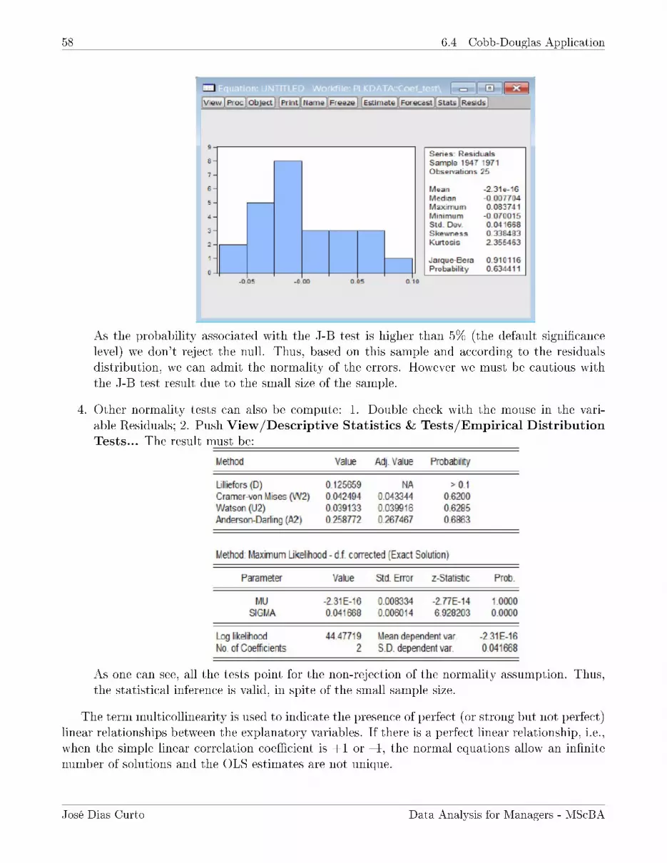
58 6.4 Cobb-Douglas Application
As the probability associated with the J-B test is higher than 5% (the default signicancelevel) we don't reject the null. Thus, based on this sample and according to the residualsdistribution, we can admit the normality of the errors. However we must be cautious withthe J-B test result due to the small size of the sample.
4. Other normality tests can also be compute: 1. Double check with the mouse in the vari-able Residuals; 2. Push View/Descriptive Statistics & Tests/Empirical DistributionTests... The result must be:
As one can see, all the tests point for the non-rejection of the normality assumption. Thus,the statistical inference is valid, in spite of the small sample size.
The term multicollinearity is used to indicate the presence of perfect (or strong but not perfect)linear relationships between the explanatory variables. If there is a perfect linear relationship, i.e.,when the simple linear correlation coecient is +1 or 1, the normal equations allow an innitenumber of solutions and the OLS estimates are not unique.
José Dias Curto Data Analysis for Managers - MScBA

59 6.5 Multicollinearity Consequences
In the other extreme situation, when the explanatory variables are linearly independent, thevariables are named orthogonal (the covariance is zero) and the parameters can be estimatedwithout problems. In this case the multiple regression is useless because each parameter βj can beestimated from the simple linear regressions between Y and each of the explanatory variables.
6.5 Multicollinearity Consequences
When the relationship between the explanatory variables is strong but not perfect, there is asingle solution for the parameters resulting from the normal equations and it is important toanalyze which are the consequences of multicollinearity.
• If at least two explanatory variables are perfectly correlated, the rank of matrices X andX′X is lower than the number of parameters to estimate [ r(X) = r(X′X) < k] and thedeterminant of X′X is zero (this is the usual way to identify the perfect correlation betweenthe explanatory variables). Consequently, the matrix X′X is singular (has no inverse) and
it is not possible to compute one single solution for β based on Ordinary Least Squares orMaximum Likelihood methods.
• If the coecient of determination is high6, in most cases the null under the F test is rejectedbut the t test results indicate that no one or a small number of estimates are statisticallysignicant. Therefore it seems there is a contradiction between F and t tests decisions.
• If the coecient of determination is high but the partial correlation coecients are small,it can suggest that explanatory variables are strongly correlated and at least one of them isuseless.
• The sign of the OLS estimates is contrary to what economic theory suggests or they have anunexpected value. However, the wrong sign can also be explained by the small size of thesample or by other factors.
• The estimates for the coecients can be too high (in absolute value) and very distant fromtheir true value.
• When the correlation between the explanatory variables is strong, it becomes harder todistinguish the eect of each explanatory variable on the dependent one.
• The OLS estimates (and the resulting forecasts) are still BLUE, i.e., they are unbiased andthe most ecient (Johnston, 1984). If they are the most ecient it means that from the classof linear unbiased estimators they are the ones with the smallest variance. But it does notmean that the variance is necessarily small in comparison with the coecients' estimates.
• The strong correlation between the explanatory variables increases the standard errors ofOLS estimators7 and decreases the t−tests value, leading to less signicant estimates, inspite of the tests being still valid. As the variance-covariance matrix of the OLS estimators
is given by cov(β)
= σ2 (X′X)−1 thus, when |X′X| → 0, cov(β)→∞.
6Gujarati (2000) suggest R2 values higher than 0.8.7In case of perfect correlation, the standard erros are innity.
José Dias Curto Data Analysis for Managers - MScBA

60 6.6 Multicollinearity Diagnostic
• The OLS estimates and standard errors are very sensitive to small changes on data and onthe model's specication.
• Even if the multicollinearity impacts on the coecients precision and interpretation, it doesnot aect the model's forecasting ability if the observed relationship between the dependentand the explanatory variables remains in the forecasting period.
6.6 Multicollinearity Diagnostic
As the multicollinearity is mostly a sample phenomena, there is no single method, generally ac-cepted, to detect and quantify the multicollinearity eects. What is available is a set of rules, fromwhich we describe the most commonly used.
6.6.1 Tolerance and Variance Ination Factor
One of the most important diagnostic measures is the Variance Ination Factor (VIF) which isbased on the coecient of determination R2
j from the regression of each Xj on the rest of the k−2explanatory variables. For k− 1 regressors there are k− 2 coecients of determination and if anyvalue is 1.0, it means there is a perfect correlation within the explanatory variables set and at leastone of them is a linear combination of the others. The relationship is almost perfect when the R2
j
value is near 1.The variance of OLS estimators can also be related with this measure of linear association.
Therefore
R2j = 1− RSSj
TSSj, (26)
where TSSj is the Total Sum of Squares for Xj, then8
RSSj = TSSj(1−R2
j
)e var
(βj
)=
σ2
TSSj(1−R2
j
) . (27)
The statistic VIFj associated to regressor j is the ratio between the variance of the estimatedcoecient and its variance if the regressors were linearly independent. Therefore the VIF can beinterpreted as the increase in the variance of βj due to the linear dependence between the regressors.The name VIF is due to the fact that it makes part of the formula for the variance of the OLSestimators and high values for VIF suggest strong linear dependence between the regressors withsignicant impact on the coecients estimates.
As it is pointed by Johnson (1984) the relationship between R2j and VIFj is non-linear and the
VIF increases dramatically when R2j is higher than 0.9. Marquardt (1970) suggests a practical rule
based on VIF to evaluate the strength of the relation between the explanatory variables: if theVIFj is higher than 10 (it means that R2
j exceeds 0.90 and Rj is higher than 0.95) the variable Xj
is strongly related with the other explanatory variables. This is simply a rule because for otherauthors the relationship between the explanatory variables is already troublesome when the VIFis higher than 2.5.
8When X′X is the correlation matrix between regressors, TSSj = 1 and var(βj
)= σ2
1−R2j.
José Dias Curto Data Analysis for Managers - MScBA

61 6.6 Multicollinearity Diagnostic
The VIF's denominator is also a multicollinearity diagnostic measure and is named by theTolerance of the variable j :
Tol = 1−R2j , j = 1, 2, . . . , k. (28)
A high R2j value (and consequently a small value for Tol) suggest that the independent variable j is
almost a linear combination of the rest of the explanatory variables. Thus, the Variance InationFactor is the inverse of the tolerance:
VIF =1
Tol=
1
1−R2j
. (29)
6.6.2 Matrix Condition
In order to identify the regression coecients that are probably more aected by the multicollinear-ity eect, Belsley, Kuh e Welsch (1980) suggest a methodology based on two diagnostic measures:the matrix condition number and the decomposition of the variance of OLS estimators. The con-dition number of a matrix A is the ratio between the highest and the smallest eigenvalues of thatmatrix:
κ (A) =λmax
λmin
. (30)
When the eigenvalues of matrix X′X are considered, and since the condition number of matrixX′X is the square of the condition number of matrix X, then:
κ (X) =
√λmax
λmin
. (31)
According to Belsley, Kuh e Welsch (1980), the dependence between explanatory variables isstrong when the condition number exceeds the value 30 and the dependence is moderate to strongfor values between 20 e 30.
The condition index )9,
γj =λmax
λj, (32)
can also be computed for each eigenvalue and its value ranges from 1 and κ (X) when λj = λmax
and λj = λmin, respectively.If the explanatory variables are linearly independent, the eigenvalues, the condition indexes
and the condition numbers of matrix X are all 1. When the correlation between the explanatoryvariables increases, the dierence between the eigenvalues also increases and some of them are nearzero implying that the matrix condition indexes and condition numbers also increase.
The condition indexes are also useful to detect the presence of strong linear relationships be-tween the columns of matrix X. There are so many linear dependencies between the explanatoryvariables as the number of high value condition indexes. In general the absence of linear depen-dencies is considered when the condition index is lower than 10. For values between 30 and 100the multicollinearity problems are moderate to strong and values higher than 100 suggest seriousproblems of dependence between the explanatory variables.
9The condition number is the condition index with the highest value.
José Dias Curto Data Analysis for Managers - MScBA

62 6.7 Solutions for Multicollinearity
6.6.3 Variance Decomposition
The decomposition of the variance of each estimator consists in associating to each eigenvalue aproportion of its variance. Thus, if X is a matrix with n × k dimension and P is a k × k matrixwhich diagonalize the matrix X′X thus, as we pointed before, (X′X) P = PΛ, where Λ is theeigenvalues diagonal matrix of X′X. Therefore,
cov(β)
= σ2 (X′X)−1
= σ2PΛ−1P′ (33)
and
var(βj
)= σ2
(p2j1
λ1
+p2j2
λ2
+ . . .+p2jk
λk
), (34)
where pj1, pj2, . . . , pjk are the elements of row j from matrix P. Based on this it is possible to
compute the proportion of var(βj
)associated to each eigenvalue:
πji =
p2ijλj∑kj=1
p2ijλj
, i, j = 1, 2, . . . , k. (35)
To determine specically which are the coecients that are more aected by multicollinearity,the procedure proposed by Belsley, Kuh e Welsch (1980) is the following:
1. Compute the eigenvalues of matrix X and select the ones with condition index higher thanthe critical value (30). The number of critical condition indexes is indicative of lineardependencies within the explanatory variables set;
2. For each condition index that exceeds the critical value, analyze the proportion of the sam-pling variance of each βj associated to that value. If a high proportion (for example, higherthan 0.5, i.e., 50%) of the variance of two or more estimators is associated to the sameeigenvalue, the corresponding explanatory variables must be involved in the strong lineardependence identied by the condition index from the rst step.
6.7 Solutions for Multicollinearity
There are dierent solutions to solve the multicollinearity problem. The most commonly used is toexclude the explanatory variable, from the ones that show strong correlation, with the smallest ttest absolute value. In general, with this operation the coecients remaining in the model becomestatistically more signicant. However, if the variable to exclude belongs to the model due totheoretical reasons, such procedure can result in a specication error that can be worse whencompared to the multicollinearity.
6.8 Application: Electric Utility
The data to support the empirical study is taken from Montgomery and Askin (1981) and ithas been collected by an electric utility during an investigation of the factors that inuence peak
José Dias Curto Data Analysis for Managers - MScBA

63 6.8 Application: Electric Utility
demand for electric energy by residential customers (this data supports also the empirical appli-cation of Montgomery et al. (1998)). The dependent variable (Y ) is the electricity demand at thehour of system peak demand in kilowatts (kW). The explanatory variables are the size (X1) ofthe customer's house (ft2/1000), the annual family income ($/1000) (X2), tons of air-conditioningcapacity (X3), the appliance index for the house (obtained by summing the kilowatt ratings for allmajor appliances) (X4) and the number of people typically in the house on a weekday (X5).
1. Open de le DataAskinMontgomery.XLS in SPSS;
2. Estimate the regression: Analyze, Regression, Linear... and proceed as follows,
3. Next gure shows the estimation results:
José Dias Curto Data Analysis for Managers - MScBA

64 6.8 Application: Electric Utility
As one can see the VIF associated with variable X2 is higher than 10. It means that X2
must be strongly correlated with at least one of the other explanatory variables. Based oncondition indexes, the value of the last one is higher than 30. If we look for the VarianceDecomposition table we conclude, based on the Belsley, Kuh e Welsch (1980) methodology,that X2 and X4 must be strongly correlated. When the t test value is considered, the solutionfor the multicollinearity problem is to exclude X2 and re-estimate the model.
REFERENCEWooldridge, Jerey M. (2015), Introductory Econometrics: A Modern Approach, South-Western,5th Edition
José Dias Curto Data Analysis for Managers - MScBA

65 7 Assumptions of the MLRM: heteroskedasticity
7 Assumptions of the MLRM: heteroskedasticity
After these two lectures students should be able to analyze the consequences of errors' Het-eroskedasticity for the OLS estimators. They should also know how to interpret the White testand to implement the White asymptotic correction procedure.
As we pointed before, the most important conditions of the Gauss-Markov theorem are:
E (ε|X) = E (ε) = 0, var (ε|X) = V (ε) = E (εε′) = σ2I,
meaning that the errors' conditional distribution, given the explanatory variables, has mean zero,constant variance (homoskedasticity) and null covariances (there is no autocorrelation in the er-rors). If these conditions hold, the OLS estimators are BLUE, i.e, they are the most ecient fromthe linear unbiased estimators set.
When at least one of these conditions is violated10, the classical linear regression model isreplaced by the Generalized Linear Regression Model:
y = Xβ + ε, E (ε|X) = E (ε) = 0, E (εε′) = σ2Ψ, (36)
where σ2 > 0 is a scale factor and Ψ is a symmetric denite positive matrix with Ψ 6= I. Ifthe errors' variance is not constant (heteroskedasticity) the elements of the σ2Ψ (σ2
i = σ2ψii) maindiagonal can be dierent ones from the others and outside the diagonal the values can be dierentfrom zero if the errors are autocorrelated (autocorrelation): cov (εi, εj) 6= 0 for i 6= j.
In this case the β OLS estimators are still unbiased and consistent but they are no longerthe most ecient. When the OLS method is applied, if the matrix X is non-stochastic andβ − β = (X′X)−1 X′ε, the β variance-covariance matrix is given by:
E
[(β − β
)(β − β
)′]=
E[(X′X)
−1X′ε
] [(X′X)
−1X′ε
]′=
= E[(X′X)
−1X′εε′X (X′X)
−1]
= σ2 (X′X)−1
X′ΨX (X′X)−1. (37)
If Ψ 6= I, the matrix resulting from (37) is dierent from the OLS variance-covariance matrix:Σβ = σ2 (X′X)−1. If this formula is used when the errors are nonspherical, the variances and
standard errors of β are estimated incorrectly. Therefore, the F and t tests are no longer valid andthe statistical inference based on these tests can be misleading. Furthermore, even if the correctformula of the variance (37) is considered, the OLS estimators are no longer the most ecient inthe presence of heteroskedasticity and/or autocorrelation.
To deal with these problems three common alternative procedures are generally adopted. Asin many applications the heteroskedasticity and/or autocorrelation are due to the model's mis-specication (omission of relevant explanatory variables or non-linearities) the rst solution is tore-specify the model. The logarithmic transformation of the dependent and/or the explanatoryvariables,
lnYi = β1 + β2 lnX2i + β3 lnX3i + ...+ βk lnXki + εi,
reduces often the heteroskedasticity of the original model.
10We refer to nonspherical disturbances instead of spherical disturbances.
José Dias Curto Data Analysis for Managers - MScBA

66 7.1 The Generalized Least Squares (GLS) Method
The second one, and if the heroskedasticity problem persists after the log transformation, im-plies the derivation of alternative BLUE estimators (this is the case of GLS estimators). However,in order to apply this method, it becomes necessary to know the pattern of the errors' heteroskedas-ticity as it is assumed that this pattern is determined by a known cedastic function.
A third alternative is to introduce corrections in the standard errors of OLS estimators in orderto get consistent estimators. If the heteroskedasticity and/or autocorrelation problems exist, andif we don't know the structure of matrix Ψ, it is still possible to estimate consistently the variance-covariance matrix of OLS estimators. These estimators are generally known by heteroskedasticityconsistent (HC) and heteroskedasticity and autocorrelation consistent estimators (HAC) as we willsee later.
7.1 The Generalized Least Squares (GLS) Method
We start by deducing the Generalized Least Squares (GLS) estimators and compare its eciencywith the one from the OLS estimators. The GLS method consists in transforming the originalmodel in order to get errors that satisfy the Gauss-Markov conditions, i.e., the transformed errorsmust have constant variance and no autocorrelation.
Let P be a n non singular symmetric matrix with the property PΨP′ = I that always exist (itcan not be unique) as Ψ is a symmetric denite matrix. Multiplying the multiple linear regressionmodel y = Xβ + ε by P results in:
Py = PXβ + Pε, (38)
ory∗ = X∗β + ε∗, (39)
where y∗ = Py, X∗ = PX and ε∗ = Pε.
In terms of the transformed errors ε∗, they have mean zero:
E (ε∗) = E (Pε) = PE (ε) = 0, (40)
and the variance-covariance matrix is:
E (ε∗ε∗′) = E (Pεε′P′) = PE (εε′) P′ = σ2PΨP′ = σ2I. (41)
The transformed errors have mean zero, constant variance, are no autocorrelated and theestimators resulting from the OLS method application are the most ecient:
β = (X∗′X∗)−1
X∗′y∗, (42)
or in terms of the original variables,
β = (X′P′PX)−1 X′P′Py,
resulting in,
β =(X′Ψ−1X
)−1X′Ψ−1y, (43)
as if PΨP′ = I then Ψ = P−1P′−1 and Ψ−1 = P′P = PP′.
José Dias Curto Data Analysis for Managers - MScBA

67 7.1 The Generalized Least Squares (GLS) Method
Therefore, the generalized least squares method consists in searching for a matrix P (namedby the square root of Ψ−1) whose elements are known such as P′P = Ψ−1 and apply the ordinaryleast squares method to the transformed variables Py and PX.
The estimators β are known by the generalized least squares estimators (GLS) andthey are, from the linear unbiased estimators, the most ecient (Gauss-Markov theorem) in themodel y = Xβ + ε, where E (ε|X) = E (ε) = 0 and E (εε′) = σ2Ψ.
We start by analyzing the unbiasedness of β. Since that,
β =(X′Ψ−1X
)−1X′Ψ−1y =
(X′Ψ−1X
)−1X′Ψ−1X︸ ︷︷ ︸
I
β +(X′Ψ−1X
)−1X′Ψ−1ε,
E (ε|X) = E (ε) = 0 and assuming that X is non-stochastic, then
E(β)
= β.
In terms of the β variance-covariance matrix, since that,
β − β =(X′Ψ−1X
)−1X′Ψ−1ε,
and E (εε′) = σ2Ψ, then
E
[(∼β −β
)(β − β
)′]= E
[(X′Ψ−1X
)−1X′Ψ−1ε
] [(X′Ψ−1X
)−1X′Ψ−1ε
]′
= E[(
X′Ψ−1X)−1
X′Ψ−1εε′Ψ−1X(X′Ψ−1X
)−1]
=(X′Ψ−1X
)−1X′Ψ−1σ2 ΨΨ−1︸ ︷︷ ︸
I
X(X′Ψ−1X
)−1
= σ2(X′Ψ−1X
)−1X′Ψ−1X
(X′Ψ−1X
)−1︸ ︷︷ ︸I
.
The result is:Σβ = σ2
(X′Ψ−1X
)−1. (44)
In general this matrix is dierent from (37) that was computed by applying directly the OLSmethod to original data without any transformation:
σ2(X′Ψ−1X
)−1 6= σ2 (X′X)−1
X′ΨX (X′X)−1. (45)
As the GLS estimators are so ecient as the OLS estimators then,
Σβ − Σβ = σ2 (X′X)−1
X′ΨX (X′X)−1 − σ2
(X′Ψ−1X
)−1= D, (46)
where D is a semidenite positive matrix.
José Dias Curto Data Analysis for Managers - MScBA

68 7.2 Heteroskedasticity
In terms of the GLS estimator for σ2,
σ2 =
(y −Xβ
)′Ψ−1
(y −Xβ
)n− k
=e′Ψ−1e
n− k. (47)
The coecient of determination resulting from the GLS method is not the most correct wayto evaluate the model's goodness-of-t. A more appropriate procedure consists in computing theresiduals from the original equation based on the GLS parameters' estimates. Next there are twoalternative ways to evaluate the goodness-of-t:
1. Compute R2 = 1− RSSTSS
but the value does not vary necessarily between 0 and 1;
2. Predict the y values based on the GLS estimates and assuming as goodness-of-t measurethe square of the linear correlation coecient between y and y.
The GLS method application requires that all the elements of matrix Ψ are known. When thisis not true, an acceptable procedure consists in replacing Ψ by an estimator Ψ. The estimatedGLS (EGLS), also named by feasible GLS, are dened as:
βEGLS =(X′Ψ
−1X)−1
X′Ψ−1
y. (48)
7.2 Heteroskedasticity
As we referred before, one of the Gauss-Markov theorem conditions is the errors' homoskedasticity,where it is assumed that the conditional variance of each εi is constant and equal to σ2:
var (εi|X) = E(ε2i |X)
= σ2, i = 1, 2, . . . , n, (49)
or, considering the vector of the errors ε,
var (ε|X) = σ2I, (50)
where σ2I is the errors' variance-covariance matrix and I is a n identity matrix.If this is not true, we say that the errors are heteroskedastic and this problem occurs more
often in cross section data when compared with time series data, the exception is high frequencynancial data: for example, daily interest rates, rates of return and rates of change. The usualproblem in time series data is the errors' autocorrelation that we analyze latter.
When the errors are heteroskedastic the variance is not constant and for now we assume thatall the rest of assumptions about the errors are true:
E (εi|X) = 0, cov (εi, εj) = E (εiεj) = 0, i 6= j. (51)
As consequence the errors' variance-covariance matrix is no longer a scalar matrix but is stilla diagonal matrix:
var (ε|X) = E (εε′) = σ2Ψ = Ω = diagσ21, σ
22, . . . , σ
2n. (52)
The heteroskedasticity has important eects on the properties of OLS estimators, on statisticalinference ( F and t tests) and forecasting:
José Dias Curto Data Analysis for Managers - MScBA

69 7.2 Heteroskedasticity
• The OLS estimators are still unbiased and consistent as these properties depend only fromthe hypotheses: E (εi|X) = 0 and cov (Xji, εi) = 0, which are not necessarily violated in thepresence of heteroskedasticity;
• The OLS estimators are no longer the most ecient in spite of the sample size, i.e., it ispossible to nd linear estimators with smaller variance when compared to OLS; the estimatorsare no longer BLUE.
• If the errors are heteroskedastic the estimators for the variances and covariances of OLSestimators are biased and inconsistent. Therefore, the t and F tests provide inaccurateresults;
• Forecasts are still unbiased and consistent but they are not the most ecient. The precisionof forecasting (measured by the respective variance) is lower than it should be when moreecient estimators are considered.
7.2.1 Detecting Heteroskedasticity
There are several statistical tests to detect if the errors are heteroskedastic based on OLS residuals:Goldfeld-Quandt (1965), Breusch-Pagan (1979), Glejser (1969), Harvey-Godfrey (1976 and 1978)and White (1980). On these lectures we concentrate on the White test.
The main characteristics of the other tests are:
• In the Goldfeld-Quandt test the middle observations are excluded from the sample withthe loss of information and the success of the test depends on the correct identication ofthe variable to sort the data. In addition, the test does not include situations where theheteroskedasticity is caused by more than one variable simultaneously;
• All the tests require a previous knowledge about the factors that are responsible for theheteroskedasticity;
• The errors' normality is necessary to deduce the sampling distribution of the tests.
To overcome the problems of previous tests, White (1980) proposed a direct test to check theerrors' homoskedasticity which is very similar to the one of Breusch-Pagan but it does not needa functional form for the structure of the heteroskedasticity. The test is valid asymptotically andthe errors do not need to be normally distributed.
For the test's description, we consider the original model with just two explanatory variables,Yi = β1 + β2X2i + β3X3i + εi.
In the White test we assume that the errors' variance is related with all the explanatoryvariables, the square of these variables and the cross-product of the explanatory variables two bytwo:
σ2i = α1 + α2X2i + α3X3i + α4X
22i + α5X
23i + α6X2iX3i + vi. (53)
The steps of the White test are the following:
1. Estimate the parameters of the original model by the OLS method;
José Dias Curto Data Analysis for Managers - MScBA

70 7.2 Heteroskedasticity
2. Compute the ordinary residuals and its square:
ei = Yi −(β1 + β2X2i + · · ·+ βkXki
)and e2
i ;
3. Estimate an auxiliar regression where the square residuals are the dependent variable and allthe explanatory variables, its square and the cross-products are the explanatory variables:
e2i = α1 + α2X2i + α3X3i + α4X
22i + α5X
23i + α6X2iX3i + vi; (54)
4. Compute the statistic of the test nR2 a∼ χ2(q−1), where R
2 is the coecient of determinationfrom the auxiliar regression, n is the number of observations and q is the number of param-eters to estimate, which is 6 on this case. If nR2 > χ2
(q−1)(α) we reject the null hypothesisand we conclude that the homoskedasticity assumption is violated.
We conclude with two additional notes about the White test auxiliar regression. Thus,
• If any of the explanatory variables is a dummy variable, the square of this variable is equal tothe original variable and if both are included in the model results in perfect linear correlationbetween the explanatory variables and no parameters can be estimated by the ordinary leastsquares method;
• The greater the number of explanatory variables is the largest the number of degrees offreedom associated with the χ2, which tends to reduce the power of the test. When thenumber of explanatory variables exceeds the number of observations, it is not possible toestimate the parameters of the model in step 3. Therefore, it is necessary to exclude some ofthese explanatory factors. The candidates are, in priority order, the linear terms and crossproducts, while the squared terms should remain in the model.
7.2.2 Corrective Measures
As mentioned earlier, if the values of σ2i are known, the simplest way to correct the heteroskedas-
ticity is to apply the generalized least squares method as the resulting estimators are BLUE.
The σ2i values are known
In the OLS method, it is assigned the same weight to each residual when the objective is to mini-mize the residuals sum of squares. This procedure is appropriate when the variance of the errorsis constant.
When this is not true, the highest weight should be attributed to the observations closer to themean which are the residuals with the lower absolute value, resulting in a more precise estimation;this is what happens in the generalized least squares method.
Assume that the variances of the errors (σ2i ) are known. If we divide each term of the linear
regression model by σi, the result should be:
Yiσi
= β11
σi+ β2
X2i
σi+ β3
X3i
σi+ . . .+ βk
Xki
σi+εiσi
(55)
or,
José Dias Curto Data Analysis for Managers - MScBA
71 7.2 Heteroskedasticity
Y ∗i = β1X∗1i + β2X
∗2i + β3X
∗3i + . . .+ βkX
∗ki + ε∗i . (56)
The variance of the transformed model is constant as we demonstrate next:
var (ε∗i ) = var
(εiσi
)=
1
σ2i
var (εi) =σ2i
σ2i
= 1. (57)
If the errors are homoskedastic, the parameters estimators resulting from OLS method appliedto the transformed model are BLUE. Thus, we can conclude that GLS minimizes the residualssum of squares of transformed residuals:
n∑i=1
(eiσi
)2
=n∑i=1
[(Yiσi
)−
(β1
σi+ β2
X2i
σi+ · · ·+ βk
Xki
σi
)]2
(58)
or,n∑i=1
λie2i =
n∑i=1
λi
(Yi − β∗1 − β∗2X2i − · · · − β∗kXki
)2
, (59)
where λi = 1/σ2i represents the weight for each observation i and it is proportionally inverse to
σ2i , i.e., the relative weight of the observations with higher σ2
i is lower when compared to theobservations with smaller σ2
i in the residuals weighted sum of squares. By this, when the GLSis used to solve the heteroskedasticity problem, the last procedure is named by Weighted LeastSquares: WLS.
To derive the transformation matrix P in the WLS method we deal rst with matrix Ψ:
Ψ =
1λ1
0 0 . . . 0
0 1λ2
0 . . . 0...
......
......
0 0 0 . . . 1λn
, (60)
where
Ψii =1
λiand σ2
i = σ2 × 1
λi.
And the result is:
Ψ−1 =
λ1 0 0 . . . 00 λ2 0 . . . 0...
......
......
0 0 0 . . . λn
⇒ P =
√λ1 0 0 . . . 00√λ2 0 . . . 0
......
......
...0 0 0 . . .
√λn
(61)
Therefore, this method transforms the original model in another one where the errors arehomoskedastic, √
λiYi =√λiβ1 + β2
√λiX2i + . . .+ βk
√λiXki +
√λiεi, (62)
where Yi, Xji and εi are weighted by√λi, since that:
var(√
λiεi
)= λi ×
σ2
λi= σ2. (63)
José Dias Curto Data Analysis for Managers - MScBA

72 7.2 Heteroskedasticity
The σ2i values are unknown
When σ2i are unknown, the elements of Ψ need to be estimated, and the resulting estimators are
usually named by estimated GLS estimators (or two steps Aitken estimators).In the usual procedure to estimate Ψ, it is assumed that the errors' variance, excluding the
constant σ2, is a known function of the independent variable (Zi) which can be one of the explana-tory variables in the model. The two most commonly used functions are presented next. In thiscase the estimates are BLUE and all the tests are valid even for small samples.
Another alternative is to estimate σi by using the auxiliar regression from one of the testsreferred before. The estimates for the coecients are consistent, as well the estimated variances,and all the tests are valid asymptotically. However, they are biased for small samples.
The errors' variance is proportional to Z2i
In this kind of heteroskedasticity it is assumed that var (εi) = σ2i = σ2Z2
i or σi = σZi, where σis the constant of proportionality whose value is unknown and Zi is an independent variable thatcan be one of the explanatory variables in the model. In this case the weight of the observation iin the residuals weighted sum of squares is: λi = 1
Z2i.
And the result is: √λi =
1√Z2i
=1
Zi.
As ψii = Z2i then Zi =
√ψii,√λi = 1√
ψiiand ψii = 1
λi, where ψii is the element i from the main
diagonal of Ψ. By this reason the variance of error i can also be presented as:
σ2i =
σ2
λi, i = 1, 2, . . . , n. (64)
Multiplying the multiple linear regression model by√λi = 1
Ziresults in:
YiZi
= β11
Zi+ β2
X2i
Zi+ β3
X3i
Zi+ ...+ βk
Xki
Zi+εiZi
(65)
or,
Y ∗i = β1X∗1i + β2X
∗2i + β3X
∗3i + ...+ βkX
∗ki + ε∗i . (66)
The variance of the errors in this transformed model is constant as we demonstrate next:
var (ε∗i ) = var
(εiZi
)=
1
Z2i
var (εi) =σ2Z2
i
Z2i
= σ2. (67)
The variance of the errors is proportional to Zi
When it is assumed that σ2i = σ2Zi, then ψi = Zi and
√λi = 1√
Ziand the original model can be
transformed in the following way:
Yi√Zi
= β11√Zi
+ β2X2i√Zi
+ β3X3i√Zi
+ ...+ βkXki√Zi
+εi√Zi, (68)
where Zi > 0.
José Dias Curto Data Analysis for Managers - MScBA

73 7.2 Heteroskedasticity
The variance of the errors in this transformed model is homoskedastic and the OLS can beapplied to (68):
var
(εi√Zi
)=
1
Zivar (εi) =
σ2ZiZi
= σ2. (69)
In a more general formulation it is considered the exponent of the variable Z as an unknownparameter: σ2
i = σ2Zpi . For p estimate it is considered the value that maximizes the logarithm of
the likelihood function (??).
José Dias Curto Data Analysis for Managers - MScBA

74 7.3 Applications
Heteroskedasticity Consistent estimators (HC)
Consistency property The consistency is an asymptotic property for the estimators (when the sample
size goes to ∞).
Let (X1, X2, . . . , Xn) and θn = f (X1, X2, . . . , Xn) be a random sample of size n and an estimator
for the parameter θ, respectively. The estimator θn is weakly consistent if, given a real number
arbitrarily small and positive ε,
limn→∞
P(∣∣∣θn − θ∣∣∣ < ε
)= 1, (70)
i.e., if θn converges in probability to θ.
With ε xed, and when the sample size increases, we are more sure that θn will assume values near
the true θ and there is more condence for θn being the estimator of that parameter.
The conditions,
limn→∞
E(θn
)= θ, lim
n→∞V AR
(θn
)= 0, (71)
are enough for θn being a consistent estimator of θ. ‡
As we pointed before, when the errors are heteroskedastic and the variance-covariance matrixof the OLS estimators is given by:
Σβ = E
[(β − β
)(β − β
)′]= (X′X)−1 X′ΨX (X′X)−1 ,
and the errors' variance-covariance matrix is:
Ψ = E (εε′) = diagσ2
1, σ22, ..., σ
2n
. (72)
White (1980) developed an estimator for Ψ based on the OLS residuals, and the result is a het-eroskedasticity consistent estimator (HC) for the variance-covariance matrix of the OLS estimatorswithout knowing the pattern of the heteroskedasticity:
Σβ = (X′X)−1
X′ΩX (X′X)−1
= (X′X)−1
(n∑i=1
e2ixix
′i
)(X′X)
−1, (73)
where Ω = diag e21, e
22, ..., e
2n and xi is the row i from the matrix X.
Based on standard errors with heteroskedasticity correction according to White (generallyknown by heteroskedasticity consistent standard errors) it is possible to perform statistical infer-ences valid asymptotically for the true value of the parameters. However, the resulting estimatorsare not so ecient as those resulting from the methods based on data transformation in order toreect specic types of heteroskedasticity.
José Dias Curto Data Analysis for Managers - MScBA

75 7.3 Applications
Table 2: Income, Sales and WorkersCOMPANY SALES WORKERS INCOME COMPANY SALES WORKERS INCOME
1 97931 152 8228 19 22104 20 764
2 103920 345 13296 20 20213 10 142
3 67291 140 2970 21 20936 29 522
4 74323 156 5607 22 33829 35 1090
5 68241 350 3652 23 33850 41 1212
6 70942 321 5136 24 30328 33 1037
7 56243 140 2836 25 35866 124 3025
8 65428 200 8227 26 26578 17 701
9 51535 195 3432 27 26368 93 992
10 38130 155 3693 28 21037 116 697
11 74020 117 2874 29 15955 10 678
12 62270 39 1177 30 18775 95 489
13 67738 131 3166 31 14579 100 189
14 60467 85 2160 32 14061 45 239
15 59808 112 2752 33 14951 95 1158
16 51815 24 852 34 29902 190 2316
17 51141 48 1371 35 12301 110 246
18 43052 155 3682 36 15620 89 1234
7.3 Applications
7.3.1 Income-Sales-Workforce
In the following table you can nd the sales (VN), the income (RL) and Workers (TRAB) of 36Portuguese companies (le HeteroRLVN.SAV).
Assuming that Income depends linearly from sales and the labor force, we start by estimatingthe parameters of the multiple linear regression model:
Yi = β1 + β2X2i + β32X3i + εi,
where Yi, X2i and X3i represent the Income, Sales and the Number of workers of company i,respectively: SPSS: ANALYZE, Regression, Linear.Next proceed as follows and be sure that Y predicted values and ordinary residuals are saved inthe le to be used later: Save, Unstandardized predicted values, Unstandardized residuals.
Some of the estimation results are presented next.
José Dias Curto Data Analysis for Managers - MScBA

76 7.3 Applications
To compute the White test, you have to create a new variable (the square of ordinary residuals):qres = e2
i by using the command: TRANSFORM, Compute.To conclude about the violation of errors' homoskedasticity assumption, rst we represent
graphically the square of residuals versus the predicted values of Income.The scatter diagram suggests the assumption's violation as the dispersion of square residuals
increases with the Income.To test the presence of heteroskedastity, we compute next the White test in four steps:
1. Regress the square of residuals as function of the explanatory variables: Sales, Workers,Sales2, Workers2 e Sales×Workers ;
2. The White test is the product of the coecient of determination R2 by the number ofobservations n. The output must be: 0.666× 36 = 23.98;
José Dias Curto Data Analysis for Managers - MScBA

77 7.3 Applications
Figure 1: Income vs Square of residuals
3. As χ2(5)(0.05) = 11.07 and nR2 = 23.98 > 11.07 we reject the null hypothesis and we conclude
that errors are heteroskedastic.
The results are presented next.
Table 3: Teste de Whitee2i = α1 + α2V Ni + α3NTi + α4V N
2i + α5NT
2i + α6V NiNTi + vi
α Std. Error t Sig.
Constant 2362333 1454470 1.624 0.115VN -62.430 66.005 -0.946 0.352VN2 0.00019 0.0010 0.196 0.846TRAB -20300.570 14425.810 -1.407 0.170TRAB2 9.546 73.498 0.130 0.898
VN×TRAB 0.640 0.448 1.428 0.164
R2 = 0.666 e nR2 = 23.98.
As the test decision points for the rejection of the homoskedasticity assumption, we adopt therst corrective measure, i.e., we re-specify the model considering the logarithmic transformationof the dependent variable: ln (Yi) = β1 + β2X2i + β3X3i + εi.
We use directly the EVIEWS to conclude about the violation of the errors' homoskedasticityassumption in the new model. First the model is re-estimated and next the value for the Whitetest is computed.
To estimate the model, and by using the <ctrl> key, select the variables RL, VN and TRAB(the variable RL must be the rst one as it is the dependent variable). Next check twice in one ofthe selected variables and choose Open Equation in the opened window. Change RL to LOG(RL)to consider the natural log of the dependent variable.
To compute the White test from the EVIEWS:VIEW, Residual Tests, White Heteroskedasticity (cross terms) .
José Dias Curto Data Analysis for Managers - MScBA

78 7.3 Applications
As the signicance associated with the White test (0.447166) is higher than 0.05 (the de-fault signicance level), we don't reject the null. Therefore, we can conclude that the errors'homoskedasticity assumption is not violated in the transformed model. As the Durbin-Watsonstatistic is 2.048477, we can also conclude (as we will see in the next lecture) for the absence of theerrors' rst order autocorrelation. Thus, we can admit that the errors of the transformed modelare spherical and the rst measure was enough to obtain BLUE estimators from the OLS method.
7.3.2 Ohlson Model
The Ohlson model (1995) relates linearly the market value of a company (measured by its marketPrice) with BVE (Book Value per share) and the (Net Income per share) and it has been usedvery often in Accounting empirical research in the last years.
In the le OhlsonUKso.XLS you can nd the values of those three variables for 561 UK companies
José Dias Curto Data Analysis for Managers - MScBA

79 7.3 Applications
in 2005. To conclude about the errors' homoskedasticity, we start by estimating the model inEVIEWS considering 561 observations:
Next check on the button VIEW and proceed as follows:Residual Tests, White Heteroskedasticity (cross terms).
As one can see, based on White test and its associated probability, we reject the errors' ho-moskedasticity assumption.
As exercise you can verify that the log transformation of the dependent variable is not enoughto solve the heteroskedasticity problem.
Weighted Least Squares (WLS)
To estimate the parameters of the model, we proceed by correcting the heteroskedasticity assuming
José Dias Curto Data Analysis for Managers - MScBA

80 7.3 Applications
thatσ2i = σ2 ×BV EPSpi ,
and using directly the SPSS:ANALYZE, Regression, Weighted estimation .
Than select the dependent variable: PRICE, as explanatory variable: BVEPS and NIPS andas Weight Variable: BVEPS(11). In Power range, that represents the exponent p of the variableBVEPS, change the values for −4, 4 and 0.1, respectively.
The SPSS consider the values between −4 and 4 with an increase of 0.1 and highlights theestimate for p which maximizes the log-likelihood function. In Options check the option Save bestweight as new variable to create a new variable whose values are the weights in the Weight LeastSquares method and it is given by: λi = 1/BV EPSpi .
The results must be:
The Value of POWER Maximizing Log-likelihood Function = 0.600.
The weights are given by λi = 1BV EPS0.60
iand they are saved in the variable wgt_1.
The last procedure gives the estimation results and the value of the weights. To obtain theresiduals and other diagnostic information proceed again:
ANALYZE, Regression, Linear .In WLS Weight, and to apply the Weighted Least Squares method, introduce the variable wgt_1.
Assuming that
σ2i = σ2 ×BV EPS0.6
i , ωi = BV EPS0.6i ,√λi =
1√BV EPS0.6
i
,
11If a variable with negative values is chosen, this is the NIPS case, the SPSS gives an error message for eachnegative value found but it presents the estimated value for p.
José Dias Curto Data Analysis for Managers - MScBA

81 7.3 Applications
the variance of the errors is constant and equal to σ2 if the errors εi were divided by√BV EPS0.6
i ,as only in this case,
var
(εi√
BV EPS0.6i
)= σ2BV EPS
0.6i
BV EPS0.6i
= σ2.
The EVIEWS and SPSS transform the original variables multiplying the respective values by1/√BV EPS0.6
i .To apply the WLS in EVIEWS start by generating a new series with the square root of the
weights (λi): PROCS, Generate Series and in the opened window introduce the equation:
weight1 = 1/@sqrt(bveps0.6
).
The new variable (weight1: the name can be another one; you decide on this matter) is addedto data le. To estimate the parameters of the model, apply the last applications' procedure butnow check no the tab Options and introduce the name of the variable weight112:
The estimation results are presented next.
12In EVIEWS you have to introduce the variable which corresponds to√λi and in SPSS you have to consider
the variable that represents λi; however, in both cases, the observations are always multiplied by√λi).
José Dias Curto Data Analysis for Managers - MScBA

82 7.3 Applications
In spite of using WLS, if you compute the White test you still reject the null and the errors'homoskedasticity assumption. However, the test value decreases from 147.31 to 78.10.
Before using the White standard errors for the OLS estimators, and assuming that variablesBVEPS and NIPS must contribute for the observed heteroskedasticity, we consider also that theerrors' variance is a function of the dependent variable predicted values that, in turn, are a linearfunction of the explanatory variables:
σ2i = σ2 × Yi,
and the result is√λi = 1√
Yi.
To obtain the predicted values for Y based on OLS proceed as follows:
By default the name of this variable in EVIEWS is the same of the dependent variable (PRICE)
José Dias Curto Data Analysis for Managers - MScBA

83 7.3 Applications
with an F (from forecast): PRICEF.Estimate again the model by using WLS but now consider the square root of the weight
(Weight):1/@sqrt(pricef).
The results are:
At the beginning of this window EVIEWS points the number of missing values due to the factthat the predicted values of the dependent variable are negative (16 = 541− 525).
If you compute the White test the decision now points for the non-rejection of the null hypoth-esis. Thus, we can admit that the errors of the transformed model are homoskedastic. Thus, thesecond corrective procedure was enough, based on GLS, to produce BLUE estimators.
White standard errors
When the heteroskedastic function is unknown, it is still possible to deduce consistent estima-tors for the standard errors of the OLS estimators based on the procedure proposed by White
José Dias Curto Data Analysis for Managers - MScBA

84 8 Assumptions of the MLRM: AUTOCORRELATION
(1980):
The results are:
As one can see, the White estimators are less ecient when compared to the ones from the GLSprocedure.
REFERENCEWooldridge, Jerey M. (2015), Introductory Econometrics: A Modern Approach, South-Western,5th Edition
8 Assumptions of the MLRM: AUTOCORRELATION
After these two lectures students should be able to analyze the consequences of errors' Autocor-relation for the OLS estimators. They should know how to interpret the Durbin-Watson and
José Dias Curto Data Analysis for Managers - MScBA

85 8.1 The consequences of autocorrelation
Breusch-Godfrey tests and to implement the Newey-West procedure.Another assumption of the multiple linear regression model is that errors εi and εj, with i 6= j,
are linearly independent. The violation of this assumption occurs more often in time series data,as the errors and residuals must be correlated.
This characteristic of errors and residuals is named by autocorrelation and when it occurs theelements out of the main diagonal of the variance-covariance matrix are non-zero:
∃i 6=j : cov (εi; εj) 6= 0, for i, j = 1, 2, . . . , n. (74)
For now we assume that all the rest of errors' assumptions hold:
E (εi|X) = 0, var (εi|X) = σ2. (75)
8.1 The consequences of autocorrelation
If there is autocorrelation the consequences for the OLS estimators are as follows:
• The estimators and forecasting from the OLS method are unbiased and consistent. However,the consistency does not hold if lagged dependent variables are considered as explanatoryvariables;
• The OLS estimators are not the most ecient and therefore they are not BLUE. The fore-casting is also inecient;
• The estimated variances for the regression coecients are biased and the hypotheses testingare no longer valid: the value of the standard errors of OLS estimators is underestimated inrelation to its true value, and consequently, the value of t and F statistics seem statisticallymore signicant than it really should be (it is noted that the distribution of Student's t of ttests was derived under the assumptions of errors' homoskedasticity and independence);
• The value of R2 is also overestimated indicating a better t than it actually should be.
8.2 First order autocorrelation
The linear regression model with rst order autocorrelated errors [AR(1)] is usually presented asfollows:
Yt = β1 + β2X2t + β3X3t + . . .+ βkXkt + εt,
εt = ρεt−1 + vt, 0 ≤ |ρ| < 1, vt ∼ N(0, σ2v).
(76)
We still assume that errors are normally distributed with constant variance:
εt ∼ N(0, σ2
ε
).
José Dias Curto Data Analysis for Managers - MScBA

86 8.2 First order autocorrelation
Since εt = ρεt−1 + vt, εt−1 = ρεt−2 + vt−1, εt−2 = ρεt−3 + vt−2, etc. and by replacing recursivelywe get:
εt =∞∑i=0
ρivt−i, (77)
which means that the error of time t is a linear combination of current and past values of v. Itfollows that the average of εt is zero. Considering the variance of εt, it can be expressed in termsof σ2
v ,var (εt) = E
(ε2t
)= E
[(ρεt−1 + vt)
2] = E[(ρ2ε2
t−1 + v2t + 2ρεt−1vt
)]=
= ρ2E(ε2t−1
)+ E
(v2t
)=
= ρ2var (εt) + σ2v , (78)
assuming that εt−1 and vt are independent, E (εt−1vt) = E (εt−1) × E (vt) = 0, as E (vt) = 0.Assuming that the errors' homoskedasticity assumption holds, var (εt) = var (εt−1) and E
(ε2t−1
)=
var (εt). Solving in order to var (εt) = σ2ε ,
σ2ε = ρ2σ2
ε + σ2v ⇔ σ2
ε =σ2v
1− ρ2. (79)
In terms of the covariance of the errors,
cov (εt, εt−1) = E (εtεt−1) = E [(ρεt−1 + vt) εt−1] = E[(ρε2
t−1 + vtεt−1
)]=
= ρE(ε2t−1
)+ E (vtεt−1) = ρσ2
ε . (80)
Therefore:
cov (εt, εt−2) = E (εtεt−2) = ρ2σ2ε (13)
,
cov (εt, εt−3) = E (εtεt−3) = ρ3σ2ε ,
. . . . . .
cov (εt, εt−k) = E (εtεt−k) = ρkσ2ε .
Previous results shows that the variance-covariance matrix of errors is:
E (εε′) = Ω = σ2Ψ = σ2
1 ρ ρ2 . . . ρT−1
ρ 1 ρ . . . ρT−2
......
......
...ρT−1 ρT−2 ρT−3 . . . 1
, (81)
To transform the model in order to make the errors linearly independent proceed as follows:
13As εt−1 = ρεt−2 + vt−1 thenE [(ρεt−1 + vt) εt−2] = E [ρ (ρεt−2 + vt−1) + vt] εt−2 = ρ2σ2
ε .
José Dias Curto Data Analysis for Managers - MScBA

87 8.2 First order autocorrelation
Yt = β1 + β2X2t + β3X3t + . . .+ βkXkt + εt, (82)
Yt−1 = β1 + β2X2t−1 + β3X3t−1 + . . .+ βkXk t−1 + εt−1. (83)
Multiplying (83) by ρ the result is:
ρYt−1 = ρβ1 + ρβ2X2t−1 + ρβ3X3t−1 + . . .+ ρβkXk t−1 + ρεt−1. (84)
Subtracting (84) from (82) results in:
Yt − ρYt−1 =
= β1 (1− ρ) + β2 (X2t − ρX2t−1) + . . .+ βk (Xkt − ρXkt−1) + (εt − ρεt−1) . (85)
Since εt = ρεt−1 + vt then vt = εt − ρεt−1 and, therefore,
Yt − ρYt−1 = β1 (1− ρ) + β2 (X2t − ρX2t−1) + . . .+ βk (Xkt − ρXkt−1) + vt. (86)
Doing,Yt − ρYt−1 = Y ∗t , Xkt − ρXkt−1 = X∗kt,
the equation can be written in the form:
Y ∗t = β∗1 + β2X∗2t + . . .+ βkX
∗kt + vt. (87)
The equation is dened only for the periods 2, 3,. . . , t. For time 1, the correct transformationshould be:
Y ∗1 =√
1− ρ2Y1, X∗21 =√
1− ρ2X21, . . . X∗k1 =√
1− ρ2Xk1.
When ρ = 1,Yt − Yt−1 = Y ∗t , Xkt −Xkt−1 = X∗kt, εt − εt−1 = vt
which are the rst dierences of the original variables.The transformation which generates the variables Y ∗ and X∗ is known as the method of
generalized dierences. Note that the error on equation (86) satises all the properties underthe ordinary least squares method, namely the errors' linear independence as we demonstratenext. If ρ is known the OLS estimators are BLUE. However, ρ is generally unknown and mustbe estimated from a data sample. The Cochrane-Orcutt and Hildreth-Lu procedures are the mostcommonly used to estimate ρ and are described below.
We demonstrate next the nullity of the covariance between vt and vt−1. We compute rst thevariance of vt:
var (vt) = E(v2t
)= E (εt − ρεt−1)2 = E
(ε2t − 2ρεtεt−1 + ρ2ε2
t−1
)=
= σ2ε − 2ρE (εtεt−1) + ρ2σ2
ε = σ2ε − 2ρ2σ2
ε + ρ2σ2ε = σ2
ε
(1− ρ2
).
The covariance between vt and vt−1 is,
cov (vt, vt−1) = E [(εt − ρεt−1) (εt−1 − ρεt−2)] =
= E(εtεt−1 − ρε2
t−1 − ρεtεt−2 + ρ2εt−1εt−2
)=
= ρσ2ε − ρσ2
ε − ρ3σ2ε + ρ3σ2
ε = 0.
José Dias Curto Data Analysis for Managers - MScBA

88 8.3 How to detect the errors' autocorrelation
8.3 How to detect the errors' autocorrelation
The graphical representation of residuals and hypotheses testing are the most common ways todetect the presence of autocorrelation. In statistical tests the null hypothesis is common to all ofthem where it is assumed the absence of autocorrelation.
The tests dier in terms of the alternative hypothesis where dierent orders are consideredfor the dependence of the errors. Thus, when analyzing data from low frequency (annual, forexample) it is enough to test the rst or second order autocorrelation. For monthly or quarterlydata it becomes necessary to analyze higher-order autocorrelations.
Before presenting a description of the various statistical tests we start by analyzing the graphicalrepresentation of residuals.
8.3.1 Graphical representation of residuals
This method is the graphical representation of residuals a function of time (t). When we observea clear trend for consecutive residuals above or below the zero line, this means that there areautocorrelation problems. The hypothesis is not violated when the distribution is done randomlyaround the line corresponding to the residual zero.
Next gure includes two graphs where the rst (a) shows no autocorrelation and the second(b) is suggestive of the presence of such problem.
(a) (b)
8.3.2 Hypotheses Testing
In the null hypothesis of the tests it is assumed that errors are not autocorrelated and in thealternative hypothesis it is considered that errors show autocorrelation of order p:
H1 : εt = φ1εt−1 + φ2εt−2 + . . .+ φpεt−p + vt, (88)
where εt = φ1εt−1 + φ2εt−2 + . . .+ φpεt−p + vt is an autoregressive process of order p: AR(p).
Durbin-Watson (D-W) test
José Dias Curto Data Analysis for Managers - MScBA

89 8.3 How to detect the errors' autocorrelation
The Durbin-Watson test is the most commonly used to check the errors' rst order autocorrelation.Let be the model:
Yt = β1 + β2X2t + . . .+ βkXkt + εt,
εt = ρεt−1 + vt − 1 ≤ ρ ≤ 1, (89)
where the errors vt are linearly independent and identically distributed random variables with zeromean and constant variance and, therefore,
E (vt) = 0, E(v2t
)= σ2
v <∞, and E (vtvs) = 0 for t 6= s.
A time series that obeys to these three properties is named white noise. Note that vt doesnot depend directly from vt−2 but depends indirectly through vt−1, since vt−1 depends from vt−2.Therefore, vt is correlated with all past errors.
If the covariance is positive, there is positive autocorrelation and when the covariance is negativethe autocorrelation is negative.
The steps to compute the test are described for the multiple linear regression model presentedin (89):
1. Null and Alternative Hypotheses: H0 : ρ = 0
Ha : ρ 6= 0(90)
2. Estimate the coecients by the OLS method and compute the residuals: et = Yt − Yt,
et = Yt −(β1 + β2X2t + · · ·+ βkXkt
);
3. Compute the value of the Durbin-Watson statistic:
d =
T∑t=2
(et − et−1)2
T∑t=1
e2t
; (91)
4. Compare the value of d statistic with the critical values from the Durbin-Watson tables (dLand dU) and decide accordingly. Since the value of d depends on matrix X the respectivecritical values can not be tabulated for all possible cases. Due to this reason Durbin andWatson set lower (dL) and upper (dU) limits for the critical values.
We conclude for the absence of errors' autocorrelation when the value of d is on region III(see gure below). If the value lies on region I we conclude that the errors are positivelyautocorrelated. The conclusion points to negative autocorrelation when d takes values in theregion IV. If the value of statistic is on region II nothing can be concluded about the errors'rst order autocorrelation (inconclusive region).
José Dias Curto Data Analysis for Managers - MScBA

90 8.3 How to detect the errors' autocorrelation
Figure 2: Regions of the Durbin-Watson statistic
Other considerations about the D-W statisticThe DW statistic is related to the rst order autocorrelation coecient of residuals. Thus, undoingthe sum of the numerator of (91) we get:
d =
∑Tt=2 e
2t +
∑Tt=2 e
2t−1 − 2
∑Tt=2 etet−1∑T
t=1 e2t
(92)
As t increases,T∑t=2
e2t +
T∑t=2
e2t−1 ' 2
T∑t=1
e2t and
d ' 2× (1− r), (93)
where r =∑T
t=2 etet−1/∑T
t=1 e2t is the residuals rst order autocorrelation coecient (which is also
the OLS estimate from the regression between et and et−1).
Limits of the Durbin-Watson statisticWe will refer three limitations of the D-W test:
• As mentioned earlier, if the null hypothesis is true the distribution of Durbin-Watson statisticdepends on the values of matrix X. The traditional method to solve this problem is to takelimits on the critical region, creating a zone where test results are inconclusive;
• The D-W test was developed on the assumption that the explanatory variables are notstochastic or deterministic, and therefore is invalid if lagged values of dependent variable areincluded in the explanatory part of the model;
• We can only test the errors' rst order autocorrelation.
Durbin h testFor the values of the lagged dependent variable to be part of the model, Durbin (1970) proposeda more general asymptotic test. Let be the model:
Yt = β1Yt−1 + β2Yt−2 + . . .+ βrYt−r + βr+1X1t + . . .+ βr+sXst + εt, (94)
εt = ρεt−1 + vt ε∼N(0;σ2εI).
If the null hypothesis is true (there is no rst order autocorrelation)
h = r
√T
1− T × var(β1)
a∼ N(0; 1), (95)
José Dias Curto Data Analysis for Managers - MScBA

91 8.3 How to detect the errors' autocorrelation
where T is the sample size, var(β1) is the variance of the Yt−1 estimated coecient in the regression(94) and r is the estimate for ρ which results from the OLS regression of et in terms of et−1.Alternatively one can consider the approach: r ' 1− d/2, where d is the D-W statistic.
Once the value of the test can not be calculated when T × var(β1) ≥ 1, Durbin proposed aprocedure asymptotically equivalent for this situation that consists of:
1. Estimate the regression (94) by the ordinary least squares method;
2. Estimate the auxiliary regression where the dependent variable is the ordinary residuals,
et = αet−1 + β1Yt−1 + β2Yt−2 + . . .+ βrYt−r + βr+1X1t + . . .+ βr+sXst + vt;
3. If the estimated coecient for et−1 is statistically signicant (decision based on t−test) rejectthe null hypothesis of no autocorrelation of rst order.
If there is autocorrelation when the lagged dependent variable makes part of the model, the pa-rameter estimation becomes more dicult because the method of ordinary least squares producesbiased results.
Breusch-Godfrey LM test (1978)To describe the Breusch-Godfrey (BG) LM test it was considered a linear regression model withtwo independent variables:
Yi = β1 + β2X2i + β3X3i + εi. (96)
After obtaining the ordinary residuals, the value of the B-G test (as it is an LM test) iscomputed based on the coecient of determination of the auxiliary regression:
et = φ1et−1 + φ2et−2 + . . .+ φpet−p + β∗1 + β∗2X2i + β∗3X3i + εi. (97)
In the null hypothesis of the test it is assumed that there is no autocorrelation of order p:
H0 : φ1 = φ2 = . . . = φp = 0,
and the test statistic, which is usually represented by BG(p), is given by:
BG(p) = n×R2 a∼ χ2(p), (98)
where R2 is the coecient of determination of the auxiliary regression (97). In the absence oferrors' autocorrelation, the statistic BG(p) has a chi-square asymptotic distribution with p degreesof freedom.
The EVIEWS computes also one F statistic to test if all the φj are equal to zero. Once thevariables associated with each φj are residuals and not independent variables, the distribution ofF for nite samples is not known. It is even possible that probabilities will be quite dierent. Theoutput of Eviews provides also estimates for each φj and values for the t tests. However, for thesame reason, the distribution of these t statistics is unknown. Therefore one should not regard thevalues of t except for indicative reasons.
José Dias Curto Data Analysis for Managers - MScBA

92 8.4 Solutions for autocorrelation
8.4 Solutions for autocorrelation
The omission of important explanatory variables and the incorrect functional form of the model,are the main causes of the errors' autocorrelation. Sometimes the introduction of a linear trendingvariable or a dummy variable to represent seasonal eects can help to eliminate or reduce theautocorrelation problem.
The re-specication of the model's functional form (taking logarithms of the dependent variableand/or explanatory variables) is another solution.
When the modied functional forms do not solve the autocorrelation problem, there are dier-ent procedures based on the transformation of variables that can be used to estimate the modelparameters and to produce more ecient estimators when compared to the ordinary least squaresestimators. The methods that we present next should be applied only for time-series data.
8.4.1 The Cochrane-Orcutt (CORC)(1949) iterative procedure
This process is based on the generalized dierences method and the steps are as follows:
1. Estimate the parameters of the equation (82) by the ordinary least squares method andcompute the residuals et;
2. The residuals from the step 1 estimation should be used to estimate the following regression:
et = ρet−1 + vt.
The estimate for the rst-order autocorrelation coecient ρ comes from:
ρ =
n∑t=2
etet−1
n∑t=1
e2t
;
3. Transform the variables in accordance to (86);
4. Estimate the parameters of the transformed regression:
Y ∗t = β∗1 + β2X∗2t + . . .+ βkX
∗kt + vt
by the ordinary least squares method;
5. Using these estimates for the β's of the equation (82) and get a new set of estimates forεt. Repeat step 2 with these new values until the stopping rule is achieved. This iterativeprocess may stop when two successive estimates for ρ do not dier by more than the valueinitially considered, for example, 0.001. The nal value of ρ is used for the CORC estimatorsof the equation (87).
It is common to stop the process when the dierence between the estimated values for ρ fromone iteration to the other is lower than 0.01 or 0.005; or after 10 or 20 iterations. The biggestdrawback of the Cochrane-Orcutt process is that there is no guarantee that the nal estimate ofρ minimizes the residuals sum of squares, since the iterative process can lead to a local minimainstead of a global minima.
José Dias Curto Data Analysis for Managers - MScBA

93 8.5 Application: GDP and PC (USA)
8.4.2 The iterative procedure of Hildreth-Lu (HL)
They are considered dierent values for ρ, for example
(0, 0.1, 0.2, 0.3, 0.4, 0.5, 0.6, 0.7, 0.8, 0.9, 1.0)
and estimate the parameters of the transformed model. The process chooses the equation with theminimum value for the residuals sum of squares. Then you can make new attempts consideringvalues close to the nding estimate for ρ.
As in the previous procedure there is no guarantee that the nal estimate for ρ minimizes theresiduals sum of squares, since the iterative process can lead to a local instead of a global minima.
8.4.3 Heteroskedasticity and Autocorrelation Consistent Estimators (HAC)
The White consistent estimator for the variance-covariance matrix of the estimators OLS assumesthat errors are not autocorrelated. Newey and West (1987) proposed a more general estimator forthis matrix that is consistent in the presence of heteroskedasticity and autocorrelation of unknownform.
The problem is to estimate consistently the matrix σ2n−1X′ΨX which is part of the variance-covariance matrix OLS estimators:
cov[√
n(β − β
)]= σ2
(n−1X′X
)−1 (n−1X′ΨX
) (n−1X′X
)−1. (99)
When the errors are autocorrelated Γ = σ2n−1X′ΨX ceases to be a diagonal matrix . In fact,
Γ = σ2n−1X′ΨX = n−1
n∑i=1
n∑j=1
cov (εi, εj) x′ixj. (100)
8.5 Application: GDP and PC (USA)
In the USAGDPCF.XLS le you can nd the yearly USA Real Gross Domestic Product (GDP)and Personal Consumption (PC) in billions of (2005) dollars from 1962 to 2010. Import the datafrom EXCEL to EVIEWS.
Estimate the linear regression model: PCt = β1 + β2GDPt + εt. The results must be:
José Dias Curto Data Analysis for Managers - MScBA

94 8.5 Application: GDP and PC (USA)
As one can see, the D-W statistic is very low (0.326), suggesting positive rst order autocor-relation. In order to conrm if we reject the null of No First Order Autocorrelation (ρ = 0), wesearch for the critical values through the site:
http://www.stanford.edu/ clint/bench/dwcrit.htmFor n = 49 and k = 2 (including the intercept) the critical values are: dL = 1.49819 anddU = 1.58129. The D-W test is on region I and we reject the null: the residuals point for positiverst order autocorrelation. Thus, the OLS estimators are no longer BLUE and the F and t testsresults are not valid.
We can conrm the residuals autocorrelation by computing the Breusch-Godfrey test (VIEW,Residual Tests, Serial Correlation LM test... (2 lags):
As one can see, we also reject the null of No Autocorrelation (until the second order) and the B-GLM test also points for rst order autocorrelation.
José Dias Curto Data Analysis for Managers - MScBA

95 8.5 Application: GDP and PC (USA)
In order to deal with errors' rst order autocorrelation, let's estimate the model considering:
PCt = α + β2GDPt + εt, εt = ρεt−1 + vt.
As PCt−1 = α + β2GDPt−1 + εt−1 thus εt−1 = PCt−1 − α− β2GDPt−1.If we replace in the rst equation we get:
PCt = α + β2GDPt + ρ (PCt−1 − α− β2GDPt−1) + vt =
= α (1− ρ) + ρPCt−1 + β2 (GDPt − ρGDPt−1) + vt.
The EVIEWS can be used directly to estimate a model with AR(1) errors. The equation must be:PC C GDP AR(1). The results are:
As one can see, we don't reject the null in the B-G LM test. Thus, we can assume the absence ofautocorrelation in the residuals of the transformed model. The estimated equation is given by:
PCt = −408.8464(1− 0.84) + 0.84PCt−1 + 0.724437 (GDPt − 0.84GDPt−1) =
= −65.4154 + 0.84PCt−1 + 0.724437 (GDPt − 0.84GDPt−1) .
The White test result is 3.807912 with Prob. Chi-Square(5)=0.5774. Thus, we don't reject theerrors' homoskedasticity assumption based on residuals of the transformed model.
In spite of theses results, as we state in the Lectures 7 and 8, Most of statistical inferenceprocedures in the classical linear regression model implicitly assumes that variables are stationary.However, this is not always the case, especially when we consider time series data. As one cansee in the graph, the series of PC and GDP are non stationary as they show a pronounced trend:
José Dias Curto Data Analysis for Managers - MScBA

96 8.5 Application: GDP and PC (USA)
In order to deal with autocorrelation, a common procedure is to compute the rst dierence ofthe original variables: ∆yt = yt − yt−1. With this transformation the new series are in generalstationary and the errors are not autocorrelated. We compute rst the natural log of the variablesin order to stabilize the variance and to get homoskedastic residuals. Thus, the new variables are:
wt = ln (PCt)− ln (PCt−1) and x2t = ln (GDPt)− ln (GDPt−1)
and the model is formulated in terms of the variations of the natural log of the original variables:
wt = β1 + β2x2t + εt.
The EVIEWS estimate directly this model by writing: dlog(PC) c dlog(GDP) in the Equation Es-timation window. The estimation results are presented next:
We can conclude for the absence of autocorrelation, as we don't reject the null in the D-W and
José Dias Curto Data Analysis for Managers - MScBA

97 8.5 Application: GDP and PC (USA)
B-G LM tests but we still reject the null in the White test. Thus, we will consider the Whiteprocedure to correct the OLS standard errors. The results are:
The estimates for the parameters remain statistically signicant and we found a solution for theheteroskedasticity and autocorrelation problems of the original variables.
REFERENCEWooldridge, Jerey M. (2015), Introductory Econometrics: A Modern Approach, South-Western,5th Edition
GROUP HOMEWORK: Students must propose a multiple linear regression model, collect the data,estimate the parameters of the model and interpret the main obtained results. Students have also todeal with non-normality, multicollinearity, autocorrelation and/or heteroskedasticity problems (if theyoccur).
José Dias Curto Data Analysis for Managers - MScBA

98 9 Models with Binary dependent variable: Logit and Probit
9 Models with Binary dependent variable: Logit and Probit
Logit and Probit models should be used when the dependent is a binary variable. Students mustbe able to estimate the parameters by Maximum Likelihood Estimation method and interpret themain results, namely: the Likelihood Ratio test, Z-statistic, McFadden R Square and Informationcriteria.
A binary or dummy is a variable that can assume just two values (0 and 1) and is often usedto represent the occurrence of a particular event or the choice between two alternatives: the value1 represents the presence of the attribute and the value 0 represents the reverse situation14.
This type of variables are included in a model to represent the position of individuals15 inalternative situations: having or not having car, using or not public transport, using or not nancialderivatives, etc...
Dummy variables can be introduced as explanatory or dependent variables in regression models.When they appear in the explanatory part of the model, the multiple linear regression model canbe used to analyze their impact on the dependent variable.
In order to consider a dummy variable in the explanatory part of the model, open the leDataSalesDummy.xls in EViews. Dummy is a dummy variable that assumes the value 1 when itoccurs a promotion and 0 otherwise. The estimation results are:
As one can see the estimate for the Dummy variable coecient is statistically signicant andcan be interpreted as: in average, when there is a promotion in a certain month, the sales of thecompany increases by 396.2698 units, supposing all the rest constant.
Based on Durbin-Watson and White tests, and according to the sample, there is no statisticalevidence to reject the homoskedasticity and no autocorrelation assumptions. Thus, we can admitthat OLS estimators are BLUE.
14Although we could consider another pair of real numbers, the choice of the numbers 1 and 0 is especiallyconvenient, because pi ≡ P (Yi = 1|Φx) = E (Yi|Φx) as we shall see later.
15As individuals we consider people, families, companies, etc..
José Dias Curto Data Analysis for Managers - MScBA
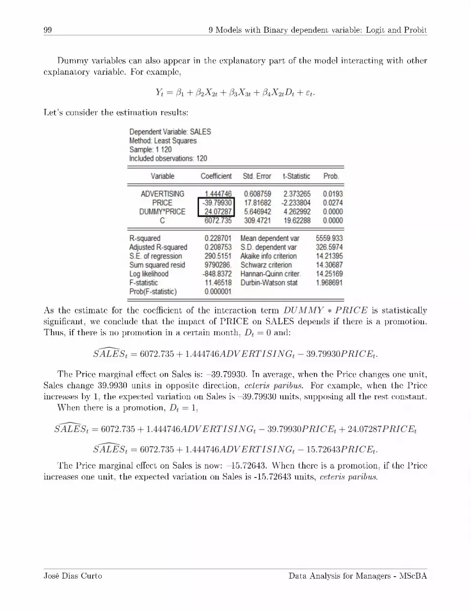
99 9 Models with Binary dependent variable: Logit and Probit
Dummy variables can also appear in the explanatory part of the model interacting with otherexplanatory variable. For example,
Yt = β1 + β2X2t + β3X3t + β4X2tDt + εt.
Let's consider the estimation results:
As the estimate for the coecient of the interaction term DUMMY ∗ PRICE is statisticallysignicant, we conclude that the impact of PRICE on SALES depends if there is a promotion.Thus, if there is no promotion in a certain month, Dt = 0 and:
SALESt = 6072.735 + 1.444746ADV ERTISINGt − 39.79930PRICEt.
The Price marginal eect on Sales is: 39.79930. In average, when the Price changes one unit,Sales change 39.9930 units in opposite direction, ceteris paribus. For example, when the Priceincreases by 1, the expected variation on Sales is 39.79930 units, supposing all the rest constant.
When there is a promotion, Dt = 1,
SALESt = 6072.735 + 1.444746ADV ERTISINGt − 39.79930PRICEt + 24.07287PRICEt
SALESt = 6072.735 + 1.444746ADV ERTISINGt − 15.72643PRICEt.
The Price marginal eect on Sales is now: 15.72643. When there is a promotion, if the Priceincreases one unit, the expected variation on Sales is -15.72643 units, ceteris paribus.
José Dias Curto Data Analysis for Managers - MScBA

100 9 Models with Binary dependent variable: Logit and Probit
When the dependent variable is binary (Yi = 0 or Yi = 1) the linear regression model is notthe most appropriate and it is necessary to use alternative models that are the subject of theselectures.
In this type of models it is assumed that individuals can choose between two alternatives andthe choice (or positioning) is dependent from a set of attributes (explanatory variables). Thepurpose is to estimate the probability of an individual to make a particular choice or to take aparticular position.
Given the responses dichotomy, they can be assigned probabilities to each of discrete results.Thus, if pi = P (Yi = 1) is the probability of Yi to assume the value 1 and 1− pi is the probabilityof Yi to assume the value 0, then this probabilistic information about Yi can be expressed in theform of a random variable with Bernoulli distribution:
Yi ∼ f (yi) = pyii (1− pi)1−yi , for Yi = 0, 1, pi ∈ [0, 1], (101)
with mean pi and variance pi (1− pi) and where f (yi) is the probability function.The interest focuses on the individual attributes to estimate the probability pi from observed
data and there are alternative specications for this kind of models, taking into account theprobabilistic nature of the decision process.
The three most commonly used specications to describe a binary dependent variable are themodels linear probabilistic, logit and probit. A linear regression model where the dependentvariable can assume only the values 0 and 1 is named by Linear Probabilistic Model: LPM, sincethe expected value of Yi may be interpreted as the conditional probability that a certain eventtakes place, or that an individual can take a certain choice. Let the multiple linear regressionmodel be:
Yi = β1 + β2X2i + β3X3i + ...+ βkXki + εi =k∑j=1
βjXji + εi = x′iβ + εi, (102)
where Yi = 0, 1(16), X1i = 1 for i = 1, 2, . . . , n (column of ones), x and β are the vectors withexplanatory variables and parameters, respectively, and both with dimension k × 1:
x′i = [X1i X2i . . . Xki] , β′ = [β1 β2 . . . βk] .
Assuming that E (εi) = 0, the conditional expectation of Yi is given by:
E (Yi|X1i, X2i, . . . , Xki) =k∑j=1
βjXji = x′iβ. (103)
Considering the distribution of eachYi, and by the denition of expected value,
E (Yi|Ωx) = 1× P (Yi = 1|Ωx) + 0× P (Yi = 0|Ωx) ,
where Ωx = X1i, X2i, . . . , Xki. Therefore:
E (Yi|Ωx) = P (Yi = 1|Ωx) . (104)
16We are assuming that random variables Yi are independent.
José Dias Curto Data Analysis for Managers - MScBA

101 9.1 Application: Credit Scoring
Combining the last two equations (103) and (104) results in,
E (Yi|X1i, X2i, . . . , Xki) =k∑j=1
βjXji = x′iβ = P (Yi = 1|Ωx) . (105)
Therefore, the deterministic part of the regression equation should be interpreted as the con-ditional probability of Yi to assume the value 1 and by this it is named by Linear ProbabilisticModel. In this type of model what we want to predict is not the values that dependent variablecan assume but the probability that an individual carries out a specic choice, which dependsfrom factors that inuence the decision process and from the considered probability distributionfunction.
As we referred before, E (Yi|Ωx) is the conditional probability that an individual can take acertain choice or that an event can take place and it must necessarily ranges between 0 and 1.However, with the LPM there is no guarantee that Y predictions assume always values between0 and 1. The solutions for this problem are two: to assume that Yi is 0 or 1, when the estimatedvalues from LPM are lower than 0 or higher than 1, or to consider an alternative specication toguarantee that the estimated value for the conditional probabilities will range between 0 and 1.logit and probit models are commonly used for this purpose.
9.1 Application: Credit Scoring
Consumer credit granted to individuals, by the operation of bank credit cards, takes the form ofrevolving credit, and customers are classied as Good or Bad depending on their behavior interms of payment.
The behavioral scoring classies users from a set of attributes (explanatory factors) which areconverted to a score which is the credit scoring.
This application seeks to identify what are the main factors accounting for the credit scoringin the form of revolving credit. For this purpose we use the data from 500 users of credit cardsfrom a nancial institution divided into two groups: one consisting of 250 users classied by thenancial institution as Good and another group of 250 users classied as Bad. To estimatethe parameters of the models 400 users are considered (200 Good and 200 Bad) and thisconstitutes the in-sample analysis. In order to validate the results outside the sample, we considerthe remaining 100 users (50 Goodand 50 Bad) and this consists in the out-of-sample analysis.Open the le Creditscoring.WF1 where this information is.
Logit and probit models will be used to identify the most relevant attributes and to estimatethe probability of each user to be a good payer (which is the main purpose of credit scoring). Inthis application it is considered a binary dependent variable (COD) that takes the value 1 whenthe client is paying good and 0 if it doesn't.
José Dias Curto Data Analysis for Managers - MScBA

102 9.1 Application: Credit Scoring
The explanatory variables considered initially are:
VARIABLE DESCRIPTION
gender (dummy) 1 - Male 0 - Femalemarried (dummy) 1 - Married 0 - Singlevscoring Behavioral scoring on the current account of the clientvlimitcredit Credit limit (maximum amount that the client can use to spend
on your card)sactualbal Present value of debtvrevolving Revolving amount that was unpaid on the previous statementage age
In order to estimate the logit model proceed as follows (COD is the binary dependent variable):
The estimation results are:
Given the results, we decided to exclude from the model the explanatory variables whose prob-
José Dias Curto Data Analysis for Managers - MScBA

103 9.1 Application: Credit Scoring
ability associated with the z-Statistic is higher than 10% (Gender, Age, Vactualbal and Vrevolving).Estimate again the model and the results are presented below.
Following is the meaning of some statistics in the tables above:
• Log likelihood is the maximum value for the natural log of the Likelihood function;
• Avg. Log likelihood (L) is the maximum value for the natural log of the Likelihoodfunction divided by the number of observations;
• Restr. Log likelihood (L) is the maximum value for the natural log of the Likelihood func-tion when it is considered the restriction that all the slope coecients (except the intercept)are equal to zero;
• LR statistic is the likelihood ratio test to test the null that all slope coecients are zero:H0 : β2 = β3 = β4 = 0. This test is equivalent to the F test in the Multiple Linear Regressionmodel and constitutes an overall signicance test of the model. If the constraints in the nullhypothesis are true, the LR statistic has an asymptotic chi-square distribution where thenumber of constraints (number of slope coecients in the model) are the degrees of freedom;
• Probability (LR statistic) is the probability associated with the value of the previoustest;
• McFadden R-squared is the index of the likelihood ratio: 1 − LLand is equivalent to the
coecient of determination of linear regression models. It also has the property to varybetween 0 and 1;
• Akaike, Schwarz e Hannan-Quinn are the Information Criteria.
According to the logit model, the estimated probability that Yi = 1 is given by:
P (Yi = 1) =1
1 + e−Zi, where Zi = β1 + β2X2i + . . .+ βkXki. (106)
José Dias Curto Data Analysis for Managers - MScBA

104 9.1 Application: Credit Scoring
Therefore, based on the estimated model, we can compute the probability that a particular userwill a good payer:
P (Yi = 1) =1
1 + e−Zi, where
Zi = −24.39296−0.578306MARRIEDi+0.000238V LIMITCREDITi+0.031148V SCORINGi.
If, for example, MARRIEDi = 1, V LIMITCREDITi = 5000 and V SCORINGi = 705, thenthe estimated probability that he/she will be a good payer is:
P (Yi = 1) =1
1 + e−(−24.39296−0.578306×1+0.000238×5000+0.031148×705)= 0.13920.
We can use the maximum value for the log-likelihood function, the McFadden R2 and theInformation Criteria to compare models' goodness-of-t. Estimate also the Probit and Gompitmodels and conclude which one seems to be the best one:
As one can see the logit seems to be the best... Why?We can also compare the models based on the Prediction-Expectation Evaluation: VIEW, Prediction-
Expectation Evaluation, 0.5 as cuto point for the probability. The results are:
Logit model beats also Probit and Gompit models (why?).
José Dias Curto Data Analysis for Managers - MScBA

105 9.1 Application: Credit Scoring
As exercise you can evaluate the models out-of-sample considering the 100 users not consideredin the estimation process.
REFERENCEWooldridge, Jerey M. (2015), Introductory Econometrics: A Modern Approach, South-Western,5th Edition
José Dias Curto Data Analysis for Managers - MScBA