1 

 

GyPSuM: A Joint Tomographic Model of Mantle Density and Seismic Wave Speeds Nathan A. Simmons1, Alessandro M. Forte2, Lapo Boschi3, Stephen P. Grand4

1 Atmospheric, Earth & Energy Division, Lawrence Livermore National Laboratory, 7000 East

Ave, L-046, Livermore CA, 94550, USA 2 GEOTOP - Dépt. Sci. Terre & Atmosphère, Université du Québec à Montréal, CP 8888

succursale Centre-Ville, Montréal QC, H3C 3P8, Canada 3Eidgenössische Technische Hochschule Hönggerberg, Institute of Geophysics, Schafmattstr. 30,

8093 Zurich, Switzerland 4Jackson School of Geosciences, University of Texas at Austin, Austin TX, 78712, USA Corresponding author:

Nathan A. Simmons L-046 Lawrence Livermore National Laboratory Livermore, CA 94550 (925) 422-2473 Simmons27@llnl.gov

SSubmitted to Journal of Geophysical Research – Solid Earth

2 

 

Abstract

GyPSuM is a 3-D model of mantle shear-wave (S) speeds, compressional-wave (P)

speeds and density. The model is developed through simultaneous inversion of seismic body-

wave travel times (P and S) and geodynamic observations while using realistic mineral physics

parameters linking wave speeds and density. Geodynamic observations include the global free-

air gravity field, divergence of the tectonic plates, dynamic topography of the free surface, and

the flow-induced excess ellipticity of the core-mantle boundary. GyPSuM is built with the

philosophy that heterogeneity that most closely resembles thermal variations is the simplest

possible solution. Models of the density field from Earth’s free oscillations have provided great

insight into the density configuration of the mantle; but are limited to very long-wavelength

solutions. Alternatively, scaling higher resolution seismic images to obtain density anomalies

generates density fields that do not satisfy geodynamic observations. The current study provides

a 3-D density model for the mantle that directly satisfies geodynamic and seismic observations

through a joint seismic-geodynamic inversion process. Notable density field observations

include high-density piles at the base of superplume structures, supporting the general results of

past normal mode studies. However, we find that these features are more localized and lower

amplitude than past studies would suggest. When we consider both fast and slow seismic

anomalies in GyPSuM, we find that P- and S-wave speeds are strongly correlated throughout the

mantle. However, we find a low correlation of fast S-wave zones in the deep mantle (>1500 km

depth) with the corresponding P-wave anomalies, suggesting a systematic divergence from

simplified thermal effects in ancient subducted slab anomalies. The cratonic lithosphere and D"

regions are shown to have strong compositional signatures. However, we argue that temperature

3 

 

variations are the primary cause of P-wave speed, S-wave speed, and density anomalies

throughout most of the mantle.

1. Introduction

Evaluating the relative behavior of various mantle properties is a powerful way to

identify compositional variations and processes occurring in the mantle [e.g., Robertson and

Woodhouse 1996; Su and Dziewonski 1997; Kennett et al. 1998; van der Hilst and Kárason

1999; Ishii and Tromp 1999, 2004; Masters et al. 2000; Saltzer et al. 2001; Kennett and

Gorbatov 2004; Trampert et al. 2004; Khan et al. 2009]. It has been well established that

correlation of shear and bulk sound speeds reduce in the deep mantle (lowest ~1000 km) and are

likely anti-correlated in some regions [e.g. Su and Dziewonski 1997; Kennett et al. 1998; Masters

et al. 2000]. Moreover, studies incorporating normal mode splitting functions have provided

evidence that high-density piles exist at the base of the mantle where ‘superplumes’ may

originate thereby contradicting the simple assumption that deep mantle heterogeneities are

produced solely by temperature variations [e.g., Ishii and Tromp 1999; Trampert et al. 2004].

Based upon very long-wavelength images of the mantle, it has been argued that chemical

variations dominate thermal heterogeneity and, therefore, buoyancy forces in the deep mantle

[Trampert et al. 2004]. However, density and wave speed heterogeneities derived from normal-

mode splitting data, that are only sensitive to the longest length-scale heterogeneities, provide a

limited understanding of the structure and dynamics of Earth’s mantle. These data appear to be

subject to considerable trade-offs and non-uniqueness [Kuo and Romanowicz 2002] and,

moreover, the inferred density anomalies provide poor fits to fundamental long-wavelength

surface geodynamic constraints [Soldati et al. 2009].

4 

 

In order to better understand the dynamics of the mantle, we must first know the density

anomalies that drive mantle flow. One way to estimate density anomalies in the mantle is

through the translation of a pure seismically derived velocity model to density anomalies through

application of mineral physics relationships. Most often, the density models resulting from this

approach provide less than satisfactory fits to key geodynamic observations such as the global

free-air gravity anomalies derived from satellite data [Forte 2007]. Thus, this approach requires

the introduction of strong compositional effects to fit geodynamic data leading to potential

overestimates of non-thermal contributions to mantle heterogeneity [Simmons et al. 2009].

Although geodynamic observations are sensitive to global integrals of 3-D anomalies throughout

the mantle, these observations alone cannot adequately resolve local density structure within the

mantle. Therefore, seismic observations are required to define the local 3-D distribution of

seismic heterogeneity which can then be interpreted in terms of density anomalies. In our

previous studies [Simmons et al. 2006, 2007, 2009], we combined geodynamic observations and

S-wave travel times in global-scale simultaneous inversions for S-wave speed and density. In

these studies, both types of data were directly inverted to produce the 3-D models of density and

seismic velocity as opposed to estimating density anomalies through a posteriori scaling of a

pure seismically derived model.

The benefit of joint inversion of multiple types of data is multifold. Firstly, joint

inversion directly accounts for the variable resolution of individual data sets that might produce

quite different distributions of mantle heterogeneities when considered alone. In addition,

simultaneous inversion of different forms of information allows for the determination of multiple

mantle properties that are most consistent with one another given some underlying hypothesis

such as the dominance of thermal effects. Moreover, we can more accurately evaluate the

5 

 

relative behavior of mantle properties as determined through a direct joint inversion process

since the model parameterization and roughness levels are equivalent. In other words, the joint

inversion process removes a number of biases that would potentially lead to unnecessarily large

degrees of compositional influence to explain multiple observations simultaneously.

In this paper, we present the GyPSuM model (G=Geodynamic, P=Compressional waves,

S=Shear waves, M=Mineral physics) which represents the next step in the evolution of a detailed

multi-component mantle model presented in our previous studies [Simmons et al. 2006, 2007,

2009]. As in our previous studies, GyPSuM is constructed through the simultaneous inversion of

seismic and geodynamic constraints using mineral physics relationships that relate the mantle

properties. Also similar to our previous model developments, we simultaneously consider

globally distributed S-wave arrival times, the global free-air gravity field, divergence of the

tectonic plates, dynamic topography of Earth’s free surface, and the flow-driven excess ellipticity

of the core-mantle boundary (CMB). The most important improvement from our previous

studies is the incorporation of globally distributed P-wave travel time measurements, thus

allowing the generation of a detailed, 3-component mantle model (density, P-wave velocity, S-

wave velocity). We also perform non-linear inversions to gradually adjust heterogeneities and

mineral physics relationships rather than the pure linear approach employed in the previous

studies.

2. Seismic and Geodynamic Data

The seismic data used in this study consist of globally distributed, teleseismic S-wave and

P-wave travel time observations (Table 1) that are not restricted to common source-receiver

pairs. The S-wave observations consist of ~46,000 travel time residuals derived from waveforms

6 

 

bandpass filtered from 0.01-0.07 Hz. The seismic phases include S, ScS, sS, sScS, SKS and

SKKS phases including surface-reflected multiples (e.g. sSS) and triplicated phases turning

within the upper mantle [Grand 1994, 2002; Grand et al. 1997; Simmons et al. 2006, 2007,

2009]. Travel time residuals are relative to a 1-D model consisting of an average of the

TNA/SNA models in the upper mantle [Grand and Helmberger 1984] and PREM in the lower

mantle [Dziewonski and Anderson 1981]. Corrections for crustal structure and ellipticity are

based upon the CRUST5.1 model of Mooney et al. [1998] and the techniques developed by

Dziewonski and Gilbert [1976], respectively. Earthquake locations were determined through an

iterative process which involved tomographic inversions followed by event relocation in several

steps [Simmons et al. 2006]. We view these data as highly reliable given that they are based

upon meticulous analyses of synthetic waveform correlation and detailed event modeling. Also,

given the diverse suite of phases reflecting and refracting through the mantle and our selection of

evaluated earthquakes, the coverage of the mantle is maximized. For more information regarding

these data (measurement procedures, coverage, etc.) see Grand [1994, 2002] and Simmons et al.

[2006, 2007].

The P-wave observations consist of ~626,000 summary travel time residuals computed in

Antolik et al. [2003]. The underlying data come from the recompilation and relocation of the

International Seismological Centre (ISC) direct P-wave arrivals performed by Engdahl et al.

[1998] (EHB). The seismic events were relocated on the basis of the S&P12/WM13 3-D model

[Su and Dziewonski 1993] and subsequently summarized on a 2x2 degree global grid and 50-100

km event depth increments [Antolik et al. 2003]. The original ISC arrivals are not based on the

more reliable waveform correlation techniques employed in the generation of the S-wave data

set; however, the level of scrutiny involved in the grooming of the P-wave data by Engdahl et al.

7 

 

[1998], the summary-data analysis of Antolik et al. [2003], and the large amount of data yield a

valuable set of global P-wave observations. Similar to the corrections applied to the S-wave

data, these data were corrected on the basis of CRUST5.1 as well as the ellipticity of Earth.

The set of geodynamic constraints we employ consists of a suite of convection-related

observables sensitive to the viscosity of the mantle, the style of mantle flow, and 3-D density

variations. These surface observables include the free-air gravity field from the EGM96

geopotential model derived through a compilation of land-, air-, and space-based observations

[Lemoine et al. 1998]. These gravity data provide robust constraints on density anomalies in

both the upper and lower mantles, with maximum sensitivity shifting to the upper mantle as the

horizontal wavelength decreases.

In addition, we employ constraints derived from the observed tectonic plate motions as

given by the NUVEL-1 plate velocity model in the no-net-rotation (NNR) frame of reference

[DeMets et al. 1990, 1994; Argus and Gordon 1991]. For a given plate geometry, assuming the

plates are rigid bodies, it can be shown that a scalar representation of the plate velocity field in

terms of its horizontal divergence (along ridges and trenches) provides a sufficient description of

the surface kinematics [Forte and Peltier 1994]. The radial vorticity of the plate motions (along

transform boundaries) is a linear function of the horizontal divergence and it does not provide

additional independent information on plate kinematics in the NNR reference frame [Forte and

Peltier 1994]. We therefore employ the horizontal divergence field derived from the NUVEL-1

(NNR) velocities as a constraint on buoyancy forces in the mantle. According to the mantle flow

theory (outlined in the next section) the tectonic plate motions are coupled to the underlying

mantle flow driven by density anomalies and they are thus important constraints on 3-D density

heterogeneity in the mid-mantle (at longest wavelengths) and the upper mantle (at shorter

wavelengths).

We also consider the dynamic topography of Earth’s free surface estimated by removal of

the crustal isostatic topography signal [Forte and Perry 2000]. These data are the least robust in

the suite of geodynamic observations given the uncertainties of the global crustal structure;

however, crust-corrected dynamic surface topography is a direct mapping of vertical stresses in

the mantle and thus provides important constraints on the range of upper-mantle density

configurations needed to explain the other geodynamic observations considered.

Large-scale mantle flow driven by density anomalies has a direct impact on the overall

shape of the CMB [see Forte et al. 1995] and may account for the ~400m of excess bulge along

the equator [Herring et al. 2002; Mathews et al. 2002]. Therefore, we also incorporate the

excess ellipticity of the CMB observed from Earth’s free-core nutation processes as an additional

constraint on mantle density [Herring et al. 2002; Mathews et al. 2002]. The full suite of data

related to mantle convection employed as the geodynamic constraints in the joint inversions are

shown in Figure 1. The harmonic coefficients used to synthesize the fields in Figure 1 are the

elements of the data vector, g , in the forward system of equations outlined in the following

section. See Table 1 for a summary of all of the seismic and geodynamic constraints employed

in this study.

3. Forward Model

The forward model consists of a combined set of seismic and geodynamic observations

that are linearly related to seismic velocity and density anomalies in a set of blocks representing

the mantle. The blocks are approximately 275x275 km in lateral dimension at all depths. Depth

8 

 

9 

 

ranges are variable with 22 layers from 75 to 240 km thick, providing a total 99,148 model

parameters. The seismic sensitivities were computed through 1-D ray tracing (infinite frequency

approximation) to form a set of sensitivity (Fréchet) kernels for both the S and P data sets

individually. The individual sets of kernels provide the basis for the linear equations relating

travel times and S-wave slowness perturbations, which are internally translated to P-wave

slowness perturbations through scaling relationships discussed below.

Geodynamic sensitivity kernels were computed from the theoretical linear relationship

between mantle density anomalies and each of the surface observables (free-air gravity field,

plate divergence, dynamic surface topography, and excess CMB ellipticity). This requires an

analytical description of the viscous flow response of the mantle to internal point sources of

density for each convection-related observation [Richards and Hager 1984; Ricard et al. 1984;

Forte and Peltier 1987]. We computed viscous flow responses for a compressible and

gravitationally consistent mantle whereby tectonic plate motions are dynamically coupled to the

underlying mantle flow [Forte and Peltier 1994; Forte 2007]. A combination of mixed free-slip

and no-slip surface boundary conditions were incorporated to calculate the responses assuming

the radially-symmetric viscosity profile derived from joint inversion of convection data and

glacial isostatic adjustment (GIA) observations [Mitrovica and Forte 2004]. Based on the study

of Simmons et al. [2006], the viscous flow responses were determined with the assumption that a

whole-mantle style of flow prevails. Therefore, no strict boundaries to vertical mass transport

are incorporated into building the responses with the exception of the CMB and the free surface.

Each of the geodynamic data fields has a unique sensitivity to the mantle that varies with the

harmonic degree, or corresponding horizontal wavelength (Figure 2). Thus, simultaneously

considering the entire suite of geodynamic observations provides significant constraints on the 3-

D arrangement of density anomalies that may exist in the mantle.

The mantle flow theory employed in making the connection (via the geodynamic kernels)

between lateral heterogeneity in the mantle and the convection data does not explicitly model the

effects arising from lateral viscosity variations (LVV) in the mantle. It is worth noting, however,

that the geodynamically inferred radial viscosity profile we employ [Mitrovica and Forte 2004]

in calculating the kernels has embedded in it the depth-dependent horizontal average of the LVV

[Moucha et al. 2007]. In this case, provided we use this mean viscosity profile, the effect of LVV

on the predicted convection-related observables is of the same order (or smaller) than the current

uncertainties in the global tomography models [Moucha et al. 2007]. Furthermore, as shown by

Wen and Anderson [1997], LVV at shallow depths have the largest impact on the predicted

surface motions, particularly in terms of generating realistic amplitude surface divergence and

radial vorticity. The tectonic plates themselves arguably constitute the largest-amplitude

manifestation of LVV anywhere in the mantle and the plate-coupled mantle flow theory we

employ [Forte 2007] explicitly models the impact of rigid surface plates on the underlying

mantle flow.

Expressing the seismic and geodynamic observations as a single set of linear equations

yields a large and complex system best described in the following matrix form:

0

g

r

r

m

D

c

G

L

L

eVR

VR

VVR

CMB

G

PP

S

S

D

SSCMB

SSG

PSSPPP

S

,

,

/,

/

/

/

(1)

10 

 

where and are the S- and P-wave sensitivity kernels matrices; and are the

corresponding travel time residuals. The gravity, dynamic topography, and plate divergence

sensitivities and harmonic coefficients (data) are represented by G and

SL PL Sr Pr

g , respectively.

Similarly, the excess CMB ellipticity sensitivity and degree 2 harmonic coefficient are

represented by c and . The matrix represents a second-order digital smoothing filter with

76% of the weight applied to the lateral elements (blocks) and 24% of the weight applied to the

vertical elements (depth extent). For the purpose of clarity, all terms in Equation (1) are

summarized in Table 2.

e D

In Equation (1), the goal is to solve for a S-wave slowness perturbation model, .

Therefore, the P-wave sensitivities ( ) and geodynamic sensitivities (G and c ) are associated

to S-wave slowness perturbations through relative heterogeneity ratios ( and

). Since

the relative heterogeneity ratios are represented in terms of seismic velocity perturbations,

conversions relating velocity perturbations (

Sm

S

PL

S/PR R /

V ) to slowness perturbations ( ) were also

propagated through the sensitivity kernel matrices using the approximation

s

V sVV 00 /

(where is the background velocity). 0V

One of the major issues when attempting to simultaneously invert multiple forms of data

is determining the relative weights for each set of observations ( P , G and CMB in Equation 1).

It might seem reasonable to dramatically down-weight the P-wave data set relative to the S-wave

data set given the ~14-fold increase in the number of P-wave data. However, simply defining

P on the basis of number observations is not ideal since P-wave travel time residuals are

systematically smaller than the S-wave residuals. Weighting based on the number of data is

particularly problematic when considering S-wave phases that travel through the high-amplitude 11 

 

anomalies in the upper mantle multiple times (e.g. SSS) producing very large residual travel

times (signals). Therefore, we chose the seismic dataset weighting on the basis of the relative

data norms:

P

SP r

r

. (2)

Equation (2) yields 7.0P which provides a suitable dataset weight based on our sensitivity

tests. The weighting of the geodynamic observations is more difficult since these data are

represented as spherical harmonic coefficients in contrast to travel time residuals. Based on our

previous joint investigations [Simmons et al. 2006, 2007, 2009], the optimum weighting of the

geodynamic observations relative to the S-wave data ( G ) was found to be ~1000. In the current

study, we chose to double the weight ( 2000G ) to account for the addition of the P-wave

observations providing an approximately equivalent influence of geodynamic and seismic

observations. CMB was chosen to be sufficiently large to fully match the observed CMB excess

ellipticity similar to the treatment of Simmons et al. [2009]. The following sections describe our

multi-step approach to solving the complicated system described in Equation (1).

4. Density-P-S Coupling in a Thermal Scenario

Adopting the philosophy of the joint seismic-geodynamic modeling approach in Simmons

et al. [2009], we chose to initially attribute mantle heterogeneities to temperature variations and

subsequently relax this requirement. This approach involves first determining the optimum

scaling relationships ( and ) that account for the relative behavior of mantle properties

when temperature variations are the dominant cause. One of the major issues is the large range

SR / SPR /

12 

 

of uncertainty of these parameters even when only considering the effects of temperature (see

Cammarano et al. [2003] and Karato and Karki [2001]). To aid in the search for the optimum

scaling relationships, it is useful to evaluate how these ratios are related. Using the notation from

Karato and Karki [2001], the relative behavior of VS to density and sound-speed can be written:

SS

S

SS

SS

RCXQ

R

CXQR

/1/

1/

2

1

21

1

21

2

(3)

where , , and S correspond to density, S-wave speed, and sound-wave speed respectively.

The parameters and S are the Anderson-Grüneisen parameters [e.g. Anderson 1989] relating

differential changes of the elastic moduli to density variations, and thus represent the pure elastic

effects to the ratios in Equation (3). is the S-wave attenuation parameter andSQ CX is a

correction factor for anelasticity. The correction factor CX is a product of the frequency

dependence of attenuation, activation enthalpy, melting temperature and the estimated range of

lateral temperature variations (see Karato and Karki [2001] for a thorough description).

Therefore, represents the anelastic component to the relative heterogeneity ratios.

If we also consider the relationship between the three types of seismic wave speeds, we can

readily derive a relationship between and :

CQS X12

S/R SPR /

12

1

3

41

//

2

2

SS

SP

P

S

S

S

P

P

RR

V

V ,

V

V

V

V

V

V

(4)

Note that this simple formulation is identical to Karato and Karki [2001] with the assumption

that bulk attenuation is negligible, yielding PS QQ / . Equation (4) shows that for simple

13 

 

thermal variations in the mantle, scales to in a predictable way. Therefore, Equation

(4) represents the full

SR /

P

SPR /

S VV coupling for thermally induced variations of iso-chemical

mantle material. If we assume that S is a fixed value at any given depth, and velocity

variations are relatively small, we need only determine one ratio ( or ) and directly

compute the other, thereby simplifying the optimization problem.

SR / SPR /

R Simmons et al. [2009] determined that a simple 1-D representation of was not

adequate to account for the relative behavior of density and S-wave velocity variations in the

mantle. This conclusion was based on the inability to simultaneously explain geodynamic and

seismic S-wave data with radially symmetric scaling profiles. There are multiple reasons for

this, including the existence of compositionally distinct cratonic keels and the dependence of

on the background temperature. In order to account for these 1

S/

SQ

st-order effects, Simmons et al.

[2009] introduced scaling model correction derivatives of the form:

S

S

V

R

ln/

. (5)

The search for the optimum values yielded highly negative values in the cratonic roots and

slightly positive numbers in the non-cratonic (‘thermal’) upper mantle. Therefore, values

in fast, cratonic zones were systematically reduced yielding less negative and sometimes positive

buoyancies in accord with the iron depletion hypothesized in these mantle regions [e.g. Jordan

1978]. Similarly, values in the low-velocity, non-cratonic upper mantle were significantly

reduced in agreement with the expected behavior due to the temperature-dependence of .

SR /

SR /

SQ

14 

 

5. Modeling Procedures

In our joint modeling approach, we initially performed inversions with simple scaling

relationships thereby forcing the spatial patterns of the heterogeneity fields (density and wave

speeds) to be correlated, which is likely an oversimplification [e.g. Masters et al. 2000]. We

subsequently allow the spatial patterns of wave speeds and density to deviate from one another in

a systematic manner. These deviations in spatial patterns are formed by allowing the scaling

relationships ( and ) to evolve from constant values in a depth layer (1-D) to fully

three-dimensional relationships.

SR / SPR /

Before proceeding to the joint inversion, we tested the ability of seismic models (derived

entirely from seismic data alone) to match the other observations considered in this study. We

selected the optimum profile (Figure 3) as well as the TX2008s S-wave velocity model

from Simmons et al. [2009] for evaluation. We note that, although a jointly derived solution

(TX2008j) was produced in Simmons et al. [2009], we chose to use the pure seismically derived

version to demonstrate the potential difficulties arising from the use of S-wave data alone. For

these tests, Equation (4) was used to calculate assuming simple depth-dependent

1DSR /

1DSPR / S and .

In the upper mantle, bulk S values were estimated by comparing the profile from

Simmons et al. [2009] and the corresponding profile computed in Cammarano et al. [2003]

yielding

1DSR /

1DSPR /

S values between 2.2 and 3.8. In the lower mantle, we estimated S to be linearly

decreasing from 2.7 (top of the lower mantle) to 1.3 (base of the mantle) based on the values for

MgSiO3 perovskite presented in Karato and Karki [2001].

Applying the 1-D scaling profiles to the TX2008s S-wave velocity model, we calculated

the variance reduction fit to all of the considered data fields (Table 3). The scaled TX2008s

15 

 

model is incapable of satisfying the geodynamic constraints since it is derived solely with S-

wave constraints as pointed out in Simmons et al. [2009]. This scaled S-wave model also

provides a poor fit to the P-wave constraints employed in the current study (~12% variance

reduction). To gain perspective on this measure of P-wave data fit, we performed tomographic

inversions considering only the P-wave data while using the same parameterization and inversion

techniques used to develop TX2008s. The inversions were carried out using the iterative LSQR

algorithm [Paige and Saunders 1982] with a spectrum of smoothing weights. The optimum P-

wave model (henceforth referred to as ‘P-only’) provided ~32% variance reduction fit to the P-

wave data set. This relatively low degree of potential fit (compared to the S-wave data set and

model) is, in part, a product of the signal-to-noise ratio of the residual P-wave travel times and is

comparable to studies using the same data (e.g. Antolik et al. [2003]). The P-only model, when

scaled to shear velocities and densities (with and ), provides a poor level of fit to the

S-wave data (~56%) and remarkably low degrees of fit to the geodynamic observations as well

(Table 3). Clearly, we could likely find a better set of 1-D conversion factors to scale these

independently produced models through a trial-and-error process. However, as demonstrated in

Simmons et al. [2009], selecting the best-fitting scaling model on the basis of a heterogeneity

model derived from a single type of data does not necessarily lead to better fitting models after a

joint inversion is performed. These tests mainly serve to provide some insight into the potential

fit that may be achieved with our model parameterization and they also provide reference levels

for subsequent comparisons.

1DSR /

1DSPR /

16 

 

The initial step in the 3-component model construction is the joint inversion for density

and wave speed variations while assuming simple 1-D scaling models ( and )

previously described. The primary reasons for initially solving the system in Equation (1)

1DSR /

1DSPR /

assuming 1-D scaling profiles are to: 1) develop an unbiased starting model for scaling model

optimization, and 2) establish the appropriate level of model roughness when considering the

combined data set. The joint solution with 1-D scaling models (‘GyPSuM_1D’) provides a more

balanced level of fit to the seismic data sets than the independently produced models (variance

reduction fit of 90% to the S-wave data and 28% to P-wave data set). In addition, the fits to the

geodynamic observations are dramatically improved with the exception of the dynamic

topography which is still poorly matched (Table 3). The problem of reconciling the dynamic

topography and gravity fields simultaneously has been recognized for quite some time (e.g.

Forte et al. 1993; Le Stunff and Ricard 1995). In the context of joint seismic-geodynamic

inversion, this problem persists when assuming simple 1-D scaling profiles that force the

geographic pattern of wave speed and density perturbations to be identical. However, when

directly considering the impact of iron depletion of the cratons and the temperature dependence

of through implementation of scaling model corrections (i.e. Equation 5), the level of fit to

the dynamic topography field can be greatly improved while maintaining a good fit to the

observed gravity field [Simmons et al. 2009]. The search for these scaling model correction

terms as well as other free parameters is described in the following section.

SQ

5.1 Scaling Model Optimization (1.5-D R values)

One major limitation of the Simmons et al. [2009] investigation was that the

determination of the velocity-based correction derivatives ( terms defined in Equation 5) were

based upon a fixed (i.e. given) velocity model. In general terms, this is a non-linear problem

since the determination of S-wave velocity structure in a joint modeling process is a function of

the corrected values and vice versa. In the current study, we wish to find the optimum 1-D SR /

17 

 

scaling models ( ) and correction derivatives (e.g. Equation 5) while considering the non-

linearity of the problem. Since we are also incorporating P-wave constraints, the selection of

impacts the calculated values of (via Equation 4) and our ability to simultaneously fit

the P-wave data set as well.

SR /

SR / SPR /

D-1S/

Given these complexities, we have formulated the scaling model optimization problem by

defining a parametric form of in the following way: SR /

SS VbaRR ln/ (6)

where is a starting 1-D scaling model and D-1SR / is a velocity-based scaling correction

derivative defined in Equation (5). The coefficients a and b represent the amplification and

baseline shift of the starting 1-D scaling model, respectively. Therefore, a controls the overall

shape of the 1-D portion of scaling factor profile, b controls the mean value, and adjusts the

scaling factor model according to the underlying S-wave velocity structure. We will further refer

to the dimension of such a scaling model as 1.5-D.

Equation (6) presents the basic form of the optimization problem; however, the

coefficients are regionally dependent. Specifically, we define two sets of coefficients (

and ) that adjust the upper (subscript ‘um’) and lower mantle (subscript ‘lm’) scaling

models independently. Additionally, we define multiple

umum ba ,

lmlm ba ,

terms to account for the cratonic

versus the non-cratonic upper mantle zones as well as potential depth dependence of these

values. In total, we consider 9 free parameters described in Table 4.

To appropriately test the validity of a single set of these 9 free parameters, we performed

a non-linear joint inversion involving the iterative updating of scaling models and global

heterogeneity models. A grid search or Monte Carlo approach would be computationally 18 

 

daunting and we have therefore adapted a very fast simulated annealing (VFSA) approach

[Ingber 1989; Jackson et al. 2004] to identify the optimum set of scaling model adjustment

parameters described in Equation (6) and Table 4. Our adaptation of the VFSA process includes

a rapid VFSA cooling schedule to limit the number of full joint inversions required (Figure 4).

We also limited the range of possible 1-D components of the scaling factors according to the

ranges presented in the mineral physics works of Cammarano et al. [2003] and Karato and Karki

[2001]. Additionally, within each VFSA iteration and parameter update, joint inversions of the

combined data set were performed by solving Equation (1) using the LSQR algorithm. Thus,

joint inversion was embedded within the VFSA process producing a new mantle model with

each step to determine if the set of parameters improved the level of fit to all of seismic and

geodynamic data.

The VFSA process was terminated after 61 model updates due to the small changes of

model parameter and misfit variations at this stage (Figure 4). The 1-D component of the

resulting relationship (Figure 3) in the upper mantle converged to the lowest allowable

values in the upper mantle similar to the results of Simmons et al. [2009]. This bias towards the

lowest acceptable values in the upper mantle (based on the range for the 1300°C adiabat

calculations in [Cammarano et al. 2003]) is most likely a product of the combined effects of

cratons and high-temperature zones that both require lowered scaling values to account for iron

depletion and the temperature-dependence of , respectively. The strongest upper mantle

velocity signatures are ‘atypical’ in that they either deviate from a simple pyrolitic composition

or are very high-temperature; yet they occupy a large portion of the shallow upper mantle and

therefore greatly influence the 1-D scaling model solution.

D-1.5

SR

/

SQ

19 

 

In the lower mantle however, we find that the 1-D component differs from the results of

Simmons et al. [2009] who strictly tested a limited number of possible scaling profiles. In the

current case, the 1-D component of the lower mantle relationship is lower amplitude in

the middle of the mantle and higher amplitude near the base. This ‘straightening’ of the scaling

model possibly reflects the lessening of the contributions of anelasticity relative to the starting

model taken from Karato and Karki [2001]. The profiles in Karato and Karki [2001] might in

fact exaggerate the bulk contributions of anelasticity to mantle heterogeneity as recently reported

in some mineral physics studies [e.g. Brodholt et al. 2007; Matas and Bukowinski 2007]; our

results suggest a similar conclusion. Since the relationship is tied to the

relationship for thermally induced variations according to Equation (4), the 1-D component of

the relationship is nearly identical to the starting model in the upper mantle. The only

notable change from the starting model is near the top of the lower mantle (Figure 3). The very

minor divergence from the starting model in the deep mantle is due to the systematic decrease of

D1.5

SR

/

D1.5

SPR

/

D-1.5

SR

/

D1.5

SPR

/

S with depth in the lower mantle, approaching a minimum of 1.3 assigned to the D" layer. In

addition, the thermally induced values systematically decrease with depth, further

diminishing the influence of variations of on the resulting values in the deepest parts of

the mantle (see Equation 4).

SR

/

SR

/ SPR

/

We find velocity-based scaling model correction terms that are highly negative (Table 4)

in the cratonic roots reflecting the mass deficiency observed in numerous previous studies. In

the non-cratonic upper mantle, we find positive terms which is in general agreement with the

expected behavior due to the temperature dependence of the S-wave attenuation parameter (often

20 

 

21 

 

ets

ects

denoted ) in the upper mantle [Cammarano et al. 2003]. With these scaling model

improvements ( and ), we can increase the level of fit to all data s

considered after joint inversion (‘GyPSuM_1.5D’; Table 3). The most notable improvement is

to the dynamic surface topography field since we are directly accounting for the 1

SQ

D1.5D1

SSRR

//

D1.5D1

SPSPRR

//

st-order eff

of cratons and other scaling model complexities in the upper mantle; thereby allowing for a

greater reconciliation of the free-air gravity and dynamic surface topography simultaneously.

5.2 Compositional Decoupling (3-D R values)

As shown in the previous section, correcting 1-D R values for cratonic mass depletion

and the temperature dependence of , allows for greater reconciliation of the combined set of

seismic and geodynamic observations. However, these corrected relationships ( and

) do not completely describe the relative behavior of density and wave speeds since we

still are not able to fit the seismic data as well as the independently produced models (e.g.

TX2008s and P-only in Table 3). The presence of lateral compositional variations is the likely

cause for the remaining data misfit, thus requiring 3-D and values to more adequately

explain all of the data simultaneously. We have therefore developed 3-D scaling models through

a process we refer to as ‘compositional decoupling’ since the scaling models are allowed to

deviate from the estimated thermal values.

SQ

D-1.5

SR

/

D1.5

SPR

/

S/R

SPR

/

In this iterative process, we allow for slow divergence of the scaling relationships from

the 1.5-D values and subsequently update the heterogeneity model through non-linear joint

inversion. We first update through inversion of the geodynamic constraints while D3

SR

/

assuming a fixed S-wave slowness perturbation model determined in the previous step.

Similarly, we update through inversion of P-wave information, disregarding the S-wave

and geodynamic constraints since our goal is to improve the level of fit to the P-wave data given

an S-wave velocity model. The linear systems to be inverted can be represented using the

variables defined in Table 2:

D3

SPR

/

P

L

mc

G

k D,3inversionP

k D,3k

k D,3inversionk D,3k

k

SPSPS

SS

S

S

RR

Re

R

//

//

rm

gm

    (7)

where we have omitted regularization, weighting and slowness-velocity conversion terms for

simplicity. At each cycle, k, we performed a limited number of LSQR iterations (we chose 4) to

restrict the divergence of scaling models from the previous model state. There is no formal basis

for the selection of the number of LSQR iterations, but through trial-and-error testing we found

that 4 iterations did not allow the scaling models to move far from the previous state. To

complete the kth inversion cycle, we inverted the full system of equations (consisting of all

seismic and geodynamic information) for mantle structure assuming the updated and

models, again with a limited number of LSQR iterations. The k

D3

SR

/

D3

SPR

/

th S-wave slowness model

( ) then formed the basis for the subsequent cycle of 3-D scaling model inversions. The

process was repeated until we observed no significant improvement in the level of fit to all of the

data fields considered. Convergence occurred after 64 inversion cycles and the process was thus

terminated.

k

Sm

The resulting 3-D scaling model distributions as a function of depth are illustrated in

Figure 5. The distribution of values in the shallow upper mantle is broad and biased D3

SR

/

22 

 

towards zero, with a substantial number of negative values. This distribution demonstrates

lowered scaling factors due to iron depletion in the cold cratonic roots and the temperature-

dependence of in the hot non-cratonic regions such as the mid-ocean ridges and rift zones. A

similar distribution is found in the deepest mantle likely demonstrating significant compositional

variations, including within the ‘superplume’ structures [e.g. Ishii and Tromp 1999; Ritsema et

al. 1999; van der Hilst and Kárason 1999; Masters et al. 2000; Wen 2001; Ni et al. 2002; Ni and

Helmberger 2003; Trampert et al. 2004; Simmons et al. 2007]. Specifically, the intrinsically

high density material in the superplume structures competes with the thermally induced density

anomalies thereby reducing the overall values [Simmons et al. 2007]. The deepest part of

the superplume structures could also be intrinsically slow, further lowering values. Aside

from the shallow and very deep mantle, we find relatively tight distributions of values with

modes similar to the thermal 1-D scaling relationship. We note that, although we find anti-

correlation (i.e. negative scaling) of density and S-wave velocity in the lower mantle, they are

not the dominant signature even in the deepest mantle. Since density and S-wave velocity

variations are highly sensitive to temperature deviations, it may be argued that the non-cratonic

mantle shear-wave speeds and density variations are primarily temperature-driven [Schuberth et

al. 2009; Simmons et al. 2009].

SQ

PR

/

1

SR

/

SR

/

R D3

S

/

The relative heterogeneity ratio (or correlation parameter) is most often referred to

by the inverse ( ) in the literature and a wide range of values have been reported

[Vasco et al. 1994; Robertson and Woodhouse 1996; Su and Dziewonski 1997; Kennett et al.

1998; Masters et al. 2000; Saltzer et al. 2001; Ritsema and van Heijst 2002; Antolik et al. 2003].

It has been well established that there are multiple regions in the deep mantle with significant S-

SPR

/

PSSR

/

23 

 

wave heterogeneities corresponding to very small P-wave anomalies. This situation generates

nearly unbounded values and may contribute to the large range of average values reported

in the literature. This may in turn lead to discounting thermal variations as a major contributor to

seismic anomalies in the lower mantle since the average values often fall well outside the

expected thermal bounds [e.g. Karato 1993; Masters et al. 2000]. For these reasons, we have

solved for in the current study.

PSR

/

D3

SPR

/

D3

SPR

/

Our results show that modes of the distributions of tend to follow the 1-D

component of the VFSA solution ( ) throughout most of the mantle (Figure 5). If we

compare these distributions to those generated by models produced solely with the individual

seismic data sets (TX2008s and P-only), we find that the joint inversion procedure clearly

produces simultaneous P and S-wave models more consistent with pure thermal effects. This

conclusion is based upon the ability to dramatically collapse the distributions of about the

1-D thermal profile with respect to the independent solutions where the complementary datasets

do not constrain one another (Figure 5). However, there are still some broad scaling model

distribution ranges even though attempts were made to produce a purely thermally driven

heterogeneity model in the previous stages. This is most obvious in the deepest mantle where

the distributions of become broad and skewed in some layers. The broad distributions, in

part, reflect compositional anomalies in the deep mantle as concluded in numerous previous

studies of the relative behavior of mantle properties [e.g. Ishii and Tromp 1999; van der Hilst

and Kárason 1999; Masters et al. 2000; Saltzer et al. 2001; Trampert et al. 2004].

D3

SPR

/

D1.5

SPR

/

D3

SPR

/

24 

 

Relative seismic heterogeneity in the D" layer appears to be least consistent with thermal

variations since a nearly bimodal distribution of is detected (Figure 5). The primary mode

of the distribution (centered near 0.5) could potentially be explained by temperature variations;

however the secondary mode in the distribution (centered near 0), clearly violates the expected

thermal behavior in an iso-chemical mantle [Karato and Karki 2001]. The decreased values of

in the D" layer might be indicative of pressure-induced phase changes to post-perovskite

(pPv) creating a partial de-correlation of P and S-wave heterogeneity [Murakami et al. 2004;

Oganov and Ono 2004; Iitaka et al. 2004; Tsuchiya et al. 2004; Wookey et al. 2005; Hirose

2006; Hernlund and Houser 2008; Hutko et al. 2008]. This hypothesis is based upon mineral

physics analyses that indicate that shear modulus increases while bulk modulus is relatively

unchanged due to the transition to the pPv phase [e.g. Tsuchiya et al. 2004]. Moreover, the large

spread of relative heterogeneity values near zero may be due to patchy occurrences of pPv (and

perhaps lens-like seams) modulated by the background temperature [Hernlund et al. 2005; Lay et

al. 2006; Hernlund and Houser 2008]. The discrepancy between the distributions of P- and S-

wave anomalies in the deep mantle is robust [Hernlund and Houser 2008] and persists after

performing a joint inversion designed to reduce these effects. However, we point out that the

joint inversion process in this study leads to seismic anomalies more consistent with thermal

variations as manifested through the distribution of (Figure 5).

D3

SPR

/

PR

SPR

/

S/

25 

 

6. GyPSuM Model

6.1. Thermal and Non-thermal Contributions

The final model, GyPSuM, is illustrated in Figures 6a-b, 8a-b and 9a-b. The inversion

procedures described within this report allow for the estimation of what we refer to ‘thermal’ and

‘non-thermal’ contributions to mantle heterogeneity. The ‘thermal’ contributions to each of the

model fields (velocities and density) are estimated from the joint inversion results obtained by

employing the temperature-induced part of the optimum 1.5-D scaling model. The ‘non-thermal’

contributions are computed by subtracting the thermal components from the final model

developed in the previous section. Therefore, the non-thermal heterogeneity field may be

thought of as a residual field required in addition to the thermal field in order to fit the data. It

should be noted that there is a probability that some of the signatures we refer to as ‘non-

thermal’ might actually be due to the effects of laterally varying since, in the development of

the 1.5-D scaling model, we only considered 1

SQ

st-order thermal scaling corrections in the upper

mantle and no systematic corrections in the lower mantle (see Section 5.1).

In the upper mantle, we find mostly minor non-thermal contributions to the S-wave

velocity heterogeneity field (Figure 6a). Some of the most prominent non-thermal contributions

to the S-wave heterogeneity field are found in the deep mantle within the superplume structures

(most notably beneath Africa, Figure 6b). Our results imply that these superplume structures are

intrinsically slow in terms of S-wave speeds lending support to the idea that these features are

partially produced by the sweeping of intrinsically dense material into regions of large-scale

upwelling mantle [McNamara and Zhong 2005]. Specifically, near 2280 km depth (Figure 6b),

we find significant low-velocity S-wave signatures in the ‘non-thermal’ field within the African

superplume structure. This apparent non-thermal signature manifests itself through the modeled

26 

 

decrease of found through the 3-D scaling model inversion process relative to the 1-D

scaling profile (i.e. thermal profile). Our inferred non-thermal (or compositional) signature

within these superplumes (notably under Africa) may be explained in terms of iron-enrichment

since this will produce a reduction in S-wave speed in addition to the reductions expected for

increased temperature [e.g. Forte and Mitrovica 2001]. Alternatively, a similar effect may be

expected due to increased temperatures and the impact to [Karato and Karki 2001].

SR

/

SQ

Although there are apparent non-thermal influences on the shear velocity field,

temperature variations appear to be the dominant factor. This is demonstrated more

quantitatively through the calculation of the root-mean-squared (RMS) amplitudes of the

individual thermal/non-thermal heterogeneity fields (Figure 7). We find that the RMS amplitude

of the thermally induced S-wave heterogeneity is the largest contributor to the overall field

throughout the entire mantle. This result is in direct agreement with Quéré and Forte [2006] and

Schuberth et al. [2009] who found that steep lateral temperature gradients could mostly account

for the large-scale, low-velocity superplume structures beneath Africa and the Pacific Ocean.

Density heterogeneity in the shallow upper mantle is produced by both temperature and

compositional variations (Figure 8a). As expected, the thermal signature in the cratonic regions

is high-density due to decreased temperatures while the compositional signature is low-density

due to depletion of basaltic components. Due to the temperature-dependence of , the thermal

signatures are higher amplitude in seismically fast (cold) regions than in slow (hot) regions.

However, the competing thermal/compositional effects in the cratonic regions produce far lower

amplitude densities in the cratons overall, relative to the purely thermally induced density field

(Figure 8a).

SQ

27 

 

28 

 

Compositional density anomalies are small relative to thermally driven density field

throughout most of the non-cratonic mantle based on the RMS amplitude calculations (Figure 7).

However, in the bottom ~400 km of the mantle, the compositional influence increases

dramatically. The major contributions to the compositional density fields are within the African

and Pacific superplume structures. The central cores of these features are found to be

intrinsically dense. The positive intrinsic density of these structures offsets the thermally driven

density in portions of the superplume structures thereby reducing the overall buoyancy similar to

the results of Simmons et al. [2007, 2009]. However, the amplitudes of the non-thermal high-

density signatures in the superplumes are larger in the GyPSuM model relative to TX2007

[Simmons et al. 2007] and TX2008 [Simmons et al. 2009]. Moreover, the net result of the

combined thermal and non-thermal density anomalies is overall positive density anomalies in

some parts of the African superplume structure, most notably within the D" layer (Figure 8b).

This significant difference from TX2007 and TX2008 is a direct product of the addition of the P-

wave constraints that are sensitive to P-wave velocity, but related to S-wave velocity and density

through scaling relationships. The introduction of P-wave data yields a joint set of constraints

that more tightly limit the ability of thermally induced heterogeneity models to simultaneously

explain the combined set of data. Given the increased difficulty of satisfying the data with a pure

thermally induced heterogeneity model, the P-wave constraints effectively increase the level of

compositional influence required and the net result is high-density anomalies at the base of the

African superplume.

Studies utilizing normal mode splitting functions [e.g. Ishii and Tromp 1999; Trampert et

al. 2004] have found overall high densities in these deep-mantle structures. Our results differ in

that the high-density material observed in these features is far more localized and much lower

amplitude than in the previous studies. The discrepancy may be explained by the study of Kuo

and Romanowicz [2002] that suggested that density anomalies resulting from normal mode data

are subject to contamination of P- and S-wave velocity structure into density structure (see the

Discussion section for more on this topic).

P-wave heterogeneity is shown to have significantly more influence from compositional

variations relative to S-wave velocity (Figures 9a-b). These signatures are most notable in the

cratonic regions which are known to be compositionally heterogeneous (Figure 9a). We also

detect significant compositional anomalies throughout the lower mantle that are typically half of

the amplitude of the thermally induced anomalies. One of the more notable non-thermal P-wave

velocity signatures in the deep mantle are negative values associated with the subducted Farallon

and Tethys slabs below ~1500 km depth (see Figure 9b at 1830 km depth). These negative non-

thermal signatures oppose the thermal signatures (fast) and act to mask the overall P-wave

signatures of the deepest extent of the ancient subducted slabs. It is therefore apparent that

compositional variations contribute significantly to P-wave heterogeneity; yet, the RMS

amplitudes of the individual thermal/non-thermal structures suggest that temperature variations

are most often the largest contributor.

We have examined this result further by computing bulk sound-speed variations from the

modeled P and S-wave anomalies, and similarly computed the RMS amplitudes as a function of

depth (Figure 7). We find that the primary contributor to sound-speed heterogeneity is variations

in composition, rather than temperature. This finding provides strong support to the initial

results by Forte and Mitrovica [2001] that showed that bulk sound-speed anomalies provide an

effective mapping of compositional heterogeneity in the deep mantle. This is especially apparent

in deep mantle where the sensitivity of sound-speed to temperature is weak due to S values

29 

 

30 

 

approaching 1 (see Equation 3). However, the considerable effect of temperature on the relative

behavior of shear modulus and density produces P-wave anomalies that are largely controlled by

thermal variations. The dominant thermal control explains the reason for well-correlated S- and

P-wave anomalies while sound-speed is often poorly correlated with S-wave speeds [Su and

Dziewonski 1997; Masters et al. 2000; Kennett and Gorbatov 2004].

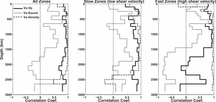
6.2. Wave-speed and Density Correlation

Based on the RMS amplitudes of wave speeds and density heterogeneities (Figure 7), we

may conclude that temperature variations are the primary cause of mantle heterogeneity. We

also find that the correlation of S-wave velocity and the other modeled fields are highly positive

in the majority of the mantle (Figure 10). In particular, the correlation coefficient of density and

S-wave speeds approaches 1 in a large portion of the mantle. This correlation drops in the

deepest mantle owing to the compositional anomalies associated with the superplume structures.

Similarly, P- and S-wave heterogeneities are highly correlated when all anomalies (estimated

thermal and non-thermal contributions) are considered. This result, along with the systematic

de-correlation of sound and shear speeds with depth, is generally consistent with past results [e.g.

Masters et al. 2000; Saltzer et al. 2001].

Sound and shear speeds become anti-correlated in the deep mantle with a negative peak

just below ~2000 km depth; a result that is also similar to the results presented in Saltzer et al.

[2001]. However, just above the D" layer, the correlation jumps to positive values and then

quickly returns to negative within the D" layer unlike the aforementioned study. Both Saltzer et

al. [2001] and Masters et al. [2000] show hints of this cyclical correlation behavior, but the

amplitude of the correlation jumps presented in the current study are more dramatic. This

31 

 

correlation behavior may imply the existence of two distinct depth zones with elevated

compositional influence centered at ~2000 km depth and within the D" layer. The layer

immediately above D" would then represent a transitional layer that is more strongly controlled

by temperature variations. This argument may have merit given the elevated compositional

sensitivity of sound speed in the deep mantle (see Figure 7). However, we are reluctant to draw

definitive conclusions from this observation alone since other mechanisms such as the pPv phase

transition could contribute to the pattern. Additionally, the correlation jump occurs over a single

model layer and is possibly an artifact of parameterization.

Although the modeled P/S-wave speeds and density are mostly correlated when all

anomalies are considered in the calculation, separating the fields according to fast and slow S-

wave anomalies reveals more complicated results (Figure 10). In particular, the correlation of

slow S-wave structures and density are much smaller (sometimes negative) in the deep mantle.

The primary source of this deep-mantle de-correlation is easily recognized to be the effects of the

opposing thermal/compositional density signatures associated with the superplume structures

(Figure 8b).

The correlation of slow S-wave anomalies and the corresponding P-wave anomalies is

high, similar to the total correlation. However, if we compute the correlation of fast shear

velocity zones with the corresponding P-wave anomalies, we find a dramatically different result

(Figure 10). Specifically, P-wave anomalies in regions with fast S-wave velocities

systematically de-correlate with depth beginning at ~1500 km and peaking to slightly negative

values at ~2100 km depth. Thus, the deep-mantle high shear-velocity zones, that may be

attributed to ancient subducted slab remnants, have significantly different geographic patterns

than the P-wave anomalies due to strong anti-correlation of shear and sound speeds. In extreme

32 

 

cases, the high-velocity shear zones correspond to low-velocity P-wave anomalies. Therefore,

the thermal P-wave signatures are significantly countered by the ‘non-thermal’ component (see

Figure 9b; 1830 km depth) producing muted or absent total P-wave structure where S-wave

velocities are fast and densities are high. It is unclear if the deep-mantle fast shear velocity blobs

are remnant slab materials. But it is evident that these features have very different P-wave

signatures that do not adhere to their expected thermal behavior, differing from zones with low

shear velocity in the lower half of the mantle.

As pointed out in Boschi et al. [2007], deep lower mantle anomalies are dominated by

negative velocities at low spatial frequencies. On the other hand, high-velocity anomalies in the

lower mantle are typically restricted to high spatial frequencies that may not be well-resolved in

some cases. Correlation properties of fast shear anomalies in the lower mantle, based on

independently derived P- and S-wave models, would therefore be dubious. However, in the

development of the GyPSuM model, both P- and S-wave data were modeled simultaneously with

the same parameterization and regularization mitigating a number of issues including the varying

resolution of each data set.

6.3. Compatibility with Geodynamic Constraints

We finally consider the extent to which the 3-D density anomalies in GyPSuM, identified

by ‘Total Density’ in Figures 8a-b, is able to reproduce the geodynamic constraints illustrated in

Figure 1. We carried out a mantle-flow calculation employing these density anomalies and using

the radial viscosity profile in Figure 2a that was previously derived by Mitrovica and Forte

[2004]. A comparison of the predicted dynamic surface topography (Figure 11b) and the

33 

 

corresponding crust-corrected surface topography (Figure 11a) shows a very good global fit,

quantified in Table 3 (final row).

The comparison of predicted and observed free-air gravity anomalies (Figures 11c,d) also

shows excellent agreement (quantified by the final row in Table 3). The almost equivalent fits to

both the surface topography and gravity anomalies resolves a longstanding debate concerning the

ability of the tomography-based mantle-flow models to reconcile both data sets [e.g. Forte et al.

1993; Le Stunff and Ricard 1995; Forte 2007].

The predicted tectonic plate motions driven by the total density anomalies in the 3-D

GyPSuM model are quantified (last row in Table 3) in terms of the fit to observed horizontal

divergence field. The match is nearly perfect (99% variance reduction) and it is therefore of

interest to determine the extent to which the predicted radial vorticity matches that of the

NUVEL-1 motions in the NNR frame. As discussed previously (section 2), the radial vorticity

may be mathematically regarded as a linear mapping of the horizontal divergence, for a given

(fixed) plate geometry. We find that the predicted radial vorticity field yields a 95% fit (variance

reduction) to the observed NUVEL-1-NNR radial vorticity field.

7. Discussion

Wave speeds and density are highly correlated throughout most of the mantle when all

anomalies are considered (Figure 10). However, fast shear velocity zones and the corresponding

P-wave anomalies systematically de-correlate in the ~1500-2500 km depth range suggesting

another mechanism besides simple thermal variations. The combined thermal and other possible

mechanism(s) mute P-wave velocity signatures in zones commonly interpreted as subducted

slabs in the deep mantle on the basis of S-wave tomographic solutions that show persistent fast

34 

 

anomalies at these depths (compare the ‘Total’ VS and VP fields in Figures 6b and 9b at 1830 km

depth). A possible explanation for the P- and S-wave discrepancies is the effect of electronic

spin transitions in iron-bearing minerals. Studies of the elastic effect of electronic spin transition

suggest that, at mid-mantle depths, the transition will generate negative seismic velocity

anomalies over a broad depth range [e.g. Crowhurst et al. 2009; Wentzcovitch et al. 2009]. The

effect of this mechanism would then oppose the thermally induced fast velocity signatures within

the subducted slab material. Moreover, if the temperature decrease is small enough, the effects

of spin transitions could overwhelm the thermally induced high P-wave velocities thereby

muting out the structure entirely. The S-wave signatures in the supposed subducted slab

remnants could remain fast given the relatively increased sensitivity of S-wave velocity to

thermal variations. In such a scenario, the high-temperature zones (producing low-velocity

signatures) would remain slow since the combined effects of increased temperature and spin

transition would be constructive. Therefore the correlation of low shear velocity zones with the

corresponding P-wave values would remain large and positive.

One potential problem with the hypothesis stated above is the fast, non-thermal S-wave

speeds we estimate in these zones (Figure 6b; 1830 km depth). If the previous scenario were

true, we would expect an opposite (slow) non-thermal shear-velocity signature. A possible

explanation for this apparent fast non-thermal anomaly is the underestimation of the thermal

contributions to the S-wave velocity field in this depth range. The joint inversion with thermal

scaling relationships (1-D in the lower mantle) incorporated both S- and P-wave data that

conflict when scaled in this simplified way as evidenced by our results. Thus the thermal S-

wave heterogeneity solution could have been corrupted by the P-wave data that require nearly no

anomalies in these subducted slab remnants. Nonetheless, we find that zones with fast S-wave

35 

 

speeds (centered at ~2000 km depth) correlate poorly with the corresponding P-wave anomalies

in the total velocity fields (Figure 10) and are often muted and/or absent (compare Figures 6b

and 9b). Spin transitions potentially explain our observations, but the actual effects that

electronic spin transitions have on mantle materials is still uncertain [see Badro et al. 2003,

2004; Hofmeister 2006; Lin et al. 2007, 2008; Speziale et al. 2007; Stackhouse et al. 2007;

McCammon et al. 2008; Crowhurst et al. 2009; Wentzcovitch et al. 2009].

Aside from the discrepancies of wave speeds in the ancient subducted slab remnants, the

superplume structures beneath Africa and the Pacific Ocean possess properties that cannot be

explained by temperature variations alone. Most notably, portions of the superplume structures

have significant positive non-thermal density signatures that are relatively broad in the D" layer

and extend upward through the mid-mantle with a more narrow lateral extent (Figure 8b). These

density signatures are interpreted as intrinsically dense material that is partially entrained within

the upwelling superplumes [Simmons et al. 2007]. The intrinsic density of this material counters

the thermally induced density, thereby reducing the overall buoyancy of the upwellings [see

Simmons et al. 2007, 2009; Forte et al. 2010]. The amplitude of the non-thermal high-density

signatures in the superplumes are larger than our previous tomography results [Simmons et al.

2007, 2009] owing to the addition of the P-wave constraints that help limit the range of possible

configurations of density heterogeneity in the joint inversion process.

Combining the thermal and non-thermal components of the density field, we find overall

positive density anomalies within the South Africa superplume structure. Studies incorporating

normal mode splitting functions have similarly modeled high density signatures in the low-

velocity superplume structures [e.g. Ishii and Tromp 1999; Trampert et al. 2004] suggesting a

dominant compositional influence on the heterogeneity in these regions. However, our results

36 

 

differ strongly in that the overall high-density zones appear to be far more localized and lower

amplitude. Specifically, we find only slightly positive density anomalies beneath the extreme

southern tip of Africa that is mostly confined to the D" layer. Beneath the Pacific Ocean, we

find no significant positive density anomalies in the low-velocity structures. However, a

localized portion of the Pacific superplume density structure is strongly affected by the positive

intrinsic density of the material, also muting the temperature-induced buoyancy.

Similar to the results of Kuo and Romanowicz [2002], our results suggest that mantle

density models developed with normal mode data [e.g. Ishii and Tromp 1999; Trampert et al.

2004] may be overestimating the amplitudes and scale-lengths of high-density anomalies at the

base of the superplume structures. Moreover, Kuo and Romanowicz [2002] suggest that up to

0.5% density anomalies could be obscured in normal mode data and that either high or low

densities could be modeled in the superplume structures depending on starting conditions of the

inversion. We cannot exclude the possibility of intense and broad high-density anomalies within

the superplume structures in the current study. However, we can conclude that there is no

requirement for extensive zones of high-amplitude positive density anomalies in the superplume

structures to simultaneously explain all the geodynamic and seismic constraints we have

employed.

8. Conclusions

We have constructed a tomographic model of mantle S-wave speeds, P-wave speeds and

density through the simultaneous inversion of seismic and geodynamic observations. The mantle

model (labeled GyPSuM) was constructed with the underlying hypothesis that temperature

variations are the dominant cause of mantle heterogeneity via the integration of mineral physics

37 

 

parameters that describe the relative behavior of mantle properties due to thermal effects. Thus,

GyPSuM represents the ‘simplest’ model of the mantle, whereby only the minimal amount of

compositional heterogeneity is introduced to satisfy P- and S-wave travel time data as well as the

global free-air gravity field, dynamic surface topography, and the divergence of the tectonic plate

velocities. Thermal dominance of heterogeneity is best demonstrated through the calculated

RMS amplitudes of the estimated thermal and non-thermal contributions to the model fields

(wave speeds and density) shown in Figure 7.

Overall, we find that P-wave, S-wave, and density anomalies may be primarily attributed

to variations in temperature. However, substantial chemical heterogeneity is required in the

cratonic roots of continents and, to a lesser extent, in the deepest mantle. In particular, we find

positive density anomalies at the base of the African superplume structure. This high-density

zone is more localized and much lower amplitude than the zones observed in density models

produced with normal mode data [e.g. Ishii and Tromp 1999; Trampert et al. 2004] which are

subject to considerable non-uniqueness [Kuo and Romanowicz 2002]. Another intriguing

observation from GyPSuM is the systematic de-correlation of fast shear velocity zones and the

corresponding P-wave anomalies in the ~1500-2500 km depth range. This observation may

suggest another mechanism besides simple thermal variations for the generation of mid-mantle

heterogeneity. We argue that a possible explanation for the P- and S-wave de-correlation is the

effect of electronic spin transitions in iron-bearing minerals, which may mask the overall P-wave

signatures of ancient subducted slabs in the deep mantle.

It should be noted that we assumed ray paths (infinite frequency approximation) and that

considering finite frequency effects could alter the results of this study. Studies considering

finite frequency effects have shown that the amplitude of low velocity anomalies could be

38 

 

considerably larger than those produced by ray theory [Montelli et al. 2004; Lekić and

Romanowicz 2010]. These amplitude differences might be significant to the study presented

herein, but direct comparisons of ray and finite-frequency theories provide evidence that the

basic arrangement of mantle heterogeneity does not dramatically change [Boschi et al. 2006;

Peter et al. 2009]. Incorporation of more data and data types may result in models that require

stronger chemical heterogeneity in the future. Resolving the issue of chemical versus thermal

causes for observed heterogeneity will also require the incorporation of more comprehensive and

stricter mineral physics constraints.

Acknowledgements

We thank Barbara Romanowicz and an anonymous reviewer for their constructive comments

that helped to improve our paper. We also acknowledge helpful discussions with Steve Myers,

Elise Knittle and Jung-Fu Lin. AMF wishes to acknowledge funding from the Canadian Institute

for Advanced Research, NSERC, and from the Canada Research Chair program. LB wishes to

thank Domenico Giardini for his constant support and encouragement. SPG thanks the Jackson

School of Geosciences at the University of Texas for their support. This work performed under

the auspices of the U.S. Department of Energy by Lawrence Livermore National Laboratory

under Contract DE-AC52-07NA27344. LLNL-JRNL-426712

39 

 

References

Anderson, D.L. (1989), Theory of the Earth, Blackwell Sci., Malden, Mass. Anderson, D.L. (2002), The case for irreversible chemical stratification of the mantle, Int. Geo.

Rev., 44, 97-116. Antolik, M., Y.J. Gu, G. Ekström and A.M. Dziewonski (2003), J362D28: a new joint model of

compressional and shear velocity in the Earth’s mantle, Geophys. J. Int., 153, 443-466. Argus, D.F. and R.G. Gordon (1991), No-net-rotation model of current plate velocities

incorporating plate motion model NUVEL-1, Geophys. Res. Lett. , 18, 2038-2042. Badro, J., G. Fiquet, F. Guyot, J.-P. Rueff, V.V. Struzhkin, G. Vankó and G. Monaco (2003), Iron

partitioning in Earth’s mantle: Toward a deep lower mantle discontinuity, Science, 300, 789-791.

Badro, J., J.-P. Rueff, G. Vankó, G. Monaco, G. Fiquet and F. Guyot (2004), Electronic transitions

in perovskite: Possible nonconvecting layers in the lower mantle, Science, 305, 383-386. Bassin, C., G. Laske and G. Masters (2000), The current limits of resolution for surface wave

tomography in North America, EOS Trans. AGU, 81, F897. Boschi, L., T.W. Becker, G. Soldati and A.M. Dziewonski (2006), On the relevance of Born

theory in global seismic tomography, Geophys. Res. Lett., 33, doi: 10.1029/2005GL025063.

Boschi, L., T.W. Becker and B. Steinberger (2007), Mantle plumes: Dynamic models and seismic

images, Geochem. Geophys. Geosys., 8(10), doi: 10.1029/2007GC001733. Brodholt, J.P., Helffrich, G. and J. Trampert (2007), Chemical versus thermal heterogeneity in

the lower mantle: The most likely role of anelasticity, Earth planet. Sci. Lett., 262, 429–437.

Cammarano, F., S. Goes, P. Vacher and D. Giardini (2003), Inferring upper-mantle temperatures

from seismic velocities, Phys. Earth Planet. Inter., 138(3-4), 197-222. Crowhurst, J.C., J.M. Brown, A.F. Goncharov and S.D. Jacobsen (2009), Elasticity of (Mg,Fe)O

through the spin transition of iron in the lower mantle, Science, 319, 451-453. DeMets, C.R., Gordon, R.G., Argus, D.F. and S. Stein (1990), Current plate motions, Geophys.

J. Int., 101(2), 425-478.

40 

 

DeMets, C.R., Gordon, R.G., Argus, D.F. and S. Stein (1994), Effect of recent revisions to the geomagnetic reversal time scale on estimates of current plate motion, Geophys. Res. Lett., 21, 2191-2194.

Dziewonski, A.M. and F. Gilbert (1976), The effect of small, aspherical perturbations on travel

times and a re-examination of the corrections for ellipticity, Geophys. J. R. Astron. Soc. 44, 7-17.

Dziewonski, A.M. and D.L. Anderson (1981), Preliminary reference Earth model, Phys. Earth

Planet. Inter., 25, 297-356. Engdahl, E., R.D. van der Hilst and R. Buland (1998), Global teleseismic earthquake relocation

with improved travel times and procedures for depth discrimination, Bull. Seis. Soc. Amer., 88, 722-743.

Forte, A.M. and W.R. Peltier (1987), Plate tectonics and aspherical Earth structure; the

importance of poloidal-toroidal coupling, J. Geophys. Res. 92, 3645-3679. Forte, A.M., W.R. Peltier, A.M. Dziewonski and R.L. Woodward (1993), Dynamic surface

topography: A new interpretation based upon mantle flow models derived from seismic tomography, Geophys. Res. Lett., 20, 225-228.

Forte, A.M. and W.R. Peltier (1994), The kinematics and dynamics of poloidal toroidal coupling

in mantle flow: The importance of surface plates and lateral viscosity variations, Adv. Geophys., 36, 1-119.

Forte, A.M., J.X. Mitrovica and R.L. Woodward (1995), Seismic-geodynamic determination of

the origin of excess ellipticity of the core-mantle boundary, Geophys. Res. Lett., 22, 1013-1016.

Forte, A.M. and H.K.C. Perry (2000), Geodynamic evidence for a chemically depleted

continental tectosphere, Science, 290, 1940-1944. Forte, A.M. and J.X. Mitrovica (2001), Deep-mantle high-viscosity flow and thermochemical

structure inferred from seismic and geodynamic data, Nature, 410(6832), 1049-1056. Forte, A.M. (2007), Constraints on seismic models from other disciplines-implications for

mantle dynamics and composition, in Volume 1 of Treatise of Geophysics, edited by B. Romanowicz and A.M. Dziewonski, Elsevier, pp. 805–858.

Forte, A.M, S. Quéré, R. Moucha, N.A. Simmons, S.P. Grand, J.X. Mitrovica and D.B. Rowley

(2010), Joint seismic-geodynamic-mineral physical modeling of African geodynamics: A reconciliation of deep-mantle convection with surface geophysical constraints, Earth Planet. Sci. Lett., 295, 329-341.

41 

 

Grand, S.P. and D.V. Helmberger (1984), Upper mantle shear structure of North America, Geophys. J. R. Astron. Soc. 76, 399-438.

Grand, S.P. (1994), Mantle shear structure beneath the Americas and surrounding oceans, J.

Geophys. Res., 99, 11591-11621. Grand, S.P., R.D. Van der Hilst and S. Widiyantoro (1997), Global seismic tomography: a

snapshot of convection in the Earth, GSA Today, 7, 1-7. Grand, S.P. (2002), Mantle shear-wave tomography and the fate of subducted slabs, Phil. Trans.

R. Soc. Lond. A, 360(1800), 2475-2491. Hernlund, J.W., C. Thomas and P.J. Tackley (2005), A doubling of the post-perovskite phase

boundary and structure of the Earth's lowermost mantle, Nature, 434, 882–886. Hernlund, J.W. and C. Houser (2008), On the statistical distribution of seismic velocities in

Earth’s deep mantle, Earth Planet. Sci. Lett., 265, 423-437. Herring, T.A., P.M. Mathews and B.A. Buffett (2002), Modeling of nutation-precession; very

long baseline interferometry results, J. Geophys. Res. Solid Earth, 107(B4), doi: 10.1029/2001JB000165.

Hirose, K. (2006), Postperovskite phase transition and its geophysical implications, Rev.

Geophys., 44(RG3001), doi:10.1029/2005RG000186. Hofmeister, A.M. (2006), Is low-spin Fe2+ present in Earth’s mantle?, Earth Planet. Sci. Lett.,

243, 44-52. Hutko, A.R., T. Lay, J. Revenaugh and E.J. Garnero (2008), Anticorrelated seismic velocity

anomalies from post-perovskite in the lowermost mantle, Science, 320, 1070-1074. Iitaka, T., K. Hirose, K. Kawamura, and M. Murakami (2004), The elasticity of the MgSiO3

post-perovskite phase in the Earth's lowermost mantle, Nature, 430, 442-445. Ingber, L. (1989), Very fast simulated re-annealing. Math. Comput. Modell., 12, 967–973. Ishii, M. and J. Tromp (1999), Normal-mode and free-air gravity constraints on lateral variations

in velocity and density of Earth’s mantle, Science, 285(5431), 1231-1236. Ishii, M. and J. Tromp (2004), Constraining large-scale mantle heterogeneity using mantle and

inner-core sensitive normal modes, Phys. Earth Planet. Inter., 146(1-2), 113-124. Jackson, C., M.K. Sen and P.L. Stoffa (2004), An efficient stochastic Bayesian approach to

optimal parameter and uncertainty estimation for climate model predictions, J. Climate, 17 2828-2841.

42 

 

Jordan, T.H. (1978), Composition and development of the continental tectosphere, Nature, 274,

544-548. Karato, S.I. (1993), Importance of anelasticity in the interpretation of seismic tomography,

Geophys. Res. Lett., 20, 1623-1626. Karato, S.I. and B.B. Karki (2001), Origin of lateral variation of seismic wave velocities and

density in the deep mantle, J. Geophys. Res. Solid Earth, 106(B10), 21771-21783. Kennett, B.L.N., S. Widiyantoro and R.D. van der Hilst (1998), Joint seismic tomography for

bulk sound and shear wave speed in the Earth’s mantle, J. Geophys. Res., 103, 12469-12493.

Kennett, B.L.N. and A. Gorbatov (2004), Seismic heterogeneity in the mantle—strong shear

wave signature of slabs from joint tomography, Phys. Earth Planet. Inter., 146, 87-100. Khan, A., L. Boschi and J.A.D. Connolly (2009), On mantle chemical and thermal

heterogeneities and anisotropy as mapped by inversion of global surface wave data, J. Geophys. Res., 114, doi:10.1029/2009JB006399.

Kuo, C. and B. Romanowicz (2002), On the resolution of density anomalies in the Earth’s

mantle using spectral fitting of normal-mode data, Geophys. J. Int., 150, 162-179. Lay, T., J. Hernlund, E.J. Garnero and M.S. Thorne (2006), A postperovskite lens and D″ heat

flux beneath the central Pacific, Science, 314, 1272–1276. Lekić, V. and B. Romanowicz (2010), Inferring mantle structure by full waveform tomography

using spectral element method, Geophys. J. Int. (submitted). Lemoine, F. G., et al. (1998), The development of the joint NASA GSFC and NIMA

Geopotential Model EGM96, NASA Tech. Rep., 1998-206861. Le Stunff, Y. and Y. Ricard (1995), Topography and geoid due to lithospheric mass anomalies,

Geophys. J. Int., 122, 982-990. Lin, J.-F., G. Vankó, S.D. Jacobsen, V. Iota, V.V. Struzhkin, V.V. Prakapenka, A. Kuznetsov,

C.-S. Yoo (2007), Spin transition zone in Earth’s lower mantle, Science, 317, 1740-1743. Lin, J.-F., H. Watson, G. Vankó, E.E. Alp, V.V. Prakapenka, P. Dera, V.V. Struzhkin, A. Kubo,

J. Zhao, C. McCammon and W.J. Evans (2008), Intermediate-spin ferrous iron in lowermost mantle post-perovskite and perovskite, Nature Geosci., 1, 688-691.

Masters, G., G. Laske, H. Bolton and A.M. Dziewonski (2000), The relative behavior of shear

velocity, bulk sound speed, and compressional velocity in the mantle: implications for

43 

 

chemical and thermal structure, in Earth’s Deep Interior: Mineral Physics and Tomography from the Atomic to the Global Scale, edited by S.-I. Karato et al., pp. 63-87, AGU, Washington, DC.

Matas, J. and M. Bukowinski (2007), On the anelastic contribution to the temperature

dependence of lower mantle seismic velocities, Earth planet. Sci. Lett., 259, 51–65. Mathews, P.M., T.A. Herring and B.A. Buffett (2002), Modeling of nutation and precession:

new nutation series for nonrigid Earth and insights into the Earth’s interior, J. Geophys. Res. Solid Earth, 107(B4), doi: 10.1029/2001JB000390.

McCammon, C., I. Kantor, O. Narygina, J. Rouquette, U. Ponkratz, I. Sergueev, M. Mezouar, V.

Prakapenka and L. Dubrovinsky (2008), Stable intermediate-spin ferrous iron in lower-mantle perovskite, Nature Geosci., 1, 684-687.

McNamara, A.K. and S. Zhong (2005), Thermochemical structures beneath Africa and the

Pacific Ocean, Nature, 437(7062), 1136-1139. Mitrovica, J.X. and A.M. Forte (2004), A new inference of mantle viscosity based upon joint

inversion of convection and glacial isostatic adjustment data, Earth Planet. Sci. Lett., 225(1-2), 177-189.

Montelli, R., G. Nolet, F.A. Dahlen, G. Masters, E.R. Engdahl and S.-H. Hung (2004), Finite-

frequency tomography reveals a variety of plumes in the mantle, Science, 303, 338-343. Mooney, W.D., G. Laske and G. Masters (1998), CRUST 5.1: a global crustal model at 5 x 5

degrees, J. Geophys. Res. Solid Earth, 103(B1), 727-747. Moucha, R., A.M. Forte, J.X. Mitrovica and A. Daradich (2007), Lateral variations in mantle

rheology: Implications for convection related observables and inferred viscosity models, Geophys. J. Int., 169, 113-135.

Murakami, M., K. Hirose, K. Kawamura, N. Sata and Y. Ohishi (2004), Post-perovskite phase

transition in MgSiO3, Science, 304, 855-858. Ni, S.D., E. Tan, M. Gurnis and D.V. Helmberger (2002), Sharp sides to the African superplume,

Science, 296(5574), 1850-1852. Ni, S.D. and D.V. Helmberger (2003), Seismological constraints on the South African

superplume; could be the oldest distinct structure on Earth, Earth Planet. Sci. Lett., 206(1-2), 119-131.

Oganov, A.R. and S. Ono (2004), Theoretical and experimental evidence for a post-perovskite

phase of MgSiO3 in Earth’s D" layer, Nature, 430, 445-448.

44 

 

Paige, C.C. and M.A. Saunders (1982), LSQR: an algorithm for sparse linear equations and sparse least squares, ACM Transactions on Mathematical Software, 8, 43-71.

Peter, D., L. Boschi and J.H. Woodhouse (2009), Tomographic resolution of ray and finite-

frequency methods: a membrane-wave investigation, Geophys. J. Int., 177, 624-638. Quéré, S. and A.M. Forte (2006), Influence of past and present-day plate motions on spherical

models of mantle convection: implications for mantle plumes and hotspots, Geophys. J. Int., 165, 1041-1057.

Ricard, Y., L. Fleitout and C. Froidevaux (1984), Geoid heights and lithospheric stresses for a

dynamic Earth, Ann. Geophys. 2, 267-286. Richards, M.A. and B.H. Hager (1984), Geoid anomalies in a dynamic earth, J. Geophys. Res.

Solid Earth, 89(B7), 5987-6002. Ritsema, J., H.J. Van Heijst and J.H. Woodhouse (1999), Complex shear wave velocity structure

imaged beneath Africa and Iceland, Science, 286(5446) 1925-1928. Ritsema, J. and H.H. van Heijst (2002), Constraints on the correlation of P- and S-wave velocity

heterogeneity in the mantle from P, PP, PPP and PKPab traveltimes, Geophys. J. Int., 149, 482-489.

Robertson, G.S and J.H. Woodhouse (1996), Ratio of relative S to P velocity heterogeneity in the

lower mantle, J. Geophys. Res., 101, 20041-20052. Saltzer, R.L., R.D.Van der Hilst and H. Kárason (2001), Comparing P and S wave heterogeneity

in the mantle, Geophys. Res. Lett., 28(7) 1335-1338. Schuberth, B.S.A., Bunge, H.P. and J. Ritsema (2009), Tomographic filtering of high-resolution

mantle circulation models: Can seismic heterogeneity be explained by temperature alone?, Geochem. Geophys. Geosys., 10, DOI: 10.1029/2009GC002401.

Simmons, N.A., Forte, A.M. and S.P. Grand (2006), Constraining mantle flow with seismic and

geodynamic data: a joint approach, Earth Planet. Sci. Lett. 246, 109–124. Simmons, N.A., Forte, A.M. and S.P. Grand (2007), Thermochemical structure and dynamics of

the African superplume, Geophys. Res. Lett., 34(2), L02301, doi: 10.1029/2006GL028009.

Simmons, N.A., Forte, A.M. and S.P. Grand (2009), Joint seismic, geodynamic and mineral

physical constraints on three-dimensional mantle heterogeneity: implications for the relative importance of thermal versus compositional heterogeneity, Geophys. J. Int. 177(5), 1284–1304.

45 

 

Soldati, G., L. Boschi, F. Deschamps and D. Giardini (2009), Inferring radial models of mantle viscosity from gravity (GRACE) data and an evolutionary algorithm, Phys. Earth Planet Inter., 176, 19-32.

Speziale, S., V.E. Lee, S.M. Clark, J.-F. Lin, M.P. Pasternak and R. Jeanloz (2007), Effects of Fe

spin transition on the elasticity of (Mg, Fe)O magnesiowüstites and implications for the seismological properties of the Earth’s lower mantle, J. Geophys. Res., 112, doi:10.1029/2006JB004730.

Stackhouse, S., J.P. Brodholt and G.D. Price (2007), Electronic spin transitions in iron-bearing

MgSiO3 perovskite, Earth Planet. Sci. Lett., 253, 282-290. Su, W. and A.M. Dziewonski (1993), Joint 3-D inversion for P- and S-velocity in the mantle,

EOS Trans. AGU, 74, 557. Su, W. and A.M. Dziewonski (1997), Simultaneous inversion for 3-D variations in shear and

bulk velocity in the mantle, Phys. Earth Planet. Inter., 100(1-4), 135-156. Trampert, J., F. Deschamps, J. Resovsky and D. Yuen (2004), Probabilistic tomography maps

chemical heterogeneities throughout the lower mantle, Science, 306(5697), 853-856. Tsuchiya, T., J. Tsuchiya, K. Umemoto and R.M. Wetzcovitch (2004), Elasticity of post-

perovskite MgSiO3, Geophys.Res. Lett., 31, L14603. Van der Hilst, R.D. and H. Kárason (1999), Compositional heterogeneity in the bottom 1000

kilometers of the Earth’s mantle: Toward a hybrid convection model, Science, 283, 1885-1888.

Vasco, D.W., L.R. Johnson, R.J. Pulliam and P.S. Earle (1994), Robust inversion of IASP91

travel-time residuals for mantle P and S velocity structure, earthquake mislocations, and station corrections, J. Geophys. Res., 99, 13727-13755.

Wen, L.X. and D.L. Anderson (1997), Present-day plate motion constraint on mantle rheology

and convection, J. Geophys. Res., 102(B11), 24,639-24,653. Wen, L.X. (2001), Seismic evidence for a rapidly varying compositional anomaly at the base of

the Earth’s mantle beneath the Indian Ocean, Earth Planet. Sci. Lett., 194(1-2), 83-95. Wentzcovitch, R.M., J.F. Justo, Z. Wu, C.R.S. da Silva, D.A. Yuen and D. Kohlstedt (2009),

Anomalous compressibility of ferropericlase throughout the iron spin cross-over, Proc. Natl. Acad. Sci., 106(21), 8447-8452.

Wookey, J., S. Stackhouse, J.-M. Kendall, J. Brodholt and G.D. Price (2005), Efficacy of the

post-perovskite phase as an explanation of lowermost mantle seismic properties, Nature, 438, 1004–1008.

46 

 

Figure Captions

Figure 1. Geodynamic observables employed in the joint seismic-geodynamic tomography

inversions. (a) Blue arrows represent the plate velocity vectors obtained from the NUVEL-1

model [DeMets et al. 1990] relative to a global frame of reference in which there is No Net

Rotation (NNR) of the lithosphere. The color contours represent the rate of horizontal divergence

of the plate velocity field. (b) The free-air gravity anomalies derived from the joint geopotential

model EGM96 [Lemoine et al. 1998]. (c) The dynamic surface topography obtained by removing

the topography due to isostatically compensated crustal heterogeneity from Earth's observed

topography. The CRUST2.0 [Bassin et al. 2000] crustal heterogeneity model is employed here.

(d) The excess or dynamic CMB ellipticity inferred from core nutation data [Mathews et al.

2002]. All fields, with the exception of (d), have been expanded in spherical harmonics up to

degree and order 16.

Figure 2. Mantle viscosity and viscous response (kernel) functions. (a) The solid black line

depicts the depth variation of effective mantle viscosity derived from the simultaneous Occam-

style inversion of mantle convection and glacial isostatic adjustment data sets [Mitrovica and

Forte 2004]. Absolute values of viscosity (in units of 1021 Pa s) are plotted. The black-dotted

grey lines depict the range of uncertainties in the viscosity inferences derived from the Occam

inversion. (b) The wavelength-dependent kernels for the rate of horizontal divergence of the

tectonic plates. The inset legend identifies the (reciprocal) wavelengths in terms of equivalent

spherical harmonic degrees. (c) The kernels for the free-air surface gravity anomalies are

represented for free-slip (black curves) and no-slip (blue curves) surface boundary conditions.

(d) The dynamic (surface) topography kernels are depicted for free-slip (black curves) and no-

slip (blue curves) surface boundary conditions.

Figure 3. Optimized relative heterogeneity ratios determined through a very fast simulated

annealing (VFSA) process. Only the 1-D part of the 1.5-D scaling models are shown. (Left)

Density-shear scaling relationships including the starting solution from Simmons et al. [2009]

(dashed line) and the solution found in the current study (thick solid line). Scaling model

profiles that were accepted within the VFSA process are also shown (thin gray lines). The

allowable range of 1-D solutions were bounded according to the results of Cammarano et al.

[2003] and Karato and Karki [2001]. (Right) Optimized 1-D compressional-shear velocity

scaling profile based on the fully coupled density-shear-compressional fields and joint inversions

(see text). The starting solution and VFSA iterations are similarly shown.

Figure 4. VFSA cooling schedule and data misfit for each accepted scaling model. (Top) We

chose a rapid cooling schedule since, with each possible set of scaling model parameters, a full-

scale non-linear joint inversion of all seismic and geodynamic data was performed. (Bottom)

Normalized average data misfit to all data fields for each accepted model update in the VFSA

process. Misfits are with respect to joint tomographic models produced with each set of scaling

model parameters selected by the optimization procedure. The process was terminated after 61

successful model updates.

Figure 5. Modeled 3-D scaling factor distributions (dark shaded regions) compared to the 1-D

thermal profiles (solid lines) determined with the VFSA optimization procedure. (Left) S

R/

47 

 

distributions tend to have modes aligning with the inferred 1-D thermal values. The most

notable exception is in the shallow upper mantle owing to the compositional signatures of

continental cratons. Additionally, distributions are skewed towards zero near the base of the

upper mantle and within the deepest mantle. (Right) Ratios of P- and S-wave speed

heterogeneity also tend to have distribution modes falling along the inferred 1-D thermal values.

The distributions tend to be significantly broader than the density-shear values and are bi-modal

in the D" layer. For reference, the dashed lines correspond to values of 2.7 and 1.7

as indicated. The distributions of values were computed for the pure seismic models

TX2008s [Simmons et al. 2009] and P-only (this study) for comparison (light gray shaded areas)

to demonstrate the impact of forcing the solution to be more consistent with thermal variations.

Note that near-zero values are a common occurrence in the deep mantle. Therefore, the

inverse, , is unbounded.

PSSPRR

//

1

SPR

/

SPR

/

PSSPRR

//

1

Figure 6a. S-wave velocity perturbations in the GyPSuM model. Each row corresponds to a

particular depth and the three columns correspond to each component of the velocity field. The

‘Total’ field is simply the sum of ‘Thermal’ and ‘Non-Thermal’ components defined in the text.

The ‘Non-Thermal’ heterogeneity levels are significantly smaller than the thermal signatures in

the upper half of the mantle. Note that the color scales change for each panel according to the

amplitude (‘X’) printed in the lower left corner of each panel.

Figure 6b. S-wave velocity perturbations in the GyPSuM model (continued). Linear fast zones

attributed to past subduction beneath North America and southern Eurasia/India persist to at least

48 

 

1800 km depth. Low-velocity zones dominate much of the deep mantle shear-wave

heterogeneity and are most evident in the African and Pacific superplume structures. High-

velocity zones in the D" layer generally occur beneath regions where subduction has occurred

since the past supercontinent cycle [Anderson 2002] suggesting that slabs eventually reach the

base of the mantle.

Figure 7. Root-mean-squared (RMS) amplitudes of wave speeds and density. Each field is

separated into thermal and non-thermal contributions and RMS amplitudes are subsequently

computed. S-wave heterogeneity is dominantly produced by variations in temperature

throughout the mantle. P-wave heterogeneity is also largely controlled by variations in

temperature, but to a lesser degree than shear-waves. Similarly, thermally induced density

anomalies are typically larger than compositionally induced heterogeneity. However, we find

substantial opposing compositional anomalies associated with the mass-depleted cratons and the

intrinsically dense superplume structures. These anomalies produce a level of compositional

influence that rivals the thermally driven density heterogeneity in the shallowest and deepest

mantles. Sound-speed heterogeneity is dominated by compositional variations throughout most

of the mantle. The low amplitude of the thermally induced sound-speed heterogeneity in the

deep mantle is a result of S values approaching 1 (see text). Therefore, the relative behaviors

of bulk modulus and density are very similar in the presence of temperature variations in the

lower mantle providing very small sound speed variations.

Figure 8a. Density perturbations in the GyPSuM model. The thermally-induced high-density

signatures in the cratonic roots are offset by the non-thermal contributions severely reducing the

49 

 

50 

 

amplitude of the overall negative buoyancies. Outside of the cratons, upper mantle density

structure is dominated by the effects of temperature variations.

Figure 8b. Density perturbations in the GyPSuM model (continued). The primary non-thermal

contributions to the density field are within the deepest portion of the superplume structures.

The central cores of these structures are intrinsically dense, offsetting the effects of temperature.

In some localized zones within the superplumes, we find near neutral buoyancies and mild

negative buoyancies which may account for the stabilization of these structures over long time

scales.

Figure 9a. P-wave velocity perturbations in the GyPSuM model. P-wave heterogeneity in the

shallow upper mantle is strongly influenced by compositional variations. This is most significant

in cratonic regions, but other scattered non-thermal anomalies are also evident.

Figure 9b. P-wave velocity perturbations in the GyPSuM model (continued). Non-thermal

influences on P-wave heterogeneity are significant in the lower half of the mantle. Most notably,

the thermally induced high-velocity zones are effectively muted by opposing low-velocity

signatures. In contrast, the patterns of the low-velocity regions in the total field generally match

the thermally-induced field. This behavior may be due to compositional variations and/or the

effect of electronic spin transitions (see text for a discussion).

Figure 10. Depth-dependent correlation of S-wave heterogeneity and other modeled properties.

(Left) Correlation coefficients with all heterogeneity considered. S- and P-wave velocities tend

51 

 

to be highly correlated throughout the mantle (Vs-Vp). Similarly, density and S-wave velocity

perturbations are positively correlated throughout the mantle (Vs-Density). However, sound-

speed is often de-correlated or mildly anti-correlated with S-wave heterogeneity (Vs-Sound).

(Center) Correlation based on low S-wave velocity regionalization. When we consider only the

low shear velocity structures in the correlation measurement, we find that P-wave anomalies

corresponding to these zones remain fairly well correlated. However, density heterogeneity

systematically de-correlates with shear-speed in the deepest mantle primarily owing to the

intrinsically dense material within the superplume structures. (Right) Correlation based on high

S-wave velocity regionalization. Fast shear velocity structure is highly correlated with density

throughout the lower mantle. Correlation of fast S-wave zones in the deep mantle (>1500 km

depth) with the corresponding P-wave anomalies decreases, suggesting a systematic departure

from simplified thermal effects in ancient subducted slab anomalies (see text for discussion).

Figure 11. Comparison of observed and predicted convection-related observables. (a) The crust-

corrected surface topography from Figure 1c. (b) The dynamic topography predicted with the

tomography-based mantle flow model. (c) The observed free-air gravity anomalies from Figure

1b. (d) The free-air gravity predicted with the tomography-based mantle flow model. The mantle

flow calculations employ the radial viscosity profile in Figure 2a and the density anomalies from

the final joint seismic-geodynamic inversion with a fully 3-D density-velocity scaling. All fields

have been expanded in spherical harmonics up to degree and order 16.

 

Table 1. Constraints on mantle heterogeneity employed in this study. Constraint Description Quantity Source

S-waves

Residual travel times for globally distributed S, ScS, sS, sScS, SKS, SKKS phases. Data also includes surface reflected multiples (e.g. SSS, ScS3, etc.) and triplicated phases turning within the upper mantle.

~46,000 Grand [2002]

Simmons et al. [2007]

P-waves

Residual travel times for teleseismic P-waves based on a recompilation of International Seismic Centre (ISC) data (EHB). Arrivals are condensed using a summary ray approach over 2 x 2 degree bins.

~626,000 Engdahl et al. [1998]

(EHB) Antolik et al. [2003]

Gravity

Global free-air gravity field from the EGM96 geopotential model derived from a compilation of land-, air-, and space-based observations.

spherical harmonic

degrees 2-16 Lemoine et al. [1998]

Plate Motions

Divergence of all tectonic plates calculated from the NUVEL-1 plate velocity model.

spherical harmonic

degrees 1-16 DeMets et al. [1990]

Dynamic Topography

Non-isostatic topography of Earth’s free surface. Estimated from removal of the crustal isostatic topography signal on the basis of CRUST2.0.

spherical harmonic

degrees 1-16

Bassin et al. [2000] Forte and Perry [2000]

CMB Ellipticity

Excess ellipticity of the core-mantle boundary (CMB) relative to Earth’s surface. The CMB is elevated by ~400 m along the equator according to studies of Earth’s free-core nutation processes.

zonal harmonic degree 2

Herring et al. [2002] Mathews et al. [2002]

Mineral Physics

Parameters

Bounds on the relative heterogeneity ratios ( SS VddR lnln //

SP VdVd lnln / and

) due to pure

thermal variations. Anharmonic and anelastic effects included.

SPR /

N/A

Karato and Karki [2001]

Cammarano et al. [2003]

52 

 

Table 2. Forward model variables. Variable Description Details

SL Shear-wave sensitivity kernels

1-D ray path lengths 46,000 x 99,148 sparse elements

PL Compressional-wave sensitivity kernels

1-D ray path lengths 620,000 x 99,148 sparse elements

G

c

Geodynamic data viscous flow response kernels

Spatial sensitivities of spherical harmonic components up to degree 16; free-air gravity,

plate divergences, dynamic topography 861 x 99,148 full elements

CMB ellipticity kernel Spatial sensitivity of the degree 2 zonal

harmonic 1 x 99,148 full elements (row vector)

D Regularization operator 2nd-order digital smoothing filter

DCMBGP ,,, Weights Relative weighting between data sets

( CMBGP ,, ); regularization weight ( D )

SV , , PV Wave speeds and density Starting model velocities and density from PREM and TNA/SNA models (see text)

SPR / Compressional/shear-wave relative heterogeneity ratio SPSP VdVdR ln/ln/

/SR Density/shear-wave relative heterogeneity ratio S/S VddR ln/ln

Sr Shear-wave travel time residual measurements

~46,000 residuals (column vector)

Pr Compressional-wave travel time residual measurements

~626,000 residuals (column vector)

g Geodynamic data

Spherical harmonic coefficients up to degree 16 of the free-air gravity, plate divergences, dynamic topography; 861 elements (column

vector)

e CMB ellipticity Degree 2 zonal harmonic coefficient

representing 400m of excess ellipticity on the core-mantle boundary

Sm Shear-wave slowness perturbation model

Heterogeneity model to be determined through inversion

53 

 

54 

 

SR / SPR /

Table 3. Model fits to all data considered.

Model Name

Scaling Models ,

S-wave arrivals

(%)

P-wave arrivals

(%)

Free-air gravity

(%)

Tectonic plate

divergence (%)

Dynamic surface

topography(%)

CMB excess

ellipticity(km)

TX2008sa 1-Db 94 12 1 48 -44 1.3 P-onlyc 1-Db 56 32 -57 30 -164 1.3

TX2008ja 3-Db 93 12 91 99 80 0.4 GyPSuM_1Dd 1-Db 90 28 69 97 -70 0.4

GyPSuM_1.5Dd 1.5Dd 90 29 73 97 32 0.4 GyPSuMe 3-De 93 31 88 99 72 0.4

Fits are expressed as variance reduction (in percent) except for excess CMB ellipticity expressed in km (0.4 km is the expected value). aShear-wave models produced with seismic data alone (TX2008s) and joint inversion of shear-wave travel times and geodynamic information (TX2008j) from Simmons et al. [2009].

bOptimum 1-D and 3-D density-shear scaling models found on the basis of joint seismic-geodynamic inversion [Simmons et al. 2009] and computed compressional-shear scaling (see text).

cCompressional velocity model produced using only P-wave data described in the text. TX2008s and P-only have similar model roughness. Models are for fit comparison only.

dJoint P-S-geodynamic models developed using 1-D scaling (GyPSuM_1D) and a modified scaling model that accounts for 1st- order effects of cratonic mass depletion and the temperature dependence of Q (GyPSuM_1.5D). Scaling model 1.5D was found through the simulated annealing process described in the text.

eFinal P-S-density and scaling models developed in this study.

Table 4. Scaling model optimization parameters. General form: S

D-1SS VbaRR ln//

Parameter Description VFSA

solution D-1SR / Starting density-shear velocity relative

heterogeneity ratio from Simmons et al. [2009]. N/A

SVln Shear-wave velocity heterogeneity N/A

Velocity-based scaling model correction derivatives of the form SS VR ln//

N/A

uma Amplification factor applied to the starting 1-D upper mantle density-velocity scaling profile.

0.916

umb Additive term that adjusts the mean of the 1-D upper mantle scaling profile.

0.0157

lma Amplification factor applied to the starting 1-D lower mantle density-velocity scaling profile.

0.651

lmb Additive term that adjusts the mean of the 1-D lower mantle scaling profile.

0.0619

100craton Scaling model correction derivative defined only in

the cratonic roots in the upper 100 km. -5.92

250craton Scaling model correction derivative defined only in

the cratonic roots from 100 to 250 km depth. -3.13

100thermal Scaling model correction derivative in the non-

cratonic upper 100 km. 1.26

250thermal Scaling model correction derivative in the non-

cratonic mantle in the 100-250 km depth range. 1.59

650thermal Scaling model correction derivative in the non-

cratonic mantle in the 250-650 km depth range. 0.341

55