GREENHOUSE GASES EMISSIONS IN A SEMI-ARID

RESERVOIR IN NORTHEASTERN BRAZIL

Vorgelegt von

M. Sc

Maricela Rodríguez Góngora

geb. in Socorro, Kolumbien

von der Fakultät III - Prozesswissenschaften

der Technischen Universität Berlin

zur Erlangung des akademischen Grades

„Doktor der Naturwissenschaften”

-Dr. rer. nat.-

genehmigte Dissertation

Promotionsausschuss:

Vorsitzender: Prof. Dr. Matthias Finkbeiner

Gutachter: Prof. Dr.-Ing. Martin Jekel

Gutachter: Dr. rer. nat. Günter Gunkel

Gutachterin: Prof. Dr. rer. nat. habil. Brigitte Nixdorf

Tag der wissenschaftlichen Aussprache: 15. Dezember 2017

Berlin 2018

Acknowledgments

I

ACKNOWLEDGMENTS

First of all, I want to express my admiration and gratitude to my supervisor Dr. Peter Casper for trusting me and gave me the opportunity to bring about this PhD project, I hope I have responded properly to his vote of confidence. I want to thank him for all the support during the development of the work, even from the distance when I was in the field and he was always available to help during crisis times. His constant advice and help were very important to conclude successfully this research. I acknowledge the German Federal Ministry of Education and Research (BMBF), for funding this study, which was performed within the project Innovate, funding code FKD: 01LL0904C.

I want to acknowledge all members of the INNOVATE project, to the German and Brazilian project directors Prof. Johann Köppel and Prof. Maria do Carmo Sobral, and to the project coordinator Dr. Marianna Siegmund-Schultze. Their engagement and work made this project possible. I want to thank Dr. Günter Gunkel from the Berlin University of Technology for leading the aquatic sub-project (SP-1) for promoting numerous scientific discussions, as well as for his guidance and support in the field. To Prof Silvana Carvalho de Sousa Calado from the Chemistry Engineering Faculty of the Federal University of Pernambuco (Brazil), and to her students, for supporting us with all the logistics, provide a place in her laboratory, but overall for being a great friend and host. Special thanks go to the PhD student crew of the Innovate-aquatic research group (SP-1) Debora Lima, Florian Selge and Jonas Keitel, for the invaluable support off all kinds during the field work. Thanks to the Brazilian INNOVATE project members, Karina Rossiter, Andre Ferreira and Nailza Arruda for helping us and guide us in the field, for opening the doors of their houses and offering their sincere friendship. Thanks to my student helpers Grazielle Martins, Manoel Ribeiro and Luísa Almeida for helping me in the field work or in the laboratory and for taking always their work very seriously. Special thanks to all members of the Santos family in fishermen village “Villa dos Pescadores” at the Icó-Mandantes bay, who taught us how much the river means for the community and help us in our cruises along the Itaparica reservoir, being there even to the rescue when we wrecked in the wild waters of the São Francisco river. I am very thankful to the INNOVATE project for giving the opportunity of knowing and exploring the semi-arid region of the Sertão in Brazil, to learn about its culture, food and wonderful people.

Thanks to the all the people from the Department Experimental Limnology of the Leibniz Institute of Freshwater Ecology and Inland Fisheries (IGB) located in Neuglobsow, which was my home during the conduction of my PhD. I want to recognize all the technical staff that helped me conducting experiments and for teaching me new analysis and sampling techniques. To the scientific crew of all different working groups who enriched my knowledge along my PhD time trough informal talks, seminaries, workshops and discussions, from which I always learned about different fields in limnology and aquatic science. I thank to all my colleagues who made of my life in Neuglobsow a wonderful experience, for those who were there to enjoy nature, swimming in Lake Stechlin, to have coffee breaks and giving a car ride to here and there. Off course I thank to all members of the “Mosquito Band”, who I joined to make some music and draw some smiles from the audience during our presentations.

I want to thank heartily all members of the Sediment Microbiology (SEMI) group at IGB Neuglobsow, special thanks go to our technicians Ute Beyer, Carola Kasprzak, Gabriele Mohr and Gonzalo Idoate, for their support in the laboratory, analysis of

Acknowledgments

II

samples and processing data. To my PhD student colleagues from the SEMI group Nina Ulrich, Andrea Fuchs, Sonia Herrero and Marc Kupetz, and to Dr. Thomas Gonsiorczyk for the invaluable help with my work, for their advices in the experimental set up and analysis of results. I am deeply thankful to Dr. Karla Martinez Cruz and Dr. Armando Sepulveda-Jauregui, not only for all the tuition and advices into the specific topic of my thesis, but also to have offered me their honest and selfless friendship and company.

Finally, I would like to thank deeply my family, my parents Hugo Fernando Rodriguez and Ana Beatriz Góngora, for raising me with dedication and love, and for teaching me the importance of values as respect, tolerance, lowliness, and most important to carry out this thesis, perseverance and determination. To my brothers, Viviana and Victor Rodríguez, for being my support, and for visiting me and share with me one of the most exiting adventures traveling through Germany and Europe. Finally, I want to thank all my relatives, my grandparents, aunts, uncles and cousins who were present from the distance for cheering me always up through their greetings, messages and gifts, thanks to all. I want to dedicate this thesis to my beloved aunt Maria Lorenza Góngora (1956-2016). Her sorrowful departure left us in a void, but her memory will live forever in our hearts.

Por último, quiero agradecer profundamente a mi familia, mis padres Hugo Fernando Rodriguez y Ana Beatriz Góngora, por criarme con dedicación y cariño, por enseñarme la importancia de los buenos valores como lo son el respeto, la tolerancia, la lealtad, y los más importantes para llevar a cabo esta tesis, la perseverancia y la determinación. A mis hermanos, Viviana y Victor Rodríguez por ser mi apoyo, por visitarme y compartir conmigo una de las más divertidas aventuras viajando por Alemania y Europa. Finalmente, quiero agradecer a todos los miembros de mi familia, mis abuelitos, tías, tíos, primos y mis amigos quienes estuvieron siempre presentes, “haciéndome barra” desde la distancia con sus saludos, mensajes y regalos, gracias a todos. Quiero dedicar mi tesis a nuestra querida tía Lorenza Góngora, (1959-2016), su triste partida dejó en todos nosotros, su familia, un gran vacío, pero su memoria vivirá por siempre en nuestros corazones.

Abstract

III

ABSTRACT

Total emissions of the greenhouse gases (GHG) carbon dioxide (CO2) and methane (CH4) from the Itaparica, a semi-arid reservoir, were estimated about 2.3 × 105 ± 0.75 × 105 t C yr-1 or 1.33 × 106 ± 0.45 × 106 t CO2-eq yr-1. Diffusion across the water surface was the main pathway accounting for 96 % of total carbon emissions. Ebullition was limited to littoral areas. A slight accumulation of CO2, but not of CH4, in bottom waters close to the turbines inlet led to degassing emissions about 8 × 103 t C y-1. Emissions per unit area were higher in littoral areas than in main-stream; however deeper waters contributed to 55 % of the total carbon emissions due to the larger surface coverage (72 %). Compared to other electricity sources, Itaparica would emit about 42 % of the total C-CO2-eq (GWP100) per kWh generated from natural gas and 19 % from diesel or coal power plants. Retention time and benthic metabolism were identified as main drivers for CO2 and CH4 emissions in littoral areas, while water column mixing and rapid water flow are important factors preventing CH4 accumulation and loss by degassing of water passing the turbines.

Incubation experiments with sediments of three distinct depth locations of the Itaparica reservoir were conducted to analyze the simultaneous impact of rising temperature and carbon and nutrient additions on methane production (MP). Maximal MP (4.2 µmol g d.w.-1 day-1), was observed under carbon addition, mean MP was about onefold higher with carbon amendments with respect control, independent of temperature. The enhancing effect of carbon additions on MP manifested differently at the three locations, MP was greater in upper (0-4 cm) sediment layers of the profundal location, while in littoral and intermediate locations MP was higher in deeper (4-8 cm) sediment layers. Positive effects of warming were more frequently observed in the absence of a carbon amendment. MP in littoral sediments increased when warming and nitrogen additions were combined. These results suggest, that the combined effect of warming and eutrophication will increase the MP and methane emissions potential in this semi-arid reservoir, particularly in littoral areas, which are prone to warming and terrestrial carbon and nutrient inputs as consequence of climate and land use changes.

Emissions of GHG from deep and shallow waters and outflow in turbines of Itaparica were used to model total emissions along the operation time of the reservoir under fluctuating water level conditions. The model included three different scenarios i.e.: mean (mean emission rates and shallow areas < 5 m depth); pessimistic (maximal rates, shallow areas < 6 m depth), and optimistic (minimal rates, shallow areas < 4 m depth). Correspondent economical costs of GHG emissions were estimated using the social cost of carbon and of the electricity generation cost. During high water level periods total GHG emissions increase accordingly with water surface area and water volume discharged through turbines. However, higher energy densities reached under full installed capacity, entail lower CO2-eq per kWh generated. Even under the pessimistic scenario maximum emissions were below the range proposed for tropical reservoirs. In contrast, during long drought periods, the low electricity generation capacity of the dam may not compensate for the emitted GHGs, reducing the carbon credentials of this hydropower reservoir.

Environmental measures to decrease and prevent raises of GHG emissions from the Itaparica reservoir include prevention of water eutrophication, maintain a constant and natural flow of water to allow water mixing and oxygenation of the entire water column and avoiding drastic water level and electricity generation drops.

Zusammenfassung

IV

ZUSAMMENFASSUNG

Die Gesamtfreisetzung der Treibhausgase Kohlendioxid (CO2) und Methan (CH4) aus dem Itaparica, einem semiariden Reservoir, wurde auf etwa 2.3 × 105 ± 0.75 × 105 t C a-1 oder 1.33 × 106 ± 0.45 × 106 t CO2-eq a-1 geschätzt. 96% der gesamten Kohlenstofffreisetzung konnten auf Diffusion über die Wasseroberfläche zurückgeführt werden. Die Freisetzung von Gasblasen war auf littorale Gebiete beschränkt. Eine geringfügige Anreicherung von CO2, aber nicht von CH4, im bodennahen Wasser nahe des Turbineneinlasses führte zur Entgasung von etwa 8 × 103 t C a-

1. Die Emissionen pro Flächeneinheit waren höher in littoralen Bereichen als im Hauptstrom; tiefere Gewässer trugen jedoch aufgrund der größeren Flächenbedeckung (72%) zu 55 % der Gesamtkohlenstofffreisetzung bei. Verglichen mit anderen Energiequellen würde die Emission aus dem Itaparica ungefähr 42 % des gesamten C-CO2-eq (GWP100) pro kWh aus natürlichem Gas und 19 % aus Diesel oder Kohlekraftwerken entsprechen. Die Verweilzeit und der benthische Stoffwechsel wurden als treibende Kräfte der CO2- und CH4-Freisetzung in littoralen Gebieten identifiziert, während die Durchmischung der Wassersäule und hohe Fließgeschwindigkeiten die Anreicherung oder Entgasung von CH4 verhindern.

Inkubationsexperimente wurden mit Sedimenten des Itaparica Reservoirs von drei Standorten unterschiedlicher Tiefe durchgeführt, um gleichzeitig den Einfluss von Temperaturerhöhung sowie Kohlenstoff- und Nährstoffzugaben auf die Methanproduktion (MP) zu analysieren. Die höchste MP (4.2 µmol g TG-1 d-1) wurde unter Kohlenstoffzugabe beobachtet, im Durchschnitt war die MP unter Kohlenstoffzugabe etwa doppelt so hoch wie in der Kontrolle, unabhängig von der Temperatur. Der steigernde Effekt der Kohlenstoffzugabe auf die MP äußerte sich unterschiedlich an den drei Standorten, die MP war größer in den oberen (0-4 cm) Sedimentschichten des profundalen Standorts, während die MP in den littoralen und dazwischenliegenden Standorten in den tiefen (4-8 cm) Sedimentschichten höher war. Positive Effekte einer Erwärmung wurden häufiger in der Abwesenheit einer Kohlenstoffanreicherung beobachtet. Die MP in littoralen Sedimenten stieg an, wenn Erwärmung und Stickstoffzugabe kombiniert wurden. Die Ergebnisse suggerieren, dass der gemeinsame Effekt von Erwärmung und Eutrophierung die MP und die potentielle Freisetzung von Methan in diesem semiariden Reservoir erhöhen wird, besonders in den littoralen Gebieten, die aufgrund des Klimas und der Veränderungen in der Landnutzung anfällig für Erwärmung und terrestrische Kohlenstoff- und Nährstoffeinträge sind.

Treibhausgasemissionen aus tiefen und flachen Gewässern und dem Auslauf aus Turbinen des Itaparica wurden dazu genutzt, die Gesamtfreisetzung des Reservoirs unter schwankenden Wasserpegelbedingungen zu modellieren. Das Model umfasste drei verschiedene Szenarien: durchschnittlich (mittlere Emissionsraten, flache Gebiete < 5 m Tiefe); pessimistisch (maximale Raten, flache Gebiete < 6 m), und optimistisch (minimale Raten, flache Gebiete < 4 m). Die ökonomischen Kosten der Treibhausgasemissionen wurden unter Einbeziehung der sozialen Kosten von Kohlenstoff und den Kosten der Stromerzeugung eingeschätzt. In Phasen hoher Wasserpegel stiegen die Treibhausgasemissionen entsprechend der Wasseroberfläche und des Wasservolumens, das durch die Turbinen gefördert wurde. Höhere Energiedichten jedoch, die unter voller Leistung erreicht wurden, zogen eine niedrigere Erzeugung von CO2-eq pro kWh nach sich. Sogar im pessimistischen Szenario waren die maximalen Emissionen unterhalb des Bereichs der für tropische Reservoirs vorgesehen ist. Im Gegensatz dazu kann jedoch die niedrige Stromerzeugungsfähigkeit des Damms während langer Trockenperioden möglicherweise nicht die Menge freigesetzter Treibhausgase aufwiegen, und verringert dadurch die Kohlenstoff-Vorteile dieses Wasserkraftwerks.

Umweltmaßnahmen, die der Verringerung und der Verhinderung des Anstiegs von Treibhausgasemissionen aus dem Itaparica Reservoir dienen, beinhalten die Prävention der Eutrophierung, die Erhaltung einer konstanten und natürlichen Fließgeschwindigkeit zur Gewährleistung der Durchmischung und Sauerstoffzufuhr in der gesamten Wassersäule, und die Vermeidung drastischer Absenkungen des Wasserpegels und der Stromerzeugung.

Contents

V

TABLE OF CONTENTS

1. INTRODUCTION 1

1.1 General background: Greenhouse gas emissions from inland waters and hydropower reservoirs 3

1.1.1 Greenhouse gases and their global warming potential 3 1.1.2 Greenhouse gases emissions from inland waters 3 1.1.3 Greenhouse gases emissions from hydropower reservoirs 4 1.1.4 Principal factors influencing GHGs production and emissions in hydropower reservoirs 8 1.1.5 Greenhouse gas emission from tropical hydropower reservoirs 9 1.1.6 Policy implications of GHGs emissions from hydropower reservoirs 10

1.2 The INNOVATE project 11

1.3 The Itaparica reservoir 12

1.4 Aims of the thesis 15 1.4.1 Outline of the thesis 16 1.4.2 Methods and research strategy 17

1.4.2.1 Greenhouse gas emissions from a semi-arid tropical reservoir in Northeastern Brazil: 17 1.4.2.2 Effect of temperature and carbon and nutrients inputs in methane production in sediments of a semiarid tropical reservoir 17 1.4.2.3 Impacts of water level fluctuation on greenhouse gas emissions from a tropical semi-arid hydropower reservoir: Economical evaluation and management implications 18

2. GREENHOUSE GAS EMISSIONS FROM A SEMI-ARID TROPICAL RESERVOIRS IN NORTHEASTERN BRAZIL 19

2.1 Introduction 21

2.2 Methods 22 2.2.1 Study site description 22 2.2.2 Sampling scheme 23 2.2.3 Analysis of dissolved CO2 and CH4 in water and sediments 23 2.2.4 CH4 and CO2 fluxes 24

2.2.4.1 Thin Boundary Layer model for diffusive flux 24 2.2.4.2 Ebullitive and diffusive fluxes from sediments 24 2.2.4.3 Degassing through turbines 25

2.2.5 Whole reservoir emissions and comparison to other tropical reservoirs and energy sources 25 2.2.6 Statistical analysis 26

2.3 Results 26 2.3.1 Atmospheric, water, and sediment physical characteristics 26

Contents

VI

2.3.2 Concentration of CH4 and CO2 in the water column and sediments 27 2.3.3 Greenhouse gases emissions 30

2.3.3.1 Diffusion - Thin boundary layer 30 2.3.3.2 Ebullition 31 2.3.3.3 Degassing through turbines 31

2.4 Discussion 31 2.4.1 Reservoir hydrology, water, and sediment characteristics 31 2.4.2 CO2 and CH4 concentration in water and sediments 32 2.4.3 GHGs emissions 33 2.4.4 Scaling and whole reservoir emissions 34 2.4.5 Comparison to other reservoirs and energy efficiency per GHGs emitted 35

2.5 Conclusions and implications 36

3. EFFECT OF TEMPERATURE AND CARBON AND NUTRIENTS INPUTS IN METHANE PRODUCTION IN SEDIMENTS OF A SEMI-ARID TROPICAL RESERVOIR 39

3.1 Introduction 41

3.2 Materials and methods 42 3.2.1 Study site 42 3.2.2 Sediment collection and sediment characteristics 43 3.2.3 Methane concentration analysis 44 3.2.4 Experimental setup of incubations experiments 44 3.2.5 Statistical analysis 45

3.3 Results 46 3.3.1 Sediment characteristics 46 3.3.2 Effects of carbon and nutrient additions on methane production 48 3.3.3 Effect of warming on MP 48

3.4 Discussion 51 3.4.1 Effect of substrate additions on MP 51 3.4.2 Effect of warming on MP 52 3.4.3 Effects of warming and eutrophication on the CH4 emission potential 53

3.5 Conclusions and implications 54

4. IMPACTS OF WATER LEVEL FLUCTUATIONS ON GREENHOUSE GAS EMISSIONS FROM A TROPICAL SEMI-ARID RESERVOIR: ECONOMICAL EVALUATION AND MANAGEMENT INPLICATIONS 55

4.1 Introduction 57 4.1.1 Hydropower reservoirs as sources of Greenhouse gases 57 4.1.2 Assessment of policy implications with the integration of economic analysis 59 4.1.3 Study area 60

Contents

VII

4.1.4 Role of Itaparica dam in electricity generation and electricity price system in Brazil 60

4.2 Methods 61 4.2.1 Data-set for GHG flux estimations 61 4.2.2 Simulations of GHG emissions. 62 4.2.3 Social cost of carbon emission from the Itaparica reservoir 63

4.3 Results 64 4.3.1 Simulation of GHG emissions 64

4.3.1.1 Case “Mean” 64 4.3.1.2 Greenhouse gas emissions for all cases 68

4.3.2 Economic assessment 69

4.4 Discussion 69

4.5 Conclusions 72

5. GENERAL CONCLUSIONS 75

5.1 Greenhouse gas (CO2 and CH4) emissions from the Itaparica reservoir 77

5.2 Effect of land use and climate change on methane production in sediments of a semi-arid reservoir 78

5.3 Water level fluctuation impacts greenhouse gas emissions from a tropical semi-arid hydropower reservoir 79

5.4 Outlook: management recomendations and further research 80 5.4.1 Recommendations: Management strategies to minimize GHG emissions from the Itaparica reservoirs 80 5.4.2 Further research 81

6. REFERENCES* 83

7. SUPPLEMENTAL MATERIAL 97

7.1 .Supplemental material chapter 2: Greenhouse gas emissions from a semi-arid tropical reservoir in Northeastern Brazil 99

7.2 Suplemental material chapter 3: Effect of temperature and carbon and nutrients inputs in methane production in sediments of a semiarid tropical reservoir 110

7.3 Supplemental material chapter 4: How water level fluctuation impacts greenhouse gas emissions from a tropical semi-arid hydropower reservoir: Economical evaluation and management implications 121

7.3.1 The empirical economic valuation of greenhouse gas emissions from dams and their lakes 121 7.3.2 Electricitity generation costs 123

Contents

VIII

7.3.3 Social cost of carbon 123 7.3.4 The National and Global social welfare normative of the SCC 125

List of tables

Table 1.1 Mean values of water parameters during low and high-water level periods * ........................................................................................................................................ 14 Table 2.1 Nutrients concentration in water; values are means of samples along the water column of sampling sites within the main-stream and the bay ± Standard deviation*. . 27 Table 2.2 Sediments parameters, values are means of the top 10 cm of sediment cores ± standard deviation*. ........................................................................................................ 27 Table 2.3 Concentration of dissolved gases in the Itaparica reservoir [µM]. ................ 28 Table 2.4 CH4 and CO2 concentrations before and after the water inlet in the dam and total degassing fluxes, values are means (+/-) standard deviation. ................................ 31 Table 2.5 Comparison of total emissions of the Itaparica reservoir to other energy sources. ........................................................................................................................... 36 Table 3.1 Values of Q10 and energy activation (E′a) for each location, layer and treatment ......................................................................................................................... 50 Table 4.1 Fluxes of CO2 and CH4 from shallow and deep lake, and from hydropower plant (discharge); Mean values and Standard Deviation (SD). Values for three emission scenarios named mean, positive and pessimistic are given. ........................................... 62 Table 4.2 SCC (values US$/tCO2) for different value position: international social planner vs. national interest perspective, values in 2012 US$. ...................................... 64 Table 4.3 Mean, minimum and maximum annual values for sum of CO2-equivalents released and CO2-equivalent per unit of electricity generated (Max.: Mean + SD; Min.: Mean - SD). .................................................................................................................... 68 Table 4.4 Mean and Standard Deviation (SD) of generating costs (year 2015) and GHG emissions damage costs for electricity generation. ........................................................ 69

List of figures

Figure 1.1 Main emissions pathways and drivers of GHGs from hydropower reservoirs to the atmosphere. GHG fluxes sampling techniques are shown ..................................... 7 Figure 1.2 Diagram showing the hierarchical structure of the project bases on research subprojects SPs. Arrows show the inter- transdisciplinarity connection among subprojects. Adapted from www.innovate.tu-berlin.de .................................................. 12 Figure 1.3 Study area: location of the São Francisco river basin, enlarged area shows the Itaparica reservoir bathymetry model at mean water level conditions (302.8 m a.s.l.) (Broecker 2014). ............................................................................................................. 13 Figure 1.4 Pictures of the study area (a and b) Luiz Gonzaga dam, (c) emerging branches of old inundated trees (d) desiccated margins and presence of the water weed Egeria densa; (e) deforested shore areas and coconut plantations (f) general view of the Caatinga forest and dry soils. Photos: Florian Reverey.................................................. 15 Figure 2.1 Location of the study area in Brazil, and of the sampling sites in the Itaparica reservoir (main-stream MS), the enlargement shows sampling sites within the Ico-Mandantes bay (littoral bay (LB), deep bay (DB). ......................................................... 23

Contents

IX

Figure 2.2 Concentration of dissolved gases (a) CO2, (b) CH4, along depth of water column. Values are means from several sampling sites at different water depths and over sampling campaigns, error bars are standard error. ................................................ 29 Figure 2.3 Concentration profiles of dissolved gases (a) CO2 and (b) CH4, along sediment depth, values are means of samples from several sediment cores, error bars are standard error. ................................................................................................................. 30 Figure 2.4 Total Carbon emissions from the Itaparica reservoir. Dif = surface diffusion, Eb = ebullition, Deg = degassing, LB = littoral-bay, DB = deep-bay, MS = Main-stream; units of fluxes across water-atmosphere are t C yr-1, fluxes across sediment-water are mg m-2 d-1 ........................................................................................................ 35 Figure 3.1 Location of the Itaparica reservoir in NE Brazil and placement of sediment collection locations. ........................................................................................................ 43 Figure 3.2 Sediment characteristics along sediment profile at each location: A) Water content (% of wet weight); B) Organic matter OM (% d.w.); C) Total nitrogen (TN g (kg d.w.).-1) and D) Total phosphorus (TP g (kg d.w.) -1). ............................................. 46 Figure 3.3 Content of soluble reactive Phosphorus (SRP) and elements in sediments pore water of each location. A) SRP (µg L-1 sed); B) Aluminum (Al); C) Iron (Fe); D) Magnesium (Mg); E) Calcium (Ca); F) is Sulfur (S); G) is Potassium (K); and H) is Manganese (Mn), units are in g L-1 sed. ......................................................................... 47 Figure 3.4 Boxplots: MP at the different locations and at different incubation temperatures and substrate additions. Black dots denote outliers. ................................. 48 Figure 3.5 Variation of MP (µmol CH4 (g d.w.)-1 d-1) along sediment depth of each location at different substrate additions and incubation temperature ............................. 49 Figure 4.1 Study site location, map shows bathymetry model of the reservoir at mean water level conditions (302.8 m a.s.l.) (Modified from Broecker et al., 2014) .............. 60 Figure 4.2 PLD electricity cost in Brazil, using historical data provided by the CCEE (2016); SE/CO: Southeast/Midwest; S: South; N: North; NE: Northeast; dotted lines for 2015 are annual mean value and mean value+/-Standard Deviation.............................. 63 Figure 4.3 Discharge, lake surface area, hydropower generation, CO2-equivalent per unit of electricity generated (left axis) and sum of CO2-equivalents released (right axis). ........................................................................................................................................ 65 Figure 4.4 Release of CO2 and CH4 (converted to CO2-equivalents) from water surface at compartments shallow and deep and degassing at turbines (discharge). .................... 65 Figure 4.5 Water level, sum of CO2-equivalentsreleased (blue) and CO2-equivalent per unit of electricity generated (red); daily values for 1988-2010. ..................................... 66 Figure 4.6 Electricity generation, sum of CO2-equivalents released (blue) and CO2-equivalent per unit of electricity generated (red); daily values for 1988-2010. ............. 66 Figure 4.7 Discharge, sum of CO2-equivalents released (blue) and CO2-equivalent per unit of electricity generated (red); daily values for 1988-2010. ..................................... 67 Figure 4.8 Annual values for mean discharge from Itaparica reservoir (Q(a)), sum of CO2-equivalents released, CO2-eq per unit of electricity generated and sum of electricity generated; the values are sorted according to annual mean discharge (Q(a)). ............... 68 Figure 5.1 Carbon emissions per area unit from the Itaparica reservoir in comparison to other tropical Amazonian and no Amazonian hydropower reservoirs and to one boreal (a) Kemenes et al. 2011; (b) dos Santos et al. 2006; (c) Abril et al. 2005: (d) Bastien et al. 2011 ........................................................................................................................... 78

List of abbreviations

X

LIST OF ABREVIATIONS

AIC Akaike information criterion BMBF German Federal Ministry of Education and Research C Carbon CCEE Câmara de comercializaçao de energia elétrica (CCEE) CDM Clean Development Mechanism CHESF Companhia ydro Elétrica de São Francisco CH4 Methane CNPq Conselho Nacional de DesenvolvimentoCientífico e Tecnológico C+N+P Sediment amendment treatment with carbon plus nitrogen plus

phosphorus CO2 Carbon dioxide CO2eq CO2 equivalents CODEVASF Companhia do Desemvolmimento dos vales do São Francisco e

Paraiba DB Deep bay DOC Dissolved organic carbon DW Dry Weight EMBRAPA Empresa brasileira de pesquisa agropecuaria EPE Empresa de pesquisa energética GHG Greenhouse gases GWP(100) Global warming potential in a 100 years horizon GWP(20) Global warming potential in a 20 years horizon ICOLD International commission of large dams IGB Leibniz Institute of Freshwater Ecology and Inland Fisheries IPCC International Panel of Climate Change ITEP Federal Institute of Pernambuco LB Littoral bay LCE Levelized cost of energy MCTI Ministério da Ciência, Tecnologia e Inovação MP Methane production MS Main-stream N Nitrogen OM Organic matter OC Organic carbon ONS Operador nacional do sistema elétrico P Phosphorus PIK Potsdam Institute of Climate Impact Research SCC Social Cost of Carbon SM Supplementary material SNSD Senckenberg Natural History Collections Dresden SRP Soluble reactive phosphorus TBL Thin boundary layer TN Total nitrogen TOC Total organic carbon TP Total phosphorus TSI Trophic state index TUB Berlin University of Technology

List of abbreviations

XI

UH Hohenheim University UFPE Federal University of Pernambuco UFPRE Federal Rural University of Pernambuco UFRN Federal University of Rio Grande do Norte UNEB University of Bahia State +C Carbon addition treatment +N Nitrogen addition treatment +P Phosphorous addition treatment +C/N/P Carbon plus Nitrogen plus Phosphorus addition treatment

List of pre-published results

XII

LIST OF PRE-PUBLISHED RESULTS

Peer reviewed publications

Rodriguez M., Casper P. (2017).Greenhouse gases emissions from a semi-arid reservoir in Northeast Brazil. Reg. Environm. Change. Spec. Issue: Follow-up ahead: Large dams lesson in managing the water and land nexus. https://doi.org/10.1007/s10113-018-1289-7

Gunkel, G., Selge, F., Keitel, J., Lima, D., Calado, S., Sobral, M., Rodriguez, M., Matta, E., Hinkelmann, R., Casper, P. & Hupfer, M. (2017) Management of a tropical reservoir (Itaparica, São Francisco, Brazil): Multiple water uses, impacts, vulnerability, and ecological sustainability. Reg. Environm. Change. Spec. Issue: Follow-up ahead: Large dams lessons in managing the water and land nexus. In revision

Rodriguez M., Gonsiorczyk T. and Casper P (2017). Methane production increases with warming and carbon additions to incubated sediments from a semi-arid reservoir. Inland Waters. https://doi.org/10.1080/20442041.2018.1429986 .

Chapter in books

Rodriguez M., Casper P. (2013). Carbon cycle and greenhouse gas emissions. In: Gunkel G., Silva J.A., Sobral M. do C. (Eds.) Sustainable management of water and land in semiarid areas. EditoraUniversitária da UFPE, Recife, pp 79-98. ISBN 978-85-415-0259-7

Rodriguez M., Casper P., Koch H. (2017). Minimize the emissions of Greenhouse gases (GHGs). In: Marianna Siegmund-Schultze (ed.) Guidance manual – a compilation of actor-relevant content extracted from scientific results of the INNOVATE project. Berlin University of Technology, Berlin, pp 85-86. ISBN 978-3-7983-2893-8

1

1. INTRODUCTION

Itaparica reservoir – view from the dam Photo: M. Rodriguez

Introduction

3

1.1 General background: Greenhouse gas emissions from inland waters and hydropower reservoirs

1.1.1 Greenhouse gases and their global warming potential

Carbon dioxide (CO2), methane (CH4) and nitrous oxide (N2O) are the major greenhouse gases (GHGs). The atmospheric concentration of these gases has increased dramatically in the last 200 years mainly due to anthropogenic emissions, e.g., from fossil fuel burning, deforestation, intense agricultural activities and changes in land uses. CO2 emissions from fossil fuel burning and industries account for 78 % of the GHGs total emissions increase from 1970 to 2010 and CH4 contributes to about 18 %. Main sources of CO2, about 50 %, come from fossil fuel combustion for transport and electricity generation (IPCC 2014). Each greenhouse gas has a specific forcing radiation potential and an atmospheric lifetime, it means the time they would remain in the atmosphere inducing warming. Methane and N2O are more powerful in terms of warming effect than CO2; however, warming effect of CH4 is shorter, 12.4 years while that of CO2 may remain after 100 years. The global warming potential (GWP) concept integrates radiation force of a mass of a particular gas within a time frame in relation to the same mass of CO2. According to this metrics each gas is given a GWP factor that allows its conversion to a common scale, named CO2 equivalents (CO2-eq). Methane has a GWP of 34, which means it is 34 times more effective at absorbing infrared radiation than CO2 in a 100-year time horizon and 86 times more in that of 20 years (Myhre et al. 2013).

1.1.2 Greenhouse gases emissions from inland waters

Freshwater ecosystems, including lakes, rivers and reservoirs, play an important role in the regulation of the global carbon cycle. Aquatic ecosystems may act as a source (emit) or as a sink (uptake) of CH4, CO2 and N2O to or from the atmosphere. Therefore, inland waters have an important effect on the atmospheric budget of these GHGs, and thus a direct effect on climate regulation (Tranvik et al. 2009). Concentration and emission of GHGs from aquatic systems are related to the interaction between production and consumption, which in turns is regulated mainly by microbial metabolism. Carbon dioxide is a main product of lake respiration, which takes place mainly in sediments and in the water column (Brothers et al. 2012). On the other side, CO2 is substrate within autotrophic primary production. In some cases, respiration may exceed primary production, this means production of CO2 is higher than its uptake in the water column; in these cases the aquatic system is considered to be heterotrophic (Almeida et al. 2016). Emissions of CO2 by the aquatic ecosystem might override its uptake, becoming a source of this gas to the atmosphere (Almeida et al. 2016; Pace and Prairie 2005). Furthermore, aquatic systems can also receive considerable external inputs of dissolved CO2, and in less amount of CH4, from tributary rivers, by both, surface runoff and ground water inflow (Raymond et al. 2013). These CO2 inputs may be even more significant than CO2 produced in situ by organic matter mineralization (Maberly et al. 2013). Global emissions of CO2 from lakes were estimated in previous studies by Cole et al. (2007) as 0.11 Pg C yr−1, later on Tranvik et al. (2009) suggested CO2 emissions from lakes to be about 0.53 Pg C yr−1, taking into account new information regarding global lakes area expansion and high CO2 emissions from saline lakes. Later on, Maberly et al. (2013) estimated mean CO2 emissions from lakes at 0.9 Pg C yr−1 (ranging from 0.7 to 1.3). Tranvik et al. (2009) syntetized CO2 emissions from inland waters at 1.4 Pg C yr−1 including lakes and streams but without including reservoirs. Raymond et al. (2013) estimated global average of CO2 carbon evasions from inland waters to be 2.1 Pg C yr-1, of which 0.32 Pg C yr−1 correspond to lakes and reservoirs and 1.8 Pg C yr−1 to streams and rivers.

Chapter 1

4

Methane is produced mainly by anaerobic respiration of methanogenic Archaea through three main metabolic pathways (i) the acetotrophic, based on acetate, (ii) the hydrogenotrophic where CH4 is produced by reduction of CO2 or (iii) based on methyl compounds (Barber 2001; Ferry 1993; Madigan et al. 1997). CH4 is produced mainly in the lower anoxic sediment layers (Chan et al. 2005; Glissmann et al. 2004). Methane production carried by anaerobic respiration can also happen in anoxic water within the water column, when thermal stratification occurs (Brothers et al. 2012; Durisch-Kaiser et al. 2011; Grand and Gaidos 2010). Recently, aerobic CH4 production has been also described in temperate lakes (Grossart et al. 2011; Tang et al. 2016; Yao et al. 2016). Concentration of CH4 in the aquatic systems is regulated by production (methanogenesis) and consumption (methanotrophy) processes, which are determined mainly by bacterial metabolism (Borrel et al. 2011). Methane is oxidized aerobically by methanotrophic bacteria in surface oxic layers of the sediment and water column. Anaerobic oxidation of methane using sulfate, nitrate and nitrite as electron acceptors is carried out by anaerobic methanotrophic Archaea (Deutzmann and Schink 2011). Both, aerobic and anaerobic, oxidation processes prevent CH4 emission from lakes and reservoirs to the atmosphere (Bastviken et al. 2002; Deutzmann and Schink 2011; Guérin and Abril 2007).

1.1.3 Greenhouse gases emissions from hydropower reservoirs

In comparison to fossil fuel combustion, hydropower has been considered as GHGs neutral and as the best alternative for efficient and price competitive energy production. At present, hydropower provides about 16 % of the world’s electricity supply and for many countries account in more than 90 % of their electricity supplies (EIA 2012). In Brazil 45 % of energy demand is fulfilled by renewable sources, from which 80 % is supplied by hydropower, at present Brazil account with 1,411 large hydropower dams (Dam height > 15m) (EIA 2016). However, hydropower reservoirs might emit considerable amounts of GHGs produced in water and sediments, mainly methane and carbon dioxide (Barrette 2005; St Louis et al. 2000). Thus, the conception of hydropower as less harmful in terms of GHGs release has been revised during the last decades (Gunkel 2009; Fearnside 2002; 2013; Wehrli 2011).

Similarly to natural freshwater systems, the main pathways of CO2 and CH4 emissions to the atmosphere in electric reservoirs are (i) molecular diffusion across the air-water interface, (ii) ebullition from the sediment through the water column, (iii) transport through emergent macrophytes, and (iv) degassing of gas-enriched water, usually taken from the hypolimnion passing through the turbines and downstream the dam (Bastviken et al. 2004; Tremblay et al. 2004) (Fig 1.1).

Molecular diffusion of CO2 and CH4 through the water-atmosphere depends on gas concentration gradients between both compartments, according to the Fick´s diffusion law. Dissolve concentration of each particular gas is related to their solubility, which according to Le Chatalier’s principle, is negatively related to temperature and positively related to pressure. Carbon dioxide is highly soluble in water (Wiesenburg and Guinasso 1979) thus high concentrations can accumulate in the water column and be released through diffusion; on the contrary, CH4 is less soluble in water (Yamamoto et al. 1976), thus emissions occur in a great extent by ebullition (Casper et al. 2000; Huttunen et al. 2001).

Diffusive flux may be estimated from concentration gradients of gases in the water-atmosphere interface and taking into account the gas-exchange coefficient, K, which is a piston velocity (cm h-1), described as the depth of the water column equilibrating with the atmosphere per time (Cole et al. 2010). Value of K vary among gases in function of the temperature, this is integrated through the Schmidt number for each particular gas. K is

Introduction

5

normalized as a Schmidt number of 600, K600, which corresponds to a gas transfer of CO2 at 20°C (McGinnis et al. 2014). The gas-exchange coefficient is driven by turbulence, which in lakes is generally directly related to wind speed (Vachon et al. 2010; Cole et al. 2010).

Diffusive fluxes of greenhouse gases at water surface may be calculated indirectly by applying the thin boundary layer concept (TBL), based on concentrations of dissolved gases in the surface water and in the atmosphere and values of K (MacIntyre et al. 1995; Schubert et al. 2012). Fluxes can be measured directly using floating chambers on the water surface to collect the gas emitted by diffusion, bubbles reaching the water surface may also be captured (Fig. 1.1). Fluxes are calculated from increase-decrease of gas concentration within the chamber along the time (Cole et al. 2010; Schubert et al. 2012; Vachon et al. 2010). Fluxes may also be measured continuously by using Eddy covariance towers placed in strategic sites of the lake, according to wind currents, and which measure atmospheric concentrations of GHG along time.

Ebullition occurs when the accumulation rates of one gas, mainly methane, exceed the rate of vertical diffusion toward the sediment-water interface (Huttunen et al. 2001; Sobek et al. 2012). Bubbles accumulate in the sediment and depending on the hydrostatic pressure and sediment disturbance, among others; bubbles are released and migrate through the water column reaching, eventually, the water surface. Ebullition is a greatly episodic event; usually burst of bubbles are releases from sediments. Fluxes are measured using inverted funnels deployed near the sediment to collect bubbles (Fig. 1) (Cole et al, 2010; Casper et al. 2003), or by hydroacustic methods using an echosounder to observe and estimate release rates of bubbles from the sediments (e.g., Del Sontro et al. 2011).

Emerging macrophytes may play also an important role in CH4 emission to the atmosphere (Schafer et al. 2012). Methane produced in the sediments can enter the plant through pores in the roots, which open to release oxygen to the rooted part of the plant. Adsorbed methane is then transported through the aerenchyma to the aerial part of the plant and emitted directly to the atmosphere (Askaer et al. 2011; Bergstrom et al. 2007; Dingemans et al. 2011). In contrast, the release of oxygen in the root zone can inhibit the production of methane directly in the sediment or by oxidizing methane, preventing its release to the water column and to the atmosphere.

Methane emissions might be prevented by aerobic oxidation carried out by methanotrophic bacteria in the oxygenated water column or in top layers of the sediment (Duchemin et al. 1995; Durisch-Kaiser et al. 2011; Lima 2005). Methane oxidation prevents oversaturation of that gas in the epilimnion and thus its emissions to the atmosphere (Marinho et al. 2009; Schubert et al. 2012). Ebullition is a main release pathway for methane in shallow waters because bubbles can reach the surface faster than in profundal areas, evading potential aerobic oxidation during its migration through the water column (Bastviken et al. 2008; Keller and Stallard 1994). Furthermore, shallower lakes are, in general, more productive compared to deeper lakes, thus they have higher potential to produce and emit larger amount of CH4 through bubbling (Bastviken et al. 2004). Additionally to ebullition from sediments, gas saturation in the water column or bubble entrainment from the atmosphere may lead to the release of methane in form of microbubbles at the water surface (McGinnis et al. 2015; Prairie and del Giorgio 2013).

Greenhouse gases produced in dammed reservoirs may potentially be exported, and eventually released, to the river downstream the dam. Additionally, the turbulent passage of water through the turbines arises to the degassing of dissolved GHGs in the water column (Guérin et al. 2006; Kemenes et al. 2011; Roehm and Tremblay 2006). Water inlets to turbines are located at a middle depth of the reservoir, and allow the passage of water from

Chapter 1

6

deeper part of the reservoir which is richer in dissolved CH4 and CO2 because of higher mineralization rates, lower temperatures and high water pressure. Turbulent pass of water through the turbines lead to increments in temperature and release of pressure, which favor rapid emissions to the atmosphere (Fig. 1.1) (Kemenes et al. 2007; Kemenes et al. 2011). Degassing due to turbines could play a main role on GHG emission, mostly in tropical areas where higher temperatures could enhance gas release (Roehm and Tremblay 2006). Although the passage of water through the turbines can lead to degassing of high amounts of CH4 and CO2, a large portion of these gases could remain dissolved in the water and may be released to the atmosphere by the river downstream of dams (Guérin et al. 2006).

Emissions from hydropower reservoirs may exceed those from natural freshwaters, because the transformation of continuously flowing rivers into more static ecosystems lead to changes in the carrying capacity of particulate matter by the river, mainly by higher sedimentation rates, changes in water metabolism, e.g. by water column stratification and change to deep water outflow (Gunkel 2009; Kelly 2001; Sobek et al. 2009; Tranvik et al. 2009). In contrast to natural inland waters, the organic material accumulated in sediments of dammed rivers has more probabilities to be decomposed by microbes, incrementing the CO2 and CH4 concentrations in sediments and the water column (Sobek et al. 2012; Weisser 2007). The particulate organic matter in sediments of artificial reservoirs, arise mainly in form of flocculated suspended material, provided by tributary rivers and watershed soils and produced by photosynthesis (Cole et al. 2007). Discharges of suspended material from soils and tributary rivers are functions of the land use in the watershed (Fearnside 1995; Kelly 2001; Roland et al. 2010).

Generally, the construction of reservoirs by damming rivers results in flooding of terrestrial vegetation and soils (Maeck et al. 2013). Depending on the rate of clear-cutting before damming, terrestrial vegetation becomes submerged together with the organic matter stored in flooded soils and form important carbon sources. This organic material is decomposed rapidly during the first few years after inundation and more slowly with the decomposition of older and more refractory organic carbon sources like wood, soil carbon or peat (Abril et al. 2005; Barros et al. 2011; Galy-Lacaux et al. 1999).

Most recent estimation of total GHGs emissions from dammed reservoirs calculated that about 0.8 (0.5-1.2) Pg CO2-eq are emitted, from which CH4 is the main contributor to the warming effect due to its larger GWP (Deemer et al. 2016). Emission values for artificial reservoirs vary significantly among reservoirs around the world, in the range of 220 to 4,460 mg m-2 d-1 of CO2 and 3 to 1,140 mg m-2 d-1 of CH4 (Barros et al. 2011). Hertwich (2013) calculated mean global GHGs emissions from hydropower reservoirs, in function of their electricity generation capacity, of 85 g CO2 kWh-1 and 3 g CH4 kWh-1, giving a multiplicative uncertainty factor of 2.

Nowadays hydroelectric reservoirs cover an area of 3.4 × 105 km2 and comprise about 20 % of all reservoirs (Barros et al. 2011). Increase in area is expected in the near future, particularly in developing economies, where approximately 3.700 new dams are currently planned, in response to higher energy and water use demands (Selge and Gunkel, 2013; Zarfl et al. 2015). In Brazil, the expansion of the energy sector would rely mostly on hydropower as a renewable low cost alternative, particularly the Amazon basin will be intensively dammed; at least 31 dams are currently under construction and 91 more dams to be built (International rivers, Fundación Proteger and ECOA 2017). In consequence, global emissions of GHGs from hydropower reservoirs are expected to increase accordingly with the area covered by reservoirs.

Introduction

7

Figure 1.1 Main emissions pathways and drivers of GHGs from hydropower reservoirs to the atmosphere. GHG fluxes sampling techniques are shown

Chapter 1

8

1.1.4 Principal factors influencing GHGs production and emissions in hydropower reservoirs

Emissions of GHGs from reservoirs have been found to be related to the age of the reservoir, that is time after impoundment. Production of GHGs as a result of the degradation of flooded organic matter is more intense during first five years after the flooding and decrease along time equaling to emissions from rivers and natural lakes (Abril et al. 2005; Barros et al. 2011). Long term analysis of CO2 and CH4 emissions conducted on a tropical and boreal reservoir found that emissions were higher during the first two years after impoundment and declined after the more labile organic matter was decomposed (Galy-Lacaux et al. 1999; Tremblay et al. 2004).

Location (latitudinal) of the reservoir and climate regimes account as main factors driving GHGs emissions (Barros et al. 2011). As biological processes, aquatic respiration, primary production, and decomposition rates of organic material in the sediments increase with water temperature (Gudasz et al. 2010). Thus, tropical reservoirs have a higher potential to emit larger amounts of GHGs than temperate reservoirs, particularly CH4, released mainly by bubble ebullition (Keller and Stallard 1994; Kemenes et al. 2011). The importance of temperature on CH4 production and emission suppose repercussions of climate change on GHGs fluxes dynamics. Predicted temperature raises under climate change scenarios will increase the potential of aquatic ecosystems to produce and emit GHGs, which in turn suppose a positive feedback on global warming (IPCC 2014, Barros et al. 2011). Nevertheless, higher production of CO2 and CH4 not necessarily imply higher emissions since other metabolic pathways preventing GHGs evasion, including methane oxidation and primary production, may also respond positively to temperature or substrates availability (Duc et al. 2010; Fuchs et al. 2016).

Climate and atmospheric parameters including precipitation and wind speed influence GHGs fluxes across the water surface. Turbulent movements of the water surface produced by wind shear or rainfall can enhance the diffusion rate, mainly of CO2 but also of CH4, to the atmosphere (Rudorff et al. 2011; Takagaki and Komori 2007). Effects of wind on GHGs fluxes are not limited to the water surface compartment, but, also can cause deep water circulation. Vertical currents, for instance, lead to the emersion of deeper waters richer in CH4 and CO2 to the surface (upwelling), leading to GHGs evasion (Schubert et al. 2012). Water warming may cause release of GHGs stored in deeper cold anoxic waters by causing water upwelling due to thermal mixing (Guérin et al. 2016; Schubert et al. 2012). Precipitation may influence GHG emissions favoring the input of organic matter and other compounds from terrestrial ecosystems by runoff of watersheds, which sediment and may be mineralized producing CO2 and CH4 (Cole et al. 2007; St Louis et al. 2000). Ecosystem productivity expressed as trophic level has been described as a main forcing factor for GHGs production in artificial reservoirs (Deemer et al. 2016; Gunkel 2009). Eutrophication of reservoirs leads to increments in GHGs emissions. The related increase in concentrations of organic carbon in water and sediments lead to higher mineralization rates. Furthermore, higher availability of nutrients enhances the development of phytoplankton and macrophytes which in turns influence carbon dynamics through photosynthesis - respiration processes and providing organic matter (OM) sources for mineralization from decaying plants and plankton. Inputs of organic matter from tributaries and changes in land use in the river basin are main factors to contribute to water eutrophication and higher GHG production and emissions.

Introduction

9

Combined effects of water eutrophication plus water temperature are expected to potentiate GHGs emissions from reservoirs. For instance, the response of methane production to water warming is positively related to the ratio of carbon and nitrogen concentration in sediments (Duc et al. 2010). Likewise, Del Sontro et al. (2016) could show in field studies that reservoirs with higher productivity emitted higher amounts of methane under warmer conditions and mainly through ebullition.

Hydromorphological characteristics of the reservoir basin as flooded area, water depth, water retention time and fraction of anoxic water volume may also influence the production and release of GHGs. in hydropower reservoirs (Bastviken et al. 2004;Vachon and Prairie 2013). Shallower (less than 20m depth) and eutrophic reservoirs with huge portion of anoxic waters emit higher amounts of GHGs, mainly CH4 (Bastviken et al. 2004; Gunkel 2009). The relation of inundated area to energy produced (kWh) is named energy density and is a good predictor explaining the efficiency of hydropower in terms of GHGs emissions. This useful factor needs to be taken into account during the planning phase of dam constructions to prevent large GHGs emissions.

Water level fluctuations in hydropower reservoirs influence GHGs fluxes. These fluctuations are related to rainfall seasonality and operational controlled water in-and-out flow according to water storage capacities and energy production demands (Gunkel et al. 2015). During high water level periods, reservoirs cover a larger area, which magnifies the proportion of water surface where diffusion and ebullition may occur. During low water level periods, reservoirs may shrink and become shallower, and changes in hydrostatic pressure lead to release of stored gases in water column and sediments (Roland et al. 2010; St Louis et al. 2000).

1.1.5 Greenhouse gas emission from tropical hydropower reservoirs

Tropical reservoirs emit larger amounts of CO2 and much higher of CH4, mainly by ebullition, than temperate and boreal hydropower reservoirs (Keller and Stallard 1994; Kemenes et al. 2011). Higher temperature ranges along the whole year and higher productivity rates in tropical aquatic systems in comparison to temperature and boreal are related to higher mineralization rates of the organic matter pools (Barros et al. 2011; Gudasz et al. 2010).

During the last decade the number of studies to determine gross (after impoundment) GHG emissions from tropical hydropower reservoirs increased (Barrette 2005; Barros et al. 2011; Delmas et al. 2001; DelSontro et al. 2011; Demarty and Bastien 2011). Galy-Lacaux et al. (1999) and Abril et al.( 2005) studied net fluxes (gross flux minus preimpoundment natural emissions) from the tropcial hydropower reservoir Petit Saut. Several studies focused on hydropower reservoirs located in the Brazilian Amazon region including the Tucuruí, Samuel and Teles Pires dam (Fearnside 1995; 1997; 2013); and the Balbina reservoir (Kemenes et al. 2007; Kemenes et al. 2011; Rosa et al. 1996). Some studies have monitored GHGs emissions from Brazilian reservoirs including the Cerrado biome in Brazil (Roland et al. 2010) and the semi-arid region (Ometto et al. 2013). Emissions of CO2 and CH4 from several hydropower reservoirs were included into the first inventory of anthropogenic greenhouse gas emissions in Brazil (Rosa et al. 2002). Quantification of GHGs emissions from natural lakes in Brazil comprises Amazon floodplains (Belger et al. 2011; Devol et al. 1990; Rudorff et al. 2011), semi-arid lakes (Almeida et al. 2016) lakes along the Pantanal floodplain which form one of the worlds largest wetland (Bastviken et al. 2010; Marani and Alvalá 2007), as well as coastal lagoons (Marotta et al. 2010). Production and emissions have been found to be strongly related to the trophic level of

Chapter 1

10

the ecosystem, but also to respond to particular hydrological characteristics of each reservoir and lake (Almeida et al. 2016; Bastviken et al. 2010).

1.1.6 Policy implications of GHGs emissions from hydropower reservoirs

Given the urgent need to avoid GHGs to reach atmospheric concentrations that may cause severe changes in the climate system, energy planning policies are oriented to favor the development of green electricity generation techniques. Considering emissions of GHGs from reservoirs, hydropower cannot be considered as totally climate neutral electricity source any more (Gunkel 2009; Kemenes et al. 2011). Therefore, the policy implications must be discussed and emissions reduction strategies have to be appraised.

Decisions regarding projection of energy production alternatives are made on base of economical evaluations. The economic basis for decision-making is the comparison of the long-term costs of generating (and transmitting) the electricity and the external production costs for the available generation technologies. Hydropower requires a high implementation investment, but it has, in general, low operational costs, which make it a more competitive alternative related to other renewable electricity generation techniques. Environmental impacts of hydropower projects are usually included into economical assessments as the cost of technologies to be implemented in order to prevent and mitigate the negative effects. The environmental costs are part of the operating costs of electricity generation that operators must account.

Economic implications of GHGs emissions from dammed rivers for hydropower were normally not taken into account within the operational cost, since there is no technology currently available to mitigate their emissions. Furthermore, GHGs emissions were assumed to be zero particularly in run-of-river hydropower schemes, where few or no water storage is necessary, thus for instance, degassing through turbines was neglected (Pacca and Horvath 2002; Sims et al. 2003). Economical evaluation of GHGs emission from reservoirs is an important factor which may facilitate more complete cost-benefit analysis of the control measurements, and to allow righteous decision making based on proper comparison to other energy generation sources (Shindell et al. 2017). In relation to the economics of climate change, the cost of carbon emissions is analyzed by using the social cost of carbon (SCC), which is described as the economic cost caused by an additional ton of carbon dioxide emissions or its equivalents. The SCC is an important tool used in climate change policy, for instance to develop regulatory policies and measurements regarding GHGs emissions (Nordhaus 2017).

Recognition of full SCC from GHGs emissions from hydropower reservoirs would also be helpful to call attention to establish actions to reduce emissions. During planning phase of hydropower projects strategies to minimize GHGs emissions are based on location and size of reservoirs. When plants are already operating options to reduce GHGs emissions include: (a) to reduce eutrophication and induce re-oligotrophication (Gunkel et al. 2013), (b) to reduce sedimentation or remove sediments and (c) to adjust water flow (water level changes and outflow), thus influencing amount of electricity generated. Economical based decisions for these options include a benefit cost analysis where environmental and recreational advantages are assessed as benefits while losses of electricity generation are mostly opportunity costs. At both stages, planning and operation, inclusion of SCC from GHGs emissions would support debate about hydropower and its implication for climate policy.

Introduction

11

1.2 The INNOVATE project

This doctoral thesis was conducted within the frame of the joint project INterplay among multiple uses of water reservoirs via inNOVative coupling of substance cycles in Aquatic and Terrestrial Ecosystems (INNOVATE) . The binational INNOVATE project was funded by the German Federal Ministry of Education and Research (BMBF, FKz 01LL0904C) and the Brazilian Conselho Nacional de Desenvolvimento Científico e Tecnológico (CNPq), Ministério da Ciência, Tecnologia e Inovação (MCTI) and the Universidade Federal de Pernambuco (UFPE).The core objective of the project was designing an innovative coupling of substance cycles, evaluated on macro, meso and local scales, and embedded in societal structures in order to generate appropriate land use strategies which can harmonize societal and ecosystem demands. The central objectives of the project were: (1) development of closed cycles of nutrient between reservoirs and their watershed (1) coupling land use changes and innovative land management strategies to contribute to GHGs reduction, (2) adapting land management to climate change, and (3) considering society and sector demands by strengthening the decision-making processes through Constellation Analysis.

The study area covers the São Francisco River catchment up to the Itaparica dam with emphasis on this hydropower reservoir and its influence area, including the aquatic and terrestrial ecosystems. Hydropower is one of the main energy sources in Brazil, accounting for 80 % of the electricity generated in the country. According to the International commission of large dams (ICOLD) Brazil with a number of 1,411 large dams (dam height > 15 m), occupies the fifth place after China (23,842), USA (9,261), India (5,102) and Japan (3,112) (ICOLD, 2017). Moreover, artificial reservoirs have multiple uses, including drinking water, irrigation, industrial utilization or recreation. Damming of rivers generates not only direct impacts on the environmental but also leads to the emergence of socio-economic conflicts. The Itaparica reservoir may be considered as a study case from which main lessons and designed management strategies are potentially transferrable to other watersheds, mainly in the tropical areas.

Among the German and Brazilian research institutions which collaborate within this join project are: Berlin Institute of Technology (Project Coordination) (TU Berlin), Leibniz Institute of Freshwater Ecology and Inland Fisheries (IGB Berlin), Hohenheim University (UHOH), Potsdam Institute of Climate Impact Research (PIK), Federal University of Pernambuco (UFPE), the Federal Rural University of Pernambuco (UFRPE), the Federal University of Rio Grande do Norte (UFRN), Technology Institute of Pernambuco (ITEP), the Federal Institute of Pernambuco (IFPE), University of Bahia State (UNEB), and the Senckenberg Natural History Collections Dresden (SNSD).

The objectives and techniques of the INNOVATE Project are strongly related and developed based on an inter and trans-disciplinary research structured plan, including seven strategic dimensions through sub-projects (SPs) (Fig. 1.2). Each sub-project is divided into various research modules (RMs) aimed to contribute to the achievement of the general objectives of the project.

Chapter 1

12

Figure 1.2 Diagram showing the hierarchical structure of the project bases on research subprojects SPs. Arrows show the inter- transdisciplinarity connection among subprojects. Adapted from

www.innovate.tu-berlin.de

The study of the present thesis was part of the subproject SP1 Aquatic ecosystem functions research modules, research module 3 (RM 3) entitled “Impact of climate change and land use on greenhouse gas emissions by the Itaparica reservoir”. Two more RMs conform the SP1 named: RM1 “Trophic upsurge and re-oligotrophication of reservoirs for a sustainable use”; and RM 2 “Importance of reservoir sediments for water quality and consequences for sustainable management measures”.

1.3 The Itaparica reservoir

Itaparica reservoir is a hydropower artificial reservoir located at the middle course of the São Francisco River in the state of Pernambuco, Brazil (9° 0’S and 38° 20’W), 25 km upstream of the city of Petrolândia (Figure 1.3). It belongs to a cascade system of reservoirs conformed by 7 dams along the middle and lower middle of the São Francisco River, including Sobradinho, Itaparica, Moxotó, Paulo Afonso I-IV, and Xingó (CHESF 2016). The construction of the barrage was finished in 1988, forming a 148 km length reservoir, comprising a total surface area of 822 km2and being one of the largest reservoir of the system.

The reservoir area is known as ‘Depression of São Francisco’, in the Caatinga ecoregion, typical from the Sertão region in Brazil, with predominance of a xeric scrubland and thorn forest (Figure 1.4; c, f). Climate is classified as semi-arid, annual precipitation varies from 350 mm to 800 mm and the annual temperature average is around 27 °C (Paes et al. 2012). A mild rainy period occurs between January and July but with high temporal and spatial variability (Barbosa et al. 2012).

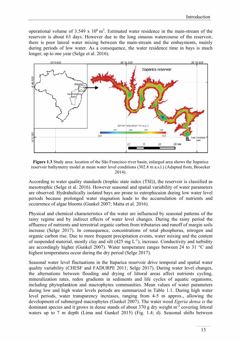
The reservoir is prone to water level fluctuations up to 5 m, derived from operational water volume control (discharge and storage), and induced by seasonal rainy patterns. Water volume in the reservoir increases along the rainy season, reaching a period of high water level at the end of the wet period. During the dry period water level decreases steadily. During maximal water level conditions (304.5 m a.s.l.) the water volume is about 4.2 × 109 m3, mean depth of the reservoir is about 18 m and the maximum water depth is about 55 m near before the dam (Matta et al. 2016). According to bathymetric modeling at mean water level conditions (302.8 m a.s.l.), deep areas (water depth > 5 m) occupy about 70 % of the reservoir and shallower areas about the 30 % (Broecker 2014) (Fig. 1.3). The water discharge of the reservoir is 2,060 m3 sec-1, maximal volume capacity is about 10.8 x 109 m3 with a minimal

Introduction

13

operational volume of 3.549 x 106 m3. Estimated water residence in the main-stream of the reservoir is about 63 days. However due to the long sinuous watercourse of the reservoir, there is poor lateral water mixing between the main-stream and the embayments, mainly during periods of low water. As a consequence, the water residence time in bays is much longer, up to one year (Selge et al. 2016).

Figure 1.3 Study area: location of the São Francisco river basin, enlarged area shows the Itaparica reservoir bathymetry model at mean water level conditions (302.8 m a.s.l.) (Adapted from, Broecker

2014).

According to water quality standards (trophic state index (TSI)), the reservoir is classified as mesotrophic (Selge et al. 2016). However seasonal and spatial variability of water parameters are observed. Hydrahulically isolated bays are prone to eutrophicaion during low water level periods because prolonged water stagnation leads to the accumulation of nutrients and occurrence of algae blooms (Gunkel 2007; Matta et al. 2016).

Physical and chemical characteristics of the water are influenced by seasonal patterns of the rainy regime and by indirect effects of water level changes. During the rainy period the affluence of nutrients and terrestrial organic carbon from tributaries and runoff of margin soils increase (Selge 2017). In consequence, concentrations of total phosphorus, nitrogen and organic carbon rise. Due to more frequent precipitation events, water mixing and the content of suspended material, mostly clay and silt (425 mg L-1), increase. Conductivity and turbidity are accordingly higher (Gunkel 2007). Water temperature ranges between 24 to 31 °C and highest temperatures occur during the dry period (Selge 2017).

Seasonal water level fluctuations in the Itaparica reservoir drive temporal and spatial water quality variability (CHESF and FADURPE 2011; Selge 2017). During water level changes, the alternations between flooding and drying of littoral areas affect nutrients cycling, mineralization rates, redox gradients in sediments and life cycles of aquatic organisms, including phytoplankton and macrophytes communities. Mean values of water parameters during low and high water levels periods are summarized in Table 1.1. During high water level periods, water transparency increases, ranging from 4-5 m approx., allowing the development of submerged macrophytes (Gunkel 2007). The water weed Egeria densa is the dominant species and it grows in dense stands of about 370 g dry weight m-2 covering littoral waters up to 7 m depth (Lima and Gunkel 2015) (Fig. 1.4; d). Seasonal shifts between

Chapter 1

14

phytoplankton dominated to macrophyte dominated systems are observed along the littoral areas, especially in inner areas of bays.

The natural and anthropogenic loads of phosphorus may exceed the carrying capacity of the reservoir; particularly during the rainy period, main loads of phosphorus come from sub-basin inputs and desiccated and mineralized macrophytes (Selge 2017). Additionally, sediments may release phosphorus and organic carbon to the water particularly during anoxic conditions, likewise, nutrients release is enhanced by sediments drying and rewetting event (Keitel et al. 2016). First studies identified Itaparica as a source of GHG, particularly CO2 by diffusion at water surface in shallow and deep waters, while ebullitive fluxes are limited to shallow waters no more than 3 m depth (Rodriguez and Casper 2013).

Table 1.1 Mean values of water parameters during low and high-water level periods *

Low water level (March) High water level (September) T (°C) 29.7 ± 1.1 25.1 ± 0.8 Conductivity (µS cm-1) 69.7 ± 1.5 64.3 ± 8.1 Dissolved Oxygen (mg L-1) 7.1 ± 0.3 7.8 ± 0.1 pH** 7.7 – 8.2 7.3 ± 7.9 TP (µg L-1) 59.6 ± 20.4 47.0 ± 37.7 DIN (µg L-1) 117.2 ± 35.4 67.9 ± 23.2 Chl a (µg L-1) 2.6 ± 0.7 3.0 ± 0.9 Secchi depth (m) 1.8 ± 0.8 3.7 ± 1.5

Source: CHESF and FADURPE 2011 *Values are means ± standard deviation of surface water samples from 12 sampling sites along the Itaparica reservoir, samples taken during March and September (low and high-water level, respectively) from December 2007 to September 2010. ** Values are minimum and maximum. Nowadays Itaparica reservoir is a multipurpose water reservoir including human and industrial consumption, irrigation, aquaculture and leisure activities (CHESF 2016; Gunkel 2007). Soils in this region are sandy, thin, acidic and nonproductive (Araújo Filho et al. 2013). Plantation of high-value export vegetable crops, mainly coconut, are found in the margins, requiring the use of fertilizers and the implementation of irrigation districts, which are sponsored by the government and administrated by the Companhia de Deselvolvimiento do Vale do Sao Francisco (CODEVASF) (Fig. 1.4; e). High permeability of sandy soils of the region enables the export of nutrients and traces of pesticides to the water body, causing eutrophication and water pollution (Araújo Filho et al. 2013). Furthermore, extensive agriculture causes conflicts due to high water consumption for irrigation, air pollution because use of agrochemicals and deforestation of the native forest Caatinga (Schulz et al. 2017).

Introduction

15

Figure 1.4 Pictures of the study area (a and b) Luiz Gonzaga dam, (c) emerging branches of old inundated trees (d) desiccated margins and presence of the water weed Egeria densa; (e) deforested

shore areas and coconut plantations (f) general view of the Caatinga forest and dry soils. Photos:Maricela Rodriguez

1.4 Aims of the thesis

The overall aim of this thesis was to estimate the emissions of GHGs (CH4 and CO2) in the semi-arid reservoir of Itaparica and to analyze the main factors driving GHGs emissions dynamics. The specific objectives addressed to: Estimate gross emissions of CO2 and CH4 from the Itaparica reservoir and to analyze:

- Spatial and temporal variation of GHGs from the Itaparica reservoir in relation to locations in the reservoir, water depth, atmospheric parameters and physical and chemical parameters of water and sediments of reservoirs.

- The significance of GHGs emissions through: (i) diffusion trough water surface (ii) from sediment to the water column, (iii) ebullition from sediments and (iv) degassing trough turbines.

Chapter 1

16

- The significance of the Itaparica reservoir and efficiency in terms of GHGs emissions in comparison to other tropical reservoirs and to other renewable and no renewable energy producing technologies.

(Chapter 2)

Predict the effects of changing land use and climate, measured as eutrophication and temperature rises on CH4 production and potential emission rates by:

- Measuring methane production rates in sediments under warmer temperatures and carbon and nutrients additions.

- Analyzing variation on methane production responses to warming and eutrophication among locations of the reservoir and along the sediment depth.

- Evaluate the variation of methane production under incubation conditions in relation to sediment chemical parameters.

(Chapter 3)

Elucidate the effect of water level changes in GHGs emissions from the Itaparica through:

- Modeling the GHGs emissions from the Itaparica reservoir along time, according to fluctuations on area of water surface covered by deep and shallow waters and water discharges through the turbines.

- Estimate GHG emissions in function of electricity produced. - Estimating the cost of carbon emissions from the reservoir taking into account the

electricity generation cost and the social cost of carbon concept. - Provide general management measurements to improve the efficiency of the

reservoir in terms of carbon source to the atmosphere. (Chapter 4)

Studies regarding GHGs fluxes from semi-arid reservoirs are scarce, thus this study provides base information on the significance of CO2 and CH4 emissions and reveals the main factors driving GHG emissions. The outcomes of this research are aimed to contribute to the better estimation of the impacts of future hydropower projects on the regional and global carbon balance, being of particular interest in tropical areas where the hydropower potential will be intensely exploited. Likewise, recommendations for minimizing GHG emissions from the Itaparica reservoir, at a local scale, are compiled in a guidance manual from the Innovate project directed to stake holder. Recommendations are oriented to avoid water eutrophication, water anoxia to prevent accumulation of CH4 and to minimize the imbalances between water level and electricity production (Rodriguez et al. 2017).

1.4.1 Outline of the thesis

This thesis is divided in five chapters, through which each of the objectives is developed:

Chapter 1: “Introduction”. This chapter provides an introduction to the specific topic of the thesis and a general background of greenhouse gases emission from inland waters and hydropower reservoirs, main emission pathways, drivers and their policy implications. A description of the bi-national joint project Innovate and the study area is provided. Additionally, it includes a description of the general aim and specifies each objective of the thesis, as well as a short explanation of methods carried out for this study.

Chapter 2: “Greenhouse gas emissions from a semi-arid tropical reservoir in Northeastern Brazil”. Gross GHGs emissions from the reservoir are estimated. Efficiency of the reservoir in

Introduction

17

terms of GHGs for energy generated is assessed trough the comparison to other energy sources and to other tropical hydropower reservoirs. This chapter provides base information regarding significance of CO2 and CH4 emissions from a semi-arid hydropower reservoir.

Chapter 3: “Effect of temperature and carbon and nutrients inputs in methane production in sediments of a semiarid tropical reservoir”. This chapter shows the responses of methane production to warming and additions of carbon and nutrients in incubated sediments of three different depth locations. Thus, possible effects of climate change and land use change on potential methane production from the reservoir are assessed.

Chapter 4: “Impacts of water level fluctuation on greenhouse gas emissions from a tropical semi-arid hydropower reservoir. Economical evaluation and management implications”. This chapter deals with the effect of water level fluctuations and water discharges on GHG emissions in function of the electricity generated. Economical cost of carbon emissions is estimated. Finally, management measurements and policy planning strategies are proposed to prevent GHG emissions to increase.

Chapter 5: “General conclusions”. Conclusions and implications of the study are described. Environmental management for reducing and preventing rises in GHGs emissions are recommended. Further research in the field of GHGs from tropical and semi-arid hydropower reservoirs is proposed

1.4.2 Methods and research strategy

1.4.2.1 Greenhouse gas emissions from a semi-arid tropical reservoir in Northeastern Brazil:

Measurements of CH4 and CO2 fluxes in Itaparica included (a) surface diffusion (b) ebullition from sediments, and (c) degassing during water turbine passage. Surveys were carried out during four sampling campaigns in March 2013, September 2013, June 2014, and October 2014. Diffusive emissions were estimated through the thin boundary layer concept (TBL), ebullitive fluxes using inverted funnels (gas traps) and degassing at turbines by comparing dissolved gas concentrations in water column before and after turbines passage. Gas concentrations in sediments and water samples were resolved through gas chromatography using a semi-portable gas chromatograph (SRI 8600c, SRI instruments, USA) (see chapter 2.2.)

In order to detect the spatial differences on CH4 and CO2 emissions within the reservoir, measurements were conducted at three main compartments: Main-stream (MS) and two different depth zones of an embayment, less and more than 5 m depth. Concentrations of CH4 and CO2 in water column and sediments were determined. Gross emissions were calculated as a weighted averaged of annual emissions from each pathway and reservoir compartment. Total emissions in CO2 equivalents were calculated using the global warming potential (GWP) of CH4 over a 100 and 20-year period, 34 and 86 times the GWP of CO2, respectively (Myhre et al. 2013). GHGs emissions from the reservoir were compared to those produced by other energy production technologies in the region and other tropical hydropower reservoirs.

1.4.2.2 Effect of temperature and carbon and nutrients inputs in methane production in sediments of a semiarid tropical reservoir

To determine the effect of temperature and carbon and nutrients additions on methane production (MP) in sediments of the Itaparica reservoirs, sediments of three locations (littoral: 1.2 m depth; intermediate: 7 m depth and profundal: 33 m depth), were incubated

Chapter 1

18

anaerobically in the laboratory at three different temperatures (20, 30 and 40 °C) and five different sediment addition treatments: (i) control, (ii) +carbon (iii) +phosphorus, (iv)+nitrogen, (v) + all combination. Effects of warming was assessed through the sensitivity index Q10 and the apparent Arrhenius equation activation energy (E′a). MP was correlated to sediment parameters using regression analysis. Values of MP across amendment treatments and incubation temperatures were compared among sites in the reservoir and along the sediment profiles (see chapter 3.2)

1.4.2.3 Impacts of water level fluctuation on greenhouse gas emissions from a tropical semi-arid hydropower reservoir: Economical evaluation and management implications

GHGs emissions were modeled according to changes in water level (area flooded) and energy production (water passing through turbines) using historical data of water storage and energy production in the reservoir applying the ecohydrological Model SWIM. Economic implications of GHGs emissions are analyzed using the concept of social cost of carbon (see chapter 4.2).

19 This chapter was submitted and accepted for publication in Regional Environmental Journal, in the special issue

INNOVATE. Cite as: Rodriguez M., Casper P (2018). Greenhouse gases emissions from a semi-arid reservoir in Northeast Brazil. Reg. Environm. Change. Spec. Issue: Follow-up ahead: Large dams lessons in managing the water and land nexus. The final publication is available at Springer via https://doi.org/10.1007/s10113-018-1289-7

2. GREENHOUSE GAS EMISSIONS FROM A SEMI-ARID TROPICAL RESERVOIRS IN

NORTHEASTERN BRAZIL

View of the dam, downstream of the Itapraica reservoir. Photo: Maricela Rodriguez

Greenhouse gas emissions from a semi-arid tropical reservoir in Northeastern Brazil

21

2.1 Introduction

Hydropower reservoirs, similar to natural lakes, rivers and wetlands, have been found to emit greenhouse gases (GHGs) to the atmosphere, mainly methane (CH4) and carbon dioxide (CO2) (Abril et al. 2005; Bastien and Demarty 2013; DelSontro et al. 2011; Diem et al. 2012). The conception of hydropower as a GHG-neutral energy source in comparison to fossil fuel combustion is being reconsidered (Fearnside 2013; Gunkel 2009; Wehrli 2011). Flooding of vegetated soil leads to loss of the carbon sink feature of terrestrial ecosystems. Additionally, the decomposition of flooded organic matter in soil and submerged terrestrial vegetation results in increasing production and release of CO2 and CH4. Emissions of GHGs from reservoirs occur through several pathways, including those known for natural water bodies such as (i) molecular diffusion across the air-water interface, following concentration gradients between both compartments, (ii) ebullition from sediments, (iii) transport through emergent macrophytes, and (iv) release of gas stored in the water column. In addition, at hydropower reservoirs, the passage of water through the turbines and spillway may cause degassing of stored CH4 and CO2 in the water column considering that the turbulent water passage causes changes in temperature and release of pressure (Guérin et al. 2006; Kemenes et al. 2011; Roehm and Tremblay 2006). Degassing at turbines and spillway may represent a significant pathway for GHGs releases, depending on the amount of water discharged and the number and performance of turbines.

Deemer et al. (2016) estimated global GHGs emissions from manmade reservoirs to account for 800 (500-1200) Tg CO2-eq yr-1 from which 79 % occurred as CH4 emissions, while CO2 and N2O represented 17 and 4 %, respectively. Barros et al. (2011) calculated emissions from hydropower reservoirs as 288 Tg of CO2-eq yr-1, CO2 contributed to emission with 62 % and CH4 with about 38 %, while N2O was not included in the estimation. Emissions from hydropower reservoirs (the study covered 85 reservoirs from boreal, temperate, and tropical regions) were equivalent to 4 % of the global emissions from inland waters. Although emission values from reservoirs are variable, most of the studied systems act as sources of CH4, and sources or minor sinks of CO2. Barros et al. (2011) found that the emissions were negatively related to the age of the reservoirs (time after impoundment) and the latitude. Reservoirs are likely to emit larger amounts of GHGs during the first 5 to 10 years after the impoundment due to the rapid degradation of the flooded vegetation, which decrease during the lifetime of the reservoir (Abril et al. 2005; Fearnside 2002; Galy-Lacaux et al. 1999).

Tropical reservoirs have been found to emit more carbon than their temperate counterparts. Higher emissions from those reservoirs are related to larger amounts of organic matter storage in soils, provided by tributaries and from a larger amount of flooded biomass, and by the direct positive effect of temperature on decomposition rates (Fearnside 1995; Gudasz et al. 2010). Beside age and latitude, GHGs fluxes are also driven by climatic and meteorological conditions and hydrological and hydromorphological characteristics of the reservoirs among others, which affect the spatial and temporal variability of GHGs fluxes, both among and within the reservoirs (Almeida et al. 2016; Roland et al. 2010; St Louis et al. 2000). Disregarding spatial and temporal variations leads to the errors in the estimation of global carbon budget (Roland et al. 2010; Zheng et al. 2011).

Despite the importance of tropical hydropower reservoirs as atmospheric GHGs sources, regional studies regarding GHGs have focused mainly to humid zones with abundant water resources. Studies on semi-arid climate reservoirs are scarce what leads to uncertainties on the significance of GHGs emissions in tropical areas. The aim of this study was to estimate the GHGs (CH4 and CO2) fluxes at the Itaparica reservoir located in the semi-arid region of

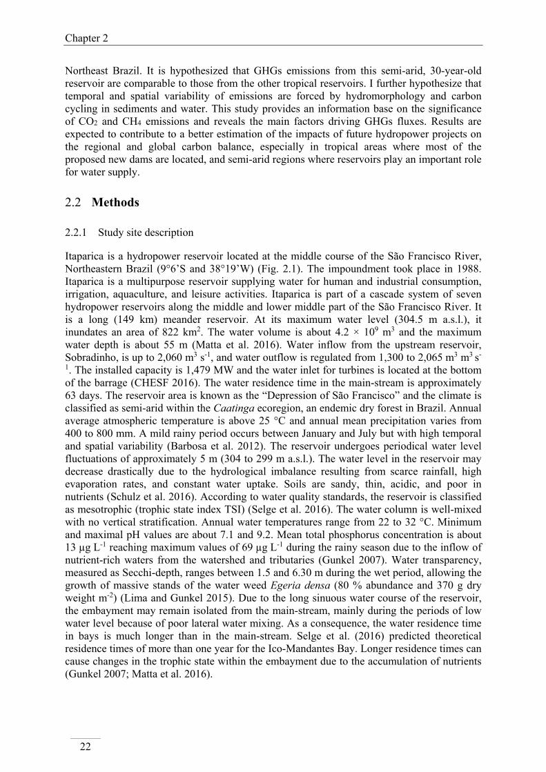
Chapter 2

22

Northeast Brazil. It is hypothesized that GHGs emissions from this semi-arid, 30-year-old reservoir are comparable to those from the other tropical reservoirs. I further hypothesize that temporal and spatial variability of emissions are forced by hydromorphology and carbon cycling in sediments and water. This study provides an information base on the significance of CO2 and CH4 emissions and reveals the main factors driving GHGs fluxes. Results are expected to contribute to a better estimation of the impacts of future hydropower projects on the regional and global carbon balance, especially in tropical areas where most of the proposed new dams are located, and semi-arid regions where reservoirs play an important role for water supply.

2.2 Methods

2.2.1 Study site description

Itaparica is a hydropower reservoir located at the middle course of the São Francisco River, Northeastern Brazil (9°6’S and 38°19’W) (Fig. 2.1). The impoundment took place in 1988. Itaparica is a multipurpose reservoir supplying water for human and industrial consumption, irrigation, aquaculture, and leisure activities. Itaparica is part of a cascade system of seven hydropower reservoirs along the middle and lower middle part of the São Francisco River. It is a long (149 km) meander reservoir. At its maximum water level (304.5 m a.s.l.), it inundates an area of 822 km2. The water volume is about 4.2 × 109 m3 and the maximum water depth is about 55 m (Matta et al. 2016). Water inflow from the upstream reservoir, Sobradinho, is up to 2,060 m3 s-1, and water outflow is regulated from 1,300 to 2,065 m3 m3 s-

1. The installed capacity is 1,479 MW and the water inlet for turbines is located at the bottom of the barrage (CHESF 2016). The water residence time in the main-stream is approximately 63 days. The reservoir area is known as the “Depression of São Francisco” and the climate is classified as semi-arid within the Caatinga ecoregion, an endemic dry forest in Brazil. Annual average atmospheric temperature is above 25 °C and annual mean precipitation varies from 400 to 800 mm. A mild rainy period occurs between January and July but with high temporal and spatial variability (Barbosa et al. 2012). The reservoir undergoes periodical water level fluctuations of approximately 5 m (304 to 299 m a.s.l.). The water level in the reservoir may decrease drastically due to the hydrological imbalance resulting from scarce rainfall, high evaporation rates, and constant water uptake. Soils are sandy, thin, acidic, and poor in nutrients (Schulz et al. 2016). According to water quality standards, the reservoir is classified as mesotrophic (trophic state index TSI) (Selge et al. 2016). The water column is well-mixed with no vertical stratification. Annual water temperatures range from 22 to 32 °C. Minimum and maximal pH values are about 7.1 and 9.2. Mean total phosphorus concentration is about 13 µg L-1 reaching maximum values of 69 µg L-1 during the rainy season due to the inflow of nutrient-rich waters from the watershed and tributaries (Gunkel 2007). Water transparency, measured as Secchi-depth, ranges between 1.5 and 6.30 m during the wet period, allowing the growth of massive stands of the water weed Egeria densa (80 % abundance and 370 g dry weight m-2) (Lima and Gunkel 2015). Due to the long sinuous water course of the reservoir, the embayment may remain isolated from the main-stream, mainly during the periods of low water level because of poor lateral water mixing. As a consequence, the water residence time in bays is much longer than in the main-stream. Selge et al. (2016) predicted theoretical residence times of more than one year for the Ico-Mandantes Bay. Longer residence times can cause changes in the trophic state within the embayment due to the accumulation of nutrients (Gunkel 2007; Matta et al. 2016).

Greenhouse gas emissions from a semi-arid tropical reservoir in Northeastern Brazil

23

2.2.2 Sampling scheme

Measurements of CH4 and CO2 fluxes in Itaparica included (a) surface diffusion (b) ebullition from sediments, and (c) degassing after turbines. Surveys were carried out during four sampling campaigns in March 2013, September 2013, June 2014, and October 2014. Due to a long drought period in the catchment area, all sampling campaigns covered low water level conditions (300 m a.s.l.). In order to detect the spatial differences on CH4 and CO2 emissions within the reservoir, measurements were conducted at a total of 36 sampling sites randomly selected within three main compartments: main-stream (MS) (9 sites) and two habitats of an embayment (Icó-Mandantes Bay, 40 km upstream the dam), namely littoral-bay (LB) (less than 5 m depth, 18 sites) and (ii) deep-bay (DB) (more than 5 m depth, 9 sites). At each sampling site, vertical profiles of CH4 and CO2 concentrations in water and sediments were estimated. Water depth was measured using a water depth gauge (UWITEC®, Austria). Atmospheric parameters including air temperature, humidity, atmospheric pressure, and wind speed were measured simultaneously during water sampling with a portable anemometer (Kestrel®4000, USA) placed 1.5 m above the water surface.

Figure 2.1 Location of the study area in Brazil, and of the sampling sites in the Itaparica reservoir (main-stream MS), the enlargement shows sampling sites within the Ico-Mandantes bay (littoral bay

(LB), deep bay (DB).

2.2.3 Analysis of dissolved CO2 and CH4 in water and sediments

Gas concentrations on the water surface and along the water column were measured at each site by collecting water samples at different depths along the water column using a horizontal Van Dorn-type water sampler. Samples were taken by carefully submerging 100 ml serum bottles into the sampler water avoiding bubbling and filling them completely free of air bubbles. The bottles were then sealed with butyl stoppers and crimped with metal caps. Prior to the analysis of the samples within the next 48 hours by gas chromatography, a headspace was created by replacing half of the water by argon gas, and a gas chromatograph (SRI 8600c, SRI instruments, USA) equipped with a flame ionization detector (GC-FID) was used for CH4 analysis and a methanizer (Ni) at 300°C for the reduction of CO2 to methane. A packed column (8600 PKDB 6′×1/8′′ SS HayeSep D) was used for the separation of gases and hydrogen was used as the carrier and the detector gas (with air supplied by a pump). Gas

Chapter 2

24

samples from the headspace of the vials were injected to the column via a 1-ml-sample loop, which was flushed with the sample by 2-3 times its volume. Calibrations were conducted using CH4 and CO2 standard mixtures (1 % v/v each) (Scotty®, Sigma Aldrich). Concentrations of gases in the headspace (µM) of water and sediment samples were calculated using the Henry’s law equation.

Water temperature, pH, and dissolved oxygen (DO) concentrations were measured at each depth where samples were collected using a multiprobe system (DS 5 Multiprobe, Hydrolab, Germany). Sediment samples for the gas concentration analysis were collected using a gravity corer (UWITEC®, Austria) with 60 mm inner diameter. At each sampling site, two cores were sampled, extruded vertically from the core line and sliced at 2 cm intervals. Two subsamples of 2 ml wet sediment were taken from each layer and placed into 10 cm vials with 4 ml distilled water. The vials were immediately closed and crimped with a metal cap with silicon septum. The gas concentration in the vial headspace was measured by gas chromatography (Casper et al. 2003; Conrad et al. 2009), as described above. Physico-chemical parameters including dry weight, total organic carbon (TOC), soluble reactive phosphorus (SRP), and total nitrogen (TN) were analyzed from additional sediments taken at several sites in the reservoir and sliced to 2 cm layers. Sediments were dried at 105 °C to constant weight, and then processed and passed through a 1 mm mesh sieve. Additionally, the elements including Fe, Al, Mn, and Mg in dry sediments were measured by Inductively Coupled Plasma (ICP iCAP 6000 series; Thermo Fisher Scientific Inc., USA).

2.2.4 CH4 and CO2 fluxes

2.2.4.1 Thin Boundary Layer model for diffusive flux

Diffusive fluxes F (mg m-2 d-1) across the air-water interface were calculated according to equation 1 (MacIntyre et al. 1995), where (Cgas) is the concentration of gas measured on the water surface and (Ceq) in the atmosphere is determined from global atmospheric partial pressure values to be 375 ppm for CO2 and 1.750 ppm for CH4 (IPCC 2007). (K) is the piston velocity or gas transfer velocity and is calculated using equation 2, where K600 is piston velocity normalized to a Schmidt number of 600 and based on the frictionless wind speed at 10 m (U), expressed in m s-1 (Cole et al. 2010; Cole and Caraco 1998; López Bellido et al. 2009).

(1)

(2)

2.2.4.2 Ebullitive and diffusive fluxes from sediments

Ebullitive fluxes were measured using gas traps, consisting of inverted funnels with a bottom area of 0.2 m2, a heavy ring was attached to each funnel to keep the horizontal position under water and a gas collector on the top. Funnels were suspended in the water column approximately 0.5 m above the sediment surface regardless of water depth using a buoy and fixed to emerging trees. The sediments were not touched to avoid disturbance (Casper et al. 2003). Two to three traps were placed at each sampling site and deployed for 24 to 48 hours. When the gas was trapped, subsamples were collected in 10 ml pre-evacuated vials. Ebullitive fluxes (mg m-2 d-1) were calculated taking into account the gas concentration of the sample gas

F = 𝐾𝐾 (Cgas − Ceq )

K600 = 2.07 + (0.215 ∗ U101.7)

Greenhouse gas emissions from a semi-arid tropical reservoir in Northeastern Brazil

25

C [µM]; the volume of the collected gas, V; the area of the gas trap, A; and deployment time T, as follows (UNESCO 2010):

(3)

The diffusive fluxes of CO2 and CH4 from the sediment to the overlying water were calculated based on the concentration gradients of those gases from pore water in top layers of the sediment (0-4 cm) and bottom water above the sediments according to Fick´s first law, using equation (4).

(4)

Where F is the flux in mg m-2d-1, φ is the porosity of the sediment, Θ is the tortuosity of the sediment, dCi/dz is the concentration gradient between the sediment pore water and the water above, and D is the diffusive coefficient at a given temperature. The coefficients reported by Arah and Stephen (1998) and Tamimi et al. (1994) were used for CH4 and CO2, respectively, both at 25 °C water temperature. Porosity and tortuosity were calculated according to the method reported by Lewandowski et al. (2002).

2.2.4.3 Degassing through turbines

Emissions of CO2 and CH4 by degassing after passage through the turbines were estimated as the difference between the mean dissolved gas concentration in the water column before the dam at the withdrawal depth (CupT) and the mean concentration of the gases in the water column after turbines (CAfterT) multiplied by the water discharge (QT), using the equation developed by Beaulieu et al. (2014), Galy-Lacaux et al. (1997) and Kemenes et al.(2011).

(5)

2.2.5 Whole reservoir emissions and comparison to other tropical reservoirs and energy sources

Gross emissions of CO2 and CH4 for the whole reservoir were estimated after averaging the emissions of each analyzed pathway (ebullitive, diffusive) within different sites of the reservoir (LB, DB, and MS). This study covered prolonged low water conditions, therefore annual emissions were calculated from averaged daily emissions across all sampling campaigns. Average emissions were scaled to the total area covered by each site as follows: LB was scaled to the area covered by shallow waters (less than 5 m depth) in the entire reservoir, DB was to the area covered by deep waters (more than 5 m depth) within the bay, and MS was scaled by area covered by deep waters in the entire reservoir (excluding the Icó-Mandantes bay). Emissions by the passage of the turbines were added to the annual emissions of the whole reservoir. The coverage area of each reservoir site was calculated using a morphometric and bathymetric model at low water conditions (299 m a.s.l.) (Matta et al. 2016) and water volume model estimated from the Operador Nacional do Sistema Elétrico (ONS), Brazil (Koch 2016, personal communication). Total emissions in CO2 equivalents were estimated using the global warming potential (GWP) of CH4 over a 100 and 20-year period (GWP100 and GWP20), 34 times and 86 times the GWP of CO2, respectively (Myhre et al. 2013). Total emissions are also expressed as total carbon (t C), by summing the amount of

𝐹𝐹 =𝐶𝐶 ∗ 𝑉𝑉𝐴𝐴 ∗ 𝑇𝑇

𝐹𝐹 =𝜑𝜑𝛩𝛩2 · 𝐷𝐷𝑖𝑖 · (

𝑑𝑑𝐶𝐶𝑖𝑖𝑑𝑑𝑑𝑑

)

𝐹𝐹𝑑𝑑𝑑𝑑𝑑𝑑𝑑𝑑𝑑𝑑𝑑𝑑𝑖𝑖𝑑𝑑𝑑𝑑 = �𝐶𝐶𝑈𝑈𝑈𝑈𝑇𝑇 − 𝐶𝐶𝐴𝐴𝐴𝐴𝐴𝐴𝑑𝑑𝐴𝐴𝑇𝑇 � ∗ 𝑄𝑄𝑇𝑇

Chapter 2

26

carbon provided by each GHG, which is calculated by multiplying the amount of CO2 and CH4 by conversion factors of 0.27 and by 0.75, respectively. Emissions per km2 of Itaparica were compared to those from other tropical reservoirs. Emissions of GHGs per energy produced were calculated by dividing annual t C -CO2-eq (GWP100 and GWP20) by the annual electricity generated (MWh/year). In order to compare the emissions of Itaparica to other energy sources, including coal, diesel, fuel oil and natural gas, the carbon emissions caused by those fossil fuels sources to produce the same amount of energy were calculated, by multiplying the annual electricity generated in Itaparica by established emission factors for the given fuel and dividing by the corresponding hydropower average efficiency with respect to each fuel, as described by Dos Santos et al. (2006) and Zhao et al (2013) (Table SM .7).

2.2.6 Statistical analysis

In order to analyze the spatial and temporal differences in CO2 and CH4 emissions at the reservoir, comparison of mean emission rates of the samples taken at the studied habitats in every sampling campaign was conducted. Since the data did not follow a normal distribution (Shapiro test), non-parametric test was used for the analysis (Kruskal–Wallis test followed by Bonferoni post hoc test). The influences of water and sediment parameters such as nutrients and elements on the gas concentrations were analyzed using a linear regression model. The relationship of diffusive and ebullitive emissions with water depth was analyzed using linear and non-linear regression coefficients. Analyses were performed in the statistical software RStudio, version 0.99.491©2015 RStudio, Inc (RStudioTeam 2015).

2.3 Results

2.3.1 Atmospheric, water, and sediment physical characteristics

The average values of relative humidity and air temperature including all sampling campaign were 55 % (± 11 %) and 30 ± 3 °C, respectively. The maximum humidity and minimum temperature values were registered in June 2014, during a short wet period. The mean wind speed over all sampling campaigns was 3.7 ± 1.78 m s-1 and minimum values were observed during the first field campaign in March 2013 (Table SM 1).

Yearly changes in seasonal water levels in the reservoir were disrupted due to a prolonged drought period in the study area. The water level in Itaparica decreased from 305 to about 300.5 m a.s.l since summer 2012 and low water level conditions remained until the end of 2014.Water inflow from the upstream Sobradinho reservoir was kept at minimum values (990 ± 200.5 m3s-1) (Fig. SM 1). In order to avoid a decrease in the water level below the minimum operating level (299 m a.s.l.) for the hydroelectric power plant, water discharge at the dam was also kept low at 1,027 ± 147 m3 s-1.

The Itaparica reservoir water column is isothermal with temperatures ranging from 29.5 °C to 24 °C and lower temperatures observed in June 2014. The water body was well-oxygenated in MS (6.7 ± 1.1 mg L-1) and the lowest values of DO were measured at the bottom water of LB (5.6 ± 1.9, min 1.5) and DB (6.1 ± 1.4 min 2.8), both in June 2014, without reaching anoxia during other campaigns. The values of pH were slightly higher at LB (max 9.2, min 6.04) than in DB (max 8.8, min 6.01) and MS (max 8.5, min 6.24) (Fig. SM 2). Nutrients concentrations including total nitrogen and phosphorus, were higher in the bay with respect MS (Table 2.1).

Greenhouse gas emissions from a semi-arid tropical reservoir in Northeastern Brazil

27

Table 2.1 Nutrients concentration in water; values are means of samples along the water column of sampling sites within the main-stream and the bay ± Standard deviation*.

Parameter Main-stream Sampling sites =3,

n=21

Icó-Mandantes Bay Sampling sites=2,

n=4

TN (µg L-1) 321±161 450±174

TP (µg L-1) 9±2.5 17±10

TOC (g L-1) 4.7±2.5 3.6±2.4

*TN = total nitrogen, TP = total phosphorous, TOC = total organic carbon, n = number of samples.

The water content of the sediments of LB and DB decreased steadily with sediment depth from 70 %-80 % in the upper layers (0 to 4 cm) to less than 30 % below 8 cm sediment depth. Sediments of MS contained more water (90 %) in surface sediments, decreasing to less than 30 % at 12 cm depth. Mean OC values in the sediment profile were significantly higher in sediments in DB (15.5 ± 5.9 % kg d.w.-1) (p-value ≤ 0.001), while there were no significant differences between the sediments of LB and MS (5.6 ± 3.2 and 5.3 ± 1.5 % kg d.w.-1 respectively) (Table 2.2). The OC content decreased with the sediment depth (Fig.SM 3). The upper layers of littoral sediments were muddy and composed of fine materials up to 10-12 cm and deeper sediments were sandy and dominated by coarser particles.

Total phosphorus content was higher in the sediments of MS (p-value ≤ 0.001) while littoral sediments have higher contents of nitrogen (p-value = 0.002). Fe and Al concentrations were higher in MS (p-values ≤ 0.001). Concentrations of Mg and Mn were slightly higher in the sediments of MS and DB compared to LB (p-value = 0.02 and 0.06, respectively) (Table 2.2).

Table 2.2 Sediments parameters, values are means of the top 10 cm of sediment cores ± standard deviation*.

Parameter Littoral bay Deep bay Main-stream

n= 9 n= 7 n= 5 Water content% 64.0 ± 23.4 65.8 ± 22.0 79.4 ± 7.7 OM [% d.w.] 11.2 ± 6.4 31 ± 11.8 11.7 ± 5.3 OC [% d.w.] 5.6 ± 3.2 15.5 ± 5.9 5.3 ± 1.5 TP [g/kg d.w.] 0.3 ± 0.2 0.2 ± 0.1 0.3 ± 0.3 N [g/kg d.w.] 2.1 ± 1.3 1.3 ± 0.6 1.4 ± 0.5 Al [mg/g d.w.] 55.4 ± 28.2 69.2 ± 35.7 99.3 ± 26.4 Fe [mg/g d.w.] 31.3 ± 18 41.5 ± 21.8 60 ± 15.7 Mg [mg/g d.w.] 5.7 ± 3.5 6.6 ± 3.1 8 ± 2.6 Mn [mg/g d.w.] 0.5 ± 0.4 0.6 ± 0.4 0.8 ± 0.6

*n = number of sampling sites. d.w. = dry weight, OM=organic matter, OC=organic carbon, TP=total phosphorus, N=total Nitrogen, Al=Aluminum, Fe= Iron, Mg=Magnesium, Mn=Manganese

2.3.2 Concentration of CH4 and CO2 in the water column and sediments

The concentration of CO2 in water ranged from 0.09 to 680 µM and that of CH4 ranged from 0.05 to 69 µM. Mean concentrations in the water column and in surface water are presented in

Chapter 2

28

Table 2.3. The concentration of both gases in the water column were significantly higher in LB and DB than MS (Kruskal-Wallis test, p-value ≤ 0.001, for CH4 and p-value = 0.00042 for CO2). Mean concentrations of dissolved gases along the water column are shown is Figure 2.2. In LB and DB, dissolved CH4 and CO2 increased along the water column and concentrations were higher near the sediment. In MS, no significant accumulation of CH4 was observed, while CO2 concentrations appeared to be higher near the bottom (Fig. 2.2).

During all four sampling campaigns (2012-2014), no significant differences in dissolved gas concentrations were found in the water. Although concentrations of both CH4 and CO2 were lower during October 2014 in DB and CH4 concentrations were consistently higher in LB, mean concentrations were not significantly different. Concentrations of CO2 were negatively correlated with dissolved oxygen (r2 = -0.5), while the concentrations of CH4 were slightly negatively correlated with pH values (r2 = -0.4). The values of pH were strongly correlated with water temperature (r2 = 0.76) (Fig.SM 4).

Table 2.3 Concentration of dissolved gases in the Itaparica reservoir [µM].

Site x n samples Meana

CO2 Mean CO2

surfaceb

Meana

CH4 Mean CH4

surfaceb Mean Surface

LB 18 66 13 102 ± 114 98 ± 130 10 ± 13 9 ± 11.8

DB 7 54 6 103 ± 116 60 ± 50 6 ± 3 6 ± 4

MS 9 76 6 72 ± 88 66 ± 74 2 ± 2 1 ± 1

a: means from several sites and depths, every meter up to 1 0m depth and every five meters when deeper than 10 m depth. (+/-) is standard deviation, x = number of sampling sites; n samples are number of water samples analyzed. b: samples taken 0.2 m below water surface. Concentrations of dissolved CH4 in sediments ranged from 0.01 to 21.2 µM and CO2 from 0.01 to 56.1 µM. Dissolved CH4 and CO2 in sediments varied significantly among zones of the reservoir (Kruskal-Wallis test, p-value ≤ 0.001, for CH4 and p-value=0.001 for CO2). Concentrations of both gases were higher in sediments of the MS. Concentrations of dissolved CH4 and CO2 in pore waters along the sediment cores varied among the reservoir sites. In LB and DB the concentrations of both gases were the highest in the top sediment layers (0-5 cm) decreasing with the sediment depth. In MS, maximum concentrations of CO2 were measured at depths of 4-12 cm and that for CH4 in 4-6 cm. Methane concentrations in LB increased in layers deeper than18-20 cm (Fig. 2.3).

Greenhouse gas emissions from a semi-arid tropical reservoir in Northeastern Brazil

29

Figure 2.2 Concentration of dissolved gases (a) CO2, (b) CH4, along depth of water column. Values are means from several sampling sites at different water depths and over sampling campaigns, error

bars are standard error.

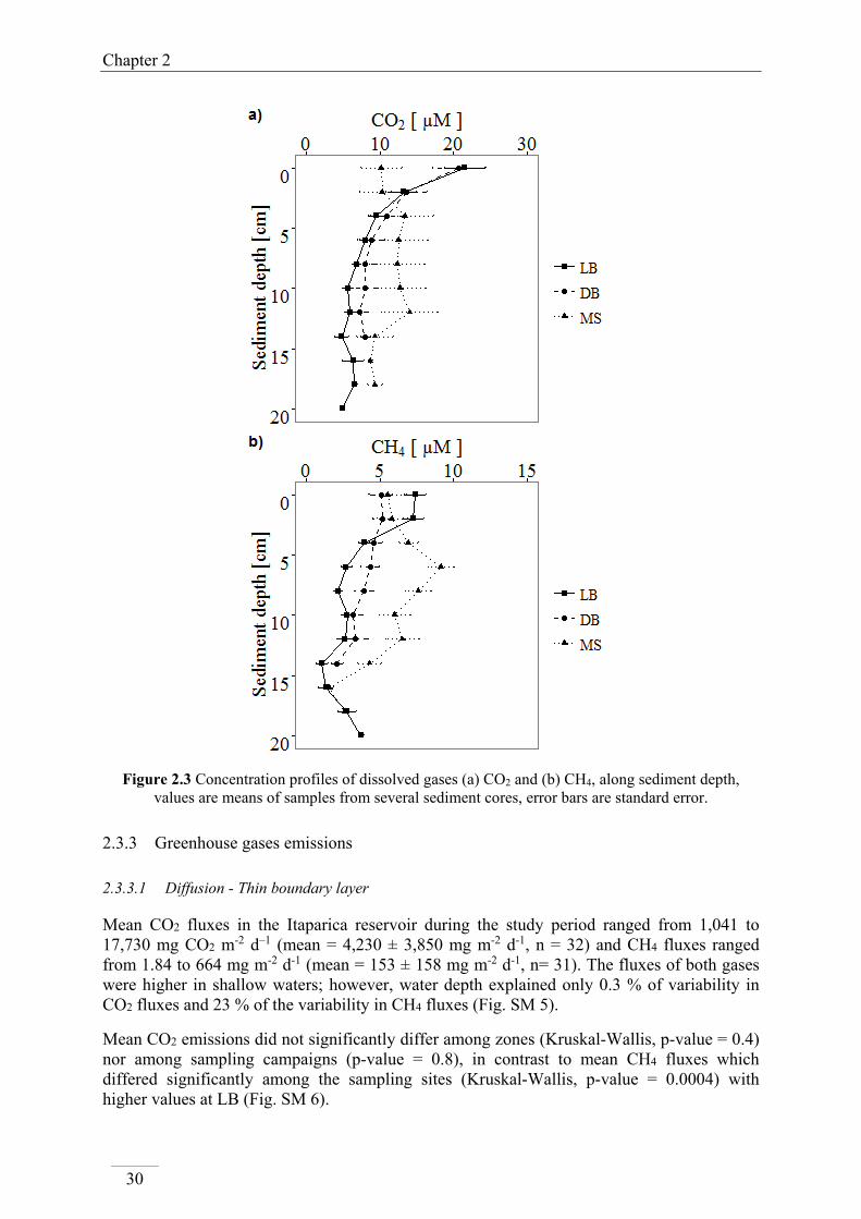
Chapter 2

30

Figure 2.3 Concentration profiles of dissolved gases (a) CO2 and (b) CH4, along sediment depth, values are means of samples from several sediment cores, error bars are standard error.

2.3.3 Greenhouse gases emissions

2.3.3.1 Diffusion - Thin boundary layer

Mean CO2 fluxes in the Itaparica reservoir during the study period ranged from 1,041 to 17,730 mg CO2 m-2 d–1 (mean = 4,230 ± 3,850 mg m-2 d-1, n = 32) and CH4 fluxes ranged from 1.84 to 664 mg m-2 d-1 (mean = 153 ± 158 mg m-2 d-1, n= 31). The fluxes of both gases were higher in shallow waters; however, water depth explained only 0.3 % of variability in CO2 fluxes and 23 % of the variability in CH4 fluxes (Fig. SM 5).

Mean CO2 emissions did not significantly differ among zones (Kruskal-Wallis, p-value = 0.4) nor among sampling campaigns (p-value = 0.8), in contrast to mean CH4 fluxes which differed significantly among the sampling sites (Kruskal-Wallis, p-value = 0.0004) with higher values at LB (Fig. SM 6).

Greenhouse gas emissions from a semi-arid tropical reservoir in Northeastern Brazil

31

2.3.3.2 Ebullition

Ebullitive fluxes were only found in LB. Up to 5 m water depth, no ebullition was observed in DB. Similarly, few measurements with chambers in MS did not indicate ebullition. Mean fluxes in LB were 1.6 ± 2 mg m-2 d-1 for CO2 and 0.8 ± 1.2 for CH4. Nonlinear regression of fluxes against water depth explained 16 % of the variation for CH4 and 19 % for CO2 (Fig. SM 7). There were no statistically significant differences between the sampling campaigns (Kruskal-Wallis test, p-value = 0.8 and p-value = 0.5) for CO2 and CH4, respectively.

2.3.3.3 Degassing through turbines

Degassing through the turbines was limited for CO2 and no emissions were estimated for CH4. Mean CH4 concentrations near the water inlet of the dam were lower or equal to those measured after the water passed through the turbines (Table 2.2). On the contrary, a minor accumulation of CO2 in bottom waters before the dam and slightly lower concentrations after turbine passage implies losses to the atmosphere calculated as 2.9 × 104 ± 3.3 × 104 t yr-1.

Table 2.4 CH4 and CO2 concentrations before and after the water inlet in the dam and total degassing fluxes, values are means (+/-) standard deviation.

At dam near inleta

[g m-3]

In river after turbine

passageb [g m-3]

Water outflow [m3 s-1]

Gas flux [g m-3 s-1]

Gas flux [t year-1]

CH4 0.03 ± 0.008 0.04 ± 0.009 1,027

-9.8 ± -1.2 -3.1x102 ± -3.9x102 CO2 2.9 ± 1.3 2.0 ± 0.3 930 ± 1053 2.9x104 ± 3.3x104 a: water samples were collected at different depths along bottom water (20 to 33 m depth) before the dam inlet b: water samples collected at different depths along the water column after the turbines passage

2.4 Discussion

2.4.1 Reservoir hydrology, water, and sediment characteristics

Lateral hydraulic disconnection of the embayment (Icó-Mandantes bay) with the main-stream explains the differences in water and sediment parameters between these zones. Longer retention times in the embayment with respect to the main-stream lead to the accumulation of substances. Deeper areas of the bay might act as a collector for allochthonous organic matter, which might be transported from littoral areas to the center of the bay. Such accumulation is supported by substance transport models in Itaparica (Matta et al. 2016). On the contrary, low carbon concentrations at LB are related to material resuspension in water caused by wave action, while in MS, sedimentation is expected to be low due to rapid and constant water flow. Higher concentrations of TP in MS than in sediments of the embayment are related to the higher uptake of P due to biological activity, e.g., by primary producers (macrophytes or phytoplankton). Fe and Al in main-stream sediments may act as efficient P-binding elements, especially at oxic conditions. Negative correlation of CH4 with Fe may indicate oxidative processes inhibiting methanogenesis (Fig. SM 8). Higher pH values in waters of LB are related to the higher photosynthetic activity by submerged macrophytes. Lower oxygen in the bottom water of LB is explained by higher biological activity including respiration occurring in the water, superficial layers of sediment, and oxidation of organic compounds.

Chapter 2

32

2.4.2 CO2 and CH4 concentration in water and sediments

Concentrations of dissolved CO2 and CH4 in the Itaparica reservoir were similar to those found in other tropical reservoirs. Mean surface concentrations of CO2 (70 ± 20 µM) and CH4

(5 ± 4 µM) at all sites of this semi-arid reservoir were similar to or lower than those measured during the dry season in the epilimnion (5-10 m below water surface) of the tropical reservoirs Balbina, Samuel, and Petit Saut (120-229 µM CO2 and 2-10 µM CH4) (Guérin et al. 2006). Similarly, the concentrations of both gases in deeper waters of MS in Itaparica were significantly lower than those in the anoxic hypolimnia of these three reservoirs (702-257 µM CH4 and 1,369-593 µM CO2). In Itaparica, the oxygenated and well-mixed water column in MS prevents the formation and accumulation of methane. Higher concentrations of dissolved CO2 and CH4 in the embayment in comparison to the main-stream have also been observed in other studies in tropical lakes, where concentrations of CH4 was found to decrease from the inner bays to offshore and from littoral to deeper zones of the lake (DelSontro et al. 2011; DelSontro et al. 2010; Musenze et al. 2014). Likewise, the diffusive release of both gases from the sediments and the dissolution of the released bubbles escaping the sediments led to higher concentrations of those gases in shallow waters (DelSontro et al. 2010). In Itaparica, the diffusion of both gases from the sediments was estimated at 5.6 and 0.79 in littoral, 7.7 and 1.14 in deeper bay, and 1.6 and 0.85 in MS (mg m-2d-1 of CO2 and CH4, respectively) (Table SM.2). There were no differences in diffusive fluxes of CH4 across the sediment-water interface among the sites but diffusive fluxes of CO2 were higher in LB and DB. Higher concentrations of CO2 and CH4 in the top layers of the sediments in LB and DB explain the higher concentrations in bottom and surface waters of LB and DB with respect to MS because of the higher level of diffusion of locally produced CO2 and CH4 as end products of respiration and methanogenesis in sediments. Higher concentrations of CH4 near surface layers (1-2 cm) in sediments of LB suggest higher production rates, which may be enhanced by warm temperatures. Enhanced CH4 concentrations in waters of LB may be better explained by the dissolution of gas bubbles and turbulent fluxes of CH4 from the sediments to the water than merely by passive diffusion across these compartments. Higher concentrations of CO2 and CH4 in surface sediment layers despite the poor accumulation of organic matter at littoral areas (see Table 2.2 and Fig. SM 3) suggest higher mineralization rates, more likely from decayed aquatic plants. Differences in mineralization rates related to the abundance of heterotrophic bacteria have been found to be related to spatial differences in concentrations of CO2 in a tropical reservoir (Cardoso et al. 2013). The presence of the water weed E. densa, growing up to depths of 5-6 m (Lima and Gunkel 2015) may provide additional organic matter, which is easy to decompose (plant total carbon is 35 % dry weight). Some studies showed that CH4 is produced as a result of anaerobic degradation of cellulose from aquatic macrophytes, where cellulose is degraded to propionate and acetate (da Cunha-Santino and Bianchini 2013; Wu and Conrad 2001). Furthermore, high water temperatures in Itaparica may increase CH4 production by the hydrogenotrophic methanogenesis pathway. Hydrogenotrophic methanogenesis contributes to almost 60 % of total methane production (Ji et al. 2016) and becomes more dominant at higher temperatures (Glissman et al. 2004).

Dissolved CO2 and CH4 in the water column in littoral areas may be laterally transported to the deeper areas of the bay, increasing the concentrations in those sites. Such transport has been found to be responsible for the concentrations in oxygenated hypolimnion in lakes (Hofmann et al. 2010). External inputs of CO2 from tributary rivers and streams have been described as main contributors to CO2 supersaturation in lakes (Maberly et al. 2013). However, in Itaparica, coupling between the primary production and respiration processes occurring in water and sediment seems to be the main factor explaining the CO2 dynamics, which further elucidates higher concentration of this gas in disconnected and more static habitats such as the Icó-Mandantes Bay in comparison to MS. Higher values of DO and pH

Greenhouse gas emissions from a semi-arid tropical reservoir in Northeastern Brazil

33

are proxies of higher photosynthetic activity. Therefore, negative correlations between dissolved CO2 and DO, and CH4 and pH (Fig. SM 4) indicate higher consumption of CO2 by photosynthesis and potential CH4 oxidation by increasing DO in the water. However, respiration in water and sediments may exceed the primary production, leading to CO2 supersaturation in shallower areas. Benthic production of CO2 at a shallow tropical semi-arid lake was responsible for high CO2 emissions to the atmosphere despite the high primary production rates (Almeida et al. 2016).

2.4.3 GHGs emissions

Diffusive fluxes of CO2 (2-5 g m-2 d-1) and CH4 (0.02-0.2 g m-2 d-1) are within the range previously reported for other tropical reservoirs (2.4-42 g m-2 d-1 and 0.003-0.16 g m-2 d-1 for CO2 and CH4, respectively) (Abril et al. 2005; DelSontro et al. 2010; Dos Santos et al. 2006; Guérin et al. 2006) and Pantanal wetlands in Brazil (0.012 g m-2 d-1 CH4) (Bastviken et al. 2010). Diffusive emissions in this study were in general higher than in other reservoirs with similar dissolved gas concentrations in surface water. Higher emission rates may be related to different parameters influencing the transfer velocity (K600 value), such as wind speed and water temperature. In Itaparica, extreme winds (over 4 m s-1) are frequently measured generally around noon and in the afternoon (Fig. SM 9) when temperatures are higher, however water surface emissions were not related to any of the atmospheric parameters (Fig. SM 10). The selection of the TBL equation also influences flux values. The equation of Cole and Caraco (1998) was considered to underestimate the fluxes in comparison to floating flux chambers (Guérin and Abril 2007; Vachon et al. 2010). On the other hand, flux chambers were also found to overestimate the fluxes, because they can either increase the turbulence inside the chamber especially at low wind conditions or decrease it by isolating the water surface from the wind shear. Using the wind-based TBL equation allowed us to calculate the fluxes based on the parameters measured in the field using portable instruments, which validated the calculations. Supersaturation of CO2 and CH4 in the water column resulting in positive diffusive fluxes and higher emission rates at shallow waters in accordance with higher surface dissolved gas concentrations highlight the importance of shallow areas as emission hotspots in the reservoir.

Higher ebullition rates were expected in shallow waters as reported by several other studies for tropical reservoirs (Abril et al. 2005; Deshmukh et al. 2014; Galy-Lacaux et al. 1997; Keller and Stallard 1994). In LB, sediment disturbance by wind promotes water mixing and enhances the release of bubbles from the sediments. Furthermore, bubbles may reach the water surface more rapidly avoiding oxidation along the oxygenated water column. Ebullition fluxes at Itaparica (1.8 mg m-2 d-1 CO2 and 0.8 mg m-2 d-1 CH4) accounted for less than 1 % of the total CH4 and CO2 emitted or 0.12 % of the total annual CO2-eq. Ebullitive methane emissions of the reservoir are much lower than the other tropical, subtropical and temperate reservoirs and lakes where ebullition was reported as the main CH4 emissions pathway, contributing to 60-80 % of methane emissions (DelSontro et al. 2010; Deshmukh et al. 2014; Sturm et al. 2014). However, at other tropical reservoirs, the contribution of ebullition to the total flux was also found to be almost negligible (Abril et al. 2005; Bastien and Demarty 2013). Low ebullitive fluxes in Itaparica might be related to high bubble dissolution and oxidation by methanotrophic activity occurring at the sediment-water interface. Aerobic and anaerobic methane oxidation was found as a key factor preventing up to 85 % of CH4 releases to the atmosphere in tropical reservoirs (Durisch-Kaiser et al. 2011; Guérin and Abril 2007).

Degassing as water passed through the turbines was limited to CO2 based on a slight accumulation of this gas in bottom waters near the dam, while no hypolimnetic accumulation of CH4 was found. I hypothesize that CO2 might be transported from littoral areas to bottom

Chapter 2

34

waters driven by the hydraulic effect of water withdrawal. In contrast, the rapid and continuous water flow prevents anoxia and by this limits CH4 accumulation in the hypolimnion before the dam inlet, similar conditions were found to restrain CH4 emissions at turbines at one of the world largest hydropower dams (Zhao et al. 2013) and a subtropical monomictic reservoir (Deshmukh et al. 2016). Emissions through spillway discharges were not considered in this study, since no water release was allowed because of the low water level of the reservoir. Emissions through spillways are expected to be negligible because of the low concentrations of both CO2 and CH4 on water surface near the dam. However, monitoring during high water levels and spillway discharges should still be conducted to improve estimations. Emissions through the turbines represent 3.5 % of total C emitted in Itaparica and this is lower than the other tropical reservoirs, e.g., Balbina in the Amazon region accounting for 51 % (Kemenes et al. 2011) and Petit Saut accounting for 18 % of total C (Abril et al. 2005) or the subtropical reservoir Nam Leuk, where CH4 degassing efficiency at turbines counted up to 77 % of all emissions (Chanudet et al. 2011). Contrary to Itaparica, CH4 emissions at those reservoirs are higher than those of CO2 as a consequence of CH4 accumulation in the hypolimnion before the dam outlet, which is related to low oxygen concentrations, long water residence time and higher production rates in bottom waters and sediments. In Itaparica, the missed accumulation of CH4 in inlet waters and the low CO2 accumulation led to lower emissions than from other reservoirs.

2.4.4 Scaling and whole reservoir emissions

When the maximum water capacity (305 m a.s.l.) is reached, the area of the total reservoir is 822 km² (Gunkel 2007). According to the bathymetric models of the reservoir (Matta et al. 2016) and calculated water volumes (Koch 2016, personal communication), at low water levels (maximum top elevation of 299 m a.s.l.), the total area of the reservoir is 611 km2. The littoral area of the reservoir (less than 5 m depth) occupies 167 km², DB area is approximately 3.3 km2, and MS extends to 440 km2. Shallower littoral areas are hotspots of emissions, accounting for 40 % of the total C emissions. Although diffusive emissions are lower and no ebullition occurs at MS, the larger coverage of its area leads to a larger amount of C losses to the atmosphere, contributing to 55 % of the C emissions, followed by the emissions at the dam (3.5%). Total annual carbon emissions are 2.3 × 105 ± 0.75 × 105 t C y-1. Total annual emissions in terms of CO2 equivalents account for 1.33 × 106 ± 0.45 × 106 t CO2-eq y-1 taking GWP of CH4 over 100 years, this value is doubled (2.14 × 106 ± 0.7.4 ×106 t CO2-eq y-1) when applying GWP of CH4 over a 20-year scenario, implying a higher impact on global warming in the short term. A summary of total carbon emissions at each site is shown in Fig. 2.4 and Table SM 3.

Greenhouse gas emissions from a semi-arid tropical reservoir in Northeastern Brazil

35

Figure 2.4 Total Carbon emissions from the Itaparica reservoir. Dif = surface diffusion, Eb = ebullition, Deg = degassing, LB = littoral-bay, DB = deep-bay, MS = Main-stream; units of fluxes

across water-atmosphere are t C yr-1, fluxes across sediment-water are mg m-2 d-1

Disruption of seasonal changes in water level, no continuous monitoring plus higher variability of CH4 emissions within the bay hinders a rightful temporal comparison of GHGs emissions. Rainfall patters and water level changes are expected to be main drivers of GHGs in Itaparica. During the wet period higher inputs of washed allochthonous terrestrial organic matter may have a rapid response on GHGs fluxes. During water level fluctuations vertical and lateral water mixing may occur leading to changes in GHGs emissions. During water level elevation GHG emissions may increase in margins by decomposition of flooded terrestrial vegetation growing in desiccated areas, or by decomposition of decaying macrophytes when the reservoir flinches gradually. In addition, total emissions would vary according to amount of water released by turbines and spillways, increase or decrease of flooded area and changes in shallow to deep area ratio since shallow waters emit higher proportions of GHGs. In other tropical reservoirs water destratification during the rainy period caused higher CH4 emissions (Abril et al. 2005; Guérin et al. 2016), during dry periods emissions may also increase due to higher temperatures, lower water discharges and prolonged water retention times which enhance organic matter mineralization (Bastien and Demarty 2013; Galy-Lacaux et al. 1997). All these aspects emphasize the importance of long term monitoring of GHGs emissions in the Itaparica reservoir in order to reveal the significance of seasonal variations of GHGs emissions.

2.4.5 Comparison to other reservoirs and energy efficiency per GHGs emitted

Emissions of total C per unit area in Itaparica are about 375 t km2 y1, which is higher than emissions from the upstream reservoir, Tres Marias (165 t km2 y1) and lower than the downstream reservoir, Xingo (622 t km2 yr1) (Dos Santos et al. 2006). In general, the emissions from Itaparica are in the range of other tropical reservoirs (Table SM 4). Electricity

Chapter 2

36

generation in Itaparica is about 1.3×107 MWh, assuming that it operates at 100 % of its power capacity (1,475 MW), during the studied period the reservoir operated at 60% of its capacity (CHESF, personal communication), annual electricity generation was 7.8 106 MWh. In terms of carbon emissions per power generation, total emissions of 2.3 × 105 t C y-1 or 1.3 × 106 t CO2-eq of Itaparica, would account for 0.03 t C MWh-10.05 t C-CO2-eq MWh-1

(GWP100) or 0.07 t C-CO2-eq MWh-1 (CH4 GWP20). Carbon emission per electricity generated in Itaparica are comparable to other tropical reservoirs including Petit Saut and Tres Marias (0.03 and 0.05 t C MWh-1, respectively), and better than Balbina, an Amazonian reservoir emitting up to 1.4 t C MWh-1 and considered very inefficient regarding its poor energy capacity and high GHGs emissions (Abril et al. 2005; Dos Santos et al. 2006; Kemenes et al. 2011). By comparing emissions in C-CO2-eq (GWP100) Itaparica emits 42 % of what it would be emitted with natural gas and about 19 % compared to coal-fired, fuel oil or diesel oil power plants, to produce the same amount of electricity, thus it may be considered more efficient compared to other not renewable energy sources. When comparing C-CO2-eq (GWP20), carbon credits of the reservoir are reduced, emitting about 67 % of natural gas and about 30% of coal-fired, fuel or diesel oil plants, comparison to other energy sources are summarized in table in table 2.5. Uncertainty may arise when comparing gross instead of net emissions from this 30-year-old reservoir to other energy sources, since hydropower emissions decline along time. Including GHGs emissions and carbon losses within life cycle assessment may reduce biases on favor of hydropower projects compared to other energy alternatives as discussed by Fearnside (2015).

Table 2.5 Comparison of total emissions of the Itaparica reservoir to other energy sources.

Emission Factor tC/TJa

Conversion factor

MWh/TJa

Emission Factor

t C MWh

Efficiency (%)b

Emissions t C

MWh*

Emissions t C CO2-eq (GWP100)

Emissions t C CO2-eq (GWP20)

Itaparica

3.6 x 105 5.8 x 105

% of other energy sources

Natural Gas 15.3 0.0036 0.05508 50 8.6 x 105 41 67

Diesel oil 20.2 0.0036 0.07272 30 1.2 x 106 19 30

Fuel Oil 21.1 0.0036 0.07596 34 2.0 x 106 18 29

Coal 25.8 0.0036 0.09288 33 2.0 x 106 18 29

*= Emissions t C MWh was calculated by multiplying the annual electricity generated in Itaparica (7.8 x 106 MWh year-1) by the emissions factor (t C MWh) and dividing by the corresponding hydropower average efficiency with respect to each fuel (Dos Santos et al. 2006; Zhao et al. 2013) a=Source IPCC (1997)b= Dos Santo et al. (2006) and Schaeffer et al. (2001)

2.5 Conclusions and implications

Itaparica reservoir acts as a source of GHGs to the atmosphere. GHGs emissions showed clear spatial variability. Shallow waters in littoral areas are main spots for GHGs releases. Continuous measurements of the seasonal water levels in the reservoir are necessary to increase the knowledge of the temporal variability on GHGs dynamics. Total carbon

Greenhouse gas emissions from a semi-arid tropical reservoir in Northeastern Brazil

37

emissions per area are comparable to or lower than the emissions in other tropical reservoirs. The amount of GHGs per MWh of electricity produced by the reservoir is about half of emission produced by natural gas and less than the amount produced by coal-fired thermoelectric power plants of equal performance, however this condition is less favorable on the short term when applying a GWP20; when emissions may reach 67% of natural gas as electricity source. Furthermore, hydropower might be less competitive in terms of GHGs emission compared to other renewable energy sources including wind and solar energy. In this 30 year operating reservoir GHG are theoretically lower than few years after the impoundment, because flooded labile OC is assumed to be already decomposed. However, new organic carbon and allochthonous sources support the production of CO2 and CH4, mainly by benthic metabolism in shallower areas. A key management factor to prevent GHGs emissions is to keep water quality at mesotrophic conditions. Hydromorphology and hydraulics at Itaparica play an important role in driving GHGs dynamics; therefore, a second management strategy is to keep the water flow constant and allow for seasonal water level fluctuations. This study revealed the importance of reservoirs in semi-arid regions for the global GHGs budget. This is important for the planning of new energy sources solutions in the region and for construction and management of new dams in similar semi-arid climate areas.

39 This is an Accepted Manuscript of an article published by Taylor & Francis in Inland waters on 19th February 2018, available online: https://doi.org/10.1080/20442041.2018.1429986

3. EFFECT OF TEMPERATURE AND CARBON AND NUTRIENTS INPUTS IN METHANE PRODUCTION

IN SEDIMENTS OF A SEMI-ARID TROPICAL RESERVOIR

Impression of sunset at Itaparica Photo: Maricela Rodríguez

Effect of temperature and carbon and nutrients inputs in methane production in sediments of a semi-arid tropical reservoir

41

3.1 Introduction

Methane (CH4) is a powerful greenhouse gas (GHG) with a global warming potential (GWP) across a 100-year horizon, 34 times higher than carbon dioxide (CO2) (Myhre et al. 2013). Inland waters play an important role in the atmospheric budget of CH4 acting as both sinks and sources (Tranvik et al. 2009). Freshwater reservoirs emit an important amount of GHGs to the atmosphere. Recent estimations suggest that globally freshwater reservoirs, contribute up to 0.8 (0.5–1.2) Pg CO2 equivalents per year, of which CH4 is the main contributor to the total warming potential (Deemer et al. 2016). A large proportion of methane production (MP) in the majority of lakes and reservoirs takes place in the sediment (Borrel et al. 2011; Ferry 1993). There is recent evidence of methanogenesis occurring also aerobically in the water column of lakes (Grossart et al. 2011; Tang et al. 2016). MP, in sediments, occurs via three main microbiological metabolic pathways: (i) acetotrophic, based on acetate, (ii) hydrogenotrophic, by reduction of CO2 or (iii) by the degradation of methylated compounds (Barber and Ferry 2001; Lessner 2009).

Methane production in lakes is directly related to water temperature and to trophic status of the lake (Sepulveda-Jauregui et al. 2015, Marotta et al. 2014, Schulz and Conrad 1996). A majority of characterized methanogenic species are mesophilic (Barber and Ferry 2001) with a temperature optimum in the range of 25-30 °C and with high activation energies (70-140 KJ mol-1) (Schulz and Conrad 1996; Westermann 1993). Methane production in lakes sediments is also related to organic carbon availability in sediments, provided mainly by organic carbon burial, primary production and sedimentation of organic matter (Sobek et al. 2009, Sjögersten et al. 204). MP is consequently enhanced by higher inputs of organic carbon sources, for instance algal deposition and loads of allochthonous organic matter (Schulz and Conrad 1995; von Wachenfeldt et al. 2008). Experimentally, addition of organic carbon sources to sediments under anoxic conditions lead to enhanced MP, particularly in carbon limited environments (Lauren and Duxbury 1993; Yagi and Minami 1990). Responses of MP to warming are highly variable most likely due to the high interdependency of temperature with other abiotic and biotic factors contributing to MP. In addition to temperature, MP has been shown to be related to the provision of substrates required for methanogenesis, sediment characteristics such as C:N-ratios (Bastviken et al. 2003; Duc et al. 2010), as well as the abundance and composition of methanogens and their interactions with microbial consortia involved in the production of substrates for MP (Falz et al. 1999).

Predicted rises in water temperature (IPCC 2014) suppose an increase in future levels of MP. Global mean lake surface temperatures between 1985 and 2009 have risen rapidly at a rate of 0.34 °C decade-1(O'Reilly et al. 2015), although warming rates are highly variable and largely driven by the specific characteristics of each lake and the regional climate conditions, rather to geographical location. Furthermore, given the importance of catchment areas as sources of organic matter in the water column (Cole et al. 2001; Cole et al. 2007), changes in land including deforestation, replacement of native vegetation by agricultural fields and livestock lead to increasing loads of terrestrial organic matter and nutrients (N and P) into freshwaters, mainly from sewage and fertilizers (Downing et al. 1999; Smith and Schindler 2009).

The effects of increments of temperature and methane substrates on the MP and in the methane dynamics have been well described for temperate and arctic aquatic ecosystems (Blake et al. 2015; Christensen and Cox 1995; Lofton et al. 2014; Schulz and Conrad

Chapter 3

42

1996), but tropical freshwaters are less studied. Marotta et al. (2014) found MP might respond exponentially to temperature raises, which indicates that small increase in temperature would have stronger effects on MP than larger changes in temperate or boreal regions. Thus, despite warming of freshwater reservoirs in tropical regions has been predicted to occur at slower rates (0.25 °C decade-1) (Schneider and Hook 2010) than in temperate lakes, slight changes in water temperature could lead to significant increases in MP in tropical areas.

Increase in MP might imply raises in methane emissions from inland waters. Methane emissions have been found to be correlated to concentrations of soluble reactive phosphorus and total nitrogen in lake waters, as well as to dissolve organic concentrations (Sepulveda-Jauregui et al.2015; Bastviken et al. 2004). Emissions of CH4 are also strongly related to climate and latitude, for instance tropical reservoirs emit higher amounts of GHGs, including methane (Barros et al. 2011). Generally higher water temperatures and productivity in tropical freshwater ecosystems imply a higher potential to emit larger amounts of CH4 than their temperate counterparts (Barros et al. 2011; Bastiviken et al. 2010), particularly hydropower reservoirs (DelSontro et al. 2016; Kemenes et al. 2011). Experimentally, it has been found that fluxes of CH4 from shallow freshwater mesocosms increased with water temperature (Yvon-Durocher et al. 2014). Furthermore, given the strong GWP of methane, emission raises are expected to result in further water warming (Marotta et al. 2014). However, methane emissions are driven by physical parameters as lake area, morphology and by balance between MP and methane consumption by oxidative bacteria (Bastviken et al. 2004; Bastviken et al. 2008; Guérin and Abril 2007). Thus, although not all the methane that is produced in sediments will be released to the atmosphere, higher MP rates due to water warming and eutrophication would increase the potential of freshwater surfaces to act as sources of CH4 to the atmosphere.

In the present study I analyzed the effects of temperature and the addition of organic carbon (OC) and nutrients (N, P) on MP in ex situ sediment incubations from several locations of the Itaparica reservoir, a semi-arid hydropower reservoir in NE Brazil. The study intent to illustrate how effects of eutrophication and global warming will lead to increases of MP, particularly in a tropical reservoir susceptible to warming and loads of carbon and nutrients related to land use change. I hypothesize that the combined effects of temperature and substrate addition enhance MP and that that the response of MP might differ among locations and along the sediment profile. Nutrient enriched sediments perhaps not reflect a direct effect of those compounds to methanogenic Archaea, but on the microbiological consortia providing suitable substrates for the MP. Eventual releases of methane from the hydropower reservoirs imply large effects on climate change by reinforce the positive feedback loop between climate warming and subsequently higher MP. This might be of particular concern in tropical areas, where number of impounded reservoirs is expected to increase significantly (Zarlf et al. 2015).

3.2 Materials and methods

3.2.1 Study site

The Itparica hydropower reservoir, located in northeastern Brazil (9° 6’S and 38° 19’W), is part of a cascade dam system along the Sao Francisco river that has been in operation since 1989. The reservoir is 149 km long and covers 828 km2 at full capacity (bottom elevation is 304.5 m a.s.l) (CHESF 2016; Gunkel 2007). Mean and maximum water depths

Effect of temperature and carbon and nutrients inputs in methane production in sediments of a semi-arid tropical reservoir

43

are 18 m and 55 m, respectively. The climate is semi-arid with annual mean temperatures exceeding 25 °C. Annual precipitation ranges from 400 to 800 mm with a wet season occurring between January and July (Barbosa et al. 2012). Water level fluctuates amount up to 5 m with the highest water level during the rainy period and a steadily decrease throughout the year. Water residence time in the main-stream is about 63 days. However, the dendritic shape of the reservoir results in numerous isolated bays, including the Icó-Mandantes bay studied here, where water residence time extends up to one year (Matta et al. 2016; Selge et al. 2016). Littoral areas up to 7 m depth are covered by dense stands of the water weed Egeria densa (Lima and Gunkel 2015). The reservoir is classified as meso - eutrophic but with spatial and seasonal variability related to water level fluctuations (Selge 2017). Water temperature is 24-31 °C year round. Total phosphorus concentration ranges from 47 to 60 µg L-1, reaching the maximum at the end of the rainy period (CHESF and FADURPE 2011; Selge 2017). The main P sources come from runoff, tributary channels and dead macrophytes in desiccated margins (Selge 2017). Land use change in the catchment area is occurring due to replacement of the native dry forest Caatinga by extensive agriculture systems (Schulz et al. 2017).

Figure 3.1 Location of the Itaparica reservoir in NE Brazil and placement of sediment collection locations.

3.2.2 Sediment collection and sediment characteristics

Sediments were collected from three sites of various depth: a) littoral (1.2 m water depth) and b) intermediate (7 m water depth), both located within the Icó-Mandantes bay and c) profundal (33 m water depth) located in the main-stream 1 km upstream from the dam (Fig. 3.1). At each location at least six sediment cores were collected using a gravity corer of 60 mm inner diameter (UWITEC®, Austria). Cores were extruded vertically from the core liner and sliced into 2 cm intervals, up to 10 cm sediment depth in sites littoral and intermediate, and up to 8cm depth in the profundal site. Sediment layers from several cores were pooled and stored in closed vials at 6°C in the dark prior to the incubation. Additional sediment cores were taken to analyze dry weight (DW), organic matter (OM),

Chapter 3

44

total phosphorus (TP), and total nitrogen (TN), following standard methods modified by Gonsiorczyk et al. (2001) and Wauer et al. (2009). Concentration of soluble reactive phosphorus (SRP) in the pore water was measured photometrically after molybdenum blue reaction. Additionally, dissolved concentrations of Fe2+, Mg2+, Al3+, Ca2+, K+ and Mn2+ were measured by Inductively Coupled Plasma (ICP 145 iCAP 6000 series; Thermo Fisher Scientific Inc., USA).

3.2.3 Methane concentration analysis

Methane and CO2 concentrations were analyzed in the headspace of the incubation vials using a gas chromatograph (SRI 8600c, SRI instruments, USA) equipped with a flame ionization detector (GC-FID) for CH4 analysis. Separation of gases was carried through a packed column (6′ × 1/8′′ stainless steel; HayeSep D). Hydrogen was used as carrier and detector gas (with air supplied by a pump). Subsamples of 250 to 500 µl were injected through a septum directly onto the column. Calibrations were conducted using CH4 and CO2 standard mixtures (1 % v/v each) (Scotty®,Sigma Aldrich, USA). Final concentrations of methane in (µmol g-1 dry weight sediment) were calculated using Henry’s law equation, using solubility coefficients from Lide (2007).

3.2.4 Experimental setup of incubations experiments

The pooled sediments were gently homogenized to minimize physical disturbance. Subsamples of 5 to 10 ml wet sediment were placed into dark glass vials (20 ml volume), closed with butyl septa and crimped. The headspace was flushed with pure nitrogen for approximately 30 min. The pressure in the vials was regulated to 1 atm by releasing overpressure with a cannula. Sediment vials were pre-incubated at 25 °C for one week. Concentrations of CH4 and CO2 were analyzed at the beginning and every two days during the pre-incubation to check whether sediments were biologically active.

After MP was confirmed during pre-incubation, vials headspace was flushed with nitrogen, as described above, to ensure CH4 free and anaerobic conditions in the vials. Directly after, different substrate additions were made to the sediments in which sources of carbon (+C), nitrogen (+N) and phosphorus (+P) were added separately and all together (+C/P/N). Experimental controls were prepared in the same way without any nutrient or carbon additions. Carbon additions were calculated on the basis of mean original carbon concentrations in Itaparica sediments, nitrogen and phosphorus were added following the Redfield ratio (C106N16P1). Finally, the added concentrations were 2·g C L-1, 0.35 g N L-1 and 0.049 g·P L-1. Carbon and nutrients were added by injecting 100 µl of a stock solution to each vial with glucose (C6H12O6) as source of carbon, ammonium chloride (NH4Cl) for nitrogen and potassium dihydrogen phosphate (KH2PO4) for phosphorus; in the treatment C+N+P 100 µl of each solution were injected. Glucose was used as a labile and soluble carbon source, while NH4Cl and KH2PO4 are N and P sources with no proven inhibitory effects on MP in lake sediments.

Each treatment was incubated in triplicates at three different temperatures (20, 30 and 40 °C). These temperatures were chosen because they cover the mean annual water temperature (25 °C), the optimum temperatures for methanogenic activity for aquatic sediments (25-30 °C), and higher water temperatures expected under global warming scenarios (+4 °C) (IPCC 2014).

Effect of temperature and carbon and nutrients inputs in methane production in sediments of a semi-arid tropical reservoir

45

Sediment slurries were incubated for 8 days; methane concentrations were measured every 48 h. Rates of MP were calculated by linear regression of CH4 increase over time.

Effects of temperature increments on MP were assessed by the temperature sensitivity index Q10, calculated as follows:

(1)

where R1 and R2 are MPR at the different temperatures T1 and T2. Additionally, the effect of temperature on MP rates was analyzed using the apparent Arrhenius equation activation energy (E′a), calculated following equation 2:

(2)

The natural logarithm of the MPR (k) was plotted against 1/T, where T is the temperature of the reaction (in Kelvin) and R is the universal gas constant (8.314 JK-1 mol-1). The slope of the plot provides the value of A.

3.2.5 Statistical analysis

Mean water concentrations of nitrogen, phosphorus and TOC (0-10 cm) of the different sampling stations were compared by ANOVA. Correlations between MPR (at each incubation temperature without any amendment) and other sediment parameters were analyzed by using linear regression coefficients.

Values of MPR in the different sediment layers and sediment treatments were not normally distributed, even after logarithmic transformation (Shapiro test). A multi-level model analysis was use in order to look for the effect of each of the factor named locations (i.e. littoral, intermediate and profundal), sediment layers (i.e. 0-2, 2-4, 4-6, 6-8, 8-10 cm), and sediment treatments, (i.e. control, +N-, +P-, +C- and +C/N/P). First, effects of each factor were analyzed separately. Secondly, interactions among factors, including all their categories, were analyzed by fitting models with distinct levels of complexity, with and without interactions of the factors and each of its categories. Comparing of Akaike’s information criterion (AIC) between models was used to estimate which combination of factors explained better differences in MP. This criteria balance models bias vs. variance, accordingly, the model with the lowest AIC value is preferred (Crawley 2007). Comparison of the effect of incubation temperature on the MP was done by analyzing frequency distribution of the temperature effects according to the Q10 values (no effect, negative and positive effect) among sediment treatments and locations. Similarly, a multi-level analysis was used to compare the effect of temperature increase on MP, expressed as the Arrhenius equation activation energy (E′a). All statistical analysis and graphics were performed by the statistical software R (RStudioTeam 2015).

𝑄𝑄10 = �𝑅𝑅2𝑅𝑅1�

� 10𝑇𝑇2−𝑇𝑇1�

ln 𝑘𝑘 =−𝐸𝐸′𝑑𝑑

𝑅𝑅 𝑇𝑇+ ln𝐴𝐴

Chapter 3

46

3.3 Results

3.3.1 Sediment characteristics

The water content of the sediments ranged between 89 and 15 %, with no significant differences among locations profundal, intermediate and littoral (ANOVA, p-value > 0.05) (Fig. 3.2 A). However, mean content of OM was significantly higher in intermediate sediments (18 ± 5 % d.w.) than in sediments from littoral (6 ± 2.4 % d.w.) and profundal (6.4 ± 0.6 % d.w.), (Tukey HSD p-value < 0.001) (Fig. 3.2 B). Littoral sediments had significantly higher mean concentration of TN (2.6 ± 1.2 g (kg d.w. -1)) in comparison to intermediate and profundal (1.3 ± 07; 1.4 ± 0.4 g (kg d.w.) -1) respectively (Tukey HSDp-value < 0.05), while highest concentrations of TP (Tukey HSD p-value < 0.001) were found in profundal sediments (0.6 ± 0.2 g (kg d.w.) -1), while in littoral and intermediate mean P concentration were 0.3 ± 0.2 and 0.2 ± 0.1 g (kg d.w.) -1), respectively (Fig. 3.2 C and D). The OM content was positively correlated to the water content (WA) in sediments of littoral and intermediate, where WA explained 70 % and 90 % of the OM content along the sediment profiles, while in profundal WA explained only 40 % of the OM content (Fig. SM 11). Mean sediment density of dry sediment was 2.4 ± 0.2 g cm-3 in littoral, 2.1 ± 0.2 g cm-3 in intermediate and 2.4 ± 0.1 g cm-3 in profundal.

Figure 3.2 Sediment characteristics along sediment profile at each location: A) Water content (% of wet weight); B) Organic matter OM (% d.w.); C) Total nitrogen (TN g (kg d.w.).-1) and D)

Total phosphorus (TP g (kg d.w.) -1).

Effect of temperature and carbon and nutrients inputs in methane production in sediments of a semi-arid tropical reservoir

47

Concentrations of SRP in the pore water were always below 25 µg L-1, total dissolved nitrogen (TDN) ranged from 3.3–4.5 mg L-1. Concentrations of Ca2+, Mg2+ and K+ were significantly higher in pore water of the littoral sediments with respect to the profundal (p-value < 0.001), likewise concentrations of SRP were higher in littoral sediments (p-value = 0.04). Concentrations of dissolved Al3+, Fe2+ and Mn2+ were not significantly different among locations (p-value = 0.12, 0.3; 0.3 respectively), (Fig. 3.3). Concentrations of dissolved Al increased with sediment depth at all locations (Fig. 3.3). Concentrations of SRP in the top 8 cm of the sediments were not much higher or even lower than in the water above the sediments (Fig. 3.3). MP values, across all incubation temperatures and no addition conditions, were not significantly correlated to any of the parameters analyzed in the sediments (OM, TN, TP, or water content) (Table SM 5), nor to any dissolved elements measured in the sediment pore water (Table SM 6).

Figure 3.3 Content of soluble reactive Phosphorus (SRP) and elements in sediments pore water of each location. A) SRP (µg L-1 sed); B) Aluminum (Al); C) Iron (Fe); D) Magnesium

(Mg); E) Calcium (Ca); F) is Sulfur (S); G) is Potassium (K); and H) is Manganese (Mn), units are in g L-1 sed.

Chapter 3

48

3.3.2 Effects of carbon and nutrient additions on methane production

The mean MP across locations and all addition treatments was 0.40 µmol g d.w.-1 day-1, values ranged from 0.001 to 4.2 µmol g d.w-1 day-1 Table SM 7). Mean MP under control conditions and at 20 °C ranged from 0 to 0.5 µmol g1 d.w.-1 day-1. There was a significant effect of location on the observed methane production rate. MP was significantly higher in profundal sediments (p-value = 0.02, Table SM 8). Of the five addition treatments, +C and +C/P/N treatments, showed the highest MP in comparison to the other treatments (p-value < 0.001, Figure 3.4, Table SM 8). Additive models combining the impact of location and substrate addition on MP performed better than interacting models, as assessed by the AIC (Table SM 9). The positive effect of +C and +C/N/P addition on MP was observed at all locations. MP with added C and C/N/P was significantly higher compared to the control, +N-and +P-treatments at all locations, with maximum MP values of 4.2, 2.7, 1.4 µmol g d.w.-1 day-1 in profundal, intermediate and littoral.

Figure 3.4 Boxplots: MP at the different locations and at different incubation temperatures and substrate additions. Black dots denote outliers.

MP rates along the sediment profiles were different for each location. The interaction model between location and sediment depth was the preferred model to explain variability of MP along the sediment profiles, having the lowest AIC (Table SM 9). In profundal sediment the highest MP was observed at 2-4 cm sediment depth. Mean MP rates at 2-4 cm were 1.3 ± 0.35 µmol g d.w.-1 day-1 and significantly higher than for the same layer in littoral and intermediate sediments (Fig. 3.5, Table SM 10). Highest MP in the intermediate sediment was reached at 8-10 cm sediment depth; mean rates were 0.95 ± 0.35 µmol g d.w.-1 day-1 and significantly higher MP rates observed at the same depth at the other locations (Table SM 10). In littoral sediments mean MP values of layer 6-8 cm were 0.2 µmol g d.w.-1 day-1 and higher than in other layers of that location. Interactions of location and sediment layer on MP were significant interdependent of the addition treatments (Table SM 9). In profundal sediments MP at a sediment depth of 2-4 cm was higher than at the other locations under all addition treatments and control conditions. However, in intermediate sediment MP was significantly higher at a depth of 8-10 cm only with carbon additions (+C and +C/N/P) (Fig. 3.5, Table SM 10).

3.3.3 Effect of warming on MP

MP did not differ significantly across incubation temperatures (20, 30 and 40 °C) (p-value > 0.05). Q10 values ranged from 0.001 to 31.8 (Table 3.1). Maximum Q10 values were

Effect of temperature and carbon and nutrients inputs in methane production in sediments of a semi-arid tropical reservoir

49

observed in littoral sediments, where an increase from 20 to 30 °C had a strong positive effect on MP particularly with +N addition at depth 0-2 cm and 6-8 cm (Q10 = 24 and 32, respectively). Accordingly, littoral 0-2 cm depth and N-treatment had the highest E´a value, although not significantly higher than in other locations (p-value = 0.08). Activation energy (E´a) values ranged between -53 to 165 kJ mol-1, with a mean value of 20 ± 43 kJ·mol-1. In general, E´a values were significantly higher under +N-treatments (60 ± 18.2 kJ·mol-1, p value=0.002) than all other treatments (Table SM 11). Effect of temperature on MP measured as E´a values differ along the sediment depth, and that variability was not explained by the location. Likewise, according to multi-level models, variability of E´a values did not depend on the interaction of location and substrate addition treatments (Table SM 12). In general, positive effects of temperature on MP, according to Q10 and E´a values were more frequent in controls or +N- and +P-treatments (Table 3.1).

Figure 3.5 Variation of MP (µmol CH4 (g d.w.)-1 d-1) along sediment depth of each location at different substrate additions and incubation temperature

Chapter 3

50

Table 3.1 Values of Q10 and energy activation (E′a) for each location, layer and treatment

Location Littoral Intermediate Profundal Sed layer

(cm) Treatment Q10

(20-30 °C) Q10

(30-40 °C) E′a (kJ mol–1)

Q10 (20-30 °C)

Q10 (30-40 °C)

E′a (kJ mol–1)

Q10 (20-30 °C)

Q10 (30-40 °C)

E′a (kJ mol–1)

0-2 Control 0 6.55 0 1.18 3.03 48.2 1.2 0.5 -22 0-2 +C/N/P 0.93 0.72 -14.8 0.97 1.2 6.2 0.7 0.4 -50.3 0-2 +C 0.75 0.88 -16 0.97 1.04 0.5 1.1 0.9 -1.1 0-2 +P 0 2.74 0 0 1.1 0 0.0 0 0 0-2 +N 23.88 3.15 165.7 0 0.9 0 0.6 0 0 2-4 Control 0 3.75 0 1.33 0.8 0.2 0.3 7.5 23.4 2-4 +C/N/P 0.78 1 -9.8 0.49 0.9 -31 0.4 3.0 3.4 2-4 +C 0.91 1 -3.4 4.24 1.4 68.8 0.1 8.2 -7.6 2-4 +P 0 10 0 1.43 0.7 -1.5 0.0 0 0 2-4 +N 1.16 8.86 88 1.22 1.1 12.6 0.3 8 30 4-6 Control 1.5 12.67 111.4 0 2.4 0 0 0 0 4-6 +C/N/P 1.36 0.85 5.5 0.73 1.2 -5.5 0 0 0 4-6 +C 1.27 1.04 10.8 0.95 1.1 2.1 0 0 0 4-6 +P 3.5 1.43 61.8 0 0 0 0 0 0 4-6 +N 0 0.23 0 0 0 0 0 0 0 6-8 Control 0 10 0 0 1.7 0 3 0.4 12 6-8 +C/N/P 1.29 1.03 10.9 0.19 1.4 -51.6 6 1.2 74 6-8 +C 1.28 0.84 2.9 2.34 0.1 -53.2 3 1.5 56 6-8 +P 2.5 1.2 42.2 2.56 0.5 12.6 1.5 1.3 26.5 6-8 +N 31.76 0.23 78.2 1.8 1 21.5 0.6 0 0

8-10 Control 0.07 0 0 0 2.4 0 n.a n.a n.a 8-10 +C/N/P 0.82 6.7 64 1.05 0.9 -3.1 n.a n.a n.a 8-10 +C 1.31 2.98 51.5 1.6 1.1 22.1 n.a n.a n.a 8-10 +P 1 3 41.4 0 0.9 0 n.a n.a n.a 8-10 +N 2.36 0.79 24.1 0 0 0 n.a n.a n.a

Bold numbers indicate a positive effect of temperature increase on MPR according to the Q10 values: 0.2-0.8 negative correlation to temperature; 0.8-1.5 no temperature effect; >1.5 positive correlations to temperature (Bennett 1990). n.a: data not available for this sediment layer.

Effect of temperature and carbon and nutrients inputs in methane production in sediments of a semi-arid tropical reservoir

51

3.4 Discussion

3.4.1 Effect of substrate additions on MP

Mean MP measured in the studied semi-arid reservoir was similar to those measured in temperate (Duc et al. 2010; Falz et al. 1999) and tropical lakes (Marotta et al. 2014). The results showed that the addition of carbon to the sediments led to an increase in MP, independent of the studied incubation temperature between 20 and 40 °C.

The rapid increase in MP following the addition of a labile carbon sources (glucose), at all locations, implies that MP in the Itaparica reservoir is carbon limited and that the complex microbial community involved in the methane formation is able to respond rapidly to changes in the availability of labile carbon sources. OM content of less than 10 % d.w. and a high density of dry material (2.1 to 2.4 g cm-3), particularly in littoral and profundal locations, indicate sediments that are rich in minerals and poor in organic substances (Rühlmann et al. 2006; Wakeham and Canuel 2016). A rapid increase in MP after the addition of glucose has been reported frequently elsewhere. Rapid turnover rates of glucose were reported in rice paddy soils (4-16 min) and also in deep lake sediments (18-62 min) (Krumböck and Conrad 1991). The fastest turnover rates (1 min) were reported from sediments of a eutrophic lake (King and Klug 1982). One of the main metabolic product of glucose fermentation is acetate (up to 71 %), which is a major substrate for methane production via the acetogenic pathway (Barber and Ferry 2001; Ferry 1993). Glucose may be converted into about 40 % of CH4 and 60 % CO2, which suggests a complete conversion of glucose to acetate (King and Klug 1982; Lovley and Klug 1982). Furthermore, glucose may also provide electron donors for MP from hydrogenotrophic CO2 reduction in addition of H2 (Winfrey et al. 1977). Accordingly, it can be concluded that in the carbon limited sediments of Itaparica the microbial community is able to metabolize glucose very efficiently and to convert it into acetate and finally to CH4 and CO2.

Given the concentrations of dissolved N and SRP in the pore water of the Itaparica sediments, the additions of P and N sources were expected to enhance MP. However mere additions of nitrogen or phosphorus did not have any significant effect on the MP. Although these nutrients are not directly required for methanogenesis, they may influence growth rates of microbes involved in the methanogenesis processes by providing metabolic sub-products necessary for MP. In sediments of a boreal oligotrophic mire, long term nitrogen deposition enhanced MP when a carbon source was added (Eriksson et al. 2010). Likewise, additions of phosphorus to P limited soils, under anoxic conditions, increased MP, while having little impact in soils with higher P content (Adhya et al. 1998). At littoral areas of the Itaparica reservoir phosphorus is likely not limiting, particularly in the context of C limitation observed, and high mobilization rates of P and OC from littoral sediments to the water were observed under anoxic experimental conditions water (Keitel et al. 2016).

The high rates of MP in profundal sediments, in comparison to littoral and intermediate sediments might be related to physical-chemical characteristics of the sediments and to microbial community structure. According to the regression analysis, sediment parameters did not explain differences in MP among locations. However littoral and intermediate sediments correspond to inundated sandy soils with higher content of minerals including Ca, Mg and K. Elevating levels of these elements with sediment depth might indicate a recent input of terrestrial soils, considered to be acidic and nutrient poor (Araújo Filho et al. 2013). High levels of iron (Fe3+), sulfate (SO42-) or pH < 5.5 can inhibit methanogenesis (Achtnich et al.

Chapter 3

52

1995). Acid conditions of the submerged soils and higher concentrations of Fe3+ and SO42- in littoral and intermediate depths compared to profundal may limit MP in the Itaparica reservoir, despite higher concentrations of OM in intermediate sediments.

MP along the sediment profiles varied in respect to the location. In profundal sediments, the highest MP was observed at the sediment surface (0-4 cm) independent of the addition. MP along sediment depth might be restricted either by the abundance of methanogens or sediment characteristics. These results agree with those found in other studies, where incubated sediments from profundal areas had higher MP than sediments from shallow zones (Zeikus and Winfrey 1976). Likewise, higher MP had been also observed at the sediment surface (0-7 cm) of deep lakes (Furtado et al. 2001), corresponding to reports of higher abundances of methanogens (Zeikus and Winfrey 1976; Zepp Falz et al. 1999). Lovley and Klug (1982) justified the higher MP in surface sediments with higher acetate turnover rates in those layers. In contrast to the profundal sediments, MP at the intermediate and littoral sites increased with sediment depth. Exposure of the sediment-water interface to oxic conditions in littoral areas might impact the abundance or activity of methanogens at top layers of the sediment. Similar results were observed by Casper (1996) in a eutrophic lake where highest MP occurred at the top layers of profundal sediments, where anoxic conditions prevail, while littoral areas exhibit low MP rates. In littoral sediments of the Itaparica reservoir methanogens are exposed to extreme conditions, with desiccation occurring during low water level periods, and the sediments becoming exposed to oxygen and higher atmospheric temperatures. Conrad et al. (2014) and Mitchell and Baldwin (1999) observed that the methanogenic community may cope well with long desiccation periods and oxygen exposures. Despite this, frequent exposure of bog peats surfaces to oxygen has been related to an increased abundance of methanogens in the deeper sediment layers (Hales et al. 1996). In the Itaparica reservoir, desiccation events and oxygen exposure of the littoral and intermediate locations may reduce or delay MP responses to nutrient additions and warming and prolonged incubation periods might be necessary to observe MP increases.

3.4.2 Effect of warming on MP

Artificial increases in temperature did not enhance MP in the nutrient and carbon limited sediments of the Itaparica reservoir. Although MP was lower at 20 °C, the high variability of MP did not allow the identification of a significant impact of temperature. This is in contrast with other studies, where an increase of temperature enhanced MP in incubated sediments of arctic (Blake et al. 2015; Lofton et al. 2014), temperate (Schulz and Conrad 1996; Zeikus and Winfrey 1976) and tropical lakes (Marotta et al. 2014). In the Itaparica reservoir the methanogenic communities are constantly exposed to higher temperatures ranging approximately from 20 to 30 °C (Gunkel 2007; Selge 2017). Accordingly, the adaptation of the methanogenic communities to warm temperatures could be the reason why an elevated temperature of 40 °C did not show any significant effect on MP. High temperatures (> 20 °C) may favor the presence of hydrogenotrophic methanogens (Glissman et al. 2004). For temperate and artic lakes, it has been shown that the hydrogenotrophic production of methane is favored under elevated temperatures (Blake et al. 2015; Schulz and Conrad 1996). In tropical lakes and reservoirs where temperatures are consistently elevated, the hydrogenotrophic pathway of MP might be more important than the acetoclastic pathway, particularly at the littoral and intermediate locations.

The wide range of Q10 values (0 to 31.8) measured in Itaparica sediments demonstrates that temperature effects are quite variable. Other studies have also found broad ranges of Q10 values for MP, varying between 1 and 35 (Duc et al. 2010; Inglett et al. 2012; Segers 1998). Positive effects of temperature increases were more frequently observed under control

Effect of temperature and carbon and nutrients inputs in methane production in sediments of a semi-arid tropical reservoir

53

conditions (no additions), suggesting that positive effects of temperature might be masked by an additional carbon source. Furthermore, E´a values indicated that MP was significantly enhanced by an increase of temperature when nitrogen instead of phosphorus was added, particularly at littoral sediments. Therefore, higher nitrogen concentrations (e.g. eutrophication) and elevated water temperatures together might boost MP, over the long term, especially in littoral zones of the reservoir.

3.4.3 Effects of warming and eutrophication on the CH4 emission potential

Emissions of CH4 from aquatic ecosystems are positively related to temperature and trophic state (Abe et al. 2009; Gonzalez-Valencia et al. 2014; Marinho et al. 2009; Palma-Silva et al. 2013). However, emissions also rely on several other factors like the balance between CH4 production and consumption rates (Lofton et al. 2014; Martinez-Cruz et al. 2015). Emissions of CH4 may be restricted by aerobic CH4 consumption by methanotrophs. Methane oxidation was observed to increase under temperature rises in sediments of arctic lakes and chalk river (Lofton et al. 2014; Shelley et al. 2015). Additionally, Fuchs et al. (2016) described that at higher temperatures anaerobic methanotrophy might balance or even exceed MP. Methane oxidation may reduce the CH4 emissions to the atmosphere by about 30 to 90 % (Bastviken et al. 2008). Thus, it is ultimately unclear to what extent increasing MP due to higher water temperatures leads to increases in methane emissions because the activity of methanotrophs is increasing as well.

Hydro-geomorphological characteristics, reservoirs size and depth (Bastviken et al. 2004) and atmospheric parameters, including wind and rain (Ho et al. 2011; Joyce and Jewell 2003) are also major factors driving CH4 emissions from water to the atmosphere. Under the given intricate net of factors controlling CH4 emissions, it is difficult to predict general scenarios of CH4 production and subsequent emissions for the Itaparica reservoir based on small scale sediment incubations. Studies dealing with water warming and nutrient-addition effects on CH4 emissions from lakes have contrasting results. For instance, Flury et al. (2010) did not find a significant effect of an increase in temperature and simultaneous nitrogen enrichments on the CH4-fluxes in freshwater marsh enclosure. Davidson et al. (2015) measured higher CH4 and CO2 emission in mesocosms under enrichments of phosphorus and nitrogen. Field surveys of CH4 and CO2 emissions of from lakes indicated a direct positive relation to the water temperature while emissions from ponds were more related to their nutrient concentration (DelSontro et al. 2016).

It is clear that higher inputs of OC and N, in combination to warming will increase the MP in the anoxic sediments of the Itaparica reservoir, and its CH4 emission potential. Climate change is not only expected to cause rises in atmospheric temperatures, but also to drive changes in climate patters, for instance rain intensity. Although longer and more intense dry periods may be expected in the semi-arid northeast Brazilian region (Gerstengarbe and Werner 2003), stronger precipitation events may also occur (Krol et al. 2003). Extensive agriculture in the catchment of Itaparica reservoir would lead to higher loads of carbon, phosphorous and nitrogen, mainly through runoff during rainy periods, with a major impact on littoral sediments (Baron et al. 2013; Larsen et al. 2011; Withers and Jarvie 2008). Furthermore, shallower waters would experience more rapid warming during periods higher air temperature and radiation. On the other hand, drier and longer periods of drought may cause reservoir shrinking due to low water inflows from previous reservoirs or tributary rivers, as well as higher evaporation rates and water uptake for human and agricultural consumption. Low water levels lead to hydrological disconnection of reservoir bays resulting in longer water retention times, which favors eutrophication and occurrence of algae blooms (Gunkel 2007; Matta et al. 2016). Additionally, dried margins act as main sources of

Chapter 3

54

phosphorus by leaching of dead and desiccated macrophytes, for instance the weed Egeria densa (Lima and Gunkel 2015; Selge 2017). Because of the low water depth, littoral areas are prone to produce and eventually emit more CH4 to the atmosphere, particularly through ebullition. (see 2.4.3). Nevertheless, profundal areas showed higher MP potential than the shallower areas. Increases in MP might also be expected in the deeper reservoir areas, particularly due to higher sedimentation of organic material as a consequence of damming. Methane accumulating in the bottom waters may be released after the passage through the turbines in the dam or exported to the rivers downstream (Diem et al. 2012; Roehm and Tremblay 2006).

Globally, the feedback between climate change and eutrophication probably will lead to an increase of MP and possibly to higher CH4 emissions from hydropower reservoirs. This would augment their carbon footprint and bear out the concept of hydropower as a carbon neutral energy source (Fearnside 2013; Wehrli 2011). Establishment of regular water monitoring, primary treatments (filtration) of runoff waters and optimized programs uses of agrochemicals and fertilizers by agriculture and aquaculture are main strategies to minimize MP and emissions in Itaparica. Furthermore, drastic water level changes should be avoided to reduce nutrient and carbon inputs from desiccated margins and avert predominance of shallow waters.

3.5 Conclusions and implications

Methane formation in the studied semi-arid tropical reservoir is carbon limited. Inputs of labile organic compounds enhanced CH4 formation, independent of changes in temperature. Under carbon limiting conditions, warming appears to exhibit a strong effect. Furthermore, the effect of phosphorus and nitrogen enrichments on CH4 formation might be enhanced by warmer temperatures. Although not all the gas produced will be emitted to the atmosphere, CH4 production potentials regulate the emissions. Littoral areas may become hotspots of CH4 release, because they are more exposed to eutrophication and warming. Understanding differences in the effect of increases in concentrations of carbon or nutrients and temperatures on MP among different local zones within the reservoir provide useful information regarding spatial effects of predicted global warming and ecosystem eutrophication on methane production and finally effects on methane fluxes to the atmosphere from this semi-arid reservoir.

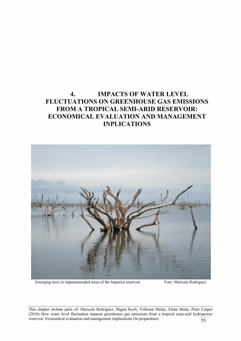
This chapter include parts of: Maricela Rodriguez, Hagen Koch, Volkmar Hartje, Elena Matta, Peter Casper

(2018) How water level fluctuation impacts greenhouse gas emissions from a tropical semi-arid hydropower reservoir: Economical evaluation and management implications (In preparation)

55

4. IMPACTS OF WATER LEVEL FLUCTUATIONS ON GREENHOUSE GAS EMISSIONS

FROM A TROPICAL SEMI-ARID RESERVOIR: ECONOMICAL EVALUATION AND MANAGEMENT

INPLICATIONS

Emerging trees in impounmended areas of the Itaparica reservoir Foto: Maricela Rodriguez

Impacts of water level fluctuation on greenhouse gas emissions from a tropical semi-arid reservoir: Economical evaluation and management implications

57

4.1 Introduction

4.1.1 Hydropower reservoirs as sources of Greenhouse gases

Hydropower is the most important renewable electricity source; it generates 85 % of actual global renewable electricity (EIA, 2016). Hydropower capacity has risen about 30 % within the last decade; in 2015 1209 GW were generated from hydropower worldwide, and is expected to continuously grow in response to increasing energy demands that accompany socioeconomic development (Zarfl et al. 2015). Hydropower generation is projected as an advantageous, clean and renewable option for electricity generation with low cost (EIA, 2016). Reduction of greenhouse gas (GHG) emissions is a priority goal under the scope of international agreements to mitigate the effects of climate change. In developing countries hydropower projects are funded by Annex B countries (Kyoto protocol) within the frame of the clean development mechanism (CDM), as a strategy to reduce GHG emissions from other electricity generation technologies as wood or fossil fuels burning (Leal Filho, 2010). However, hydropower electricity may act as important source of GHGs too, due to the emissions of biogenic GHGs produced in the reservoirs (Rudd 1993; St Louis et al, 2000). Some reservoirs have even been found emitting considerable amounts of GHGs, comparable to emissions from fuel burning or thermal power plants (DelSontro et al. 2010; Kemenes et al. 2011). In consequence the carbon credentials and the conception of hydropower as an alternative for reducing GHGs emissions is under discussion and already revised (Fearnside, 2015; Gunkel 2009; Wehrli 2011).

Biogenic GHGs, including methane (CH4), carbon dioxide (CO2) and nitrous oxide (N2O), are produced in reservoirs, mainly in sediments, as a result of respiration and the decomposition of flooded vegetation and deposited organic matter. Tributaries may also import significant amounts of inorganic carbon to the reservoirs, mainly in the form of CO2 (Maberly et al. 2013). These produced gases may be eventually released to the atmosphere, when concentrations in the reservoirs surface water exceed that in the atmosphere. Release of GHGs across water-atmosphere interface in hydropower reservoirs occurs through two main pathways, i) molecular diffusion or ii) ebullition. Diffusion follows the concentration gradient of dissolved gases between both water and atmosphere, depending on conditions as wind speed and temperature. Gas fluxes are measured either directly using floating chambers or calculated from thin boundary layer models. The release of bubbles (ebullition) can be found when the gases, produced in sediments reach oversaturation in the sediments. This is very likely for gases with low solubility in water, e.g., methane. Ebullition is a random event, occurring mainly in shallower areas and mean drivers are methane production rates in sediments, temperature and changes in hydrostatic pressure. Ebullitive fluxes are measured in situ using inverted funnels as gas traps deployed close to the sediment (0.5 m, Bastien et al. 2011; Wehrli 2011). A third pathway could be via aerenchyma of rooted macrophytes (Askaer et al. 2011; Bergstrom et al. 2007; Dingemans et al. 2011).

At dams a fourth emission pathway arises, when GHGs dissolved in the water in front of the dam become degassed due to turbulent water passage through turbines and spillways. Degassing may be estimated as the gradient of concentrations of dissolved gas in the water column before and after the turbines passage, scaled to water discharged. GHGs produced in the reservoir may be also exported to and eventually emitted by the river downstream (Diem et al. 2012; Roehm and Tremblay, 2006).

Production of GHG in water and sediments of freshwaters is directly related to trophic state of the system and water temperature. Emissions of GHGs from hydropower reservoirs are driven several factors including atmospheric parameters (e.g. wind and temperature), reservoir depth,

Chapter 4

58

morphometry, age and history. Generally, shallow, young, tropical and eutrophicated reservoirs tend to produce and emit higher amounts of GHGs (Barros et al. 2011; Deemer et al. 2016; Galy-Lacaux et al. 1999).

Emissions of GHGs are expressed normally in CO2 equivalents (CO2-eq), related to global warming potential (GWP) of a given gas. It expresses the amount of CO2 that would have the same warming effect over a time scale, normally 100 years. Methane and N2O are powerful warming forcing gases, having GWP of 34 and 298 respectively, over a 100-year horizon, with respect to CO2 (Myhre et al. 2013).

The most recent estimation of GHGs emission from reservoirs resulted in 800 Tg CO2-eq yr-1 (Deemer et al. 2016). GHG emissions from hydropower reservoirs have been accounted up to 288 Tg CO2-eq yr-1, from which 62 % corresponds to CO2 and 38 % to CH4, while N2O emissions were neglected. According to Barros et al. (2011), emissions from hydropower represent about 36 % of the total emissions from reservoirs worldwide and about 4 % of emissions from freshwaters.

Emissions of GHGs from hydropower reservoirs are often reported per reservoir area and in relation to the power generation, allowing the comparison of emissions from different generation technologies (Hertwich, 2013). For instance, some studies have shown that despite larger amounts of GHG emissions from some hydropower reservoirs, it may still be considered more competitive compared to thermal power plants fueled by coal or other fuels because it generates more electricity per GHGs emitted (Dos Santos et al. 2006; Zhao et al. 2013).

Hertwich (2013) estimated global average GHG emissions of hydropower reservoirs in relation to their electricity generation as 85 g CO2 kWh-1 and 3 g CH4 kWh-1, giving a multiplicative uncertainty factor of 2. Furthermore, according to the multivariate regression analysis, energy density, expressed as the ratio of area flooded by a reservoir with respect to the electricity generated, is a main factor to explain GHGs from reservoirs. Thus, reservoirs having larger water surface area and a low electricity generation capacity are more likely to emit higher amounts of GHGs. In principle, larger reservoirs have an extended water surface, where diffusive and ebullitive emissions may occur (Gunkel 2009). Moreover, degassing emissions at the dam may be significant due to the passing of large volumes of water through turbines or spillways. Hence GHG emissions may be prevented by avoiding construction of low energy density hydropower projects and managing the ratios of area flooded in regard the electricity generated. In fact, new hydropower projects are restricted to receive funding within the frame of CDM when energy densities are equal or higher than 4 W/m2, and projects having energy densities above 10 W/m2 are considered to have negligible emissions of GHGs (Soanes et al. 2016)

The volume of water and the water surface area of dammed reservoirs are related to climate. Reservoirs may shrink dramatically during drought periods, which in consequence limit electricity generation capacity of the dam. Accordingly, water level changes will affect GHGs dynamics in the reservoir by increasing or decreasing the water surface area, shifting the ratio between deeper and shallower areas in the reservoir, given that shallower areas may act as emissions hotspots, and finally by affecting the performance of the dam to generate electricity.

Impacts of water level fluctuation on greenhouse gas emissions from a tropical semi-arid reservoir: Economical evaluation and management implications

59

4.1.2 Assessment of policy implications with the integration of economic analysis

Traditionally, policy-making for electricity generation is based on selecting the lowest cost technology in relation to the load curve during investment planning and operation. The environmental implications were usually analyzed separately, in a non-economic analysis, looking for ways of minimizing negative environmental effects, very often in a technology-oriented manner. The situation is different for the GHGs emissions, as there is no technology currently available to mitigate these emissions. As an alternative, the social cost of carbon (SCC) is used, this term is the economic cost caused by emissions of an additional ton of carbon or its equivalents (Nordhaus 2017) (see supplemental material 7.3). The external costs of generating electricity from hydropower in terms of climate change (or Social costs of carbon) are estimates of the accumulated global damages resulting from the emissions of GHG. There are markets for the trading of emission rights, but they are restricted to regions (EU and some North American states) and do not reflect the global social cost of carbon (OECD/IEA 2013).

The SCC is added to the generating cost to calculate the total cost of electricity generation. The external costs of climate change have been given a standard carbon price of 30 US$/t CO2, based on emission factors provided by IPCC (IEA 2010) (see supplemental material 7.3.1). The International Energy Agency (IEA) estimates generating costs, called Levelized Cost of Electricity (LCOE), using a standardized cost accounting approach. Here, all costs categories are added over the lifetime of the project, as accounted for in a discounted cash flow analysis and divided by the total generated electricity (EIA 2016; Khatib 2016).

Combining the generation cost with the damage cost of climate change permits a fully integrated economic evaluation of the electricity generation technologies, i.e. including the external costs of the specific technology. The climate change damage costs are unique in character as the damages are global and long lasting due to the long residence time of the GHGs involved. This requires identifying and quantifying all effects of climate change on the globe, converting them into monetary damage units and adding them over 100 to 200 years over their residence time for all global regions. Relating the damages to the total cumulative emissions allows calculating the damages per unit of GHGs, yielding global uniform figures, albeit with a very high degree of uncertainty.

This chapter presents and discusses the simulation results for GHG emissions from a semi-arid hydropower reservoir in the tropical northeast of Brazil along a 30-year period with climate variability driven changes in inflow and water surface area of the reservoir, water depth and electricity generation (water discharged). Estimated GHGs emissions (CO2 and CH4) from the reservoir water surface (diffusion and ebullition) and the water passage through turbines were used to simulate GHGs emissions across time, by using historical climate data to simulate water surface and volumes applying the reservoir module (Koch et al. 2013) of the eco-hydrological Model SWIM (Krysanova et al. 1998, 2000). Emissions of GHGs converted into CO2-eq are simulated per unit of electricity generated. The economic evaluation of GHGs emissions is assessed by using the social carbon cost concept. Changes in water levels and water discharge were found to be useful predictors to connect GHG emissions from the reservoir to electricity generation. The integration of the economical evaluation of the GHGs emitted by hydropower reservoirs becomes an essential factor looming large on the policies regarding GHG emission managements, at both levels, during hydropower project planning and during their operation.

Chapter 4

60

4.1.3 Study area

The Itaparica reservoir is a hydropower reservoir located in northeastern Brazil (9°6'S and 38°19'W) (Fig. 4.1). The region is known as 'Depression of São Francisco’, the climate is semi-arid, and the rainy period is generally between January and July, but with high temporal variability (Barbosa et al. 2012; Gunkel 2007). The reservoir is prone to seasonal water level changes of up to 5 m (between 299 and 304 m a.s.l.), related to variations in rainfall along year, high evaporation rates, the regulated water inflow from upstream Sobradinho reservoir and the water discharge at the dam. Mean water inflow is 2,060 m3 s-1 while water outflow is regulated from 1,300 to 2,065 m3 s-1, depending on reservoir volume and electricity generation demands. Total installed capacity is 1,479.6 MW. At maximal water level (304 m a.s.l.) the reservoir comprises an area of about 828 km2 (Gunkel, 2007). Retention time in the main-stream is about 2 months and rapid and continuous water flow prevents vertical water stratification. Due to the meandering water course, bays of the systems are generally hydraulically disconnected from the main-stream and water retention times can be significantly longer, up to one year (Matta et al., 2016).

Figure 4.1 Study site location, map shows bathymetry model of the reservoir at mean water level conditions (302.8 m a.s.l.) (Modified from Broecker et al., 2014)

4.1.4 Role of Itaparica dam in electricity generation and electricity price system in Brazil

The Itaparica reservoir is part of a cascade system of reservoirs formed by seven barrages along the Sub-Middle and Lower São Francisco River to serve the Northeast of Brazil with electricity. Itaparica operates since 1988 as a base load electricity source (CHESF 2016; ONS 2010). The cascade system has a large storage capacity to compensate for the months with low river flow. The Itaparica reservoir provides water for human and industrial consumption, irrigation, aquaculture, leisure activities and serves as flood protection (CHESF, 2016; Gunkel, 2007).

Impacts of water level fluctuation on greenhouse gas emissions from a tropical semi-arid reservoir: Economical evaluation and management implications

61

The cascade system of hydropower dams is owned and operated by the governmental company Companhia Hidro Elétrica do São Francisco S.A. (CHESF). The operating company must guarantee the generation of a certain amount of electricity, while electricity prices are established on the basis of auction markets regulated by a governmental agency (EPE), based on a hybrid regulatory system which generates multiple prices. For large hydropower plants in Brazil, for 2015 the LCOE have been calculated to be at 35.26 US$/MWh at a 7 % discount rate (CCEE 2017; EIA 2016). Generally, old hydropower plants demand lower auction prices compared to new ones, as their capital cost are written off. The operation of the electricity grid in Brazil is performed by the governmental agency Operador Nacional do Sistema Elétrico (ONS), which dispatches the power plants based on the operational costs (Calabria et al. 2014; Maceira et al. 2008). Once power plants have been built, the construction costs are considered as sunk costs and only operating and opportunity costs of the water stored for electricity generation are included in economic analysis (Forsund 2007). The operational costs include the variable costs of thermal generation and the opportunity cost of water storage for hydropower generation. If higher costs producers are called upon to contribute to grid stability their costs are allocated to the lower cost producers, who are mostly selling hydropower. This compensation scheme is called Price of the Difference Settlement (Preço de Liquidação das Diferenças- PLD) (Calabria et al. 2014; Maceira et al. 2008). The PLD are calculated and disclosed by the Câmara de comercializaçao de energia elétrica (CCEE). The PLD averaging system determines the short term prices for electricity in the wholesale market of Brazil. These prices vary over time and by region.

The national market is sub-divided into four regions (South, Southeast/Midwest, Northeast and North) for which individual PLDs are determined on a weekly basis for three load steps (heavy, medium, and light). The historic price level can be seen from Figure SM 12 which delineates the PLD curve 1 based on price information from 2011 to 2014 provided by the CCEE; During this period the average price bid determined in the aforementioned public auctions amounts to110.29 R$/MWh) (CCEE 2014).

4.2 Methods

4.2.1 Data-set for GHG flux estimations

Fluxes of the greenhouse gases CH4 and CO2 in the Itaparica reservoir have been previously measured and discussed by Rodriguez and Casper (2013, 2017). Three emissions pathways were analyzed: (i) diffusion across water surface, (ii) ebullition from sediments and (iii) degassing after turbine water passage. Measurements were conducted in four campaigns (March and September 2013, June and October 2014), restricted to low water conditions of the reservoir (299 m a.s.l.), due to a prolonged drought period in the study region. To include spatial variability on GHG emissions over the entire reservoir, the reservoir was divided into two main compartments according to water depth named shallow for less than 5 m depth, and deep or more than 5 m depth. Ebullitive fluxes were limited to shallow waters. In general, the fluxes from the shallow areas are higher compared to the deeper areas. Mean daily emissions (g m2 d-1) from the reservoir are summarized in Table 4.1. Emissions by degassing at the dam are restricted to CO2 due to a slight accumulation of this gas in bottom water before dam inlet, in contrast to negligible concentrations of CH4. Fluxes of CO2 from the hydropower plant (degassing) (g/m3) were calculated taking mean outflow values along the study time frame (1,027 m3/s). Degassing through spillways was not taken into account since spillways were closed during the studied period given the low water level conditions.

Chapter 4

62

4.2.2 Simulations of GHG emissions.

Simulations of total emissions from the reservoir were assessed using mean daily emissions values of CO2 and CH4 (g m2 d-1) (ebullition plus diffusion) from each reservoir compartment and the emissions at the dam (Table 4.1). To calculate total emission for the entire reservoir, emissions from each reservoir compartment were scaled to the water surface area covered by each compartment, and water discharge in the case of emissions occurring through degassing at the dam. Total emissions were then simulated along time using the eco-hydrological Model SWIM for the Itaparica reservoir (i.e. water level, discharge, and hydropower generation). The model is run on a daily time step for a 22-year time period 1988-2010, in order to include wet, normal and dry years. Because there are gaps in the observation records for water level and discharge, and to include climate variability over a longer time period, simulation results were used instead of observed data. As the age of reservoir counts approximately 28 years it must be assumed that fluxes were higher in the first decade after commissioning the dam. Fluxes data applied represent current emissions state and simulated GHG emissions for the 1980ies and 1990ies might not be representative for these decades. Total GHG emissions are presented in CO2 equivalents, using 34 as GWP factor for CH4 on a 100-year horizon. Emissions per electricity generated are calculated by dividing total GHG emissions by electricity generation (kWh).

In order to include uncertainties into the simulations, e.g. regarding GHG fluxes and area and depths of compartments, three scenarios were analyzed (Table 4.1):

i) Mean: mean values for estimated fluxes, assuming the shallow part of the lake having a depth lower 5 m,

ii) Pessimistic: Mean values plus Standard Deviation for fluxes, assuming the shallow part of the lake having a depth lower 6 m (area of shallow lake larger than for case “Mean”),

iii) Optimistic: Mean values minus Standard Deviation for fluxes, assuming the shallow part of the lake having a depth lower 4 m (area of shallow lake smaller than for case “Mean”).

Table 4.1 Fluxes of CO2 and CH4 from shallow and deep lake, and from hydropower plant (discharge); Mean values and Standard Deviation (SD). Values for three emission scenarios named

mean, positive and pessimistic are given.

Reservoir compartment Flux CO2 g m2/d Flux CH4 g m2/d

Mean (Standard Deviation)

Shallow (depth < 5m) 4.87 (0.98) 0.18 (0.07) Deep (depth >= 5m) 2.96 (1.06) 0.025 (0.008) Discharge (CO2: g/m3) 0.91 (0.91)

Pessimistic (mean + SD)

Shallow (depth < 6m) 5.84 0.25 Deep (depth >= 6m) 4.02 0.034 Discharge (CO2: g/m-3) 1.93

Optimistic (mean - SD)

Shallow (depth < 4m) 3.89 0.11 Deep (depth >= 4m) 1.90 0.018 Discharge (CO2: g/m-3) 0.00

Impacts of water level fluctuation on greenhouse gas emissions from a tropical semi-arid reservoir: Economical evaluation and management implications

63

4.2.3 Social cost of carbon emission from the Itaparica reservoir

For an integrated economic assessment, the generating costs and the social cost of carbon need to be integrated. For the estimation of profits from hydropower generation, PLD values provided by CCEE (2016) are used. CCEE calculates the short term price that a hydropower company has to pay for electricity sold at the spot-market that was not generated. For the year 2015 the minimum, mean, and maximum values were 145.1, 310.6 and 388.5 R$/MWh, respectively (Fig. 4.2). To convert the Brazilian Real to US$ an exchange rate of 0.30 US$ for 1 Real is used (in 2015 the exchange rate was between 0.24 and 0.39 US$ for 1 Real with an annual mean of 0.30 US$).

Figure 4.2 PLD electricity cost in Brazil, using historical data provided by the CCEE (2016); SE/CO: Southeast/Midwest; S: South; N: North; NE: Northeast; dotted lines for 2015 are annual mean value

and mean value+/-Standard Deviation.

In Brazil there is no emission trading system, thus a market price for the damage cost of GHG emissions does not exist. Instead a summary of international models calculating the damage costs relevant for the electricity system of Brazil may be applied to calculate GHG emissions cost. The value of the damage cost is calculated with the help of integrated climate change economic growth models. Three models, called Integrated Assessment Models (IAM), are combined in order to increase predictability and model robustness (DICE –Nordhaus, 2014; PAGE –Hope, 2011; and FUND –Anthoff, 2011). The IAM are based on macroeconomic growth models of global per capita consumption. As a consequence, the resulting estimates of the SCC are highly uncertain and their description by one mean value only is not adequate, and should therefore include figures describing the distribution There are a number of governmental summaries in OECD countries and they operate with mean values, but their estimate summaries vary widely as well (Smith, Braathen 2015).

The estimates of the SCC depend on the models used and their modelling assumptions. The variations in the estimates are due the structure of the models and their specification and judgments about central parameters, for which there is no agreements in the literature how to derive the parameters. In practice they turn into policy judgments. These central parameters are the discount rate (the interest rate used to aggregate estimates over time), equity weights (Weights to value damages between countries with different income levels) and whether

Chapter 4

64

national or global damages are included. The various national assessments decide which judgments reflect the national governments position best (Compare the results of the IAWG estimate for the US position).

In addition, to reflect rivaling modeling choices two alternative measures of the social cost of carbon (SCC) [i.e. (i) the global social welfare (based on Johnson & Hope, 2012) and (ii) the national interest perspective (based on IAWG, 2013)] are reported (see Supplemental material 7.3.4). The SCC was added to the generation cost taking into account values from the two ideal-type positions of the SCC) (Table 4. 2).

Table 4.2 SCC (values US$/tCO2) for different value position: international social planner vs. national interest perspective, values in 2012 US$.

National interest (based on IAWG, 2013)

Global social welfare (based on Johnson & Hope, 2012)

Mean 95% Mean 95% 3% constant discount rate, No equity weighting

21 65 1.5% constant discount rate, Multiple with Equity weighting (global averages)

122 357

Share of regional damages (sub-global) Latin America (Hope, 2011)

0.07 Global damages (Anthoff et al., 2011)

× 3.0 n.a.

Proposed range of values (rounded)

1.5 5 366 1070

4.3 Results

4.3.1 Simulation of GHG emissions

4.3.1.1 Case “Mean”

In terms of CO2-eq, emissions due to surface water diffusion accounted for 98 % of the emissions, degassing through turbines to 1.3 %. Ebullition occurred exclusively at shallower areas and accounted to just 0.3 % of the emissions in the entire reservoir.

Discharge, lake surface area, hydropower generation, CO2-equivalent per unit of electricity generated and sum of CO2-equivalents released are summarized for the years 2000 and 2001 (Fig. 4.3). These years can be used to explain the results, because 2000 was rather wet while 2001 was very dry. During the year 2000, the months April to December show high water levels (large water surface), high discharges and hydropower generation. Due to the large water surface and high discharges, also the sum of CO2-eq released is very high (maximum 4.629 t CO2-eq/ d; right axis).

Impacts of water level fluctuation on greenhouse gas emissions from a tropical semi-arid reservoir: Economical evaluation and management implications

65

Figure 4.3 Discharge, lake surface area, hydropower generation, CO2-equivalent per unit of electricity generated (left axis) and sum of CO2-equivalents released (right axis).

In the year 2001 the water levels (water surface), discharges and hydropower generation declined. Thus, the sum of CO2-eq released is lower. However, calculating the CO2-equivalent per unit of electricity generated, shows that the emissions are approximately 221 g/kWh for 2000, for 2001 approximately 385 g/kWh. The different sources for the GHG emissions are shown in Fig. 4.4. The main source of emissions is the water surface (ebullition and diffusion), while emissions through degassing in the turbines contribute only little to the emissions.

Figure 4.4 Release of CO2 and CH4 (converted to CO2-equivalents) from water surface at compartments shallow and deep and degassing at turbines (discharge).

Results for water level, sum of CO2-equivalents released and released CO2-equivalent per unit of electricity generated are shown in figure 4.5 (1988-2010). Figure 4.6 reports the results for electricity generation, sum of CO2-eq released and released CO2-eq per unit of electricity

Chapter 4

66

generated, while Fig. 4.7 shows discharge, sum of CO2-eq released and released CO2-eq per unit of electricity generated.

Figure 4.5 Water level, sum of CO2-equivalentsreleased (blue) and CO2-equivalent per unit of electricity generated (red); daily values for 1988-2010.

Figure 4.6 Electricity generation, sum of CO2-equivalents released (blue) and CO2-equivalent per unit of electricity generated (red); daily values for 1988-2010.

Data of GHG emissions from Itaparica are available only for the last few and dry years, and there is a lack of data for wet and high water level periods with discharges higher than 3,300 m3/s and when water is spilled, i.e. not passing through the turbines. However, those conditions occurred during approximately 3 % (319 days) of the total operational time since September 1988 until end of July 2017.

Impacts of water level fluctuation on greenhouse gas emissions from a tropical semi-arid reservoir: Economical evaluation and management implications

67

In summary (Figs. 4.5- 4.7), the results show that the sum of CO2-eq released is increasing during the calculated 20-years-span, with higher water levels, higher electricity generation and higher discharge. The relations between water level, electricity generation, discharge and the sum of CO2-eq released are not linear (Figs. 4.5 to 4.7). For instance, the same electric charge can be produced at high water levels (large head) and lower discharges or low water levels (low head) and higher discharges. Low water levels (volumes) at the end of a weak rainy season require reduced discharges to prevent the reservoir from falling dry already at the beginning of the dry season. At the end of the dry season low water levels may not restrict discharges, as the upcoming rainy season is used to fill the reservoir.

Figure 4.7 Discharge, sum of CO2-equivalents released (blue) and CO2-equivalent per unit of electricity generated (red); daily values for 1988-2010.

Furthermore, from Figures 4.5 to 4.7 it can be concluded that with high water levels, high electricity generation and high discharge GHG emissions per unit of electricity generated decrease. While in Figures 4.3 to 4.7 daily results are shown, in Figure 4.8 annual mean values and annual sums are given. The data (30 annual values) are sorted according to the mean discharge from Itaparica reservoir. In dry years, here defined as 10th percentile (driest 3 years of the 30-year period), the mean discharge is approximately 1,000 to 1,100 m3/s. For wet years, here defined as 90th percentile (wettest 3 years), the mean discharge is in the range of 2,800 to 3,200 m3/ s. In dry years the sum of CO2-eq released is approximately 1,418,000 to 1,430,000 t/a, for wet years 1,612,000 to 1,637,000 t/a. The annual sum of electricity generated 3,655 to 4,018 GWh/a for dry years and 8,436 to 8,814 GWh/a for wet years. The CO2-equivalent per unit of electricity generated is in the range of 368 to 408 g/kWh for dry years and 198 to 203 g/kWh for wet years.

Chapter 4

68

Figure 4.8 Annual values for mean discharge from Itaparica reservoir (Q(a)), sum of CO2-equivalents released, CO2-eq per unit of electricity generated and sum of electricity generated; the values are

sorted according to annual mean discharge (Q(a)).

4.3.1.2 Greenhouse gas emissions for all cases

The results (mean, minimum and maximum annual values for the period 1981-2010) for all three cases are summarized in Table 3. In the pessimistic case the sum of CO2-equivalents released can reach 2,434,059 t/a (599 g/kWh), while in the optimistic case is only 907,719 t/a (121 g/kWh). For mean case the sum of CO2-eq released can reach 1,542,221 t/a (266 g/kWh).

Table 4.3 Mean, minimum and maximum annual values for sum of CO2-equivalents released and CO2-equivalent per unit of electricity generated (Max.: Mean + SD; Min.: Mean - SD).

Case Value Sum CO2-eq. [t/a] CO2-eq. per unit [g/kWh]

Mean Max. 1,647,228 408 Mean 1,542,221 266 Min. 1,418,310 193

Pessimistic Max. 2,434,059 599 Mean 2,273,909 392 Min. 2,082,933 285

Optimistic Max. 1,033,737 261 Mean 975,107 169 Min. 907,719 121

Impacts of water level fluctuation on greenhouse gas emissions from a tropical semi-arid reservoir: Economical evaluation and management implications

69

4.3.2 Economic assessment

For the economic assessment of the operational changes of the existing power plants, particularly the existing hydropower plants, the short term generation costs and the damage costs of climate change need to be combined.

Table 4.4 Mean and Standard Deviation (SD) of generating costs (year 2015) and GHG emissions damage costs for electricity generation.

Mean (SD) Mean ± SD

Generating costs (spot prices)

310.6 (83.0) R$/MWh 93.2 (24.9) US$/MWh

227.6 / 393.5 R$/MWh 68.3 / 118.1 US$/MWh

National interest Global welfare National interest Global welfare Damage cost (US$/MWh) GHG- emissions: Mean Pessimistic Optimistic

Mean

0.45 0.67 0.29

95%

1.51 2.22 0.96

Mean

110.2 162.4 70.0

95%

322.3 474.7 204.5

Mean

0.26/0.62 0.42/0.91 0.18/0.39

95%

0.95/2.06 1.41/3.02 0.60/1.32

Mean

69.9/150.6 103.3/221.4 43.6/96.3

95%

204.2/440.3 302.1/647.2 127.6/281.4

The generating costs dominate the social costs of carbon only under the assumption that a national interest position prevails (generating cost 93.2 US $/MWh vs. SCC of 0.67 US $/MWh for mean for pessimistic case of GHG emissions). The perspective of moving towards the extreme value (95 %; 2.22.US$/MWh) has only a relatively small effect. Only if one switches to the global welfare position (low discount rate, use of equity weighs and global damage), the SCC become a cost factor equal or larger than the generating costs (162.4 US$/MWh vs.93.2 US$/MW).

4.4 Discussion

At the Itaparica reservoir emissions of GHGs occur mainly through diffusion at the water surface, while emissions through the turbines contribute only o 1.3 % to the total emissions. Emissions are significantly higher in shallower in comparison to deeper areas. In consequence, higher emissions are expected during high water level periods when the reservoir surface area enlarges. Accordingly, results of modeling GHGs comparing two contrasting water level periods, high and low, show that total emissions expressed as CO2-equivalents are higher during a wet period when high water level conditions maintained along almost the whole year. In contrast to total CO2-equivalents emissions, emissions in relation to the electricity generation (g CO2-eq/kWh) are negatively correlated to reservoirs area. During high water levels periods, the reservoirs may operate at full generation capacity and the relation of electricity per water surface area, ergo energy density, increases. Higher electricity density during high water level periods compensate the rises of emissions from water surface, thus the ratio of GHGs produced in relation to electricity generated decreases.

At Itaparica, emissions through turbines are limited to CO2 while emissions of CH4 were negligible due to low dissolved concentrations of that gas in the water column upstream of the dam. Rapid and constant flow of water in the main-stream of the Itaparica reservoir prevents water column stratification and anaerobic conditions (Rodriguez and Casper, 2013). Such conditions limit the production and accumulation of CH4 in bottom waters entering the turbines. Similar results regarding emissions through turbines have been found at the 10 years

Chapter 4

70

old reservoir Three Gorges in China, where rapid flow and water oxygenation also prevents CH4 accumulation and subsequent emissions at the dam passage (Zhao et al. 2013). However, degassing through turbines may represent main GHGs evasion pathway from hydropower reservoirs, for instance in a tropical dry biome reservoir in Brazil, degassing of GHGs represented 30 % of total emissions of the reservoir (Ometto et al. 2013). In the Amazonian reservoir Balbina, and in the subtropical reservoir Nam Leuk where degassing account for 51 % and 71 % of the total GHG emissions, respectively, large emissions are related to the accumulation of CH4 in the water column (Chanudet et al. 2011; Kemenes et al. 2011). Given the 34 times higher warming potential of CH4 storage of CH4 in bottom waters of Itaparica would subsequently lead to significant increments of CO2-eq emissions by the dam. In that case increases in water discharges would lead to peaks of CO2-eq emissions, thus higher electricity generation would then not balance carbon evasion from the reservoir.

Emission rates of GHGs in the Itaparica reservoir are quite variable, and flux rates at the water surface, ebullition plus diffusion, and at the turbines have a high standard deviation. High variability of GHG emissions is related to the complex net of factors driving the production and fluxes of CO2 and CH4 in aquatic systems. Due to the high variability on GHG emissions in the Itaparica reservoir, simulation results for these emissions show a broad range for the different scenarios. For instance, in the positive scenario emissions of CO2 through turbines are assumed to be zero and consequently maximal CO2-eq emissions in the pessimistic scenario are two times higher than maximal values of the positive scenario. Despite the uncertainty on the estimated GHG emissions from the reservoir, the model provides insight to the significance of the Itaparica reservoir as a source of GHGs to the atmosphere. For instance, it can be observed that even under the scope of a positive scenario, the reservoir still behaves as source of GHGs. These results highlight the importance of emissions of biogenic GHGs produced and emitted by the water surface of the Itaparica reservoir.

In terms of carbon emissions per electricity generated Itaparica is less intensive, emitting less than 20 % than coal-fired thermoelectric power plants or diesel oil plants, about 40 % when compared to natural gas (See section 2.4.5). Thus would make Itaparica more competitive if generating costs and SCC were added. Similar outcomes were discussed by Ometto et al. (2013), and Dos Santos et al. (2006), when comparing GHG emissions from several Brazilian hydropower reservoirs to other energy sources. Tropical reservoirs usually are expected to emit higher amounts of GHGs. Emissions per electricity generated from the Itaparica reservoir, even for the pessimistic scenario (599 g CO2-eq/kWh), are below the range of emissions for tropical reservoirs 1,300 to 3,000 g CO2-eq/kWh, according to a summary of hydropower GHG emissions in life cycle assessment by Steinhurst et al. (2012). Biogenic GHG emissions from reservoirs may overpass emissions by construction or removal phases, depending on the type of reservoir, ammount of vegetation flooded or removed (Weisser, 2006). This comparison would reduce the climate benefits for the Itaparica reservoir with respect to other nonrenewable and renewable energy sources.

Another disadvantage for hydropower dams with respect to other renewable electricity generation technologies is the strong dependence of GHG production and emissions to climate driven changes in the reservoirs. According to simulated GHG emissions of the model, the emissions from the Itaparica reservoir would be compensated well along the time by generating higher amounts of electricity during high water level periods. On the contrary, during drier seasons the electricity generation rates should be reduced in order to keep the water volume above the minimum operational level. During long drought periods in the catchment area, the proportion of GHGs emitted to produce a certain amount of electricity

Impacts of water level fluctuation on greenhouse gas emissions from a tropical semi-arid reservoir: Economical evaluation and management implications

71

increase, while GHG emissions from other generation technologies are expected to decrease accordingly to their power capacities.

In other respect, it has to be considered that emissions correspond to the operation of a 30-year-old reservoir, and emissions might be much higher during first years after the impoundment because of decomposition of flooded terrestrial vegetation. In point of fact, the IPCC suggest a period of 10 years as time frame for considering emissions of biogenic GHGs from reservoirs into the national inventories of GHG emissions (IPCC 2007; Ometto et al. 2013). Thus, the model might not properly estimate emissions from the reservoir because current emission rates are not representative for those occurred through the initial 10 years of dam operation. Notwithstanding the foregoing, assumptions of higher GHGs emissions during the first decade, particularly in the Itaparica reservoir, are very uncertain, because inundated soils are sandy, acid and poor in organic carbon content, which constraints GHG production (Araujo Filho et al. 2013). Additionally, the vegetation of this biome, called Caatinga consists mainly of dry bushes and shrubs. Itaparica reservoir face nowadays increasing loads of allochthonous organic matter and nutrients derived from land use changes, like aquaculture and discharges of waste waters (Gunkel 2007; Selge 2017). According to that, emissions from the Itaparica hydropower reservoirs may have not decreased dramatically with reservoirs aging, or may have even increased if actual organic matter overpass original amounts of organic matter flooded.

Nevertheless, the evidence regarding the significance of GHG emissions from water surface of flooded land in hydropower reservoirs, these are generally not included as potential carbon sources within Life Cycle Assessments (LCA). Although water surface and degassing at turbines are recognize as main contributors of GHGs emissions during dam operation, these are normally excluded because of high level of uncertainty and variability. If emissions from flooded land are excluded, uncertainty decrease and the emissions of GHGs are supposed to occur principally during the construction stage, mainly from concrete production and transport of materials (50 % to 99.6 % of LCA emissions) (Raadal et al. 2011). Furthermore, estimation of GHG emissions from some reservoirs have omitted gas emissions from turbines, river downstream or underestimate emissions due to calculation errors or neglecting CH4 emissions (Fearnside 2015). Moreover, most of the studies include gross emissions but not net emissions (before and after impoundment). Neglecting or underestimating biogenic GHGs emissions of hydropower operation masks the significance of carbon emissions from hydropower and makes inequitable the comparison to other electricity generation technologies.

To recognize the importance of emissions of biogenic GHGs of hydropower from flooded land and degassing at turbines as sources of carbon is crucial to have a better estimation of the impact of hydropower dams as GHGs sources. Likewise, the inclusion of the economical evaluation of carbon emissions from hydropower would allow a more objective evaluation of the potential damage and impacts on climate change in comparison to other electricity generation alternatives. Projections of GHG emissions from hydropower operation and the damage cost for the climate are important factor to take into account into future electricity generation planning and management strategies for minimizing GHG emissions.

The best options to minimize or reduce GHG emissions from hydropower reservoirs exist during the planning phase, particularly when the site and the size of the reservoir are decided. The public debate about hydropower generation and its implication for climate policy basically takes place during this phase and it is particularly intense in those countries where hydropower generation plays a major role for the governmental plans of the expansion of the generation capacity. Brazil intends to increase its electricity generation by doubling its

Chapter 4

72

capacity in the next 25 years, based on expanding low carbon emission technologies, including hydropower, wind, gas, bioenergy and solar capacity (IEA 2016). Brazil has been efficient to reduce its GHG emissions in a 41%, from 14.4 t CO2-eq in 2004 to 6.5 t CO2-eq in 2012. Likewise, energy related GHG emissions per capita are low (2.4 t CO2 in 2014), compared to major GHGs emitters countries, explained by increments in clean energy sources (La Rovere 2017). Brazil has a great potential of renewable energy sources which would facilitate GHGs emissions reduction goals, according to commitments taken by Brazil to reduce in GHG emissions in 37 % in 2025 and 43 % in 2030, related to GHGs emissions reached in 2005 (La Rovere 2017).

The economic basis for decision-making between electricity technologies is the comparison of the long term costs of generating (and transmitting) the electricity and the external costs of the generation for the available generation technologies. The objective of the Decennial Plan for Energy Expansion (DPEE) in Brazil is to secure electricity supply with the lowest expansion cost (Losekann et al. 2013). Results observed in Itaparica regarding higher electricity densities diminish GHGs emissions would reaffirm the climate benefits of more efficient hydropower plants. Hertwich (2013), described how ratio of land use to electricity generated is a good predictor of GHG emissions. Generally, hydropower dams which generate low amounts of electricity per flooded area will emit higher amounts of GHG emissions per kWh produced.

When hydropower plants are built the options to reduce GHG emissions include: (a) reducing eutrophication, (b) reducing sedimentation or remove sediments and (c) adjusting the reservoir operation (water level changes and outflow), thus influencing the amount of electricity generated, usually by reducing it. In Itaparica, to maintain full electricity generation rates during dry periods is not a feasible strategy in order to reduce GHG emissions per kWh generated. Higher water volume discharges would lead to a rapid decrease of water volume down to critical levels and cease of power house operation. Such situation is avoided at any cost given the importance of the reservoir as electricity source and water storage for this semi-arid region. Therefore, adapting the management of Itaparica reservoir is only possible in case the management of the much larger Sobradinho reservoir upstream is also adapted. Economical based decisions for these options include a benefit cost analysis where environmental and recreational advantages are assessed as the benefits while the losses of electricity generation are mostly opportunity costs.

GHG emissions and their economical evaluation obtained through simulation involve a high level of uncertainty given the strong relation of the results to the assumptions, i.e. optimistic, mean or pessimistic and to different perspectives for estimating damages from greenhouse gas emissions, i.e. ‘National interest’ or ‘Global social welfare’. Despite the uncertainties the models provide important information regarding the importance of water level changes as drivers of GHG emissions from reservoirs. Furthermore, the models represent a new methodological approach to estimate and predict GHG emissions under diverse climatic conditions and their respective economical cost for climate change.

4.5 Conclusions

For the Itaparica reservoir it can be concluded that high water level periods increase the GHG emissions from water surface to the atmosphere given the positive relation between water volume and area flooded. But at the same time, high electricity generation is reducing the released CO2-eq per unit of electricity generated considerably. During long dry periods, high electricity generation can reduce the water volume rapidly, leading to a strong reduction in

Impacts of water level fluctuation on greenhouse gas emissions from a tropical semi-arid reservoir: Economical evaluation and management implications

73

electricity generation. In consequence, GHG emissions per electricity generated increase during low water level periods. Existing GHG fluxes from Itaparica represent only dry and low water level conditions, but these conditions prevail in this reservoir and high water level conditions with discharges higher than 3,300 m3/s occurred only during approximately 3 % (319 days) since operation time. Therefore, the model would explain well emissions during prevalent conditions in Itaparica. Continuous water flow and water column oxygenation prevents high GHG emissions by degassing through turbines. As a result, estimations of maximal emission per generated electricity during pessimistic scenario reached 599 g CO2-eq/kWh, which is lower than the emissions proposed for tropical reservoirs. Management measures to reduce and to prevent rises in GHG emissions from Itaparica are focused on the control of water level fluctuations in the reservoir, balancing electricity generation during low water level periods to avoid peaks of GHG emissions in relation to electricity generated. Water level management is possible only when integrating the previous reservoir of Sobradinho. The analysis of the effects of water level changes on GHG per MWh produced and their economical evaluation provides new information to compare hydropower reservoirs to other electricity generation technologies in function of GHG emitted to services provided. The decrease of GHG emission per MWh generated in Itaparica when energy densities are higher, confirms the importance of dam electricity generation efficiency as a predictor of GHG emissions. Therefore, construction of new dams which need a large area inundated to generate low amounts of electricity (energy density less than 4 W/m2) must be avoided.

75

5. GENERAL CONCLUSIONS

Portrait of the artist Luiz Gonzaga. – a mural at the main building of the hydropower plant. Photo: M. Rodriguez

General conclusions

77

5.1 Greenhouse gas (CO2 and CH4) emissions from the Itaparica reservoir

The Itaparica reservoir is a source of methane and carbon dioxide to the atmosphere. However, emissions from Itaparica exhibit a high variability, mean total annual carbon emissions are 2.3 × 105 ± 0.745 × 105 t C. High variability of greenhouse gases (GHG) emissions from aquatic systems is reported in several studies dealing with GHG fluxes from natural systems and hydropower reservoirs. GHG fluxes from water to the atmosphere depend on a complex net of physical factors which increase the spatial and temporal variation of gas emissions. Likewise, concentration of CH4 and CO2 in surface waters of Itaparica reservoir depend directly on highly dynamic parameters as biological production, water temperature and wind disturbance. In consequence, diffusive fluxes are variable. In the same way, ebullitive fluxes are highly variable, given the irregularity and randomness of bubbles release from sediments.

Despite the variability a clear spatial pattern on GHG emissions was observed in Itaparica. Shallow areas (less than 5 m depth) emit larger amounts of CH4 and CO2 to the atmosphere than deeper zones of the reservoir. Dissolved gases concentrations in water and sediments were higher in shallower areas. Spatial variability could not be directly explained by differences of sediment and water parameters like OM or TP content between deep and shallow areas including. High respiration and mineralization rates in sediments in littoral areas could be responsible for elevated concentrations of dissolved CO2 and CH4. While in profundal waters epilimnetic primary production might be the main factor driving lower concentrations of CO2 in surface waters. Dense stands of the water weed Egeria densa form a main carbon source in littoral areas. Effects of wind shear and wave action on water mixing induce to convective transport of CO2 and CH4 from shallow waters in offshore directions, lead to increase concentrations of dissolved gases in intermediate depths of the studied Icó-Mandantes bay.

Temporal variability on GHGs releases in the Itaparica reservoirs was not clearly observed. In this semi-arid reservoir, water level fluctuations are expected to act as main temporal driver of GHGs emissions. However, this could not be corroborated due to the prevalent low water level conditions during the course of this study, resulting from a long drought period in the region. Continuous monitoring of GHG fluxes and concentrations of dissolved gases in water and sediments are necessary to elucidate potential seasonal patterns of GHG emissions. Analysis of temporal variations of GHG from the reservoir is possible only considering atmospheric and water parameters from monitories.

Annual carbon emissions per area unit of the Itaparica reservoir are comparable to other tropical reservoirs, including two that belongs to the reservoirs cascade system along the São Francisco River, namely Tres Marias located upstream and the semi-arid reservoir Xingó, downstream Itaparica. Emissions from Itaparica are notably lower than Amazonian reservoirs e.g., Balbina (Figure 5.1). Likewise, amount carbon emitted per MWh generated energy, expressed as total carbon from CO2-eq depend on the GWP value used. Over the 100-years scenario carbon emissions represent about 42 % of the emissions that would have occurred using natural gas or about 19 % by using diesel, oil or coal-fired thermo electric plants. Carbon emissions using CO2-eq (GWP20), increases the emissions from Itaparica reservoir dramatically, generating 67% from natural gas emissions or about 30% from diesel, oil or coal-fired electricity. Thus the carbon credentials from this semi-arid hydropower reservoir decrease over the short term.

Hydraulic and hydromorphology of the reservoir are considered to play an important role preventing GHG emissions from Itaparica. Constant water flow and water mixing in the

Chapter 5

78

reservoir prevent anoxia and thus the accumulation of methane in bottom waters. Methane oxidation in the sediment-water interface is responsible for low concentrations of methane in bottom water before the dam inlets but lead to an accumulation of dissolved CO2. Furthermore, inundated soils in this semi-arid region are poor in organic matter and vegetation coverage. The major sources for mineralization, flooded vegetation and soil, are assumed to be already consumed within the first decade after impoundment. In this semi-arid, 30-years operating reservoir, production of GHG is supported by inputs of new organic carbon, particularly from allochthonous sources related to human activities in the catchment. Inputs of CO2 from tributaries channels may also be important sources of this gas for the reservoir.

Figure 5.1 Carbon emissions per area unit from the Itaparica reservoir in comparison to other tropical Amazonian and no Amazonian hydropower reservoirs and to one boreal (a) Kemenes et al. 2011; (b)

dos Santos et al. 2006; (c) Abril et al. 2005: (d) Bastien et al. 2011

5.2 Effect of land use and climate change on methane production in sediments of a semi-arid reservoir

Effects of land use and climate change on methane production in sediments of the Itaparica reservoir were analyzed through incubation experiments under warming and additions of sources of organic carbon and nutrients (nitrogen and phosphorous). Methane production (MP) in the Itaparica reservoir is carbon limited. Inundated soils in the region are reported to be poor in organic matter content. High content of minerals was observed in samples of incubated sediments from three different locations in the reservoir (i.e. littoral, intermediate and profundal). According to sediment density, sediments of Itaparica may be classified as mineral rich and carbon low. Thus MP is restrained by low organic carbon availability. Additions of a labile organic compound, as glucose, increase methane production significantly, particularly in sediments of a profundal location, near the dam.

Higher MP in sediments of profundal with respect littoral and intermediate may be explained by spatial differences of sediment characteristics. Higher content of minerals including Fe, Ca, Mg and K, in littoral and intermediate locations are indicators of the terrestrial origin of these sediments. Acidic conditions and higher concentrations of Fe in littoral and intermediate depths may limit MP in the Itaparica, which would also explain lower MP rates in intermediate sediments, under control conditions, despite higher concentrations of OM compared to profundal or littoral sediments.

375

1695

31 165

402

622

193

1236

0

200

400

600

800

1000

1200

1400

1600

1800

ItaparicaThis study

Balbina (a) Tucurui (b) Tres Marias (b)

Barra Bonita (b)

Xingo (b) Samuel (b) Petit saut (2003) (c)

Eastmain 1 (d)

t C K

m2

year

-1

ReservoirAmazonian No Amazonian Boreal

General conclusions

79

Responses of MP to nutrients and carbon additions varied along the sediment profiles in respect to the location. In profundal sediments, the highest MP was observed at the sediment surface (0-4 cm) independent of the addition while in littoral and intermediate sediments MP increased in deeper sediments layers (6-8 cm) with the addition of carbon source. Such variations are related to differential abundance of methanogens along the sediment profile. Abundance of methanogenic bacteria in littoral sediments are restricted by exposure to desiccation and oxygenated conditions of bottom waters, while in profundal waters anoxic conditions may occur.

Increase of incubation temperatures up to 40 °C did enhance MP, but not significantly. Positive effects of warming, measured through the temperature sensitivity index (Q10) and the activation energy equation (E’a), were more frequently observed in carbon free treatments. This suggests that positive effects of warming are masked by additions of organic carbon. The mere addition of nutrients sources did show a positive effect on MP, but nitrogen addition combined with warming enhanced MP.

Increase of MP to additions of organic carbon sources and the combined effect of nitrogen and warming lead to raises in methane emissions potential from Itaparica. Land use changes in margins include the development of crop plantations, which required soil amendments using fertilizers due the low availability of carbon and macro and micro elements in soils of that semi-arid region. Due to the permeability of sandy soils, excess of nutrients and terrestrial carbon are easily exported to the reservoir (Araújo et al. 2013). Climate change is not supposed only to drive water warming, but also changes in seasonal rain regimes, for example longer drought periods and stronger precipitation events. Both situations may influence MP, under potential conditions of intensive use of fertilizer strong rainy events will prove higher amounts of terrestrial nutrients and carbon from runoff, while droughts periods will favor nutrients retention and sedimentation, particularly during low water level periods.

Higher inputs of terrestrial nutrients in littoral areas boost MP indirectly by enhancing the development of macrophytes and phytoplankton, which are main carbon sources to be mineralized in sediments. During strong and prolonged rainy periods water transparency decreases and macrophyte community is damaged, death plants are rapidly mineralized producing higher amounts of CH4 and CO2.

In profundal areas organic carbon loads are likely to increase and water stratification may occur if water retention times are prolonged. Under this conditions methane production in sediments increases as well as its accumulation in bottom waters previous the dam, which augment the potential of methane release by degassing of water passing the turbines.

Due to the complex net of factor controlling methane emissions from aquatic systems, and in particular from hydropower reservoirs, clear predictions on the effects of water warming and land use change on methane emissions are difficult to state based on incubation experiments. However, it is clear that MP is enhance by organic carbon inputs and combined effects of nitrogen additions and warming. Furthermore, effects on MP exhibit spatial differences. Littoral areas may act as hot spots of GHG emissions.

5.3 Water level fluctuation impacts greenhouse gas emissions from a tropical semi-arid hydropower reservoir

Estimations of GHG emissions along time using models based on hydromorpholocial and hydraulic characteristics of the reservoir show that GHG emissions from Itaparica are indirectly driven by water level fluctuations which in turns drive changes in flooded area and

Chapter 5

80

water discharges. During high water level periods, reservoir area enlarges, therefore emissions through water surface increase. Likewise, rises in water volume during high water levels allow higher water discharges through turbines to generate larger amounts of electricity, or water drain through the spillways to avoid the reservoir to overflow. In consequence, emissions occurring by degassing at the turbines increase. On the contrary, during low water levels total GHG emissions would decrease accordingly to water surface shrinking and reduction of water discharged to prevent reaching the minimal operational water volume.

Emissions of GHG per electricity generated behave on the opposite way. Larger volumes released through turbines during high water level periods, help to increase the performance and energy density, which is the amount of electricity per area covered by the reservoir (KWh/m2). During low water level periods, electricity production is restrained to avoid the reservoir to reach critical low water volumes. Therefore, emissions per KWh generated decrease during high water level periods and increase during low water level periods.

Estimation of GHG emissions and their economical evaluation strongly depend on the different assumptions used for the model, i.e. optimistic, mean or pessimistic and to different perspectives for estimating damages from greenhouse gas emissions, i.e. ‘National interest’ or ‘Global social welfare’. Thus, the level of uncertainty increases when more factors are involved. Nevertheless, it can be concluded that even under the most pessimistic scenario, taking maximal GHG values and larger proportion of littoral areas, emissions per electricity generated from Itaparica (599 g CO2-eq/kWh) are lower than those proposed for tropical reservoirs. Continuous water flow and water column oxygenation prevents high GHG emissions by degassing through turbines, but slightly accumulation of methane in bottom water previous the dam would significantly increase the emissions, given the high global warming potential of this gas.

Using models based on hydraulic and hydro morphology characteristics of reservoirs and data bases of GHG emissions is a useful and innovative methodological approach to estimate and predict GHG emissions behavior under different climate conditions (water level fluctuations). The estimations of carbon emissions per electricity generated and their economical evaluation provide useful information to compare electrical reservoirs to other electricity generation technologies in function of GHG emitted to services provided and the management cost of carbon emitted and economical cost of damage by climate change.

5.4 Outlook: management recomendations and further research

5.4.1 Recommendations: Management strategies to minimize GHG emissions from the Itaparica reservoirs

Given the positive relation between CH4 and CO2 production in aquatic systems to their trophic state, the management measurements to prevent rises in GHG emissions from the Itaparica reservoir should be aimed to improve water quality. Accordingly, water eutrophication in hydraulically disconnected bays should be prevented by avoiding water stagnation due to prolonged water retention times. Export of terrestrial organic carbon, provided by organic fertilizers and cattle raise in margin soils, will lead to significant increase in methane production is this carbon limited reservoir, particularly in littoral waters. Likewise, excessive use of fertilizers may increase the loads of nitrogen and phosphorus to water of the reservoir. These nutrients lead to eutrophication of the reservoir, promoting the occurrence of algae blooms and the development of dense stands of macrophytes, which represent main sources of organic matter to be decomposed anaerobically in sediments, producing CH4 and

General conclusions

81

CO2. Excess of nitrogen plus water temperature raises lead to higher production of methane. Therefore, good management of agricultural practice may be developed in order to make an adequate use of fertilizers and avoid overloads of carbon and nutrients by soil infiltration and exports by runoff during strong rains. Complementary, primary water treatment for residual water of aquaculture ponds using the “green liver system” using macrophytes for nutrients and substances retention as described by Marques and Pflugmacher-Lima (2017), may be implemented as a strategy to decrease concentration loads of nutrients into the Itaparica reservoir. Additionally, constant water quality monitories are necessary to improve the data availability that allows appropriate and timely environmental management.

Given the importance of methane oxidation restraining accumulation and potential emissions of this gas through water surface and particularly the degassing at turbines, it is important to maintain a constant and natural flow of water to allow water mixing and oxygenation of the entire water column.

Management of water level fluctuations would allow a better balance of electricity production, thus peaks of GHG emissions per KWh generated during low water level periods may be avoided. Since Itaparica makes part of a cascade system of reservoirs, water level changes management is only possible by controlled water inflow–outflow rates from reservoirs up- and- downstream Itaparica.

Results from this study also highlight the importance of decisions taken during the planning phase to minimize or reduce GHG emissions from hydropower, particularly regarding the location and the size of the reservoirs. Reservoirs located in semi-arid regions would tend to have fewer emissions than those located in tropical and organic matter rich areas as the Amazon basin. According to result of GHG per electricity generated, it would be confirmed that energy density might be use as a good predictor of GHG emissions from hydropower reservoirs, thus, dams which need a large area inundated to generate low amounts of energy will emit larger amounts of GHGs. This confirms the aim of the Clean Development Mechanism (CDM) to favor construction of new hydropower projects with power densities higher than 4 W/m2.

5.4.2 Further research

In this study estimation of gross emissions of Itaparica reservoir were calculated, and results provide relevant information regarding the significance of GHG release of a semi-arid hydropower reservoir. Furthermore, it is possible to draw clear conclusions about spatial differences of GHG emissions. Littoral areas were recognized as hotspots of production and emissions of methane and carbon dioxide and environmental drivers were discussed. Carbon additions and combined effect of nitrogen loads and temperature rises were identified as main factors enhancing methane production in sediments of the Itaparica reservoir, under incubation conditions. Water level fluctuations have severe impacts on the amount of GHG released by water surface and turbines at the dam.

During the course of this study prolonged dry season prevailed, thus gross GHG emissions correspond to a period of low water level and no water stratification conditions. Thus, further research should be focused on the analysis of spatial and temporal variations of GHG emissions in the reservoir. Long term monitories of GHG fluxes are necessary in order to improve data availability and recognize seasonal patterns. Likewise, monitories should include more sites within the reservoir, for instance more than one bay, particularly those subjected to different hydrological and environmental conditions, for example larger inputs of drainage and sewage waters or bays which have continuous water loads from tributaries.

Chapter 5

82

Water inflow areas were not included in this study but may also emit higher amounts of GHG which are imported from previous reservoir. Correspondingly, GHG fluxes previous the dam and downstream the dam are fundamental to determine the role of the Itaparica reservoir exporting GHG to the river downstream.

Monitories of dissolved gas concentrations in sediments, water and gas fluxes to atmosphere should be supported by measurements of water and sediment quality parameters, as well as water biodiversity studies, particularly focused on phytoplankton and macrophyte communities. Besides, long term data of atmospheric parameters as wind speed, air temperature and atmospheric pressure should be integrated. During the study period no water stratification was identified in the main-stream. Water stratification and upwelling events are important factors controlling accumulation of dissolved GHG in bottom waters, methane oxidation and gas releases. Measurements of aquatic parameters including water temperature, oxygen concentrations and pH along the water column and along several sites in the reservoir are required in order to recognize seasonal stratification patterns in the reservoirs, especially in the main-stream. Correlation of GHG fluxes to aquatic and atmospheric parameters allows a better understanding of seasonal and temporal patterns and the main forcing parameters. These data may be used to estimate or to model GHG dynamics in the reservoir.

Methane oxidation is a key factor preventing methane emissions from the Itaparica reservoir. Therefore, it is worthwhile to investigate more into detailed oxidation processes as well as the main factor controlling methane consumption in the water column. Moreover, methane production in sediments was identified to vary within the reservoir and along the sediment depth. Those variations are related to sediment chemical and physical parameters but also to microbiological activity. One promising research field lay on the identification of methane producing Archaea community (methanogens), as well of methane oxidation bacteria (methanotrophs). Description of main methanogenesis processes (hydrogenotrophic or acetoclastic) is also a remarkable research gap in tropical semi-arid aquatic systems.

Integration of different techniques to measure GHG fluxes from aquatic ecosystem should be considered in order to decrease uncertainties. Some techniques allow for continuous flux measurements, for example Eddy-covariance towers. Ebullition fluxes may be measured with better accuracy with hydroacustic methods using an echosounder as described by Del Sontro et al. (2011). However, disadvantages on the implementation of these techniques include expensive equipment, difficult installation or operation procedures, and the need of expensive and adequate maintenance. These facts hinder their use in remote places with difficult access to proper infrastructure as is the case of the Itaparica reservoir.

A complete balance of GHG dynamics in the Itaparica reservoir may be drawn when including flux estimations under different environmental conditions (dry-low and wet-high water levels), methane production, methane oxidation and respiration rates and exports of GHG to the river downstream.

Finally, GHG emissions from the Itaparica reservoir should be considered to be included into the carbon inventories of aquatic ecosystems in Brazil. Results obtained in this study are worth to publish so scientific community and stakeholders may use the information with the purpose of supporting management and policies involving GHG emissions reductions. In this respect, the cooperation with Brazilian scientific institutions as well as among scientific disciplines, are the bases to undergo further research in the field of GHG emissions in semi-arid hydropower reservoirs.

References

83

6. REFERENCES

Abe DS, Sidagis-Galli C, Tundisi MT, Tundisi JEM, Grimberg DE, Medeiros GR, Teixeira-Silva V, Tundisi JG (2009) The effect of eutrophication on greenhouse gas emissions in three reservoirs of the Middle Tiete River, southeastern Brazil. In: Limnology ISo (ed) 30th Congress of the International Association of Theoretical and Applied Limnology, Montréal, 12-18 August 2007. Schweizerbartsche Verlagsbuchhandlung, Stuttgart, pp 822-825

Abril G, Guerin F, Richard S, Delmas R, Galy-Lacaux C, Gosse P, Tremblay A, Varfalvy L, Dos Santos MA, Matvienko B (2005) Carbon dioxide and methane emissions and the carbon budget of a 10-year old tropical reservoir (Petit Saut, French Guiana). Glob Biogeochem Cycle 19:GB 4007 doi:Gb4007 10.1029/2005gb002457

Achtnich C, Bak F, Conrad R (1995) Competition for electron donors among nitrate reducers, ferric iron reducers, sulfate reducers, and methanogens in anoxic paddy soil. Biology and Fertility of Soils 19:65-72 doi: https://doi.org/10.1007/BF00336349

Adhya TK, Pattnaik P, Satpathy SN, Kumaraswamy S, Sethunathan N (1998) Influence of phosphorus application on methane emission and production in flooded paddy soils. Soil Biology and Biochemistry 30:177-181 doi:http://dx.doi.org/10.1016/S0038-0717(97)00104-1

Almeida RM, Nobrega GN, Junger PC, Figueiredo AV, Andrade AS, de Moura CG, Tonetta D, Oliveira ES, Jr., Araujo F, Rust F, Pineiro-Guerra JM, Mendonca JR, Jr., Medeiros LR, Pinheiro L, Miranda M, Costa MR, Melo ML, Nobre RL, Benevides T, Roland F, de Klein J, Barros NO, Mendonca R, Becker V, Huszar VL, Kosten S (2016) High Primary Production Contrasts with Intense Carbon Emission in a Eutrophic Tropical Reservoir. Front Microbiol 7:717 doi:10.3389/fmicb.2016.00717

Anthoff D, Rose, S. Tol, R.S.J., Waldhoff, S (2011) Regional and sectoral estimates of the social cost of carbon: An application of FUND. Economic and Social Research Institute, Dublin. Economics discussion paper No 2011-18 doi: http://dx.doi.org/10.2139/ssrn.1972778

Arah JRM, Stephen KD (1998) A model of the processes leading to methane emission from peatland. Atmos Environ 32:3257-3264 doi:http://dx.doi.org/10.1016/S1352-2310(98)00052-1

Araújo Filho JCd, Gunkel G, Sobral M, Kaupenjohann M, Lopes HL (2013) Soil attributes functionality and water eutrophication in the surrounding area of Itaparica Reservoir, Brazil. Revista Brasileira de Engenharia Agrícola e Ambiental 17:1005-1013

Askaer L, Elberling B, Friborg T, Jorgensen CJ, Hansen BU (2011) Plant-mediated CH4 transport and C gas dynamics quantified in-situ in a Phalaris arundinacea-dominant wetland. Plant Soil 343:287-301 doi:10.1007/s11104-011-0718-x

Barber RD (2001) Methanogenesis: Ecology. In: eLS. John Wiley & Sons, Ltd. doi:10.1002/9780470015902.a0000475.pub3

Barbosa JEL, Medeiros ESF, Brasil J, Cordeiro RS, Crispim MCB, Silva GHG (2012) Aquatic systems in semi-arid Brazil: limnology and management. Acta Limnol Bras 24:103-118 doi: http://dx.doi.org/10.1590/S2179-975X2012005000030

Baron JS, Hall EK, Nolan BT, Finlay JC, Bernhardt ES, Harrison JA, Chan F, Boyer EW (2013) The interactive effects of excess reactive nitrogen and climate change on aquatic ecosystems and water resources of the United States. Biogeochemistry 114:71-92 doi:10.1007/s10533-012-9788-y

References

84

Barrette N (2005) Greenhouse Gas Emissions from Hydroelectric Reservoirs. In: Lehr JHK, Jack. (ed) Water Encyclopedia, vol 3. Surface and agricultural water. John Wiley & Sons, Inc., New Jersey, pp 180-183. doi:10.1002/047147844X.sw383

Barros N, Cole JJ, Tranvik LJ, Prairie YT, Bastviken D, Huszar VLM, del Giorgio P, Roland F (2011) Carbon emission from hydroelectric reservoirs linked to reservoir age and latitude. Nat Geosci 4:593-596 doi:10.1038/ngeo1211

Bastien J, Demarty M (2013) Spatio-temporal variation of gross CO2 and CH4 diffusive emissions from Australian reservoirs and natural aquatic ecosystems, and estimation of net reservoir emissions. Lakes Reserv Res Manag 18:115-127 doi:10.1111/lre.12028

Bastien J, Demarty M, Tremblay A (2011) CO2 and CH4 diffusive and degassing fluxes from 2003 to 2009 at Eastmain 1 reservoir, Québec, Canada. Inland Waters 1:113-123

Bastviken D, Cole J, Pace M, Tranvik L (2004) Methane emissions from lakes: Dependence of lake characteristics, two regional assessments, and a global estimate. Glob Biogeochem Cycle 18:GB4009 doi:10.1029/2004gb002238

Bastviken D, Cole JJ, Pace ML, Van de Bogert MC (2008) Fates of methane from different lake habitats: Connecting whole-lake budgets and CH4 emissions. J Geophys Res-Biogeosci 113: G G02024 doi: 10.1029/2007jg00608

Bastviken D, Ejlertsson J, Tranvik L (2002) Measurement of methane oxidation in lakes: a comparison of methods. Environmental science & technology 36:3354-3361 doi: 10.1021/es010311p

Bastviken D, Olsson M, Tranvik L (2003) Simultaneous measurements of organic carbon mineralization and bacterial production in oxic and anoxic lake sediments. Microb Ecol 46:73-82 doi: https://doi.org/10.1007/s00248-002-1061-9

Bastviken D, Santoro AL, Marotta H, Pinho LQ, Calheiros DF, Crill P, Enrich-Prast A (2010) Methane emissions from Pantanal, South America, during the low water season: toward more comprehensive sampling. Environ Sci Technol 44:5450-5455 doi: 10.1021/es1005048

Beaulieu JJ, Smolenski RL, Nietch CT, Townsend-Small A, Elovitz MS (2014) High methane emissions from a midlatitude reservoir draining an agricultural watershed. Environ Sci Technol 48:11100-11108 doi: 10.1021/es501871g

Belger L, Forsberg BR, Melack JM (2011) Carbon dioxide and methane emissions from interfluvial wetlands in the upper Negro River basin, Brazil. Biogeochemistry 105:171-183 doi:10.1007/s10533-010-9536-0

Bergstrom I, Makela S, Kankaala P, Kortelainen P (2007) Methane efflux from littoral vegetation stands of southern boreal lakes: An upscaled regional estimate. Atmos Environ 41:339-351 doi:10.1016/j.atmosenv.2006.08.014

Blake LI, Tveit A, Øvreås L, Head IM, Gray ND (2015) Response of methanogens in Arctic sediments to temperature and methanogenic substrate availability. PloS one 10:e0129733 doi: https://doi.org/10.1371/journal.pone.0129733

Borrel G, Jézéquel D, Biderre-Petit C, Morel-Desrosiers N, Morel J-P, Peyret P, Fonty G, Lehours A-C (2011) Production and consumption of methane in freshwater lake ecosystems. Research in microbiology 162:832-847 doi:https://doi.org/10.1016/j.resmic.2011.06.004

Broecker T, (2014) Simulation of two-dimensional flow and transport processes in a Brazilian reservoir. Master Thesis Technische Universität Berlin

Brothers SM, Prairie YT, del Giorgio PA (2012) Benthic and pelagic sources of carbon dioxide in boreal lakes and a young reservoir (Eastmain-1) in eastern Canada. Glob Biogeochem Cycle 26:GB1002 doi:Gb100210.1029/2011gb004074

Calabria FA, Saraiva JT, Glachant J-M (2014) Enhancing flexibility and ensuring efficiency and security: Improving the electricity market in Brazil via a virtual reservoir model. Robert

References

85

Schuman Centre for Advanced Studies Research RSCAS 2014/2085 doi:http://dx.doi.org/10.2139/ssrn.2490377

Cardoso SJ, Vidal LO, Mendonca RF, Tranvik LJ, Sobek S, Fabio R (2013) Spatial variation of sediment mineralization supports differential CO2 emissions from a tropical hydroelectric reservoir. Front Microbiol 4:101 doi:10.3389/fmicb.2013.00101

Casper P (1996) Methane production in littoral and profundal sediments of an oligotrophic and eutrophic lake. Arch Hydrobiol Spec Issues Advanc Limnol 48:253-259

Casper P, Chan OC, Furtado ALS, Adams DD (2003) Methane in an acidic bog lake: The influence of peat in the catchment on the biogeochemistry of methane. Aquat Sci 65:36-46 doi:10.1007/s000270300003

[CCEE] Câmara de Comercializão da energía elétrica (2017) Precos. https://www.ccee.org.br/portal/faces/pages_publico/o-que-fazemos/como_ccee_atua/precos/precos_medios?_adf.ctrl-state=peozuqyf1_196&_afrLoop=359501614565268#%40%3F_afrLoop%3D359501614565268%26_adf.ctrl-state%3D9qheq63ta_4. Accessed 10.04 2017

Chan OC, Claus P, Casper P, Ulrich A, Lueders T, Conrad R (2005) Vertical distribution of structure and function of the methanogenic archaeal community in Lake Dagow sediment. Environ Microbiol 7:1139-1149 doi:10.1111/j.1462-2920.2005.00790.x

Chanudet V, Descloux S, Harby A, Sundt H, Hansen BH, Brakstad O, Serca D, Guerin F (2011) Gross CO2 and CH4 emissions from the Nam Ngum and Nam Leuk sub-tropical reservoirs in Lao PDR. Sci Total Environ 409:5382-5391 doi:10.1016/j.scitotenv.2011.09.018

[CHESF] Companhia Hidroelétrica do São Francisco (2016) [Hydroelectric Company of São Francisco] . Portal Corporativo da CHESF, [ CHESf corporate portal]; [cited 17 Sep 2016]. https://www.chesf.gov.br/SistemaChesf/ Pages/SistemaGeracao/LuizGonzaga.aspx

[CHESF] Companhia Hidroelétrica do São Francisco [Hydroelectric company of São Francisco], [FADURPE] Fundação Apolônio Salles [Apolônio Salles Foundation]. 2011. Inventario dos ecosistemas aquáticos do baixo Sao Francisco; Reservatorio de Itaparica: vol 3, Relatorio trianual Dec 2007- Nov 2010. [Inventory of the aquatic ecosystems of the São Francisco river, lower basin; Itaparica Reservoir: vol 3, Tri-annual Report Dec 2007- Nov 2010]. 1st ed. Recife (Brazil)

Christensen T, Cox P (1995) Response of methane emission from Arctic tundra to climatic change: results from a model simulation. Tellus B 47:301-309 doi:10.1034/j.1600-0889.47.issue3.2.x

Cole JJ, Bade DL, Bastviken D, Pace ML, Van de Bogert M (2010) Multiple approaches to estimating air-water gas exchange in small lakes. Limnol Oceanogr-Meth 8:285-293 doi:10.4319/lom.2010.8.285

Cole JJ, Caraco NF (1998) Atmospheric exchange of carbon dioxide in a low-wind oligotrophic lake measured by the addition of SF6. Limnol Oceanogr 43:647-656 doi:10.4319/lo.1998.43.4.0647

Cole JJ, Cole JJ, Caraco NF, Caraco NF (2001) Carbon in catchments: connecting terrestrial carbon losses with aquatic metabolism. Marine and Freshwater Research 52:101-110 Doi:http://dx.doi.org/10.1071/MF00084

Cole JJ, Prairie YT, Caraco NF, McDowell WH, Tranvik LJ, Striegl RG, Duarte CM, Kortelainen P, Downing JA, Middelburg JJ, Melack J (2007) Plumbing the global carbon cycle: Integrating inland waters into the terrestrial carbon budget. Ecosystems 10:171-184 doi:10.1007/s10021-006-9013-8

Conrad R, Claus P, Casper P (2009) Characterization of stable isotope fractionation during methane production in the sediment of a eutrophic lake, Lake Dagow, Germany. Limnol Oceanogr 54:457-471 doi:10.4319/lo.2009.54.2.0457

References

86

Conrad R, Ji Y, Noll M, Klose M, Claus P, Enrich-Prast A (2014) Response of the methanogenic microbial communities in Amazonian oxbow lake sediments to desiccation stress. Environ Microbiol 16:1682-1694 doi:10.1111/1462-2920.12267

Crawley MJ (2007) The R Book. Wiley Publishing, 950 p. ISBN:0470510242 9780470510247

da Cunha-Santino MB, Bianchini I (2013) Tropical macrophyte degradation dynamics in freshwater sediments: relationship to greenhouse gas production. J Soils Sediments 13:1461-1468 doi:10.1007/s11368-013-0735-x

Davidson TA, Audet J, Svenning J-C, Lauridsen TL, Søndergaard M, Landkildehus F, Larsen SE, Jeppesen E (2015) Eutrophication effects on greenhouse gas fluxes from shallow-lake mesocosms override those of climate warming. Global Change Biology 21:4449-4463 doi:10.1111/gcb.13062

Deemer BR, Harrison JA, Li S, Beaulieu JJ, DelSontro T, Barros N, Bezerra-Neto JF, Powers SM, dos Santos MA, Vonk JA (2016) Greenhouse Gas Emissions from Reservoir Water Surfaces: A New Global Synthesis. BioScience 66: 949-964 doi:10.1093/biosci/biw117

Delmas R, Galy-Lacaux C, Richard S (2001) Emissions of greenhouse gases from the tropical hydroelectric reservoir of Petit Saut (French Guiana) compared with emissions from thermal alternatives. Glob Biogeochem Cycle 15:993-1003 doi:10.1029/2000gb001330

Del Sontro T, Boutet L, St‐Pierre A, del Giorgio PA, Prairie YT (2016) Methane ebullition and diffusion from northern ponds and lakes regulated by the interaction between temperature and system productivity. Limnol Oceanogr 61:1-16 doi:10.1002/lno.10335

DelSontro T, Kunz MJ, Kempter T, Wüest A, Wehrli B, Senn DB (2011) Spatial Heterogeneity of Methane Ebullition in a Large Tropical Reservoir. Environ Sci Technol 45:9866-9873 doi:10.1021/es2005545

DelSontro T, McGinnis DF, Sobek S, Ostrovsky I, Wehrli B (2010) Extreme methane emissions from a Swiss hydropower reservoir: contribution from bubbling sediments. Environ Sci Technol 44:2419-2425 doi:10.1021/es9031369

Demarty M, Bastien J (2011) GHG emissions from hydroelectric reservoirs in tropical and equatorial regions: Review of 20 years of CH4 emission measurements. Energy Policy 39:4197-4206 doi:10.1016/j.enpol.2011.04.033

Deshmukh C, Guérin F, Labat D, Pighini S, Vongkhamsao A, Guédant P, Rode W, Godon A, Chanudet V, Descloux S, Serça D (2016) Low methane (CH4) emissions downstream of a monomictic subtropical hydroelectric reservoir (Nam Theun 2, Lao PDR). Biogeosciences 13:1919-1932 doi:10.5194/bg-13-1919-2016

Deshmukh C, Serça D, Delon C, Tardif R, Demarty M, Jarnot C, Meyerfeld Y, Chanudet V, Guédant P, Rode W (2014) Physical controls on CH4 emissions from a newly flooded subtropical freshwater hydroelectric reservoir: Nam Theun 2. Biogeosciences 11:4251-4269 doi:10.5194/bg-11-4251-2014

Devol A, Richey J, Forsberg B, Martinelli L (1990) Seasonal dynamics in methane emissions from the Amazon River floodplain to the troposphere. Journal of Geophysical Research 95:16417-16426 doi:10.1029/JD095iD10p16417

Diem T, Koch S, Schwarzenbach S, Wehrli B, Schubert CJ (2012) Greenhouse gas emissions (CO2, CH4, and N2O) from several perialpine and alpine hydropower reservoirs by diffusion and loss in turbines. Aquat Sci 74:619-635 doi:10.1007/s00027-012-0256-5

Dingemans BJJ, Bakker ES, Bodelier PLE (2011) Aquatic herbivores facilitate the emission of methane from wetlands. Ecology 92:1166-1173 doi: 10.1890/10-1297.1

Dos Santos MA, Rosa LP, Sikar B, Sikar E, Dos Santos EO (2006) Gross greenhouse gas fluxes from hydro-power reservoir compared to thermo-power plants. Energy Policy 34:481-488 doi:10.1016/j.enpol.2004.06.015

References

87

Downing JA, McClain M, Twilley R, Melack JM, Elser J, Rabalais NN, Lewis WM, Turner RE, Corredor J, Soto D, Yanez-Arancibia A, Kopaska JA, Howarth RW (1999) The impact of accelerating land-use change on the N-cycle of tropical aquatic ecosystems: Current conditions and projected changes. Biogeochemistry 46:109-148 doi:10.1023/a:100615621376

Duc NT, Crill P, Bastviken D (2010) Implications of temperature and sediment characteristics on methane formation and oxidation in lake sediments. Biogeochemistry 100:185-196 doi:10.1007/s10533-010-9415-8

Duchemin E, Lucotte M, Canuel R, Chamberland A (1995) Production of the greenhouse gases CH4 and CO2 by hydroelectric reservoirs of the Boreal region. Glob Biogeochem Cycle 9:529-540 doi:10.1029/95gb02202

Durisch-Kaiser E, Schmid M, Peeters F, Kipfer R, Dinkel C, Diem T, Schubert CJ, Wehrli B (2011) What prevents outgassing of methane to the atmosphere in Lake Tanganyika? J Geophys Res-Biogeosci 116:G02022 doi:G0202210.1029/2010jg001323

[EIA] International Energy Agency (2012) Technology Roadmap: Hydropower vol 1. Technology Roadmaps. International Energy Agency, Paris

[EIA] International Energy Agency (2016) Hydropower. https://www.iea.org/topics/ renewables/subtopics/hydropower/. Accessed 10.04 2017

Eriksson T, Öquist MG, Nilsson MB (2010) Production and oxidation of methane in a boreal mire after a decade of increased temperature and nitrogen and sulfur deposition. Global change biology 16:2130-2144 doi:10.1111/j.1365-2486.2009.02097.x

Falz KZ, Holliger C, Grosskopf R, Liesack W, Nozhevnikova A, Müller B, Wehrli B, Hahn D (1999) Vertical distribution of methanogens in the anoxic sediment of Rotsee (Switzerland). Appl. Environ. Microbiol 65:2402-2408

Fearnside PM (1995) Hydroelectric dams in the Brazilian Amazon as sources of green house gases. Environ Conserv 22:7-19 doi: https://doi.org/10.1017/S0376892900034020

Fearnside PM (1997) Greenhouse-gas emissions from Amazonian hydroelectric reservoirs: the example of Brazil's Tucuruí Dam as compared to fossil fuel alternatives. Environmental Conservation 24:64-75

Fearnside PM (2002) Greenhouse Gas Emissions from a Hydroelectric Reservoir (Brazil’s Tucuruí Dam) and the Energy Policy Implications. Water Air Soil Pollut 133:69-96 doi:10.1023/a:1012971715668

Fearnside P (2013) Carbon credit for hydroelectric dams as a source of greenhouse-gas emissions: the example of Brazil’s Teles Pires Dam. Mitig Adapt Strat Glob Change:1-9 doi:10.1007/s11027-012-9382-6

Fearnside PM (2015) Emissions from tropical hydropower and the IPCC. Environ Sci Policy 50:225-239 doi:https://doi.org/10.1016/j.envsci.2015.03.002

Ferry J (1993) Methanogenesis: Ecology, Physiology, Biochemestry and Genetics. Chapman &Hall, London

Flury S, McGinnis DF, Gessner MO (2010) Methane emissions from a freshwater marsh in response to experimentally simulated global warming and nitrogen enrichment. J Geophys Res-Biogeosci 115:G01007 doi:G0100710.1029/2009jg001079

Fuchs A, Lyautey E, Montuelle B, Casper P (2016) Effects of increasing temperatures on methane concentrations and methanogenesis during experimental incubation of sediments from oligotrophic and mesotrophic lakes. J Geophys Res-Biogeosci 121:1394-1406 doi:10.1002/2016JG003328

International Rivers, Fundación Proteger, [ECOA] Ecología e Ação (2017) Dams in Amazonia. http://dams-info.org/en. Accessed 14.05 2017

References

88

Furtado A, Dos S, Casper P (2001) Factors influencing methane production in an oligotrophic and in a eutrophic German lake. Internationale Vereinigung fur Theoretische und Angewandte Limnologie Verhandlungen 27:1441-1445

Galy‐Lacaux C, Delmas R, Jambert C, Dumestre JF, Labroue L, Richard S, Gosse P (1997) Gaseous emissions and oxygen consumption in hydroelectric dams: A case study in French Guyana. Glob Biogeochem Cycle 11:471-483 doi:10.1029/97GB01625

Galy-Lacaux C, Delmas R, Kouadio G, Richard S, Gosse P (1999) Long-term greenhouse gas emissions from hydroelectric reservoirs in tropical forest regions. Glob Biogeochem Cycle 13:503-517 doi:10.1029/1998gb900015

Gerstengarbe, F. W., & Werner, P. C. (2003). Climate analysis and scenarios for Northeast Brazil.. In: Gaiser T, Maarten K, Frischkorn, H, de Araujo, J. (Eds) Global change and regional impacts: Water availability and vulnerability of ecosystems and society in the semiarid northeast of Brazil. Springer, Berlin Heidelberg New York, 137-151.

Glissmann K, Chin KJ, Casper P, Conrad R (2004) Methanogenic pathway and archaeal community structure in the sediment of eutrophic Lake Dagow: Effect of temperature. Microb Ecol 48:389-399 doi:10.1007/s00248-003-2027-2

Gonsiorczyk T, Casper P, Koschel R (2001) Mechanisms of phosphorus release from the bottom sediment of the oligotrophic Lake Stechlin: importance of the permanently oxic sediment surface. Archiv für Hydrobiologie 151:203-219

Gonzalez-Valencia R, Sepulveda-Jauregui A, Martinez-Cruz K, Hoyos-Santillan J, Dendooven L, Thalasso F (2014) Methane emissions from Mexican freshwater bodies: correlations with water pollution. Hydrobiologia 721:9-22 doi:10.1007/s10750-013-1632-4

Grand M, Gaidos E (2010) Methane Emission from a Tropical Wetland in Ka'au Crater, O'ahu, Hawai'i. Pac Sci 64:57-72 doi:10.2984/64.1.057

Grossart H-P, Frindte K, Dziallas C, Eckert W, Tang KW (2011) Microbial methane production in oxygenated water column of an oligotrophic lake. Proceedings of the National Academy of Sciences 108:19657-19661

Gudasz C, Bastviken D, Steger K, Premke K, Sobek S, Tranvik LJ (2010) Temperature-controlled organic carbon mineralization in lake sediments. Nature 466:478-481 doi:10.1038/nature09186

Guérin F, Abril G (2007) Significance of pelagic aerobic methane oxidation in the methane and carbon budget of a tropical reservoir. J Geophys Res 112:G03006 doi:10.1029/2006JG000393

Guerin F, Abril G, de Junet A, Bonnet MP (2008) Anaerobic decomposition of tropical soils and plant material: Implication for the CO2 and CH4 budget of the Petit Saut Reservoir. Appl Geochem 23:2272-2283 doi:10.1016/j.apgeochem.2008.04.001

Guérin F, Abril G, Richard S, Burban B, Reynouard C, Seyler P, Delmas R (2006) Methane and carbon dioxide emissions from tropical reservoirs: Significance of downstream rivers. Geophys Res Lett 33:L21407 doi:10.1029/2006gl027929

Guérin F, Deshmukh C, Labat D, Pighini S, Vongkhamsao A, Guédant P, Rode W, Godon A, Chanudet V, Descloux S, Serça D (2016) Effect of sporadic destratification, seasonal overturn, and artificial mixing on CH4 emissions from a subtropical hydroelectric reservoir. Biogeosciences 13:3647-3663 doi:10.5194/bg-13-3647-2016

Gunkel G (2007) Contamination and eutrophication risk of a reservoir in the semi-arid zone: reservoir Itaparica, Pernambuco/Bahia, Brazil. In: Gunkel G, Sobral M (eds) Reservoir and River Basin Management: Exchange of Experiences from Brazil, Portugal and Germany, vol 1. Technical University of Berlin Berlin, pp 81-95

Gunkel G (2009) Hydropower – A Green Energy? Tropical Reservoirs and Greenhouse Gas Emissions. Clean-Soil Air Water 37:726-734 doi:10.1002/clen.200900062

References

89

Gunkel G, Lima D, Selge F, Sobral M, Calado S (2015) Aquatic ecosystem services of reservoirs in semiarid areas: sustainability and reservoir management. WIT Transactions on Ecology and the Environment 197:187-200

Gunkel G, Selge F, Sobral M (2013) Re-oligotrophication of tropical water reservoirs as to minimize environmental impact. In:. Brebbia C. A (eds.) River Basin Management VII, 313-326. WIT Press Southampton, UK, ISBN 978-1-84564-712-4

Hales BA, Edwards C, Ritchie DA, Hall G, Pickup RW, Saunders JR (1996) Isolation and identification of methanogen-specific DNA from blanket bog peat by PCR amplification and sequence analysis. Appl. Environ. Microbiol 62:668-675

Hertwich EG (2013) Addressing Biogenic Greenhouse Gas Emissions from Hydropower in LCA. Environ Sci Technol 47:9604-9611 doi:10.1021/es401820p

Hertwich EG, Gibon T, Bouman EA, Arvesen A, Suh S, Heath GA, Bergesen JD, Ramirez A, Vega MI, Shi L (2015) Integrated life-cycle assessment of electricity-supply scenarios confirms global environmental benefit of low-carbon technologies. Proceedings of the National Academy of Sciences 112:6277-6282

Ho DT, Bliven LF, Wanninkhof R, Schlosser P (2011) The effect of rain on air-water gas exchange. Tellus B 49: 149-158 doi:10.3402/j.1600-0889.49.issue2.3.x

Hofmann H, Federwisch L, Peeters F (2010) Wave‐induced release of methane: Littoral zones as source of methane in lakes. Limnol Oceanogr 55:1990-2000 doi:10.4319/lo.2010.55.5.1990

Hope C (2011) New Insights from the PAGE09 Model: The Social cost of CO2. Judge Business School, Wp 8/2011

Huttunen J, Lappalainen KM, Saarijarvi E, Vaisanen T, Martikainen PJ (2001) A novel sediment gas sampler and a subsurface gas collector used for measurement of the ebullition of methane and carbon dioxide from a eutrophied lake. Science of The Total Environment 266:153-158 doi:10.1016/s0048-9697(00)00749-x

[IAWG] Inter Agency Working Group (2013) Technical support document: Technical update of the social cost of carbon for regulatory impact analysis under executive order 12866. Interagency Working Group on Social Cost of Carbon, United States Government, Washington, DC

[ICOLD] International Commission on Large Dams (2017). http://www.icold-cigb.net/. Accessed 25.05 217

Inglett KS, Inglett PW, Reddy KR, Osborne TZ (2012) Temperature sensitivity of greenhouse gas production in wetland soils of different vegetation. Biogeochemistry 108:77-90 doi:10.1007/s10533-011-9573-3

[INNOVATE] INterplay among multiple uses of water reservoirs via inNOVative coupling of substance cycles in Aquatic and Terrestrial Ecosystems. www.INNOVATE.tu-berlin.de Accessed 16.06 2017

[IPCC] Intergovernmental Panel on Climate Change (1997) EFDB. IPCC. http://www.ipcc-nggip.iges.or.jp/EFDB/main.php. Accessed 26.08 2016

[IPCC] Intergovernmental Panel on Climate Change (2007) Climate Change 2007: The physical science basis: summary for policymakers. Contribution of Working Groups I to the Fourth Assessment Report of the Intergovernmental Panel on Climate Change. Paris, France.

[IPCC] Intergovernmental Panel on Climate Change (2014). Synthesis Report. In: Pachauri R.K and Meyer L. A, editors. Climate change 2014: Contribution of Working Groups I, II and III to the Fifth Assessment Report of the Intergovernmental Panel on Climate Change. Geneva, Switzerland, 151 pp.

Jauhiainen J, Silvennoinen H, Könönen M, Limin S, Vasander H (2016) Management driven changes in carbon mineralization dynamics of tropical peat. Biogeochemistry 129:115-132 doi:10.1007/s10533-016-0222-8

References

90

Ji Y, Angel R, Klose M, Claus P, Marotta H, Pinho L, Enrich-Prast A, Conrad R (2016) Structure and function of methanogenic microbial communities in sediments of Amazonian lakes with different water types. Environ Microbiol 18:5082-5100 doi:10.1111/1462-2920.13491

Joyce J, Jewell PW (2003) Physical controls on methane ebullition from reservoirs and lakes. Environmental & Engineering Geoscience 9:167-178

Keitel J, Zak D, Hupfer M (2016) Water level fluctuations in a tropical reservoir: the impact of sediment drying, aquatic macrophyte dieback, and oxygen availability on phosphorus mobilization. Environmental Science and Pollution Research 23:6883-6894

Keller M, Stallard RF (1994) Methane emission by bubbling from Gatun Lake, Panama. J Geophys Res-Atmos 99:8307-8319 doi:10.1029/92jd02170

Kelly VJ (2001) Influence of reservoirs on solute transport: a regional-scale approach. Hydrol Process 15:1227-1249 doi:10.1002/hyp.211

Kemenes A, Forsberg BR, Melack JM (2007) Methane release below a tropical hydroelectric dam. Geophys. Res. Lett 34:L12809 doi:10.1029/2007gl029479

Kemenes A, Forsberg BR, Melack JM (2011) CO2 emissions from a tropical hydroelectric reservoir (Balbina, Brazil). J Geophys Res 116:G03004, doi:03010.01029/02010jg001465

Khatib H (2016) A review of the IEA/NEA Projected Costs of Electricity – 2015 edition. Energy Policy 88:229-233 doi:http://doi.org/10.1016/j.enpol.2015.10.030

King GM, Klug MJ (1982) Glucose Metabolism in Sediments of a Eutrophic Lake: Tracer Analysis of Uptake and Product Formation. Appl. Environ. Microbiol 44:1308-1317

Koch, H., Liersch, S., and Hattermann, F.F., (2013) Integrating water resources management in eco-hydrological modelling. Water Science and Technology, 67 (7), 1525-1533 doi: 10.2166/wst.2013.022

Krol MS, Jaeger A-K, Bronstert A (2003) Integrated modeling of climate change impacts in Northeastern Brazil. In: Gaiser T, Maarten K, Frischkorn, H, de Araujo, J. (Eds) Global change and regional impacts: Water availability and vulnerability of ecosystems and society in the semiarid northeast of Brazil. Springer, Berlin Heidelberg New York, pp 43-56

Krumböck M, Conrad R (1991) Metabolism of position-labelled glucose in anoxic methanogenic paddy soil and lake sediment. FEMS Microbiology Letters 85:247-256 doi:http://dx.doi.org/

Krysanova, V., Müller-Wohlfeil, D. I., & Becker, A. (1998). Development and test of a spatially distributed hydrological/water quality model for mesoscale watersheds. Ecological Modelling, 116, 261-289 doi: https://doi.org/10.1016/S0304-3800(97)00204-4

Krysanova, V., Wechsung, F., Arnold, J., Srinivasan, R., & Williams, J. (2000). Soil and Water Integrated Model: User Manual. PIK Report 69. Potsdam: Potsdam Institute for Climate Impact Research.

La Rovere EL (2017) Low-carbon development pathways in Brazil and ‘Climate Clubs’. Wiley Interdisciplinary Reviews: Climate Change 8:e439-n/a doi:10.1002/wcc.439

Larsen S, Andersen T, Hessen DO (2011) Predicting organic carbon in lakes from climate drivers and catchment properties. Glob Biogeochem Cycle 25:n/a-n/a doi:10.1029/2010GB003908

Lauren JG, Duxbury JM (1993) Methane emissions from flooded rice amended with a green manure. Agricultural Ecosystem Effects on Trace Gases and Global Climate Change:183-192

Leal Filho W.(Ed.).(2010) The economic, social and political elements of climate change. Springer, Berlin Heidelberg doi: 10 1007/978-3-642-144776-0

Lessner DJ (2009) Methanogenesis Biochemistry. In: Ferry J. G (Ed) Encyclopedia of Life Sciences John Wiley & Sons, Ltd; Chichester doi:10.1002/9780470015902.a0000573.pub2

References

91

Lewandowski J, Rüter K, Hupfer M (2002) Two-dimensional small-scale variability of pore water phosphate in freshwater lakes: results from a novel dialysis sampler. Environ Sci Technol 36:2039-2047 doi:10.1021/es0102538

Lide DR (2007) Standard thermodynamic properties of chemical substances. CRC handbook of Chemistry and Physics 5

Lima D, Gunkel G (2015) Controlling the growth of Egeria densa in Itaparica Reservoir, Brazil Paper presented at the 17th IWA International Conference on Diffuse Pollution and Eutrophication, Berlin, Germany, 13–18 September

Lima IBT (2005) Blogeochemical distinction of methane releases from two Amazon hydroreservoirs. Chemosphere 59:1697-1702 doi:10.1016/j.chemosphere.2004.12.011

Lofton DD, Whalen SC, Hershey AE (2014) Effect of temperature on methane dynamics and evaluation of methane oxidation kinetics in shallow Arctic Alaskan lakes. Hydrobiologia 721:209-222 doi:10.1007/s10750-013-1663-x

López Bellido J, Tulonen T, Kankaala P, Ojala A (2009) CO2 and CH4 fluxes during spring and autumn mixing periods in a boreal lake (Pääjärvi, southern Finland). J Geophys Res 114:G04007 doi:10.1029/2009JG000923

Losekann L, Marrero GA, Ramos-Real FJ, de Almeida ELF (2013) Efficient power generating portfolio in Brazil: Conciliating cost, emissions and risk. Energy policy 62:301-314

Lovley DR, Klug MJ (1982) Intermediary Metabolism of Organic Matter in the Sediments of a Eutrophic Lake. Appl. Environ. Microbiol 43:552-560

Maberly SC, Barker PA, Stott AW, De Ville MM (2013) Catchment productivity controls CO2 emissions from lakes. Nature Clim Change 3:391-394 doi:10.1038/nclimate1748

Maceira MEP, Duarte V, Penna D, Moraes L, Melo A (2008) Ten years of application of stochastic dual dynamic programming in official and agent studies in brazil-description of the newave program. 16th PSCC, Glasgow, Scotland:14-18

MacIntyre S, Wanninkhof R, Chanton J (1995) Trace gas exchange across the air-water interface in freshwater and coastal marine environments. In Marson P.A and Harris R.C (Eds) Biogenic trace gases: Measuring emissions from soil and water. Wiley-Blackwell, London, pp 52-97 ISBN: 978-0-632-03641-7

Madigan MT, Martinko JM, Parker J (1997) Brock biology of microorganisms. vol 11. prentice hall Upper Saddle River, NJ

Maeck A, DelSontro T, McGinnis DF, Fischer H, Flury S, Schmidt M, Fietzek P, Lorke A (2013) Sediment trapping by dams creates methane emission hot spots. Environmental science & technology 47:8130-8137

Marani L, Alvalá PC (2007) Methane emissions from lakes and floodplains in Pantanal, Brazil. Atmos Environ 41:1627-1633 doi:http://dx.doi.org/10.1016/j.atmosenv.2006.10.046

Marinho CC, Silva CP, Albertoni EF, Trindade CR, Esteves FA (2009) Seasonal dynamics of methane in the water column of two subtropical lakes differing in trophic status. Braz J Biol 69:281-287

Marques E, Pflugmacher-Lima S (2017) The green liver system (GLS) an approach to purify water In: Marianna Siegmund-Schultze (ed.) Guidance manual – a compilation of actor-relevant content extracted from scientific results of the INNOVATE project. Berlin University of Technology, Berlin, pp 39-42. ISBN 978-3-7983-2893-8

Marotta H, Duarte CM, Pinho L, Enrich-Prast A (2010) Rainfall leads to increased pCO2 in Brazilian coastal lakes. Biogeosciences 7:1607-1614 doi:10.5194/bg-7-1607-2010

Marotta H, Pinho L, Gudasz C, Bastviken D, Tranvik LJ, Enrich-Prast A (2014) Greenhouse gas production in low-latitude lake sediments responds strongly to warming. Nature Climate Change 4:467-470

References

92

Martinez-Cruz K, Sepulveda-Jauregui A, Walter Anthony K, Thalasso F (2015) Geographic and seasonal variation of dissolved methane and aerobic methane oxidation in Alaskan lakes. Biogeosciences 12:4595-4606 doi: https://doi.org/10.5194/bg-12-4595-2015

Matta E, Selge F, Gunkel G, Rossiter K, Jourieh A, Hinkelmann R (2016) Simulations of nutrient emissions from a net cage aquaculture system in a Brazilian bay. Water Sci Technol 73:2430-2435 doi:10.2166/wst.2016.092

McGinnis DF, Kirillin G, Tang KW, Flury S, Bodmer P, Engelhardt C, Casper P, Grossart H-P (2015) Enhancing surface methane fluxes from an oligotrophic lake: exploring the microbubble hypothesis. Environ. Sci. Technol 49:873-880 doi: 10.1021/es503385d

Mendes ALS, de Castro N, Brandão R, Câmara L, Moszkowicz M (2016) The role of imbalance settlement mechanisms in electricity markets: A comparative analysis between UK and Brazil. In: European Energy Market (EEM), 13th International Conference on the, IEEE, pp 1-6

Mitchell AM, Baldwin DS (1999) The effects of sediment desiccation on the potential for nitrification, denitrification, and methanogenesis in an Australian reservoir. Hydrobiologia 392:3-11 doi:10.1023/a:1003589805914

Musenze RS, Grinham A, Werner U, Gale D, Sturm K, Udy J, Yuan Z (2014) Assessing the Spatial and Temporal Variability of Diffusive Methane and Nitrous Oxide Emissions from Subtropical Freshwater Reservoirs. Environ Sci Technol 48:14499-14507 doi:10.1021/es505324h

Myhre G, D. Shindell, F. M. Bréon, W. Collins, J. Fuglestvedt, J. Huang, D. Koch, J.-F. Lamarque, D. Lee, B. Mendoza, T. Nakajima, A. Robock, G. Stephens, T.Takemura, Zhang H (2013) Anthropogenic and Natural Radiative Forcing. In: Stocker T et al. (eds) Climate Change 2013: The Physical Science Basis. Contribution of Working Group I to the Fifth Assessment Report of the Intergovernmental Panel on Climate Change. Cambridge University Press, Cambridge, United Kingdom and New York, , NY, USA, pp 659 – 740. doi:10. 1017/ CBO9781107415324.018

Nordhaus W (2014) Estimates of the Social Cost of Carbon: Concepts and Results from the DICE-2013R Model and Alternative Approaches. Journal of the Association of Environmental and Resource Economists 1:273-312 doi:doi:10.1086/676035

Nordhaus WD (2017) Revisiting the social cost of carbon. Proceedings of the National Academy of Sciences 114: 1518-1523 doi: 10.1073/pnas.1609244114 vol.

Ometto JP, Cimbleris ACP, dos Santos MA, Rosa LP, Abe D, Tundisi JG, Stech JL, Barros N, Roland F (2013) Carbon emission as a function of energy generation in hydroelectric reservoirs in Brazilian dry tropical biome. Energy Policy 58:109-116 doi:http://dx.doi.org/10.1016/j.enpol.2013.02.041

O'Reilly CM, Sharma S, Gray DK, Hampton SE, Read JS, Rowley RJ, Schneider P, Lenters JD, McIntyre PB, Kraemer BM (2015) Rapid and highly variable warming of lake surface waters around the globe. Geophys. Res. Lett 42: 10773–10781 doi:10.1002/2015gl066235.

Pacca S, Horvath A (2002) Greenhouse gas emissions from building and operating electric power plants in the Upper Colorado River Basin. Environ. Sci. Technol 36: 3194-3200 doi: 10.1021/es0155884

Pace ML, Prairie YT (2005) Respiration in lakes. In: del Giorgio PA, Williams PJLB (Eds) Respiration in aquatic ecosystems. Oxford Univ. Press., pp 103-122

Paes R, Cadeias AL, Do Carmo Sobral M (2012) Sistemas de informações geográficas para subsidiar a tomada de decisão na gestão ambiental de reservatórios Paper presented at the III Simpósio Brasileiro de Ciências Geodésicas e Tecnologias da Geoinformação, Recife-Pe, 30 June 2010

Palma-Silva C, Marinho CC, Albertoni EF, Giacomini IB, Figueiredo Barros MP, Furlanetto LM, Trindade CRT, Esteves FdA (2013) Methane emissions in two small shallow neotropical

References

93

lakes: The role of temperature and trophic level. Atmos Environ 81:373-379 doi:http://dx.doi.org/10.1016/j.atmosenv.2013.09.029

Prairie YT, del Giorgio PA (2013) A new pathway of freshwater methane emissions and the putative importance of microbubbles. Inland Waters 3:311-320 doi: 10.5268/IW-3.3.542

Raadal HL, Gagnon L, Modahl IS, Hanssen OJ (2011) Life cycle greenhouse gas (GHG) emissions from the generation of wind and hydro power. Renewable and Sustainable Energy Reviews 15:3417-3422 doi:http://dx.doi.org/10.1016/j.rser.2011.05.001

Raymond PA, Hartmann J, Lauerwald R, Sobek S, McDonald C, Hoover M, Butman D, Striegl R, Mayorga E, Humborg C, Kortelainen P, Durr H, Meybeck M, Ciais P, Guth P (2013) Global carbon dioxide emissions from inland waters. Nature 503:355-359 doi:10.1038/nature12760

Rego EE, Parente V (2013) Brazilian experience in electricity auctions: Comparing outcomes from new and old energy auctions as well as the application of the hybrid Anglo-Dutch design. Energy Policy 55:511-520 doi: https://doi.org/10.1016/j.enpol.2012.12.042

Rodriguez M., Casper P. (2013).Carbon Cycle and Greenhouse Gas Emissions. In: Gunkel G., Silva J.A., Sobral M. do C. (Eds.) 2013 – Sustainable Management of Water and Land in Semiarid Areas. EditoraUniversitária UFPE, Recife, pp 79-98.

Rodriguez M., Casper P.,Koch H. (2017). Minimize the emissions of Greenhouse gases (GHGs). In: Marianna Siegmund-Schultze (ed.) Guidance manual – a compilation of actor-relevant content extracted from scientific results of the INNOVATE project. Berlin University of Technology, Berlin, pp 85-86. ISBN 978-3-7983-2893-8, pp 128

Roehm C, Tremblay A (2006) Role of turbines in the carbon dioxide emissions from two boreal reservoirs, Quebec, Canada. J Geophys Res-Atmos 111:D24101, doi:24110.21029/22006jd007292

Roland F, Vidal LO, Pacheco FS, Barros NO, Assireu A, Ometto J, Cimbleris ACP, Cole JJ (2010) Variability of carbon dioxide flux from tropical (Cerrado) hydroelectric reservoirs. Aquat Sci 72:283-293 doi:10.1007/s00027-010-0140-0

Rosa LP, Dos Santos MA, Sikar B, Sikar E (2002) Carbon dioxide and methane emissions from Brazilian hydroelectric reservoirs. In: Xavier AE, Oliveria E (eds) First Braszilian inventory of antropogenic greenhouse gas emissions, vol First Braszilian inventory of antropogenic greenhouse gas emissions. Background reports. Braszilian Ministry of Science and Technology, Brazilia, p 112

Rosa LP, Schaeffer R, Santos MAd (1996) Are hydroelectric dams in the Brazilian Amazon significant sources of ‘greenhouse’ gases? Environmental Conservation 23:2-6 doi:doi:10.1017/S0376892900038194

RStudioTeam (2015) R Studio: Integrated Development Environment for R

Rudd JWMH, R.; Kelly (1993) Are hydroelectric reservoirs significant sources of greenhouse gases?. Ambio 22:246-248

Rudorff CM, Melack JM, MacIntyre S, Barbosa CCF, Novo E (2011) Seasonal and spatial variability of CO2 emission from a large floodplain lake in the lower Amazon. J Geophys Res 116:G04007 doi:10.1029/2011jg001699

Rühlmann J, Körschens M, Graefe J (2006) A new approach to calculate the particle density of soils considering properties of the soil organic matter and the mineral matrix. Geoderma 130:272-283 doi: https://doi.org/10.1016/j.geoderma.2005.01.024

Schafer CM, Elsgaard L, Hoffmann CC, Petersen SO (2012) Seasonal methane dynamics in three temperate grasslands on peat. Plant Soil 357:339-353 doi:10.1007/s11104-012-1168-9

Schaeffer, R., J. Logan, A. S. Szklo, W. Chandler and J. C. de Souza Marques (2001) Brazil's Electric Power Choices and Their Corresponding Carbon Emissions Implications. Mitigation and

References

94

Adaptation Strategies for Global Change 6 (1): 47-69. https://doi.org/10.1023/A:1011365526243

Schneider P, Hook SJ (2010) Space observations of inland water bodies show rapid surface warming since 1985. Geophys. Res. Lett 37: L22405 doi:10.1029/2010GL045059

Schubert CJ, Diem T, Eugster W (2012) Methane Emissions from a Small Wind Shielded Lake Determined by Eddy Covariance, Flux Chambers, Anchored Funnels, and Boundary Model Calculations: A Comparison. Environ Sci Technol 46:4515-4522 doi:10.1021/es203465x

Schubert CJ, Diem T, Eugster W (2012) Methane Emissions from a Small Wind Shielded Lake Determined by Eddy Covariance, Flux Chambers, Anchored Funnels, and Boundary Model Calculations: A Comparison. Environ Sci Technol 46:4515-4522 doi:10.1021/es203465x

Schulz C, Koch R, Cierjacks A, Kleinschmit B (2017) Land change and loss of landscape diversity at the Caatinga phytogeographical domain – Analysis of pattern-process relationships with MODIS land cover products (2001–2012). Journal of Arid Environments 136:54-74 doi:https://doi.org/10.1016/j.jaridenv.2016.10.004

Schulz K, Voigt K, Beusch C, Almeida-Cortez JS, Kowarik I, Walz A, Cierjacks A (2016) Grazing deteriorates the soil carbon stocks of Caatinga forest ecosystems in Brazil. For Ecol Manage 367:62-70 doi:http://dx.doi.org/10.1016/j.foreco.2016.02.011

Schulz S, Conrad R (1996) Influence of temperature on pathways to methane production in the permanently cold profundal sediment of Lake Constance. FEMS Microbiology Ecology 20:1-14

Segers R (1998) Methane production and methane consumption: a review of processes underlying wetland methane fluxes. Biogeochemistry 41:23-51 doi:10.1023/a:1005929032764

Selge F (2017) Aquatic ecosystem functions and oligotrophication potential of the Itaparica reservoir, São Francisco river, in the semi-arid Northeast Brasil. Dissertation. Berlin University of Technology. ITU Schriftenreihe Nr. 33, 141 pp. Papierflieger Verlag Clausthal-Zellerfeld. ISBN 978-3-86948-580-5

Selge F., Gunkel G. (2013). Water reservoirs worldwide: distribution, morphometric characteristics and thermal stratification processes. In: Gunkel G., Silva J.A., Sobral M. do C. (Eds.) 2013 – Sustainable Management of Water and Land in Semiarid Areas. EditoraUniversitária UFPE, Recife, pp 15-27.

Selge F, Matta E, Hinkelmann R, Gunkel G (2016) Nutrient load concept-reservoir vs. bay impacts: a case study from a semi-arid watershed. Water Sci Technol 74:1671-1679 doi:10.2166/wst.2016.342

Sepulveda-Jauregui A, Walter Anthony K. M, Martinez-Cruz K, Greene S, Thalasso F. 2015. Methane and carbon dioxide emissions from 40 lakes along a north-south latitudinal transect in Alaska. Biogeosciences. 12:3197-3223.

Shelley F, Abdullahi F, Grey J, Trimmer M (2015) Microbial methane cycling in the bed of a chalk river: oxidation has the potential to match methanogenesis enhanced by warming. Freshwater Biology 60:150-160 doi: 10.1111/fwb.12480

Shindell D, Fuglestvedt JS, Collins WJ (2017) The Social Cost of Methane: Theory and Applications. Faraday Discussions 200: 429-451 doi: 10.1039/C7FD00009J

Sims RE, Rogner H-H, Gregory K (2003) Carbon emission and mitigation cost comparisons between fossil fuel, nuclear and renewable energy resources for electricity generation. Energy policy 31:1315-1326 doi: 10.1016/S0301-4215(02)00192-1

Sjögersten S, Black CR, Evers S, Hoyos‐Santillan J, Wright EL, Turner BL (2014) Tropical wetlands: A missing link in the global carbon cycle? Glob Biogeochem Cycle 28:1371-1386 doi: 10.1002/2014GB004844

References

95

Smith VH, Schindler DW (2009) Eutrophication science: where do we go from here? Trends in Ecology & Evolution 24:201-207 doi: 10.1016/j.tree.2008.11.009

Smith, S. and N. Braathen (2015) Monetary Carbon Values in Policy Appraisal: An Overview of Current Practice and Key Issues, OECD Environment Working Papers 92 doi.org/10.1787/5jrs8st3ngvh-en

Soanes M, Skinner J, Haas L (2016) Sustainable hydropower and carbon finance. IIED, London p 1-40 ISBN: 978-1-784 31-302-9

Sobek S, DelSontro T, Wongfun N, Wehrli B (2012) Extreme organic carbon burial fuels intense methane bubbling in a temperate reservoir. Geophysical Research Letters 39:L01401 doi:10. 1029/2011gl050144

Sobek S, Durisch-Kaiser E, Zurbrugg R, Wongfun N, Wessels M, Pasche N, Wehrli B (2009) Organic carbon burial efficiency in lake sediments controlled by oxygen exposure time and sediment source. Limnol Oceanogr 54:2243-2254 doi:10.4319/lo.2009.54.6.2243

St Louis VL, Kelly CA, Duchemin E, Rudd JWM, Rosenberg DM (2000) Reservoir surfaces as sources of greenhouse gases to the atmosphere: A global estimate. Bioscience 50:766-775 doi: 10.1641/0006-3568(2000)050[0766:RSASOG]2.0.CO;2

Steinhurst W, Knight P, Schultz M (2012) Hydropower Greenhouse Gas Emissions: State of the Research. Synapse Energy Economics, Inc., Cambridge, Massachusetts, USA 24 pp.

Sturm K, Yuan Z, Gibbes B, Werner U, Grinham A (2014) Methane and nitrous oxide sources and emissions in a subtropical freshwater reservoir, South East Queensland, Australia. Biogeosciences 11:5245-5258 doi:10.5194/bg-11-5245-2014

Takagaki N, Komori S (2007) Effects of rainfall on mass transfer across the air-water interface. J Geophys Res-Oceans 112: C06006 doi: 10.1029 /2006jc003752

Tamimi A, Rinker EB, Sandall OC (1994) Diffusion Coefficients for Hydrogen Sulfide, Carbon Dioxide, and Nitrous Oxide in Water over the Temperature Range 293-368 K. J Chem Eng Data 39:330-332 doi:10.1021/je00014a031

Tang G, Zheng J, Xu X, Yang Z, Graham DE, Gu B, Painter SL, Thornton PE (2016) Biogeochemical modeling of CO2 and CH4 production in anoxic Arctic soil microcosms. Biogeosciences 13:5021-5041 doi:10.5194/bg-13-5021-2016

Tang KW, McGinnis DF, Ionescu D, Grossart H-P (2016) Methane Production in Oxic Lake Waters Potentially Increases Aquatic Methane Flux to Air. Environmental Science & Technology Letters 3:227-233 doi:10.1021/acs.estlett.6b00150

Tranvik LJ, Downing JA, Cotner JB, Loiselle SA, Striegl RG, Ballatore TJ, Dillon P, Finlay K, Fortino K, Knoll LB, Kortelainen PL, Kutser T, Larsen S, Laurion I, Leech DM, McCallister SL, McKnight DM, Melack JM, Overholt E, Porter JA, Prairie Y, Renwick WH, Roland F, Sherman BS, Schindler DW, Sobek S, Tremblay A, Vanni MJ, Verschoor AM, von Wachenfeldt E, Weyhenmeyer GA (2009) Lakes and reservoirs as regulators of carbon cycling and climate. Limnol Oceanogr 54:2298-2314 doi:10.4319/lo.2009.54.6_part_2.2298

Tremblay A, Lambert M, Gagnon L (2004) Do Hydroelectric Reservoirs Emit Greenhouse Gases? Environmental Management 33:S509-S517 doi:10.1007/s00267-003-9158-6

Vachon D, Prairie YT (2013) The ecosystem size and shape dependence of gas transfer velocity versus wind speed relationships in lakes. Canadian Journal of Fisheries and Aquatic Sciences 70:1757-1764 doi: https://doi.org/10.1139/cjfas-2013-0241

Vachon D, Prairie YT, Cole JJ (2010) The relationship between near-surface turbulence and gas transfer velocity in freshwater systems and its implications for floating chamber measurements of gas exchange. Limnol Oceanogr 55:1723 doi:10.4319/lo.2010.55.4.1723

References

96

von Wachenfeldt E, Sobek S, Bastviken D, Tranvik LJ (2008) Linking allochthonous dissolved organic matter and boreal lake sediment carbon sequestration: The role of light-mediated flocculation. Limnol Oceanogr 53:2416 doi: 10.4319/lo.2008.53.6.2416

Wakeham S, Canuel E (2016) The nature of organic carbon in density-fractionated sediments in the Sacramento-San Joaquin River Delta (California). Biogeosciences 13:567-582 doi: doi.org/10.5194/bg-13-567-2016

Wauer G, Gonsiorczyk T, Hupfer M, Koschel R (2009) Phosphorus balance of Lake Tiefwarensee during and after restoration by hypolimnetic treatment with aluminum and calcium salts. Lake and Reservoir Management 25:377-388 doi:10.1080/07438140903238591

Wehrli B (2011) Climate science: Renewable but not carbon-free. Nature Geosci 4:585-586 doi:doi:10.1038/ngeo1226

Weisser D (2007) A guide to life-cycle greenhouse gas (GHG) emissions from electric supply technologies. Energy 32:1543-1559 doi:10.1016/j.energy.2007.01.008

Westermann P (1993) Temperature regulation of methanogenesis in wetlands. Chemosphere 26:321-328 doi:http://dx.doi.org/10.1016/0045-6535(93)90428-8

Wiesenburg DA, Guinasso NL (1979) Equilibrium solubilities of methane, carbon monoxide, and hydrogen in water and sea water. Journal of Chemical and Engineering Data 24:356-360

Winfrey M, Nelson D, Klevickis S, Zeikus J (1977) Association of hydrogen metabolism with methanogenesis in Lake Mendota sediments. Appl. Environ. Microbiol 33:312-318

Withers PJA, Jarvie HP (2008) Delivery and cycling of phosphorus in rivers: A review. Science of The Total Environment 400:379-395 doi:http://dx.doi.org/10.1016/j.scitotenv.2008.08.002

Wu X, Conrad R (2001) Functional and structural response of a cellulose‐degrading methanogenic microbial community to multiple aeration stress at two different temperatures. Environ Microbiol 3:355-362 doi: 10.1046/j.1462-2920.2001.00199.x

Yagi K, Minami K (1990) Effect of organic matter application on methane emission from some Japanese paddy fields. Soil Science and Plant Nutrition 36:599-610 doi:10.1080/00380768.1990.10416797

Yamamoto S, Alcauskas JB, Crozier TE (1976) Solubility of methane in distilled water and seawater. Journal of Chemical and Engineering Data 21:78-80

Yao M, Henny C, Maresca JA (2016) Freshwater bacteria release methane as a by-product of phosphorus acquisition. Appl. Environ. Microbiol 82:6994-7003 doi:10.1128/aem.02399-16

Yvon-Durocher G, Allen AP, Bastviken D, Conrad R, Gudasz C, St-Pierre A, Thanh-Duc N, Del Giorgio PA (2014) Methane fluxes show consistent temperature dependence across microbial to ecosystem scales. Nature 507:488-491 doi:10.1038/nature13164

Zarfl C, Lumsdon AE, Berlekamp J, Tydecks L, Tockner K (2015) A global boom in hydropower dam construction. Aquat Sci 77:161-170 doi:10.1007/s00027-014-0377-0

Zeikus J, Winfrey M (1976) Temperature limitation of methanogenesis in aquatic sediments. Appl. Environ. Microbiol 31:99-107

Zepp Falz K, Holliger C, Großkopf R, Liesack W, Nozhevnikova AN, Müller B, Wehrli B, Hahn D (1999) Vertical Distribution of Methanogens in the Anoxic Sediment of Rotsee (Switzerland). Appl. Environ. Microbiol 65:2402-2408

Zhao Y, Wu B, Zeng Y (2013) Spatial and temporal patterns of greenhouse gas emissions from Three Gorges Reservoir of China. Biogeosciences 10:1219-1230 doi: 10:1219 10.5194/bg-10-1219-2013

Zheng H, Zhao X, Zhao T, Chen F, Xu W, Duan X, Wang X, Ouyang Z (2011) Spatial–temporal variations of methane emissions from the Ertan hydroelectric reservoir in southwest China. Hydrol Process 25:1391-1396 doi:10.1002/hyp.7903

Supplementary material

97

7. SUPPLEMENTAL MATERIAL

Content List of figures Figure SM 1 Water level in the Itaparica reservoir along time. Vertical dashed line indicates the time at when sampling campaigns began, covering particularly low water level conditions, data: ANA (2016) ..................................................................................... 99 Figure SM 2 Vertical profiles of a) water temperature, b) pH and c) dissolved oxygen in the water column of each sampling zone in the Itaparica reservoir during every sampling campaign, values are means of water samples of several sites along water depth (taken every 1-5 m depth), error bars denote standard error ........................................................ 100 Figure SM 3 (a) Organic carbon content and (b) water content profiles in sediment, values are means of several sediment cores within reservoir sites, values, error bars are standard error ................................................................................................................................... 101 Figure SM 4 Water parameter correlation to dissolved concentrations of CO2 and CH4. Correlation coefficient is represented accordingly by the size of the ellipse and color scale from dark red (negative) to dark blue (positive) ................................................................ 102 Figure SM 5 Linear regression between mean diffusive fluxes (TBL) of (a) CO2 and (b) CH4 with water depth (m) ................................................................................................. 103 Figure SM 6 Boxplots of mean diffusive fluxes (TBL) of (a) CO2 and (b) CH4 in studied sites .................................................................................................................................... 104 Figure SM 7 Non linear regression between ebullitive fluxes and water depth (gas traps with no ebullition included) ............................................................................................... 104 Figure SM 8 Correlation of dissolved CH4 and CO2 in pore water to sediment elements, correlation coefficient is represented accordingly by the size of the ellipse and color scale from dark red (negative) to dark blue (positive) ................................................................ 105 Figure SM 9 Mean daily atmospheric parameters measured during October and June 2014. (a) Wind seep (m s-1), (b) Relative humidity (%), (c) Air temperature (°C) (Source: INPE 2016) .................................................................................................................................. 106 Figure SM 10 Linear correlation of diffusive fluxes (TBL) of CO2 and CH4 with atmospheric parameters. Relative humidity (%) with (a) CO2, and (b) CH4 and Air temperature (°C) with (c) CO2 and (d) CH4. Data: INPE (2016) ...................................... 107 Figure SM 11 Correlation between Organic Carbon (% of dry weight-1) and water content (%) in sediments of each location. Organic carbon content was strongly positively related to water content in Littoral (R2= 0.9, p < 0.001) and Intermediate (R2= 0.7, p < 0.001) in comparison to Profundal (R2= 0.4 p < 0.001) .................................................................... 110 Figure SM 12 Development of PLD prices between 2001 and 2014 ................................ 123

List of tables

Table SM 1 Atmospheric parameter measured during each sampling campaign (n= number of measurements, sd= standard deviation) ........................................................................ 108

Supplementary material

98

Table SM 2 Diffusive flux of CO2 and CH4 across the sediment water interface ............. 108 Table SM 3 Total emission in the reservoir for each site and emissions pathways .......... 108 Table SM 4 Comparison of total carbon emissions per area of reservoir ......................... 109 Table SM 5 Linear correlation between Methane production (MP µmol g D.W -1) at each incubation temperature and no-amended sediment, to parameters in dry sediments: water content WA; Organic matter OM [% Dry weight]; Total Nitrogen (TN g Kg D.W -1) and Total Phosphorus (TP g Kg D.W -1) ..................................................................................... 111 Table SM 6 Linear correlation of MP (µmol g D.W -1), at Control treatment (no-substrate addition) , in each incubation temperature to SRP (µg L-1 sed) and dissolved elements (mg L-1 sed) in pore water of sediments ................................................................................... 112 Table SM 7 MP (µmol CH4 g D.W-1day-1) resulting from linear regression of CH4 concentrations in the incubations vials along time, the coefficient of determination (R2) is presented within parenthesis. ............................................................................................. 114 Table SM 8 Summary of multi-level analysis of effects on MP of each categorical factor named Locations, sediment layer or substrate addition treatment .................................... 115 Table SM 9 Summary of statistics of multi-level analysis, including models without parameter interactions vs. models with parameter interaction. Degrees of freedom (d.f) and Akaike’s information criterion (AIC). ............................................................................... 116 Table SM 10 Summary statistics of selected interaction models Moel2: location and sediment layer; Model 6: Location and sediment layer and addition treatment ................ 116 Table SM 11 Summary statistics of multi-level analysis of interaction effects of activation energy (E´a) and location, sediment layer or addition treatment on MP. Degrees of freedom (d.f), estimate ± Standard deviation (SE). ........................................................... 119 Table SM 12 Summary statistics of covariance (ANCOVA) models without parameter interactions vs. models with parameter interaction among activation energy values (E´a) and location, sediment layer and addition treatments. Degrees of freedom (d.f) and Akaike’s information criterion (AIC) ................................................................................ 120 Table SM 13 Estimates of SCC for 2015 by IAM,US $t/CO2 (in 2007 US$) .................. 122

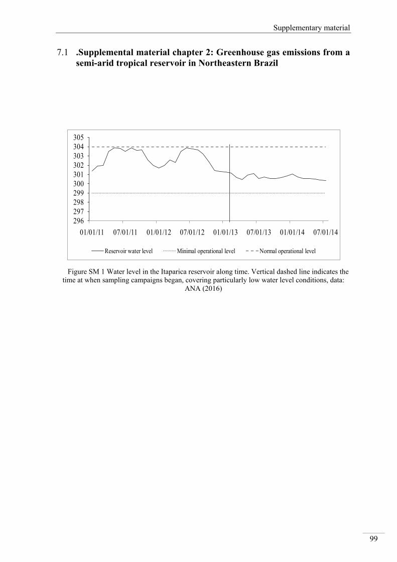
Supplementary material

99

7.1 .Supplemental material chapter 2: Greenhouse gas emissions from a semi-arid tropical reservoir in Northeastern Brazil

Figure SM 1 Water level in the Itaparica reservoir along time. Vertical dashed line indicates the time at when sampling campaigns began, covering particularly low water level conditions, data:

ANA (2016)

296297298299300301302303304305

01/01/11 07/01/11 01/01/12 07/01/12 01/01/13 07/01/13 01/01/14 07/01/14

Reservoir water level Minimal operational level Normal operational level

Supplementary material

100

Figure SM 2 Vertical profiles of a) water temperature, b) pH and c) dissolved oxygen in the water column of each sampling zone in the Itaparica reservoir during every sampling campaign, values are means of water samples of several sites along water depth (taken every 1-5 m depth),

error bars denote standard error

Supplementary material

101

Figure SM 3 (a) Organic carbon content and (b) water content profiles in sediment, values are means of several sediment cores within reservoir sites, values, error bars are standard error

b

a

Supplementary material

102

Figure SM 4 Water parameter correlation to dissolved concentrations of CO2 and CH4. Correlation coefficient is represented accordingly by the size of the ellipse and color scale from

dark red (negative) to dark blue (positive)

Supplementary material

103

Figure SM 5 Linear regression between mean diffusive fluxes (TBL) of (a) CO2 and (b) CH4 with water depth (m)

y = -7.451x + 226.8R² = 0.228

-100

0

100

200

300

400

500

600

700

0 10 20 30 40

Flux

CH

4[m

g m

-2d-1

]

Water depth [m]

b

y = -69.34x + 4908,R² = 0.031

0

4000

8000

12000

16000

20000

0 10 20 30 40

Flux

CO

2[m

g m

-2d-1

]

Water depth [m]

a

Supplementary material

104

Figure SM 6 Boxplots of mean diffusive fluxes (TBL) of (a) CO2 and (b) CH4 in studied sites

Figure SM 7 Non linear regression between ebullitive fluxes and water depth (gas traps with no ebullition included)

y = -0.68ln(x) + 1.218R² = 0.196

-5

0

5

10

15

20

0 2 4 6 8 10 12 14

Flux

CO

2[mg m

-2d-1

]

Water depth [m]

a

y = -0.33ln(x) + 0.588R² = 0.156

-2

0

2

4

6

8

10

12

14

0 2 4 6 8 10 12 14

Flux

CH

4[m

g m

-2d-1

]

Water depth [m]

b

Supplementary material

105

Figure SM 8 Correlation of dissolved CH4 and CO2 in pore water to sediment elements, correlation coefficient is represented accordingly by the size of the ellipse and color scale from

dark red (negative) to dark blue (positive)

Supplementary material

106

Figure SM 9 Mean daily atmospheric parameters measured during October and June 2014. (a) Wind seep (m s-1), (b) Relative humidity (%), (c) Air temperature (°C) (Source: INPE 2016)

0

2

4

6

8

10

12

14

16

18

0 2 4 6 8 10 12 14 16 18 20 22 24

wind

spee

d [m

s-1]

Time [hours]

Wind speed [m s-1]

October 2014

June 2014

0

20

40

60

80

100

120

0 2 4 6 8 10 12 14 16 18 20 22 24

Rela

tive h

umid

ity[%

]

Time [hours]

Relative humidity [%]

October 2014

June 2014

0

5

10

15

20

25

30

35

40

0 2 4 6 8 10 12 14 16 18 20 22 24

Air t

empe

raur

e [°

C]

Time [hours]

Air temperature [°C]

October 2014

June 2014

a

b

c

Supplementary material

107

Figure SM 10 Linear correlation of diffusive fluxes (TBL) of CO2 and CH4 with atmospheric parameters. Relative humidity (%) with (a) CO2, and (b) CH4 and Air temperature (°C) with (c)

CO2 and (d) CH4. Data: INPE (2016)

0102030405060708090

100

0 5000 10000 15000 20000R

elat

ive h

umid

ity [%

]

Flux CO2 mg m-2 d-1

R2= 0.002

0102030405060708090

100

0 100 200 300 400 500 600 700

Rel

ativ

e hum

idity

[%]

Flux CH4 mg m-2 d-1

R2= 0.05

05

101520253035404550

0 5000 10000 15000 20000

Air

tem

pera

ture

[°C

]

Flux CO2 mg m-2 d-1

R2= 0.004c

05

101520253035404550

0 100 200 300 400 500 600 700

Air

tem

pera

ture

[°C

]

Flux CH4 mg m-2 d-1

R2= 0.06d

a

b

Supplementary material

108

Table SM 1 Atmospheric parameter measured during each sampling campaign (n= number of measurements, sd= standard deviation)

sampling campaign n temperature [°C]

relative humidity [%]

wind speed [m s-

1]

range sd range sd range sd

March 2013 7 29.3-35.5 2.3 39.7-59.7 8.0 0.4-3.9 1.2

Sept-October 2013 14 25.1-38.0 3.5 24.9-74.5 12.3 1.6-6.6 1.3

June 2014 7 22.5-30.9 2.7 44-92.8 16.7 2.5-6.5 1.2

October 2014 5 27-31.6 1.7 44.3-61.5 7.0 4.2-6.7 1.0

Table SM 2 Diffusive flux of CO2 and CH4 across the sediment water interface

Site Flux CO2 mg m-2 d-1

Flux CH4 mg m-2 d-

1

LB 5.63 0.8

DB 7.7 1.1

MS 1.6 0.9

Table SM 3 Total emission in the reservoir for each site and emissions pathways

Emission pathway Site

Area[km2] Total Flux CO2

[t year-1]

Total Flux CH4

[sites year-1]

Ebullition LB 167

49±98 75±125

Diffusion LB 3.0105±6.0104 1.1104±4.1103

DB 3.3 3.8104±9.4102 1.9102±63

MS 440.2 4.7105±1.7105

Degassing Dam 3.0104±3.3104

∑ Total Fluxes

8.1105±2.6105 1.5104±5.6103

Supplementary material

109

Emission pathway Site

Area[km2] Total Flux CO2

[t year-1]

Total Flux CH4

[sites year-1]

Total fluxes

[t C year-1]

2.2105±7.1104 1.2104±4.2103

Total fluxes reservoir

[t C year-1]

2.3105±7.45104

CO2 equivalents (GW

1.33106±4.5105

Table SM 4 Comparison of total carbon emissions per area of reservoir

Reservoir Area Km2 MWh

Emissions

t C y-1 t C Km2 year-1

t C MWh-1

Itaparicaa 611 1479 2.3105 375 0.02

Petit sautb 300 116 2.8104 93 0.03

Balbinac 1770 250 2106 1695 1.4

Samueld 559 218 4.3102 0.8 0.0002

Tucurui d 2430 4228 7.5104 31 0.002

Tres Marias d 1040 395 1.7104 165 0.05

Barra Bonita

d 312 140 1.3105 402 0.1

Xingo d 60 3000 3.7104 622 0.001

a=this study, b=Abril et al. 2005, c=Kemenes et al.2011, d=Dos Santos et al. 2006

Supplementary material

110

7.2 Suplemental material chapter 3: Effect of temperature and carbon and nutrients inputs in methane production in sediments of a semiarid tropical reservoir

Figure SM 11 Correlation between Organic Carbon (% of dry weight-1) and water content (%) in sediments of each location. Organic carbon content was strongly positively

related to water content in Littoral (R2= 0.9, p < 0.001) and Intermediate (R2= 0.7, p < 0.001) in comparison to Profundal (R2= 0.4 p < 0.001)

Littoral: y = 0.157x - 5.15R² = 0.9

Intermediate: y = 0.158x + 8.98R² = 0.7

Profundal: y = 0.045x + 2.82R² = 0.4

-5

0

5

10

15

20

25

30

35

0 20 40 60 80 100

Org

anic

Car

bon

(% g

-1 D

W-1

)

Water content

Littoral Intermediate Profundal

Supplementary material

111

Table SM 5 Linear correlation between Methane production (MP µmol g D.W -1) at each incubation temperature and no-amended sediment, to parameters

in dry sediments: water content WA; Organic matter OM [% Dry weight]; Total Nitrogen (TN g Kg D.W -1) and Total Phosphorus (TP g Kg D.W

-1)

Location Parameter MP 20°C MP 30°C MP 40°C

Slope R2 P-value Slope R2 P-value Slope R2 P-value

Littoral

WA

-0.0002 0.1286 0.3089 0.0007 0.2674 0.1259 0.0043 0.2605 0.1317

Intermediate 0.0001 0.0913 0.3960 0.0001 0.0027 0.8875 0.0033 0.0886 0.4036

Profundal 0.0273 0.1680 0.3133 0.0073 0.1932 0.2758 0.0536 0.1702 0.3097

Littoral

OM

-0.0008 0.1265 0.3132 0.0013 0.0425 0.5678 0.0091 0.0481 0.5428

Intermediate 0.0012 0.1232 0.3199 0.0004 0.0010 0.9315 0.0232 0.0869 0.4084

Profundal -0.0519 0.0086 0.8268 -0.0117 0.0071 0.8423 -0.1014 0.0087 0.8262

Littoral

TN

-0.0094 0.3061 0.0971 0.0177 0.1486 0.2713 0.1144 0.1447 0.2782

Intermediate 0.0020 0.0844 0.4153 0.0003 0.0002 0.9726 0.0495 0.0981 0.3781

Profundal -0.0354 0.0037 0.8855 -0.0044 0.0009 0.9424 -0.0689 0.0037 0.8856

Littoral

TP

-0.0487 0.1638 0.2460 0.1611 0.2482 0.1428 1.0611 0.2506 0.1406

Intermediate 0.0049 0.0130 0.7535 -0.0073 0.0025 0.8906 -0.0479 0.0023 0.8957

Profundal -0.2415 0.0341 0.6617 -0.0491 0.0228 0.7211 -0.4655 0.0333 0.6653

Supplementary material

112

Table SM 6 Linear correlation of MP (µmol g D.W -1), at Control treatment (no-substrate addition) , in each incubation temperature to SRP (µg L-1 sed) and

dissolved elements (mg L-1 sed) in pore water of sediments

Location Parameter MP 20°C MP 30°C MP 40°C

Slope R2 P-value Slope R2 P-value Slope R2 P-value

Littoral

SRP

-0.0005 0.8783 0.0807 0.0385 0.7577 0.4513 0.2430 0.7628 0.4334

Intermediate 0.0000 0.7897 0.5999 -0.0640 0.8629 0.3936 -0.0990 0.6121 0.8940

Profundal 0.2710 0.3064 0.8721 0.0595 0.2662 0.9112 0.5050 0.2982 0.8808

Littoral

Al

0.0606 0.2137 0.0152 -0.0468 0.0128 0.5738 -0.3255 0.0144 0.5506

Intermediate -0.0573 0.2149 0.0705 0.0342 0.0645 0.3426 0.0261 0.0060 0.7759

Profundal -0.4567 0.0542 0.4665 -0.1104 0.0506 0.4823 -0.8990 0.0550 0.4632

Littoral

Fe

-0.0003 0.0063 0.7008 -0.0048 0.1196 0.0835 -0.0317 0.1235 0.0784

Intermediate -0.0004 0.0279 0.5516 -0.0006 0.0445 0.4502 -0.0010 0.0197 0.6174

Profundal -0.0263 0.0777 0.3803 -0.0074 0.0987 0.3200 -0.0537 0.0847 0.3586

Littoral

Ca

0.0000 0.0016 0.8319 -0.0007 0.1099 0.0685 -0.0046 0.1117 0.0661

Intermediate 0.0002 0.0064 0.7681 -0.0006 0.0313 0.5121 -0.0009 0.0138 0.6652

Profundal 0.0085 0.0233 0.6354 0.0022 0.0253 0.6216 0.0172 0.0248 0.6251

Littoral

K

-0.0002 0.0040 0.7348 -0.0022 0.0488 0.2321 -0.0145 0.0481 0.2357

Intermediate 0.0018 0.0107 0.7026 -0.0019 0.0102 0.7101 -0.0118 0.0606 0.3581

Profundal -0.3564 0.0857 0.3558 -0.1050 0.1187 0.2728 -0.7344 0.0953 0.3289

Supplementary material

113

Littoral

Mg

-0.0003 0.0049 0.7088 -0.0033 0.0372 0.2984 -0.0215 0.0379 0.2942

Intermediate 0.0000 0.0000 0.9916 -0.0019 0.0270 0.5429 -0.0047 0.0272 0.5412

Profundal 0.1141 0.1102 0.2918 0.0286 0.1106 0.2909 0.2262 0.1135 0.2843

Littoral

Mn

-0.0007 0.0069 0.6810 -0.0078 0.0984 0.1111 -0.0517 0.1007 0.1068

Intermediate -0.0006 0.0006 0.9323 -0.0043 0.0288 0.5456 -0.0020 0.0010 0.9113

Profundal 0.1708 0.0762 0.3852 0.0470 0.0919 0.3380 0.3461 0.0819 0.3673

Littoral

Na

-0.0011 0.0391 0.2948 -0.0040 0.0508 0.2310 -0.0252 0.0467 0.2515

Intermediate -0.0043 0.1920 0.0895 0.0012 0.0133 0.6709 -0.0038 0.0201 0.6001

Profundal 0.0106 0.0039 0.8462 0.0022 0.0027 0.8722 0.0196 0.0035 0.8542

Littoral

S

-0.0040 0.1260 0.3883 -0.0097 0.0807 0.4954 -0.0566 0.0652 0.5418

Intermediate 0.0006 0.2673 0.0852 0.0336 0.1531 0.2085 0.3052 0.2136 0.1303

Profundal -0.0114 0.0331 0.4998 -0.0053 0.1128 0.2034 -0.0274 0.0543 0.3850

Supplementary material

114

Table SM 7 MP (µmol CH4 g D.W-1day-1) resulting from linear regression of CH4 concentrations in the incubations vials along time, the coefficient of determination (R2) is presented within parenthesis.

n.a: data no availale for this layer

Sed layer (cm) Addition treatment MP 20°C MP 30°C MP 40°C MP 20°C MP 30°C MP 40°C MP 20°C MP 30°C MP 40°C0-2 Control 0 ( 0.8 ) 0.08 ( 0.2 ) 0.524 ( 0.8 ) 0.033 ( 0.3 ) 0.039 ( 0.4 ) 0.118 ( 0.7 ) 0.009 ( 0.3 ) 0.011 ( 0.2 ) 0.005 ( 0.2 )0-2 +C/P/N 0.474 ( 0.8 ) 0.443 ( 0.5 ) 0.321 ( 0.3 ) 0.682 ( 0.6 ) 0.661 ( 0.5 ) 0.804 ( 0.8 ) 1.15 ( 0.6 ) 0.839 ( 0.8 ) 0.305 ( 0.5 )0-2 +C 1.115 ( 0.9 ) 0.834 ( 1 ) 0.735 ( 1 ) 0.665 ( 0.7 ) 0.646 ( 0.5 ) 0.674 ( 0.7 ) 1.246 ( 0.6 ) 1.338 ( 0.8 ) 1.209 ( 0.8 )0-2 +P 0 ( 0.7 ) 0.136 ( 0.5 ) 0.372 ( 0.5 ) 0 ( 0.4 ) 0.072 ( 0.1 ) 0.08 ( 0.2 ) 0 ( 0 ) 0 ( 0.1 ) 0 ( 0.4 )0-2 +N 0.008 ( 0 ) 0.191 ( 0.7 ) 0.602 ( 0.7 ) 0 ( 0.4 ) 0.122 ( 0.1 ) 0.11 ( 0.7 ) 0.007 ( 0.7 ) 0.004 ( 0.1 ) 0 ( 0.3 )2-4 Control 0 ( 0.1 ) 0.004 ( 0.1 ) 0.015 ( 0.4 ) 0.021 ( 0.7 ) 0.028 ( 0.6 ) 0.021 ( 0.6 ) 0.53 ( 0.8 ) 0.136 ( 0.1 ) 1.017 ( 0.6 )2-4 +C/P/N 0.32 ( 0.5 ) 0.249 ( 0.4 ) 0.248 ( 0.2 ) 0.161 ( 0.8 ) 0.079 ( 0.3 ) 0.072 ( 0.7 ) 3.431 ( 0.8 ) 1.285 ( 0.7 ) 3.837 ( 0.8 )2-4 +C 0.737 ( 0.6 ) 0.672 ( 0.7 ) 0.675 ( 0.5 ) 0.041 ( 0.6 ) 0.174 ( 0.6 ) 0.246 ( 0.2 ) 4.202 ( 0.9 ) 0.44 ( 0.2 ) 3.613 ( 0.8 )2-4 +P 0 ( 0.6 ) 0.008 ( 0.2 ) 0.08 ( 0.2 ) 0.021 ( 0.6 ) 0.03 ( 0.6 ) 0.02 ( 0.3 ) 0.404 ( 0.8 ) 0 ( 0 ) 1.895 ( 0.8 )2-4 +N 0.019 ( 0.2 ) 0.022 ( 0.3 ) 0.195 ( 0.8 ) 0.023 ( 0.7 ) 0.028 ( 0.4 ) 0.032 ( 0.7 ) 0.511 ( 0.7 ) 0.145 ( 0.1 ) 1.149 ( 0.7 )4-6 Control 0.002 ( 0.1 ) 0.003 ( 0.1 ) 0.038 ( 0.9 ) 0 ( 0.2 ) 0.011 ( 0.1 ) 0.026 ( 0.2 ) 0.018 ( 0 ) 0 ( 0 ) 0 ( 1 )4-6 +C/P/N 0.738 ( 0.9 ) 1.001 ( 0.9 ) 0.848 ( 0.8 ) 0.132 ( 0.8 ) 0.096 ( 0.6 ) 0.115 ( 0.5 ) 0 ( 0.1 ) 0 ( 0.4 ) 2.091 ( 0.4 )4-6 +C 0.657 ( 0.8 ) 0.836 ( 0.8 ) 0.869 ( 0.8 ) 0.122 ( 0.8 ) 0.116 ( 0.2 ) 0.129 ( 0.4 ) 0 ( 0.1 ) 0 ( 0 ) 3.866 ( 0.2 )4-6 +P 0.002 ( 0.3 ) 0.007 ( 0.4 ) 0.01 ( 0.6 ) 0 ( 0.7 ) 0 ( 0.1 ) 0.024 ( 0.3 ) 0 ( 0.9 ) 0 ( 1 ) 0.083 ( 0.2 )4-6 +N 0 ( 0.1 ) 0.532 ( 0.6 ) 0.124 ( 0.6 ) 0 ( 0.1 ) 0.018 ( 0.4 ) 0 ( 0 ) 0 ( 0.8 ) 0 ( 0 ) 1.608 ( 0.5 )6-8 Control 0 ( 0.9 ) 0.002 ( 0.3 ) 0.02 ( 0.2 ) 0 ( 0.1 ) 0.075 ( 0.5 ) 0.125 ( 0.8 ) 0.003 ( 0.4 ) 0.009 ( 0.9 ) 0.004 ( 0.3 )6-8 +C/P/N 0.893 ( 0.8 ) 1.155 ( 0.8 ) 1.185 ( 0.8 ) 0.684 ( 0.6 ) 0.128 ( 0.1 ) 0.181 ( 0.5 ) 0.015 ( 0.6 ) 0.089 ( 1 ) 0.102 ( 0.6 )6-8 +C 1.099 ( 0.7 ) 1.404 ( 1 ) 1.18 ( 0.8 ) 0.934 ( 1 ) 2.19 ( 1 ) 0.224 ( 0.4 ) 0.01 ( 0.6 ) 0.029 ( 0.8 ) 0.043 ( 0.7 )6-8 +P 0.002 ( 0.8 ) 0.005 ( 0.2 ) 0.006 ( 0.4 ) 0.079 ( 0.7 ) 0.202 ( 0.9 ) 0.108 ( 0.9 ) 0.002 ( 0.5 ) 0.003 ( 0.4 ) 0.004 ( 0.6 )6-8 +N 0.017 ( 0.2 ) 0.54 ( 0.5 ) 0.125 ( 0.5 ) 0.075 ( 0.3 ) 0.135 ( 0.4 ) 0.131 ( 0.7 ) 0.005 ( 0.7 ) 0.003 ( 0.3 ) 0 ( 0 )8-10 Control 0.03 ( 1 ) 0.002 ( 1 ) 0 ( 0 ) 0 ( 0.4 ) 0.032 ( 0.4 ) 0.078 ( 0.3 ) n.a n.a n.a8-10 +C/P/N 0.033 ( 0.5 ) 0.027 ( 0.2 ) 0.181 ( 0.9 ) 2.279 ( 1 ) 2.396 ( 1 ) 2.097 ( 1 ) n.a n.a n.a8-10 +C 0.039 ( 0.8 ) 0.051 ( 0.3 ) 0.152 ( 0.3 ) 1.509 ( 1 ) 2.413 ( 1 ) 2.682 ( 1 ) n.a n.a n.a8-10 +P 0.002 ( 0.5 ) 0.002 ( 0.4 ) 0.006 ( 0.2 ) 0 ( 0 ) 0.066 ( 0.7 ) 0.06 ( 0.6 ) n.a n.a n.a8-10 +N 0.014 ( 0.6 ) 0.033 ( 0.1 ) 0.026 ( 0.4 ) 0 ( 0 ) 0 ( 0 ) 0.047 ( 0.6 ) n.a n.a n.a

Location Littoral Intermediate Profundal

Supplementary material

115

Table SM 8 Summary of multi-level analysis of effects on MP of each categorical factor named Locations, sediment layer or substrate addition treatment

Category Statistics Value Categories Estimate ± SE

t value p-value *

Location

Residual SE 0.74 Intercept 0.3± 0.09 3.6 0.0005

Df 207 Intermediate 0.03±0.12 0.3 0.78

Adjusted R-Squared

0.021 Profundal 0.3 ± 0.12 2.4 0.02

F-statistic 3.26 on 2 and 207 Df

P-value 0.04

Sediment Layer

Residual SE 0.75 Intercept 0.4 ± 0.11 3.305 0.00112

Df 205 2-4 0.2 ± 0.16 1.42 0.15

Adjusted R-Squared

0.004 4-6 -0.06 ± 0.16 -0.35 0.72

F-statistic 1.23 on42 and 205 Df

6-8 -0.08 ± 0.16 -0.48 0.62

P-value 0.30 8-10 0.10 ± 0.17 0.59 0.55

Substrate addition treatment

Residual SE 0.66 Intercept 0.073 ±1.10 0.72 0.47

Df 205 +N 0.084 ±0.14 0.58 0.56

Adjusted R-Squared

0.23 +Ps 0.017 0. ± 144

0.12 0.90

F-statistic 16.54 on 4 and 205 Df

+C 0.87 ± 0.14 6.06 6.47 x 10-

9

P-value 9.19 x 10-12 +C/N/P 0.68 ± 0.14 4.74 3.97 x 10-

6

*Statistical significance (P value <0.05) is indicated in bold

According to multi-level analysis, effect on MP was significant related to:

Location- Profundal

Substrate addition treatments - +C and +C/N/P

Supplementary material

116

Table SM 9 Summary of statistics of multi-level analysis, including models without parameter interactions vs. models with parameter interaction. Degrees of freedom (d.f) and

Akaike’s information criterion (AIC).

Model

No interactions

d.f AIC* Model

With interactions

d.f AIC*

Model 1: MP ~ Location+ Sediment layer

8 479.2157 Model 2: MP~ Locatio * Sediment layer

15 442.9448

Model 3: MP ~ Location + Addition treatment

8 424.7726 Model 4:MP~ Location Addition treatment

16 436.4705

Model 5: MP ~ Location + Sediment layer + Addition treatment

12 424.1166 Model 6: MP~ Locatio *Sed. layer* Additio treatment

71 355.0258

*Lowest AIC value between models with and without interactions are presented in bold

According to AIC values preferred interactions models are

Model 2: Location and sediment layer (cm)

Model 6: Location and sediment layer (cm) and amendment treatment

Table SM 10 Summary statistics of selected interaction models Moel2: location and sediment layer; Model 6: Location and sediment layer and addition treatment

Coefficients

Model 2: MP~ Location * Sediment layer

Statistics description

Value Location Sed Layer (cm)

Estimate ± SE

t value Pr(>|t|)

Intermediate 2-4 0.07 ± 0.34 -0.22 0.83

0.2109 Profundal 2-4 1.30 ± 0.35

3.70

0.00031

F-statistic: 5.3 on 13 and 196 DF

Intermediate 4-6 -0.25± 0.35

-0.72

0.47

p-value: 4.1 x 10-8

Profundal 4-6 0.11± 0.35 0.33

0.74

Intermediate 6-8

-0.082±0.35

-0.24 0.81

Profundal 6-8 -0.51± 0.35

-1.47

0.14

Supplementary material

117

Intermediate 8-10 0.95 ± 0.35 2.74

0.007

Profundal 8-10

Coefficients

Model 6: MP~ Location * Sediment layer* Sed. Addition treatment

Statistics description Value Location

Sed layer (cm)

Addition treatment

Estimate ± SE

t value Pr(>|t|)*

Intermediate 2-4 Carbon 0.16±0.80 0.20 0.84

Adjusted R-squared: 0.60 Profundal 2-4 +C -0.54±0.8 -0.67 0.50

F-statistic: 5.08 Intermediate 4-6 +C 0.62 ± 0.8 0.77 0.44

p-value: <2.2 x 10-16 Profundal 4-6

+C 0.65 ± 0.8 0.81 0.42

Intermediate 6-8 +C 1.17 ± 0.8 1.46 0.15

Profundal 6-8

+C -0.21 ± 0.8 -0.26 0.80

Intermediate 8-10 +C 0.48 ± 0.8 0.60 0.55

Profundal 8-10 +C NA NA NA

Intermediate 2-4 Control 0.63 ± 0.8 0.78 0.44

Profundal 2-4 Control

-1.48 ± 0.8 -1.84 0.07

Intermediate 4-6 Control 1.19 ± 0.8 1.48 0.14

Profundal 4-6 Control 0.70 ± 0.8 0.87 0.38

Intermediate 6-8 Control 1.25 ± 0.8 1.55 0.12

Profundal 6-8 Control 1.55 ± 0.8 1.93 0.06

Intermediate 8-10 Control

-1.71 ± 0.8 -2.13 0.04

Profundal 8-10 Control NA NA NA

Intermediate 2-4 +N 0.61 ± 0.8 0.76 0.45

Profundal 2-4

+N -1.44 ± 0.8 -1.79 0.08

Intermediate 4-6 +N 1.03 ± 0.8 1.28 0.20

Profundal 4-6 +N 1.10 ± 0.8 1.37 0.17

Intermediate 6-8 +N 1.13 ± 0.8 1.40 0.16

Profundal 6-8 +N 1.40 ± 0.8 1.74 0.08

Intermediate 8-10

+N -1.69 ± 0.8 -2.11 0.04

Profundal 8-10 +N NA NA NA

Supplementary material

118

Intermediate 2-4 +P 0.58 ± 0.8 0.73 0.47

Profundal 2-4

+P -1.32 ± 0.8 -1.64 0.10

Intermediate 4-6 +P 1.17 ± 0.8 1.46 0.15

Profundal 4-6 +P 0.71 ± 0.8 0.88 0.38

Intermediate 6-8 +P 1.29 ± 0.8 1.61 0.11

Profundal 6-8 +P 1.53 ± 0.8 1.90 0.06

Intermediate 8-10

+P -1.72 ± 0.8 -2.14 0.03

Profundal 8-10 +P NA NA NA

*Statistical significance (P value <0.05) is indicated in bold

According multi-level analysis interactions effects were significant for:

Location Profundal and sediment layer 2-4 and location Intermediate and layer 8-10

Location Intermediate and sediment layer 8-10 and treatments Control or Nitrogen or Phosphorus

Supplementary material

119

Table SM 11 Summary statistics of multi-level analysis of interaction effects of activation energy (E´a) and location, sediment layer or addition treatment on MP. Degrees of freedom

(d.f), estimate ± Standard deviation (SE).

Category Statistics Value Categories Estimate ± SE t value p-value *

Location

Residual SE

40.13 Intercept 3.06 ± 10.0 3

0.31

0.76

d.f 42 Littoral 36.633 ±13.8

2.66

0.01

Adjusted R-Squared

0.11 Profundal 9.97 ± 15.72 0.63

0.53

F-statistic 3.759 on 2

and 42 DF

P-value 0.032

Sediment Layer

Residual SE

43.91 Intercept 12.93 ± 14.66 0.884 0.38

Df 40 2-4 1.45 ± 19.36 0.075 0.94

Adjusted R-Squared

-0.064 4-6

18.08 ± 23.14 0.781 0.44

F-statistic 0.34 on 4 and 40 DF

6-8

6.36 ± 19.36 0.328 0.74

P-value 0.084 8-10 20.4 ± 23.14 0.882 0.38

Addition treatment

Residual SE

39 Intercept -0.1769 10.8234 -0.02 0.99

Df 40 Control 29.01 ± 19.26 0.68 0.51

Adjusted R-Squared

0.16 +N

60.12 ± 18.3 3.29 0.0021

F-statistic 3.09 on 4 and 40 Df

+P

30.68 ± 19.26 1.59 0.12

P-value 0.026 +C 10.43 ± 15.31 0.68 0.50

*Statistical significance (P value <0.05) is indicated in bold According to multi-level analysis effects on Ea were significant related to:

Location Littoral and addition treatment Nitrogen

Supplementary material

120

Table SM 12 Summary statistics of covariance (ANCOVA) models without parameter interactions vs. models with parameter interaction among activation energy values (E´a) and

location, sediment layer and addition treatments. Degrees of freedom (d.f) and Akaike’s information criterion (AIC)

No interaction model d.f AIC Interaction model d.f AIC

Model 7: E´a ~ Location+ Sediment layer

8 472.4511

Model 8: E´a ~ Location * Sediment layer

14 476.4233

Model 9: E´a ~ Location+ addition treatment

8 460.5723

Model 10: E´a ~ Location * addition treatment

16 464.8269

*Lowest AIC value between models with and without interactions are presented in bold According to AIC values, no interaction models were preferred, but the additive models:

Model 7: Location plus sediment layer (cm) Model 9: Location plus addition treatment

Supplementary material

121

7.3 Supplemental material chapter 4: How water level fluctuation impacts greenhouse gas emissions from a tropical semi-arid hydropower reservoir: Economical evaluation and management implications

7.3.1 The empirical economic valuation of greenhouse gas emissions from dams and their lakes

The value of the damage is calculated with the help of integrated climate change economic growth models, (Nordhaus 1994, Cline 1992). Three models called Integrated Assessment Models (IAM) are integrated in a reduced form which allows a relatively easy handling and understanding of the integration, (DICE - Nordhaus 2014; PAGE - Hope 2011; and FUND - Anthoff et al. 2011). These models are based on macroeconomic growth models of the per capita consumption of the world. The growth of per capita consumption without the damages over the next (two) centuries is taken as a reference for the no climate change case. The growth of per capita consumption with climate change and the resulting damages and costs (labelled “business as usual”) are compared to the reference case and the difference constitutes the SCC. Aggregated on a global scale and over the lifetime of the greenhouse gases in the atmosphere and divided by annual emissions, this calculation generates the damage cost per ton of carbon.

The business-as-usual model run can be modified to reflect adaptation to climate change and various forms and degrees of mitigation policies. The estimated social cost of carbon (SCC) depends to a large extent on the structure of the models and on a number of assumptions for some of the central parameters. Some of the parameters are estimates based on expert judgments while other are to large extent based on ethical judgments. As a consequence, the resulting estimates of the SCC are highly uncertain and their description by one mean value only is not adequate, but it should include figures describing the distribution.

Important elements of the models determined externally and which are to a large extent based on ethical considerations concern the aggregation of the estimated damages, e.g.

i) the weights given to damages in countries with low income to aggregate over the regions to arrive at a global figure,

ii) ii) the discount rate as the weight given to future damages when they are aggregated to a current period, and

iii) iii) the question whether to use global or national/regional figures.

The modeling elements are topics of scientific debate and the expectation among the modelers is that they can be resolved with model improvement. There has been an intensive debate, particularly after the Stern Report (Stern 2007) where the authors argued in favor of a very low discount rate. Such topics will not be resolved with model improvement. The practical solution is to use different discount rates and to use different equity weights parallel, which then generates different figures of the SCC.

Another newer topic relates the use of SCC in the context of national-decision-making: In the USA, a number of court cases with respect to the regulation of energy uses led to the obligation of the national agencies to apply SCC in the context of the cost benefit analysis. Here, the question is whether the global damages (and thus the corresponding larger,

Supplementary material

122

aggregated figure) should be used or the figure that capture only the damages in the USA (Gayer &Viscusi2016).

Although the three models mentioned above are classified as IAM in the literature and they are used intensively in policy-making, they show a number of differences which influence their estimates and their position. The lowest value has been calculated with the FUND model because it models a relatively high positive effect of carbon fertilization, at least in the early phases of climate change. The DICE model has been associated with a conservative valuation approach since the author defends relatively high discount rates, generating low values of the SCC under an optimal control scenario, but here the value of SCC for 2015 is already double the value from FUND. In a newer model version, it uses the global objective of limiting climate change to an increase of average temperature to 2°C and thereby reaches a SCC value of 47.6 US $/tCO2, two and half times higher than the value under optimal control. The PAGE model also used in the Stern report (2007) shows in the highest value with a mean of 106 US $/tCO2 for 2011. The major reason is the use of a low discount rate and the weighting of the damages in developing countries with a factor related to the utility of income.

The central values of the SCC have to be put in the context of the high degree of uncertainty under which these estimates are made. The major factors are the long causal chain from emissions to damages, the high complexity of the climate system and its economic implications, and the limited data for calibrating the models, particularly if a temperature increase of more than 2°C is included. Further sources of uncertainties are the effects of potentially extreme events, including the occurrence of tipping points and the limited coverage of the damages which can be expected, but are not included because of their non-market nature. To deal with this uncertainty, the modelers deal with it explicitly, e.g. discussing underlying probability distribution or using Monte Carlo techniques, but the implication on the values of the SCC are communicated together with the central values (mean or median). Most explicit about these issues are the modelers of PAGE which yields a highly skewed distribution to the right, i.e. larger values, with a 5-95% range of 12-290 US $/tCO2 (Hope 2011).

Table SM 13 Estimates of SCC for 2015 by IAM,US $t/CO2 (in 2007 US$)

DICE FUND PAGE Central values Mean Baseline: 18.6

(2015) Optimal control: 17.7 2°C limit damage: 47.6

Mean: 8 Mean: 106

Range of values Parameters

Optimal control: 17.7 With Stern review discounting: 89.8

0.36 US$tCO2; discount rate: 3% 50,7 US $/tCO2; discount rate:0.1%

5-95%: 12-290 (AB1 scenario)

If an option of operating hydropower plants reduces the amount of electricity, these cost become the opportunity costs: They consist of the additional costs expressed as the short term prices minus / plus thechange in the damage cost as aconsequence of the reduction/increase of GHG emission from the substitute electricity generation technology. If the substitute technology is solar or wind, then the damage costs from hydropower can be subtracted. If thesubstitute is coal based or another hydropower plant additional emissions might increase the damage cost.

Supplementary material

123

7.3.2 Electricitity generation costs

In Brazil, a large range of values can also be observed of the short electricity prices as they are calculated for the PLD. In the past 15 years, the average values of the PLD have been within the range of the auctions prices. But the energy crises of 2000/2001, 2007 and the recent crisis (2013-2015) have led to peak prices, between 5 and 8 times this average value. Since these crises were largely due to droughts, an increase in the PLD can be expected as they include the opportunity costs of the water stored for electric generation. When the stored water is reduced as a consequence of the drought, the opportunity costs of the remaining water increase as more (thermal) generation capacity has to be used for a given load, which is more expensive. In other countries, the short term electricity prices has been observed as being volatile as well, but there the question has been to what extent the volatility of the short term prices were the result of the market design as the prices there were the result of market interactions (Borenstein et al. 2002). There has been a debate about the adequacy of the current Brazilian design, but the government has currently abstained from a redesign and focused instead on ensuring the financial viability of the sector (Calabria et al. 2014, Mendes et al. 2016). There filling of the reservoirs in the spring of 2016 saved the sector.

Figure SM 12 Development of PLD prices between 2001 and 2014

Source Calabria et al. 2014

7.3.3 Social cost of carbon

The different assumptions and diverging results of the IAM are making a comparison difficult. As a consequence of a number of governmental agencies in OECD countries and the OECD have undertaken reviews of the models and used the reviews to develop official SCC valuesThe most prominent and best documented are the efforts of an Interagency Working Group (IAWG) in the USA, consisting among others of the US EPA, a number of Departments with environmental responsibilities and the Office of Management and Budget of the White House, relying on the three IAM dealt with above. The IAWG was set up as a consequence of a US court decision demanding that the SCC were to be taken into

Supplementary material

124

account during rulemaking by the US government. The three models were run on homogenuous assumptions (discount rates of 2.5%; 3.0% and 5.0%), no use of equity weights, use of global figures instead of national or regional figures) and based on five socio-economic scenarios. The estimated range of the mean values is relatively small for a given scenario: For the IMAGE scenario with a 3% discount rate DICE generates 35.8 $, PAGE 39.5 $ and FUND 8.2.$/t CO2 while the range increases with declining the discount rates and compared to the 95th percentile value: For PAGE, the values of the mean increase from 8.3$ (5%discount rate), to 39,5 $ (3%) and 65.5$ (2.5%) compared to a 95th percentile value 142.4 $ at a 3% discount rate.

This short survey of various efforts to estimate the values of the social costs of carbon shows that the IAM cannot, contrary to the initial expectations, provide a single value (or manageable small range of values) helpful to identify the optimal path of climate change policy. This is largely due to the inherent complexity and range of the underlying problem which requires the modeling to be supported with a number of assumptions resulting in considerable uncertainty. The major sources of uncertainties are the effects of potentially extreme events, including the occurrence of tipping points and the limited coverage of the damages which can be expected but are not included because of their non-market nature. This leads to two major conclusions: First, most of the values are underestimates1 and second, the best way of presenting the resulting estimates is to provide a central value and an extreme value (or a set of values), providing an indicator of the nature of the distribution. Thus, it has become common to present the mean and an extreme value as a second indicator.

An example is the following presentation of the IAWG (2016).

1In a comparable survey, van den Bergh & Botzen (2012) come to the assessment that a value of 125US$ constitutes a conservative minimum value

Supplementary material

125

The second sources of variation are different value judgments influencing the aggregation procedures, i.e. the use of equity weights and discount rates, and as a third point, the scoping decision as a consequence of the decision context. Following the inconclusive debate after the Stern report, it has become common practice to provide a range of discount rates and show the results as can be seen in most governmental summaries. This has not been true for equity weights: As an academic issue, it gained relatively limited attention (Anthoff and Tol 2010) and the governmental agencies made a decision one way or the other. In the case of the US, no equity weighting was undertaken while the German governmental research agency opted in favor (UBA 2012).

The third point concerns whether to use global or sub-global damage figures when actually using these values in CBA contexts. The existing answers are to a large extent based on value judgments as the anthropogenic climate change is a global issue and a large share of the damages are external to the industrialized countries occurring in poorer developing countries. At the same time, it is a strategic issue and a methodological issue. The global SCC reflects the global benefits of having a global climate policy agreement which achieves a solution of an optimal nature. Currently, such an agreement does not exist and one can summarize the current situation as one where governments take only the national damages into account. When governments make cost benefit calculations of national policies relevant for climate change and make their valuation of the damages explicit, they have a choice between a national level SCC or a global SCC. If they use a global SCC, they anticipate a global agreement as a principle. In the USA, the IAWG has made a decision in favor of a global value, as the German government (UBA 2012). But there are critical views on the position of the US governmental Working Group in the USA which argue that only US Citizens have standing in governmental cost benefit analysis (Gayer and Viscusi 2016).

7.3.4 The National and Global social welfare normative of the SCC

The relatively broad range of SCC values resulting from different value judgments gives the impression that the values are to a large extent arbitrary. In order to structure the implications of these judgments and uncertainties, here two ideal-type positions are developed which correspond to the normative and positive aspects inherent in economics. The normative side can be represented by a global agent implementing a global welfare function, usually assumed when the objective function is formulated to identify an optimal climate change policy.

At the other end of the range, a SCC can be characterized which reflects the calculation based on national interest: This would involve a positive, relatively high discount rate, no equity weight and the restriction to national (or sub-global damages). With the exception of the use of global damages, the modeling of IAWG can be used to calculate the national interest perspective: With a 3% constant discount rate (and no equity weighting), the mean value amounts to 21 US $. If the national perspective would be followed, then only the regional or sub-global share of these global values would be used in the context of national decision-making. The global values are calculated as the aggregation of the values of 9-16 (depending on the IAM) different sub-global regions. PAGE09 calculates that Latin America emits 10.5% of global emissions, causing 7% of the global damage (Hope 2011). With a regional version of DICE, Nordhaus uses the national SCC as starting for a game-theoretic analysis for achieving the global optimum (Nordhaus 2015).

Supplementary material

126

For the perspective of global social welfare, here the modeling of the IAWG is used, but recalculated by (Johnson and Hope 2012) with a lower discount rate of 1.5%, and with global damages, yielding a mean value of 122 US $/ t CO2. Depending on the interaction with the discount rates, the effect of the use of equity varies. Here, the equity weighting from a global perspective is applied which results in a value times 3.0 the unweighted global SCC, based on the application of the FUND model by Anthoff (2011).

Supplementary material

127

References

Abril, G., F. Guerin, S. Richard, R. Delmas, C. Galy-Lacaux, P. Gosse, A. Tremblay, L. Varfalvy, M. A. Dos Santos and B. Matvienko (2005) Carbon dioxide and methane emissions and the carbon budget of a 10-year old tropical reservoir (Petit Saut, French Guiana). Global Biogeochemical Cycles 19(4): GB 4007, doi:4010.1029/2005GB002457.

Agencia Nacional de Aguas (ANA)(2016). Dados hidrológicos em tempo real. from http://www2.ana.gov.br/Paginas/servicos/informacoeshidrologicas/informacoeshidro.aspx

Anthoff, D., Rose, S. Tol, R.S.J., Waldhoff, S (2011) Regional and sectoral estimates of the social cost of carbon: An application of FUND. Economic and Social Research Institute, Dublin(Working Paper 375 ).

Borenstein, S. (2002). The trouble with electricity markets: understanding California's restructuring disaster. The Journal of Economic Perspectives, 16(1), 191-211.

Botzen, W. W., & van den Bergh, J. C. (2012). Risk attitudes to low-probability climate change risks: WTP for flood insurance. Journal of Economic Behavior & Organization, 82(1), 151-166.

Calabria FA, Saraiva JT, Glachant J-M (2014) Enhancing flexibility and ensuring efficiency and security: Improving the electricity market in Brazil via a virtual reservoir model. Robert Schuman Centre for Advanced Studies Research RSCAS 2014/2085 doi:http://dx.doi.org/10.2139/ssrn.2490377

Cline, W. R. (1992). Global warming: The economic stakes. Institute for International Economics.

Dos Santos, M. A., L. P. Rosa, B. Sikar, E. Sikar and E. O. Dos Santos (2006) Gross greenhouse gas fluxes from hydro-power reservoir compared to thermo-power plants. Energy Policy 34(4): 481-488.

Gayer T and Viscusi W. (2016) Determining the Proper Scope of Climate Change Policy Benefits in U.S. Regulatory Analyses: Domestic versus Global Approaches, Review of Environmental Economics and Policy, 10 (2): 245–263, doi: https://doi.org/10.1093

Hope, C. (2011) New Insights from the PAGE09 Model: The Social cost of CO2. Wp 8/2011, Judge Business School.

Instituto Nacional de Pesquisas Espaciais (INPE) (2016). Sistema Integrado de Dados Ambientais (SINDA) Retrieved June 2016, from http://www.inpe.br/.

IPCC. (1997). EFDB. Retrieved 26.08.2016, 2016, from http://www.ipcc-nggip.iges.or.jp/EFDB/main. php.

Johnson, L. T. and C. Hope (2012) The social cost of carbon in US regulatory impact analyses: an introduction and critique. Journal of Environmental Studies and Sciences 2(3): 205-221.

Kemenes, A., B. R. Forsberg and J. M. Melack (2011) CO2 emissions from a tropical hydroelectric reservoir (Balbina, Brazil). Journal of Geophysical Research-Biogeosciences 116: G03004, doi:03010.01029/02010jg001465.

Mendes ALS, de Castro N, Brandão R, Câmara L, Moszkowicz M (2016) The role of imbalance settlement mechanisms in electricity markets: A comparative analysis between UK and Brazil. In: European Energy Market (EEM), 13th International Conference on the, IEEE, pp 1-6

Supplementary material

128

Nordhaus, W. (2015) Climate clubs: overcoming free-riding in international climate policy. The American Economic Review 105(4): 1339-1370.

Schaeffer, R., J. Logan, A. S. Szklo, W. Chandler and J. C. de Souza Marques (2001) Brazil's Electric Power Choices and Their Corresponding Carbon Emissions Implications. Mitigation and Adaptation Strategies for Global Change 6(1): 47-69.

Stern, N. (2007). The economics of climate change: the Stern report. Cambridge, UK.