Graph-Based Inter-Subject Pattern Analysis of fMRI DataSylvain Takerkart1,2*, Guillaume Auzias1, Bertrand Thirion3, Liva Ralaivola2

1 Institut de Neurosciences de la Timone UMR 7289, Aix Marseille Universite, CNRS, Marseille, France, 2 Laboratoire d’Informatique Fondamentale UMR 7279, Aix Marseille

Universite, CNRS, Marseille, France, 3 Parietal Team, INRIA Saclay - Ile-de-France, Saclay, France

Abstract

In brain imaging, solving learning problems in multi-subjects settings is difficult because of the differences that exist acrossindividuals. Here we introduce a novel classification framework based on group-invariant graphical representations,allowing to overcome the inter-subject variability present in functional magnetic resonance imaging (fMRI) data and toperform multivariate pattern analysis across subjects. Our contribution is twofold: first, we propose an unsupervisedrepresentation learning scheme that encodes all relevant characteristics of distributed fMRI patterns into attributed graphs;second, we introduce a custom-designed graph kernel that exploits all these characteristics and makes it possible toperform supervised learning (here, classification) directly in graph space. The well-foundedness of our technique and therobustness of the performance to the parameter setting are demonstrated through inter-subject classification experimentsconducted on both artificial data and a real fMRI experiment aimed at characterizing local cortical representations. Ourresults show that our framework produces accurate inter-subject predictions and that it outperforms a wide range of state-of-the-art vector- and parcel-based classification methods. Moreover, the genericity of our method makes it is easilyadaptable to a wide range of potential applications. The dataset used in this study and an implementation of our frameworkare available at http://dx.doi.org/10.6084/m9.figshare.1086317.

Citation: Takerkart S, Auzias G, Thirion B, Ralaivola L (2014) Graph-Based Inter-Subject Pattern Analysis of fMRI Data. PLoS ONE 9(8): e104586. doi:10.1371/journal.pone.0104586

Editor: Daniele Marinazzo, Universiteit Gent, Belgium

Received April 25, 2014; Accepted July 10, 2014; Published August 15, 2014

Copyright: � 2014 Takerkart et al. This is an open-access article distributed under the terms of the Creative Commons Attribution License, which permitsunrestricted use, distribution, and reproduction in any medium, provided the original author and source are credited.

Data Availability: The authors confirm that all data underlying the findings are fully available without restriction. The dataset used in this study and animplementation of our framework are available on the FigShare web portal at http://dx.doi.org/10.6084/m9.figshare.1086317.

Funding: This study was funded thanks to the Neuro-IC interdisciplinary program of the Centre National pour la Recherche Scientifique, France (CNRS, http://www.cnrs.fr). The funders had no role in study design, data collection and analysis, decision to publish, or preparation of the manuscript.

Competing Interests: The authors have declared that no competing interests exist.

* Email: Sylvain.Takerkart@univ-amu.fr

Introduction

Functional Magnetic Resonance Imaging (fMRI) is a modality

that has proved extremely useful for understanding brain function

as it offers the possibility to map cognitive processes to brain

activation patterns. Traditional univariate analysis methods of

fMRI data process each voxel separately to perform forwardinference [1], that is, identify those voxels that show an activation

profile significantly associated with a given task. With the recently

proposed application of multivariate pattern recognition methods

to fMRI data, one can also make reverse inference, that is, predict

a behavioral variable directly from the imaging data, as in the

pioneering work described in [2]. This new approach, often

referred to as multi-voxel pattern analysis (MVPA), brain decodingor mind reading, has received an increasing amount of attention

over the last few years. The vast majority of papers published so

far (see reviews [3–5]) study the organization of cortical

representations, a problem particularly suited for MVPA since

such representations arise from neural activity distributed across

networks that can cover a large number of fMRI voxels. Another

problem that can be addressed through MVPA techniques is to

examine the consistency of patterns across tasks by testing whether

patterns observed in a given task may arise in different tasks, as in

[6,7]. Finally, one can also use MVPA to characterize patient

groups from fMRI data, in order to identify putative fMRI

biomarkers that could be used in diagnosis tools [8–10]. All

these applications ask for constructing group-invariant

characterizations. Most studies published until today address this

question with a two-level inference, performing MVPA within

subject, and testing the consistency of within-subject classification

scores across individuals. However, this limits the interpretability

of the results because within-subject MVPA often relies on sub-

voxel idiosyncratic information [11]. It is therefore of the highest

interest to address this question more directly by performing inter-

subject MVPA, i.e. by looking for features that are common across

subjects and learning a decision rule on data recorded in a set of

subjects to use it on data from different subjects.

ChallengeThe potentially large inter-individual variability represents a

major challenge to construct group-invariant representations that

will allow for successfull inter-subject MVPA. Only few studies

have directly addressed this question. Most rely on full brain

analysis, using large-scale features that are stable across subjects

after spatial normalization [1]. While a recent study proposes to

use a multi-task framework to handle large scale inter-subject

variability [12], all the others focus on the feature construction/

selection: several papers use univariate feature selection with

different criteria (relative entropy in [13], most active or

discriminative voxels in [14] and [15]); others summarize the

signal present in a set of regions by their mean, using, e.g., cubic

regions [16], anatomically defined regions [17] and [18], or

functionally defined parcels [17]; [19] uses principal component

PLOS ONE | www.plosone.org 1 August 2014 | Volume 9 | Issue 8 | e104586

analysis; finally [20] and [21] use sparse learning methods that

automatically select features. When examining patterns at a finer

spatial scale, inter-individual variability is yet larger and perform-

ing such inter-subject predictions becomes even more challenging.

At such scale, the alignement between cortical folding and the

underlying functional organization vary between subjects [22,23],

in a way that the potentially poor voxel-to-voxel correspondance

provided by spatial normalization procedures limits the general-

ization power of classifiers that use voxel values as features [24].

To our knowledge, only two studies describe methods specifically

designed for inter-subject classification without the need for spatial

normalization. The first one [25] uses Procrustes transformations

to maximally align, in a high-dimensional space, the spatio-

temporal patterns recorded during a specific training experiment.

The second one [26] is a discriminant analysis that projects the

data (through a generalized PCA) onto multiple-subjects factorial

maps designed to maximize class separation. Both these techniques

do not enforce the preservation of the spatial organization of the

input patterns to construct their latent space.

Structured learningIn order to tackle the challenge posed by inter-subject

variability, structural analysis schemes have proved efficient for

forward inference group studies in neuroimaging, as described in

[27,28]. However, no such structural approach has been

developed to perform reverse inference. Our goal here is to

develop a learning framework that specifically aims at predicting a

behavioral variable from imaging data while overcoming inter-

subject variability by exploiting the structural properties of the

input patterns. Such a framework should address three problems:

N What are the structures of interest? In neuroimaging, two main

classes of elementary objects are used in such approaches: points

(local maxima of activation [29]) or regions (clusters of activation

[27], parcels [30]). These functional features can be represented

into a graph to encode their relationships, as it is now classically

done with connectivity-based models of functional or anatomical

networks.

N How is the inter-individual variability conveyed? Regardless of

the chosen feature type, models of inter-individual functional

variability let their location [28] and intensity [31] vary across

subjects.

N What learning method to use? Learning from structured data

can be done with a wide variety of methods, among which,

neural/deep belief networks [32], probabilistic/graphical models

(such as Markov fields [27], hierarchical Dirichlet processes [31]

or Conditional random fields [33]), or large margin kernel-based

methods with appropriately engineered kernels (see [34,35]).

ContributionsIn the present paper, we introduce a Graph-based Support

Vector Classification (G-SVC) framework that respectively

addresses the previous questions by i) using unsupervised learning

to construct attributed graphs that represent fMRI patterns of

activation; the nodes are patches of activation given by a

parcellation algorithm; the graph edges carry the spatial relation-

ships between nodes and their relevant characteristics (location

and activation) are encoded as attributes of the graph nodes;

ii) assuming that both attributes of the nodes can vary across

subjects, i.e. that the inter-individual variability can be character-

ized along these two dimensions; iii) designing a graph similarity

measure (a graph kernel) that is robust to inter-individual

variability, and that makes it possible to perform supervised

learning directly in graph space, for instance by using support

vector classification. These contributions are summarized in

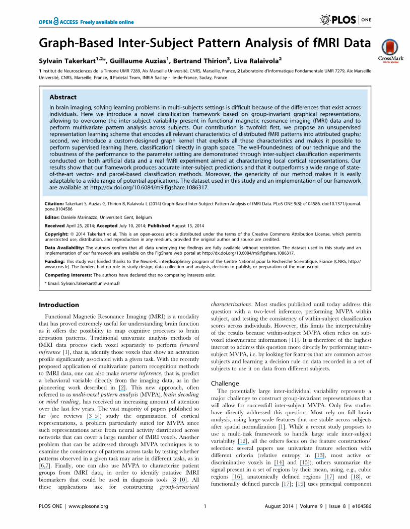
Fig. 1.

While the use of graphical representations of fMRI data has

seen a tremendous boost in the last decade with the fast

development of connectivity analyses (see for instance [36,37]),

graph kernels have only recently been introduced in the

neuroimaging field. The few studies that make use of graph

kernels to solve neuroimaging learning problems address different

sorts of questions (subject classification based on resting-state

functional connectivity [38] or task-based fMRI [39], character-

ization of the mental state of the subject from its connectivity [40]

or activation [41,42] patterns), showing their potential versatility.

Our framework, for which a preliminary study was presented in

[43], falls in the latter category. It is specifically aimed at

overcoming the fine scale functional variability observed in a given

region of interest for a task-based fMRI experiment, which is a key

issue in understanding local neural representations [25,44]. In

such case where using spatial normalization is the bottleneck, our

framework allows to explicitely take into account the different

sources of inter-individual variability without requiring perfect

cross-subject matching of brain anatomy, hereby alleviating the

dependecy of the method to the registration accuracy. Further-

more, it can easily be tuned to address numerous problems

provided one may have at hand a meaningful parcellation for the

question of interest, as for instance in full brain resting state studies

(see a review in [45]) or diffusion weighted-based segmentation of

grey matter regions (as for instance in [46]).

Materials and Methods

2.1 Graph-based Support Vector Classification (G-SVC)The defining task that is usually addressed in inter-subject

MVPA might be stated as the learning of a classifying function fable to reliably predict a categorical experimental variable y from

fMRI data X recorded in a given set of subjects. In order to gain

invariance with respect to the inter-subject variability and be able

to generalize to data from new subjects, we use a graphical

representation X of the input data (described below). Effective

methods have recently emerged to learn from such structured data

([27,31–35], and among those, similarity-based learning approach-

es (nearest-neighbors methods, kernel machines, relevance vector

machines, …) have received much attention. We focus here on

support vector classifiers [47], or SVC, because of their well-

foundedness and their effectiveness in various application

domains, including neuroimaging. Without entering into too

much detail, the most prominent way to perform support vector

classification works by solving the following quadratic problem

(note that we here recall the binary approach to support vector

classification; composition methods such as the well-known one-vs-all or one-vs-one strategies make it possible to directly build

multiclass predictors from the binary method):

mina[Rn

1

2

Xij

aiajyiyjK(Xi,Xj){X

i

ai

s:t:X

i

aiyi~0 and 0ƒaiƒC, Vi

ð1Þ

the solution (a�,b�) of which (where b* is given by the optimality

conditions of the problem) defines a classifier f given by:

f (X )~signX

i

yia�i K(Xi,X ) z b�

!,

Graph-Based Inter-Subject Pattern Analysis of fMRI Data

PLOS ONE | www.plosone.org 2 August 2014 | Volume 9 | Issue 8 | e104586

where f(Xi,yi)gNi~1 is the training data of labeled pairs (Xi, yi),

made of pattern Xi and associated (binary) target yi, Cw0 is a user-

defined (soft-margin) parameter and K is a positive kernel function.

This kernel function implicitly allows one to map the training

patterns Xi’s into a relevant Hilbert space (an idea, known as the

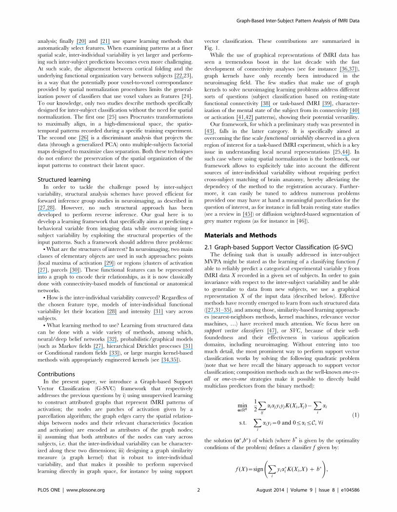
‘kernel trick’, that dates back to [48]) where large-margin linear

classification is possible (see Fig. 2). Choosing/designing an

appropriate kernel for the data at hand, is therefore the crux of

using support vector classification for real-world applications,

knowing that dealing with structured inputs merely requires the

design of a sound kernel.

In what follows, we describe how we build a graphical

representation of functional patterns (section 2.2) and a graph

kernel (section 2.3). With these tools, one can define numerous

classifiers to perform inter-subject fMRI prediction (illustrated on

Fig. 3); here, without loss of generality, we instantiate the support

vector classification framework. Therefore, our graph construction

scheme and graph kernel fully define our Graph-based Support

Vector Classifier (G-SVC) framework.

We assume that for the considered task-based fMRI experi-

ment, we have at our disposal for each subject: i) a pre-defined

contiguous region of interest (ROI) R, ii) the function w describing

the BOLD activation at each experimental trial (each trial

providing a different observation), and iii) a coordinate system v(in practice, we use a 2d cortex-based set of coordinates, which is

more meaningful than working in the 3d volume [49]). Further-

more, we assume that the functional organization of R with

respect to our experiment is consistent across subjects.

Remark. The way we use support vector classification in what

follows departs a little bit from what is suggested by the theory that

supports the use of SVM. Indeed, the classical framework assumes

the training set f(Xi,yi)gNi~1 be made of identically and

independently distributed random pairs, whereas the pairs we

are going to work with may be dependent as different training

pairs (Xi, yi) could relate to the same subject. Carefully

characterizing and taking into account these dependencies is an

important challenge posed by many inter-subject prediction

problem (see [50]) that goes beyond the scope of the present

paper. Ideas taken from [51,52], may lay the theoretical ground to

build relevant and original approaches and constitute the main

axis of our future researches. In any case, our use of SVM is

frequently encountered in the literature, in e.g. information

retrieval problems [53–55], where no particular care of such

dependencies exist and still very good classification results are

achieved.

2.2 Graphical representation of fMRI patternsHere, we detail the unsupervised representation learning

scheme that we use to derive graphical representations from

fMRI activation patterns.

2.2.1 Graphical representation - Parcellation of the

ROI. Assuming that the ROI R admits an underlying subdivi-

sion into a set of smaller and functionally meaningful sub-regions,

the first step to construct our graphical representation consists in

estimating a partition ofR into a set of sub-regions or parcels [30].

Specifically, a parcellation P ofR, is a set P~fPigqi~1 of q parcels

so that the parcels verify: |qi~1Pi ~R and Pi\Pj~60 whenever

i=j.

We use Ward’s hierarchical clustering algorithm to learn the

parcellation in an unsupervised manner. The algorithm starts with

Figure 1. Our contributions: i) attributed graphs are learnt in an unsupervised manner to represent local functional patternsobserved in unregistered subjects; ii) graphs similarities are evaluated by a custom-designed kernel, allowing to solve variousproblems (classification, regression, clustering).doi:10.1371/journal.pone.0104586.g001

Figure 2. The kernel trick: the use of a positive kernel K implicitely maps data from some input space X into a Hilbert space H —thanks to the canonical mapping w : X.w(X )~K(X ,:)— where linear separation is possible.doi:10.1371/journal.pone.0104586.g002

Graph-Based Inter-Subject Pattern Analysis of fMRI Data

PLOS ONE | www.plosone.org 3 August 2014 | Volume 9 | Issue 8 | e104586

one parcel at each point v[R, and iteratively merges two parcels

into one so that the variance across all parcels is minimal, with the

added constraint that two parcels can be merged only if they are

spatially adjacent [56]. The input vector that we used is

fw(v),v(v)gv[R; it combines the anatomical information provided

by the coordinate system v, and the full functional information

available for a given subject (i.e. the activation maps recorded at

each trial for all experimental conditions). Incorporating the

anatomical information on top of the functional features acts as a

spatial regularization process in the search for functionally

meaningful units, which makes the parcellation more robust to

the low contrast-to-noise ratio of the functional data usually

encountered when using MVPA. The resulting parcels constitute

the elementary functional features that are the base elements of

our approach.

2.2.2 Graphical representation - Graph nodes and

edges. We use P as the set of nodes of our graphical

representation, i.e. each parcel defines an elementary functional

feature of the pattern that is represented by a node of the graph.

The set of edges is represented by a binary adjacency matrix

A~(aij)[Rq|q, where aij = 1 if parcels Pi and Pj are connected,

and aij = 0 otherwise. In this work, since we assume that the

topological properties of the patterns are stable across subjects, we

use spatial adjacency as the criterion to decide whether two nodes

are connected (i.e. aij = 1 if Avi[Pi,Avj[Pj so that vi and vj are

neighbors). This defines a region adjacency graph [57] where the

structure of the graph encodes the spatial organization of the

parcels. Note that our method is also fully valid if one had used

other criteria (for instance functional connectivity) to define the

edges of the graph.

2.2.3 Graphical representation - Activation attri-

butes. In a parcel Pi and for a given observation (i.e.

experimental trial), the activation values fw(v)gv[Viare summa-

rized by their mean inside the parcel, that we note W(Pi). We note

W the vector W~½W(P1) � � �W(Pq)� of activation attributes. Note

that, more generally, we may summarize the activation values

measured in Pi using a feature vector W(Pi); this vector could

include the mean, the variance, the skewness, …, or any other

summary statistics.

2.2.4 Graphical representation - Geometric attri-

butes. The geometric information of parcel Pi is summarized

by a feature vector V(Pi), computed from the locations fv(v)gv[Vi.

In this study, we use the coordinates of the center of mass of the

ROI, computed within the coordinate system v. We note V the

matrix of geometric features V~½V(P1) � � �V(Pq)�. As before,

richer geometric information, accounting for instance for the

shape of the parcel, may be considered.

2.2.5 Graphical representation - Full graphical

model. Using these definitions, we have defined an attributed

relational graph [58] G~(P,A,W,V) and described how to learn

such graphical representations in an unsupervised manner. These

graphs fully represent the functional patterns recorded within the

ROI R and carry activation, geometric and structural informa-

tion, as illustrated in Fig. 4.

2.3 Graph similarityAmong the various frameworks that exist to learn from

structured data, what makes similarity-based methods popular is

that the difficulty of the learning process is transferred to that of

defining a similarity function on the space of structured objects at

hand. It turns out that a plethora of graph similarity functions

exist, defined with respect to the number of edit operations needed

to transform one graph to another [59], the number of common

subgraphs of certain type (walks [60], trees [61], graphlets [62]), or

the similarity between vector representations of graphs (see for

instance [63]).

Here, we decide to use a positive kernel as a similarity measure

between graphs: this makes it possible to envision the use of kernel-

based machine learning algorithms (such as the support vectorclassifiers described above), which have proved efficient in this

context [5] and offer solid theoretical guarantees. When choosing

or designing a graph kernel for a given application, one need to

find a good compromise between expressivity (i.e. the ability of the

kernel to capture the features of interest in the available graphs)

and computational efficiency [64]. The recently developed

Weisfeiler-Lehman graph kernel [65] offers such properties (which

has made it the kernel of choice for several recent neuroimaging

applications [39,41,42]) but its applicability is limited to labeled

graphs. Since the key features of our graphical representations are

carried by the real-valued attributes of the nodes, we want to avoid

having to quantify the values of these attributes into discrete labels,

which would imply loosing both some precision and the also the

structure provided by real-valued attributes. We therefore decided

to construct a dedicated kernel. In order for our kernel to provide

a good balance between the two aforementioned criterion, we

followed two directions: on the one hand, our design builds upon

the work of [60] which layed the ground for the construction of

efficient walk-based kernels computable in polynomial time; on the

other hand, the expressivity of our kernel is based on an intuitive

design scheme which aims at exploiting each type of graph features

available in our representation, and in particular its real-valued

node attributes. Below, we describe our design step by step as an

instantiation of the generic family of R-convolution kernels [66],

which are defined as:

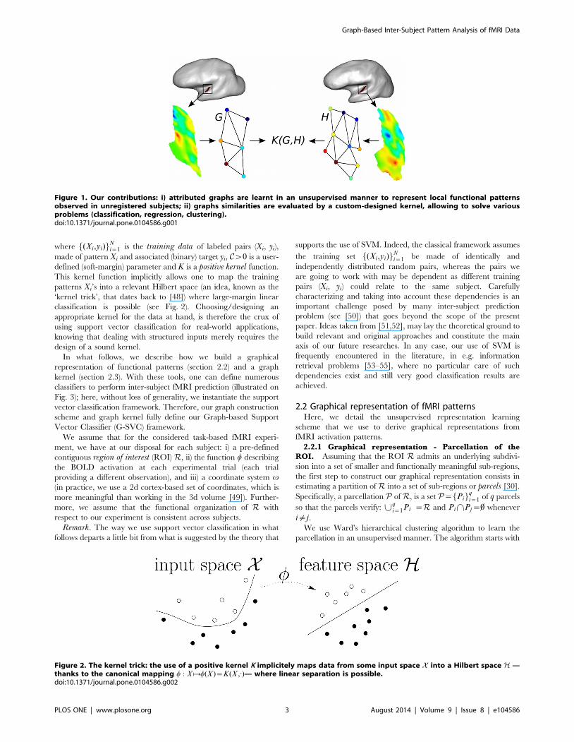
Figure 3. Inter-subject graph-based learning. Equipped with a graph construction scheme and a graph similarity function such asthose designed in this paper, one can define numerous classifiers. The decision function f is learnt on a training set composed of labelledgraphs (Xi, yi), with yi[f1 . . . Cg from a set of subjects, and can be used on graphs from another subject, potentially with a different number of nodes.We here use support vector machines to demonstrate the soundness of this approach when dealing with inter-subject variability of fMRI activationpatterns.doi:10.1371/journal.pone.0104586.g003

Graph-Based Inter-Subject Pattern Analysis of fMRI Data

PLOS ONE | www.plosone.org 4 August 2014 | Volume 9 | Issue 8 | e104586

K(G,H)~X

g(G,h(H

Pt

t~1kt(g,h), ð2Þ

where G and H are two graphs, t[N� is the number of base

kernels kt, which act on subgraphs g and h (for simplicity reasons,

we here use walks of length one; note that the definitions below are

directly extendable to other types of subgraphs).

For two graphs G~(PG,AG,WG,VG) and H~(PH ,AH ,WH ,VH ), we note gij and hkl two pairs of nodes (i.e. walks of

length one) in G and H, respectively; let qG and qH be the number

of nodes in G and H, respectively – note that qG and qH may be

different. Given the nature of our graphical representation, we

define t~3 elementary kernels ks, kg and ka, respectively acting on

structural, geometric and activation information, and thus

covering all characteristics of the graphs.

2.3.1 Graph similarity - Structural kernel. Because the

structure of our graphical representations encodes the spatial

adjacency of the parcels and because we assume that the spatial

organization of the functional patterns is consistent across subjects,

we include a first base kernel ks which aims at valuing the

structural similarity of G and H. We simply adopt the linear kernel

on binary entries aGij and aH

kl of the adjacency matrices AG and AH:

ks(gij ,hk l)~aGij :a

Hkl ð3Þ

It gives 1 if aGij ~1 and aH

kl~1, and 0 otherwise, meaning that

the other base kernels are only taken into account if gij and hkl are

both actual edges. Our kernel in fact compares each edge of a

graph to all edges of the other graph.

2.3.2 Graph similarity - Geometric kernel. Kernel kg acts

on the geometric attributes, i.e. the location of the graph nodes

within the coordinate system v. The goal of this kernel is to match

edges across graphs. To allow for inter-individual differences, we

implement a soft matching by using the following product of

Gaussian kernels:

kg(gij ,hkl)~e{EVG

i{VH

kE2=2s2

g :e{EVG

j{VH

lE2=2s2

g , ð4Þ

where sg[R�z, and VGm (resp. VH

m ) is the mth column of VG (resp.

VH ). The contribution of the following base kernel is therefore be

weighted by this soft matching term, and quasi-zero if the

considered edges are not close to each other.

2.3.3 Graph similarity - Activation kernel. Finally, base

kernel ka is the heart of the functional pattern comparisons since it

handles the functional activation information which carries the

discrimative power for our classification task. This kernel measures

the similarity of the activation levels recorded in parcels of gij and

hkl. As with kg, we use a product of Gaussian kernels:

ka(gij ,hkl)~e{EWG

i{WH

kE2=2s2

a :e{EWG

j{WH

lE2=2s2

a , ð5Þ

where sa[R�z and WGm (resp. WH

m ) is the mth column of WG (resp.

WH ). Using such kernel allows for variations in the activation

attributes across subjects.

2.3.4 Graph similarity - Resulting kernel. With the

definitions of ks, kg and ka, we may define the resulting kernel:

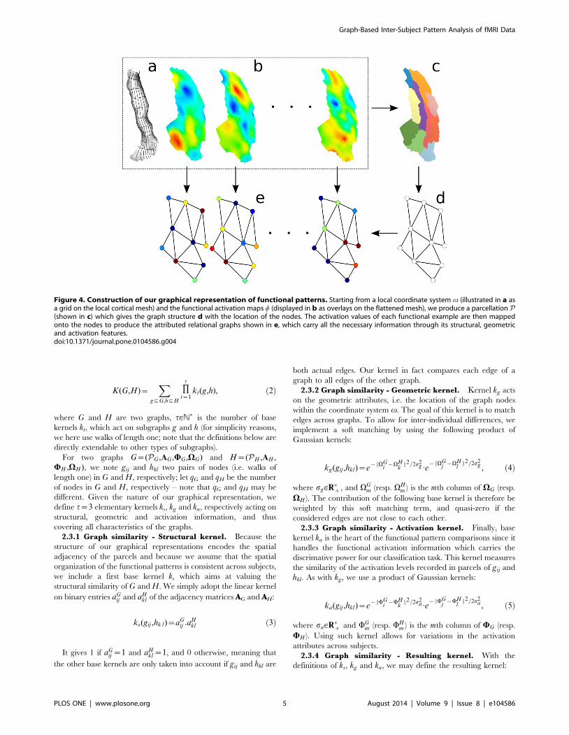
Figure 4. Construction of our graphical representation of functional patterns. Starting from a local coordinate system v (illustrated in a asa grid on the local cortical mesh) and the functional activation maps w (displayed in b as overlays on the flattened mesh), we produce a parcellation P(shown in c) which gives the graph structure d with the location of the nodes. The activation values of each functional example are then mappedonto the nodes to produce the attributed relational graphs shown in e, which carry all the necessary information through its structural, geometricand activation features.doi:10.1371/journal.pone.0104586.g004

Graph-Based Inter-Subject Pattern Analysis of fMRI Data

PLOS ONE | www.plosone.org 5 August 2014 | Volume 9 | Issue 8 | e104586

Ksga(G,H)~XqG

i,j~1

XqH

k,l~1

ks(gij ,hkl):kg(gij ,hkl):ka(gij ,hkl), ð6Þ

This kernel includes two parameters sa and sg, that are the

bandwidths of the activation and geometrical base kernels. In

standard learning problems working with vectorial inputs, a

classical heuristic to estimate the value of the bandwidth of a

Gaussian kernel consists in choosing the median euclidean

distance between all observations in the training dataset [67].

Here, we use this heuristic by choosing the median euclidean

distance between activation and geometric (respectively) attributes

of all nodes and all observations (i.e. all graphs) in the training set.

2.4 Datasets2.4.1 Datasets - Artificial data. The generative model

described here creates artificial datasets that allows to precisely

evaluate G-SVC. Also not designed to simulate patterns with a

spatial organization as complex as in real data, the important point

here is that these patterns contain variations across subjects with

respect to two dimensions, the location of functional features and

their activation levels, which makes these artificial datasets realistic

for that matter and challenging for inter-subject learning

algorithms. By parametrically choosing the amounts of variability

along these two dimensions, we are able to study the robustness of

G-SVC to such functional variability.

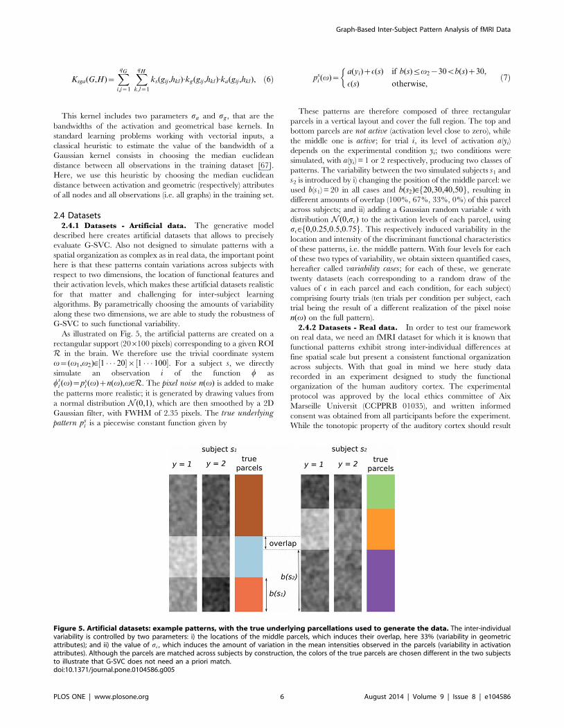
As illustrated on Fig. 5, the artificial patterns are created on a

rectangular support (206100 pixels) corresponding to a given ROI

R in the brain. We therefore use the trivial coordinate system

v~(v1,v2)[½1 � � � 20�|½1 � � � 100�. For a subject s, we directly

simulate an observation i of the function w as

wsi (v)~ps

i (v)zn(v),v[R. The pixel noise n(v) is added to make

the patterns more realistic; it is generated by drawing values from

a normal distribution N (0,1), which are then smoothed by a 2D

Gaussian filter, with FWHM of 2.35 pixels. The true underlyingpattern ps

i is a piecewise constant function given by

psi (v)~

a(yi)zE(s) if b(s)ƒv2{30vb(s)z30,

E(s) otherwise,

�ð7Þ

These patterns are therefore composed of three rectangular

parcels in a vertical layout and cover the full region. The top and

bottom parcels are not active (activation level close to zero), while

the middle one is active; for trial i, its level of activation a(yi)

depends on the experimental condition yi; two conditions were

simulated, with a(yi) = 1 or 2 respectively, producing two classes of

patterns. The variability between the two simulated subjects s1 and

s2 is introduced by i) changing the position of the middle parcel: we

used b(s1) = 20 in all cases and b(s2)[f20,30,40,50g, resulting in

different amounts of overlap (100%, 67%, 33%, 0%) of this parcel

across subjects; and ii) adding a Gaussian random variable E with

distribution N (0,sE) to the activation levels of each parcel, using

sE[f0,0:25,0:5,0:75g. This respectively induced variability in the

location and intensity of the discriminant functional characteristics

of these patterns, i.e. the middle pattern. With four levels for each

of these two types of variability, we obtain sixteen quantified cases,

hereafter called variability cases; for each of these, we generate

twenty datasets (each corresponding to a random draw of the

values of E in each parcel and each condition, for each subject)

comprising fourty trials (ten trials per condition per subject, each

trial being the result of a different realization of the pixel noise

n(v) on the full pattern).

2.4.2 Datasets - Real data. In order to test our framework

on real data, we need an fMRI dataset for which it is known that

functional patterns exhibit strong inter-individual differences at

fine spatial scale but present a consistent functional organization

across subjects. With that goal in mind we here study data

recorded in an experiment designed to study the functional

organization of the human auditory cortex. The experimental

protocol was approved by the local ethics committee of Aix

Marseille Universit (CCPPRB 01035), and written informed

consent was obtained from all participants before the experiment.

While the tonotopic property of the auditory cortex should result

Figure 5. Artificial datasets: example patterns, with the true underlying parcellations used to generate the data. The inter-individualvariability is controlled by two parameters: i) the locations of the middle parcels, which induces their overlap, here 33% (variability in geometricattributes); and ii) the value of sE, which induces the amount of variation in the mean intensities observed in the parcels (variability in activationattributes). Although the parcels are matched across subjects by construction, the colors of the true parcels are chosen different in the two subjectsto illustrate that G-SVC does not need an a priori match.doi:10.1371/journal.pone.0104586.g005

Graph-Based Inter-Subject Pattern Analysis of fMRI Data

PLOS ONE | www.plosone.org 6 August 2014 | Volume 9 | Issue 8 | e104586

in a reproducible topographical organization of the activation

maps across subjects, it has been shown that these functional maps

suffer from a large variability across subjects [68,69]. Such dataset

therefore represents an adequate challenge for our framework.

For each of the ten subjects, a T1 image was acquired (1 mm

isotropic voxels). Each stimulus consisted of a 8 s sequence of 60

isochronous tones covering a narrow bandwidth around a central

frequency n. There were five types of sequences (i.e. five conditions

y[½1,5� corresponding to five classes of patterns), each one

centered around a different frequency n[f300Hz,500Hz,1100Hz,2200Hz,4000Hzg, with no overlap between the band-

widths covered by any two types of stimuli. Five functional sessions

were acquired, each containing six sequences per condition

presented in a pseudo-random order. Echo-planar images (EPI)

were acquired with slices parallel to the sylvian fissure (repetition

time = 2.4 s, voxel size = 26263 mm, matrix size 1286128).

The preprocessing of the functional data, carried on in SPM8[1], consisted of slice timing correction and realignment. Then, a

generalized linear model was performed (using nipy [70]) with one

regressor of interest per stimulus. The weights of these regressors

(beta coefficients) were used to compute the inputs of the classifiers

because they provide a robust estimate of the response size for

each stimulus [71]. We then used freesurfer [72] to extract the

cortical surface from the T1 image and automatically delineate the

primary auditory cortex (Heschl’s gyrus) as it is defined in the

Destrieux atlas [73], thus obtaining two cortical ROIs R for each

subject (one in each hemisphere). Note that this definition of R,

which implictly uses a spatial normalization, was chosen because it

is fully automatic; other strategies working in the subjects’ native

spaces (manual drawing on the anatomy, functional definition)

could also have been used.

In order to compute the graphical representations and apply

our G-SVC framework, one need to define the function w and a

coordinate system v. For this, we fully work in the subject’s native

space, i.e. without having to perform spatial normalization of the

data into a common space. The function w is the result of two

operations executed in freesurfer: first, the beta maps obtained

above are projected onto the subject’s individual cortical mesh,

and second, a slight spatial smoothing is performed along the

cortical surface (equivalent FWHM of 3 mm). The values of w are

then linearly normalized to the [0,1] interval within the ROI R.

Several examples (for different observations) of the values of wwithin the region R are shown on Fig. 4. Furthermore, since

Heschl’s gyrus has a rectangular-like shape (with another region of

the Destrieux atlas on each side), we can define a 2D local

coordinates system through a conformal mapping of R onto a

rectangle (with a local version of the method described in [74]),

defining (v1(v),v2(v),)v[R[½0,1�2. It is illustrated as a coordinate

grid on Fig. 4. Note that forcing v[½0,1�2 separately for each

subject allows dealing with the case where the size and shape of Ris different across subjects.

2.5 Evaluation frameworkIn this section, we briefly describe the experiments that we

perform, the state of the art methods chosen to benchmark our G-

SVC framework, as well as the methodology used to compare the

performances of the different algorithms.

2.5.1 Evaluation – Experiments. The first set of experi-

ments consists in testing G-SVC and state-of-the-art vector-based

methods on the artificial datasets. Since in these datasets, the

amount of inter-individual variability is parametrically controlled

along two dimensions (the location and activation levels of

functional features in the pattern), studying the differential

performances of G-SVC and benchmark methods for each

variability case allows identifying the type(s) and amount(s) of

functional variability for which G-SVC offers improved robust-

ness. Then a series of experiments conducted on the real fMRI

dataset makes it possible to i) overall compare the performances of

G-SVC to those produced by state-of-the-art vector-based

methods; ii) evaluate the influence of the number of graph nodes,

compare the performances of G-SVC to those produced by

standard parcel-based methods and examine the influence of

working with individual vs. group parcellations; iii) test the

robustness of G-SVC when its inputs are graphs with different

numbers of nodes; iv) examine the usefulness of each of the three

base kernels; and v) assess the stability in the estimation of the

values of the kernel hyper-parameters.

2.5.2 Evaluation - State-of-the-art vector- and parcel-

based methods. In order to benchmark our G-SVC frame-

work, we compare its performances to state-of-the-art inter-subject

classification methods. The standard strategy to solve such inter-

subject problem is to obtain a point-to-point mapping across

individuals for the spatial domain of interest. This indeed allows

flattening a pattern into a feature vector that is used as input for

the classification algorithms. In our artificial datasets, the

rectangular regions are matched across subjects by construction.

In the real experiment where the regions might be slightly different

from subject to subject, such feature vector can be constructed

using a spatial normalization procedure, i.e. by bringing the data

from all subjects into a common standard space. We here used the

surface-based normalization process available in freesurfer, which

provides a vertex-to-vertex correspondance across all subjects in

the common fsaverage space. The function w that was defined in

each individual subject’s space (see section 2.4) is resampled into

this common space, and its values within the ROI (defined as the

intersection of all the individual regions projected in the common

space) makes up the common feature vector. Several classification

algorithms, chosen because they have shown to be efficient for

MVPA, are then tested, each time with a large set of values for

their respective hyper-parameters: 1) linear SVC; 2) nonlinear

SVC, with Gaussian (with c[f2{ngn[½0���25�) and polynomial (of

order n[f2,3,4g) kernels; 3) k-nearest neigbors (with

k[f3,5,7,9,15,20g); 4) logistic regression with l1 and l2 regular-

ization (with weight l[f2ngn[½{5���10�). The parameter sets were

empirically selected to ensure capturing the optimal performances

of each of these algorithms for all the experiments described

above.

Moreover, we also tested parcel-based methods as benchmarks

for G-SVC. Once the data is projected in the standard space

described above, one can compute a group parcellation for all

subjects by using the anatomo-functional parcellation algorithm

described previously, but with functional input features coming

from all available subjects at training time. The parcels are thus

naturally mapped to one another across subjects, and we can use a

feature vector composed of the mean activation within each parcel

(equivalent to the graph activation attributes W) as input to any of

the classification methods described above. Furthermore, using

this group-parcellation, one can also construct graphical repre-

sentations and use our kernel to perform inter-subject predictions;

we denote this method as G-SVCg, as opposed to G-SVC when

using individual parcellations. Comparing G-SVC with the results

obtained with G-SVCg and the other parcel-based benchmark

methods was sued to clarify the role of using graphical

representations learnt from individual parcellations and the

usefulness of our graph metric itself.

2.5.3 Evaluation - Performance evaluation and algorithms

comparison. Amongst the wide range of metrics available for

Graph-Based Inter-Subject Pattern Analysis of fMRI Data

PLOS ONE | www.plosone.org 7 August 2014 | Volume 9 | Issue 8 | e104586

measuring the performances of classification methods, we selected

the global classification accuracy, i.e. the fraction of correct

predictions amongst all attempted predictions (one reflecting a

perfect prediction score). Indeed, the design of both the artificial

and real datasets used in this study yield balanced classes (identical

number of observations in each class and each subject), and it has

been shown that the global classification accuracy is perfectly

adapted to such case [75]. For G-SVC, we report the global

classification accuracy for different values of its hyper-parameters;

for the benchmark methods, we report the highest accuracy

obtained across all values of their hyper-parameters, thus putting

G-SVC in the hardest possible case for performance comparison.

Since the different observations recorded in a given subject can

be correlated, it is crucial to use a testing dataset composed of

observations from subjects that were not part of the training

dataset. We perform a leave-one-subject-out cross-validation and

look at the average classification accuracy across folds, which is a

natural strategy to measure the performance of an inter-subject

classification algorithm. Assessing the significance of such an

average classification accuracy and comparing different methods

using the same scheme require a carefully elaborated evaluation

method, that should for instance avoid employing Student’s t test[76]. A solution is to use non-parametric tests. Here, we focus on

comparing algorithms, and we apply two permutation tests that

allow estimating the distribution of the null hypothesis that the

algorithms perform identically. The first test (hereafter called

test1), described in [77], allows to compare the performance scores

of two algorithms by generating random sign permutations of the

paired performance differences. The second one (hereafter called

test2), described in [78], is a randomized ANOVA that allows to

compare curves describing the performance of several algorithms

in function of the value of one hyper-parameters shared by the

different methods.

Results

3.1 Results on artificial data - G-SVC vs. vector-basedmethods

In the artificial datasets, the true number of parcels composing

the patterns is known by construction (three). Therefore we used

the corresponding number of nodes, q = 3, in the graph

construction phase of our G-SVC framework. We compared the

results given by G-SVC with the performances of the different

vector-based benchmark methods. For each variability case, we

used test1 to assess whether G-SVC performs at a different level

than each of the vector-based benchmark methods. The mean

results (across the twenty datasets randomly generated for each

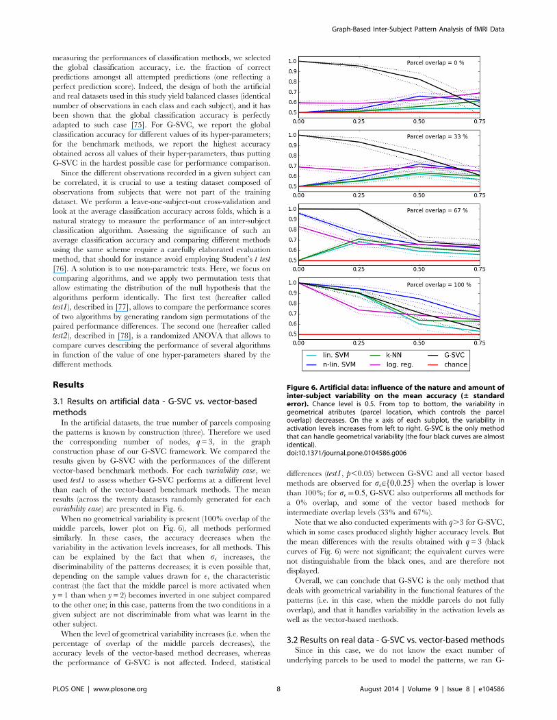
variability case) are presented in Fig. 6.

When no geometrical variability is present (100% overlap of the

middle parcels, lower plot on Fig. 6), all methods performed

similarly. In these cases, the accuracy decreases when the

variability in the activation levels increases, for all methods. This

can be explained by the fact that when sE increases, the

discriminability of the patterns decreases; it is even possible that,

depending on the sample values drawn for E, the characteristic

contrast (the fact that the middle parcel is more activated when

y = 1 than when y = 2) becomes inverted in one subject compared

to the other one; in this case, patterns from the two conditions in a

given subject are not discriminable from what was learnt in the

other subject.

When the level of geometrical variability increases (i.e. when the

percentage of overlap of the middle parcels decreases), the

accuracy levels of the vector-based method decreases, whereas

the performance of G-SVC is not affected. Indeed, statistical

differences (test1, p,0.05) between G-SVC and all vector based

methods are observed for sE[f0,0:25g when the overlap is lower

than 100%; for sE~0:5, G-SVC also outperforms all methods for

a 0% overlap, and some of the vector based methods for

intermediate overlap levels (33% and 67%).

Note that we also conducted experiments with q.3 for G-SVC,

which in some cases produced slightly higher accuracy levels. But

the mean differences with the results obtained with q = 3 (black

curves of Fig. 6) were not significant; the equivalent curves were

not distinguishable from the black ones, and are therefore not

displayed.

Overall, we can conclude that G-SVC is the only method that

deals with geometrical variability in the functional features of the

patterns (i.e. in this case, when the middle parcels do not fully

overlap), and that it handles variability in the activation levels as

well as the vector-based methods.

3.2 Results on real data - G-SVC vs. vector-based methodsSince in this case, we do not know the exact number of

underlying parcels to be used to model the patterns, we ran G-

Figure 6. Artificial data: influence of the nature and amount ofinter-subject variability on the mean accuracy (± standarderror). Chance level is 0.5. From top to bottom, the variability ingeometrical atributes (parcel location, which controls the parceloverlap) decreases. On the x axis of each subplot, the variability inactivation levels increases from left to right. G-SVC is the only methodthat can handle geometrical variability (the four black curves are almostidentical).doi:10.1371/journal.pone.0104586.g006

Graph-Based Inter-Subject Pattern Analysis of fMRI Data

PLOS ONE | www.plosone.org 8 August 2014 | Volume 9 | Issue 8 | e104586

SVC with a fixed number of nodes q for all subjects, and repeated

the analysis for q[f5,10,15,20,25,30,35,40g. We chose the smaller

value of q to be five because according to the functional

architecture of the primary auditory cortex, the five stimuli used

in our experiment should result in at least five different activated

regions [68,69]. Table 1 contains the performances of G-SVC vs.

the vector-based benchmark methods. For the benchmark

methods, the reported score is the highest accuracy obtained

across all values of their hyper-parameters; for G-SVC, we report

the highest and lowest accuracy levels obtained across all values of

q. All vector-based methods performed fairly similarly, with

accuracy levels between 0.27 and 0.31, i.e. slightly higher than

chance level (0.2). G-SVC yielded higher level of accuracies in all

cases, with performances between 0.39 and 0.56, depending on q.

In the right hemisphere, the performance differences between both

the highest and lowest accuracies obtained with G-SVC and any

benchmark methods is statistically significant (test1, p,0.05). In

the left hemisphere, the highest and lowest accuracies of G-SVC

are significantly higher (test1, p,0.05) than the best accuracies

produced by linear SVM, and the l1- and l2-logistic regressions;

the mean differences between the accuracy of G-SVC and the

ones of nonlinear SVM and k-nearest neighbors are large (the

lowest G-SVC score is 0.39, compared to 0.30 for nonlinear SVM

and k-NN), but not significant.

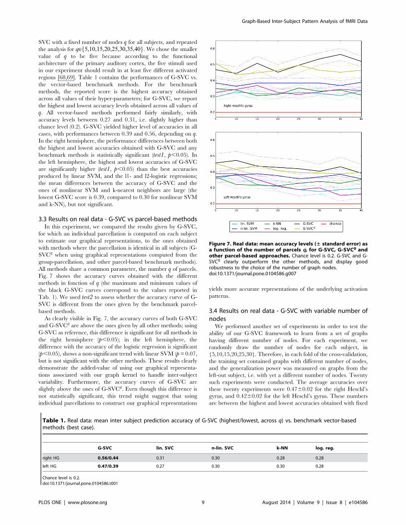
3.3 Results on real data - G-SVC vs parcel-based methodsIn this experiment, we compared the results given by G-SVC,

for which an individual parcellation is computed on each subject

to estimate our graphical representations, to the ones obtained

with methods where the parcellation is identical in all subjects (G-

SVCg when using graphical representations computed from the

group-parcellation, and other parcel-based benchmark methods).

All methods share a common parameter, the number q of parcels.

Fig. 7 shows the accuracy curves obtained with the different

methods in fonction of q (the maximum and minimum values of

the black G-SVC curves correspond to the values reported in

Tab. 1). We used test2 to assess whether the accuracy curve of G-

SVC is different from the ones given by the benchmark parcel-

based methods.

As clearly visible in Fig. 7, the accuracy curves of both G-SVC

and G-SVCg are above the ones given by all other methods; using

G-SVC as reference, this difference is significant for all methods in

the right hemisphere (p,0.05); in the left hemisphere, the

difference with the accuracy of the logistic regression is significant

(p,0.05), shows a non-significant trend with linear SVM (p = 0.07,

but is not significant with the other methods. These results clearly

demonstrate the added-value of using our graphical representa-

tions associated with our graph kernel to handle inter-subject

variability. Furthermore, the accuracy curves of G-SVC are

slightly above the ones of G-SVCg. Even though this difference is

not statistically significant, this trend might suggest that using

individual parcellations to construct our graphical representations

yields more accurate representations of the underlying activation

patterns.

3.4 Results on real data - G-SVC with variable number ofnodes

We performed another set of experiments in order to test the

ability of our G-SVC framework to learn from a set of graphs

having different number of nodes. For each experiment, we

randomly draw the number of nodes for each subject, in

{5,10,15,20,25,30}. Therefore, in each fold of the cross-validation,

the training set contained graphs with different number of nodes,

and the generalization power was measured on graphs from the

left-out subject, i.e. with yet a different number of nodes. Twenty

such experiments were conducted. The average accuracies over

these twenty experiments were 0.4760.02 for the right Heschl’s

gyrus, and 0.4260.02 for the left Heschl’s gyrus. These numbers

are between the highest and lowest accuracies obtained with fixed

Table 1. Real data: mean inter subject prediction accuracy of G-SVC (highest/lowest, across q) vs. benchmark vector-basedmethods (best case).

G-SVC lin. SVC n-lin. SVC k-NN log. reg.

right HG 0.56/0.44 0.31 0.30 0.28 0.28

left HG 0.47/0.39 0.27 0.30 0.30 0.28

Chance level is 0.2.doi:10.1371/journal.pone.0104586.t001

Figure 7. Real data: mean accuracy levels (± standard error) asa function of the number of parcels q, for G-SVC, G-SVCg andother parcel-based approaches. Chance level is 0.2. G-SVC and G-SVCg clearly outperform the other methods, and display goodrobustness to the choice of the number of graph nodes.doi:10.1371/journal.pone.0104586.g007

Graph-Based Inter-Subject Pattern Analysis of fMRI Data

PLOS ONE | www.plosone.org 9 August 2014 | Volume 9 | Issue 8 | e104586

q for all subjects (see Tab. 1). In only 6 of the 40 cases (20 for each

hemispheres) was the accuracy significantely lower than the

highest one obtained with fixed q (test1, p,0.05). This set of

experiment shows that G-SVC can handle graphs with different

number of nodes, and therefore is robust to some structural

variation between the graphical representations learnt from

different observations/subjects.

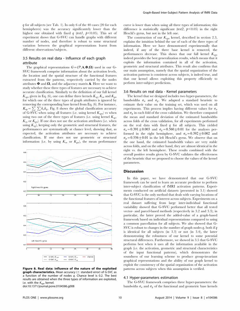
3.5 Results on real data - Influence of each graphattribute

The graphical representations G~(P,A,W,V) used in our G-

SVC framework comprise information about the activation levels,

the location and the spatial structure of the functional features

extracted from the patterns, respectively carried by the nodes

attributes W and V, and the adjacency matrix A. Here we want to

study whether these three types of features are necessary to achieve

accurate classification. Similarly to the definition of our full kernel

Ksga given in Eq. (6), one can define three kernels Ksg, Ksa and Kga

for which one of the three types of graph attributes is ignored by

removing the corresponding base kernel from Eq. (6). For instance,

Ksg~P P

kskg. Fig. 8 shows the global classification accurary

of G-SVC when using all features (i.e. using kernel Ksga) vs when

using two out of the three types of features (i.e. using kernel Ksg,

Ksa or Kga). If one does not use the activation attributes (i.e. when

using Ksg), keeping only the geometric and structural features, the

performances are systematically at chance level, showing that, as

expected, the activation attributes are necessary to achieve

classification. If one does not use geometric or structural

information (i.e. by using Ksa or Kga), the mean performance

curve is lower than when using all three types of information; this

difference is statistically significant (test2, p,0.05) in the right

Heschl’s gyrus, but not in the left one.

The construction of our Ksga kernel, described in section 2.3,

explains the intuition behind the use of each of the three types of

information. Here we have demonstrated experimentally that

indeed, if any of the three base kernel is removed, the

performances decrease. This shows that our full kernel Ksga

indeed provides the best generalization results, which means that it

exploits the information contained in all of the activation,

geometric and structural attributes. This result also confirms that

our main assumption, namely that the spatial organization of the

activation patterns is consistent across subjects, is indeed true, and

that our kernel allows exploiting this property efficiently to

perform inter-subject predictions.

3.6 Results on real data - Kernel parametersThe kernel that we designed includes two hyper-parameters, the

bandwidths sa and sg. We adapted a standard heuristic to

estimate their value on the training set, which was used on all

experiments. This process implies having different values for sa

and sg in each fold of the cross validation. We therefore computed

the mean and standard deviation of the estimated bandwidths

across folds of the cross validation, for all experiments performed

on the real data with fixed q for all subjects. This yielded

sa~0:391+0:003 and sg~0:560+0:01 for the analyses per-

formed in the right hemisphere, and sa~0:392+0:002 and

sg~0:556+0:01 in the left Heschl’s gyrus. We observe that on

the one hand, the estimated bandwidth values are very stable

across folds, and on the other hand, they are almost identical in the

right vs. the left hemisphere. These results combined with the

overall positive results given by G-SVC validates the effectiveness

of the heuristic that we proposed to choose the values of the kernel

parameters.

Discussion

In this paper, we have demonstrated that our G-SVC

framework can be used to learn an accurate predictor to perform

inter-subject classification of fMRI activation patterns. Experi-

ments conducted on artificial datasets (presented in 3.1) showed

that G-SVC is the only method that deals with varying locations of

the functional features of interest across subjects. Experiments on a

real dataset suffering from large inter-individual functional

variability showed that G-SVC performed better that all tested

vector- and parcel-based methods (respectively in 3.2 and 3.3); in

particular, the latter proved the added-value of a graph-based

framework based on individual representations compared to using

a common parcellation for all subjects. We also showed that G-

SVC is robust to changes in the number of graph nodes q, both if qis identical for all subjects (in 3.3) or not (in 3.4), the latter

demonstrating the robustness of our kernel to some potential

structural differences. Furthermore, we showed in 3.5 that G-SVC

performs best when it uses all the information available in the

graph (i.e. the activation, geometric and structural characteristics

of the input functional patterns), which demonstrates the

soundness of our learning scheme to produce group-invariant

graphical representations and the ability of our graph kernel to

exploit the consistency of the spatial organization of the activation

patterns across subjects when this assumption is verified.

4.1 Hyper-parameters estimationThe G-SVC framework comprises three hyper-parameters: the

bandwiths sa and sg of the functional and geometric base kernels

Figure 8. Real data: influence of the nature of the exploitedgraph characteristics. Mean accuracy (6 standard error) of G-SVC asa function of the number of nodes q. Chance level is 0.2. The bestresults are obtained when the three types of information are exploited,i.e. with the Ksga kernel.doi:10.1371/journal.pone.0104586.g008

Graph-Based Inter-Subject Pattern Analysis of fMRI Data

PLOS ONE | www.plosone.org 10 August 2014 | Volume 9 | Issue 8 | e104586

used to design the full Ksga kernel, and the number of nodes q of

the constructed graphs. For the former two, we have proposed a

heuristic that estimates the values of sa and sg on the training

dataset. This heuristic selects the median distance between the

corresponding attribute values of the observations of the training

set. It is simple to implement and the results shown in this paper

demonstrate its effectiveness, thus providing an easy way to

automatically select the values of these two hyper-parameters.

Regarding the number of graph nodes q, we hereafter describe

three potential strategies for choosing q that explore three different

directions. First, we have shown that when q is chosen identical for

all subjects, G-SVC is robust with regards to the selected value

since it significantely outperforms benchmark methods for almost

all values of q (see Fig. 7). In order to choose the value of q, one

can therefore exploit prior knowledge about the functional

properties of the studied region, as we did in this study with the

architecture of the primary auditory cortex [68,69]. Second, in

paragraph 0, we also showed that G-SVC can handle input graphs

with different number of nodes q. This suggests that one could

attempt to work at the individual level to optimize the graphical

representation of such distributed patterns. One simple strategy to

do so could be to apply a standard univariate analysis on each

subject of the training set, and use the number of significantly

activated clusters across all experimental conditions as a lower

bound for q. Finally, if one need a fully automatic strategy, the

value of q can be chosen in a nested cross validation amongst a

given list of values that can be constructed using any of the

aforementioned strategies.

4.2 Linear vs nonlinear classifiersSince G-SVC uses a graph kernel to find a nonlinear decision

boundary in the original data space, it is in fact a nonlinear SVM

classifier. The usefulness of such nonlinear classifiers for neuro-

imaging applications is the subject of an on-going debate in the

litterature (see the introduction of [79] for a summary). The appeal

of linear classifiers for fMRI applications is mainly twofold: i) they

facilitate the interpretation of the classification results, for instance

thanks to the ability to directly visualize weight maps when

working with linear SVM [80]; and ii) despite their simplicity, their

performances always are amongst the highest [81]. Regarding the

first point, [79] offers a solution to ease the interpretation of the

results given by nonlinear classifiers by visualizing sensitivity maps.

As for the second point, our study is a new example where a

nonlinear method clearly outperforms linear classifiers.

While it is not the focus of this paper, note that our framework is

directly applicable to the equivalent within-subject learning task

(see results in Table S1). In this easier task, G-SVC produces mean

accuracy levels that are not statistically higher than those of vector-

based methods.

Therefore G-SVC allows reaching higher accuracy rates than

benchmark methods for the inter-subject classification task, but

not for the within-subject one. We believe that it is the case

because i) we have identified a factor that contributes to the poor

performances of standard, and in particular linear, methods (the

inter-individual variability) for the selected learning problem

(inter-subject classification), ii) we use prior knowledge to model

the influence of this factor and exploit it into the design of a

nonlinear classifier (here, to construct a graph kernel), and iii) we

allow the classifier to work in a fairly low-dimensional space (our

graph construction scheme uses a small number of parcels, and

therefore acts as a dimensionality reduction process), thus offering

a reasonable ratio between the sample size (number of observa-

tions available) and the dimensionality of the space in which the

classification is performed. These three points could constitute a

set of rules that can help identify questions for which it might be

worth developing nonlinear classifiers in neuroimaging.

Moreover, this interpretation is consistent with another

explanation for the potential usefulness of nonlinear methods,

that was for instance described in [82]. Building upon the example

of the quadratic kernel, which is equivalent to adding features

equal to the products (i.e. the interactions) between the original

features, one could understand the added value of nonlinear

models when such interactions are related to the experimental

variable y to be predicted. In the case of our G-SVC framework,

the graphical representation explicitely encodes some these

potential interactions by linking spatially adjacent parcels:

therefore, instead of using all interactions terms between original

features (as with the quadratic kernel), only a subpart of these

interactions are considered, those for which there exist an edge

between graph nodes. Our G-SVC framework takes advantage of

these interactions because the Ksga kernel directly uses the

information carried by the graph edges.

4.3 Examining assumptions and potential applicationsThe G-SVC framework in its most generic form comprises an

unsupervised learning step that constructs attributed graphs built

upon a parcellation and a supervised learning step using a carefully

designed kernel. It is therefore applicable as soon as it is possible to

learn a meaningful parcellation for the problem of interest

(classification, regression, clustering etc.). If one wants to extend

the framework to other applications than the one described in

the present paper, one simply needs to determine what is the

information of interest in the parcels (in order to define the

attributes of the graph nodes), what criterion to choose to build

the graph structure (spatial adjacency, connectivity) and then to

define one base kernel for each type of graph attributes.

As implemented in the present paper, our G-SVC framework

relies on the main assumption that the spatial organization of the

activation patterns is consistent across subjects. Indeed, our model

of functional variability lets the intensity levels and locations of

functional features vary across subjects, but their relative positions

is supposed to be invariant across subjects, which we enforce by

looking for region adjacency graphs that have a common

structure. The question is then to know under what circumstances

this assumption holds true. At the full brain scale, it is well known

that the macroscopic organization of the cerebral cortex is

reproducible across subjects, as for instance demonstrated by the

reproductibility of the respective positions of the Brodmann areas,

together with their functional specificity. We therefore believe that

our G-SVC framework should be directly applicable to study large

scale activation patterns based on full brain individual parcella-

tions such as provided in freesurfer [73].

Studying neural representations at a finer scale is a crucial issue

in modern neuroscience [2,25,44,83]. The topographical organi-

zation of primary sensory areas (see for instance [68,69] for the

auditory cortex) ensures the consistency of the spatial organization

of activation patterns across subjects. The successful results

provided by our framework show that G-SVC is able to overcome

the large functional variability encountered at such fine spatial

scale; furthermore, it constitutes yet another confirmation that

fMRI is able to capture the spatial organization of the auditory

cortex and it shows that its topography is indeed reproducible

across subjects. Furthermore, it is to be noted that G-SVC yields

higher classification performances in the right vs. the left Heschl’s

gyrus. This might reflect a lateralization in the functional

specialization of the auditory cortex, such as described in [84],

but such a claim would need further investigation.

Graph-Based Inter-Subject Pattern Analysis of fMRI Data

PLOS ONE | www.plosone.org 11 August 2014 | Volume 9 | Issue 8 | e104586

In general, G-SVC is therefore a tool perfectly suited to study

the consistency of representations in all sensory areas, and also the

influence of a pathology on the organization of processing in these

areas (see an example with macular degeneration in [85]). The

question whether our main assumption is still valid in higher level

cortical areas remains open, and the methods that attempt to deal

with functional variability at such fine spatial scale take different

routes with respect to this question. The so-called hyper-

alignement (hereafter HA, [25]), maps the activation patterns of

different individuals to a common ‘‘high dimensional’’ space

without enforcing the preservation of the spatial organization of

the input patterns. Even if HA has proved successful in inter-

subject decoding tasks, its success does not demonstrate per se the

existence of idiosyncrasies, i.e. subject-specific architectures of the

activation patterns at the scale offered by fMRI voxels. Indeed,

finding common representations across subjects is a learning task

that is simply easier to solve when relaxing the constraint on the

spatial organization as in HA. Another method, the function-based

alignment (hereafter FBA, [23]) estimates an explicit set of

anatomical correspondences between brain voxels of different

individuals by matching full-brain functional patterns. The use of a

diffeomorphic model to estimate this spatial transformation

implicitly requires the spatial organization of activation patterns

to be consistent across subjects over the whole cortex; the positive

results obtained by FBA would tend to validate this assumption,

but it remains to be seen whether such method allows to improve

prediction accuracy in inter-subject MVPA.

The successful results of the G-SVC framework described in the

present paper indicate that it is possible to learn representations

that have a common spatial organization across subjects and use

them to perform inter-subject MVPA. An interesting feature of

our framework is that it bypasses the need of explicit correspon-

dence between brain voxels, which are hard to establish due to the

conjunction of shape variability and variable functional organiza-

tion of anatomical areas. When the delineation of a cortical area is

so variable across individuals that it requires the use of functional

paradigms known as localizers (see examples in [86]), our G-SVC

framework will allow studying fine scales representations within

these functionally defined regions, thanks to its ability to work with

regions that are not matched across subjects. Finally, contrarily to

FBA and HA that estimate their respective models on a dedicated

experiment during which the subjects watched a movie, G-SVC

does not require such dedicated ‘‘calibration’’ experiment to

perform inter-subject predictions. These three methods are

therefore somehow complementary, and we believe that compar-

ing their behaviors and results should prove useful to assess the

consistency of the spatial organization of brain patterns across

individuals, but it is clearly beyond the scope of this paper.

4.4 Which graph kernel for fMRI graphs?In the last two years, the use of graph kernels has emerged as a

new tool to handle graphical representations estimated from fMRI

data. We here try to summarize the different routes taken in the

few published studies and provide directions that could help shape

future work. We start by making a clear distinction between the

different nature of the input data, namely whether the graphs have

been constructed from connectivity (resting state fMRI) or

activation (task-based fMRI) studies.

Indeed, connectivity graphs are most often constructed by

thresholding a correlation (or other similar criteria) matrix [37],

which makes them inherently unlabeled. In this context, one can

expect that it is the topological properties of the graphs that carry

most of the predictive power for the learning task at hand. This is

the case when trying to characterize populations of patients for

which the pathology has affected the connectivity of the brain,

which is a major issue in clinical neuroscience. Most existing graph

kernels make use of such properties, and when the effect of the

pathology is global, one can therefore rely on the vast graph

kernels literature that deals with unlabeled graphs. Note that the

unifying framework described in [87] has allowed to demonstrate

that a large number of previously designed graph kernels are

actually instances of the R-convolution kernel family that we

instanciated in the present paper. Furthermore, those kernels are

often tunable to handle labeled nodes. If one need to add local

information to better handle pathologies which result in focal,

rather than global, connectivity dysruptions, an easy strategy

consists in adding labels on the nodes, as done in [38]. In such

case, the efficiency of the Weisfeiler Lehman kernel has made it

popular in the emerging litterature of graph kernels applications

for fMRI data [38,39,41,42].

In contrast, when working with task-based fMRI data, the

predictive power is conveyed by the amplitude differences of the

BOLD signal. The most natural way to encode this information in

graphical representations is to derive activation features from the

BOLD signal (for instance contrast maps estimated with a

univariate GLM) and use them as real-valued attributes of the

graph nodes. In that case, because the activation differences of

interest are often very small, it is crucial to avoid any quantization

or discretization of these nodes attributes. It therefore becomes

necessary to use graph kernels that handle real-valued attributes,

for which the litterature is somewhat smaller. The most popular

kernel in this categorty is the shortest path kernel [88], which was

successfully used in [40]. In the present study, we took another

route by constructing a dedicated kernel as yet another instance of

the R-convolution kernel family, and demonstrated that such

approach can yield accurate inter-subject predictions.

In all cases, fMRI graphs usually have a relatively small number

of nodes (at most a few hundreds for graphs generated from full

brain parcellations) compared to the more classical applications of

graph kernels (world wide web networks, chemo- and bio-

informatics) for which graphs often have thousands and sometimes

millions of nodes. Even if this allowed us to focus our design

scheme on the expressivity of the kernel, rather than its

computational efficiency, it remains crucial to use kernels that

scale up efficiently to a few hundreds of nodes. The complexity of

the classical shortest path kernel is in O(q4), where q is the number

of graph nodes. Our kernel scales up as O(q2n), where n is the size

of the considered subgraphs, which gives O(q4) for the implemen-

tation given in the present study (with edges as subgraphs, i.e for

n = 2). Since all kernels scale up linearly with the number of

examples, using such kernels in O(q4) might require several (dozens

of) hours, depending on the number of examples. Therefore it

remains important to improve the efficiency of the kernel

computation. One could envision using recently developed kernels

that deal with real-valued attributes and that are significantely

more efficient than O(q4) [89,90]. In the case of our intuitively

designed Ksga kernel, which compares all of the chosen types of

subgraphs to all other subgraphs, one way to gain in efficiency

would be to use the location of the nodes to limit the number of

comparisons (i.e by comparing a given subgraph only to the ones

located close-by). This should also improve its expressivity by

avoiding meaningless comparisons of edges that are far away from

each other. This strategy could also make it possible to use more

complex subgraphs (triplets etc.) while maintaining affordable run

times, although it remains to be investigated whether it would

improve the prediction accuracy.

Graph-Based Inter-Subject Pattern Analysis of fMRI Data

PLOS ONE | www.plosone.org 12 August 2014 | Volume 9 | Issue 8 | e104586

Conclusions

We described a new graph-based structured learning scheme

designed to overcome inter-individual variability present in

functional MRI data. Our approach constructs attributed graphs

to represent distributed functional patterns and performs inter-

subject classification to predict an experimental variable from the

data. The graph construction scheme that we introduced starts

with a parcellation, and then encodes the relevant characteristics

of the parcels (their locations, activation levels and spatial

organization) into the graph. The classification is performed with

support vector machines using a custom-designed kernel that

exploits all the attributes of the graphs. Results on artificial

datasets generated to parametrically control the amount of inter-

individual variability along two dimensions (the location and

intensity of functional features) showed that our G-SVC frame-

work is the only method able to yield satisfactory performances

when the locations of functional features vary across subjects.

Results on real data showed that G-SVC outperforms both vector-

and parcel-based state of the art classification methods, that it is

robust to the number of graph nodes in the observations, both if it

is chosen constant for all observations in the different subjects, or if

it is different across subjects. As implemented in this paper for

fMRI data, this framework is a tool of choice to study local neural

representations at fine spatial scales in regions that are not well

aligned across individuals, which is a crucial problem in modern

neuroscience. Moreover, it is easily adaptable to other types of

learning problems posed by different neuroimaging modalities.

Supporting Information

Table S1 Real data: within subject mean accuracy of G-SVC (highest/lowest across q) vs. benchmark vector-based methods (best case). Chance level is 0.2.

(PDF)

Acknowledgments

The authors would like to thank the Centre IRMf de Marseille and its staff

for setting up the data acquisition, as well as Daniele Schon for designing

the tonotopy paradigm.

Author Contributions

Conceived and designed the experiments: ST BT. Performed the

experiments: ST. Analyzed the data: ST GA. Contributed reagents/

materials/analysis tools: ST GA BT LR. Contributed to the writing of the

manuscript: ST GA BT LR.

References

1. Friston KJ (2007) Statistical parametric mapping: the analysis of funtional brain

images. Amsterdam; Boston: Elsevier/Academic Press, 1st ed edition.

2. Haxby JV, Gobbini MI, Furey ML, Ishai A, Schouten JL, et al. (2001)

Distributed and overlapping representations of faces and objects in ventral

temporal cortex. Science 293: 2425–2430.

3. Norman KA, Polyn SM, Detre GJ, Haxby JV (2006) Beyond mind-reading:

multi-voxel pattern analysis of fMRI data. Trends in cognitive sciences 10: 424–

430.

4. Haynes JD, Rees G (2006) Decoding mental states from brain activity in

humans. Nature Reviews Neuroscience 7: 523–534.

5. Mahmoudi A, Takerkart S, Regragui F, Boussaoud D, Brovelli A (2012)

Multivoxel pattern analysis for fMRI data: A review. Computational and

Mathematical Methods in Medicine 2012: 1–14.

6. Meyer K, Kaplan JT, Essex R, Webber C, Damasio H, et al. (2010) Predicting

visual stimuli on the basis of activity in auditory cortices. Nature Neuroscience

13: 667–668.

7. Knops A, Thirion B, Hubbard EM, Michel V, Dehaene S (2009) Recruitment of

an area involved in eye movements during mental arithmetic. Science 324:

1583–1585.

8. Coutanche MN, Thompson-Schill SL, Schultz RT (2011) Multi-voxel pattern

analysis of fmri data predicts clinical symptom severity. NeuroImage 57: 113–

123.

9. Zhang L, Samaras D (2005) Machine learning for clinical diagnosis from

functional magnetic resonance imaging. In: Proc. IEEE Conference on

Computer Vision and Pattern Recognition. pp. 1211–1217.

10. Honorio J, Tomasi D, Goldstein RZ, Leung HC, Samaras D (2012) Can a single

brain region predict a disorder? Medical Imaging, IEEE Transactions on 31:

2062–2072.

11. Kamitani Y, Tong F (2005) Decoding the visual and subjective contents of the

human brain. Nat Neurosci 8: 679–685.

12. Marquand AF, Brammer M, Williams SC, Doyle OM (2014) Bayesian multi-

task learning for decoding multi-subject neuroimaging data. NeuroImage 92:

298–311.

13. Poldrack RA, Halchenko YO, Hanson SJ (2009) Decoding the Large-Scale

structure of brain function by classifying mental states across individuals.

Psychological Science 20: 1364–1372.

14. Shinkareva SV, Mason RA, Malave VL, Wang W, Mitchell TM, et al. (2008)

Using fmri brain activation to identify cognitive states associated with perception

of tools and dwellings. PLoS ONE 3: e1394.

15. Cabral C, Silveira M, Figueiredo P (2012) Decoding visual brain states from fmri

using an ensemble of classifiers. Pattern Recognition 45: 2064–2074.

16. Davatzikos C, Ruparel K, Fan Y, Shen D, Acharyya M, et al. (2005) Classifying

spatial patterns of brain activity with machine learning methods: Application to

lie detection. NeuroImage 28: 663–668.

17. Mitchell T, Hutchinson R, Niculescu R, Pereir a F, Wang X, et al. (2004)

Learning to decode cognitive states from brain images. Machine Learning 57:

145–175.

18. Wang X, Hutchinson R, Mitchell TM (2004) Training fmri classifiers to

discriminate cognitive states across multiple subjects. In: Proc. Sixteenth NIPS

Conference, Cambridge, MA: MIT Press.

19. Mourao-Miranda J, Bokde AL, Born C, Hampel H, Stetter M (2005) Classifying

brain states and determining the discriminating activation patterns: Support

vector machine on functional mri data. NeuroImage 28: 980–995.

20. Ryali S, Supekar K, Abrams DA, on VM (2010) Sparse logistic regression for

whole-brain classification of fmri data. NeuroImage 51: 752–764.

21. Grosenick L, Klingenberg B, Katovich K, Knutson B, Taylor JE (2013)

Interpretable whole-brain prediction analysis with graphnet. NeuroImage 72:

304–321.

22. Essen DCV, Dierker DL (2007) Surface-Based and probabilistic atlases of

primate cerebral cortex. Neuron 56: 209–225.

23. Sabuncu MR, Singer BD, Conroy B, Bryan RE, Ramadge PJ, et al. (2010)

Function-based intersubject alignment of human cortical anatomy. Cerebral

Cortex 20: 130–140.

24. Clithero JA, Smith DV, Carter RM, Huettel SA (2011) Within- and cross-

participant classifiers reveal different neural coding of information. NeuroImage

56: 699–708.

25. Haxby JV, Guntupalli JS, Connolly AC, Halchenko YO, Conroy BR, et al.

(2011) A common, High-Dimensional model of the representational space in

human ventral temporal cortex. Neuron 72: 404–416.

26. Abdi H, Williams LJ, Connolly AC, Gobbini MI, Dunlop JP, et al. (2012)

Multiple subject barycentric discriminant analysis (MUSUBADA): how to assign

scans to categories without using spatial normalization. Computational and

Mathematical Methods in Medicine 2012: 1–15.

27. Coulon O, Mangin JF, Poline JB, Zilbovicius M, Roumenov D, et al. (2000)

Structural group analysis of functional activation maps. NeuroImage 11: 767–

782.

28. Thirion B, Pinel P, Tucholka A, Roche A, Ciuciu P, et al. (2007) Structural

analysis of fmri data revisited: Improving the sensitivity and reliability of fmri

group studies. Medical Imaging, IEEE Transactions on 26: 1256–1269.

29. Thirion B, Pinel P, Poline JB (2005) Finding landmarks in the functional brain:

detection and use for group characterization. In: Medical Image Computing and

Computer-Assisted Intervention–MICCAI 2005, Springer. pp. 476–483.

30. Flandin G, Kherif F, Pennec X,Malandain G, Ayache N, et al. (2002) Improved

detection sensitivity of functional MRI data using a brain parcellation technique.

In: Proc. 5th MICCAI. LNCS 2488 (Part I), pp. 467–474.

31. Lashkari D, Sridharan R, Vul E, Hsieh PJ, Kanwisher N, et al. (2012) Search for

patterns of functional specificity in the brain: A nonparametric hierarchical

bayesian model for group fmri data. NeuroImage 59: 1348–1368.

32. Frasconi P, Gori M, Sperduti A (1997) On the efficient classification of data

structures by neural networks. In: Proc. Int. Joint Conf. on Artificial Intelligence

(IJCAI 97).

33. Lafferty J, McCallum A, Pereira F (2001) Conditional random fields:

Probabilistic models for segmenting and labeling sequence data. In: Proc. 18th

Int. Conf. on Machine Learning (ICML 2001). pp. 282–289.

Graph-Based Inter-Subject Pattern Analysis of fMRI Data

PLOS ONE | www.plosone.org 13 August 2014 | Volume 9 | Issue 8 | e104586

34. Mahe P, Ralaivola L, Stoven V, Vert JP (2006) The pharmacophore kernel for

virtual screening with support vector machines. J Chem Inf Model 46: 2003–2014.

35. Ralaivola L, Swamidass SJ, Saigo H, Baldi P (2005) Graph kernels for chemical

informatics. Neural Networks, special issue on Neural Networks and KernelMethods for Structured Domain 18: 1093–1110.

36. Sporns O, Tononi G, Ktter R (2005) The human connectome: A structural

description of the human brain. PLoS Comput Biol 1: e42.

37. Richiardi J, Achard S, Bunke H, Van De Ville D (2013) Machine Learning WithBrain Graphs: predictive modeling approaches for functional imaging in systems

neuroscience. {IEEE} Signal Processing Magazine: 58–70.

38. Jie B, Zhang D, Wee CY, Shen D (2014) Topological graph kernel on multiple

thresholded functional connectivity networks for mild cognitive impairment

classification. Human brain mapping 35: 2876–97.

39. Gkirtzou K, Honorio J, Samaras D, Goldstein R, Blaschko MB (2013) fMRI

Analysis with Sparse Weisfeiler-Lehman Graph Statistics. In: Machine Learning

in Medical Imaging, LNCS vol. 8184. pp. 90–97.

40. Mokhtari F, Hossein-Zadeh GA (2013) Decoding brain states using backward

edge elimination and graph kernels in fMRI connectivity networks. Journal of

Neuroscience Methods 212: 259–268.

41. Vega-Pons S, Avesani P (2013) Brain decoding via graph kernels. In: Pattern

Recognition in Neuroimaging (PRNI), 2013 International Workshop on. pp.

136–139. doi:10.1109/PRNI.2013.43.

42. Vega-Pons S, Avesani P, Andric M, Hasson U (2014) Classification of inter-

subject fmri data based on graph kernels. In: Pattern Recognition inNeuroimaging (PRNI), 2014 International Workshop on. pp. 5–8.

43. Takerkart S, Auzias G, Thirion B, Schon D, Ralaivola L (2012) Graph-based

inter-subject classification of local fmri patterns. In: Machine Learning inMedical Imaging, LNCS Vol. 7588. pp. 184–192.

44. Shinkareva SV, Malave VL, Just MA, Mitchell TM (2012) Exploring

commonalities across participants in the neural representation of objects.Human Brain Mapping 33: 1375–1383.

45. Blumensath T, Jbabdi S, Glasser MF, Essen DCV, Ugurbil K, et al. (2013)

Spatially constrained hierarchical parcellation of the brain with resting-statefmri. NeuroImage 76: 313–324.

46. Behrens TEJ, Johansen-Berg H, Woolrich MW, Smith SM, Wheeler-Kingshott

CAM, et al. (2003) Non-invasive mapping of connections between humanthalamus and cortex using diffusion imaging. Nat Neurosci 6: 750–757.

47. Cortes C, Vapnik V (1995) Support Vector Networks. Machine Learning 20: 1–

25.

48. Aizerman M, Braverman E, Rozonoer L (1964) Theoretical foundations of the

potential function method in pattern recognition learning. Automation and

Remote Control 25: 821–837.

49. Van Essen DC, Drury HA, Joshi S, Miller MI (1998) Functional and structural

mapping of human cerebral cortex: Solutions are in thesurfaces. Proceedings of

the National Academy of Sciences 95: 788–795.

50. Takerkart S, Ralaivola L (2014) Multiple subject learning for inter-subject

prediction. In: Pattern Recognition in Neuroimaging (PRNI), 2014 International

Workshop on. pp. 9–12.

51. Janson S (2004) Large deviations for sums of partly dependent random variables.

Random Struct Algorithms 24: 234–248.

52. Ralaivola L, Szafranski M, Stempfel G (2010) Chromatic pac-bayes bounds fornon-iid data: Applications to ranking and stationary b-mixing processes. Journal

of Machine Learning Research 11: 1927–1956.

53. Cao Y, Xu J, Liu TY, Li H, Huang Y, et al. (2006) Adapting ranking svm todocument retrieval. In: SIGIR06: Proceedings of the 29th Annual International

Conference on Research and Development in Information Retrieval. p. 186193.

54. Joachims T (2002) Optimizing search engines using clickthrough data. In:KDD02: Proceedings of the 8th international conference on Knowledge

discovery and data mining. p. 133142.

55. Liu TY (2009) Learning to rank for information retrieval. Foundations andTrends in Information Retrieval 3: 225331.

56. Michel V, Gramfort A, Varoquaux G, Eger E, Keribin C, et al. (2012) A

supervised clustering approach for fMRI-based inference of brain states. PatternRecognition 45: 2041–2049.

57. Pavlidis T (1977) Structural pattern recognition. Springer-Verlag, xii, 302 p. pp.

58. Eshera M, Fu Ks (1986) An image understanding system using attributedsymbolic representation and inexact graph-matching. Pattern Analysis and

Machine Intelligence, IEEE Transactions on PAMI-8: 604–618.

59. Bunke H (1997) On a relation between graph edit distance and maximumcommon subgraph. Pattern Recognition Letters 18: 689–694.

60. Gartner T, Flach PA,Wrobel S (2003) On graph kernels: Hardness results and

efficient alternatives. In: Proceedings of the 16th Annual Conference onComputational Learning Theory.

61. Mahe P, Vert JP (2009) Graph kernels based on tree patterns for molecules.

Machine Learning 75: 3–35.

62. Przulj N, Corneil DG, Jurisica I (2004) Modeling interactome: scale-free or

geometric? Bioinformatics 20: 3508–3515.63. Riesen K, Bunke H (2009) Graph classification based on vector space

embedding. International Journal of Pattern Recognition and Artificial

Intelligence 23: 1053–1081.64. Ramon J, Grtner T (2003) Expressivity versus efficiency of graph kernels. In:

Proceedings of the First International Workshop on Mining Graphs, Trees andSequences. pp. 65–74.

65. Shervashidze N, Schweitzer P, Leeuwen EJV, Mehlhorn K, Borgwardt KM

(2011) Weisfeiler-Lehman Graph Kernels. Journal of Machine LearningResearch 12: 2539–2561.

66. Haussler D (1999) Convolution kernels on discrete structures. Technical ReportUCSC-CRL-99-10, UC Santa Cruz.

67. Scholkopf B, Smola AJ (2001) Learning with Kernels: Support Vector Machines,Regularization, Optimization, and Beyond. Cambridge, MA, USA: MIT Press.

68. Humphries C, Liebenthal E, Binder JR (2010) Tonotopic organization of human

auditory cortex. NeuroImage 50: 1202–1211.69. Formisano E, Kim DS, Di Salle F, van de Moortele PF, Ugurbil K, et al. (2003)

Mirror-symmetric tonotopic maps in human primary auditory cortex. Neuron40: 859–869.

70. Brett M, Taylor J, Burns C, Millman KJ, Perez F, et al. (2009) NIPY: an open

library and development framework for FMRI data analysis. NeuroImage 47:S196.

71. Mumford JA, Turner BO, Ashby FG, Poldrack RA (2012) Deconvolving{BOLD} activation in event-related designs for multivoxel pattern classification

analyses. NeuroImage 59: 2636–2643.72. Dale A (1999) Cortical surface-based analysis i. segmentation and surface

reconstruction. NeuroImage 9: 179–194.

73. Destrieux C, Fischl B, Dale A, Halgren E (2010) Automatic parcellation ofhuman cortical gyri and sulci using standard anatomical nomenclature.

NeuroImage 53: 1–15.74. Auzias G, Lefevre J, Le Troter A, Fischer C, Perrot M, et al. (2013) Model-

driven harmonic parameterization of the cortical surface: Hip-hop. Medical

Imaging, IEEE Transactions on 32: 873–887.75. Ferri C, Hernndez-Orallo J, Modroiu R (2009) An experimental comparison of

performance measures for classification. Pattern Recognition Letters 30: 27–38.76. Dietterich TG (1998) Approximate statistical tests for comparing supervised

classification learning algorithms. Neural Computation 10: 1895–1923.77. Menke J, Martinez TR (2004) Using permutations instead of students t

distribution for p-values in paired-difference algorithm comparisons. In: Proc.

IEEE Joint Conference on Neural Networks.78. Piater J, Cohen P, Zhang X, Atighetchi M (1998) A Randomized ANOVA

Procedure For Comparing Performance Curves. In: Proc. Fifteenth Interna-tional Conference on Machine Learning. pp. 430–438.

79. Rasmussen PM, Madsen KH, Lund TE, Hansen LK (2011) Visualization of

nonlinear kernel models in neuroimaging by sensitivity maps. NeuroImage 55:1120–1131.

80. LaConte S, Strother S, Cherkassky V, Anderson J, Hu X (2005) Support vectormachines for temporal classification of block design fmri data. NeuroImage 26:

317–329.81. Misaki M, Kim Y, Bandettini PA, Kriegeskorte N (2010) Comparison of

multivariate classifiers and response normalizations for pattern-information fmri.

NeuroImage 53: 103–118.82. Pereira F, Mitchell T, Botvinick M (2009) Machine learning classifiers and fmri:

A tutorial overview. NeuroImage 45: S199–S209.83. Hanson SJ, Schmidt A (2011) High-resolution imaging of the fusiform face area

(ffa) using multivariate non-linear classifiers shows diagnosticity for non-face

categories. NeuroImage 54: 1715–1734.84. Tervaniemi M, Hugdahl K (2003) Lateralization of auditory-cortex functions.

Brain Research Reviews 43: 231–246.85. Baker CI, Peli E, Knouf N, Kanwisher NG (2005) Reorganization of visual

processing in macular degeneration. The Journal of Neuroscience 25: 614–618.

86. Pinel P, Thirion B, Meriaux S, Jobert A, Serres J, et al. (2007) Fast reproducibleidentification and large-scale databasing of individual functional cognitive

networks. BMC Neuroscience 8: 91.87. Shervashidze N, Schweitzer P, Leeuwen EJV, Mehlhorn K, Borgwardt KM

(2010) Graph Kernels. Journal of Machine Learning Research 11: 12011242.88. Borgwardt KM, Kriegel HP (2005) Shortest-Path Kernels on Graphs. 2013

IEEE 13th International Conference on Data Mining 0: 74–81.

89. Kriege N, Mutzel P (2012) Subgraph matching kernels for attributed graphs. In:Langford J, Pineau J, editors, Proceedings of the 29th International Conference

on Machine Learning (ICML-12). New York, NY, USA: Omnipress, ICML ’12,pp. 1015–1022.

90. Feragen A, Kasenburg N, Petersen J, de Bruijne M, Borgwardt K (2013)

Scalable kernels for graphs with continuous attributes. In: Burges C, Bottou L,Welling M, Ghahramani Z, Weinberger K, editors, Advances in Neural

Information Processing Systems 26, Curran Associates, Inc. pp. 216–224.

Graph-Based Inter-Subject Pattern Analysis of fMRI Data

PLOS ONE | www.plosone.org 14 August 2014 | Volume 9 | Issue 8 | e104586