construction of subject-independent brain decoders for human fmri with deep learning

Construction of Subject-independent Brain Decoders for Human FMRI with Deep Learning

Sotetsu Koyamada1, 2, Yumi Shikauchi1, 2, Ken Nakae1 and Shin Ishii1, 2

1. Graduate School of Informatics, Kyoto University, Kyoto, Japan 2. ATR Cognitive Mechanisms Laboratories, Kyoto, Japan

[email protected], [email protected]

ABSTRACT Brain decoding, to decode a stimulus given to or a mental state of human participants from measurable brain activities by means of machine learning techniques, has made a great success in recent years. Due to large variation of brain activities between individuals, however, previous brain decoding studies mostly put focus on developing an individual-specific decoder. For making brain decoding more applicable for practical use, in this study, we explored to build an individual-independent decoder with a large-scale functional magnetic resonance imaging (fMRI) database. We constructed the decoder by deep neural network learning, which is the most successful technique recently developed in the field of data mining. Our decoder achieved the higher decoding accuracy than other baseline methods like support vector machine (SVM). Furthermore, increasing the number of subjects for training led to higher decoding accuracy, as expected. These results show that the deep neural networks trained by large-scale fMRI databases are useful for construction of individual-independent decoders and for their applications for practical use. KEYWORDS FMRI, brain decoding, brain machine interface (BMI), subject-independent decoding, deep learning 1 INTRODUCTION Brain decoding is a technology to read out (decode) a stimulus given to or a mental state of human participants from measurable brain activities, which has potential applications in neuroscience-based engineering, such as brain machine interface, neuro rehabilitation, and

even therapy of mental disorders. Brain decoding is usually based on machine learning, especially, supervised learning framework; the decoder is trained to associate brain activities as its input and stimuli or mental states as its output. Because brain activities are very different between individuals, previous brain decoding studies mostly focused on construction of subject-dependent decoder for each subject (e.g., [1], [2], [3], [4]). In practical situations of applying brain decoding, however, it may be difficult to collect sufficient data for training subject-dependent decoders for various reasons; especially in the scenario of BMI, the subjects could be disabled, then they may not be able to perform a number of task sessions to collect sufficient amount of data. When considering practical brain decoding technology, construction of subject-independent decoders based on extraction of subject-independent features inside has been highly demanded. Here, subject-independent decoders are required to read out the brain activities of an unseen subject whose data have never been used for training the decoders. With an interest in building subject-independent decodes, in this study, we applied deep neural network learning to a large fMRI dataset which includes many subjects' data when performing various kinds of cognitive tasks. In particular, we used the Human Connectome Project (HCP) dataset [5], which is one of the largest public-available fMRI databases. HCP includes fMRI data of over 500 subjects when they are performing seven kinds

Proceedings of the International Conference on Data Mining, Internet Computing, and Big Data, Kuala Lumpur, Malaysia, 2014

ISBN: 978-1-941968-02-4 ©2014 SDIWC 60

of cognitive tasks. The deep neural network leaning has the potential to make the best use of this ‘big data’; it recently attracts much attention because of its high classification performance in various artificial intelligence issues, like image recognition, speech recognition, and so on [6], [7]. Very recently, some studies applied the deep learning technique to analyses of fMRI data; Plis et al., [8] compared schizophrenia patients and healthy controls, and Hatakeyama et al., [9] presented an application to voxel-wise decoding of hand motions. However, there has been no study that used the deep learning technique for subject-independent decoding of cognitive tasks, especially with the help of big data. To our best knowledge, this is the first study, so would be important for allowing the brain decoding technology to be applicable to many practical situations. 2 METHODS 2.1 Data Acquisition and Preprocessing In this study, we used the preprocessed task-evoked fMRI data registered in the HCP Q3 fMRI database [5], [10]. The HCP dataset is one of the largest open databases, covering fMRI data during various types of cognitive tasks. Here, we briefly explain key data specifications and preprocessing procedure. For more details, see HCP Q3 Release Reference Manual(www.humanconnectome.org/documentation/Q3). FMRI data were acquired from eighty healthy and unrelated adult subjects, by a Siemens 3T Skyra, with TR = 720 ms, TE = 33.1 ms, flip angle 52° , FOV = 208×180 mm, 72 slices,

2.0×2.0 mm in plane resolution. Our fMRI data have been applied by low level pre-processing: removal of spatial artifacts and distortions, within-subject cross-modal registrations, reduction of the bias field, and normalization to standard space [10]. To the preprocessed fMRI data, we applied voxel-wise z-score transformation, followed by averaging over each anatomical region of interests (aROI) to obtain robust features against the large inter-subject variability of brain activities. AROIs were determined by the automated anatomical labeling method [11] for each subject, which utilized the anatomical predefinition in terms of templates in the WFU PickAtlas [12]. After these preprocesses, the dimension per fMRI scan was 116. Each of the eighty subjects performed all of seven tasks: emotion, gambling, language, motor, relational, social and working memory (WM), for two runs, and each cognitive task continued for different time duration (see Table 1). The experimental design of each task is summarized below. See Barch et al., [13] for more details. 1. Emotion: this task was a modified version

of Hariri et al., [14]. Participants were required to match one of two simultaneously presented images with a target image (angry face or fearful face).

2. Gambling: participants guessed the number on a card in order to win or lose money. See Delgado et al., [15] for more details.

3. Language: after listening to a brief story, participants were asked a two-alternative forced choice question about the topic of the story. See Binder et al., [16] for more details.

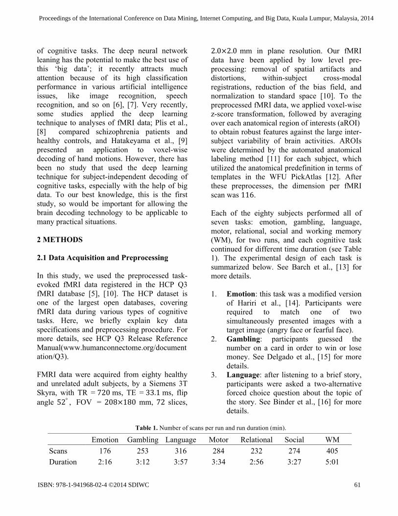
Emotion Gambling Language Motor Relational Social WM Scans 176 253 316 284 232 274 405 Duration 2:16 3:12 3:57 3:34 2:56 3:27 5:01

Table 1. Number of scans per run and run duration (min).


ISBN: 978-1-941968-02-4 ©2014 SDIWC 61

4. Motor: participants were requested to move one of five body parts (left or right finger, left or right toe, or tongue) instructed by a visual cue [17].

5. Relational: this task was a modified version of Smith et al., [18]. Participants answered a second-order question between two pairs of objects, whether or not these pairs share the mismatch dimension (texture or shape) across the pair.

6. Social: participants were asked if objects in video clips interacted in some way or not. These videos were taken from either Castelli et al., [19] or Wheatley et al., [20].

7. Working memory: two-back working memory task and zero-back working memory task with four different types of picture stimuli (places, tools, faces or body parts).

2.2 Decoding with Deep Learning The objective of deep neural network leaning was to acquire the input-output relationship with the input being the fMRI signals and the output being their labeled task classes, i.e., the category of cognitive task performed by the participants. For example, each fMRI scan during the participant performed the emotion task was labeled as ‘emotion class’. Then, the deep neural network was required to solve the classification problem into seven classes according to the supervised learning framework. As shown in Table 1, the number of scans in a single run was different between the tasks. To avoid harmful influence stemming from this difference in the data number, we resized the number of samples by randomly sub-sampling for each participant, hence the number of samples per run became 176, common for all tasks. This number 176 was the same as the smallest scan number per run among the seven tasks. Hence, the total sample number in the dataset was 176×2×80 for each class. The architecture and learning method of deep neural networks used in this study are similar to those

previously used in the MNIST classification experiments of Hinton et al., [21]. A neural network was configured as a feed-forward network incorporating 𝐿 hidden layers. The internal potential of the 𝑖-th unit in the 𝑙-th hidden layer 𝑎!

(!) 𝑙 = 1,⋯ 𝐿 is given as a weighted summation of its inputs:

𝑎!(!) = 𝑤!"

(!)!!!!

!!!

𝑧!(!!!) + 𝑏!

(!) (1)

where 𝑤!"(!) and 𝑏!

(!) are a weight and a bias. 𝑛! is the number of units in the 𝑙-th hidden layer, which was set at 𝑛! = 500 for any 𝑙 > 0. 𝒛(!) denotes the input vector 𝒙 to the network, hence 𝑛! equals to the input's dimension d(=116) .

𝒛(!) = 𝑧!(!),⋯ , 𝑧!!

(!) ! represents the output of

the 𝑙-th hidden layer and is given by applying a nonlinear activation function f to the internal potential as

𝑧!(!) = 𝑓 𝑎!

(!) . (2) Here, ReLU [22], a piecewise linear function max 0, 𝑥 , was used for the activation function 𝑓. Usage of ReLU for the activation function has a couple of advantages; its piecewise linearity can save the computational cost to calculate its derivative, and its non-saturating character prevents the learning algorithm from halting due to gradient vanishing of nonlinear activation functions. The last hidden layer was connected to the softmax (output) layer, so that the output from the 𝑘-th unit of the output layer was interpreted as the posterior probability of class 𝑘, given by

𝑃 𝑌 = 𝑘 𝒙,𝑾

=exp 𝑤!"

!!!!! 𝑧!

(!) + 𝑏!

exp 𝑤!!!!!!!! 𝑧!

(!) + 𝑏!!!!!!!

(3)


ISBN: 978-1-941968-02-4 ©2014 SDIWC 62

where 𝐾(= 7) is the number of classes, and 𝑾 denotes all the parameters (weights and biases). 𝑌 is a random variable signifying the class to which 𝒙 belongs. We used a negative log-likelihood as the cost function of the learning

𝐿 𝑾 = − log𝑃 𝑌! = 𝑡! 𝒙!,𝑾!

!!!

(4)

where 𝒙!, 𝑡! ,⋯ , 𝒙! , 𝑡! constituted the given dataset. 𝑡 ∈ 1,⋯ ,𝐾 denotes a class label. To minimize the above cost function, minibatch stochastic gradient descent (MSGD) with a momentum was introduced so that the stochastic gradient descent was performed every 100 samples: 𝑾! = 𝑾!!! + 𝒗! (5)

𝒗! = 𝑝!𝒗!!! − 1 − 𝑝! 𝜂!𝜕𝐿! 𝑾𝜕𝑾 𝑾!𝑾!!!

(6)

where 𝐿! is the cost function for the cached subset of 100 samples in the minibatch, and 𝜂! and 𝑝! are the learning rate and the momentum rate, respectively. The learning rate 𝜂! started with 𝜂!, then was exponentially decreased as 𝜂! = 𝑟𝜂!!! . The momentum rate 𝑝! was increased linearly from 𝑝! to 𝑝!"" = 0.99; after 100 times updates, 𝑝! was fixed at 𝑝!"". When searching for appropriate values of the hyper-parameters 𝜂!, 𝑟,𝑝!, 𝑙 , we used random search rather than grid search [23], in which 𝜂!, 𝑟, 𝑝! and 𝑙 were randomly sampled from their individual uniform distributions on the intervals 1.0, 20.0 , 0.95, 0.9999 , 0.4, 0.6 and 3.0, 20.0 respectively. The best parameters

were chosen among 9 combinations of 𝜂!, 𝑟,𝑝!, 𝑙 .

Each weight was initialized as a small value randomly sampled from a zero-mean normal distribution with the standard deviation of 0.01,

and biases were initialized to zero. During learning, the weight vector of each hidden unit

𝑤!!(!),⋯ ,𝑤!!!!!

(!) ! was not allowed to make its

𝐿! norm larger than a fixed positive constant 𝑚. If the 𝐿! norm of the weight vector got larger than 𝑚 after each update, it was simply divided by the norm and then multiplied by 𝑚. This upper bound setting of the norm enabled the initial learning rate to be fairly large, by which we expected accelerated learning. Early stopping was also adopted. If the decoding accuracy for the validation dataset did not increase for 200 learning epochs, then learning was terminated. Even if the early stopping did not occur, the whole learning procedure was terminated after 5000 learning epochs.

For avoiding over-fitting, we used the dropout technique [21]. During training, the activity 𝑧!

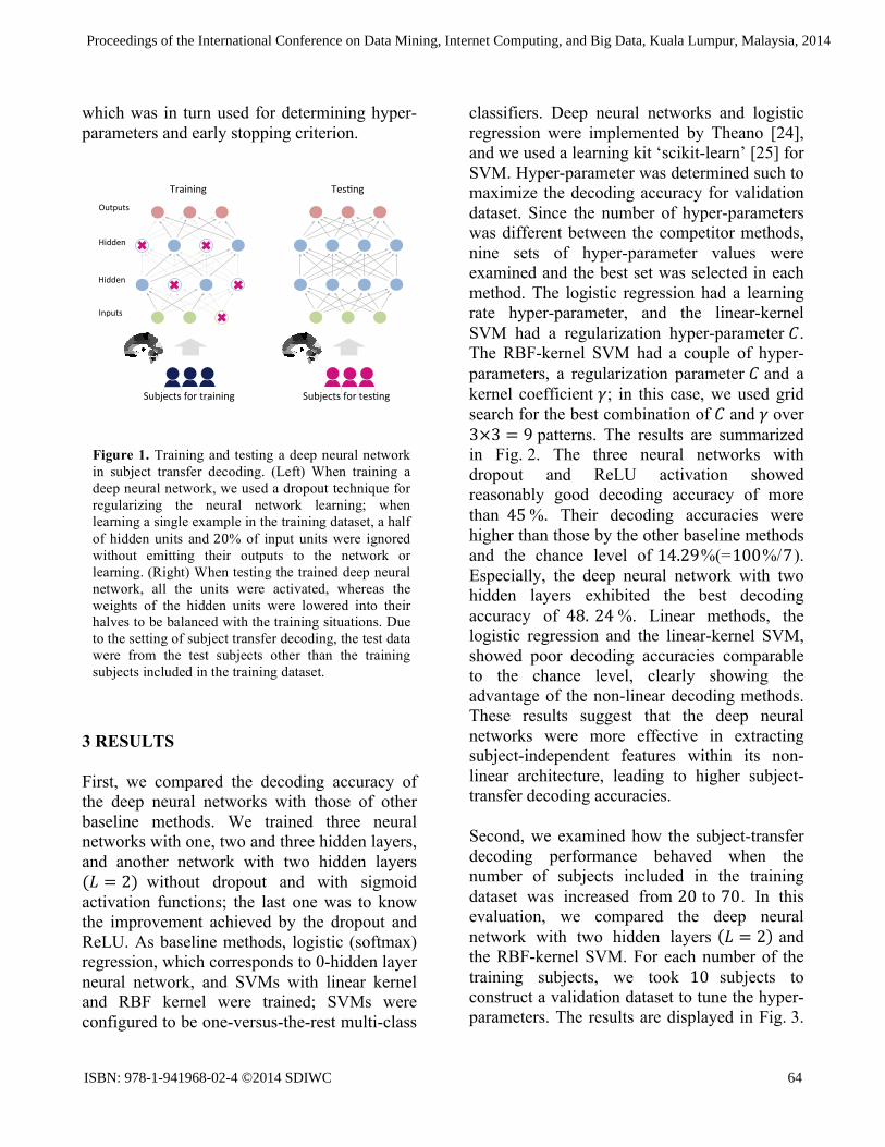
(!) was randomly replaced by 0 with probability 𝑝. We set 𝑝 = 0.5 for hidden units and 0.2 for inputs. This dropping out of activities plays a role of regularization and is expected to prevent the decoder from acquiring subject-specific features. When testing the trained neural network, on the other hand, all the nodes were activated, but their weights were multiplied by 1− 𝑝, to make the mean activity level of each network element consistent between the training phase and the test phase (see Fig. 1).

The trained neural network was tested by unseen data. Since in this study we expect the deep neural network can extract subject-independent features based on training from the large-scale fMRI database, we examined subject-transfer decoding performance. In specific, we executed 8-fold cross validation, or equivalently, leave-10-subjects-out cross validation: the whole dataset of 80 subjects were repeatedly separated into a training dataset of 70 subjects and a test dataset of the remaining 10 subjects. In addition, 10 subjects were randomly taken from the training dataset of 70 subjects to construct a validation dataset,


ISBN: 978-1-941968-02-4 ©2014 SDIWC 63

which was in turn used for determining hyper-parameters and early stopping criterion.

3 RESULTS

First, we compared the decoding accuracy of the deep neural networks with those of other baseline methods. We trained three neural networks with one, two and three hidden layers, and another network with two hidden layers (𝐿 = 2) without dropout and with sigmoid activation functions; the last one was to know the improvement achieved by the dropout and ReLU. As baseline methods, logistic (softmax) regression, which corresponds to 0-hidden layer neural network, and SVMs with linear kernel and RBF kernel were trained; SVMs were configured to be one-versus-the-rest multi-class

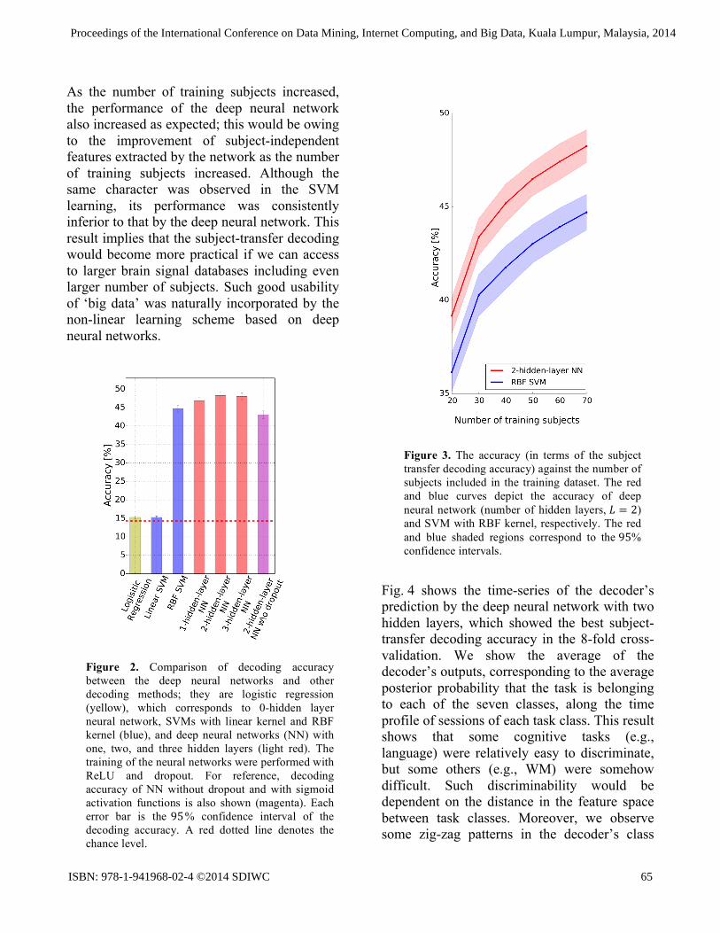
classifiers. Deep neural networks and logistic regression were implemented by Theano [24], and we used a learning kit ‘scikit-learn’ [25] for SVM. Hyper-parameter was determined such to maximize the decoding accuracy for validation dataset. Since the number of hyper-parameters was different between the competitor methods, nine sets of hyper-parameter values were examined and the best set was selected in each method. The logistic regression had a learning rate hyper-parameter, and the linear-kernel SVM had a regularization hyper-parameter 𝐶. The RBF-kernel SVM had a couple of hyper-parameters, a regularization parameter 𝐶 and a kernel coefficient 𝛾; in this case, we used grid search for the best combination of 𝐶 and 𝛾 over 3×3 = 9 patterns. The results are summarized in Fig. 2. The three neural networks with dropout and ReLU activation showed reasonably good decoding accuracy of more than 45%. Their decoding accuracies were higher than those by the other baseline methods and the chance level of 14.29%(=100%/7). Especially, the deep neural network with two hidden layers exhibited the best decoding accuracy of 48. 24%. Linear methods, the logistic regression and the linear-kernel SVM, showed poor decoding accuracies comparable to the chance level, clearly showing the advantage of the non-linear decoding methods. These results suggest that the deep neural networks were more effective in extracting subject-independent features within its non-linear architecture, leading to higher subject-transfer decoding accuracies.

Second, we examined how the subject-transfer decoding performance behaved when the number of subjects included in the training dataset was increased from 20 to 70. In this evaluation, we compared the deep neural network with two hidden layers 𝐿 = 2 and the RBF-kernel SVM. For each number of the training subjects, we took 10 subjects to construct a validation dataset to tune the hyper-parameters. The results are displayed in Fig. 3.

Training� Tes)ng*

Outputs*

Inputs*

Hidden*

Hidden*

Subjects*for*training� Subjects*for*tes)ng�

Figure 1. Training and testing a deep neural network in subject transfer decoding. (Left) When training a deep neural network, we used a dropout technique for regularizing the neural network learning; when learning a single example in the training dataset, a half of hidden units and 20% of input units were ignored without emitting their outputs to the network or learning. (Right) When testing the trained deep neural network, all the units were activated, whereas the weights of the hidden units were lowered into their halves to be balanced with the training situations. Due to the setting of subject transfer decoding, the test data were from the test subjects other than the training subjects included in the training dataset.


ISBN: 978-1-941968-02-4 ©2014 SDIWC 64

As the number of training subjects increased, the performance of the deep neural network also increased as expected; this would be owing to the improvement of subject-independent features extracted by the network as the number of training subjects increased. Although the same character was observed in the SVM learning, its performance was consistently inferior to that by the deep neural network. This result implies that the subject-transfer decoding would become more practical if we can access to larger brain signal databases including even larger number of subjects. Such good usability of ‘big data’ was naturally incorporated by the non-linear learning scheme based on deep neural networks.

Fig. 4 shows the time-series of the decoder’s prediction by the deep neural network with two hidden layers, which showed the best subject-transfer decoding accuracy in the 8-fold cross-validation. We show the average of the decoder’s outputs, corresponding to the average posterior probability that the task is belonging to each of the seven classes, along the time profile of sessions of each task class. This result shows that some cognitive tasks (e.g., language) were relatively easy to discriminate, but some others (e.g., WM) were somehow difficult. Such discriminability would be dependent on the distance in the feature space between task classes. Moreover, we observe some zig-zag patterns in the decoder’s class

Figure 2. Comparison of decoding accuracy between the deep neural networks and other decoding methods; they are logistic regression (yellow), which corresponds to 0-hidden layer neural network, SVMs with linear kernel and RBF kernel (blue), and deep neural networks (NN) with one, two, and three hidden layers (light red). The training of the neural networks were performed with ReLU and dropout. For reference, decoding accuracy of NN without dropout and with sigmoid activation functions is also shown (magenta). Each error bar is the 95% confidence interval of the decoding accuracy. A red dotted line denotes the chance level.

Figure 3. The accuracy (in terms of the subject transfer decoding accuracy) against the number of subjects included in the training dataset. The red and blue curves depict the accuracy of deep neural network (number of hidden layers, 𝐿 = 2) and SVM with RBF kernel, respectively. The red and blue shaded regions correspond to the 95% confidence intervals.


ISBN: 978-1-941968-02-4 ©2014 SDIWC 65

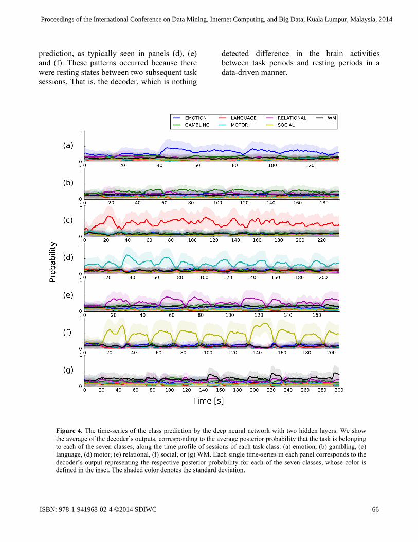
prediction, as typically seen in panels (d), (e) and (f). These patterns occurred because there were resting states between two subsequent task sessions. That is, the decoder, which is nothing

detected difference in the brain activities between task periods and resting periods in a data-driven manner.

Figure 4. The time-series of the class prediction by the deep neural network with two hidden layers. We show the average of the decoder’s outputs, corresponding to the average posterior probability that the task is belonging to each of the seven classes, along the time profile of sessions of each task class: (a) emotion, (b) gambling, (c) language, (d) motor, (e) relational, (f) social, or (g) WM. Each single time-series in each panel corresponds to the decoder’s output representing the respective posterior probability for each of the seven classes, whose color is defined in the inset. The shaded color denotes the standard deviation.


ISBN: 978-1-941968-02-4 ©2014 SDIWC 66

4 CONCLUSION

In this study, we proposed to use deep neural network learning for constructing task classification decoders trained by a large dataset from a public fMRI database. The trained decoders were also available for subject-transfer decoding. As a result, our approach based on deep learning achieved the higher decoding accuracy than other baseline methods, and got even improved as the number of training subjects increased. We thus concluded the deep neural network learning was ready for obtaining subject-independent non-linear features from a ‘big-data’ of brain activities, and then for applying to subject-transfer decoding, which is an important methodology for making the brain-machine-interface more practical in realistic situations.

5 ACKNOWLEDGEMENT Data were provided by the Human Connectome Project, WU-Minn Consortium (Principal Investigators: David Van Essen and Kamil Ugurbil; 1U54MH091657) funded by the 16 NIH Institutes and Centers that support the NIH Blueprint for Neuroscience Research; and by the McDonnell Center for Systems Neuroscience at Washington University. This research was supported in part by the Ministry of Internal Affairs and Communications, Japan, under a contract “Novel and innovative R&D making use of brain structures” and by JSPS KAKENHI (No. 24300114). REFERENCES

[1] J. V Haxby, M. I. Gobbini, M. L. Furey, A. Ishai, J. L. Schouten, and P. Pietrini, “Distributed and overlapping representations of faces and objects in ventral temporal cortex,” Science, vol. 293, no. 5539, pp. 2425–2430, 2001.

[2] D. D. Cox and R. L. Savoy, “Functional magnetic resonance imaging (fMRI) ‘brain

reading’: detecting and classifying distributed patterns of fMRI activity in human visual cortex,” Neuroimage, vol. 19, no. 2, pp. 261–270, 2003.

[3] S. Nishimoto, A. T. Vu, T. Naselaris, Y. Benjamini, B. Yu, and J. L. Gallant, “Reconstructing visual experiences from brain activity evoked by natural movies,” Current Biology, vol. 21, no. 19, pp. 1641–1646, 2011.

[4] T. Horikawa, M. Tamaki, Y. Miyawaki, and Y. Kamitani, “Neural decoding of visual imagery during sleep,” Science, vol. 340, no. 6132, pp. 639–642, 2013.

[5] D. C. Van Essen, S. M. Smith, D. M. Barch, T. E. J. Behrens, E. Yacoub, and K. Ugurbil, “The WU-Minn Human Connectome Project: an overview,” Neuroimage, vol. 80, pp. 62–79, 2013.

[6] A. Krizhevsky, I. Sutskever, and G. Hinton, “Imagenet classification with deep convolutional neural networks,” in Advances in neural information processing systems, pp. 1097–1105, 2012.

[7] F. Seide, G. Li, and D. Yu, “Conversational Speech Transcription Using Context-Dependent Deep Neural Networks,” in Proceedings of the Annual Conference of the International Speech Communication Association, INTERSPEECH, pp. 437–440, 2011.

[8] S. M. Plis, D. R. Hjelm, R. Salakhutdinov, E. a Allen, H. J. Bockholt, J. D. Long, H. J. Johnson, J. S. Paulsen, J. a Turner, and V. D. Calhoun, “Deep learning for neuroimaging: a validation study,” Frontiers in Neuroscience, vol. 8, p. 229, Jan. 2014.

[9] Y. Hatakeyama, S. Yoshida, H. Kataoka, and Y. Okuhara, “Multi-voxel pattern analysis of fmri based on deep learning methods,” in Soft Com- puting in Big Data Processing, vol. 271, pp. 29–38, 2014.

[10] M. F. Glasser, S. N. Sotiropoulos, J. A. Wilson, T. S. Coalson, B. Fischl, J. L. Andersson, J. Xu, S. Jbabdi, M. Webster, J. R. Polimeni, D. C. Van Essen, and M. Jenkinson, “The minimal preprocessing pipelines for the Human Connectome Project,” Neuroimage, vol. 80, pp. 105–124, 2013.


ISBN: 978-1-941968-02-4 ©2014 SDIWC 67

[11] N. Tzourio-Mazoyer and B. Landeau, “Automated anatomical labeling of activations in SPM using a macroscopic anatomical parcellation of the MNI MRI single-subject brain,” Neuroimage, vol. 15, no. 1, pp. 273–289, 2002.

[12] J. a. Maldjian, P. J. Laurienti, R. a. Kraft, and J. H. Burdette, “An automated method for neuroanatomic and cytoarchitectonic atlas-based interrogation of fMRI data sets,” Neuroimage, vol. 19, no. 3, pp. 1233–1239, 2003.

[13] D. M. Barch, G. C. Burgess, M. P. Harms, S. E. Petersen, B. L. Schlaggar, M. Corbetta, M. F. Glasser, S. Curtiss, S. Dixit, C. Feldt, D. Nolan, E. Bryant, T. Hartley, O. Footer, J. M. Bjork, R. Poldrack, S. Smith, H. Johansen-Berg, A. Z. Snyder, and D. C. Van Essen, “Function in the human connectome: task-fMRI and individual differences in behavior,” Neuroimage, vol. 80, pp. 169–189, 2013.

[14] A. R. Hariri, A. Tessitore, V. S. Mattay, F. Fera, and D. R. Weinberger, “The Amygdala Response to Emotional Stimuli: A Comparison of Faces and Scenes,” Neuroimage, vol. 17, no. 1, pp. 317–323, 2002.

[15] M. R. Delgado, L. E. Nystrom, C. Fissell, D. C. Noll, and J. A. Fiez, “Tracking the hemodynamic responses to reward and punishment in the striatum,” Journal of Neurophysiology, vol. 84, no. 6, pp. 3072–3077, 2000.

[16] J. R. Binder, W. L. Gross, J. B. Allendorfer, L. Bonilha, J. Chapin, J. C. Edwards, T. J. Grabowski, J. T. Langfitt, D. W. Loring, M. J. Lowe, K. Koenig, P. S. Morgan, J. G. Ojemann, C. Rorden, J. P. Szaflarski, M. E. Tivarus, and K. E. Weaver, “Mapping anterior temporal lobe language areas with fMRI: a multicenter normative study,” Neuroimage, vol. 54, no. 2, pp. 1465–1475, 2011.

[17] R. L. Buckner, F. M. Krienen, A. Castellanos, J. C. Diaz, and B. T. T. Yeo, “The organization of the human cerebellum estimated by intrinsic functional connectivity,” Journal of Neurophysiology, vol. 106, no. 5, pp. 2322–2345, 2011.

[18] R. Smith, K. Keramatian, and K. Christoff, “Localizing the rostrolateral prefrontal cortex at

the individual level,” Neuroimage, vol. 36, no. 4, pp. 1387–1396, 2007.

[19] F. Castelli, F. Happé, U. Frith, and C. Frith, “Movement and mind: a functional imaging study of perception and interpretation of complex intentional movement patterns,” Neuroimage, vol. 12, no. 3, pp. 314–325, 2000.

[20] T. Wheatley, S. C. Milleville, and A. Martin, “Understanding animate agents: distinct roles for the social network and mirror system,” Psychological. Science, vol. 18, no. 6, pp. 469–474, 2007.

[21] G. E. Hinton, N. Srivastava, A. Krizhevsky, I. Sutskever, and R. R. Salakhutdinov, “Improving neural networks by preventing co-adaptation of feature detectors,” arXiv preprint arXiv:1207.0580, 2012.

[22] K. Jarrett, K. Kavukcuoglu, M. A. Ranzato, and Y. LeCun, “What is the best multi-stage architecture for object recognition?,” in Computer Vision, 2009 IEEE 12th International Conference on, pp. 2146–2153, 2009.

[23] J. Bergstra and Y. Bengio, “Random search for hyper-parameter optimization,” The Journal of Machine Learning Research, vol. 13, pp. 281–305, 2012.

[24] J. Bergstra, O. Breuleux, F. Bastien, P. Lamblin, R. Pascanu, G. Desjardins, J. Turian, D. Warde-farley, and Y. Bengio, “Theano  : A CPU and GPU Math Compiler in Python,” in Proceedings of the Python for scientific computing conference (SciPy), pp. 1–7, 2010.

[25] F. Pedregosa, G. Varoquaux, A. Gramfort, V. Michel, B. Thirion, O. Grisel, M. Blondel, P. Prettenhofer, R. Weiss, V. Dubourg, J. Vanderplas, A. Passos, D. Cournapeau, M. Brucher, M. Perrot, and É. Duchesnay, “Scikit-learn: Machine Learning in Python,” The Journal of Machine Learning Research, vol. 12, pp. 2825–2830, 2012.


ISBN: 978-1-941968-02-4 ©2014 SDIWC 68

construction of subject-independent brain decoders for human fmri with deep learning

Documents