grammar-based genetic programming - adam nohejl
TRANSCRIPT
Charles University in PragueFaculty of Mathematics and Physics
MASTER THESIS
Adam Nohejl
Grammar-based genetic programming
Department of Software and Computer Science Education
Supervisor of the master thesis: RNDr. František Mráz, CSc.
Study programme: Computer scienceSpecialisation: Theoretical computer science
Prague 2011


I would like to thank to František Mráz, who supervised my work on thisthesis, for his guidance and helpful suggestions. I am also grateful to Dr ManLeung Wong for providing his implementation of the logic grammar basedframework LOGENPRO.

Copyright © 2010–2011, Adam Nohejl.All rights reserved.
This work is licensed under the Creative Commons Attribution 3.0 Czech RepublicLicence. More information and its full text:http://creativecommons.org/licenses/by/3.0/cz/deed.en_GBor send a letter to Creative Commons, 444 Castro Street, Suite 900, Mountain View,California, 94041, USA.
You are free:to copy, distribute, display and perform the work,to make derivative works,to make commercial use of the workunder the following condition:
Attribution: You must give the original author credit.
With the understanding that:• Waiver: Any of the above conditions can be waived if you get permission
from the copyright holder.• Public Domain: Where the work or any of its elements is in the public domain
under applicable law, that status is in no way affected by the licence.• Other Rights: In no way are any of the following rights affected by the licence:
your fair dealing or fair use rights, or other applicable copyright exceptionsand limitations; the author’s moral rights; rights other persons may haveeither in the work itself or in how the work is used, such as publicity orprivacy rights.
• Notice: For any reuse or distribution, you must make clear to others thelicence terms of this work.
Both the full text and the accompanying software project can be downloadedfrom http://nohejl.name/age/.
I declare that I carried out this master thesis independently, and only with thecited sources, literature and other professional sources.
I understand that my work relates to the rights and obligations under the ActNo. 121/2000 Coll., the Copyright Act, as amended, in particular the fact thatthe Charles University in Prague has the right to conclude a license agreementon the use of this work as a school work pursuant to Section 60 paragraph 1 ofthe Copyright Act.
Prague, 25 July 2011 Adam Nohejl


Title: Grammar-based genetic programming
Author: Adam Nohejl
Department: Department of Software and Computer Science Education
Supervisor of the master thesis: RNDr. František Mráz, CSc.
Abstract: Tree-based genetic programming (GP) has several known shortcomings: dif-ficult adaptability to specific programming languages and environments, the problemof closure and multiple types, and the problem of declarative representation of know-ledge. Most of the methods that try to solve these problems are based on formalgrammars. The precise effect of their distinctive features is often difficult to analyseand a good comparison of performance in specific problems is missing. This thesisreviews three grammar-based methods: context-free grammar genetic programming(CFG-GP), including its variant GPHH recently applied to exam timetabling, gram-matical evolution (GE), and LOGENPRO, it discusses how they solve the problemsencountered by GP, and compares them in a series of experiments in six applicationsusing success rates and derivation tree characteristics. The thesis demonstrates thatneither GE nor LOGENPRO provide a substantial advantage over CFG-GP in any ofthe experiments, and analyses the differences between the effects of operators usedin CFG-GP and GE. It also presents results from a highly efficient implementation ofCFG-GP and GE.
Keywords: genetic programming, formal grammar, evolutionary algorithms,grammatical evolution.
Název práce: Genetické programování založené na gramatikách
Autor: Adam Nohejl
Katedra: Kabinet software a výuky informatiky
Vedoucí diplomové práce: RNDr. František Mráz, CSc.
Abstrakt: Genetické programování (GP) založené na stromech má nekolik známýchnedostatku: složité prizpusobení specifickým programovacím jazykum a prostredím,problém uzáveru a více typu a problém deklarativní reprezentace vedomostí. Vetšinametod, které se snaží tyto problémy vyrešit, je založena na formálních gramatikách.Presné dusledky vlastností, které je odlišují, je težké analyzovat a dobré srovnánívýsledku v konkrétních problémech chybí. Tato práce zkoumá tri metody založenéna gramatikách: genetické programování s bezkontextovými gramatikami (CFG-GP),vcetne jeho varianty GPHH nedávno aplikované na rozvrhování zkoušek, gramatickouevoluci (GE) a LOGENPRO, pojednává o tom, jak reší problémy GP, a porovnává je v sé-rii experimentu v šesti aplikacích podle cetností úspechu a charakteristik derivacníchstromu. Práce ukazuje, že GE ani LOGENPRO neposkytují podstatnou výhodu v žád-ném z experimentu a analyzuje rozdíly v úcincích operátoru používaných v CFG-GPa GE. Jsou také prezentovány výsledky velmi efektivní implementace metod CFG-GPa GE.
Klícová slova: genetické programování, formální gramatika, evolucní algoritmy,gramatická evoluce.

Contents
Introduction 1
1 Grammar-Based Genetic Programming Methods 31.1 Formal grammars and programming . . . . . . . . . . . . . . . . 41.2 Genetic programming . . . . . . . . . . . . . . . . . . . . . . . . 81.3 Grammatically biased ILP . . . . . . . . . . . . . . . . . . . . . . 111.4 CFG-GP, language bias, and search bias . . . . . . . . . . . . . . 121.5 Logic grammar based genetic programming: LOGENPRO . . . 141.6 Grammatical evolution . . . . . . . . . . . . . . . . . . . . . . . . 151.7 Common features and shortcomings . . . . . . . . . . . . . . . . 171.8 Implications for performance . . . . . . . . . . . . . . . . . . . . 18
2 Existing Applications 212.1 Simple symbolic regression . . . . . . . . . . . . . . . . . . . . . 212.2 Artificial ant trail . . . . . . . . . . . . . . . . . . . . . . . . . . . 222.3 Symbolic regression with multiple types . . . . . . . . . . . . . . 232.4 Boolean symbolic regression . . . . . . . . . . . . . . . . . . . . . 242.5 Hyper-heuristics . . . . . . . . . . . . . . . . . . . . . . . . . . . . 242.6 Other applications . . . . . . . . . . . . . . . . . . . . . . . . . . 25
3 Experiments with Grammar-Based Methods 273.1 Observed characteristics . . . . . . . . . . . . . . . . . . . . . . . 273.2 Setup . . . . . . . . . . . . . . . . . . . . . . . . . . . . . . . . . . 283.3 Statistics . . . . . . . . . . . . . . . . . . . . . . . . . . . . . . . . 283.4 Simple symbolic regression . . . . . . . . . . . . . . . . . . . . . 29
3.4.1 Experimental setups 1 . . . . . . . . . . . . . . . . . . . . 293.4.2 Results from setups 1 . . . . . . . . . . . . . . . . . . . . . 313.4.3 Experimental setups 2 . . . . . . . . . . . . . . . . . . . . 343.4.4 Results from setups 2 . . . . . . . . . . . . . . . . . . . . . 343.4.5 Conclusion . . . . . . . . . . . . . . . . . . . . . . . . . . 36
3.5 Santa Fe ant trail . . . . . . . . . . . . . . . . . . . . . . . . . . . . 383.5.1 Experimental setups 1 . . . . . . . . . . . . . . . . . . . . 383.5.2 Results from setups 1 . . . . . . . . . . . . . . . . . . . . . 403.5.3 Experimental setups 2 . . . . . . . . . . . . . . . . . . . . 433.5.4 Results from setups 2 . . . . . . . . . . . . . . . . . . . . . 433.5.5 Conclusion . . . . . . . . . . . . . . . . . . . . . . . . . . 44
3.6 Dot product symbolic regression . . . . . . . . . . . . . . . . . . 473.6.1 Experimental setups . . . . . . . . . . . . . . . . . . . . . 493.6.2 Results . . . . . . . . . . . . . . . . . . . . . . . . . . . . . 513.6.3 Conclusion . . . . . . . . . . . . . . . . . . . . . . . . . . 52
3.7 Symbolic regression with ADFs . . . . . . . . . . . . . . . . . . . 543.7.1 Experimental setups . . . . . . . . . . . . . . . . . . . . . 543.7.2 Results . . . . . . . . . . . . . . . . . . . . . . . . . . . . . 543.7.3 Conclusion . . . . . . . . . . . . . . . . . . . . . . . . . . 56
3.8 Boolean parity functions with ADFs . . . . . . . . . . . . . . . . 613.8.1 Experimental setups . . . . . . . . . . . . . . . . . . . . . 613.8.2 Results . . . . . . . . . . . . . . . . . . . . . . . . . . . . . 623.8.3 Conclusion . . . . . . . . . . . . . . . . . . . . . . . . . . 64
3.9 Exam timetabling hyper-heuristics . . . . . . . . . . . . . . . . . 673.9.1 Experimental setup . . . . . . . . . . . . . . . . . . . . . . 703.9.2 Results . . . . . . . . . . . . . . . . . . . . . . . . . . . . . 733.9.3 Computational time . . . . . . . . . . . . . . . . . . . . . 743.9.4 Conclusion . . . . . . . . . . . . . . . . . . . . . . . . . . 74
3.10 Conclusion . . . . . . . . . . . . . . . . . . . . . . . . . . . . . . . 75
4 Implementation Notes 774.1 Implementation of CFG-GP . . . . . . . . . . . . . . . . . . . . . 774.2 Accompanying files . . . . . . . . . . . . . . . . . . . . . . . . . . 80
Conclusion 83
Bibliography 85
List of Abbreviations 89
Introduction
This thesis explores and analyses methods of genetic programming based onformal grammars. Genetic programming (GP) is a metaheuristic for derivingproblem solutions in the form of programs based on evolutionary principles,and thus belonging to the family of evolutionary algorithms. Traditionally, ge-netic programming was tied to the Lisp programming language, taking advant-age of its simplicity and straightforward correspondence between a programand its parse tree. Several other strains of genetic programming were devisedover time: linear GP systems departed from the original premise of the tree-based GP that programs are trees, and variants of tree-based GP usually eitherextended the original genetic programming with new features (such as auto-matically defined functions, which effectively add co-evolution of subroutines)or placed restrictions on permitted tree forms (such as strongly-typed geneticprogramming).
Various grammar-based GP methods, which have also emerged, either canbe put in the same category with tree-based GP or linear GP, or often moreappropriately, can be thought of as being in between them. For a computerscientist, a formal grammar is the natural link between program as a tree andprogram as a linear string. This is always the primary role of grammars ingenetic programming: they specify the language of candidate solutions. Thegrammar-based GP methods, however, can be employed in several ways:
(1) Constraining tree-based GP: The grammar is used to restrict the searchspace, and consequently also to redefine search operators under which therestricted search space is algebraically closed.
(2) Introduction of bias into tree-based GP: The grammar is used as a vehiclefor bias toward certain solutions. The bias may also be adjusted over the courseof the algorithm’s execution.
(3) Replacement of the traditional tree-based GP mechanisms: The gram-mar may serve both of the above purposes, but more importantly it is an integralpart of the algorithm that provides mapping between two representations ofcandidate solutions.
From the short descriptions we can already glimpse that different grammar-based GP methods have different aims. In case (1) the grammar is used toremedy a shortcoming of GP: the so-called closure problem, but most grammar-based methods also raise problems and questions of their own concerning theencoding of individuals, and the design of operators. In spite of the differentmotivations behind the methods, there are also significant areas of overlap
1
between them. The goal of this thesis will therefore be to
• describe the problems arising from integration of grammars and geneticprogramming,
• compare the approaches of several existing methods,
• compare appropriateness and performance of the methods on benchmarkproblems.
The text is organised in the following chapters:
• Chapter 1 introduces the techniques of traditional tree-based GP, thenecessary concepts from formal language theory, and several grammar-based GP methods. Common features and issues are pointed out.
• Chapter 2 presents applications that we will use for comparison andbenchmarking.
• Chapter 3 describes several experiments with grammar-based methodsin the presented applications, and analyses the results.
• Chapter 4 provides information about the implementation used for theexperiments, which is available on the accompanying medium and on-line1.
• The closing chapter concludes the thesis and suggests possibilities forfurther research.
1http://nohejl.name/age/
2

Chapter 1
Grammar-Based GeneticProgramming Methods
In this chapter we will introduce several methods for genetic programmingbased on formal grammars, assuming basic knowledge about evolutionaryalgorithms, particularly genetic programming and genetic algorithms (GA), andformal grammars. If you are not familiar with evolutionary algorithms, thetextbooks by Goldberg (1989) (on genetic algorithms) or Poli et al. (2008) (ongenetic programming in a broad sense) provide a good overview. Alternatively,you can find a short summary of the commonest techniques in my bachelorthesis (Nohejl, 2009).
We will begin with an informal review of the basic concepts and methodsthat preceded grammar-based genetic programming:
• in Section 1.1, we will describe the grammars and notations for themcommonly used in grammar-based methods,
• in Section 1.2, we will review the plain tree-based genetic programmingand one of its developments highlighting the points that will later interestus,
• in Section 1.3, we will outline how grammars were used to encode biasin inductive logic programming.
Then, we will describe the following grammar-based GP methods:
• in Section 1.4, context-free grammar genetic programming,
• in Section 1.5, LOGENPRO, a genetic programming system based on logicgrammars,
• in Section 1.6, grammatical evolution.
To complete our tour we will discuss the common features and shortcomings ofthe methods in Section 1.7 and examine the implications for their performancein applications in Section 1.8.
3

1.1 Formal grammars and programming
Context-free grammars (CFGs) are used to express syntax of most currently usedprogramming languages because they provide a reasonable trade-off betweenexpressiveness (relative size of the class of expressible languages) and efficiency,which is especially important for syntactic analysis (parsing) of programs.
This also makes them a natural choice for augmenting genetic programmingwith grammars. Most of the methods that we are going to discuss are based onCFGs, while the remaining use grammars that extend CFG in some way. We willtherefore begin with a precise definition and the corresponding terminologyand notation:
Definition. A context-free grammar, or CFG, is formed by four components(adapted from Hopcroft et al., 2000, ch. 5):
1. There is a finite set of symbols that form the strings of the language beingdefined. We call this alphabet the terminals, or terminal symbols.
2. There is a finite set of nonterminals, or nonterminal symbols.1 Each nonter-minal represents a language; i.e., a set of strings.
3. One of the nonterminals represents the language being defined; it is calledthe start symbol. Other nonterminals represent auxiliary classes of stringsthat are used to help define the language of the start symbol.
4. There is a finite set of productions or rules that represents the recursivedefinition of a language. Each production consists of:
(a) A nonterminal that is being (partially) defined by the production.This nonterminal is often called the head of the production.
(b) The production symbol→.
(c) A string of zero or more terminals and nonterminals. This string,called the body of the production, represents one way to form stringsin the language of the nonterminal of the head. In so doing, we leaveterminals unchanged and substitute for each nonterminal of the bodyany string that is known to be in the language of that nonterminal.
When applying the rule, we say that it is used to rewrite its head to itsbody, or that using the rule a string containing the body derives from the stringcontaining the head. The terminology that we have introduced can be usedfor other kinds of grammars as well. It is the restriction that production headsconsist of a single nonterminal that gives context-free grammars their name byruling out context dependence.
Formally, a CFG is usually represented as the ordered quadruple G =
(N,T,P,S), where N is the set of nonterminals, T the set of terminals, P theset of productions, and S the start symbol.1 Hopcroft et al. (2000) prefer the name variables, which is reserved for its more common
use in this text.
4
Notation. We will use a number of conventions when working with CFGs andgrammars in general:
1. Letters, digits and symbols in upright or non-proportional type representterminals. Examples: x, 4, ×, %.
2. Identifiers consisting of lower-case letters in italic type represent nonter-minals. Examples: s, var, expr.
3. Uppercase letters in italic type are used as meta-variables (symbols thatstand for an unspecified nonterminal, or less often terminal). Examples:A, B, X.
4. Lower-case Greek letters stand for strings consisting of terminals andnonterminals, λ denotes an empty string, and period is used to makeconcatenation explicit. Examples: α, β, ξ = ξ.λ.
Note particularly the representation of nonterminals, which is contrary to theusual convention of the formal language theory, but allows us to use moreexpressive identifiers.
We will also use the Backus-Naur form (BNF) as a notation for context-freegrammars. Examples of a CFG describing simple arithmetic expressions anda corresponding BNF notation are provided in Listing 1.1 and Listing 1.2. SeeNaur (1963) for a formal definition.
Definition. Let G = (N,T,P,S) be a context-free grammar. The derivation trees,or parse trees, for G are rooted, ordered trees that satisfy the following conditions(adapted from Hopcroft et al., 2000, ch. 5):
1. Each internal node is labelled by a nonterminal in N.
2. Each leaf is labelled by either a nonterminal, a terminal, or λ. However,if a leaf is labelled λ, then it must be the only child of its parent.
3. If an internal node is labelled A, and its children are labelled X1,X2, . . . ,Xk
respectively, from the left, then A→ X1X2 · · ·Xk is a production in P.
The yield of a derivation tree is the concatenation of its leaves in the orderthey appear in the tree. The depth of a node in a tree is the length of the pathfrom root to that node counted as the number of edges. The height of a treeis the largest depth of a node in the tree. Thus root node has depth 0, andthe minimum height of a tree whose yield consists of terminals and λ is 1.These definitions are in line with the standard textbook terminology (Hopcroftet al., 2000, ch. 5; Cormen et al., 2001, sec. B.5.2), and can be easily extendedto derivation trees for other types of grammars, and in case of depth andheight to any rooted trees. (See Figure 1.1 for an example.) There is no formaldifference between a derivation tree and a parse tree: the former emphasisesthe generative aspect, the latter emphasises the aspect of syntactic analysis.
5

expr → ( expr op expr ) expr → primop →+ op →×
prim→ x prim→ 1.0
Listing 1.1: Production rules for a CFG whose set of nonterminals is {expr, op, prim}, itsset of terminals is {(, ),+,×, x, 1.0}, and its start nonterminal is expr.
<expr> ::= ( <expr> <op> <expr> ) | <prim><op> ::= + | *<prim> ::= x | 1.0
Listing 1.2: A BNF version of the previous example. Note that | denotes alternatives,and that the sets of terminals and nonterminals are implied, as is the startnonterminal following the convention of putting its productions first.
Let’s state informally several basic facts about context-free grammars:
Fact 1. The same language can be described by multiple context-free grammars. Con-sider the rules s → p, s → q, s → 1, p → s + s, q → s × s, the rules s → s + s,s→ s × s, s→ 1, and the rules s→ s + s, s→ s × s, s→ s + s × s, s→ 1.
Fact 2. A CFG may be ambiguous. Consider the rules s → s + s, s → s× s, ands → 1, and a string 1 + 1 × 1. It is impossible to tell if it was derived by firstusing the first rule or the second rule. Thus, for an ambiguous CFG, differentderivation trees can yield the same string.
Fact 3. A CFG cannot express all what is usually considered part of a programminglanguage syntax. Notably, the use of declared variables is context-dependent.Consider a language with a “let var = expr in expr” construct: by syntacticanalysis (or generation) according to any given context-free grammar, it isimpossible to ensure that each var nonterminal occurring in the derivation ofthe second expr nonterminal is rewritten to an identifier declared in an enclosinglet construct.
Fact 4. For a given CFG the set of strings yielded by parse trees such that (1) they arerooted in the start symbol, and (2) they yield a terminal string, is the language definedby the CFG. A corresponding derivation of a terminal string from the languagecan be constructed from any given derivation tree and vice versa.
Definite clause grammars (DCGs) are a formalism tied to the Prolog pro-gramming language and related to its early application to natural languageprocessing. Rather than being another type of a formal grammar, they are a spe-cific notation for grammars with semantics derived from logic programming.In the context of logic programming languages such as Prolog or Mercury, theyare often used to create complex parsers.
DCGs can easily capture long distance dependencies, and can be used as anatural notation for context-free grammars, as well as for the more expressiveattribute grammars (as shown by Sterling and Shapiro, 1994, ch. 19), which are
6

expr --> ['('],expr,op,expr,[')']. expr --> prim.op --> ['+']. op --> ['*'].prim --> ['x']. expr --> ['1.0'].
Listing 1.3: A DCG version of the previous example. Note that commas denote con-catenation and square brackets enclose terminals, which can be strings, asin the example, or any terms.
s --> rep(N,a), rep(N,b), rep(N,c).rep(end,_) --> [].rep(s(N),X) --> [X], rep(X,N).
Listing 1.4: A DCG grammar for anbncn, a language that cannot be described by acontext-free grammar. Note the Prolog variables X and N, the number ofrepetitions expressed using the term structure s(s(· · · s(end)· · · )).
expr(V) --> ['let'],X,['='],expr(V),['in'],expr([X|V]),{var(X)}.expr(V) --> X, {member(X,V)}.
Listing 1.5: A fragment of a DCG grammar for checking variable declaration in a “letvar = expr in expr” construct. Note the Prolog variables V, X and theexternal predicates var/1, member/2 in curly braces.
commonly employed for syntactic analysis in compilers rather than plain CFGs.The looser term logic grammars may refer to DCGs or a derived formalism ofequal or restricted expressive power (see Section 1.5, Section 1.3).
In the simplest case a DCG expresses a context-free grammar (Listing 1.3).As in CFGs, a head of a production consists of a single item, and its body isa string of items. The items, however, may be arbitrary terms with Prologvariables (Listing 1.4), and further extending the computational power, a listof arbitrary Prolog goals may be added to each rule (Listing 1.5). As shown inListing 1.4 and Listing 1.5, a DCG can describe context-dependency such as arestriction to use only declared variables in a programming language syntax.
A precise definition and more complex examples can be found in The Art ofProlog by Sterling and Shapiro (1994, ch. 19, 24), and Sperberg-McQueen (2004)provides a good practical overview online. The semantics should intuitivelybe clear to readers familiar with logic programming: the notation is translatedinto a Prolog program for a top-down left-to-right parser resulting in a clausefor each production with any goals in square brackets being added to the bodyof the clause. When the parser is executed, the terms and variables used in thegrammar are subject to unification. Finally, let’s state an obvious fact:
Fact 5. The DCG formalism has enough power to express unrestricted grammars.Prolog is Turing-complete (Sterling and Shapiro, 1994, sec. 17.2), and any Prologgoals can be added to the grammar rules.
7
1.2 Genetic programming
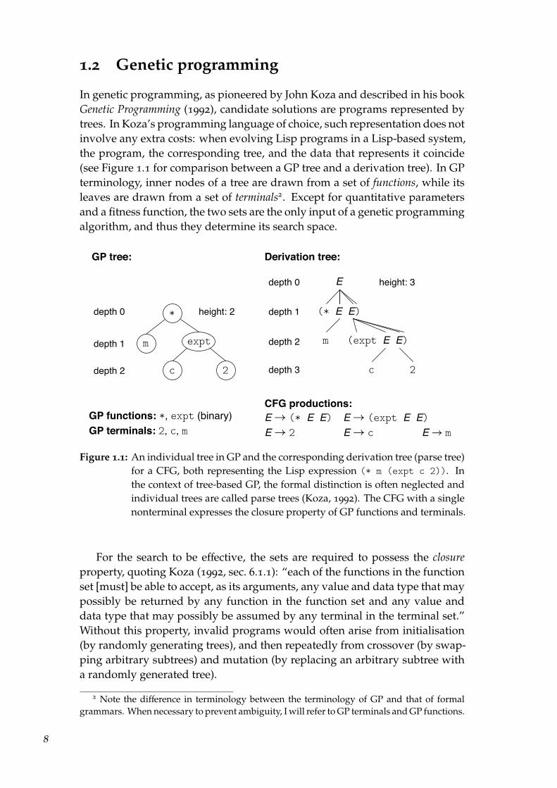
In genetic programming, as pioneered by John Koza and described in his bookGenetic Programming (1992), candidate solutions are programs represented bytrees. In Koza’s programming language of choice, such representation does notinvolve any extra costs: when evolving Lisp programs in a Lisp-based system,the program, the corresponding tree, and the data that represents it coincide(see Figure 1.1 for comparison between a GP tree and a derivation tree). In GPterminology, inner nodes of a tree are drawn from a set of functions, while itsleaves are drawn from a set of terminals2. Except for quantitative parametersand a fitness function, the two sets are the only input of a genetic programmingalgorithm, and thus they determine its search space.
*
exptm
c 2
E
(* E E)
m
c
(expt E E)
2
GP functions: *, expt (binary)GP terminals: 2, c, m
CFG productions:E → (* E E) E → (expt E E)E → 2 E → c E → m
GP tree: Derivation tree:
depth 0
depth 1
depth 2
depth 0
depth 1
depth 2
depth 3
height: 2
height: 3
Figure 1.1: An individual tree in GP and the corresponding derivation tree (parse tree)for a CFG, both representing the Lisp expression (* m (expt c 2)). Inthe context of tree-based GP, the formal distinction is often neglected andindividual trees are called parse trees (Koza, 1992). The CFG with a singlenonterminal expresses the closure property of GP functions and terminals.
For the search to be effective, the sets are required to possess the closureproperty, quoting Koza (1992, sec. 6.1.1): “each of the functions in the functionset [must] be able to accept, as its arguments, any value and data type that maypossibly be returned by any function in the function set and any value anddata type that may possibly be assumed by any terminal in the terminal set.”Without this property, invalid programs would often arise from initialisation(by randomly generating trees), and then repeatedly from crossover (by swap-ping arbitrary subtrees) and mutation (by replacing an arbitrary subtree witha randomly generated tree).
2 Note the difference in terminology between the terminology of GP and that of formalgrammars. When necessary to prevent ambiguity, I will refer to GP terminals and GP functions.
8
The other required property stated by Koza is sufficiency: if the functions andterminals are not sufficient to represent a solution, no solution can be found.This is a general problem of all machine learning algorithms: analogously,inputs and outputs of a neural network need to be assigned before training thenetwork. A more subtle point, however, is worth noting: not all sufficient setsof terminals and nonterminals result in equally efficient searches.
Satisfying the closure property was not intended only as a workaroundfor the issue of syntactic invalidity but also for runtime errors (for instancedivision by zero). It proved to be an effective solution in some cases, but itis not feasible for problems that demand extensive use of several mutuallyincompatible types of values (such as scalars, vectors and matrices of differentdimensions). The obvious way to solve this is to restrict the genetic operatorsad hoc, as shown by Koza (1992, ch. 19).
Koza (1992) stressed that genetic programming is, like GA (Goldberg, 1989),a weak method: the search algorithm is problem-independent. He also emphas-ised the positive consequences, universality and ability to “rapidly [search] anunknown search space”, over the nontrivial issues of adapting such a methodto a specific problem, which we anticipated in the discussion of closure andsufficiency. These issues motivated the development of the more advancedgenetic programming techniques that we are going to discuss.
One such early technique, a more general way of restricting the searchspace than Koza’s ad hoc modification of operators, was devised by DavidMontana (1994). In his strongly-typed genetic programming (STGP), all functionsand terminals have types, which are used to automatically constrain how treescan be composed and modified. As noted by Montana, although this is acleaner method, it is in the end equivalent with Koza’s solution.
What Montana thought of as a “big new contribution” was the introductionof generics, which allows you to specify for instance a general function formatrix multiplication, which takes an m × n matrix and an n × p matrix andreturns an m × p matrix, where m, n, and p are arbitrary integers. The useful-ness of generics beyond specific problems with multi-dimensional structureshinges on the assumption that “the key to creating more complex programs isthe ability to create intermediate building blocks capable of reuse in multiplecontexts,” and that generics induce an appropriate level of generality. WhetherSTGP with generics really results in more reusable building blocks within asingle complex problem remains to be confirmed3 but the idea of restrictingthe search space of the GP algorithm declaratively by formal rules has sincebecome widespread.
Another important technique that extends in tree-based GP are automat-
3 Arguably, one of the more complex problems to which genetic programming has beenapplied was evolving a strategy for a virtual soccer team in the RoboCup competition. Thealgorithm ran for months on a 40-node DEC Alpha cluster to evolve a “team” that won itsfirst two games against hand-coded opponents and received the RoboCup Scientific ChallengeAward (Luke et al., 1997; Luke, 1998). While the authors did use STGP, they employed its basicform without generics.
9
root
ADF1 ADFn mainprogram
…
value-returning branchfunction-defining branches
ARG1, …, ARGmi for ADFi
problem-dependent, and ADF1, …, ADFn
GP functions: problem-dependent
GP terminals: problem-dependent
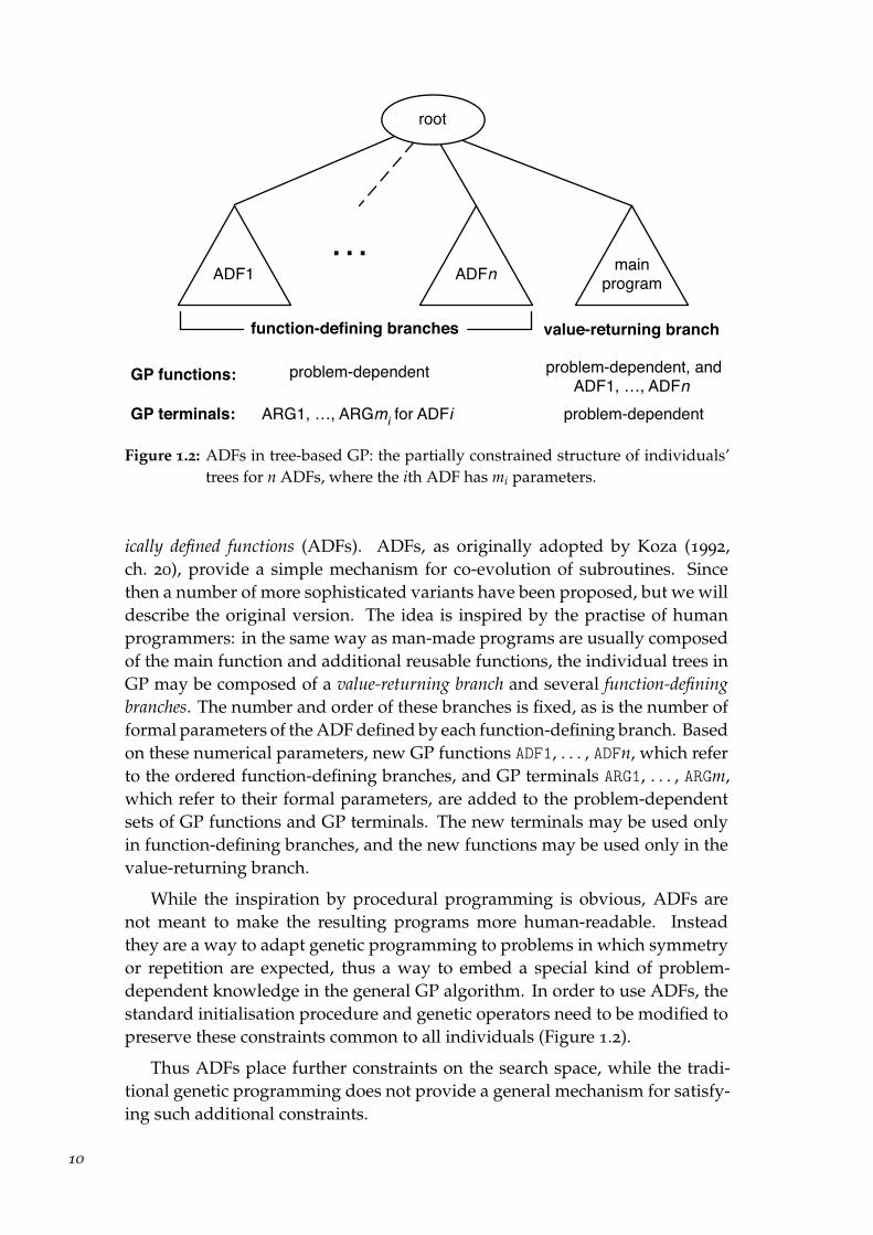
Figure 1.2: ADFs in tree-based GP: the partially constrained structure of individuals’trees for n ADFs, where the ith ADF has mi parameters.
ically defined functions (ADFs). ADFs, as originally adopted by Koza (1992,ch. 20), provide a simple mechanism for co-evolution of subroutines. Sincethen a number of more sophisticated variants have been proposed, but we willdescribe the original version. The idea is inspired by the practise of humanprogrammers: in the same way as man-made programs are usually composedof the main function and additional reusable functions, the individual trees inGP may be composed of a value-returning branch and several function-definingbranches. The number and order of these branches is fixed, as is the number offormal parameters of the ADF defined by each function-defining branch. Basedon these numerical parameters, new GP functions ADF1, . . . , ADFn, which referto the ordered function-defining branches, and GP terminals ARG1, . . . , ARGm,which refer to their formal parameters, are added to the problem-dependentsets of GP functions and GP terminals. The new terminals may be used onlyin function-defining branches, and the new functions may be used only in thevalue-returning branch.
While the inspiration by procedural programming is obvious, ADFs arenot meant to make the resulting programs more human-readable. Insteadthey are a way to adapt genetic programming to problems in which symmetryor repetition are expected, thus a way to embed a special kind of problem-dependent knowledge in the general GP algorithm. In order to use ADFs, thestandard initialisation procedure and genetic operators need to be modified topreserve these constraints common to all individuals (Figure 1.2).
Thus ADFs place further constraints on the search space, while the tradi-tional genetic programming does not provide a general mechanism for satisfy-ing such additional constraints.
10
1.3 Grammatically biased ILP
In parallel with the beginnings Koza’s genetic programming and its first vari-ants such as STGP, grammars already started to be used in inductive logicprogramming (ILP), another branch of machine learning research4 that emergedat the time. As we will later see, this is where the grammar-based GP methodsdrew inspiration.
ILP constructs a hypothesis in the form of a logic program, more preciselya Prolog program, from a set of positive examples, from a set of negative ex-amples, and from background knowledge, also a Prolog program. The articleby Muggleton (1994) provides a concise description of the basic techniques ofILP and the theory behind it. It also acknowledges the importance of problem-dependent knowledge to restrict the search space: “in order to ensure efficiency,it is usually found necessary to employ extra-logical constraints within ILPsystems”. Two categories of such constraints are discussed: “statistical con-firmation” via a confirmation function, which “fits a graded preference surfaceto the hypothesis space”, and language bias, which “reduce[s] the size of thehypothesis space”.
From the point of view of evolutionary algorithms, the confirmation func-tion is simply a type of fitness function. We will focus our attention the otherkind of constraint, language bias: particularly interesting is a “generalised”approach that “provides a general purpose ‘declarative bias’” (as described byMuggleton, 1994). (In this context, “bias” is used to encompass both restric-tion and preference.) This approach devised by Cohen (1992, 1994) consists oftranslating the background knowledge into a grammar in a way that guidesthe formation of a hypothesis. Cohen noted that various existing ILP methods,each using a different algorithm, were well-suited for different problems, andfelt that the search bias embedded in the algorithms should instead be “com-piled into” the background knowledge. To achieve this he used “antecedentdescription grammars”, which are a special case of definite clause grammarsthat retains the use of arbitrary terms and unification among these terms (asshown in the Listing 1.4) but does not allow adding external goals to the pro-ductions.5 Such grammars describe antecedents (bodies) of Prolog clauses of ahypothesis.
To search with a weak bias, the grammar could allow various combinationsof problem-specific predicates to occur in a clause body, while a strong biascould prescribe a mostly fixed body and restrict the variation only to its part.Unification is used both to ensure that variables from the head of a clause4 Koza (1992) originally considered GP a machine learning parading, similarly, Muggleton
(1994), who conceived the original ILP, considered it a machine learning framework. Geneticprogramming can, however, be applied to search and optimisation problems likely to beconsidered out of the traditional scope of machine learning.5 A notation A → α where P, where P is a Prolog goal, superficially similar to the curly-
bracketed goals in DCGs, is introduced in the 1994 article. It is, however, clarified that the goalP is evaluated with regards to A and α “by a macro-expansion process when the grammar isread in”.
11
are used in its body and to impose further constraints: for instance that twopredicates should share a variable, or that variables in some predicate shouldbe of the same type. In addition to the “hard constraint” defined by a grammar,Cohen (1992) uses what he calls “preference bias”: some production rules aremarked “preferred” and some “deferred”. Only if the system does not succeedusing the preferred productions, it resorts to the deferred ones.
In his articles, Cohen (1992, 1994) shows how to emulate different strategies,including that of a well-known ILP system FOIL, and how to improve on FOIL’sperformance by adding various kinds of background knowledge using onlyantecedent description grammars: “The contribution of this paper is to describea single technique which can make use of all of these types of backgroundknowledge—as well as other types of information about the target concept—ina uniform way.” As we will show in the next section, the concept of declarativebias and some of these mechanisms can be transposed to genetic programming.In Section 1.5 we will describe a more recent system integrating ILP and GP,which shares even more details with Cohen’s methods.
1.4 CFG-GP, language bias, and search bias
The first notable use of formal grammars to control the search algorithm ofgenetic programming probably came from Peter Whigham as both another, ina way more general, solution to the typing problem recognised by Montana,and a means of introducing more bias into genetic programming (Whigham,1995, 1996). In the 1995 article Whigham noted that a context-free grammar canbe used in similar ways as types to restrict the structure of candidate solutions,in his terminology, to introduce language bias. The proposed method, calledcontext-free grammar genetic programming (CFG-GP), is based on a straightfor-ward redefinition of the elements of tree-based GP to respect a given context-free grammar. The individuals still have the form of trees, but instead ofrepresenting Lisp expressions, the trees are derived according to an arbitraryCFG, and genetic operators are altered to preserve this representation.
We have already mentioned a coarser form of language bias, which is createdby the sets of terminals and functions in original GP, but a CFG allows to embedmore problem-dependent knowledge and also to easily use the programminglanguage most appropriate for a given problem.
Whigham (1995) also proposes the following mechanism for learning bias:
• Let each production rule in the grammar have an integer weight (called“fitness” by Whigham, although it’s a different concept from individualfitness) and let the weights initially be equal to 1.
• In each generation: Find the fittest individual (choosing one of the leasthigh among equally fit); choose one of the deepest nonterminals B in itsderivation tree; let α be the string of terminals into which it is rewritten;if B is a singleton, then let A be the parent of the highest node in the chain
12
of singletons that ends in B, else let A = B. Create a new production ruleA → α; if A → α is already in the grammar, increase its weight by 1,otherwise add A→ α with weight 1 to the grammar.
• When applying mutation or “replacement” (creating new individuals):select production rules for a given nonterminal with probability propor-tional to their weights.
The additional operator called replacement simply replaces a fixed part of thepopulation with individuals created in the same way as when creating theinitial population. The learnt bias thus affects the mutation and “replacement”operators in each generation, and can also be used in a subsequent run of thealgorithm.
Later, Whigham (1996) emphasised the distinction between three kinds ofbias: selection bias, language bias, and search bias. In his terminology selectionbias is the compound effect of a selection scheme and the fitness function,language bias consists of the restriction imposed by language (grammar), andsearch bias consists of the factors that control search (crossover and mutation).Seen from this perspective, the bias learning in Whigham’s original articlecompiled search bias into language bias. In contrast to this, the 1996 articlepresents a mechanism to control search bias separately:
• “Selective” versions of the mutation and crossover operators are intro-duced. A selective operator may be applied only to a subtree rooted ina nonterminal from a particular set. Several instances of such a selectiveoperator may be used, each with a different probability. These probab-ilities are considered the principal means of search bias. Note that theprobabilities do not govern frequencies of particular nonterminals in thepopulation, but frequencies of operator application to them.
• Production rules in the grammar may still be assigned weights (in thisarticle called “merit weighting”), but the weights are only constant, andno new production rules are added to the grammar. The weights applyto initialisation and mutation as already described, and are presumablypart of search bias.
Whigham’s approach has shown that grammars, in this case CFGs, can beused in GP in a straightforward manner to constrain the search space. As notedby Whigham (1995) without going into detailed comparison, it is a “differentapproach to the closure problem [than STGP].” A context-free grammar can beused both to express constructs of a wide range of languages and to emulate atype system with a small finite set of types by having one nonterminal for each.STGP with its generics (Montana, 1994) is more powerful in this regard, butsuch power comes with a performance trade-off (Poli et al., 2008, sec. 6.2.4).
Additionally, Whigham has used grammars a vehicle for a finer control ofbias. In the two articles, Whigham (1995, 1996) proposed two different ways ofworking with bias: in the former using means analogous to those that Cohen
13

used in ILP (see Section 1.3: knowledge is being compiled into grammar, somerules may be preferred to others), but added a simple learning mechanism;in the latter he abandoned learning and tried to keep search bias separatedfrom language bias, while still taking advantage of using a grammar. Neitherof these approaches would be possible if the language bias wasn’t specifieddeclaratively.
1.5 Logic grammar based genetic programming:LOGENPRO
Wong and Leung (1995) presented a genetic programming system based onlogic grammars, called LOGENPRO (LOgic grammar based GENetic PRO-gramming system), and later (2000) the same authors published a book on thissystem. LOGENPRO is presented as “a framework [. . . ] that can combine GPand ILP to induce knowledge from databases” (Wong and Leung, 2000). Thesystem is based on the same core algorithm as tree-based GP or CFG-GP: iter-ated application of fitness-based selection and genetic operators, but instead ofcontext-free grammars, LOGENPRO employs logic grammars “described in anotation similar to that of definite clause grammars”.
The only difference other than in notation between DCGs and these logicgrammars seems to be that the “logical goals” that can be added to rules inLOGENPRO are not strictly limited to logic goals as used in Prolog: they arein fact procedures defined in Lisp, the language in which the framework itselfis implemented. (See Listing 3.3 on page 47 for an example of a LOGENPROgrammar.) The framework emulates the mechanisms of logic programming tointerpret the grammar, but it does not feature a complete or cleanly separatedlogic programming environment.6
LOGENPRO does not use any mechanisms or algorithms specific to ILPbut Wong and Leung (2000) demonstrate that with a suitable grammar, itcan be used to learn logic programs and it achieves results competitive withearlier ILP systems not based on GP and grammars. What differentiates itfrom CFG-GP is the more powerful formalism for grammars, which is closerto the one used by Cohen in ILP. As we have noted in Section 1.1, definiteclause grammars can be used to describe the context-dependent constructsoften found in programming languages. The representation of individuals inLOGENPRO is still conceptually the same as in CFG-GP (a derivation tree,although with structured nodes, as they can contain terms and goals), butoperators need to be much more complex to respect the grammar.
While DCGs are essentially Turing-complete (see Fact 5, page 7), LO-GENPRO does not evaluate logical goals except when generating new trees:
6 I obtained LOGENPRO source code from the authors via personal communication. Al-though Wong and Leung (1995, 2000) present the “logic grammars” used in LOGENPRO asdifferent from DCGs, no difference is evident from their description, and no details about theimplementation are given.
14
the subtrees that contain logic goals cannot be changed by the operators (Wongand Leung, 2000, sec. 5.3), so they behave as atomic and immutable compon-ents throughout the evolution (compare with the approach used by Cohen,1994, see footnote 5, page 11).
On one hand, even the remaining power of DCGs, which lies in the useof variables and unification, still make operators, particularly crossover, quitecomplex: according to Wong and Leung (2000, sec. 5.3), the worst-case timecomplexity of crossover is O(m · n · log m), where m and n are the sizes of thetwo parental trees, slightly higher than O(mn) in Koza’s GP with ADFs andMontana’s STGP. On the other hand, the same power allows it to emulatethe effect of both of these methods (Wong and Leung, 2000). The scheme ofindividuals that use ADFs (as shown in Figure 1.2) can be easily embeddedin a grammar (see Section 3.7, also demonstrated by Wong and Leung, 2000).While the authors do not explain how exactly LOGENPRO can emulate STGPincluding generics, a finite set of types can be emulated even using a CFG (aswe have remarked in Section 1.4).
LOGENPRO focuses on sophisticated constraints on the search space thatcan be described declaratively using a DCG, and performs a search usingelaborate operators that preserve these constraints. It does not provide anyspecial mechanisms for learning bias, or any additional parameters for thesearch.
1.6 Grammatical evolution
Grammatical evolution (GE) (Ryan et al., 1998; O’Neill and Ryan, 2003) is a recentmethod for grammar-based GP that, unlike LOGENPRO or CFG-GP, signi-ficantly changes the paradigm of traditional tree-based GP by introduces thenotion of genotype-phenotype mapping. In a parallel to the biological process ofgene expression, each individual has a variable-length linear genotype consist-ing of integer codons, to which the genetic operators such as mutation andcrossover are applied. In order to evaluate the individual’s fitness, the geno-type is mapped to phenotype, a program in the language specified by the givencontext-free grammar. Trees are not used for individual representation butimplicitly as a temporary structure used in the course of mapping.
The mapping used in GE is so simple that we can describe it in full details(adapted from Nohejl, 2009):
In analogy to the DNA helix and nucleobase triplets, the stringis often called chromosome, and the values it consists of are calledcodons. Codons consist of a fixed number of bits. The mapping tophenotype, proceeds by deriving a string as outlined below in thepseudocode for Derivation-Using-Codons. The procedure acceptsthe following parameters:
15

– G, a context-free grammar in BNF. Note that BNF ensuresthat there is a non-empty ordered list of rewriting rules for eachnonterminal.
– S, a nonterminal to start deriving from. The start nonterminalof G should be passed in the initial call.
– C, a string of codons to be mapped. Note that it is passedby reference and the recursive calls will sequentially consume itscodons using the procedure Pop.
Derivation-Using-Codons(G,S,C)
1 P← array of rules for the nonterminal S in G indexed from 02 n← length[P]3 if n = 1 � only one rule (no choice necessary)
4 then r← 05 elseif length[C] > 0 � choice necessary, enough codons
6 then r← Pop(C) mod n7 else error “Out of codons” � or wrap C, more on that later
8 σ← body of the rule P[r]9 τ← λ10 foreach A← symbols of σ sequentially11 do if A is terminal12 then τ← τ .A13 else τ← τ .Derivation-Using-Codons(G,A,C)14 return τ
Out of the context of fitness evaluation, the individuals are simple binarystrings to which standard GA (Goldberg, 1989) operators for one-point cros-sover and mutation are applied (the only differences are that the chromosomesare variable-length and the crossover is applied on codon boundary, not at ar-bitrary position), the population can also be initialised by generating randombinary strings. Thus the operators for GE can be implemented very efficiently,and the performance penalty of performing the mapping is also low.
It would appear that this efficiency comes at the cost of a high proportionof invalid individuals (see line 7 of the pseudocode). This issue is addressedby wrapping the chromosome (interpreting it in a circular fashion) if needed,which can greatly reduce the number of invalid individuals (O’Neill and Ryan,2003, sec. 6.2). Still, the operators clearly may have a different effect thanthe traditional GP operators, which tend to preserve most of the individuals’structure and are designed to have a predictable effect. In GE, on the one hand,minor changes in genotype can translate into massive changes in phenotype;on the other hand, some parts of genotype (and thus any changes to them)may not have any effect on the phenotype. O’Neill and Ryan (2003) justifythese issues as parallels to genetic phenomena (such as genetic code degeneracyin the case of unused genetic information), and show that in some cases theycan improve performance.
16

While a formal analysis of the general effect of these simple operators onphenotype, and thus the overall search performance, is lacking, the effect canbe measured and compared statistically in specific applications. This methodis used by O’Neill and Ryan (2003) to compare different variants of operators,and we will use it to compare performance with CFG-GP in Chapter 3.
Compared with CFG-GP, and especially with LOGENPRO, grammaticalevolution has an extremely simple implementation that consists of highly effi-cient elements. We could call these elements (operators, simple random initial-isation) grammar-agnostic: they do not depend on the grammar at all, and thesearch bias that they create cannot be adjusted with regards to the grammar.The constraints of the grammar are ensured by the genotype-phenotype map-ping at the expense of preservation of phenotypic structure that the traditionalGP, as well as CFG-GP or LOGENPRO, strive for.
1.7 Common features and shortcomings
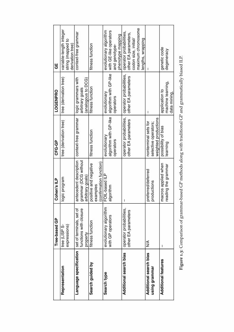
Figure 1.3 provides an overview of the grammar-based GP methods that wehave presented along with traditional GP and grammatically biased ILP. Themost important trait of all grammar-based methods is that they provide a gen-eral framework for declaratively describing the search space that the traditionalGP or ILP lacks. One aspect that differentiates them is the power of this de-clarative description. The relatively weak context-free grammars can describethe basic structure of common programming languages or their subsets (exceptcontext-dependent constructs), and emulate simple type systems, and ADFs.The logic grammars (antecedent description grammars used in Cohen’s ILP orDCG-like logic grammars in LOGENPRO) can capture context-dependency us-ing logic variables and unification, but their ability to use arbitrary logic goalsis of limited use in genetic programming (as exemplified by genetic operatorsin LOGENPRO, Section 1.5).
The expressive power of grammars entails a performance trade-off forstructure-preserving operators. Grammatical evolution seems to avoid thisissue by using grammar-agnostic, possibly destructive operators similar tothose traditionally used in GA.
Apart from the hard constraints of the search space, the grammar mayserve as a vehicle for further bias (preference). This direction was explored byWhigham (1995, 1996) through selective operators and learning of productionweights. It may be less obvious that the grammar itself creates a bias byinteraction of its form (equal grammars may differ in form, see Fact 1, page 6)and the operators, or the genotype-phenotype mapping in case of GE. Thegrammar-based methods seem to be designed as if using a particular form ofthe grammar was an obvious way to embed problem-dependent knowledge,but with their growing complexity (logic grammars in LOGENPRO, interactionof operators and the mapping in GE) this is not the case. (The grammar for theartificial ant problem in Section 3.5, and the grammars for timetabling heuristics
17
in Section 3.9 will later be discussed in this context.) The otherwise relativelysimple CFG-GP provides a mechanism (Whigham, 1995) to adjust the form ofthe grammar over the course of running the algorithm, but the more recentmethods (GE and LOGENPRO) do not address this issue.
1.8 Implications for performance
LOGENPRO seems to be very different from the two other methods by using amore powerful formalism for grammars. This could be a double-edged swordif it was actually used in some application. We will attempt to replicate twoexperiments done by Wong and Leung (2000) with LOGENPRO (in Section 3.6and Section 3.7). We will show that the experiments do not actually require alogic grammar, and that the results are comparable with those of CFG-GP.
Grammatical evolution ensures constraints given by the grammar by itsgenotype-phenotype mapping but its operators can be applied to any part ofits genotype regardless of the grammar and the phenotype. This makes anygrammatical constraints work in an essentially different way in GE than inCFG-GP or LOGENPRO. We can expect this to cause GE to produce differentshapes of trees than the other two methods, which work with derivation trees(considered to represent the phenotype for GE). This in turn will result in adifferent search space. We will attempt to analyse this effect and link it to dif-ferences in performance using experiments with several different applicationsin Chapter 3.
Techniques for reuse of building blocks are crucial for performance in ap-plications that use such blocks. As we will show, it is easy to carry over thetechniques used by Koza (1992) for ADFs to any of the grammar-based meth-ods. In fact, it is far easier to specify the ADFs using a grammar than to addthe necessary ad hoc constraints to tree-based GP operators. The same gram-mar will, however, have a different effect in GE than in the other two methodsbecause operators are applied regardless of the grammar. We will see how thisimpacts performance in experiments in Section 3.7 and Section 3.8.
18
Tree
-bas
ed G
PCo
hen'
s IL
PCF
G-G
PLO
GEN
PRO
GE
Repr
esen
tatio
ntre
e (L
ISP
S-ex
pres
sion
s)lo
gic
prog
ram
tree
(der
ivatio
n tre
e)tre
e (d
eriva
tion
tree)
varia
ble-
leng
th in
tege
r st
ring
(map
ped
to
deriv
atio
n tre
e)La
ngua
ge s
peci
ficat
ion
set o
f ter
min
als,
set
of
func
tions
with
clo
sure
pr
oper
ty
ante
cede
nt d
escr
iptio
n gr
amm
ar (D
CG w
ithou
t ar
bitra
ry g
oals
)
cont
ext-f
ree
gram
mar
logi
c gr
amm
ars
with
ar
bitra
ry g
oals
(a
nalo
gous
to D
CG)
cont
ext-f
ree
gram
mar
Sear
ch g
uide
d by
fitne
ss fu
nctio
npo
sitiv
e an
d ne
gativ
e ex
ampl
es
(con
firm
atio
n fu
nctio
n)
fitne
ss fu
nctio
nfit
ness
func
tion
fitne
ss fu
nctio
n
Sear
ch ty
peev
olut
iona
ry a
lgor
ithm
wi
th G
P op
erat
ors
FOIL
-bas
ed IL
P al
gorit
hmev
olut
iona
ry
algo
rithm
with
GP-
like
oper
ator
s
evol
utio
nary
al
gorit
hm w
ith G
P-lik
e op
erat
ors
evol
utio
nary
alg
orith
m
with
GE-
like
oper
ator
s an
d ge
noty
pe-
phen
otyp
e m
appi
ngAd
ditio
nal s
earc
h bi
asop
erat
or p
roba
bilit
ies,
ot
her E
A pa
ram
eter
s–
oper
ator
pro
babi
litie
s,
othe
r EA
para
met
ers
oper
ator
pro
babi
litie
s,
othe
r EA
para
met
ers
oper
ator
pro
babi
litie
s,
othe
r EA
para
met
ers,
co
don
size
, ini
tial/
max
imum
chr
omos
ome
leng
ths,
wra
ppin
gAd
ditio
nal s
earc
h bi
as
usin
g gr
amm
arN/
Apr
efer
red/
defe
rred
prod
uctio
nsno
nter
min
al s
ets
for
sele
ctive
ope
rato
rs;
wei
ghte
d pr
oduc
tions
––
Addi
tiona
l fea
ture
s–
mac
ros
appl
ied
when
re
adin
g th
e gr
amm
arpo
ssib
ility
of b
ias
lear
ning
appl
icat
ion
to
mac
hine
lear
ning
, da
ta m
inin
g,
gene
tic c
ode
dege
nera
cy
Figu
re1.3:
Com
pari
son
ofgr
amm
ar-b
ased
GP
met
hods
alon
gw
ith
trad
itio
nalG
Pan
dgr
amm
atic
ally
bias
edIL
P.

20
Chapter 2
Existing Applications
Genetic programming is a very general method that has been applied to a vari-ety of problem domains from circuit design to the arts (Poli et al., 2008, ch. 12).While methods that are more efficient and have gained more widespread indus-trial use exist in most of these fields, the strength of GP lies in its applicability toproblems in which the precise form of the solution is unknown and analyticalmethods cannot be employed or would be too resource-intensive.
As we have explained in the previous chapter, the addition of grammarsto genetic programming serves primarily as a means of adapting the generalmethod to a particular problem or an implementation language: a grammar canbe used both to embed problem-dependent knowledge such as variable typesand structural restrictions, and to specify a subset of a programming language(or some other formal language) that we want to use for implementation.
Our goal is to compare the results both among different methods and withpreviously published results. Thus we will focus on relatively simple applica-tions suitable for comparing the three main methods that we have presented:CFG-GP, GE, and in two instances also LOGENPRO. All applications presen-ted in this chapter have been described in existing literature in conjunctionwith one of the methods or with traditional GP, usually in order to highlightadvantages of these methods. One application, the use of grammar-based GPmethods for hyper-heuristic (Section 2.5), stands out a little: as we will see,this area is relatively open-ended and demanding on implementation but alsocapable of producing heuristics competitive with those designed by humans.
Before we proceed to evaluating the methods in the next chapter, we willdescribe the chosen applications.
2.1 Simple symbolic regression
Regression is concerned with finding a function that best fits known data. Theproblem has most commonly been reduced parametric regression: finding para-meters for a function whose form is specified in advance (e.g., an nth-degreepolynomial). Assuming that the chosen form is adequate, such methods maybe very efficient. In situations in which the adequate form is not known, ge-
21
netic programming can be used to solve the more general problem as symbolicregression: search for a function represented in symbolic form, as an expressionusing some predefined operations.
A simple problem of real-valued symbolic regression was used as one ofthe introductory examples by Koza (1992) and continues to be used both asa basic benchmark for newer GP techniques and in more advanced researchapplications (Poli et al., 2008, sec. 12.2). When used as a benchmark, as opposedto a real-world application, the target values are precomputed using the knowntarget function, which may be a polynomial. The point is that GP is able to findthe expression representing the polynomial in the space of expressions thatalso involve operations unnecessary for the target function such as division orlogarithm.
Fitness of candidate solutions is usually measured as a sum of absolute orsquared errors at the given points to which various scaling methods can beapplied.
Except for specifying a custom language instead of Lisp, there is little ad-vantage in using grammar-based methods over using tree-based GP for simpleinstances of the problem. But these simple instances can serve as a test bedfor unusual operators, such as those employed in GE, which do not behaveanalogously to those used in tree-based GP.
More intricate cases of symbolic regression will be presented in Section 2.3and Section 2.4.
2.2 Artificial ant trail
The artificial ant trail is another classic introductory GP problem. The goal is tonavigate an artificial ant so that it finds all food lying on a toroidal floor withina time limit. The pieces of food are placed on a rectangular grid to form a trailwith increasingly demanding gaps and turns. The ant can use the actions– Left: turn left by 90 ° without moving,– Right: turn right by 90 ° without moving,– Move: advance one square in the direction the ant is facing, eating any food
on that square,combined using conditional branching on Food-Ahead: test the square the antis facing for food. All actions take one unit of time, the test is instant.
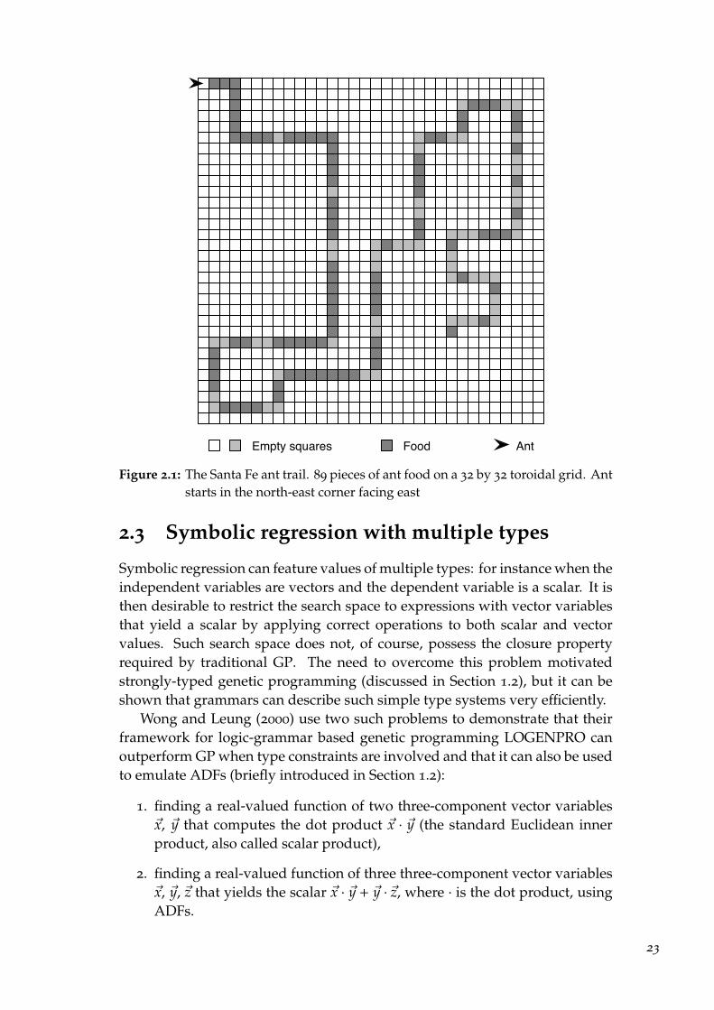
The problem was originally designed to test evolution of finite-state ma-chines using GA and various trails have appeared in subsequent versions ofthe experiment. The most common one, also used by Koza (1992) to demon-strate the competence of GP in solving this problem, is the so-called Santa Feant trail. When using GP, the solution has a form of a short program, whichis executed in a loop until time runs out. The syntactic restrictions placed onthe program play an important role that we will discuss when evaluating theexperiments. Fitness of candidate solution is measured as the number of foodpieces eaten within the time limit.
22
Empty squares Food Ant
Figure 2.1: The Santa Fe ant trail. 89 pieces of ant food on a 32 by 32 toroidal grid. Antstarts in the north-east corner facing east
2.3 Symbolic regression with multiple types
Symbolic regression can feature values of multiple types: for instance when theindependent variables are vectors and the dependent variable is a scalar. It isthen desirable to restrict the search space to expressions with vector variablesthat yield a scalar by applying correct operations to both scalar and vectorvalues. Such search space does not, of course, possess the closure propertyrequired by traditional GP. The need to overcome this problem motivatedstrongly-typed genetic programming (discussed in Section 1.2), but it can beshown that grammars can describe such simple type systems very efficiently.
Wong and Leung (2000) use two such problems to demonstrate that theirframework for logic-grammar based genetic programming LOGENPRO canoutperform GP when type constraints are involved and that it can also be usedto emulate ADFs (briefly introduced in Section 1.2):
1. finding a real-valued function of two three-component vector variables~x, ~y that computes the dot product ~x · ~y (the standard Euclidean innerproduct, also called scalar product),
2. finding a real-valued function of three three-component vector variables~x, ~y, ~z that yields the scalar ~x · ~y + ~y · ~z, where · is the dot product, usingADFs.
23
While Wong and Leung (2000) compare the performance of LOGENPROwith a GP setup that does not use any syntactic constraints, I would suggestthat the point should not be that GP cannot use ad hoc syntactic constraints tothe same effect but that doing so using a grammar is more general but also fareasier and less error-prone: note that even in this seemingly simple examplethere are three “natural” types of unary and binary operations (scalar-to-scalar,vector-to-vector, vector-to-scalar) and perhaps scalar multiplication.
We will discuss the approach used by Wong and Leung (2000) and demon-strate that other grammar-based methods can be used with similar results. Wewill also analyse the role of ADFs in the second variant of the problem, whichWong and Leung (2000) did not do properly.
2.4 Boolean symbolic regression
The spaces of k-ary Boolean functions are relatively small (22k), as are the suffi-cient sets of basic functions from which they can be composed (e.g. the set ofcommon logical connectives {and, or,not}), yet the search space of their symbolicrepresentations is vast. Although symbolic regression of Boolean functions isof no practical interest, these properties make it suitable for evaluating geneticprogramming systematically. Koza (1992) has demonstrated that the difficultyof finding different ternary Boolean functions by blind random search amongexpressions of certain maximum size varies considerably and that GP is stat-istically more successful than blind random search in finding those that areparticularly hard to find. (More details in Koza, 1992, ch. 9.)
His experiments have also shown that the hardest to find among ternaryfunctions are the parity functions (the even and odd parity function are true ifand only if the number of true arguments is even and odd, respectively). Con-sequently, the parity functions are relatively hard to find even in the classes ofhigher-arity Boolean functions. At the same time they can be easily composedfrom simple building blocks: the exclusive-or functions, and a negation in caseof even parity. This in turn makes Boolean symbolic regression of the parityfunctions suitable for testing the impact of ADFs on performance.
We will use the even-parity Boolean regression problem to test the perform-ance of techniques for the grammar-based methods that emulate ADFs. Resultswill be compared to those presented by Koza (1992) for tree-based GP with andwithout ADFs.
2.5 Hyper-heuristics
In contrast to the previously presented applications, hyper-heuristics is actuallya whole field covering very diverse problems. A hyper-heuristic search enginedoes not search for problem solutions but rather for heuristics for solving aproblem. Thus if the class of problems of interest was Boolean satisfiability,
24

heuristics for a SAT solver would be sought rather than truth-value assign-ments.
Different approaches can be used to find heuristics, but if some heuristicshave already been developed and can be combined in more complex ways thenjust choosing a sequence, grammar-based GP can be used to great advantage.The grammar allows us both to use the language of our problem-solving frame-work directly and to embed our knowledge about the existing heuristics thatare to be used as building blocks.
Bader-El-Den et al. (2009) have recently successfully applied a grammar-based GP hyper-heuristic framework to timetabling. The method they usedwas essentially CFG-GP. We will try to replicate their results with our im-plementation of CFG-GP, and compare them to the results obtained usinggrammatical evolution in Section 3.9.
2.6 Other applications
While we will not experiment with other problems, several other areas ofapplication are worth at least mentioning:
The authors of LOGENPRO have developed their system specifically totarget data mining problems. They see their logic grammar based framework(covered in Section 1.5) as a combination of two important approaches to datamining: ILP and GP (Section 1.2 and Section 1.3). In addition to artificialproblems such as the dot product problem (see Section 2.3 above), they applyLOGENPRO to two benchmark data mining problems (credit card screeningusing decision trees and the chess endgame problem using logic programming),and to data mining from “real-life medical databases”. LOGENPRO providesresults competent with other learning systems in the first benchmark and out-performs ILP systems FOIL, BEAM-FOIL, and mFOIL significantly at mostnoise levels in the latter benchmark. It is interesting to note that in none of theapplications presented by Wong and Leung (2000) the specific feature of theirsystem, the power of logic grammars, is used. In particular, their applicationsuse only simple logic goals that could be replaced by short enumerations, andnone of the grammars feature context-dependence via unification. Conceiv-ably, any of their results could be replicated using grammar-based methodsother than LOGENPRO, in the same way as we will show on the example ofthe dot product problem in Section 3.6. Thus, grammar-based methods canalso be used as a viable data mining framework.
Grammatical evolution has recently been used in dynamic applications,where the grammar itself is described by a (meta-)grammar and co-evolvesalong with the individual, allowing for further adaptability (Dempsey et al.,2009).
Natural Computing Research & Applications Group at University CollegeDublin (UCD NCRA), where most of the current work on grammatical evolu-tion is being done, has also used GE to evolve a logo for the group interactively
25
(O’Neill and Brabazon, 2008). Their web site1 showcases other unconventionaland creative applications including evolution of elevator music. Results in suchapplications cannot of course be quantitatively measured but they demonstratethe variety of objects and processes that can be described using a grammar andconsequently evolved using grammar-based GP methods.
1http://ncra.ucd.ie/
26
Chapter 3
Experiments with Grammar-BasedMethods
In this chapter we will perform several experiments with instances of theproblems chosen in Chapter 2.
When evaluating CFG-GP and GE, we will use the AGE (Algorithms forGrammar-based Evolution, originally Algorithms for Grammatical Evolution)framework, which is a competent and well-documented implementation of GEand common evolutionary algorithm elements, as I have shown in my bachelorthesis (Nohejl, 2009). For the purpose of these experiments AGE has been ex-tended with CFG-GP algorithm elements implemented according to Whigham(1995). This will allow us to test CFG-GP and GE in almost identical setups. SeeChapter 4 for more information about AGE and its implementation of CFG-GP.The software is available on the accompanying medium and online1.
The performance of LOGENPRO will be evaluated using the implementa-tion that Dr Man Leung Wong, a co-author of the method (Wong and Leung,1995, 2000), has kindly provided to me.
3.1 Observed characteristics
As a measure of success I adopt the cumulative success rate over a number ofruns, as usual when evaluating evolutionary algorithms. The success in eachexperiment is defined by the Success predicate entry in its table (see Section 3.2below). For the purpose of these experiments, the algorithms are left runninguntil the maximum number of generations is reached even when the successpredicate has been satisfied.
To further facilitate comparison, we will use several characteristics of de-rivation trees applicable to both methods: tree height (defined in Section 1.1),number of choice nodes, and bushiness (both defined below). In the followingdefinitions, let G = (N,T,P,S) be a context-free grammar and ρ a derivationtree for the grammar G.
1http://nohejl.name/age/
27

Definition. We will say that a particular node of ρ is a choice node if it is labelledwith a nonterminal for which P contains more than one production. (Thusa choice of production had to be made at this node.) Internal choice node is achoice node that has at least one choice node among its descendants.
When using GE, the number of choice nodes coincides with the number ofcodons used during the mapping process. Additionally, the number of choicenodes reflects the amount of information contained in a given derivation treemore accurately than the total number of nodes.
Definition. Let n be the number of all choice nodes in ρ, and k the number ofinternal choice nodes in ρ. The ratio n
k+1 expresses the bushiness of ρ.
Bushiness is simply the ratio of the total number of choice nodes and thenumber of their “parents”. Note that in any derivation tree that contains atleast one choice node, there is a non-empty group of topmost choice nodes (thegroup has no choice node ancestor): the additive constant 1 in the formula actsas a virtual parent of these choice nodes. The bushiness is thus analogous to theaverage branching factor, except that it is defined only based on choice nodes.
AGE can report tree characteristics for both GE and CFG-GP. LOGENPROoffers only basic data about fitness and success.
3.2 Setup
Both AGE, and LOGENPRO allow to configure parameters such as selectionmethod, operator probabilities, or maximum tree heights. We will present theseparameters for each experiment in a table derived from the “tableau” formatused by Koza (1992), and in a modified form by O’Neill and Ryan (2003). Inaddition to the entries used by either of them, I also specify the details ofthe algorithm in the entries Algorithm, Selection, Initialisation, Operators, andParameters (for other method-specific parameters).
In order to make comparisons statistically relevant, we will use data from atleast 100 runs. In the case of AGE, these are always runs from one sequence withrandom number generator (RNG) seed value 42; in the case of LOGENPROthese are runs with RNG seeds from the sequence 1, 2, 3, . . . ,n. (LOGENPROnormally seeds the generator with the current time. I have modified its sourcecode to use a fixed number to seed the generator.)
3.3 Statistics
We will use several statistics: average using arithmetic mean, variance, andcoefficient of variance (CV), which is a relative measure of dispersion definedas the ratio of the standard deviation to the absolute value of the mean. Thestatistics will be computed from a population of individuals from a particulargeneration. When evaluating results from multiple runs of the same setup
28
we will average these statistics (using arithmetic mean) over the performedruns. If a population contains invalid individuals, they are excluded from thestatistics.
When I describe a difference between two sets of numerical results (or ratesof success in two sets) as significant, it means that the statistical hypothesis thatthe two sets are samples of a statistical population with the same mean (or thatthe probabilities of success in the two sets are the same), has to be rejected onthe level of statistical significance of 5 %. Accordingly, whenever a differenceis said to be insignificant, the same hypothesis cannot be rejected on the levelof 5 %. Unless stated otherwise, any differences I point out are significant. Iuse Student’s t-test for testing equivalence of means, and a simple test of equalproportions for testing the probabilities of success.2
3.4 Simple symbolic regression
We will compare the performance of CFG-GP and GE in a simple instance ofthe symbolic regression problem (Section 2.1).
3.4.1 Experimental setups 1
The first setup of GE is deliberately based on the parameters used in the sym-bolic regression example supplied with GEVA3. I have used the same setup(except for maximum tree height, see explanation below) in my bachelor thesis(Nohejl, 2009) to show that the codon size higher than 8 bits does not providesubstantial advantage, and that AGE achieves a success rate of 706 and 701out of 1000 runs (with 31 and 8 bits per codon, respectively), which was sig-nificantly better than the rate achieved by GEVA. Thus we will also use 8-bitcodons in the current experiment.
When possible, we will use the same settings for CFG-GP: elite size, fitnessmeasure, selection scheme, etc., and also the crossover rate will be the same:even though each method has a different crossover operator, the crossoverrate of 0.9 is a standard value of crossover probability in GP, which is usedsystematically by both Whigham (1995, 1996) and O’Neill and Ryan (2003).
The mutation rate for CFG-GP will be, somewhat arbitrarily, set to 0.1.The higher nominal value is meant to reflect that the mutation rate in CFG-GP is equivalent to its effective per-individual mutation rate, whereas theeffective per-individual rate in GE is much higher then the 0.02 per-codonrate, and is dependent on the number of used codons and the distribution ofnonterminals in each individual. Therefore, no fixed per-individual mutation2Both are computed using the R stats package (functions t.test and prop.test), which is part
of the open-source R Project for Statistical Computing available at http://www.r-project.org/.3 GEVA is “an open source implementation of Grammatical Evolution [. . . ], which provides
a search engine framework in addition to a simple GUI and the genotype-phenotype mapper ofGE.” (O’Neill et al., 2008). It is being developed at Natural Computing Research & ApplicationsGroup (NCRA) at University College Dublin: http://ncra.ucd.ie/Site/GEVA.html.
29

rate corresponds to a given per-codon rate used in GE. Whigham (1995, 1996)has used mutation rates of 0.15 and 0, respectively, so 0.1 is a conservativechoice.
Because CFG-GP uses a maximum tree height for its operators, while GEusually ensures reasonable tree size only implicitly, we will use 20 as maximumtree height for both methods, a limit high enough to have only marginal impacton the results of the GE setup.
The only parameter left is the maximum height of derivation trees createdby the CFG-GP initialisation method. We would like to operate on individualsof roughly the same size as in the GE setup, so that both methods are evalu-ated on search spaces of comparable size. I have experimentally determinedthat maximum height 5 results in derivation trees of height closest to thosegenerated by the GE setup (as shown in Figure 3.1).
The setup for both methods is detailed in Table 3.1.
Objective: Find a function of one variable x represented by anexpression to fit a given set of the target function values atspecified points. The target function is x4 + x3 + x2 + x.
Terminal operands: x, 1.0.Terminal operators: +, −, · (all binary).Grammar: See Listing 3.1.Fitness cases: 20 fixed points −1.0, −0.9, . . . , 1.9.Raw fitness: The sum of squared errors taken over the 20 fitness cases.Scaled fitness: Same as raw fitness.Algorithm: Simple with elite size: 10, generations: 101, population:
100.Selection: Tournament, size: 3.GE initialisation: Random codon string initialisation, length: 200.CFG-GP initialisation: “Grow” method (Whigham, 1995), maximum height: 5.GE operators: Fixed-length one-point crossover, probability: 0.9.
Codon-level mutation, probability: 0.02.CFG-GP operators: Crossover (Whigham, 1995), probability: 0.9.
Mutation (Whigham, 1995), probability: 0.1.Common parameters: Maximum tree height: 20.GE parameters: Maximum wraps: 3. Codon size: 8.Success predicate: Raw fitness lower than 0.00001 (to allow for floating-point
round-off error.)
Table 3.1: Simple symbolic regression, parameters for setups 1, CFG-GP (1) and GE(1).
<expr> ::= ( <expr> <op> <expr> ) | <var><op> ::= + | - | *<var> ::= x | 1.0
Listing 3.1: Simple grammar for symbolic regression in Lua.
30
3.4.2 Results from setups 1
The final success rate of 999 out of 1000 runs achieved by CFG-GP has beensubstantially higher than the 733 out of 1000 runs achieved by GE, moreoverCFG-GP was more successful in all generations and converged very fast (seeFigure 3.1). While derivation tree heights suggest that both methods weresearching a similar space, a closer look at the tree characteristics (Figure 3.3)reveals differences:
(1) During the first five generations, GE has a very high CV of both treeheight and bushiness compared to CFG-GP, and consequently also a high vari-ance of the number of choice nodes. This can be explained by the initialisationmethod, and does not seem to have an important lasting effect.
(2) After (1), CFG-GP has a significantly larger CV of tree height, and neithermethod continuously dominates in average height.
(3) CFG-GP produces significantly bushier trees throughout the run. After(1), neither method continuously dominates in CV of bushiness.
(4) The compound effect of (2) and (3) is a higher variance of the numberof choice nodes in trees produced by CFG-GP. We can interpret this variance(which is an absolute measure as opposed to CV) in conjunction with theaverage as the extent of the search space. Note that this is observable evenif we do not take into account the portion of CFG-GP results after CFG-GPreaches almost full success rate.
To examine the possibility that grammatical evolution produces less diversecandidate solutions because of inappropriate operator parameters, let’s havea look at fitness statistics in Figure 3.2: GE soon reaches higher coefficient ofvariance than CFG-GP, and the CV keeps growing while average fitness staysnearly constant in GE. Note that the difference is not due to invalid individuals,which are excluded from the statistics.
This shows that the parameters of the operators result in enough phenotypicdiversity but fail to produce a favourable distribution of tree characteristics.Additionally, even if a higher mutation rate had the effect of producing bettertree characteristics, it would effectively turn GE into a blind search: both itsstandard operators can be very disruptive (their effect is not localised to asubtree: see the “ripple” crossover discussed in O’Neill and Ryan, 2003, andthe codon and bit-level mutation in my bachelor thesis, Nohejl, 2009). Thesuccess rate reached in this experiment depends on the high elitism, whichcompensates for the disruptive effect of operators.
We can conclude that CFG-GP has searched a larger search space (bushiertrees of more varied height) and has achieved substantially better results thanGE. (Note that the larger search space is not necessarily a superset of thesmaller one as GE may explore less bushy trees better). This may not be asingle direct cause of the higher success rate but being able to find a solutionmore reliably while searching through more diverse candidate solutions iscertainly beneficial.
31
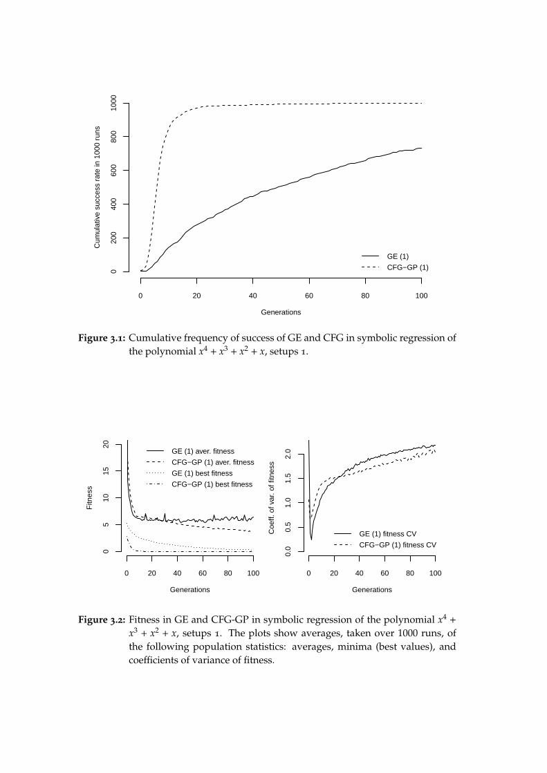
Generations
Cum
ulat
ive
succ
ess
rate
in 1
000
runs
0 20 40 60 80 100
020
040
060
080
010
00
GE (1)
CFG−GP (1)
Figure 3.1: Cumulative frequency of success of GE and CFG in symbolic regression ofthe polynomial x4 + x3 + x2 + x, setups 1.
Generations
Fitn
ess
0 20 40 60 80 100
05
1015
20
GE (1) aver. fitness
CFG−GP (1) aver. fitness
GE (1) best fitness
CFG−GP (1) best fitness
Generations
Coe
ff. o
f var
. of f
itnes
s
0 20 40 60 80 100
0.0
0.5
1.0
1.5
2.0
GE (1) fitness CV
CFG−GP (1) fitness CV
Figure 3.2: Fitness in GE and CFG-GP in symbolic regression of the polynomial x4 +
x3 + x2 + x, setups 1. The plots show averages, taken over 1000 runs, ofthe following population statistics: averages, minima (best values), andcoefficients of variance of fitness.
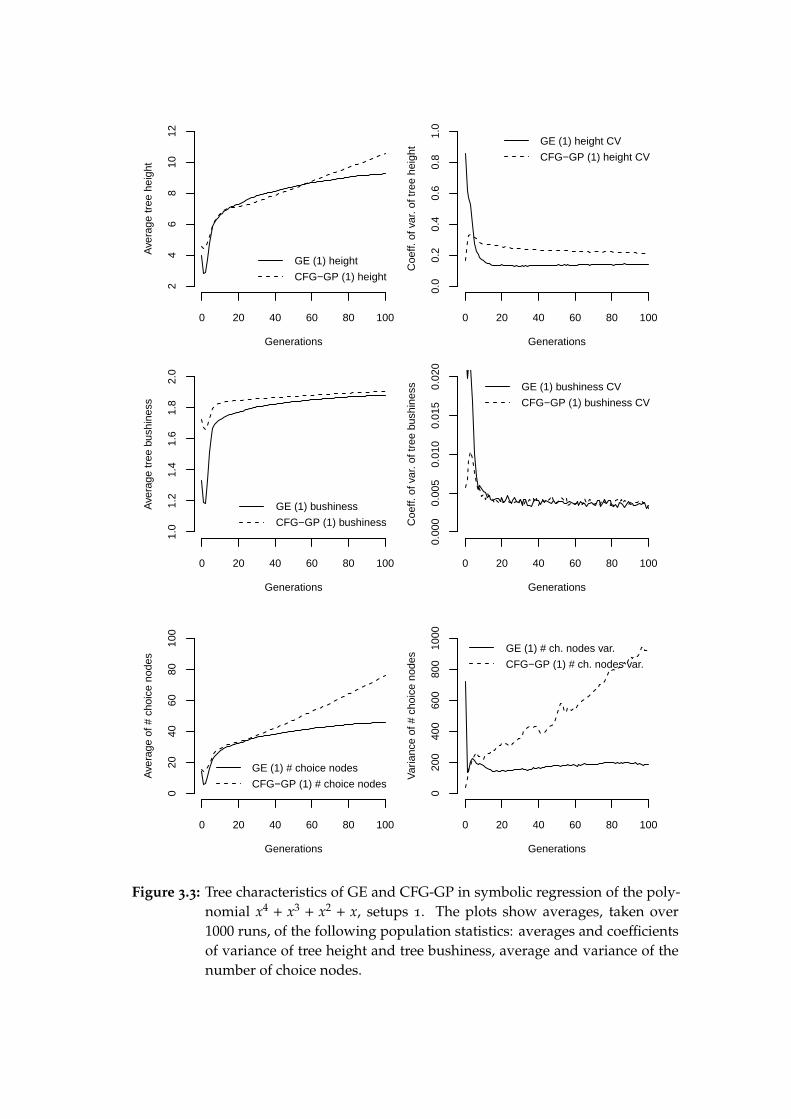
Generations
Ave
rage
tree
hei
ght
0 20 40 60 80 100
24
68
1012
GE (1) height
CFG−GP (1) height
Generations
Coe
ff. o
f var
. of t
ree
heig
ht
0 20 40 60 80 100
0.0
0.2
0.4
0.6
0.8
1.0
GE (1) height CV
CFG−GP (1) height CV
Generations
Ave
rage
tree
bus
hine
ss
0 20 40 60 80 100
1.0
1.2
1.4
1.6
1.8
2.0
GE (1) bushiness
CFG−GP (1) bushiness
Generations
Coe
ff. o
f var
. of t
ree
bush
ines
s
0 20 40 60 80 100
0.00
00.
005
0.01
00.
015
0.02
0
GE (1) bushiness CV
CFG−GP (1) bushiness CV
Generations
Ave
rage
of #
cho
ice
node
s
0 20 40 60 80 100
020
4060
8010
0
GE (1) # choice nodes
CFG−GP (1) # choice nodes
Generations
Var
ianc
e of
# c
hoic
e no
des
0 20 40 60 80 100
020
040
060
080
010
00
GE (1) # ch. nodes var.
CFG−GP (1) # ch. nodes var.
Figure 3.3: Tree characteristics of GE and CFG-GP in symbolic regression of the poly-nomial x4 + x3 + x2 + x, setups 1. The plots show averages, taken over1000 runs, of the following population statistics: averages and coefficientsof variance of tree height and tree bushiness, average and variance of thenumber of choice nodes.
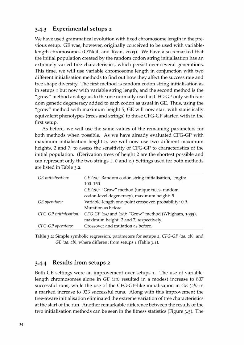
3.4.3 Experimental setups 2
We have used grammatical evolution with fixed chromosome length in the pre-vious setup. GE was, however, originally conceived to be used with variable-length chromosomes (O’Neill and Ryan, 2003). We have also remarked thatthe initial population created by the random codon string initialisation has anextremely varied tree characteristics, which persist over several generations.This time, we will use variable chromosome length in conjunction with twodifferent initialisation methods to find out how they affect the success rate andtree shape diversity. The first method is random codon string initialisation asin setups 1 but now with variable string length, and the second method is the“grow” method analogous to the one normally used in CFG-GP only with ran-dom genetic degeneracy added to each codon as usual in GE. Thus, using the“grow” method with maximum height 5, GE will now start with statisticallyequivalent phenotypes (trees and strings) to those CFG-GP started with in thefirst setup.
As before, we will use the same values of the remaining parameters forboth methods when possible. As we have already evaluated CFG-GP withmaximum initialisation height 5, we will now use two different maximumheights, 2 and 7, to assess the sensitivity of CFG-GP to characteristics of theinitial population. (Derivation trees of height 2 are the shortest possible andcan represent only the two strings 1.0 and x.) Settings used for both methodsare listed in Table 3.2.
GE initialisation: GE (2a): Random codon string initialisation, length:100–150.GE (2b): “Grow” method (unique trees, randomcodon-level degeneracy), maximum height: 5.
GE operators: Variable-length one-point crossover, probability: 0.9.Mutation as before.
CFG-GP initialisation: CFG-GP (2a) and (2b): “Grow” method (Whigham, 1995),maximum height: 2 and 7, respectively.
CFG-GP operators: Crossover and mutation as before.
Table 3.2: Simple symbolic regression, parameters for setups 2, CFG-GP (2a, 2b), andGE (2a, 2b), where different from setups 1 (Table 3.1).
3.4.4 Results from setups 2
Both GE settings were an improvement over setups 1. The use of variable-length chromosomes alone in GE (2a) resulted in a modest increase to 807successful runs, while the use of the CFG-GP-like initialisation in GE (2b) ina marked increase to 923 successful runs. Along with this improvement thetree-aware initialisation eliminated the extreme variation of tree characteristicsat the start of the run. Another remarkable difference between the results of thetwo initialisation methods can be seen in the fitness statistics (Figure 3.5). The
34

use of the random string initialisation in conjunction with variable-length chro-mosomes resulted in frequent occurrence of highly unfit individuals through-out the run (the plot had to be cropped). While such individuals could havein principle occurred using any settings of both methods (they just representrelatively complex arithmetic expressions with output very far from the tar-get function), the occurred only in GE with variable-length chromosomes andrandom-string initialisation (a combination used by O’Neill and Ryan, 2003,although they acknowledge the positive effect of tree-based initialisation).
CFG-GP with both initialisation parameters was still better than GE. Withmaximum initialisation height 2 it reached full success rate already in genera-tion 58, and with maximum initialisation height 7 it succeeded in 992 runs outof 1000. The success rates for heights 2, 5, and 7 are significantly different, yetall three have led to successful solution quite consistently compared to GE.
We can make almost identical observations as in setups 1 about tree char-acteristics of the two methods: regardless of the initialisation method, GEresults in bushier trees of more varied height and is able to expand the sizeof its search space over that of GE, at the same time CV of bushiness is sim-ilar for the two methods, and achieved tree heights can be too. This shows aconsistent difference between GE and CFG-GP not caused by initialisation oruse of variable-length vs. fixed-length chromosomes in GE, that is a differenceresulting from the nature of operators of the two methods. The CFG-GP oper-ators have searched the solution space of this simple problem more effectivelythan those of GE; additionally, CFG-GP has been relatively insensitive to thecharacteristics of the initial population.
Generations
Cum
ulat
ive
succ
ess
rate
in 1
000
runs
0 20 40 60 80 100
020
040
060
080
010
00
GE (2a)
GE (2b)
CFG−GP (2a)
CFG−GP (2b)
Figure 3.4: Cumulative frequency of success of GE and CFG-GP in symbolic regressionof the polynomial x4 + x3 + x2 + x, setups 2.
35
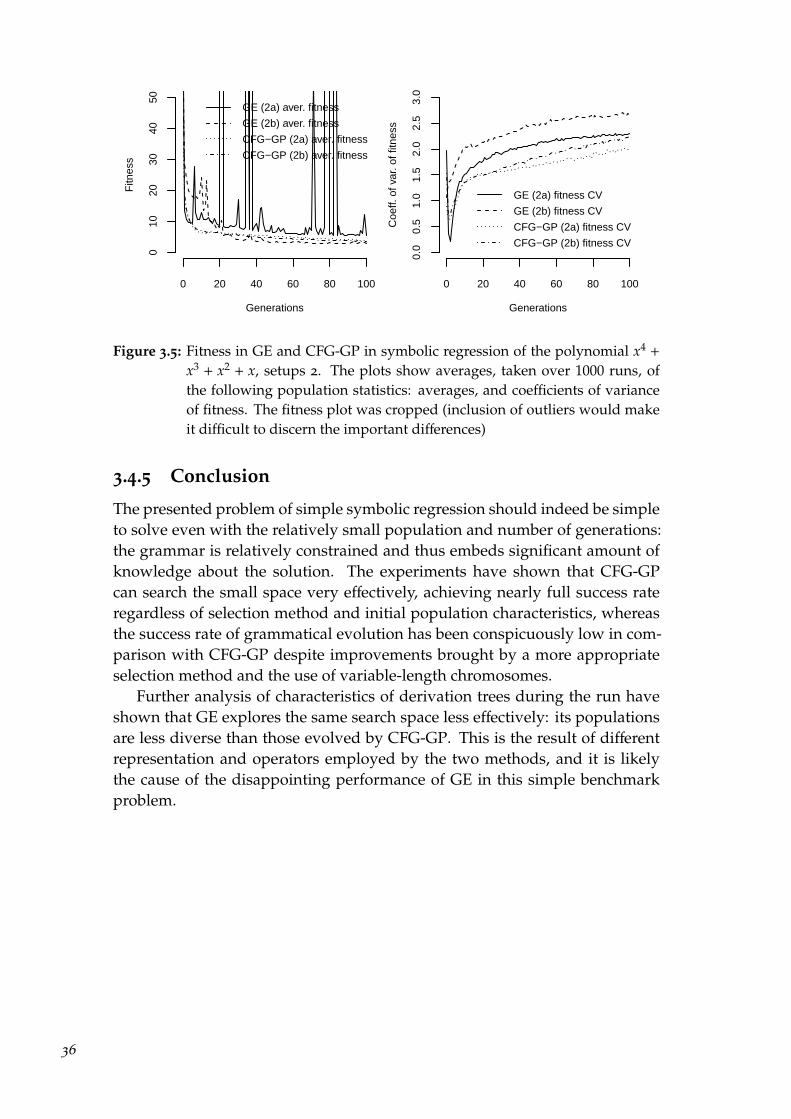
Generations
Fitn
ess
0 20 40 60 80 100
010
2030
4050
GE (2a) aver. fitness
GE (2b) aver. fitness
CFG−GP (2a) aver. fitness
CFG−GP (2b) aver. fitness
Generations
Coe
ff. o
f var
. of f
itnes
s
0 20 40 60 80 100
0.0
0.5
1.0
1.5
2.0
2.5
3.0
GE (2a) fitness CV
GE (2b) fitness CV
CFG−GP (2a) fitness CV
CFG−GP (2b) fitness CV
Figure 3.5: Fitness in GE and CFG-GP in symbolic regression of the polynomial x4 +
x3 + x2 + x, setups 2. The plots show averages, taken over 1000 runs, ofthe following population statistics: averages, and coefficients of varianceof fitness. The fitness plot was cropped (inclusion of outliers would makeit difficult to discern the important differences)
3.4.5 Conclusion
The presented problem of simple symbolic regression should indeed be simpleto solve even with the relatively small population and number of generations:the grammar is relatively constrained and thus embeds significant amount ofknowledge about the solution. The experiments have shown that CFG-GPcan search the small space very effectively, achieving nearly full success rateregardless of selection method and initial population characteristics, whereasthe success rate of grammatical evolution has been conspicuously low in com-parison with CFG-GP despite improvements brought by a more appropriateselection method and the use of variable-length chromosomes.
Further analysis of characteristics of derivation trees during the run haveshown that GE explores the same search space less effectively: its populationsare less diverse than those evolved by CFG-GP. This is the result of differentrepresentation and operators employed by the two methods, and it is likelythe cause of the disappointing performance of GE in this simple benchmarkproblem.
36
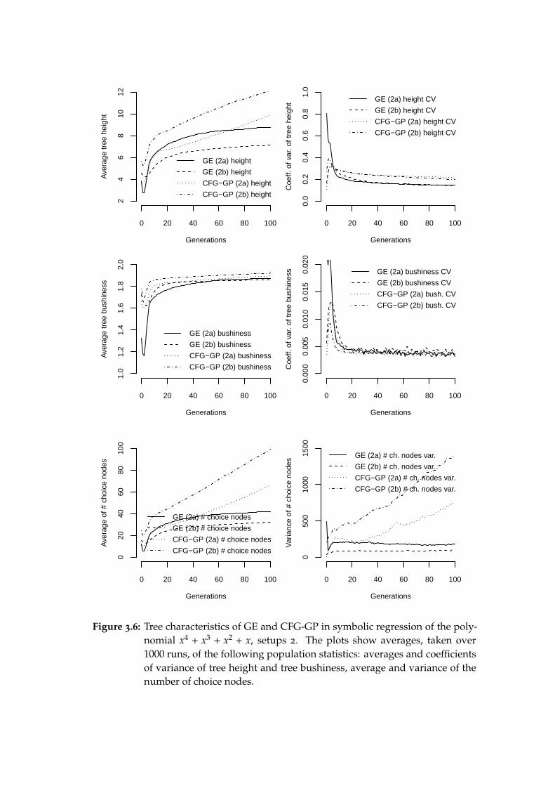
Generations
Ave
rage
tree
hei
ght
0 20 40 60 80 100
24
68
1012
GE (2a) height
GE (2b) height
CFG−GP (2a) height
CFG−GP (2b) height
Generations
Coe
ff. o
f var
. of t
ree
heig
ht
0 20 40 60 80 100
0.0
0.2
0.4
0.6
0.8
1.0
GE (2a) height CV
GE (2b) height CV
CFG−GP (2a) height CV
CFG−GP (2b) height CV
Generations
Ave
rage
tree
bus
hine
ss
0 20 40 60 80 100
1.0
1.2
1.4
1.6
1.8
2.0
GE (2a) bushiness
GE (2b) bushiness
CFG−GP (2a) bushiness
CFG−GP (2b) bushiness
Generations
Coe
ff. o
f var
. of t
ree
bush
ines
s
0 20 40 60 80 100
0.00
00.
005
0.01
00.
015
0.02
0
GE (2a) bushiness CV
GE (2b) bushiness CV
CFG−GP (2a) bush. CV
CFG−GP (2b) bush. CV
Generations
Ave
rage
of #
cho
ice
node
s
0 20 40 60 80 100
020
4060
8010
0
GE (2a) # choice nodes
GE (2b) # choice nodes
CFG−GP (2a) # choice nodes
CFG−GP (2b) # choice nodes
Generations
Var
ianc
e of
# c
hoic
e no
des
0 20 40 60 80 100
050
010
0015
00
GE (2a) # ch. nodes var.
GE (2b) # ch. nodes var.
CFG−GP (2a) # ch. nodes var.
CFG−GP (2b) # ch. nodes var.
Figure 3.6: Tree characteristics of GE and CFG-GP in symbolic regression of the poly-nomial x4 + x3 + x2 + x, setups 2. The plots show averages, taken over1000 runs, of the following population statistics: averages and coefficientsof variance of tree height and tree bushiness, average and variance of thenumber of choice nodes.

3.5 Santa Fe ant trail
In this experiment with the Santa Fe ant trail (described in Section 2.2) wewill again start with a setup based upon an example GE application as imple-mented and configured in GEVA. Although the success of GE will initially bepoor, it should be noted that this is not due to the implementation (as I havedemonstrated in my bachelor thesis, Nohejl, 2009, GEVA achieves similarlypoor results: in fact, AGE achieved exactly the same level of success whenusing the same initialisation method). All setups will use a relatively smallpopulation (100) and number of generations (101), so it is very likely that noparameters for GE and CFG-GP would result in full success. This way we willbe able to compare population characteristics more clearly. In the symbolicregression experiment, CFG-GP converged so fast, that only a relatively smallportion of the statistics concerned what happens until the solution is found.
3.5.1 Experimental setups 1
We will use the standard Santa Fe ant trail map in conjunction with a 600-ticktime limit for each individual and the grammar in Listing 3.2 to replicate theconfiguration used in GEVA. Our goal is to compare different methods, notdifferent grammars, but it is worth noting that the specification of grammarin this application offers room for subtle but important choices. The terminalssimply represent the ant’s actions and senses but we can decide how to combinethem: for instance the grammar that we use does not allow nested conditionalbranching. We can see this as a bit of knowledge about the problem that hasbeen embedded in the grammar: we (correctly) assume that nested conditionalbranching is not necessary for the solution. Additionally, the way the <line>and <op> nonterminals are chained in <code> and <opcode> productions willresult in relatively high and sparse trees (compare to Listing 3.1 for symbolic re-gression, which can produce binary branching recursively). Both these featuresof the grammar result in a smaller search space and a faster search.
<prog> ::= <code><code> ::= <line> | <code> <line><line> ::= <condition> | <op><condition> ::= if foodAhead(h)==1 then <opcode> else <opcode> end<op> ::= left(h) | right(h) | move(h)<opcode> ::= <op> | <opcode> <op>
Listing 3.2: A Lua equivalent to the Groovy grammar used for Santa Fe ant trailapplication included with GEVA.
In Section 3.4we have suggested that different operators in CFG-GP and GEresult in different spaces of tree shapes to be searched, but different initialisationtechniques may have also played a role. This time, we will use the same twoinitialisation techniques with both methods. For GE (1a) and CFG-GP (1a), we
38
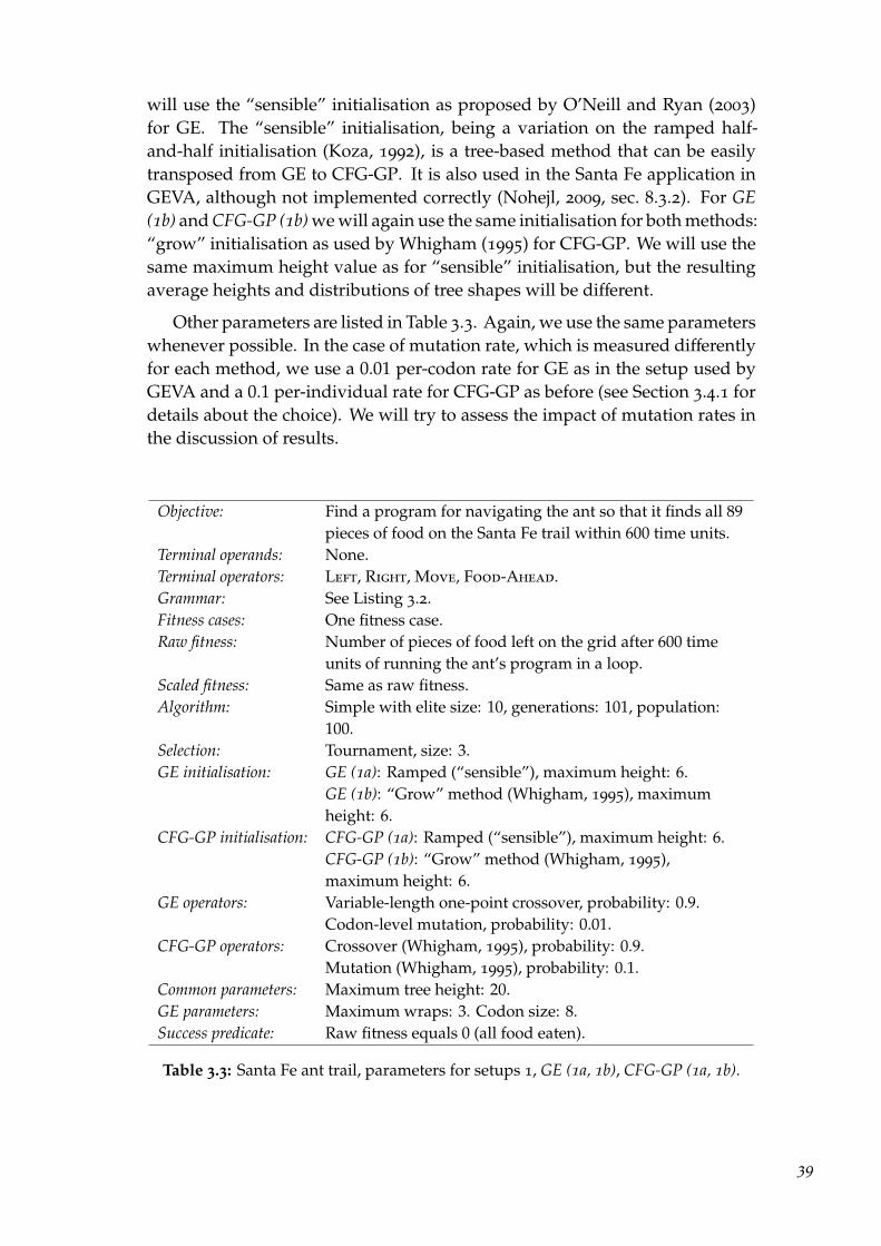
will use the “sensible” initialisation as proposed by O’Neill and Ryan (2003)for GE. The “sensible” initialisation, being a variation on the ramped half-and-half initialisation (Koza, 1992), is a tree-based method that can be easilytransposed from GE to CFG-GP. It is also used in the Santa Fe application inGEVA, although not implemented correctly (Nohejl, 2009, sec. 8.3.2). For GE(1b) and CFG-GP (1b) we will again use the same initialisation for both methods:“grow” initialisation as used by Whigham (1995) for CFG-GP. We will use thesame maximum height value as for “sensible” initialisation, but the resultingaverage heights and distributions of tree shapes will be different.
Other parameters are listed in Table 3.3. Again, we use the same parameterswhenever possible. In the case of mutation rate, which is measured differentlyfor each method, we use a 0.01 per-codon rate for GE as in the setup used byGEVA and a 0.1 per-individual rate for CFG-GP as before (see Section 3.4.1 fordetails about the choice). We will try to assess the impact of mutation rates inthe discussion of results.
Objective: Find a program for navigating the ant so that it finds all 89pieces of food on the Santa Fe trail within 600 time units.
Terminal operands: None.Terminal operators: Left, Right, Move, Food-Ahead.Grammar: See Listing 3.2.Fitness cases: One fitness case.Raw fitness: Number of pieces of food left on the grid after 600 time
units of running the ant’s program in a loop.Scaled fitness: Same as raw fitness.Algorithm: Simple with elite size: 10, generations: 101, population:
100.Selection: Tournament, size: 3.GE initialisation: GE (1a): Ramped (“sensible”), maximum height: 6.
GE (1b): “Grow” method (Whigham, 1995), maximumheight: 6.
CFG-GP initialisation: CFG-GP (1a): Ramped (“sensible”), maximum height: 6.CFG-GP (1b): “Grow” method (Whigham, 1995),maximum height: 6.
GE operators: Variable-length one-point crossover, probability: 0.9.Codon-level mutation, probability: 0.01.
CFG-GP operators: Crossover (Whigham, 1995), probability: 0.9.Mutation (Whigham, 1995), probability: 0.1.
Common parameters: Maximum tree height: 20.GE parameters: Maximum wraps: 3. Codon size: 8.Success predicate: Raw fitness equals 0 (all food eaten).
Table 3.3: Santa Fe ant trail, parameters for setups 1, GE (1a, 1b), CFG-GP (1a, 1b).
39

3.5.2 Results from setups 1
Both methods were relatively unsuccessful. CFG-GP with either initialisationtechnique achieved a substantially higher success rate (191 and 206 out of 1000runs were successful) than GE (9 and 24 runs out of 1000), see Figure 3.7. Thedifferences caused by initialisation are small relatively to differences betweenGE and CFG-GP. The same pattern can be observed in tree characteristicsexcept for bushiness where all differences are too small to draw a conclusion.Regardless of the initialisation method, the GE setups and likewise the CFG-GPsetups converge to similar characteristics.
As in the previous setups for symbolic regression, in the long run CFG-GP with either initialisation method results in trees that are higher and morevaried in height and number of choice nodes. The difference in success of thetwo methods is, however, much larger than before. Could this be attributedto a disparity in mutation rates? The coefficient of variance of fitness in thesymbolic regression setups was either similar for both methods or higher forGE, now it is lower for GE (see Figure 3.8), which would suggest a lowereffective mutation rate given no disparity in other parameters.
Generations
Cum
ulat
ive
succ
ess
rate
in 1
000
runs
0 20 40 60 80 100
050
100
150
200
250
GE (1a)
GE (1b)
CFG−GP (1a)
CFG−GP (1b)
Figure 3.7: Cumulative frequency of success of GE and CFG-GP in Santa Fe ant trail,setups 1. (Scale from 0 to 250 out of 1000.)
We have observed the same kind of differences in success rates and treecharacteristics between GE and CFG-GP as before but now independently ofinitialisation. Comparison of fitness statistics suggests, however, that part ofthe difference in success may be attributed to different effective mutation rates.Additionally, the less sophisticated “grow” method was more successful withboth GE and CFG-GP. We will investigate the effect of initialisation using thesecond set of experimental setups.
40
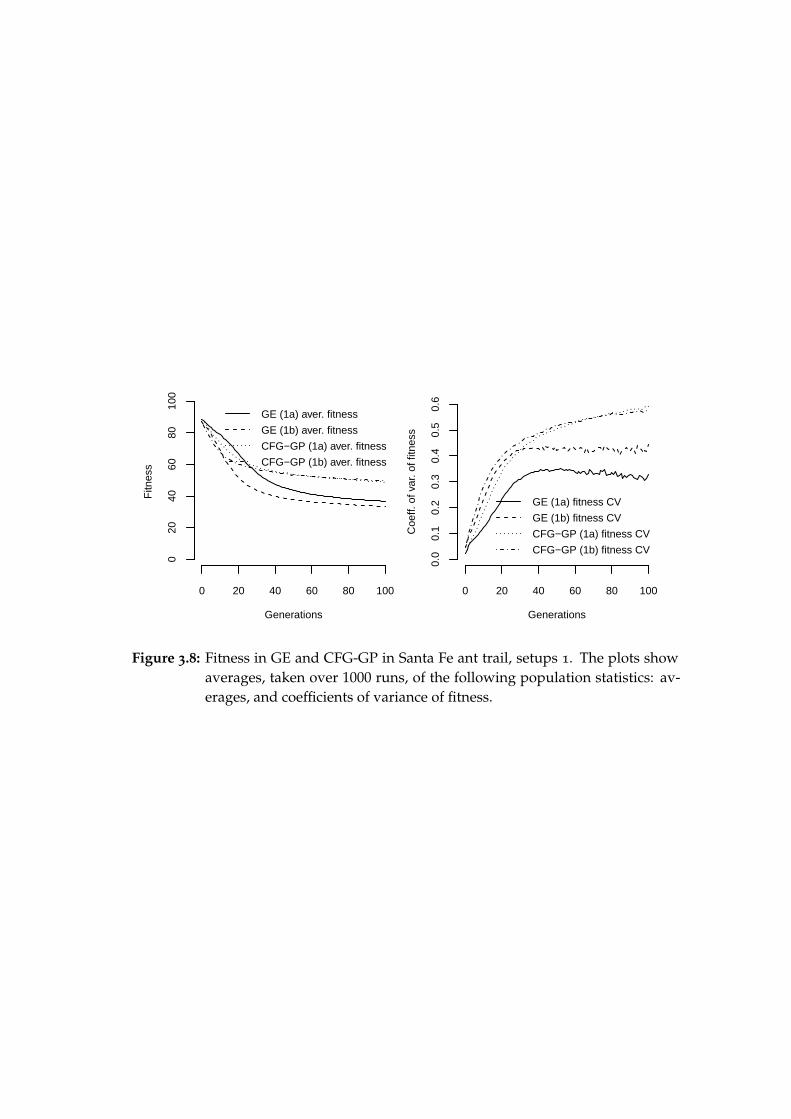
Generations
Fitn
ess
0 20 40 60 80 100
020
4060
8010
0
GE (1a) aver. fitness
GE (1b) aver. fitness
CFG−GP (1a) aver. fitness
CFG−GP (1b) aver. fitness
Generations
Coe
ff. o
f var
. of f
itnes
s
0 20 40 60 80 100
0.0
0.1
0.2
0.3
0.4
0.5
0.6
GE (1a) fitness CV
GE (1b) fitness CV
CFG−GP (1a) fitness CV
CFG−GP (1b) fitness CV
Figure 3.8: Fitness in GE and CFG-GP in Santa Fe ant trail, setups 1. The plots showaverages, taken over 1000 runs, of the following population statistics: av-erages, and coefficients of variance of fitness.

Generations
Ave
rage
tree
hei
ght
0 20 40 60 80 100
46
810
12
GE (1a) height
GE (1b) height
CFG−GP (1a) height
CFG−GP (1b) height
Generations
Coe
ff. o
f var
. of t
ree
heig
ht
0 20 40 60 80 100
0.0
0.1
0.2
0.3
0.4
GE (1a) height CV
GE (1b) height CV
CFG−GP (1a) height CV
CFG−GP (1b) height CV
Generations
Ave
rage
tree
bus
hine
ss
0 20 40 60 80 100
1.0
1.1
1.2
1.3
1.4
1.5
1.6
GE (1a) bushiness
GE (1b) bushiness
CFG−GP (1a) bushiness
CFG−GP (1b) bushiness
Generations
Coe
ff. o
f var
. of t
ree
bush
ines
s
0 20 40 60 80 100
0.00
00.
005
0.01
00.
015
0.02
0
GE (1a) bushiness CV
GE (1b) bushiness CV
CFG−GP (1a) bush. CV
CFG−GP (1b) bush. CV
Generations
Ave
rage
of #
cho
ice
node
s
0 20 40 60 80 100
010
2030
40
GE (1a) # choice nodes
GE (1b) # choice nodes
CFG−GP (1a) # choice nodes
CFG−GP (1b) # choice nodes
Generations
Var
ianc
e of
# c
hoic
e no
des
0 20 40 60 80 100
020
4060
GE (1a) # ch. nodes var.
GE (1b) # ch. nodes var.
CFG−GP (1a) # ch. nodes var.
CFG−GP (1b) # ch. nodes var.
Figure 3.9: Tree characteristics of GE and CFG-GP in Santa Fe ant trail, setups 1. Theplots show averages, taken over 1000 runs, of the following populationstatistics: averages and coefficients of variance of tree height and treebushiness, average and variance of the number of choice nodes.
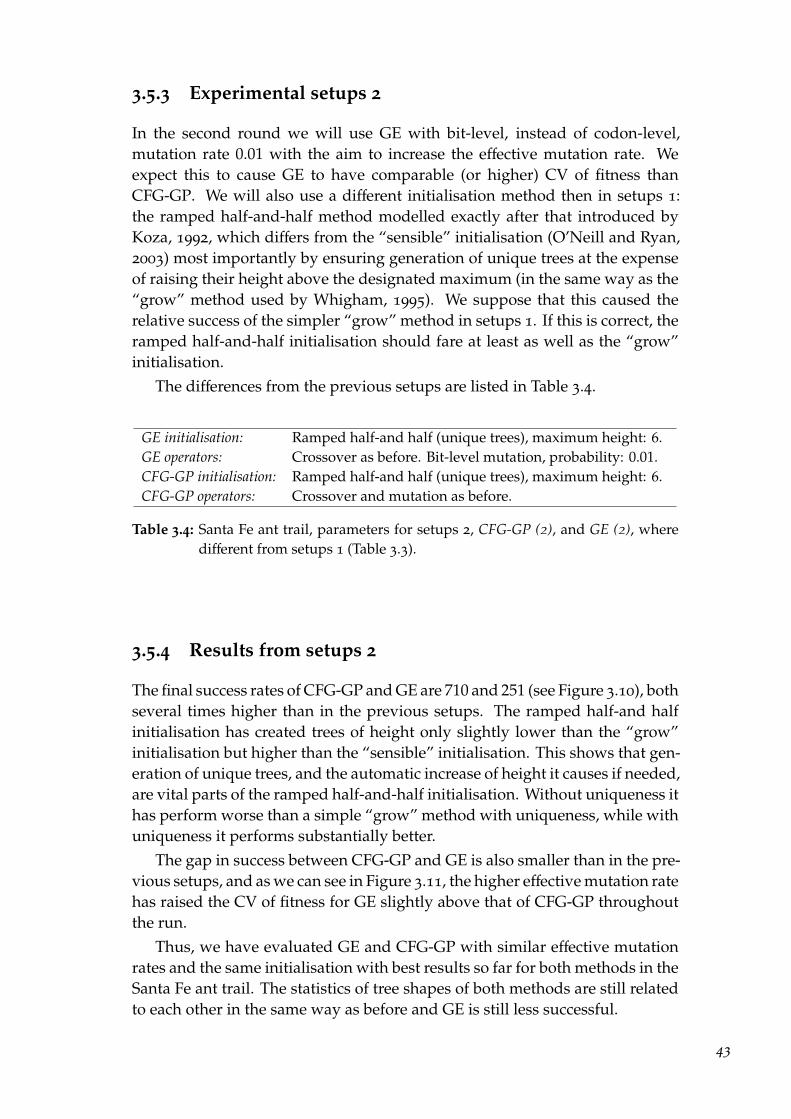
3.5.3 Experimental setups 2
In the second round we will use GE with bit-level, instead of codon-level,mutation rate 0.01 with the aim to increase the effective mutation rate. Weexpect this to cause GE to have comparable (or higher) CV of fitness thanCFG-GP. We will also use a different initialisation method then in setups 1:the ramped half-and-half method modelled exactly after that introduced byKoza, 1992, which differs from the “sensible” initialisation (O’Neill and Ryan,2003) most importantly by ensuring generation of unique trees at the expenseof raising their height above the designated maximum (in the same way as the“grow” method used by Whigham, 1995). We suppose that this caused therelative success of the simpler “grow” method in setups 1. If this is correct, theramped half-and-half initialisation should fare at least as well as the “grow”initialisation.
The differences from the previous setups are listed in Table 3.4.
GE initialisation: Ramped half-and half (unique trees), maximum height: 6.GE operators: Crossover as before. Bit-level mutation, probability: 0.01.CFG-GP initialisation: Ramped half-and half (unique trees), maximum height: 6.CFG-GP operators: Crossover and mutation as before.
Table 3.4: Santa Fe ant trail, parameters for setups 2, CFG-GP (2), and GE (2), wheredifferent from setups 1 (Table 3.3).
3.5.4 Results from setups 2
The final success rates of CFG-GP and GE are 710 and 251 (see Figure 3.10), bothseveral times higher than in the previous setups. The ramped half-and halfinitialisation has created trees of height only slightly lower than the “grow”initialisation but higher than the “sensible” initialisation. This shows that gen-eration of unique trees, and the automatic increase of height it causes if needed,are vital parts of the ramped half-and-half initialisation. Without uniqueness ithas perform worse than a simple “grow” method with uniqueness, while withuniqueness it performs substantially better.
The gap in success between CFG-GP and GE is also smaller than in the pre-vious setups, and as we can see in Figure 3.11, the higher effective mutation ratehas raised the CV of fitness for GE slightly above that of CFG-GP throughoutthe run.
Thus, we have evaluated GE and CFG-GP with similar effective mutationrates and the same initialisation with best results so far for both methods in theSanta Fe ant trail. The statistics of tree shapes of both methods are still relatedto each other in the same way as before and GE is still less successful.
43

Generations
Cum
ulat
ive
succ
ess
rate
in 1
000
runs
0 20 40 60 80 100
020
040
060
080
010
00
GE (2)
CFG−GP (2)
Figure 3.10: Cumulative frequency of success of GE and CFG-GP in Santa Fe ant trail,setups 2.
3.5.5 Conclusion
The Santa Fe ant trail problem differed from the simple symbolic regression.Foremost, it was more difficult to solve given the relatively small populationsize and number of generations. Also, the grammar we used was more re-strictive in the sense that it excluded some constructs that traditional geneticprogramming would allow in this problem (nested if-then-else conditions) andthat it did not allow recursive binary branching. Without recursive binarybranching, trees are less bushy, and consequently there are not as many uniquetrees of a given height.
We have used the same parameters based on the setup used in GEVAfor both GE and CFG-GP, including the same initialisation method (“sensibleinitialisation” proposed for GE by O’Neill and Ryan, 2003). We have alsoevaluated both methods with the “grow” initialisation (designed for use withCFG-GP by Whigham, 1995), and the ramped half-and-half initialisation (ori-ginally designed for tree-based GP by Koza, 1992). We have adjusted mutationrate for GE to reach similar effect in both methods (the mutation operators arequalitatively different, so we could do this only based on the CV of fitness).In all cases the methods displayed the same differences in tree characteristicswe have already observed in simple symbolic regression (Section 3.4), whichprevailed in the long run over the effect of initialisation. At the same time,we could see that both methods benefit from the same changes in initialisa-tion. Koza’s ramped half-and-half initialisation had the best results of the threetree-based techniques, partially thanks to the generation of unique individualswhich automatically raises tree height as necessary.
44
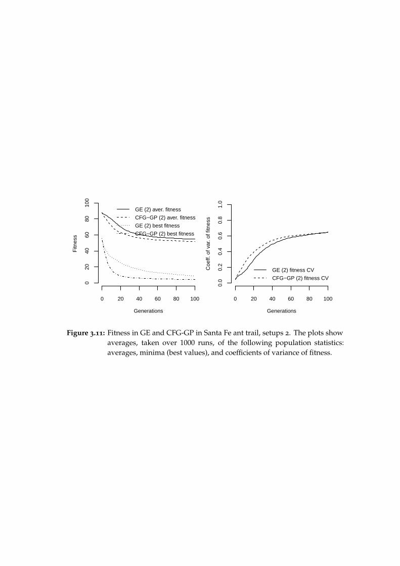
Generations
Fitn
ess
0 20 40 60 80 100
020
4060
8010
0
GE (2) aver. fitness
CFG−GP (2) aver. fitness
GE (2) best fitness
CFG−GP (2) best fitness
Generations
Coe
ff. o
f var
. of f
itnes
s
0 20 40 60 80 100
0.0
0.2
0.4
0.6
0.8
1.0
GE (2) fitness CV
CFG−GP (2) fitness CV
Figure 3.11: Fitness in GE and CFG-GP in Santa Fe ant trail, setups 2. The plots showaverages, taken over 1000 runs, of the following population statistics:averages, minima (best values), and coefficients of variance of fitness.

Generations
Ave
rage
tree
hei
ght
0 20 40 60 80 100
46
810
12
GE (2) height
CFG−GP (2) height
Generations
Coe
ff. o
f var
. of t
ree
heig
ht
0 20 40 60 80 100
0.0
0.1
0.2
0.3
0.4
GE (2) height CV
CFG−GP (2) height CV
Generations
Ave
rage
tree
bus
hine
ss
0 20 40 60 80 100
1.0
1.1
1.2
1.3
1.4
1.5
1.6
GE (2) bushiness
CFG−GP (2) bushiness
Generations
Coe
ff. o
f var
. of t
ree
bush
ines
s
0 20 40 60 80 100
0.00
00.
005
0.01
00.
015
0.02
0
GE (2) bushiness CV
CFG−GP (2) bush. CV
Generations
Ave
rage
of #
cho
ice
node
s
0 20 40 60 80 100
010
2030
40
GE (2) # choice nodes
CFG−GP (2) # choice nodes
Generations
Var
ianc
e of
# c
hoic
e no
des
0 20 40 60 80 100
020
4060
8010
0 GE (2) # ch. nodes var.
CFG−GP (2) # ch. nodes var.
Figure 3.12: Tree characteristics of GE and CFG-GP in Santa Fe ant trail, setups 2. Theplots show averages, taken over 1000 runs, of the following populationstatistics: averages and coefficients of variance of tree height and treebushiness, average and variance of the number of choice nodes.

3.6 Dot product symbolic regression
In the previous experiments we have compared GE and CFG-GP as imple-mented in AGE, and we started with setups based on those used for GE inGEVA. In this section we will compare three methods: GE, CFG-GP, and LO-GENPRO. The dot product problem and the initial setup we will use has beendescribed by Wong and Leung (2000, sec. 6.1.2), who use it to demonstrate thatLOGENPRO can express type constraints, thus outperforming basic tree-basedGP, and generate ephemeral constants using logic goals (see Section 2.3).
start -> s-expr(number).s-expr([list,number,?n]) -> [ (mapcar(function ], op2, [ ) ],
s-expr([list,number,?n]),s-expr([list,number,?n]), [ ) ].
s-expr([list,number,?n]) -> [ (mapcar(function ], op1, [ ) ],s-expr([list,number,?n]), [ ) ].
s-expr([list,number,?n]) -> term([list,number,?n]).s-expr(number) -> term(number).s-expr(number) -> [ (apply(function ], op2, [ ) ],
s-expr([list,number,?n]),[ ) ].s-expr(number) -> [ ( ], op2, s-expr(number),
s-expr(number), [ ) ].s-expr(number) -> [ ( ], opl, s-expr(number), [ ) ].op2 -> [ + ].op2 -> [ - ].op2 -> [ * ].op2 -> [ % ].op1 -> [ protected-log ].term([list,number,n]) -> [ X ].term([list,number,n]) -> [ Y ].term(number) -> { random(-10, 10, ?a) }, [ ?a ].
Listing 3.3: Logic grammar (LOGENPRO) for dot product symbolic regression in Lisp(from Wong and Leung, 2000). Unlike in a DCG, -> is the production sym-bol, logic variables are denoted by leading question marks, and terminals(in square brackets) do not need additional quotes.
To this end, Wong and Leung (2000) use an elaborate logic grammar (List-ing 3.3) in a formalism based on DCGs. The terminals that contain calls to(1) mapcar and (2) apply are segments of Lisp code that apply the scalar op-erators to vectors (1) by components and (2) to components of a single vector,respectively. This is not something inherent to logic grammars, it is a conveni-ent way to express different types of unary and binary operators in Lisp, whichLOGENPRO uses to evaluate individuals.
What is interesting about the grammar is how it expresses type constraints.Two types are used: scalars and vectors of a given number of components. The
47
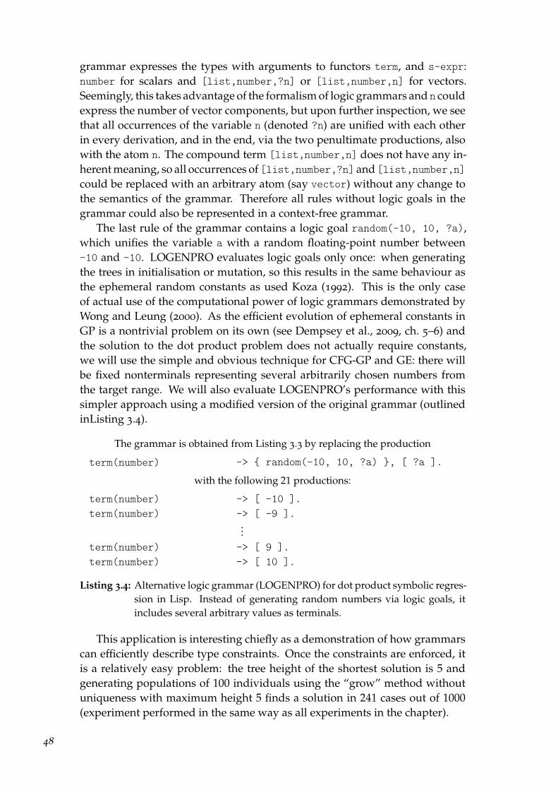
grammar expresses the types with arguments to functors term, and s-expr:number for scalars and [list,number,?n] or [list,number,n] for vectors.Seemingly, this takes advantage of the formalism of logic grammars and n couldexpress the number of vector components, but upon further inspection, we seethat all occurrences of the variable n (denoted ?n) are unified with each otherin every derivation, and in the end, via the two penultimate productions, alsowith the atom n. The compound term [list,number,n] does not have any in-herent meaning, so all occurrences of [list,number,?n] and [list,number,n]could be replaced with an arbitrary atom (say vector) without any change tothe semantics of the grammar. Therefore all rules without logic goals in thegrammar could also be represented in a context-free grammar.
The last rule of the grammar contains a logic goal random(-10, 10, ?a),which unifies the variable a with a random floating-point number between-10 and -10. LOGENPRO evaluates logic goals only once: when generatingthe trees in initialisation or mutation, so this results in the same behaviour asthe ephemeral random constants as used Koza (1992). This is the only caseof actual use of the computational power of logic grammars demonstrated byWong and Leung (2000). As the efficient evolution of ephemeral constants inGP is a nontrivial problem on its own (see Dempsey et al., 2009, ch. 5–6) andthe solution to the dot product problem does not actually require constants,we will use the simple and obvious technique for CFG-GP and GE: there willbe fixed nonterminals representing several arbitrarily chosen numbers fromthe target range. We will also evaluate LOGENPRO’s performance with thissimpler approach using a modified version of the original grammar (outlinedinListing 3.4).
The grammar is obtained from Listing 3.3 by replacing the production
term(number) -> { random(-10, 10, ?a) }, [ ?a ].
with the following 21 productions:
term(number) -> [ -10 ].term(number) -> [ -9 ].
...term(number) -> [ 9 ].term(number) -> [ 10 ].
Listing 3.4: Alternative logic grammar (LOGENPRO) for dot product symbolic regres-sion in Lisp. Instead of generating random numbers via logic goals, itincludes several arbitrary values as terminals.
This application is interesting chiefly as a demonstration of how grammarscan efficiently describe type constraints. Once the constraints are enforced, itis a relatively easy problem: the tree height of the shortest solution is 5 andgenerating populations of 100 individuals using the “grow” method withoutuniqueness with maximum height 5 finds a solution in 241 cases out of 1000(experiment performed in the same way as all experiments in the chapter).
48
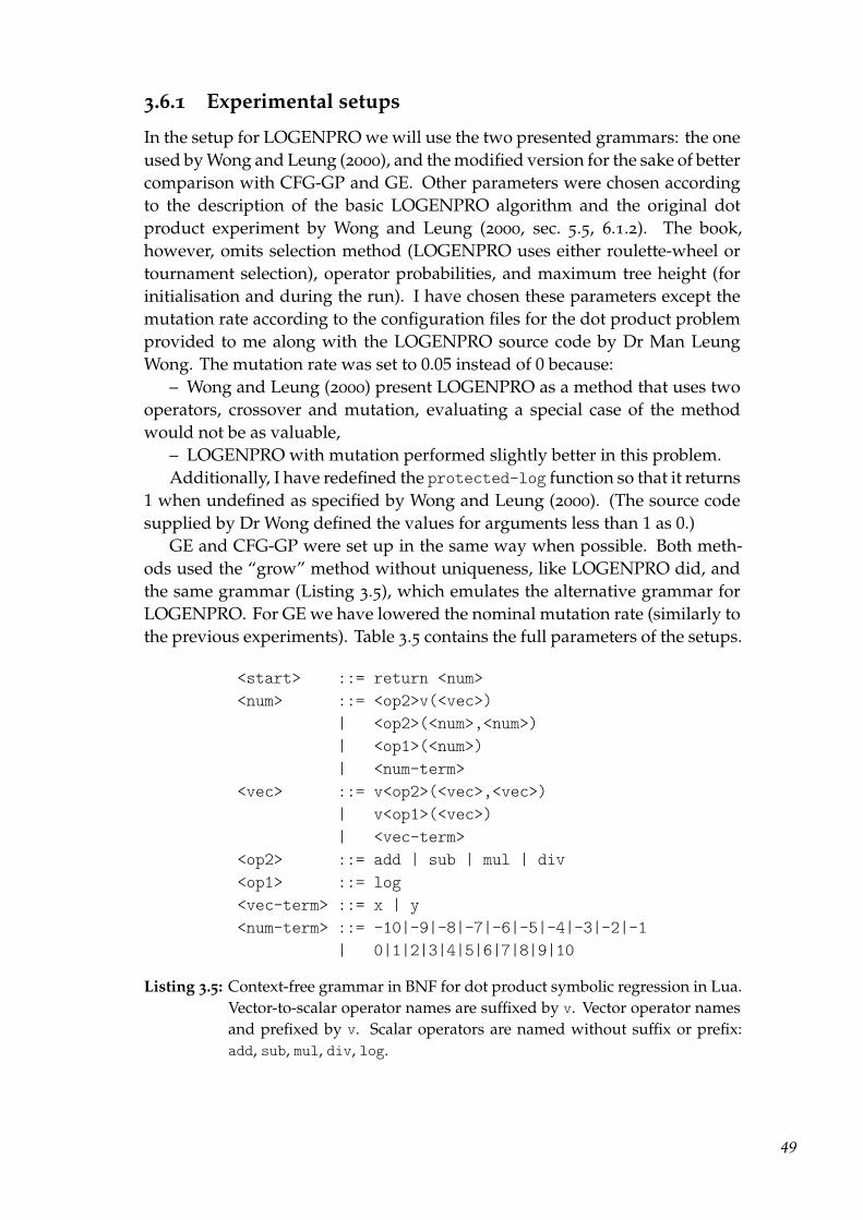
3.6.1 Experimental setups
In the setup for LOGENPRO we will use the two presented grammars: the oneused by Wong and Leung (2000), and the modified version for the sake of bettercomparison with CFG-GP and GE. Other parameters were chosen accordingto the description of the basic LOGENPRO algorithm and the original dotproduct experiment by Wong and Leung (2000, sec. 5.5, 6.1.2). The book,however, omits selection method (LOGENPRO uses either roulette-wheel ortournament selection), operator probabilities, and maximum tree height (forinitialisation and during the run). I have chosen these parameters except themutation rate according to the configuration files for the dot product problemprovided to me along with the LOGENPRO source code by Dr Man LeungWong. The mutation rate was set to 0.05 instead of 0 because:
– Wong and Leung (2000) present LOGENPRO as a method that uses twooperators, crossover and mutation, evaluating a special case of the methodwould not be as valuable,
– LOGENPRO with mutation performed slightly better in this problem.Additionally, I have redefined the protected-log function so that it returns
1 when undefined as specified by Wong and Leung (2000). (The source codesupplied by Dr Wong defined the values for arguments less than 1 as 0.)
GE and CFG-GP were set up in the same way when possible. Both meth-ods used the “grow” method without uniqueness, like LOGENPRO did, andthe same grammar (Listing 3.5), which emulates the alternative grammar forLOGENPRO. For GE we have lowered the nominal mutation rate (similarly tothe previous experiments). Table 3.5 contains the full parameters of the setups.
<start> ::= return <num><num> ::= <op2>v(<vec>)
| <op2>(<num>,<num>)| <op1>(<num>)| <num-term>
<vec> ::= v<op2>(<vec>,<vec>)| v<op1>(<vec>)| <vec-term>
<op2> ::= add | sub | mul | div<op1> ::= log<vec-term> ::= x | y<num-term> ::= -10|-9|-8|-7|-6|-5|-4|-3|-2|-1
| 0|1|2|3|4|5|6|7|8|9|10
Listing 3.5: Context-free grammar in BNF for dot product symbolic regression in Lua.Vector-to-scalar operator names are suffixed by v. Vector operator namesand prefixed by v. Scalar operators are named without suffix or prefix:add, sub, mul, div, log.
49
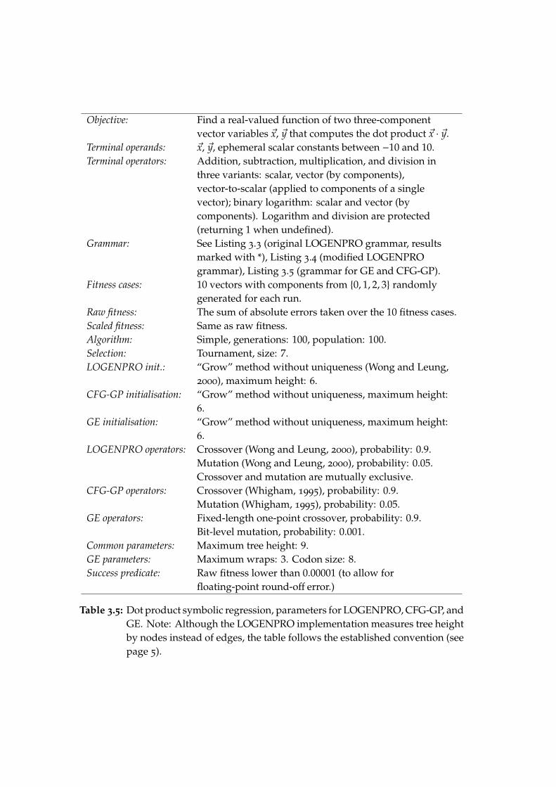
Objective: Find a real-valued function of two three-componentvector variables ~x, ~y that computes the dot product ~x · ~y.
Terminal operands: ~x, ~y, ephemeral scalar constants between −10 and 10.Terminal operators: Addition, subtraction, multiplication, and division in
three variants: scalar, vector (by components),vector-to-scalar (applied to components of a singlevector); binary logarithm: scalar and vector (bycomponents). Logarithm and division are protected(returning 1 when undefined).
Grammar: See Listing 3.3 (original LOGENPRO grammar, resultsmarked with *), Listing 3.4 (modified LOGENPROgrammar), Listing 3.5 (grammar for GE and CFG-GP).
Fitness cases: 10 vectors with components from {0, 1, 2, 3} randomlygenerated for each run.
Raw fitness: The sum of absolute errors taken over the 10 fitness cases.Scaled fitness: Same as raw fitness.Algorithm: Simple, generations: 100, population: 100.Selection: Tournament, size: 7.LOGENPRO init.: “Grow” method without uniqueness (Wong and Leung,
2000), maximum height: 6.CFG-GP initialisation: “Grow” method without uniqueness, maximum height:
6.GE initialisation: “Grow” method without uniqueness, maximum height:
6.LOGENPRO operators: Crossover (Wong and Leung, 2000), probability: 0.9.
Mutation (Wong and Leung, 2000), probability: 0.05.Crossover and mutation are mutually exclusive.
CFG-GP operators: Crossover (Whigham, 1995), probability: 0.9.Mutation (Whigham, 1995), probability: 0.05.
GE operators: Fixed-length one-point crossover, probability: 0.9.Bit-level mutation, probability: 0.001.
Common parameters: Maximum tree height: 9.GE parameters: Maximum wraps: 3. Codon size: 8.Success predicate: Raw fitness lower than 0.00001 (to allow for
floating-point round-off error.)
Table 3.5: Dot product symbolic regression, parameters for LOGENPRO, CFG-GP, andGE. Note: Although the LOGENPRO implementation measures tree heightby nodes instead of edges, the table follows the established convention (seepage 5).

3.6.2 Results
The success rates of the four setups (Figure 3.13) are similar, often withouta significant difference, only during the first thirteen generations. Thereafter,LOGENPRO with the original grammar is significantly less successful thenany of the other three setups, LOGENPRO with the modified grammar is notsignificantly different from CFG-GP in generations 28 through 59, and CFG-GPis not significantly different from GE in generations 60 through 70, 75, 76, andthen from 82 on. LOGENPRO with the original grammar, LOGENPRO withthe modified grammar, CFG-GP, and GE have respectively succeeded in 53, 62,68, and 68 of the 100 runs.
Generations
Cum
ulat
ive
succ
ess
rate
in 1
00 r
uns
0 20 40 60 80 100
020
4060
8010
0
LOGENPRO*
LOGENPRO
CFG−GP
GE
Figure 3.13: Cumulative frequency of success of LOGENPRO, CFG-GP and GE insymbolic regression of the dot product ~x · ~y.
The most pronounced was the difference caused by the change of grammarin LOGENPRO, which can be attributed to the difference in search space size,given that ephemeral constants are of no use in this problem. As we couldexpect based on our discussion of the grammar used by LOGENPRO, there isno practical difference between the performance of LOGENPRO with a logicgrammar and that of CFG-GP with a context-free grammar.
The 0.53 success rate (53 out of 100) obtained from LOGENPRO with theoriginal grammar is lower than the 0.8 rate reported by Wong and Leung (2000,sec. 6.1.2, approximate reading of a plot). Regardless of the number of trialsperformed (not mentioned by Wong and Leung, 2000), such a difference wouldbe statistically significant. I have not been able to replicate this success rate byvarying operator probabilities, maximum tree heights or selection parameters,with either grammar. That said, even with the more modest success rate theircomparison with tree-based GP would still hold (success rate of GP with the
51

same population size was reported below 0.1).As LOGENPRO does not provide any statistics about the generated trees,
we can compare these only for CFG-GP and GE, see Figure 3.14. In contrastwith the previous experiments, in which CFG-GP performed better, GE hasnow reached exactly the same level of success, and in a large part of therun, there was no significant difference in success between the two. Despitethese similar rates of success, we can still observe the differences in the treecharacteristics: CFG-GP has soon reached both higher average values and CVof height and bushiness and maintained them throughout the run. As we havenoted in the beginning of Section 3.6, correct solutions occur relatively denselyamong random trees of height 5, so the lower tree height close to 5 maintainedby the operators of grammatical evolution (see Figure 3.14) are a very likelyexplanation for the improved success of GE.
3.6.3 Conclusion
We have shown that the use of logic grammars to describe types demonstratedby Wong and Leung (2000) does not require any of their distinctive features(unification and incorporation of logic goals): the same can be done using acontext-free grammar in either CFG-GP or GE. Both methods have performedon a par with LOGENPRO (with a slightly higher success rate) using an equi-valent context-free grammar and other parameters.
One could conceive of a type system that could be properly enforced using alogic grammar but not a context-free grammar. It is not obvious, however, thatLOGENPRO would perform well if such a type system was necessary. It woulddepend on how efficiently the genetic operators would be able to fulfil theirroles in the evolutionary algorithm under the more complex type constraints.
52
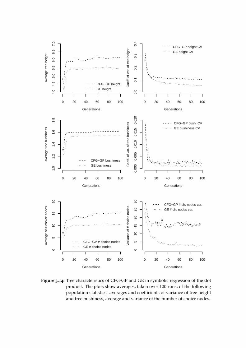
Generations
Ave
rage
tree
hei
ght
0 20 40 60 80 100
4.0
4.5
5.0
5.5
6.0
6.5
7.0
CFG−GP height
GE height
Generations
Coe
ff. o
f var
. of t
ree
heig
ht
0 20 40 60 80 100
0.0
0.1
0.2
0.3
0.4
CFG−GP height CV
GE height CV
Generations
Ave
rage
tree
bus
hine
ss
0 20 40 60 80 100
1.0
1.2
1.4
1.6
1.8
CFG−GP bushiness
GE bushiness
Generations
Coe
ff. o
f var
. of t
ree
bush
ines
s
0 20 40 60 80 100
0.00
00.
005
0.01
00.
015
0.02
0
CFG−GP bush. CV
GE bushiness CV
Generations
Ave
rage
of #
cho
ice
node
s
0 20 40 60 80 100
05
1015
20
CFG−GP # choice nodes
GE # choice nodes
Generations
Var
ianc
e of
# c
hoic
e no
des
0 20 40 60 80 100
05
1015
2025
30
CFG−GP # ch. nodes var.
GE # ch. nodes var.
Figure 3.14: Tree characteristics of CFG-GP and GE in symbolic regression of the dotproduct. The plots show averages, taken over 100 runs, of the followingpopulation statistics: averages and coefficients of variance of tree heightand tree bushiness, average and variance of the number of choice nodes.

3.7 Symbolic regression with ADFs
In this section, we will try to replicate another experiment presented by Wongand Leung (2000) using LOGENPRO, and compare the results with the othertwo grammar-based methods. It is again an instance of symbolic regressionwith multiple types but the target function is more complex. It has threevector variables ~x, ~y, ~z, and can be expressed as ~x · ~y + ~y · ~z, where · is thedot product. To find an equivalent expression in a random search using the“grow” initialisation method with the grammar that we are going to use is anorder of magnitude more difficult than it was to find the dot product. Wongand Leung (2000) designed the experiment to show that LOGENPRO can useADFs similarly as traditional genetic programming (see Section 2.3).
To emulate ADFs, the grammar employed by Wong and Leung (2000) (List-ing 3.6) uses two sets of nonterminals: those for the main program (s-expr(· · · ),term(· · · )) and those for the body of the ADF (s-expr2(· · · ), term2(· · · )). Thisway the terminals X, Y, Z, ADF0, and arg0, arg1 can be restricted to occur onlyin the main subtree and the ADF subtree, respectively, and only subtrees of thesame kind can be combined via crossover, which is equivalent to how ADFsare handled in tree-based GP. The grammar does not depend on any specificfeatures of logic grammars (see explanation for a similar grammar in the previ-ous experiment), so an equivalent CFG can be constructed (Listing 3.7) for usewith GE and CFG-GP.
3.7.1 Experimental setups
As in Section 3.6, the setup of LOGENPRO replicates the one used by Wongand Leung (2000), and the missing parameters are chosen based on the config-uration file obtained from Dr Wong. For the same reasons as before I also usethe 0.05 mutation rate. Table 3.6 contains the full details of parameters for LO-GENPRO, CFG-GP, and GE. The parameters are unchanged from the previousexperiment without ADFs except for the number of generations lowered to 50and a smaller number of terminals. Note that while the problem is obviouslymore difficult than the previous one, the search space has been restricted byremoving several terminals from the grammar.
3.7.2 Results
All three methods have produced similar results in terms of success (see Fig-ure 3.15): 51, 45, and 56 runs were successful out of 100 in the case of LO-GENPRO, CFG-GP, and GE, respectively. There were significant differences insuccess between all of them in all generations of the second half of the run. Inthis experiment, grammatical evolution achieved the best performance of thethree methods.
As in the previous experiment without ADFs, the success rate I have beenable to achieve with LOGENPRO was significantly lower than that reported
54
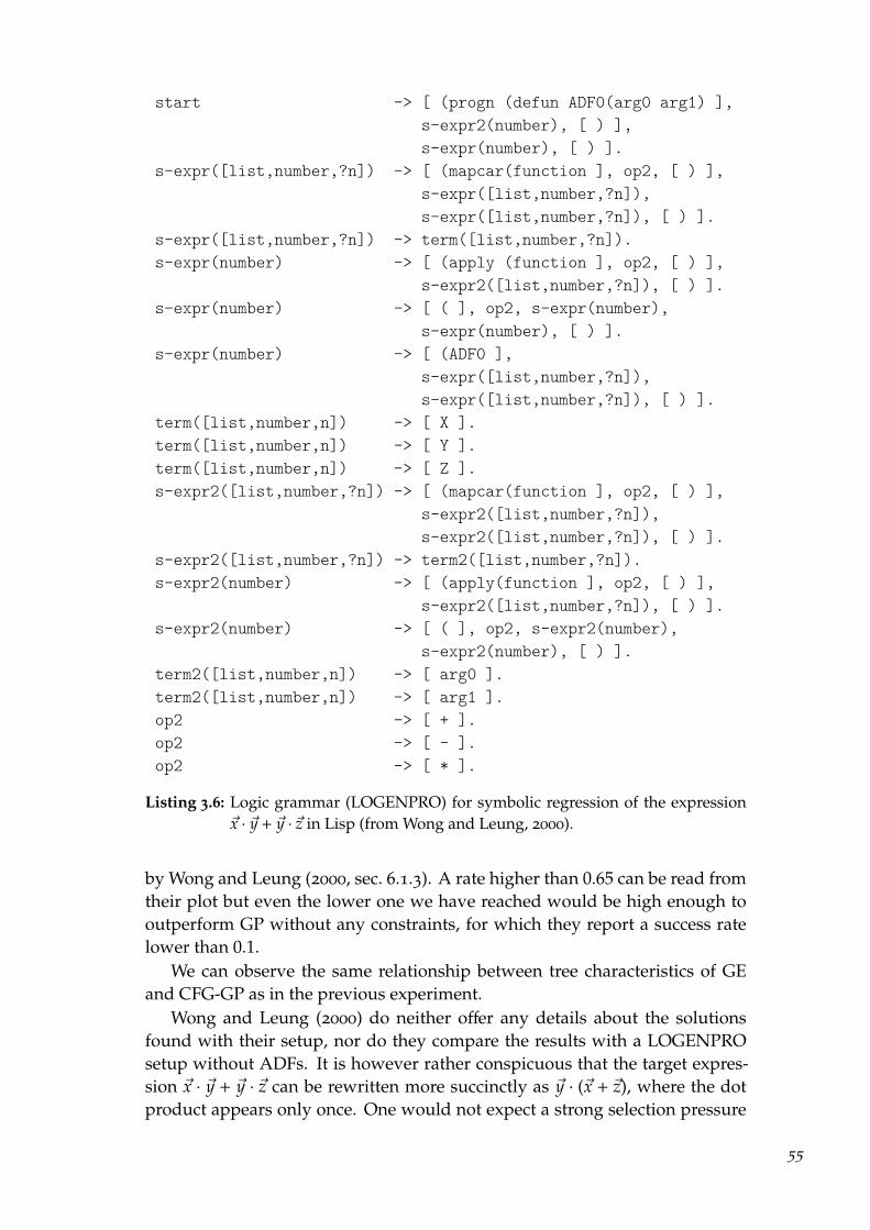
start -> [ (progn (defun ADF0(arg0 arg1) ],s-expr2(number), [ ) ],s-expr(number), [ ) ].
s-expr([list,number,?n]) -> [ (mapcar(function ], op2, [ ) ],s-expr([list,number,?n]),s-expr([list,number,?n]), [ ) ].
s-expr([list,number,?n]) -> term([list,number,?n]).s-expr(number) -> [ (apply (function ], op2, [ ) ],
s-expr2([list,number,?n]), [ ) ].s-expr(number) -> [ ( ], op2, s-expr(number),
s-expr(number), [ ) ].s-expr(number) -> [ (ADF0 ],
s-expr([list,number,?n]),s-expr([list,number,?n]), [ ) ].
term([list,number,n]) -> [ X ].term([list,number,n]) -> [ Y ].term([list,number,n]) -> [ Z ].s-expr2([list,number,?n]) -> [ (mapcar(function ], op2, [ ) ],
s-expr2([list,number,?n]),s-expr2([list,number,?n]), [ ) ].
s-expr2([list,number,?n]) -> term2([list,number,?n]).s-expr2(number) -> [ (apply(function ], op2, [ ) ],
s-expr2([list,number,?n]), [ ) ].s-expr2(number) -> [ ( ], op2, s-expr2(number),
s-expr2(number), [ ) ].term2([list,number,n]) -> [ arg0 ].term2([list,number,n]) -> [ arg1 ].op2 -> [ + ].op2 -> [ - ].op2 -> [ * ].
Listing 3.6: Logic grammar (LOGENPRO) for symbolic regression of the expression~x · ~y + ~y · ~z in Lisp (from Wong and Leung, 2000).
by Wong and Leung (2000, sec. 6.1.3). A rate higher than 0.65 can be read fromtheir plot but even the lower one we have reached would be high enough tooutperform GP without any constraints, for which they report a success ratelower than 0.1.
We can observe the same relationship between tree characteristics of GEand CFG-GP as in the previous experiment.
Wong and Leung (2000) do neither offer any details about the solutionsfound with their setup, nor do they compare the results with a LOGENPROsetup without ADFs. It is however rather conspicuous that the target expres-sion ~x · ~y + ~y · ~z can be rewritten more succinctly as ~y · (~x + ~z), where the dotproduct appears only once. One would not expect a strong selection pressure
55

<start> ::= function adf0(arg0,arg1) return <num'> endreturn <num>
<num> ::= <op2>v(<vec>)| <op2>(<num>,<num>)| adf0(<vec>,<vec>)
<vec> ::= v<op2>(<vec>,<vec>)| <vec-term>
<num'> ::= <op2>v(<vec'>)| <op2>(<num'>,<num'>)
<vec'> ::= v<op2>(<vec'>,<vec'>)| <vec'-term>
<vec-term> ::= x | y | z<vec'-term> ::= arg0 | arg1<op2> ::= add | sub | mul
Listing 3.7: Context-free grammar in BNF for symbolic regression of the expression~x · ~y + ~y ·~z in Lua. Vector-to-scalar operator names are suffixed by v. Vectoroperator names and prefixed by v. Scalar operators are named withoutsuffix or prefix: add, sub, mul.
to evolve a building block that needs to be used a single time. Indeed, out ofthe 51 solutions found by the successful runs of LOGENPRO I have performed,24 use ADFs. 21 out of the 24 ADFs perform just addition on the componentsof one of its arguments. Two ADFs out of the remaining three do compute thedot product, which is then used in an expression equal to ~y · (~x + ~z), and thelast remaining ADF computes a more complex expression ~arg0 · ( ~arg1 − ~arg0),which is then used in a similar way. The experiments with GE and CFG-GPhad the same outcome: ADFs are not used as intended in any of the 100 runs.
This suggest that the experiment devised by Wong and Leung (2000) isnot suitable for demonstrating the ability to use ADFs. I have performed itagain with CFG-GP and GE but with ADF-related structures removed from thegrammar (see Figure 3.17). The removal of ADFs has improved performancesignificantly for CFG-GP (from 45 to 55 successful runs out of 100), and insigni-ficantly for GE (from 56 to 57 successful runs). This reflects that GE operatorsare grammar-agnostic as a result of the genotype-phenotype distinction, andso crossover can occur between a function-defining subtree and a main subtreeregardless of the grammar. Without ADFs, CFG-GP and GE achieved similarperformance: there is a significant difference in generations 1 through 16 andthen only in the last 7 generations.
3.7.3 Conclusion
We have discovered that the problem specified by Wong and Leung (2000)is not suitable for evaluating performance grammar-based GP methods withautomatically defined functions as it can be solved more simply and efficiently
56

Generations
Cum
ulat
ive
succ
ess
rate
in 1
00 r
uns
0 10 20 30 40 50
020
4060
8010
0
LOGENPRO
CFG−GP
GE
Figure 3.15: Cumulative frequency of success of LOGENPRO, CFG-GP, and GE insymbolic regression of the expression ~x · ~y + ~y · ~z.
without them. Nevertheless we have made three valuable observations. First,GE and CFG-GP have performed on a par with LOGENPRO. Secondly, as inthe previous experiments, CFG-GP has in the long run produced more variedtree shapes, as characterised by bushiness and height. Thirdly, GE has sufferedless from the unnecessary addition of ADF-related structures to the grammarbecause, in contrast with CFG-GP and LOGENPRO, the syntactical constraintsdo not constrain the operators, which act only on the genotype. In order toenforce similar behaviour in grammatical evolution, we would have to useseparately mapped chromosomes for each function-defining branch and foreach value-returning branch and allow crossover only between chromosomesof the same type.
57

Objective: Find a real-valued function of three three-componentvector variables ~x, ~y, ~z that yields ~x · ~y + ~y ·~z, where · is thedot product.
Terminal operands: ~x, ~y, ~z. Within ADF: ~arg0, ~arg1.Terminal operators: Addition, subtraction, and multiplication in three
variants: scalar, vector (by components), vector-to-scalar(applied to components of a single vector). Out of ADF:the vector-to-scalar function ADF0 of two arguments.
Grammar: See Listing 3.6 (LOGENPRO), Listing 3.7 (GE andCFG-GP).
Fitness cases: 10 vectors with components from {0, 1, 2, 3} randomlygenerated for each run.
Raw fitness: The sum of absolute errors taken over the 10 fitness cases.Scaled fitness: Same as raw fitness.Algorithm: Simple, generations: 50, population: 100.Selection: Tournament, size: 7.LOGENPRO init.: “Grow” method without uniqueness (Wong and Leung,
2000), maximum height: 6.CFG-GP initialisation: “Grow” method without uniqueness, maximum height:
6.GE initialisation: “Grow” method without uniqueness, maximum height:
6.LOGENPRO operators: Crossover (Wong and Leung, 2000), probability: 0.9.
Mutation (Wong and Leung, 2000), probability: 0.05.Crossover and mutation are mutually exclusive.
CFG-GP operators: Crossover (Whigham, 1995), probability: 0.9.Mutation (Whigham, 1995), probability: 0.05.
GE operators: Fixed-length one-point crossover, probability: 0.9.Bit-level mutation, probability: 0.001.
Common parameters: Maximum tree height: 9.GE parameters: Maximum wraps: 3. Codon size: 8.Success predicate: Raw fitness lower than 0.00001 (to allow for
floating-point round-off error.)
Table 3.6: Symbolic regression of the expression ~x ·~y+~y ·~z, parameters for LOGENPRO,CFG-GP, and GE. Note: Although the LOGENPRO implementation soft-ware tree height by nodes instead of edges, the table follows the establishedconvention (see page 5).

Generations
Ave
rage
tree
hei
ght
0 10 20 30 40 50
5.0
5.5
6.0
6.5
7.0
7.5
8.0
CFG−GP height
GE height
Generations
Coe
ff. o
f var
. of t
ree
heig
ht
0 10 20 30 40 50
0.00
0.10
0.20
0.30
CFG−GP height CV
GE height CV
Generations
Ave
rage
tree
bus
hine
ss
0 10 20 30 40 50
1.70
1.75
1.80
1.85
1.90
CFG−GP bushiness
GE bushiness
Generations
Coe
ff. o
f var
. of t
ree
bush
ines
s
0 10 20 30 40 50
0.00
00.
002
0.00
40.
006
CFG−GP bush. CV
GE bushiness CV
Generations
Ave
rage
of #
cho
ice
node
s
0 10 20 30 40 50
2025
3035
4045
50
CFG−GP # choice nodes
GE # choice nodes
Generations
Var
ianc
e of
# c
hoic
e no
des
0 10 20 30 40 50
050
100
150
200
CFG−GP # ch. nodes var.
GE # ch. nodes var.
Figure 3.16: Tree characteristics of CFG-GP and GE in symbolic regression of the ex-pression ~x · ~y + ~y · ~z. The plots show averages, taken over 100 runs, ofthe following population statistics: averages and coefficients of varianceof tree height and tree bushiness, average and variance of the number ofchoice nodes.
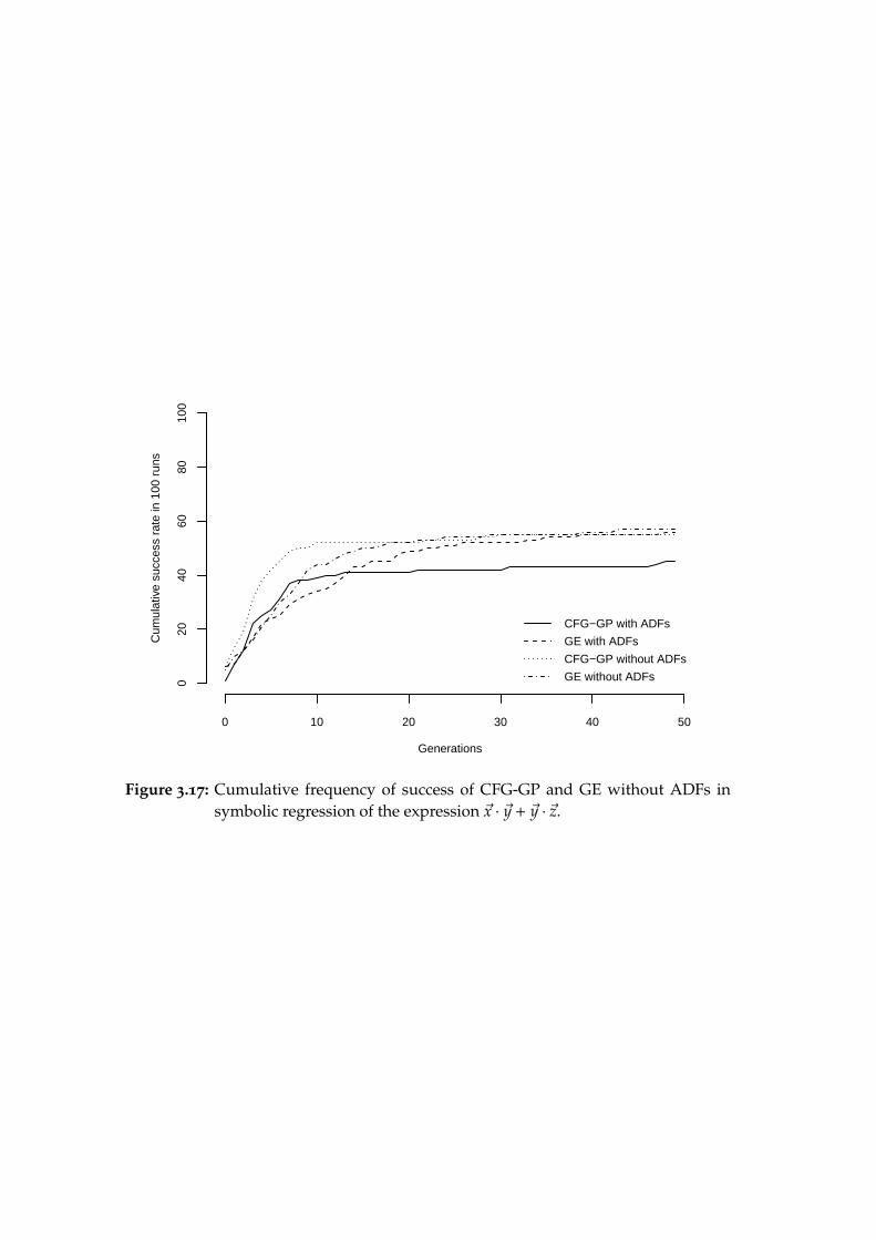
Generations
Cum
ulat
ive
succ
ess
rate
in 1
00 r
uns
0 10 20 30 40 50
020
4060
8010
0
CFG−GP with ADFs
GE with ADFs
CFG−GP without ADFs
GE without ADFs
Figure 3.17: Cumulative frequency of success of CFG-GP and GE without ADFs insymbolic regression of the expression ~x · ~y + ~y · ~z.
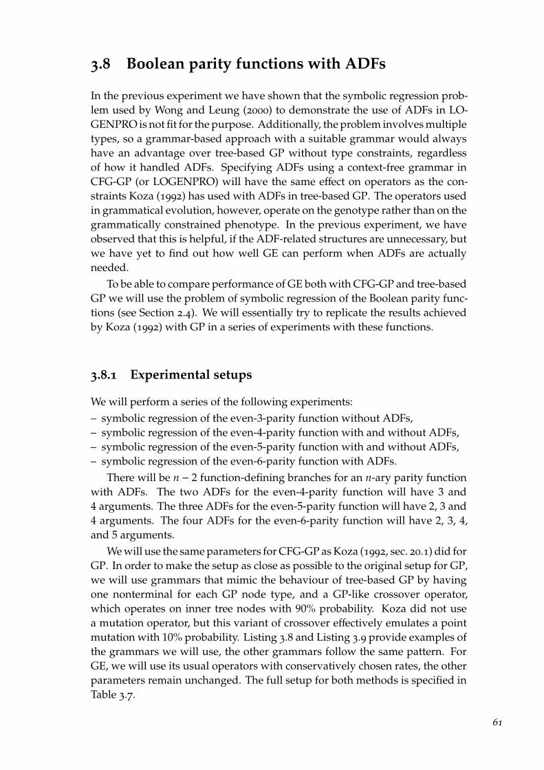
3.8 Boolean parity functions with ADFs
In the previous experiment we have shown that the symbolic regression prob-lem used by Wong and Leung (2000) to demonstrate the use of ADFs in LO-GENPRO is not fit for the purpose. Additionally, the problem involves multipletypes, so a grammar-based approach with a suitable grammar would alwayshave an advantage over tree-based GP without type constraints, regardlessof how it handled ADFs. Specifying ADFs using a context-free grammar inCFG-GP (or LOGENPRO) will have the same effect on operators as the con-straints Koza (1992) has used with ADFs in tree-based GP. The operators usedin grammatical evolution, however, operate on the genotype rather than on thegrammatically constrained phenotype. In the previous experiment, we haveobserved that this is helpful, if the ADF-related structures are unnecessary, butwe have yet to find out how well GE can perform when ADFs are actuallyneeded.
To be able to compare performance of GE both with CFG-GP and tree-basedGP we will use the problem of symbolic regression of the Boolean parity func-tions (see Section 2.4). We will essentially try to replicate the results achievedby Koza (1992) with GP in a series of experiments with these functions.
3.8.1 Experimental setups
We will perform a series of the following experiments:– symbolic regression of the even-3-parity function without ADFs,– symbolic regression of the even-4-parity function with and without ADFs,– symbolic regression of the even-5-parity function with and without ADFs,– symbolic regression of the even-6-parity function with ADFs.
There will be n − 2 function-defining branches for an n-ary parity functionwith ADFs. The two ADFs for the even-4-parity function will have 3 and4 arguments. The three ADFs for the even-5-parity function will have 2, 3 and4 arguments. The four ADFs for the even-6-parity function will have 2, 3, 4,and 5 arguments.
We will use the same parameters for CFG-GP as Koza (1992, sec. 20.1) did forGP. In order to make the setup as close as possible to the original setup for GP,we will use grammars that mimic the behaviour of tree-based GP by havingone nonterminal for each GP node type, and a GP-like crossover operator,which operates on inner tree nodes with 90% probability. Koza did not usea mutation operator, but this variant of crossover effectively emulates a pointmutation with 10% probability. Listing 3.8 and Listing 3.9 provide examples ofthe grammars we will use, the other grammars follow the same pattern. ForGE, we will use its usual operators with conservatively chosen rates, the otherparameters remain unchanged. The full setup for both methods is specified inTable 3.7.
61

Objective: Find an expression for the even parity function of 3, 4, 5,and 6 arguments using ADFs as described in the text.
Terminal operands: A subset of d0, d1, . . . , d5 (variables), a0, a1, . . . , d4 (ADFparameters) based on arity and whether ADFs are used.
Terminal operators: Boolean connectives and, or, nand, nor; a subset of adf0,adf1, adf2 based on arity and whether ADFs are used.
Grammar: See Listing 3.8 and Listing 3.9 for examples.Fitness cases: The set of all possible arguments.Raw fitness: The number of fitness cases for which the value returned
by the expression is different from the correct value of theeven parity function.
Scaled fitness: Koza’s adjusted fitness, and greedy over-selection withthe parameters used by Koza (1992).
Algorithm: Simple, generations: 51, population: 4000.Selection: Roulette-wheel.CFG-GP initialisation: Ramped half-and half (unique trees), maximum height:
8/7 (with/without ADFs).GE initialisation: Ramped half-and half (unique trees), maximum height:
8/7 (with/without ADFs).CFG-GP operators: Only GP-like crossover (Koza, 1992), probability: 0.9.GE operators: Fixed-length one-point crossover, probability: 0.9
Bit-level mutation, probability: 0.002.Common parameters: Maximum tree height: 18/19 (with/without ADFs).GE parameters: Maximum wraps: 3. Codon size: 8.Success predicate: Raw fitness equal to 0.
Table 3.7: Symbolic regression of the Boolean parity function, CFG-GP, and GE. Note:the maximum initialisation tree height and the overall maximum tree heightcorrespond to GP tree heights 6 and 17, respectively, used by Koza (1992).
3.8.2 Results
Figure 3.18 shows plots of cumulative frequency of success for all experiments.In Table 3.8we compare the final success rates with those reported for tree-basedGP by Koza (1992). Koza performed tens of runs in all experiments except foreven-5-parity with ADFs (7 runs) and even-6-parity with ADFs (unreported).Both CFG-GP and GE perform surprisingly well without ADFs compared tothe results reported by Koza (1992) for GP: for instance in the even-4-parity,CFG-GP has more than twice the success rate of GP, and even the even-5-paritywithout ADFs intimidates neither CFG-GP nor GE.
We are, however, more interested in the performance with ADFs. Context-free grammar genetic programming performs only slightly worse than tree-based genetic programming in the even-4-parity problem (96% vs. 99% suc-cess). For even-5-parity, Koza (1992) reports results from mere 7 runs, so I willavoid drawing any conclusion from the comparison: incidentally the first 7runs I have performed with CFG-GP were also successful.) CFG-GP performsrelatively well even in the even-6-parity problem (Koza does not report any
62
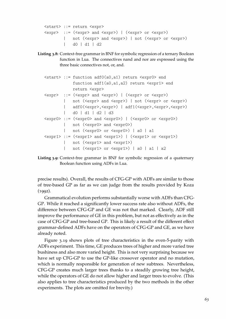
<start> ::= return <expr><expr> ::= (<expr> and <expr>) | (<expr> or <expr>)
| not (<expr> and <expr>) | not (<expr> or <expr>)| d0 | d1 | d2
Listing 3.8: Context-free grammar in BNF for symbolic regression of a ternary Booleanfunction in Lua. The connectives nand and nor are expressed using thethree basic connectives not, or, and.
<start> ::= function adf0(a0,a1) return <expr0> endfunction adf1(a0,a1,a2) return <expr1> endreturn <expr>
<expr> ::= (<expr> and <expr>) | (<expr> or <expr>)| not (<expr> and <expr>) | not (<expr> or <expr>)| adf0(<expr>,<expr>) | adf1(<expr>,<expr>,<expr>)| d0 | d1 | d2 | d3
<expr0> ::= (<expr0> and <expr0>) | (<expr0> or <expr0>)| not (<expr0> and <expr0>)| not (<expr0> or <expr0>) | a0 | a1
<expr1> ::= (<expr1> and <expr1>) | (<expr1> or <expr1>)| not (<expr1> and <expr1>)| not (<expr1> or <expr1>) | a0 | a1 | a2
Listing 3.9: Context-free grammar in BNF for symbolic regression of a quaternaryBoolean function using ADFs in Lua.
precise results). Overall, the results of CFG-GP with ADFs are similar to thoseof tree-based GP as far as we can judge from the results provided by Koza(1992).
Grammatical evolution performs substantially worse with ADFs than CFG-GP. While it reached a significantly lower success rate also without ADFs, thedifference between CFG-GP and GE was not that marked. Clearly, ADF stillimprove the performance of GE in this problem, but not as effectively as in thecase of CFG-GP and tree-based GP. This is likely a result of the different effectgrammar-defined ADFs have on the operators of CFG-GP and GE, as we havealready noted.
Figure 3.19 shows plots of tree characteristics in the even-5-parity withADFs experiment. This time, GE produces trees of higher and more varied treebushiness and also more varied height. This is not very surprising because wehave set up CFG-GP to use the GP-like crossover operator and no mutation,which is normally responsible for generation of new subtrees. Nevertheless,CFG-GP creates much larger trees thanks to a steadily growing tree height,while the operators of GE do not allow higher and larger trees to evolve. (Thisalso applies to tree characteristics produced by the two methods in the otherexperiments. The plots are omitted for brevity.)
63
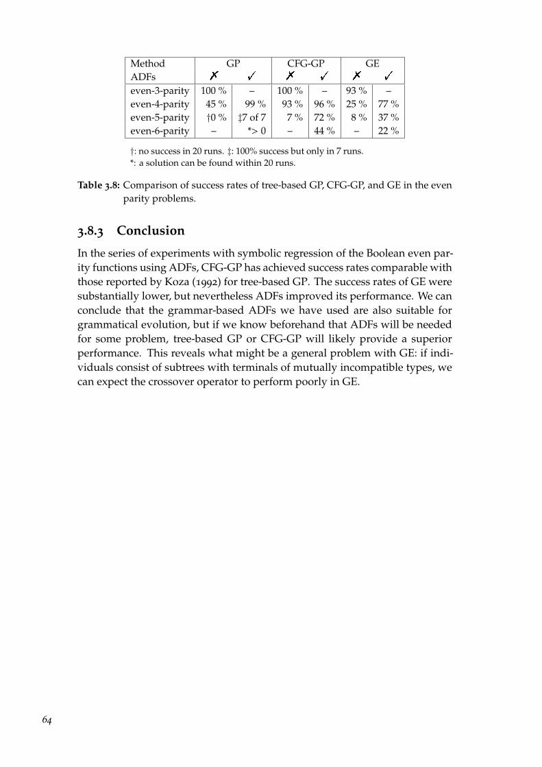
Method GP CFG-GP GEADFs % ! % ! % !
even-3-parity 100 % – 100 % – 93 % –even-4-parity 45 % 99 % 93 % 96 % 25 % 77 %even-5-parity †0 % ‡7 of 7 7 % 72 % 8 % 37 %even-6-parity – *> 0 – 44 % – 22 %
†: no success in 20 runs. ‡: 100% success but only in 7 runs.*: a solution can be found within 20 runs.
Table 3.8: Comparison of success rates of tree-based GP, CFG-GP, and GE in the evenparity problems.
3.8.3 Conclusion
In the series of experiments with symbolic regression of the Boolean even par-ity functions using ADFs, CFG-GP has achieved success rates comparable withthose reported by Koza (1992) for tree-based GP. The success rates of GE weresubstantially lower, but nevertheless ADFs improved its performance. We canconclude that the grammar-based ADFs we have used are also suitable forgrammatical evolution, but if we know beforehand that ADFs will be neededfor some problem, tree-based GP or CFG-GP will likely provide a superiorperformance. This reveals what might be a general problem with GE: if indi-viduals consist of subtrees with terminals of mutually incompatible types, wecan expect the crossover operator to perform poorly in GE.
64
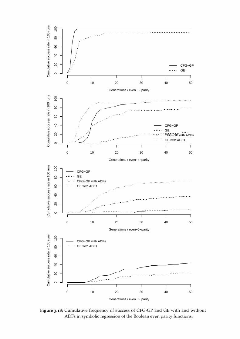
Generations / even−3−parity
Cum
ulat
ive
succ
ess
rate
in 1
00 r
uns
0 10 20 30 40 50
020
4060
8010
0
CFG−GP
GE
Generations / even−4−parity
Cum
ulat
ive
succ
ess
rate
in 1
00 r
uns
0 10 20 30 40 50
020
4060
8010
0
CFG−GP
GE
CFG−GP with ADFs
GE with ADFs
Generations / even−5−parity
Cum
ulat
ive
succ
ess
rate
in 1
00 r
uns
0 10 20 30 40 50
020
4060
8010
0
CFG−GP
GE
CFG−GP with ADFs
GE with ADFs
Generations / even−6−parity
Cum
ulat
ive
succ
ess
rate
in 1
00 r
uns
0 10 20 30 40 50
020
4060
8010
0
CFG−GP with ADFs
GE with ADFs
Figure 3.18: Cumulative frequency of success of CFG-GP and GE with and withoutADFs in symbolic regression of the Boolean even parity functions.
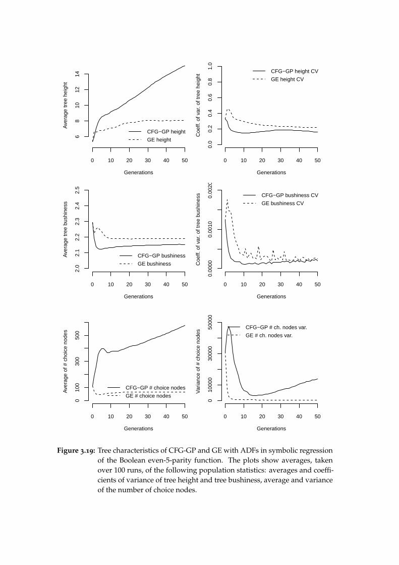
Generations
Ave
rage
tree
hei
ght
0 10 20 30 40 50
68
1012
14
CFG−GP height
GE height
Generations
Coe
ff. o
f var
. of t
ree
heig
ht
0 10 20 30 40 50
0.0
0.2
0.4
0.6
0.8
1.0
CFG−GP height CV
GE height CV
Generations
Ave
rage
tree
bus
hine
ss
0 10 20 30 40 50
2.0
2.1
2.2
2.3
2.4
2.5
CFG−GP bushiness
GE bushiness
Generations
Coe
ff. o
f var
. of t
ree
bush
ines
s
0 10 20 30 40 50
0.00
000.
0010
0.00
20
CFG−GP bushiness CV
GE bushiness CV
Generations
Ave
rage
of #
cho
ice
node
s
0 10 20 30 40 50
010
030
050
0
CFG−GP # choice nodes
GE # choice nodes
Generations
Var
ianc
e of
# c
hoic
e no
des
0 10 20 30 40 50
010
000
3000
050
000
CFG−GP # ch. nodes var.
GE # ch. nodes var.
Figure 3.19: Tree characteristics of CFG-GP and GE with ADFs in symbolic regressionof the Boolean even-5-parity function. The plots show averages, takenover 100 runs, of the following population statistics: averages and coeffi-cients of variance of tree height and tree bushiness, average and varianceof the number of choice nodes.
3.9 Exam timetabling hyper-heuristics
Exam timetabling is a real-world problem of scheduling exams for universitycourses under given constraints. The constraints may vary according to institu-tion but the most usual hard constraint is that no student can attend two examsat the same time, and the most usual soft constrain is that exams scheduledvery close to each other for some students should be avoided. Most literat-ure uses problems that can be scheduled relatively easily to satisfy the hardconstraint, and the focus is on optimising the soft one. Various methods havebeen applied to exam timetabling and a widely used set of problem data hasbeen established by Carter et al. (1996). The problems are based on real datafrom thirteen universities and are often referred to as the University of Torontobenchmark data.
Recently, Bader-El-Den et al. (2009) have applied a grammar-based GPhyper-heuristic approach (see Section 2.5) to timetabling and have evaluatedthe method on the above mentioned data sets. As follows from using a hyper-heuristic approach, they compose several simple hand-crafted heuristics usingconditional branching, to create a new heuristic. The grammar-based GP partof their method (called GPHH, Grammar-based Genetic Programming Hyper-Heuristic) claims to be “a new, hybrid way of using grammars in GP” differentfrom both Koza’s GP and Whigham’s CFG-GP: the method operates accordingto the grammar directly on GP trees instead of derivation trees in order toincrease performance. Other than this difference, which could be consideredan implementation detail, the method based on the “grow” initialisation andthe two familiar operators seems practically identical to CFG-GP.
Bader-El-Den et al. (2009) have evaluated their method on ten problemsfrom the Toronto data set and their results were comparable with several exist-ing algorithms. In the previous sections, we have applied GE and CFG-GP toseveral artificial problems that are either commonly used in the realm of geneticprogramming or highlight the use of grammar for ensuring type constraints.These artificial problems were also well-suited for comparing the characterist-ics of GE and CFG-GP. Exam timetabling is an opportunity to evaluate theperformance of grammar-based GP methods on a real-world problem to whichmany methods other than GP have been applied. Another interesting differ-ence from the previous experiments is that there are no known target solutions,instead there are many correct solutions that differ in how well they satisfy thesoft constraints.
We will try to replicate the published results with CFG-GP, compare themwith a similar setup of grammatical evolution, and we will also briefly discussthe performance in terms of computational time.
Let’s start by stating the exam timetabling problem formally using the samenotation as Bader-El-Den et al. (2009): Let E be the set of exams, S the set ofstudents, P the set of time slots, R : S→ P(E) a registration function (Pdenotes apower set). The quadruple consisting of E, S, P, and R is a timetabling problem.A solution to the timetabling problem (E,S,P,R) is a function O : E → P. The
67

solution is incorrect if ∃ s ∈ S, i, j ∈ E : i , j & {i, j} ⊆ R(s) & P(i) = P( j) (a studentis to attend two exams at the same time), and the solution is incomplete if O isa partial function.
The soft constraint can be expressed quantitatively for correct solutions asa penalty p:
p =1S
N−1∑i=1
N∑j=i+1
w(|pi − p j|) · ai j (1)
where S is the total number of students, N is the total number of exams, ai j isthe number of students attending both exams i and j, pi is the time slot to whichexam i is assigned, and w(d) is defined as 25−d if d ≤ 5 and as 0 otherwise. Thisformula proposed by Carter et al. (1996) has since been used in the literatureto compare the quality of solutions.
We will use a fitness value f based on the penalty formula:
f =
( M−1∑i=1
M∑j=i+1
w(|pi − p j|) · ai j
)+ α · (N −M) (2)
where M is the number of assigned exams. This is only a minor modificationof the fitness function used by Bader-El-Den et al. (2009): we leave out the 1
Sfactor as it does not serve any purpose when computing fitness. The differencefrom the penalty function is that it allows for incomplete solutions. Bader-El-Den et al. (2009) do not mention any value for the α constant, but I havefound out that any value large enough to disqualify incomplete solutions intournaments with complete solutions works well. If we were to use a fitness-proportionate selection, however, it might not be the case.
Algorithms for timetabling that use heuristics usually proceed by repeatedlyusing the heuristic to select an exam and then its slot. It may happen that noslot is available for a given exam (the partial assignment would be incorrect), inwhich case the algorithm may stop, continue constructing an incomplete solu-tion, or continue constructing an incorrect solution. This first phase may thenbe followed by a repair or improvement phase. Bader-El-Den et al. (2009) makea distinction between “constructive” algorithms without a repair or improve-ment phase and “improvement” algorithms, and they compare their resultsprimarily with other constructive algorithms. They do not describe preciselythe algorithm they use, but it is conceivably the one that continues to constructan incomplete solution even if some exams cannot be scheduled, as outlinedin this pseudocode:
68
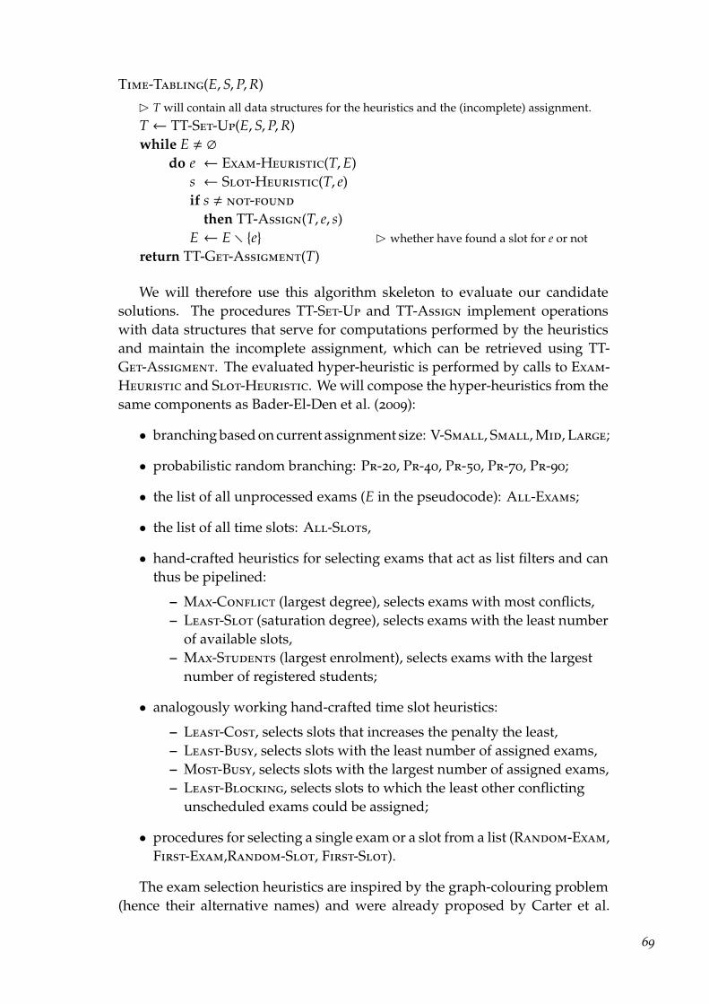
Time-Tabling(E,S,P,R)
� T will contain all data structures for the heuristics and the (incomplete) assignment.
T← TT-Set-Up(E,S,P,R)while E , ∅
do e ← Exam-Heuristic(T,E)s ← Slot-Heuristic(T, e)if s , not-found
then TT-Assign(T, e, s)E ← E r {e} � whether have found a slot for e or not
return TT-Get-Assigment(T)
We will therefore use this algorithm skeleton to evaluate our candidatesolutions. The procedures TT-Set-Up and TT-Assign implement operationswith data structures that serve for computations performed by the heuristicsand maintain the incomplete assignment, which can be retrieved using TT-Get-Assigment. The evaluated hyper-heuristic is performed by calls to Exam-Heuristic and Slot-Heuristic. We will compose the hyper-heuristics from thesame components as Bader-El-Den et al. (2009):
• branching based on current assignment size: V-Small, Small, Mid, Large;
• probabilistic random branching: Pr-20, Pr-40, Pr-50, Pr-70, Pr-90;
• the list of all unprocessed exams (E in the pseudocode): All-Exams;
• the list of all time slots: All-Slots,
• hand-crafted heuristics for selecting exams that act as list filters and canthus be pipelined:
– Max-Conflict (largest degree), selects exams with most conflicts,– Least-Slot (saturation degree), selects exams with the least number
of available slots,– Max-Students (largest enrolment), selects exams with the largest
number of registered students;
• analogously working hand-crafted time slot heuristics:
– Least-Cost, selects slots that increases the penalty the least,– Least-Busy, selects slots with the least number of assigned exams,– Most-Busy, selects slots with the largest number of assigned exams,– Least-Blocking, selects slots to which the least other conflicting
unscheduled exams could be assigned;
• procedures for selecting a single exam or a slot from a list (Random-Exam,First-Exam,Random-Slot, First-Slot).
The exam selection heuristics are inspired by the graph-colouring problem(hence their alternative names) and were already proposed by Carter et al.
69

(1996). The time selection heuristics seem to have been introduced by Bader-El-Den et al. (2009) who give commonsense explanations for them. The basicidea is that even if some of the heuristics would not be useful alone, they maybecome useful in conjunction with each other or at particular stages of thetimetable construction (using assignment size conditions).
The basic heuristics and other components can be combined according tothe grammar shown Listing 3.10. Note particularly that conditional branchingcan occur anywhere, and so the pipelines of heuristics may form branches ofarbitrarily shaped trees.
<assign> ::= while <exam>~=0 do <slot> end<exam> ::= randomExam(<eList>) | firstExam(<eList>)<eList> ::= maxConflict(<eList>)
| leastSlot(<eList>)| maxStudents(<eList>)| allExams(t)| (<cond> and <eList> or <eList>)
<slot> ::= randomSlot(<sList>) | firstSlot(<sList>)<sList> ::= leastCost(<sList>)
| leastBusy(<sList>)| mostBusy(<sList>)| leastBlocking(<sList>)| allSlots(t)| (<cond> and <sList> or <sList>)
<cond> ::= <prob> | <size><size> ::= vSmall(t) | small(t) | mid(t) | large(t)<prob> ::= pr20(t) | pr40(t) | pr50(t) | pr70(t) | pr90(t)
Listing 3.10: Context-free grammar in BNF for a timetabling hyper-heuristic in Lua.The (· · · and · · · or · · · ) construct is a Lua idiom for a functional if-then-else condition with short-circuit (lazy) evaluation. The exam heuristicfunctions are implemented so that they return 0 when there are no examsleft, the slot heuristic functions perform an exam-slot assignment if a slotis found. All data structures and the currently selected exam and slotare kept in the t data structure. This is a Lua equivalent of the grammarpresented by Bader-El-Den et al. (2009).
3.9.1 Experimental setup
In addition to the grammar equivalent to the one used by Bader-El-Den et al.(2009), we will also report results with an alternative grammar without randomselection of exams and slots and conditional branching for slots.
For CFG-GP, we will use the parameters specified by Bader-El-Den et al.(2009). The values of maximum initialisation height and maximum height aremissing in their article as well as the already discussedαparameter of the fitness
70
function. As we do not have any beforehand knowledge of suitable tree heightparameters, we will out of cautiousness use a low maximum initialisation treeheight, letting the initialisation procedure raise it as needed for generation ofunique individuals, and a high maximum tree height. There are only a fewminor differences from the setup used by Bader-El-Den et al. (2009):– We do not use mutually exclusive operators.– We will evaluate individuals that use random selection or probabilistic condi-
tions three times with different random number generator states and assignthem the mean fitness value of the three runs. We will also report only thismean value in the results. Bader-El-Den et al. (2009) ran “the best performingindividuals [. . . ] for an extra 2 times”. It is not clear if this concerns onlythe best individuals in a generation and whether the mean or the minimumvalue is used.
– We will perform only runs with 50 generations and 50 individuals in the pop-ulation. In addition to this, Bader-El-Den et al. (2009) performed runs with“larger populations, with sizes ranging between 500 and 1000 individuals”,but they do not give precise value for each experiment.
We will, as usual, use a lower nominal mutation rate for GE to reach an effectivemutation rate similar to that of CFG-GP. The full list of parameters is providedin Table 3.9.)
71
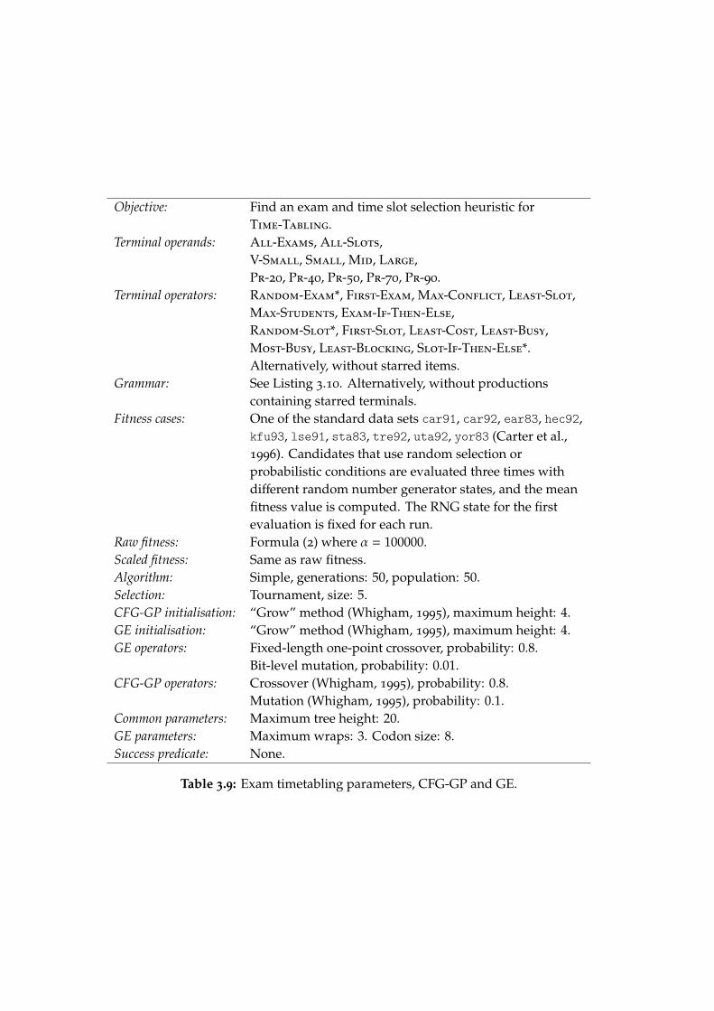
Objective: Find an exam and time slot selection heuristic forTime-Tabling.
Terminal operands: All-Exams, All-Slots,V-Small, Small, Mid, Large,Pr-20, Pr-40, Pr-50, Pr-70, Pr-90.
Terminal operators: Random-Exam*, First-Exam, Max-Conflict, Least-Slot,Max-Students, Exam-If-Then-Else,Random-Slot*, First-Slot, Least-Cost, Least-Busy,Most-Busy, Least-Blocking, Slot-If-Then-Else*.Alternatively, without starred items.
Grammar: See Listing 3.10. Alternatively, without productionscontaining starred terminals.
Fitness cases: One of the standard data sets car91, car92, ear83, hec92,kfu93, lse91, sta83, tre92, uta92, yor83 (Carter et al.,1996). Candidates that use random selection orprobabilistic conditions are evaluated three times withdifferent random number generator states, and the meanfitness value is computed. The RNG state for the firstevaluation is fixed for each run.
Raw fitness: Formula (2) where α = 100000.Scaled fitness: Same as raw fitness.Algorithm: Simple, generations: 50, population: 50.Selection: Tournament, size: 5.CFG-GP initialisation: “Grow” method (Whigham, 1995), maximum height: 4.GE initialisation: “Grow” method (Whigham, 1995), maximum height: 4.GE operators: Fixed-length one-point crossover, probability: 0.8.
Bit-level mutation, probability: 0.01.CFG-GP operators: Crossover (Whigham, 1995), probability: 0.8.
Mutation (Whigham, 1995), probability: 0.1.Common parameters: Maximum tree height: 20.GE parameters: Maximum wraps: 3. Codon size: 8.Success predicate: None.
Table 3.9: Exam timetabling parameters, CFG-GP and GE.

3.9.2 Results
In Table 3.10we report the best results from ten runs for each method, grammar,and data set, as Bader-El-Den et al. (2009) did, along with the results reportedby them. We use the same ten data sets.4
car91 car92 ear83 hec92 kfu93 lse91 sta83 tre92 uta92 yor83GPHH ‡5.12 4.46 ‡37.10 ‡11.78 ‡14.72 ‡11.11 ‡158.70 †8.62 3.47 †40.56CFG-GP †5.11 ‡4.44 38.78 12.67 15.21 11.93 159.44 8.78 3.49 40.73GE 5.15 ‡4.44 39.95 12.20 14.86 12.04 159.37 ‡8.63 3.51 ‡40.60CFG-GP* 5.13 †4.37 37.29 12.15 14.74 11.75 160.22 ‡8.63 ‡3.44 40.94GE* 5.22 4.51 39.68 12.27 15.23 11.96 160.22 8.79 ‡3.44 41.47Best other Fuzzy Fuzzy Car. Car. Car. Car. Tabu Fuzzy TM Fuzzy
5.20 4.52 †36.4 †10.8 †14.0 †10.5 †158.19 8.67 †3.04 40.66
*: alternative grammar. Best other: best other constructive heuristic, as reported byBader-El-Den et al. (2009). †, ‡: best and second best results. Car.: Carter et al. (1996).Fuzzy: Asmuni et al. (2005). Tabu, TM (Tabu-Multi-stage): Burke et al. (2007).
Table 3.10: Penalties achieved by time tabling heuristics. Mean values are reportedfor stochastic heuristics evolved with CFG-GP and GE.
CFG-GP with the original grammar has in two cases (car91, car92) outper-formed GPHH, which is the more interesting as these are two of the four casesin which Bader-El-Den et al. (2009) reported that GPHH already outperformedthe best other constructive method.
GE with the original grammar has performed similarly to CFG-GP (fourtimes better, five times worse). With the car92 data set it has performedequally with CFG-GP, also beating both GPHH and the best other constructivemethod. With car92 and tre92 it has still performed better than the best othermethod, but worse than GPHH.
Because the grammar used by Bader-El-Den et al. (2009) is quite rich and theauthors do not discuss their choices in much detail, I have experimented withremoving various features. Most of the changes, such as permitting conditionalbranching only at the top level, or reducing the number of conditions, resultedin inferior performance. Removal of random selection of exams and slotsand conditional branching for slots did, however, improve CFG-GP and GEresults for seven and four data sets, respectively. CFG-GP with the alternativegrammar outperformed all other methods in car92. Both CFG-GP and GE withthe alternative grammar have outperformed GPHH. What is interesting aboutthese results is that we have managed to remove a large part of randomnessfrom the heuristics without impacting the quality of solutions.
4 Bader-El-Den et al. (2009) refer to one of the Toronto data sets as uta93. Although theygive parameters for ute92, it must be uta92, judging from the achieved penalty.
73
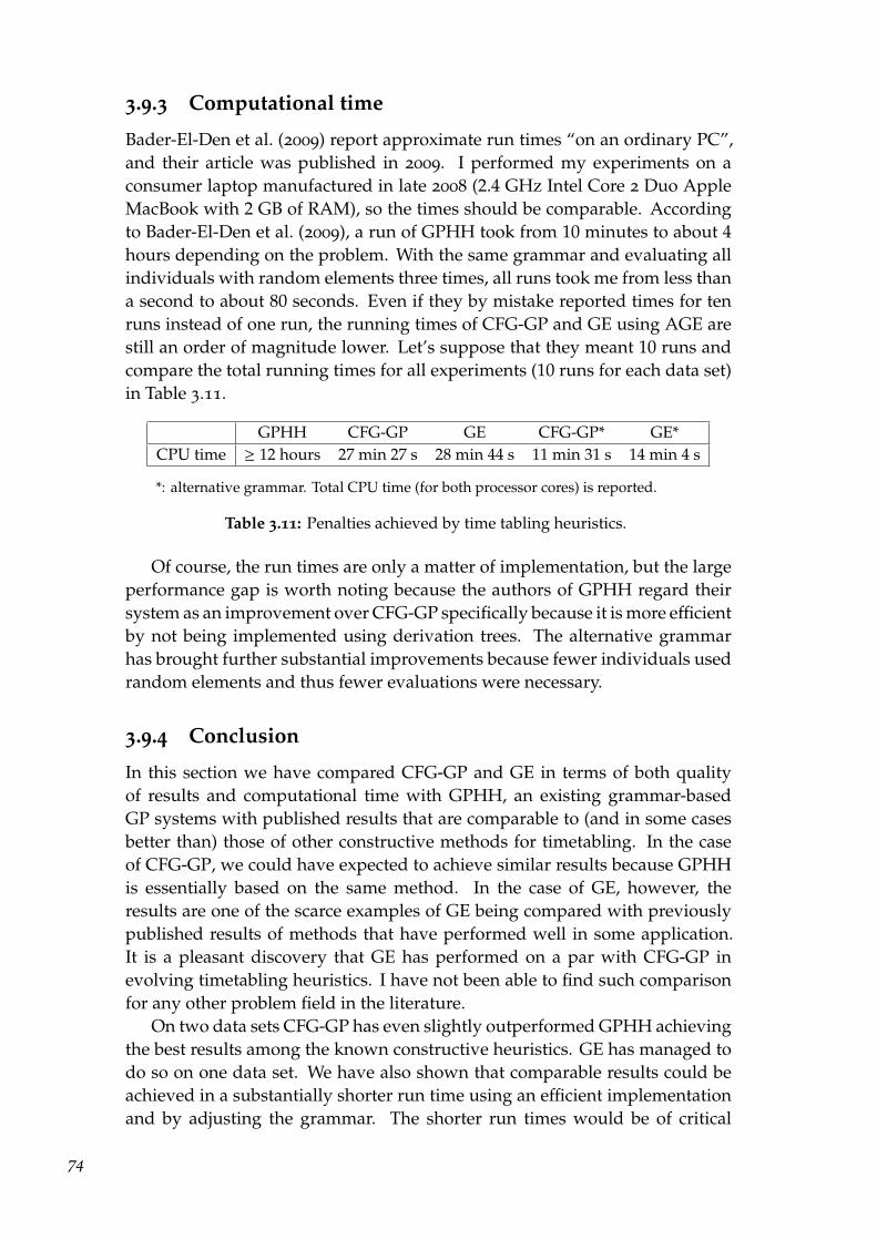
3.9.3 Computational time
Bader-El-Den et al. (2009) report approximate run times “on an ordinary PC”,and their article was published in 2009. I performed my experiments on aconsumer laptop manufactured in late 2008 (2.4 GHz Intel Core 2 Duo AppleMacBook with 2 GB of RAM), so the times should be comparable. Accordingto Bader-El-Den et al. (2009), a run of GPHH took from 10 minutes to about 4hours depending on the problem. With the same grammar and evaluating allindividuals with random elements three times, all runs took me from less thana second to about 80 seconds. Even if they by mistake reported times for tenruns instead of one run, the running times of CFG-GP and GE using AGE arestill an order of magnitude lower. Let’s suppose that they meant 10 runs andcompare the total running times for all experiments (10 runs for each data set)in Table 3.11.
GPHH CFG-GP GE CFG-GP* GE*CPU time ≥ 12 hours 27 min 27 s 28 min 44 s 11 min 31 s 14 min 4 s
*: alternative grammar. Total CPU time (for both processor cores) is reported.
Table 3.11: Penalties achieved by time tabling heuristics.
Of course, the run times are only a matter of implementation, but the largeperformance gap is worth noting because the authors of GPHH regard theirsystem as an improvement over CFG-GP specifically because it is more efficientby not being implemented using derivation trees. The alternative grammarhas brought further substantial improvements because fewer individuals usedrandom elements and thus fewer evaluations were necessary.
3.9.4 Conclusion
In this section we have compared CFG-GP and GE in terms of both qualityof results and computational time with GPHH, an existing grammar-basedGP systems with published results that are comparable to (and in some casesbetter than) those of other constructive methods for timetabling. In the caseof CFG-GP, we could have expected to achieve similar results because GPHHis essentially based on the same method. In the case of GE, however, theresults are one of the scarce examples of GE being compared with previouslypublished results of methods that have performed well in some application.It is a pleasant discovery that GE has performed on a par with CFG-GP inevolving timetabling heuristics. I have not been able to find such comparisonfor any other problem field in the literature.
On two data sets CFG-GP has even slightly outperformed GPHH achievingthe best results among the known constructive heuristics. GE has managed todo so on one data set. We have also shown that comparable results could beachieved in a substantially shorter run time using an efficient implementationand by adjusting the grammar. The shorter run times would be of critical
74

importance if the grammar-based GP methods were to be used in a morecomplex setup to evolve improvement heuristics for timetabling and competewith other improvement methods as Bader-El-Den et al. (2009) suggest forfurther research.
3.10 Conclusion
We have compared performance of GE and CFG-GP in a variety of applicationand discovered links between the differences in the produced tree shapes andthe relative success of the two methods. The two methods performed simil-arly well a few times but in several applications the performance of GE wassubstantially worse.
In Section 3.4 we have found out that the more successful CFG-GP pro-duces higher trees of more varied shapes, thus searching a larger space. InSection 3.5 we have made the same observation and verified it with differentinitialisation techniques. In the long run, both methods tended to convergeto tree characteristics typical for them regardless of tree characteristics of theinitial populations. In the two experiments done in Section 3.6 and Section 3.7,which compared performance with LOGENPRO, all three methods performedsimilarly. Nonetheless, we could observe the same patterns in developmentof tree characteristics for GE and CFG-GP. We have explained why the goodresults of GE were likely caused by its tendency to preserve low tree heightthroughout its run, the same property that would often have the opposite effect.In Section 3.8, we have shown that both GE and CFG-GP can use ADFs suc-cessfully but that the technique adapted from tree-based GP is not as effectivefor GE. As we have not used the usual mutation operators, the patterns of treecharacteristics were different than in the earlier experiments but CFG-GP stillproduced higher and larger trees than GE, and was more successful even inthe ADF-less versions of the experiments. GE has, however, found solutions ofsimilar quality to those of CFG-GP in the real-world application to timetablingin Section 3.9.
We have thus shown a consistent difference between the tree shapes pro-duced by GE and CFG-GP. GE tends to produce shorter trees, usually also lessbushy and of less varied height and bushiness. The search of this smaller searchspace tends to be explorative thanks to the disruptive operators used in GE,and GE can provide slightly but significantly better results in some cases. Inother cases, though, this seems to hamper performance. Additionally, the factthat the operators used in GE are grammar-agnostic clearly worsens perform-ance with ADFs, and it would likely have the same effect with any grammarspecifying subtrees with terminals of mutually incompatible types. We havenot found GE to provide a substantial advantage in any of the problems.
In Section 3.9 we have also compared computational times needed by GE,CFG-GP, and another implementation of a CFG-GP-like algorithm to evolvetimetabling heuristics. The efficient implementation of CFG-GP and GE I have
75

developed was at least an order of magnitude faster than the one used byBader-El-Den et al. (2009). CFG-GP has performed slightly better than GE interms of CPU time. This is a consequence of what individuals evolved duringthe run, and it demonstrates that the simpler operators of GE do not implyshorter overall run times.
76
Chapter 4
Implementation Notes
All experiments with GE and CFG-GP in Chapter 3 were done using an open-source framework called AGE (Algorithms for Grammar-based Evolution). Ihave created the initial version of the framework as an implementation of GEand general evolutionary algorithm elements as part of my bachelor thesis withthe following goals:– a clean, comprehensive implementation of standard algorithms,– modularity,– adequate documentation,– versatile output,– reproducible results,– acceptable performance.
Thanks to the modular approach it was easy to extend the framework withimplementation of CFG-GP and several new features. Although the frameworkaimed only at an “acceptable performance” in terms of computational time,it outperformed GEVA (an implementation of GE maintained at NCRA atUniversity College Dublin) by an order of magnitude in benchmarks done aspart of my bachelor thesis (Nohejl, 2009). The comparison of the CFG-GPimplementation, which is now part of AGE, with published results from theCFG-GP-based GPHH framework (Bader-El-Den et al., 2009) was similarlyfavourable (Section 3.9.3).
In this chapter, we will describe the implementation of CFG-GP used inAGE (in Section 4.1), provide information about the accompanying files andabout how to use them to replicate the results presented in the previous chapter(Section 4.2). User and developer documentation of the framework and tools,written as part of my bachelor thesis, is available inside the software package.
4.1 Implementation of CFG-GP
The original version of AGE already featured an efficient implementation ofgrammatical evolution. This implementation does not store derivation trees, in-stead phenotype strings are created directly from the codon strings (genotype),and when initialising individuals, genotype is generated directly. Thus deriva-
77
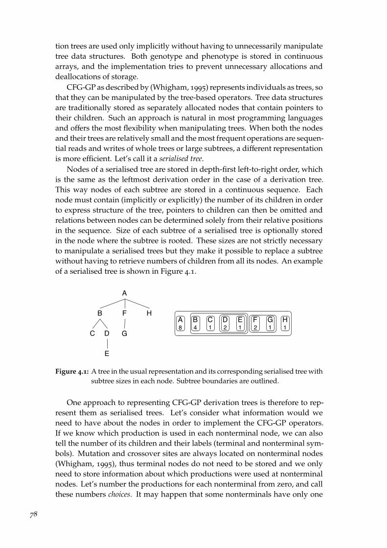
tion trees are used only implicitly without having to unnecessarily manipulatetree data structures. Both genotype and phenotype is stored in continuousarrays, and the implementation tries to prevent unnecessary allocations anddeallocations of storage.
CFG-GP as described by (Whigham, 1995) represents individuals as trees, sothat they can be manipulated by the tree-based operators. Tree data structuresare traditionally stored as separately allocated nodes that contain pointers totheir children. Such an approach is natural in most programming languagesand offers the most flexibility when manipulating trees. When both the nodesand their trees are relatively small and the most frequent operations are sequen-tial reads and writes of whole trees or large subtrees, a different representationis more efficient. Let’s call it a serialised tree.
Nodes of a serialised tree are stored in depth-first left-to-right order, whichis the same as the leftmost derivation order in the case of a derivation tree.This way nodes of each subtree are stored in a continuous sequence. Eachnode must contain (implicitly or explicitly) the number of its children in orderto express structure of the tree, pointers to children can then be omitted andrelations between nodes can be determined solely from their relative positionsin the sequence. Size of each subtree of a serialised tree is optionally storedin the node where the subtree is rooted. These sizes are not strictly necessaryto manipulate a serialised trees but they make it possible to replace a subtreewithout having to retrieve numbers of children from all its nodes. An exampleof a serialised tree is shown in Figure 4.1.
A
B F
E
C D G
HA B C D E F G H8 4 1 1 1 122
Figure 4.1: A tree in the usual representation and its corresponding serialised tree withsubtree sizes in each node. Subtree boundaries are outlined.
One approach to representing CFG-GP derivation trees is therefore to rep-resent them as serialised trees. Let’s consider what information would weneed to have about the nodes in order to implement the CFG-GP operators.If we know which production is used in each nonterminal node, we can alsotell the number of its children and their labels (terminal and nonterminal sym-bols). Mutation and crossover sites are always located on nonterminal nodes(Whigham, 1995), thus terminal nodes do not need to be stored and we onlyneed to store information about which productions were used at nonterminalnodes. Let’s number the productions for each nonterminal from zero, and callthese numbers choices. It may happen that some nonterminals have only one
78
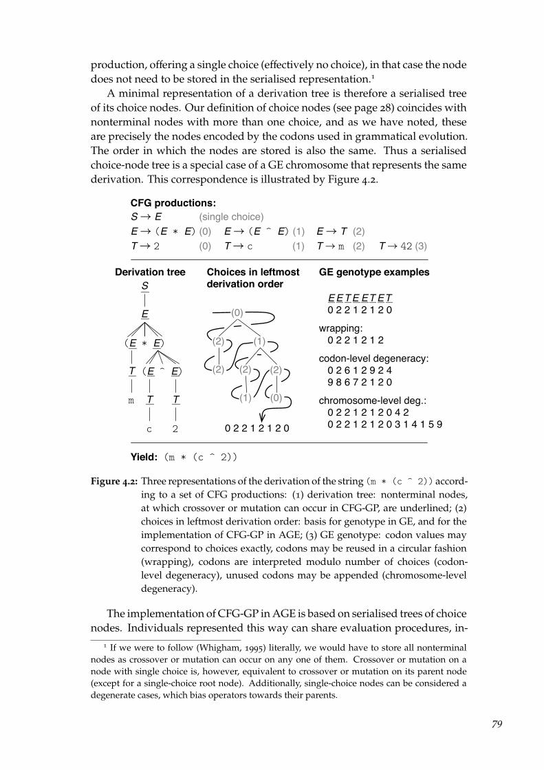
production, offering a single choice (effectively no choice), in that case the nodedoes not need to be stored in the serialised representation.1
A minimal representation of a derivation tree is therefore a serialised treeof its choice nodes. Our definition of choice nodes (see page 28) coincides withnonterminal nodes with more than one choice, and as we have noted, theseare precisely the nodes encoded by the codons used in grammatical evolution.The order in which the nodes are stored is also the same. Thus a serialisedchoice-node tree is a special case of a GE chromosome that represents the samederivation. This correspondence is illustrated by Figure 4.2.
CFG productions:S → E (single choice)E → (E * E) (0) E → (E ^ E) (1) E → T (2)T → 2 (0) T → c (1) T → m (2) T → 42 (3)
E
(E * E)
T
T
(E ^ E)
T
Derivation treeS
Choices in leftmost derivation order
(2) (1)
(2) (2)
0 2 2 1 2 1 2 0
GE genotype examples
(0)
c 2
m
(2)
(1) (0)
E E T E ET ET0 2 2 1 2 1 2 0
wrapping:0 2 2 1 2 1 2
codon-level degeneracy:0 2 6 1 2 9 2 49 8 6 7 2 1 2 0
chromosome-level deg.:0 2 2 1 2 1 2 0 4 20 2 2 1 2 1 2 0 3 1 4 1 5 9
Yield: (m * (c ^ 2))
Figure 4.2: Three representations of the derivation of the string (m * (c ^ 2)) accord-ing to a set of CFG productions: (1) derivation tree: nonterminal nodes,at which crossover or mutation can occur in CFG-GP, are underlined; (2)choices in leftmost derivation order: basis for genotype in GE, and for theimplementation of CFG-GP in AGE; (3) GE genotype: codon values maycorrespond to choices exactly, codons may be reused in a circular fashion(wrapping), codons are interpreted modulo number of choices (codon-level degeneracy), unused codons may be appended (chromosome-leveldegeneracy).
The implementation of CFG-GP in AGE is based on serialised trees of choicenodes. Individuals represented this way can share evaluation procedures, in-1 If we were to follow (Whigham, 1995) literally, we would have to store all nonterminal
nodes as crossover or mutation can occur on any one of them. Crossover or mutation on anode with single choice is, however, equivalent to crossover or mutation on its parent node(except for a single-choice root node). Additionally, single-choice nodes can be considered adegenerate cases, which bias operators towards their parents.
79
cluding the genotype-phenotype mapping, with GE. The tree-based initialisa-tion procedures used for GE need only one modification: removal of geneticcode degeneracy (see Figure 4.2 for comparison). Other general evolution-ary algorithm elements such as selection methods can be shared regardless ofrepresentation. Only the mutation and crossover operators need to be imple-mented separately.
For the purposes of these operators, AGE generates other node informationsuch as the already mentioned subtree size. Because such data can be generatedquickly, it is relatively small, and its reuse is limited, it is actually more efficientto re-generate it every time it is needed. Along with this data, statistics abouttree characteristics that we have used in Chapter 3 can be generated usingcommon procedures for both GE and CFG-GP.
The main advantages of this implementation is that CFG-GP trees are storedin compact and easily manipulated data structures (arrays of choice numbersand temporarily generated arrays of other node data). Note that in contrast totraditional Lisp-based GP the derivation trees to which operators are appliedcannot share the representation with the parse trees used when evaluating indi-viduals because arbitrary grammars are allowed. We cannot avoid generatingthe full string representation of each individual (the phenotype in GE) whichis then parsed in order to be evaluated. Therefore the minimal representationis advantageous.
4.2 Accompanying files
This thesis is accompanied by the following files on the enclosed medium:
• Adam-Nohejl-2011-Master-Thesis.pdf, a PDF version of this thesis,
• AGE-1.1.tar.gz, the AGE source package with documentation,
• Experiments.tar.gz, results from LOGENPRO and several scripts:
– AGE-run.sh, a shell script to run experiments for this thesis,
– AGE-stats.sh, a helper R script for stats.sh,
– exstats.sh, a helper shell script for stats.sh,
– plot.r, an R script to draw plots used in this thesis,
– runner.sh, a helper shell script for AGE-run.sh,
– stats.sh, a shell script to compute statistics for the plots.
The included version of the AGE framework has been extended mainlyby the CFG-GP algorithm elements as described above. The implementationsof all experimental problems used in this thesis are also part of the defaultbuild. The software is portable: it can be built on a POSIX-compliant system(tested on Mac OS X, NetBSD and Linux) with a decent standards-compliant
80

C/C++ compiler (tested with GCC and Clang) and it does not have any externaldependencies (details in the included documentation). The whole package is inthe archive named AGE-1.1.tar.gz and has a customary UNIX source packagestructure (you can start by reading the README and INSTALL text files).
To replicate the experiments done in Chapter 3, follow these steps:
1. Build and install AGE from the source package and make sure it is in yoursearch path (your PATH variable must include the directory where youhave installed the AGE executable). Suggested commands for installationinto your home directory:
% tar xzf path/AGE-1.1.tar.gz% cd AGE-1.1; make INSTALL_PREFIX=~ install% cd ..; export PATH=~/bin:"$PATH"
where path is path to the directory containing the file AGE-1.1.tar.gz(mount point of the accompanying disc).
2. Expand the Experiments.tar.gz archive. The resulting Experimentsdirectory will contain the results obtained from LOGENPRO that wehave presented in Chapter 3. Suggested command:
% tar xzf path/Experiments.tar.gz
where path is path to the directory containing the file Experiments.tar.gz.
3. Change your working directory to the newly created Experiments direct-ory. Suggested command:
% cd Experiments
4. Run the AGE-run.sh script. Running all the experiments will likely takea few hours to finish. Alternatively, you can open the file in a text editorand extract only commands for the experiments you want to run or adjustoptions. Suggested command:
% ./AGE-run.sh
Output from the experiments is in a documented format and results fromeach run can be displayed using a XSLT style sheet (consult the AGEdocumentation for details).
5. Optionally, to compute the necessary statistics and render the plots usedin the thesis, run the stats.sh script and then the plot.r script. (TheR statistical package must be installed.) Suggested commands:
% ./stats.sh; ./plot.r
81

The generated plots will be saved in PDF files with the following namepatterns:
• plot-ad*.pdf: Symbolic regression with ADFs (Section 3.7),
• plot-at*.pdf: Santa Fe ant trail (Section 3.5),
• plot-bp*.pdf: Boolean parity functions with ADFs (Section 3.8),
• plot-dp*.pdf: Dot product symbolic regression (Section 3.6),
• plot-sr*.pdf: Simple symbolic regression (Section 3.4).
82
Conclusion
We have discussed the problems encountered by traditional genetic program-ming that can be solved using grammars. We have reviewed three differentgrammar-based GP methods, described their distinctive features, and testedthem in a number of benchmark application, including the real-world applic-ation of finding heuristics for timetabling. We have implemented two of themethods, grammatical evolution and context-free grammar genetic program-ming, in a common framework, which allowed us to compare their perform-ance in identical setups. In addition to comparing performance, we have fo-cused on a statistical analysis of tree characteristics produced by each method,which has provided insight into differences between GE and CFG-GP. As mostof the research in this field focuses either on novel applications or comparesresults only with traditional genetic programming, we have been able to shedmore light on actual performance and comparative advantages of the grammar-based methods.
In Chapter 1 we have introduced the basic concepts of genetic program-ming and formal grammars, and we have pointed to the following problemsencountered by GP that grammars can solve: adaptability to different pro-gramming languages and environments, the problem of closure and multipletypes, and the problem of declarative representation of knowledge. We havepresented three different approaches to applying grammars to GP: context-freegrammar genetic programming, LOGENPRO, and grammatical evolution. Wehave described their distinctive features, and what they imply for performanceof these methods. Based on this survey, we have focused on the role of thepower of logic grammars in LOGENPRO, on the unclear effect of operators inGE, and the problem of bias (whether wanted or not) encoded in a grammar.
In Chapter 2we have described several problem classes and areas of applic-ation, most of them admittedly artificial and of little practical value but usefulfor comparing the performance of grammar-based GP methods. We have alsobriefly presented hyper-heuristics, a field that offers possibilities of real-worldapplication to grammar-based genetic programming.
In Chapter 3 we have tested GE and CFG-GP in six different applications.In two of them we have also compared the results with LOGENPRO, andfound no particular advantage in using logic grammars in the applications thatWong and Leung (2000) used to demonstrate the abilities of LOGENPRO. Inone application we have compared the performance of CFG-GP and GE withtree-based GP (Koza, 1992, results reported by), demonstrated that ADFs can
83

be carried over to the grammar-based methods, particularly to CFG-GP, andexplained the inferior performance of GE. In the last application we have com-pared performance both in terms of quality and speed with recently publishedresults of a grammar-based hyper-heuristic framework (GPHH, Bader-El-Denet al., 2009) for timetabling. The comparison was very favourable: using CFG-GP we have outperformed the published results in two problem instances, inwhich GPHH was already reported to be the best constructive heuristic to date.Additionally, our implementation is at least an order of magnitude faster. Ibelieve that such a large improvement in speed could open new possibilitiesfor practical applications of grammar-based GP methods.
Perhaps even more important output from the six experiments is that GEdoes not provide a substantial advantage in any of them. In several experimentsit performs substantially worse, and we have been able to link this perform-ance to the tree characteristics resulting from its operators, and the fact thatgrammatical constraints in GE are enforced only by the genotype-phenotypemapping, not by the operators. Additionally, we have demonstrated that thesimpler operators of GE do not transform in shorter overall run times. I seethis as the largest contribution of my thesis, as the effect of operators used inGE is hard to analyse, and I have not been able to find such comparisons withother grammar-based GP methods in the literature.
The thesis has fulfilled its goal of thoroughly comparing the grammar-basedGP methods, has showed that CFG-GP, the simplest of the three comparedmethods, provides comparable or even better results than the other two, andhas demonstrated that CFG-GP can be implemented very efficiently. We haveseveral times touched the problem of embedding knowledge (bias) in gram-mars. The choice of grammar obviously has a great effect on performance ofany grammar-based GP algorithm, and if at least part of the problem could beautomated by co-evolving grammars or transforming them into more suitableforms, it would provide great advantage, especially when CFG-GP is applied tomore complex problems. This seems to be the most promising area for furtherresearch.
84

Bibliography
Hishammuddin Asmuni, Edmund Burke, Jonathan Garibaldi, and Barry Mc-Collum. Fuzzy multiple heuristic orderings for examination timetabling. InEdmund Burke and Michael Trick, editors, Practice and Theory of AutomatedTimetabling V, volume 3616 of Lecture Notes in Computer Science, pages 334–353. Springer Berlin / Heidelberg, 2005.
Mohamed Bahy Bader-El-Den, Riccardo Poli, and Shaheen Fatima. Evolvingtimetabling heuristics using a grammar-based genetic programming hyper-heuristic framework. Memetic Computing, 1(3):205–219, 2009.
Edmund K Burke, Barry Mccollum, Amnon Meisels, Sanja Petrovic, and RongQu. A graph-based hyper-heuristic for educational timetabling problems.European Journal of Operational Research, 176:177–192, 2007.
Michael W. Carter, Gilbert Laporte, and Sau Yan Lee. Examination timetabling:Algorithmic strategies and applications. J Oper Res Soc, 47(3):373–383, 031996. URL http://dx.doi.org/10.1057/jors.1996.37.
William W. Cohen. Compiling prior knowledge into an explicit bias. In Proceed-ings of the Ninth International Conference on Machine Learning, pages 102–110.Morgan Kaufmann, 1992.
William W. Cohen. Grammatically biased learning: Learning logic programsusing an explicit antecedent description language. Artif. Intell., 68(2):303–366,1994.
T. H. Cormen, C. E. Leiserson, R. L. Rivest, and C. Stein. Introduction to Al-gorithms. MIT Press, second edition, 2001.
Ian Dempsey, Michael O’Neill, and Anthony Brabazon. Foundations in Gram-matical Evolution for Dynamic Environments, volume 194 of Studies in Com-putational Intelligence. Springer, 2009. URL http://www.springer.com/engineering/book/978-3-642-00313-4.
David E. Goldberg. Genetic Algorithms in Search, Optimization, and MachineLearning. Addison-Wesley Professional, 1989. ISBN 0201157675.
John E. Hopcroft, Rajeev Motwani, and Jeffrey D. Ullman. Introduction toAutomata Theory, Languages, and Computation. Addison Wesley, 2 edition,2000. ISBN 0201441241.
85

John R. Koza. Genetic programming: On the programming of computers by naturalselection. MIT Press, 1992. ISBN 0-262-11170-5.
Sean Luke. Genetic programming produced competitive soccer softbot teamsfor RoboCup97. In Genetic Programming 1998: Proceedings of the Third AnnualConference, pages 214–222. Morgan Kaufmann, 1998.
Sean Luke, Charles Hohn, Jonathan Farris, Gary Jackson, and James Hendler.Co-evolving soccer softbot team coordination with genetic programming. InHiroaki Kitano, editor, RoboCup-97: Robot Soccer World Cup I, pages 398–411.Springer-Verlag, 1997.
David J. Montana. Strongly typed genetic programming. Evolutionary Compu-tation, 3:199–230, 1994.
Stephen Muggleton. Inductive logic programming: derivations, successes andshortcomings. SIGART Bull., 5:5–11, January 1994. ISSN 0163-5719.
Peter Naur. Revised report on the algorithmic language Algol 60. CACM, 6(1):1–17, 1963. URL http://www.cc.gatech.edu/data_files/classes/cs6390/readings/algol.pdf.
Adam Nohejl. Grammatical Evolution. Bachelor thesis, available at http://nohejl.name/age/documentation/, 2009.
Michael O’Neill and Anthony Brabazon. Evolving a logo design using linden-mayer systems, postscript and grammatical evolution. In Jun Wang, ed-itor, 2008 IEEE World Congress on Computational Intelligence, pages 3788–3794,Hong Kong, 1-6 June 2008. IEEE Computational Intelligence Society, IEEEPress.
Michael O’Neill and Conor Ryan. Grammatical Evolution: Evolutionary AutomaticProgramming in an Arbitrary Language. Springer, 1st edition, 2003.
Michael O’Neill, Erik Hemberg, Conor Gilligan, Eliott Bartley, James McDer-mott, and Anthony Brabazon. GEVA – Grammatical Evolution in Java (v 1.0).Technical report, UCD School of Computer Science and Informatics, 2008.URL http://www.csi.ucd.ie/files/ucd-csi-2008-09.pdf.
Riccardo Poli, William B. Langdon, and Nicholas Freitag McPhee. A fieldguide to genetic programming. Published via http://lulu.com and freelyavailable at http://www.gp-field-guide.org.uk, 2008. URL http://www.gp-field-guide.org.uk. (With contributions by J. R. Koza).
Conor Ryan, J. J. Collins, and Michael O’Neill. Grammatical evolution:Evolving programs for an arbitrary language. In Wolfgang Banzhaf, Ric-cardo Poli, Marc Schoenauer, and Terence C. Fogarty, editors, Proceedings ofthe First European Workshop on Genetic Programming, volume 1391 of LNCS,pages 83–95, Paris, 14-15 April 1998. Springer-Verlag. ISBN 3-540-64360-5.
86

C. M. Sperberg-McQueen. A brief introduction to definite clause grammars and defin-ite clause translation grammars. A working paper prepared for the W3C XMLSchema Working Group, 2004. URL http://cmsmcq.com/2004/lgintro.html.
Leon Sterling and Ehud Shapiro. The Art of Prolog: Advanced ProgrammingTechniques. MIT Press, 2nd edition, 1994. ISBN 978-0-262-69163-5.
Peter Whigham. Inductive bias and genetic programming. In First Interna-tional Conference on Genetic Algorithms in Engineering Systems: Innovations andApplications, GALESIA, pages 461–466, 1995.
Peter Whigham. Search bias, language bias and genetic programming. InGenetic Programming 1996: Proceedings of the First Annual Conference, pages230–237. MIT Press, 1996.
Man Leung Wong and Kwong Sak Leung. Applying logic grammars to inducesub-functions in genetic programming. In 1995 IEEE Conference on Evolution-ary Computation, volume 2, pages 737–740, Perth, Australia, 29November - 1December 1995. IEEE Press.
Man Leung Wong and Kwong Sak Leung. Data Mining Using Grammar-BasedGenetic Programming and Applications. Kluwer Academic Publishers, Norwell,MA, USA, 2000. ISBN 079237746X.
87

88
List of Abbreviations
ADF automatically defined function. 9, 10, 15, 17, 18, 23, 24, 54–58, 61–64, 75,83
BNF Backus-Naur form. 5
CFG context-free grammar. 4–7, 12, 13, 15, 54
CFG-GP context-free grammar genetic programming. 12, 14, 15, 17, 18, 21, 25,27–31, 34–36, 38–40, 43, 44, 47–52, 54–58, 61–64, 67, 70–80, 83, 84
CV coefficient of variance. 28, 31, 35, 43, 44, 52
DCG definite clause grammar. 6, 7, 11, 14, 15, 17, 47
GA genetic algorithms. 3, 9, 16, 17, 22
GE grammatical evolution. 15–18, 21, 22, 25, 27–31, 34–36, 38–40, 43, 44, 47–52,54–58, 61–64, 67, 71–77, 79, 80, 83, 84
GP genetic programming. 1, 8–12, 14–17, 21–25, 48, 51, 55, 61–64, 67, 80, 83
ILP inductive logic programming. 11, 12, 14, 17, 25
STGP strongly-typed genetic programming. 9, 11, 13, 15
89