Gramian-Based Model Reduction of the Dynamics of anAircraft

Amarendra Chaudhuri

Abstract: Gramian-based model reduction realization presented in

this paper has significant contribution to system theory,

especially, its application to model reduction known as balanced

truncation1. It can preserve stability and give an explicit bound on

response error. The paper concentrates on describing numerical

algorithms for computing state-space balancing transformations for

transfer function reduction of the longitudinal or lateral dynamics

of an aircraft. Simple linear controllers are normally preferred

over complex linear controllers for linear time-invariant plants.

It is therefore necessary to reduce the order of the physical

plant transfer function. There are fewer things to go wrong in

the hardware or bugs to fix in the software; they are easier to

understand; and the computational requirements are less if the

order of transfer function is less. A great deal of

qualitative/quantitative knowledge exists which is vital in the

applications of the design algorithms to practical procedures.

Development of controllability and observability grammians is key

to reduction procedures. Such procedures are the subject of this

paper. MATLAB procedures are extensively used in this work.

1

Key Words : balancing transformation,

controllability ,observability, Gramians, model reduction

Introduction

The equations of motion of an aircraft are a set of coupled

nonlinear ordinary equations in the longitudinal and lateral state

variables. The standard procedure which is often employed to derive

these nonlinear equations and is based on the free-body-diagram of

the aircraft. In this diagram, all fundamental aerodynamic forces

acting on the aircraft are included and balanced. These equations

are then linearized about some nominal values using perturbational

analysis. Finally, the linearized equations are described in the

state space form and are augmented by adding additional states for

actuators, gusts, and so forth if necessary. This procedure often

results in an eight order system of equations with a little or no

coupling between the longitudinal or lateral dynamics. For this

reason, the longitudinal and lateral dynamics can be decoupled

completely in most cases and studied separately.

Examples of such methods include the work of Gangsaas et al.2. A

great deal of qualitative/conceptual knowledge exists which is

vital in the applications of the design algorithms to practical

procedures 3. Such procedures are the subject of this paper.

Transfer function reduction amounts to representing a stable

transfer function matrix in operational form, and approximating by

throwing away the summand with the smallest value of magnitude

2

order. This method becomes equivalent asymptotically to a scheme

known as approximation based on balanced realization truncation.

The motivation for undertaking this work has come from the works

of Boeing engineers, especially D. Gangsaas 2. Specific motivating

examples have had plant orders between 8 and 55.

The model reduction is based on closed-loop considerations. Order

reduction should after all preserve closed-loop stability, and the

closed-loop performance.

An algorithm is presented in this paper for computing state-space

balancing transformations directly from a state-space realization.

The algorithm requires no unnecessary matrix products. Various

algorithmic aspects are discussed in detail. A key feature of the

algorithm is the determination of a transformation through

computing the singular value decomposition of a certain product of

matrices without explicitly forming the product.

Singular Value Decomposition (SVD)

The crucial component of our algorithm will involve the computation

of the singular value decomposition (SVD) of a product of matrices

without explicitly forming the product. The basic ideas will first

be presented in the context of the familiar time-invariant linear

system

where ‘.

3

The pair (A, B) is assumed controllable while the pair (C, A) is assumed

observable.

State-Space Balancing Algorithms

Controllability Gramian

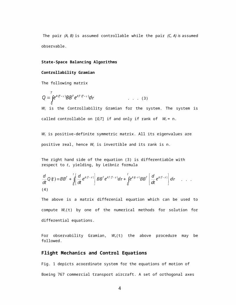
The following matrix

. . . (3)

Wc is the Controllability Gramian for the system. The system is

called controllable on [0,T] if and only if rank of Wc = n.

Wc is positive-definite symmetric matrix. All its eigenvalues are

positive real, hence Wc is invertible and its rank is n.

The right hand side of the equation (3) is differentiable with respect to t, yielding, by Leibniz formula

. . .

(4)

The above is a matrix differenial equation which can be used to

compute Wc(t) by one of the numerical methods for solution for

differential equations.

For observability Gramian, Wo(t) the above procedure may befollowed.

Flight Mechanics and Control Equations

Fig. 1 depicts acoordinate system for the equations of motion of

Boeing 767 commercial transport aircraft. A set of orthogonal axes

4

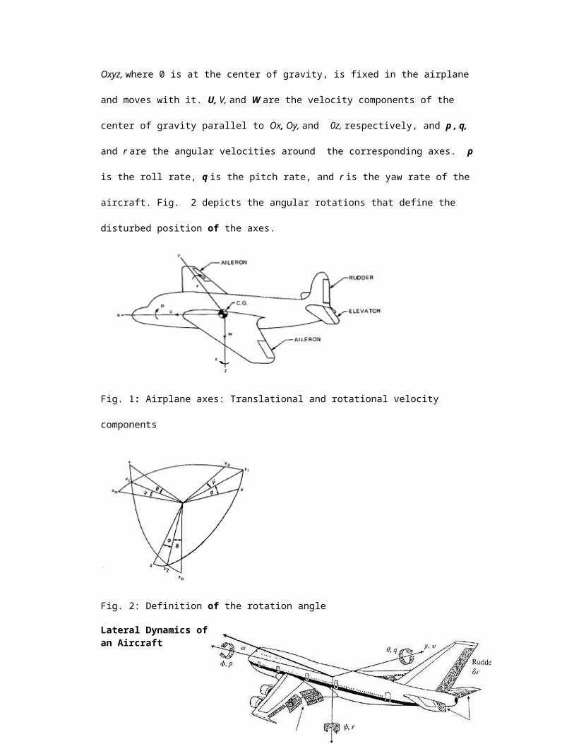
Oxyz, where 0 is at the center of gravity, is fixed in the airplane

and moves with it. U, V, and W are the velocity components of the

center of gravity parallel to Ox, Oy, and 0z, respectively, and p , q,

and r are the angular velocities around the corresponding axes. p

is the roll rate, q is the pitch rate, and r is the yaw rate of the

aircraft. Fig. 2 depicts the angular rotations that define the

disturbed position of the axes.

Fig. 1: Airplane axes: Translational and rotational velocity

components

Fig. 2: Definition of the rotation angle

Lateral Dynamics ofan Aircraft

5

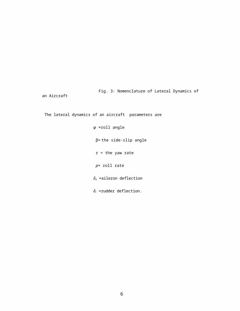
Fig. 3: Nomenclature of Lateral Dynamics of an Aircraft

The lateral dynamics of an aircraft parameters are

φ =roll angle

β= the side-slip angle

r = the yaw rate

p= roll rate

δa =aileron deflection

δr =rudder deflection.

6

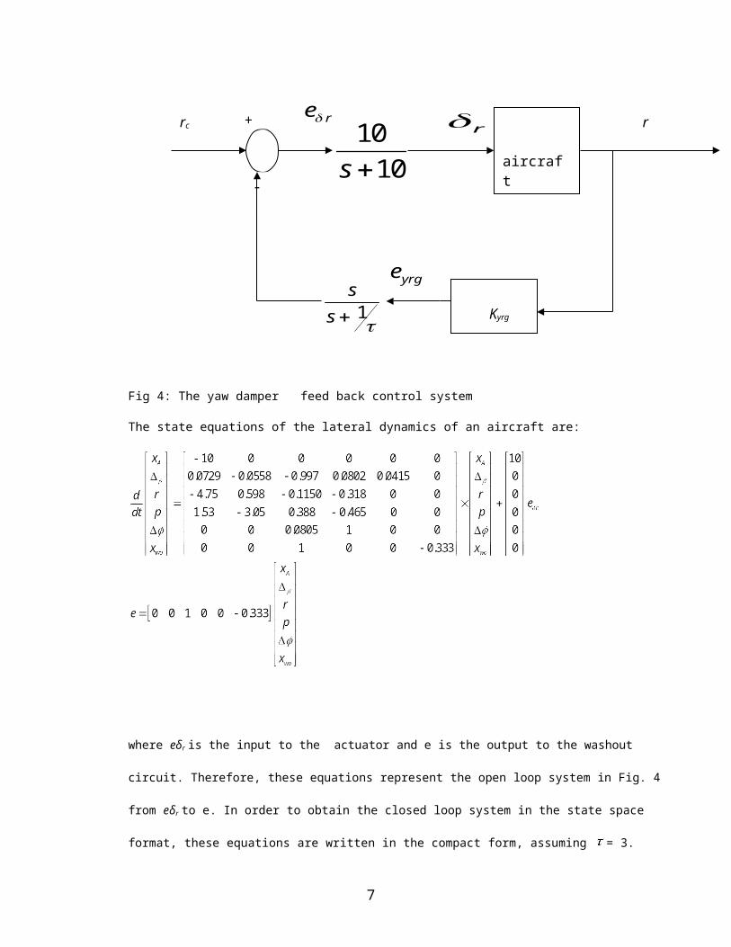
Fig 4: The yaw damper feed back control system

The state equations of the lateral dynamics of an aircraft are:

where eδr is the input to the actuator and e is the output to the washout

circuit. Therefore, these equations represent the open loop system in Fig. 4

from eδr to e. In order to obtain the closed loop system in the state space

format, these equations are written in the compact form, assuming = 3.

aircraft

1s

s Kyrg

rc +

-

rre 1010s

r

yrge

7

where

noting that

We finally obtained the closed loop system

where AC = A-BC is the closed loop system matrix.

Compensator Transfer Function of the Yaw Damper System

Swept-wing aircraft have a natural tendency to be highly damped in

one of the lateral modes of motion. Every swept-wing aircraft has a

feedback system to help the pilot. A typical commercial aircraft

cruising with high speeds and attaining high altitudes, this dynamic

mode is difficult to control. Therefore, the goal of the control

system is to modify the natural dynamics so that the plane is

pleasant for the pilot to fly. Studies have shown that pilots like

natural frequencies ωn ≤ 0.5 and damping ratio of ζ ≥ 0.5.

Aircraft with dynamics that violate these guidelines are generally

considered fatiguing to fly and highly undesirable. Thus the system

specifications are to achieve lateral dynamics that meet these

8

specification. Study of the lightly damped lateral mode

indicates that it is primarily a yawing phenomenon, so

measurement of the yaw rate is the logical starting point for

the design. Most new aircraft systems have relied on a laser

device (called a ring-laser gyroscope) for the measurement. Here two

laser beams transverse a closed path (often a triangle) in

opposite directions. As the triangular device rotates, the

detected frequencies of the two beams shift according to Doppler

effects, and this frequency shift is measured, producing a

measure of rotational rate. These devices have fewer moving

parts and are more reliable at low cost. Two aerodynamic

surfaces typically influence the lateral aircraft motion: the

rudder and the ailerons. The highly damped yaw mode that will

be stabilized by the yaw damper is most affected by the rudder.

Therefore, use of that single control input is a logical

starting point for the design. Hydraulic devices are

universally employed in large aircraft to provide the force

that moves the aerodynamic surfaces. No other kind of device

has been developed to provide the combination of high force,

high speed, and light weight desirable for the actuation of the

controlling aerodynamic surfaces. On the other hand, the low-

speed flaps, which are extended slowly prior to landing, are

typically actuated by an electric motor with a worm gear. The

linearized lateral equations of motion in horizontal flight at

9

40,000(ft) and nominal forward speed V0 = 774(ft/sec) (Mach

0.8) are stated above .

The simple physical fact is that a positive or clockwise rudder

motion causes a negative or counterclockwise yaw rate. In other

words, turning the rudder left (clockwise) causes the front of

the aircraft to rotate left (counterclockwise). The natural motion

corresponding to the complex poles is referred to as the Dutch roll (s = —

0.033 ±j'O.95). The motion corresponding to the stable real poles is

referred to as the spiral mode (s1= —0.0073) and the roll mode (s2 = —

0.563). From looking at the system poles, we see that the offending

mode that needs repair for good pilot handling is the Dutch roll.

The roots have an acceptable frequency, but their damping ratio £ =

0.03 is far short of the desired value £ = 0.5. As a first try at the

design, consider proportional feedback of the yaw rate to the

rudder. Plot the root locus and the frequency response with respect

to the gain of this feedback. From these plots show that a damping of

£ = 0.45 is achievable and this damping occurs at a gain of about

3.0.

In practice, however, it is found that this simple feedback changes

the overall gain from the pilot to the roll rate at low frequencies

from about 15 to one over the feedback gain of about 0.33. The

change in DC or zero-frequency gain creates an objectionable

situation during a steady turn. Because the feedback produces a

steady rudder input opposite the pilot's input, the pilot must

10

introduce a much larger steady command for the same yaw rate than is

necessary in the open-loop case. The dilemma is solved by feeding

back not the yaw rate but the derivative of the yaw rate, since the

derivative-feedback is approximated by including in the feedback path

a lead compensation with its zero at the origin (called a washout

circuit). The result is a feedback that passes transients and provides

the desired damping but washes out steady and low-frequency signals.

If the dynamic model of the system is augmented by adding the

actuator and washout circuit with τ = 3, we obtain the state-

variable model as given above in equations .

From the root locus it is observed that the addition of the washout

circuit allows the damping ratio to be increased from 0.03 to about

0.35. Although feedback of yaw rate through the washout circuit

results in a considerable improvement over the original aircraft

control, the response needs to be improved.

An optimal design using the pole placement has been tried and the

corresponding state feedback gain vector has been incorporated in

the transfer function. An optimal design using an estimator has been

tried and the estimator gain vector has been included in the

transfer function model.

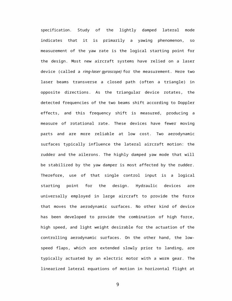
The compensator transfer function ,

GC(s) =

11

-844(s + 10.0)(s - 1.04)(s2 + 1.948s + 1.261)(s+ .023)

(s + 0.0272)(s2 + 1.674s + 1.151)(s2 + 8.14s + 118.575)(s + 51.3)

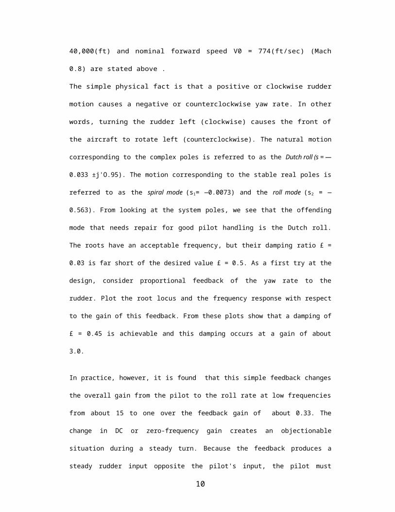
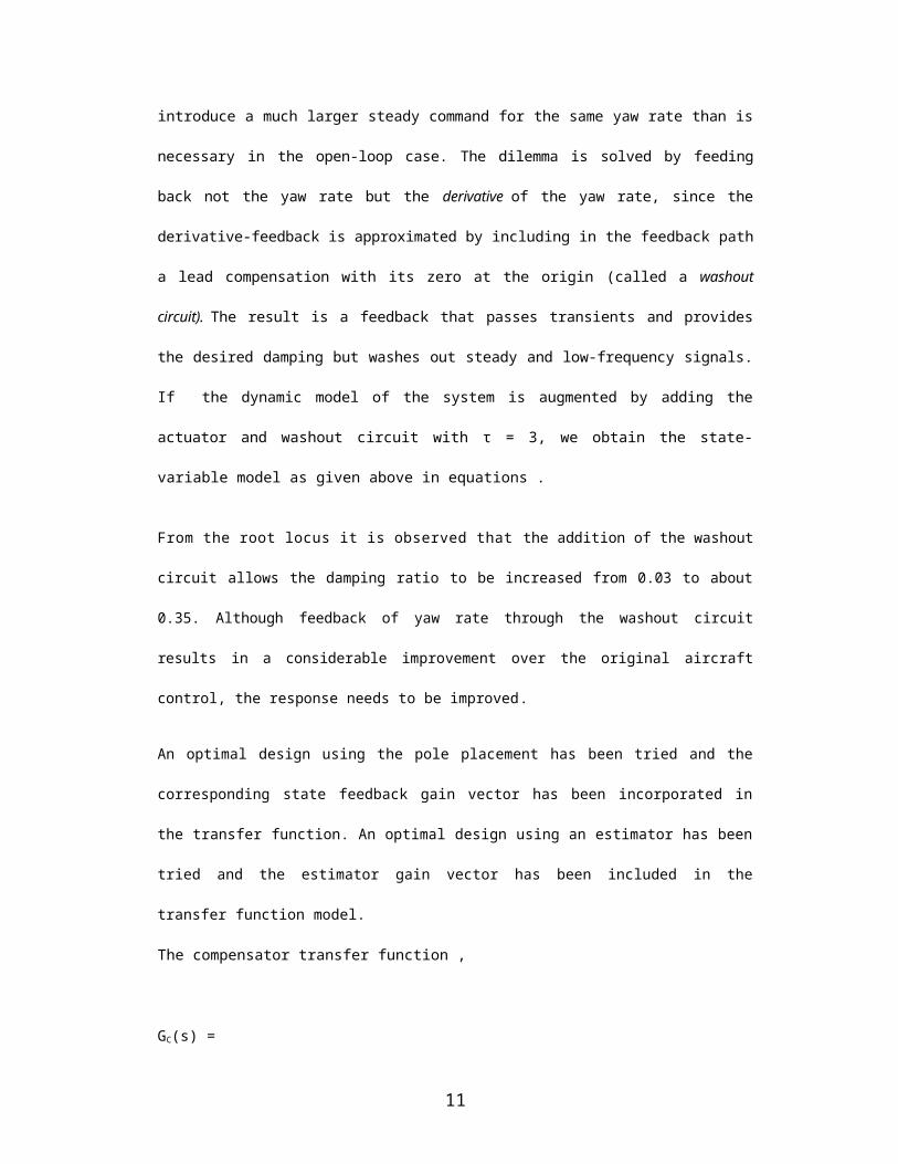
Transfer Function for Longitudinal Dynamics

The block diagram of the longitudinal dynamics of an aircraft is shown in Fig 5.

Fig 5: Longitudinal Dynamics

The corresponding transfer function is given as

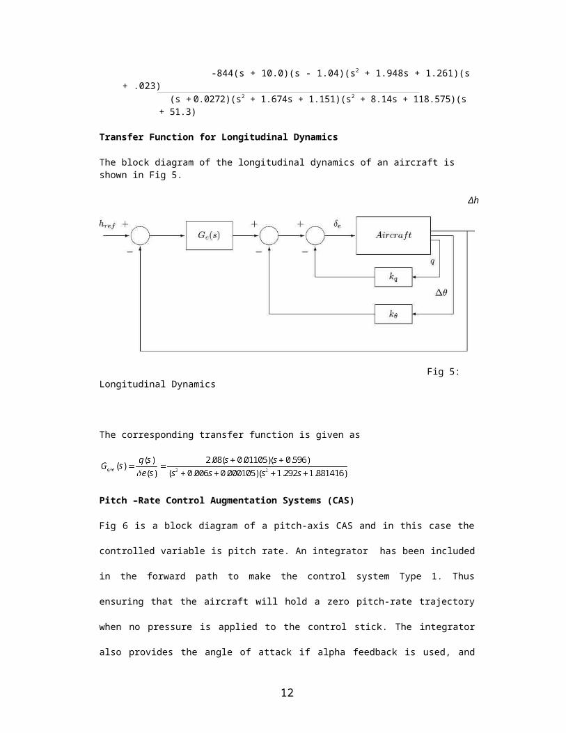
Pitch –Rate Control Augmentation Systems (CAS)

Fig 6 is a block diagram of a pitch-axis CAS and in this case the

controlled variable is pitch rate. An integrator has been included

in the forward path to make the control system Type 1. Thus

ensuring that the aircraft will hold a zero pitch-rate trajectory

when no pressure is applied to the control stick. The integrator

also provides the angle of attack if alpha feedback is used, and

Δh

12

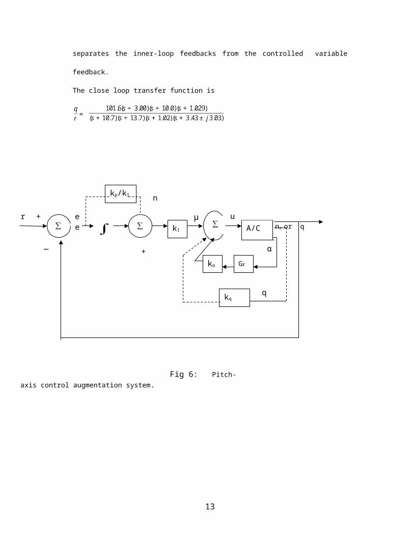
separates the inner-loop feedbacks from the controlled variable

feedback.

The close loop transfer function is

=

13

∑ ∑ k1

kp/k1

kα GF

kq

A/C

Fig 6: Pitch-axis control augmentation system.

ee

n nz or q

u

q

+

+

_

r

α

∑µ

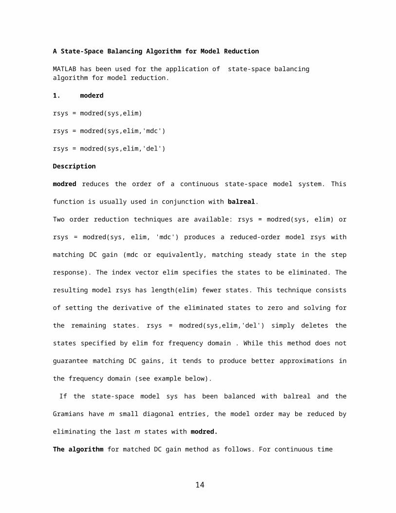
A State-Space Balancing Algorithm for Model Reduction

MATLAB has been used for the application of state-space balancing algorithm for model reduction.

1. moderd

rsys = modred(sys,elim)

rsys = modred(sys,elim,'mdc')

rsys = modred(sys,elim,'del')

Description

modred reduces the order of a continuous state-space model system. This

function is usually used in conjunction with balreal.

Two order reduction techniques are available: rsys = modred(sys, elim) or

rsys = modred(sys, elim, 'mdc') produces a reduced-order model rsys with

matching DC gain (mdc or equivalently, matching steady state in the step

response). The index vector elim specifies the states to be eliminated. The

resulting model rsys has length(elim) fewer states. This technique consists

of setting the derivative of the eliminated states to zero and solving for

the remaining states. rsys = modred(sys,elim,'del') simply deletes the

states specified by elim for frequency domain . While this method does not

guarantee matching DC gains, it tends to produce better approximations in

the frequency domain (see example below).

If the state-space model sys has been balanced with balreal and the

Gramians have m small diagonal entries, the model order may be reduced by

eliminating the last m states with modred.

The algorithm for matched DC gain method as follows. For continuous time

14

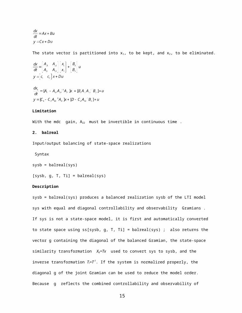
The state vector is partitioned into x1, to be kept, and x2, to be eliminated.

Limitation

With the mdc gain, A22 must be invertible in continuous time .

2. balreal

Input/output balancing of state-space realizations

Syntax

sysb = balreal(sys)

[sysb, g, T, Ti] = balreal(sys)

Description

sysb = balreal(sys) produces a balanced realization sysb of the LTI model

sys with equal and diagonal controllability and observability Gramians .

If sys is not a state-space model, it is first and automatically converted

to state space using ss[sysb, g, T, Ti] = balreal(sys) ; also returns the

vector g containing the diagonal of the balanced Gramian, the state-space

similarity transformation Xb=Tx used to convert sys to sysb, and the

inverse transformation Ti=T-1. If the system is normalized properly, the

diagonal g of the joint Gramian can be used to reduce the model order.

Because g reflects the combined controllability and observability of

15

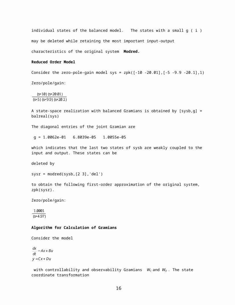
individual states of the balanced model. The states with a small g ( i )

may be deleted while retaining the most important input-output

characteristics of the original system Modred.

Reduced Order Model

Consider the zero-pole-gain model sys = zpk([-10 -20.01],[-5 -9.9 -20.1],1) Zero/pole/gain:

A state-space realization with balanced Gramians is obtained by [sysb,g] = balreal(sys)

The diagonal entries of the joint Gramian are

g = 1.0062e-01 6.8039e-05 1.0055e-05

which indicates that the last two states of sysb are weakly coupled to the input and output. These states can be

deleted by

sysr = modred(sysb,[2 3],'del')

to obtain the following first-order approximation of the original system, zpk(sysr).

Zero/pole/gain:

Algorithm for Calculation of Gramians

Consider the model

with controllability and observability Gramians WC and WO . The state coordinate transformation

16

; produces the equivalent model

and transforms the Gramians to

The function balreal computes a particular similarity transformation T such that

Limitations

The LTI model sys must be stable. In addition, controllability and observability are required for state-space models.

Gramian

Compute controllability and observability Gramians

Syntax

Wc = gram(sys,'c')

Wo = gram(sys,'o')

Grammians can be used to study the controllability and observability

properties of state-space models and for model reduction . They have better

numerical properties than the controllability and observability matrices

formed by ctrb and obsv.

Given the continuous-time state-space model

17

The controllability Gramian is positive definite if and only if (A,B) is

controllable. Similarly, the observability Gramian is positive definite if

and only if is (C,A)observable.

The commands

Wc = gram(sys,'c') % controllability Gramian

Wo = gram(sys,'o') % observability Gramian

to compute the Gramians of a continuous time system the LTI model sys must

be in state-space form.

Algorithm

The controllability Gramian WC is obtained by solving the continuous-time

Lyapunov equation

Similarly, the observability Gramian Wo solves the Lyapunov equation

in the continuous time.

Limitations

The matrix must be stable (all eigen values have negative real part in continuous time).

Illustrations with MATLAB

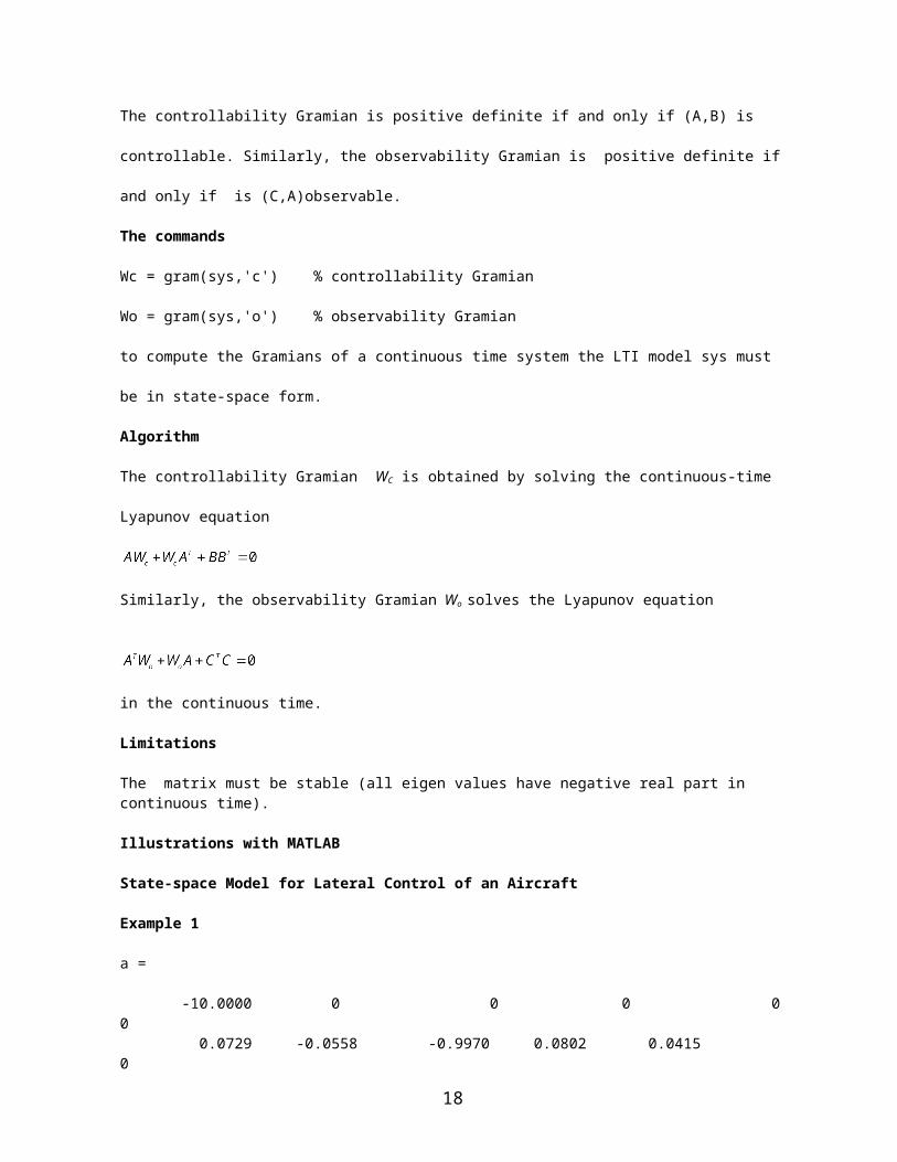
State-space Model for Lateral Control of an Aircraft

Example 1

a =

-10.0000 0 0 0 00 0.0729 -0.0558 -0.9970 0.0802 0.0415 0

18

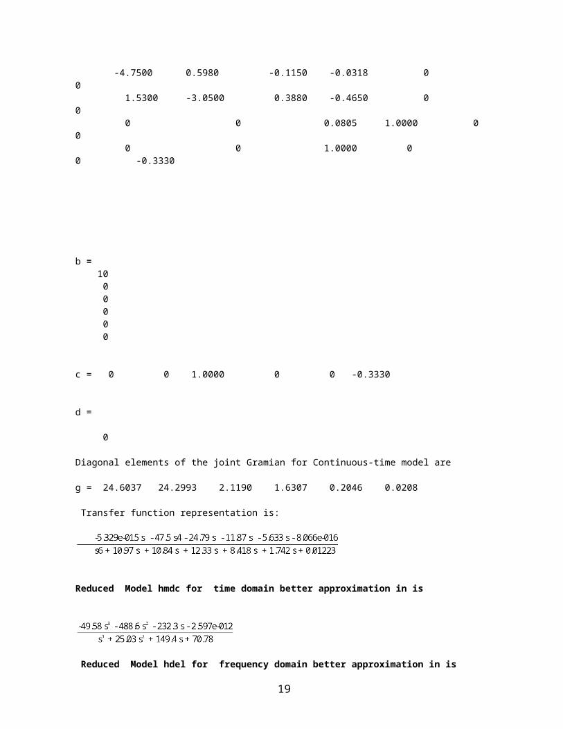
-4.7500 0.5980 -0.1150 -0.0318 0 0 1.5300 -3.0500 0.3880 -0.4650 0 0 0 0 0.0805 1.0000 0 0 0 0 1.0000 0 0 -0.3330

b = 10 0 0 0 0 0

c = 0 0 1.0000 0 0 -0.3330

d =

0

Diagonal elements of the joint Gramian for Continuous-time model are

g = 24.6037 24.2993 2.1190 1.6307 0.2046 0.0208

Transfer function representation is:

Reduced Model hmdc for time domain better approximation in is

Reduced Model hdel for frequency domain better approximation in is

19

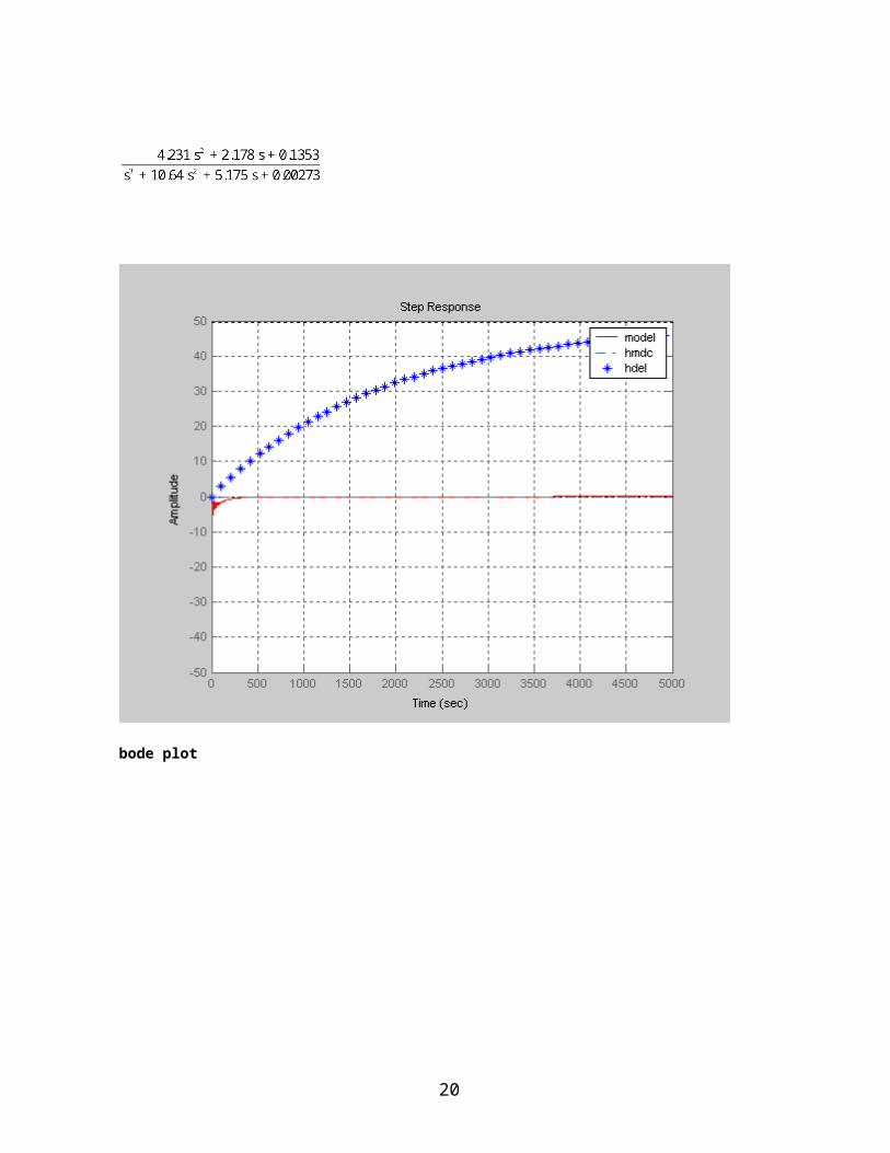
bode plot

20

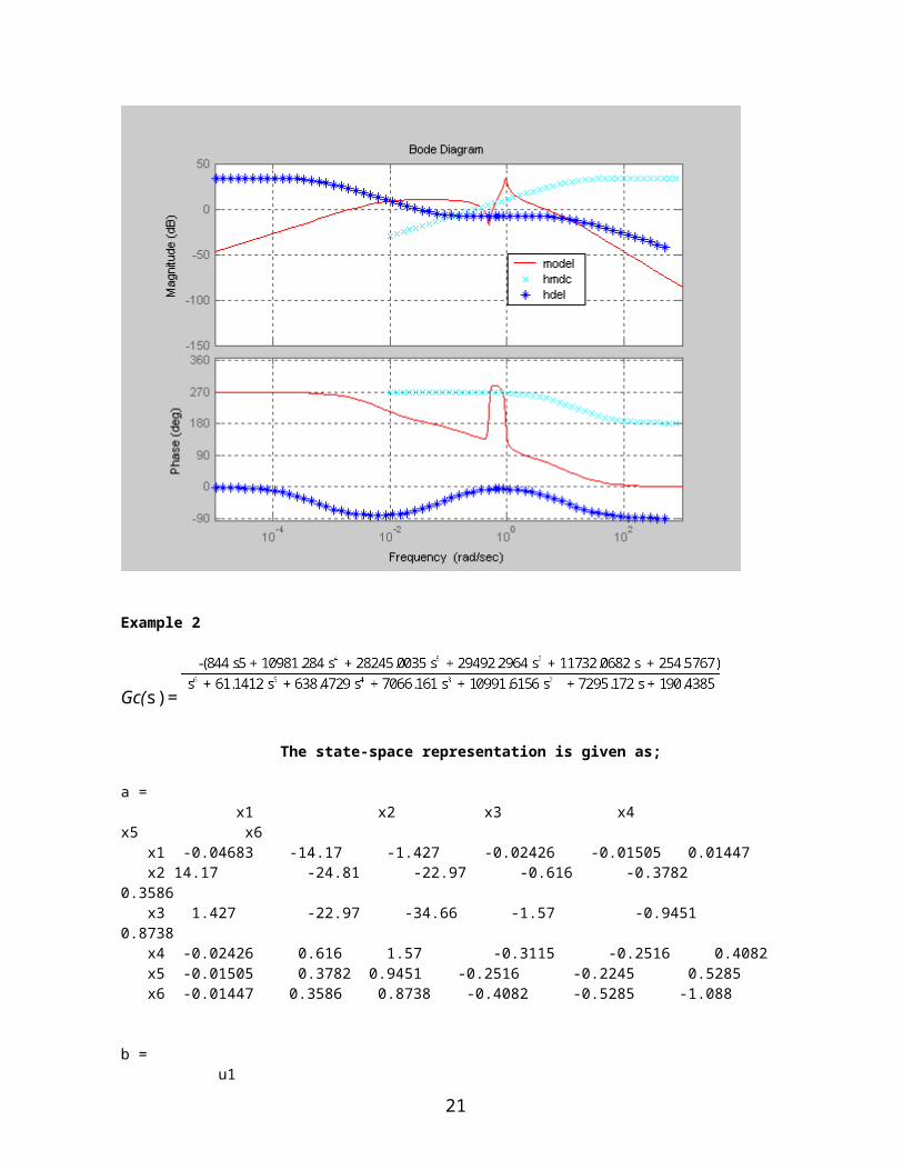
Example 2

Gc(s)=

The state-space representation is given as;

a = x1 x2 x3 x4 x5 x6 x1 -0.04683 -14.17 -1.427 -0.02426 -0.01505 0.01447 x2 14.17 -24.81 -22.97 -0.616 -0.3782 0.3586 x3 1.427 -22.97 -34.66 -1.57 -0.9451 0.8738 x4 -0.02426 0.616 1.57 -0.3115 -0.2516 0.4082 x5 -0.01505 0.3782 0.9451 -0.2516 -0.2245 0.5285 x6 -0.01447 0.3586 0.8738 -0.4082 -0.5285 -1.088 b = u1

21

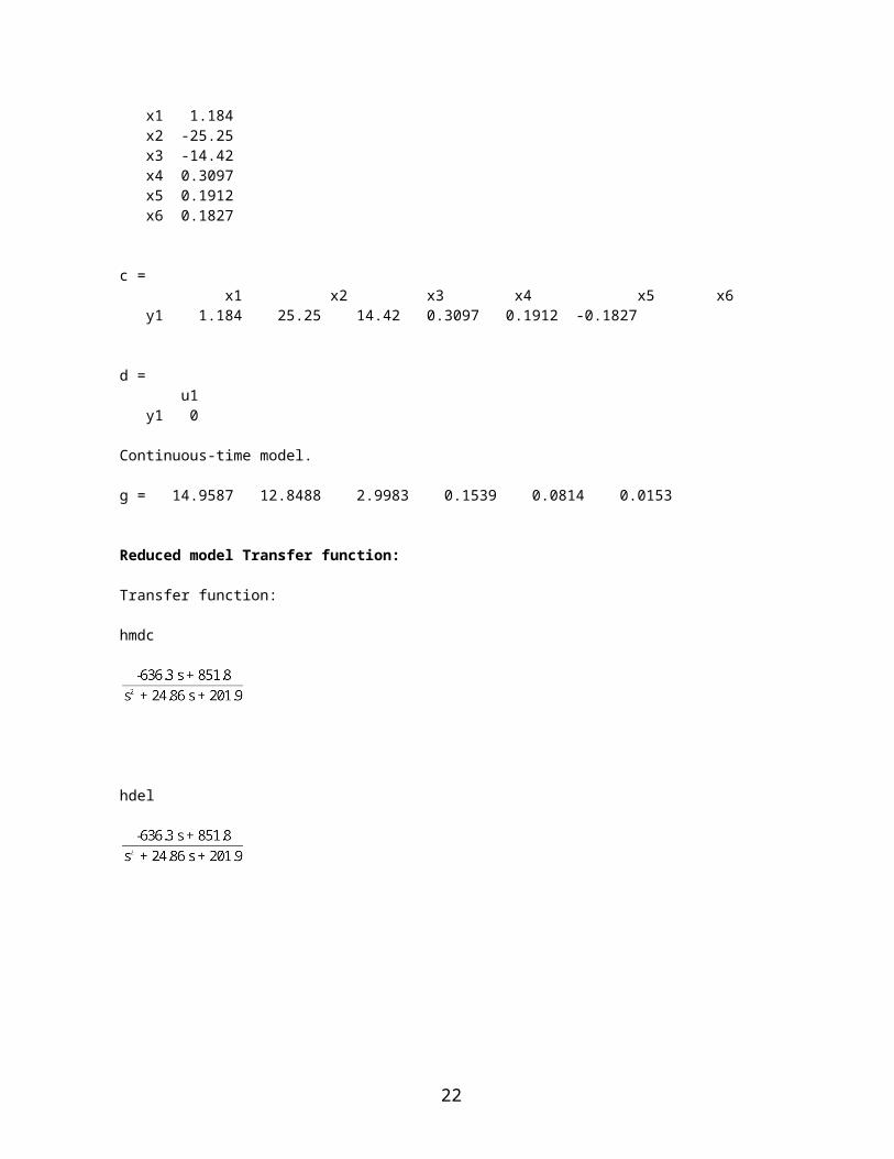
x1 1.184 x2 -25.25 x3 -14.42 x4 0.3097 x5 0.1912 x6 0.1827 c = x1 x2 x3 x4 x5 x6 y1 1.184 25.25 14.42 0.3097 0.1912 -0.1827 d = u1 y1 0 Continuous-time model.

g = 14.9587 12.8488 2.9983 0.1539 0.0814 0.0153

Reduced model Transfer function: Transfer function:

hmdc

hdel

22

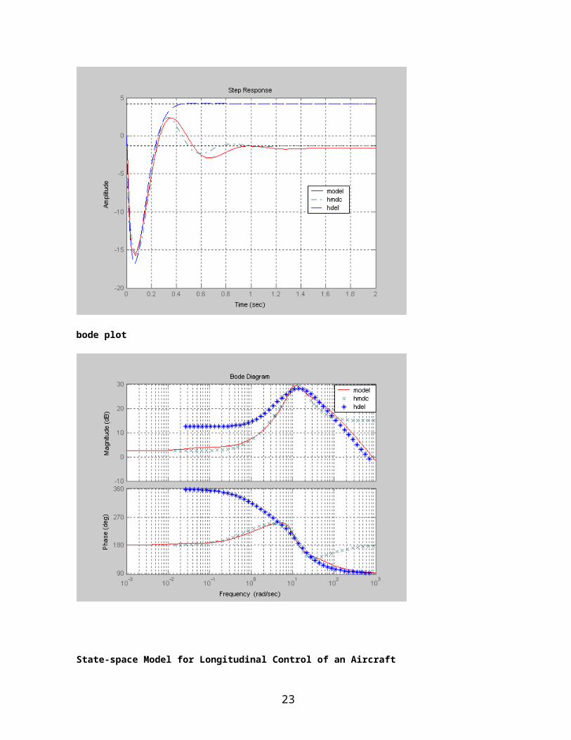
bode plot

State-space Model for Longitudinal Control of an Aircraft

23

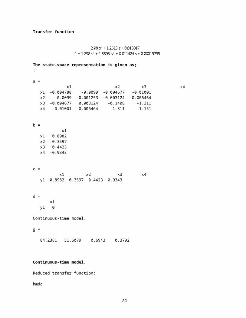
Transfer function

The state-space representation is given as;:

a = x1 x2 x3 x4 x1 -0.004788 -0.0099 -0.004677 -0.01001 x2 0.0099 -0.001253 -0.003124 -0.006464 x3 -0.004677 0.003124 -0.1408 -1.311 x4 0.01001 -0.006464 1.311 -1.151 b = u1 x1 0.8982 x2 -0.3597 x3 0.4423 x4 -0.9343 c = x1 x2 x3 x4 y1 0.8982 0.3597 0.4423 0.9343 d = u1 y1 0 Continuous-time model.

g =

84.2381 51.6079 0.6943 0.3792

Continuous-time model. Reduced transfer function:

hmdc

24

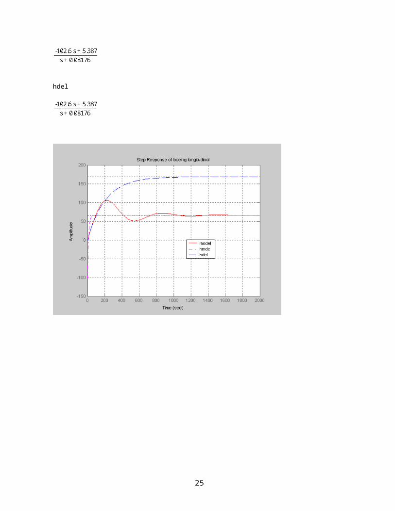
hdel

25

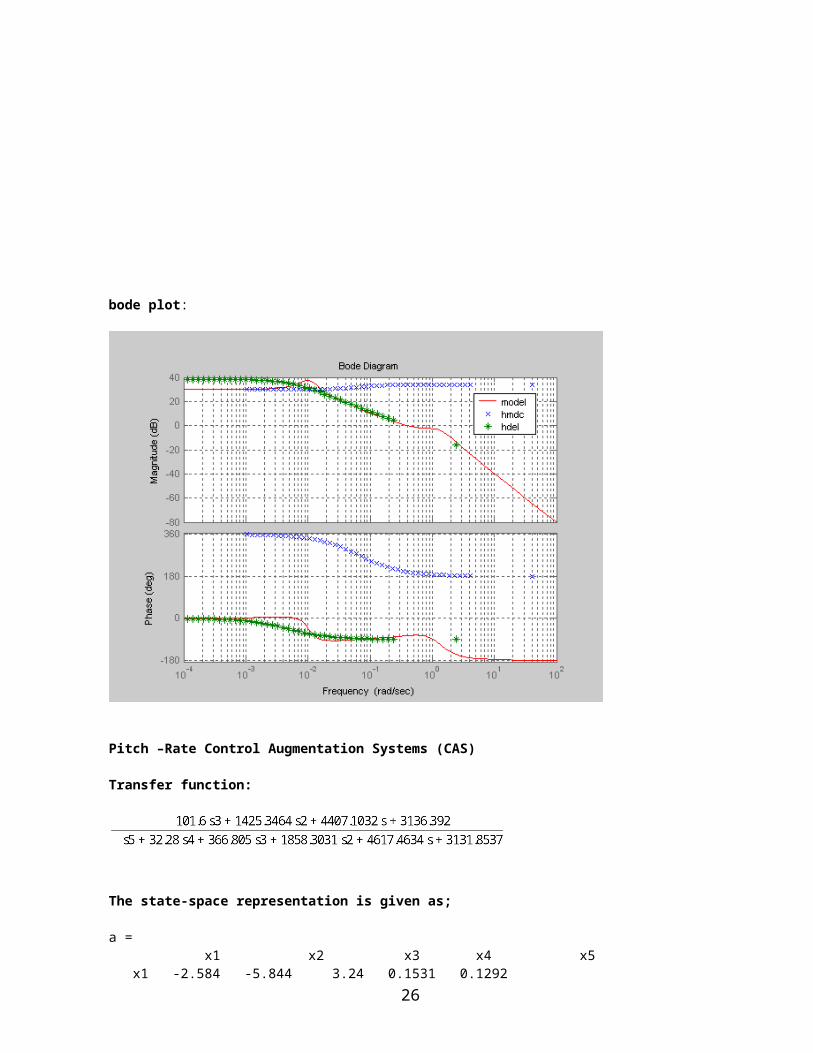
bode plot:

Pitch –Rate Control Augmentation Systems (CAS)

Transfer function:

The state-space representation is given as;

a = x1 x2 x3 x4 x5 x1 -2.584 -5.844 3.24 0.1531 0.1292

26

x2 5.844 -6.076 7.007 0.4454 0.3741 x3 -3.24 7.007 -12.77 -1.322 -1.097 x4 0.1531 -0.4454 1.322 -1.776 -2.629 x5 0.1292 -0.3741 1.097 -2.629 -9.072 b = u1 x1 -1.993 x2 1.62 x3 -1.163 x4 0.05911 x5 0.04985

c = x1 x2 x3 x4 x5 y1 -1.993 -1.62 1.163 0.05911 0.04985 d = u1 y1 0 Continuous-time model.

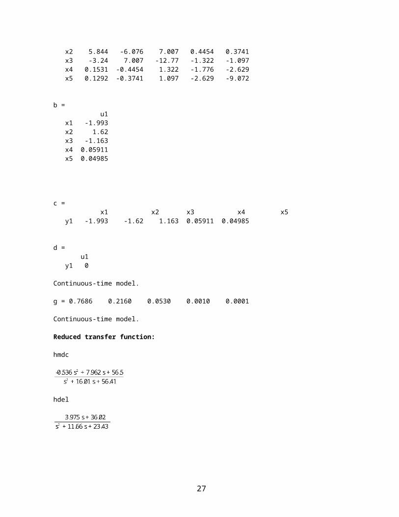
g = 0.7686 0.2160 0.0530 0.0010 0.0001 Continuous-time model. Reduced transfer function:

hmdc

hdel

27

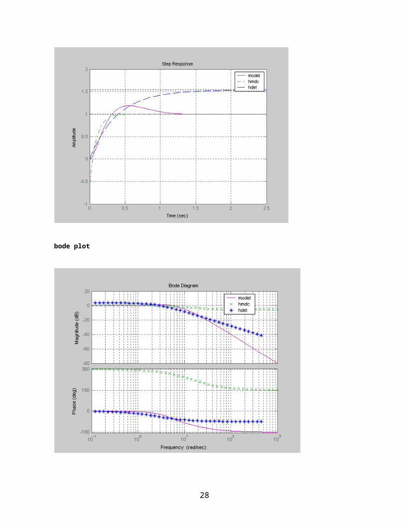
bode plot

28

Conclusion

The primary focus in this paper has been on the principal application of

computing of state-space balancing transformations directly from a state-

space realization (A, B, C) for continuous-time linear systems. Under a

balancing transformation T the equivalent realization has controllability

and observability Gramians. Higher order models of lateral and longitudinal

dynamics of an aircraft have been reduced extensively using MATLAB. The

computation presented has two main advantages which include: 1) stability

of reduced-order models and 2) easily computable error bounds. Numerical

simulation shows that the algorithms give a better approximation of the

original system both in time domain as well as in frequency domain. It has

been found that reduced models both in time domain and frequency domain

compare favourably with higher order models suggesting fewer things to go

wrong in the hardware or bugs to fix in the software.

References:

1. Abdul Ghafoor and Victor Sreeram,” Model Reduction Via Limited Frequency Interval Gramians,” IEEE Trans. Circuits and Systems—I: Regular Papers, Vol. 55, No. 9, pp. 2802-2812,October 2008

2. D. Gangsaas. K. R. Bruce, J. D. Blight, and U. -L. Ly, "Applicationof modern synthesis to aircraft control: Three case studies," IEEE Trans. Automat. Contr., vol. AC-31, pp. 995-1104, Nov. 1986.

3. B D O Anderson and Yi Liu, “Controllers reduction: concepts and approaches”, IEEE Trans. Automat.Contr., vol. AC-34, pp. 802-812, August ,1989.

29