global and local virtual metrology models for a plasma etch process
TRANSCRIPT

94 IEEE TRANSACTIONS ON SEMICONDUCTOR MANUFACTURING, VOL. 25, NO. 1, FEBRUARY 2012
Global and Local Virtual Metrology Modelsfor a Plasma Etch Process
Shane A. Lynn, John Ringwood, Senior Member, IEEE,and Niall MacGearailt
Abstract—Virtual metrology (VM) is the estimation of metrol-ogy variables that may be expensive or difficult to measure usingreadily available process information. This paper investigates theapplication of global and local VM schemes to a data set recordedfrom an industrial plasma etch chamber. Windowed VM modelsare shown to be the most accurate local VM scheme, capableof producing useful estimates of plasma etch rates over multiplechamber maintenance events and many thousands of wafers. Par-tial least-squares regression, artificial neural networks, and Gaus-sian process regression are investigated as candidate modelingtechniques, with windowed Gaussian process regression modelsproviding the most accurate results for the data set investigated.
Index Terms—Gaussian process regression, local modeling,neural network applications, plasma etch, virtual metrology(VM).
I. Introduction
V IRTUAL metrology (VM) is an active area of researchin semiconductor manufacture [1]. Traditionally, manu-
facturing processes such as plasma etch are monitored usingstatistical process control methodologies with few measure-ments and large metrology delays. Such monitoring systemscan result in wafer scraps due to slow response times and theydo not provide the immediate feedback capability required foradvanced process control (APC) of processing tools. APC isseen as a core enabling technology required for the continuedadvancement of the semiconductor industry [2], and fab-wide APC and VM schemes capable of increasing factorythroughput, reducing wafer scraps, cutting production costs,and facilitating automated wafer-2-wafer control have beeninvestigated [2]–[4].
Fab-wide APC systems cannot be implemented without thedevelopment of accurate VM models for each process in themanufacturing cycle. Plasma etch remains one of the mostchallenging modeling exercises [5]. While the etch processitself is quite complex, modeling of the process is furthercomplicated by multistep recipes with changing chemistries,
Manuscript received November 18, 2010; revised June 21, 2011; acceptedSeptember 10, 2011. Date of publication November 18, 2011; current versionFebruary 3, 2012. This work was supported by the Irish Research Council forScience, Engineering, and Technology.
S. A. Lynn and J. Ringwood are with the Department of ElectricalEngineering, National University of Ireland, Maynooth, Kildare, Ireland(e-mail: [email protected]; [email protected]).
N. MacGearailt is with Intel Ireland, Leixlip, Co. Kildare, Ireland (e-mail:[email protected]).
Color versions of one or more of the figures in this paper are availableonline at http://ieeexplore.ieee.org.
Digital Object Identifier 10.1109/TSM.2011.2176759
chamber conditioning effects, shifts in process characteristicsdue to preventative maintenance (PM) operations, and lim-ited downstream metrology with which to validate modelingresults. A complete review of the semiconductor etch VMliterature is found in [6].
VM relies on process data recorded from etch processingtools to generate estimates of process outputs. Chamber-relatedprocess data such as temperature, pressure, gas flows, andpower are typically collected from etch chambers using in-builtsensors. Such data has been used by several authors to createempirical input-output models relating chamber inputs to etchrates, etch bias, and uniformity measures [7]. Additional datacan be collected by installing more sensors on the etchchamber. Optical emission spectroscopy is one of the mostcommonly used noninvasive tools [8] providing informationon the chemical species active in plasmas. Plasma impedancemonitors (PIMs) analyze the electrical system of the chamber,noninvasively providing information on the current, voltage,and phase of the radio frequency energy applied to thechamber electrodes. PIM signals have been shown to relate tooutput variables such as etch rate [9] and etch end point [10].
With vast quantities of data available in fabrication plants,the difficulty faced by manufacturers is the effective extractionof useful information from the recorded variables. Variableselection and data reduction techniques are essential to identifykey variables and to find useful correlations between recordedvariables and process outputs [8], [11].
The treatment of large data sets is a subject requiringconsideration by practitioners of VM in semiconductor manu-facturing. The two paradigms investigated in this paper areglobal models and local models. As defined here, globalmodels use all available training points to learn the behaviorof a system. Training is carried out once at initialization,ideally using a training data that covers the full operationalrange of the system; all further activity is assumed to operatein the same regime. Local models, however, are models thatare trained using subsets of the available data. The subsetscan be determined from the full data set based on wafercontext information, time, or any other criteria. In this manner,local models can provide more accurate estimates than globalmodels over certain operation regimes, while global modelsmay provide more general estimates but across the entiresystem operating space. Multiple local models are typicallyrequired to perform VM over a complete operating space,thus incurring a small complexity overhead over their global
0894-6507/$26.00 c© 2011 IEEE

LYNN et al.: GLOBAL AND LOCAL VIRTUAL METROLOGY MODELS FOR A PLASMA ETCH PROCESS 95
counterparts. In this paper, partial least squares (PLS), artificialneural networks (ANNs), and Gaussian process regression(GPR) are compared as candidate VM modeling techniquesfor global and local modeling of plasma etch rate.
The use of Gaussian processes (GPs) for regression andclassification is a relatively new concept. In 1996, Williamsand Rasmussen [12] successfully extended the use of GPs tohigh dimension problems that have been traditionally tackledusing other modeling techniques such as neural networksand decision trees [13]. GPR does not impose a specificparametric structure on the underlying function being modeled[14]; rather, the training data are used to discover the modelproperties in a supervised manner.
GPR has several advantages over other modeling tech-niques. Using GPR, useful models can be created from trainingdata sets with a relatively small number of training points, andthe analyst’s prior beliefs about the data can be encapsulated inthe choice of a covariance function. Because the model formis not specified explicitly, both linear and nonlinear functionscan be approximated. Confidence intervals on predictions canbe easily evaluated since each prediction is given in the formof a distribution. However, during the training procedure, GPmodels require the inversion of covariance matrices, the sizeof which is determined by the number of training data points.For very large data sets, the computational demands of suchinversions may become an issue. To the best of the authors’knowledge, this paper reports the first application of GPR tosemiconductor etch data, apart from preliminary explorationspreviously reported in [15].
This paper is organized as follows. Section II describesthe modeling techniques used. Because it is rarely seen inthe semiconductor literature, particular focus is given to anexplanation of GPR. Section III describes the data availablefor modeling while Sections IV and V discuss global and localmodeling results, respectively. Finally, conclusions are givenin Section VI.
II. Modeling Techniques
The estimated etch rate for wafer k, r(k), is given by
r(k) = f (u1(k), u2(k), . . . , um(k)) (1)
where u1(k), u2(k), . . . , um(k) are the measurements takenfrom the chamber sensors during the processing of wafer k.Static models are employed because etch rate measurementsare not performed on a uniform basis, precluding the use of atime series model. It is assumed that the relationship betweenthe measurements and the plasma etch rate is time-invariantduring VM modeling.
A. PLS Regression
PLS is a statistical technique originally applied to the areaof chemometrics for statistical process modeling, and now reg-ularly employed in the area of semiconductor manufacturing.Unlike simpler linear regression techniques, PLS can constructpredictive models in the presence of collinear input variables.
PLS is related to another latent variable technique, principalcomponent analysis (PCA). Suppose that we begin with a data
matrix X ∈ Rn×p made up of n samples of p variables. PCA[16] performs an eigenvalue decomposition of the covariancematrix of the data matrix XT X to decompose X as the sumof the outer product of the column vectors ti ∈ Rn×1 andpi ∈ Rp×1, plus a residual matrix E [16]
X = t1p1T + t2p2
T + · · · + tlplT + E (2)
= TPT + E (3)
where
T = [t1 t2 · · · tl], P = [p1 p2 · · · pl] (4)
l is the number of principal components, and E ∈ Rn×p is amatrix of residuals. The vectors ti ∈ Rn×1 are the scores orprincipal components, with T ∈ Rn×l the principal componentmatrix, and the vectors pi ∈ Rp×1 are the loadings, whereP ∈ Rp×l is the loadings matrix. The principal componentsare arranged in descending order, consistent with the amountof variance explained in the original data set by each one.
In PLS analysis, a similar decomposition to PCA is simul-taneously carried out on the output matrix Y such that
Y = UQT + F (5)
where Y = [y1, y2 · · · ym], Y ∈ Rn×m, is the output matrixcomprising n samples of m output variables, U ∈ Rn×h andQ ∈ Rm×h are the Y -components and Y -loadings, respectively,F ∈ Rn×m is the Y -residual matrix, and finally h is thenumber of principal components used in the output matrixdecomposition. Although PLS is similar to PCA in that com-ponents describing the data set are extracted using eigenvaluedecompositions, it has the advantage of being a supervisedtechnique that uses information in the output to create a model.
The X-components and Y -components are chosen so thatthe relationship between successive pairs of principal com-ponents is as strong as possible by manipulating the innerrelation, U = TB, where B is a diagonal matrix of weights op-timized to maximize the covariance between the componentsin U and T . An adjusted version of the noniterative partial leastsquares algorithm, described in [17], can be used to calculatePLS models. Predictions from PLS models are obtained usingthe multivariate regression formula Y = TBQT [18].
B. Artificial Neural Networks (ANNs)
ANNs have been applied extensively to the area of plasmaetch for fault detection [19], modeling [20], and control [21],and have been shown to yield superior estimation accuracyover statistical techniques for some data sets [22].
Here, multilayer perceptron (MLP) neural networks areused where neurons are arranged in an input layer, a singlehidden layer, and an output layer. The neurons in each layerreceive weighted inputs from all neurons in the precedinglayer, calculate an output value using tan-sigmoid activationfunctions and a preset bias value, and pass their outputs tothe next layer. This a feed-forward neural network. Throughexperimentation, it is found that no significant improvement inmodel accuracy is achieved through the use of multiple hiddenlayers for the etch data set. To avoid limiting the output range,linear output neurons are used.

96 IEEE TRANSACTIONS ON SEMICONDUCTOR MANUFACTURING, VOL. 25, NO. 1, FEBRUARY 2012
MLPs are trained by finding the optimal set of networkweights and biases that minimizes the sum squared error(SSE), defined [23] as
SSE =n∑
i=1
m∑j=1
(yij − yij)2 (6)
where n is the number of samples in the training set, yij is thedesired value for output j at sample i, and yij is the estimatedvalue for output j at sample i.
Training is carried out by first initializing the networkweights randomly and then optimizing the weight valuesusing a training algorithm. Back propagation, for example,gives an effective error measure for each neuron layer andallows a gradient descent optimization routine to adjust theweights and biases to achieve a minimum SSE. Higher orderoptimization techniques, such as the second-order gradientBroyden—Fletcher—Goldfarb—Shannon method [24] or theLevenberg—Marquardt (LM) algorithm [25], are also em-ployed. The models described in this paper were trained usingthe LM method due to its fast convergence properties [26].
In all of the ANN models created in this paper, ANNswere optimized in a number of ways. First, the number ofhidden neurons was varied from 5 to 25 neurons. Second,for each network structure, ten random weight initializationsare tested in an attempt to ensure that the optimization routinefinds the global minimum error solution. The network structurewith the lowest validation error, which is a good measureof generalization capability, across both variations in networktopology and training step number, is retained.
C. GP Regression
A GP can be viewed as a collection of random vari-ables f (xi) with joint multivariate Gaussian distributionf (x1), f (x2), · · · , f (xn) ∼ N(0, �), where �ij gives the valueof the covariance between f (xi) and f (xj), and is a functionof the inputs xi and xj , �ij = k(xi, xj) [27]. For the purposesof this discussion, a 1-D input–output process is assumed.
Gaussian process models fit naturally into the Bayesianmodeling framework where, instead of parameterizing themodel function f (x), a Gaussian prior is placed on the range ofpossible functions that could represent the mapping of inputsx to outputs y. The Gaussian prior incorporates the analyst’sknowledge about the underlying function in the data, and isspecified using the GP covariance function.
The covariance function k(xi, xj) can be any function,provided that it generates a positive definite covariance matrix�. A common covariance function is the squared exponential(SE) covariance function
k(xi, xj) = ν2 exp
(− (xi − xj)2
2l2
)(7)
where ν and l are hyperparameters that vary the propertiesof the covariance function to best suit the training data set.The SE covariance function assumes that input points that arenumerically close in the input space correspond to outputsthat are more correlated in the output space than outputscorresponding to input points which are far apart. Variations
in l and ν control the smoothness of the covariance function.The parameter ν controls the scale of the variations betweenpoints f (xi) and f (xj) in the output space, while l, knownas the length scale, determines the degree of variation in theinput dimension. The squared exponential covariance functioncan be extended to many dimensions by introducing individuallength scales for each input dimension.
For example, let the underlying function of the data bey = f (x) + ε, where ε is a Gaussian white noise term withvariance σ2
n such that ε ∼ N(0, σ2n). A Gaussian process prior
is put on the range of possible underlying functions f (x)with covariance function as exemplified in 7 with unknownhyperparameters. Hence
y1, y2, . . . , yn ∼ N(0, K) (8)
K = � + σ2nI (9)
where σ2nI represents the covariance between outputs due to
white noise. I is the n × n identity matrix.The aim now is to use the set of training data points
{xi, yi}ni=1 to find the posterior distribution of y∗, given inputx∗, that is p(y∗|x∗, xtr, ytr), where {x∗, y∗} denotes an unseentest data point and xtr and ytr denote the complete set of inputand output training data. Before the posterior distribution ofy∗ is found, the unknown hyperparameters of the covariancefunction 7, l, ν, and σ2
n , must be optimized. This can beperformed via a Monte Carlo method or, more typically, viamaximization of the log marginal likelihood
log(p(ytr|xtr)) = −1
2yT
trK−1ytr − 1
2log(|K|) − n
2log(2π). (10)
Equation 10 is made up of a combination of a data fit term,12 yT
trK−1ytr, that determines the success of the model in fitting
the output training data, along with a model complexity term12 log(|K|). Maximization of 10 requires the computation ofthe derivative of log(p(ytr|xtr)) with respect to each of thehyperparameters in the covariance function 7. To initializethe gradient descent optimization in the current application,the initial values for the hyperparameters are initialized tothe values suggested by Rasmussen [28] and also randomlyinitialized several times in an attempt to find a global minimumsolution for the likelihood function. During optimization formultidimensional covariance functions, dimensions that donot influence the process being modeled are automaticallyassigned longer length scales than variables of influence. Thisprocess is a form of automatic relevance determination.
With the hyperparameters optimized, the GP model is usedto predict the distribution of y∗ for input x∗. The predictivedistribution of y∗, p(y∗|x∗, xtr, ytr), can be shown to be Gaus-sian [29], with mean and variance
μ(x∗) = k∗K−1ytr (11)
σ2(x∗) = k∗∗ − k∗K−1kT∗ + σ2
n
respectively, where k∗∗ = k(x∗, x∗) is the autocovariance ofthe test input and k∗ = [k(x∗, x1), k(x∗, x2), · · · k(x∗, xn)] is avector of covariances between the test and training data points.The vector k∗K−1 can be seen as a vector of weights that forma linear combination of the observed outputs ytr to form theprediction at x∗. The variance on the predicted values, σ2(x∗),

LYNN et al.: GLOBAL AND LOCAL VIRTUAL METROLOGY MODELS FOR A PLASMA ETCH PROCESS 97
Fig. 1. Example prediction and 95% confidence intervals (2 × standarddeviation) for a 1-D GP. The variance on the prediction grows with the distancefrom observed training points.
is given by the prior variance k∗∗, which is a positive term,minus the posterior variance k∗K−1kT
∗ which is also positive.The posterior variance will be inversely proportional to thedistance between the test point and the training points in theinput space, as it depends on k∗, resulting in large variances fortest points that are far from training points, as shown in Fig. 1.
The covariance function can be chosen to include a numberof different components, depending on the prior knowledgeof the physical system being modeled, for example, periodicfunctions, linear components, or rational quadratic functions[27], [29]. The etch rate models in this paper use a covariancefunction with one linear component, a noise component, anda squared exponential component for each dimension. Thesquared exponential function is a somewhat intuitive choice forGPR applications since one might expect covariance betweentraining outputs to decrease with distance in the input space.Previous work has shown that the GPR estimation perfor-mance for the plasma etch data is relatively insensitive to thecovariance function choice [15]. However, the GPR trainingprocedure may not be robust to the inappropriate covariancefunction choice [30].
III. Data Set Description
The models examined in this report are constructed andtested on a data set collected from a multistep industrial trenchetch process over a period of six months. The data consists ofmeasurements collected from three sources.
1) Etch process (EP) data consist of 131 variables suchas temperature, pressure, and gas flow rates for eachprocess step collected directly from the processing tool.These EP data are reduced to a set of 28 variables bydiscarding variables unrelated to the main etch step andvariables with constant values.
2) A PIM records an additional 159 variables for everywafer, comprising 53 harmonics of electrode current,voltage, and phase.
TABLE I
Data Sets Available for Modeling
Data Set A Data Set BNumber of wafers 12 133 18 513Etch rate measurements 529 793PM cycles 12 18Measurement frequency 4.4% 4.3%Inputs available EP, PIM, XR, EP+ EP
3) Etch depth measurements, taken downstream from theetch process, are available for a small number of wafers.
Summary statistics such as mean and standard deviation arederived from the time series traces for each variable, andwafers recorded with erroneous data are detected using a T 2
statistic and removed.Values for plasma reactance (X) and resistance (R) at
the 53 harmonic frequencies are calculated from the PIMvariables. These reactance and resistance values are henceforthreferred to as “XR” data. To investigate whether VM resultsare improved by combining information from multiple sensorsources, plasma power and impedance values are calculatedfrom the PIM data for each process step and combined withthe EP variables for modeling. This set of variables is labeled“EP+” data.
For each virtual metrology scheme, the data points used tobuild the models form the training data and the data pointsused to check model performance form the test data. Validationdata can be extracted from the training data to enhance thetraining procedure for some modeling techniques, e.g., earlystopping during ANN training and selection of the optimumnumber of components for PLS models.
The data set is collected from a single etch chamber in thefabrication plant and consists of correctly recorded EP datafor 18 513 wafers. After removal of wafers with incorrectlyrecorded PIM data, only 12 133 wafers remain. For the pur-poses of this paper, it is useful to form two separate data setsfrom these data: Data Set A and Data Set B as described inTable I. Due to operational constraints, these are the only datasets available for this VM exercise.
IV. Global Modeling
As described in Section I, global models use all availabletraining points to learn the behavior of a system. Althoughdata from designed experiments are often used to train globalmodels [3], the high value nature of semiconductor processingmeans that such experiments can be prohibitively expensive interms of wafer scrap and tool down-time. In this paper, onlypast production data are used for model training.
To explore global model performance, 30% of the wafersin Data Set A are put aside as test wafers. Since the inputvariables originate from measurements with different scales,all input and output variables are normalized to have zero meanand unit variance before modeling. Error metrics are reportedon the estimates using the original scale of the variables.
In an online system, test wafer data chronologically followtraining wafer data. Hence, chamber drift and PM eventscan result in models estimating etch rate for operational
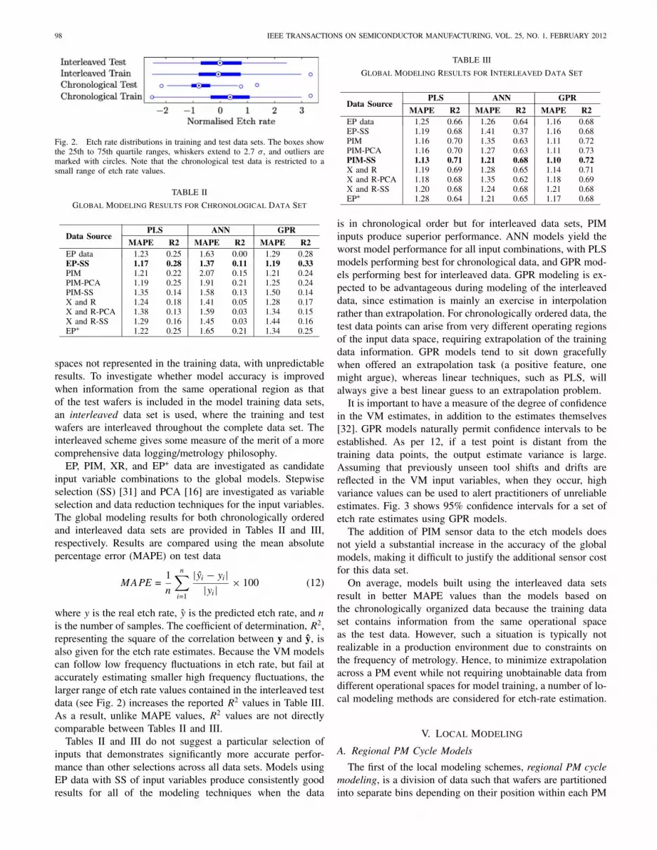
98 IEEE TRANSACTIONS ON SEMICONDUCTOR MANUFACTURING, VOL. 25, NO. 1, FEBRUARY 2012
Fig. 2. Etch rate distributions in training and test data sets. The boxes showthe 25th to 75th quartile ranges, whiskers extend to 2.7 σ, and outliers aremarked with circles. Note that the chronological test data is restricted to asmall range of etch rate values.
TABLE II
Global Modeling Results for Chronological Data Set
PLS ANN GPRData Source
MAPE R2 MAPE R2 MAPE R2EP data 1.23 0.25 1.63 0.00 1.29 0.28EP-SS 1.17 0.28 1.37 0.11 1.19 0.33PIM 1.21 0.22 2.07 0.15 1.21 0.24PIM-PCA 1.19 0.25 1.91 0.21 1.25 0.24PIM-SS 1.35 0.14 1.58 0.13 1.50 0.14X and R 1.24 0.18 1.41 0.05 1.28 0.17X and R-PCA 1.38 0.13 1.59 0.03 1.34 0.15X and R-SS 1.29 0.16 1.45 0.03 1.44 0.16EP+ 1.22 0.25 1.65 0.21 1.34 0.25
spaces not represented in the training data, with unpredictableresults. To investigate whether model accuracy is improvedwhen information from the same operational region as thatof the test wafers is included in the model training data sets,an interleaved data set is used, where the training and testwafers are interleaved throughout the complete data set. Theinterleaved scheme gives some measure of the merit of a morecomprehensive data logging/metrology philosophy.
EP, PIM, XR, and EP+ data are investigated as candidateinput variable combinations to the global models. Stepwiseselection (SS) [31] and PCA [16] are investigated as variableselection and data reduction techniques for the input variables.The global modeling results for both chronologically orderedand interleaved data sets are provided in Tables II and III,respectively. Results are compared using the mean absolutepercentage error (MAPE) on test data
MAPE =1
n
n∑i=1
|yi − yi||yi| × 100 (12)
where y is the real etch rate, y is the predicted etch rate, and n
is the number of samples. The coefficient of determination, R2,representing the square of the correlation between y and y, isalso given for the etch rate estimates. Because the VM modelscan follow low frequency fluctuations in etch rate, but fail ataccurately estimating smaller high frequency fluctuations, thelarger range of etch rate values contained in the interleaved testdata (see Fig. 2) increases the reported R2 values in Table III.As a result, unlike MAPE values, R2 values are not directlycomparable between Tables II and III.
Tables II and III do not suggest a particular selection ofinputs that demonstrates significantly more accurate perfor-mance than other selections across all data sets. Models usingEP data with SS of input variables produce consistently goodresults for all of the modeling techniques when the data
TABLE III
Global Modeling Results for Interleaved Data Set
PLS ANN GPRData Source
MAPE R2 MAPE R2 MAPE R2EP data 1.25 0.66 1.26 0.64 1.16 0.68EP-SS 1.19 0.68 1.41 0.37 1.16 0.68PIM 1.16 0.70 1.35 0.63 1.11 0.72PIM-PCA 1.16 0.70 1.27 0.63 1.11 0.73PIM-SS 1.13 0.71 1.21 0.68 1.10 0.72X and R 1.19 0.69 1.28 0.65 1.14 0.71X and R-PCA 1.18 0.68 1.35 0.62 1.18 0.69X and R-SS 1.20 0.68 1.24 0.68 1.21 0.68EP+ 1.28 0.64 1.21 0.65 1.17 0.68
is in chronological order but for interleaved data sets, PIMinputs produce superior performance. ANN models yield theworst model performance for all input combinations, with PLSmodels performing best for chronological data, and GPR mod-els performing best for interleaved data. GPR modeling is ex-pected to be advantageous during modeling of the interleaveddata, since estimation is mainly an exercise in interpolationrather than extrapolation. For chronologically ordered data, thetest data points can arise from very different operating regionsof the input data space, requiring extrapolation of the trainingdata information. GPR models tend to sit down gracefullywhen offered an extrapolation task (a positive feature, onemight argue), whereas linear techniques, such as PLS, willalways give a best linear guess to an extrapolation problem.
It is important to have a measure of the degree of confidencein the VM estimates, in addition to the estimates themselves[32]. GPR models naturally permit confidence intervals to beestablished. As per 12, if a test point is distant from thetraining data points, the output estimate variance is large.Assuming that previously unseen tool shifts and drifts arereflected in the VM input variables, when they occur, highvariance values can be used to alert practitioners of unreliableestimates. Fig. 3 shows 95% confidence intervals for a set ofetch rate estimates using GPR models.
The addition of PIM sensor data to the etch models doesnot yield a substantial increase in the accuracy of the globalmodels, making it difficult to justify the additional sensor costfor this data set.
On average, models built using the interleaved data setsresult in better MAPE values than the models based onthe chronologically organized data because the training dataset contains information from the same operational spaceas the test data. However, such a situation is typically notrealizable in a production environment due to constraints onthe frequency of metrology. Hence, to minimize extrapolationacross a PM event while not requiring unobtainable data fromdifferent operational spaces for model training, a number of lo-cal modeling methods are considered for etch-rate estimation.
V. Local Modeling
A. Regional PM Cycle Models
The first of the local modeling schemes, regional PM cyclemodeling, is a division of data such that wafers are partitionedinto separate bins depending on their position within each PM

LYNN et al.: GLOBAL AND LOCAL VIRTUAL METROLOGY MODELS FOR A PLASMA ETCH PROCESS 99
Fig. 3. Test wafer etch rate estimates, with 95% confidence intervals, fromglobal GPR model based on stepwise selected EP data for chronologicallyordered data. The high variance of the measured etch rate arises fromunmodeled process variation and this variance is not reflected in the etch rateestimates because it is not captured by the EP variables. The etch rate varianceremains constant in this figure because the data for the wafers shown are takenfrom the same operational space as those used to train the GPR model.
Fig. 4. Regional PM modeling scheme.
cycle. As depicted in Fig. 4, a different VM model is thenconstructed for each region of the PM cycle, and the modelsare switched for each unseen wafer depending on its PM cycleposition.
The purpose of the regional PM cycle modeling scheme is toinvestigate whether similarities exist between the plasma etchdata at different stages in PM cycles. It is conjectured that thebeginning, middle, and end sections of individual maintenancecycles may be more similar to the corresponding sectionsin other PM cycles than to the other sections of the samecycle. Supporting this hypothesis are the facts that severalof the measurements recorded from the etch chamber exhibitrepeatable patterns over the course of each PM cycle, and it isknown that chambers undergo a conditioning process as wafersare processed throughout each PM cycle.
The performance of the regional PM cycle models is testedusing Data Set A to allow performance comparisons betweenmodels built using different input combinations. The test dataset (30% of data points) occurs chronologically later than thetraining (50%) and validation (20%) data.
Fig. 5. MAPE for the regional PM cycle modeling scheme using EP datawith varying numbers of regional models per PM cycle.
The number of models per PM cycle is varied from one toten in order to determine an appropriate level of granularityand to highlight the effect of the PM cycle partitioningtechnique on estimation accuracy. Fig. 5 shows the MAPEperformance for PLS, ANN, and GPR-based models. The firstpoint for each model type is equivalent to the global modelingscheme seen in Section IV as it uses one model to cover allPM stages.
Fig. 5 illustrates that regional PM cycle models do notincrease the estimation accuracy of the virtual metrologymodels using EP data as input variables. Rather, accuracyworsens with increasing numbers of models per PM cycle.Similar results are found for different input variable selections[33], [34]. This degradation in performance is attributed to alack of exploitable commonality between similar sections ofdifferent PM cycles in the etch rate data set. Furthermore, thereis a reduction in the number of training points available foreach model as the number of models per PM cycle increases.
B. PM Cycle Clustering
This section investigates whether similarities between dif-ferent PM cycles can be found and harnessed to increase etchrate estimation accuracy. Analysis of Data Set A, where bothEP and PIM data are available, reveals four distinct clustersof self-similar data points. The clusters are visible in Fig. 6by performing a PCA on the EP and XR data separately andplotting the first two principal components of the XR dataagainst the first principal component of the EP data.
Each cluster contains a number of different PM cycles withsimilar EP and XR data. The existence of these clusters in thedata set suggests that the etch process moves between a finitenumber of operating points over the course of the completedata set. Similar modal behavior is seen in a stack etch processby He et al [35], and Zeng and Spanos [36] also reportedon clustered behavior in an etch process where the clusterswere associated with different etch chambers. In our work,changes in cluster, indicating changes of operating space, are

100 IEEE TRANSACTIONS ON SEMICONDUCTOR MANUFACTURING, VOL. 25, NO. 1, FEBRUARY 2012
Fig. 6. First principal component of EP data plotted against the first twoPCs of XR data. Data from one PM cycle from each cluster is chosen as testdata.
brought about by PM events on the same chamber. An analysisof variance of the etch rates in each cluster rejects the nullhypothesis that the mean etch rates in each cluster are equalat the α = 0.01 significance level.
Specialized models for each cluster are tested to examinewhether they can estimate etch rate more accurately thanglobal models trained using information from all clusters. Totest the performance of such cluster-based modeling, one PMcycle of wafers is extracted from each cluster to be used asunseen test data during model tests as shown in Fig. 6. Tocompare the cluster performance to a global-type scenario, onemodel is trained using the training data from all clusters, andthe same unseen test data is used to measure its performance.Because Cluster 4 comprises a single PM cycle, no separatetraining and test data exists for Cluster 4 model creation. Thedata from Cluster 4 provide an opportunity to explore VMstrategies during modes of chamber operation not previouslycaptured by other cluster models.
PLS, ANN, and GPR models are examined as candidatemodeling techniques for cluster models. EP, PIM, XR andEP+ data are investigated as input variable options. Stepwiseselection is applied to the input variables before GPR andANN modeling to reduce the number of input variables andimprove performance. Because PLS first projects the incomingdata onto its latent variable space as described in Section II-A,it is capable of modeling the cluster data sets that have moreinput variables than training samples. Results are presented inTable IV.
In tests completed for Cluster 4, for which there is only onePM cycle, no cluster model is capable of accurately estimatingetch rate; the global models yield the best estimates. Hence,when the etch tool operates in a previously unseen operationalspace, measurements of etch depth can be taken with greaterfrequency than before to allow new cluster model identificationand to ensure the process is operating within specifications.
By way of an example, Fig. 7 shows the estimates fromthe cluster and global GPR models on the test data points.Improvements in accuracy can be seen for Cluster 2 in Fig. 7for the cluster models. Cluster models are useful only in the
TABLE IV
Global and Cluster Model for All Data Types
Global Model Cluster ModelData Model
MAPE R2 MAPE R2PLS 1.79 0.53 1.60 0.52
EP ANN 2.08 0.48 1.74 0.42GPR 1.77 0.52 1.62 0.52PLS 1.57 0.50 1.59 0.49
PIM ANN 1.62 0.50 1.78 0.41GPR 1.63 0.47 1.77 0.44PLS 1.65 0.52 1.59 0.49
XR ANN 1.76 0.42 1.96 0.32GPR 1.69 0.46 1.58 0.52PLS 1.97 0.51 1.71 0.51
EP+ ANN 1.65 0.49 1.86 0.45GPR 1.77 0.52 1.70 0.50
The global model results differ from Tables II and III because the globalmodel here is trained using data from every cluster in the data set and thentested using the same data as the cluster models.
Fig. 7. Example etch rate estimates from global and clustered models usingEP data as input.
cluster over which they are trained, while the global modelcan provide meaningful estimates over the full test data set.
In Table IV, cluster models yield better estimation accuracyfor half of the model types and input selections, with superiorglobal models being those trained using PIM data, and thoseusing neural networks. The best overall MAPE is reportedfor the global PLS model using PIM data. Due to the lackof consistent results and the considerable extra complexity ofcluster model implementation, we cannot definitively concludethat cluster modeling is superior to global modeling for thisdata set. A larger set of historical data is required to fullyassess the capability of the clustering technique, but thepotential benefits are demonstrated here. In the case of moredata being available, new clusters are expected to be generated,or the wafer data is expected to return to an existing cluster,allowing model reuse.
C. Windowed Models
Time-windowed models can be used to maintain modelaccuracy in time-varying systems. For example, Qin [37]

LYNN et al.: GLOBAL AND LOCAL VIRTUAL METROLOGY MODELS FOR A PLASMA ETCH PROCESS 101
TABLE V
Comparison of Model Training Times (in S)
Window Length PLS ANN GPR70 0.03 1.90 26.27150 0.08 4.24 121.85250 0.13 6.97 320.90
applied a moving window PLS scheme to a catalytic reformer.Khan et al. [3] described a virtual metrology and run-to-runcontrol strategy that uses a continually updating windowedPLS model in their simulations of a semiconductor manufac-turing fabrication environment.
PLS, ANN, and GPR-based models are compared as can-didate modeling techniques for windowed modeling of theplasma etch data. Data Set B is used for windowed modelanalysis since the data set is almost fully contiguous, withonly one substantial gap where wafer records are not available.The data set is kept in a chronological order throughoutthe experiments, providing a realistic representation of dataproduced by an etch tool during processing. The use of DataSet B restricts the analysis to using EP data only duringmodeling (see Table I). The models are applied to the dataset using window lengths between 30 and 300 samples. Thewindow length describes the number of past wafers used totrain VM models that are used to estimate the etch ratesof wafers subsequently processed. When a new etch ratemeasurement becomes available, the window is advanced toinclude the new measurement and a new model is created.Global models using similar numbers of wafers fail to produceaccurate etch rate estimates over the complete data set becausethey fail to maintain their validity in new operating spaces [38].
Training times for PLS models are faster than those of ANNand GPR models because the latter two techniques require theuse of optimization techniques and multiple initializations dur-ing training. Table V shows model training times (in seconds)for each technique, using a computer with a 2.6 GHz dual-coreprocessor and 2 GB RAM. Although a second-order optimiza-tion technique is used during ANN model training, first-ordergradient descent is used to optimize the GPR hyperparameters.Hence, although GPR training arguably involves a more com-plex optimization task than ANN training, the GPR trainingtimes may be improved through the use of more complexoptimization techniques. However, the estimation times for allmodel types are typically less than 1 s. The etch processingtime for each wafer is approximately 5 min, and there is ametrology delay of several hours for etch rate measurements.Hence, according to Table V, which indicates that models canbe completely retrained in the order of seconds, any of thethree modeling techniques investigated are suitable for real-time implementation of a window-based VM system.
To increase windowed modeling accuracy, the most recentlymeasured value of etch rate is included as an input vari-able to the models. PLS model accuracy is enhanced via amaintenance-dependent sample weighting scheme as describedin [38]. Stepwise selection of input variables is performed oneach window before modeling for both ANN and GPR models.
Fig. 8. Windowed model MAPE performance for varying window length.
Fig. 9. Windowed model R2 values for varying window length.
The error performance for each modeling technique is shownin Figs. 8 and 9 for the range of window lengths investigated.
The R2 and MAPE values for the windowed models aresignificantly better than the global models values. Consideringthat a much smaller amount of training data is used duringwindowed model training, and that the models can performaccurately over numerous PM events in the test set, windowedmodels are preferable. The GPR-based windowed modelsoutperform windowed models based on PLS and ANNs,especially for smaller window sizes. For small window sizes,ANN models perform poorly due to a lack of training data.Increasing the window size improves ANN model perfor-mance, but the GPR models still follow the etch rate moresuccessfully.
The best results for the windowed GPR models are recordedfor a window length of 70 wafers. This model estimated theactual etch rate for the 493 unseen test wafers (that spanover 11 000 processed but unmeasured wafers) with a MAPEof 1.15% and R2 of 0.75. The etch rate estimates, confidence

102 IEEE TRANSACTIONS ON SEMICONDUCTOR MANUFACTURING, VOL. 25, NO. 1, FEBRUARY 2012
Fig. 10. Best etch rate estimates using windowed GPR model with windowlength 70.
TABLE VI
Comparison of MAPE Achieved by All Modeling Techniques
and Approaches for EP Data
PLS ANN GPRChronological 1.23 1.63 1.29Global modelingInterleaved 1.25 1.26 1.16Regional 1.43 2.01 1.57
Local modeling Clustering 1.60 1.74 1.62Windowed 1.2 1.23 1.14
limits, and actual etch rates for a section of the test data setare shown in Fig. 10.
While the windowed GPR model follows the overall trendof the etch rate variations, it struggles to accurately modelhigh frequency fluctuations in the data. These high frequencyfluctuations do not appear to be reflected in the recordedinput variables, and may arise from other processes in themanufacturing line, or unmeasured disturbances in incomingmaterial. However, the 95% confidence limits produced usingthe GPR models, which vary over the data set, encapsulatea large enough range to allow for the vast majority of thesevariations as shown in Fig. 10.
VI. Conclusion
The results in this paper reflect the reality of using pro-duction data, with a limited number of measured wafers,to develop VM models. Particular difficulties attach to theutilization of VM models across PM boundaries, and a varietyof local modeling approaches are explored to minimize thisproblem. However, disaggregation of production data for localmodel development results in small local data sets and thiscreates problems for a number of modeling paradigms, partic-ularly ANNs. In contrast, GPR models work well with smalldata sets, and produce an accompanying variance value foreach etch rate estimate. Table VI compares all of the modelingtechniques and data disaggregation approaches explored in thispaper for the EP data set.
Concerning the performance of various local modelingapproaches, the division of PM cycles into separate sectionsfor modeling is not beneficial, while the clustering of PMcycles with similar characteristics can improve marginally onthe accuracy of models with global scope for some inputvariable selections. The use of a wafer window scheme (withGPR modeling) produces the best estimation accuracy of etchrate on the data set investigated.
Acknowledgment
The authors would like to thank Intel Ireland, Leixlip, Co.Kildare, Ireland, for their help with this research.
References
[1] P. Chen, S. Wu, J. Lin, F. Ko, H. Lo, J. Wang, C. Yu, and M. Liang,“Virtual metrology: A solution for wafer to wafer advanced processcontrol,” in Proc. IEEE Int. Symp. Semicond. Manuf., Sep. 2005, pp.155–157.
[2] A. Khan, J. Moyne, and D. Tilbury, “An approach for factory-widecontrol utilizing virtual metrology,” IEEE Trans. Semicond. Manuf.,vol. 20, no. 4, pp. 364–375, Nov. 2007.
[3] A. A. Khan, J. Moyne, and D. Tilbury, “Virtual metrology and feedbackcontrol for semiconductor manufacturing processes using recursive par-tial least squares,” J. Process Control, vol. 18, no. 10, pp. 961–974,2008.
[4] A. Ferreira, A. Roussy, and L. Conde, “Virtual metrology models forpredicting physical measurement in semiconductor manufacturing,” inProc. IEEE/SEMI Adv. Semicond. Manuf. Conf., May 2009, pp. 149–154.
[5] Y. Yang, M. Wang, and M. J. Kushner, “Progress, opportunities andchallenges in modeling of plasma etching,” in Proc. Int. InterconnectTechnol. Conf., Jun. 2008, pp. 90–92.
[6] J. V. Ringwood, S. Lynn, G. Bacelli, B. Ma, E. Ragnoli, andS. McLoone, “Estimation and control in semiconductor etch: Practiceand possibilities,” IEEE Trans. Semicond. Manuf., vol. 23, no. 1, pp.87–98, Feb. 2010.
[7] B. Kim and K. Kim, “Prediction of profile surface roughness inCHF3/CF4 plasma using neural network,” Appl. Surf. Sci., vol. 222,nos. 1–4, pp. 17–22, Jan. 2004.
[8] E. Ragnoli, S. McLoone, S. Lynn, J. Ringwood, and N. Macgearailt,“Identifying key process characteristics and predicting etch rate fromhigh-dimension datasets,” in Proc. IEEE/SEMI Adv. Semicond. Manuf.Conf., May 2009, pp. 106–111.
[9] M. N. A. Dewan, P. J. McNally, T. Perova, and P. A. F. Herbert, “Useof plasma impedance monitoring for determination of SF6 reactive ionetching end point of the SiO2/Si system,” Microelectron. Eng., vol. 65,nos. 1–2, pp. 25–46, Jan. 2003.
[10] M. Kanoh, M. Yamage, and H. Takada, “End-point detection of reactiveion etching by plasma impedance monitoring,” Japan. J. Appl. Phys.,vol. 40, no. 3A, pp. 1457–1462, Mar. 2001.
[11] D. Zeng, Y. Tan, and C. J. Spanos, “Dimensionality reduction methodsin virtual metrology,” Proc. SPIE, vol. 6922, no. 1, p. 692238, Feb.2008.
[12] C. K. I. Williams and C. E. Rasmussen, Gaussian Processes forRegression. Cambridge, MA: MIT Press, 1996, ch. 8, pp. 514–520.
[13] C. K. I. Williams, “Prediction with Gaussian processes: From linearregression to linear prediction and beyond,” Neural Comput. Res. Group,Aston Univ., Birmingham, U.K., Tech. Rep. NCRG/97/012, Oct. 1997.
[14] M. Ebden. (2008, Aug.). Gaussian Processes for Regression: A QuickIntroduction [Online]. Available: http://www.robots.ox.ac.uk/mebden/reports/GPtutorial.pdf
[15] S. Lynn, J. Ringwood, and N. MacGearailt, “Gaussian process regressionfor virtual metrology of plasma etch,” in Proc. IET Irish Signals Syst.Conf., vol. 2010, no. CP566. 2010, pp. 42–47.
[16] J. E. Jackson, A User’s Guide to Principal Components. New York:Wiley-Interscience, 1991.
[17] P. Geladi and B. R. Kowalski, “Partial least-squares regression: Atutorial,” Anal. Chim. Acta, vol. 185, no. 1, pp. 1–17, 1986.

LYNN et al.: GLOBAL AND LOCAL VIRTUAL METROLOGY MODELS FOR A PLASMA ETCH PROCESS 103
[18] H. Abdi. (2003). Partial Least Squares (PLS) Regression. ThousandOaks, CA: Sage [Online]. Available: http://www.utdallas.edu/herve/Abdi-PLS-pretty.pdf
[19] Y.-J. Chang, “Fault detection for plasma etching processes using RBFneural networks,” in Proc. Int. Symp. Neural Netw., 2005, pp. 538–543.
[20] B. Kim, W. Choi, and H. Kim, “Using neural networks with a linearoutput neuron to model plasma etch processes,” in Proc. IEEE Int. Symp.Ind. Electron., vol. 1. Jun. 2001, pp. 441–445.
[21] D. Stokes and G. May, “Real-time control of reactive ion etching usingneural networks,” IEEE Trans. Semicond. Manuf., vol. 13, no. 4, pp.469–480, Nov. 2000.
[22] C. Himmel and G. May, “Advantages of plasma etch modeling usingneural networks over statistical techniques,” IEEE Trans. Semicond.Manuf., vol. 6, no. 2, pp. 103–111, May 1993.
[23] B. Kim and S. Kim, “Partial diagnostic data to plasma etch modelingusing neural network,” Microelectron. Eng., vol. 75, no. 4, pp. 397–404,Jul. 2004.
[24] R. Battiti and F. Masulli, “BFGS optimization for faster and automatedsupervised learning,” in Proc. Int. Neural Netw. Conf., vol. 2. 1990, pp.757–760.
[25] D. Marquardt, “An algorithm for least squares estimation of non-linearparameters,” SIAM J. Appl. Math., vol. 11, no. 2, pp. 431–441, Jun. 1963.
[26] M. Hagan and M. Menhaj, “Training feedforward networks with theMarquardt algorithm,” IEEE Trans. Neural Netw., vol. 5, no. 6, pp.989–993, Nov. 1994.
[27] J. Kocijan. (2008). “Gaussian process models for systems identification,”in Proc. 9th Int. Ph.D. Workshop Syst. Control Young Gener. Viewpoint,pp. 8–15 [Online]. Available: http://dsc.ijs.si/jus.kocijan/GPdyn/
[28] C. E. Rasmussen. (1996). “Evaluation of Guassian processes andother methods for non-linear regression,” Ph.D. dissertation, Dept.Comput. Sci., Univ. Toronto, Toronto, ON, Canada [Online]. Available:http://www.gaussianprocess.org/
[29] C. E. Rasmussen and C. K. I. Williams, Gaussian Processes forMachine Learning. Cambridge, MA: MIT Press, 2006.
[30] P. Sollich, “Gaussian process regression with mismatched models,” inProc. Neural Inform. Process. Syst., 2001, pp. 519–526.
[31] D. C. Montgomery, E. A. Peck, and G. G. Vining, Introduction toLinear Regression Analysis. New York: Wiley, 2001.
[32] F.-T. Cheng, Y.-T. Chen, Y.-C. Su, and D.-L. Zeng, “Evaluating reliancelevel of a virtual metrology system,” IEEE Trans. Semicond. Manuf.,vol. 21, no. 1, pp. 92–103, Feb. 2008.
[33] S. Lynn, J. Ringwood, E. Ragnoli, S. McLoone, and N. MacGearailt,“Virtual metrology for plasma etch using tool variables,” in Proc.IEEE/SEMI Adv. Semicond. Manuf. Conf., May 2009, pp. 143–148.
[34] S. Lynn, “Local modeling of a plasma etch data set,” Dept. Electr.Eng., Natl. Univ. Ireland, Maynooth, Kildare, Ireland, Tech. Rep.EE/JVR/1/2010, Feb. 2010.
[35] Q. He and J. Wang, “Fault detection using the k-nearest neighbor rulefor semiconductor manufacturing processes,” IEEE Trans. Semicond.Manuf., vol. 20, no. 4, pp. 345–354, Nov. 2007.
[36] D. Zeng and C. J. Spanos, “Virtual metrology modeling for plasmaetch operations,” IEEE Trans. Semicond. Manuf., vol. 22, no. 4, pp.419–431, Nov. 2009.
[37] S. J. Qin, “Recursive PLS algorithms for adaptive data modeling,”Comput. Chem. Eng., vol. 22, nos. 4–5, pp. 503–514, 1998.
[38] S. Lynn, J. V. Ringwood, and N. MacGearailt, “Weighted windowedPLS models for virtual metrology of an industrial plasma etch process,”in Proc. IEEE Int. Conf. Ind. Technol., Mar. 2010, pp. 271–276.
Shane A. Lynn received the B.Eng. degree incomputer engineering and the Ph.D. degree in en-gineering from the National University of Ireland,Maynooth, Kildare, Ireland, in 2006 and 2011, re-spectively. His Ph.D. research focused on the virtualmetrology and real-time control of a plasma etchprocess used in semiconductor manufacturing.
He has completed an internship with Ad AstraRocket Company, Guanacaste, Costa Rica. He hasworked with Intel Ireland, Leixlip, Co. Kildare,Ireland, on the development of virtual metrology
and data analysis systems. He is currently with the Department of ElectricalEngineering, National University of Ireland, Maynooth. His current researchinterests include empirical modeling of complex processes, advanced processcontrol applications, and data analysis and data reduction of large data sets.
Dr. Lynn has received the Endeavour Award from the Australian Govern-ment to complete research on autonomous vehicles with the University ofTechnology, Sydney, Australia in 2012.
John Ringwood (M’87–SM’97) received theDiploma degree in electrical engineering from theDublin Institute of Technology, Dublin, Ireland, andthe Ph.D. degree in control systems from StrathclydeUniversity, Glasgow, Scotland, in 1981 and 1985,respectively.
He is currently a Professor of electronic engineer-ing with the Department of Electrical Engineering,National University of Ireland (NUI), Maynooth,Kildare, Ireland. He was the Founding Head of theElectronic Engineering Department, NUI, from 2000
to 2005, and also served as the Dean of the Faculty of Engineering. His currentresearch interests include semiconductor manufacturing, ocean energy, andbiomedical engineering.
Dr. Ringwood is a Chartered Engineer and a Fellow of Engineers Ireland.
Niall Macgearailt received the Bachelors degreein mechanical engineering from University CollegeDublin, Dublin, Ireland, in 1991. He is currently pur-suing the Ph.D. degree with Dublin City University,Dublin.
He joined Intel Ireland, Leixlip, Co. Kildare, Ire-land, in 2002 as a Process Engineer and worked ondeveloping fault detection systems using advancedsensors before moving to a research role in 2005. Hisresearch with Intel focuses on the areas of metrologyreduction and equipment performance improvement.
He is also responsible for establishing and leading collaboration programsbetween Intel and universities to address key technology problems. Beforeworking with Intel, he was with Lam Research, Fremont, CA, for 8 years,where he worked as a Research and Development Engineer developing next-generation plasma chambers and processes. He spent a number of years atvarious wafer fabrication facilities in San Jose, CA.