geophysical and astrophysical fluid dynamics beyond the traditional approximation

GEOPHYSICAL AND ASTROPHYSICAL FLUID

DYNAMICS BEYOND THE TRADITIONAL

APPROXIMATION

T. Gerkema,1 J. T. F. Zimmerman,1,2 L. R. M. Maas,1,2 and H. van Haren1

Received 7 November 2006; revised 6 June 2007; accepted 28 September 2007; published 16 May 2008.

[1] In studies on geophysical fluid dynamics, it is commonpractice to take the Coriolis force only partially into accountby neglecting the components proportional to the cosine oflatitude, the so-called traditional approximation (TA). Thisreview deals with the consequences of abandoning the TA,based on evidence from numerical and theoretical studiesand laboratory and field experiments. The phenomena mostaffected by the TA include mesoscale flows (Ekman spirals,deep convection, and equatorial jets) and internal waves.

Abandoning the TA produces a tilt in convective plumes,produces a dependence on wind direction in Ekman spirals,and gives rise to a plethora of changes in internal wavebehavior in weakly stratified layers, such as the existence oftrapped short low-frequency waves, and a polewardextension of their habitat. In the astrophysical context ofstars and gas giant planets, the TA affects the rate of tidaldissipation and also the patterns of thermal convection.

Citation: Gerkema, T., J. T. F. Zimmerman, L. R. M. Maas, and H. van Haren (2008), Geophysical and astrophysical fluid dynamics

beyond the traditional approximation, Rev. Geophys., 46, RG2004, doi:10.1029/2006RG000220.

1. INTRODUCTION

[2] In a now famous memoir, Coriolis [1835] derived the

equations of motion for rotating devices, in which he

identified a deflecting force that he called ‘‘force centrifuge

composee,’’ now known as the Coriolis force. It acts on

particles moving in the frame of reference of the rotating

system, is proportional to their velocity, and produces a

deflection in a direction perpendicular to velocity. The

rotating ‘‘device’’ we are primarily concerned with in this

paper is, of course, the Earth. The notion that the Earth’s

diurnal rotation produces a deflecting force had, in fact,

been recognized before Coriolis, albeit initially in rudimen-

tary form; in the 18th century, G. Hadley thus provided a

qualitative explanation of the trade winds [Burstyn, 1966].

In a preamble to his dynamic theory of tides, Laplace

[1798] derived the exact mathematical form of the deflect-

ing force. Adopting a geographical coordinate system, he

showed that there are four ‘‘Coriolis’’ terms, whose roles are

indicated in Table 1 (an elementary derivation of each of

these terms is provided in Appendix A).

[3] Of these four terms, two are proportional to the sine

of latitude; the other two are proportional to the cosine. This

distinction has a deeper, dynamical significance. The force

associated with the sine terms is due to, and induces, only

horizontal movements. In the cosine terms, on the other

hand, the vertical direction is always involved: the associ-

ated force either is due to a vertical velocity or induces a

vertical acceleration. (These effects are perhaps most readily

appreciated by means of the following simple mechanical

examples: (1) the eastward deflection of a stone dropped

from a tower and (2) the upward force undergone by an

eastward moving object, reducing its weight, the so-called

Eotvos effect.) Exploiting this distinction, Laplace devel-

oped a chain of arguments which led him to conclude that

while the sine terms are to be retained, the cosine terms can

be neglected (see Laplace [1878, Livre I, sections 35 and

36]; for a valuable summary of this and other aspects of

Laplace’s tidal theory, see Dubois [1885]). In this, he has

been followed almost universally in later studies on geo-

physical fluid dynamics (GFD), which inspired Eckart

[1960] to coin the apt name ‘‘traditional approximation’’

(TA) to refer to the neglect of the cosine terms, i.e., the

terms with ~f in Table 1. The TA’s widespread adoption

notwithstanding, studies devoted to the role of ~f have

occasionally appeared since the late 1920s and more fre-

quently so in recent years. As the interest in the topic has

waxed and waned repeatedly, the literature is scattered, and

much of it has slipped into oblivion. The principal goals of

this review are to give a coherent overview of the existing

literature, to pinpoint the kinds of motion in which ~f is

plausibly significant, and to outline the unresolved issues.

ClickHere

for

FullArticle

1Royal Netherlands Institute for Sea Research, Texel, Netherlands.2Institute for Marine and Atmospheric Research, Utrecht University,

Utrecht, Netherlands.

Copyright 2008 by the American Geophysical Union.

8755-1209/08/2006RG000220$15.00

Reviews of Geophysics, 46, RG2004 / 2008

1 of 33

Paper number 2006RG000220

RG2004

http://dx.doi.org/10.1029/2006RG000220

[4] The justification for the TA centers around the ob-

servation that the depth of the oceans and atmosphere is

very thin compared to the radius of the Earth; large-scale

motions are therefore necessarily nearly horizontal. For

Coriolis effects to be important, timescales need to be of

the order of W�1 (the inverse Earth’s angular velocity) or

larger. Such low-frequency motions usually have large

horizontal scales; the vertical motions must then be much

weaker than the horizontal ones, rendering the Coriolis

terms with ~f insignificant compared to those with f and

rendering the pressure field nearly hydrostatic. (Similarly,

strong vertical stratification in density, which suppresses

vertical motions, also diminishes the role of the ~f terms.)

This argument becomes, however, problematic near the

equator (where ~f � f ) and also in kinds of motion with a

manifestly vertical character (such as deep convection) or for

low-frequencymotions with short horizontal scales (such as a

class of internal waves discussed in section 6.1.2).

[5] The neglect of the ~f terms conveniently aligns the

remaining part of the rotation vector to gravity. This is

illustrated in Figure 1, showing how at latitude f the (full)

rotation vector W can be decomposed into a radial and

meridional component; the former is proportional to f; the

latter is proportional to ~f . Under the TA, only the radial

component, aligned to gravity, is taken into account. Aban-

doning the TA breaks this symmetry: the rotation vector is

then neither aligned to the vertical nor to the horizontal

(except at the poles and equator), which implies, mathemat-

ically, that the set of partial differential equations that

govern the motion cannot be solved by separation of

horizontal and vertical variables. This, presumably, has

often been taken as a practical (rather than a physically

motivated) reason for making the TA.

[6] From Table 1 it is clear that the effect of f is isotropic

in the horizontal geographical plane: it always produces an

acceleration to the right with respect to velocity in the

Northern Hemisphere (NH) and to the left in the Southern

Hemisphere (SH), irrespective of the horizontal orientation

of velocity. The component ~f , by contrast, introduces

anisotropy in the horizontal plane: vertical velocities pro-

duce a zonal acceleration not a meridional one (third row of

Table 1), and only zonal velocities produce a vertical

acceleration (first row of Table 1). To summarize, we can

identify three key elements of the nontraditional component~f , which we will encounter repeatedly in this review: first,

the crucial role of vertical movements (the Coriolis compo-

nents with ~f are due to a vertical current or induce a vertical

acceleration); second, horizontal anisotropy, singling out

zonal movements; and third, the tilt due to ~f between the

rotation vector and gravity, which is a source of nonsepar-

ability (i.e., mixed spatial derivatives in the governing

partial differential equation).

[7] The TA may often be applicable in GFD but certainly

not always; the present review is devoted to these excep-

tions. In sections 3–5 we discuss the role of ~f in mesoscale

motions, namely, Ekman flows, deep convection, and equa-

torial flows, a subject which has attracted much attention in

recent years. Most of the literature questioning the TA has

dealt with internal waves, which we address in section 6.1

(dynamics at a fixed latitude), where we also present

observational work, and in section 6.2 (including latitudinal

variation). The validity of the TA in the Laplace tidal equations

has also been the subject of much debate (section 6.3). An

excursion to the astrophysical context, finally, is made in

section 7; here we focus on tidal oscillations and dissipation

in giant planets and stars and on thermal convection.One of the

conceptual problems of the TA is that it does not always stand

by itself; for reasons of consistency, certain approximations

need to be accompanied by the TA. Section 2 aims to discuss

these connections. Readers who are primarily interested in the

concrete manifestations of nontraditional effects may want to

skip this section and consult it only when referred to in later

sections.

2. MOMENTUM EQUATIONS: FROM THEELLIPSOID TO THE f PLANE

[8] On the long geological timescale, the Earth has

adjusted itself to the state of rotation; it has taken an oblate

shape such that its surface forms, on the whole, a level of

constant geopotential F (defined as the sum of gravitational

and centrifugal potential). A fluid parcel at this level

therefore experiences no tangential force so far as the

geopotential is concerned. Overall, the surface closely

TABLE 1. Components of the Coriolis Accelerationa

Initial VelocityInduced Coriolis Acceleration

(Northern Hemisphere)

Eastward (u) southward (�fu) and vertically upward (~f u)Northward (v) eastward (fv)Vertically upward (w) westward (�~f w)

aHere, f = 2Wsinf and ~f = 2Wcosf, where W is the Earth’s angularvelocity (7.292 � 10�5 rad s�1) and f is latitude in the NorthernHemisphere. In the Southern Hemisphere, f is negative, so in the column onthe right, ‘‘southward’’ is then replaced by ‘‘northward,’’ and ‘‘eastward’’ isreplaced by ‘‘westward.’’

Figure 1. Decomposition of the rotation vector W atlatitude f, giving rise to the components f = 2W? and ~f =2Wk. Under the TA, the terms associated with Wk areneglected.

RG2004 Gerkema et al.: GFD BEYOND THE TRADITIONAL APPROXIMATION

2 of 33

RG2004

resembles an ellipsoid of revolution; hence it is natural to

adopt oblate spherical coordinates [Gates, 2004]. However,

anticipating later approximations (by which the ocean and

atmosphere are treated as a spherical shell), we adopt

spherical coordinates instead, so that the inviscid momen-

tum equations become [e.g., Veronis, 1963a]:

Dsul

Dtþ ulwr � ulvf tanf

rþ 2Wwr cosf� 2Wvf sinf

¼ � 1

rr cosf@p

@l; ð1Þ

Dsvf

Dtþ vfwr þ u2l tanf

rþ 2Wul sinf ¼ � 1

rr@p

@f� 1

r

@F@f

; ð2Þ

Dswr

Dt�u2l þ v2f

r� 2Wul cosf ¼ � 1

r@p

@r� @F

@r: ð3Þ

[9] Here l is longitude, f is latitude, r is the radius, and

ul, vf, wr are the associated velocity components; t is time,

r denotes density, p is pressure, and W is the Earth’s angular

velocity (7.292 � 10�5 rad s�1). The material derivative is

defined as

Ds

Dt¼ @

@tþ ul

r cosf@

@lþ vf

r

@

@fþ wr

@

@r:

On the left-hand side of (1)–(3), metric terms ( )/r are

present, which are associated with advection. One also

recognizes the four Coriolis terms of Table 1, here brought

to the left-hand side. The terms 2Wwrcosf and 2Wulcosfare the ones neglected under the TA. For later reference, we

note that the momentum equations (1)–(3) imply an exact

conservation law for axial angular momentum:

rDs

Dtul þ Wr cosfð Þr cosf½ � ¼ � @p

@l: ð4Þ

2.1. Thin-Layer Approximations

[10] The layers of the terrestrial atmosphere and oceans

are very thin compared to the mean radius of the Earth (R);

hence the inequality jr � Rj/R 1 is always satisfied,

irrespective of the kind of motion under consideration.

(Note that here we are comparing distances in the radial

direction; any connotation with the ‘‘shallow water approx-

imation,’’ which refers to the aspect ratio, should be

avoided.) This purely geometric fact, combined with the

small eccentricity of the Earth’s surface, suggests that we

may treat the ocean and atmosphere as if they were a thin

spherical shell. This entails several approximations. To

begin with, for this approach to be consistent at all,

spherical surfaces within the shell must act as levels of

constant geopotential. A thorough analysis of this problem

is given by van der Toorn and Zimmerman [2008]; the

upshot is that in a lowest-order expansion involving three

small parameters (eccentricity, relative shell thickness, and

relative rotation rate), the gradient @F/@f can indeed be

neglected, while @F/@r reduces to a constant g.

[11] Another natural approximation, seemingly, is to

replace r by R in the metric terms in (1)–(3), as is common

practice in textbooks on GFD. However, N. A. Phillips

[1966] showed that there is then no longer an exact

conservation law for angular momentum. He proposed an

alternative to avoid this problem; instead of the ad hoc

replacement of r by R in (1)–(3), he introduced the thin-

layer approximation in the metric tensor, which was then

applied to the covariant form of the momentum equations.

(An alternative derivation, using a variational principle, is

given by Muller [1989] and in more detail by White et al.

[2005].) This leads to the set

D0sul

Dt� ulvf tanf

R� 2Wvf sinf ¼ � 1

rR cosf@p

@l; ð5Þ

D0svf

Dtþ u2l tanf

Rþ 2Wul sinf ¼ � 1

rR@p

@f; ð6Þ

D0swr

Dt¼ � 1

r@p

@r� g; ð7Þ

with

D0s

Dt¼ @

@tþ ul

R cosf@

@lþ vf

R

@

@fþ wr

@

@r:

[12] There is now an exact conservation law for axial

angular momentum similar to the one in (4), with r replaced

by R. But to achieve this, a number of terms have been

‘‘sacrificed,’’ notably the Coriolis terms proportional to cosf. In other words, this form of the thin-layer approximation

implies the TA. (Still another way of introducing the thin-

layer approximation was suggested by Wangsness [1970],

but this leads to a conservation law for energy in which

metric terms act as a source, which is ‘‘undesirable’’

[Phillips, 1970].) Veronis [1968] pointed out that the use

of (5)–(7) may give a serious misrepresentation of the real

physics, especially in equatorial regions, when the full

rotation vector needs to be included. In other words, the

TA, and hence the use of (5)–(7), cannot be justified on

mere geometrical grounds (i.e., the shell being thin); the

physical context must be considered.

[13] The somewhat intricate variety of thin-layer approx-

imations can easily obscure the fact that we actually face a

simple choice so far as the TA is concerned. The point is

that the presence of nontraditional terms renders the prob-

lem nonseparable and hence, in spherical geometry, virtu-

ally impossible to solve analytically. For exact analytical

treatment of nontraditional problems, one thus has to resort

to more radical approximations that eliminate the spherical

geometry still implied by the thin-layer approximation (see

section 2.2). In numerical studies, on the other hand, there is

no advantage in replacing r by R in the metric terms, and


3 of 33

RG2004

one might as well use the original momentum equations (1)–

(3) or their quasi-hydrostatic form, discussed in section 2.3,

which too is dynamically consistent. The interpretation of

numerical solutions requires, however, some care; even

though it is tempting to think in terms of ‘‘normal modes’’

[e.g., Thuburn et al., 2002a], this concept is not carried over

straightforwardly from the traditional to the nontraditional

setting because of the nonseparable nature of the solution in

the latter case.

2.2. The b Plane and f Plane Approximations

[14] The b plane is a hybrid construction in the sense that

one adopts a local Cartesian coordinate system (representing

the Earth’s surface as ‘‘flat’’), while still preserving the

variation of the Coriolis parameter(s) with latitude, which is

due to the curvature of the Earth’s surface. The b plane

equations can be derived from (1)–(3) by appropriate

scaling and then making an expansion in small parameters

L/R and H/R, where L and H denote the characteristic

horizontal and vertical scales, respectively, of the problem.

The usual west-east, south-north, and vertical Cartesian

coordinates are introduced via x = (Rcosf0)l, y = R(f �f0), and z = r � R, where f0 is the reference latitude around

which the expansion is made. It is immediately clear from

(1) and (2) that no proper transition to Cartesian coordinates

is possible near the poles, since the metric terms propor-

tional to tanf become infinite there (this is due to the

nongeodesic character of spherical coordinates [see Verkley,

1990]). Sufficiently far away from the poles, however, one

can make an expansion as presented by LeBlond and Mysak

[1978]. This results in a set from which metric terms are

absent and which is expressed in terms of the coordinates x,

y, and z and their associated velocities u, v, and w:

Du

Dtþ ~f w� fv ¼ � 1

r@p

@xð8Þ

Dv

Dtþ fu ¼ � 1

r@p

@yð9Þ

Dw

Dt� ~f u ¼ � 1

r@p

@z� g; ð10Þ

with D/Dt = @/@t + u � r. The Coriolis parameters ~f and f

stem from a Taylor expansion of 2Wcos(f0 + y/R) and

2Wsin(f0 + y/R), respectively:

~f ¼ 2W cosf0; f ¼ 2W sinf0 þ by; where b ¼ 2W cosf0=R:

ð11Þ

Here the linear term in y is included in the expansion of the

‘‘traditional’’ f term, thus allowing for effects of its

latitudinal variation. In the ‘‘nontraditional’’ ~f term,

however, only the first (i.e., constant) term of the expansion

is retained. The reason for ignoring the meridional

dependence here lies not in the derivation as such but

rather in the a posteriori consideration of conservation laws.

It was shown by Grimshaw [1975b] that the b plane

equations (8–10) do imply angular momentum and vorticity

conservation laws if ~f is taken to be constant, while they do

not if ~f varies with y. There are perhaps not many problems

in which the b effect and nontraditional effects are both

important, but they are arguably so for near-inertial internal

waves. As discussed below, there are in that case also

dynamical reasons why the latitudinal variation of f matters,

whereas that of ~f does not. This lends further validity to the

approximation (11) proposed by Grimshaw [1975b]. On the

f plane, finally, the b term is neglected so that f and ~f are

now both treated as constants; this renders the momentum

equations (8)–(10) dynamically fully consistent.

2.3. Hydrostatic and Quasi-hydrostaticApproximations

[15] The hydrostatic approximation means that the pres-

sure at any point depends only on the weight of the fluid

column above it; this amounts to replacing (10) by

@p

@z¼ �rg; ð12Þ

the hydrostatic balance. (Similarly, in spherical coordinates,

one replaces (3) by @p/@r = �r@F/@r.) One is now forced to

neglect also the term ~f w in (8), lest the Coriolis force does

work (as can be seen by multiplying (8), (9), and (12) by u,

v, and w, respectively, and summing the resulting equations

in order to make an energy equation). In other words,

consistency requires that the hydrostatic approximation be

accompanied by the TA.

[16] The principal advantage of making the hydrostatic

approximation in theoretical and especially in numerical

studies lies not so much in the assumption of the hydrostatic

balance per se, as in the removal of the time derivative from

the vertical momentum equation. This has led several

authors [White and Bromley, 1995; Marshall et al., 1997;

White et al., 2005] to propose an alternative, the quasi-

hydrostatic approximation, which means that one replaces

(10) by an equation from which only the material derivative

is removed:

�~f u ¼ � 1

r@p

@z� g; ð13Þ

the quasi-hydrostatic balance. (Similarly, in (3) one removes

Dswr /Dt while retaining the metric and Coriolis terms.)

Clearly, the nontraditional terms can coexist with the quasi-

hydrostatic approximation. White and Bromley [1995] and

White et al. [2005] showed that the quasi-hydrostatic

momentum equations are dynamically consistent and that

they correctly imply conservation laws for energy, angular

momentum, and potential vorticity.

[17] In summary, the following versions of the momen-

tum equations, with nontraditional terms included, can be

considered dynamically consistent: first, the full version in

spherical coordinates (1)–(3); second, its quasi-hydrostatic


4 of 33

RG2004

version; third, the approximated momentum equations on

the f plane (8)–(10); fourth, the corresponding quasi-

hydrostatic version with (10) replaced by (13). In the bplane version, consistency requires that ~f be taken constant.

3. EKMAN FLOWS

[18] In the classical paper by Ekman [1905], the friction

layers at the bottom of ocean or atmosphere and at the top of

the ocean are typical ‘‘traditional’’ flows. They are purely

horizontal and suppose a dynamic balance between the

traditional components of the Coriolis acceleration and the

divergence of vertical momentum transport by a constant

viscosity (which may be thought of as an eddy viscosity

representing small-scale turbulence). Since the nontradi-

tional components do not enter the problem, the classical

Ekman solution is characterized by horizontal isotropy: a

change in the forcing direction produces a corresponding

change in the orientation of the response, but otherwise, the

response remains the same; its structure as such does not

depend on the forcing direction. (‘‘Forcing’’ here means

either the applied wind stress at the top of the ocean, the so-

called ‘‘oceanic’’ case, or the external geostrophic current

over a rigid bottom, the ‘‘atmospheric’’ case.) Besides this

absence of the influence of forcing direction, the principal

outcome of the classical Ekman problem is the direction of

the surface current, being 45� to the right (left) of the

applied stress in the NH (SH). As a matter of fact, observed

angles usually deviate significantly from this value; Ekman

himself discussed observations by Nansen, who had

observed deflection angles substantially less than 45�, i.e.,between 20� and 40�. Interestingly, this is counter to the

result of an important modification that Ekman introduced

at the end of his 1905 paper. There he discusses the case of

an eddy viscosity that depends on the vertical shear of the

current. This makes the eddy viscosity a function of depth,

which renders the problem nonlinear though still integrable.

It results in two properties that deviate from the constant

viscosity solution: the layer is not exponentially decaying

but becomes of finite depth, and the deflection angle

becomes slightly larger than 45�. In spite of the latter result,

by relating vertical shear and eddy viscosity Ekman was on

the right track to a more sophisticated boundary layer theory

that recognizes the instability of the shear flow, its

generation of coherent roll vortices, and, finally, the creation

of large-scale turbulence, i.e., eddies with a size of the

Ekman layer depth. These motions, which are disturbances

on the mean Ekman shear flow, react back to the mean flow

itself by creating enhanced vertical momentum transport. As

these motions have substantial vertical velocities, they are

subject to the full Coriolis acceleration and hence must bear

signs of the anisotropy inherent to the full Coriolis force.

This, in turn, must translate into effective eddy coefficients

that depend not only on depth but also on the direction of

the forcing, and this may have its bearing on the deflection

angle. This is the route on which the rest of this section

focuses.

3.1. Ekman Layer Instability: Vortex Rolls

[19] The classical Ekman flow may become unstable,

giving rise to the formation of vortex rolls. These vortices

take the form of a rotational motion around horizontal axes

as shown in Figure 2, where the axes are (horizontally)

tilted with respect to the geostrophic current at an angle of

typically less than 20� (to the left or right). The dominant

underlying mechanism of the instability can be convection

(if the static stratification is unstable) or shear [Etling,

1971]; the two cannot always be clearly distinguished.

[20] As mentioned in section 3, the geostrophic and mean

Ekman currents are purely horizontal; hence the effect of ~fis limited to a modification of the hydrostatic balance, see

(13). Ekman [1932] argued that this effect is extremely

small. For the vortex rolls, arising from the instability of the

Ekman layer, the situation is very different since they do

involve vertical motions. This has led Wippermann [1969],

and later authors, to split the problem into two parts: the basic

flow, which is treated under the TA, and the instability

problem, in which ~f is taken into account. In linear instability

Figure 2. Sketch of vortex rolls due to the instability of the Ekman layer beneath the geostropic wind.On the right, the arrows indicate the wind, being geostrophic at high positions (directed along y) andturning anticlockwise in the downward direction in the Ekman layer; near the bottom, the angle is 45� tothe left of the geostrophic wind. Within the Ekman layer, instabilities in the form of vortex rolls appear,depicted on the left. Their main axis is typically nearly aligned to the geostrophic wind.


5 of 33

RG2004

theory, the perturbation (i.e., vortex rolls) is assumed to be

weak; Wippermann [1969] derived the equations for the

vertical structure functions of the perturbation, assuming plane

wave propagation in the horizontal direction at a certain angle �with the basic geostrophic flow.

[21] Etling [1971] analyzed numerically some parameter

regimes for unstable, neutral, and stable stratification. The

neutral case was later examined more systematically by

Leibovich and Lele [1985]. In the context of this review, the

principal outcome of both studies is that the horizontal

component ~f plays an important role in that it introduces a

dependence on the direction of the geostrophic flow in the

horizontal geographical plane. Specifically, the threshold for

instability is reduced most strongly if the axes of the vortex

rolls are oriented west-east, with a near easterly geostrophic

flow (i.e., directed to the west); beyond this threshold,

moreover, growth rates are significantly enhanced. In a

sequel to this work, a nonlinear instability analysis was

carried out by Haeusser and Leibovich [1997, 2003]. They

derived a coupled pair of differential equations for the

amplitude of the rolls (anisotropic two-dimensional com-

plex Ginzburg-Landau equation) and for the mean drift

(Poisson equation). The resulting patterns reveal ‘‘defects,’’

the intensity of which is much higher for easterly than for

northwesterly winds, which presumably can be interpreted

as enhanced small-scale turbulence in the former case. We

note that all of the above mentioned studies assume constant

eddy viscosity.

3.2. Vertical Turbulent Transfer

[22] In a direct numerical simulation (DNS), Coleman et

al. [1990] studied the effect of ~f on an atmospheric Ekman

layer by doing model runs for four different wind directions.

The most extreme cases turn out to be an easterly versus

westerly wind; at latitude 45�N, quantities like the frictionalvelocity and the angle of the stress at the bottom (with

respect to the geostropic current) differ by as much as 6%

and 30% between these extremes. The case with an easterly

wind can be characterized as the most turbulent. Coleman et

al. [1990] explain the difference by noting that ~f brings

about a redistribution of turbulent kinetic energy (TKE)

between its horizontal and vertical components. This

argument is developed in more detail by Zikanov et al.

[2003], who carried out a large-eddy simulation (LES) for

various parameter regimes of the wind-induced turbulent

Ekman layer in the upper ocean. (The paper by Zikanov et

al. [2003] states, however, some of the signs of the

nontraditional terms incorrectly. For a correct reading, the

angle g defining the wind direction should be replaced by

�g; as a consequence, ‘‘west’’ and ‘‘east’’ should be

interchanged throughout their text.) They point out that ~fhas a dual role: it affects the vertical turbulent momentum

transfer, and (as noted already) it redistributes TKE between

its horizontal and vertical components. Unlike f, which

creates only an isotropic coupling between horizontal

fluctuations [see Tritton, 1978], ~f provides a coupling

between horizontal and vertical fluctuations and introduces

an anisotropy in the horizontal plane. The vertical turbulent

momentum transfer, changed by ~f , in turn, affects the mean

flow and the turbulence production by the mean shear.

[23] Zikanov et al. [2003], moreover, present an intui-

tively appealing method to incorporate these effects in a

simple way. On the basis of their model results, they

construct a vertically dependent effective eddy viscosity

Az(z). This Az turns out to depend strongly on the wind

direction (all other parameters being the same), a manifesta-

tion of the change in turbulent momentum transfer due to ~f .For example, at latitude 15�N the maximum of Az found for

northeasterly winds exceeds the maximum for south-

westerly winds by as much as a factor of 5. If one now

takes these profiles as a starting point, the Ekman flow can

be reconstructed; Zikanov et al. [2003] show that the flow

thus obtained shares the principal characteristics with the

mean flow produced by LES. The effect of ~f is thus

transferred, via Az, to the Ekman flow. This idea was later

extended by McWilliams and Huckle [2006], who incorpo-

rated ~f and the resulting dependence on wind direction in a

representation of the effective eddy viscosity profiles in the

ocean Ekman layer (see Figure 3); ~f was also found to alter

significantly the response to time-variable wind, e.g., the

direction of the surface current.

[24] A related issue is the possible influence of ~f on the

mixed layer depth. Garwood et al. [1985a] argued that ~f ,combined with easterly winds, would deepen the mixed

layer. Garwood et al. [1985b] applied this idea to the

equatorial Pacific to explain the observed fact that the depth

of the mixed layer increases substantially toward the west.

However, Galperin et al. [1989], using a numerical model,

did not find a significant influence of ~f on mixed layer

depth. It seems indeed more plausible that the observed

deepening is simply due to horizontal convergence of mass

Figure 3. Effective eddy viscosity profiles for differentwind directions. The solid line represents the profile underTA, in which case there is no dependence on wind direction.The other three lines include the effect of ~f : the largestvalues occur for winds to the SW (dashed line), the smallestoccur for winds to the NE (dash-dotted line), and theintermediate case (dotted line) is for winds to the NWor SE.From McWilliams and Huckle [2006].


6 of 33

RG2004

in the warm upper layer, driven by the westward mean wind

stress [Lukas and Lindstrom, 1991].

[25] We note that the studies by Coleman et al. [1990],

Zikanov et al. [2003], and McWilliams and Huckle [2006]

assume a neutrally stratified Ekman layer. Stratification is

known to affect the characteristics of the Ekman spiral (see,

e.g., Price and Sundermeyer [1999] for an overview). One

would expect that stable stratification diminishes the role of~f and hence the dependence on wind direction, but this has

not yet been looked into.

4. DEEP CONVECTION

[26] In the Labrador, Greenland, and Weddell seas, deep

water is intermittently formed by deep convection in plumes

with a horizontal extent of the order of 1 km, in which

vertical velocities can be as high as 10 cm s�1 [Marshall

and Schott, 1999]. Apart from these high-latitude regions,

convection also occurs in the Mediterranean (e.g., Gulf of

Lions).

[27] Deep convection, with its strong vertical motions,

seems a plausible candidate for a clear manifestation of the

nontraditional component ~f . Several studies have been

devoted to this aspect, most of them numerical. Garwood

[1991] found a dependence on wind direction in numerical

experiments on forced convection; for easterly winds a

transfer was found to take place from horizontal to vertical

TKE, while the reverse was the case for westerly winds. As

a consequence, the mixed layer depth was larger (by about a

factor of 2) in the former case. This result is in line with the

discussion in section 3.2 on TKE in Ekman flows. Denbo

and Skyllingstad [1996] looked into the structure of the

plume and found that ~f creates horizontal asymmetries, a

manifestation of the horizontal anisotropy introduced by ~f .[28] Marshall and Schott [1999] point out that lateral

inhomogeneities such as shear currents or fronts, or indeed~f , cause the convection to occur along slanted rather than

strictly vertical paths. In the absence of other lateral

inhomogeneities, ~f alone creates a tilt along the rotation

axis; this follows from (8), with derivatives taken to be zero:

�fyþ ~f z ¼ const:

Looking downward, the tilt is toward the equator in both

hemispheres. This effect is clearly visible in results from

nonhydrostatic numerical models [Straneo et al., 2002;

Wirth and Barnier, 2006; 2008]; see Figure 4. This finding

that mixing takes place along the axis of rotation rather than

in the direction of gravity has important observational

implications. Measurements are, of course, taken along

vertical profiles, which means that one crosses tilted plumes

rather than penetrating them. Interestingly, observations in

the Labrador Sea by Pickart et al. [2002] indeed reveal

convective sublayers; they put forward slantwise convection

as a possible explanation. This would, however, not be

necessarily due to ~f alone since, as noted, other lateral

inhomogeneities can also cause a tilt.

[29] In a series of ingenious ‘‘nontraditional’’ laboratory

experiments on convection, Sheremet [2004] demonstrated

a tilting of plumes caused solely by ~f . (The experiment was

later carried out with sinking balls [see Riemenschneider

and Sheremet, 2006].) In this setting (see Figure 5), a

platform rotates at a rate W on a vertical axis; a tank is

placed at a certain distance (R) from the axis. The fluid in

the tank experiences an effective gravity formed by the

vectorial sum of vertical gravity g and the horizontal

centrifugal acceleration W2R and is thus directed at an angle

a with the vertical, with tana = W2R/g. The surface of the

fluid aligns itself to the level of constant ‘‘geopotential,’’ the

well-known parabolic shape; within the small tank, its

curvature can, however, be neglected. The tank is placed

such that its bottom is parallel to the free surface.

[30] The angle a between the rotation axis and effective

gravity introduces nontraditional terms proportional to

2Wsina, formally similar to those in the geophysical context

if we set a = 90� � f, where f is latitude. The tilt of the

plumes is, indeed, very similar to those found in the

numerical experiments by Straneo et al. [2002] and Wirth

Figure 4. Convection simulated with a nonhydrostatic Boussinesq model, using parameter valuesappropriate for the Labrador Sea in (a) under the TA and (b) with ~f included. Y is the meridionalcoordinate (poleward to the right). Solid lines follow isopycnals (contour interval 5 � 10�6 m s�2);dashed lines indicate surfaces of constant ‘‘zonal absolute momentum,’’ defined as u � fy + ~f z (contourinterval 0.1 m s�1). The straight solid lines represent a prediction of plume orientation from an analyticalmodel. From Straneo et al. [2002].


7 of 33

RG2004

and Barnier [2006]; Figure 6 shows an initial and more

developed stage of convection, in which the view is

adjusted to the geographical setting. Although initially near

vertical (Figure 6a), the plume is nearly aligned to the

rotation axis at later stages and directed toward the

‘‘equator’’ (Figure 6b). Moreover, Sheremet [2004] found

a small tilt toward the ‘‘east’’ (not shown here), as can be

expected for a downward plume (see Table 1).

[31] Convection is not the only phenomenon in which ~fcreates a tilt. Theory predicts that so-called ‘‘meddies’’

(mesoscale anticyclonic lenses in the deep ocean) undergo

a small tilt in their rotation axis if the TA is abandoned.

These meddies typically have horizontal scales of 100 km

and vertical scales of 100 m. Lavrovskii et al. [2000] and

Semenova and Slezkin [2003] discuss the orientation of

triaxial ellipsoidal lenses of homogeneous density sub-

merged in a linearly stratified fluid of constant buoyancy

frequency N. Incorporating the full Coriolis acceleration,

these lenses appear to have a tilt in the sense that the line

connecting the centers of horizontal circulation in the

ellipsoid is inclined with respect to the vertical (see

Figure 7). The slope of this tilt is given by k = ~f /( f + w),where 2w is the vertical component of the relative vorticity.

The tilt of the line is poleward in the upward direction and is

for characteristic midlatitude values of the parameters of the

order of 60�–80�. Similarly, there is an inclination in the

same direction of the major axis of the ellipsoid with respect

to the horizontal at an angle a, which can be approximated

as a = jwj ~f /N2, which gives a rather small angle of the

order of 0.01�. Clearly, in this theory, both inclinations

would vanish under the TA.

5. NEAR-EQUATORIAL FLOWS

5.1. Thermal Wind Balance

[32] At midlatitudes, the assumption of geostrophy leads

to the well-known expressions for the ‘‘thermal wind

balance,’’ based on the TA, which have been widely

adopted in meteorology and oceanography to deduce ve-

locity fields from density measurements:

f@u

@z¼ g

r*

@r@y

; f@v

@z¼ � g

r*

@r@x

: ð14Þ

Figure 6. Laboratory experiments on ‘‘nontraditional’’convection: (a) the plume at an early stage and (b) the fullydeveloped, tilted plume. In geophysical terms, the hor-izontal refers to the meridional coordinate (poleward to theleft). From Sheremet [2004]. Reprinted by permission fromCambridge University Press.

Figure 5. Sketch of the rotating platform used for ‘‘nontraditional’’ convection experiments. FromSheremet [2004]. Reprinted by permission from Cambridge University Press.


8 of 33

RG2004

(Here r* is a constant reference value of density.) Thus,

meridional density gradients are linked to vertical gradients

of the zonal velocity and vice versa. These expressions

obviously fail close to the equator, where f ! 0.

[33] A generalized formulation of the thermal wind

balance, valid at any latitude including the equator, was

derived by Colin de Verdiere and Schopp [1994]. In their

simplest form, the equations governing this balance can be

obtained from the momentum equations in spherical

coordinates (1)–(3), if one neglects the advective terms

by assuming Ds/Dt = 0 and also the associated metric terms.

This gives a nontraditional geostrophic balance in the zonal

and meridional directions and the quasi-hydrostatic balance

in the vertical. The pressure gradients can then be

eliminated, resulting in

~f

r

@u

@fþ f

@u

@r¼ g

r*r@r@f

; ð15Þ

~f

r

@v

@fþ f

@v

@rþ~f w

r¼ � g

r*r cosf@r@l

; ð16Þ

~f

r

@w

@fþ f

@w

@r�~f v

r¼ 0; ð17Þ

where f = 2Wsinf and ~f = 2Wcosf retain their full

dependence on latitude (as opposed to their usage on the f

and b planes). In deriving (16) and (17), use was made of

the continuity equation in spherical coordinates. (We note

that the signs of the last terms on the left-hand sides of (16)

and (17) are stated incorrectly in the introduction of the

paper by Colin de Verdiere and Schopp [1994], but they are

correct in their equation (11).) Equations (15) and (16) are

the nontraditional generalizations of (14), while (17) is a

generalization of an expression underlying the Sverdrup

balance. Zonal and meridional density gradients are now no

longer related to vertical gradients of velocity but to the

gradient of velocity projected onto the rotation vector 2W =

(0, ~f , f ), as is clear from the fact that the Coriolis terms in

(15) and (16) can be written as (2W � r)u and (2W � r)v,

respectively (r in spherical coordinates). Strictly, at the

equator, one thus finds that horizontal density gradients are

related to meridional gradients in velocity.

[34] In the derivation as we sketched it, nonlinear terms are

wholly neglected, implying that we assume weak flows (i.e.,

smallRossby number:U/2WL, where U and L are velocity and

length scales, respectively). A careful scaling analysis and

expansion, described by Colin de Verdiere and Schopp

[1994], shows, however, that (15) remains valid even for

finite amplitude flows as long as the flow is meridionally

confined; this generality is, however, not shared by (16).

[35] Veronis [1963b] derived a condition for neglecting

the nontraditional terms: d tanf (with aspect ratio d =

H/L), which for small f (in radians) reduces to d f� L/R,

or L� (HR)1/2; the same criterion was obtained by Colin de

Verdiere and Schopp [1994]. This means that the nontradi-

tional terms should generally be included for flows occurring

within 200 km of the equator or two degrees in latitude.

Indeed, as Colin de Verdiere and Schopp [1994, p. 244]

note, ‘‘The fact that considerable energy is found at low

latitudes in the form of zonal jets on these lateral scales

indicates that the traditional approximation should be

seriously questioned.’’

[36] The generalized expressions (15) and (16) still await

observational verification. Joyce et al. [1988] compared

observational results (from profiling current meters and

salinity/temperature measurements) with nontraditional

equatorial b plane equations, which imply a set similar to

(15)–(17); in particular, a quasi-hydrostatic balance was

assumed as in (13). The deviation from a purely hydrostatic

balance was found to be significant, although it improved

the comparison only partially.

Figure 7. Meridional cross section of a ‘‘meddy’’ with a tilt due to ~f , following Semenova and Slezkin[2003]. The line with steepness k connects the centers of circulation at each depth, and a represents thetilt of the major axis. North is to the left (Northern Hemisphere).


9 of 33

RG2004

5.2. An Alternative View: Cylindrical Coordinatesand Taylor Columns

[37] The common usage in GFD of spherical coordinates

(section 2.1) or local Cartesian approximations thereof

(section 2.2) is naturally motivated by the (near) spherical

geometry of the Earth and the fact that the effective gravity

acts in the vertical direction. The Earth’s rotation, on the

other hand, fits in awkwardly unless the TA is made, in

which case the rotation vector becomes aligned to gravity

(Figure 1). It is in this respect illuminating to change

perspective by giving primacy to the Earth’s rotation; this

is done if one uses cylindrical coordinates: y (azimuthal

angle), r (radial distance from the rotation axis), and z

(distance along the rotation axis) and associated velocity

components u, v, and w. We briefly present some of the

ideas put forward along these lines by Schopp and Colin de

Verdiere [1997] and Colin de Verdiere [2002].

[38] In cylindrical coordinates, the geostrophic and hy-

drostatic balances read

�2Wv ¼ � 1

r@p

r@y; ð18Þ

2Wu ¼ � 1

r@p

@r� g cosf; ð19Þ

@p

@z¼ �rg sinf; ð20Þ

where f = arctan(z/r) denotes, as before, latitude. Note that

the Coriolis force is present here in complete and exact form

yet involves no more than two terms with constant

coefficient 2W! This invites the question as to what has

happened to the ‘‘b effect.’’ The answer is sketched in

Figure 8. Considering a spherical shell, one finds that the

height of the water column, measured along the rotation

axis, varies with latitude; specifically, it stretches as one

approaches the equator. This stretching is none but the beffect in disguised form.

[39] Combining (18)–(20) into vorticity equations, one

finds that for a homogeneous fluid (r constant), each of the

velocity components must be uniform along the rotation

axis (i.e., @/@z = 0), the Taylor-Proudman theorem. Thus,

motions take the form of Taylor columns whose axes are

directed parallel to the rotation axis. They can move freely

zonally but not meridionally since this would involve

column stretching. Schopp and Colin de Verdiere [1997]

point out, however, that the column can move to other

latitudes if one includes appropriate sources and sinks to

compensate the column stretching. In particular, fluid

parcels can cross the equator if the forcing is not symmetric.

[40] These elegant principles are, of course, not directly

applicable to the ocean or atmosphere since both are

stratified. They may, however, be quite relevant in the

astrophysical context (see section 7.2).

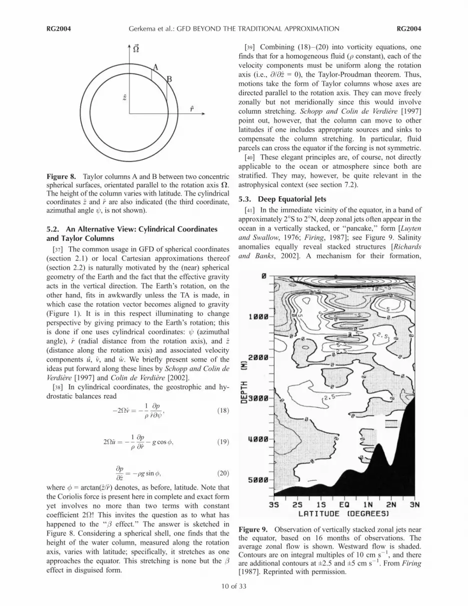
5.3. Deep Equatorial Jets

[41] In the immediate vicinity of the equator, in a band of

approximately 2�S to 2�N, deep zonal jets often appear in theocean in a vertically stacked, or ‘‘pancake,’’ form [Luyten

and Swallow, 1976; Firing, 1987]; see Figure 9. Salinity

anomalies equally reveal stacked structures [Richards

and Banks, 2002]. A mechanism for their formation,

Figure 8. Taylor columns A and B between two concentricspherical surfaces, orientated parallel to the rotation axis W.The height of the column varies with latitude. The cylindricalcoordinates z and r are also indicated (the third coordinate,azimuthal angle y, is not shown).

Figure 9. Observation of vertically stacked zonal jets nearthe equator, based on 16 months of observations. Theaverage zonal flow is shown. Westward flow is shaded.Contours are on integral multiples of 10 cm s�1, and thereare additional contours at ±2.5 and ±5 cm s�1. From Firing[1987]. Reprinted with permission.


10 of 33

RG2004

employing a stability argument, was proposed by Hua et al.

[1997], following the analysis by Emanuel [1979] on

mesoscale convective systems in the atmosphere. Both

considered an equatorial zonal jet �u, uniform in the zonal

direction, and examined the instability problem. So-called

inertial instabilities can arise if fQE � 0, where QE is the

Ertel potential vorticity, which depends on the stratification,

the Coriolis parameters f and ~f , and the meridional and

vertical shear of �u. Analytical and numerical results by Hua

et al. [1997] show that the instability manifests itself as a

stacked structure of equatorial zonal jets. Later observations

possibly confirm this mechanism [Send et al., 2002; Bourles

et al., 2003]; the condition for instability, at least, is

fulfilled. The specific role (and importance) of ~f in this

mechanism has not yet been clarified.

[42] We note that the deep jets are actually more complex

than Figure 9 might suggest. Dengler and Quadfasel [2002]

showed that they also involve significant meridional

currents and, moreover, vary considerably in time. One

may speculate that the deep jets are in some way linked to

the deep western boundary current, for Richardson and

Fratantoni [1999] found that floats sometimes follow this

deep current across the equator but are at other times carried

eastward parallel to the equator, typically between 2� and

4�N/S, while floats in the immediate vicinity of the equator

are carried westward. In numerical model calculations,

d’Orgeville et al. [2007] found that oscillations in the

western boundary current may provoke mixed Rossby-

gravity waves, whose instability subsequently leads to

equatorial deep jets. An alternative line of explanation was

pursued by Dengler and Quadfasel [2002], who showed

that an interpretation in terms of (traditional) equatorial

Rossby waves fits the data on deep jets reasonably well.

Still another hypothesis on the origin of deep jets, namely,

the development of mean flows by internal wave focusing,

is discussed in section 6.2.2.

[43] We finally note that stacked equatorial jets have

equally been observed in the mesosphere at heights of

around 50 km. Following Hua et al. [1997], Fruman

[2005] developed a theory for the atmospheric case and

found from the stability analysis that ~f makes the basic jet

more unstable. This underlines the importance of abandon-

ing the TA in the equatorial region.

6. INTERNAL WAVES

[44] Internal waves are oscillatory motions whose largest

amplitudes occur in the interior of the fluid; they are an

ubiquitous phenomenon in the oceans and atmosphere. Here

buoyancy and the Coriolis force act as the restoring forces.

This lends a key role to the three parameters associated with

these forces: the buoyancy frequency N (being a measure of

the density stratification), the Earth’s angular velocity W,and latitude f. The buoyancy frequency is defined as

N2 ¼ � g

r0

dr0dz

þ r0gc2s

� �: ð21Þ

[45] Here cs is the speed of sound, and r0(z) is the static

in situ density field. (Under the Boussinesq approximation,

the r0 in the denominator is replaced with a constant

reference value of density, r*.) For buoyancy (gravity) to actas a restoring force, the fluid must be stably stratified, i.e.,

N2 > 0. In the lower atmosphere, values range from 0.01

(troposphere) to 0.02 rad s�1 (stratosphere). In the ocean,

values of N can be as high as 10�2 rad s�1 (seasonal

thermocline), but they are much lower in the deep ocean,

typically in the range 3 � 10�4 to 2 � 10�3 rad s�1. An

example is shown in Figure 10 for a latitudinal section; here

N is scaled with 2W. We note that the condition N � 2W (on

which the TA implicitly hinges, as will be discussed below)

is not satisfied in the deepest layers of the ocean.

[46] In the atmosphere, internal waves are particularly

important in relatively strongly stratified layers such as the

stratosphere [Fritts and Alexander, 2003]. In the ocean, they

have vertical amplitudes as large as tens, or even hundreds,

of meters and periods that range, roughly, from minutes to

days. However, most of their energy is contained at low

frequencies, especially at the tidal and near-inertial

frequencies. In recent years, much attention has been paid

to their role in (deep) ocean mixing [see, e.g., Garrett and

St. Laurent, 2002].

[47] The significance of the parameters N (regarded as a

constant for the moment), W, and f to the dynamics of

internal waves can be most easily appreciated by looking at

the range of allowable frequencies. Internal waves of a

given frequency do not necessarily exist at all latitudes;

propagating poleward, they may encounter a ‘‘turning’’ or

‘‘critical’’ latitude fc, beyond which they cannot propagate

as a free wave. An expression for fc was derived by Hughes

[1964] [see also LeBlond and Mysak, 1978]:

fc ¼ � arcsinw2

4W2� w2

N2

w2

4W2� 1

� �� 1=2; ð22Þ

where w is the internal wave frequency; the plus (minus)

sign applies to the Northern (Southern) Hemisphere. This

expression is based on the full Coriolis force. Making the

TA amounts to taking N ! 1 in (22), so that the turning

latitude shifts to the inertial latitude, i.e., the latitude at

which the wave frequency equals the inertial frequency jfj:

fi ¼ � arcsinw2W

� �: ð23Þ

The distance between the ‘‘nontraditional’’ critical latitude

(22) and the ‘‘traditional’’ version (23) is very substantial in

the weakly stratified abyssal ocean, as is illustrated in

Figure 19 (discussed in section 6.2.1); near-inertial waves

can propagate much farther poleward in the former case.

[48] For weak stratification, the difference between the

two is further illustrated in Figure 11, where stratification

increases from zero (Figure 11a) to 4W (Figure 11d). The

former value is representative of convective layers; the latter

is found in the deepest parts of the ocean (dark blue regions

in Figure 10). The grey area indicates the range of internal


11 of 33

RG2004

Figure 11. Internal wave frequency range as a function of latitude, stratification increasing from (a) N =0, (b) N = W, (c) N = 2W, to (d) N = 4W. The boundaries of the range (depicted in grey) are indicated bysolid curves, representing (22). For comparison, the range as obtained under the TA is also shown(dashed lines and dotted regions).

Figure 10. Relative strength of stratification, N/2W, derived from temperature and salinity profiles inthe Pacific Ocean for a south-north section near 179�E (WOCE section P14 from the Fiji Islands to theBering Sea). These profiles were used to calculate, via the equation of state for the Gibbs potential, in situdensity r0 and the speed of sound cs, and hence N2 = g2(dr0/dp � cs

�2), being equivalent to (21).Smoothing was applied by taking the running mean over 15 pressure levels (�30 m); incidental pointswhere N2 < 0 were then set to zero. Note the logarithmic color scaling. In the deepest layers (dark blue),the ratio N/2W is fairly low; here nontraditional effects can be expected to significantly affect internalwave dynamics; the same applies to the upper mixed layer.


12 of 33

RG2004

wave frequencies, being enclosed by the solid curves

calculated from (22). In Figures 11a–11d, the range

under the TA is shown as well (dotted region), enclosed

by the inertial latitude fi at one side (the dashed curve,

being the same in all plots since fi is independent of

stratification) and by N (vertical dashed line) at the

other side. Figure 11 clearly demonstrates that the TA

reduces the range of allowable frequencies at all latitudes

(except the poles). Furthermore, it either introduces a

turning latitude where none exists if the TA is not made

(Figures 11a and 11b) or shifts it to the lower, inertial

latitude (Figures 11b–11d).

[49] In Figure 11a, gravity cannot act as a restoring force

because N = 0, leaving the Coriolis force as the sole

restoring force. Internal waves are then usually referred to

as gyroscopic or inertial waves. The latter term is not to be

confused with the so-called inertia oscillation, a circular

oscillation strictly at w = j f j; for this reason, we shall adoptthe former term, following Tolstoy [1963] and LeBlond and

Mysak [1978]. Overall, the allowable frequencies of

gyroscopic waves cover the whole range from zero to 2W.They can exist at all latitudes if the TA is not made (grey

area in Figure 11a); the TA reduces their habitat to the

region poleward of the inertial latitude (i.e., above the

dashed curve).

[50] In sections 6.1 and 6.2, we consider the effect of the

TA on internal waves in more detail, with increasing

geometric complexity. The simplest approach is to assume

that the whole dynamics takes place at a fixed latitude

(f plane); one key result here is the existence of a low-

frequency short-wave limit, which disappears under the TA.

In reality, of course, waves propagating in the meridional

direction undergo a variation in latitude, a particularly

important effect for waves having a frequency close to j f j(near-inertial waves). To a first approximation, this effect

can be included by using the b plane. One can then study

what happens when a near-inertial wave approaches its

turning latitude. A key result, discussed in section 6.2.1, is

that in spite of its name, internal wave energy may

accumulate at the ‘‘turning’’ latitude; this effect disappears

under the TA.

[51] A still higher degree of complexity arises when one

considers a thick spherical shell, as is usually necessary in

the case of giant planets and rotating stars, or the Earth’s

liquid outer core. The metric terms then come fully into

effect, accounting for the different curvature of concentric

shells. Moreover, the variation of gravity g with radial

distance needs to be included. This modifies N in (21); for

example, if one regards the part in brackets as a constant,

then N2 still varies linearly with radius r via g. This leads to

a modification of the picture presented in Figure 11, where

N was assumed constant; there the turning latitude

(belonging to a given wave frequency) was the same

throughout the water column. In the general case of a (thick)

spherical shell, a dependence on depth arises. Specifically,

Friedlander and Siegmann [1982] and Dintrans et al.

[1999], using the full Coriolis force throughout, introduced

a classification by distinguishing w < 2W and w > 2W; in the

former case, the turning surfaces are of hyperboloidal shape

(‘‘H modes’’); in the latter, they are ellipsoidal (‘‘E

modes’’). A further distinction is made between w < N

(H2 and E1) and w > N (H1 and E2). These modes, of

course, also appear in Figure 11, even though the

curvature of the turning surfaces is extinguished by the

implicit assumption of a thin shell. For example, in Figure

11a, there are only H1 modes, while in Figure 11d, there

are three modes: H2 (w < 2W), E1 (2W < w < N), and E2

modes (N < w < (N2 + 4W2)1/2). However, in the terrestrial

case, the ellipsoidal turning surface E1 lies inside the

‘‘solid’’ Earth, and for this reason no turning latitude is

found in that regime unlike for E2.

6.1. Internal Waves on the (Nontraditional) f Plane

[52] For later reference, we start with a concise overview

of the linear internal wave theory on the ‘‘nontraditional’’ f

plane, bringing together elements that are somewhat

scattered in the literature [Tolstoy, 1963; O. M. Phillips,

1966; Saint-Guily, 1970; LeBlond and Mysak, 1978;

Brekhovskikh and Goncharov, 1994; Miropol’sky, 2001].

6.1.1. Summary of Linear Internal Wave Theory[53] The momentum equations (8–10) are used with

b = 0. The advective terms are neglected as we assume

wave amplitudes to be infinitesimal (linear theory).

Together with the continuity and energy equations (under

the Boussinesq approximation), wave solutions of the form

exp iwt (with wave frequency w > 0) are then found to be

governed by

A*@ 2w

@y2þ 2B*

@ 2w

@y@zþ C

@ 2w

@z2þ D

@2w

@x2¼ 0 ð24Þ

where A* = N2� w2 + ~f 2, B* = f~f , C = f 2� w2, andD = N 2�w2. The presence of ~f has two important consequences.

First, it introduces a mixed derivative (the term with B*),

thereby changing the character of the partial differential

equation; second, it makes the roles of x and y dissimilar

(since B* 6¼ 0 and A* 6¼ D), implying anisotropy in the

horizontal plane. Both effects disappear under the TA.

Strong stratification (N � 2W) diminishes the role of ~f in

A* but does not affect the presence of the mixed derivative.

Phillips [1968] already pointed out that ~f ‘‘may enter

significantly in the finer details’’ even when N � 2W. Aswill become clear in sections 6.1.2 and 6.2, ‘‘finer’’ can be

taken literally here: short-scale wave patterns arise at

subinertial frequencies (i.e., lower than j f j) that wholly

disappear under the TA.

[54] Assuming plane waves traveling in a direction anorth of east, i.e., along the direction of increasing c =

xcosa + ysina, (24) reduces to

A@ 2w

@c2þ 2B

@ 2w

@c@zþ C

@ 2w

@z2¼ 0; ð25Þ

with A = N2 � w2 + fs2 and B = ffs; here fs = ~f sina. For

wave propagation to be possible, hyperbolicity is required,


13 of 33

RG2004

i.e., B2 � AC > 0; this inequality provides the upper and

lower bounds of the frequency domain of internal waves:

wmin;max ¼1ffiffiffi2

p

� N2 þ f 2 þ f 2s�

� N2 þ f 2 þ f 2s� 2� 2fNð Þ2h i1=2� 1=2

:

ð26Þ

For meridional propagation (a = p/2), we have f 2 + fs2 =

4W2. Equation (26) can then be rewritten such that f is

expressed in terms of the frequencies w, W, and N; this

yields the critical latitude fc already mentioned in (22): the

extremes of the frequency domain are reached precisely atfc (Figure 11). For zonal propagation (a = 0), on the other

hand, the upper and lower bounds (26) become identical

to those found under the TA, namely, min{j f j, N}< w <

max{j f j, N}.[55] For a strongly stratified fluid (N � 2W), (26) can be

approximated by

wmin ¼ jf j 1� f 2s2N2

þ OW4

N4

� �� ;

wmax ¼ N 1þ f 2s2N2

þ OW4

N4

� �� ;

where the last term in each equation represents the order of

magnitude (O) of the higher-order terms. Thus, in this limit,

the lower and upper bounds approach the traditional values.

However, as illustrated in Figure 10, the condition N � 2Wis not satisfied in the deeper layers of the ocean, and here

nontraditional effects can be expected to be important.

[56] There are two main roads to solve (25). For constant

stratification (N = const), all coefficients are constant, and

the general solution can be written

w ¼ F xþ�

þ G x�ð Þ; ð27Þ

where F and G are arbitrary functions and x± = m±c � z are

the characteristic coordinates, with

m� ¼ B� B2 � ACð Þ1=2

A: ð28Þ

Internal wave energy propagates along the characteristics

x+ = const or x� = const; examples are sketched in Figure 12

for different frequency regimes.

[57] The dispersion relation can be derived by substitut-

ing w = exp i(kc + mz) in (25). Writing the wave vector as

(k, m) = k(cosq, sinq) then gives the dispersion relation

w2 ¼ N2 cos2 qþ fs cos qþ f sin qð Þ2: ð29Þ

As under the TA, the wave frequency depends on the

direction q of the wave vector but not on its length k, whichimplies that the group velocity vector (@w/@k, @w/@m) must

be perpendicular to the wave vector, as is illustrated in

Figure 13 for gyroscopic waves. (This is borne out by the

identity m± = �cotq, which follows from (29).) For the fully

three-dimensional case (24), the dispersion relation is

discussed by LeBlond and Mysak [1978], in which case,

surfaces of constant wave frequency are cone-like. Here,

too, the dispersion relation leaves the magnitude of the

wave number (k) undetermined; an external length scale

needs to be introduced to specify wave numbers. The size of

a body force may serve this purpose. Notice also that the

relations derived so far implicitly assume a medium of

infinite extension. Once one introduces a horizontal bottom

and surface (and hence the external scale, water depth), a

discrete set of wave numbers appears with specific length

scales, as, for example, in (32).

[58] So far, we assumed N to be constant. If N varies with

the vertical z, (27) no longer provides a solution. The

underlying reason is that the inhomogeneity of the medium

causes internal reflections, so the wave energy no longer

stays on the same characteristic in the interior of the fluid.

However, if the fluid is contained between two horizontal

boundaries (an even bottom below and a ‘‘rigid lid’’ above),

a solution may be obtained in terms of vertical modes for

arbitrary N(z). These modes Wn, with mode number n, are

found by substituting

w ¼ W zð Þ exp ik c� Bz=Cð Þ ð30Þ

into (25), which yields

d2W

dz2þ k2

B2 � AC

C2

� �W ¼ 0: ð31Þ

Figure 12. An example of ‘‘nontraditional’’ characteristics, showing the direction of energy

propagation in the meridional/vertical plane (poleward to the right) for the regime j f j < (N2 + fs2)1/2.

Three different cases are shown (left to right): j f j < w < (N 2 + fs2)1/2, w = j f j, and w < j f j. Note the

change in orientation of the characteristic x� as it goes from superinertial to subinertial. Under the TA(not shown), only the superinertial case would exist, with then x+ and x� of equal steepness. FromGerkema and Shrira [2005b]. Reprinted by permission from Cambridge University Press.


14 of 33

RG2004

Together with the boundary conditions W = 0 at z = �H,0

(bottom and surface), this constitutes a Sturm-Liouville

problem. Its solution is formed by a set of eigenvalues knand corresponding eigenfunctions Wn, whose form depends,

of course, on N(z). Importantly, (30) contains two types of z

dependences, unlike under the TA, where B = 0. Indeed, the

nonseparable nature of the solution, due to the presence of

the mixed derivative, becomes apparent if one takes the real

part of (30).

6.1.2. Properties of Internal Inertiogravity Waves[59] In the ocean and lower atmosphere, one generally has

N > 2W. Under the TA, the lower bound of the frequency

range is then j f j. In the ‘‘nontraditional’’ equation (26), by

contrast, the lower bound lies slightly below j f j (see also

Figure 11d). So there is a class of subinertial internal

inertiogravity waves (wmin < w < j f j), which wholly

disappears under the TA. They were examined in the

oceanic context [Saint-Guily, 1970; Badulin et al., 1991;

Brekhovskikh and Goncharov, 1994; Gerkema and Shrira,

2005b] and recently also in the atmospheric context

[Thuburn et al., 2002b; Kasahara, 2003a, 2003b, 2004;

Durran and Bretherton, 2004]. This class of waves appears

under various names in the literature; Durran and

Bretherton [2004] rightly emphasized that despite the

distinctive properties of these waves, the restoring forces

at work are just buoyancy and rotation (possibly combined

with elastic forces in compressible fluids) and that they can

exist in the absence of boundaries; in these respects, they

are no different from traditional internal inertiogravity

waves.

[60] There are two possible regimes, depending on which

of the two, j f j or (N 2 + fs2)1/2, is the largest. For the regime

j f j < (N 2 + fs2)1/2, the dispersion relation (29) is shown in

Figure 14a. Segments where the frequency increases

(decreases) as a function of q correspond to propagation

along a m+ (m�) characteristic. The wave vector and group

velocity vector are either vertically or horizontally opposed

but not both (Figures 14b and 14c). In Figure 14a, dotted

lines are drawn at two frequency levels: w = (N2 + fs2)1/2 and

w = j f j; these are precisely the values at which the

coefficients A and C in (25) change sign, respectively. Their

special significance is furthermore seen from the simple rule

that one can distill from Figure 14: for the m+ characteristic,

the wave vector and group velocity are vertically opposed for

wmin < w < (N2 + fs2)1/2 and horizontally opposed for (N2 +

fs2)1/2 < w < wmax; for the m� characteristic, they are vertically

opposed for j f j < w < wmax and horizontally opposed for wmin

< w < j f j. A similar kind of rule can be derived for the other

regime, (N2 + fs2)1/2 < j f j. This variety of behavior is to be

contrasted with the traditional limit (fs = 0), where one finds

that they are always vertically opposed in the ‘‘strongly’’

stratified regime (i.e., j f j < N) and always horizontally

opposed in the ‘‘weakly’’ stratified regime (N < j f j).[61] In a vertically bounded domain, energy needs to

propagate both upward and downward, and this results in a

combined role of the characteristics, one taking over from

the other at the boundaries. (An example for N = 0, i.e.,

gyroscopic waves, is shown in Figure 13.) One can

alternatively obtain a solution in terms of modes from

(31). For constant N, this yields the following dispersion

relation:

kn ¼� np=Hð Þ w2 � f 2ð Þ

w2 � w2min

� w2max � w2

� � �1=2 : ð32Þ

This relation, as well as that of the horizontal component of

the group velocity, is shown in Figure 15. As usual, waves

become short at the upper bound wmax. Importantly, here

they also become short at the lower bound wmin; we refer to

this phenomenon as the subinertial short-wave limit. It

affects not only the horizontal scale but also the vertical one

via the second vertical dependence in (30). This subinertial

short-wave limit is present no matter how strong the

stratification is, but it disappears under the TA; in this sense,

the TA has the character of a singular limit. Another

important feature is the smooth passage through j f j (seeFigure 15); such a transition occurs when low-frequency

waves move to higher latitudes, so that j f j increases, andthe waves may turn from superinertial into subinertial. This

is discussed in section 6.2.1.

[62] For variable N(z), another property of subinertial

waves emerges. Brekhovskikh and Goncharov [1994] noted

that their habitat lies in weakly stratified regions; for a given

Figure 13. Characteristics for gyroscopic waves (N = 0) ina vertically confined basin for (a) subinertial frequencies(w < j f j) and (b) superinertial frequencies (w > j f j). Here,energy propagates upward along solid lines and downwardalong dotted-dashed lines. The direction of phase propaga-tion, which is perpendicular to energy propagation, isindicated by solid and dotted-dashed arrows, respectively.The TA is not made, so the rotation vector W is not aligned tothe vertical. Under the TA, only the case in Figure 13a wouldexist but then with symmetric propagation with respect tothe vertical. From Durran and Bretherton [2004].


15 of 33

RG2004

subinertial wave frequency, stratification needs to be

sufficiently weak for them to exist, a consequence of (26).

For example, with N2 linearly decreasing downward with z,

the subinertial vertical modes can be solved from (31) in

terms of Airy functions, which are oscillating in the deepest

part of the water column and fall off exponentially above it,

where stratification is higher. They are thus trapped in the

weakly stratified abyss (Figure 16).

[63] The results presented here demonstrate clearly that

abandoning the TA does not pose any mathematical hurdle

as long as we consider internal waves on the (nontraditional)

f plane. The theory can be extended to the treatment of

internal wave reflection from sloping boundaries [Gerkema

and Shrira, 2006; Gerkema, 2006]. For nontraditional

effects in critical layer absorption, see Grimshaw [1975a].

There have been some ‘‘nontraditional’’ numerical studies

on internal waves [Beckmann and Diebels, 1994; Kasahara

and Gary, 2006], illustrating the properties discussed above.

Baines and Miles [2000] recommend that the horizontal

component ~f be included in internal tide generation models;

they found that the component causes a small increase in the

conversion rate from barotropic to baroclinic tidal energy, as

well as a change in the paths of energy propagation. Both

features are illustrated for a realistic setting in Figure 17,

based on recent numerical model calculations.

6.1.3. Observations[64] Current measurements in the ocean provide infor-

mation on the polarization of the horizontal velocity field.

From the general expressions of Gerkema and Shrira

[2006], one can derive the following relation for plane

waves propagating at an angle a with respect to the east:

jv0j=ju0j ¼ j fsm� � fð Þ=wj: ð33Þ

Figure 14. Dispersion relation (29) for internal inertiogravity and related quantities for the regime j f j <(N2 + fs

2)1/2. (a) Wave frequency versus q, the angle of the wave vector with the horizontal. Segmentswhere w increases (decreases) correspond to the characteristic m+ (m�). (b) Horizontal and verticalcomponents of the wavevector (normalized), also as a function of q. (c) Components of the groupvelocity factor (multiplied by w and normalized). Parameter values are f = 45�N and a = p/2; for optimalclarity, N has been chosen to be only marginally larger than 2W (N = 1.5 � 10�4 rad s�1).

Figure 15. Dispersion relation in a vertically boundedsystem, equation (32), for plus and minus signs (solid anddashed lines, respectively). (a) Wave frequency as a functionof the horizontal wave number kn. (b) Horizontal componentof the group velocity. Thick lines represent the nontradi-tional dispersion relation; thin lines represent dispersionunder the TA ( fs = 0). Horizontal and vertical dotted linesrepresent zero axes. After Gerkema and Shrira [2005b].Reprinted by permission from Cambridge University Press.


16 of 33

RG2004

Here ju0j denotes the amplitude of the velocity in the

direction of wave propagation, and jv0j denotes the

amplitude of the velocity in the perpendicular direction.

Unlike under the TA, the polarization is not the same for the

characteristics m+ and m�. For example, at the inertial

frequency w = j f j, the m� corresponds to circular polariza-

tion (as under TA), but m+ corresponds to an ellipse-like

polarization, whose eccentricity depends on stratification N.

An interesting test case for (33) is the observation in the

Mediterranean by van Haren and Millot [2004]; they band-

pass filtered their current meter data around f; see Figures 18b

and 18c. Although the stratification varies with time (see

especially the change in the ‘‘steps’’ above 1500 m), the

ambience of the upper current meter at 1800 m was

significantly stratified throughout (N � 2–3 f ), while

stratification was extremely weak at 2700 m (N � 0–0.4f ),

where the lower current meter was placed. Vertical

propagation of near-inertial energy can occur only via the

x+ characteristic (see Figure 12 (middle)), so we use m+ in

(33). One then finds that in the stratified layer at 1800 m,

theory predicts a ratio of major to minor axis between 1.24

and 1.34. (The error range stems from the dependence on the

horizontal direction of wave propagation a, which can only

approximately be inferred from the observations.) The

observed value derived from Figure 18b lies between 1.25

and 1.5 in good agreement with the theoretical range. The

ratio is much larger in the near-homogeneous layer at 2700 m

(Figure 18c): 3.2–4.2 (theory) against the observed value of

2–3.5. Another nontraditional effect is the occurrence of a

significant vertical velocity component at near-inertial

frequencies, which has also been observed [van Haren and

Millot, 2005].

[65] The coexistence of nearly unstratified layers (N 2W) with significantly stratified ones, as, for example, in

Figure 18a, raises the question of whether they may act as

waveguides for internal waves of a given frequency. The

answer depends strongly on whether one makes the TA or

not [van Haren, 2006]. Under the TA, there is no overlap at

all between the frequency range for gyroscopic waves

occurring for N = 0, i.e., 0 < w < j f j, and that for

inertiogravity waves in layers with N > j f j, i.e., j f j < w < N.

In other words, internal waves existing in one layer cannot

penetrate the other layer. By contrast, if one abandons the

TA, an overlap between the regimes exists, which covers at

least a range of near-inertial frequencies (see Figures 11a

and 11d). The very existence of near-inertial waves in both

layers, as demonstrated in Figures 18b and 18c, thus lends

support to the ‘‘nontraditional’’ theory. The transition

between gyroscopic and inertiogravity waves is important

in the astrophysical context as well; see section 7.1.

[66] We note that near-inertial waves seem to undergo a

change in polarization (from predominantly circular to

rectilinear) within a narrow band across the equator [van

Haren, 2005]; one would expect this to be due to

nontraditional effects, but (33) does not, in fact, predict

such a transition. Possibly a more complete description,

including the equatorial b effect, is needed to explain the

observed features, but this has not yet been examined.

6.2. Internal Waves Subject to Latitudinal Variation

[67] Section 6.1.2 makes clear that the lower bound wmin

acts as a short-wave limit if the TA is abandoned. One can

therefore expect a short-wave singularity to occur at the

turning latitude, and this is indeed a recurring theme in the

remainder of this section.

Figure 16. An example in which the buoyancy frequency N decreases in the downward direction,mimicking the slow decrease of N with depth in the abyssal ocean. Subinertial modes are now trapped inthe region of weakest stratification. The amplitude of the vertical velocity is shown (subject to anarbitrary scale factor) for a superposition of five modes. From Gerkema and Shrira [2005b]. Reprinted bypermission from Cambridge University Press.


17 of 33

RG2004

6.2.1. Propagation on the b Plane[68] Latitudinal variation of the Coriolis parameter f is

important to near-inertial waves, even though their

horizontal length scales are fairly small compared to the

radius of the Earth. The reason is that they may over a short

distance turn from superinertial to subinertial or vice versa.

To describe these effects in the simplest possible way, one

adopts the b plane as described in section 2.2; here f = f0 + by varies linearly with the meridional coordinate y, while ~f istaken to be constant. Since nontraditional effects are strongest

for propagation in the meridional direction, we examine only

this case. The generalization of (25) then becomes

N2 � w2 þ ~f 2�

yyy þ 2f ~f yyz þ f 2�;w2�

yzz þ ~f byz ¼ 0; ð34Þ

[Gerkema and Shrira, 2005a] where we introduced the stream

functiony: v =yz andw =�yy. (For a more general version in

terms of spherical coordinates, see Needler and LeBlond

[1973]). Thus, the generalization from (25) into (34) consists

simply in replacing the constant f in (25) by the y-dependent

f(y) in (34) and in adding one new term, the last one on the left-

hand side of (34).

[69] Equation (34) can be simplified for certain regions.

Near the equator, f0 � 0 so that f can be replaced by bythroughout (section 6.2.2). For near-inertial waves propa-

gating outside the near-equatorial band, on the other hand,

we can make the following approximations. The variation

with latitude matters here only because of the proximity of

j f j to wave frequency w; apart from that, the b effect can be

neglected. Now, the difference j f j � w occurs only in one

place in (34), namely, in the the factor f 2 � w2, which we

may approximate by f02 � w2 + 2f0b y. Hence (34) becomes

Ayyy þ 2Byyz þ C þ 2f0byð Þyzz ¼ 0 ; ð35Þ

with A = N2 � w2 + ~f 2, B = f0 ~f , and C = f02 � w2.

Characteristics are now defined by

dz

dy¼ B� B2 � A C þ 2f0byð Þ½ �1=2

A:

Even though the medium is now inhomogeneous because of

b, and possibly also because of N(z), we will assume that

these variations are sufficiently weak in the sense that

Figure 17. Amplitudes of isopycnal excursions z (in m) from a linear internal tide generation model,using observed stratification and topography (Bay of Biscay). (a) Original model, described by Gerkemaet al. [2004], hydrostatic and using the TA. (b) Inclusion of nontraditional terms, giving a quasi-hydrostatic version. In both plots, the asterisks show at what depth maximum excursions occur accordingto in situ observations by Pingree and New [1991]. Overall, the nontraditional model run gives a bettercorrespondence with these observations, the downgoing beam originating from the shelf break beingsteeper and the bottom-reflected one being less steep than under the TA. The conversion rate (CR), orenergy flux, is increased by nontraditional effects by 4.5%.


18 of 33

RG2004

internal wave energy propagates along the characteristics

without the occurrence of any internal reflections (geome-

trical-optics approach). An example of such a propagation is

shown in Figure 19, where the stratification follows an

exponential profile, decreasing with depth. The wave

energy enters the domain from the outer left, where the

wave is slightly superinertial (w > j f j). As the wave

propagates to the right, i.e., poleward, the Coriolis

parameter j f j increases and at y = 0 becomes equal to the

wave frequency w. At this point, the inertial latitude, the

wave reflects under the TA (thin line). However, with ~fincluded (thick line), the wave can propagate beyond the

inertial latitude and becomes subinertial. This gives rise to

the two phenomena that were discussed in section 6.1.2:

First, the more poleward the wave gets, and hence the more

subinertial, the closer it stays to the bottom; this is because

the subinertial wave can only exist in sufficiently weakly

stratified regions. Second, the length scale becomes shorter,

in which we recognize the subinertial short-wave limit that

comes into effect as the wave frequency approaches its

lower bound. These two elements are interesting in view of

the important topic of deep-ocean mixing, but this aspect

has not yet been fathomed, although Walter et al. [2005]

speculated that they may help explain latitudinal variations

in abyssal vertical diffusivities. In any case, the mechanism

would result in an enhancement of near-inertial energy in

the deepest parts of the water column, a phenomenon that

has been observed in some internal wave spectra [van

Haren et al., 2002; van Aken et al., 2005].

6.2.2. Near-Equatorial Region[70] Not all waves are trapped at the turning surface

though; part of them reflect back toward the equator and

may enter the other hemisphere and approach the opposite

turning surface. While reflecting from surface, bottom, and

turning surfaces, the waves still focus their energy but now

onto one or two limit cycles that are present around the

equator in between the turning surfaces. These periodic

orbits act as ‘‘wave attractors,’’ on which wave energy

accumulates regardless of the exact source location. The

location of these wave attractors appears to have a fractal

dependence on a lumped parameter containing wave fre-

quency, stratification rate, rotation rate, and the fluid

domain’s aspect ratio [Maas and Harlander, 2007]. The

trapping that was observed on the b plane (section 6.2.1),

near the intersection of turning surface and bottom, can be

considered as a special, degenerate case of a (point) wave

attractor.

[71] Historically, the discovery of the equatorial wave

attractor proceeded in a few steps, which were carried

through without applying the TA. Stern [1963] examined

the dynamics of a homogeneous fluid on a nontraditional

equatorial b plane, which is governed by (34) with N = 0

and f0 = 0. In terms of scaled coordinates, he arrived at a

simplified version by exploiting the fact that the resulting

equation can be factorized:

@

@y� s � yð Þ @

@z

� �@

@yþ s þ yð Þ @

@z

� �y ¼ 0; ð36Þ

where s is a rescaled and dimensionless version of the wave

frequency. Taking Y = 4 y s and Z = 2(2z � y2 � s2)transforms (36) into the hyperbolic spatial wave equation

yYY � yZZ = 0 (employing the subscript-derivative

notation), which is to be solved subject to the requirement

of vanishing stream function at the boundary. As such, this

problem is ill-posed; conditions under which it becomes

Figure 18. Observations from the Mediterranean. (a) Potential density profiles, showing a layer of veryweak stratification below 2100 m. Hodographs based on near-inertial band-pass-filtered current meterdata (u east and v north) at (b) 1800 m (where N � 2.5 � f ) and (c) 2700 m (N � 0). After van Haren andMillot [2004]. Reprinted by permission from Elsevier, copyright 2004.


19 of 33

RG2004

well posed are described by Maas and Harlander [2007].

The general solution, in terms of the original coordinates,

is formed by a superposition of the arbitrary functions

F[(y ± s)2/2 � z]. Stern deduced that the waves are

equatorially trapped for some frequencies. Bretherton

[1964] realized that Stern’s solution might be related to

the occurrence of certain closed raypaths for low-

frequency internal (i.e., gyroscopic) waves in an unstrati-

fied spherical shell. These waves reflect from the

boundaries while retaining their inclination relative to the

rotation axis, and periodic paths were obtained for

particular frequencies; examples are shown in Figure 20.

This was indeed confirmed by Stewartson [1971, 1972a,

1972b], who showed that these periodic rays were actually

attracting. Israeli [1972] subsequently showed that these

wave attractors arose not just for special frequencies but

over continuous frequency intervals. The occurrence of

attractors is borne out by exact solutions of the Stern

equation, an example of which is shown in Figure 21.

[72] Restoring stratification, the waves are spatially con-

fined to reside within turning surfaces, across which the

character of the governing differential equation changes

from hyperbolic to elliptic [Friedlander and Siegmann,

1982]. Dintrans et al. [1999] observed that wave attractors

are ubiquitous in this setting and that trapping may now also

occur in the form of point attractors at the intersections of

turning surface and inner shell, an example of which was

shown in Figure 19.

[73] The notion of a wave attractor is not specific to the

equatorial shell per se. In fact, it arises in any geometry

where reflecting boundaries break the symmetry imposed

by the restoring forces [Maas, 2005]. As shown by (29), the

frequency fixes the direction into which wave energy

propagates, and only in oversymmetrized geometries (e.g.,

boundaries either parallel or perpendicular to net restoring

direction) will the reflection of the wave be such that

focusing (and defocusing) of wave rays can be avoided. It is

exactly this oversymmetrization of the geometrical setting

that the TA achieves by aligning the rotation axis to gravity.

In doing so, it also simplifies the mathematical structure of

the governing equation and boundary conditions by

allowing separation of variables. In this way, only large-

scale, regular standing wave structures arise. Dynamically,

the significance of dropping the TA thus lies in breaking this

reflectional symmetry [Maas, 2001]. But, it should be

mentioned that abandoning the TA is merely one way of

enforcing the solution to develop its generic behavior,

characterized by dominance of wave focusing and the

appearance of wave attractors with associated fine-scale

structure. Adding ‘‘topography’’ provides another instance

by which the reflectional symmetry is broken [Maas and

Lam, 1995].

Figure 19. Characteristics showing the direction of energy propagation for near-inertial waves on the bplane. The stratification decreases exponentially downward: N =N0exp(z/b), withN0 = 5.24� 10�3 rad s�1

and b = 1.3 km, the standard Garrett-Munk profile. The coordinate y denotes the meridional direction(poleward to the right). The position y = 0 corresponds to latitude 45�N; a fixed wave frequency w is chosensuch that it equals f at y = 0. Since f increases poleward, waves are superinertial (w > f ) for negative y andsubinertial (w < f ) for positive y. The transition between the two regimes occurs at y = 0, the inertiallatitude. It acts as a turning latitude under the TA (thin solid line). In the nontraditional case (thick solidline), however, wave energy can propagate beyond the inertial latitude, so that the wave becomessubinertial; it then gets trapped in the weakly stratified abyss, its wavelength becoming progressivelyshorter as it further penetrates the waveguide. After Gerkema and Shrira [2005a].


20 of 33

RG2004

[74] On approaching the wave attractors, small-scale

wave structures appear, which are susceptible to shear

instabilities and may lead to mixing. In a laboratory exper-

iment, Maas [2001] observed the development of a wave

attractor in a periodically perturbed rotating homogeneous

fluid, as illustrated in Figure 22a. (Here a sloping boundary

provided the symmetry breaking instead of nontraditional

effects.) A cyclonic mean flow coincided with its

appearance (Figures 22b and 22c). This mean flow was

present at all depths over the position where the internal

wave attractor reflects from a sloping boundary and was

attributed to the mixing of angular momentum that

accompanies the internal wave focusing. Maas [2001]

speculates that wave focusing onto an equatorial wave

attractor may equally drive such a cyclonic mean flow, which

may be partly responsible for the enigmatic equatorial deep

jets discussed in section 5.3. In this explanation, the

robustness of these jets is, on the one hand, due to the fact

that wave attractors exist simply because of the geometry of

the spherical shell in combination with the average

stratification and Earth’s rotation and, on the other hand, to

their ability to continuously collect and amplify waves within

the relevant frequency ranges from wherever these waves are

generated within a particular equatorial belt.

[75] Meridional flows associated with equatorially

trapped internal waves may have periods ranging from days

to semiannual, as was analytically shown by Raymond

[2000]; some of his wave solutions, moreover, were entirely

dependent on the inclusion of ~f . Equatorial Kelvin waves

(defined as having no meridional flow), too, are modified

when the nontraditional Coriolis terms are taken into account.

For a stratified fluid, Raymond [2001] showed that the

usual Gaussian decay with meridional distance from the

Figure 20. Examples of equatorially trapped gyroscopic waves in a spherical shell, illustrated byraypaths, along which their energy propagates. These patterns were later shown to act as wave attractors.From Bretherton [1964]. Reprinted by permission from Blackwell Publishing.

Figure 21. Example of an exact solution of the Stern[1963] equation (36), showing the stream function. Thisequation includes no stratification (N = 0). In the regioninside the wave attractor, banded flow structures can beobserved. The velocity is singular along the wave attractor.Here s = 0.9; Y and Z are transformed coordinates. AfterHarlander and Maas [2006]. Reprinted with permissionfrom E. Schweizerbart’sche Verlagsbuchhandlung, http://www.borntraeger-cramer.de/.


21 of 33

RG2004

equator now imposes a high-frequency cutoff. However, one

may infer that the waves remain regular only in a flat

equatorial channel-type geometry (bottom parallel to surface,

both perpendicular to gravity). Since the equation governing

the equatorial stream function is again of hyperbolic type, the

presence of a slope in the seafloor in zonal direction would

enforce again wave focusing and wave attractors but now in

the equatorial plane.

6.3. Intermezzo: Controversy Over Laplace’s TidalEquations

[76] In his doctoral thesis, Solberg [1928] carried out a

theoretical study on internal waves in a neutrally stratified

medium, i.e., N = 0; as before, we will refer to these waves

as ‘‘gyroscopic.’’ He included the full Coriolis force, so that

the range of allowable frequencies (26) becomes 0 < w < 2W(for meridional propagation), which includes both the

diurnal and semidiurnal tidal frequencies. The theoretical

discovery of these gyroscopic tidal waves prompted him

and collaborators to conclude that Laplace’s tidal equations

(LTE) are seriously deficient because they do not admit

wave solutions of this kind [Bjerknes et al., 1933; Solberg,

1936]. The point on the deficiency of the LTE was raised

independently by Brillouin and Coulomb [1933], who

examined gyroscopic waves in a rotating cylinder. (The LTE

are obtained from (5)–(7) by removing the nonlinear,

including metric, terms and making the hydrostatic

approximation.) The ensuing debate has been somewhat

clouded by confusion, perhaps fueled by a logical weakness

in the reasoning put forward by Bjerknes et al. After all, the

mere formal existence of gyroscopic waves of tidal

frequency does not in itself mean that they must be relevant

in the dynamic theory of tides; only if the latter were shown

to be the case, could we conclude that LTE are inadequate.

It is, furthermore, important to realize that the absence of

gyroscopic waves in LTE is primarily due to the hydrostatic

approximation, since in a nonhydrostatic setting they do

exist irrespective of whether the TA is made (although the

TA reduces the latitudinal range for any given frequency,

see Figure 11a). Now, Hylleraas [1939] brought in a new

element in the debate by noticing that Solberg [1936]

omitted the ocean’s vertical density stratification, the

inclusion of which, he argued, would render the nontradi-

tional Coriolis terms negligible. This point, while true

(provided N � W), concerns the TA and not the hydrostatic

approximation and hence has little bearing on the original

issue. But, gradually the debate drifted toward the validity

of the TA and the notion that stratification ‘‘saves’’ the LTE.

The importance of stratification was reiterated by Proudman

[1948] and Miles [1974]; a comprehensive overview on the

assumptions involved in LTE is given by Hendershott

[1981].

[77] Meanwhile, further insights were obtained in studies

ignoring stratification. Thus, for a homogeneous layer of

fluid (i.e., N = 0), Longuet-Higgins [1964] solved LTE and

obtained regular solutions of planetary waves in terms of

toroidal modes (also called Tesseral harmonics), lacking any

variation in radial direction. This solution presents the

lowest-order solution in an expansion in relative shell

thickness. The incompleteness of these modes was first

demonstrated by Stewartson and Rickard [1969] upon

continuing the expansion in shell thickness in this way

removing the TA underlying the LTE. They came to the

remarkable conclusion that for subinertial frequencies the

next-order fields develop a singularity around the inertial

latitude where the characteristics are grazing the inner

sphere. The singularity could partly be healed by adding

viscosity, but the fine-scale structure remained [Walton,

1975]. It thus transpired that the LTE normal mode is, in

fact, continuously leaking energy by generating a beam of

short-scale gyroscopic waves along the grazing character-

istics at the (critical) inertial latitude [Huthnance, 1978].

Numerical analysis confirmed the importance of the grazing

singularity for the dynamics of a thick homogeneous

spherical shell [Kerswell, 1995; Hollerbach and Kerswell,

1995; Rieutord and Valdettaro, 1997; Fotheringham and

Hollerbach, 1998]. This singularity exists along with wave

attractors that were also found. Additionally, quasiperiodic,

large-scale wave structures were encountered, familiar from

Figure 22. (a) Horizontal-vertical (x, z) distribution in aparticular (y) cross section of the amplitude of a gyroscopicwavefield (white, high; black, small). The waves are excitedin a homogeneous rotating fluid (rotation rate W) by weakmodulation at frequency w < 2W. It demonstrates thelocalization of wave energy at a wave attractor, whosepredicted location is given by solid lines. Here the rotationaxis is aligned to gravity, making the setting ‘‘traditional.’’However, the symmetry breaking that could otherwise bethe result of nontraditional effects is caused here by asloping bottom, giving rise to a wave attractor (Figure 22a)and a mean flow producing a dye distribution, seen fromabove (Figures 22b and 22c). (b) Initial distribution and(c) distribution after six wave periods. The sloping wall islocated in the upper part. Strong leftward dye displacementoccurs halfway over that slope, where the wave attractorreflects. From Maas [2001]. Reprinted by permission fromCambridge University Press.


22 of 33

RG2004

the gyroscopic wave modes that exist in a full sphere. But,

because of their fine structure, most of the physically

relevant dissipation was found to take place near the

singularities [Rieutord et al., 2001].

7. AN EXCURSION TO ASTROPHYSICAL FLUIDDYNAMICS

[78] In this section, we consider stars and giant planets.

Although the TA has its roots in geophysical fluid dynamics

and is much less commonly used in astrophysical fluid

dynamics, there are a few astrophysical subjects wherein it

has been adopted, either explicitly or implicitly. These are

stellar or planetary (tidal) oscillations and their dissipation

(section 7.1) and thermal convection (section 7.2).

7.1. Tidal Oscillations and Dissipation

[79] Surprisingly, the discussion of the influence of

rotation on free and (tidally) forced oscillations of stars

and giant planets has lagged behind compared to its

geophysical counterpart, but, in the last decade, the gap

has quickly narrowed. As to the TA, phenomena similar to

those discussed above are now also at the astrophysical

research front, extending even to general relativistic fluid

dynamics of neutron stars [Maniopoulou and Andersson,

2004]. Here we discuss the following subjects: first, tidal

forcing and dissipation of oscillations in slowly rotating

giant planets and stars, where ‘‘slowly’’ means a rotational

frequency W W cr, where W cr = (GM/R3)1/2 is the Kepler

or ‘‘breakup’’ frequency [Savonije et al., 1995; Savonije

and Papaloizou, 1997; Ogilvie and Lin, 2004]; and second,

free oscillations of a star [Dintrans and Rieutord, 2000].

Both Savonije et al. [1995] and Ogilvie and Lin [2004] give

a comparison of calculations using either the full Coriolis

acceleration or the TA. Savonije and Papaloizou [1997] and

Dintrans and Rieutord [2000] do not make the TA at all.

[80] For any star or planet, its radial equilibrium structure

is of paramount importance to the structure of its forced and

free oscillations. This is particularly true when it comes to

the effect of the TA on their qualitative properties or, more

specifically, on phenomena such as wave attractors, disper-

sion relations, and discrete or continuous spectra. Most

celestial bodies are built up by concentric shells of different

compositional and/or thermodynamic structure. In the pres-

ent discussion, each shell is considered either solid or fluid.

And if fluid, it is either marginally gravitationally unstable

in a convective regime (N = 0) or stable in a radiative

regime (N2 > 0); here N is the buoyancy or Brunt-Vaisala

frequency, essentially as defined in (21) (for the precise

definition in the astrophysical context, see Ogilvie and Lin

[2004]). As has already been illustrated in Figure 11, the

value of N relative to the rotational frequency W determines

the qualitative structure of the oscillations, and in a star this

may differ from shell to shell.

[81] Savonije et al. [1995] and Savonije and Papaloizou

[1997] discuss tidal forcing by its companion and tidal

dissipation of a massive, 20M� (i.e., 20 times the mass of

the Sun), ‘‘zero age main sequence’’ (ZAMS) star that is

part of a close binary. The radial shell sequence of such a

star, as chosen by these authors, is from the center outward:

a convective core, an extensive inner radiative envelope,

and a shallow outer convective envelope. The core and

radiative envelope are about 0.3 and 0.7 of the star’s radius

R; the outer convective envelope is of very small width but

yet of some importance to the problem at hand. In the

convective core and envelope, the relevant frequency

inequality is N � 0 < 2W; in the radiative shell, 2W N =

O(Wcr). Two regimes of forcing frequencies (in the rotating

frame) w are treated: superrotational (w > 2W) and

subrotational (w � 2W). Although the convective core and

envelope support only gyroscopic waves (as before, we will

refrain from using the common term ‘‘inertial waves’’) and

the radiative shell inertiogravity waves (or, in astrophysical

parlance, rotationally modified g modes), the shells cannot

be treated separately since both kinds exist at subrotational

frequencies. (Compare the overlap in grey regions in

Figures 11a and 11d for w < 2W, implying coupling. Under

the TA, by contrast, there is no overlap in the dotted regions

in Figures 11a and 11d and hence no coupling.)

[82] Indeed, for forcing in the subrotational regime, Savonije

et al. [1995] find that there are two dominant effects in the

tidal response with respect to applying the TA or not. If the

TA is not made, the response for the subrotational frequen-

cies gets swamped by very short wavelength resonances in

the convective core and the adjacent regions of the radiative

envelope, which in the core reaches amplitudes of several

times the equilibrium tide at the star’s surface. This singular

response is suppressed if the TA is applied. Moreover, if the

TA is not made, a subrotational response is found from

equator to pole, but applying the TA confines it to regions

poleward of the inertial latitude. These conclusions are in

line with the properties of gyroscopic and inertiogravity

waves as discussed in section 6. Under the TA, j f j serves asan upper bound for gyroscopic waves and as a lower bound

for inertiogravity waves; in both cases, the wavelength

becomes infinitely long. Without the TA, how-ever, waves

always become short at their lower and upper bounds, as is

evident from (32). Furthermore, the confinement of

subrotational response to regions poleward of the inertial

latitude is a feature of the TA if N = 0 (see Figure 11a). This

confinement is thus an artifact of the TA, as is the

suppression of short-wavelength low-frequency oscillations.

[83] It is now interesting to compare these results on

tidally forced oscillations to those of Dintrans and Rieutord

[2000] on free oscillations. Their setting is a lower-mass

ZAMS star (g Doradus type) of 1.5 M�, with a radial

structure like above, except that the outer (convective)

envelope is now thicker. They start with some important

remarks concerning the mathematical problems entailed in

the calculation of eigenmodes and eigenfrequencies of

rotating stars. First, the usual practice in astrophysics of

calculating the eigenfrequencies by expanding them in a

power series in the rotation rate W around their values of the

nonrotating state is only valid for very slow rotation and

will not converge for strong rotation. Second, the alternative

of trying to calculate the eigenfrequencies directly from the


23 of 33

RG2004

equations of motion in a rotating frame leads to an infinite

series of coupled equations because of rotational mode

coupling, the truncation of which does not guarantee a

convergent result either, particularly for low-frequency

inertiogravity waves of high radial order for which w �<2W. They then refer to their fundamental results for a

single reflective rotating shell [Rieutord and Valdettaro,

1997; Dintrans et al., 1999] and conclude that the mixed

hyperbolic/elliptic operator that describes internal inertio-

gravity wave propagation in a rotating shell gives rise to

wave focusing and the phenomenon of wave attractors.

Since attractors, indeed, require the sum of an infinite

number of spherical harmonics to reproduce them, the usual

ordering of eigenvalues in the degree of the harmonic and

the radial order no longer makes sense. The conclusion then

is that a nonperturbative approach is necessary for resolving

these orbits. It should be noted that this requires from the

outset a nontraditional approach since no attractors are

possible in this case when the TA is used; under the TA, the

internal wave solutions are regular, their radial and

meridional structures being separable (the latter contains

Airy turning points); see the discussion by Miles [1974].

[84] As the star considered by Dintrans and Rieutord

[2000] has no solid core, any wave attractor that might

occur must find its origin in the reflective properties of the

interfaces of the different shells and the outer boundary, the

latter being treated under the rigid lid approximation. First,

it is shown that a nonrotating star contains the familiar pure

gravity waves trapped within the radiative envelope; here

the turning surfaces are spheres. Introducing rotation makes

these surfaces complicated in that they become nonsphe-

rical, crossing the spherical shells, and thus the wave

operator also becomes mixed in the meridional direction.

This can lead to additional trapping in the meridional plane,

depending on the value of stratification N and the wave

frequency. For the classification of possible wave modes,

the scheme of Friedlander and Siegmann [1982] and

Dintrans et al. [1999] is used, as discussed in the beginning

of section 6. At subrotational frequencies, gyroscopic waves

exist throughout the convective layers (as H1 modes), while

in the radiative layer, inertiogravity waves are trapped

equatorward of their critical latitude (H2 modes); the two are

coupled. See Figure 23a. (As discussed in section 6.1.3, TA

would destroy the coupling.) Characteristics are straight

lines for gyroscopic modes in the neutrally stratified regime

of the inner core and outer shell and are nearly circles for

inertiogravity waves in the strongly stratified central shell.

At superrotational frequencies, on the other hand, only

inertiogravity waves exist in the radiative core (as E1

modes); see Figures 23b and 23c.

[85] Characteristic orbits can also be divided in ‘‘ergodic’’

ones, filling the whole hyperbolic domain (Figure 23b), as

they always are in the stably stratified nonrotating case, or

‘‘periodic’’ ones (Figure 23c). The latter are wave attractors

on which all characteristics of a finite continuous band of

frequencies focus. Although in the present case most of

these bands have small width and thus most frequencies

possess an ergodic characteristic, the number of bands

connected to an attractor increases with rotation rate, and

they then crowd increasingly at the subrotational side of the

spectrum.

[86] We now return to the problem of tidally forced

oscillations and their dissipation as discussed by Ogilvie

and Lin [2004]. Their prototype is the planet Jupiter and its

tides as forced by its companion Io. For Jupiter, the radial

shell sequence used by these authors is a solid core, an

extensive convective envelope, and a radiative outer

envelope in the fractions 0.1, 0.7, and 0.2, respectively, of

the planet’s radius (see section 7.2 for further remarks on

Jupiter’s interior structure). Such a sequence can also stand

for exoplanets and low-mass ZAMS stars. Ogilvie and Lin

[2004] provide an extensive comparison between tidal

excitation with and without the TA (and also without any

Coriolis effects at all). In an earlier study, Ioannou and

Figure 23. Webs of characteristics in a star for (a) a subrotational frequency (w < 2W) and (b and c)superrotational ones (w > 2W). The inner and outer layers are convective (N = 0); the middle layer isradiative (N � 2W); the transition between the spherical layers is indicated by Z1 and Z2. These resultswere obtained by including the full Coriolis force. (If the TA were made, the gyroscopic waves in theinner and outer shells in Figure 23a would exist only at high latitudes, in which case the coupling with themiddle layer would be destroyed.) From Dintrans and Rieutord [2000]. Reprinted with permission.


24 of 33

RG2004

Lindzen [1993a, 1993b] had already found that the TA

could describe the tides in the radiative shell reasonably

well, while it was not appropriate in the adiabatic interior of

Jupiter, the gyroscopic waves of which, however, they did

not consider relevant to the tidal dissipation problem. But,

Ogilvie and Lin [2004] note that the tidal forcing frequency

is in the subrotational range, so that gyroscopic waves are,

in fact, likely to be excited in the convective shell. By

including a small amount of viscosity, Ogilvie and Lin

[2004] numerically computed the tidal dissipation rate in the

convective shell (split up into that due to viscosity within

the convective shell and to gyroscopic waves leaking away

into the radiative shell as inertiogravity waves). Resonances

show up as maxima in the dissipation rate. Using the full

Coriolis force, they find that in the subrotational frequency

range strong resonances appear, which become increasingly

dense and of strongly irregular amplitude distribution if

viscosity is lowered, so that ‘‘a resonant response is almost

guaranteed for any forcing frequency in the subrotational

range,’’ the spectrum becoming dense or continuous.

Furthermore, the dissipation rate does not seem to vanish

for vanishing viscosity. The resonance peaks in the

subrotational regime are connected to wave attractors on

which the viscous dissipation is concentrated because of the

very strong shear at the attractor. The most prominent

attractor is the one that emanates from the critical latitude at

the core boundary. An example of the spatial structure of a

characteristic web with an attractor is shown in Figure 24.

[87] By contrast, using the TA gives a completely dis-

torted response spectrum with a dense set of subrotational

resonances superposed on broad global resonance ‘‘should-

ers’’ on both sides of the zero frequency. These ‘‘shoulders’’

are clearly an artifact of the TA, probably due to decoupling

of radial and angular motion, giving a strong global subrota-

tional response. As already discussed above, wave attractors

in the subrotational regime of the convective core are not

expected to occur with the TA. Finally, the TA overesti-

mates the viscous tidal dissipation rate by 2 orders of

magnitude and should therefore according to Ogilvie and

Lin [2004, p. 498], ‘‘never be used for inertial [i.e.,

gyroscopic] waves in gaseous giant planets.’’ It seems

appropriate to extend this conclusion to any celestial body

that carries a substantial convective shell.

7.2. Thermal Convection on or in a Rotating Planet

[88] The celestial bodies of section 7.1, rotating gas giant

planets and stars, usually have extensive convective shells

in their interior produced by internal heating (and some-

times by chemical fractionation). Without rotation, this

convection would be of the Rayleigh-Benard type with an

overall spherical symmetric pattern of convective rolls that

transport the internally generated heat outward. Under

strong rotation, this picture changes drastically. Rotation

breaks the spherical symmetry in the sense that convective

rolls tend to align with the rotation axis forming Taylor-

Proudman columns [Taylor, 1923]. Veronis [1959] has

shown that on a rotating plane the Taylor-Proudman

constraint leads to columnar cells in which the convective

flow spirals upward and downward, as illustrated in Figure 25

[see also Chandrasekhar, 1961]. This is reminiscent of the

deep convection in the polar oceans as discussed in section 4.

Busse [1976] proposed that in the spherical setting of a

rotating convective planet, the alignment of the convection

cells with the rotation axis leads to rolls perpendicular to the

equatorial plane in the planet’s interior (Figure 26). This is

reminiscent of the deep-equatorial jets of section 5.3. It thus

appears that the thin shells of the Earth’s atmosphere and

ocean and the deep convection of giant planets have

characteristics in common, a theme that has been elaborated

upon by Colin de Verdiere and Schopp [1994] and Schopp

and Colin de Verdiere [1997]. We shall now discuss recent

progress in understanding convection of a giant planet,

Jupiter, where the question of TA or non-TA shows up in a

disguised form in the question of ‘‘thin shell’’ or ‘‘deep

shell.’’ (The results also apply to Saturn but not to Neptune

or Uranus, which have a different internal structure.) In this,

we shall follow the excellent recent review of Jovian

dynamics by Vasavada and Showman [2005] to which we

refer the reader for a much more detailed discussion than can

be presented here.

[89] Jupiter’s interior consists of a small solid core, an

extensive hydrogen shell that can be divided into a molec-

Figure 24. High-resolution calculation showing the pat-tern of the tidal response of a uniformly rotating planet. TheRMS velocity of the total tide (equilibrium plus dynamic) isplotted in a meridional slice through the convective regiononly. The velocity scale is linear, black representing zero.The forcing frequency is chosen to be near the peak of agyroscopic-mode resonance. From Ogilvie and Lin [2004].Reproduced by permission of the AAS.


25 of 33

RG2004

ular outer and a metallic inner region, and a shallow

troposphere [Guillot, 2005]. It is thought that convection

is restricted either to the molecular layer of uncertain depth

(deep convection) or to the troposphere only (shallow

convection) and that the transition from the molecular to the

metallic shell is diffuse and thus not well defined. All that is

visible of Jupiter’s interior activity from the outside occurs

in the shallow troposphere on top of the molecular hydrogen

shell. The troposphere contains Jupiter’s characteristic cloud

bands (Figure 27). This banded structure is the reflection of

a system of approximately 30 zonal jets from pole to pole

with a doubly peaked strong prograde jet at the equator

(Figure 28a). Every theory of convection must ultimately

explain the zonal jet structure in all its detail (the prograde

equatorial jet, its amplitude and width, and the number,

width, and amplitude of the smaller jets at higher latitudes).

Broadly speaking, there are two sorts of theory that have

been developed for explaining the jet structure as a result of

convection. The reason for including these in this review is

that the two lines of approach can be seen as implicitly TA

and explicitly non-TA.

[90] In the thin shell approach, convection is thought to

be restricted to the outer layer, the troposhere, and to lead to

a turbulent state. Because of the planet’s rotation and

possibly a static vertical stability produced by latent heat

release in the cloud bands, the turbulence is quasi-two-

dimensional. In its simplest form, the turbulence can then be

described by the 2-D shallow water equations or their

derivate, the quasigeostrophic vorticity equation on a sphere

(either including 2-D divergent flow or not), both of which

imply the TA. Apart from making the ‘‘thin shell’’ and the

‘‘shallow water’’ approximation, for later reference it is

important to stress two more properties of such an approach:

the 2-D shallow water or the vorticity equations on a sphere

are based on the non-Euclidean metric of the spherical

surface [Muller, 1992], and fluid columns are implicitly

thought to move with their axes always in the vertical

direction, defined by the local gradient of the effective

gravity potential. This also applies to Taylor columns, and

the Taylor-Proudman constraint thus necessarily weakens in

the equatorial direction as a result of the TA. Their ‘‘TA

character’’ is implicit in the sense that fluid columns move

in an artificial planetary vorticity gradient in the meridional

direction and conserve their absolute vorticity by an

artificial ‘‘Coriolis torque’’ on the fluid column when

moving in that gradient (‘‘artificial’’ here means due to

making the TA). If we now choose the 2-D nondivergent

vorticity equation as the simplest way to describe the

evolution of 2-D turbulence, then in a planar setting,

rotating or not, this kind of turbulence has the property of

transferring energy from the injection (forcing) scale to ever

larger scales by vortex merging until the domain size is

reached. However, in the shallow water approximation

under the TA, a rotating spherical shell is an anisotropic

medium that carries Rossby waves with an anisotropic

dispersion relation. When vortex merging then leads to

length scales comparable to the Rossby wave length or,

equivalently, when the advection timescale L/U of a vortex

of length L and characteristic velocity U matches the

Rossby wave period, vortex merging breaks down, and

wave dynamics takes over [Rhines, 1975]. The dispersion

Figure 25. Columnar rotating convection cells. Thegravitational acceleration and the rotation vector are bothperpendicular to the bottom plane. From Veronis [1959].

Figure 26. Columnar convection in equatorial and polarregions of a giant planet like Jupiter. From Busse [1994].Reused with permission: copyright 1994, American Instituteof Physics.


26 of 33

RG2004

relation of a (nondivergent) Rossby wave in its local form

(the beta plane) reads as follows:

w ¼ � bkxk2x þ k2y

¼ �b cos qjkj ;

where w is the frequency, kx and ky are the longitudinal and

latitudinal wave numbers, and q is the angle of Rossby wavepropagation with respect to the positive x axis (i.e., eastern

direction). This relation traces, for a given frequency, a

circle in the kx ky plane with its center at (x = �b/2w, y = 0)

and radius b/2w. The smallest accessible wave numbers

for the energy cascade when the advection timescale reaches

the Rossby wave period are now located near the origin of

the kx ky plane, where the wave number vector is smallest

and nearly meridional, whence the wave crests are nearly

zonally oriented. The characteristic meridional width of

these zonally elongated eddies is then given by the so-called

Rhines scale Lb = (U/b)1/2. Finally, zonal jets appear as a

rectified flow generated by these strongly anisotropic

eddies.

[91] This interesting explanation of the zonal jets suc-

ceeds rather well in explaining the zonal jet structure in the

midlatitudes and high latitudes of Jupiter. It, however, fails

at the equator where it predicts a retrograde jet instead of a

prograde one. This failure is a consequence of mixing of

vorticity (or, for that matter, of angular momentum) by 2-D

turbulence in a thin shell over a region around the equator,

which reduces the angular momentum at the equator,

reflected in the retrograde jet [Yano et al., 2005] on the

assumption of a dissipative medium without which the

nonacceleration theorem holds and no rectified flow is

possible.

Figure 28. (a) Observed zonal wind pattern of Jupiter. (b) Simulated zonal wind pattern. (c) Snapshot ofthe simulated azimuthal velocity field on the inner and outer spherical surface and on a meridional slice.Red is prograde flow, and blue is retrograde flow. Reprinted by permission from Macmillan PublishersLtd: Nature [Heimpel et al., 2005], copyright 2005, http://www.nature.com/nature/index.html.

Figure 27. True-color mosaic of Jupiter acquired byCassini. The portrait shows Jupiter’s zonal bands, the GreatRed Spot and other vortices, several discrete storms withinthe orange band north of the equator and also west of theGreat Red Spot, and two equatorial hot spots at the northernedge of the equatorial band near the planetary limb. NASAimage PIA04866. PIA images can be accessed at NASA’sPlanetary Photojournal, http://photojournal.jpl.nasa.gov.


27 of 33

RG2004

[92] We now turn to the other extreme: deep convection.

As has already been noticed, it is not well known how deep

the convective layer of Jupiter really is. If we first suppose

that the whole of the interior is in a convective state, which

is certainly not so, then a remarkable similarity exists in the

dynamics of deep turbulent convection in a sphere with that

of shallow water turbulence on a sphere. In the sphere,

according to the Taylor-Proudman theorem all convection is

thought to be columnar with the roll axes in the direction of

the rotation axis. This setting is thus principally non-TA,

and the description of its dynamics is best done in a

cylindrical coordinate system (see also section 5.2). More-

over, the metric of the space in which the columns are

restricted to move, i.e., the equatorial plane, is a Euclidean

space in contrast to that of the shallow water equations on a

sphere. The position of a column is given by a radial and an

azimuthal coordinate only, and its height is determined by

the radial coordinate because of the spherical surface, rigid

by assumption, surrounding the fluid. The latter is the clue

to the similarity noticed above as it introduces an anisotropy

in the sense that if columns move radially, they are stretched

or compressed, and if they move azimuthally, they are not.

If they conserve potential vorticity, they will spin up or

down when moving radially. In other words, the medium

carries so-called ‘‘thermal Rossby waves’’ [Busse, 1994,

2002] with the topographic beta effect of the spherical

surface as the restoring mechanism. But, there is an

important difference with the shallow water approach in a

thin shell: the planetary potential vorticity gradient, the

topographic beta term so to speak, has opposite sign as the

columnar height decreases in the outward direction

[Ingersoll and Pollard, 1982]. This immediately implies

that potential vorticity mixing in the outer layers produces a

prograde jet in the equatorial region. Outside the equatorial

region, however, this approach fails to produce zonal jets of

sufficient number and strength, apparently because of the

strong decrease of the beta effect poleward.

[93] The outcome of the former two paragraphs seems to

be that a successful theory of explaining the Jovian zonal

bands as a result of convection should use ‘‘the best of two

worlds.’’ Indeed, recently, simulations of Jupiter’s (and

Saturn’s) zonal jet structure by a hybrid model of potential

vorticity dynamics have succeeded in reproducing the

required prograde equatorial jet together with a realistic

midlatitudinal and higher-latitudinal structure of zonal jets

[Heimpel et al., 2005; Heimpel and Aurnou, 2007]. If it is

supposed that the convective layer is moderately deep, i.e.,

extends from the surface to about 0.9 of Jupiter’s radius,

which is only a fraction of the molecular hydrogen layer,

then the inner structure of the convection in such a shell can

Figure 29. Illustration of the shell structure and the location of the tangent cylinder. Reprinted bypermission from Macmillan Publishers Ltd: Nature [Heimpel et al., 2005], copyright 2005, http://www.nature.com/nature/index.html.


28 of 33

RG2004

be subdivided into two sections separated by the ‘‘tangent

cylinder’’ touching the inner boundary of the convecting

shell (Figure 29). Outside the tangent cylinder, the

convection is of the ‘‘deep’’ sort; that is, columns are able

to move in the equatorial plane between the outer and inner

concentric boundaries of the shell. This produces the

equatorial prograde jet as the potential vorticity gradient is

inwardly directed (Figures 28b and 28c). Inside the cylinder,

however, the same gradient is outwardly directed; that is, it

has the same sign as the beta term in the 2-D vorticity

equation of the shallow water approximation and thus

produces zonal jets in the shell in much the same way as on

the sphere in the shallow water approach (Figures 28b and

28c). However, its dynamics is different from the shallow

water approach and from the dynamics in the outer region in

the following aspects: (1) The columns move in the radial,

azimuthal and vertical (i.e., rotational) direction keeping the

column axis always aligned to the rotation axis, in contrast

to columns in the ‘‘thin’’ shell approximation using the

shallow water equations under the implicit TA; their vertical

coordinate is therefore not free but set by the radial

coordinate (or vice versa). (2) In doing so, they move in a

non-Euclidean 2-D space along a spherical surface, as in the

‘‘thin’’ shell, in contrast to the columns in the region outside

the cylinder. (3) As Taylor columns, keeping their axis

always aligned to the rotation axis, their dynamics is

definitely non-TA, like it is for the columns in the region

outside the tangent cylinder. The tangent cylinder is thus in

several senses a singular boundary: it divides the outer

region with cross-equatorial columns from two separate

polar inner regions each with a potential vorticity gradient

opposite to that of the outer region and each with a metric

different from the outer region.

[94] All in all, and this is, of course, the principal reason

for discussing rotating convection on and in a sphere in

this review, a strictly non-TA approach appears to be

preferred in explaining the zonal jet structure of Jupiter

and Saturn.

8. CONCLUSION AND PERSPECTIVES

[95] A quarter century ago, Hendershott [1981, p. 297]

concluded with regard to the TA: ‘‘its domain of validity has

not yet been entirely delineated.’’ This is still true today,

but, as the preceding sections show, it has since become

much clearer what phenomena are likely to be affected by

the TA. A common thread between various topics discussed

here is the occurrence of a tilt, which is due to the fact that

the rotation axis is no longer aligned to gravity if one

abandons the TA. The most extreme example is found in the

idealized concept of Taylor columns near the equator,

whose axes are aligned to the rotation axis and thus are

oriented horizontally (section 5.2); a similar phenomenon

occurs in patterns of thermal convection in giant planets

(section 7.2). Numerical models show that convective

plumes at higher latitudes equally undergo a tilt toward

the rotation axis; meddies are weakly tilted (section 4).

Finally, the asymmetry in internal wave propagation can

also be traced back to a realignment, as is most clearly seen

in gyroscopic waves (Figure 13).

[96] Some studies fall outside the main categories dis-

cussed so far. For example, Backus [1962] examined the

role of nontraditional terms in surface inertiogravity waves,

and a new obliquely rotating set of ‘‘shallow water

equations’’ (but with first-order nonhydrostatic and non-

traditional effects included) was formulated by Dellar and

Salmon [2005]. The dispersion relation showed that short

inertiogravity waves are the most affected, but the departure

from traditional theory is not dramatic; from these studies,

one can safely conclude that nontraditional effects may be

neglected here.

[97] As demonstrated in section 6, the situation is very

different for internal waves. Scaling arguments have some-

times been used to show that the effect of ~f becomes

negligible for strong stratification in the sense that N � 2W,but this condition is satisfied only within the thermocline.

Moreover, while it is true that the role of ~f is most

prominent in weakly stratified layers, scaling arguments

cannot be entirely trusted because the TA has the character

of a singular limit. The subinertial short-wave limit, which

exists no matter how strong the stratification is but

disappears under the TA, is a case in point (section 6.1.2).

These short subinertial waves are trapped in weakly

stratified layers and may play some role in ocean dynamics

in a wider sense (e.g., deep-ocean mixing), but this has yet

to be explored.

[98] One elementary but far-reaching consequence of

abandoning the TA is the enlargement of the range of

allowable internal wave frequencies. The starkest contrast

with the TA occurs if one has adjacent layers of very weak

(N � 0 2W) and stronger (N > 2W) stratification, the

former being typically the case in convective layers. The

frequency ranges for the two layers are then disjoint under

the TA; in other words, internal waves of a certain

frequency that exist in one layer are excluded from the

other layer. If one abandons the TA, however, an overlap

between the ranges is found, allowing (near-inertial) waves

to pass from one layer into the other. Observational

evidence supports this (section 6.1.3). An example of such

an overlap in the astrophysical context is shown in Figure 23a.

The role of ~f gains further importance in that it acts as a

symmetry breaker, which, in turn, is a necessary condition for

the occurrence of internal wave attractors (section 6.2.2); these

attractors affect tidal dissipation in giant planets and stars

(section 7.1).

[99] Although the larger part of the ‘‘nontraditional’’

literature has dealt with internal waves, in recent years

various kinds of mesoscale phenomena have attracted much

attention as well. The studies discussed in section 3.2

suggest that Ekman dynamics is significantly affected by~f , especially in that it introduces horizontal anisotropy and

hence a fundamental dependence on wind direction, but we

should add the cautionary note that all these studies have

neglected stratification. This lacuna needs to be filled to

establish what, realistically, the effects of ~f could be in the

ocean.


29 of 33

RG2004

[100] The dynamics near the equator is of extraordinary

complexity, and a unified picture is still lacking; the detailed

observations on equatorial flows made in recent years (some

of it mentioned in this review) still often lack proper

theoretical interpretation. Yet the literature discussed here

suggests that ~f is likely to play a role in a satisfactory

explanation of the observed phenomena. Its importance is

furthermore seen in the nontraditional thermal wind bal-

ance; see equations (15) and (16).

[101] Sheremet [2004] demonstrated that examining

nontraditional effects is feasible even in laboratory experi-

ments. An encouraging conclusion that transpires from this

review is that there is often no need to make the TA in

analytical studies; the basic theory of internal waves, for

example, is as simple without as with the TA. For all the

topics discussed in this review, observational work

dedicated to examining nontraditional effects is still scarce

but would provide a much needed test for the theories and

models that have been developed. In numerical studies, the

inclusion of the nontraditional terms poses no hurdle at all

and can be consistently done in a nonhydrostatic or quasi-

hydrostatic setting [Marshall et al., 1997]. Indeed, as White

and Bromley [1995] note, since the early 1990s the full

Coriolis force has been incorporated in the weather

prediction model of the U.K. Met Office; this suggests it

might some day become traditional not to make the

traditional approximation!

APPENDIX A: DERIVATION OF CORIOLISCOMPONENTS

[102] The four components of the Coriolis force, as stated

in Table 1, can all be derived from elementary mechanical

principles. For the benefit of the general reader, we outline

the derivation below. We notice that in an arbitrarily

oriented coordinate system, as employed by Coriolis

[1835], one finds six Coriolis terms in total; however, if

one adopts the usual geographical system, as did Laplace,

four terms appear instead of six because the rotation vector

is then perpendicular to one of the coordinates’ basic

vectors (namely, the zonal one).

[103] From the terrestrial perspective, a fluid parcel at rest

on the Earth is subject to a balance of forces. From the

perspective of the ‘‘fixed stars,’’ the parcel traverses a

latitudinal circle of radius Rf = Rcosf at an eastward

velocity U = WRf. The centripetal force (U2/Rf) required for

this circular motion is provided by gravity and pressure

gradients. We now consider three cases in which the parcel,

instead of being at rest, has a velocity of its own. (1) If the

parcel has an eastward velocity u, its total velocity will be

U+u, enhancing the required centripetal force by an amount

2Uu/Rf (to first order, assuming u U), or, using the

definition of U, 2Wu. From the terrestrial perspective, this

increment acts as a centrifugal force, tending to sweep the

parcel outward in the latitudinal plane. This outward

acceleration can be decomposed into a radial component

2Wucosf = ~f u and a southward one, �2Wusinf = �fu, in

the Northern Hemisphere (northward in the SH). This is

precisely the result stated in the first row of Table 1. (2) If in

the NH the parcel moves northward to latitude f0 = f + df,its latitudinal circle becomes smaller by an amount �Rsinfdf (to first order). By conservation of angular momentum

(URf = (U + u)Rf0), it will obtain an eastward velocity of its

own: u = Wsinf Rdf. Parcels at rest at latitude f0,

meanwhile, rotate at U0 = WRf0 � U � Wsinf Rdf. With

respect to those parcels, the initially northward moving

parcel will thus get an excess of eastward velocity of

2Wsinf Rdf = fRdf, equivalent to an eastward acceleration

fv, as stated in the second row of Table 1. (3) Finally, we

consider a parcel that moves initially upward (i.e., radially

outward) to R0 = R + dR. Again from the perspective of the

‘‘fixed stars’’ and by conservation of angular momentum

(URf = (U + u)R0f), the parcel will get a smaller eastward

velocity by an amount u = �Wcosf dR. Ambient parcels at

rest at this higher altitude have an eastward velocity U0 =

WR0f, an excess compared to U, i.e., of Wcosf dR. With

respect to those parcels, the initially upward moving parcel

will thus get an excess of westward velocity of �2WcosfdR = �~f dR, equivalent to a westward acceleration �~f w, asstated in the third row of Table 1.

[104] ACKNOWLEDGMENTS. This paper has greatly

benefited from conversations and correspondence with numerous

colleagues. We acknowledge in particular the fruitful and ongoing

collaboration with Victor Shrira. T.G. is supported by the NWO/

ALW program CLIMA-DIM.

[105] The Editor responsible for this paper was Henk Dijkstra.

He thanks three technical reviewers and one anonymous cross-

disciplinary reviewer.

REFERENCES

Backus, G. E. (1962), The effect of the Earth’s rotation on thepropagation of ocean waves over long distances, Deep SeaRes. Oceanogr. Abstr., 9, 185–197.

Badulin, S. I., V. M. Vasilenko, and M. I. Yaremchuk (1991),Interpretation of quasi-inertial motions using Megapoligon dataas an example, Izv. Atmos. Ocean. Phys., 27(6), 446–452.

Baines, P. G., and J. W. Miles (2000), On topographic coupling ofsurface and internal tides, Deep Sea Res., Part I, 47, 2395–2403.

Beckmann, A., and S. Diebels (1994), Effects of the horizontalcomponent of the Earth’s rotation on wave-propagation on anf-plane, Geophys. Astrophys. Fluid Dyn., 76, 95–119.

Bjerknes, V., J. Bjerknes, H. Solberg, and T. Bergeron (1933),Physikalische Hydrodynamik, 797 pp., Springer, Berlin.

Bourles, B., et al. (2003), The deep currents in the eastern equatorialAtlantic Ocean, Geophys. Res. Lett., 30(5), 8002, doi:10.1029/2002GL015095.

Brekhovskikh, L. M., and V. Goncharov (1994), Mechanics ofContinua and Wave Dynamics, 342 pp., Springer, Berlin.

Bretherton, F. P. (1964), Low frequency oscillations trapped nearthe equator, Tellus, 16, 181–185.

Brillouin, M., and J. Coulomb (1933), Oscillations d’un liquidepesant dans un bassin cylindrique en rotation, 70 pp., Gauthier-Villars, Paris.

Burstyn, H. L. (1966), Early explanations of the role of the Earth’srotation in the circulation of the atmosphere and the ocean, Isis,57(2), 167–187.

Busse, F. H. (1976), A simple model of convection in the Jovianatmosphere, Icarus, 29, 255–260.


30 of 33

RG2004

Busse, F. H. (1994), Convection driven zonal flows and vortices inthe major planets, Chaos, 4, 123–134.

Busse, F. H. (2002), Convective flows in rapidly rotating spheresand their dynamo action, Phys. Fluids, 14, 1301–1314.

Chandrasekhar, S. (1961), Hydrodynamic and Hydromagnetic Sta-bility, 652 pp., Oxford Univ. Press, Oxford, UK.

Coleman, G. N., J. H. Ferziger, and P. R. Spalart (1990), A numer-ical study of the turbulent Ekman layer, J. Fluid Mech., 213,313–348.

Colin de Verdiere, A. (2002), Un fluide lent entre deux spheres enrotation rapide: Les theories de la circulation oceanique, Ann.Math. Blaise Pascal, 9(2), 245–268.

Colin de Verdiere, A., and R. Schopp (1994), Flows in a rotatingspherical shell: The equatorial case, J. Fluid Mech., 276, 233–260.

Coriolis, G. (1835), Memoire sur les equations du mouvementrelatif des systemes de corps, J. Ec. Polytech. Paris, XXIV(XV),142–154.

Dellar, P. J., and R. Salmon (2005), Shallow water equations with acomplete Coriolis force and topography, Phys. Fluids, 17(10),106601, doi:10.1063/1.2116747.

Denbo, D. W., and E. D. Skyllingstad (1996), An ocean large-eddysimulation model with application to deep convection in theLabrador Sea, J. Geophys. Res., 101(C1), 1095–1110.

Dengler, M., and D. Quadfasel (2002), Equatorial deep jets andabyssal mixing in the Indian Ocean, J. Phys. Oceanogr., 32,1165–1180.

Dintrans, B., and M. Rieutord (2000), Oscillations of a rotatingstar: A non-perturbative theory, Astron. Astrophys., 354, 86–98.

Dintrans, B., M. Rieutord, and L. Valdettaro (1999), Gravito-inertial waves in a rotating stratified sphere or spherical shell,J. Fluid Mech., 398, 271–297.

d’Orgeville, M., B. L. Hua, and H. Sasaki (2007), Equatorial deepjets triggered by a large vertical scale variability within the wes-tern boundary layer, J. Mar. Res., 65, 1–25.

Dubois, E. (1885), Resume analytique de la theorie des mareestelle qu’elle est etablie dans la Mecanique Celeste de Laplace,Rev. Marit. Colon., 85, 116–154, 419–460, 687–710.

Durran, D. R., and C. Bretherton (2004), Comments on ‘‘The rolesof the horizontal component of the Earth’s angular velocity innonhydrostatic linear models,’’ J. Atmos. Sci., 61, 1982–1986.

Eckart, C. (1960), Hydrodynamics of Oceans and Atmospheres,290 pp., Pergamon, New York.

Ekman, V. W. (1905), On the influence of the Earth’s rotation onocean currents, Ark. Mat. Astron. Fys., 2(11), 1–52.

Ekman, V. W. (1932), Studien zur Dynamik der Meeresstromun-gen, Gerlands Beitr. Geophys., 36, 385–438.

Emanuel, K. A. (1979), Inertial instability and mesoscale convec-tive systems. part I: Linear theory of inertial instability in rotatingviscous fluids, J. Atmos. Sci., 36, 2425–2449.

Etling, D. (1971), Einfluß der thermischen Schichtung auf derStabilitat einer Ekman’schen Grenzschichtstromung, Beitr. Phys.Atmos., 44, 168–186.

Firing, E. (1987), Deep zonal currents in the central equatorialPacific, J. Mar. Res., 45, 791–812.

Fotheringham, P., and R. Hollerbach (1998), Inertial oscillations ina spherical shell, Geophys. Astrophys. Fluid Dyn., 89, 23–43.

Friedlander, S., and W. L. Siegmann (1982), Internal waves in arotating stratified fluid in an arbitrary gravitational field, Geo-phys. Astrophys. Fluid Dyn., 19, 267–291.

Fritts, D. C., and M. J. Alexander (2003), Gravity wave dynamicsand effects in the middle atmosphere, Rev. Geophys., 41(1),1003, doi:10.1029/2001RG000106.

Fruman, M. D. (2005), Equatorial symmetric instability, 178 pp.,Ph.D. thesis, Univ. of Toronto, Toronto, Ont., Canada.

Galperin, B., A. Rosati, L. H. Kantha, and G. L. Mellor (1989),Modeling rotating stratified turbulent flows with application tooceanic mixed layers, J. Phys. Oceanogr., 19, 901–916.

Garrett, C., and L. St. Laurent (2002), Aspects of deep oceanmixing, J. Oceanogr., 58, 11–24.

Garwood, R. W. (1991), Enhancements to deep turbulent entrain-ment, in Deep Convection and Deep Water Formation in theOceans, edited by P. C. Chu and J. C. Gascard, pp. 197–213,Elsevier, Amsterdam.

Garwood, R. W., P. C. Gallacher, and P. Muller (1985a), Winddirection and equilibrium mixed layer depth: General theory,J. Phys. Oceanogr., 15, 1325–1331.

Garwood, R. W., P. Muller, and P. C. Gallacher (1985b), Winddirection and equilibrium mixed layer depth in the tropical Pa-cific Ocean, J. Phys. Oceanogr., 15, 1332–1338.

Gates, W. L. (2004), Derivation of the equations of atmosphericmotions in oblate spherical coordinates, J. Atmos. Sci., 61,2478–2487.

Gerkema, T. (2006), Internal-wave reflection from uniform slopes:Higher harmonics and Coriolis effects, Nonlinear ProcessesGeophys., 13, 265–273.

Gerkema, T., and V. I. Shrira (2005a), Near-inertial waves onthe ‘‘nontraditional’’ b plane, J. Geophys. Res., 110, C01003,doi:10.1029/2004JC002519.

Gerkema, T., and V. I. Shrira (2005b), Near-inertial waves in theocean: Beyond the ‘traditional approximation,’ J. Fluid Mech.,529, 195–219.

Gerkema, T., and V. I. Shrira (2006), Non-traditional reflectionof internal waves from a sloping bottom, and the likelihoodof critical reflection, Geophys. Res. Lett., 33, L06611,doi:10.1029/2005GL025627.

Gerkema, T., F. P. A. Lam, and L. R. M. Maas (2004), Internaltides in the Bay of Biscay: Conversion rates and seasonal effects,Deep Sea Res., Part II, 51, 2995–3008.

Grimshaw, R. (1975a), Internal gravity waves: Critical layer ab-sorption in a rotating fluid, J. Fluid Mech., 70, 287–304.

Grimshaw, R. H. J. (1975b), A note on the b-plane approximation,Tellus, 27, 351–356.

Guillot, T. (2005), The interiors of giant planets: Models and out-standing questions, Annu. Rev. Earth Planet. Sci., 33, 493–530.

Haeusser, T. M., and S. Leibovich (1997), Amplitude and meandrift equations for the oceanic Ekman layer, Phys. Rev. Lett.,79(2), 329–332.

Haeusser, T. M., and S. Leibovich (2003), Pattern formation in themarginally unstable Ekman layer, J. Fluid Mech., 479, 125–144.

Harlander, U., and L. R. M. Maas (2006), Characteristics and en-ergy rays of equatorially trapped, zonally symmetric internalwaves, Meteorol. Z., 15(4), 439–450.

Heimpel, M., and J. Aurnou (2007), Turbulent convection in ra-pidly rotating spherical shells: A model for equatorial and highlatitude jets on Jupiter and Saturn, Icarus, 187, 540–557.

Heimpel, M., J. Aurnou, and J. Wicht (2005), Simulation of equa-torial and high-latitude jets on Jupiter in a deep convectionmodel, Nature, 438, 193–196.

Hendershott, M. C. (1981), Long waves and ocean tides, in Evo-lution of Physical Oceanography, edited by B. A. Warren andC. Wunsch, pp. 292–341, MIT Press, Cambridge, Mass.

Hollerbach, R., and R. R. Kerswell (1995), Oscillatory internalshear layers in rotating and precessing flows, J. Fluid Mech.,298, 327–339.

Hua, B. L., D. W. Moore, and S. le Gentil (1997), Inertial nonlinearequilibration of equatorial flows, J. Fluid Mech., 331, 345–371.

Hughes, B. (1964), Effect of rotation on internal gravity waves,Nature, 201, 798–801.

Huthnance, J. M. (1978), Inertial waves and an initial-value pro-blem for a thin spherical rotating fluid shell, J. Fluid Mech., 86,273–288.

Hylleraas, E. A. (1939), Uber die Schwingungen eines stabilgeschichteten, durch Meridiane begrenzten Meeres, Astrophys.Nor., III(6), 139–164.

Ingersoll, A. P., and D. Pollard (1982), Motion in the interiors andatmospheres of Jupiter and Saturn—Scale analysis, anelasticequations, barotropic stability-criterion, Icarus, 52, 62–80.


31 of 33

RG2004

Ioannou, P. J., and R. S. Lindzen (1993a), Gravitational tides in theouter planets. I. Implications of classical tidal theory, Astrophys. J.,406, 252–265.

Ioannou, P. J., and R. S. Lindzen (1993b), Gravitational tides in theouter planets. II. Interior calculations and estimation of the tidaldissipation factor, Astrophys. J., 406, 266–278.

Israeli, M. (1972), On trapped oscillations of rotating fluids inspherical shells, Stud. Appl. Math., L1, 219–237.

Joyce, T. M., R. Lukas, and E. Firing (1988), On the hydrostaticbalance and equatorial geostrophy, Deep Sea Res., Part A, 35,1255–1257.

Kasahara, A. (2003a), The roles of the horizontal component ofthe Earth’s angular velocity in nonhydrostatic linear models,J. Atmos. Sci., 60, 1085–1095.

Kasahara, A. (2003b), On the nonhydrostatic atmospheric modelswith inclusion of the horizontal component of the Earth’s angularvelocity, J. Meteorol. Soc. Jpn., 81(5), 935–950.

Kasahara, A. (2004), Reply, J. Atmos. Sci, 61, 1987–1991.Kasahara, A., and J. M. Gary (2006), Normal modes of an incom-pressible and stratified fluid model including the vertical andhorizontal components of Coriolis force, Tellus, Ser. A, 58,368–384.

Kerswell, R. R. (1995), On the internal shear layers spawned by thecritical regions in oscillatory Ekman boundary layers, J. FluidMech., 298, 311–325.

Laplace, P.-S. (1798), Traite de mecanique celeste, vol. 1, 368 pp.,Crapelet, Paris.

Laplace, P.-S. (1878), Oeuvres completes de Laplace, vol. 1,395 pp., Gauthier-Villars, Paris.

Lavrovskii, E. K., I. P. Semenova, L. N. Slezkin, and V. V.Fominykh (2000), Mediterranean lenses as liquid gyroscopesin the ocean, Dokl. Phys., 45(11), 606–609.

LeBlond, P. H., and L. A. Mysak (1978), Waves in the Ocean,602 pp., Elsevier, Amsterdam.

Leibovich, S., and S. K. Lele (1985), The influence of the hori-zontal component of Earth’s angular velocity on the instability ofthe Ekman layer, J. Fluid Mech., 150, 41–87.

Longuet-Higgins, M. S. (1964), Planetary waves on a rotatingsphere, Proc. R. Soc. London, Ser. A, 279, 446–473.

Lukas, R., and E. Lindstrom (1991), The mixed layer of the wes-tern equatorial Pacific Ocean, J. Geophys. Res., 96, 3343–3357.

Luyten, J. R., and J. C. Swallow (1976), Equatorial undercurrents,Deep Sea Res. Oceanogr. Abstr., 23, 999–1001.

Maas, L. R. M. (2001), Wave focusing and ensuing mean flow dueto symmetry breaking in rotating fluids, J. Fluid Mech., 437,13–28.

Maas, L. R. M. (2005), Wave attractors: Linear yet nonlinear, Int.J. Bifurcation Chaos, 15(9), 2757–2782.

Maas, L. R. M., and U. Harlander (2007), Equatorial wave attrac-tors and inertial oscillations, J. Fluid Mech., 570, 47–67.

Maas, L. R. M., and F. P. A. Lam (1995), Geometric focusing ofinternal waves, J. Fluid Mech., 300, 1–41.

Maniopoulou, A., and N. Andersson (2004), The traditional ap-proximation in general relativity, Mon. Not. R. Astron. Soc., 351,1349–1358.

Marshall, J., and F. Schott (1999), Open-ocean convection: Obser-vations, theory, and models, Rev. Geophys., 37, 1–64.

Marshall, J., C. Hill, L. Perelman, and A. Adcroft (1997), Hydro-static, quasi-hydrostatic, and nonhydrostatic ocean modeling,J. Geophys. Res., 102(C3), 5733–5752.

McWilliams, J. C., and E. Huckle (2006), Ekman layer rectifica-tion, J. Phys. Oceanogr., 36, 1646–1659.

Miles, J. W. (1974), On Laplace’s tidal equations, J. Fluid Mech.,66, 241–260.

Miropol’sky, Y. Z. (2001), Dynamics of Internal Gravity Waves inthe Ocean, 406 pp., Kluwer, Dordrecht.

Muller, D. (1992), Angular momentum budget of shallow waterson a rotating sphere, Phys. Rev. A, 45, 5545–5555.

Muller, R. (1989), A note on the relation between the ‘‘traditionalapproximation’’ and the metric of the primitive equations, Tellus,Ser. A, 41, 175–178.

Needler, G. T., and P. H. LeBlond (1973), On the influence of thehorizontal component of the Earth’s rotation on long periodwaves, Geophys. Fluid Dyn., 5, 23–46.

Ogilvie, G. I., and D. N. C. Lin (2004), Tidal dissipation in rotatinggiant planets, Astrophys. J., 610, 477–509.

Phillips, N. A. (1966), The equations of motion for a shallowrotating atmosphere and the ‘‘traditional approximation,’’ J. At-mos. Sci., 23, 626–628.

Phillips, N. A. (1968), Reply, J. Atmos. Sci, 25, 1155–1157.Phillips, N. A. (1970), Reply, J. Atmos. Sci, 27, 506.Phillips, O. M. (1966), The Dynamics of the Upper Ocean, 261 pp.,Cambridge Univ. Press, Cambridge, UK.

Pickart, R. S., D. J. Torres, and R. A. Clarke (2002), Hydrographyof the Labrador Sea during active convection, J. Phys. Ocea-nogr., 32, 428–457.

Pingree, R. D., and A. L. New (1991), Abyssal penetration andbottom reflection of internal tidal energy into the Bay of Biscay,J. Phys. Oceanogr., 21, 28–39.

Price, J. F., and M. A. Sundermeyer (1999), Stratified Ekmanlayers, J. Geophys. Res., 104(C9), 20,467–20,494.

Proudman, J. (1948), The applicability of Laplace’s differentialequations of the tides, Int. Hydrogr. Rev., 25(2), 122–129.

Raymond, W. H. (2000), Equatorial meridional flows: Rotationallyinduced circulations, Pure Appl. Geophys., 157, 1767–1779.

Raymond, W. H. (2001), Kelvin waves: Rotationally induced cir-culations, Dyn. Atmos. Oceans, 34, 23–43.

Rhines, P. B. (1975), Waves and turbulence on a beta-plane,J. Fluid Mech., 69, 417–443.

Richards, K., and H. Banks (2002), Characteristics of interleavingin the western equatorial Pacific, J. Geophys. Res., 107(C12),3231, doi:10.1029/2001JC000971.

Richardson, P. L., and D. M. Fratantoni (1999), Float trajectories inthe deep western boundary current and deep equatorial jets of thetropical Atlantic, Deep Sea Res., Part II, 46, 305–333.

Riemenschneider, U., and V. A. Sheremet (2006), Ball releaseexperiments on a centrifuge: Misalignment between the buoy-ancy force and the axis of rotation, J. Fluid Mech., 564, 435–454.

Rieutord, M., and L. Valdettaro (1997), Inertial waves in a rotatingspherical shell, J. Fluid Mech., 341, 77–99.

Rieutord, M., B. Georgeot, and L. Valdettaro (2001), Inertial wavesin a rotating spherical shell: Attractors and asymptotic spectrum,J. Fluid Mech., 435, 103–144.

Saint-Guily, B. (1970), On internal waves. Effects of the horizontalcomponent of the Earth’s rotation and of a uniform current,Dtsch. Hydrogr. Z., 23(1), 16–23.

Savonije, G. J., and J. C. B. Papaloizou (1997), Non-adiabatic tidalforcing of a massive, uniformly rotating star—II. The low-frequency, inertial regime, Mon. Not. R. Astron. Soc., 291,633–650.

Savonije, G. J., J. C. B. Papaloizou, and F. Alberts (1995), Non-adiabatic tidal forcing of a massive, uniformly rotating star, Mon.Not. R. Astron. Soc., 277, 471–496.

Schopp, R., and A. Colin de Verdiere (1997), Taylor columnsbetween concentric spheres, Geophys. Astrophys. Fluid Dyn.,86, 43–73.

Semenova, I. P., and L. N. Slezkin (2003), Dynamically equili-brium shape of intrusive vortex formations in the ocean, FluidDyn., 38(5), 663–669.

Send, U., C. Eden, and F. Schott (2002), Atlantic equatorial deepjets: Space-time structure and cross-equatorial fluxes, J. Phys.Oceanogr., 32, 891–902.

Sheremet, V. A. (2004), Laboratory experiments with tilted con-vective plumes on a centrifuge: A finite angle between the buoy-ancy force and the axis of rotation, J. Fluid Mech., 506, 217–244.


32 of 33

RG2004

Solberg, H. (1928), Integrationen der atmospharischen Storungs-gleichungen. Erster Teil: Wellenbewegungen in rotierenden, in-kompressiblen Flussigkeitsschichten, Geofys. Publ., V(9), 1–120.

Solberg, H. (1936), Uber die freien Schwingungen einer homoge-nen Flussigkeitsschicht auf der rotierenden Erde I, Astrophys.Nor., I(7), 237–340.

Stern, M. E. (1963), Trapping of low frequency oscillations in anequatorial ‘boundary layer,’ Tellus, 15, 246–250.

Stewartson, K. (1971), On trapped oscillations of a rotating fluid ina thin spherical shell, Tellus, 23, 506–510.

Stewartson, K. (1972a), On trapped oscillations of a rotating fluidin a thin spherical shell II, Tellus, 24, 283–287.

Stewartson, K. (1972b), On trapped oscillations in a slightly vis-cous rotating fluid, J. Fluid Mech., 54, 749–761.

Stewartson, K., and J. A. Rickard (1969), Pathological oscillationsof a rotating fluid, J. Fluid Mech., 5, 577–592.

Straneo, F., M. Kawase, and S. C. Riser (2002), Idealized modelsof slantwise convection in a baroclinic flow, J. Phys. Oceanogr.,32, 558–572.

Taylor, G. I. (1923), Experiments on the motion of solid bodies inrotating fluids, Proc. R. Soc. London, Ser. A, 104, 213–218.

Thuburn, J., N. Wood, and A. Staniforth (2002a), Normal modes ofdeep atmospheres. I: Spherical geometry, Q. J. R. Meteorol. Soc.,128, 1771–1792.

Thuburn, J., N. Wood, and A. Staniforth (2002b), Normal modes ofdeep atmospheres. II: f-F-plane geometry, Q. J. R. Meteorol.Soc., 128, 1793–1806.

Tolstoy, I. (1963), The theory of waves in stratified fluids includingthe effects of gravity and rotation, Rev. Mod. Phys., 35(1), 207–230.

Tritton, D. J. (1978), Turbulence in rotating fluids, in RotatingFluids in Geophysics, edited by P. H. Roberts and A. M.Soward, pp. 105–138, Academic, London.

van Aken, H. M., L. R. M. Maas, and H. van Haren (2005), Ob-servations of inertial wave events near the continental slope offGoban Spur, J. Phys. Oceanogr., 35, 1329–1340.

van der Toorn, R., and J. T. F. Zimmerman (2008), On the sphericalapproximation of the geopotential in Geophysical Fluid Dy-namics and the use of a spherical coordinate system, Geophys.Astrophys. Fluid Dyn, in press.

van Haren, H. (2005), Sharp near-equatorial transitions in inertialmotions and deep-ocean step-formation, Geophys. Res. Lett., 32,L01605, doi:10.1029/2004GL021630.

van Haren, H. (2006), Asymmetric vertical internal wave pro-pagation, Geophys. Res. Lett., 33, L06618, doi:10.1029/2005GL025499.

van Haren, H., and C. Millot (2004), Rectilinear and circular in-ertial motions in the western Mediterranean Sea, Deep Sea Res.,Part I, 51, 1441–1455.

van Haren, H., and C. Millot (2005), Gyroscopic waves inthe Mediterranean Sea, Geophys. Res. Lett., 32, L24614,doi:10.1029/2005GL023915.

van Haren, H., L. R. M. Maas, and H. van Aken (2002), On thenature of internal wave spectra near a continental slope, Geophys.Res. Lett., 29(12), 1615, doi:10.1029/2001GL014341.

Vasavada, A. R., and A. P. Showman (2005), Jovian atmosphericdynamics: An update after Galileo and Cassini, Rep. Prog. Phys.,68, 1935–1996.

Verkley, W. T. M. (1990), On the beta plane approximation,J. Atmos. Sci., 47, 2453–2460.

Veronis, G. (1959), Cellular convection with finite amplitude in arotating fluid, J. Fluid Mech., 5, 401–435.

Veronis, G. (1963a), On the approximations involved in transform-ing the equations of motion from a spherical surface to the b-plane. I. Barotropic systems, J. Mar. Res., 21, 110–124.

Veronis, G. (1963b), On the approximations involved in transform-ing the equations of motion from a spherical surface to the b-plane. II. Baroclinic systems, J. Mar. Res., 21(3), 199–204.

Veronis, G. (1968), Comments on Phillips’ proposed simplificationof the equations of motion for a shallow rotating atmosphere,J. Atmos. Sci., 25, 1154–1155.

Walter, M., C. Mertens, and M. Rhein (2005), Mixing estimatesfrom a large-scale hydrographic survey in the North Atlantic,Geophys. Res. Lett., 32, L13605, doi:10.1029/2005GL022471.

Walton, I. C. (1975), On waves in a thin rotating spherical shell ofslightly viscous fluid, Mathematika, 22, 46–59.

Wangsness, R. K. (1970), Comments on ‘‘The equations of motionfor a shallow rotating atmosphere and the ‘traditional approxima-tion’ ,’’ J. Atmos. Sci., 27, 504–506.

White, A. A., and R. A. Bromley (1995), Dynamically consistent,quasi-hydrostatic equations for global models with a completerepresentation of the Coriolis force, Q. J. R. Meteorol. Soc., 121,399–418.

White, A. A., B. J. Hoskins, I. Roulstone, and A. Staniforth (2005),Consistent approximate models of the global atmosphere: Shal-low, deep, hydrostatic, quasi-hydrostatic and non-hydrostatic,Q. J. R. Meteorol. Soc., 131, 2081–2107.

Wippermann, F. (1969), The orientation of vortices due to instabil-ity of the Ekman-boundary layer, Beitr. Phys. Atmos., 42, 225–244.

Wirth, A., and B. Barnier (2006), Tilted convective plumes innumerical experiments, Ocean Modell., 12, 101–111.

Wirth, A., and B. Barnier (2008), Mean circulation and structuresof tilted ocean deep convection, J. Phys. Oceanogr., 38, 803–816.

Yano, J., O. Talagrand, and P. Drossart (2005), Deep two-dimen-sional turbulence: An idealized model for atmospheric jets of thegiant outer planets, Geophys. Astrophys. Fluid Dyn., 99, 137–150.

Zikanov, O., D. N. Slinn, and M. R. Dhanak (2003), Large-eddysimulations of the wind-induced turbulent Ekman layer, J. FluidMech., 495, 343–368.

��T. Gerkema, L. R. M. Maas, H. van Haren, and J. T. F. Zimmerman,

Royal Netherlands Institute for Sea Research, P.O. Box 59, NL-1790AB Den Burg, Texel, Netherlands. ([email protected])


33 of 33

RG2004

geophysical and astrophysical fluid dynamics beyond the traditional approximation

Documents