astrophysical effects of scalar dark matter miniclusters

Transport and Telecommunication Vol. 13, No 3, 2012

219

Transport and Telecommunication, 2012, Volume 13, No 3, 219–228 Transport and Telecommunication Institute, Lomonosova 1, Riga, LV-1019, Latvia DOI 10.2478/v10244-012-0018-4

URBAN PUBLIC TRANSPORT SYSTEM’S RELIABILITY

ESTIMATION USING MICROSCOPIC SIMULATION

Irina Yatskiv1, Irina Pticina2, Mihails Savrasovs3

Transport and Telecommunication Institute

Lomonosova 1, Riga, LV-1019, Latvia 1Ph.: (+371)-67100544. E-mail: [email protected] 2Ph.: (+371)-67100584. E-mail: [email protected]

3Ph.: (+371)-67100584. E-mail: [email protected]

In the article the procedure of the reliability measures estimation for one route of the public transport network on the basis of a traffic flow modelling is suggested. A definition of UPTS reliability is based on the analysis of the Travel Time Reliability, Arrival Time Reliability and Probability of arriving to the stops with delay no more than m minutes. The approach is applied to the real task of the reliability estimation for Riga city public transport route. The microscopic model of transport network fragment is used for it.

Keywords: public transport, reliability, travel time, microscopic model

Introduction and Review of Literature

Urban public transport system’s (UPTS) reliability is an important characteristic of transportation

service quality both from service recipients (customers, passengers) and service providers (public transport operators) points of view. As the results of some researches [1, 2], it was exposed that the reliability is a property of the same importance for the passengers as the frequency and is the determinant choosing in the transportation mode. Moreover, the unreliability contributes to the low level of public transport competition with the private vehicles.

Reliability is a term that can be defined differently depending on field to which it applies. Directly the reliability is defined to be the probability that a component or system will perform a required function for a given period of time when used under stated operating conditions [3]. For a UPTS service the reliability is defined as the ability of the service to provide a consistent service over a period of time [4]. A definition of UPTS reliability is based on the analysis of the different types of time: Travel Time Reliability, Waiting Time Reliability, Arrival Time Reliability, and Punctuality. All these variants of reliability estimation approaches are connected with the analysis of the real travel time, waiting time or arrival time compliance with the planned (or scheduled) time. These measures may be estimated both for one route of public transport or one destination, which can involve one or some modes of public transport and for UPTS as a whole.

Some researchers suggest using the standard deviation of real travel time on the whole route as the necessary and sufficient criteria for the route’s reliability estimation [5, 6]. In addition to route travel time standard deviation the following measures for the travel time reliability estimation are suggested [5, 7]: coefficient of variation of route travel time, difference between the 90th and 50th percentile of travel time, difference between the 80th and 50th percentile of travel time. In [8, 9] travel time reliability has also been defined as the inverse of the standard deviation of journey times and the percentage of journeys on a route that takes no longer than the expected travel time plus an acceptable additional time.

One of the reliability measures is the probability of no-failure, which is defined as the probability of that an object (item, system) failure does not appear during a specified period of time under stated conditions. Therefore, the public transport route reliability may be considered as the probability of arriving to the stops in time or with delay no more than m minutes.

So, the UPTS reliability estimation based on the time measures refer to the problem in the requirement of the information about real vehicle arrival time to the stops, real travel time between stops, real travel time on the whole route. For gathering this kind of data the following approaches may be used: transport surveys without technical facilities or applying technical facilities (for instance, GPS) and modelling.


220

For all these variants it is necessary to have the sufficient scope statistics to create the definite level of confidence. Due to frequent changing in the factors that influence the punctuality such as weather, congestions, number of passengers etc., the qualitative statistical estimation is too much expensive and can take long time to receive such kind of data about the real arrival time. It is more acceptable to receive the information about arrival time under the impact of different factors on the transport system modelling base [10, 11, 12].

In this research the procedure of the reliability measures estimation for one route of the public transport network on the basis of a traffic flow modelling is suggested. The approach is applied to the real task of the reliability estimation for Riga city public transport route.

1. Reliability Estimation Proposed Procedure

Let consider the estimation of reliability of UPTS route on the basis of simulation modelling

approach. The next reliability characteristics will be used: • Travel Time Reliability (TTR), computed as difference between modelled travel times (TTmodelled) and

scheduled travel times (TTscheduled):

.mod scheduledelleddif TTTTTTTTR −=Δ= (1)

Fours variants (descriptive characteristics) of TTmodelled will be used for calculation: mean modelled travel time, median, max and 95% percentile.

The standard deviation of travel time – S (TTmodelled) and coefficient of variation – CoV (TTmodelled) will be analysed. • Arrival Time Reliability (ATR), which measures as delay time on the last stop:

,mod scheduledelled ATATDTATR −== (2) where DT – delay time, ATmodelled – modelled arrival time to the last stop, ATscheduled – scheduled arrival time to the last stop.

The following descriptive characteristics as ATmodelled will be used: mean value, median, maximum, 95% percentile. Also, the standard deviation of the delay time S(DT) and coefficient of variation CoV(DT) will be considered. • Let us define the probability of non-delay as the arrival time probability to the last stop with delay no more than m minutes and estimate it as the ratio of vehicle journeys number, which arrived to the last stop with the delay no more than m minutes (nm) to the number of vehicle journeys (N) in whole:

Nnm=ρ . (3)

The following notation will be used: i – vehicle journey number (i = 1, ..., V); s – stop number (s = 1, ..., S); j – simulation run number (j = 1, ..., N); ttij – travel time of i-th vehicle journey in j-th simulation run; TTschedule – vehicle travel time in the researched part of transport system according to the schedule; dtisj – delay time at the stop s of i-th vehicle journey relative to scheduled time in j-th simulation run.

So, the next procedure for the reliability estimation on the basis of the simulation approach is proposed.

Firstly, simulation model is fulfilled N times. For each simulation run the data about travel and delay times ttij and dijs is captured.

Also, for each simulation run the following characteristics are calculated: • mean value of travel time for vehicles journeys for j-th simulation run (j = 1, ..., N):


221

∑=

=V

iijj tt

Vtt

1

1; (4)

• mean value of delay time to the stop S for vehicle journeys for j-th simulation run (j = 1, ..., N):

∑=

=V

iijsjS dt

Vdt

1

1. (5)

Secondly, we obtain for TTR analysis the next characteristics:

A. mean value of travel time for all simulation runs:

∑=

=N

jjtt

NTT

1

1; (6)

B. TTmed – median value of travel time ( jtt );

C. TTmax – maximum value of travel time ( jtt );

D. TT95% – 95% percentile of travel time ( jtt )

and use it for the TTmodelled estimation.

So, TTR is calculated on the basis of four variants of TTmodelled (A, B, C, D) by the formula (1) and introduce the following notations: TTmean, TTRmed, TTRmax and TTR95%.

Also, for TTR analysis the next descriptive characteristics are calculated: – standard deviation of travel time:

∑=

−−

=N

jjj TTtt

NttS

1

2)(1

1)( ; (7)

– coefficient of variation of travel time:

TT

ttsttCoV j

j

)()( = . (8)

Then, we calculate the Arrival Time Reliability on the base next characteristics: A. Mean value of delay time for the all simulation runs:

∑=

==N

jjSSmean dt

NDTATR

1

1; (9)

B. ATRmed – median value of delay time )( jSdt ;

C. ATRmax – maximum value of delay time )( jSdt ;

D. ATR95% – value of 95% percentile of delay time )( jSdt .

As in previous case (on the basis TTR analysis) we calculate standard deviation of delay time on

the last stop )( jSdtS and coefficient of variation of delay time at the last stop )( jSdtCoV .

Probability of arrival to the last stop with delay no more than m minutes will be calculated by formula (3).

Finally, to assess the impact of factors affecting the travel time and delay time a set of experiments will be conducted:


222

• to estimate the impact of traffic flow volume on reliability measures traffic flow will be increased by 5, 10 and 15%;

• to estimate the impact of passenger flow volume factor on the reliability measures the dwell time will be increased.

2. Application of the Proposed Procedure on Real Data

Let us apply the proposed procedure to evaluate the reliability of separate public transport route of

Riga city transport system. Public transport in Riga is represented by five modes of transport: tram, trolleybus, bus, minibus and train. Public transport network is star-shaped, where the majority of public transport routes converge in city centre (Figure 1).

Figure 1. The scheme of trolleybus routes in Riga

The route of trolleybus number 14 was chosen as the investigated route. On Figure 1 this route is highlighted by the red colour. This route runs from the dormitory area Mezhciems to City Centre and back. The route's length is 10.33 km in the direction of the Centre and includes 16 stops (including the last stop). The frequency on workdays is from 2 to 9 times per hour.

2.1. Model Description

In this study the microscopic model of Riga transport system part, which was developed in the LAS (Laboratory of Applied Software System in Transport and Telecommunication Institute, Riga) as part of the project “Pedestrian and Transport Flows Analysis for Pedestrian Street Creation in Riga City” [13, 14] was used. The model was developed in the software application PT VISION VISSIM (version 5.4).

The modelled part of transport system is located in the city centre, near by the historical centre and includes part of the main transport arteries of the city. The total characteristics of the modelling object: the total extension is approximately 1.5 km from south-west to north-east; the territory covers more than 50 intersections, 51 routes of public transport (bus, trolleybus, tram), – and 59 stops. The scheme of the modelled area of the Riga transport system and the volumes of traffic flow are presented on Figure 2.

The data sources for the model are as follows: – the results of traffic flow survey, which has been conducted in September 2010 between 7:30 and

9:30 at workdays (morning peak hours); – public transport routes and schedule; – cycles of traffic lights signal; – parking places and their capacity.


223

The morning peak hour (8:15 to 9:15) has been chosen for the simulation. Morning peak hour is a typical problem for the Riga city and the public transport is characterized by problems associated with it as well, especially in Riga, where the practice of separated lanes for public transportation is not sufficiently widespread yet.

Figure 2. The scheme of the modelled area of the Riga transport system and the volumes of traffic flow

2.2. Descriptions of Experiments Conditions

Initial data: – the investigated route: trolleybus routing number 14; – the investigated direction: from Mezhciems to Centre; – the amount of stops: S = 4. In the investigated area the route goes along Brivibas Street, where there

are 4 stops: Tallinas iela, Matisa iela, Gertrudes iela, Esplanade (last stop in the investigated direction) (Figure 3). Accordingly: s1 = Tallinas iela, s2 = Matisa iela, s3 = Gertrudes iela, s4 = Esplanade. This fragment is more problematic fragment of the route.

Figure 3. The scheme of trolleybus routing number 14

– TTscheduled – 8.17 minutes; – simulation time – from 8:15 to 9:15, workday; – the amount of simulation runs for each experiment: N = 100; – the amount of vehicle journeys: V = 10, where i∈V – vehicle journey ordinal number; – the dwell time for each stop is defined as the random value with normal distribution Normal (20,2)

with the mean value equal to 20 seconds and standard deviation – 2 seconds; – the volume of traffic flow acquired from the result of survey (September 2010) (real volume of traffic flow).


224

2.3. The Analysis of Results of Experiment with Current Conditions

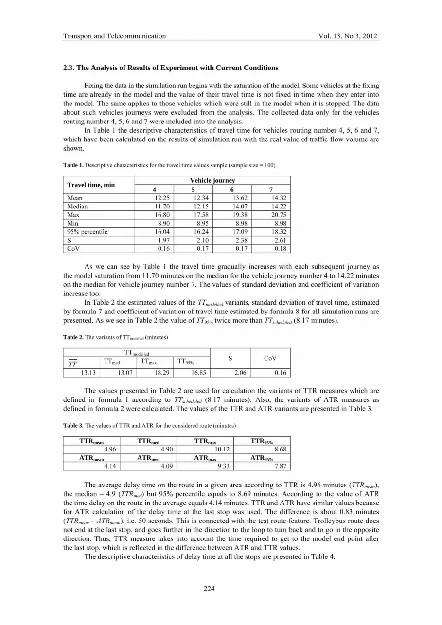
Fixing the data in the simulation run begins with the saturation of the model. Some vehicles at the fixing time are already in the model and the value of their travel time is not fixed in time when they enter into the model. The same applies to those vehicles which were still in the model when it is stopped. The data about such vehicles journeys were excluded from the analysis. The collected data only for the vehicles routing number 4, 5, 6 and 7 were included into the analysis.

In Table 1 the descriptive characteristics of travel time for vehicles routing number 4, 5, 6 and 7, which have been calculated on the results of simulation run with the real value of traffic flow volume are shown.

Table 1. Descriptive characteristics for the travel time values sample (sample size = 100)

Vehicle journey Travel time, min

4 5 6 7 Mean 12.25 12.34 13.62 14.32 Median 11.70 12.15 14.07 14.22 Max 16.80 17.58 19.38 20.75 Min 8.90 8.95 8.98 8.98 95% percentile 16.04 16.24 17.09 18.32 S 1.97 2.10 2.38 2.61 CoV 0.16 0.17 0.17 0.18

As we can see by Table 1 the travel time gradually increases with each subsequent journey as

the model saturation from 11.70 minutes on the median for the vehicle journey number 4 to 14.22 minutes on the median for vehicle journey number 7. The values of standard deviation and coefficient of variation increase too.

In Table 2 the estimated values of the TTmodelled variants, standard deviation of travel time, estimated by formula 7 and coefficient of variation of travel time estimated by formula 8 for all simulation runs are presented. As we see in Table 2 the value of TT95% twice more than TTscheduled (8.17 minutes).

Table 2. The variants of TTmodelled (minutes)

TTmodelled

TT TTmed TTmax TT95% S CoV

13.13 13.07 18.29 16.85 2.06 0.16 The values presented in Table 2 are used for calculation the variants of TTR measures which are

defined in formula 1 according to TTscheduled (8.17 minutes). Also, the variants of ATR measures as defined in formula 2 were calculated. The values of the TTR and ATR variants are presented in Table 3. Table 3. The values of TTR and ATR for the considered route (minutes)

TTRmean TTRmed TTRmax TTR95% 4.96 4.90 10.12 8.68

ATRmean ATRmed ATRmax ATR95% 4.14 4.09 9.33 7.87

The average delay time on the route in a given area according to TTR is 4.96 minutes (TTRmean),

the median – 4.9 (TTRmed) but 95% percentile equals to 8.69 minutes. According to the value of ATR the time delay on the route in the average equals 4.14 minutes. TTR and ATR have similar values because for ATR calculation of the delay time at the last stop was used. The difference is about 0.83 minutes (TTRmean – ATRmean), i.e. 50 seconds. This is connected with the test route feature. Trolleybus route does not end at the last stop, and goes further in the direction to the loop to turn back and to go in the opposite direction. Thus, TTR measure takes into account the time required to get to the model end point after the last stop, which is reflected in the difference between ATR and TTR values.

The descriptive characteristics of delay time at all the stops are presented in Table 4.


225

Table 4. Descriptive characteristics of delay time at the stops (minutes)

Stops Delay time characteristics Tallinas Matisa Gertrudes Esplanade Mean 1.41 3.16 4.74 4.14 Median 1.18 3.04 4.68 4.09 Max 3.53 8.21 9.86 9.33 95% percentile 2.61 6.66 8.38 7.87 S 0.68 1.87 2.07 2.08 CoV 0.48 0.59 0.44 0.50

The smallest value of the delay time is observed at the bus stop Tallinas (95% percentile = 2.61

minutes), the greatest value of the delay time occurs at the bus stop Gertrudes (95% percentile = 8.38 minutes). At the last stop, Esplanade, the delay time slightly decreases (95% percentile = 7.87 minutes), that is explained by the fact that the distance between the stops Gertrude and Esplanade is less (0.46 km), than between the previous stops (0.6 km) however, the values of travel times between the stops, set by the schedule are the same – 2 minutes, because this last fragment of route more often have problem connected with traffic. The high coefficients of variation values from 0.44 for Gertrudes stop to 0.59 for Matisa stop signify about low level of arrival time reliability.

On the Figure 4 the histogram of delay time values at the stops is presented (the stops are listed in route successive order).

Figure 4. Histogram of delay time at the stops

The probability of delayed arrival at the stops no more than m minutes were calculated by formula 3 and the values are presented in Table 5, the high values of probability values (> 0.9) are put in bold. Table 5. Probability values of delay time at the stops no more than m minutes

Stops m (minutes) Tallinas Matisa Gertrudes Esplanade

0 0.31 0.17 0.01 0.06 1 0.80 0.31 0.09 0.18 2 0.97 0.50 0.23 0.33 3 1.00 0.68 0.38 0.47 4 1.00 0.83 0.56 0.66 5 1.00 0.91 0.72 0.80 6 1.00 0.98 0.86 0.91 7 1.00 0.99 0.93 0.95 8 1.00 1.00 0.99 0.99 9 1.00 1.00 1.00 1.00

10 1.00 1.00 1.00 1.00


226

As it is seen in the table and in the histogram above the most problematic stop is Gertrudes and the probability of arrival at this stop with delay more than 4 minutes is 0.44.

3. Analysis of the Impact of Factors Affecting the Travel Time and Delay Time

The dwell time at the stops and the volume of traffic flow were used as variable factors for experiments. They were changed as follows (see Table 6): – the volume of traffic flow was increased by 5, 10 and 15% (the experiments with № 1, 2 and 3); – the dwell time at each the stops were increased and it was defined as the random value with normal

distribution Normal (45,10) with the mean value 45 seconds and standard deviation value – 10 seconds (the experiment with № 4).

Table 6. The changed conditions in model for the four experiments

Experiments Factors 1 2 3 4 Volume of traffic flow

real volume +5% real volume +10% real volume +15%

real volume

Dwell time Normal (20, 2) Normal (20, 2) Normal (20, 2) Normal (45, 10) The results of each experiment were analysed, for each of them the reliability measures have been

calculated and values of TTR are presented in Table 7 in comparison with the reliability measures for the current situation.

Table 7. Travel Time Reliability values for experiments

Experiments TTR Current situation 1 2 3 4

TTRmean 4.97 7.21 7.83 8.70 6.41 TTRmed 4.90 7.15 8.09 9.05 5.98 TTRmax 10.12 15.05 14.52 12.80 14.80 TTR95% 8.69 11.08 11.38 11.68 11.24 S 2.06 2.27 2.84 2.91 2.41 CoV 0.16 0.14 0.18 0.17 0.17

The values of TTR measures increase by increasing the volume of traffic flow. TTR values

increased from 4.97 minutes to 7.21 minutes that is almost 2.5 minutes by increasing the volume of traffic flow by 5%. Also with the traffic flow volume increase by 15% of the TTR increases by almost 4 minutes. The same situation happens with the ATR values. With the increase of dwell time (i.e. number of passengers or it may be result of bad weather); the average delay time at the last stop grew by nearly 1.5 minutes (on average from 4.14 to 5.62 minutes).

The values of probability of delay at the last stop for the time less than m minutes have been calculated by formula 3 for each experiment. The values are presented in Table 8 in comparison with the real situation. We can see the probability of delay more than 4 minutes at last stop equal approximately to 1 if traffic increased by 15%. The probability of delay no more than 1 minute at the last stop in all experiments practically equals zero.

Table 8. The probability values of the delay at the last stop no more than m minutes

Experiments m (min.)

Current situation 1 2 3 4

0 0.06 0 0 0 0 1 0.18 0.01 0 0 0 2 0.33 0.06 0 0.01 0.12 3 0.47 0.12 0.07 0.02 0.29 4 0.66 0.30 0.12 0.06 0.44 5 0.80 0.45 0.20 0.14 0.65 6 0.91 0.64 0.28 0.23 0.76 7 0.95 0.75 0.51 0.40 0.85 8 0.99 0.86 0.66 0.59 0.89 9 1.00 0.93 0.83 0.80 0.93 10 1.00 0.98 0.90 0.94 0.97


227

Figure 5 presents the cumulative distribution function (cdf) of the delay time at the last stop for conditions on the 3rd experiment. It is practically easy to analyse the tendency in reliability based on delay time values using the 95% level this histogram (only 5% of delay time more than according delay time value).

Figure 5. The cdf of the delay time at the last stop and 95% level for the 3rd experiment

Conclusions and Further Investigation

1. Nowadays transport systems provide both support for economic development and social equality, and

allow inhabitants regardless of their social strata to implement mobility. Sustainable development of transport systems requires the ability to measure the quality of services provided by transport systems. The reliability of public transport is one of the most important properties of UPTS, which also increases, trust to transport and contributes to its more frequent use. The monitoring of quality and reliability of public transport must be day-to-day practice of transport authority.

2. This paper provides an example of evaluating the UPTS reliability of one route fragment and the use of simulation modelling. The tasks of this research didn’t include the simulation model development and the existed simulation model (developed in the previous research) was used. That’s why the proposed approach realised only data of fragment of investigated route of public transport that was included in existed model.

3. In the further research, it is necessary to proceed from the assessment of the separate route reliability to the UPTS reliability in whole. Some researches prompt to use the average value of the reliability measures for the route system in whole. However, it may not allow seeing real problems with the reliability, because different routes have different significance for the mobility support and the routes’ features should be taken into account in the indicator of reliability for the public transport system in whole. This can be achieved by assigning weights coefficients to each route (for example, on the basis the Analytic Hierarchy Process estimation method), which must take into account:

• the volume of passenger flow (demand for the public system route service), • the availability (presence) of alternative routes or modes of transport, • headways, • frequency, • the features of the serviced urban areas, • cover degree, • etc.

Acknowledgement

The article is written with the financial assistance of European Social Fund. Project

No 2009/0159/1DP/1.1.2.1.2/09/IPIA/VIAA/006 (The Support in Realisation of the Doctoral Programme “Telematics and Logistics” of the Transport and Telecommunication Institute).


228

References

1. Balcombe, R., R. Mackett, N. Paulley, J. Preston, J. Shires, H. Titheridge, M. Wardman, P. White (2004). The Demand for Public Transport: A Practical Guide. Transport Research Laboratory Report TRL No 593.

2. König, A. and Axhausen, Kay W. (2002). The reliability of the transportation system and its influence on the choice behaviour. Presentation at STRC 2002. In Proceedings of the 2nd Swiss Transport Research Conference, March 20–22, 2002. Zurich: ETHZ, Institute of Transportation, Traffic, Highway- and Railway-Engineering.

3. Ebeling, C. E. (1997). Introduction to Reliability and Maintainability Engineering. Boston: McGraw-Hill Companies Inc.

4. Polus, A. (1978). Modeling and Measurements of Bus Service Reliability. Transportation Research, 12(4), 253–256.

5. Turnquist, M. A., and L. A. Bowman (1980). The Effects of Network Structure on Reliability of Transit Service. Transportation Research B, 14, 79–86.

6. Tseng, Y.-Yen &Verhoef, E. (2004). A meta-analysis of valuation of travel time reliability. In Proceedings of the ERSA Conference. Rotterdam: Colloquium Vervoersplanologisch Speurwerk.

7. Tseng, Yin-Yen & Verhoef, Erik T. (2008). Value of time by time of day: A stated-preference study. Transportation Research Part B: Methodological, 42(7–8), 607–618.

8. Polus, A. (1978). Modeling and Measurements of Bus Service Reliability. Transportation Research, 12(4), 253–256.

9. Sterman, B. and J. Schofer. (1976). Factors affecting reliability of urban bus services. Transportation Engineering Journal, volume 102, p. 147–159.

10. Liu, R., Sinha, Sh. (2007). Modelling Urban Bus service and Passenger Reliability. In The Third International Symposium on Transportation Network Reliability (INSTR), July 2007. The Hague, the Netherlands. Available from http://eprints.whiterose.ac.uk/3686/ (accessed June 2012).

11. Sobota, A., Zochowska, R. (2008). Model of urban public transport network for the analysis of punctuality. Journal of Achievements in Materials and Manufacturing Engineering, 28(1), 63–66.

12. Transport and Telecommunication institute. (2010). Gājēju un transporta plūsmu izpēte gājēju ielas izveidei Rīgā, Tērbatas ielā posmā no Elizabetes ielas līdz Tallinas ielai. Gala atskaite, Riga, 2010. Rīga: Transporta un sakaru instituts. (In Latvian)

13. Yurshevich, E., Yatskiv, I. (2011). Decision support system for transport system management and microsсopic traffic modeling, In Proceedings of the 7th International Scientific Conference TRANSBALTICA 2011, Vilnius, May, 2011 (74–81). Lithuania: Vilnius.

astrophysical effects of scalar dark matter miniclusters

Documents