geomagnetically induced currents (gic) in large power
TRANSCRIPT
Univers
ity of
Cap
e Tow
n
GEOMAGNETICALLY INDUCED CURRENTS
(GIC) IN LARGE POWER SYSTEMS INCLUDING
TRANSFORMER TIME RESPONSE
THESIS BY: DAVID TEMITOPE OLUWASEHUN OYEDOKUN DEPARTMENT OF ELECTRICAL ENGINEERING
UNIVERSITY OF CAPE TOWN
This thesis was submitted to the University of Cape Town in fulfilment of the academic
requirements for the Doctor of Philosophy degree in Electrical Engineering

The copyright of this thesis vests in the author. No quotation from it or information derived from it is to be published without full acknowledgement of the source. The thesis is to be used for private study or non-commercial research purposes only.
Published by the University of Cape Town (UCT) in terms of the non-exclusive license granted to UCT by the author.
Univers
ity of
Cap
e Tow
n

GEOMAGNETICALLY INDUCED CURRENTS (GIC) IN LARGE POWER SYSTEMS INCLUDING TRANSFORMER TIME RESPONSE
Page | i
Acknowledgements I am glad that I accepted the challenge to do my PhD research in the field of
geomagnetically induced currents (GIC). During my research, I was privileged to participate
in several meetings, workshops and conferences. These events provided me with the
opportunity to share ideas with various people, from senior researchers and professors to
my colleagues in the Department of Electrical Engineering at UCT. Despite the difficulties
faced, I enjoyed all aspects of my research in this emerging field. More often than not, these
engagements challenged me to think deeper and ensured that my research was thorough. I
am not able to mention all those who contributed significantly to my research. However, I
would like to thank:
my colleagues in the power engineering group of the Department of Electrical
Engineering at UCT. Their dedication and active participation in our weekly seminar
helped refine my ideas for my thesis.
my supervisors, Prof. C.T. Gaunt and Prof. K.A. Folly, who assisted me academically. I
benefited from their wealth of experience and knowledge.
Prof. C.T. Gaunt for providing me with the much needed financial assistance
throughout my research.
Chris Wozniak for his contribution to the development of the laboratory test
procedure.
Hilary Chisepo whose MSc laboratory work formed the basis upon which I was able
to conduct laboratory experiments.
Dr. P.J. Cilliers and Dr. S. Lotz of the South African National Space Agency (SANSA) for
constructive comments on the algorithms that addressed my hypothesis.

GEOMAGNETICALLY INDUCED CURRENTS (GIC) IN LARGE POWER SYSTEMS INCLUDING TRANSFORMER TIME RESPONSE
Page | ii
my family who gave me the encouragement I needed and provided the support
structure for my perseverance.
my wife, Dr Anthonia Oyedokun for her love, care and support throughout my
research.
I would like to quote from Prof. C.T. Gaunt’s PhD thesis: “For all this help there is no debt to
repay, except to help others in their turn.”
Declaration Although much literature was consulted during the preparation of this thesis, caution was
exercised to properly reference all work. The rest is my own work and it has not been
submitted (prior to this submission) to any academic institution for examination.
The number of words in the main text of the thesis do not exceed 80,000.
…………………………….
DTO Oyedokun
25 November 2015.
GEOMAGNETICALLY INDUCED CURRENTS (GIC) IN LARGE POWER SYSTEMS INCLUDING TRANSFORMER TIME RESPONSE
Page | iii
Abstract Geomagnetically induced currents (GIC) are the result of changing geomagnetic fields which
are a consequence of a geomagnetic disturbance (GMD). The flow of GIC through
transmission lines and transformers across the power network could have severe
consequences, if the magnitudes of the GIC are high enough. Problems that could arise from
the flow of GIC in transmission networks include an increase in the amount of reactive
power demand by GIC-laden transformers, half-wave saturation, excessive heating in
transformers, incorrect operation of transmission line protection schemes and voltage
collapse in affected sections of the network.
In the past, GIC were calculated without taking the transformer’s response time into
account. The limitation of this approach is that the size and core type of the transformer is
neglected. This may affect the assessment of GIC in the power network as the flux pattern
and winding inductance distribution are not uniform across all transformer core structures.
This thesis postulates that these characteristics could have far-reaching effects on the GIC
that flows through a transformer as a function of time.
Based on this assumption, a novel way of calculating GIC is introduced in this thesis. This
method combines the uniform plane wave model and the network Nodal Admittance Matrix
(NAM) method and incorporated for the first time, the transformer time response, which
does not appear to have been considered in previous calculation methods.
A general formula, which describes the transformer’s time response to GIC was derived,
followed by the derivation of the electric field induced in each transmission line.
A key input to the prospective GIC with transformer time response calculation, is a set of
piecewise linear equations derived from a laboratory test and PSCAD simulations. These
suitably characterise the response of three transformer core structures, namely: bank of
single phase (3(1P-3L)), three-phase three-limb (3P-3L) and three-phase five-limb
transformers (3P-5L). Each of these core types were considered as a Generator Step-up Unit
(GSU) and a Transmission Transformer (TT).
GEOMAGNETICALLY INDUCED CURRENTS (GIC) IN LARGE POWER SYSTEMS INCLUDING TRANSFORMER TIME RESPONSE
Page | iv
The results of the laboratory experiment and simulations in PSCAD led to the conclusion
that the transformer time response to GIC is irregular across the transformer cores that
were tested. The 300 VA transformer core structure with the shortest response time is the
3P-3L, followed by the 3P-5L and the 3(1P-3L). For the 500 MVA transformers, the order
was: 3P-3L; 3(1P-3L); and 3P-5L. The 3P-3L transformers permit the flow of GIC through the
windings of the transformer over a shorter length of time. Therefore based on the order in
response time, during GMDs leading to higher GIC, the prospective GIC with or without
transformer time response flowing through 3P-3L transformers will be similar.
Furthermore, the response time to GIC in 3P-3L, 3P-5L and 3(1P-3L) transformer core types
are load-dependant. The 3(1P-3L) and 3P-5L transformers operating as TT’s (modelled as
transformers at 40 % load) have the longest response time to GIC, while 3P-3L transformers
operating as a GSU (modelled as transformers at full load) have the longest response time to
DC. The shortest response time to DC was with a GSU at light load (modelled as
transformers at 80 % load), which was consistent across the three transformer core types.
This correlates well with the notion that power networks could stand a better chance of
surviving a high GMD when all generating units and loads are online.
Three different core structures were modelled with a variation of DC current levels and load
conditions, both in PSCAD and in the laboratory. These results are unique to the transformer
models used, but are representative of major types of core configurations used on power
networks. These results provide an indication that it is incorrect to lump the responses of all
transformers and transformer time response should be taken into consideration, especially
when sampling at intervals as low as 2 seconds.
GEOMAGNETICALLY INDUCED CURRENTS (GIC) IN LARGE POWER SYSTEMS INCLUDING TRANSFORMER TIME RESPONSE
Page | v
List of abbreviations CME coronal mass ejection
DC direct current
FFT Fast Fourier Transform
GIC geomagnetically induced currents
GMD geomagnetic disturbance
GSU generator step up unit (transformer)
NGC National Grid Company
NI National Instruments
SECS spherical elementary current systems
TT transmission transformer
SSC sudden storm commencement
UT universal time
3P-3L three-phase three-limb
3P-5L three-phase five-limb
3(1P-3L) three single-phase three-limb
GEOMAGNETICALLY INDUCED CURRENTS (GIC) IN LARGE POWER SYSTEMS INCLUDING TRANSFORMER TIME RESPONSE
Page | vi
Table of Contents
Acknowledgements ........................................................................................................... i
Declaration ...................................................................................................................... ii
Abstract .......................................................................................................................... iii
List of abbreviations ......................................................................................................... v
Table of Contents ............................................................................................................ vi
List of Figures ................................................................................................................... x
List of Tables ..................................................................................................................xiv
1. INTRODUCTION ......................................................................................................... 1
1.1 Background to Thesis .......................................................................................................................... 2
1.2 Objectives of the thesis ....................................................................................................................... 6
1.3 Hypothesis .......................................................................................................................................... 7
1.4 Research methodology ........................................................................................................................ 7
1.5 Outline of this thesis ........................................................................................................................... 8
1.6 Novel contributions ............................................................................................................................. 9
2. REVIEW OF GIC CALCULATION METHODS ................................................................. 10
2.1 Electric field calculation .................................................................................................................... 10
2.2 Network calculation .......................................................................................................................... 16
2.3 Calculation and modelling of GIC in power systems .......................................................................... 22
GEOMAGNETICALLY INDUCED CURRENTS (GIC) IN LARGE POWER SYSTEMS INCLUDING TRANSFORMER TIME RESPONSE
Page | vii
2.4 Summary of GIC calculation Techniques and proposed GIC calculation technique ............................ 25
3. INTRODUCTION OF TRANSFORMER TIME RESPONSE INTO GIC CALCULATION ........... 27
3.1 Derivation of transformer time response .......................................................................................... 27
3.2 Derivation of the magnitude of Electric field induced on the transmission line ................................. 33
3.3 Derivation of the prospective GIC without transformer time response ............................................. 35
4. LABORATORY TEST PROTOCOL AND COMPUTER SIMULATION ................................. 41
4.1 Test Protocol ..................................................................................................................................... 42
4.2 Laboratory test setup ........................................................................................................................ 43
4.3 PSCAD Simulation ............................................................................................................................. 47
5. LABORATORY TEST FOR TRANSFORMER TIME RESPONSE ......................................... 50
5.1 Bench scale 300 VA transformer ........................................................................................................ 50
6. PSCAD SIMULATION OF TRANSFORMER TIME RESPONSE TO GIC .............................. 55
6.1 Bench scale 300 VA Transformers ..................................................................................................... 55
6.2 Comparison of Laboratory test and PSCAD 300 VA transformer simulation results ........................... 59
6.3 500 MVA Power Transformer ............................................................................................................ 60
6.4 Average response time ratios for core structures .............................................................................. 66
7. TEST AND IMPLEMENTATION ................................................................................... 68
7.1 Validating the prospective gic without transformer time response ................................................... 68
7.2 Incorporating transformer time response ......................................................................................... 80
7.3 Effect of increased Magnetic field sampling time interval on the magnitudes of the prospective GIC
with and without transformer time response ................................................................................................ 92
GEOMAGNETICALLY INDUCED CURRENTS (GIC) IN LARGE POWER SYSTEMS INCLUDING TRANSFORMER TIME RESPONSE
Page | viii
7.4 Comparison between measured GIC and calculated GIC ................................................................. 102
8. ASSUMPTIONS ON WHICH RESEARCH IS BASED AND DISCUSSIONS ........................ 129
8.1 Assumptions ................................................................................................................................... 129
8.2 Discussions ...................................................................................................................................... 130
9. CONCLUSIONS ....................................................................................................... 137
9.1 Differential transformer core response time to GIC ........................................................................ 137
9.2 Effect of load on transformer response time to GIC ........................................................................ 137
9.3 Characterising transformer time response to GIC ............................................................................ 138
9.4 Answers to research questions ........................................................................................................ 138
9.5 Validity of Hypothesis ..................................................................................................................... 140
List of References ......................................................................................................... 141
APPENDIX A: PLC specifications .................................................................................... 149
APPENDIX B: Electric and magnetic field data used in chapter 7.1 to 7.3 ........................ 150
APPENDIX C: GIC profiles from section 7.1 .................................................................... 153
APPENDIX D: Substation GIC profiles in case 1 .............................................................. 157
APPENDIX E: Substation GIC profiles in case 2 ............................................................... 160
APPENDIX F: substation GIC profiles in case 3 ............................................................... 164
APPENDIX H: GIC values in chapter 7.2 ......................................................................... 170
GEOMAGNETICALLY INDUCED CURRENTS (GIC) IN LARGE POWER SYSTEMS INCLUDING TRANSFORMER TIME RESPONSE
Page | ix
APPENDIX I: Matlab code for calculating the prospective GIC with transformer time
response ...................................................................................................................... 173
APPENDIX J: Eskom 400 kV substations ......................................................................... 181
APPENDIX K: Eskom 400 kV transmission line data ........................................................ 181
APPENDIX L: Eskom 400 kV substation admittance data ................................................ 181
APPENDIX M: Sample calculations in case 2 .................................................................. 182
APPENDIX N: Sample calculations in case 3 ................................................................... 186
APPENDIX O: Sample calculations in case 4 ................................................................... 189
APPENDIX P: DC Current rise time ................................................................................. 193
GEOMAGNETICALLY INDUCED CURRENTS (GIC) IN LARGE POWER SYSTEMS INCLUDING TRANSFORMER TIME RESPONSE
Page | x
List of Figures Figure 2.1 The SECS showing the ground field measurements and the grid of elementary currents [7] ............. 15
Figure 2.2 Three-bus network with induced electric field .................................................................................... 17
Figure 2.3 Norton's current equivalent ................................................................................................................ 17
Figure 2.4 Conversion of induced electric field to Norton equivalent .................................................................. 21
Figure 2.5 Overview of the real-time GIC simulator [36] ..................................................................................... 24
Figure 3.1 Illustration of GIC flow in transformers and transmission lines [73] ................................................... 28
Figure 3.2 Non-ideal transformer model [74]....................................................................................................... 28
Figure 3.3 Reduced model of the primary winding .............................................................................................. 29
Figure 3.4 Different GIC values over time, transformer time response and the time when the GIC value changes
......................................................................................................................................................... 32
Figure 3.5 Calculation of the induced electric field on a transmission line .......................................................... 34
Figure 3.6 Three-bus network with induced electric field .................................................................................... 36
Figure 3.7 Norton's current equivalent ................................................................................................................ 36
Figure 4.1 Laboratory setup outside the safety fence showing control and data logging systems ...................... 44
Figure 4.2 Laboratory setup inside the safely fence showing transformers and loads ........................................ 45
Figure 4.3 From left to right in order of appearance, single phase, three-phase five-limb and three-phase three-
limb transformers [76] ..................................................................................................................... 46
Figure 4.4 Mathematically equivalent model of transformer electric circuit [80] ............................................... 48
Figure 4.5 Transformer time response to GIC test circuit in PSCAD ..................................................................... 49
Figure 5.1 Response time by practical test of the transformers with no load ..................................................... 51
Figure 5.2 Response time of the transformer under 40 % load ........................................................................... 52
Figure 5.3 Response time for GSU transformer under light load conditions ....................................................... 53
Figure 5.4 Response time for GSU transformer under full load conditions ......................................................... 53
Figure 6.1 Profiles of the transformer time response to GIC between 0 pu and 1 pu for the three transformer
core types under consideration. ...................................................................................................... 56
Figure 6.2 Initial condition test response time in PSCAD: 300 VA ........................................................................ 57
Figure 6.3 Response time of TT under 40 % load in PSCAD: 300 VA .................................................................... 58
Figure 6.4 Response time for GSU transformers at light load in PSCAD: 300 VA ................................................. 58
Figure 6.5 Response time for GSU transformer at full load in PSCAD: 300 VA ..................................................... 59
Figure 6.6 Response time for the initial condition test in PSCAD: 500 MVA ........................................................ 61
Figure 6.7 Response time for TT in PSCAD: 500 MVA ........................................................................................... 62
Figure 6.8 Response time for GSU under light load in PSCAD: 500 MVA ............................................................. 63
Figure 6.9 Response time for GSU under full load in PSCAD: 500 MVA ............................................................... 63
Figure 7.1 The test network used in section 7.1 to 7.3. It has 10 substations and 13 unique transmission lines 69
GEOMAGNETICALLY INDUCED CURRENTS (GIC) IN LARGE POWER SYSTEMS INCLUDING TRANSFORMER TIME RESPONSE
Page | xi
Figure 7.2 FFT of the magnitude of the magnetic field data used in chapter 7 .................................................... 70
Figure 7.3 Magnetic and electric field profiles at Hermanus Magnetic Observatory (HMO) on 13 March 1989 . 71
Figure 7.4 Substation 1: Comparison of GIC values obtained using NAM and Lehtinen-Pirjola methods ........... 78
Figure 7.5 Substation 4: Comparison of GIC values obtained using NAM and Lehtinen-Pirjola methods ........... 79
Figure 7.6 Substation 6: Comparison of GIC values obtained using NAM and Lehtinen-Pirjola methods ........... 79
Figure 7.7 Substation 7: Comparison of GIC values obtained using NAM and Lehtinen-Pirjola methods ........... 80
Figure 7.8 Prospective GIC profile with and without transformer time response at substation 1 ....................... 85
Figure 7.9 Prospective GIC profile with and without transformer time response at substation 4 ...................... 86
Figure 7.10 Prospective GIC profile with and without transformer time response at substation 6 .................... 86
Figure 7.11 Prospective GIC profile with and without transformer time response at substation 7 ..................... 87
Figure 7.12 Case 2: Prospective GIC profile with and without transformer time response at substation 1 ........ 90
Figure 7.13 Case 2: Prospective GIC profile with and without transformer time response at substation 4 ........ 90
Figure 7.14 Case 2: Prospective GIC profile with and without transformer time response at substation 6 ........ 91
Figure 7.15 Case 2: Prospective GIC profile with and without transformer time response at substation 7 ........ 91
Figure 7.16 Prospective GIC profile with and without transformer time response at substation 1 ..................... 95
Figure 7.17 Prospective GIC profile with and without transformer time response at substation 4 ..................... 96
Figure 7.18 Prospective GIC profile with and without transformer time response at substation 6 .................... 96
Figure 7.19 Prospective GIC profile with and without transformer time response at substation 7 ..................... 97
Figure 7.20 Prospective GIC profile with and without transformer time response at substation 1 ..................... 99
Figure 7.21 Prospective GIC profile with and without transformer time response at substation 4 ................... 100
Figure 7.22 Prospective GIC profile with and without transformer time response at substation 6 ................... 100
Figure 7.23 Prospective GIC profile with and without transformer time response at substation 7 ................... 101
Figure 7.24: Comparison between the prospective GIC without transformer time response and the measured
GIC at Grassridge using two-second sampling time interval data ................................................. 104
Figure 7.25 Comparison between the prospective GIC without transformer time response and the measured
GIC at Grassridge using four-second sampling time interval data ................................................. 104
Figure 7.26 Comparison between the prospective GIC without transformer time response and the measured
GIC at Grassridge using 10-second sampling time interval data ................................................... 105
Figure 7.27 Comparison between the prospective GIC without transformer time response and the measured
GIC at Grassridge using 30-second sampling time interval ............................................................ 105
Figure 7.28 Comparison between the prospective GIC without transformer time response and the measured
GIC at Grassridge using one-minute sampling time interval data ................................................. 106
Figure 7.29 Comparison between the prospective GIC without transformer time response and the measured
GIC at Grassridge using two-minute sampling time interval data ................................................. 106
Figure 7.30 Comparison between the prospective GIC without transformer time response and the measured
GIC at Grassridge using four-minute sampling time interval data ................................................. 107
GEOMAGNETICALLY INDUCED CURRENTS (GIC) IN LARGE POWER SYSTEMS INCLUDING TRANSFORMER TIME RESPONSE
Page | xii
Figure 7.31 Comparison between the prospective GIC without transformer time response and the measured
GIC at Grassridge using 10-minute sampling time interval data ................................................... 107
Figure 7.32 Difference between calculated and measured GIC during SSC (06:45 UT) ..................................... 108
Figure 7.33 Difference between calculated and measured GIC around 21:00 ................................................... 109
Figure 7.34 Comparison between the prospective GIC with and without transformer time response with the
measured GIC using two-second sampling time interval data ...................................................... 111
Figure 7.35 Section A Zoomed: Comparison between the prospective GIC with and without transformer time
response with the measured GIC using two-second sampling time interval data ........................ 111
Figure 7.36 Section B Zoomed: Comparison between the prospective GIC with and without transformer time
response with the measured GIC using two-second sampling time interval data ........................ 112
Figure 7.37 Section C Zoomed: Comparison between the prospective GIC with and without transformer time
response with the measured GIC using two-second sampling time interval data ........................ 113
Figure 7.38 Section D Zoomed: between the prospective GIC with and without transformer time response with
the measured GIC using two-second sampling time interval data ................................................ 113
Figure 7.39 Comparison between the prospective GIC with and without transformer time response with the
measured GIC using two-minute sampling time interval data ...................................................... 115
Figure 7.40 Section A Zoomed: Comparison between the prospective GIC with and without transformer time
response with the measured GIC using two-minute sampling time interval data ........................ 116
Figure 7.41 Section B Zoomed: Comparison between the prospective GIC with and without transformer time
response with the measured GIC using two-minute sampling time interval data ........................ 117
Figure 7.42 Section C Zoomed: Comparison between the prospective GIC with and without transformer time
response with the measured GIC using two-minute sampling time interval data ........................ 117
Figure 7.43 Section D Zoomed: Comparison between the prospective GIC with and without transformer time
response with the measured GIC using two-minute sampling time interval data ........................ 118
Figure 7.44 Comparison between the prospective GIC with and without transformer time response with the
measured GIC using 10-minute sampling time interval data ........................................................ 120
Figure 7.45 The curves in the graph compares the mean absolute error (MAE) calculated in 10-minute moving
intervals between the measured GIC versus the prospective GIC without transformer time
response and the MAE between the measured GIC versus the prospective GIC with transformer
time response. The grey blocks show the 10-minute block interval where the MAE was improved
due to the incorporation of the transformer time response. ........................................................ 124
Figure 7.46 Comparison between the variance profile of the measured GIC versus the calculated GIC with the
transformer time response and the variance profile of the measured GIC versus the calculated GIC
without the transformer time response. ....................................................................................... 125
GEOMAGNETICALLY INDUCED CURRENTS (GIC) IN LARGE POWER SYSTEMS INCLUDING TRANSFORMER TIME RESPONSE
Page | xiii
Figure 7.47 Quiet time: Comparison between the variance profile of the measured GIC versus the calculated
GIC with the transformer time response and the variance profile of the measured GIC versus the
calculated GIC without the transformer time response. ............................................................... 126
Figure 7.48 Pre-SSC, SSC: Comparison between the variance profile of the measured GIC versus the calculated
GIC with the transformer time response and the variance profile of the measured GIC versus the
calculated GIC without the transformer time response. ............................................................... 126
Figure 7.49 Period of reduced geomagnetic activity: Comparison between the variance profile of the measured
GIC versus the calculated GIC without the transformer time response and the variance profile of
the measured GIC versus the calculated GIC with the transformer time response. ..................... 127
Figure 7.50 Period of low geomagnetic activity: Comparison between the variance profile of the measured GIC
versus the calculated GIC without the transformer time response and the variance profile of the
measured GIC versus the calculated GIC with the transformer time response............................. 127
Figure 8.1 Profile of the average response time for the three transformer core structures ............................. 132
Figure 8.2 Comparison between the peak values of measured and calculated GIC using different sampling time
intervals ......................................................................................................................................... 135
GEOMAGNETICALLY INDUCED CURRENTS (GIC) IN LARGE POWER SYSTEMS INCLUDING TRANSFORMER TIME RESPONSE
Page | xiv
List of Tables Table 4.1 Table showing the parameters of each of the transformer that formed the 3(1P-3L) transformer bank
......................................................................................................................................................... 43
Table 4.2 Table showing the parameters of the 3P-3L transformer ..................................................................... 43
Table 4.3 Table showing the parameters of the 3P-5L transformer ..................................................................... 43
Table 6.1 Presented in this table are the magnetization currents in each phase for three transformer core
structures ......................................................................................................................................... 60
Table 6.2 Time response equations derived for the 500 MVA TT (40% load) in PSCAD: ...................................... 65
Table 6.3 Transformer time response equations derived for the 500 MVA GSU under light load in PSCAD ....... 65
Table 6.4 Transformer time response equations derived for the GSU under full load in PSCAD ......................... 66
Table 6.5 Average time response ratios for 3(1P-3L) and 3P-5L with respect to 3P-3L for 500 MVA transformers.
......................................................................................................................................................... 67
Table 6.6 Average time response ratios for the 500 MVA 3P-5L and 3(1P-3L) core structures ........................... 67
Table 7.1 Transmission line admittance, length and substation GPS coordinates of the test network ............... 72
Table 7.2 Substation transformer and reactor data used in the test network ..................................................... 72
Table 7.3 Prospective GIC values calculated for the 10 substation network using 2-min sampling time interval
magnetic field data .......................................................................................................................... 75
Table 7.4 Substation data with additional data on the transformer core structure and operational state ......... 81
Table 7.5 Substation data with additional data on the transformer core structure and operational state. In this
case, the transformer core structure is not the same across the network ..................................... 88
Table 7.6 Prospective GIC values without transformer time response calculated for the 10 substation network
with four-minute sampling time interval magnetic field data ......................................................... 93
Table 7.7 Substation data with additional data on the transformer core structure and operational state. In this
case study, all the transformer core structure and operational state are the same ....................... 94
Table 7.8 Substation data with additional data on the transformer core structure and operational state. In this
case, the transformer core structure is not the same across the network ..................................... 98
Table 7.9 Improvement in GIC calculation with transformer time response included using two-second sampling
time interval data .......................................................................................................................... 114
Table 7.10 Improvement in GIC calculation with transformer time response using two-minute sampling interval
data ................................................................................................................................................ 118
Table 7.11 Improvement in GIC calculation with transformer time response using 10-minute sampling time
interval data ................................................................................................................................... 120
Table 8.1 Probabilities of improved GIC calculation using variable time intervals to sample the magnetic field
....................................................................................................................................................... 136
GEOMAGNETICALLY INDUCED CURRENTS (GIC) IN LARGE POWER SYSTEMS INCLUDING TRANSFORMER TIME RESPONSE
Page | 1
CHAPTER 1
INTRODUCTION
1. INTRODUCTION
Geomagnetically induced currents (GIC) are the result of changing geomagnetic fields which
are a consequence of a geomagnetic disturbance. During solar storms, enormous explosions
of plasma are ejected from the sun’s surface into interplanetary space. These ejections are
called Coronal Mass Ejections (CME) [1-3]. CMEs disrupt the solar wind [4] through
interplanetary space and the resulting interaction with the Earth’s magnetic field is known
as a geomagnetic storm [5, 6].
During geomagnetic storms, solar wind pressure and wind speed can suddenly increase on
average from 2 nPa to 30 nPa and from 400 km/s to 2000 km/s, respectively, if the CME is
directed towards the Earth [7]. Geo-effective CMEs lead to large fluctuations of the Earth’s
magnetic fields, which induce an electric field according to Faraday’s law of induction [8].
This gives rise to quasi-DC currents in electric power systems through the grounded neutrals
of power transformers. These geomagnetically induced currents have frequencies less than
1 Hz [9, 10].
The flow of GIC through transmission lines and transformers across a power network could
have negative consequences. These include an increase in the reactive power demanded by
GIC-laden transformers [11, 12], transformers operating within the region of non-linearity
due to half-wave saturation [13, 14], excessive heating [15] in transformers leading to
thermal damage, incorrect operation of transmission line protection schemes [16, 17] and
voltage problems in affected sections of the network [18, 19]. To mitigate the flow of GIC,
DC current blocking devices have been designed and some have been developed [20, 21]. In
Finland, neutral-point reactors have been used decrease the GIC magnitudes in its high-
voltage system [22]. In England, series capacitors have been used to block GIC [23, 24] in
transmission lines. However, studies by Erinmez et al [24] showed that it would be
GEOMAGNETICALLY INDUCED CURRENTS (GIC) IN LARGE POWER SYSTEMS INCLUDING TRANSFORMER TIME RESPONSE
Page | 2
advantageous to strategically place the devices to prevent the risk of adversely increasing
the flow of GIC in other parts of the network.
In the past, GIC were calculated using either a uniform or non-uniform electric field model in
the geophysical solution. A number of methods for the network calculation have been used
which include the Lehtinen-Pirjola method [25, 26] and the Nodal Admittance Matrix (NAM)
method [27]. Details of these are discussed in chapter 2. Over the years, software has been
developed to carry out these calculations [28-35]. The general assumption in the network
calculation is that GIC, which are quasi-DC currents, should be treated as DC currents. In
some cases, measured GIC have been compared with calculated GIC with a variation in
correlation. The literature review shows that researchers have taken into account the
transmission line resistance, transformer resistance, grounding resistance and ground
conductivity, but have hardly paid attention to the transformer’s time response to GIC [27],
[29], [30-34], [36]. This thesis suggests that the transformer time response to GIC, which
may be core dependent, contributes to the differences between the measured and
calculated GIC flowing through a transformer.
Therefore, this thesis investigates the GIC calculation approach, which includes the
transformer time response to changing GIC, with the objective of determining whether the
time response is significant in modelling GIC. The method proposed in this thesis combines
the uniform plane wave model, network NAM method [36] and incorporates the
transformer time response.
To this end a software programme was written in Matlab. This contribution extends the
capabilities of existing GIC calculators, such as the GIC calculator in the PowerWorld
Simulator, Version 17 by Overbye [35]. PowerWorld Simulator takes into account the core
structure to determine the reactive power demand by transformers due to GIC.
1.1 BACKGROUND TO THESIS
Power networks comprise components like transformers, transmission lines, reactors,
capacitor banks, protection instruments, etc., [37]. This research deals mainly with GIC in

GEOMAGNETICALLY INDUCED CURRENTS (GIC) IN LARGE POWER SYSTEMS INCLUDING TRANSFORMER TIME RESPONSE
Page | 3
power transformers and transmission lines. Bolduc [38] indicated that the other
components of power networks are also affected by GIC which may lead to the disruption of
the entire power network. The Hydro-Quebec blackout in 1989 [38], which occurred due to
a geomagnetic disturbance, and led to millions of people being in the dark for hours
towards the end of winter, is an example of what can happen [38, 39]. The flow of GIC in the
Swedish power grid during the Halloween storm on 30 October 2003 led to a large-scale
blackout which affected about 50,000 customers for about one hour [40].
The calculation of GIC involves calculating the electric field induced in the transmission lines
as a result of the changing Earth’s magnetic field, the resulting currents in the transmission
line and the currents flowing through the grounded neutrals of transformers [16], [41].
Several methods have been used to determine the electric field induced in the Earth and
consequently, calculate the GIC flowing in transmission lines and transformers. In 1940,
McNish [42] derived a mathematical expression for the Earth’s electric field, but entirely
omitted the conductivity of the Earth. In 1966, the Earth’s electric field was calculated by
Kellogg [43] using Maxwell’s equation. In this method, a plane downward propagating wave
(towards the Earth) was used to represent the magnetic field. This model took the
conductivity of the ground into consideration. However, Kellogg assumed that the
conductivity of the ground was uniform which later was found not to be the case generally.
In 1970, Albertson and Van Baelen [44] derived a mathematical relation between changes in
the Earth’s magnetic field and the induced electric field which leads to the flow of GIC. Their
method considered the conductivity distribution of the Earth and used a recording of the
measured Earth’s magnetic field.
In 1985, Lehtinen & Pirjola [25] developed a method for calculating GIC. This method which
is further discussed in chapter 2, is appropriate for a network that is exposed to a uniform or
non-uniform electric field. This method was subsequently used in 2000 and 2002 by Koen
and Gaunt [31], [45] for the calculation of GIC in the Southern Africa electricity transmission
network. Koen’s study led to three conclusions: (i) the Lehtinen-Pirjola method is suitable
for calculating GIC in the Southern Africa electricity transmission network, (ii) a significant
amount of GIC are present during strong geomagnetic disturbances and (iii) a strong
GEOMAGNETICALLY INDUCED CURRENTS (GIC) IN LARGE POWER SYSTEMS INCLUDING TRANSFORMER TIME RESPONSE
Page | 4
correlation between transformer failures and past geomagnetic disturbances exists in South
Africa. Recently, this method was also used for the analysis of GIC in Brazil [34].
In 1998, Boteler and Pirjola [46] demonstrated that the GIC produced by a uniform electric
field when modelled in series with the transmission line or between the transformer and
ground are the same. However, for a non-uniform electric field, only the line approach can
be used. This is because according to Boteler and Pirjola [46], realistic electric fields have a
non-conservative vector function component which cannot be represented by a
conservative electric field.
The mesh impedance method and the NAM method can be used for solving the network
calculation by modelling the electric field in series with the transmission line [28]. The
advantage of the NAM method over the mesh impedance method is that the need to derive
voltage equations for all the loops in the network is avoided. For very large power networks
such as the South African electricity transmission network, this is a significant advantage
since the complexity of the calculation and computational time is reduced. In 2007, the
NAM method was used to calculate the low of GIC in a real-time GIC simulator [36].
The electric field can easily be calculated, as mentioned earlier, if the magnetic source field
is assumed to be uniform. Other methods that have been adopted to calculate electric fields
for non-uniform source fields include spherical elementary current systems (SECS) [47-49]
and the complex image method (CIM) [33]. Bernhardi et al [7] in 2008 improved GIC
calculation in Southern Africa by using SECS to calculate the electric field and the Lehtinen-
Pirjola method for the network. In contrast to the uniform plane wave model, SECS assumes
that the electric field distribution is non-uniform for the entire network, whilst segments of
the network experience uniform plane wave electric field distribution. That is, transmission
line segments experience a uniform electric field. Their results indicated that SECS is a more
accurate method when compared to the uniform plane wave approach for electric field
calculation, especially in a large network.
Not all reports of GIC measurements in the power grid is accompanied by the calculated GIC
for the same time frame. An example of this is the publication on the GIC measurements in
GEOMAGNETICALLY INDUCED CURRENTS (GIC) IN LARGE POWER SYSTEMS INCLUDING TRANSFORMER TIME RESPONSE
Page | 5
Japan [50]. Having both GIC measurements and calculated values for a substation enables
the validation of the calculation, which can be used to calculate GIC at other stations with
no GIC measurement setups.
In some cases of GIC calculation, the calculated GIC values were compared with measured
GIC [30]. For instance, Koen and Gaunt [30] used the uniform plane wave model and the
Lehtinen-Pirjola method to calculate GIC flowing through a 400/132/15 kV 240 MVA
autotransformer at the Grassridge substation in South Africa on 31 March 2001. The
calculated GIC profile was compared with the measured GIC during the same time frame.
Although the profiles were very similar, the measured GIC were higher than the calculated
GIC for most of the time. Koen and Gaunt suggested that a proportionating constant be
introduced to reduce the variance between measured and calculated GIC. This suggestion is
similar to that made by Viljanen in 1998 [51], where he compared the measured GIC flowing
in the Nurmijärvi - Loviisa transmission line in Finland with the calculated GIC in the same
line, using the uniform plane wave electric field model and the Lehtinen-Pirjola method.
In his comparison, he used a multiplier c to fit the measured GIC and calculated GIC as
closely as possible. A possible source of discrepancy between measured and calculated GIC
is the Earth’s conductivity structure. Therefore, the multiplier c was deduced from local
geomagnetic readings in order to “calibrate” the calculated GIC. In line with the impact of
ground conductivity models on the correlation between measured and calculated GIC,
Trichtchenko and Boteler [52] found that, depending on the site where the transformers are
located, the ground conductivity structure may act like a high pass filter or a low pass filter,
thereby allowing corresponding frequencies which determine the measured GIC profile.
A uniform ground conductivity profile was used to calculate the electric field in this work.
Discrepancies between measured and calculated GIC was also observed in the research
conducted by Marti et al [18] when they compared the absolute values of the measured GIC
and the absolute values of the calculated GIC through a 500/230 kV 750 MVA
autotransformer. With the assumption that GIC in the transformer will flow through the
common winding to ground, differences of up to 100 % between the two were found.
GEOMAGNETICALLY INDUCED CURRENTS (GIC) IN LARGE POWER SYSTEMS INCLUDING TRANSFORMER TIME RESPONSE
Page | 6
Another case where measured and calculated GIC differed was at the Vykhodnoy substation
in Russia during the storm on 15 March 2012 [53].
Overbye et al [35] suggested the introduction of a factor k for different transformer core
types for the integration of geomagnetic disturbances into power flow calculations, with
specific focus on the additional reactive power linked to GIC. This was based on the notion
that different transformer core types respond to GIC differently [54]. Similarly, several
research papers have graded the response of different transformer core types to GIC [55],
[56]. Viljanen, Pirjola and Makinen in their discusses on Boteler’s research publication [57],
which stated that the time constant of large transformers is an aspect that may correlate
their response to GIC according to core types, felt that this aspect had not been adequately
investigated. Thus it became important to find a way of incorporating the time response of
different transformer core types to GIC into GIC calculation.
1.2 OBJECTIVES OF THE THESIS
Calculation of GIC is crucial to the understanding of the impact of GIC on transformers and
the entire power network. As mentioned earlier, several comparisons between calculated
GIC and measured GIC in transformers have been made in the past. In almost all cases, there
are discrepancies of various magnitudes between the two.
The objectives of this thesis are to summarise the above discrepancies between calculated
and measured GIC, investigate the contribution of the transformer core type and
transformer time response. Furthermore, this thesis will propose a calculation method to
improve GIC modelling by reducing the difference between measured and calculated GIC.
This will be accomplished by taking into account the transformer’s time response to GIC.
The use of a non-uniform electric field has been reported [7] to reduce the error between
measured and calculated GIC to an extent. In a previous study by Boteler [46], it was stated
that GIC calculations are correct based on their input electric field. The validity of the
calculated GIC is determined by how well the calculated GIC matches the measured GIC in
instances where the measured GIC is available. This research was focused on the
GEOMAGNETICALLY INDUCED CURRENTS (GIC) IN LARGE POWER SYSTEMS INCLUDING TRANSFORMER TIME RESPONSE
Page | 7
transformer time response as a potential source or discrepancy between measured and
calculated GIC.
1.3 HYPOTHESIS
This thesis tests the following hypothesis:
The integration of transformer core characteristics and time response to GIC into
GIC calculations improves the modelling of GIC as indicated by reduced differences
between measured GIC and calculated GIC, and helps to improve the
understanding of the transformer response to GIC.
The validity of this hypothesis is tested by investigating the following guiding questions:
1. How is the network part of GIC calculation affected by transformer response to
changing geo-electric fields?
2. What is the time response of transformers to a changing geo-electric field imposed
at low frequencies and how does it vary with transformer core type?
3. Why was the time response of transformers neglected in the past? Are the reasons
valid?
4. To what extent can the modelled and tested transformers represent all
transformers?
5. How does the sampling time interval of the magnetic field and measured GIC affect
GIC calculations?
1.4 RESEARCH METHODOLOGY
An extensive review of relevant literature was conducted at the beginning of this research.
This review included calculation techniques based on various models and cases where
measured GIC were compared with calculated GIC.
Thereafter, a new GIC calculation technique was developed by combining the best of the
GIC calculation approaches reviewed in literature with transformer time response
GEOMAGNETICALLY INDUCED CURRENTS (GIC) IN LARGE POWER SYSTEMS INCLUDING TRANSFORMER TIME RESPONSE
Page | 8
modelling. The new GIC calculation technique was tested with and without the transformer
time response.
PSCAD/EMTDC simulations were used to test for the effect of transformer time response to
GIC-like currents. This was followed by a similar test in the laboratory.
The existing PSCAD/EMTDC transformer models includes saturation and is apparently
suitable for the simulations related to the transformer time response. Therefore, no new
PSCAD models were developed.
The effect of the transformer time response on the flow of GIC through transformers was
analysed to determine the significance of the transformer time response.
1.5 OUTLINE OF THIS THESIS
This outline of this thesis is presented below.
In chapter 2, the uniform plane wave model, spherical elementary current systems and
complex image method for calculating electric fields are reviewed. This is followed by a
review of the Lehtinen-Pirjola method and NAM method.
In the third chapter, the mathematical derivation for calculating the prospective GIC with
transformer time response is shown. Thereafter, the magnitude of electric field induced on
a transmission line is derived using the uniform plane wave model. The last section of
chapter 3 presents the derivation of the prospective GIC without the transformer time
response using the NAM method.
The protocol for the laboratory experiments and PSCAD simulations is presented in chapter
4. The laboratory experimental setup and PSCAD simulation setup are also explained in this
chapter.
Chapter 5 describes the transformer time response to GIC tests in the laboratory and the
results for the three 300 VA transformer core types namely; bank of three single-phase
GEOMAGNETICALLY INDUCED CURRENTS (GIC) IN LARGE POWER SYSTEMS INCLUDING TRANSFORMER TIME RESPONSE
Page | 9
three-limb transformers referred to as 3(1P-3L), three-phase three-limb transformer
referred to as 3P-3L and the three-phase five-limb transformer referred to as 3P-5L.
Chapter 6 describes the time response to GIC simulation results of the 300 VA, 3(1P-3L), 3P-
3L and 3P-5L transformer core type in PSCAD. This is followed by a comparison of the
laboratory test result and the PSCAD simulation result. The next section in this chapter
describes the tests conducted on the same transformer core types but rated at 500 MVA to
represent large power transformers. Finally, the chapter offers the analysis of the average
transformer response time to GIC.
In chapter 7, the prospective GIC without the transformer time response calculation method
is validated. Following this, four case studies are presented with step-by-step calculation of
the prospective GIC with transformer time response with a variety of transformer core
structures. Using the measured GIC at Grassridge substation in South Africa, the effect of
using different time intervals of the magnetic field on GIC calculation is investigated.
Chapter 8 discusses the findings of this research and in chapter 9, conclusions are drawn
from the findings of the research.
1.6 NOVEL CONTRIBUTIONS
The research:
1. Presented new knowledge on GIC flow through transformers and their responses,
including the difference between Generator Step-up Units (GSU) and Transmission
Transformers (TT);
2. Showed that the profile of GIC flow through different transformer core structures of
the same capacity are not the same.
3. Proved that a sampling interval between 2 seconds and 10 seconds is sufficient to
adequately measure GIC and the geomagnetic field used for GIC calculations.
GEOMAGNETICALLY INDUCED CURRENTS (GIC) IN LARGE POWER SYSTEMS INCLUDING TRANSFORMER TIME RESPONSE
Page | 10
CHAPTER 2
REVIEW OF GIC CALCULATION METHODS
2. REVIEW OF GIC CALCULATION METHODS
Calculating GIC involves two major parts [58]. The first part is the geophysical response of
the geo-electric field to a given geomagnetic disturbance arising from ionospheric and
magnetospheric currents, which is discussed in section 2.1. The second part is the derivation
of GIC in the network from the geo-electric fields, which is discussed in section 2.2. In
section 2.3, GIC calculation software is discussed. All the software and techniques discussed
in this chapter were developed between 1940 and 2013. Some software calculates GIC,
while other software calculates the reactive power demand due to GIC.
2.1 ELECTRIC FIELD CALCULATION
In 1940, McNish derived a mathematical expression for the Earth’s electric field using the
formula in equation 2.1 [42]:
𝐸 = −𝜕𝐴
𝜕𝑡 (2.1)
where E is the induced electric field, A is the magnetic vector potential of the auroral line
current flowing in the atmosphere and t is time.
In this model, the conductivity of the Earth was neglected which made it incomplete. The
Earth conductivity model is an important factor to be considered, because the Earth
conductivity affects the size of the electric field. In some applications, a uniform Earth
conductivity structure is sufficient, while the non-uniform Earth conductivity structure can
be considered for more accurate results.
In 1966, the Earth’s electric field was calculated by Kellogg [43] from Maxwell’s equation as:
𝑐𝑢𝑟𝑙 𝐸 = −𝜕𝐵
𝜕𝑡 (2.2)
GEOMAGNETICALLY INDUCED CURRENTS (GIC) IN LARGE POWER SYSTEMS INCLUDING TRANSFORMER TIME RESPONSE
Page | 11
where E is the induced electric field and B is the magnetic field.
In this method, a plane downward propagating wave is used to represent the magnetic field
and the conductivity of the ground is assumed to be uniform [43, 44].
Albertson and Van Baelen [44] derived a mathematical relationship between changes in the
Earth’s magnetic field and the induced electric field. These changes lead to the flow of GIC.
This method takes into consideration the conductivity distribution of the Earth and uses a
log of the measured Earth’s magnetic field [25], [59-61].
The electric field 𝐸𝑜 was calculated as:
𝐸0 = 𝑅𝑒 (𝐸𝑦) (2.3a)
where Re is the real part, and
𝐸𝑦 = ∫ 𝐸𝑦(𝑣)𝑑𝑣∞
0 (2.3b)
But
𝐸𝑦(𝑣) is defined in equation 2.4 as:
𝐸𝑦(𝑣) =𝐽𝑒𝑗𝑤𝑡
𝜋𝑒−𝑣ℎ
𝑗𝑤𝜇0𝑍𝑠(𝑣)
𝑗𝑤𝜇0+𝑣𝑍𝑠(𝑣)cos 𝑣𝑥 (2.4)
The variable v describes partly the induced electric field [44].
In 2004, Viljanen et al [60] stated that to solve the geophysical problem, a model of the
magnetospheric-ionospheric current system as a function of time and the Earth’s
conductivity structure is needed. Then, in theory, Maxwell’s equations and boundary
conditions for the Earth’s electric and magnetic fields can be solved. However in practice,
inputs to these equations are partially unknown. Even if the inputs are known, the solution
is time-consuming, which is a significant drawback [62]. Other methods include the uniform
plane wave model, the spherical elementary current systems (SECS) method (introduced
and validated in 1997 by Amm [49]) and the complex image method (CIM) [62], [33].
GEOMAGNETICALLY INDUCED CURRENTS (GIC) IN LARGE POWER SYSTEMS INCLUDING TRANSFORMER TIME RESPONSE
Page | 12
2.1.1. Uniform plane wave model
The uniform plane wave model application to the calculation of induced electric field in
transmission lines was introduced by Viljanen and Pirjola [61]. It is based on Faraday’s law of
induction. This law states that a time-varying magnetic field in a conductive medium induces
an electric field, the magnitude of which depends on the rate of change of the magnetic
field. In this model, the Earth is described as a half space where the geomagnetic field
propagates vertically, but the wave front is horizontal in the Earth with a constant
conductivity. The horizontal electric field 𝐸𝑦 can be written in terms of the horizontal
magnetic field 𝐵𝑦 due to the orthogonal relationship between the two as shown in equation
2.5a.
𝐸𝑦 = −√𝜔
𝜇0𝜎𝑒𝑖
𝜋
4𝐵𝑥 (2.5a)
where 𝜔 is the angular frequency, is the Earth conductivity, 𝜇𝑜 is the permeability of the
Earth and 𝐵𝑥 is the horizontal geomagnetic field component.
Taking the inverse Fourier transform of equation 2.5a to give the time domain convolution
integral, equation 2.5b is derived. The derived equation shows the relationship between the
magnetic and the electric field.
E(t) = −1
√σπμo∫
g(t−u)
√u du
∞
0 (2.5b)
where g(t) is the time derivative of the perpendicular magnetic field, is the Earth’s
conductivity, 𝜇𝑜 is the Earth permeability, t is time and u is time delay.
In planar geometry, where the x–axis corresponds to geographic north, y-axis to the
geographic east and z downwards, the electric field 𝐸(𝑇𝑁) in the network can be calculated
using equation 2.6 as:
E(TN) =2
√πσμ0∆(RN−1 − RN − √MbN−M) (2.6)
GEOMAGNETICALLY INDUCED CURRENTS (GIC) IN LARGE POWER SYSTEMS INCLUDING TRANSFORMER TIME RESPONSE
Page | 13
Where ∆ is the sampling interval, N is the sample number, and b is the magnetic
component.
M is the number of past samples of the B-field considered. M is calculated by dividing the
integral duration, which is normally 20 minutes, by the sampling time interval of the
magnetic field data [63]. Therefore, for two-minute sampling time interval magnetic field
data, M= 10.
Equation 2.6 which is the time series expansion of the E-field for a homogeneous Earth
model, is an approximation of the inverse Fourier transform.
Calculated GIC values are sensitive to the choice of M, especially during rapid changes in the
Earth’s magnetic field. This is because the electric field calculation formula has M as one of
its inputs. Therefore, this number can be increased or decreased based on specific
application needs, especially when measured GIC values are compared with calculated GIC
values.
E(TN) = Electric field sample at sampling instant, TN.
RN = ∑ bn√N− n + 1Nn=N−M+1 (2.7)
where:
bn = Bn − Bn−1 (2.8a)
N and n are integer numbers.
Due to the orthogonal relationship between magnetic and electric fields, 𝐸𝑥 is calculated
from 𝐵𝑦 and 𝐸𝑦 is the calculated from 𝐵𝑥.
Alternatively, in practice a more appropriate method can be used to calculate the geo-
electric field from ground-based geo-magnetic field data and local surface impedance. In
the frequency domain, the geo-electric field is the ratio of the surface impedance and the
geomagnetic field [60]. This is shown in equations 2.8b and 2.8c.
𝐸𝑥(𝜔) =𝐵𝑦(𝜔)
𝑍(𝜔)𝜇0 (2.8b)
GEOMAGNETICALLY INDUCED CURRENTS (GIC) IN LARGE POWER SYSTEMS INCLUDING TRANSFORMER TIME RESPONSE
Page | 14
𝐸𝑦(𝜔) =−𝐵𝑦(𝜔)
𝑍(𝜔)𝜇0 (2.8c)
where 𝑍(𝜔) is the local surface impedance, namely the transfer function that relates the
geo-electric and geomagnetic fields. The frequency 𝜔 characterises the surface impedance
[33].
The inverse Fourier transform of 𝐸𝑥(𝜔) and 𝐸𝑦(𝜔) gives the north and east component of
the geo-electric field, respectively.
2.1.2 Spherical elementary current systems (SECS) method
Elementary currents are derived by fitting the modelled field to the measured field in a
spherical coordinate system. A planar model is used to simplify the computations without
much effect on the modelled fields. According to research conducted by Tjimbandi in 2007
[64], this holds because the Earth’s curvature can be neglected for regional computations.
Two types of SECS were identified by Amm [49], one being divergence-free (Jdf,el):
Jdf,el(r′ ) =Io,df
4πRIcot (
ϑ′
2)eϑ′ (2.9)
and the other curl-free (Jcf,el):
Jcf,el(r′ ) =Io,cf
4πRIcot (
ϑ′
2)eϑ′ (2.10)
where RI is the radius of the ionosphere and IOdfcf
are the divergence-free and curl-free
scaling factors of the elementary systems.
Both are written in the spherical coordinate system (r′, ϑ′, φ′) with unit vectors
(eri , eϑ′ , eφ′) of which the North Pole is in the centre of the elementary system. The
application of SECS to the computation of GIC [65] is based on the fact that the horizontal
geomagnetic variations of the Earth’s surface can be explained by a horizontal divergence-
free curl system at the ionospheric level. The actual 3-D ionospheric current system cannot
GEOMAGNETICALLY INDUCED CURRENTS (GIC) IN LARGE POWER SYSTEMS INCLUDING TRANSFORMER TIME RESPONSE
Page | 15
be determined by using only ground collected magnetic data. However, a horizontal
equivalent current system exists for every 3-D ionospheric current system [60], [49].
The surface current density 𝐽(𝑟) of an elementary system in cylindrical coordinates is:
J(r) =I
(2πr)eφ (2.11)
where: I is the amplitude of the current density, r = √x2 + y2 and the x, y plane is the
Earth’s surface. e is the unit vector in the direction of .
Therefore, the electric field at the Earth’s surface due to one element is derived as:
E = −iωμ0I
4π
√r2+h2−h
reφ (2.12)
where 𝜇𝑜 is the Earth permeability, 𝜔 is the angular frequency and I is the amplitude of any
surface current density at height h in cylindrical coordinates.
The magnetic field is derived by:
B =μ0I
4πr( (1 −
h
√r2+h2) er +
r
√r2+h2 ez) (2.13)
where z is the z-axis pointing vertically downwards.
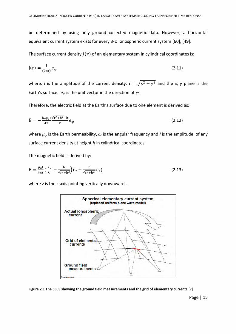
Figure 2.1 The SECS showing the ground field measurements and the grid of elementary currents [7]
GEOMAGNETICALLY INDUCED CURRENTS (GIC) IN LARGE POWER SYSTEMS INCLUDING TRANSFORMER TIME RESPONSE
Page | 16
The elementary ionospheric currents are placed in an equally spaced grid pattern over the
area of interest, as seen in Figure 2.1 [49, 60].
This method was used by Bernhardi et al [7] in 2008 to improve the accuracy of GIC
calculations for Southern Africa. They concluded that SECS allows for the interpolation of
geomagnetic fields as accurately as possible, with the existing configuration of magnetic
observatories in the region. Their results with SECS were closer to the measured GIC when
compared to GIC calculated using the uniform plane wave method.
2.1.3 The Complex Image method (CIM)
The complex image method (CIM) has also been used to calculate electric fields produced by
a line current (electrojet) source. This method adopts a layered conductivity model of the
Earth [62, 66] and is considered to be very accurate and fast [66, 67]. In 2003, Pulkkinen et
al [47] introduced a combination of SECS and CIM.
2.2 NETWORK CALCULATION
2.2.1 Lehtinen-Pirjola method
One of the most common methods that has been used for network calculation is the
Lehtinen - Pirjola method [25, 26].
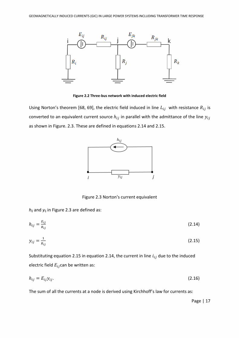
To illustrate this method, a small three-bus network is shown in Figure 2.2 with the induced
electric field shown on the lines as 𝐸𝑖𝑗 and 𝐸𝑗𝑘. The nodal resistances 𝑅𝑖𝑗, 𝑅𝑗 and 𝑅𝑗𝑘
represent the resistances at each substation per phase.
GEOMAGNETICALLY INDUCED CURRENTS (GIC) IN LARGE POWER SYSTEMS INCLUDING TRANSFORMER TIME RESPONSE
Page | 17
Figure 2.2 Three-bus network with induced electric field
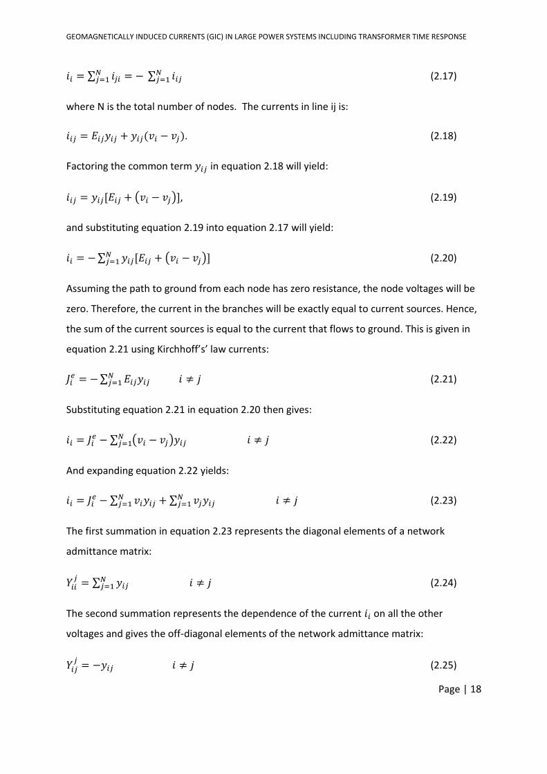
Using Norton’s theorem [68, 69], the electric field induced in line 𝐿𝑖𝑗 with resistance 𝑅𝑖𝑗 is
converted to an equivalent current source ℎ𝑖𝑗 in parallel with the admittance of the line 𝑦𝑖𝑗
as shown in Figure. 2.3. These are defined in equations 2.14 and 2.15.
Figure 2.3 Norton's current equivalent
hij and yij in Figure 2.3 are defined as:
ℎ𝑖𝑗 =𝐸𝑖𝑗
𝑅𝑖𝑗 (2.14)
𝑦𝑖𝑗 =1
𝑅𝑖𝑗 (2.15)
Substituting equation 2.15 in equation 2.14, the current in line 𝑖𝑖𝑗 due to the induced
electric field 𝐸𝑖𝑗can be written as:
ℎ𝑖𝑗 = 𝐸𝑖𝑗𝑦𝑖𝑗. (2.16)
The sum of all the currents at a node is derived using Kirchhoff’s law for currents as:
GEOMAGNETICALLY INDUCED CURRENTS (GIC) IN LARGE POWER SYSTEMS INCLUDING TRANSFORMER TIME RESPONSE
Page | 18
𝑖𝑖 = ∑ 𝑖𝑗𝑖𝑁𝑗=1 = − ∑ 𝑖𝑖𝑗
𝑁𝑗=1 (2.17)
where N is the total number of nodes. The currents in line ij is:
𝑖𝑖𝑗 = 𝐸𝑖𝑗𝑦𝑖𝑗 + 𝑦𝑖𝑗(𝑣𝑖 − 𝑣𝑗). (2.18)
Factoring the common term 𝑦𝑖𝑗 in equation 2.18 will yield:
𝑖𝑖𝑗 = 𝑦𝑖𝑗[𝐸𝑖𝑗 + (𝑣𝑖 − 𝑣𝑗)], (2.19)
and substituting equation 2.19 into equation 2.17 will yield:
𝑖𝑖 = −∑ 𝑦𝑖𝑗[𝐸𝑖𝑗 + (𝑣𝑖 − 𝑣𝑗)]𝑁𝑗=1 (2.20)
Assuming the path to ground from each node has zero resistance, the node voltages will be
zero. Therefore, the current in the branches will be exactly equal to current sources. Hence,
the sum of the current sources is equal to the current that flows to ground. This is given in
equation 2.21 using Kirchhoff’s’ law currents:
𝐽𝑖𝑒 = −∑ 𝐸𝑖𝑗𝑦𝑖𝑗
𝑁𝑗=1 𝑖 ≠ 𝑗 (2.21)
Substituting equation 2.21 in equation 2.20 then gives:
𝑖𝑖 = 𝐽𝑖𝑒 − ∑ (𝑣𝑖 − 𝑣𝑗)𝑦𝑖𝑗
𝑁𝑗=1 𝑖 ≠ 𝑗 (2.22)
And expanding equation 2.22 yields:
𝑖𝑖 = 𝐽𝑖𝑒 − ∑ 𝑣𝑖𝑦𝑖𝑗
𝑁𝑗=1 + ∑ 𝑣𝑗𝑦𝑖𝑗
𝑁𝑗=1 𝑖 ≠ 𝑗 (2.23)
The first summation in equation 2.23 represents the diagonal elements of a network
admittance matrix:
𝑌𝑖𝑖𝑗= ∑ 𝑦𝑖𝑗
𝑁𝑗=1 𝑖 ≠ 𝑗 (2.24)
The second summation represents the dependence of the current 𝑖𝑖 on all the other
voltages and gives the off-diagonal elements of the network admittance matrix:
𝑌𝑖𝑗𝑗= −𝑦𝑖𝑗 𝑖 ≠ 𝑗 (2.25)
GEOMAGNETICALLY INDUCED CURRENTS (GIC) IN LARGE POWER SYSTEMS INCLUDING TRANSFORMER TIME RESPONSE
Page | 19
Substituting equation 2.24 and 2.25 in equation 2.23 gives:
𝑖𝑖 = 𝐽𝑖𝑒 − ∑ 𝑣𝑗𝑌𝑖𝑗
𝑗𝑁𝑗=1 (2.26)
In matrix form, equation 2.26 can be written for all the nodes as:
[𝐼𝑒] = [𝐽𝑒] − [𝑌𝑗][𝑉𝑗] (2.27)
Where the elements of the column matrix [𝐼𝑒] are the nodal currents, elements of the
column matrix [𝑉𝑗] are the nodal voltages and [𝐽𝑒] is the column matrix of the current
sources at each node.
The nodal voltage at each node can be derived as the product of the earthing impedance
and the nodal current given in equation 2.28:
[𝑉𝑗] = [𝑍𝑒][𝐼𝑒] (2.28)
where [𝑍𝑒] is the earthing impedance matrix.
Substituting equation 2.28 in equation 2.27 gives:
[𝐼𝑒] = [𝐽𝑒] − [𝑌𝑗][𝑍𝑒][𝐼𝑒] (2.29)
Re-arranging equation 2.29 in terms of [𝐼𝑒] gives
[𝐼𝑒] ([1] + [𝑌𝑗][𝑍𝑒]) = [𝐽𝑒] (2.30)
where [1] is a unit matrix.
Matrix [𝐼𝑒]can be calculated by taking the inverse of ([1] + [𝑌𝑗][𝑍𝑒]) and multiplying the
result by [𝐽𝑒] given in equation 2.31:
[𝐼𝑒] = ([1] + [𝑌𝑗][𝑍𝑒])−1[𝐽𝑒] (2.31)
The current in each node in [𝐼𝑒] is the GIC flowing through the node to ground.
GEOMAGNETICALLY INDUCED CURRENTS (GIC) IN LARGE POWER SYSTEMS INCLUDING TRANSFORMER TIME RESPONSE
Page | 20
2.2.1.1 Superposition
When the electric field induced in the network is decomposed into the eastern component
and the northern component, [𝐽𝑒] in equation 2.21 will be calculated twice:
𝐽𝑖(𝑥)𝑒 = −∑ 𝐸(𝑥)𝑖𝑗𝑦𝑖𝑗
𝑁𝑗=1 𝑖 ≠ 𝑗 (2.32)
where 𝐽𝑖(𝑥)𝑒 is the sum of the current source at a node due to the eastern component of the
electric field, and:
𝐽𝑖(𝑦)𝑒 = −∑ 𝐸(𝑦)𝑖𝑗𝑦𝑖𝑗
𝑁𝑗=1 𝑖 ≠ 𝑗 (2.33)
where 𝐽𝑖(𝑦)𝑒 is the sum of the current source at a node due to the northern component of the
induced electric field.
Therefore, the nodal current as a result of the induced electric field will be:
[𝐼𝑒] = ([1] + [𝑌𝑗][𝑍𝑒])−1[𝐽𝑥𝑒] + ([1] + [𝑌𝑗][𝑍𝑒])
−1[𝐽𝑦𝑒] (2.34)
For an electric field of 1 V/km in both eastern and northern components for node i:
𝑎𝑖 = ([1] + [𝑌𝑗][𝑍𝑒])
−1[𝐽𝑥𝑒] (2.35)
where 𝑎 is nodal current corresponding to the eastern electric field of 1 V/km, and:
𝑏𝑖 = ([1] + [𝑌𝑗][𝑍𝑒])−1[𝐽𝑦𝑒] (2.36)
where 𝑏 is the nodal current corresponding to the northern electric field of 1 V/km.
This allows for equation 2.34 to re-written as:
[𝐼𝑒] = [𝑎𝑖]𝐸𝑥 + [𝑏𝑖]𝐸𝑦 (2.37)
Where 𝐸𝑥 represents the induced electric field in the northern direction and 𝐸𝑦 represents
the electric field in the eastern direction.
GEOMAGNETICALLY INDUCED CURRENTS (GIC) IN LARGE POWER SYSTEMS INCLUDING TRANSFORMER TIME RESPONSE
Page | 21
Equation 2.35 and equation 2.36 are fixed network parameters for a specific network.
Therefore once the 𝑎 and 𝑏 network parameters are calculated, the nodal currents can be
calculated as shown in equation 2.37.
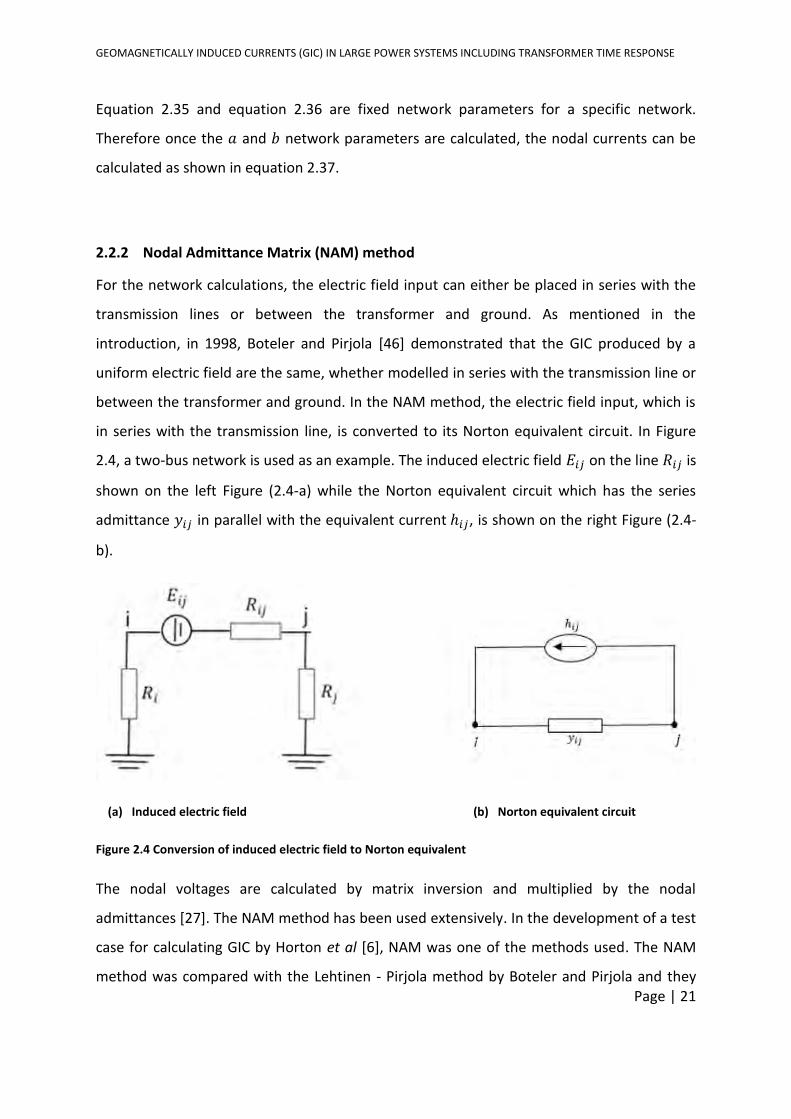
2.2.2 Nodal Admittance Matrix (NAM) method
For the network calculations, the electric field input can either be placed in series with the
transmission lines or between the transformer and ground. As mentioned in the
introduction, in 1998, Boteler and Pirjola [46] demonstrated that the GIC produced by a
uniform electric field are the same, whether modelled in series with the transmission line or
between the transformer and ground. In the NAM method, the electric field input, which is
in series with the transmission line, is converted to its Norton equivalent circuit. In Figure
2.4, a two-bus network is used as an example. The induced electric field 𝐸𝑖𝑗 on the line 𝑅𝑖𝑗 is
shown on the left Figure (2.4-a) while the Norton equivalent circuit which has the series
admittance 𝑦𝑖𝑗 in parallel with the equivalent current ℎ𝑖𝑗, is shown on the right Figure (2.4-
b).
(a) Induced electric field (b) Norton equivalent circuit
Figure 2.4 Conversion of induced electric field to Norton equivalent
The nodal voltages are calculated by matrix inversion and multiplied by the nodal
admittances [27]. The NAM method has been used extensively. In the development of a test
case for calculating GIC by Horton et al [6], NAM was one of the methods used. The NAM
method was compared with the Lehtinen - Pirjola method by Boteler and Pirjola and they
GEOMAGNETICALLY INDUCED CURRENTS (GIC) IN LARGE POWER SYSTEMS INCLUDING TRANSFORMER TIME RESPONSE
Page | 22
were found to be mathematically equivalent [26]. The derivation of the matrix equations
are in section 3.3 of this thesis, where they are directly linked to the example that was used
to derive the transformer time response equation.
2.3 CALCULATION AND MODELLING OF GIC IN POWER SYSTEMS
The aim of this section is to cover the techniques that have been used in software, to either
calculate GIC or to model the effect of GIC on power systems. This section will not delve
much into the half-wave saturation effects of GIC on power transformers because it has
been extensively studied. The underlying assumptions in each of the programs will be
discussed.
2.3.1 Koen
Koen wrote software in MATLAB to calculate GIC flowing through transformers in the
Southern African power network, using the Lehtinen-Pirjola method and the uniform plane
wave electric field model. The Earth’s conductivity was assumed to be uniform and the
effect of autotransformers was neglected. The GIC flowing through one of the transformers
at Grassridge power station (South Africa) was calculated and compared with the measured
GIC flowing through the same transformer. The profiles of the measured GIC and the
calculated GIC were similar. In some instances, the difference between the measured GIC
and calculated GIC was as low as 1 %, while on the other extreme, the difference between
the measured and calculated GIC was up to 110 %. Some of the reasons cited for these
discrepancies included the currents that flow through the autotransformer’s series winding,
GIC flow through connected reactors at the same substation, the actual ground resistivity at
the substation and the location of the magnetometer site relative to Grassridge substation.
To compensate for the difference between the measured and calculated GIC, a scaling
factor was used to adjust the calculated results. The author gave no indication of the
possibility that the transformer time response to changes in the magnetic field could
influence the difference between the measured and calculated GIC [31].

GEOMAGNETICALLY INDUCED CURRENTS (GIC) IN LARGE POWER SYSTEMS INCLUDING TRANSFORMER TIME RESPONSE
Page | 23
2.3.2 PowerWorld Simulator
PowerWorld simulator is a power system simulation software, designed to simulate high
voltage power systems in the time domain. It is equipped with the ability to incorporate the
flow of GIC into its load flow calculation. However, the flow of GIC can be calculated without
solving the load flow because it is generally considered as a DC problem. This software also
models the additional reactive power demand due to GIC [70], by using a constant to relate
GIC to the increase in reactive power lost in the transformer. This is done by adding a
parallel reactance to the existing shunt magnetization reactance. The magnitude of the
additional reactance is determined dynamically by the software.
In PowerWorld simulator, the induced electric field is modelled in series with the
transmission line. It is assumed that the reactance of the transmission lines and
transformers are negligible. The major system parameters that are used are the
transmission line resistance, transformer winding resistance and substation grounding
resistance. For auto-transformers the series winding resistance is required. The common
winding resistance for auto-transformers is only required if it is grounded. In terms of
geophysical calculations, the electric field can be entered either as a uniform plane wave or
a non-uniform plane wave. For the former, the uniform electric field magnitude and angle
are entered for the network. Using the longitude and latitude coordinates for the
transmission line, the size of electric field induced on the transmission line is calculated. For
the non-uniform electric field, the point of maximum electric field is chosen. From this
point, it is assumed that the electric field taper linearly down to zero over the geographic
area of the network. The electric fields induced on different segments of the transmission
line as it transverses different regions, is calculated using the uniform plane wave approach
[32], [71].
2.3.3 Boteler et al
The real-time simulator for GIC developed by Boteler et al for the Hydro One power
transmission network in Ontario uses real-time measurements of the magnetic field from a
magnetic observatory [36]. Based on the conventional uniform plane wave electric field
calculation method, the Fast Fourier Transform (FFT) of the magnetic field in the frequency
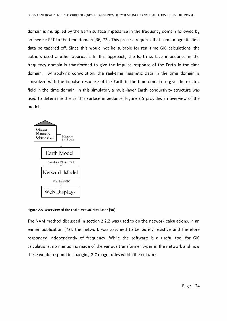
GEOMAGNETICALLY INDUCED CURRENTS (GIC) IN LARGE POWER SYSTEMS INCLUDING TRANSFORMER TIME RESPONSE
Page | 24
domain is multiplied by the Earth surface impedance in the frequency domain followed by
an inverse FFT to the time domain [36, 72]. This process requires that some magnetic field
data be tapered off. Since this would not be suitable for real-time GIC calculations, the
authors used another approach. In this approach, the Earth surface impedance in the
frequency domain is transformed to give the impulse response of the Earth in the time
domain. By applying convolution, the real-time magnetic data in the time domain is
convolved with the impulse response of the Earth in the time domain to give the electric
field in the time domain. In this simulator, a multi-layer Earth conductivity structure was
used to determine the Earth’s surface impedance. Figure 2.5 provides an overview of the
model.
Figure 2.5 Overview of the real-time GIC simulator [36]
The NAM method discussed in section 2.2.2 was used to do the network calculations. In an
earlier publication [72], the network was assumed to be purely resistive and therefore
responded independently of frequency. While the software is a useful tool for GIC
calculations, no mention is made of the various transformer types in the network and how
these would respond to changing GIC magnitudes within the network.
GEOMAGNETICALLY INDUCED CURRENTS (GIC) IN LARGE POWER SYSTEMS INCLUDING TRANSFORMER TIME RESPONSE
Page | 25
2.3.4 Berge and Varma
The GIC simulator developed by Berge and Varma focuses on modelling aspects of the
network, such as locating the termination points of transmission lines, autotransformers
and the electric fields induced in the power system [29]. Where an autotransformer
connects two buses, its winding resistance is divided between the coupling resistance and a
resistance to the neutral terminal (if grounded) [8, 29]. In cases where an autotransformer
connects more than one bus, the autotransformer is treated as a transmission line [29]. The
NAM method [27, 57] was used for the network part of the GIC calculation. Although the
assumption was made that the network could be treated as DC, the authors acknowledge
that this is not “strictly correct” [29]. The main contributions by the authors are the
elaborate method of locating transmission lines and the modelling of auto-transformers. As
in other case studies, no mention was made of the transformer time response to GIC for
different transformer core types.
2.4 SUMMARY OF GIC CALCULATION TECHNIQUES AND PROPOSED GIC
CALCULATION TECHNIQUE
A review of calculation methods, software used for GIC calculation and comparisons of
measured and calculated GIC was carried out to identify:
1. Some of the underlining assumptions about GIC calculation that have been made in
the past;
2. Reasons for the differences between measured and calculated GIC;
3. Other factors which have not been rigorously investigated in the literature, that
could contribute to the difference between measured and calculated GIC, and
4. The most suitable approach to be used for the method proposed in chapter 3.
The literature review pointed out the absence of any rigorous research into the effect of
transformer time response, and how this varies by transformer core type, and transformer
operation either as a GSU or a TT. To fill this gap in knowledge, a new method for calculating
GIC is proposed in this thesis. This calculation method comprises the uniform plane wave

GEOMAGNETICALLY INDUCED CURRENTS (GIC) IN LARGE POWER SYSTEMS INCLUDING TRANSFORMER TIME RESPONSE
Page | 26
electric field model for deriving the electric field on the transmission line and the NAM
method with the addition of the transformer time response. A uniform ground conductivity
was assumed because it was used to calculate the electric field in the previous work to
which the results in this thesis would be compared. Moreover for consistency in the
analysis, to avoid distorting the analysis of the impact of the transformer time response to
GIC, uniform ground conductivity is assumed.
GEOMAGNETICALLY INDUCED CURRENTS (GIC) IN LARGE POWER SYSTEMS INCLUDING TRANSFORMER TIME RESPONSE
Page | 27
CHAPTER 3
INTRODUCTION OF TRANSFORMER TIME
RESPONSE INTO GIC CALCULATION
3. INTRODUCTION OF TRANSFORMER TIME RESPONSE INTO GIC CALCULATION
In the first section of this chapter, the formula for calculating the prospective GIC with
transformer time response is derived, which takes into account the core type and
operational mode (i.e. GSU or TT) of the transformer. This is followed by the derivation of
the electric field induced in each transmission line and finally, a formula for calculating the
prospective GIC without the transformer time response.
3.1 DERIVATION OF TRANSFORMER TIME RESPONSE
The induced electric field during geomagnetic storms causes GIC to flow through grounded
transformers. Transformers are made up of primary windings, secondary windings and in
some cases tertiary windings which are wound in a number of configurations. These
configurations include [19]:
Single-phase shell- or core-type
Three-phase shell-type seven- limb core
Three-phase shell-type conventional core
Three-phase core-type five-limb core
Three-phase core-form three-limb core
Figure 3.1 illustrates the flow of GIC in the transmission lines, grounded neutrals and
windings or wye-connected transformers.
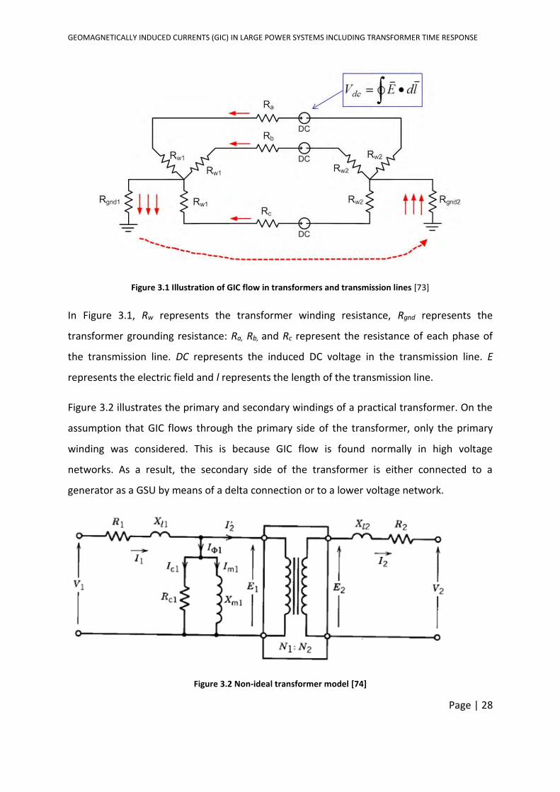
GEOMAGNETICALLY INDUCED CURRENTS (GIC) IN LARGE POWER SYSTEMS INCLUDING TRANSFORMER TIME RESPONSE
Page | 28
Figure 3.1 Illustration of GIC flow in transformers and transmission lines [73]
In Figure 3.1, Rw represents the transformer winding resistance, Rgnd represents the
transformer grounding resistance: Ra, Rb, and Rc represent the resistance of each phase of
the transmission line. DC represents the induced DC voltage in the transmission line. E
represents the electric field and l represents the length of the transmission line.
Figure 3.2 illustrates the primary and secondary windings of a practical transformer. On the
assumption that GIC flows through the primary side of the transformer, only the primary
winding was considered. This is because GIC flow is found normally in high voltage
networks. As a result, the secondary side of the transformer is either connected to a
generator as a GSU by means of a delta connection or to a lower voltage network.
Figure 3.2 Non-ideal transformer model [74]

GEOMAGNETICALLY INDUCED CURRENTS (GIC) IN LARGE POWER SYSTEMS INCLUDING TRANSFORMER TIME RESPONSE
Page | 29
In Figure 3.2
V1 = Voltage across the primary winding
Xl1 = Leakage reactance of the primary winding
I1 = Current in the primary winding
Ic1 = Current due to core losses
Im1 = Magnetization current
Xm1= Magnetization reactance
Rc1 = Core losses
V2 = Voltage across the secondary winding
R2 = Resistance of the secondary winding
Xl2 = Leakage reactance of the secondary winding
I2 = Current in the secondary winding
I’2 = Current in the secondary winding refereed to the primary winding
R1 = Resistance of the primary winding
If mutual inductance is neglected under GIC conditions, the secondary winding can be
reduced to the self-inductance of the winding and the resistance of the winding as seen in
Figure 3.3.
Figure 3.3 Reduced model of the primary winding
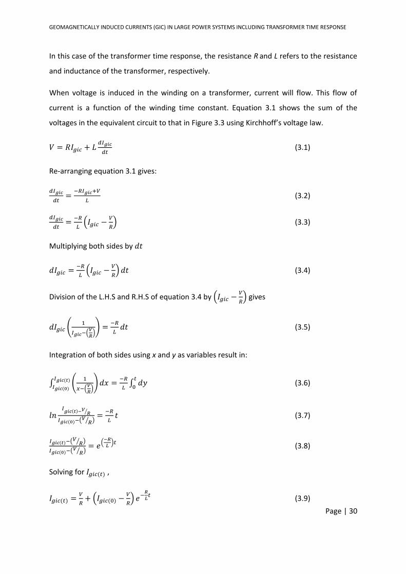
GEOMAGNETICALLY INDUCED CURRENTS (GIC) IN LARGE POWER SYSTEMS INCLUDING TRANSFORMER TIME RESPONSE
Page | 30
In this case of the transformer time response, the resistance R and L refers to the resistance
and inductance of the transformer, respectively.
When voltage is induced in the winding on a transformer, current will flow. This flow of
current is a function of the winding time constant. Equation 3.1 shows the sum of the
voltages in the equivalent circuit to that in Figure 3.3 using Kirchhoff’s voltage law.
𝑉 = 𝑅𝐼𝑔𝑖𝑐 + 𝐿𝑑𝐼𝑔𝑖𝑐
𝑑𝑡 (3.1)
Re-arranging equation 3.1 gives:
𝑑𝐼𝑔𝑖𝑐
𝑑𝑡=
−𝑅𝐼𝑔𝑖𝑐+𝑉
𝐿 (3.2)
𝑑𝐼𝑔𝑖𝑐
𝑑𝑡=
−𝑅
𝐿(𝐼𝑔𝑖𝑐 −
𝑉
𝑅) (3.3)
Multiplying both sides by 𝑑𝑡
𝑑𝐼𝑔𝑖𝑐 =−𝑅
𝐿(𝐼𝑔𝑖𝑐 −
𝑉
𝑅)𝑑𝑡 (3.4)
Division of the L.H.S and R.H.S of equation 3.4 by (𝐼𝑔𝑖𝑐 −𝑉
𝑅) gives
𝑑𝐼𝑔𝑖𝑐 (1
𝐼𝑔𝑖𝑐−(𝑉
𝑅)) =
−𝑅
𝐿𝑑𝑡 (3.5)
Integration of both sides using x and y as variables result in:
∫ (1
𝑥−(𝑉
𝑅))
𝐼𝑔𝑖𝑐(𝑡)𝐼𝑔𝑖𝑐(0)
𝑑𝑥 =−𝑅
𝐿∫ 𝑑𝑦𝑡
0 (3.6)
𝑙𝑛𝐼𝑔𝑖𝑐(𝑡)−𝑉 𝑅⁄
𝐼𝑔𝑖𝑐(0)−(𝑉𝑅⁄ )=
−𝑅
𝐿𝑡 (3.7)
𝐼𝑔𝑖𝑐(𝑡)−(𝑉𝑅⁄ )
𝐼𝑔𝑖𝑐(0)−(𝑉𝑅⁄ )= 𝑒(
−𝑅
𝐿)𝑡 (3.8)
Solving for 𝐼𝑔𝑖𝑐(𝑡) ,
𝐼𝑔𝑖𝑐(𝑡) =𝑉
𝑅+ (𝐼𝑔𝑖𝑐(0) −
𝑉
𝑅) 𝑒−
𝑅
𝐿𝑡 (3.9)
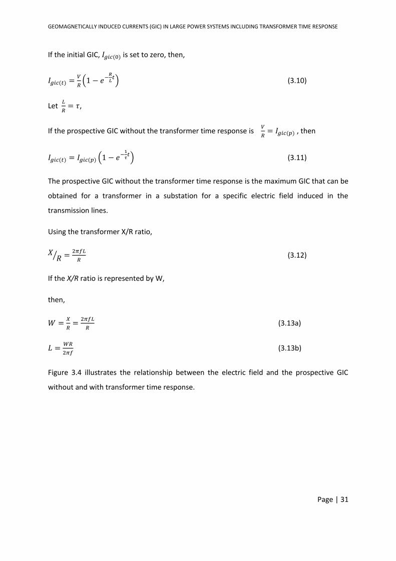
GEOMAGNETICALLY INDUCED CURRENTS (GIC) IN LARGE POWER SYSTEMS INCLUDING TRANSFORMER TIME RESPONSE
Page | 31
If the initial GIC, 𝐼𝑔𝑖𝑐(0) is set to zero, then,
𝐼𝑔𝑖𝑐(𝑡) =𝑉
𝑅(1 − 𝑒−
𝑅
𝐿𝑡) (3.10)
Let 𝐿
𝑅= 𝜏,
If the prospective GIC without the transformer time response is 𝑉
𝑅= 𝐼𝑔𝑖𝑐(𝑝) , then
𝐼𝑔𝑖𝑐(𝑡) = 𝐼𝑔𝑖𝑐(𝑝) (1 − 𝑒−1
𝜏𝑡) (3.11)
The prospective GIC without the transformer time response is the maximum GIC that can be
obtained for a transformer in a substation for a specific electric field induced in the
transmission lines.
Using the transformer X/R ratio,
𝑋𝑅⁄ =
2𝜋𝑓𝐿
𝑅 (3.12)
If the X/R ratio is represented by W,
then,
𝑊 =𝑋
𝑅=
2𝜋𝑓𝐿
𝑅 (3.13a)
𝐿 =𝑊𝑅
2𝜋𝑓 (3.13b)
Figure 3.4 illustrates the relationship between the electric field and the prospective GIC
without and with transformer time response.
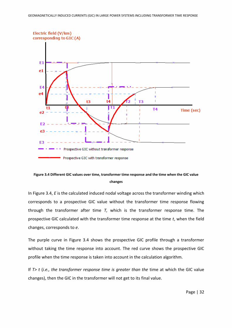
GEOMAGNETICALLY INDUCED CURRENTS (GIC) IN LARGE POWER SYSTEMS INCLUDING TRANSFORMER TIME RESPONSE
Page | 32
Figure 3.4 Different GIC values over time, transformer time response and the time when the GIC value
changes
In Figure 3.4, E is the calculated induced nodal voltage across the transformer winding which
corresponds to a prospective GIC value without the transformer time response flowing
through the transformer after time T, which is the transformer response time. The
prospective GIC calculated with the transformer time response at the time t, when the field
changes, corresponds to e.
The purple curve in Figure 3.4 shows the prospective GIC profile through a transformer
without taking the time response into account. The red curve shows the prospective GIC
profile when the time response is taken into account in the calculation algorithm.
If T> t (i.e., the transformer response time is greater than the time at which the GIC value
changes), then the GIC in the transformer will not get to its final value.
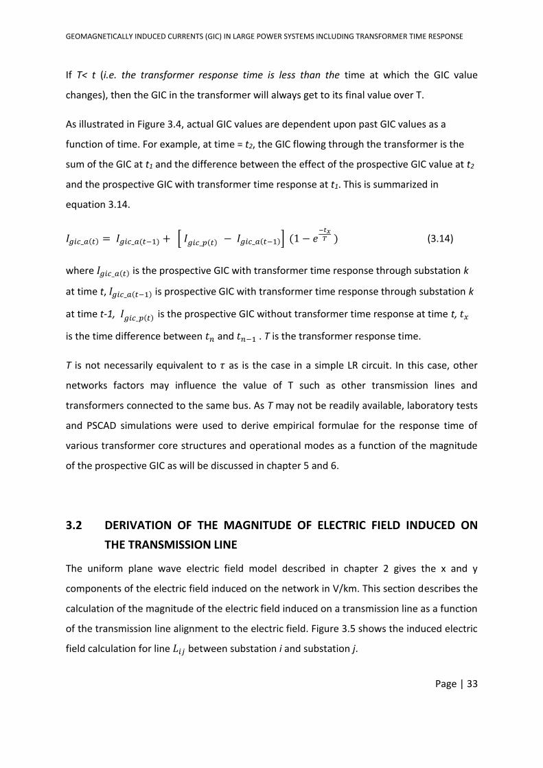
GEOMAGNETICALLY INDUCED CURRENTS (GIC) IN LARGE POWER SYSTEMS INCLUDING TRANSFORMER TIME RESPONSE
Page | 33
If T< t (i.e. the transformer response time is less than the time at which the GIC value
changes), then the GIC in the transformer will always get to its final value over T.
As illustrated in Figure 3.4, actual GIC values are dependent upon past GIC values as a
function of time. For example, at time = t2, the GIC flowing through the transformer is the
sum of the GIC at t1 and the difference between the effect of the prospective GIC value at t2
and the prospective GIC with transformer time response at t1. This is summarized in
equation 3.14.
𝐼𝑔𝑖𝑐_𝑎(𝑡) = 𝐼𝑔𝑖𝑐_𝑎(𝑡−1) + [ 𝐼𝑔𝑖𝑐_𝑝(𝑡) − 𝐼𝑔𝑖𝑐_𝑎(𝑡−1)] (1 − 𝑒−𝑡𝑥𝑇 ) (3.14)
where 𝐼𝑔𝑖𝑐_𝑎(𝑡) is the prospective GIC with transformer time response through substation k
at time t, 𝐼𝑔𝑖𝑐_𝑎(𝑡−1) is prospective GIC with transformer time response through substation k
at time t-1, 𝐼𝑔𝑖𝑐_𝑝(𝑡) is the prospective GIC without transformer time response at time t, 𝑡𝑥
is the time difference between 𝑡𝑛 and 𝑡𝑛−1 . T is the transformer response time.
T is not necessarily equivalent to 𝜏 as is the case in a simple LR circuit. In this case, other
networks factors may influence the value of T such as other transmission lines and
transformers connected to the same bus. As T may not be readily available, laboratory tests
and PSCAD simulations were used to derive empirical formulae for the response time of
various transformer core structures and operational modes as a function of the magnitude
of the prospective GIC as will be discussed in chapter 5 and 6.
3.2 DERIVATION OF THE MAGNITUDE OF ELECTRIC FIELD INDUCED ON
THE TRANSMISSION LINE
The uniform plane wave electric field model described in chapter 2 gives the x and y
components of the electric field induced on the network in V/km. This section describes the
calculation of the magnitude of the electric field induced on a transmission line as a function
of the transmission line alignment to the electric field. Figure 3.5 shows the induced electric
field calculation for line 𝐿𝑖𝑗 between substation i and substation j.
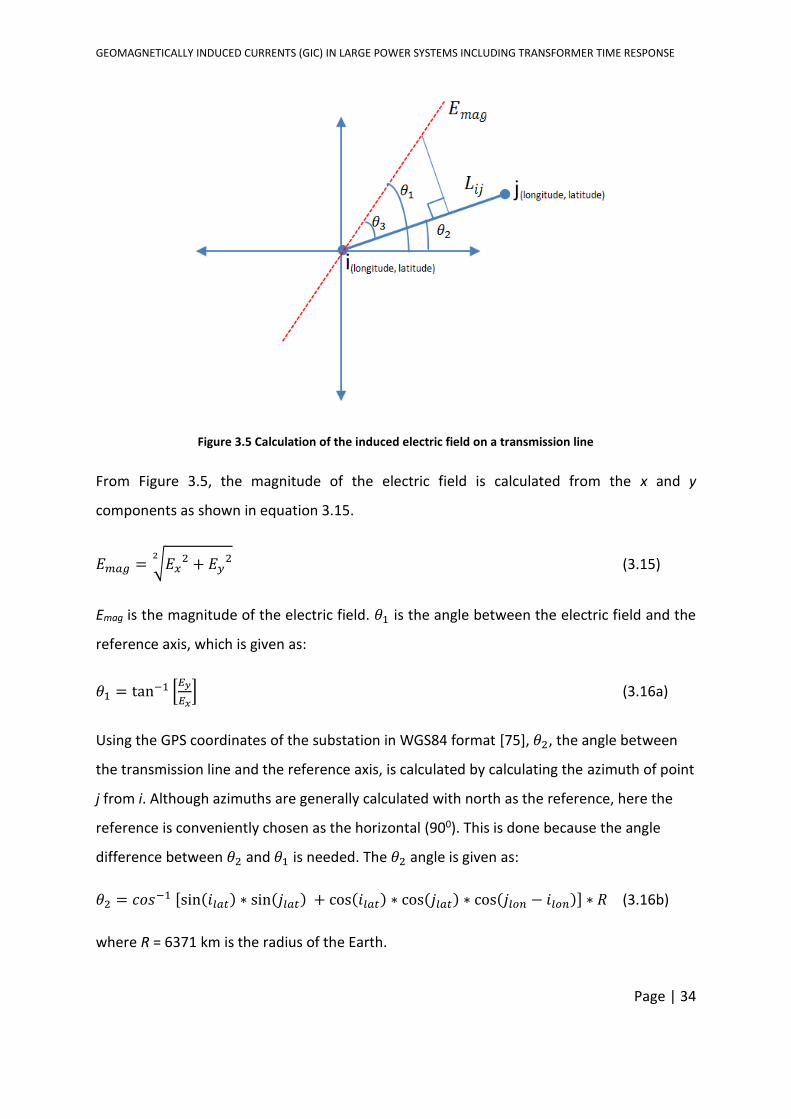
GEOMAGNETICALLY INDUCED CURRENTS (GIC) IN LARGE POWER SYSTEMS INCLUDING TRANSFORMER TIME RESPONSE
Page | 34
Figure 3.5 Calculation of the induced electric field on a transmission line
From Figure 3.5, the magnitude of the electric field is calculated from the x and y
components as shown in equation 3.15.
𝐸𝑚𝑎𝑔 = √𝐸𝑥2 + 𝐸𝑦
22 (3.15)
Emag is the magnitude of the electric field. 𝜃1 is the angle between the electric field and the
reference axis, which is given as:
𝜃1 = tan−1 [𝐸𝑦
𝐸𝑥] (3.16a)
Using the GPS coordinates of the substation in WGS84 format [75], 𝜃2, the angle between
the transmission line and the reference axis, is calculated by calculating the azimuth of point
j from i. Although azimuths are generally calculated with north as the reference, here the
reference is conveniently chosen as the horizontal (900). This is done because the angle
difference between 𝜃2 and 𝜃1 is needed. The 𝜃2 angle is given as:
𝜃2 = 𝑐𝑜𝑠−1 [sin(𝑖𝑙𝑎𝑡) ∗ sin(𝑗𝑙𝑎𝑡) + cos(𝑖𝑙𝑎𝑡) ∗ cos(𝑗𝑙𝑎𝑡) ∗ cos(𝑗𝑙𝑜𝑛 − 𝑖𝑙𝑜𝑛)] ∗ 𝑅 (3.16b)
where R = 6371 km is the radius of the Earth.
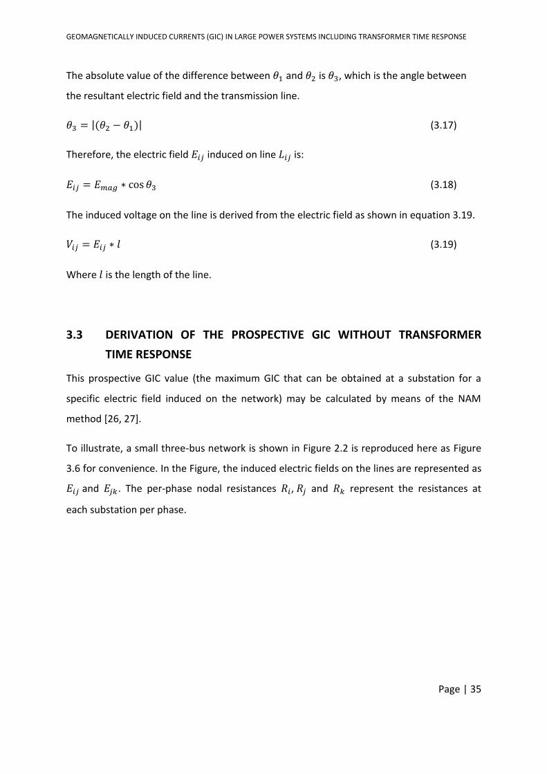
GEOMAGNETICALLY INDUCED CURRENTS (GIC) IN LARGE POWER SYSTEMS INCLUDING TRANSFORMER TIME RESPONSE
Page | 35
The absolute value of the difference between 𝜃1 and 𝜃2 is 𝜃3, which is the angle between
the resultant electric field and the transmission line.
𝜃3 = |(𝜃2 − 𝜃1)| (3.17)
Therefore, the electric field 𝐸𝑖𝑗 induced on line 𝐿𝑖𝑗 is:
𝐸𝑖𝑗 = 𝐸𝑚𝑎𝑔 ∗ cos 𝜃3 (3.18)
The induced voltage on the line is derived from the electric field as shown in equation 3.19.
𝑉𝑖𝑗 = 𝐸𝑖𝑗 ∗ 𝑙 (3.19)
Where 𝑙 is the length of the line.
3.3 DERIVATION OF THE PROSPECTIVE GIC WITHOUT TRANSFORMER
TIME RESPONSE
This prospective GIC value (the maximum GIC that can be obtained at a substation for a
specific electric field induced on the network) may be calculated by means of the NAM
method [26, 27].
To illustrate, a small three-bus network is shown in Figure 2.2 is reproduced here as Figure
3.6 for convenience. In the Figure, the induced electric fields on the lines are represented as
𝐸𝑖𝑗 and 𝐸𝑗𝑘. The per-phase nodal resistances 𝑅𝑖, 𝑅𝑗 and 𝑅𝑘 represent the resistances at
each substation per phase.
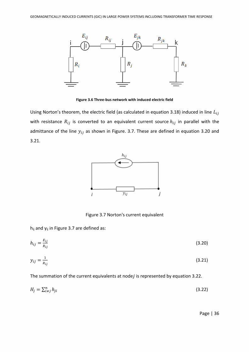
GEOMAGNETICALLY INDUCED CURRENTS (GIC) IN LARGE POWER SYSTEMS INCLUDING TRANSFORMER TIME RESPONSE
Page | 36
Figure 3.6 Three-bus network with induced electric field
Using Norton’s theorem, the electric field (as calculated in equation 3.18) induced in line 𝐿𝑖𝑗
with resistance 𝑅𝑖𝑗 is converted to an equivalent current source ℎ𝑖𝑗 in parallel with the
admittance of the line 𝑦𝑖𝑗 as shown in Figure. 3.7. These are defined in equation 3.20 and
3.21.
Figure 3.7 Norton's current equivalent
hij and yij in Figure 3.7 are defined as:
ℎ𝑖𝑗 =𝐸𝑖𝑗
𝑅𝑖𝑗 (3.20)
𝑦𝑖𝑗 =1
𝑅𝑖𝑗 (3.21)
The summation of the current equivalents at node𝑗 is represented by equation 3.22.
𝐻𝑗 = ∑ ℎ𝑗𝑖 𝑛𝑖≠𝑗 (3.22)
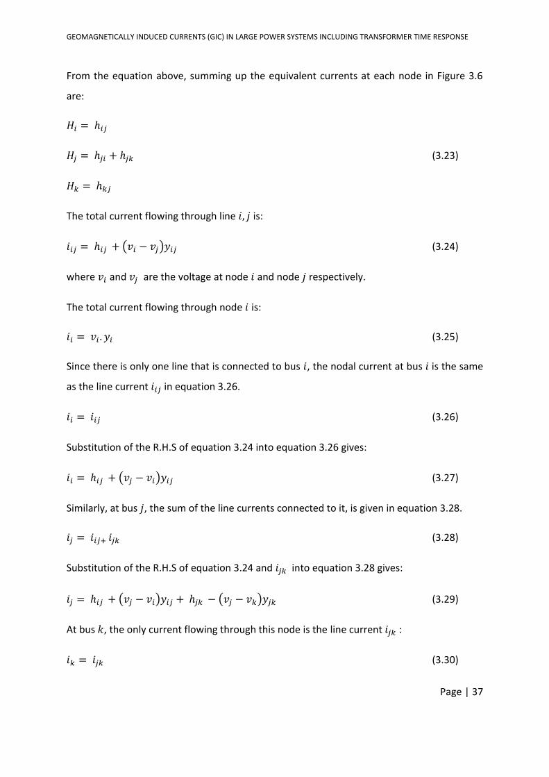
GEOMAGNETICALLY INDUCED CURRENTS (GIC) IN LARGE POWER SYSTEMS INCLUDING TRANSFORMER TIME RESPONSE
Page | 37
From the equation above, summing up the equivalent currents at each node in Figure 3.6
are:
𝐻𝑖 = ℎ𝑖𝑗
𝐻𝑗 = ℎ𝑗𝑖 + ℎ𝑗𝑘 (3.23)
𝐻𝑘 = ℎ𝑘𝑗
The total current flowing through line 𝑖, 𝑗 is:
𝑖𝑖𝑗 = ℎ𝑖𝑗 + (𝑣𝑖 − 𝑣𝑗)𝑦𝑖𝑗 (3.24)
where 𝑣𝑖 and 𝑣𝑗 are the voltage at node 𝑖 and node 𝑗 respectively.
The total current flowing through node 𝑖 is:
𝑖𝑖 = 𝑣𝑖 . 𝑦𝑖 (3.25)
Since there is only one line that is connected to bus 𝑖, the nodal current at bus 𝑖 is the same
as the line current 𝑖𝑖𝑗 in equation 3.26.
𝑖𝑖 = 𝑖𝑖𝑗 (3.26)
Substitution of the R.H.S of equation 3.24 into equation 3.26 gives:
𝑖𝑖 = ℎ𝑖𝑗 + (𝑣𝑗 − 𝑣𝑖)𝑦𝑖𝑗 (3.27)
Similarly, at bus 𝑗, the sum of the line currents connected to it, is given in equation 3.28.
𝑖𝑗 = 𝑖𝑖𝑗+ 𝑖𝑗𝑘 (3.28)
Substitution of the R.H.S of equation 3.24 and 𝑖𝑗𝑘 into equation 3.28 gives:
𝑖𝑗 = ℎ𝑖𝑗 + (𝑣𝑗 − 𝑣𝑖)𝑦𝑖𝑗 + ℎ𝑗𝑘 − (𝑣𝑗 − 𝑣𝑘)𝑦𝑗𝑘 (3.29)
At bus 𝑘, the only current flowing through this node is the line current 𝑖𝑗𝑘 :
𝑖𝑘 = 𝑖𝑗𝑘 (3.30)
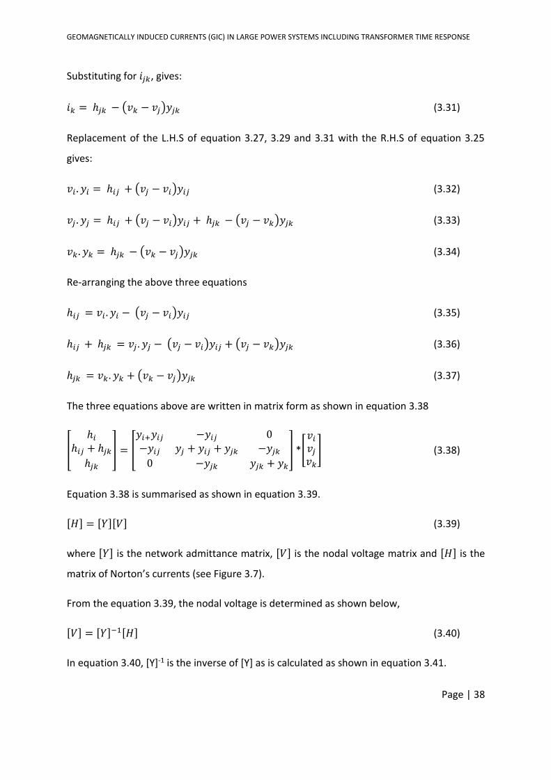
GEOMAGNETICALLY INDUCED CURRENTS (GIC) IN LARGE POWER SYSTEMS INCLUDING TRANSFORMER TIME RESPONSE
Page | 38
Substituting for 𝑖𝑗𝑘, gives:
𝑖𝑘 = ℎ𝑗𝑘 − (𝑣𝑘 − 𝑣𝑗)𝑦𝑗𝑘 (3.31)
Replacement of the L.H.S of equation 3.27, 3.29 and 3.31 with the R.H.S of equation 3.25
gives:
𝑣𝑖 . 𝑦𝑖 = ℎ𝑖𝑗 + (𝑣𝑗 − 𝑣𝑖)𝑦𝑖𝑗 (3.32)
𝑣𝑗 . 𝑦𝑗 = ℎ𝑖𝑗 + (𝑣𝑗 − 𝑣𝑖)𝑦𝑖𝑗 + ℎ𝑗𝑘 − (𝑣𝑗 − 𝑣𝑘)𝑦𝑗𝑘 (3.33)
𝑣𝑘. 𝑦𝑘 = ℎ𝑗𝑘 − (𝑣𝑘 − 𝑣𝑗)𝑦𝑗𝑘 (3.34)
Re-arranging the above three equations
ℎ𝑖𝑗 = 𝑣𝑖 . 𝑦𝑖 − (𝑣𝑗 − 𝑣𝑖)𝑦𝑖𝑗 (3.35)
ℎ𝑖𝑗 + ℎ𝑗𝑘 = 𝑣𝑗 . 𝑦𝑗 − (𝑣𝑗 − 𝑣𝑖)𝑦𝑖𝑗 + (𝑣𝑗 − 𝑣𝑘)𝑦𝑗𝑘 (3.36)
ℎ𝑗𝑘 = 𝑣𝑘. 𝑦𝑘 + (𝑣𝑘 − 𝑣𝑗)𝑦𝑗𝑘 (3.37)
The three equations above are written in matrix form as shown in equation 3.38
[
ℎ𝑖ℎ𝑖𝑗 + ℎ𝑗𝑘ℎ𝑗𝑘
] = [
𝑦𝑖+𝑦𝑖𝑗 −𝑦𝑖𝑗 0
−𝑦𝑖𝑗 𝑦𝑗 + 𝑦𝑖𝑗 + 𝑦𝑗𝑘 −𝑦𝑗𝑘0 −𝑦𝑗𝑘 𝑦𝑗𝑘 + 𝑦𝑘
] *[
𝑣𝑖𝑣𝑗𝑣𝑘] (3.38)
Equation 3.38 is summarised as shown in equation 3.39.
[𝐻] = [𝑌][𝑉] (3.39)
where [𝑌] is the network admittance matrix, [𝑉] is the nodal voltage matrix and [𝐻] is the
matrix of Norton’s currents (see Figure 3.7).
From the equation 3.39, the nodal voltage is determined as shown below,
[𝑉] = [𝑌]−1[𝐻] (3.40)
In equation 3.40, [Y]-1 is the inverse of [Y] as is calculated as shown in equation 3.41.
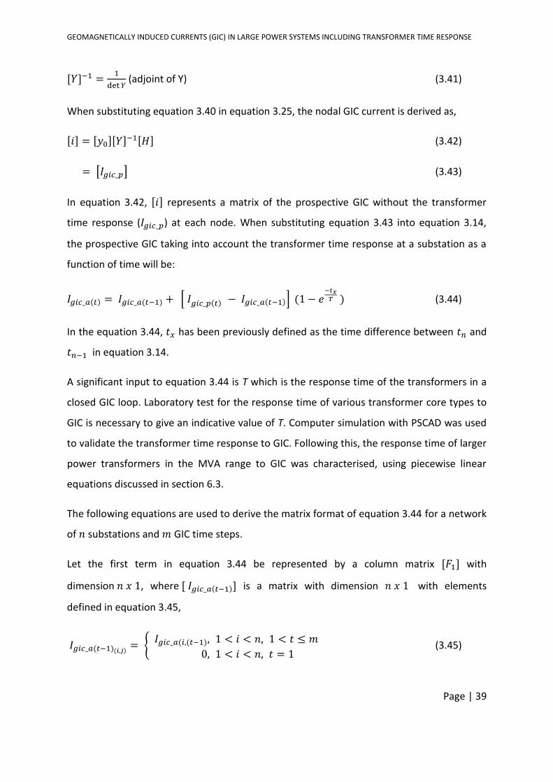
GEOMAGNETICALLY INDUCED CURRENTS (GIC) IN LARGE POWER SYSTEMS INCLUDING TRANSFORMER TIME RESPONSE
Page | 39
[𝑌]−1 =1
det 𝑌 (adjoint of Y) (3.41)
When substituting equation 3.40 in equation 3.25, the nodal GIC current is derived as,
[𝑖] = [𝑦0][𝑌]−1[𝐻] (3.42)
= [𝐼𝑔𝑖𝑐_𝑝] (3.43)
In equation 3.42, [𝑖] represents a matrix of the prospective GIC without the transformer
time response (𝐼𝑔𝑖𝑐_𝑝) at each node. When substituting equation 3.43 into equation 3.14,
the prospective GIC taking into account the transformer time response at a substation as a
function of time will be:
𝐼𝑔𝑖𝑐_𝑎(𝑡) = 𝐼𝑔𝑖𝑐_𝑎(𝑡−1) + [ 𝐼𝑔𝑖𝑐_𝑝(𝑡) − 𝐼𝑔𝑖𝑐_𝑎(𝑡−1)] (1 − 𝑒−𝑡𝑥𝑇 ) (3.44)
In the equation 3.44, 𝑡𝑥 has been previously defined as the time difference between 𝑡𝑛 and
𝑡𝑛−1 in equation 3.14.
A significant input to equation 3.44 is T which is the response time of the transformers in a
closed GIC loop. Laboratory test for the response time of various transformer core types to
GIC is necessary to give an indicative value of T. Computer simulation with PSCAD was used
to validate the transformer time response to GIC. Following this, the response time of larger
power transformers in the MVA range to GIC was characterised, using piecewise linear
equations discussed in section 6.3.
The following equations are used to derive the matrix format of equation 3.44 for a network
of 𝑛 substations and 𝑚 GIC time steps.
Let the first term in equation 3.44 be represented by a column matrix [𝐹1] with
dimension 𝑛 𝑥 1, where [ 𝐼𝑔𝑖𝑐_𝑎(𝑡−1)] is a matrix with dimension 𝑛 𝑥 1 with elements
defined in equation 3.45,
𝐼𝑔𝑖𝑐_𝑎(𝑡−1)(𝑖,𝑗) = 𝐼𝑔𝑖𝑐_𝑎(𝑖,(𝑡−1), 1 < 𝑖 < 𝑛, 1 < 𝑡 ≤ 𝑚
0, 1 < 𝑖 < 𝑛, 𝑡 = 1 (3.45)
GEOMAGNETICALLY INDUCED CURRENTS (GIC) IN LARGE POWER SYSTEMS INCLUDING TRANSFORMER TIME RESPONSE
Page | 40
Let the second term [ 𝐼𝑔𝑖𝑐_𝑝(𝑡) − 𝐼𝑔𝑖𝑐_𝑎(𝑡−1)] (1 − 𝑒−𝑡𝑥𝑇 ) in equation 3.44 be represented in
matrix form by ([𝐹2] − [𝐹3]) × [𝐹4] .
where the elements of [𝐹2] with dimension 𝑛 𝑥 1 are derived in equation 3.43, the elements
of [𝐹3] are defined in equation 3.45.
If the factor (1 − 𝑒−𝑡
𝑇 ) in equation 3.44 is represented in matrix form as [𝐹4], then:
[𝐹4] = [1] − [𝐹5] (3.46)
where [𝐹5] is a square matrix with dimension 𝑛 𝑥 𝑛 such that:
𝑓5(𝑖,𝑗)𝑡 = 𝑒−𝑡
𝑇𝑖 , 𝑖 = 𝑗0, 𝑖 ≠ 𝑗
(3.47)
In the equation 3.47, 𝑖 and 𝑗 represents the row and column reference respectively. 𝑇𝑖
represent the time response of the transformers in substation 𝑖 . The dimension of the
identity matrix [1] in equation 3.46 is 𝑛 𝑥 𝑛 . Therefore, the dimension of [𝐹4] is 𝑛 𝑥 𝑛 .
Therefore for a network with 𝑛 substations, the prospective GIC with transformer time
response can be derived as:
[𝐼] = [𝐹1]𝑇 + ([𝐹2]
𝑇−[𝐹3]𝑇) × [𝐹4] (3.48)
where the superscript 𝑇 means the transpose of the matrix.
GEOMAGNETICALLY INDUCED CURRENTS (GIC) IN LARGE POWER SYSTEMS INCLUDING TRANSFORMER TIME RESPONSE
Page | 41
CHAPTER 4
LABORATORY TEST PROTOCOL AND COMPUTER
SIMULATION
4. LABORATORY TEST PROTOCOL AND COMPUTER SIMULATION
In this chapter, the protocol that was used for the transformer time response test is
outlined. The test protocol has two sections. The first part of the protocol was developed by
Chisepo [76] as a standard procedure for testing transformer response to GIC in terms of
reactive power, active power, harmonics and saturation. The second part of the test
protocol describes the method to determine the range of DC current values that are
injected into the transformer to emulate GIC. Tests were conducted on three types of
transformer core structures namely, bank of single-phase transformers referred to as 3(1P-
3L), three-phase three-limb referred to as 3P-3L and three-phase five-limb referred to as
3P-5L. These three core structures were selected to test the algorithm because they
represent the most common types of transformers used in power networks.
Section 4.1 outlines the test protocol and describes the laboratory equipment that was
used. The PSCAD simulations for both VA-rated and MVA-rated transformers are outlined in
section 4.3.
GEOMAGNETICALLY INDUCED CURRENTS (GIC) IN LARGE POWER SYSTEMS INCLUDING TRANSFORMER TIME RESPONSE
Page | 42
4.1 TEST PROTOCOL
1. Determine the operating voltage at which the harmonics and distortion in the
transformer complies with IEEE standard 1459 [77].
2. Determine the magnetization current (Imag) of the transformer.
3. Determine the short circuit and open circuit parameters of the transformer.
Tests conducted by Chisepo [76] on the same set of transformers determined these
parameters. Tables 4.1 to 4.3 give the transformer ratings and parameters for the open
and short circuit tests. The transformer inductance is calculated using equation 4.1.
𝐿 =𝑋𝑝𝑢×𝑉
2
2×𝜋×𝑓×𝑆 (4.1)
where L is the inductance, X is the reactance, V is the voltage, S is the power base
(rating), f is the frequency (50 Hz).
4. Calculate the load current to DC current ratio 𝑘𝐿𝐷 given in equation 4.2.
𝑘𝐿𝐷 =𝐼𝑟
𝐼𝑚 (pu) (4.2)
where 𝐼𝑟 is the rated line current and 𝐼𝑚 is the magnetization current.
5. Calculate the DC current in pu given in equation 4.3.
𝐼𝑝𝑢 =𝐼𝑑𝑐
𝐼𝑚 (pu)
𝐼𝑑𝑐 coupled with the AC current should not exceed the rating of the transformer.
6. Inject the DC current into the transformer neutral, such that the DC current per phase
follows the inequality 1 ≤ 𝐼𝑝𝑢 ≤ 𝑘𝐿𝐷 .
7. A NI data acquisition set was used to record the time taken for the DC current to rise
from 0.5 pu to 𝐼𝑝𝑢, and the time taken for the DC current to drop from 𝐼𝑝𝑢to 0.5 pu. A
value of 0.5 pu was chosen since it is relatively small compared to the value of the
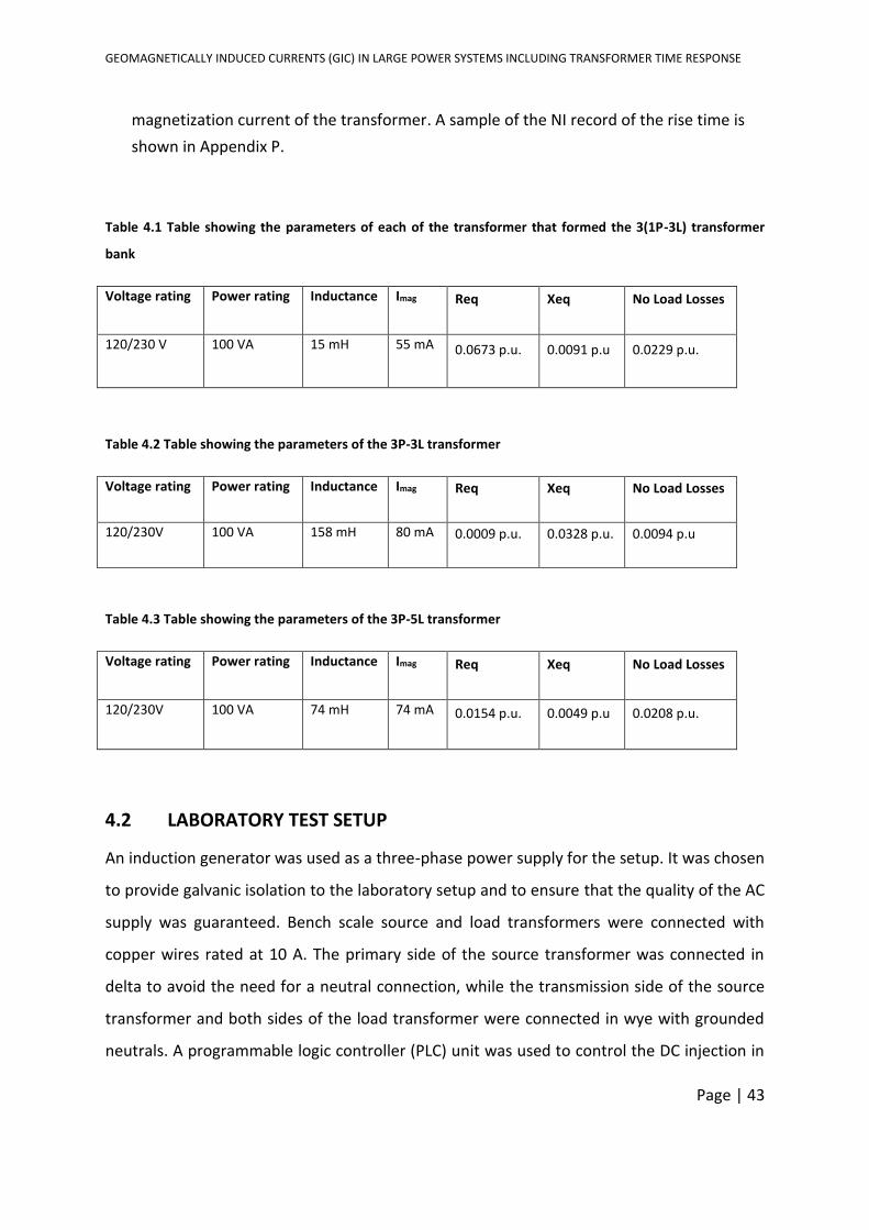
GEOMAGNETICALLY INDUCED CURRENTS (GIC) IN LARGE POWER SYSTEMS INCLUDING TRANSFORMER TIME RESPONSE
Page | 43
magnetization current of the transformer. A sample of the NI record of the rise time is
shown in Appendix P.
Table 4.1 Table showing the parameters of each of the transformer that formed the 3(1P-3L) transformer
bank
Voltage rating Power rating Inductance Imag Req Xeq No Load Losses
120/230 V 100 VA 15 mH 55 mA 0.0673 p.u. 0.0091 p.u 0.0229 p.u.
Table 4.2 Table showing the parameters of the 3P-3L transformer
Voltage rating Power rating Inductance Imag Req Xeq No Load Losses
120/230V 100 VA 158 mH 80 mA 0.0009 p.u. 0.0328 p.u. 0.0094 p.u
Table 4.3 Table showing the parameters of the 3P-5L transformer
Voltage rating Power rating Inductance Imag Req Xeq No Load Losses
120/230V 100 VA 74 mH 74 mA 0.0154 p.u. 0.0049 p.u 0.0208 p.u.
4.2 LABORATORY TEST SETUP
An induction generator was used as a three-phase power supply for the setup. It was chosen
to provide galvanic isolation to the laboratory setup and to ensure that the quality of the AC
supply was guaranteed. Bench scale source and load transformers were connected with
copper wires rated at 10 A. The primary side of the source transformer was connected in
delta to avoid the need for a neutral connection, while the transmission side of the source
transformer and both sides of the load transformer were connected in wye with grounded
neutrals. A programmable logic controller (PLC) unit was used to control the DC injection in
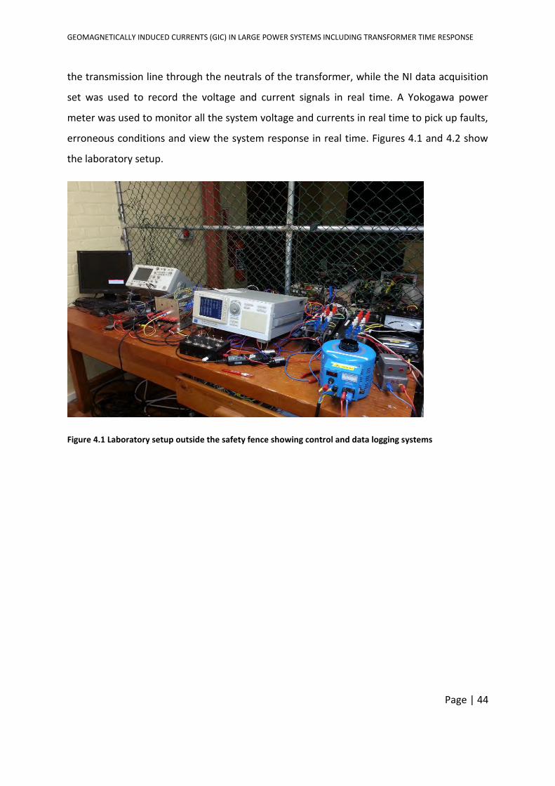
GEOMAGNETICALLY INDUCED CURRENTS (GIC) IN LARGE POWER SYSTEMS INCLUDING TRANSFORMER TIME RESPONSE
Page | 44
the transmission line through the neutrals of the transformer, while the NI data acquisition
set was used to record the voltage and current signals in real time. A Yokogawa power
meter was used to monitor all the system voltage and currents in real time to pick up faults,
erroneous conditions and view the system response in real time. Figures 4.1 and 4.2 show
the laboratory setup.
Figure 4.1 Laboratory setup outside the safety fence showing control and data logging systems
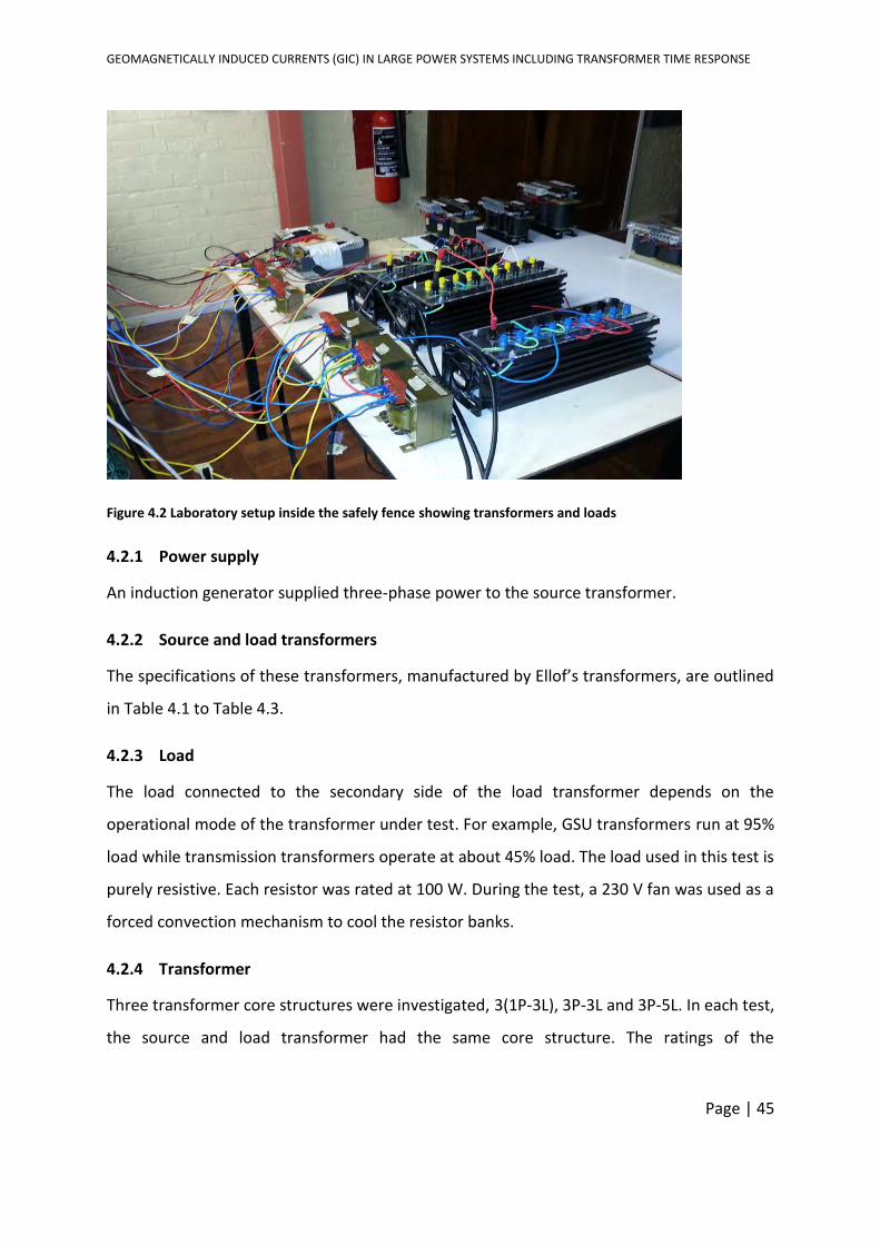
GEOMAGNETICALLY INDUCED CURRENTS (GIC) IN LARGE POWER SYSTEMS INCLUDING TRANSFORMER TIME RESPONSE
Page | 45
Figure 4.2 Laboratory setup inside the safely fence showing transformers and loads
4.2.1 Power supply
An induction generator supplied three-phase power to the source transformer.
4.2.2 Source and load transformers
The specifications of these transformers, manufactured by Ellof’s transformers, are outlined
in Table 4.1 to Table 4.3.
4.2.3 Load
The load connected to the secondary side of the load transformer depends on the
operational mode of the transformer under test. For example, GSU transformers run at 95%
load while transmission transformers operate at about 45% load. The load used in this test is
purely resistive. Each resistor was rated at 100 W. During the test, a 230 V fan was used as a
forced convection mechanism to cool the resistor banks.
4.2.4 Transformer
Three transformer core structures were investigated, 3(1P-3L), 3P-3L and 3P-5L. In each test,
the source and load transformer had the same core structure. The ratings of the
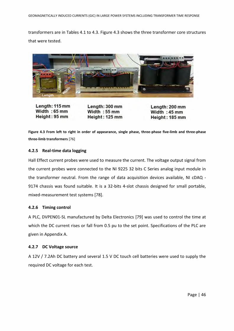
GEOMAGNETICALLY INDUCED CURRENTS (GIC) IN LARGE POWER SYSTEMS INCLUDING TRANSFORMER TIME RESPONSE
Page | 46
transformers are in Tables 4.1 to 4.3. Figure 4.3 shows the three transformer core structures
that were tested.
Figure 4.3 From left to right in order of appearance, single phase, three-phase five-limb and three-phase
three-limb transformers [76]
4.2.5 Real-time data logging
Hall Effect current probes were used to measure the current. The voltage output signal from
the current probes were connected to the NI 9225 32 bits C Series analog input module in
the transformer neutral. From the range of data acquisition devices available, NI cDAQ -
9174 chassis was found suitable. It is a 32-bits 4-slot chassis designed for small portable,
mixed-measurement test systems [78].
4.2.6 Timing control
A PLC, DVPEN01-SL manufactured by Delta Electronics [79] was used to control the time at
which the DC current rises or fall from 0.5 pu to the set point. Specifications of the PLC are
given in Appendix A.
4.2.7 DC Voltage source
A 12V / 7.2Ah DC battery and several 1.5 V DC touch cell batteries were used to supply the
required DC voltage for each test.
ANT DATA C
GEOMAGNETICALLY INDUCED CURRENTS (GIC) IN LARGE POWER SYSTEMS INCLUDING TRANSFORMER TIME RESPONSE
Page | 47
4.3 PSCAD SIMULATION
PSCAD/EMTDC version X4 developed by Manitoba Hydro was used for the simulation. The
purpose of the simulation was to:
1. Replicate the transformer time response to GIC laboratory test with PSCAD.
2. Compare the results obtained with PSCAD to those of the laboratory test.
3. Develop a relationship between the results with PSCAD and the laboratory test.
4. Scale up the test to the MVA-range using the results from 2 and 3 above.
The results of the transformer time response test in the MVA range are fed directly into the
algorithm developed in chapter 3. This is described in chapter 7.
4.3.1 Saturation and transformer model in PSCAD
The DC current that will be injected in the transformers during the laboratory test and in the
PSCAD simulation will range from values that will not drive the transformer into saturation
to values that will see the transformer go into saturation. The general transformer model in
PSCAD version X4 models saturation [80]. The model takes into consideration that as a
transformer gets into saturation, the inductance of the windings reduces [81] while the
magnetization current increases.
In most applications, saturation characteristics are modelled using piecewise linear
inductance with two slopes, one for the linear region and the other for the air-core region
with current injection at one terminal of the transformer [82]. However, when such a
terminal is connected to a strong AC source, the secondary voltage is not distorted. When
the saturation current is injected into the secondary winding, the distortion increase [80]. In
PSCAD, saturation is modelled by current injection at both terminals of the transformer. The
injected current in each terminal is calculated to be mathematically equivalent such that the
effect is as though the current was only injected in the magnetisation branch in the
transformer model. This approach not only retains computational efficiency but over comes
some of the setbacks of only injecting the saturation current in either the primary or the
secondary side of the transformer (see Figure 4.4) [80].
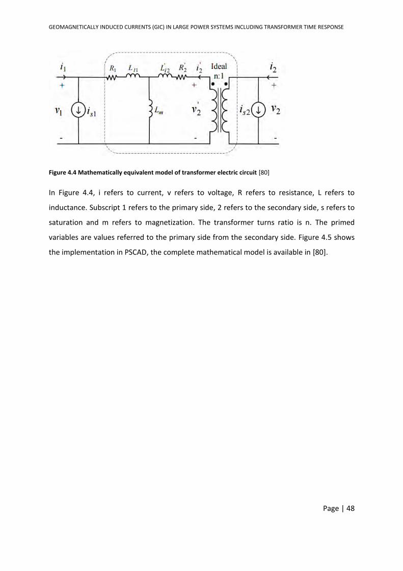
GEOMAGNETICALLY INDUCED CURRENTS (GIC) IN LARGE POWER SYSTEMS INCLUDING TRANSFORMER TIME RESPONSE
Page | 48
Figure 4.4 Mathematically equivalent model of transformer electric circuit [80]
In Figure 4.4, i refers to current, v refers to voltage, R refers to resistance, L refers to
inductance. Subscript 1 refers to the primary side, 2 refers to the secondary side, s refers to
saturation and m refers to magnetization. The transformer turns ratio is n. The primed
variables are values referred to the primary side from the secondary side. Figure 4.5 shows
the implementation in PSCAD, the complete mathematical model is available in [80].
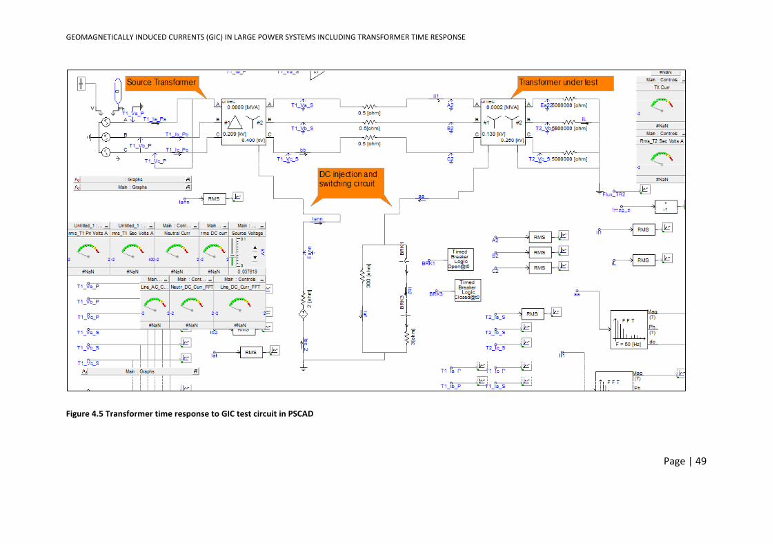
GEOMAGNETICALLY INDUCED CURRENTS (GIC) IN LARGE POWER SYSTEMS INCLUDING TRANSFORMER TIME RESPONSE
Page | 49
Figure 4.5 Transformer time response to GIC test circuit in PSCAD
GEOMAGNETICALLY INDUCED CURRENTS (GIC) IN LARGE POWER SYSTEMS INCLUDING TRANSFORMER TIME RESPONSE
Page | 50
CHAPTER 5
LABORATORY TEST FOR TRANSFORMER TIME
RESPONSE
5. LABORATORY TEST FOR TRANSFORMER TIME RESPONSE
In this chapter, two major transformer categories were tested namely GSU and TT. The
former is typically operated at full load, which in most cases is around 95 % of its rated
capacity [83]. These transformers are built to carry full load continuously. On the other
hand, TTs operate normally around 40 % to 45 % load as more than one transformer is
usually connected in parallel. Each TT rating may go up to the power rating of the
transmission line connected to it [83].
Based on specific application needs, each of these categories may contain the following core
structures: 3(1P-3L), 3P-3L and 3P-5L.
In order to investigate the time response of these transformer core types, three load
conditions were considered: 40 % load to represent the TTs, 80 % load to represent a GSU
under light load conditions and 95 % load to represent GSUs under normal load conditions.
The maximum value of the y-axis in all the graphs is fixed so that the graphs are easily
compared.
5.1 BENCH SCALE 300 VA TRANSFORMER
To establish the initial time response of the transformer, a no-load test was conducted.
During the no-load test, the transformer under test (TUT) was supplied by the source
transformer. The secondary side of the TUT was disconnected from the load bank. Figure 5.1
shows the time response profile of the three core structures to the range of DC currents
injected at no-load.
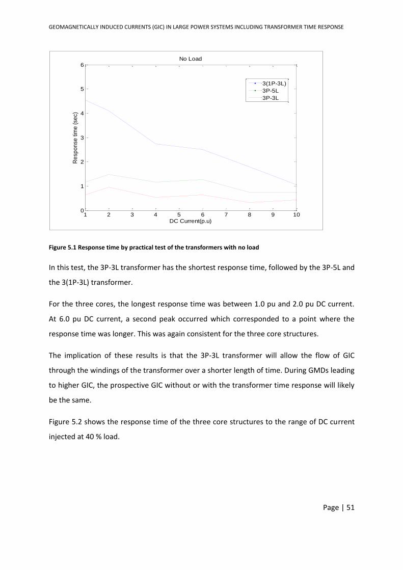
GEOMAGNETICALLY INDUCED CURRENTS (GIC) IN LARGE POWER SYSTEMS INCLUDING TRANSFORMER TIME RESPONSE
Page | 51
Figure 5.1 Response time by practical test of the transformers with no load
In this test, the 3P-3L transformer has the shortest response time, followed by the 3P-5L and
the 3(1P-3L) transformer.
For the three cores, the longest response time was between 1.0 pu and 2.0 pu DC current.
At 6.0 pu DC current, a second peak occurred which corresponded to a point where the
response time was longer. This was again consistent for the three core structures.
The implication of these results is that the 3P-3L transformer will allow the flow of GIC
through the windings of the transformer over a shorter length of time. During GMDs leading
to higher GIC, the prospective GIC without or with the transformer time response will likely
be the same.
Figure 5.2 shows the response time of the three core structures to the range of DC current
injected at 40 % load.
1 2 3 4 5 6 7 8 9 100
1
2
3
4
5
6
DC Current(p.u)
Re
sp
on
se
tim
e (
se
c)
No Load
3(1P-3L)
3P-5L
3P-3L
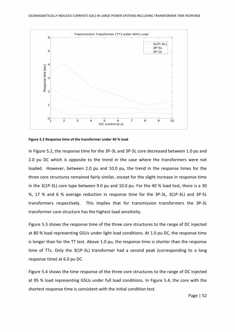
GEOMAGNETICALLY INDUCED CURRENTS (GIC) IN LARGE POWER SYSTEMS INCLUDING TRANSFORMER TIME RESPONSE
Page | 52
Figure 5.2 Response time of the transformer under 40 % load
In Figure 5.2, the response time for the 3P-3L and 3P-5L core decreased between 1.0 pu and
2.0 pu DC which is opposite to the trend in the case where the transformers were not
loaded. However, between 2.0 pu and 10.0 pu, the trend in the response times for the
three core structures remained fairly similar, except for the slight increase in response time
in the 3(1P-3L) core type between 9.0 pu and 10.0 pu. For the 40 % load test, there is a 30
%, 17 % and 6 % average reduction in response time for the 3P-3L, 3(1P-3L) and 3P-5L
transformers respectively. This implies that for transmission transformers the 3P-3L
transformer core structure has the highest load sensitivity.
Figure 5.3 shows the response time of the three core structures to the range of DC injected
at 80 % load representing GSUs under light load conditions. At 1.0 pu DC, the response time
is longer than for the TT test. Above 1.0 pu, the response time is shorter than the response
time of TTs. Only the 3(1P-3L) transformer had a second peak (corresponding to a long
response time) at 6.0 pu DC.
Figure 5.4 shows the time response of the three core structures to the range of DC injected
at 95 % load representing GSUs under full load conditions. In Figure 5.4, the core with the
shortest response time is consistent with the initial condition test.
1 2 3 4 5 6 7 8 9 100
1
2
3
4
5
6Transmission Transformer (TT) under 40% Load
DC current (p.u)
Re
spo
nse
tim
e (
sec)
3(1P-3L)
3P-5L
3P-3L
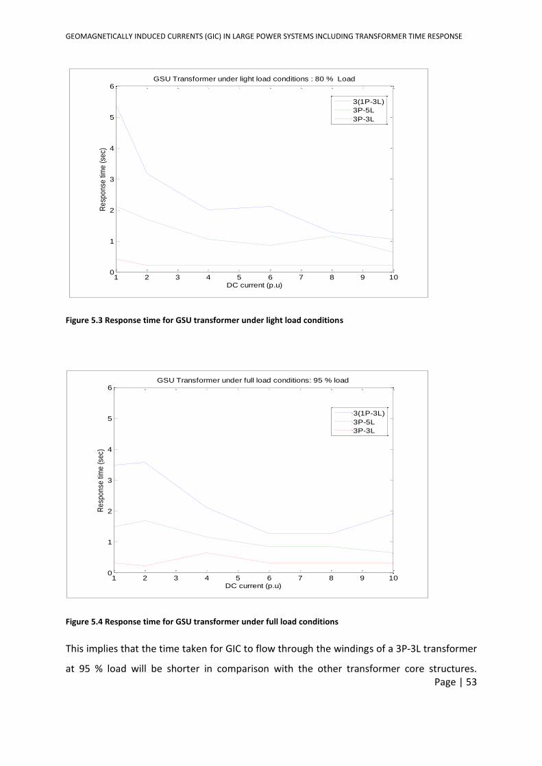
GEOMAGNETICALLY INDUCED CURRENTS (GIC) IN LARGE POWER SYSTEMS INCLUDING TRANSFORMER TIME RESPONSE
Page | 53
Figure 5.3 Response time for GSU transformer under light load conditions
Figure 5.4 Response time for GSU transformer under full load conditions
This implies that the time taken for GIC to flow through the windings of a 3P-3L transformer
at 95 % load will be shorter in comparison with the other transformer core structures.
1 2 3 4 5 6 7 8 9 100
1
2
3
4
5
6GSU Transformer under light load conditions : 80 % Load
DC current (p.u)
Re
spo
nse
tim
e (
sec)
3(1P-3L)
3P-5L
3P-3L
1 2 3 4 5 6 7 8 9 100
1
2
3
4
5
6GSU Transformer under full load conditions: 95 % load
DC current (p.u)
Re
spo
nse
tim
e (
sec)
3(1P-3L)
3P-5L
3P-3L
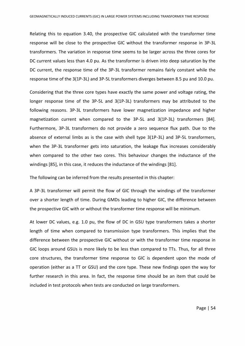
GEOMAGNETICALLY INDUCED CURRENTS (GIC) IN LARGE POWER SYSTEMS INCLUDING TRANSFORMER TIME RESPONSE
Page | 54
Relating this to equation 3.40, the prospective GIC calculated with the transformer time
response will be close to the prospective GIC without the transformer response in 3P-3L
transformers. The variation in response time seems to be larger across the three cores for
DC current values less than 4.0 pu. As the transformer is driven into deep saturation by the
DC current, the response time of the 3P-3L transformer remains fairly constant while the
response time of the 3(1P-3L) and 3P-5L transformers diverges between 8.5 pu and 10.0 pu.
Considering that the three core types have exactly the same power and voltage rating, the
longer response time of the 3P-5L and 3(1P-3L) transformers may be attributed to the
following reasons. 3P-3L transformers have lower magnetization impedance and higher
magnetization current when compared to the 3P-5L and 3(1P-3L) transformers [84].
Furthermore, 3P-3L transformers do not provide a zero sequence flux path. Due to the
absence of external limbs as is the case with shell type 3(1P-3L) and 3P-5L transformers,
when the 3P-3L transformer gets into saturation, the leakage flux increases considerably
when compared to the other two cores. This behaviour changes the inductance of the
windings [85], in this case, it reduces the inductance of the windings [81].
The following can be inferred from the results presented in this chapter:
A 3P-3L transformer will permit the flow of GIC through the windings of the transformer
over a shorter length of time. During GMDs leading to higher GIC, the difference between
the prospective GIC with or without the transformer time response will be minimum.
At lower DC values, e.g. 1.0 pu, the flow of DC in GSU type transformers takes a shorter
length of time when compared to transmission type transformers. This implies that the
difference between the prospective GIC without or with the transformer time response in
GIC loops around GSUs is more likely to be less than compared to TTs. Thus, for all three
core structures, the transformer time response to GIC is dependent upon the mode of
operation (either as a TT or GSU) and the core type. These new findings open the way for
further research in this area. In fact, the response time should be an item that could be
included in test protocols when tests are conducted on large transformers.
GEOMAGNETICALLY INDUCED CURRENTS (GIC) IN LARGE POWER SYSTEMS INCLUDING TRANSFORMER TIME RESPONSE
Page | 55
CHAPTER 6
PSCAD SIMULATION OF TRANSFORMER TIME
RESPONSE TO GIC
6. PSCAD SIMULATION OF TRANSFORMER TIME RESPONSE TO GIC
In this chapter, section 6.1 presents results from the PSCAD simulation with the bench scale
300 VA transformer models. The aim of the PSCAD simulation is to investigate whether
PSCAD can model the laboratory test setup to produce similar results. Section 6.2 compares
results obtained in section 5.1 (laboratory test) and section 6.1 (PSCAD simulation) to
determine how well the results from the PSCAD simulation correlate with the results of the
laboratory test. The power transformer models in the PSCAD simulation are uprated to 500
MVA which is more representative of power transformers used in main transmission
systems. The PSCAD simulation results for 500 MVA power transformers are presented in
section 6.3. Finally, the response time for the three transformer types are compared in
section 6.4.
6.1 BENCH SCALE 300 VA TRANSFORMERS
In PSCAD, modelling a bank of three single phase transformers can be achieved in one of
two ways. Either by wiring three single-phase transformer models together 3(1P-3L) or using
a single model called a three-phase bank. The former of the two options was used in this
thesis because it best represents the test model in chapter 5. However, when the three-
phase bank transformer models where used, the response time dropped significantly to
between 0.15 and 0.3 second from an average of 10 seconds. This contradictory result
indicates that both PSCAD models do not yield the same time response, although similar in
terms of the saturation aspect that is included in both models as explained in section 4.3.1.
As in the laboratory test, the first simulation is the no-load (initial condition) test. This was
followed by the, TT, GSU light load condition and GSU typical load condition tests. Although
the laboratory test and PSCAD simulations were carried out with DC current values ranging
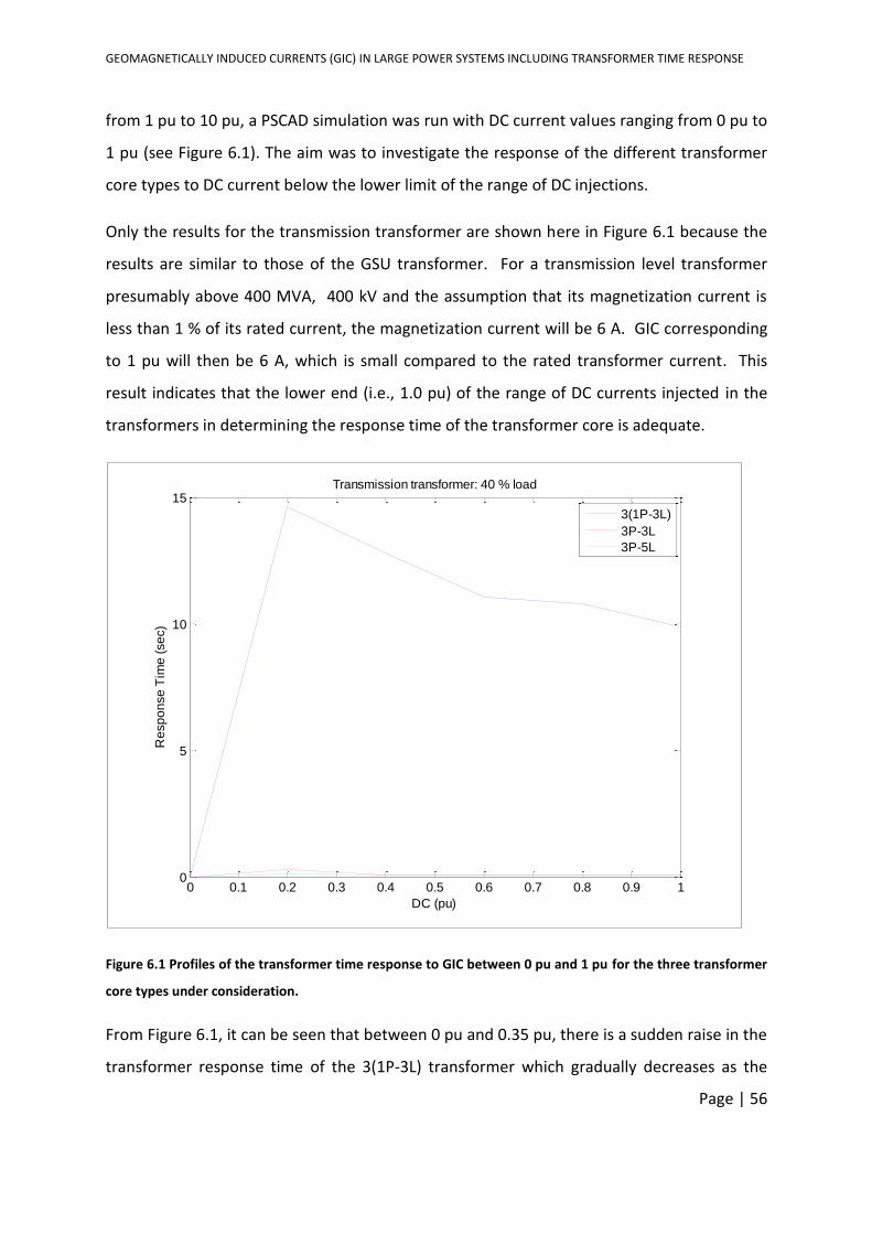
GEOMAGNETICALLY INDUCED CURRENTS (GIC) IN LARGE POWER SYSTEMS INCLUDING TRANSFORMER TIME RESPONSE
Page | 56
from 1 pu to 10 pu, a PSCAD simulation was run with DC current values ranging from 0 pu to
1 pu (see Figure 6.1). The aim was to investigate the response of the different transformer
core types to DC current below the lower limit of the range of DC injections.
Only the results for the transmission transformer are shown here in Figure 6.1 because the
results are similar to those of the GSU transformer. For a transmission level transformer
presumably above 400 MVA, 400 kV and the assumption that its magnetization current is
less than 1 % of its rated current, the magnetization current will be 6 A. GIC corresponding
to 1 pu will then be 6 A, which is small compared to the rated transformer current. This
result indicates that the lower end (i.e., 1.0 pu) of the range of DC currents injected in the
transformers in determining the response time of the transformer core is adequate.
Figure 6.1 Profiles of the transformer time response to GIC between 0 pu and 1 pu for the three transformer
core types under consideration.
From Figure 6.1, it can be seen that between 0 pu and 0.35 pu, there is a sudden raise in the
transformer response time of the 3(1P-3L) transformer which gradually decreases as the
0 0.1 0.2 0.3 0.4 0.5 0.6 0.7 0.8 0.9 10
5
10
15
DC (pu)
Re
sp
on
se
Tim
e (
se
c)
Transmission transformer: 40 % load
3(1P-3L)
3P-3L
3P-5L
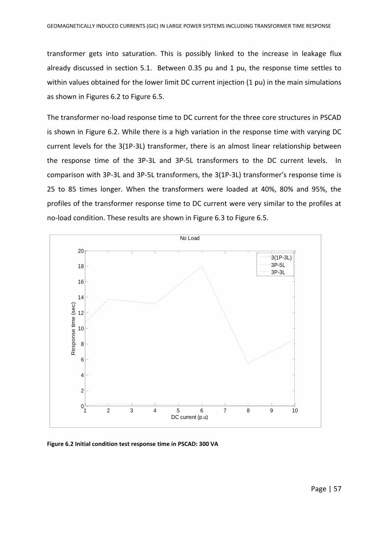
GEOMAGNETICALLY INDUCED CURRENTS (GIC) IN LARGE POWER SYSTEMS INCLUDING TRANSFORMER TIME RESPONSE
Page | 57
transformer gets into saturation. This is possibly linked to the increase in leakage flux
already discussed in section 5.1. Between 0.35 pu and 1 pu, the response time settles to
within values obtained for the lower limit DC current injection (1 pu) in the main simulations
as shown in Figures 6.2 to Figure 6.5.
The transformer no-load response time to DC current for the three core structures in PSCAD
is shown in Figure 6.2. While there is a high variation in the response time with varying DC
current levels for the 3(1P-3L) transformer, there is an almost linear relationship between
the response time of the 3P-3L and 3P-5L transformers to the DC current levels. In
comparison with 3P-3L and 3P-5L transformers, the 3(1P-3L) transformer’s response time is
25 to 85 times longer. When the transformers were loaded at 40%, 80% and 95%, the
profiles of the transformer response time to DC current were very similar to the profiles at
no-load condition. These results are shown in Figure 6.3 to Figure 6.5.
Figure 6.2 Initial condition test response time in PSCAD: 300 VA
1 2 3 4 5 6 7 8 9 100
2
4
6
8
10
12
14
16
18
20
No Load
DC current (p.u)
Re
sp
on
se
tim
e (
se
c)
3(1P-3L)
3P-5L
3P-3L
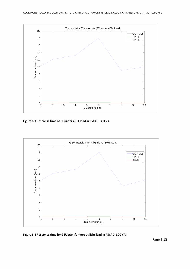
GEOMAGNETICALLY INDUCED CURRENTS (GIC) IN LARGE POWER SYSTEMS INCLUDING TRANSFORMER TIME RESPONSE
Page | 58
Figure 6.3 Response time of TT under 40 % load in PSCAD: 300 VA
Figure 6.4 Response time for GSU transformers at light load in PSCAD: 300 VA
1 2 3 4 5 6 7 8 9 100
2
4
6
8
10
12
14
16
18
20Transmission Transformer (TT) under 40% Load
DC current (p.u)
Re
sp
on
se
tim
e (
se
c)
3(1P-3L)
3P-5L
3P-3L
1 2 3 4 5 6 7 8 9 100
2
4
6
8
10
12
14
16
18
20GSU Transformer at light load: 80% Load
DC current (p.u)
Re
sp
on
se
tim
e (
se
c)
3(1P-3L)
3P-5L
3P-3L
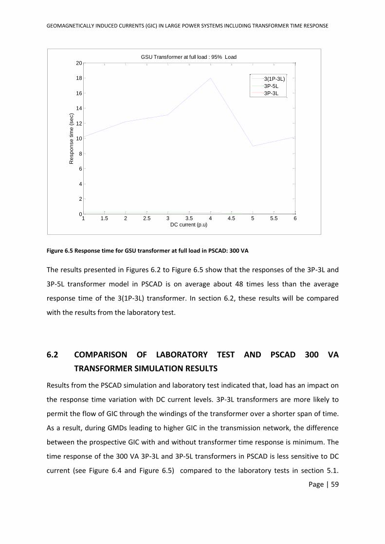
GEOMAGNETICALLY INDUCED CURRENTS (GIC) IN LARGE POWER SYSTEMS INCLUDING TRANSFORMER TIME RESPONSE
Page | 59
Figure 6.5 Response time for GSU transformer at full load in PSCAD: 300 VA
The results presented in Figures 6.2 to Figure 6.5 show that the responses of the 3P-3L and
3P-5L transformer model in PSCAD is on average about 48 times less than the average
response time of the 3(1P-3L) transformer. In section 6.2, these results will be compared
with the results from the laboratory test.
6.2 COMPARISON OF LABORATORY TEST AND PSCAD 300 VA
TRANSFORMER SIMULATION RESULTS
Results from the PSCAD simulation and laboratory test indicated that, load has an impact on
the response time variation with DC current levels. 3P-3L transformers are more likely to
permit the flow of GIC through the windings of the transformer over a shorter span of time.
As a result, during GMDs leading to higher GIC in the transmission network, the difference
between the prospective GIC with and without transformer time response is minimum. The
time response of the 300 VA 3P-3L and 3P-5L transformers in PSCAD is less sensitive to DC
current (see Figure 6.4 and Figure 6.5) compared to the laboratory tests in section 5.1.
1 1.5 2 2.5 3 3.5 4 4.5 5 5.5 60
2
4
6
8
10
12
14
16
18
20GSU Transformer at full load : 95% Load
DC current (p.u)
Re
sp
on
se
tim
e (
se
c)
3(1P-3L)
3P-5L
3P-3L
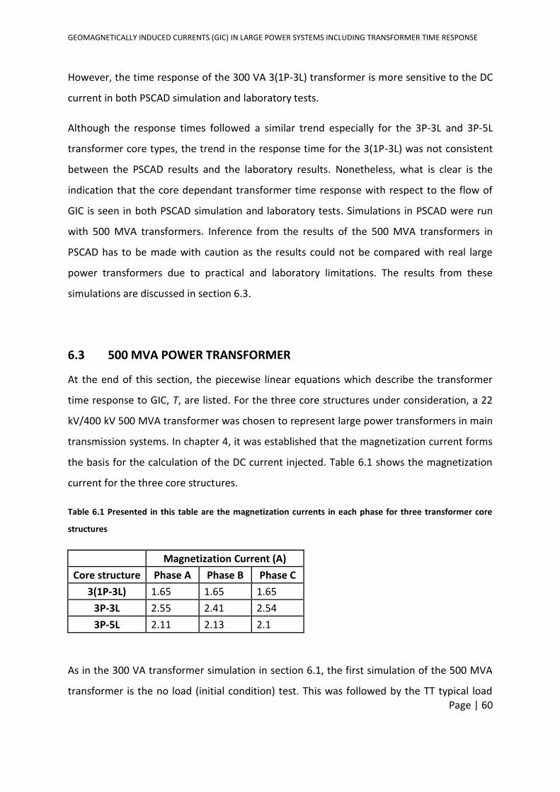
GEOMAGNETICALLY INDUCED CURRENTS (GIC) IN LARGE POWER SYSTEMS INCLUDING TRANSFORMER TIME RESPONSE
Page | 60
However, the time response of the 300 VA 3(1P-3L) transformer is more sensitive to the DC
current in both PSCAD simulation and laboratory tests.
Although the response times followed a similar trend especially for the 3P-3L and 3P-5L
transformer core types, the trend in the response time for the 3(1P-3L) was not consistent
between the PSCAD results and the laboratory results. Nonetheless, what is clear is the
indication that the core dependant transformer time response with respect to the flow of
GIC is seen in both PSCAD simulation and laboratory tests. Simulations in PSCAD were run
with 500 MVA transformers. Inference from the results of the 500 MVA transformers in
PSCAD has to be made with caution as the results could not be compared with real large
power transformers due to practical and laboratory limitations. The results from these
simulations are discussed in section 6.3.
6.3 500 MVA POWER TRANSFORMER
At the end of this section, the piecewise linear equations which describe the transformer
time response to GIC, T, are listed. For the three core structures under consideration, a 22
kV/400 kV 500 MVA transformer was chosen to represent large power transformers in main
transmission systems. In chapter 4, it was established that the magnetization current forms
the basis for the calculation of the DC current injected. Table 6.1 shows the magnetization
current for the three core structures.
Table 6.1 Presented in this table are the magnetization currents in each phase for three transformer core
structures
Magnetization Current (A)
Core structure Phase A Phase B Phase C
3(1P-3L) 1.65 1.65 1.65
3P-3L 2.55 2.41 2.54
3P-5L 2.11 2.13 2.1
As in the 300 VA transformer simulation in section 6.1, the first simulation of the 500 MVA
transformer is the no load (initial condition) test. This was followed by the TT typical load
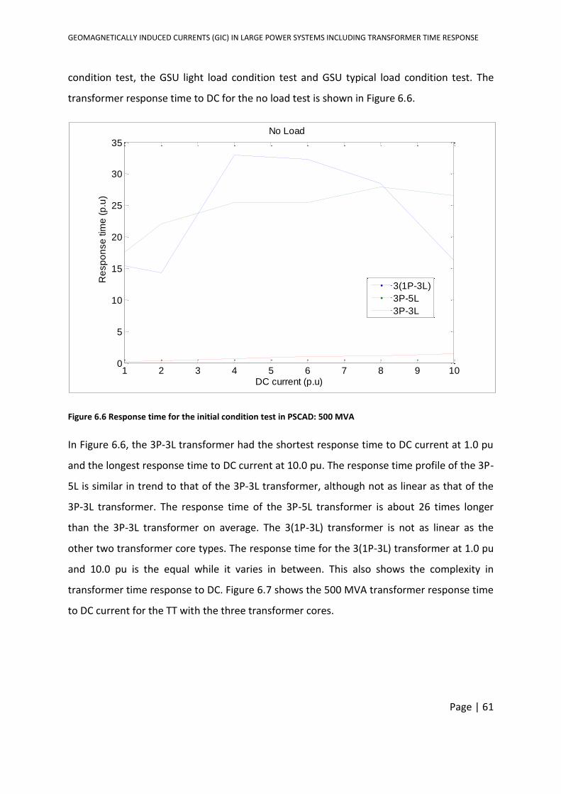
GEOMAGNETICALLY INDUCED CURRENTS (GIC) IN LARGE POWER SYSTEMS INCLUDING TRANSFORMER TIME RESPONSE
Page | 61
condition test, the GSU light load condition test and GSU typical load condition test. The
transformer response time to DC for the no load test is shown in Figure 6.6.
Figure 6.6 Response time for the initial condition test in PSCAD: 500 MVA
In Figure 6.6, the 3P-3L transformer had the shortest response time to DC current at 1.0 pu
and the longest response time to DC current at 10.0 pu. The response time profile of the 3P-
5L is similar in trend to that of the 3P-3L transformer, although not as linear as that of the
3P-3L transformer. The response time of the 3P-5L transformer is about 26 times longer
than the 3P-3L transformer on average. The 3(1P-3L) transformer is not as linear as the
other two transformer core types. The response time for the 3(1P-3L) transformer at 1.0 pu
and 10.0 pu is the equal while it varies in between. This also shows the complexity in
transformer time response to DC. Figure 6.7 shows the 500 MVA transformer response time
to DC current for the TT with the three transformer cores.
1 2 3 4 5 6 7 8 9 100
5
10
15
20
25
30
35
DC current (p.u)
Re
sp
on
se
tim
e (
p.u
)
No Load
3(1P-3L)
3P-5L
3P-3L
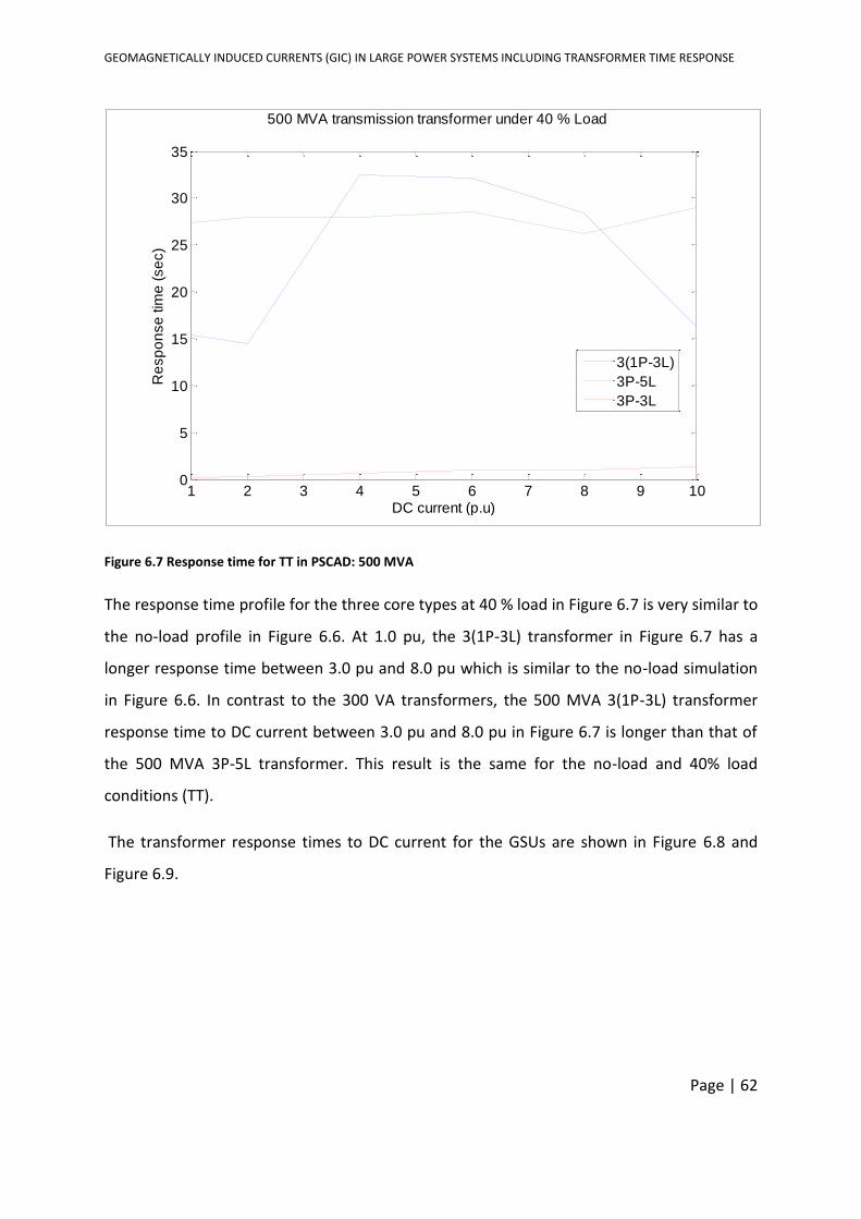
GEOMAGNETICALLY INDUCED CURRENTS (GIC) IN LARGE POWER SYSTEMS INCLUDING TRANSFORMER TIME RESPONSE
Page | 62
Figure 6.7 Response time for TT in PSCAD: 500 MVA
The response time profile for the three core types at 40 % load in Figure 6.7 is very similar to
the no-load profile in Figure 6.6. At 1.0 pu, the 3(1P-3L) transformer in Figure 6.7 has a
longer response time between 3.0 pu and 8.0 pu which is similar to the no-load simulation
in Figure 6.6. In contrast to the 300 VA transformers, the 500 MVA 3(1P-3L) transformer
response time to DC current between 3.0 pu and 8.0 pu in Figure 6.7 is longer than that of
the 500 MVA 3P-5L transformer. This result is the same for the no-load and 40% load
conditions (TT).
The transformer response times to DC current for the GSUs are shown in Figure 6.8 and
Figure 6.9.
1 2 3 4 5 6 7 8 9 100
5
10
15
20
25
30
35
500 MVA transmission transformer under 40 % Load
DC current (p.u)
Re
sp
on
se
tim
e (
se
c)
3(1P-3L)
3P-5L
3P-3L
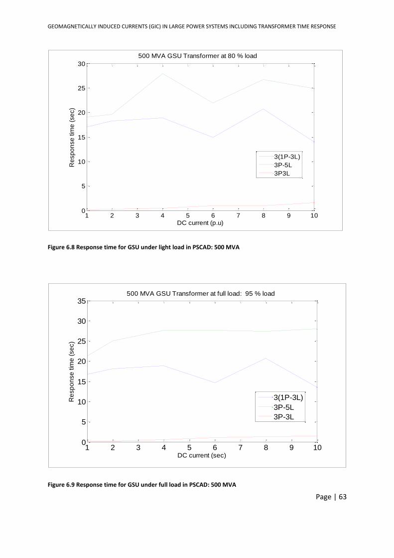
GEOMAGNETICALLY INDUCED CURRENTS (GIC) IN LARGE POWER SYSTEMS INCLUDING TRANSFORMER TIME RESPONSE
Page | 63
Figure 6.8 Response time for GSU under light load in PSCAD: 500 MVA
Figure 6.9 Response time for GSU under full load in PSCAD: 500 MVA
1 2 3 4 5 6 7 8 9 100
5
10
15
20
25
30
500 MVA GSU Transformer at 80 % load
DC current (p.u)
Re
sp
on
se
tim
e (
se
c)
3(1P-3L)
3P-5L
3P3L
1 2 3 4 5 6 7 8 9 100
5
10
15
20
25
30
35500 MVA GSU Transformer at full load: 95 % load
DC current (sec)
Re
sp
on
se
tim
e (
se
c)
3(1P-3L)
3P-5L
3P-3L
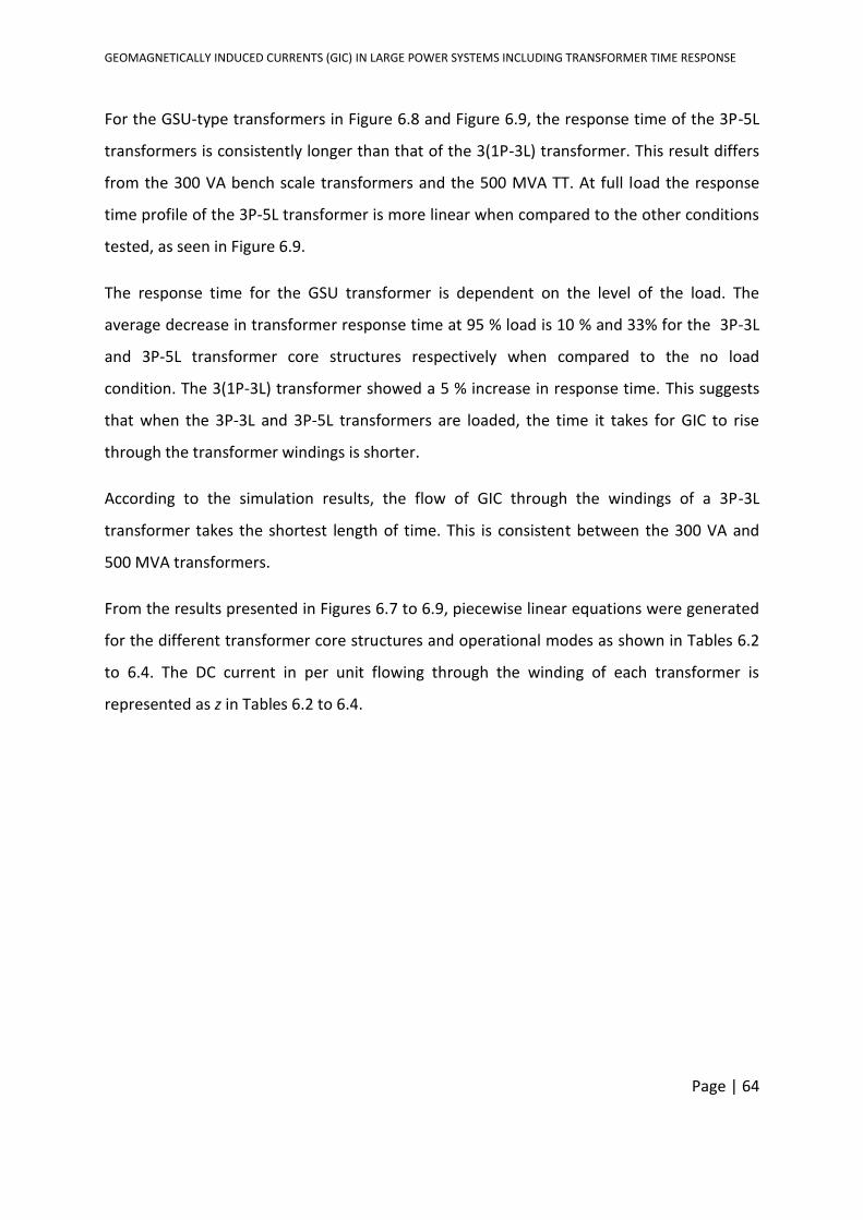
GEOMAGNETICALLY INDUCED CURRENTS (GIC) IN LARGE POWER SYSTEMS INCLUDING TRANSFORMER TIME RESPONSE
Page | 64
For the GSU-type transformers in Figure 6.8 and Figure 6.9, the response time of the 3P-5L
transformers is consistently longer than that of the 3(1P-3L) transformer. This result differs
from the 300 VA bench scale transformers and the 500 MVA TT. At full load the response
time profile of the 3P-5L transformer is more linear when compared to the other conditions
tested, as seen in Figure 6.9.
The response time for the GSU transformer is dependent on the level of the load. The
average decrease in transformer response time at 95 % load is 10 % and 33% for the 3P-3L
and 3P-5L transformer core structures respectively when compared to the no load
condition. The 3(1P-3L) transformer showed a 5 % increase in response time. This suggests
that when the 3P-3L and 3P-5L transformers are loaded, the time it takes for GIC to rise
through the transformer windings is shorter.
According to the simulation results, the flow of GIC through the windings of a 3P-3L
transformer takes the shortest length of time. This is consistent between the 300 VA and
500 MVA transformers.
From the results presented in Figures 6.7 to 6.9, piecewise linear equations were generated
for the different transformer core structures and operational modes as shown in Tables 6.2
to 6.4. The DC current in per unit flowing through the winding of each transformer is
represented as z in Tables 6.2 to 6.4.
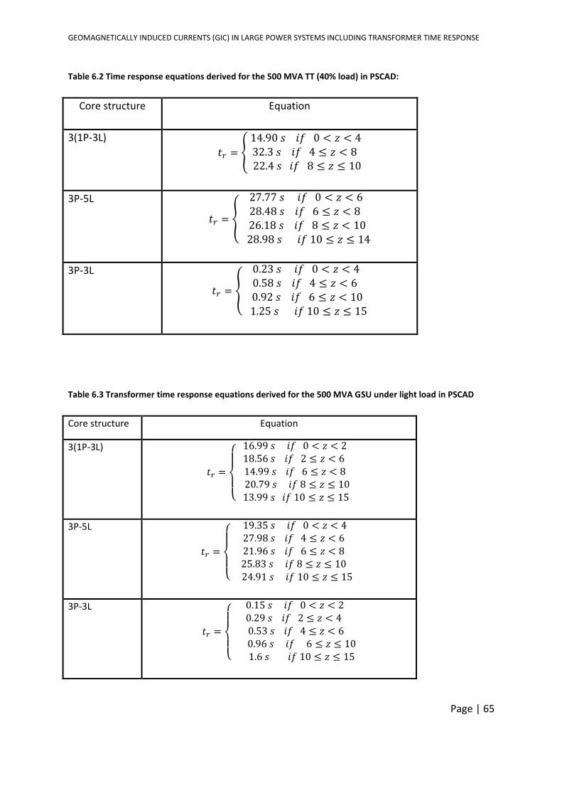
GEOMAGNETICALLY INDUCED CURRENTS (GIC) IN LARGE POWER SYSTEMS INCLUDING TRANSFORMER TIME RESPONSE
Page | 65
Table 6.2 Time response equations derived for the 500 MVA TT (40% load) in PSCAD:
Core structure Equation
3(1P-3L)
𝑡𝑟 =
14.90 𝑠 𝑖𝑓 0 < 𝑧 < 432.3 𝑠 𝑖𝑓 4 ≤ 𝑧 < 8 22.4 𝑠 𝑖𝑓 8 ≤ 𝑧 ≤ 10
3P-5L
𝑡𝑟 =
27.77 𝑠 𝑖𝑓 0 < 𝑧 < 628.48 𝑠 𝑖𝑓 6 ≤ 𝑧 < 8 26.18 𝑠 𝑖𝑓 8 ≤ 𝑧 < 10 28.98 𝑠 𝑖𝑓 10 ≤ 𝑧 ≤ 14
3P-3L
𝑡𝑟 =
0.23 𝑠 𝑖𝑓 0 < 𝑧 < 40.58 𝑠 𝑖𝑓 4 ≤ 𝑧 < 6 0.92 𝑠 𝑖𝑓 6 ≤ 𝑧 < 10 1.25 𝑠 𝑖𝑓 10 ≤ 𝑧 ≤ 15
Table 6.3 Transformer time response equations derived for the 500 MVA GSU under light load in PSCAD
Core structure Equation
3(1P-3L)
𝑡𝑟 =
16.99 𝑠 𝑖𝑓 0 < 𝑧 < 218.56 𝑠 𝑖𝑓 2 ≤ 𝑧 < 6 14.99 𝑠 𝑖𝑓 6 ≤ 𝑧 < 8 20.79 𝑠 𝑖𝑓 8 ≤ 𝑧 ≤ 10 13.99 𝑠 𝑖𝑓 10 ≤ 𝑧 ≤ 15
3P-5L
𝑡𝑟 =
19.35 𝑠 𝑖𝑓 0 < 𝑧 < 427.98 𝑠 𝑖𝑓 4 ≤ 𝑧 < 621.96 𝑠 𝑖𝑓 6 ≤ 𝑧 < 825.83 𝑠 𝑖𝑓 8 ≤ 𝑧 ≤ 10
24.91 𝑠 𝑖𝑓 10 ≤ 𝑧 ≤ 15
3P-3L
𝑡𝑟 =
0.15 𝑠 𝑖𝑓 0 < 𝑧 < 20.29 𝑠 𝑖𝑓 2 ≤ 𝑧 < 4 0.53 𝑠 𝑖𝑓 4 ≤ 𝑧 < 6
0.96 𝑠 𝑖𝑓 6 ≤ 𝑧 ≤ 10 1.6 𝑠 𝑖𝑓 10 ≤ 𝑧 ≤ 15
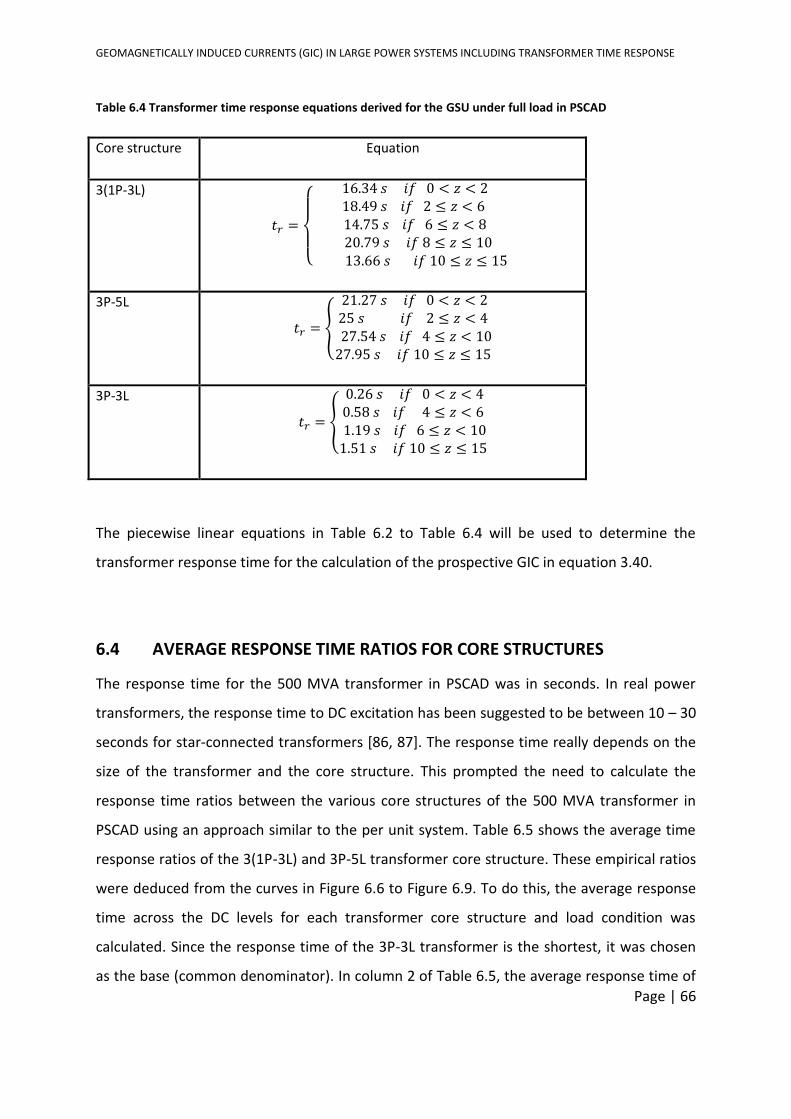
GEOMAGNETICALLY INDUCED CURRENTS (GIC) IN LARGE POWER SYSTEMS INCLUDING TRANSFORMER TIME RESPONSE
Page | 66
Table 6.4 Transformer time response equations derived for the GSU under full load in PSCAD
Core structure Equation
3(1P-3L)
𝑡𝑟 =
16.34 𝑠 𝑖𝑓 0 < 𝑧 < 218.49 𝑠 𝑖𝑓 2 ≤ 𝑧 < 6 14.75 𝑠 𝑖𝑓 6 ≤ 𝑧 < 8 20.79 𝑠 𝑖𝑓 8 ≤ 𝑧 ≤ 10
13.66 𝑠 𝑖𝑓 10 ≤ 𝑧 ≤ 15
3P-5L
𝑡𝑟 =
21.27 𝑠 𝑖𝑓 0 < 𝑧 < 225 𝑠 𝑖𝑓 2 ≤ 𝑧 < 4 27.54 𝑠 𝑖𝑓 4 ≤ 𝑧 < 1027.95 𝑠 𝑖𝑓 10 ≤ 𝑧 ≤ 15
3P-3L
𝑡𝑟 =
0.26 𝑠 𝑖𝑓 0 < 𝑧 < 40.58 𝑠 𝑖𝑓 4 ≤ 𝑧 < 6 1.19 𝑠 𝑖𝑓 6 ≤ 𝑧 < 101.51 𝑠 𝑖𝑓 10 ≤ 𝑧 ≤ 15
The piecewise linear equations in Table 6.2 to Table 6.4 will be used to determine the
transformer response time for the calculation of the prospective GIC in equation 3.40.
6.4 AVERAGE RESPONSE TIME RATIOS FOR CORE STRUCTURES
The response time for the 500 MVA transformer in PSCAD was in seconds. In real power
transformers, the response time to DC excitation has been suggested to be between 10 – 30
seconds for star-connected transformers [86, 87]. The response time really depends on the
size of the transformer and the core structure. This prompted the need to calculate the
response time ratios between the various core structures of the 500 MVA transformer in
PSCAD using an approach similar to the per unit system. Table 6.5 shows the average time
response ratios of the 3(1P-3L) and 3P-5L transformer core structure. These empirical ratios
were deduced from the curves in Figure 6.6 to Figure 6.9. To do this, the average response
time across the DC levels for each transformer core structure and load condition was
calculated. Since the response time of the 3P-3L transformer is the shortest, it was chosen
as the base (common denominator). In column 2 of Table 6.5, the average response time of
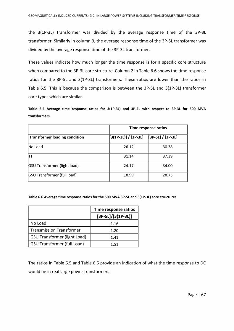
GEOMAGNETICALLY INDUCED CURRENTS (GIC) IN LARGE POWER SYSTEMS INCLUDING TRANSFORMER TIME RESPONSE
Page | 67
the 3(1P-3L) transformer was divided by the average response time of the 3P-3L
transformer. Similarly in column 3, the average response time of the 3P-5L transformer was
divided by the average response time of the 3P-3L transformer.
These values indicate how much longer the time response is for a specific core structure
when compared to the 3P-3L core structure. Column 2 in Table 6.6 shows the time response
ratios for the 3P-5L and 3(1P-3L) transformers. These ratios are lower than the ratios in
Table 6.5. This is because the comparison is between the 3P-5L and 3(1P-3L) transformer
core types which are similar.
Table 6.5 Average time response ratios for 3(1P-3L) and 3P-5L with respect to 3P-3L for 500 MVA
transformers.
Time response ratios
Transformer loading condition [3(1P-3L)] / [3P-3L] [3P-5L] / [3P-3L]
No Load 26.12 30.38
TT 31.14 37.39
GSU Transformer (light load) 24.17 34.00
GSU Transformer (full load) 18.99 28.75
Table 6.6 Average time response ratios for the 500 MVA 3P-5L and 3(1P-3L) core structures
Time response ratios
[3P-5L]/[3(1P-3L)]
No Load 1.16
Transmission Transformer 1.20
GSU Transformer (light Load) 1.41
GSU Transformer (full Load) 1.51
The ratios in Table 6.5 and Table 6.6 provide an indication of what the time response to DC
would be in real large power transformers.
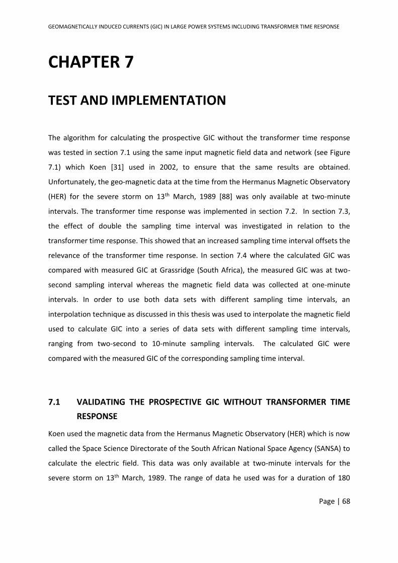
GEOMAGNETICALLY INDUCED CURRENTS (GIC) IN LARGE POWER SYSTEMS INCLUDING TRANSFORMER TIME RESPONSE
Page | 68
CHAPTER 7
TEST AND IMPLEMENTATION
7. TEST AND IMPLEMENTATION
The algorithm for calculating the prospective GIC without the transformer time response
was tested in section 7.1 using the same input magnetic field data and network (see Figure
7.1) which Koen [31] used in 2002, to ensure that the same results are obtained.
Unfortunately, the geo-magnetic data at the time from the Hermanus Magnetic Observatory
(HER) for the severe storm on 13th March, 1989 [88] was only available at two-minute
intervals. The transformer time response was implemented in section 7.2. In section 7.3,
the effect of double the sampling time interval was investigated in relation to the
transformer time response. This showed that an increased sampling time interval offsets the
relevance of the transformer time response. In section 7.4 where the calculated GIC was
compared with measured GIC at Grassridge (South Africa), the measured GIC was at two-
second sampling interval whereas the magnetic field data was collected at one-minute
intervals. In order to use both data sets with different sampling time intervals, an
interpolation technique as discussed in this thesis was used to interpolate the magnetic field
used to calculate GIC into a series of data sets with different sampling time intervals,
ranging from two-second to 10-minute sampling intervals. The calculated GIC were
compared with the measured GIC of the corresponding sampling time interval.
7.1 VALIDATING THE PROSPECTIVE GIC WITHOUT TRANSFORMER TIME
RESPONSE
Koen used the magnetic data from the Hermanus Magnetic Observatory (HER) which is now
called the Space Science Directorate of the South African National Space Agency (SANSA) to
calculate the electric field. This data was only available at two-minute intervals for the
severe storm on 13th March, 1989. The range of data he used was for a duration of 180
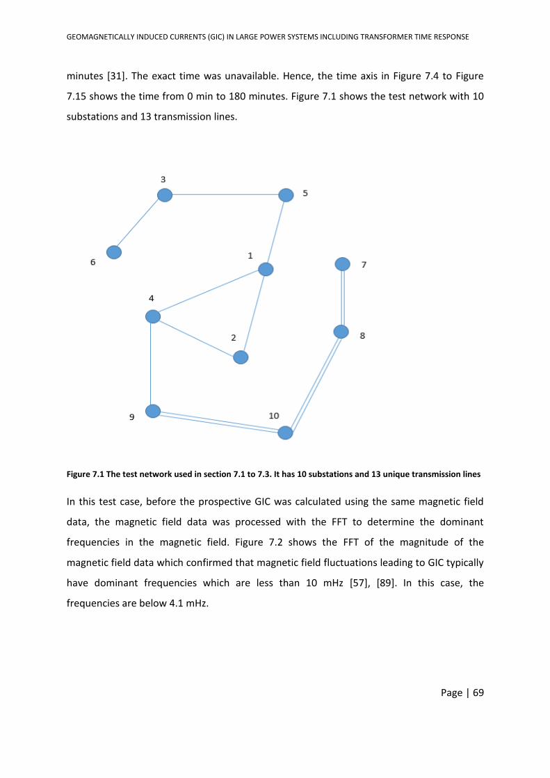
GEOMAGNETICALLY INDUCED CURRENTS (GIC) IN LARGE POWER SYSTEMS INCLUDING TRANSFORMER TIME RESPONSE
Page | 69
minutes [31]. The exact time was unavailable. Hence, the time axis in Figure 7.4 to Figure
7.15 shows the time from 0 min to 180 minutes. Figure 7.1 shows the test network with 10
substations and 13 transmission lines.
Figure 7.1 The test network used in section 7.1 to 7.3. It has 10 substations and 13 unique transmission lines
In this test case, before the prospective GIC was calculated using the same magnetic field
data, the magnetic field data was processed with the FFT to determine the dominant
frequencies in the magnetic field. Figure 7.2 shows the FFT of the magnitude of the
magnetic field data which confirmed that magnetic field fluctuations leading to GIC typically
have dominant frequencies which are less than 10 mHz [57], [89]. In this case, the
frequencies are below 4.1 mHz.
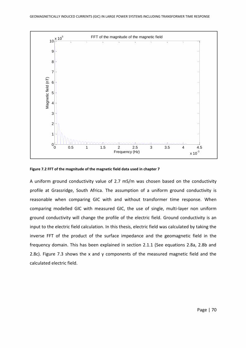
GEOMAGNETICALLY INDUCED CURRENTS (GIC) IN LARGE POWER SYSTEMS INCLUDING TRANSFORMER TIME RESPONSE
Page | 70
Figure 7.2 FFT of the magnitude of the magnetic field data used in chapter 7
A uniform ground conductivity value of 2.7 mS/m was chosen based on the conductivity
profile at Grassridge, South Africa. The assumption of a uniform ground conductivity is
reasonable when comparing GIC with and without transformer time response. When
comparing modelled GIC with measured GIC, the use of single, multi-layer non uniform
ground conductivity will change the profile of the electric field. Ground conductivity is an
input to the electric field calculation. In this thesis, electric field was calculated by taking the
inverse FFT of the product of the surface impedance and the geomagnetic field in the
frequency domain. This has been explained in section 2.1.1 (See equations 2.8a, 2.8b and
2.8c). Figure 7.3 shows the x and y components of the measured magnetic field and the
calculated electric field.
0 0.5 1 1.5 2 2.5 3 3.5 4 4.5
x 10-3
0
1
2
3
4
5
6
7
8
9
10x 10
5 FFT of the magnitude of the magnetic field
Frequency (Hz)
Ma
gn
etic fie
ld (
nT
)
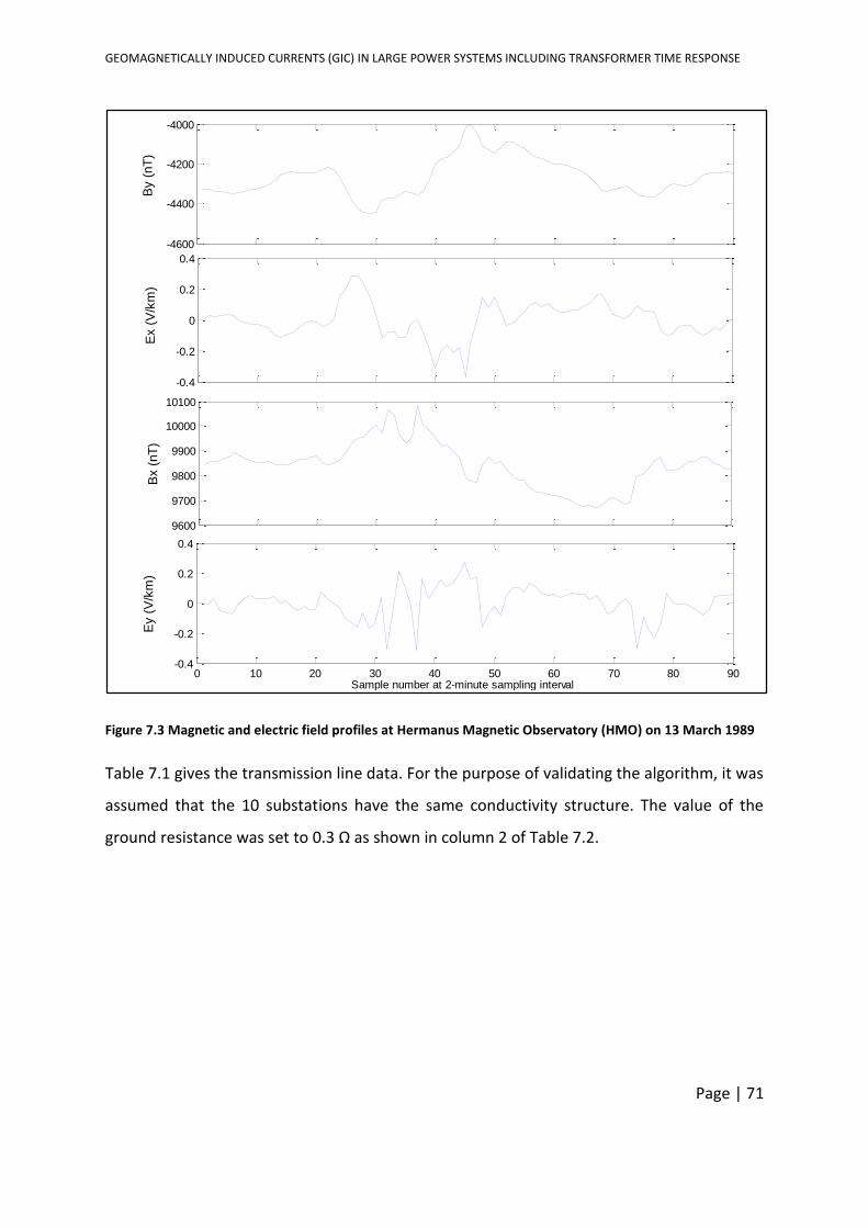
GEOMAGNETICALLY INDUCED CURRENTS (GIC) IN LARGE POWER SYSTEMS INCLUDING TRANSFORMER TIME RESPONSE
Page | 71
Figure 7.3 Magnetic and electric field profiles at Hermanus Magnetic Observatory (HMO) on 13 March 1989
Table 7.1 gives the transmission line data. For the purpose of validating the algorithm, it was
assumed that the 10 substations have the same conductivity structure. The value of the
ground resistance was set to 0.3 Ω as shown in column 2 of Table 7.2.
-0.4
-0.2
0
0.2
0.4
Ex (
V/k
m)
-4600
-4400
-4200
-4000
By (
nT
)
9600
9700
9800
9900
10000
10100
Bx (
nT
)
0 10 20 30 40 50 60 70 80 90-0.4
-0.2
0
0.2
0.4
Sample number at 2-minute sampling interval
Ey (
V/k
m)
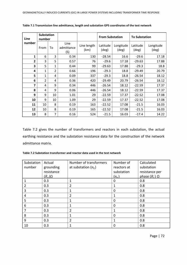
GEOMAGNETICALLY INDUCED CURRENTS (GIC) IN LARGE POWER SYSTEMS INCLUDING TRANSFORMER TIME RESPONSE
Page | 72
Table 7.1 Transmission line admittance, length and substation GPS coordinates of the test network
Line number
Substation number
From Substation To Substation
From To Line
admittance (S)
Line length (km)
Latitude (deg)
Longitude (deg)
Latitude (deg)
Longitude (deg)
1 6 3 0.34 130 -28.54 16.6 -29.6 17.18
2 3 5 0.57 76 -29.6 17.18 -29.63 17.88
3 5 1 0.44 99 -29.63 17.88 -29.3 18.8
4 1 2 0.66 196 -29.3 18.8 -29.49 20.79
5 1 4 0.09 337 -29.3 18.8 -26.54 18.12
6 2 4 0.36 420 -29.49 20.79 -26.54 18.12
7 4 9 0.34 446 -26.54 18.12 -22.59 17.37
8 4 9 0.06 446 -26.54 18.12 -22.59 17.37
9 9 10 1.01 29 -22.59 17.37 -22.52 17.08
10 9 10 1.09 29 -22.59 17.37 -22.52 17.08
11 10 8 0.19 163 -22.52 17.08 -21.5 16.03
12 10 8 0.19 165 -22.52 17.08 -21.5 16.03
13 8 7 0.16 524 -21.5 16.03 -17.4 14.22
Table 7.2 gives the number of transformers and reactors in each substation, the actual
earthing resistance and the substation resistance data for the construction of the network
admittance matrix.
Table 7.2 Substation transformer and reactor data used in the test network
Substation number
Actual grounding resistance (𝑅𝑒)Ω
Number of transformers at substation (𝑛𝑡)
Number of reactors at substation (𝑛𝑟)
Calculated substation resistance per phase (𝑅𝑗) Ω
1 0.3 1 0 0.8
2 0.3 2 1 0.8
3 0.3 1 0 0.8
4 0.3 2 1 0.8
5 0.3 1 0 0.8
6 0.3 1 0 0.8
7 0.3 2 1 0.8
8 0.3 1 0 0.8
9 0.3 2 1 0.8
10 0.3 1 0 0.8
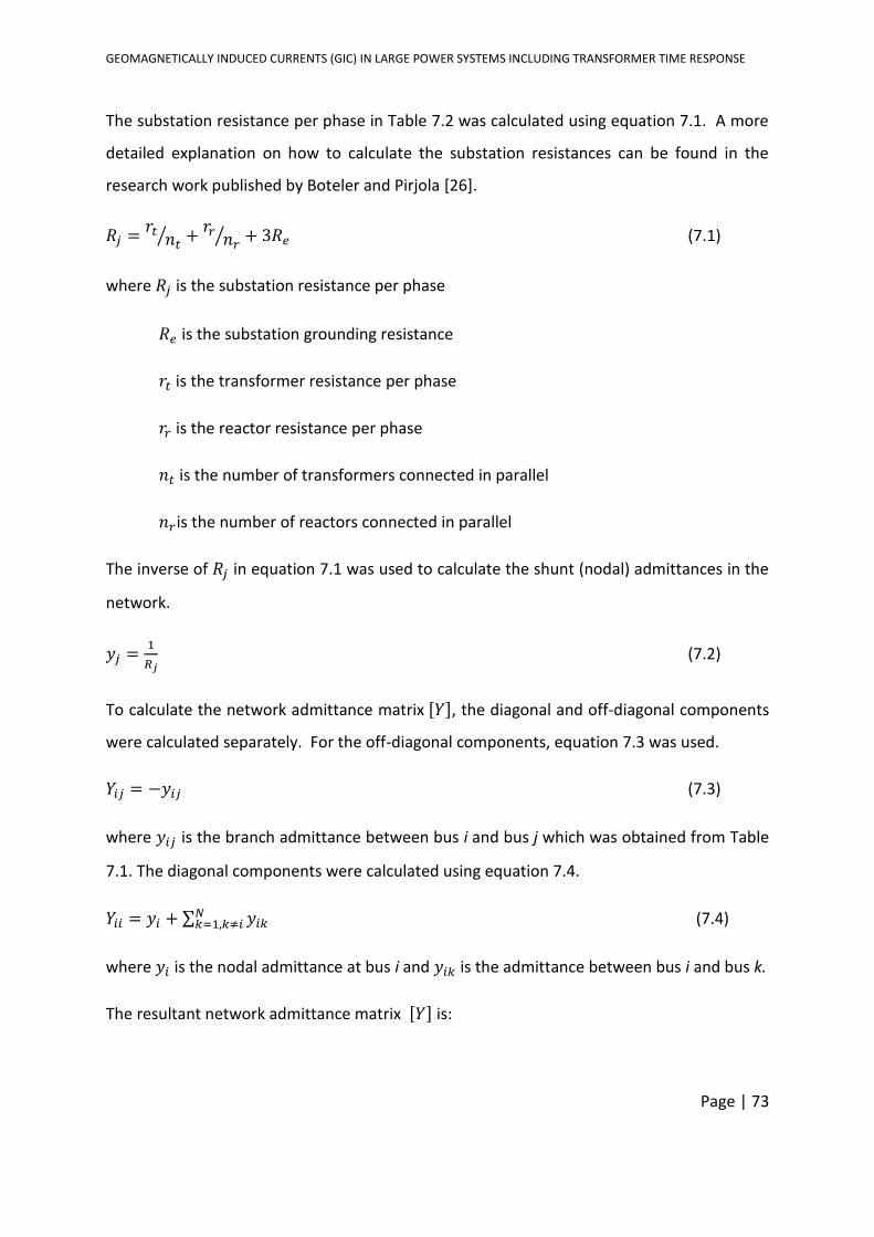
GEOMAGNETICALLY INDUCED CURRENTS (GIC) IN LARGE POWER SYSTEMS INCLUDING TRANSFORMER TIME RESPONSE
Page | 73
The substation resistance per phase in Table 7.2 was calculated using equation 7.1. A more
detailed explanation on how to calculate the substation resistances can be found in the
research work published by Boteler and Pirjola [26].
𝑅𝑗 =𝑟𝑡𝑛𝑡⁄ +
𝑟𝑟𝑛𝑟⁄ + 3𝑅𝑒 (7.1)
where 𝑅𝑗 is the substation resistance per phase
𝑅𝑒 is the substation grounding resistance
𝑟𝑡 is the transformer resistance per phase
𝑟𝑟 is the reactor resistance per phase
𝑛𝑡 is the number of transformers connected in parallel
𝑛𝑟is the number of reactors connected in parallel
The inverse of 𝑅𝑗 in equation 7.1 was used to calculate the shunt (nodal) admittances in the
network.
𝑦𝑗 =1
𝑅𝑗 (7.2)
To calculate the network admittance matrix [𝑌], the diagonal and off-diagonal components
were calculated separately. For the off-diagonal components, equation 7.3 was used.
𝑌𝑖𝑗 = −𝑦𝑖𝑗 (7.3)
where 𝑦𝑖𝑗 is the branch admittance between bus i and bus j which was obtained from Table
7.1. The diagonal components were calculated using equation 7.4.
𝑌𝑖𝑖 = 𝑦𝑖 + ∑ 𝑦𝑖𝑘𝑁𝑘=1,𝑘≠𝑖 (7.4)
where 𝑦𝑖 is the nodal admittance at bus i and 𝑦𝑖𝑘 is the admittance between bus i and bus k.
The resultant network admittance matrix [𝑌] is:
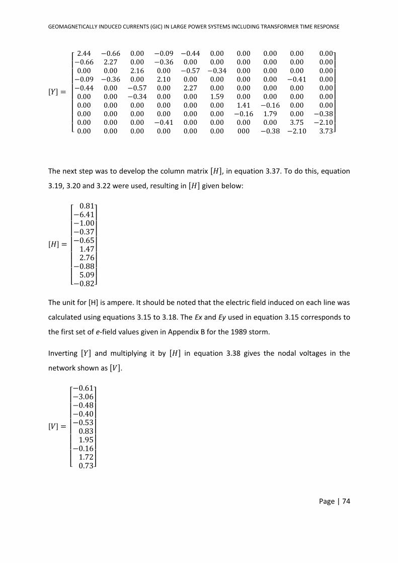
GEOMAGNETICALLY INDUCED CURRENTS (GIC) IN LARGE POWER SYSTEMS INCLUDING TRANSFORMER TIME RESPONSE
Page | 74
[𝑌] =
[ 2.44 −0.66 0.00 −0.09 −0.44 0.00 0.00 0.00 0.00 0.00−0.66 2.27 0.00 −0.36 0.00 0.00 0.00 0.00 0.00 0.000.00 0.00 2.16 0.00 −0.57 −0.34 0.00 0.00 0.00 0.00−0.09 −0.36 0.00 2.10 0.00 0.00 0.00 0.00 −0.41 0.00−0.44 0.00 −0.57 0.00 2.27 0.00 0.00 0.00 0.00 0.000.00 0.00 −0.34 0.00 0.00 1.59 0.00 0.00 0.00 0.000.00 0.00 0.00 0.00 0.00 0.00 1.41 −0.16 0.00 0.000.00 0.00 0.00 0.00 0.00 0.00 −0.16 1.79 0.00 −0.380.00 0.00 0.00 −0.41 0.00 0.00 0.00 0.00 3.75 −2.100.00 0.00 0.00 0.00 0.00 0.00 000 −0.38 −2.10 3.73]
The next step was to develop the column matrix [𝐻], in equation 3.37. To do this, equation
3.19, 3.20 and 3.22 were used, resulting in [𝐻] given below:
[𝐻] =
[ 0.81
−6.41−1.00−0.37−0.651.47 2.76−0.88 5.09−0.82]
The unit for [H] is ampere. It should be noted that the electric field induced on each line was
calculated using equations 3.15 to 3.18. The Ex and Ey used in equation 3.15 corresponds to
the first set of e-field values given in Appendix B for the 1989 storm.
Inverting [𝑌] and multiplying it by [𝐻] in equation 3.38 gives the nodal voltages in the
network shown as [𝑉].
[𝑉] =
[ −0.61−3.06−0.48−0.40−0.530.83 1.95−0.16 1.720.73]
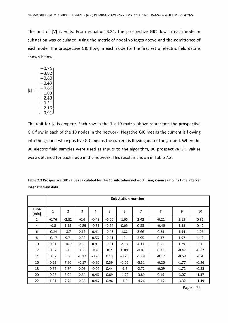
GEOMAGNETICALLY INDUCED CURRENTS (GIC) IN LARGE POWER SYSTEMS INCLUDING TRANSFORMER TIME RESPONSE
Page | 75
The unit of [V] is volts. From equation 3.24, the prospective GIC flow in each node or
substation was calculated, using the matrix of nodal voltages above and the admittance of
each node. The prospective GIC flow, in each node for the first set of electric field data is
shown below.
[𝑖] =
[ −0.76−3.82−0.60−0.49−0.661.03 2.43−0.21 2.150.91]
The unit for [i] is ampere. Each row in the 1 x 10 matrix above represents the prospective
GIC flow in each of the 10 nodes in the network. Negative GIC means the current is flowing
into the ground while positive GIC means the current is flowing out of the ground. When the
90 electric field samples were used as inputs to the algorithm, 90 prospective GIC values
were obtained for each node in the network. This result is shown in Table 7.3.
Table 7.3 Prospective GIC values calculated for the 10 substation network using 2-min sampling time interval
magnetic field data
Substation number
Time (min)
1 2 3 4 5 6 7 8 9 10
2 -0.76 -3.82 -0.6 -0.49 -0.66 1.03 2.43 -0.21 2.15 0.91
4 -0.8 1.19 -0.89 -0.91 -0.54 0.05 0.55 -0.46 1.39 0.42
6 -0.24 -8.7 0.19 0.41 -0.43 1.82 3.66 0.29 1.94 1.06
8 -0.17 -9.71 0.32 0.56 -0.41 2 3.95 0.37 1.97 1.12
10 0.01 -10.7 0.55 0.81 -0.31 2.13 4.11 0.51 1.79 1.1
12 0.32 -1 0.38 0.4 0.2 0.09 -0.02 0.21 -0.47 -0.12
14 0.02 3.8 -0.17 -0.26 0.13 -0.76 -1.49 -0.17 -0.68 -0.4
16 0.22 7.86 -0.17 -0.36 0.39 -1.65 -3.31 -0.26 -1.77 -0.96
18 0.37 5.84 0.09 -0.06 0.44 -1.3 -2.72 -0.09 -1.72 -0.85
20 0.96 6.94 0.64 0.46 0.89 -1.72 -3.89 0.16 -3.07 -1.37
22 1.01 7.74 0.66 0.46 0.96 -1.9 -4.26 0.15 -3.32 -1.49
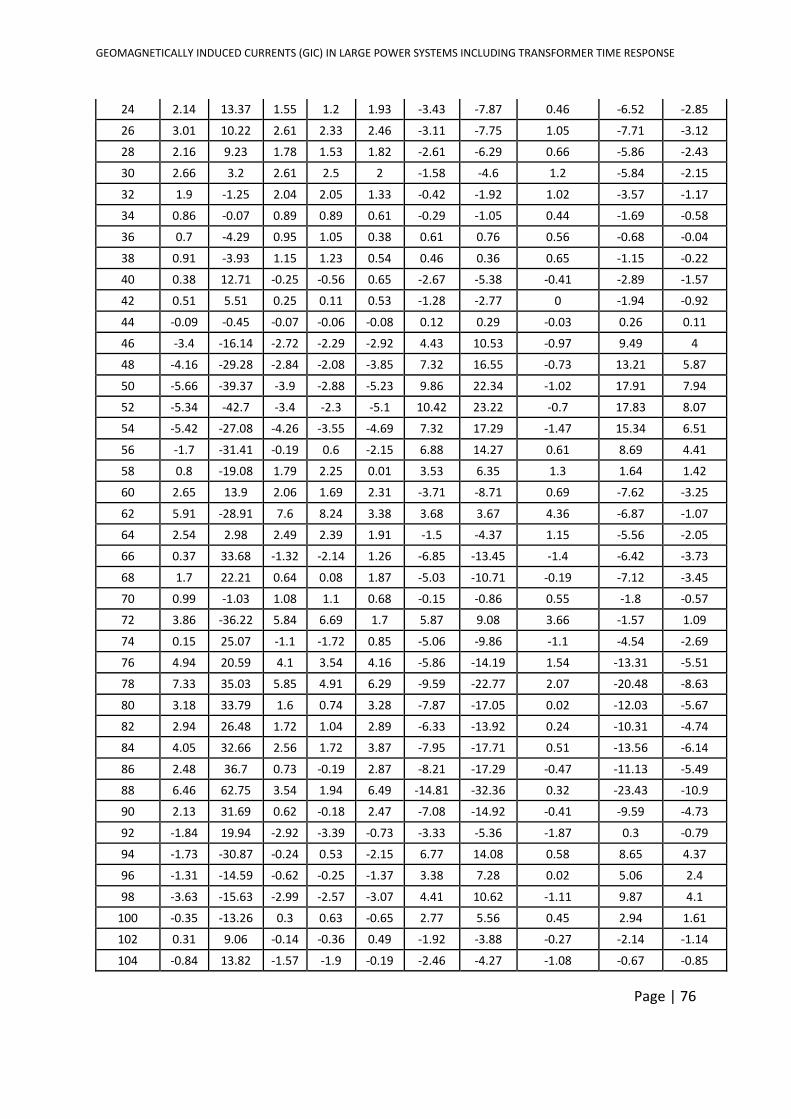
GEOMAGNETICALLY INDUCED CURRENTS (GIC) IN LARGE POWER SYSTEMS INCLUDING TRANSFORMER TIME RESPONSE
Page | 76
24 2.14 13.37 1.55 1.2 1.93 -3.43 -7.87 0.46 -6.52 -2.85
26 3.01 10.22 2.61 2.33 2.46 -3.11 -7.75 1.05 -7.71 -3.12
28 2.16 9.23 1.78 1.53 1.82 -2.61 -6.29 0.66 -5.86 -2.43
30 2.66 3.2 2.61 2.5 2 -1.58 -4.6 1.2 -5.84 -2.15
32 1.9 -1.25 2.04 2.05 1.33 -0.42 -1.92 1.02 -3.57 -1.17
34 0.86 -0.07 0.89 0.89 0.61 -0.29 -1.05 0.44 -1.69 -0.58
36 0.7 -4.29 0.95 1.05 0.38 0.61 0.76 0.56 -0.68 -0.04
38 0.91 -3.93 1.15 1.23 0.54 0.46 0.36 0.65 -1.15 -0.22
40 0.38 12.71 -0.25 -0.56 0.65 -2.67 -5.38 -0.41 -2.89 -1.57
42 0.51 5.51 0.25 0.11 0.53 -1.28 -2.77 0 -1.94 -0.92
44 -0.09 -0.45 -0.07 -0.06 -0.08 0.12 0.29 -0.03 0.26 0.11
46 -3.4 -16.14 -2.72 -2.29 -2.92 4.43 10.53 -0.97 9.49 4
48 -4.16 -29.28 -2.84 -2.08 -3.85 7.32 16.55 -0.73 13.21 5.87
50 -5.66 -39.37 -3.9 -2.88 -5.23 9.86 22.34 -1.02 17.91 7.94
52 -5.34 -42.7 -3.4 -2.3 -5.1 10.42 23.22 -0.7 17.83 8.07
54 -5.42 -27.08 -4.26 -3.55 -4.69 7.32 17.29 -1.47 15.34 6.51
56 -1.7 -31.41 -0.19 0.6 -2.15 6.88 14.27 0.61 8.69 4.41
58 0.8 -19.08 1.79 2.25 0.01 3.53 6.35 1.3 1.64 1.42
60 2.65 13.9 2.06 1.69 2.31 -3.71 -8.71 0.69 -7.62 -3.25
62 5.91 -28.91 7.6 8.24 3.38 3.68 3.67 4.36 -6.87 -1.07
64 2.54 2.98 2.49 2.39 1.91 -1.5 -4.37 1.15 -5.56 -2.05
66 0.37 33.68 -1.32 -2.14 1.26 -6.85 -13.45 -1.4 -6.42 -3.73
68 1.7 22.21 0.64 0.08 1.87 -5.03 -10.71 -0.19 -7.12 -3.45
70 0.99 -1.03 1.08 1.1 0.68 -0.15 -0.86 0.55 -1.8 -0.57
72 3.86 -36.22 5.84 6.69 1.7 5.87 9.08 3.66 -1.57 1.09
74 0.15 25.07 -1.1 -1.72 0.85 -5.06 -9.86 -1.1 -4.54 -2.69
76 4.94 20.59 4.1 3.54 4.16 -5.86 -14.19 1.54 -13.31 -5.51
78 7.33 35.03 5.85 4.91 6.29 -9.59 -22.77 2.07 -20.48 -8.63
80 3.18 33.79 1.6 0.74 3.28 -7.87 -17.05 0.02 -12.03 -5.67
82 2.94 26.48 1.72 1.04 2.89 -6.33 -13.92 0.24 -10.31 -4.74
84 4.05 32.66 2.56 1.72 3.87 -7.95 -17.71 0.51 -13.56 -6.14
86 2.48 36.7 0.73 -0.19 2.87 -8.21 -17.29 -0.47 -11.13 -5.49
88 6.46 62.75 3.54 1.94 6.49 -14.81 -32.36 0.32 -23.43 -10.9
90 2.13 31.69 0.62 -0.18 2.47 -7.08 -14.92 -0.41 -9.59 -4.73
92 -1.84 19.94 -2.92 -3.39 -0.73 -3.33 -5.36 -1.87 0.3 -0.79
94 -1.73 -30.87 -0.24 0.53 -2.15 6.77 14.08 0.58 8.65 4.37
96 -1.31 -14.59 -0.62 -0.25 -1.37 3.38 7.28 0.02 5.06 2.4
98 -3.63 -15.63 -2.99 -2.57 -3.07 4.41 10.62 -1.11 9.87 4.1
100 -0.35 -13.26 0.3 0.63 -0.65 2.77 5.56 0.45 2.94 1.61
102 0.31 9.06 -0.14 -0.36 0.49 -1.92 -3.88 -0.27 -2.14 -1.14
104 -0.84 13.82 -1.57 -1.9 -0.19 -2.46 -4.27 -1.08 -0.67 -0.85
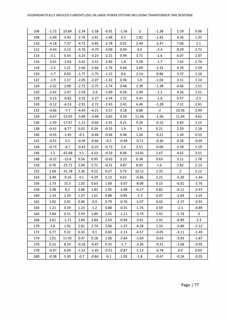
GEOMAGNETICALLY INDUCED CURRENTS (GIC) IN LARGE POWER SYSTEMS INCLUDING TRANSFORMER TIME RESPONSE
Page | 77
106 -1.72 10.84 -2.34 -2.58 -0.91 -1.56 -2 -1.38 1.59 0.06
108 -2.49 3.43 -2.76 -2.81 -1.68 0.2 1.82 -1.42 4.36 1.35
110 -4.18 7.37 -4.71 -4.85 -2.78 0.01 2.44 -2.47 7.06 2.1
112 -4.43 3.13 -4.76 -4.79 -3.09 0.94 4.4 -2.4 8.29 2.72
114 -3.1 0.54 -3.25 -3.23 -2.21 0.99 3.71 -1.6 6.07 2.07
116 -3.61 -2.63 -3.62 -3.51 -2.66 1.8 5.58 -1.7 7.62 2.74
118 -2.5 1.21 -2.66 -2.66 -1.76 0.64 2.69 -1.32 4.76 1.59
120 -1.7 0.03 -1.77 -1.75 -1.22 0.6 2.14 -0.86 3.37 1.16
122 -1.9 1.57 -2.05 -2.07 -1.32 0.36 1.8 -1.04 3.51 1.14
124 -2.52 2.08 -2.72 -2.75 -1.74 0.48 2.38 -1.38 4.66 1.51
126 -2.42 1.47 -2.59 -2.6 -1.69 0.56 2.49 -1.3 4.56 1.51
128 -3.23 -0.82 -3.32 -3.27 -2.34 1.31 4.41 -1.6 6.57 2.3
130 -3.12 -6.53 -2.91 -2.72 -2.43 2.41 6.46 -1.28 7.31 2.81
132 -4.66 -7.7 -4.45 -4.21 -3.57 3.18 8.86 -2 10.56 3.99
134 -4.47 -15.05 -3.89 -3.48 -3.65 4.59 11.46 -1.56 11.44 4.62
136 -1.93 -17.67 -1.12 -0.66 -1.91 4.21 9.26 -0.15 6.83 3.15
138 -0.41 -8.77 0.02 0.24 -0.55 1.9 3.9 0.21 2.29 1.18
140 -0.55 -1.45 -0.5 -0.46 -0.44 0.48 1.26 -0.21 1.34 0.53
142 -0.41 3.2 -0.59 -0.66 -0.2 -0.49 -0.71 -0.36 0.28 -0.05
144 -0.73 -6.7 -0.43 -0.25 -0.73 1.6 3.51 -0.06 2.59 1.19
146 1.3 -42.68 3.5 4.53 -0.33 8.06 14.81 2.67 4.62 3.51
148 -0.22 -15.8 0.56 0.95 -0.63 3.23 6.38 0.63 3.11 1.78
150 0.76 -25.72 2.09 2.71 -0.21 4.87 8.95 1.6 2.82 2.13
152 1.69 -31.78 3.36 4.12 0.27 5.75 10.11 2.35 2 2.12
154 3.49 -9.24 4.1 4.29 2.23 0.61 -0.86 2.21 -5.39 -1.44
156 1.73 15.3 1.02 0.63 1.69 -3.67 -8.08 0.15 -6.01 -2.76
158 2.38 8.2 2.06 1.83 1.95 -2.48 -6.17 0.82 -6.11 -2.47
160 1.14 2.24 1.07 1.01 0.88 -0.85 -2.3 0.47 -2.64 -1.01
162 1.02 2.01 0.96 0.9 0.79 -0.76 -2.07 0.42 -2.37 -0.91
164 1.21 0.59 1.23 1.2 0.88 -0.55 -1.76 0.59 -2.5 -0.89
166 2.84 0.51 2.93 2.89 2.05 -1.11 -3.79 1.42 -5.74 -2
168 3.61 -1.71 3.84 3.84 2.54 -0.94 -3.91 1.91 -6.89 -2.3
170 2.8 1.92 2.81 2.74 2.06 -1.37 -4.28 1.33 -5.89 -2.12
172 0.77 9.31 0.33 0.1 0.83 -2.13 -4.57 -0.05 -3.11 -1.49
174 1.01 11.45 0.47 0.18 1.06 -2.64 -5.69 -0.03 -3.93 -1.87
176 0.15 8.24 -0.26 -0.47 0.35 -1.7 -3.36 -0.31 -1.68 -0.95
178 -0.97 6.09 -1.31 -1.45 -0.51 -0.87 -1.13 -0.78 0.9 0.03
180 -0.38 5.93 -0.7 -0.84 -0.1 -1.05 -1.8 -0.47 -0.24 -0.35
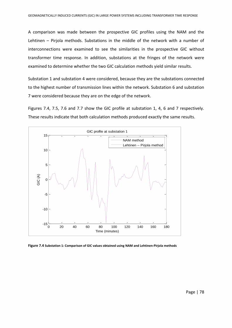
GEOMAGNETICALLY INDUCED CURRENTS (GIC) IN LARGE POWER SYSTEMS INCLUDING TRANSFORMER TIME RESPONSE
Page | 78
A comparison was made between the prospective GIC profiles using the NAM and the
Lehtinen – Pirjola methods. Substations in the middle of the network with a number of
interconnections were examined to see the similarities in the prospective GIC without
transformer time response. In addition, substations at the fringes of the network were
examined to determine whether the two GIC calculation methods yield similar results.
Substation 1 and substation 4 were considered, because they are the substations connected
to the highest number of transmission lines within the network. Substation 6 and substation
7 were considered because they are on the edge of the network.
Figures 7.4, 7.5, 7.6 and 7.7 show the GIC profile at substation 1, 4, 6 and 7 respectively.
These results indicate that both calculation methods produced exactly the same results.
Figure 7.4 Substation 1: Comparison of GIC values obtained using NAM and Lehtinen-Pirjola methods
0 20 40 60 80 100 120 140 160 180-15
-10
-5
0
5
10
15
Time (minutes)
GIC
(A
)
GIC profile at substation 1
NAM method
Lehtinen -- Pirjola method
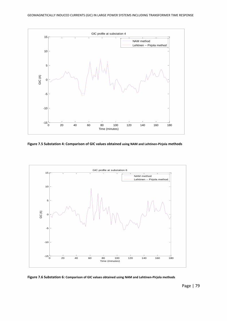
GEOMAGNETICALLY INDUCED CURRENTS (GIC) IN LARGE POWER SYSTEMS INCLUDING TRANSFORMER TIME RESPONSE
Page | 79
Figure 7.5 Substation 4: Comparison of GIC values obtained using NAM and Lehtinen-Pirjola methods
Figure 7.6 Substation 6: Comparison of GIC values obtained using NAM and Lehtinen-Pirjola methods
0 20 40 60 80 100 120 140 160 180-15
-10
-5
0
5
10
15
Time (minutes)
GIC
(A
)
GIC profile at substation 4
NAM method
Lehtinen -- Pirjola method
0 20 40 60 80 100 120 140 160 180-15
-10
-5
0
5
10
15
Time (minutes)
GIC
(A)
GIC profile at substation 6
NAM method
Lehtinen -- Pirjola method
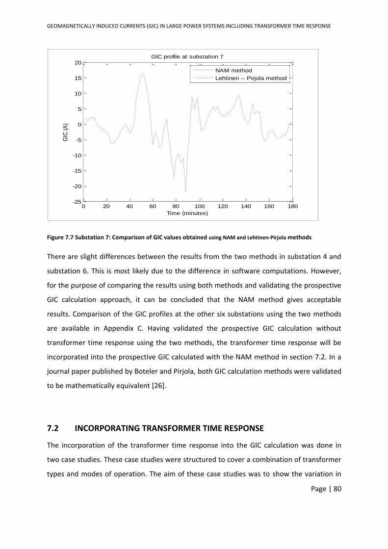
GEOMAGNETICALLY INDUCED CURRENTS (GIC) IN LARGE POWER SYSTEMS INCLUDING TRANSFORMER TIME RESPONSE
Page | 80
Figure 7.7 Substation 7: Comparison of GIC values obtained using NAM and Lehtinen-Pirjola methods
There are slight differences between the results from the two methods in substation 4 and
substation 6. This is most likely due to the difference in software computations. However,
for the purpose of comparing the results using both methods and validating the prospective
GIC calculation approach, it can be concluded that the NAM method gives acceptable
results. Comparison of the GIC profiles at the other six substations using the two methods
are available in Appendix C. Having validated the prospective GIC calculation without
transformer time response using the two methods, the transformer time response will be
incorporated into the prospective GIC calculated with the NAM method in section 7.2. In a
journal paper published by Boteler and Pirjola, both GIC calculation methods were validated
to be mathematically equivalent [26].
7.2 INCORPORATING TRANSFORMER TIME RESPONSE
The incorporation of the transformer time response into the GIC calculation was done in
two case studies. These case studies were structured to cover a combination of transformer
types and modes of operation. The aim of these case studies was to show the variation in
0 20 40 60 80 100 120 140 160 180-25
-20
-15
-10
-5
0
5
10
15
20
Time (minutes)
GIC
(A
)
GIC profile at substation 7
NAM method
Lehtinen -- Pirjola method
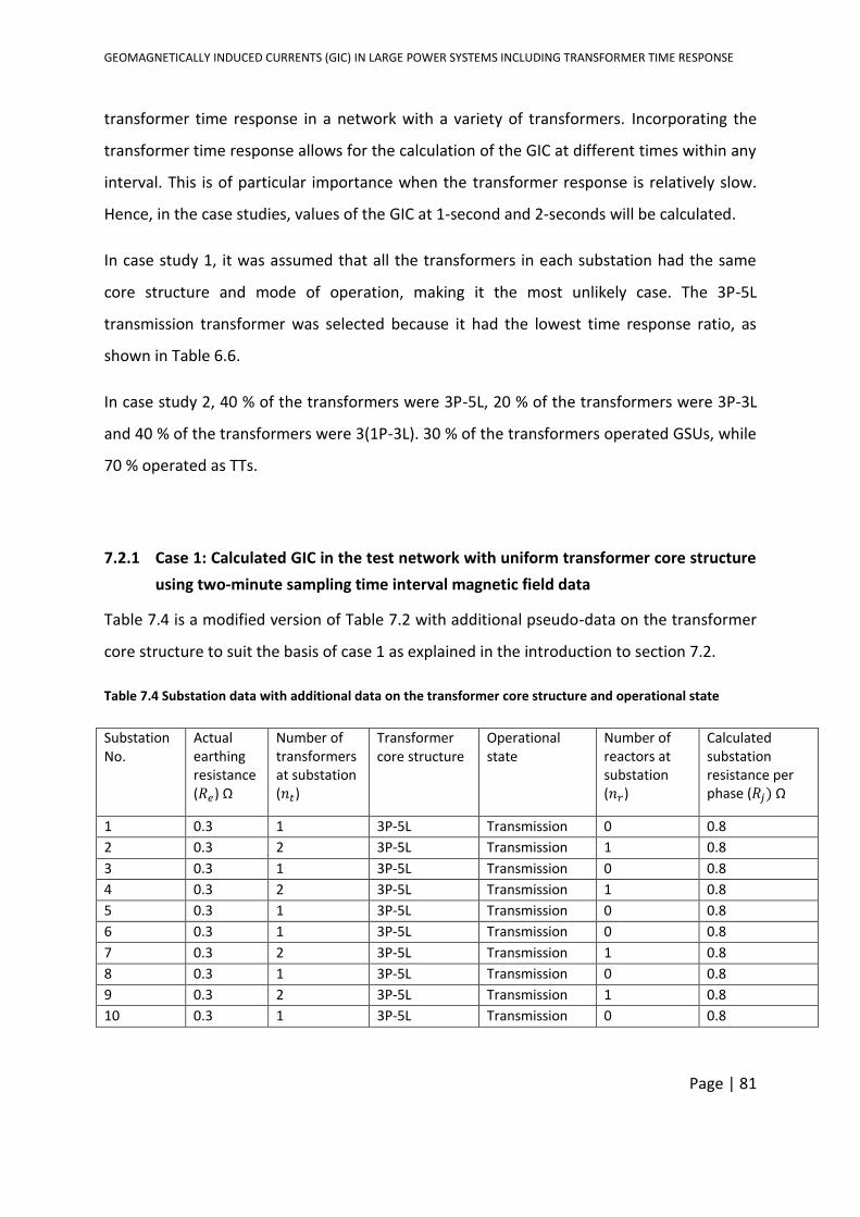
GEOMAGNETICALLY INDUCED CURRENTS (GIC) IN LARGE POWER SYSTEMS INCLUDING TRANSFORMER TIME RESPONSE
Page | 81
transformer time response in a network with a variety of transformers. Incorporating the
transformer time response allows for the calculation of the GIC at different times within any
interval. This is of particular importance when the transformer response is relatively slow.
Hence, in the case studies, values of the GIC at 1-second and 2-seconds will be calculated.
In case study 1, it was assumed that all the transformers in each substation had the same
core structure and mode of operation, making it the most unlikely case. The 3P-5L
transmission transformer was selected because it had the lowest time response ratio, as
shown in Table 6.6.
In case study 2, 40 % of the transformers were 3P-5L, 20 % of the transformers were 3P-3L
and 40 % of the transformers were 3(1P-3L). 30 % of the transformers operated GSUs, while
70 % operated as TTs.
7.2.1 Case 1: Calculated GIC in the test network with uniform transformer core structure
using two-minute sampling time interval magnetic field data
Table 7.4 is a modified version of Table 7.2 with additional pseudo-data on the transformer
core structure to suit the basis of case 1 as explained in the introduction to section 7.2.
Table 7.4 Substation data with additional data on the transformer core structure and operational state
Substation No.
Actual earthing resistance (𝑅𝑒) Ω
Number of transformers at substation (𝑛𝑡)
Transformer core structure
Operational state
Number of reactors at substation (𝑛𝑟)
Calculated substation resistance per phase (𝑅𝑗) Ω
1 0.3 1 3P-5L Transmission 0 0.8
2 0.3 2 3P-5L Transmission 1 0.8
3 0.3 1 3P-5L Transmission 0 0.8
4 0.3 2 3P-5L Transmission 1 0.8
5 0.3 1 3P-5L Transmission 0 0.8
6 0.3 1 3P-5L Transmission 0 0.8
7 0.3 2 3P-5L Transmission 1 0.8
8 0.3 1 3P-5L Transmission 0 0.8
9 0.3 2 3P-5L Transmission 1 0.8
10 0.3 1 3P-5L Transmission 0 0.8
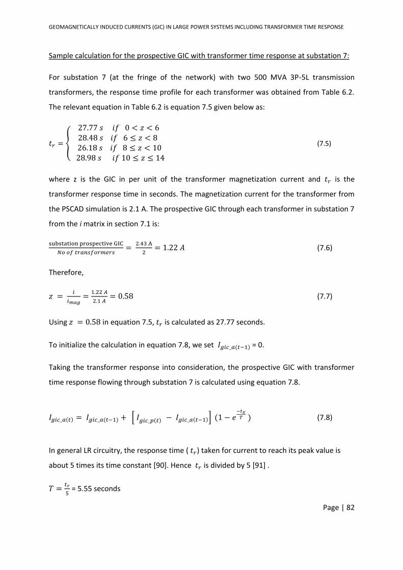
GEOMAGNETICALLY INDUCED CURRENTS (GIC) IN LARGE POWER SYSTEMS INCLUDING TRANSFORMER TIME RESPONSE
Page | 82
Sample calculation for the prospective GIC with transformer time response at substation 7:
For substation 7 (at the fringe of the network) with two 500 MVA 3P-5L transmission
transformers, the response time profile for each transformer was obtained from Table 6.2.
The relevant equation in Table 6.2 is equation 7.5 given below as:
𝑡𝑟 =
27.77 𝑠 𝑖𝑓 0 < 𝑧 < 628.48 𝑠 𝑖𝑓 6 ≤ 𝑧 < 8 26.18 𝑠 𝑖𝑓 8 ≤ 𝑧 < 10 28.98 𝑠 𝑖𝑓 10 ≤ 𝑧 ≤ 14
(7.5)
where z is the GIC in per unit of the transformer magnetization current and 𝑡𝑟 is the
transformer response time in seconds. The magnetization current for the transformer from
the PSCAD simulation is 2.1 A. The prospective GIC through each transformer in substation 7
from the i matrix in section 7.1 is:
substation prospective GIC
𝑁𝑜 𝑜𝑓 𝑡𝑟𝑎𝑛𝑠𝑓𝑜𝑟𝑚𝑒𝑟𝑠=
2.43 A
2= 1.22 𝐴 (7.6)
Therefore,
𝑧 = 𝑖
𝑖𝑚𝑎𝑔=
1.22 𝐴
2.1 𝐴= 0.58 (7.7)
Using 𝑧 = 0.58 in equation 7.5, 𝑡𝑟 is calculated as 27.77 seconds.
To initialize the calculation in equation 7.8, we set 𝐼𝑔𝑖𝑐_𝑎(𝑡−1) = 0.
Taking the transformer response into consideration, the prospective GIC with transformer
time response flowing through substation 7 is calculated using equation 7.8.
𝐼𝑔𝑖𝑐_𝑎(𝑡) = 𝐼𝑔𝑖𝑐_𝑎(𝑡−1) + [ 𝐼𝑔𝑖𝑐_𝑝(𝑡) − 𝐼𝑔𝑖𝑐_𝑎(𝑡−1)] (1 − 𝑒−𝑡𝑥𝑇 ) (7.8)
In general LR circuitry, the response time ( 𝑡𝑟) taken for current to reach its peak value is
about 5 times its time constant [90]. Hence 𝑡𝑟 is divided by 5 [91] .
𝑇 =𝑡𝑟
5 = 5.55 seconds
GEOMAGNETICALLY INDUCED CURRENTS (GIC) IN LARGE POWER SYSTEMS INCLUDING TRANSFORMER TIME RESPONSE
Page | 83
From Table 7.3 in section 7.1, the first prospective GIC in substation 7 is 2.43 A.
From this, the first prospective GIC with transformer time response at one second is
calculated as,
𝐼𝑔𝑖𝑐_𝑎(1) = 0 + [2.43 − 0](1 − 𝑒−1
5.55) = 0.39 A, which is 84 % lower than the prospective
without the transformer time response.
At t = 2 seconds,
𝐼𝑔𝑖𝑐_𝑎(2) = 𝐼𝑔𝑖𝑐_𝑎(1) + [ 𝐼𝑔𝑖𝑐_𝑝(1) − 𝐼𝑔𝑖𝑐_𝑎(1)] ∗ (1 − 𝑒−2
5.55 ) (7.9)
= 0.39 + [2.43 − 0.39] ∗ (0.30) = 1.0 𝐴.
From the calculation of the prospective GIC with transformer response in substation 7 at
two seconds, it can be seen that the transformer response time to GIC suppresses the
prospective GIC, such that the difference between the prospective GIC with and without the
transformer response is 59 %. It should be noted that when the time between two
successive GIC samples are as long as two minutes, based on the time response profile of
the transformer, the prospective GIC with and without the transformer time response may
be the same. This is because the exponential term in equation 7.9 tends to zero with longer
sampling time intervals.
Sample calculation for the prospective GIC with transformer time response at substation 4:
Substation 4 has 2 units of 500 MVA 3P-5L transmission transformers. The time response
profile for each transformer is obtained from Table 6.2. The relevant equation in Table 6.2 is
equation 7.5. The magnetization current for the transformer from the PSCAD simulation is
2.1 A. The prospective GIC through each transformer in substation 4, from Table 7.3 in
section 7.1 is:
substation prospective GIC
𝑁𝑜 𝑜𝑓 𝑡𝑟𝑎𝑛𝑠𝑓𝑜𝑟𝑚𝑒𝑟𝑠=
−0.49 A
2 = −0.25 𝐴 (7.10)
Therefore,
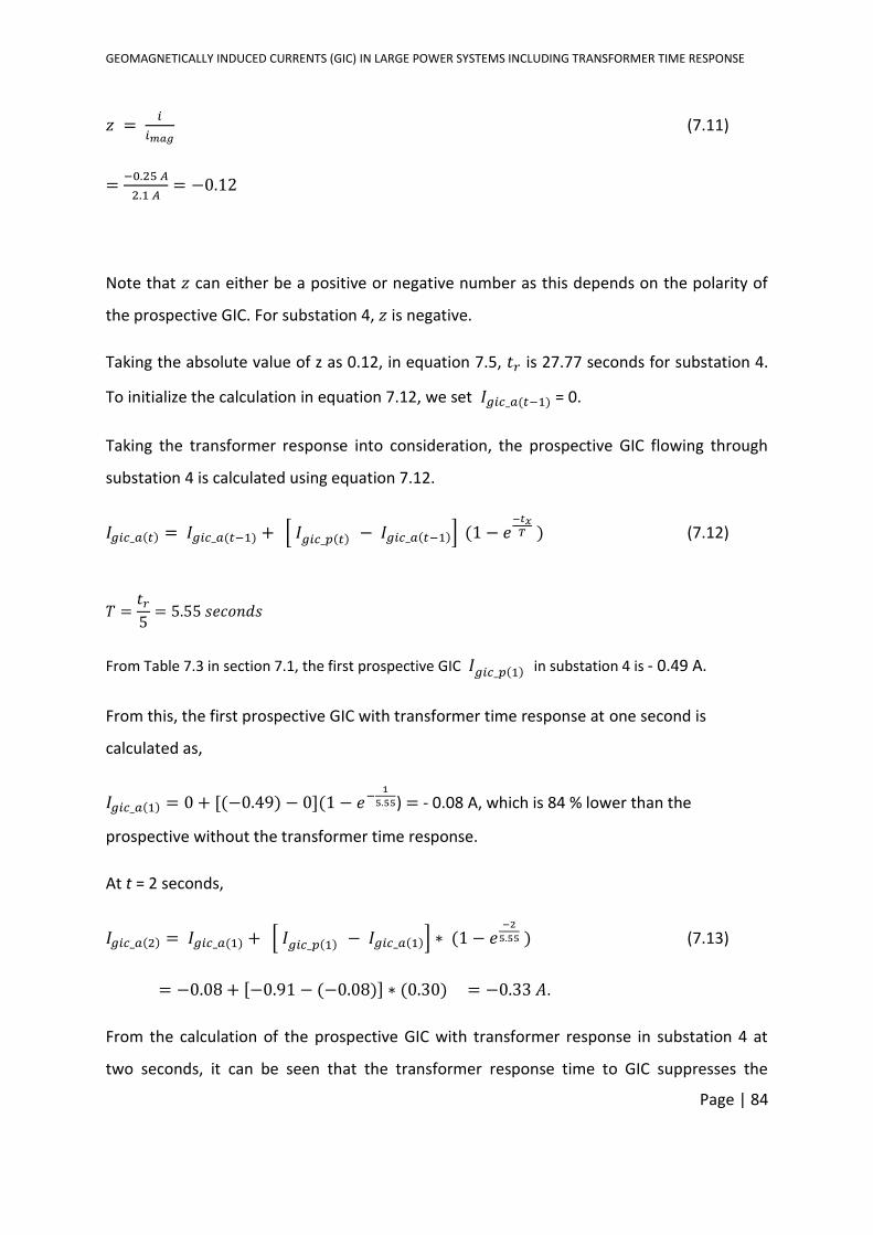
GEOMAGNETICALLY INDUCED CURRENTS (GIC) IN LARGE POWER SYSTEMS INCLUDING TRANSFORMER TIME RESPONSE
Page | 84
𝑧 = 𝑖
𝑖𝑚𝑎𝑔 (7.11)
=−0.25 𝐴
2.1 𝐴= −0.12
Note that 𝑧 can either be a positive or negative number as this depends on the polarity of
the prospective GIC. For substation 4, 𝑧 is negative.
Taking the absolute value of z as 0.12, in equation 7.5, 𝑡𝑟 is 27.77 seconds for substation 4.
To initialize the calculation in equation 7.12, we set 𝐼𝑔𝑖𝑐_𝑎(𝑡−1) = 0.
Taking the transformer response into consideration, the prospective GIC flowing through
substation 4 is calculated using equation 7.12.
𝐼𝑔𝑖𝑐_𝑎(𝑡) = 𝐼𝑔𝑖𝑐_𝑎(𝑡−1) + [ 𝐼𝑔𝑖𝑐_𝑝(𝑡) − 𝐼𝑔𝑖𝑐_𝑎(𝑡−1)] (1 − 𝑒−𝑡𝑥𝑇 ) (7.12)
𝑇 =𝑡𝑟5= 5.55 𝑠𝑒𝑐𝑜𝑛𝑑𝑠
From Table 7.3 in section 7.1, the first prospective GIC 𝐼𝑔𝑖𝑐_𝑝(1) in substation 4 is - 0.49 A.
From this, the first prospective GIC with transformer time response at one second is
calculated as,
𝐼𝑔𝑖𝑐_𝑎(1) = 0 + [(−0.49) − 0](1 − 𝑒−1
5.55) = - 0.08 A, which is 84 % lower than the
prospective without the transformer time response.
At t = 2 seconds,
𝐼𝑔𝑖𝑐_𝑎(2) = 𝐼𝑔𝑖𝑐_𝑎(1) + [ 𝐼𝑔𝑖𝑐_𝑝(1) − 𝐼𝑔𝑖𝑐_𝑎(1)] ∗ (1 − 𝑒−2
5.55 ) (7.13)
= −0.08 + [−0.91 − (−0.08)] ∗ (0.30) = −0.33 𝐴.
From the calculation of the prospective GIC with transformer response in substation 4 at
two seconds, it can be seen that the transformer response time to GIC suppresses the
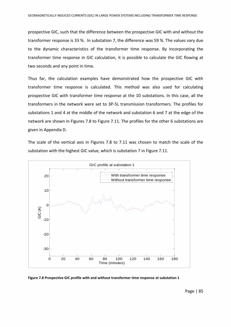
GEOMAGNETICALLY INDUCED CURRENTS (GIC) IN LARGE POWER SYSTEMS INCLUDING TRANSFORMER TIME RESPONSE
Page | 85
prospective GIC, such that the difference between the prospective GIC with and without the
transformer response is 33 %. In substation 7, the difference was 59 %. The values vary due
to the dynamic characteristics of the transformer time response. By incorporating the
transformer time response in GIC calculation, it is possible to calculate the GIC flowing at
two seconds and any point in time.
Thus far, the calculation examples have demonstrated how the prospective GIC with
transformer time response is calculated. This method was also used for calculating
prospective GIC with transformer time response at the 10 substations. In this case, all the
transformers in the network were set to 3P-5L transmission transformers. The profiles for
substations 1 and 4 at the middle of the network and substation 6 and 7 at the edge of the
network are shown in Figures 7.8 to Figure 7.11. The profiles for the other 6 substations are
given in Appendix D.
The scale of the vertical axis in Figures 7.8 to 7.11 was chosen to match the scale of the
substation with the highest GIC value, which is substation 7 in Figure 7.11.
Figure 7.8 Prospective GIC profile with and without transformer time response at substation 1
0 20 40 60 80 100 120 140 160 180
-30
-20
-10
0
10
20
Time (minutes)
GIC
(A
)
GIC profile at substation 1
With transformer time response
Without transformer time response
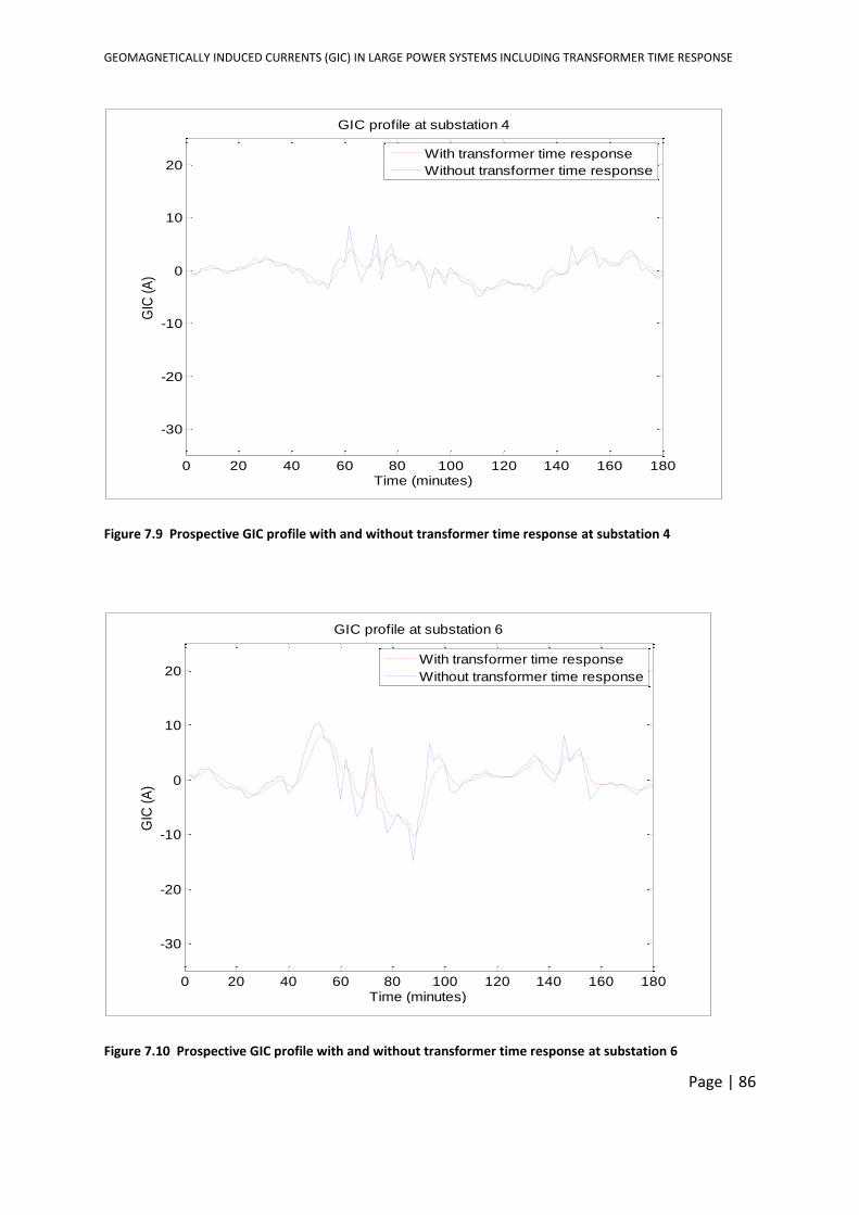
GEOMAGNETICALLY INDUCED CURRENTS (GIC) IN LARGE POWER SYSTEMS INCLUDING TRANSFORMER TIME RESPONSE
Page | 86
Figure 7.9 Prospective GIC profile with and without transformer time response at substation 4
Figure 7.10 Prospective GIC profile with and without transformer time response at substation 6
0 20 40 60 80 100 120 140 160 180
-30
-20
-10
0
10
20
Time (minutes)
GIC
(A
)
GIC profile at substation 4
With transformer time response
Without transformer time response
0 20 40 60 80 100 120 140 160 180
-30
-20
-10
0
10
20
Time (minutes)
GIC
(A
)
GIC profile at substation 6
With transformer time response
Without transformer time response
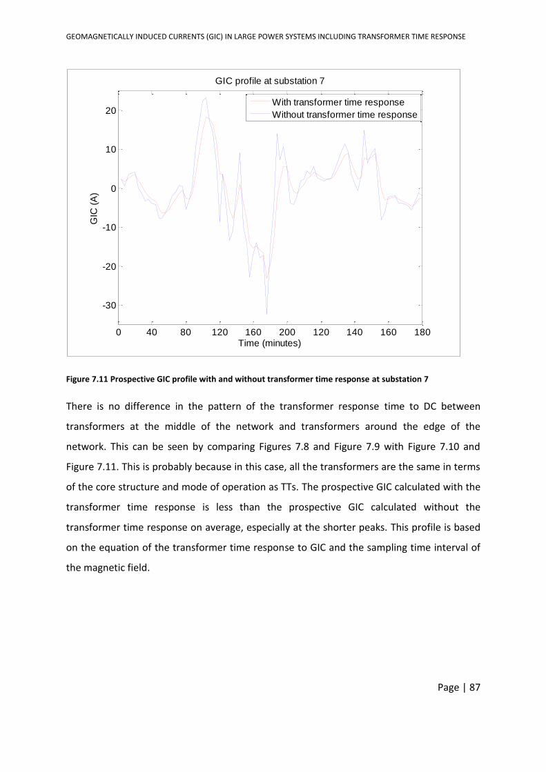
GEOMAGNETICALLY INDUCED CURRENTS (GIC) IN LARGE POWER SYSTEMS INCLUDING TRANSFORMER TIME RESPONSE
Page | 87
Figure 7.11 Prospective GIC profile with and without transformer time response at substation 7
There is no difference in the pattern of the transformer response time to DC between
transformers at the middle of the network and transformers around the edge of the
network. This can be seen by comparing Figures 7.8 and Figure 7.9 with Figure 7.10 and
Figure 7.11. This is probably because in this case, all the transformers are the same in terms
of the core structure and mode of operation as TTs. The prospective GIC calculated with the
transformer time response is less than the prospective GIC calculated without the
transformer time response on average, especially at the shorter peaks. This profile is based
on the equation of the transformer time response to GIC and the sampling time interval of
the magnetic field.
0 40 80 120 160 200 120 140 160 180
-30
-20
-10
0
10
20
Time (minutes)
GIC
(A
)
GIC profile at substation 7
With transformer time response
Without transformer time response
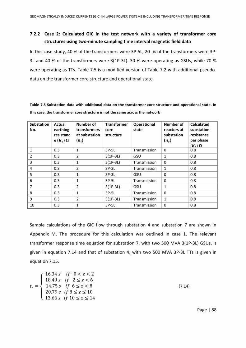
GEOMAGNETICALLY INDUCED CURRENTS (GIC) IN LARGE POWER SYSTEMS INCLUDING TRANSFORMER TIME RESPONSE
Page | 88
7.2.2 Case 2: Calculated GIC in the test network with a variety of transformer core
structures using two-minute sampling time interval magnetic field data
In this case study, 40 % of the transformers were 3P-5L, 20 % of the transformers were 3P-
3L and 40 % of the transformers were 3(1P-3L). 30 % were operating as GSUs, while 70 %
were operating as TTs. Table 7.5 is a modified version of Table 7.2 with additional pseudo-
data on the transformer core structure and operational state.
Table 7.5 Substation data with additional data on the transformer core structure and operational state. In
this case, the transformer core structure is not the same across the network
Substation No.
Actual earthing resistance (𝑹𝒆) Ω
Number of transformers at substation (𝒏𝒕)
Transformer core structure
Operational state
Number of reactors at substation (𝒏𝒓)
Calculated substation resistance per phase (𝑹𝒋) Ω
1 0.3 1 3P-5L Transmission 0 0.8
2 0.3 2 3(1P-3L) GSU 1 0.8
3 0.3 1 3(1P-3L) Transmission 0 0.8
4 0.3 2 3P-3L Transmission 1 0.8
5 0.3 1 3P-3L GSU 0 0.8
6 0.3 1 3P-5L Transmission 0 0.8
7 0.3 2 3(1P-3L) GSU 1 0.8
8 0.3 1 3P-5L Transmission 0 0.8
9 0.3 2 3(1P-3L) Transmission 1 0.8
10 0.3 1 3P-5L Transmission 0 0.8
Sample calculations of the GIC flow through substation 4 and substation 7 are shown in
Appendix M. The procedure for this calculation was outlined in case 1. The relevant
transformer response time equation for substation 7, with two 500 MVA 3(1P-3L) GSUs, is
given in equation 7.14 and that of substation 4, with two 500 MVA 3P-3L TTs is given in
equation 7.15.
𝑡𝑟 =
16.34 𝑠 𝑖𝑓 0 < 𝑧 < 218.49 𝑠 𝑖𝑓 2 ≤ 𝑧 < 614.75 𝑠 𝑖𝑓 6 ≤ 𝑧 < 820.79 𝑠 𝑖𝑓 8 ≤ 𝑧 ≤ 10 13.66 𝑠 𝑖𝑓 10 ≤ 𝑧 ≤ 14
(7.14)
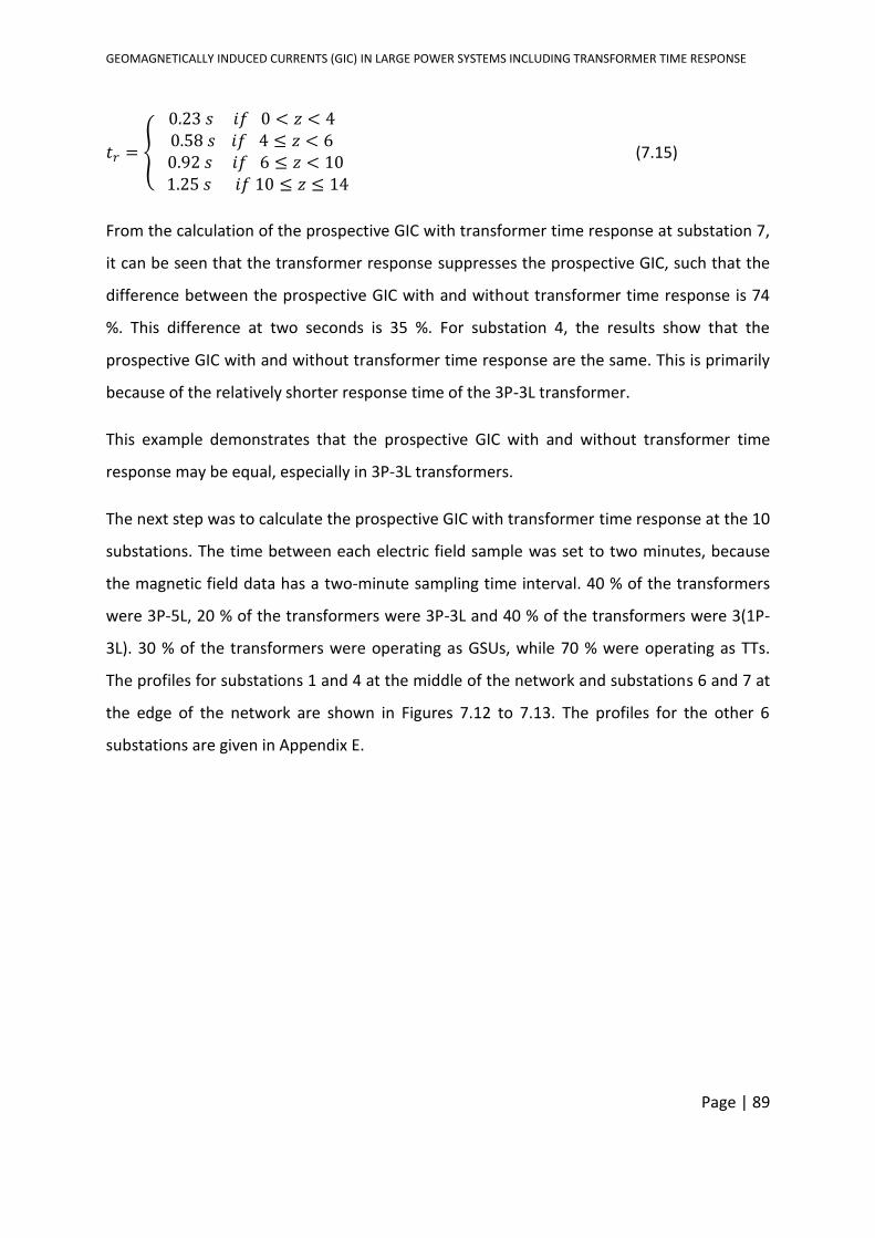
GEOMAGNETICALLY INDUCED CURRENTS (GIC) IN LARGE POWER SYSTEMS INCLUDING TRANSFORMER TIME RESPONSE
Page | 89
𝑡𝑟 =
0.23 𝑠 𝑖𝑓 0 < 𝑧 < 40.58 𝑠 𝑖𝑓 4 ≤ 𝑧 < 6 0.92 𝑠 𝑖𝑓 6 ≤ 𝑧 < 10 1.25 𝑠 𝑖𝑓 10 ≤ 𝑧 ≤ 14
(7.15)
From the calculation of the prospective GIC with transformer time response at substation 7,
it can be seen that the transformer response suppresses the prospective GIC, such that the
difference between the prospective GIC with and without transformer time response is 74
%. This difference at two seconds is 35 %. For substation 4, the results show that the
prospective GIC with and without transformer time response are the same. This is primarily
because of the relatively shorter response time of the 3P-3L transformer.
This example demonstrates that the prospective GIC with and without transformer time
response may be equal, especially in 3P-3L transformers.
The next step was to calculate the prospective GIC with transformer time response at the 10
substations. The time between each electric field sample was set to two minutes, because
the magnetic field data has a two-minute sampling time interval. 40 % of the transformers
were 3P-5L, 20 % of the transformers were 3P-3L and 40 % of the transformers were 3(1P-
3L). 30 % of the transformers were operating as GSUs, while 70 % were operating as TTs.
The profiles for substations 1 and 4 at the middle of the network and substations 6 and 7 at
the edge of the network are shown in Figures 7.12 to 7.13. The profiles for the other 6
substations are given in Appendix E.
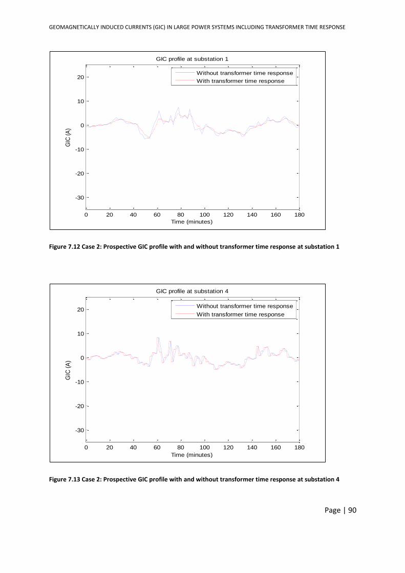
GEOMAGNETICALLY INDUCED CURRENTS (GIC) IN LARGE POWER SYSTEMS INCLUDING TRANSFORMER TIME RESPONSE
Page | 90
Figure 7.12 Case 2: Prospective GIC profile with and without transformer time response at substation 1
Figure 7.13 Case 2: Prospective GIC profile with and without transformer time response at substation 4
0 20 40 60 80 100 120 140 160 180
-30
-20
-10
0
10
20
Time (minutes)
GIC
(A
)
GIC profile at substation 1
Without transformer time response
With transformer time response
0 20 40 60 80 100 120 140 160 180
-30
-20
-10
0
10
20
Time (minutes)
GIC
(A
)
GIC profile at substation 4
Without transformer time response
With transformer time response
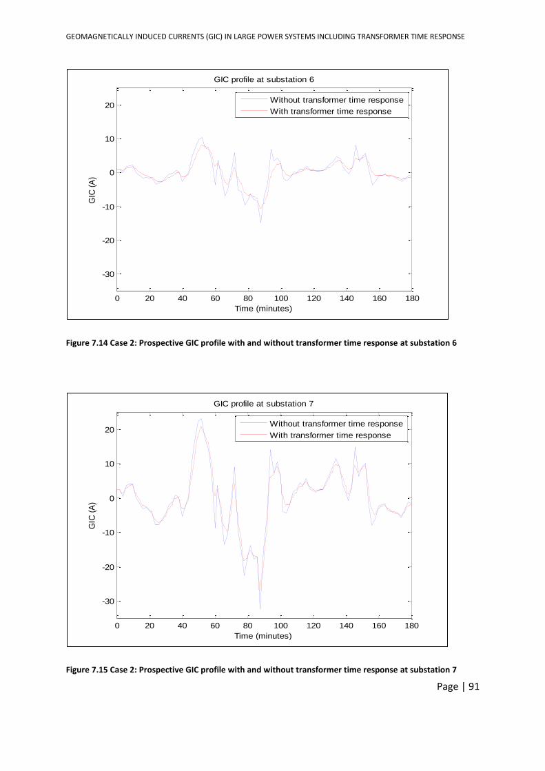
GEOMAGNETICALLY INDUCED CURRENTS (GIC) IN LARGE POWER SYSTEMS INCLUDING TRANSFORMER TIME RESPONSE
Page | 91
Figure 7.14 Case 2: Prospective GIC profile with and without transformer time response at substation 6
Figure 7.15 Case 2: Prospective GIC profile with and without transformer time response at substation 7
0 20 40 60 80 100 120 140 160 180
-30
-20
-10
0
10
20
Time (minutes)
GIC
(A
)
GIC profile at substation 6
Without transformer time response
With transformer time response
0 20 40 60 80 100 120 140 160 180
-30
-20
-10
0
10
20
Time (minutes)
GIC
(A
)
GIC profile at substation 7
Without transformer time response
With transformer time response
GEOMAGNETICALLY INDUCED CURRENTS (GIC) IN LARGE POWER SYSTEMS INCLUDING TRANSFORMER TIME RESPONSE
Page | 92
The difference in the profiles of the prospective GIC with and without transformer time
response for substation 4 is reduced when compared with substation 7. This is attributed to
the short response time to GIC of the 3P-3L transformers in substation 4. Substation 7
shows a larger difference between the two GIC profiles which stems from the longer time
response of the 3(1P-3L) GSU transformers in substation 7. In the next section the effect of
using interpolated magnetic field data on the magnitude of the prospective GIC with and
without transformer time response is investigated.
7.3 EFFECT OF INCREASED MAGNETIC FIELD SAMPLING TIME INTERVAL
ON THE MAGNITUDES OF THE PROSPECTIVE GIC WITH AND WITHOUT
TRANSFORMER TIME RESPONSE
In chapter 3, where the transformer time constant was introduced, it was mentioned that if
the magnetic field sampling interval is chosen such that it is longer than the average
transformer response time to GIC, the prospective GIC with and without the transformer
time response will be similar. In section 7.1 and section 7.2, the sampling time interval of
the magnetic field data used to calculate the electric field was two minutes. In this, section,
the magnetic field sampled at two-minute interval was interpolated at four-minute intervals
in order to determine the effect that doubling the magnetic field sampling interval has on
the prospective GIC, taking the transformer time response into account.
Two case studies, cases 3 and 4 were done. These case studies are similar to case 1 and case
2 in section 7.2. The only difference is that the magnetic field data was interpolated at 4-
minute sampling intervals.
7.3.1 Case 3: Calculated GIC in the test network with uniform transformer core structure
using 4-minute sampling time interval magnetic field data
The procedure for calculating the prospective GIC without the transformer time response
was sufficiently explained in section 7.1. Thus, only the table of these values are shown.
Table 7.6 shows the prospective GIC values without transformer time response at the 10
substations with four-minute sampling time interval magnetic field data.
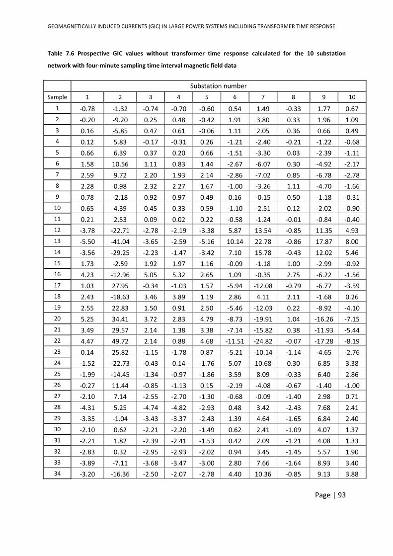
GEOMAGNETICALLY INDUCED CURRENTS (GIC) IN LARGE POWER SYSTEMS INCLUDING TRANSFORMER TIME RESPONSE
Page | 93
Table 7.6 Prospective GIC values without transformer time response calculated for the 10 substation
network with four-minute sampling time interval magnetic field data
Substation number
Sample 1 2 3 4 5 6 7 8 9 10
1 -0.78 -1.32 -0.74 -0.70 -0.60 0.54 1.49 -0.33 1.77 0.67
2 -0.20 -9.20 0.25 0.48 -0.42 1.91 3.80 0.33 1.96 1.09
3 0.16 -5.85 0.47 0.61 -0.06 1.11 2.05 0.36 0.66 0.49
4 0.12 5.83 -0.17 -0.31 0.26 -1.21 -2.40 -0.21 -1.22 -0.68
5 0.66 6.39 0.37 0.20 0.66 -1.51 -3.30 0.03 -2.39 -1.11
6 1.58 10.56 1.11 0.83 1.44 -2.67 -6.07 0.30 -4.92 -2.17
7 2.59 9.72 2.20 1.93 2.14 -2.86 -7.02 0.85 -6.78 -2.78
8 2.28 0.98 2.32 2.27 1.67 -1.00 -3.26 1.11 -4.70 -1.66
9 0.78 -2.18 0.92 0.97 0.49 0.16 -0.15 0.50 -1.18 -0.31
10 0.65 4.39 0.45 0.33 0.59 -1.10 -2.51 0.12 -2.02 -0.90
11 0.21 2.53 0.09 0.02 0.22 -0.58 -1.24 -0.01 -0.84 -0.40
12 -3.78 -22.71 -2.78 -2.19 -3.38 5.87 13.54 -0.85 11.35 4.93
13 -5.50 -41.04 -3.65 -2.59 -5.16 10.14 22.78 -0.86 17.87 8.00
14 -3.56 -29.25 -2.23 -1.47 -3.42 7.10 15.78 -0.43 12.02 5.46
15 1.73 -2.59 1.92 1.97 1.16 -0.09 -1.18 1.00 -2.99 -0.92
16 4.23 -12.96 5.05 5.32 2.65 1.09 -0.35 2.75 -6.22 -1.56
17 1.03 27.95 -0.34 -1.03 1.57 -5.94 -12.08 -0.79 -6.77 -3.59
18 2.43 -18.63 3.46 3.89 1.19 2.86 4.11 2.11 -1.68 0.26
19 2.55 22.83 1.50 0.91 2.50 -5.46 -12.03 0.22 -8.92 -4.10
20 5.25 34.41 3.72 2.83 4.79 -8.73 -19.91 1.04 -16.26 -7.15
21 3.49 29.57 2.14 1.38 3.38 -7.14 -15.82 0.38 -11.93 -5.44
22 4.47 49.72 2.14 0.88 4.68 -11.51 -24.82 -0.07 -17.28 -8.19
23 0.14 25.82 -1.15 -1.78 0.87 -5.21 -10.14 -1.14 -4.65 -2.76
24 -1.52 -22.73 -0.43 0.14 -1.76 5.07 10.68 0.30 6.85 3.38
25 -1.99 -14.45 -1.34 -0.97 -1.86 3.59 8.09 -0.33 6.40 2.86
26 -0.27 11.44 -0.85 -1.13 0.15 -2.19 -4.08 -0.67 -1.40 -1.00
27 -2.10 7.14 -2.55 -2.70 -1.30 -0.68 -0.09 -1.40 2.98 0.71
28 -4.31 5.25 -4.74 -4.82 -2.93 0.48 3.42 -2.43 7.68 2.41
29 -3.35 -1.04 -3.43 -3.37 -2.43 1.39 4.64 -1.65 6.84 2.40
30 -2.10 0.62 -2.21 -2.20 -1.49 0.62 2.41 -1.09 4.07 1.37
31 -2.21 1.82 -2.39 -2.41 -1.53 0.42 2.09 -1.21 4.08 1.33
32 -2.83 0.32 -2.95 -2.93 -2.02 0.94 3.45 -1.45 5.57 1.90
33 -3.89 -7.11 -3.68 -3.47 -3.00 2.80 7.66 -1.64 8.93 3.40
34 -3.20 -16.36 -2.50 -2.07 -2.78 4.40 10.36 -0.85 9.13 3.88
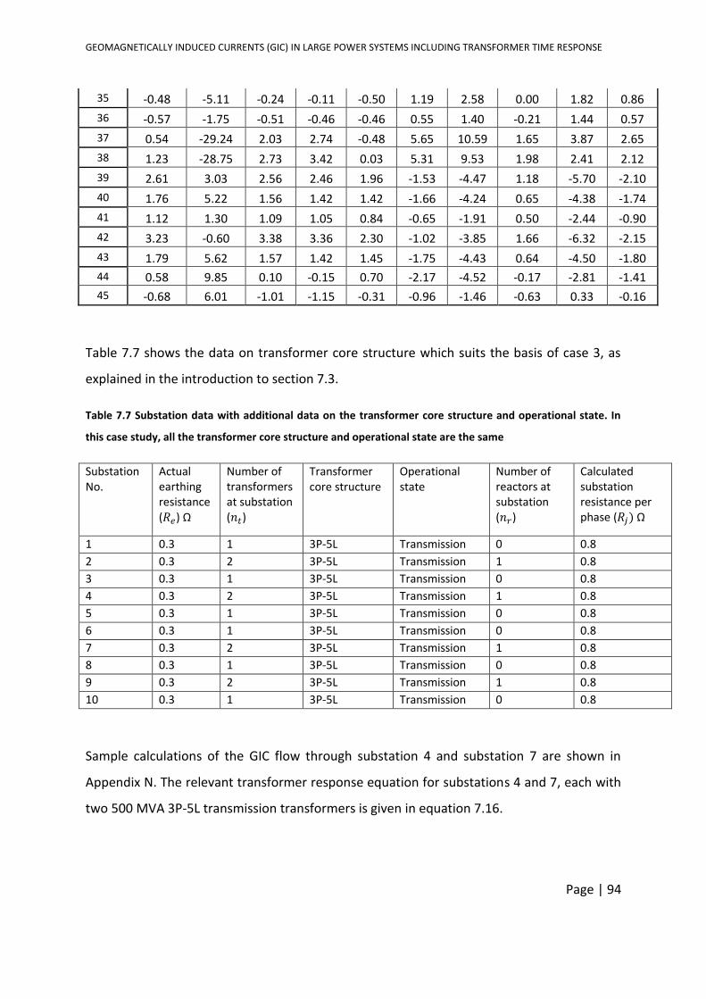
GEOMAGNETICALLY INDUCED CURRENTS (GIC) IN LARGE POWER SYSTEMS INCLUDING TRANSFORMER TIME RESPONSE
Page | 94
35 -0.48 -5.11 -0.24 -0.11 -0.50 1.19 2.58 0.00 1.82 0.86
36 -0.57 -1.75 -0.51 -0.46 -0.46 0.55 1.40 -0.21 1.44 0.57
37 0.54 -29.24 2.03 2.74 -0.48 5.65 10.59 1.65 3.87 2.65
38 1.23 -28.75 2.73 3.42 0.03 5.31 9.53 1.98 2.41 2.12
39 2.61 3.03 2.56 2.46 1.96 -1.53 -4.47 1.18 -5.70 -2.10
40 1.76 5.22 1.56 1.42 1.42 -1.66 -4.24 0.65 -4.38 -1.74
41 1.12 1.30 1.09 1.05 0.84 -0.65 -1.91 0.50 -2.44 -0.90
42 3.23 -0.60 3.38 3.36 2.30 -1.02 -3.85 1.66 -6.32 -2.15
43 1.79 5.62 1.57 1.42 1.45 -1.75 -4.43 0.64 -4.50 -1.80
44 0.58 9.85 0.10 -0.15 0.70 -2.17 -4.52 -0.17 -2.81 -1.41
45 -0.68 6.01 -1.01 -1.15 -0.31 -0.96 -1.46 -0.63 0.33 -0.16
Table 7.7 shows the data on transformer core structure which suits the basis of case 3, as
explained in the introduction to section 7.3.
Table 7.7 Substation data with additional data on the transformer core structure and operational state. In
this case study, all the transformer core structure and operational state are the same
Substation No.
Actual earthing resistance (𝑅𝑒) Ω
Number of transformers at substation (𝑛𝑡)
Transformer core structure
Operational state
Number of reactors at substation (𝑛𝑟)
Calculated substation resistance per phase (𝑅𝑗) Ω
1 0.3 1 3P-5L Transmission 0 0.8
2 0.3 2 3P-5L Transmission 1 0.8
3 0.3 1 3P-5L Transmission 0 0.8
4 0.3 2 3P-5L Transmission 1 0.8
5 0.3 1 3P-5L Transmission 0 0.8
6 0.3 1 3P-5L Transmission 0 0.8
7 0.3 2 3P-5L Transmission 1 0.8
8 0.3 1 3P-5L Transmission 0 0.8
9 0.3 2 3P-5L Transmission 1 0.8
10 0.3 1 3P-5L Transmission 0 0.8
Sample calculations of the GIC flow through substation 4 and substation 7 are shown in
Appendix N. The relevant transformer response equation for substations 4 and 7, each with
two 500 MVA 3P-5L transmission transformers is given in equation 7.16.
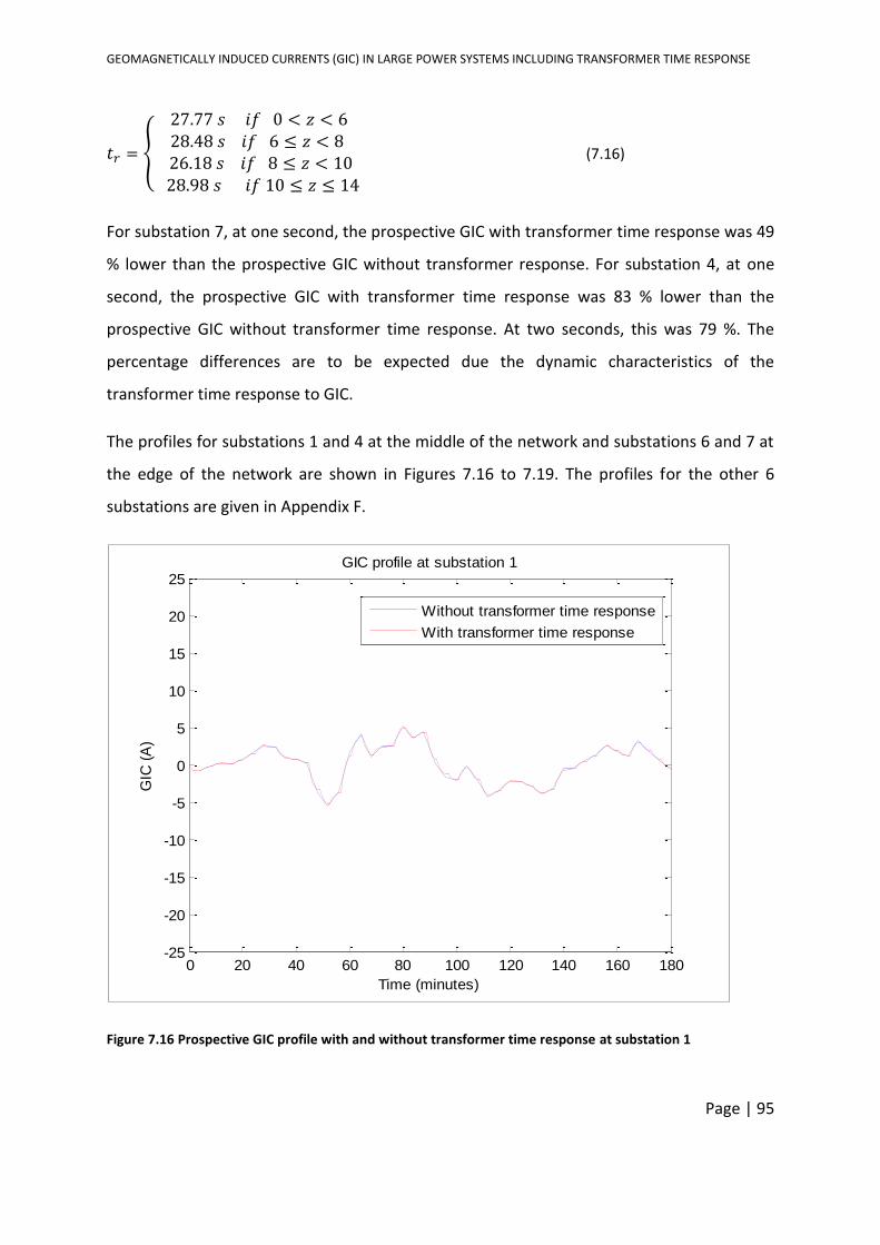
GEOMAGNETICALLY INDUCED CURRENTS (GIC) IN LARGE POWER SYSTEMS INCLUDING TRANSFORMER TIME RESPONSE
Page | 95
𝑡𝑟 =
27.77 𝑠 𝑖𝑓 0 < 𝑧 < 628.48 𝑠 𝑖𝑓 6 ≤ 𝑧 < 8 26.18 𝑠 𝑖𝑓 8 ≤ 𝑧 < 10 28.98 𝑠 𝑖𝑓 10 ≤ 𝑧 ≤ 14
(7.16)
For substation 7, at one second, the prospective GIC with transformer time response was 49
% lower than the prospective GIC without transformer response. For substation 4, at one
second, the prospective GIC with transformer time response was 83 % lower than the
prospective GIC without transformer time response. At two seconds, this was 79 %. The
percentage differences are to be expected due the dynamic characteristics of the
transformer time response to GIC.
The profiles for substations 1 and 4 at the middle of the network and substations 6 and 7 at
the edge of the network are shown in Figures 7.16 to 7.19. The profiles for the other 6
substations are given in Appendix F.
Figure 7.16 Prospective GIC profile with and without transformer time response at substation 1
0 20 40 60 80 100 120 140 160 180-25
-20
-15
-10
-5
0
5
10
15
20
25
Time (minutes)
GIC
(A
)
GIC profile at substation 1
Without transformer time response
With transformer time response
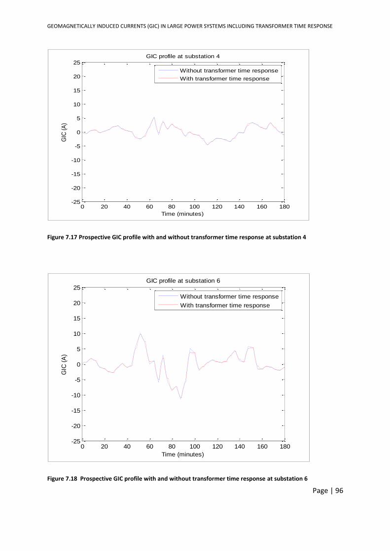
GEOMAGNETICALLY INDUCED CURRENTS (GIC) IN LARGE POWER SYSTEMS INCLUDING TRANSFORMER TIME RESPONSE
Page | 96
Figure 7.17 Prospective GIC profile with and without transformer time response at substation 4
Figure 7.18 Prospective GIC profile with and without transformer time response at substation 6
0 20 40 60 80 100 120 140 160 180-25
-20
-15
-10
-5
0
5
10
15
20
25
Time (minutes)
GIC
(A
)GIC profile at substation 4
Without transformer time response
With transformer time response
0 20 40 60 80 100 120 140 160 180-25
-20
-15
-10
-5
0
5
10
15
20
25
Time (minutes)
GIC
(A
)
GIC profile at substation 6
Without transformer time response
With transformer time response
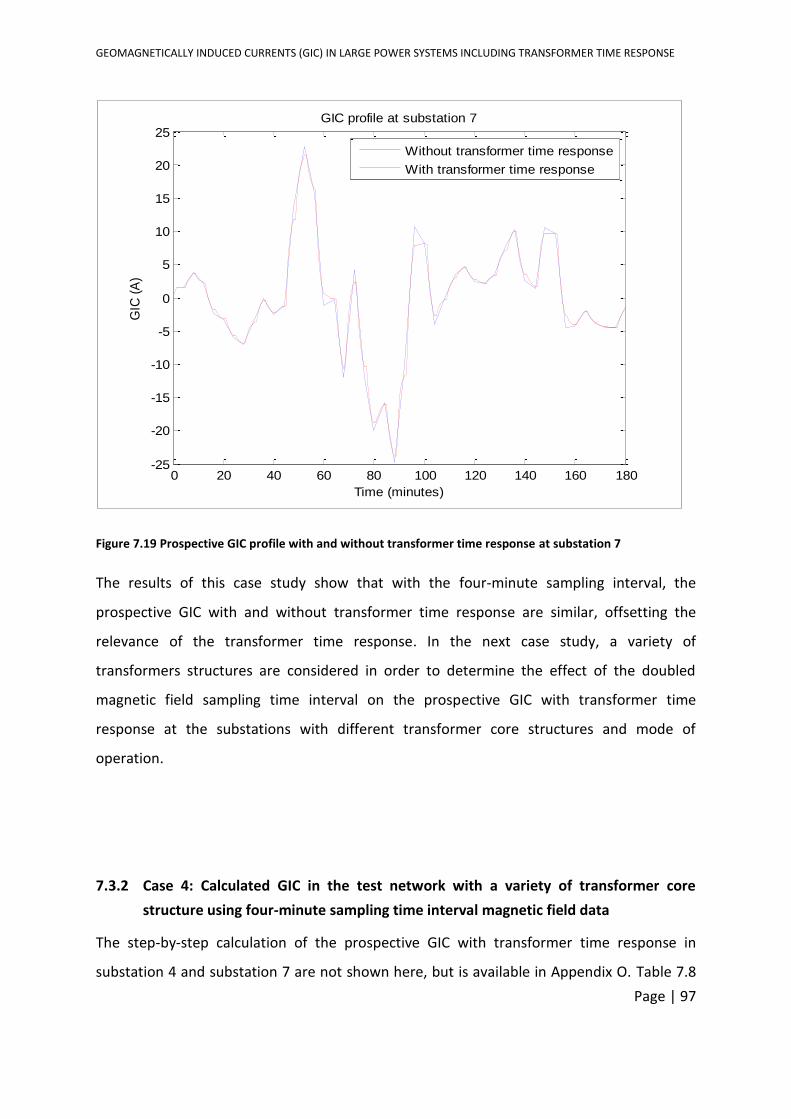
GEOMAGNETICALLY INDUCED CURRENTS (GIC) IN LARGE POWER SYSTEMS INCLUDING TRANSFORMER TIME RESPONSE
Page | 97
Figure 7.19 Prospective GIC profile with and without transformer time response at substation 7
The results of this case study show that with the four-minute sampling interval, the
prospective GIC with and without transformer time response are similar, offsetting the
relevance of the transformer time response. In the next case study, a variety of
transformers structures are considered in order to determine the effect of the doubled
magnetic field sampling time interval on the prospective GIC with transformer time
response at the substations with different transformer core structures and mode of
operation.
7.3.2 Case 4: Calculated GIC in the test network with a variety of transformer core
structure using four-minute sampling time interval magnetic field data
The step-by-step calculation of the prospective GIC with transformer time response in
substation 4 and substation 7 are not shown here, but is available in Appendix O. Table 7.8
0 20 40 60 80 100 120 140 160 180-25
-20
-15
-10
-5
0
5
10
15
20
25
Time (minutes)
GIC
(A
)GIC profile at substation 7
Without transformer time response
With transformer time response
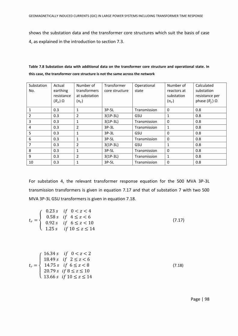
GEOMAGNETICALLY INDUCED CURRENTS (GIC) IN LARGE POWER SYSTEMS INCLUDING TRANSFORMER TIME RESPONSE
Page | 98
shows the substation data and the transformer core structures which suit the basis of case
4, as explained in the introduction to section 7.3.
Table 7.8 Substation data with additional data on the transformer core structure and operational state. In
this case, the transformer core structure is not the same across the network
Substation No.
Actual earthing resistance (𝑅𝑒) Ω
Number of transformers at substation (𝑛𝑡)
Transformer core structure
Operational state
Number of reactors at substation (𝑛𝑟)
Calculated substation resistance per phase (𝑅𝑗) Ω
1 0.3 1 3P-5L Transmission 0 0.8
2 0.3 2 3(1P-3L) GSU 1 0.8
3 0.3 1 3(1P-3L) Transmission 0 0.8
4 0.3 2 3P-3L Transmission 1 0.8
5 0.3 1 3P-3L GSU 0 0.8
6 0.3 1 3P-5L Transmission 0 0.8
7 0.3 2 3(1P-3L) GSU 1 0.8
8 0.3 1 3P-5L Transmission 0 0.8
9 0.3 2 3(1P-3L) Transmission 1 0.8
10 0.3 1 3P-5L Transmission 0 0.8
For substation 4, the relevant transformer response equation for the 500 MVA 3P-3L
transmission transformers is given in equation 7.17 and that of substation 7 with two 500
MVA 3P-3L GSU transformers is given in equation 7.18.
𝑡𝑟 =
0.23 𝑠 𝑖𝑓 0 < 𝑧 < 40.58 𝑠 𝑖𝑓 4 ≤ 𝑧 < 6 0.92 𝑠 𝑖𝑓 6 ≤ 𝑧 < 10 1.25 𝑠 𝑖𝑓 10 ≤ 𝑧 ≤ 14
(7.17)
𝑡𝑟 =
16.34 𝑠 𝑖𝑓 0 < 𝑧 < 218.49 𝑠 𝑖𝑓 2 ≤ 𝑧 < 614.75 𝑠 𝑖𝑓 6 ≤ 𝑧 < 820.79 𝑠 𝑖𝑓 8 ≤ 𝑧 ≤ 10 13.66 𝑠 𝑖𝑓 10 ≤ 𝑧 ≤ 14
(7.18)
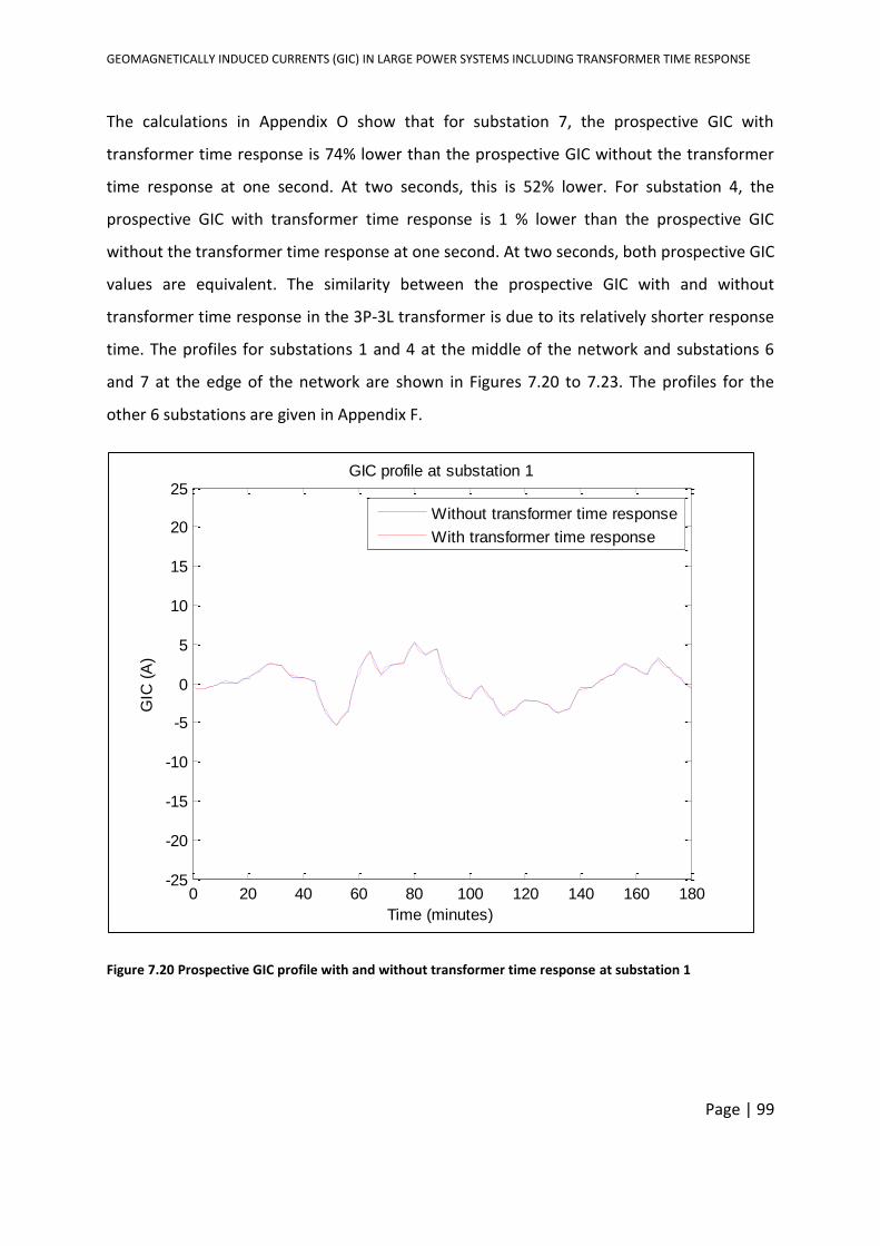
GEOMAGNETICALLY INDUCED CURRENTS (GIC) IN LARGE POWER SYSTEMS INCLUDING TRANSFORMER TIME RESPONSE
Page | 99
The calculations in Appendix O show that for substation 7, the prospective GIC with
transformer time response is 74% lower than the prospective GIC without the transformer
time response at one second. At two seconds, this is 52% lower. For substation 4, the
prospective GIC with transformer time response is 1 % lower than the prospective GIC
without the transformer time response at one second. At two seconds, both prospective GIC
values are equivalent. The similarity between the prospective GIC with and without
transformer time response in the 3P-3L transformer is due to its relatively shorter response
time. The profiles for substations 1 and 4 at the middle of the network and substations 6
and 7 at the edge of the network are shown in Figures 7.20 to 7.23. The profiles for the
other 6 substations are given in Appendix F.
Figure 7.20 Prospective GIC profile with and without transformer time response at substation 1
0 20 40 60 80 100 120 140 160 180-25
-20
-15
-10
-5
0
5
10
15
20
25
Time (minutes)
GIC
(A
)
GIC profile at substation 1
Without transformer time response
With transformer time response

GEOMAGNETICALLY INDUCED CURRENTS (GIC) IN LARGE POWER SYSTEMS INCLUDING TRANSFORMER TIME RESPONSE
Page | 100
Figure 7.21 Prospective GIC profile with and without transformer time response at substation 4
Figure 7.22 Prospective GIC profile with and without transformer time response at substation 6
0 20 40 60 80 100 120 140 160 180-25
-20
-15
-10
-5
0
5
10
15
20
25
Time (minutes)
GIC
(A
)GIC profile at substation 4
Without transformer time response
With transformer time response
0 20 40 60 80 100 120 140 160 180-25
-20
-15
-10
-5
0
5
10
15
20
25
Time (minutes)
GIC
(A
)
GIC profile at substation 6
Without transformer time response
With transformer time response
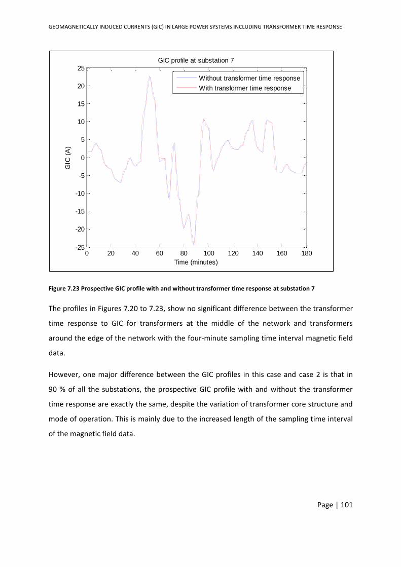
GEOMAGNETICALLY INDUCED CURRENTS (GIC) IN LARGE POWER SYSTEMS INCLUDING TRANSFORMER TIME RESPONSE
Page | 101
Figure 7.23 Prospective GIC profile with and without transformer time response at substation 7
The profiles in Figures 7.20 to 7.23, show no significant difference between the transformer
time response to GIC for transformers at the middle of the network and transformers
around the edge of the network with the four-minute sampling time interval magnetic field
data.
However, one major difference between the GIC profiles in this case and case 2 is that in
90 % of all the substations, the prospective GIC profile with and without the transformer
time response are exactly the same, despite the variation of transformer core structure and
mode of operation. This is mainly due to the increased length of the sampling time interval
of the magnetic field data.
0 20 40 60 80 100 120 140 160 180-25
-20
-15
-10
-5
0
5
10
15
20
25
Time (minutes)
GIC
(A
)GIC profile at substation 7
Without transformer time response
With transformer time response

GEOMAGNETICALLY INDUCED CURRENTS (GIC) IN LARGE POWER SYSTEMS INCLUDING TRANSFORMER TIME RESPONSE
Page | 102
7.4 COMPARISON BETWEEN MEASURED GIC AND CALCULATED GIC
During the Halloween storm of 2003, between 29 and 31 October, the GIC flow through
Grassridge substation, South Africa was recorded at two-second time intervals. The
geomagnetic field data at the closest INTERMAGNET observatory, Hermanus, was recorded
at one-minute time intervals. The geomagnetic field data was interpolated using the
Brownian (i.e., stochastic) method from one-minute intervals to two-second intervals, so
that both the measured GIC and the geomagnetic field data will have the same time
interval. This allowed for the comparison of the measured GIC against the prospective GIC
with transformer time response.
Interpolating the one-minute sampling interval geomagnetic field data to two-second
intervals may result in the loss of higher frequency components in the geomagnetic field
data. However, since the frequencies of concern are very low, typically well below 1 Hz,
interpolating the geomagnetic field data was considered acceptable. The effect of
interpolating the geomagnetic field data from one-minute intervals to two-second intervals
and GIC data sampled at two-second interval to one-minute intervals was investigated.
The results of the investigation showed that higher frequency components between 8 mHz
and 250 mHz were lost. Considering GIC frequencies are very low frequencies, this
interpolated data was considered valid, Both geomagnetic field data and measured GIC
were then interpolated to four-second, 10-second, 30-second, one-minute, two-minute,
four-minute and 10-minute sampling time intervals, so that the transformer response could
be analysed extensively. In literature, it is not clear which sampling time interval is most
adequate for measuring GIC and geomagnetic data for GIC calculation. Hence, these
intervals were chosen as multiples of the one-second and one-minute sampling time
intervals that are commonly used, to allow for the extensive analysis of the data and to
show the impact of different sampling time intervals on the time response based GIC
calculation.
This is not linked to “M” which is the ratio of the integral duration for the discretization of
the electric field and the sampling time interval of the magnetic field. In general, this
integral duration has been suggested to be 20 minutes. Hence for magnetic field data
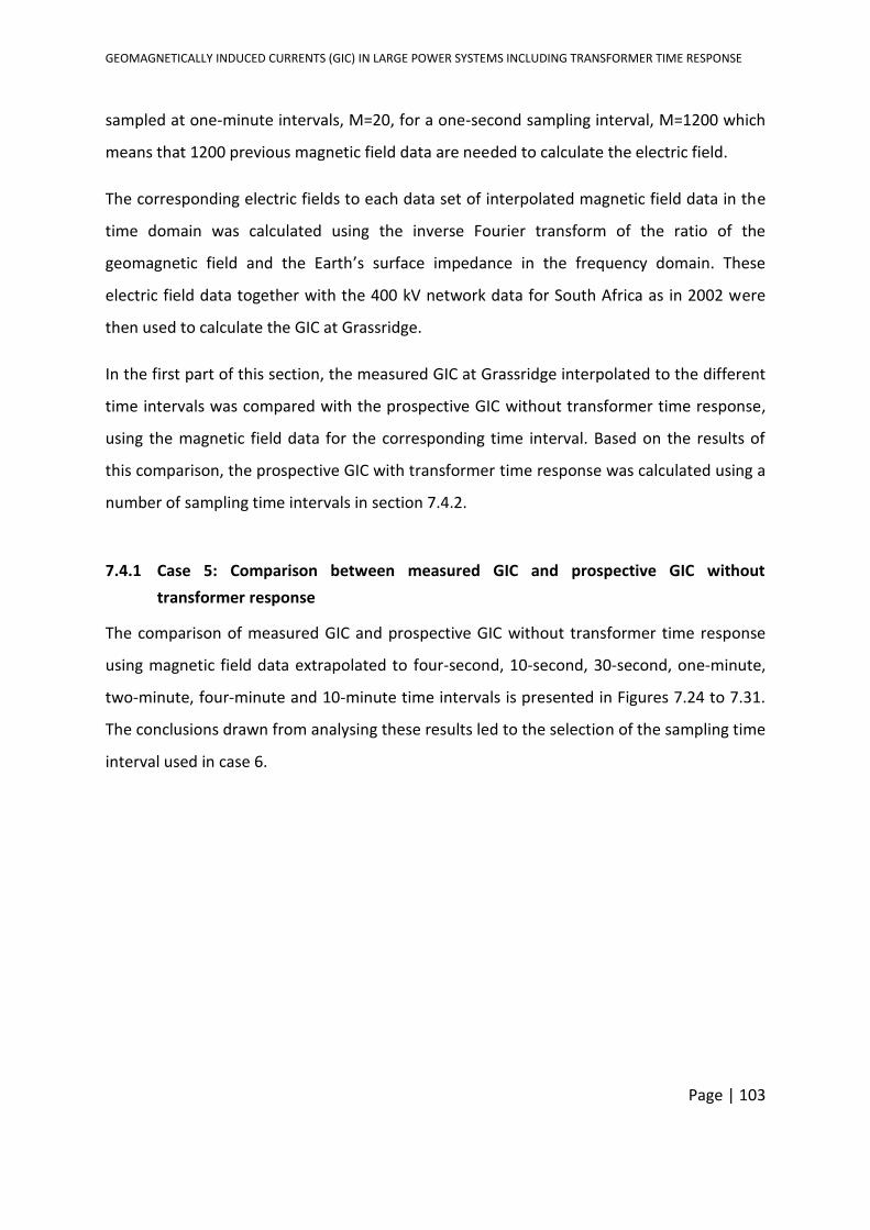
GEOMAGNETICALLY INDUCED CURRENTS (GIC) IN LARGE POWER SYSTEMS INCLUDING TRANSFORMER TIME RESPONSE
Page | 103
sampled at one-minute intervals, M=20, for a one-second sampling interval, M=1200 which
means that 1200 previous magnetic field data are needed to calculate the electric field.
The corresponding electric fields to each data set of interpolated magnetic field data in the
time domain was calculated using the inverse Fourier transform of the ratio of the
geomagnetic field and the Earth’s surface impedance in the frequency domain. These
electric field data together with the 400 kV network data for South Africa as in 2002 were
then used to calculate the GIC at Grassridge.
In the first part of this section, the measured GIC at Grassridge interpolated to the different
time intervals was compared with the prospective GIC without transformer time response,
using the magnetic field data for the corresponding time interval. Based on the results of
this comparison, the prospective GIC with transformer time response was calculated using a
number of sampling time intervals in section 7.4.2.
7.4.1 Case 5: Comparison between measured GIC and prospective GIC without
transformer response
The comparison of measured GIC and prospective GIC without transformer time response
using magnetic field data extrapolated to four-second, 10-second, 30-second, one-minute,
two-minute, four-minute and 10-minute time intervals is presented in Figures 7.24 to 7.31.
The conclusions drawn from analysing these results led to the selection of the sampling time
interval used in case 6.
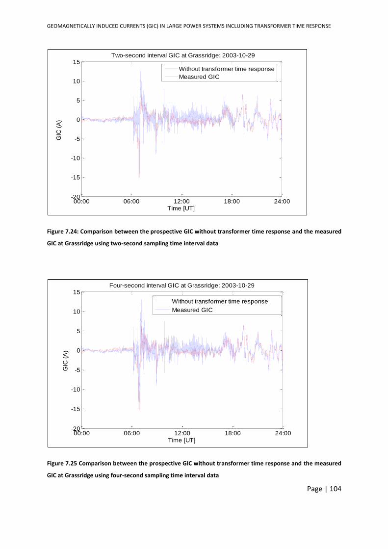
GEOMAGNETICALLY INDUCED CURRENTS (GIC) IN LARGE POWER SYSTEMS INCLUDING TRANSFORMER TIME RESPONSE
Page | 104
Figure 7.24: Comparison between the prospective GIC without transformer time response and the measured
GIC at Grassridge using two-second sampling time interval data
Figure 7.25 Comparison between the prospective GIC without transformer time response and the measured
GIC at Grassridge using four-second sampling time interval data
00:00 06:00 12:00 18:00 24:00-20
-15
-10
-5
0
5
10
15
Time [UT]
GIC
(A
) Two-second interval GIC at Grassridge: 2003-10-29
Without transformer time response
Measured GIC
00:00 06:00 12:00 18:00 24:00-20
-15
-10
-5
0
5
10
15
Time [UT]
GIC
(A
)
Four-second interval GIC at Grassridge: 2003-10-29
Without transformer time response
Measured GIC
GEOMAGNETICALLY INDUCED CURRENTS (GIC) IN LARGE POWER SYSTEMS INCLUDING TRANSFORMER TIME RESPONSE
Page | 105
Figure 7.26 Comparison between the prospective GIC without transformer time response and the measured
GIC at Grassridge using 10-second sampling time interval data
Figure 7.27 Comparison between the prospective GIC without transformer time response and the measured
GIC at Grassridge using 30-second sampling time interval
00:00 06:00 12:00 18:00 24:00-20
-15
-10
-5
0
5
10
15
Time [UT]
GIC
(A
)
10-second interval GIC at Grassridge: 2003-10-29
Without transformer time response
Measured GIC
00:00 06:00 12:00 18:00 24:00-20
-15
-10
-5
0
5
10
15
Time [UT]
GIC
(A
)
30-second interval GIC at Grassridge: 2003-10-29
Without transformer time response
Measured GIC
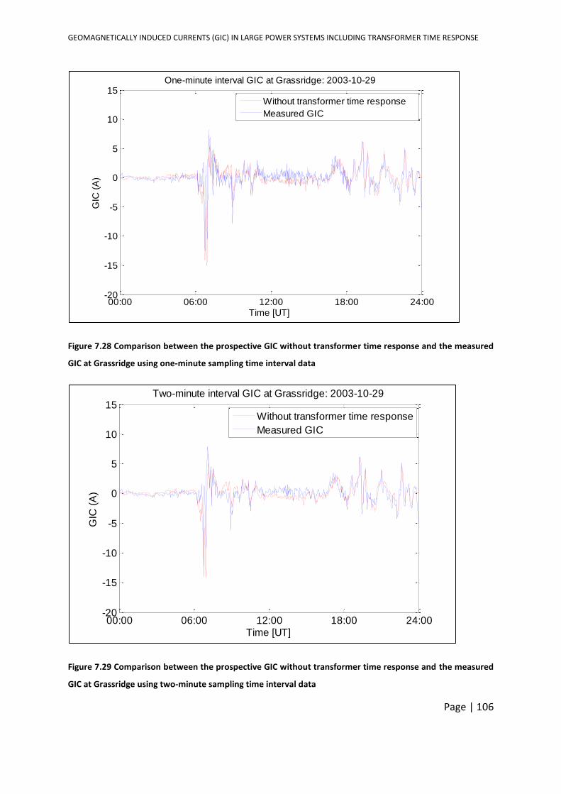
GEOMAGNETICALLY INDUCED CURRENTS (GIC) IN LARGE POWER SYSTEMS INCLUDING TRANSFORMER TIME RESPONSE
Page | 106
Figure 7.28 Comparison between the prospective GIC without transformer time response and the measured
GIC at Grassridge using one-minute sampling time interval data
Figure 7.29 Comparison between the prospective GIC without transformer time response and the measured
GIC at Grassridge using two-minute sampling time interval data
00:00 06:00 12:00 18:00 24:00-20
-15
-10
-5
0
5
10
15
Time [UT]
GIC
(A
)
One-minute interval GIC at Grassridge: 2003-10-29
Without transformer time response
Measured GIC
00:00 06:00 12:00 18:00 24:00-20
-15
-10
-5
0
5
10
15
Time [UT]
GIC
(A
)
Two-minute interval GIC at Grassridge: 2003-10-29
Without transformer time response
Measured GIC
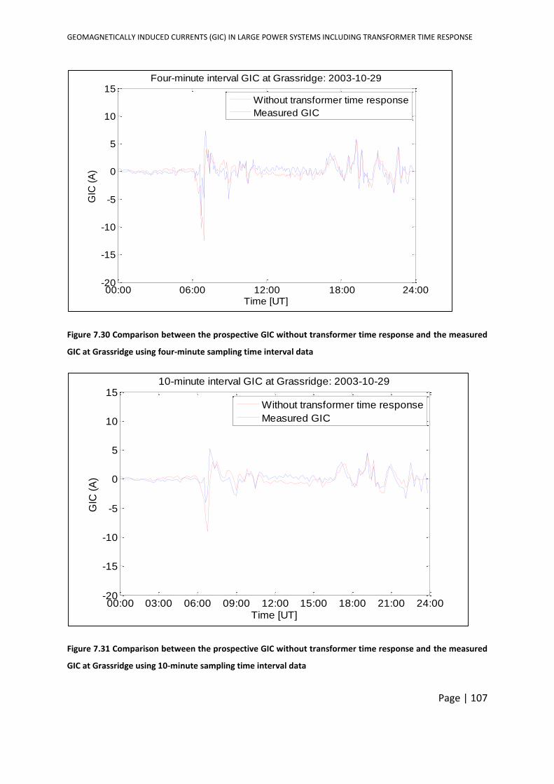
GEOMAGNETICALLY INDUCED CURRENTS (GIC) IN LARGE POWER SYSTEMS INCLUDING TRANSFORMER TIME RESPONSE
Page | 107
Figure 7.30 Comparison between the prospective GIC without transformer time response and the measured
GIC at Grassridge using four-minute sampling time interval data
Figure 7.31 Comparison between the prospective GIC without transformer time response and the measured
GIC at Grassridge using 10-minute sampling time interval data
00:00 06:00 12:00 18:00 24:00-20
-15
-10
-5
0
5
10
15
Time [UT]
GIC
(A
)
Four-minute interval GIC at Grassridge: 2003-10-29
Without transformer time response
Measured GIC
00:00 03:00 06:00 09:00 12:00 15:00 18:00 21:00 24:00-20
-15
-10
-5
0
5
10
1510-minute interval GIC at Grassridge: 2003-10-29
Time [UT]
GIC
(A
)
Without transformer time response
Measured GIC
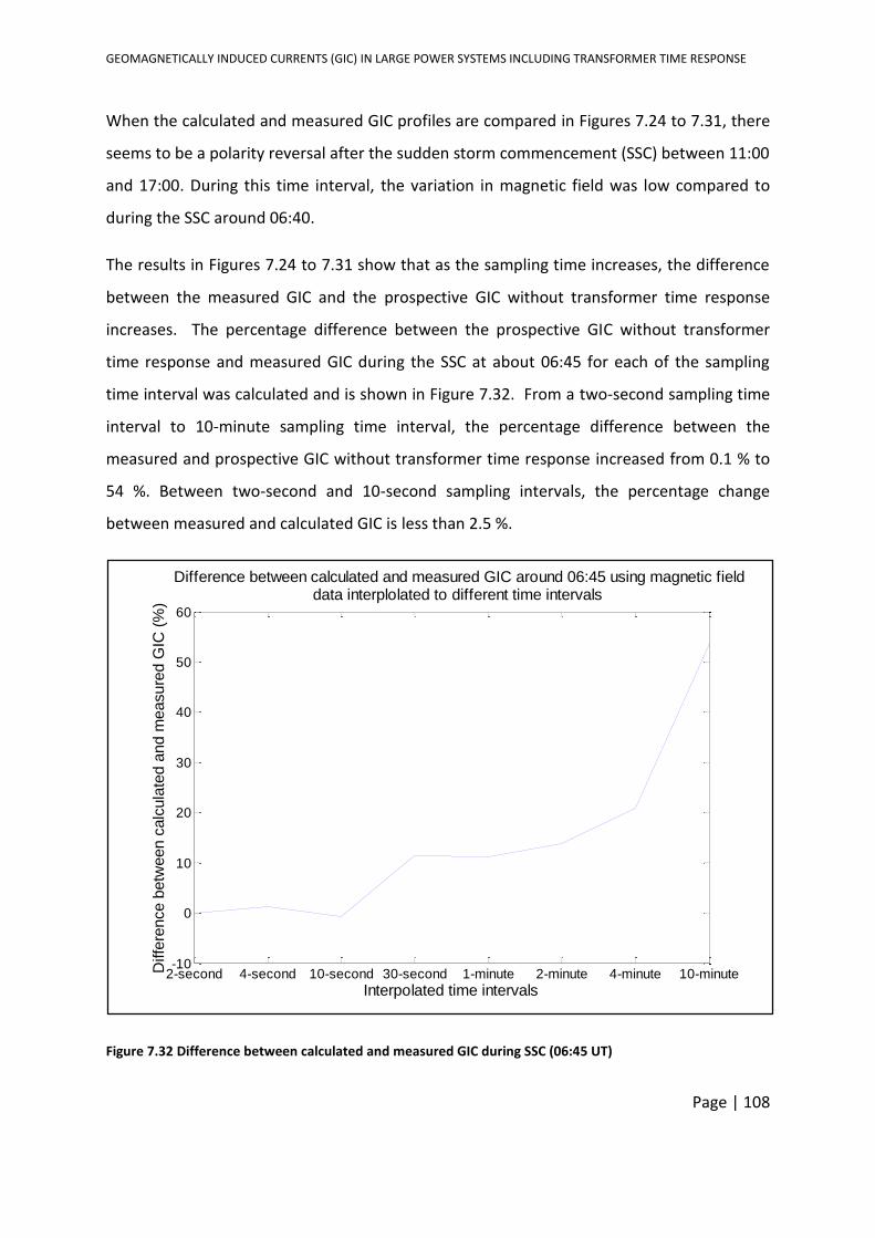
GEOMAGNETICALLY INDUCED CURRENTS (GIC) IN LARGE POWER SYSTEMS INCLUDING TRANSFORMER TIME RESPONSE
Page | 108
When the calculated and measured GIC profiles are compared in Figures 7.24 to 7.31, there
seems to be a polarity reversal after the sudden storm commencement (SSC) between 11:00
and 17:00. During this time interval, the variation in magnetic field was low compared to
during the SSC around 06:40.
The results in Figures 7.24 to 7.31 show that as the sampling time increases, the difference
between the measured GIC and the prospective GIC without transformer time response
increases. The percentage difference between the prospective GIC without transformer
time response and measured GIC during the SSC at about 06:45 for each of the sampling
time interval was calculated and is shown in Figure 7.32. From a two-second sampling time
interval to 10-minute sampling time interval, the percentage difference between the
measured and prospective GIC without transformer time response increased from 0.1 % to
54 %. Between two-second and 10-second sampling intervals, the percentage change
between measured and calculated GIC is less than 2.5 %.
Figure 7.32 Difference between calculated and measured GIC during SSC (06:45 UT)
2-second 4-second 10-second 30-second 1-minute 2-minute 4-minute 10-minute-10
0
10
20
30
40
50
60
Difference between calculated and measured GIC around 06:45 using magnetic field data interplolated to different time intervals
Interpolated time intervals
Diffe
rence b
etw
een c
alc
ula
ted a
nd m
easure
d G
IC (
%)
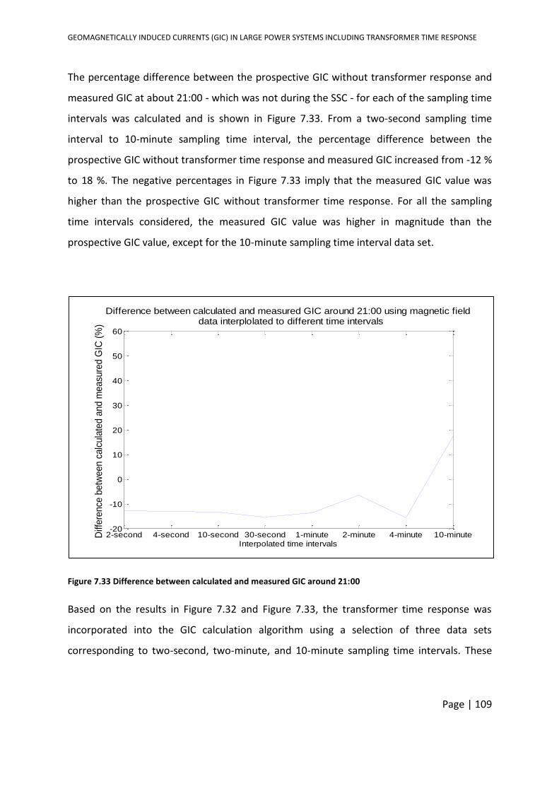
GEOMAGNETICALLY INDUCED CURRENTS (GIC) IN LARGE POWER SYSTEMS INCLUDING TRANSFORMER TIME RESPONSE
Page | 109
The percentage difference between the prospective GIC without transformer response and
measured GIC at about 21:00 - which was not during the SSC - for each of the sampling time
intervals was calculated and is shown in Figure 7.33. From a two-second sampling time
interval to 10-minute sampling time interval, the percentage difference between the
prospective GIC without transformer time response and measured GIC increased from -12 %
to 18 %. The negative percentages in Figure 7.33 imply that the measured GIC value was
higher than the prospective GIC without transformer time response. For all the sampling
time intervals considered, the measured GIC value was higher in magnitude than the
prospective GIC value, except for the 10-minute sampling time interval data set.
Figure 7.33 Difference between calculated and measured GIC around 21:00
Based on the results in Figure 7.32 and Figure 7.33, the transformer time response was
incorporated into the GIC calculation algorithm using a selection of three data sets
corresponding to two-second, two-minute, and 10-minute sampling time intervals. These
2-second 4-second 10-second 30-second 1-minute 2-minute 4-minute 10-minute-20
-10
0
10
20
30
40
50
60
Difference between calculated and measured GIC around 21:00 using magnetic field data interplolated to different time intervals
Interpolated time intervals
Diff
ere
nce
betw
een c
alc
ula
ted a
nd m
easu
red G
IC (
%)

GEOMAGNETICALLY INDUCED CURRENTS (GIC) IN LARGE POWER SYSTEMS INCLUDING TRANSFORMER TIME RESPONSE
Page | 110
three sampling time intervals were chosen such that the effect of the sampling time interval
on the prospective GIC with transformer time response can be investigated.
The results indicated that sampling at intervals above 10 seconds results in an increased
discrepancy between measured and calculated GIC. In addition to this, sampling above 10-
second intervals is not sufficient to correctly capture the profile of the GIC. See Figures 7.32
and 7.33.
7.4.2 Case 6: Comparison between measured GIC, prospective GIC with and without
transformer response
The comparison between measured GIC and calculated GIC interpolated to two-second,
two-minute and 10-minute sampling time interval data is shown in Figures 7.34 to 7.42. Due
to the large number of data points (43,200 for 2-second sampling time intervals and 720 for
two-minute sampling time interval), the two-second and two-minute sampling time interval
graphs were split into four sections for clarity. Section A shows the GIC pre-SSC; section B
shows the GIC during the SSC and sections C and D show the GIC post-SSC. The vertical axis
for each section is different because the amplitude of the GIC in each section is different.
Two-second sampling time interval
Figure 7.34 shows the measured and calculated GIC using two-second sampling time interval
data.
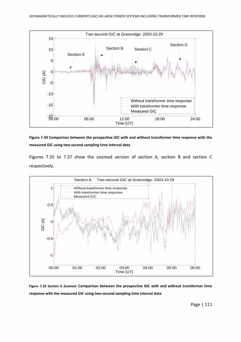
GEOMAGNETICALLY INDUCED CURRENTS (GIC) IN LARGE POWER SYSTEMS INCLUDING TRANSFORMER TIME RESPONSE
Page | 111
Figure 7.34 Comparison between the prospective GIC with and without transformer time response with the
measured GIC using two-second sampling time interval data
Figures 7.35 to 7.37 show the zoomed version of section A, section B and section C
respectively.
Figure 7.35 Section A Zoomed: Comparison between the prospective GIC with and without transformer time
response with the measured GIC using two-second sampling time interval data
00:00 06:00 12:00 18:00 24:00-20
-15
-10
-5
0
5
10
15
Time [UT]
GIC
(A
)
Two-second GIC at Grassridge: 2003-10-29
Without transformer time response
With transformer time response
Measured GIC
Section A
Section B Section CSection D
00:00 01:00 02:00 03:00 04:00 05:00 06:00
-1
-0.5
0
0.5
1
Time [UT]
GIC
(A
)
Section A. Two-second GIC at Grassridge: 2003-10-29
Without transformer time response
With transformer time response
Measured GIC
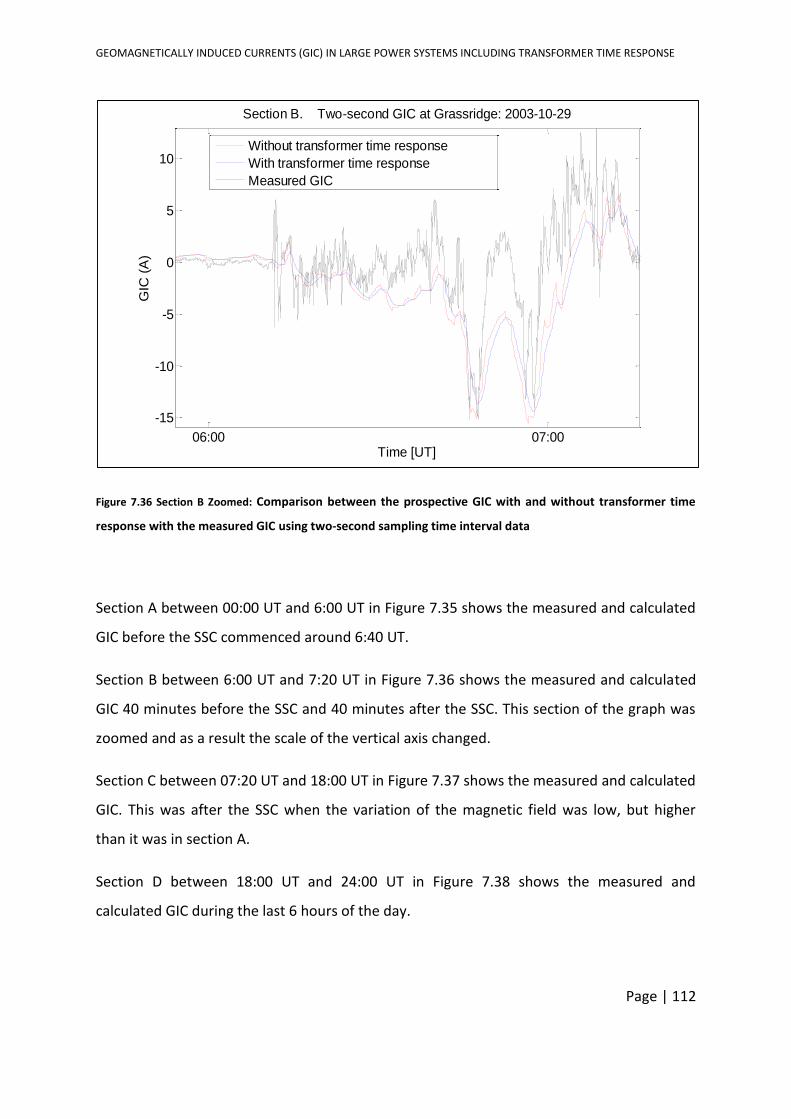
GEOMAGNETICALLY INDUCED CURRENTS (GIC) IN LARGE POWER SYSTEMS INCLUDING TRANSFORMER TIME RESPONSE
Page | 112
Figure 7.36 Section B Zoomed: Comparison between the prospective GIC with and without transformer time
response with the measured GIC using two-second sampling time interval data
Section A between 00:00 UT and 6:00 UT in Figure 7.35 shows the measured and calculated
GIC before the SSC commenced around 6:40 UT.
Section B between 6:00 UT and 7:20 UT in Figure 7.36 shows the measured and calculated
GIC 40 minutes before the SSC and 40 minutes after the SSC. This section of the graph was
zoomed and as a result the scale of the vertical axis changed.
Section C between 07:20 UT and 18:00 UT in Figure 7.37 shows the measured and calculated
GIC. This was after the SSC when the variation of the magnetic field was low, but higher
than it was in section A.
Section D between 18:00 UT and 24:00 UT in Figure 7.38 shows the measured and
calculated GIC during the last 6 hours of the day.
06:00 07:00
-15
-10
-5
0
5
10
Time [UT]
GIC
(A
)
Section B. Two-second GIC at Grassridge: 2003-10-29
Without transformer time response
With transformer time response
Measured GIC
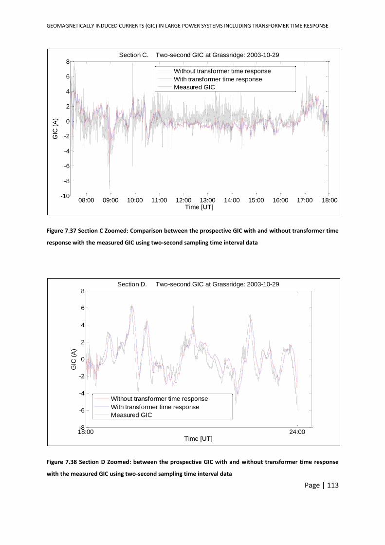
GEOMAGNETICALLY INDUCED CURRENTS (GIC) IN LARGE POWER SYSTEMS INCLUDING TRANSFORMER TIME RESPONSE
Page | 113
Figure 7.37 Section C Zoomed: Comparison between the prospective GIC with and without transformer time
response with the measured GIC using two-second sampling time interval data
Figure 7.38 Section D Zoomed: between the prospective GIC with and without transformer time response
with the measured GIC using two-second sampling time interval data
08:00 09:00 10:00 11:00 12:00 13:00 14:00 15:00 16:00 17:00 18:00-10
-8
-6
-4
-2
0
2
4
6
8
Time [UT]
GIC
(A
)Section C. Two-second GIC at Grassridge: 2003-10-29
Without transformer time response
With transformer time response
Measured GIC
18:00 24:00-8
-6
-4
-2
0
2
4
6
8
Time [UT]
GIC
(A
)
Section D. Two-second GIC at Grassridge: 2003-10-29
Without transformer time response
With transformer time response
Measured GIC
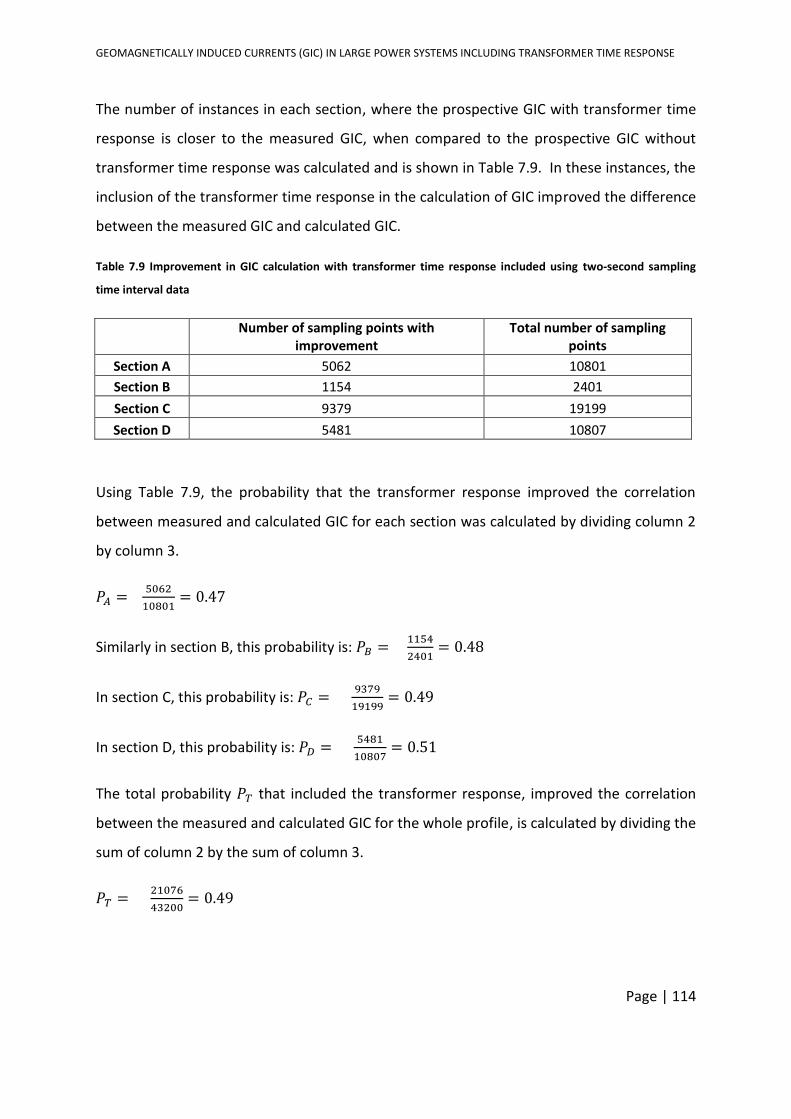
GEOMAGNETICALLY INDUCED CURRENTS (GIC) IN LARGE POWER SYSTEMS INCLUDING TRANSFORMER TIME RESPONSE
Page | 114
The number of instances in each section, where the prospective GIC with transformer time
response is closer to the measured GIC, when compared to the prospective GIC without
transformer time response was calculated and is shown in Table 7.9. In these instances, the
inclusion of the transformer time response in the calculation of GIC improved the difference
between the measured GIC and calculated GIC.
Table 7.9 Improvement in GIC calculation with transformer time response included using two-second sampling
time interval data
Number of sampling points with improvement
Total number of sampling points
Section A 5062 10801
Section B 1154 2401
Section C 9379 19199
Section D 5481 10807
Using Table 7.9, the probability that the transformer response improved the correlation
between measured and calculated GIC for each section was calculated by dividing column 2
by column 3.
𝑃𝐴 = 5062
10801= 0.47
Similarly in section B, this probability is: 𝑃𝐵 = 1154
2401= 0.48
In section C, this probability is: 𝑃𝐶 = 9379
19199= 0.49
In section D, this probability is: 𝑃𝐷 = 5481
10807= 0.51
The total probability 𝑃𝑇 that included the transformer response, improved the correlation
between the measured and calculated GIC for the whole profile, is calculated by dividing the
sum of column 2 by the sum of column 3.
𝑃𝑇 = 21076
43200= 0.49
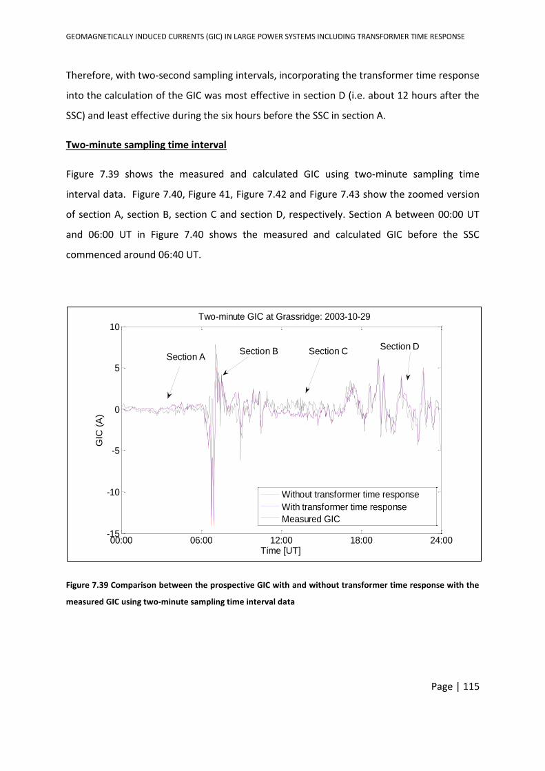
GEOMAGNETICALLY INDUCED CURRENTS (GIC) IN LARGE POWER SYSTEMS INCLUDING TRANSFORMER TIME RESPONSE
Page | 115
Therefore, with two-second sampling intervals, incorporating the transformer time response
into the calculation of the GIC was most effective in section D (i.e. about 12 hours after the
SSC) and least effective during the six hours before the SSC in section A.
Two-minute sampling time interval
Figure 7.39 shows the measured and calculated GIC using two-minute sampling time
interval data. Figure 7.40, Figure 41, Figure 7.42 and Figure 7.43 show the zoomed version
of section A, section B, section C and section D, respectively. Section A between 00:00 UT
and 06:00 UT in Figure 7.40 shows the measured and calculated GIC before the SSC
commenced around 06:40 UT.
Figure 7.39 Comparison between the prospective GIC with and without transformer time response with the
measured GIC using two-minute sampling time interval data
00:00 06:00 12:00 18:00 24:00-15
-10
-5
0
5
10
Time [UT]
GIC
(A
)
Two-minute GIC at Grassridge: 2003-10-29
Without transformer time response
With transformer time response
Measured GIC
Section BSection A
Section CSection D
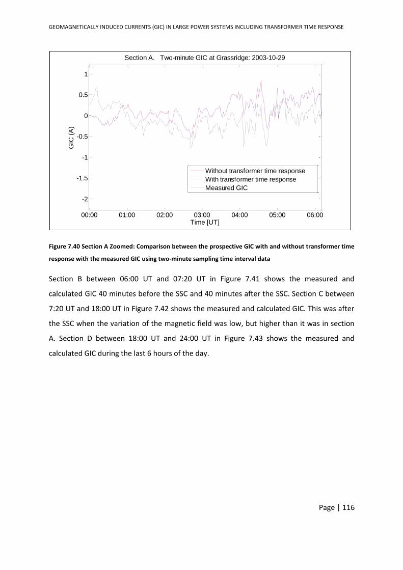
GEOMAGNETICALLY INDUCED CURRENTS (GIC) IN LARGE POWER SYSTEMS INCLUDING TRANSFORMER TIME RESPONSE
Page | 116
Figure 7.40 Section A Zoomed: Comparison between the prospective GIC with and without transformer time
response with the measured GIC using two-minute sampling time interval data
Section B between 06:00 UT and 07:20 UT in Figure 7.41 shows the measured and
calculated GIC 40 minutes before the SSC and 40 minutes after the SSC. Section C between
7:20 UT and 18:00 UT in Figure 7.42 shows the measured and calculated GIC. This was after
the SSC when the variation of the magnetic field was low, but higher than it was in section
A. Section D between 18:00 UT and 24:00 UT in Figure 7.43 shows the measured and
calculated GIC during the last 6 hours of the day.
00:00 01:00 02:00 03:00 04:00 05:00 06:00
-2
-1.5
-1
-0.5
0
0.5
1
Time [UT]
GIC
(A
)
Section A. Two-minute GIC at Grassridge: 2003-10-29
Without transformer time response
With transformer time response
Measured GIC

GEOMAGNETICALLY INDUCED CURRENTS (GIC) IN LARGE POWER SYSTEMS INCLUDING TRANSFORMER TIME RESPONSE
Page | 117
Figure 7.41 Section B Zoomed: Comparison between the prospective GIC with and without transformer time
response with the measured GIC using two-minute sampling time interval data
Figure 7.42 Section C Zoomed: Comparison between the prospective GIC with and without transformer time
response with the measured GIC using two-minute sampling time interval data
06:00 07:00 07:20
-10
-5
0
5
Time [UT]
GIC
(A
)
Section B. Two-minute GIC at Grassridge: 2003-10-29
Without transformer time response
With transformer time response
Measured GIC
08:00 09:00 10:00 11:00 12:00 13:00 14:00 15:00 16:00 17:00 18:00
-6
-4
-2
0
2
4
Time [UT]
GIC
(A
)
Section C. Two-minute GIC at Grassridge: 2003-10-29
Without transformer time response
With transformer time response
Measured GIC
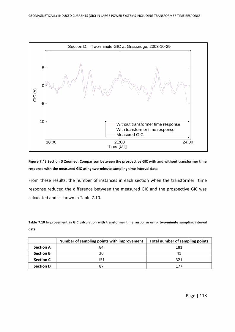
GEOMAGNETICALLY INDUCED CURRENTS (GIC) IN LARGE POWER SYSTEMS INCLUDING TRANSFORMER TIME RESPONSE
Page | 118
Figure 7.43 Section D Zoomed: Comparison between the prospective GIC with and without transformer time
response with the measured GIC using two-minute sampling time interval data
From these results, the number of instances in each section when the transformer time
response reduced the difference between the measured GIC and the prospective GIC was
calculated and is shown in Table 7.10.
Table 7.10 Improvement in GIC calculation with transformer time response using two-minute sampling interval
data
Number of sampling points with improvement Total number of sampling points
Section A 84 181
Section B 20 41
Section C 151 321
Section D 87 177
18:00 21:00 24:00
-10
-5
0
5
Time [UT]
GIC
(A
)
Section D. Two-minute GIC at Grassridge: 2003-10-29
Without transformer time response
With transformer time response
Measured GIC
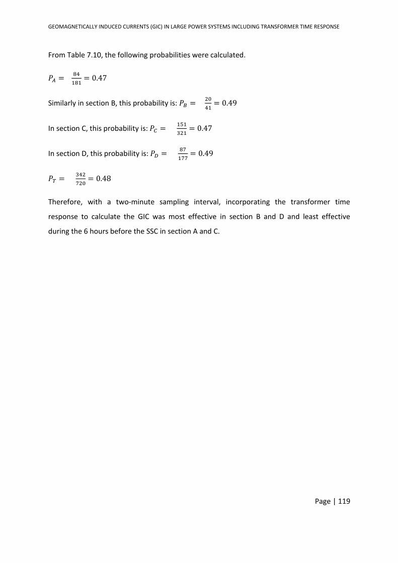
GEOMAGNETICALLY INDUCED CURRENTS (GIC) IN LARGE POWER SYSTEMS INCLUDING TRANSFORMER TIME RESPONSE
Page | 119
From Table 7.10, the following probabilities were calculated.
𝑃𝐴 = 84
181= 0.47
Similarly in section B, this probability is: 𝑃𝐵 = 20
41= 0.49
In section C, this probability is: 𝑃𝐶 = 151
321= 0.47
In section D, this probability is: 𝑃𝐷 = 87
177= 0.49
𝑃𝑇 = 342
720= 0.48
Therefore, with a two-minute sampling interval, incorporating the transformer time
response to calculate the GIC was most effective in section B and D and least effective
during the 6 hours before the SSC in section A and C.
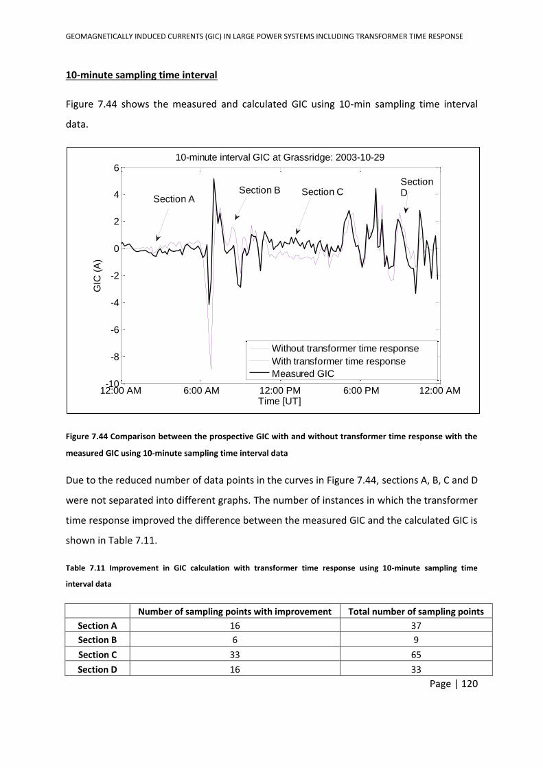
GEOMAGNETICALLY INDUCED CURRENTS (GIC) IN LARGE POWER SYSTEMS INCLUDING TRANSFORMER TIME RESPONSE
Page | 120
10-minute sampling time interval
Figure 7.44 shows the measured and calculated GIC using 10-min sampling time interval
data.
Figure 7.44 Comparison between the prospective GIC with and without transformer time response with the
measured GIC using 10-minute sampling time interval data
Due to the reduced number of data points in the curves in Figure 7.44, sections A, B, C and D
were not separated into different graphs. The number of instances in which the transformer
time response improved the difference between the measured GIC and the calculated GIC is
shown in Table 7.11.
Table 7.11 Improvement in GIC calculation with transformer time response using 10-minute sampling time
interval data
Number of sampling points with improvement Total number of sampling points
Section A 16 37
Section B 6 9
Section C 33 65
Section D 16 33
12:00 AM 6:00 AM 12:00 PM 6:00 PM 12:00 AM-10
-8
-6
-4
-2
0
2
4
6
Time [UT]
GIC
(A
)
10-minute interval GIC at Grassridge: 2003-10-29
Without transformer time response
With transformer time response
Measured GIC
Section ASection B Section C
SectionD
GEOMAGNETICALLY INDUCED CURRENTS (GIC) IN LARGE POWER SYSTEMS INCLUDING TRANSFORMER TIME RESPONSE
Page | 121
From Table 7.11, the following probabilities were calculated.
𝑃𝐴 = 16
37= 0.43
Similarly in section B, this probability is: 𝑃𝐵 = 6
9= 0.67
In section C, this probability is: 𝑃𝐶 = 33
65= 0.51
In section D, this probability is: 𝑃𝐷 = 16
33= 0.49
𝑃𝑇 = 71
144= 0.49
Therefore, with a 10-minute sampling interval, incorporating the transformer time response
into the calculation of the GIC was most effective in section B and least effective during the
6 hours before the SSC in section A. An extensive discussion on comparison between the
different sections of the storm using the different sampling time interval is given in section
8.2.6.
7.4.3 Transformer time response and the error between measured GIC and calculated
GIC
Determining the error is aimed at investigating whether or not including the transformer
time response reduced the error between measured and calculated GIC. Storm
characteristics vary from storm to storm, so does the characteristics of a segment of a storm
differ from other segments within the same storm. Further to this, as the profile of the
transformer core structures across the network changes, results of the error analysis may
change. These implicitly suggests that the information deduced from the error analysis is
unique to the specific GIC and geomagnetic data.
Before the impact of the transformer time response on the error between measured and
calculated GIC is considered, it is vital to mention some of the underlying issues that might
have contributed to the discrepancies between measured GIC and calculated GIC. These
include:
GEOMAGNETICALLY INDUCED CURRENTS (GIC) IN LARGE POWER SYSTEMS INCLUDING TRANSFORMER TIME RESPONSE
Page | 122
i. Possible filtering in the measurement of GIC.
ii. The impact of temperature variation on the GIC measurement device.
iii. The INTERMAGNET site (Hermanus) at which the geomagnetic data was logged is
about 800 km from Grassridge, the site where the GIC was measured.
iv. The assumption of uniform ground conductivity based on the limited data available.
The conductivity value is linked to the calculation of the electric field from the magnetic
field. The calculated electric field is one of the inputs to the prospective GIC calculation.
Hence, changing the conductivity value does not increase or decrease the variance between
the prospective GIC with transformer time response and the prospective GIC without
transformer time response.
Taking the aforementioned issues into consideration, error analysis is conducted on three
sets of data used in chapter 7.4.2. These are two-seconds, two-minute and 10-minutes
sampling intervals.
Two methods are used to determine the performance of the time response based model
used to calculate the prospective GIC. These methods are the mean absolute error (MAE)
and Variance.
Mean absolute error (MAE)
Mean absolute error is a measure of error which takes the mean of the absolute difference
between measured and predicted values. MAE is considered to be a dimensioned measure
of error, because it expresses average model-prediction error in the units of the variable of
interest. In contrast to other measures of average error such as Root Means Square Error
(RMSE), which is based on the sum of square errors with the setback that it inadvertently
does not describe average error alone, MAE has been shown in literature to be an
unambiguous measure of average error magnitude [92], [93].
Chai and Draxler [92] argues that the singular advantage of RMSE over MAE is that RMSE
does not use absolute values. However, this may not be satisfactory in some applications
where gradients are calculated as an example. Moreover, the sensitivity of RMSE to outliers
GEOMAGNETICALLY INDUCED CURRENTS (GIC) IN LARGE POWER SYSTEMS INCLUDING TRANSFORMER TIME RESPONSE
Page | 123
is the most reported concern with its use. This setback can be circumvented by the removal
of outlier data points which may not be suitable in application to the specific GIC model
under consideration. This is because all the GIC values calculated or measured during any
segments of a storm is of particular significance in the understanding of the transformer
response.
The mean absolute error [93] is defined by equation 7.19 as:
𝑀𝐴𝐸 =1
𝑛∑ |𝑚𝑑 − 𝑐𝑑|𝑛𝑑=1 (7.19)
Where 𝑑 is an integer, 𝑛 is the number of samples points, 𝑚𝑑 is the measured GIC, 𝑐𝑑 is the
calculated prospective GIC without or with transformer time response. MAE is typically used
to determine the performance of prediction models [93]. The MAE is computed between
the measured GIC and the prospective GIC without transformer time response and
compared with the MAE between the measured GIC and the prospective GIC with the
transformer time response.
The MAE was calculated with GIC data over a period of 24 hours, sampled at two-second
intervals using equation 7.16. The MAE between the measured GIC and the prospective GIC
with transformer time response using equation 7.19 is 1.01, while the MAE computed
between the measured GIC and the prospective GIC without the transformer time response
is 0.92. This implies that including the transformer time response increased the overall MAE.
However, when the MAE is calculated for moving blocks of 10-minutes as shown in Figure
7.45, it is evident that the MAE is lower with the transformer time response in certain
segments of the profile. To determine this, the MAE was calculated for 10-minute unique
block intervals. The intervals in which the MAE was reduced due to the transformer time
response were assigned to “8” while the converse were assigned to “0” and plotted in
Figure 7.45.
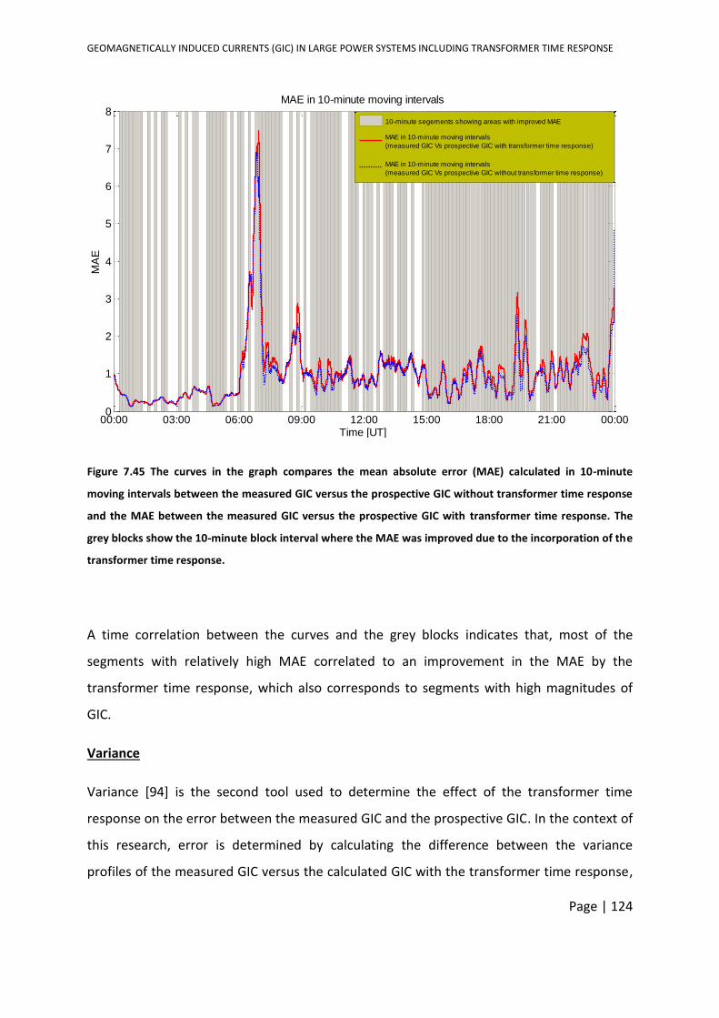
GEOMAGNETICALLY INDUCED CURRENTS (GIC) IN LARGE POWER SYSTEMS INCLUDING TRANSFORMER TIME RESPONSE
Page | 124
Figure 7.45 The curves in the graph compares the mean absolute error (MAE) calculated in 10-minute
moving intervals between the measured GIC versus the prospective GIC without transformer time response
and the MAE between the measured GIC versus the prospective GIC with transformer time response. The
grey blocks show the 10-minute block interval where the MAE was improved due to the incorporation of the
transformer time response.
A time correlation between the curves and the grey blocks indicates that, most of the
segments with relatively high MAE correlated to an improvement in the MAE by the
transformer time response, which also corresponds to segments with high magnitudes of
GIC.
Variance
Variance [94] is the second tool used to determine the effect of the transformer time
response on the error between the measured GIC and the prospective GIC. In the context of
this research, error is determined by calculating the difference between the variance
profiles of the measured GIC versus the calculated GIC with the transformer time response,
00:00 03:00 06:00 09:00 12:00 15:00 18:00 21:00 00:000
1
2
3
4
5
6
7
8
Time [UT]
MA
EMAE in 10-minute moving intervals
10-minute segements showing areas with improved MAE
MAE in 10-minute moving intervals
(measured GIC Vs prospective GIC with transformer time response)
MAE in 10-minute moving intervals
(measured GIC Vs prospective GIC without transformer time response)
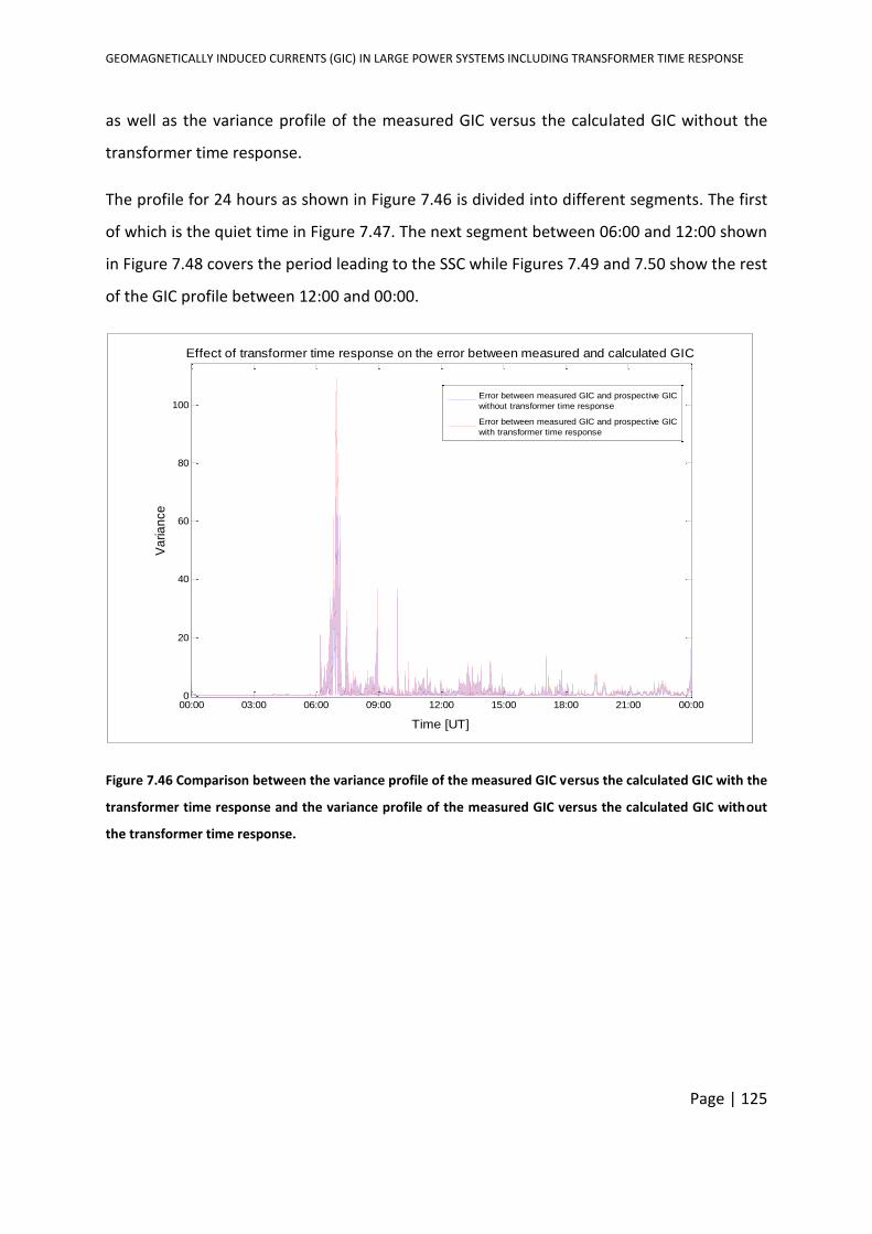
GEOMAGNETICALLY INDUCED CURRENTS (GIC) IN LARGE POWER SYSTEMS INCLUDING TRANSFORMER TIME RESPONSE
Page | 125
as well as the variance profile of the measured GIC versus the calculated GIC without the
transformer time response.
The profile for 24 hours as shown in Figure 7.46 is divided into different segments. The first
of which is the quiet time in Figure 7.47. The next segment between 06:00 and 12:00 shown
in Figure 7.48 covers the period leading to the SSC while Figures 7.49 and 7.50 show the rest
of the GIC profile between 12:00 and 00:00.
Figure 7.46 Comparison between the variance profile of the measured GIC versus the calculated GIC with the
transformer time response and the variance profile of the measured GIC versus the calculated GIC without
the transformer time response.
00:00 03:00 06:00 09:00 12:00 15:00 18:00 21:00 00:000
20
40
60
80
100
Effect of transformer time response on the error between measured and calculated GIC
Time [UT]
Va
ria
nce
Error between measured GIC and prospective GIC
without transformer time response
Error between measured GIC and prospective GIC
with transformer time response
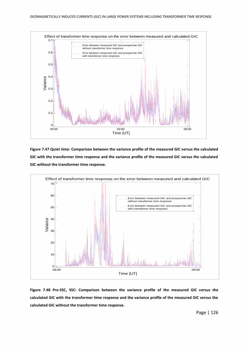
GEOMAGNETICALLY INDUCED CURRENTS (GIC) IN LARGE POWER SYSTEMS INCLUDING TRANSFORMER TIME RESPONSE
Page | 126
Figure 7.47 Quiet time: Comparison between the variance profile of the measured GIC versus the calculated
GIC with the transformer time response and the variance profile of the measured GIC versus the calculated
GIC without the transformer time response.
Figure 7.48 Pre-SSC, SSC: Comparison between the variance profile of the measured GIC versus the
calculated GIC with the transformer time response and the variance profile of the measured GIC versus the
calculated GIC without the transformer time response.
00:00 03:00 06:00
0
0.1
0.2
0.3
0.4
0.5
0.6
0.7
Effect of transformer time response on the error between measured and calculated GIC
Time [UT]
Va
ria
nce
Error between measured GIC and prospective GIC
without transformer time response
Error between measured GIC and prospective GIC
with transformer time response
06:00 09:00
0
10
20
30
40
50
60
70
Effect of transformer time response on the error between measured and calculated GIC
Time [UT]
Va
rian
ce
Error between measured GIC and prospective GIC
without transformer time response
Error between measured GIC and prospective GIC
with transformer time response
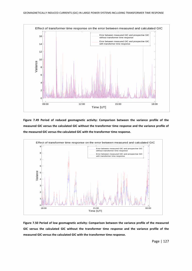
GEOMAGNETICALLY INDUCED CURRENTS (GIC) IN LARGE POWER SYSTEMS INCLUDING TRANSFORMER TIME RESPONSE
Page | 127
Figure 7.49 Period of reduced geomagnetic activity: Comparison between the variance profile of the
measured GIC versus the calculated GIC without the transformer time response and the variance profile of
the measured GIC versus the calculated GIC with the transformer time response.
Figure 7.50 Period of low geomagnetic activity: Comparison between the variance profile of the measured
GIC versus the calculated GIC without the transformer time response and the variance profile of the
measured GIC versus the calculated GIC with the transformer time response.
09:00 12:00 15:00 18:00
0
2
4
6
8
10
12
14
16
Effect of transformer time response on the error between measured and calculated GIC
Time [UT]
Va
rian
ce
Error between measured GIC and prospective GIC
without transformer time response
Error between measured GIC and prospective GIC
with transformer time response
18:00 21:00 00:00
0
1
2
3
4
5
6
7
8
9
Effect of transformer time response on the error between measured and calculated GIC
Time [UT]
Va
rian
ce
Error between measured GIC and prospective GIC
without transformer time response
Error between measured GIC and prospective GIC
with transformer time response
GEOMAGNETICALLY INDUCED CURRENTS (GIC) IN LARGE POWER SYSTEMS INCLUDING TRANSFORMER TIME RESPONSE
Page | 128
In the graphs shown in Figures 7.45 to 7.50, the effect of the transformer time response is
less prominent during high peaks in the GIC profile. This is because the variance between
the measured GIC and the prospective GIC with transformer time response increased. From
the probabilities calculated in case 6 (section 7.4.2) and the analysis using the MAE and
variance, the following can be deduced:
o The average probability the transformer time response improves GIC calculation is
about 0.5 which means that in general, calculating GIC with or without the
transformer time response is equally good.
o The MAE increases during high GIC and so does the variance between the measured
GIC and the calculated GIC. However, when 10-minutes segments are considered,
the transformer time response reduces the MAE even during segments with
relatively high GIC. This corroborates the first point that the impact of the
transformer time response could be pronounced during smaller time intervals.
GEOMAGNETICALLY INDUCED CURRENTS (GIC) IN LARGE POWER SYSTEMS INCLUDING TRANSFORMER TIME RESPONSE
Page | 129
CHAPTER 8
ASSUMPTIONS ON WHICH THE RESEARCH IS
BASED AND DISCUSSIONS
8. ASSUMPTIONS ON WHICH RESEARCH IS BASED AND DISCUSSIONS
In this chapter, the assumptions made in this thesis are presented, followed by a discussion
of the results of the research.
8.1 ASSUMPTIONS
A number of assumptions were made in the effort to calculate GIC using the developed
algorithms explained in chapter 3.
8.1.1 Imaginary location of the voltage source
Some sources in the literature [95-98] mention that the imaginary location of the voltage
source due to a geomagnetic disturbance (GMD) is in series with the transmission lines. This
gives rise to the flow of GIC in transmission lines connected to wye-connected transformers
with grounded neutrals. In this configuration, the Earth serves as a parallel path for the GIC.
This approach was chosen to place the induced electric field in the model used for
calculation.
8.1.2 Time-dependent flow of GIC in transformer windings
The assumption was made that the maximum expected GIC (referred to as the prospective
GIC without transformer time response) that flows through a transformer is a function of
time.
8.1.3 Flow of GIC in a three-phase four-wire system
The assumption was made that the GIC flow in the different phases of a three-phase
transmission line and transformer are the same. Furthermore, the GIC in the grounded
GEOMAGNETICALLY INDUCED CURRENTS (GIC) IN LARGE POWER SYSTEMS INCLUDING TRANSFORMER TIME RESPONSE
Page | 130
neutral of the transformer was assumed to be the algebraic sum of the GIC in the three
phases.
8.1.4 Line inductance should not be considered in GIC calculations
When calculating the GIC in transmission networks, the inductance of the line is neglected
at GIC frequencies (< 1 Hz). This is because the frequency is regarded as quasi-DC (less than
1 Hz). Therefore, only the line resistance is taken into account.
8.2 DISCUSSIONS
8.2.1 Introduction of prospective GIC with and without transformer response
calculations
One of the key findings in this thesis is that there is a difference between the prospective
GIC with transformer time response and the prospective GIC without transformer time
response. The time response being the distinguishing factor which affects the flow of GIC
through a transformer. This difference is based on the characteristics of the transformer
among others and the transformer’s time response to changing GIC magnitudes. The
equations derived in chapter 3 showed the difference between the prospective GIC without
and with the transformer response.
The Lehtinen - Pirjola method has been widely used for calculating GIC. There was a strong
correlation when the GIC values calculated using this method were compared to the GIC
values calculated using the NAM methods. Therefore the similarity in the results validated
the code that was written in MATLAB for this calculation.
For the calculation of the prospective GIC with transformer time response, the transformer
core type and the GIC flow through the transformer was taken into account to determine
the transformer response time to GIC. Only three transformer core structures were tested:
3(1P-3L), 3P-3L and 3P-5L. While the results of the test could not confirm that all
transformer designs with the same core structure have the same time response to GIC, the
results indicated that different core structures respond differently to GIC. This conclusion
contributes greatly to the improvement of GIC calculations.
GEOMAGNETICALLY INDUCED CURRENTS (GIC) IN LARGE POWER SYSTEMS INCLUDING TRANSFORMER TIME RESPONSE
Page | 131
All the previous calculation algorithms did not take into account the core-dependant
transformer time response to GIC.
8.2.2 Differential transformer core time response to GIC
Laboratory tests were conducted on 300 VA 3(1P-3L), 3P-3L and 3P-5L transformer core
structures to determine their time response to DC. To validate the laboratory tests,
corresponding simulations in PSCAD were done. In both cases, the results showed that load
had an impact on the response time variation with DC current injected. The major
difference was that the time response to DC current of the 300 VA 3P-3L and 3P-5L
transformers modelled in PSCAD was less than when tested in the laboratory.
The 3P-3L transformer was more likely to permit the flow of GIC through the windings of the
transformer over a shorter length of time in comparison to the other two core types. The
300 VA transformers were uprated to 500 MVA to represent power transformers in main
transmission systems. The 500 MVA 3P-3L transformer core type had the shortest response
time to GIC, followed by the 3(1P-3L) and the 3P-5L transformers. Figure 8.1 shows the
average time response profile for the three core structures under no-load and load
conditions.
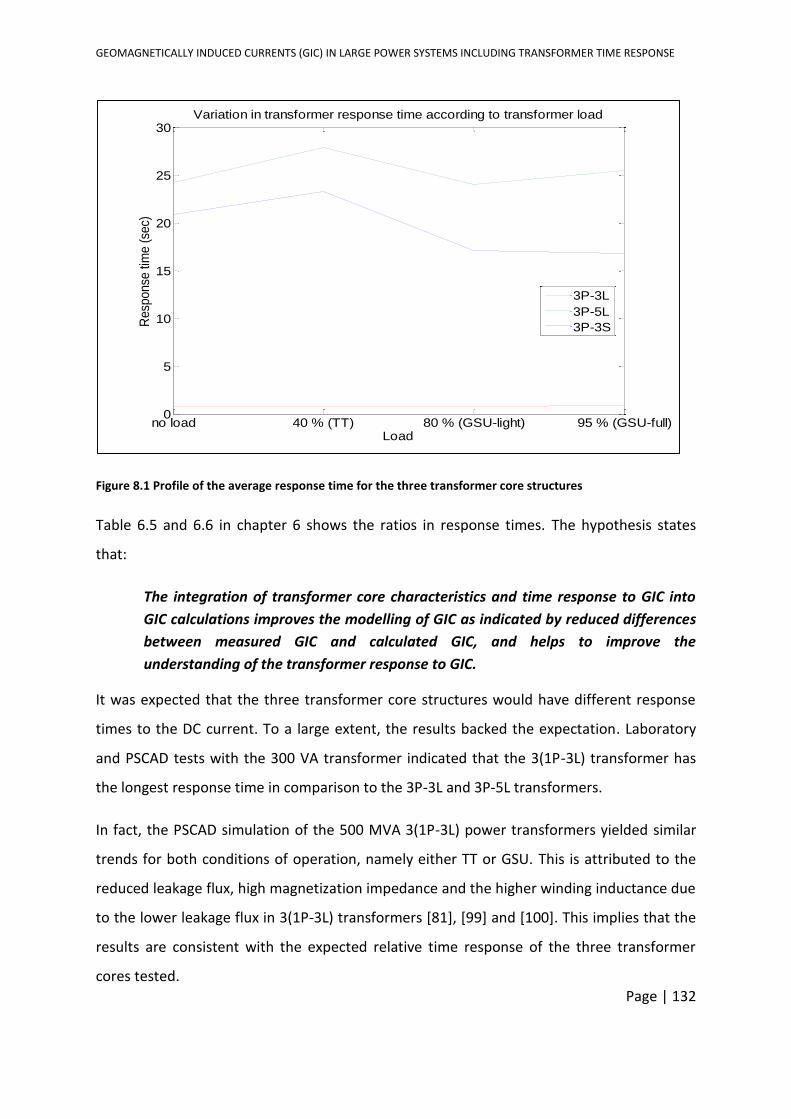
GEOMAGNETICALLY INDUCED CURRENTS (GIC) IN LARGE POWER SYSTEMS INCLUDING TRANSFORMER TIME RESPONSE
Page | 132
Figure 8.1 Profile of the average response time for the three transformer core structures
Table 6.5 and 6.6 in chapter 6 shows the ratios in response times. The hypothesis states
that:
The integration of transformer core characteristics and time response to GIC into
GIC calculations improves the modelling of GIC as indicated by reduced differences
between measured GIC and calculated GIC, and helps to improve the
understanding of the transformer response to GIC.
It was expected that the three transformer core structures would have different response
times to the DC current. To a large extent, the results backed the expectation. Laboratory
and PSCAD tests with the 300 VA transformer indicated that the 3(1P-3L) transformer has
the longest response time in comparison to the 3P-3L and 3P-5L transformers.
In fact, the PSCAD simulation of the 500 MVA 3(1P-3L) power transformers yielded similar
trends for both conditions of operation, namely either TT or GSU. This is attributed to the
reduced leakage flux, high magnetization impedance and the higher winding inductance due
to the lower leakage flux in 3(1P-3L) transformers [81], [99] and [100]. This implies that the
results are consistent with the expected relative time response of the three transformer
cores tested.
no load 40 % (TT) 80 % (GSU-light) 95 % (GSU-full)0
5
10
15
20
25
30Variation in transformer response time according to transformer load
Load
Resp
onse
tim
e (
sec)
3P-3L
3P-5L
3P-3S
GEOMAGNETICALLY INDUCED CURRENTS (GIC) IN LARGE POWER SYSTEMS INCLUDING TRANSFORMER TIME RESPONSE
Page | 133
8.2.3 Limitations with scaling up transformer size from 300 VA to 500 MVA
Sometimes when test systems are scaled up, the results may not always be the same under
similar conditions. This was found to be the case in this research. The 500 MVA 3(1P-3L)
transformer’s response time to DC between 3.0 pu and 8.0 pu was longer in comparison to
the 500 MVA 3P-5L transformer. This was the same for the no-load and 40 % load condition,
representing TTs.
Another difference between the 300 VA and 500 MVA transformers was that, during
operation under the GSU conditions, the response time of the 500 MVA 3(1P-3L)
transformer was less than the 500 MVA 3P-5L, while the opposite was true for the 300 VA
transformer under the same GSU conditions.
8.2.4 Incorporating the transformer time response piecewise linear equations into the
GIC calculation: 10 substation test network
The piecewise linear equations derived from the PSCAD simulation of the 500 MVA
transformers represent the specific transformer core type under test. These equations are
listed in section 6.3. While these equations may not fully reflect the exact time response
profiles for real larger power transformers, such as 1,000 MVA, or a medium-sized power
transformer, such as 500 MVA, the results brought to light the expected response time
profile of power transformers. In so doing, they provide a platform upon which further
research can be done.
The calculation examples with the test network in chapter 7 demonstrate how the GIC with
transformer response is calculated. For each substation, this was calculated initially for a
case where all the transformers in the network have the same core structure and later for a
case where the transformer core structures as well as mode of operation differed.
In line with the results of the PSCAD simulations and the laboratory tests, the 3P-3L
transformer had the smallest percentage difference in prospective GIC with transformer
time response when compared to the prospective GIC without transformer time response.
GEOMAGNETICALLY INDUCED CURRENTS (GIC) IN LARGE POWER SYSTEMS INCLUDING TRANSFORMER TIME RESPONSE
Page | 134
This is based on the fact that the 3P-3L transformer has the shortest response time to DC
current.
An investigation was done to determine whether the location of a transformer in the
network has an impact on the profile of the prospective GIC with transformer time
response. The investigation showed that the location of the transformer within the power
network does not determine its response time to GIC but rather the core characteristics of
the transformer.
8.2.5 Effect of interpolation on peak GIC
Interpolation was used to obtain the magnetic field data sets for the various sampling time
intervals. For each set, the magnetic field data was used to calculate the corresponding
electric field as an input to the GIC calculation. To quantify the effect of the interpolation
method on the GIC calculation, the measured GIC interpolated to a series of sampling time
intervals and the corresponding prospective GIC with and without transformer time
response were compared. The outcome shows that the absolute peak values of measured
and calculated GIC decrease as the sampling time interval increases as shown in Figure 8.2.
The absolute peak values of the measured and calculated GIC in Figure 8.2 are not
necessarily exactly time correlated with the same polarity. The monotonic shape of all the
curves illustrates that the effects of averaging over longer periods are consistent for the
whole range.
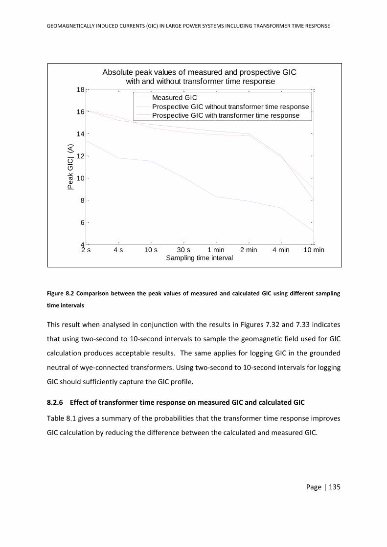
GEOMAGNETICALLY INDUCED CURRENTS (GIC) IN LARGE POWER SYSTEMS INCLUDING TRANSFORMER TIME RESPONSE
Page | 135
Figure 8.2 Comparison between the peak values of measured and calculated GIC using different sampling
time intervals
This result when analysed in conjunction with the results in Figures 7.32 and 7.33 indicates
that using two-second to 10-second intervals to sample the geomagnetic field used for GIC
calculation produces acceptable results. The same applies for logging GIC in the grounded
neutral of wye-connected transformers. Using two-second to 10-second intervals for logging
GIC should sufficiently capture the GIC profile.
8.2.6 Effect of transformer time response on measured GIC and calculated GIC
Table 8.1 gives a summary of the probabilities that the transformer time response improves
GIC calculation by reducing the difference between the calculated and measured GIC.
2 s 4 s 10 s 30 s 1 min 2 min 4 min 10 min4
6
8
10
12
14
16
18
Absolute peak values of measured and prospective GIC with and without transformer time response
Sampling time interval
|Pe
ak G
IC| (
A)
Measured GIC
Prospective GIC without transformer time response
Prospective GIC with transformer time response
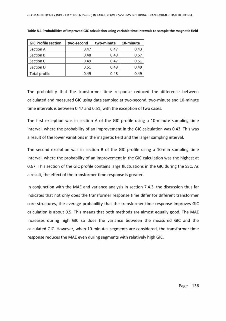
GEOMAGNETICALLY INDUCED CURRENTS (GIC) IN LARGE POWER SYSTEMS INCLUDING TRANSFORMER TIME RESPONSE
Page | 136
Table 8.1 Probabilities of improved GIC calculation using variable time intervals to sample the magnetic field
GIC Profile section two-second two-minute 10-minute
Section A 0.47 0.47 0.43
Section B 0.48 0.49 0.67
Section C 0.49 0.47 0.51
Section D 0.51 0.49 0.49
Total profile 0.49 0.48 0.49
The probability that the transformer time response reduced the difference between
calculated and measured GIC using data sampled at two-second, two-minute and 10-minute
time intervals is between 0.47 and 0.51, with the exception of two cases.
The first exception was in section A of the GIC profile using a 10-minute sampling time
interval, where the probability of an improvement in the GIC calculation was 0.43. This was
a result of the lower variations in the magnetic field and the larger sampling interval.
The second exception was in section B of the GIC profile using a 10-min sampling time
interval, where the probability of an improvement in the GIC calculation was the highest at
0.67. This section of the GIC profile contains large fluctuations in the GIC during the SSC. As
a result, the effect of the transformer time response is greater.
In conjunction with the MAE and variance analysis in section 7.4.3, the discussion thus far
indicates that not only does the transformer response time differ for different transformer
core structures, the average probability that the transformer time response improves GIC
calculation is about 0.5. This means that both methods are almost equally good. The MAE
increases during high GIC so does the variance between the measured GIC and the
calculated GIC. However, when 10-minutes segments are considered, the transformer time
response reduces the MAE even during segments with relatively high GIC.
GEOMAGNETICALLY INDUCED CURRENTS (GIC) IN LARGE POWER SYSTEMS INCLUDING TRANSFORMER TIME RESPONSE
Page | 137
CHAPTER 9
CONCLUSIONS
9. CONCLUSIONS
The research conducted for this thesis was aimed at developing a method for incorporating
the transformer time response to GIC into GIC calculations, and to determine whether this
will reduce the discrepancies between measured and calculated GIC. To this effect, several
areas contiguous to transformer time response to GIC were developed. In this chapter,
conclusions are drawn about each of these areas.
9.1 DIFFERENTIAL TRANSFORMER CORE RESPONSE TIME TO GIC
The transformer response time to DC current was not the same for the different
transformer cores tested namely, 3P-3L, 3P-5L and 3(1P-3L). The response time for the 300
VA transformers increased in the following order: 3P-3L, 3P-5L, 3(1P-3L) and increased in
the following order for the 500 MVA transformers in PSCAD: 3P-3L, 3(1P-3L), 3P-5L.
9.2 EFFECT OF LOAD ON TRANSFORMER RESPONSE TIME TO GIC
The laboratory test and PSCAD simulations showed that the response time to GIC for the 3P-
3L, 3P-5L and 3(1P-3L) transformer core types are load dependant. From the average time
response to DC for the three transformer cores shown in Figure 8.1, it was concluded that
3(1P-3L) and 3P-5L transformers operating as TT’s have the longest response time to GIC.
The shortest response time to GIC was at GSU (light load), which was consistent across the
three transformer cores. This correlates well with the notion that power transmission
networks would stand a better chance of surviving a high GMD when all generating units
and loads are online.
GEOMAGNETICALLY INDUCED CURRENTS (GIC) IN LARGE POWER SYSTEMS INCLUDING TRANSFORMER TIME RESPONSE
Page | 138
9.3 CHARACTERISING TRANSFORMER TIME RESPONSE TO GIC
Piecewise linear equations are suitable for characterising the response time of different
transformer core structures at different load levels to different levels of GIC. This promotes
a more detailed understanding and analysis of GIC flow through large power transformers
with different core structures.
9.4 ANSWERS TO RESEARCH QUESTIONS
Five research questions were posed in chapter 1 to probe the hypothesis. This section
summarises the answers to these questions. These answers are based on the results of the
laboratory test and PSCAD simulations.
1. How is the network part of GIC calculations affected by the transformer response to
changing electric fields?
The sampling time interval of the geomagnetic field influences the peak values of the
geomagnetic field. This in turn is linked to the peak values of the calculated electric field.
Since the rate of change of the magnetic field may vary during any time frame under
consideration, the prospective GIC with transformer time response approach is a preferred
method, as it presents a better understanding of the exact GIC flow through the transformer
during a storm. This is because the transformer response time determines whether or not
the prospective GIC flow through the transformer in the network will be reached as the
electric field changes.
2. What is the response of transformers to changing electric fields imposed at low
frequencies and how does it vary with transformer core type?
The response of transformers to GIC - like frequencies is such that the prospective GIC with
and without transformer response are not always the same. This is attributed to the varying
transformer response time.
GEOMAGNETICALLY INDUCED CURRENTS (GIC) IN LARGE POWER SYSTEMS INCLUDING TRANSFORMER TIME RESPONSE
Page | 139
3. Why was the time response of transformers neglected in the past? Are the reasons
valid?
In the past, the time response of transformers was neglected because it was assumed that
the contribution of the transformer time response to GIC was insignificant. This assumption
now proves to be inaccurate, since it has been established that transformer’s time response
to GIC is core type and load dependent.
Taking into account that the transformer time response reduces the difference between the
measured GIC and the calculated GIC. This would prevent an overestimation of the
maximum GIC expected to flow through the substation. As a result, it will be possible to plan
a more appropriate contingency measure to mitigate possible network problems anticipated
during severe GMDs.
4. To what extent can the modelled and tested transformers represent all transformers?
The three main core structures were modelled with a variety of DC current levels and load
conditions, both in PSCAD and in the laboratory. Therefore, while these results are unique
to these transformer models, they provide an indication that it is incorrect to lump the
transformer response of all transformers.
5. How does the sampling interval of the magnetic field and measured GIC affect GIC
calculations?
As the sampling interval increases, the difference between the measured and calculated GIC
increases. However, the difference between the peaks of the measured and calculated GIC
is less than 2 %, when the sampling time interval is either two-second, four-second or 10-
second. Therefore, the sampling between two-second and 10-second intervals is the
recommended sampling time interval for GIC studies. This will increase the amount of data
that can be stored in a given storage and still capture sufficient data for GIC analysis.

GEOMAGNETICALLY INDUCED CURRENTS (GIC) IN LARGE POWER SYSTEMS INCLUDING TRANSFORMER TIME RESPONSE
Page | 140
9.5 VALIDITY OF HYPOTHESIS
The background to this research work and the objectives as laid out in chapter 1 led to the
hypothesis which states that:
The integration of transformer core characteristics and time response to GIC into
GIC calculations improves the modelling of GIC as indicated by reduced differences
between measured GIC and calculated GIC, and helps to improve the
understanding of the transformer response to GIC.
The results in chapter 5, 6 and 7 as well as the discussions in chapter 8, which improved the
understanding of transformer response to GIC, prove that the hypothesis is valid.
This research lays a foundation for further work on the transformer time response in GIC
calculations.
GEOMAGNETICALLY INDUCED CURRENTS (GIC) IN LARGE POWER SYSTEMS INCLUDING TRANSFORMER TIME RESPONSE
Page | 141
List of References
[1] T. Forbes, "A review on the genesis of coronal mass ejections," Journal of Geophysical Research: Space Physics (1978–2012), vol. 105, pp. 23153-23165, 2000.
[2] J. T. Gosling, D. J. McComas, J. L. Phillips, V. J. Pizzo, B. E. Goldstein, R. J. Forsyth and R. P. Lepping, "A CME-driven solar wind disturbance observed at both low and high heliographic latitudes," Geophys. Res. Lett., vol. 22, pp. 1753-1756, 1995.
[3] A. Viljanen, H. Nevanlinna, K. Pajunpää and A. Pulkkinen, "Time derivative of the horizontal geomagnetic field as an activity indicator," in Annales Geophysicae, 1999, pp. 1107-1118.
[4] J. A. Jacobs, Geomagnetism. Elsevier, 2013.
[5] A. J. Dessler and E. N. Parker, "Hydromagnetic theory of geomagnetic storms," Journal of Geophysical Research, vol. 64, pp. 2239-2252, 1959.
[6] R. Horton, D. Boteler, T. J. Overbye, R. Pirjola and R. C. Dugan, "A test case for the calculation of geomagnetically induced currents," Power Delivery, IEEE Transactions on, vol. 27, pp. 2368-2373, 2012.
[7] E. Bernhardi, P. Cilliers and C. Gaunt, "Improvement in the modelling of geomagnetically induced currents in southern Africa," S. Afr. J. Sci., vol. 104, pp. 265-272, 2008.
[8] V. Albertson, B. Bozoki, W. Feero, J. Kappenman, E. Larsen, D. Nordell, J. Ponder, F. Prabhakara, K. Thompson and R. Walling, "Geomagnetic disturbance effects on power systems," IEEE Trans. Power Del., vol. 8, pp. 1206-1216, 1993.
[9] C. T. Gaunt, "Reducing uncertainty–responses for electricity utilities to severe solar storms," Journal of Space Weather and Space Climate, vol. 4, pp. A01, 2014.
[10] K. Zheng, D. Boteler, R. J. Pirjola, L. Liu, R. Becker, L. Marti, S. Boutilier and S. Guillon, "Effects of system characteristics on geomagnetically induced currents," Power Delivery, IEEE Transactions on, vol. 29, pp. 890-898, 2014.
[11] W. Radasky and J. Kappenman, "Impacts of geomagnetic storms on EHV and UHV power grids," in Electromagnetic Compatibility (APEMC), 2010 Asia-Pacific Symposium on, 2010, pp. 695-698.
[12] H. Lundstedt, "The sun, space weather and GIC effects in Sweden," Advances in Space Research, vol. 37, pp. 1182-1191, 2006.
GEOMAGNETICALLY INDUCED CURRENTS (GIC) IN LARGE POWER SYSTEMS INCLUDING TRANSFORMER TIME RESPONSE
Page | 142
[13] K. Zheng, L. Trichtchenko, R. J. Pirjola and L. Liu, "Effects of geophysical parameters on GIC illustrated by benchmark network modeling," Power Delivery, IEEE Transactions on, vol. 28, pp. 1183-1191, 2013.
[14] V. D. Albertson, J. Thorson, R. Clayton and S. Tripathy, "Solar-induced-currents in power systems: cause and effects," Power Apparatus and Systems, IEEE Transactions on, pp. 471-477, 1973.
[15] J. G. Kappenman, "Geomagnetic storms and their impact on power systems," IEEE Power Engineering Review, vol. 16, 1996.
[16] D. Boteler. "Chapter 4. The impact of space weather on the electric power grid," in (1st ed.), C. J. Schrijver, F. Bagenal and J. J. Sojka, Eds. 2014, [Online].
[17] B. Bozoki, S. Chano, L. Dvorak, W. Feero, G. Fenner, E. Guro, C. Henville, J. Ingleson, S. Mazumdar and P. McLaren, "The effects of GIC on protective relaying," Power Delivery, IEEE Transactions on, vol. 11, pp. 725-739, 1996.
[18] L. Marti, J. Berge and R. K. Varma, "Determination of Geomagnetically Induced Current Flow in a Transformer from Reactive Power Absorption," Power Delivery, IEEE Transactions on, vol. 28, pp. 1280-1288, 2013.
[19] T. S. Molinski, "Why utilities respect geomagnetically induced currents," J. Atmos. Solar Terr. Phys., vol. 64, pp. 1765-1778, 2002.
[20] J. Kappenman, S. Norr, G. Sweezy, D. Carlson, V. Albertson, J. Harder and B. Damsky, "GIC mitigation: a neutral blocking/bypass device to prevent the flow of GIC in power systems," Power Delivery, IEEE Transactions on, vol. 6, pp. 1271-1281, 1991.
[21] L. Bolduc, M. Granger, G. Paré, J. Saintonge and L. Brophy, "Development of a DC current-blocking device for transformer neutrals," Power Delivery, IEEE Transactions on, vol. 20, pp. 163-168, 2005.
[22] R. J. Pirjola and A. Viljanen, "Research of geomagnetically induced currents (gic) in finland," in Electromagnetic Compatibility and Electromagnetic Ecology, 2007 7th International Symposium on, 2007, pp. 269-272.
[23] A. W. Thomson, C. Gaunt, P. Cilliers, J. Wild, B. Opperman, L. McKinnell, P. Kotze, C. M. Ngwira and S. I. Lotz, "Present day challenges in understanding the geomagnetic hazard to national power grids," Advances in Space Research, vol. 45, pp. 1182-1190, 2010.
[24] I. A. Erinmez, J. G. Kappenman and W. A. Radasky, "Management of the geomagnetically induced current risks on the national grid company's electric power transmission system," J. Atmos. Solar Terr. Phys., vol. 64, pp. 743-756, 2002.
GEOMAGNETICALLY INDUCED CURRENTS (GIC) IN LARGE POWER SYSTEMS INCLUDING TRANSFORMER TIME RESPONSE
Page | 143
[25] M. Lehtinen and R. Pirjola, "Currents produced in earthed conductor networks by geomagnetically-induced electric fields," in Annales Geophysicae, 1985, pp. 479-484.
[26] D. Boteler and R. Pirjola, "Comparison of methods for modelling geomagnetically induced currents," in Annales Geophysicae, 2014, pp. 1177-1187.
[27] A. A. Trichtchenko, D. H. Boteler and A. Foss, "GIC modelling for an overdetermined system," in Electrical and Computer Engineering, 2006. CCECE'06. Canadian Conference on, 2006, pp. 394-397.
[28] D. Boteler, "Methodology for simulation of geomagnetically induced currents in power systems," Journal of Space Weather and Space Climate, vol. 4, pp. A21, 2014.
[29] J. Berge and R. K. Varma, "A software simulator for geomagnetically induced currents in electrical power systems," in Electrical and Computer Engineering, 2009. CCECE'09. Canadian Conference on, 2009, pp. 695-700.
[30] J. Koen and T. Gaunt, "Geomagnetically induced currents in the southern african electricity transmission network," in Power Tech Conference Proceedings, 2003 IEEE Bologna, 2003, pp. 7 pp. Vol. 1.
[31] J. Koen, "Geomagnetically induced currents in the Southern African electricity transmission network," University of Cape Town, South Africa, 2002.
[32] (2014, February 06). Modeling Geomagnetically Induced Currents in PowerWorld Simulator. Available: http://www.powerworld.com/files/GICModeling.pdf.
[33] M. Wik, A. Viljanen, R. Pirjola, A. Pulkkinen, P. Wintoft and H. Lundstedt, "Calculation of geomagnetically induced currents in the 400 kV power grid in southern Sweden," Space Weather, vol. 6, pp. S07005, 2008.
[34] C. Barbosa, K. Pinheiro, G.A. Hartmann, R.I.F. Trindade, "Numerical model test of geomagnetic induced currents in Brazil," Latinmag Letters, vol. Volume 3, 2013.
[35] T. J. Overbye, T. R. Hutchins, K. Shetye, J. Weber and S. Dahman, "Integration of geomagnetic disturbance modeling into the power flow: A methodology for large-scale system studies," in North American Power Symposium (NAPS), 2012, 2012, pp. 1-7.
[36] D. Boteler, L. Trichtchenko, R. Pirjola, J. Parmelee, S. Souksaly, A. Foss and L. Marti, "Real-time simulation of geomagnetically induced currents," in Electromagnetic Compatibility and Electromagnetic Ecology, 2007 7th International Symposium on, 2007, pp. 261-264.
[37] R. Walling and A. Khan, "Characteristics of transformer exciting-current during geomagnetic disturbances," Power Delivery, IEEE Transactions on, vol. 6, pp. 1707-1714, 1991.
GEOMAGNETICALLY INDUCED CURRENTS (GIC) IN LARGE POWER SYSTEMS INCLUDING TRANSFORMER TIME RESPONSE
Page | 144
[38] L. Bolduc, "GIC observations and studies in the Hydro-Québec power system," J. Atmos. Solar Terr. Phys., vol. 64, pp. 1793-1802, 2002.
[39] D. H. Boteler, R. J. Pirjola and H. Nevanlinna, "The effects of geomagnetic disturbances on electrical systems at the Earth's surface," Advances in Space Research, vol. 22, pp. 17-27, 1998.
[40] A. Pulkkinen, S. Lindahl, A. Viljanen and R. Pirjola, "Geomagnetic storm of 29–31 October 2003: Geomagnetically induced currents and their relation to problems in the Swedish high‐voltage power transmission system," Space Weather, vol. 3, 2005.
[41] T. J. Overbye, K. S. Shetye, T. R. Hutchins, Q. Qiu and J. D. Weber, "Power grid sensitivity analysis of geomagnetically induced currents," Power Systems, IEEE Transactions on, vol. 28, pp. 4821-4828, 2013.
[42] A. McNish, "Magnetic storms," Edison Electric Institute Bulletin, 1940.
[43] P. J. Kellogg, "Terrestrial effects of solar activity," in Proceedings Minn. Power Systems Conf., Minnesota, 1966,.
[44] V. D. Albertson and J. A. Van Baelen, "Electric and magnetic fields at the earth's surface due to auroral currents," Power Apparatus and Systems, IEEE Transactions on, pp. 578-584, 1970.
[45] J. Koen and C. Gaunt, "Disturbances in the Southern African power network due to geomagnetically induced currents," Cigré Session, pp. 206, 2002.
[46] D. Boteler and R. Pirjola, "Modelling geomagnetically induced currents produced by realistic and uniform electric fields," Power Delivery, IEEE Transactions on, vol. 13, pp. 1303-1308, 1998.
[47] A. Pulkkinen, O. Amm and A. Viljanen, "Ionospheric equivalent current distributions determined with the method of spherical elementary current systems," Journal of Geophysical Research, vol. 108, pp. 1053, 2003.
[48] O. Amm and A. Viljanen, "Ionospheric disturbance magnetic field continuation from the ground to the ionosphere using spherical elementary current systems," Earth, Planets and Space, vol. 51, pp. 431-440, 1999.
[49] O. AMM, "Ionospheric elementary current systems in spherical coordinates and their application," Journal of Geomagnetism and Geoelectricity, vol. 49, pp. 947-955, 1997.
[50] S. Watari, M. Kunitake, K. Kitamura, T. Hori, T. Kikuchi, K. Shiokawa, N. Nishitani, R. Kataoka, Y. Kamide and T. Aso, "Measurements of geomagnetically induced current in a power grid in Hokkaido, Japan," Space Weather, vol. 7, 2009.
GEOMAGNETICALLY INDUCED CURRENTS (GIC) IN LARGE POWER SYSTEMS INCLUDING TRANSFORMER TIME RESPONSE
Page | 145
[51] A. Viljanen, "Relation of geomagnetically induced currents and local geomagnetic variations," Power Delivery, IEEE Transactions on, vol. 13, pp. 1285-1290, 1998.
[52] L. Trichtchenko and D. Boteler, "Effects of recent geomagnetic storms on power systems," in Electromagnetic Compatibility and Electromagnetic Ecology, 2007 7th International Symposium on, 2007, pp. 265-268.
[53] A. Viljanen, R. Pirjola, M. Wik, A. Ádám, E. Prácser, Y. Sakharov and J. Katkalov, "Continental scale modelling of geomagnetically induced currents," Journal of Space Weather and Space Climate, vol. 2, 2012.
[54] W. McNutt, "The effect of GIC on power transformers," in IEEE PES Summer Meeting July, 1990, pp. 32-37.
[55] J. Berge, L. Marti and R. K. Varma, "Modeling and mitigation of geomagnetically induced currents on a realistic power system network," in Electrical Power and Energy Conference (EPEC), 2011 IEEE, 2011, pp. 485-490.
[56] N. Takasu, T. Oshi, F. Miyawaki, S. Saito and Y. Fujiwara, "An experimental analysis of DC excitation of transformers by geomagnetically induced currents," Power Delivery, IEEE Transactions on, vol. 9, pp. 1173-1182, 1994.
[57] D. Boteler, "Geomagnetically induced currents: present knowledge and future research," Power Delivery, IEEE Transactions on, vol. 9, pp. 50-58, 1994.
[58] R. Pirjola, "Review on the calculation of surface electric and magnetic fields and of geomagnetically induced currents in ground-based technological systems," Surv. Geophys., vol. 23, pp. 71-90, 2002.
[59] A. Pulkkinen, A. Thomson, E. Clarke and A. McKay, "April 2000 geomagnetic storm: Ionospheric drivers of large geomagnetically induced currents," in Annales Geophysicae, 2003, pp. 709-717.
[60] A. Viljanen, A. Pulkkinen, O. Amm, R. Pirjola and T. Korja, "Fast computation of the geoelectric field using the method of elementary current systems and planar earth models," in Annales Geophysicae, 2004, pp. 101-113.
[61] A. Viljanen and R. Pirjola, "Statistics on geomagnetically-induced currents in the Finnish 400 kV power system based on recordings of geomagnetic variations," Journal of Geomagnetism and Geoelectricity, vol. 41, pp. 411-420, 1989.
[62] R. Pirjola, "Geomagnetically induced currents during magnetic storms," Plasma Science, IEEE Transactions on, vol. 28, pp. 1867-1873, 2000.
GEOMAGNETICALLY INDUCED CURRENTS (GIC) IN LARGE POWER SYSTEMS INCLUDING TRANSFORMER TIME RESPONSE
Page | 146
[63] C. Liu, L. Liu, R. Pirjola and Z. Wang, "Calculation of geomagnetically induced currents in mid‐to low‐latitude power grids based on the plane wave method: A preliminary case study," Space Weather, vol. 7, 2009.
[64] T. A. Tjimbandi, "Geomagnetically Induced Currents in South Africa," BSc Elec Eng Thesis, University of Cape Town., 2007.
[65] H. Vanhamäki, A. Viljanen, R. Pirjola and O. Amm, "Deriving the geomagnetically induced electric field at the Earth’s surface from the time derivative of the vertical magnetic field," Earth, Planets and Space, vol. 65, pp. 997-1006, 2013.
[66] R. Pirjola and A. Viljanen, "Complex image method for calculating electric and magnetic fields produced by an auroral electrojet of finite length," in Annales Geophysicae, 1998, pp. 1434-1444.
[67] R. Pirjola, A. Viljanen, A. Pulkkinen and O. Amm, "Space weather risk in power systems and pipelines," Physics and Chemistry of the Earth, Part C: Solar, Terrestrial & Planetary Science, vol. 25, pp. 333-337, 2000.
[68] P. A. Tipler and G. Mosca, Physics for Scientists and Engineers. Macmillan, 2007.
[69] P. E. Gray and C. L. Searle, Electronic Principles: Physics, Models, and Circuits. Wiley, 1969.
[70] K. S. Shetye, T. J. Overbye, Q. Qiu and J. Fleeman, "Geomagnetic disturbance modeling results for the AEP system: A case study," in Power and Energy Society General Meeting (PES), 2013 IEEE, 2013, pp. 1-5.
[71] J. D. Glover, M. S. Sarma and T. J. Overbye, Power System Analysis and Design. CengageBrain. com, 2011.
[72] L. Trichtchenko and D. H. Boteler, "Modeling geomagnetically induced currents using geomagnetic indices and data," Plasma Science, IEEE Transactions on, vol. 32, pp. 1459-1467, 2004.
[73] (8th January, 2014). GIC flow in power systems. Available: http://www.powerworld.com/files/GICGroundLoop.jpg.
[74] P. C. Sen, Principles of Electric Machines and Power Electronics. John Wiley & Sons, 2007.
[75] National Imagery and Mapping Agency (NIMA), "Department of defence world geodetic system 1984," NIMA/Geodesy and Geophysics Department, Tech. Rep. NIMA TR8350.2, 2000.
GEOMAGNETICALLY INDUCED CURRENTS (GIC) IN LARGE POWER SYSTEMS INCLUDING TRANSFORMER TIME RESPONSE
Page | 147
[76] H. K. Chisepo, "The Response of Transformers to Geomagnetically Induced-like Currents," MSc Dissertation. University of Cape Town, 2014.
[77] A. E. Emanuel, "Summary of IEEE standard 1459: definitions for the measurement of electric power quantities under sinusoidal, nonsinusoidal, balanced, or unbalanced conditions," Industry Applications, IEEE Transactions on, vol. 40, pp. 869-876, 2004.
[78] (). NI 9225 3-Channel, 300 Vrms Analog Input Module. Available: http://sine.ni.com/nips/cds/view/p/lang/en/nid/208795.
[79] (). PLC: DVPEN01-SL. Available: http://www.delta.com.tw/product/em/control/cm/download/manual/DVPEN01-SL_O_EN_20090721.pdf.
[80] M. Salimi, A. Gole and R. Jayasinghe, "Improvement of Transformer Saturation Modeling for Electromagnetic Transient Programs," IPST, Vancouver, 2013.
[81] (2013, December 28). Design of Transformers . Available: http://elearning.vtu.ac.in/16/ENotes/Elec%20Mac%20Des/Unit3-Era.pdf.
[82] J. Martinez, R. Walling, B. Mork, J. Martin-Arnedo and D. Durbak, "Parameter determination for modeling system transients-Part III: Transformers," Power Delivery, IEEE Transactions on, vol. 20, pp. 2051-2062, 2005.
[83] Siemens, "Siemens energy sector power engineering guide" Tech. Rep. Edition 7.
[84] (2013, December 28). Lecture 3- Power Transformers. Available: http://services.eng.uts.edu.au/pmcl/pct/Downloads/Lecture03.pdf.
[85] D. Boteler, "Characteristics of time-varying inductance," Magnetics, IEEE Transactions on, vol. 30, pp. 172-176, 1994.
[86] B. Hembroff, M. Ohlen and P. Werelius, "A Guide to Transformer Winding Resistance," Application Notes, April, 2010.
[87] B. Hembroff, "A Guide To Transformer DC Resistance Measurements, Part 2," Electricity Today, April, 1996.
[88] F. Prabhakara, J. Ponder and J. Towle, "Computing GIC in large power systems," Computer Applications in Power, IEEE, vol. 5, pp. 46-50, 1992.
[89] P. R. Price, "Geomagnetically induced current effects on transformers," Power Delivery, IEEE Transactions on, vol. 17, pp. 1002-1008, 2002.
[90] J. Bird, Electrical and Electronic Principles and Technology. Routledge, 2013.
GEOMAGNETICALLY INDUCED CURRENTS (GIC) IN LARGE POWER SYSTEMS INCLUDING TRANSFORMER TIME RESPONSE
Page | 148
[91] J. Bird and A. May, Electrical Principles 3 Checkbook: The Checkbook Series. Elsevier, 2013.
[92] T. Chai and R. R. Draxler, "Root mean square error (RMSE) or mean absolute error (MAE)?–Arguments against avoiding RMSE in the literature," Geoscientific Model Development, vol. 7, pp. 1247-1250, 2014.
[93] C. J. Willmott and K. Matsuura, "Advantages of the mean absolute error (MAE) over the root mean square error (RMSE) in assessing average model performance," Climate Research, vol. 30, pp. 79, 2005.
[94] F. A. Graybill, Theory and Application of the Linear Model. Cengage Learning, 2000.
[95] L. Trichtchenko and D. H. Boteler, "Response of power systems to the temporal characteristics of geomagnetic storms," in Electrical and Computer Engineering, 2006. CCECE'06. Canadian Conference on, 2006, pp. 390-393.
[96] L. Bolduc, A. Gaudreau and A. Dutil, "Saturation time of transformers under dc excitation," Electr. Power Syst. Res., vol. 56, pp. 95-102, 11/1, 2000.
[97] C. Gaunt and G. Coetzee, "Transformer failures in regions incorrectly considered to have low GIC-risk," in Power Tech, 2007 IEEE Lausanne, 2007, pp. 807-812.
[98] W. Barlow, "On the spontaneous electrical currents observed in the wires of the electric telegraph," Philosophical Transactions of the Royal Society of London, vol. 139, pp. 61-72, 1849.
[99] C. W. T. McLyman, Transformer and Inductor Design Handbook. CRC press, 2004.
[100] N. Tleis, Power Systems Modelling and Fault Analysis : Theory and Practice. Oxford, 2008.

GEOMAGNETICALLY INDUCED CURRENTS (GIC) IN LARGE POWER SYSTEMS INCLUDING TRANSFORMER TIME RESPONSE
Page | 149
APPENDIX A: PLC specifications
Transmission method: IEEE 802.3, IEEE 802.3u
Transmission interface: RJ-45 MDI/MDIX, no jumper cable required
Baudrate: 10/100 Mbps, auto-detection
Network protocols: ICMP, IP, TCP, UDP, DHCP, SMTP, NTP, Modbus TCP
Power supply voltage: 24 V DC
Power consumption: 1.5 W
Insulation voltage: 500 V
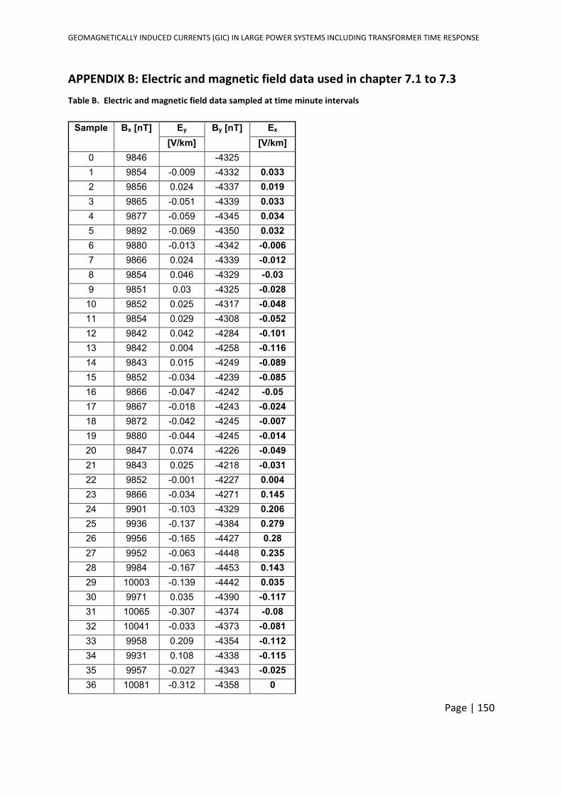
GEOMAGNETICALLY INDUCED CURRENTS (GIC) IN LARGE POWER SYSTEMS INCLUDING TRANSFORMER TIME RESPONSE
Page | 150
APPENDIX B: Electric and magnetic field data used in chapter 7.1 to 7.3
Table B. Electric and magnetic field data sampled at time minute intervals
Sample Bx [nT] Ey By [nT] Ex [V/km] [V/km]
0 9846 -4325 1 9854 -0.009 -4332 0.033 2 9856 0.024 -4337 0.019 3 9865 -0.051 -4339 0.033 4 9877 -0.059 -4345 0.034 5 9892 -0.069 -4350 0.032 6 9880 -0.013 -4342 -0.006 7 9866 0.024 -4339 -0.012 8 9854 0.046 -4329 -0.03 9 9851 0.03 -4325 -0.028
10 9852 0.025 -4317 -0.048 11 9854 0.029 -4308 -0.052 12 9842 0.042 -4284 -0.101 13 9842 0.004 -4258 -0.116 14 9843 0.015 -4249 -0.089 15 9852 -0.034 -4239 -0.085 16 9866 -0.047 -4242 -0.05 17 9867 -0.018 -4243 -0.024 18 9872 -0.042 -4245 -0.007 19 9880 -0.044 -4245 -0.014 20 9847 0.074 -4226 -0.049 21 9843 0.025 -4218 -0.031 22 9852 -0.001 -4227 0.004 23 9866 -0.034 -4271 0.145 24 9901 -0.103 -4329 0.206 25 9936 -0.137 -4384 0.279 26 9956 -0.165 -4427 0.28 27 9952 -0.063 -4448 0.235 28 9984 -0.167 -4453 0.143 29 10003 -0.139 -4442 0.035 30 9971 0.035 -4390 -0.117 31 10065 -0.307 -4374 -0.08 32 10041 -0.033 -4373 -0.081 33 9958 0.209 -4354 -0.112 34 9931 0.108 -4338 -0.115 35 9957 -0.027 -4343 -0.025 36 10081 -0.312 -4358 0
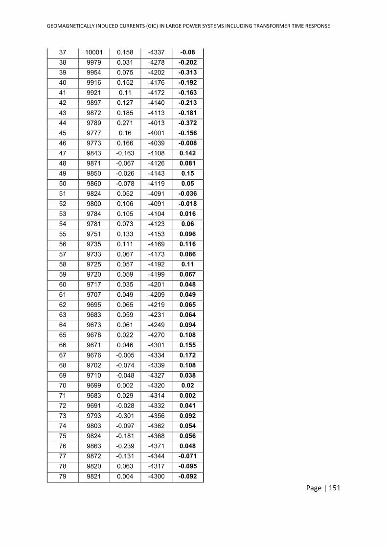
GEOMAGNETICALLY INDUCED CURRENTS (GIC) IN LARGE POWER SYSTEMS INCLUDING TRANSFORMER TIME RESPONSE
Page | 151
37 10001 0.158 -4337 -0.08 38 9979 0.031 -4278 -0.202 39 9954 0.075 -4202 -0.313 40 9916 0.152 -4176 -0.192 41 9921 0.11 -4172 -0.163 42 9897 0.127 -4140 -0.213 43 9872 0.185 -4113 -0.181 44 9789 0.271 -4013 -0.372 45 9777 0.16 -4001 -0.156 46 9773 0.166 -4039 -0.008 47 9843 -0.163 -4108 0.142 48 9871 -0.067 -4126 0.081 49 9850 -0.026 -4143 0.15 50 9860 -0.078 -4119 0.05 51 9824 0.052 -4091 -0.036 52 9800 0.106 -4091 -0.018 53 9784 0.105 -4104 0.016 54 9781 0.073 -4123 0.06 55 9751 0.133 -4153 0.096 56 9735 0.111 -4169 0.116 57 9733 0.067 -4173 0.086 58 9725 0.057 -4192 0.11 59 9720 0.059 -4199 0.067 60 9717 0.035 -4201 0.048 61 9707 0.049 -4209 0.049 62 9695 0.065 -4219 0.065 63 9683 0.059 -4231 0.064 64 9673 0.061 -4249 0.094 65 9678 0.022 -4270 0.108 66 9671 0.046 -4301 0.155 67 9676 -0.005 -4334 0.172 68 9702 -0.074 -4339 0.108 69 9710 -0.048 -4327 0.038 70 9699 0.002 -4320 0.02 71 9683 0.029 -4314 0.002 72 9691 -0.028 -4332 0.041 73 9793 -0.301 -4356 0.092 74 9803 -0.097 -4362 0.054 75 9824 -0.181 -4368 0.056 76 9863 -0.239 -4371 0.048 77 9872 -0.131 -4344 -0.071 78 9820 0.063 -4317 -0.095 79 9821 0.004 -4300 -0.092
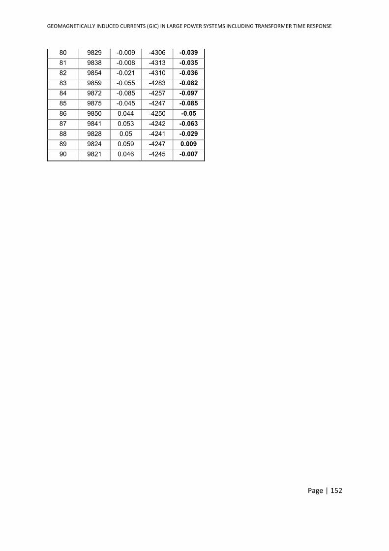
GEOMAGNETICALLY INDUCED CURRENTS (GIC) IN LARGE POWER SYSTEMS INCLUDING TRANSFORMER TIME RESPONSE
Page | 152
80 9829 -0.009 -4306 -0.039 81 9838 -0.008 -4313 -0.035 82 9854 -0.021 -4310 -0.036 83 9859 -0.055 -4283 -0.082 84 9872 -0.085 -4257 -0.097 85 9875 -0.045 -4247 -0.085 86 9850 0.044 -4250 -0.05 87 9841 0.053 -4242 -0.063 88 9828 0.05 -4241 -0.029 89 9824 0.059 -4247 0.009 90 9821 0.046 -4245 -0.007
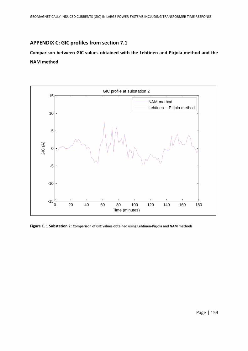
GEOMAGNETICALLY INDUCED CURRENTS (GIC) IN LARGE POWER SYSTEMS INCLUDING TRANSFORMER TIME RESPONSE
Page | 153
APPENDIX C: GIC profiles from section 7.1
Comparison between GIC values obtained with the Lehtinen and Pirjola method and the
NAM method
Figure C. 1 Substation 2: Comparison of GIC values obtained using Lehtinen-Pirjola and NAM methods
0 20 40 60 80 100 120 140 160 180-15
-10
-5
0
5
10
15
Time (minutes)
GIC
(A
)
GIC profile at substation 2
NAM method
Lehtinen -- Pirjola method
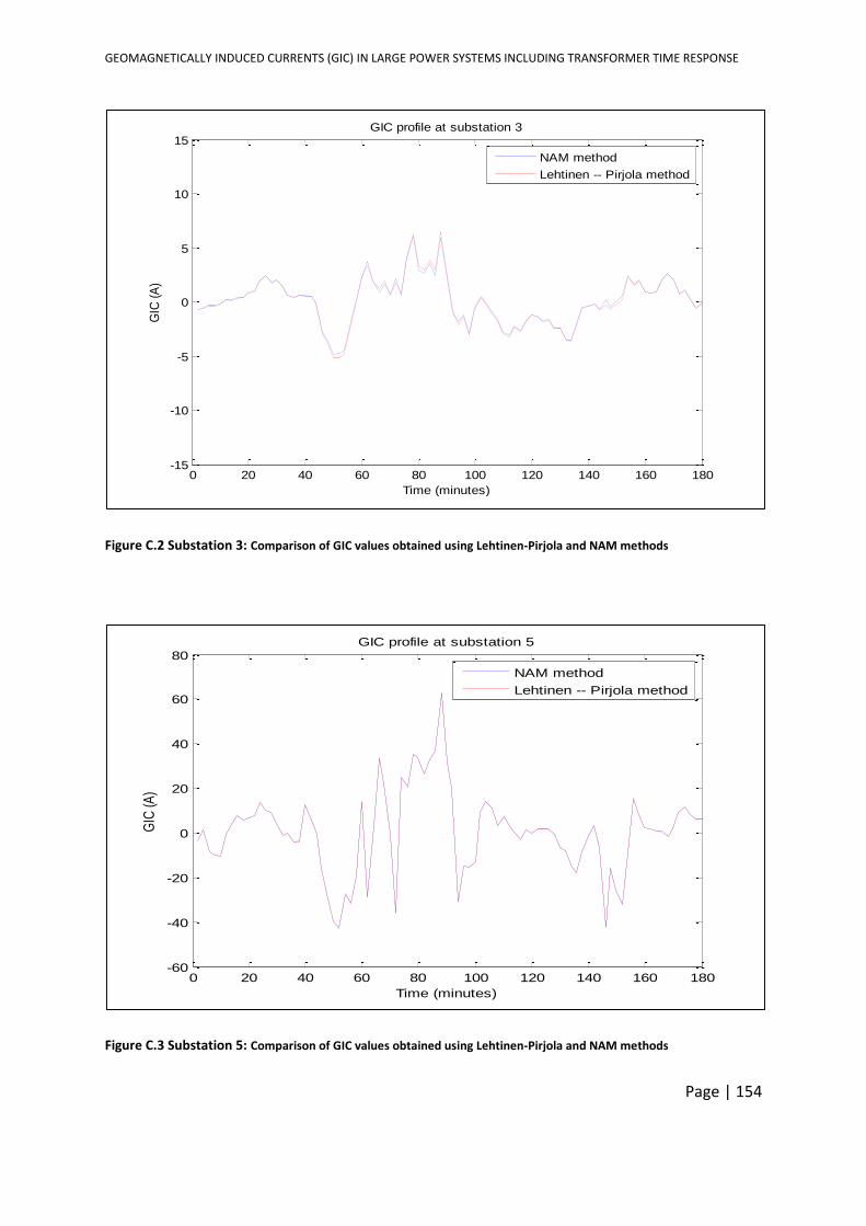
GEOMAGNETICALLY INDUCED CURRENTS (GIC) IN LARGE POWER SYSTEMS INCLUDING TRANSFORMER TIME RESPONSE
Page | 154
Figure C.2 Substation 3: Comparison of GIC values obtained using Lehtinen-Pirjola and NAM methods
Figure C.3 Substation 5: Comparison of GIC values obtained using Lehtinen-Pirjola and NAM methods
0 20 40 60 80 100 120 140 160 180-15
-10
-5
0
5
10
15
Time (minutes)
GIC
(A
)
GIC profile at substation 3
NAM method
Lehtinen -- Pirjola method
0 20 40 60 80 100 120 140 160 180-60
-40
-20
0
20
40
60
80
Time (minutes)
GIC
(A
)
GIC profile at substation 5
NAM method
Lehtinen -- Pirjola method
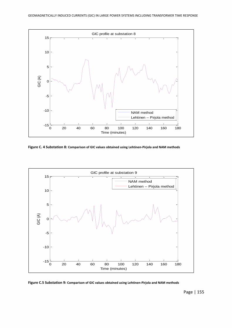
GEOMAGNETICALLY INDUCED CURRENTS (GIC) IN LARGE POWER SYSTEMS INCLUDING TRANSFORMER TIME RESPONSE
Page | 155
Figure C. 4 Substation 8: Comparison of GIC values obtained using Lehtinen-Pirjola and NAM methods
Figure C.5 Substation 9: Comparison of GIC values obtained using Lehtinen-Pirjola and NAM methods
0 20 40 60 80 100 120 140 160 180-15
-10
-5
0
5
10
15
Time (minutes)
GIC
(A
)
GIC profile at substation 8
NAM method
Lehtinen -- Pirjola method
0 20 40 60 80 100 120 140 160 180-15
-10
-5
0
5
10
15
Time (minutes)
GIC
(A
)
GIC profile at substation 9
NAM method
Lehtinen -- Pirjola method
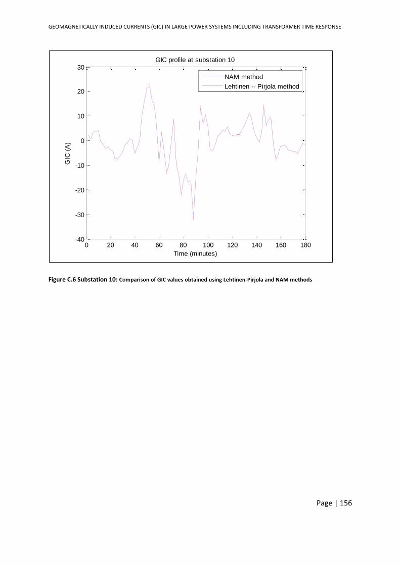
GEOMAGNETICALLY INDUCED CURRENTS (GIC) IN LARGE POWER SYSTEMS INCLUDING TRANSFORMER TIME RESPONSE
Page | 156
Figure C.6 Substation 10: Comparison of GIC values obtained using Lehtinen-Pirjola and NAM methods
0 20 40 60 80 100 120 140 160 180-40
-30
-20
-10
0
10
20
30
Time (minutes)
GIC
(A
)GIC profile at substation 10
NAM method
Lehtinen -- Pirjola method
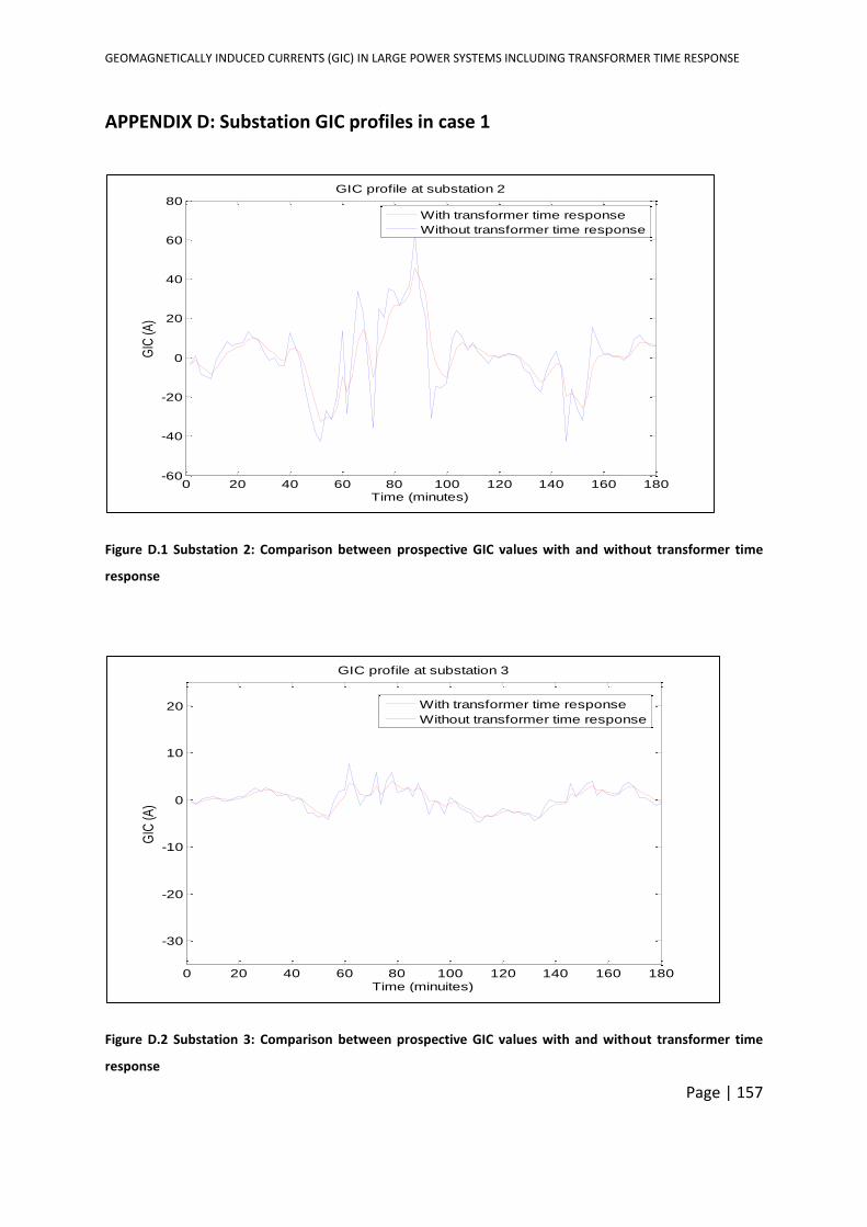
GEOMAGNETICALLY INDUCED CURRENTS (GIC) IN LARGE POWER SYSTEMS INCLUDING TRANSFORMER TIME RESPONSE
Page | 157
APPENDIX D: Substation GIC profiles in case 1
Figure D.1 Substation 2: Comparison between prospective GIC values with and without transformer time
response
Figure D.2 Substation 3: Comparison between prospective GIC values with and without transformer time
response
0 20 40 60 80 100 120 140 160 180-60
-40
-20
0
20
40
60
80
Time (minutes)
GIC
(A)
GIC profile at substation 2
With transformer time response
Without transformer time response
0 20 40 60 80 100 120 140 160 180
-30
-20
-10
0
10
20
Time (minuites)
GIC
(A)
GIC profile at substation 3
With transformer time response
Without transformer time response
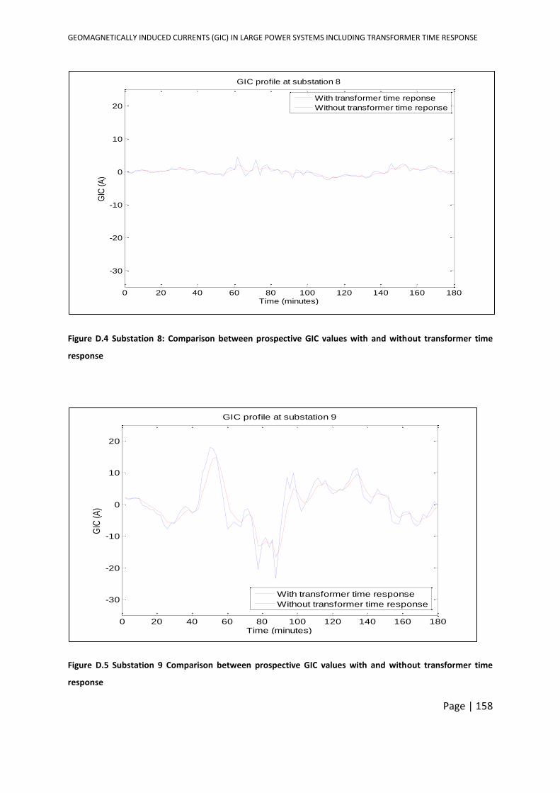
GEOMAGNETICALLY INDUCED CURRENTS (GIC) IN LARGE POWER SYSTEMS INCLUDING TRANSFORMER TIME RESPONSE
Page | 158
Figure D.4 Substation 8: Comparison between prospective GIC values with and without transformer time
response
Figure D.5 Substation 9 Comparison between prospective GIC values with and without transformer time
response
0 20 40 60 80 100 120 140 160 180
-30
-20
-10
0
10
20
Time (minutes)
GIC
(A)
GIC profile at substation 8
With transformer time reponse
Without transformer time reponse
0 20 40 60 80 100 120 140 160 180
-30
-20
-10
0
10
20
Time (minutes)
GIC
(A)
GIC profile at substation 9
With transformer time response
Without transformer time response
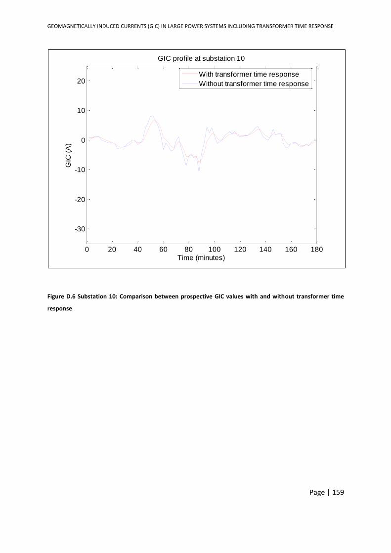
GEOMAGNETICALLY INDUCED CURRENTS (GIC) IN LARGE POWER SYSTEMS INCLUDING TRANSFORMER TIME RESPONSE
Page | 159
Figure D.6 Substation 10: Comparison between prospective GIC values with and without transformer time
response
0 20 40 60 80 100 120 140 160 180
-30
-20
-10
0
10
20
Time (minutes)
GIC
(A
)
GIC profile at substation 10
With transformer time response
Without transformer time response
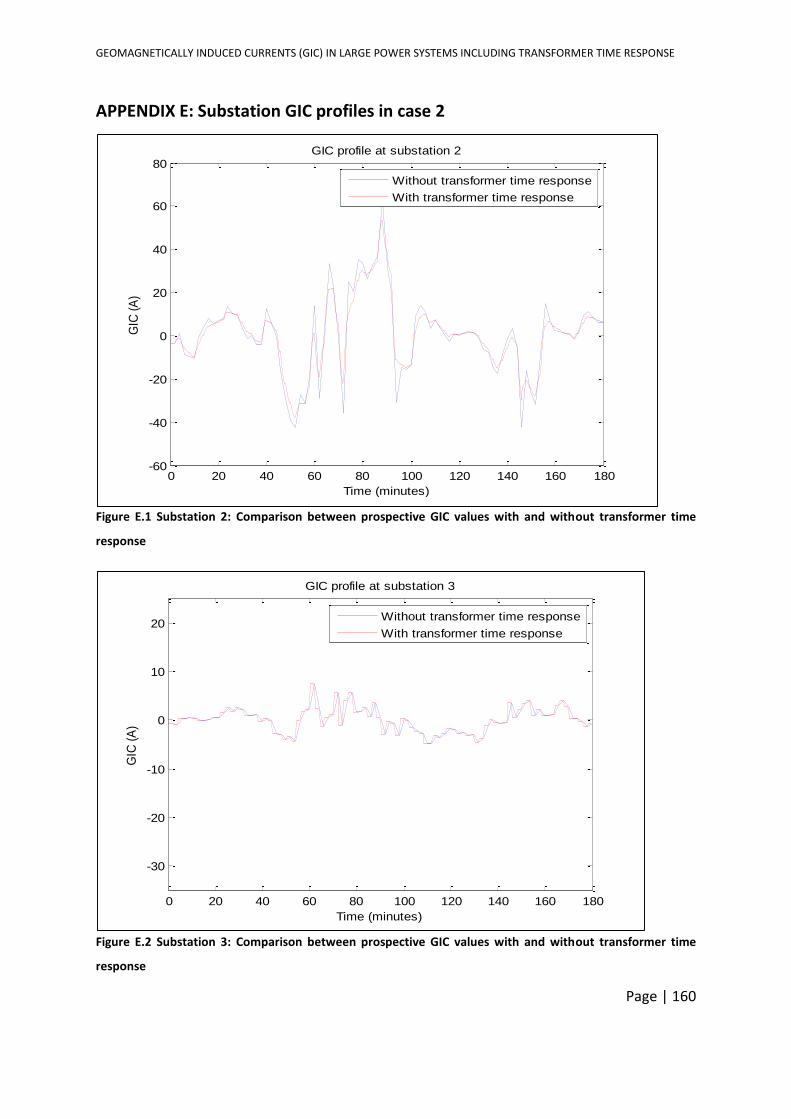
GEOMAGNETICALLY INDUCED CURRENTS (GIC) IN LARGE POWER SYSTEMS INCLUDING TRANSFORMER TIME RESPONSE
Page | 160
APPENDIX E: Substation GIC profiles in case 2
Figure E.1 Substation 2: Comparison between prospective GIC values with and without transformer time
response
Figure E.2 Substation 3: Comparison between prospective GIC values with and without transformer time
response
0 20 40 60 80 100 120 140 160 180-60
-40
-20
0
20
40
60
80
Time (minutes)
GIC
(A
)
GIC profile at substation 2
Without transformer time response
With transformer time response
0 20 40 60 80 100 120 140 160 180
-30
-20
-10
0
10
20
Time (minutes)
GIC
(A
)
GIC profile at substation 3
Without transformer time response
With transformer time response
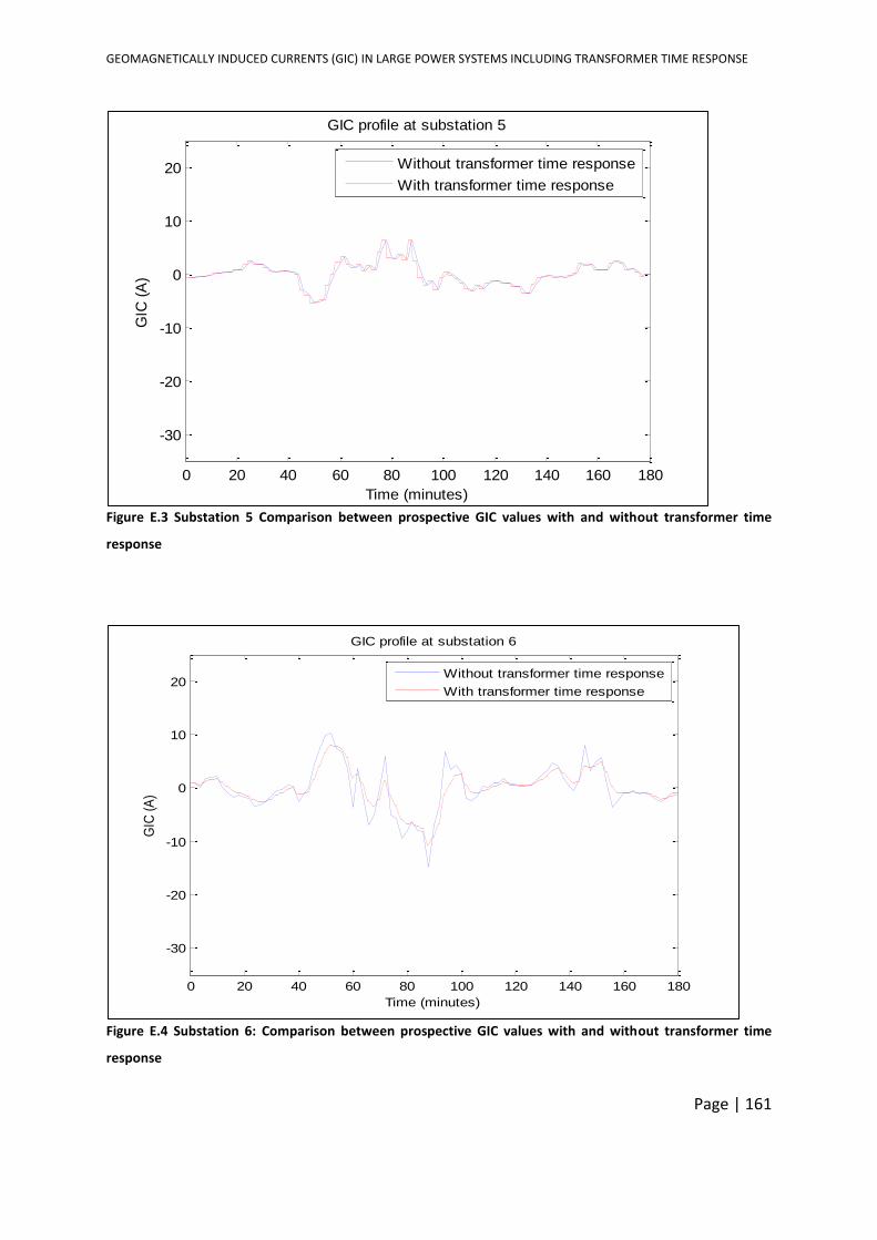
GEOMAGNETICALLY INDUCED CURRENTS (GIC) IN LARGE POWER SYSTEMS INCLUDING TRANSFORMER TIME RESPONSE
Page | 161
Figure E.3 Substation 5 Comparison between prospective GIC values with and without transformer time
response
Figure E.4 Substation 6: Comparison between prospective GIC values with and without transformer time
response
0 20 40 60 80 100 120 140 160 180
-30
-20
-10
0
10
20
Time (minutes)
GIC
(A
)GIC profile at substation 5
Without transformer time response
With transformer time response
0 20 40 60 80 100 120 140 160 180
-30
-20
-10
0
10
20
Time (minutes)
GIC
(A
)
GIC profile at substation 6
Without transformer time response
With transformer time response
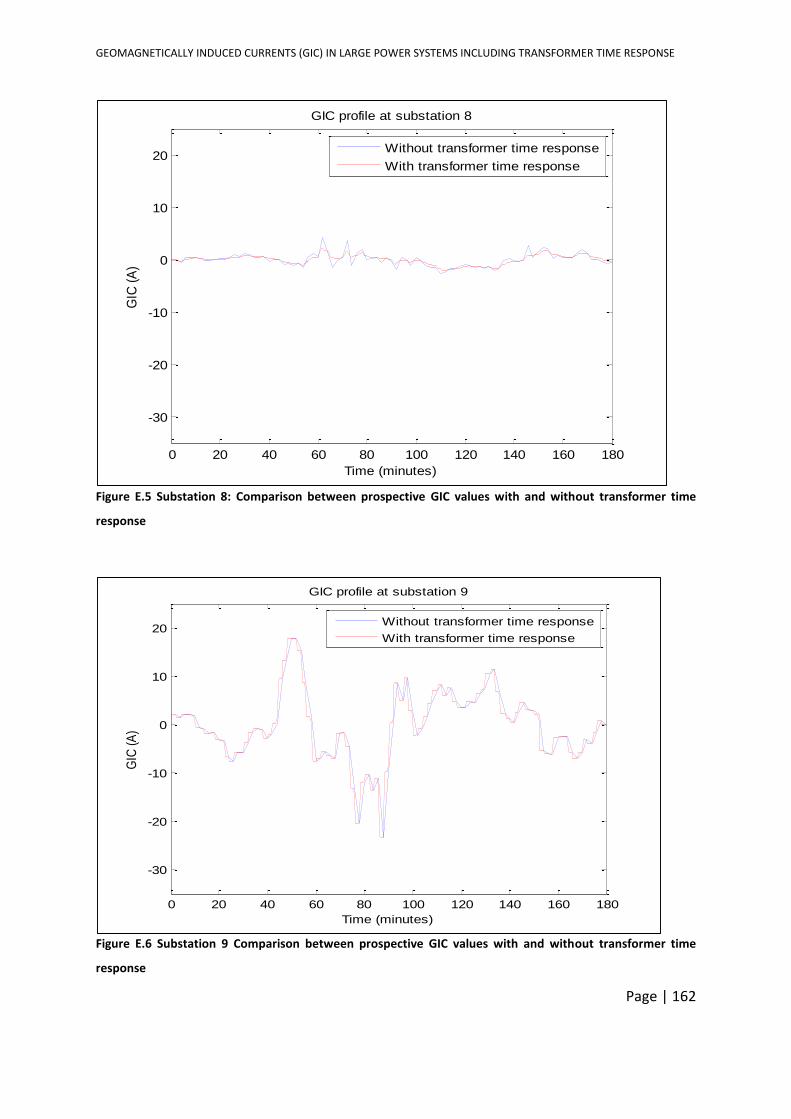
GEOMAGNETICALLY INDUCED CURRENTS (GIC) IN LARGE POWER SYSTEMS INCLUDING TRANSFORMER TIME RESPONSE
Page | 162
Figure E.5 Substation 8: Comparison between prospective GIC values with and without transformer time
response
Figure E.6 Substation 9 Comparison between prospective GIC values with and without transformer time
response
0 20 40 60 80 100 120 140 160 180
-30
-20
-10
0
10
20
Time (minutes)
GIC
(A
)GIC profile at substation 8
Without transformer time response
With transformer time response
0 20 40 60 80 100 120 140 160 180
-30
-20
-10
0
10
20
Time (minutes)
GIC
(A
)
GIC profile at substation 9
Without transformer time response
With transformer time response
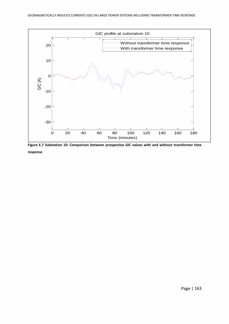
GEOMAGNETICALLY INDUCED CURRENTS (GIC) IN LARGE POWER SYSTEMS INCLUDING TRANSFORMER TIME RESPONSE
Page | 163
Figure E.7 Substation 10: Comparison between prospective GIC values with and without transformer time
response
0 20 40 60 80 100 120 140 160 180
-30
-20
-10
0
10
20
Time (minutes)
GIC
(A
)
GIC profile at substation 10
Without transformer time response
With transformer time response
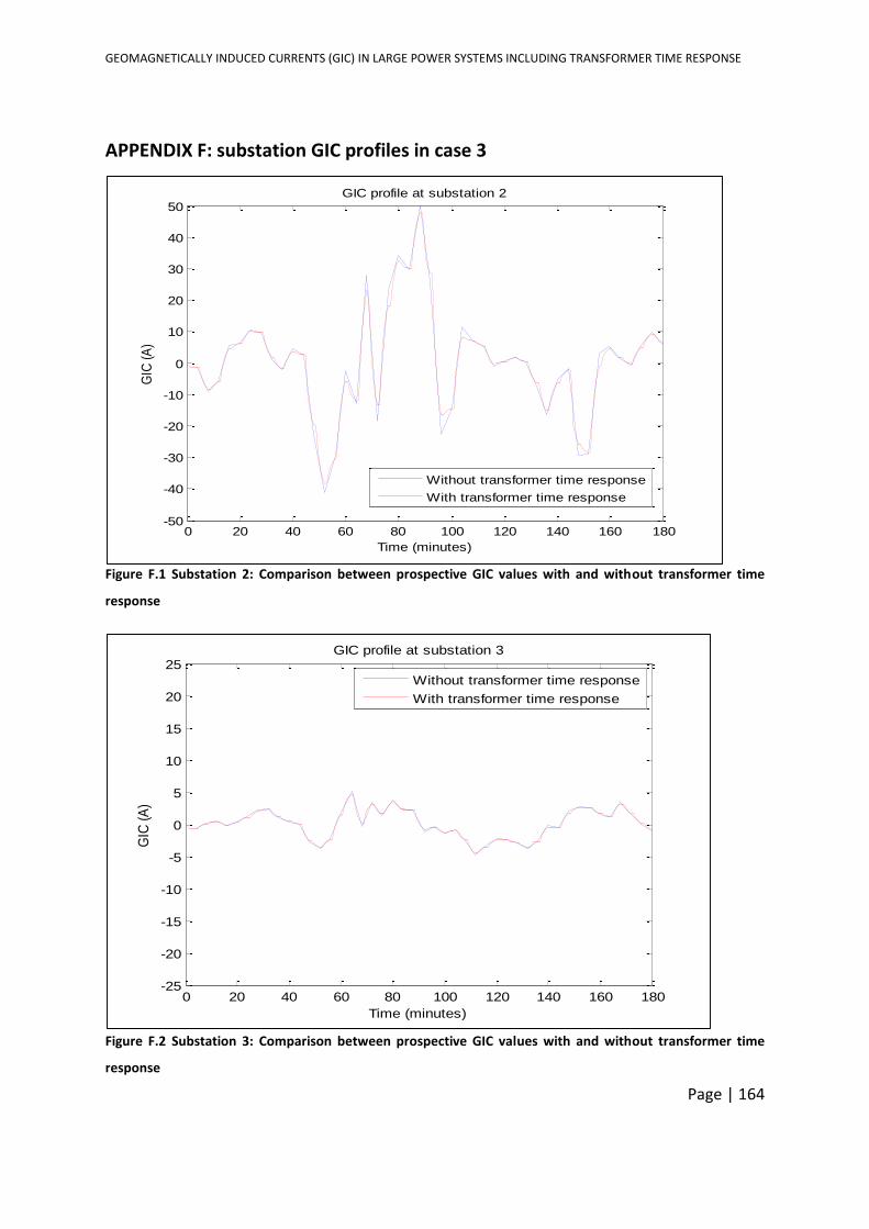
GEOMAGNETICALLY INDUCED CURRENTS (GIC) IN LARGE POWER SYSTEMS INCLUDING TRANSFORMER TIME RESPONSE
Page | 164
APPENDIX F: substation GIC profiles in case 3
Figure F.1 Substation 2: Comparison between prospective GIC values with and without transformer time
response
Figure F.2 Substation 3: Comparison between prospective GIC values with and without transformer time
response
0 20 40 60 80 100 120 140 160 180-50
-40
-30
-20
-10
0
10
20
30
40
50
Time (minutes)
GIC
(A
)
GIC profile at substation 2
Without transformer time response
With transformer time response
0 20 40 60 80 100 120 140 160 180-25
-20
-15
-10
-5
0
5
10
15
20
25
Time (minutes)
GIC
(A
)
GIC profile at substation 3
Without transformer time response
With transformer time response
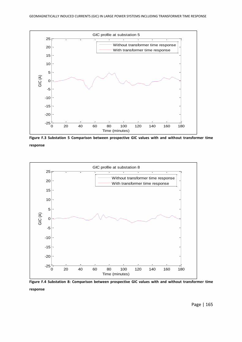
GEOMAGNETICALLY INDUCED CURRENTS (GIC) IN LARGE POWER SYSTEMS INCLUDING TRANSFORMER TIME RESPONSE
Page | 165
Figure F.3 Substation 5 Comparison between prospective GIC values with and without transformer time
response
Figure F.4 Substation 8: Comparison between prospective GIC values with and without transformer time
response
0 20 40 60 80 100 120 140 160 180-25
-20
-15
-10
-5
0
5
10
15
20
25
Time (minutes)
GIC
(A
)GIC profile at substation 5
Without transformer time response
With transformer time response
0 20 40 60 80 100 120 140 160 180-25
-20
-15
-10
-5
0
5
10
15
20
25
Time (minutes)
GIC
(A
)
GIC profile at substation 8
Without transformer time response
With transformer time response
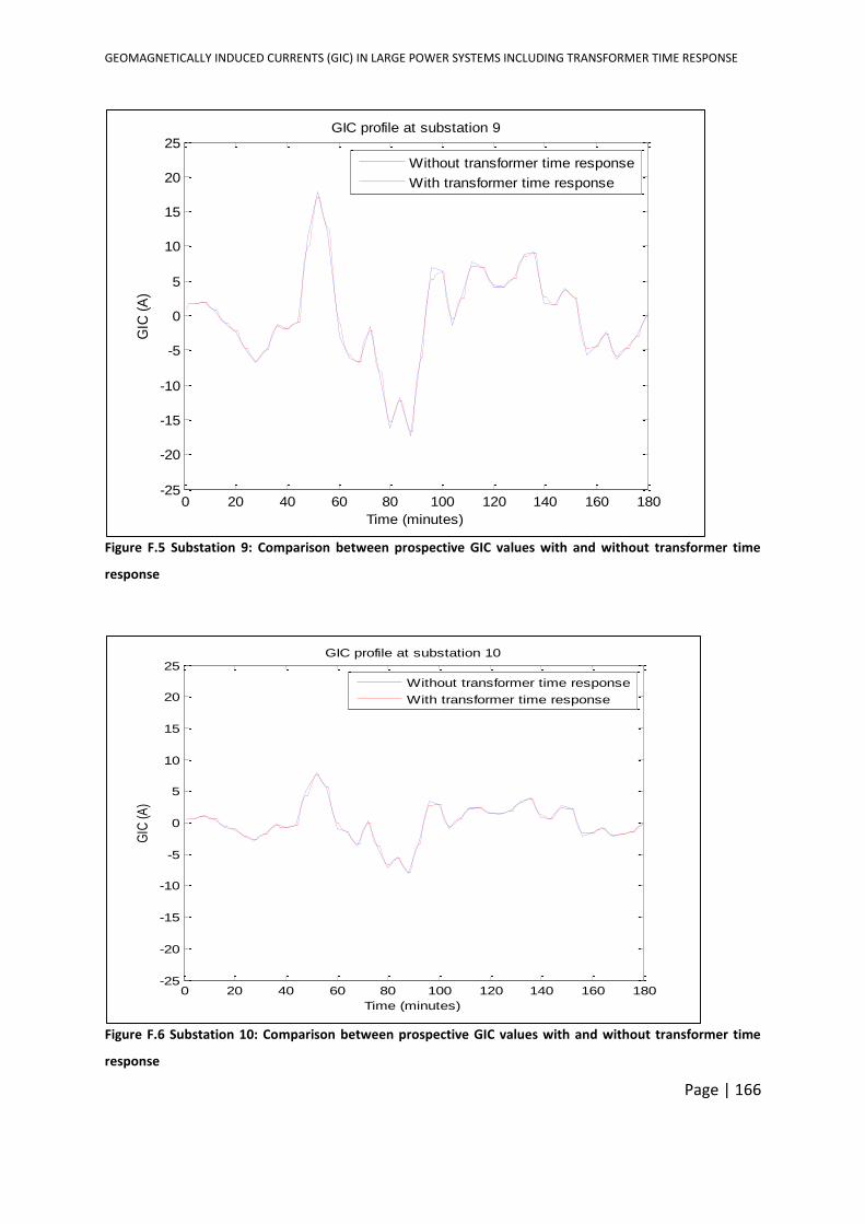
GEOMAGNETICALLY INDUCED CURRENTS (GIC) IN LARGE POWER SYSTEMS INCLUDING TRANSFORMER TIME RESPONSE
Page | 166
Figure F.5 Substation 9: Comparison between prospective GIC values with and without transformer time
response
Figure F.6 Substation 10: Comparison between prospective GIC values with and without transformer time
response
0 20 40 60 80 100 120 140 160 180-25
-20
-15
-10
-5
0
5
10
15
20
25
Time (minutes)
GIC
(A
)GIC profile at substation 9
Without transformer time response
With transformer time response
0 20 40 60 80 100 120 140 160 180-25
-20
-15
-10
-5
0
5
10
15
20
25
Time (minutes)
GIC
(A
)
GIC profile at substation 10
Without transformer time response
With transformer time response
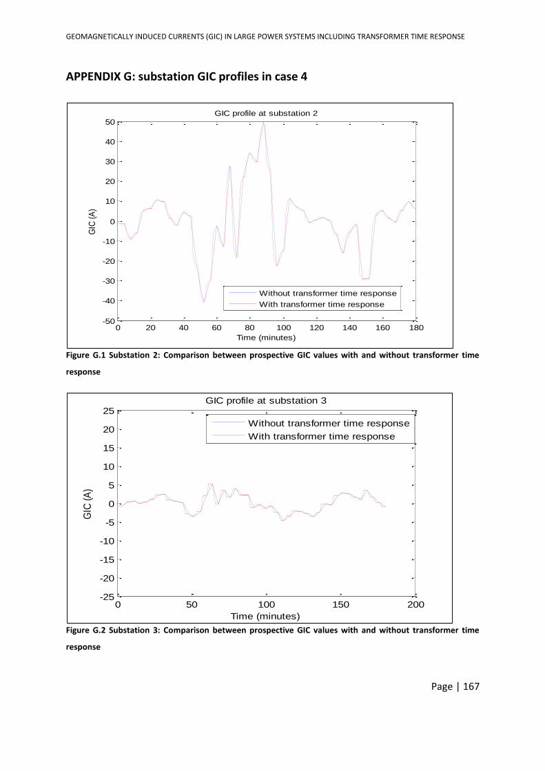
GEOMAGNETICALLY INDUCED CURRENTS (GIC) IN LARGE POWER SYSTEMS INCLUDING TRANSFORMER TIME RESPONSE
Page | 167
APPENDIX G: substation GIC profiles in case 4
Figure G.1 Substation 2: Comparison between prospective GIC values with and without transformer time
response
Figure G.2 Substation 3: Comparison between prospective GIC values with and without transformer time
response
0 20 40 60 80 100 120 140 160 180-50
-40
-30
-20
-10
0
10
20
30
40
50
Time (minutes)
GIC
(A
)
GIC profile at substation 2
Without transformer time response
With transformer time response
0 50 100 150 200-25
-20
-15
-10
-5
0
5
10
15
20
25
Time (minutes)
GIC
(A
)
GIC profile at substation 3
Without transformer time response
With transformer time response
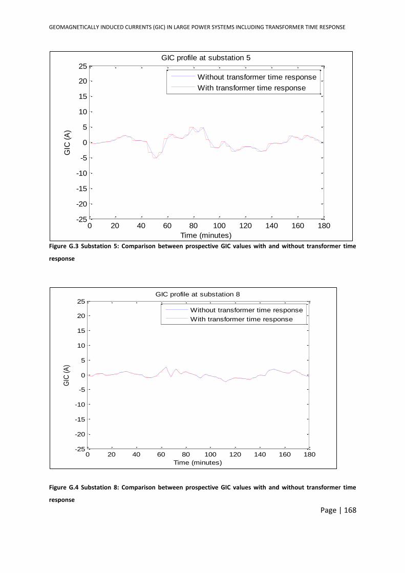
GEOMAGNETICALLY INDUCED CURRENTS (GIC) IN LARGE POWER SYSTEMS INCLUDING TRANSFORMER TIME RESPONSE
Page | 168
Figure G.3 Substation 5: Comparison between prospective GIC values with and without transformer time
response
Figure G.4 Substation 8: Comparison between prospective GIC values with and without transformer time
response
0 20 40 60 80 100 120 140 160 180-25
-20
-15
-10
-5
0
5
10
15
20
25
Time (minutes)
GIC
(A
)GIC profile at substation 5
Without transformer time response
With transformer time response
0 20 40 60 80 100 120 140 160 180-25
-20
-15
-10
-5
0
5
10
15
20
25
Time (minutes)
GIC
(A
)
GIC profile at substation 8
Without transformer time response
With transformer time response
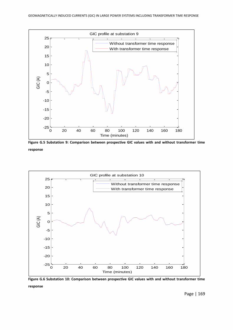
GEOMAGNETICALLY INDUCED CURRENTS (GIC) IN LARGE POWER SYSTEMS INCLUDING TRANSFORMER TIME RESPONSE
Page | 169
Figure G.5 Substation 9: Comparison between prospective GIC values with and without transformer time
response
Figure G.6 Substation 10: Comparison between prospective GIC values with and without transformer time
response
0 20 40 60 80 100 120 140 160 180-25
-20
-15
-10
-5
0
5
10
15
20
25
Time (minutes)
GIC
(A
)GIC profile at substation 9
Without transformer time response
With transformer time response
0 20 40 60 80 100 120 140 160 180-25
-20
-15
-10
-5
0
5
10
15
20
25
Time (minutes)
GIC
(A)
GIC profile at substation 10
Without transformer time response
With transformer time response
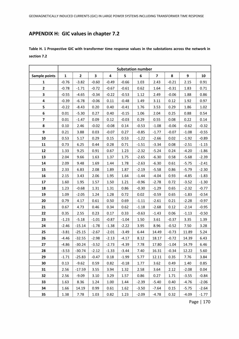
GEOMAGNETICALLY INDUCED CURRENTS (GIC) IN LARGE POWER SYSTEMS INCLUDING TRANSFORMER TIME RESPONSE
Page | 170
APPENDIX H: GIC values in chapter 7.2
Table H. 1 Prospective GIC with transformer time response values in the substations across the network in
section 7.2
Substation number
Sample points 1 2 3 4 5 6 7 8 9 10
1 -0.76 -3.82 -0.60 -0.49 -0.66 1.03 2.43 -0.21 2.15 0.91
2 -0.78 -1.71 -0.72 -0.67 -0.61 0.62 1.64 -0.31 1.83 0.71
3 -0.55 -4.65 -0.34 -0.22 -0.53 1.12 2.49 -0.06 1.88 0.86
4 -0.39 -6.78 -0.06 0.11 -0.48 1.49 3.11 0.12 1.92 0.97
5 -0.22 -8.43 0.20 0.40 -0.41 1.76 3.53 0.29 1.86 1.02
6 0.01 -5.30 0.27 0.40 -0.15 1.06 2.04 0.25 0.88 0.54
7 0.01 -1.47 0.09 0.12 -0.03 0.29 0.55 0.08 0.22 0.14
8 0.10 2.46 -0.02 -0.08 0.14 -0.53 -1.08 -0.06 -0.62 -0.32
9 0.21 3.88 0.03 -0.07 0.27 -0.85 -1.77 -0.07 -1.08 -0.55
10 0.53 5.17 0.29 0.15 0.53 -1.22 -2.66 0.02 -1.92 -0.89
11 0.73 6.25 0.44 0.28 0.71 -1.51 -3.34 0.08 -2.51 -1.15
12 1.33 9.25 0.91 0.67 1.23 -2.32 -5.24 0.24 -4.20 -1.86
13 2.04 9.66 1.63 1.37 1.75 -2.65 -6.30 0.58 -5.68 -2.39
14 2.09 9.48 1.69 1.44 1.78 -2.63 -6.30 0.61 -5.75 -2.41
15 2.33 6.83 2.08 1.89 1.87 -2.19 -5.58 0.86 -5.79 -2.30
16 2.15 3.43 2.06 1.95 1.64 -1.44 -4.04 0.93 -4.85 -1.83
17 1.60 1.95 1.57 1.50 1.21 -0.96 -2.78 0.72 -3.52 -1.30
18 1.23 -0.68 1.31 1.31 0.86 -0.30 -1.29 0.65 -2.32 -0.77
19 1.09 -2.05 1.24 1.28 0.72 0.02 -0.59 0.65 -1.83 -0.54
20 0.79 4.17 0.61 0.50 0.69 -1.11 -2.61 0.21 -2.28 -0.97
21 0.67 4.73 0.46 0.34 0.62 -1.18 -2.68 0.12 -2.14 -0.95
22 0.35 2.55 0.23 0.17 0.33 -0.63 -1.43 0.06 -1.13 -0.50
23 -1.23 -5.18 -1.01 -0.87 -1.04 1.50 3.61 -0.37 3.35 1.39
24 -2.46 -15.14 -1.78 -1.38 -2.22 3.95 8.96 -0.52 7.50 3.28
25 -3.81 -25.15 -2.67 -2.01 -3.49 6.44 14.49 -0.73 11.89 5.24
26 -4.46 -32.55 -2.98 -2.13 -4.17 8.12 18.17 -0.72 14.39 6.43
27 -4.86 -30.24 -3.52 -2.73 -4.39 7.78 17.80 -1.04 14.79 6.46
28 -3.53 -30.74 -2.12 -1.33 -3.44 7.40 16.31 -0.34 12.22 5.60
29 -1.71 -25.83 -0.47 0.18 -1.99 5.77 12.11 0.35 7.76 3.84
30 0.13 -9.62 0.59 0.82 -0.18 1.77 3.62 0.49 1.40 0.85
31 2.56 -17.59 3.55 3.94 1.32 2.58 3.64 2.12 -2.08 0.04
32 2.56 -9.09 3.10 3.29 1.57 0.86 0.27 1.71 -3.55 -0.84
33 1.63 8.36 1.24 1.00 1.44 -2.39 -5.40 0.40 -4.76 -2.06
34 1.66 14.19 0.99 0.61 1.62 -3.50 -7.64 0.15 -5.75 -2.64
35 1.38 7.78 1.03 0.82 1.23 -2.09 -4.78 0.32 -4.09 -1.77
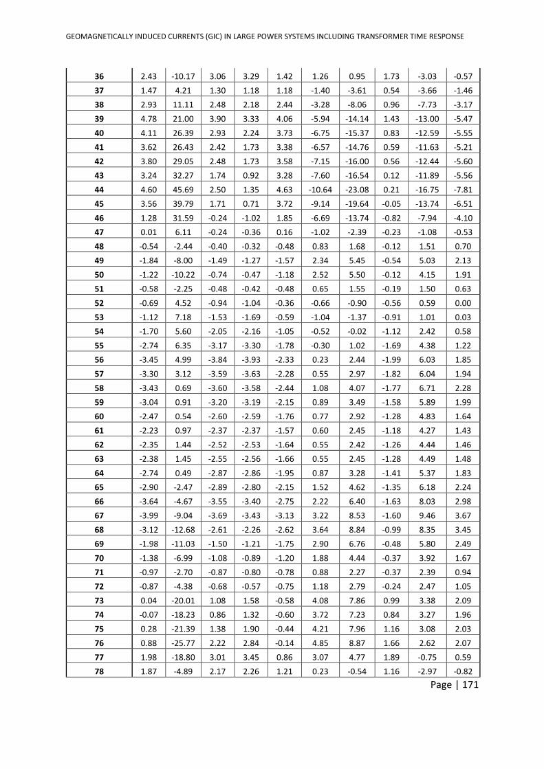
GEOMAGNETICALLY INDUCED CURRENTS (GIC) IN LARGE POWER SYSTEMS INCLUDING TRANSFORMER TIME RESPONSE
Page | 171
36 2.43 -10.17 3.06 3.29 1.42 1.26 0.95 1.73 -3.03 -0.57
37 1.47 4.21 1.30 1.18 1.18 -1.40 -3.61 0.54 -3.66 -1.46
38 2.93 11.11 2.48 2.18 2.44 -3.28 -8.06 0.96 -7.73 -3.17
39 4.78 21.00 3.90 3.33 4.06 -5.94 -14.14 1.43 -13.00 -5.47
40 4.11 26.39 2.93 2.24 3.73 -6.75 -15.37 0.83 -12.59 -5.55
41 3.62 26.43 2.42 1.73 3.38 -6.57 -14.76 0.59 -11.63 -5.21
42 3.80 29.05 2.48 1.73 3.58 -7.15 -16.00 0.56 -12.44 -5.60
43 3.24 32.27 1.74 0.92 3.28 -7.60 -16.54 0.12 -11.89 -5.56
44 4.60 45.69 2.50 1.35 4.63 -10.64 -23.08 0.21 -16.75 -7.81
45 3.56 39.79 1.71 0.71 3.72 -9.14 -19.64 -0.05 -13.74 -6.51
46 1.28 31.59 -0.24 -1.02 1.85 -6.69 -13.74 -0.82 -7.94 -4.10
47 0.01 6.11 -0.24 -0.36 0.16 -1.02 -2.39 -0.23 -1.08 -0.53
48 -0.54 -2.44 -0.40 -0.32 -0.48 0.83 1.68 -0.12 1.51 0.70
49 -1.84 -8.00 -1.49 -1.27 -1.57 2.34 5.45 -0.54 5.03 2.13
50 -1.22 -10.22 -0.74 -0.47 -1.18 2.52 5.50 -0.12 4.15 1.91
51 -0.58 -2.25 -0.48 -0.42 -0.48 0.65 1.55 -0.19 1.50 0.63
52 -0.69 4.52 -0.94 -1.04 -0.36 -0.66 -0.90 -0.56 0.59 0.00
53 -1.12 7.18 -1.53 -1.69 -0.59 -1.04 -1.37 -0.91 1.01 0.03
54 -1.70 5.60 -2.05 -2.16 -1.05 -0.52 -0.02 -1.12 2.42 0.58
55 -2.74 6.35 -3.17 -3.30 -1.78 -0.30 1.02 -1.69 4.38 1.22
56 -3.45 4.99 -3.84 -3.93 -2.33 0.23 2.44 -1.99 6.03 1.85
57 -3.30 3.12 -3.59 -3.63 -2.28 0.55 2.97 -1.82 6.04 1.94
58 -3.43 0.69 -3.60 -3.58 -2.44 1.08 4.07 -1.77 6.71 2.28
59 -3.04 0.91 -3.20 -3.19 -2.15 0.89 3.49 -1.58 5.89 1.99
60 -2.47 0.54 -2.60 -2.59 -1.76 0.77 2.92 -1.28 4.83 1.64
61 -2.23 0.97 -2.37 -2.37 -1.57 0.60 2.45 -1.18 4.27 1.43
62 -2.35 1.44 -2.52 -2.53 -1.64 0.55 2.42 -1.26 4.44 1.46
63 -2.38 1.45 -2.55 -2.56 -1.66 0.55 2.45 -1.28 4.49 1.48
64 -2.74 0.49 -2.87 -2.86 -1.95 0.87 3.28 -1.41 5.37 1.83
65 -2.90 -2.47 -2.89 -2.80 -2.15 1.52 4.62 -1.35 6.18 2.24
66 -3.64 -4.67 -3.55 -3.40 -2.75 2.22 6.40 -1.63 8.03 2.98
67 -3.99 -9.04 -3.69 -3.43 -3.13 3.22 8.53 -1.60 9.46 3.67
68 -3.12 -12.68 -2.61 -2.26 -2.62 3.64 8.84 -0.99 8.35 3.45
69 -1.98 -11.03 -1.50 -1.21 -1.75 2.90 6.76 -0.48 5.80 2.49
70 -1.38 -6.99 -1.08 -0.89 -1.20 1.88 4.44 -0.37 3.92 1.67
71 -0.97 -2.70 -0.87 -0.80 -0.78 0.88 2.27 -0.37 2.39 0.94
72 -0.87 -4.38 -0.68 -0.57 -0.75 1.18 2.79 -0.24 2.47 1.05
73 0.04 -20.01 1.08 1.58 -0.58 4.08 7.86 0.99 3.38 2.09
74 -0.07 -18.23 0.86 1.32 -0.60 3.72 7.23 0.84 3.27 1.96
75 0.28 -21.39 1.38 1.90 -0.44 4.21 7.96 1.16 3.08 2.03
76 0.88 -25.77 2.22 2.84 -0.14 4.85 8.87 1.66 2.62 2.07
77 1.98 -18.80 3.01 3.45 0.86 3.07 4.77 1.89 -0.75 0.59
78 1.87 -4.89 2.17 2.26 1.21 0.23 -0.54 1.16 -2.97 -0.82
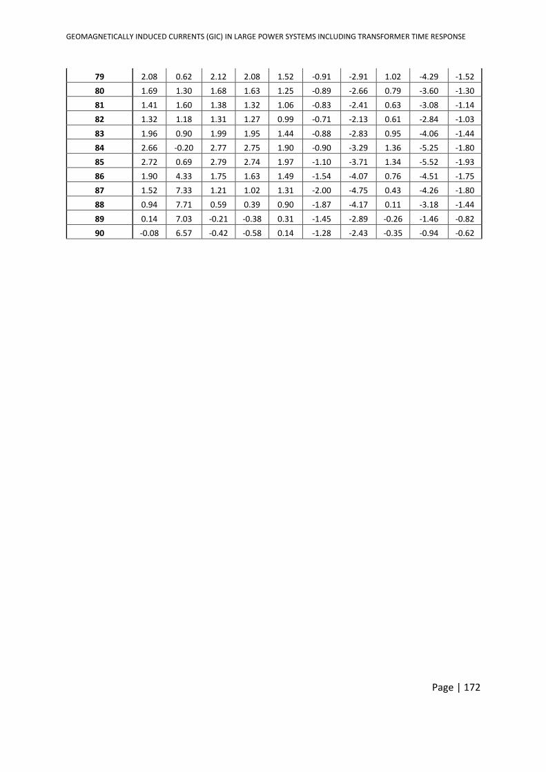
GEOMAGNETICALLY INDUCED CURRENTS (GIC) IN LARGE POWER SYSTEMS INCLUDING TRANSFORMER TIME RESPONSE
Page | 172
79 2.08 0.62 2.12 2.08 1.52 -0.91 -2.91 1.02 -4.29 -1.52
80 1.69 1.30 1.68 1.63 1.25 -0.89 -2.66 0.79 -3.60 -1.30
81 1.41 1.60 1.38 1.32 1.06 -0.83 -2.41 0.63 -3.08 -1.14
82 1.32 1.18 1.31 1.27 0.99 -0.71 -2.13 0.61 -2.84 -1.03
83 1.96 0.90 1.99 1.95 1.44 -0.88 -2.83 0.95 -4.06 -1.44
84 2.66 -0.20 2.77 2.75 1.90 -0.90 -3.29 1.36 -5.25 -1.80
85 2.72 0.69 2.79 2.74 1.97 -1.10 -3.71 1.34 -5.52 -1.93
86 1.90 4.33 1.75 1.63 1.49 -1.54 -4.07 0.76 -4.51 -1.75
87 1.52 7.33 1.21 1.02 1.31 -2.00 -4.75 0.43 -4.26 -1.80
88 0.94 7.71 0.59 0.39 0.90 -1.87 -4.17 0.11 -3.18 -1.44
89 0.14 7.03 -0.21 -0.38 0.31 -1.45 -2.89 -0.26 -1.46 -0.82
90 -0.08 6.57 -0.42 -0.58 0.14 -1.28 -2.43 -0.35 -0.94 -0.62
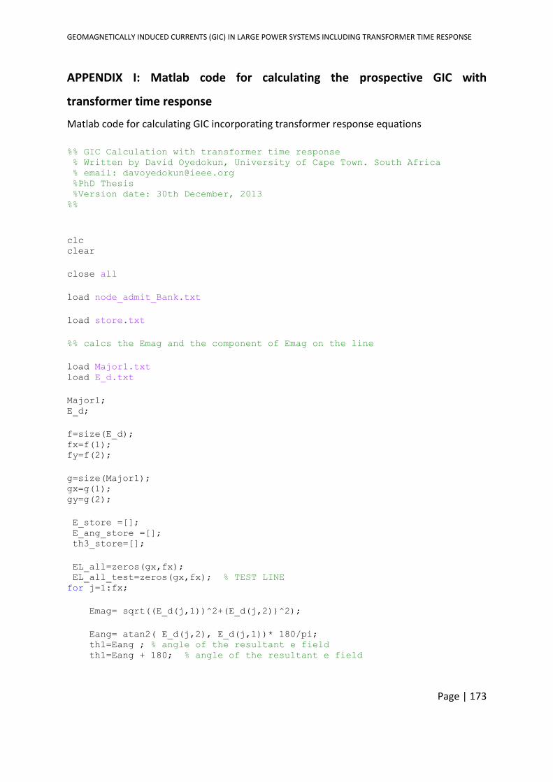
GEOMAGNETICALLY INDUCED CURRENTS (GIC) IN LARGE POWER SYSTEMS INCLUDING TRANSFORMER TIME RESPONSE
Page | 173
APPENDIX I: Matlab code for calculating the prospective GIC with
transformer time response
Matlab code for calculating GIC incorporating transformer response equations
%% GIC Calculation with transformer time response % Written by David Oyedokun, University of Cape Town. South Africa
% email: [email protected] %PhD Thesis %Version date: 30th December, 2013 %%
clc clear
close all
load node_admit_Bank.txt
load store.txt
%% calcs the Emag and the component of Emag on the line
load Major1.txt load E_d.txt
Major1; E_d;
f=size(E_d); fx=f(1); fy=f(2);
g=size(Major1); gx=g(1); gy=g(2);
E_store =[]; E_ang_store =[]; th3_store=[];
EL_all=zeros(gx,fx); EL_all_test=zeros(gx,fx); % TEST LINE for j=1:fx;
Emag= sqrt((E_d(j,1))^2+(E_d(j,2))^2);
Eang= atan2( E_d(j,2), E_d(j,1))* 180/pi; th1=Eang ; % angle of the resultant e field th1=Eang + 180; % angle of the resultant e field
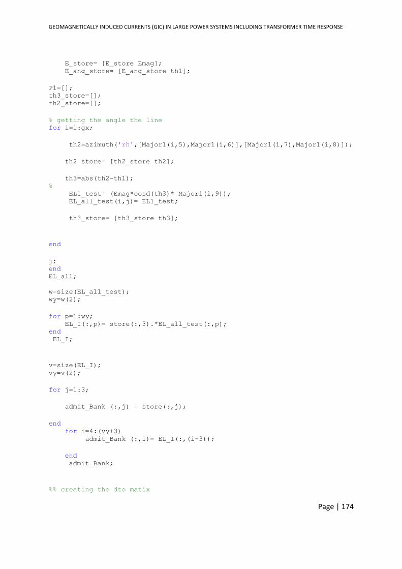
GEOMAGNETICALLY INDUCED CURRENTS (GIC) IN LARGE POWER SYSTEMS INCLUDING TRANSFORMER TIME RESPONSE
Page | 174
E_store= [E_store Emag]; E_ang_store= [E_ang_store th1];
P1=[]; th3_store=[]; th2_store=[];
% getting the angle the line for i=1:gx;
th2=azimuth('rh',[Major1(i,5),Major1(i,6)],[Major1(i,7),Major1(i,8)]);
th2_store= [th2_store th2];
th3=abs(th2-th1); % EL1_test= (Emag*cosd(th3)* Major1(i,9)); EL_all_test(i,j)= EL1_test;
th3_store= [th3_store th3];
end
j; end EL_all;
w=size(EL_all_test); wy=w(2);
for p=1:wy; EL_I(:,p)= store(:,3).*EL_all_test(:,p); end EL_I;
v=size(EL_I); vy=v(2);
for j=1:3;
admit_Bank (:,j) = store(:,j);
end for i=4:(vy+3) admit_Bank (:,i)= EL_I(:,(i-3));
end admit_Bank;
%% creating the dto matix
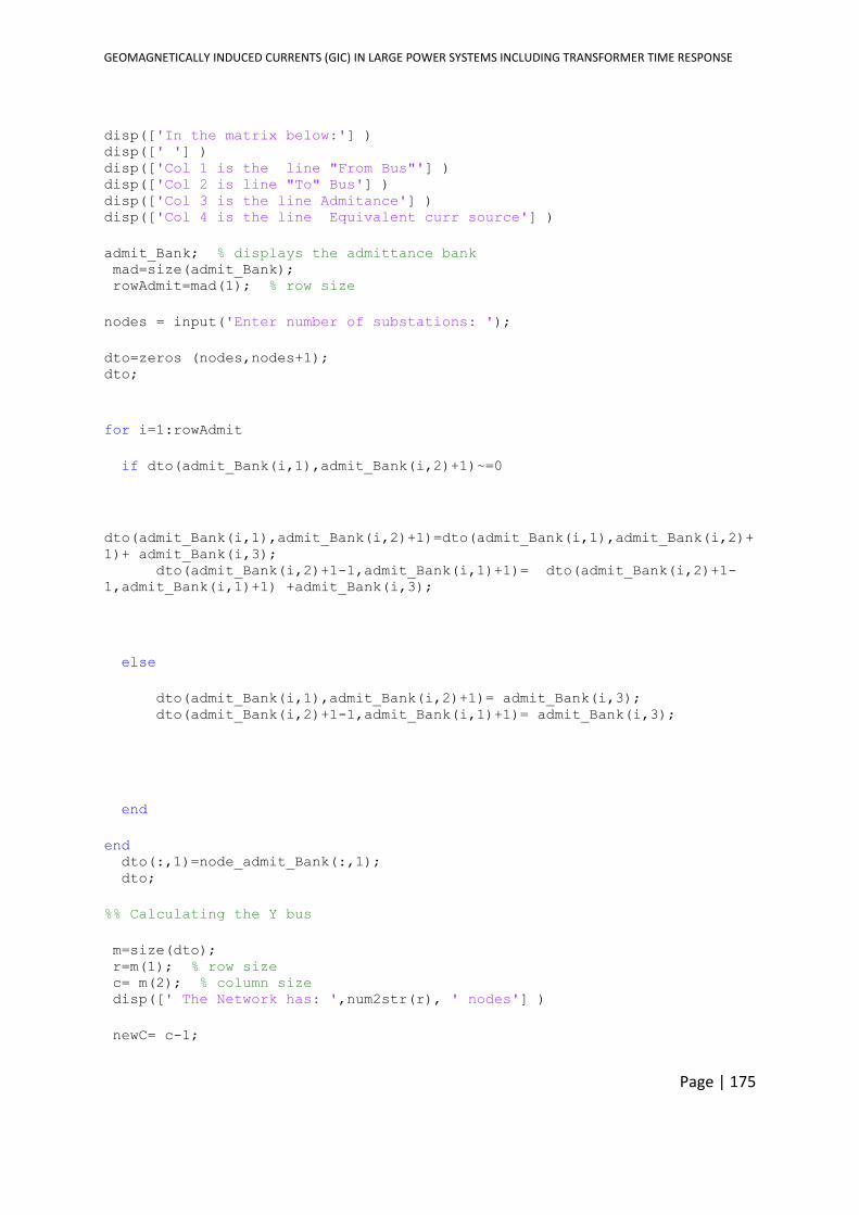
GEOMAGNETICALLY INDUCED CURRENTS (GIC) IN LARGE POWER SYSTEMS INCLUDING TRANSFORMER TIME RESPONSE
Page | 175
disp(['In the matrix below:'] ) disp([' '] ) disp(['Col 1 is the line "From Bus"'] ) disp(['Col 2 is line "To" Bus'] ) disp(['Col 3 is the line Admitance'] ) disp(['Col 4 is the line Equivalent curr source'] )
admit_Bank; % displays the admittance bank mad=size(admit_Bank); rowAdmit=mad(1); % row size
nodes = input('Enter number of substations: ');
dto=zeros (nodes,nodes+1); dto;
for i=1:rowAdmit
if dto(admit_Bank(i,1),admit_Bank(i,2)+1)~=0
dto(admit_Bank(i,1),admit_Bank(i,2)+1)=dto(admit_Bank(i,1),admit_Bank(i,2)+
1)+ admit_Bank(i,3); dto(admit_Bank(i,2)+1-1,admit_Bank(i,1)+1)= dto(admit_Bank(i,2)+1-
1,admit_Bank(i,1)+1) +admit_Bank(i,3);
else
dto(admit_Bank(i,1),admit_Bank(i,2)+1)= admit_Bank(i,3); dto(admit_Bank(i,2)+1-1,admit_Bank(i,1)+1)= admit_Bank(i,3);
end
end dto(:,1)=node_admit_Bank(:,1); dto;
%% Calculating the Y bus
m=size(dto); r=m(1); % row size c= m(2); % column size disp([' The Network has: ',num2str(r), ' nodes'] )
newC= c-1;
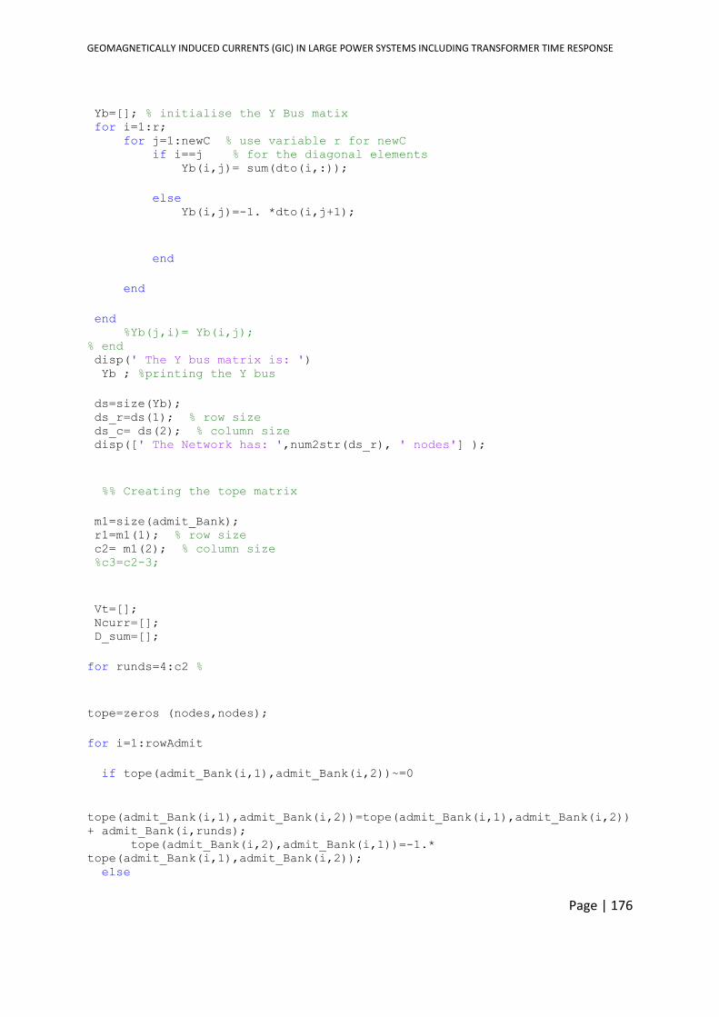
GEOMAGNETICALLY INDUCED CURRENTS (GIC) IN LARGE POWER SYSTEMS INCLUDING TRANSFORMER TIME RESPONSE
Page | 176
Yb=[]; % initialise the Y Bus matix for i=1:r; for j=1:newC % use variable r for newC if i==j % for the diagonal elements Yb(i,j)= sum(dto(i,:));
else Yb(i,j)=-1. *dto(i,j+1);
end
end
end %Yb(j,i)= Yb(i,j); % end disp(' The Y bus matrix is: ') Yb ; %printing the Y bus
ds=size(Yb); ds_r=ds(1); % row size ds_c= ds(2); % column size disp([' The Network has: ',num2str(ds_r), ' nodes'] );
%% Creating the tope matrix
m1=size(admit_Bank); r1=m1(1); % row size c2= m1(2); % column size %c3=c2-3;
Vt=[]; Ncurr=[]; D_sum=[];
for runds=4:c2 %
tope=zeros (nodes,nodes);
for i=1:rowAdmit
if tope(admit_Bank(i,1),admit_Bank(i,2))~=0
tope(admit_Bank(i,1),admit_Bank(i,2))=tope(admit_Bank(i,1),admit_Bank(i,2))
+ admit_Bank(i,runds); tope(admit_Bank(i,2),admit_Bank(i,1))=-1.*
tope(admit_Bank(i,1),admit_Bank(i,2)); else
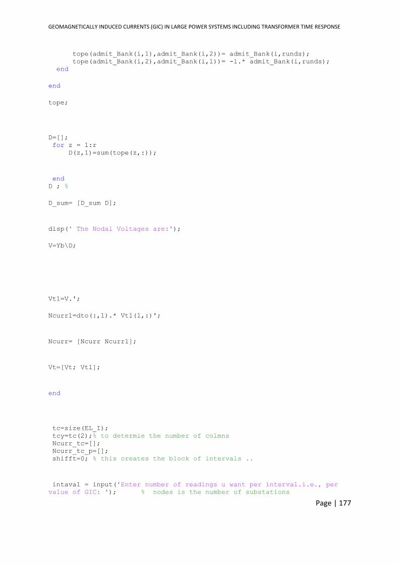
GEOMAGNETICALLY INDUCED CURRENTS (GIC) IN LARGE POWER SYSTEMS INCLUDING TRANSFORMER TIME RESPONSE
Page | 177
tope(admit_Bank(i,1),admit_Bank(i,2))= admit_Bank(i,runds); tope(admit_Bank(i,2),admit_Bank(i,1))= -1.* admit_Bank(i,runds); end
end
tope;
D=[]; for z = 1:r D(z,1)=sum(tope(z,:));
end D ; %
D_sum= [D_sum D];
disp(' The Nodal Voltages are:');
V=Yb\D;
Vt1=V.';
Ncurr1=dto(:,1).* Vt1(1,:)';
Ncurr= [Ncurr Ncurr1];
Vt=[Vt; Vt1];
end
tc=size(EL_I); tcy=tc(2);% to determie the number of colmns Ncurr_tc=[]; Ncurr_tc_p=[]; shifft=0; % this creates the block of intervals ..
intaval = input('Enter number of readings u want per interval.i.e., per
value of GIC: '); % nodes is the number of substations
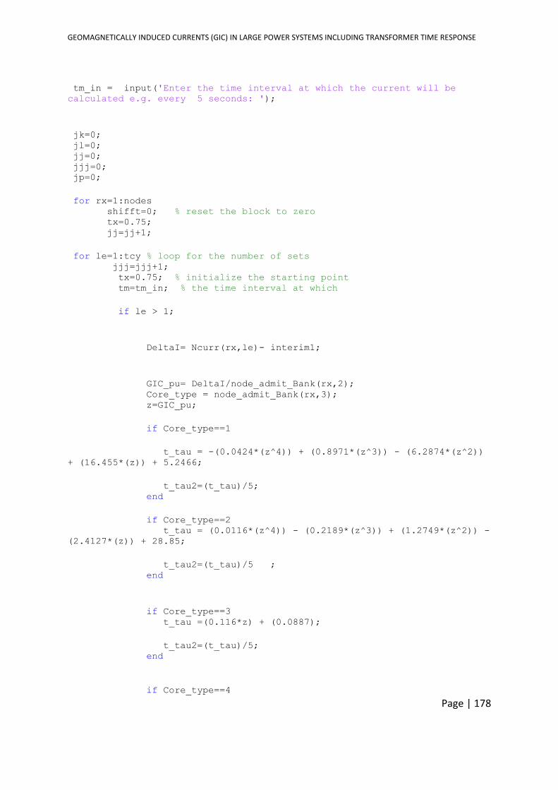
GEOMAGNETICALLY INDUCED CURRENTS (GIC) IN LARGE POWER SYSTEMS INCLUDING TRANSFORMER TIME RESPONSE
Page | 178
tm_in = input('Enter the time interval at which the current will be
calculated e.g. every 5 seconds: ');
jk=0; jl=0; jj=0; jjj=0; jp=0;
for rx=1:nodes shifft=0; % reset the block to zero tx=0.75; jj=jj+1;
for le=1:tcy % loop for the number of sets jjj=jjj+1; tx=0.75; % initialize the starting point tm=tm_in; % the time interval at which
if le > 1;
DeltaI= Ncurr(rx,le)- interim1;
GIC_pu= DeltaI/node_admit_Bank(rx,2); Core_type = node_admit_Bank(rx,3); z=GIC_pu;
if Core_type==1
t_tau = -(0.0424*(z^4)) + (0.8971*(z^3)) - (6.2874*(z^2))
+ (16.455*(z)) + 5.2466;
t_tau2=(t_tau)/5; end
if Core_type==2 t_tau = (0.0116*(z^4)) - (0.2189*(z^3)) + (1.2749*(z^2)) -
(2.4127*(z)) + 28.85;
t_tau2=(t_tau)/5 ; end
if Core_type==3 t_tau =(0.116*z) + (0.0887);
t_tau2=(t_tau)/5; end
if Core_type==4
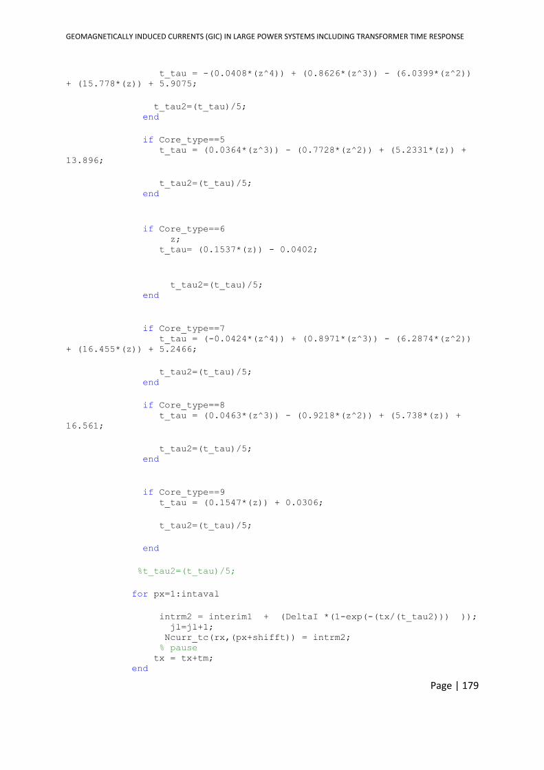
GEOMAGNETICALLY INDUCED CURRENTS (GIC) IN LARGE POWER SYSTEMS INCLUDING TRANSFORMER TIME RESPONSE
Page | 179
t_tau = -(0.0408*(z^4)) + (0.8626*(z^3)) - (6.0399*(z^2))
+ (15.778*(z)) + 5.9075;
t_tau2=(t_tau)/5; end
if Core_type==5 t_tau = (0.0364*(z^3)) - (0.7728*(z^2)) + (5.2331*(z)) +
13.896;
t_tau2=(t_tau)/5; end
if Core_type==6 z; t_tau= (0.1537*(z)) - 0.0402;
t_tau2=(t_tau)/5; end
if Core_type==7 t_tau = (-0.0424*(z^4)) + (0.8971*(z^3)) - (6.2874*(z^2))
+ (16.455*(z)) + 5.2466;
t_tau2=(t_tau)/5; end
if Core_type==8 t_tau = (0.0463*(z^3)) - (0.9218*(z^2)) + (5.738*(z)) +
16.561;
t_tau2=(t_tau)/5; end
if Core_type==9 t_tau = (0.1547*(z)) + 0.0306;
t_tau2=(t_tau)/5;
end
%t_tau2=(t_tau)/5;
for px=1:intaval
intrm2 = interim1 + (DeltaI *(1-exp(-(tx/(t_tau2))) )); jl=jl+1; Ncurr_tc(rx,(px+shifft)) = intrm2; % pause tx = tx+tm; end
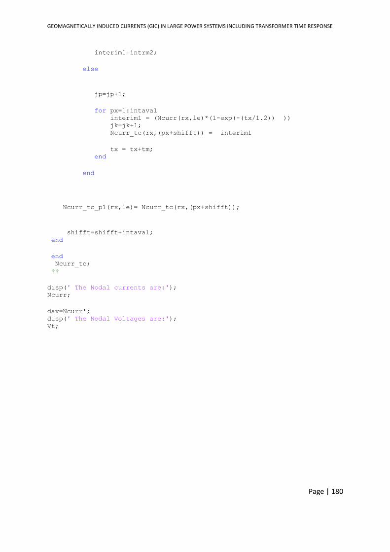
GEOMAGNETICALLY INDUCED CURRENTS (GIC) IN LARGE POWER SYSTEMS INCLUDING TRANSFORMER TIME RESPONSE
Page | 180
interim1=intrm2;
else
jp=jp+1;
for px=1:intaval interim1 = (Ncurr(rx,le)*(1-exp(-(tx/1.2)) )) jk=jk+1; Ncurr_tc(rx,(px+shifft)) = interim1
tx = tx+tm; end
end
Ncurr_tc_p1(rx,le)= Ncurr_tc(rx,(px+shifft));
shifft=shifft+intaval; end
end Ncurr_tc; %%
disp(' The Nodal currents are:'); Ncurr;
dav=Ncurr'; disp(' The Nodal Voltages are:'); Vt;

GEOMAGNETICALLY INDUCED CURRENTS (GIC) IN LARGE POWER SYSTEMS INCLUDING TRANSFORMER TIME RESPONSE
Page | 181
APPENDIX J: Eskom 400 kV substations
APPENDIX K: Eskom 400 kV transmission line data
APPENDIX L: Eskom 400 kV substation admittance data
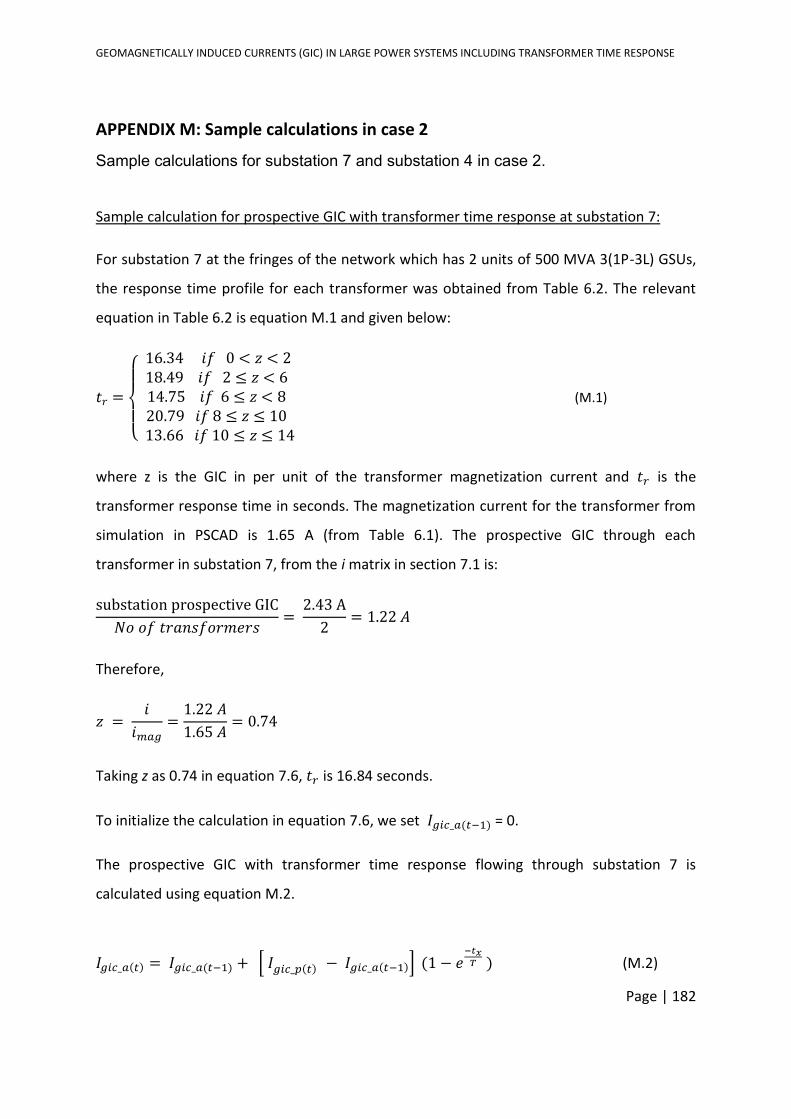
GEOMAGNETICALLY INDUCED CURRENTS (GIC) IN LARGE POWER SYSTEMS INCLUDING TRANSFORMER TIME RESPONSE
Page | 182
APPENDIX M: Sample calculations in case 2
Sample calculations for substation 7 and substation 4 in case 2. Sample calculation for prospective GIC with transformer time response at substation 7:
For substation 7 at the fringes of the network which has 2 units of 500 MVA 3(1P-3L) GSUs,
the response time profile for each transformer was obtained from Table 6.2. The relevant
equation in Table 6.2 is equation M.1 and given below:
𝑡𝑟 =
16.34 𝑖𝑓 0 < 𝑧 < 218.49 𝑖𝑓 2 ≤ 𝑧 < 614.75 𝑖𝑓 6 ≤ 𝑧 < 820.79 𝑖𝑓 8 ≤ 𝑧 ≤ 10 13.66 𝑖𝑓 10 ≤ 𝑧 ≤ 14
(M.1)
where z is the GIC in per unit of the transformer magnetization current and 𝑡𝑟 is the
transformer response time in seconds. The magnetization current for the transformer from
simulation in PSCAD is 1.65 A (from Table 6.1). The prospective GIC through each
transformer in substation 7, from the i matrix in section 7.1 is:
substation prospective GIC
𝑁𝑜 𝑜𝑓 𝑡𝑟𝑎𝑛𝑠𝑓𝑜𝑟𝑚𝑒𝑟𝑠= 2.43 A
2= 1.22 𝐴
Therefore,
𝑧 = 𝑖
𝑖𝑚𝑎𝑔=1.22 𝐴
1.65 𝐴= 0.74
Taking z as 0.74 in equation 7.6, 𝑡𝑟 is 16.84 seconds.
To initialize the calculation in equation 7.6, we set 𝐼𝑔𝑖𝑐_𝑎(𝑡−1) = 0.
The prospective GIC with transformer time response flowing through substation 7 is
calculated using equation M.2.
𝐼𝑔𝑖𝑐_𝑎(𝑡) = 𝐼𝑔𝑖𝑐_𝑎(𝑡−1) + [ 𝐼𝑔𝑖𝑐_𝑝(𝑡) − 𝐼𝑔𝑖𝑐_𝑎(𝑡−1)] (1 − 𝑒−𝑡𝑥𝑇 ) (M.2)
GEOMAGNETICALLY INDUCED CURRENTS (GIC) IN LARGE POWER SYSTEMS INCLUDING TRANSFORMER TIME RESPONSE
Page | 183
𝑇 =𝑡𝑟
5 = 3.37 seconds
From Table 7.3 in section 7.1, the first prospective GIC in substation 7 is 𝐼𝑔𝑝(1) = 2.43 A.
Hence,
𝐼𝑔𝑖𝑐_𝑎(1) = 0 + [2.43 − 0](1 − 𝑒−1
3.37) = 0.63 A. This value is 55.98 % higher than the value
in case 1 where substation 7 has a 3P-5L transmission transformer. Nevertheless, 𝐼𝑔𝑖𝑐_𝑎(1) <
is 𝐼𝑔𝑝(1) because 𝐼𝑔𝑖𝑐_𝑎(1) is calculated at one second.
At 𝑡𝑥 = two seconds,
From Table 7.3 in section 7.1, the second prospective GIC in substation 7 is 𝐼𝑔𝑝(2) = 0.55 A.
Hence,
𝐼𝑔𝑖𝑐_𝑎(2) = 𝐼𝑔𝑖𝑐_𝑎(1) + [ 𝐼𝑔𝑝(2) − 𝐼𝑔𝑖𝑐_𝑎(1)] ∗ (1 − 𝑒−2
3.37 )
= 0.40 + [0.55 − 0.63] ∗ (0.47) = 0.36 𝐴. This value is 17.23 % lower than the value in
case 1 where substation 7 has a 3P-5L transmission transformer. This reason for this is based
the difference factor between 𝐼𝑔𝑝(2) and 𝐼𝑔𝑖𝑐_𝑎(1) .
This calculation continues until the nth prospective GIC value is reached. From the
calculation of the prospective GIC with and without transformer time response in substation
7 at 2 seconds, it can be seen that the transformer response time to GIC suppresses the
prospective GIC, such that the difference between the prospective GIC with and without
transformer time response is 34.54 %.
Sample calculation for bus 4:
For substation 4 within the network with a high number of interconnections has two units of
500 MVA 3P-3L transmission transformers, the response time profile for each transformer is
obtained from Table 6.2. The relevant equation in Table 6.2 is equation M.3 as shown
below:
GEOMAGNETICALLY INDUCED CURRENTS (GIC) IN LARGE POWER SYSTEMS INCLUDING TRANSFORMER TIME RESPONSE
Page | 184
𝑡𝑟 =
0.23 𝑖𝑓 0 < 𝑧 < 40.58 𝑖𝑓 4 ≤ 𝑧 < 6 0.92 𝑖𝑓 6 ≤ 𝑧 < 10 1.25 𝑖𝑓 10 ≤ 𝑧 ≤ 14
(M.3)
The magnetization current for the transformer from simulation in PSCAD is 2.50 A. The
prospective GIC through each transformer in substation 4 from Table 7.3 in section 7.1 is:
substation prospective GIC
𝑁𝑜 𝑜𝑓 𝑡𝑟𝑎𝑛𝑠𝑓𝑜𝑟𝑚𝑒𝑟𝑠=
−0.49 A
2= −0.25 𝐴
Therefore,
𝑧 = 𝑖
𝑖𝑚𝑎𝑔=
−0.25 𝐴
2.50 𝐴= − 0.10.
The absolute value 𝑧 is 0.10 which is 16.67 % lower than the absolute value of z in the
corresponding calculation in case 1. This reflects the difference in time responses to GIC
between different transformer types.
Taking the absolute value of z as 0.10 in equation 7.7, 𝑡𝑟 is 0.23 seconds. This value was
27.77 seconds in the corresponding calculation in case 1.
To initialize the calculation in equation 7.6, we set 𝐼𝑔𝑖𝑐_𝑎(𝑡−1) = 0.
The prospective GIC with transformer time response flowing through substation 4 is
calculated using equation M.4.
𝐼𝑔𝑖𝑐_𝑎(𝑡) = 𝐼𝑔𝑖𝑐_𝑎(𝑡−1) + [ 𝐼𝑔𝑖𝑐_𝑝(𝑡) − 𝐼𝑔𝑖𝑐_𝑎(𝑡−1)] (1 − 𝑒−𝑡𝑥𝑇 ) (M.4)
𝑇 =𝑡𝑟
5 = 0.05 seconds
From Table 7.3 in section 7.1, the first prospective GIC 𝐼𝑔𝑝(1) in substation 4 is - 0.49 A. Hence,
𝐼𝑔𝑖𝑐_𝑎(1) = 0 + [(−0.49) − 0](1 − 𝑒−1
0.05) = - 0.49 A.
At 𝑡𝑥 = two seconds,
GEOMAGNETICALLY INDUCED CURRENTS (GIC) IN LARGE POWER SYSTEMS INCLUDING TRANSFORMER TIME RESPONSE
Page | 185
From Table 7.3 in section 7.1, the second prospective GIC 𝐼𝑔𝑝(2) in substation 4 is -0.91 A. Hence,
𝐼𝑔𝑖𝑐_𝑎(2) = 𝐼𝑔𝑖𝑐_𝑎(1) + [ 𝐼𝑔𝑝(2) − 𝐼𝑔𝑖𝑐_𝑎(1)] ∗ (1 − 𝑒−2
0.05 )
= −0.49 + [−0.91 − (−0.49)] ∗ (0.99) = −0.91 𝐴.
The results show that the prospective GIC values with and without transformer time
response are the same. This is primarily because of the relatively shorter response time of
the 3P-3L transformer.
Similar to the calculation for bus 7, this calculation continues till the nth prospective GIC
value is reached.
GEOMAGNETICALLY INDUCED CURRENTS (GIC) IN LARGE POWER SYSTEMS INCLUDING TRANSFORMER TIME RESPONSE
Page | 186
APPENDIX N: Sample calculations in case 3
Sample calculations for substation 7 and substation 4 in case 3. Sample calculation for the prospective GIC with transformer time response at substation 7:
For substation 7 at the fringes of the network which has 2 units of 500 MVA 3P-5L
transmission transformers, the response time profile for each transformer was obtained
from Table 6.2. The relevant equation in Table 6.2 is equation N.1 given below as:
𝑡𝑟 =
27.77 𝑖𝑓 0 < 𝑧 < 628.48 𝑖𝑓 6 ≤ 𝑧 < 8 26.18 𝑖𝑓 8 ≤ 𝑧 < 10 28.98 𝑖𝑓 10 ≤ 𝑧 ≤ 14
(N.1)
where z is the GIC in per unit of the transformer magnetization current and 𝑡𝑟 is the
transformer response time in seconds. The magnetization current for the transformer from
simulation in PSCAD is 2.1 A. The first prospective GIC through each transformer in
substation 7 from Table 7.6 in section 7.1 is:
substation prospective GIC
𝑁𝑜 𝑜𝑓 𝑡𝑟𝑎𝑛𝑠𝑓𝑜𝑟𝑚𝑒𝑟𝑠= 1.49 A
2= 0.75 𝐴
Therefore,
𝑧 = 𝑖
𝑖𝑚𝑎𝑔=0.75 𝐴
2.1 𝐴= 0.36
Using the value of z as 0.36 in equation 7.9, 𝑡𝑟 is 27.77 seconds.
The prospective GIC with transformer time response flowing through substation 7 is
calculated using equation N.2.
𝐼𝑔𝑖𝑐_𝑎(𝑡) = 𝐼𝑔𝑖𝑐_𝑎(𝑡−1) + [ 𝐼𝑔𝑖𝑐_𝑝(𝑡) − 𝐼𝑔𝑖𝑐_𝑎(𝑡−1)] (1 − 𝑒−𝑡𝑥𝑇 ) (N.2)
To initialize the calculation in equation N.2, we set 𝐼𝑔𝑖𝑐_𝑎(𝑡−1) = 0.
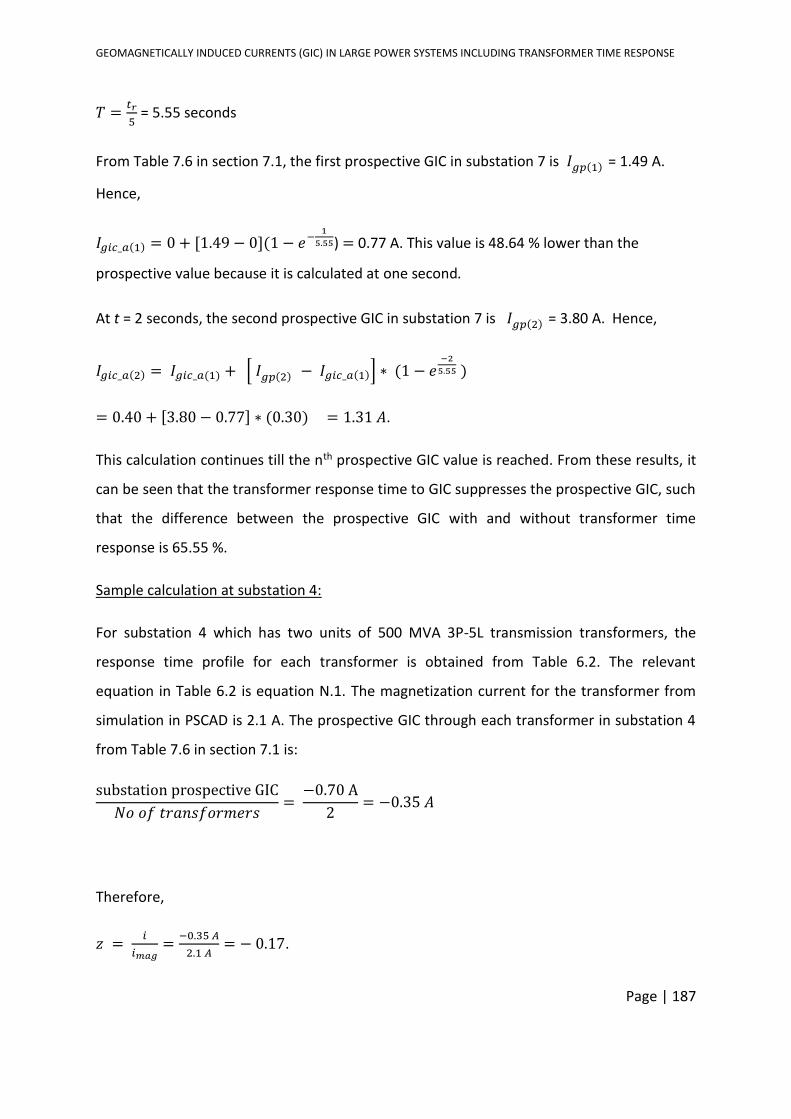
GEOMAGNETICALLY INDUCED CURRENTS (GIC) IN LARGE POWER SYSTEMS INCLUDING TRANSFORMER TIME RESPONSE
Page | 187
𝑇 =𝑡𝑟
5 = 5.55 seconds
From Table 7.6 in section 7.1, the first prospective GIC in substation 7 is 𝐼𝑔𝑝(1) = 1.49 A.
Hence,
𝐼𝑔𝑖𝑐_𝑎(1) = 0 + [1.49 − 0](1 − 𝑒−1
5.55) = 0.77 A. This value is 48.64 % lower than the
prospective value because it is calculated at one second.
At t = 2 seconds, the second prospective GIC in substation 7 is 𝐼𝑔𝑝(2) = 3.80 A. Hence,
𝐼𝑔𝑖𝑐_𝑎(2) = 𝐼𝑔𝑖𝑐_𝑎(1) + [ 𝐼𝑔𝑝(2) − 𝐼𝑔𝑖𝑐_𝑎(1)] ∗ (1 − 𝑒−2
5.55 )
= 0.40 + [3.80 − 0.77] ∗ (0.30) = 1.31 𝐴.
This calculation continues till the nth prospective GIC value is reached. From these results, it
can be seen that the transformer response time to GIC suppresses the prospective GIC, such
that the difference between the prospective GIC with and without transformer time
response is 65.55 %.
Sample calculation at substation 4:
For substation 4 which has two units of 500 MVA 3P-5L transmission transformers, the
response time profile for each transformer is obtained from Table 6.2. The relevant
equation in Table 6.2 is equation N.1. The magnetization current for the transformer from
simulation in PSCAD is 2.1 A. The prospective GIC through each transformer in substation 4
from Table 7.6 in section 7.1 is:
substation prospective GIC
𝑁𝑜 𝑜𝑓 𝑡𝑟𝑎𝑛𝑠𝑓𝑜𝑟𝑚𝑒𝑟𝑠= −0.70 A
2= −0.35 𝐴
Therefore,
𝑧 = 𝑖
𝑖𝑚𝑎𝑔=
−0.35 𝐴
2.1 𝐴= − 0.17.
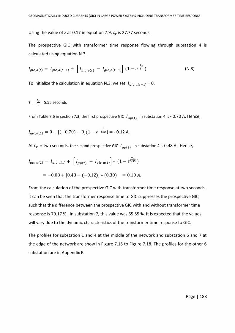
GEOMAGNETICALLY INDUCED CURRENTS (GIC) IN LARGE POWER SYSTEMS INCLUDING TRANSFORMER TIME RESPONSE
Page | 188
Using the value of z as 0.17 in equation 7.9, 𝑡𝑟 is 27.77 seconds.
The prospective GIC with transformer time response flowing through substation 4 is
calculated using equation N.3.
𝐼𝑔𝑖𝑐_𝑎(𝑡) = 𝐼𝑔𝑖𝑐_𝑎(𝑡−1) + [ 𝐼𝑔𝑖𝑐_𝑝(𝑡) − 𝐼𝑔𝑖𝑐_𝑎(𝑡−1)] (1 − 𝑒−𝑡𝑥𝑇 ) (N.3)
To initialize the calculation in equation N.3, we set 𝐼𝑔𝑖𝑐_𝑎(𝑡−1) = 0.
𝑇 =𝑡𝑟
5 = 5.55 seconds
From Table 7.6 in section 7.3, the first prospective GIC 𝐼𝑔𝑝(1) in substation 4 is - 0.70 A. Hence,
𝐼𝑔𝑖𝑐_𝑎(1) = 0 + [(−0.70) − 0](1 − 𝑒−1
5.55) = - 0.12 A.
At 𝑡𝑥 = two seconds, the second prospective GIC 𝐼𝑔𝑝(2) in substation 4 is 0.48 A. Hence,
𝐼𝑔𝑖𝑐_𝑎(2) = 𝐼𝑔𝑖𝑐_𝑎(1) + [ 𝐼𝑔𝑝(2) − 𝐼𝑔𝑖𝑐_𝑎(1)] ∗ (1 − 𝑒−2
5.55 )
= −0.08 + [0.48 − (−0.12)] ∗ (0.30) = 0.10 𝐴.
From the calculation of the prospective GIC with transformer time response at two seconds,
it can be seen that the transformer response time to GIC suppresses the prospective GIC,
such that the difference between the prospective GIC with and without transformer time
response is 79.17 %. In substation 7, this value was 65.55 %. It is expected that the values
will vary due to the dynamic characteristics of the transformer time response to GIC.
The profiles for substation 1 and 4 at the middle of the network and substation 6 and 7 at
the edge of the network are show in Figure 7.15 to Figure 7.18. The profiles for the other 6
substation are in Appendix F.
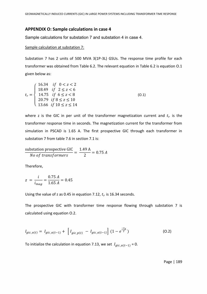
GEOMAGNETICALLY INDUCED CURRENTS (GIC) IN LARGE POWER SYSTEMS INCLUDING TRANSFORMER TIME RESPONSE
Page | 189
APPENDIX O: Sample calculations in case 4
Sample calculations for substation 7 and substation 4 in case 4. Sample calculation at substation 7:
Substation 7 has 2 units of 500 MVA 3(1P-3L) GSUs. The response time profile for each
transformer was obtained from Table 6.2. The relevant equation in Table 6.2 is equation O.1
given below as:
𝑡𝑟 =
16.34 𝑖𝑓 0 < 𝑧 < 218.49 𝑖𝑓 2 ≤ 𝑧 < 614.75 𝑖𝑓 6 ≤ 𝑧 < 820.79 𝑖𝑓 8 ≤ 𝑧 ≤ 10 13.66 𝑖𝑓 10 ≤ 𝑧 ≤ 14
(O.1)
where z is the GIC in per unit of the transformer magnetization current and 𝑡𝑟 is the
transformer response time in seconds. The magnetization current for the transformer from
simulation in PSCAD is 1.65 A. The first prospective GIC through each transformer in
substation 7 from table 7.6 in section 7.1 is:
substation prospective GIC
𝑁𝑜 𝑜𝑓 𝑡𝑟𝑎𝑛𝑠𝑓𝑜𝑟𝑚𝑒𝑟𝑠= 1.49 A
2= 0.75 𝐴
Therefore,
𝑧 = 𝑖
𝑖𝑚𝑎𝑔=0.75 𝐴
1.65 𝐴= 0.45
Using the value of z as 0.45 in equation 7.12, 𝑡𝑟 is 16.34 seconds.
The prospective GIC with transformer time response flowing through substation 7 is
calculated using equation O.2.
𝐼𝑔𝑖𝑐_𝑎(𝑡) = 𝐼𝑔𝑖𝑐_𝑎(𝑡−1) + [ 𝐼𝑔𝑖𝑐_𝑝(𝑡) − 𝐼𝑔𝑖𝑐_𝑎(𝑡−1)] (1 − 𝑒−𝑡𝑥𝑇 ) (O.2)
To initialize the calculation in equation 7.13, we set 𝐼𝑔𝑖𝑐_𝑎(𝑡−1) = 0.
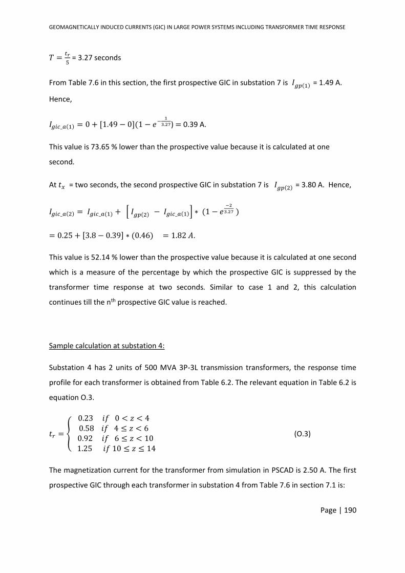
GEOMAGNETICALLY INDUCED CURRENTS (GIC) IN LARGE POWER SYSTEMS INCLUDING TRANSFORMER TIME RESPONSE
Page | 190
𝑇 =𝑡𝑟
5 = 3.27 seconds
From Table 7.6 in this section, the first prospective GIC in substation 7 is 𝐼𝑔𝑝(1) = 1.49 A.
Hence,
𝐼𝑔𝑖𝑐_𝑎(1) = 0 + [1.49 − 0](1 − 𝑒−1
3.27) = 0.39 A.
This value is 73.65 % lower than the prospective value because it is calculated at one
second.
At 𝑡𝑥 = two seconds, the second prospective GIC in substation 7 is 𝐼𝑔𝑝(2) = 3.80 A. Hence,
𝐼𝑔𝑖𝑐_𝑎(2) = 𝐼𝑔𝑖𝑐_𝑎(1) + [ 𝐼𝑔𝑝(2) − 𝐼𝑔𝑖𝑐_𝑎(1)] ∗ (1 − 𝑒−2
3.27 )
= 0.25 + [3.8 − 0.39] ∗ (0.46) = 1.82 𝐴.
This value is 52.14 % lower than the prospective value because it is calculated at one second
which is a measure of the percentage by which the prospective GIC is suppressed by the
transformer time response at two seconds. Similar to case 1 and 2, this calculation
continues till the nth prospective GIC value is reached.
Sample calculation at substation 4:
Substation 4 has 2 units of 500 MVA 3P-3L transmission transformers, the response time
profile for each transformer is obtained from Table 6.2. The relevant equation in Table 6.2 is
equation O.3.
𝑡𝑟 =
0.23 𝑖𝑓 0 < 𝑧 < 40.58 𝑖𝑓 4 ≤ 𝑧 < 6 0.92 𝑖𝑓 6 ≤ 𝑧 < 10 1.25 𝑖𝑓 10 ≤ 𝑧 ≤ 14
(O.3)
The magnetization current for the transformer from simulation in PSCAD is 2.50 A. The first
prospective GIC through each transformer in substation 4 from Table 7.6 in section 7.1 is:
GEOMAGNETICALLY INDUCED CURRENTS (GIC) IN LARGE POWER SYSTEMS INCLUDING TRANSFORMER TIME RESPONSE
Page | 191
substation prospective GIC
𝑁𝑜 𝑜𝑓 𝑡𝑟𝑎𝑛𝑠𝑓𝑜𝑟𝑚𝑒𝑟𝑠= −0.70 A
2= −0.35 𝐴
Therefore,
𝑧 = 𝑖
𝑖𝑚𝑎𝑔=
−0.35 𝐴
2.5 𝐴= − 0.14.
Taking the absolute value of z as 0.14 in equation 7.5, 𝑡𝑟 is 0.23 seconds for substation 4.
The prospective GIC with transformer time response flowing through substation 4 is
calculated using equation O.4.
𝐼𝑔𝑖𝑐_𝑎(𝑡) = 𝐼𝑔𝑖𝑐_𝑎(𝑡−1) + [ 𝐼𝑔𝑖𝑐_𝑝(𝑡) − 𝐼𝑔𝑖𝑐_𝑎(𝑡−1)] (1 − 𝑒−𝑡𝑥𝑇 ) (O.4)
To initialize the calculation in equation 7.15, we set 𝐼𝑔𝑖𝑐_𝑎(𝑡−1) = 0.
𝑇 =𝑡𝑟
5 = 0.05 seconds
From Table 7.3 in section 7.1, the first prospective GIC 𝐼𝑔𝑝(1) in substation 4 is - 0.70 A.
Hence,
𝐼𝑔𝑖𝑐_𝑎(1) = 0 + [(−0.70) − 0](1 − 𝑒−1
0.05) = - 0.69 A.
At 𝑡𝑥 = two seconds, the second prospective GIC 𝐼𝑔𝑝(2) in substation 4 is 0.48 A. Hence,
𝐼𝑔𝑖𝑐_𝑎(2) = 𝐼𝑔𝑖𝑐_𝑎(1) + [ 𝐼𝑔𝑝(2) − 𝐼𝑔𝑖𝑐_𝑎(1)] ∗ (1 − 𝑒−2
0.05 )
= −0.12 + [0.48 − (−0.12)] ∗ (1) = 0.48 𝐴.
The results for substation 4 shows that the prospective GIC with and without transformer
time response are the same. This is because of the relatively shorter response time of the
3P-3L transformer.

GEOMAGNETICALLY INDUCED CURRENTS (GIC) IN LARGE POWER SYSTEMS INCLUDING TRANSFORMER TIME RESPONSE
Page | 192
The profiles for substation 1 and 4 at the middle of the network and substation 6 and 7 at
the edge of the network are show in Figure 7.19 to Figure 7.22. The profiles for the other 6
substation are in Appendix F.
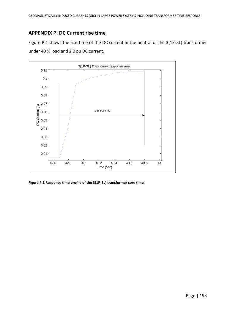
GEOMAGNETICALLY INDUCED CURRENTS (GIC) IN LARGE POWER SYSTEMS INCLUDING TRANSFORMER TIME RESPONSE
Page | 193
APPENDIX P: DC Current rise time
Figure P.1 shows the rise time of the DC current in the neutral of the 3(1P-3L) transformer
under 40 % load and 2.0 pu DC current.
Figure P.1 Response time profile of the 3(1P-3L) transformer core time
42.6 42.8 43 43.2 43.4 43.6 43.8 44
0.01
0.02
0.03
0.04
0.05
0.06
0.07
0.08
0.09
0.1
0.11
3(1P-3L) Transformer response time
Time (sec)
DC
Cu
rre
nt (A
)
1.26 seconds