Generating Adaptive Alarms For Condition Monitoring Data

R. Willetts

1, A.G. Starr

1 A. Doyle

2, J. Barnes

1

1Maintenance Engineering Research Group (MERG)

Manchester School of Engineering

Oxford Road, Manchester, M13 9PL

{bob_willetts@hotmail.com, a.starr@man.ac.uk} http://www.maintenance.org.uk

2WM Engineering Limited

Kilburn House

Manchester Science Park, Pencroft Way,

Manchester, M15 6SE

{Tony@wmeng.co.uk} http://www.wmeng.co.uk

ABSTRACT

Maintenance actions cannot be defined and undertaken in isolation from the business

and production objectives of a typical company. They must be predicted and

subsequently planned into the production schedule. Condition monitoring identifies

changes within defined monitoring parameters to trigger maintenance. These changes

when combined with engineering knowledge, historical data and other monitoring

parameters enable the prediction and identification of these changes in state. The data

carries with it uncertainties in measurement accuracy, running conditions, and

regularity. This paper reviews methods for trending and prediction, and describes how

an adaptive approach to the definition of alarm levels can be used to improve the

prediction capabilities when analysing routine condition monitoring measurement

data.

KEYWORDS

Adaptive Alarms, Condition Based Maintenance, Holistic Condition Monitoring

INTRODUCTION

The term holistic has been used in numerous industries and research activities to

describe methods which analyse the overall system and establish how the different

inputs to such a system can affect the overall performance. In the field of condition

based maintenance (CBM), a holistic system first establishes failure modes before

identifying the most relevant combination of monitoring parameters. This can then be

used to assess the effect of the occurrence of these failures on the overall

performance, availability and utilisation of the plant item.

Computerised Maintenance Management Systems (CMMS) have made extensive use

of CBM for their scheduling of maintenance actions. The state of health of a machine

or process is estimated by analysis of measured parameters. Typically, the parameter

is compared to a predefined threshold, and the CMMS automatically compares

incoming data to a look-up table of alarm levels. However, these systems have

traditionally relied heavily on the manual determination and subsequent review of

alarm levels used. This approach has a number of drawbacks:

the initial setting has no historical data, so a heuristic approach may be used -

this relies on the expertise to interpret standards or to draw on experience of

similar machines;

the alarm levels, if not optimal, can generate false alarms or fail to observe

early degradation, both of which decrease the faith in the system;

there is no adaptation to running conditions, e.g. load or speed;

manual review is laborious and is often not done.

This paper reviews the use of alarm levels for routine monitoring within CMMS, and

identifies their function in the management of integrated CBM. The use of classical

statistics, for estimation of parameters or prediction of state, is fundamental to the

methodology. Recent research in intelligent systems is also important, and is briefly

reviewed here. The advances in the use of multivariate data are important to robust

alarms, and the fusion of qualitative and quantitative data takes this forward. The use

of such fused data requires a range of robust input data streams in a hierarchical

architecture [1]. The work reported here concentrates on the pre-processing of single

data streams, which is essential to the automation of integrated systems, and of

immediate use in conventional CBM systems.

CMMS AND INTEGRATED CONDITION MONITORING

Computerised maintenance management systems base maintenance actions on the

change of state of a defined monitoring parameter. The underlying philosophy of

CBM is the prediction of failures prior to their occurrence. CBM achieves this by the

use of condition monitoring, which establishes the present condition of the plant by

the regular monitoring of defined parameters. The data from such parameters can be

expected to display characteristics of normal and abnormal behaviour, masked with

systematic and stochastic errors. Measurement and processing are designed to

minimise the impact of such errors. Usually, machines and processes work within

their specifications (otherwise they are replaced or redesigned), so normal behaviour

is identified fairly readily. Changes over time are therefore important to the

identification of early signs of degradation. These changes are traditionally manually

identified by inspection of a long term time graph or trend.

The trend of the data allows the normal safe working condition of the plant item over

a period of time to be established. Any normal variation in the condition is also

recorded. Deviation from this norm can then be identified, whether increasing or

decreasing amplitude, or increasing or decreasing variance. The trend itself may not

diagnose the fault directly, although some parameters would allow this. In some cases

a serious change is sufficient to make a tactical decision without diagnosis. In

proprietary CMMS’s the extent of such a change is typically determined by one or

more thresholds. In this work two levels are defined, warning and alarm. The warning

level is used as a trigger to investigate further before taking action.

In a typical system the alarm and warning levels are manually determined. These

levels are often based upon the previous experience and knowledge of the engineer

during the initial system definition and setting up period. Figure 1 shows a typical

trend, which illustrates the overall vibration measured on part of a paper machine. It

can be seen that there are three distinct states, namely normal, warning and alarm.

These states are used to define the different operating conditions of the parameter

being monitored. The measured points are also labelled in colour in the CMMS

output. If there is no history, the warning and alarm levels are typically set at the

mean plus 2 and 3 times the standard deviation of the trend, for a high-going alarm.

Exceptions include, of course, low-going alarms, but also specific measurements or

machines which are known from experience to be particularly sensitive or insensitive.

Once the levels are set, the CMMS is programmed to check all incoming data against

them, and to bring exceptions to the attention of the operator by reporting or a visual

indication. In a well set up system, there should be many measurements taken, but few

alarms.

Unfortunately, two apparently identical systems will never behave or wear out in

exactly the same way, so these levels need to be periodically monitored and tuned to

ensure that the values used are correct at the present time. This is a time consuming

task and is one that is often overlooked until a situation occurs that requires analysis

of the trend. Some situations are normal, but some can be catastrophic in nature and

hence expensive:

a flagged change in the condition of the plant, e.g. increased vibration,

indicates genuine degradation or contamination of the signal from another

nearby component;

a change in the plant configuration, e.g. increased running speed or process

change invokes a planned review;

an unexpected failure resulting from the alarm levels being too high;

numerous false alarms resulting from the alarm levels being too low.

The last two situations are common in mature systems because an initially well set up

system appears to require little attention, and the tuning then appears unnecessary an

laborious. Some users do not have local expertise. These problems have serious

implications for system suppliers, because unexpected failures and false alarms are

easily blamed on the CBM system.

Other uncertainties to be considered by the engineer undertaking the definition

process include the present operating condition of the plant, together with what and

how the plant item is connected. From these factors it is easy to see that manual

determination of alarm levels can leave the user open to increased costs in terms of:

unforeseen shut downs;

increased breakdown maintenance;

increased system monitoring and upkeep;

reduction of user confidence in both the ability of the system to do its job and

also the results obtained from it.

Overa

ll vib

ratio

n

(mm

/s)

Alarm limit Warning limit

Figure 1: Typical trend from a CMMS, showing the interaction of the trended

data with manually determined alarm and warning states.

These costs could be reduced, and confidence increased, if the alarm levels were set

based upon the actual time history of the measurement parameter. There are numerous

techniques available that could be used to define these levels, for example:

1. classical statistics;

2. multi-variant statistics;

3. intelligent systems, for example neural networks, classifiers, and genetic

algorithms.

CLASSICAL STATISTICS

Classical statistical methods have been used in numerous condition monitoring

systems. It is common to calculate alarm levels based upon multiples of the standard

deviation of a data set, which is the historical trend. Some systems allow the user to

manually censor abnormal readings to produce a smoothed representation of the

original trend. The alarm levels are typically calculated by adding (for a high-going

alarm) or subtracting (for a low-going alarm) two or three to the mean for warning

and alarm levels respectively. The method is derived from statistical process control,

where further rigour is applied to the sampling, but condition monitoring in the field

suffers with limited sample sizes, and major effects from a range of noise such as:

systematic noise, including change of machine speed or load;

stochastic noise, such as temperature variation or poor repeatability of

transducer coupling conditions, easily introduced by human operators;

delayed or missed readings resulting from operating conditions.

These limitations can be controlled by rigorous procedures to some extent, but they

always affect the confidence of fault detection and diagnosis based on a single

variable.

Regression analysis

Condition monitoring does not aim simply to analyse what has happened in the past;

rather, it aims to predict what will happen next. The analysis of trends of data

examines the tendency of a line of best fit to remain steady, or to move towards a

threshold. The line can be projected to predict a future date for a maintenance action.

Regression analyses are defined as a set of statistical techniques that allow assessment

of the relationship between a dependent variable (DV) and one or more independent

variables (IVs) [2]. The method fits a model based on a straight line (or other curve

such as the exponential):

BXAy (1)

where

y’ – predicted value of the DV;

A – the intercept of the trend on the Y axis;

X – the IV;

B – the regression coefficient.

The regression is optimised such that the regression coefficient brings the predicted

data set Y’ from the equation as close as possible to the real measured Y values. The

coefficient is obtained by minimising the square of the sum of the errors between the

predicted range of Y’ and the actual range of Y values.

Regression analysis can be observed in software systems in maintenance and

production, applied to problems such as:

prediction of the probable direction of a defined parameter;

scheduling of preventive maintenance actions;

prediction of supply and demand of products and services.

Regression based on a single variable is simple and robust, but continues to suffer

from many of the errors described above, and hence limits the user’s faith in its

predictions.

Multi-Variant Statistics

Multi-variant systems have been developed that attempt to both model the

relationships between different parameters and predict changes based upon these

relationships. Multiple regression analysis allows fitting of models based one more

than IV. Again, the model can be linear or non-linear [2]:

kk XBXBXBAy 2211 (2)

where

y’ – predicted value of the DV;

A – the intercept of the trend on the Y axis;

Xi – the different IVs (i = 1 to k);

Bi – regression coefficients assigned to each IV during regression;

The aim of optimisation is the same as for a single variable. The multiple coefficients

are obtained by minimising the square of the sum of the errors between the predicted

range of Y’ and the actual range of Y values. While this is relatively trivial for one or

two IVs (straight line or square fits), it rapidly becomes computationally intensive in

higher order problems, and is prone to local minima which give non-optimal

solutions. There is a great deal of literature to be found which deals with optimisation

of multivariant problems (e.g. genetic algorithms), but this will not be further

expanded here.

Markov methods

Another technique used for the integration of measurements from different parameters

is the Markov Chain. This technique can be used to represent the behaviour of a

physical system [3]. This representation is obtained by describing all possible states

the system can occupy and then indicating the probability of a change within the

system from one state to another, within a given time period. The major difference

between these systems and the regression model described above is that the future

evolution of a Markov system is only dependent upon the present condition, whereas

the regression method predicts a dependent variable (DV) based upon the history of

one or more independent variables (IVs).

Markov chains have been successfully used in condition monitoring by identifying

real states. Markov modelling, coupled with the proportional hazard model, is

encapsulated in the EXAKT system [4]. Here the maintenance interval is optimised for

groups of identical machines, by fusing together measurements from multiple

variables with the time between failures. A major difference between this system and

a typical CMM system is the alarm levels used. Instead of fixed warning and alarm

levels, a series of statistically determined state bands are defined.

Typically this system uses five bands which encapsulate all the historical

measurements for the defined parameters. Figure 2 shows an example of these state

bands when imposed onto a vibration history [5,6]. These bands have the effect of

defining different operating conditions for that group of machines. The system then

determines a risk factor for each of these bands, which states the probability of the

band 5

band 4

band 3

band 2

band 1

Figure 2: Typical state bands defined within the EXAKT system: here a large set

of acceleration data from a paper machine is plotted to identify typical variance

Figure 3: A replacement decision graph using the EXAKT methodology. Above

the alarm level, a replacement is scheduled. The level reduces according to an age

model. Hence, sensitivity to measured data increases. Here, the composite

covariate comprises a linear combination of acceleration and a gear meshing

frequency from a paper machine. The distribution and trend of the covariate also

demonstrates the limitation of a decision made on few measurements with noise.

Replacement decision

0

2

4

6

8

10

0 500 1000 1500

Working age (days)

Co

mp

os

ite

co

va

ria

te

Composite covariate

Alarm level

Trend of composite

covariate

multi-variant system parameter changing from its present location to each of these

states in the next monitoring period. If these risk factors are then combined with the

failure history and costs of both planned maintenance and unpredicted failures, the

optimal replacement interval for that group of machines can be defined. A decision

graph can then be developed (figure 3), which plots the combined parameters as a

composite covariate against the working age, to state if the unit needs to be replaced

before the next monitoring interval. It can be seen from this graph that the alarm

levels decrease (according to a Weibull distribution) as the working age increases, and

thus the risk of changing state also increases.

The alarm levels are variable once the method is prepared, and express a relationship

between the measured data, previous experience, and age. The manual preparation of

state bands is a limitation, and the method is dependant on complete data sets, which

must be prepared manually if not collected automatically.

INTELLIGENT SYSTEMS

The term intelligent systems can be used to cover a wide range of disciplines and

technologies. For example, these disciplines can include artificial intelligence, data

fusion and machine learning. Whatever the discipline they all have basically the same

underlying concept. This has been defined as the ability of a computer program to

learn from the experience it gains by being repeatedly subjected to defined tasks

against some measure of its performance [7]. As such, the program’s performance

will improve the more experience it has the tasks. However, it is possible for these

systems to become over-taught on these tasks and as such they will not be capable of

reacting to new or novel situations and tasks.

The maintenance community has been active within this area with a lot of emphasis

being focused on expert systems, neural networks or hybrid combinations of the two

technologies. Neural networks and expert systems have been used to perform

diagnostics on generic forms of rolling element bearings [8]. Neural networks have

been used to combine data from three sensors within a CNC machine to establish five

different types of tool wear [9]. A generic diagnostic system has been described,

based upon the fusion of different sensor outputs [10]. A multi-sensor based condition

monitoring system for CNC machine tools has been reported, based upon the fusion

of parameters such as power, vibration, temperature and pressure [11].

The industrial community has also developed several systems, for example the Tiger

system, an on-line model-based system designed to monitor the operating conditions

of gas turbines [12]. The MAINTelligence system developed by Design Maintenance

Systems works at the generic level and allows the data from different monitoring

systems to be combined within a diagnostic system. However this system requires

extensive knowledge of the process under investigation, as the knowledge base needs

to be up-dated for each new fault [13]. The Advisor system is based upon the

combination of neural networks and expert systems to provide a diagnostic aid for the

analysis of failures within rotating machinery [14]. However one of the main

problems with these systems is the amount of data needed to train the networks. There

remains a distinct need for automatic selection of alarms for less complex input

streams.

ADAPTIVE ALARMS

A problem with all of the above techniques is that a large amount of time and

resources are required throughout the life cycle of the machine, particularly during the

initial program definition, evaluation and system monitoring. A more cost-effective

system would be capable of aligning itself to the trend data within an automated

process, whilst performing self-monitoring during subsequent operation. The

approach presented here, called Predictive Adaptive Trends (PAT) is based upon the

fusion of a number of different classical statistical methods into a novel adaptive

system. The main emphasis of this system is the fusion of a variable sized

autoregressive moving average (ARMA) filter, with an exponential smoothing

algorithm, thus enabling adaptive alarms to be produced together with estimates of the

probable time to a change of state.

Predicting Values Using an ARMA filter.

It is difficult if not impossible to predict precisely the actual value of the next

measurement of a monitored parameter. It is only possible to estimate with a degree of

confidence a probable value based upon the history of the trend, which can be used to

give an indication of the possible trend direction. There are numerous methods

available for predicting values. One of the most common methods for this prediction

is linear projection:

bxxmy )'( (3)

22 xxn

yxxynm (4)

22

2

xxn

xyxxyb (5)

where

b = intercept of trend with y axis

m = slope of trend

n = number of points used in prediction

x = time or date of current trend value

x’ = projection from current measurement date

y = projected trend value

This method is an extension to the linear regression described above, but projects the

line of best of fit into the future to give a predicted value of y in the x direction at an

offset of x’. However, the predicted value is dependant upon a number of factors:

the number of points used to calculate the predicted value;

the values of the historical trend;

the x direction offset.

These factors can result in widely different predicted values for the same trend, which

has the effect of producing a band of probable values. This is better shown in figure 4

where predicted values of y are calculated in the x direction based upon 2,3,4,5 and 6

point historical lines of best fit to simulated raw data, which includes typical noise.

The two-point trend is downwards, because the trend from Yn-1 to Yn-2 is downwards.

The three-point to five-point trends are level or upwards. The high first point ensures

that the six-point trend is downwards. These variations are of sufficient concern if we

project only one point forward – they become worse if we project further. The human

eye, coupled with experience of variable measured data, tends to censor the unwanted

noise, but this is not possible in a simple statistical fit. In practice, we wish to retain

all the available data to some extent if it can be sensibly managed.

It is possible to calculate a trended value based on the mean value of a chosen number

of historical data points. The autoregressive moving average (ARMA) calculates a

mean value based upon the summation of all points and the division by the number of

points within the filter [15]. However, as with the linear projection method described

above, the mean value produced depends upon the number of points used. This again

can result in a band of average values, which when used to calculate alarm levels can

result in widely varying values. Figure 5 shows the mean values obtained from the

ARMA filter for an extension of the data set above. The ARMA does not explicitly

predict the next value, but nonetheless is useful for taking stock of variable historical

data. Note that the influence of the first high point on all the fitted lines is quickly

diminished, and “forgotten” by the end of the appropriate sample length.

1.0

1.5

2.0

2.5

3.0

3.5

4.0

4.5

5.0

5.5

1 2 3 4 5 6 7

X values (time)

Y v

alu

es

(m

ea

su

rem

en

ts)

Raw data

2 point

3 point

4 point

5 point

6 point

Figure 4: Prediction from straight trend lines values

based upon different number of historical points.

2.0

2.5

3.0

3.5

4.0

4.5

5.0

5.5

1 2 3 4 5 6 7 8 9 10 11 12 13 14 15 16 17 18 19 20

X values

Y v

alu

es

Trend Data

2 Point

3 Point

4 Point

5 Point

6 Point

Figure 5: Mean values obtained by use of the ARMA

algorithm based on varying numbers of historical points

The ARMA is thus a useful and simple first step in preparing variable measured data

for an automatic assessment of normal behaviour. A less desirable feature is that is

takes equal account of all data points, whether they are old or new. Exponential

smoothing allows an alternative approach to the problem, building in a variable

approach to the “forgetting” factor. It works on a minimum of two values, the first of

which is defined as the initial condition (x’) and the second denoted as the current

value (x’’). Equation 4 defines this function, from which it can be seen that the mean

value is calculated by taking 10% of the current value (x’’) and adding it to 90% of

the previous calculated value (x’), in this case the mean value. This calculated mean

value is then used to replace the initial value (x’) in the next calculation. In this way

all previous mean values are used within the calculation of the new mean. However,

the relevance of these values diminishes over time, as new measured values are

entered. The rate at which the equation “forgets” the previous values can be changed

to get a more reactive or damped response to changes within the signal.

''1.0'9.0''' xxx (6)

If this equation is nested within the ARMA algorithm it is possible to produce a range

of mean values that are smoother and less variable than the values obtained from the

standard ARMA algorithm. Figure 6 shows the exponential smoothed mean values for

the same data as above. As in the prediction calculation above, a range of values is

possible, but the performance is smoother. In this example, the mean values produced

stay high for a long period of time. This is due to the forgetting factors used. It is

possible to generate a more reactive system by varying the factors used. This will

allow alarm levels to be calculated based upon the variability of this smoothed trend.

Note that the raw data is retained for comparison to the calculated alarms – the

smoothing is a preparatory step for the definition of alarm levels.

If the data prepared for the smoothed trend contains abnormal readings, they remain

part of the calculations for the alarm levels, and can still be a source of noise, albeit

reduced. This variability can be further reduced by the comparison of the original data

to an automatically generated acceptability band. The values of this band would be

generated in the same way as the adaptive alarms and as such would change

depending upon the trend itself. This would have the effect of censoring abnormal

readings from the mean trend for the purposes of generating the adaptive alarm levels.

Figure 6: Mean values obtained from the combined ARMA and exponential

smoothing algorithms; forgetting factors of (left) 0.9 and 0.1 and (right) 0.8 and 0.2

2.0

2.5

3.0

3.5

4.0

4.5

5.0

5.5

1 2 3 4 5 6 7 8 9 10 11 12 13 14 15 16 17 18 19 20

X values

Y v

alu

es

Trend Data

2 Point

3 Point

4 Point

5 Point

6 Point

2.0

2.5

3.0

3.5

4.0

4.5

5.0

5.5

1 2 3 4 5 6 7 8 9 10 11 12 13 14 15 16 17 18 19 20

X values

Y v

alu

es

Trend Data

2 Point

3 Point

4 Point

5 Point

6 Point

We repeat that the raw data is not censored when ultimately compared to the

automatic alarm levels.

Generating alarm levels

The adaptive alarm levels are generated from the automatically smoothed trend,

coupled with the censored raw data. The strategy differs from the traditional approach

in that the centre mean is pre-processed as described above, and the high and low

going alarm limits are not based solely on the standard deviation.

The changes within the smoothed trend are inherently small, so the standard deviation

of this trend will also be inherently small. Thus if the calculation of the adaptive

alarms is based on ± 2 or 3 the alarm levels will be too close to the mean, which

results in numerous false alarms. It is possible to reduce this number of false alarms

by calculating the larger standard deviation from the raw data. However, the raw data

can be inherently noisy and, as such the standard deviation can become variable,

which would result in widely variable alarm levels.

Here the noise in the signal has been measured by averaging the rate of change in the

censored raw data in a given sample (equation 5), and that value is added to the

standard deviation of the censored raw data before being used to calculate warning

and alarm levels (equation 6).

1

1

1

1

k

yy

Y

k

i

ii

(5)

where

Y = current average rate of change

y = censored raw data

k = sample length

YnxA (6)

where

A = warning or alarm limit

x = current mean from smoothed data

n = 2, 3

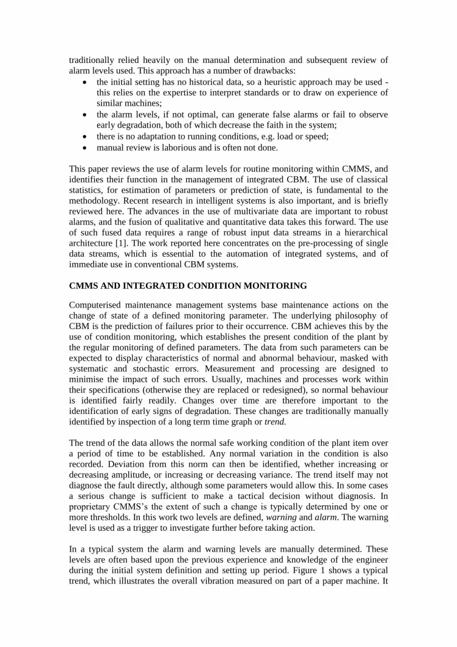
Figure 7 shows the difference between manually set, fixed alarm levels and adaptive

alarm levels obtained by the use of the PAT system. In this case the data set is the

overall vibration level in the harmonics filter, axial direction, as described in table 1

below. The original levels appear a little high, but it is emphasised that they were set

and tuned by an expert and were suitable across a range of similar machines. The

adaptive alarm levels retrospectively identify two incidents of interest which

correspond with real failure events.

CASE STUDY

This case study was undertaken to determine the effectiveness of adaptive alarms

generated by the PAT system when compared to the original fixed levels within

Wolfson’s MIMIC 2001 system. The study made use of a section of an archived

database of measurements from a variable speed paper mill in London, which

produces two- and three-layer carbon copy till receipt paper. This database contained

all the readings for a series of defined measurement parameters collected by the

MIMIC system. The majority of the measurement points defined and monitored by

the mill were vibration readings. However, a number of production parameters are

also monitored, including factors such as feed rates and machine running speeds. A

ten year history was available, with a number of known failure events. It is impossible

to test the ability of the algorithm to detect failures unless the archive has a good

event history. The alarm levels set within the data base had been optimised manually

over a period of years by human experts, and constituted the best possible control

conditions for test of the adaptive alarms. The same data was used in the proportional

hazard model built under EXAKT reported in [5].

Database structure

The data used is part of a commercial operation in regular use. The proprietary CMM

software has been through a series of generations, and this particular version used a

Borland dBase shell. Data was loaded through a proprietary interface from both

portable and hard-wired instruments.

Several paper machines were registered in the database, along with a data structure for

power supply. Paper machines were divided into sections including press, driers,

condenser and steam systems, ventilation, winders, and ancillaries, with other sections

totalling 17 data structures.

At a lower hierarchical level in the data structure the sections above were further

divided into production units and specific plant items. Each item is allocated a number

of measurement parameters, which could be single measurements, e.g. temperatures

Point in alarm Alarm limit Warning limit

Harm

onic

s

vib

ratio

n (

mm

/s)

Figure 7: Alarm levels for a harmonics feature filtered from the gearbox data: (upper) fixed levels;

(lower) adaptive levels obtained by use of the PAT system. The events in the failure history are

numbered 1-4 in the upper graph.

Alarm limit Warning limit

Harm

onic

s

vib

ratio

n (

mm

/s) 1

4 2 & 3

and pressures, or features extracted from vibration spectra such as overall levels,

looseness, bearing damage, or harmonics.

Each data record is permanently archived, so that long-term data trends can be

examined. The alarm levels are recorded with each measurement parameter, and new

data items are automatically compared to the alarm thresholds on upload. Fault

indications are used to trigger further investigation or ultimately maintenance action.

Operation of PAT

The size of the archive allowed a large choice of test conditions. Initially random

records were chosen to test operation. Later a review of whole sections of the database

was possible. The adaptive alarm levels were then automatically prepared for all

measurement parameters. The interface for the controls for PAT was prepared as part

of a software development for the existing proprietary CMMS.

It is important to note that the PAT algorithm simply prepares new adaptive alarm

levels. When this is applied to a historical database, some of the alarms triggered

change, and some remain the same. Since event history is a prerequisite to evaluate

the performance of the algorithms, specific sections of the data archives were chosen

which had a rich event history. In commercial use the testing phase will not be

necessary, and PAT simply replaces the fixed alarm levels.

Selected parameters

The full archive consisted of tens of thousands of records, so for illustration a specific

example is selected to be reported here. The case study focuses on the Aft Drier

section, which consists of a number of groups of machines. One of the groups

contained 18 identical gearboxes, which were monitored by 8 defined parameters as

shown in table 1. The parameters are prepared by filtering frequency spectra during

upload, and the filter criteria are stored with each parameter record. Full spectra are

also stored where appropriate.

Parameter name Direction Units Comment

Overall Vertical mm/s Overall vibration

Gear mesh Vertical mm/s Filter focused on the meshing frequency

Harmonics Vertical mm/s Filter focused on meshing harmonics/machine resonance

Acceleration Vertical g Broad band filter

ESP Vertical g Proprietary envelope signal processing algorithm

Overall Axial mm/s Overall vibration

Gear mesh Axial mm/s Filter focused on the meshing frequency

Harmonics Axial mm/s Filter focused on meshing harmonics/machine resonance

Table 1: Gearbox monitoring parameters

The gearbox experienced 4 maintenance actions during the monitoring period. As can

be seen from table 2 there were two types of maintenance action undertaken on this

unit, namely actions caused by a failure and preventive actions.

Failure Date Comments Action Action Type

1 5/7/95 Loose gear, worn key way New shaft, gear and bearing Failure

2 27/11/96 Replacement failure New bearing and shaft Failure

3 25/12/96 Strip and rebuild Preventive

4 29/9/97 Strip and re-build Preventive

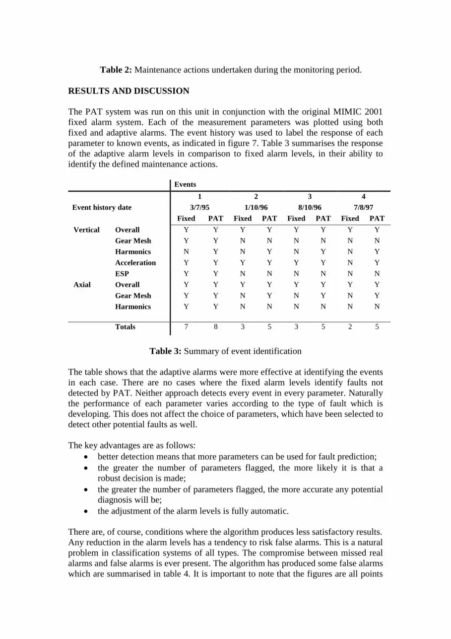
Table 2: Maintenance actions undertaken during the monitoring period.

RESULTS AND DISCUSSION

The PAT system was run on this unit in conjunction with the original MIMIC 2001

fixed alarm system. Each of the measurement parameters was plotted using both

fixed and adaptive alarms. The event history was used to label the response of each

parameter to known events, as indicated in figure 7. Table 3 summarises the response

of the adaptive alarm levels in comparison to fixed alarm levels, in their ability to

identify the defined maintenance actions.

Events

1 2 3 4

Event history date 3/7/95 1/10/96 8/10/96 7/8/97

Fixed PAT Fixed PAT Fixed PAT Fixed PAT

Vertical Overall Y Y Y Y Y Y Y Y

Gear Mesh Y Y N N N N N N

Harmonics N Y N Y N Y N Y

Acceleration Y Y Y Y Y Y N Y

ESP Y Y N N N N N N

Axial Overall Y Y Y Y Y Y Y Y

Gear Mesh Y Y N Y N Y N Y

Harmonics Y Y N N N N N N

Totals 7 8 3 5 3 5 2 5

Table 3: Summary of event identification

The table shows that the adaptive alarms were more effective at identifying the events

in each case. There are no cases where the fixed alarm levels identify faults not

detected by PAT. Neither approach detects every event in every parameter. Naturally

the performance of each parameter varies according to the type of fault which is

developing. This does not affect the choice of parameters, which have been selected to

detect other potential faults as well.

The key advantages are as follows:

better detection means that more parameters can be used for fault prediction;

the greater the number of parameters flagged, the more likely it is that a

robust decision is made;

the greater the number of parameters flagged, the more accurate any potential

diagnosis will be;

the adjustment of the alarm levels is fully automatic.

There are, of course, conditions where the algorithm produces less satisfactory results.

Any reduction in the alarm levels has a tendency to risk false alarms. This is a natural

problem in classification systems of all types. The compromise between missed real

alarms and false alarms is ever present. The algorithm has produced some false alarms

which are summarised in table 4. It is important to note that the figures are all points

flagged as exceeding warning or alarm levels which are not identified against a

known event. Even where an unrecorded event is clear in the raw data as a series of

high points, the false alarms are still recorded here as individual instances. Again we

note that the difference recorded is not the same for all parameters. Overall the change

in warning flags is marginally down, but the change in alarm flags is approximately

doubled.

False indications

Fixed PAT

Warning Alarm Warning Alarm Warning Alarm

Vertical Overall 17 7 13 8 -4 1

Gear Mesh 0 0 0 0 0 0

Harmonics 0 0 5 1 5 1

Acceleration 12 0 8 2 -4 2

ESP 7 0 6 4 -1 4

Axial Overall 16 8 11 5 -5 -3

Gear Mesh 0 0 7 9 7 9

Harmonics 5 0 4 2 -1 2

Totals 57 15 54 31 -3 16

Table 3: Summary of false indications

CONCLUSIONS

CMM systems have traditionally used manually-determined fixed warning and alarm

levels for the identification of changes within defined parameters. Manual

determination is subject to the experience and capabilities of the engineer. The levels

must be periodically reviewed to ensure the levels are correct and accurate. This is not

always practical because expertise is at a premium.

Systems have been developed in both the research and industrial communities based

on both intelligent and classical methods. However, one of the main problems with all

existing systems is the large amount of data required in training and justifying them,

and the level of expertise required in preparation.

This paper has described an automatic approach to the calculation of continually

adaptive warning and alarm levels. It is based on a multi-stage algorithm which

smoothes the parameter trend with variable forgetting factors, prior to placing

thresholds calculated from both standard deviation of the smoothed data and rate of

change of the raw data.

The PAT algorithm was tested on data from a variable speed paper mill. Tests showed

that the system was capable of predicting and identifying failures prior to their

occurrence with better performance than existing fixed warning and alarm levels. The

PAT algorithm tended to produce a higher rate of agreement between multiple

parameters, which improves the robustness of decision making, and eases diagnosis.

The algorithm has been tested on a variety of trend data patterns produced from five

different filtered vibration data types over eight parameters over a supervised data set

ten years in length. It required no tuning for individual parameters or time segments.

An extension to the algorithm was also capable of predicting the probable time until

the parameter changes from its present state to a different one, though this has not

been elaborated here .

The algorithm has some limitations in its current state. There is a penalty in terms of

false alarms, which must be managed carefully in order to retain faith in a condition

monitoring system. The algorithm also experiences problems in transition when there

is a step change in speed or loading, because it takes a while to adapt. These criticisms

must be tempered by the observation that unexplained false alarms and transition

problems also occur in fixed-limit systems set up by experts.

Further work, as well as addressing identified limitations, will extend the single

parameter trending into classification. Work is under way to use a Bayesian approach,

firstly on a naïve basis for classification of faults identified by PAT, and then latterly

into a multi-parameter system with a classification module based upon Bayesian

belief networks.

ACKNOWLEDGEMENTS

The authors gratefully acknowledge the support of the Engineering and Physical

Sciences Research Council, through the auspices of the Total Technology department

of The University of Manchester, and of WM Engineering Ltd.

References

1. Starr A, Hannah P, Esteban J, Willetts R, 2002, Data Fusion as a model for

advanced condition based maintenance, Insight, ISSN 1354-2575, v44 no 8

pp503-507

2. Tabachnick B.G., Fidel L.S., 1996, “Using Multivariate Statistics”,

HarpersCollins College Publishers, ISBN 0-673-99414-7

3. Stewart W.J., 1994, “Introduction to the Numerical Solution of Markov Chains”,

Princeton University Press, ISBN 0-691-03699-3

4. Jiang X., Makis V., Jardine A. K. S., 2001, Optimal repair/replacement policy for

a general repair model, Advances in Applied Probability ISSN 0001-8678 v 33

pp206-222

5. Willetts R., Starr A.G., Banjevic D., Jardine A.K.S., Doyle A., 2001, “Optimising

Complex CBM Decisions using Hybrid Fusion Methods”, Proceedings 14th

International Congress on Condition Monitoring and Diagnostic Engineering

Management (COMADEM 2001), Manchester UK, ISBN 0-08-0440363 pp 909-

918

6. Willetts R, 2002, Holistic Condition Monitoring, EngD Thesis, The University of

Manchester

7. Mitchell T M, 1997, “Machine Learning”, McGraw-Hill, ISBN 0-07-115467-1

8. Harris T.J and Kirkham C., 1997, “A Hybrid Neural Network System for Generic

Bearing Fault Detection” , Proceedings of COMADEM 97, Vol 2, pp 85-93,

ISBN 951-38-4563-X

9. Smith G.T, 1996, “Condition Monitoring of Machine Tools”, Southampton

Institute, Handbook of Condition Monitoring, Rao (Ed.) 1st edition, pp 171-207,

ISBN 185617 234 1

10. Taylor O. and Macintyre J., (1998),”Modified Kohonen Network for Data Fusion

and Novelty Detection Within Condition Monitoring”, Proceedings EuroFusion98,

pp145-155

11. Hu W, Starr A G, Leung A Y T, 2001, A Multisensor Based System for

Manufacturing Process Monitoring, Journal of Engineering Production,

Institution of Mechanical Engineers Proceedings Part B v215 pp1165-1175

12. Travè-Massuyés L., Milne R., 1997 “Gas-turbine condition monitoring using

qualitative model-based diagnosis”, IEEE Expert, May/June 1997, pp22-31

13. http://www.desmaint.com/

14. Flanagan, M A, Andersson, C, Surland, P, 1997, Effective automatic expert

systems for dynamic predictive maintenance applications, Proc Int Gas Turbine &

Aeroengine Cong & Exp, Orlando, ASME 97-GT-64 ISSN: 0402-1215

15. Brown R G, 1962, “Smoothing Forecasting and Prediction of Discrete Time

Series”, Prentice Hall International, ISBN 63 – 13271