Gene ranking and biomarker discovery undercorrelation

Verena Zuber ∗and Korbinian Strimmer ∗

4 February 2009; last revision 16 July 2009

Abstract

Motivation: Biomarker discovery and gene ranking is a standard task in genomichigh throughput analysis. Typically, the ordering of markers is based on a stabilizedvariant of the t-score, such as the moderated t or the SAM statistic. However, theseprocedures ignore gene-gene correlations, which may have a profound impact onthe gene orderings and on the power of the subsequent tests.Results: We propose a simple procedure that adjusts gene-wise t-statistics to takeaccount of correlations among genes. The resulting correlation-adjusted t-scores(“cat” scores) are derived from a predictive perspective, i.e. as a score for variableselection to discriminate group membership in two-class linear discriminant analysis.In the absence of correlation the cat score reduces to the standard t-score. Moreover,using the cat score it is straightforward to evaluate groups of features (i.e. genesets). For computation of the cat score from small sample data we propose ashrinkage procedure. In a comparative study comprising six different synthetic andempirical correlation structures we show that the cat score improves estimation ofgene orderings and leads to higher power for fixed true discovery rate, and viceversa. Finally, we also illustrate the cat score by analyzing metabolomic data.Availability: The shrinkage cat score is implemented in the R package “st” availablefrom URL http://cran.r-project.org/web/packages/st/.Contact: strimmer@uni-leipzig.de

∗Institute for Medical Informatics, Statistics and Epidemiology (IMISE), University of Leipzig, Härtelstr.16–18, D-04107 Leipzig, Germany

1

arX

iv:0

902.

0751

v3 [

stat

.AP]

22

Jul 2

009

1 Introduction

The discovery of genomic biomarkers is often based on case-control studies. For instance,consider a typical microarray experiment comparing healthy to cancer tissue. A shortlistof genes relevant for discriminating the phenotype of interest is compiled by rankinggenes according to their respective t-scores. Because of the high-dimensionality of thegenomic data special stabilizing procedures such as “SAM”, “moderated t” or “shrinkaget” are warranted and most effective – see Opgen-Rhein and Strimmer (2007) for a recentcomparative study.

However, microarrays are only one particularly prominent example of a series ofmodern technologies emerging for high-throughput biomarker discovery. In additionto gene expression it is now common practice in biomedical laboratories to measuremetabolite concentrations and protein abundances. A distinguishing feature of pro-teomic and metabolic data is the presence of correlation among markers, due to chemicalsimilarities (metabolites) and spatial dependencies (spectral data). These correlationsmay impact statistical conclusions.

There are three main strategies for dealing with the issue of correlation amongbiomarkers. One approach is to initially ignore the correlation structure and to computeconventional t-scores. Subsequently, the effects of correlation are accommodated inthe last stage of the analysis when statistical significance is assigned (Efron, 2007; Shiet al., 2008). An alternative approach is to model the correlation structure explicitlyin the data generating process, and base all inferences on this more complex model.For example, in case of proteomics data a spatial autoregressive model can account fordependencies between neighboring peaks (Hand, 2008). A third strategy, occupyingmiddle ground between the two described approaches, is to combine t-scores and theestimated correlations to a new gene-wise test statistic. This approach is followed inTibshirani and Wasserman (2006) and Lai (2008) and it is also the route we pursue here.

Specifically, we propose “correlation-adjusted t”-scores, or short “cat” scores. Thesescores are derived from a predictive perspective by exploiting a close link betweengene ranking and and two-class linear discriminant analysis (LDA). It is well known(Fan and Fan, 2008) that the t-score is the natural feature selection criterion in diagonaldiscriminant analysis, i.e. when there is no correlation. As we argue here in the generalLDA case assuming arbitrary correlation structure this role is taken over by the cat score.

For practical application of the cat score as a ranking criterion for biomarkers we de-velop a corresponding shrinkage procedure, which can be employed in high-dimensionalsettings with a comparatively small number of samples. This statistic reduces to theshrinkage t approach (Opgen-Rhein and Strimmer, 2007) if there is no correlation. Wealso provide a recipe for constructing cat scores from other regularized t-statistics. Fur-thermore, we show that the cat score enables in a straightforward fashion the ranking ofsets of features and thus facilitates the analysis of gene set enrichment (Ackermann andStrimmer, 2009).

The rest of the paper is organized as follows. Next, we present the methodologicalbackground, the definition of the cat score, and a corresponding small sample shrinkage

2

procedure. Subsequently, we report results from a comparative study where we investi-gate the performance of the shrinkage cat score relative to other gene ranking proceduresincluding the approaches by Tibshirani and Wasserman (2006) and Lai (2008). In ourstudy we assume a variety of both synthetic as well as empirical correlation scenariosfrom gene expression data. Finally, we illustrate the cat score approach by analyzing ametabolomic data set and conclude with recommendations.

2 Methods

2.1 Linear discriminant analysis

Linear discriminant analysis (LDA) is a simple yet very effective classification algorithm(Hand, 2006). If there are K distinct class labels, then LDA assumes that each class canbe represented by a multivariate normal density

f (x|k) = (2π)−p/2|Σ|−1/2 ×

exp{−12(x− µk)

TΣ−1(x− µk)}

with mean µk and a common covariance matrix Σ, which can be decomposed intoΣ = V1/2PV1/2 with correlations P = (ρij) and variances V = diag{σ2

1 , . . . , σ2p}. The

observed p-dimensional data x (e.g., the expression levels of all genes in a sample) arethus modeled by the mixture

f (x) =K

∑j=1

πj f (x|j),

where the πj are the a priori mixing weights. Applying Bayes’ theorem gives theprobability of group k given x,

Pr(k|x) =πk f (x|k)

f (x),

which in turns allows to define the discriminant score dk(x) = log{Pr(k|x)}. Droppingterms constant across groups this results for LDA in

dLDAk (x) = µT

k Σ−1x− 12

µTk Σ−1µk + log(πk)

= µTk (V1/2PV1/2)−1x

− 12

µTk (V1/2PV1/2)−1µk + log(πk) .

Due to the common covariance dLDAk (x) is linear in x, hence the name of the procedure.

In order to assign a class label to a data sample x the discriminant function for allclasses is computed, and the class is selected that maximizes dk(x). The discriminant

3

function itself is learned from a separate training data set (i.e. independently from thetest samples).

An important special case of LDA is diagonal discriminant analysis (DDA), to whichLDA reduces if there is no correlation (P = I) among features. Then the discriminantfunction simplifies to

dDDAk (x) = µT

k V−1x− 12

µTk V−1µk + log(πk).

In the machine learning literature prediction using the function dDDAk (x) is known as

“naive Bayes” classification (Bickel and Levina, 2004).

2.2 Feature selection in two-class LDA

Gene ranking and feature selection for class prediction are closely connected. We exploitthis here to define a score for ranking genes (features) in the presence of correlation.In what follows, we consider LDA for precisely two classes, i.e. the typical setup incase-control studies.

For K = 2 the difference ∆LDA(x) = dLDA1 (x)− dLDA

2 (x) between the discriminantscores of the two classes provides a simple prediction rule: if ∆LDA ≥ 0 then a testsample is assigned to class 1, otherwise class 2 is chosen. ∆LDA(x) can be written aftersome algebra

∆LDA(x) = ωTδ(x) + log(π1

π2) (1)

with weight vectorω = P−1/2V−1/2(µ1 − µ2) (2)

and vector-valued distance function

δ(x) = P−1/2V−1/2(x− µ1 + µ22

). (3)

The benefit of expressing two-class LDA in this fashion is that it clarifies the underlyingmechanism. In particular, the difference score ∆LDA(x) is governed solely by threefactors:

• the log-ratio of the mixing proportions π1 and π2,

• δ(x), the standardized and decorrelated distance of the test sample x to the averagecentroid, and

• the variable-specific feature weights ω.

Note in particular that the weight vector ω is not a function of the test data x and that itcarries no units of measurements. Its components ωi directly control how much eachparticular gene i contributes to the overall score ∆LDA. Thus, ω is a natural univariateindicator for feature selection in two-class linear discriminant analysis. Moreover, note

4

fold change

µ1 − µ2

standardize- t−score

c · V −1/2(µ1 − µ2)

decorrelate- cat score

c · P−1/2V −1/2(µ1 − µ2)

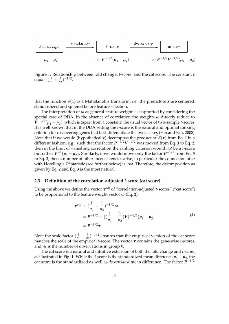
Figure 1: Relationship between fold change, t-score, and the cat score. The constant cequals ( 1

n1+ 1

n2)−1/2.

that the function δ(x) is a Mahalanobis transform, i.e. the predictors x are centered,standardized and sphered before feature selection.

The interpretation of ω as general feature weights is supported by considering thespecial case of DDA. In the absence of correlation the weights ω directly reduce toV−1/2(µ1 − µ2), which is (apart from a constant) the usual vector of two-sample t-scores.It is well known that in the DDA setting the t-score is the natural and optimal rankingcriterion for discovering genes that best differentiate the two classes (Fan and Fan, 2008).Note that if we would (hypothetically) decompose the product ωTδ(x) from Eq. 1 in adifferent fashion, e.g., such that the factor P−1/2V−1/2 was moved from Eq. 3 to Eq. 2,then in the limit of vanishing correlation the ranking criterion would not be a t-scorebut rather V−1(µ1 − µ2). Similarly, if we would move only the factor P−1/2 from Eq. 3to Eq. 2, then a number of other inconsistencies arise, in particular the connection of ωwith Hotelling’s T2 statistic (see further below) is lost. Therefore, the decomposition asgiven by Eq. 2 and Eq. 3 is the most natural.

2.3 Definition of the correlation-adjusted t-score (cat score)

Using the above we define the vector τadj of “correlation-adjusted t-scores” (“cat score”)to be proportional to the feature weight vector ω (Eq. 2):

τadj ≡ (1n1

+1n2

)−1/2 ω

= P−1/2 × {( 1n1

+1n2

)V}−1/2(µ1 − µ2)

= P−1/2τ.

(4)

Note the scale factor ( 1n1

+ 1n2

)−1/2 ensures that the empirical version of the cat scorematches the scale of the empirical t-score. The vector τ contains the gene-wise t-scores,and nk is the number of observations in group k.

The cat score is a natural and intuitive extension of both the fold change and t-score,as illustrated in Fig. 1. While the t-score is the standardized mean difference µ1 − µ2, thecat score is the standardized as well as decorrelated mean difference. The factor P−1/2

5

responsible for the decorrelation is well-known from the Mahalanobis transform that isfrequently applied to prewhiten multivariate data. Also note that the inverse correlationmatrix is closely related to partial correlations.

2.4 Estimation of feature weights and computation of the cat score from data

Substituting empirical estimates for means, variances, and correlations into Eqs. 2 and 4provides a simple recipe for estimating the feature weights and computing the cat scorefrom data. However, this is only a valid approach if sample size is large compared to thedimension.

For small-sample yet high-dimensional settings we suggest to employ James-Stein-type shrinkage estimators of correlation (Schäfer and Strimmer, 2005) and of variances(Opgen-Rhein and Strimmer, 2007). Plugging these two James-Stein-type estimators intoEq. 4 yields a shrinkage version of the cat score

tadjshrink = (Rshrink)−1/2 tshrink. (5)

A major obstacle in the application of Eq. 5 is the problem of efficiently computing(Rshrink)−1/2. Direct calculation of the matrix square root, e.g., by eigenvalue decompo-sition, is extremely tedious for large dimensions p. Instead, we present here a simpletime-saving identity for computing the α-th power of Rshrink (though here we only needthe case α = −1/2).

The shrinkage correlation estimator of Schäfer and Strimmer (2005) is given byRshrink = γIp + (1− γ)R, where R is the empirical correlation matrix and γ the shrink-age intensity. We define Z = Rshrink/γ = Ip + 1−γ

γ R = Ip + U MUT, where M is asymmetric positive definite matrix of size m times m and U an orthonormal basis. Notethat m is the rank of R. Subsequently, to calculate the α-th power of Z we use theidentity1

Zα = Ip −U(Im − (Im + M)α)UT (6)

that requires only the computation of the α-th power of the matrix Im + M. This trickenables substantial computational savings when the number of samples (and hence m)is much smaller than p.

We note that identity Eq. 6 is related but not identical to the well-known Woodburymatrix identity for the inversion of a matrix. For α = −1 our identity reduces to

Z−1 = Ip −U(Im − (Im + M)−1)UT,

whereas the Woodbury matrix identity equals

Z−1 = Ip −U(Im + M−1)−1UT.

1The validity of the identity can be verified by noting that the eigenvalues of (Ip + U MUT)α and of therighthand side of Eq. 6 are identical (which implies similarity between the two matrices) and that no furtherrotation is needed for identity.

6

Finally, additional information about the structure of the correlation matrix P (orits inverse) may also be taken into account when estimating the cat score. This is donesimply by replacing the unrestricted shrinkage estimator by a more structured estimator(e.g., Tai and Pan, 2007; Li and Li, 2008; Guillemot et al., 2008).

2.5 Selection of single genes

The cat score offers a simple approach to feature selection, both of individual genes andof sets of genes (see below).

By construction, the cat score is a decorrelated t-score. As such it measures theindividual contribution of each single feature to separate the two groups, after removingthe effect of all other genes. Therefore, to select individual genes according to theirrelative effect on group separation one simply ranks them according to the magnitudeof the respective τ

adji .

For determining p-values and FDR values we fit a two-component mixture modelto the observed cat scores (Efron, 2008). Asymptotically, for large dimension the nulldistribution is approximately normal as a consequence of central limit theorems fordependent random variables (e.g., Hoeffding and Robbins, 1948; Romano and Wolf,2000) – recall that the cat score is a weighted sum over p dependent t-statistics. This isvalidated empirically in section 3.5 discussing the analysis of a metabolomic data set.

For practical analysis we suggest employing the “fdrtool” algorithm (Strimmer,2008a,b). A comparison of methods for assigning significance to cat scores is given inAhdesmäki and Strimmer (2009).

2.6 Selection of gene sets

For evaluating the total effect of a set of features on group separation we exploit theclose connection of cat scores with the Hotelling’s T2 statistic, a standard criterion ingene set analysis (Lu et al., 2005; Kong et al., 2006).

Specifically, T2 = (tadj)Ttadj = tTR−1t, where R is the empirical correlation matrix,tadj the empirical cat score vector, and t the vector containing the gene-wise Studentt-statistic. In other words, the T2 statistic is identical to the sum of the squared individualempirical cat scores for the genes in the set. Note that any normalization with regard tothe size of the set is implicit in the factor R−1. For example, if there is strong correlationamong the genes in a set then T2 is approximately the average of the underlying squaredt-scores.

With this in mind, we define the grouped cat score for gene i belonging to a givengene set as the signed square root of the sum over the squared cat scores of all genes inthe given gene set,

τadj,groupedi = sign(τ

adji )

√∑

g∈gene set(τ

adjg )2 .

7

There are two main cases when it is important to consider sets of genes rather thanindividual genes:

• First, in a gene set enrichment analysis where prespecified pathways or functionalunits rather than individual genes are being investigated (cf. Ackermann andStrimmer (2009)).

• Second, if genes are highly correlated and thus provide the same information ongroup separation. To accommodate for this collinearity we suggest constructing asuitable correlation neighborhood around each gene, e.g., by the rule |r| ≥ 0.85.Typically, the resulting sets are rather small and for most genes are comprisedonly of the gene itself – see Tibshirani and Wasserman (2006) and also Läuter et al.(2009) for similar procedures. Note that the suggested threshold of 0.85 – whichwe use throughout this paper – is rather conservative. It defines a priori whichpair of genes are assumed to be collinear.

We note that using the grouped cat score provides to a simple procedure for high-dimensional feature selection where whole sets of variables are simultaneously includedor excluded, in contrast to the classical view of feature selection where only one ofthose features is retained (see also Bondell and Reich (2008) for references to relatedapproaches).

3 Results

In order to study the performance of the cat score for feature selection and gene ranking,we conducted an extensive study. Specifically, we investigated six different correlationscenarios, three synthetic models and three empirical correlation matrices estimatedfrom three different gene expression data sets, and compared the results with a diversenumber of regularized t-scores. Furthermore, we analyzed a metabolomic data setinvestigating prostate cancer.

3.1 Correlation scenarios

For the correlation structure, we considered a variety of scenarios. Specifically, weemployed six different correlation patterns (cf. Fig. 2):

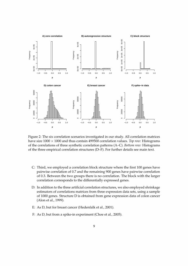
A: First, as a negative control we assumed a diagonal correlation matrix P = I of size1000× 1000.

B: Next, we employed an autoregressive block-diagonal correlation matrix (Guo et al.,2007). We used 10 blocks of size 100× 100 genes. Within each block, the correlationbetween two genes i, j, = 1, . . . , 100 equals ρ(i, j) = ρabs(i−j). We set ρ = 0.99 withalternating sign in each block. This correlation matrix is sparse with most entriesbeing very small, nevertheless it also contains some highly correlated genes.

8

A) zero correlation

ρρ

Fre

quen

cy

−1.0 −0.5 0.0 0.5 1.0

0e+

002e

+05

4e+

05

B) autoregressive structure

ρρ

Fre

quen

cy−1.0 −0.5 0.0 0.5 1.0

0e+

002e

+05

4e+

05

C) block structure

ρρ

Fre

quen

cy

−1.0 −0.5 0.0 0.5 1.0

0e+

001e

+05

2e+

053e

+05

4e+

05

D) colon cancer

ρρ

Fre

quen

cy

−1.0 −0.5 0.0 0.5 1.0

010

000

3000

050

000

E) breast cancer

ρρ

Fre

quen

cy

−1.0 −0.5 0.0 0.5 1.0

020

000

6000

0

F) spike−in data

ρρ

Fre

quen

cy

−1.0 −0.5 0.0 0.5 1.00

2000

060

000

Figure 2: The six correlation scenarios investigated in our study. All correlation matriceshave size 1000× 1000 and thus contain 499500 correlation values. Top row: Histogramsof the correlations of three synthetic correlation patterns (A–C). Bottom row: Histogramsof the three empirical correlation structures (D–F). For further details see main text.

C: Third, we employed a correlation block structure where the first 100 genes havepairwise correlation of 0.7 and the remaining 900 genes have pairwise correlationof 0.3. Between the two groups there is no correlation. The block with the largercorrelation corresponds to the differentially expressed genes.

D: In addition to the three artificial correlation structures, we also employed shrinkageestimators of correlations matrices from three expression data sets, using a sampleof 1000 genes. Structure D is obtained from gene expression data of colon cancer(Alon et al., 1999).

E: As D, but for breast cancer (Hedenfalk et al., 2001).

F: As D, but from a spike-in experiment (Choe et al., 2005).

9

3.2 Test statistics

In our comparison we included the following gene ranking statistics: fold change,empirical t statistic, “SAM” (Tusher et al., 2001), “moderated t” Smyth (2004), and“shrinkage t” Opgen-Rhein and Strimmer (2007). As in Opgen-Rhein and Strimmer(2007) the latter three regularized t-scores gave nearly identical estimates and alwaysoutperformed Student t, so we report here only the results for “shrinkage t”. As baselinereference we also included random ordering in the analysis.

For the cat score we investigated two variants: the shrinkage cat score (Eq. 5) and anoracle version, which uses the true underlying correlation matrix rather than estimatingthe correlation structure. For the two structures with high correlations (B and C) weemployed the grouped cat score using a correlation neighborhood threshold of 0.85.

In addition, we included in our study two recently proposed gene ranking proce-dures that, like the cat score, also aim at incorporating information about gene-genecorrelations in gene ranking: the “correlation-shared t-score” introduced by Tibshiraniand Wasserman (2006) and the “correlation-predicted t-score” suggested by Lai (2008).Correlation-shared t averages over gene-specific Student t-scores in a data-dependentcorrelation neighborhood. The approach by Lai (2008) employs a local smoothing ap-proach to “predict” the t-score of a particular gene from t-scores of other genes highlycorrelated with it. Here, we use the Lai (2008) approach with the smoothing parameterset to its default value f = 0.2. Note that the cat score, the correlation-shared t-score andthe correlation-predicted t-score all are based on linear combinations of t-scores, albeitwith different weights.

3.3 Data generation

In our data generation procedure we followed closely the setup in Smyth (2004) andOpgen-Rhein and Strimmer (2007), with the additional specification of a correlationstructure among genes. In detail, the simulations were conducted as follows:

• The number of genes was fixed at p = 1000. The first 100 genes were designatedto be differentially expressed.

• The variances across genes were drawn from a scale-inverse-chi-square distribu-tion Scale-inv-χ2(d0, s2

0). We used s20 = 4 and d0 = 4, which corresponds to the

“balanced” variance case in Smyth (2004). Thus, the variances vary moderatelyfrom gene to gene.

• The difference of means for the differentially expressed genes (1–100) were drawnfrom a normal distribution with mean zero and the gene-specific variance. For thenon-differentially expressed genes (101–1000) the difference was set to zero.

• The data were generated by drawing from group-specific multivariate normaldistributions with the given variances and means. The correlation matrix assumedone of the above structures A–F.

10

0 20 40 60 80 100 120

0.0

0.2

0.4

0.6

0.8

1.0

Quality of Gene Ranking

No. of Top Ranking Genes Included

TD

R (

"pre

cisi

on")

)

A) zero correlation

0 20 40 60 80 100 120

0.0

0.2

0.4

0.6

0.8

1.0

No. of Top Ranking Genes Included

TD

R (

"pre

cisi

on")

)

B) autoregressive structure

0 20 40 60 80 100 120

0.0

0.2

0.4

0.6

0.8

1.0

No. of Top Ranking Genes Included

TD

R (

"pre

cisi

on")

)

C) block structure

0.0 0.2 0.4 0.6 0.8 1.0

0.0

0.2

0.4

0.6

0.8

1.0

Precision−Recall Plot

Power ("recall")

TD

R (

"pre

cisi

on")

)

oracle catshrink catcorr. shared tLai t (f=0.2)shrink tfold changerandom order

0.0 0.2 0.4 0.6 0.8 1.0

0.0

0.2

0.4

0.6

0.8

1.0

Power ("recall")

TD

R (

"pre

cisi

on")

)

0.0 0.2 0.4 0.6 0.8 1.0

0.0

0.2

0.4

0.6

0.8

1.0

Power ("recall")

TD

R (

"pre

cisi

on")

)

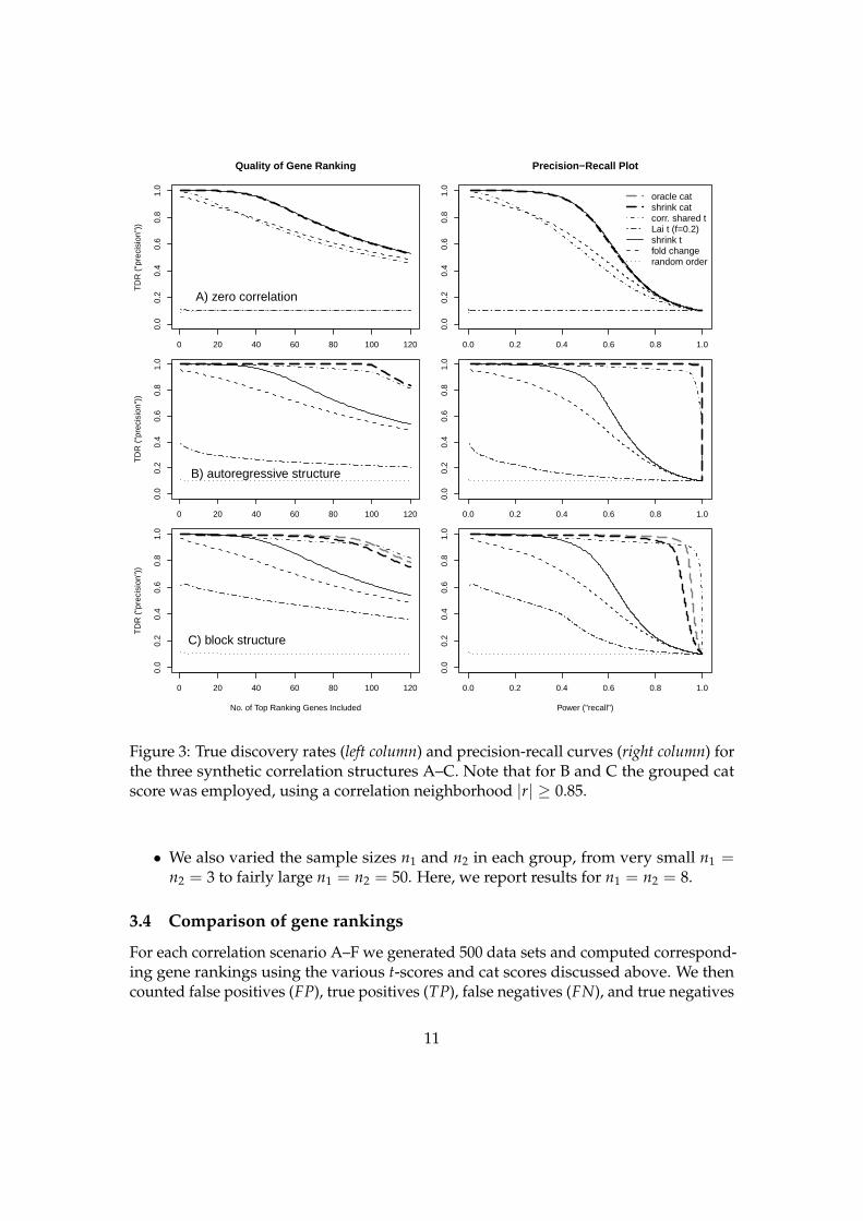
Figure 3: True discovery rates (left column) and precision-recall curves (right column) forthe three synthetic correlation structures A–C. Note that for B and C the grouped catscore was employed, using a correlation neighborhood |r| ≥ 0.85.

• We also varied the sample sizes n1 and n2 in each group, from very small n1 =n2 = 3 to fairly large n1 = n2 = 50. Here, we report results for n1 = n2 = 8.

3.4 Comparison of gene rankings

For each correlation scenario A–F we generated 500 data sets and computed correspond-ing gene rankings using the various t-scores and cat scores discussed above. We thencounted false positives (FP), true positives (TP), false negatives (FN), and true negatives

11

0 20 40 60 80 100 120

0.0

0.2

0.4

0.6

0.8

1.0

Quality of Gene Ranking

No. of Top Ranking Genes Included

TD

R (

"pre

cisi

on")

)

D) colon cancer

0 20 40 60 80 100 120

0.0

0.2

0.4

0.6

0.8

1.0

No. of Top Ranking Genes Included

TD

R (

"pre

cisi

on")

)

E) breast cancer

0 20 40 60 80 100 120

0.0

0.2

0.4

0.6

0.8

1.0

No. of Top Ranking Genes Included

TD

R (

"pre

cisi

on")

)

F) spike−in data

0.0 0.2 0.4 0.6 0.8 1.0

0.0

0.2

0.4

0.6

0.8

1.0

Precision−Recall Plot

Power ("recall")

TD

R (

"pre

cisi

on")

)

0.0 0.2 0.4 0.6 0.8 1.0

0.0

0.2

0.4

0.6

0.8

1.0

Power ("recall")

TD

R (

"pre

cisi

on")

)

oracle catshrink catcorr. shared tLai t (f=0.2)shrink tfold changerandom order

0.0 0.2 0.4 0.6 0.8 1.0

0.0

0.2

0.4

0.6

0.8

1.0

Power ("recall")

TD

R (

"pre

cisi

on")

)

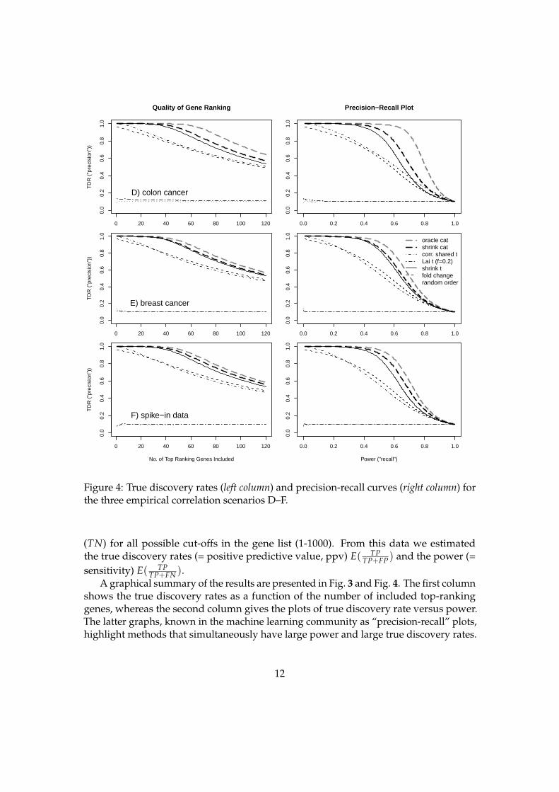
Figure 4: True discovery rates (left column) and precision-recall curves (right column) forthe three empirical correlation scenarios D–F.

(TN) for all possible cut-offs in the gene list (1-1000). From this data we estimatedthe true discovery rates (= positive predictive value, ppv) E( TP

TP+FP ) and the power (=sensitivity) E( TP

TP+FN ).A graphical summary of the results are presented in Fig. 3 and Fig. 4. The first column

shows the true discovery rates as a function of the number of included top-rankinggenes, whereas the second column gives the plots of true discovery rate versus power.The latter graphs, known in the machine learning community as “precision-recall” plots,highlight methods that simultaneously have large power and large true discovery rates.

12

The first row in Fig. 3 shows the control case when there is no correlation present. Asexpected, the cat score performs identical to the shrinkage t approach. A similar perfor-mance is given by the correlation-shared t and the fold change statistic, slightly worsethan shrinkage t- and cat score. The ordering provided by the correlation-predictedt-score is random, which is not surprising as prediction fails when there is no correlation.

For the autoregressive and the block structure (scenarios B and C in Fig. 3) substantialgains are achieved over the shrinkage t-score, both by the cat score and the correlation-shared t-score by Tibshirani and Wasserman (2006). In particular in case B these twomethods show near-perfect recovery of the gene ranking. The shrinkage t approachand fold change remain the second and third best feature ranking approach, with thecorrelation-predicted t-score of Lai (2008) trailing the comparison.

For the empirically estimated correlation structures the picture changes slightly (cf.Fig. 4). All these scenarios have in common that there is common background correlationbut no very strong individual pairwise correlations exist (cf. Fig. 2, bottom row). In thissetting the shrinkage cat score also improves over the shrinkage t-score. The oracle catscore shows that further benefits are possible if the correlation structure was known, orif a better estimator was used. For the empirical scenarios the correlation-shared t-scoreperforms similar as the fold change, and the correlation-predicted t-score again deliversrandom orderings.

In summary, in all the six quite different correlation scenarios the (grouped) cat scoreoffers in part substantial performance improvements over standard regularized t-scores,which were represented here by shrinkage t-score. The correlation-shared t-score alsoperforms exceptionally well if there are a few highly correlated genes, but otherwisefalls back to the efficiency of using fold-change approach. The correlation-predictedapproach did in general not provide any reasonable orderings. It seems to us that this isdue to the fact that it is the only test statistic that discards the actual value of the t-scoreof a gene, and instead relies exclusively on closely correlated genes – which may notexist.

3.5 Ranking of metabolomic markers of prostate cancer

To illustrate the effect of correlation on gene ranking we analyzed a subset of datafrom a recent metabolomic study concerning prostate cancer (Sreekumar et al., 2009).The original study investigated three groups of tissues, benign, localized cancer andmetastatic prostate cancer. Here, we focused on the two types of cancer tissue. Specifi-cally, we compared 12 samples of clinically localized prostate cancers versus 14 samplesof metastatic prostate cancers. For each sample the concentrations of 518 metaboliteswere measured. We use here the preprocessed data as kindly provided by Dr. Sreekumarand Dr. Chinnaiyan.

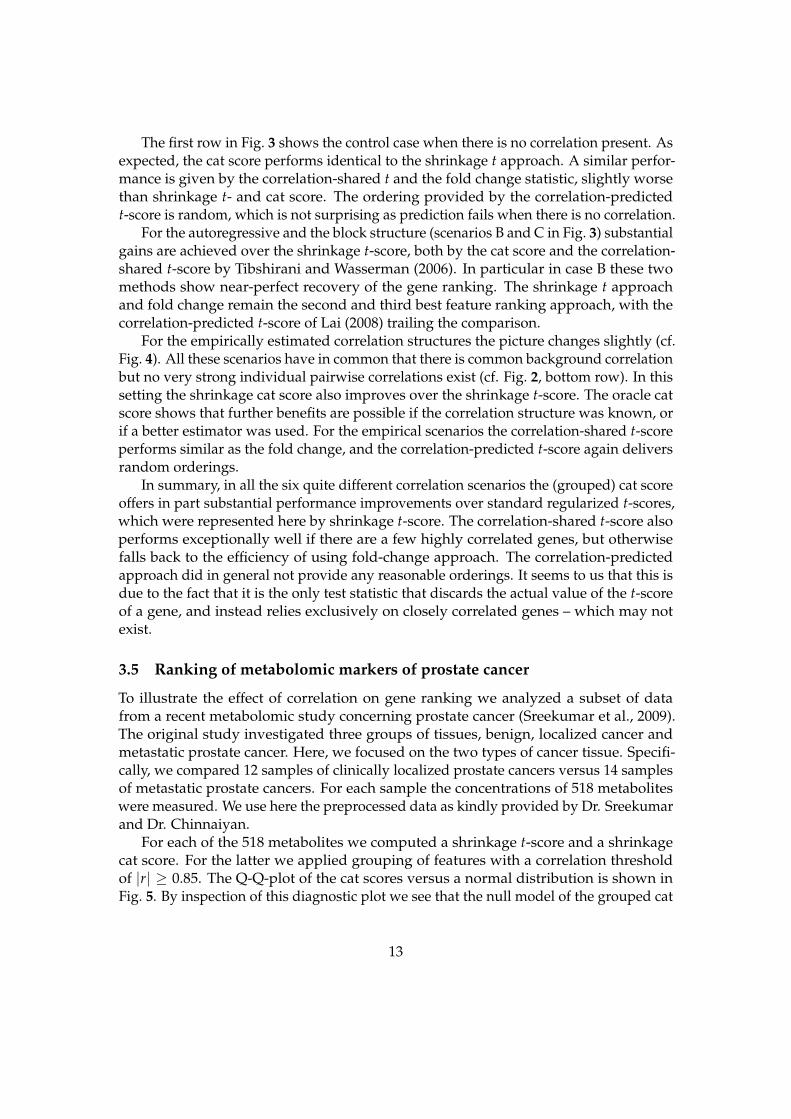
For each of the 518 metabolites we computed a shrinkage t-score and a shrinkagecat score. For the latter we applied grouping of features with a correlation thresholdof |r| ≥ 0.85. The Q-Q-plot of the cat scores versus a normal distribution is shown inFig. 5. By inspection of this diagnostic plot we see that the null model of the grouped cat

13

●

●

●

●

●

●

●

●

●

●

●

●

●

●

●

●

●

●

●

●

●

●

●

●

●

●

●

●

●

●

●

●

●

●

●

●

●

●

●

●

●

●

●

●

●

●

●●

●

●

●

●

●

●

●●

●

●

●

●

●

●

●

●

●

●

●

●

●

●

●

●

●

●

●

●●

●

●

●

●

●

●

●●

●

●

●

●

●

●

●

●

●

●

●

●

●

●

●

●

●●

●

●

●

●

●

●

●

●

●

●

●

●

●

●

●

●

●

●

●

●

●●

●

●

●

●

●

●

●

●●

●

●

●

●

●●

●

●

●

●

●

●

●●

●

●●

●●

●

●

●

●

●

●

●●

●

●

●

●

●

●

●

●

●

●

●

●

●

●

●

●

●

●

●

●

●

●

●

●

●

●

●

●

●

●

●

●●

●

●

●

●

●

●

●

●

●

●

●

●

●

●

●

●

●●

●

●

●

●

●

●

●

●

●

●

●

●

●

●

●●

●

●

●

●

●●

●

●

●

●

●

●

●

●

●

●

●

●●

●

●

●

●●

●

●

●

●●

●

●

●

●

●

●

●

●

●

●

●

●

●●●

●

●

●

●

●

●

●

●

●

●

●

●

●

●

●

●

●

●

●

●

●

●

●

●

●

●

●

●

●

●

●

●

●

●

●

●

●●

●

●

●

●

●

●

●

●

●

●

●

●

●

●

●

●

●

●

●

●

●

●

●

●

●

●

●

●

●

●

●●

●

●●

●

●

●●

●

●

●

●●

●●

●

●

●

●

●

●

●

●

●

●

●

●

●

●

●

●

●

●

●

●●

●

●

●

●

●

●

●

●●

●●

●●

●

●

●

●●

●●

●

●

●

●

●

●

●

●

●

●

●

●

●

●

●

●

●

●

●

●

●

●

●

●

●

●

●

●

●

●

●

●

●●

●

●

●

●

●

●

●

●

●

●

●

●

●

●

●

●

●

●

●

●

●

●

●

●

●

●

●●

●

●

●

●

●●

●

●

●

●

●

●

●

●

●

●●

●

●●

●

●

●

●

●

●

●

●●

●●

●

●

●

●

●

●●

●

●

●

●

●

●

●

●

●

●

●●●

●

●

●

●

●

●

●●

−3 −2 −1 0 1 2 3

−5

05

10

Normal Q−Q Plot

Theoretical Quantiles

Sam

ple

Qua

ntile

s

Figure 5: Plot of normal versus empirical quantiles for the grouped cat scores computedfrom the metabolomic prostate data. The linearity in the central part indicates a normalnull model.

scores, represented by the linear middle part, is approximately a normal distribution.The deviations from normality at the tails correspond to the alternative distributioncontaining the high-ranked metabolites of interest.

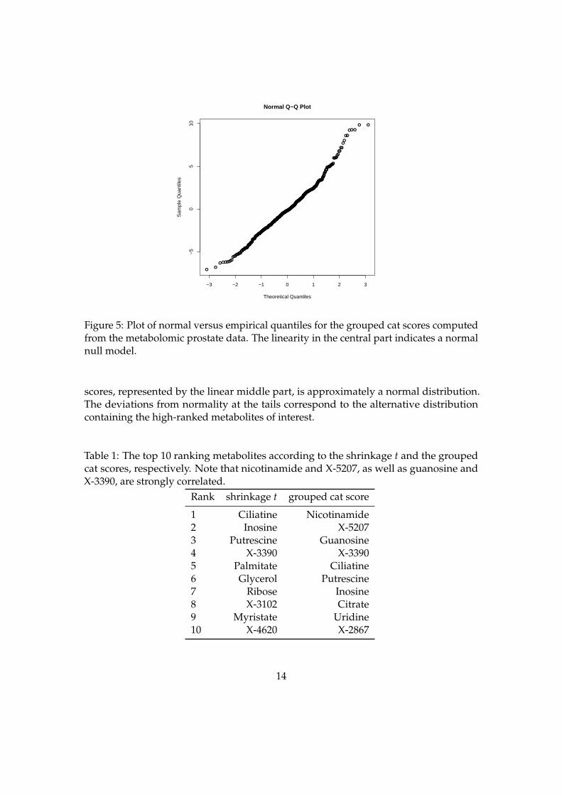
Table 1: The top 10 ranking metabolites according to the shrinkage t and the groupedcat scores, respectively. Note that nicotinamide and X-5207, as well as guanosine andX-3390, are strongly correlated.

Rank shrinkage t grouped cat score

1 Ciliatine Nicotinamide2 Inosine X-52073 Putrescine Guanosine4 X-3390 X-33905 Palmitate Ciliatine6 Glycerol Putrescine7 Ribose Inosine8 X-3102 Citrate9 Myristate Uridine10 X-4620 X-2867

14

The ten top ranking metabolic features that differentiate between localized andmetastatic cancer according to t-scores and cat scores, respectively, are listed in Tab. 1.Overall, the two rankings differ quite notably, as expected in the presence of correlation.In particular, at the top of the list there are differences due to very strong correlationbetween the substrate X-5207 and Nicotinamide (r = 0.9444) and likewise betweenGuanosine and X-3390 (r = 0.9389). Unlike with t-scores, in a grouped cat score analysisthe features in these two pairs are treated as a unit. Jointly, the correlated markersoutperform other individual markers with respect to distinguishing between the twophenotypic groups.

Regarding the interpretation of observed enrichment of nicotinamide and guanosine,we caution that without further additional information it is not possible to decidewhether this is due to intake of medication or rather due to the different progression ofcancer.

For a series of other data examples further illustrating the analysis of cat scores andestimation of corresponding predictive errors we refer to Ahdesmäki and Strimmer(2009).

4 Discussion

4.1 Harmonizing gene ranking and feature selection

The correlation-adjusted t-score is the result of our attempt to harmonize gene rankingwith LDA feature selection. While it is well known that in the absence of correlationthe t-score provides optimal rankings (Fan and Fan, 2008), the situation is less clearin the LDA case where genes are allowed to be correlated. Here we show that the catscore provides a natural weight for feature selection in LDA analysis and that it can besucessfully employed to rank genes and gene groups.

In order to apply cat scores in the analysis of high-dimensional data we developin this paper a corresponding shrinkage procedure. For moderately high dimensionsand sufficient sample size we demonstrate that incorporating correlation informationinto the gene ranking can lead to substantial improvement in power. However, this isonly feasible if either the sample size is large or the signal is strong enough to estimatecorrelations (Hall et al., 2005). For microarray data with very small sample size (in theorder of n1 = n2 = 3) it is impossible to estimate a large-scale correlation matrix, andunsurprisingly for that case we did not see any benefits. However, as our study shows(Fig. 3 and Fig. 4) using the cat score can lead to substantial gains already for relativelymoderate sample sizes (n1 = n2 = 8).

4.2 Recommendations

In high-dimensional genomic experiments with very small sample size, when nothing isknown a priori about the correlation structure, we recommend employing the standardregularized t-scores.

15

However, for moderate ratios of p/n, say smaller than 100, it is often possible to ob-tain reliable estimates of the correlation among markers. Thus, in this setting we proposeranking of biomarkers by the correlation-adjusted t-score, computed by the shrinkageprocedure outlined above. In addition, if inspection of the correlation histogram showsexistence of highly correlated features, then joint evaluation of those features by com-puting the grouped cat score is advised. Using more constrained correlation estimatorsmay further improve the efficiency.

Finally, as pointed out by a referee, gene ranking by cat scores may be combinedwith fold change-based thresholding, in order to filter out statistically significant yetbiologically irrelevant features (e.g. McCarthy and Smyth, 2009).

In short, we propose to view gene ranking as a generically multivariate problem. Inthis perspective it seems stringent not only to standardize the mean differences (i.e. usingthe corresponding t-scores) but also to additionally decorrelate them, which results inthe cat score proposed here.

Acknowledgments

We are grateful to the anonymous referees for their very valuable comments. We thankour colleagues at IMISE for discussion and Anne-Laure Boulesteix, Florian Leitenstorferand Abdul Nachtigaller for additional suggestions.

Appendix: Computer implementation

The “shrinkage cat” estimator (Eq. 5) is implemented in the R package “st”, which isfreely available under the terms of the GNU General Public License (version 3 or later)from CRAN (http://cran.r-project.org/) and from URL http://strimmerlab.org/

software/st/.

References

Ackermann, M. and Strimmer, K. (2009). A general modular framework for gene setenrichment. BMC Bioinformatics, 10:47.

Ahdesmäki, M. and Strimmer, K. (2009). Feature selection in “omics” prediction prob-lems using cat scores and false non-discovery rate control. arXiv, stat.AP:0903.2003.

Alon, U., Barkai, N., Notterman, D. A., Gish, K., Ybarra, S., Mack, D., and Levine, A.(1999). Broad patterns of gene expression revealed by clustering analysis of tumorand normal colon tissues probed by oligonucleotide arrays. Proc. Natl. Acad. Sci. USA,96:6745–6750.

16

Bickel, P. J. and Levina, E. (2004). Some theory for Fisher’s linear discriminant func-tion, ‘naive Bayes’, and some alternatives when there are many more variables thanobservations. Bernoulli, 10:989–1010.

Bondell, H. D. and Reich, B. J. (2008). Simultaneous regression shrinkage, variableselection, and supervised clustering of predictors with OSCAR. Biometrics, 64:115–123.

Choe, S. E., Boutros, M., Michelson, A. M., Church, G. M., and Halfon, M. S. (2005).Preferred analysis methods for Affymetrix GeneChips revealed by a wholly definedcontrol data set. Genome Biology, 6:R16.

Efron, B. (2007). Correlation and large-scale simultaneous significance testing. J. Amer.Statist. Assoc., 102:93–103.

Efron, B. (2008). Microarrays, empirical Bayes, and the two-groups model. Statist. Sci.,23:1–22.

Fan, J. and Fan, Y. (2008). High-dimensional classification using features annealedindependence rules. Ann. Statist., 36:2605–2637.

Guillemot, V., Le Brusquet, L., Tenenhaus, A., and Frouin, V. (2008). Graph-constraineddiscriminant analysis of functional genomics data. In IEEE International Conference onBioinformatics and Biomedicine, Philadelphia, PA, USA.

Guo, Y., Hastie, T., and Tibshirani, T. (2007). Regularized discriminant analysis and itsapplication in microarrays. Biostatistics, 8:86–100.

Hall, P., Marron, J. S., and Neeman, A. (2005). Geometric representation of high dimen-sion, low sample size data. J. R. Statist. Soc. B, 67:427–444.

Hand, D. J. (2006). Classifier technology and the illusion of progress. Statistical Science,21:1–14.

Hand, D. J. (2008). Breast cancer diagnosis from proteomic mass spectrometry data: acomparative evaluation. Statist. Appl. Genet. Mol. Biol., 7 Issue 2:15.

Hedenfalk, I., Duggan, D., Chen, Y., Radmacher, M., Bittner, M., Simon, R., Meltzer, P.,Gusterson, B., Esteller, M., Kallioniemi, O. P., Wilfond, B., Borg, A., and Trent, J. (2001).Gene-expression profiles in hereditary breast cancer. N. Engl. J. Med., 344:539–548.

Hoeffding, W. and Robbins, H. (1948). The central limit theorem for dependent randomvariables. Duke Math. J., 15:773–780.

Kong, S. W., Pu, W. T., and Park, P. J. (2006). A multivariate approach for integratinggenome-wide expression data and biological knowledge. Bioinformatics, 22:2373–2380.

Lai, Y. (2008). Genome-wide co-expression based prediction of differential expression.Bioinformatics, 24:666–674.

17

Läuter, J., Horn, F., Rosolowski, M., and Glimm, E. (2009). High-dimensional dataanalysis: selection of variables, data compression and graphics — applications to geneexpression. Biometr. J., 51:235–251.

Li, C. and Li, H. (2008). Network-constrained regularization and variable selection foranalysis of genomic data. Bioinformatics, 24:1175–1182.

Lu, Y., Liu, P.-Y., Xiao, P., and Deng, H.-W. (2005). Hotelling’s T2 multivariate profilingfor detecting differential expression in microarrays. Bioinformatics, 21:3105–3113.

McCarthy, D. J. and Smyth, G. K. (2009). Testing significance relative to fold-changethreshold is a TREAT. Bioinformatics, 25:765–771.

Opgen-Rhein, R. and Strimmer, K. (2007). Accurate ranking of differentially expressedgenes by a distribution-free shrinkage approach. Statist. Appl. Genet. Mol. Biol., 6:9.

Romano, J. P. and Wolf, M. (2000). A more general central limit theorem for m-dependentrandom variables with unbounded m. Stat. Probabil. Lett., 47:115–124.

Schäfer, J. and Strimmer, K. (2005). A shrinkage approach to large-scale covariancematrix estimation and implications for functional genomics. Statist. Appl. Genet. Mol.Biol., 4:32.

Shi, J., Levinson, D. F., and Whittemore, A. S. (2008). Significance levels for studies withcorrelated test statistics. Biostatistics, 9:458–466.

Smyth, G. K. (2004). Linear models and empirical Bayes methods for assessing differen-tial expression in microarray experiments. Statist. Appl. Genet. Mol. Biol., 3:3.

Sreekumar, A., Poisson, L. M., Rajendiran, T. M., Khan, A. P., Cao, Q., Yu, J., Laxman,B., Mehra, R., Lonigro, R. J., Li, Y., Nyati, M. K., Ahsan, A., Kalyana-Sundaram, S.,Han, B., Cao, X., Byun, J., Omenn, G. S., Ghosh, D., Pennathur, S., Alexander, D. C.,Berger, A., Shuster, J. R., Wei, J. T., Varambally, S., Beecher, C., and Chinnaiyan, A. M.(2009). Metabolomic profiles delineate potential role for sarcosine in prostate cancerprogression. Nature, 457:910–914.

Strimmer, K. (2008a). fdrtool: a versatile R package for estimating local and tail area-based false discovery rates. Bionformatics, 24:1461–1462.

Strimmer, K. (2008b). A unified approach to false discovery rate estimation. BMCBioinformatics, 9:303.

Tai, F. and Pan, W. (2007). Incorporating prior knowledge of gene functional groups intoregularized discriminant analysis of microarray data. Bioinformatics, 23:3170–3177.

Tibshirani, R. and Wasserman, L. (2006). Correlation-sharing for detection of differentialgene expression. arXiv, math.ST:math/0608061.

Tusher, V., Tibshirani, R., and Chu, G. (2001). Significance analysis of microarrays appliedto the ionizing radiation response. Proc. Natl. Acad. Sci. USA, 98:5116–5121.

18