econstorMake Your Publications Visible.

A Service of

zbwLeibniz-InformationszentrumWirtschaftLeibniz Information Centrefor Economics

Sobotka, Tomá� et al.

Working Paper

Monthly estimates of the quantum of fertility: Towardsa fertility monitoring system in Austria

Vienna Institute of Demography Working Papers, No. 01/2005

Provided in Cooperation with:Vienna Institute of Demography (VID), Austrian Academy of Sciences

Suggested Citation: Sobotka, Tomá� et al. (2005) : Monthly estimates of the quantum of fertility:Towards a fertility monitoring system in Austria, Vienna Institute of Demography WorkingPapers, No. 01/2005, Austrian Academy of Sciences (ÖAW), Vienna Institute of Demography(VID), Vienna

This Version is available at:http://hdl.handle.net/10419/96979

Standard-Nutzungsbedingungen:

Die Dokumente auf EconStor dürfen zu eigenen wissenschaftlichenZwecken und zum Privatgebrauch gespeichert und kopiert werden.

Sie dürfen die Dokumente nicht für öffentliche oder kommerzielleZwecke vervielfältigen, öffentlich ausstellen, öffentlich zugänglichmachen, vertreiben oder anderweitig nutzen.

Sofern die Verfasser die Dokumente unter Open-Content-Lizenzen(insbesondere CC-Lizenzen) zur Verfügung gestellt haben sollten,gelten abweichend von diesen Nutzungsbedingungen die in der dortgenannten Lizenz gewährten Nutzungsrechte.

Terms of use:

Documents in EconStor may be saved and copied for yourpersonal and scholarly purposes.

You are not to copy documents for public or commercialpurposes, to exhibit the documents publicly, to make thempublicly available on the internet, or to distribute or otherwiseuse the documents in public.

If the documents have been made available under an OpenContent Licence (especially Creative Commons Licences), youmay exercise further usage rights as specified in the indicatedlicence.

www.econstor.eu

VIENNA INSTITUTEOF DEMOGRAPHY

tion Forecastinglity in Austria:

Working Papers

tion Forecastinglity in Austria:Monthly Estimates of the Quantum of Fertility:

Tomáš Sobotka, Maria Winkler-Dworak, Maria Rita Testa, Wolfgang Lutz,

Vienna Institute of DemographyAustrian Academy of Sciences

Prinz Eugen-Strasse 8-10 · A-1040 Vienna · Austria

E-Mail: vid@oeaw.ac.atWebsite: www.oeaw.ac.at/vid

01 / 2005

tion Forecastinglity in Austria:Towards a Fertility Monitoring System in Austria

tion Forecastinglity in Austria:Dimiter Philipov, Henriette Engelhardt, and Richard Gisser

Abstract Short-term variations in fertility and seasonal patterns of childbearing have been of interest to demographers for a long time. Presenting our detailed study of period fertility in Austria since 1984, we discuss the problems and advantages of constructing and analysing various period fertility indicators that reflect real exposure and potentially minimise the distortions caused by changes in fertility timing. We correct monthly birth data for calendar and seasonal factors and show that seasonality of births in Austria varies by birth order. Our study reveals that the methods explicitly aimed at adjusting fertility rates for tempo distortions are not suitable for computing monthly fertility rates. However, most of the timing distortions can be eliminated when using an indicator derived from the period parity progression ratios based on birth interval distributions, termed the Period Average Parity (PAP). We illustrate the insights gained from PAP and compare it with the commonly used total fertility rates in an analysis of the recent upswing in period fertility, starting in the late 2001. This investigation will serve for establishing a monitoring of monthly fertility rates in Austria. Keywords Austria, fertility, fertility measurement, birth seasonality Authors Tomáš Sobotka, Maria Winkler-Dworak, and Maria Rita Testa are Researchers at the Vienna Institute of Demography of the Austrian Academy of Sciences. Wolfgang Lutz is the Director of the Vienna Institute of Demography of the Austrian Academy of Sciences, and director of the World Population Project at the International Institute for Applied Systems Analysis, Laxenburg, Austria. Dimiter Philipov is the Leader of the Research Group on Comparative European Demography at the Vienna Institute of Demography of the Austrian Academy of Sciences. Henriette Engelhardt is the Deputy Research Group Leader of the Research Group “Demography of Austria” at the Vienna Institute of Demography of the Austrian Academy of Sciences. Richard Gisser is the Deputy Director and the Leader of the Research Group “Demography of Austria” at the Vienna Institute of Demography of the Austrian Academy of Sciences.

Acknowledgements This paper is a result of our work on the project “Birth Barometer” (Geburtenbarometer), supported by the Austrian Federal Ministry of Social Security, Generations and Consumer Protection (Bundesministerium für Soziale Sicherheit, Generationen und Konsumentenschutz), grant number BMSG-442030/006-V7/2004. We gratefully acknowledge the assistance provided by Statistics Austria in acquiring the data on births used in our analyses. We would like to thank Werner Richter for his careful editing of the text.

2

Monthly Estimates of the Quantum of Fertility: Towards a Fertility Monitoring System in Austria

Tomáš Sobotka, Maria Winkler-Dworak, Maria Rita Testa, Wolfgang Lutz, Dimiter

Philipov, Henriette Engelhardt, and Richard Gisser 1. Introduction

Observing variation constitutes the primary source of information about the determinants of change. This holds for our everyday learning as well as for much of the natural and social sciences. The three dimensions along which we observe variation in behaviour—the inter-individual, the spatial and the temporal dimension—taken together, provide us with a rich set of empirical data from which we can derive plausible hypotheses about the reasons for this differential behaviour and the drivers of change that can also be extrapolated into the future.

Demographic analysis typically is carried out along all three dimensions. But at

different times and in various schools of demographic research the weights placed on these dimensions differ. Traditional macro-level demography almost exclusively studied change and variation at the level of populations, as the word demography (derived from the Greek demos = people and graphein = to write) implies. More recently, thanks to the advance of statistical methods and the availability of large data sets collected through sample surveys, the research emphasis has strongly shifted toward the individual level, trying to disentangle the reasons for differential behaviour in population subgroups through multivariate analysis. Even more recently the study of individual biographies (life course analysis) also introduced the dimension of temporal change into the analysis, opening thus a broad and previously untapped field of research. The time steps considered in these life course studies are now typically calendar months because years turned out to be too crude a time unit.

But the analysis of individual-level variation cannot tell us the full story. In order

to understand the reasons of differential behaviour we also need to consider its societal context. Different welfare regimes, labour market patterns, cultural values, norms and public sentiments all present important macro-level determinants of demographic behaviour. Typically, these questions have been considered at the level of countries but more recent attempts to capture the contextual variables have gone much further along this path to characterising the contexts of demographic behaviour in smaller areas, combining the individual level with aggregate-level analysis. Temporal variation has remained the most important source of information at the macro-level, but the unit of temporal analysis has almost exclusively been the calendar year. The main reason for this prominent focus on annual variations is probably the availability of data, which are typically published and often collected on an annual basis.

From a theoretical point of view one might assume that a smaller, i.e., more

precise unit of temporal variation would provide us more information about the nature of the process under study. At the level of individual life course analysis the transition

3

from annual to monthly data has long been made. Why should not a similar transition be made for the analysis of aggregate demographic data?

This is the issue this article aims to address. Since some of the contextual

variables change from month to month, there is a great potential gain from a transition to monthly data. Presenting our detailed study of period fertility in Austria since 1984, we discuss the problems and advantages of analysing monthly data and constructing period fertility indicators that are free not only of seasonality effects, but also of the distortions caused by the changes in the timing of childbearing. Studying monthly trends in period fertility is particularly useful for analysing changes in relevant social security and child benefit policies, but in a broader perspective also changes in widespread feelings and public sentiments. One could also get a better handle on perception lags and reaction times to such changes.

Short-term variations in fertility and seasonal patterns of childbearing have been

of interest to demographers for a long time and a variety of hypotheses have been postulated on the biological, cultural, environmental, and social determinants of birth seasonality in various historical and contemporary settings (e.g., Lam, Miron, and Riley 1994, Doblhammer-Reiter, Rodgers, and Rau 1999, Bobak and Gjonca 2001). Nevertheless, seasonal cycles constitute an obstacle for assessing short-term trends in period fertility. Especially in low-fertility settings, changes in the registered monthly number of births may capture the attention of the media and the general public. Thus, it is important to disentangle seasonal variation and the real increase in fertility rates. An advanced analysis of monthly fertility rates was developed by G. Calot (see, e.g., Calot and Nadot 1977, Calot 1981a and 1981b). Although most statistical offices publish only raw data on the observed monthly number of births, the Office of National Statistics for England and Wales publishes both crude and seasonally adjusted monthly total fertility rates in its birth statistics yearbook (e.g., ONS 2004).

Our investigation of monthly fertility in Austria goes several steps further than the

existing studies. We calculate fertility rates for each birth order separately, using the usual total fertility rates as well as the exposure-specific rates and fertility table indicators. To our knowledge, birth order (parity) has rarely been considered in the studies on birth seasonality (Prioux 1988 and Haandrikman 2004 being notable exceptions) and parity-specific fertility indicators have never been constructed on a monthly basis. In addition, we also analyse the possibilities of eliminating the distortions in period fertility rates caused by changes in the timing of childbearing. The practical outcome of our endeavours is the establishment of a monthly monitoring system providing a database of the most recent fertility indicators in Austria, which will be updated every month with the latest birth records obtained from Statistics Austria.

The remaining parts of this paper are structured as follows. First, we discuss

tempo distortions in period fertility and the existing methods that aim to eliminate these distortions. Then we specify the data and methods employed and introduce different indicators analysed. The subsequent Section 5 discusses selected general findings on birth seasonality and on the analysis of monthly fertility data. Section 6 provides a comparative analysis of fertility indicators studied. Section 7 uses the most recent data

4

to illustrate the insights gained with monthly fertility indicators. The last section concludes. 2. Tempo Distortions in Period Fertility Rates

Commonly used indicators of period fertility, such as the period total fertility rate (TFR), are sensitive to the changes in the timing of childbearing. When women advance or postpone childbearing, total fertility rates do not reflect the “pure” level (quantum) of period fertility, but rather an interplay of the quantum and timing influences, the latter often being referred to as tempo effects. These timing shifts do not affect the completed cohort fertility rate which constitutes an unambiguous indicator of fertility quantum. A shift towards a later timing of childbearing, which is currently underway in almost all European countries, pushes the period total fertility rates towards lower levels than would be observed if the timing of childbearing remained stable. In other words, since the younger generations of men and women wait increasingly longer before entering parenthood, a considerable proportion of births is perpetually postponed towards the future. This process is reflected by a divergence between the period total fertility rates, which are deflated by tempo effects, and the completed cohort fertility rates. For instance, the mean value of the period TFR in Austria in 1984-1990 was 1.46, well below the estimated completed fertility among women born in 1960 (1.77), who had realised a substantial portion of their childbearing during that period. These contrasts between the period and the cohort TFR are particularly strong in the case of first births (Sobotka 2004a).1

The issue of timing distortions has received much attention since 1998, when

Bongaarts and Feeney proposed an adjustment of the period TFR based on order-specific total fertility rates and annual changes in the order-specific mean age at childbearing. At least three different factors have contributed to the subsequent rapidly evolving debate on tempo effects. First, many Northern and Western European countries have experienced more than three decades of continuous fertility postponement—which is a very long period of one-directional shift in fertility timing when compared with other timing shifts during the last century.2 Second, countries representing more than half the European population have experienced a decline of the period TFR to extreme low levels of 1.1-1.3 (Sobotka 2004b). In this context, the question whether such low fertility levels are attributable to distortions caused by fertility postponement or whether they reflect alarmingly low levels of fertility quantum appears crucial. While the latter possibility would justify calls for explicit pronatalist interventions, the first possibility reflects a growing need for detailed assessment on the

1 While the mean value of the first-order TFR in Austria in 1984-1990 (0.668) seemingly indicates that about one third of women might eventually remain childless, the estimated level of final childlessness among women born in 1962 is only at a half of this value, namely 16 to 17%. 2 Austria has been no exception to a Europe-wide trend of delayed parenthood, although there the process started somewhat later than in most Western European countries, namely after 1980. In the early 1980s a typical Austrian woman gave birth to her first child before reaching age 24. Since then, the mean age at first birth among women in Austria (calculated from the age schedule of incidence rates) has increased by more than three years, reaching 27 years in 2004.

5

magnitude of tempo distortions in period fertility and the possible extent of the future increase in the period TFR. Third, Bongaarts and Feeney offered a relatively simple method of period fertility adjustment, which can be readily used in the majority of European countries.

The debate on timing effects in period fertility indicators and the Bongaarts-

Feeney adjustment in particular has proceeded in several main directions. On a general level, many contributions have addressed the issue of delayed parenthood and its impact on fertility level and trends (e.g., Lesthaeghe and Willems 1999; Frejka and Calot 2001; Lesthaeghe 2001; Kohler, Billari, and Ortega 2002; Ní Bhrolcháin and Toulemon 2003; Sobotka 2004a) as well as on the long-term population dynamics (Lutz, O’Neil, and Scherbov 2003; Goldstein, Lutz and Scherbov 2003). From a methodological perspective, the Bongaarts-Feeney method has been repeatedly criticised for its unrealistic assumptions3 (e.g., van Imhoff and Keilman 2000, Schoen 2004) and, from the practical point of view, for the occasional erratic values and considerable fluctuations in the adjusted period TFR. Despite its deficiencies, the procedure received support by the sensitivity analysis presented by Zeng and Land (2001) and has been repeatedly used for an assessment of tempo effects in the period TFR in developed societies (e.g., Philipov and Kohler 2001, Bongaarts 2002, UN 2003, Sobotka 2003 and 2004b).

Further development of the more sophisticated methods of period fertility

adjustment was a logical outcome of the criticism towards the Bongaarts-Feeney method. Kohler and Philipov (2001) suggested an adjustment which additionally incorporates changing variance in the age-specific schedule of incidence rates, while Kohler and Ortega (2002) and Yamaguchi and Beppu (2004) proposed an adjustment of the exposure-specific fertility indicators. A different approach was advocated by Schoen (2004), who employed completed cohort fertility data to derive an indicator of period fertility that is free of tempo distortions. This indicator, called the average cohort fertility rate at time t (ACF(t)), has an obvious disadvantage: it can be calculated for any given year t only when women bearing children in that year approach the end of their reproductive period and their completed cohort fertility can be derived. Only limited attention was paid to examining the usefulness of other existing indicators in reflecting the fertility level during the periods marked by substantial shifts in fertility timing; the analysis presented by Toulemon (2004) constitutes the main exception.

This study assesses the usefulness of parity-specific fertility indicators constructed

within the life table framework as well as the indicators providing an explicit adjustment for the tempo distortions in constituting a workable alternative to the period total fertility rate. Our explicit aim is to propose an indicator that is sufficiently stable 3 The main objections to the Bongaarts-Feeney formula are as follows: (1) It assumes that the age shape of the fertility schedule remains constant over time, i.e., that all cohorts postpone or advance childbearing to the same extent. (2) It is based on order-specific incidence rates (‘reduced’ rates) which do not take into account the actual parity distribution of the female population by age. As a result, the adjusted TFR, when specified by birth order, is often distorted by changes in the parity distribution among women as much as the ordinary period TFR. Furthermore, it can be shown that the period mean age at childbearing, calculated from the age and order-specific incidence rates, is itself an imperfect indicator of change in fertility timing (Sobotka 2004a: 74-75), which may also contribute to the instability of results provided by the Bongaarts-Feeney adjustment.

6

when used on a monthly basis and at the same time capable of eliminating most of the tempo distortions typical of the TFR. 3. Data

Our study requires highly disaggregated data which are not commonly tabulated on a monthly basis. Statistics Austria supplied us with extracts from individual birth records in 1984-2004, which allowed us to construct any of the existing indicators of period fertility. We draw on data on all live-born children in Austria between January 1984 and November 2004, consisting of 1.8 million records. The variables used are the date of birth of mother and child, biological live birth order of each child, and the date of the last previous birth that serves for a computation of birth interval (duration) analysis. The collection of birth statistics pertaining to the real (biological) birth order of a child started in Austria only in 1984 and therefore our analysis could not be extended to the period before 1984, when a rapid fertility decline had already been underway.

Estimating the denominator (female population at risk) required combining

different data sources. As the population by age and parity cannot be derived from a population register, these data had to be derived by combining the 1991 Census data on age and parity distribution among women (OSZ 1996) with our continually updated monthly estimates of age and order-specific fertility rates and the annual time series on the number of women by age, taken from EUROSTAT (2004). For the more recent time series starting from January 2001 we updated our estimates with the 2001 Census results (SA 2005). More details on the estimation procedure are provided in the Appendix 3. We performed sensitivity analysis to test whether our updated recent age-parity estimates based on the 2001 Census produce different estimations of the age-parity fertility table indicator (PATFR) than the original estimates based on the 1991 Census and found relatively minor differences, which did not create any obvious break in the time series of fertility rates (see Appendix 6). Finally, to compute parity-specific fertility indicators based on duration since the previous birth, we had to estimate the distribution of live births by birth order for the years prior to 1984. Data for 1961-1979 were derived from retrospective data on the distribution of births by birth order as recorded in the 1981 Census (OSZ 1989) combined with the total registered number of live births in that period. The number of live births by birth order in 1980-1983 was estimated from the total number of live births and the relative distribution of order-specific births in 1978-1979 and 1984-1985. 4. Methods

4.1. Seasonal and Calendar Adjustment of Raw Number of Births

The analysis of monthly number of births requires calendar and seasonal adjustments. The reason for the calendar corrections is that different numbers of weekdays within a month and different lengths of the months within a year may alter

7

the final amount of monthly births. Indeed, as shown in previous work (Calot 1981b; Höhn 1981; Gisser 1984), births occur more frequently on working days than in the weekends, and moreover, differences in the monthly number of births may well be influenced by the different number of days in a given month. Seasonal corrections are necessary for a proper interpretation of seasonal patterns in births and become prerequisites for a more advanced analysis of fertility trends.

We compute a corrected monthly number of births by using the following

adjustment:

CBi(a) = Bi(a) ·IC · ISi , (1)

where Bi(a) represents the observed number of births of birth order i by the age of mother a, CB denotes the corrected number of births; IC is the calendar factor, and ISi denotes the seasonality fluctuations of births of order i.

To estimate the calendar factor we compute the weekday coefficients. These

coefficients are given by the average daily number of births of the particular weekday divided by the mean number of births per day. Births are more frequent on Mondays to Fridays, irrespective of birth order. 4 As the differences by birth order were not significant, we did not include birth order components in the calendar adjustment.

Then, the calendar factor is derived by summarising over the distribution of

weekdays within the month, which are weighted by the corresponding weekday coefficient.5 Note that the calendar factor can be decomposed into two parts: an effect which can be linked to the length of the month, and a net effect for each day of the week (Ladiray and Quenneville 2001). The net effect only involves days of the week occurring five times in a month. Since every month contains four complete weeks, their net effects cancel out, and only the net effects of the additional days are controlled for.6 Finally, the calendar factor standardises the monthly number of births to 1/12 of the year. Computations of the weekday coefficients, as well as the statistical tests, were performed using the statistical software package STATA (StataCorp 2004).

Seasonal adjustments are aimed at removing seasonal variations from the time

series. There are numerous methods for the adjustment of seasonal variation; a useful review is provided by Ladiray and Quenneville (2001). We use the X-12-ARIMA method implemented in the software package Gretl (Cottrell 2004). This method, developed by the US Bureau of the Census (Findley et al. 1998), is an iterative seasonal adjustment algorithm based on ratio-to-moving averages and is similar to the method proposed by Calot (1981a) for the seasonal adjustment of births. However, the X-12-ARIMA differs from the Calot’s method in that the future values are forecasted by the 4 The figures of the weekday coefficients by birth order for all years since 1984 can be found in Appendix 1; Appendix 2 specifies in detail the decomposition of the calendar adjustment factor. 5 Since the birth records of 2004 are not yet complete, we used the weekday coefficients derived from 2003 in order to correct the monthly number of births from January 2004 to November 2004. 6 I.e., the net effect of 1 additional day for a February in a leap year, 2 additional days for April, June, September, and November, and 3 additional days for January, March, May, July, August, October and December remains.

8

use of ARIMA models (following the Box-Jenkins method) and the extended series is seasonally adjusted in order to increase stability at the end of the time series.

We find that the seasonal pattern is rather stable over the whole investigation

period, but unlike the calendar factor, the seasonality in births varies by birth order (see Section 5.1). Hence, we perform the seasonal adjustment of the monthly number of births separately for birth orders 1, 2, and 3+.

4.2. The Selection of Fertility Indicators Analysed in this Study

Since the changes in fertility timing make the interpretation of the total fertility rate highly problematic, any credible analysis of recent fertility trends should consider the distortions caused by fertility postponement. At the same time, the issue of how to correct period fertility indicators for these distortions remains disputed and none of the methods proposed thus far provides an unambiguous indicator of period fertility quantum. No research undertaken in the past has studied tempo distortions in shorter intervals than annual time series. We were facing a number of obstacles when deriving the monthly fertility indicators. Besides extensive data requirements, the computation of various fertility indicators by calendar month implied that the age and parity structure of the female population had to be estimated by calendar month as well. In order to test whether using more detailed birth data would change the resulting fertility rates, we also investigated the differences between monthly fertility rates specified by single years of age of women (annual birth cohorts) and the rates calculated for monthly birth cohorts (see Section 5.2). Furthermore, since the existing fertility adjustment methods have all been constructed on an annual basis, accommodating these methods for correcting fertility rates on a monthly basis required their modification. Finally, the tempo-adjustment methods do not allow to estimate adjusted indicators for the most recent calendar year (month), as they use the most recent data for the period t to estimate the tempo-adjusted indicators in the period t-1. Analysing the Bongaarts-Feeney method, we therefore investigated the possibilities of calculating tempo-adjusted indicators for the most recent period (month) of observation (see Section 6.2).

In our selection of fertility indicators, we put the main emphasis on parity-

specific indicators that reflect real exposure and on indicators that potentially minimise the distortions caused by the changes in fertility timing. A parity-specific approach is consistent with the sequential nature of childbearing and approximates the family-building behaviour of real cohorts much closer than the usual approach based on incidence rates (Lutz 1989). Specifically, the life table (or ‘fertility table’) model constitutes our preferred framework to analyse period fertility.

All indicators considered here are based on the synthetic cohort approach. The

total quantum of fertility is expressed in terms of the mean number of children per woman, which is an intuitively understandable and easily interpretable unit of measurement. The aggregate total fertility quantum can be decomposed by birth order. To allow a compact and readable overview of various methods and indicators analysed, we kept the use of equations and symbols at the minimum level. A complete overview of all the equations used is provided in Appendix 4.

9

4.3. Fertility Indicators Selected for the Analysis

Our study analyses the following indicators of period fertility: a) Indicators not explicitly adjusted for changes in the timing of childbearing The total fertility rate (TFR) Despite its shortcomings, this most widely used indicator of period fertility

constitutes a starting point of our analysis as well as a benchmark to compare other fertility indicators.

The fertility index based on age and parity life table (PATFR) Although not frequently used, a multistate fertility table based on age and parity is

the most established parity-specific method of period fertility analysis. For any given period, fertility behaviour is specified by the set of age and parity-specific birth probabilities (or occurrence-exposure rates). Starting from the age when all women are childless (in our analysis age 12) the period life table model generates for every age a parity distribution that corresponds to the schedule of age-parity birth probabilities in a given period. The final parity distribution of the synthetic cohort of women at the end of their reproductive period (age 50 in our analysis) can be summarised in the overall fertility index PATFR (this acronym follows Rallu and Toulemon (1994), who termed the PATFR an index controlling for parity and age).

Parity progression ratios based on duration since previous birth (parity and

duration life table model, PPRd) In this framework, the transition rate between different parities is a function of the

time elapsed since the previous birth. As contrasted with the PATFR index specified above, duration (birth interval) rather than the actual age is seen as a main parameter of fertility behaviour among women having at least one child.7 For each parity, a summary indicator combining fertility rates across all the birth intervals considered gives the period parity progression ratio (PPR).

In this study we employ duration-specific ‘incidence rates,’ which relate births of

order i in the period t at duration d to the initial number of women who experienced birth of order i-1 in the period t-d. Other than with the more frequently used duration-parity birth probabilities, the exposure is based solely on the time series of the total number of live births specified by birth order. In contrast, computing duration-parity birth probabilities would involve an estimation of the population of women by parity status and duration since previous birth for each calendar month considered. We compute the period parity progression ratios for each parity above 0 as a sum of order-specific incidence rates for all durations (birth intervals) considered, namely 0 to 25

7 This assumption finds a strong support in empirical data. Rates of subsequent childbearing are usually highest 2 to 4 years after the birth of a (previous) child, with a sharp decline thereafter. For instance, among women in Austria giving birth to their first child in 1984, almost a half (49%) had a second child during the next four years, while a quarter (24%) had a second child after five years or later, i.e., between 1989 and 2003. Age is an important factor as well, but with the exception of old mothers it merely changes the overall intensity of subsequent childbearing, not the general pattern of birth interval distribution.

10

years. This method is an analogy to duration-specific incidence rates, pioneered by L. Henry to analyse marital fertility (e.g., Henry 1961).

The period average parity (PAP) The parity-duration model specified above cannot be applied for first births.

However, two different approaches are methodologically compatible with this framework to derive the fertility index of birth order 1 and consequently also the overall total fertility. Traditionally, the parity progression method has been used to analyse marital fertility and the date of marriage then served as a starting point of exposure to first birth (e.g., Henry 1953, Feeney and Yu 1987). Alternatively, first birth duration may be seen as a function of age. Then, the parity progression ratio to a first birth is given by the age and parity model specified above. This is a clearly preferred option to analyse fertility changes in any advanced society, since the high rates of non-marital childbearing imply that the study of marital fertility has become obsolete as it captures only a portion of the aggregate fertility. A combination of the PATFR index for birth order 1 with the parity-progression ratios to second and later births based on duration (birth intervals) yields the summary index of period fertility, which we call period average parity (PAP).8

Although deriving the PAP index is a data-intensive endeavour, it has one

considerable advantage: it is less affected by the changes in fertility timing than the other (non-adjusted) period fertility indicators. Its first component, the PATFR index of parity 1, is distorted by the timing changes to a relatively minor extent when compared with the period TFR (Sobotka 2004a), which is also apparent in the case of Austrian data (see Section 6.3 and Figure 5). Assuming that the trend towards later timing of childbearing is primarily driven by the postponement of first births and the subsequent pace of childbearing remains relatively constant, the duration-based parity progression ratios should be little affected by tempo effects. Since this method does not involve any explicit adjustment for tempo effects, it does not suffer all the methodological and technical problems linked to the various adjustment procedures.

b) Indicators adjusted for changes in fertility timing Bongaarts and Feeney’s (1988) tempo-adjusted TFR (adjTFR) Irrespective of its flaws, the Bongaarts-Feeney adjustment constitutes the most

established procedure to correct the period TFR for tempo effects. It is also less data-demanding than alternative methods. As we demonstrate in Section 6.2, its main weakness in the case of Austria does not lie in suggesting implausible levels of fertility quantum in general, but rather in its volatility, which is particularly pronounced in the time series of monthly data.

8 There is no established way to term this summary indicator. Feeney and Yu (1987), for instance, simply use the term TFR or “parity progression ratio TFR,” while Rallu and Toulemon (1994) refer to the “index of parity and duration since previous birth” (PDTFR) and, in the particular case of duration-specific incidence rates, to the “duration-specific incidence rates index” (PDiTFR). We propose the term period average parity (PAP) in order to distinguish this index clearly from the commonly used total fertility rates, to emphasise its derivation from the period parity progression ratios and at the same time to keep the name reasonably short.

11

Kohler and Ortega’s (2002) adjusted PATFR index (adjPATFR) Unlike the Bongaarts-Feeney approach, Kohler and Ortega’s procedure employs a

set of exposure-specific fertility indicators computed for each age and parity status of women, which can be summarised within the framework of parity-specific fertility tables. This method is methodologically preferable to the Bongaarts-Feeney approach as it reflects real fertility behaviour more adequately. In addition, this procedure may be used for formulating explicit scenarios of cohort fertility linked to different assumptions about the future course of fertility postponement and the interaction between fertility delay and fertility quantum (Kohler and Ortega 2004). We outline the essence of the highly complex Kohler-Ortega adjustment in Appendix 4 (Section A-4.6); a full description may be consulted in the original contribution (Kohler and Ortega 2002).

However, besides clear methodological advantages, the Kohler-Ortega adjustment

also has a number of problematic features, which are especially hard to deal with in the analysis of monthly time series. These features, which we discuss in more detail in the Appendix 4, include the issue of smoothing the observed data, the difficulty to derive the most recent adjusted indicators, the need of limiting the age range of rates used for the adjustment procedure and the instability of the adjusted rates at higher parities. Facing these difficulties, we decided after preliminary analysis not to include the Kohler-Ortega method into our study of monthly fertility rates. Instead, we used it only for the overall evaluation of results depicted on an annual basis and we restrict its use for birth orders 1 and 2 (see Appendix 7). 5. Analysing Monthly Birth Data and Fertility Rates: General Findings

This section summarises some general findings from our analysis of monthly birth data. The next section then provides an assessment of different fertility indicators studied.

5.1. Birth Seasonality Differs by Birth Order The seasonal pattern of childbearing remained relatively stable during the

analysed period, with a peak in summer and early fall and a trough in the last quarter of the year. In line with Prioux (1988) and Haandrikman (2004), our analysis depicted in Figure 1 reveals that this profile is not equal for different birth orders. While there are fewer births for birth orders 1 and 3+ in spring (especially in April and May), births of order 2 occur more often in spring; the seasonal coefficient is by 2% above the average monthly level in March and April. Furthermore, the peak in September is more pronounced for first births than for higher parities (coefficients 1,07 versus 1,04).

However, the causes of the parity-specific differences of the seasonality in births

are less clear. Prioux (1988) finds that the seasonal variation of first births in the 1960s and 1970s can to some extent be traced back to the seasonal variation in marriage planning, and thus partly explains the differences in seasonality between first and higher-order births during these periods. But there is less evidence on the influence of seasonality of marriages in more recent times. Haandrikman (2004) proposes that the birth order specific seasonality differences may be partly due to parity-specific

12

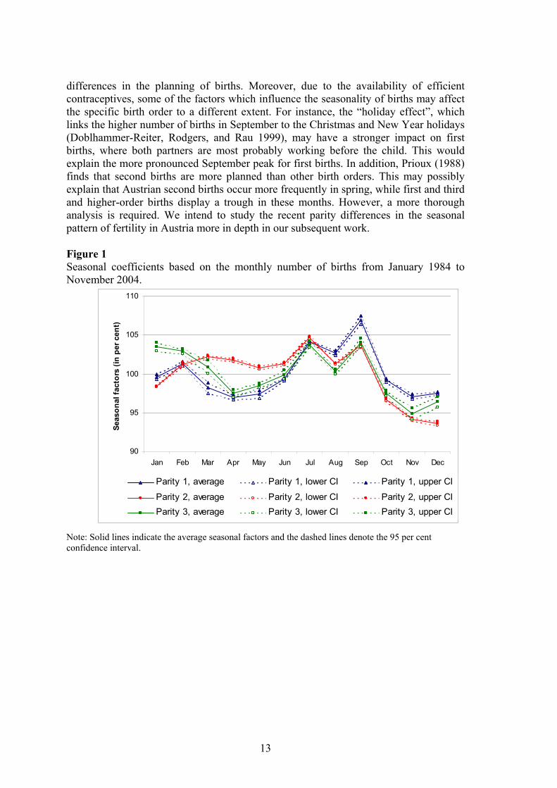
differences in the planning of births. Moreover, due to the availability of efficient contraceptives, some of the factors which influence the seasonality of births may affect the specific birth order to a different extent. For instance, the “holiday effect”, which links the higher number of births in September to the Christmas and New Year holidays (Doblhammer-Reiter, Rodgers, and Rau 1999), may have a stronger impact on first births, where both partners are most probably working before the child. This would explain the more pronounced September peak for first births. In addition, Prioux (1988) finds that second births are more planned than other birth orders. This may possibly explain that Austrian second births occur more frequently in spring, while first and third and higher-order births display a trough in these months. However, a more thorough analysis is required. We intend to study the recent parity differences in the seasonal pattern of fertility in Austria more in depth in our subsequent work.

Figure 1 Seasonal coefficients based on the monthly number of births from January 1984 to November 2004.

90

95

100

105

110

Jan Feb Mar Apr May Jun Jul Aug Sep Oct Nov Dec

Seas

onal

fact

ors

(in p

er c

ent)

Parity 1, average Parity 1, lower CI Parity 1, upper CI

Parity 2, average Parity 2, lower CI Parity 2, upper CIParity 3, average Parity 3, lower CI Parity 3, upper CI

Note: Solid lines indicate the average seasonal factors and the dashed lines denote the 95 per cent confidence interval.

13

5.2. Considering Monthly Birth Cohorts does not Alter the Resulting Fertility Indicators

Seeking to derive as precise estimates as possible, we calculated all the order-

specific incidence rates, the total fertility rates and the mean ages at childbearing from month-cohort data as well as in the usual age cohort format defined by single years of age. Using the detailed monthly data, specified for ages 132 to 612 months (ages 11 to 51 in completed years), did not bring any detectable change in the resulting order-specific fertility indicators. While the monthly age-specific rates were extremely erratic when monthly birth cohorts were considered due to the small number of births in each category, the aggregate indexes of fertility were identical with those derived from rates specified by single years of age. As a result, we did not pursue the computations of rates by monthly birth cohorts any further and used the annual birth cohorts of women aged 12 to 50 to derive all age-specific fertility indicators. Considering monthly birth cohort also did not alter the indicators of fertility timing, namely mean and median age of mother at childbearing, which are utilised in the computation of the Bongaarts-Feeney adjusted TFR. Appendix 5 provides further details on our comparisons of month-cohort and year-cohort age data format.

5.3. Raw Data and Crude Fertility Rates Display Considerable Monthly Variation

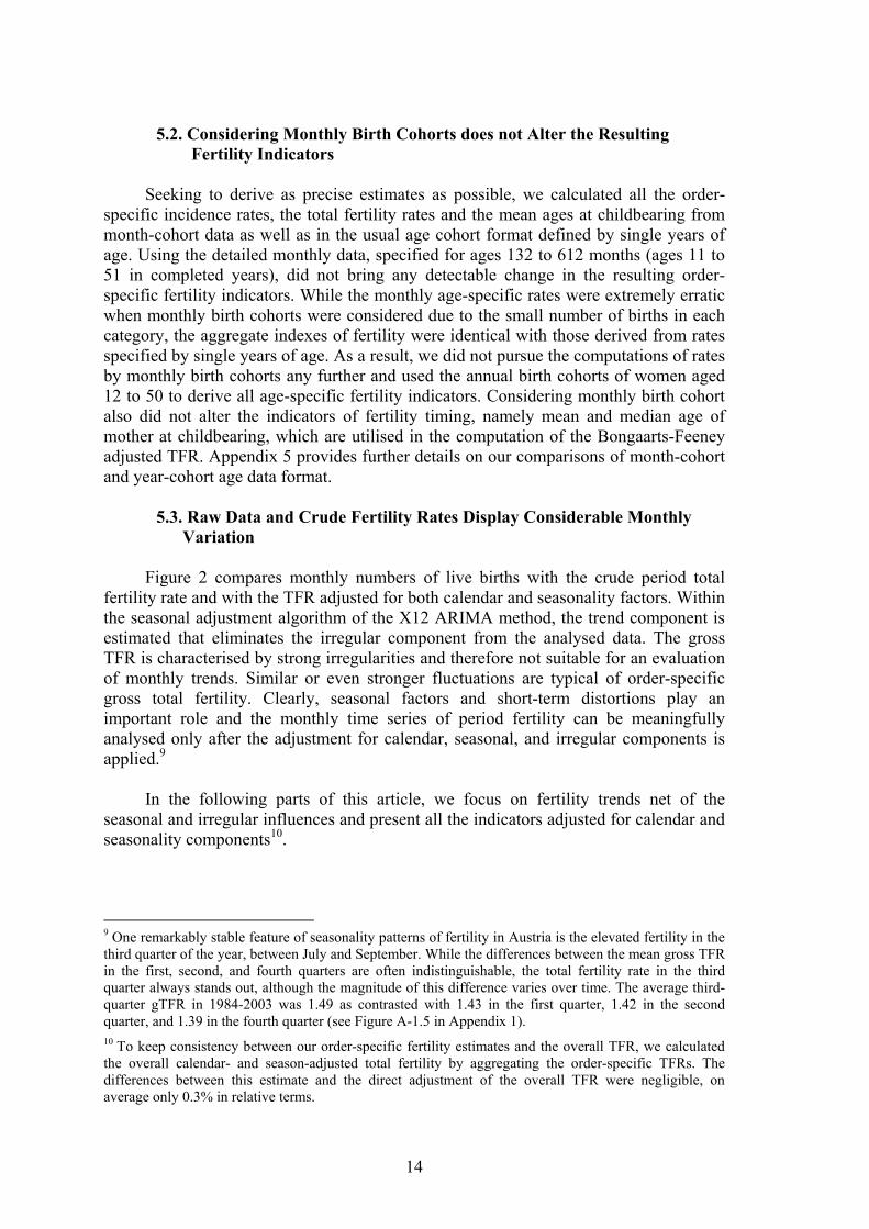
Figure 2 compares monthly numbers of live births with the crude period total

fertility rate and with the TFR adjusted for both calendar and seasonality factors. Within the seasonal adjustment algorithm of the X12 ARIMA method, the trend component is estimated that eliminates the irregular component from the analysed data. The gross TFR is characterised by strong irregularities and therefore not suitable for an evaluation of monthly trends. Similar or even stronger fluctuations are typical of order-specific gross total fertility. Clearly, seasonal factors and short-term distortions play an important role and the monthly time series of period fertility can be meaningfully analysed only after the adjustment for calendar, seasonal, and irregular components is applied.9

In the following parts of this article, we focus on fertility trends net of the seasonal and irregular influences and present all the indicators adjusted for calendar and seasonality components10.

9 One remarkably stable feature of seasonality patterns of fertility in Austria is the elevated fertility in the third quarter of the year, between July and September. While the differences between the mean gross TFR in the first, second, and fourth quarters are often indistinguishable, the total fertility rate in the third quarter always stands out, although the magnitude of this difference varies over time. The average third-quarter gTFR in 1984-2003 was 1.49 as contrasted with 1.43 in the first quarter, 1.42 in the second quarter, and 1.39 in the fourth quarter (see Figure A-1.5 in Appendix 1). 10 To keep consistency between our order-specific fertility estimates and the overall TFR, we calculated the overall calendar- and season-adjusted total fertility by aggregating the order-specific TFRs. The differences between this estimate and the direct adjustment of the overall TFR were negligible, on average only 0.3% in relative terms.

14

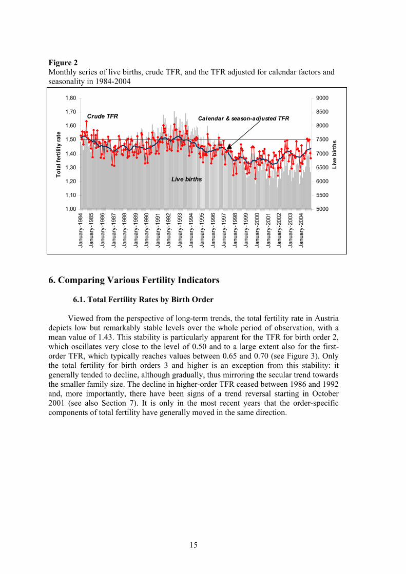
Figure 2 Monthly series of live births, crude TFR, and the TFR adjusted for calendar factors and seasonality in 1984-2004

1,00

1,10

1,20

1,30

1,40

1,50

1,60

1,70

1,80

Janu

ary-

1984

Janu

ary-

1985

Janu

ary-

1986

Janu

ary-

1987

Janu

ary-

1988

Janu

ary-

1989

Janu

ary-

1990

Janu

ary-

1991

Janu

ary-

1992

Janu

ary-

1993

Janu

ary-

1994

Janu

ary-

1995

Janu

ary-

1996

Janu

ary-

1997

Janu

ary-

1998

Janu

ary-

1999

Janu

ary-

2000

Janu

ary-

2001

Janu

ary-

2002

Janu

ary-

2003

Janu

ary-

2004

Tota

l fer

tility

rate

5000

5500

6000

6500

7000

7500

8000

8500

9000

Live

birt

hs

Live births

Crude TFR Calendar & season-adjusted TFR

6. Comparing Various Fertility Indicators

6.1. Total Fertility Rates by Birth Order

Viewed from the perspective of long-term trends, the total fertility rate in Austria depicts low but remarkably stable levels over the whole period of observation, with a mean value of 1.43. This stability is particularly apparent for the TFR for birth order 2, which oscillates very close to the level of 0.50 and to a large extent also for the first-order TFR, which typically reaches values between 0.65 and 0.70 (see Figure 3). Only the total fertility for birth orders 3 and higher is an exception from this stability: it generally tended to decline, although gradually, thus mirroring the secular trend towards the smaller family size. The decline in higher-order TFR ceased between 1986 and 1992 and, more importantly, there have been signs of a trend reversal starting in October 2001 (see also Section 7). It is only in the most recent years that the order-specific components of total fertility have generally moved in the same direction.

15

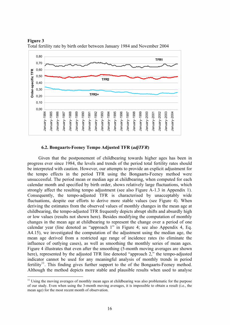
Figure 3 Total fertility rate by birth order between January 1984 and November 2004

0,00

0,10

0,20

0,30

0,40

0,50

0,60

0,70

0,80

Janu

ary-

1984

Janu

ary-

1985

Janu

ary-

1986

Janu

ary-

1987

Janu

ary-

1988

Janu

ary-

1989

Janu

ary-

1990

Janu

ary-

1991

Janu

ary-

1992

Janu

ary-

1993

Janu

ary-

1994

Janu

ary-

1995

Janu

ary-

1996

Janu

ary-

1997

Janu

ary-

1998

Janu

ary-

1999

Janu

ary-

2000

Janu

ary-

2001

Janu

ary-

2002

Janu

ary-

2003

Janu

ary-

2004

Ord

er-s

peci

fic T

FR

TFR1

TFR3+

TFR2

6.2. Bongaarts-Feeney Tempo Adjusted TFR (adjTFR)

Given that the postponement of childbearing towards higher ages has been in

progress ever since 1984, the levels and trends of the period total fertility rates should be interpreted with caution. However, our attempts to provide an explicit adjustment for the tempo effects in the period TFR using the Bongaarts-Feeney method were unsuccessful. The period mean or median age at childbearing, when computed for each calendar month and specified by birth order, shows relatively large fluctuations, which strongly affect the resulting tempo adjustment (see also Figure A-1.3 in Appendix 1). Consequently, the tempo-adjusted TFR is characterised by unacceptably wide fluctuations, despite our efforts to derive more stable values (see Figure 4). When deriving the estimates from the observed values of monthly changes in the mean age at childbearing, the tempo-adjusted TFR frequently depicts abrupt shifts and absurdly high or low values (results not shown here). Besides modifying the computation of monthly changes in the mean age at childbearing to represent the change over a period of one calendar year (line denoted as “approach 1” in Figure 4; see also Appendix 4, Eq. A4.15), we investigated the computation of the adjustment using the median age, the mean age derived from a restricted age range of incidence rates (to eliminate the influence of outlying cases), as well as smoothing the monthly series of mean ages. Figure 4 illustrates that even after the smoothing (5-month moving averages are shown here), represented by the adjusted TFR line denoted “approach 2,” the tempo-adjusted indicator cannot be used for any meaningful analysis of monthly trends in period fertility11. This finding gives further support to the of the Bongaarts-Feeney method. Although the method depicts more stable and plausible results when used to analyse 11 Using the moving averages of monthly mean ages at childbearing was also problematic for the purpose of our study. Even when using the 3-month moving averages, it is impossible to obtain a result (i.e., the mean age) for the most recent month of observation.

16

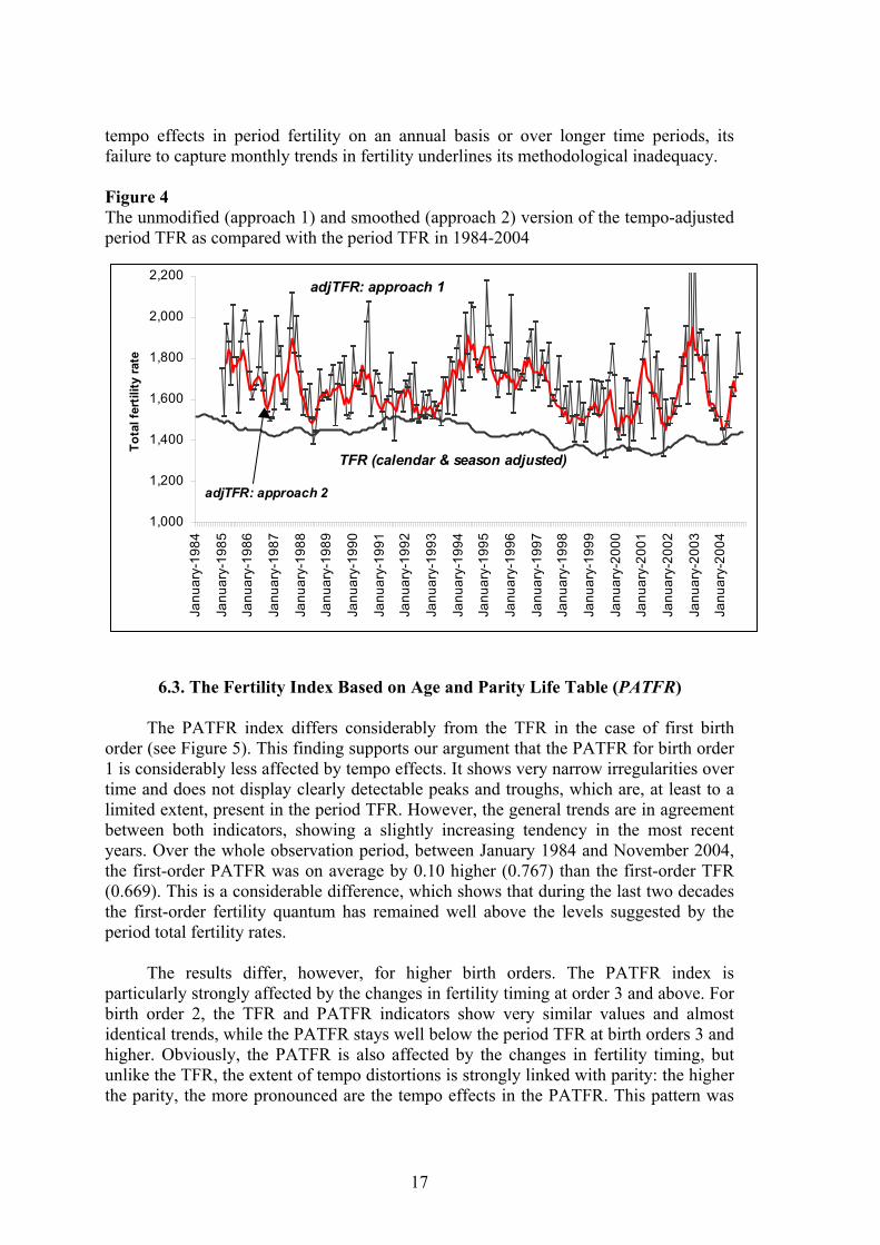
tempo effects in period fertility on an annual basis or over longer time periods, its failure to capture monthly trends in fertility underlines its methodological inadequacy.

Figure 4 The unmodified (approach 1) and smoothed (approach 2) version of the tempo-adjusted period TFR as compared with the period TFR in 1984-2004

1,000

1,200

1,400

1,600

1,800

2,000

2,200

Janu

ary-

1984

Janu

ary-

1985

Janu

ary-

1986

Janu

ary-

1987

Janu

ary-

1988

Janu

ary-

1989

Janu

ary-

1990

Janu

ary-

1991

Janu

ary-

1992

Janu

ary-

1993

Janu

ary-

1994

Janu

ary-

1995

Janu

ary-

1996

Janu

ary-

1997

Janu

ary-

1998

Janu

ary-

1999

Janu

ary-

2000

Janu

ary-

2001

Janu

ary-

2002

Janu

ary-

2003

Janu

ary-

2004

Tota

l fer

tility

rate

TFR (calendar & season adjusted)

adjTFR: approach 1

adjTFR: approach 2

6.3. The Fertility Index Based on Age and Parity Life Table (PATFR)

The PATFR index differs considerably from the TFR in the case of first birth order (see Figure 5). This finding supports our argument that the PATFR for birth order 1 is considerably less affected by tempo effects. It shows very narrow irregularities over time and does not display clearly detectable peaks and troughs, which are, at least to a limited extent, present in the period TFR. However, the general trends are in agreement between both indicators, showing a slightly increasing tendency in the most recent years. Over the whole observation period, between January 1984 and November 2004, the first-order PATFR was on average by 0.10 higher (0.767) than the first-order TFR (0.669). This is a considerable difference, which shows that during the last two decades the first-order fertility quantum has remained well above the levels suggested by the period total fertility rates.

The results differ, however, for higher birth orders. The PATFR index is

particularly strongly affected by the changes in fertility timing at order 3 and above. For birth order 2, the TFR and PATFR indicators show very similar values and almost identical trends, while the PATFR stays well below the period TFR at birth orders 3 and higher. Obviously, the PATFR is also affected by the changes in fertility timing, but unlike the TFR, the extent of tempo distortions is strongly linked with parity: the higher the parity, the more pronounced are the tempo effects in the PATFR. This pattern was

17

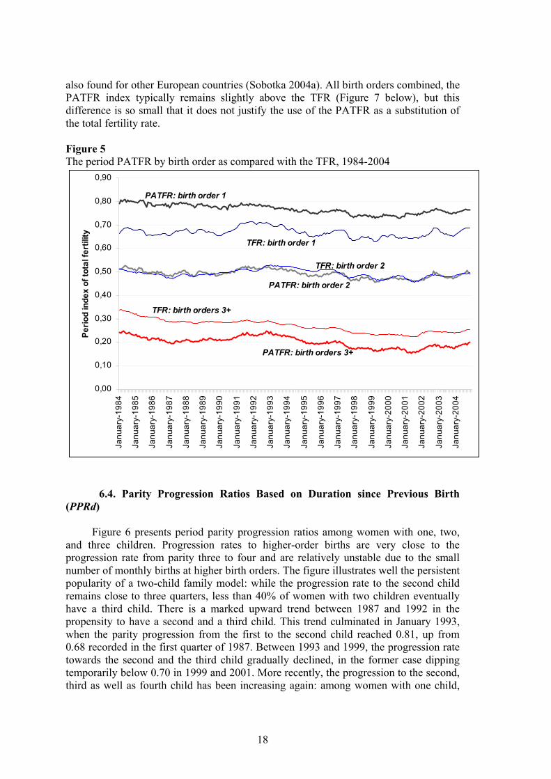
also found for other European countries (Sobotka 2004a). All birth orders combined, the PATFR index typically remains slightly above the TFR (Figure 7 below), but this difference is so small that it does not justify the use of the PATFR as a substitution of the total fertility rate. Figure 5 The period PATFR by birth order as compared with the TFR, 1984-2004

0,00

0,10

0,20

0,30

0,40

0,50

0,60

0,70

0,80

0,90

Janu

ary-

1984

Janu

ary-

1985

Janu

ary-

1986

Janu

ary-

1987

Janu

ary-

1988

Janu

ary-

1989

Janu

ary-

1990

Janu

ary-

1991

Janu

ary-

1992

Janu

ary-

1993

Janu

ary-

1994

Janu

ary-

1995

Janu

ary-

1996

Janu

ary-

1997

Janu

ary-

1998

Janu

ary-

1999

Janu

ary-

2000

Janu

ary-

2001

Janu

ary-

2002

Janu

ary-

2003

Janu

ary-

2004

Perio

d in

dex

of to

tal f

ertil

ity

PATFR: birth order 1

TFR: birth order 1

PATFR: birth order 2

TFR: birth order 2

PATFR: birth orders 3+

TFR: birth orders 3+

6.4. Parity Progression Ratios Based on Duration since Previous Birth

(PPRd)

Figure 6 presents period parity progression ratios among women with one, two, and three children. Progression rates to higher-order births are very close to the progression rate from parity three to four and are relatively unstable due to the small number of monthly births at higher birth orders. The figure illustrates well the persistent popularity of a two-child family model: while the progression rate to the second child remains close to three quarters, less than 40% of women with two children eventually have a third child. There is a marked upward trend between 1987 and 1992 in the propensity to have a second and a third child. This trend culminated in January 1993, when the parity progression from the first to the second child reached 0.81, up from 0.68 recorded in the first quarter of 1987. Between 1993 and 1999, the progression rate towards the second and the third child gradually declined, in the former case dipping temporarily below 0.70 in 1999 and 2001. More recently, the progression to the second, third as well as fourth child has been increasing again: among women with one child,

18

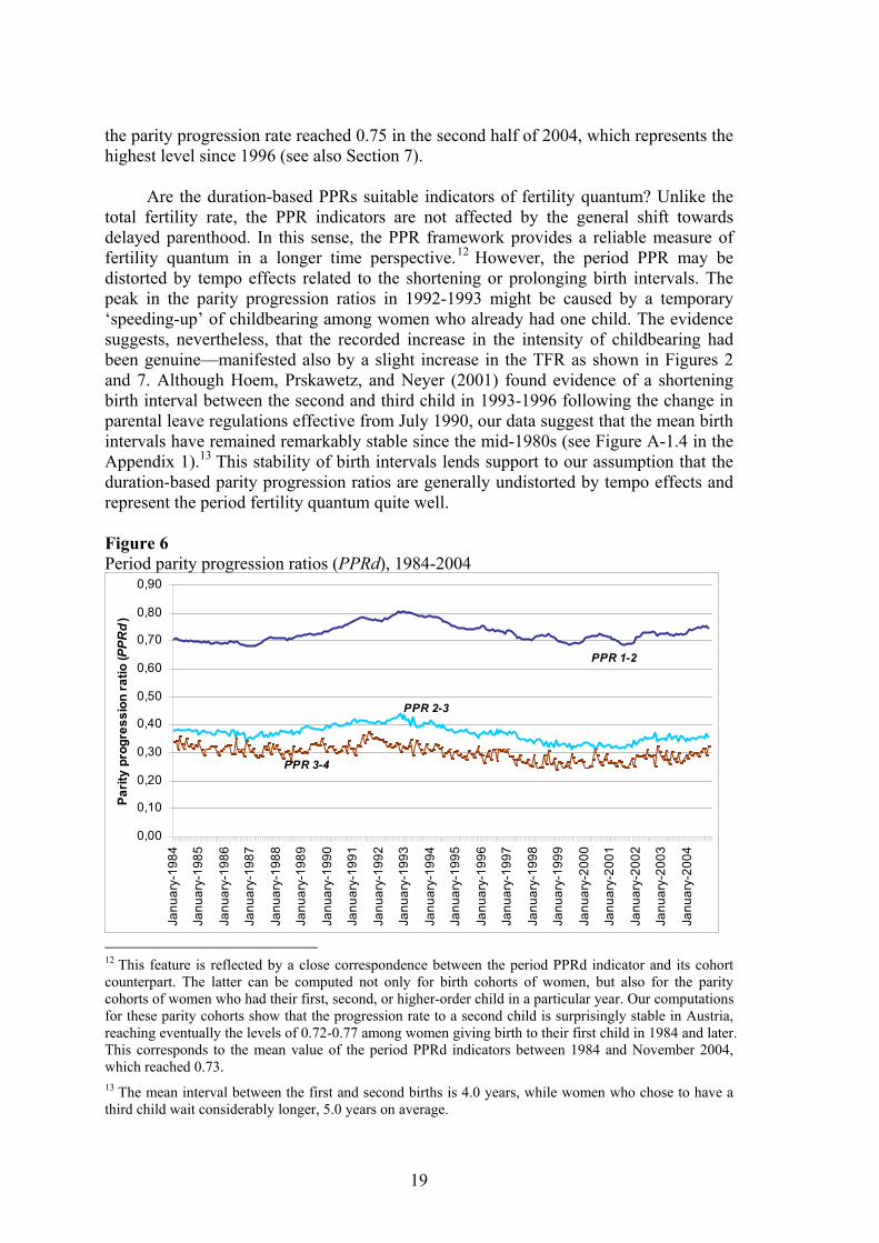
the parity progression rate reached 0.75 in the second half of 2004, which represents the highest level since 1996 (see also Section 7).

Are the duration-based PPRs suitable indicators of fertility quantum? Unlike the

total fertility rate, the PPR indicators are not affected by the general shift towards delayed parenthood. In this sense, the PPR framework provides a reliable measure of fertility quantum in a longer time perspective.12 However, the period PPR may be distorted by tempo effects related to the shortening or prolonging birth intervals. The peak in the parity progression ratios in 1992-1993 might be caused by a temporary ‘speeding-up’ of childbearing among women who already had one child. The evidence suggests, nevertheless, that the recorded increase in the intensity of childbearing had been genuine—manifested also by a slight increase in the TFR as shown in Figures 2 and 7. Although Hoem, Prskawetz, and Neyer (2001) found evidence of a shortening birth interval between the second and third child in 1993-1996 following the change in parental leave regulations effective from July 1990, our data suggest that the mean birth intervals have remained remarkably stable since the mid-1980s (see Figure A-1.4 in the Appendix 1).13 This stability of birth intervals lends support to our assumption that the duration-based parity progression ratios are generally undistorted by tempo effects and represent the period fertility quantum quite well.

Figure 6 Period parity progression ratios (PPRd), 1984-2004

0,00

0,10

0,20

0,30

0,40

0,50

0,60

0,70

0,80

0,90

Janu

ary-

1984

Janu

ary-

1985

Janu

ary-

1986

Janu

ary-

1987

Janu

ary-

1988

Janu

ary-

1989

Janu

ary-

1990

Janu

ary-

1991

Janu

ary-

1992

Janu

ary-

1993

Janu

ary-

1994

Janu

ary-

1995

Janu

ary-

1996

Janu

ary-

1997

Janu

ary-

1998

Janu

ary-

1999

Janu

ary-

2000

Janu

ary-

2001

Janu

ary-

2002

Janu

ary-

2003

Janu

ary-

2004

Parit

y pr

ogre

ssio

n ra

tio (P

PRd

)

PPR 1-2

PPR 2-3

PPR 3-4

12 This feature is reflected by a close correspondence between the period PPRd indicator and its cohort counterpart. The latter can be computed not only for birth cohorts of women, but also for the parity cohorts of women who had their first, second, or higher-order child in a particular year. Our computations for these parity cohorts show that the progression rate to a second child is surprisingly stable in Austria, reaching eventually the levels of 0.72-0.77 among women giving birth to their first child in 1984 and later. This corresponds to the mean value of the period PPRd indicators between 1984 and November 2004, which reached 0.73. 13 The mean interval between the first and second births is 4.0 years, while women who chose to have a third child wait considerably longer, 5.0 years on average.

19

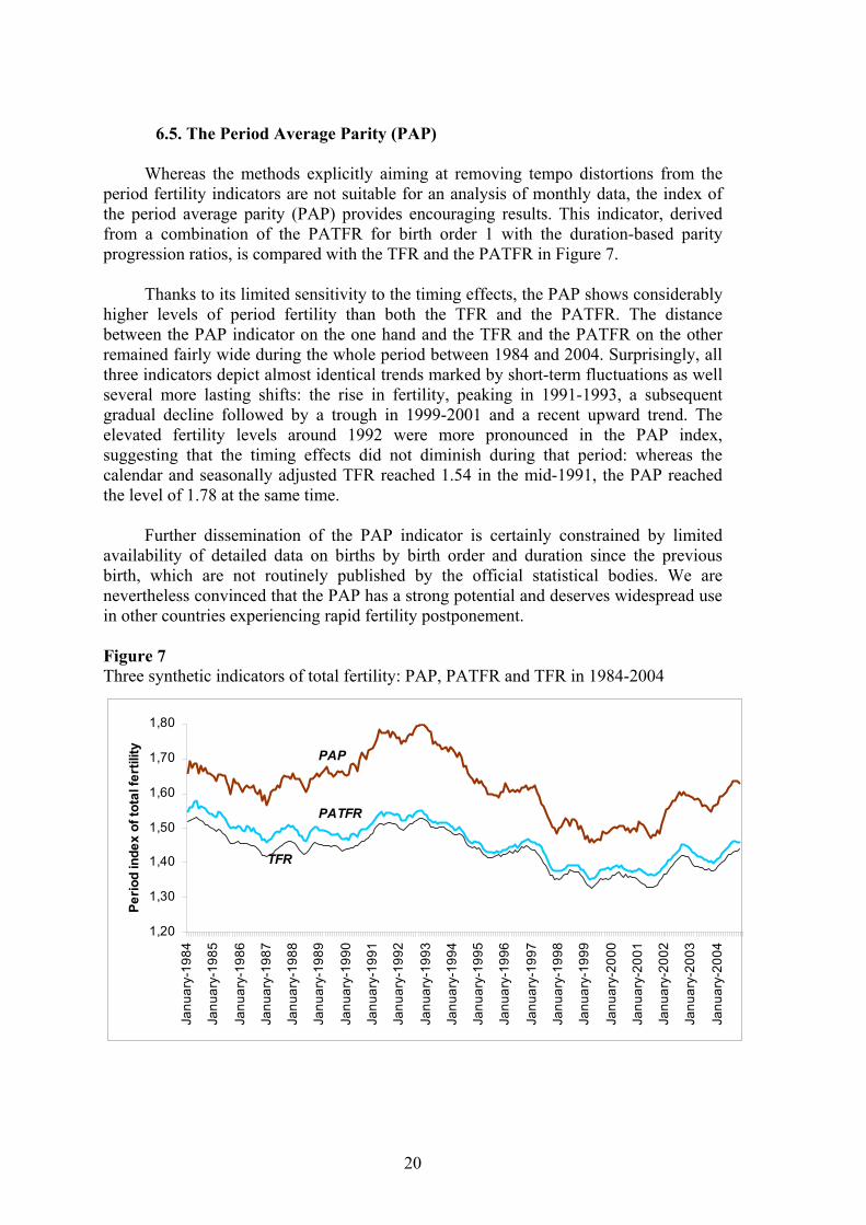
6.5. The Period Average Parity (PAP)

Whereas the methods explicitly aiming at removing tempo distortions from the period fertility indicators are not suitable for an analysis of monthly data, the index of the period average parity (PAP) provides encouraging results. This indicator, derived from a combination of the PATFR for birth order 1 with the duration-based parity progression ratios, is compared with the TFR and the PATFR in Figure 7.

Thanks to its limited sensitivity to the timing effects, the PAP shows considerably higher levels of period fertility than both the TFR and the PATFR. The distance between the PAP indicator on the one hand and the TFR and the PATFR on the other remained fairly wide during the whole period between 1984 and 2004. Surprisingly, all three indicators depict almost identical trends marked by short-term fluctuations as well several more lasting shifts: the rise in fertility, peaking in 1991-1993, a subsequent gradual decline followed by a trough in 1999-2001 and a recent upward trend. The elevated fertility levels around 1992 were more pronounced in the PAP index, suggesting that the timing effects did not diminish during that period: whereas the calendar and seasonally adjusted TFR reached 1.54 in the mid-1991, the PAP reached the level of 1.78 at the same time.

Further dissemination of the PAP indicator is certainly constrained by limited

availability of detailed data on births by birth order and duration since the previous birth, which are not routinely published by the official statistical bodies. We are nevertheless convinced that the PAP has a strong potential and deserves widespread use in other countries experiencing rapid fertility postponement. Figure 7 Three synthetic indicators of total fertility: PAP, PATFR and TFR in 1984-2004

1,20

1,30

1,40

1,50

1,60

1,70

1,80

Janu

ary-

1984

Janu

ary-

1985

Janu

ary-

1986

Janu

ary-

1987

Janu

ary-

1988

Janu

ary-

1989

Janu

ary-

1990

Janu

ary-

1991

Janu

ary-

1992

Janu

ary-

1993

Janu

ary-

1994

Janu

ary-

1995

Janu

ary-

1996

Janu

ary-

1997

Janu

ary-

1998

Janu

ary-

1999

Janu

ary-

2000

Janu

ary-

2001

Janu

ary-

2002

Janu

ary-

2003

Janu

ary-

2004

Perio

d in

dex

of to

tal f

ertil

ity PAP

PATFR

TFR

20

7. Analysing Short-Term Movements in Period Fertility: 2001-2004

The main purpose of our investigation is to construct fertility indicators that would allow to trace and analyse short-term trends in period fertility rates. The recent upswing in period fertility, originating in 2001, may serve as an example of change that can be studied with the monthly series of the TFR and PAP indicators. To gain better insights into the recent fertility movements, we analyse order-specific components of both indicators.

The recent fertility increase has occurred in two waves. During the first wave,

fertility increased between November 2001 and August 2002. The PAP index grew by 8%, from 1.48 to 1.60. Subsequently, fertility was slightly declining for about a year, when the PAP reached a low level of 1.55 in October 2003. Then, fertility started to increase again, peaking at 1.64 in August 2004, representing an increase of almost 6% and more than 10% over the whole 3-year period since November 2001. Considering the timing of conception, rather than the actual timing of births, we may conclude that pregnancy rates increased for most of the years 2001 and 2003, starting in the February-March period. Changes in the total fertility rate have been less pronounced; overall, the TFR has risen by 8% during the last three years, from 1.33 in October 2001 to 1.44 in November 2004. The most recent data for November 2004 show that the fertility level has been the highest since the mid-1990s. The increase in the PAP index points out that the recent rise in fertility is due to a ‘genuine’ increase in fertility quantum and has not been driven by a decline in tempo distortions. On the contrary, the estimated tempo effect, as represented by a difference between the PAP and the TFR, has slightly increased since 2001.

What has been the role of order-specific components? In absolute terms, almost half the increase in total fertility has been driven by an increase in its first-order component, corresponding to its share on the TFR. More interesting is an analysis of relative changes in order-specific components of the TFR and PAP, revealing a strong relative increase in the propensity to have a child among women with two or more children, especially between October 2001 and July 2002 and, most recently, since April 2004. Whereas in November 2004 the TFR exceeded by 7% the level reached in January 2001, the TFR at birth orders 3+ increased by 12% (see Figure 8). However, due to the low share of higher-order births on the overall TFR, the absolute impact of this increase was limited. The increase in higher-order fertility rates is even more pronounced in the decomposition of the PAP. This indicator suggests that the increase in fertility was mostly driven by the rising propensity of mothers with one or more children to have another child. Whereas the PATFR of first birth order increased only by 2% between January 2001 and November 2004, the PAP index at parity 3+ shot up by about 26%.

Despite considerable differences between the TFR and PAP, the relative increase in fertility among women with two or more children is well detected by both indicators. When the timing of conception is considered, the steeper part of this increase can be traced back to the period between January (or March when measured with the parity progression data) to October 2001. The decomposition of change in parity-progression ratios and the PAP indexes between October-November 2001 and October-November 2004, depicted in Table 1, further shows that the propensity to have another child

21

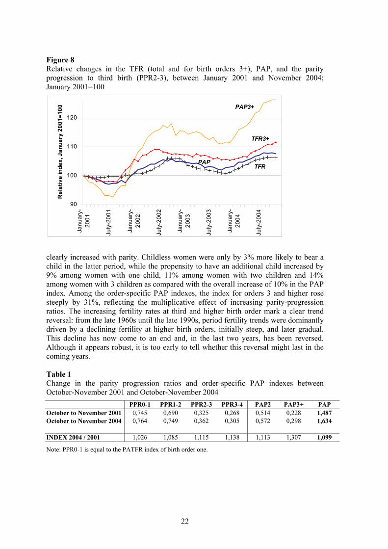
Figure 8 Relative changes in the TFR (total and for birth orders 3+), PAP, and the parity progression to third birth (PPR2-3), between January 2001 and November 2004; January 2001=100

90

100

110

120

Janu

ary-

2001

July

-200

1

Janu

ary-

2002

July

-200

2

Janu

ary-

2003

July

-200

3

Janu

ary-

2004

July

-200

4

Rel

ativ

e in

dex,

Jan

uary

200

1=10

0 PAP3+

TFR3+

TFRPAP

clearly increased with parity. Childless women were only by 3% more likely to bear a child in the latter period, while the propensity to have an additional child increased by 9% among women with one child, 11% among women with two children and 14% among women with 3 children as compared with the overall increase of 10% in the PAP index. Among the order-specific PAP indexes, the index for orders 3 and higher rose steeply by 31%, reflecting the multiplicative effect of increasing parity-progression ratios. The increasing fertility rates at third and higher birth order mark a clear trend reversal: from the late 1960s until the late 1990s, period fertility trends were dominantly driven by a declining fertility at higher birth orders, initially steep, and later gradual. This decline has now come to an end and, in the last two years, has been reversed. Although it appears robust, it is too early to tell whether this reversal might last in the coming years. Table 1 Change in the parity progression ratios and order-specific PAP indexes between October-November 2001 and October-November 2004

PPR0-1 PPR1-2 PPR2-3 PPR3-4 PAP2 PAP3+ PAP October to November 2001 0,745 0,690 0,325 0,268 0,514 0,228 1,487 October to November 2004 0,764 0,749 0,362 0,305 0,572 0,298 1,634

INDEX 2004 / 2001 1,026 1,085 1,115 1,138 1,113 1,307 1,099

Note: PPR0-1 is equal to the PATFR index of birth order one.

22

8. Conclusion

Computation of monthly indicators of period fertility presented here required solving a number of methodological and practical issues. This study utilised a database of individual birth records in Austria in order to find out whether we can derive monthly indicators of fertility that are parity-specific and at the same time minimise the distortions caused by the shifts in the timing of childbearing. We have shown that in order to derive meaningful indicators of monthly fertility, the raw data should be adjusted for seasonality and the trend component. Since the seasonal childbearing patterns differ by birth order, it is useful to differentiate the seasonal adjustment by birth order. The indicators of period fertility aimed at removing tempo distortions present in the commonly used fertility measures, especially the total fertility rates, turned out to be problematic for an analysis of monthly data: the adjustment suggested by Kohler and Ortega in particular due to the complexities involved in deriving the monthly time series, and the indicator of Bongaarts-Feeney due to huge fluctuations and generally erratic results. Considering a finer level of detail by using indicators computed for monthly birth cohorts instead of the usual year-cohort format did not appreciably change any of the fertility indicators computed. Our focus on indicators that are parity-specific (i.e., they correctly reflect exposure) and may at the same time reduce the magnitude of tempo distortions proved fruitful. We advocate using the period average parity (PAP), a methodologically sound indicator based on a life table model, which provides a realistic estimate of fertility quantum without applying any of the simplifying assumptions that are typical of the tempo-adjustment methods.

The PAP is not entirely free of tempo effects as its first-order component is based

on the (unadjusted) age-parity fertility table indicator PATFR, which is slightly affected by the changes in fertility timing. However, in comparison with the commonly used TFR, the PAP consistently indicates higher levels of period fertility quantum in Austria during the entire period since 1984. It suggests that the period total fertility rates in Austria in 1984-2004 had been on average ‘deflated’ by 0.19 by the ongoing trend towards later timing of childbearing. Its mean level in 1985-2001 (1.62) was slightly above our estimates of the annual mean values of the Kohler-Ortega adjusted PATFR index (1.57). Our analysis indicates that if the PAP were entirely free of tempo effects, its level would probably be close to 1.70 (see Appendix 7). Even this estimate implies that by using the PAP at least two thirds of the tempo effects present in the TFR can be eliminated. Thus, the PAP provides a considerably better estimate of the period fertility quantum than the existing conventional indicators. The future ending up of fertility postponement is likely to be associated with a modest increase in the period TFR. The use of the PAP index will help to distinguish between the ‘genuine’ increase in period fertility and the increase related to the ending of the tempo distortions in the period TFR. Our favourable assessment on the PAP index hinges upon the validity of its underlying assumption concerning the relative stability of the mean birth intervals in the duration-based parity progression ratios. This assumption was supported in the case of Austrian data, but might be violated in other cases. Certainly, the PAP should also be evaluated with data for other countries and regions. The theoretical and methodological discussion regarding the interpretation of different period fertility indicators as well as the issue of timing effects is still in full swing. From this perspective, the analysis presented in this

23

paper may stimulate further debates as it contributes to this discussion and to the methodological advancement in fertility research.

Finally, we would like to point out that although we were able to document

considerable changes and fluctuations in period fertility since the mid-1980s, the long-term fertility trends in Austria has remained remarkably stable when compared with most other European countries. Despite this stability, the analysis of monthly time series of period fertility brings important insights that can be useful in evaluating recent trends as well as possible effects of particular policy measures. The recent increase in period fertility, which has been more pronounced among mothers with two or more children, suggests the possibility that it was partly related to the extension of the period of paid parental leave (“Kindergeld”) and the broader eligibility for mothers and fathers to receive the leave, proposed by the government in April 2001 and in effect since January 2002. (Gisser and Fliegenschnee 2004) Whether the recent stabilisation and subsequent increase in fertility at third and higher birth orders marks a trend reversal or rather constitutes a short-time fluctuation remains unknown. However, our study of monthly fertility in Austria has a practical outcome that makes it possible to keep our eye on these recent trends: In collaboration with Statistics Austria, which will regularly supply us with the most recent data on births, we will establish a continually updated monitoring system and regularly publish the most recent indicators of monthly period fertility.

24

References Bobak, M. and A. Gjonca. 2001. “The seasonality of live birth is strongly influenced by

sociodemographic factors”. Human Reproduction 16 (7): 1512-1517. Bongaarts, J. 2002. “The end of the fertility transition in the developed world”. Population and

Development Review 28 (3): 419-443. Bongaarts, J. and G. Feeney. 1998. “On the quantum and tempo of fertility”. Population and

Development Review 24 (2): 271-291. Brass, W. 1991. Cohort and time period measures of quantum fertility: Concepts and

methodology. In.: Becker, H. A. (ed.). Life histories and generations. University of Utrecht, ISOR, pp. 455-476.

Calot, G. 1981a. L’observation de la fécondité à court et moyen terme. Population 36(1): 9-40. Calot, G. 1981b. Le mouvement journalier des naissances à l’intérieur de la semaine.

Population 36(3): 477-504. Calot, G. and Nadot. 1977. “Combien y aura-t-il de naissances dans l’année?” Population 32

(numero special): 185-229. Doblhammer-Reiter, J. L. Rodgers, and R. Rau. 1999. “Seasonality of birth in nineteenth and

twentieth century Austria: Steps toward a unified theory of human reproductive seasonality”. MPIDR Working Paper WP 1999-013, Max Planck Institute for Demographic Research, Rostock. Accessed at «http://www.demogr.mpg.de/Papers/Working/WP-1999-013.pdf».

EUROSTAT. 2004. NewCronos database. Theme 3: Population and social conditions. Accessed in October 2004 at «http://europa.eu.int/comm/eurostat/newcronos/reference/display.do?screen=welcomeref&open=/&product=EU_population_social_conditions&depth=1&language=en».

Feeney, G and J. Yu. 1987. “Period parity progression measures of fertility in China“. Population Studies 41 (1): 77-102.

Findley, D. F., B. C. Monsell, W. R. Bell, M. C. Otto, and B. Chen. 1998. “New capabilities and methods of the X-12-ARIMA seasonal adjustment program”. Journal of Business and Economic Statistics, 16: 127-177.

Frejka, T. and G. Calot. 2001a. “Cohort childbearing age patterns in low-fertility countries in the late 20th century: Is the postponement of births an inherent element?” MPIDR Working Paper WP 2001-009, Max Planck Institute for Demographic Research, Rostock. «http://www.demogr.mpg.de/Papers/Working/wp-2001-009.pdf».

Gisser, R. and K. Fliegenschnee. 2004. Country report on general family-related policies and attitudes“. Vienna Institute of Demography, internal paper, August 2004.

Gisser, Richard. 1984. Geborene und Gestorbene 1982. Statistische Nachrichten 39(3): 148-151. Goldstein, J., W. Lutz, and S. Scherbov. 2003. “Long-term population decline in Europe: The

relative importance of tempo-effects and generational length”. Population and Development Review 29 (4): 699-707.

Haandrikman, K. 2004. “Seizonfluctuaties in geboorten: veranderte patronen door planning?“ Bevolkingstrends, 2004 (4): 14-22.

Hajnal, J. 1947. “The analysis of birth statistics in the light of the recent international recovery of the birth-rate”. Population Studies 1 (2): 137–164.

Henry, L. 1961. “Un nouveau tableau statistique: Les naissances suivant le rang et l’année de naissance de l’enfant precedent”. Population 16 (3): 513-515.

Henry, L. 1953. “Fécondité des mariages. Nouvelle méthode de mesure” Travaux et Documents no. 16, INED-PUF, Paris.

25

Höhn, C. 1981. “Die CALOT-Methode zur aktuellen Beurteilung von Geburtenniveau und –trend”. Zeitschrift für Bevölkerungswissenschaft 7(2): 231-254.

Kohler, H.-P. and J. A. Ortega. 2004. “Old insights and new approaches: Fertility analysis and tempo adjustment in the age-parity model”. Vienna Yearbook of Population Research 2004: 57-89.

Kohler, H.-P. and J. A. Ortega. 2002. “Tempo-adjusted period parity progression measures, fertility postponement and completed cohort fertility”. Demographic Research 6, Article 6: 92-144. «www.demographic-research.org».

Kohler, H.-P. and D. Philipov. 2001. “Variance effects in the Bongaarts-Feeney formula”. Demography 38 (1): 1-16.

Kohler, H.-P., F. C. Billari, and J. A. Ortega. 2002. “The emergence of lowest-low fertility in Europe during the 1990s”. Population and Development Review 28 (4): 641-680.

Ladiray, D. and B. Quenneville. 2001. Seasonal adjustments with the X-11 method. Lecture notes on Statistics, New York: Springer.

Lam, D. A., J. A. Miron, and A. Riley. 1994. “Modelling seasonality in fecundability, conceptions, and births”. Demography 31 (2): 321-346.

Lesthaeghe, R. 2001. “Postponement and recuperation: Recent fertility trends and forecasts in six Western European countries”. Paper presented at the IUSSP Seminar “International perspectives on low fertility: Trends, theories and policies”, Tokyo, 21-23 March 2001. Accessed in 2001 at «demography.anu.edu.au/VirtualLibrary/ConferencePapers/IUSSP2001/».

Lesthaeghe, R. and P. Willems. 1999. “Is low fertility a temporary phenomenon in the European Union?” Population and Development Review 25 (2): 211-228.

Lutz, W. Distributional aspects of human fertility: A global comparative study. Academic Press, Harcourt Brace Jovanovich, Publishers, London.

Lutz, W., B. C. O’Neill, and S. Scherbov. 2003. “Europe’s population at a turning point”. Science 299: 1991–1992.

Miller and Williams. 2004. “Damping seasonal factors: shrinkage estimators for the X-12-ARIMA program”. International Journal of Forecasting 20: 529-549.

Murphy, M. 1994. Time-series approaches to the analysis of fertility change. In.: M. Ní Bhrolcháin, (ed.) New perspectives on fertility in Britain. Studies on medical and population subjects No. 55, London: HMSO.

Ní Bhrolcháin, M. and L. Toulemon. 2003. “The trend to later childbearing: is there evidence of postponement?” SSRC Applications and policy Working Paper A03/10, Social Statistics Research Centre, University of Southampton. Accessed at: «http://www.s3ri.soton.ac.uk/publications/papers-applications/ssrc-workingpaper-a03-10.pdf».

ONS. 2004. Birth statistics. Review of the Registrar General on births and patterns of family building in England and Wales, 2003. Series FM1, no. 32, Office of National Statistics, London. Accessed at «www.statistics.gov.uk/downloads/theme_population/FM1_32/FM1no32.pdf».

OSZ. 1996. Volkszählung 1991. Haushalte und Familien. Herausgegeben vom Österreichischen Statistischen Zentralamt, 1.030/26. Heft, Wien.

OSZ. 1989. Volkszählung 1981. Eheschließungs- und Geburtenstatistik. Herausgegeben vom Österreichischen Statistischen Zentralamt, Heft 630/27, Wien.

Philipov, D. and H.-P. Kohler. 2001. “Tempo effects in the fertility decline in Eastern Europe: Evidence from Bulgaria, the Czech Republic, Hungary, Poland and Russia”. European Journal of Population 17 (1): 37-60.

26

Prioux, F. 1988. “Mouvement saisonnier des naissances”. Population 43(3): 587-610. Rallu, L. and L. Toulemon. 1994. “Period fertility measures. The construction of different

indices and their application to France, 1946-89”. Population, An English Selection, 6: 59-94.

Ryder, N. 1980. “Components of temporal variations in American fertility”. In.: R. W. Hiorns (ed.) Demographic patterns in developed societies, Symposia of the Society for the Study of Human Biology, Vol. XIX, Taylor & Francis Ltd., London, pp. 15-54.

Schoen, R. 2004. “Timing effects and the interpretation of period fertility”. Demography 41 (4): 801-819.

Smallwood, S. 2002. “The effect of changes in timing of childbearing on measuring fertility in England and Wales”. Population Trends, No. 109: 36-45. Accessed at «www.statistics.gov.uk/statbase/Product.asp?vlnk=6303».

Sobotka, T. 2004a. Postponement of childbearing and low fertility in Europe. Doctoral thesis, University of Groningen. Amsterdam: Dutch University Press.

Sobotka, T. 2004b. “Is lowest-low fertility explained by the postponement of childbearing?” Population and Development Review 30 (2): 195-220.

Sobotka, T. 2003. “Re-emerging diversity: Rapid fertility changes in Central and Eastern Europe after the collapse of the communist regimes”. Population-E 2003, 58 (4-5): 451-486.

StataCorp. 2004. Stata Stastical Software: Release 8.2. College Station, TX: Stata Corporation. Stier, Winfried. 2001. Methoden der Zeitreihenanalyse. Berlin: Springer. Toulemon, L. 2004. Cohort fertility analysis and population projections. Presentation at the

United Nations, New York, 22-24 April 2004. UN. 2003. Partnership and reproductive behaviour in low-fertility countries. Population

Division, Department of Economic and Social Affairs, United Nations, New York. Accessed in 2003 at «http://www.un.org/esa/population/publications/reprobehavior/partrepro.pdf».

Van Imhoff, E. 2001. “On the impossibility of inferring cohort fertility measures from period fertility measures”. Demographic Research 5, Article 2: 23-64. «www.demographic-research.org».

Van Imhoff, E. and N. Keilman. 2000. “On the quantum and tempo of fertility: Comment”. Population and Development Review 26 (3): 549-553.

Yamaguchi, K. and M. Beppu. 2004. “Survival probability indices of period total fertility rate”. Discussion Paper Series 2004-01, The Population Research Centre, NORC & The University of Chicago. Accessed in March 2004 at «http://www.src.uchicago.edu/prc/pdfs/yamagu04.pdf».

Zeng Yi and K. C. Land. 2001. “A sensitivity analysis of the Bongaarts-Feeney method for adjusting bias in observed period total fertility rates”. Demography 38 (1): 17-28.

27

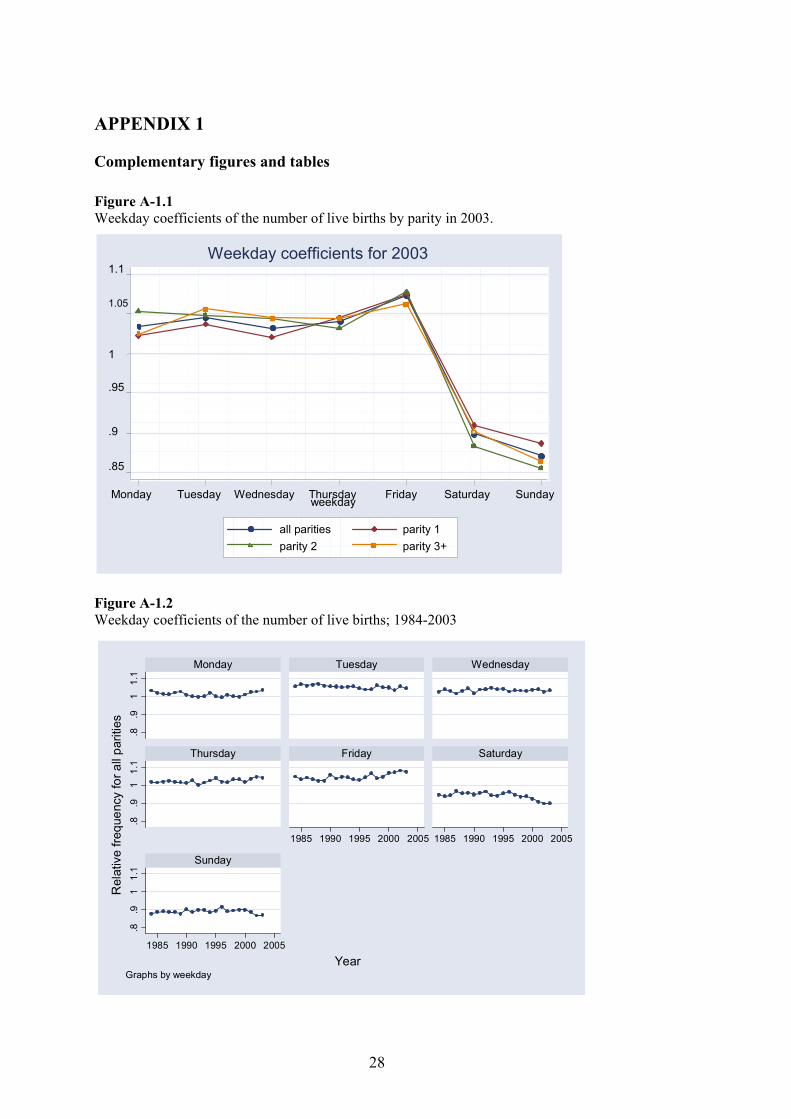
APPENDIX 1

Complementary figures and tables Figure A-1.1 Weekday coefficients of the number of live births by parity in 2003.

.85

.9

.95

1

1.05

1.1

Monday Tuesday Wednesday Thursday Friday Saturday Sundayweekday

all parities parity 1parity 2 parity 3+

Weekday coefficients for 2003

Figure A-1.2 Weekday coefficients of the number of live births; 1984-2003

.8.9

11.

1.8

.91

1.1

.8.9

11.

1

1985 1990 1995 2000 2005 1985 1990 1995 2000 2005

1985 1990 1995 2000 2005

Monday Tuesday Wednesday

Thursday Friday Saturday

Sunday

Rel

ativ

e fre

quen

cy fo

r all

parit

ies

YearGraphs by weekday

28

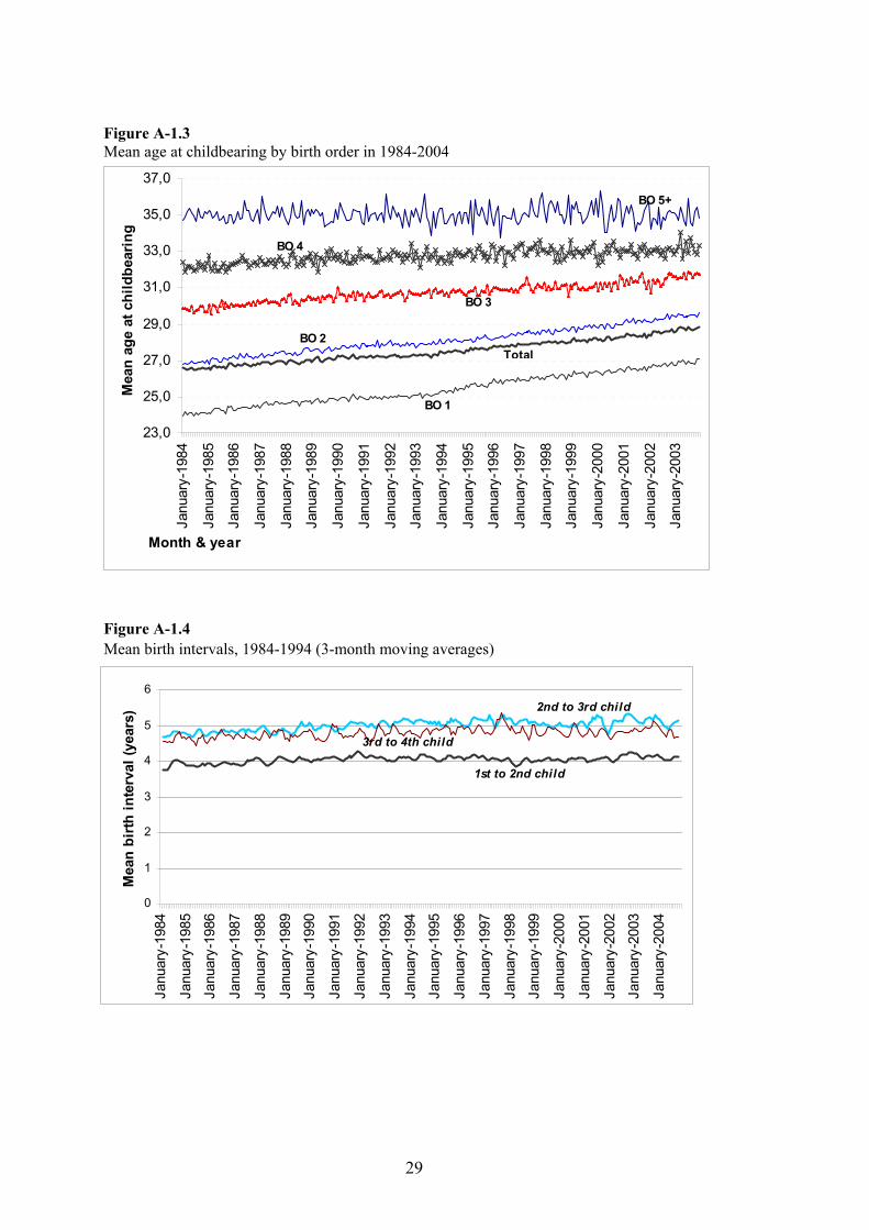
Figure A-1.3 Mean age at childbearing by birth order in 1984-2004

23,0

25,0

27,0

29,0

31,0

33,0

35,0

37,0Ja

nuar

y-19

84

Janu

ary-

1985

Janu

ary-

1986

Janu

ary-

1987

Janu

ary-

1988

Janu

ary-

1989

Janu

ary-

1990

Janu

ary-

1991

Janu

ary-

1992

Janu

ary-

1993

Janu

ary-

1994

Janu

ary-

1995

Janu

ary-

1996

Janu

ary-

1997

Janu

ary-

1998

Janu

ary-

1999

Janu

ary-

2000

Janu

ary-

2001

Janu

ary-

2002

Janu

ary-

2003

Month & year

Mea

n ag

e at

chi

ldbe

arin

g

BO 1

TotalBO 2

BO 3

BO 4

BO 5+

Figure A-1.4 Mean birth intervals, 1984-1994 (3-month moving averages)

0

1

2

3

4

5

6

Janu

ary-

1984

Janu

ary-

1985

Janu

ary-

1986

Janu

ary-

1987

Janu

ary-

1988

Janu

ary-

1989

Janu

ary-

1990

Janu

ary-

1991

Janu

ary-

1992

Janu

ary-

1993

Janu

ary-

1994

Janu

ary-

1995

Janu

ary-

1996

Janu

ary-

1997

Janu

ary-

1998

Janu

ary-

1999

Janu

ary-

2000

Janu

ary-

2001

Janu

ary-

2002

Janu

ary-

2003

Janu

ary-

2004

Mea

n bi

rth

inte

rval

(yea

rs)

1st to 2nd child

2nd to 3rd child

3rd to 4th child

29

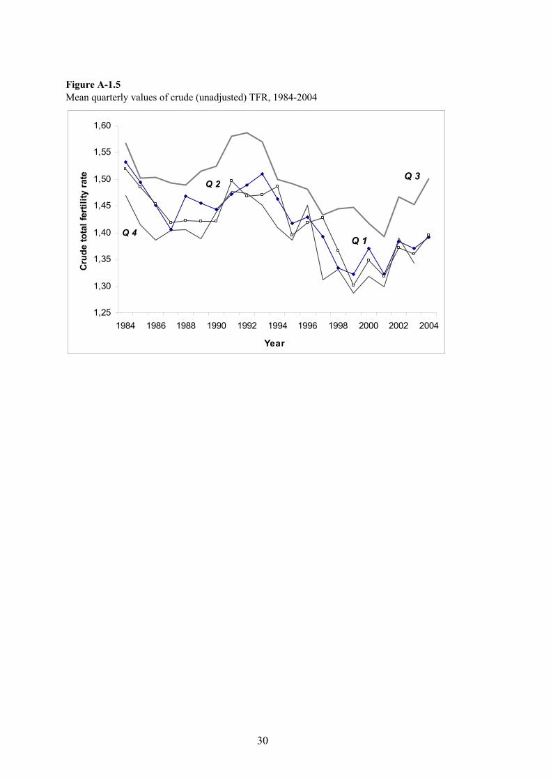
Figure A-1.5 Mean quarterly values of crude (unadjusted) TFR, 1984-2004

1,25

1,30

1,35

1,40

1,45

1,50

1,55

1,60

1984 1986 1988 1990 1992 1994 1996 1998 2000 2002 2004

Year

Cru

de to

tal f

ertil

ity ra

te

Q 1

Q 2Q 3

Q 4

30

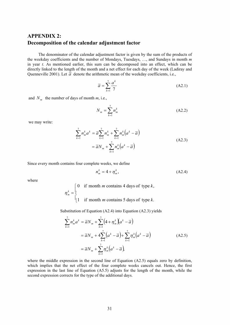
APPENDIX 2: Decomposition of the calendar adjustment factor

The denominator of the calendar adjustment factor is given by the sum of the products of the weekday coefficients and the number of Mondays, Tuesdays, …, and Sundays in month m in year t. As mentioned earlier, this sum can be decomposed into an effect, which can be directly linked to the length of the month and a net effect for each day of the week (Ladiray and Quenneville 2001). Let a denote the arithmetic mean of the weekday coefficients, i.e.,

∑=

=7

1 7k

kaa (A2.1)

and the number of days of month m, i.e., mN

(A2.2) ∑=

=7

1k

kmm nN

we may write:

( )

( )∑

∑∑∑

=

===

−+=

−+=

7

1

7

1

7

1

7

1

k

kkmm

k

kkm

k

km

k

kkm

aanNa

aannaan (A2.3)

Since every month contains four complete weeks, we define

(A2.4) ,4 km

kmn η+=

where

=

.typeofdays5containsmonthif1

,typeofdays4containsmonthif0

km

kmkmη

Substitution of Equation (A2.4) into Equation (A2.3) yields

( )( )

( ) ( )

( ),

4

4

7

1

7

1

7

1

7

1

7

1

∑

∑∑

∑∑

=

==

==

−+=

−+−+=

−++=

k

kkmm

k

kkm

k

km

k

kkmm

k

kkm

aaNa

aaaaNa

aaNaan

η

η

η

(A2.5)

where the middle expression in the second line of Equation (A2.5) equals zero by definition, which implies that the net effect of the four complete weeks cancels out. Hence, the first expression in the last line of Equation (A5.5) adjusts for the length of the month, while the second expression corrects for the type of the additional days.

31

APPENDIX 3: Specification of the estimates of age structure and ‘at risk’ population

A-3.1 Mid-month female population by single years of age (birth cohort)

Purpose: Serves as a basis for computing age- and order-specific incidence rates by age of mother and birth order in each calendar month; women aged 12 to 50 (age reached during the year) are considered.

Estimation procedure: First, linear approximation is used to estimate the age structure of the female population

on the 1st day of each month between 1st January of the years t and t+1. The number of days in any given month or period served for estimating the total share of this period on the change in the number of women by age. The number of women belonging to the birth cohort C (or, alternatively, aged a=t-C) at the beginning of a month m (expressed as M) in a year t was calculated as follows:

PF(C,t,M) = PF(C,t,1) + [PF(C,t+1,1) - PF(C,t,1)] · Sd (t, m-1) , (A3.1)

where Sd (t, m-1) is the share of the cumulated number of days in months 1 to m-1 on the total number of days in the year t. The mid-month female population by single years of age, denoted as PF(C,t,m) was then computed from the population at the beginning of two consecutive months (denoted as M and M+1):

PF(C,t,m) = [PF(C,t,M) + PF(C,t,M+1)] / 2 (A3.2)

Note: All age-specific calculations are expressed in a cohort format (data sorted by age

reached during the year). If the official age structure during the year pertains to the actual age (age in completed years), the data must be reorganised to estimate the age distribution by birth cohort.

A-3.2 Mid-month female population by single months of age (birth month

cohort) Note: These data are used to a limited extent only since our computations of the total

fertility rates show that using the more detailed month birth cohort indicators does not make any appreciable change in the indicators of fertility quantum and timing (see Appendix 5).

Specification: Number of women by single months of birth specified for the middle of

each calendar month in the period of January 1984 to December 2003 Purpose: Serves as a basis for computing age- and order-specific incidence rates by birth

month-cohort of mother and birth order in each calendar month

32

Additional data sources: Number of births by calendar month in 1950 to 2002: EUROSTAT New Cronos database, accessed in December 2004. Number of births by calendar month in 1930 to 1949: data from the 1981 Census (OSZ 1989).

Estimation procedure: Data on the mid-month population of women by single years of age (birth cohorts), as

described in above, served for estimating the mid-month number of women for every month-cohort in reproductive age. For every calendar month considered, the data initially referring to the year-birth cohorts (C) born in the year t=C were redistributed into month-birth cohorts (Cm) on the basis of the proportion of live births in each single month m on the total number of live births during the year t=C:

PF(Cm,t,m) = PF(C,t,M) · [Bm(t=C) / B(t=C)] (A3.3) where Bm(t=C) denotes the total number of live births during the month when the birth cohort Cm was born and B(t=C) is the total number of live births during that year. To connect these month-cohort data with other indicators specified by birth month or calendar month, all data are subsequently expressed in century-month codes, which are calculated for any month since January 1900 as follows:

CMC = (t – 1900) · 12 + m (A3.4)

The CMCs permit an easy computation of age-specific indicators, such as age of mother at childbearing etc.

A-3.3 Monthly age-parity structure of the female population by single years of age (birth cohort)

Purpose: Serves for computing age-parity birth probabilities (exposure-specific

indicators) used in the computation of the PATFR index and the Kohler-Ortega adjPATFR indicator.

Specification: Estimated for the beginning (1st day) of each calendar month. Computed

by combining monthly data on the total number of women by single years of age (birth cohorts) as specified in Eq. A3.1 above and continually updated monthly series of the age-parity distribution of the female population (specified by birth cohort). Except for the birth cohorts 1982-89, the latter is based on the 1991 Census data combined with the age and order-specific incidence rates in the subsequent period. For the more recent time series starting from January 2001 we updated our estimates with the 2001 Census results. The relative age-parity distribution among women born in 1982-89 was reconstructed on the basis of cumulative age and order-specific incidence rates calculated from the vital statistics data.

The relative age-parity composition of the female population at the beginning of a month

m (expressed as M) in a year t is derived from the age-parity composition at the beginning of month m-1 (i.e., at time M-1) and order-specific incidence rates in month m-1. This estimation is performed for every single birth cohort and for each parity status (denoted as i) as follows:

33

wi(C,t,M) = wi(C,t, M-1) + fi(C,t, m-1) - fi+1(C,t, m-1), (A3.5)

where wi(C,t,M) denotes the proportion of women at parity i at the beginning of a month m among each birth cohort C and fi (C,t, m) represents cohort-specific incidence rates of order i, recorded during the month m. Parities 0, 1, 2, 3, and 4+ are distinguished. Note that for parity 0 (childless women), the equation simplifies to:

w0(C,t,M) = w0(C,t, M-1) - f1(C,t, m-1) (A3.6)

The relative proportion of women in the highest-parity category (4+) is computed as

follows:

w4+(C,t,M) = 1 - w0(C,t,M) – w1(C,t,M) - w2 (C,t,M) – w3(C,t,M) (A3.7) For any age and parity category, the number of women at the beginning of each calendar

month m is calculated by combining Eq. (A3.1) above with the Eq. (A3.5) (or A3.6 and A3.7, respectively):

PF, i(C,t,M) = PF (C,t,M) · wi(C,t,M) (A3.8)

Appendix 6 features the table of age and parity composition of the female population as

estimated for December 1, 2004 (Table A-6.1) and sensitivity analysis exploring the effect of differences between the two estimates of the age and parity composition of the female population (one based on the 1991 Census data and the other on the 2001 Census results) on the PATFR index.

A-3.4 Number of live births by biological (true) birth order in 1961-1992

Purpose: Serves for the computation of duration-specific ‘incidence rates,’ and the period parity progression ratios (PPRd).

Source data & estimations: Number of live births by birth order in 1984-2003 derived

from the individual birth records provided by Statistics Austria. Since Statistics Austria collects data on ‘true’ birth order only since 1984, the number of live births by birth order had to be estimated for the previous years, namely for 1961-1983. Composition of live births by birth order in 1961-1979 was derived from the retrospective data on the distribution of births by birth order as recorded in the 1981 Census combined with the total registered number of live births in that period (OSZ 1989). Number of live births by birth order in 1980-1983 was estimated from the total number of births and the relative distribution of order-specific births in 1978-1979 and 1984-1985.

34

APPENDIX 4: Specification of fertility indicators analysed in this study (including calendar and seasonality-trend adjustments)

A-4.1 Age- and order-specific incidence rates and the period TFR

All indicators were computed for birth orders 1, 2, 3, 4, 5+, and for all birth orders combined. For each birth cohort (C) and birth order (i), monthly incidence rates are calculated as follows:

fi(C,t,m) = Bi(C,t,m) / PF(C,t,m), (A4.1)

where Bi(C,t,m) is a total number of live births of order i in a month m among women born in the year C. In our computations, birth orders 1, 2, 3, 4, and 5+ were considered separately.

We considered only cohorts reaching ages 12 to 50 in a given calendar year. In case of

recorded births to women below age 12 or above age 50, they were grouped together with the births to women aged 12 and 50, respectively.

The crude (unadjusted) monthly period total fertility rate (denoted as gTFR), specified by

birth order, is computed as a sum of age- and order-specific incidence rates, multiplied by 12:

gTFRi(t,m) = f∑=

50

12a i(a,t,m) · 12 and gTFR(t,m) = gTFR∑

+

=

5

1i i(t,m), (A4.2)

where a is cohort age (age reached during the calendar year), which is simply calculated as a = t – C (recall that C denotes birth cohort, i.e., the year of birth of the mother).

Calendar adjustment is identical for all birth orders and can be used to adjust the overall

gross total fertility rate:

TFRC(t,m) = gTFR(t,m) · IC (t,m), (A4.3)

where IC denotes the monthly index allowing an adjustment for calendar factor. Seasonality/trend adjustment is order-specific. For any calendar-adjusted TFR, the

trend-season adjustment is computed as follows:

TFRCS,i(t,m) = TFRC,i(t,m) · IS,i (t,m), (A4.4)

where IS denotes the monthly index allowing an adjustment for seasonality and trend fluctuations, net of calendar factor.

Note: All computations are presented here for the yearly birth cohorts, which was our

usual data format. When we used data specified by month cohorts, all cohort-specific calculations (here denoted as C) were based on month birth cohorts (denoted as Cm). The age

35

categories a were expressed in months, ranging from “ages” 132 (age 11.0 in completed years) to 612 months (age 51.0 in completed years).

A-4.2 Age-parity birth probabilities and the period fertility index PATFR

Note: These indicators are mostly used for parity 1, especially in combination with the

parity-progression ratios specified below. As a result, all specifications here are illustrated for birth order 1.

The gross probability for a childless woman belonging to a birth cohort C to give birth to

a first child during a month m is computed as follows: q1(C,t,m) = B1(C,t,m) / PF,0(C,t,M) = B1(C,t,m) / [PF (C,t,M) · w0(C,t,M)], (A4.5)

where PF,0(C,t,M) denotes the total number of childless women among the birth cohort C at the beginning of a month m (see Eq. A3.6 and A3.8 in Appendix 3).

Similarly to the incidence rates calculations, only birth cohorts reaching ages 12 to 50 in a

given calendar year were considered. Births recorded among women below age 12 or above age 50 were coded as births to women aged 12 and 50, respectively.

Calendar and seasonality/trend adjustment is performed for each age separately. The

calendar and season-adjusted first birth probability for a woman born in the year C is computed as

qCS,1(C,t,m) = q1(C,t,m) · IC (t,m) · IS,1 (t,m) (A4.6)

The calendar and season-adjusted total fertility index of parity 1 (PATFRCS,1) is

computed as follows:

PATFRCS,1(t,m) = 1 – ∏ [1- q=

50

12aCS,1(a,t,m)] · 12 (A4.7)

Recall that a is the age reached during the calendar year, which is calculated as a = t – C Note: More details on the age-parity model can be consulted in Rallu and Toulemon

(1994; the original was published in French in 1993). We follow Rallu and Toulemon’s notation of the total parity-specific index as PATFR.

A-4.3 Parity-progression ratios PPRd based on duration (birth interval data)

For birth orders 2 and higher, duration-specific gross ‘incidence rates’ of having a child of order i among women who had their (i-1)th child in a year y is computed as follows:

ni,d(t,m) = Bi,d(t,m) / Bi-1(y) ; i ≥ 2 ; t ≥ d, (A4.8)

36

where d indicates ‘duration,’ which is in this case simplified as a difference between the years when births of order i-1 (year y) and i (year t) took place: d = t – y.

Thus, ni,d(t,m) expresses the (incidence) rate of having an i-th child during a month m in a

year t among women who have given birth to their i-1th child in a year y and Bi,d(t,m) is the total number of live-born children of order i during a month m in a year t among these women. Bi-1(y) is the total number of live-born children of order i-1 reached in a year y.

The ‘duration’ indicator d ranged from 0 to 25; i.e. the earliest year of giving birth to a

previous child (birth order i-1) that was considered in my analysis was y(min) = t-25. In case some women had given birth to their previous child even earlier, they were considered as giving birth in a year y(min).

Note: Although the birth order i refers to live-born children only, the coding of the date

of the previous birth in the official vital statistics pertains to any previous birth, including stillbirths. Thus, the birth interval between two consecutive live births is slightly underestimated insofar as a small fraction of the registered birth intervals refers to the interval between the most recent live birth of order i and the preceding stillbirth, while the preceding live birth of order i-1 had taken place at an unknown date before this stillbirth. Since the proportion of stillbirths in Austria is very small (0.39% of all births in 1984-2002; Statistics Austria 2003), however, the influence of stillbirths on computing fertility rates by duration can be disregarded.

Gross parity-progression ratios (gPPRs) were estimated for women at parities 1, 2, 3, 4,

and the open-ended parity category 5+:

gPPRi-1,i(t,m)= n∑=

25

0d i,d(t,m) · 12 ; i ≥ 2 (A4.9)

The highest birth order considered constitutes an open-ended parity progression to 6th+ child among women having 5+ children.

The gross parity-progression ratios are then adjusted for calendar factor and seasonality in

a similar way as the gross TFR (see Equations A4.3 and A4.4 above):

PPRCS,i-1,i(t,m) = gPPRi-1,i (t,m) · IC (t,m) · IS,i (t,m) (A4.10)

A-4.4 The period average parity (PAP)

The period average parity, adjusted for calendar and seasonality factors (PAPCS) is

calculated for each parity category j by combining the adjusted PATFR index for parity 1 with the adjusted parity progression ratios for parities 2 to 6+:

PAPCS,j(t,m) = PATFRCS,1(t,m) ∏PPR=

j

i 2CS,i-1,i(t,m) (A4.11)

For example, the PAP index for parity 4 is derived as follows:

37

PAPCS,4(t,m) = PATFRCS,1(t,m)⋅ PPRCS,1,2 (t,m)⋅ PPRCS,2,3 (t,m) ⋅ PPRCS,3,4 (t,m) (A4.12) The highest parity-progression category (5+ to 6+) was assumed to reflect the progression

from 5th to 6th childbirth instead. The progression from the sixth to higher parities was disregarded. Given the very small

values of estimated PAP index for birth order 6 (the mean value was 0.005 for the whole 1984-2003 period), this procedure involves a systematic underestimation of the total TFRI index by about 0.002 in absolute terms (i.e., about 0.1% in relative terms).

The overall index of total fertility was calculated as follows:

PAPCS(t,m) = PATFRCS,1(t,m) + PAP∑=

6

2j CS,j(t,m) (A4.13)

A-4.5 Bongaarts and Feeney’s (1988) tempo-adjusted TFR (adjTFR)

The adjusted total fertility rate proposed by Bongaarts and Feeney (further denoted as adjTFR) is calculated as follows:

adjTFRi(t) = TFRi(t) / (1-ri(t)) (A4.14)

where ri(t) is the change in the mean age at childbearing at birth order i between the beginning and the end of year t. Our initial computations show that a similar approach cannot be used to calculate the change in the mean age between two consecutive months, as the mean age shows strong irregularities on a monthly basis. To solve this problem, we utilised the change in the mean age at childbearing in a month m against the same month a year ago—a solution which comes closer to the mean age measurement in the original formula:

adjTFRi(t,m) = TFRi(t,m) / (1-ri(t,m)), (A4.15)

where m denotes a particular month in the year t and ri(t,m) is the change in the mean age at childbearing of birth order i between the month m in the year t-1 and the month m in the year t. In agreement with the Bongaarts-Feeney method, we calculate the mean age at childbearing from the set of age and order-specific fertility rates fi(a) calculated for every month m considered. As the results depicted in Section 5.2 indicate, even this solution did not provide reasonably stable estimates of the adjusted TFR and the level of irregularities and erratic values remained unacceptable.

The overall adjusted TFR is computed as a sum of order-specific adjusted TFRs; birth

orders 1, 2, and 3+ were distinguished. The calendar and season-trend adjustment is applied in the same way as in the case of the total fertility rates (see Equations A4.3 and A4.4 above).

38

A-4.6 Kohler and Ortega’s adjusted PATFR (adjPATFR)

Given that we use the Kohler-Ortega adjusted fertility index, the adjPATFR, only in the comparative section evaluating the aggregated annual results, and given that this method is relatively complex, a complete overview of all the equations would be beyond the scope of this report. Rather, we provide only a very brief characterisation of this method; a full description can be consulted in Kohler and Ortega (2002).

This method permits an estimation of period fertility measures that are free of the three

distortions present in the TFR, namely distortions caused by (1) changes in the parity distribution of women, (2) changes in fertility timing and (3) changes in the variance of the fertility schedule. The authors employ a procedure that iteratively corrects the observed mean age and the inferred tempo for distortions caused by the variance effects (see also Kohler and Philipov 2001). For each parity and single age group, the Kohler-Ortega adjustment allows to derive the adjusted age-parity birth probability q’i(a) = qi(a) / (1-ri(a,t)), where qi(a) is the observed probability that a woman aged a, who has i-1 children at the beginning of the year t will give birth to another child during that year. The adjusted parity-specific tempo change ri(a,t) is computed following Kohler and Philipov (2001: 8, Eq. 11): ri(a) = γi + δi (a –āi), where γi is the annual change in the mean age of the fertility schedule (here represented by birth probabilities) at parity i, δ is the annual increase in the standard deviation of the schedule, and ā is the mean age of the schedule.

Besides its advantages, the Kohler-Ortega adjustment also has a number of problematic

features which are especially hard to deal with in the analysis of monthly time series: The authors apply a state-space smoothing procedure to the observed series of the mean

age and variance changes (Kohler and Ortega 2002: 127). Although the smoothing reduces instability in the adjusted fertility indicators, part of the variability in fertility trends—a phenomenon we aim to explore—might be lost as a result. The derivation of the adjusted fertility indicators in the period t is contingent upon the

observed fertility indicators in the periods t-1 and t+1. As a result, it is impossible within the original framework to derive the adjusted fertility indexes for the most recent period. Furthermore, the estimates of the most recent adjusted results are relatively unstable and subject to revisions as fertility data for the subsequent periods are later incorporated. To reduce the instability in the adjusted indicators, a limited age range including only

the prime reproductive period may be considered for a computation of adjusted rates at each parity (see also Kohler and Ortega 2002: 127). Consequently, the results are not influenced by outlying and unusual cases, which are quite common in the detailed age-parity data14. However, there is no clear criterion which age range should be included and our preliminary computations have shown that different age range selections affect the final results.

14 Consider an extreme case of a woman giving birth to a third child at age 16. Given that the population of women with two children (population ‘at risk’) is extremely small at that age (for most of the year 2004, there was just one such case), an occurrence of a third birth might increase the estimated probability of having a third child for a woman aged 16 and having two children from 0.0 to 1.0. This result, if included, would affect all the adjustment computations.

39

The Kohler-Ortega adjustment leads to considerable fluctuations at higher birth orders and may cause an underestimation of higher-order fertility rates (Sobotka 2004a).

Facing these difficulties, we decided after preliminary analysis not to include the Kohler-

Ortega’s method to our study of monthly fertility rates. Instead, we used it only for the evaluation of tempo distortions performed on an annual basis (see Appendix 7) and we restrict its use for birth orders 1 and 2. Our adjustment differs somewhat from the original Kohler and Ortega (KO) application. First, we work with age-parity birth probabilities as contrasted with the occurrence-exposure rates (birth intensities) utilised by KO. Although the difference in results is small, birth probabilities are in our view methodologically better compatible with the life table framework. Second, we did not smooth the observed set of age-parity probabilities before the adjustment nor did we apply an iterative procedure aiming to provide a correction for variance effects. In order to reduce irregularities in the adjusted fertility index, we restricted the age range of birth probabilities to be used for inferring all the parameters necessary for the adjustment to ages 20 to 40 for birth order 1 and 22 to 40 for birth order 2. Although we computed the adjusted PATFR for the higher birth orders as well, we do not utilise these results in this study.

40

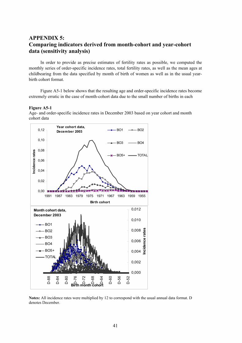
APPENDIX 5: Comparing indicators derived from month-cohort and year-cohort data (sensitivity analysis)

In order to provide as precise estimates of fertility rates as possible, we computed the monthly series of order-specific incidence rates, total fertility rates, as well as the mean ages at childbearing from the data specified by month of birth of women as well as in the usual year-birth cohort format.

Figure A5-1 below shows that the resulting age and order-specific incidence rates become

extremely erratic in the case of month-cohort data due to the small number of births in each

Figure A5-1 Age- and order-specific incidence rates in December 2003 based on year cohort and month cohort data

0,00

0,02

0,04

0,06

0,08

0,10

0,12

1991 1987 1983 1979 1975 1971 1967 1963 1959 1955

Birth cohort

Inci

denc

e ra

tes

BO1 BO2

BO3 BO4

BO5+ TOTAL

Year cohort data,December 2003

0,000

0,002

0,004

0,006

0,008

0,010

0,012

D-5

2

D-5

6

D-6

0

D-6

4

D-6

8

D-7

2

D-7

6

D-8

0

D-8

4

D-8

8

Birth month cohort

Inci

denc

e ra

tes

BO1

BO2

BO3

BO4

BO5+

TOTAL

Month cohort data,December 2003

Notes: All incidence rates were multiplied by 12 to correspond with the usual annual data format. D denotes December.

41

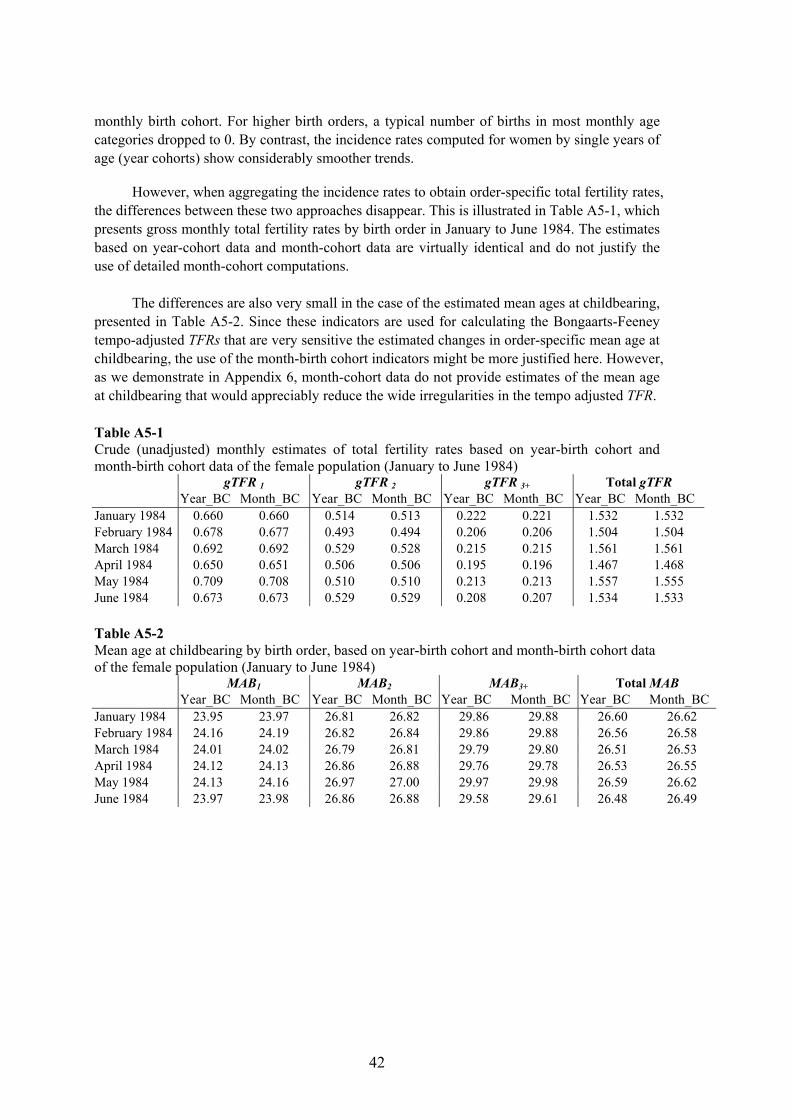
monthly birth cohort. For higher birth orders, a typical number of births in most monthly age categories dropped to 0. By contrast, the incidence rates computed for women by single years of age (year cohorts) show considerably smoother trends.

However, when aggregating the incidence rates to obtain order-specific total fertility rates, the differences between these two approaches disappear. This is illustrated in Table A5-1, which presents gross monthly total fertility rates by birth order in January to June 1984. The estimates based on year-cohort data and month-cohort data are virtually identical and do not justify the use of detailed month-cohort computations.

The differences are also very small in the case of the estimated mean ages at childbearing,

presented in Table A5-2. Since these indicators are used for calculating the Bongaarts-Feeney tempo-adjusted TFRs that are very sensitive the estimated changes in order-specific mean age at childbearing, the use of the month-birth cohort indicators might be more justified here. However, as we demonstrate in Appendix 6, month-cohort data do not provide estimates of the mean age at childbearing that would appreciably reduce the wide irregularities in the tempo adjusted TFR. Table A5-1 Crude (unadjusted) monthly estimates of total fertility rates based on year-birth cohort and month-birth cohort data of the female population (January to June 1984)

gTFR 1 gTFR 2 gTFR 3+ Total gTFR Year_BC Month_BC Year_BC Month_BC Year_BC Month_BC Year_BC Month_BC

January 1984 0.660 0.660 0.514 0.513 0.222 0.221 1.532 1.532 February 1984 0.678 0.677 0.493 0.494 0.206 0.206 1.504 1.504 March 1984 0.692 0.692 0.529 0.528 0.215 0.215 1.561 1.561 April 1984 0.650 0.651 0.506 0.506 0.195 0.196 1.467 1.468 May 1984 0.709 0.708 0.510 0.510 0.213 0.213 1.557 1.555 June 1984 0.673 0.673 0.529 0.529 0.208 0.207 1.534 1.533 Table A5-2 Mean age at childbearing by birth order, based on year-birth cohort and month-birth cohort data of the female population (January to June 1984)

MAB1 MAB2 MAB3+ Total MAB Year_BC Month_BC Year_BC Month_BC Year_BC Month_BC Year_BC Month_BC

January 1984 23.95 23.97 26.81 26.82 29.86 29.88 26.60 26.62 February 1984 24.16 24.19 26.82 26.84 29.86 29.88 26.56 26.58 March 1984 24.01 24.02 26.79 26.81 29.79 29.80 26.51 26.53 April 1984 24.12 24.13 26.86 26.88 29.76 29.78 26.53 26.55 May 1984 24.13 24.16 26.97 27.00 29.97 29.98 26.59 26.62 June 1984 23.97 23.98 26.86 26.88 29.58 29.61 26.48 26.49

42

APPENDIX 6: Estimating age and parity composition of the female population. Sensitivity analysis of the estimated age-parity composition on the computed PATFR index

In order to compute age-parity birth probabilities, we had to reconstruct the age and parity structure of the female population in reproductive age (age 12 to 50 was considered) for each calendar month since January 1984. Two possible approaches to derive the relative distribution for each birth cohort—(1) using the Census data on the age-parity distribution among women and (2) cumulating time series of age and order-specific incidence rates that cover the whole reproductive history of the birth cohorts under study—usually yield slightly different results. The second approach disregards possible effects of migration on the parity composition among women. However, the continuous recording of the age- and parity composition always has to rely on the time series of incidence rates. The question is whether this database should be occasionally updated with the latest census data, whether such updating makes a significant difference for the age-parity composition records, and whether this difference is in turn translated into different values of the PATFR index.

We deal with this topic in the first section (A6-1); the consequent section features the

most recent estimate of the age and parity composition among women born between 1954 and 1990 as of December 1, 2004.

A-6.1 Comparing the estimates of the age-parity composition of the female population based on the 1991 and 2001 Census data

We compared two different estimates of the age-parity composition among women born between 1950 and 1985 computed for the date of the 2001 Census (May 15). The first estimate, denoted as “Estimate 1,” is based on the 1991 Census results and the subsequent time series of age (cohort) and order-specific incidence rates computed up until May 15, 2001. The second estimate, “Estimate 2,” is based on the age-parity composition as reported in the 2001 Census. We also compared these data with the third estimate, derived for women born since 1970 solely from on the cumulated series of age and order-specific incidence rates. We do not present these results here.

Overall, the differences between the two estimates were not wide. The 2001 census

results indicated a lower proportion of childless women and a higher proportion of women having one, two, three and four or more children. These differences implied that Estimate 2 indicates slightly higher levels of actual cohort fertility than Estimate 1 based on the 1991 Census data. In absolute terms, the largest differences were recorded for the proportion of childless women—the 2001 Census (Estimate 2) recorded childlessness by 0.9-1.8% lower among women born in 1962-1979 than the Estimate 1 data (see Figure A6-1). These women were distributed across all parity distributions. For instance, among women born in 1968, where the difference in the estimated proportion childless has been largest (-1.8% in the Estimate 2), the proportion of women with one child in Estimate 2 was by 0.7% higher, with 2 children by 0.9% higher, and with 3 children by 0.1% higher than in Estimate 1 (Figure A6-1). The relative differences were most pronounced among younger birth cohorts (especially for parity 1), and, in the case of parity 4+, also among the ‘older’ women of reproductive age born between 1952 and 1964 (relative difference up to 5%). Combined together, these parity differences resulted in

43

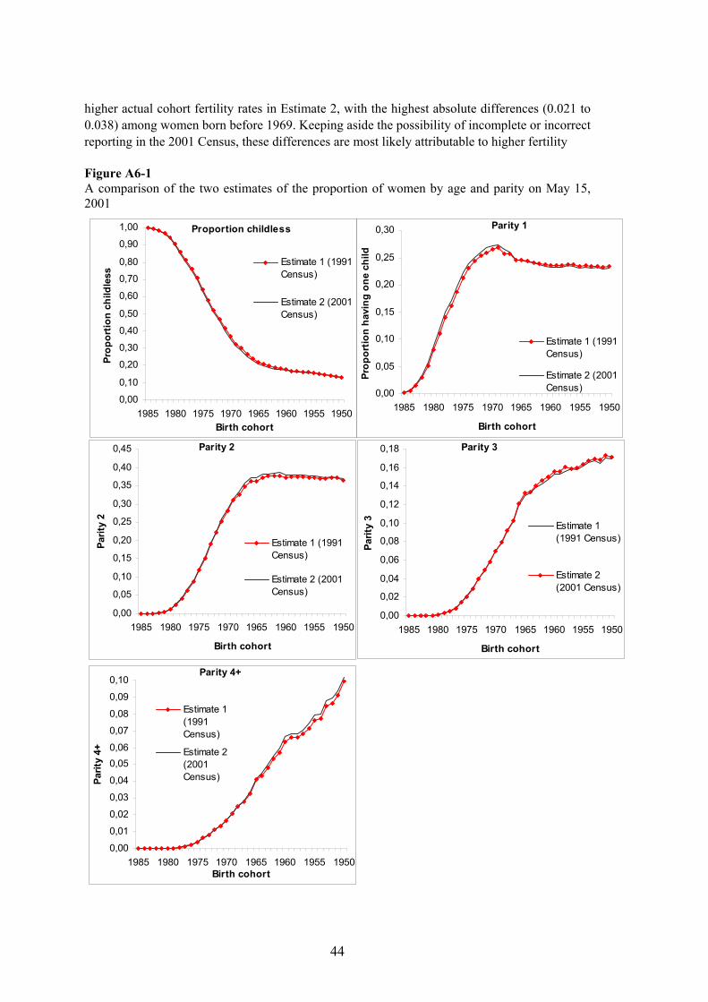
higher actual cohort fertility rates in Estimate 2, with the highest absolute differences (0.021 to 0.038) among women born before 1969. Keeping aside the possibility of incomplete or incorrect reporting in the 2001 Census, these differences are most likely attributable to higher fertility

Figure A6-1 A comparison of the two estimates of the proportion of women by age and parity on May 15, 2001

0,00

0,10

0,20

0,30

0,40

0,50

0,60

0,70

0,80

0,90

1,00

1985 1980 1975 1970 1965 1960 1955 1950Birth cohort

Prop

ortio

n ch

ildle

ss

Estimate 1 (1991Census)

Estimate 2 (2001Census)

Proportion childless

0,00

0,05

0,10

0,15

0,20

0,25

0,30

1985 1980 1975 1970 1965 1960 1955 1950

Birth cohort

Prop

ortio

n ha

ving

one

chi

ld

Estimate 1 (1991Census)

Estimate 2 (2001Census)

Parity 1

0,00

0,05

0,10

0,15

0,20

0,25

0,30

0,35

0,40

0,45

1985 1980 1975 1970 1965 1960 1955 1950

Birth cohort

Parit

y 2

Estimate 1 (1991Census)

Estimate 2 (2001Census)

Parity 2

0,00

0,02

0,04

0,06

0,08

0,10

0,12

0,14

0,16

0,18

1985 1980 1975 1970 1965 1960 1955 1950

Birth cohort

Parit

y 3

Estimate 1(1991 Census)

Estimate 2(2001 Census)

Parity 3

0,00

0,01

0,02

0,03

0,04

0,050,06

0,07

0,08

0,09

0,10

1985 1980 1975 1970 1965 1960 1955 1950Birth cohort

Parit

y 4+

Estimate 1(1991Census)

Estimate 2(2001Census)

Parity 4+

44

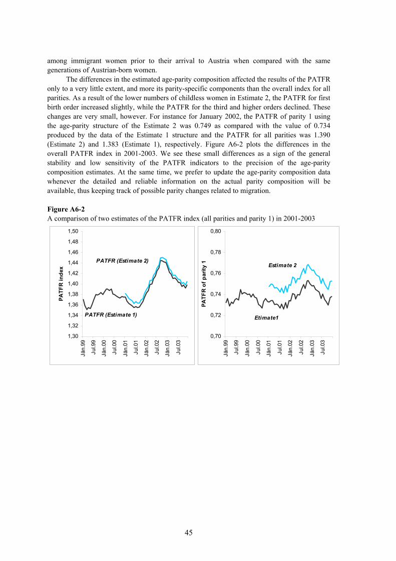
among immigrant women prior to their arrival to Austria when compared with the same generations of Austrian-born women.

The differences in the estimated age-parity composition affected the results of the PATFR only to a very little extent, and more its parity-specific components than the overall index for all parities. As a result of the lower numbers of childless women in Estimate 2, the PATFR for first birth order increased slightly, while the PATFR for the third and higher orders declined. These changes are very small, however. For instance for January 2002, the PATFR of parity 1 using the age-parity structure of the Estimate 2 was 0.749 as compared with the value of 0.734 produced by the data of the Estimate 1 structure and the PATFR for all parities was 1.390 (Estimate 2) and 1.383 (Estimate 1), respectively. Figure A6-2 plots the differences in the overall PATFR index in 2001-2003. We see these small differences as a sign of the general stability and low sensitivity of the PATFR indicators to the precision of the age-parity composition estimates. At the same time, we prefer to update the age-parity composition data whenever the detailed and reliable information on the actual parity composition will be available, thus keeping track of possible parity changes related to migration. Figure A6-2 A comparison of two estimates of the PATFR index (all parities and parity 1) in 2001-2003

1,30

1,32

1,34

1,36

1,38

1,40

1,42

1,44

1,46

1,48

1,50

Jän.

99

Jul.9

9

Jän.

00

Jul.0

0

Jän.

01

Jul.0

1

Jän.

02

Jul.0

2

Jän.

03

Jul.0

3

PATF

R in

dex

PATFR (Estimate 1)

PATFR (Estimate 2)

0,70

0,72

0,74

0,76

0,78

0,80Jä

n.99

Jul.9

9

Jän.

00

Jul.0

0

Jän.

01

Jul.0

1

Jän.

02

Jul.0

2

Jän.

03

Jul.0

3

PATF

R o

f par

ity 1 Estimate 2

Etimate1

45

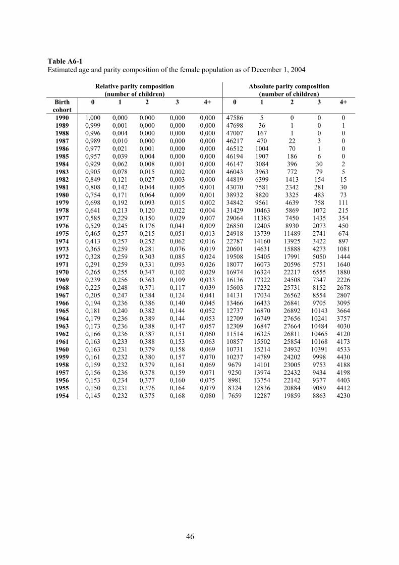
Table A6-1 Estimated age and parity composition of the female population as of December 1, 2004

Relative parity composition (number of children)

Absolute parity composition (number of children)

Birth cohort

0 1 2 3 4+ 0 1 2 3 4+

1990 1,000 0,000 0,000 0,000 0,000 47586 5 0 0 0 1989 0,999 0,001 0,000 0,000 0,000 47698 36 1 0 1 1988 0,996 0,004 0,000 0,000 0,000 47007 167 1 0 0 1987 0,989 0,010 0,000 0,000 0,000 46217 470 22 3 0 1986 0,977 0,021 0,001 0,000 0,000 46512 1004 70 1 0 1985 0,957 0,039 0,004 0,000 0,000 46194 1907 186 6 0 1984 0,929 0,062 0,008 0,001 0,000 46147 3084 396 30 2 1983 0,905 0,078 0,015 0,002 0,000 46043 3963 772 79 5 1982 0,849 0,121 0,027 0,003 0,000 44819 6399 1413 154 15 1981 0,808 0,142 0,044 0,005 0,001 43070 7581 2342 281 30 1980 0,754 0,171 0,064 0,009 0,001 38932 8820 3325 483 73 1979 0,698 0,192 0,093 0,015 0,002 34842 9561 4639 758 111 1978 0,641 0,213 0,120 0,022 0,004 31429 10463 5869 1072 215 1977 0,585 0,229 0,150 0,029 0,007 29064 11383 7450 1435 354 1976 0,529 0,245 0,176 0,041 0,009 26850 12405 8930 2073 450 1975 0,465 0,257 0,215 0,051 0,013 24918 13739 11489 2741 674 1974 0,413 0,257 0,252 0,062 0,016 22787 14160 13925 3422 897 1973 0,365 0,259 0,281 0,076 0,019 20601 14631 15888 4273 1081 1972 0,328 0,259 0,303 0,085 0,024 19508 15405 17991 5050 1444 1971 0,291 0,259 0,331 0,093 0,026 18077 16073 20596 5751 1640 1970 0,265 0,255 0,347 0,102 0,029 16974 16324 22217 6555 1880 1969 0,239 0,256 0,363 0,109 0,033 16136 17322 24508 7347 2226 1968 0,225 0,248 0,371 0,117 0,039 15603 17232 25731 8152 2678 1967 0,205 0,247 0,384 0,124 0,041 14131 17034 26562 8554 2807 1966 0,194 0,236 0,386 0,140 0,045 13466 16433 26841 9705 3095 1965 0,181 0,240 0,382 0,144 0,052 12737 16870 26892 10143 3664 1964 0,179 0,236 0,389 0,144 0,053 12709 16749 27656 10241 3757 1963 0,173 0,236 0,388 0,147 0,057 12309 16847 27664 10484 4030 1962 0,166 0,236 0,387 0,151 0,060 11514 16325 26811 10465 4120 1961 0,163 0,233 0,388 0,153 0,063 10857 15502 25854 10168 4173 1960 0,163 0,231 0,379 0,158 0,069 10731 15214 24932 10391 4533 1959 0,161 0,232 0,380 0,157 0,070 10237 14789 24202 9998 4430 1958 0,159 0,232 0,379 0,161 0,069 9679 14101 23005 9753 4188 1957 0,156 0,236 0,378 0,159 0,071 9250 13974 22432 9434 4198 1956 0,153 0,234 0,377 0,160 0,075 8981 13754 22142 9377 4403 1955 0,150 0,231 0,376 0,164 0,079 8324 12836 20884 9089 4412 1954 0,145 0,232 0,375 0,168 0,080 7659 12287 19859 8863 4230

46

APPENDIX 7: Assessment of tempo effects and period fertility quantum in Austria

This appendix analyses period fertility indicators in an aggregated annual format and focuses on the total quantum of fertility and on first births. In addition to fertility indicators scrutinised in Section 6 we make use of the Kohler-Ortega adjusted adjPATFR index, which is calculated from the time series of annual age-parity birth probabilities for birth orders 1 and 2; Tables A-7.3 and A-7.4 below present results for birth orders 2 and 3+. The inclusion of the Kohler-Ortega method allows us to compare the results provided by the PAP index with the indicator explicitly aimed at correcting the tempo effects. For birth order 1, the adjPATFR provides a benchmark to estimate the magnitude of the tempo effects in the (unadjusted) PATFR index, which is used in the PAP computations.

Figure A-7.1 and Table A-7.1 below summarise mean annual values of the TFR as

compared with the PATFR, PAP, and the adjPATFR (Kohler-Ortega method). The table further features two estimates of tempo effects, the first based on the difference between the PAP index and the TFR, and the second based on the difference between the adjPATFR and the TFR. The results presented here point out the persistence and relative stability of timing distortions in the period TFR in Austria. For most periods, the Kohler-Ortega adjustment suggests similar extent of tempo effects and similar trends as the PAP index; both indicators have shown very close values since 1994. Only during the period of elevated fertility in the early 1990s, the KO adjPATFR indicated considerably less pronounced tempo effects and lower fertility level than the PAP. The ongoing fertility postponement is estimated to have depressed the recorded TFR by 0.19 on average when measured by the PAP and 0.14 when measured by Kohler-Ortega index. Given that PAP is likely to slightly underestimate the extent of timing distortion, the Kohler-Ortega index probably underestimates the size of timing effects even to a larger extent. Overall, the mean TFR value in 1984-2004 was 1.43 as contrasted with the PATFR of 1.46 and PAP of 1.62. This may appear as a relatively small difference but in the context of low fertility, even minor differences in fertility quantum may have strong implications in terms of the eventual rates of population decline and the pace of population ageing.

Figure A-7.2 and Table A-7.2 below show the results of the mean annual values of the

TFR, PATFR, the adjPATFR and the estimated tempo effects for first birth order, which accounts for almost half of all births (44-48% in 1984-2004) in Austria. The persistent difference between the TFR and the PATFR is clearly illustrated, indicating that the TFR has been strongly affected by the ongoing fertility postponement (see Section 6.3 above). Furthermore, the Kohler-Ortega adjusted PATFR index consistently indicates somewhat higher values than the (unadjusted) PATFR. Although this difference cannot serve for a precise evaluation of tempo effects on a continuous basis, it gives a rough indication of the overall quantum of first birth in 1985-2002. In comparison with the mean TFR values of 0.67 and the mean PATFR of 0.77, the Kohler-Ortega adjPATFR reached 0.80.

Although the difference between the PATFR for birth order 1 and its ‘corrected’ version

is small, it becomes somewhat larger once we combine it with the subsequent parity progression ratio and estimate the tempo-adjusted PAP index. Applying the proportionality assumption, we arrive at the total fertility quantum in 1985-2003 of 1.71 as compared with the PAP index of 1.62 and the TFR of 1.43. As a result, the estimated negative influence of timing changes of the period TFR was close to 0.3 (0.28). In relative terms, our estimates imply that the period

47

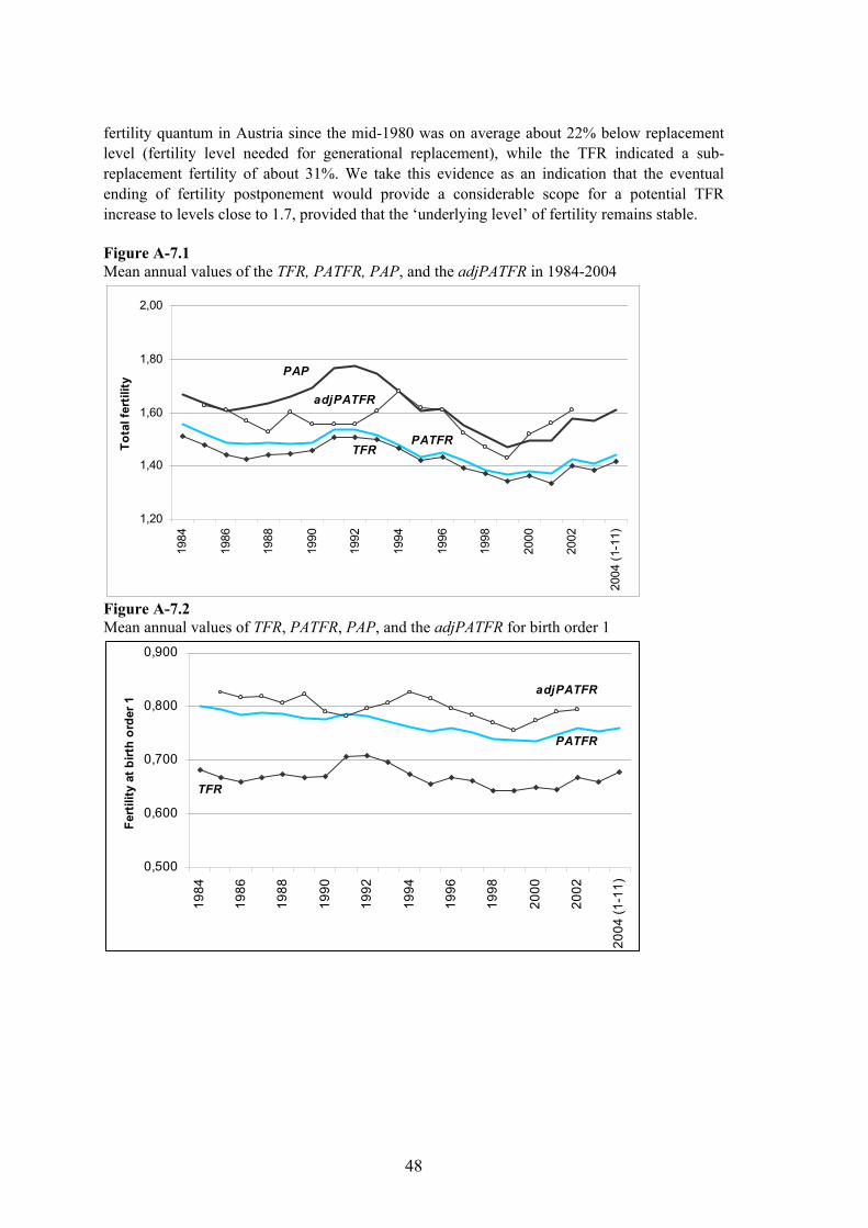
fertility quantum in Austria since the mid-1980 was on average about 22% below replacement level (fertility level needed for generational replacement), while the TFR indicated a sub-replacement fertility of about 31%. We take this evidence as an indication that the eventual ending of fertility postponement would provide a considerable scope for a potential TFR increase to levels close to 1.7, provided that the ‘underlying level’ of fertility remains stable. Figure A-7.1 Mean annual values of the TFR, PATFR, PAP, and the adjPATFR in 1984-2004

1,20

1,40

1,60

1,80

2,00

1984

1986

1988

1990

1992

1994

1996

1998

2000

2002

2004

(1-1

1)

Tota

l fer

tility

adjPATFR

PATFRTFR

PAP

Figure A-7.2 Mean annual values of TFR, PATFR, PAP, and the adjPATFR for birth order 1

0,500

0,600

0,700

0,800

0,900

1984

1986

1988

1990

1992

1994

1996

1998

2000

2002

2004

(1-1

1)

Fert

ility

at b

irth

orde

r 1

TFR

PATFR

adjPATFR

48

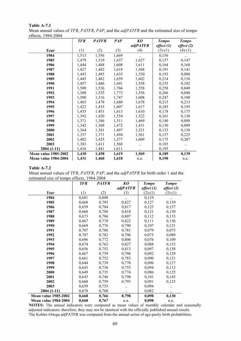
Table A-7.1 Mean annual values of TFR, PATFR, PAP, and the adjPATFR and the estimated size of tempo effects, 1984-2004

TFR PATFR PAP KO adjPATFR

Tempo effect (1)

Tempo effect (2)

Year (1) (2) (3) (4) (3)-(1) (4)-(1) 1984 1,513 1,556 1,669 .. 0,156 .. 1985 1,479 1,519 1,637 1,627 0,157 0,147 1986 1,444 1,488 1,608 1,611 0,164 0,168 1987 1,427 1,482 1,618 1,568 0,191 0,141 1988 1,443 1,485 1,635 1,530 0,193 0,088 1989 1,445 1,482 1,659 1,602 0,214 0,156 1990 1,457 1,486 1,691 1,558 0,235 0,102 1991 1,509 1,536 1,766 1,558 0,258 0,049 1992 1,508 1,535 1,773 1,556 0,266 0,048 1993 1,500 1,516 1,747 1,608 0,247 0,108 1994 1,465 1,478 1,680 1,678 0,215 0,213 1995 1,422 1,435 1,607 1,617 0,185 0,195 1996 1,435 1,451 1,613 1,610 0,178 0,175 1997 1,392 1,420 1,554 1,522 0,161 0,130 1998 1,371 1,386 1,511 1,469 0,140 0,098 1999 1,342 1,368 1,472 1,431 0,130 0,089 2000 1,364 1,381 1,497 1,521 0,133 0,158 2001 1,337 1,371 1,494 1,561 0,157 0,225 2002 1,402 1,425 1,577 1,609 0,175 0,207 2003 1,383 1,411 1,568 .. 0,185 ..

2004 (1-11) 1,416 1,441 1,611 .. 0,195 .. Mean value 1985-2002 1,430 1,458 1,619 1,569 0,189 0,139 Mean value 1984-2004 1,431 1,460 1,618 n.a. 0,190 n.a. Table A-7.2 Mean annual values of TFR, PATFR, PAP, and the adjPATFR for birth order 1 and the estimated size of tempo effects, 1984-2004

TFR PATFR KO adjPATFR

Tempo effect (1)

Tempo effect (2)

Year (1) (2) (3) (2)-(1) (3)-(1) 1984 0,681 0,800 .. 0,119 .. 1985 0,668 0,795 0,827 0,127 0,159 1986 0,659 0,784 0,817 0,125 0,157 1987 0,668 0,788 0,818 0,121 0,150 1988 0,673 0,786 0,807 0,112 0,133 1989 0,667 0,778 0,822 0,111 0,156 1990 0,669 0,776 0,790 0,107 0,121 1991 0,707 0,786 0,781 0,079 0,075 1992 0,707 0,782 0,796 0,075 0,089 1993 0,696 0,772 0,806 0,076 0,109 1994 0,674 0,762 0,827 0,088 0,153 1995 0,656 0,753 0,813 0,097 0,158 1996 0,667 0,759 0,796 0,092 0,129 1997 0,661 0,752 0,783 0,090 0,121 1998 0,644 0,739 0,770 0,096 0,127 1999 0,643 0,736 0,755 0,094 0,112 2000 0,649 0,735 0,774 0,086 0,125 2001 0,645 0,746 0,790 0,101 0,145 2002 0,668 0,759 0,793 0,091 0,125 2003 0,659 0,753 .. 0,094 ..

2004 (1-11) 0,678 0,760 .. 0,082 .. Mean value 1985-2002 0,668 0,766 0,798 0,098 0,130 Mean value 1984-2004 0,668 0,767 n.a. 0,098 n.a.

NOTES: The annual indicators were computed as mean values of monthly calendar and seasonally adjusted indicators; therefore, they may not be identical with the officially published annual results. The Kohler-Ortega adjPATFR was computed from the annual series of age-parity birth probabilities.

49

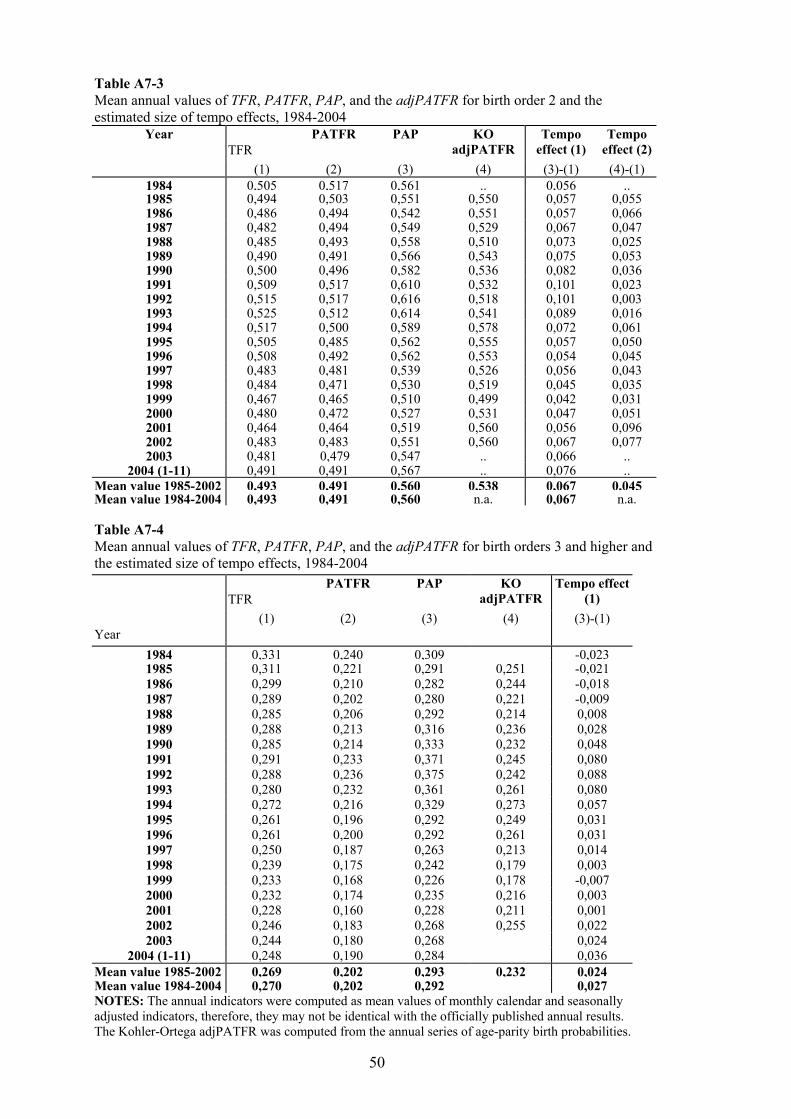
Table A7-3 Mean annual values of TFR, PATFR, PAP, and the adjPATFR for birth order 2 and the estimated size of tempo effects, 1984-2004

Year TFR

PATFR PAP KO adjPATFR

Tempo effect (1)

Tempo effect (2)

(1) (2) (3) (4) (3)-(1) (4)-(1) 1984 0,505 0,517 0,561 .. 0,056 .. 1985 0,494 0,503 0,551 0,550 0,057 0,055 1986 0,486 0,494 0,542 0,551 0,057 0,066 1987 0,482 0,494 0,549 0,529 0,067 0,047 1988 0,485 0,493 0,558 0,510 0,073 0,025 1989 0,490 0,491 0,566 0,543 0,075 0,053 1990 0,500 0,496 0,582 0,536 0,082 0,036 1991 0,509 0,517 0,610 0,532 0,101 0,023 1992 0,515 0,517 0,616 0,518 0,101 0,003 1993 0,525 0,512 0,614 0,541 0,089 0,016 1994 0,517 0,500 0,589 0,578 0,072 0,061 1995 0,505 0,485 0,562 0,555 0,057 0,050 1996 0,508 0,492 0,562 0,553 0,054 0,045 1997 0,483 0,481 0,539 0,526 0,056 0,043 1998 0,484 0,471 0,530 0,519 0,045 0,035 1999 0,467 0,465 0,510 0,499 0,042 0,031 2000 0,480 0,472 0,527 0,531 0,047 0,051 2001 0,464 0,464 0,519 0,560 0,056 0,096 2002 0,483 0,483 0,551 0,560 0,067 0,077 2003 0,481 0,479 0,547 .. 0,066 ..

2004 (1-11) 0,491 0,491 0,567 .. 0,076 .. Mean value 1985-2002 0,493 0,491 0,560 0,538 0,067 0,045Mean value 1984-2004 0,493 0,491 0,560 n.a. 0,067 n.a. Table A7-4 Mean annual values of TFR, PATFR, PAP, and the adjPATFR for birth orders 3 and higher and the estimated size of tempo effects, 1984-2004

TFR

PATFR PAP KO adjPATFR

Tempo effect (1)

Year (1) (2) (3) (4) (3)-(1)

1984 0,331 0,240 0,309 -0,023 1985 0,311 0,221 0,291 0,251 -0,021 1986 0,299 0,210 0,282 0,244 -0,018 1987 0,289 0,202 0,280 0,221 -0,009 1988 0,285 0,206 0,292 0,214 0,008 1989 0,288 0,213 0,316 0,236 0,028 1990 0,285 0,214 0,333 0,232 0,048 1991 0,291 0,233 0,371 0,245 0,080 1992 0,288 0,236 0,375 0,242 0,088 1993 0,280 0,232 0,361 0,261 0,080 1994 0,272 0,216 0,329 0,273 0,057 1995 0,261 0,196 0,292 0,249 0,031 1996 0,261 0,200 0,292 0,261 0,031 1997 0,250 0,187 0,263 0,213 0,014 1998 0,239 0,175 0,242 0,179 0,003 1999 0,233 0,168 0,226 0,178 -0,007 2000 0,232 0,174 0,235 0,216 0,003 2001 0,228 0,160 0,228 0,211 0,001 2002 0,246 0,183 0,268 0,255 0,022 2003 0,244 0,180 0,268 0,024

2004 (1-11) 0,248 0,190 0,284 0,036 Mean value 1985-2002 0,269 0,202 0,293 0,232 0,024 Mean value 1984-2004 0,270 0,202 0,292 0,027 NOTES: The annual indicators were computed as mean values of monthly calendar and seasonally adjusted indicators, therefore, they may not be identical with the officially published annual results. The Kohler-Ortega adjPATFR was computed from the annual series of age-parity birth probabilities.

50

VIENNA INSTITUTE OF DEMOGRAPHY

Working Papers Winkler-Dworak, Maria. 2003. Food Security, Fertility Differentials and Land Degradation in

Sub-Saharan Africa: A Dynamic Framework. VID Working Papers 01/2003. Vienna Institute of Demography.

Frejka, Tomas and Jean-Paul Sardon. 2003. Fertility Austria: Past, Present and the Near

Future. VID Working Papers 02/2003. Vienna Institute of Demography. Sanderson, Warren C., Sergei Scherbov, Brian C. O'Neill, and Wolfgang Lutz. 2003.

Conditional probabilistic population forecasting. VID Working Papers 03/2003. Vienna: Vienna Institute of Demography.

Fliegenschnee, Katrin, Anne Goujon, and Wolfgang Lutz. 2004. Neue demographische

Szenarien zur Zukunft der Evangelischen Kirche in Österreich. VID Working Papers 01/2004. Vienna: Vienna Institute of Demography.

Engelhardt, Henriette. 2004. Fertility Intentions and Preferences: Effects of Structural and

Financial Incentives and Constraints in Austria. VID Working Papers 02/2004. Vienna: Vienna Institute of Demography.

Prskawetz, Alexia, Tomas Kögel, Warren C. Sanderson, and Sergei Scherbov. 2004. The

Effects of Age Structure on Economic Growth: An Application of Probabilistic Forecasting to India. VID Working Papers 03/2004. Vienna: Vienna Institute of Demography.

Schwarz, Franz. 2004. Analysis of Inequalities in Waiting Time at the Visit to the Physician

using Regression Modeling for Duration Data. VID Working Papers 04/2004. Vienna: Vienna Institute of Demography.

Sobotka, Tomáš, Maria Winkler-Dworak, Maria Rita Testa, Wolfgang Lutz, Dimiter Philipov,

Henriette Engelhardt, and Richard Gisser. 2005. Monthly Estimates of the Quantum of Fertility: Towards a Fertility Monitoring System in Austria. VID Working Papers 01/2005. Vienna: Vienna Institute of Demography.

Engelhardt, Henriette und Alexia Prskawetz. 2005. Arbeitsmarkt und Demographie VID

Working Papers 02/2005. Vienna: Vienna Institute of Demography. Heiland, Frank, Alexia Prskawetz, and Warren C. Sanderson. 2005. Do the More-Educated

Prefer Smaller Families? VID Working Papers 03/2005. Vienna: Vienna Institute of Demography.

Kim, Jungho. 2005. Learning by Doing and Learning from Others in Contraceptive

Technology. VID Working Papers 04/2005. Vienna: Vienna Institute of Demography. The Vienna Institute of Demography Working Paper Series receives only limited review. Views or opinions expressed herein are entirely those of the authors.