anchor point selection - econstor
TRANSCRIPT
econstorMake Your Publications Visible.
A Service of
zbwLeibniz-InformationszentrumWirtschaftLeibniz Information Centrefor Economics
Strobl, Carolin; Kopf, Julia; Hartmann, Raphael; Zeileis, Achim
Working Paper
Anchor point selection: An approach for anchoringwithout anchor items
Working Papers in Economics and Statistics, No. 2018-03
Provided in Cooperation with:Institute of Public Finance, University of Innsbruck
Suggested Citation: Strobl, Carolin; Kopf, Julia; Hartmann, Raphael; Zeileis, Achim (2018) :Anchor point selection: An approach for anchoring without anchor items, Working Papers inEconomics and Statistics, No. 2018-03, University of Innsbruck, Research Platform Empiricaland Experimental Economics (eeecon), Innsbruck
This Version is available at:http://hdl.handle.net/10419/184981
Standard-Nutzungsbedingungen:
Die Dokumente auf EconStor dürfen zu eigenen wissenschaftlichenZwecken und zum Privatgebrauch gespeichert und kopiert werden.
Sie dürfen die Dokumente nicht für öffentliche oder kommerzielleZwecke vervielfältigen, öffentlich ausstellen, öffentlich zugänglichmachen, vertreiben oder anderweitig nutzen.
Sofern die Verfasser die Dokumente unter Open-Content-Lizenzen(insbesondere CC-Lizenzen) zur Verfügung gestellt haben sollten,gelten abweichend von diesen Nutzungsbedingungen die in der dortgenannten Lizenz gewährten Nutzungsrechte.
Terms of use:
Documents in EconStor may be saved and copied for yourpersonal and scholarly purposes.
You are not to copy documents for public or commercialpurposes, to exhibit the documents publicly, to make thempublicly available on the internet, or to distribute or otherwiseuse the documents in public.
If the documents have been made available under an OpenContent Licence (especially Creative Commons Licences), youmay exercise further usage rights as specified in the indicatedlicence.
www.econstor.eu

Anchor point selection: An approach foranchoring without anchor items
Carolin Strobl, Julia Kopf, Raphael Hartmann, Achim Zeileis
Working Papers in Economics and Statistics
2018-03
University of Innsbruckhttps://www.uibk.ac.at/eeecon/

University of InnsbruckWorking Papers in Economics and Statistics
The series is jointly edited and published by
- Department of Banking and Finance
- Department of Economics
- Department of Public Finance
- Department of Statistics
Contact address of the editor:research platform “Empirical and Experimental Economics”University of InnsbruckUniversitaetsstrasse 15A-6020 InnsbruckAustriaTel: + 43 512 507 71022Fax: + 43 512 507 2970E-mail: [email protected]
The most recent version of all working papers can be downloaded athttps://www.uibk.ac.at/eeecon/wopec/
For a list of recent papers see the backpages of this paper.
Anchor point selection: An approach for anchoringwithout anchor items
Carolin StroblUniversiät Zürich
Julia KopfLudwig-Maximilians-Universität München
Raphael HartmannAlbert-Ludwigs-
Universität Freiburg
Achim ZeileisUniversität Innsbruck
Abstract
For detecting differential item functioning (DIF) between two groups of test takers,their item parameters need to be aligned in some way. Typically this is done by meansof choosing a small number of so called anchor items. Here we propose an alternativestrategy: the selection of an anchor point along the item parameter continuum, wherethe two groups best overlap. We illustrate how the anchor point is selected by means ofmaximizing an inequality criterion. It performs equally well or better than establishedapproaches when treated as an anchoring technique, but also provides additional infor-mation about the DIF structure through its search path. Another distinct property ofthis new method is that no individual items are flagged as anchors. This is a major dif-ference to traditional anchoring approaches, where flagging items as anchors implies - butdoes not guarantee - that they are DIF free, and may lull the user into a false sense ofsecurity. Our method can be viewed as a generalization of the search space of traditionalanchor selection techniques and can shed new light on the practical usage as well as onthe theoretical discussion on anchoring and DIF in general.
Keywords: item response theory (IRT), Rasch model, differential item functioning (DIF),anchor items, invariant item clusters.
1. IntroductionOne of the major advantages of item response theory (IRT) is that its assumptions are em-pirically testable. With regard to test fairness, a crucial step in test validation is to identifyitems that exhibit differential item functioning (DIF) for different groups of test takers. DIFitems can lead to unfair test decisions and threaten the validity of the test (cf., e.g., Cohen,Kim, and Wollack 1996; Magis and De Boeck 2011) as well as its acceptance from the side ofthe test takers and policy makers.Once DIF items are identified, they need to be improved or excluded from the final testform (cf., e.g., Westers and Kelderman 1992). But, in order to identify them, first the itemparameters of the groups need to be aligned in some way that allows to compare the individualitem parameters between the groups on one common scale. This is usually done by choosinga set of so called anchor items.A large body of literature has been discussing and investigating different strategies for select-ing these anchor items for DIF testing (see, e.g., Teresi and Jones 2016, for a recent and broadoverview on anchoring and DIF testing techniques). Questions that are being addressed in
2 Anchor point selection
this literature – but have not all been answered satisfactorily yet – include the choice of thenumber of items (also termed anchor length) as well as the search strategy to select thoseitems.Studies on the anchor length show that a too short anchor decreases the power of the followingDIF tests, while a too long anchor increases the risk of a contaminated anchor (i.e., an anchorthat includes DIF items), which can lead to artificial DIF (see also Andrich and Hagquist2012) in the other items and thus drive up the false alarm rate of the following DIF tests.Since the effect of the anchor length also depends on the number of actual DIF items, whichin pratice is unknown, an anchor length of three to five, most often four, items has beensuggested as a compromise (cf. Shih and Wang 2009; Wang, Shih, and Sun 2012; Egberink,Meijer, and Tendeiro 2015). Note, however, that this number is somewhat arbitrary becauseits performance in a selection of simulation settings may not generalize well to all practicalproblems.The different strategies that have been proposed for selecting the anchor items have beenclassified by Kopf, Zeileis, and Strobl (2015b) into several groups, including approaches thatuse all other items as preliminary anchors to judge the quality of a candidate item for a finalanchor of a certain length (employed, e.g., by Wang 2004; Woods 2009) as well as iterativeapproaches (employed, e.g., by Candell and Drasgow 1988; Kopf, Zeileis, and Strobl 2015a;Kopf et al. 2015b).Going back one step in our reasoning, the fact that an anchor has to be chosen in the firstplace is due to the scale indeterminacy of the Rasch model (see, e.g., Fischer and Molenaar1995). Anchoring solves this indeterminacy in a way that allows the item parameters of thegroups to be compared in order to detect DIF. This is achieved by placing the same restrictionon the item parameters in both groups (as formalized, e.g., by Glas and Verhelst 1995; Eggenand Verhelst 2006) in order to define a common scale.In the DIF literature, we can find several additional assumptions, some of which are made veryexplicitly while others seem to be taken for granted. Moreover, some of these assumptionsmay be more realistic than others, as well as more necessary than others, where the lattermay also depend on the chosen anchoring approach. These implicit or explicit assumptionsinclude the notions
• that some items in a test may have DIF, but that there are also items in the test thatdo not have any DIF at all (which may or may not be realistic),
• that, more specifically, it is the minority of items that have DIF and the majority ofitems that do not (which we would hope holds in a real test developed with lots ofeffort by content experts – but may restrict our theoretical thinking about the generalconcepts of anchoring and DIF, and is also critically discussed by Bechger and Maris2015; Pohl, Stets, and Carstensen 2017),
• that in practice we do not know which items are the ones that have DIF and which arethe ones that do not (or, thinking more continuously rather than in categories: whichhave more and which have less DIF),
• that DIF needs to be separated from actual ability differences by means of somehowconditioning on an estimate of the ability (Lord 1980; Van der Flier, Mellenbergh, Adèr,and Wijn 1984; DeMars 2010),
Carolin Strobl, Julia Kopf, Raphael Hartmann, Achim Zeileis 3
• and that those items that end up being selected into the anchor should be DIF free(which is a desirable property, because otherwise the false alarm rate of the DIF testsincreases, as shown, e.g., by Wang et al. 2012, but in practice there is no way to checkin an empirical setting whether the anchor selection worked properly – yet there is ahigh risk that researchers consider those items that have been selected into the anchoras “safe”).
The aim of this paper is to raise the question whether it is even necessary – or desirable –to select a set of individual items to form the anchor, when all we need is some restriction toalign the scales between the groups. Therefore, here we suggest an approach for automaticallyselecting a point on the item parameter continuum, rather than a set of items, for achievingthis alignment. We will do this by means of maximizing a criterion from poverty research,the Gini index, that is usually used to judge the inequality of wealth in a society, but will beapplied to the item parameter differences here.In this paper, we focus on the case of items that exhibit DIF between two groups of test takers,which are often termed reference group and focal group, as well as on the Rasch model as theunderlying IRT model. This will allow us to focus on the properties of our newly suggestedmethod under circumstances that are easy to understand and can be related to the existingliterature on DIF and anchoring, that also has a strong focus on the two group case and theRasch model. However, the extension of this approach to more general cases is possible andsubject of ongoing research.In the following, we will first introduce a little notation and two ways of illustrating the twogroup anchoring problem in a very simplified setting, that will help us understand and discussthe fundamentals. Then the new approach for finding the anchor point will be introduced.Its usefullness will be illustrated by means of an extensive simulation study, a few additionalsimulated toy examples (that are displayed graphically in the main body of the paper andby means of movie-like slide shows in online supplements), as well as an application examplefrom a general knowledge quiz, where we will investigate DIF between female and male testtakers.
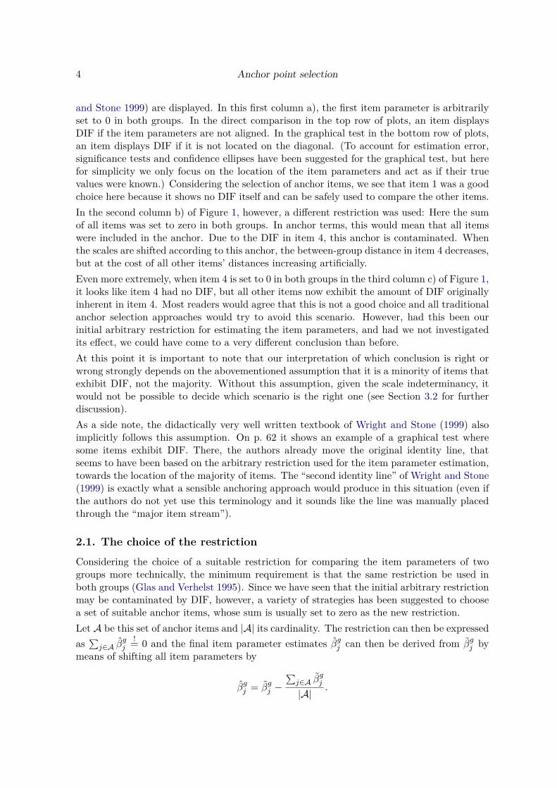
2. Anchoring revisitedDue to its scale indeterminacy, i.e., the fact that the latent scale has no natural origin, arestriction is necessary for estimating the item parameters in the Rasch model. Commonlyused restrictions are setting (arbitrarily) the first item parameter or the sum of all itemparameters to zero (Glas and Verhelst 1995; Eggen and Verhelst 2006). When the aim is tocompare the item parameters in two (or more) groups, the item parameters are first estimatedseparately. Since any linear restriction can easily be obtained from any other, it does notmatter which particular restriction is applied in this first step. In the following, the initialitem parameter estimates are termed βgj for group g and item j.However, as is illustrated in Figure 1, if these initial item parameter estimates were naivelyused for a comparison between the two groups, the choice of the restriction would affect ourconclusion. This example was set up such that the first three item parameters are the samefor both groups while the fourth item parameter differs between the groups.This is obvious in the first column a) of Figure 1, where in the top row a direct comparison ofthe item parameters and in the bottom row the setup of a graphical test (Rasch 1960; Wright
4 Anchor point selection
and Stone 1999) are displayed. In this first column a), the first item parameter is arbitrarilyset to 0 in both groups. In the direct comparison in the top row of plots, an item displaysDIF if the item parameters are not aligned. In the graphical test in the bottom row of plots,an item displays DIF if it is not located on the diagonal. (To account for estimation error,significance tests and confidence ellipses have been suggested for the graphical test, but herefor simplicity we only focus on the location of the item parameters and act as if their truevalues were known.) Considering the selection of anchor items, we see that item 1 was a goodchoice here because it shows no DIF itself and can be safely used to compare the other items.In the second column b) of Figure 1, however, a different restriction was used: Here the sumof all items was set to zero in both groups. In anchor terms, this would mean that all itemswere included in the anchor. Due to the DIF in item 4, this anchor is contaminated. Whenthe scales are shifted according to this anchor, the between-group distance in item 4 decreases,but at the cost of all other items’ distances increasing artificially.Even more extremely, when item 4 is set to 0 in both groups in the third column c) of Figure 1,it looks like item 4 had no DIF, but all other items now exhibit the amount of DIF originallyinherent in item 4. Most readers would agree that this is not a good choice and all traditionalanchor selection approaches would try to avoid this scenario. However, had this been ourinitial arbitrary restriction for estimating the item parameters, and had we not investigatedits effect, we could have come to a very different conclusion than before.At this point it is important to note that our interpretation of which conclusion is right orwrong strongly depends on the abovementioned assumption that it is a minority of items thatexhibit DIF, not the majority. Without this assumption, given the scale indeterminancy, itwould not be possible to decide which scenario is the right one (see Section 3.2 for furtherdiscussion).As a side note, the didactically very well written textbook of Wright and Stone (1999) alsoimplicitly follows this assumption. On p. 62 it shows an example of a graphical test wheresome items exhibit DIF. There, the authors already move the original identity line, thatseems to have been based on the arbitrary restriction used for the item parameter estimation,towards the location of the majority of items. The “second identity line” of Wright and Stone(1999) is exactly what a sensible anchoring approach would produce in this situation (even ifthe authors do not yet use this terminology and it sounds like the line was manually placedthrough the “major item stream”).
2.1. The choice of the restriction
Considering the choice of a suitable restriction for comparing the item parameters of twogroups more technically, the minimum requirement is that the same restriction be used inboth groups (Glas and Verhelst 1995). Since we have seen that the initial arbitrary restrictionmay be contaminated by DIF, however, a variety of strategies has been suggested to choosea set of suitable anchor items, whose sum is usually set to zero as the new restriction.Let A be this set of anchor items and |A| its cardinality. The restriction can then be expressedas
∑j∈A β
gj
!= 0 and the final item parameter estimates βgj can then be derived from βgj bymeans of shifting all item parameters by
βgj = βgj −∑j∈A β
gj
|A|.
Carolin Strobl, Julia Kopf, Raphael Hartmann, Achim Zeileis 5
●
●
●
●
1 2 3 4
−1.
5−
0.5
0.5
1.5
difference plot a)
item number
item
par
amet
er
● group 1group 2
●
●
●
●
1 2 3 4−
1.5
−0.
50.
51.
5
difference plot b)
item number
item
par
amet
er
● group 1group 2
●
●
●
●
1 2 3 4
−1.
5−
0.5
0.5
1.5
difference plot c)
item number
item
par
amet
er
● group 1group 2
−1.5 −0.5 0.5 1.5
−1.
5−
0.5
0.5
1.5
graphical test a)
item parameters group 1
item
par
amet
ers
grou
p 2
●
●
●
●
1
2
3
4
−1.5 −0.5 0.5 1.5
−1.
5−
0.5
0.5
1.5
graphical test b)
item parameters group 1
item
par
amet
ers
grou
p 2
●
●
●
●
1
2
3
4
−1.5 −0.5 0.5 1.5
−1.
5−
0.5
0.5
1.5
graphical test c)
item parameters group 1
item
par
amet
ers
grou
p 2
●
●
●
●
1
2
3
4
Figure 1: Illustration of comparisons of item parameters (top row) and graphical tests(bottom row) for different restrictions: a) βg1 = 0, b)
∑j β
gj = 0, c)βg4 = 0. Item numbers are
displayed on the x-axis in the top row and next to the plotting symbols in the bottom row.
More abstractly speaking, this corresponds to shifting all item parameters by a constant cg
βgj = βgj − cg,
where in all traditional anchoring approaches cg = cg(A) =∑
j∈A βgj
|A| depends on the choiceof A and can only take a limited number of different values, that result from the differentcombinations of anchor items that are being in- or excluded in A.Philosophically speaking, this approach to select items in or out of the anchor set stronglycorresponds to the deterministic notion that an item either has DIF or not. This view maymake sense for the true item parameters – and may also be an indicator of the politicalnecessity to exclude all items with significant DIF and consider all remaining items as fair.However, even if the true item parameters were indeed equal between groups, their estimateswould not be exactly equal due to random sampling fluctuation. In addition, one couldconsider it as more realistic that even the majority of “good” items may have some minorgroup difference even in their true parameters, while a minority of items does exhibit moresevere DIF of a larger extent (here it would be useful to think of some reasonable measures
6 Anchor point selection
of effect size or practical impact on person parameter estimates or classification decisions toquantify this extent, like described, e.g., by Teresi and Jones 2016; Teresi et al. 2017).Another adverse side effect of choosing designated anchor items is that – once they made itinto the anchor – they are usually considered to be DIF free by definition (cf., e.g., Woods2009), despite the fact that anchor selection strategies themselves are not flawless (see, e.g.,the thorough discussion on anchor contamination in Kopf et al. 2015b).Going back to our starting point, that we need some restriction or anchor only to fix theorigin of the scale, the question is: Do we even need to select designated anchor items tochoose this restriction, or could we just pick a single point in the latent continuum to fix ourorigin and avoid selecting a set of anchor items entirely?We will show in the following that, yes, it is possible to uncouple the shift of the itemparameters to a position that is ideal for DIF detection from a certain choice of anchor items.This can be accomplished by means of searching over a wider range of values for cg, includingvalues that do not result from any specific combination of anchor items. Therefore, in thefollowing, cg is no longer restricted to be equal to
∑j∈A βg
j
|A| , but will be found by searchingover an interval [cmin, cmax]. This interval will be chosen such that the item parameter rangesof both groups are safely overlapping, as described in more detail below.Without loss of generality, rather than shifting the item parameters of both groups, we leavethe item parameters of the first group at their initial estimates
βg1j = βg1
j with cg1 = 0,
where any arbitrary restriction can be used for the initial estimates βg1j . The item parameters
of the second group are then “moved past” the item parameters of the first group (as illustratedin the movie-like slide shows in the online supplements) by means of shifting them by aconstant
βg2j = βg2
j − cg2 with cg2 = c,
which will be selected in a way that is suitable for DIF detection, as described below.For the final DIF test, we will then look at a test statistic based on the difference between thefinal item parameter estimates of the two groups on the shifted scale: βg1
j −βg2j = βg1
j −βg2j −c.
Note that this comparison depends on the choice of c, which we will select in a suitable way,but not on the choice of the initial restrictions, because the selection of c will make up forany shift in the βg.A common choice of such a test statistic for the final DIF test is that of the item-wise Waldtest
tj =βg1j − β
g2j
sej=βg1j − β
g2j − c
sej,
with sej =√V ar(βg1)j,j + V ar(βg2)j,j . Note that we apply the item-wise Wald test to the
conditional maximum likelihood estimates in the following (like in Glas and Verhelst 1995;Kopf et al. 2015a,b).When we reconsider the idea of moving the item parameters of the second group past thoseof the first group, as illustrated in Figure 1 as well as in the movie-like slide shows in theonline supplements, for us as human beings it is straightforward to see that some positions aresmarter than others and that the most suitable anchor point is the value for c where the item
Carolin Strobl, Julia Kopf, Raphael Hartmann, Achim Zeileis 7
parameter estimates for the majority of items will interlock. This is also the rationale behindthe manually inserted “second identity line” through the “major item stream” of Wright andStone (1999). But the crucial question is: Can we find an objective criterion to make thisdecision for us automatically – both to avoid subjectiveness in our decision and to make itcomputationally feasible?At first sight it may seem like c could be optimized directly with respect to a test statisticlike that of the Wald test displayed above, or with respect to some kind of norm ||d(c)|| ofthe vector d(c) = (d1(c), . . . , dm(c))> of the item-wise absolute distances on the shifted scale
dj(c) = |βg1j − β
g2j | = |β
g1j − β
g2j − c|.
Measures based on these distances could capture what could be called the overall amount ofDIF, for example by using the sum of squared (Euclidean) or absolute (Cityblock) distances(corresponding to the L2 or L1 norm) as the criterion. However, a norm-based criterioncould become large both if there are many small differences or a few large differences in thevector d(c). For DIF detection and interpretation, however, these would have very differentmeanings and – as argued above – the situation with few items having large differences isusually more intuitive.To illustrate this, imagine again a scenario like in the first column a) of Figure 1, where oneitem shows a large distance and the rest of the items overlap, as opposed to a scenario likein the second column b) of Figure 1, where all items are shifted and show some distancebetween the groups. Both types of scenarios can produce the same sum of (squared/absolute)distances, but again it is the notion that only a minority of items has DIF makes most readersprefer the first scenario as the basis for DIF detection. Therefore, we would like the criterionfor finding the most suitable value of c to respect this notion.We will show in the next section that this can be achieved by applying a measure of inequalityinstead of a measure of the overall amount of DIF to d(c) by using, for example, the popularGini index as our criterion.
2.2. The Gini index
As an objective criterion for automatically selecting the value of the anchor point we suggestto use the Gini index (Gini 1912, reprinted 1955). The Gini index is a popular inequality mea-sure, that is usually employed for assessing the distribution of wealth between the members ofa society. It takes high values if, for example, a small minority of persons has a lot of wealthwhile the vast majority has very little. It is therefore used to compare different countries withrespect to their distribution of wealth or income, and lists are published how the rankingdevelopes (cp., for example, Central Intelligence Agency 2017). Scandinavian countries, forexample, tend to have a low Gini index indicating a rather equal income distribution, whilethe US, for example, has a medium Gini index and some countries that have been politicallytroubled in their recent history, such as Haiti, have a high Gini index.We will now show how the Gini index can also be used as a means for selecting the anchorpoint. This is most easily imagined when the majority of items displays no DIF. Then atthe anchor point, where the scales for the two groups are aligned as well as possible, mostitems will interlock (i.e., they will lie on top of or very close to each other for the two groups),while a minority of items will differ for the two groups and show DIF. So while initially theGini index was used to indicate whether a minority of persons has a lot of wealth while the
8 Anchor point selection
majority has very little, we will use it here to see whether a minority of items has a lot ofDIF (i.e., large absolute differences in their item parameters between the groups) while themajority has very little or no DIF.The Gini index of the absolute item-wise distances dj(c) for the j = 1, . . . ,m items can becomputed via their order statistics d(1)(c), d(2)(c), . . . , d(m)(c) as
GI(c) =2 ·
∑mj=1 j · d(j)(c)
m ·∑mj=1 d(j)(c)
− m+ 1m
.
The anchor point then corresponds to
cmax = arg maxc∈[cmin,cmax]
GI(c).
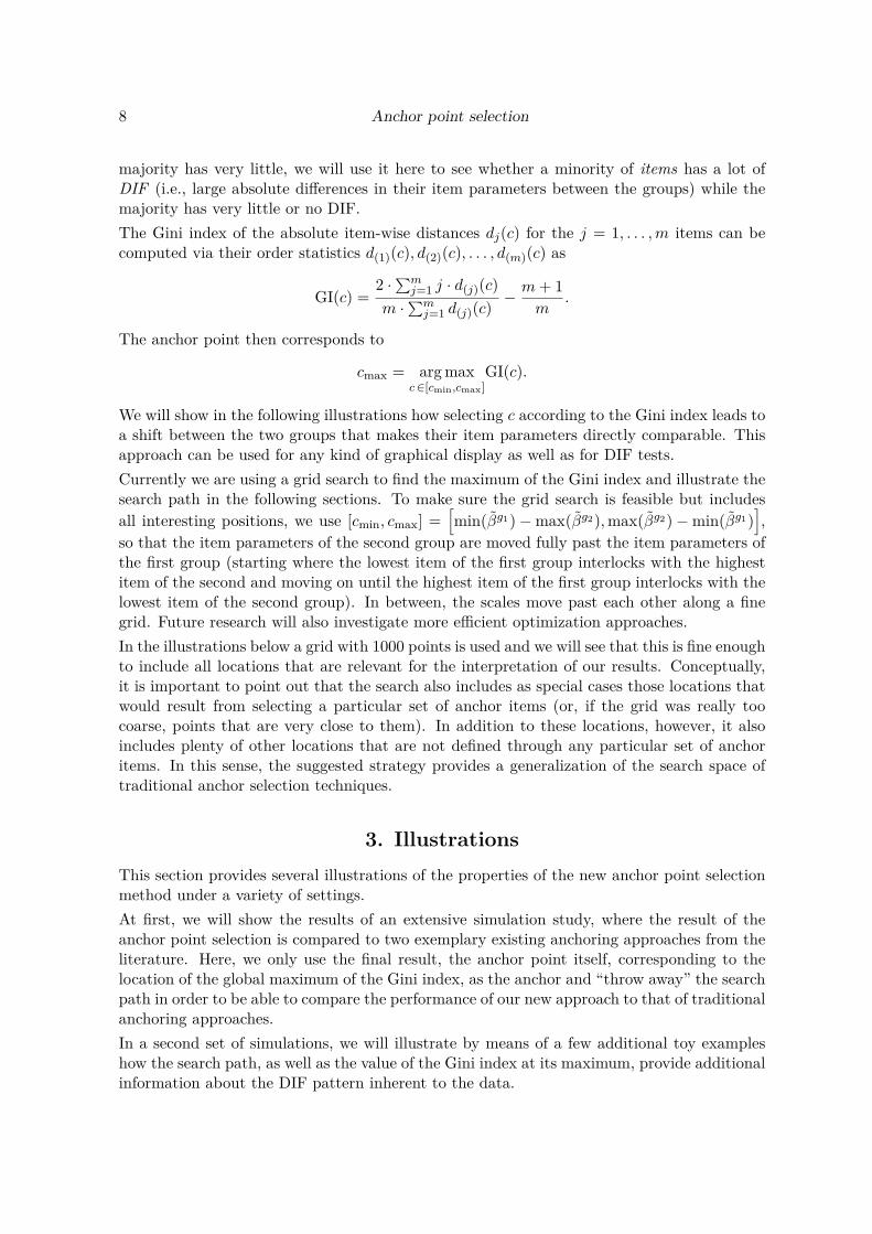
We will show in the following illustrations how selecting c according to the Gini index leads toa shift between the two groups that makes their item parameters directly comparable. Thisapproach can be used for any kind of graphical display as well as for DIF tests.Currently we are using a grid search to find the maximum of the Gini index and illustrate thesearch path in the following sections. To make sure the grid search is feasible but includesall interesting positions, we use [cmin, cmax] =
[min(βg1)−max(βg2),max(βg2)−min(βg1)
],
so that the item parameters of the second group are moved fully past the item parameters ofthe first group (starting where the lowest item of the first group interlocks with the highestitem of the second and moving on until the highest item of the first group interlocks with thelowest item of the second group). In between, the scales move past each other along a finegrid. Future research will also investigate more efficient optimization approaches.In the illustrations below a grid with 1000 points is used and we will see that this is fine enoughto include all locations that are relevant for the interpretation of our results. Conceptually,it is important to point out that the search also includes as special cases those locations thatwould result from selecting a particular set of anchor items (or, if the grid was really toocoarse, points that are very close to them). In addition to these locations, however, it alsoincludes plenty of other locations that are not defined through any particular set of anchoritems. In this sense, the suggested strategy provides a generalization of the search space oftraditional anchor selection techniques.
3. IllustrationsThis section provides several illustrations of the properties of the new anchor point selectionmethod under a variety of settings.At first, we will show the results of an extensive simulation study, where the result of theanchor point selection is compared to two exemplary existing anchoring approaches from theliterature. Here, we only use the final result, the anchor point itself, corresponding to thelocation of the global maximum of the Gini index, as the anchor and “throw away” the searchpath in order to be able to compare the performance of our new approach to that of traditionalanchoring approaches.In a second set of simulations, we will illustrate by means of a few additional toy exampleshow the search path, as well as the value of the Gini index at its maximum, provide additionalinformation about the DIF pattern inherent to the data.
Carolin Strobl, Julia Kopf, Raphael Hartmann, Achim Zeileis 9
At the end of this section we illustrate the practical usage of the approach by means of anempirical example from a general knowledge quiz.
3.1. Simulation study I: Using the anchor point as a traditional anchorselection method in DIF testingThe anchor point selected by our new approach can be used for traditional anchoring in DIFtests just like any anchor selection strategy with designated anchor items. The followingstudy compares its performance as a traditional anchor method to two other anchor methodsthat have been proposed in the literature, as well as to two baseline conditions.From the variety of anchor methods available in the literature, we have included only thefollowing two as examples in order to keep the results simple and be able to focus on theproperties of the new method. The first exemplary comparison method is the anchor methodsuggested by Woods (2009), that is classified as the “constant four all other” method bythe taxonomy of Kopf et al. (2015b), is based on the all other strategy: In the initial step,each item is tested for DIF using all remaining items as anchors. The four anchor itemscorresponding to the lowest ranks of the absolute DIF statistics from the initial step are thenchosen as the final set of anchor items. This method represents a rather common approach,but has been shown to exhibit an increased false alarm rate in certain settings (Kopf et al.2015b,a). It serves as a comparison method here to see whether the new approach is affectedby similar problems. It should be pointed out, however, that Woods (2009) provides a verythorough discussion of anchor length choice, while here we consider only a fixed anchor lengthof four items because this is not the focus of our study.The second exemplary comparison method is the more recent “constant four mean p-valuethreshold” anchor method suggested by Kopf et al. (2015a). Its selection of four anchoritems is based on the number of p-values that exceed a threshold p-value determined frompreliminary DIF tests for every item with every other item as single anchor (for a moredetailed description see Kopf et al. 2015a). This method has been shown to be one out of twotop performing methods in the extensive comparison study of Kopf et al. (2015a) and thusserves as a strong competitor here.Besides the two competitor methods by Woods (2009) and Kopf et al. (2015a) and the anchorpoint selection method, we have included two baseline conditions. These conditions, termed“perfect . . . ” in the results section, serve only for illustration purposes and cannot be usedfor real data, because they are based on the information which items were simulated with andwithout DIF, which is of course not available in real data. Still these approaches will helpus evaluate the performance of the actual anchoring methods, as is explained in more detailbelow.Like in Kopf et al. (2015b) and Kopf et al. (2015a) the item-wise Wald test based on theconditional maximum likelihood item parameter estimates (cp. Glas and Verhelst 1995; Kopfet al. 2015b, and the original references therein) was used for the final DIF test, but as willbecome clear below, our results are of a general nature that straightforwardly generalizes toother DIF tests.
Simulation designThe simulation design was very similar to that of Kopf et al. (2015a) to ensure comparabilitywith this extensive comparison study. We simulated data sets for two groups of subjects, the
10 Anchor point selection
reference and the focal group, under the Rasch model. In most of the scenarios, a certainpercentage of the items was simulated to show DIF between the groups, but there are alsoscenarios that were simulated completely under the null hypothesis with no DIF in any item.Each data set represents one of 500 replications from one simulation setting.
• Person and item parametersThe person parameters were generated from a normal distribution with variance 1 anda mean of 0 for the reference group and of -1 for the focal group.A set of 40 item parameters, that had been previously used by Wang et al. (2012) andKopf et al. (2015a), were the basis for our study design: β = (−2.522, −1.902, −1.351,−1.092, −0.234, −0.317, 0.037, 0.268, −0.571, 0.317, 0.295, 0.778, 1.514, 1.744, 1.951,−1.152, −0.526, 1.104, 0.961, 1.314, −2.198, −1.621, −0.761, −1.179, −0.610, −0.291,0.067, 0.706, −2.713, 0.213, 0.116, 0.273, 0.840, 0.745, 1.485, −1.208, 0.189, 0.345, 0.962,1.592). These item parameters were used for all settings with a test length of 40 items.In order to be able to manipulate the test length, for settings with test lengths of 20 or60 items, the respective number of parameters was randomly drawn from the original setof 40 values (in the case of 20 without replacement, in the case of 60 with replacement).
• DIF itemsA randomly chosen set of items were simulated to display DIF by setting the differencein the item parameters between reference and focal group to +0.6 or −0.6 dependingon the intended direction of DIF.
• IRT modelThe item responses in each group were generated by means of the Rasch model.
Manipulated variables
Similar to previous simulation studies such as Woods (2009); Wang et al. (2012) and Kopfet al. (2015a), the manipulated variables were the sample size, the test length, the directionof DIF, the percentage of DIF and the anchor methods.
• Sample sizesThe sample size for the simulated data sets was varied between 500 and 3000 in stepsof 500. This overall sample size was divided equally between the two groups.(We also investigated settings with unequal samples sizes. For unequal group sizes thepower was slightly diminished for all methods, so that the comparisons between themethods are not affected by this factor. Therefore, and in the interest of saving space,here we present only results for equal group sizes because this makes the following plotseasier to read.)
• Directions and proportions of DIFThe direction of DIF is either balanced (where each DIF item favors either the referenceor the focal group but no systematic advantage for one group remains because the effectscancel out), an advantage for the reference group or an advantage for the focal group.
Carolin Strobl, Julia Kopf, Raphael Hartmann, Achim Zeileis 11
The proportion of DIF items relative to the overall test length was set to either 0%,20% or 40%.
• Anchoring methodsThe following methods were compared in this study:
– the “constant four all other” method suggested by Woods (2009),– the “constant four mean p-value threshold” method suggested by Kopf et al.
(2015a),– the “anchor point selection” method suggested in this paper,– the “perfect random selection”, that randomly selects four anchor items from the
set of items that (in the simulation) are known to be DIF-free,– the “perfect anchor point”, that selects the anchor point from the grid that directly
optimizes the false alarm rate and hit rate.
Note that both “perfect . . . ” methods rely on information that is not available inpractical settings and only serve as (unrealistic) baseline conditions here, as furtherexplained below.
Outcome variables
The false alarm rate (that corresponds to the type I error) and the hit rate (that correspondsto the power of the DIF tests) were computed. The false alarm rate is the percentage ofitems that were simulated as DIF free, but erroneously show a significant test result. The hitrate is the percentage of items that were in fact simulated to have DIF and correctly show asignificant test result.
Further specifications
Due to the fact that one restriction is necessary for the item parameter estimation, for atest length of m items only m− 1 parameters can be estimated and tested freely. Therefore,one item cannot be formally tested for DIF in the final test. To account for this in a waythat is comparable between the anchoring methods, the item that was first selected into the“constant four mean p-value threshold” anchor by Kopf et al. (2015a), meaning that it showedthe least indication of DIF, was left out of the final DIF test for all methods. For conveniencethe same anchor was also used as the initial restriction βg1 in the specification of the grid.Note again that this choice of the initial restriction has no effect on the result of the anchorpoint selection or the item-wise distances for the selected anchor point, but may lead to smalldifferences in the standard errors ˆsej of the Wald statistics.
Computational details
Our results were obtained using the R system for statistical computing (R DevelopmentCore Team 2017), version 3.3.0. The code for the anchor point selection was implementedby ourselves and will be made available in an R package. For the Gini index we used theimplementation from the R package ineq (Zeileis 2014).
12 Anchor point selection
sample size
hit r
ate
fals
e al
arm
rat
e
0.0
0.2
0.4
0.6
0.8
1.0
500 1000 1500 2000 2500 3000
●
●
● ● ● ●
●
●
● ● ● ●
●
●
● ● ● ●
●
●● ● ● ●
●
●● ● ● ●
DIF is balanced20% DIF items
test length 40 itemsdata simulated with impact
hit rate
0.0
0.2
0.4
0.6
0.8
1.0
●
●
● ● ● ●
●
●
●● ● ●
●
●● ● ● ●
●
●● ● ● ●
●
●● ● ● ●
DIF favors focal group20% DIF items
test length 40 itemsdata simulated with impact
hit rate
0.0
0.2
0.4
0.6
0.8
1.0
500 1000 1500 2000 2500 3000
●
●
● ● ● ●
●
●
●
●● ●
●
●
● ● ● ●
●
●
● ● ● ●
●
●● ● ● ●
DIF favors reference group20% DIF items
test length 40 itemsdata simulated with impact
hit rate
0.0
0.2
0.4
0.6
0.8
1.0
● ● ● ● ● ●● ● ● ● ● ●● ● ● ● ● ●● ● ● ● ● ●● ● ● ● ● ●
DIF is balanced20% DIF items
test length 40 itemsdata simulated with impact
false alarm rate
500 1000 1500 2000 2500 3000
0.0
0.2
0.4
0.6
0.8
1.0
● ● ● ● ● ●●●
●●
●●
● ● ● ● ● ●● ● ● ● ● ●● ● ● ● ● ●
DIF favors focal group20% DIF items
test length 40 itemsdata simulated with impact
false alarm rate
0.0
0.2
0.4
0.6
0.8
1.0
● ● ● ● ● ●●
●●
●● ●
● ● ● ● ● ●● ● ● ● ● ●● ● ● ● ● ●
DIF favors reference group20% DIF items
test length 40 itemsdata simulated with impact
false alarm rate
Kopf et al. (2015)Woods (2009)anchor point selectionperfect random selectionperfect anchor point
●
●
●
●
●
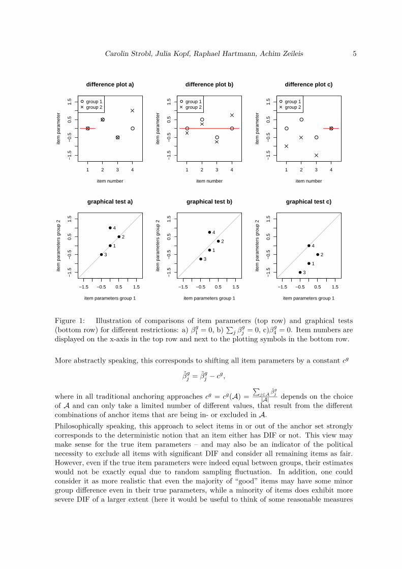
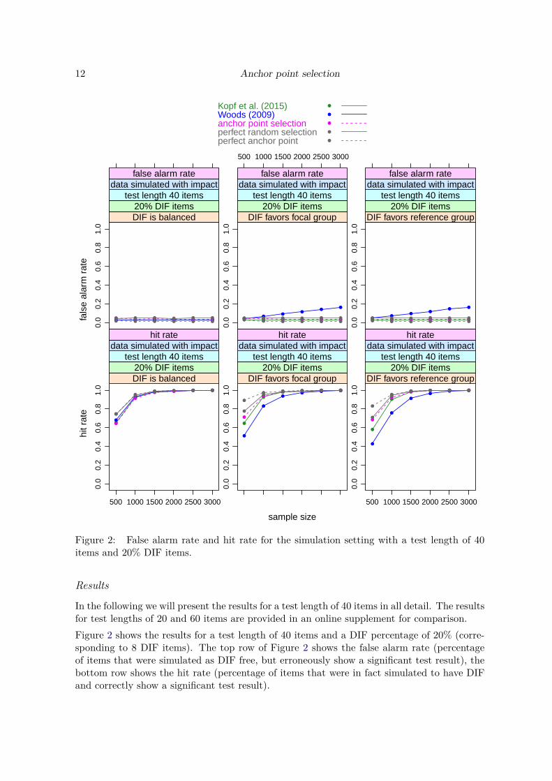
Figure 2: False alarm rate and hit rate for the simulation setting with a test length of 40items and 20% DIF items.
Results
In the following we will present the results for a test length of 40 items in all detail. The resultsfor test lengths of 20 and 60 items are provided in an online supplement for comparison.Figure 2 shows the results for a test length of 40 items and a DIF percentage of 20% (corre-sponding to 8 DIF items). The top row of Figure 2 shows the false alarm rate (percentageof items that were simulated as DIF free, but erroneously show a significant test result), thebottom row shows the hit rate (percentage of items that were in fact simulated to have DIFand correctly show a significant test result).
Carolin Strobl, Julia Kopf, Raphael Hartmann, Achim Zeileis 13
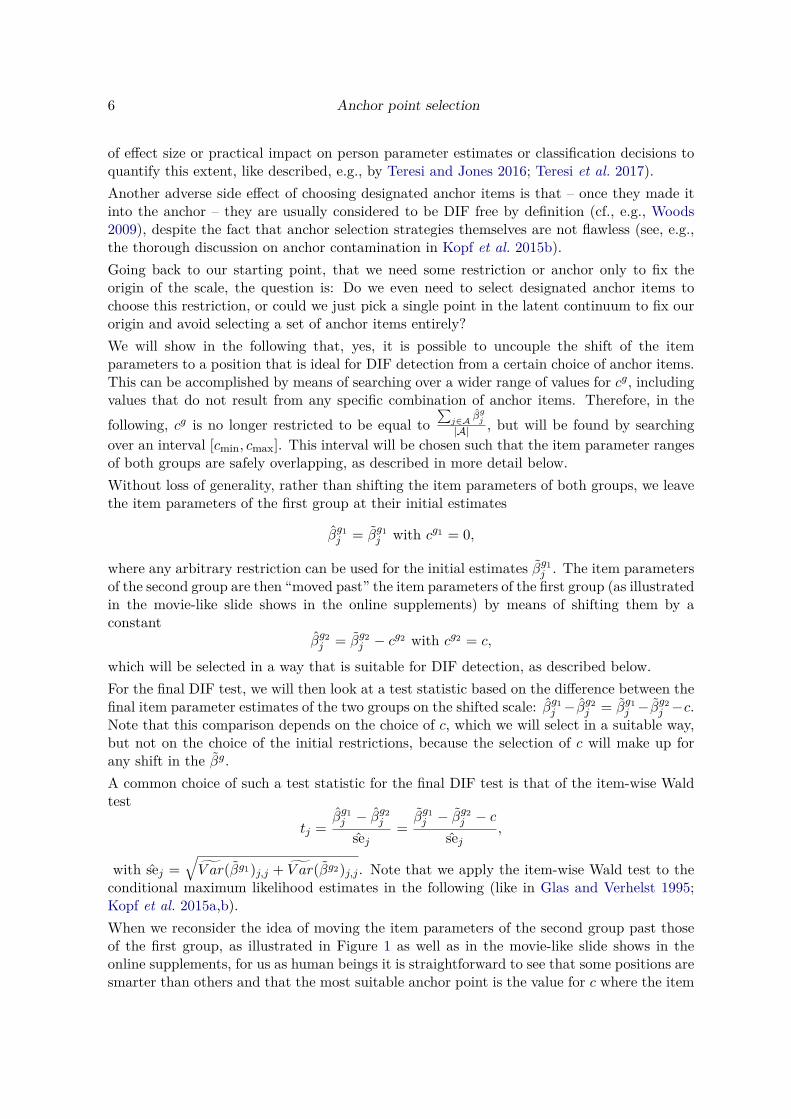
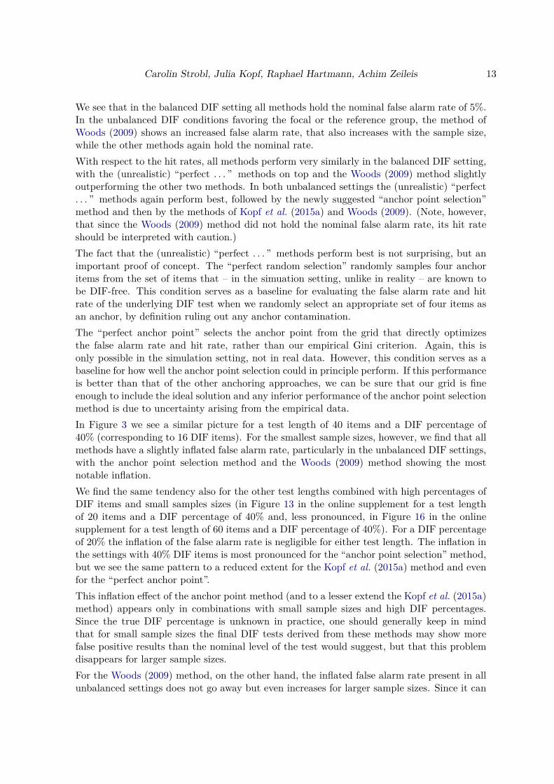
We see that in the balanced DIF setting all methods hold the nominal false alarm rate of 5%.In the unbalanced DIF conditions favoring the focal or the reference group, the method ofWoods (2009) shows an increased false alarm rate, that also increases with the sample size,while the other methods again hold the nominal rate.With respect to the hit rates, all methods perform very similarly in the balanced DIF setting,with the (unrealistic) “perfect . . . ” methods on top and the Woods (2009) method slightlyoutperforming the other two methods. In both unbalanced settings the (unrealistic) “perfect. . . ” methods again perform best, followed by the newly suggested “anchor point selection”method and then by the methods of Kopf et al. (2015a) and Woods (2009). (Note, however,that since the Woods (2009) method did not hold the nominal false alarm rate, its hit rateshould be interpreted with caution.)The fact that the (unrealistic) “perfect . . . ” methods perform best is not surprising, but animportant proof of concept. The “perfect random selection” randomly samples four anchoritems from the set of items that – in the simuation setting, unlike in reality – are known tobe DIF-free. This condition serves as a baseline for evaluating the false alarm rate and hitrate of the underlying DIF test when we randomly select an appropriate set of four items asan anchor, by definition ruling out any anchor contamination.The “perfect anchor point” selects the anchor point from the grid that directly optimizesthe false alarm rate and hit rate, rather than our empirical Gini criterion. Again, this isonly possible in the simulation setting, not in real data. However, this condition serves as abaseline for how well the anchor point selection could in principle perform. If this performanceis better than that of the other anchoring approaches, we can be sure that our grid is fineenough to include the ideal solution and any inferior performance of the anchor point selectionmethod is due to uncertainty arising from the empirical data.In Figure 3 we see a similar picture for a test length of 40 items and a DIF percentage of40% (corresponding to 16 DIF items). For the smallest sample sizes, however, we find that allmethods have a slightly inflated false alarm rate, particularly in the unbalanced DIF settings,with the anchor point selection method and the Woods (2009) method showing the mostnotable inflation.We find the same tendency also for the other test lengths combined with high percentages ofDIF items and small samples sizes (in Figure 13 in the online supplement for a test lengthof 20 items and a DIF percentage of 40% and, less pronounced, in Figure 16 in the onlinesupplement for a test length of 60 items and a DIF percentage of 40%). For a DIF percentageof 20% the inflation of the false alarm rate is negligible for either test length. The inflation inthe settings with 40% DIF items is most pronounced for the “anchor point selection” method,but we see the same pattern to a reduced extent for the Kopf et al. (2015a) method and evenfor the “perfect anchor point”.This inflation effect of the anchor point method (and to a lesser extend the Kopf et al. (2015a)method) appears only in combinations with small sample sizes and high DIF percentages.Since the true DIF percentage is unknown in practice, one should generally keep in mindthat for small sample sizes the final DIF tests derived from these methods may show morefalse positive results than the nominal level of the test would suggest, but that this problemdisappears for larger sample sizes.For the Woods (2009) method, on the other hand, the inflated false alarm rate present in allunbalanced settings does not go away but even increases for larger sample sizes. Since it can
14 Anchor point selection
sample size
hit r
ate
fals
e al
arm
rat
e
0.0
0.2
0.4
0.6
0.8
1.0
500 1000 1500 2000 2500 3000
●
●
●● ● ●
●
●
● ● ● ●
●
●
●● ● ●
●
●
● ● ● ●
●
●
● ● ● ●
DIF is balanced40% DIF items
test length 40 itemsdata simulated with impact
hit rate
0.0
0.2
0.4
0.6
0.8
1.0
●
●
●● ● ●
●
●
●
●●
●
●
●
●● ● ●
●
●● ● ● ●
●
●● ● ● ●
DIF favors focal group40% DIF items
test length 40 itemsdata simulated with impact
hit rate0.
00.
20.
40.
60.
81.
0
500 1000 1500 2000 2500 3000
●
●
●● ● ●
●
●
●
●
●●
●
●
● ● ● ●
●
●
● ● ● ●
●
●● ● ● ●
DIF favors reference group40% DIF items
test length 40 itemsdata simulated with impact
hit rate
0.0
0.2
0.4
0.6
0.8
1.0
● ● ● ● ● ●● ● ● ● ● ●●
● ● ● ● ●● ● ● ● ● ●● ● ● ● ● ●
DIF is balanced40% DIF items
test length 40 itemsdata simulated with impact
false alarm rate
500 1000 1500 2000 2500 3000
0.0
0.2
0.4
0.6
0.8
1.0
●● ● ● ● ●
●
●
● ● ● ●
●
● ● ● ● ●● ● ● ● ● ●●● ● ● ● ●
DIF favors focal group40% DIF items
test length 40 itemsdata simulated with impact
false alarm rate
0.0
0.2
0.4
0.6
0.8
1.0
●● ● ● ● ●
●
●
●● ● ●
●● ● ● ● ●● ● ● ● ● ●●● ● ● ● ●
DIF favors reference group40% DIF items
test length 40 itemsdata simulated with impact
false alarm rate
Kopf et al. (2015)Woods (2009)anchor point selectionperfect random selectionperfect anchor point
●
●
●
●
●
Figure 3: False alarm rate and hit rate for the simulation setting with a test length of 40items and 40% DIF items.
go up to 0.4 in certain settings (cf. Figure 16 in the online supplement), and in reality wehave no means of knowing whether this is the situation that underlies our data, we do notrecommend this method, despite the fact that in some other scenarios this method shows thehighest hit rate of the three empirically applicable methods.
With respect to the hit rates, Figure 3 shows again that for the balanced DIF setting allmethods perform very similarly, with the (unrealistic) “perfect . . . ” methods on top and theWoods (2009) method slightly outperforming the other two empirically applicable methods.
Carolin Strobl, Julia Kopf, Raphael Hartmann, Achim Zeileis 15
sample size
fals
e al
arm
rat
e
0.0
0.2
0.4
0.6
0.8
1.0
500 1000 1500 2000 2500 3000
● ● ● ● ● ●● ● ● ● ● ●● ● ● ● ● ●● ● ● ● ● ●
DIF is balanced0% DIF items
test length 40 itemsdata simulated with impact
false alarm rate
Kopf et al. (2015)Woods (2009)anchor point selectionperfect random selectionperfect anchor point
●
●
●
●
●
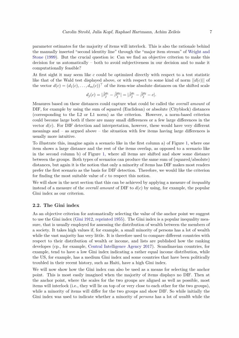
Figure 4: False alarm rate and hit rate for the simulation setting with a test length of 40items and 0% DIF items.
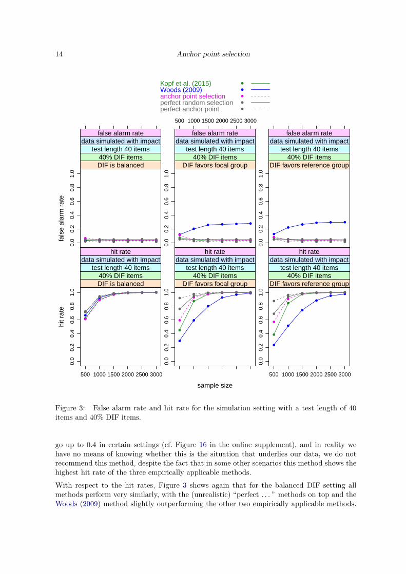
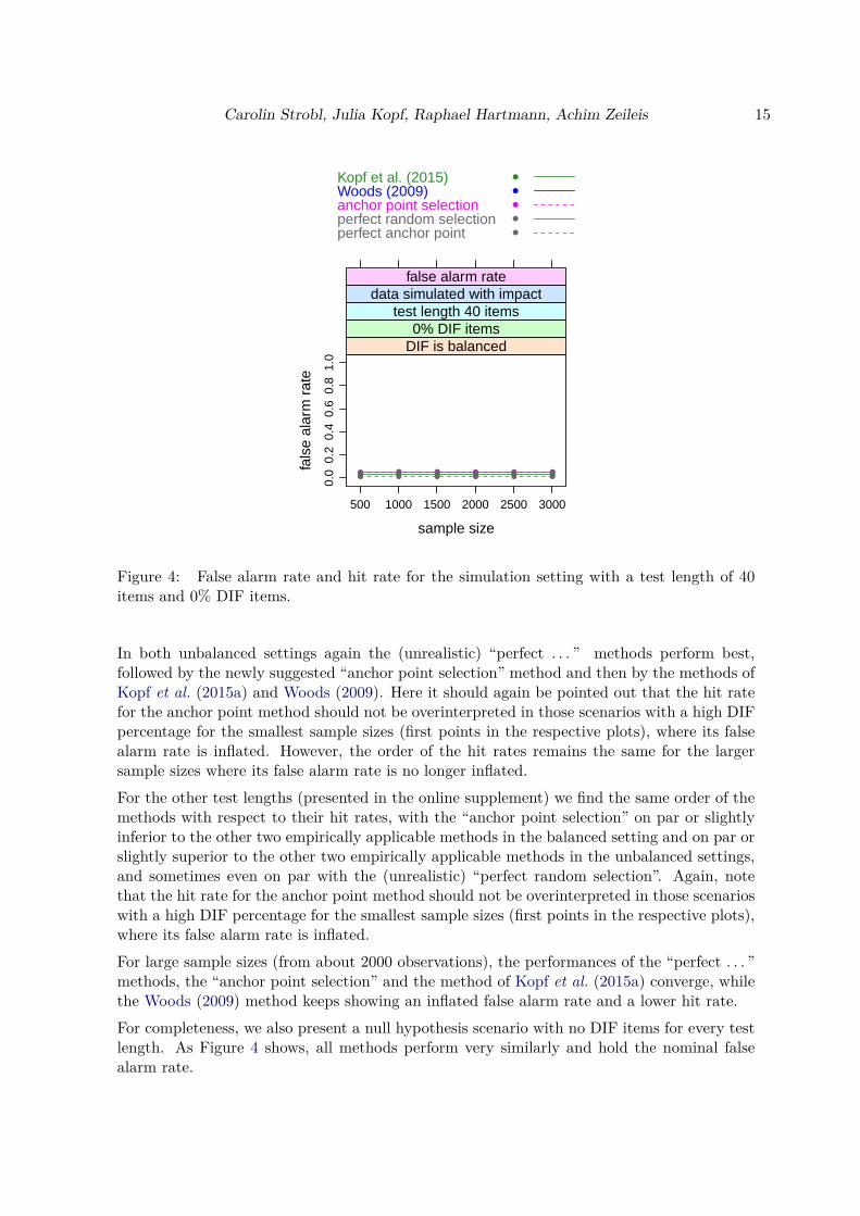
In both unbalanced settings again the (unrealistic) “perfect . . . ” methods perform best,followed by the newly suggested “anchor point selection” method and then by the methods ofKopf et al. (2015a) and Woods (2009). Here it should again be pointed out that the hit ratefor the anchor point method should not be overinterpreted in those scenarios with a high DIFpercentage for the smallest sample sizes (first points in the respective plots), where its falsealarm rate is inflated. However, the order of the hit rates remains the same for the largersample sizes where its false alarm rate is no longer inflated.For the other test lengths (presented in the online supplement) we find the same order of themethods with respect to their hit rates, with the “anchor point selection” on par or slightlyinferior to the other two empirically applicable methods in the balanced setting and on par orslightly superior to the other two empirically applicable methods in the unbalanced settings,and sometimes even on par with the (unrealistic) “perfect random selection”. Again, notethat the hit rate for the anchor point method should not be overinterpreted in those scenarioswith a high DIF percentage for the smallest sample sizes (first points in the respective plots),where its false alarm rate is inflated.For large sample sizes (from about 2000 observations), the performances of the “perfect . . . ”methods, the “anchor point selection” and the method of Kopf et al. (2015a) converge, whilethe Woods (2009) method keeps showing an inflated false alarm rate and a lower hit rate.For completeness, we also present a null hypothesis scenario with no DIF items for every testlength. As Figure 4 shows, all methods perform very similarly and hold the nominal falsealarm rate.
16 Anchor point selection
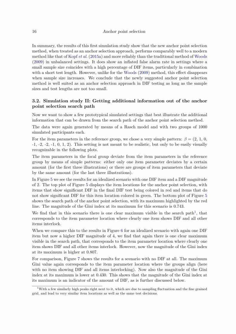
In summary, the results of this first simulation study show that the new anchor point selectionmethod, when treated as an anchor selection approach, performs comparably well to a modernmethod like that of Kopf et al. (2015a) and more reliably than the traditional method of Woods(2009) in unbalanced settings. It does show an inflated false alarm rate in settings where asmall sample size coincides with a high percentage of DIF items, particularly in combinationwith a short test length. However, unlike for the Woods (2009) method, this effect disappearswhen sample size increases. We conclude that the newly suggested anchor point selectionmethod is well suited as an anchor selection approach in DIF testing as long as the samplesizes and test lengths are not too small.
3.2. Simulation study II: Getting additional information out of the anchorpoint selection search path
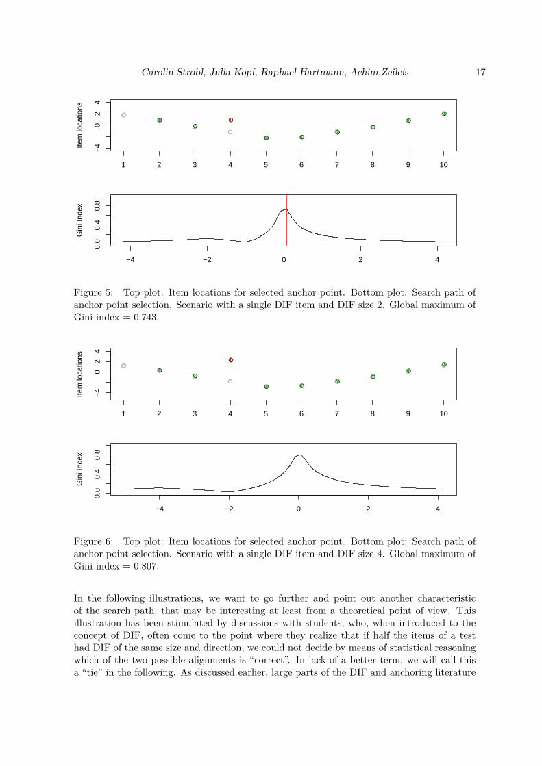
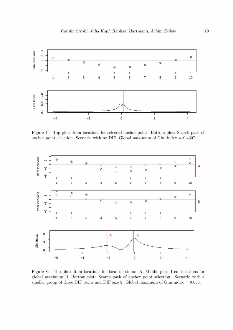
Now we want to show a few prototypical simulated settings that best illustrate the additionalinformation that can be drawn from the search path of the anchor point selection method.The data were again generated by means of a Rasch model and with two groups of 1000simulated participants each.For the item parameters in the reference group, we chose a very simple pattern: β = (2, 1, 0,-1, -2, -2, -1, 0, 1, 2). This setting is not meant to be realistic, but only to be easily visuallyrecognizable in the following plots.The item parameters in the focal group deviate from the item parameters in the referencegroup by means of simple patterns: either only one item parameter deviates by a certainamount (for the first three illustrations) or there are groups of item parameters that deviateby the same amount (for the last three illustrations).In Figure 5 we see the results for an idealized scenario with one DIF item and a DIF magnitudeof 2. The top plot of Figure 5 displays the item locations for the anchor point selection, withitems that show significant DIF in the final DIF test being colored in red and items that donot show significant DIF for this item location colored in green. The bottom plot of Figure 5shows the search path of the anchor point selection, with its maximum highlighted by the redline. The magnitude of the Gini index at its maximum for this scenario is 0.743.We find that in this scenario there is one clear maximum visible in the search path1, thatcorresponds to the item parameter location where clearly one item shows DIF and all otheritems interlock.When we compare this to the results in Figure 6 for an idealized scenario with again one DIFitem but now a higher DIF magnitude of 4, we find that again there is one clear maximumvisible in the search path, that corresponds to the item parameter location where clearly oneitem shows DIF and all other items interlock. However, now the magnitude of the Gini indexat its maximum is higher at 0.807.For comparison, Figure 7 shows the results for a scenario with no DIF at all. The maximumGini value again corresponds to the item parameter location where the groups align (herewith no item showing DIF and all items interlocking). Now also the magnitude of the Giniindex at its maximum is lower at 0.430. This shows that the magnitude of the Gini index atits maximum is an indicator of the amount of DIF, as is further discussed below.
1With a few similarly high peaks right next to it, which are due to sampling fluctuation and the fine grainedgrid, and lead to very similar item locations as well as the same test decisions.
Carolin Strobl, Julia Kopf, Raphael Hartmann, Achim Zeileis 17Anchor point selection
max. Gini Index = 0.743
Item
loca
tions
●●
●●
● ●
●●
●
●●●
●
●
● ●●
●
●
●
1 2 3 4 5 6 7 8 9 10
−4
02
4
−4 −2 0 2 4
0.0
0.4
0.8
Gin
i Ind
ex
Anchor point selection
max. Gini Index = 0.743
Item
loca
tions
●●
●●
● ●
●●
●
●
●●
●
●
● ●●
●
●
●
1 2 3 4 5 6 7 8 9 10
−4
02
4
−4 −2 0 2 4
0.0
0.4
0.8
Gin
i Ind
ex
Figure 5: Top plot: Item locations for selected anchor point. Bottom plot: Search path ofanchor point selection. Scenario with a single DIF item and DIF size 2. Global maximum ofGini index = 0.743.
Anchor point selection
max. Gini Index = 0.807
Item
loca
tions
●●
●●
● ●●
●●
●●●
●
●
● ●●
●
●
●
1 2 3 4 5 6 7 8 9 10
−4
02
4
−4 −2 0 2 4
0.0
0.4
0.8
Gin
i Ind
ex
Anchor point selection
max. Gini Index = 0.807
Item
loca
tions
●●
●●
● ●●
●●
●
●●
●
●
● ●●
●
●
●
1 2 3 4 5 6 7 8 9 10
−4
02
4
−4 −2 0 2 4
0.0
0.4
0.8
Gin
i Ind
ex
Figure 6: Top plot: Item locations for selected anchor point. Bottom plot: Search path ofanchor point selection. Scenario with a single DIF item and DIF size 4. Global maximum ofGini index = 0.807.
In the following illustrations, we want to go further and point out another characteristicof the search path, that may be interesting at least from a theoretical point of view. Thisillustration has been stimulated by discussions with students, who, when introduced to theconcept of DIF, often come to the point where they realize that if half the items of a testhad DIF of the same size and direction, we could not decide by means of statistical reasoningwhich of the two possible alignments is “correct”. In lack of a better term, we will call thisa “tie” in the following. As discussed earlier, large parts of the DIF and anchoring literature
18 Anchor point selection
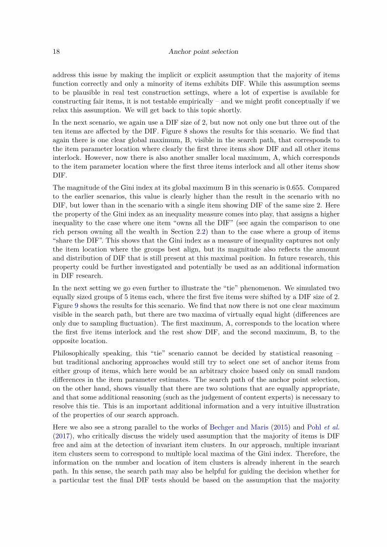
address this issue by making the implicit or explicit assumption that the majority of itemsfunction correctly and only a minority of items exhibits DIF. While this assumption seemsto be plausible in real test construction settings, where a lot of expertise is available forconstructing fair items, it is not testable empirically – and we might profit conceptually if werelax this assumption. We will get back to this topic shortly.
In the next scenario, we again use a DIF size of 2, but now not only one but three out of theten items are affected by the DIF. Figure 8 shows the results for this scenario. We find thatagain there is one clear global maximum, B, visible in the search path, that corresponds tothe item parameter location where clearly the first three items show DIF and all other itemsinterlock. However, now there is also another smaller local maximum, A, which correspondsto the item parameter location where the first three items interlock and all other items showDIF.
The magnitude of the Gini index at its global maximum B in this scenario is 0.655. Comparedto the earlier scenarios, this value is clearly higher than the result in the scenario with noDIF, but lower than in the scenario with a single item showing DIF of the same size 2. Herethe property of the Gini index as an inequality measure comes into play, that assigns a higherinequality to the case where one item “owns all the DIF” (see again the comparison to onerich person owning all the wealth in Section 2.2) than to the case where a group of items“share the DIF”. This shows that the Gini index as a measure of inequality captures not onlythe item location where the groups best align, but its magnitude also reflects the amountand distribution of DIF that is still present at this maximal position. In future research, thisproperty could be further investigated and potentially be used as an additional informationin DIF research.
In the next setting we go even further to illustrate the “tie” phenomenon. We simulated twoequally sized groups of 5 items each, where the first five items were shifted by a DIF size of 2.Figure 9 shows the results for this scenario. We find that now there is not one clear maximumvisible in the search path, but there are two maxima of virtually equal hight (differences areonly due to sampling fluctuation). The first maximum, A, corresponds to the location wherethe first five items interlock and the rest show DIF, and the second maximum, B, to theopposite location.
Philosophically speaking, this “tie” scenario cannot be decided by statistical reasoning –but traditional anchoring approaches would still try to select one set of anchor items fromeither group of items, which here would be an arbitrary choice based only on small randomdifferences in the item parameter estimates. The search path of the anchor point selection,on the other hand, shows visually that there are two solutions that are equally appropriate,and that some additional reasoning (such as the judgement of content experts) is necessary toresolve this tie. This is an important additional information and a very intuitive illustrationof the properties of our search approach.
Here we also see a strong parallel to the works of Bechger and Maris (2015) and Pohl et al.(2017), who critically discuss the widely used assumption that the majority of items is DIFfree and aim at the detection of invariant item clusters. In our approach, multiple invariantitem clusters seem to correspond to multiple local maxima of the Gini index. Therefore, theinformation on the number and location of item clusters is already inherent in the searchpath. In this sense, the search path may also be helpful for guiding the decision whether fora particular test the final DIF tests should be based on the assumption that the majority
Carolin Strobl, Julia Kopf, Raphael Hartmann, Achim Zeileis 19
Anchor point selection
max. Gini Index = 0.43
Item
loca
tions
●●
●●
● ●
●●
●
●●●
●●
● ●●
●
●
●
1 2 3 4 5 6 7 8 9 10
−4
02
4
−4 −2 0 2 4
0.0
0.4
0.8
Gin
i Ind
ex
Anchor point selection
max. Gini Index = 0.43
Item
loca
tions
●●
●●
● ●
●●
●
●
●●
●●
● ●●
●
●
●
1 2 3 4 5 6 7 8 9 10
−4
02
4
−4 −2 0 2 4
0.0
0.4
0.8
Gin
i Ind
ex
Figure 7: Top plot: Item locations for selected anchor point. Bottom plot: Search path ofanchor point selection. Scenario with no DIF. Global maximum of Gini index = 0.4307.
Anchor point selection
max. Gini Index = 0.655
Item
loca
tions ●
●
●●
● ●●
●●
●●
●●
●
● ●●
●●
●
1 2 3 4 5 6 7 8 9 10
−6
−2
2
−6 −4 −2 0 2 4
0.0
0.4
0.8
Gin
i Ind
ex A B
A
Anchor point selection
max. Gini Index = 0.655
Item
loca
tions ●
●
●●
● ●●
●●
●
●
●●
●
● ●●
●●
●
1 2 3 4 5 6 7 8 9 10
−6
−2
2
−6 −4 −2 0 2 4
0.0
0.4
0.8
Gin
i Ind
ex A B
B
Anchor point selection
max. Gini Index = 0.655
Item
loca
tions ●
●
●●
● ●●
●●
●
●
●●
●
● ●●
●●
●
1 2 3 4 5 6 7 8 9 10
−6
−2
2
−6 −4 −2 0 2 4
0.0
0.4
0.8
Gin
i Ind
ex A B
Figure 8: Top plot: Item locations for local maximum A. Middle plot: Item locations forglobal maximum B. Bottom plot: Search path of anchor point selection. Scenario with asmaller group of three DIF items and DIF size 2. Global maximum of Gini index = 0.655.
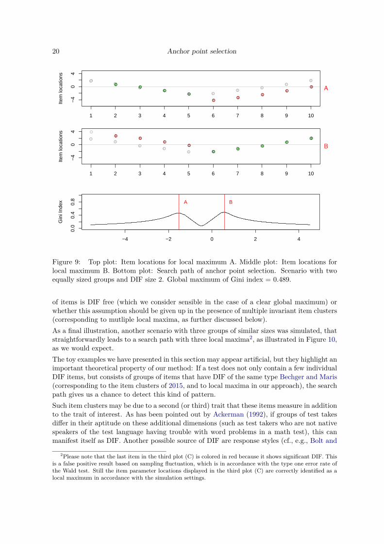
20 Anchor point selectionAnchor point selection
max. Gini Index = 0.489
Item
loca
tions
●●
●●
● ●●
●●
●●
●●
●●
●●
●
●
●
1 2 3 4 5 6 7 8 9 10
−4
04
−4 −2 0 2 4
0.0
0.4
0.8
Gin
i Ind
ex A B
A
Anchor point selection
max. Gini Index = 0.489
Item
loca
tions
●●
●●
● ●●
●●
●
●
●●
●●
●●
●
●
●
1 2 3 4 5 6 7 8 9 10
−4
04
−4 −2 0 2 4
0.0
0.4
0.8
Gin
i Ind
ex A B
B
Anchor point selection
max. Gini Index = 0.489
Item
loca
tions
●●
●●
● ●●
●●
●
●
●●
●●
●●
●
●
●
1 2 3 4 5 6 7 8 9 10
−4
04
−4 −2 0 2 4
0.0
0.4
0.8
Gin
i Ind
ex A B
Figure 9: Top plot: Item locations for local maximum A. Middle plot: Item locations forlocal maximum B. Bottom plot: Search path of anchor point selection. Scenario with twoequally sized groups and DIF size 2. Global maximum of Gini index = 0.489.
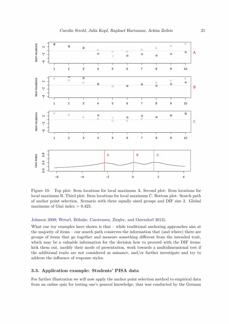
of items is DIF free (which we consider sensible in the case of a clear global maximum) orwhether this assumption should be given up in the presence of multiple invariant item clusters(corresponding to mutliple local maxima, as further discussed below).As a final illustration, another scenario with three groups of similar sizes was simulated, thatstraightforwardly leads to a search path with three local maxima2, as illustrated in Figure 10,as we would expect.The toy examples we have presented in this section may appear artificial, but they highlight animportant theoretical property of our method: If a test does not only contain a few individualDIF items, but consists of groups of items that have DIF of the same type Bechger and Maris(corresponding to the item clusters of 2015, and to local maxima in our approach), the searchpath gives us a chance to detect this kind of pattern.Such item clusters may be due to a second (or third) trait that these items measure in additionto the trait of interest. As has been pointed out by Ackerman (1992), if groups of test takesdiffer in their aptitude on these additional dimensions (such as test takers who are not nativespeakers of the test language having trouble with word problems in a math test), this canmanifest itself as DIF. Another possible source of DIF are response styles (cf., e.g., Bolt and
2Please note that the last item in the third plot (C) is colored in red because it shows significant DIF. Thisis a false positive result based on sampling fluctuation, which is in accordance with the type one error rate ofthe Wald test. Still the item parameter locations displayed in the third plot (C) are correctly identified as alocal maximum in accordance with the simulation settings.
Carolin Strobl, Julia Kopf, Raphael Hartmann, Achim Zeileis 21Anchor point selection
max. Gini Index = 0.423
Item
loca
tions ●
●
●●
● ●●
●●
●●
●●
●
● ●●
●●
●
1 2 3 4 5 6 7 8 9 10
−6
−2
2
−6 −4 −2 0 2 4
0.0
0.4
0.8
Gin
i Ind
ex A B C
A
Anchor point selection
max. Gini Index = 0.423
Item
loca
tions ●
●
●●
● ●●
●●
●
●
●●
●
● ●●
●●
●
1 2 3 4 5 6 7 8 9 10
−6
−2
2
−6 −4 −2 0 2 4
0.0
0.4
0.8
Gin
i Ind
ex A B C
B
Anchor point selection
max. Gini Index = 0.423
Item
loca
tions ●
●
●●
● ●●
●●
●
●
●●
●
● ●●
●●
●
1 2 3 4 5 6 7 8 9 10
−6
−2
2
−6 −4 −2 0 2 4
0.0
0.4
0.8
Gin
i Ind
ex A B C
C
Anchor point selection
max. Gini Index = 0.423
Item
loca
tions ●
●
●●
● ●●
●●
●
●
●●
●
● ●●
●●
●
1 2 3 4 5 6 7 8 9 10
−6
−2
2
−6 −4 −2 0 2 4
0.0
0.4
0.8
Gin
i Ind
ex A B C
Figure 10: Top plot: Item locations for local maximum A. Second plot: Item locations forlocal maximum B. Third plot: Item locations for local maximum C. Bottom plot: Search pathof anchor point selection. Scenario with three equally sized groups and DIF size 2. Globalmaximum of Gini index = 0.423.
Johnson 2009; Wetzel, Böhnke, Carstensen, Ziegler, and Ostendorf 2013).What our toy examples have shown is that – while traditional anchoring approaches aim atthe majority of items – our search path conserves the information that (and where) there aregroups of items that go together and measure something different from the intended trait,which may be a valuable information for the decision how to proceed with the DIF items:kick them out, modify their mode of presentation, work towards a multidimensional test ifthe additional traits are not considered as nuisance, and/or further investigate and try toaddress the influence of response styles.
3.3. Application example: Students’ PISA data
For further illustration we will now apply the anchor point selection method to empirical datafrom an online quiz for testing one’s general knowledge, that was conducted by the German
22 Anchor point selectionAnchor point selection
max. Gini Index = 0.504
Item
loca
tions
●● ●
●● ●
●
● ●
●
●
●
●
●
●●
●●
●
●●
● ● ●
● ●
●
●
●●
●●
●●
● ● ●●
●
●
●
●●
●
●
● ● ●
●
●●
●
● ●
●
●
●
●
●
● ●● ●
●●
●
●
●
●● ●
●
● ●● ●
●
●●
●●
●●
●
●●
●● ●
●
1 3 5 7 9 11 13 15 17 19 21 23 25 27 29 31 33 35 37 39 41 43 45
−4
04
−4 −2 0 2 4
0.0
0.4
0.8
Gin
i Ind
ex
Anchor point selection
max. Gini Index = 0.504
Item
loca
tions
●● ●
●● ●
●
● ●
●
●
●
●
●
●●
●●
●
●●
● ● ●
● ●
●
●
●●
●●
●●
● ● ●●
●
●
●
●●
●
●
● ● ●
●
●●
●
● ●
●
●
●
●
●
● ●● ●
●●
●
●
●
●● ●
●
● ●● ●
●
●●
●●
●●
●
●●
●● ●
●
1 3 5 7 9 11 13 15 17 19 21 23 25 27 29 31 33 35 37 39 41 43 45
−4
04
−4 −2 0 2 4
0.0
0.4
0.8
Gin
i Ind
ex
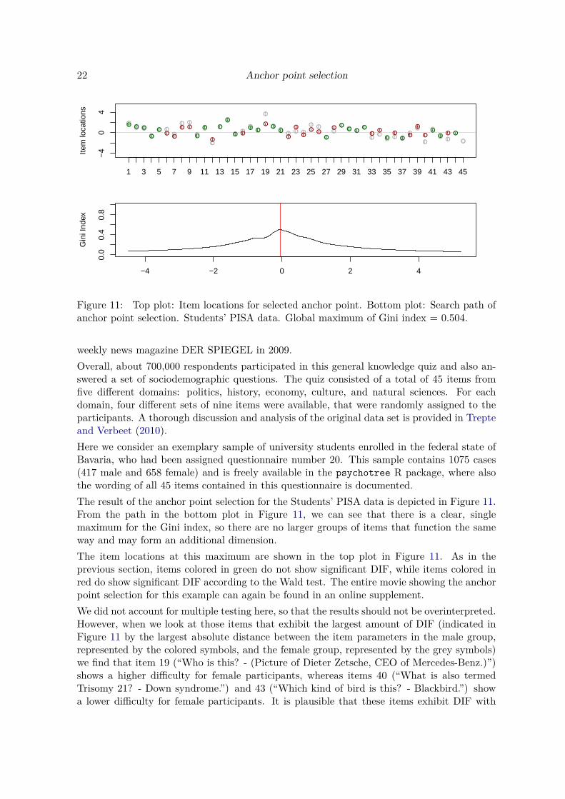
Figure 11: Top plot: Item locations for selected anchor point. Bottom plot: Search path ofanchor point selection. Students’ PISA data. Global maximum of Gini index = 0.504.
weekly news magazine DER SPIEGEL in 2009.Overall, about 700,000 respondents participated in this general knowledge quiz and also an-swered a set of sociodemographic questions. The quiz consisted of a total of 45 items fromfive different domains: politics, history, economy, culture, and natural sciences. For eachdomain, four different sets of nine items were available, that were randomly assigned to theparticipants. A thorough discussion and analysis of the original data set is provided in Trepteand Verbeet (2010).Here we consider an exemplary sample of university students enrolled in the federal state ofBavaria, who had been assigned questionnaire number 20. This sample contains 1075 cases(417 male and 658 female) and is freely available in the psychotree R package, where alsothe wording of all 45 items contained in this questionnaire is documented.The result of the anchor point selection for the Students’ PISA data is depicted in Figure 11.From the path in the bottom plot in Figure 11, we can see that there is a clear, singlemaximum for the Gini index, so there are no larger groups of items that function the sameway and may form an additional dimension.The item locations at this maximum are shown in the top plot in Figure 11. As in theprevious section, items colored in green do not show significant DIF, while items colored inred do show significant DIF according to the Wald test. The entire movie showing the anchorpoint selection for this example can again be found in an online supplement.We did not account for multiple testing here, so that the results should not be overinterpreted.However, when we look at those items that exhibit the largest amount of DIF (indicated inFigure 11 by the largest absolute distance between the item parameters in the male group,represented by the colored symbols, and the female group, represented by the grey symbols)we find that item 19 (“Who is this? - (Picture of Dieter Zetsche, CEO of Mercedes-Benz.)”)shows a higher difficulty for female participants, whereas items 40 (“What is also termedTrisomy 21? - Down syndrome.”) and 43 (“Which kind of bird is this? - Blackbird.”) showa lower difficulty for female participants. It is plausible that these items exhibit DIF with
Carolin Strobl, Julia Kopf, Raphael Hartmann, Achim Zeileis 23
respect to the variable gender, for example because they are of differently high interest formale and female participants.This example also shows that the item location derived from the anchor point selection pro-vides a helpful means of visually aligning the item parameters for interpretation.
4. Summary and discussionIn this paper we have suggested a new approach for anchoring the item parameters of twogroups of test takers for DIF testing, that is not based on an anchor in its original sense. Thisnew approach does not select a set of designated anchor items, but searches for the point onthe item parameter continuum where the groups best overlap. The resulting item parameterlocations at the maximum criterion value can be used as a traditional anchor in DIF testing,but the entire search path also provides additional information about the item structure.We have shown by means of extensive simulation studies that the new anchor point selectionmethod performs comparably well or more reliably than existing anchor selection approacheswhen its single best result is used as an anchor for DIF testing. It does show an inflatedfalse alarm rate in settings where a small sample size coincides with a high percentage of DIFitems and a short test length, but this effect disappears when sample size increases.In addition to being usable as an anchor selection strategy, however, our method also providesa lot of extra information through its search path, as well as through the magnitude of theinequality criterion itself. While the latter should be investigated more thoroughly in futureresearch, we have already shown here by means of a set of simulated toy examples thatthe method is able to identify clusters of items that function similarly and may representadditional trait dimensions.We believe another advantage of the anchor point selection approach is that it does not flagindividual items as anchors – a practice that all traditional anchoring approaches share, andthat may lead to wrongly assuming those items were indeed DIF free.In future research we will work on extending this approach to multiple groups of test tak-ers (such as different language groups) and other IRT models as well as a more efficientoptimization approach.
AcknowledgementsThe first author would like to thank Thomas Augustin for his encouragement when she firsthad a very vague idea of this a very long time ago.This research was supported in part by the Swiss National Science Foundation (project00019_152548).
References
Ackerman TA (1992). “A Didactic Explanation of Item Bias, Item Impact, and Item Validityfrom a Multidimensional Perspective.” Journal of Educational Measurement, 29(1), 67–91.doi:10.1111/j.1745-3984.1992.tb00368.x.

24 Anchor point selection
Andrich D, Hagquist C (2012). “Real and Artificial Differential Item Functioning.” Journal ofEducational and Behavioral Statistics, 37(3), 387–416. doi:10.3102/1076998611411913.
Bechger TM, Maris G (2015). “A Statistical Test for Differential Item Pair Functioning.”Psychometrika, 80(2), 317–340. doi:10.1007/s11336-014-9408-y.
Bolt DM, Johnson TR (2009). “Addressing Score Bias and Differential Item Functioning Dueto Individual Differences in Response Style.” Applied Psychological Measurement, 33(5),335–352. doi:10.1177/0146621608329891.
Candell GL, Drasgow F (1988). “An Iterative Procedure for Linking Metrics and AssessingItem Bias in Item Response Theory.” Applied Psychological Measurement, 12(3), 253–260.doi:10.1177/014662168801200304.
Central Intelligence Agency (2017). “The World Factbook: Distribution of Family Income –Gini Index.” URL https://www.cia.gov/library/publications/the-world-factbook/fields/2172.html.
Cohen AS, Kim SH, Wollack JA (1996). “An Investigation of the Likelihood Ratio Test forDetection of Differential Item Functioning.” Applied Psychological Measurement, 20(1),15–26. doi:10.1177/014662169602000102.
DeMars CE (2010). “Type I Error Inflation for Detecting DIF in the Presence of Im-pact.” Educational and Psychological Measurement, 70(6), 961–972. doi:10.1177/0013164410366691.
Egberink IJL, Meijer RR, Tendeiro JN (2015). “Investigating Measurement Invariancein Computer-Based Personality Testing: The Impact of Using Anchor Items on Ef-fect Size Indices.” Educational and Psychological Measurement, 75(1), 126–145. doi:10.1177/0013164414520965.
Eggen T, Verhelst N (2006). “Loss of Information in Estimating Item Parameters in Incom-plete Designs.” Psychometrika, 71(2), 303–322. doi:10.1007/s11336-004-1205-6.
Fischer G, Molenaar I (eds.) (1995). Rasch Models: Foundations, Recent Developments andApplications. Springer-Verlag, New York.
Gini C (1912, reprinted 1955). “Variabilità e Mutabilità.” In E Pizetti, T Salvemini (eds.),Memorie Di Metodologica Statistica. Libreria Eredi Virgilio Veschi, Rome.
Glas CAW, Verhelst ND (1995). “Testing the Rasch Model.” In GH Fischer, IW Molenaar(eds.), Rasch Models – Foundations, Recent Developments, and Applications, chapter 5.Springer-Verlag, New York.
Kopf J, Zeileis A, Strobl C (2015a). “Anchor Selection Strategies for DIF Analysis: Review,Assessment, and New Approaches.” Educational and Psychological Measurement, 75(1),22–56. doi:10.1177/0013164414529792.
Kopf J, Zeileis A, Strobl C (2015b). “A Framework for Anchor Methods and an IterativeForward Approach for DIF Detection.” Applied Psychological Measurement, 39(2), 83–103.doi:10.1177/0146621614544195.
Carolin Strobl, Julia Kopf, Raphael Hartmann, Achim Zeileis 25
Lord F (1980). Applications of Item Response Theory to Practical Testing Problems. LawrenceErlbaum, Hillsdale, New Jersey. doi:10.4324/9780203056615.
Magis D, De Boeck P (2011). “Identification of Differential Item Functioning in Multiple-Group Settings: A Multivariate Outlier Detection Approach.” Multivariate BehavioralResearch, 46(5), 733–755. doi:10.1080/00273171.2011.606757.
Pohl S, Stets E, Carstensen C (2017). “Cluster-Based Anchor Item Identification and Selec-tion.” Technical Report 68, Leibniz Institute for Educational Trajectories, National Educa-tional Panel Study.
R Development Core Team (2017). R: A Language and Environment for Statistical Com-puting. R Foundation for Statistical Computing, Vienna, Austria. URL https://www.R-project.org/.
Rasch G (1960). Probabilistic Models for Some Intelligence and Attainment Tests. TheUniversity of Chicago Press, Chicago, London.
Shih CL, Wang WC (2009). “Differential Item Functioning Detection Using the MultipleIndicators, Multiple Causes Method with a Pure Short Anchor.” Applied PsychologicalMeasurement, 33(3), 184–199. doi:10.1177/0146621608321758.
Teresi JA, Jones RN (2016). “Methodological Issues in Examining Measurement Equiva-lence in Patient Reported Outcomes Measures: Methods Overview to the Two-Part Series,“Measurement Equivalence of the Patient Reported Outcomes Measurement InformationSystem (PROMIS) Short Forms”.” Psychological Test and Assessment Modeling, 58(1),37–78. doi:10.1037/e689602007-001.
Teresi JA, Ocepek-Welikson K, Toner JA, Kleinman M, Ramirez M, Eimicke JP, Gurland BJ,Siu A (2017). “Methodological Issues in Measuring Subjective Well-Being and Quality-of-Life: Applications to Assessment of Affect in Older, Chronically and Cognitively Impaired,Ethnically Diverse Groups Using the Feeling Tone Questionnaire.” Applied Research inQuality of Life, 12(2, SI), 251–288. doi:10.1007/s11482-017-9516-9.
Trepte S, Verbeet M (eds.) (2010). Allgemeinbildung in Deutschland – Erkenntnisse Aus DemSPIEGEL Studentenpisa-Test. VS Verlag, Wiesbaden.
Van der Flier H, Mellenbergh GJ, Adèr HJ, Wijn M (1984). “An Iterative Item Bias De-tection Method.” Journal of Educational Measurement, 21(2), 131–145. doi:10.1111/j.1745-3984.1984.tb00225.x.
Wang WC (2004). “Effects of Anchor Item Methods on the Detection of Differential ItemFunctioning within the Family of Rasch Models.” Journal of Experimental Education,72(3), 221–261. doi:10.3200/jexe.72.3.221-261.
Wang WC, Shih CL, Sun GW (2012). “The DIF-Free-Then-DIF Strategy for the Assessmentof Differential Item Functioning.” Educational and Psychological Measurement, 72(4), 687–708. doi:10.1177/0013164411426157.
Westers P, Kelderman H (1992). “Examining Differential Item Functioning Due to ItemDifficulty and Alternative Attractiveness.” Psychometrika, 57(1), 107–118. doi:10.1007/bf02294661.

26 Anchor point selection
Wetzel E, Böhnke JR, Carstensen CH, Ziegler M, Ostendorf F (2013). “Do Individual Re-sponse Styles Matter?” Journal of Individual Differences, 34(2), 69–81.
Woods CM (2009). “Empirical Selection of Anchors for Tests of Differential Item Functioning.”Applied Psychological Measurement, 33(1), 42–57. doi:10.1177/0146621607314044.
Wright BD, Stone M (1999). Measurement Essentials. Wide Range Inc., Wilmington.
Zeileis A (2014). ineq: Measuring Inequality, Concentration, and Poverty. R package version0.2-13, URL https://CRAN.R-project.org/package=ineq.
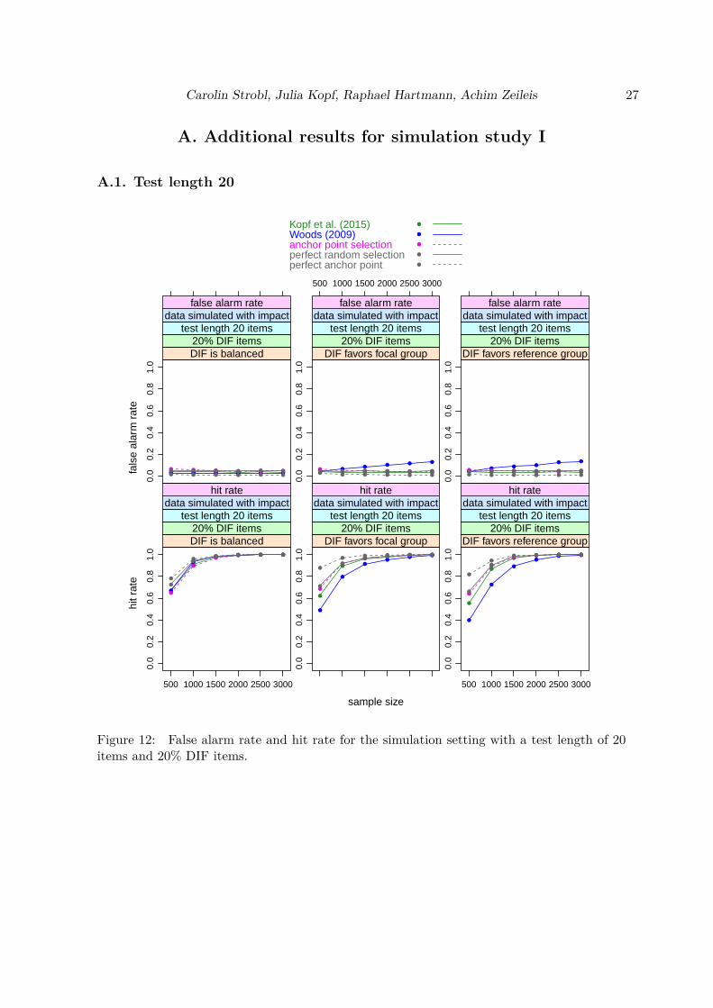
Carolin Strobl, Julia Kopf, Raphael Hartmann, Achim Zeileis 27
A. Additional results for simulation study I
A.1. Test length 20
sample size
hit r
ate
fals
e al
arm
rat
e
0.0
0.2
0.4
0.6
0.8
1.0
500 1000 1500 2000 2500 3000
●
●
●● ● ●
●
●
● ● ● ●
●
●
●● ● ●
●
●● ● ● ●
●
●● ● ● ●
DIF is balanced20% DIF items
test length 20 itemsdata simulated with impact
hit rate
0.0
0.2
0.4
0.6
0.8
1.0
●
●
● ● ● ●
●
●
●●
● ●
●
●
●● ● ●
●
●
● ● ● ●
●
●● ● ● ●
DIF favors focal group20% DIF items
test length 20 itemsdata simulated with impact
hit rate
0.0
0.2
0.4
0.6
0.8
1.0
500 1000 1500 2000 2500 3000
●
●
●● ● ●
●
●
●
●● ●
●
●
● ● ● ●
●
●
● ● ● ●
●
●
● ● ● ●
DIF favors reference group20% DIF items
test length 20 itemsdata simulated with impact
hit rate
0.0
0.2
0.4
0.6
0.8
1.0
● ● ● ● ● ●● ● ● ● ● ●● ● ● ● ● ●● ● ● ● ● ●● ● ● ● ● ●
DIF is balanced20% DIF items
test length 20 itemsdata simulated with impact
false alarm rate
500 1000 1500 2000 2500 3000
0.0
0.2
0.4
0.6
0.8
1.0
● ● ● ● ● ●●●
●● ● ●
●● ● ● ● ●● ● ● ● ● ●
● ● ● ● ● ●
DIF favors focal group20% DIF items
test length 20 itemsdata simulated with impact
false alarm rate
0.0
0.2
0.4
0.6
0.8
1.0
● ● ● ● ● ●●● ● ●
● ●
● ● ● ● ● ●● ● ● ● ● ●● ● ● ● ● ●
DIF favors reference group20% DIF items
test length 20 itemsdata simulated with impact
false alarm rate
Kopf et al. (2015)Woods (2009)anchor point selectionperfect random selectionperfect anchor point
●
●
●
●
●
Figure 12: False alarm rate and hit rate for the simulation setting with a test length of 20items and 20% DIF items.
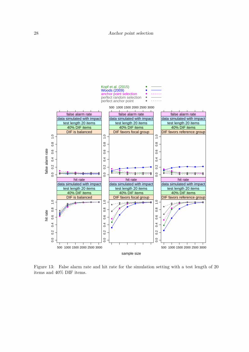
28 Anchor point selection
sample size
hit r
ate
fals
e al
arm
rat
e
0.0
0.2
0.4
0.6
0.8
1.0
500 1000 1500 2000 2500 3000
●
●
●● ● ●
●
●
● ● ● ●
●
●
●● ● ●
●
●
● ● ● ●
●
●● ● ● ●
DIF is balanced40% DIF items
test length 20 itemsdata simulated with impact
hit rate
0.0
0.2
0.4
0.6
0.8
1.0
●
●
● ● ● ●
●
●
●
●● ●
●
●
●● ● ●
●
●● ● ● ●
●
● ● ● ● ●
DIF favors focal group40% DIF items
test length 20 itemsdata simulated with impact
hit rate
0.0
0.2
0.4
0.6
0.8
1.0
500 1000 1500 2000 2500 3000
●
●
●● ● ●
●
●
●
●
● ●
●
●
●● ● ●
●
●
● ● ● ●
●
●● ● ● ●
DIF favors reference group40% DIF items
test length 20 itemsdata simulated with impact
hit rate
0.0
0.2
0.4
0.6
0.8
1.0
● ● ● ● ● ●● ● ● ● ● ●
●● ● ● ● ●● ● ● ● ● ●
● ● ● ● ● ●
DIF is balanced40% DIF items
test length 20 itemsdata simulated with impact
false alarm rate
500 1000 1500 2000 2500 30000.
00.
20.
40.
60.
81.
0
●●
● ● ● ●
●
● ● ● ● ●
●●
●● ● ●● ● ● ● ● ●●
● ● ● ● ●
DIF favors focal group40% DIF items
test length 20 itemsdata simulated with impact
false alarm rate
0.0
0.2
0.4
0.6
0.8
1.0
●●
● ● ● ●
●
●● ● ● ●
●
●
● ● ● ●● ● ● ● ● ●●● ● ● ● ●
DIF favors reference group40% DIF items
test length 20 itemsdata simulated with impact
false alarm rate
Kopf et al. (2015)Woods (2009)anchor point selectionperfect random selectionperfect anchor point
●
●
●
●
●
Figure 13: False alarm rate and hit rate for the simulation setting with a test length of 20items and 40% DIF items.
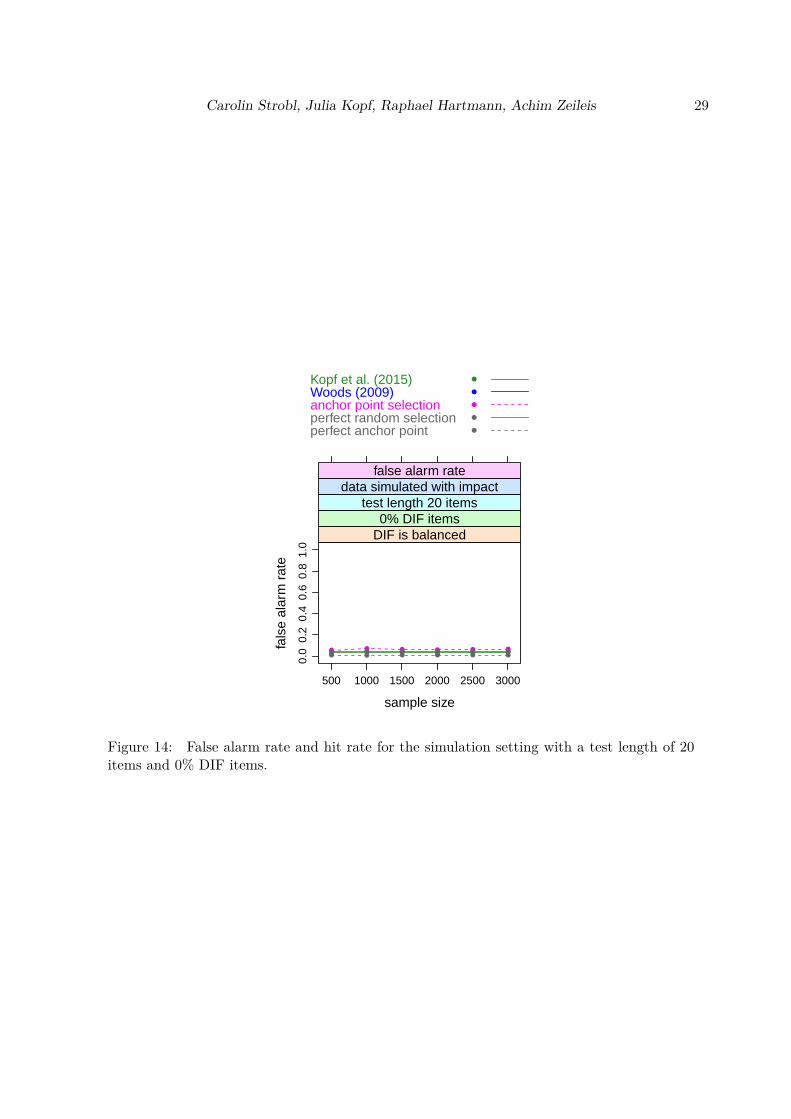
Carolin Strobl, Julia Kopf, Raphael Hartmann, Achim Zeileis 29
sample size
fals
e al
arm
rat
e
0.0
0.2
0.4
0.6
0.8
1.0
500 1000 1500 2000 2500 3000
● ● ● ● ● ●● ● ● ● ● ●● ● ● ● ● ●● ● ● ● ● ●
DIF is balanced0% DIF items
test length 20 itemsdata simulated with impact
false alarm rate
Kopf et al. (2015)Woods (2009)anchor point selectionperfect random selectionperfect anchor point
●
●
●
●
●
Figure 14: False alarm rate and hit rate for the simulation setting with a test length of 20items and 0% DIF items.
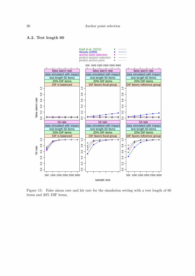
30 Anchor point selection
A.2. Test length 60
sample size
hit r
ate
fals
e al
arm
rat
e
0.0
0.2
0.4
0.6
0.8
1.0
500 1000 1500 2000 2500 3000
●
●
● ● ● ●
●
●● ● ● ●
●
●
● ● ● ●
●
●● ● ● ●
●
●● ● ● ●
DIF is balanced20% DIF items
test length 60 itemsdata simulated with impact
hit rate
0.0
0.2
0.4
0.6
0.8
1.0
●
●
● ● ● ●
●
●
●● ● ●
●
●● ● ● ●
●
●● ● ● ●
●
● ● ● ● ●
DIF favors focal group20% DIF items
test length 60 itemsdata simulated with impact
hit rate0.
00.
20.
40.
60.
81.
0
500 1000 1500 2000 2500 3000
●
●
● ● ● ●
●
●
●
●● ●
●
●
● ● ● ●
●
●
● ● ● ●
●
●● ● ● ●
DIF favors reference group20% DIF items
test length 60 itemsdata simulated with impact
hit rate
0.0
0.2
0.4
0.6
0.8
1.0
● ● ● ● ● ●● ● ● ● ● ●● ● ● ● ● ●● ● ● ● ● ●● ● ● ● ● ●
DIF is balanced20% DIF items
test length 60 itemsdata simulated with impact
false alarm rate
500 1000 1500 2000 2500 3000
0.0
0.2
0.4
0.6
0.8
1.0
● ● ● ● ● ●●●
●●
●●
● ● ● ● ● ●● ● ● ● ● ●● ● ● ● ● ●
DIF favors focal group20% DIF items
test length 60 itemsdata simulated with impact
false alarm rate
0.0
0.2
0.4
0.6
0.8
1.0
● ● ● ● ● ●●
●●
●●
●
● ● ● ● ● ●● ● ● ● ● ●● ● ● ● ● ●
DIF favors reference group20% DIF items
test length 60 itemsdata simulated with impact
false alarm rate
Kopf et al. (2015)Woods (2009)anchor point selectionperfect random selectionperfect anchor point
●
●
●
●
●
Figure 15: False alarm rate and hit rate for the simulation setting with a test length of 60items and 20% DIF items.
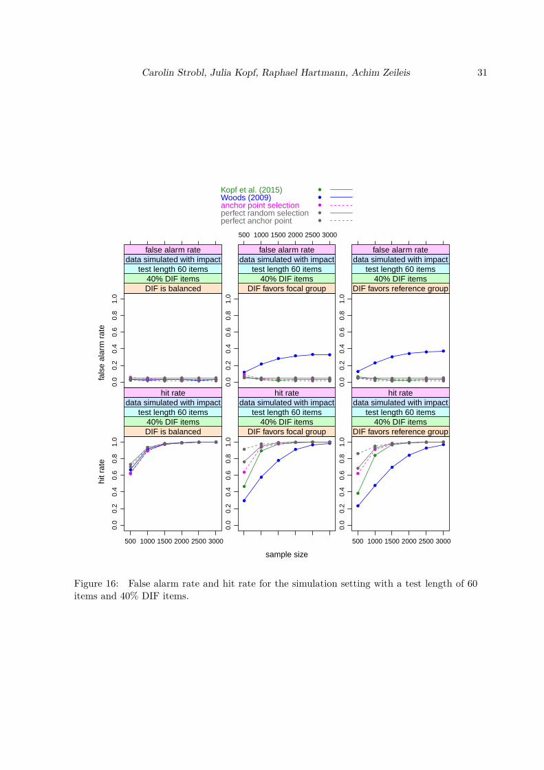
Carolin Strobl, Julia Kopf, Raphael Hartmann, Achim Zeileis 31
sample size
hit r
ate
fals
e al
arm
rat
e
0.0
0.2
0.4
0.6
0.8
1.0
500 1000 1500 2000 2500 3000
●
●
●● ● ●
●
●
● ● ● ●
●
●
●● ● ●
●
●
● ● ● ●
●
●
● ● ● ●
DIF is balanced40% DIF items
test length 60 itemsdata simulated with impact
hit rate
0.0
0.2
0.4
0.6
0.8
1.0
●
●
● ● ● ●
●
●
●
●
●●
●
●● ● ● ●
●
●● ● ● ●
●
● ● ● ● ●
DIF favors focal group40% DIF items
test length 60 itemsdata simulated with impact
hit rate
0.0
0.2
0.4
0.6
0.8
1.0
500 1000 1500 2000 2500 3000
●
●
●● ● ●
●
●
●
●
●●
●
●
● ● ● ●
●
●
● ● ● ●
●
●● ● ● ●
DIF favors reference group40% DIF items
test length 60 itemsdata simulated with impact
hit rate
0.0
0.2
0.4
0.6
0.8
1.0
● ● ● ● ● ●● ● ● ● ● ●●
● ● ● ● ●● ● ● ● ● ●● ● ● ● ● ●
DIF is balanced40% DIF items
test length 60 itemsdata simulated with impact
false alarm rate
500 1000 1500 2000 2500 30000.
00.
20.
40.
60.
81.
0
●● ● ● ● ●
●
●
●● ● ●
●
● ● ● ● ●● ● ● ● ● ●●
● ● ● ● ●
DIF favors focal group40% DIF items
test length 60 itemsdata simulated with impact
false alarm rate
0.0
0.2
0.4
0.6
0.8
1.0
●● ● ● ● ●
●
●
●●
● ●
● ● ● ● ● ●● ● ● ● ● ●●● ● ● ● ●
DIF favors reference group40% DIF items
test length 60 itemsdata simulated with impact
false alarm rate
Kopf et al. (2015)Woods (2009)anchor point selectionperfect random selectionperfect anchor point
●
●
●
●
●
Figure 16: False alarm rate and hit rate for the simulation setting with a test length of 60items and 40% DIF items.
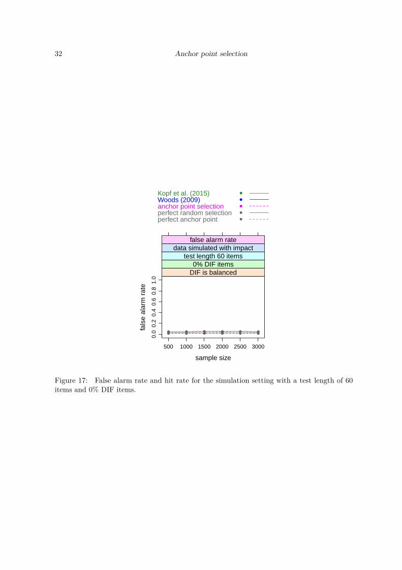
32 Anchor point selection
sample size
fals
e al
arm
rat
e
0.0
0.2
0.4
0.6
0.8
1.0
500 1000 1500 2000 2500 3000
● ● ● ● ● ●● ● ● ● ● ●● ● ● ● ● ●● ● ● ● ● ●
DIF is balanced0% DIF items
test length 60 itemsdata simulated with impact
false alarm rate
Kopf et al. (2015)Woods (2009)anchor point selectionperfect random selectionperfect anchor point
●
●
●
●
●
Figure 17: False alarm rate and hit rate for the simulation setting with a test length of 60items and 0% DIF items.

Carolin Strobl, Julia Kopf, Raphael Hartmann, Achim Zeileis 33
Affiliation:Carolin StroblDepartment of PsychologyUniversität ZürichBinzmühlestrasse 14, Box 27CH-8050 Zürich, SwitzerlandE-mail: [email protected]
Achim ZeileisDepartment of StatisticsFaculty of Economics and StatisticsUniversität InnsbruckUniversitätsstr. 156020 Innsbruck, AustriaE-mail: [email protected]: https://eeecon.uibk.ac.at/~zeileis/

University of Innsbruck - Working Papers in Economics and StatisticsRecent Papers can be accessed on the following webpage:
https://www.uibk.ac.at/eeecon/wopec/
2018-03 Carolin Strobl, Julia Kopf, Raphael Hartmann, Achim Zeileis: Anchor point selec-tion: An approach for anchoring without anchor items
2018-02 Michael Greinecker, Christopher Kah: Pairwise stablematching in large economies
2018-01 Max Breitenlechner, Johann Scharler: How does monetary policy influence banklending? Evidence from the market for banks’ wholesale funding
2017-27 Kenneth Harttgen, Stefan Lang, Johannes Seiler: Selective mortality and undernu-trition in low- and middle-income countries
2017-26 Jun Honda, Roman Inderst: Nonlinear incentives and advisor bias
2017-25 Thorsten Simon, Peter Fabsic, Georg J. Mayr, Nikolaus Umlauf, Achim Zeileis:Probabilistic forecasting of thunderstorms in the Eastern Alps
2017-24 Florian Lindner: Choking under pressure of top performers: Evidence frombiathloncompetitions
2017-23 ManuelGebetsberger, JakobW.Messner, Georg J.Mayr, AchimZeileis: Estimationmethods for non-homogeneous regression models: Minimum continuous rankedprobability score vs. maximum likelihood
2017-22 Sebastian J. Dietz, Philipp Kneringer, Georg J. Mayr, Achim Zeileis: Forecastinglow-visibility procedure states with tree-based statistical methods
2017-21 Philipp Kneringer, Sebastian J. Dietz, Georg J. Mayr, Achim Zeileis: Probabilisticnowcasting of low-visibility procedure states at Vienna International Airport duringcold season
2017-20 Loukas Balafoutas, Brent J. Davis,Matthias Sutter: Howuncertainty and ambiguityin tournaments affect gender differences in competitive behavior
2017-19 Martin Geiger, Richard Hule: The role of correlation in two-asset games: Someexperimental evidence
2017-18 Rudolf Kerschbamer, Daniel Neururer, Alexander Gruber: Do the altruists lie less?
2017-17 Meike Köhler, Nikolaus Umlauf, Sonja Greven: Nonlinear association structures inflexible Bayesian additive joint models

2017-16 Rudolf Kerschbamer, Daniel Muller: Social preferences and political attitudes: Anonline experiment on a large heterogeneous sample
2017-15 Kenneth Harttgen, Stefan Lang, Judith Santer, Johannes Seiler: Modeling under-5 mortality through multilevel structured additive regression with varying coeffi-cients for Asia and Sub-Saharan Africa
2017-14 Christoph Eder, Martin Halla: Economic origins of cultural norms: The case of ani-mal husbandry and bastardy
2017-13 Thomas Kneib, Nikolaus Umlauf: A primer on bayesian distributional regression
2017-12 Susanne Berger, Nathaniel Graham, Achim Zeileis: Various versatile variances: Anobject-oriented implementation of clustered covariances in R
2017-11 Natalia Danzer, Martin Halla, Nicole Schneeweis, Martina Zweimüller: Parentalleave, (in)formal childcare and long-term child outcomes
2017-10 Daniel Muller, Sander Renes: Fairness views and political preferences - Evidencefrom a large online experiment
2017-09 Andreas Exenberger: The logic of inequality extraction: An application to Gini andtop incomes data
2017-08 Sibylle Puntscher, Duc TranHuy, JanetteWalde, Ulrike Tappeiner, Gottfried Tappeiner:The acceptance of a protected area and the benefits of sustainable tourism: Insearch of the weak link in their relationship
2017-07 Helena Fornwagner: Incentives to lose revisited: The NHL and its tournament in-centives
2017-06 Loukas Balafoutas, Simon Czermak, Marc Eulerich, Helena Fornwagner: Incen-tives for dishonesty: An experimental study with internal auditors
2017-05 Nikolaus Umlauf, Nadja Klein, Achim Zeileis: BAMLSS: Bayesian additive modelsfor location, scale and shape (and beyond)
2017-04 Martin Halla, Susanne Pech, Martina Zweimüller: The effect of statutory sick-payon workers’ labor supply and subsequent health
2017-03 Franz Buscha, Daniel Müller, Lionel Page: Can a common currency foster a sharedsocial identity across different nations? The case of the Euro.
2017-02 Daniel Müller: The anatomy of distributional preferences with group identity
2017-01 Wolfgang Frimmel, Martin Halla, Jörg Paetzold: The intergenerational causal ef-fect of tax evasion: Evidence from the commuter tax allowance in Austria
University of Innsbruck
Working Papers in Economics and Statistics
2018-03
Carolin Strobl, Julia Kopf, Raphael Hartmann, Achim ZeileisAnchor point selection: An approach for anchoring without anchor items
AbstractFor detecting differential item functioning (DIF) between two groups of test takers, theiritem parameters need to be aligned in some way. Typically this is done by means ofchoosing a small number of so called anchor items. Here we propose an alternative strat-egy: the selection of an anchor point along the item parameter continuum, where thetwo groups best overlap. We illustrate how the anchor point is selected by means ofmaximizing an inequality criterion. It performs equally well or better than establishedapproaches when treated as an anchoring technique, but also provides additional infor-mation about the DIF structure through its search path. Another distinct property of thisnew method is that no individual items are flagged as anchors. This is a major differenceto traditional anchoring approaches, where flagging items as anchors implies - but doesnot guarantee - that they are DIF free, and may lull the user into a false sense of security.Our method can be viewed as a generalization of the search space of traditional anchorselection techniques and can shed new light on the practical usage as well as on the the-oretical discussion on anchoring and DIF in general.
ISSN 1993-4378 (Print)ISSN 1993-6885 (Online)