from object grammars to eco systems

Theoretical Computer Science 314 (2004) 57–95www.elsevier.com/locate/tcs

From object grammars to ECO systemsEnrica Duchia ;∗ , Jean-Marc Fedoub , Simone Rinaldic

aBureau 231, CAMS, EHESS, 54 boulevard Raspail, 75006 Paris, FrancebLaboratoire I3S, UNSA-CNRS 2000, Route des lucioles BP.121,

06903 Sophia Antipolis-Cedex, FrancecDipartimento di Matematica, Via del Capitano, 15, 53100 Siena, Italy

Received 21 October 2002; received in revised form 14 October 2003; accepted 22 October 2003Communicated by A. Del Lungo

Abstract

In this paper we make a comparison between two methods for the enumeration of combinato-rial objects, namely the ECO method and object grammars, both based on a recursive descriptionfor the examined class of objects. In particular, we study the problem of passing from an objectgrammar to an “equivalent” ECO system. First, we solve this problem for any unidimensional,unambiguous, and complete object grammar, with any linear parameter. Then we treat the morecomplex cases of q-linear parameters, and of multidimensional object grammars, giving someexplanatory examples. In particular, we determine a new ECO system for the class of directedconvex polyominoes.c© 2003 Elsevier B.V. All rights reserved.

1. Introduction

Recursive descriptions of combinatorial objects allow one to obtain enumerative re-sults including: generating functions, bijections, and uniform random generation. Weare interested in comparing two di=erent ways of describing objects recursively, onethrough object grammars and the other through the Enumeration of CombinatorialObjects method, or simply, ECO.

The >rst way originated from the classical grammar description of applying re-cursively operations to elementary objects. This approach, introduced by Flajoletet al. [18], >rst dealt with decomposable structures and used the basic operationsof union, product, sequence of, set of, or cycle of. A nice presentation appears in [18].

∗ Corresponding author.E-mail addresses: [email protected] (E. Duchi), [email protected] (J.-M. Fedou), [email protected] (S. Rinaldi).

0304-3975/$ - see front matter c© 2003 Elsevier B.V. All rights reserved.doi:10.1016/j.tcs.2003.10.037

mailto:[email protected]



58 E. Duchi et al. / Theoretical Computer Science 314 (2004) 57–95

Dutour [12] followed the same approach for object grammars, related to the context-free grammars theory, for which one is allowed to describe objects using more generaloperations.

A signi>cantly di=erent way of recursively describing objects appears in the ECOmethodology, introduced by Barcucci et al. [3]. It essentially grows objects by allowinggrowth at elementary objects, called active sites. The method is related to successionrules, >rst introduced by Chung et al. [8] for studying permutations avoiding someparticular subsequences [24].

These two ways of thinking recursively have many immediate applications:Description of objects. An “ECO” object is described completely by a path in the

generating tree. Similarly, an “object grammar” object is described completely by itsderivation tree.Generating functions. From a succession rule it is possible to derive an equation

satis>ed by the generating function according to the size and the number of active sites.Also using object grammars we can obtain generating functions for the generated class.Bijections. Both approaches allow us to determine bijections between classes of

di=erent combinatorial objects, either when succession rules are the same [3] or whenobject grammars are isomorphic [15].Uniform random generation. The general method of random generation introduced

by Wilf [25] has been applied by Flajolet et al. [19] for decomposable structures andby Dutour and FFedou in [14] for object grammars. Roughly, the random generation ofan n-sized object is realized by choosing randomly an integer k¡n, and then randomlygenerating a k-sized and a (n−1− k)-sized object. A random ECO object correspondsto a random path in the generating tree which is obtained by a random growing ofelementary objects [4].

Another application of both the ECO and the decomposable structure approach isin dealing with q-analogs. The notion of q-grammars, introduced by Delest and FFedouin [9], is based on the idea that coding the objects with the words of an algebraiclanguage provides a structure on the objects themselves. By >tting the notion of attributegrammars [20], sometimes it is possible to describe nonalgebraic equations veri>edby the generating function of the class of objects, according to a further parameterrepresented by the indeterminate q. The resulting equations are some q-analogs ofthe original algebraic equations. Recently, the application of attribute grammars toalgorithm analysis has also been considered [22].

Let O be a class of combinatorial objects, and let p be a parameter on O, such thatthere are >nitely many objects of O having the same value under p. In the settingof the ECO method, we usually speak of an ECO system for O, to encompass theclass O, the parameter p, an ECO operator describing a construction for O, and thesuccession rule associated with such operator.

In this paper, an object grammar and an ECO system will be considered “equivalent”when they both de>ne a construction for the same class O according to the sameparameter p.

There are two natural questions:1. Is it possible to obtain an object grammar from a given ECO system?2. Is it possible to obtain an ECO system from a given object grammar?

E. Duchi et al. / Theoretical Computer Science 314 (2004) 57–95 59

The >rst question, the problem of deriving an object grammar equivalent to a givenECO system, has been partially solved by FFedou and Garcia [16] for some algebraicrules, i.e. rules having an algebraic generating functions.

Here we examine the second question, that is, the problem of passing from an objectgrammar to an equivalent ECO system.

The application of the ECO method often leads to simple solutions for problemsthat are commonly believed “hard” to solve. For example, in [10] the authors give anECO construction, and then derive the associated succession rule, for the classes ofconvex polyominoes and column-convex polyominoes according to the semi-perimeter.A simple algebraic computation leads then to the determination of generating functionsfor the two classes.

In [1] it is shown that an ECO construction easily leads to an algorithm for theexhaustive generation of the examined class. If some special conditions are satis>ed,this algorithm has also the CAT property.

Moreover, an ECO construction can often produce interesting combinatorial infor-mation about the class of objects studied, as is shown in [3] using analytic methods,or as shown in [5], using bijective techniques.

Also succession rules and their relationships with other counting methods wereinvestigated in several papers: in [2], Banderier et al. reintroduced the kernelmethod in order to determine the generating function of various types of successionrules; di=erent from unambiguous object grammars, succession rules permit one toenumerate structures having a transcendental generating function.

Furthermore, succession rules have deep connections with many topics in algebraiccombinatorics (for example the concept of AGT matrix [21] or the production matri-ces [11]), whereas object grammars are prevalently linked with the theory of formallanguages.

In Section 2 we give the basic de>nitions and examples about ECO method andsuccession rules. Similarly, in Section 3 we introduce the concept of object grammar,providing various examples. In Section 4 we describe the main steps used to pass fromany given unidimensional, unambiguous, and complete grammar, to an “equivalent”ECO system. In a word, such an ECO system is de>ned by repeatedly developing leavesin derivation trees of object grammars. We consider uniform and linear parameters, andgive several examples. In Section 5 we deal with q-linear parameters, and >nally, inSection 6, we treat the more general case of multidimensional object grammars. Toclarify this last case we present a detailed example concerning the class of directedconvex polyominoes. The main result of this section is the determination of a newECO system for this class.

2. ECO method and succession rules

ECO method is a recursive method for the enumeration of a class of combinatorialobjects so that each object is obtained from another of lower size by making somelocal expansions on the so-called active sites of that object. By the size of an object wemean the value of a parameter de>ned on that object. Let O be a class of combinatorial


objects and let p :O→N+ be a parameter on O such that |{O∈O :p(O) = n}| is>nite (i.e., there are >nitely many objects of each size). For n∈N, let On denote{O∈O :p(O) = n}, and let # be an operator from On to 2On+1 , the power set of On+1.

Proposition 1 (Barcucci et al. [3]). If, for n¿0; # satis>es the following:1. for each O′ ∈On+1, there exists O∈On such that O′ ∈#(O), and2. for every O;O′ ∈On; #(O)∩#(O′) = ∅ whenever O =O′,then the family of sets Fn+1 = {#(O) :O∈On} is a partition of On+1.

If # satis>es the conditions 1 and 2 above, then all the objects of O are generated, andeach object O′ ∈On+1 is obtained from a unique O∈On. The construction performedby the ECO operator # can be described suitably by a generating tree [3,7], i.e., arooted tree whose nodes correspond to the objects of O. The root, placed at level 0 ofthe tree, is the object with minimum size, say m¿0. The objects having the same valueof parameter p lie at the same level, and the sons of an object O are those producedby O through #. More speci>cally, the construction determined by a generating treecan be formalized by means of a succession rule of the form{

(a)(k) ❀ (e1(k))(e2(k)) : : : (ek(k));

(1)

where a; k; ei(k)∈N+, meaning that the root object has a sons and the k objectsO′

1; : : : ; O′k , produced by an object O are such that |#(O′

i)|= ei(k); 16i6k. One ofthe main properties of succession rules, the so-called consistency principle, is that eachlabel (k) must produce exactly k elements. A succession rule describes a sequence{fn}n of positive integers, where fn is the number of nodes at level n of the gen-erating tree and its generating function is denoted by f(x) =

∑n¿0 fnx

n. Then wehave fO(x) = xmf(x), where fO(x) =

∑n¿m |On|xn is the generating function of O

according to p. If m= 0 then fO(x) =f(x).Here we adopt a slight extension of ECO method, recently introduced by Ferrari

et al. [17]. They allow the ECO operator to generate objects of di=erent sizes, greaterthan or equal to n, from any object of size n (n¿m). More formally, let # :On →2⋃t

j=1 On+ij , n; ij ∈N and 06i1¡i2¡ · · ·¡it . Proposition 1 generalizes as follows:

Proposition 2. If # satis>es, for t¿0; n¿m,1. for each O′ ∈On there exists O∈ ⋃t

j=1 On−ij such that O′ ∈#(O), and2. for every O;O′ ∈O, #(O)∩#(O′) = ∅, whenever O =O′,then the family of sets F= {#(O) :O∈ ⋃t

j=1 On−ij}∩ 2On is a partition of On. 1

Let us consider a tree represented in the cartesian plane so that the root has ordinate0 and each son has ordinate lower than that of its father. The level l(N ) of a node Nin the tree is then de>ned as follows: if N is the root, then l(N ) = 0; otherwise, if Nis located in (x; y), then l(N ) =−y. The length of an edge is the di=erence betweenthe level of the son and that of its father.

1 The case i1 = 0 refers to zero length jumps, i.e. for some n¿m, and some O∈On; #(O)∩On �= ∅.


We associate with the operator # a generating tree having edges of di=erent lengths,say, i1; : : : ; it , and a jumping succession rule (brieMy, succession rule) of the form

(ta)

(tk) i1❀ (te1

1(k))(te12(k)) : : : (te1

k(k))...it❀ (tet1(k))(tet2(k)) : : : (tetk(k));

(2)

where a; k; e ji (k)∈N+. Every object O corresponding to a node labelled (tk) in thegenerating tree, produces k objects O′

1ij; : : : ; O′

kijat levels ij; j = 1 : : : m, respectively

such that |#(O′lij

)|= te jl ; 16l6k. 2 A simple succession rule in the form of (1) is thenjust a jumping succession rule with t = 1 and i1 = 1. As for a simple succession rule,we denote by {fn}n the sequence de>ned by a jumping succession rule, where fn is thenumber of nodes at level n in the generating tree. Let # be an ECO operator describingthe class O according to the parameter p; often the quadruple �= (O; p; #; #) is calledan ECO system, where # (brieMy ) is the succession rule describing #.

Example 3. Fig. 1 represents the >rst levels of the generating tree associated with thesuccession rule:

(2)

(2k) 1❀ (2)(4) : : : (2k)2❀ (4)(6) : : : (2k + 2):

(2)(4) (2)(4)(2) (2)

(2)

(2)

(2)

(2)

(4)

(4)

(4)

(4) (6)

(4)(2)

1

2

4

9

1

Fig. 1. The >rst levels of the generating tree associated with the rule in Example 3.

2 We remark that each label in the production of (2) is multiplied by t, in order to satisfy the consistencyprinciple.


The reader can easily verify that this rule de>nes the sequence 1; 1; 2; 4; 9; 21; : : : ofMotzkin numbers (sequence A001006 in [23]), and is equivalent to the simple rule(see [3]):

(1)(1) ❀ (2)(k) ❀ (1)(2) : : : (k − 1)(k + 1);

in the sense that they de>ne the same integer sequence.

3. Object grammars

An object grammar gives a recursive description for a class of combinatorial objects,by giving a set of terminal objects and some operations applied to the objects. Fordetailed de>nitions and examples we refer to [13]. Here, we only recall some basicde>nitions:

De�nition 4. Let O be a >nite family of classes of objects. A k-ary object operationon O, k ∈N+, is a mapping � :O1 × · · · ×Ok →O, where O;Oi ∈O; i= 1; : : : ; k. Thedomain and codomain of an object operation � are respectively denoted as dom(�)and cod(�).

An object operation describes a way of building recursively an object of O startingfrom k objects belonging to O1; : : : ;Ok , respectively.

De�nition 5. An object grammar (or simply, a grammar) is a quadruple 〈O; E; �;A〉where:• O is a >nite family of classes of objects.• E= {EO}O∈O is a >nite family of >nite subclasses of elements O; the objects of E

are called terminal objects.• � is a set of object operations in O.• A is a >xed class of O, called the axiom of the grammar.

We call the cardinality of O the dimension of the corresponding object grammar.Hence the grammar is unidimensional when O consists of a single class.

De�nition 6. Let G = 〈O; E; �;A〉 be an object grammar and let O∈O. A derivationtree of G on O is an ordered labelled tree T , recursively described as follows:• the labels of the leaves are terminal objects of O,• if the root of T has k sons then its label is an object operation �∈�,

� : O1 × · · · × Ok → O;

where Oi ∈O and such that the ith son of the root is the root of a derivation treeon the class Oi ; i= 1 : : : k.


The valuation ev(T ) of a derivation tree T is an object de>ned as follows:• if T is a single node labelled E, then ev(T ) =E,• otherwise, if the root of T is labelled �∈� and its k subtrees are T1 : : : Tk , then

ev(T ) =�(ev(T1); : : : ; ev(Tk)).The above de>nition will be clari>ed in Example 12.We say that an object O∈O is generated in G by O if there is a derivation tree T on

O such that ev(T ) =O. The class generated in G by A is said to be the class generatedby G. A grammar G is complete if, for all O∈O, the class of objects generated inG by O is equal to O. A grammar G is unambiguous if every object generated byG admits only one derivation tree. If TG denotes the class of derivation trees of agrammar G, then the following statement trivially holds:

Proposition 7. If G is a complete and unambiguous object grammar generating theclass O, then the function ev :TG →O is a bijection.

3.1. Linear parameters and q-parameters

In this subsection we brieMy recall some de>nitions about linear and q-linear para-meters.

De�nition 8. Let O;O1; : : : ;Ok be some classes of combinatorial objects and p; qparameters on O;O1; : : : ;Ok . We also assume that p is a >nite parameter. Let � bean object operation such that dom(�) =O1 × · · · ×Ok and cod(�) =O.(i) The parameter p is said to be a linear parameter with respect to � if

p(�(O1; : : : ; Ok)) =k∑

i=1p(Oi) + p(�); (3)

where (O1; : : : ; Ok)∈dom(�) and p(�)∈N is constant for �.(ii) The parameter q is a q-parameter with respect to � if, for all (O1; : : : ; Ok)∈

dom(�),

q(�(O1; : : : ; Ok)) =k∑

i=1q(Oi) +

k∑i=1

qi(�)t(Oi) + q(�); (4)

where the qi(�)∈N for i= 1 : : : k, and q(�)∈N are constants, and t is a param-eter on O1; : : : ;Ok .

De�nition 9. Let G = 〈O; E; �;A〉 be an object grammar. A parameter p (resp. q) issaid to be G-linear (G − q-linear) if, for all O∈O; p (resp. q) is linear (resp. aq-parameter) with respect to each operation �∈� such that cod(�) =O.

A G-linear parameter p is called uniform if,

∀� ∈ �; p(�) = 1


and,

∀e ∈ ⋃O∈O

EO; p(e) = 1:

In [13] Dutour proved that linear parameters lead to algebraic generating functions forthe classes O∈O.

Lemma 10. (i) Let p be a G-linear parameter on G. Then, for any object O generatedby G with ev(T ) =O, we have

p(O) =∑x∈T

p(�x); (5)

where, for any node x of T; �x denotes its label.(ii) Let q be a G−q-linear and t be a parameter. Then, for any object O generated

by G with derivation tree T , we have

q(O) =∑x∈T

(k(x)∑i=1

qi(�x)t(ev(Ti;x)) + q(�x)

); (6)

where, for x a node of T; �x is its label, and the Ti;x; i= 1 : : : k(x), are the subtreesattached to x.

Proof. The proof can be achieved by recursion on Eqs. (3) and (4) de>ning respec-tively p and q.

Remark 11. If the parameter t is G-linear, we can apply (5) to (6) and then obtainthe following:

q(O) =∑x∈T

(k(x)∑i=1

qi(�x)∑

y∈Ti;xt(�y) + q(�x)

): (7)

From now on, we will only deal with complete and unambiguous object grammars.

Example 12. In the plane Z×Z, we consider lattice paths using steps of two types:rise steps (1; 1) and fall steps (1;−1). A Dyck path of length 2n is a sequence of riseand fall steps, running from (0; 0) to (2n; 0), and remaining weakly above the x-axis.The mapping �1 depicted in Fig. 2 is a binary object operation on the class D of Dyck

,�1

Fig. 2. The operation �1 on the class D of Dyck paths.


φ1

φ1φ1

φ1 φ1

Fig. 3. A derivation tree of GD and the corresponding Dyck path.

Fig. 4. A parallelogram polyomino having perimeter 20 and area 12.

paths: it takes a pair of Dyck paths as its argument, adds a rise (resp. fall) step at thebeginning (resp. end) of the >rst path and then appends the second path.

The class D is generated by the unidimensional object grammar

GD = 〈D; {{:}}; {�1};D〉;where the terminal object is the Dyck path of zero length, commonly represented as adot. Each Dyck path is then univocally associated with a derivation tree of GD (see forinstance Fig. 3). The length of a path is a linear parameter on the class D (generatedby GD), since length(:) = 0 and, for every D1; D2 ∈ D,

length(�1(D1; D2)) = length(D1) + length(D2) + 2:

We remark that �1 adds two steps to D1, therefore l(�1) = 2.

Example 13. In the plane Z×Z we consider lattice paths using north steps (0; 1) andeast steps (1; 0). A parallelogram polyomino is the region lying between two north-eastpaths that are disjoint except their common end points (see Fig. 4 for example).

The perimeter of a parallelogram polyomino is the sum of the lengths of the twopaths. We denote by P the set of parallelogram polyominoes. The area of a parallelo-gram polyomino is the number of unit cells constituting it. The mappings �1

1; �21, and

�2, illustrated in Fig. 5, are object operations on P, the >rst two being unary, whilethe third is binary:• operation �1

1 adds a cell at the left of the lowest cell of the >rst column of thepolyomino;


,

�21

�11

�2

Fig. 5. The object operations �11; �2

1; �2 on the class of parallelogram polyominoes.

• operation �21 adds a cell at the bottom of every column of the polyomino;

• operation �2 applies �21 to the >rst parallelogram and then glues the right side of

the top cell of its last column of the >rst one to the left side bottom cell of the >rstcolumn of the second one.

The grammar:

GP = 〈{P}; {{ }}; {�11; �

21; �2};P〉

generates the whole class P, where denotes the one-cell polyomino. Fig. 6 representsthe derivation tree of GP associated with the polyomino in Fig. 4.

Trivially, the perimeter is a linear parameter on the class P generated by GP. Onthe other hand, the area of the polyomino is a q-linear parameter. Indeed for everyP1; P2 ∈P we have:

a(�11(P1)) = a(P1) + 1;

a(�21(P1)) = a(P1) + c(P1);

a(�2(P1; P2)) = a(P1) + a(P2) + c(P1);

where the parameter c gives the number of columns of a polyomino, and

c(�11(P1)) = c(P1) + 1;

c(�21(P1)) = c(P1);

c(�2(P1; P2)) = c(P1) + c(P2):


�11

�21

�2

�2

�11

�21

Fig. 6. The derivation tree of GP corresponding to the polyomino in Fig. 4.

4. ECO method and object grammars: the unidimensional case

In this section we will assume that the grammar G is always unidimensional, un-ambiguous, and complete. Let O be the class generated by G; � the set of operationsof the grammar, and p a linear parameter on O. As usual, let On denote the subset ofobjects of size n from O.

Basically, the idea is to de>ne a particular class of trees, the weighted $-trees, and a>nite parameter p′ on this class, such that the number of trees with size n is equal to|On|. Then we determine an ECO system describing the growth for this class of treesaccording to p′.

For a >xed positive integer d, let �j; 0¡j6d, denote the subset of � with operationsof degree j. Let �0 denote the set of terminal objects of the grammar G.

De�nition 14. Let d be a >xed non-negative integer and

$ = ($0; $1; : : : ; $d); $i ∈ N:

An $-tree is a labelled tree with nodes of degree at most d and such that each node ofdegree j has a color i∈{1; 2; : : : ; $j}. Given a weight wij ∈N for each node of colori and degree j, the associated weighted $-tree has labels of the form (i; wij) on nodesof degree j.

There is a simple bijection from TG, the set of derivation trees of G, to Tw$G ,

the set of weighted $-trees, where $= (|�0|; |�1|; : : : ; |�d|) and wij =p(�ij) for all


�11

�2

(1 , 0)

(2 , 2)(1 , 2)

(2 , 2)(1 , 0)

(1 , 4)(1 , 4) (1 , 4)

(1 , 2)

�21�1

1

�21 �2

Fig. 7. A derivation tree from the grammar GP and the corresponding weighted (1; 2; 1)-tree.

i= 1 : : : |�j|; j = 0 : : : d. For any T ∈TG, the corresponding tree is obtained by replacingeach label �i

j in the tree T by the label (i; p(�ij)), and vice versa. From the previous

statements one can easily adapt Proposition 7 to the class Tw$G .

De�nition 15. Let T ∈Tw$G . For any x∈T , the label of the node, denoted l(x) is a

pair (co(x); w(x)). Then p′(T ) =∑

x∈Tw(x).

Then, from De>nition 15, and Lemma 10 we deduce that p′(T ) =p(ev(T )).

Example 16. Fig. 7 shows one derivation tree of the grammar GP of Example 13and the corresponding weighted (1; 2; 1)-tree. If parameter p is the perimeter of thepolyomino, p(�1

1) =p(�21) = 2 and p(�2) = 0, then p′ is 20.

In order to complete the objective of this section, we must next determine an ECOconstruction for the class Tw$

G according to p′. For this purpose we need to extendslightly the class Tw$

G including the empty tree of size 0, denoted by &, correspondingto the root of the generating tree associated with the ECO construction. This rootproduces the initial $0 leaves in the generating tree. We remark that, by extending theclass Tw$

G with &, the generating function of such a class increases by one. We beginby showing the ECO construction in the simpler case of uniform parameters, then weextend the construction to the general case of linear parameters.

4.1. Uniform parameter

For the case where the parameter is uniform, given an object grammar and theresulting TG, the problem reduces to determining an ECO system de>ning the growthof the class of (unweighted) $-trees, T$

G , which corresponds bijectively to TG.Our application of the ECO method now follows closely that described in details in

[3] for ordered trees. Let T$n be the set of trees in T$

G having exactly n nodes, andlet #1 be an operator from T$

n to 2⋃d

i=1 T$

n+i . Let us consider an object T in T$n. Before


← last internal node.

1

11

1

1

1

11 1

2

Fig. 8. A (2; 1; 1)-tree. The label over each node denotes its color, while the active sites are circled.

describing the behavior of the operator #1 on T , we must de>ne the set of active sitesof T . This set consists of all leaves of T following the last internal node in the pre-ordertraversal. For example, in Fig. 8 we have marked the active sites of a (2; 1; 1)-tree.The operator #1 performs the following transformations on T , a ($0; $1; : : : ; $d)-tree:

(i) if T is the empty tree, then #1 produces $0 leaves;(ii) otherwise, for any active site A of T , labelled C0; 16C06$0; #1 adds i new sons

to A, where i= 1 : : : d. Then the rightmost son is labelled C0, and the remainingi− 1 can be labelled 1; : : : ; $0. At this stage A is an internal node of degree i andcan be labelled in $i ways. The number of trees generated by #1, through thistransformation, is then equal to

∑di=1 $i−1

0 $i.In Fig. 9 has been developed, through #1, the last active site (the >rst leaf in pre-

order transversal) of the tree in Fig. 8. Let c=∑d

j=1 $j−10 $j. Let us suppose that T

has k active sites. Then, from the construction, #1 produces kc trees, among which($j−1

0 $j)k lie j levels below in the generating tree, for j = 1 : : : d.

Theorem 17. Any unidimensional, complete, and unambiguous object grammar witha uniform parameter can be represented by an ECO system with bounded jumps.

Proof. Let G be a unidimensional, complete, and unambiguous object grammar, andlet p be a uniform parameter. Let us consider the system �= (T$

G ; p′; #1; 1), where

T$G ; p′, and #1 have been de>ned above, and 1 is the succession rule:

1 =

($0);

($0) 1❀ (c)$0 ;

(kc) 1❀ (c)$1 : : : ((k − 1)c)$1 (kc)$1

2❀ (2c)$0$2 : : : (kc)$0$2 ((k + 1)c)$0$2

......

......

...d−1❀ ((d− 1)c)$

d−20 $d−1 : : : ((k + d− 3)c)$

d−20 $d−1 ((k + d− 2)c)$

d−20 $d−1

d❀ (dc)$

d−10 $d : : : ((k + d− 2)c)$

d−10 $d ((k + d− 1)c)$

d−10 $d :

To prove that � is an ECO system, we only need to show that the operator #1

satis>es the conditions 1 and 2 of Proposition 2:1. for each T ′ ∈T$

n there is a T ∈ ⋃dj=1 T$

n−j such that T ′ ∈#1(T ). To prove this,let l be the last internal node of T ′ in the pre-order traversal; T is then obtained


2

2

1 2

2

2

1

11

1

1

1

11 1

11

1

1

1

11 1

1

11

1

1

1

11 1

1

11

11

1

1

1

11 1

1

1

Fig. 9. The trees obtained from a (2; 1; 1)-tree by developing the last active site in the pre-order transversal.

from T ′ by replacing the subtree having l as root with a leaf having the same labelas the rightmost son of l;

2. for each T ∈T$n ; T ′ ∈T$

m such that T =T ′; #1(T )∩#1(T ′) = ∅. This is easilydeduced from the construction.

In the generating tree of 1 each path from the root to a node with label (kc)univocally identi>es an object O of O; more precisely the path describes the derivationtree of G corresponding to O. Each of these paths can be decomposed into indivisiblesub-paths of lengths i; i= 1; : : : ; d, each corresponding to a jump of length i. A jumpof length i then corresponds to the application of a i-ary operation in the derivationtree of some object O.


Now we can make some observations about the generating function of 1. We recallthat f1 =

∑n¿0 fnxn, where n is the level in the generating tree of 1 and fn is the

number of labels at this level. Let us denote g′1(x) the generating function of

′1 =

(1)

(k) 1❀ (1)$1 : : : (k − 1)$1 (k)$1

2❀ (2)$0$2 : : : (k)$0$2 (k + 1)$0$2

......

......

...d−1❀ (d− 1)$

d−20 $d−1 : : : (k + d− 3)$

d−20 $d−1 (k + d− 2)$

d−20 $d−1

d❀ (d)$

d−10 $d : : : (k + d− 2)$

d−10 $d (k + d− 1)$

d−10 $d ;

the succession rule obtained from 1 by eliminating the constant c from each labeland by choosing a di=erent axiom. Changing the axiom of 1 into (1) consists indescending of one level in the generating tree of 1. Then

f1 (x) = 1 + x$0g′1(x): (8)

As usual let gn be the number of nodes at level n of the generating tree of ′1 and

let gn; k be the number of nodes at level n having label k. The following generatingfunctions will be of interest:

g′1(x) =

∑n¿0

gnxn and g′1(x; y) =

∑n¿0;k¿1

gn;kxnyk :

Thus g′1(x) = g′

1(x; 1). Our next step is to determine the generating function of ′

1,using the standard method described in [2].

According to rule ′1, a node labelled (k) produces ($j−1

0 $j)k nodes, j levels below,for j = 1; : : : ; d. Among these, $j−1

0 $j are labelled (k ′), for k ′ = j : : : k + j−1. Then wehave the following:

g′1(x; y) = y +

∑n¿0;k¿1

gn;kxnd∑

j=1$j−1

0 $jxj(yj + yj+1 + · · · + yk+j−1)

= y +∑

n¿0;k¿1gn;kxn

d∑j=1

$j−10 $jxj

yj − yk+j

1 − y:

Consequently,

g′1(x; y) = y + $1x

∑n¿0;k¿1

gn;kxny − yk+1

1 − y+ $0$2x2 ∑

n¿0;k¿1gn;kxn

y2 − yk+2

1 − y

+ · · · + $d−10 $dxd

∑n¿0;k¿1

gn;kxnyd − yk+d

1 − y:


Then g′1(x; y) satis>es the equation:

g′1(x; y) = y +

($1x

y1 − y

+ $0$2x2 y2

1 − y+ · · · + $d−1

0 $dxdyd

1 − y

)×(g′

1(x; 1) − g′

1(x; y)):

Let us de>ne h(x; y) as

h(x; y) = (1 − y + $1xy + $0$2x2y2 + · · · + $d−10 $dxdyd);

then

g′1(x; y)h(x; y) = y(1 − y) + g′

1(x; 1)(h(x; y) − 1 + y):

Using the kernel method [2,7] we have

g′1(x; 1) = y0(x); (9)

where y0(x) is the unique formal power series satisfying h(x; y) = 0, that is to say

y = 1 + $1xy + $0$2x2y2 + · · · + $d−10 $dxdyd:

Then from (8) and (9) we obtain

f1 (x) = 1 + x$0y0:

Example 18. Let us consider the class of (1; 2; 2)-trees. Then c, de>ned as∑2

j=1 $j−10 $i,

is equal to 4. Consequently, the rule 1 for the class of (1; 2; 2)-trees, extended withthe empty tree &, is

1 =

(1)

(1) 1❀ (4)

(4k) 1❀ (4)2 : : : (4(k − 1))2(4k)2

2❀ (8)2 : : : (4k)2(4(k + 1))2:

Here h(x; y) = 1 − y + 2xy + 2x2y2 and then the generating function is 1 + [1 − 2x −√((2x − 1)2 − 8x2)]=4x.

4.2. Linear parameter

In this section we extend the statement of Theorem 17 considering the case of linearparameters. Recall that p′(T ) =

∑x∈T w(x), so that in general adding a node changes

the value of the parameter by w(x) instead of by 1.The main idea is to adapt the construction of the uniform case by “playing” on the

jumps of the associated generating tree: in practice we de>ne an operator #2 in the sameway as the operator #1 of Section 4.1, but when the new operator attaches j new sonsto an active site A, the resulting tree is produced at a level that depends on the exactcolors of the nodes. More precisely, A becomes an internal node of degree j, with label


(ij; wijj), where ij ∈{1 : : : $j}; the rightmost son of A has the same color of A, while theother j − 1 sons are colored (i0; t ; wi0; t0), where i0; t ∈{1 : : : $0} for t = 1 : : : j − 1. Then,the jump produced in the generating tree has length wijj +

∑j−1t=1 wi0; t0, or, in terms of

the p(�ij); p(�ijj ) +

∑j−1t=1 p(�i0; t

0 ). As a result we have the following succession rulewhere, for clarity, we keep writing the jumps in terms of p(�i

j) instead of wij.

2 =

($0)

($0)p(�

i00 )

¿ (c) i0 = 1 : : : $0

(kc)p(�

i11 )

¿ (c) : : : ((k − 1)c) (kc) i1 = 1 : : : $1

p(�i22 )+p(�

i0;10 )

¿ (2c) : : : (kc) ((k + 1)c){

i2 = 1 : : : $2i0;1 = 1 : : : $0

......

......

...p(�

ijj )+

∑j−1t=1 p(�

i0;t0 )

¿ (jc) : : : ((k + j − 2)c) ((k + j − 1)c){

ij = 1 : : : $ji0;t = 1 : : : $0

......

......

...p(�

idd )+

∑d−1t=1 p(�

i0;t0 )

¿ (dc) : : : ((k + d− 2)c) ((k + d− 1)c){

id = 1 : : : $di0;t = 1 : : : $0:

Finally, the following theorem generalizes Theorem 17:

Theorem 19. The system �= (Tw$G ; p′; #2; 2) is an ECO-system.

The calculus of f2 , the generating function of 2, is analogous, though more com-plicated, to that in Section 4.1. We obtain:

f2 (x) = 1 +$0∑

i0=1xp(�

i00 )y0(x);

where y0(x) is the unique formal power series that satis>es:

1 − y +d∑

j=1

∑ij

∑i0;1 ;:::;i0; j−1

xp(�ijj )+

∑j−1t=1 p(�

i0;t0 )yj = 0;

where ij = 1 : : : $j and i0; t = 1 : : : $0.In particular, if we let

p(�ijj ) =

{1 if j ¿ 1;0 if j = 0;

the rule 2 is a simple succession rule:

($0)

($0) 0❀ (c)$0

(kc) 1❀

(c)$1 : : : ((k − 1)c)$1 (kc)$1

(2c)$0$2 : : : (kc)$0$2 ((k + 1)c)$0$2

......

......

(dc)$d−10 $d : : : ((k + d− 2)c)$

d−10 $d ((k + d− 1)c)$

d−10 $d :


The notation ($0) 0❀ (c)$0 means that at level 0 of the generating tree we have a node

labelled by ($0) and we have $0 nodes labelled by (c), each of which produces cnodes at level 1. The generating function of this rule is f(x) = 1 +y0(x), where y0(x)satis>es

y = 1 +d∑

j=1$j−1

0 $jxyj:

As a concluding remark, we point out that, when p is a linear parameter, the rule2 de>nes the sequence {|O0|+ 1; |O1|; |O2|; |O3|; : : : ; }. The reason why the number ofobjects having size 0 is increased by one is the empty tree added in order to constructthe class Tw$

G .The bijection between the class of weighted $-trees and the class of objects produced

by the object grammar allows us to translate the ECO construction for the >rst classonto the second one.

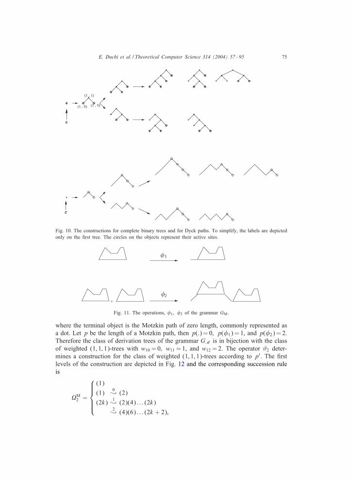
Example 20. Let GD be the grammar for Dyck paths de>ned in Example 12, and p bethe semi-length of a Dyck path. Then the class of derivation trees of the grammar isin bijection with the class of weighted (1; 0; 1)-trees with w10 = 0 and w12 = 1. Indeed,the grammar GD has only one terminal object, with semi-length 0, and one operation�2 of degree 2, such that p(�2) = 1. The operator #2 determines a construction for theweighted (1; 0; 1)-trees according to p′ and, consequently, it determines a constructionfor D according to p. Fig. 10 shows the >rst levels of the generating trees associatedwith the two constructions: the empty tree corresponds to an object of size 0 in theclass of Dyck paths, still represented by &. The construction determined by #2 leadsthen to the following succession rule:

D2 =

(1)

(1) 0❀ (1)

(k) 1❀ (2)(3) : : : (k + 1):

The generating function of D2 is 1+(1−√

1 − 4x)=2x, where (1−√1 − 4x)=2x de>nes

the sequence of Catalan numbers.

Example 21. In the plane Z×Z, we consider lattice paths using steps of three types:rise steps (1; 1), fall steps (1;−1), and horizontal steps of length 1 (1; 0). A Motzkinpath of length n is a sequence of rise, fall, and horizontal steps, running from (0; 0) to(n; 0), and remaining weakly above the x-axis. Let M be the class of Motzkin paths.The mappings �1 and �2, illustrated in Fig. 11, are object operations on M. The >rstis unary while the second is binary:• operation �1 adds an horizontal step at the beginning of the Motzkin path;• operation �2 takes a pair of Motzkin paths as its argument, adds a rise (resp. fall)

step at the beginning (resp. end) of the >rst path and then appends the second path.The class M is generated by the unidimensional object grammar

GM = 〈{M}; {{:}}; {�1; �2}; M〉;


(1 , 1)

(1 , 0) (1 , 0)

Fig. 10. The constructions for complete binary trees and for Dyck paths. To simplify, the labels are depictedonly on the >rst tree. The circles on the objects represent their active sites.

,

�1

�2

Fig. 11. The operations, �1; �2 of the grammar GM.

where the terminal object is the Motzkin path of zero length, commonly represented asa dot. Let p be the length of a Motzkin path, then p(:) = 0; p(�1) = 1, and p(�2) = 2.Therefore the class of derivation trees of the grammar GM is in bijection with the classof weighted (1; 1; 1)-trees with w10 = 0; w11 = 1, and w12 = 2. The operator #2 deter-mines a construction for the class of weighted (1; 1; 1)-trees according to p′. The >rstlevels of the construction are depicted in Fig. 12 and the corresponding succession ruleis

M2 =

(1)

(1) 0❀ (2)

(2k) 1❀ (2)(4) : : : (2k)2❀ (4)(6) : : : (2k + 2);


(1 , 0)

(1 , 2)

(1 , 0)

(1 , 1)

(1 , 0)

Fig. 12. The construction for the class of (1; 1; 1)-trees.

already introduced in Example 3. The generating function of M2 is 1 + (1 − x −√

1 − 2x − 3x2)=2x2, where (1−x−√1 − 2x − 3x2)=2x2 de>nes the sequence of Motzkin

numbers.

5. Extension to q-parameters

In this section we shall consider q-parameters in the case of unidimensional gram-mars. In particular, given a unidimensional grammar G, we de>ne a special class ofq-parameters on G, called natural q-parameters, and then we transport them into the


setting of the ECO system corresponding to the class O. In order to do it we >rst needto introduce the concept of parameterized succession rules.

The functional equations arising from these rules are solved by using the followinglemma, introduced in [6] by Bousquet-MFelou. Let us denote by f(s) any series of theform f(s; t; x; y; q).

Lemma 22 (Bousquet-MFelou). Let R[[s; t; x; y; q]] be the algebra of formal power se-ries in the variables s; t; x; y; q with real coe@cients. Let A be the sub-algebra ofR[[s; t; x; y; q]] such that the series converge for s= 1. Given A(s; t; x; y; q) a formalpower series in A, we suppose that:

A(s) = xe(s) + xf(s)A(1) + xg(s)A(sq);

where e(s); f(s); g(s) are some given power series in A. Then

A(s) =E(s) + E(1)F(s) − E(s)F(1)

1 − F(1);

where

E(s) =∑n¿0

xn+1g(s)g(sq) : : : g(sqn−1)e(sqn)

and

F(s) =∑n¿0

xn+1g(s)g(sq) : : : g(sqn−1)f(sqn):

Parameterized succession rules. Let �= (O; p; #; #) be an ECO system. Let usconsider the parameters p1; : : : ; ph, h∈N+, on the class O. Substantially, a parame-terized succession rule describes the e=ects determined by the ECO operator on thevalues of these parameters. It has the following form:

=

(a; a1; : : : ; ah)(k; p1; : : : ; ph) ❀ (e1(k); t11(k; p1; : : : ; ph); : : : ; th1(k; p1; : : : ; ph))

(e2(k); t12(k; p1; : : : ; ph); : : : ; th2(k; p1; : : : ; ph))...(ek(k); t1k (k; p1; : : : ; ph); : : : ; thk (k; p1; : : : ; ph))for k ∈ M; (p1; : : : ; ph) ∈ Nh;

(10)

where the set of labels is M ⊆ N+; a∈M , (a1; a2; : : : ah)∈Nh, and the tji are functionsM ×Nh → N, for all i; j.

Now, we introduce the class of natural q-parameters. Then we transport this kind ofparameter from unidimensional object grammars to ECO-systems.

De�nition 23. Let G = 〈O; E; �;A〉 be an object grammar. Let O;Oi ∈O for i= 1 : : : kand q be a parameter on O;O1; : : : ;Ok . Let �∈� be an object operation such that


dom(�) =O1 × · · · ×Ok and cod(�) =O. Then q is a natural q-parameter with respectto � if, for all (O1; : : : ; Ok)∈dom(�),

q(�(O1; : : : ; Ok)) =k∑

i=1q(Oi) +

k∑i=1

(k − i)t(Oi) + q(�);

where i∈N+; q(�)∈N, and t is a G-linear parameter on the grammar G.

Let G be a unidimensional object grammar, p a G-linear parameter, and q a naturalG−q-linear parameter with associated G-linear parameter t. Here, in order to deal withq-parameters, we naturally extend the de>nition of weighted $-trees (De>nition 14), byconsidering trees with labels of the form (i; wij; w′

ij ; w′′ij). Then we extend the bijection

between derivation trees and weighted $-trees, by taking w′ij = q(�i

j) and w′′ij = t(�i

j),for i= 1 : : : |�j| and j = 0 : : : d.

De�nition 24. Let T ∈Tw$G . For any x∈T the label of the node, denoted l(x), is

(co(x); w(x); w′(x); w′′(x)):

Then

q′(T ) =∑x∈T

(k(x)∑i=1

(k(x) − i)∑

y∈Ti;xw′′(y) + w′(x)

)

and

t′(T ) =∑x∈T

w′′(x):

From De>nition 24 and from Eq. (7) we obtain the following lemma:

Lemma 25. Let T ∈Tw$G , then q′(T ) = q(ev(T )).

Let us consider the ECO operator #2 de>ned in Section 4.2 for the class of weighted$-trees associated with G. Our aim is to de>ne a parameterized succession rule de-scribing the variation of the parameter q when the operator #2 is applied.

Lemma 26. Let T ∈Tw$G , and let T ′ be the tree obtained through #2 by adding a

tree S on the lth active site A of T . Then we have:

q′(T ′) − q′(T ) = (l− 1)(t′(S) − w′′(A)) + q(S) − w′(A):

Proof. Let b be the branch in T , starting from the root and ending at the father of A.Because of the de>nition of #2, only the subtrees of T having their root in b changethrough the application of #2. Since b is also the branch from the root of T ′ to the


father of the root of S, we have

q′(T ′) − q′(T ) =∑

x∈b∪S

(k(x)∑i=1

(k(x) − i)∑

y∈T ′i;x

w′′(y) + w′(x)

)

− ∑x∈b∪{A}

(k(x)∑i=1

(k(x) − i)∑

y∈Ti;xw′′(y) + w′(x)

)

=∑x∈b

k(x)∑i=1

(k(x) − i)

( ∑y∈T ′

i;x

w′′(y) − ∑y∈Ti;x

w′′(y)

)

+ q′(S) − w′(A):

For each x in b, let i(x) be the index of the subtree Ti;x that contains A. Since onlythe subtrees containing A change due to the application of #2, we have T ′

i;x =Ti;x fori = i(x) and T ′

i(x);x =Ti(x);x\{A} ∪ S. Hence

q′(T ′) − q′(T ) =∑x∈b

(k(x) − i(x))

( ∑y∈T ′

i(x);x

w′′(y) − ∑y∈Ti(x);x

w′′(y)

)

+ q′(S) − w′(A);

=∑x∈b

(k(x) − i(x))

(∑y∈S

w′′(y) − w′′(A)

)

+ q′(S) − w′(A):

Since A is an active site, the sons of x with index larger than i(x) are then active sites:the number of active sites attached to x is k(x) − i(x). Moreover, A is the lth activesite, and

q′(T ′) − q′(T ) = (l− 1)

(∑y∈S

w′′(y) − w′′(A)

)+ q′(S) − w′(A)

= (l− 1)(t′(S) − w′′(A)) + q′(S) − w′(A):

Thus we have that

q′(T ′) = q′(T ) + (l− 1)(t′(S) − w′′(A)) + q′(S) − w′(A): (11)

According to the de>nition of #2; S is a tree with j leaves, and the rightmostof these is A, for j = 1 : : : d. More precisely, S is associated with a derivation tree(�ij

j ; (�i0; 10 ; : : : ; �i0; j−1

0 ; A)). Therefore, Eq. (11) becomes

q′(T ′) = q′(T ) + (l− 1)

(t(�ij

j ) +j−1∑r=1

t(�i0;r0 )

)+

j−1∑r=1

(j − r)t(�i0;r0 )

+ q(�ijj ) +

j−1∑r=1

q(�i0;r0 ): (12)


Let us denote

R(S) = t(�ijj ) +

j−1∑r=1

t(�i0;r0 ); and

Q(S) =j−1∑r=1

(j − r)t(�i0;r0 ) + q(�ij

j ) +j−1∑r=1

q(�i0;r0 );

then

q′(T ′) = q′(T ) + (l− 1)R(S) + Q(S):

Now we have the variation of the parameter q when the operator #2 attaches j leaveson the lth active site. Therefore we can extend the succession rule 2 (see Section 4.2)to a parameterized succession rule considering also the parameter q. Observe that theaxiom of 2 corresponds to the empty tree, therefore in this case the value of q is 0.Then we obtain the following:

q2 =

($0; 0)

($0; 0)p(�

i00 )

❀ (c; q(�i00 ))

(kc; q)P(S)❀ (jc; q + Q(S))((j + 1)c; q + Q(S) + R(S))

: : : ((k + j − 1)c; q + Q(S) + (k − 1)R(S));

where there is a production for each tree S corresponding to a derivation tree (�ijj ; (�

i0; 10 ;

: : : ; �i0; j−1

0 ; A)) with j = 1 : : : d; ij = 1 : : : $j, and i0; r = 1 : : : $0, and where we have set

P(S) = p(�ijj ) +

j−1∑r=1

p(�i0;r0 );

R(S) = t(�ijj ) +

j−1∑r=1

t(�i0;r0 );

Q(S) =j−1∑r=1

(j − r)t(�i0;r0 ) + q(�ij

j ) +n−1∑r=1

q(�i0;r0 ): (13)

Example 27. An m-Dyck path is a path with steps (1; m) and (1;−1), going from(0; 0) to ((m+ 1)l; 0) with m∈N+ and l∈N, and remaining weakly above the x-axis.Let Dm be the set of m-Dyck paths. We want to enumerate these paths according tothe parameter area, de>ned as the sum of the ordinates of the endpoints of the risesteps. The mapping �m+1 is an object operation on Dm: it takes m + 1 m-Dyck paths,adds a rise step at the beginning of the >rst path, and attaches at its end an alternatingsequence of down steps and paths. See Fig. 13 for the case m= 3.

The class Dm is generated by the unidimensional object grammar

GDm = 〈{Dm}; {{:}}; {�m+1}〉;where the terminal object is the path of zero length, commonly represented as a dot.Let (m+1)l be the length of an m-Dyck path, and a its area. We easily see that a is a


,,,�3

Fig. 13. The object operation �3.

natural q-parameter with respect to the operation �m+1, since given d1; : : : ; dm+1 ∈Dm,the following relations hold:

l(:) = 0; l(�m+1(d1; : : : ; dm+1)) = l(d1) + · · · + l(dm+1) + 1;

a(:) = 0; a(�m+1(d1; : : : ; dm+1)) = a(d1) + · · · + a(dm+1)

+ml(d1) + (m− 1)l(d2) + · · ·+ l(dm) + m: (14)

The class of (1; 0; : : : ; 0︸︷︷︸m

; 1)-trees is the class of weighted $-trees associated with the

grammar GDm . Now, from the general rule q2 we obtain the parameterized succession

rule for the (1; 0; : : : ; 0︸︷︷︸m

; 1)-trees. In this case we have

l(�0) = 0; l(�m+1) = 1;

a(�0) = 0; a(�m+1) = m;

and t = l. Consequently, using the same notation as in (13), P(S) = 1; Q(S) =m andR(S) = 1 for j =m+ 1. Moreover, $0 = 1; c= 1, and the parameterized succession ruleis:

m =

(1; 0)

(1; 0) 0❀ (1; 0)

(k; a) 1❀ (m + 1; a + m)(m + 2; a + m + 1)

: : : (m + k; a + m + k − 1):

(15)

Let L be the set of nodes of the generating tree associated with ′m, where

′m =

(1; 0)

(k; a) 1❀ (m + 1; a + m)(m + 2; a + m + 1)

: : : (m + k; a + m + k − 1):(16)

Given v∈L, by l(v) we denote the level of v in the generating tree. Then the generatingfunction of m with respect to l; k, and a is

fm(x; y; q) = 1 + f′m(x; y; q);


where

f′m(x; y; q) =

∑v∈L

xl(v)yk(v)qa(v):

From ′m we obtain

f′m(x; y; q) = y + x

∑v∈L

xl(v)k(v)∑i=1

yi+mqa(v)+m+i−1

= y +xym+1qm

1 − yq(f′

m(x; 1; q) − f′

m(x; yq; q))

= y + xym+1qm

1 − yqf′

m(x; 1; q) − x

yqm

1 − yqf′

m(x; yq; q):

Now we can apply Lemma 22, where

e(y) =yx; f(y) =

ym+1qm

1 − yq; g(y) = −ym+1qm

1 − yq:

From Lemma 22 we have

f′m(x; 1; q) =

E(x; 1; q)1 − F(x; 1; q)

:

Let us denote E0(x; 1; q) =E(x; 1; q) and E1(x; 1; q) = 1 − F(x; 1; q), then

f′m(x; 1; q) =

E0(x; 1; q)E1(x; 1; q)

;

where

E0(x; 1; q) =∑n¿0

(−1)nxn

(q)nqn

n−1∏k=0

(q(m+1)k+m)

and

E1(x; 1; q) =∑n¿0

(−1)nxn

(q)n

n−1∏k=0

(q(m+1)k+m):

6. A multidimensional case: directed convex polyominoes

The main results in Section 4 give us an e=ective methodology to obtain an ECOsystem starting from any unambiguous, complete, and unidimensional grammar (The-orems 17 and 19). In this section we are going to treat the more general case ofmultidimensional object grammars.

Let G = 〈{O1;O2; : : : ;Om}; E; �;A〉 be a grammar with dimension m¿1, and p aG-linear parameter on G. As for the unidimensional case we introduce a suitable classof trees (weighted $-trees), and a >nite parameter p′ on it, such that the numberof trees with size n is equal to |An|. In the multidimensional case, the de>nition of


weighted $-trees shall take into consideration the fact that we are dealing with treeswhose nodes belong to m di=erent classes. Without loss of generality, throughout thesection we suppose that A=O1.

De�nition 28. Let m∈N+ and M = {1; : : : ; m}. Let us >x

$: $iw ∈ N; with i ∈ M and w ∈ M∗:

A weighted $-tree is a labelled tree whose nodes belong to m di=erent classes. Eachnode of class i with l sons of respective classes w1; : : : ; wl has a color

k ∈ {(i; 1; uiw(1)); (i; 2; uiw(2)); : : : (i; $iw; uiw($iw))};

where w=w1 : : : wl, and where uiw(j) is the weight associated with the jth color, forj = 1; : : : ; $iw. In particular for each node we must have $iw¿0.

Let i∈M and w∈M∗. We denote by �iw the subset of � with operations from

Ow1 ×Ow2 × · · · ×Owl to Oi ; wj being the jth term of w and l being its length. LetTG be the set of derivation trees of G, and let Tw$

G be the set of weighted $-treeswhere $iw = |�i

w| for i∈M and w∈M∗, and uiw(j) =p(�iw(j)) for all j = 1 : : : |�i

w|.As it happened for the unidimensional case, there is a simple bijection between the

classes TG and Tw$G . Indeed, for any T ∈TG, the corresponding tree T ′ is obtained by

replacing each label �iw(j) in the tree T by the label (i; j; p(�i

w(j))), and vice versa.In particular we have that the root of T ′ is obtained by replacing the label �1

w(j) ofthe root of T by the label (1; j; p(�1

w(j))), and vice versa.

De�nition 29. Let T ∈Tw$G . For any x∈T denote l(x) = (cl(x); co(x); u(x)) the label

of x. We de>ne

p′(T ) =∑x∈T

u(x):

By using the same arguments as in the previous sections we deduce that p′(T ) =p(ev(T )).

The authors have proved that, using De>nition 28, the statements in Theorems 17and 19 can be extended to the case of multidimensional grammars [12]. However, forthe sake of clarity we prefer to focus on an example. In particular, we will take intoconsideration the class of weighted $-trees associated with a three-dimensional objectgrammar generating the class of directed convex polyominoes. An ECO system for thisclass was >rst determined in [5], and some bijective results were established; in thissection we derive a completely new ECO system, with a form di=erent from that ofall the ECO systems known in literature.

First, let us brieMy recall some basic de>nitions. A polyomino is said to be column-convex [row-convex] when its intersection with any vertical [horizontal] line is convex.A polyomino is convex if it is both column and row convex. A polyomino is said tobe directed when each of its cells can be reached from a distinguished cell, calledthe root, by a path which is contained in the polyomino and uses only north and east


Fig. 14. A directed convex polyomino having semi-perimeter 17 and area 34.

unitary steps. A polyomino is directed-convex if it is both directed and convex (seeFig. 14). In [15] an object grammar for directed convex polyominoes is proposed:

GP1 = 〈{P1;P2;P3}; {{�1&}; ∅; {�3

&}};{�1

1; �131; �

12; �

21; �

22; �

232; �

33(1); �3

3(2); �333};P1〉;

where:(i) P1 is the class of directed convex polyominoes,

(ii) P2 is the class of directed convex polyominoes with one marked cell in their lastcolumn,

(iii) P3 is the class of parallelogram polyominoes.The operations �1

1; �22; �

131, and �2

32 are analogous to those de>ned for the grammarGP of parallelogram polyominoes. The operation �1

2 takes a polyomino in P2 and itglues a new cell to the right of the marked cell in the polyomino. Finally �2

1 takes apolyomino in P1 and marks the bottom cell of the last column. The object operationsof the grammar are graphically represented in Fig. 15. Thus we have

|�1& | = 1; |�1

1| = 1; |�131| = 1; |�1

2| = 1;

|�21| = 1; |�2

2| = 1; |�232| = 1;

|�3& | = 1; |�3

3| = 2; |�333| = 1; (17)

and, for each other set �iw, with i∈{1; 2; 3} and w∈{1; 2; 3}∗; |�i

w|= 0. Let p be thesemi-perimeter of a polyomino: it is a GP1 -linear parameter, and

p(�1& ) = 2; p(�1

1) = 1; p(�12) = 1; p(�1

31) = 0;

p(�21) = 0; p(�2

2) = 1; p(�232) = 0;

p(�3& ) = 2; p(�3

3(1)) = 1; p(�33(2)) = 1; p(�3

33) = 0: (18)

The de>nition of the grammar GP1 suggests that each weighted $-tree in Tw$G

P1has

nodes of 3 di=erent classes, and the root is of class 1. Moreover

$1& = 1; $1

1 = 1; $131 = 1; $1

2 = 1;

$21 = 1; $2

2 = 1; $232 = 1;

$3& = 1; $3

3 = 2; $333 = 1 (19)


= + + +�1

�11

�131

�12

= + +

�21

�22

�232

=�3

�33(1) �3

3(2)

� 333

+ ++

Fig. 15. The grammar for directed convex polyominoes.

with $iw = 0 for each other i∈{1; 2; 3} and w∈{1; 2; 3}∗. Table (20) shows the relationsbetween the possible labels of a node of a weighted tree and the classes of its sons(presented in the >rst line).

& 1 2 3 31 32 33(1; 1; 2) (1; 1; 1) (1; 1; 1) (3; 1; 1) (1; 1; 0) (2; 1; 0) (3; 1; 0)(3; 1; 2) (2; 1; 0) (2; 1; 1) (3; 2; 1)

(20)

For instance a node with one son of class 1 can be labelled (1; 1; 1) or (2; 1; 0). Fig. 16represents a tree of the class Tw$

GP1

.Now, we want to determine an ECO construction for the class Tw$

GP1

according to theparameter p′ (see De>nition 29). In a given tree T , let li(T ) (brieMy, li) be the lastinternal node in the pre-order traversal, and f(li) the number of leaves following li.We will divide Tw$

GP1

into >ve mutually disjoint subsets, basing both on the class of li,and on f(li). Observe that, by de>nition, li is not a leaf. Let us take into considerationthe following cases:(i) f(li) = 1: since li cannot be of class 3, the only leaf following li is of class 1

(therefore it is equal to (1; 1; 2)). There are two possible subcases:• li is of class 1 and it has one son of class 1 (li = (1; 1; 1)). This set of trees

is denoted by A. The other type of node of class 1 with one son cannot be thelast internal node in the pre-order transversal, since its son is of class 2.


(1,1,1)

(2,1,0)

(1,1,2)

(1,1,1)

(3,2,1)

(2,1,0)

(3,1,0)

(3,1,1)

(1,1,0)

(3,1,2)(3,1,2)

(1,1,1)

(2,1,1)

(2,1,0)

(3,1,2)

Fig. 16. A tree belonging to Tw$GP1

.

• li is of class 2 and it has one son of class 1 (li = (2; 1; 0)). Looking at table(20), we observe that the other type of node of class 2 with one son cannotbe the last internal node, since its son is of class 2. We then distinguish thefollowing subcases:◦ the father of li is of class 1, and it has one son of class 2 (therefore it is

equal to (1; 1; 1)): this set of trees is denoted by B. Observe that the othertypes of nodes of class 1 cannot be the father of the last internal node.

◦ the father of li is of class 2, and it has one son of class 2 (therefore it isequal to (2; 1; 1)): this set of trees is denoted by C.

◦ the father of li is of class 2, and it has two sons of classes 32 (therefore itis equal to (2; 1; 0)): this set of trees is denoted by E.We remark that the last type of a node of class 2 cannot appear as the fatherof li, since its son is of class 1. Moreover, we observe that the father of licannot be of class 3.

(ii) f(li)¿1: this set of trees is denoted by D. Observe that the last leaf following liis of class 1, and all the other ones are of class 3. Moreover, observe that li canbe only of classes 1 or 3.

In Fig. 17, a tree of each class de>ned above is presented. The trivial tree (1; 1; 2)does not belong to any of the above de>ned classes, and then we have:

Lemma 30. The family of sets {A; B; C; D; E}∪ {(1; 1; 2)} is a partition of Tw$G

P1.

6.1. The ECO construction for the trees associated with GP1

Let T$n be the set of trees belonging to Tw$

GP1

with p′ = n, and # an operator from T$n

to 2T$

n+1∪T$n+2 ; the action of # on a tree T ∈T$

n , depends on the belonging class of T :


(C)

(2,1,1)

(2,1,0)

(1,1,2)

(1,1,1)

(A)

(1,1,0)

(3,1,2) (1,1,1)

(1,1,2)

(3,1,0)

(1,1,0)

(1,1,2)

(1,1,1)

(3,1,2)(3,1,2)

(D)

(1,1,1)

(1,1,2)

(3,1,0)

(3,1,2)(3,1,2)

(2,1,0)

(2,1,0)

(E)

(B)

(3,1,0)

(3,1,2)(3,1,2)

(1,1,0)

(1,1,2)

(2,1,0)

(1,1,1)

Fig. 17. A tree for each class constituting Tw$GP1

.

(1,1,1)

(1,1,1)

(1,1,2)

(1,1,0)

(3,1,2) (1,1,2)

(1,1,1)

(1,1,2)

(1,1,1) (1,1,1)

(1,1,1)

(1,1,2)

(2,1,0)

Fig. 18. The operator # on a tree belonging to A.

(a) T is the leaf (1; 1; 2) or T belongs to A (see Fig. 18). Let us call L the only leaffollowing li. If T = (1; 1; 2) then L= (1; 1; 2). Then:(i) # produces a tree with 1 new son having label (1; 1; 2), attached to L. Thus

L becomes an internal node with a son of class 1 and it is labelled (1; 1; 1).The new tree belongs to A and the value of the parameter p′ increases byone.


(1,1,2)

(2,1,0)

(1,1,1)

(2,1,0)

(1,1,1)

(1,1,2)

(1,1,1)

(2,1,1)

(1,1,1)

(1,1,2)

(2,1,0)

(2,1,0)

(1,1,1)

(1,1,1)

(2,1,0)

(1,1,2)

(2,1,0)

(1,1,0)

(3,1,2) (1,1,2)

(1,1,1)

Fig. 19. The operator # on a tree belonging to B.

(ii) # replaces L with the tree ((1; 1; 1); ((2; 1; 0); (1; 1; 2))). The new tree obtainedthrough # belongs to B, and the value of the parameter p′ increases by one.

(iii) # produces a tree with 2 new sons attached to L. The label of the left sonis (3; 1; 2) and that of the right one is (1; 1; 2). Thus L becomes an internalnode with two sons (of classes 31) and it is labelled (1; 1; 0). The new treebelongs to D and the value of the parameter p′ increases by two.

(b) T belongs to B (see Fig. 19). In this case # performs on T the operations (i)–(iii) de>ned in (a), thus obtaining three new trees belonging to A; B, and D,respectively. Moreover,(iv) # substitutes li with the tree ((2; 1; 1); (2; 1; 0)). The new tree obtained through

# belongs to C and the value of p′ increases by one.(c) T belongs to C (see Fig. 20). In this case # performs the operations (i)–(iv)

described in (a), and (b). The trees obtained belong to A; B; C, and D, respectively.Moreover # performs a further operation on the father F of li:(v) it attaches a left son labelled (3; 1; 2) to F . Thus F becomes a node with two

sons (of classes 32) and it has label (2; 1; 0). The tree obtained belongs to Eand the parameter p′ increases by one.

(d) T belongs to D (see Fig. 21). In this case # performs the transformations describedin (i), (ii), (iii) on the last leaf following li in the pre-order transversal, thusobtaining three trees belonging to A; B, and D, respectively. Moreover it makes afurther operation on each leaf L following li, except the last one:


(2,1,1)

(1,1,1)

(1,1,2)

(2,1,0)(1,1,0)

(3,1,2) (1,1,2)

(1,1,1)

(2,1,1)

(2,1,0)

(2,1,1)

(2,1,1)

(1,1,1)

(2,1,0)

(1,1,2)

(2,1,0)

(3,1,2) (2,1,0)

(1,1,1)

(1,1,2)

(2,1,1)

(2,1,0)

(1,1,1)

(1,1,1)

(1,1,2)

(2,1,0)

(1,1,1)

(2,1,0)

(1,1,2)

(1,1,1)

(2,1,1)

Fig. 20. The operator # on a tree belonging to C.

(vi) for i∈{1; 2}; # attaches i new sons labelled (3; 1; 2) to L. At this stage L isan internal node with i sons of class 3. If i= 1 then L can be labelled in 2ways (i.e. (3; 1; 1), or (3; 2; 1)), otherwise it is labelled (3; 1; 0).

The obtained new trees still belong to the class D, and the value of the parameterp′ increases by one when i= 1, otherwise it increases by two.Summarizing, let T be a tree of size n; if the number of leaves following li isk + 1, the application of # to T produces: 3 trees of type A; B, and D (the >rsttwo of size n + 1, the last one of size n + 2). Moreover # produces 2k trees oftype D of size n + 1, and k trees of type D of size n + 2.

(e) T belongs to E (see Fig. 22). In this case # performs the operations (i), (ii), (iii),and (iv) on the (only) leaf following li, thus obtaining trees belonging to A; B; C,and D. Moreover # performs the operation (vi) on each leaf following the last butone internal node, except the last one. In this case, the obtained trees still belongto E.Finally, let T be a tree of size n; if the number of leaves following the last butone internal node is k + 1, the application of # to T produces: 3 trees of type


A; B; C, of size n + 1; one tree of type D, of size n + 2; 2k trees of type E, ofsize n + 1; k trees of type E, of size n + 2.

Fig. 23 represents the >rst levels of the generating tree associated with the operator#. For simplicity at level 3 only one tree has been developed.

Theorem 31. The system �= (T$G

P1; p′; #; ) is an ECO-system, where:

=

(3)a

(3)a1❀ (3)a(4)b2❀ (6)d

(4)b1❀ (3)a(4)b(5)c2❀ (6)d

(5)c1❀ (3)a(4)b(5)c(7)e2❀ (6)d

(3k + 3)d1❀ (3)a(4)b2❀ (6)d1❀ (6)2

d : : : (3k + 3)2d

2❀ (6 + 3)d : : : (3(k + 1) + 3)d

(3k + 4)e1❀ (3)a(4)b(5)c2❀ (6)d1❀ (3 + 4)2

e : : : (3k + 4)2e

2❀ (6 + 4)e : : : (3(k + 1) + 4))e:

Proof. The operator # satis>es the conditions of Proposition 2.1. for each T ′ ∈T$

n there is T ∈ ⋃2j=1 T$

n−j such that T ′ ∈#(T ). Let li be the lastinternal node of T ′. We distinguish the following cases:(a) T ′ belongs to A. Then T is obtained by replacing the subtree (of T ′) of root li

with the leaf (1; 1; 2).(b) T ′ belongs to B. Then T is obtained by replacing the subtree whose root is the

father of li, with the leaf (1; 1; 2).(c) T ′ belongs to C. Then T is obtained by replacing the subtree whose root is the

father of li with the tree ((2; 1; 0)(1; 1; 2)).(d) T ′ belongs to D. Then we must distinguish two cases:

• li is a node of class 1 with two sons, i.e. (1; 1; 0). Then T is obtained byreplacing the subtree of root li with the leaf (1; 1; 2).


(1,1,0)

(3,1,2)

(3,1,0)

(3,1,2) (3,1,1)

(1,1,0)

(3,1,2) (1,1,2)

(1,1,0)

(1,1,2)(3,1,0)

(3,1,2) (3,1,1)

(3,1,0)

(3,1,2) (3,1,2)

(1,1,0)

(1,1,2)(3,1,0)

(3,1,2) (3,1,1)

(3,1,2)

(1,1,0)

(3,1,2)

(3,1,0)

(3,1,2) (3,1,1)

(1,1,1)

(1,1,2)

(1,1,0)

(3,1,2)

(3,1,0)

(3,1,2) (3,1,1)

(1,1,1)

(2,1,0)

(1,1,2)

(1,1,0)

(3,1,0)

(3,1,2) (3,1,1)

(1,1,2)

(3,1,2)

(3,1,1)

(1,1,0)

(3,1,0)

(3,1,2) (3,1,1)

(1,1,2)

(3,1,2)

(3,2,1)

Fig. 21. The operator # on a tree belonging to D.

• li is a node of class 3. Then T is obtained by replacing the subtree of rootli with the leaf (3; 1; 2).

(e) T ′ belongs to E. Then we must distinguish two cases:• the last but one internal node is a node of class 2 with two sons, i.e. (2; 1; 0).

Then T is obtained by replacing the subtree whose root is the last but oneinternal node, with the tree ((2; 1; 1); ((2; 1; 0)(1; 1; 2))).

• the last but one internal node is a node of class 3. Then T is obtained byreplacing the subtree whose root is the last but one internal node, with theleaf (3; 1; 2).

2. for each T ∈T$n ; T ′ ∈T$

m such that T =T ′; #(T )∩#(T ′) = ∅. This can be easilydeduced from the construction.

7. Future work

The method we have proposed in the previous sections allows us to pass froman object grammar to an “equivalent” ECO system. However, concerning our initial


(1,1,2)

(2,1,0)

(2,1,0)

(1,1,1)

(2,1,1)(3,1,2)

(1,1,2)

(2,1,0)

(1,1,1)

(2,1,0)(3,1,1)

(3,1,2)

(1,1,2)

(2,1,0)

(1,1,1)

(2,1,0)(3,2,1)

(3,1,2)

(2,1,0)

(1,1,1)

(2,1,0)

(3,1,2)

(1,1,1)

(2,1,0)

(1,1,2)

(2,1,0)

(3,1,2)

(1,1,2)

(1,1,1)

(2,1,0)

(1,1,2)

(2,1,0)

(1,1,1)

(2,1,0)(3,1,0)

(3,1,2) (3,1,2)

(2,1,0)(3,1,2)

(1,1,0)

(3,1,2) (1,1,2)

(2,1,0)

(1,1,1)

(2,1,0)

(1,1,1)

(1,1,2)

(2,1,0)

(3,1,2)

(1,1,1)

Fig. 22. The operator # on a tree belonging to E.

purpose to create a bond between ECO method and object grammars, much workremains to be done. Hereafter we underline one of the main topics that the authors arenow carrying on.

In [16] FFedou and Garcia developed a new method in order to determine the gen-erating function of some algebraic succession rules. In practice, starting from an ECOsystem � for a certain class O, each object with size n can be easily represented as aword of length n of a noncommutative formal power series S� over an in>nite alpha-bet. In several cases it is possible to determine a recursive decomposition of S� usingother auxiliary formal power series, and then obtain an algebraic system of equationsby taking the commutative image of S�. Finally, the solution of this system producesthe desired generating function for the class O.

In a successive work [9], the authors show how, applying the ideas in [16], itis possible to derive an object grammar for the classes of convex polyominoes, andcolumn-convex polyominoes, starting from a simple ECO system.


(2,1,0)

4

(1,1,2)

(1,1,1)

(2,1,0)

210

(1,1,2)

(2,1,0)

(1,1,1)

(1,1,2)

(1,1,1)

(2,1,1)

3

(2,1,0)

(1,1,2)

(1,1,1)

(1,1,2)

(2,1,0)

(1,1,1)

(1,1,1)

(2,1,1)

(1,1,2)

(2,1,0)

(1,1,1)

(2,1,1)

(2,1,0)

(1,1,2)

(1,1,1)

(2,1,1)

(1,1,0)

(2,1,0)

(3,1,2) (2,1,0)

(1,1,1)

(1,1,2)

(1,1,2)

(1,1,1)

(1,1,1)

(2,1,0)

(1,1,2)

(1,1,1)

(1,1,1)

(1,1,1)

(1,1,2)

(1,1,1)

(2,1,0)

(1,1,0)

(1,1,1)

(2,1,0)

(1,1,2)

(1,1,1)

(3,1,2)

(1,1,1)

(1,1,2)

(2,1,1)

(3,1,2) (1,1,2)

(1,1,0)

(3,1,2) (1,1,2)

(2,1,0)

(1,1,1)

�

Fig. 23. The >rst levels of the generating tree of #.

In some future work, we plan to apply the methodology proposed in [10] in orderto treat a great number of combinatorial structures, and in particular some structuresfor which the ECO approach does not bring to enumerative results (for example: per-mutations avoiding subsequences of the form (1; 2; : : : ; k), k ∈N, walks in the slitplane).

By a theoretical point of view we are interested in developing a general methodologyto pass from an ECO system to an “equivalent” object grammar. In some sense thiswould constitute the inversion of the process presented in the present work, and thencomplete the study of the relationship between ECO and object grammars.


Acknowledgements

The authors wish to thank the anonymous referees for suggestions that greatly im-proved the quality of the paper. The author also would like to thank Robert BobSulanke and Gilles Schae=er for providing interesting comments.

References

[1] S. Bacchelli, E. Barcucci, E.Grazzini, E. Pergola, Exhaustive generation of combinatorial objects byECO, preprint.

[2] C. Banderier, M. Bousquet-MFelou, A. Denise, P. Flajolet, D. Gardy, D. Gouyou-Beauchamps, Generatingfunctions for generating trees, Discrete Math. 246 (2002) 29–55.

[3] E. Barcucci, A. Del Lungo, E. Pergola, R. Pinzani, ECO: a methodology for the enumeration ofcombinatorial objects, J. Di=erence Equations Appl. 5 (1999) 435–490.

[4] E. Barcucci, A. Del Lungo, E. Pergola, R. Pinzani, Random generation of trees and other combinatorialobjects, Theoret. Comput. Sci. 218 (1999) 219–232.

[5] E. Barcucci, A. Frosini, S. Rinaldi, Directed-convex polyominoes: ECO method and bijective results,in: R. Brak, O. Foda, C. Greenhill, T. Guttman, A. Owczarek (Eds.), Proc. Formal Power Series andAlgebraic Combinatorics, 2002, Melbourne, # 9.

[6] M. Bousquet-MFelou, A method for the enumeration of various classes of column-convex polygons,Discrete Math. 154 (1996) 1–25.

[7] M. Bousquet-MFelou, M. PetkovQsek, Linear recurrences with constant coeRcients: the multivariate case,Discrete Math. 225 (2000) 51–75.

[8] F.R.K. Chung, R.L. Graham, V.E. Hoggatt, M. Kleimann, The number of Baxter permutations,J. Combin. Theory Ser. A 24 (1978) 382–394.

[9] M. Delest, J.M. FFedou, Attribute grammars are useful for combinatorics, Theoret. Comput. Sci. 98(1992) 65–76.

[10] A. Del Lungo, E. Duchi, A. Frosini, S. Rinaldi, Enumeration of convex polyominoes using the ECOmethod, Discrete Models for Complex Systems, DMCS’03, in: M. Morvan, E. Remila (Eds.), DiscreteMathematics and Theoretical Computer Science Proc. AB, 2003, pp. 103–116.

[11] E. Deutsch, L. Ferrari, S. Rinaldi, Production matrices, preprint.[12] E. Duchi, ECO method and object grammars: two methods for the enumeration of combinatorial objects,

Tesi dell’UniversitUa degli Studi di Firenze, 2003.[13] I. Dutour, Grammaires d’objets: FenumFeration, bijections et gFenFeration alFeatoire, ThUese del’UniversitFe de

Bordeaux I, 1996.[14] I. Dutour, J.M. FFedou, Object grammars and random generation, Discrete Math. Theoret. Comput. Sci.

2 (1998) 47–61.[15] I. Dutour, J.M. FFedou, Object grammars and bijections, Theoret. Comput. Sci. 290 (2003) 1915–1929.[16] J.M. FFedou, C. Garcia, Algebraic succession rules, Proceedings of the 14th International Conference on

Formal Power Series and Algebraic Combinatorics, Melbourne, 2002.[17] L. Ferrari, E. Pergola, R. Pinzani, S. Rinaldi, Jumping succession rules and their generating functions,

Discrete Math. 271 (2003) 29–50.[18] P. Flajolet, R. Sedgewick, Analytic Combinatorics—Symbolic Combinatorics, available at http://algo.

inria.fr/flajolet/Publications/books.html (2002).[19] P. Flajolet, P. Zimmermann, B. Van Cutsem, A calculus for the random generation of labelled

combinatorial structures, Theoret. Comput. Sci. 132 (1994) 1–35.[20] D.E. Knuth, Semantics of context-free languages, Math. Systems Theory 2 (1968) 127–145, and errata

in 1971.

http://algo.inria.fr/flajolet/Publications/books.html

http://algo.inria.fr/flajolet/Publications/books.html


[21] D. Merlini, M.C. Verri, Generating trees and proper Riordan Arrays, Discrete Math. 218 (2000)167–183.

[22] M. Mishna, Attribute grammars and automatic complexity analysis, Adv. Appl. Math. 30 (2003)189–207.

[23] N.J.A. Sloane, S. Plou=e, The Encyclopedia of Integer Sequences, Academic Press, New York, 1996.[24] J. West, Generating trees and the Catalan and SchrYoder numbers, Discrete Math. 146 (1995) 247–262.[25] H.S. Wilf, Generating Functionology, Academic Press, San Diego, 1992.

from object grammars to eco systems

Documents