flexible pavement design and management n

160

FEB 17 1976

MAT. LAB.

NATIONAL COOPERATIVE HIGHWAY RESEARCH PROGRAM 160 REPORT

FLEXIBLE PAVEMENT DESIGN AND MANAGEMENT

SYSTEMS APPROACH IMPLEMENTATION

IDAHO TRArtISPORTATION DEPARTMENT

RESEARCH LIBRARY

N

TRANSPORTATION RESEARCH BOARD -NATIONAL RESEARCH COUNCIL

Cpy Refer To: Act Inf

Mat'Is. Supv.________

Asst. Mat's. Engr.

Mat'Is. Engr. II

Qu&. Cort.

'c!s&Lna.

____ Tasing C,i3f

Chn - As,h.

Soils- Agg Mix

StrConcInsp.

Moscow Lab.

/

J

cC

- 7

TRANSPORTATION RESEARCH BOARD 1975

Officers

MILTON PIKARSKY, Chairman

HAROLD L. MICHAEL, Vice Chairman

W. N. CAREY, JR., Executive Director

Executive Committee

HENRIK E. STAFSETH, Executive Director, American Assn. of State Highway and Transportation Officials (ex officio)

NORBERT T. TIEMANN, Federal Highway Administrator, U.S. Department of Transportation (ex officio)

ROBERT E. PATRICELLI, Urban Mass Transit Administrator, U.S. Department of Transportation (ex officio) ASAPH H. HALL, Acting Federal Railroad Administrator, U.S. Department of Transportation (ex officio) HARVEY BROOKS, Chairman, Commission on Sociotechnical Systems, National Research Council

WILLIAM L. GARRISON, Director, Inst. of Transp. and Traffic Eng., University of California (ex officio, Past Chairman 1973) JAY W. BROWN, Director of Road Operations, Florida Department of Transportation (ex officio, Past Chairman 1974) GEORGE H. ANDREWS, Vice President (Transportation Marketing) Sverdrup and Parcel

MANUEL CARBALLO, Secretary of Health and Social Services, State of Wisconsin

S. CRANE, Executive Vice President (Operations), Southern Railway System

JAMES M. DAVEY, Managing Director, Detroit Metropolitan Wayne County Airport

LOUIS J. GAMBACCINI, Vice President and General Manager, Port Authority Trans-Hudson Corporation

HOWARD L. GAUTHIER, Professor of Geography, Ohio State University ALFRED HEDEFINE, Senior Vice President, Parsons, Brinckerhoff, Quade and Douglas

ROBERT N. HUNTER, Chief Engineer, Missouri State Highway Commission

SCHEFFER LANG, Assistant to the President, Association of American Railroads

BENJAMIN LAX, Director, Francis Bitter National Magnet Laboratory, Massachusetts Institute of Technology

DANIEL McFADDEN, Professor of Economics, University of California HAROLD L. MICHAEL, School of Civil Engineering, Purdue University

D. GRANT MICKLE, Bethesda, Md. JAMES A. MOE, Executive Engineer, Hydro and Community Facilities Division, Bechtel, Inc.

MILTON PIKARSKY, Chairman of the Board, Chicago Regional Transportation Authority

J. PHILLIP RICHLEY, Vice President (Transportation), Dalton, Dalton, Little and Newport

RAYMOND T. SCHULER, Commissioner, New York State Department of Transportation

WILLIAM K. SMITH, Vice President (Transportation), General Mills

R. STOKES, Executive Director, American Public Transit Association PERCY A. WOOD, Executive Vice President and Chief Operating Officer, United Air Lines

NATIONAL COOPERATIVE HIGHWAY RESEARCH PROGRAM

Advisory Committee

MILTON PIKARSKY, Chicago Regional Transportation Authority (Chairman) HAROLD L. MICHAEL, Purdue University HENRIK E. STAFSETH, American Association of State Highway and Transportation Officials

NORBERT T. TIEMANN, U.S. Department of Transportation HARVEY BROOKS, National Research Council WILLIAM L. GARRISON, University of California JAY W. BROWN, Florida Department of Transportation W. N. CAREY, JR., Transportation Research Board

General Field of Design Area of Parements Advisory Panel for Project Cl-bA

H. T. DAVIDSON, Retired (Chairman) P. G. VELZ, Minnesota Department of Highways

W. B. DRAKE, Kentucky Department of Transportation A. S. VESIC, Duke University

WILLIAM GARTNER, JR., Florida Department of Transportation E. J. YODER, Purdue University

H. HAVENS, Kentucky Department of Highways RICHARD A. McCOMB, Federal Highway Administration

FRANK L. HOLMAN, JR., Alabama Highway Department L. F. SPAINE, Transportation Research Board

JAMES F. SHOOK. University- of Waterloo (Ontario) J. W. GUINNEE, Transportation Research Board

Program Staff

W. HENDERSON, JR., Program Director DAVID K. WITHEFORD, Assistant Program Director HARRY A. SMITH, Projects Engineer

LOUIS M. MAcGREGOR, Ad,ninistratime Engineer ROBERT E. SPICHER, Projects Engineer

JOHN E. BURKE, Projects Engineer HERBERT P. ORLAND, Editor

R. IAN KINGHAM, Projects Engineer PATRICIA A. PETERS, Associate Editor

ROBERT J. REILLY, Projects Engineer EDYTHE T. CRUMP, Assistant Editor

NATIONAL COOPERATIVE HIGHWAY RESEARCH PROGRAM -60 REPORT


SYSTEMS APPROACH IMPLEMENTATION R. L. LYTTON, W. F. McFARLAND,

AND D. L. SCHAFER

TEXAS A&M UNIVERSITY

COLLEGE STATION, TEXAS

RESEARCH SPONSORED BY THE AMERICAN ASSOCIATION OF STATE HIGHWAY AND TRANSPORTATION OFFICIALS IN COOPERATION WITH THE FEDERAL HIGHWAY ADMINISTRATION

AREAS OF INTEREST:

PAVEMENT DESIGN

BITUMINOUS MATERIALS AND MIXES

MAINTENANCE, GENERAL

FOUNDATIONS, SOILS

TRANSPORTATION RESEARCH BOARD NATIONAL RESEARCH COUNCIL

WASHINGTON, D.C. 1975

N

NATIONAL COOPERATIVE HIGHWAY RESEARCH PROGRAM NCHRP Report 160

Systematic, well-designed research provides the most ef-fective approach to the solution of many problems facing highway administrators and engineers. Often, highway problems are of local interest and can best be studied by highway departments individually or in cooperation with their state universities and others. However, the accelerat-ing growth of highway transportation develops increasingly complex problems of wide interest to highway authorities. These problems are best studied through a coordinated program of cooperative research.

In recognition of these needs, the highway administrators of the American Association of State Highway and Trans-portation Officials, initiated in 1962 an objective national highway research program employing modern scientific techniques. This program is supported on a continuing basis by funds from participating member states of the Association and it receives the full cooperation and support of the Federal Highway Administration, United States Department of Transportation.

The, Transportation Research Board of the National Re-search Council was requested by the Association to admin-ister the researcb program because of the Board' recog-nized objectivity and understanding of modern research practices. The Board is uniquely suited for this purpose as: it maintains an extensive committee structure from which authorities on any highway transportation subject may be drawn; it possesses avenues of comm unications and cooperation with federal, state, and local governmental agencies, universities, and industry; its relationship to its parent organization, the National Academy of Sciences, a private, nonprofit institution, is an insurance of objectivity; it maintains a full-time research correlation staff of special-ists in highway transportation matters to bring the findings of research directly to those who are in a position to use them.

The program is developed on the basis of research needs identified by chief administrators of the highway and trans-portation departments and by committees of AASHTO. Each year, specific areas of research needs to be included in the program are proposed to the Academy and the Board by the American Association of State Highway and Trans-portation Officials. Research projects to fulfill these needs are defined by the Board, and qualified research agencies are selected from those that have submitted proposals. Ad-ministration and surveillance of research contracts are responsibilities of the Academy and its Transportation Research Board.

The needs for highway research are many, and the National Cooperative Highway Research Program can make signifi-cant contributions to the solution of highway transportation problems of mutual concern to many responsible groups. The program, however, is intended to complement rather than to substitute for or duplicate other highway research programs.

Project 1-10A FY '72 ISBN 0-309-02339-4 L. C. Catalog Card No. 75-34977

Price: $4.00

Notice

The project that is the subject of this report was a part of the National Cooperative Highway Research Program conducted by the Transportation Research Board with the approval of the Governing Board of the National Research Council, acting in behalf of the National Academy of Sciences. Such approval reflects the Governing Board's judgment that the program concerned is of national impor-tance and appropriate with respect to both the purposes and re-sources of the National Research Council. The members of the advisory committee selected to monitor this project and to review this report were chosen for recognized scholarly competence and with due consideration for the balance of disciplines appropriate to the project. The opinions and con-clusions expressed or implied are those of the research agency that performed the research, and, while they have been accepted as appropriate by the advisory committee, they are not necessarily those of the Transportation Research Board, the National Research Coun7 cil, the National Academy of Sciences, or the program sponsors. Each report is reviewed and processed according to procedures established and monitored by the Report Review Committee of the National Academy of Sciences. Distribution of the report is ap-proved by the President of the Academy upon satisfactory comple-tion of the review process. The National Research Council is the principal operating agency of the National Academy of Sciences and the National Academy of Engineering, serving government and other organizations. The Transportation Research Board evolved from the 54-year-old High-way Research Board. The TRB incorporates all former HRB activities but also performs additional functions under a broader scope involving all modes of transportation and the interactions of transportation with society.

Published reports of the


are available from:

Transportation Research Board National Academy of Sciences 2101 Constitution Avenue, N.W. Washington, D.C. 20418

(See last pages for list of published titles and prices)

Printed in the United States of America.

FOREVVORD This report describes an operational computer program (SAMP6) that provides a

By Stafi basis for selecting flexible pavement design and management strategies with the lowest predicted total cost over a prescribed analysis period when considering such cost

Transportation elements as initial construction, routine maintenance, periodic rehabilitation, interest

Research Board on investment, salvage value, and roadway user costs. The program uses the AASHTO Interim Guides as its structural subsystem and the predicted decrease in serviceability with time and traffic as developed at the AASHO Road Test. It has been pilot tested in three states and found to be implementable where suitable com-puter facilities and personnel are available. A certain amount of modification of the current system is likely to be needed to reflect the unique facets of an individual agency's approach to pavement design. The report will be of particular interest to administrators who must make policy decisions concerning use' of the systems approach to pavement design and management; to pavement designers who will be involved in its implementation; and to materials, soils, maintenance, and traffic engineers who provide the input information for its operation.

One of the first activities of the Highway Research Board (formed more th'an 50 years ago, and recently renamed the Transportation Research Board to reflect its actual scope of operation) was to investigate the economics of highway improve-ments. At its Fourth Annual Meeting, in December 1924, the Committee on Eco-nomic Theory of Highway Improvements reported that the superiority of aggregate-surfaced roads over ordinary earth roads was generally conceded, but highway officials were plagued with the question of whether aggregate surfacing was a good investment from a financial standpoint. A study conducted at that time determined that, on the basis of the cost of the road itself, including such items as interest on investment and maintenance, and the cost of operation of the vehicles using the road, a good aggregate-surfaced road was less costly in terms of total annual cost of trans-portatioii per mile than either an earth-surfaced or a paved road when traffic aver-aged 100 vehicles per day. After this early interest in the economics of highway improvements, emphasis shifted to the structural design of pavements to withstand the effects of traffic and environmental condItions.

In recent years there has been renewed interest Within the highway field in the concept of total cost analysis. Acceptance of the systems approach to the design and management of pavements is a most timely development because new legislative funding likely will apply to all modes of transportation. Therefore, determination of the total cost of movement of people, goods, and services will be necessary to determine priorities for use of funds and material resources. A Systems Analysis Model for Pavements (SAMP5), as' described in NCHRP Report 139, "Flexible Pavement Design and Management—Systems Formulation," is one approach to considering initial construction, operational, and user costs in the decision-making process.

The responsibility of the Texas A&M researchers, under Project 1-1A, was to finalize SAMP5 as an operational computer program, including preparation of a users' guide, and to pilot test the program in several states. The project was success-ful in that the systems model (now designated as SAMP6) has been modified to include full roadbed cross sections, variable unit costs with quantity and time, stochastic variability of some variables, environmental roughness, and a modified structural subsystem. The program has also been modularized into distinct sub-systems that can be replaced or reprogrammed with a minimum of effort and placed on magnetic tape. Trial implementation of the SAMP6 program has been under-taken in Florida, Kansas, and Louisiana, with the finding that SAMP6 is a useful tool in the pavement design and management process.

Use of the systems approach to pavement design and management, and more specifically the operational SAMP6 program, provides highway decision-makers with the capability for comprehensively selecting optimum strategies and updating decisions as conditions change. By using computer techniques, a large number of parameters and their interactions (as many as several thousand combinations for one problem) can be evaluated within realistic time and cost limitations. Optimiza-tion is normally based on lowest total cost over the analysis period, but other parameters—such as user costs, initial construction costs, use of materials, or re-habilitation programs—can be optimized by proper program control. The strategy selection capability primarily is a quantitative procedure for considering the long-term advantages and disadvantages of staged construction versus strong initial struc-tural designs, thus providing a basis for more objective decision-making. The capability of quantitatively updating decisions is a unique feature of the approach. Existing pavements, as well as those being designed, can be analyzed in terms of optimization and strategy selectiOn, and decisions affecting them can be revised in view of changes in material costs, material availability, funds availability, and traffic conditions.

The researchers have identified several areas for improvement of the program, including (1) development of a rigid pavement system so that both portland cement and asphaltic pavements can be considered simultaneously and (2) development of a new flexible pavement structural subsystem based on mechanistic models. The latter is the objective of NCHRP Project 1-10B, "Development of Pavement Struc-tural Subsystems," scheduled to be completed in 1976.

Appendices B, C, G, and H, containing SAMP6 computer program documenta-tion and a users' guide, are of primary value to persons directly involved in opera-tion of the program. They are not included in this report but are available on a loan basis, as are copies of the SAMP6 program on magnetic tape, from the Program Director, NCHRP, Transportation Research Board, 2101 Constitution Ave., N.W., Washington, D.C. 20418.

CONTENTS

1 SUMMARY

PART I

2 CHAPTER ONE Introduction and Research Approach

Purpose and Scope Objectives Background Research Approach

4 CHAPTER TWO Findings

Systems Approach The SAMP6 Computer Program Input SAMP6 Computer Program Pilot Implementation of SAMP6 SAMP6 Program Changes SAMP6 Documentation SAMP6 Users' Guide Sensitivity Analyses Pavement Data Feedback Systems

17 CHAPTER THREE Interpretation and Appraisals

SAMP6 Strategy Strategic Benefits of Using SAMP6 Evaluation of Best Uses for SAMP6 Implementation of SAMP6 SAMP6 Adaptability

20 CHAPTER FOUR Conclusions and Research Recommendations

22 REFERENCES

PART II

24 APPENDIX A Discussion of SAMP6 Computer Program

40 APPENDIX B SAMP6 Computer Program Documentation

40 APPENDIX C SAMP6 Users' Guide

40 APPENDIX D SAMP6 Sensitivity Analysis

48 APPENDIX E States' Evaluations and Expected Use of SAMP6

51 APPENDIX F States' Evaluations of SAMP6 Data Inputs and Pavement Feedback Data Systems

53 APPENDIX G Pavement Feedback Data Systems

53 APPENDIX H Computer Software for Pavement Feedback Data Systems

ACKNOWLEDGMENTS

The research reported herein was conducted by the Texas Trans-portation Institute of Texas A&M University; Robert L. Lytton served as Principal Investigator, William F. McFarland served as Co-Principal Investigator, and Frank H. Scrivner served as Program Manager. Dale Schafer and Chester Michalak assisted with making computer program changes and preparing program documentation. Other Institute staff members gave suggestions and provided assistance through various phases of the research.

The authors are especially grateful to the numerous individ-uals in the pilot implementation states who participated in the study through development, implementation, and evaluation of the SAMP6 system. Among the state highway administrators who helped with over-all coordination and provided leadership in implementation were: John D. McNeal, State Highway En-gineer and R. R. Biege, Engineer of Location and Design Con-cepts, State Highway Commission of Kansas; William Gartner, Assistant State Highway Engineer, Koerner Schenk, Assistant State Highway Engineer, and Robert Orth, Engineer of Prelimi-nary Location and Design, Florida Department of Transporta-

tion; and Roger Guissinger, Executive Administrator, Louisiana Department of Highways.

To the numerous other individuals in the pilot states who helped with developing SAMP6, collecting data, running pro-grams, and providing evaluations go special thanks. These in-dividuals include: for Florida, Steve Sklute, Engineer of Pave-ment Design, Jatinder Sharma, Assistant Engineer of Pavement Design, and Steve Fuller, Research Engineer; for Kansas, G. Norman Clark, Soils Engineer, and Herb Worley, Pavement Re-search Engineer; for Louisiana, Ali S. Kemahli, Soils Design Engineer, J. B. Esnard, Assistant Soils Design Engineer, and Steve Spohrer. Other individuals, too numerous to list, partici-pated in one or more of the pilot study meetings and thanks are extended to them also. Acknowledgment also is given to J. L. Brown of the Texas Highway Department and W. R. Hud-son and B. F. McCullough of the Center for Highway Research, University of Texas, for their development of information used in the project.


SYSTEMS APPROACH IMPLEMENTATION

SUMMARY The primary objectives of this project were to develop an existing computerized systems analysis model for flexible pavement design (SAMP) to its field application stage, to pilot test it in several state highway departments, and to get an in-depth evaluation by the states of the systems approach. This required that the participating states run the program on their own computers with input variables that were well understood and simple to collect.

The major finding of this project is that the SAMP6 computer program is a working, implementable systems analysis model for pavements. Current weak spots in the computer program are the structural and environmental subsystems. The states in which the computer program was pilot tested expect to use it in their design system: Louisiana, for flexible pavement design; Florida, for design studies and as a building block for a future, more mechanistically oriented design system; Kansas, as a research tool and a supplement to their current, design system. States that cur-rently use the AASHO Interim Guide for flexible pavement design can use the SAMP6 computer program directly. Other states that wish to use some other struc-tural subsystem must use one that predicts the decrease of serviceability index with time and traffic. Having met this provision, their structural subsystem can be inserted directly into the SAMP6 computer program as it presently stands.

Implementation of the system will require a policy decision to use the systems approach and a certain amount of modification of the current system to reflect unique facets of the agency's approach to pavement design. Modification efforts will be minimal because:

Modularization of SAMP6 into distinct subsystems allows them to be re-placed or reprogrammed with a minimum of effort.

A Users' Guide, a program documentation deck, and flow charts have been prepared.

These programs are available on magnetic tape. The appendices to this report explain modifications. -

Several management benefits of using the systems approach were identified as:

The ability to quantify decisions. An example of this is the decision of selecting between light pavement with several overlays, as opposed to thick, heavy pavements with virtually zero rehabilitation.

The capability of updating decisions. Several runs of the program at various stages of design, construction and service will give a good basis for judging the effects of fluctuating prices and interest rates, scarcity of materials, and revised maintenance and rehabilitation policy, among others.

The capability of considering large numbers of factors. Several long-range physical and economic factors not normally considered in pavement design are included in the' analysis. They include users' costs due to traffic delay around

OA

rehabilitation work, investment costs to the highway agency, and salvage values of

materials in place at the end of an analysis period.

The total cost of the system is most sensitive to changes in the following

variables:

Traffic delay costs when congestion occurs. Serviceability loss because of environmental factors (e.g., swelling clay,

frost heave, various forms of cracking). Soil support offered by the subgrade. Material properties and unit costs of the surface and base courses. Degree of reliability the designer requires of the performance of the

pavement.

Some of the variables found to be less important were as follows:

Serviceability index at the time of overlay. Total 1 8-kip equivalent single-axle loads applied to the pavement.

Interest rates. Length of analysis period.

Further research in areas of the most sensitive variables is strongly indicated, as are further developments of the structural and environmental subsystems of SAMP6. Maintenance management systems and feedback data systems are indi-cated as valuable collateral developments to provide reliable input data to SAMP6 and to assist in making sound decisions concerning pavement design and management.

CHAPTER ONE

INTRODUCTION AND RESEARCH APPROACH

PURPOSE AND SCOPE

The performance of pavement systems involves the inter-action of numerous variables such as material properties, environment, traffic loading, construction practices, main-tenance activities, and management constraints. The pave-ment design process has as its objective the design and man-agement of a pavement throughout its lifetime in order to minimize the total cost to the general public. In order to select an optimum pavement strategy, methods are needed that consider the interaction of these variables and con-straints. One approach to meeting this need was the de-velopment of an operational pavement systems model (SAMP5), a computer program produced during work on NCHRP Project 1-10 (24). Although the program used up to 100 input variables that were thought to cover the range of variables normally considered in the pavement design process, it still needed to be implemented;, that is, to be applied to actual pavement design problems. If discrepan-cies were noted between the program and practice then the

program needed to be changed to reflect as closely as pos-sible the real decision-making process. Full implementation of the computer program required detailed descriptions of how it was to be used, how data was to be input, and how data was to be obtained from the field using data feedback storage systems.

OBJECTIVES

The primary objectives of this project were the further de-velopment of the SAMP5 program to the field application stage and its pilot testing in one or more state highway de-partments. It was anticipated that meeting these objectives would involve:

1. Pilot testing SAMP5, including a sensitivity analysis on one or more state highway departments using the cur-rent pavement structural design procedure of the test state as the structural subsystem. It was recognized that con-siderable development work in pilot testing a pavement 'de-

sign system similar to SAMP5 was in progress in the Texas Highway Department. However, it was desired that the pilot testing activities of this project would be undertaken in state highway departments other than Texas in order to develop a broader base of experience.

Revising the working system as necessary in accord-ance with the experience gained during pilot testing.

Finalizing the SAMP5 working system as a pavement design and management tool, including the preparation of detailed descriptions for the Users' Guide, input forms, and data feedback storage systems.

Determining research needs in each of the subsystems of SAMP5, using sensitivity analysis as needed.

The main aim of the project was to pilot test an over-all system with a strategic approach to the pavement design process. The essential element in the pilot test was an in-depth evaluation by the states of the systems approach. The test states ran the SAMP5 program on their own com-puters using input variables that were well understood and simple to collect.

BACKGROUND

The SAMP5 computer program was developed from Flexi-ble Pavement System (FPS)-4, one of the FPS-series com-puter programs written for implementation within the Texas Highway Department. Two structural subsystems, the AASHO Interim Guide (3) flexible pavement equation and the deflection equation developed by Scrivner and Moore (1), were represented in the FPS series. Consid-erable progress had been made in implementing the latter system within the State of Texas. Successes gave rise to the questions: "Can this system be implemented in other states? Can a pavement design procedure that has been found useful in 6ne state be transported across the bounda-ries to another state?" These were practical questions and the answers could only be determined by a trial implemen-tation of SAMP5. Major implementation queries posed were:

Does the SAMP5 system "fit" design practice in other states?

Are the required input data to SAMP5 available in other states?

Are the sensitive variables in Texas the same or dif-ferent in other states?

Does the SAMP5 system include most of the impor-tant design variables?

Is SAMP5 flexible enough to allow major changes of subsystems without a major effort at reprogramming? (An-other way of phrasing this question is: Is SAMP5 modu-larized?)

Can SAMP5 be run easily on the states' computers?

A final practical major concern was whether the over-all process of pavement design and management was viewed realistically. The SAMP5 computer program adopts the view that routine maintenance and future rehabilitation (overlays) are part of the total pavement management process. Future costs are discounted to the present and the total cost per square yard is used as the criterion for de-

ternlining which pavement is the optimum. Included in the total cost are the users' costs, a term for the expense to the traveling public of being delayed while detouring an overlay activity. These costs are weighed equally with actual con-struction dollars. It is also generally agreed that pavement materials would have a salvage value which depends mainly upon their expected future use. This is an important con-cern because a major alteration in the salvage value of different paving materials can significantly alter the opti-mum pavement design and management strategy.

All of these concerns are considered critically in the implementation phase of this project.

RESEARCH APPROACH

The State Highway Departments of Florida, Kansas, and Louisiana cooperated in the implementation phase of this project. Implementing SAMP5 in each of these three states was a heuristic process involving two pilot test cycles sepa-rated by a period in which major program revisions were made. In each cycle, the computer program was tried and evaluated to determine the necessary changes to be made. Procedures for each of the three phases in the research ap-proach are outlined.

Pilot Study—Cycle One

The five steps in this first pilot study cycle allowed for:

Initial coordination meeting with the states. At this meeting the over-all concept of SAMP5 was explained and detailed input data guides were given to the contact per-sonnel in each state. The states were asked to assemble data on two typical pavement problems.

Minor program modifications. Preliminary sensitivity analysis of the SAMP5 pro-

gram and running all of the states' problems with certain variations they had indicated would be of interest.

A second meeting with each state during which they were shown the results of step three.

Preliminary evaluation by the states, including an assessment of how SAMP5 designs compare with the states' standard designs under the same circumstances. At this stage, the states were asked to determine whether additional features in SAMP5 would allow more realistic problems to be run. The states were asked what difficulty they had in locating input information and whether they consider their current data collection and feedback system to be adequate.

Major Program Revisions

As a result of the first pilot-study cycle, extensive revisions were recommended by each of the states. While these re-visions were being made, the states were being asked to consider the output of the problems that they had in hand and to assemble data for additional runs they might wish to make on the improved computer program. In this phase of research the aim was to:

I. Develop SAMP5 into its final form. Rerun the typical problems and ascertain whether re-

sults were as desired. Make selective sensitivity analyses.

Develop the Users' Guide as well as a program docu-mentation deck and a dictionary computer card deck.

Develop information on data feedback systems.

Pilot Study—Cycle Two

The aim of the second cycle was to have the states run the revised SAMP5 (SAMP6) program on their own comput-ers. The cycle proceeded in four steps:

A third meeting was held with each of the partici-pants to familiarize them with the new SAMP6 computer program and to deliver to them the Users' Guide, the pro-gram documentation deck, and sensitivity analysis informa-tion. During these meetings, the SAMP6 program was run on the states' own computers.

Each state tested SAMP6 on selected pavement design problems using data that were either collected or assumed by state personnel.

A final meeting was held with each participating state. During this meeting, complete explanations of SAMP6 changes were given. Also discussed thoroughly were the subjects of program documentation, sensitivity analyses, the Users' Guide, and the data feedback system. The partici-pants' experiences in the pilot testing period were discussed and future developments of the computer program were considered.

Final evaluation of the SAMP6 computer program from several points of view questioned:

Were the designs produced by the SAMP6 pro-gram realistic in terms of thicknesses, projected service lives, costs, and rankings of pavement strategies? What was the expected future use of the SAMP6 program within the state organization (e.g., design, preliminary design, building block for future)? What would be desirable future developments of SAMP6?

CHAPTER TWO

FINDINGS

The major finding of this project is that the SAMP6 com-puter program is a working, implementable systems analysis model for pavements. A number of changes were made in the SAMP5 computer program that SAMP6 replaces and more changes should be made to satisfy the requirements of any state other than those in which the computer program has been implemented. Current weak spots in the computer program are the structural and environmental subsystems. The states in which the computer program was pilot tested expect to use it in their design system: Louisiana, for de-sign; Florida, for design studies and as a building block for a future, more mechanistically oriented design system; Kan-sas, as a research tool and supplement to their current de-sign system. There were no problems encountered in inter-facing computer programs between states. States that cur-rently use the AASHO Interim Guide as a design method can use the SAMP6 computer program direckly. Other states desiring to use some other structural subsystem must use one that predicts the decrease of serviceability index with time and traffic. Having met this provision, their struc-tural subsystems can be inserted directly into the SAMP6 computer program as it presently exists. The effort re-quired to implement the SAMP6 system within any state has been reduced to a minimum by modifications made to the SAMP5 program and by providing:

I. Modularization of SAMP6 into distinct subsystems

that can be replaced or reprogrammed with a minimum of effort.

Preparation of a Users' Guide, a program documenta-tion deck, and flow charts.

Availability of aforementioned programs on magnetic tape.

Explanations provided in the appendices. * to this report.

Each of the states conducting pilot studies developed a major interest in pavement data feedback systems, minIy as part of a larger effort in maintenance management. The main problems encountered in implementation concern:

Organization. It is important to consider the agency organization with regard to the pavement design and man-agement process: whether centralized or decentralized or whether a single person, section, or committee has. pri-mary responsibility for technical details of pavement de-sign. The more dispersed the responsibility, the, more extensive are the required implementation efforts.

Establishing confidence in the model. There is a

Only Appendices A, ID, E, and F of the original report are published herein. Appendices B, C, G, and H of the original agency report are pub-lished separately as Supplement to NCHRP Report 160, which contains the SAMP6 computer program documentation, the SAMP6 Users' Guide, and information on pavement data feedback systems and, thus, will be of interest primarily to those persons desiring to implement the project findings.

greater tendency for pavement designers to use the pro-gram when they are familiar with its contents, when they trust and agree with the models used, when they believe that all or most of the pertinent factors are included and, finally, when the predicted results on conventional pave-ments match what their experience indicates is a suitable design.

3. Collection of reliable data. Sometimes too many data are collected for some subsystems and too few for others. The SAMP6 program provides a framework within which the right amount of data can be collected. With experience, the reliability of the data can be improved.

SYSTEMS APPROACH

Pavement design is normally a heuristic process in which the designer assumes a certain combination of thicknesses of layered materials and subsequently checks the layered system for adequacy from the points of view of traffic and environmental deterioration, construction and rehabilita-tion costs, as well as costs of future seal coats, overlays, and routine maintenance. If a designer is comparing this layered system with any other, one can attempt to estimate the cost to the traveling public of its use of this system. In the course of this analysis, a designer may see areas in which he could improve the over-all cost by making modi-fications in his trial designs. The SAMP6 computer pro-gram herein follows essentially the same process. A sche-matic computation diagram of an ideal pavement design system is shown in Figure 1. Actually, SAMP6 considers all of what is shown with the exception of seal coat costs and costs of skidding accidents.

The designer who uses the SAMP6 program will specify ranges of thicknesses for each of the layers and each of the materials he wishes SAMP6 to consider. With the variety of materials and thicknesses available to highway designers, SAMP6 is normally required to consider between one and two thousand different trial designs. The material proper-ties and the traffic and environmental factors are combined to predict a time at which the serviceability index of the pavement would drop below an acceptable level. For each trial design there are a number of different trial overlay strategies that could be used. SAMP6 tries all of those specified by the designer and selects the one least expensive. The total initial cost of the trial design is later added to the cost of the best overlay strategy and the costs of routine maintenance to give a total cost figure to the constructing agency. This cost is paid directly out of taxes.

Pavement costs that are not paid for out of tax money include users' costs and costs of skidding accidents. Both topics are complex and are the subjects of considerable research being done at the present time. Users' costs in-clude the costs of delay time for the traveling public to detour maintenance activities and motorist delay due to general road roughness and reduced skid resistance. The latter delay is due to a reduction in speed to avoid dis-comfort and the greater likelihood of skidding accidents. Because very few data are available on these important costs to the public, they were not included in the SAMP6 program. As information from current research on these factors becomes available, they should be included as a

RI I I ROAPTIC .D-.SEj OCAR

01111111-01

VERLAY

TIME

tOE OF OVERLAID PAVEMENT

- 1 EDINVERL*V$

TIME

ROUTINEMAIEFASCE H COATS H H INCOST

ROAL

SALVAGE VALUE SEIRoISO SEAL I S I AUCIDENR ROAR

Figure 1. Schematic computation diagram of an ideal pave-ment design system.

future development of the SAMP6 computer program. At present, the only users' cost included within SAMP6 is that of delay in detouring an overlay operation. This cost is added to the total cost to the construction agency to deter-mine a total cost to the public. It is this total cost per square yard of paved area which is minimized in SAMP6.

All of the component subsystems of the SAMP6 pave-ment design system are simplified models of what actually happens. Their simplicity is desirable to reduce the com-puter time required to evaluate many trial layered designs and their associated overlay strategies. In addition to be-ing simple, each of the component subsystems should be as reliable as possible, although simplicity and reliability can very rarely be found to the same degree. The best that can be expected of the output of such a general systems analy-sis program would be over-all guidelines within which more detailed suboptimization can be done. Once the systems program has determined which combinations of layered materials and thicknesses will produce the lowest total cost within a given analysis period, better designs can be fur-ther evaluated on the basis of local experience and more complex models. Such will certainly be the case with the structural subsystem in which stress and distress analysis will be carried out. Also, the traffic delay subsystem, which considers the detours for maintenance activities, should re-ceive further evaluation. Such may be the case in the fu-ture when costs associated with pavement safety and sal-vage value become available through research. While the over-all systems analysis program is concerned with the strategy to minimize total cost, each type of analysis done on a subsystem will be concerned with suboptimization and detailed technical predictions.

A major advantage of using a strategic system of this sort is that all analysis will be coordinated and aimed at pro-ducing a minimum total cost. In all of the states where this systematic approach has been tried, the advantages of a coordinated effort at pavement design and management have also pointed toward the advantages of a coordinated effort at data collection. In addition, new combinations of

thicknesses and materials were suggested, as were new

cross-section geometries and shoulder treatments. A major

organizational benefit is that the use of the systems ap-

proach to pavement design requires coordination and en-

genders cooperation among those who collect and use data

for the various subsystems.

THE SAMP6 COMPUTER PROGRAM INPUT

The SAMP6 program requires twelve classes of input variables:

Program control and miscellaneous input. Environmental and serviceability variables.

Traffic and reliability variables.

Constraint variables.

Traffic delay variables.

Maintenance variables.

Cross-section, cost model, and shoulder variables.

Tack coat, prime coat, and bituminous materials variables.

Wearing surface variables.

Overlay variables. Pavement material variables.

Shoulder layer material variables.

Although these input variables are discussed in detail in

the Users' Guide in Appendix C herein, a general discus-

sion of each of them follows.

Program Control and Miscellaneous Input

Although listed as miscellaneous inputs, some of these var-

iables are among the most important in the entire program.

They include the number of lanes on a highway in both

directions, the length of the analysis period in years, the

width of each traffic lane, and the interest rate or the time

value of money.

Environmental and Serviceability Variables

Two types of environmental variables are considered. One is the regional factor that accounts for general climatic and

geologic effects of the region. The numerical value of the

regional factor is not well determined anywhere in the United States (2). The second environmental variable is that of expansive clay, for which three input variables are

required. One gives the frequency of occurrence of ex-

pected expansive clay trouble spots, another indicates how

active the soil is, and the third gives the rate with which

expansive clay roughness develops. Because of the simi-

larity in the roughness patterns and growth characteristics

of expansive clay and frost heave, it is expected that this

same model could be modified to account for frost effects.

There are three serviceability variables. They are the

serviceability index of the pavement immediately after con-

struction, the serviceability index of the pavement imme-

diately after an overlay, and the minimum acceptable value

serviceability index at which it is generally believed an

overlay must be placed.

* Appendices B, C, C, and H are published as Supplement to NCJIRP Report 160. See Foreword for additional information.

Traffic and Reliability Variables

Average daily traffic is assumed to increase uniformly from

the beginning to the end of the analysis period. The aver-age daily traffic at the beginning and the end of the analy-

sis period are input variables. Another traffic input is an

estimate of the 18-kip equivalent single-axle loads that are

expected to be applied to the pavement within the analysis period.

Two reliability variables input are a coefficient of varia-

tion and a confidence level indicator. The designer is re-

quired to furnish various stiffness coefficients, soil support

values, and a regional factor—all of which must be esti-

mated on the basis of field experience and some lab tests.

Despite the fact that none of these factors can be deter-

mined directly from a lab test, each designer having ex-

perience with the design method contained within the AASHO Interim Guide (3) has some idea of within what accuracy he knows each of these variables. The coefficient of variation tells within what percentage of the average he

is sure that approximately 70 percent of all observed values will fall. The confidence level indicator allows the designer

to chose how certain he wants to be that the pavement he

is designing will last for at least a minimum period of time

before the first overlay and between successive overlays.

The confidence levels that can be selected within the pro-gram vary between 50 percent and 99.9 percent.

Constraint Variables

The constraint variables usually are specified either by

geometry or by fiscal and management policy. These var-

iables include the minimum time allowed between initial

construction and the first overlay, as well as the minimum

time allowed between suceessive overlays. Another impor-

tant constraint specified in this category is the maximum

amount of funds available for initial construction. The

maximum thickness of initial construction and the maxi-

mum allowable thickness for all combined overlays is also specified. This latter value becomes important where drain-

age inlets might be covered up by successive overlays or

where clearance beneath bridges and other overhead struc-tures becomes critical. Although other constraints are speci-

fied elsewhere within the program, the constraint variables

mentioned here are among the most important in control-ling the over-all pavement strategy.

Traffic Delay Variables

These variables affect the cost to the motorist of having to

slow down and be diverted around an overlay operation. The traffic delay costs usually are not very large except in

cases of high-volume traffic. In such cases, delay costs are

sometimes of sufficient size to justify the construction of

very strong low-maintenance pavements. Variables include:

The distance the traffic is slowed both in the overlay and non-overlay direction.

The detour distance around the overlay zone.

The number of hours per day of overlay construction.

The number of lanes left open in the overlay and non-overlay directions.

The average approach speed. 6. The average speed of traffic through the overlay zone

in both the overlay and non-overlay directions.

Some estimate of the amount of time required for the over-lay construction to be completed is computed from an as-phaltic concrete production rate, which usually is controlled by the capacity of the batch plant.

Maintenance Variables

Routine maintenance variables are assumed to include all future pavement costs except those associated with over-lays and rehabilitation. Two different ways of viewing rou-tine maintenance costs are included within the SAMP6 computer program. One assumes that maintenance costs increase linearly with time after initial construction or over-lay. The second routine maintenance costs model is based on NCHRP Report 42 (20); it also assumes that main-tenance costs vary with time but includes other variables such as the number of days per year recorded as having below-freezing temperatures, the composite labor rate, the composite equipment rental rate, and a relative material cost for the locality and type of road.

Cross-Section, Cost Model, and Shoulder Variables

The optimum pavement design and management strategy depends on the total cost of all materials used in the entire cross section of a pavement, including those in the shoulders. Studies with the SAMP6 pavement design sys-tem have indicated that the cost of these materials in the shoulders can significantly affect the design strategy. The cross-section variables include the width and depth of lay-ers beneath the pavement and in the shoulders and the total area of fill material outside of these layers. There are two cost models that can be selected for use in the SAMP6 program. One assumes that costs decrease linearly with increasing layer thickness and the other assumes a loga-rithmic decrease. Each of these has been found to accu-rately represent normal variations of costs with layer thicknesses.

Tack Coat, Prime Coat, Bituminous Material Variables

Pavement designers who are interested in using SAMP6 as a cost estimating tool will find these variables helpful. The costs of tack coat, prime coat, as well as bitumen and layer thicknesses at which tack coats will be applied are specified.

Wearing Surface Variables

In some flexible pavements the wearing surface differs in its gradation, material coefficient, and costs from the asphaltic concrete or black base which lies below it. It may be a very thin layer used to provide a smooth, quiet ride or high skid resistance. Provision has been made in the SAMP6 computer program for considering separately the structural characteristics of this layer, its cost, its salvage value, its density, and its asphalt content. The asphalt content is used by some states in calculating the cost of the wearing surface.

Overlay Variables

When an overlay is applied, the SAMP6 computer program assumes that it covers the full width of the pavement. In addition, if the original pavement shoulders are asphaltic, the overlay material and level-up are assumed to be applied across the shoulder. If the original pavement has shoulders that are not asphaltic, the overlay materials are used only on the traffic lanes and the shoulders are overlaid with the same material used in the top layer in the original shoulder. Provisions are made to specify the minimum and maximum thicknesses of each overlay and the in-place costs of the overlay at those thicknesses. The salvage value of the over-lay material at the end of the analysis period as well as other application rate variables, which are used by some states in determining the costs of the overlay, are among these input variables.

Pavement Material Variables

All of the materials considered by the pavement designer to be available for construction are listed here for considera-. tion by the SAMP6 computer program. The designer speci-fies the maximum and minimum thicknesses and the costs at those thicknesses as well as the material oefficients, the layer and number in which the material is expected to be used, the salvage value of that material at the end of the analysis period, and various bitumen application rates used by some states in determining the costs of these layers.

Shoulder Layer Material Variables

It has been found in various studies using the SAMP6 com-puter program that the material used in shoulders, as well as the unit costs, the shoulder slopes, and the way ,the shoulders are built, can affect the choice of an optiniUm pavement. For this reason the SAMP6 computer program makes provision for including the cost of shoulder ma-terial in the complete pavement cross section. These vari-ables include a description of the thickness, the cost and salvage value in the material, tack and prime coat applica-tion rates, asphaltic concrete density and asphalt content, and other variables. Provision has been made within the computer program to use the same materials in the shoulder as are used in corresponding layers beneath the pavement.

SAMP6 COMPUTER PROGRAM

The SAMP6 computer program contains the MAIN pro-gram, nine subroutine subprograms, and four function sub-programs. Table I gives a cross-reference listing of the SAMP6 MAIN program and subprograms. Within SAMP6, the MAIN program is followed by the subprograms ar-ranged in alphabetical order. Table I shows each sub-routine in SAMP6 and which of the other subroutines it calls. A brief description of these subroutines is given below.

MAIN Program

The MAIN program does the following, in sequence, for each problem:

TABLE I

CROSS-REFERENCE LISTING OF SAMP6 MAIN PROGRAM AND SUBPROGRAMS

CALLING PROGRAM NAME

D H 1 0 0 R S S

C E N 1 U V M 0 U

M C S A C N T R P A I M T U

A A T 0 0 P P L U I V A I S

CALLED I L Y N S U U A P N E R M C

PROGRAM N C P G T T T Y Y T 2 Y C R

I. Calls INPUT to obtain input data for a problem. (In-put reads and prints this data for a problem.)

Calls DESTYP to obtain a "design type"; that is, a specific set of materials.

Calls SOLVE2 to obtain an initial design (i.e., spe-cific depths of layers) with its initial cost, salvage value, and time to first overlay. SOLVE2 calls INCOST to calculate the initial cost and the salvage value of the initial construc-tion and calls TIME to calculate the time to first overlay.

Calls OVRLAY to select an optimum overlay policy and its associated cost (including overlay cost, maintenance cost, and user cost) and salvage value. Overlay uses RMAINT, TIME, and USER. OVRLAY determines the optimum overlay policy for each feasible initial design and returns the cost of that policy.

Determines if the design being considered should be saved for later printing (i.e., if it is the best design for this design type or if it is one of the better over-all designs considered in this problem).

After all initial designs for a design type have been investigated, calls OUTPUT to print optimum design for that design type.

After all design types for a problem have been in-vestigated, calls SUMARY to print a summary table of the better over-all designs for a problem; then, goes to the next problem if there is one.

Subprograms

Subroutine CALC is called by subroutine TIME and calcu-lates constants for the performance equation and also re-turns an estimate of pavement life without environmental losses.

Subroutine DESTYP is called by MAIN and prints the layer materials and number of layers of a design type and

returns with the design-type data associated with those materials.

Subroutine HEADING is called by DESTYP, INPUT, and SUMARY and simply prints a page heading with an incremented page number.

Subroutine INCOST is called by SOLVE2 and calculates the volumes, costs, and salvage values for materials in the initial pavement and shoulders.

Subroutine INPUT is called by MAIN and reads and prints the input data. It also calculates the wearing surface cost and the overlay cost equation constants.

Subroutine OUTPUT is called by MAIN and prints the optimum design for each design type.

Subroutine OVRLAY is called by MAIN. OVRLAY calls the following subprograms: TIME, which calculates the times at which overlays occur; USER, which calculates motorists' costs associated with overlay operations; and RMAINT, which calculates the routine maintenance cost.

Function PUPY is called by TIME and determines a stochastic multiplier for traffic based on the stochastic inputs.

Function RMAINT is called by OVRLAY and calculates the discounted routine maintenance cost for a performance period using one of two maintenance models.

Subroutine SOLVE2 is called by MAIN. It selects an initial design and returns with the time to first overlay, which is obtained by calling TIME, and the initial cost and salvage value of the initial construction, which are obtained by calling INCOST.

Subroutine SUMARY prints a summary table of the better (lowest cost) designs for each problem.

Function TIME is called by SOLVE2 to calculate the length of time to first overlay for the initial pavement and is called by OVRLAY to calculate the length of time between successive overlays.

Function USER is called by OVRLAY and calculates motorists' vehicle operating and time costs associated with overlays. It contains POLATE, a statement function for linear interpolation and extrapolation of unit user costs.

of each of the states, and particularly those that required revisions of SAMP5, are described.

Design Requirements of Florida

Program Output

The output of the SAMP6 computer program is provided in three parts, as follows:

I. A summary of the input data, shown in Figure 2. An output summary of the best design strategy for

each material and layer combination, shown in Figure 3. An output summary of the better over-all design

strategies in order of increasing total cost per square yard of traffic lane, shown in Figure 4.

The input summary is an echo printing of all of the input data. Designers find this tabulation useful in checking the accuracy of the data input. The second part of the output presents a summary of the better design strategies for each set of materials and layers, including the optimum thick-ness, overlay policy, costs, and other characteristics. Many of these designs may not appear in the over-all summary table, the third item of output. By comparing these designs with the over-all optimum designs, the program user can determine why some sets of materials do not appear in the over-all optimum ranking. The third part of the output is presented in tabular form showing the thirty better over-all designs in order of increasing total costs. Based on judg-ment and experience, the pavement designer can then select which of these designs he will use for the pavement under consideration.

PILOT IMPLEMENTATION OF SAMP6

Implementation of a systems analysis model program such as SAMP6 requires attention to details. The research team had to become familiar with the organization of each of the states as well as with their current method of structural design, traffic projection, and cost estimation. The team had to be familiar with the states' performance criteria, the expected lives of pavements, and the dominant modes of distress that caused the pavements to lose riding quality. The team determined what data were being collected within each state, how they were being collected, whether more were needed for SAMP6 input, and what kind of assistance each state needed in assuming those variables for which data were not currently available. Each state had different design requirements and although many of these were com-mon with the other states there were still unique features which each state regarded as essential to its design effort. The research team had the task of modifying SAMP5 so that it would meet the major requirements of each of the states. It soon became apparent that SAMP5 needed to be reorganized completely in order to minimize the reprogram-ming effort that major changes might cause. Thus, although it had not been envisioned as a project objective, the modu-larization of the systems analysis program into distinct sub-systems became a major consideration in this project. In the following subsections the general design requirements

The Florida Department of Transportation currently uses a number of methods for design and compares the results of one with another. The department is currently in the process of establishing a single design method for Florida and in the past few years has been committed to extensive field and laboratory tests of base courses. One of the design methods used in Florida has been the AASHO Interim Guide, but the general consensus among the pavement de-signers is that a more mechanistic structural subsystem, one which predicts stresses and strains, is going to be required. Florida had to assume a number of the material coefficients for the paving materials used in their example problems and the relation between material coefficient and soil support value, which is explained in Appendix A, was valuable to them in using the SAMP6 program. The Florida DOT con-siders cost important in the selection of a final design. It wanted to consider the costs of all materials used in the full cross-sectional width of the pavement. In normal con-struction practice in Florida, the same materials are used in the shoulder layers as in the corresponding layers be-neath the pavement. In addition, the cost of asphaltic con-crete is separated into the costs of the aggregate and the bitumen. These requirements were the occasion of a major revision of the SAMP6 computer program. An unusual problem in Florida that causes a decrease of riding quality is pavement cracking, the source of which has not been determined. The implementation effort in Florida was greatly aided by the fact that all pavement design is con-ducted in a central office in Tallahassee. Florida's interest in pavement data feedback stems from the maintenance management system presently in operation in the state.

Design Requirements of Kansas

The State Highway Commission of Kansas has had in op-eration for over two decades a flexible pavement design method that is based on elastic theory and triaxial test-ing of the subgrade soil. The method considers different load levels and moisture corrections and estimates thick-nesses of base course and surface course using the cube root of the ratio of elastic moduli. The final design is de-cided upon by a committee which had considered a num-ber of different designs once detailed cost estimates were worked out. These cost estimates include assumptions about the contractors' operations, plant and pit locations, haul distances, and prevailing wages. Cost records kept by Kansas showed that the unit prices of the same material may vary quite widely depending upon the previously men-tioned factors. Kansas wanted to consider the costs of all materials used in the full cross-sectional width of the pave-ment, including the shoulders and select fill. In planning a highway, future land developments were projected and, es-pecially in proposed industrial areas, this resulted in a non-linear growth of average daily traffic with time and in a change of 18-kip equivalents per vehicle with age. Kansas uses the AASHO Interim Guide on occasion to evaluate

IDJ

SAMP6 RUN='SAMP6 ExAVPLE PPDI1EM 4 IAHE 1NESrATT HIGHWAY (( SWELLING CLAY) PAGE 1

PROB= ='t UINIMu IM.E O 1VELAY Or W0 yEAqs.

INPUT CAA

PROGRAM CONTROL A MISCELLANEOUS VARIABLES MPG-THE NUMBER OF OuTPUT PAGES FOR THE SUMMARY TABLE(10 DESIGNS/PAGE). 3 NL-THE NUMBER OF LANES UN THE HIGHWAY (BOTH DIRECTIONS). 4

CL-THE LENGTH OF THE ANALYSIS PERIOD(YEARS). 20.

XLWFT-THE WIDTH OF EACH LANE (FEET). 12.

POTRAT-THE INTEREST RATE OR TIME VALUE OF MONEY(PERCENT). 5.00

UPLVI-'HF LEVEL-UP THICKNESS REQUIRED PER OVERIAY(INCHES). 0.5

WSPR-WEARING SURFACE PRODUCTION RATEITONS/HOUR). 75.0

ENVIRONMENTAL AND SERVICEABILITY VARIABLES R-REGIONAL FACTOR.

1.5

PSI-THE SERVICEABILITY INDEX OF THE INITIAL. STRUCTURE. 4.2

P1-THE SERVICEABILITY INDEX OF AN OVERLAY. 4.5

P2-THE MINIMUM ALLOWED VALUE OF THE SERVICEABILITY INDEX, 2.0

AT WHICH AN OVERLAY WILL BE APPLIBO. SACT-PROPORTION OF THE PROJECT'S LENGTH LIKELY TO SWELL 0.0

SRISE-VERT!CAI DISTANCE THE SURFACE OF A CLAY LAYER CAN RISE(INCHES) 0.0

SRATE-CALCULATES HOW FAST SWELLING OCCURS 0.0

LOAD AND TRAFFIC VARIABLES RO-THE ONE-DIRECTION AVERAGE DAILY TRAFFIC AT THE START OF THE ANALYSIS PERIOD. 5635.

RC-THE ONE-DIRECTION AVERAGE DAILY TRAFFIC AT THE END OF ANALYSIS PERIOD. 8635.

XNC-THE ONE-DIRECTION ACCUMULATED NUMBER OF EQUIVALENT 18-RIP AXLES DURING 6700000.

THE ANALYSIS PERIOD. PROPCT-THE PERCENT OF ADT WHICH WILL PASS THROUGH THE OVERLAY ZONE DURING 5.5

EACH HOUR UHILE OVERLAYING IS TAKING PLACE. (TYPE-THE TYPE OF ROAD UNDER CONSTRUCTIONII-RURAL,2-UP.BANI., 2

COEFVR-COEFFICIENT OF VARIATION. 0.0

NCONF-CONFIOENCE LEVEL INDICATOR. 3

CONSTRAINT VARIABLES XTTO-THE MINIMUM ALLOWED TIME TO THE FIRST OVERLAY. 2.0

XTBO-THE MINIMUM ALLOWED TIME BETWEEN OVERLAYS. 2.0

CMAX-THE MAXIMUM FUNDS AVAILABLE FOR INITIAL CONSTRUCTION. 10.00

TMAXIN-THE MAXIMUM ALLOWABLE TOTAL THICKNESS OF INITIAL CONSTRUCTIONIINCHES). 32.00

TMOVIN-THE ACCUMULATED THICKNESS MAXIMUM OF ALL OVERLAYS (INCHES), 10.00

IEXCLUDING WEAR-COAT AND LEVEL-UP). UPGCST-COSTICU. YD. TO UPGRADE AFTER AN OVERLAY. 0.0

WIDUPG-WIDTH OF PAVEMENT C SHOULDERS TO BE UPGRAOED(FEET). 0.0

TRAFFIC DELAY VARIABLES ASSOCIATED WITH OVERLAY AND ROAD GEOMETRICS ACPR-4SPHALTIC CONCRETE PPOOUCTION RATE (TONSIHOUR). 75.0

ACCD-ASPHAIIC CONCRETE COMPACTED DENSITY(TONS/COMPACTED CY) 1.80

XLSO-THE DISTANCE OVER WHICH TRAFFIC IS SLOWED IN THE OVERLAY DIRECTION. 0.50

XLSN-THE DISTANCE OVER WHICH TRAFFIC IS SLOWED IN THE NON-OVERLAY DIRECTION. 0.50

XLSD-THE DISTANCE AROUND THE OVERLAY ZONEIMILES). 0.0

HPD-THE NUMBER OF HOURS/DAY OVERLAY CONSTRUCTION TAKES PLACE. 8.0

NLRO-THE NUMBER OF LANES IN THE RESTRICTED ZONE IN THE OVERLAY DIRECTION. 1

NLRW-THE NUMBER OF LANES IN THE RESTRICTED ZONE IN THE NON-OVERLAY DIRECTION. 2

SANP6 RUN.'SANPb EXAMPLE PROBLEM 4 LANE INTERSTATE HIGHWAY (NO SWELLING CLAY) PAGE 2

PROB. •'l MINIMUM TIME TO OVERLAY OF TWO YEARS.

TRAFFIC DELAY VARIABLES ASSOCIATED WITH TRAFFIC SPEEDS AND DELAYS THE PERCENT OF VEHICLES STOPPED DUE TO MOVEMENT OF PERSONNEL OR EQUIPMENT.

PP02-IN THE OVERLAY DIRECTION. 5.00

PPN2-IN THE NON-OVERLAY DIRECTION. 0.0

THE AVERAGE DELAY PER VEHICLE STOPPED DUE TO MOVEMENT OF PERSONNEL I EQUIP. 002 -IN THE OVERLAY DIRECTION(HOURS). 0.130

DN2 -IN THE NON-OVERLAY DIRECTIONIHOURS). 0.0

LAS-THE AVERAGE APPROACH SPEED TO THE OVERLAY AREA. 60. THE AVERAGE SPEED THROUGH THE OVERLAY AREA

ASO-IN THE OVERLAY DIRECTIONIMPHI. 43. 60. ASN-IN THE NON-OVERLAY OIRECTION(MPH).

MODEL-THE TRAFFIC HANDLING MODEL USED.

MAINTENANCE VARIABLES 2 MNTMOD-THE MAINTENANCE MOOEL(EXPLICIT.1,NCHRP.2). CMI-INITIAL ANNUAL ROUTINE COSTISILANE MILE. NNTNOOI). 0.0

CMZ-ANNUAL INCREMENTAL INCREASE IN COSTS($/LANE MILE/YR, NNTMOOL). 0.0

U-DAYS THE TEMPERATURE REMAINS BELOW 32F.(DAYS/YEAR, NNTMODZ). 10.

CLW-THE COMPOSITE LABOR WAGE(S/NN). 2.03

CERR-THE COMPOSITE EQUIPMENT RENTAL RATE. 2.30 CMAT-THE RELATIVE MATERIAL COST(1.00 IS AVERAGE). 1.00

Figure 2. An example su,n,nary of time input data.

11

CROSS SECTION MODEL. COST AND SHOULDER VARIABLES NDXSEC-THE CROSS SECTION MODEL USED. MOCOST-THE COST MODEL USED. NASPHS-ASPHALTIC SHOULDER MODEL 40 IF NOT ASPHALTIC SHOULDERS). SOWID-WIDTH OF OUTSIDE SHOULDER, IN FEET 10.00 SIWIDWIDTH OF INSIDE SHOULDER. IN FEET 4.00 XOWIO-CROSS SECTION WIDTH OUTSIDE OF OUTSIDE SHOULDERIFEET) 0.0 ZIWID-CROSS SECTION WIDTH OUTSIDE OF. INSIDE SHOILDERIFEET) 0.0

ADDITIONAL WIDTH(FEET) OF LAYERS RELATIVE TO LAYER ONE.

LAYER ,'PAVEMENT-tAYERS SHOULDER-LAYERS

NO. OUTSIDE INSIDE OUTSIDE INSIDE 1 0.0 0.0 0.0 0.0 2 2.00 2.00 0.25 0.25 3 10.25 4.25 4 10.25 4.25

TACK. PRIME. AND BITUMINOUS VAA*ABL(S ACYL-TACM COAT COSYLI/GAL). 0.0 ALPC-PRIME COAT COSY(SlGAt). 0.0 ACO-BITUMENOUS MATERIAL. COSTI$/GAL). 0.0 TLMAX-NAXIMIJN LAYER DEPTH FOR NO TACK COATS. INCHES 4.00 TLINC-MAXIMUM DEPTH OP EACH LIFT ABOVE UMAX. INCHES 3.00

SAMPB RUN.'SAMPe EXAMPLE PROBLEM 4 LANE INTERSTATE HIGHWAY (NO SWELLING CLAY) PAGE 3 PROB= =11 MINIMUM TIME TO OVERLAY OF TWO YEARS.

THE CONSTRUCTION MATERIALS UNDER CONSIDERATION ARE

LAYER -PAVEMENT MATERIALS- STRENGTH SOIL ---- MINIMUM ---- ---- MAXIMUM---- SALVAGE NO. CODE DESCRIPTION COEFF. SUPPORT DEPTH S/CU.YD. DEPTH S/CU.YD. VALUE INCREMENT - - NO SEP. W.S. 0.0 ---- 0.0 0.0 ---- 0.0 - - AC.TYPE3 0.44 ----- 1.00 18.00 5.00 18.00 30.00 1.00 1 A ASPH.CONC.TYPE 3 0.44 0.0 1.50 18.00 1.50 18.00 30.00 0.50 2 3 ASPH.CONC.TYPE3 0.40 10.00 2.00 18.00 12.00 18.00 30.00 2.00 3 1 LIME STAB.S-C-G 0.11 7.80 4.00 7.00 20.00 5.00 50.00 4.00 4 H SELECT MATERIAL 0.04 3.50 4.00 2.00 10.00 2.00 50.00 2.00 - - SUBGRADE ----- 3.10 ---- ---- ----

--- APPLICATION RATES--- ASPHALT LAYER -PAVEMENT MATERIALS- TACK PRIME ASPHALT CONTENT NO. CODE DESCRIPTION COAT COAT (LB/IN) (PCT) - NO SEP. W.S. 0.0 0.0 0.0 0.0 - AC.TYPE3 0.0 0.0 0.0 0.0 1 A ASPH.COP4C.TYPE 3 0.0 0.0 0.0 0.0 2 3 ASPH.COP4C.TYPE3 0.0 0.0 0.0 0.0 3 L LIME STAB.S-C-G 0.0 0.0 0.0 0.0 4 N SELECT MATERIAL 0.0 0.0 0.0 0.0

---APPLICATION RATES--- ASPHALT LAYER -SHOULDER MATERIALS- -------------- SALVAGE TACK PRIME ASPHALT CONTENT ADJUST. NO. DESCRIPTION DEPTH SICU.YD. VALUE COAT COAT (LB/IN) (PCI) VOLUME - AC-WC-SH-MIX 1.50 18.00 30.00 0.0 0.0 0 .0 0.0

2 - SELECT MAT'L 8.00 2.00 50.00 0

0 0.0 0.0 0..0

0.0 0.0 - - NO FILL MAT. 0.0 0.0 - ----- ---- ----- 0.0

Figure 2. (Continued)

specific variables referenced in questionnaires and research papers. On the basis of their triaxial tests on the variety of materials available within the state, the committee was able to estimate material coefficients fairly readily and they found the relation between materials coefficients and soil support value explained in Appendix A to be helpful. There are a number of sections of highway in Kansas on which performance and sufficiency rating data are being collected. Kansas pavements have a variety of problems caused by the environment. There is a mild expansive clay area in the Kansas River Valley, extensive transverse cracking of pave-ment is found in southern and western Kansas, and frost

heave occurs in a number of areas of the state. Implemen-tation of the SAMP6 computer program was greatly aided by the fact that Kansas has a centralized pavement design operation.

Design Requirements of Louisiana

The Louisiana Department of Highways uses the AASHO Interim Guide for designing pavements. In the number of years that the department has been using this method, it has arrived at a set of material coefficients for most of the ma-terials available within the state (4). Traffic projections for

12

DAGC 7 SAMP6 RUN.'SAMPo EXAMPLE PROBLEM 4 LANE INTERSTATE HIGHWAY (NO.SWELIING CLAYJ PROB= ='L MINIMUM TIME To OVERLAY OF TWO YEARS.

DESIGN TYPE 4. A 4 LAYER DESIGN MATERIAL ARRANGEMENT A3LM

EXCLUDING TACK, PRIME, BITUMEN, AND THE SHOULDERS, THE MATERIAL LAYER COSTSRSO.YD.) ARE

LAYER -----MATERIALS--------OOLLARS-PER-SQUARE-YARO- NO. CODE DESCRIPTION MINIMUM MAXIMUM INCREMENT

I A ASPH.CONC.TYPE 3 0.750 0.750 2 3 ASPH.CONC.TYPE3 1.000 6.000 3 L LIME STAB.S-C-G 0.778 2.778 4 M SELECT MATERIAL. 0.222 0.556

4 THE OPTIMAL DESIGN FOR THE MATERIALS UNDER CONSIDERATION— FOR INITIAL CONSTRUCTION THE DEPTHS SHOULD BE

A ASPH.CONC.TYPE 3 1.50 INCHES 3 * ASPH.COP4C.TYPE3 8.00 INCHES t. LIME STAB.S-C-G 4.00 INCHES M SELECT MATERIAL 4.00 INCHES

THE LIFE OF THE INITIAL STRUCTURE 8.6 YEARS STRUCTURAL NUMBER 4.46 THE OVERLAY SCHEDULE IS

1.00INCH(ES) (EXCLUSIVE OF LEVEL-UP AND WEAR-COURSE) AFTER 8.6 YEARS. THE TOTAL LIFE • 22.6 YEARS.

THE TOTAL COSTS PER SO. YD. FOR THESE CONSIDERATIONS ARE INITIAL CONSTRUCTION COST 7.653 TOTAL ROUTINE MAINTENANCE COST 0.453 TOTAL OVERLAY CONSTRUCTION COST 0.781 TOTAL USER COST DURING

OVERLAY CONSTRUCTION 0.028 SALVAGE VALUE -1.135 TOTAL OVERALL COST 7.780

SAMP6 PROGRAM ACTIVITY REPORT, DESIGN TYPE A3LM INITIAL DESIGNS-

72 WITHIN COST AND THICKNESS C0NSTRA1NTS 45 FEASIBLE TO FIRST OVERLAY -

OVERLAYS 163 CONSIDERED 98 FEASIBLE 72 FEASIBLE OVERLAY POLICIES

COMPLETE DESIGNS 43 FEASIBLE -

Figure 3. Example output summary of an optimum design strategy for a four-layer system.

an analysis period of 20 years are usually made by load categories and converted into 18-kip single-axle equivalents. Because Louisiana had already implemented a maintenance management system within the Department of Highways, there was already an interest in salvage value of paving materials and the problems involved in data collection and feedback. Louisiana has a number of sections of roadway around the state where measurements of skid, deflection, and roughness are being made periodically and these data are filed in the central office in Baton Rouge. Special prob-lem areas causing deterioration of pavement riding quality are settlement of soft clays, expansive clay heaving, differ-ential movement of bridge approach slabs, pavement crack-ing, reflection cracking, and a tendency for the asphaltic wearing surface to be softer than the underlying asphalt layers. Because Louisiana had a centralized pavement de-sign operation and because they were experienced in the use of the AASHO Interim Guide, the implementation effort in that state was minimal. In fact, Louisiana had- a version of SAMP5 running on its own computer within 6 months of the beginning of this project.

Modularization Needed

At the end of the first cycle of pilot study meetings it was the general impression in each state that SAMP5 had a number of desirable features but more were needed. Con-sidering the many different requirements on costs, cross sections, structural subsystems, environmental roughness subsystems, and the like, as well as the needs other states might have in the future, it was decided that the first and most important job in this project—dne not envIsioned in the project objectives—was to modularize SAMP5. Other major changes and additions had to be made as well and these are discussed in the next subsection of this report. The reworking of the SAMP5 computer program was so extensive and the additions and revisions were so numerous that the new program was named SAMP6.

SAMP6 PROGRAM CHANGES

The changes that were made included modularization of the program, as discussed previously, and some other changes further discussed. For more detail on any of these changes, see Appendix A. -

13

SAMP6 RUN='SAMP6 EXAMPLE PROBLEM 4 LANE INTERSTATE HIGHWAY (NO SWELLING CLAY) PAGE 8 PROB. =It MINIMUM TIME TO OVERLAY OF TWO YEARS.

PROBLEM SUMMARY OF THE BETTER FEASIBLE DESIGNS IN ORDER OF INCREASING TOTAL COST

1 2 3 4 5 6 7 8 9 10

MATERIAL ARRANGEMENT A3 A3 A3LM A3LM A31. A3L A3LM A31. A3LM A3LM INIT. CONST. COST 6.049 7.215 7.653 7.349 7.296 7.808 7.831 8.074 7.527 8.009 OVERLAY CONST. COST 2.302 0.680 0.781 1.533 1.338 0.818 0.742 0.781 1.457 0.701 USER COST 0.082 0.026 0.028 0.055 0.050 0.029 0.027 0.028 0.053 0.026 ROUTINE MAINT. COST 0.115 0.515 0.453 0.231 0.400 0.480 0.452 0.453 0.276 0.484 SALVAGE VALUE -1.101 -0.965 -1.13 -1.300 -1.202 -1.252 -1.169 -1.390 -1.334 -1.202

TOTAL COST 7.446 7.471 7.780 7.867 7.882 7.883 7.883 7.946 7.979 8.019 *************************************************************************** *********************** ********************* ***************s********************************** **** ************************* NUMBEROF LAYERS 2 2 4 4 3 3 4 3 4 4

LAYER OEPTH (INCHES) D(1) 1.50 1.50 1.50 1.50 1.50 1.50 1.50 1.50 1.50 1.50 0(2) 8.00* 10.00* 8.00* 6.00* 8.00* 6.00* 8.00* 4.00* 6.00* 8.00* 0(3) 4.00 8.00 4.00 12.00 4.00 20.00 8.00 4.00 0(4) 4.00 4.00 6.00 6.00 8.00

STRUCTURAL NUMBER 3.86 4.66 4.46 4.10 4.30 4.38 4.54 4.46 4.18 4.62

NO.OF PERF.PERI0OS 4 2 2 3 3 2 2 2 3 2

PERF. TIME (YEARS) T(I) 3.3 11.4 8.6 4.9 6.8 7.6 9.6 8.6 5.6 10.8

9.8 28.6 22.6 14.0 18.4 20.4 25.0 22.6 15.6 27.5 15.5 21.7 21.6 24.1 20.7

***********************************************************s************* *************************** OVERLAY POLICY(INCH) EXCLUSIVE OF LEVEL-UP C WEAR-COURSE)

0(1) 1.00 1.00 1.00 1.00 1.00 1.00 1.00 1.00 1.00 1.00 0(2) 1.00 1.00 1.00 1.00 0(3) 1.00

Figure 4. Example output summary of the better over-all designs.

Soil Support Options

The original SAMP5 computer program required use of soil support values for the subgrade and all pavement layers except the top layer. These soil support values were used together with material coefficients to calculate critical inter-face lives. The soil support option is retained in SAMP6 but two additional options were added. Each of the two new options uses only the soil support value of the subgrade in estimating pavement life, but one of the options also calculates and identifies critical interfaces when soil support values are provided for layers other than the subgrade.

Wearing Surface and Overlay

The SAMP5 program was changed to allow for separate strength and cost estimates for wearing surface and overlay materials. Also, the program was changed to allow the program user to stipulate the increments used within the program for changing overlay and layer thicknesses.

Cross-Section Volumes

The SAMP5 program did not consider the entire pavement cross section in estimating pavement costs, but considered the cross section of a square yard of pavement in the traffic

lanes. The SAMP6 program includes a method of calculat-ing full cross-section volumes, including shoulders.

Variable Unit Costs

The SAMP5 program used fixed unit costs for pavement layers and overlays. The SAMP6 program allows the user to input unit costs at the minimum and maximum depths of each layer and fits either a logarithmic or linear equation to these costs, whichever is designated in the program in-puts. This new method of calculating costs allows unit costs to decrease with increased quantities.

Environmental Roughness

An improved method of estimating the reduction in pave-ment serviceability due to swelling clay was developed and incorporated in SAMP6. This new method uses input var-iables that are easy to obtain and are reliable characteris-tics of a moisture-reactive subgrade as well.

Stochastics

A method of including stochastic considerations in pave-ment life predictions was developed for the SAMP6 pro-gram. This method allows the program user to determine

14

one of several possible confidence levels together with an estimated coefficient of variation. The program uses these two inputs to reject pavement designs that will not last the minimum times to first overlay and between overlays, with the stipulated level of confidence.

Maintenance Costs

The SAMP5 computer program had one maintenance cost equation, which was based on regression analysis performed with maintenance cost data from Interstate highways. An additional, linear maintenance cost equation was incorpo-rated in SAMP6, and both methods were modified to use continuous cost discounting to increase program accuracy and to reduce running time.

Other Cost Calculations

The SAMP6 program now has provisions for calculating the costs of. bitumen, prime coats, tack coats, and upgrad-ing of earth shoulders. Also, the users' costs and capacity tables for estimating motorists' costs were updated and an interpolation and extrapolation scheme was added to in-crease the accuracy of users' costs calculations.

Other Changes

A change was made in the TIME subroutine of SAMP5 to decrease program running time. Numerous other changes were made in the program output and input subroutines.

SAMP6 DOCUMENTATION

The mathematical formulas used in SAMP6 are docu-mented in Appendix A, and documentation of the com-puter program is given in Appendix B.* The mathematical formulas used in SAMP6 include the traffic equation and the performance equations, in addition to the different cost calculation procedures and formulas. Documentation of the SAMP6 program includes program external cross-reference tables, a name dictionary, a SAMP6 flow-chart listing, and other information. The cooperating states had little difficulty using the SAMP6 program and rated the program documentation favorably in their evaluations (See Appendix E).

SAMP6 USERS' GUIDE

The SAMP6 Users' Guide is included as Appendix C.* It contains explanations of the SAMP6 program input and output, in addition to providing input format guides. The states had little difficulty understanding the SAMP6 inputs and output, even though they did have some difficulty in estimating some of the inputs.

Cooperating States' Evaluations

The results of the states' evaluations of SAMP6 subsystems are summarized in Table 2. These evaluations were made with point ratings from 1 to 5 and the states also gave rea-

* Appendices B, C, G, and H are published as Supplement to NCHRP Report 160. See Foreword for additional information.

sons for most of their ratings. The lowest average evalua-tions were given to the structural and the environmental subsystems, and some of the other subsystems received fairly low ratings from one or two states. Each of the major subsystems is discussed below giving the states' rea-sons for their ratings. States' evaluations of the inputs, computer operation, documentation, and data feedback capabilities are given in Appendices E and F.

Structural Subsystem

Since Louisiana personnel have extensive experience with the AASHTO structural subsystem used in SAMP6 and plan to use it in the future, they gave it a high rating. Neither Kansas nor Florida is satisfied with the AASHTO structural subsystem, however. Kansas personnel believe that they need better correlation for AASHTO design parameters and would like to develop a new structural sub-system that utilizes their current design procedure. One of the principal difficulties encountered in using the Kansas design method directly is that designs giving estimated ini-tial lives other than ten years cannot be considered at present. Kansas has extensive data and experience with triaxial testing procedures and it would be desirable to make better use of this information than can be done with the current SAMP6 structural subsystem. Although Florida plans to make interim use of SAMP6 with the AASHTO structural subsystem, it is not satisfied with the program and wants to change the entire structural subsystem to a mechanistic approach. It is especially interested in predict-ing pavement cracking and rut depth. In the over-all scheme, the structural subsystem received one of the lowest subsystem ratings; only one of the three participating states was satisfied with it.

Environmental Subsystem

The SAMP6 environmental subsystem was ranked low by all states and had the lowest average of any subsystem. None of the states has a significant problem with expan-sive clay and only Kansas has frost-heave deterioration. Florida's main environmental problem is with pavement cracking allowing water to penetrate to their limerock base materials. Therefore, they believe environmental effects should consider cracking and might best be considered in material characterization. Kansas needs better values for the regional factor and would like a provision in SAMP6 for applying swelling soil parameters to only the portion of the project that is affected. Although this can be accom-plished in SAMP6 by dividing the project into several sec-tions, it cannot be done within a specific SAMP6 problem.

Users'-Cost Traffic Delay Subsystem

Kansas would like a provision within SAMP6 that would allow the introduction of a variable to reduce the effect of users'-costs data. Florida noted that the users'-costs sub-system needs verification in Florida and users'-costs infor-mation needs to be developed specifically for Florida.

15

Maintenance Cost Subsystem

Kansas and Louisiana believed that better information con-cerning maintenance costs should be developed, although the emphasis was placed more on the data inputs than on the structure of the subsystem.

Unit Cost Subsystem

Kansas gave a low rating to the unit cost calculation meth-ods in SAMP6. Kansas noted that the program, as written, does not allow for variation of soil support or traffic within a project. Therefore, each time the soil support or traffic values change, each project must be divided into sections and each section must be run as a separate problem. The variation of unit cost with thickness then becomes mean-ingless because each section would have a different thick-ness and, therefore, would use a different unit cost. The shoulder quantity would also increase the volume suffi-ciently to reduce the unit cost, but this is not considered.

Cross-Section Geometry

Kansas cross sections are not accurately represented by the current SAMP6 cross-section model. Kansas would like to -. use different cross-section models that include the pavement width and sideslope and shoulder width and sideslope. Such models also would be useful for some of Louisiana's cross sections.

Traffic Prediction Subsystem

Both Kansas and Florida would like to have modifications in the traffic prediction subsystem of SAMP6. Kansas would like to be able to change the rate of traffic growth at given times within the analysis period, instead of assum-ing that traffic growth is linear. Florida would like to have restraints in the program based on roadway geometry such that the traffic growth rate would decrease when level of service E is reached. This is the congestion level as defined in the Highway Capacity Manual (23). Congestion level varies with the type of roadway and vehicle characteristics.

Salvage Value

Louisiana would like to have a different method of con-sidering salvage value or better guidelines for determining the salvage value percentages in different situations.

Over-All Rating of Subsystems

The average rating of all subsystems was 3.5. The fact that the structural and environmental subsystems were consist-ently rated lower than any others is a reflection of the fact that, of all of the technical problems involved in engineer-ing an economical pavement, these two have not yet been solved adequately. The more severe ratings of these two subsystems may indicate an engineering design bias be-cause a number of problems remain to be resolved in the representation of such important factors as user costs, maintenance costs, and traffic prediction.

TABLE 2

STATES' EVALUATIONS OF ADEQUACY OF SAMP6 SUBSYSTEMS IN PILOT TEST

RATING OF SUFFICIENCY FOR DESIGN FROM

LOW(l) TO HIGH(S)

TYPE OF LOUIS!- AvER- SUBSYSTEM FLORIDA KANSAS ANA AGE

Structural 2 2 4 2.7 Environmental 2 2 1 1.7 Users'-costs traffic delay 5 4 3 4 Maintenance costs 5 4 3 4 Initial unit costs 5 1 5 3.7 Cross-section geometry 5 2 5 4 Traffic prediction 3 4 5 4 Salvage value 5 5 2 4

Average: 4.0 3.0 3.5 3.5

SENSITIVITY ANALYSES

A sensitivity analysis of a computer system is a study of the way output values change as the input variables are ad-justed one at a time between their high and low values. Sensitivity analyses are undertaken for two reasons. The first is to determine from output sensitivities whether or not the system is working properly. The second is to deter-mine those input variables that produce the most important effects on the output. Once a reliable system has been developed, sensitivity analyses to determine important in-put variables can be expected to give reliable results. In this respect, some of the sensitivity analyses conducted on SAMP6 are premature. However, because some of the models within SAMP6 are fairly reliable, the results of the sensitivity analyses made on SAMP6 are reported in Ap-pendix D and they record the current state of sensitivity of the SAMP6 computer program.

Pavement Strategy Sensitivity

The sensitivity analysis brought to light several results that may be important for pavement design strategy. Use of variable unit cost and consideration of all of the materials in the full cross section tended to lead the computer pro-gram to select fewer and thicker layers as the optimum design. Variations in unit costs can greatly affect the total cost of the pavement, and this is particularly true of the surface course materials. This would indicate the wisdom of the procedure now in practice in Kansas of making very careful cost estimates based upon detailed consideration of the contractor's most likely construction operations. The area of construction simulation is a fruitful field for study and optimization, and can bring about significant reduc-tions in total costs. Computer programs written to simu-late paving operations have been verified with actual con-struction data and are available (5).

16

important Variables

Traffic delay costs incurred by having to redirect motorists around overlay operations are insignificant until congestion occurs, at which time these costs become enormous, sometimes doubling the total cost of the pavement. Those fac-tors that directly affect the riding quality of the pavement greatly affect the total cost. Serviceability loss due to expansive clay activity does not have much effect on the total cost under light traffic situations, but as the traffic begins to build, so does an increase in total cost. Overlays are re-quired in less than half the normal expected time in order to restore riding quality. The soil support value of the sub-grade is one of the most important structural properties of the pavement so far as total costs are concerned. A 100-percent variation in the soil support values can cause the total cost to vary by as much as 40 to 60 percent. The structural number is important in determining what the total cost of the pavement will be. It is made up of the sum of the products of the thickness and material coefficient of each of the layers. The sensitivity analyses indicated that under moderate to heavy traffic conditions the base and subbase course material coefficients are the most important in changing total cost. Under light traffic conditions the surface course material coefficient is most effective in changing total cost. The cost of uncertainty of these ma-terial properties runs high. If the designer wishes to be 90 percent certain that his pavement will not be overlaid before some minimum specified time, the total cost of that pavement may run 15 to 20 percent higher than if he were willing to have a 50-percent certainty. To obtain 95-percent certainty, total costs increase approximately 25 to 31 per-cent, and to obtain a 99.5-percent certainty, total costs are increased approximately 80 percent.

Less Important Variables

There were several factors which, although causing varia-tions, did not prove to be very important. The service-ability index level at overly raises the total cost by around 7 percent in going up from 2.0 to 3.0 under moderate to heavy traffic. Being off by 100 percent on the estimate of the total I 8-kip equivalent single-axle loads that will be applied to the pavement over the analysis period will only change the total cost by 5 to 10 percent. Interest rates or the time value of money can be doubled (changed from 5 to 10 percent) and only decrease the present value of the total cost by 9 percent. The analysis period can change from 20 to 40 years and raise the total cost of the pavement about 6 to 7 percent.

Obviously, there will be cases that can be found to differ significantly from what has been reported above. Such will always be the case with any sensitivity analysis because the sensitivity of the system to a single variable often depends on the values of a number of other variables. Conse- quently, the results previously given and reported in Ap- pendix D must be regarded only as general indications of the trends of the SAMP6 computer program. If the designer wishes to know more precise sensitivity results on a given problem, it would be best for him to make his own sensitivity analysis upon that specific problem.

The major research needs pointed up by the sensitivity analyses made upon SAMP6 were requirements to be more certain of the variables in the structural subsystem and in the environmental serviceability loss subsystem. Also indi-cated was that accurate choice of unit costs of materials, particularly those of the surfae course, could profitably be studied in some detail, even to the extent of estimating the cost by using computer simulation of the envisioned con-struction operation. Another critical need is to determine the point at which congestion begins to occur and users' costs begin to mount up. Finally, the cost of uncertainty about material properties in the structural subsystem seems high. Better characterization of the materials and perhaps a more mechanistic approach to predicting loss of riding quality will pay dividends in reduced pavement costs.

PAVEMENT DATA FEEDBACK SYSTEMS

All states expressed an interest in developing pavement data feedback systems. Florida has an excellent maintenance management system that includes much information on pavement condition. They also have developed a compre-hensive system for estimating unit material costs. Their primary difficulty with developing a pavement data feed-back system is in developing computerized records of pave-ment structure.

Louisiana has a comprehensive maintenance manage-ment system for determining maintenance costs. They also are planning to purchase generalized data management software in the near future and are considering using their pavement test sections as a data system for deriving design inputs and testing the SAMP6 computer program.

Kansas had excellent pavement structure records, which are almost completely computerized. Since their planned use of the SAMP6 computer program in the immediate future is as a research tool, it is not expected that they will develop a SAMP6 pavement data feedback system, even though they may further develop their pavement data sys-tem for research and design purposes.

CHAPTER THREE

INTERPRETATION AND APPRAISALS

17

The SAMP6 computer program developed in this project has been found to be implementable in several states. Be-cause of unique facets of the organization and design phi-losophy within other states, implementation-will always re-quire some revision of the program. All future revisions will be accomplished much easier by the fact that the SAMP6 is now modularized; that is, the subsystems have been broken into distinct subroutines or subprograms, mak-ing their replacement much easier and reducing the neces-sity for any extensive reprogramming. Although none of the states that pilot tested SAMP6 believed that they would use it in its present form for establishing final flexible pave-ment designs, they indicated the probability was fairly high that the program would be used for design strategy stud-ies, preliminarydesign, sensitivity analysis, or as a building block for a future design system.

SAMP6 STRATEGY

One of the major questions to be answered by this imple-mentation phase of the SAMP6 program was whether the over-all systems approach to pavement design and manage-ment is realistic. The management of pavements in the pub-lic interest is usually concerned with carrying the traveling public.in comfort and safety at a minimum total cost to the public. The total cost of a pavement system is the sum of the following costs: the cost of initial construction, the cost of maintenance and rehabilitation strategy, and the costs to the traveling public. At present, the sum of these costs is not easily minimized for major highway systems because Federal-aid financing provides a large portion of the initial construction cost but leaves all maintenance and rehabili-tation work to be financed by the states. The scarcity of state tax revenues and the fluctuating priorities on rehabili-tation efforts make it difficult to carry out such work at the optimum time. Nevertheless, studies of pavement manage-ment strategy made by SAMP6 can show what combina-tions of initial construction, maintenance, and rehabilita-tion can reasonably be expected to minimize the costs to the public. Findings from such studies as these may indi-cate the need for a change in policy on cooperative financ-ing of rehabilitation activities.

Costs to the Traveling Public

Not all costs to the traveling public are included within the present version of SAMP6. The costs to the users of being delayed by an overlay operation are included within this program and have proven to be important under heavy traffic conditions. Another important delay cost not pres-ently included in SAMP6 is attributed to roughness be-cause motorists slow down when the pavement is rough. As the serviceability index drops, time delay costs gradually

overcome the benefits due to more efficient gasoline use. Another cost that is not presently considered in the SAMP6 program, but should be, is the cost of accidents directly at-tributable to pavement properties. The causes of skidding accidents are very complex and the skid resistance and hydroplaning characteristics of a pavement are only part of the factors involved. Before accident costs can be con-sidered in a strategic pavement design, some means of re-lating them to pavement properties must first be found.

Construction Costs

Many of the unit costs of initial construction used in the SAMP6 example problems of this project were either as-sumed or taken from historical data of contractor bid items. These latter unit costs rarely reflect the true unit costs of the material in place. Both highway contractors and high-way departments have become aware of this in the past decade and, with a view toward optimizing operations, have begun to make more careful estimates of the unit costs. Deterministic estimates of the unit costs include such fac-tors as the-prevailing local wage rates, projected plant and pit locations, haul distances, and contractors' capitalization and set-up costs. Non-deterministic cost estimation meth-ods are more complex and involve the computer simulation of expected construction operations. Such simulation pro-grams are available (5) and have the advantage of includ-ing the stochastic nature of the delays in construction op-erations and variable haul, laydown, and compaction rates.

The purpose of making more accurate cost estimates or of using computer simulation of construction operations to get more accurate unit costs is not to arrive at a truer engi-neers' estimate of the construction cost. Rather, it is to give a reliable means of comparing one pavement design alternative with another. Such comparisons are best made in a strategic program such as SAMP6.


A strategic pavement design program must be capable of comparing a wide variety of possible pavement types. A characteristic SAMP6 run will consider 1,000 to 2,000 different combinations of materials, layers, and layer thick-nesses. From these, it selects and retains in its memory the 30 better designs from the point of view of total cost. The initial service life and service life of the overlaid pavements of each of these 1,000 or 2,000 possible combinations must be predicted and. costs must be calculated from them. In order to make such calculations on the computer in a rea-sonable period of time (2 to 15 mm), it is desirable to have simplified models that relate the performance of the pave-ment to its material and geometric properties. SAMP6 has such a simplified model and others have been proposed

18

(1, 6). These models can be supplemented by checking rules which have been developed either analytically or from experience. Any such checking rule will exclude from con-sideration those combinations of materials and thicknesses known to be unsuitable and will reduce the running time of the strategic pavement design program.

STRATEGIC BENEFITS OF USING SAMP6

One illustration of the kinds of studies that can be made with SAMP6 is a comparison of the economics of staged construction and rehabilitation versus the "zero mainte-nance" approach. The top ten designs shown in Figure 4 were of the staged-rehabilitation type because the minimum time to the first overlay was set at a very unrestrictive 2-year period and the minimum time period between overlays was 5 years. By way of contrast, the top ten designs in Figure 5 use the same input data as the other example problem but the minimum time period to first overlay has been set at 20 years. The initially constructed pavement is required to last for that period of time with only routine maintenance being done.

Table 3 compares average results of the top ten designs for each of the two strategies.

In all cases, the zero maintenance strategy is more ex-pensive by approximately 25 percent. This is true regard-less of whether the initial cost or the present value of the

SAMP6 RUN='SAMP6 EXAM°LE PROBLEM 4 LANE INTERSTATE PROB= 2=' MINIMUM TIME TO OVERLAY OF 20.YEARS

PROBLEM SUMMARY OF THE BETTER FEA IN ORDER OF INCREASING TOT

total cost is considered. The reason for this difference be-comes obvious only on closer investigation of the optimum designs. These are compared in detail in Table 4. In each case, the optimum design had a 11/2 -in, surface course underlain by a black base. Other designs in the top ten used a lime-stabilized sand-clay-gravel subbase below which was a select compacted material.

The major difference between the two kinds of pavement strategy is in the cost of routine maintenance, which is needed far less frequently on the pavement built and re-habilitated by stages. This fact raises several important questions:

I. Is the routine maintenance cost subroutine accu-rate? The answer is that it is based on the best mainte-nance cost information available-which is not adequate but is improving.

Would it actually cost that much to perform routine maintenance on a "zero maintenance" pavement? This answer cannot be given except by means of experience throughout which careful records have been kept.

What is the payoff for keeping detailed records of routine maintenance costs? The answer is that it appears to be the swing element between two attractive pavement management strategies. Detailed cost records can improve the prediction of these costs within SAMP6 and possibly indicate where more economy and efficiency can be intro-duced into routine maintenance activities.

HIGHWAY (N3 SWELLING CLAY) PAGE 20

SIBLE DESIGNS AL COST

1 2 3 4 5 6 7 8 9 10

MATERIAL ARRANGEMENT A3 A31. A3LM A3LM A3LM A3LM A3LM A3LM *31 A3LM INIT. CONST. COST 8.382 9.150 9.176 9.176 9.184 9.354 9.354 9.363 9.374 9.646 OVERLAY CONSY. COST 0.0 0.0 0.0 0.0 0.0 0.0 0.0 0.0 0.0 0.0 USER COST 0.0 0.0 0.0 0.0 0.0 0.0 0.0 0.0 0.0 0.0 ROUTINE MAINT. COST 1.684 1.684 1.684 1.684 1.684 1.684 1.684 1.684 1.684 1.684 SALVAGE VALUE -0.962 -1.195 -1.200 -1.200 -1.202 -1.234 -1.234 -1.235 -1.237 -1.464

TOTAL COST 9.103 9.638 9.660 9.660 9.666 9.804 9.804 9.811 9.820 9.865

NUMBER OF LAYERS 2 3 4 4 4 4 4 4

LAYER DEPTH (INCHES) 0(1) 1.50 1.50 1.50 1.50 1.50 1.50 1.50 1.50 1.50 1.50 0(2) 12.00* 10.00* 10.00* 10.00* 10.00* 10.00* 10.00* 10.00* 10.00* 6.00* 0(3) 8.00 4.00 4.00 6.00 4.00 4.00 6.00 8.00 20.00 0(4) 8.00 8.00 4.00 10.00 10.00 6.00 4.00


NO.OF PERF.PERIDDS 1 1 1 1 1 1 1 1 1 1 ********************* **************** ************************ *********s*************************s*s* PERF. TIME (YEARS)

1(1) 30.5 33.3 29.2 29.2 31.2 31.9 31.9 34.0 33.3 29.2 ******************************s** ******************************************************************* OVERLAY POLICYIINCH) EXCLUSIVE OF LEVEL-UP C WEAR-COURSE)

Figure 5. Example swnmary of ten best over-all designs with a 20-year minimum time to overlay.

Note: A = surface course, asphaltic concrete, type 3. 3 = base course, asphaltic concrete, type 3. L = subbase course, lime-stabilized sand-clay-gravel.

M= subbase course, select material.

TABLE 3

AVERAGED COSTS OF STAGED CONSTRUCTION COMPARED WITH THOSE OF ZERO MAINTENANCE FOR TOP TEN DESIGNS

STAGED CONSTRUC- TION AND ZERO PERCENT REHABILI- MAINTE- DIFFER-

CATEGORY TATION NANCE ENCE

Number of overlays (20-yr period) 2.5 0 -

Thickness, inches 17.85 22.7 +27 Costs, dollars per

square yard Total 7.82 9.71 +24 Initial 7.48 9.26 +24

Difference 0.34 0.45 +34

The previous discussion illustrated the use of SAMP6 in studying various pavement strategies. It is also possible to study the effect of fluctuating costs on the optimum design within a given pavement strategy.

An example of this latter use is a typical problem run for Florida in 1973 when the cost of asphalt was estimated at $0.18 per gallon. SAMP6 was run again in 1974 with the same data assuming that the asphalt cost had doubled to $0.36 per gallon. The results are shown in Table 5.

Pavement designs using thick asphalt surface courses or sand-asphalt hot-mix base courses generally remained in the top thirty designs, but lost an average of 3.3 positions in the rankings. On the other hand, designs using water-bound limerock base moved up in the rankings by an average of 2.4 positions. The general trend is obviously to use less asphalt.

The ability to make routine studies of this sort can result in a fine-tuning of pavement design practice to the current market situation. The management and financial benefits to the highway department and the public are readily apparent.

These two examples illustrate the use of SAMP6 in mak-ing strategic pavement management decisions. When using the systems approach, it is possible to quantify decisions concerning light pavements with many overlays versus heavy pavements with little or no required major rehabili-tation. In addition, the decision process can be updated as market prices of materials, available finances, or the time-value of money changes. The systems approach makes it possible to consider a large number of factors, including investment and users' costs, in minimizing the total cost to the public.

EVALUATION OF. BEST USES FOR SAMP6

As part of the pilot studies, each state was asked to eval-uate possible uses for SAMP6. Details of the evaluation are given in Appendix E. The most probable immediate use of the program is for preliminary pavement design and sensitivity analysis. Florida indicated that they would be-

19

TABLE 4

STAGED CONSTRUCTION VERSUS ZERO MAINTENANCE, COMPARISON OF THE OPTIMUM DESIGNS

STAGED

CONSTRUC- TION AND ZERO PERCENT REHABILI- MAINTE- DIFFER-

CATEGORY TATION NANCE ENCE

Thickness, inches Surface course ' 1½ 11/2 - Base course b 8 12 +50

Number of overlays (20-yr period) 4 0 -

Costs, dollars per square yard

Initial 6.05 8.38 +39 Overlay construction 2.30 0.00 - Users' costs 0.08 0.00 - Routine maintenance 0.12 1.68 + 1360

Total: 8.55 10.06 +18 Less salvage value —1.10 —0.96 —13

Present value of total cost: 7.45 9.10 +22

11 Asphaltic concrete. " Asphaltic concrete black base

gin using the SAMP6 program for preliminary design and Louisiana indicated that this would be their probable use of the program. Florida also plans to use the SAMP6 pro-gram as a building block for a future design system by replacing the SAMP6 structural subsystem. Kansas indi-cated that they might use the SAMP6 program for pre-liminary and final design if the program could consider rigid as well as flexible pavements. Kansas also noted that because present policy does not favorably consider fre-quent overlays and no means exist for programming them, probable use of SAMP6 for the immediate future will be as a research tool.

IMPLEMENTATION OF SAMP6

The implementation effort in the pilot states was discussed in Chapter Two. The major factors found to aid the im-plementation effort were centralized organization of the states' pavement design operations, modularization of SAMP6, adaptability of the structural subsystem to pre-dict pavement performance, credibility of the models, and adequate data collection capability. Other states desiring to implement SAMP6 will be aided by this information. At the beginning of their implementation efforts their first decision will be to determine how SAMP6 will be used, given what is known of its capabilities. If it is to be used for preliminary design or final design, attention should be paid to the structural subsystem. The determination should be made whether to keep the present structural subsystem, which is compatible with the AASHO Interim Guide, or to switch to the Texas Deflection Equation (1) or to linear

20

TABLE 5

EFFECT OF ENERGY CRISIS ON OPTIMUM PAVEMENT STRATEGY

BEFORE AFTER ENERGY ENERGY

CATEGORIES CRISIS CRISIS

Optimum pavement thickness, inches: Surface course ' 4 1 Base course - 4 Subbase course - 8

Number of overlays (40-yr period) 9. 4 Average thickness of best 30 designs,

inches 10.5 11.6 Minimum total cost, dollars

per square yard 7.18 7.94 Increase of cost, percent - + 10.6

C Asphaltic concrete. 11 Limerock base. ' Type B stabilized.

elasticity (6), both of which are compatible with SAMP6 as it is presently written. The advantage of the latter two is that deflection field data can be used to obtain the re-quired material properties. If the anticipated use of SAMP6 is as a cost-estimating tool, more attention should be paid to the cost models within the program. If it is determined that SAMP6 will be used as a building block for some future design system, a list should be made at the outset of all of those SAMP6 subsystem models that need to be improved. If the experience with this project holds true, the structural and the environmental subsystems are two that will need further attention.

Those implementing SAMP6 will need to determine the level of data collection. Consideration of material in Ap-pendix C (Users' Guide) and Appendices G and H * hav-ing to do with pavement data feedback systems will be of assistance.

Appendices B, C, G, and H are published as Supplement to NCHRP Report 160. See Foreword for additional information.

SAMP6 ADAPTABILITY

Chapter One posed eight practical questions concerning the ability of SAMP5 to be implemented in states other than Texas. The same questions could be asked of SAMP6 and now, as a result of this implementation project, can be answered. SAMP6, as it presently stands, does fit design practice in other states reasonably well. Input data re-quired for SAMP6 are available in other states and the sensitive variables (structural, environmental, congestion, and cost factors being the dominant ones) in other states are generally the same as in Texas. As it presently stands, SAMP6 does include most of the variables ordinarily used in flexible pavement design and management. In addition, SAMP6 is flexible enough to allow changes of subsystems without a major effort at reprogramming. This is because SAMP6 is modularized. There was no difficulty in running SAMP6 on the states' own computers. This is partly due to the fact that the research team and the states all had access to IBM equipment. Because very few extensions of stan-dard FORTRAN were used in programming SAMP6 and the program can be read onto magnetic tape at a num-ber of different densities, the transfer of SAMP6 to other equipment is expected to be a fairly simple matter. Almost all of the input data are simple to understand and fairly easy to collect. It was the states' opinions that the over-all view of the pavement design and management process, as incorporated in SAMP6, is realistic. It considers the cost of initial construction, pavement maintenance, rehabilita-tion, and the costs to the users of their delay during these operations as part of the total cost of the pavement. SAMP6 then seeks out those strategies with the lowest total cost dur-ing a prescribed analysis period. Whether users' costs dol-lars should be rated equally with actual construction dollars is a problem not resolved. By considering users' costs as part of the total cost to be minimized, the computer pro-gram generally arrives at optimum pavements which de-crease inconvenience to the public and reduce complaints to the maintaining agency. A final appraisal of SAMP6 is that it is a working program capable of being readily implemented.

CHAPTER FOUR

CONCLUSIONS AND RESEARCH RECOMMENDATIONS

SAMP6 is a working computer program for the design and management of flexible pavements. It has been developed to a point that it can be implemented within any state that chooses to have it. It incorporates most of the major var-iables involved in the pavement design process in a realis-tic way. Certain desirable improvements should be made

to the system and to specific subsystems, such as the structural and environmental subsystems.

The states in which the computer program was pilot tested expect to use it in their design system: Louisiana, for flexible pavement design; Florida, for design studies and as a building block for a future, more mechanistically

21

oriented design system: Kansas, as a research tool and a supplement to the current design system. States which cur-rently use the AASHO Interim Guide for pavement design can use the SAMP6 computer program directly. Other states that desire to use some other structural subsystem must use one that predicts the decrease of serviceability index with time and traffic. Having met this provision, their structural subsystem programs can be inserted directly into the SAMP6 computer program as it presently exists. The effort required to implement the SAMP6 system within any state has been reduced to a minimum by providing:

I. Modularization of SAMP6 into distinct subsystems, which can be replaced or reprogrammed with a minimum of effort.

Preparation of a Users' Guide, a program documen-tation deck, and flow charts.

Availability of these programs on magnetic tape. Explanations provided in the appendices to this report.

The management benefits of using a systems approach include:

Strategy. It is possible to determine the effect on total costs of fluctuations in unit prices and interest rate, varia-tions of construction techniques, and maintenance and re-habilitation policies and thus provide a more comprehensive and objective basis for decisions.

Optimization. It is possible tc. select optimum pave-ments that minimize total cost to the public or that main-tain total cost at a reasonable level and minimize users' costs, initial construction cost, or rehabilitation costs.

Updating decisions. It is possible to make new stud-ies of pavements that have already been built to update the management decisions that have been made in the light of changing service and financial conditions.

Comprehensiveness. It is possible to consider explic-itly a large number of factors, including users' costs, high-way agency investment costs, and salvage value of materials in place at the end of the analysis period.

Organization. Assembling data for the systems ap-proach both requires and builds teamwork among people of several sections within the highway agency.

RECOMMENDED RESEARCH

Research is recommended in the three major areas of im-provements to the system itself, improvements to the sub-systems, and collateral improvements that, although they are not contained within the SAMP6 program, can contrib-ute greatly to the reliability of input data and output results.

These recommendations are based on evaluations by the participating pilot-test states and the research team of the current capabilities and limitations of the SAMP6 com-puter program. Recommended system and subsystem im-provements can be incorporated within the SAMP6 pro-gram. The collateral improvements to be suggested are entirely separate computer programs or data systems.

System Improvements

An improvement that would expand the usefulness of the SAMP6 program is an ability to consider different designs

along a single stretch of road. A designer is normally faced with variations in subgrade type as well as transitions from cut to fill along the length of a project. Although one could consider each of these sections separately using the current version of SAMP6, the separate design of pavement sec-tions which are, in reality, constructed in series may not be the optimum design. For example, the designer may wish to match depths and material of each of the pavement sec-tions. The use of nearly standard details may result in an over-all savings in construction cost. In addition to its present inability to consider pavement sections in series, SAMP6 also lacks the capability of considering pavement sections in parallel, such as is the case when the pavement width must be expanded to carry more traffic. It may be that the optimum material and layer combinations for a widened pavement to be built 10 or 15 years in the future will be different from those combinations which will prove to be optimum if built now. A longer-range improvement of SAMP6 would be the development of a rigid pavement system similar to the flexible one so that both concrete and asphalt pavements can be considered side by side in the same program. In addition, a need exists to develop cri-teria for determining the weighting of various costs. The decision to be made will indicate whether the following costs should be considered equally in arriving at the total cost of the system: initial construction, routine mainte-nance, and rehabilitation; users' costs, such as traffic delay due to rehabilitation, roughness, and accidents; salvage value; and inflation and time value of money. Finally, a need appears to exist for an additional measure of system performance. A serviceability index measures riding qual-ity; perhaps a safety index might also be added to SAMP6.

Collateral Improvements

Three major developments aid the operation and reliability of a pavement design and management system such as SAMP6. These are (1) data feedback systems, whether or not computerized, (2) construction cost estimation by com-puter simulation, and (3) maintenance rating systems. The pavement data feedback system is used most efficiently when part of an over-all maintenance management system as is the case in Louisiana and Florida. Construction cost estimation by computer simulation can be done with existing programs and can show areas where improved operations can save substantial costs. A maintenance rating system should be composed carefully so as to provide numerical values for various forms of pavement distress.

Subsystem Improvements

A number of improvements should be made in the sub-systems currently in SAMP6. Generally they fall into the areas of the structural subsystem, environmental service-ability loss subsystem, users' costs and maintenance costs subsystems, and safety. In the case of the structural sub-system, the models to be developed should be based on mechanistic techniques but should not be so complicated as to require extensive computer running time. Any new structural subsystem for SAMP6 should be capable of pre-dicting a pavement's riding quality and safety deteriora-

22

tion due to traffic and environmental conditions. Each of these is affected differently by distress mechanisms such as cracking, roughness, rutting, and polishing. Cracking can be caused by thermal cooling, thermal fatigue, and shrink-age. Roughness can be caused by cracking, frost heave, and expansive clay. An adequate structural subsystem should include the interaction between traffic and environmentally induced distress and should consider the amplification of traffic loads as the roughness increases. The development of such a structural subsystem will probably require the characterization of the different kinds of roughness using stochastic measures of pavement profiles, such as power spectral density and coherence. Experimental and analyti-cal studies should be made to determine the response of typical vehicles to each kind of roughness.

The users' costs subsystem should be improved and up-dated. A currently funded FHWA project is expected to produce results that will be applicable in the users' costs subsystem. There is a continuing need to keep the unit

costs within that subsystem up to date. The maintenance cost models within SAMP6 should be improved to include important variables such as traffic and temperature, which are not presently included in a satisfactory way.

There is a need for the SAMP6 program to consider the effect of seal coats. The opinion of many experienced en-gineers is that seal coating extends the service life of a pave-ment and upgrades the skid resistance of the surface as well. Studies of the effect of seal coating on service life are needed.

All of these research recommendations are summarized in Table 6 and assigned priorities, in order of decreasing importance, that the research team believes are warranted by the results of this study.

Although it is a high-priority item, the data feedback sys-tem is listed in second priority under collateral improve-ments because a long period of time will be required to develop the system and because its development will be guided and assisted best when added as an integral part of a maintenance management system.

TABLE 6

TABLE OF PRIORITIES FOR RESEARCH RECOMMENDATIONS

SYSTEM IMPRovEMENTs

SUBSYSTEM IMPROVEMENTS

COLLATERAL IMPROVEMENTh

I. Rigid pavement design 1. Structural 1. Maintenancerating system system

2. System performance cri- 2. Environmental Data feedback teria on safety system

Decision criteria: weights 3. Users' costs 3. Construction cost on costs estimation by

simulation 4. Pavement sections in 4. Maintenance costs

series 5. Pavement sections in 5. Seal coating effects

parallel on safety, service life.

REFERENCES

SCRIVNER, F. H., and MOORE, W. M., "An Empirical 4. "Flexible Section Design Procedure." Report (Rev.) Equation for Predicting Pavement Deflections." Res. of R&D Section of Louisiana Dept. of Hwys. (Sept. Rept. 32-12, Texas Transportation Inst. (1968). 1970). VAN TIL, C. J., MCCULLOUGH, B. F., VALLERGA, B. A., 5. "Systems Analysis of Storage, Hauling and Discharge and HICKS, R. G., "Evaluation of AASHO Interim of Hot Asphalt Paving Mixtures." NAPA Pub. QIP-

Guides for Design of Pavement Structures." NCHRP ..94, Prepared by Civil Eng. Systems Lab., Texas A&M Report 128 (1972) 111 pp. Univ., for National Asphalt Pavement Assoc. (1972). AMERICAN ASSOCIATION OF STATE HIGHWAY OFF!- 6. Lu, DANNY Y, CHIA SHUN SHIH, and SCRIVNER, FRANK

CIALS, AASHO Interim Guide for Design of Pavement

H., "The Optimization of a Flexible Pavement System

Structures (1972). Using Linear Elasticity." Res. Rep. 123-17, Published

23

jointly by Texas Highway Dept., Texas Transportation 15. HANEY, DAN G., and THOMAS, THOMAS C., "The Inst., Texas A&M Univ., and Center for Highway Value of Time for Passenger Cars." Stanford Re- Research, The University of Texas at Austin (March search Inst., Menlo Park, Calif. (May 1967). 1973). 16. Lisco, THOMAS E., "Value of Commuters' Travel

"The AASHO Road Test, Report 5, Pavement Re- Time: A Study in Urban Transportation." Hwy. Res. search." HRB Spec. Rept. 61E (1962) 352 pp. Record No. 245 (1968) p. 36.

Manual of Instructions, "Part 8, Materials." Utah 17. ADK1NS, W. 0., WARD, A. W., and MCFARLAND, W. Dept. of Highways (1966). F., "Values of Time Savings of Commercial Vehicles."

9. LYTTON, R. L., "Expansive Clay Roughness in the NCHRP Report 33 (1967) 74 pp. Highway Design System." Proc., FHWA Workshop 18. TANNER, J. C., "A Problem of Interference Between on Expansive Clays and Shales, Denver (1972). Two Queues." Biometrica, Vol. 40, Parts 1 and 2

10. MCDOWELL, C., "Interrelationship of Load, Volume (June 1953) pp. 58-69.

Change, and Layer Thickness of Soils to the Behavior 19. SMITH, WALTER P., J., "Delay to Traffic Due to

of Engineering Structures." Proc. HRB, Vol. 35 Future Resurfacing Operations." Traffic Bull. No. 7,

(1956) pp. 754-770. Dept. of Public Works, Div. of Highways, Sacra-

11. SCRIVNER, F. H., MCFARLAND, W. F., and CAREY, G. mento, Calif. (Nov. 1963).

R., "A Systems Approach to the Flexible Pavement 20. TALLAMY, BERTRAM D., AND ASSOCIATES, "Interstate

Design Problem." Res. Rept. 32-11, Texas Transpor- Highway Maintenance Requirements and Unit Main-

tation Inst. (1968). tenance Expenditure Index." NCHRP Report 42

12. HUDSON, W. RONALD, MCCULLOUGH, B. FRANK, 21.

(1967) 144 pp. HAAS, R. C. G., "Developing a Pavement Feedback

"A SCRIVNER, F. H., and BROWN, JAMES L., Systems Data System." Res. Rept. 123-4, Published jointly

Approach Applied to Pavement Design and Research." by Texas Highway Dept., Texas Transportation Inst.,

Res. Rept. 123-1, Published jointly by Texas Highway Texas A&M Univ., and Center for Highway Research,

Dept., Texas Transportation Inst., Texas A&M Univ., The University of Texas at Austin (1970)..

and Center for Highway Research, The University of 22. STROM, 0. G., HUDSON, W. R., and BROWN, J. L., "A

Texas at Austin (Apr. 1970). Pavement Feedback Data System." Res. Rept. 123-12,

13. SCHAFER, DALE L., "Flexible Pavement System Corn- Published jointly by Texas Highway Dept., Texas puter Program Documentation." Res. Rept. 123-11, Transportation Inst., Texas A&M Univ., and Center Published jointly by Texas Highway Dept., Texas for Highway Research, The University of Texas at Transportation Inst., Texas A&M Univ., and Center Austin (1972). for Highway Research, The University of Texas at 23. "Highway Capacity Manual." HRB Spec. Rept. 87 Austin (April 1972). (1965) 149 pp.

14. WINFREY, ROBLEY, Motor Vehicle Running Costs for 24. HUDSON, W. R., and MCCULLOUGH, B. R., "Flexible Highway Economy Studies. Arlington, Va. (Nov. Pavement Design and Management-Systems For- 1963). mulation." NCHRP Report 139 (1973) 64 pp.

24

APPENDIX A DISCUSSION OF SAMP6 COMPUTER PROGRAM

To expedite publication the appenthces included herein

are reproduced (is submitted by the research agency.

TABLE A-i

SUBPROGRAM AND MAIN CROSS-REPRRENCR

INTRODUCTION

The purpose of this appendix is to give a general description of the

SAMP6 canputer program and to provide additional documentation of the

formulas used in the program. AppendluB provides overall documentation

of the SAMP6 program and contains a flowchart listing of the program.

Appendio C is the SAMP6 Users Guide and provides descriptions of SAMP6

inputs and output.

SAMP6 COMPUTER PUTGRJUI

The SAMP6 computer program contains the MAIN program, nine (9) subroutine

subprograms, and four (4) function subprograms. Table A-i gives a cross-ref-

erence listing of the SAMP6 RUVIG program and subprograms. Within S1531P6 • the

14410 program is follooed by the subprograms which are arranged in alphabetical

order, and are as follows: SUBROUTINE tALC. SUBROUTINE DESTVP, SUBROU-

TINE HEADNG, SUBROUTINE IRCOST, SUBROUTINE INPUT, SUBROUTINE OUTPUT,

SUBROUTINE OVRLAY, FUNCTION PUPY, FUNCTION RMAINT, SUBROUTINE SOLVE2,

SUBROUTINE SUMARV, FUNCTION TIME, FUNCTION USER.

A-i

CALLING PROGRAM NAPE CULL R.......... Sw................................................

• 0 UI 0 0 N 5 S • B E N I U V N 0 U • N C 5 A C NT N P U L N I U • U A T 0 0 P P 1 U I V U I S

-. II R N 5 UU A P N N N N E .4 C P U T T T V V T 2 V N N

CAIC

IIESTVP 0

URAONG -------0 --------- 0 --------------------- 0 ------

INCOST --------------------------------------- U

INPUT 0

OUTPUn U

OVRLAV 0 --------------------------------------------------

PUpv ----------------------------------------------- 0---

RMUINT ---------------------------0

SOLVR2 S --------------------------------------------------

Su4IuRY 0 --------------------------- ----------------------- TIME --------------------------- a --------- 0 ----------

USER --------------------------- 0

A-2

The MAIN program does the following, in neqoence, for each problem:

(I) Calls INPUT to obtain input data for a problem. (Input reads and

prints this data for a problem.)

Calls OESTVPE to obtain a 'design type." i.e. • a specific set of

materials.

Calls SOLVE2 to obtain an initial design (i.e., specific depths)

with its initial cost, salvage value, and time to first overlay.

SOLVE2 calls IN0ST which calculates the initial cost and the

salvage value of the initial construction and calls TIRE which

calculates the time to first overlay

Calls OVRLAY to select an optimum overlay policy and its

associated cost (including overlay cost, maintenance cost, and

user cost) and salvage value. OVRLAY calls the following sub-

programs: TIME. which calculates the times at which overlays

occur; USER, which calculates motorists' costs associated with

overlay operations; and RI1RINT, which calculates the routine

maintenance cost

Oeternnlnes if the design being considered should be saved for

later prlvtlng (i.e., if It is the best design for this design

type or if it is one of the better overall designs considered in

this problem).

After all initial designs for a design type have been investigated,

calls OUTPUT to print optimum design for that design type.

After all design types for a problem have been investigated, calls

SUMARV which prints a sunmary table of the better overall designs

for a problem; then, goes to neot problem if there is one.

A-3

SubproGrams

Subroutine CALC is called by Subroutine TIRE and calculates constants

for the performance equation and also returns an estimate of pavement life

without environmental losses.

Subroutine DESTYP is called by MAIN and prints the layer materials and

number of layers of a design type and returns with the design type data

associated with those materials.

Subroutine HEAORO is called by DESTVP. INPUT, and SUMARY and simply

prints a page heading with an incremented page nonber.

Subroutine INST is called by SOLVE2 and calculates the volumes,

casts, and salvage values for materials in the initial pavement and shoulders.

Subroutine INPUT is called by MAIN and reads and prints the Input data.

It also calculates the wearing surface cost and the overlay cost equativn con-

staots. It contains a statement that sets the soil support option (SSOPT)

equal to 3. (Valves of 1., 2., or 3. are valid for SSOPT.)

Subroutine OUTPUT is called by MAIN and prints the optimum design for

each design type.

Subroutine OVRLAY is called by MAIN. It uses RPl.4INT, TIME, and USER.

OVRLAY determines the optimum overlay policy for each feasible initial design

and returns the cost of that policy.

function PUPV is called by TIME and determines a stochastic multiplier

for traffic based on the stochastic inputs.

Function RMAINT is called by OVRLAY and calculates the discoonted routine

maintenance cost for a performance period using one of two maintenance models.

Subroutine SOLVE2 is called by MAIN. It selects an initial design and

returns with the time to first overlay which is obtained by calling TIME.

A-4

25

and the initial cast and salvage value of the initial construction, which

are obtained by calling INCOST.

Subroutive SUMAgY prints a summary table of the better (lowest cost)

designs for each problem.

Function TIME is called by SOLVE2 to calculate the length of time to

first overlay for the initial pavement and is called by OVRLAY to calculate

the length of time between successive overlays. Each of these times is the

length of time before the pavement serviceability index deteriorates to

is minimum acceptable level (P2), uith the constraint that neither the

initial pavement nor an overlay will be predicted to last to a time beyond

twice the analysis period (2 CL).

Function USER is called by OVRLAY and calculates motorists vehicle

Operating and time costs associated with overlays. It contains POLATE,

a statement function for linear interpolation and extrapolation of unit

user casts.

TOAFFIC EQUATION

This equation appears in subroutine INPUT and is used in calculating

cumulative 18-hip equivalents at some specified time t. The equation was

proposed by the Teuas Highway Department (11) and is as follows:

C(ro* rc) •(2'ot + (---)t2] (Al)

where

the time in years since initial construction.

N = the total number of 18-hip equivalent axle loads that will be applied in one direction during the time, t.

A-S

C = length of the analysis period in years.

NC = total number of 18-hip equivalents that will be applied in the entire analysis period.

r0 = average daily traffic (ADT) in one direction when t a

rc = ADT in one direction when C = C

The average daily traffic at the beginning )r0 ) and at the end )rc)

of the analysis period should be the total number of vehicles per day ex-

pected in one direction regardless of whether the highway is simple lane or

oulti-lane in that direction. The variable Nc is the total number of 18 hip

equivalent loads that will travel in the design lane within the analysis

period. On rural nulti-lane highways, the entire amount of 18 hip equivalent

loads can be assumed to be applied to the outside lane because of the amount

of truck traffic that normally travels there. On urban nulti-lane highways,

trucks are more evenly distributed among the lanes. In this case, a special

determination most be mode of the total number of 18-hip equivalents that

will be expected in the design lane. The accoracy of the estimate is not

critical however, since the optinum design of the pavement will not be great-

ly effected by large variations in the total 18 kip equivalent applied.

LOAD-ASSOCIATED PERFO4ANCE EQUATION

The load-associated performance equation expresses the present service-

ability index in terms of traffic, structural number, soil support value

and other variables. It is the AASMO Road Test equation ( 7) which is

further developed in the AUSHO Interim Guide ) 3) and has been modified for

use in the CALC subroutine of SAPIP6. The equation is as follows:

1.051 9.3633O P P1 - )P1 - 1.5) [R)N - 11k) (SN * l)X

j (0.2)

A-6

where

P = the present serviceability index at time, t.

P1 the initial serviceability index either after construction or after an overlay, as appropriate.

Nk the total 18-kip equivalent axles that had been applied up to the end of the kji performance period. The first performance period is ended when the first overlay is placed.

SN the structural number which is to be discussed separately below.

O the regional factor which is a moltiplier on the 18-hip equivalent loading.

=10 0.03973(SS - 3) (A.3)

55 the soil support value of subgrade material.

0 0.4 + 0.081 )19 323

(SN + 1 ) .19 (0.4)

STRUCTURAL NUMBER EQUATION

The structural number was taken from the results of the MSHO Rood

Test (7). It represents the "strength of the pavement layers and is given

below.

SN 01D1 O2O2+ --- + a D (0.5)

where

SN the structural number of the pavement.

xi = material coefficient of the iLh. pavement layer. -

Di = the thickness of the i)i layer in inches.

= the total number of pavement layers above the subgrade.

INTERFACE LIFE EQUATION

An alternative procedure for selecting pavement thickness which is

._given in Uppendix C of the AUG00 Interim Guide enforces the condition that

the first place where failure" will occur is at the interface between the

bottom layer and the subgrade. This alternate pracedare and one other to

be discussed below are provided as options in subroutine CALC. The two

design constraint conditions are illustrated in Figure 0.1 for a four

layer pavement. Each layer below the surface course is considered in turn

to be a subgrade with an appropriate soil support value. (An assumed

equivalence between each layer material coefficient and its soil support

value is discussed below). The total 18-hip equivalent axle loads which

will cause each "pavement to reach a minimum serviceability index (P2) is

calculated using Equation A.! in the following form.

[(SN+ 1)X]93633 4 N (A.6)

where

9 p1 - p2

is the damage fonctinn.

Pp the minimum allowable serviceability index.

S?Ij=a101+••+oj-1tijl

Nj the total 18-hip equivalent loading that will cause a i-layered pavement to fail.

100•97 )55j - repeated here for ready reference.

SSj the soil support value for the material in the jLh layer.

The time tj at which the i-layered pavement will fail is calculated

using Equation A.1 in the following form.

A-7 A-S

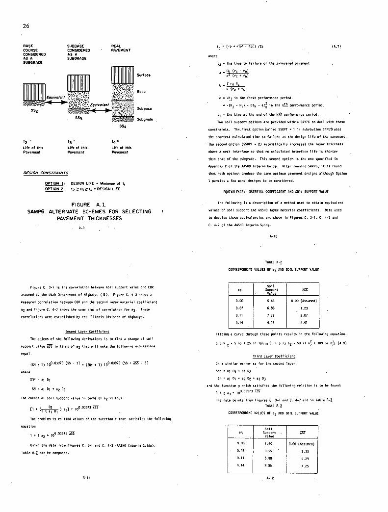
26

BASE SUBBASE REAL COURSE CONSIDERED PAVEMENT CONSIDERED AS A AS A SUBGRAOE SUBGRADE

Surface

_____

iuiva/eniO0oO ro Base

ss2 (quivo/ent

03 Subbase

SS3 Subgrade

S54

t2m t3,m

Life of this Life of this Life of this Pavement Pavement Pavement

O(Sf GA' CoNs rRm rs

OPTION 1 DESIGN LIFE • Minimum of t

OPTION 2 t2 93 N4 • DESIGN LIFE

FIGURE A. 1.

SAMP6 ALTERNATE SCHEMES FOR SELECTING PAVEMENT THICKNESSES

A-V

t (-b + /E2Q) /2a (A.7)

where

tj = the time to failure of the i-layered pavement

= TMç (rc - ro)

c2 (rc r0 )

b 2 r0 N

C (ro + rc)

in the firht performance period.

-(Nj - NO - bti, - at in the k)U performance period.

tk = the time at the end of the k)i performance period.

Two soil support options are provided within SAMP6 to deal with these

constraints. Thefirst option (called SSUPT = 1 in subroutine INPW) uses

the shortest calculated time to failure as the design life of the pavement.

The second option (SSOPT = 2) automatIcally increases the layer thickness

above a weak interface so that no calculated interface life is shorter

than that of the subgrade. This second option is the one specified in

Appendio C of the AASHO Interim Guide. After running SAIIP6. it is found

that both options produce the same optimum pavement designs although Option

I permits a few more designs to be considered.

EQUIVALENCE: MATERIAL COEFFICIENT AND SOIL SUPPORT VALUE

The following is a description of a method used to obtain equivalent

values of soil support and AASHO layer material coefficients. Data used

to develop these equivalencies are shown in Figures C. 3-1, C. 4-3 and

C. 4-7 of the AASHO Interim Guide.

A-IN

TABLE A.2

CORRESPONDING VALUES OF a2 AND SOIL SUPPORT VALUE

Figure C. 3-1 is the correlation between soil support value and CBR

assuned by the Utah Department of Highways (U). Figure C. 4-3 shows a

neasured correlation between CNN and the second layer material coefficient

a2 and Figure C. d_7 shows the sane kind of correlation for a3. These

correlations were established by the Illinois Diolsion of Highways.

Second Layer Coefficient

The object of the following derivations is to find a change of soil

support value AM in terms of a2 that will make the following eopressions

equal.

(SN * 1) 100.03973 (SS - 3) = (SN. + 1) 10003973 (SS + - 3)

where

SN- a1 D1

SN = a1 01 + a2 D2

The chanVe of soil support value in terms of a2 is thus

D2 0.03973 SS [l+(l+ulDl)a2]_ - 1O

The problem is to find values of the function f that satisfies the following

equation

1 • f a2 10003973 ASS

Using the data from figures C. 3-1 and C. 4-3 (AASHO Interim Guide),

Table A.2 can be composed.

07 soil

Support Value

0.00 5.65 0.00 (Assumed)

0.07 6.88 1.23

0.11 7.72 2.07

0.14 9.16 3.51

Fitting a curoe throuVh these points results in the following equation.

S.S.V. 5.65 25.17 10910 (1 + 3.73 a2 - 50.71 a • 309.52 a) (A.8)

Third Layer Coefficient

In a similar manner as for the second layer,

59 01 01* a2

SN a, 111+ a2 02 + a3 03

and the function g which satisfies the following relation is to be found:

1 + g a3 = 100.03973 WS

The data points from FiVures C. 3-1 and C. 4-7 are in Table 0.3

TABLE A.3

CORRESPONDING VALUES OF 03 AND SOIL SUPPORT VALUE

a3 Soil

Support . Value

V.')') 1.60 0.00 (Assumed)

0.95 3.95 2.35

0.11 639 5.2S

3.14 8.95 7.25

A-il A-12

—J

0 U)

In

27

4, ' ' — 0 0

ma .M

0 0

It, 0

0 0 2 2 en ix, a ó 0 0

,1N31,2/3d300 8'3AY7 OHStfD'

A-l3

The curve fitting these points has the following equation.

S.S.V.3 1.60 + 25.17 log10 (1 + 5.41 a3 - 24.06a + 237.65 a) (AN)

Both curves are plotted in Figure A.2

ENVIRONMENTAL PERFORMANCE EQUATION

Up to the present, this equation has been used to describe the loss of

serviceability index due to expansive clay roughness. The equation is based

approximately on a diffusion nodel of the swelling process (9) and because

most environmentolly-caused pavement deterioration is caused by diffusion

of either noisture or tmxperatore, it is expected that the present form of

the environmental performance equation will be useful for other fonns of

environmental serviceability loss. The equation is included in subroutine

TIME and is given below.

'1 + 0.335 C1C2 (e_ 0t - e_Otk) - (A.lO)

where

P the serviceability index at time t.

P1 the initial serviceability equation.

C1 the probability of surface activity. This is the percentage of the project length (expressed in decimal form) where environmentally caused roughness is expected to occur.

C2 the maoirojm differential rmve!nent expected to occur on the pavement over a long period of time if the pavement is not overlaid. (In expansive clay areas, this is the potential vertical rise as proposed by McDowell (10)).

= the sxrface rise rate factor which is roughly proportional to the diffusion constant.

Methods of estioating each of these quantities for expansive clay areas

are given in the Users Gaide (Appendix C). In SAMP6, the serviceability

loss dxc to traffic is assumed to be independent of the environmental service-

ability loss, although there are certainly interactions between them in

reality.

A-14

TOTAL PERFORMANCE EQUATION

The serviceability loss doe to traffic is added to the environmental

serviceability loss to produce the total performance equation below.

P P1 - (P1 - 1.5) (R(N - Rh) [(SN1;°X] 9.3633)8

*0335 C1C2 (v_Ut - eOtk) (All)

The variables have been defined previously.

STOCHASTIC VARIATIONS OF THE TOTAL PERFORMANCE EQUATION

The purpose of considering stochastic variations in SAMP6 is to allow

the pavement designer to take into account in a systematic way the risk he

takes by assuming that all variables in the performance equation are at

their average value. The critical constraint that the pavement must meet

is that it should not require an overlay too500n after construction or

after a previous overlay. The expected time for an overlay to be placed

is calculated with the average values of all of the variables but there is

only a 50 per cent certainty that the overlay will actually be required at

that time. If the designer wishes to be 90 per cent certain that the over-

lay will not be needed before a specific time, he mast use altAred values

of the variables to predict the NO per cent time. The way that the variables

are altered in a consistent way is exploined below.

Variance of a Multivariate Function

For convenience, only two variables x and y are used for this following

illustration which can be generalized. A function can be expanded in the

form of a Taylor series about the mean (or expected) values of variables

a and y. -

hk 0 f*hf0 +kfy * 2 f00 *

where

- xv h

y = y* k

1'hk f(x,y)

= which is the expected value of the function.

f. (lfho) evaluated at o =

- (of/sy) evaluated at y =

The variance of the function, v(= the standard error squared,02 (is

- 'hk -

which is approximately equal to

= (hf0 + kfy)2 - h2f02 * k2f 2 * 2hhf0fy (4.12)

if the hiqher order terms of the expansion can be considered negligible. It

is voted that in the above equatioxs

vx h2, the variance of

vy k2, the variance of y

cxn0 , - 2hkff, the covariance term

Equation V.12 is used as the variance of a function of two variables and

calculations of that sort will be used in what follows.

A-1 S A-16

TABLE V.4

RELIARILITY FACTORS

ReliabilityN (Percent1

Reliability Factor

50 0.00

90 1.28

95 1.65

99 2.33

99.5 2.58

99.9 3.09

Thus, is It possible to determine the reliability of a pavement at any

time t if estimates of the variances of the distributions of N (failure

condition) and n (predicted condition) are known.

Variance of the Predicted Condition )n)

The number n is predicted with the traffic Equation (V.1). An estimate

of the variance of its log-normal distribution is given below.

2 (i [log,, (2n) - log10 (d/2)]2 logy \4 I

where

2n = an estimated maximum number of 19-hip equivalent load applications in time t.

0/2 = an estimated minimum number of iN-kip equivalent load applications in time t.

28

Pavement Reliabil ity Condition

In the discussion that follows. N is the number of 18-kip equivalent

loads which will bring the serviceability index of the pavement down to P2

(the minimum serviceability Index at overlay) and represents a failure

condition. The actual condition of the pavement is represented by a which

is the predicted number of 18-hip equivalent loads that will pass over the

pavement in time, t. Each of these quantities. N and n, is assumed to be

log-normally distributed. The reliability of the pavement is the probability

that at any time t, log N is greater than log n. In equation form, this is

P(1og10 S 10910

With the assumption of log-normality of both 8 and a, it can be shown that

this is equivalent to

P((1mg10 N - 10910 n) v 0)

The difference of the two distributiuns if o distribution 0 such that

10910 0 - 10910 n (All)

which has a variance equal to

2_ 2 2 0p - 0109 II °loq o (V.14)

and the rellabilityR is a function of

R f e - 2 do (A.15)

where n is selected from a normal distribution table such as given below and

is the expected value of 9.

A-li A-18

this gives an estimate of the variance of log a as

0oq n 0.0227 (V.16)

Variance of the failure Conditiao (5)

The number N is calculated from the total performance equation which

has been written below.

11 66 [(SN + 1)x] 9.3633 (g - g )l/Be (V.17)

where all terms have been defined previously but the following

- C C q" u 1 2 e-et C • the environmental damage function. P1 - 1.5

u usually 0.335, a constant.

the multiplicative lack-of-fit error from the MSVO Road Test.

Taking the logarithm to the base 10 of the total performance equation gives

log II = -log N • log (0.62766) + 9.363 log (SN + 1)

+ log (g - g') v 0.372 (SS - 3) + loge

where in all cones, log u means 109100.

Assuming that all of the terms are independent of each other (no

c000riance) gives the following equation for the variance of log N.

2 2 2 2 2 2 0 109 9 na °b 0c °d w e V.16)

where

a log N

= 9.363 log (SN + 1)

c log (9 - 9")

A-1 9

0.372 (SS - 3)

e log e

Each of these variances is derived in the following discussion in which

Equation V.12 is used frequently. It is assumed throughout that there is

no covariance term to be considered.

The first variance term is found to be:

2 0.4343 2 2

(-9---) OR (V.19)

where

the variance of the regional factor, R.

The second variance term is

2 - 9.363 u 0.4343 2 2 0b (laSN) 'SN

where

SN = the expected value of the structural number.

0Sli the variance of the structural number which is approximately

=62 02 +o22 +22 +...+o22 1 a 2 a2 3 a3 n can

= the variance of the itLh layer material coefficient aj

c a

ci = the coefficient of variation of the ii? layer material coefficient.

The third variance term is

2 - 1 0.43a3 1 0.4343 - tiT ry 09 - 17 09,,

log (g-g') 22 62 6

A-20

29

where

2 .. 2 2 - (P1 - i'2

(p q 11

op )2 + . o)

+)2 + (5_ )2 2 2

0 0

+ 177L2 (te_0t - tke_Otk) 12

the variance of P1.

the variance of C1 , the probability of surface activity.

the variance of C2, the maminmim differential movement.

= the variance of u, the constant in the environnental performance equation. Its usuol value is 0.335.

= the variance of u, the surface rise rate constant.

2 - [(0.08lj__)•J.9))19) 23 2 the variance of 8.

08 (1 + SN)

The fourth variance term is

(0.372)2 OS

' )A.22)

where

nS the variance of the soil support value.

0-21

The fifth variance tern is the variance of the lack-of-fit of the AASHO

Road Test Equation. The lack-of-fit variance is only part of the total

variance of the Road Test Equation part is due to replication errors in

the data and the other part, the lack-of-fit, is due to the mobility of

the equation to reproduce the data.

2 - 2 2 0109 e - 0109 e 0109 0

Total Lack-of-Fit Replication Error

(Lack of Control)

The totol variance was 0.0961 as reported in ) 7). The replication

error for 117 replicate test sections and serviceability indeues ranging

from 1.5 to 3.5, was computed from the Road Test data to be 0.0198. This

gives the desired result.

0.0763 (9.23)

At this point, the coefficient of variation times the mean-value is

inserted in all eopresslovs where variances appear. In general, the

coefficient of variation is the ratio of the standord deviation (o) to the

mean value of a given variable. in equation form, this is

n = c0

where

c0 the coefficient of variation of u.

the moan value of a.

The factors for which coefficients of variation are inserted are:

structural number, regionol factor, soil support value, the environmental

0-22

performance equation variobles C1. C2, and e, and the serviceability indeoes

P1 and P2. Most of these are known with doubtful occuracy. It is assumed,

as a farther simplification, that all of these have the same value for their

coefficient of variation. c. The variance of log N then becomes:

2 c [O.2549 2

4.0664 2 8 - - 0109 + 'i--ii SN) + 0.1384

0.6142 p2 to)q -

SN B)g - 9=) - - B?l * si

0.4343 g P1 (2 + 3(g=)2 (og t)2]-]2] (9.24) - o)

where uCC

1 2 -Ot -ot (te _tke k)

This equation uppeurs in subroutine PUPY which anplifies n, the

predicted number of 18-kip equivalent loads that would occur in time

by a factor which depends upon the desired reliability. This amplified

numberis then compared with the foilure condition. 8, to determine whether

the reliability condition has been net.

Pavement Reliability Equation

A number of equations which have been presented earlier will be given

here again for reody reference. The differemce density function is given

by the following equation.

log N - logo '0 (0.13)

for a certain reliability given by the factor o in Table 9.4, the

above equation becomes

log N - log o - 000 1 0 (9.25)

which implies that

log N I log n + oo3 (A.26)

Since 08 is given in Equation (0.14) as

+ 2 (014 00 loaN 010gm

then the condition of the pavement which verifies its reliability is derived

from Equation (0.26).

9 1 n 10000 = amplified loading (0.27)

Physically speaking, this means that as long as the number of 13-hip

equivalent loads to failure still exceeds the amplified loads up to time t,

then the desiqner is assured with at least a degree- of confidence dorres-

pondinq to o that the pavement will not foil up to that time.

0-23 0-24

U U) I 7TL: 1L Cr

I I-IJ0 an o uoa o

Sd ISd ISd

A-27 0-28

30

OVERLAY OPTIMIZATION

Subroutine OVRLAY is called by the MAIN program to calculate the

Optinal overlay policy for each feasible initial pavement design. The

optimal overlay policy for an initial design is that overlay policy, of

all feasible overlay policies for that design, for which the son of

overlay costs, maintenance coats and user costs, less the overlay salvage

aaloe, is the least. Overlay depths that are considered within an overlay

policy include those ranging from the minimum overlay depth (a program input)

to the oaoimum overlay depth (a program input), in overlay increments (a

program input). For example, if the minimum overlay depth (not including

level-up and nearing surface) is 1/2', the maaimun overlay depth is 3', and

the overlay incre000t is 1/2, overlay depths that will be considered are

1/2', 1", 1-1/2, 2', 2-1/2" and 3'. A feasible overlay is an overlay,

with one of these acceptable depths, that lasts at least the minimum ac-

ceptable time between overlays (a program input). A feasible overlay

policy is a set of feasible overlays that maintain the pavement serviceability

index above some minimum acceptable level (a program input) throughout the

analysis period. This minimum-serviceability-index restriction serves as a

limiting factor on the time that can elapse before an unerlay oust be ap-

plied and it generally forces at least one overlay to be performed during

the analysis period.

All that is required to determine an optimal overlay policy is to

determine the feasible overlay policies and determine which of these is

least costly.

There are three types of variables associated with an overlay policy:

(1) the number of performance periods, K; (2) the times Tk, k = 1, 2,...,

K - 1, at which overlays are applied; and (3) the depths °k of each overlay.

A-OS

The alternative, feasible overlay policies for a specific initial

design can be represented by a tree of the type shown in Figure A-3. Each

branch of this tree represents an individual overlay policy. In this example,

the minimum 0k

is 1/2', the maximum °k

is 3' and the overlay increment is

1/2'. The last overlay in each overlay policy must last beyond the end of

the analysis period, T. Thicker overlay depths are not considered at an

overlay time when a thinner, feasible depth will last beyond the end of

the analysis period; e.g. • in Figure 0-3, there is no policy with 01 1/2',

= 1/2'. and 03 = 1", sInce 03 = 1/2' lasts beyond the end of the analysis

period (given that °l = 1/2" and 02 = 1/2).

ilypathetical performance histories are depicted in Figure A-V to A-7 for

the overlay policies enumerated in Figure A-3. These policies are for one

initial design that last approximately six years from initial construction,

To, to time of first overlay, T1, and are for an analysis period, T. of 20

years. Enperience with the SN126 program indicates that the actual number

of branthes on an overlay tree for a 20-year analysis period usually is

less than the number shown in the example tree.

Some designs may require no overlays, especially If the analysis

period is short, the traffic and ennironnental deterioration are low, and

minimum initial pavement layers are thick. . It also night be mentioned that

no adjustment is made in the overlay salvage value for the last overlay of

an overlay policy lasting to the end of the period. There are several

ways such an adjustment could be made, or the program coold be nodifled to

calculate the last overlay depth such that it lasts precisely to the end

of the analysis period.

A-26

31

I I

I I

aS

2 2 2 2

L7 I I

I N I I -

I — I 0 I' w I

I LCJ- I 1

o LIJ

— 0

' N LU

:---

LU o

--

a, us

cr

I

C

I -

0 0 9 9

Ia

0 0

I I I

I I I I

I • I C

0 I 0

I— I I a,

L -0 _

I I I 0 0

u0 ,O ) 0 uT00u5 0 0000 0 0 0 0000 0 ItOu,0a 0 aSOnoas 00 0'i I')c)N

Sd ISd ISd

Sd IScJ ISd

0-29

- 9-30

us

N CROSS-SECTION VOLUMES AND INITIAL COST

Subroutine INCOST is called by Subroutine SOLOE2 and calculates the

I material volumes in the initial pavement and shoulders and uses these

volumes together with unit costs to calculate the cost of the initial

0 construction per square yard of traffic lane (CT). The sal cage nalue

I of the initial construction per square yard of traffic lane (SV) also I - C

is calculated in Subroutine INCOST.

I C

I Cross-Section Models

0 ° Two different models, called "0"and 1, are available in SAIIP6 -

I 0

for calculating Cross-section volumes, and it is anticipated that

Cli Other models eventually will be developed since these two models do

I — LU not cover all situations. Cross-section Model No. 0 (i.e.. MDXSEC = 0)

is in effect the provision for not considering the full cross-section; 0

I 0 °

I i.e., a square yard of pavement is considered and pavement layer

volumes are assumed to be proportionate to layer depths and shoulders

are omitted from all calculations.

I - Cross-section Model 110. 1 (MODSEC 1) assumes that pavement and

1/.

shoulder layers within the pavement are as shown in Figure A-N. The 1- a,

in the Users Guide in Appendin C. This general cross-section model

- computer program inputs for this cross-section model are eupl ained

is used in SAFO6 to represent both two-lane and multi-lane highways.

If the traffic handling model (MODEL) is either 1 or 2, it is assumed

in SAIIP6 that the cross-section diagram and inputs represent both

c,Oa)oai 00

0 0 N directions of travel.

(Sd

A-3l A-32

32

If the traffic model (lDEL) used in SAIIP6 is 3,4, or 5, the

cross-section diagram and inputs are assumed to represent only one

direction of travel. For divided highways with wide earth medians,

such as most Interstate Highways, the inputs are fairly straightfor-

ward with some program inputs representing the configuration of the

inside shoulder and other inputs representing the configuration of the

outside shoulder. For four-or-mere-lane, undivided highways, the inside

shoulder layers and the lower pavement layer inputs have zero width.

If a wearing surface is used, it is assumed to be plated across

the top pavement layer unless the first shoulder layer also is aspholtic

(ltVSpn = 1), in which case the wearing surface is assumed to cover the

inside and outside shoulders also; the wearing surface Is not shown in

Figure 4-8.

Calculations of the volumes of materials, in compacted cubic yards,

is simple and straightforward. The volume in each layer is simply

the depth (in yards) of that layer multiplied by its width (in yards),

multiplied by the length of pavement for which calculations are being

made, which always is assumed to be one centerline yard.

The volume of fill material basically is calculated as the volume

of the entire cross-section less the volumes of pavement layers and

shoulder layers. The cross-section model also provides the ability to

reduce the volume of each shoulder layer and the fill material by

allowing adjustment volume inputs that are subtracted from these

volumes. (See Users Guide in Appendix C).

A-33

A-34

Initial Cost and Salvage Value

The initial pavement cost for a particular design is calculated

in Subroutine INCOST as the sum of:

the cost of materials other than bitumen in the pavement

cross-section, includIng wearing surface pavement layers,

shoulder layers, and fill material.

the cost of bitumen in the wearing surface, pavement layers

and shoulder layers.

the cost of tack coats used with the wearing surface, pave-

ment layers, and shoulder layers, and

the cost of prime coats used with the pavement layers and

shoulder layers.

Cost and Salvage Value of Materials

The total cost of materials other than bitumen per centerline

yard of cross-section, C, is the sun of: the cost of such materials

in the pavement layers, denoted by Cnp the shoulder layers, Cr5 . the

fill material, C. and the wearing surface, Cow; i.e.,

C C CC +C +C n np ns nf ow

YkCk + Y1C + YfCf + YwCw

where all material volumes are measured in cubic yards per centerline

yard of cross-section, and:

the cubic yards of material in pavement layer k,

Ck the cost of material in pavement layer k, in dollars per

compacted cubic yard.

H the number of pavement layers,

the cubic yards of material in shoulder layer j,

C1 = the cost of material in shoulder layerj , in dollars per

compacted cubic yard,

N the number of shoulder layers.

= the cubic yards of fill material.

Cf = the cost of fill material, in dollars per compacted cubic

yard,

the cubic yards of material in the wearing surface, and

Cw the cost of material in the wearing surface, in dollars

per compacted cubic yard.

As was explained previously, the 0k' Yi.and Yf are calculated

within INCOST from cross-section inputs. The Ck. Cj, and Cf are

calculated with the use of one of two equations, one of which assumes

layer material costs per square yard are a linear function of layer

thickness (MOCOST 0); the other assumes the logarithm of pavement

material cost per square yard is a function of the log of material

thickness (MOCOST = 1). Cost equations are fitted, in SOLOE2, to

the costs at the minimum and maximum thicknesses. Cow' the cost of

the wearing surface, is calculated in INPUT.

The salvage value of the materials other than bitumen in the

initial pavement. 5n'

is:

5e PhVkCk +PJ YJCj C PfCTh * PC

4-35 . 4-36

33

where:

Pk

the proportion that salvage value is of initial construction

cost, for pavement layer k,

P1 the proportion that salvage value is of initial construction

cost for shoulder layer j

Pf = the proportion that salvage value is of initial construction

cost for the fill material,

the proportion that salvage value is of initial construction

cost for the wearing surface,

and where the other variables are as previously defined.

Cost and Salvage Value of Bitumen

The total cost of bitumen per centerline yard of cross-section.

Cb. is the sum of: the cost of such bitumen in the pavement layers,

denoted by Cbp. in the shoulder layers, Cbs. and in the wearing surface.

CbW; i.e.,

Ch Cbp • C,5 + Cbw

+

P,JLJY * PbWLWY

where:

Cbg S the cost of bitumen in dollars per gallon,

bk the proportion asphalt content of pavement layer k.

Lk the pounds of bituminous material per cubic yard of pave-

ment layer k,

A-37

bi the proportion asphalt content of shoulder layer J.

Lj the pounds of bituminous material per cubic yard of shoulder

layer 1,

bw = the proportion asphalt content of the wearing surface,

= the pounds of bituminous material per cubic yard of wearing

surface,

and where Yi.5'Yw, M, and N are as previously defined.

The salvage value of bitumen in the initial pavement. Sb. is

calculated as: M N

Sb PkPbkUkYkPlPblLlil v PWPbWLWYW)

where all variables are as previously defined; i.e.. P k' P

1, and P, are

the same as those used with materials other than bitumen.

Cost of Tack Coats

It is assumed that one tack coat is applied for the wearing

surface and that other tack Coats are applied in minimum Increments,

Di' so long as this minimum exceeds Input value Dm• These tack coats

are applied to any layer that has a rate of tack coat application

that is greater than 0.0.

CtuCt (KkWkRtk • L1WR *

where:

C = the tack coat cost in dollars per gallon.

= the nunter of tack coats for pavement layer k,

A-38

Wk = the width of pavement layer k, in yards,

0tk = the tack coat application rate for pavement layer k, in

gallons per square yard,

L3 = the nunter of tack coats for shoulder layer I,

Bj the width of shoulder layer I, in yards,

Rtj the tack coat application rate for shoulder layer I • in


W = the width of the wearing surface, in yards.

S the tack coat application rate for the wearing surface,

in gallons per square yard,

and where M and N are as previously defined.

It is assumed that tack coats in the initial pavement have no

salvage value.

Cost of Prime Coats

The method of calculating the cost of prime coats, C, is similar

to that for tack coats, except that only one prime coat is allowed per

layer:

C g (WkRPkkWIRPJ )

where:

Cpg the prime coat cost in dollars per gallon,

pk = the prime coat application rate for pavement layer b,

in gallons per square yard.

B,1 = the prime coat application rate for shoulder layerl, in


and where M. N, 0k'

and W are as previously defined.

It is assumed that prime coats in the initial pavement have no

salvage value.

It night be noted that by choosing an appropriate prime coat

application rate (N Pj ) for the top shoulder layer, the cost of adding

a special seal to the shoulder can be calculated as a prime coat.

for this purpose would equal the cost of the special seal per square

yard divided by

Initial Cost and Salvage Value Per Square Yard

The total initial cost per square yard of traffic lane. C1, is

calculated as: C1 = (C,, • Cb + C + C)/w1

where these variables are as previously defined. (W1 is the width of

the tap pavement layer, in yards). The salvage value of the initial

pavement per square yard of traffic lane, sI, is calculated as:

= *

where these variables are as previously defined. These two values.

C1 and S1, are calculated for an initial pavement design each time

Subroutine SOLVC2 calls Subroutine INCOST.

A-39. A-go

.34

OVERLAY COST AND SALVAGE VALUE

The overlay cost is calculated in a way sinilar to that described

for calculating Initial cost, and includes:

the cost of materials other than bitumen in the wearing

surface (which is assumed to have the same thickness as

in the Initial construction), the level-up, and the overlay.

the cost of bitumen in the wearing surface, the level-up,

and the overlay.

the cost of tack coats and prime coats.

the cost of shoulder material other than asphalt, if the

shoulders are not paved, and

the cost of upgrading the earth shoulders outside the

paved or aggregate shoulders.

Within Subroutine INPUT, the cost of overlaying, excluding level-up

but including all other overlay construction coats, is calculated at the

minioum and oauioum overlay depths; then, a linear cost equation relating

overlay cost to overlay depth is estimated using these two costs and their

associated depths. This equation is then used to estimate the level-up

cost, which is then added into the constant term of the equation. This

resulting equation of overlay costs, including level-up, then is used in

Subroutine OVRLAY to calculate all overlay construction costs.

The overlay salvage value is calculated as the total overlay con-

struction cost (including all five of the costs enumerated above) multiplied

by the proportion that overlay salvage value is of overlay cost.

MAINTENANCE COSTS

Two different models are available for calculating maintenance costs.

Each model is used to estimate maintenance costs during a performance period.

Within Function RVtAINT, maintenance costs are calculated for a performance

period and discounted to the beginning of the period using continuous dis-

counting. Each of the two models makes use of four different times, all of

which are in years dated from the time the pavement is built:

11 = the time at the beginning of the performance

period (called TPRIM in the program).

12 the time at the end of the performance period

(called T in the program),

C the length of the analysis period (called CL

in the program).

T the length of the performance period that falls within the

analysis period (called TPERF in the program), and

Min(C,T2) - T1 where Min(C,T2( demotes that the

oiniouo time of the two times C and 12 is used.

Each of the models also uses a discount rate, i, expressed as an annual

rate in fractional terms (i.e., rate of 6% is .05 per year(. In the compater

program, I is designated as MATE.

MODEL NO. 1

In Ilaintenance Model No. 1 (i.e., MNTMOD = l(, the annual rate of

routine maintenance cost in dollars per lane, CMt is expressed as:

A-42

A-Al

CMC = C1 l C2t

where C1 and C2 are input constants and t is the time in years from the

beginning of the performance period. The RMC for an entire performance

period of length T, discounted to the beginning of the performance period

is designated as RMC and calculated as follows:

RMC f(ci C C2t)etdt

MUIC =Cf e ldt a Cfe ltdt

C1 C2 C1 C2(iT * i( -it RMC Tv 17 (1_v I

In the case where I = 0.0.

RMC C1T C 0.50212

To Obtain RMAINT, maintenance cost per square yard of traffic-lane pavement.

RMC is divided by the square yards of pavement per lane mile:

RMAINT WIC/17600LW

where XLW is the lane width in yards.

MODEL NO. 2

In Maintenance Model No. 2 (i.e., MNTMOD = 2), the annual rate of rou-

tine maintenance cost per centerline mile of four-lane pavement, CM, is

expressed as:

CM = VP(CVP(

A-43

where:

Op = Pavement and shoulder maintenance requirement units

for a centerline mile of four-lane highway, and

COP = the cost in dollars per unit of VP.

The rate of TP units per year YPis calculated as follaws:

183. + 13.725 C 19.72t2

where:

the number of days per year when the mavinun daily temperature

is below 32 Fahrenheit, and

= age of the pavement surface in years after the beginning

of the performance period. -

Since CYP and 0 are constants (program inputs), let A = CVP(-183. * 13.72U(

and B a 19.72CYP. Then, the routine maintenance cost per four-lane mile for

a performance period discounted to the beginning of the performance period,

is: -

RMC =f(A + Bt2( etdt

- 1T iT elT - 1 12 1 - A(-1---.--* 2Be- (—fl----- -

In the case where i 0.0.

RMC AT + 8T

The routine maintenance cost per performance period per square yard of

traffic-lane pavement, RMAINT, is calculated as:

RMAINT z RS4C/7040XLW

where 01W is the lane width in yards and 7040 is the length at four lanes in

yards of lane oiles.

A-44

35

COP, the cost per unit of VP is calculated as follows:

COP = P1C1 a P.C. • PeCe

where

P1 P0. and P. the proportion of each VP maintenvnte unit that

is devoted to labor, materials and equipnent,

respectively, and

C1 ,C, and Ce the costs of, labor, materials and equipment per

maintenance unit.

The values used In the program for P1. P., and P. are different for urban

and rural areas and are as follows (1, P. 54):

iype aT area

)!CU Rural

P1 0.60 0.44

0.21 0.35

pe 0.19 0.21

Cl,and C. are inputs to the computer program if Maintenance Model No. 2

is used. Eaplanations of these inputs are given in NCHRP Report Na. 42.

Maintenance Model No. 1 was added to SAMP6 and was not in SAMP5. Also,

both maintenance models were changed to continuous discounting to increase

mathematical accuracy and to reduce computer time.

USER COSTS

Increases in motorists' costs, or user costs, because of disruption

during overlay operations are calculated In Function USER. Function USER in

4-45

SU.9P6 is basically the same as Subroutine USER in SAMPS, which was developed

by one of the authors of this report with the assistance of Mr. James L. Brown

of the Texas Highway Department. In SAMP6, the cost and capacity tables have

been updated and eotended and an interpolation and extrapolation sr,hmoe was

added for increasing accuracy of calculations. The following description of

Function USER relies on descriptions of the Subrautine USER. AS originally

published in 1968 (11) and later changed and updated (12). It also has been

used and documented elsewhere (13).

This section is divided into four sub-sections, the first of which

describes the assumed speed profiles of vehicles In the vicinity of the

overlay operation. The second sub-section gives the time and opert1ng

costs associated with the different movements described by the speed pro-

files. In the third sub-section the five methods of handling traffic are

described and equations are given for calculating the proportion of vehicles

stopped and the average time stopped for conditions where traffic congestion

arises because of the overlay operation. The final sub-section gives for-

mulas for calculating total user cost and total user cost per square yard

of pavement.

Speed Prmfiles

It is assumed that all vehicles approach the overlay area at the same

speed, called the approach speed. It is further assumed that there is a

restricted area, the length of which is LSO or LSN, through which vehicles

travel at a reduced speed. For some methods of handling traffic this reduced

speed may be the same for vehicles traveling in both direttiuns but for

ather methods it may be different for each direction; it is assumed to

4-46

always be the same for all vehicles going in the same direction. Generally,

the vehicles traveling in the "overlay direction" will have their speed

reduced as much or more than will those traveling in the "non-overlay direc-

tion" • LOU and LSN respectively.

The length LSO of the restricted area generally will be longer than

the length LU of the actual overlay operation. The amount by which LSO is

losger than LU will be determined by the road geometrics and the method of

handling traffic. This is discussed more fully below in the section on

methods of handling traffic.

As was mentioned above it is assumed that vehicles approach the restricted

area at an "approach speed' demoted by SA. If there were no overlay taking

place then the vehicles would travel through the area which is restricted

during overlay at the "approach speed'. During overlay, however, most

vehicles travel through the restricted area at a reduced speed called the

"through speed, overlay direction" denoted by SO or the "through speed, non-

overlay direction" demoted by SN. It is assumed that vehicles maintain these

"through speeds" all the way through the restricted area.

A proportion (called P01 In the overlay direction and P91 in the non-

overlay direction) of all vehicles will be stopped as they approach the

restricted area. It is assumed that these vehicles stop and then accelerate

back to the through speed which is reached at the moment they enter the

restricted area of length LSO or LSN; the vehicles then travel at the reduced

speed (SO or SN) through the restricted area for a distance, and as soon as

they leave the restricted area they returm to a speed which is the same as

their approach speed.

Figure A-9 shows the speed profile for such a vehicle which is stopped.

The letters along the horizontal aois denote points where speeds are changed.

The vehicle, approaches the restricted area at a speed of SA, begins deceler-

ating at point A and is stopped by the time it reaches point B. remains

stopped for a time (001 in the overlay direction and EN1 in the non-overlay

direction) at point B, then accelerates back to the through speed SO or SN

which is reached at point C which is the beginning of the restricted area of

length LOU or LSN, then travels from point C to point 0 at the through speed,

and at point 0 begins accelerating back to the approach speed which is

reached at point E.

Vehicles which do not stop are slowed dawn when they pass through the

restricted area and it is assumed that their deceleration is such that they

reach the through speed (SO or SN) at the moment they enter the restricted

area. The proportion of vehicles which do not stop equals one minus PB1 for

the overlay direction and one minus P111 for the non-overlay direction.

Figure A-10 shows the speed profile for a vehicle which is not stopped

but is slowed by the overlay operation. The letters along the horizontal

axis denote points where speeds are changed. The vehicle appruaches the

restricted area at a speed of SA, begins decelerating at point A, decelerates

to the through speed SO or SN which is reached at point B which is the begin-

ning of the restricted area of length LSU, continues at the through speed

from point N to point C which is at the end of the restricted are, then at -

point C begins accelerating back to the approach speed which is reached at

point D.

Because of overlay operatiuns, vehicles will travel through the overlay

area with speed profiles as shown in Figures A-N and A-lU. In the absence

A-47 A-48

36

of overlay operations they would have traveled at the approach speed through

the overlay area. The excess traffic costs due to overlay include the excess

time and operating costs due to reducing from the approach speed to a stop

(from A to B in Figure A-9), retarnivg bach to that speed (from B to C and

from 0 to E in Figure A-9), the excess time and operating (idling) costs due

to being stopped (at paint B in Figure A-9), the excess time and operating

costs due to reducing from the approach speed to the through speed (from A

to B in Figure A-la) and returning to the approach speed (from C to D in

Figure A-b), and the excess time and operating costs due to traveling dis-

tance LSB or LSN (from C toO in Figure A-9 and from B to C in Figure A-b

at a reduced speed (SO or SN) instead of traveling at the approach speed

(SA).

Time and Operating Costs

The excess user costs because of an overlay include the excess cost of

stopping and slowing down, the cost of delay while stopped, and the excess

cost of traveling at a reduced speed through the restricted area. The

information needed for calculating these costs is given in Tables A-S through

A-B. The program user mast stipulate whether the overlay operation is in an

urban or rural area and this determines which tables or which columns in the

table are used. The difference hetaeen the urban and rural costs is the

vehicle distribvtiOns used to derive the costs. The operating costs for

different types of vehicles were taken from a publication by Wlnfrey (14).

and this same source was used for the excess time of making speed changes.

The values of time used in calculations were based on information in studies

by the Stanford Research Institute (15), Lisca (16), and Adkins (17). Pro-

0-49

portions of vehicles of different types for urban and rural areas are used

to derive wmighted time and vehicle operating costs. The reason that the

costs are higher for rural area than for urban areas is that there is a

higher proportion of trucks in rural areas and their costs are higher than

those for passenger cars.

Tables A-S and A-6 give the excess time and operating costs for stopping

(in the first columns) and for slowing down (in the other columns). Table

A-P gives the time and operating costs for operating at a uniform (constant)

speed. Table A-B gives the time and operating costs of delay (or idling).

Methods of Handling Traffic

There are several methods of handling traffic daring an overlay opera-

tion. The method used depends mainly on highway geovetrics, especially the

number of lanes, the type of median (if any), and the presence of absence of

pavement shoulders, frontage roads, or other alternate routes. In the two

following subsections are described the five methods of handling traffic

which are most comonly used and the way of calculating average delay and

proportion of vehicles stopped for each method.

The five methods. The first two methods of handling traffic are for

two-lone roads (with or without shoulders) and the other three methods are

for roads with four or more lanes. Figures 0-11 through 6-15 depict in gen-

eral way the five situations. In each figure LB. LSB. and LSN are shown. LB

is the amaunt of road which is overloyed at any one time -- not the total

overlay job length. LSB is the distance over which traffic is slowed down

by the overlay by the overlay operation at any one time in the overlay

direction, LSN is the non-overlay direction. In the situations depicted in

DISTANCE (MILES)

FIGURE A-9. SPEED PROFILE FOR VEHICLES WHICH ARE STOPPED DURING OVERLAY.

* This speed is SO,in the overlay direction but would be SN in the non-overlay direction. LB is length of overlay work. LSO or LSN is the length of restricted area in the overlay direction or non-overlay direction as applicable.

LSO or tso

LO

0 1- - N - - "',

A B C D

DISTANCE(MILES) FIQJRE A-la. SPEED PROFILE FOR VEHICLES WHICH ARE NOT STOPPED BUT ARE

SLOWED DORING OVERLAY.

* This speed is SO in the overlay direction but would be SN in the non-overlay direction. LB is length of overlay. LSO or LSN is the length of restricted area overlay or non-overlay direction respectively.

A-SO

TABLE A-S

DOLLARS OF EXCESS OPERATING AND TIME

COST OF SPEED CHANGE CYCLES - EXCESS COST ABOVE

CONTINUING AT INITIAL SPEED, FOR RURAL ROADS

Initial Dollars Per 1000 Cycles Speed Speed Reduced to and Returned F rem (MPH)

10 10.676

20 22.932 11.660

30 39753 27.079 14.306

40 63.454 49.907 35.812 19.902

SD 98.194 93.454 67.935 50.326 28.491

60 151.888 134.793 116.527 95.788 71.070 40.931

TABLE A-6

DOLLARS OF EXCESS OPERATING AND TIME

COST OF SPEED CHANGE CYCLES - EXCESS COST ABOVE

CONTINUING AT IVITIAL SPEED, FOR URBAN ROADS

Initial Dollars Per 1000 Cycles Speed Speed Reduced To and Returned From (MPH) MPH 0 10 20 30 40 50

10 7.395

20 14.829 7.059

30 24.570 16200 8.191

40 37.838 28.896 20.130 10.845

50 56.703 47046 37.309 27.024 14.939

60 85514 74.330 61.884 50.705 36994 20.704

6-51 A-52

37

TABLE 0-7

DOLLARS OF OPERATING AND TIME COST

PER 1000 VEHICLE MILES AT UNIFORM SPEEDS

Onitorm Uollars Per 1000 MIles Speed Rural Urban MPH Roads Roads

10 495.77 456.66

20 270.31 248.30

30 196.62 179.64

40 162.58 147.22

SO 145.54 130.08

60 138.80 121.88

TABLE A-8

DOLLARS OF OPERATING AND TIME COST OF DELAY

(OR IDLING) PER 1000 VEHICLE MOORS

Type Dollars Per 1000 Hours Of Delay Rural Urban Cast . Roads Roads

OperatinR .0 166.60 $ 154.84

Time 4,243.10 3,956.68

Total 4,409.70 4,111.52

A-53

Figures A-il through A-14. LSB and LSN are only slightly longer than 10 by

say one-tenth of a mile, but in the situations depicted in Figure A-15, LSO

may be considerably longer than LØ. LSØ and LSN are input variables provided

by the program user. LO is not used in the calculation of user costs and is

included only for Illustration. (Note The variable LO used as a subscript

In subroutine USER is not Lfl as illustrated in these figures.) In the

figures, the overlay direction is always to the left.

MODEL = 1 (Figure A-lI). For two-lane roads with shoulders, one lane

of traffic can be diverted onto a shoulder. Traffic going west' in the

overlay direction can be diverted onto the shoulder as shown in Figure A-il

and such traffic will generally be sluwed down. Traffic in the non-overlay

direction proceeds as usual but also nest slow down though probably not by

as mach as the traffic going in the overlay direction. Another version of

this method is to divert the traffic In the non-overlay direction onto their

shoulder and divert the traffic going in the overlay direction into the east-

ward lane. In addition to the delay due to traveling at a reduced speed,

traffic may be additionally delayed by having to stop due to movement of

overlay personnel and equipment in the overlay area and by the inability to

overtake other traffic in the overlay area.

MODEL = 2 (Figure A-12). For two-lane roads without shoulders, it is

sometimes necessary to post flagmen at each end of the overlay operation and

to stop traffic In one direction while traffic from the other direction pro-

ceeds through the overlay area. The flagmen determine from which direction

traffic is let through the overlay area at any one time. The vehicle arriving

first usually has priority. !f an additional vehicle arrives while other

vehicles going in the same direction are proceeding through the overlay area

0-54

FIGURE 0-11. MODEL1: TRAFFIC ROUTED TO SMOULDER.

LS (LSN)

FIGURE A-12. lDEL=2 ALTERNATING TRAFFIC IN ONE LANE

FIGURE A-13. MODEL3: IWO LANES MERGE, NON_OVERLAY DIRECTION NOT AFFECTED.

eucept that it will be stopped when the vehicles in the queue from the other

direction are a number or have been waiting a time which justifies priority

for them. Traffic from each direction travels through the overlay area at

a reduced speed. Some vehicles from each direction are stopped to give way

to vehicles from the opposite direction, or because of the movement of over-

lay personnel and equipment in the overlay area, or because vehicles do not

have the ability to overtake other vehicles in the overlay area. Generally

speaking, the proportion of traffic stopped to give way to vehicles from

the opposite direction will be higher the longer is LSfl and the larger is

the traffic volume.

MODEL = 3 (Figure A-13). For roads with two or mare lanes in each

direction and with a non-tronsversable median, it is assumed that traffic In

only one direction will be affected by the overlay operation. It is also

assumed that at least one lane in the overlay direction remains open for

traffic. For low traffic volumes the effects on traffic in the overlay

direction will be that of reduced speed through the area, stops due to

movement of overlay personnel and equipment, and inability to overtake other

vehicles as easily. For higher volumes for which the flow of traffic is

above the capacity of the restricted roadway, a queue will result upstream

of the overlay operation and will lead to vehicles being stopped due to con-

gestion.

MODEL 4 (Figure 0-12). for roads with two or more lanes In each

direction and with no medians or with medians which can be crossed at any

point or which have median openings, it may sometimes be desirable to block

all lanes in the overlay direction and divert the overlay direction traffic

to nov-overlay-direction lanes. MODEL = 1 depicts the situation and those

A-5S 0-56

38

FIGURE A-14. MODEL4: OVERLAY DIRECTION TRAFFIC ROUTED TO NON-OVERLAY LANES.

FIGUR A-is. MODELS: OVERLAY DIRECTION TRAFFIC ROUTED TO FRONTAGE ROAD OR OTHER PARALLEL ROUTE.

A-57

with either no median, or situations for which It is intended that traffic

will cross the median iconedlately In front and behind the overlay job, is

that LSØ and LSN In these latter two cases would bear approulnately the same

relation to L0 as is the relation where MODEL = 1, 2. or 3 Instead of being

the distance between median openings at each end of the overlay job as when

MODEL = 4. For these sitaatians both lanes of traffic will be affected, and

the method of calculating average delay and proportion of vehicles stopped

is the same as that used for MODEL = 3, but In MODEL 4 traffic going in

both directions is affected.

MODEL = 5 (FIgure A-iS). In some situatians traffic In the overlay

direction is diverted to an alternate route such as a frontage road or some

other parallel road or street. The addition variable of ISO is the distance

traveled by detour In the overlay direction.

Average Delay and Proportion of Vehicles Stopped. The delay to traffic

due to overlay is of four basic types which are related to vehicles:

traveling at a reduced uniform speed in the restricted area.

not having the ability to overtake and pass other vehicles

traveling In the same direction.

Having to stop because of the movement of overlay personnel

and equipment in the overlay area, and

having to stop because of congestion when the traffic demand

exceeds the capacity of the restricted area.

The delay per vehicle due to traveling at a reduced speed equals the

travel time at the reduced speed through the restricted area minus the travel

vehicles woald have had through the restricted area had It not been restricted.

A-S8

The delay due to vehicles not having the ability to overtake and 'pass

other vehicles traveling in the same direction because of the overlay opera-

tion may result both in the restricted area and outside the restricted area.

This delay when it occurs in the restricted area is Included In the delay

discussed in the preceding paragraph if accurate estimates of speeds through

the restricted area are used. The delay due to the inability to pass outside

the restricted area because of the overlay is a more complicated calculation

and is probably largest in the cases where the capacity of the restricted

area is smaller than the demand (or input) for use of the area. In such

cases wherein demand exceeds capacity there will be congestion and queueing

of vehicles. These queues nust disperse after leaning the restricted area

and before such dispersion occurs there probably will be some inability to

pass outside the restricted area. Such effects probably will be small in all

cases except MODEL 2 with considerable queueing. If the length of the

restricted area is fairly long and/or the traffic volumes are fairly large,

then when MODEL 2, there will arise fairly long queues of vehicles. Such

queues arise in one direction while vehicles are traveling through the

restricted area from the other direction; then, when this queue is allowed

to proceed through the restricted area it will emerge as a moving queue,

ndmetlmes of considerable length, and extra delay will result outside the

restricted area until the queue disperses. The rate of dispersion of this

moving queue will depend mainly upon the amount of traffic from the opposite

direction, the road geometrics, and the type of vehicles in the queue. This

moving queue will also Impede passing by traffic from the opposite direction;

however, there will be a considerable length of road In front of this queue

in which there will be no (or very few) vehicles which will somewhat offset

the effects of the moving queue on traffic in the opposite direction. Since

the type of delay discussed In this paragraph probably is small in most cases

and niece It is difficult to calculate, it is ignored (i.e., assumed to be

zero).

The third type of delay, that resulting from vehicles having to stop

because of the movement of overlay personnel and equipment in the overlay

area, is calculated by multiplying the number of vehicles stopped by the

excess delay of stopping. The program user must estimate (1) P02 and P112,

the proportion of vehicles stopped due to the movement of overlay personnel

and equipment and (2) DO2 and DN2. the average time that each vehicle stopped

(because of such movement) remains stopped. It is expected that the overlay

operation will be conducted in a way such that the number of vehicles stopped

due to the movement OF overlay personnel and equipment will be small.

Therefore, in the absence of information on the number of such stnps, the

program user probably should estimate that number to be near or equal to zero.

The last type of delay (denoted by 001 in the overlay direction and by

0111 in the non-overlay direction) results when a proportion of vehicles

(denoted by P01 in the overlay direction and PM1 In the non-overlay direction)

have to stop because of congestion which results when traffic demand or inpat

per hoar (Q) exceeds the hourly capacity or output (H) of the restricted area.

When MODEL = 1 (shoulder rooted traffic model) is used, congestion

stopping delay should be almost nonexistent and is assumed to be zero: i.e.,

001 = ON I =0 and PO1 PN1 O for MODEL = 1.

When MODEL m 2 (alternating traffic model) is used, it is assumed that

the hourly traffic is evenly divided brlween directions, It I:; also assumed

A-59 0-60

39

that vehicle arrivals from each direction are Poisson. The proportion of

vehicles stopped due to congestion from each direction (P01 or PM1 ) is

estimated by the following equation:

1 -a02 PD1 = ( p9)

-e

where a the time that it takes a vehicle to travel through the restricted area, in hours, and

the number of vehicles arriving at the overlay area per hour in the overlay direction.

An equation for estimating the average delay per stopped vehicle (001 or ON,

for MODEL = 2 is developed from equations formulated by Tanner (18) and

given by:

001 (S 001) = (1je2( (eaQ_aQ_l) 2Q(e2_eaQ*l( po

1

where a. Q, and PD1 are as previously defined.

If MODEL = 3 or 5, both P111 and 001 will equal zero. If MODEL c 3, 4.

or 5 is used to handle traffic 001 for all three methods and 001 for MODEL

4 are calculated using the following equation developed and verified by the

California Division of Highways (19):

001 HQ_ R-Q) if 0

001=8 ifQ.'Ø -

where H = the number of hours per day that overlay construction takes place,

= the recovery rate in vehicles per hour,

0 = the restricted output rate in vehicles per hour. and

Q and PD1 are as previously defined.

A-61

It is assumed that the Input rate Q is the same for both directions of

travel and equals 6 percent of average daily traffic in rural areas and 5

percent of average daily traffic in urban areas. The output rate 0 and

recovery rate 9 are taken from the California study (19) and are given in

Table A-9. The California study also gives the number of vehicles which

will be stopped at the time when recovery begins. I.e. • when all lanes are

reopened for travel, and this number equals H(Q-0). The average number of

vehicles which will be stopped at any one time during overlay will be H(Q-0)/2.

By assuming that each vehicle which is stopped stays stopped for some aver-

age amount of time 0, which is assumed to equal 1/12 hour, not Including

the time stopped after recovery begins, and assuming that no vehicles are

stopped after recovery begins, the total number of vehicles stopped can be

estimated as H2(0-0)/2D if 0= 0 and is zero if Q 0. Thus, for MODEL 3,

4, or 5. the proportion of vehicles stopped PD1 (and also PN1 for MODEL = 4)

is estimated by dividing the total number of vehicles stopped by the total

input of vehicles during overlay (H a

PD1 = if Q = 0

P01 0 ifQfl

with the constraint that: if this value euceeds 1.0, it is assigned a

value of 1.0.

More research, imcludimg field observations, needs to be done an the

precise number of stops under stop-and-go operation which results from

congestion. Use of the above formulas gives reasonable accurate estimates

of hours of delay but may underestimate the vehicle operating costs associ-

ated with stop-and-go operation.

4-62

TABLE A-H

OUTPUT AND RECOVERY.RATES FOR RURAL AND URBAN ROADS WITH DIFFERENT

NUMBERS OF LANES, FOR USE WITH TRAFFIC MODELS 3, 4, AND 5

Overluy Lanv capacities in Variuble Rural or Vehiclen per Rove

Name U or Renovery Lumen (mne directimm) (FORTRAN) Trunhn Urban Zone 1 2 3 4 5 6 1

RUTFOV 10+ RU 0 1350 2700 4350 6000 7650 9300 mu

RUTFRV 10+ RU R mu 3000 4500 6200 7900 9600 11300

OtTFOV 0 - 10 OR 0 1400 2800 4500 6200 7900 9620 vu

URTFRV 0 = 10 OR R no 3000 4700 6600 8100 9800 11500

Dote: In SUBROUTINE USER edditional lanes are ignored if beyond the ruble limits of 6 lanes for the overlay none and 7 lanes for the recovery none.

Calculation of User Cost Per Square Yard of Overlay

Subroutine OVRLAY calculates the time in hours (HPSY) for over-

laying a square yard of pavement, as follows (in FORTRAN):

HPSY = ACCDu(DELD + OVLEOL)/ACPR * (ACCDOWSTHK/WSPR(nSHFCTR

where:

ACCO = density of overlay and level-up materials (tons per

cubic yard).

DELD = overlay thickness (yards).

DOLE DL "level-up" Increment (yards).

ACPR production rate of overlay and level-up (tons per hour).

WSTHK thickness of wearing surface (yards).

WSPR production rate of wearing surface (tons per hour),

SHFCTR = shoulder factor (ratio of width of traffic lanes and

paved shoulders to width of traffic lanes).

OVRLAY supplies function USER with HPSY and the hourly traffic

(ADTPRDP). Functivn USER calculates the user cost per hour of over-

lay (TUCH), multiplies TUCH times HPSY and returns the multiplicand,

called USER, which is the total user cost per square yard of traffic

lane that is overlaid.

Within Function USER. TUCH is calculated as follows (in FORTRAN):

TUCH = TIPHu)POlu(COSvCO2-aCO3( + (1.0_POl)w(CO3+t04) + P02*C05)

* TIPHc(PN1a)tNl+CN2vCN3)-* (1.0_PN1(u(CN3+CN4) .a PN2.CN5(

where '0' in a variable name denotes overlay direction and "N" denotes

nan-overlay direction, and where: -

TIPH = vehicles per hour from each direction.

P01 U P61 = proportions of traffic stopped because of congestion,

P02 U PN2 = proportion of traffic stopped due to overlay personnel

and equipment,

CO1 & CN1 = excess costs of stopping from highway speeds.

CO2 6 CN2 = excess costs of vehicle idliog time while stopped,

CO3 & CN3 = excess costs for reduced speed.

C04 U CN4 = excess costs of changing speed,

C05 & CNS = excess costs due to delays from overlay personnel

and equipment (stopping plus idling).

TOTAL DESIGN COST

The total cost, per square yard of traffic lane, for each pave-

ment design considered in SAMP6 is calculated as:

A-63 A-h4

40

CT = Cl +C14 ° C0+C - Sj - So

where all costs and salvage values are discounted to present value

terms and are in dollars per square yard of traffic lane, and where:

C1 the cost of the initial pavenent and shoulders.

CM the cost of routine naintenance over the analysis period.

Co the cost of all pavenent overlays (including level-up and

wearing course) placed during the analysis period.

Cu the users • or netarists • costs associated with overlays

made during the analysis period.

Sj the salvage value of the initial pavenent and shoulders, and

S0 = the salvage value of all overlays placed during the analysis

period.

Subroutine INCOST calculates C1 (called CT) and S (called SO).

Subroutine 000100 calculates CM (called PUN), Co (called POCCI), Cj

(called PTUC). and So (called P501). Subroutine OVRLAY calls Function

RINAINT to calculate the routine maintenance cost for each performance

period. (U performance period is the length of time from initial

Construction to first overlay; from first overlay to second overlay;

and so forth, with the last performance period being the length of

tive between the last overlay and the end of the analysis period).

OVRLAY discounts the maintenance costs for each performance period and

sums then to obtain CM. Sinilarly. OVRLAY calls Function USER to

calculate the user costs associated with each overlay and discounts

and sums these costs to obtain Cu.

0-65

APPENDIX B SAMP6 COMPUTER PROGRAM DOCUMENTATION

(See Note below.)

APPENDIX C SAMP6 USERS' GUIDE

(See Note below.)

NOTE

Appendices B, C, G, and H of the agency report, which cover SAMP6 com-puter program documentation, the Users' Guide, and data feedback systems, are not published in this report. They will be of value primarily to persons directly involved in implementatiOn of the SAMP6 program and are avail-able on a loan basis or for the cost of reproduction from the Program Direc-tor, NCHRP, Transportation Research Board, 2101 Constitution Ave., N.W., Washington, D.C. 20418. Loan copies of the SAMP6 program on magnetic rape are also available from the same source.

APPENDIX D SAMP6 SENSITIVITY ANALYSIS

41

APPENDIX

SAMP6 SENSITIVITY ANALYSIS

INTRODUCTION

There are two major purposes for sensitivity analyses, one in a

detailed study and the other in a more general study. Detailed Studies

are made to improve mathiiatical models contained within a computer program

or to establish priorities for research and implementation or to derive

reliable simulation models to replace more complicated ciiputation schemes.

On the other hand, a general sensitivity analysis is made to acquaint the

user with operating characteristics of the computer program. The user is

generally not interested in the intricacies usually required of the detailed

sensitivity analysis. He is concerned mainly with the most significant

variables that are input to the computer program and what effect they have

on the final results of the computations made. In the SAMP6 computer-program

for example, one of the major results of interest to designers is the total

cost of the pavement per square yard. This cost is affected significantly by

the cost of materials used, by the length of time over which the road is

analyzed, by the amount of traffic that passes over the road, and by the

traffic loading. These are significant variables, and the designer is

interested in how they affect the cost of the final design.

TECHNIQUES OF SENSITIVITY ANALYSIS

A sensitivity analysis is usually done by selecting a typical problem

and determining its vornoal input values. Then, each of the input values is

varied one at a time to determine its effect upon the output results. A

thorough sensitivity analysis would assign several values to each--for

example, high, medium and low values--and use each of these with each

0-I

USE OF RESULTS OF SENSITIVITY ANALYSIS

If the results of the sensitivity analysis can be fit reliably by an

assumed function such as the quadratic function discussed above, then one

can proceed to determine sensitivity coefficients by taking the partial

derivative of the dependent variable with respect to each of the indepen-

dent variables in turn. For example, in the equation below

dy/do1 = a1 a 2a11o1 + a12u2.

For any given value of xl and 02, the rate of change of the dependent vari-

able y can be found. The larger the size of this derivative, the more im-

portant the variable is in determining the value of the dependent variable.

This derivative is the sensitivity coefficient.

A simpler method of displaying the importance of different variables is

to plot the results of rams of several problems on a piece of graph paper.

That way the most important variables can be seen visually to have the higher

slopes. A third way of using the results of the sensitivity analysis are by

calculating the percentage change in a result with the variation of the sin-

gle input variable. This technique is used here.

SENSITIVITY ANALYSIS OF SAMP6

Eleven different studies were made using the problems proposed by the

cooperating statss, Kansas. Louisiana. and Florida. The reference problems

included variations of (1) structural number

soil support value

projections of expected 18-kip equivalent loads applied

confidence levels due to stochastic variations of material and pavement properties

interest rate.

combination of all of the other variables at their high, medium, and low

values. Such combinations would lead to a full factorial study, and the

number of times a problem must be worked amounts to 3n where n is the total

number of variables. The numbers of problems to be run for a full factorial

study quickly becomes anonaoageuble. Euperinental design of the sensitivity

analysis may reduce the total number of runs to something that is more man-

ageable. But as the number of problems run decreases, there is a sacrifice

in the accuracy of the knowledge of how different variables interact with

each other. Instead of taking three levels--high, medium, and low--only

two levels may be chosen--high and low. If it is farther assumed that sane

calculated Output result such as the total cost per square yard is at most

a quadratic function of the input variables, then a large reduction in the

total number of problems that oust be run is possible. The quadratic func-

tion is composed of linear terms of the variables, their squares, and pro-

ducts of each of the variables two at a time. If there are two variables,

and 02, the quadratic function associated with then would be as follows:

Y a0 +a1u1 v a2a2 + 01101 + a22u22 a a12o1u2

Since there are around 120 variables in the SAMP6 computer program.

around 8.400 different problems would be required to determine all of the

coefficients of the quadratic function. Not all of the interactions between

the variables, such as in xl and 02 in the equation shown above, would be

interesting or significant, and ouch of the effort and cost of running. the

8.400 problems would be wasted, furthermore, it is known that there are

several variables which interact in a more complicated fashion than simply

as (a1 02). For example, there are a number of variables which interact

three or four at a time, and these interactions would not be considered by

an assumed quadratic function.

D-2

analysis period

user costs due to congestion and traffic delay,

enviromentally caused loss of serviceability

(N) unit costs of materials

pavement strategy as affected by material costs which vary with volume,

pavement strategy as affected by considering the cost of the full cross section

design and total cost variation with soil support option.

thickness design and total cost variations with minimum serviceability indeo

Tables D-1, D-2. and D-3 show the significant features of the pavement

sections used in these sensitivity analyses.

TABLE 0-1. LOUISIANA PAVEMENT SECTIONS

Acadia St. Proj. 801-32-05

Calcasieu I - 10

Pointe Coupee La. 1

Rapides St. Proj. 8-09-20

Initial Average Daily Traffic 40 5,635 1,820 6,560

Final Anerage Daily Traffic 85 8,635 3.200 14,760

18- ki p Equivalent Loading 14,535 6.700,000 1,974,000 17.860.000

Analysis Period 20 20 20 20

Layers Above Subgrade 2 4 2 3,4

0-3 . D-4

42

TABLE D-2. KANSAS PAVEMENT SECTIONS

Sensitivity Analysis No. 1 -- Structural Number

- Douglas Co. S.H.*K-10

Kingman Co. U.S. 54

Initial ederage Daily Traffic 3.230 1,090

Final Average Daily Traffic 5,150 3.250

18-kip Equivalent Loading 380.000 1,440000

Analysis Period . 20 20

Layers Above Subgrade 2 2

TABLE 0-3. FLORIDA PAVEMENT SECTIONS

Florida Sec. 6

Florida Sec. 17

Florida Sec. 19

Initial Average Daily Traffic 485 6.655 6.055

Final Average Daily Traffic 1.103 27,555 27.555

18-kip Equivalent Loading 102.000 17408.032 17.408,032

Analysis Period 20 40 40

Layers Above Subgrode 3.1 3 3

Number of Lanes 2 4 6

0-5

The first section chosen for sensitivity analysis of structural number

was from Florida and termed their Section 17. The traffic was ooderate to

high, beginning at around 6,700 vehicles per day and arriving at the end of

the 40-year analysis period at around 28.000 vehicles per day. Total 18-kip

vquivalents over the life of the pavement would be about seventeen million.

Each of the designs considered three layers on top of the subgrade. The

surface course material coefficient was varied from .44 to .40 to .30. The

base course material coefficient was varied from .20 to .13 to .10. The

subbase material coefficient had only two oariativns, .10 and .08. The sub-

grade in all cases was maintained at a soil support value of about 6.50.

The assumed medium value for each of the courses in this three-layer pavement

system was .40 for the surface course, .13 for the base course, .08 for the

subbase, and 6.50 for the soil support value of the subgrade.

,Table D-4 shows the results of varying the material coefficients of the

surface course while keeping the material coefficients of all other courses

the same. Because there is so little of the surface course material in the

optimum designs, the total cost of the pavement per square yard was affected

very little.

TABLE D-4. TOTAL COSTS -- SURFACE COURSE MATERIAL COEFFICIENT (FLORIDA, SEC. 17)

Percent Optimum Total Cost Variation

Material Thickness per from Coefficient Design Square Yard Medium

0.30 1" - 12" - 24" 07.023 +0.38

0.40 1' - 12" - 24" 86.996 - 0.44 1" - 12" - 24" 87.003 nil

0-6

Another item of note in this portion of the sensitivity analysis is that

the optimum thichnesses for each of the designs did not change, that is, there

was one inch of surface course, twelve inches of base course, and twenty-four

inches of subbase course which proved to be the least eopensive design no mat-

ter what the material coefficient happened to be. This is not the case when

the material coefficients of the base course and subbase courses are varied.

Table D-5 shows the results of the sensitivity analysis of the material

coefficients of the base course material. The optimum thickness design

remained the same as long as the material coefficient was around 10 and .13,

but it changed significantly when the material coefficient rose to .20. In

this case the strength to cost ratio exceeded that of the other two, layers.

and so the computer program indicated that the least expensive strategy would

be to use surface and subbase courses at their minimuo thicknesses and use the

greatest amount of base course material available. The total cost per square

yard dropped steadily as the material coefficient for the base course rose.

TABLE 8-5. TOTAL COSTS -- BASE COURSE MATERIAL COEFFICIENT (FLORIDA. SEC. 17)



0.10 1" - 12' - 20" 08.686 +5.3

0.13 1" - 12" - 20" 88.245 - 0.20 1" - 15" - 4' 87.127 -13.6

Table D-6 shows the results of sensitivity analysis of the material co-

efficient of the subbase course material. Here again as in the base course

material, the optimum thickness design changed. In mahiog the slight change

of material coefficient from .08 to .10, the cost to strength ratio of the

subbase material became dominant, and the computer program indicates that

the best strategy is to use the maximum amount of subbase material while

keeping the surface and base course materials at their minimum levels. The

total cost per square yard dropped sharply as the material coefficient for

subbase material was raised.

ABLE 0-6. TOTAL COSTS -- SUBBASE COURSE MATERIAL COEFFICIENT (FLORIDA. SEC. 17)

Optimum Total Cost Variation Material Thickness per from Coefficient Design Square Yard Medium

0.08 1" - 12" - 20" 88.245 - 0.10 1" - 4" - 20" 87.410 -10.1

Figure 8-1, no which the percent variation from the medium cost is plotted

agalvst variations of material coefficients from their medium values. Indi-

cates that the greatest reduction in the total cost per square yard comes

from an increase in the subbase course material coefficient. This presumes,

of course, that the subbase course still costs the same. A certain degree

of caution oust be eoercised in applying the results of this sensitivity

analysis over a broad scale. For example, it is significant that this Fix.

section 17 had a moderate to high degree of traffic. On Florida section 6,

which is characterized by low traffic and a small number of 18-kip equiva-

lent single aole loads, the material coefficient of the surface course became

important, as shown in Table 0-7. As the material coefficient changed from .30

to .40, there was less subbase material required, its thickness changing from

twenty-four to twenty inches. But as the material coefficient changed from

.40 to .44, the strength to cost ratio for the surface course material passed

D-7 D-8

soil support value to 6.5 results in a further decrease in thickness of

the surface course and also a decrease in the thickness of the base course.

The soil support valves indicate the strength of the untreated natural sub-

grade soil, and cmvsequevtly, this is a material over which the pananent

designer has little cuntrvl. Nevertheless, this table indicates that there

are considerable benefits to pavavent design in moving from one location

where the soil is poor to another location where it is much better.

TABLE 0-8. TOTAL COSTS -- SOIL SUPPORT VALUE (FLORIDA, SEC. 17)


Soil Support Thickness per from Value Design Square Yard Medium

3.50 4' - 14' - 20' 411.714 *8.0

4.00 2" - 14' - 20' $10.851 - 6.50 1" - 12" - 20" 58.245 -24.0

Sensitivity Analysis No. 3 -- Projection of 18-kip Eqaivalencies

This sensitivity analysis was done on two sections - one in Florida.

section 17, over a 40-year analysis period and the other in Kingman Co.,

Kansas, over a 20-year analysis period. The purpose of these sensitivity

analyses was to determine in what way the total cost per square yard and

the optimum designs varied as the estimate of 18-kip equivalent single

aole loads changed. All other input variables ranain the same in both Fla.

section 17 and the Kingman Cu. runs. Florida section 17 data have been

discussed in sensitivity analysis number 1. However, to repeat briefly.

it Consists of moderate to high traffic and fairly high total 18-kip equiv-

alents over its 40-year analysis period. The optimum designs were always

three layers on top of the subgrade. By way of contrast, Kingman Co., Kansas,

43

SURFACE)

Mediwn, Cost

-.10 -OS +01 .05 .10 Mediun, Value

VARIATIONS OF MATERIAL COEFFICIENTS FROM

TUE MEDIUM

FIG. 0-1 COSTS VERSUS MATERIAL COEFFICIENT CHANGES

D-9

through that critiCal value which then made it the most cost-effective

pavanent material to use. Consequently, the cheapest pavonent designs

switch from a three layer to a one layer design using six inches of the

surface course material. The total cost per square yard dropped steadily

as the material coefficient for the surface course rose. The major difference

between the results shown in Table 0-6 and those in Table 0-7 could be ascribed

to the traffic. There was high traffic on section 17 and low traffic and low

loads on section 6.

TABLE 0-7. TOTAL COSTS -- SURFACE COURSE MATERIAL COEFFICIENT (FLORIDA. SEC. 6)



0.30 1 - 4" - 24" $5.053 +4.0

0.40 1" - 4" - 20' $4858 -

0.44 6" $4379 -9.9

Sensitivity Analysis No. 2 -- Soil Support Value

The problan selected for a sensitivity analysis of the soil support

value was again Florida section 17. The details of Florida section 17 are

given in the teot above; it is characterized mainly by moderate to high

traffic and fairly heavy 18-kip equivalent loads. As shown in Table 0-8, the

thickness for the optimum design changes as the soil support value rises.

and the total cost per square yard drops. The way the thicknesses change as

the soil support value rises indicates which of the materials have the better

cost-to-strength ratius. As the soil support value rises from 3.5 to 4.0,

the optimum design keeps the thicknesses of the base course and subbase the

sane but reduces the thickness of the surface course. A further increase of

0-10

on A. S. Highway 54, had an estimated traffic beginning at about 2,000

vehicles per day and ending after twenty years at about 3.300 vehicles per

day. Optimum designs for that pavanent section generally resulted in two

layers on top of the subgrade.

In each of the problavs the estimated number of 18-kip equivalents was

doubled and halved to see what effect this would have upon the total cost

per square yard and the optimum design. Table 0-9 shows the results for the

Florida prublav. Because the subbase layer has the highest strength-to-cost

ratio, the major variations in thickness design will be found there. The

changes in structural number indicate that although the 18-klp equivalents

have been halved, there has been only a 15.6 percent decrease of structural

number. Similarly, when the 18-kip equivalents have been doubled, there was

only an 8.6 percent increase of structural number. The total cost per

square yard varied less than these. Having 18-kip equivalents cut the cost

by 6.9 percent. Doubling the 18-kip equivalents raised the cost by 5.5

percent. These results indicate a rather general rule that although the

18-kip equivalents may change widely, neither the optimum structural num-

ber nor the total cost per square yard will usually vary nearly as much.

However, the thickness of the most cost-effective layer may be changed Con-

siderably.

TABLE 0-9. TOTAL COSTS -- OPTIMUM DESIGN -- lS-KIP EQUIVALENTS (FLORIDA SEC. 17, 40-YEAR ANALYSIS PE9IOD)

Percent Total Percent 18-Kip Optimum Variation Cost per Variation

Equivalents Thickness Structural from Square from (Millions) Design Number Medium Yard Medium

8.704 1" - 12" - 16" 3.14 15.6 $7.792 -6.9

17.408 1'- 14' - 20" 3.72 - $8.371 -

34.816 1" - 14" - 24" 4.04 +8.6 $8.832 . +5.5

0-12

44

Table 0-10 shows the results of the sensitivity analysis on the Kingman

Co., Kansas, U. S. Highway 54 problem. As the 18-kip equivalents increase,

so does the optimum thickness design. the lower layer has the highest

strength-to-cost ratio, and thus it is the one that changes fran one opti-

mum design to another. The structural number is more greatly affected in

this problem than it was in the Florida problem, whereas the total cost per

square yard varies about as before. This indicates another fairly general

role that at the lower level of 18-kip equivalents, there will be a larger

variation of optimum structural number.

TABLE D-lO. TOTAL COSTS -- OPTIMUM DESIGN -- 18-KIP EQUIVALENTS (KINGZ4AN CO.. KANSAS, U. S. 54, 20-TEAR ANALYSIS PERIOD)

Percent Total Percent 18-Kip Optimum Variation Costper Variation

Equivalents Thickness Structural fran Square from (Millions) Design Number Medium Yard Medium

1.44 2" - 12" 3.28 -15.5 96.082 -7.4

4.32 2" - 15" 3.88 - $6569

12.96 2" - 19' 4.68 +20.6 97.119 +8.4

Sensitivity Analysis No. 4 -- Stochastic Variations of Material and Riding Quality Properties

There are several sources of error in the values of material coefficients,

soil support values, initial and final serviceability indeu levels, and envi-

ronmental roughness. Some of the error is due to the failure of lab tests to

measure the actual properties of the soil in the field. Another source of

error is the randan variation of these material properties along a project

length. There is still another error that is involved in using the AASHO

Road Test equation for flexible pavements to try to predict when the service-

ability indeu drops below an acceptable level. There is yet another error

0-13

TABLE 0-11. CONFIDENCE LEVELS

Chances That An Overlay Will Have

Confidence to Be Plated

Levels Sooner Than Desired

1 lin 2

2 3m n 10

3 lin 10

4 ho 20

5 1 in 100

6 1 in 200

7 linl000

TABLE 0-12. OPTIMUM DESIGN AND TOTAL COST VARIATIONS WITH CONFIDENCE LEVEL (FLORIDA, SEC. 17, 40-YEAR ANALYSIS PERIOD)

Optimum Initial Total Cost of Confidence Thickness Structural Percent per Percent Overlays

Level Design Number Increase Square Yard Increase Required

1 1 - 12 - 24' 3.78 - $7.02 -

2 1"- - 14' - 24' 4.04 6.9 $7.27 3.6 1

3 2" - 14" - 24" 4.34 14.8 $7.72 10.0 0

4 4" - 14' - 24" 4.94 30.7 98.91 26.9 0

0-15

in estimating the total 18-kip equivalent loading that has been applied to

a given stretch of road up to a particular time. All of these errors have

been considered in deriving this method for making certain withio confi-

dence limits that an overlay will not be applied within the specified min-

imum period of time. Sensitivity analyses were made on the Florida section

17 which is by now familiar, a section of Douglas Co. • Kansas. State High-

way K-b, and a section of Interstate Highway 10 near Lake Charles,Louisiana.

in Calcasieu Parish. The'Florida section 17 is characterized by moderate

to high traffic and heavy 18-kip equivalents and an analysis period of 40

years. Douglas Co., Kansas is characterized by moderate to low traffic,

low 18-kip equivalents, and a 20-year analysis period. Calcasieu, La.

has moderate traffic and 18-kip equivalent louding. In using the SAPIP6

program the designer specifies a minimum time to first overlay and a minimum

time between overlays. There are a variety of reasons for doing this, some

of than being related to the frequency of canplaints from the public if pave-

ment rehabilitation work is done too frequently on any one stretch of highway.

The stronger the initial design, the more certain the designer is that the

pavement will last at least the minimum period of time before requiring

additional work. Obviously, where there is high traffic, the designer will

require a higher level of confidence than he would on some rural section of

road. For this reason the SAMP6 computer program includes several levels

of confidence, and Table D-ll indicates their meaning. Confidence level 1

indicates that the chances that an overlay will have to be placed sooner than

desired are one in two, which means a fifty-fifty chance. Confidence level

5 indicates that the chances are only one in one hundred that an overlay

will have to be placed sooner than desired. Table D-12 shows some of the re-

sults of the sensitivity analysis of Florida section 17. As the confidence

0-14

level rose, the optimum thickness design changed. First the hose course

reached its oauinum allowable thickness, and then additional thicknesses

were added to the surface course at confidence levels 3 and 4. The ini-

tial structural numbers climbed steadily, with percent increases of about

seven, fifteen, and thirty percent. The total cost per square yard In-

creased steadily, being about 26.9 percent greater at confidence level 4

than at confidence level 1. This increase would not have been as greut had

not the base and subbase layers reached their maximum-permitted depths. The

number of overlays required at confidence levels 1 and 2 were only one,

whereas at confidence levels 3 and 4, no overlays were required for the

entire 40-year analysis period.

Table 0-13 shows that in Calcasieu Parish, Lguisiana. the optimum thick-

ness design remained the same for confidence levels 1 and 2 although the

minimum initial structural number for the top thirty designs rose steadily.

The total cost per square yard rose to fourteen percent greater than at

confidence level 1. and the number of overlays required was one at confi-

dence levels 1 and 2. Overall, the pattern is generally the same as for

the Florida section 17 result.

TABLE 0-13. OPTIMUM DESIGN AND TOTAL COST VARIATIONS WITH CONFIDENCE LEVEL (CALCASIEU PARISH, LOUISIANA,

I-hO, 20-VEAR ANALYSIS PERIOD)

Minimum Number

Optimum Initial Total Cost of

Confidence Thickness Structural Percent per Percent Overlays Level Design Number Increase Square Yard Increase Required

1 1½" - 7" - 10' 4.14 - $12753 -

2 l's' - 7" - 10" 4.44 7.2 812.753 0.0 1

3 111"-8'-1O'-6" 5.00 20.8 914.172 11.1 0

4 1''-8"-10'-12" 5.30 28.0 914.573 14.3 0

D- 16

45

Table 0-14 shows the results of the sensitivity analysis of the Douglas

Co. Kansas, State Highway K-lO project. Although the optimum thickness de-

sign did not change very nuch until the final confidence level was reached,

the minimum initial structural number for the top thirty designs rose stead-

fly. The 3/4 inch surface coarse thickness was an HMR asphaltic concrete.

It remained the optimum surface coarse until confidence level number 6 was

reached. There an HM3 asphaltic concrete took over with its minimum thick-

ness of two inches. It is significant that in this problem threw layers

were allowed, the third and bottom layer being specified as six inches of

lime-treated soil. Despite this provision, the optimum design always in-

cluded only two layers above the subgrade. the third being deleted. Beyond

confidence level number 2 the total cost per square yard ruse steadily, the

difference between the result in confidence level 2 and 3 being the thickness

of the overlay required. No overlay was. required at confidence level number

6.

TABLE 0-14. OPTIMUM DESIGN AND TOTAL COST VARIATIONS WITH CONFIDENCE LEVEL (0000LIiS CO.. KANSAS, S.H. K-b, 20-YEAR ANALYSIS PERIOD)

Minimum Number

Optimum Initial Total Cost of

Confidence Thickness Structural Percent per Percent Overlays

Level Design Number Increase Square Yard Increase Required

1 3/4' - 14' 2.56 - 85.110 - ½'

2 3/4' - 14' 2.76 7.8 88.110 0.0 ½'

3 3/4 - 14' 2.76 15.6 85.340 4.5 1'

4 3/4" - 15" 3.20 25.0 85.699 11.5 1½'

6 '2" - 18" 4.56 78.1 86.790 32.9 0

* Material for surface course changed from NM-N to HM-3 asphaltic concrete

0-17

six lanes. The soil support value in each case was varied from 6.5 to 4.0

to 3.5, and analysis perimds of twenty and forty years were used. Results

for the four-lane highway are shown in Table 0-16 where the percent increases

of total costs per square yard were around six percent when the analysis

period was raised from twenty to forty years.

TABLE 0-16. TOTAL COST VARIATIONS WITH ANALYSIS PERIOD (FLORIDA. SEC. 17. 4 LANES)

Soil Analysis Total Cost Support Period per Percent

Value Years Square Yard Increase

6.50 20 87.797 - 40 88.245 +5.7

4.00 20 810.257 - 40 $10.851 +5.8

3.50 20 010.976

40 811.714 +6.7

As shown in Table 0-17, results of the six-lane pavement problems varied from

about five to eleven percent increase for an increase of analysis period

from twenty to forty years. These figures indicate that it takes only five

to eleven percent more money at its present value to provide a pavement

that is serviceable over a period that is twice as long as the usual anal-

ysis period of twenty years. The quality of the subgrade soil makes some

difference in this percentage and the number of lanes to be built also has

a certain amount of significance.

Sensitivity Analysis No. 5 -- Interest Rates

Sensitivity analysis was made of the variations in interest rates on

the Kingman Co., Kansas, pavement design problem. The major effect of a

variation of interest rates is to reduce the total cost per square yard as

the interest rate goes up. Kingman to. • Kansas, was selected for this anal-

ysis because It has a moderate amount of traffic, a moderate amount of 18-hip

equivalents over a 20-year analysis period, and has an optimum design of two

layers over the subgrade. The interest rate is used to discount future costs

to the present time. Of coarse, the higher the interest rate, the lower will

be the present value of funds that will be expended in the future. Table 0-15

shows the results of this sensitivity analysis of interest rates.

TABLE 0-15. TOTAL COST VARIATIONS WITH INTEREST RATES (KINSMAN CO., KANSAS, U.S. 54)

Optimun Total Cost Interest Thickness per Percent Rate Design Square Yard Variation

2 - 12" 86.082 - 7 2 - 12" 85.833 -4.1

10 2 - 12' 85.551 -8.7

Sensitivity Analysis No. 6 -- Analysis Period

Two eatro variables were included in this sensitivity analysis to see

what would be the effects of four lanes or six lanes and the effects of var-

ious soil support values on the total cost per square yard. The sections

chosen for this sensitivity analysis were the Florida Sectivns 17 and 19.

The 18-hip equivalent loadings are identical on each of these pavements.

the only difference being that section 17 has four lanes and section 19 has

0-18

TABLE 0-17. TOTAL COST VARIATIONS WITH ANALYSIS PERIOD (FLORIDA, SEC. 19, 6 LANES)

soil Analysis Total Cost Support Period per Percent Value Years Square Yard Increase

6.50 20 86.727 - 40 87.051 +4.8

4.00 20 88.625 - 40 89.536 +10.6

3.50 20 99.192 - 40 89.966 +8.4

Sensitivity Analysis No. 7 -- User Costs Due to Congestion and Traffic Delay

In the SVMP6 computer program congestion Is assumed to begin when a

certain flow rate of vehicles per hour occurs. Table 0-18 shows these rates

which are slightly higher for urban situations than for rural. This is

based upon the fact that usually there is a lower percentage of trucks in

typical urban traffic. When the product of the average daily traffic and

the percent of ADT passing through the overlay zone each hour rises above the

appropriate number in Table 0-18, then congestion and traffic delay costs begin

to accumulate. Table 0-19 shows the results of the sensitivity analysis run on

the Rapides Parish, La., pavement design problem. The first level of initial

and final AOT were the ones specified by Louisiana for this problem. The

vehicles arriving per hour were well below those specified in Table 0-17 for

the beginning of congestion. Consequently, the user costs were due only to

the delay of traffic stopped by coostructioo equipment. The nest level which

was twice that specified by Louisiana began to accumulate user costs dan to

0-19 1 0-20

46

traffic delay because the final vehicles per hour count rose above the rural

congestion rate for one lane left open in the overlay direction as Shows is

Table D-18. The third level of HOT, which was three times that originally

specified by Louisiana's Department of Highway Designers quickly became con-

gested, and the user costs more than doubled the total cost of the pavement

per square yard.

TABLE 0-18. VEHICLES PER HOUR WHEN CONGESTION BEGINS (FOR TP.AFFIC MODELS 3, 4, 000 5)

RURAL URBAN*

Number Vehicles Number Vehicles Of Lanes per Of Lanes per

Left Open Hour Left Open Hour

1350 1 1400

2 2700 2 2800

3 4350 3 4500

4 HUGO 4 6200

7650 5 7000

0300 6 0600

* Higher urban rates are based on a lower percentage of trucks in typical urban traffic.

TABLE 0-19. USER COSTS DUE TO CONGESTION AND TRAFFIC DELAY (RAPIDES PARISH, LA. • ST. PROJ. 8-09-20, 1 LANE LEFT OPEN IN OVERLAY DIRECTION)

Initial Initial Final Final Average Vehicles Average Vehicles Optimum Total Cost Users Cost Daily per Daily per Thickness per per

Traffic Hour Traffic Hour Design Square Yard Square Yard

6560 394 14760 886 115' - 10' - 10' $13.686 $ 0.034

13120 787 29520 1771 11,' - 10' - 10" $13.774 $ 0.122

19680 1181 44200 2657 l 3s"-lO-6"-l2" $28.381 $14.378

0-20

TABLE D-20. EFFECT OF EXPANSIVE CLAY ON TOTAL COSTS AND OVERLAY SCHEDULING (ACADIA PARISH. LA ., ST. PROJ. 801-32-05)

Maulmum Time(s) Surface Surface Optimum to Total Cost Rise. Rise, Thickness Overlay, per

Inches Rate Design Years Square Yard

ND EXPANSIVE CLAY 1½' - 6" 10.7 $4.418

24 0.03 115' - 6' 8.8 $4.446

10 0.12 14' - 6 7.8 $4.503

The effects of expansive clay on the total costs and overlay scheduling

in Douglas Co. • Kansas, St. Highway (-10 are showy in Table D-2I. This loca-

tion is in the Kansas River galley and is known for a moderate amount of

expansive clay activity. The traffic on this state highway is moderate, and

the 18-kip equivalent loadings are low. There was a twenty-year analysis

period and although three layers were permitted in this design, two layers

consistently proved to be the optimum. With no expansive clay present, the

first time to overlay was 9.9 years. With the expansive clay present, the

optimum thickness design did not change, but the time to overlay was shortened

considerably. In fact, during the twenty-year analysis period there were two

overlays, one at 3.9 years and the other at 11.0 years. The total cost rose

by more than ten percent.

TABLE 0-21. EFFECT OF EXPANSIVE CLAY ON TOTAL COSTS AND OVERLAY SCHEDULING (RAUGLAS CO., S.H. K-la)

Maximum Time(s) Surface Surface Optimum to lotal Cost Rise, Rise, Thickness Overlay, per Percent

Inches Rate I Design Years Square Yard Increase

NO EXPANSIVE CLAY 3/4" - 14 9.9 $5110 -

6.0 0.12 3/4" - 14 3.9, 11.0 $5.632 +10.2

0-23

Sensitivity Analysis No. 8 -- Environmentally Caused Loss of Serviceability

Loss of serviceability due to expansive clay activity is widespread

throughout the United States. There is a direct analogy between the kind

of roughness caused by expansive clay and that caused by frost heave. Only

expansive clay roughness was considered in this sensitivity analysis. Prob-

levis were selected from areas of Louisiana and Kansas which are known Co

have expansive clay, and typical values were used to determine the effect

on pavement costs and design strategy that would be caused by expansive clay

activity. The Acadia Parish. La. pavement section was chosen for the first

sensitivity analysis (see Table 0-20). It is characterized by very low traffic

and low 18-kip loading. Over a twenty-year analysis period, the two layers

above the subgrade were at their minimum thickness. When no expansive clay

was considered to be acting on this stretch of road, the first overlay would

be expected around 10.7 years after initial construction. Two cases of ex-

pansive clay activity are considered here, one in which there is potentially

a very large amount of heaving (24') which occurs over a long period of time.

The second case is where there is only a moderate amount of heaving that may

occur (10') but the rate of heaving is moderate )0.12). In the first case

with the slow heaving rate (0.03), the optimum thickness design did not change.

It remained at the minimum thickness, but the time to overlay was shortened

to 8.8 years, and the total cost per square yard rose slightly. In the third

problem run, although a maximum surface rise of only ten inches was assumed,

the moderate surface rise rate of 0.12 had a dominating effect. Although it

did not change the optimum thickness design, it shortened the time to overlay

still farther to 7.8 years.

0-22

Sensitivity Analysis No. 9 -- Unit Costs of Materials

The section of highway in Rapides Parish, Louisiana, State Project No.

8-09-20, was selected for this sensitivity analysis because it had a mod-

erate amount of traffic and a heavy 18-ktp equivalent loading over a twenty-

year analysis period and because there were a number of materials available

for use in this pavement section. Four layers were permitted in this prob-

lem, and depending upon the variation tried, either three or four layers

proved to be the optimum thickness design. The first sensitivity analysis

was oade varying all unit costs of materials above and below the normal level

eupected in Louisiana. Table 0-22 shows that although the optimum thickness

design didn't change, the percent variation in the total cost per square

yard was less than the variation in the unit cost level. One additional

problem was run in this sensitivity analysis keeping the unit cost level at

75 percent and raising the traffic to a point where congestion was likely

to occur. In this case the optimum thickness design was altered considerably

and the total cost per square yard was raised significantly as could be eu-

petted with the congested user costs.

TABLE 0-22. VARIATIONS OF UNIT COSTS OF ALL MATERIALS (RAPIDES PARISH. LA. • ST. PROJ. 8-07-20)

Cost Optimum Total Cost

Level. Thickness per Percent Percent Design Square Yard Variation

75 1½" - 10" - IX" $11.109 -18.8

100 14" - 10" - 10" $13.686 -

150 14" - 10" - 10" $18.921 +38.3

75" 115" - 10" - 6" - 12" 925.770 +88.3

* With high traffic

B- 24

47

Since nuch of the material that was used in the design was a base

course or a subbase course, a farther sensitivity analysis was done to see

what effect the variation of simply base course prices would cause on thick-

ness design and total cost. As shown in Table D-23, when the unit cost level

dropped to 75 percent, a different optimum thickness design was dictated

although the percent variation of total cost was rather small. When the unit

cost level of base course materials rose to 150 percent, the optimum thickness

design remained the same, and the percent variation in total costs again

remained fairly small. On the basis of these two sensitivity analyses

which are sumarized in Tables D-22 and 0-23 and upon other such sensitivity

analyses, it has became apparent that the most important unit cost is that

of the surface course material.

TABLE D-23. VAgIATIONS OF UNIT COSTS OF BASE MATERIALS

Cost Optimum Total Cost Level, Thickness per Percent Percent Design Square Yard Variation

75 1½" - 9 10" - 6 $12885 - 5.9

100 1½" - 101,- 10" 013.686 - 150 1½" -

10.1- 10 015.272 +11.6

Sensitivity Analysis No. 10 -- Pavement Strategy Affected by Variable Omit Casts of Materials

Unit costs of materials generally decrease with an increasing volume

of material placed. This sensitivity analysis was done on a section of

Interstate 10 in Calcasieu Parish. Louisiana, where the traffic and the

18-kip equivalent loading were moderate. The analysis period was twenty

years, and there were four layers above the subgrade. This sensitivity

0-25

Sensitivity Analysis No. 11 -- Pavement Strategy Variations With Full Cross Section Design

Full cross section design includes the costs of pavement layers as

well as materials used in the shoulder and considers the future costs of

overlaying the shoulders. The effect of including the costs of these shoulder

materials becomes more pronounced as the level of 18-kip equivalent loading is

increased. Higher loads require thicker pavements and thus a greater amount

of shoulder material. Because variable costs tend to place a premium upon

the use of greater quantities of material in initial Construction, the thick-

ness of the optimum pavement section will generally prove to be greater when

full cross section design is used. If the 18-kip equivalent loading is light

to moderate as in the case of La. Hwy. I in Pointe Couphe Parish, there will

be an increase of total cost per square yard of paving area once the shoulder

materials are Included. However, as is shown to be the case in Table 0-25.

the optimum thickness design may not change. When the 18-kip equivalent

TABLE 0-25. TOTAL COST VARIATIONS WITH FULL CROSS SECTIOR DESIGN (POINTE COUPEE, LA., LA. 1)

Optimum Total Cost Cross Thickness per Percent

Section Design Square Yard Increase

Pavement 5" - 2" $5.101 - Layers

Full Cross 5 - 2" 06.178 +21.1 Section

loadings become moderate to high as in the case of Florida Section 17, there

is a substantial amount of shoulder material that is to be considered. Conse-

quently. full cross section design gives a large increase in total costs per

square yard. The optimum thickness design is changed, the thickness becomes

analysis was carried out to determine whether the Optimum thickness design

changed with the level of 18-kip loading applied to the pavement. Less ma-

terial would be required with light loading than with heavier loadings, and

the way that unit costs of these materials vary with the amount of material

required could change the optimum design. Table D-24 shows the results of

this sensitivity analysis. The constant unit costs used in this study were

eoactly halfway between the manimum and minimum variable unit costs. The

TABLE 0-24. VAgIATIONS OF OPTIPRJM THICKNESS DESIGN WITH VAgIABLE COSTS (CALCASIEU PARISH, LA., 1-10)

18-kip Total Cost Design Sumnary of the Equivalents, per Percent Top 30 Designs

Millions Costs Square Yard Change Number of Layers 2 3 4

0.67 Constant $ 9.979 - 1 10 19

Variable $ 9.801 -1.18 2 11 17

Constant $13.483 - 0 8 22 6.7

Variable 012.753 -5.4 2 10 18

20.1 Constant 015.242 - 0 8 22

Variable 014.422 -5.4 0 11 19

total cost per square .yard was always smaller than that produced by constant

unit costs. Since variable unit costs are generally a more realistic repre-

sentation of the actual cost structure, it would appear that use of constant

unit costs results in a conservative estimate of the total cost per square

yard. The discrepancy between the estiaated total costs grows larger as the

level of 18-kip equivalent loads is increased. Because variable unit costs

place a premium upon the use of larger quantities of material, there is a

tendency to use fewer layers in the design. The greater the variation of

cost with volume, the more this tendency will predominate.

0-26

greater, and the average thickness of the top ten designs is also thicker.

These data are shown in Table 0-26. A further Increase in 18-kip equivalent

loading or a wider variation of unit costs of materials will show still

greater changes in optimum thickness design and total costs per square yard.

TABLE 0-26. PAVEgENT STRATEGY VARIATION WITH FULL CROSS SECTION DESIGN (FLORIDA, SEC. 17)

Optimum Total Cost Average Thickness of Cross Thickness per Percent Top 10 Designs,

Section Design Squore Yard Increase Inches

Pavement Layers Only 1" - 8 - 24 05.167 - 33.1

Full Cross Section 1 - 14" - 20" 08.371 62.0 33.7

Sensitivity Analysis No. 12 -- Design and Total Cost Variation with Soil Support Option

The SemP6 computer program allows the pavement designer to Choose one

of three Options for selecting layer thicknesses. (These options are

internal within the program and the option is not a program input. They

are described in more detail within the computer program and in Appendio A.)

For the purposes of the discussion here it is sufficient to say that optioms

one and two reject from consideration those designs in which it would be

eapected that the initial failure would occur above the subgrade level.

Option three allows the designer to put in any conbination of materials and

thicknesses he desires exactly as specified in the AASHO Interim Guide.

Options one and two are also specified as alternate procedures for deter-

mining thickness of layers in the AASHO Interim Guide (page 95). Options

one and two are used to screen Out those designs in which large thicknesses

D-27 D-28

48

of weak material have been specified by the designer. Usually. pavement

designers have Chosen not to specify such combinations and have preferred

to use option three. Nevertheless, options one and two are available

within SAMP6 as alternate procedures. In Table 0-27 a weak material was

specified and the computer program predicted that there was a weak layer

interface between layers two and three. The designs produced by options

one and two are more realistic for the conditions in Florida on Section 17

but are more costly.

TABLE 0-27. DESIGN AND TOTAL CUST VARIATION WITH SOIL SUPPORT OPTION

(Florida. Section 17)

Soil Support Option 1 2 3

Total cost/Square Yard 012.803 $12893 $8371

Optimum Thickness (inches) 5½ - 8 5½ - 8 1_14*_20

Structural number 3.01 3.01 3.72

Initial Life (years) 11.6 11.6 25.6

Total Feasible Designs 5 4 465

* Weak layer ioterface between layers 2 and 3

Sensitivity Analysis No. 13 -- Thickness Design and Total cost Variations with Minimum Serviceability Indeo

There is 'a question of design strategy that is not completely answered

by this sensitivity analysis. SAMP6 results indicate that it is less eapen-

sive to overlay at lower serviceability indexes, but a major factor has not

been considered. The general trend of speed vs. serviceability index data

collected on a number of speed monitored sections in different states,

indicates that traffic will slow dawn as the pavement gets rougher. This

0-29

reduction in speed can be converted into a time cost of delay due to

roughness. This factor is not included in the current version of SAMP6.

If these costs were included and the traffic on the road were maderate to

heavy, it is eapected that the results would show that there is an optimum

serviceability index at which to overlay. The provision for computing

delay costs due to roughness is not included in the current version of

SAMP6. Therefore, the results of this sensitivity analysis indiCate that

the lower the serviceability index at overlay the lower is the overall total

cost of the pavement. If the pavement riding quality is allowed to deteriorate

to a serviceability index of 2.0. then the total cost of the pavement, as

shown in Table 0-28, will be 6.6% less than if the pavement had been overlaid

at a serviceability index of 3.0.

TABLE 0-28. DESIGN AND COST VARIATION WITH MINIMUM SERVICEABILITY INDEX (Florida, Section 17)

Optimum Total Minimum Thickness Initial cost/Per

Serviceability Design Life Square Percent Index (inches) )years) Yard Increase

2.0 1-8-20 24.2. 07.851 -

3.0 1-14-20 25.6 08.371 +6.6

0-30

APPENDIX E STATES' EVALUATIONS AND EXPECTED USE OF SAMP6

APPENDIX

STATES EVALUATIONS AND EXPECTED USE OF SAMP6

IOT800UCT ION

The three pilot implenwotatian states provided detailed evaluations

of the SAMP6 subsystems, inputs, computar program, documentation, and

related information. These evaluations were made with point ratings from

1 to S and the states also gave reasons for most of their ratings. This

appendix samarizes these evalaatioes. Evaluations of the adequacy of data

input and data feedback are given in Appendio F.

SAMP6 SUUSYSTEIIS

The results of the states evaluations of SAMP6 subsystems are sonunari med

in Table E-l. The lowest average evaluations were given to the environmental

and structural subsystems, and some of the other subsystems received fairly

lxv ratings from one or two states.


Since Lvuisiana personnel have extensive experience with the AASHO

structeral subsystem used in SAMP6 and plans to use it in the future, they

gave it a high rating. Neither Kansas oar Florida is satisfied with the

AASIi5I stroctural subsystem, however. Kansas personnel feel that they need

better correlatiem for AOSHO design parameters and would like to develop a

new structaral subsystem that utilizes the Kansas Design Method directly.

TABLE E-1

PILOT STATES EVALUATION OF ADEQUACY OF SAMP6 SUBSYSTEMS

Type Rating of Sufficiency for Design

of from Luw)l) to High)5) Subsystem Florida Kansas Louisiana Average

Structural 2 2 4 2.7

Environmental 2 2 1 1.7

User Costs-Traffic Delay 5 4 3 4

Maintenance Costs 5 4 3 4

Initial Unit Costs 5 1 5 3.7

Cross-Section Geometry 5 2 5 4

Traffic. Prediction 3 4 5 4

Salvage Value S N 2 4

Average 4.0 3.0 3.5 3.5

One of the principal difficulties encounte,ed in using the Kansas Design

Ilethod directly is that designs giving estimated initial lives other than

ten years cannot be considered at present. Kansas.has extensive data and

eaperience with their triaxial testing procedures and it would be desirable

to make better use of this information than can be done with the current

SAMP6 stroctural subsystem. Although Florida plans to make interin use of

E-1 E-2

TABLE E-2

PILOT STATES' EVALUATION OF EXTENT TO WHICH INPUTS

WITHIN EACH GROUP OR SUBROUTINE ARE COMPREHENSIVE

Type Ratingof Comprehensiveness of of Inputs from Low(l) to Hiqh(5)

Input Florida Kansas Louisiana Average

Program Control 5 4 5 4.7

Environmental 5 4 3 4

Serviceability 5 5 5 5

Traffic 5 5 5 5

Time and Thickness Constraints 5 5 5 5

Traffic Delay 5 5 5 5

Maintenance 5 4 3 4

Cross-Section Geometry 5 2 4 3,7

Cost Models 5 2 4 3.7

Bitumen Variables 5 5 4 4.7

Wearing Surface 5 3 4 4

Overlay 5 3 4 4

Pavement Materials 5 5 4 4.7

Shoulder Materials 5 1 4 33

Shoulder Geometry 5 2 4 3.7

Overall-Realistic Synthesis 5 4 3 4

Overall-Includes Main Vuriabies 5 5 4 4.7

SAMP6 with the AASiiO Structural subsystem, they are not Satisfied with

it and want to change the entire Structural subsystem to a layered systems

approach. They are especially interested in predicting pavement cracking

and rut depth. Overall the structural subsystem received one of the lowest

subsystem ratings since only one of the three states was satisfied with it.

Envi ronuental Subsystem

The SAMP6 envi ronnmntal subsystem was ranked low by all states and

had the lowest average of any subsystem. gone of the states has a signifi-

cant problem with swelling clay and only Kansas has frost-heave deterioration.

Florida's main environmental problem is with pavement cracking allowing water

to penetrate to their lioerock base materials. Therefore, they believe en-

vironmental effects should consider cracking and might best be considered in

material characterization. Kansas needs better values for the regional factor

and would like a provision in SPd1P6 for applying swelling soil parameters to

only the portion of the project that is affected. Although this can be ac-

complished in SMP6 by dividing the project Into several sections, it cannot

be dune within a Specific SMIP6 problem.

Users Cost-Traffic Oelay Subsystem

Kansas would like a provision within SAI1P6 that would allow the intro-

duction of variable to reduce the effect of users cost. Florida noted

that the user cost subsystem needs verification in Florida and user costs

developed specifically for Florida.

49

Maintenance Cost Subsystem

Kansas and Louisiana believed that better infonnation should be

developed on maintenance costs, although the concero was more with the

data inputs than with the structure of the subsystem.

Unit Cost Subsystem

Kansas gave a low rating to the unit cost-calculation methods in

SAMP6. They noted that the program, as written, does not allow for

variation of soil support or traffic within a project. Therefore, each

project east be divided into sections each time the soil support or traffic

changes and each section most be run as a separate problem. The variation

of unit cost with thickness then becomes meaningless since each section will

have a different thickness and therefore use different unit cost. The

shoulder quantity will also increase the volume sufficiently to reduce the

unit cost but this is not considered.

Cross-Section Geometry

Kansas cross-sections are not accurately represented by the current

SAMP6 cross-section model. They would like to have different cross-section

models using the pavement width and sideslope and shoulder width and sideslupe.

Such models also would be useful for some of Louisiana's cross-sections.

Traffic Prediction Subsystem

Both Kansas and Florida would like to have modifications in the traffic

predaction subsystem of SAMP6. Kansas would like to be able to change the

rate of traffic growth at given times within the analysis period, instead of

ussuming that traffic growth is linear. Florida would like to have restraints

E -3

in the program based on roadway geometry such that the traffic growth rate

would decrease when the "K level of service (congestion) is reached.

Salvage Value

Louisiana would like to have a different method of considering salvage

value or better guidelines for dntermining the salvage value percentages in

different situations.

SUBSYSTEM IIIPUTS

Panther way of evaluating the adequacy of SPPU'6 sabsystvnm is by rating

the comprehensiveness of inputs within different groups and subsystems. Such

an evaluation was provided by the cooperating states and is given in Table E-2.

These evaluations basically confirm the evaluations given in Table E-l. Louisi-

ana would like to consider additional inputs in the environmental and mainte-

nance cost subroutines. Kansas would like to have modifications in the method

of calculating cross-section (including shoulder) volumes and also would like

to have-unit initial costs related to volumes instead of to layer thicknesses.

Kansas noted that the cross-section geometry inputs were awkward for thei r

cross-sections and should utilize side slopes. Kansas and Florida would like

to hove the ability to consider a seal on the shoulder that would not be on

the roadway. Florida would like to have the ability to consider skid resist-

ance, fatigue choracteristics, and fundamental strength characteristics in

the initial pavement, shoulders, and overlay materials.

Vverall, the states believed that most of the important pavement

design variables were included as inputs in SAMP6 and that the overall approach

was a fairly realistic synthesis of the pavement design process--although,

as the preceding discussion has indicated, they noted several limitations

and desired additional changes in SAMP6.

K-s E-6

TABLE E-3

PILOT STATES EVALUATION OF COMPUTER PROGRAM

Type Rating from of Low(l) to Hlgh(5)

Evaluation Florida Kansas Louisiana Average

Flexibility 5 5 5 5

Ease of Making Changes - 5 5 5

Ease to Get Rumning 5 5 5 5

Data Coding Effort 5 4 4 4.3

Keypunch Effort 5 3 4 4

Note: Types of Computers are as follows: Florida - IBM 360/65 Kansas - IBM 370/155

Louisiana - IBM 370/145.

TABLE E-4

PILOT STATES' EVALUATION OF PROGRAM DOCUMENTATION

Type Ratingfrom of Lmw(l) to High(s)


Cunprehemsiveness - 5 4 5 4.7

Dictionary of Terms 5 4 5 4.7

Cross Reference Tables 5 5 4 4.7

Program Listing 5 4 4 4.3

Helpful to Programer 5 3 4 4

PILOT STATES EVALUATION OF USERS MANUAL

Type Rating from of Low(l( to High(S)


Explanation of Inputs 5 4 3 4

Organization of Inputs 5 4 5 4.7

Ease of Use 5 4 5 4.7

Helpful Figures 5 4 2 3.7

Interpretation of Output 5 5 2 4

TABLE E-6

PILOT STATES' EVALUATIO3 OF EXTEHT TO WHICH OPTIMUM OESIGNS GIVEN NV COMPUTER

PROGRAM MATCH WITH EXPERIENCE

Type Rating From Lou (l( of to High (5(

Results Florida Kansas Louisiana Average

Optimum Thicknesses 4 4 4 4

Optimum Material Combinations 5 4 3 4

aeighting of Costs 4 3 4 3.7

Overlay Scheduling 4 4 2 3.3

50

SIVIP6 COMPUTER PROGRAM

The cooperating states had little difficulty with the 5N4P6 computer

program and rated it fairly high as is shown by the ratings in Table E-3.

There were some problems with interim versions of the program associated

with soil support values for layers other than the subgrade and with

problems run with very low and very high traffic. It is believed that

all of these difficulties have been resolved satisfactorily in the latest

version of the program. The only computer program ratings of less than 5

were associated with data coding effort and keypunch effort, particularly

with respect to the way data cards are punched. This resulted from con-

fusion with the format stateoents: for exoxgle, Kansas noted that some

inputs which will always be whale mumbers are shown in the input formats

as being read in an FlO.2 format while others are read in on 110, P10.0, f10.5,

etc. A statement has been added in the users manual to clarify this ambiguity.

All cards which do not have alphanumeric description fields are either 'real

variables or integer' variables. The 'real variables begin with letters

A-H or 0-Z; even though the farmats read F1O.0, flO.2, etc. for these variables,

they may be punched anywhere in the field so long as the decimal is punched.

Integer' variables (with first letter of I-;l( must be right-justified in the

field and no decimal is punched.

SP.MP6 PROGRAM DOCUMENTATION

Eval uations of the SAI'96 program documentatiun that was provided to the

states is suornarized in Table E-4. The states indicated that additional docu-

rentatian would facilitate their use of the program. Kansas specifically

noted that they need additional eoplunations of variables and their expected

In E-B

TABLE E-5

values, dxcunmmtatiom of formulas, subroutine identifications, and a program

flow chart. A flaw-charted program with subroutine Identification has been

added to the program docunwntation in response to their. cxnnrents.

SOMP6 USERS MANUAL

Evaluations of the SA1IP6 Users Manual are sumarized in Table E-5. Kansas

and Louisiana would like additional explanation of some inputs and of the

output and would like additional figures in the manual.

SAIV6 OPTIMUM DESIGNS

The cooperating states were asked for eualuations of how well the vp-

timsun pavement design strategies given by SAl6 matched with their usual

practice and experiemce in comparable situations. These evaluations are

sunisarized in Table E-6. The optimum thicknesses matched the states usual

designs fairly well if they cunstrained such thicknesses within reasonable

limits. Unrealistic designs were given by SAMA6 when a weak subbase, such

as lime-treated soil, was not constrained to a reasonably thin depth (such as

6 to 12 inches, as opposed to, say, 24 to 30 inches(. Examples of these

unreasonable designs are plentiful in the sensitivity analyses, most of

which were run without constraining the weak subbase layers. Florida noted

that their design strategies were not confirmed because skid resistance con-

cern dominates their Current strategies and the wear characteristics and

structural value of their skid nines presently are unknxwo. Kansas noted

that, by adjusting the SAIHP6 inputs, the results can be made to match our

design but this can hardly be construed to mean that it confirms our

strategy. Any desired results can be obtained by putting in the right inputs."

TABLE E-7

PILOT STATES' EVALUATION OF PR0808ILITV OF USING SAMP6 FOR THIS PURPOSE

Type Probability of of Use (US to 100%)

use Florida Kansas Louisiana

Cost Estimating BU 20 0

Preliminary Design lOU 20 60

Sensitivity Ilanalysis 100 40 40

Final Design 40 20 20

Design Strategy Studies 80 20 20

Building Dlock for Future Design System 100 40 0

51

The SAMP6 program gave optimum material conisinations that differed from

what Louisiana normally used. The source of this discrepancy was not

innoediately obvious. It might be due to material unit costs or material

coefficients being inaccurately estimated or used within the SAMP6 program.

Louisiana also noted that the overlay schedule given by SAMP6 optimian de-

signs did not agree well with their present practice. Both Kansas and

Florida use Inflation adjustments in calculating the cost of future over-

lays and this presently is not considered in SAMP6; and thus, the weighting

of costs does not agree with their normal practice. As noted previously,

Kansas unit costs are not accurately estimated in SAMP6 since such costs

are Considered as a function of thickness and not of volume.

EXPECTED USE OF SAMP6

The cooperating states were asked to evaluate the probability of their

using SAMP6 for different uses and these are given in Table 0-7. The most

probable innnediate use of the program is for preliminary pavement design.

Florida indicated that they would begin using the SAMP6 program for pre-

liminary design and Louisiana indicated that this would be their probable

use of the program. Florida also plans to use the SAMP6 program as a building

block for a future design system by replacing the SAMP6 structural subsystem.

Kansas indicated that they might use the SAMP6 program for preliminary and

final design if the program could consider rigid as well as flexible pave-

ment. Kansas also noted that, since present policy does not favorably con-

sider frequent overlays and no means waists for programing them, probable

use of SAMP6 for the Inwediate future will be as a research tool.

ME

APPENDIX F STATES' EVALUATIONS OF SAMP6 DATA INPUTS AND PAVEMENT FEEDBACK DATA SYSTEMS

APPENDIX F

STATES' EVALUATIONS OF SAMP6 DATA INPUTS

AND PAVEMENT FEEDBACK DATA SYSTEMS

INTRODUCTION

ON

TABLE F-I

PILOT STATES' EVALUATION OF

EASE OF ODTAINING INPUT DATA

The purpose of this appendix is to give the cooperating states'

evaluations of SAMP6 data inputs and pavement feedback data systems.

Each of the cooperating states rated the ease of obtaining input data

for SAMP6 and rated the adequacy of their present data systens for

developing inputs for SAMP6. Also, each states gave a subjective

evaluation of the expected benefits of developing a more comprehensive

pavement feedback data system.

EASE OF OBTAINING DATA

Table F-1 presents the states' evaluations of the ease of obtain-

ing input data for the SAMP6 computer program. The lowest average

rating was placed on the traffic delay inputs because the states do not

collect such Information on a systematic basis. Fortunately, the

Federal Highway Administration has recently funded research on user

cost subsystems for pavement design and better estimates of the inputs

should be developed within a year or so. The environmental inputs

also received low ratings including the lowest possIble rating from

Florida. This should not be a problem in Florida. however, because

they do not plan to use the environmental roughness model since they

have no swelling-clay or frost-heave problems. The overlay and wear-

ing surface inputs also were difficult to obtain, especially the esti-

mate of the AASHO strength coefficients for these layers.

F-1

Type Rating of Ease of Obtaining Data of from Low(l) to High(s)

Input Florida Kansas Louisiana Average

Program Control 5 5 4 4.7

EnvIronmental 1 3 3 2.3

Serviceability 1 5 4 3.3

Traffic 3 5 4 4

Time and Thickness Constraints 5 5 4 4.7

Traffic Delay 1 3 2 2

Maintenance 3 2 3 2.7

Cross-Section Geometry 5 3 5 4.3

Cost Models 5 3 3 3.7

Ditunen 5 5 3 4.3

Wearing Surface 3 3 3 3

Overlay 2 3 3 2.7

Pavement Materials 4 3 3 3.3

Shoulder Materials 4 5 4 4.3

Shoulder Geometry 5 3 3 3.7

mg

52

Even though all of the states have information on pavement

maintenance costs, it was difficult for them to estimate the cost for

a specific pavement. Partially as a result of the difficulty of esti-

mating the maintenance cost inputs for the maintenance cost rmdel in

SAME'S, another maintenance cost irodel was added to SAIIP6 as an alter-

native. Kansas specifically mentioned that they had no way of making

acceptable estimates of the regional factor and layer coefficients

needed in the &ASHO structural subsystem.

ADEQUACY OF DATA SYSTEMS

Each of the states evaluated the adequacy of their current data

systems for obtaining inputs needed in the SAMP6 computer program.

these ratings are presented in Table F-2. As might be eapected, these

ratings are somewhat similar to those in Table 1-1. However, there

is a difference in meamiog since it might be fairly easy to obtain

an input, but it might be considered quite inadequate if a state had

little confidence in it. Two types of subsystem inputs that are not

now in SAMP6 • but will probably be added to it in the future, also

were evaluated -- skid murDer and pavement cracking. Each of these

was rated low by most of the states. Overall, it can be concluded

that none of the states considers its current data system to be com-

pletely adequate for developing inputs for SAJIP6.

EXPECTED BtNEFITS VERSUS COSTS FOR PAVEMENT FEEDBACK DATA SYSTEMS

Each of the states gave estimates of the expected bemefit-to-cost

ratio, from -5 to +5, of developing a pavement feedback data system

F-3

TABLE F-2

PILOT STATES EVALUATION OF ADEQUACY OF CURREnT

DATA SYSTEM FOR DERIVING PAVEMENT BESIDE INPuTS FOR

EACH SUBSYSTEM

Type of

Subsysteo

Rating

Florida

of Adequacy to High

Kansas

froo Low (I) (5) Louisiana Average

Structural 3 2 4 3

Environmental -- 2 2 2

Users Cost-Traffic Belay 3 2 2 2.3

Maintenance Costs 2 2 2 2

Materials 1 2 4 2.3

Unit Costs 5 4 4 4.3

Cress-Section Geometry 5 5 4 4.7

Traffic Prediction 3 4 4 3.7

Loads 3 3 4 3.3

Skid hunter 3 2 4 3

Weather Data 5 S 4 4.7

Roughness 5 3 4 4

Cracking 5 3 1 3

ME

covering different types of inputs. These estimates are given in

Table F-3.

Both Florida and Kansas estimated that the benefits to them of

developing pavement feedback data systeos would considerably eoceed

the cost of such a system. Louisiana estimated that they would benefit

from establishing a limited pavement feedback data system covering

some subsystems. Both Florida and Kansas ranked the structural sub-

system high because they are not satisfied with the current SAJIP6

version. Louisiana, on the other hand, ranked it low because they

plan to continue axing the AASHO structural subsystem.

Florida estimated high benefit/cost ratios for all subsystems

eocept environmental, which they do not plan to use or further develop,

and cross-section geometry, which is standardized and thus needs no

further development. They also ranked unit costs relatively low since

they already have developed a comprehensive procedure for estimating

unit costs. Kansas gave highest ratios for structural, environmental,

materials, traffic prediction, and loads because they believe their

principal design problens are associated with developing better esti-

mates and inputs for these subsystems. For sinilar reasons, Louisiana

gave high ratios for the environmental, users cost, maintenance costs,

and cracking subsystems.

TABLE F-3

PILOT STATES EVALUATION OF EXPECTED VALUE, IN TERMS OF SUBJECTIVE

BENEFIT/COST RATIO, OF DEVELOPING A PAVEMENT FEERMACK DATA

SYSTEM COVERING DIFFERENT BESIDE SUBSYSTEMS

Type of Data by

Subsystem Florida

Expected Benefit/Cast Ratio Ranging from -5 to +5

Kansas Lvaisiana Average

Structural 5 5 0 3.3

Environmental - 5 2 3.5

Users Cast-Traffic Delay S 1 2 2.7

Maintenance Costs 5 4 2 3.7

Materials 4 S 0 3

Unit Costs 3 4 B 2.3

Cross-Sectiom Geometry 0 3 0

Traffic Prediction 4 5 U 3

Loads 4 5 0 3

Skid Hunter 3 4 0 2.3

Weather Data 4 5 0 3

Raughoess 5 2 U 2.3

Cracking 5 2 2 3

F-S F-6

APPENDIX G PAVEMENT FEEDBACK DATA SYSTEMS

APPENDIX H COMPUTER SOFTWARE FOR PAVEMENT FEEDBACK DATA SYSTEMS

53

See footnote on page 4 and Note on page 40.

Published reports of the


are available from:

Transportation Research Board National Academy of Sciences

2101 Constitution Avenue Washingtoii, D.C. 20418

Rep. No. Title

- A Critical Review of Literature Treating Methods of Identifying Aggregates Subject to Destructive Volume Change When Frozen in Concrete and a Proposed Program of Research—Intermediate Report (Proj. 4-3(2)), 81p., $1.80

1 Evaluation of Methods of Replacement of Deterio- rated Concrete in Structures (Proj. 6-8), 56 p., $2.80

2 An Introduction to Guidelines for Satellite Studies of Pavement Performance (Proj. 1-1), 19 p., $1.80

2A Guidelines for Satellite Studies of Pavement Per- formance, 85 p.+9 figs., 26 tables, 4 app., $3.00

3 Improved Criteria for Traffic Signals at Individual Intersections—Interim Report (Proj. 3-5), 36 p., $1.60

4 Non-Chemical Methods of Snow and Ice Control on Highway Structures (Proj. 6-2), 74 p., $3.20

5 Effects of Different Methods of Stockpiling Aggre- gates—Interim Report (Proj. 10-3), 48 p., $2.00

6 Means of Locating and Communicating with Dis- abled Vehicles—Interim Report (Proj. 3-4), 56 p. $3.20

7 Comparison of Different Methods of Measuring Pavement Condition—Interim Report (Proj. 1-2), 29 p., $1.80

8 Synthetic Aggregates for Highway Construction (Proj. 4-4), 13p., $1.00

9 Traffic Surveillance and Means of Communicating with Drivers—Interim Report (Proj. 3-2), 28 p., $1.60

10 Theoretical Analysis of Structural Behavior of Road Test Flexible Pavements (Proj. 1-4), 31 p., $2.80

11 Effect of Control Devices on Traffic Operations— Interim Report (Proj. 3-6), 107 p., $5.80

12 Identification of Aggregates Causing Poor Concrete Performance When Frozen—Interim Report (Proj. 4-3(1)), 47p., $3.00

13 Running Cost of Motor Vehicles as Affected by High- way Design—Interim Report (Proj. 2-5), 43 p., $2.80

14 Density and Moisture Content Measurements by Nuclear Methods—Interim Report (Proj. 10-5), 32 p., $3.00

15 Identification of Concrete Aggregates Exhibiting Frost Susceptibility—Interim Report (Proj. 4-3(2)), 66 p., $4.00

16 Protective Coatings to Prevent Deterioration of Con- crete by Deicing Chemicals (Proj. 6-3), 21 p., $1.60

17 Development of Guidelines for Practical and Realis- tic Construction Specifications (Proj. 10-1), 109 p., $6.00

18 Community Consequences of Highway Improvement (Proj. 2-2), 37 p., $2.80

19 Economical and Effective Deicing Agents for Use on Highway Structures (Proj. 6-1), 19 p., $1.20

* Highway Research Board Special Report 80.

Rep. No. Title

20 Economic Study of Roadway Lighting (Proj. 5-4), 77 p., $3.20

21 Detecting Variations in Load-Carrying Capacity of Flexible Pavements (Proj. 1-5), 30 p., $1.40

22 Factors Influencing Flexible Pavement Performance (Proj. 1-3(2)), 69 p., $2.60

23 Methods for Reducing Corrosion of Reinforcing Steel (Proj. 6-4), 22 p., $1.40

24 Urban Travel Patterns for Airports, Shopping Cen- ters, and Industrial Plants (Proj. 7-1), 116 p., $5.20

25 Potential Uses of Sonic and Ultrasonic Devices in Highway Construction (Proj. 10-7), 48 p., $2.00

26 Development of Uniform Procedures for Establishing Construction Equipment Rental Rates (Proj. 13-1), 33 p., $1.60

27 Physical Factors Influencing Resistance of Concrete to Deicing Agents (Proj. 6-5), 41 p., $2.00

28 Surveillance Methods and Ways and Means of Com- municating with Drivers (Proj. 3-2), 66 p., $2.60

29 Digital-Computer-Controlled Traffic Signal System for a Small City (Proj. 3-2), 82 p., $4.00

30 Extension of AASHO Road Test Performance Con- cepts (Proj. 1-4(2)), 33 p., $1.60

31 A Review of Transportation Aspects of Land-Use Control (Proj. 8-5), 41 p., $2.00

32 Improved Criteria for Traffic Signals at Individual Intersections (Proj. 3-5), 134 p., $5.00

33 Values of Time Savings of Commercial Vehicles (Proj. 2-4), 74 p., $3.60

34 Evaluation of Construction Control Procedures— Interim Report (Proj. 10-2), 117 p., $5.00

35 Prediction of Flexible Pavement Deflections from Laboratory Repeated-Load Tests (Proj. 1-3(3)), 117 p., $5.00

36 Highway Guardrails—A Review of Current Practice (Proj. 15-1), 33 p., $1.60

37 Tentative Skid-Resistance Requirements for Main Rural Highways (Proj. 1-7), 80 p., $3.60

38 Evaluation of Pavement Joint and Crack Sealing Ma- terials and Practices (Proj. 9-3), 40 p., $2.00

39 Factors Involved in the Design of Asphaltic Pave- ment Surfaces (Proj. 1-8), 112 p., $5.00

40 Means of Locating Disabled or Stopped Vehicles (Proj.3-4(1)), 40 p., $2.00

41 Effect of Control Devices on Traffic Operations (Proj. 3-6), 83 p., $3.60

42 Interstate Highway Maintenance Requirements and Unit Maintenance Expenditure Index (Proj. 14-1), 144 p., $5.60

43 Density and Moisture Content Measurements by Nuclear Methods (Proj. 10-5), 38 p., $2.00

44 Traffic Attraction of Rural Outdoor Recreational Areas (Proj. 7-2), 28 p., $1.40

45 Development of Improved Pavement Marking Ma- terials—Laboratory Phase (Proj. 5-5), 24 p., $1.40

46 Effects of Different Methods of Stockpiling and Handling Aggregates (Proj. 10-3), 102 p., $4.60

47 Accident Rates as Related to Design Elements of Rural Highways (Proj. 2-3), 173 p., $6.40

48 Factors and Trends in Trip Lengths (Proj. 7-4), 70 p., $3.20

49 National Survey of Transportation Attitudes and Behavior—Phase I Summary Report (Proj. 20-4), 71 p., $3.20

Rep. l?ep. No. Title No. Title 50 Factors Influencing Safety at Highway-Rail Grade 76 Detecting Seasonal Changes in Load-Carrying Ca-

Crossings (Proj. 3-8), 113 p., $5.20 pabilities of Flexible Pavements (Proj. 1-5(2)). 51 Sensing and Communication Between Vehicles (Proj. 37 p., $2.00

3-3), 105 p., $5.00 77 Development of Design Criteria for Safer Luminaire 52 Measurement of Pavement Thickness by Rapid and Supports (Proj. 15-6), 82 p., $3.80

Nondestructive Methods (Proj. 10-6), 82 p., 78 Highway Noise—Measurement, Simulation, and $3.80 Mixed Reactions (Proj. 3-7), 78 p., $3.20

53 Multiple Use of Lands Within Highway Rights-of- 79 Development of Improved Methods for Reduction of Way (Proj. 7-6), 68 p., $3.20 Traffic Accidents (Proj. 17-1), 163 p., $6.40

54 Location, Selection, and Maintenance of Highway 80 Oversize-Overweight Permit Operation on State High- Guardrails and Median Barriers (Proj. 15-1(2)), ways (Proj. 2-10), 120 p., $5.20 63 p., $2.60 81 Moving Behavior and Residential Choice—A Na-

55 Research Needs in Highway Transportation (Proj. tional Survey (Proj. 8-6), 129 p., $5.60 20-2), 66 p., $2.80 82 National Survey of Transportation Attitudes and

56 Scenic Easements—Legal, Administrative, and Valua- Behavior—Phase II Analysis Report (Proj. 20-4), tion Problems and Procedures (Proj. 11-3), 174 p., 89 p., $4.00 $6.40 83 Distribution of Wheel Loads on Highway Bridges

57 Factors Influencing Modal Trip Assignment (Proj. (Proj. 12-2), 56 p., $2.80 8-2), 78 p., $3.20 84 Analysis and Projection of Research on Traffic

58 Comparative Analysis of Traffic Assignment Tech- Surveillance, Communication, and Control (Proj. niques with Actual Highway Use (Proj. 7-5), 85 p., 3-9), 48 p., $2.40 $3.60 85 Development of Formed-in-Place Wet Reflective

59 Standard Measurements for Satellite Road Test Pro- Markers (Proj. 5-5), 28 p., $1.80 gram (Proj. 1-6), 78 p., $3.20 86 Tentative Service Requirements for Bridge Rail Sys-

60 Effects of Illumination on Operating Characteristics tems (Proj. 12-8), 62 p., $3.20 of Freeways (Proj. 5-2) 148 p., $6.00 87 Rules of Discovery and Disclosure in Highway Con-

61 Evaluation of Studded Tires—Performance Data and demnation Proceedings (Proj. 11-1(5)), 28 p., Pavement Wear Measurement (Proj. 1-9), 66 p.,

$2.00

$3.00 88 Recognition of Benefits to Remainder Property in

62 Urban Travel Patterns for Hospitals, Universities, Highway Valuation Cases (Proj. 11-1 (2)), 24 p., Office Buildings, and Capitols (Proj. 7-1), 144 p.,

$2.00

$5.60 89 Factors, Trends, and Guidelines Related to Trip

63 Economics of Design Standards for Low-Volume Length (Proj. 7-4), 59 p., $3.20

Rural Roads (Proj. 2-6), 93 p., $4.00 90 Protection of Steel in Prestressed Concrete Bridges

64 Motorists' Needs and Services on Interstate Highways (Proj. 12-5), 86 p., $4.00

(Proj. 7-7), 88 p., $3.60 91 Effects of Deicing Salts on Water Quality and Biota

65 One-Cycle Slow-Freeze Test for Evaluating Aggre- —Literature Review and Recommended Research

gate Performance in Frozen Concrete (Proj. 4-3(1)), (Proj. 16-1), 70 p., $3.20

21 p., $1.40 92 Valuation and Condemnation of Special Purpose

66 Identification of Frost-Susceptible Particles in Con- Properties (Proj. 11-1(6)), 47 p., $2.60

crete Aggregates (Proj. 4-3(2)), 62 p., $2.80 93 Guidelines for Medial and Marginal Access Control

67 Relation of Asphalt Rheological Properties to Pave- on Major Roadways (Proj. 3-13), 147 p., ment Durability (Proj. 9-1), 45 p., $2.20 $6.20

68 Application of Vehicle Operating Characteristics to 94 Valuation and Condemnation Problems Involving Geometric Design and Traffic Operations (Proj. 3 Trade Fixtures (Proj. 11-1(9)), 22 p., $1.80 10), 38 p., $2.00 95 Highway Fog (Proj. 5-6), 48 p., $2.40

69 Evaluation of Construction Control Procedures— 96 Strategies for the Evaluation of Alternative Trans- Aggregate Gradation Variations and Effects (Proj. portation Plans (Proj. 8-4), 111 p., $5.40 10-2A), 58 p., $2.80 97 Analysis of Structural Behavior of AASHO Road

70 Social and Economic Factors Affecting Intercity Test Rigid Pavements (Proj. 1-4(1)A), 35 p., Travel (Proj. 8-1), 68 p., $3.00 $2.60

71 Analytical Study of Weighing Methods for Highway 98 Tests for Evaluating Degradation of Base Course Vehicles in Motion (Proj. 7-3), 63 p., $2.80 Aggregates (Proj. 4-2), 98 p. $5.00

72 Theory and Practice in Inverse Condemnation for 99 Visual Requirements in Night Driving (Proj. 5-3), Five Representative States (Proj. 11-2), 44 p.. 38 p., $2.60 $2.20 100 Research Needs Relating to Performance of Aggre-

73 Improved Criteria for Traffic Signal Systems on gates in Highway Construction (Proj. 4-8), 68 p., Urban Arterials (Proj. 3-5/1), 55 p., $2.80 $3.40

74 Protective Coatings for Highway Structural Steel 101 Effect of Stress on Freeze-Thaw Durability of Con- (Proj. 4-6), 64 p., $2.80 crete Bridge Decks (Proj. 6-9), 70 p., $3.60

74A Protective Coatings for Highway Structural Steel— 102 Effect of Weldments on the Fatigue Strength of Steel Literature Survey (Proj. 4-6), 275 p.. $8.00 Beams (Proj. 12-7), 114 p., $5.40

74B Protective Coatings for Highway Structural Steel— 103 Rapid Test Methods for Field Control of Highway Current Highway Practices (Proj. 4-6), 102 p.. Construction (Proj. 10-4), 89 p., $5.00 $4.00 104 Rules of Compensability and Valuation Evidence

75 Effect of Highway Landscape Development on for Highway Land Acquisition (Proj. 11-1). Nearby Property (Proj. 2-9), 82 p., $3.60 77 p.. $4.40

Rep. No. Title

105 Dynamic Pavement Loads of Heavy Highway Vehi- cles (Proj. 15-5), 94.p., $5.00

106 Revibration of Retarded Concrete for Continuous Bridge Decks (Proj. 18-1), 67 p., $3.40

107 New Approaches to Compensation for Residential Takings (Proj. 11-1(10)), 27 p., $2.40

108 Tentative Design Procedure for RiprapLined Chan- nels (Proj. 15-2), isp., $4.00 r

109 Elastomeric Bearing Research (Proj. 12-9), 53 p., $3.00

110 Optimizing Street Operations Through Traffic Regu- lations and Control (Proj. 3-11), lOOp., $4.40

111 Running Costs of Motor Vehicles as Affected by Road Design and Traffic (Proj. 2-5A and 2-7), 97 p., $5.20

112 Junkyard Valuation—Salvage Industry Appraisal Principles Applicable to Highway Beautification (Proj. 11-3(2)), 41 p., $2.60

113 Optimizing Flow on Existing Street Networks (Proj. 3-14), 414 p., $15.60

114 Effects of Proposed Highway Improvements on Prop- erty Values (Proj. 11-1(1)), 42 p., $2.60

115 Guardrail Performance and Design (Proj. 15-1(2)), lOp., $3.60

116 Structural Analysis and Design of Pipe Culverts (Proj. 15-3), 155 p., $6.40

117 Highway Noise—A Design Guide for Highway En- gineers (Proj. 3-7), 79 p., $4.60

118 Location, Selection, and Maintenance of Highway Traffic Barriers (Proj. 15-1(2)), 96 p., $5.20

119 Control of Highway Advertising Signs—Some Legal Problems (Proj. 11-3(1)), 72 p., $3.60

120 Data Requirements for Metropolitan Transportation Planning (Proj. 8-7), 90 p., $4.80

121 Protection of Highway Utility (Proj. 8-5), 115 p., $5.60

122 Summary and Evaluation of Economic Consequences of Highway Improvements (Proj. 2-11), 324 p., $13.60

123 Development of Information Requirements and Transmission Techniques for Highway Users (Proj. 3-12), 239 p., $9.60

124 Improved Criteria for Traffic Signal Systems in Urban Networks (Proj. 3-5), 86 p., $4.80

125 Optimization of Density and Moisture Content Mea-surements by Nuclear Methods (Proj. 10-5A), 86 p., $4.40

126 Divergencies in Right-of-Way Valuation (Proj. 11- 4), 57 p., $3.00

127 Snow Removal and Ice Control Techniques at Inter- changes (Proj. 6-10), 90 p., $5.20

128 Evaluation of AASHO Interim Guides for Design of Pavement Structures (Proj. 1-1 1), 111 p., $5.60

129 Guardrail Crash Test Evaluation—New Concepts and End Designs (Proj. 15-1(2)), 89 p., $4.80

130 Roadway Delineation Systems (Proj. 5-7), 349 p., $14.00

131 Performance Budgeting System for Highway Main- tenance Management (Proj. 19-2(4)), 213 p., $8.40

132 Relationships Between Physiographic Units and Highway Design Factors (Proj. 1-3(1)), 161 p., $7.20

Rep. No. Title

133 Procedures for Estimating Highway User Costs, Air Pollution, and Noise Effects (Proj. 7-8), 127 p., $5.60

134 Damages Due to Drainage, Runoff, Blasting, and Slides (Proj. 11-1(8)), 23 p., $2.80

135 Promising Replacements for Conventional Aggregates for Highway Use (Proj. 4-10), 53 p., $3.60

136 Estimating Peak Runoff Rates from Ungaged Small Rural Watersheds (Proj. 15-4), 85 p., $4.60

137 Roadside Development—Evaluation of Research (Proj. 16-2), 78 p., $4.20

138 Instrumentation for Measurement of Moisture—Literature Review and Recommended Research (Proj. 21-1), 60 p., $4.00

139 Flexible Pavement Design and Management—Sys- tems Formulation (Proj. 1-10), 64 p., $4.40

140 Flexible Pavement Design and Management—Ma- terials Characterization (Proj. 1-10), 118 p., $5.60

141 Changes in Legal Vehicle Weights and Dimensions—Some Economic Effects on Highways (Proj. 19-3), 184 p., $8.40

142 Valuation of Air Space (Proj. 11-5), 48 p., $4.00

143 Bus Use of Highways—State of the Art (Proj. 8-10), 406 p., $16.00

144 Highway Noise—A Field Evaluation of Traffic Noise Reduction Measures (Proj. 3-7), 80 p., $4.40

145 Improving Traffic Operations and Safety at Exit Gore Areas (Proj. 3-17) 120 p., $6.00

146 Alternative Multimodal Passenger Transportation Systems—Comparative Economic Analysis. (Proj. 8-9), 68 p., $4.00

147 Fatigue Strength of Steel Beams with Welded Stiff- eners and Attachments (Proj. 12-7), 85 p., $4.80

148 Roadside Safety Improvement Programs on Freeways —A Cost-Effectiveness Priority Approach (Proj. 20- 7), 64 p., $4.00

149 Bridge Rail Design—Factors, Trends, and Guidelines (Proj. 12-8), 49 p., $4.00

150 Effect of Curb Geometry and Location on Vehicle Behavior (Proj. 20-7), 88 p., $4.80

151 Locked-Wheel Pavement Skid Tester Correlation and Calibration Techniques (Proj. 1-12(2)), 100 p., $6.00

152 Warrants for Highway Lighting (Proj. 5-8), 117 p., $6.40

153 Recommended Procedures for Vehicle Crash Testing of Highway Appurtenances (Proj. 22-2), 19 p., $3.20

154 Determining Pavement Skid-Resistance Requirements at Intersections and Braking Sites (Proj. 1-12), 64 p., $4.40

155 Bus Use of Highways—Planning and Design Guide- lines (Proj. 8-10), 161 p., $7.60

156 Transportation Decision-Making—A Guide to Social and Environmental Considerations (Proj. 8-8(3)), 135 p., $7.20

157 Crash Cushions of Waste Materials (Proj. 20-7), 73 p., $4.80

158 Selection of Safe Roadside Cross Sections (Proj. 20-7), 57 p., $4.40

159 Weaving Areas—Design and Analysis (Proj. 3-15), 119 p., $6.40

Rep. No. Title

160 Flexible Pavement Design and Management—Sys-tems Approach Implementation (Proj. 1-1A), 53 p., $4.00

Synthesis of Highway Practice

No. Title

1 Traffic Control for Freeway Maintenance (Proj. 20-5, Topic 1), 47 p., $2.20

2 Bridge Approach Design and Construction Practices (Proj. 20-5, Topic 2), 30 p., $2.00

3 Traffic-Safe and Hydraulically Efficient Drainage Practice (Proj. 20-5, Topic 4), 38 p. $2.20

4 Concrete Bridge Deck Durability (Proj. 20-5, Topic 3), 28 p., $2.20

5 Scour at Bridge Waterways (Proj. 20-5, Topic 5), 37 p., $2.40

6 Principles of Project Scheduling and Monitoring (Proj. 20-5, Topic 6), 43 p., $2.40

7 Motorist Aid Systems (Proj. 20-5, Topic 3-01), 28 p., $2.40

8 Construction of Embankments (Proj. 20-5, Topic 9) 38 p., $2.40

No. Title 9 Pavement Rehabilitation—Materials and Techniques

(Proj. 20-5, Topic 8), 41 p., $2.80 10 Recruiting, Training, and Retaining Maintenance and

Equipment Personnel (Proj. 20-5, Topic 10), 35 p., $2.80

11 Development of Management Capability (Proj. 20-5, Topic 12), 50p., $3.20

12 Telecommunications Systems for Highway Admin-istration: and Operations (Proj. 20-5, Topic 3-03), 29 p., $2.80

13 Radio Spectrum Frequency Management (Proj. 20-5, Topic 3-03), 32 p., $2.80

14 Skid Resistance (Proj. 20-5, Topic 7), 66 p., $4.00

15 Statewide Transportation Planning—Needs and Re- quirements (Proj. 20-5, Topic 3-02), 41 p., $3.60

16 Continuously Reinforced Concrete Pavement (Proj. 20-5, Topic 3-08), 23 p., $2.80

17 Pavement Traffic Marking—Materials and Applica-tion Affecting Serviceability (Proj. 20-5, Topic 3- 05), 44 p., $3.60

18 Erosion Control on Highway Construction (Proj. 20-5, Topic 4-01), 52 p., $4.00

19 Design, Construction, and Maintenance of PCC Pavement Joints (Proj. 20-5, Topic 3-04), 40 p., $3.60

20 Rest Areas (Proj. 20-5, Topic 4-04), 38 p., $3.60

21 Highway Location Reference Methods (Proj. 20-5, Topic 4-06), 30 p., $3.20

22 Maintenance Management of Traffic Signal Equip- ment and Systems (Proj. 20-5, Topic 4-03) 41 p., $4.00

23 Getting Research Findings into Practice (Proj. 20-5, Topic 11) 24.p., $3.20

24 Minimizing Deicing Chemical Use (Proj. 20-5, Topic 4-02), 58 p., $4.00

25 Reconditioning High-Volume Freeways in Urban Areas (Proj. 20-5, Topic 5-01), 56 p., $4.00

26 Roadway Design in Seasonal Frost Areas (Proj. 20-5, Topic 3-07), 104 p., $6.00

27 PCC Pavements for Low-Volume Roads and City Streets (Proj. 20-5, Topic 5-06), 31 p., $3.60

28 Partial-Lane Pavement Widening (Proj. 20-5, Topic 5-05), 30 p., $3.20

29 Treatment of Soft Foundations for Highway Em- bankments (Proj. 20-5, Topic 4-09), 25 p., $3.20

30 Bituminous Emulsions for Highway Pavements (Proj. 20-5, Topic 6-10), 76p., $4.80

31 Highway Tunnel Operations (Proj. 20-5, Topic 5-08), 29 p., $3.20

THE TRANSPORTATION RESEARCH BOARD is an agency of the National Research Council, which serves the National Academy of Sciences and the National Academy of Engineering. The Board's purpose is to stimulate research concerning the nature and performance of transportation systems, to disseminate information that the research produces, and to encourage the application of appropriate research findings. The Board's program is carried out by more than 150 committees and task forces composed of more than 1,800 administrators, engineers, social scientists, and educators who serve without compensation. The program is supported by state transportation and highway departments, the U.S. Department of Transportation, and other organizations interested in the development of transportation.

The Transportation Research Board operates within the Commission on Sociotech-nical Systems of the National Research Council. The Council was organized in 1916 at the request of President Woodrow Wilson as an agency of the National Academy of Sciences to enable the broad community of scientists and engineers to associate their efforts with those of the Academy membership. Members of the Council are appointed by the president of the Academy and are drawn from academic, industrial, and govern-mental organizations throughout the United States.

The National Academy of Sciences was established by a congressional act of incorpo-ration signed by President Abraham Lincoln on March 3, 1863, to further science and its use for the general welfare by bringing together the most qualified individuals to deal with scientific and technological problems of broad significance. It is a private, honorary organization of more than 1,000 scientists elected on the basis of outstanding contribu-tions to knowledge and is supported by private and public funds. Under the terms of its congressional charter, the Academy is called upon to act as an official—yet indepen-dent—advisor to the federal government in any matter of science and technology, although it is not a government agency and its activities are not limited to those on behalf of the government.

To share in the tasks of furthering science and engineering and of advising the federal government, the National Academy of Engineering was established on December 5, 1964, under the authority of the act of incorporation of the National Academy of Sciences. Its advisory activities are closely coordinated with those of the National Academy of Sciences, but it is independent and autonomous in its organization and election of members.

TRANSPORTATION RESEARCH BOARD

National Research Council -

2101 Constitution Avenue, N.W.

Washington, D.C. 20418

ADDRESS CORRECTION REQUESTED

NON-PROFIT ORG.

U.S. POSTAGE

PAID

WASHINGTON, D.C.

PERMIT NO. 42970

S

0

LU rc't Ov

Ow

SYSTEMS APPROACH TO PAVEMENT DESIGN IMPLEMENTATION PHASE

APPENDICES B,C,G,H

Supplement to NCHRP REPORT 160, 'Flexible Pavement Design and

Management—Systems Approach Implementation"

Prepared for

Transportation Research Board National Cooperative Highway Research Program

National Academy of Sciences

R. L. Lytton and W. F. McFarland Texas Transportation Institute

College Station, Texas

SYSTEMS APPROACH TO PAVEMENT DESIGN IMPLEMENTATION PHASE

APPENDICES B,C,G,H

Supplement to NCHRP REPORT 160, "Flexible Pavement Design and

Management—Systems Approach Implementation"

Prepared for

Transportation Research Board National Cooperative Highway Research Program

National Academy of Sciences

R. L. Lytton and W. F. McFarland

Texas Transportation Institute

College Station, Texas

V

PREFACE

NCHBP Report 160, "Flexible Pavement Design and Management--Systems Approach Implementation," describes an operational computer program (SAMP6) that provides a basis for selecting flexible pavement design and management strategies with thelowest predicted total cost over a prescribed analysis period when considering such cost elements as initial construction, routine maintenance, periodic rehabilitation, interest on investment, salvage value, and roadway user costs. The program uses the AASHTO Interim Guides as its structural subsystem and the predicted decrease in serviceability with time and traffic as developed at the AASHO Road Test. It has been pilot tested in three states and found to be implementable where suitable computer facil-ities and personnel are available. A certain amount of modification of the current system is likely to be needed to reflect the unique facets of an individual agency's approach to pavement design. The report will be of particular interest to administrators who must make policy decisions concerning use of the systems approach to pavement design and management; to pavement designers who will be, involved in its implementation; and to materials, soils, maintenance, and traffic engineers who provide the input information for its operation.

Appendices B, C, G, and Hof the agency report for NCHRP Project 1-1A were not published in Report 160 but are reproduced in this supple-ment for the use of persons directly involved in the operation of the SAMP6 program. Report 160 is available from the Transportation Research Board, Publications Office, 2101 Constitution Ave., N.W., Washington, DC 20418.

APPENDIX B

SAMP6 COMPUTER PROGRAM DOCUMENTATION

INTRODUCTION

THE SAMPRCOMPUTER PROGRAM IS THE SIXTH OP A SERIES CALLED A SYSTEMS ANALYSIS MODEL FOR PAVEMENTS.

THE DAMP SERIES IS BASED ON A PAVEMENT SYSTEMS ANALYSES MOREL CONCEPT AND COMPUTER PROGRAM DEVELOPED BY F.H. SCRIVNER, G.E. CARRY, W.F. MCFARLAND. AND W.M. MORRE AS REPORTED IN TEXAS TRANSPORTATION INSTITUTE PESEARCH REPORT 32-Il, •A SYSTEMS APPROACH TO THE FLEXIBLE PAVEMENT DESIGN PROBLEM.'

IN COMPARISON WITH EARLIER VEPSION, THE SAMP6 VERSION HAS EXTENSIVE REVISIONS TO PROVIDE A MODULAR PROGRAM 10 ALLOW MODIFICATION FOR CUSTOMIZING TO THE NEEDS AND REQUIREMENTS OF A PARTICULAR USING ORGANIZNT!ON. THE MODULES AEF DESIGNED TO ALLOW MODIFICATION OF PARTICULAR SUBPROGRAM MODULES FOR CUSTOM REQUIREMENTS WITH AN UNDERSTANDING OF POSSIBIR INTERACTIONS WITH OTHER PORTIONS OF THE PROGRAM. THE DOCUMENTATION ITEMIZES AND DEFINES THE THR VARIABLES WHICH INTERACT BETWEEN DIFFERENT MODULES OF THE PROGRAM.

THE PURPOSE OF THIS DOCUMENTATION IS TO AID THE SYSTEMS ANALYST OR PROXRAMER TO MAINTAIN OR MODIFY THE PROGRAM. INCLUDES WITHIN THIS PROGRAM DOCUMENTATION SECTION ARE ADDITIONAL AIDS TO ENABLE THE ANALYST TO MAINTAIN AN UPDATED DOCUMENTATION USING THESAME MATERIALS AND PROCEDURES USED IN MAINTAINING THE SAMP COMPUTER PROGRAM. THE PRIMARY AID FOR A CONTINUIEG DOCUMENTATION IS THE 'TEXLIS' COMPUTER PROGRAM USED 10 PRODUCE AN EDITED LISTING OF A DOCUMENTATION DECK.

THE SAMP6 COMPUTER PROGRAMAND THIS DOCUMENTATION ARE AVAILABLE ON TAPE AS 80 CHARACTER CARD IMAGES FROM THE ADDRESSES BELOW. EACH USING ORGANIZATION MAY MAINTAIN AN INDEPENDENT DOCUMENTATION UTILIZING THE 'lRXLIS' PROGRAM FOR FUTURE CHANGES.

SAMP6 COMPUTER PROGRAM AND OOCUMENTATION AVAILABLE FROM

NATIONAL COOPERATIVE HIGHWAY RESEARCH PROGRAM HIGHWAY RESEARCH BOARD

2501 CONSTITUTION AVENUE NW WASHINGTON. D.C. 20418

OR

PAVEMENT DESIGN DEPARTMENT TEXAS TRANSPORTATION INSTITUTE

TEXAS ACM UNIVERSITY COLLEGE STATION, TEXAS 77843

SAMP6 PROGRAM DOCUMENTATION B- 1

DEFINITION OF TERMS

A BRIEF DEFINITION OF THE FOLLOWING TERMS IS GIVEN BELOW TO AID IN 'JMDERSTANDING THIS DOCUMENTATION AND THE OUTPUT OF SP,MP6.

PROBLEM A PROBLEM IS DEFINED BY ONE SET OF DATA AS INPUT FOR THE SAMP6

COMPUTERPROGRAM AND ON OUTPUT BY PAGES WITH THE SAME HEADING. A COMPUTFR RUN MAY CONSIST OF ONE OR MORE PROBLEMS.

DESIGN TYPE WITHIN A PROBLEM. A UNIQUE SET OF INITIAL DESIGN MATERIALS IS

A DESIGN TYPE. EACH DESIGN TYPE PRODIPCES AN OPTIMUM DESIGN ON OUTPUT OR A STAtEMENT THAT NO DESIGN WAS POSSIBLE FOR THAT OESIGN TYPE.

INITIAL DESIGN WITHIN EACH DESIGN TYPE, EACH COMBINATION OF DIFFERENT LAYER

THICKNESS POSSIBLE WITH THE GIVEN LIMITS ON THICKNESSES AND INCREMENTS MAKES AN INITIAL DESIGN. IF THE INITIAL DESIGN MEETS ALSO CONSTRAINTS OF COST AND TOTAL INITIAL DESIGN THICKNESS, IT IS A FEASIBLE INITIAL DESIGN.

FEASIBLE THEWIlED FEASIBLE USUALLY SHOULD BE COMBINED WITH A MODIFIER

SUCH AS 'FEASIBLE INITIAL DESIGN', 'FFASIRLE OVERLAY' • OR 'FEASIBLE OVERLAY POLICY'. IF A DESIGN OR POLICY IS FEASIBLE, IT HAS MET ONE OR MORE CONSTRAINTS. IT MAY BE REJECTED IF WHEN COMPARED TO OTHER FEASIBLE DESIGNS IT IS OF HIGHER COST.

BEST OVERLAY POLICY FOR A GIVEN INITIAL DESIGN, THE OPTIMUM OVERLAY POLICY OBTAINED

BY COMPARING COSTS BETWEENALL FEASIBLE OVERLAYS IS KNOWN AS THE REST OVERLAY POLICY WITH A PARTICULAR INITIAL DESIGN.


EXTERNAL CROSS-REFERENCE TABLES

THE FOLLOWING TWO CROSS-REFERENCE TABLES ARE DESIGNED TO All) THE PEOGRAMER OR ANALYST TO ALTER ONE PORTION OF. THE PROGRAM WITHOUT CAUSING UNKNOWN OR DISASTROUS EFFECTS ON OTHER PORTIONS OF THE PROGRAM.

SUBPROGRAM AND MAIN CROSS-REFERENCE TABLE,

EACH SUBROUTINE AND FUNCTION CALL IS LISTEDDOWN THE LEFT WITH AN 'X' UNDER THE COLUMN FOR THE MAIN OR SUBPROGRAM WHICH REFERENCES THAT SUBPROGRAM WHICH WAS CALLED.

IN ADDITION TO THE SUBROUTINES AND FUECTIONS INCLUDED WITH THE PROGRAM, OTHER STANDARD FORTRAN FUNCTIONS USED ARE LISTED WITH THE EXTERNAL REFERENCES. OTHER STANDARD FORTRAN FUNCTIONS ARE REFERENCED, BUT ARE COMPILED 'IN-LINE' SUCH AS AMAXI, AMINE, MAXD, MATE, AND FLOAT.

THE FORTRAN LANGUAOFALSO IMPLIES CERTAIN FUNCTION CALLS AND THEIR NAMES MAY DIFFER DEPENDING ON THE COMPUTER SYSTEM. THE NAMES SHOWN ARETHOSE BY THE IBM OS/360 SYSTEM. IRCOM IS THE IBM FORTRAN INPUT-OUTPUT SUBPROGRAM.FBXPB IS AN IMPLICIT FUNCTION CALLED FOR FLOATING POINT EXPONENT CALCULATIONS.

COMMON VARIABLES CROSS-REFERENCE TABLE.

THIS TABLE LISTS EACHOF THE VARIABLES IN COMMON AND IDENTI-FIES THE PROGRAM OR PROGRAMS WHICH USE THOSE VARIABLES AND WHETHER THEY ARE JUST REPEEENCED (FETCHED) AN IF THE PROGRAM STORES A NEW VALUE. SUBROUTINE CALLING ARGUMENTS WHICH ARE ALSO IN COMMON ARE IDEBTIFIFO.

SUBPROGRAM AND MAIN CROSS-REFERENCE TABLE

BELOW IS A TABLE SHOWING THE EXTERNAL REFERENCES OF EACH OF THE PROGRAMS.

RSR*RflW **H**$*****R***HH****W***fl*X*RSS**S$**R,W,*.$$*RR

* CALLING PROGRAM NAME CALLED H R**S*RRW*H***WW*WW*****RR*R***R******

* I) H 1 0 0 N .5 S * B F N I U V N 0 U

C S A C N •T B •P A. L T 'U A AT 0 0 P PL U I V A I 5 I L V N S U U A P N F B N E N C P G T T T V Y T 2 Y E N *

CALC -----------------------------------------------x --

DESTYP

HERITNG 0 ---------A

INCOST

INPUT A .

OUTPUT A --------------------------------------------------

DVRLAY 0 -------------- --------------------------

PUPY

RHAIRT --------------------------- x -----------------------

SOLVE2 N --------------------------------------------------

SUHARY A - _________________________

TIME ---------------------------x ---------x ----------

USER ---------------- ----------- x ---------------------- / / / / / / / / I EXPLICIT FORTRAN AND LIBRARY REFERENCE / / / / / /

ALOG R __________________________________________

ALOGLO -------------------------------o ---- --------------

EXP A ---------- X - E ---------X - A

SORT -- _____________________________- A — - / / / / I / T B H IMPLIES FORTRAN LIBRARY RNFFRENCF.S

FEXPR X------X -----S --------- A - A -------------X --

I BCOM A ------ U - A -----X - A -----------------U ------

S4MP6 PROGRAM DOCUMFNTAT ION SAMP6 PROGRAM DOCUMENEAT ION B—Il R-4

COMMON VEAl ARLFS CROSS-REFERENCE TABLE

F FETCH FOR COIPUTATION OR PRINT INT, S STOVE N NFw VALUE IN CORE 4 CULL ISO 4RT..JMFNT USFO IN A SLJRPI)LJTINE OR FUNCTION

S. .....S ..... fl S E S N I U V N I) U N N C 5 4 C NT N P A C M T II N S 4 4 T 0 0 p p L U I V o j s O • I I V N S U U A P N S R N F N S N C p 5 T T I V V T V V F B

..S... ...........SSS*SMS.****.e•S*SM..* .......•55•55•fl$S

--------------------------------------------

4AS --------------------SF-------------------------------F

ACID -------------------SF

ACG ----------------- F--SF--------------------------------

ACPR —SF ---------F

ACTL ----------------- F--SF________________________________

AOTG F -------------- SF ------- F------------------------

ElITE F----------SF F

NI ------- --------- F--SF --------------------------------

Ut PC. ----- F—SF

ANI FE ------ FE--FR ------ SF4 --------------------- FA--------

AN2 FE ------ FE--FE ------ SF4 --------------------- FE--------

40 -----------------F--SF

APER -------- SF ------- F------------------------------------

4PERS F—SF

APPY- -------- SF-- ----- F ------------------------------------

APPVS----------------- F--SF --------------------------------

UPSV- ----------------- F--SF ----

ASS --------------------SF-------------------------------F

ASO SF -------------------------F

S4MP6 PROGRAM DOCUMENTATIONB- 5

REFERENCES TO COMMON CONTO.

C '4 0 H I 0 0 R S S O 5 F E N I U V M 0 U N R N C S A C N S N P 4 1 '4 1 U M 5 A A F 0 0 P P 1 U I V A I S O 5 I I V N 5 U 'J A P N F B '4 F N S N C P G 1 T T V V T 2 V F R

*RM$S.SS..*SS*SSS$S*.*M.R.MSR..SM5*SSSSMMM*•*S•R•SSSSSSSS**SS*BS*M*t*R•

MPG SF

IL 4VFR ---------F----------SF

I PERF —F 5F --- F ------ SF------------

ST SF ----------------------- F--SF ---------- SF------------

LAYER SF --- F--SF ------- F------F --- F --------- —F------------

MCONF --------------------SF F—

MOCOST --------- F ---------- SF-----------

MOESEC F—SF - -

MNTMOO-------------------- SF ----- ---------- F----------------

MODEL-------------------- SF ------------------------------ F

510 F—SF

SCONE-------------------- SF ------------------------------- F

SIRS SF ---------------------------F

5150 --------------------SF --------------------------F

NM -F-------F----------SF ---------------

AMA FA ----- - ------------ SF CA

SPAGE SFA ----- FA--FA ------ FE ---------------------- FE

NPROB FA—F4—FA---SF --- FA--------

NSHOIJL----------------- F--SF ----------------------------- ---

OVCDS1- -------------------- SF ------- F------------------------

COMMON VARIABLES CROSS-REFERENCE TABLE ICONTINUEDI

*5*0* *00 0 00*50 000 *05 **0*00*5*S *00*0 *S0S55S0***** 05*5 *05* 0**fl S**0*•*5*5

C 5 0 H I 0 0 5 5 S O • E F N I U V M 0 U P 5 M C S A C N T R P A I M T U N S A A T 0 0 P P L U I V A I S O • I I V N S U U A P N R B N F N R N C P C, T T T V V T 2 V E P. ........... *5$S*SSS***S*S00SSS***SMS*500$055*505**0S.00$R*$0*5*0.555.*.*

CERR -------------------- SF -------------- F................ CL -F --- P -------------- SF ------ F ------- F -----------

CLV -----------------SF F

CM4T -------------------- SF --------------- F----------------

CMAE 5F --------------- F------------

CMI -------------------- SF --------------- F----------------

C42 -------------------- SF --------------- F------------

CODE -F SF

COEFVP-------------------- SF ------- ---- F--------------------

COST SF r

DATA --------- F ---------- SF--------------------------------

DFLD F ---------------- -----SF------------------------

DESC --------SF --------------- F----------------------------

DM40 -------- SF ---------- F------------

0515 --------SF

052 --------------------SF-------------------------------F

002 SF-------------------------------F

OOVER -F --- F ----------- F-- -------------------- SF-------------

DS ----------------- F---S-------------------------------

FLEE -F--SF ---------- --5F


REFESENCES TO COMMON COST'S.

C • 0 H I 0 0 5 S 5 0 5 F E N I U V N I) Ii S S N C S N C N T B P A 1 M F. II S S A S F 0 11 P P 1 U I V A I S 1 '4 I I V N S U I) 4 P N F R N F N S N C P 5 F T T V V F 2 V F R -

10 INC -------------------- SF ------- F________________________

OVLFVL FA ------------------ SF ------- F --------------- F--------

DVMAX SF----F------------------------

OVMIN-------------------- SF ------- F------------------------

0V541V -------------------- SF ------- F------------------------

OVSTR —F SF -----------------------------

PN2 --------------------SF-------------------------------F

P02 --------------------SF-------------------------------F

PREP SF F—

PSI -------------------- SF ---------- - -------- F------------

PSVGE SF F

P1 --------------------

SF ------- F------------------------

P2 F -------------- SF ----------- F --------------- F----

S F -------------- SF----

RATE -F ------------------ SF ------- F ------- F----------------

RI4BL F—SF

BIAS ----------------- F--SF________________________________

RPC SF ------- F ---------------- - ------ -------------

RPCS F—SF

RTC SF-------F ------------------------------------

SAMP6 PROGRAM DOCUMENTATION SAMPF, PROGRAM DOCUMENTATION B- 7 B- 8

REFERENCES TO COMMON CONTD.

*..R.*fl. *sflflM*MRRV****t****RR**SW*M*****R**R**MRS**RRW*WRM•**•t*R**St C • 0 H 1 0 0 A S.S O W E P N I U V N 0 U N W N C S A C N T R P A L M T U H V A 4 1 0 0 P P 1 U I V A I S o • I I Y N S U U A F N P R H F N V N C P 5 T I I Y 1 T 2 V E V

RICO----------------- F--SF ----------------------- ---------

RURAL-------------------- S --------------- F --------------- F

SACT SF------ F --------------- F----

SCA ----------------- F--Sf -------------------------------

SHCDST----------------- F--Sf ------------- -------------------

SHFCTR ----------------- F--Sf ------- F ----------------- ---

SI ----------------- f--SF--------------------------------

SO F—SF

SPSV----------------- F--SF--------------------------------

SWAIF SF F --------------- F----

SN ISE-------------------- SF ----------- F --------------- F----

SS'TPT F -------------- SF--------------------------------

STRNLIR -F--SF

SWI ----------------- F--SF--------------------------------

SWO F--SF

TC INC -----------------

TCKHAX-------------------- SF ------------------- F------------

TCMAX F—SF

THKOV ---------- ---------- 5f ------- f------------------------

IT -_______________________ SF------------------------

REFERENCES TO COMMON CDNT'D.

***S•*•*• e•S*•RWSRWMa*SRSa$S**SSWM*MWW*SS*fl**SSt*SSMMSMS*MM***S*•**e*S* C * 0 H I 0 0 R S S O • E E N I U V N 0 U H V M C S A C N I R P A L H I U H * A A 1 0 0 P P L U I V A I S O 0 1 L V N S U U A P N E B M E N V N C P 5 T T T Y V 1 2 Y E R S*WV*WVV***•**M*******WVMVMVVVWW*M•VMSV*RW •*MVV•**V*•V**VV•*M***VV**R•W* 118KG ----F SF r— TI8KO F ---------- ---- SF -----------------------p

WSCST F--SF ---------------------------------

WSPR-------------------- SF ------- F------------------------

WSSPV -----------------F--Sf

WSSTR F---- ---------- 5f

WSTHK F ----------- F--SF ------ F ------------- - --------

XINC SF— ---------------- F------------

XJ F--SF -------------------------------------------

XLSD-------------------- SF -------- ----------------- -----F

XLSN-------------------- SF-------------------

TLSO-------------------- SF ------------------------------ F

XLV F—SF

TIED---------- SF ------- F ------------------------

BITT SF ---- ---------- ----- F------------

OWl ----------------- F--SF--------------------------------

TWO----------------- F--SE-------------------------------

X2 'SF— ------------ f................

SAMP6 PROGRAM TACUMENTATTON A- 9

NAME DICTIONARY

THE NAME DICTIONARYDOCUMENTS WITH A DESCRIPTION AND THE UNITS OF MEASURE THE INPUT VARIABLES, VARIABLES IN COMMON, AND VARIBLES PASSED AS SUBROUTINE AND FUNCTION ARGUMENTS. DOCUMENTATION OF IMPORTANT VARIABLES LOCAL WITHIN A GIVEN SUBPROGRAM MAY BE DOCUMENTED WITH COMMENT CARDS WITHIN .AT PROGRAM. IT MAY BE' MAY BE THAT FSSENTIALLY ALL THE VARIRLES PASSED BETWEEN PROGRAMS ARE IN YARDS, SQUARE YARDS. OR CUBIC YARDS. WITH THE EXCEPTION DF DETOUR AND OVERLAY OPERATITNS WHICH ARE IN MILES. INPUT VARIABLES ARE IN UNITS WHICH ARE DESIGNED TO BE CONVENIENT FOR THE USER.

$•*•••••• •R•S*S***MS•**W•RWSV*S*******MMSMW**W**fl*****M***R*W*RSVS*MS*S

A A VECTOR OF STRENGTH COEFFIC)FNTS FOR EACH MATERIAL IN A DESIGN.

AAS THE AVERAGE APPROACH SPEED TO THE OVERLAY AREA, ASSUMED TO BE THE SAME IN ROTH DIRECTIONS (MILES PER HOUR).

ACCI) ASPHALTECCONCRETE COMPACTED DENSITY (TONS PER COMPACTED CUBIC YARD).

ACG RITUHINOUS MATERIAL COST (V/GALLON).

ACPR ASPHALTIC CONCRETE PRODUCTION RATE(TONS PER HOuR).

ACTL TACK COAT COST (B/GALLON).

ADDWID ADDITIONAL WIDTH. OUTSIDE AND INSIDE, PAVEMENT LAVRRS AND SHOULDER LAYERS RESPECTIVELY. ADDITIONAL WIDTH IS RELATIVE TO LAYER ONE.

ADT AVERAGE DAILY TRAFFIC AT A GIVEN POINT IN TIME.

ADTG AVERAGE DAILY TRAFFIC GROWTH PATE, THE IRREASE IN ANNUAL AVERAGE DAILY TRAFFIC PER YEAR.

ADTO AVERAGE DAILY TRAFFIC VOLUME AT THE BEGINNING OF THE ANALYSIS PERIOD IVEHICLES/DAY.ONE WAY).

Al THE INSIDE WIDTH OF A LAYER, RELATIVE TO LAYER STIR (YARDS).

ALPC PRIME COAT COST I I/GALLON I.

AMINCT THE TOTAL COST OF THE CURRENT OVERLAY POLICY FOR A DESIGN IS/ SQ.YO.I

ANE ANARBAY)20 WORDS) OF ALPHANUMERIC CHARACTERS ASSOCIATED WITH THE PAVEMENT SYSTEM,USED FOR PAGE HEADINGS.

AN2 AN ARRAY119 WORDS) OF ALPHANUMERIC CHARACTERS ASSOCIATED WITH THE PAVEMENT SYSTEM. USED FOR PAGE HEADINGS.

TAMPA PROGRAM DOCUMENTATION B-ES

SAHP6 PROGRAM DOCUMENTATION B-ED

NAME DICTIONARY (CONTINUED)

AD OUTSIDE WIDTH OF A LAYER RELATIVE TO LAYER ONE)YARDS).

APRR ASPHALTIC CONTENT OF PAVEMENT LAYER(PROPORT)ONI.

APCT SALVAGE VALUE OF OTHER FILL MATERIALIPERCENT).

AYERS ASPHALT CONTENT OF SHOULDER LAYER (PROPORTION).

APPY POUNDS OF BITUMINOUS MATERIAL PER CO. YO. FOR A PAVEMENT LAYER.

APPYS P3UNDS OF BITUMINOUS MATERIAL PER CUBIC YARD FOR A SHOULDER LAYER.

ASN THE AVERAGE SPEED THROuGH THE OVERLAY AREA, IN THE NON-OVERLAY DIRECTION (MILES PER HOUR).

ASIT THEAVERAGE SPEED THROUGH THE OVERLAY AREA,IM THE OVERLAY DIRECTION IMILES PFR HOUR).

BALL AN ARRAY CONTAINING THE OPTIMAL DESIGN.

NBPDCC JVERLAY COST FOR THE LEAST COSTLY)OVFRALL) DESIGN FOR A PARTICULAR SET OF MATERIALS IV/5Q.YD.I.

RBPRM ROUTINE MAINTENANCE COST FOR THE LEAST COSTLY (OVERALL) DESIGN FTP A PARTICULAR SET OF MATERIALS )R/SQ.YO.).

RBPTI)C uSER COST FOR THE LEAST COSTLY (OVERALL) DESIGN FOR A PARTICULAR SET OF MATERIALS

ARSAL lVFRLAY SALVAGE VALUE FOR THE LEAST COSTLY (OVERALL) DESIGN FOR A PARTICULAR SET OF MATERIALS (RI.

RRTT U.N ARRAY OF OVERLAY SCHEOULFS IN SUBROUTINE OUTPUT (YEARS).

RCOST THE TOTAL COST OF THE BFST DESIGN FOR THE SET OF MATERIALS UIDER CONSIDERATION. IF AMINCT IS LESS THAN ACOST THIS PEST IS REPLACED BY 'THY CURRENT DESIGN UNDER CONSIDERATION.

BDEOT AN ARRAY OF OVERLAY THICENESSFS FOR THE PEST OVERLAY POLICY (YARDS).

81CC INITIAL COSTFOR THE LEAST COSTLY (OVERALL) DESIGN FOR A PARTICULAR SET OF MATERIALS )R/SQ.YO.).

RPOCCT THE OVERLAY COST FOR A PARTICULAR DESIGN 1/SO.YO.).

RPRM THE PRESENT WORTH VALUE OF THE ROUTINE MAINTENANCE FOP THE NEST OVERLAY POLICY (PRESENT VALUE DOLLARS PER SGI)ARE YARD).

GAMP6 PROGRAM DOCUMENTATION 8-12

NAME DICTIONARY )CONTINUFO)

RPTUC THE PRESENT WORTH VALUE OF TOTAL USER-COSTS FOR THE REST OVER-LAY POLICY. )PRESENT WORTH OOLLARS PER SQ')ARE YARO).

BSAL THE PRESENT WORTH OF THE SALVAGE VALUETO OF.SURTRACTFD FROM OTHER COSTS FOR THE SFST OVFRLNY POLICY OF A DESIGN.

VTT AN ARRAY OF PERFORMANCE TIME PFRI)IO5 SET EQUAL CORRESPOND- ING TT ITEM) FOR THE BFST OVERLAY POLICY (YEARS).

CERR THE COMPOSITE EQRIPMCNT RENTAL RATE.

CL THE LENGTH OF THE ANALYSIS PERIOD IN YEARS.

CLW THE COMPOSITE LABOR WAGE.

CHAT THE RELATIVE MATERIALCOST RASFD ON A VALUE GE 1.00 FOR A ROAD IF THE )NTERSTATE TYPE.

CRUX MAXIMUM FUNDS AVAILABLE FOR INITIAL CONSTRUCTION.

CMI INITIAL ANNUAL ROUTINE MAINTENANCE COSTI I/LANE MILE,MNTMDD11

CR2 ANNUAL INCREMENTAL INCREASE IN ROUTINE MAINTENANCE COSTS I I/LANE MILE/YEAR,MNTMOO.1)

CODE AN ALPHATEIMEUIC CODELETTER TO IDENTIFY A PAVEMENT MATERIAL MATERIAL AND IS ASSOC IATED WITH DFSC' FOR THAT LAYER.

COEFVR COEFFICIENT OF VARIATION.

COST THECOST VECTOR FOR CALC'JLAT ION OF DOLLARS PER SQUARE YARD GIVEN THE YARDS 'iF THICKNESS FOR EACH LAYER.

COSTIN COST OF THE INITIAL DESIGN IN).

CT TOTAL COST OF INITIAL CONSTRIJCTION IN).

DATA AN ARRAYWITH A IRTW()ST SUBSCRIPT) FOR EACH MATERIAL. SEE ALSO ILUYER.

DATA) .1) A CODE LETTFR IDENTIFYING THE MATERIAL. DATA) .2 3 4 5) NAME OF THE MATERIAL 16 CHARACTER ALPMI. DATA .6) THE STRENGTH COEFFICIENT. DATA) .7) SOIL SUPPORT VALUE. DATA) ,RI MINIMUM LAYER THICKNESS. DATAI .9) AT MIS., IN-PLACE COST/COMPACTED CU. RD. DATA).10) MAXIMUM LAYER THICKNESS. DATA) .11) AT MAX THICKNR5S,IN PLACE COST/CU. TO. DATA).)2) SALVAGE VALUE PERCENTAGE OF THE MATERIAL. DATA) .13) MINIMUM LAYER INCREMENT IN INCHES. DATA) 1 )4) THE TUCK COAT APPLICATION RATE IGAL/SO Vol. DATA) ,)5)THE PRIME COAT APPLICATION RATE (GAL/SO TO). DATA) .16) ASPHALTIC CXNCRETE TRNSITY)LB./IN/./SO.YO.I. DATA) .171 THE ASPHALT CONTENT [PER CENT).

SAMP6 PROGRAM DOCUMENTATION B-) 3

NAME DICTIONARY ICONTINUEO)

KSKIP A VECTOR SET NONZERO TO INDICATE CONSTRAINTS WHICH PREVENT A DESIGN.

IT A COUNTER VECTOR PRINTED IN OUTPUT.

LAST THIS FLAG ISSET NONZERO IN INPUT TO INDICATE THE LAST DATA THAT HAVE SEEN USED.

LAYER U COUNTERUSED FOR THE NUMBER OF LAYERS XEXCL)JXING SUEGRADEI FOR EACH DESIGN.

MASPHS THE MODEL FOR ASPHALTIC SHOULDERS) I FOR ASPHALTIC SHOULDERS, O OTHERWISE)

MCONF CONFIDENCE LEVEL INDICATOR.

MDC3ST THE MODEL USED TO CALCULATE CROSS SECTION COSTS.

MDXSEC THE MODEL USED TO CALCULATE CROSS 5ECTIEIN'AREAS.

MODEL THE MODEL NUMBER WHICH DESCRIBES THE TRAFFIC SITUATION.

14511100 THE MAINTENANCE MODEL.

NOP THE NUMBER OF DESIGNS PER PAGE.

NL NUMBER OF LANES ON THE HIGHWAY IN BOTH DIRECTIONS.

NLO THE NuMBER OF TRAFFIC LANES PER PAIR OF SHOULDERS FOR EXAMPLE, A FOUR-LANE HIGHWAY WITH A MEDIAN, NLO2,. BUT WITHOUT A MEDIAN, NLD4.

NLONE THE ONE DIRECTION NUMBER OF TRAFFIC LANES.

NLRN THE NUMBER OF LANES LEFT OPEN TO TRAFFIC IN THE RESTRICTED (ONE IN THE NON-OVERLAY DIRECTION.

NLRO THENUMBER OF LANES LEFT OPEN TO TRAFFIC IN THE RESTRICTED ZDNF IN THE DVE.RLAY DIRECTION.

NM THE TOTAL NUMBER OF MATERIALS AVAILABLE, EXCLUDING SURGRAOE.

5MB THE NUMBER OF OUTPUT PAGES FOR THE PROBLEM SUMMARY TABLE I SO DESIGNS I PAGE I.

NMDGNT THE MAXIMUM NUMBER XE DESIGNS.

NPASE PAGE NUMBER USED FOR THE HEADING.

NPG NUMBER OF OUTPUT PAGES FOR THE SUMMARY TABLEIID DESIGNS/PAGE), THE MAXIMUM •NPG' IS THBFE.

NAME DICTIONARY ICONTINUEDI

(TRIO THE OVERLAY THICKNESS IN YARDS.

DESC NAME OF THE MATERIAL.

SHAD AN ARRAY,ONE MAXIMUM LAYER THICKNESS PER LAYER. FOR THE CURRENT rXESIGN IYAROS).

DMIN AN ARRAY, ONE MINIMUM LAYER THICKNESS PER LAYER, FOR THE CURRENT DESIGN (YARDS).

DN2 AVERAGE DELAY PER VEHICLE STOPPED IN THE NON-OVERLAY DIRECTION DUE TO THE OVERLAY CONSTRUCTION IHOUSSI.

DOVER AN ARRAY OF CALAULATEO LAYER THICKNESSES FOR A DESIGN.

002 AVERAGE DELAY PER VEHICLE STOPPED IN THE OVERLAY DIRECTION DUE TO OVERLAY CONSTRUCTION IHOURS)

D5 DEPTH OF A SHOULDER LAYER YARDS).

FLAG USEDAS AN INDICATOR OF POTENTIAL INTERFACE PROBLEMS. SUBROUTINE CALC SUBROUTINE CALC WILL PLACE AN 'M' IN FLAG,PRINTED IN INPUT ANDSUMARY.

HPD THE NUMBER OF HOIJS5 PER DAY THAT OVERLAY CONSTRUCTION TAKES PLACE.THE PRODUCT OF EROPMHPO SHOULD NOT RE GREATER THAN 1.00 IF T HE STRIP IS UNDER CONSTRUCTION FOR 24 HOURS EACH DAY. THN IPROP • IWO) IS EQUAL ONE.

IBBT THE OPTIMAL NUMBER OF PERFORMANCE PERIODS.

ILAYER AN ARRAY, ASSOCIATED WITH A MATERIAL PROPERTY IN THE DATA ARRAY. WHICH IS THE LAYER NUMBER IN WHICH THE MATERIAL MAY BE USED. ILAYER 1 IS •E TOP LAYER)

INDEX ANARRAY USED FOR LAYER INDEXING AND POINTS TO THE MATERIAL IN THE DATA ARRAY FOR EACH LAYER USED IN A DESIGN.

IPERF THE PERFORMANCE PERIOD NUMBER.

ITYPE A CODE FOR THE TYPE OF ROAD UNDER CONSIDERATION hYPE I DES IGNATES A RI)RAL ROAD ITYPE = 2 DESIGNATES AN URBAN RONT).

EDESGN ACOUNTER XE THE NUMBER OF COMPLETE DESIGNS WITHIN A DESIGN TYPE.

KNTTL IS A COUNTER THAT KEEPS TRACK OF THE TOTAL NUMBER OF FEASIBLE DESIGNS INCLUDED IN A

L L COMBINATIONS OF MATERIALS.

SAMP6 PROGRAM DOCUMENTATION B-EN

NAME DICTIONARY ICONTINUFO)

SPED)) AN ALPHANUMERIC LITERAL ASSOCIATED WITH THE PROBLEM, USED FOR PAGE HEADINGS.

NSUOIJL THE NUMBER OF SHOULOLR LAYERS FXCL)IOINC, FILL ATERIALS.

NUMBER A COUNTER OF THE NI)MDER OF FEUSIRIFINITIAl DESIGNS.

((APP ASPHALTIC CONCRETE DENSITY ) LR/S0.YD. PER INCH THICKNESS).

OMAXIN MAXIMUM THICKNESS OF EACH OVERLAY I INCHES I.

OMININ MINIMUM THICKNESS OF EACH OVERLAY I INCHES I.

OPC PRIME COAT APPLICATION RATE ) GALLON/SQ. TO.).

DECO ASPHALTIC CONTENT (PERCENT).

OTC TACK COAT APPLICATION RATE IGALLDNS/SQ.YO).

OVCOST A VECTOR OF CONSTANTS IN THE OVERLAY COST EOUATIDN.

OVDESC OVERLAY MATERIAL DESCRIPTION.

OVINC THE OVERLAY INCREMENT DEPTH )YARO5).

OVINCIINCREMENT IN OVERLAY THICKNESS INCHES).

OVLEVL THF AMOUNT OF OVERLAY LEVEL-UP IYABDSI.

OVMAX THE ACCUMULATED MAXIMUM THICKNESSES OF ALL OVERLAYS.

OVMUXC IN PLACE COST OF OVERLAY AT MAXIMUM THICKNESS IN/CU.YDI.

OVMIN TUE MINIMUM THICKNESS OF AN INDIVIDUAL OVERLAYIYARDS).

OVMINC IN PLACE COST OF OVERLAY AT MINIMUM THICKNESS )M/CU.YD.).

OVSALV THE PROPORTION OF THE OVERLAY COST WHICH HAS A SALVAGE VALUE ILESS THAN OR EQUAL ONE).

OVSTR OVERLAY STRENGTH COEFFICIENT

PCTRAT ANNUAL INTEREST RATE OR TIME VALUE OF MONEY )PERCENT).

PERFB A CONSTANT USED IN THE PERFORMANCE EQUATION.

P52 THE PROPORTION OF VEHICLES THAT I. RE STOPPED IN THE MON-OVERLAY DIRECTION BECAUSE OF PERSONNEL OR EQUIPMENT.

SAMP6 PROGRAM DOCUMENTATION SAMP6 PROGRAM DOCUMENTATION B-15 R-16

NAME DICTIONARY (CONTINI)ED)

POLICY-AN ARRAY OF INFORMATION ON THE REST OESIGNS SELECTED. THE POLICYARRAY IS FILLED IN 'OUTPUT • ONE COLUMN IS FILLED FOR EACH NEW DESIGN STORFO IN THE POLICY ARRAY. THE ROWS 3F THE POLICY ARRAY ARE AS GIVEN BELOW.

POLICY)2,) THE INITIAL CONSTRuCTION COST. POLICY)3,) THE OVERLAY CONSTR'ICTION COST. POLICY)4,) THE USER COST. POLICYI 5.1 THE STRUCTURAL NUMBER. POLICY)6,) THE ROUTINE MAINTENANCE COST. POLICY)?,) THE SALVAGE VALuE. POL)CY)R,) THE TOTAL COST. Pull ICYIO.) THE NUMRRR OF LAYERS. POLICYILAY, I DEPTH OF EACH LAYER. P'ILTCT)20, I THE NUMBER OF PERFORMANCE PERIODS. POLICY) 1.20. 1 LENGTH OF EACH PERFORMANCE PERIOD IYF.ARS). POLICY) 1.30. I THE THICKNESS TiE EACH OVERLAY (YARDSI. POLICYIL*40, ) FLAG SET TO H FOR A CRITICAL LAYER INTERFACE. PGLICVIL*49. I CODE LETTER FOR EACH LAYER.

PONT VALUE OF THE SERVICEABILITY INDEX AT THE BEGINNING OF A PERFORMANCE PERIOD, SET EQUAL TO Pt OR PSI.

P02 THE PROPORTION OF VEHICLES STOPPED IN THE OVERLAY DIRECTION GUY TO PVFRLAY CONSTRUCTION.

PPY2 THE PERCENT OF VEHICLES THAT WILL BE STOPPED IN THE NON-OVERLAY OIRFCTION DUE TO OVERLAY CONSTRUCTION.

PPT2 THEPERCENT OF VEHICLRS THAT WILL RE STOPPED IN THE OVERLAY DIRECTION DUE TO OVERLAY CONSTRUCTION ACTIVITIES.

PROP THE PROPORTION OF THE AVERAGE DAILY TRAFFIC PASSING THROIIC.H THE OVERLAY ZONE EACHHOUR.

PROPCT PERCENT IF AOT PASSING TIMRUIJGH OVERLAY ZONE EACH HO'IR.

PSI THE SERVICEABILITY INDFD OF THE INITIAL STRUCTURE.

PSVGE THE PROPORTION OF THE ORIGINAL COST WHICH CAN BE DEDUCTFO FOR SALVAGE VALUE IMAGNTTUPF LESS THAN ONE. RUT MAY RE POSITIVF. NEGATIVE. OR YFRO.

P1 THE NEGINNING SERVICEABILITY INDEX OF THE PAVEMENT AFTER AN 1VERLAY.

P2 THF MINIMUM AILOWEU VALUE OF THE SF.RVICEAVILITY INI)EX (POINT ST WHICH AN OVERLAY MUST RE APPLIED).

N THE REGIONAL FACTOR.

RATE THE INTEREST ARTY OR TIME VALUE OF MONEY IPERCENT/100.0I.

SAMP6 PROGRAM DOCUMENTATION 5-17


SRISE A MEASURE (INCHES) OF HOW MUCH A SURFACE OF A BED OF CLAY CAN RISE IF IT IS SUPPLIED WITH ALL OF THE MOISTURE IT CAN TAKE.IT :AN BE ESTIMATED IN A PARTICULAR LOCALITY FROM THE TOTAL AMOUNT OF DIFFERENTIAL HEAVE THE ENGINEER WOULD EXPECT TO OBSERVE OVER A LONG PERIOD OF TIME.

SSUPT AN OPTION FOR DETERMINATION OF PROGRAM ACTION. IF DuRING THE CALCULATIONS OF PAVEMENT LIFE USING THE SOIL-SUPPORT VALUES iF INTERMEDIATE LAYERS, A POTENTIAL LAYER INTFRFACE PPOBLEM. IS INDICATED. SSOPT.1 DESIGN LIFE ESTIMATES BASED ON THE SHORTEST CALCULATED

LAYER INTERFACE. SSOPT.2 CAUSES ANY DESIGN WITH A CALCULATED LAYER FAILURE TO BE

ELIMINATED,IN EFFECT INCREASING LAYER THICKNESSES UNTIL NO CALCULATED LAYER FAILURE EXISTS ABOVE THE SUBGRBDE.

5SOPT3 DESIGN LIFE ESTIMATES BASED ON SUBGRADE SOIL SUPPORT, OTHER SOIL SUPPORT VALUES ONLY FOR LOCATING THE

STRAtuM STRUCTURAL NUMBER FOR THE I-TH PERFORMANCE PERIOD.

SR OVERALL SALVAGE VALUE OF INITIAL CONSTRUCTION IS/SQ ED).

SWI THE WIDTH OF THE INSIDE SHOUIDER(YARDSI.

SWO THE WIDTH OF THE OuTSIDE SHOULDER (YARDS).

TIME TO LOSS OF SERVICEABILITY OF A DESIGN. CALCULATED BY T IMF

TCINC THEMAXIMUM DEPTH ABOVE TLMAX FOR A TACK COAT BETWEEN LIFTS. YOGI.

TCKMAX THE MAXIMUM ALLOWABLE TOTAL THICKNESS OF INITIAL CONSTRUCTION.

TCMAX THE MAXIMUM DEPTH AT WHICH A PAVEMENT LAYER WILL BE APPLIED WITHOUT TACKCOATS BETWEEN LIFTS.

THKOV THE MAXIMUMTHICKNESS ALLOWABLE FOR ALL OVERLAYS COMBINED. NOT INC LUDING WEAR-COATS AND LEVEL-UPS (YARDS).

TK OVRRALL THICKNESS OF INITIAL. CONSTRUCTION EXCLUDING WEARING SURFACE YARDS).

EL INC THE MAXIMUM DEPTH ABOVE TLMAX FOR A TACK COAT BETWEEN LIFTS. I IRHXS).

TLMAX MAXIMUM LAYER DEPTH NOT REQUIRING A TACK COAT IINCUES).

TMAXIN ALLOWABLE THICKNESS FOR ALL COMBINED OVERLAYS EXCLUDING WEAR COAT AND LEVEL-UP )INCHRSI.


RE THE ONE-DIRECTION AVERAGE DAILY TRAFFIC AT THE END OF THE ANALYSIS PERIOD.

RIARL FILL ADJUSTMENT VOLUMR(CU YOSI.

RIAS SH)LDER LAYER ADJUSTMENT VOLUME (CU YOGI.

RPC THE RATE OF APPLICATION OF THE PRIME COAT (GALLON/SQ ED)

RPCS THE RATE OF APPLICATION OF THE PRIME COAT FOR THE SHOULDER (GALLON / SQ ED)

ETC RATE OF APPLICATION OF TACK COAT (GALLON / SQ ED)

RTCS RATE OF APPLICATION OF TACK COAT FOR THE SHOULDER (GALLON/SQ ED)

RURAL A LOGICAL TYPE VARIABLE,SET.TR)(E.IF I ITYPE.tI • OTHERWISE .FALSE.

RD THE ORE-DIRECTION AVERAGE DAILY TRAFFIC AT THE BEGINNING OF THE ANALYSIS PERIOD.

SACT THE PROPORTION OF THE PROJECT'S LENGTH WHICH (S LIKELY TO EXPERIENCE SWELL.

SYLVIA SALVAGE VALUE OF INITIAL DESIGN I N/SQ ED).

SCAIN PLACE COST CU TO OF OTHER FILL MATERIALS

SDESC NAME OF SHOuLDER MATERIAL FOR EACH SHOULDER LAYER.

SUCOST THE SHOULDER MATERIAL COST I NCU YDI.

SHFCTB RATIO OF I LANE WIDTHS • SHOULDER WIDTHS I TO I LANE WIDTH' I. IF MASPHS' IS EQUAL ONE • THIS NUMBER CAN BE GREATER THAN ONE.

SI ADDITIONAL WIDTH OF AN INSIDE SHOULDER LAYER RELATIVE TO SHOIILDER LAYER ONE (YARDS).

SIWID WIDTH OF INSIDE SHOULDER (FEET).

SD ADDITIONAL WIDTH OF AN OUTSIDE SHOULDER LAYER RELATIVE TO SHOULDER LAYER ONE ITARDSI.

SOWID WIDTH OF OUTSIDE SHOULDER (FEET).

SPSV SHOULDER PERCENT SALVAGE VALUE.

SPATE THE SWELL RATE,VARIES BETWEEN 0.04 AND 0 20.IT IS USED TO CALCULATE HOW FAST SWELLING TAKES PLACE.IT IS LARGER WHEN THE SOIL IS CRACKED AND OPEN AND WHEN A LARGE MOISTURE SUPPLY IS AVAILABLE DUE TO POOR DRAINAGE CONDITIORS,UNGERGROUNO SEEPAGE OR OTHER SOURCES OF WATER.WHEN DRAINAGE CONDITIONS ABE GOOD AND THE SOIL IS TIGHT.THEN SERIF BECOMES SMALLER.

SAMP6 - PROGRAM OOCUMFNTATION B-SR

NAMEDICTIONARY (CONTINUED)

TMOV(N THE MAD IMIIM ALLOWABLE THICKNESS FOR ALL OVERLAYS COMBINED (INCHES).

TPRIM TIME FROMINITIAL CONSTRUCTION TO THE PRESENT PERFORMANCE PERIOD OR OVERLAY (YEARS).

TRPR(M THE TRAFFIC LOAD AT TIME TPAIN ((B KIP EQUIVALENTS).

IT AN ARRAY OF 0'S. FOE EACH PERFORMANCE PERIOD, THE TIME TO THE NEXT OVERLAY (YEARS).

TI8KG THE GROWTH RATE OF 18-KIP EQUIVALENTS PER YFAR.

T1BKO TRAFFIC LOAD RATE IN 18-RIP EQUIVALENTS PER YEAR AT TIMEO.O.

UPGCST COST OF 'JPGRADE AFTER AN OVERLAY (B/CUYD.).

UPLVL AMOUNT OF OVERLAY LEVEL-lIP THICKNESS REGUIRFO PER OVERLAY ( INCHES).

WAPP THE ASPHALTIC CONCRETE DENSITY FOR THE WEARING SURFACE LB. /1 N.ISQ.YD. I.

WIOIJP,G WIDT,I) OF SHOULDERS UPGRADED AT OVERLAY (FEET).

WPC PRIME COAT APPLICATION RATE IITALLONS/SQ.YO.I..

WPCT ASPHALTIC CONTENT (PER CENT).

WSCOST TN PLACE CGST OF WEARING SIIRFACE MATERIAL.) N/Cl). ED

WSCST WEARING SURFACE MATERIAL COST IN/SQ ED).

WSPR WEARING SURFACE MATERIAL PRODUCTION RATFITONS PER HOUR)

WSSPCO REAP ING SURFACE SALVAGE VALUE I PERCENT

WSSPV WEARING SURFACE SALVAGE VALUE (N/SQ YO).

WSSTR WEARING SURFACE STRENGTH COEFFICIENT.

WSTHK WEARING SURFACE THICKNESS (YOSI.

WSTMIN WEARING SURFACE THICKNESS (INCHES).

WTC TACK COAT APPLICATION RATE IGALLONS/SQ.TD.I.

DINE A VECTOR WITH THE INCRFMENT IN LAYER THICKNESS FOR EACH LAYER OF RN INITIAL OESITN)YGS).

XJ AN ARRAY OF CONSTANTS CALCuLATED FROM SOIL SUPPORT RALlIES FOR EACH LAYER.

SAMPE, PROGRAM OOCUMENTATION SAMP6 PROGRAM DOCUMENTATION

B-NO . 15-20 -

NAME DICTIONARY icnNTiNuFni

ViNY 4 CONSTANT FOR A LAYER OF AN TNT TTAL DESIGN, CALCuLATED FROM THE SOT). SUPPORT VALUE OF THE LAYER.

X)WTD CROSS SECTION WIDTH IIITSIOF OF INSIDE SHOULDER IFEETI.

XiS)) THE DISTANCE, MEASURES ALONG THE DETOUR, AROUND THE OVERLAY TONF )MILF.S).

OLGA THEIT) STANCE, MEASURES ALONG THE C.1. ,OVER WHICH TRAFFIC IS SLOWED IN THF NON-OVERLAY DIRECTION (MILFS).

OLGA THE DISTANCE,MEASURED ALONG THE C.L.,OVFR WHICH TRAFFIC IS SLOWED IN THE OVERLAY OIRFCTION (MILES).

XLW THE WIDTH OF EACH LANE (YARDS).

XLWFT WIUTH OF EACH HIGHWAY LANE IEEETI.

ONE THE I)NE-OIRECTION ACCUMULATED NI'MRER OF EQUIVALENT (B-RIP SALE EQUIV ALEN TS '(((RING THE ANALYSIS PERIOD.

XPWIO CROSS SECTION RIATH OUTSIDE OF OUTSIDE SHOULDER (FEET).

UTNO THE MINIMUM ALLOWED TINE RETWFCN OVERLAYS PERMITTED (YEARS).

XTT!T THC W)NIMIJM ALLOWEI) TINE TO THE FIRST OVERLAY (YEARS).

OWl CROSS SECTION WIDTH oUTSIDE OF INSIDE SHOULDER (YARDS).

WAD CROSS SECTION WIDTH OUTSIDE OF OUTSIDE SHOULDER (YARDS).

0) (HFNO. OF DAYS PER SEAR THAT THE TEMPERATURE REMAINS RFLOW 32 DEGREES FA)MENI)EIT.

SAMP6 PROGRAM DOCUMENTATION V-TI

COMPUTER PROGRAM MACHINE REQUIREMENTS AND TIMING ESTIMATES.

CRITICAL DIMENSION STATEMENTS

THE FOLLOWING VARIABLES WITH FORTRAN DIMENSION AND COMMON STATEMENTS SHOULD BE CHECKED WHFN PLANNING CUANORS TO THE SAMP6 PROGRAM TO PREVENT POTENTIAL ILLEGAL S))BSCRIPT VALUES AND STORING NUMBERS OUTSIDE THEIR ASSIGNED ARRAYS.

IFYIMFNS IONS OF THE ARRAYS ARF DEFINED AS 1400 MAXIMUM NUMBER OF LAYERS IN A DESIGN, EXCLUDING SU8GRADE. NMD • NUMBER OF MATERIALS EXCLUDING S(JMGRAOB. NPERFO ' MAXIMUM NUMBER OF PERFORMANCE PERIODS. NPI) • NJMBER OF ITEMS ALLOWED FOP EACH BETTER DES IGN)55 IN SAMP6). NSHO • MAXIMUM NUMBER OF SHOULDER LAYER )EXCLUDING FILL MATERIAL)

IN A DESIGN. NSUMD • MAXIMUM NUMBER OF SUMMARY DESIGNS (BETTER DESIGNS),

THE FOLLOWING ARRAYS SHOULD BE DIMENSIONED AS A(LAYD) Al ILAYO) AD I LA 00) APERS INSHO) AP PY ) I ROD I AP PT S I NS HO CODE) LAYS) COST)LAYS,3) DATA)NMD, 20)

0 ESC)LAYDWI,4)

ON AX (L AYO I DM IN IL ROD I DOVER 1140 DI OS )NSHD) FL AGI L ROD) IL AVER) NMI)* 1) INXR 0) LAY 00 1) IPOSS (NED) NM RN AT I L A YD) NN)LAYD) POL ICY) NPD,NSUMD) PSVGFILAYD) RIAS)NSHO) RPC)LAYO) RPCS ( NSHO) B TC ) L A YD SHCI3ST)NSHO,3I SI )NSH0I SO INSHD) SPSV)NSHDI ST RN) IM (NP ER FD I TT)NPERFD X INC )LAYD) OJ ILAYDOI I

SAMP6 PROGRAM DOCUMENTATION B—TO

'TROLlS' ((SEN'S GUIDE

3

THE SAMP6 IS WRITTEN IN FORTRAN IV WITH A DF.IIRERATE EFFORT TO AVOID EEATIJRES WHICH ARE NOT STANDARD FORTRAN. THE PROGRAM HAS BERN CORP ICED AND RUN WITH COMPARABLE RESULTS (SING THE FOLLOWING FORTRAN COMPILERS. IBM' FORTRAN 0, (RN'S FORTRAN H ROTH WITH AND WITHOLIT OPTIMIZATION DPTIONIOPT2), AND ALSO WATEIV, A Co. PILEV DEVELOPED AT THE UNIVERSITY OF WATERLOO. THE PROGRAM HAS RUN WITHOUT MODIFICAT ION ON SEVERAL MODELS OF IBM 360 AND 370 COMPUTERS. THE FIRST 'HEAD' STATEMENT IN SUBROUTINE INPUT HAS AN 'ENO=' OPTION TO BE REMOVED IF NOT AVATLARLE ON ANOTHER MANUFACTURER'S COMPUTER. NO OTHER CHANGE (5 NEEDED IF A BLARE CARD IS USED AFTER THE LAST SET OF DATA. SOME CASES OF MIRED MODE ARITHMETIC AND ARITHMETIC EXPRESSIONS AS SUBSCRIPTS ARE NON-STANDARD, RUT ARE COMMONLY AVAIL-ABLE, HOWEVER THESE INSTANCES ARE EASILY LOCATED USING KNOWN COMPILERS FOR MANUFACTURER'S MACHINES WHEN THESE EXTENSIONS OF FORTRAN IV A

R E

NOT AVAILABLE.

PROGRAM RUNNING TIME )CPU SECONDS) ON IBM.360/65

THE TEST DATA DISTRIBUTED WITH THE PROGRAMS REQUIRED TEN TO TWFNTY SECONDS EXECUTION TIME EACH. EXECUTION TIME FOR OTHER PROBLEMS IS DEPENDENT ON THE CONSTRAINTS IN THE INPUT DATA AN ON THE INCREMENTS SELECTRO FOE PAVEMENT AND OVERLAY MATERIALS.

CORE REQUIREMENTS 18 BIT BYTES, IBM 360)

COMP(JTERMEMORY REQUIREMENTS WITH THE PROGRAM COMPILED WITH FULL OPTIMZATION IOPT.X) USING IRNS FORTRAN H COMPILER IS 76 BYTES. THIS WOULD BE ROUGHLY EQUIVALENT TO 20,000 TO 30,000 WORDS OF A WORD ORIENTED COMPUTER.

TEOL IS'

A COMPUTER PPOGRAM AID FOP DOCUMENTATION

VERSION 73266

SAMP6 PROGRAM DOCUMENTATION

SAMP6 PROGRXM DOCUMENTATION B- 23

R-24

'TEXI.IS USER'S GUIDE -SUMMARY-

TEOL IS

THE PROGRAM 'TEXLIS' IS USEFuL AS A DOCIIMENTATIONAlO FOR COMPUTER PROGRAMS. LISTING OF PROGRAMS, OR AS A SIMPLE TEXT EDITOR. TROLlS PROVIDES A USEFUL AID FOR DOCUMENTATION OF FORTRAN COMPUTER PROGRAMS BECAUSE THE DOCUMENTATION MAY BE CHANGED, EITHER LINE BY LINE OR WITH EXTENSIVE REVISIONS AND INSERTIONS WITH AN UPDATED REPOP.T GENEPATEU IMMEDIATELY, COMPLETE WITH PAGE NUMBERS, BY SU9MITXING TFXLIS AND THE UPDATED DECK OF COMPUTER CARDS USING SIMILAR EJIPRENT AND PROCEDURES AS USED IN CHANGING THE PROGRAM WHICH IS EEING DOCUMENTED.

AC KR OWL F DDE MEN

THE PROGRAM TERLIS IS BASED ON AN EARLIER PROGRAM TXTLST BY LARRY BRISTOL, TEXAS ACM UNIVERSITY, COLLEGE STATION, TEXAS.

SHOULD ANY PROBLEMS ARISE WHEN USING THIS PROGRAM, PLEASE DIRECT THE INQUIRY TO

DALE L. SCHAFER TEXAS TRANSPORTATION INSTITUTE

TEXAS ACM IJNIVEESITY COLLEGE STATION, TEXAS PHONE 713 845-1717

PROGRAM ACTION

THIS PROGRAM IS OSEn TO LIST ALPHABETIC TEXT TO FORM AN EDITED LISTING OF PROGRAM DOCUMENTATION. THIS LISTING WAS PRINTED BY THE PROGRAM. THE PROGRAM PROVIDES FOR CHANGING THE PAGE SIZE, AND ALLOWS FOR THREE BASIC OUTPUT FORMATS.

THE PROGRAM READS INPUT CARDS SEQuENT I ALLY AND PRODIJCES SE-QUENTIAL LISTINGS AS DIRECTED BY THE INPUT CURTIS. ANY CARD WITH A DOLLOP SIGN (R) IN COLUMN 1 IS TREATED AS A COMMAND CART. OTHER CARDS ARE TEXT CARDS. THE PROGRAM PRINTS EACH TEXT CARD ON A LINE

SINGLE SPACING. IT AUTOMATICALLY DETECTS THE END OF A PAGE AS SET BY U PAGE LINE LIMIT, AND RHOOIJCES FOOTINGS AND HEADINGS AT THESE POINTS. TEXT CARDS ARE PUNCHED IN COLUMNS 1-72 AND ARE OUTPUT FOR 8 1/2 BY El UNLESS THE FULL SIZE OPTION IS REQUESTED FOR PRINTING ON IJL( WIDTH 11 BY 14 PAGE SIZE (SEE CARD FORMAT UNDER PROGRAM OPTIONS)

SAMP6 PROGRAM DOCUMENTATION B-25

TEXIIS' USER'S GUIDE -COMMAND CARDS (CONTINUED)-

31 BFOOTING - THIS CARD SPECIFIES TEXT TO BE PRINTED AS A AS A PAGE FOOTING. THE FOOTING TEXT IS PUNCHED STARTING IN COLUMN 10. THIS TEXT IS PRINTED CENTERED ON THE SPECIFIED FOOTING LINE OF EACH PAGE UNTIL CHANGED.

BPAGE - THIS CARD CAUSES A NEW PAGE TO BE STARTED BY GENERATING A FOOTING FOR THE CURRENT PAGE, PRODUCING THE HEADING ON THE NEXT PAGE, AND POSITIONING TO THE FIRST TEXT LINE SPECIFIED.

(LINE - THIS CART) SPECIFIES AN ABSOLUTE LINE ON A PAGE TO BE SKIPPED TO. THE SKIP IS MADE IN A FORWARD DIRECTION ONLY. IF THE SPECIFIES LINE HAS BEEN PASSED ON THE CURRENT PAGE, THE PROGRAM SKIPS TO THE LINE ON THE FOLLOWING PAGF, GENERATING FOOTING AND HEADING. IF THE LINE SPECIFIED IS OUTSIDE THE TEXT RANGE (FIRST LINE TO LAST LINE) THE EFFECT IS THE SAME AS THE BPASE CARD. THE LINE NUMBER IS SPECIFIED IN COLUMNS 10-11.

ESKIP - THIS CARD CAUSES A SPECIFIED NUMBER OF LINES TO BE SKIPPED. FIELD 1 (COLUMNS 10-11) SPECIFIES THESE NUMBER OF LINES. FIELD 2 [COLUMNS 12-E3) SPECIFIES THE NUMBER OF LINES THAT MUST REMAIN ON THE CURRENT PAGE AFTER THE SKIP. IF THE SKIP WOULD RESULT IN FEWER THAN THE SPECIFIED LINES TO REMAIN, THE ACTION TAKEN IS THE SAME AS A BPAGE CARD.

71 ECENTER THIS IS THE SAME AS A TEXT CARD EXCEPT THAT THE TEXT (STARTING IN COLUMN LXI IS CENTERED IN THE PRINTED LINE. THIS COMMAND IS USEFUL FOR TITLES AND HEADINGS IN THE TEXT.

'TEXIIS' USER'S GUIDE -COMMAND CARDS-

COMMAND CARD FORMATS

THERE ARE EIGHT COMMAND TYPES. A COMMAND CARD IS INDICATED BY A DOLLAR SIGN IS) IN COLUMN 1. THE COMMAND TYPE IS PUNCHED IN COLUMNS 2-9. STARTING IN COLUMN LX ADDITIONAL DATA MAY BE PUNCHED TO FURTHER PROVIDE CONTROL INFORMATION.

1) BSTART - THIS CARD ENDS ONE DATA SEOUP, AND INDICATES THE START OF A NEW GROUP. SIX ADDITIONAL FIELDS ARE READ FROM THE CARD IN THE FORMAT 19X, 412,21.11

FIELD 1 - PAGE NUMBER OF THE FIRST PAGE OF RD-Il THE LISTING. IF ZERO THE PAGE

COUNTER WILL NOT BE CHANGED.

FIELD 2 - LINE NUMBER FOR THE FIRST TEXT 12-13 LINE OF EVERY PAGE.

FIELD 3 - LINE NUMBER FOR THE LAST TEXT 14-15 LINE ON EVERY PAGE.

FIELD 4 - LINE NUMBER TO FlIT FOOTING. 16-17

FIELD 5 - PUNCH T TO TAKE FULL SIZE OPTION. 18

FIELD 6 - PUNCH T TO TAKE CARD 2 OPTION. 19

NOTE THE DEFAULT VALUES SELECTED IF ANY OF THE FIELDS ARE BLANK OR ZERO ARE )OD. 03, 56, 58, F, F).

2) EHEAOINS - THIS CARD SPECIFIES TEXT TO BE PRINTED AS A PAGE HEADING ON ALL SUBSEQUENT PAGES. THE HEADING TEXT IS PUNCHED STARTING IN COLUMN IX. THIS TEXT IS PRINTED CENTERED ON LINE ONE OF EACH PAGE.

SAMP6 PROGRAM DOCUMENTATION R-26

TFXLIS' USER'S GUIDE -COMMAND CARDS )CDNTINUED)-

NOTE . . . ONLY THE FIRST TWO CHARACTERS (AND THIRD IN THE CASE OF ASTART) ARE CHECKED ON COMMAND CARDS, THEREFORE S5PACR, ESKIP, OR 85 ARE EQUIVALENT COMMANDS.

TEXT CARD AND PAGE SUE OPTIONS

THE TWO OPTIONS AS SPECIFIED ON THE SSTART CARD HAVE THE FOLLOWING EFFECTS (NOTE THAT THEY WORK IN COMBINATION.)

SI NO FULL SIZE AND NO CARD 2 - EACH (SPIlT CARD IS A SEPARATE LINE IN THE LISTING. THE PAGE FORMAT FOR 9 1/2 X 11 FORMS IS ASSUMED.

2) NO FULL SIZE WITH CARD 2 - THIS COMBINATION IS ILLEGAL.

3) FULL SIZE WITH NO CARD 2 - EACH INPIIT CARD IS A SEPARATE LINE. THE PAGE FORMAT IS ASSUMED TO FIT 132 CHARACTER 114 X 11) FORMS.

4) FULL SIZE AND CARD 2 - TWO TEXT CARDS FORM A SINGLE PRINT LINE. THE FIRST 72 OF CARD 1 AND 60 FROM COLUMNS 7-66 TIE CARD 2 FORM A 132 CHARACTER LINE. NOTE THAT CONTROL CARDS STILL USE ONLY ONE CARD.

TEXT CARD FORMAT

THERE ARE TWO FORMATS FOR TEXT CARDS, DFPENOING ON THE USE OF CARD 2 OPTION. IF THE OPTION IS NOT 'uSED, TEXT IS BRAS FROM COLUMNS 1-72 OF EACH CARD. COLUMNS 73-80 ARE IGNORED. IF THE OPTION IS USED, THE FIRST 72 CHARACTERS OF THE LINF CORE FROM COLUMNS 1-72 OF CARD I, AFt) THE REMAINING 60 COME FROM COLUMNS 7-66 OF CARD 2. THE REMAINING COLUMNS ARE IGNORED. NOTE. HTWFVKR, THAT COLUMNS 1-6 iF CARD 2 MOST BE BLANK.

MULTI-PRINTING ON ONE LINE

B) REND - THIS CARD IS THE LAST CARD OF THE DECK. SUCCESSFUL EXECUTION OF THE PROGRAM WILL BE INDICATED ON THE LAST PAGE OF THE OUTPUT.

THE FOLLOWING PARAGRAPH ON RVFRPRINTING APPL IFS IF A '*' IN COLUMN ONE AS CARRIAGE CONTROL WILL CAUSE THE PRINTER TO PRINT WITHRLIT SKIPPING TO A NEW LINE.

MULTIPLE TEXT CARDS CAN RE PVER-PRINTED ON A SINGLE LINE BY PLACING A DLAR SIGN 'N' IN COLUMN 72 EBB NO CARD 2, RE IN COLUMN 66 XE CARD 2 FOR USE WITH THE CARD 2 OPTION.

SAMP6 PROGRAM DOCUMENTATION SAMP6 PROGRAM DOCUMENTATION 8-27 028

'TEXLIS USER'S G)IOE -PROGRAM REVISIONS-

CHANCES INCORPORATED TN THTS VERSION OF THE PROGRAM.

THE FOLLOWING CHANGES HAVF TEEN MADE FROM 'TXTLST'. EARLIER DATA WILL HUN UNDER THIS VERSION, HOWEVER CENTERING OF HEADINGS AS)) F-COT INGS WILL BE DIFFERENT. THE ADDITIONAL COMMANDS WILL BE CONSIOEBEI) ILLEGAL IF USED AND RTJN UNDER FARLIER VERSIONS.

I. ONLY THE FIRST FEW CHARACTERS OF COMMAND CARDS ARC CHECKED TO ALIO OPTIONAL SPELLING.

BEND COMMAND HAS SEEN ADDED

%CEMTFR COMMAND HAS BEFN ADDED AND CENTERING OF HEADINGS ANT) FOOTINGS HAS BEEN INCORPORATED.

THE PROGRAM HAS REEN CHANGED TO BE LESS COMPUTER AND INSTAL-LATION DEPENDENT BY REMOVING 'REREAO AND OTHER SPECIAL ROUTINES.

4. PAGE NUMRFEING HAS REEN CHANGED FROM THE UPPER RIGHT TO THF ROTTOM CENTER OF THE PAGE.

THE DVFRPRINT OPTION REQUIRES A DOLLAR SIGN 'B', INSTEAD OF THE PLUS '* IN THE LUST uSABLE COLuMN OF THE CARD.

IF-SLID PROGRAM SOURCF LISTING

C PROGRAM TROLlS, A TEXT LISTING PROGRAM

C ACKNOWLEDGEMENT BASED ON 'TXTLST' BY LARRY REISTOL C TEXAS ACM UNIVERSITY

INTEGER LIMEI(T2), LINE2(64). MEADNGI64), FOOTNG)64), PAGE, * SLIME, F-LINE -

INTEGER UT, CHKI, CHE2, PLUS, BLANK, DOLLAR, COMND)7) LOGICAL PULLS?, CARD2, FIRST CDMMON HEADNG, FOOTNG, LINRI, IINF2, LINE, PAGE, SLIME, MLINE,

I F-LINE, FULLS?, CARD2, FIRST DATA BLANK /IM /. DOLLAR 1HL/, UT/lU)! DATA COMMD/IHS, IHM, LUF, IMP, (HI, (MC, IME/

C-INITIALIZE HEADING AND FOOTING AT BLANK. On 20 1 • 1,64 HEAONC,) I) • BLANK F-DO TNG( I) • BLANK LINE2II1 BLANK

20 CONTINUE FULLS?. .FALSE. - CBRD2 .FALSE. FIRST. .TRUE. LINE = 1 0 000 PAGE.O - SLINE • 3 MLINR = NB F-LINE = 56

SAMP6 PROGRAMDOCUMENTATIDN I(29

TRAITS PROGRAM SOURCE LISTING ICONTIN'IEDI

PAGE 0 St. INF.INTGIL INEA, 72, 12, 21 ML INR.INTG)LINRI,7Z,14,2) ELI F.INTGI LINE 1,72.16,2I FULLSZ • .FALSR. IF-I L INEII SRI .EQ. MT IFULI.50 • .TRUE. CARD2 • .FALSR. IF-I LINEI(19I .EQ. MT )CARD2 • .TRUE. IF INPAGE .ME. 01 PAGE • NPAGR - 1 IF ICARD2 .AND. .NOT FULLS?) GO TO 1001 IF (SLINE .IT. 3 .OR. . SLIME .GT. 24) SLIME 3 IF IMLINR .LT. SLIME .OR. MLINE .GT. 56) MLINE • 56 IF IF-LIME .17. MLINE-1 .OR. FLINE .GT. SB) FuME MLINE • 2 LINE = 10 000 GO TO 1

C--N SE IP 1151 .INTGILIMEI,72,10,ZI

N •INTGILINR1,72,12,21 - IF IL .LR. 01 L • 1

LINE H IF LAM .ST. MLINR) GO TO 140 GO 10 145

C-BHRAOI ND 120 CALL CENTER

DI) 121 I 1, 64

121 HRADNGI I) IINEIII*2) G0TOL

C-- NFOOT 1MG 130 CALL CENTER

00 131 I• 1,64 131 FT)OTNGII) • IINE1)I*2)

GIl TO I C-- NP AGE

140 CALL FOOT CALL HEAD GO TO I

C--BLINE 150L .IMTGILIMRI,72,13,21 145 IF IL .17. SLIME .OR. I .GT. MLINEI I • SLIME

IF (LINE .LR LI GO TO 152 IF (PAGE .EQ. . 01 GO TO 151 CALL FOOT

151 CALL HEAD 152 CALL POD (L)

GO TO 1 C-SCENTRR

160 CALLCENTER IF) .NOT. CARO2 I GO TO 10 03 161 I • 1, 26 LIME2II) • LINE1 11.461 LINEIIIW 46) .LINRL)IA2O) LINRI)I*20) • BLANK IF) I I.E.• 6 IGO TO 161 LINRIIIR20) • LINE 1)I-61

C****W FOR OTHER THAN IBM MACMINES, CA"** EXCHANGE THE 'C' ON FIlE FOLLOWING TWO STATEMENTS. •*S•* C 1 READ) 5,501 ) LIMFI

1 READ)5,501,EMD.1701 LINEL IF )LINEI)I) .EQ, DOLLAR) GO 10 100 FIRST • .FALSE. IF (.NOT. CARD2) GO TO 10 REAO)5,SAA) CHKI, CMK2, ILI4R2II), 1.1,60) IF-I CUKI.NE.BLANK .0K. CHK2.NE.BLANK )GO TO 1000

C-WRITE A LIME 10 CALL WRITE

GOTO I C--EDIT COMMAND CONTROL CARD, CHECK FOR TYPE

100 03 101 (GO • 1, 1 IF-) LINELI2I.RQ.COMNO)IGOI I

I GO TDIIIO, 120, 130, 140, 150, 160, 1701, IOn 101 CONTINUE

GO TO 1002 C-- IS TAR T C--NSKIP IF- THIRD CHARACTER NOT A 'T' 110 IF-I LINRL)3) .ME. UT I GO TO 115

IF) .NOT. FIRST) CALL FOOT MPAGE•IMTG(LIMEI, 12, 10, 2)

SAMP6 - PROGRAM DOCUMENTATION B-3D

TEXLIS PROGRAM SOIIRCE LISTING (CONTINIIFO)

LINEIII-6) • BLANK 161 CINTINUE

Dl 162 I =21, 64 LINE2III • BLANK

162 CONTINUE GO TO 10

C--BEND OR ROE ITO CALL FOOT

WE I TE (6,666 I STOP

1000 WQITE)6,6000) CMKI, CHK2, )LINX?(II, 1.1,601 STOP -

IDOl WRITEI6,60011 STOP

1002 WRITEI6,6002) LINEL STOP

501 FORMAT hARt) 502 FORMAT hAl, A3, 60411 666 FORMAT I23HIPROGRAM • TElL IS BEND / 14H MAINTAINED BY /

16H DALE L. SCHAFER / 13H 113 V45-1711 I 6000 FORMATI

1 IWHIILLF-GAL CARD 2 - 'A"A3, 6061) 6001 FORMATI55HICARD-2 OPTION MUST ALSO HAVF FuLL-SIZE OPTION 6002 F-ORMATI2OHIUNOEFINED COMMAND-- , flU , ROAII

END - SIJEROIIT INE CENTER INTEGER LINEII72(, LINE2I64), MEADNGI64(, F-OOTNGI64I, PAGE

SLIME, FLINE LOGICAL FULLS?, CARO2, FIRST COMMON HFADNG, FOOTNG, LIMEL, LIME2, LINE, PAGE. SLIME.

I F-LINE, FULLS?, CARD?, FIRST INTEGER BLANK/' K.) 00 1 I • L. 72 LIMEIIII • BLANK IF) I .LF. 63) LIMEIII) • LIMBIII*9) IF( LINEL)I) .ME. BLANK I K • I J • 66 -h)62-K)/2 DO 2 I • 1, K LINEI) J - I) • LINEIIK-1*1I

2LINEI)E-I*1) - BLANK RET URN EMIl SUBROUTINE FOOT INTEGER LIMEI(12I, LIME2I64I, MEADNG)64I, FDOTMG)64), PAGE

SLIME, F-LINE LOGICAL FULLS?, CABO2, FIRST COMMON HEAOMG, FOOTNG, LIMFI, LINE2, LINE, PAGE, SLIME.

1 F-LIME, FULLS?, CABD2, FIRST IF) LINE .GT. F-LINE) RETURN CALL P05 )F-LINR.) LINE • LINE A 1 IF )FULLSZ) WRITEI6,601I FOOTNG, PAGE IF 1.501. FULLS?I WRITRI6,6021 F-DOING, PAGE

MLINE,

SAMP6 PROGRAM DOCUMENTATION - SAMP6 PROGRAM OOCUMFMTATION B- al - - )(-32

TROLlS PROGRAM SOURCE LISTING ICONTINUEDI

RETURN

601 FORMATI29X,64At 571, 13) 602 FORMAT(IIX,64A1/ 410, 131

END SU3ROUTINE HEAD INTEGERLINEI(72), LINE2I64I, HEAI)NGI6NI, FODTNC(64). PACE.

* SLINE, FLINE LOGICAL FULLS). CARD2, FIRST CO'IMOTI HEADNG, FDOTNG. LINFI, LINE2, LINE, PAGE, SLIME, MLINE,

F1INE. FULLS), CARD2. FIRST PAGE PAGE *I IF )FULLSZI WRITE(6,601) HEADNO IF I.NOT. FUJLLSZI WRITE)6,602) HRAONG LINF 2 CALL P05. ISLINFI RETURN

601F0 RMAT I IHI,28X,64A1I 602 FORMAT UN), lOX, 6401 I

END FUNCTION IMTGI IALPHA, NOIM, IREG, NCHAR)

C--INTGAN INTEGER FROM ALPHA CONVFRSION FuNCTION. ASSUMES ALL NON- C-NUMERICS TO RE ZFROS.

DIMENSION NIJMBRSI 9), IALPHAINDIMI DATA NIIMRRS /IHI. 1H2, 1H3, 1114, 1H5. 1H6, (UT, tHE, (HO / INIG.D ITRN1 lENT. TUIEG*NCHAR-1 In 10 I lEES, lEND

INDEX • lEND N IHEG - I

on R J 1. 9 IF)IALPHAIINDFXI .111. NIJMRRSIJ) I GO TO H 1975 • INTG H J N ITEN GO TO ID

CONTINUE 10 ITEM ITEM * 10

RETURN END SUAROUTINE POS IL) T'ITFGERLINFI(721, LINF2I64I, HEAI)NG)64), FOrITNGI64I, PAGE,

* SLINF, FLINF LOTICIUL FULLST, CAR02, FIRST COMMON HEAONG, F(IOTNG, LINE), LINE2, LINE, PAGF, SLINE, MLINE,

EL INF, FULLS), CA*A2, FIRST IF IL .LE. I IRE) RETURN LINE ' LINE 11*1 TEI6,600I GO TO I

600 FORMAT III-) I Fr)') SURPUIITINE 4RITE I4TF.GFRLINFII72I, LINF2I64I,HERONGI64I, FOOTNGI64I, PAGE,

SLINE. FLINE INTEGER PLUS LTGICAL FULLS), CARDZ, FIRST

TEXLIS PROGRAM SOURCE LISTING ICONTINUF.D)

COMMON HEADNO, FOOTNG, LINRI, LINE2, LINE. PAGE, SLIME, MLINR, 1 FLINR,FULLS), CARD2. FIRST DATA PLUS /IUR/ IF ILINE.LE, MLINE) GO TO 1 IF IPAGE .ME. 01 CALL FOOT CALL HEAD

1 IF IFULLS)) GO TO 100 IF ILINEII72) •E0. PLUS) GO TO 10 WOITEI6,601I LINER LINE LINE •U1 RETURN

10 WRITE(6,602) ILINEIII), I • 1,711 RETURN

100 IF ICARD2I GO TO 150 IF ILINFIIYZIEQ. PLUS) GO TO 110 WTITEI6,6031 LINE) LINE • LINE H 1 RETURN

110 WRITEI6,6041 )LINEI(I), I • 1,711 RET URN

150 IF ILINE2I6OI .10. PLUS) GO TO 160 WRITEI6,605) LINEI, )LINF2(I), I 1. 60 I LINE • LINE * 1 RETURN

160 WRITEI6,606) LINEI, (LINE2III, I 1,59) RET URN

601 FORMAT 190,72A1I 602 FORMAT(IH*.8X.72A1) 603 FORMAT I27X,8DAII 604 FORMAT IIH*,26X,7941) 605 FORMAT 11X.132A1) 606 FORMAT IIH..131A1)

END

SAMPN PROGRAM DOCUMENTATION . . SAMP6 PROGRAM DOcuMENTATIoN -

3 3 R-34

M.A I N SYMBOL KEY

EEEEE - ENTRY TTTTT TERMINAL CCCCC = CALL RRRRR READ WWWWW = WRITE

C

C C SYSTEMS ANALYSIS MODEL FOR PAVEMENTS C C C C C PROGRAM SAMP6 IS THE SIXTH IN A SERIES OF COMPUTER C PROGRAMS CALLED SYSTEMS ANALYSIS MODEL FOR PAVEMENTS. C THE SAMP SERIES IS BASED ON A PAVEMENT SYSTEMS ANALYSIS C MODEL CONCEPT AND COMPUTER PROGRAM DEVELOPED BY F H SCRIVNER, C G R CAREY F MCFARLAND, AND V H MOORE AS REPORTED IN TEXAS C TRANSPORTATI

V ON INSTITUTE RESEARCH REPORT 32-11, 'A SYSTEMS

C APPROACH 10 THE FLEXIBLE PAVEMENT DESIGN PROBLEM.' C

LOGICAL RURAL COMMON A 161, AAS , ACCO , ACG

1 ACPR , ACTL • ADTG , ADTO

2 Al (11), ALPC , ANt (20), AN2 (19),

3 AD (11), APER (6), APERS (5). APPY (6),

4 APPYS (5), APSV , ASN , 650 COMMON CERR , CL ,CLW , CMAT.

1 CHAX , CMI ,CM2 , CODE (6),

2 COEFVR , COST (6 3), DATA (11,20), DELD

3 DESC (1.4). DMAX 16), DMIN (6), DN2

4 D02 - , DOVER (6), OS (5) COMMON FLAG (6), HPD , ILAYER (IL), IPERF

1 ItT (10), LAYER , MCONF , MOCOST

2 NDXSEC , MNTMOD • MODEL , NLO

3 NLONE , NLRN , NIRO • NM

4 NMB , NPAGE , NPROB , NSHOUL COMMON OVCOST (4), OVINC , OVLEVL , OVMAX

1 OVMIN • OVSALV , OVSTR , PN2

2 P02 , PROP , PSI , PSVGE (6),

3 P1 • P2 COMMON R ,RATE , RIABL , RIAS (5),

L RPC (6), RPCS (6), RTC (6), RTCS (5).

2 RURAL , SACT • SHCOST (5,3), SCA

3 SHFCTR , SI (51, SO (5), SPSV (5

4 SRAIE , SRISE , SSOPT , STRNUM (20

5 SWI • SWO COMMON YCINC . , TCKMAX • TCMAX • THKOV -

1 11 120), T18k6 , TI8KO , WSCST

2 WSPR , WSSPV , WSSTR • WSTHK

3 XINC (6), XJ (7), XLSD • XLSN

4 *1,50 , XLV , XT8O , XTTO

5 XWI , XWO , X2

C*S 5*5*8

DIMENSION 81(20) 8DEXT)20), POLICY(55,30), KSKIP(10), BBTT(20), IBBDEXT(20), BA1L(0I DATA LAYD/6/,MDTYPE/100/,NPO/55/,NKTDF10/,NINDESI10OO DATA BLANK/LH /,HICOST/1.0E30/

C

EEEEEEEEEEEEEEEEEEEEEEEEFEEEEEEEEEEEEEEEEEEEEEEEEEEEEEEEEEEEEEEEEEEEEFEEEE E LASTO E EEEEEEEEEEEEEEE-EEEEEEEEEEEEEEEEEEEEEEEEFEEEEEEEEEEEEEEEEEEEEEEEEEEEEEEEEEE

NPAGEO

C--SUBROUTINE INPUT SUPPLIES DATA FOR ANOTHER PROBLEM

OK

.10 CONTINUE . .

CCCCCCCCCCCCCCCCCCCCCCCCCCCCCCCCCCCC&CC CCCCCCCCCCCCCCCCCCCCCCCCCCCCCCCCCC C CALL INPUT (LAST) C CCCCCCCCCCCCCCCCCCCCCCCCCCCCCCCCCCCCCCCCCCCCCCCCCCCCCCCCCCCCCCCCCCCCCCCCCC I

IF (LAST.NE.0) GO TO 280 * -

00 30 J=1,NM8 .

--- DO 20 I1,NPO . . I

II .1 II

S • 0 ...............

--------* 30 CONTINUE - -

I I I C--KNTOI. IS COUNTER FOR A PROBLEM OF NUMBER OF COMPLETED DESIGNS. I I

I I

KNTOLO

t . C--NMP IS THE SUBGRADE IN THE DATA ARRAY

I I

NNP-NM+1 • I LAYER=O •

B - 3 5

MA I N

PAGE1 2

C—NMDGNT IS A COUNTER OF THE *DESIGN TYPES.

00 260 NMOGNTI.MOTYPE

C BEST COST INITIALIZED AT A VERY lIGH VALUE

BCOSTHICOST

C--ZERO COUNTERS FOR THIS DESIGN TYE

ROE SGN0

DO 40 IKL.NKTD

S 40 KT(IK).0

CCCCCCCCCCCCCCC CCCCCCCCCCCCCCCCCCCCCkCCCCCCCCCCCCCCCCCCCCCCCCCCCCCCCCCCCC C CALL OESTYP (NMDGNTI C CCCCCCCCCCCCCCCCCCCCCCCCCCCCCCCCCCCCCCCCCCCCCCCCCCCCCCCCCCCCCCCCCCCCCCCCC

IF ILAYER.EQ.0) GO TO 270

--- 00 240 NUMBERI,NINDES

CCCCCCCCCCCCCCCCCCCCCCCCCCCCCCCCCCCCCCCCCCCCCCCCCCCCCCCCCCCCCCCCCCCCCCCCCC C. CALL SOt VE2 (NUMBER KSKJP T COSTIN SALVINI C CCCCCCCCCCCCCCCCCCCCCCCCCCCCCCCCLCCCCCCi.CCCCCCCCCCCCCCCCCCCCCCCCCCCCCCCC

IF IT.LE.0.0) GO TO 250

5ALVINSALVIN/I1.0,RATE)**CL

CCCCCCCCCCCCCCCCCCCCCCCCCCCCCCCCCCCCCCCCCCCCCCCCCCCCCCCCCCCCCCCCCCCCCCCGCC C CALL OVRLAY 1167 T BPTUC BPOCCT BPRN AMINCT Bit BOEXT BSAL. K&SKIP) C CCCCCCCCCCCCCCCCCCCCCCCCLCCCCCLCCCCCCLCCCC&CCCCCCCC&CCCCCCCCCCCCCCC

IF (T.LE.0.O( GO TO 240 *-------------------V

C--FEASIBLE INITIAL DESIGN NUMBER 1 HAS A FEASIBLE OVERLAY POLICY.

KT(61K116)*l ROE S GNKOE SONG I

C NOW CHECK TO SEE IF THE TOTAL1COSTIAMINCT) OF THE CURRENT DESIGN C RANKS AMONG THE BEST NMBEST DESIGNS SO FAR.

ôCoSTAMiNCT,COsTiN+SALviN .. KNTOL.KNTOL+L S •

o::i;oo........................................... *--------------- v

...... .•

..• a• uo . S-----------V

OK------------------------------------------------ ---- 10

.....INUMNMB

:.. IF IKNTOL.GT.INUM) GO TO 60 *---------------V

.................................................................. .60 IF (DCOSI.LT.POIICY(B,INUMI) GO TO 70

* I I I I I I

I I I IF (INUM.EQ.NMB) GO TO 190 S -------V I I I

I I I I I I I I I I I I I I I I I I I I

B • 1 6 • 5

B - 3 6

MA I N

PAGE 3 I I

.B.t.O. I I

• I I I NEW!NUM+1 • I

I I I

I I

I I I I I I I

GOTOI2O *--_v I!!

I I I !

.80 IF (OCOST.LT.POLICY(8,NEWI) GO TO 90

NEWNEW+1

GO TO 80

a_i_

---- --- ---- ----- --------- C

.90 IF INEW.EQ.NMBI GO TO 120

IIINUM-NEW+1 IF IINUN.EQ.NMBI II.INUM-NEW.

DO 110 11,II

.JJ.INUM-J+1 IF (INUM.EQ.NMBI JJINUN-J

C— THE COST OF THE CURRENT DESIG( UNDER I

CON SE

D

EERA TIO N

CIOS UAMONG

D THE

C-- BETTER NMB

E SO

IFAR.THIS DESGNGOES NW TH

L.

MN ANC

OT HER C DESIGNS A SHFTED DOWN ONE (FROM TH

N JTHTO THE 11 S OLUMN

DO 100 K.1.NPO

a 100 POLICY(K,JJ+1)=POLICY(K.JJ)

a 110 CONTINUE

C--INSERT THE CURRENT BETTER DESIGN1 IN COLUMN NEW OF THE ARRAY POLICY.

-- ---- --------------------------------- .120 CONTINUE

OK------------------------ -------------- .130 POLICY(2,NEW)COSTIN -

POt ICY(3,NEW(BPOCCT. POLICY(4.NEW)=BPTUC POL(CY(5,NEWSTRNUM(I) POLICY(6.N I EWBPRM POLICY(T,NEWI.BSALI-SALVIN POLICY(8,NEWP=DCOST POLICY(9 NEW)LAYER NLAY=NINULAYO,LAYER)

00 140 1NLAY,LAYD

POLICY(L+40,NEW)=BLANK POLICY(L449,NEWI=BLANI(

- -------a 140 CONTINUE

00 150 L1,NLAY

I • POLICY(L+49,NEW)=CODEIL) I • POLICYIL+40,NEW)=FLAGII)

- --------------a 150 POLICY(L+9.NEW)DOVER(L)

R-37

MA I U

PAGE 4 B

Kk=MINOI 10,161) • I POLICYI2O.NEW)KK

• I I

I ---------------------- 00 160 I1,KK

I I

--* 160 POLICY(I+2O,NEW)BTT(I) • I

IF I IBT.EQ.1) GO TO 180 * ------- I ------ v I I It

IBTMlBT-1 • I

I I

I ---------------- DO 170 I.1,IBTN • I

I I

* 110 P0LICYII.30.NEWIBDEXTII+1I • I

I I OK I I

.180 CONTINUE

I I

r .190 IF (OCOST.GE.BCOST) GO TO 230 * --------------- V

C-- BCOST IS THE TOTAL COST OF TH BEST DESIGN SO FAR FOR THE SET OF C-- MATERIALS UNDER CoNSIDERATION.IF AMINCT IS LESS THAN 8COST THIS BE C— IS REPLACED BY THE CURRENT DESIGN UNDER CONSIDERATION.

I --------------- 00 200 L1,LAYER

---------* 200 BALLILPDOVER(LI

8COSTDCOST 81CC COST IN BSTNUNSTRNUM(1) • 8BPOCCBPOCCT • • . BBPTUCBPTUC • BBPRM.BPRM • B6SALBSAL.SALVIN . IBBT.IBT •

---------- --* 210 BBT1(KN)BTTIKNI •

• C 9*1881 WILL BE THE OPTIMAL NU48ER OF PERFORMANCE PERIODS.

IF (IBBT.EQ.1) GO TO 230 S---------------

--S 220 BBOEXT(KN)BDEITIKNP

C THE ARRAY BALL CONTAINS THE OTIMAL INITIAL DESIGN.

OK_______________________________________________________ I

.230 CONTINUE

(IF'----------------------- ------------------------ 0 I I I

* 240 CONTINUE •

I I NUMBER=NINDES+1 • I

WWWWWWWWWWWWWWWWWWWWWWWWWWWWWWWWWWWWWWWWWWWWWWWWWWWWWhWWWWWWWWWWWWWWWWWWWW I W WRITE 16,290) NINOES w

WWWWWWWWWWWWWWWWWWWWWWWWWWWWWWWWWWWWWWWWWWWWWWWWWWWWWWWWWWWWWWWWWWWWWWWWWW I

OK-- --- ---- — --------------------------------------- ------- .250 NUMBER-NUMBER-I

B - 3 8

M A I N

PAGE 5

CCCCCCCCCCCCCCCCCCCCCCCCCCCCCCCCCCCC CCCCCCCCCCCCCCCCCCCCCCCCCCCCCCCC CCCCCC C CALL OUTPUT INMDGNT,KDESGN.KSKIP BCOST.IBBT.AMINCT,BSTNUM.BALL,BBOC C LEET BBTT 81CC BBPRM BBPOCC BBPTUC BBSAL)CCCCCCCCCCCC C CCC

260 CONTINUE

C--OPTIONAL, A MESSAGE HERE THAT Not ALL DESIGN TYPES OBTAINED.

NMOGNT10k

1K ------------- ----- - --- ----

NMDGNTNNDGNT1

C--PRINT THE PROBLEM SUMMARY

CCCCCCCCCCCCCCCCCCCCCCCCCCCCCCCCCCCC&CCCCCCCCCCCCCCCCCCCCCCCCCCCCCCCCCCCC C CALL SUMARY (NMB OVLEYL KNIDI. POLICY NPAGE AWL NPROB 8N2) C CCCCCCCCCCCCCCCCCCCCCCCLCCCCCCCCCCCCCCCCCCCCCC&CCLCCCCCCCCCCCCCCCCCCC

GOTOLO

.280 CONTINUE

TT1TTTTTTTTTTTTTTTTTTTTTTTTTTTTTTTTTTTTTTTTTTTTTTTTTTTTTTTTTTTTTTTTTTTTTTT T STOP 1 TTTTTTTETTTTT TTTTTTTTTT.TTTTTTTTTTTTTTTTTTTTTTTTTTTTTTTTTTTTTTTTTTTTTTTTTTT

C--FORMAT STATEMENTS

290 FORMAT 44H0***,I6,41H INITIAL DESIGNS WITHIN A DESIGN TYPE IS ,I.TH LTHE PROGRAM LIMIT /35H ***THE OPTIMUM WITHIN THIS DESIGN •I9HTYPE 2MAY NOT APPEAR,/35H **RECONMEND DATA WITH CONSTRAINTS ,5IHTO LIMIT 3 THE NUMBER OF POSSIBLE INITIAL OESIGNS.S*S/I

END

B - 3 9

C A L C SYMBOL KEY

EEEEE • ENTRY TTTTT - TERMINAL CCCCC • CALL RRRRR • READ WWWWW • WRITE

&EEEEEEEEEEEEEEEEEEEEEEEEEEEEEEEEEEEEEEEEEEEEEEEEEEEEEEEEEEEEEEEEEEEEEEEEE

B SUBROUTINE CALC (PONE TPRIM TRPRIN PERFB PERFY XJAY,TTRAF) B EEEEEEEEEEEEEEEEEEEEEEEEEEEEEEEEE9EEEEEEEEE&EEEEEIEEEEEEEEEEEEEEEEEEEE

C—CALC CALCULATES CONSTANTS FOR THE PERFORMANCE EqUATION PERFAt PERFY C--ALSO RETURNS JYRAF, AN ESTIMATE OF PAVEMENT LIFE WITHOUT ENVIONMENTAL C—LOSSES. C$*S*$*******************$*****S****

LOGICAL RURAL I

COMMON AlA) AAS ACCD ACG ACPR ACTL ADTG ADTO AJ(1L),ALPC,ANL*20) A 1N2419I,AO(11),AERl61 APRS(51,APP'I6) XPPYS5) APSV ASH ASO CERA 2C1 CLU CHAT CHAX CML LM2 COOE(61 COEFVA COST46 ),DA1Al1t.20I,DELlI 3,D1SC(},4),6HAX(I D4IN(LI,DN2 D62 OOVEAI6) D55),FLAG(6I,HPO hAY 4ERI L1I.IPERF,KT( L01,LAYER,NCON,HDLOST,HDXS1C.MNTMOD,MO0EL,NI.ô,NL0 5NE,NLRN NLRO NH,NMB NPAGE,NPROB,NSHOUL

COMMON 6VCOS+)4) OVJNC,OVLEVL OVHAX OVMIN,OVSALV,OVSTR PNZ P02 PRO LP PSI.PSVGE(6) p1 P2 R,RATE RtABL RIAS(5) RPC(6) RPCS(.) RICI6J RI 2Cl5).RURAL,SAlI,lHC6STlS 31,SCA HFCTR,SI(5) SO5I.SPSV5) SWAIE 3SRISE SSOPT STRNUM(201 SWI,SWO TINC.TCKMAX TMAX THIcOV TTlo),T1 4KG,TIlK0 WSIST,WSPR,WSPV,WSSTA,WSTHK,XINC(L), )IJ(i),XLS6,XLSN,XLSO 5,XLW,XTBII,XTTO,XWI,XWO,X2

C S S * * * * *5 ** * S * * S * ** * * * S S * S S * * * * * * * S *

DIMENSION SNI6), B(6), 11I6)

C--DIMENSION STATEMENT VECTORS THE NUMBER OF LAYERS(EXCLUDING SUBGRAOE)

DATA XKONSTI1093.602/.STAR/1H*/

C—DEFINITION XKONST = 0.081*19.S*.23

G.IPONE-P21/IPONF-L.5) TLIML.OETS TP=(( T18K0+)CL*TL8KG*0.5)I) LFAILLAYER

--- 00 20 LL,LAYER

SN(LI.WSSTR*WSTHK*FLOATIIPERF)

C--- - ADD THE STRENGTH DUE TO OVERLAY

IF IIPERF.GT.1) SNlL)SNIL)lOVSTRSDELD*36.O

------- DO 10 KK1,L

---5 [0 SN(L)SN(L),AIKK)*(OOVER(Kk)*36.0)

IF (XJILGL).E0.0.0h GO 10 20 S

BIL)0.4+XKONST/I SN)L)+L.) 5*5.L9 BINVI./BIL) W=l0.62766S(G**BINV)*I (SNIL),L.)*XJIL+1))**9.3633)IR,TRPRIM •

C--lULl FOR THAT INTERFACE IS CALCULATED LIFE EXCLUDING SWELLING CLAY.

TLhL)-lAOT0ISQRTIADT0**2+W'TP) )/ADTG

IF )TLIL).GE.TIIMI GO TO 20 * -----------------------------------V

C--CALCULATED LIFE AT THIS INTERFACE IS LESS THAN PREVIOUS INTERFACE. I

I I .•

I LFAIL=t. •

I I OK------------------------------------------------------------------------ -J

* 20 CONTINUE

C--SET A FLAG FOR THE LAYER INTERFACE WHERE POTENTIAL FAILURE EXISTS.

FLAGIL FA IL *11= 5 TAR

C--OPTION 3 • IGNORE DESIGN LIFE ESIMATES BASED ON OTHER THAN SUBGRAOE.

IF ISSOPT.EQ.33 LFAILLAYER STRNUNIIPERF)=SN(LFAIL) )(JAY U I Lf A IL' L I

CDEFINITION—PERFB=0.4,O.081S(19.**3.23I/IISTRNUM5L.0I**5.t9I

PERFR=B(LFAIL) PRFv= RS.051(ISNh1FAIL)+1.)SXJAYflSS9.3633 IIRAF-EIILFAIL)

C—OPTION 2 = DESIGN FAILURE IF IH E SUBGRAOE INTERFACE IS NOT THE C--WEAKEST.

I

TTTTTTTTTTTTTTTTTTTTTT•TTTTTTTTTtTTTTTTTTTTTTTTTTTITt TTVTTTTTTTTTTTTTITITE

T RETURN TTTTTTTTTTTTT1TTTTITTITTITTT ITTTTTTTTIT-TTTTTTTTTTTTITTTTTTTI TITTTTTTII TITI

END

B - 4 0

DESTYP

SYMBOL KEY

EEEEE • ENTRY TTTTT TERMINAL CCCCC • CALL RRRRR = READ WWWWW WRTTF

EEEEEEEEEEEEEEEEEEEEEEEEEEEEEEEEEEEEEEEEEEEEEEEEEEEEEEEEEEEEEEEEEEFEEEEEEE

EEEEEEEEEEEEEEEEEEEEEEEEEEEEEEEEIEEEEEEEEEEEEEEFEEEEEEEEEEEEEEEEEEEEEEEEFE

C--'DESTYP' PRINTS THE LAYER MATERIALS AND NUMBER OF LAYERS OF A C-- DESIGN TYPE AND RETURNS WITH THE DESIGN TYPE DATA ASSOCIATED

WITH THOSE MATERIALS. a * a aa a a a a a a a a a * a a a a a a a

ACCO ACG ACPR ACTL.ADTG ADTO AIUI).ALPC,ANII2O)1'A LN2(L9),AO(1L),AERI6I APRSI5I,APPY(6) PPYSI5) APSVtASN,ASO,CERR

CODE(61 COEFV& COSTI6 3),DATA(L1.201.DEL ZCL CLV CHAT CMIX CM1,M2 3 DSC(I 41 MAXII) DMINIL) DN2 062 DOVE(6),O5IS),FLAGI6I,HPD hAY 4R(1IJ 1PEIF,KTI1OI,LAYERjICON,HDLOST,MDXSEC,MNTHOD,MODEL,NL0,NL0

COMMON P02 PRO EP PSI PSVGEI6I p1 P2 A RATE RIABL AlAS(S) RPCI6),RPCS() RfC(61 RI I 2CI5),RURAL,SAT,HC65h5 31,SCA HFCTR,SIISI SO(5),SPSVIS,SRATE 3SRISE SSOPT STRNUM(20) swl,swo TLINC,TCKMAX,TNAXjTHKOV1TTI?OI,TL 4KG,T1&KO.WSST,WSPR,WSPV,WSST,WSTHR,XINC(6),XJ(I) ,XLSO,XLSN.XLSO 5,XLW,XTBO,XTTO,XbI,BWO.X2

C a a a a * a a a a a a a a a a a a1a a a a a a a a a a a a a a a a a a —GIV

THE NUMBER OF MATERIALS, MUST BE GREATER THAN ZERO, NOT C GREATER THAN NMD. C DATA AN ARRAY WITH A ROW FOR EACH MATERIAL COLUMNS WITH C INFORMATION USED TO CALCULATE DESIGN TYPE INFORMATION. C [LAYER AN ARRAY WITH THE LAYERS WHICH EACH MATERIAL MAY C OCCUR. ILAYER MUST BE SORTED IN ASCENDING ORDER WITH C AT LEAST ONE MATERIAL PER LAYER. C LAYER MUST BE EQUAL ZERO THE FIRST CALL FOR A GIVEN SET OF C MATERIALS OTHERWISE MUST BE RETURNED WITH THE VALUE FROM C THE LAST CALL TO LAYIOX. --RETURNED

CC LAYER THE NUMBER OF LAYERS FOR THIS DESIGN TYPE OR LAYER SET C EQUAL ZERO IF NO MORE DESIGN TYPES FOR THIS SET OF C MATERIALS. C CODE, OMIN DNAX COST, PSVGE, XINC, RTC, PPC APPY, APER, ECT. C !NF6RMATI6N ABOUT THE DESIGN TYPE SELECTED. C--AN OPTIMUM DESIGN IS CALCULATED IF PDSSIBLE FOR EACH DESIGN TYPE C—WITHIN THIS HIERARCHY UNLESS SUCCESIVE LAYERS HAVE THE SAME C--MATERIAL CODE LETTER. THE ARRAY INDEX POINTS TO THE DATA ARRAY C--FOR THE MATERIAL TYPES UNDER CONSIDERATION IN THE CURRENT DESIGN. C--THE FOLLOWING DIMENSIONS MUST BE NOT LESS THAN THE MAXIMUM NUMBER C—OF LAYERS (THE MAXIMUM VALUE IN THE (LAYER ARRAY)

DIMENSION NN(06). NMBMAT(06),INOEX(6)

C--LAYD IS DIMENSIONED NUMBER OF LAYERS XINCM IS INCREMENT MINIMUM C— FOR ANY LAYER MATERIAL (.6444444E-2 IS .25 INCH IN YARDS).

DATA LAYO/61,XINCM/.6444444E-021

- .10 IF (LAYER.NE.0) GO TO 40 a ------------------------------- V

I ---------------- --- DO 20 I=1,LAYD

NN(I)=O • I

I I ---- --------s zo NMBMAT (I (=0

• I

I— -- 00 30 J1,NM • I

I I

LAY=ILAYER(J)

C--------OPTIONAL, CHECK OF SORTING1AND MAXIMUM VALUES OF (LAYER I I

a 30 NMBNAT(LAY)=NMBMATILAY)+1 I I I

MAXLAYLAY , I OK------ ---------------- ----------------------------------- ______

.40 IF ILAYER.GE.MAXLAY) GO TO SO a-------------------------------V

I I LAYER=LAYER+1

• I

GO TO 60 a-

------------ I

— ------- I I

OK----------------- - ---------------------------------------------- I I I

.50 IF INN(LAYER).LT.NMBMATILAYER)) GO TO 60 a -------------- - ------------I I I

I I I I I I I I I I I I I I

.3.2

B - 4 1

D E S T Y P

PAGE 2

IF ILAYER.EQ.1I GO TO 170 *

NNI'LAYER)O LAYERLAYER-1

G01050

.60 NN(LAYER)NNU.AYER)+I

DO 80 J1,MAXLAY

IF )NNIJI.EQ.0) GO TO 90

INDEXIJ)NN)J)

IF )J.EQ.1) GO TO 80

I------------ 00 70 I2,J

----* 70 INDEX)JIINDEXIJ)'NMBMATIII)

3.2 I I I I I I I I I I I I I I I I I I I I I I

-4

V

--------* 80 CONTINUE

.90 IF )LAYER.EQ.0) GO TO 170

C--'INDEX POINTS TO THE OATA FOR1 MATERIALS FOR THIS DESIGN TYPE. C--SELECT THE MATERIALS WITH THEIR PROPERTIESICONVERTED TO YARDS I.

LPLLAYEK+1 INOEX)LPL)NM+1

-------- 00 150 L1.LP1

I I

I •

I I

I • IF (L.EQ.LPI) GO TO 130 *

I . CODE(LPDATAIIDX.1)

I I I C-THE SAME MATERIAL MAY NOT BE USED IN SUCCESIVE LAYERS OF A DESIGN.

I I IF (L.

---------------------

LE.1) GO TO 100 *

I I I • IF ICODE)L).EQ.CODE(L-1)) GO TO 10

C COST. KINC, OMIN, OMAX, AND PSVGE ARE INVALID FOR THE SU8GRADE. I I IOK----------------------------

I I I .100 DMINIL)'DATAIIDX,081/36.0 I • OMAX(L)=OATA(IOX,10)/36.0 I • A(L)DATA) lOX 6)

PSVGE(L)OA1A(iOX,12)*0.0L

C--COST) 1) IS THE INTERCEPT OR LAI'ER INSTALLATION C. REGARDLESS I C-OF THIKNESS FOR THAT LAYER.

I I

I . COSTIL,1)0.0

C--COST( .21 IS THE SLOPE OR 1NCREMNTAL COST PER YARD OF THICKNESS

I . COSTIL,2)6A11(I6X,9)

I I I I I I I I

B - 4 2

DESTYP

PAGE 3

C--COST) .31 IS THE AMOUNT OF CURVE INTRODUCED BY THE LOG MODEL.

COST IL , 3) SI .0

C--NO FURTHER CALCULATIONS OF COST FEEDED IF MIN COST .EQ. MAXCOST.

IF IDMIN(L).EQ.OMAX(L)) GO TO 120

.3.2. 1

(F (DATA(IDX,9).EQ.DATA(IOX,11)) GO TO 120 *_______________________

IF (HDCOST.EQ.1) GO TO 110 a_______________________

COlT IDMIN(Lh

COST(1,1)=IDMINIL)aDATA(IDX,9) )—(COST(1,2100MIN(L))

6010120 a _______________________

.110 COST(L 3)=ALOG((DATAIIDX,9)*DMIN(L)I/IOATA(IDX,11I*OMAX(LI))/ALOG(. 1DMIN(L)/DMAX(L)) COSTIL,2IEXP(ALO6(OATA(IDX.9)*DMIN(L))—COSTIL,3)*ALO6(OM1NIL)))

OK------------------------------------------------------------

.120 CONTINUE

C--IF THE INPUT INCREMENT IS 0.0 A1 MULTIPLE OF FIRST LAYER BY COST IS C--ASSUMED, BUT NOT LESS THAN 1/'. INCH.

• XINCLAMAXI(XINCH,DATAI IDX,13)/36.OI IF

••

IL.EQ X.NCISXINCL

IF (COST.L2)NE.0.0.N D.DATA

N(CD*,13).EQ.O.0) XINCLAMAX1IX1NCL,AI.

LNT(.5.COSTh,2)/COSL2)axI lI

XINC)LI=XINCL RTC(L)=DATA(IDX,14) RPC(L)sDATA(IDX,15) APPY IL I sDATA( I DX, 16) *3 6. 0 APERILIsOATA)IDX,1TJ/100.O .

.130 CONTINUE

C--INCLUDE THE PROPERTIES OF THE SUGRADE.

00 140 LLI,4

- --------a 140 OESC(L,LL)OATA(IDX,LL+LI

C—CALCULATE XJ FOR PERFORMANCE EQUiTION IF SOIL SUPPORT .61. 0.

XJIL).0.0 IF (DATAIIDX,fl.NE.O.0) XJ(L)SL0.0*4.03973*(DA1A(IDx,7)3.01)

------* 150 CONTINUE

C--PAGE HEADING DESCRIBING THE MATE6ALS UNDER CONSIDERATION.

CCCCCCCCCCCCCCCCCCCCCCCCCCCCCCCCCCCCCCCCCCCCCCCCCCCCCCCCCCCCCCCCCCCCCCCCC C CALL HEADNG (NPAGE AN1 NPROB 4N2) C CCCCCCCCCCCCCCCCCCCCCCCCCtCCCLCCCCC1CCCCCCCCCCCCCCCCCCCCCCCCCCCCCCCCCCCCCC WWWWWWWWWWWWWWWWWWWWWWWWWWWWWWWWWWWWdWWWWWWWWWWWWWWWWWWWWWWWWWWWWWWWWWWWWW W WRITE (6,190) NMDGNT,LAYER,(CODE(L),L=1.LAYER) W W WRITE (6,200) W WWWWWWWWWWWWW WWWWWWWWWWWWWWWWWWWWWWWWWWWWWWWWWWWWWWWWWWWWWWWWWWWWWWW WWWW

--- DO 160 Lj,1AYFR

CSYMIN=COSTIL, 1)+COST(L.2)*(DNINIL)aSCOST(L,31 I CSYMAX=COST(L 1),COST(L,21*(DMAX(L)a* COST( L,3)) CINCSCOST(L,2)*XINC(L)

WWWWWWWWWWWWWWWWWWWWWWWWWWWWWWWWWWWW)(WWWWWWWWWWWWWWWWWWWWWWWWWWWWWWWWWWWWW W IF (MDCOST.EQ.1) WRITE (6,210) L,CODE(L),(OESC(L,J),J=j,4).CSyMIN,w w ICSYMAX w W IF )MDCDST.NE.1) WRITE (6,210) L,CODE(L(,IDESC(1,JI.J.1,4),C5YI4IN,w W ICSYMAX.CINC W WWWWWWWWWWWWWWWWWWWWWWWWWWWWWWWWWWWWWWWWWWWWWWWWWWWWWWWWWWWWWWWWWWWWWWWWWW

.3.2.1

B-3

DES TV P

PAGE 4 4

--'ôóf ..........................................................

.......t3io.......................................................... *----------------------- ------------

OK 0 I ............................................................

OK -------- ------ 01 TTTTTTTTTTTTTTTTTTTTTTTTTTTTTTTTTTTITTTTTTTTTTTTTTTTTTTTTTTTTTTTTTTTITTTTT TiBO RETURN T TT1TTTT TTTTTTTTTTTTTTTITTTTTTTTTTTTTTTTTTTT1TTTTTTTTTTTTTTTTTTTT TTTTTTTTTT

C--FORMAT STATEMENTS — — — — — — — — — — — — — — — — — — — — — — — — — —

190 FORMAT (I3HOOESIGN TYPE ,I3,3H, A,12.13H LAYER DESIGN/22H MATERIAL I ARRANGEMENT 6A1/I

200 FORMAT (lHO,4H EXCLUDING TACK PRIME BITUMEN AND THE ,IOHSH IOULDERS 13914 THE MATERIAL LAYER COST/(SQ.YD.I 9HARE . . 256HOLAY ----MATERIALS-------—DDLLARS—PER—SQUAR-YARD—/25H NO 3. CODE DESCRIPTION,6X 25HMINIIRJM MAXIMUM INCREMENT/)

210 FORMAT (2X, I 1,5X,Al,X,4A,,2X,6FB.3)

END

SYMEnI EFY

FEEEE ENTRY TTTTT • TERMINAL CCCCC CALL RRRRR • PEAD WWWWW WRITE

EEEEEEEEEEEEEEEEEEEEEEEEEEEEE EEEEEEEEEEEEEEEEEEEEEEEEEEEEEEEEEEEEEEFEEEEEE E SUBROUTINE HEADNG INPAGE ANI NPROB AN2J E EEEEEEEEEEEEEEEEEEEEEEEEEEEEEEEEEEhEEEEëEEEEEEEEEEEEEEEEEEEEEEEEEEEEEEEE

C SUBROUTINE HEADNG IS A PROGRAM TJ PRINT A PAGE HEADING WITH AN C INCREMENTED PAGE NUMBER. I

DIMENSIUN AN1(20), AN2(19) I

N PA GE NP AGE. 1

WWWWWWWWWWWWWWWWWWWWWWWWWWWWWWWWWWWWLWWWWWWWWWWWWWWWWWWWWWWWWWWWWWWWbIWWWW W WRITEI6LO)ANI,NPAGE W U WRITE (6,20) NPRJB,AN2 w WWWWWWWWWWWWWWWWWWWWWWWWWWWWWWWWWWWWWWWWWWWWWWWWWWWWWWWWWWWWWWWWWWWWWWWWWW

II FTTTTTTTTTTTTTTTTTTTTTTTTTTTTTTTTTTTTTTTTTT.TTTTTTTTTTTTTTTTTTTTTTTTITTTT RETURN

TTTTTTT TTTTTTTTTTTTT TTTTTTTTTTTTTTTTTTTTTTTTTTTTTT1TTTTTTTTTTTTTTTIITTTTTT

C--FORMAT STATEMENTS——————————————--—————————-

10 FORMAT (L2HISAMP6 RUN' 20A4,IH',LX,4HPAGE,I3) 20 FORMAT (614 PROR,A4,2H .1964,144')

6ND

B - 4 4

I NCOST SYMBOL REV

EEEEE ENTRY TTTTT TERMINAL CCCCC = CALL RRRRR READ WWWWW WRITF

E'€EEEEEEEEEEEEEEEEEEEEEEEEEEEEEEEEEE EEEEEEEFEEEEEEEEEEEEEEEEEEEE EEEEEEEEEE

OG! AL RURL5 LCOMMON A(6) ACCO ACG ACPR ACTL,ADTG ADTO AIUII,ALPC,ANI(20),A

1N2U9),AOI1tI,AER(6I APRS(5I,APPY(6) PPYS!5) APSV ASN ASO CERR 2CL.CLW CMAT CMAX,CM1.M2 CODE(6) COEFVI.00STU,,),DAIA)1I,20I,OEL6 3 0ESCI 4) IMAXI6) DMIN(L),DN2 D!2 DOVERI6I OS(S) ,FLAGI6) ,HPD ILAY 4tR( 11) ,IPEF,KTI tol ,LAYER,MCON,MD0ST,MDXSC,MNTM0O,MOOEL,NLIJ.NLO SNE,NLRN NLRO NM NMB NPAGE NPROB,NSHOUL

COMMON 6VCOSh4 OVTNC,OVLEVL OVMA* QVMIN,OVSALV,OVSTR PN2 P02 PRO 19 PSI,PSVGE(6) p1 P2 B RATE RIABL RIASI5) RPCI6) RPCS(L) RfC(6 RE 2C(5),RURA1.SA1,IHC!Sf(5 3.SCA HFCTR,SI(5( SOk),SPSVI5) SRA+E. 3SRISE SSOPT STRNUMI2OI SWI.SWO TINC,TCKMAX,TMAX 1141(08 TT(OhTj8 4kG,t1K0,WSlST,WSPR.WSIPV.WSS1II,WSTHX,XINC(6),XJ(h,XLS6,XLSN,XLSO 5,XLW,XTBO,XTTO,XhI ,XWO,X2

CS******.'***************************

D!MEN5IONCOSLAY(6), CY(6). C'S45), 0(6), 05T15), WW46), WS(S)

IF IMOXSEC.NF.O( GO TO 20 *-----------------------------------V

C--CROSS-SECtION MODEL ZERO.

CT0.O •

It SV=O•O •

- DO 10 L1,LAYER

....óô6io * ------------------------------ -

................•.;•.. ................. CT=CT4COSLAY(L) • SV=SV+COSLAY(LI*PSVGEILI •

OK-------------------------------------------------------- ---------- - - CONTINUE .

GO .....

C—CROSS-SECTION MODEL ONE - - - - - - - - - - - - - - - - - - - - - - - OK - •--

.20 NLAYLAVER NSLAY=MINOIMLAY,NSHOUL)

I.— - 00 30 L1,NLAV

I I I . D(L)=OOVERIL) • IF ID(LI.GT.0.0) COSLAY(L).COST(L,1).CO5TIL,2)*(D(L)**CO5T(L,3))

I I - -------- * 30 WWIL)=INLO'XLW)+AOILI+AI(L)

C--CALCULATE VOLUME OF BASIC MATERIAL PERSIAVER AND TOTAL.

CYBO.D

--- 00 40 L1,MLAY

1 .....................................

1

I • CY(L)=D(L)*I(NLO*XLW).AI(LI+AO(L)) I • CYBCYB*CYIL)

I I __________ * 40 CONTINUE

C-- CALCULATE VOLUME OF SHOULDER LAYERS

• IF )NSLAY.EQ.0) GO 10 80 *

• TSL=WSTHK TD=wStHK • IF (SHFCTR.E0.1.0) TSL0.0

B - 4 5

IN COST

PAGE 2

00 50 K1,NSLAY

WSIKI.SWI,SWO+SO(K)+SIIKI L.K TOTOD(LI OST(K)AMINI(OS(K).TD—TSL)

C-- --WITHOUT ASPHALTIC SHOULDERS, TOP SHOULDER LAYER ALLOWED THICKER

IF IL.EQ.1.AND.SHFCTR.EQ.L.OI DST(K)D5(K) TSLTSL+DSTIK1

50 CONTINUE

BSLWSTHK IF ISHFC1R.EQ.1i BSLO.O

00 70 K1,NSLAY

TSL.BSL BSLTSL1DSt(K) ADJVO.O ADJWO.O TDO.O

00 60 iL,iAYER .

IF (TO.LT.BSLI ADJV=ADJV+IBSL—AMAXI(TD,TSLI ISIAI ILPGAO(L I—AOJWI AOJW

DAID(L(L)+AO(L)

TDT*)

5 60 CONTINUE

CYSIK)=IDSTIKJ*( SWI,SWOSIIK)lSO(K)fl—ADJV—RIASIK)

5 70 CONTINUE

C CALCULATE VOLUME OF MATERIAL IITHER THAN BASE OR SHOULDER MATERIAL

OK-----

.80 AREA=I CYA AREA—CYB—RIABL

(NLO*XLWI,ISWO,S WI+Xb81+XWI) )*(TKlWSTHKI

IF INSLAY.E0.OI GO TO 100 5-

00 9Q K1,NSLAY

* 00 CYA=CYA—CYSIKI*RIASIK)

.100 BCTO.O SVa=O.O

DO 110 L1.MLAY

BCSTIICOS1AY(LI/DOVERILIISCY(L)I/WWI1) BCTBCT+BCSt

---S 110 SVBSVB+IBCST*PSVGE(LII

ACSTISCASCYA1/(NLOSXLWI DCOST-BCT+ACST SVO SVB +IACST*APSV)

IF INSLAY.LE.0J GO TO 130

DO 120 K1,NSIAY

I—V I I I I I I I I I I I I I I I I 2.1

B-146

I NCOST

PAGE 3 2

...1o:oiooio *--------------------------- • It

I

I

SCSHCOSTIK 1).SHCOST(I( 21*(DSIIK)**SHCOSTIK,3)) • • I I

. SCST-ISC/DShKI)*ICYSIId/WW(1)) • I I DCOST=DCOST.SCST • I I SVDSVDSCST*SPSV(K) • I I

I I

OK ---------- ---- ------------------------------------------------ 0 I

.......................................................................... CONTINUE....................................................

C CALCULATE TACK COAT COSTS, OIE INCH 0.027778 YARDS I -----------

.130 CTCSO.0 CTCB0.0 .

I --- DO 140 L1,MLAY • I I

IF (RTC(LI.LE.O.OI GO TO 140 *-------------------------------

I I I I

NTCIDILP-0.027778I/TCINC • I

IF (DIL.LE.TCMASXT)

HNtCT0 0F L.EQ1.A 01 NTCANTC.1 . I

WW(L.*(ACTL*TCIL*F1OflNTCIICrC8CTCB+ • I ........................................................................... OK--------- ------------------------ ------------------------- - -- C

--------- * 140 CONTINUE

IF (NSLAY.LE.0I GO 10 160 * ------------------------------- - --- V

00 150 K1,NSLAY •

I I

IF IRTCSIK).LE.0.0I CO TO 150 * --------------------------- V I I I i I I I I

NTSIDST(K)-0.027778)/TCINC • I I IFIDSTIKI.LE.TCMAX) NTSO • I I CTCS=CTCS*WSIK)*(ACTLSRTCS(K)*FLOATINTSI) • I I

I I I I I I OK------------------------------ ----0 I I I

--------- * 150 CONTINUE

OK - - .- al .160 TCTC=(CTCB+CTCSI/WWI1I

C--PRIME COAT COSTS, COSTS AND SALVAGE VALUE OF BITUMINOUS MATERIALS. 11

CPCS=0.0 C PC 8= 0 • 0 CBMB=0.O CBMS=0.0 SVBMB=0.0 S VBM 5. 0. 0

-------- - 00 170 L=1,MLAY

IF IRPCIL).GT.0.OI CPCR.CPCB+WWIL)*IALPC*RPC(LU

IF IAPERIL).LE.0.0) GO TO 170 * --V

.CBNBCBMB+WWI1I;IAPERILI/8.5I*APPY(L)*OIL)*ACG • I I OK - ------------ -------------------------- -------- -- C

--------- * 170 CONI INUE

IF INSLAY.LE.0) GO TO 190 *- -_______________________ I I I I I I I I

B - 4 7

I NCOST

PAGE 4

I - 00 160 K1,NSLAY

I I

I . IF (RPCS(KI.GT.O.0) CPCS=CPCS,WS(K)*IAIPC*RPCSU()I

I I

I • IF IAPERS(K).LE.O.OI GO TO 180 *---------------------------V

I ................... ........... ...... .................................. .... .I I I

............ I I . SV8MSSV8MS+SPSV(KI*WS(K)*(APERSIK)/8.5I*APPYStKI*DSTIKI*ACG • I I ......................................

I ..................................... . I

I I I OK-- I)

1 .1 -------* 130 CONTINUE

IK------- -- .190 TCPC(CPC6+CPCS)/WW(L

TC8M(CaN8+CBHS)/wW(i CTDCOST+TC8M+TCTCITCPC*WSCST SV= SVD • SVBM6+SVBNSWSSPV

--- - TT1TTTTTTTTTTTTTTTTTTTTTTTTTTTTTTTTTTTTTTTTTTTTTTTTTTTITTTTITTTTTTTTTTTTTT

200 RETURN TTTTT1TTTTTTTTTTTITTTTTITTTTTTTTTTTTTTTTTTTTTTITTTTTTTITTTTTTTTTTTTTTTTTTT

END

B - 4 8

I N P U T

SYMBOL KEY

= ENTRY TTTTT TERMINAL CCCCC = CALL RRRRR READ WWWWW = WRITE

EEEEEEEEEEEEEEEEEEEEEEEEEEEEEEEEEEEEEEEEEEEEEEEEEEEEEEEEEEEEEEEEEEEEEEEEEE

EEEEEEEEEEEEEEEEEEEEEEEdEEkEEEEEEEEEEEEEEEEEEEEEEEEEEEEEEEEEEEEEEEEEEEE

c * * * a * * a * a * * * * a a a aa * * • a * * . * * • * * * *

LOGICAL RURAL COMMON A(6),AAS,ACCD ACG ACPR,ACTL,ADTG,AOTO,AI(1E),ALPC,ANI(20) A

APPYSISI APSV ASN,ASO,CERII 1N2U91.AO(11),APER(61 APRSI5),APPY(6) 2CL.CLW.CMAT.CMAX,CM1,LM2,CO0E(61,CtIEFV,COST(6j),OAfA( 11,201,DEL6 3.DESC(7,4),ONAX(6) DMIN(6).DN2,002 OOVER(6),0S151,FLAGI6I,NPO ILAY 4ER(1I),IPERF,KT)10I,LAYER,MCONF,MDIOST,MDXSEC,MNTMOO,MODEL,NLâ,NLO 5NE.NLRN,NLRO NM,NMB.NPAGE,NPROB,NSHOUL

COMMON OVCOS+(4),OVINC,OVLEVL OVMAX OVMIN.OVSALV,OVSTR,PN2 P02 PRO 1P.PSI,PSVGE(61,P1,P2,R RATE,RIABL R!AS(5),RPC(6) RPCS(61 RfC(S RT 2CS(5.) ,RURAL.SACT,SHCOSt(5,3),SCA HFCTR,SI(5).SOI5),SPSVl5),SRAfE, 3SRISE,SSOPT,STRNUM(20) SW) ,SWO,TINC,1CKMAX,TCMAX THKOV TTI2OhTI8 4KG,T18KO,USCST,WSPR,WSPV,WSSTR,WSTHK,XINCI6),XJI),XLS,XLSN,XLSO 5,XLW,XTBO.XTTO,XWI,XWD,X2

I Caaa***a**********a*****aaaa****aaa*

DIMENSION SOA1AI6,131, WSOESC(4), OVDESC(4), AOOWIOI4,6)

C--NDP=OESIGNS/PAGE.NMPD=NO.PAVEMENT MATERIALS,LAYD=LAYERS,NSH0UD=SHOUL— C--DEE MATERIALS INCLUDING FILL MATERIAL, NSHD EXCLUDES FILL MATERIAL.

DATA BLANK/1H / NDP/jQ/, NMPD/11/, NSHOUO ,'o/. LAYO/6/,NSHD/51, 1 FEET/3.0/. X!NCHI36.Ol

I C a a a a a a a a a * a a a PROBLEM CARD 1 * a a a a * a a a * a a a a C--FIRST HEADER CARD

I RRRRRRRRRRRRRRRBRRRRRRRRRRRRRRRRRRRRRRRRRRRRRRRRRRRRRRRRRRRRRRRRBRRRRRRRRR R READ (5.210, END=1901 AN1 * ----------------------------------- v RRRRRRRRRBRRRRRRRRRRRRRRRRRRRRRRRRRRRRRRRRRRRRRRRRRRRRRRRRRRRRRRRRRRRRRRRR

DO 10 1=1,20

IF (AN1(I1.NE.BLANK) GO TO 20 * ------------- ------------------

10 CONTINUE •

C--IF ALL OF THE HEADER CARD IS B1AIX, END—OF—FILE ASSUMED, RETURN -

t6•f5•jo.......................................................... *-------------------------------I

c * a a a a a a * * a * a * PROBLEM CARD 2 a * a * a a * * a a a * a a C--SECOND HEADER CARD

RRRRRRRRRRRRRRRRRRRRRRRRRRRRRRRRRRRRRRRRRRRRRRRRRRRRRRRRRRRRRRRRRRRRRRRRRR R READI5, 210, END=190) NPROB AN2 a RRRRRRRRRRRRRRRRRRRRRRRRRRRRRRRRRRRRRRRRRRRRRRRRRRRRRRRRRRRRRRRRRRRRRRRRR

C--CALL SUBROUTINE HEADNG TO WRITE THE HEADING

CCCCCCCCCCCCCCCCCCCCCCCCCCCCCCCCCCCCCCCCCCCCCCCCCCCCCCCCCCCCCCCCCCCCCCCCCC C CALL HEAONG (NPAGE 4N1 NPROB AN2P C CCCCCCCCCCCCCCCCCCCCCCCCCCCCCCCCCCCCCCCCCCCCCCCCCCCCCCCCCCCCCCCCCCCCCCC

WWWWWWWWWWWWWWWWWWWWWWWWWWWWNWWWWWWWWWWWWWWWWWWWWWWWWWWWWWWWWWWWWWWWWWWWWW W WRITE (6,220) W WWWWWWWWWWWWWWWWW WWWWWWWWWWWWWWWWWWWWWWWWWWWWWWWWWWWWWWWWWWWWWWWWWWWWWWWWW

C a a a * a * a a a a a * $ PROBLEI( CARD 3 a a a a a a a a a a a a a a C--PROGRAM CONTROL AND MISCELLANEOUS VARIABLES.

RE RRRRRRR ERR RRR ER RRRRRRRRRRRRRRRRRRRRRRR RRRR ERR RRRRRR RRRRRRRRRRRRRRR ERR RRR R READ (5,230) NPG.NL CL XLWFT PCTRAT,UPLVL,WSPR R RRRRRRRRRRRRRRRRRRRRRRRRR$IIRRl(RRRRRRRRRRRRRRRRRRRRRRRRRRRRRRRRRRRRRRRRRRR

C NPG—THE NUMBER OF OUTPUT PAGES FOR THE SUMMARY TABLE 110 DESIGNS/P C NL—THE NUMBER OF LANES ON THE HIGHWAY (BOTH DIRECTIONS). C CL— THE LENGTH OF THE ANALYSIS PERIOD IN YEARS. C XLWFT— THE WIDTH OF EACH LANE (FEET). C PCTRAT INTEREST RATE OR TIME VALUE OF MONEY (PERCENT). C UPLVL—THE AMOUNT OF OVERLAY LEVEL—UP THICKNESS (INCHES)

NMBNPG*NDP

C NMB = NUMBER OF BETTER DESIGNS REQUESTED USING NPG PAGES

NLONENL/2

C NIONE IS THE ONE—DIRECTION NUMBER OF TRAFFIC LANES. -

......................................... RATE=PCTRAT/100.0

B -

I N P U T

PAGE 2

C RATE-THE INTEREST RATE OR TIME VALUE OF MONEYIPERCENT/100.1 C a a a a a * * a 4 a a * * PROBLEM CARD 4 • a a * * * a a * a * a a a C--ENVIONMENTAL AND SERVICEABILITY VARIABLES

RRRRRRRRRRRRRRRRRRRRRRRRRRRRRRRRRRRRRRRRRRRRRRRRRRRRRRRRRRRRRRRRRRRRRRRRRR R READ 15.2401 R.PSI P1,P2 SACT SRI5E SRATE R RRRRRRRRRRRRRRRRR RRRRRRRRPRRRRRRRR(RRRRRRRRRRRRRRRRRRRRRRRRRRRRRRRRRRRR

C P-THE REGIONAL FACTOR. I

C PSI-THE SERVICEABILITY INDEX OF THE INITIAL STRUCTURE. C PL-SERVICEABILITY INDEX AFTER AN OVERLAY. C P2-THE MINIMUM ALLOWED VALUE OF THE SERVICEABILITY INDEX C (POINT UT WHICH AN OVERLAY MUST BE APPLIED). C SACT- A FRACTION BETWEEN 0.0 AND 1 .0 WHICH REPRESENTS THE C PROPORTION OF THE PROJECTS LENGTH WHICH IS LIKELY TO C EXPERIENCE SWELL-.IT IS A PROBABILITY OF SWELL. C SRISE- A MEASUREXIN INCHES) OF HOW MUCH THE SURFACE OF A BED OF C CLAY CAN RISE IF IT IS SUPPLIED WITH ALL OF THE MOISTURE IT WANTS C IT CAN BE ESTIMATED IN A PARTICULAR LOCALITY FROM THE TOTAL AMOUNT C OF DIFFERENTIAL HEAVE THE ENGINEER WOULD EXPECT TO OBSERVE OVER A C LONG PERIOD OF TIME. C SRATE-(SWELL RATE) VARIE C CALCULATE HOW FAST SWELL C SOIL IS CRACKED AND OPEN C AVAILABLE DUE TO POOR OR C OTHER SOURCES OF WATER.W C SOIL IS TIGHT,THEN SPATE caaaaaaaaaaaaa p C--LOAD AND TRAFFIC VARIABLES.

RRRRRRRRRRRRRRRRRRRRRRRRRRRRRRRRRRRRRRRRRRRRRRRRRRRRRRRRRRRRRRRRRRRRRRRRRR READ (5.250) R0,RC.XNC,PROPCT,ITYPE,COEFVR.MCONF R

RRRRRRRRRRRRRRRRRRRRRRRRRRRRRPRRRRRRRRRRRRRRRRRRRRRRRRRRRRRRRRRRRRRRRRRRRR

C MO-THE ONE-DIRECTION AVERAGE !IAILY TRAFFIC AT THE BEGINNING OF THE C ANALYSIS PERIOD. C RC-THE ONE-DIRECTION AVERAGE DAILY TRAFFIC AT THE END OF THE C ANALYSIS PERIOD. C XNC-THE ONE-DIRECTION ACCUMULATED NUMBER OF EQUIVALENT 18-KIP AXLE C DURING THE ANALYSIS PERIOD. C PROPCT-THE PERCENT OF AOl WHICH WILL PASS THROUGH THE OVERLAY ZONE C DURING EACH HOUR WHILE OVERLAYING TAKES PLACE(NORMALLY ABOUT C 6 PERCENT FOR RURAL AREAS AND 5.5 PERCENT FOR URBAN AREAS). C hYPE-IS A CODE FOR THE TYPE OF ROAD UNDER CONSIDERATION. C ITYPE1 DESIGNATES A RURAL ROAD AND ITYPE2 DESIGNATES AN C URBAN ROAD. C COEFVR-THE COEFFICIENT OF VARIATION. C MCONF-THE CONFIDENCE LEVEL INDICATOR.

pROp=PROpCTaO.O1 A 010= RD AOTG=(AC-ROI/CL TE)4p=xNCa2/ICLa(RO+RC)) I 18K 0R OaT EM P TL8KG((RC-R0)/CL)STEMP RURAL.FALSE. - IF (ITYPE.E0.1) RURAL=.TRUE. -

C a * a a a * * a a * a a * PROBLEM CARD 6 • * a a a a a a a a * a a a C--CONSTRAINTS.

I RRRRRRRRRRRRRRRRRRRRRRRRRRRRRRRRRRRRRRRRRRRRRRRRRRRRRRRRRRRRRRRRRRRRRRRRRR R READ (5.240) XTTO.XTBO CMAX.TMAXIN.TMOVIN,UPGCST.WIDUPG P RRRRRRRRRRRRRRRRRRRRRRRRRRRRRRRRRRRRRPRRRRRRRRRRRRRRRRRRRRRRRRRRRRRRRRRRR

C XTTO-THE MINIMUM ALLOWED TIME TO THE FIRST OVERLAY. C XTBO-THE MINIMUM ALLOWED TIME BETWEEN OVERLAYS PERMITTED. CCMAX-MAXIMUH FUNDS AVAILABLE FOR INITIAL CONSTRUCTION. C TMAXIN-THICKNESS ALLOWOWED AX MAXIMUM FOR INITIAL CONSTRUCTION C (INCHES). C IMOVIN-IHICKNESS ALLOWABLE FOR ALL OVERLAYS COMBINEO(INCHES). C IJPGCST-COST OF UPGRADING PAVEMENT C SHOULDERS AFTER AN OVERLAY C W(OIJPG-WIDTH OF PAVEMENT C SHOULDERS UPGRADED AFTER AN OVERLAY, FT

TCKMAXTMAXIN/36.0 THKOV=TMOVIN/36.0 UPGWIDWIDUPG/3.

C a a a a * a a a a a a a a PROBLEM CARD 7 a a a a a a a a * a a a a a C--TRAFFIC DELAY VARIABLES.

RRRRRRRRRRRRRRRRRRRRRRRRRRRRRRRRRRRRRRRRRRRRRRRRRRRRRRRRRRRRRRRRRRRRRRRRRR R READ 15.2701 ACPR.ACCD.XLSO,XLSN.XLSD,HPD.NLRO.NLRN R RRRRRRRRRRRRRRRRRRRRRRRRPRRRRRRRRRRRRRRRRRRRRRRRRRRRRRRRRRRRRRRRRRRRRRRRRR

C ACPR-ASPHALTIC CONCRETE PRODUCTION RATE ITONS PER HOUR) C ACCO-ASPHALTIC CONCRETE COMPACTED DENSITY(TONS/COMACTED CV) C XLSO-THE OISTANCE,MEASURED ALONG THE C.L. ,OVER WHICH TRAFFIC IS C SLOWED IN THE OVERLAY DIRECTION. C XLSN-THE DISTANCE,MEASURED ALONG THE C.L.,OVER WHICH TRAFFIC ISC C SLOWED IN THE NON-OVERLAY DIRECTION. C XLSD-THE DISTANCE.MEASURED ALONG THE DETOUR,ARQUND THE OVERLAY ZON C HPD-THE NUMBER OF HOURS PER DAY THAT OVERLAY CONSTRUCTION TAKES PL C NLRO-THE NUMBER OF LANES IN THE RESTRICTED ZONE IN THE C OVERLAY DIRECTION. C NLPN-THE NUMBER OF LANES IN THE RESTRICTED ZONE IN THE C NON-OVERLAY DIRECTION. C a a a a a a a a a a a a a PROBLEM CARD B a a a a a a a a a a a a a a C--MORE TRAFFIC DELAY AND USER COST VARIABLES.

RRRRRRRRRRRRRRRRRRRRRRRRRRRRRRRRRRRRRRRRRRRRRRRRRRRRRRRRRRRRRRRRRRRRRRRRRR R READ (5.260) PP02 PPN2 002 DN2 AAS ASO ASN MODEL R

C PP02-THE PERCENT OF VEHICLES THAT WILL BE STOPPED IN THE OVERLAY C DIRECTION BECAUSE OF MOVEMENT OF PERSONNEL OR EQUIPMENT. C PPN2-THE PERCENT OF VEHICLES THAT WILL BE STOPPED IN THE C NON-OVERLAY DIRECTION BECAUSE OF PERSONNEL OR EQUIPMENT. C 002--THE AVERAGE DELAY PER VEHICLE STOPPED IN THE OVERLAY DIRECT C BECAUSE OF MOVEMENT OF OVERLAY PERSONNEL AND EQUIPMENT IN THE C RESTRICTED ZONE. C DN2--THE AVERAGE DELAY PER VEHICLE STOPPED IN THE NON-OVERLAY C DIRECTION BECAUSE OF MOVEMENT OF PERSONNEL OR EQUIPMENT. C AAS-THE AVERAGE APPROACH SPEED TO THE OVERLAY AREA,ASSUMED TO B

B - 5 0

O 0.20. IT IS USED TO I IS LARGER WHEN THE MOISTURE SUPPLY IS UNDERGROUND SEEPS OR ITIONS ARE GOOD AN b THE

aa.,a*aaa aaaa

I N P U T

PAGE 3 C THE SANE FOR BOTH DIRECTIONS. C ASO-THE THE AVERAGE SPEED THROUGH THE OVERLAY AREA, IN THE OVERLAY C DIRECTION. C ASN-THE THE AVERAGE SPEED THROUGH THE OVERLAY AREA, IN THE C NON-OVERLAY DIRECTION. C MODEL- THE MODEL NUMBER WHICH DESCRIBES THE TRAFFIC SITUATION.

PO2PPO2/1OO. PN2=PPNZ/100.

C * S * * * * * * * S * * S PROBLEM CARD 9 * * * * S * * S * * * S S * C--MAINTENANCE VARIABLES.

I RRRRRRRRRRRRRRRRRRRRRRRRRRRRRRRRRRRRRRRRRRRRRRRRRRRRRRRRRRRRRRRRRRRRRRRRRR R READ (5,290) MNTNOD,CMI CM2,X2 CLW CERR CNAT R. RRRRRRRRRRRRRRRRRRRRRRRRRRRRRRRRRRRRARRR4RRRRARRRRRRRRRRRRRRRRRRRRRRRRRRR

C MNTMOD-MAINTENANCE MODEL, 1 =1

EXPLICIT COSTS PER MILE, 2=NCHRP. C CMO-INITIAL ANNUAL ROUTINE COSTIS/LANE MILE, MNTMOD=1l. C CM2-ANNUAL INCREMENTAL INCREASE IN COSTS(B/LANE MI/YR,MNTMOD-j) C X2-DAYS PER YEAR THAT TEMPERATURE IS BELOW FREEZING (NNTMOD=2). C CIW- THE COMPOSITE LABOR WAGE(MNTMOD=2). C CERR-THE COMPOSITE EQUIPMENT RENTAL RATEIMNTMOD=2). C CMAT-THE RELATIVE MATERIAL COST BASED ON A VALUE OF 1.00 FOR A C ROAD OF INTERSTATETYPE (MNTMOD=2). C ***FOR INFORMATION ON THESE VARIABLES SEE NCHRP REPORT 42.88* C 6 5 S * * 5 * * 8 8 * * S PRO

MOBLEM CARD 10 * * * * 6 8 * * * S * * S *

C-----READ IN XSECTION C COST DELS, NO. OF SHOULDERS C SHOULDER WIDTHS

RRRRRRRRRRRRRRRRRRRRRRRRRRRRRRRRRRRRRRRRRRRRRRRRRRRRRRRRRRRRRRRRRRRRRRRRRR R READ 15,3003 MDXSEC,MDCOST MASPHS,SOWID SIWID,XOWIO XIWID R RRRRRRRRRRRRRRRRRRRRRRRRRRRRRRRRRIRRRRRRRRRRRRRRRRRRRRRRRRRRRRRRRRRRRRRR

MDXSEC - THE MODEL USED TO CALCULATE CROSS SECTION AREAS. MOCOST - THE MODEL USED TO CALCULATE CROSS SECTION COSTS. MASPHS - MODEL FOR ASPHALTIC SHOULDERSIO=NOT ASPHALTIC) SOWID - WIDTH OF OUTSIDE SHOULDER IN FEET. SIWID - WIDTH OF INSIDE SHOULDER IN FEET. SOWID - XSECTION WDTH OUTSIDE OF OUTSIDE SHOULDER, IN FT. XIWIO - XSECTIDN WIDTH OUTSIDE OF INSIDE SHOULDER, IN FT.

SWO=SOWIO/FEE SWI=SIWID/FEE XWO=XOWID/FEET XWI=XIWIDIFEET

C * * S S * * * * * * S CARDS 11 12 13, AND 14 * S * * S * * * * S S C--ADDITIONAL WIDTH OF OUTSIDE AN6 INIDE, PAVEMENT AND SHOULDER LAYERS. C--OMIT IF HDXSEC=0. BITUMINOUS MATERIAL COST ZERO FOR MDXSEC=0.

ACG=O.0

IF(MDXSEC .LT. 13 GO TO 25 *---------

DO 21 1 1, 4

RRRRRRRRRRRRRRRRRRRRRRRRRRRRRRRRRRRRI!(RRRRRRRRRRRRRRRRRRRRRRRRRRRRRRRRRRRRR ----------* 21 READI5,240)lAODWI0(I,LI,L1, LAYDI R

RRRRRRRRRRRRRRRRRRRRRRRRRRRRRRRRRRRRRRRRRRRRRRRRRRRRRRRRRRRRRRRRRRRRRRRRRR

I -------------------- DO 22 L 1, LAYD

. AO(L) = AODWIDIS,L)/FEET

----------* 22 ..IiLi=4DDWiQL2, ..................

00 23 (=1. NSHO

. ..••.......

----------* 23 SI

C * * * *

.........................................IK)=AW

* * * * * * * * * PROBLEI CARD 15 8 * * * * S * * * 5 * * * C--COST/SQ.YD. OF TACK, PRIME, BITMEN, AND LIFT THICKNESS. C--OMIT IF MDXSEC=0

RRRRRRRRRRRRRRRRRRRRRRRRRRRRRRRRRRRRRRRRRRRRRRRRRRRRRRRRRRRRRRRRRRRRRRRRR R READ (5 240) ACTL ALPC ACG TLMAX TLINC N RRRRRRRRRRRRRRRRRRRRRRRRRRRRRRRRRRRRRRRRRRRR4RRRRRRRRRRRRRRRRRRRRRRRRR

C ACTL - TACK COAT COST 1 B/GAL. C ALPC - PRIME COAT COS S/GAL. C ACG - BITUMINOUS MATERIAL COST, S/GAL. C TLMAX -. MAXIMUM LAYER DEPTH FOR NO TACK COATS. INCHES. C TLINC - MAXIMUM DEPTH OF EACH LIFT ABOVE TLMAX, INCHES.

TCMAX=TLNAX/XINCH TC INC= AMAX1II. O,TL INC 1/3 INCH

C * S * * * * * * * S * * * PROBLEM CARD 16 * * * * * * * * * * * * S C--WEARING SURFACE PROPERTIES.

B - 5 1

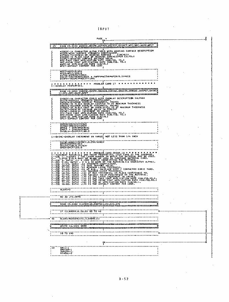
I N P U T

PAGE 4

OK----------------------- RRRRRRRRRRRRRRRRRRRRRRRRRRRRRRRRRRRRRRRRRRRRRRRRRRRRRRRRRRRRRRRRRRRRRRRRRR R 25' READ (5,3101 WSDESC.WSSTR WSTMIN,WSCOST,WSSPCT WTC WPC.WAPP WPCT B RRRRRRRRRRBRRRRRRRRRRRRRRRRRRRRRARRRRRRRRRRRRRRRRRRRRRRRRRRRRRRRRRRRRRR

C WSDESC-16 CHARACTER ALPHA FIEI1D WITH WEARING SURFACE DESCRIPTION C WSSTR-WEAR SURFACE STRENGTH COEFFICIENT. C WSTMIN-THICKNESS OF WEARING SURFACE (INCHES) C WSCOST-IN PLACE COST OF WEARING SURFACEIPER CU.YD..I C WSSPCT-WEARING SURFACE SALVAGE VALUE C WTC-TACK COAT APPLICATION RATE (GAL/SQ. TO.) C WPC-PRIME COAT APPLICATION RATE (GAL/SQ. YD.) C WAPP-AC APPLICATION RATE (LB/IN.) C WPCI-ASPHALT CONTENT PER CENT1

WPPY=WAPP*XINCH WPER=WPCT100.0 WSTHK=WSTMIN/XINCH WSCST=(WSTHK*WSCOSTI • )WPPYaWSTHK*WPER/8.5)*ACG WSSPV=-WSSPCT'WSCSTIIOO.

c a a a a a * * a a a a a a PROBLEM CARD 17 * a a a * * a a a a a a a C--OVERLAY PROPERTIES.

RRRRRRRRRRRRRRRRRRRRRRRRRRRRRRRRRRRRRRRRRRRRRRRRRRRRRRRRRRRRRRRRRRRRRRRRRR R READ (5,320) OVDESC,OVSTR,OMININ,OVMINC.OMAXIN.OVMAXC,OVSPCT,0VINCR K 1I.OTC,OPC,OAPP,OPCT R RRRRRRRRRRRRRRRRRRRRRRRRRRRRRRRRRRRRRRRRRRRRRRRRRRRRRRRRRRRRRRRRRRRRRRRRRR

C OVOESC-16 CHARACTER FIELD WITH OVERLAY DESCRIPTION (ALPHA) C OvSrR-OVERLAY STRENGTH COEFFICIENT. C OMININ-MINIMUM OVERLAY THICKNESS, INCHES C OVMINC-IN PLACE OVERLAY COST/CU YD AT MINIMUM THICKNESS C OMAXIN-MAXIMUM OVERLAY THICKNESS INCHES C OVNAXC-IN PLACE COST OF OVERLAY/LU YD AT MAXIMUM THICKNESS C OVLPCT-OVERLAY SALVAGE VALUE IN PERCENT C OVINCI-OVERLAY INCREMENT IN INCHES C OTC-TACK COAT APPLICATION RATE (GAL/SQ. TO.) C OPC-PRIME COAT APPLICATION RATE (GAL/SQ. YD.) C OAPP-AC APPLICATION RATE lLBIN.) C OPCT-ASPHALT CONTENT PER CENT

OVMIN-OMININ/XINCH OVNAX=OMAXIN/XINCH OMNCT OVMIN*OVMINC OMXCT OVMAX*OVMAXC DVSAIV

:. -OVSPCT/100.0

C--OVINC--OVERLAY INCREMENT IN YARDS NOT LESS THAN 1/4 INCH

OV.INC=AMAXI(OVINCI,0.25)/XINCH OPPY=OAPPaXINCH OVLEVL=UPLVL/XINCH' OPER=OPCT/100.0

C a a a a a a a a * a a a a PROBLEM CARD GROUP 18 a a a a a a a a a a a C--PAVEMENT MATERIALS AND THEIR PROPERTIES LAST CARD IS THE SUBGRADE. C--COL 1, ILAYER) ) THE LAYER NUMBER IN WHICH THE MATERIAL MAY BE USED. C-- ILAYER FIELD MUST BE BLANK OR ZERO ON SUBGRADE MATERIAL CARD. C--COL 3. DATA) .1) A CODE LETTER IDENTIFYING THE MATERIAL. C--COL 5-20. DATA) . 2 3 4 51 NAME OF THE MATERIAL(16 CHARACTER ALPHA). C--COL 21-25, DATA) .6) STRENGTH COEFFICIENT. C--COL 26-30, DATA) .7) SOIL SUPPORT VALUE. C--COL 31-35. DATA) .81 MINIMUM LAYER THICKNESS. C--COL 36-40, DATA) .91 AT MIN., IN-PLACE COST / COMPACTED CUBIC YARD. C--COL 41-45, DATA) .10) MAX IMUM LAYER THICKNESS. C--COL 46-50. DATA( .11) AT MAX THICKNESS, IN PLACE COST/CUBIC YD. C--COL 51-95. DATA) .12) SALVAGE VALUE PERCENTAGE OF THE MATERIAL. C--COL 56-60, DATA) .13) IS THE LAYER INCREMENT IN INCHES. C--COL 61-65, DATA) .14) IS THE TACK COAT APPLICATION RATE (GAL/SQ.YD.). C--COL 66-70. DATA) .15) IS THE PRIME COAT APPLICATION RATE )GAL/SQ.YD.I C--COL 71-75. DATA) .16) IS THE AC APPLICATION RATE )LBIN.). C--COL 16-80. DATA) .171 IS THE ASPHALT CONTENT PER CENT.

NLAYSO

DO 30 Jl.NMP0

RRRRRRRRRRRRRRRRRRRRRRRRRRRRRRRRRRRRRRRRRRRRRRRRRRRRRRRRRRRRRRRRRRRRRRRRRR READ (5 330) ILAYERIJ) )DATAIJ K) K1 11) R

IF) XLAYER)J).EQ.0) GO TO 40 a -------------------------------- V I

I I I I I

I I a 30 N1AYSMAXOINLAYS.ILAYER)J)) • I I

I I I I I

WWWWWWWWWWWWWWWWWWWWWWWWWWWWWWWWWWWWWWWWWWWWWWWWWWWWWWWWWWWWWWWWWWWWWWWWWW I I W WRITE (6.340) NMPD W I I

WWWWWWWWWWWWWWWWWWWWWdWWWWWWWWWWWWWWWWWWWWWWWWWWWWWWWWWWWWWWWWWdWWWWWWWWWW I I I I I

I I GO TO 190 a ------------------------------- I---V

I I

I I

I I

I I

OK------------------------------------------------------------------- 0 I I - I

.40 NM=J-1 • I NMP'NM

-1 . I

SHFCTR1. • I NSHOULO

2 -O

B - 5 2

I N P U T

PAGE 5 -

IF IP(OXSEC EQ 0) GO fo 15

C****S *S****** PROBLECAROGROUP 19****SS***S* C--SHOULDER MATERIALS AND THEIR PROPERTIES LAST CARD IS FILL MATERIAL. C--FILL MATER. HAS ZERO IN DEPTH FIELD, OMIT GROUP IF MDXSEC=O. C--CaL 5-20.SDATA( .2 3 4 5) NAME OF MATERIALII6 CHAR. ALPHA).

FOR FILL MATERIAL) I I C--COL 21-25,SDATA(

C--COL 26-30,SOATA( .6) DEPTH IN INCHESIZERO OR BLANK

711N PLACE COST/CU YD. SALVAGE VALUE(PCf).

I I C--COL 31-35,SDATA(,)

C--COL 36-40.SOATA .9) TACK COAT APPLICATION RATE (GALISQ.YD.I. RATE(GAL/SQ.YD.).

I I C--CaL 41-45.SDATA

C--COL 46-50.SDATA PRIME COAT APPLICATION AC APPLICATION RATE (LB/IN).

C--COL 51-56,SDATA( .12) ASPHALTIC CONTENT PER CENT. C--COL 56-60,SDATA( .131 ADJUSTMENT VOLUME.

I I I

I--- ------------------ DO 60 NFILL 1. NSHOUD •

It I I

RRRRRRRRRRRRRRRRRRRRRRRRRRRRRRRRRRRRRRRRRRRRRRRRRRRRRRRRRRRRRRRRRRRRRRRRRR R READ (5.3501 (SOATAINFILL J) Js2 13) R RRRRRRRRRRRRRRRRRRRRRRRRRRRRRRRRRRIRRRRRRRRRRRRRRRRRRRRRRRRRRRRRRRRRRRRR

I I

. IFISOATAINFILI,61 .EQ. 01 GO TO.70 *---------------------------

I II

! - ------------------ * 60 CONTINUE • I I

I I

NFILL NSHOUD

OK------------------ - -

I 70 NSHOUL = NFILL-1

.

SCA •SDATA(NFILL.7) • I APSV-SDATA(NFILL.8)/100.O RIABL=SDATA(NFILL.131

••••••••••••••••••••••••• I .. ............................

I

. DS(I)=SDATA(I,6)/XINCH SHCQSTII.1)=O.O . I I SHCOSTI I,31=1.O SHCOSTI.21=SDATA(I.71 SPSV(I)-SDATA(I 81/100. RTCS(I)=SOATAU.) RPCS(I)=SDAIA(I 10) APPYSIIISDATA(I,11)*36. . APERSII)SOATAII.12)/100.

i RIAS(I)SDATAII:13) I I

--------* 90 CONTINUE

.100 CONTINUE IF (MODEL.GT .2) UPGWID=UPGWID/2. NLONLONE IF (MOOEL.LT .3) NLONLONE*2

C--SHFCTR IS THE PROPORTION OF OVERIAY C WEARCOURSE WIDTH TO PAVE. WIDTH C--SHFCTR .GT. 1 ONLY MDXSEC .EQ.1 AND IF ASPHALTIC SHOULDERS.

* ---------------------------v

o .j2OuPICMN=uPGID;(wSiHK.OVNIN);UPGCSTflNLo.xLwI

UPGCMX=UPGWID*(WSTHK+OVMAX)*UPGCST/( NLO*XLW) OVMNCT=IOVMIN*OVHINC)*SHFCTR OVMXCT=IOVMAX*OVMAXC)*SHFC)R OMINAC((OPP3*OVMIN*OPERI8.5)*ACG)*SHFCTR OMAXAC (I OPPY*OVMAX*OPER8.5)*ACG)*SHFCTR

C--OVERLAY. WEARING-SURFACE, AND TAIf K-COAT COSTS. INCLUDE SHOULDERS.

WSCST WSCST * SHFCTR WSSPV WSSPV *SHFCTR NTCMIN=(OVMIN-0.027778)ITC INC IF (OVMIN.IE.TCMAX) NTCMIN=0 NWCO IF IWSTHK.GT.0.0) NWCA TCTMIN=(ACTLSOTC*NTCM(N+(ACTL*WTC*NWC))*SHFCTR NTCMAX=(OVMAX-0.027778)/TCIP4C IF IOVMAX.LE.TCMAXI NTCMAX=0 NWCO IF (WSTHK.GT.0 01 NWC1 TCTNAX= IACTL*OfC*NTCMAX.IACTL*WTC*NWC) )*SHFCTR

B - 5 3

I N P U T

PAGE 6

C CALCULATE COSTS AT MINIMUM ANI MAXIMUM

OSNNCTO.O OSMXCTO. 0

A:Cfofto . *

IF (MASPHS.NE.0) GO TO.130

C--IF SHOULDERS NOT ASPHALTIC. TOP SHOULDER LAYER To BE MADE THICKER.

OK--- ----- - . .130 ONNCT=WSCST+UPGCMN+OVMNCT. OHINAC,TCTNIN*OSMNCT

OMXC1WSC ST'UPGCMX,OVMXCT. OMAXAC ,TCTMAx.osMXcT

C CALCULATE OVCOSTS

OK--- -- ------ — ---- -------------------

.135 OVCOST(2)=O.0

IF IOVMIN.EQ.OVNAX) GO TO 140

.140 CONTINUE OVCOSTI 1)=ONNCT-OVCOST(2)'OVMIN OVCOSTI3IO.0 OVCOST(4)1.0 OVCOST(1)OVCOST(1)*OVCOSTI2)*OVLEVL

C---- SAMP6 PERMITS THE INPUT OF SOIL SUPPORT VALUES FOR MATERIALS C ABOVE THE SUBGRADE. IF SOIL SUPPORT VALUES ABOVE THE SUBGRADE ARE C OMITTED OR 1ERO, ONLY THE SUBGRADE SOIL SUPPORT IS USED. IF SOIL C SUPPORT VALUES ARE GIVEN, A PAVEMENT LIFE ESTIMATE IS MADE FOR C EACH LAYER ASSUMING AN INFINITE DEPTH OF THE SOIL SUPPORT VALUE C OF THE NEXT LOWER LAYER. ONE OF THE FOLLOWING OPTIONS IS THEN TAKEN C**** SSOPT1 DESIGN LIFE ESTIMATES BASED ON THE SHORTEST CALCULATED

LAYER INTERFACE. Cia's SSOPT=2 CAUSES ANY DESIGN WITH A CALCULATED LAYER FAILURE TO BE C***S ELIMINATED, IN EFFECT INCREASING LAYER THICKNESSES UNTIL NO CisiS CALCULATED LAYER FAILURE EXISTS ABOVE THE SUBGRADE. C'55 SSOPT=3 DESIGN LIFE ESTIMATES BASED ON SUBGRADE SOIL SUPPORT. C**** OTHER SOIL SUPPORT VALUES ONLY FOR LOCATING THE C-----A SOIL-SUPPORT VALUE ABOVE THE SUBGRADE RESULTING IN A SHORTER C LIFE THAN THE PAVEMENT PERFORMANCE PERIOD CALCULATED WITHIHE SUB- C GRADE SOIL-SUPPORT WILL HAVE AN 'a' PRINTED WITH THAT LAYER ON C THE OUTPUT (USING EITHER OPTION 1 OR 3).

S S OPT

C--WRITE THE INPUT DATA C a a S * * S 5*5* * * * * a * 5* * * * * * * * * * ass * as * *

WWWWWWWWWWWWWWWWWWWWWWWWWWWWWWWWWWWWWWWWWWWWWWWWWWWWWWWWWWWWWWWWWWWWWWUWWN W WRITE (6,3701NDP,NPG NI W W WRITE 16.380) CL XLWFT A W WRITE (6,390) PCTRAT W W WRITE (6.400) UPLVL.WSPR A W WRITE 6.410) R,PSI A U WRITE 6,420) P1 P2 U WRITE 6,430) SALT SRISE,SRATE w W WRITE 6.440) RO.R A WWWWWWWWWUWWWWWWWWWWWWWWWWWWWWWWWWWWWWWWWWWWWWWWIWWWWWWWWWWWWWWWWWWWWWWWWA

C THE PRODUCT OF PROP*HPD SHOULb NOT BE GREATER THAN 1. IF THE STRIP C IS UNDER CONSTRUCTION FOR 24 HOURS EACH DAY, PROP*HPO=1.

6,500) UPGCST WIOUPG 6,510) ACPR,A&D 6.520) XLSO,XISN,XLSO,HPD

CCCCCCCCCCCCCCCCCCCCCCCCCCCCCCCCCCCCCCCCCCCCCCCCCCCCCCCCCCCCCCCCCCCCCCCCCC C CALL HEAONG (NPAGE AN1 &NPROB AN2) C CCCCCCCCCCCCCCCCCCCCCCCCCCCCCCCCCCCCCCCCCCCCCCCCCCCCCCCCCCCCCCCCCCCCC

WWWWWWWWWWWWWWWWWWWWWWWWWWWWWWWWWUWWWWWWWWWWWWWWWWWWWWWWWWWWWWWWWWWUWWWWWW U WRITE (6,540) PPO2 PPN2 W U WRITE (6,550) 002,bNZ.AAS W U WRITE (6,560) ASO,ASN MODEL U W WRITE 16,570) MNTMOD,CM1,CM2 w W WRITE (6,580) X2,CLW U U WRITE 16,5901 CERR,CNAT w

- ----------------------V

------------------------ V

- -----0

B - 5 4

I N P U T

PAGE 1 W WRITE (6,600) NDXSEC.MOCOST,MASPHS U wwwwwWwwwwwwwwwwwwwwwwwwwwwwwwwwwwwwwwwwwwwwwwwwwwwwwwwwwwwwwwwwwwwwwwww

IF (MOXSEC.EO.0) GO TO 145

WWWWWWWWWWWWWWWWWWWWWWWWWWWWWVWWWWWW(WWWWWWWWWwWWWWWWWWWWWWWWWWWWWWWWWWWWW W WRITE 16.610) SOWIQ,S(W(O W U WRITE (6.620) XOWIO,XIWID W U WRITE(6.621) U WWWWWWWWWWWWWWWWWWWWWWWWWWWWWWWWWWW(WWWWWWWWWWWWWWWWWWUWWWWWWWWWWWWWWWWWWW

NMAX NAXO(NIAYS,NSHOUI)

DO 141 I. 1. NNAX

U WU U U U WWW WUW U U U WW WU U W WU WW W J,LI, J1,4) W WWWWWWUWWWWWWWWWWWUWWWWWWW

WUWWWWWWWWWWUWWWUWWWWWWWWWWWWWWWW W W

WWW WWW WU WW WWWWWWW H WWW U WWW WW UWU U WU

---------S

U U WWW

C CC CCCCCC C CCCC CCC CCCCC CCCCCCCCCCCCCCCCCCCCCCCCCCCCCCCCCCCCCCCCC CCCCCCCCCCC C 145 CAlL HEAONG (NPAGE,ANI,NPROB.AN2) C C CCCCCCCC CCCCCCCC CCCC C CCCCC CCCCCCCCCCCCCCCC CCC CC CCC C CCCCCCCCCC CCCCCCCCCCC

WWWWWWWWWWWUUWWWWWWWWWWWWWWWWWWWWWWWWWWWWWWWUWWUWWWWWWWWWWWWWWWWWWWWWWWWWW U WRITE (6.650) U W WRITE (6.660) WSOESC,W551R,USININ,WSCOST,WSSPCT U W WRITE (6.670) OVOESC,OVSTR.OMININ,OVMINC,OMAXIN,OVMAXC,OVSPCT,OVCNW U id WWUWUWWWWWWWWWWWWWWWWWWWIIUWWWWWWWWWWWWWUWVWWUWWWWWWWWWWWWWWWWUWWWWWWWUWWWW

00 150 I1 .Nfl

WWWWWWWWWWWWWWWWWWWWWWWWWUWWWWWWWWWW(WUWWWWWWWUWWWWUWWWWUWWWWWWWWWWWWWWWWU - ----------------- * 150 WRITE (6,680) ILAYERII) (DATA(I,J),J=i,13) w UWWWWWWWUWWWWWWWWWWWWWWWWWWWWWWWWWWWWWWUUWWWWUWWWWWWWWUWWWWWWWWWWWWWWWWWWW

WWWWWWWWWWWWWWWWWWWWWWWWWWUUWWWWWWWWWWUWWWWWWWWWWWWWWWUWWWWWWWWWWWWWWUWWWW U WRITE (6,690) (O#TA(NMP,JJ,J=2,5),OA1A(NMP,7) H WUWWWWWWWWWWWUWWWWWWWWWWWWWWWWWWWWWWWWWWWWWHWWWWWWWWWWWWWWWWWWWUWWWWWWWWWW

IF(NDXSEC.LT.1) GD TO 200

WWWWWWWUWWWWWWWWWWWWWWUWWWWWWWWWWWWU4WWWWUWWWUWWWUWUWWWWWWWWWWWWWWWWWWWWWW U WRITE (6,100) w W WRITE (6.110) WSDESC,WTc,WPC,WAPP,WPCT W W WRITE (6.7101 OVDESC,OTC.OPC.OAPP,OPCT H UWWWWWWWWWUWWWWWWWWUWWWWWWWWWWWWWWWWWWWUWWWWWWWWWUWWUWUWWWWWWWWWWWUWWWWWWW

I-------------- ------........................ 00 160

I I I WWWWIWWWWWUWWWWWWWWWWWWWWWWWWVW1JWWWWWWWWUWWWWWWWWWWWWWWWWWWWWWWWUWWWWWWWWW

---------- S 160 WRITE (6,680) IIAYER(I) (DATA(I,Jl.J1,5(,(DATA(I,J),J.j4,17) U WWWWWWWWWWWWWWWWWWWWWWWWWWWWWWWWWWWWWWWWWWWWWWWWWWWWWWWWWWWWWWWWWUWWWWUWWW

WWWWWWWWWWWWWWWWWWWWWUWWWWWWWWWWWUWWWUUWWWWWWWWWUWWWWWWWWWWWWWWWWWWWWWWWWW U WRITE 6.720) U WWWWWWWWWWWWWW WWWWWWWWWWWWWWWWWWWWWWWWWWWWUWWWWWWWWWWWWWWWWWWWWWWWWWWWWWWW

IF INSHOUL.LT.II GO TO 180 *-----

I--------------------- DO 170 K1 .NSHOUL

I I I WWWWWWWWWWWWWWWWWWUWWWWWWWWWWWWWWWUW WWWWWWWWWWWWWWWWWWWWWWWWWWWWWWWWWUWWWW

---------- * 170 WRITE (6,130) K,(SDATA(k.J) .J2.133 W WWWWWWWWWWWWWWWWWWWWWWWUWUWWWWWWWWWWWWWWWWWWWWWWWWWUWWWWWWWWWWWWWWWWWWWWWW

- 0k .-------- -

.180 CONTINUE - . -

WWWWWWWWWUWWWWWWWWWWWWWWWUWWWWWWWWWWIWWWUIflWWWWWWWWWWWWWWWWWWWWWWWWWWUWWWW W WRITE (6.740)ISDATA(NFILL,J, J2 5), SOATA(NFILL.7l, H W 1. SDAIA(NFILI.8), SOATA(NFILL,13 U WWWWWWWWWWWWWWWWWWWWWWWWWWWWWWWWWWWWWWWWWWWWWWWWWWWWWWWWWWWWWWWWWWWWWWWUWW

GO TO 200 - *-----

.190 LAST=1

B - 5 5

I N P U T

PAGE B

OK- -- ---------- ------ -- TTTTTTTTTTTTTTTTTTTTTTTTTTTTTTTTTTTTITTTTTTTTTT

TTTTTITTTTYTTTTTTTTTTTTTTT

T200 RETURN TTTTTTTTT TTTTTTTTTTTTTTTTTTTTTTTTTTTTTTTTTTTTTITTTTTTTTTTTTTTTITTTTTTT

C__FORMAISTATENENT5

210 FORMAT (2084I

220 FORMAT (IHOINPUT DATA)

230 FORMAT )210.6F10.2) 240 FORMAT 8F10.2)

250 FORMAJ I4F1O.2.I1O610.Z.Il0)

270 FORMAT (6FI0.0,2I1 280 FORMA (7F10.2.I10)

290 FORMAT (I10.7F10.2) 300 FORMAT I3I1O,4F1D.2.IL0

310 FORMAT (4X ,4A4.F5.2,5X, F5. 2. 1OX.F5.2.5X ,4F5.2)

320 FORMAT I4X.4A4,F5.2,58.10F5.21

330 FORMAT LI1LX,A1.1X,4A4 12F5.2)

340 FORMAT (OH. ***ERROR.)5,34HMATER1ALS ALLOWED IN A PROBLEM•***)

350 FORMA )IX,3X,4A4.12F5.2)

370 FORMAT (IHD,5X,43HPROGRAM CONTROL AND MISCELLANEOUS VARIABLES/ LIX 1,52HNPG-THE NUMBER OF OUTPUT PAGES FOR THE SUMMARY TABLE.1HI,I,L5 2H OESIGNSFPAGE). ,lOX,!10./;11X.26HNlTI1E NUMBER OF LANES ON ,33HTH 3E HIGHWAY 180TH DIRE IONS . ,ZIX.I10)

380 FORMAT (IIX.45HCL-THE LENGTH OF THE ANALYSIS PERIOO4YEARSI. 1 35X.F

110_0./.I1X.36HXLWFT WIDTH OF EACH LANE )FEET)..44X.FL0.0

390 FORMAT (L1X,47HPCTRA -THE INTEREST RATE OR TIME VALUE OF MONEY,LOH

1(PERCENT). ,23X,F10.2)

400 FORMAT (LIX,65HUPLVL-THE LEVEL-UP THICKNESS REQUIRED PER OVERLAY)) iNCHES). .15X,F1O.1/1LX,48HWSPRWEARI SURFACE PRODUCTION BA 2TE(TONSIHOUR).,32X F10.1I

410 FORMAT (IHO.5x.42HçNVIRONNENTAL AND SERVICEABILITY VARIABLES,/ LIX 1.IBHR-REGIONAL FAC OR.A62X.F10.L/.111b55HP -THE SERVICEABILItY I 2NDEX OF THE INITIAL ST UCTURE. , 5X,F1 .1)

420 FORMAT IXIX,45HP1-THE SERVICEABILITY INDEX OF AN OVERLAY. •35X,F

LIO.1,/,IIX,36HP2-THE MINIMUM ALLOWED VALUE OF THE 21HSEBVICEABILI 2TY INDEX,,23X.F10.,/.L6X,36HAT WHICH AN OVERLAY WILL BE APPLIED.)

430 FORMAT )IIX.47HSAC -PROPORTION OF THE PROJECT'S LENGTH LIKELY 1X,8 INTO SWELL,24X,F10.29/ ISX.6DHSRISE-VERTICAL DISTANCE THE SURFACE 0 ZF A CLAY LAYER CAN RIE.BH(INCHESI,12X,F10.2,/,h1x,41HSR8TELCUL 3ATES HOW FAST SWELLING QCCURS,39X F10.2)

440 FORMAT )IHO,5X 26HL0A0 NO IR FF VARIAB1ES./..1X,19HR0THE ONE-D

IIBECTION AVER46E DAILY TRAFFIC A THE START OF HE ANALYSIS PERIOD 2. • F11.D / LIX,35HRC-THE ONE-DIRECTION AVERAGE D 3AILY 3BHTRAFFIC AT THE END DY ANALYSIS PER1OD,.X F10.0)

4500 FORMAl ( 12H0* WARNING *, 49HAS INPU , HI PRODUCT OF HPD 1 AND PROPCT IS GREATER. ,,LOX,38HTHAN 100.0 P RCENT --PROGRAMCD ZNTINUESI

440 FORMAT (I1X,44KXNCTHE ONE-DIRECJON ACCUMULATED NUMBER OF 30HEQU IIVALENT 18-KIP AXLES DURING 6X,F .0,F,16X,2OHTHE ANALYSIS ERIOD. 2,,.I1X.54HPROPCTTHE PERCENt OF ADT WH CH WILL PASS THROUGH THE .2 30HOVERLAY ZONE DURING •AX.F1D.1./L6X.15HEACH HOUR WH(LE.2BH DYE L 4AYING IS TAKING PLACE..l LLX,15HI YPE-THE TYPE ,45H0F ROAD UNDER C 5ONSTRUCTIONI i_RURAL,2_URAN).(2DX, liD)ARIATION. ,4$X,F1O.2/iiX,33HM

470 FORMAT II1X.3ZHCOEFVR-COEFFIC ENT OF V 1CONF-CONFIDENCE LEVEL INDICTOR. 47X IL

480 FORMAT (IHD.5X,2DHCONS RAIN VARIABLIS V11X,5LHXTTOTHE A MINIMUM

1LLOWED TIME TO HE FIRS OVERLAV.,29X,16.1./,11X,38HXTB0- HE MINI 2MUM ALLOWED TIME BETWEEN .9HOVERLAYS. 33X,F10.1./ LLX,23HCMAX-THE 3HAXIMUM FUNDS ,35HAVAILABLE FOR INITIAL CONSTRUCT1ON.,22X.Fi0.21

400 FORMAT )LIX.45HTMAXINJHE MAXIMUM ALLOWABLE TOTA, THICKNESS 32HOF 1 INITIAL CONSTRUCTION) NCHES)..3X,F 0.2./LLX,57H MOVIN-TI-4E ACUPWL 2ATEO THICKNESS MAXIMUM OF ALL OVERLAYS ,IDH ((NHES),,13X,F10.2LS 3X,25H(EXCLUDING WEAR-COAT AND •1DHLEVEL-UPI.)

500 FORMAT I11X.48HUPGCSTCOSI/CU. YD. TO UPGRADE AFTER AN OVERLAY.,32 IX.Fl0.2/1IX,6IHWIDUPG.W10TH OF PAVEMEN C SHOULDERS TO BE UPGRA ED 2IFEETI. ,19X.F10 13

510 FORMAT (IH0 9 5X.47HfRAFFIC DELAY VARIABLES ASSOCIATED WITH OVERLAY 6 121H AND ROAD GEOMETRICS ,,,11X,24HACPR-ASPHALTIC CONCRETE ,27HPRO 2UCTION RATE(TONS/HOUR)., 9X,F10.1 ,,iiX,5HACCD-.55HASPHALT C CONCR 3ETE COMPACTED DENSITY(TONS/COMPACtEO CYI,20X1Fi0.2)

520 FORMAT ILIX,47HXLSO-THE DISTANCE OVER WHICH RAFFIC IS SLOWED .25H tIN THE OVERLAY OIRECTION.8X,F10.21/,1iX.HXLSTHE S6HDISTANCE 0 1ZVER WHICH TRAFFIC IS SLOW 0 IN THE NDN-OVERLAY,IIH DIRECTION..4X,F 310.2,/.11X.25HXLSD-THE DISTANCE AROUND ,24HTHE OVERLAY ZONE(MILES) 4.,3lX.F10.2,/.LLX.8HHP0-THE ,53HNUMBER OF HOURS/DAY OVERLAY CONSTR SUCTION TAKES PLACE.,9X,FiD.1I

530

FORMAT (IIX,48HNLRO- HE NUMBER OF LANES IN THE RESTRICTED ZONE .25 1HIN THE OVERLAY DIRECTION.,117/LIX,L9HNLRNTHE NyMBER OF I5BHLANES

540

FORMAT (IHO,5X.47HTRAFFIC DELAY VARIABLES ASSOCIATED WITH TRAFFIC 119H SPEEDS AND DELAYS ,/,16X,24HTHE PERCENT OF VEHICLES ,27HSTOPP 20 DUE TO MOVEMENT OF 23HPERSONNEL OR EQUIPMENT.,/.1i Xt20HPPO2IN 3THE OVERLAY ,iOHDIRECfION.,50X,F10.2./,1iX,24HP2- HE NON-OVER 4LAY ,1OHDIRECTIOP4.,46XF1D.2)

550

FORMAT (16X.45HTHE AVERAGE DELAY PER VEHICLE STOPPED DUE TO ,30HM0 IVEMENT OF PERSONNEL C EQUIP..,'.iiX31HDO2 -IN THE OVERLAY QIRECTID 2N(HOURS).,43X.F10.3./11xA4lHDNZ -IN THE NON-OVERLAY DIREC ION(HDU 3RS)..39X,FiD.3./.11X. 5HA S-THE AVERAGE APPROACH SPEED TO THE OVER 4LAY,6H AREA..29X,F10.0)

560 FORMAT (I6X,42HTHE AVERAGç SPEED THROUGH THE OVERLAY AREA./ IIX,34 LHASO-IN THE OVERLAY DIREC N(MPH).,46X,F10.0,,11X,3BHASNiN THE 2NON-OVERLAY OIRECTION(MPH). 3ANDLING MODEL USED.,42X

1 42X.F1D.O,/,LLX.3BHMODELTHE TRAFFIC H

570 FORMAT )IHO,5X,2IHMAINTtNANCE VARIABLES,/,LIX 49HMNTMOD-THE MAINTE 1NANCE MODELIEX LI

LCIT1,NCHRP2).,31X, 10/1iX.5HC4 1-INITIAL ANNUAL

2 ROUTINE COST(8ANE MILE. MTMOD1b.25X,FL0.2/11X.40HCM 3INCRENENTAL INCREASE IN COSTS,27H(8/LANE MILE/V • MNTMOD I. .13X,F 410.2)

580

FORMAT (1IX.47HX2-DAYS THE TEMPERATURE REMAINS BELOW 32F.(DAVS,iPH 1/YEAR. MNTMOD2). .16X,F10.0/IIX,35HCLW-THE COMPOSITE LABOR WAGEI$/ 2KB) .. 45 X,F 10.2)

590 FORMAT (ILX,41HCERR-THE C0MPOS41R EQUIPHNT RENJAL RATE.1 39X FID.2 [,,I1X.40HCMA - HE RELATIVE MA IAL COS (.00 S AVERAG ). !41.2)

600 FORMAT (IHO,5X,48HCRO S SECTION MODEL, COS AND SHOULDER VAIIABLES 1 ,1IX,36HMDXSECTHE CROSS SECTION MODEL U5EO.,44X,IiOiiX,27HMDC0 2ST-THE COST MODEL USED. 163 111X, A3HMASPHS-ASPHAL IC SHOULDER 2MOOEL (0 IF NOT ASPHALT1C SHOULDERS ., 1271

610 FORMAT (LIX.4OHSOWID_W1?TH OF OUTSIDE SHOULDER IN FEET,40X,F10.21 liIX.4OHSIWID-.WIDTH OF NSIDE SHOULDER IN FEEf,40X,FI0.2)

620 FORMAT (1IX,b2HXOWID-CROSS SECTION WID+H OUTSIDE OF 0UTSIE SHOULD LERIFEET) •IBX.FLO.2/iiR,62HXIWIDCROSS SECTION WIDTH OU SIDE OF 2 INSIDE SHOULDER(FEET) ,18X.F1 0

.2I

I 621 FORMAT(61H0 ADDTIONAL WIDTH(FEET) OF LAYERS RELATIVE TO LAYER

1 ONE. F IHO, LOX. 4HLAYER PAVENEN -LAYERS SHOULDER-LAYERS /

B - 5 6

(

I N P U T

PAGE 9 2 I1X. 41H NO. OUTSIDE INSIDE OUTSIDE INSIDE I

622 FORMATI6X. 110, P10.2. F8.2. P10.2. P8.2) 630

FORMAT IIHO.5X 38HTACK PRIME. AND BITUMINOUS VARIABLES /118 28HAC ITI—TACK COAT OST(B/GALI..52X F10.2/1IX,28HAIPCPRIME COAT OST(B 2/GAL)..52X.F 10.2111X.36+IACG—BIfUMINOUS MATERIAL COST(BGAL)..44X.F 310.2)

640

FORMAT (I1X.5IHTLMAX—MAXIMUM LAYER DEPTH FOR NO TACK COATS. INCHES 1.29X,F1O.2/LIX 52HTLINC—MAXIMUM DEPTH OF EACH LIFT ABOVE TIMAX, IN 2CHES.28X P10.21

650 FORMAT (IHO.20X,4EHTHE CONSTRUCTION MATERIALS UNDER CONSIDER.IOHAT lION ARE ./.40HOLAYER —PAVEMENT MATERIALS— STRENGTH 147HSOIL - 2 --- MINIMUM ---- ---- MAXIMUM---- SALVAGE,/,47H NO. CODE DESCRIP 3TION COEFF. SUPPORT.2116H DEPTH B/CU.YD.b.8H VALUE.2X.9H 41 NCREMENT)

660 FORMAT IIH ,lX.l-.5X.1I+,2X,4A4,2X,F8.2.8H S ------.2F8.2,IX.218H 1 ------ I.2X.

I+F8.2.8H ---1

670

FORMAT IIH ,1X.IH—.5X,1I+.2X.4A4.2X,F8.2.8H ------,2F8.2,IX,2F8.2 1.2* .3F 8.21

680

FORMAT (1H ,1X.I(.5X.A1.2X,484,2X,F8.2,F8.2,2F8.2.1X.2F8.2.28,3F8. 12)

690 FORMAT (1H .IX.IH—.5X.1H—.2X.4A4.2X,8H -----,F8.2,2(218H L).1X),1X,8H -----,F8.2)

700 FORMAT (IHO 28* 32H--APPLICATION RATES---- ASPHALT/IX 5HLAYER,2X, 12OH—PAVEMEN MAtERIALS— 5X.3OHTACK PRIME ASPHALT CONtENT 2 /EX.3HNO..4X,ITHCODE O ESCRIP1ION.8X,3OHCOAT COAT ILB/ 3IN) IPCT)

710 FORMAT CLH .IX.IH—,5X.IH 2* 464,2* 4F8.7) 720 FORMAT (/IHO.52X 32H---APILII!AIION ATES---- ASPN8LT/IX,5HLAYER 2X 1.45H—SHOULOER MA+ERIALS— ----- --------SALVAGE,4X,28HTACK i'RI

2MB ASPHALT CONTENT.8H ADJUST./4H NO..5X,IIHDESCRIPTION,12X.6IHDEPT 3H $/CU.YD. VALUE COAT COAT (LB/IN) (PCT) VOLUME)

730 FORMAT IIH .IX.I1,5X.LH—.2X.4A4,2X.8F8.2) 740 FORMAT (iN .ZH —,5X,IH—.2X.4A4.28,8H -----,2F8.2,8H ------,2(8H

1 ------ ) • 8H ------.F8.2)

END

V. I

I I

-----------------------

I I

I I

I I I---))

OUTPUT

SYMBOL KEY

EEEEE ENTRY TTTTT • TERMINAL CCCCC CALL RRRRR READ WWWWN WRITE

EEEEEEEEEEEEEEE EEEEEEEEEEEEEEEEEEEEEEEEEEEEEEEEEEEEEEFEEEEEEEEEEEEEEFEEEEE E SUBROUTINE OUTPUT (NMDGNT,KDESGN,KSKIP,BCOST,IBBT,AMINCT,BSTNUM,BAE B ILL BBDEXI BBTT 81CC BBPRM BBPOCC BBPTUC BBSAL) E EEEEEEEEE EEEEEE EEEEEEEEEEEEEEEEEEEEEEEEEEEEE

C * S • * 0 * * S 0 0 * a * 0 * I. * * •• * * * • * * S * * S * S *

LOGICAL RURAL I

COMMON A(6),AAS,ACCD,ACG ACPR ACTL,AOTG ADTO AI)11).AI.PC,ANI(20) A 1N2)19),AOI11) APER)6) APRS(5LAPPY(6)jPPYS5) APSV AS(1,ASO CERI, 2CL CLW CMAT,C14AX,CM1,M2,CODE(6),COEFVR COSTIA 3),DAAU1,2Of,OELO 3,0SC),4),DMAX16I DMIN(6),DN2 002 DOVE.(6I,OS5),FLAG(6I ,HPD,ILAY 4ER(11),1PERF.KT)IO1,LAYER,MCON.M0OST,MDXSEC.MNTM0D,M0DE1,NL0,0 5N8,NLRN NLRO NM NMB NPAGE NP000,NSHOUL COMMON 1VCOSI)4 OVINC.OVLEVL OVMAX OVMIN,OVSALV,OVSTR,PN2 P02 PRO

1P PSI,PSVGE(6) P2 R RATE cdABI RIASI5) RPC(61,RPCS(61 R1C161 RY 2C(5I,RURAL,SAT,HCbSiI5 31,SCA HFCTR,Sh5).SOI5l.SPSVE5) SRAIE 3581 SE, 550PT STRNUMI 20) SWI,SWO,T1 INC. TCKMAX,TCMAX 1HKOV.TT(OI , T1 4KG,Tl8KO,WSST,WSPR,WSPV,WSSTR,WSTHK,XINC(6).XJ)h,XLSO,XLSN,XLS0 5,XLW,XTBO,XTTO,X6I,XWO,82

C*SS * .0*0*0*0*0.0.1.0... * S S *05*55 * *5 *

DIMENSION 8011(20), 86DEXT(20, BALL(20), KSKIP(L0)

IF IXDESGN.GT.0) GO 10 10 • *

WW b,WWWWWWWWWWWWWWWWWWWWWWWWWWWWWWW4WWWWWWWWWWWWWWWWWWWWWWWWWWWWWWWhWWWWW W WRITE 16 60) W W IF IKSKI(11.NE.0) WRITE 16,170) W W IF )KSKIP(2).NE.0) WRITE 16,180) S W W IF )KSKIP(4).NE.0I WRITE 16,150) V V IF )I(SKIP(3).NE.0) WRITE (6,160) W WWWWWWWWWWWWWWWWWWWWWWWWWWWWWWWWWWWWWWWWWWWWWWWWWWWWWWWWWWWWWWWWWWWWWWWWWW

------------------------------------------ GDTO5O

.10 CONTINUE

WWWW WWWWWWWWWWWWWWWWWWWWWWWWWWWWWWWWWWWWWWWWWWWWWWWWWWWWWWWWWWWWWWWWWWWWWW W WRITE (6,70) NMDGNT V WWWW*WWWWWWWWWWWWWWW WWWWWWWWWWWWWWWW6WWWWWWWWWWWWWWWWWWWWWWWWWWWWWWWWWWWWW

--------------------------- 00 20 L1,LAYER

• BALLLBALL(L)*36.O

WWWWWWWWWWWWWWWWWWWWWWWWWWWWWWWWWWWWWWWWWWWWWWWWWWWWWWWWbdWW*bdWWWWWWWWWWWWW -----* 20 WRITE (6,80) CODE(L),FLAG(L),IDESC(L,J),J1,41 BAILL V

WWWWWWWWWWWWWWWWWWWWWWWWWWWWWWWWWWWWWWWWWWWWWWWWWWWWWWWWWWWWWWWWWWWWWWWWWW

WWWWWWWWWWWWWWWWWWWWWWWWWWWWWWWWWWWWWWWVWWWWWWWWWWWWWWWWWWWWWWWWWWWWWWWWWW W WRITE (6,90) 8811111,BSTNUM V WWWWI,WWWVWWWWWWWWWWWWWWWWWWWWWWWWWVWWWWWWWWWWWWVWWWWWWWWWWVWWWWWWWWWWWWWWW

............... . ............................ * WWI4WWWWWWWWWWWWWWWWWWWWWWVWWWWWWWWWWWWWWWWWWWWWWWWWWWWWWWWWWWWWWWWWWWWWWWW V WRITE (6,100) W WWWWWWWWWWWWWWWWWWWWWWWWWWWWWWWWWWWWWWWWWWWWWWWWWWWWWWWWWWWWWWWWWVWWWbWWWW

IMI-1

C--CALCULATE OV ERLAY INCHES FOR OUT'UT.

TO VER= BODE XI( 1) S 36.0

WWWWWWVWWWWWWWVWWWVWVWWWWWWWWWWWWWVWWWWVWWVWWWWWWWWUWWWWWWWWWWWWWWWWVWWWWW -----0 30 WRITE (6,110) TOVER,BBTT(IM) V

WWWVWWWWWWWWWWVWWWWWWWWWWWWWWWWWWWWWWWWWWWWWWWUWWWWWWWWWWVWWWWWWWWWWWWWWVV

OK

WVWWWWWWWWWWWWWWWWWWWWWVWWWWWVWWWVWWWWWWWWWWWVWVVWWWWWhWWWWWWWWWWWWWWWWW W40 WRITE 16,190) 8811) 1081) W V WRTE (6.120) BICC,BBPRM,88POCC,08PTUC,08SAL,BCOST W WWWWWWWWWWWWWWWWWWWWWWWWWWWWWWWWWWWWWWWWWWVWWWWWWWWWWWWWWWWWWWWWWWWWWWWWWW

OK

WWWWWWWWWWWWWWWWWWWWVVWVWVWWWWVWVWWW(WWWWWWVWWWWWWWWWWWWVWWWWWVWWWWWWkWWWW W50 WRITE (6,130) (CODE)L),L=1 LAYER) V V WRITE (6,140) IKT(JI,J=1,6 V. WWWWWWWWWWWWWVWWVWWWWWWWVWWWWWWWWWWWWWWWWWWWWWWWWWVWW WWWWWWWWWVWVWWWWWWWWW

TTTTTTTTTT1TT1TTT1TT11TTTTTTTTTTTTTT1T1TT1TTT1TTTTTTTTTTTTTTTTTTTTTTTTTTT T RETURN 1 TTTTTTTTTTTTTTTTTTTTTTTTTTITITTTTTTTTTTTTTTTTTTTTTTTTITTTTTTTTTTTIITTTTTTI

B - 5 8

o.0 I P•U I

PAGE 2

C-FORMAT STATEMENTS__________________________ 60 FORMAT (50HOTHE FOLLOWING CONSTRAINTS PREVENTED A DESIGN W(TH,/43H

1 THIS SET OF MATERIALS (THIS DESIGN TYPE).) 70 FORMAT II2X,I2,3X,58HTHE OPTIMAL DESIGN FOR THE MATERIALS UNDER CO

LNSIDERATION—/8X,45HFOR INITIAL CONSTRUCTION THE DEPTHS SHOULD BE) 80 FORMAT (15X 43 A2,4A4 F8.2 TH INCHES) 90 FORMAT I8X,5HHE 1IF OF fHE INITIAL STRUCTURE ,F6.1,6H YEARS,5X

1 I7HSTRUCTURAL NUMBER F6.2) 100 FORMAT (OX,23HTHE OVEILAY SCHEDULE IS) 110 FORMAT (15X F5.2,4IHINCH)E5) (EXCLUSIVE OF LEVEL-UP AND WEAR-,13HC IDURSE) AFTF F6.1,7H YEARS.) 120 FORMAT (/8X6HTHE TOTAL COSTS PER SQ. YD. FOR THESE CONSIDERATION

15 ARE/15X,2HINITIAL CONSTRUCTION COST,9X,F6.3/15X,30HTOT ROUTIN 2E MAINTENANCE COST, 4X,F6.3/15X.3IHTOTAL OVERLAY CONSTRUCTION COST, 33X,F6.3/15X 22HTOTAL USER COST DURING/25X,2OHDVERLAY CONSTRUCTION 43X.F7.3,I,1X,13HSALVAr,E VALUE.20X,F7.3,/,15X,18HTOTAL OVERALL CO 5T 15X F7.3)

130 FbRMA (44H05A1IPA PROGRAM ACTIVITY REPORT DESIGN TYPE ,IOAI) 140 FORMAT (2X.I5HINITIAL OESIGNS/1X,I9,17H WITHIN COST AND ,2IHTHICKN -LESS CONSTRAINTS/1X,19,26H FEASIBLE 10 FIRST OVERLAY/2X 8HOVERLAYS, 21X.19 IIH CONSIOERED/1X !9.9n FEASI8LE/4X,I6 27H FEASIBLE OVERLAY 3POLICIES ,12X 16HCOMPLEfE OESIGNS/4X,I6,9H FASIBLEI 150 FORMAT (//4X,2HTHE MINIMUM TIME BETWEEN OVERLAYSIS TOO LONG AND/ IOR/4X 52HTHE MAXIMUM ALLOWABLE TOTAL OVERLAY THICKNESS IS TOO/4X,5 22HSMAIL TO OBTAIN A FEASIBLE OVERLAY POLICY FOR ANY OF/4X,2OHTHE I-3NITIAL DESIGNS.)

160 FORMAT (//4X,67HTHE CONSTRUCTION RESTRICTIONS ARE TOO BINDING TO 0 I8TAIN-A STRUCTURE/4X.65HTHAT WILL MEET THE MINIMUM TIME TO THE FIR 257 OVERLAY RESTRICTION.)

170 FORMAT (61HOFOR THE DESIGN UNDER CONSIDERATION THE FUNDS AVAILABLE I ID BE/54H SPENT PER SQ. YD. ARE NOT ENOUGH TO COVER THE DESIGN.) 180 FORMAT I//4X,46HTHE DEPTH-OF EACH MATERIAL RESULTED IN A TOTAL,/4X 1,5IHPAVEMENT THICKNESS GREATER THAN THE MAXIMUM ALLOWEQ,/4X,1AHTOT 241 THICKNESS.)

190 FORMAT (BX,I7HTHE TOTAL LIFE = ,F6.1,7H YEARS.)

END

B - 5 9

0V R L A V

SYMBOL KFY

EEEEE ENTRY

Trill TF.RMINAL CCCCC CALL RRRRR READ WWWWW WRITE

EEEEEEEEEEEEEEEEEEEEEEEEEEEEEEEEEEEEEEEEEEEEEF EEEEEEE EEEEEEEEEEEEEEEEEEEEE E SUBROUTINE OVRLAY (IBT,T,BPTUC,BPOCCT,BPRM,ANINCT,BTT.BDEXT,BSAL,KE

FEEEE EEEEEEEEEEEEEEEEEEEEEEEEEEEEEEEEEEEEEEEEEEEEEEEEEEEEEEEEEEEEEE

C—IBTNUMBER OF PERFORMANCE PERII1D C--T=TIME AT END OF FIRST PERFORMANCE PERIOD AT SUBPROGRAM ENTRY C— BUT RETURNED AS TIME Al END OF LAST PERFORMANCE PERIOD OF THE C-- OPTIMUM OVERLAY POLICY., ELSE 0.0 IF NO SUCCESSFUL POLICIES. c * $ * * * * * * * * * * * * a a a * a * * C * * * * * * * * * a * * *

LOGICAL RURAL I

COMMON AlA) AAS ACCD ACG ACPR ACTL,ADTG ADTO AIIILI,ALPC,ANI(20) A 1N2I19),AO(1II,AER(6l APRS(5 APPY(6),APPYS15) APSV ASN,ASO CER 2CL CLW CMAT CMAX.CM1,H2 COOE(I COEFVR COSTIA ),DAA(1),20I,OELl3 3,OSCI,4l,)IMAX(6) DMIN(b),DN2,0&2 DOVE(6) 0S15),FLAG)6I,HPD hAY 4ER)111,IPERF,Ktt1OLLAYER,MCONF,MOIOST,MDXSk,MNTMOO,MODEL,M6,NLO 5NE,NLRN NLRO NM NMB NPAGE,NPROB,NSHOUL

COMMON IVCO5f(41 OVINC,OVLEVL OVMAX OVMIN,OVSALV,OVSTR,PN2 P02 PRO IP.PSI,PSVGE(63 .pl P2.R RATE RIABL,RIAS)5) RPC)A).RPCS(61 RIC(6 RT 2CSh5I,RURAL,SACT,HCOSi(S 3,SCA SIIFCTR,5l(51 SOI5I.SPSV15) SRAE 3SRISE,SSOPT,STRNUMI2OI SWf.SWO TIlNC, TCKMAX,TLMAX,THKOV TT(0),T1 4KG,TLBK0,WSCS1,WSPR.WSPV,WSSTl,WSTHK,XINCI6),XJ(7) ,*is6, XLSN,XISO 5,XLW.XTBD,XTTO,XWI ,XWO,X2

c a sac * a * a * * a a sass I a a a ass * * a a a seas. a

DIMENSION OAOOI20I, OCOSTI2O)! OEXTI20), USERCT(20), KSKIPI 101, BI 11(20), BDEXT(20)

DATA HICOST/1.0E30/, 5MALLN/1.OR-30/

LPII.AYER+1

C--MINIMUM COST OFOVFMLAY POLICY ST AT A VERY HIGH NUMBFR.

- AMINCT.HICOST

C-- --INITIALIZE USER FUNCf ION FOR THIS INITIAL DESIGN.

USERCTUIUSER)O.O,0.0) 000ST(1)O. OAOD(1I0.O BT1(1)=O.0 11 IBT=1 TT)I)T

IF )T.GE.CLI GO 10 40 *------------------

C THE REMAINDER OF THE OVERLAY OPTIMIZATION RESEMBLES A •*TREE5*.IT C IS NECESSARY TO SELECT THE OVERLAY POLICY WITH THE LEAST COST.

ABODO.0

C ABOD IS THE ACCUMULATED DEPIHIOF ALL PREVIOUS OVERLAYS.

TPRIM1

OK----------------------------------------------

.10 DELD.OVMIN

C THE DEPTH OF LAYER I IS = ORIGINAL DIII • SUM OF PREVIOUS OVERLAYS C CURRENT OVERLAY DEPTH.

------------------------------------------------

66ôA bióo a---------

KT(3)K1I3)+l IPERF.I T1IME(IPRIM,P1.IPRIM.XTBO)

IF IT.GT.0.OI GO TO 30 $---------

(1ELO.OELO.OVINC

GO TO 20 a------

.30 DEXIIII=DELD

V

B - 6 0

.3.

OVRLAY

PAGE 2

C--FEASIBLE OVERLAY, I

KT14).KTI4)+l

C--USER COSTS FOR DELAYS AT BEGINNING OF I TH PERF. PERIOD.

AOT.ADTOIAOTGSTPRIM HPSY=I I IACCD*(OELD+OVLEVLI) p. AMAXLISMALLN,ACPR) I I (ACCO*WSTHK) / AMAXI(SMALLN,WSPRI ) ) * SHFCTR

USERCT(I)=USER(AOT*PROP,HPSY)

C--OVERLAY CONSTRUCTION COST FOR TH ITH PERFORMANCE PERIOD.

OCOSTI I(0 VCOSTIE (0 VCOST 121*DELO IF IOVCOST(3)SDELD.GT.O.0) OCOSTII)

I =OCOSTIII,OVCOST(3I*(DELO**OVCO.

IST(4I) DADD(I)DELD TT(I(1

C THE PREVIOUS OVERLAY WAS NOT UFFICIENT TO LAST THROUGH THE ANALYS C PERIOD IF T IS LESS THAN CL.

IF IT.GE.CLI GO 10 40

IF (IABDD,DELDI.GE.THKOV) GO TO 80

I I I.

TPRIMT • ABOD.ABDD+OADD(I—t(

* -----------------------I---

OK

.40 CONTINUE

C—LAST OVERLAY PERFORMANCE PERIOD EXCEEDS ANALYSIS PERIOD, EVALUATE C--THIS POLICY BY COMPARISON WITH OTHER OVERLAY POLICIES FOR THIS DESIGN

KT(51KT(51+t ICLI

C--TOTAL ALL COSTS AFFECTED BY OVERLAY POLICY IN PRESENT WORTH VALUES.

P0CC 1= 0. PRMO.0 PTUCO.0 PSAL=0.0

C--PRESENT WORTH FACTOR FOR SALVAGE T VALUES, FROM END OF ANALYSIS PERIOD.

SALP WF=1. 0/I 1. 0.RA YE) * *CL TPRIM0.0

DO 50 I1,ICL

C--PRESENT WORTH FROM BEGINNING OF PERFORMANCE PERIOD.

PWFCTR=L.0/II1.0*RATE)**TPRIMI

C--PRESENT WORTH OF ROUTINE MALNTENANCEIITH PERF. PERIOD) TOTALED.

PRM= PRM* Pw FCTR*RMA INT IT PR !M,T TI I) I POCC1=POCCTGPWFCTR*000STII) PTUCPTUCGUSERCT(II*PWFCTR PSAL=PSAL+OCOSTI I )*SALPWF*OVSALV TPRIM=T1III

---* 50 CONTINUE

C EVALUATE THE COST (IF THE AlTERNATIVE OVERLAY PROCEDURE AND COMPARE

C TOTHE CHEAPEST COST SO FAR.

C TC—THE SUM OF ALL PRESENT WORTHS OF OVERLAY COSTS.

TC POCC T eP T oCt PlO MtP SAL I=ICI.

I. IF IAMINCT.IE.TC) GO TO 80 *------------

3 2.1

B - 6 1

OVRLAY

PAGE 3

AMINCTTC BPOCCTPOCCT BPTUCPTUC 8PRMPRM

. BSALPSAL IB1ICL

DO 60 JK1,1BT

60 BTTIJKITTIJK)

IF IIBT.EQ.1) GO TO 80 *

---- 00 70 JK.2,IBT

---* 70 BDExE(JK)=DEXTIJK) . I

IIBT •

C SELECT A DIFFERENT OERLAY PO1CYIANOTHER BRANCH THE TREE) AND C GO BACK TO DETERMINE OVERLAY COSTS. I

I I OK-------------------------------------------- 0

.80 IF II.LE.23 GO TO 100 *

1=1-S OELO=DADD)I)+OVINC INI-1 ABODO.O

----- --- DO 90 K=1,IM

--------* 90 A800=ABDD+OADD(K)

IPRINTTIIM)

GOTO2O

OK -

.100 TBTTIIBTI IF IT.LE.0.0) KSKIP(4)KSKIP)4)+1

lET ETTTTITTTITT TTTTTTITTTTITTTTTTTTTTTTTTTTTTTTTTTTTTTTTTTTTTTTTTITTTTTTTT 7 RETURN T TT1TTTTTTTETTTTTTTT1TTTTTTTTTTTTTTTTTTTTTTTTTTTTTTTTTTTTTTTTTTTTTTTTTTTTTT

END

I I I I A I

-----------------------

B - 6 2

P U P Y

SYMBOL KEY

EEEEE ENTRY 11111 TERMINAL CCCCC CALL RRRRR • READ WWWWW WRITE

EEEEEEEEEEEEEEEEEEEEEEEEEEEEEEEEEEEEEEEEEEEEEEEEEEEEEEEEEEEEEEEEEEEEEEEEEE E FUNCTION PUPY (PaNE TPRIM I PERFB PERFY XJAYI E EEEEEEEEEEEEEEEEEEEEEEEEEEEEEEdEEEEEEEEEEEEEEEEEEEEEEEEEEEEEEEEEEEEEE

C.*a**ass***a******a**s*s****iss*ass I

LOGICAL RURAL COMMONA(6) AAS ACCD ACG ACPR ACTL,AOTG ADTO AIUI.I,ALPC,ANL(20) A

1N2(19),AOL11).AER(6I,APRS(5.APPY(6I,XPPYSi5).APSV ASN 650 CE,E. 2CL.CLW.CNAT.CMAX,CM1,CMZ.COOE(6),COEFVR,COST(6,3),DATA(1t,20I,OEtO 3.OESC(7.41.DMAX(6I,DMIN(6).0N2,002 DOVERI6) DS(5,FLAG(6I,HPO hAY 4ER(1L),IPERF.KT(10).LAYER.MCONF,MD0S1,MDXSC,MNTMOO,MODEL.NLô,NLO SNE.NLRN.NLRO NM,NMB NPAGE,NPROB,NSHOUL

PNZ P02 PRO COMMON OVCOSfI4) OVINC,OVLEVL,OVNAX OVMIN,OVSALV,OVSTR 1P,PS1.PSVGE(6)P2 R RATE RIABL RIAS(5) RPC(6) RPCSI1.) RtC(6) RI .P 2CS(5).RURAL,SACT,HCb5fI5 3LSCA HFCTR.SI(5! SO51,SPSV15) SRATE 3SRISE,SSOPT.SIRNUM(201 SWf,SWO IINC,ICKMAX,TMAX THKOV TTIO).TL 4KG,TE8K0,WSCST,WSPR,WSPV,WSST,WSTHK,XINC(6I .XJ(h.XLSI.XLSN.XLSO 5.XLW.ETBO,XTTO.XWI .XWO,X2

Ca... * a. a... a a. * oar. a * . * * * * * * •. * * * * * * I

DIMENSION CONFI?) DATA CONFO.0,0.525, 1.28,1.645.2.33, 2.575.3.08/

PUPY=1•O

IF (MCONF.LE.1) GO 10 10 a

..=COEFVR .. SN=STRNUMIIPERF) . SS=3.0+ALOGIO(XJAY)F0.03973 GP=O.335a5ACT*SRISE/(PONE-1.51 • TA=EXPI-SRATE5IPRIM) TB=-EXP(-SRATE*T3 • E TC=TA-TB

•TD=T*TB-TPRIM5TA . GPP=GP*IC GPT=GPaTD . GG=1.-GPP BGG=PERFB*GG •

11 S2D=(C*C*(O.2649+(6.O664*SN( 1.O+SN) )**2+O.1384*SSaSS.(O.6142*P2/( • 1BGGS(PONE-P2) I-SNSALOGGO(GGUIPERFB*( 1.+SN) P-IO.4343/BGG)*SQRT( (GP. 2P*PONE/(PONE-1.51)*a2+3.0*GPPa*2+( SRATE*GPT)*a2)1**2) 1*0.0227 •

PUPY=10.0**(CONFIMCONFI*SQRT(S2D)) •

____ --------------------------------- ( ITTTTTTTTTTITT1TT1TTTTTTTIT1TTTTTTII3ITTTITTTTTTTTTTTTTTTTTTTTTTTITITTITII 110 RETURN I TTTTTTTTTTTTTTTTTTTTTITITITITTTIIIIITTITT1ITTITTTTIITTTTITITTIIITITTTTTTTT

END

B - 6 3

R M A I NT SYMBOL KEY

EEEEE ENTRY TTTTT • TERMINAL CCCCC - CALL RRRRR REAO WWWWW WRITE

EEEEEEEEEEEEEEEEEEEEEEEEEEEEEEEEEEEEEEEEEEEEEEEEEEEEEEEEEEEEEEEEEEEEEEEEEE

FUNCTION RMAINT (IPRIM TI E

EEEEEEEEEEE EEEEEEEEEEEEEEEEEEhEEEEEEEEEEEEEEEEEEEEEEEEEEEEEEEEEEEEEEEEEE

C*S*a**Ss*S.S*..*S***.S..SsSSS 5*5*S$

LOGICAL RURAL COMMON AlA) AAS ACCO ACG

i&RA.CAPCR

O

,ACT

N

L,A

O

DSTTG,,AOTSDj.Altl PC. L(ZO) A LNZ(19hAO(1I).AER(6 APRS(5I APPYIA) APPYS(5) APSV ASN ASO CERA 2CL CLW CMAT CMAX CM1,M2 CODE(L) COEFVA.COSTI6 3),DAfA(11.2OJ,)EL6 3 OSCI} 4),6MAXI&) OMIN() DM2 062 DOVERI6) DS5).FLAG(6) HPD hAY 4R( 11) ,PERF.K1( SNE.NLRN NIRO NM NNB NPAGE NPROB.NSHOUL COMMON 6vcOSt(4 OVtNC.OVEVL OVMA* OVMIN,OVSALV.OVSTR,PN2 P02 PRO

[P PSI,PSVGE(6),PtP2 B RATE RIABL RAS(5) RPC(6) RPCSIA) R1C(6.RT 2C(5),RURAL,SACT,HC6SIl5 3,SCA HFCTR.SIl5) SOl5),SPSV1S) SRA1E. 3SRISE SSOPT STRNUMI2O) SWt,SWO T$INC,TCKMAX TMAX THROY TTl0).T18 4KG.TLAKO,WSST.WSPR,WSPV,W5STA,T,x,x , x15N 50 5,XLW.XTSO.XTTO,KWI,XWO.X2

* $ S * * • * • • •• I 5*5*5* • * •..• * ..

flc MAINTENANCE

TPERFAMINIICL T)-TPRIM XPRT.EXP(-RATE*TPERF)

C GO TO CORRECT MAINTENENCE COST FORMULAS

GO TO (10,30), MNTMOD

C—MOOELI, USER ESTIMATES OF ANNUAL1 MAINT. COST AND GROWTH RATE.

.10 CONTINUE

------------------------------- IF IRATE.EQ.O.OI GO TO 20

AAIAi iii Mi/TCM l,I.0)/(RATE*$2)I))/(1760.*XLW(

GOTO7OV

--------

.20 CONTINUE RMAINT(CMI*TPERF+ICM2*TPERF**21/2.01 1(1760.' XLV)

•

GO TO 70

C-----CALCULATE MAINTENANCE COST FROM NCHRP FORMULA, MODEL 2

OK—- - ------------------------------

.30 CONTINUE

IF (RURAL) GO TO 40

XL WX .0.60 XERR 0.19 XMAT.0.21

GO TO 50

- .40 CONTINUE

XLWX.0. 44 XERR•0.2L XMATO.35

.50 CONTINUE CYP.( XLWXSCLW+XERR*CERRSXMAT*CMAT)/17040.*XLW)

IF (RATE.EQ.0.0) GO TO 60

B - 6 4

RMA I NT

PAGE 2

1IRATEA*IITPEAF/RATE.S2I_ITPE*F..2J(2.O*RAVE I) RMAINT.AMAXL(O.CyP.y O,pl

YP-4-83..L3 72*K2)STPE.F.l6.573*TPERF.s3) RMAINT.AMAXLIO.O,YPSCYPI

.70 CONTINUE

TTTTTTT!TTVTTTtTTTTTTTTTTTTTTTTTTTTVtTT7TTTTTTTYTTT1TTT!TTTTTTT TTTTTVTTTTT V RETIJAN 7 TTTTVTTTTTTTTTT !TTTTTTTTTTTTTTYTTTTITTTTTTVTTTTTTTT!TTTTTTTTTTTTTTVTTTT VT,

9.A.1.6.5.4.3.2.

B - 6 5

SOLVE2

SYMBOL KEY

EEEEE • ENTRY TTTTT • TERMINAL CCCCC • CALL RRRRR • READ wWWWW = WRITE

EEEEEEEEEEEEEEEEEEEEEEIEEE€EEEEEEEEEEEEEEEEEEEEEEEEEEEECEEEE€EEEEEEEEEEEEEE

E SUBROUTINE SOLVE2 (NUMBER KSKIP T COSTIN SALVINI B EEEEEEEEEEEEEEEEEEEEEEEEEEEEEEEEEEEFEEEEEEEEEEEEEEEEEEEEEEEEEEEEEEEEE E

C *5 5 5 5 0 5 S * a * a S S a S ** S S S a a * S S S a a a a a S a a

LOGICAL RURAL I

COMMON A(61 AAS ACCD ACG ACPA ACTL ADYG AOTO AI(i1),ALPC.ANI(20) A iN2(iql.Ao(LI).AER(o APRS(5

p9(6) APPYS(5) APSV ASN ASO CERA 2CL CLW CMAT CMAX.CML,M2 COOE(LI COEFVa COSTIE ),DAtA(1L.20l,DELi 3 DSCI+ 41 6MAxIoI DNIN(( 0N2 DIZ OOVE(6I 0515) .FLAG(6) HPD ILAY 4R( 5NE,NLRN NLRO NM NMB NPAGE NPROB,NSHOUI

COMMON IVCOSfI4J OVINC,OVtEVL OVMAX OVMIN,OVSALV.OVSTR PN2 P02 PRO iP PSI.PSVGE(6) Pt P2 R RATE RIABL RIAS(5) RPCI6) RPCS(&I- RTCI6I RI 2CI5) .RURAL.SAI!T.tHCiStI5 33.SCA HFCrR.St(5hSOl5) ,SPSV13I SRAE 3SRISE SSOPT STRNUM(20) swl,swo TINC.YCKMAX TCMAX THKOV TT(20),Ti 4KG.T1K0 WSST.WSPR,WSPV.WSSTA.WSTHK.XINC(&l.XJIb ,XLStI,XLSN.XLSO 5.XLW.XTBO.XTTO,XUI ,XWO,X2

C • a a S S * * a a a a a a a a a a1a a as a as a a a a a's a a S a a

DIMENSION KSRIP(1OI, JSKIPI3I flATA BLANK/in /

C--JSKIP IS ISET NON-ZERO IF COST. THICKNESS. OR MINIMUM TIME C--CONSTRAINTS PREVENT AN INITIAL DESIGN.

I ------------------- DO 10 J-1,3 .

IPERF.i T=O.0

ALVIN

. COSTINO.O SO.O

IF (NUMBER.NE.i) GO TO 30 *-----------------------------------

C INITIALIZE ON FIRST1 CALL WITH A GIVEN SET OF MATERIALS.

It TK=O. .

CTO. .It I-a .

--- DO 20 L.L,LAYER

TK•TKGDMIN(L)

- --------* 20 DOVERIL)•DMIN(1I

CCCCCCCCCCCCCCCCCCCCCCCCCCCCCCCCCCCdCCCCCCCCCCCCCCCCCCCCCCCCCCCCCCCCCCCCC

C CALL INCOST (TX CT SV) ' C CCCCCCCCCCCCCCCCCCCCCC&CCCCCCCCCCCCCCCCCCCCCCCCCCCCCCCCCCGCCCCCCCCCCCCC

IF leT.GT.CMAXI JSKIPUI•1 IF (TK.GT.TCKMAX) JSKIPI2II

..........................................................................

GO TO 60 a------------

I1j11fj&118f84o................................................

tir.................................................... DOVER(L).DOVERIII+XINCRE I TK-TKIXINCRE •

CCCCCCCCCCCCCCCCCCCCCCCCCCCCCCCCCCCCCCCCCCCCCCCCCCCCCCCCCCCCCCCCCCCCCCCCC C CALL INCOST (TX CT SY) CCCCCCCCCCCCCCCCCCCCCCCC&CCCCCCCCCCCCCCCCCCCCCCCCCCCCCCCCCCCCCCCCCCCCCCC

S GOTO6O

C—RESET ITH LAYER TO MINIMUM AND AND INCREASE NEXT LAYER THICKNESSES. I OK------- --------------------------------------------------

--- — - ..... .6Iôo

1 4

B — 6 6

SOLVE 2

I' Ab

DOVERIII=OM!NII) Il*1 TK0.

--------------------------- DO 50 L1,LAYER

------------- * 50 TKTK*DOVERILT

C CC CC CCCC CCCCCC CC CC CC CCCCCC CC C CC CCC' C CALL INCOST UK CT SV) ccccccccccccccccccccccLccLccccccccc

IF IIOOVERII)+AINCII)).GT.DM

XINCRE=XINC(I) OOVER(Ii=DOVERIII+xINCRE TKTK.XINCRE

CCC CC CC CC CCCC CCCCCC CCC C CCC CCC CC CC CCI C CALL INCOST (1K CI SVI cccccccccccccc ccc ccccdccccccccccci

1=1

.60 CONTINUE IF ICT.GT.CMAX) JSKIPI1)I IF ITK.GT .TCKMAX) JSKIP(21=1

•

KT(IIKT(l)+1

00 70 L1.LAYER

- -------------------* 70 FLAG( L I=BI..ANK

CKIINSUNES FUNCTION TIME NOT

.......ifiAo:fiifo.......

IF. (1.11.0.) GO 10 80

JSKIP(3)1

GO 10 30

.80 COST!N=C1 SAL VINS V JSkIP(3)O KI ( 2) K1( 2 I. 1

I -----------------90 00 100 J= 1 • 3

-------------------- S 100 KSKIP(J)KSKIP(J),JSKIp(J)

T11TTTT11T1T1TTT11ITTTT1TTT1TTTTTTT11TT1TTTT1TTT1TT1TTTTTTTTTTT1TTTTTTTI I RETURN ITTTTTTTITTTTTTIITTTTTITTITTTITTTTTTTTTTITITTTTTTTTTTTITTTTTTTTTTTTTTTTTTT

B - 6 7

S U MARY

SYMBOL KFY

EFEEE ENTRY TYTTY - TERMINAL CCCCC • CALL RRRRR - READ WWWWW • WRITE

E BA B ERR RE BE BE RE BE EE RE EEE EEE EE E SUBROUTINE SUMARY (NNB EREE BEER fEE IEEE EEEEEEE EF BE BEE

C-A SUMMARY OF THE 8ETTER(LOWEST COST) DESIGNS ARE PRINTED FOR PROBLEM.

DIMENSION IOUMMY(34) POLICY(5,3O) ANI(20), AN2U9) DIMENSION P850(26), 854(26) P858(k)

/4H11X,F, FB50l)/4H2HDI, FB50(3)4H,IL I 1 F85014 F850(26)1314IX) DATA P854(1

/4HLHI,I, F85015)I4HI2X I, /4H(7X,/, F854(2)/4HZHT(/, P854(3)14(4,11 I,

I P854(4

DATA F850(1i/4H/H),lj/FB5B(5f,,4HIIX,/,

/4HLH),I. F854(5)/4H11X I, F854(26)/3HLX) / DATA P858(1 14H(TX,I, F858)14H2H0(/, P858(3)/4H.I1.I,

I F858(4 I F858126)/3HIX)/ DATA ABLE/VIA?, F4F7.1/, COM/4H,IX / F2I4HP?.2/,411411,A1,/ DATA BLANKILH I, STAR/4H***S/ f NDP/10I, LAYD/6/

IF INMB*ENTOL.EQ.0) GO TO 220 -

NMBESTMINO(NMB,KNTQL)

-- DO 2L0 L-1,NMBEST.NDP

LL-MINOIL,NOP-l.NMBEST)

C--LL-THE NO. DESIGNS THIS PAGE, NM1-WORDS OF 'ASSA' REQUIRED.

NM81((LL-L)'8+31I/4

CCCCCCCCCCCCCCCCCCCCCCCCCCCCCCCCCCCC&CCCCCCCCCCCCCCC CCCCCCCCCCCCCCCCCCCCC C CALL HEADNG INPAGE ANt NPROB AN2) CCCCCCCCCCCCCCCCCCCCCCCCCCCC&CCCCCCCCCCCCCCCCCCCCCCCCCCCCCCCCCCCCCCCCC

WWWWWWWWWWWWWWWWWWWWWWWWWWWWWWWWWWWW4WWWWWWWWWWWWWWWWWWWWWWWWWWWhWWW),WWWWW 8 WRITE (6,2401 (I,I-L,LL) 8 WWWWWWWWWWWWWWWWWWWWWWWWWWWWWWWWWWWWWWWWWWWWWWWWWWWWWWWWWWWWWWWWI,WWWWWWWWW

I----------------- 00 10 I-t.,LL

---* Q IDUMMY(I).POLICY(9,II

00 40 t-1,LAYO

NKOUNT-O

--- 00 30 k.L,LL

.......................................................................... I .......................................................................

POLICYII'9,*)-O.Q

60T030

OK--------------------------------------------------------------- I

'.20 NKOUNT-NKOUNT+1 -t

--• 30 CONTINUE

IF INKOUNT.EQ.0) GD TO 50 ------------------

-------------- v

•......NL&NE:I . •

....•.

.......................................................................... -------- r

WWWWWWWWWWWWWWWWWWWWWWWWWWWWWWWWWWWWWWWWWWWWWW8WWWWWWWWWWWWWWWWWWWWWWWWWWW 850 WRITE (6,2501 ISTAR,I1,NNBT) W WWWWWWWWWWWWWWWWWWWWWWWWWWWWWWWWWWWWWWWW WWWWWWWWWWUWWWWWWWWWWWWWWWWWWWWWWW

B - 6 8

S U MARY

PAGE 2

S

NLP.NLINE+2

W60 WRITE (6.260) ((POLICY(I II),I50 55),IIL,LL) W WRITE (6,270) (POLICY(2,I),1L.LL)

(POLICY(3.I),I.L.L1) W N

WRITE WRITE

(6,280) (6,290) (POLICY(4,I),1L.LL

N WRITE WRITE

(6.300 16.310

(POLICV(6,I),I.L.I.L (POLICY(7.I) I-L,LL

WRITE (6.250 (STAR,I.1,NMBT WRITE WRITE

(6,250 (6,320

(STAR I.1,NMBT (POLICY(8,I) 1-1,11)

WRITE (6,250 (STAR,I.1,NMBT) WRITE WRITE

(6.250 (6,330

(STAR,11 NMBT) (IDUMMY(I,11. LL)

WRITE (6,250 (STAR,I.1,NMBT) WRITE (6,340)

(WWWWWWWWWWWWWWWWWWWWWWWWWWWWWWWWWWWWWWWWWWWWWWWWWWWWWWWWWWWWWWWWWWWWWI

00 90 I.1,NLINE

I— ..... ----- DO 70 (.6,24.2

I I

I • F850(k).F2

I I

------ - --------5 70 F8504k*1).A1

I------ --------- 00 80

I I

I

•

C—CONVERT LAYER DEPTHS TO INCHES FIR PRINTING. I I

IF (POLICY(t.9.K).NE.0.) GO TO 80 S

I I I I • POLICY(I.9 K)8LANI( I I • F850120M.41A8L1( I I • F850(28M55)A1 I I II I I I OK ------- - ------------- ------ II I II I ---------------S 80 CONTINUE

I I WWWWWWWWWWWWWWWWWWWWWWWWWWWWWWWWWWWWW

IWWWWWWWWWW WWWWWWWWWNIiWWWWWWWWWWWWWWWW

I N WRITE (6,F850) I,(POLICY(I.9,J).POLICY(I.40,J),J.L.LL) N WWWWWWWWWWWWWWWWWWWWWWWWWWWWWWWWWWWWWWWWWWWWWWWWWWWWWWWWWWWWWWWWWIWWWWWWWW

--' -----S 90 CONTINUE

I ---------- 00 100 IL,LL

I I ----S 100 IOUMI4Y(I)POLICY(20,I)

WWWWWWWWWWWWWWWWWWWWWWWWWWWWWWWWWWWWWWWWWWWWWWWWWWWWWWWWWWWWWWWWbWWWWWWWWW N WRITE (6,250) (STAR IL,NM8T) N W WRITE (6,350) (POLICY(5.J) JL,I.LI

NMT) W N W

N WRITE (6,250) (STAR (.1 WRITE (6,360) (IDUNAY(If,I.L IL) w

N WRITE (6,250) (STAR,I.1,NNBT) W N WRITE (6.370) W WWWWWWWNWWWWWNWWWWWWWWWWWWWWWWWWWWWWWWWWWWWWWWWWWWWWWWNWWWWWWWWWWWWWWWWWWW

I i ----- ---------- 000k6,24.. .

II I II

I • F854(K)F1 II II I II - -------* 110 I ------ I I I I I I I I I I 2

B - 6 9

S U MARY

PAGE 3

NIcOUNT.0

-------------- 00 130 k.L,LL

........ •

POLICY(I+20,K*.BLANK F854I2eM•4).A8Lk

........ ............- ------ -------

OK--

.120 NXOUNTNKOUNT+1 • .............................................................. ............ tK-- ---- ----------

--• 130 CONTINUE

IF I NKOUNT.EQ.0) GO TO 150 S ------------- - ---------- ---- W WW

W0 WWWWWWWWWWW

,WWWWWWWWWWWWW W J L WWRITE 16,F854) t.(P*ICY2WWWW

LL) WWWWWWWWWWWWWWWWWMWWWWWWWWWWWWWWWWWWWWWWWWWWWWWWWWWWWWWWWWWWWWWWWWWWWWWWWW

--5 140 CONTINUE • OK ------

wwwwwwwwwwwwwwwwwwwwwWWWWWWWWWWWWWWWLWWWWWWwwwwwwwwwwwwwwwwwwwwwwwwwwwwwww W150 WRITE 16,2501ISTAR,I.1,NMRTI - N W WRITE (6,3801 W WWWWWWWWWWWWWWWWWWWWWWWWWWWWWWWWWWWWIWWWWWWWWWWWWWWWWWWWWWWWWWWWWwWWWWWWWW

DO 190 1.1,9

I----------- DO 160 K.6,24,2

•••••••••••••••••••••••••••••••••••••••••••••••••••••••••••••••••••••••••• S 160 F858(K'1lCON

NKUUNT•0

--- 00 180 K.L,LL

P4-K-Ll1

IF (IDUNMY(K1.GE.I+1) GO TO 170 5

poLicyli.3o,K)-BLANK . . F85812*N+4)-ABLK

60T0180 S---------------------------v

- --------------------------------- - :z" .................................................... : C--CONVERT OVERLAY TO INCHES It

POtICY(I•30,KI.(PoLICY(I,30,K)1536.o

II 1•

It

B - 7 0

S U M A RV

23 PAGE 4 3

H OK----— -------- --------

II -----* 180 CONTINUE

I • IF INKOUNT.EQ.0) GO TO ZOO *---------------------------

I I I WWWWWWWWWWWWWWWWWWWWWWWWWWWWWWWWWWWWWWWWWWWWWWWWWWWWWNWWWWWUWWWWWWWWWWWWWW I N WRITE 16,F8581 I.(POL)CY(I+30,J),JL,IL) W I WWWWWWWWWWWWWVWWWWWWWWWWWWWWWWWWWWWWWWWWWWWWWWWWWWWWWWWWbIWWWWWWW

------------------ S 190 CONTINUE

* 210 CONTINUE

WWWWIIWWWWWWWWWWWWWWWWWWWWWWWWWWWWWWWWWWWWWWWWWWWWWWWWWWWWWWWWWWWWWWWWWWWWW W WRITE (6,390) RNTOL U WWWWWWWWWWWWWWWWWWWWWWWWWWWWWWWWWUWWpWWWWWWWWWWWWWWWWWWWWWWWWWWWWWWWWWWWW

GOTO23O e

.220 CONTINUE

CCCCCCCCCCCCCCCCCCCCCCCCCCCCCCCCCCCCCCCCCCCCCCCCCCCCCCCCCCCCCCCCCCCCCCCCCC C CALL. HEADNG INPAGE AWL

&NPROB ANZ) C

CCCCCCCCCCCCCCCCCCCCCCCCC&CCCCCCCCCCCCCCCCCCCCCCCCCCCCCCCCCCCCCCCCCCCC

WWW WU U NUN WWWW WWWWWW WU NW WUWU NUN V N

WWWWWWWWWWWWWWWWWWWWWWWWWWWWWW

TTTTTTTTTTTTTTTTTTTTTTTITTTTTTTTTTTTtTTTTTTTTTTTTTTTETTTTTTTTTTTTTTTTTTTT T230 RETURN TTTTTTTTTTTTTTTTTTTTTTTTTTTTTTTTITTTTTTTTTITTTTTTTTTTTTETTTTTTITTTTTTTTTTT

C--FORMATSTATENENTS______ --- __________________

240 FORMAT 119X,46HPROBLEN SUMMARY OF THE BETTER FEASIBLE DESIGNS26X, 133141W ORDER OF INCREASING TOTAL COST//20X,10183

250 FORMAT 12X.32A4,A2) 260 270

FORMAT FORMAT

12X.2OHMATERIAL ARRANGEMENT,3X 1O(6A1.2X)) (2X,LTHINII. CONST. COST 3X,1OB.3)

280 FORMAT 12*,19HOVERLAY CONST. CO 1X.10F8.3) (2X,9HUSER COST,11X LOFB.31 290

300 FORMAT FORMAT (2X,I9HROUTINE MAINI. COST,IX,10F8.3)

310 FORMAT (2X,13HSAI.VAGE VALUE.TX,IOFB.3) 320 FORMAT I2x.1014TOTAL COST,1OX.0f8.3) 330 340

FORMAT FORMAT

(2X,16HNUMBER OF LAYER.3X,10I8) (ZX.2OHLAYER DEPTH (INCHES))

350 FORMAT (2X.2OHSTRUCTURAL NUMBER ,IOFB.2) 360 FORMAT (2X.IBHNO.OF PERF.PERIODS,1X,iOIB) 370 FORMAT (2X.L8HPERF. TIME (YEARS)) 380 FORMAT (2X,20HOVERLAY POLICY(INCH)2X,23HEXCLUSIVE OF LEVEL—UP 1,1

13H WEAR—COURSE)) 390 FORMAT (//IOX.51HTHE TOTAL NUMBER OF FEASIBLE DESIGNS CONSIDERED U

lAS .110/Ill) 400 FORMAT I//I/EOX.60HTHERE WERE NO FEASIBLE DESIGNS FOR THE CONDITIO

INS SPECIFIED.//I/)

UN U N NW

B - 7 1

SYMPOL KEY

EFEEE - ENTRY TT!TT • TERMINAL CCCCC - CALL RRRRP - READ WWWWW - WRITE

TI ME

=

EEEEEEEEEEEEEEEEEEEEEEEEEEEEE EEEEEEEEEEEEEEEEEEEEEEEEEEEEEEEEEEEEEEEEIEEEE E FUNCTION TIME IIPRIM PONE THIN) E EEEAEEEEEEE EEEEEEEEEEEEEEEEEEEEEEEEEEEEEEEEEEEEEEEEEEEEEEEEEEEEEEEEEEEEE

C--WITHIN A MAXIMUM OF (2*CL) TIN RETURNS THE TIME WHEN THE PAVEMENT C—HAS DETERIORATED TO A SERVICEABILITY INDEX OF P2, OTHERWISE C I. ZERO IF MINIMUM TIME LIMIT NOT EXCEEDED. C 2. NEGATIVE TIME INDICATES FAILURE TO MEET MINIMUM TIMES WITH C THE VARIANCE AND CONFIDENCE LEVEL INPUT. C TPRIM IS YEARS SINCE INITIAL CONSTRUCTION FOR THIS PERFORMANCE C PERIOD TPRIM IS 0.0 FOR THE FIRST PERFORMANCE PERIOD. C PONE - SERVIEABILITY INDEX AT TPRIM. C P2-THE SERVICEABILITY ICEX ALLOWED FOR PAVEMENT DETERIORATION. C TMINMINIMUM TIME FOR PAVEMENT LIFE. C—REFERENCES TO COMMON SACT SRISE SPATE TL8KG. T18K0 CL CS..... * SS* * * * * * * •S****8 * S * * S 5 * 8 * * 5*

ACCO ACG ACPR ACTL,ADTG ADTO AU)),ALPC,ANII2O),A 1N2U9I.AOI1IhAER(6I AP&RSI5,APPYI6IJPPYSl5) APSV ASH ASO CERR 2CL CLW CHAT CMAX CMI,CM2 CODE(6) COEFVR COST(6 3).OATA(LL,Z0),DEL 3 OISC(i 4),I!MAX(L) DMIN(L).DNZ OZ DOVEAIA) DS15hFLAG(6) HPD ILAY 4R1 11) ,IPERF,KT( iol ,LayER,NCON,MDIOST.MDXSk,MNTMOO.MODEt.NC6,NL0 5NE,NLRN,NLRD NM NMB NPAGE NPROB,NSUL COMMON OVCOStI4I OVb4C,OVEVL OVMAX OVMIN.OVSALV,OVSTR PN2 P02 PRO

IP PSI.PSVGEI6) P2 P RATE RIABL RIASI5) RPCI6) RPCS(L),RIC(6) RT. 2CI5).RURAL.SAIT,HC6SfI5 3hSCA SHFCTR.SI(5) SOI5hSPSVE5) SRAE 3SRISE SSOPT STRNUMI2O) 5W1,SWO TCINC TCKMAX VCMAX THKOV TT(20) T5 4KG,T1KO wSST,W5PR.WSPV,WSST.WSTHI(,XINCIL) .XJ('E) .XLSII, XLSNJILSO 5.XLW.XTBO.XTTO.XWI ,XWO,X2

C 5*8* S * * 5*58*5 * ...I.....,.. • • * * .e... -- ITERATION COMPLETE IF /ACCUR/ LESS THAN RELATIVE ERROR IN TIME OR C—/PCCURl IS LESS THAN ABSOLUTE ERROR IN P2.

DATA ACCUR/0.0Ot/ -

C---------------------STATEMENT FUNCTIONS C--- TRAF A STATEMENT FUNCTION FOR TRAFFIC IN 18 KIP EQUIV. AT TIME T.

TRAP IT)T8ITL8KO,T*118k6S0.5)

C --- ENLOSS STATEMENT FUNCTION FOR EVIONNENTAL LOSS AT TIME T

11 fIA ii- H.........

C- - - - - - - - - - - - - - - - - ----- - - - - - - -

- -

TRPRIMTRAPITPRIM) TIMEO.0

CCCCCCCCCCCCCCCCCCCCCCCCCCCCCCCCCCCC&CCCCCCCCCCCCCCCCCCCCCCCCCCCCCCCCCCCC C CALL CALC (PONE TPRIM TRPRIM PERFB PERFY XJAY YTRAF) C CCCCCCCCCCCCCCCCCCCCCCCCCCCtCCCCCCCCCC&CCCC&CCCCCCCCCCCCCCCCCCCCCCCC

IF (TTRAF.LT.TMINI GO TO 30

TTRY.IPRIM TINC.AMINI(TTRAF.CLITTRY

DO 10 ITERI,20

TTRY.TTRY.TINC

IF (ABS(TINC).LT.ACCURSTTRY) GO TO 20

TRAFIC.TRAF(TTRY)TRPRIM TRLOS( PONE-1. 5)*(PERFYSTRAFIC)**PERF8 P-PONE-TRLOS-ENLOSSITTRY) ERROR- P-P2

IF IABSIERROR).LT.ACCUR) GO TO 20

' C----------HALVE THE INCREMENT WITHSIGN SET TO APPROACH ROOT.

VINC.SIGN)O.5*TINC,ERROR)

10 CONTINUE

--------

.20 IF ITTRY,ACCUR.LT.IMIN).GO TO 30

JIMETTRY

C—USE THE STOCASTIC MULTIPLIER ON tRAFFIC FOR A CHECK OF MIN. TIME.

IRAFITMIN)_TRPRIM))*SPERFB IF PONE-TRLOSS-FNLOSSI1MIN).L1.P2) TIME--TIME

______________________________________ TTTTTTTTTTTTTTTTTTTTTTTTTTTTTTTTTTTTTTTTTTTTTTTTTTTTTTTT1TTTTTTTTTTTTTTTT T30 RETURN TTTTTTT TTTTTTTITTTTTTTTTTTTTTTTTTTTTTTTTTTTTYTTTTTTTTTTTTTTTTTTTTTTTTTTTTT

END .B-72

SYMBOL KEY

EEEEE - ENTRY TTTTT TERMINAL CCCCC CALL RRRRR • READ WWWWW • WRITI

U S E R

EEEEEAEEEEEEEEEEEEEEFEEEEEEEEEEEEEEE EEEEEEEEEEEEEEEEEEEEEEEEEEEEEEEFEEEEEE

C--THIS SUBROUTINE OPERATES IN TWO MODES, NORMAL AND INITIALIZATION. C— FOR NORMAL USE TIPH SHOLLO NEVER BE ZERO. C-- THE INITIALIZATION MODE CAM BE EFFECTIVE IN SAVING COMPUTER TIME C—IF THE REFERENCED VALUES IN COMMON ARE NOT CHANGED FOR SEVERAL C-- CALLS TO THIS FUNCTION. USERIO.O,0.0) WILl. REFERENCE THE VALUES IN C— COMMON AND CALULATE INTERMEDIATE VALUES USED BY THE FUNCTION. C-- U5ER(0,0.O,0I WILL AGAIN RE-INITIALIZE THE INTERMEDIATE VARIABLES. C.e...s*.e..**...*ss*ss.sese*es*****

ACCD ACG ACPR ACTL,AOTG ADTO AI(11hALPC,AN1lO) A 1N2I19),AO(1t),AER(6f APRSl5l APPY(6) APPYS5) APSV ASPI ASO CERA ZCL CLW,CMAT CMAX CML,b42 CODE(A) COEFV6 COST(6,A),DAIAIII,20),DEL 3 DiSCIZ 4) 6NAX(L) DMIN(A),DN2 DI2 DOV(A)6) 05(5) FLAGI6J.HPD ILAY 4R(11),1PEF,KT)10I,1AYER,NCON,MD&OST,MDXSk,MNTkD,MODEL,P&6.NLO SNE NLRN,NLRO NM NMB.NPAGE,NPROB,NSHOUL COMON OVCOSII4 OVINC,OVLEVL OVMAX DVNIN,OVSALV,OVSTR PN2 P02 PRO

IP PSI.PSVGE(6) p1 P2 K RATE RIABI. RIAS(S) RPC(6) RPCS(L) RIC(61 RT 2C1(5),RURAL,SAI!T,IHC6SI(5 3),SCA IHFCTR,SI(5) SOl5).SPSVI5I SRATE 3SRISE,SSOPT 5TRN1JM(20) SWI,SWO TINC,TCXMAX,Tb4AX THKOVTT(6O).T1l 4KG, T18K0 WSI!ST,WSPR,WSIPV,WSST6,WSTHK,XI NC(6),XJIi') ,XLSO, XLSN,XLSO 5,XLW,XTBO.XTTO,XWI.XWO,X2

DIMENSION CCSRI6 7), CCSU46 it. CURS(6 2) DIMENSION RUTFOV16I, RUTFRV16). URTFOVI6), URTFRV(6)

C--USEs COSTS AND MODELS IN TTI REPIRT 123-11, APPENDIX It-PART 2. C--THE FORTRAN ARRAY IS AS FOLLOWS . . C—CCSRII,1). CCSRI2.1), . . . CCSR(6,1), CCSR(1,2), CCSR(2.21 ..... C--CCSR(6 6), CCSR(1 7), CCSR(2 7) ..... CCSRI6.7). C COST OF SLOWING DOWN IN A RURAL AREA

DATA CCSR/ 10.676 22.932 39'753 63.454 98.194, 151.888, 0.0, 11.860 21.079 44.907 81.454 114.793,

* 0.0, 0.0, )J,.306 3.812 61.935 116.521, 0.0. 0.0, 0.0. 16.902 56.326 96.788. 0.0, 0.0. 0.0, 0.0, 2B.491 11.010.

0.0. 0.0. 0.0, 0.0, 4&931, 0.0. 0.0, 0.0, 0.0. 0.0, 0.0/

C COST OF SLOWING DOWN IN AN URBAN1AREA

DATA CCSU/ 7.395, 14.829, 37.838, 56.703, 85.514, 0.0, 1.059 16.200 28.896 47.046 74.330, 0.0. 0.0, 6.191 26.130 31.309 61 884.

* 0.0. 0.0. 0.0, 10.845 b.024 lo.765, 0.0. 0.0. 0.0. 0.0. 1L,.939 3L.994, 0.0. 0.0. 0.0, 0.0, 0.0, 2.704, 0.0, 0.0. 0.0, 0.0. 0.0. 0.0/

C COST OF OPERATING AT A REDUCED dEED

DATA CURS/ 495.77, 270.31, 14.62, 162.58, 145.54, 138.80. 456.66, 248.30, 179.64. 147.22, 130.08. 121.88 /

C--COST OF DELAY, RURAL AND URBAN

DATA COOR! 4.409 70/, CODU/4.I11 52/

C TRAFFIC MODELS AND THEIR ASSOCIAED CAPACITY TABLES DOCUMENTED BY C REPORT 123-11 APPENDIX II, PART 3. C RIJTFOV-RURAL TRAFFIC IN OVERLAY ZONEINO. OF LANES OPEN SUBSCRIPT)

DATA RUTFOV/1350., 2700., 4350.. 6000., 7650.. 9300.1

C RUTFRV-RURAI. TRAFFIC IN RECOVERY 1ZONEIONE LESS THAN PRJM8ER OF LANES, C ONE-DIRECTION (NORMAL TRAFICP FOR A SUBSCRIPT)

DATA RUTFRV/3000,, 4500.. 620?.. 7900., 9600., 11300.!

C URTFOV AND URTFRV-SIMILAR TO ABOVE FOR URBAN TRAFFIC.

DATA URTFOV/1400., 2800., 454., 6200., 7900., 9600.! DATA URTFRV/3000.. 4700., 6400., 8100.. 9800., 11500.! LOGICAL INITA). DATA INITAL/.FALSE./

C•**••*•*•*.•* C--'POLATE' A STATEMENT FUNCTION FOR LINEAR IN!ERPOLATION,EXTRAPOLATION C—WHERE XLOW IS NEXT LOWER TABLE VALUE BELOW DESIRED X. C--b. IS THE INCREMENT IN X VALUES ON THE TABLE, C—SLOW IS THE TABLE VALUE CORRESPONOINT TO XLOW, C--YHI CORRESPONDS TO XLOW • 10. ON THE TABLE C—POLATE WILL BE THE INTERPOLATED V VALUE FaA X HOWEVER IF X IS NOT C--BETWEEN XLOW AND XLOW.10. LATE WILL BE AN AXTRAPOLAIED VALUE. C * • 0 S * S * S S * S S * S S

PO* * * S * * S • S * * S S S S S S S * S

POtATEIX, XLOW, YLOW, YHI) • YLOW + (X—XLOW) S 0.1 0 (YHI—YLOW)

COO *SSS*5*SS*S SS**b0000 S*SS**00500505 C--GO BELOW TO USE PREVIOUS VALUES IF INITIALIZATIONMODE AND NON-ZERO

I?TA1fif11ôW6ôi5'io...............................

C--RESTRICTED SPEED SUBSCRIPTS FOR hOPPING-SLOWING TABLES.. C--SUBSCRIPTS GREATER THAN ZERO, LESS THAN 6 FOR YLOW.

£ÔAÔ1Ô11A6O......................................... LN-MAXOII. MINO(5 IFIX(ASN)/b0)) K-MAXO( 1.MINO(5,IFIX(AAS)/bQ))

B - 7 3

L - H

(II-3N01N'9)0NIW'1)0XVW01W

((O111N'9IONIW9IOXVWO111W 04

- 9 01 1 440111 011lWIlOSlV SIII83S9OS S31991 AII3VdV3--3

- 130044 900,'0S0L0Z1) 01 09

:4 911044 3WOS S'ti'E S130044 'SISO3 8ISA 110d alSO SINVISNO3 IAO9V 3141-3

021 01 00 (1VIINII dl

• (1003*7140.50-31 01.((1'1+N1)flS33'I1'N1lflS33'N1l01X'NSV)31V1O4SN3 (198 (100V1ON) dl

1 03.200+50-1 O9.((1'1401IOS33'(P01)flS33'01M01X'OSV)31V10d5U3 (19dn81oPr) dl

11003*74401 ,(o-ao•1*((1'T,N1)11S33'(1'N1)11s33'N1Mo1x'NSvl31v1odcN3 (198(1111 dl

11003*7001

................................. - 93$V (1313l111S311 3441 44114111 3

11V'3WI1 Ilol dO 1S03 + OlIdS fl8HI W0d ONIddOIS dO 1503 SS3333 3

£O-301+NS1XS(((3dAII '1.)IISEI3'(3dAII ')4)Sfl3')INO1X'1 SVVI3IV1Od-((ldAIl l+PJ1)Sfl3 (3dAJI N1)S3fl3'N1MO1X NSV)31V10dI.N3

£0-301s1(3dALI 1+0)S3(13 (II dA1IO1IS1ffl3'01IO1X'DSYI31V1OdS(OSlX-0SlXI+O3EO3 IFb31IOOWI dl

£0j0*1s0S1X*j((3dA1'1+)I)Sfl3 13dA+I 1(ISfl3 )MO1X I ................... - -------

033dS 033flO3 V IV 0NIAIO dO 1S03'3 93119 03131111S311 3141 301S1?O N01IS39NO3 01 IflO A9130 dO 1S03 3

£0-301*( ((7+N11+11)flS3?(7+N1IOS33'OXSVV)31V10d(1 (l,N1'1,11)flS33 jl+N1 )I)flS33')IMO1X VVl31y10d'N1IO1X

I NVl31V1OdN3

01

0-39 1.1( 3 12+01 13'+11)flS3 SV9(7+Ø )4)fl3311M01X SYVIllYlOd (1

(1,01'1411)flS33 (1. 11lflSN01X 131910d 01M01X'0SVI31V10d03

939 449911(1 NV NI 0I3dS (111441 01 ONIMO1S 10 1S03 3

103.1443 (0-309.1(1 1.)I)flS33 (1'11IflS33)IMO1X'SVV)31V10d103 01

--------1(0

93119 449911(1 NV NI OlIdS H39011dd9 440111 ONIdIOIS 10 1S03--3

070100

£O_lO1e(l(7,N1'1+1()11S33'(7+N1'1()11S33')IM01XSVVl31910d'(1 11,N1'1,,1111S33'(1.N1 III11S?3)IMO1X 5VV)3j110d'N1MO1X'NV)31V10dN3 Z4O1 1+1(I11S3? (2401 )1111S33'1(M01X SVV)31910d'(T

91,OVI+,l)11S33 (1.01 )1111S331(M01X SVV)3IV1OdO1MO1XOSV)3i9l0d403

V311V 1911(18 v NI 033dS (111441 01 ONIMO1S 10 1S03 3

103IN3 1! Y!9:!9'......

- 9311V 198fl8 V NI 033.S H3VO11ddV 44081 ONIddOIS 10 1503-3

* 01 01 09 (198(11190449 dl

1-3dAlI (1911(184 I 2-IdAl 0.INO 0.100

- 01Nd 0.lOd

1 130044--3 NOII3IUI0 AV103AO 94407 031311115311 SINV1 10 1139WflN 3441 SI 081N 3

N011331110 AV183A0 3441 NI 514491 10 33944(144 3441 SI 0144 44011331110 AV18IAO-N014 NI S313I143A 10 511(1014 NI CIddOIS 34411 3441 54 2440 3

440113311I0 A11183A0 NI SI13IHIA 10 511(1044 NI OlddOLS 34411 IHI SI 200 dOIS 39 1111 44,1441 NOII3I8IO AV1H3AO-P40N 3441 NI 44011110d08d 3441 SI 2441 19111 A1190 113A9 3441 10 4401133810 A91113A0 3441 NI N0IL8OdOWd 3441 $I lOd 3

03Sfl 3119 53199I119A ?IIIV$1 94414401101 3441 440444403 443111--3

001+)4)IM01X 001eN1N1M01X 001.01-0144018

SldId3S11flS 3H1 1101 S031d5--3

2 309d

I3Sfl

U S E R

PAGE 3

----------------------

CRURAL (MODELS 3 4, AND 5) C OUTPUT AND RECOVRY RATFS • BUT DO NOT EXCEED ARRAY MAXIMUMS I

I II

OUTRAT.RUTFOV(MLRO) . I RECOVY.RUTFRV(MLO) • I

I I

ó•f)i• 0 *------- V I I I I I

C URBAN(MODELS 3 4, AND Sb I I C OUTPUT AND RECOVERY RATES • BUT DO NOT EXCEED ARRAY MAXIMUMS I I

I I

OK-----------------------------------------------------------

S I I

....................................................... . ............... I RECOVY.URTERV(MLO) .

C--RECOVERY MAY BE NOT LOWER THAN I VEHICLE/HR., GO TO 3,4, OR 5 MODEL.

.60 RECTPH.AMAXII 1.O,RECOVY—TIPH)

IF (MOOEI-41 80,90,110 S---------- - --- ------

C—MODEL 2

OK-

- ------------------------------------------

.70 AQ.XLSOSTIPH/ASO POL-0.5*(1.—EXP(—AQ))**2 PNt.PD1 DO1-(1.+EXPI2.SAQI )*IEXP(AQ)—AQ—L.)/(2.*TIPH*PO1*(EXP(2.SAQ)—EXP(A. LQ)+1.)I UN1OO1

GOTOL2O S

C—MODEL 3

.80 IF (TIPH.LE.OUTRAT) GO TO 120 9---

POL.HPD*IT.IPH—OUTRATI/IZ.STIPH*Ob IF (P0L.GT.1.) P01.1 DO1.HPD*(TIPH—OUTRAT*RECOVY—OUTRAT)/12.OSTIPHSPO1*RECTPH)

GOTO1O 5-

C--MODEL 4

.90 IF ITIPH.LE.OUTRAT) GO TO 100 S-------------------

PO1•HPOS(TIPH—OUTRATI/12. STIPH*D) IF (PO1.GT.L.b P01.1. DO1.HPD*(TIPH—OUTRAT)*(RECOVY_OUTRATi(2.0*3iPHSPO1*RECTPHJ

IK --------- --------- ------ -----------------------

.100 OUTRAT-RUTFOVINLRNI IF (ITYPE.EQ.2) OUTRAT-LTFOV(NI.RNI

1:u:o m10.................................................- -------

IF IPNI.GT 1.) PNRAT)IL.

ONI.HPD*(TiPH—OUT*(RECOVY—OUTRAT)I(2.0*TIPHSPNISRECTPHI

B - 7 5

U S E R

PAGE 4 1 I I 60T0120 V

I I

C--MODEL S I

.110 IF (TIPH.LE.OUTRATI GO To 120

IF (P01.GT.1.) P01.1 ooL.Hpo.ITIpH_OUTRAT3SZRECOVY_OUTRAT,nz.o.TIPHSpO1eRECTpH)

OK------- 120 CONTINUE

IF ••

RURAL) IF URAL

R UCCN022-.ODNOI1

2

SCC

OO

D IF (.NORAL 0DO

DRR 'CODU

• IF (.NOT.RURALI CN2.0N1*C000

C—NOW COLLECT ALL PERTINENT INFORMJITION SO THAT THE USER COST C FOR THE OVERLAY CAN BE COMPUTED.

1S(CN1 ,CN2.CN3I+(1.-PNI)*(CN3.CN4).PN2*CNS)

C—USER RETURNED AS ZERO IF IN INITIALIZATION MODE.

USER .H P S TUC H

TTTTTTTTTTTTTTTTT TTTTTTTTTTTTTTTTTTTiTTTTTTTTTTTTTTTTTTTTTTTTTVTTTTTTTTTTT T RETURN T TTTTTTTTTTTTTTTTTTTTTTTVTTTTTTTTTTTTTTTTTTTTTTTTTTTTTTTTTTTT1TTTTTTTTTTTYT

END

B - 7 6 p

manes

TREA IUXU&Cn DC

InPUT DATA

sruncT A 1 QUXLGU

CCCI I I

sang fun

I so

POINT THE NATERIAOS

SELECT A FEaSIBLE

SELECT A I cotoci FUn T PEASIMFE I I I I Rescue

'Es

i PRIR? THU

CALCULA?C I seUsoen ro xcscuo f xuvn&XI

CDXZ I

APPENDIX C

SMP6 USERS GUIDE

CHAPTER 1

INTRODUCTION

Environmental serviceability loss subsystem

Overlay strategy subsystem

input and output subsystem

Maintenance costs subsystem

Cross-sectional area and initial cost subsystem

The objective of the Systems Flexible Pavement Design Manual is to

provide instructions for highway departnmnt personnel to design flexible

pavements using the system approach. This design system is built around

the f4.ASHO Road Test flexible pavement performance equation and uses the

computer for making numerous calculations df different trial designs. The

least costly of these designs are retained and printed Out for considera-

tion by the highway designer. The computer program which does these Cal-

culations is called 5P11P6. SAIN' being an acronym for ystenm Analysis

Madel for Pavements and the 6 iedicatiug that this is the sixth in the

series of development.

The design of a pavement involves considering a nunter of different

factors.such as material costs, material properties, traffic, the effects

of the environment, deterioration of the pavement riding quality due to

traffic and non-traffic causes and the costs of different overlay strate-

gies sometime in the future.

The SA*6 computer program is written to reflect all of these variables

and others to be shown later in this design manual. The SAJ4P6 system is

broken down into a easter of subsystem. some of which are listed below:

Structural subsystem

User cost subsystem

ff

8. Stochastic variation subsystem.

Each of these subsystem is written as a smdule of the overall pavement

system so that each can be taken out and replaced with some other similar

system with a minimum of programming effort. A more detailed description

of the 5A14'6 pavement design system is given in the NCHRP Project 1-10U

final report. Data is input to the computer program on a series of cards,

each of which will be explained in detail in the remainder of the design

manual.

GENERAl. DESCRIPTION OF THE SAIO'6 PROGRAII

The SAIH'6 system is built around the general concept of the service-

ability index. It is assuried in composing this program that the design

engineer wishes to provide from available materials a pavement that can

be maintained above a specified level of serviceobility over a specified

period of time withtea specified degree of reliability at a minimum

overall total cost. The computer program provides for selecting a complete

pavement design strategy which calls for action both at present, during

initial constrActiom and in the future with overlays, reconstruction, or

routine maintenance. For a given design analysis, both initial construc-

tion costs and future costs are computed for various design strategies.

Future costs consist of future overlay costs, user costs during the overlay

operation, maintenance costs, and present worth of the salvage value of

C-2

the materials at the end of the specified analysis period. In order to

compare design strategies on an equitable basis, all future costs are

discounted to the present using an input interest rate or tine value of

noney. The computer program is so structured that it first computes the

thicknesses of each of the continations of materials chosen by the designer,

then It begins to check each initial design for feasibility from the point

of view of cost and thickness, then various overlay strategies are tried

by the computer program. A summary flow chart of the SAMP6 computer pro-

gram is shown in Figaro 1.1. This figure illustrates how the program checks

each initial design against its constraints to determine all feasible

design strategies. If the funds available are inadequate or the maximum

allowable thickness too small, then the initial design is not feasible and

the program considers the next design. If these first two restrictions

are net, the design life of the initial construction is calculated. If

the initial design life does not meet the constraint of minimum tine to

the first overlay, the program discards this level of overlay thickness

and proceeds to the next. If the constraint of the minimum tine to first

overlay is met, then the program checks to see if there are any overlay

strategies which last the amalysls period. These checks invvlve calculat-

ing the design life of each overlay thickness for all combinations of

overlay strategies. Depending upun the range of thicknesses that the

designer wishes to try, there can be a large number of possible overlay

strategies for each initial design. A feasible design strategy is one

for which both the initial construction and the overlay strategy meet all

constraints placed upon them. Total cost is calculated for each of the

feasible design strategies. The costs include initial construction cost,

user cost during overlay, maintenance cost and costs of overlay materials.

Mn

FIGURE 1.1. GENERAL FI.OWOIART FUR 5134P6

C-4 C-3

C-7

I

The program then considers the next initial design and repeats this pro-

cedure until all possible design strategies are either found to be feasi-

ble or not. The feasible strategies are sorted by total cost and a set

of design strategies are printed in order of increasing total cost. Out

of the 30 design strategies arranged in ascending order according to

total cost, the designer can usually find one which is most suitable in

his experience for the kinds of construction and maintenonce capabilities

that he expects to prevail.

PAVEMENT DESIGN PROCESS

The design process using the SAIQ6 Pavement Design System involves

three steps. First, obtain the inputs for the SAIQ6 program. Second,

use the computer program to calculate different design strategies, and -

third, out of the feasible design strategies select the preferred Pavement

design. This last step is an essential part of the design process because

often there are practical considerations that cannot be incorporated Into

the SAPR'6 Program which nevertheless should influence the choice of the

preferred design strategy. For example, the feasible design that has

the lowest total cost may have large overlay thicknesses which night

reduce the effectiveness of drainage and drop inlet capacities. Another

design night be preferred because of this consideration.

CHAPTER 2

PROGRAJI, RUN, AND PROJECT IDENTIFICATION

The first two cards input into the SAJIP6 Pavement Design System are

for identification of the run to be made. Extensive use of the design

system will result in large numbers of runs on different projects through-

out the state. - As an aid to filing and record keeping it has been found

useful to include a fairly complete description of the project and its

location on the first two data cards.

These data will provide the engineer with away to classify each

computer run in his use of the SAIIP6 Pavement Design System. Input number

1.1 is 80 colunais of verbal or numerical description of the project for

which the computer is to be run and the specific run identification number.

This same identification may be used for a number of different problem to

be run on the same project only varying one or more of the input variables

in his efforts to evaluate different design strategies on the same stretch

of read. This card should never be completely blank.

Input number 2.1, called NPROB, is a four cohmns number. This number

can be used to identify the specific problem within a project that the

engineer is attempting to run.

Input number 2.2 is 76 colunms of verbal or numerical description

of the project itself. These 76 colums may be used to idnntify some of

the major inputs that are being varied with this run. Cards number 1 and

2 are shown in Figure 2.1.

C-5

C-V

CHAPTER 3

PROGRAM CONTROL AND MISCELLANEOUS. INPUT

The data input on this card controls the amount of Output the program

produces and certain other important time, costs, geometrical and produc-

tion variables.

Input number 3.1 is the number of output pages (maximum of 3) for the

sunrary table which will be printed Out at the end of the problem run.

There will be 10 designs summinarized on each page.

Input number 3.2 is the number of lanes on a highway in both directions.

Input number 3.3 is the length of the analysis period in years.

Input number 3.4 is the width of each traffic lane in feet.

Input number 3.5 is the interest rate or the ttmw value of money in

percent per year.

Input number 3.6 is the muxinimm amount of overlay thickness of all

overlays combined that will be allowed during the analysis period.

Input number 3.7 is the production rate in tons per hour at which the

wearing surface material can be produced.

C-8

0

I 0

oil d

U

0

2

3.3 Length of Analysis Period

Selection of an analysis period should be based upon the expected period

of time that the geometry of the pavement will remain adequate. Most

pavement facilities will use a 20 year analysis period although some of

the rural roads may best be designed for a 10 year analysis period.

Other important urban arterial streets and expressways and other high

volume facilities should be designed for an even longer analysis period.

In some cases designers have chosen analysis periods of 30 to 40 years.

Temporary connections, detours, and other short life expectancy pavements

should use an analysis period equal to the eopected life of the pavement.

3.4 Width of Each Lane

This input is the average width of each traffic lane (not including shoul-

ders) in feet per lane.

3.5 Interest Rate

Interest rate is used in 5N4P6 to discount future expenditures. By dis-

counting these future expenses, the designer is planning realistically

for the investment of only that money that should be spent now to provide

the pavement services needed. The amount of the casts shown for overlays,

maintenance, and salvage value is the amount of money that would have to

be invested at x specified interest rate in Order to have the needed monies

available to perform these various operations at the appropriate time.

Although this money is not literally being invested by a highway department,

C-H

C-i 0

this concept is necessary to have a valid conqsarison of design strategies.

It could be considered that this money is being invested in other projects

which have a return equal to or greater than the specified interest rate.

It is reconeended that a value of Interest rate of about 7% be used in

SA16 unless the state has guidelines or information that suggest that

some other rate be used.

The SAPU'6 program currently has no provision for cansidering inflation

If a state desires to consider inflation, a slight modification in the

SA)O'6 canqsater program will be required.

3.6 Mount of Overlay Level-Up Thickness Required Per Overlay

The program has the option of including the cost of a level-up at asphal-

tic concrete pavement in each overlay, although no structural value is

attributed to the level-up and the pavement thickness is not, considered

to be increased. The level-up cost is calculated by using this input,

level-up thickness, in inches, together with the overlay casts from Card

No. 17. The level-up is assumed to be necessary to smooth up the unevenness

that develops in a pavement, and it is assumed that the level-up also is

applied to the shoulders if they are asphaltic (i.e., if variable 10.3.

MASPHS, equals 1). This level-up thickness Is not considered in testing

for constraint of muxinnsm total thickness of all overlays during the

analysis period.

3.7 Wearing Surface Material Production Rate (Non-Compacted Tons Per Hoar)

The production rate of the asphaltic concrete batch plant is osually the

controlling factor in the speed with 8hich a new wearing surface can be

placed. This input is used to calculate how long it will take to place

a wearing surface and, therefore, the nunther of cars that will be delayed.

This input is divided by input no. 7.2, the asphaltic concrete compacted

density, In tons per compacted cubit yard, to determine the wearing surface

production rate in cubic yards per hour, which is used in determining the

time traffic will be delayed while constructing the wearing surface.

C-ll C-l2

CHAPTER 4

ENVIRONMENTAl. AND SERVICEABILITY VARIABLES

The SM4P6 design system is built around the concept of the serviceability

index which measures the perturmaacn of a pavement based upon its riding

quality. The serviceability index of a new pavement usually begins at a

level somewhere between 4.0 and 5.0 and then decreases with time as a re-

suit of traffic and nomtraffic influences. When the serviceability index

has dropped to a certain mininuan level then some major maintenance effort

mist be applied to return the riding quality to on acceptable level. Pro-

vision is made in SAMP6 for the program user to input the expected service-

ability index for both initial construction and overlays.

The user also may provide factors which are related mainly to the envi-

ronnient. First, there is the regional factor which multiplies the traffic

- loading on a pavement and indicates the relative severity of traffic loading

to u pavement in a local region as compared to pavements at the A.ASHO Read

Test in Ottawa, Illinois. The remaining three enviroirmental variables are

related to the general roughness that a pavement surface may develop due

to a variety of causes, none of which is associated with traffic loading.

There are vuious interpretations that can be given to the enviramimentul

deterioration model that uses these three variables. One is that rough-

ness is due to expansive cloy activity, and another is that the roughness

is due to frost heave. Still another is that roughness is due to a soften-

ing of material properties with time due perhaps to the action of water or

to a brittleness in the aspholtic layers. Another useful interpretation

of the enviromonental deterioration model is that roughness develops in a

C-l3

pavement surface due to post construction compaction and settlement of

foundation sails. In all cases this enviromumental deterioration of the

pavement riding quality can be specified by three quantities, the first

of which tells the proportion of a pro.lect on which such roughness is

expected to develop. The second is a measure of the differential onuve-

ment from peak to trough of any of the roughness patterns. The third

indicates the rote at which such roughness develops after construction

has been completed. The expansive clay serviceability lass model is pre-

sented in this user guide, for it is the one on which there is most expe-

rience. The concepts presented should be applicable to other forms of

environmental deterioration of riding quality.

4.1 The Regional factor

The regional factor should be equal to 1.0 In all cases where the climatic

and foundation soil conditions are expected to be about the same as that

of the MSHO Road Test in Ottawa, Illinois. If the climate is greatly

different, and is expected to accelerate the effect of the traffic loading

on the pavement then the regional factor should be greater than 1.0. If

the experience of the designer is such that the climate is expected to be

less severe then a regional factor lower than 1.0 is justified. The

regional factor is used as a multiplier on the traffic loading within the

program. Figure 4.1 shows the layout of Input Card No. 4.

4.2 Serviceability Index of Initial Structure

This input depends upon the materials used and the construction practices

employed. Initial serviceability indicen are somewhere between 4.0 and

C-1 4

5.0, perhaps averaging about 4.2. Surface treatments may be near 3.8 and

very smooth asphultic concrete pavement may be as high as 4.8.

4.3 Beginning Seryiceability Index of Pavement After an Overlay

The serviceability index expected after overlays usually is not greatly

different from that of initial construction, but may be either higher or

lower. Experience is the best guide on what to choose here; numbers 0

between 4.0 and 4.5 often are selected.

4.4 Minixuon Allowed Value of Serviceability Index

This input specifies the riding quality of a pavement at which a pavement

is overlaid. The minimum acceptable level of the serviceability index may - change with the purpose of the highway and the average travelling spend.

Serviceability indices beteen 2.5 and 3.0 have been used in a number of

states on high type interstate and VS highway routes. Serviceability

H. indices below 2.5 have been found to be acceptable on roads with posted

speed limits of 45 MPH or less and a serviceability index of 2.0 has been

found acceptable on those stretches of pavement where stop signs, signals,

dips, and other impedances prevent drivers from operatinj their vehicles

faster than about 20MPH. Inputs 4.2. 4.3. and 4.4 are depicted graphically

C oil in Figure 4.2.

a

• 4.5 Probability of Surface Activity

0 wE In general. the probability of surface activity is a fraction between 0.0

-. .... . . • . and 1.0 representing the proportion of a project that is expected to expe-

rience environmentally caused roughness. In areas where mon-traffic

C-iS C-l6

Initial Serv Serviceability md

Overlaying (4.3) lndex

Minimum

I I

Serviceability Levet(4.4)

I I

0 5 10 15 20 25

ITIME (years)

Length of Analysis Period

FIGURE 4.2 INPUTS 4.2. 4.3. MID 4.4

5.0

Very Good

4.0 a Z Good

,- 3.0 I-. xl Fair

4 lxi 2.0 U

Poor

19 1.0

Very Poor

0

Swell Rate

IN

19

4101

10 20 30 40

Age of Eoioiing Roadbed

FIGURE 4.3 CHART FOR ESTII4ATING RERAINENG PVR' FOR All EXIS3ING ROAD

RE 0.8

0.7

2 0.6

RE > °- 0.5 rz

0.4

0.3

0.2

0.1

0

roughness is caused by expansive clay this probability of surface activity

indicates that proportian of the project where swelling clay is present and

local conditions such as drainage are conducive to swelling. These local

conditions might be cuts, grade points, bridge approaches, grass root grade

lines, and choppy fills which seen to be more of a problen in expansive clay

areas than uniform fills. In areas where frost heave prevails, this prob-

ability of surface activity indicates those areas where the subgrade and

base courses are susceptible to frost action. Local experience may be

helpful in estimating the probability of surface activity if more definite

guidelines are not available.

4.6 Potential Vertical Rise of the Surface

The potential vertical rise (PVR) is an estimate of-how much the surface of a

panexwnt can rise under the influence of different,kieds of environmestally

caused roughness. This PVR can be estimated in a particular locality from

the total amount of differential heave. The designer or maintenance personnel

night expect to observe, over a long, period of tine, eotremely active expan-

sive clays having a PVR in the order of 10 to 20 inches. Even larger heaves

may be expected from frost action.

Once a highway has been built, the paving materials and sxpporting

soils begin to adjust to the surrounding climate. After a highway has been

in service for some time, a certain amount of the iwoinuim vertical rise

has taken place and the ronaining portion of the maximum vertical rise is

what should be used for the design of any improvements of that highway.

Flow much maximum vertical 'rise has occurred will depend upon the age of the

C-i 7

C-i 8

road bed and the rate at which the adjustment to the ci mate has taken pace.

The adjustment rate constant will be discassed in the next section.

Figure 4.3 provides a multiplier ratio to apply to the original maximum

vertical rise if the adjustment rate constant and the age of eoisting pave- 1.0

Dent are known.

0.9

4.7 Surface Climatic Adjustment Rate Constant

The adjustment rate constant is used to calculate how fast the adjustment

of the povoneot materials and the supporting soils heave with time. Usual

values of the adjustment rate constant lie betweeii 0.04 and 0.20. It is

larger when the adjustment rate proceeds at a much faster pace. In the

case of expansive clay the adjustment rate constant is larger when the soil

is cracked and open and when a large moisture supply is available to the

poor drainage, high rainfall, underground seeps, or Other sources of water.

When drainage conditions are good or the soil is tight, the adjustment

rate constant becomes smaller. The nsinograph in Figure 4.4 gives an

approximate nethod of selecting this input, based upon the judgment of the

designer of local soil and moisture conditions.

Figure 4.5 shows the effects in the absence of traffic for three values

of surface rise and two values of the adjustment rate constants on the per-

forisance curve. For the curves shown the probability of surface activity

used is 1.0. The effect of other values of surface activity probability can

be evaluated considering that this inpot is used solely as a multiplying

modifier on the maximum surface rise in the program. For example, a surface

activity probability of 0.10 and a maximum surface rise of 10 inches is

exactly equal'in the program to a surface activity probability of 1.0 and

C-iN C-20

5.0

4.0

1.0

0.0

0 "O

HIGH * FRACTURED

MOISTURE

SUPPLY

LOW ' o' TIGHT C4

))IO a) LOW MOISTURE SUPPLY

La,, Rainfall Good drainage

b HIGH MOISTURE SUPPLY -

High Rainfall Poor drainage Vicinity of culvertO, bridge abutnento. inlet leodo

SOIL FAOSIC CONDITIONS

Self rnplanatOry

USE OP THE HOMOGRAPH

Select the appropriate vointure napply condition which nay be noorwhero between low and high (ouch an A).

Select the appropriate soil fabric (ouch on H).

Draw a ntraight line between the orlected points (A to 0).

Read SWHATE from the diagonal anin (read 0.10).

FIGURE 4.4 HOMOGRAPH FOR SELECTING INPUT 4.7

C-21

PVR c l••.-_._

[SweIIimq Probability 1.0

Swell Role Cnrntont 0.04

0 OVERLAY REQI.AREO

I I I I

5 10 IS 20

TIME (YEARS)

FIGURE 4.5 PERFORMANCE CURVES ILLUSTRATING SERVICEABILITY LOSS NOT CAUSED BY TRAFFIC

C-22

SUBORADE SOIL FABRIC

a maximum surface rise of 1 inch. Until the designer has had some experience

in asieg this envirnrnnental deterioration nmdel, it would be well for bin

to try a number of designs at different levels of surface activity and sur-

face rise, so that he can evaluote the effect of each of these variables on

the overall paveuwnt design strategy. If the designer does not wish to

consider enviroomentolly caused roughness, inputs 4.5. 4.6. and 4.7 should

be set at 0.0.

CHAPTER 5

TRAFFIC AND RELIABILITY VARIABLES

Two different hinds of input variables are considered in this chapter.

Within the 5VJ4P6 design systeo the traffic inputs are used twice. once to

estimate the loading history on the pavement, and the other is in the calcu-

lation of the cost of delaying traffic during on overlay construction.

The reliability inputs have been found useful in a few states, because

they ullow the designer to say how accurately he knows the material pro-

perties and regional factor that he is using. These inputs also allow the

designer to specify the degree of certainty that he wishes to have that

his structural subsystem will lost at least a nieimum period of time.

5.1 and 5.2 One Direction ADT at Beginning and End of Analysis Period

Average daily traffic (ADT) is assumed to increase uniformly from the

beginning to the end of the analysis period. These two inputs are used

together to determine the distribution of equivalent 16-hip single aole

loads with tirma and they are also used for calculating traffic delay costs

during overlay construction. Traffic delay cost increases with an increose

in ADT. For traffic volumes greater than obout 1350 to 1400vehicles per

hoar per lane left open during overlay constraction, the coriuted cost

of traffic delay is, exceptionally high because the assumed lone capacity

is exceeded. Such high traffic delay cost has the greoteit influence on

the selection of an optimum design when the high hourly traffic is pre-

dicted to occur early in the analysis period.

C C-23

-24

A certain anmunt of design experience with the SAIIP6 Povement Design

System will Indicate to the designer at what level of confidence he usually

likes to design pavementu.

The following list Indicates the chances the designer is taking that

the structural design will be adequate to last the required time.

Confidence Chances That the Design Pr oduced Will Level Not Last the Minimum Required Time

1 1 1n2 2 3mb 3 hobO 4 1 in2O 5 hobO 6 1 1n200 7 linb000

5.3 One Direction Accumulated 18-tIP Equivalent Single Axle Applications

This input is an estimate of the total number of 18-kip axle equivalents

that are expected to be accumulated in the heaviest-traveled (i.e., design)

lane during the entire analysis period. These load applications are assumed

to accumulate in proportion to the rate of accumulation of total traffic.

This is the same thing as assuming that the distribution of trucks and pas-

senger vehicles in the traffic now does not chunge with time. This input

actually is dependent on the structural number of the pavement yet to be

calculated, but any reasonable assumption regarding the structural number

should not appreciably affect the load estimate and thus should not unduly

influence the program results.

5.4. Percent ADT Passing Through Overlay Zone Each Hour

If traffic were evenly distributed through the day. 4.17 percent would

pass each hour. The percent ADT Passing through the overlay zone each

hour is used in the traffic delay nadels to calculate user cost daring

overlay construction. Estimated percentages usually are about 6 percent

for rural areas and about 5.5 percent for urban areas, but will vary accord-

inq to the time internal of the doy that overlay constructivn is expected

to Occur.

5.5 Code For Typo of Road Construction

This cede tells the type of area, urban or rural, in which the road being

designed will be built, with "1' denoting rural and '2' denoting urban.

This input is used to select the appropriate roadway capacity and user

cost tables in the user cost subroutine within the program. This input

C-25

C-26

is also used internally in the program in calculating the cost per unit

of maintenance effort when the N.C.H.R.P. maintenance madel is used, i.e.,

when MNNOO (Input 9.1) - 2.

5.6 Coefficient of Variation

In the SNIP6 Pavement Design System the designer is required to furnish

various stiffness coefficients, soil support values, and regional factors,

all of which have to be estimated on the basis of lab tests and field

experience. Each designer has some idea within what accuracy he knows

each of these numbers. A coefficient of euriution tells within what per-

cent of the average he estimates that about 70 percent of all values that he

measures will fall. Standard percentages for the coefficient of vaiatioo

may be estimated from materials data and will normally range around 10 to

15 percent. which would be input as .10 or .15.

5.7 Confidence Level Indicator

The confidence level indicator varies from 1 to 7 and allows the program

user to choose how certain he wants to be that the pavement will last for

at least the minimum period of time between overlays that he specified else-

where in this program. A confidence level of 1 indicates that he is willing

to accept a fairly high degree of risk and is willing to be only 50 percent

certain that the pavement will not have to be overlaid in less than the

minimum time. On the other hand, confidence level 7 indicates that the

designer places great importance upon the requirement that the pavement

should last at least the minimum period of time that he has specified.

C-27 C-28

ChAPTER 6

CONSTRAINT VARIABLES

The constraint variables described in this chapter permit the

designer to control the kind of performance that he wants the pavement to

have and constrain the SAIc6 program to practical designs. The designer

may specify the minimum time between initial construction and first overlay,

the minimum allowed time between sacceeding overlays, the maximum funds

available for initial construction. 'the maximum allowable thickness of ini-

tial construction, the allowable thickness for all subsequent overlays

combined and the overlay thickness increment which specifies the difference

between overlay thicknesses that will be tried. In general, the program

will try all possible designs within the constraints using the input design

increments, therefore judicioas use of the constraints provides mare

effective utilization of conVuter resources. The variables described in

this chapter are on Input Card Number 6, as shown in Figure 6.1.

6.1 Minimum Allowed Time to First Overlay

This input specifies the minimum time the initial design must last.

Choice of an appropriate value for use in the SAIN'6 Flexible Pavement

Design System depends essentially upon four considerations. First, If

funds are limited for initial construction, it is possible to build a

pavement of only limited initial life. In other cases, funds may be pro-

vided only for initial construction and no overlaying funds will be availa-

ble during the analysis period; in such cases, the designer must specify

that the .lniomn time to the first overlay is equal to the length of the

C-29 C-3O

analysis period. The second consideration is that having to overlay

pavement too soon after construction can be unpopular with the travelling

public and embarrassing to the design agency. For this reasgn the initial

design should be specified to last a reasonable, minimum length of time.

The third consideration is the rate of development of non-traffic roughness,

such as in expansive clay or frost heave areas. In numerous cases it is

not economically feasible to reduce or eliminate such heaving with initial

construction and the expected time to the first overlay is usually very

short. In such cases, neither those pavements which are initially very

strong nor those which are fairly weuk will show much advantage in reduc-

ing the expected roughness. It is recoeanended in such cases that the

designer select a very short (I to 3 years) expected time to first overlay.

The fourth consideration is economics. On some highways it is more economical

to maintain the required serviceability level by using frequent overlays

rather than by ivnesting in an expensive initial design.

It is recoorwnded that, on.the initial design atterrt, a minimum time

to the first overlay of five to tee years be used. If, because of limited

available funds or extensive activity of expansive clay or frost action, this

gives no solutions or results in unacceptable solutions, the minimum time

to overlay can be changed and additional calculations made.

6.2 Minimum Allowed Time Between Overlays

This input has an effect similar to input number 6.1 in determining a flexi-

ble pavement design overlay strategy except that it is the minimum time

between succesive overlays instead of minimum time to the first overlay

after initial construction. In most situations, this input should be

about the savos or less than input 6.1. For analysis periods substantially

greater than twenty years. however, it is recotarended that this input be

only one-half to two-thirds as large as input 6.1, unless there are concrete

reasons for having it otheruise. It should be recognized that this input

interacts with 17.3, minimum thickness of each overlay, to produce practical

overlay strategies.

6.3 Maximum Funds Available for Initial Construction Per Square Yard

When the designer can specify the funds that will be available for initial

construction, this input will be a constraint and the SAl4l'6 program will

consider only those designs that have initial costs less than the specified

limit. When funds for initial construction are limited, this input should

be such that it constrains designs to those limits except when the designer

is interested in knowing what the optimum design would be If funds were

not limited. When there are high traffic volume conditions, a high initial

cost pavement nay be a part of the least cost design strategy. If there

are no specific fund limitations, input should be large enough that poten-

tially interesting designs are not omitted because of this constraint.

However, this input or the layer and pavement thickness constraints should

be used to constrain designs and conuter running time to reasonable limits.

6.4 Maximum Total Thickness of Initial Cxnstruction (Inches)

This input should be no greater than the sum of the maximum thicknesses of

the thickest individual layers input as Item 18.8. If the designer is restricted

to a fixed total thickness less than this amount for initial construction, this

C-3l C-32

input will act as a constraint that will result in a solution that may not

be the least costly strategy. It also may prevest calculation of any feasible

solutions if it is too binding. Therefore, eves though this input can

be used to control the eer of calculations made by the SAW6 Pavement

Design System, care mast be used in such cases so that the optirusm design

strategy will not be omitted from consideration.

6.5 Allowable Thickness for All Overlays (Inches)

This input is usually determined by the geometry of the cress-section or

curbing, drainage, and clearance details. If the designer has specified

level-up courses, their thickness will not be included in testing whether

the maairrwm total thickness of all overlays has been exceeded. No struc-

tural value is attributed to the level-up.

6.6 Overlay Thickness Increment (Inches)

The SAJQ6 program tries a variety of overlay thicknesses before it finds

one which is optimal. This input specifies the difference in thickness

between successive overlay thicknesses that are tried. For example, if the

designer wishes to try overlay thicknesses of 1 inch, 1-1/2 inches. 2 inches.

2-1/2 Inches, etc., his overlay thickness Increment would be 1/2 inch. This

custer should be made as large as is practical since a small overlay thick-

ness increment results in large nimers of trial computations to determine

the optiosas overlay strategy. The program will not use an increment, less

than 1/4 inch.

C-33

CHAPTER 7

TRAFFIC DELAY VARIURLES

This chapter is concerned with variables that affect the costs to

notorists of having to slow down and detour or be diverted around an

overlay operation. These traffic delay costs usually are not very large

except in high traffic volume situations but are sometimes of sufficient

size to justify the construction of very strong, low-maintenance pavemEnts

Two conuter input cards must be filled out to complete the list of

traffic delay inputs. These cards are shown in figure 7.1.

7.1 Asphaltic Concrete Production Rate (Tons Per Hour).

This input is used to calculate the time it will take to place the overlay

and the nunher of cars that will be delayed due to the overlaying operation.

It affects the traffic delay cost.

7.2 Asphultic Concrete Compacted Density (Tons Per Compacted Cubic Yard).

This input is used together with Input Muster 7.1 to determine how long it

will take to place an overlay and therefore the nuster of cars that will be

delayed. It also affects the traffic delay cost.

7.3 and 7.4 Distance Traffic Is Slowed in the Overlay and Non-Overlay

Directions (Miles).

These two inputs are used in calculating the time that vehicles are delayed

in travelling around an overlay operation. (Seefigures 7.2 through 7.6.)

C-34

A

CL A 98b

NA A

fl

.

H1Ii A

O

9

§

Inputs 7.3. 7.4

ii2___

FIGURE 7.2 TRAFFIC MDDEL 1

!

Inputs 7.3, 7.4

OverioySec?ion S

FIGURE 7.3 TRAFFIC MODEL 2

Inputs 7.3. 7.4 -

--:—

FIGURE 7.4' TRAFFIC IR)OEL 3

C-3D C-36

Inputs 7.3, 7.4 -I

Overh

FIGURE 7.5 TRAFFIC iDEL 4

-- -

I- Input 7.4 -I FIGURE 7.6 TRAFFIC PDEL 5

C-37

8.1 and 8.2 Percent Vehicles Stopped in Overlay and Non-Overlay Directions

Due to Overlay Construction.

Input Numbers 8.1 and 8.2 are estimates of the percent of traffic that is

expected to be stopped due to monument of overlay equipment and personnel

in the overlay zone. This percent does not include vehicle stop dae to con-

gestion.

8.3 and 8.4 Average Delay Per Vehicle Stopped and the Overlay and Non-

Overlay Directions Dee to Overlay Construction.

Input Nuiters 8.3 and 8.4 are self-explanatory. These delays are averages

for vehicles stopped and do not include delay because of congestion.

8.5 Average Approach Speed to Overlay Zone (iH).

This Input is assumed to be the same for both directions. It is assumed that

all vehicles approach the overlay area at the same speed called the approach

speed and upon leaving this restricted zone the vehicles reture to the

approach speed. This input is used to cuinpate the cost of delaying traffic

during overlay operations. (See Figure 7.7.)

7.5 Detour Distance Around Overlay Zone.

In some cases daring overlay operations a special detour has to be built

to handle traffic. At other tines traffic is directed along an alternate

route. Detour model five is used for these two cases. The length in miles

of this detour is coded for this input. This input is not used and can be

left blank unless detour model five is used.

7.6 Number of Hours Per Day of Overlay Construction (Hours Per Day).

The expected number of hours per day that overlay operations will take

place is coded for this input. It is used in calculating the number of cars

that will be delayed daring an overlay operation, wMch in torn will affect

the traffic delay costs

7.7 and 7.8 Number of Lanes in the Restricted Zone in the Overlay and

Non-Overlay Directions.

Input Number 7.7 is the total number of lanes left open to traffic travelling

in the overlay direction. Input Number 7.8 is the muster of lanes in the re-

stricted zone left open to traffic travelling in the non-overlay direction.

These two inputs depend upon the method of handling traffic around the

overlay operation and the number of lanes on the highway. They should be

chosen to be consistent with the traffic delay model being used to represent

the detour or diversion of traffic around the overlay operation. The model

number is Input Number 8.8.

C-38

Restricind Zone I

___________

Speed

Approach

(8.5) i : /11 Through

I i I I I I

(8.6. 8.7)

I

I

DISTANCE (MILES)-

FIGURE 7.7 INPUTS 8.5. 8.6, N1D8.7

8.6 and 8.7 Average Speed Through the Overlay Zone in the Overlay and Non-

Overlay Directions (lH).

During overlay operations, vehicles oust travel through the restricted zone

at reduced speed celled the through-speed-overlay-direction and through-speed-

non-overlay direction. It is assumed in each of the traffic models that ve-

hicles maintain these speeds throughout the restricted zone. (See Figure 7.7.)

C-39 C-4O

L I A

Erg . 3•

- it

C

is

NP

vffl- It

.31

6

7FAnnual incremental b,crease In maintenance coat(9.3

First year cost of routine maintenance (9.2)

TIME -

FIQJRE 8.2 INPUTS9.2M09.3TOBEUSEDom01 INPUT9.l1

8.8 Detour Pbdel Used During Overlaying.

The program provides for five different methods of handling traffic during

overlay operations. (See Figures 7.2 and 7.6.) The first two methods of

detouring traffic, Figures 7.2 and 7.3, offer two-lane roads with or without

shoulders and the Other three methods are for roads with four lanes or more.

The designer rust decide which detouring method he expects will be used

when asphaltic concrete overlays are mode upon the proposed project. The

model mLarer selected is coded for this input.

Chapter 8

MAINTENANCE VARIABLES

Routine maintenance costs are assumed to include all future pavement

costs except overlay costs. In SNIP6, maintenance costs are assumed to

be the some base level iraxediately after initial construction and after

each overlay and are assumed to increase over time until the pavement is

voerlaid, at which time they return to the base rate.

Two maintenance cost models are available in SAI6. ttdel 1 is a

siiayle linear model relating maintenance costs to time after initial con-

struction or overlay. Madel 2 is based on HCHRP Report 42 and also assumes

that maintenance cost is related to pavement age, but takes into consider-

ation other variables.

9.1 Routine Maintenance Cost Rodel.

The value of this input should be either I or 2. Routine maintenance

cost model 1 assumes a linear increase, over time, in routine maintenance

costs and uses inputs 9.2 and 9.3. If 2 is input as the routine maintenance

cost model, inputs 9.4 through 9.7 must be provided and are used in the

routine maintenance cost model as reported in 90119' Report 42.

9.2 First Year Cost of Routine Maintenance (Dellars Per Lave-Hile).

The avnuul rate of routine maintenance for the first year after initial or

overlay constroctian should be coded for this input. As an eoumele, the

first year costs of routine maintenance in some states may vary betogen

$25 and $50 per lane-mile. It is assumed in discounting these expenses to

the present that they are paid at the beginning of the year in which they

C-41 occur. (See Figaro 8.2.)

C-42

C-43 C-44

N

I N

C

11

U 8 U

U

U , S

U

L

U

9.3 Renual Incremental Increase in Maintenance Cost (Dollars Per Lone-Mile).

The annual incremental increase in routine maintenance cost during each year

after the initial or overlay construction is completed is assumed to in-

crease at a uniform rate. As an example, the annual incremental increase

in routine maintenance costs in some states varies between $10 and $30 per

1 ane-mi 10.

9.4 Nisrer of Days Per Year that Tenverature Remains Below 32°F.

This Input can be obtained from U.S. Weather Bureau data and is used in

calculating the routine maintenance cost.

9.5 ConVosite Lnbor Wage (Dollars Per Hour).

This input is the average wage for a maintenance crow and is used in the

NCH8' yodel for routine maintenance costs. (SEE NC9' Report No. 42.)

9.6 Conposite Eguipoent Rnntal Rate (Dollars Per Hour).

This inpat is an average of the rental rates of all equipnent used in routine

maintenance activity. (See NCHRP Report No. 42.)

9.7 Relative Material Cost Factor.

The cost of materials used in routine maintenance activities vary considerably

depending mainly upon the location of the project within the state and the

type of road, whether they be Interstate, U. S., State or Rural roads. The

relative cost factor assumes a value of 1.0 for Interstate type roads. (See

RCHRP Report No.42.)

C-45

8

CHAPTER 9

CROSS-SECTION, COST IDEL, AND SHOULDER VARIABLES

The optlnniim pavement design strategy depends upon the total cost of

all materials used in the entire cross section of a pavement including

those materials in the shoulders. Studies with the SA11P6 pavement design

system have indicated that the cost of these materials in the shoulders can

significantly affect the optinom design strategy. Cards Nuither 10 through

14 Specify the cross-section geometry and the initial cost yodel. (See

Figures 9.1. 9.2, and 9.3.) Several of the inputs for these cards are

Shown in Figure 9.4. If the traffic rrodel (Input 8.8) is either Nuither 1

or Hunter 2, these inputs should apply to the entire roadway cross section;

also, with two-lame roads, the "inside" and outside widths should be

thesame for similar variables. If the project under consideration has

four or more traffic lanes (i.e., traffic yodel 3, 4, or 5), then these

inputs should apply only to half of the total roadway cross-section, for

one direction of travel.

10.1 Model Used to Calculate Cross-Sectional Areas

The SAI4'6 program has two cross-section yodels • 0 and 1 . The "0"

cross-section yodel Is, in effect, the provision for no cross section.

If the "0' medel is used. Input Cards 1.1 through 15 are omitted. Cross-

Section Model No. 1 is the basic cross-section ndvl with which the cross

section inputs are used. Cross-Section Model No. 1 has provision for con-

sidering the arimunt that pavement and shoulder layers extend past the traf-

fic lames and shoulder. Also, with Model No. 1. the shoulders are overlaid

C-46

C-47 C-48

8 "

I. 2.

2' 2

N

- 2

9 9 F

2 2 2

§ §

N

c-49

C-SO

and upgraded whenever the traffic lanes are overlaid. Consideration of the

entire cross-section often leads to thicker initial designs since overlays

are relatively more expensive when overlay of the shoulders is taken into

consideration.

Another aspect of Model No. 1 is that the bitumen costs for the asphal-

tic layers are calculated separately using Input 15.3 together with inputs

on Cards Nuther 16 through 19. With Cross-Section Model No. 0. the bitumen

costs are assujeed to be included in the basic material costs for each mater-

ial on Cards Ntznber 16 through 19. Also, with Model No. 0, no provision

Is nude for explicitly calculating tack coat and prima coat costs.

10.2 Model Used to Calculate Cross-Section Costs

Input 10.2 is the nmdel used to estimate the unit costs of materials used

in the initial pavement design. This input is "0" for Model No. 0 and 1

for Model No. 1. Model No. 0 assumes that unit material costs per square

yard are a sinqle linear function of pavement depth. Model No. 1 assumes

that the logarithm of pavement material cost per square yard is a linear

function of the log of material thickness. Either nodel uses constant

unit costs for any material that has the same cost at the rnaximwn and

minimum material depths.

10.3 Model for Asphaltic Shoulders

Input 10.3 should be 1" if the pavement has asphaltic shoalders and should

be "0 if the pavement does not have asphaltic shoulders. (Omit with Cross-

Section Model No. 0)

10.4 Width of Outside Shoulder (Feet)

This width is the distance between the edge of the pavement and the outside

edge of the outside shoulder. (Omit with Cross-Section Model No. 0.)

10.5 Width of Inside Shoulder (Feet)

This width is the distance between the inside edge of the pavement and

the outside edge of the inside shoulder. This input should be equal to

one-half the median if there is a paved median between inside edges of the

pavement; and, all Inputs on Cards 12 and 14 should also equal one-half the

median width. (Omit with Cross-Section Model No. 0.)

10.6 Cross-Section Width Outside of Outside Shoulder (Feet)

This input is the distance between the outside edge of the shoulder and

the end of the cross section being considered. (Omit with Cross-Section

Model No. 0.)

10.7 Cross-Section Width Outside of Inside Shoulder (Feet)

This Input is the distance between the inside edge of the shoulder and the

Inside edge of the cress section being considered. (Omit with Cross-Section

Model No. 0.)

C-51 C-57

11.1. 11.2. 11.3 and 11.4 Outside Widths of Layers Relative to pavement

These inputs permit the designer to describe various widths of materials

underlying the pavement. They are shown schematically in Figure 9.4.

There are numerous practical reasons for carrying base course and subbase

courses below the pavement Out beyond the edge of the pavement and the

construction practices of several state highway depurteunts reflect this

in their standard cross sections. Input 11.1 is the outside width of layer

1 relative to pavement layer I and is always zero by definition. This input

is included as a reminder to the designer that layer 1 is the reference

layer for the width of all subsequent layers beneath. Input 11.2 is the

outside width of layer 2 relative to the outside edge of pavement layer

1. This is the distance by which layer 2 beneath the pavement is wider

than the outside edge of the pavement. Input 11.3 is the outside width

of layer 3 relative to pavement layer I. This input is the distance by

which layer 3 beneath the pavement is wider than the outside edge of the

pavement. Input 11.4 is the outside width of. layer 4 relative to pavement

layer 1. This input is the distance by which layer 4 beneath the pavement

is wider than the outside edge of the pavement.. (See Figure 9.4.)

12.1, 12.2. 12.3 and 12.4 Inside Width of Layers Relative to pavement

Input 12.1 is the distance by which pavement layer 1 is wider than itself

on the inside. Consequently this input is always set to zero. Input 12.2

is the inide width of layer 2 relative to pavement layer 1. This input is

C-53

the distance by which layer 2 beneath the pavement is wider than the inside

edge of the pavement. Input 12.3 is the inside width of layer 3 relative

to pavement layer I. This input is the distance by which layer 3 beneath

the pavement is wider than the inside edge of pavement layer 1. Input 12.4

is the inside width of layer 4 relative to pavement layer I. This input

is the distance by which layer 4 beneath the pavement is wider than the

inside edge of pavement layer 1

13.1. 13.2. 13.3.ond 13.4 Additional Width of Outside Shoulder Relative

to Shoulder 1

These inputs allow a variety of widths of shoulder materials to be pSaced.

Input 13.1 is the additional width of the outside shoulder layer 1 relative

to itself. Consequently, Input 13.1 willalwoys be zero since it will never

be wider than itself. Input 13.2 is the additional width of outside shoulder

2 relative to the topside edge of shoulder layer 1. Input 13.3 is the

additional width of outside shoulder layer 3 relative to the outside edge

of shoulder layer 1 and input 13.4 is the additional width of outside

shoulder layer 4 relative to the outside edge of shoulder layer 1. These

inputs are shown schematically in Figure 9.4.

14.1. 14.2. 14.3 and 14.4 Additionnl Width of lilside Shoulder Layers

Relative to Shoulder Layer 1

Input 14.1 is always set to zero since it is the additional width of inside

shoulder layer 1 relative to itself. Input 14.2 is the additional width of

inside shoulder layer 2 relative to the outside edge of shoulder layer 1.

C-54

Input 14.3 is the additional width of the inside shoulder layer 3 relative

to the outside edge of shoulder layer 1. Input 14.4 is the additional

width of inside shoulder layer 4 relative to the outside edge of shoulder

layer I. These inputs are shown on Figure 9.4. They may be left blank

if the cross section does not require them.

OIAPTER 10

TACK COAT, PRII€ COAT, MD BITUIIINOUS MATERIAl. VARIABLES

This chapter deals with the costs and limiting dimensions on several

of the bituminous material variables associated with canstraction and

maintenance activities. These. include tack coat and prime coat costs as

well as the maximum depth of layers which will not require a tack coat.

Figure 10.1 shows the layout of card No. 15 where these variables are input.

This card moat be omitted with Cross-Section Model No. 0.

15.1 Tack Coat Cost. (Dollars Per Galloni

Input 15.1 is the cost per gallon of material used for tack coats. This

input is useful in estimating a fairly accurate total cost of a project.

It axoumts to such a small portion of the total cost of a paving project

that it usually will not alter the choice of which kind of pavement design

is optimum. Its major use is in getting a fairly accurate cost estimate.

15.2 Prime Coat Cost. (Dollars Per Gallon)

Input 15.2 is the cost per gallon of material used for prime coats. Like

Input 15.1 it will rarely affect the optimum design chosen and is used pri-

marily in getting an accurate cost estimate.

15.3 Bitumen Cost, (Dollars Per Gallon)

Input 15.3 is the cost per gallon of bitumen, which is used in calculating

the cost of bitumen for each asphaltic layer, when Cross-Section Model No. 1

is used.

C-55

C-56

15.4 Maximum Layer Depth Not Begairing a Tack Coat (Inches)

This input is self-explanatory. The computer program will check to see

whether the depth of each asphal tic layer in greater than thin maximum,,

and it it is, a tack coat cost will be Included in the total cost of

that layer.

15.5 Maximum Depth of Each Lift Above Input 11.4 (Inches)

S

For thick asphaltic concrete thicker than Input 15.4, an additional tack

coat is assumed to be applied for each increment of depth equal to Input 15.5.

N

N

S

WYA

C-5B

CHAPTER 11

WEARING SURFACE VARIABLES

In most flexible pavements the xspholtic concrete used for the wearing

surface differs in its gradation and in Its strength coefficient from the

aspholtic concrete or block base which nay lie below It. Because of this.

provision has been made in the SAW6 computer program for considering

separately the structural characteristics of this layer. Figaro 11.1

shows how the wearing surface variables are input Into the computer program.

This card must be included, but will have no effect if the cost variables

ore zero or blank.

16.1 Wearing Surface Description

There is provided on this card sufficient space for a description of the

kind of material placed in the wearing surface.

16.2 Wearing Surface Strength Coefficient

This input is the AASHO structural coefficient for the wearing surface

layer. It will normally vary between about .38 and .50 and will depend

upun its composition, its rilative value in standard engineering tests,

and its performance. If this layer has a high asphalt content and is sub-

ject to ratting, then It would be appropriate to lower the stractaral

coefficient to reflect that fact.

C-sg . C-NO

16.3 Wearing Surface Thickness (Inches)

16.7 Prime Coat Application Rote (Gallons Per Sq. Yd.)

Input no. 16.3 is the thickness in inches of the wearing surface, appli-

Input 16.7 is the prime coat application rate, assumed to be used with

cable to both initial construction and overlay. the wearing surface, and nonmally will be blank or 0.0.

16.4 In Place Cost of Wearing Surface Material (Dollars Per Cubic Yard)

Input 16.4 is the estimated cost of the wearing surface material in place

In dollars per comçracted cubic yard.

16.5 Wearing Surface Salvage Value (PerCent)

Input 16.5 is the wearing surface salvage value expressed as a per cent

of initial cost. Because wearing surfaces usually are expensive relative

to the strength they add, this percentage usually will be less than that

for the first pavement layer, but of similar magnitude. Input 16.5 is

applicable only to calculating the salvage value of the wearing surface

used in the initial construction. Input 17.8 is used for the wearing

surface used with overlays.

16.8 Asphaltic Concrete Density (Pounds Per Sq. Yd. Per Inch)

Input 16.8 given the density of the wearing surface material, which is

used together with Inputs 16.9 and 15.3 to calculate the coat of bitumen

in the wearing surface.

16.9 Asphaltic Content (Percent)

Input 16.9 is the asphaltic content by weight of the wearing surface

material, expressed in percent.

16.6 Tack Coat Application Rate (Gallons Per Sq. Yd.]

Input no. 16.6 is the tack coat application rote. In SAIO'6, it is assumed

that one tack coat is used with the wearing surface and Inputs 16.6 and

15.1 are used to calculate its cost.

C-61

C-62

DIVPTER 12

OVE8.AY VARIPSIES

When an overlay is applied, it is assumed to the SAMP6 canputer

program that it covers the full width of the pavement. If the original

pavement shoulders are asphaltic, the overlay material and level-up are

applied across the shoulder. If the original pavement has shoulders that

are not asphaltic, the overlay material is used only on the traffic lanes

and the shoulders are overlaid with the same material used in the top

shoulder layer in the original pavement.

If the program user wants to use a level-up but does not wish to

use an overlay material as provided for on Card No. 17, then he etist

nevertheless provide an overlay card with Inputs 17.4, 17.5. 17.6. 17.7. and

17.9. For this situation. Input 17.4 must be 0.0; Input 17.6 should be

some thickness such as 2.0; both Inputs 17.5 and 17.7 must be the cost

per cubic yard that the user wishes to use as the cost per cubic yard for

level-up; and Input 17.9 must be some number larger than Input 17.6. These

inputs must be coded this way to provide a cost for the level-up material,

since the program uses the overlay material costs to calculate level-up

cost.

Card No. 17 makes provisian for including all of the material and

cost variables for the overlays that are expected to be placed. (See

Figure 12.1 for the layout of Card No. 17.)' If the program user wishes

to use only a wearing surface for overlays and does not use a level-up,

this card must nevertheless be included even though it will be totally

blank.

V

4 AM -

2 C.

8

S u5o5, -.

S

O

V

C-63 C-64

17.1 Overlay Material Description

Input 17.1 provides space for describing the overlay material that will

be used.

17.2 Overlay Structural Coefficient

Input 17.2 is the AVHO structural coefficient for the overlay material.

It may or may not be the same as the structural coefficient of the top

pavement layer (Input 18.4 on the first card in Card Group 18). The

overlay structural coefficient usually will be between .30 and .50, the

precise number depending upon the material used, its engineering test

properties, and its expected behavior in service.

17.3 Minimum Thickness of Each Overlay (Inches)

Input 17.3 is the minimum thickness that will be considered on each in-

dividual overlay. This input and the following three are used to calcu-

late the variable costs of overlay materials as the quantities of materials

used are changed. Generally speaking, as a greater volume of overlay

material is placed, the uoit cost goes down.

17.4 In-Place Cost of Overlay at Minimum Thickness (Dollars Per Cubic Yard)

Input 17.4 is the cost per cubic yard of the overlay material at the thick-

ness used for Input 17.3. Input 17.4 should be estimated separately from,

and usually will be greater than. Input 17.6. If Cross-Section Model 1 is

used. Input 17.4 does not include bitumen cost which is calculated separately

using other inputs.

C-65

17.5 Maximum Thickness of Each Overlay (Inches)

Input 17.5 is the maximum thickness that will be considered on each

individual overlay and is the maximum thickness that the designer believes

is practical to use on an individual overlay. At this thickness, the in-

place cost of the overlay material is expected to be at its minimum.

17.6 In-Place Cost of Overlay at Maximum Thickness (Dollars Per Cubic Yard)

Input 17.6 is the unit cost of the overlay material at its maximum thickness

and is expected to be less, or at least no greater than, Input 17.4. If

Cross-Section Model 1 is used, Input 17.6 does not include bitumen cost

which is Calculated separately using other inputs.

17.7 Overlay Salvage Value (Percent)

Input 17.7 is the salvage value of overlays expressed as a percentage of

their cost. The salvage value of the overlay material will, depend upon

its anticipated future use at the end of the analysis period. If the right-

of-way is fairly well established and the alignment and geometry of the

pavement appear to be adequate for years beyond the analysis period, it

may be that the present pavement will simply be overlaid and be used as a

base material for some future pavement. In this case it would be appropriate

to consider the overlay material take salvageable as a base course and dis-

counted accordingly. On the other hand, if the alignment and geometry of

thepavanent are inadequate and it is expected that some reconstruction MAY

occar in the future requiring that the present pavement be tore up, the

overlay materials should have little salvage value or even a negative salvage

value if the cost of removing and disposing of the material is expected to

Cost more than it would be worth in its best use at that time.

C-66

17.8 Increment in Overlay Thickness (InchesJ

A variety of overlay thicknesses may be tried in determining the optimum

overlay strategy. The increment in overlay thickness is road into the

computer program at this place to specify the different overlay thicknesses

that will be tried. The minimum overlay thickness is Input 17.3, and the

maximum is Input 17.5, and the overlay increment, Input 17.8, determines

how many overlay thicknesses will be tried between chose two inputs.

17.9 Tack Coat Application Rate (Gallons Per Sq. Yd.)

Input 17.9 is the tack coat application rate used to tack the overlay to

an existing surface layer. This input together with Inputs 15.1. 15.4 and

15.5 is used to calculate overlay tack cost coats. If Cross-Section Model

No. 0 is used. Inputs 17.9 through 17.12 should be left blank since they

will be ignored.

17.10 Prima Coat Application Rate (Gollons Per Sq. Yd.)

This input is the application rate of prime coats in applying an overlay.

and normally should be 0.0.

17.11 Asphaltic Concrete Density (Pounds Per Sq. Yd. Per Inch)

Input 17.11 specifies the density of the overlay material, which is used

together with Inputs 17.12 and 15.3 to calculate the Cost of bitumen in

the overlay and level-up.

17.12 Asphaltic Content (Perctnt)

Input 17.12 specifies the asphalt Content by weight of the overlay material,

expressed in percent.

CRAPTER 13

PAVEMENT MATERIAL VARIABLES

This chapter describes Card Group No. 18. Each card is used to describe

a different material that is used in the different pavement designs generated

in the program. The last card in this group is the subgrade material card.

Incladed on each card except the subgrade card is a layer where the material

is used, a cede letter identifying the material, the name of the material,

the structural coefficient, the equivalent soil support value (which is

optional), minimum and maximum thicknesses, minimum and maximum costs, a

salvage value, a layer increment, and narioas asphalt variables. Figure 13.1

shows how each of these inputs are to be entered on the cards of Card Group

No. 18. As noted on that figure, some of the inputs nay be left blank, but

others are .required for the computer program to run. If Cross-Section Model

No. 0 is used, Inputs 18.12 through 18.15 are ignored and can be left blank

on all cards.

18.1 Layer Number Whore Material Is Used

Each material card except the subgrade card must have a layer designation

number which indicates the layer in which the material will be used. The

layer numbering is done in seqaemce from top to bottn. For top-layer mate-

rials, this number is 1; for base materials it is 2; etc.; for the subgrade,

this space nust be blank. This numbering scheme allows alternative materials

to be used in each layer of different design. For example, the program user

may want to Consider two or more base materials. The surface material would

be designated by the number 1, and each of the base materials would be

designated by the number 2. The program is ve-itten so that all conbinations

C-67 C-68

of materials are analyzed with the stipulation that no two materials with

the same designation number are used in the same design and no higher-

numbered layer is used above a lower-numbered layer. In addition to the

layer designation each naterial must have an alphabetic code. This code is

Input No. 18.2 which is decribed below. Also, an example is given below

of the way that the layer number and material code are used.

0

18.2 Code Letter. Identifying Material (User Specified)

- 8-. Input 18.2 is a code letter for the material on the card with which it appears.

U N A unique letter code should be assigned to each material so that it can be

8 8 .15 identified in the output suinnary table and to prevent successive layers of

01 the same material. The example given below shows the way in which the layer CI

82 8 numbers and material codes are used In faming the design combinations that

will be tried by the computer program.

C

19.4 Layer Code Design Cominutions

ti Surfacing I A lA 1A 18 1A 1A

rg Base 2 B Subg .28 20 2C . 2C

Base 2 C Subg 3D Subg 30

Subbase 3 D Subg Subg

Subgrude (unnumbered)

Design(s) using the top layer(s) over only the subbase and subgrade can be

obtained by having an additional material card similar to the subbase card

(i.e., same now and same code) but with the layer number designated as 2.

Having the additional subbase card designated as Layer • 2 allows it to be

rum as a design with all layers designated as Layer • 1, but having a

C-69

C-70

material Code 0 prohibits it from being ran with the third layer (which

actually is the same material). The additional design would be lA, 20.

Subg.

18.3 Name of Material

Input 18.3 provides space to identify the material in words as well as with

a letter code. Input 18.2.

18.4 Material Structural Coefficient

AASHO structural coefficients are used to describe the structural properties

of each material. The structural coefficients found at the AASHO road test

were as follows: for the surface course, 0.44; for the base course. 0.14;

and for the subbase course. 0.11. Values have been estimated for materials

other than those used at the 88580 road test by comparing their engineering

test properties with those of materials used at the AASHO road test. For

compilation of the AASHO structural coefficients of other materials, see

NCHRP reports on projects 1-11 and 1-104.

18.5 Soil Support Value

This soil support value may be provided for each of the materials or it may

be provided only for the subgrade depending upon what options the designer

wished to have checked out. There is on option in the computer program

explained in NCHRP Report 1-108 that checks to see which of the iaterfaces

between materials is most critical. In order to do this, the materials

above the interface must have an AASHO structural coefficient, and the

materials below the interface must have a soil support value. Empirical

equations relating AASHO structural coefficients to soil support value

have been derived and are presented in NCHRP Report 1-108.

If the designer is confident that the materials he is specifying in

each of the layers will perform well in service, there is no need for this

test to be applied, and Input 18.5 can be left blank on all material cards

except the last, which applies to the subgrade and always must be provided.

The soil support value for the subgrade at the AASHD road test has been

assumed to be 3.0. The soil support value for a very stiff subgrade cor-

responding with a very good base course has been assumed to be about 10.0.

Typical soil support values are given in NCHRP Report 1-bA.

18.6 I4ininuni layer Thickness (Inches)

Input 18.6 and the following three inputs are used to specify layer thicknesses

and to detemine variable anit costs. Unit material costs are assumed to

decrease with increases in layer thicknesses. The minimum thickness, input

18.6, and the maximum thickness, 18.8 and the layer increment, 18.11 should

be chosen wisely to reduce the number of thicknesses that are tried by the

computer program. The greater the number of thicknesses that are tried, the

larger is the number of alternatives considered and the computer running

time. It is reconnended that minimum and maximum thicknesses that are prac-

tical to construct be chosen It is especially important to restrict layers

with low structural coefficients to ranges of thickness that are practical.

18.7 In Place Cost of Material at Mininnam Thickness (Cost Per Compacted Cubic Yard

Input 18.7 is the cost of the material described on this card at the minimum

thickness. It is generally expected that this cost will be higher than

C-il C-72

Input 18.9, although for some materials the cost per compacted cubic yard

does not neon to vary mach with the material thickness.

large in order to reduce computation time. For surface layers the increment

may be 1/2 inch. For base layers it may be one inch or two inches. For sub-

base layers it may be two or four inches and so on. If Input 18.11 is blank

the increment of Layer No. 1 will be assumed to be 1/4 inch and successive

layer increments will -be multiples of the Layer No. 1 increment depending

on the relative cost of the materials.

18.8 Maxiimxo Layer Thickness (Inches)

Input 18.8 specifies the oauissnn layer thicknesses of each layer which the

designer wishes the colquter program to consider.

18.9 In-Place Cost of Material at Maxinvm Thickness (Cost Per Compacted Cubic Yard)

Input 18.9 is the unit cost of material at the maxionim thickness. It

usually is expected that the unit cost at this thickness will be lower than

the unit cost at the minimum thickness.

18.10 Material Salvage Value (Percent)

Input 18.10 is the material salvage value expressed as a percent of its initial

Cost. The salvage value percentage for a layer depends upon its expected

use at the end of the analysis period. Selection of a percentage for the

asphaltic layers should be on a basis sioilur to that discussed for Input 17.7.

Other layers probably should have higher percentages than the asphaltic layers

since they might be expected to deteriorate less with time and be more easily

salvaged. All layers should have higher percentages the higher the design

standards of the roadway and the longer the expected life relative to the analysis

period that is used.

18.11 Layer Increment (inches)

There are a variety of layer thicknesses which will be tried by the Computer

program for each material that is specified. This number should be relatively

C-73

18.12 Tack Coat Application Rate (Gallons Per Sq. Sd.)

Input 18.12 gives the tack coat application rate used for this material. It

should be left blank for materials not using tack coats. Input 18.12 is used

together with Inputs 15.1, 15.4, and 15.5 to calculate the total cost of tack

coats applied to a given layer. (Inputs 18.12 through 18.15 are ignored if

Cross-Section Model No. 0 is used.)

18.13 Prime Coat Application Rate (Gallons Per Sq. Sd.)

Input 18.13 is the prime coat application rate used with this material. It

should be left blank for materials not using prime coats. Input 18.13 is

used together with Input 15.2, prime coat cost in dollars per gallon. in

arriving at a total prime coat cost for a given pavonent.

18.14 Asphalt Comcrete Density (Pounds Per Sq. Yd. Per Inch)

Input 18.14 is the in-place density of the asphalt concrete as placed. If

the material being described on this card is not asphalt concrete, then this

input should be left blank.

C-74

18.15 Asphalt Content (Percent)

This input gives the asphalt content of the material being descri hod. It

should be left blank if the material has no asphalt in it.

DIAPTER 14

SHOULIIR LAYER MATERIAL VARIANLES

It has been found that the materials used in shoulders, their unit

costs, their slopes, and the way they are built can affect the choice

of an optimum strategy. For this reason the SMP6 conVuter program makes

provision for including the cost of shoulder materials in the corilete

pavement cross-section using Cross-Section Model No. 1. The input format

for the input variables is shown in Figure 14.1 Each card of Card Group

Na. 19 describes a different material. Included in the description of

this material is the thickness, cost and salvage value of the material,

the tack and prime coat application rates, asphaltic concrete density and

asphaltic content, and other variables. This card group is similar to Card

Group No. 18 with the following exceptions. Layer numbers and code letters

are not provided for the shoulder layers; instead, each shoulder material

is used in the order In which it is read into the program and there are no

options available for varying these materials in the SPJ4P6 program. (Mother

version of the program that changes shoulder materials as pavement materials

are changed is available.) Only one thickness is specified for each layer

and, with one eoception, this layer thickness is used if the sam of the

shoulder layer depths down to the button of that layer do not exceed the

sum of the sane number of pavement layers, in which case the shoulder depth

is set equal to a depth that equalizes the shoulder depth and the pavement

depth. The one exception to this is the first shoulder layer when it is

not asphaltic; if the first shoulder layer is not asphaltic, then it is

permitted to be thicker than the first pavement layer, if there is a second

C-ps C-76

Ti

1 6

B

I -

3 8

PB

B 3

I

,0 rI• 9

93 3

3

Ti 23'

I

I 3635

- I"...." I

C-77

pavement layer; however, the first and second shoulder layers are not allowed

to be thicker than the first and second pavement layers even in this case.

Strength coefficients and soil support values are not provided for

shoulder layers. Also only one thickness and one cost is provided; this

thickness is, in effect, the mauimum thickness the shoulder layer is allowed

to take. No layer increment is used on shoulder layers; the shoulder layers

are incremented along with corresponding pavement layers up to the point

where the shoulder layers reach their maximum or constrained thicknesses.

The last card in Card Group No. 19 is the fill material card. It

specifies the material that is used to fill out all cross section areas

not filled out by pavement and shoulder layers. That is, the entire

cross-section is basically a rectangular box; the rectangles depth is

equal to the sum of the pavement layer thicknesses, for a particular

design, plus the thickness of the wearing surface. The rectangles width

is the sum of the lane widths, the shoulder widths, and the widths outside

the shoulder. The rectangles length, measured along the centerline of the

pavement is taken as one yard. The fill material is equal to this total

volume less the volume of the pavement and shoulder layers. Since the

volume of fill material is calculated in this way, it has no input for

layer thickness. The only inputs provided on the last, fill material card

are Inputs 19.1, 19.3. and 19.4; the entire card is blank if no fill

material is used.

Each shoulder layer volume and the fill material volume can be reduced

by any specified nurrber of cubic yards through use of on adjustment volume.

the last input on each card in this group.

This entire card group is omitted if Cross-Section Model No. 0 is used.

C-78

19.1 Name of Shoulder Material

Input 19.1 provides spuce to describe the shoulder material in words.

19.2 Thickness of Shoulder Layer (1pchug)

The thickness of each shoulder material is specified by Input 19.2.

19.3 In-Place Cost of Shoulder Material at Thickness (Cost Per Compacted

Cubic Ydj

Input 19.3 is the cost of the shoulder material per compacted cubic yard.

19.4 Shoulder Material Salvage Valae (Percent)

The salvage values for the shoulder materials should be similar to that

for the pavement materials and depends primarily upon their eopected use

at the end of the analysis period. If it is eopected that the pavement

will simply be overlaid or broadened, then the shoulder material may be

regarded as a base course and estimated accordingly. However, if recon-

struction is anticipated at the end of the analysis period or sometime

thereafter requiring a relocation of the road or the removal of the

shoulders along with the pavement, then the shoulder material may have a

small or negative salvage value reflecting the cost that it would take to

dig up the material and transport it elsewhere.

19.5 lock Coat Application Rate (Gallons Per Sq. Id.)

Input 19.5 gives the tack coat application rate for this material, and

should be left blank if the material is not asphaltic.

19.6 Prime Coat Application Rate (Gallons Per Sq. Id.)

Input 19.6 is the prime coat application rate for this material. It may

not be applicuble, in which case it is left blank. This input contined

with input 15.2 prime coat cost per gallon. is used to calculate the prime

coat cost for this layer.

19.7 Asphalt Concrete Density (Pounds Per Sq. Id. Per Inch)

This is the density of the asphalt concrete that is used. If this material

is not asphaltic concrete, then this input is left blank.

19.8 Asphaltic Content (Percent)

This is the asphaltic content by weight of the material described on this

card. If there is no asphalt in the material, then It is left blank.

19.9 Shoulder Layer Adjustment Volume (Cubic Yds.)

Because of the slopes of the pavement and mthunkment cross-section in a

roadway, it is not always possible to describe the total area of any one

shoulder layer as a rectangular area. A certain area in cubic yards must

be subtracted from the total area of the shoulder material in order to

arrive at an accurate estimate of the total area of material used. The

shoulder layer adjustment volume is the total area that must be subtracted

in order to get a good estimate. It is multiplied by one yard length in

order to get the total cubic yards per yard of length of pavement that

must be subtracted in order to get an accurate estimate of cubic yards

per center-line yard. For two-lane pavements this is the volume subtracted

from both shoulders. For four-or.ixore lanes, undivided roads, it is the

volume subtracted from one shoulder and half of the median. For roads that

C-lg C-Ba

are divided, this volume is the allount subtracted from both the inside and

outside shoulders in one direction of travel.

NOTE: Input data for SAMP6 is composed of one or more sets of cards, one

set for each problen. After the last problem therm should be one or more

blonk cards.

Although 19 card formats may appear complex, all cards which do not

have alphanumeric description fields may be prepared by only noting the

first letter of the variable names to punch the data in the ten coluno

fields. The 'REAL' variables (beginning with letters A-H, 0-2) are punched

anywhere in the field with the decimal punched. "INTEGER" variables (first

letter I, J. K, L. N or N) mast be right-justified in the field with no

decimal.

C-81

SU1QIARY OF BEST OVERALL DESIGNS

The third part of the output is presented in the form of a table that

shows the best overall designs, of which there may be up to 30, in order

of increasing total cost. These designs are presented as an aid to the

pavement designer. Using this output together with judgment, he shoald

be able to choose a design to use for the pavement under consideration.

(See Figure 15.3.)

CHAPTER 15

PROGRAM OUTPUT

The output of the SAII'6 computer program is provided in three

parts, as follows:

A sullanary of the Input data,

A swionary of the best design strategy for each material contination, and

A slmanary of the best design strategies in order-of increasing total cost per square yard of traffic lone.

Figures 15.1, 15.2, and 15.3 show example output.

SUII4ARY OF INPUT DATA

All input data are sunosarized in the first part of the output. The

inputs are listed in the same order and units used in the inpat card fonoats.

Figure 15.1 shows an euanple listing.

SUIIART OF BEST DESIGN STRATEGY FOR EACH SET OF MATERIALS

The second part of the output presents a nunosary of the best design

strategies for each set of materials. The design with least total cost

is determined and printed for each set of materials. These designs are

presented so that the program user will know the optimum thickness, over-

lay policy, costs, and other characteristics of the least costly design

for a set of materials. Many of these designs may not appear in the over-

all susanary table, but the program user, nevertheless, can compare then

with the optimum overall designs to determine why some particular sets

of materials do not appear in the optimum overall ranking. (See Figure 15.2.)

C-82

C-83

TRANSPORTATION RESEARCH BOARD

TRANSPORTATION PROGRESS THROUGH RESEARCH

2101 Constitution Avenue Washington, D.C. 20418

For further' information call:

(202) 389-67 41

For immediate 'rëlëae

COMPUTER PROGRAM HELPS TO DESIGN

AND MANAGE ASPHALT PAVEI'[ENTS

"Flexible Pavement Design and Management -- Systems Approach Implementation," NATIONAL COOPERATIVE HIGHWAY RESEAFCH PROGRAM REPORT 160, 53 Pages, -$1L00. ' ' ' '(Is:BN" 0-30902339 14)

An operati.onal computer program that provides' a basi,s for selecting flexible

pavement design and management strategies with, the lowest' predicted total cost' over

a prescribed period is described in NCHRP REPORT 160,, "Flexible Pavement Design and

Management -- Systems Approach Implementation," recently published by the Transpor-

tation Research Board, which administers the National Cooperative Highway Research

Program (NcI{RP). The computer program, designated SAMP6, considers such cost

elements as initial construction, routine maintenance, periodic rehabilitation,

interest on investment, salvage value, and roadway user cost. The program uses the

AASHTO Interim Guides as its structural subsystem and the predicted decrease in

serviceability with time and traffic as developed at the AASHO Road Test. The

program has been pilot tested in three states and found to be workable where suitable

computer facilities and personnel are available.

- more -

NCHRP-B/25/76/2 81+; 86+; 87+; 88+; 89+, 8A+; 8B+; 8D+; 8F+

14

Commission on Sociotechnical Systems . National,Research Council • National Academy of Sciences . National Academy of Engineering

I -2-

Management benefits of using s6 include the ability to q.uanti'y- decisions.

An example 'of thi:s, is the chOice between Ught pavement wi:,ttL severe.], overlays and

thiák heavy pavements with' virtually zerO rehabilitation. Decisions can also be

updated; several runs of the' program at. various' stages of design construction and

service will allow the' user to judge the effects of fluctuating prices and 'interest

rates, scarcity of materials, and revised maintenance and rehabilitation policy.

Several- long-range physical and economic factors not normally- considered in

pavement design are included in the' analysis. They include users' costs due' to

traffic delay around rehabilitation work, investment costs to the highway agency,

and salvage values of materials in place at the end of' an analysis period. -'

Predicted- total costs,. as determined by the computer program, are most sen-

sitive to cThanges in the' fnllnwing vR.ri,111e -.

-' Traffic delay costs.when congestion occurs.'

Sêrviceäbility' loss' because of environmental factors,' e .g,-

- ' swelling clay, frost heave, various forms of cracking. ' ':• -

- Soil support offered by,.the subgrade.' -

Material properties and unit costs of the' surface and the -

base.courses.

Degree of reliability the designer requiresl of the performance

of the pavement.:

Someof the variables found, to be'. less' important were the serviceability-index at the

time .of overlay, the total :18-kip equivalent single-axle' loads applied to the pavement,

interest rates, and the length of the analysis period.

- more -

/

-3-

I

Researchers at Texas A & N University, who carried out the research. under

contract to NCKRP', strongly recommend further research in the rea of the most

sensitive vari'ablés, along' with further develOpment of the structural and environ-

mental subsystems of- SAIVIP6. In the interim, this report will be of particular

interest to administrators who must make policy decisions concerning use of the

systems approach to pavement design and management; to pavement designers Who will

be:invdlved in i-ts implementation; and to materials, soils, maintenance,, and

traffI'c engineers who, provide the' input information for its operation.

NCHRP REPORT 160 is available for $14.00 a' copy from the Transportation

Research Bbard, Publications Department 805,2101 Constitution Avenue, N. W.,

Washington,D.. C. 201418. (Payment in advance is required on orders of $750

or less.)

The NCHBP waa createdl in June 1962 as, a meaha:'to. accelèràte.re:aearch into.

' particularly acute problems affecting highway transportation on a nationwide s:cale.

It is sponsored by' the American Association of State Highway and Transportation

Officials in cooperation with the U.S. Department. of' Transportation's Federal

Highway Administration. '

The Transportation Research Board evolved from the Highway Research Board,

which was organized in' 1920. It is a cooperative organization of professionals

from government, the academic world, and industry. The Board's purpose is to

advance knowledge of the nature and performance of transportation systems-and

their interaction with society through the stimulation of research- and' the dis-

semination of information resulting 'from research. " \, •" '

the Board operates within the Commission on Sociotechniclystems of the

National Research Council, whih serves both. 'the National AcadeThy ofiences

and the National Academy of Engineering.

SAMP6 RUN-'PUBLICATION EXAMPLE, SYSTEMS APPROACH TO PAVEMENT DESIGN NCHRP 1-I0A

PAGE 1

PROB=IEST'CONSTANT COST/CU.YD NO SEPARATE WEARING SURFACE

INPUT DATA

PROGRAM CTROL AND MISCELLANEOUS VARIABLES NPG-THE NUMBER OF OUTPUT PAGES FOR THE SUMMARY TABIEtLO DESIGNS/PAGE). NI-THE NUMBER OF LANES ON THE HIGHWAY (BOTH DIRECTIONS). CL-THE LENGTH OF THE ANALYSIS PER IODIYEARS). XLWFT-THE WIDTH OF EACH LANE (FEET). PCTRAT-THE INTEREST RATE OR TIME VALUE OF NONEY(PERCENT). UPIVI-THE LEVEL-UP THICKNESS REQUIRED PER OVERLAY( INCHES). WSPR-WEARING SURFACE PRODUCTION RATE(TONS/HOUR).

ENVIRONMENTAL AND SERVICEABILITY VARIABLES R-REGIONAL FACTOR. PSI-THE SERVICEABILITY INDEX OF THE INITIAL STRUCTURE. Pt-THE SERVICEABILITY INDEX OF AN OVERLAY. P2-THE MINIMUM ALLOWED VALUE OF THE SERVICEABILITY INDEX,

AT WHICH AN OVERLAY WILL BE APPLIED. SAd-PROPORTION OF THE PROJECT'S LENGTH LIKELY TO SWELL SRISE-VERTICAL DISTANCE THE SURFACE OF A CLAY LAYER. CAN RISE(INCHES) SRATE-CALCULATES HOW FAST SWELLING OCCURS

LOAD AND TRAFFIC VARIABLES RD-THE ONE-DIRECTION AVERAGE DAILY TRAFFIC AT THE START OF THE ANALYSIS PERIOD. 5635.

RC-THE ONE-DIRECTION AVERAGE DAILY TRAFFIC AT THE END OF ANALYSIS PERIOD. 8635.

XNC-THE ONE-DIRECTION ACCUMULATED NUMBER OF EQUIVALENT 18-KIP AXLES DURING 6700000.

THE ANALYSIS PERIOD. PROPCT-THE PERCENT OF ADT WHICH WILL PASS THROUGH THE OVERLAY ZONE DURING 5.5

EACH HOUR WHILE OVERLAYING IS TAKING PLACE. hYPE-THE TYPE OF ROAD UNDER CONSTRUCTIONII-RURAL,2-URBAN)., 2

COEFVR-COEFFICIENT OF VARIATION. 0.0

MCONF-CONFIDENCE LEVEL INDICATOR. 3

CONSTRAINT VARIABLES XTTO-THE MINIMUM ALLOWED TIME TO THE FIRST OVERLAY. 2.0

XTBO-THE MINIMUM ALLOWED TIME BETWEEN OVERLAYS. 10.0

CMAX-THE MAXIMUM FUNDS AVAILABLE FOR INITIAL CONSTRUCTION. 10.00 TMAXIN-THE MAXIMUM ALLOWABLE TOTAL THICKNESS OF INITIAL CONSTRUCTION(INCHES). 32.00

TMOVIN-THE ACCUMULATED THICKNESS MAXIMUM OF ALL OVERLAYS (INCHES), 10.00

(EXCLUDING WEAR-COAT AND LEVEL-UP). UPGCST-COST/CU. YD. TO UPGRADE AFTER AN OVERLAY. 0.0 WIDUPG-WIDTH OF PAVEMENT C SHOULDERS TO BE UPGRADED(FEET). 0.0

TRAFFIC DELAY VARIABLES ASSOCIATED WITH OVERLAY AND ROAD GEOMETRICS ACPR-ASPHALTICCONCRETE PRODUCTION RATE(TONS/HOUR). 75.0

ACCD-ASPHALTIC CONCRETE COMPACTED DENSITY( TONS/C OMPACTED CY) 1.80

XLSO-THE DISTANCEOVER WHICH TRAFFIC IS SLOWED IN THE OVERLAY DIRECTION. 0.50

XLSN-THE DISTANCE OVER WHICH TRAFFIC IS SLOWED IN THE NON-OVERLAY DIRECTION. 0.50

XLSD-THE DISTANCE AROUND THE OVERLAY ZONE(MILES). 0.0

HPO-THE NUMBER OF HOURS/DAY OVERLAY CONSTRUCTION TAKES PLACE. 8.0

NLRO-THE NUMBER OF LANES IN THE RESTRICTED ZONE IN THE OVERLAY DIRECTION. 1

NLRN-THE NUMBER OF LANES IN THE RESTRICTED ZONE IN THE NON-OVERLAY DIRECTION. 2

SAMP6 RUN'PUBL.ICATION EXAMPLE, SYSTEMS APPROACH TO PAVEMENT DESIGN NCHRP -1OA I PAGE 2

PROB=TEST='CONSTANT COST/CU.YD NO SEPARATE WEARING SURFACE

TRAFFIC DELAY VARIABLES ASSOCIATED WITH TRAFFIC SPEEDS AND DELAYS THE PERCENT OF VEHICLES STOPPED DUE TO MOVEMENT OF PERSONNEL OR EQUIPMENT.

PP02-IN THE OVERLAY DIRECTION. 5.00

PPN-IN THE NON-OVERLAY DIRECTION. 0.0

THE AVERAGE DELAY PER VEHICLE STOPPED DUE TO MOVEMENT OF PERSONNEL C EQUIP.

002 -IN THE OVERLAY DIRECTIDN(HOURS). 0.150

0N2 -IN THE NON-OVERLAY OIRECTION(HOURS). 0.0

AAS-THE AVERAGE APPROACH SPEED TO THE OVERLAY AREA. 60.

THE AVERAGE SPEED TPROUGH THE OVERLAY AREA ASO-IN THE OVERLAY DIRECTIONIMPHI. 45.

ASN-IN THE NON-OVERLAY DIRECTION(MPH). 60.

MODEL-THE TRAFFIC HANDLING MODEL USED. 3

MAINTENANCE VARIABLES MNTMOO-THE MAINTENANCE MODEL(EXPIICTTI,NCHRP.2). 2

CML-INITIAL ANNUAL ROUTINE COST($/LANE MILE, MNTMOD.11. 0.0

dM2-ANNUAL INCREMENTAL INCREASE IN COSTS($/LANE MILE/YR, MNTNOD1). 0.0

X2-OAYS THE TEMPERATURE REMAINS BELOW 32F.(DAYS/YEAR, MNTNOD=21. 10.

CIW-THE COMPOSITE LABOR WAGE($/HR). 2.05

CERP-THE COMPOSITE EQUIPMENT RENTAL RATE. 2.50

CMAT-THE RELATIVE MATERIAL COSTI 1.00 IS AVERAGE). 1.00

3 -4 20. 12.

5.00 0.5 75.0

1.5 4.2 4.5 2.0

0.0 0.0 0.0

FIGURE 15.1 SAMPLE INPUT DATA

CROSS SECTION MODEL, COST AND SHOULDER VARIABLES MDXSEC-TME CROSS SECTION MODEL USED. MDCOST-THE COST MODEL USED. MASPHS-ASPHAITIC SHOULDER MODEL (0 IF NOT ASPHAITIC SHOULDERS). SOWID-WIDTH OF OUTSIDE SHOULDER, IN FEET SIWI0-WIDTH OF INSIDE SHOULDER, IN FEET XOWID-CROSS SECTION WIDTH OUTSIDE OF OUTSIDE SHOULDERIFEET) XIWID-CROSS SECTION WIDTH OUTSIDE OF INSIDE SI1OULOE(FEET3

ADDITIONAL WIDTH(FEET) OF LAYERS RELATIVE TO LAYER ONE.

LAYER PAVEMENT-L AYERS SHOULDER-LAYERS

NO. OUTSIDE INSIDE OUTSIDE INSIDE

1 0.0 0.0 0.0 0.0

2 2.00 2.00 0.25 0.25

3 10.25 4.25

4 10.25 4.25

TACK, PRIME, AND BITUMINOUS VARIABLES ACTL-TACK COAT COST(S/GAL). ALPC-PRIME COAT COST($/GAL). ACG-BITUMINOUS MATERIAL COST(S/GAL). TLMAX-MAXINUM LAYER DEPTH FOR NO TACK COATS, INCHES TLINC-MAXIMUM DEPTH OF EACH LIFT ABOVE TLMAX, INCHES

SAMP6 RUN=PU8LICATI0N EXAMPLE, SYSTEMS APPROACH TO PAVEMENT DESIGN NCHRP 1-104 PROB=TEST'CONSTaNT COST/CU.YO NO SEPARATE WEARING SURFACE

10.00 4.00 0.0 0.0

0.0 0.0 0.0 4.00 3.00

PAGE 3

THE CONSTRUCTION MATERIALS UNDER CONSIDERATION ARE

LAYER -PAVEMENT MATERIALS- STRENGTH SOIL ---- MINIMUM ---- ---- MAXIMUM---- SALVAGE NO. CODE DESCRIPTION. COEFF. SUPPORT DEPTH $/CU.Y0. DEPTH S/CU.YD. - VALUE INCREMENT - - NO SEP. W.S. 0.0 ------- 0.0 0.0 ------------ 0.0 - - AC,TYPE 3 0.44 1.00 18.00 5.00 18.00 30.00 1.00

I A ASPH.CONC.TYPE 3 0.44 0.0 1.50 18.00 1.50 18.00 30.00 0.50 2 3 ASPH.CONC.TYPE 3 0.40 10.00 2.00 18.00 -8.00 18.00. 30.00 1.00 3 S LIME STAB.SOIL 0.11 7.80 4.00 5.00 - 10.00 5.00 50.00 2.00 3 L LIME STAB. S-C-G 0.11 7.80 4.00 7.00 10.00 - 7.00 50.00 200 3 C CEM.STAB.S-C-G 0.15 10.00 4.00 8.00 10.00 8.00 50.00. 2.00 4 N SELECT MATERIAL 0.04 0.50 4.00 2.00 10.00 2.00 50.00 2.00 - - SUBGRAOE ------ - 3.10 ------ ---------------

---APPLICATION RATES---- ASPHALT LAYER -PAVEMENT MATERIALS- TACK PRIME ASPHALT CONTENT NO. CODE DESCRIPTION COAT COAT (LB/IN) (PCI) - NO SEP. W.S. . 0.0 0.0 0.0 0.0 - AC,TYPE 3 0.0 0.0 0.0 0.0 1 A ASPH.CONC.TYPE 3 0.0 0.0 0.0 0.0 - 2 3 ASPH.CONC.TYPE 3 0.0 0.0 0.0 0.0 - 3 S LIME STAB.SOIL 0.0 0.0 0.0 0.0 3 L LIME STAB. S-C-G 0.0 0.0 0.0 0.0 3 C CEM.STAB.S-C-G 0.0 0.0 0.0 0.0 4 M SELECT MATERIAL 0.0 0.0 0.0 0.0

-APPLICATION RATES---- ASPHALT LAYER -SHOULDER MATERIALS- ------------ SALVAGE TACK PRIME ASPHALT CONTENT ADJUST. NO. DESCRIPTION DEPTH S/CU.YD. VALUE COAT COAT It.B/IN) (PCT) VOLUME

1 - AC-WC-S)4-MIX 1.50 18.00 30.00 0.0 0.0 -0.0 0.0 0.0 2 - SELECT MATERIAL 8.00 2.00 50.00 0.0 0.0 0.0 0.0 0.0 - - NO FILL USED 0.0 0.0 ---------------- - 0.0

FIGURE 15.1 (CONTINUED) SAMPLE INPUT DATA

SAMP6 RUN='PUBLICAIION EXAMPLE, SYSTEMS APPROACH TO PAVEMENT DESIGN NCHRP i-ba • PAGE 4

PRIJB=TE5T'CONSTANT COST/CU.YD NO SEPARATE WEARING SURFACE

DESIGN TYPE 1, A I LAYER DESIGN . MATERIAL ARRANGEMENT A

EXCLUDING TACK, PRIME, BITUMEN, AND THE SHOULDERS, THE MATERIAL LAYER COSTS/(SQ.YD.) ARE .

LAYER ----MATERIALS--------DOLLARS-PER-SQUARE-YARD-. NO. CODE DESCRIPTION MINIMUM MAXIMUM INCREMENT

1 A ASPH.CONC.TYPE 3 0.750 0.750

THE FOLLOWING CONSTRAINTS PREVENTED A DESIGN WITH THIS SET OF MATERIALS (THIS DESIGN TYPE).

THE CONSTRUCTION RESTRICTIONS ARE TOO BINDING TO OBTAIN A STRUCTURE THAT WILL MEET THE MINIMUM TIME TO THE FIRST OVERLAY RESTRICTION.

SAMP6 PROGRAM ACTIVITY REPORT, DESIGN TYPE A INITIAL DESIGNS

.1 WITHIN COST AND THICKNESS CONSTRAINTS 0 FEASIBLE TO FIRST OVERLAY

OVERLAYS 0 CONSIDERED 0 FEASIBLE O FEASIBLE OVERLAY POLICIES

COMPLETE DESIGNS O FEASIBLE

SAMP6 RUN.'PUBIICATION EXAMPLE, SYSTEMS APPROACH TO PAVEMENT DESIGN NCHRP l-1OA I PAGE 5 PROB=TEST='CONSTANT COST/CU.YO NO SEPARATE WEARING SURFACE

DESIGN TYPE 2, A 2 LAYER DESIGN MATERIAL ARRANGEMENT A3

EXCLUDING TACK, PRIME, BITUMEN, AND THE SHOULDERS, THE MATERIAL LAYER COSTSf(SQ.YD.) ARE .

LAYER ----MATER! M5--------DOLLARS-PER-SQUARE-YARD- NO. CODE DESCRIPTION MINIMUM MAXIMUM INCREMENT -.

1 A ASPH.CONC.TYPE 3 0.750 0.750 . . .1 2 3 ASPH.CONC.TYPE 3 1.000 4.000

2 THE OPTIMAL DESIGN FOR THE MATERIALS UNDER CONSIDERATION— FOR INITIAL CONSTRUCTION THE DEPTHS SHOULD BE

A ASPH.CONC.TYPE 3 1.50 INCHES 3 * ASPH.CONC.TYPE 3 8.00 INCHES

THE LIFE OF THE INITIAL STRUCTURE 3.3 YEARS STRUCTURAL NUMBER . 3.86 THE OVERLAY SCHEDULE IS

3.00INCH(ES) (EXCLUSIVE OF LEVEL-UP AND WEAR-COURSE) AFTER 3.3 YEARS. THE TOTAL LIFE 25.2 YEARS..

THE TOTAL COSTS PER SQ. YD. FOR THESE CONSIDERATIONS ARE INITIAL CONSTRUCTION COST 6.049 TOTAL ROUTINE MAINTENANCE COST 0.934 TOTAL OVERLAY CONSTRUCTION COST 2.358 TOTAL USER COST DURING


SAMP6 PROGRAM ACTIVITY REPORT, DESIGN TYPE A3 INITIAL DESIGNS

7 WITHIN COST AND THICKNESS CONSTRAINTS 1 FEASIBLE TO FIRST OVERLAY

OVERLAYS 3 CONSIDERED I FEASIBLE 1 FEASIBLE OVERLAY POLICIES

COMPLETE DESIGNS 1 FEASIBLE

FIGURE 15.2 SUMMARY OF BEST DESIGN STRATEGY

SAMP6 RUN'PUBLTCAT ION EXAMPLE, SYSTEMS APPROACH TO PAVEMENT DESIGN NCHRP 1-1A .' PAGE 6 PPOB.TE5T'CONSTANT COST/CU.VD NO SEPARATE WEARING SURFACE

DESIGN TYPE 3, A 3 LAYER DESIGN MATERIAL ARRANGEMENT A3S

EXCLUDING TACK, PRIME, BITUMEN, AND THE SHOULDERS, THE MATERIAL LAYER COSTSI(SQ.YD.) ARE

LAYER ----MATERI 615--------DOLLARS-PER-SQUARE-YARD- NO. CODE DESCRIPTION MINIMUM MAXIMUM INCREMENT

1 A ASPH.CONC.TYPE 3 0.750 0.750 2 3 ASPH.CONC.TYPE 3 1.000 4.000 3 S LIME STAB.SOIL 0.556 1.389

3 THE OPTIMAL DESIGN FOR THE MATERIALS UNDER CONSIDERATION-- FOR INITIAL CONSTRUCTION THE DEPTHS SHOULD BE

A ASPH.CONC.TYPE 3 1.50 INCHES 3 * ASPH.CONC.TYPE 3 8.00 INCHES S LIME STAB.SOIL 6.00 INCHES

THE LIFE OF THE INITIAL STRUCTURE = 9.4 YEARS STRUCTURAL NUMBER 4.52 THE OVERLAY SCHEDULE IS

1.00INCH(ES) (EXCLUSIVE OF LEVEL-UP AND WEAR-COURSE) AFTER 9.4 YEARS. THE TOTAL LIFE 24.4 YEARS.



SAMP6 PROGRAM ACTIVITY REPORT, DESIGN TYPE A3S INITIAL DESIGNS




SAMP6 RUN='PUBLTCATION EXAMPLE, SYSTEMS APPROACH TO PAVEMENT DESIGN NCHRP 1-bOA PROB.TEST.'CONSTANT COST/CU.YD NO SEPARATE WEARING SURFACE

DESIGN TYPE 4, A 4 LAYER DESIGN MATERIAL ARRANGEMENT A3SM

EXCLUDING TACK, PRIME, BITUMEN, AND THE SHOULDERS, THE MATERIAL LAYER COSTS/(SQ.YD.) ARE

PAGE 7

LAYER -----MATERIALS----NO. CODE DESCRIPTION

1 A ASPH.CONC.TYPE 3 2 3 ASPH.CONC.TYPE 3 3 S LIME STAB.SOIL 4 N SELECT MATERIAL

-DOLLARS-PER-SQUARE-YARD-MINIMUM MAXIMUM INCREMENT

0.750 0.750 1.000 4.000 0.556 1.389 0.222 0.556


A ASPH.CONC.TYPE 3 1.50 INCHES 3 * ASPH.CONC .TYPE 3 8.00 INCHES S LIME STAB.SOIL 4.00 INCHES M SELECT MATERIAL 6.00 INCHES


1.00INCH(ES) (EXCLUSIVE OF LEVEL-UP AND WEAR-COUR5E( AFTER 9.6 YEARS. THE TOTAL LIFE = 25.0 YEARS.

THE TOTAL COSTS PER SQ. YD. FOR THESE CONSIDERATTONS ARE INITIAL CONSTRUCTION COST 7.475 TOTAL ROUTINE MAINTENANCE COST 0.452 TOTAL OVERLAY CONSTRUCTION COST 0.742 TOTAL USER COST DURING


SAMP6 PROGRAM ACTIVITY REPORT, DESIGN TYPE A3SM INITIAL DESIGNS




FIGURE 15.2 (CONTINUED) SUMMARY OF BEST DESIGN STRATEGY

SAMP6 RUN='PUBLICATION EXAMPLE, SYSTEMS APPROACH TO PAVEMENT DESIGN NCHRP 1-104 ' PAGE 8 PPOB=TEST='CONSTANT COST/CU.YO NO SEPARATE WEARING SURFACE

DESIGN TYPE 5. A 3 LAYER DESIGN MATERIAL ARRANGEMENT 431

EXCLUDING TACK, PRIME, BITUMEN, AND THE SHOULDERS, THE MATERIAL LAYER COSTS/(SQ.YD.( ARE

LAYER -----MATERIALS ------- -OOLLARS-PER-SQIIARE-YARb- No.

----MATERIALS--------OOLLARS-PER-SQtJARE-YARD- NO. CODE DESCRIPTION MINIMUM MAXIMUM INCREMENT

1 A ASPH.CONC.TYPE 3 0.750 0.750 2 3 ASPH.CONC.TYPE 3 1.000 4.000

0

3 L LIME STAB. S-C-G 0.778 1.944


A ASPH.CONC.TYPE 3 1.50 INCHES 3 * ASPH.CONC.TYPE 3 8.00 INCHES I LIME STAB. S-C-G 6.00 INCHES


1.00INCH(ESI (EXCLUSIVE OF LEVEL-UP AND WEAR-COURSE) AFTER 9.4 YEARS. THE TOTAL LIFE 24.4 YEARS.

THE TOTAL COSTS PER SQ. rD. FOR THESE CONSIDERATIONS ARE INITIAL CONSTRUCTION COST 7.920 TOTAL ROUTINE MAINTENANCE COST 0.450 TOTAL OVERLAY CONSTRUCTION COST 0.752 TOTAL USER COST DURING


SAMP6 PROGRAM ACTIVITY REPORT, DESIGN TYPE A3L INITIAL DESIGNS


OVERLAYS 22 CONSIDERED 9 FEASIBLE 9FEASIBLE OVERLAY POLICIES


SAMP6 RUN='PUBLTCATION EXAMPLE, SYSTEMS APPROACH TO PAVEMENT DESIGN NCHRP 1-iDA ' PAGE 9 PROB=TEST='CONSTANT COST/CU.YD NO SEPARATE WEARING SURFACE

DESIGN TYPE 6, A 4 LAYER DESIGN MATERIAL ARRANGEMENT A3LM

EXCLUDING TACK, PRIME, BITUMEN, AND THE SHOULDERS, THE MATERIAL LAYER COSTSflSQ.YD.) ARE

LAYER -----MATERIALS------ -DOLLARS-PER-SQUARE-YARD- NO. CODE DESCRIPTION MINIMUM MAXIMUM INCREMENT

1 A ASPH.CONC.TYPE 3 0.750 0.750 2 3 ASPH.CONC.TYPE 3 1.000 4.000 3 L LIME STAB. S-C-G 0.778 1.944 4 M SELECT MATERIAL 0.222 0.556

6 THE OPTIMAL DESIGN FOR THE MATERIALS UNDER CONSIDERATION-- - FOR INITIAL CONSTRUCTION THE DEPTHS SHOULD BE

A ASPH.CONC.TYPE 3 1.50 INCHES 3 * ASPH.CONC.TYPE 3 8.00 INCHES I LIME STAB. S-C-G 4.00 INCHES M * SELECT MATERIAL 6.00 INCHES

THE LIFE OF THE INITIAL STRUCTURE 9.6 YEARS STRUCTURAL NUMBER 4.54 THE OVERLAY SCHEDULE IS 0 :

1.00INCH(ES) (EXCLUSIVE OF LEVEL-UP AND WEAR-COURSE) AFTER 9.6 YEARS. THE TOTAL LIFE = 25.0 YEARS.



SAMP6 PROGRAM ACTIVITY REPORT, DESIGN TYPE A3LM INITIAL DESIGNS


OVERLAYS 113 CONSIDERED

42 FEASIBLE 0

45 FEASIBLE OVERLAY POLICIES COMPLETE DESIGNS

45 FEASIBLE

FIGURE 15.2 (CONTiNUED) SUMMARY OF BEST DESIGN STRATEGY

SANP6 RUN='PUBIICATION EXAMPLE, SYSTEMS APPROACH TO PAVEMENT DESIGN NCIIRP 1-LOA ' PAGE 10 PROB=TEST='CONSTANT COST/CU.YD NO SEPARATE WEARING SURFACE

DESIGN TYPE 7, A 3 LAYER DESIGN MATERIAL ARRANGEMENT A3C

EXCLUDING TACK, PRIME, BITUMEN, AND THE SHOULDERS, THE MATERIAL LAYER COSTS/(SQ.YD.) ARE

LAYER ----MATERIALS--------DOLLARS-PER-SQUARE-YARD- NO. CODE DESCRIPTION MINIMUM MAXIMUM INCREMENT

1 A ASPH.CONC.TYPE 3 0.750 0.750 2 3 ASPH.CONC.TYPE 3 1.000 4.000 3 C- CEM.STAB.S-C--G 0.889 2.222


A ASPH.CONC.TYPE 3 1.50 INCHES 3 * ASPH.CONC.TYPE 3 8.00 INCHES C CEM.STAB.S-C--G 4.00 INCHES


2.00INCH(ES) (EXCLUSIVE OF LEVEL-UP AND EAR-COURSE) AFTER 8.6 YEARS. THE TOTAL LIFE = 31.4 YEARS.

THE TOTAL COSTS PER SQ. YD. FOR THESE CONSIDERATIONS ARE INITIAL CONSTRUCTION COST 7.475

- TOTAL ROUTINE MAINTENANCE COST 0.453 TOTAL OVERLAY CONSTRUCTION COST 1.302 TOTAL USER COST DURING


SAMP6 PROGRAM ACTIVITY REPORT, DESIGN TYPE A3C INITIAL DESIGNS




SAMPA RUN='PUBIICATIQN EXAMPLE, SYSTEMS APPROACH TO PAVEMENT DESIGN NCHRP 1-iDA • PAGE LI PROB-TEST='CONSTANT COST/CU.vD NO SEPARATE WEARING SURFACE -

DESIGN TYPE 89 A 4 LAYER DESIGN MATERIAL ARRANGEMENT A3CM

EXCLUDING TACK, PRIME, BITUMEN, AND THE SHOULOEP,S, THE MATERIAL LAYER COSTS/(SQ.YD.) ARE . . .

LAYER - ---MATERIALS ------- -DOLLARS-PER-SQUARE-YARD- NO. CODE DESCRIPTION MINIMUM MAXIMUM INCREMENT

1 A ASPH.CONC.TYPE 3 0.750 0.750 2 3 ASPH.CONC.TYPE 3 1.000 4.000 3 C CEM.STAB.S-C--G 0.889 2.222 4 M SELECT MATERIAL 0.222 0.556

8 - THE OPTIMAL DESIGN FOR THE MATERIALS UNDER CONSIDERATION-FOR INITIAL CONSTRUCTION THE DEPTHS SHOULD BE

- A ASPH.CONC.TYPE 3 1.50 INCHES 3 S ASPH.CONC.TYPE 3 8.00 INCHES C CEM.STAB.S-C-G 4.00 INCHES M . SELECT MATERIAL 4.00 INCHES


1.00INCH(ES) (EXCLUSIVE OF LEVEL-UP AND WEAR-COURSE) AFTER 10.8 YEARS. THE TOTAL LIFE 27.5 YEARS.



SAMPA PROGRAM ACTIVITY REPORT, DESIGN TYPE 43CM INITIAL DESIGNS




FIGURE 15.2 (CONTINUED) SUMMARY OF BEST DESIGN STRATEGY

SAMP6 RUNPUBLICATION EXAMPLE, SYSTEMS APPROACH TO PAVEMENT DESIGN NCHRP 1-10* ' PAGE 12 PPOB.TEST.'CONSTANT CUST/CU.YO NO SEPARATE WEARING SURFACE


1 2 3 4 5 6 7 8 9 10

MATERIAL ARRANGEMENT A3S 43,M A3S A3SM A3S4 435W A3SM A3S 43CM A3LM INIT. CONST. COST 7.385 7.475 7.669 7.669 7.653 7.758 7.742 6.940 7.831 7.831 OVERLAY CONST. COST 0.752 0.742 0.732 0.752 0.701 0.721 0.670 1.423 0.701 0.742 USER COST 0.027 0.027 0.027 0.027 0.026 0.027 0.026 0.049 0.026 0.027 ROUTINE MAINT. COST 0.450 0.452 0.457 0.450 0.484 0.464 0.534 0.526 0.484 0.452 SALVAGE VALUE -1.085 -1.102 -1.182 -1.182 -1.135 -1.199 -1.152 -1.090 -1.169 -1.169 ,,s*s*sss***************.************ ****o******************************• ***,*s*,,****••***•*******c

TOTAL COST 7.529 7.594 1.703 7.715 7.729 7.771 7.819 7.847 7.874 7.883 ******•***•***** *****************************************************$** ****.****.*•***************

NUMBER OF LAYERS 3 4 3 4 4 4 4 3 4 4 ***** s********** ******************s*******S********************s************************************ LAYER DEPTH (INCHES)

0(1) 1.50 1.50 1.50 1.50 1.50 1.50 1.50 1.50 1.50 1.50 0(2) 9.00 8.00* 7.00* 7.00' 8.00* 7.00* 8.00* 8.00* 8.00* 8.00' 0(3) 6.00 4.00 10.00 6.00 4.00 8.00 6.00 4.00 4.00 4.00 D(4) 6.00 10.00 8.00 6.00 4.00 4.00 6.00

STRUCTURAL NUMBER 4.52 4.54 4.56 4.52 4.62 4.58 4.68 4.30 4.62 4.54 *************************** S************************************************************************

NO.OF PERF.°ERIOCS 2 2 2 2 2 2 2 2 2 2

PERF. TIME (YEARS) 1(1) 9.4 9.6 9.9 9.4 10.8 10.2 11.7 6.8 10.8 9.6 1(2) 24.4 25.0 25.6 24.4 27.5 26.2 28.2 27.5 27.5 25.0

OVERLAY POLICY) INCH) EXCLUSIVE OF LEVEL-UP C WEAR-COURSE)

0(1) 1.00 1.00 1.00 1.00 1.00 1.00 1.00 2.00 1.00 1.00 **************** ***********************V***********S********$***********S***************************

SAMPo RUN'PUB1ICATION EXAMPLE, SYSTEMS APPROACH TO PAVEMENT DESIGN NCHRP 1-10* ' PAGE 13 PPOM=TEST='CONSTANT COST/CU.YD NO SEPARATE WEARING SURFACE


11 12 13 14 15 16 17 18 19 20

MATERIAL ARRANGEMENT A3SM A3SM A3SM 43CM A3S A3SM 435 *31 A3SM 43$ INIT. CONST. COST 7.953 7.831 7.936 7.936 7.831 7.296 6.778 7.920 6.689 7.223 OVERLAY CONST. COST 0.732 0.659 0.680 0.752 0.638 1.302 1.544 0,752 1.580 1.394 USER COST ).027 0.025 0.026 0.027 0.025 0.047 0.051 0.027 0.052 0.048 ROUTINE MAINT. COST 0.457 0.556 0.515 0.450 .0.608 0.453 0.677 0.450 0.735 0.501 SALVAGE VALUE -1.280 -1.169 -1.233 -1.233 -1.169 -1.157 -1.104 -1.186 -1.087 -1.188

TOTAL COST 7.889 7.903 7.925 7.932 7.933 7.940 7.946 7.963 7.968 7.979 g*******•******* $***********************S***********************************************************

NUMBER OF LAYERS 4 4 4 4 3 4 . 3 3 4 3

LAYER DEPTH (INCHES) 0(1) 1.50 1.50 1.50 1.50 1.50 1.50 1.50 1.50 1.50 1.50 0(2) 6.00* 8.00* 7.00* 7.00* 8.00* 8.00* 7.00* 8.00' 7.00* 7.00* 0(3) 10.00 4.00 8.00 6.00 8.00 4.00 6.00 6.00 4.00 8.00 D(4) 10.00 10.00 8.00 4.00 4.00* 4.00*


NO.OF PERF.PERIODS 2 2 2 2 2 2 2 2 2 2

PERF. TIME (YEARS) TU) 9.9 12.1 [[.4 9.4 12.7 8.6 5.1 . 9.4 4.6 7.2 T(2) 25.6 27.9 28.6 24.4 27.3 31.4 22.1 24.4 20.5 28.8

*****************$*******s*********************************************** *************************** OVERLAY POLICY) INCH) EXCLUSIVE OF LEVEL-UP C WEAR-COURSE)

0(1) 1.00 1.00 1.00 1.00 1.00 2.00 2.00 1.00 2.00 2.00

FIGURE 15.3 SUMMARY OF BEST OVERALL DESIGNS

SAMP6 RUN='PUBLICATION EXAMPLE, SYSTEMS APPROACH 10 PAVEMENT DESIGN NCHRP 1-1A • PAGE 14 PROBTEST='CONSTANT COST/CU.YD NO SEPARATE WEARING SURFACE

PROBLEM SUMMARY OF THE BETTER FEASIBLE DESIGNS IN ORDER OF INCREASING TOTAl. COST

21 22 23 24 25 26 27 28 29 30 **********a***** ************s****** ****S*********************************

MATERIAL ARRANGEMENT A3SM A3SM A3SM A3LM A3SM A3SM A3SM A3SM 63CM 43CM INIT. CONST. COST 6.867 7.134 7.045 8.009 7.312 7.920 8.025 7.223 8.009 8.115 OVERLAY CONST. COST 1.531 1.437 1.479 0.701 1.379 0.627 0.648 1.423 0.659 0.711 USER COST 0.051 0.049 0.050 0.026 0.048 0.025 0.025 0.049 0.025 0.026 ROUTINE MAINT. COST 0.658 0.540 0.587 0.484 0.489 0.639 0.581 0.526 0.556 0.473 SALVAGE VALUE -1.121 -1.171 -1.154 -1.202 -1.204 -1.186 -1.249 -1.188 -1.202 -1.266

TOTAL COST 7.986 7.990 8.006 8.019 8.025 8.026 8.030 8.033 8.047 8.059 **************** ****************************************************************$*******************

NUMBER OF LAYERS 4 4 4 4 4 4 4 4 4 4

LAYER DEPTH (INCHES) 0(1) 1.50 1.50 1.50 1.50 1.50 1.50 1.50 1.50 1.50 1.50 Dl?) 7.00* 7.00* 7•00* 8.00* 7.00* 8.00* 7.00* 7.00 8.00* 7.00* 0(3) 4.00 6.00 4.00 4.00 6.00 6.00 10.00 4.00 -4.00 6.00 D(4) 6.00* 4.00* 8.00* 8.00 6.00* 6.00 4.00 10.00* 6.00 6.00


NO.OF PERF.PERIOOS 2 2 2 2 2 2 2 2 2 2

PERF. TIME (YEARS) T(l) 5.3 6.6 6.0 10.8 7.4 13.1 12.4 6.8 12.1 10.5 T1 2) 22.6 26.8 25.0 27.5 29.5 26.9 27.6 27.5 27.9 26.9

OVERLAY POLICY( INCH) EXCLUSIVE OF LEVEL-UP E WEAR-COURSE)

0(1) 2.00 2.00 . 2.00 1.00 2.00 1.00 1.00 2.00 1.00 1.00 *************************************************************a********s* ***************************

THE TOTAL NUMBER OF FEASIBLE DESIGNS CONSIDERED WAS 173

FIGURE 15.3 (CONTINUED) SUMMARY OF BEST OVERALL DESIGNS

APPENDIX S

PAVEMENT FEEDBACK DATA SYSTEMS

I INTRODUCTION .

As is apparent from the ratings and benefit-cost ratios presented

in Appendix F. the cooperating States consider their current data

systems to be inadequate for purposes of developing inputs for SAI4P6,

and they estimate that they would benefit considerably from developing

better data systems. The purpose of this appendix is to give a short,

general discasslon of pavement feedback data systems and to indicate

baa the pilot states may proceed to develop such systems.

SAMP6 MD PAVEMENT NAUIAGEMENT

The SA*6 coxputer program for designing flexible pavements is 2

J. only a small part of an overall pavement management system. Even

though, with nmdificntions, it can be used to design overlays and to

evaluate reconstruction strategies, it is only a building block for

approaching pavement management. Thus • such a conputer program can 2

be regarded as amend in itself or it can be regarded as one step

toward developing a comprehensive pavement management system.

Researchers have outlined how a pavement management system night

be developed. Figure 5-1, developed by Hans (21) shows the principal

elements of pavement management and the role of performance evaluation

in a pavement management system. Using the SAI4P6 computer program

simply as a design tool without data feedback evaluation, a design

*Refers to main report (NCHRP Report 160).

G-1

engineer would be concerned only with the five blocks in the upper-

right side of Figure 5-1. That is, he would develop inputs and then

ran the SVIH'6 program which would predict output and performance for

different designs and would also optimize and reconrwnd the best

strategies. The pavement then would be constructed according to the

program recormendatlon. If, however, he wanted to determine how well

the as-built pavement matched the SA51P6 optinnim design and how well

the pavement's actual performance matched the predicted performance,

he would have to develop a pavement data system for collecting, storing,

and analyzing information on design, construction, and performance,

as outlined in the lower part of Figure 0-1. Other information and

decision rules regarding alternative types of activities, standards.

and programing would have to be developed if the goal was to develop

a comprehensive pavement management system. Thus • to develop an

overall pavement management system, a state can develop an overall

performance evaluation scheme. The major phases of such a scheme,

outlined in Figure 0-2, have been listed by Haas(21) as follows:

preliminary planning, including an inventory of

present practices and data collection resources (manpower

and equipment), a review of other systems in use, a state- (Field

ment of goals and objectives as they relate to both the

collection of performance data and to the aser, a state-

ment of constraints, and a preliminary estimate of costs

in relation to a feasible schedule for the scheme;

identification and classification of all factors (climatic,

materials, load, construction, maintenance, etc.), and

their interactions, that affect pavement performance or

are measures of the performance achieved, and/or the

G-3

..2-8 0.

2 2

I

Li - "a, 9

PAVHT I

loecioxun TO DEVELOP MPB2HEHSIVE PER-

FOOMHCE EVALUhTI.ON ScxnnvE

IdentlEyPwrfor,nenee FaetorO: Physical. dinette and Economic (Present and Future) Clesetfy Pector.

or

Develop Pamnet: - Codirs8 System - Data sheets

Softwere Development (Date Storege and Retrieval Progran.) and Computer Hardware

Analysis Techniquen and Application to Evaluating, Updating, etc. of Pave-ment aienauenent Otreteotea

Preltotenry Planning: - Inventory of Present Practices

& Oat. Collection Rw.avrces - Review of Other SpoKen. - Specify Goal. and Objectiven

(Data Input and leer) Define Constraint.

- Preliminary Schedule and Coot Estimates

FIG. 0-2 MAJOR PHASES IN DEVELOPING MD APPLYING A PAVEMENT PERFORMASCE EVALUATION SCHEME. AFTER dM5 (21).

G-4

pavement strategy adopted, which includes an initial

selection of key factors (subject to future additions or

deletions) based on:

how many factors can be practically incorporated

within the constraints of available resources, and

what variables are recognized as most inportant by

current technology.

selection or development of techniques and/or units for

quantitatively measuring the performance factors which.

for the most part, would likely be those currently in

use for measuring deflection, identifying costs, deter-

mining material properties. measuring serviceability,

and so on;

development of a format for the various factors, including

coding sheets. etc. • the design of which may be in accord-

ance with the classification of factors, to reflect, for

exanqle, separate data files on serviceability, materials,

costs, etc. • and oust also be in accordance with various

software considerations, as shown in the Figure 0-2.

development of a saiayling plan for acquiring data on the

various evaluation segments (the assuntion is made that

it is not possible to obtain data on the whole network;

consequently, representative evaluation segments will

have to be established ) which would include operational

guides or manuals for actually obtaining measurements

and recording them;

inlmientation of the soxrling plan which would likely

require initial testing of the plan, on a trial basis;

design and irilementation of the data bank itself, includ-

ing primarily software development for data storage and

retrieval (assuming that collVuter hardware requirements

pose no special problmis); and

development of analysis techniques on stored data for:

checking and updating management (including design)

nodels.

establishing sensitivity of performance factors.

evaluating the effects of maintenance, and

predicting terminal serviceability (or updating

predictions) for progrunining or budgeting purposes.

PILOT STATES' DEVELOPMENT OF PAVEMENT FEEDBACK DATA SYSTEME

As was explained in Appendix F, all •three of the cooperating

states believe they would benefit cossiderably from development of

pavement feedback data system. Also, it should perhaps be mentioned

that the Teoas Highway Department also has decided it would be bene-

ficial to develop such a system and has proceeded with developing and

pilot testing such a system.

Both Florida and Louisiana have developed maintenance management

systems which are fully operative. These systems cover not only

0-5

6-6

pavement maintenance, but also structures, right-of-way, etc. Florida's

system also has been developed to Include the collection of pavement

condition and ratings. Thus, Florida's maintenance management system

already covers one of the most inortant facets of a pavement data

system. Lacking in both of these systems, however, Is a way of relating

pavement maintenance, overlaying, and performance to the existing

structure of the pavement. Also, information on traffic, loads, and

environmental conditions are not collected in a way that they can easily

be cross-referenced with other parts of their data system. Kansas has

conuteri zed detailed lefonsatlon on pavement structure • reconstruction,

and overlays, and was the only one of the three states that had fully

conuterized such records.

Louisiana currently is evaluating different generalized data

management systems and probably will purchase one of these some time

in 1973 or 1974. Since it would be quite eupensive to conuterize all

of their pavement records. Louisiana probably should begin their

pavement feedback data system on a limited basis, using any pavements

designed with the SAIH'6 program together with their test sections for

which they have cxeçlete data. This limited system would serve as

means of further evaluating and madifying SAIQ6 and also for developing

better SA16 ieputs.

If Florida decides to develop a conrehensive pavement feedback

data system for SNIP6, they probably should begin with a conlete

evaluation of their existing pavement records (e.g., following

Figure 0-2) and also make a coslete evaluation of existing generalized

data management system (GOI) software such as that outlined in

Appendix H.

Since Kansas plans to use the SPJ4P6 program only as a research

tool, at least in the Iiirediate future, it would be premature to

suggest that they proceed with developing a pavement feedback storage -

system for use with S014P6. This is not meant to suggest, however, that

it would not be possible for them to proceed with developing a pavement

data system for pavement management. In fact, since mach of their

existing pavement data already is corayuterized and easily accessible, -

it appears that the cost to them of developing a system would be less

than in the other states.

APPENDIX H

CDBPUTER SOFTWARE FOR PAVEMENT FEEDBACK DATA SYSTEMS

PAVEI(NT FEEDBACK DATA SYSTEM SOFTWARE

Researchers in Texas (22) evaluated 21 different general data rnanagenent

systems (GDl) for use in a pavenent feedback data system. All but five were

eliminated because of . . .inconatab11ity with IBM hardeare or the resident

operating system, or because the package was no longer being maintained.

The five systems given a detailed study (attached at end of section) were:

(l)DM-1,

COGENT III.

MARK IV.

XIS. and

HIPS.

The MARK 10/260 file handling system marketed'by Inforniatics was chosen

by the Texas Highway Departxent, mainly to be used for handling personnel,

equi poent and accounting records but will be used with their PFDS. Al though

the THO did not evaluate the MARK IV system solely for use only with a PFDS,

the cost, which exceeded $40,000. was considered justified for their overall

data handling needs. One important feature considered essential for PFDB

and handling of other data files was the MARK Ifs "Indexed Coordinated Files.

a feature that permits randen (instead of sequential) access to the data base.

It should perhaps be nentioned that initial study of the five previously

nentioned systems first led to the conclusion that none of the systems net

Refers to main report (NCHRP Report 160).

H-1

all specifications for their PFDS and "a tentative conclusion was made that

a best all-around answer would be to write the software package patterned

after a system prepared by the itntana Highway Department.

Mother feature of MARK IV found to be advantageous to PFDS in Texas is

the 'Extended File Processing' feature that permits simultaneous processing

of vine files as compared to the basic MARK 10/260 without this feature.

The conclusions of the Texas evaluation of MARK IV are that it possesses

several characteristics that make its use in PFDS very premising (22).

Data files are referred to by nave,

File record structare may be changed with little effort to

insert or delete data fields. This is a pawerfxl asset in

any research endeavor.

The coding forms are preprinted by the vendor and vastly

simplify the use of the system.

The files created by MARK IV are fully compatible with the

eaisting (TaD) operating system (OS) and are readily available

for accessing by custom-written analysis routines.

If a state decides to develop a PFDS that does not have a generalized

data managenent system, it is suggested that they carefully study the

available systems since this probably anuld save time and money in imple-

venting a PFDS. Many improvements have been made in generalized data manage-

vent systems in the recent past. Therefore, the attached specifications and

canparisons are only neant to be illustrative and are not intended as a

recommendation for or against any data moanagermeot system.

e-2

+0

+.

81

+0

0

'a '.5 CO 4.

.. a

ax om'

0.

',.

St

° ° ° °

3

ox xv ox ox me S. '0. '5 . ax

9 50

L.

. xv

g , n

xa, o V u 'r

o

H-3

P155 SPECIFICAIIOSS AND MACRO COMPARISON OF GG (Contiosed)

GUMS Specification. '\ COGNMT MASS PrOS Using ISAUI +

for FF05 0)4-1 III IV Cli NIPS Pt/I + Sit + Utilities

Levels of Nesting 9 4 8 64

Temporary Hold File I I I / 1144 sysOtrr (SCL)

Update Multiple Files S in One Pass / NP NM

lexible Dots Elenents Dynamic Decloratioss

overriding data

rl of DataStroctsre in

ttnibutes) / S I / Program

Data Mona Directed X X I Pt/i

Update /

List Directed Update I I I I PI/l

Interruption and "ON" Options of Pt/I Recovery

Input Edit (error check)

)laoimam or Minimum I NM I As Progroomed

Values I

Range of Values # I I I I As Progronmod

Specific Choracters # I I I / As Progreenod

S.qsenry or Identify # I I I I As Progroesed

S. Cross Comparison # I I 1141 1 As Progronned

çconn ccuen)

PFDS SP!CIIICATIOMS ASO MACRO COMPARISON OP 05)6 (Cootim.ed)

\Gton Specifications '\ COCONT MASK FF55 Using ISIJ( + for FF50 554-1 III IV GIl NIPS Pt/l + JCL + Utilities

Decode and Encode NP c' I I As Prograesned

Subordinate File Cr ea- Derived from Source don from Source File a' a' N N File from Programming

Physical Forest of the Input Data to Cenerate a File:

Must be Specific HF S S S Not Necessory

May be Several pp a' I Optional

May be Any HF NM / S As Prograsmed

Pagination I I I I As Progronuosd

Size, Title, Line. Positioning. etc. I I I I As Progranmnd

Scatieticsl Functions HF S S I 5311 Routines

Picture Specification (input/output) a' a' K Pt/I

Backup Copability Utilities

AUTOMATIC, CONTROLLED, Dynamic Storage in BASED, ALLOCATE, and Frograsming FREE

(Continued)

5055 SPECIPICMMM AM MACRO CONISMOR OF CONS (Continued)

\CR!is Specifications \ COODIT MASS PFON Using ISAM +

far WON OM-1 III IV CR5 NIPS Pt/I + SCL + Utilities

not

DoctSttom Generally

(detailed system) HF HF Proprietary a' Anailbls

Read File Sequentially Onto New Storage Area

File I.engemioation Before Releasing Old

to Spree. ES fieicy di Storage Area

Eas, of L..ge loterfar.

Ption of Cisomem, Ls CMM Diffionit Difficult Difficult PL/l

Niss1n DeBut Onto Elta P.em*te.d 1 17 5 I 11K Feature of Pt/i

Security: File I a' S a' a' XL

MAcny, Group, Us. a' I K I I SC!.

0501553!.!

Data Ut Physical $ic.: 1. Variable Leng th 2541 I I NM 2USD

2. Timed Length Homeric 2541 41 31U 41 3100

Alphaxom.ric 2541 2351 255D 255D 2553

3. Variable Rean 31 Length (max.) 29 7 44*

P755 SWCUICATIONS AND MACRO COMPMISON OF 5046 (Cootioued)

DMS Specifications \ COCDST MARK FF05 Using 13*84 + for WON '\

Il-I lIE IV 015 HIPS FIji + lit 4 Utilities

Not

Doocuantation Generally

(detailed system) HF NI Proprietary I Available

Read File Seqaeutiallp Onto Now Storage Area

File Rsorgaoioatien Before Releasing Old

to Improve Efficiency Storage Area

tao. of Langssage Interface

Fnsctioo of asosem Language CODOL Difficult Difficult Difficult Pt/l

MissingInput Data Elnts Permitted a' HF I S 504 Feature of Pt/i

Security: l.File I I S I I SC!.

2. Entry, Group, Etc. / I -. X S S SC!.

DUKIRABLE

Data Element Physical Sims: 1. Variable Length 2543 5 5 NM 2553

2. fixed L.rch Homeric 2561

- 43 3150 43 3100

Alph.nseeric 2543 2553 2553 2353 2550

3. Vsniable None 31

Length (mae.) I 29 7 NA

WDS SPECIFICATIONS AND MACRO COIQAR!SON OF 5050 (Cestiorned)

GEM Speritications \ C000ST MARX WON Using 55dM + for PFDS ON-i III IV GIS NIPS FL/i + JCL + Utiliti..

OPTIONAL -

Online Configaration NP X. I IRS Facility

Noitipie Console! Tereinols NP X I I TND Facility

Interactive Mode (tutorial) p4 NP X I S As Progr.ed

tr.oe NP S QW( S Optional

User Priorities p4 NP S QTAX S SCL

B.otegremd Proce.oieg NP X QIAN S OS

Syaten Tallies (keeping irork) p4 NP / I I OS

Sorting Capability I 1 / 1 Utilities

Legend

I ye., conpatible

X No

p4 Need to Onpionent

5*4 Need nodificotion

NP Not firso

flexible pavement design and management n

Documents