T E C H N I C A L

R E P O R T

06107

FLEXIBLE ESTIMATION OF SERIAL CORRELATION

IN LINEAR MIXED MODELS

SERROYEN, J., MOLENBERGHS, G., AERTS, M.,

VLOEBERGHS, E., DE DEYN, P. P. and G. VERBEKE

*

I A P S T A T I S T I C S

N E T W O R K

INTERUNIVERSITY ATTRACTION POLE

http://www.stat.ucl.ac.be/IAP

Flexible Estimation of Serial Correlation inLinear Mixed Models

Jan Serroyen, Geert Molenberghs, Marc Aerts

Center for Statistics, Hasselt University,Agoralaan 1, Diepenbeek, Belgium

Ellen Vloeberghs, Peter Paul De Deyn

Laboratory of Neurochemistry & Behaviour, University of Antwerp,Universiteitsplein 1, Wilrijk, Belgium

Geert Verbeke

Biostatistical Centre, Katholieke Universiteit Leuven,Kapucijnenvoer 35, Leuven, Belgium

Abstract

The linear mixed effects model has, arguably, become the most commonly usedtool for analyzing continuous, normally distributed longitudinal data. In its generalmodel formulation four structures can be distinguished: fixed effects, random effects,measurement error and serial correlation. Broadly speaking, serial correlation capturesthe phenomenon that the correlation structure within a subject depends on the timelag between two measurements. While the general linear mixed model is rather flexible,the need has arisen to further increase flexibility. In response, quite some work hasbeen done to relax the model assumptions and/or to extend the model. For example,the normality assumption for the random effects has been generalized in several ways.Comparatively less work has been devoted to more flexible serial correlation structures.Therefore, we propose the use of spline-based modeling of the serial correlation function.The approach is applied to data from a pre-clinical experiment in dementia which studiedthe eating and drinking behavior in mice.

Some Keywords: Alzheimer’s Disease; Dementia; Generalized estimating equations;Ordinary least squares; Mixed-effects model; Random effect.

Running Title: Flexible Serial Correlation.

1

1 Introduction

Arguably, the linear mixed effects model (Laird and Ware 1982, Verbeke and Molenberghs

2000, Diggle et al 2002) has become the most commonly used tool for analyzing continuous,

normally distributed longitudinal data, arising from measuring a subject’s response repeat-

edly over time. In its general formulation, based on Diggle’s (1988) model, four structures

can be distinguished. First, so-called fixed regression effects describe population-averaged

relationships between covariates and the outcome of interest. Second, between-subject vari-

ability is captured by means of subject-specific parameters. For example, one often assumes

a subject-specific intercept and slope in time. Such effects are then assumed to follow from a

stochastic distribution, usually of the normal type. This gives rise to the term random effects.

Third, the outcome is often measured with error, adding a second stochastic component to

the model, the measurement error , usually assumed to follow a normal distribution. When

model specification concludes here, the so-called conditional independence model is obtained,

meaning that all within-subject correlation is captured by the random-effects structure. In

case this is deemed less plausible, the fourth structure, termed serial correlation can be in-

cluded into the model. Broadly speaking, serial correlation captures the phenomenon that the

correlation structure within a subject depends on the time lag between two measurements.

Often, indeed, measurements taken closer in time will exhibit a larger correlation than when

they are further apart. Diggle (1988) assumed the serial correlation to arise from a normally

distributed stochastic process. Combining these four components leads to the general linear

mixed-effects model, which has been implemented in a good number of standard statistical

software packages, such as the SAS procedure MIXED. Standard fitting methods are based on

maximum likelihood and variations there upon. Diggle (1988) proposed the semi-variogram as

a convenient graphical tool to study the overall variance-covariance structure and to separate

it into its three constituents. For this tool to be applicable, one has to assume a constant

variance over time and restrict the random-effects structure to a random intercept only.

While the above model is rather flexible, the need has arisen for further flexibility. In response,

quite some work has been done to relax the model assumptions and/or to extend the model.

2

One strand of research is directed towards flexible covariance-structure modeling (Pan and

Mackenzie 2003). Furthermore, the normality assumption for the random effects has been

generalized in several ways. Lee and Nelder (1996) proposed hierarchical generalized linear

models in which, combined with an alternative fitting method, both the outcome as well as the

random effects can, but do not have to be normally distributed. Verbeke and Lesaffre (1996)

presented what they termed the heterogeneity linear mixed model , allowing the random effect

to follow a mixture of normal distributions. Aitkin (1999) assumed a discrete random effects

distribution, based on a finite number of support points, and suggests to use non-parametric

maximum likelihood as a convenient fitting tool. Various strands of research have considered

spline-based formulations for the random-effects structure (Verbyla et al 1999, Ruppert et al

2003). Such spline-based models can be implemented, on a routine basis, in the SAS procedure

GLIMMIX. Ruppert et al (2003) present the necessary SPlus code to fit their model.

Comparatively less work has been devoted to more flexible serial correlation structures. Ver-

beke, Lesaffre, and Brant (1998) presented an extension of the semi-variogram, allowing for

random effects other than merely a random intercept. While elegant in concept, the method

is not invariant to the choice of transformation on which it is based. Lesaffre et al (2000) used

fractional polynomials (Royston and Altman 1994) to obtain a flexible yet still fully paramet-

ric description of the serial correlation function. This is an appealing idea, worth of further

refinement. Consequently, it is taken up in this paper. Next to this, we also propose the use

of spline-based modeling of the serial correlation function.

When one is not directly interested in the correlation structure as such, but merely needs to

correct for it, the generalized estimating equations (GEE) approach of Liang and Zeger (1986)

can be adopted. Even in this situation, however, there are reasons to prefer a mixed model

approach. First, this is the case when subject-specific predictions are needed. Second, the full

likelihood-based mixed models are preferable when one is confronted with missing data and

the assumption of missing completely at random (MCAR, Little and Rubin 2002) is considered

too restrictive and one needs to revert to missing at random (MAR).

Section 2 introduces the motivating case study, of which the analysis is taken up in Section 5.

3

An overview of existing methodology, the linear mixed model and relevant extensions to be

found in the literature, is the topic of Section 3. Our proposals for flexible serial correlation

methodology are described in Section 4.

2 Motivating Case Study

Alzheimer’s disease (AD) and other dementias have been defined by cognitive and non-

cognitive symptomatology. These neuropsychological characteristics are referred to as Behav-

ioral and Psychological Signs and symptoms of Dementia (BPSD). Besides these behavioral

disturbances and psychological symptoms described by Reisberg et al (1987), demented pa-

tients develop changes in eating and drinking behavior. The data introduced in this section

were obtained from a study which was set up to investigate behavioral changes in genetically

modified mice. These so-called transgenic APP23 mice were genetically engineered based on

an animal model for dementia (Vloeberghs et al 2004). The specific aim of the study was

to investigate whether this valuable mouse model develops eating and drinking disturbances.

The APP23 mice were compared with wild-type (WT) control littermates. The total sample

size was 85, of which 44 were transgenic mice and 41 were controls.

Eating and drinking behavior were simultaneously recorded for one week by employing so-

called Skinner boxes placed inside ventilated isolation compartments. Each mouse cubicle was

equipped with a pellet feeder and a water bottle (optical lickometer) to provide 20mg dustless

precision pellets of the rodent grain-based formula and tap water. Photocell sensors were used

to detect pellet removal, i.e., the number of pellets taken, and the number of licks at the

drinking tube. Registration periods typically started Wednesday at 10 am and ended exactly

167 hours later on Wednesday at 9 am. During this 1-week recording period, the 12-hour

light—12-hour dark cycle was continued in the same way as in the facility where mice were

previously housed (i.e., lights off at 8 pm).

Figure 1 presents the average evolutions in number of licks and pellets over time for the

WT and APP23 group. A circadian pattern can clearly be observed: the mice show more

activity at night (e.g., after 12 hours) compared to during the day (e.g., after 24 hours). The

4

0 50 100 150

010

020

030

040

050

060

0

Time (hours)

Ave

rage

num

ber

of li

cks

Wild TypeAPP23

0 50 100 150

05

1015

2025

30

Time (hours)

Ave

rage

num

ber

of p

elle

ts

Wild TypeAPP23

Figure 1: Average evolutions for number of licks and pellets over time.

individual ordinary least squares (OLS) residual profiles of the log-transformed number of licks

of 5 randomly selected mice are shown in Figure 2. The variability is not constant and the

circadian pattern also seems to be present in the variance structure.

3 Existing Methodology

After briefly describing the well-known linear mixed model, we turn to existing proposals for

flexible random-effects modeling, where the main focus will be placed on spline-based methods.

3.1 The Linear Mixed Model

As mentioned in the introduction, the linear mixed-effects model (Laird and Ware 1982, Ver-

beke and Molenberghs 2000) is very commonly used with continuous longitudinal data. The

model will be introduced and briefly discussed.

Let Yi denote the ni-dimensional vector of measurements available for subject i = 1, . . . , N .

A general linear mixed model decomposes Yi as:

Yi = Xiβ + Zibi + εi, (1)

in which β is a vector of population-average regression coefficients called fixed effects, and

5

0 50 100 150

−6

−4

−2

02

46

Time (hours)

Res

idua

l

Figure 2: Ordinary least squares (OLS) residual profiles for log(licks) of 5 randomlyselected mice.

where bi is a vector of subject-specific regression coefficients. The bi describe how the

evolution of the ith subject deviates from the average evolution in the population. The matrices

Xi and Zi are (ni × p) and (ni × q) matrices of known covariates. The random effects bi

and residual components εi are assumed to be independent with distributions N(0, D), and

N(0, Σi), respectively. Note that Σi depends on i only dimension-wise, i.e., through the

number of measurements available for a particular subject. In other words, the parameters

governing Σi are generally common to all subjects. Thus, in summary,

Yi|bi ∼ N(Xiβ + Zibi, Σi), bi ∼ N(0, D). (2)

Let f(yi|bi) and f(bi) be the density functions of Yi conditional on bi, and of bi, respectively.

The marginal density function of Yi is then given by

f(yi) =∫

f(yi|bi) f(bi) dbi, (3)

the density of the ni-dimensional normal distribution N(Xiβ, ZiDZ ′i + Σi). Further, let α

denote the vector of all variance and covariance parameters (usually called variance compo-

6

nents) found in Vi = ZiDZ ′i + Σi, that is, α consists of the q(q + 1)/2 different elements

in D and of all parameters in Σi. Finally, let θ = (β′, α′) be the s-dimensional vector of all

parameters in the marginal model for Yi.

Oftentimes, Σi in model (2) is chosen to be equal to σ2Iniwhere Ini

denotes the identity matrix

of dimension ni. We then call this model the conditional independence model, since it implies

that the ni responses on individual i are independent, conditional on bi and β. This model

may imply unrealistically simple covariance structures for the response vector Yi, especially

for models with few random effects. The covariance assumptions can often be relaxed by

allowing an appropriate, more general, residual covariance structure Σi for the vector εi of

subject-specific error components.

Diggle et al (2002), based on Diggle (1988), proposed such a general model. They assume

that εi has constant variance and can be decomposed as εi = ε(1)i + ε(2)i in which ε(2)i is a

component of serial correlation, suggesting that at least part of an individual’s observed profile

is a response to time-varying stochastic processes operating within that individual. This type

of random variation results in a correlation between serial measurements, which is usually,

and quite sensibly, a decreasing function of the time separation between these measurements.

Further, ε(1)i is an extra component of measurement error reflecting variation added by the

measurement process itself, and assumed to be independent of ε(2)i.

The resulting linear mixed model can now be written as

Yi = Xiβ + Zibi + ε(1)i + ε(2)i

bi ∼ N(0, D),

ε(1)i ∼ N(0, σ2Ini),

ε(2)i ∼ N(0, τ 2Hi),

b1, . . . , bN, ε(1)1, . . . , ε(1)N, ε(2)1, . . . , ε(2)N independent,

(4)

and the model is completed by assuming a specific structure for the (ni×ni) correlation matrix

Hi. One usually assumes that the serial effect ε(2)i is a population phenomenon, independent

of the individual. The serial correlation matrix Hi then only depends on i through the number

7

of ni observations and the time points tij at which measurements were taken. Further, it is

assumed that the (j, k) element hijk of Hi is modeled as

hijk = g(|tij − tik|) (5)

for some decreasing function g(·) with g(0) = 1. This means that the correlation between the

measurements ε(1)ij and ε(2)ik only depends on the time interval between the measurements

yij and yik, and decreases if the length of this interval increases.

Two frequently used g(·) functions are the exponential and Gaussian serial correlation functions

defined as g(u) = exp(−φu) and g(u) = exp(−φu2), respectively (φ > 0).

The marginal covariance matrix is then of the form

Vi = ZiDZ ′i + τ 2Hi + σ2Ini

. (6)

A classical inferential approach is based on maximizing the marginal likelihood function

LML(θ) =N∏

i=1

{(2π)−ni/2|Vi(α)|−1/2 × exp

(−1

2(Yi − Xiβ)′ V −1

i (α) (Yi − Xiβ))}

(7)

with respect to θ. Alternatively, and with an eye on reducing small-sample likelihood-type

bias, restricted maximum likelihood (REML, Harville 1974, 1977, Molenberghs and Verbeke

2000) can be used, which comes down to the maximization of the so-called REML likelihood

LREML(θ) =

∣∣∣∣∣N∑

i=1

X ′i V −1

i (α) Xi

∣∣∣∣∣

−1/2

LML(θ). (8)

The proposals made further in this paper can be implemented with both ML and REML

according to taste.

3.2 Finite Mixture

Verbeke and Lesaffre (1996) relaxed the assumption of normal random effects to a mixture

of normal distributions. Beunckens, Molenberghs, and Verbeke (2006) broadened this type of

model for the incomplete data setting. Verbeke and Lesaffre (1996) used the form

Y i|qik = 1, bi ∼ N(Xiβk + Zibi, Σ(k)i ),

8

where Xi and Zi are design matrices, βk are fixed effects, possibly depending on the group

components, bi denote the random-effect parameters, following a mixture of g normal distri-

butions with indicator variables qik, mean vectors µk, and covariance matrices Dk, i.e.,

bi|qik = 1 ∼ N(µk, Dk),

and thus

bi ∼g∑

k=1

πkN(µk, Dk).

The measurement error terms εi follow a normal distribution with mean zero and covariance

matrix Σ(k)i . The mean and the variance of Y i take the form:

E(Y i) = Xi

g∑

k=1

πkβk + Zi

g∑

k=1

πkµk,

Var(Y i) = Z ′i

g∑

k=1

πkµ2k −

( g∑

k=1

πkµk

)2

+g∑

k=1

πkDk

Zi +

g∑

k=1

πkΣ(k)i .

To ensure identifiability, a restriction has to be placed on the µk parameters. A common

choice is to impose a zero sum constraint.

3.3 Smoothing Splines

Another flexible way for obtaining a smooth fit to one’s data is through splines, which are

piecewise polynomials with components smoothly spliced together. The joining points of the

polynomial pieces are called knots, that do not have to be evenly spaced. A spline is of degree

p when the highest degree of the polynomial segments is p. Ruppert et al (2003) define a

pth-degree spline model with knots at κ1, . . . , κK as

f(x) = β0 + β1 x + . . . + βp xp +K∑

k=1

βp+k (x − κk)p+, (9)

where (x − κk)+ is the truncated power basis function, i.e., the positive part of the function

(x − κk). Other possible basis functions include the B-spline (Dierckx 1993), P-spline (Eilers

and Marx 1996), natural cubic spline, and radial basis.

A simple and straightforward way to fit splines is by using ordinary least squares to estimate

the (unrestricted) knot point coefficients βp+k. This essentially means that the coefficient at

9

each knot point is considered a fixed effect. Thus, each knot point is associated with a single

parameter, hence the term parametric spline. However, this approach usually tends to overfit

the data, leading to too coarse a regression curve, unless the number of knot points is small

and their location carefully chosen.

Owing to the aforementioned coarseness of the parametric spline, various methods have been

developed to constrain the knots’ influence. Classically, the amount of smoothing is controlled

by adding a term to the likelihood function, penalizing large coefficients at the knot points,

which amounts to counterbalancing such coefficients’ contribution to the raggedness of the

curves. An candidate penalty term is∑K

k=1 β2p+k, but there are many more. Roughly speaking,

they can be subdivided into three classes. First, the fixed smoothing parameter approach

controls the amount of smoothing by fixing the degrees of freedom of the fit, dffit, which

is the trace of the so-called smoother matrix (Ruppert et al 2003). Another way to refer

to this concept is by equivalent number of parameters. However, this approach is not easily

translated to the setting of smoothing serial correlation functions, the goal of this manuscript,

since constructing the smoother matrix is less than straightforward, owing to the fact that

this method can be cast into the form of a ridge regression when applied to conventional

regression or the fixed-effects structure in a linear mixed model, whereas such a reformulation

is not possible in the serial correlation case. Second, we can fit models with different numbers

of knot points, combined with the use of some information criterion, such as, for example,

the Akaike Information Criterion (AIC). However, for this method to work, adequately fit-

ting a large number of knot points is crucial, and this can be problematic in the context of

covariance modeling. Third, penalized splines can also be represented in mixed-model form

(Verbyla et al 1999, Ruppert et al 2003), meaning that each knot point coefficient acts as a

random effect. This results in a multivariate normal density entering the marginal likelihood,

which then needs to be integrated out. The variance component governing these additional

random effects is usually set equal for all knot points. This variance component controls and

describes the degree of flexibility and smoothness. The fitted curve can be constructed by

means of the empirical Bayes estimates. The aforementioned integration can be carried out

using conventional numerical integration (e.g., Gaussian quadrature, Laplace approximation)

10

or sampling based (e.g., Monte Carlo Markov chain) methods.

The linear mixed model representation can be set up by considering the following random-spline

design matrix:

Zi =

(x1 − κ1)+ · · · (x1 − κK)+...

. . ....

(xn − κ1)+ · · · (xn − κK)+

.

Of course, such additional random effects can be combined with random effects already present

in (1). Other modeling assumptions expressed in conjunction with (1) are left unaltered. Let

the sole variance component governing the smoothing process be σ2u and assume the residual

error structure is of the conditional independence type with variance component σε2, then the

smoothing parameter λ2 can be shown to take the form λ2 = σ2ε/σ

2u (Verbyla et al 1999,

Ruppert et al 2003).

4 Flexible Serial Correlation Structures

In analogy with choosing flexible functions and modeling concepts for the fixed and random

effects structures, it would also be desirable to dispose of flexible tools for the serial structure.

Verbeke, Lesaffre, and Brant (1998) proposed an extended semi-variogram to flexibly explore

this structure, which, together with some issues surrounding it, will be reviewed briefly in

Section 4.1. Subsequent sections deal with using smoothing spline ideas, the concept of which

was introduced before, when describing the serial association. All of these methods are rooted

in studying the function g(·) in (5).

4.1 An Extension of the Variogram

Borrowing ideas from spatial statistics, the empirical semi-variogram was introduced by Diggle

(1998) into the field of longitudinal data. For a linear mixed model with random intercepts,

a time-stationary serial correlation process, and constant-variance measurement error, he was

able to (graphically) separate these three components of variability so as to enable convenient

assessment of, amongst others, the relative importance of each of the three components. In

its original form, the variogram is restrictive in the variance-covariance structure allowed; in

11

particular, the random-effects structure is confined to a random intercept only. Subsequently,

Verbeke, Lesaffre, and Brant (VLB, 1998) extended the technique to allow for models con-

taining additional random effects.

The main idea of VLB is to project the ordinary least squares residuals ri = yi − Xi β̂OLS

orthogonal to the columns of Zi, allowing one to directly study the variability in the data

not explained by the random effects. It follows from the theory of generalized estimating

equations (GEE) that this OLS estimator is consistent for β (Liang and Zeger 1986, Verbeke

and Molenberghs 2000, p. 125). This justifies the use of the OLS residuals ri for studying the

dependence among the repeated measures. For each i, i = 1, . . . , N , let Ai be an ni×(ni−q)

matrix such that A′iZi = 0 and A′

iAi = Ini−q. The (ni − q)-dimensional transformed OLS

residuals are then defined as <i = A′iri. Similar to the logic developed by Diggle (1998)

the relative importance of the variance components can then be assessed by means of the

quantities (<ij − <ik)2.

However, there are several pitfalls associated with the VLB approach. Using simulations, Ver-

beke (1995) has shown that the method yields estimates for the g(·) function too instable to

be useful for residual serial correlation detection, which is caused by the high degree of scatter

in the values (<ij−<ik)2 and, at the same time, by the high degree of multicollinearity in the

approximate regression model that is needed by VLB to calculate these residuals. Furthermore,

the choice of the matrix Ai is non-unique and leads to different residuals. Notwithstanding the

fact that VLB empirically found that different choices for Ai yield only slightly different non-

parametric estimates for g(·), leaving conclusions about presence and type of serial correlation

untouched, this feature subtracts some appeal from the method and suggests consideration of

alternative approaches.

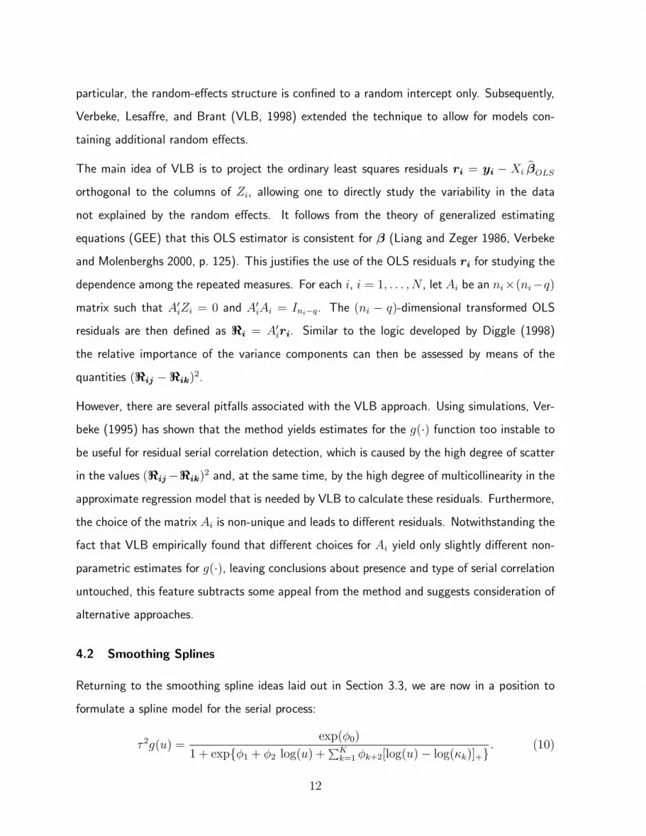
4.2 Smoothing Splines

Returning to the smoothing spline ideas laid out in Section 3.3, we are now in a position to

formulate a spline model for the serial process:

τ 2g(u) =exp(φ0)

1 + exp{φ1 + φ2 log(u) +∑K

k=1 φk+2[log(u) − log(κk)]+}. (10)

12

This means that φ0 acts as a (strictly positive) intercept, capturing the variance of the se-

rial correlation component, τ 2. Further, φ1 acts as an intercept, φ2 is the linear slope and

φ3, . . . , φK+2 are the spline coefficients associated with the serial correlation function g(·).

The logistic link ensures that the estimated g(·) function stays within the [0, 1] interval.

A penalty term is added to (7) to obtain a smoother fit, leading to the following marginal

likelihood function:

l(θ) = LML(θ) + λK∑

k=1

φ2k+2, (11)

where the fixed, user-defined, λ controls the amount of smoothing. In principle, it is con-

ceivable to develop methods for data-driven selection of λ. However, this falls outside of the

scope of this paper. Moreover, we have observed in our case study and limited simulations

(the latter not reported here), that the presence of λ has a favorable since stabilizing effect

on the algorithm’s convergence.

5 Analysis of Case Study

The approach as described above in Section 4.2 has been applied to the case study data

introduced in Section 2. For the reasons mentioned in Section 4.1, the analyzes were performed

on the OLS residual profiles for the log-transformed number of licks. A small smoothing

parameter value (λ = 0.01) was chosen since this improved convergency, while it only had a

small impact on the actual fit. No random effects were included in the model, since they did

not lead to a significant improvement in likelihood value. A classical exponential fit together

with spline fits at two different sets of knot points of the serial correlation function g(.) for

number of licks is shown in Figure 3.

The spline fits indicate that the serial correlation function is non-monotone. This fact would

go entirely unnoticed with a conventional serial correlation approach. For example, we now

see that the serial correlation is substantially lower for a 12-hour time lag than for one of 24

hours. Very likely, this can be ascribed to the circadian rythm. This 24-hours pattern could

also be observed in Figure 1. It therefore plays a role in the mean structure and the correlation

structure simultaneously. Since a classical serial correlation model would not allow for this,

13

0 20 40 60

0.0

0.2

0.4

0.6

0.8

1.0

u

g(.)

SplineExponential

0 20 40 60

0.0

0.2

0.4

0.6

0.8

1.0

u

g(.)

SplineExponential

Figure 3: Exponential and spline fit of the serial correlation function g(.) for number oflicks. Left graph: knot points at u = 6, 12, 18, 24, 36. Right graph: knot points at u =8, 14, 20, 26, 36.

it is conceivable that in such a model the mean structure fit would be distorted, rendering

associated inferences less reliable.

The fact that the one-parameter exponential function cannot detect this type of serial cor-

relation also shows through the difference in log-likelihood between the exponential, and the

spline model with knots located at u = 6, 12, 18, 24, 36. Precisely, the test statistic equals

2(27395.0 − 27306.9) = 176.2, which under the null follows a χ26. This represents a consid-

erable improvement in fit of the spline model compared to the exponential model.

Note that all knot points were positioned for time lags below 36 hours, confirming that this

is the time frame were quite a lot is happening, in contrast to larger lags. Of course, there is

more information in a set of data about shorter lags, since relatively more pairs corresponding

to such lags can be formed.

6 Concluding Remarks

Flexible serial correlation structures, just like flexible random-effects modeling, are necessary

when modeling complex longitudinal profiles, especially with a long period of follow up and/or

14

a large number of measurements within subjects. To this effect, we have proposed a spline-

based approach. Such a parametric spline approach works acceptably well, as long as the

number of knot points is chosen to be relatively small compared to the number of time points.

In our case study, we essentially used 5 knot points for 167 follow-up occasions. The choice

of the knot points’ position, too, is important, both for the quality of the fit as well as for

convergence of the updating algorithm.

Convergency can be problematic when fitting an elaborate covariance structure. However, in

the analysis of the case study the proposed spline approach actually performed better than

some of the simpler serial correlation based models, such as one featuring Gaussian serial

correlation. Arguably, the added flexibility allows for a better fit and ultimately therefore

better convergence.

The choice of the smoothing parameter λ is rather subjective by nature. In our analysis, we

chose a small value since this improved convergence, without smoothing out the non-monotone

trend in the fitted serial correlation function and without adversely impacting the model’s fit.

Admittedly, observations made in a case study are always a bit ad hoc. Therefore, we performed

a small simulation study (details not reported), which largely confirmed the finding that adding

knot points can improve the fit, while at the same time causing rapid variance increases and

having a detrimental influence on convergence.

References

Aitkin, M. (1999) A general maximum likelihood analysis of variance components in gener-

alized linear models. Biometrics, 55, 218–234.

Dierckx, P. (1993) Curve and Surface Fitting with Splines. Clarendon, Oxford.

Diggle, P.J. (1988) An approach to the analysis of repeated measures. Biometrics, 44,

959–971.

Diggle, P.J., Heagerty, P.J., Liang, K.-Y., and Zeger, S.L. (2002) Analysis of Longitudinal

Data (2nd ed.). Oxford Science Publications. Oxford: Clarendon Press.

15

Eilers, P.H.C. and Marx, B.D. (1996) Flexible smoothing with B-splines and penalties (with

discussion). Statistical Science, 11, 89–121.

Harville, D.A. (1974) Bayesian inference for variance components using only error contrasts.

Biometrika, 61, 383–385.

Harville, D.A. (1977) Maximum likelihood approaches to variance component estimation and

to related problems. Journal of the American Statistical Association, 72, 320–340.

Laird, N.M. and Ware, J.H. (1982) Random effects models for longitudinal data. Biometrics,

38, 963–974.

Lee, Y. and Nelder, J.A. (1996) Hierarchical generalized linear models (with discussion).

Journal of the Royal Statistical Society, Series B, 58, 619–678.

Lesaffre, E., Todem, D., Verbeke, G. and Kenward, M. (2000) Flexible modelling of the

covariance matrix in a linear random effects model. Biometrical Journal, 42, 807–822.

Liang, K.-Y. and Zeger, S.L. (1986) Longitudinal data analysis using generalized linear mod-

els. Biometrika, 73, 13–22.

Little, R.J.A. and Rubin, D.B. (2002) Statistical Analysis with Missing Data (2nd ed.). New

York: John Wiley & Sons.

Pan, J. and Mackenzie, G. (2003) On modelling mean-covariance structures in longitudinal

studies. Biometrika, 90, 239–244.

Reisberg, B., Borenstein, J., Salob, S.P., Ferris, S.H., Franssen, E., Georgotas, A. (1987)

Behavioral symptoms in Alzheimer’s disease: phenomenology and treatment. Journal of

Clinical Psychiatry, 48, 9–15.

Royston, P. and Altman, D.G. (1994) Regression using fractional polynomials of continuous

covariates: parsimonious parametric modelling. Applied Statistics, 43, 429–468.

Ruppert, D., Wand, M.P. and Carroll, R.J. (2003) Semiparametric Regression. New York:

Cambridge University Press.

Verbeke, G. (1995) The linear mixed model. A critical investigation in the context of lon-

gitudinal data analysis. Ph.D. thesis, Catholic University of Leuven, Faculty of Science,

16

Department of Mathematics.

Verbeke, G. and Lesaffre, E. (1996) A linear mixed-effects model with heterogeneity in the

random-effects population. Journal of the American Statistical Association, 91, 217–221.

Verbeke, G., Lesaffre, E. and Brant, L.J. (1998) The detection of residual serial correlation

in linear mixed models. Statistics in Medicine, 17, 1391–1402.

Verbeke, G. and Molenberghs, G. (2000). Linear mixed models for longitudinal data, Springer

Series in Statistics, Springer-Verlag, New-York.

Verbyla, A.P., Cullis, B.R., Kenward, M.G. and Welham, S.J. (1999) The analysis of designed

experiments and longitudinal data by using smoothing splines. Applied Statistics, 48,

269–311.

Vloeberghs, E., Van Dam, D., Engelborghs, S., Nagels, G., Staufenbiel, M. and De Deyn,

P.P. (2004) Altered circadian locomotor activity in APP23 mice: A model for BPSD

disturbances. European Journal of Neuroscience, 20, 2757–2766.

17