Fiscal Policy and Macroeconomic Uncertainty in

Emerging Markets: The Tale of the Tormented Insurer

Enrique G. Mendoza

University of Maryland, International Monetary Fund, & NBER

P. Marcelo Oviedo

Iowa State University

December 2005

Abstract

Governments in emerging markets often behave like a “tormented insurer”, tryingto use non-state-contingent debt instruments to avoid sharp adjustments in paymentsto private agents despite large fluctuations in public revenues. In the data, their abilityto sustain debt is inversely related to the variability of their revenues, and their primarybalances and current expenditures follow a cyclical pattern that contrasts sharply withthe countercyclical behavior observed in industrial countries. This paper proposesa dynamic, stochastic equilibrium model of a small open economy with incompletemarkets that can rationalize this behavior. In the model, a fiscal authority thatchooses optimal expenditure and debt plans given stochastic revenues interacts withprivate agents that also make optimal consumption and asset accumulation plans.The competitive equilibrium of this economy is solved numerically as a Markov perfectequilibrium using parameter values calibrated to Mexican data. If perfect domestic riskpooling were possible, the ratio of public-to-private expenditures would be constant.With incomplete markets, however, this ratio fluctuates widely and results in welfarelosses that dwarf conventional estimates of the benefits of risk sharing and consumptionsmoothing. The model generates a negative relationship between average public debtand revenue variability similar to the one observed in the data, and matches the GDPcorrelations of government purchases and the primary balance found in Mexican data.

Keywords: debt sustainability, public debt, fiscal solvency, procyclical fiscal policy, incompletemarkets.JEL classification codes: E62, F34, H63

1 Introduction

The empirical regularities of fiscal policy in developing countries, and particularly in emerg-

ing economies, differ sharply from those observed in the industrial world. Three key stylized

facts summarize the differences:

(1) The ratios of public revenue to GDP are significantly smaller on average and sub-

stantially more volatile (as indicated by coefficients of variation) in developing economies,

as Figures 1 and 2 show.

(2) The ability of countries to support higher ratios of public debt to GDP on average

is inversely related to the volatility of their public revenue ratios (see Figure 3): The higher

coefficients of variation of public revenue in developing countries are associated with lower

average debt ratios.

(3) Fiscal policy is clearly countercyclical in industrial countries but acyclical or pro-

cyclical in developing countries. Talvi and Vegh (2005) and Gavin and Perotti (1997) first

documented this fact, and recent studies by Catao and Sutton (2002), Kaminsky, Reinhart

and Vegh (2004) and Alessina and Tabellini (2005) provide detailed cross-country evidence

confirming it. These studies show that GDP and the primary fiscal balance (government

expenditures) are positively (negatively) correlated over the business cycle in industrial

countries, while in developing countries the GDP correlation of the primary balance (gov-

ernment expenditures) is close to zero or slighlty negative (positive).

This paper argues that the striking differences in the stylized facts of fiscal policy in

emerging economies may result from the combination of frictions in the financial markets

they have access to with imperfections in their own structure of government revenues and

outlays. In particular, this paper models fiscal authorities in developing countries as playing

the role of a “tormented insurer,” who tries to maintain a relatively smooth stream of

current expenditures and transfer payments for the private sector (i.e., provide a form of

social insurance) in the face of substantial, non-insurable fiscal revenue risk and having

access only to a non-state-contingent debt instrument.

Mendoza and Oviedo (2004) show how a simple, partial-equilibrium model of a tormented

insurer that tries to keep fiscal outlays constant at an ad-hoc exogenous level, given a

2

Markov process of fiscal revenues, delivers results that combine the notion of a “natural debt

limit” from the precautionary savings literature with Barro’s (1979) prediction regarding

the Random Walk behavior of public debt in his tax smoothing framework. The government

keeps its outlays constant as long as the history of revenue realizations and the dynamics of

debt result in a debt level above the annuity value of the “worst,” or “catastrophic,” level

of fiscal revenues (i.e., the government’s natural debt limit). When, and if, this limit is

reached, government outlays adjust to a “fiscal crisis” (or “lowest tolerable”) level.1 In the

long run, the public debt-GDP ratio has dynamics that are determined by initial conditions

and lacks a well-defined limiting distribution. Depending on the initial debt ratio, public

debt ends up hitting either the natural debt limit or being retired entirely (with zero debt

imposed as a lower bound at which the government effectively rebates its fiscal revenue to

the private sector).

This basic setup cannot say much about procyclical fiscal policy, since both revenues

and outlays are exogenous, and cannot say much about the implications of the tormented

insurer’s behavior for the private sector’s plans, equilibrium allocations, and the overall

welfare of the economy. Yet, it does illustrate the potential for the tormented insurance

framework to account for the observed negative relationship between the volatility of gov-

ernment revenues and average debt ratios: the governments of countries with more volatile

revenues have tighter natural debt limits and require more precautionary savings, so they

tolerate less debt. This simple model is also helpful for showing that traditional approaches

to evaluate fiscal solvency ignoring aggregate uncertainty can be very misleading.

This paper reformulates the tormented insurer’s problem in a dynamic, stochastic general

equilibrium framework. The paper focuses in particular on the competitive equilibrium of an

incomplete-markets economy in which the government chooses optimal plans for public debt

and government expenditures facing two exogenous sources of revenue volatility. The first

source are the cyclical variations in the economy’s output. The second source are fluctuations

1This level of outlays can be set to zero without loss of generality, and in this case the government’snatural debt limit allows the largest debt and satisfies the same definition as in Aiyagari (1994). A positive(and far more realistic) crisis level of government outlays results in a tighter natural debt limit, and thelimit is tighter the smaller the cut in outlays, so that countries that are perceived as capable of strongerfiscal adjustment can support higher debt ratios.

3

in an “implied” tax process that captures both the volatility of tax policy and, perhaps of

just as much relevance for developing countries, the volatility of key exogenous determinants

of fiscal revenues. Among the latter fluctuations in real world commodity prices figure

prominently because commodity exports are an important source of government revenues

for many developing nations. The government issues one-period, non-state contingent bonds

with a return perfectly arbitraged with the return on foreign bonds of the same type.

Domestic agents make optimal consumption and savings plans facing the volatility of their

after-tax income and using as vehicles of saving domestic public debt and international

bonds. In contrast with the basic setup in Mendoza and Oviedo (2004), the model features

well-defined limiting distributions of public and foreign debt, and can be used to examine

the cyclical co-movement of the primary balance and government purchases, as well as

the positive and normative implications of the tormented insurer setup for equilibrium

allocations and welfare.

This paper’s tormented insurer setup has two forms of asset market incompleteness.

The first one is the standard “external” asset market incompleteness typical of small open

economy models: the economy as a whole experiences idiosyncratic income fluctuations and

has only access to a world market of non-state-contingent bonds as an insurance mechanism.

The second one is “domestic” asset market incompleteness. If the government could issue

state contingent debt, or enact state-contingent, non-distorting taxes, it could attain a

domestic social planner’s optimum in which the incomes of the government and the private

sector are pooled (so that the relevant constraint is the resource constraint of the economy

as a whole) and the marginal utilities of public and private spending are equalized across

time and states of nature. Hence, cyclical fluctuations in fiscal revenues and after-tax

private income do not alter the distribution of wealth between the government and the

private sector.2 In the tormented insurer’s world, however, the implied tax process splits

the economy’s output across the private and public sectors, and the government can only

issue non-state-contingent debt. Hence, the fiscal authority cannot replicate the domestic

2Because the first form of market incompleteness is not eliminated by allowing the government to issuedomestic debt contingent on fiscal revenues, this social optimum does not correspond to the Arrow-Debreucomplete markets equilibrium.

4

social optimum and must operate in a second-best environment.

The competitive equilibrium of this second-best outcome is represented in recursive

form as a Markov perfect equilibrium (MPE): The government (private sector) formulates

its optimal spending and financing plans taking as given a conjecture of the private sector’s

(government’s) optimal plans, but behaving competitively so that both agents move simul-

taneously and take all relevant prices as given. The MPE is attained when the optimal

plans chosen by the government (private sector) are consistent with the conjecture of the

government’s (private sector’s) optimal plans under which the private sector (government)

formulates its plans. In this MPE, fluctuations in fiscal revenue and after-tax private income

result in changes in the distribution of wealth across the private and public sectors.

The quantitative predictions of the model are examined by conducting a set of numerical

experiments in a version of the model calibrated to Mexican data. The results show that

the model, when calibrated to capture the low average and high volatility of Mexico’s public

revenues, makes progress in explaining the other stylized facts that distinguish fiscal policy

in developing countries from that of industrial nations. In particular, the model produces an

inverse relationship between average debt ratios and fiscal revenue volatility similar to the

one found in international data, and generates GDP correlations for government purchases

and the primary balance very similar to the ones found in Mexican data. Moreover, a

comparison of the domestic social optimum with the MPE shows that domestic asset market

incompleteness has important implications for equilibrium allocations and welfare. The

volatility of expenditures is significantly higher in the MPE than in the social optimum,

even though both result in very similar long-run averages of private and public expenditures,

and this translates into welfare costs of market incompleteness that are several orders of

magnitude larger than standard results in the literature. The costs range from 1.6 to

3.5 percent in terms of the long-run average of a compensating variation in a time-and-

state-invariant level of private consumption that equates national expected lifetime utility

across the social optimum and the MPE. In the literature, the welfare costs of eliminating

asset markets for purposes of consumption smoothing and/or risk sharing with standard

preferences are generally below 1/10th of a percent (see, for example, Lucas (1987) or

Mendoza (1991)) .

5

This paper forms part of a growing literature examining fiscal policy in environments

with incomplete asset markets, including, among others, the studies by Aiyagari, Marcet,

Sargent, and Seppala (2002), Aguiar, Amador and Gopinath (2005), Celasun, Durdun and

Ostry (2005), Schmitt-Grohe and Uribe (2002), and Yakadina and Kumhof (2005). The

contribution of this paper to the literature is the focus on the domestic side of the asset

market incompleteness, in a setup that shifts attention from the study of the Ramsey op-

timal taxation problem to the study of the optimal debt and expenditure policies for a

given stochastic process of fiscal revenues. The latter is taken as an institutional feature of

developing countries, intended to represent their heavy reliance on commodity exports as a

large source of revenue and these countries’ limited ability to fine-tune conventional direct

and indirect tax rates with the aim to improve risk sharing.

The rest of the paper is organized as follows. Section 2 describes the model and charac-

terizes the competitive equilibrium. Section 3 describes the calibration of the model to the

Mexican economy and derives the model’s quantitative predictions. Section 4 concludes.

2 The Model

Consider a small open economy with stochastic endowment income and limited opportuni-

ties for risk sharing and consumption smoothing because financial markets are incomplete.

This economy is inhabited by two infinitely-lived agents: a representative household and a

government. The government receives stochastic public revenues that are affected by two

sources of uncertainty: fluctuations in the economy’s endowment income and fluctuations

in an implied tax rate that represents fluctuations in tax policy and in other key exogenous

determinants of fiscal revenues. The government’s total non-interest outlays include current

expenditures (i.e., purchases of goods and services), which will be chosen optimally, and

transfer payments to the private sector, which are kept at a deterministic, constant level for

simplicity. The government can sell one-period, non-state contingent bonds to the private

sector to finance primary fiscal deficits. On the side of the private sector, households collect

stochastic after-tax income, which is affected by the same sources of uncertainty as fiscal

6

revenues. Households make optimal intertemporal consumption plans and they have access

to the domestic market of public bonds and to a world market of one-period, non-state con-

tingent bonds. These two bonds are perfect substitutes from the standpoint of households,

and the gross real rate of return on both equals R. The combination of market incom-

pleteness and income uncertainty induces both agents to undertake precautionary saving in

order to self-insure against endowment and tax shocks.

The variables that describe the state of the economy at any point in time are the stock of

public debt, bgt−1, the net foreign asset position, bI

t−1 and a pair of realizations of the shocks,

εt = (εyt , ε

τt ), where εy

t is the shock to national income and ετt is the implied tax shock. Thus,

the state of the economy at date t is given by the triple st = (bgt−1, b

It−1, εt).

The economy’s endowment income, yt exp(εyt ), is the product of a deterministic trend

component, yt, and a cyclical component, exp(εyt ). The trend component grows at the

constant, exogenous, gross rate γ and all equilibrium allocations follow this common trend,

as in the standard exogenous balanced-growth setup. Following Carroll (2004), the analysis

focuses, without loss of generality, on a detrended representation of the model in which:

(a) all allocations are expressed as ratios of yt and (b) the subjective discount factor and

the gross return on assets are adjusted so that the solutions of the detrended model can be

mapped into the equivalent solutions of the growing economy.3 These adjustments imply

an effective discount factor given by βγ1−σ, where β is the subjective discount factor and σ

is the coefficient of relative risk aversion, and an effective gross return on assets R ≡ R/γ.

The implied tax shocks will be calibrated so that, taking GDP as the overall tax base,

the stochastic process of total public revenues in the model matches one observed in actual

data. The stochastic tax rate is τ y exp(ετt ) and includes a (detrended) average tax rate τ y

and a cyclical tax shock exp(ετt ). Note that, to the extent that this implied tax shock reflects

fluctuations in world commodity prices, it is analogous to a terms-of-trade shock.

The shocks to GDP and implied taxes are represented by a joint Markov process defined

by an NS× 2 matrix E containing NS realizations of the pair ε = (εy, ετ ) and an NS×NS

transition probability matrix P with typical element Pij = Prob(εt = εj|εt−1 = εi), where

3Carroll also shows how to generalize this setup to include i.i.d. shocks to the trend component, whichwould add to the model permanent shocks as those studied by Aguiar and Gopinath (2004).

7

i, j = 1, ..., NS index the NS realizations of the pair ε, and∑NS

j=1 Pij = 1, ∀i = 1, ..., NS.

2.1 The Government’s Problem

The government chooses sequences of (detrended) expenditures and debt issues {gt, bgt}∞t=0

so as to maximize a standard CRRA expected utility function:

E0

[ ∞∑t=0

(βγ1−σ

)t g1−σt

1− σ

]; σ 6= 1; σ > 0 (1a)

subject to the following government budget constraint:

gt + z +Rbgt−1 ≤ bg

t + exp(εyt )τ

y exp(ετt ) (1b)

where gt represents government expenditures at time t, z are time-and-state-invariant trans-

fer payments to the private sector, R ≡ R/γ is the growth-adjusted interest rate, and bgt is

the stock of public debt chosen at time t. The budget constraint (1b) states that total gov-

ernment outlays, consisting of expenditures, transfers, and gross debt repayments, must not

exceed the total government resources, consisting of issues of new debt and fiscal revenues.

Given that the marginal utility of public expenditures goes to infinity as gt approaches

zero from above, the government never chooses a plan that leaves it exposed to the risk of

facing less than strictly positive expenditures in all dates and states of nature. As a result,

the government imposes on itself a “natural debt limit,” which is given by the annuity value

of the lowest Markov realization of fiscal revenues net of transfers min[exp(εy)τ exp(ετ )]−zR−1

. This

upper bound on debt is exactly analogous to the concept of the natural debt limit introduced

by Aiyagari (1994) in the heterogenous agents-precautionary savings literature. Following

Aiyagari, the debt constraint faced by the government can be expressed more generally as

an upper bound φg that satisfies:

bgt ≤ φg ≤ min [exp(εy)τ exp(ετ )]− z

R− 1(1c)

Hence, the government’s debt constraint can be set at the natural debt limit, or at an

8

arbitrarily tighter limit, which Aiyagari (1994) labeled an ad-hoc debt limit. This ad- hoc

debt limit can be justified as a form of natural debt limit implied by a constraint requiring

government purchases not to fall below an exogenous minimum level at any date and state

of nature. The quantitative solutions of the MPE will focus on cases in which φg is set equal

to the natural debt limit.

In the context of the tormented insurer’s framework, Mendoza and Oviedo (2004) show

that the government’s natural debt limit also implies a credible commitment to remain

“able” to repay (i.e., to have enough resources to repay) the debt at all times. This is

because the natural debt limit represents the stock of debt the government can honor even

if it draws the worst realization of fiscal revenue “almost surely.” Mendoza and Oviedo

obtain this debt limit as an exogenous requirement that an effective insurer, defined as one

that wants to remain able to keep government outlays smooth for the longest possible time,

would want to meet. In this case, situations where levels of debt higher than this debt limit

were to be allowed correspond to situations in which there exist sequences of fiscal revenues

{(exp εyt )τ exp(ετ

t )}Tt=0 with non-zero probability of occurrence under which the government

cannot repay its debt even by setting gT = 0 at some date T . In the model of this paper,

the CRRA form of the government’s payoff function rules out this possibility.

The optimality conditions of the government’s problem are the budget constraint (1b),

the debt constraint (1c), and the following Euler equation:

g−σt = βRE

[g−σ

t+1

]+ µg

t (1d)

where µgt is the non-negative Lagrange multiplier on the debt constraint. The above Euler

equation has the standard interpretation of equating the marginal cost and benefit of sac-

rificing a unit of public expenditures at date t, with the caveat that if the debt constraint

binds the multiplier in the right-hand-side is positive. Note, however, that when φg in (1c)

is set equal to the natural debt limit, the CRRA utility function implies that µgt = 0 at

equilibrium for all t.

9

2.2 The Household’s Problem

The household ’s problem is analogous to the government’s problem, except that the house-

hold is the holder of the public debt and can also trade in the world’s bond market. The

representative household’s choice variables are stochastic sequences of consumption and

bond holdings {ct, bgt , b

It}∞t=0 that maximize expected lifetime utility:

E0

[ ∞∑t=0

(βγ1−σ

)t c1−σt

1− σ

](2a)

subject to the following budget constraint:

ct + x + (bgt + bI

t ) ≤ exp(εyt ) [1− τ exp(ετ

t )] +R(bgt−1 + bI

t−1) + z (2b)

This budget constraint restricts the sum of consumption, an exogenous, invariant level of

private absorption x (which is used in the calibration to represent investment expenditures),

and purchases of public and foreign bonds not to exceed the household’s resources. The

latter are given by the sum of after-tax private income, financial income, and government

transfers.

Since the household’s payoff function has the same CRRA form as the government’s, the

household’s problem features a similar natural debt limit on its total bond position (bgt + bI

t )

given by the annuity value of the lowest Markov realization of after tax income, adjusted

to add transfers and subtract x. Alternatively, for a given Markov plan of domestic public

debt given by the policy function bgt = bg(bg, bI , ε), the household faces a natural limit on

external debt that results in the following constraint on foreign bond holdings:

bIt ≥ φI ≥ −min

[exp(εy) [1− τ exp(ετ )] +Rbg − bg′(bg, bI , ε)

]+ z − x

R− 1(2c)

The right-most expression in this constraint is the natural debt limit on foreign debt. Hence,

condition (2c) allows for the external debt constraint to be set at its natural debt limit or

at a tighter ad-hoc debt limit. As before, ad-hoc debt limits can be thought of as implied

by an exogenous constraint requiring consumption never to fall below a pre-determined

10

minimum level. As explained in section ??, the quantitative experiments use an ad-hoc

debt limit for the household’s problem to calibrate the baseline simulation to match the

average consumption-output ratio observed in actual data.

The set of optimality conditions of the private sector are the flow budget constraint (2b),

the external debt constraint (2c), and the following Euler equation:

c−σt = βRE

[c−σt+1

]+ µc

t (2d)

where µct is the non-negative Lagrange multiplier on the external debt constraint that, as

in the case of the government, is equal to zero for all t if φI is set at the natural debt limit.

This Euler equation is also standard, with the caveat of the multiplier on the borrowing

constraint, and it states that the private sector equates the marginal benefit and cost of an

additional unit of consumption expenditures.

Given the perfect substitutability between bgt and bI

t , the household is indifferent between

the two assets and their returns are perfectly arbitraged. The government has, however,

a well-defined supply of government debt that it desires to place each period according

to its optimal plans. Hence, the model assumes that the household, given its infinitely-

elastic demand for domestic public debt at the world real interest rate, is willing to hold the

amount of this debt that the government issues. This does not introduce any wealth or price

distortions on the optimality conditions of the household’s problem and is consistent with

the competitive equilibrium conditions. Foreign bonds and domestic public debt markets

could be segmented by introducing additional frictions in the financial setup of the model,

but the aim of the analysis is to highlight the implications of the incompleteness of asset

markets that emerge in the tormented insurer’s framework even when domestic public debt

and foreign bonds are perfect substitutes.

2.3 Competitive Equilibrium

Definition (CE) The competitive equilibrium of the economy is characterized by stochastic

sequences representing the allocations of private and public expenditures, government debt,

11

and private net foreign asset holdings, {ct, gt, bgt , b

It}∞t=0, such that:

i) {gt, bgt}∞t=0 solve the government’s problem.

ii) {ct, bgt , b

It}∞t=0 solve the household’s problem.

iii) The following economy-wide resource constraint holds:

ct + x + gt ≤ exp(εyt ) +RbI

t−1 − bIt (3)

2.4 Markov Perfect Equilibrium

The above competitive equilibrium cannot be represented as the solution to a social planner’s

problem because the incompletness of asset markets prevents the private and public sectors

from pooling risk. In particular, the non-insurable, idiosyncratic income shocks faced by the

private and public sectors lead to fluctuations in the “domestic distribution of wealth” (i.e.,

the wealth distribution of the government vis-a-vis the private sector). The absence of risk

pooling across the two sectors is reflected in fluctuations in the ratio of marginal utilities of

expenditures, or, given the CRRA structure of preferences, in the ratio ct/gt.

Under these conditions, solving for the competitive equilibrium requires adopting a so-

lution strategy that can capture the state-contingent wealth dynamics accurately. The

adopted strategy solves for the competitive equilibrium as a Markov perfect equilibrium

where the government and the private sector behave competitively by taking all relevant

prices as given and by making simultaneous moves. Each agent formulates optimal plans

taking as given a conjecture of the other agent’s optimal plans, and none of the agents inter-

nalizes the effect of its actions on each other’s choices. The equilibrium is a Nash equilibrium

of a two-player dynamic game with uncertainty; the solution strategy involves representing

the game in recursive form and solving for its equilibrium by backward induction.

The two agent’s optimization problems are expressed in recursive form as follows. At

the beginning of each period, agents observe the state of the economy s = (bg, bI , ε). The

state space of the Markov shocks includes the NS possible realizations of the pair ε =

12

(εy, ετ ) defined earlier. The state space of domestic and external debt is defined by discrete

grids with NBG and NBI nodes respectively. Hence, the state space of public debt is

bg ∈ Bg = {bg1 < bg

2 < ... < bgNBG = φg} and the one for net foreign assets is bI ∈ BI =

{bI1 = φI < bI

2 < ... < bgNBI

}. Each agent takes as given a conjectured decision rule for the

other agent’s optimal plans. The government conjectures that the household’s decision rule

is bI′ = bI(bg, bI , ε) and the household conjectures that the government’s decision rule is

bg′ = bg(bg, bI , ε). Given these, each agent finds an optimal decision rule that solves the

Bellman equation representing their individual optimization problems.

The Bellman equation for the government’s optimization problem, given the conjecture

bI(bg, bI , ε), is:

V (bg, bI , ε) = maxbg′∈Bg ,g

{g1−σ

(1− σ)+ β γ1−σE

[V (bg′, bI(bg, bI , ε), ε′)

]}(4)

s.t.: g + z +Rbg ≤ bg′ + exp(εy)τ y exp(ετ )

bg′ ≤ φg

where the debt limit φgcan be set at the government’s natural debt limit or at a tighter

ad-hoc debt limit. The solution to this dynamic programming problem yields a decision

rule for the government’s debt bg(bg, bI , ε).

The Bellman equation for the private sector’s optimization problem, given the conjecture

bg(bg, bI , ε), is:

W (bg, bI , ε) = maxbI′∈BI ,c

{c1−σ

1− σ+ β γ1−σE

[W (bg(bg, bI , ε), bI′, ε′)

]}(5)

s.t.: c + x + bg(bg, bI , ε) + bI′ ≤ exp(εy) [1− τ exp(ετ )] +R(bg + bI) + z

bI′ ≥ φI

where the debt limit φIcan be set at the household’s natural debt limit or at a tighter ad-hoc

debt limit. The solution to this dynamic programming problem yields a decision rule for

the private sector of the form bI(bg, bI , ε).

Definition (MPE) A Markov perfect equilibrium for the small open economy is a pair

13

of value functions V and W and a pair of decision rules bg and bI such that:

i) Given the conjecture bI , V solves the Bellman equation (4), and bg is the associated

optimal policy rule.

ii) Given the conjecture bg, W solves the Bellman equation (5), and bI is the associated

optimal policy rule.

iii) The conjectured and optimal decision rules satisfy bg(·) = bg(·) and bI(·) = bI(·)

Conditions i) to iii) imply that, at equilibrium, each agent’s conjecture of the other

agent’s optimal decisions matches the decisions that the other agent actually finds optimal

to choose. Note that the computation of this MPE is simplified by the fact that, while the

government’s actions affect the household’s dynamic programming problem, the household’s

choices do not affect the government’s optimal plans. Hence, the MPE can be computed by

solving first the government’s Bellman equation, and then imposing the resulting public debt

decision rule on the household’s problem. This feature of the model follows from the lack of

feedback from actions of the private sector on the government’s payoff and constraints, which

in turn results from the simplifying assumptions making fiscal revenues independent of the

actions of the private sector. The rationale for these assumptions is to show that even in this

case, in which the strategic interaction between the two agents is simplified substantially,

the incompleteness of domestic financial markets has important consequences. Extending

the analysis to the case in which there is two-way feedback between the government’s and

the private sector’s plans is straightforward, albeit computationally intensive.

It is straightforward to show that a Markov perfect equilibrium, if it exists, is a compet-

itive equilibrium for the small open economy. Consider first the Bellman equations (4) and

(5). Using the standard Benveniste-Sheinkman equation (or the Envelope theorem), it fol-

lows that the first order conditions of the Bellman equations imply that the Euler equations

of the competitive equilibrium, eqs. (1d) and (2d), hold. Moreover, the budget constraints

of the Bellman equations yield the economy-wide resource constraint (3) of the competitive

equilibrium.

14

The numerical solutions to the MPE are obtained by iterating to convergence on the

Bellman equations (4) and (5) on the discrete state space containing NBG possible public

debt positions, NBI possible net foreign asset positions, and NS pairs of income and tax

shocks. In the implementation of the solution algorithm, NBG=200, NBI=200 and NS=9,

so the discrete state space is of dimensions 200× 200× 9.4 As long as there is no feedback

from the private sector choices to the government’s Bellman equation, the algorithm can

be simplified by solving first the government’s problem as a stand-alone value-function-

iteration problem, and then using the resulting optimal decision rule for public debt as the

conjectured decision rule for the same variable in the Bellman equation of the private sector.

2.5 Domestic Social Optimum

As explained in the Introduction, the main distortion preventing the tormented insurer from

implementing fiscal policies that support perfect risk pooling across the private and public

sectors is the incompleteness of domestic asset markets. The quantitative analysis of the

next section explores the effects of this distortion on allocations and welfare by comparing

the outcome of the MPE with that of a social optimum in which domestic asset markets

are assumed to be rich enough to support perfect domestic risk pooling. The domestic

economy as a whole still faces incomplete markets vis-a-vis the rest of the world because

GDP fluctuations still represent non-insurable, idiosyncratic income shocks for the small

open economy.

The social planner’s problem that yields the domestic social optimum is similar to the

standard Negishi-Mantel social planner’s representation of the complete markets equilib-

rium as a weighted sum of individual utilities subject to the resource constraint. The only

caveat is that, because the international asset markets remain incomplete, the outcome

of the social planner’s problem defined here does not correspond to the complete-markets

equilibrium of the small open economy. The domestic social optimum is defined as the

sequences of allocations {ct, gt}∞t=0 that maximize the weighted sum of the government and

4We explore the robustness of the results to enlarging the state space or conforming it with finer gridsby solving the model with a state space of dimensions 400 × 400 × 9. The results are largely robust, withthe ergodic means, standard deviations, and autocorrelations differing by at most 5 percent.

15

private payoffs,

E0

{η

∞∑t=0

(βγ1−σ

)t c1−σt

1− σ+ (1− η)

∞∑t=0

(βγ1−σ

)t g1−σt

1− σ

}, (6a)

where η > 0 and (1 − η) are the weights assigned to the private and public sector payoffs

respectively, subject to the small open economy’s resource constraint:

ct + gt + x + bIt ≤ exp(εy) +RbI

t−1 (6b)

and the following borrowing constraint on net foreign assets:

bI′ ≥ φSO ≥ −min [exp(εy)]− x

R− 1(6c)

where the quotient in the right-hand-side of this borrowing constraint is the social planner’s

natural debt limit.

In this equilibrium with perfect domestic risk pooling, the marginal utilities of public

and private expenditures are equalized across states and over time. Given CRRA utility

functions, this translates into an equilibrium condition that determines a time- and state-

invariant expenditure ratio:ct

gt

= [η/(1− η)]1/σ (6d)

Note that ct and gt still fluctuate because the external market incompleteness still exists

and it does not allow the small open economy to fully insure away its macroeconomic risk.

The recursive form of the social planner’s problem is given by the following dynamic

programming problem:

V so(bI , εy) = maxbI′∈BI ,c,g

[η

(c1−σ

1− σ

)+ (1− η)

(g1−σ

1− σ

)+ β γ1−σE

[V so(bI′, εy′)

]](6e)

subject to the resource constraint (6b) and the external debt constraint (6c).

If the government had access to state contingent tax or debt instruments, it could im-

plement the above domestic social optimum as a competitive equilibrium. State contingent

16

taxes could work as follows: Assume that the public and private debt limits are set at

their natural debt limits, public debt is set to zero at all times, and the government in-

troduces a set of state-contingent income taxes τ(εyt , ε

τt ) = (g∗t + z) / (exp(εy

t )τy exp(ετ

t )),

where starred variables represent optimal allocations of the social planner’s problem. This

policy would support the social optimum because: (a) {g∗t }∞t=0 would satisfy the government

budget constraint and the government’s Euler equation; (b){c∗t , b

I∗t

}∞t=0

would satisfy the

private sector’s budget constraint and its Euler equation; and (c) the resource constraint

holds. That the Euler equations are satisfied is obvious from the fact that the same Euler

equations hold for the social planner. The government budget constraint obviously holds

given the definition of the tax rule. The budget constraint of the private sector holds for{c∗t , b

I∗t

}∞t=0

because the resource constraint holds for the social optimum, the government’s

budget constraint holds, and there is no public debt.

Similarly, the social optimum could be obtained as a competitive equilibrium with a

policy setting income taxes to zero and issuing state-contingent public debt (i.e., domes-

tic one-period Arrow securities) to effectively implement state contingent lump-sum taxes

LSTt = g∗t + z. This policy would tax away from households, in a lump-sum fashion, ex-

actly the resources needed to pay for the time-invariant transfers and the social optimum

sequence {g∗t }∞t=0. The private sector would then find it optimal to choose the allocations{c∗t , b

I∗t

}∞t=0

because {c∗t}∞t=0 satisfies its Euler equation and the lump-sum tax leaves just

enough disposable income for the private sector to satisfy its budget constraint by choosing{c∗t , b

I∗t

}∞t=0

.

3 Quantitative Findings

3.1 Baseline Calibration and Discrete State Space

This section’s quantitative analysis uses a baseline calibration of the model to Mexican

data at an annual frequency. The calibration has two components. First, a set of parameter

values set so that variables in the model match their counterparts in Mexican data or taken

as standard from the Real Business Cycle (RBC) literature. Second, a discrete Markov

17

representation of the stochastic process of output and implied taxes observed in the data.

Table 1 summarizes the calibration parameters.

The growth rate is set to γ = 1.0088, which is the average growth rate of Mexico’s

real GDP per capita between 1980 and 2000 computed using data from the World Bank’s

World Development Indicators. In the same source and sample, the average investment-

GDP ratio yields x = 0.226. The mean income tax rate is set to τ = 0.256, which is

the 1980-2002 average ratio of total public revenue to GDP using data at current prices

from Mexico’s INEGI Bank of Economic Information (at http://dgcnesyp.inegi.gob.mx/cgi-

win/bdieintsi.exe). The time-invariant government transfers are set at z = 0.111, which is

the difference between the average ratio of total non-interest government outlays to GDP

(from the same INEGI source) and the average government expenditures-GDP ratio, g =

0.0978, from World Development Indicators.

The real interest rate is set to R = 1.0986, which is the average EMBI+ real return on

Mexican sovereign debt for the 1994-2002 period computed using the data from Neumeyer

and Perri (2005). This rate includes both the risk-free rate as well as the default risk

premium. The model does not consider default explicitly, but using an interest rate that is

more representative of the actual rate at which the Mexican government borrows is more

reasonable than simply applying the real rate on U.S. T-bills.

Regarding preference parameters, the value of the coefficient of relative risk aversion is

σ = 2, which is the usual value in RBC models. Unlike in the RBC literature, however,

the subjective discount factor β cannot be set simply to match the inverse of the growth-

adjusted gross interest rate because precautionary savings makes asset holdings diverge to

infinity in this case, as agents try to attain a non-stochastic consumption stream in the

face of non-diversifiable income shocks. In models without long-run growth (see Aiyagari

(1994), Hugett (1993) and Ljungqvuist and Sargent (2000, ch. 14)), the condition βR < 1

yields a well-defined unique invariant distribution of asset holdings. In models with growth,

Carroll (2004) showed that the condition required to prevent asset holdings from diverging

to infinity is: βR × max[(1/R)σ, (1/γ)σ] < 1. Precautionary savings also implies that

the averages of the model’s stochastic stationary state vary with the choice of parameters

(particularly those that appear in Carroll’s condition, the Markov process of shocks, and

18

the choice of φg).

Figure 4 shows how the mean level of public debt obtained from the MPE falls as β

increases so that βR × max[(1/R)σ, (1/γ)σ] converges to 1 from below (using the values

of R, γ and σ set above, and keeping φg at the level of the government’s natural debt

limit obtained using (1c) and the Markov process of shocks described below). The Figure is

plotted with the horizontal axis inverted to show that it yields the same concave relationship

as the Aiyagari-Hugget class of models (with the elasticity of average public “assets” going

to infinity as β increases).5 Each average level of debt has associated with it an average

level of public expenditures obtained from the budget constraint, and this level is lower the

higher the debt because of the extra income allocated to debt service. Hence, the baseline

calibration of the model uses a value of β such that, given the calibrated values of R, γ and

σ, and with φg set at the government’s natural debt limit, Carroll’s condition holds and

the long-run average of government purchases equals Mexico’s average of 9.78 percent. The

resulting value is β = 0.925 (for which Carroll’s condition yields βRγ−σ = 0.9984 < 1).

The joint Markov process driving the shocks to endowment income and implied taxes is

constructed using annual data for Mexico’s real GDP and total fiscal revenues for the period

1980-2004. The implied tax-rate series, TX, is constructed by computing the ratio of total

public revenue to GDP . The data for GDP and TX are then expressed in per capita terms,

logged, and detrended using the Hodrick-Prescott filter to obtain their cyclical components,

GDP and TX. Panel (a) of Table 2 reports the unconditional moments of these two time

series. The joint process driving the endowment and implied tax shocks is obtained by

estimating a VAR(1), Xt = ΦXt−1 + ζt, where Xt = (GDP t, TX t)′, Φ is the 2×2 matrix

of autocorrelation coefficients, and ζt is an i.i.d. random vector with covariance matrix Σζ .

The estimation results of this VAR are as follows:6

5Formally, public debt should go to -∞ as Carroll’s condition approaches 1 from below. Since the upperbound of public debt is set to zero, however, the entire mass of the ergodic distribuion of debt concentratesat this upper bound as β raises to levels for which Carroll’s condition is “close enough” to 1.

6t-statistics are shown in parenthesis.

19

Φ =

0.2789 0.4389(1.4495) (1.2614)

-0.1489 0.6004(-1.5643) (3.4867)

; Σζ =

(0.000727 -0.000268-0.000268 0.002378

)

Since the MPE is solved using a discrete state space, the VAR representation of the

shocks needs to be converted into a discrete Markov process. This is done using Tauchen’s

(1991) quadrature method, setting the Markov chain to carry nine pairs of shocks to GDP

and taxes (i.e., nine states in total). Given that the off-diagonal elements of Φ are not

statistically different from zero, we use the diagonal version of Φ and Σζ as inputs for

Tauchen’s algorithm. The resulting set of Markov realizations and their associated long-run

probabilities are reported in the Appendix. Panel (b) of Table 2 shows the unconditional

moments of GDP and taxes produced by the Markov chain. These do not match exactly

the moments from the data in Panel (a) because of the approximation error of the Markov

chain with 9 states, but the standard deviation, correlation and autocorrelation coefficients

are close to their empirical counterparts.7

The grids of public debt and foreign assets are specified as follows. The upper bound of

the public debt grid is its natural debt limit. Given the values of R, γ, z and the lowest

realization of government revenue supported by the states of income and tax shocks in the

Markov process, equation (1c) yields bg200 = φg = 1.318 (or about 132 percent of GDP). The

lower bound of public debt is set to zero (bg1 = 0) which implies that the government cannot

become a net creditor (i.e., hold negative debt positions). This constraint binds with 0.51

percent probability in the long run.

Given the optimal decision rule for public debt, the values of R, γ, z and x, and the

lowest realization of private disposable income (defined as exp(εy) [1− τ exp(ετ )] + Rbg −bg′(bg, bI , ε)) supported by the states in the Markov process, equation (2c) yields a natural

debt limit on net foreign assets of -7.105 (more than 7 times larger than GDP). However, the

7The approximation improves as NS, but at a high cost in computing time. The drawback of workingwith a limited number of states is that, by construction, natural debt limits are produced with the lowestrealizations of income supported by the Markov chain, and the extent to which these realizations reflectadverse outcomes that are truly relevant (i.e., that have nontrivial probability) depends on the number ofstates in the chain.

20

MPE obtained with such a large maximum external debt ratio yields an average foreign debt

ratio that is also too large (at 200 percent of GDP), and consequently the corresponding

long-run average consumption ratio is too low relative to the average in Mexican data (53

percent in the MPE v. 66.9 percent in the data). Hence, instead of using the natural

debt limit for the lower bound of external assets, we set an ad-hoc debt limit such that

the baseline MPE yields an average private consumption ratio consistent with the data.

The ad-hoc debt limit that satisfies this criterion is bI1 = φI = −0.5. The upper bound

for bI is chosen so that its long-run probability is approximately zero (without any binding

constraint) and has no effect on the moments of the ergodic distribution. The resulting

upper bound is bI200 = 0.1.

3.2 Cyclical Co-movements in the Baseline Calibration

Table 3 shows the statistical moments that characterize cyclical co-movements in the com-

petitive equilibrium (i.e., moments computed with the ergodic distribution of the MPE).

All moments in the table correspond to the model’s detrended variables, which are ratios

relative to GDP. The mean value of GNP is lower than that for GDP (which by construction

is equal to 1) because the economy is paying interest to the rest of the world on a stock

of net foreign assets of about 36 percent of GDP (in line with the estimates for Mexico

obtained by Lane and Milesi-Ferretti (1999)). This debt position and the value of R, imply

that the economy runs a trade surplus of 3.2 percent of GDP on average in the long run.

The average public debt ratio is equal to 53 percent of GDP, and hence the mean total asset

position of the household (i.e., E[bgt + bI

t ]) is equal to 17 percent of GDP.

Figures 5.a and 5.b show the limiting distributions of public debt and international

assets. These figures show that the support of the equilibrium allocations of public debt

and net external assets differ sharply from the corresponding debt limits. The long-run mean

of public debt (external assets), is 79 (14) percentage points lower (higher) than its natural

debt limit. The substantial difference between the mean of public debt and the government’s

natural debt limit shows that it is optimal for a government acting as a tormented insurer,

aiming to do its best to keep its total outlays smooth given the volatility of its revenues and

21

the incompleteness of asset markets, not to use a large portion of its borrowing capacity on

average. There are non-zero-probability histories of exogenous adverse revenue outcomes

that can lead the government to hold large amounts of debt in the stochastic steady state,

of up to 130 percent of GDP, but the endogenous probability of observing these outcomes is

very low (see Figure 5a). Outcomes with higher debt ratios are not consistent with optimal

behavior in the economy’s long-run competitive equilibrium.

The variability and co-movement indicators in Table 3 illustrate the challenges that

the private and public sectors face in trying to smooth consumption in the competitive

equilibrium. Private consumption is more volatile than after-tax income and government

expenditures are more volatile than fiscal revenues. Private and public expenditures are

positively correlated with the relevant income measures (after-tax income and fiscal revenues

respectively), but the correlations are low. Precautionary savings helps agents lower the

correlation between their incomes and their expenditures in the long run, but still, because

asset markets are incomplete, they cannot fully hedge idiosyncratic income risk. The end

results are significantly higher levels of variability for expenditures than for incomes, even

when the correlations between expenditures and incomes are not very high.

The effects of imperfect risk pooling can also be observed in the relative variability of

private and public expenditures. When the government has access to state-contingent fiscal

instruments, the ratio of private to public expenditures is constant across time and states

of nature, and hence government expenditures and private consumption have identical co-

efficients of variation. In contrast, in the model’s competitive equilibrium the coefficient

of variation of government expenditures is nearly 6 times larger than that for private con-

sumption. The coefficient of variation of the ratio ct/gt itself is 42.4 percent.

The low, positive correlation between aggregate income and government expenditures

(at 0.02) matches the estimate of this correlation observed in the data (see Appendix Table

5 in Kaminsky et al. (2004)). This pattern of non-negative correlations between government

purchases and GDP is one of the defining features of the puzzling phenomenon of procyclical

fiscal policies that characterize developing economies. For the United States, for example,

Kaminsky et al. report an estimate of the same correlation of -0.37, and the average of

their estimates for G7 countries is about -0.2. Thus, the model is successful at explaining

22

the absence of a clear countercyclical pattern in the behavior of government purchases

observed in emerging economies, and it mimics very accurately Mexico’s correlation between

government expenditures and output.

The model is also able to replicate a second key feature of procyclical fiscal policies in

developing countries: the primary fiscal balance is nearly uncorrelated with output, instead

of displaying the marked positive correlations observed in industrial countries. Alesina and

Tabellini (2005) estimate regressions of the (differenced) primary balance-GDP ratio on

the cyclical components of GDP and terms of trade, and the lagged primary balance-GDP

ratio, and find that the “beta” coefficients on GDP are significantly higher for industrial

economies than for developing countries. The average of their beta coefficients for industrial

OECD countries is 0.26, while their average for Latin American and the Caribbean is -0.13

(see Table 1 of Alessina and Tabellini’s paper). Their beta coefficient for Mexico is -0.094.

Using a long stochastic simulation of the model’s decision rules to generate data for 20,000

periods, and estimating the analog of their regression, the model produces a beta coefficient

of 0.097 (with a negligible standard error of 0.00326). It is difficult to assess the accuracy

of this match between the betas produced by the model and the data because Alessina

and Tabellini do not report country-specific standard errors. They do note that their beta

coefficients have generally large standard errors, and that many of the developing country

betas are not statistically different from zero. Hence, this suggests that it is possible that

again the model matches not just the general feature that developing countries tend to have

betas much closer to zero than industrial countries, but that the model could match closely

Mexico’s true beta.

The autocorrelations of asset holdings (both public debt and net foreign assets) are very

close to 1, and in addition, public and private expenditures are highly serially correlated.

These results are consistent with the high autocorrelation of assets typical of models of in-

complete markets and precautionary saving with non-state-contingent assets, and they are

also in line with the findings of Aiyagari et al. (2002), who found that the solution to the

Ramsey optimal taxation problem with incomplete markets and exogenous government ex-

penditures yields near-random-walk behavior in optimal taxes and debt. Here, tax revenue

is exogenous and hence optimal public expenditures, instead of optimal taxes, and debt

23

display near-unit-root behavior.8 As Aiyagari et al. also note, the high autocorrelation of

public debt is a feature that is in line with the predictions of Barro’s (1979) classic work on

optimal debt under tax smoothing.

It is interesting to compare the outcome of the model’s competitive equilibrium with

the predictions of the simpler partial equilibrium model of Mendoza and Oviedo (2004).

In the partial equilibrium setup, the government keeps outlays constant at an exogenous

ad-hoc level, except when a sufficiently long sequence of adverse revenue realizations puts

the economy in a state of “fiscal crisis”, at which the natural debt limit binds and the fiscal

authority therefore cuts its outlays to an ad-hoc crisis level. Given a Markov process of

revenue realizations, simulated time paths of public debt always diverge eventually to either

zero (i.e., the no-assets constraint) or to the natural debt limit, depending on the initial debt

ratio–truly matching Barro’s (1979) result stating that the long-run behavior of debt is fully

determined by initial conditions. Since there is no well-defined stochastic stationary equi-

librium, however, the partial equilibrium model is of limited use for assessing the long-run

dynamics of public debt. In contrast, the competitive equilibrium of the model of this paper

has a unique, invariant limited distribution to which the economy converges regardless of

initial conditions. When perturbed by an initial shock, all endogenous (detrended) variables

eventually revert to their means as the effect of the shock vanishes. As shown below, this

unique distribution yields precise predictions about the expected value and the time series

dynamics of public debt, and the rest of the model’s endogenous variables, in the long-run

and the short-run for any given set of initial conditions. It is also true, however, that the

near-random-walk patterns of public debt, net foreign assets and expenditures implies that

the mean-reverting behavior of these variables will take a very long time to be felt after an

exogenous shock to GDP or implied taxes hits the economy.

Figure 6 plots the Markov forecast functions of public debt and net foreign assets starting

8Aiyagari et al. also need limits on government assets (i.e., negative debt) to recover Barro’s predictions,because otherwise the optimal taxes are set to zero an all expenditures are financed with a large enough“war chest” of precautionary savings. In contrast, the model of this paper needs only to satisfy Carroll’sstationarity condition to have a well-defined ergodic distribution of assets. Limits on government assets arerequired only if one is interested in particular long-run equilibria that match particular features of the data(as was the case in the baseline calibration that uses the natural debt limit as a lower bound for debt and0 as an upper bound to match the observed average GDP share of government expenditures).

24

from the mean value of the latter and an initial public debt ratio of 0.634 (roughly 10

percentage points above the mean in the ergodic distribution). The plots show nine forecast

functions (i.e., non-linear impulse responses conditional on the initial asset ratios and a

date-0 pair of shocks) corresponding to each of the nine pairs of shocks in the states of the

Markov chain of GDP and implied tax shocks. Thus, each plot has nine forecast functions,

one for each of the nine possible initial states: s =(bg0 = 0.634, bI

0 =E[bI ], εj) for j = 1, .., 9.

Although the nine forecast functions start at bg = 0.634 (which is visually imperceptible in

the graph given that the time horizon goes through t = 2000) the nine realizations of ε give

rise to nine different values of bg in the second period of the figure. One way to interpret

these forecast functions is to view them as plotting the expected responses of public debt

and foreign assets given a date-0 unanticipated shock (e.g. the rescue of failing banks) that

puts the stock of public debt 10 percentage points above its long-run average.

Figures 6a and 6b illustrate the effects of the high persistence of assets discussed above,

in the form of the very low speed of convergence of the public debt and net foreign asset

ratios to their corresponding long-run averages. This is near-Random-Walk behavior, but is

clearly not a true Rando Walk, as in Barro (1979), because the competitive equilibrium of

the tormented insurer model features a unique invariant distribution of assets, even though

the effects of purely transitory shocks on asset holdings can take very long to fade away.

Figure 7 shows a sample of 10 simulated time series of the public debt-GDP ratio for

the same starting state s0 described above. For each simulation, a 50-period time series of

realizations of εt is drawn from the Markov matrix of realizations E (which is detailed in

the Appendix). As the length of the simulations grows sufficiently large, the expected value

of bgt computed with each of the 10 time series converges to the mean public debt ratio in

the limiting distribution. As each time series fluctuates over time, however, the effect of

the high persistence of asset holdings is reflected in the wide range of debt ratios that are

consistent with the competitive equilibrium starting from the same initial conditions.

Figures 8-10 show impulse-response functions to tax and GDP shocks constructed by

estimating a standard, unrestricted VAR(1) model using data generated from the model

in a stochastic time-series simulation that runs for 20,100 periods, discarding the first 100

periods. This simulation uses the optimal asset accumulation rules of the MPE and the

25

Markov chain of the exogenous shocks. The impulse response functions show responses

to Cholesky one-standard-deviation, positive innovations to the tax and GDP processes

(starting from initial conditions equal, by construction, to the averages of public debt and

foreign assets). Figures 8 and 9 also include asymptotic two-standard-error bands for each

variable’s impulse response.

Figure 8 shows the impulse responses of the c/g ratio for tax and output shocks. The

plots are truncated at 20 periods, even though if plotted for a sufficiently long sample, the

two of them return to the zero line because of the mean-reverting nature of the model’s

stochastic steady state. The positive output shock has a small impact effect that lowers

the c/g ratio below its long run average. In contrast, the positive tax shock has a negative

impact effect on the c/g ratio that is more than 4 times larger than that for the output

shock, and this effect grows to be nearly 6 times larger by the 6th period, before beginning

its slow-moving reversion to the zero line. These results reflect the fact that the positive

output shock increases the incomes of both the private and public sector, but the tax shock

moves the two agent’s incomes in opposite directions. Hence, the tax shock implies larger

foregone opportunities for efficient risk sharing because of the incompleteness of asset mar-

kets. Government revenues rise while private disposable income falls, and this opposing

moves result in persistent differences in expenditure patterns that imply relatively higher

(lower) government (private) expenditures for a long period of time. In contrast, the do-

mestic social optimum would imply a constant c/g ratio, which in the plots of Figure 8

corresponds to the zero line.

Figure 9 provides further details on the impulse response functions of the rest of the

model’s endogenous variables to a positive tax shock. Public debt and net foreign assets

exhibit highly persistent declines. Private consumption declines on impact and then re-

covers very gradually, while public expenditures rise on impact and continue to increase

until they level off about 6 periods after the tax shock hits. The current account falls as

private agents borrow to moderate the consumption effect of the adverse shock to disposable

income. Conversely, the primary fiscal balance increases on impact and then falls gradually,

as the government reacts to its positive revenue shock by saving to transfer part of its extra

income for future expenditures. The persistence of the effects shown in the impulse re-

26

sponse functions of assets and expenditures illustrate once more the wealth effects induced

by the incompleteness of asset markets. The tax shock plays no role in the domestic social

optimum, since the social planner pools the income of the public and private sectors, thus

effectively providing full insurance against implied tax shocks, so again the zero line is the

relevant point for comparing the responses of the competitive equilibrium with those of the

social optimum.

Figure 10 shows the impulse-response functions that follow a positive, one-standard-

deviation innovation to the output process in the competitive equilibrium and the domestic

social optimum. The output shock is non-insurable risk for both economies, because both

have access to the same set of incomplete international asset markets. Hence, the output

shock does not result in large differences in the responses of macroeconomic variables. Still,

the plots show that the wealth effects of the asset market incompleteness are not exactly

identical in the two economies. In particular, private consumption (public consumption)

is always lower (higher) in the competitive equilibrium than in the social optimum. Note

also that public expenditures increase on impact, illustrating again the procyclical pattern

of government purchases predicted by the model.

3.3 Welfare Costs of the Tormented Insurer’s Problem

This section compares the competitive equilibrium allocation and welfare resulting from

the MPE with those produced by the domestic social optimum. Welfare comparisons are

conducted following the approach introduced by Lucas (1987), which is based on computing

compensating variations in time- and state-invariant (i.e., stationary) consumption levels

that represent particular levels of expected lifetime utility under alternative environments

(in this case, between the MPE and the domestic social optimum). The aim is to convert the

ordinal units of the payoff functions into cardinal measures that can be used for quantitative

welfare comparisons.

To construct the welfare measure for the domestic social optimum, define cSO(bg, bI , ε)

as a stationary consumption function that represents the collective welfare of the public and

27

private sectors. This welfare measure satisfies:9

cSO(bg, bI , ε)1−σ

(1− σ) (1− β)= V so(bg, bI , ε)

A comparable measure of collective welfare of the two sectors in the MPE is constructed

by definining the stationary consumption function cMPE(bg, bI , ε) that satisfies the following

condition:cMPE(bg, bI , ε)1−σ

(1− σ)(1− β)= (1− η)V (bg, bI , ε) + ηW (bg, bI , ε)

where V and W are the value functions defined in (4) and (5). There are also stationary

consumption functions that measure the individual welfare of each sector, and these are

given by the function g(bg, bI , ε) that yields the same payoff as V (bg, bI , ε) and the function

c(bg, bI , ε) that yields the same payoff as W (bg, bI , ε).

The key variable to evaluate the welfare costs of the domestic asset market incomplete-

ness is the percentage difference bewteen cSO(bg, bI , ε) and cMPE(bg, bI , ε). The minimum

and maximum differences across the 360,000 triples (bg, bI , ε) in the state space are 0.07 and

41.45 percent respectively. These figures do not mean much, however, because they do not

take into account the long-run probability of the particular coordinate in the state space

that produced them. To address this issue, it makes more sense to evaluate welfare effects

by comparing expected welfare costs computed using the limiting distributions of the MPE

or the domestic social optimum. Using the limiting distribution of the MPE, the expected

welfare cost is:∑

(bg ,bI ,ε)∈Bg×BI×s

ΠMPE∞ (bg, bI , ε)

(cSO(bg, bI , ε)

cMPE(bg, bI , ε)− 1

)

where ΠMPE∞ (bg, bI , ε) is the endogenous ergodic distribution of public debt, foreign assets

and the shocks in the MPE. The second alternative measure of expected welfare costs uses

the limiting distribution of the social optimum, ΠSO∞ (bg, bI , ε), instead of ΠMPE

∞ (bg, bI , ε). A

problem with this second measure is that these probabilities are not defined for the grid Bg,

9These welfare-equivalent stationary consumption levels are computed for each pair (bI , εy) in the socialoptimum, and for each triple (bg, bI , ε) in the MPE. To express the stationary consumption levels of thesocial optimum in terms of the state triples of the MPE, note that neither bg nor ετ affect the social planner’sproblem so that cSO(bg, bI , ε) could equivalently be defined as cSO(bI , εy).

28

since public debt does not enter into the social planner’s problem. To make this probability

measure cover the state space for all triples (bg, bI , ε), the probability of each pair (bI , ε) is

distributed evenly across each of the NBG elements of the Bg grid.

The average welfare costs yield striking results. Using the ergodic distribution of the

domestic social optimum, the benefits of eliminating the tormented insurer’s problem are

equivalent to an increase of 3.52 percent in the trend level of consumption per capita. If

we use the ergodic distribution of the MPE instead, the increment in trend consumption

per capita reaches 1.57 percent. These welfare gains from improving risk sharing dwarf the

negligible measures of the benefits of consumption smoothing and risk sharing obtained in

standard RBC models, and are comparable with those obtained in the quantitative analysis

of the efficiency gains of replacing capital income taxes with consumption taxes (see, for

example, Lucas (1996), Mendoza (1991), Mendoza and Tesar (1998)). The main reason for

the marked difference with previous measures of the welfare gains of risk sharing is that the

tormented insurer’s problem deviates sharply from the representative agent environment

of the standard RBC models. In the competitive equilibrium examined here, the income

process of the government is significantly different from that faced by the private sector,

and the two agents can only used non-state-contingent debt to smooth consumption and

self-insure. As a result, the ratio of ct/gt (i.e., the proxy for shifts in the distribution of

wealth between the private and public sectors) fluctuates widely over the business cycle, as

documented earlier, and the fluctuations in government expenditures are particularly costly

(since the average of gt is nearly 7 times smaller than the average of ct, and hence the

curvature of the CRRA payoff function, with the same σ parameter, is more pronounced

and yields larger utility changes for the fluctuations in gt).

Table 4 compares the long-run moments of macroeconomic aggregates in the MPE and

the social optimum to offer more insight on the determinants of the large welfare costs of

imperfect risk sharing in the model. The mean values of the variables are almost identical in

the two economies, so the welfare costs do not arise because the social planner has access to

resources not available to the agents in the competitive equilibrium. The welfare costs arise

instead because, when the government can access state-contingent debt or taxes, the ability

to implement perfect risk pooling results in public and private expenditure allocations that

29

fluctuate much less than when the economy lacks state-contingent fiscal instruments. As

Table 4 shows, the standard deviation of public expenditures (private consumption) is 13.5

(2.3) times higher in the competitive equilibrium than in domestic social optimum.

3.4 The Revenue Process and Public Debt Dynamics

The properties of the stochastic process of public revenue are a key determinant of the

equilibrium dynamics of public debt that the model produces. The significantly larger effects

of the tax shock compared to those of the GDP shock found in the impulse response analysis

already illustrate this fact. We explore further the relationship between public debt and

the revenue process by analyzing the model’s ability to account for the inverse relationship

between average public debt ratios and coefficients of variability of public revenues found

in the data (recall Figure 3). The model has the potential to account for this pattern of the

data because higher revenue variability reduces the mean debt ratio, as it strengthens the

incentives for the government to build precautionary savings given the incompleteness of

asset markets. This is a result well-known in the precautionary savings literature. Chapter

14 of Ljungqvist and Sargent (2000) shows, for example, that the concave curve mapping

the relationship between mean asset holdings and the risk free interest rate in the Aiyagari-

Hugett class of models shifts to the right as the variance of endowment shocks increases

because of stronger incentives for precautionary savings by private agents.

Figure 3 shows a set of 45 pairs of exogenous coefficients of variation of public revenues

and endogenous mean public debt ratios in the model’s competitive equilibrium produced

as numerical solutions to variations from the baseline calibration of the Markov process

of shocks.10 These model pairs are identified by asterisks in the scater diagram of Figure

3, and the continuous curve represents the corresponding logartihmic regression line. As

the figure shows, the model is consistent with the data in predicting that (a) the long-run

average debt ratio is a negative function of the variability of fiscal revenues, and (b) this

relationship is non-linear, with the ability to sustain average debt ratios declining at a faster

10The 45 coefficients of variation of public revenues were generated by applying Tauchen’s algorithm tothe 45 combinations of 5 values of the autocorrelation coefficient of taxes in the VAR (Φ(2,2) = ...) and 9values of the variance element of tax innovations (Σε(2,2) = ...).

30

rate as the coefficient of variation of public revenues increases. A comparison of the model’s

regression line with that produced with actual data shows, however, that the model’s mean

debt-revenue variability curve is steeper than that observed in the data.

The negative relationship between the variability of government revenues and average

debt holds even when the government’s debt limit remains unaltered. Consider, for example,

an experiment in which the autocorrelation coefficient of implied taxes of the VAR (i.e., the

element Φ2,2 of the matrix Φ) increases to 0.9 from 0.6 in the baseline calibration.11 With

Φ2,2 =0.6, the Markov representation of the VAR yields a coefficient of variation of fiscal

revenue of 6.13, while Φ2,2 =0.9 yields a coefficient of variation of revenue of 6.68. The

natural debt limit remains constant at φg = 1.318, but the long-run average of the public

debt ratio falls by 12 percentage points from 53 to 41 percent.

4 Concluding Remarks

Fiscal policy in developing countries, particularly in emerging economies, differs sharply

from that of industrial countries in three key respects: (1) public revenue-GDP ratios are

much smaller and significantly more volatile, (2) countries with more variable revenue ra-

tios support lower average debt ratios, and (3) fiscal policy follows acyclical or procyclical

patterns, with GDP correlations of the primary balance (government expenditures) close to

zero or slighlty negative (positive).

This paper proposes a model of fiscal policy in small open economies with incomplete

asset markets that can rationalize these facts. The model shifts the focus from the study

of Ramsey optimal taxation problems toward the study of optimal debt and expenditure

policies in an environment where the government tends to act as a “tormented insurer,”

seeking to keep payments to the private sector smooth despite low and volatile revenues

and debt markets limited to non-state-contingent debt. The competitive equilibrium that

characterizes the interaction between this tormented insurer and the private sector of the

11Note that, using Tauchen’s method to generate the Markov representation of the VAR, changes in theautocorrelation matrix Φ change the transition probabilities of the Markov but not the vector of realizationsof the shocks. Since the natural debt limit on public debt depends on the worst revenue realization, changesin Φ do not change the government’s debt limit even though they change the coefficient of variation of fiscalrevenues.

31

economy is modeled in a dynamic, stochastic, general equilibrium framework and solved

numerically as a Markov perfect equilibrium.

Domestic asset market incompleteness has important implications for welfare and for

optimal public debt and government expenditure choices. The welfare costs arising from this

form of market incompleteness are derived by comparing the MPE with the domestic social

optimum attained by a planner who can pool the fiscal risk, and thus equate the marginal

utilities of public and private expenditures across states and over time. The average welfare

costs of imperfect domestic risk sharing are large, with an average gain of 3.5 percent in

a utility-equivalent compensating variation in stationary consumption calculated with the

limiting distribution of the MPE, or 1.6 percent if the stationary distribution of the social

optimum is used instead. Costs of these magnitude dwarf the negligible costs of imperfect

risk sharing and cyclical variability of consumption obtained with conventional RBC models.

The model is able to explain why countries suffering from higher fiscal risk support lower

average public debt-GDP ratios. In particular, the model is consistent with international

data in producing a negative, non-linear relationship between the variability of fiscal rev-

enues and the average public debt ratios. The model also matches the GDP-correlations of

government expenditures and the primary fiscal balance found in data for Mexico.

The implications of a modification of the MPE in which the government shifts from the

implied tax on GDP to a non-state-contingent consumption tax are studied in an ongoing

extension of this paper. This modification adds complexity to the MPE by introducing

two-way feedback between the plans of the private and public sector via an endogenous tax

base determined by the private sector’s consumption plans. The presumption is that the

consumption tax may be more desirable from a social welfare perspective because private

consumption smoothing can act as an endogenous stabilizer that yields more stable fiscal

revenues than the implied tax (i.e., than commodity export revenues). In turn, reduced

revenue variability implies more access to debt for the government and improved ability to

self-insure and smooth expenditures.

32

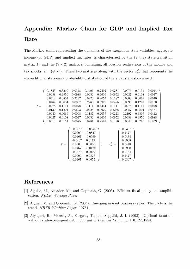
Appendix: Markov Chain for GDP and Implied Tax

Rate

The Markov chain representing the dynamics of the exogenous state variables, aggregate

income (or GDP) and implied tax rates, is characterized by the (9 × 9) state-transition

matrix P , and the (9 × 2) matrix E containing all possible realizations of the income and

tax shocks, ε = (εy, ετ ). These two matrices along with the vector πE∞ that represents the

unconditional stationary probability distribution of the ε pairs are shown next:

P =

0.1853 0.3210 0.0348 0.1496 0.2592 0.0281 0.0075 0.0131 0.00140.0988 0.3950 0.0988 0.0652 0.2609 0.0652 0.0027 0.0108 0.00270.0412 0.3807 0.2197 0.0223 0.2057 0.1187 0.0008 0.0069 0.00400.0464 0.0804 0.0087 0.2268 0.3929 0.0425 0.0693 0.1201 0.01300.0278 0.1111 0.0278 0.1111 0.4444 0.1111 0.0278 0.1111 0.02780.0130 0.1201 0.0693 0.0425 0.3929 0.2268 0.0087 0.0804 0.04640.0040 0.0069 0.0008 0.1187 0.2057 0.0223 0.2197 0.3807 0.04120.0027 0.0108 0.0027 0.0652 0.2609 0.0652 0.0988 0.3950 0.09880.0014 0.0131 0.0075 0.0281 0.2592 0.1496 0.0348 0.3210 0.1853

E =

-0.0467 -0.06550.0000 -0.08270.0467 -0.0999-0.0467 0.01720.0000 0.00000.0467 -0.0172-0.0467 0.09990.0000 0.08270.0467 0.0655

; πE∞ =

0.03970.14770.04340.09680.34480.09680.04340.14770.0397

References

[1] Aguiar, M., Amador, M., and Gopinath, G. (2005). Efficient fiscal policy and amplifi-cation. NBER Working Paper.

[2] Aguiar, M. and Gopinath, G. (2004). Emerging market business cycles: The cycle is thetrend. NBER Working Paper. 10734.

[3] Aiyagari, R., Marcet, A., Sargent, T., and Seppala, J. I. (2002). Optimal taxationwithout state-contingent debt. Journal of Political Economy, 110:12201254.

33

[4] Aiyagari, S. R. (1994). Uninsured idiosyncratic risk and aggregate saving. QuarterlyJournal of Economics, 109(3):659–684.

[5] Alesina, A. and Tabellini, G. (2005). Why is fiscal policy often procyclical. WorkingPaper. IGIER Bocconi.

[6] Barro, R. J. (1979). On the determination of public debt. Journal of Political Economy,87:940–971.

[7] Carroll, C. (2004). Theoretical foundations of buffer stock saving. NBER WorkingPaper, (10867).

[8] Catao, L. A. and Sutton, B. W. (2002). Sovereign defaults: The role of volatility. IMFWorking Papers, 02/149.

[9] Celasun, O., Debrun, X., and Ostry, J. (2005). Primary surplus behavior and risks topublic debt sustainability in emerging market countries: A ‘fan-chart’ approach. mimeo.IMF, Washington DC.

[10] Kaminski, G., Reinhart, C., and Vegh, C. (2004). When it rains it pours: procyclicalcapital flows and macroeconomic policies. NBER Macroeconomic Annual. edited by MarkGertler and Kenneth Rogoff; Cambridge, MA: MIT Press.

[11] Lane, P. and Milesi-Ferretti, G. M. (1999). The external wealth of nations: Measuresof foreign assets and liabilities fond industrial and developing countries. IMF WorkingPaper, (WP/99/115). Washington, DC.: International Monetary Fund.

[12] Lucas, R. (1985). Models of Business Cycles, volume Yrjo Jahnsson Lectures. Oxford,England: Basil Blackwell.

[13] Lucas, R. E. J. (1996). Nobel lecture: Monetary neutrality. Journal of Political Econ-omy, 104(4):661–682.

[14] Mendoza, E. G. (1991). Capital controls and the dynamic gains from trade in a businesscycle model of a small open economy. IMF Staff Papers, 38:480–505.

[Mendoza and Oviedo] Mendoza, E. G. and Oviedo, P. M. Public debt, fiscal solvency, andmacroeconomic uncertainty in latin america: The cases of brazil, colombia, costa rica andmexico. Proceedings: Dollars, Debt & Deficits: Sixty Years after Bretton Woods, Bancode Espana-International Monetary Fund, Washington DC.

[15] Neumeyer, P. A. and Perri, F. (2005). Business cycles in emerging economies: the roleof interest rates. Journal of Monetary Economics, 52(2):345–380.

[16] Talvi, E. and Vegh, C. (2005). Tax base variability and procyclical fiscal policy indeveloping countries. Journal of Development Economics, 78(1):156–190.

[17] Tauchen, G. (1991). Quadrature-based methods for obtaining approximate solutionsto nonlinear asset pricing models. Econometrica, 59(2):371–396.

34

Table 1: Calibration of the Model to the Mexican EconomyNotation Parameter / Variable Value

β Discount factor 0.925γ Gross growth rate 1.036φg Natural debt limit on public debt 1.318φI Ad-hoc debt limit on international debt -0.500σ Coefficient of relative risk aversion 2.000τ Mean income-tax rate 0.256R Gross world interest rate 1.0986x Private investment expenditures 0.226z Government transfers 0.111

Minimum value government debt 0.000Maximum value of international assets 0.100

Table 2: Unconditional Moments of GDP and the Implied Tax Rate. Mexican Annual Data,1980-2004 and Unconditional Moments of the Markov Chain

Mexican data Markov chain(a) (b)

Statistic GDP Implied GDP Impliedtax rate tax rate

Standard deviation 0.02948 0.06027 0.02781 0.05689Minimum -0.07073 -0.12294 -0.04670 -0.09991Maximum 0.05018 0.01080 0.04670 0.09991Cross correlation -0.24172 -0.24172 -0.19786 -0.19786Autocorrelation 0.351 0.535 0.278 0.576

35

Table 3: Moments of Macroeconomic Aggregates in the Ergodic Distribution of the MarkovPerfect Equilibrium (Baseline Calibration)

Variable (x) E[x] σ(x) cv(x) ρ(x) ρ(x, yi), where yi =GDP after fiscal

tax inc. revenueGDP 1.00 2.80 2.80 0.28 1.00 0.86 0.28GNP 0.97 3.03 3.13 0.42 0.95 0.82 0.26After-tax income 0.74 2.78 3.73 0.38 0.86 1.00 -0.25

Consumption 0.64 3.20 4.97 0.97 0.20 0.24 -0.07Gov. expenditures 0.10 2.83 29.07 1.00 0.02 -0.04 0.12

Tax rate 0.26 1.47 5.73 0.58 -0.20 -0.68 0.88Fiscal revenue 0.26 1.50 5.86 0.53 0.28 -0.25 1.00Primary fiscal balance 0.05 3.05 64.47 0.90 0.12 -0.09 0.38

Current account 0.00 2.27 - 0.24 0.96 0.80 0.31Trade balance 0.03 2.55 79.43 0.34 0.82 0.68 0.28Public debt 0.53 30.51 57.37 1.00 0.00 0.02 -0.05International assets -0.36 10.72 -29.72 0.98 0.08 0.08 0.00

Note: For each variable x, E[x] is the mean, σ(x) is the percentage standard deviation, cv(x) is thepercentage coefficient of variation, ρ(x) the autocorrelation, and ρ(x, yi) is the cross-correlationwith the variable yi indicated in the heading of the columns.

Table 4: Comparison of Limiting Moments of Macroeconomic Aggregates: Markov PerfectEquilibrium versus Social Optimum

Markov Perfect Equilibrium Social Optimum

Variable (x) E[x] σ(x) cv(x) ρ(x) ρ(x, y) E[x] σ(x) cv(x) ρ(x) ρ(x, y)GDP 1.00 2.80 2.80 0.28 1.00 1.00 2.80 2.80 0.28 1.00GNP 0.97 3.03 3.13 0.42 0.95 0.97 3.01 3.11 0.41 0.96

Consumption 0.64 3.20 4.97 0.97 0.20 0.64 1.39 2.16 0.89 0.46Gov. expenditures 0.10 2.83 29.07 1.00 0.02 0.10 0.21 2.16 0.89 0.46

Current account 0.00 2.27 - 0.24 0.96 0.00 2.25 - 0.23 0.95Trade balance 0.03 2.55 79.43 0.34 0.82 0.03 2.51 75.35 0.33 0.82International assets -0.36 10.72 -29.72 0.98 0.08 -0.37 10.01 -26.76 0.97 0.08

Note: For each variable x, E[x] is the mean, σ(x) is the percentage standard deviation, cv(x) isthe percentage coefficient of variation, ρ(x) the autocorrelation, and ρ(x, y) is the cross-correlationwith GDP.

36

Figure 1: Average Public Revenue-GDP Ratios in Emerging and Industrial Countries: 1990-2002

0 10 20 30 40 50 60 70

United States

United Kingdom

Sweden

Spain

Portugal

Norway

New Zealand

Netherlands

Japan

Italy

Ireland

Greece

Germany

France

Finland

Denmark

Canada

Belgium

Austria

Australia

Venezuela

Uruguay

Ukraine

Turkey

Thailand

South Africa

Russia

Poland

Philippines

Peru

Panama

Pakistan

Morocco

Mexico

Malaysia

Lebanon

Korea

Indonesia

India

Hungary

Ecuador

Croatia

Costa Rica

Colombia

China

Chile

Brazil

Argentina

Ratio with respect to GDP (in percentages)

37

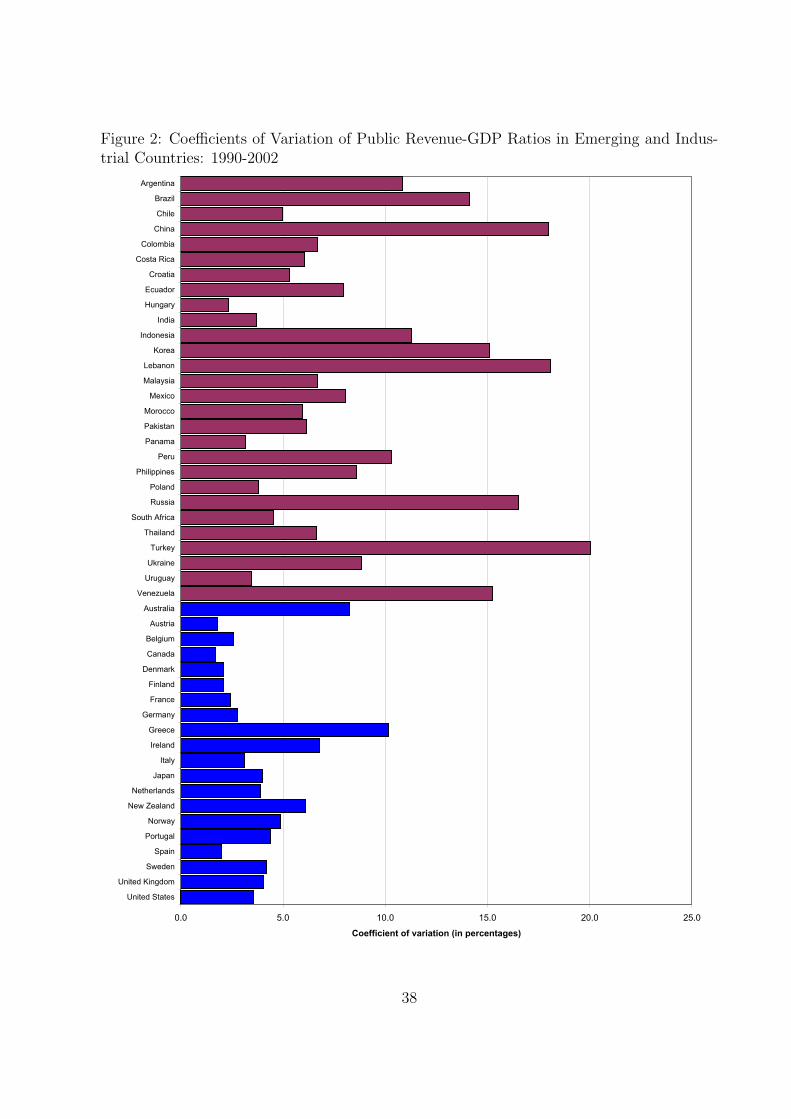
Figure 2: Coefficients of Variation of Public Revenue-GDP Ratios in Emerging and Indus-trial Countries: 1990-2002

0.0 5.0 10.0 15.0 20.0 25.0

United States

United Kingdom

Sweden

Spain

Portugal

Norway

New Zealand

Netherlands

Japan

Italy

Ireland

Greece

Germany

France

Finland

Denmark

Canada

Belgium

Austria

Australia

Venezuela

Uruguay

Ukraine

Turkey

Thailand

South Africa

Russia

Poland

Philippines

Peru

Panama

Pakistan

Morocco

Mexico

Malaysia

Lebanon

Korea

Indonesia

India

Hungary

Ecuador

Croatia

Costa Rica

Colombia

China

Chile

Brazil

Argentina

Coefficient of variation (in percentages)

38

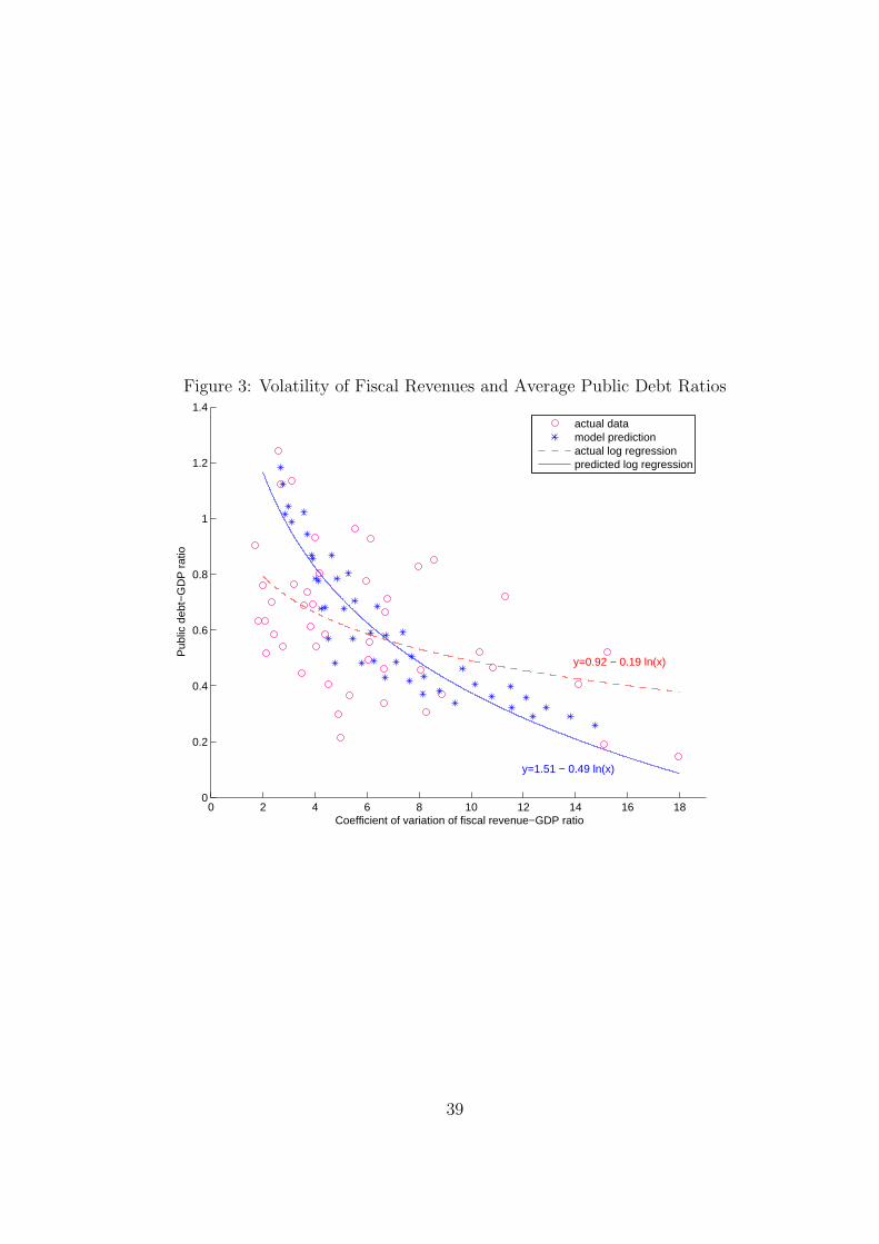
Figure 3: Volatility of Fiscal Revenues and Average Public Debt Ratios

0 2 4 6 8 10 12 14 16 180

0.2

0.4

0.6

0.8

1

1.2

1.4

Coefficient of variation of fiscal revenue−GDP ratio

Pub

lic d

ebt−

GD

P r

atio

actual datamodel predictionactual log regressionpredicted log regression

y=1.51 − 0.49 ln(x)

y=0.92 − 0.19 ln(x)

39

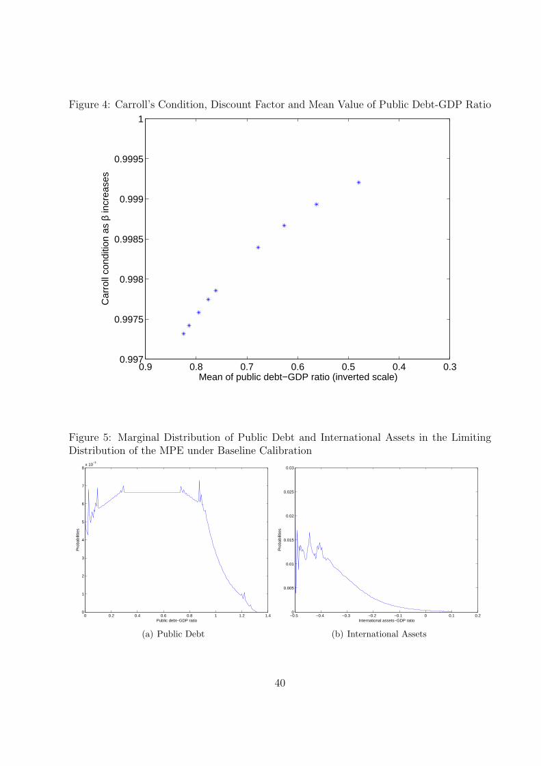
Figure 4: Carroll’s Condition, Discount Factor and Mean Value of Public Debt-GDP Ratio

0.30.40.50.60.70.80.90.997

0.9975

0.998

0.9985

0.999

0.9995

1

Mean of public debt−GDP ratio (inverted scale)

Car

roll

cond

ition

as

β in

crea

ses

Figure 5: Marginal Distribution of Public Debt and International Assets in the LimitingDistribution of the MPE under Baseline Calibration

0 0.2 0.4 0.6 0.8 1 1.2 1.40

1

2

3

4

5

6

7

8x 10

−3

Public debt−GDP ratio

Pro

babi

litie

s

(a) Public Debt

−0.5 −0.4 −0.3 −0.2 −0.1 0 0.1 0.20

0.005

0.01

0.015

0.02

0.025

0.03

International assets−GDP ratio

Pro

babi

litie

s

(b) International Assets

40

Figure 6: Forecasting Functions of Assets

0 500 1000 1500 20000.52

0.54

0.56

0.58

0.6

0.62

0.64

0.66

0.68

0.7

Time (years)

Pub

lic d

ebt−

GD

P r

atio

(a) Public Debt

0 10 20 30 40 50 60 70 80−0.44

−0.42

−0.4

−0.38

−0.36

−0.34

−0.32

−0.3

Time (years)

Inte

rnat

iona

l ass

ets−

GD

P r

atio

(b) International Assets

Note: Starting value of public debt is equal to 0.634 (120% of its mean value in thelimiting distribution); starting value of international assets is equal to its mean value in

the limiting distribution.

Figure 7: Simulations of Public Debt Using Simulations of the Markov Chain and OptimalPolicy Functions

0 10 20 30 40 500.2

0.3

0.4

0.5

0.6

0.7

0.8

0.9

1

Pub

lic d

ebt−

GD

P r

atio

Time (years)

Mean of simulated debt ratio at t=50: 0.515

Note: Starting value of public debt is equal to 0.634 (120% of its mean value in thelimiting distribution).

41

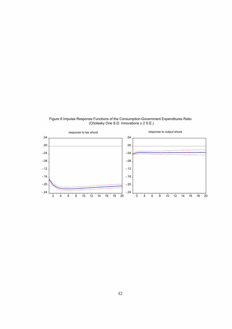
-.24

-.20

-.16

-.12

-.08

-.04

.00

.04

2 4 6 8 10 12 14 16 18 20

response to tax shock

-.24

-.20

-.16

-.12

-.08

-.04

.00

.04

2 4 6 8 10 12 14 16 18 20

response to output shock

Figure 8 Impulse Response Functions of the Consumption-Government Expenditures Ratio

(Cholesky One S.D. Innovations ± 2 S.E.)

42

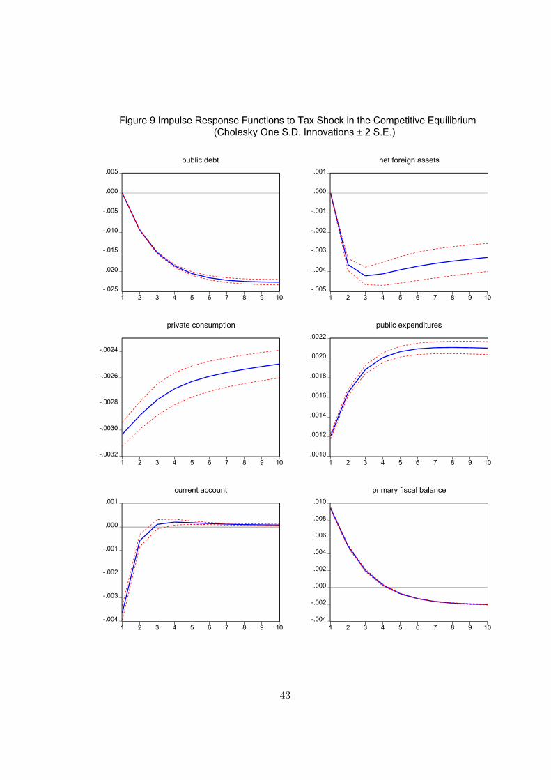
-.025

-.020

-.015

-.010

-.005

.000

.005

1 2 3 4 5 6 7 8 9 10

public debt

-.005

-.004

-.003

-.002

-.001

.000

.001

1 2 3 4 5 6 7 8 9 10

net foreign assets

-.0032

-.0030

-.0028

-.0026

-.0024

1 2 3 4 5 6 7 8 9 10

private consumption

.0010

.0012

.0014

.0016

.0018

.0020

.0022

1 2 3 4 5 6 7 8 9 10

public expenditures

-.004

-.003

-.002

-.001

.000

.001

1 2 3 4 5 6 7 8 9 10

current account

-.004

-.002

.000

.002

.004

.006

.008

.010

1 2 3 4 5 6 7 8 9 10

primary fiscal balance

Figure 9 Impulse Response Functions to Tax Shock in the Competitive Equilibrium

(Cholesky One S.D. Innovations ± 2 S.E.)

43

-.005

.000

.005

.010

.015

.020

.025

.030

2 4 6 8 10 12 14 16 18 20-.004

.000

.004

.008

.012

.016

.020

.024

2 4 6 8 10 12 14 16 18 20

.001

.002

.003

.004

.005

.006

2 4 6 8 10 12 14 16 18 20

.0001

.0002

.0003

.0004

.0005

.0006

.0007

.0008

.0009

2 4 6 8 10 12 14 16 18 20

competitive equilibrium domestic social optimum

Figure 10 Impulse Response Functions to an Output Shock in the

Competitive Equilibrium and the Domestic Social Optimum

(responses to Cholesky One S.D. Innovations)

net foreign assets current account

private consumption government expenditures

44

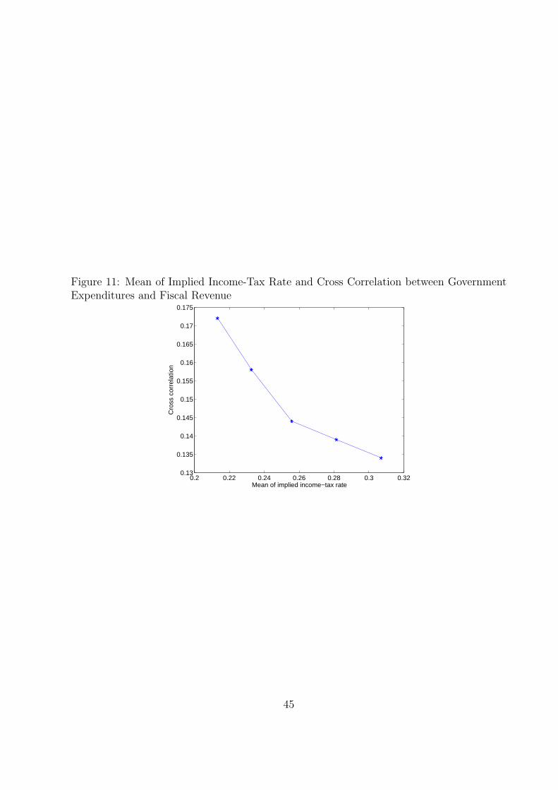
Figure 11: Mean of Implied Income-Tax Rate and Cross Correlation between GovernmentExpenditures and Fiscal Revenue

0.2 0.22 0.24 0.26 0.28 0.3 0.320.13

0.135

0.14

0.145

0.15

0.155

0.16

0.165

0.17

0.175

Mean of implied income−tax rate

Cro

ss c

orre

latio

n

45