fine-grained complexity analysis of some combinatorial
TRANSCRIPT

Foundations of computing Volume 12
Universitätsverlag der TU Berlin
Vincent Froese
Fine-Grained Complexity Analysis of Some Combinatorial Data Science Problems


Vincent FroeseFine-Grained Complexity Analysis of Some Combinatorial
Data Science Problems

The scientific series Foundations of computing of theTechnische Universität Berlin is edited by:Prof. Dr. Rolf Niedermeier,Prof. Dr. Uwe Nestmann,Prof. Dr. Stephan Kreutzer.
Foundations of computing | 12
Vincent Froese
Fine-Grained Complexity Analysis of Some CombinatorialData Science Problems
Universitätsverlag der TU Berlin
Bibliographic information published by the Deutsche Nationalbibliothek The Deutsche Nationalbibliothek lists this publication in theDeutsche Nationalbibliografie; detailed bibliographic dataare available on the internet at http://dnb.dnb.de.
Universitätsverlag der TU Berlin, 2018http://www.verlag.tu-berlin.de
Fasanenstr. 88, 10623 BerlinTel.: +49 (0)30 314 76131 / Fax: -76133E-Mail: [email protected]
Zugl.: Berlin, Techn. Univ., Diss., 2018Gutachter: Prof. Dr. Rolf NiedermeierGutachter: Prof. Dr. Tobias FriedrichGutachter: Prof. Dr. Marek CyganDie Arbeit wurde am 28. Mai 2018 an der Fakultät IV unterVorsitz von Prof. Dr. Uwe Nestmann erfolgreich verteidigt.
This work – except for quotes, figures and where otherwise noted –is licensed under the Creative Commons Licence CC BY 4.0http://creativecommons.org/licenses/by/4.0
Cover image: NASA Goddard Space Flight Center |https://www.flickr.com/photos/gsfc/5588722815 | CC BY 2.0 https://creativecommons.org/licenses/by/2.0
Print: docupoint GmbHLayout/Typesetting: Vincent Froese
ISBN 978-3-7983-3003-0 (print)ISBN 978-3-7983-3004-7 (online)
ISSN 2199-5249 (print)ISSN 2199-5257 (online)
Published online on the institutional repository of theTechnische Universität Berlin:DOI 10.14279/depositonce-7123http://dx.doi.org/10.14279/depositonce-7123
Zusammenfassung
Die vorliegende Dissertation befasst sich mit der Analyse der Berechnungskom-plexität von NP-schweren Problemen aus dem Bereich Data Science. Für diemeisten der hier betrachteten Probleme wurde die Berechnungskomplexitätbisher nicht sehr detailliert untersucht. Wir führen daher eine genaue Komplexi-tätsanalyse dieser Probleme durch, mit dem Ziel, effizient lösbare Spezialfälle zuidentifizieren. Zu diesem Zweck nehmen wir eine parametrisierte Perspektive ein,bei der wir bestimmte Parameter definieren, welche Eigenschaften einer konkre-ten Probleminstanz beschreiben, die es ermöglichen, diese Instanz effizient zulösen. Wir entwickeln dabei spezielle Algorithmen, deren Laufzeit für konstanteParameterwerte polynomiell ist. Darüber hinaus untersuchen wir, in welchenFällen die Probleme selbst bei kleinen Parameterwerten berechnungsschwerbleiben. Somit skizzieren wir die Grenze zwischen schweren und handhabbarenProbleminstanzen, um ein besseres Verständnis der Berechnungskomplexität fürdie folgenden praktisch motivierten Probleme zu erlangen.
Beim General Position Subset Selection Problem ist eine Menge vonPunkten in der Ebene gegeben und das Ziel ist es, möglichst viele Punkte inallgemeiner Lage davon auszuwählen. Punktmengen in allgemeiner Lage sindin der Geometrie gut untersucht und spielen unter anderem im Bereich derDatenvisualisierung eine Rolle. Wir beweisen etliche Härteergebnisse und zeigen,wie das Problem mittels Polynomzeitdatenreduktion gelöst werden kann, fallsdie Anzahl gesuchter Punkte in allgemeiner Lage sehr klein oder sehr groß ist.
Distinct Vectors ist das Problem, möglichst wenige Spalten einer ge-gebenen Matrix so auszuwählen, dass in der verbleibenden Submatrix alleZeilen paarweise verschieden sind. Dieses Problem hat Anwendungen im Bereichder kombinatorischen Merkmalsselektion. Wir betrachten Kombinationen ausmaximalem und minimalem paarweisen Hamming-Abstand der Zeilenvekto-ren und beweisen eine Komplexitätsdichotomie für Binärmatrizen, welche dieNP-schweren von den polynomzeitlösbaren Kombinationen unterscheidet.
Co-Clustering ist ein bekanntes Matrix-Clustering-Problem aus dem Ge-biet Data-Mining. Ziel ist es, eine Matrix in möglichst homogene Submatrizenzu partitionieren. Wir führen eine umfangreiche multivariate Komplexitätsana-
v

lyse durch, in der wir zahlreiche NP-schwere, sowie polynomzeitlösbare undfestparameterhandhabbare Spezialfälle identifizieren.
Bei F -free Editing handelt es sich um ein generisches Graphmodifikations-problem, bei dem ein Graph durch möglichst wenige Kantenmodifikationen soabgeändert werden soll, dass er keinen induzierten Teilgraphen mehr enthält,der isomorph zum Graphen F ist. Wir betrachten die drei folgenden Spezialfälledieses Problems: Das Graph-Clustering-Problem Cluster Editing aus demBereich des Maschinellen Lernens, das Triangle Deletion Problem aus derNetzwerk-Cluster-Analyse und das Problem Feedback Arc Set in Tourna-ments mit Anwendungen bei der Aggregation von Rankings. Wir betrachteneine neue Parametrisierung mittels der Differenz zwischen der maximalen AnzahlKantenmodifikationen und einer unteren Schranke, welche durch eine Menge voninduzierten Teilgraphen bestimmt ist. Wir zeigen Festparameterhandhabbarkeitder drei obigen Probleme bezüglich dieses Parameters. Darüber hinaus beweisenwir etliche NP-Schwereergebnisse für andere Problemvarianten von F -freeEditing bei konstantem Parameterwert.
DTW-Mean ist das Problem, eine Durchschnittszeitreihe bezüglich derDynamic-Time-Warping-Distanz für eine Menge gegebener Zeitreihen zu berech-nen. Hierbei handelt es sich um ein grundlegendes Problem der Zeitreihenanalyse,dessen Komplexität bisher unbekannt ist. Wir entwickeln einen exakten Expo-nentialzeitalgorithmus für DTW-Mean und zeigen, dass der Spezialfall binärerZeitreihen in polynomieller Zeit lösbar ist.
vi
Abstract
This thesis is concerned with analyzing the computational complexity of NP-hard problems related to data science. For most of the problems consideredin this thesis, the computational complexity has not been intensively studiedbefore. We focus on the complexity of computing exact problem solutionsand conduct a detailed analysis identifying tractable special cases. To thisend, we adopt a parameterized viewpoint in which we spot several parameterswhich describe properties of a specific problem instance that allow to solve theinstance efficiently. We develop specialized algorithms whose running times arepolynomial if the corresponding parameter value is constant. We also investigatein which cases the problems remain intractable even for small parameter values.We thereby chart the border between tractability and intractability for somepractically motivated problems which yields a better understanding of theircomputational complexity. In particular, we consider the following problems.
General Position Subset Selection is the problem to select a maximumnumber of points in general position from a given set of points in the plane.Point sets in general position are well-studied in geometry and play a role indata visualization. We prove several computational hardness results and showhow polynomial-time data reduction can be applied to solve the problem if thesought number of points in general position is very small or very large.
The Distinct Vectors problem asks to select a minimum number of columnsin a given matrix such that all rows in the selected submatrix are pairwisedistinct. This problem is motivated by combinatorial feature selection. Weprove a complexity dichotomy with respect to combinations of the minimumand the maximum pairwise Hamming distance of the rows for binary inputmatrices, thus separating polynomial-time solvable from NP-hard cases.
Co-Clustering is a well-known matrix clustering problem in data miningwhere the goal is to partition a matrix into homogenous submatrices. Weconduct an extensive multivariate complexity analysis revealing several NP-hardand some polynomial-time solvable and fixed-parameter tractable cases.The generic F -free Editing problem is a graph modification problem
in which a given graph has to be modified by a minimum number of edge
vii
modifications such that it does not contain any induced subgraph isomorphicto the graph F . We consider three special cases of this problem: The graphclustering problem Cluster Editing with applications in machine learning,the Triangle Deletion problem which is motivated by network clusteranalysis, and Feedback Arc Set in Tournaments with applications inrank aggregation. We introduce a new parameterization by the number ofedge modifications above a lower bound derived from a packing of inducedforbidden subgraphs and show fixed-parameter tractability for all of the threeabove problems with respect to this parameter. Moreover, we prove several NP-hardness results for other variants of F -free Editing for a constant parametervalue.
The problem DTW-Mean is to compute a mean time series of a givensample of time series with respect to the dynamic time warping distance. Thisis a fundamental problem in time series analysis the complexity of which isunknown. We give an exact exponential-time algorithm for DTW-Mean andprove polynomial-time solvability for the special case of binary time series.
viii
Preface
This thesis contains some outcomes of my research activity at TU Berlin in theAlgorithmics and Computational Complexity group of Prof. Rolf Niedermeierfrom December 2012 until December 2017 (including a parental leave fromAugust 2016 to March 2017). From December 2012 to February 2015, I gratefullyreceived financial support by Deutsche Forschungsgemeinschaft in the projectDAMM (NI 369/13).
The presented results are partly based on journal and conference publicationswhich were prepared in close collaboration with several coauthors, which are,in alphabetical order, René van Bevern, Markus Brill, Laurent Bulteau, TillFluschnik, Sepp Hartung, Brijnesh Johannes Jain, Iyad Kanj, Christian Ko-musiewicz, André Nichterlein, Rolf Niedermeier, David Schultz, and ManuelSorge.
In the following, I will briefly elaborate on my contributions to the respectivepublication corresponding to each chapter.
Chapter 3. Iyad Kanj (visiting TU Berlin from October 2014 to March 2015)proposed to study the General Position Subset Selection problem whichI found appealing due to its simple and natural definition. Basically all resultswere jointly developed by all authors. I was especially involved in provingthe kernelization results and wrote down major parts of our results for aconference version. Iyad Kanj presented the results at the 25th Fall Workshopon Computational Geometry (FWCG ’15) and at the 28th Canadian Conferenceon Computational Geometry (CCCG ’16) [Fro+16b]. I was also responsiblefor preparing a journal version for the International Journal of ComputationalGeometry & Applications [Fro+17].
Chapter 4. In my master thesis [Fro12], I studied several combinatorial fea-ture selection problems, among which was Distinct Vectors. The resultsincluded the NP-hardness for binary matrices with maximum row Hammingdistance four and minimum row Hamming distance two and polynomial-time
ix
solvability for maximum Hamming distance three. I presented the results atthe 38th International Symposium on Mathematical Foundations of ComputerScience (MFCS ’13) [Fro+13]. Afterwards, I realized that the polynomial-timesolvable cases can actually be generalized to arbitrary maximum Hammingdistance depending on the minimum Hamming distance. I wrote down theproof for the full dichotomy which is published in the Journal of Computer andSystem Sciences [Fro+16a]. The chapter of this thesis consists of this dichotomyresult.
Chapter 5. Rolf Niedermeier suggested to study the complexity of co-clusteringproblems. I contributed the hardness results. The idea for the reduction toSAT was by Laurent Bulteau. I was involved in developing the algorithmicresults based on the SAT reduction and also in writing major parts for aconference version which I presented at the 25th International Symposium onAlgorithms and Computation (ISAAC ’14) [Bul+14]. I was also responsiblefor preparing the journal version for which I implemented the SAT solvingapproach and conducted some preliminary experiments. The article appearedin Algorithms [Bul+16a].
Chapter 6. René van Bevern and Christian Komusiewicz had the idea toparameterize edge modification problems above lower bounds obtained bypackings of induced forbidden subgraphs. They already had some preliminaryresults for Triangle Deletion with triangle packings when I joined the project.Together, we developed the generic framework for vertex-disjoint packings ofarbitrary cost-t subgraphs. Additionally, I contributed the results for FeedbackArc Set in Tournaments. We prepared a conference version which waspresented by René van Bevern at the 11th International Computer ScienceSymposium in Russia (CSR ’16) [BFK16]. A journal version was invited to aspecial issue of Theory of Computing Systems [BFK18]. For this thesis, I alsorevised some of the proofs.
Chapter 7. In January 2017, Brijnesh Johannes Jain contacted me with aquestion regarding the complexity of the DTW-Mean problem. On the annualresearch group retreat in April 2017 near Boiensdorf, we started to investigatethe problem together with Markus Brill, Till Fluschnik and Rolf Niedermeier.We developed some first ideas for a polynomial-time algorithm for the binarycase. Back in Berlin, I figured out the details and wrote down the proof.
x

Together, we discovered some flaws in some claims from the literature regardingthe computation of exact solutions. I developed the dynamic program solvingDTW-Mean exactly and implemented it for some benchmark experiments. Aconference version was presented by Till Fluschnik at the SIAM InternationalConference on Data Mining (SDM ’18) [Bri+18]. I presented the results at theWorkshop on Optimization, Machine Learning, and Data Science and also atthe 3rd Highlights of Algorithms Conference.
Besides the abovementioned research, I also contributed to projects, which arenot covered by my thesis. I was involved in studying vertex dissolution problemsin networks [Bev+15], degree-based graph anonymization [Bre+15b], trianglecounting in graph streams [Bul+16b], diffusion games on graphs [BFT16], degree-constrained editing of undirected graphs [FNN16] and directed graphs [Bre+18],influence propagation in social networks [Bul+17], graph partitioning prob-lems [Bev+17], and complexity aspects of point visibility graphs [Him+18].
Acknowledgements. I am thankful to Rolf Niedermeier for teaching me asa master’s student and giving me the opportunity to work in his group as aPhD student. Starting in 2010, I attended his lectures on algorithmics andcomplexity at TU Berlin. In 2012, he supervised my master thesis. Subsequently,he supervised my work on this PhD thesis until 2018.Furthermore, I would like to thank all my former and current colleagues
Matthias Bentert, René van Bevern, Robert Bredereck, Markus Brill, LaurentBulteau, Jiehua Chen, Stefan Fafianie, Till Fluschnik, Marcelo Garlet Millani,Sepp Hartung, Falk Hüffner, Andrzej Kaczmarczyk, Christian Komusiewicz,Stefan Kratsch, Junjie Luo, Hendrik Molter, André Nichterlein, Piotr Skowron,Manuel Sorge, Nimrod Talmon, Christlinde Thielcke, Anh Quyen Vuong, Math-ias Weller, Gerhard J. Woeginger, and Philipp Zschoche.
Moreover, I enjoyed working with my groupexternal coauthors Anne-SophieHimmel, Clemens Hoffmann, Brijnesh Johannes Jain, Iyad Kanj, Marcel Koseler,Pascal Kunz, Konstantin Kutzkov, Rasmus Pagh, and David Schultz.Finally, I am thankful to Deutsche Forschungsgemeinschaft for financial
support.
xi

Contents
1 Introduction 1
2 Preliminaries and Notation 52.1 Numbers, Sets, and Matrices . . . . . . . . . . . . . . . . . . . . 52.2 Graph Theory . . . . . . . . . . . . . . . . . . . . . . . . . . . . . 62.3 Computational Complexity . . . . . . . . . . . . . . . . . . . . . 72.4 Parameterized Complexity . . . . . . . . . . . . . . . . . . . . . . 82.5 Approximation . . . . . . . . . . . . . . . . . . . . . . . . . . . . 11
3 General Position Subset Selection 133.1 Introduction . . . . . . . . . . . . . . . . . . . . . . . . . . . . . . 133.2 Hardness Results . . . . . . . . . . . . . . . . . . . . . . . . . . . 163.3 Fixed-Parameter Tractability . . . . . . . . . . . . . . . . . . . . 24
3.3.1 Fixed-Parameter Tractability Results for the ParameterSolution Size k . . . . . . . . . . . . . . . . . . . . . . . . 24
3.3.2 Fixed-Parameter Tractability Results for the Dual Pa-rameter h . . . . . . . . . . . . . . . . . . . . . . . . . . . 30
3.3.3 Excluding O(h2−ε)-point Kernels . . . . . . . . . . . . . . 333.4 Conclusion . . . . . . . . . . . . . . . . . . . . . . . . . . . . . . 37
4 Distinct Vectors 394.1 Introduction . . . . . . . . . . . . . . . . . . . . . . . . . . . . . . 394.2 A Complexity Dichotomy for Binary Matrices . . . . . . . . . . . 42
4.2.1 NP-Hardness for Heterogeneous Data . . . . . . . . . . . 434.2.2 Polynomial-Time Solvability for Homogeneous Data . . . 49
4.3 Conclusion . . . . . . . . . . . . . . . . . . . . . . . . . . . . . . 62
5 Co-Clustering 635.1 Introduction . . . . . . . . . . . . . . . . . . . . . . . . . . . . . . 635.2 Problem Definition and First Observations . . . . . . . . . . . . . 66
xiii
5.3 Hardness Results . . . . . . . . . . . . . . . . . . . . . . . . . . . 695.3.1 Constant Number of Clusters . . . . . . . . . . . . . . . . 705.3.2 Constant Number of Rows . . . . . . . . . . . . . . . . . . 715.3.3 Clustering into Consecutive Clusters . . . . . . . . . . . . 73
5.4 Tractability Results . . . . . . . . . . . . . . . . . . . . . . . . . 755.4.1 Reduction to CNF-SAT Solving . . . . . . . . . . . . . . . 765.4.2 Polynomial-Time Solvability . . . . . . . . . . . . . . . . . 775.4.3 Fixed-Parameter Tractability . . . . . . . . . . . . . . . . 81
5.5 Conclusion . . . . . . . . . . . . . . . . . . . . . . . . . . . . . . 86
6 F -Free Editing 896.1 Introduction . . . . . . . . . . . . . . . . . . . . . . . . . . . . . . 906.2 General Approach . . . . . . . . . . . . . . . . . . . . . . . . . . 956.3 Triangle Deletion . . . . . . . . . . . . . . . . . . . . . . . . . . . 966.4 Feedback Arc Set in Tournaments . . . . . . . . . . . . . . . . . 1016.5 Cluster Editing . . . . . . . . . . . . . . . . . . . . . . . . . . . . 1066.6 NP-Hardness Results . . . . . . . . . . . . . . . . . . . . . . . . . 113
6.6.1 Hard Edge Deletion Problems . . . . . . . . . . . . . . . . 1136.6.2 Hardness for Edge-Disjoint Packings . . . . . . . . . . . . 1166.6.3 Hard Vertex Deletion Problems . . . . . . . . . . . . . . . 118
6.7 Conclusion . . . . . . . . . . . . . . . . . . . . . . . . . . . . . . 122
7 Dynamic Time Warping 1257.1 Introduction . . . . . . . . . . . . . . . . . . . . . . . . . . . . . . 1257.2 Preliminaries . . . . . . . . . . . . . . . . . . . . . . . . . . . . . 1277.3 Problematic Statements in the Literature . . . . . . . . . . . . . 1297.4 An XP Algorithm for the Number of Input Series . . . . . . . . . 1317.5 Polynomial-Time Solvability for Binary Data . . . . . . . . . . . 1387.6 Conclusion . . . . . . . . . . . . . . . . . . . . . . . . . . . . . . 145
8 Outlook 147
Bibliography 151
xiv
Chapter 1
Introduction
In this thesis, we perform an in-depth computational complexity analysis ofvarious computationally hard problems related to data science questions. Thegoal is to obtain a fine-grained picture of their complexity landscapes. Such adetailed analysis provides insights into which properties make a problem hardto solve, thereby allowing one to devise specialized algorithms to efficientlycompute a solution for certain special cases. Thus, we chart the border betweenintractable and tractable cases (always considering exact solutions).
To this end, we adopt a parameterized viewpoint, where a specific property ofa problem instance is measured in terms of a parameter which usually comprisesa single integer value (for example, the number of rows of an input matrix). Thisapproach is motivated by the idea that, in practice, real-world instances oftenhave an underlying structure with certain properties (that is, small parametervalues) that may render these instances tractable. As a tool for designingefficient algorithms, we adopt the concept of fixed-parameter tractability, whichhas successfully been applied over the last years to overcome the intractabilityof NP-hard problems. The notion of fixed-parameter tractability describes thefact that an instance with a small parameter value can be solved efficiently(a constant parameter value implying a polynomial running time where thedegree of the polynomial does not depend on the parameter). In some cases,where fixed-parameter tractability is unknown or unlikely, we show that it isstill possible to spot polynomial-time solvability for specific constant parametervalues.
While a majority of parameterized complexity research so far mainly focusedon (classic) graph-theoretic problems, we study a diverse selection of combi-natorial problems originating from data science-related domains which havenot been intensively studied from a parameterized viewpoint until now, suchas machine learning, data mining, time series analysis, and also computational
1
geometry (geometric questions play a role in data visualization for example).The contribution of this research is twofold:
First, we broaden the field of application of parameterized algorithmics tosome “non-standard” problems such as finding points in general position, featureselection, co-clustering, or time series averaging. Problems like these have sofar rarely been investigated from a parameterized viewpoint. In fact, some ofthe problems we study have drawn no or only little attention concerning their(classical) computational complexity at all. Hence, in parts, our results initializecomplexity-theoretic studies of some practically motivated problems (whichare often solved heuristically) and encourage further research in this direction.Moreover, by studying problems on a variety of discrete structures such as pointsets, matrices, (di-) graphs, and time series, we showcase the versatility and themerit of a parameterized view for a fine-grained complexity analysis1.Second, in conducting our complexity analysis we en passant enrich the
toolbox of parameterized and exact algorithmics by some further algorithmicideas and facets. For example, this includes the following aspects:
• A crucial part of deriving fixed-parameter tractability is the choice ofparameter. While often the so-called “standard parameter” (usually thesize or the quality of a sought solution) is considered for many problems,we aim at identifying “non-standard” parameters for our problems. Forexample, we consider multivariate parameters which are combinationsof multiple single parameters. This provides a systematic understandingof the inherent computational hardness of a problem. In addition, weconsider above-guarantee parameterization, where the parameter is thedifference between the size of a sought solution and a lower bound forthe size of a solution for the given input instance. This “data-driven”parameter can be computed in advance for a given input instance and canbe much smaller than the standard parameter solution size. Hence, thismight lead to faster algorithms in practice.
• Fixed-parameter tractability results often involve a detailed analysis of thecombinatorial structure of a problem instance (it has even been describedas “polynomial-time extremal structure theory” [Est+05]). Sometimesit is possible to make use of known results from pure combinatorics in
1This is in the spirit of the Workshop on Parameterized Complexity - “Not About Graphs”(organized by Michael Fellows and Frances Rosamond) which first took place in 2011 atCharles Darwin University.
2
order to achieve an algorithmic result. A famous example is the use of thesunflower lemma for kernelizations of Hitting Set [FG06, Chapter 9].This thesis contains two further examples of how to make algorithmic useof extremal combinatorics for a geometry problem and a matrix problem.
• A prominent technique to derive fixed-parameter tractability is to applypolynomial-time data reduction to obtain problem kernels. We providesome generic data reduction rules which are equipped with an additionalparameter that allows for a tradeoff between running time and effectiveness.The possibility of such a fine-tuned data reduction might be valuable inpractice.
In the following, we give a brief overview of this work.To start with, we provide preliminaries such as the theoretical background of
(parameterized) computational complexity theory in Chapter 2.Chapter 3 studies a point set problem from computational geometry, where
the goal is to select a maximum number of points in general position from agiven set of points in the plane. The computational complexity of this problemhas not been studied before. We prove several intractability results and alsoshow how polynomial-time data reduction can be applied in order to obtain(tight) problem kernels based on results from combinatorial geometry. We alsonote that existing ideas in the literature generalize to a framework for showingkernel lower bounds for other point set problems.In Chapter 4, we again make use of a combinatorial result (this time from
extremal set theory). Notably, in doing so, we even achieve polynomial-timesolvability (in contrast to fixed-parameter tractability in Chapter 3). Theproblem we study is motivated by combinatorial feature selection tasks in datamining and machine learning and asks to select a minimum number of columns ofa matrix that are sufficient to distinguish all rows. We consider the combinationof the maximum and the minimum Hamming distance between any pair of rowsas a parameter. This allows us to define a clear complexity border, that is,we prove a dichotomy fully separating NP-hard cases from polynomial-timesolvable cases (for binary matrices).
Chapter 5 is concerned with a data mining problem which is to cluster a matrixinto homogenous submatrices by partitioning both the rows and the columns ofthe matrix. While in Chapter 4 we considered a combination of two parameters,we now conduct an extensive multivariate complexity analysis (involving fiveparameters) revealing NP-hardness for several parameter combinations and somepolynomial-time solvable and also fixed-parameter tractable cases (yet, we do
3
not reach a complete dichotomy as in Chapter 4, since some cases remain open).Interestingly, the polynomial-time and fixed-parameter tractability results areachieved via a reduction to SAT solving, which draws a connection between twoseemingly remote domains.In Chapter 6, we continue with graph-based clustering. We develop a gen-
eral framework for deriving fixed-parameter tractability (problem kernels andalgorithms) of graph (edge) modification problems with applications in machinelearning and bioinformatics such as correlation clustering (or cluster editing),that is, to find a clustering that maximizes similarity (or agreement) betweengiven data points. We consider a parameterization above a given lower boundof required edge modifications computed from a packing of induced subgraphs.Here, the packing incorporates structural information about the input graphwhich can be used to apply data reduction. We apply the framework to threeexample problems including cluster editing and two other problems motivated bynetwork cluster analysis and rank aggregation. Moreover, we prove NP-hardnessfor a constant parameter value for several other problems, thus outlining theborder of what is achievable with our parameterization.
Finally, Chapter 7 discusses a problem related to clustering time series, namely,to compute a mean of a sample of time series in dynamic time warping spaces.This is a fundamental problem in time series analysis whose computationalcomplexity is unknown. In practice, the task is solved only by heuristics withoutprovable performance guarantees. We give a first exact algorithm for thisproblem running in exponential time (the running time is polynomial for aconstant number of input time series). As in Chapters 4 and 5, we also spot apolynomial-time solvable special case, namely for binary time series. We recentlyproved several hardness results and a running time lower bound [BFN18] (notincluded in this thesis).Chapter 8 concludes the thesis and outlines possible directions for future
research.
4
Chapter 2
Preliminaries and Notation
In this section, we define notation and introduce basic concepts used in thisthesis.
2.1 Numbers, Sets, and MatricesWe use the following notation for sets of numbers• N = 0, 1, 2, 3, . . . the set of natural numbers,• Z the set of integers,• Q the set of rational numbers,• R the set of real numbers.
A superscript + (or −) indicates the subset of positive (or negative) numbersand a subscript 0 indicates that 0 is also contained in the set. For n, i, j ∈ N,we define [n] := 1, 2, . . . , n and [i, j] := i, i+ 1, . . . , j. The set of all size-ksubsets of a set X is denoted by
(Xk
).
We use standard terminology for matrices. A matrix A = (aij) ∈ Qm×nconsists of m rows and n columns where aij denotes the entry in row i and col-umn j. We denote the i-th row vector of A by ai and the j-th column vectorby a∗j . For subsets I ⊆ [m] and J ⊆ [n] of row and column indices, wewrite A[I, J ] := (aij)(i,j)∈I×J for the (|I| × |J |)-submatrix of A containing onlythe rows with indices in I and the columns with indices in J . For a vector x, wedenote by (x)j the j-th entry of x. The null vector is denoted by 0 := (0, . . . , 0).
5
2.2 Graph Theory
This section provides some basic definitions from graph theory.
Undirected Graphs. An undirected graph (or graph) is a pair G = (V,E)containing a vertex set V (G) := V and an edge set E(G) := E ⊆
(V2
). We
set n := |V |, m := |E| and |G| := n+m.A vertex v ∈ V is a neighbor of (or is adjacent to) a vertex u ∈ V if u, v ∈ E
and a vertex v ∈ V is incident with an edge e ∈ E if v ∈ e. The openneighborhood of vertex v is the set NG(v) := u ∈ V | u, v ∈ E of itsneighbors. The closed neighborhood of v is NG[v] := NG(v) ∪ v. For a vertexset V ′ ⊆ V , we define NG(V ′) :=
⋃v∈V ′ NG(v). The degree of a vertex v is
the number degG(v) := |NG(v)| of its neighbors. We omit subscripts if thecorresponding graph is clear from the context.We denote by G := (V,
(V2
)\ E) the complement graph of G. For a vertex
subset V ′ ⊆ V , the subgraph induced by V ′ is G[V ′] := (V ′, E ∩(V ′
2
)). For an
edge subset E′ ⊆(V2
), V (E′) denotes the set of all endpoints of edges in E′
and we define the induced subgraph G[E′] := (V (E′), E′). For a set E′ ⊆(V2
),
we denote by G + E′ := (V,E ∪ E′) the graph that results from inserting alledges in E′ into G and by G − E′ := (V,E \ E′) we denote the graph thatresults from deleting the edges in E′. For a vertex set V ′ ⊆ V , we define thegraph G− V ′ := G[V \ V ′].
Directed Graphs. A directed graph (or digraph) G = (V,A) consists of avertex set V (G) and an arc set A(G) := A ⊆ (u, v) ∈ V 2 | u 6= v.
A tournament is a directed graph (V,A) such that, for each pair u, v ∈(V2
),
either (u, v) ∈ A or (v, u) ∈ A.
Hypergraphs. A hypergraph is a pair H = (V,E) containing a vertex set Vand a set E of hyperedges. Each hyperedge in E is a subset F ⊆ V of vertices.For d ∈ N, a hypergraph H is called d-uniform if all hyperedges in H containd elements. Thus, an undirected graph is a 2-uniform hypergraph.
6

2.3 Computational ComplexityIn this section, we briefly recall the basic concepts of classical complexity theory(we refer to the books by Garey and Johnson [GJ79], Papadimitriou [Pap94],and Arora and Barak [AB09] for a detailed introduction). Complexity theoryinvestigates the computational complexity of decision problems usually in termsof the worst-case running time required to solve a given problem algorithmically(often formalized by Turing machines).
Formally, given a finite alphabet Σ (usually the binary alphabet Σ = 0, 1),a decision problem is to decide whether a given word (or instance) x ∈ Σ∗ iscontained in a given language L ⊆ Σ∗. For example, an instance x might bean appropriate encoding of numbers, a matrix or a graph. If x ∈ L, then x iscalled a yes-instance, otherwise, x is a no-instance.
The two most important complexity classes are called P and NP. The class Pcontains all languages which can be decided in polynomial time, that is, in O(|x|c)time for some constant c, where |x| denotes the length of the input instance,by a deterministic Turing machine. Problems contained in P are considered tobe computationally tractable. The class NP contains all problems that can besolved in polynomial time by a nondeterministic Turing machine. It is clearthat P ⊆ NP but it is a famous open problem whether P = NP holds. In fact,it is widely conjectured that P 6= NP. Thus, the hardest problems in NP arebelieved to be intractable.
NP-hardness is defined in terms of reductions.
Definition 2.1. Let A,B ⊆ Σ∗. A polynomial-time many-one reduction from Ato B is a polynomial-time computable function f : Σ∗ → Σ∗ such that forall x ∈ Σ∗ it holds x ∈ A⇔ f(x) ∈ B.
A problem A is NP-hard if for every problem B in NP there exists a polynomial-time many-one reduction from B to A. If A is also contained in NP, then Ais called NP-complete. A polynomial-time algorithm solving an NP-completeproblem implies P = NP. Hence, all NP-complete problems are presumablyintractable.
Exponential Time Hypothesis. The assumption P 6= NP asserts that no NP-complete problem can be solved in polynomial time. There exist even strongerconjectures arising from the experienced difficulty to find sub-exponential-timealgorithms (that is, running in 2o(|x|) time) for certain NP-complete problems.One of those problems is the following:
7
k-CNF-Satisfiability (k-SAT)Input: Boolean formula φ in conjunctive normal form with at most k
literals per clause.Question: Is there a truth assignment of the variables that satisfies φ?
Impagliazzo and Paturi [IP01] formulated the following conjecture that 3-SATcannot be solved in time sub-exponential in the number of variables.
Conjecture 2.1 (Exponential Time Hypothesis (ETH)). There exists a con-stant c > 0 such that 3-SAT cannot be solved in O(2cn) time, where n is thenumber of variables in the input formula.
Note that the Exponential Time Hypothesis implies P 6= NP. Based onthe Exponential Time Hypothesis, it is also possible to derive exponentialrunning time lower bounds for other problems. Assuming the Exponential TimeHypothesis, it is however still possible that k-SAT with n-variable formulas canbe solved in 2cn time for some constant c with 0 < c < 1 for every k. An evenstronger conjecture (implying ETH) asserts that this is not possible [IP01].
Conjecture 2.2 (Strong Exponential Time Hypothesis (SETH)). There existsno constant c < 1 such that k-SAT can be solved in O(2cn) time for every k ≥ 3,where n is the number of variables in the input formula.
2.4 Parameterized Complexity
Parameterized complexity theory was developed by Downey and Fellows [DF13,DF99] in order to cope with the inctractability of NP-hard problems. The ideais to measure the time complexity of a problem not only with respect to theinput size but also with respect to an additional parameter value (usually anatural number). Intuitively, the parameter holds some information about theinput instance and its structure which might be used algorithmically.We briefly introduce the formal definitions of relevant notions from parame-
terized algorithmics (refer to the monographs [Cyg+15, DF13, FG06, Nie06] fora detailed introduction).
Definition 2.2. A parameterized problem is a language L ⊆ Σ∗ × N. Aparameterized instance (x, k) consists of the input x ∈ Σ∗ and the parameter k ∈N.
8
A parameterized problem is classified as tractable if it can be solved by analgorithm for which the superpolynomial part of the running time solely dependson the parameter. Hence, if the parameter of an instance is small, then thisalgorithm solves the instance efficiently. This motivates the following definition.
Definition 2.3. A parameterized problem is fixed-parameter tractable if thereexists an algorithm that decides any instance (x, k) in f(k) · |x|O(1) time, where fis a computable function only depending on k.
The class FPT contains all fixed-parameter tractable parameterized problems.If the parameter of a fixed-parameter tractable problem is a constant, thenthe problem is polynomial-time solvable (that is, the corresponding classicaldecision problem is contained in P). Moreover, note that the degree of thepolynomial |x|O(1) is a constant not depending on the parameter k. If thedegree of the polynomial depends on k (for example |x|O(k2)) then the problemis contained in the class XP. Clearly, FPT ⊆ XP. A multivariate parameter isa tuple (k1, . . . , kd) and the parameter value is defined as the sum k1 + . . .+ kd.
Kernelization. A common approach to show that a problem is fixed-parametertractable is to apply polynomial-time data reduction as a preprocessing ofa given instance. The goal is to obtain an equivalent instance whose size isupper-bounded by a function of the parameter. This is known as kernelization.
Definition 2.4. A problem kernelization for a parameterized problem A is analgorithm that given an instance (x, k) outputs an instance (x′, k′) in (|x|+k)O(1)
time such that
(i) |x′| ≤ λ(k) for some computable function λ,
(ii) k′ ≤ λ(k), and
(iii) (x, k) ∈ A⇔ (x′, k′) ∈ A.
The instance (x′, k′) is called a problem kernel and λ is called its size. If λis a polynomial, then (x′, k′) is called a polynomial problem kernel. We saythat (x′, k′) and (x, k) are equivalent instances. A decidable parameterizedproblem is in FPT if and only if it has a problem kernelization [Cai+97].A problem kernelization is often achieved by describing a set of polynomial-
time data reduction rules which are applied to an instance (x, k) of a problemand yield an instance (x′, k′). We say that a data reduction rule is correctif (x, k) and (x′, k′) are equivalent instances.
9
Kernelization Lower Bounds. It is known that every parameterized problemin FPT has a problem kernel, but it is not clear whether every fixed-parametertractable probem has a “small”, that is, a polynomial kernel. Several tech-niques have been developed to exclude the existence of polynomial problemkernels for some problems based on the complexity-theoretic assumptions thatNP 6⊆ coNP/poly (or coNP 6⊆ NP/poly) [BJK14, Bod+09, DM14, Dru15].Here, NP/poly is the (nonuniform) class of problems that can be solved by apolynomial-time nondeterministic Turing machine with polynomial advice (andcoNP/poly contains all complements of languages in NP/poly). Yap [Yap83]showed that NP ⊆ coNP/poly (and also coNP ⊆ NP/poly) implies that thepolynomial hierarchy collapses to its third level which is considered unlikely incomplexity theory.One way to show that a problem presumably has no polynomial problem
kernel is to use a polynomial parameter transformation. A polynomial parametertransformation from a parameterized problem L to another parameterizedproblem Q is a polynomial-time algorithm mapping an instance (x, k) of L to anequivalent instance (x′, p(k)) of Q, where p is a polynomial [BTY11]. If L doesnot have a polynomial problem kernel and the classical (non-parameterized)decision problem of L is NP-hard and the decision problem of Q is in P, then Qalso has no polynomial problem kernel [BJK14].
Parameterized Intractability. Some parameterized problems turn out to bepresumably not fixed-parameter tractable. In parameterized complexity theory,these problems are captured in the classes of the W-hierarchy:
FPT ⊆W[1] ⊆W[2] ⊆ . . . ⊆ XP.
It is unknown whether FPT = W[1] and it is believed that in fact all aboveinclusions are strict.A parameterized problem A is W[t]-hard for t ≥ 1 if for every problem B
in W[t] there exists a parameterized reduction from B to A.
Definition 2.5. Let A,B ⊆ Σ∗ ×N be two parameterized problems. A param-eterized reduction from A to B is a function f : (Σ∗ ×N)→ (Σ∗ ×N) such thatfor all (x, k) ∈ (Σ∗ × N) the following holds:
(i) (x′, k′) := f((x, k)) can be computed in g(k) · |x|O(1) time for some com-putable function g,
(ii) k′ ≤ h(k) for some computable function h, and
10
(iii) (x, k) ∈ A⇔ (x′, k′) ∈ B.
2.5 ApproximationAnother way to deal with NP-hard problems is to relax the optimality conditionof a solution. That is, instead of solving a decision problem, we aim at finding anapproximate solution for the corresponding optimization problem in polynomialtime such that this solution is close to optimal. We briefly introduce the basicconcepts. Refer to the books by Vazirani [Vaz01] and Williamson and Shmoys[WS11] for a more comprehensive discussion of approximation algorithms.
Definition 2.6. An optimization problem Q is a quadruple (I, S, f, g) where
1. I ⊆ Σ∗ is the set of input instances;
2. for each instance x ∈ I, S(x) is the set of feasible solutions for x. Thelength of each solution y ∈ S(x) is upper-bounded by a polynomial in |x|and it is polynomial-time decidable whether y ∈ S(x) holds for given yand x;
3. f is the objective function mapping an instance x ∈ I and a solutiony ∈ S(x) to a natural number f(x, y) ∈ N. The function f is computablein polynomial time;
4. g ∈ max,min is the goal function.
We speak of a maximization problem if g = max and of a minimization problemif g = min.
For an instance x ∈ I, we denote by opt(x) := gf(x, y) | y ∈ S(x) theoptimal objective value of a solution for x. The task is to find a solution y ∈ S(x)that achieves the optimal objective value, that is, f(x, y) = opt(x) holds. Afeasible solution y ∈ S(x) has an approximation factor of
r(x, y) :=
opt(x)/f(x, y), if g = max
f(x, y)/ opt(x), if g = min≥ 1.
Definition 2.7. Let ρ : N→ Q be a function. A ρ-approximation algorithm foran optimization problem Q is a polynomial-time algorithm that for every instancex ∈ I returns a feasible solution y(x) ∈ S(x) such that r(x, y(x)) ≤ ρ(|x|).
11
An optimization problem Q has a constant-factor approximation algorithm ifit has a ρ-approximation algorithm for a constant function ρ. The class of alloptimization problems that admit constant-factor approximation algorithms isdenoted by APX. The class APX contains problems which can even be solvedarbitrarily close to optimal in polynomial time. These problems are said toadmit a polynomial-time approximation scheme.
Definition 2.8. A polynomial-time approximation scheme (PTAS) for an op-timization problem Q is an algorithm that takes an instance x ∈ I and aconstant ε > 0 as input and returns in O(nλ(ε)) time (for some computablefunction λ) a feasible solution y ∈ S(x) such that r(x, y) ≤ 1 + ε.
There also exists an inctractability theory concerning polynomial-time approx-imation. An optimization problem that is APX-hard does not admit a PTASunless P = NP. APX-hardness is defined in terms of so-called PTAS-reductions.
Definition 2.9. Given two optimization problems Q = (I, S, f, g) and Q′ =(I ′, S′, f ′, g′), a PTAS-reduction from Q to Q′ consists of three polynomial-timecomputable functions h, h′ and α : Q→ Q+ such that:
(i) h : I → I ′ maps an instance of Q to an instance of Q′, and
(ii) for any instance x ∈ I of Q and any solution y′ ∈ S′(h(x)) of h(x) ∈ I ′and for any ε ∈ Q+, h′(x, y′, ε) ∈ S(x) is a solution of x such that
r(h(x), y′) ≤ 1 + α(ε) ⇒ r(x, h′(x, y′, ε)) ≤ 1 + ε.
12
Chapter 3
General Position Subset Selection
In this chapter, we study the problem of selecting a maximum number ofpoints in general position from a given point set in the plane. Even though theconcept of general position is fundamental in geometry, this problem has notbeen studied with respect to its computational complexity. We prove severalintractability results for this problem as well as fixed-parameter tractabilityresults. In particular, we use a result from combinatorial geometry to obtaina cubic-point problem kernel with respect to the number of selected pointsbased on a simple reduction rule (improving on the kernel size known fromthe literature). We also prove a quadratic-point problem kernel for the dualparameter (that is, the number of points to delete in order to obtain a point setin general position) while excluding strongly subquadratic kernels, in the courseof which we observe a framework for proving kernel lower bounds for point setproblems as a side result.
3.1 IntroductionFor a set P = p1, . . . , pn of n points in the plane, a subset S ⊆ P is in generalposition if no three points in S are collinear (that is, lie on the same straightline). A frequent assumption for point set problems in computational geometryis that the given point set is in general position. In fact, testing whethera given point set is in general position is a key problem in computationalgeometry [Bar+17]. We consider the generalization of this problem which isto select a maximum-cardinality subset of points in general position from agiven set of points. Point sets in general position occur in many different fieldsincluding graph drawing [FKV14] and pattern recognition [Cov65, Joh14].
13
Figure 3.1: Example of a point set consisting of 25 points on a (5× 5)-grid. The tenblack points are in general position. Since all the points can be covered by five straightlines, it follows that there can be at most ten points in general position (two fromeach covering line).
Formally, the decision version of the problem is as follows:
General Position Subset SelectionInput: A set P of points in the plane and k ∈ N.Question: Is there a subset S ⊆ P in general position of cardinality at
least k?
See Figure 3.1 for an example. This problem has received quite some attentionfrom the combinatorial geometry perspective, but it was hardly consideredfrom the computational complexity perspective. In particular, the classicalcomplexity of General Position Subset Selection was unknown.
A well-known special case of General Position Subset Selection, calledthe No-Three-In-Line problem, asks to place a maximum number of pointsin general position on an (n× n)-grid. Since at most two points can be placedon any grid-line, the maximum number of points in general position that canbe placed on an (n× n)-grid is at most 2n. Indeed, only for small n it is knownthat 2n points can always be placed on the (n × n)-grid (Figure 3.1 shows asolution for n = 5). Erdős [Rot51] observed that, for sufficiently large n, onecan place at least (1 − ε)n points in general position on the (n × n)-grid, forany ε > 0. This lower bound was improved by Hall et al. [Hal+75] to ( 3
2 − ε)n.It was conjectured by Guy and Kelly [GK68] that, for sufficiently large n, onecan place no more than π√
3n points in general position on an (n× n)-grid. This
conjecture remains unresolved, hinting at the challenging combinatorial natureof No-Three-In-Line, and hence of General Position Subset Selectionas well.
14

A problem closely related to General Position Subset Selection isPoint Line Cover: Given a point set in the plane, find a minimum-cardinalityset of straight lines, the size of which is called the line cover number, that coverall points. Interestingly, the size of a maximum subset in general position isrelated to the line cover number in the following way (see also Observation 3.11).If there are k points in general position, then at least k/2 lines are required tocover all points since each line can cover at most two of the k points in generalposition. Also, if k is the maximum number of points in general position, then atmost
(k2
)lines are required to cover all points since every point lies on some line
defined by two of the k points in general position. Thus, knowing the maximumnumber of points in general position allows to derive lower and upper bound onthe line cover number.While Point Line Cover has been intensively studied with respect to its
computational complexity, we start filling the gap for General Position Sub-set Selection by providing both computational hardness and fixed-parametertractability results for the problem. In doing so, we particularly consider theparameters solution size k (size of the sought subset in general position) andits dual h := n − k (number of points to delete to obtain a subset in generalposition), and investigate their impact on the computational complexity ofGeneral Position Subset Selection.
Related Work. Payne and Wood [PW13] proved lower bounds on the size of apoint set in general position, a question originally studied by Erdős [Erd86]. Inhis Master’s thesis, Cao [Cao12] showed a problem kernel with O(k4) points forGeneral Position Subset Selection (there called Non-Collinear Pack-ing problem) and a simple greedy factor-O(
√opt) approximation algorithm for
the maximization version. An improved approximation algorithm for GeneralPosition Subset Selection was recently published by Rudi [Rud17] andfinds a subset in general position of size at least max2n2/(coll(P ) + 2n),
√opt,
where coll(P ) denotes the total number of collinear pairs in lines with at leastthree points in P . Cao [Cao12] also presented an Integer Linear Programformulation and showed that it is in fact the dual of an Integer Linear Programformulation for Point Line Cover.The General Position Testing problem is to decide whether any three
points of a given point set are collinear (this corresponds to the special caseof General Position Subset Selection where k = |P |). It is a majoropen question in computational geometry whether this problem can be solved
15
in subquadratic time. Recently, Barba et al. [Bar+17] showed how to solveGeneral Position Testing in subquadratic time for special point sets.
As to results for Point Line Cover (refer to Kratsch et al. [KPR16] and thework cited therein): It is known to be NP- and APX-hard (a factor-O(log(opt))approximation algorithm is known). It is fixed-parameter tractable with respectto the number k of lines and solvable in (k/1.35)k · nO(1) time. Also, a problemkernel containing k2 points is known and there is no problem kernel with O(k2−ε)points for any ε > 0 unless coNP ⊆ NP/poly.
Our Contributions. In Section 3.2, we show that General Position SubsetSelection is NP- and APX-hard (as is Point Line Cover) and we prove anexponential running time lower bound based on the Exponential Time Hypoth-esis. Our main algorithmic results concern the power of polynomial-time datareduction for General Position Subset Selection. In Section 3.3, we givean O(k3)-point problem kernel and an O(h2)-point problem kernel for the dualparameter h := n− k, and show that the latter kernel is asymptotically optimalunder a reasonable complexity-theoretic assumption. Table 3.1 summarizes ourmain results. Note that our kernelization results for the dual parameter h matchthe kernelization results for Point Line Cover with respect to the numberof lines (in fact, our lower bound result is based on the ideas of Kratsch et al.[KPR16]).
Preliminaries. We consider points in the plane encoded as pairs of coordinatesand assume all coordinates to be rational numbers. The collinearity of a setof points P ⊆ Q2 is the maximum number of points in P that lie on the samestraight line. A blocker for two points p, q is a point on the open line segment pq.
3.2 Hardness ResultsIn this section, we prove that General Position Subset Selection is NP-hard, APX-hard, and presumably not solvable in sub-exponential time. Ourhardness results follow from a polynomial-time transformation mapping arbitrarygraphs to point sets. The construction is due to Ghosh and Roy [GR15, Section 5],which they used to prove NP-hardness of the Independent Set problem onso-called point visibility graphs. This transformation, henceforth called Φ, allowsus to obtain the above-mentioned hardness results (using polynomial-time many-one reductions from NP-hard restrictions of Independent Set to General
16
Table 3.1: Overview of our results for General Position Subset Selection, where nis the number of input points, k is the parameter size of the sought subset in generalposition, h = n− k is the dual parameter, and ` is the line cover number.
Result Reference
Hardn
ess NP-hard Th. 3.7
APX-hard Th. 3.7no 2o(n) · nO(1)-time algorithm (unless the ETH fails) Th. 3.7no O(h2−ε)-point kernel (unless coNP ⊆ NP/poly) Th. 3.20
Tractab
ility
O(k3)-point kernel (computable in O(n2 log n) time) Th. 3.9O(n2 log n+ αkk2k)-time solvable (for some constant α) Cor. 3.10O(h2)-point kernel (computable in O(n2) time) Th. 3.16O(2.08h + n3)-time solvable Prop. 3.14O(`3)-point kernel (computable in O(n2 log n) time) Cor. 3.12O(n2 log n+ α2``4`)-time solvable (for some constant α) Cor. 3.12
Position Subset Selection). Moreover, in Section 3.3.2, we will use Φ togive a polynomial-time many-one reduction from Vertex Cover to GeneralPosition Subset Selection in order to obtain kernel size lower bounds withrespect to the dual parameter (see Theorem 3.17 and Theorem 3.20). We startby formally defining some properties that are required for the output point setof the transformation Φ. As a next step, we prove that such a point set can becomputed in polynomial time.
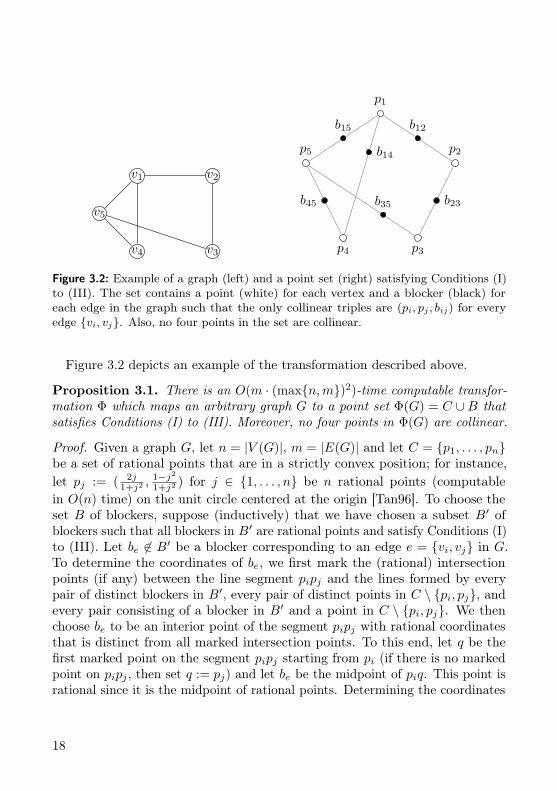
Let G be a graph with vertex set V (G) = v1, . . . , vn. Let Φ(G) := C ∪B bea set of points where C = p1, . . . , pn are points in strictly convex position, thatis, the points in C are vertices of a convex polygon (pi ∈ C corresponds to vi,i = 1, . . . , n). For each edge e = vi, vj ∈ E(G), we place a blocker be ∈ B onthe line segment pipj such that the following three conditions are satisfied:
(I) For any edge e ∈ E(G) and for any two points pi, pj ∈ C, if be, pi, pj arecollinear, then pi, pj are the points in C corresponding to the endpointsof edge e.
(II) Any two distinct blockers be, be′ are not collinear with any point pi ∈ C.
(III) The set B := be | e ∈ E(G) of blockers is in general position.
17
v1 v2
v3v4
v5
p1
p2
p3p4
p5
b12b15
b14
b23b35b45
Figure 3.2: Example of a graph (left) and a point set (right) satisfying Conditions (I)to (III). The set contains a point (white) for each vertex and a blocker (black) foreach edge in the graph such that the only collinear triples are (pi, pj , bij) for everyedge vi, vj. Also, no four points in the set are collinear.
Figure 3.2 depicts an example of the transformation described above.
Proposition 3.1. There is an O(m · (maxn,m)2)-time computable transfor-mation Φ which maps an arbitrary graph G to a point set Φ(G) = C ∪B thatsatisfies Conditions (I) to (III). Moreover, no four points in Φ(G) are collinear.
Proof. Given a graph G, let n = |V (G)|, m = |E(G)| and let C = p1, . . . , pnbe a set of rational points that are in a strictly convex position; for instance,let pj := ( 2j
1+j2 ,1−j21+j2 ) for j ∈ 1, . . . , n be n rational points (computable
in O(n) time) on the unit circle centered at the origin [Tan96]. To choose theset B of blockers, suppose (inductively) that we have chosen a subset B′ ofblockers such that all blockers in B′ are rational points and satisfy Conditions (I)to (III). Let be 6∈ B′ be a blocker corresponding to an edge e = vi, vj in G.To determine the coordinates of be, we first mark the (rational) intersectionpoints (if any) between the line segment pipj and the lines formed by everypair of distinct blockers in B′, every pair of distinct points in C \ pi, pj, andevery pair consisting of a blocker in B′ and a point in C \ pi, pj. We thenchoose be to be an interior point of the segment pipj with rational coordinatesthat is distinct from all marked intersection points. To this end, let q be thefirst marked point on the segment pipj starting from pi (if there is no markedpoint on pipj , then set q := pj) and let be be the midpoint of piq. This point isrational since it is the midpoint of rational points. Determining the coordinates
18
of a blocker can thus be done in O(m2 + n2 + nm) time. The overall runningtime is thus in O(m · (maxn,m)2) Clearly, all points in C ∪ B are rationaland satisfy Conditions (I) to (III). Moreover, the construction of C ∪B ensuresthat no four points in C ∪B are collinear.
In what follows, we will use transformation Φ as a reduction from Inde-pendent Set to General Position Subset Selection in order to proveour hardness results. The following observation will be helpful in proving thecorrectness of the reduction.
Observation 3.2. Let G be an arbitrary graph, and let P := Φ(G) = C ∪ B.For any point set S ⊆ P that is in general position, there is a general positionset of size at least |S| that contains the set of blockers B.
Proof. Suppose that S ⊆ P is in general position, and suppose that there isa point b ∈ B \ S. If b does not lie on a line defined by any two points in S,then S ∪ b is in general position. Otherwise, b lies on a line defined by twopoints p, q ∈ S. By Conditions (I) and (II), it holds that p, q ∈ C. Moreover,p and q are the only two points in S that are collinear with b. Hence, weexchange one of them with b to obtain a set of points in general position of thesame cardinality as S. Since b ∈ B was arbitrarily chosen, we can repeat theabove argument to obtain a subset in general position of cardinality at least |S|that contains B.
Using Observation 3.2, we give a polynomial-time many-one reduction fromIndependent Set to General Position Subset Selection based ontransformation Φ.
Independent SetInput: An undirected graph G and k ∈ N.Question: Is there a subset I ⊆ V (G) of size at least k such that no two
vertices in I are connected by an edge?
Lemma 3.3. There is a polynomial-time many-one reduction from Indepen-dent Set to General Position Subset Selection. Moreover, each instanceof General Position Subset Selection produced by this reduction satisfiesthe property that no four points in the instance are collinear.
Proof. Let (G, k) be an instance of Independent Set, where k ∈ N. TheGeneral Position Subset Selection instance is defined as (P := Φ(G), k +
19

|E(G)|). Clearly, by Proposition 3.1, the set P can be computed in polynomialtime, and no four points in P are collinear. We show that G has an independentset of cardinality k if and only if P has a subset in general position of cardinalityk + |E(G)|.Suppose that I ⊆ V (G) is an independent set of cardinality k, and let S :=pi | vi ∈ I ∪B, where B is the set of blockers in P . Since |B| = |E(G)|, wehave |S| = k+ |E(G)|. Suppose towards a contradiction that S is not in generalposition, and let q, r, s be three distinct collinear points in S. By Conditions (II)and (III), and since the points in C are in a strictly convex position, it followsthat exactly two of the points q, r, s must be in C. Suppose, without loss ofgenerality, that q = pi, r = pj ∈ C and s ∈ B. By Condition (I), there is an edgebetween the vertices vi and vj in G that correspond to the points pi, pj ∈ C,contradicting that vi, vj ∈ I. It follows that S is a subset in general position ofcardinality k + |E(G)|.
Conversely, assume that S ⊆ P is in general position and that |S| = k+|E(G)|.By Observation 3.2, we may assume that B ⊆ S. Let I be the set of verticescorresponding to the points in S \B, and note that |I| = k. Since B ⊆ S, notwo points vi, vj in I can be adjacent; otherwise, their corresponding pointspi, pj and the blocker of edge vi, vj would be three collinear points in S. Itfollows that I is an independent set of cardinality k in G.
Lemma 3.3 implies the NP-hardness of General Position Subset Se-lection. Furthermore, a careful analysis of the proof of Lemma 3.3 revealsthe intractability of an extension variant of General Position Subset Se-lection, where as an additional input to the problem a subset S′ ⊆ P ofpoints in general position is given and the task is to find k additional points ingeneral position, that is, one looks for a point subset S ⊆ P in general positionsuch that S′ ⊂ S and |S| ≥ |S′| + k. By Observation 3.2, we can assumefor the instance created by transformation Φ that B (the set of blockers) iscontained in a maximum-cardinality point subset in general position. Thus,we can set S′ := B. The proof of Lemma 3.3 then shows that k points can beadded to S′ if and only if the graph G contains an independent set of size k.Since Independent Set is W[1]-hard with respect to the solution size [DF13],we can observe the following:
Observation 3.4. The extension variant of General Position SubsetSelection described above is W[1]-hard when parameterized by the number kof additional points.
20
Hence, this extension is not fixed-parameter tractable with respect to k,unless W[1] = FPT. The W[1]-hardness for the extension variant is in contrastto the fixed-parameter tractability results for General Position SubsetSelection that will be shown in Section 3.3.1.Next, we turn our attention to approximation, that is, we consider the
following optimization problem.
Maximum General Position Subset SelectionInput: A set P of points in the plane.Task: Select a subset S ⊆ P in general position of maximum cardinality.
By IS-3 we denote the Maximum Independent Set problem restricted tographs of maximum degree at most three.
IS-3Input: An undirected graph G of maximum degree at most three.Task: Find an independent set I ⊆ V (G) of maximum size.
The next lemma implies APX-hardness of Maximum General PositionSubset Selection. Recall the definition of a PTAS-reduction from Section 2.5.
Definition 3.1. Given two maximization problems Q = (I, S, f, g) and Q′ =(I ′, S′, f ′, g′), a PTAS-reduction from Q to Q′ consists of three polynomial-timecomputable functions h, h′ and α : Q→ Q+ such that:
(i) h : I → I ′ maps an instance of Q to an instance of Q′, and
(ii) for any instance x ∈ I of Q and any solution y′ ∈ S′(h(x)) of h(x) ∈ I ′and for any ε ∈ Q+, h′(x, y′, ε) ∈ S(x) is a solution of x such that
opt(h(x))
f ′(h(x), y′)≤ 1 + α(ε) ⇒ opt(x)
f(x, h′(x, y′, ε))≤ 1 + ε.
Lemma 3.5. There is a PTAS-reduction from IS-3 to Maximum GeneralPosition Subset Selection.
Proof. Let G be an instance of IS-3, and note that |E(G)| ≤ 3|V (G)|/2. Itis easy to see that G has an independent set I0 of cardinality at least |I0| >|V (G)|/4 that can be obtained in polynomial time by repeatedly selecting avertex in G of minimum degree and discarding all its neighbors until the graphis empty.
21
We define the computable functions h, h′ and α in Definition 3.1 as follows.For a graph G, the function h is defined as h(G) := Φ(G) and is computablein polynomial time by Proposition 3.1. Let P := h(G) = C ∪B and let S ⊆ Pbe a subset in general position. For every ε > 0, we define an independentset h′(G,S, ε) ⊆ V (G) as follows: If |S \B| < |V (G)|/4, then h′(G,S, ε) := I0.Otherwise, we have |S \ B| ≥ |V (G)|/4. If B ⊆ S, then h′(G,S, ε) is the setof vertices corresponding to the points in S \ B (by the proof of Lemma 3.3,these vertices form an independent set in G). If B 6⊆ S, then we first computein polynomial time a subset S′ ⊆ P in general position such that B ⊆ S′
and |S′| ≥ |S| (as described in the proof of Observation 3.2). Now, if |S′ \B| <|V (G)|/4, then we set h′(G,S, ε) := I0 again. Otherwise, we define h′(G,S, ε)to be the independent set corresponding to the points in S′ \B. This finishesthe definition of h′. Note that h′ is clearly polynomial-time computable andthat h′(G,S, ε) is always of size at least |V (G)|/4. Finally, we define α(ε) := ε/7.Let G be a graph, P := h(G) = C ∪ B be a point set and let S ⊆ P
be a subset in general position. Further, let opt(G) ≥ |V (G)|/4 denote thecardinality of a maximum independent set in G, and let opt(P ) be the cardinalityof a largest subset in general position in P . From Lemma 3.3, it follows thatopt(P ) = |B|+ opt(G). To finish the proof, we need to show that
opt(P )
|S|≤ 1 + α(ε) ⇒ opt(G)
|h′(G,S, ε)|≤ 1 + ε
holds for every ε > 0. Let I := h′(G,S, ε). Then, we have
opt(P )
|S|=|B|+ opt(G)
|B|+ |S \B|≤ 1 + α(ε)
⇐⇒ opt(G) ≤ (1 + α(ε))(|S ∩B|+ |S \B|)− |B|
⇐⇒ opt(G)
|I|≤ (1 + α(ε)) · |S ∩B|+ |S \B|
|I|− |B||I|
Since |S ∩B| ≤ |B|, we obtain
opt(G)
|I|≤ α(ε)
|B||I|
+ (1 + α(ε))|S \B||I|
Using |B| = |E(G)| ≤ 3|V (G)|/2 and |I| ≥ |V (G)|/4, we have
opt(G)
|I|≤ α(ε) · 6 + (1 + α(ε))
|S \B||I|
.
22
Now, if |S \ B| ≤ |V (G)|/4 or B ⊆ S, then, by definition of h′, it holds|S \B|/|I| ≤ 1, and thus
opt(G)
|I|≤ α(ε) · 6 + (1 + α(ε)) = 1 + 7α(ε) = 1 + ε.
If B 6⊆ S and |S \ B| > |V (G)|/4, then consider the set S′ from which I isdetermined by definition of h′ and note that since |S′| ≥ |S|, we also have
opt(P )
|S′|≤ (1 + α(ε)) ⇐⇒ opt(G)
|I|≤ α(ε) · 6 + (1 + α(ε))
|S′ \B||I|
.
By definition of h′, it holds |S′ \B| ≤ |I| and thus
opt(G)
|I|≤ 1 + 7α(ε) = 1 + ε.
Finally, we prove that transformation Φ yields a polynomial-time many-onereduction from IS-3 to Maximum General Position Subset Selection,where the number of points in the point set depends linearly on the number ofvertices in the graph. This implies an exponential-time lower bound based onthe Exponential Time Hypothesis (ETH) [IPZ01].
Lemma 3.6. There is a polynomial-time many-one reduction from Indepen-dent Set on graphs with maximum degree three to General Position SubsetSelection mapping a graph G to a point set P of size O(|V (G)|).
Proof. For an instance (G, k) of Independent Set, where G has maximumdegree three, the point set P := Φ(G) is of cardinality |P | = |V (G)|+ |E(G)| ≤|V (G)|+3|V (G)|/2 ∈ O(|V (G)|). By the proof of Lemma 3.3, Φ is a polynomial-time many-one reduction.
We summarize the consequences of Lemmas 3.3, 3.5 and 3.6 in the followingtheorem:
Theorem 3.7. The following statements are true:(a) General Position Subset Selection is NP-hard.(b) Maximum General Position Subset Selection is APX-hard.
23
(c) Unless ETH fails, General Position Subset Selection is not solvablein 2o(n) · nO(1) time, where n is the number of points in the input.
The above hardness results even hold for instances in which no four points arecollinear.
Proof. Part (a) follows from the NP-hardness of Independent Set [GJ79],combined with Proposition 3.1 and Lemma 3.3. Part (b) follows from theAPX-hardness of IS-3 [AK00], combined with Proposition 3.1 and Lemma 3.5.Concerning Part (c), it is well known that, unless the ETH fails, IndependentSet is not solvable in sub-exponential time [IPZ01], and the same is true forthe restriction to graphs of maximum degree three by the result of Johnson andSzegedy [JS99]. Hence, by the reduction in Lemma 3.6, General PositionSubset Selection cannot be solved in sub-exponential time since this wouldimply a sub-exponential-time algorithm for Independent Set on graphs ofmaximum degree three.Parts (a)–(c) remain true for instances in which no four points are collinear
because the point set produced by transformation Φ satisfies this property (seeProposition 3.1).
3.3 Fixed-Parameter Tractability
In this section, we prove several fixed-parameter tractability results for GeneralPosition Subset Selection. In Section 3.3.1 we develop problem kernelswith a cubic number of points for the parameter size k of the sought subset ingeneral position, and for the line cover number `. In Section 3.3.2, we show aquadratic-size problem kernel with respect to the dual parameter h := n− k,that is, the number of points whose deletion leaves a set of points in generalposition. Moreover, we prove that this problem kernel is essentially optimal,unless coNP ⊆ NP/poly (which implies an unlikely collapse in the polynomialhierarchy).
3.3.1 Fixed-Parameter Tractability Results for theParameter Solution Size k
Let (P, k) be an instance of General Position Subset Selection, andlet n = |P |. Cao [Cao12] gave a problem kernel for General Position SubsetSelection with O(k4) points based on the following idea. Suppose that there
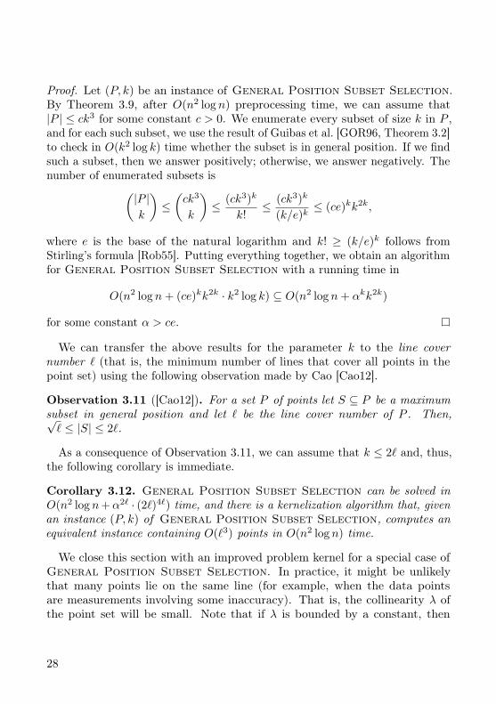
24
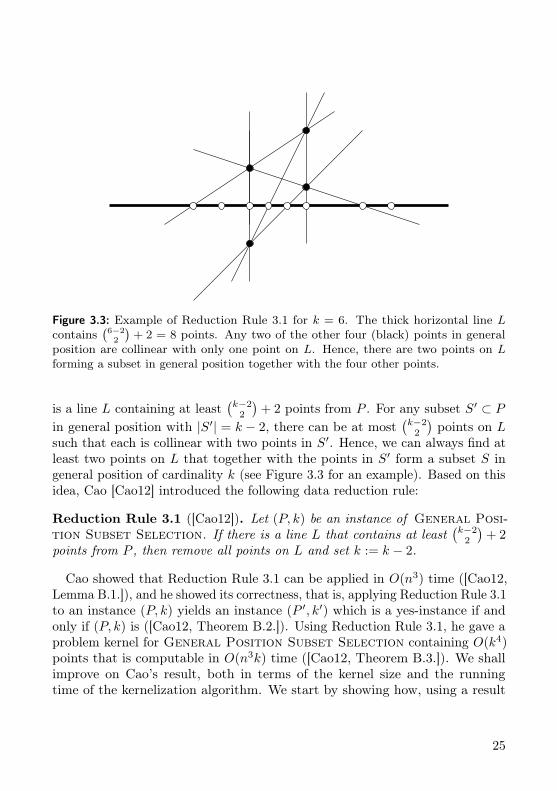
Figure 3.3: Example of Reduction Rule 3.1 for k = 6. The thick horizontal line Lcontains
(6−22
)+ 2 = 8 points. Any two of the other four (black) points in general
position are collinear with only one point on L. Hence, there are two points on Lforming a subset in general position together with the four other points.
is a line L containing at least(k−2
2
)+ 2 points from P . For any subset S′ ⊂ P
in general position with |S′| = k − 2, there can be at most(k−2
2
)points on L
such that each is collinear with two points in S′. Hence, we can always find atleast two points on L that together with the points in S′ form a subset S ingeneral position of cardinality k (see Figure 3.3 for an example). Based on thisidea, Cao [Cao12] introduced the following data reduction rule:
Reduction Rule 3.1 ([Cao12]). Let (P, k) be an instance of General Posi-tion Subset Selection. If there is a line L that contains at least
(k−2
2
)+ 2
points from P , then remove all points on L and set k := k − 2.
Cao showed that Reduction Rule 3.1 can be applied in O(n3) time ([Cao12,Lemma B.1.]), and he showed its correctness, that is, applying Reduction Rule 3.1to an instance (P, k) yields an instance (P ′, k′) which is a yes-instance if andonly if (P, k) is ([Cao12, Theorem B.2.]). Using Reduction Rule 3.1, he gave aproblem kernel for General Position Subset Selection containing O(k4)points that is computable in O(n3k) time ([Cao12, Theorem B.3.]). We shallimprove on Cao’s result, both in terms of the kernel size and the runningtime of the kernelization algorithm. We start by showing how, using a result
25
by Guibas et al. [GOR96, Theorem 3.2], Reduction Rule 3.1 can be appliedexhaustively in O(n2 log n) time. Notably, the idea of reducing lines with manypoints (based on Guibas et al. [GOR96]) also yields a kernelization result forPoint Line Cover [LM05].
Lemma 3.8. For an instance (P, k) of General Position Subset Selec-tion where |P | = n, we can compute in O(n2 log n) time an equivalent instance(P ′, k′) such that the collinearity of P ′ is at most
(k−2
2
)+ 1.
Proof. Let λ =(k−2
2
)+ 2. We start by computing the set L of all lines
that contain at least λ points from P . By a result of Guibas et al. [GOR96,Theorem 3.2], this can be performed in O(n2 log (n/λ)/λ) time (the algorithmalso yields for every such line the points of P lying on that line). We theniterate over each line L ∈ L, checking whether L, at the current iteration,still contains at least λ points; if it does, we remove all points on L from Pand decrement k by 2. For each line L, the running time of the precedingstep is O(λ), which is the time to check whether L contains at least λ points.Additionally, we might need to remove all points on L. If k reaches zero, thenwe can return a trivial yes-instance (P ′, k′) of General Position SubsetSelection in constant time. Otherwise, after iterating over all lines in L, byReduction Rule 3.1, the resulting instance (P ′, k′) is an equivalent instance to(P, k) satisfying that no line in P ′ contains λ points, and hence the collinearityof P ′ is at most
(k−2
2
)+ 1. Overall, the above can be implemented in time
O((n2 log (n/λ)/λ) · λ) ⊆ O(n2 log n).
We move on to improving the size of the problem kernel. Payne and Wood[PW13, Theorem 2.3] proved a lower bound on the maximum cardinality of asubset in general position when an upper bound on the collinearity of the pointset is known. We show next how to obtain a kernel for General PositionSubset Selection containing O(k3) points based on this result.
Theorem 3.9. General Position Subset Selection admits a problemkernel containing O(k3) points that is computable in O(n2 log n) time.
Proof. By Lemma 3.8, after O(n2 log n) preprocessing time, we can either returnan equivalent yes-instance of (P, k) of constant size, or obtain an equivalentinstance with a point set of cardinality O(k4) ([Cao12, Theorem B.3.]) andcollinearity at most
(k−2
2
)+ 1. Hence, without loss of generality, we assume in
what follows that |P | ∈ O(k4) and that the collinearity of P is λ ≤(k−2
2
)+ 1.
26

Payne and Wood [PW13, Theorem 2.3] showed that any set of n points whosecollinearity is at most λ contains a subset of points in general position of size atleast
αn√n lnλ+ λ2
for some constant α > 0. Since λ ≤(k−2
2
)+ 1 ≤ k2, we have at least
αn√2n ln k + k4
points in general position. Note that this number is monotonically increasingin n. Thus, if n ≥ cnk3 for a constant cn > 0, then there are at least
αcnk3
√2cnk3 ln k + k4
points in general position. Since 2cnk3 ln k ∈ o(k4), it follows that for large
enough k ≥ ck (for some constant ck > 0), the number of points in generalposition is at least
αcnk3
√2k4
=αcnk
3
√2k2
=αcn√
2· k.
Hence, for cn ≥√
2/α, the number of points in general position is at least k.Thus, we derived that there exists a constant cn (depending on α) such thatthere exists a constant ck (depending on cn) such that, for n ≥ cnk3 and k > ck,there exist at least k points in general position.The kernelization algorithm distinguishes the following three cases: First, if
k ≤ ck, then the instance is of constant size and the algorithm decides it in O(1)time and returns an equivalent constant-size instance. Second, if k > ck and|P | ≥ cnk
3, then the algorithm returns a trivial yes-instance of constant size.Third, if none of the two above cases applies, then the algorithm returns the(preprocessed) instance (P, k) which satisfies |P | ∈ O(k3).
We can derive the following result by a brute-force algorithm on the aboveproblem kernel:
Corollary 3.10. General Position Subset Selection can be solved inO(n2 log n+ αkk2k) time for some constant α.
27
Proof. Let (P, k) be an instance of General Position Subset Selection.By Theorem 3.9, after O(n2 log n) preprocessing time, we can assume that|P | ≤ ck3 for some constant c > 0. We enumerate every subset of size k in P ,and for each such subset, we use the result of Guibas et al. [GOR96, Theorem 3.2]to check in O(k2 log k) time whether the subset is in general position. If we findsuch a subset, then we answer positively; otherwise, we answer negatively. Thenumber of enumerated subsets is(
|P |k
)≤(ck3
k
)≤ (ck3)k
k!≤ (ck3)k
(k/e)k≤ (ce)kk2k,
where e is the base of the natural logarithm and k! ≥ (k/e)k follows fromStirling’s formula [Rob55]. Putting everything together, we obtain an algorithmfor General Position Subset Selection with a running time in
O(n2 log n+ (ce)kk2k · k2 log k) ⊆ O(n2 log n+ αkk2k)
for some constant α > ce.
We can transfer the above results for the parameter k to the line covernumber ` (that is, the minimum number of lines that cover all points in thepoint set) using the following observation made by Cao [Cao12].
Observation 3.11 ([Cao12]). For a set P of points let S ⊆ P be a maximumsubset in general position and let ` be the line cover number of P . Then,√` ≤ |S| ≤ 2`.
As a consequence of Observation 3.11, we can assume that k ≤ 2` and, thus,the following corollary is immediate.
Corollary 3.12. General Position Subset Selection can be solved inO(n2 log n+α2` · (2`)4`) time, and there is a kernelization algorithm that, givenan instance (P, k) of General Position Subset Selection, computes anequivalent instance containing O(`3) points in O(n2 log n) time.
We close this section with an improved problem kernel for a special case ofGeneral Position Subset Selection. In practice, it might be unlikelythat many points lie on the same line (for example, when the data pointsare measurements involving some inaccuracy). That is, the collinearity λ ofthe point set will be small. Note that if λ is bounded by a constant, then
28

Observation 3.11 implies an O(k2)-point kernel (the line cover number is atleast n/λ, thus, there are Ω(
√n) points in general position). For the case λ = 3,
we can show an even smaller problem kernel.Let 3-General Position Subset Selection denote the restriction of
General Position Subset Selection to instances in which the point setcontains no four collinear points (that is, collinearity λ ≤ 3). By Theorem 3.7, 3-General Position Subset Selection is NP-hard. Füredi [Für91, Theorem 1]showed that every set P of n points in which no four points are collinear containsa subset in general position of size Ω(
√n log n). Based on Füredi’s result, we
get the following:
Theorem 3.13. 3-General Position Subset Selection admits a problemkernel containing O(k2/ log k) points that is computable in O(n) time.
Proof. Let (P, k) be an instance of 3-General Position Subset Selectionwith |P | = n. Note that the line cover number ` of P is at least n/3 since at mostthree points lie on the same line. Therefore, if n ≥ 3k2, then by Observation 3.11we know that P contains at least k points in general position. Thus, we canreturn a trivial constant-size yes-instance.
We henceforth assume that n < 3k2. Then, there exists a constant α > 0 suchthat P contains at least α
√n log n points in general position [Für91, Theorem 1].
Let n ≥ cnk2/ log k for some constant cn > 0. Then, P contains at least
α
√cnk2
log klog
(cnk2
log k
)= α
√cnk2
(2 +
log cn − log log k
log k
)points in general position. Since there exists a constant ck (depending on cn)such that
log cn − log log k
log k≥ −1
holds for all k ≥ ck, it follows that there are at least α√cnk2(2− 1) = α
√cn · k
points in general position for large enough k. Hence, for cn ≥ α−2, we have ayes-instance.
The kernelization algorithm works as follows: If k < ck, then P is of constantsize and we decide the instance in constant time returning an equivalent constant-size instance. If k ≥ ck and n ≥ cnk2/ log k, then we return a constant-size yes-instance. Otherwise, we simply return the instance (P, k) with |P | ∈ O(k2/ log k).The running time is in O(n) for counting the number of points in the input.
29
We remark that the presented problem kernels (relying on non-constructivelower bounds) only can be used to solve the decision problem, that is, they donot allow to actually find a point set in general position. It is not clear how toconstructively find the points in general position for large yes-instances.
3.3.2 Fixed-Parameter Tractability Results for the DualParameter h
In this section we consider the dual parameter number h := n− k of points thathave to be deleted (that is, excluded from the sought point set in general position)so that the remaining points are in general position. We show a problem kernelcontaining O(h2) points for General Position Subset Selection. Moreover,we show that most likely this problem kernel is essentially tight, that is, there ispresumably no problem kernel with O(h2−ε) points for any ε > 0.
We start with the problem kernel that relies essentially on a problem kernelfor the 3-Hitting Set problem:
3-Hitting SetInput: A universe U , a collection C of size-3 subsets of U , and h ∈ N.Question: Is there a subset H ⊆ U of size at most h containing at least
one element from each subset S ∈ C?
There is a close connection between General Position Subset Selectionand 3-Hitting Set: For any collinear triple p, q, r ∈ P of distinct points, one ofthe three points has to be deleted in order to obtain a subset in general position.Hence, the set of deleted points has to be a hitting set for the family of allcollinear triples in P . Since 3-Hitting Set can be solved in O(2.08h+ |C|+ |U |)time [Wah07], we get:
Proposition 3.14. General Position Subset Selection can be solved inO(2.08h + n3) time.
3-Hitting Set is known to admit a problem kernel with a universe ofsize O(h2) computable in O(|U | + |C| + h1.5) time [Bev14]. Based on this,one can obtain a problem kernel of size O(h2) computable in O(n3) time. Thebottleneck in this running time is listing all collinear triples. We can improve therunning time of this kernelization algorithm by giving a direct kernel exploitingthe simple geometric fact that two non-parallel lines intersect in one point.We first need two data reduction rules for which we introduce the followingdefinition:
30
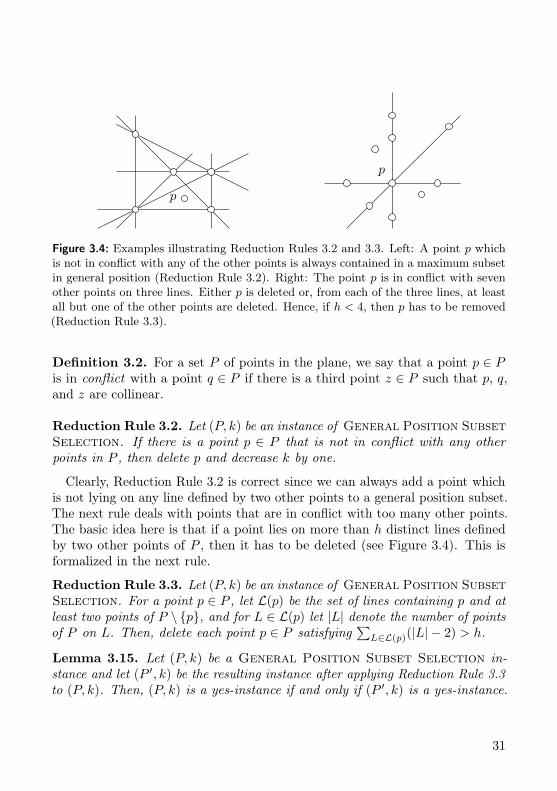
p
p
Figure 3.4: Examples illustrating Reduction Rules 3.2 and 3.3. Left: A point p whichis not in conflict with any of the other points is always contained in a maximum subsetin general position (Reduction Rule 3.2). Right: The point p is in conflict with sevenother points on three lines. Either p is deleted or, from each of the three lines, at leastall but one of the other points are deleted. Hence, if h < 4, then p has to be removed(Reduction Rule 3.3).
Definition 3.2. For a set P of points in the plane, we say that a point p ∈ Pis in conflict with a point q ∈ P if there is a third point z ∈ P such that p, q,and z are collinear.
Reduction Rule 3.2. Let (P, k) be an instance of General Position SubsetSelection. If there is a point p ∈ P that is not in conflict with any otherpoints in P , then delete p and decrease k by one.
Clearly, Reduction Rule 3.2 is correct since we can always add a point whichis not lying on any line defined by two other points to a general position subset.The next rule deals with points that are in conflict with too many other points.The basic idea here is that if a point lies on more than h distinct lines definedby two other points of P , then it has to be deleted (see Figure 3.4). This isformalized in the next rule.
Reduction Rule 3.3. Let (P, k) be an instance of General Position SubsetSelection. For a point p ∈ P , let L(p) be the set of lines containing p and atleast two points of P \ p, and for L ∈ L(p) let |L| denote the number of pointsof P on L. Then, delete each point p ∈ P satisfying
∑L∈L(p)(|L| − 2) > h.
Lemma 3.15. Let (P, k) be a General Position Subset Selection in-stance and let (P ′, k) be the resulting instance after applying Reduction Rule 3.3to (P, k). Then, (P, k) is a yes-instance if and only if (P ′, k) is a yes-instance.
31
Proof. Let (P, k) be an instance of General Position Subset Selectionand let (P ′ := P \D, k) be the reduced instance, where D ⊆ P denotes the setof removed points.Clearly, if (P ′, k) is a yes-instance, then so is (P, k). For the converse, we
show that no point p ∈ D can be contained in a size-k subset of P in generalposition: For each line L ∈ L(p), all but two points need to be deleted. If asubset S ⊆ P in general position contains p, then the points that have to bedeleted on the lines in L(p) are all distinct since any two of these lines onlyintersect in p. This means that
∑L∈L(p)(|L| − 2) points need to be deleted.
However, since this value is by assumption larger than h, the solution S is ofsize less than k = |P | − h.
Theorem 3.16. General Position Subset Selection admits a problemkernel containing at most 2h2 + h points that is computable in O(n2) time,where h = n− k.Proof. Let (P, k) be a General Position Subset Selection instance. Wefirst show that applying Reduction Rule 3.2 exhaustively and then applyingReduction Rule 3.3 once indeed gives a small instance (P ′, k′). Note that eachpoint p ∈ P ′ is in conflict with at least two other points, that is, p is on at leastone line containing two other points in P ′, since the instance is reduced withrespect to Reduction Rule 3.2. Moreover, since the instance is reduced withrespect to Reduction Rule 3.3, it follows that each point is in conflict with atmost 2h other points. Thus, deleting h points can give at most h · 2h pointsin general position. Hence, if P ′ contains more than 2h2 + h points, then theinput instance is a no-instance.
We next show how to exhaustively apply Reduction Rules 3.2 and 3.3 in O(n2)time. To this end, we follow an approach described by Edelsbrunner et al.[EOS86] and Gómez et al. [GRT97] which uses the dual representation and linearrangements. The dual representation maps points to lines as follows: (a, b) 7→y = ax + b. A line in the primal representation containing some points of Pcorresponds in the dual representation to the intersection point of the linescorresponding to these points. Thus, a set of at least three collinear points inthe primal corresponds to the intersection of the corresponding lines in the dual.An arrangement of lines in the plane is, roughly speaking, the partition of theplane formed by these lines. A representation of an arrangement of n lines canbe computed in O(n2) time [EOS86]. Using an algorithm of Edelsbrunner et al.[EOS86], we compute in O(n2) time the arrangement A(P ∗) of the lines P ∗ inthe dual representation of P .
32

Reduction Rule 3.2 is now easily executable in O(n2) time: Initially, markall points in P as “not in conflict”. Then, iterate over the vertices of A(P ∗)and whenever the vertex has degree six or more (each line on an intersectioncontributes two to the degree of the corresponding vertex) mark the pointscorresponding to the intersecting lines as “in conflict”. In a last step, remove allpoints that are marked as “not in conflict”.
Reduction Rule 3.3 can be applied in a similar fashion in O(n2) time: Assign acounter to each point p ∈ P and initialize it with zero. We want this counter tostore the number
∑L∈L(p)(|L| − 2) on which Reduction Rule 3.3 is conditioned.
To this end, we iterate over the vertices in A(P ∗) and for each vertex of degreesix or more (each line contributes two to the degree of the intersection vertex)we increase the counter of each point corresponding to a line in the intersectionby d/2− 2 where d is the degree of the vertex. After one pass over all verticesin A(P ∗) in O(n2) time, the counters of the points store the correct values andwe can delete all points whose counter is more than h.
Another interesting parameter for geometry problems is the number γ ofinner points (that is, all points which are not a vertex of the convex hull of P ),which successfully has been deployed algorithmically [Deı+06, HO06]. Note thatProposition 3.14 and Theorem 3.16 also hold if we replace the parameter h by γ.The reason is that in all non-trivial instances we have h ≤ γ since removing allinner points yields a set of points in general position.
3.3.3 Excluding O(h2−ε)-point KernelsIn this section we show that the O(h2)-point problem kernel of Theorem 3.16is essentially optimal. We start by proving a (conditional) lower bound on theproblem kernel size (the number of encoding bits) for General PositionSubset Selection via a reduction from Vertex Cover.
Vertex CoverInput: An undirected graph G and k ∈ N.Question: Is there a subset V ′ ⊆ V (G) of size at most k such that every
edge is incident to at least one vertex in V ′ ?
Using a lower bound result by Dell and Melkebeek [DM14] for Vertex Cover,we obtain the following:
Theorem 3.17. Unless coNP ⊆ NP/poly, for any ε > 0, General PositionSubset Selection admits no problem kernel of size O(h2−ε).
33
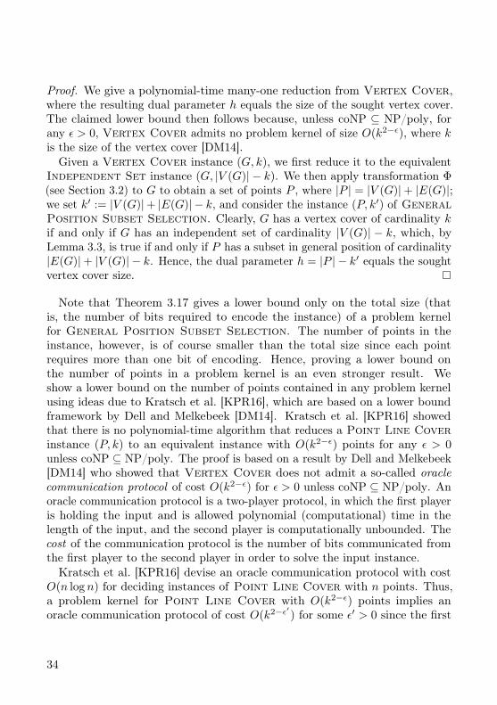
Proof. We give a polynomial-time many-one reduction from Vertex Cover,where the resulting dual parameter h equals the size of the sought vertex cover.The claimed lower bound then follows because, unless coNP ⊆ NP/poly, forany ε > 0, Vertex Cover admits no problem kernel of size O(k2−ε), where kis the size of the vertex cover [DM14].
Given a Vertex Cover instance (G, k), we first reduce it to the equivalentIndependent Set instance (G, |V (G)| − k). We then apply transformation Φ(see Section 3.2) to G to obtain a set of points P , where |P | = |V (G)|+ |E(G)|;we set k′ := |V (G)|+ |E(G)| − k, and consider the instance (P, k′) of GeneralPosition Subset Selection. Clearly, G has a vertex cover of cardinality kif and only if G has an independent set of cardinality |V (G)| − k, which, byLemma 3.3, is true if and only if P has a subset in general position of cardinality|E(G)|+ |V (G)| − k. Hence, the dual parameter h = |P | − k′ equals the soughtvertex cover size.
Note that Theorem 3.17 gives a lower bound only on the total size (thatis, the number of bits required to encode the instance) of a problem kernelfor General Position Subset Selection. The number of points in theinstance, however, is of course smaller than the total size since each pointrequires more than one bit of encoding. Hence, proving a lower bound onthe number of points in a problem kernel is an even stronger result. Weshow a lower bound on the number of points contained in any problem kernelusing ideas due to Kratsch et al. [KPR16], which are based on a lower boundframework by Dell and Melkebeek [DM14]. Kratsch et al. [KPR16] showedthat there is no polynomial-time algorithm that reduces a Point Line Coverinstance (P, k) to an equivalent instance with O(k2−ε) points for any ε > 0unless coNP ⊆ NP/poly. The proof is based on a result by Dell and Melkebeek[DM14] who showed that Vertex Cover does not admit a so-called oraclecommunication protocol of cost O(k2−ε) for ε > 0 unless coNP ⊆ NP/poly. Anoracle communication protocol is a two-player protocol, in which the first playeris holding the input and is allowed polynomial (computational) time in thelength of the input, and the second player is computationally unbounded. Thecost of the communication protocol is the number of bits communicated fromthe first player to the second player in order to solve the input instance.Kratsch et al. [KPR16] devise an oracle communication protocol with cost
O(n log n) for deciding instances of Point Line Cover with n points. Thus,a problem kernel for Point Line Cover with O(k2−ε) points implies anoracle communication protocol of cost O(k2−ε′) for some ε′ > 0 since the first
34
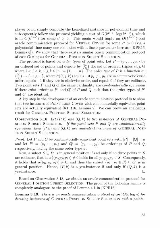
player could simply compute the kernelized instance in polynomial time andsubsequently follow the protocol yielding a cost of O(k2−ε · log(k2−ε)), whichis in O(k2−ε′) for some ε′ > 0. This again would imply an O(k2−ε′′)-costoracle communication protocol for Vertex Cover for some ε′′ > 0 (via apolynomial-time many-one reduction with a linear parameter increase [KPR16,Lemma 6]). We show that there exists a similar oracle communication protocolof cost O(n log n) for General Position Subset Selection.The protocol is based on order types of point sets. Let P = 〈p1, . . . , pn〉 be
an ordered set of points and denote by(
[n]3
)the set of ordered triples 〈i, j, k〉
where i < j < k, i, j, k ∈ [n] := 1, . . . , n. The order type of P is a function σ :([n]3
)→ −1, 0, 1, where σ(〈i, j, k〉) equals 1 if pi, pj , pk are in counter-clockwise
order, equals −1 if they are in clockwise order, and equals 0 if they are collinear.Two point sets P and Q of the same cardinality are combinatorially equivalentif there exist orderings P ′ and Q′ of P and Q such that the order types of P ′and Q′ are identical.
A key step in the development of an oracle communication protocol is to showthat two instances of Point Line Cover with combinatorially equivalent pointsets are actually equivalent [KPR16, Lemma 2]. We can prove an analogousresult for General Position Subset Selection:
Observation 3.18. Let (P, k) and (Q, k) be two instances of General Po-sition Subset Selection. If the point sets P and Q are combinatoriallyequivalent, then (P, k) and (Q, k) are equivalent instances of General Posi-tion Subset Selection.
Proof. Let P and Q be combinatorially equivalent point sets with |P | = |Q| = nand let P ′ = 〈p1, . . . , pn〉 and Q′ = 〈q1, . . . , qn〉 be orderings of P and Q,respectively, having the same order type σ.
Now, a subset S ⊆ P ′ is in general position if and only if no three points in Sare collinear, that is, σ(〈pi, pj , pk〉) 6= 0 holds for all pi, pj , pk ∈ S. Consequently,it holds that σ(〈qi, qj , qk〉) 6= 0, and thus the subset qi | pi ∈ S ⊆ Q′ is ingeneral position. Hence, (P, k) is a yes-instance if and only if (Q, k) is ayes-instance.
Based on Observation 3.18, we obtain an oracle communication protocol forGeneral Position Subset Selection. The proof of the following lemma iscompletely analogous to the proof of Lemma 4.1 in [KPR16]:
Lemma 3.19. There is an oracle communication protocol of cost O(n log n) fordeciding instances of General Position Subset Selection with n points.
35
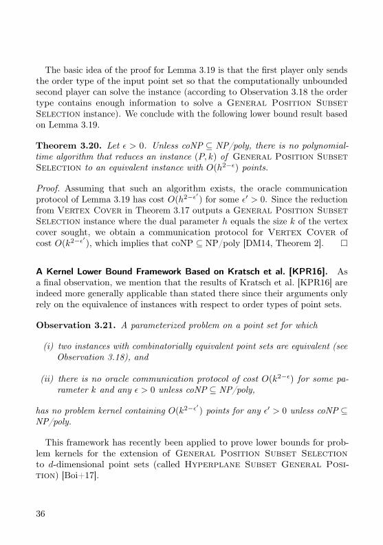
The basic idea of the proof for Lemma 3.19 is that the first player only sendsthe order type of the input point set so that the computationally unboundedsecond player can solve the instance (according to Observation 3.18 the ordertype contains enough information to solve a General Position SubsetSelection instance). We conclude with the following lower bound result basedon Lemma 3.19.
Theorem 3.20. Let ε > 0. Unless coNP ⊆ NP/poly, there is no polynomial-time algorithm that reduces an instance (P, k) of General Position SubsetSelection to an equivalent instance with O(h2−ε) points.
Proof. Assuming that such an algorithm exists, the oracle communicationprotocol of Lemma 3.19 has cost O(h2−ε′) for some ε′ > 0. Since the reductionfrom Vertex Cover in Theorem 3.17 outputs a General Position SubsetSelection instance where the dual parameter h equals the size k of the vertexcover sought, we obtain a communication protocol for Vertex Cover ofcost O(k2−ε′), which implies that coNP ⊆ NP/poly [DM14, Theorem 2].
A Kernel Lower Bound Framework Based on Kratsch et al. [KPR16]. Asa final observation, we mention that the results of Kratsch et al. [KPR16] areindeed more generally applicable than stated there since their arguments onlyrely on the equivalence of instances with respect to order types of point sets.
Observation 3.21. A parameterized problem on a point set for which
(i) two instances with combinatorially equivalent point sets are equivalent (seeObservation 3.18), and
(ii) there is no oracle communication protocol of cost O(k2−ε) for some pa-rameter k and any ε > 0 unless coNP ⊆ NP/poly,
has no problem kernel containing O(k2−ε′) points for any ε′ > 0 unless coNP ⊆NP/poly.
This framework has recently been applied to prove lower bounds for prob-lem kernels for the extension of General Position Subset Selectionto d-dimensional point sets (called Hyperplane Subset General Posi-tion) [Boi+17].
36
3.4 ConclusionWe studied the computational complexity of General Position SubsetSelection and proved its (approximation) intractability. Then, we started aparameterized complexity analysis obtaining several fixed-parameter tractabilityresults mainly based on problem kernelizations. The considered parameters arethe solution size k, its dual h, the line cover number ` and the number γ ofinner points. The kernelization results mostly rely on combinatorial arguments(similar ideas were recently used to develop kernelizations for generalizingGeneral Position Subset Selection to d dimensions [Boi+17]). Thus,a natural question to ask is whether there are any geometric properties thatcan be exploited in order to obtain further improved algorithmic results forGeneral Position Subset Selection. For practical purposes, it would alsobe interesting to find out which data reduction rules can be applied in lineartime.
We conclude with some further questions:• Can the O(k3)-point kernel (Theorem 3.9) for General Position Subset
Selection be asymptotically improved (for example by proving strongercombinatorial bounds or by finding further data reduction rules)? Or canwe derive a quadratic (or even a cubic) lower bound on the kernel size (oreven on the number of points)?• For which other problems on point sets can we derive kernel lower bounds
using the framework described in Observation 3.21?• What are further interesting parameterizations for General Position
Subset Selection? Maybe there exist other (geometrically motivated)parameters which allow for (stronger) fixed-parameter tractability results.Regarding parameterization above a lower bound (as studied in Chap-ter 6), however, note that the W[1]-hardness of the extension variant(Observation 3.4) already indicates intractability.
More generally, studying the complexity of other computational geometryproblems from a parameterized view (as done by Knauer et al. [KKW15]) couldbe a rewarding direction for future research. For example, a special case of theCo-Clustering∞ problem studied in Chapter 5 boils down to the geometricproblem of separating points in the plane with few axis-parallel lines. Maybe itis also possible to show fixed-parameter tractability with respect to the numberof lines for this problem based on combinatorial results.
37


Chapter 4
Distinct Vectors
In this chapter, we study the Distinct Vectors problem which asks to deleteas many columns as possible from a given matrix such that all rows in theresulting matrix are still pairwise distinct. This NP-complete problem arisesin the context of feature selection in data mining and machine learning. Its(classic) computational complexity has previously been studied. We conducta fine-grained complexity analysis with respect to the maximum (H) and theminimum (h) pairwise Hamming distance between matrix rows. Based on thiscombined parameterization, we prove a dichotomy result for binary matrices:Distinct Vectors can be solved in polynomial time if H ≤ 2dh/2e+ 1, and isNP-complete otherwise. Interestingly, as in Chapter 3, we again make use of acombinatorial result: The polynomial-time solvable cases are based on a resultfrom extremal set theory concerning certain set systems called sunflowers1.Moreover, we reveal a connection to matchings in bipartite graphs.
4.1 IntroductionFeature selection in a high-dimensional feature space means to choose a subsetof features (that is, dimensions) such that some desirable data propertiesare preserved or achieved in the induced subspace. Combinatorial featureselection [Cha+00, KS96] is a well-motivated alternative to the more frequentlystudied affine feature selection. While affine feature selection combines featuresto reduce dimensionality, combinatorial feature selection simply discards somefeatures. The advantage of the latter is that the resulting reduced feature space iseasier to interpret. See Charikar et al. [Cha+00] for a more extensive discussionin favor of combinatorial feature selection. Unfortunately, combinatorial feature1Note that the concept of sunflowers has been used before in parameterized complexity (forexample to show problem kernels [FG06, Chapter 9]).
39
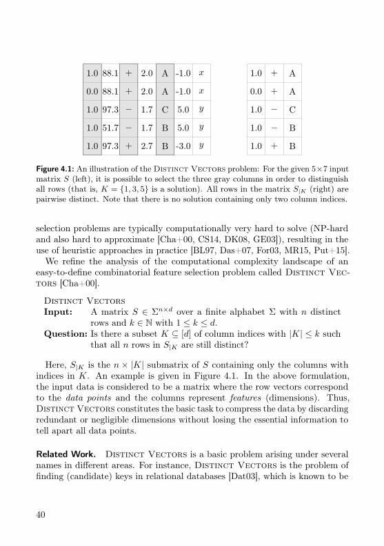
1.0
0.0
1.0
1.0
1.0
88.1
88.1
97.3
51.7
97.3
+
+
−
−
+
2.0
2.0
1.7
1.7
2.7
A
A
C
B
B
-1.0
-1.0
5.0
5.0
-3.0
x
x
y
y
y
1.0
0.0
1.0
1.0
1.0
+
+
−
−
+
A
A
C
B
B
Figure 4.1: An illustration of the Distinct Vectors problem: For the given 5×7 inputmatrix S (left), it is possible to select the three gray columns in order to distinguishall rows (that is, K = 1, 3, 5 is a solution). All rows in the matrix S|K (right) arepairwise distinct. Note that there is no solution containing only two column indices.
selection problems are typically computationally very hard to solve (NP-hardand also hard to approximate [Cha+00, CS14, DK08, GE03]), resulting in theuse of heuristic approaches in practice [BL97, Das+07, For03, MR15, Put+15].We refine the analysis of the computational complexity landscape of an
easy-to-define combinatorial feature selection problem called Distinct Vec-tors [Cha+00].
Distinct VectorsInput: A matrix S ∈ Σn×d over a finite alphabet Σ with n distinct
rows and k ∈ N with 1 ≤ k ≤ d.Question: Is there a subset K ⊆ [d] of column indices with |K| ≤ k such
that all n rows in S|K are still distinct?
Here, S|K is the n × |K| submatrix of S containing only the columns withindices in K. An example is given in Figure 4.1. In the above formulation,the input data is considered to be a matrix where the row vectors correspondto the data points and the columns represent features (dimensions). Thus,Distinct Vectors constitutes the basic task to compress the data by discardingredundant or negligible dimensions without losing the essential information totell apart all data points.
Related Work. Distinct Vectors is a basic problem arising under severalnames in different areas. For instance, Distinct Vectors is the problem offinding (candidate) keys in relational databases [Dat03], which is known to be
40
NP-complete [Bee+84]. It is also known as the Minimal Reduct problem inrough set theory [Paw91, SR92]. Later, Charikar et al. [Cha+00] investigatedthe computational complexity of several problems arising in the context ofcombinatorial feature selection, including Distinct Vectors. They showedthat there exists a constant c such that Distinct Vectors is NP-hard toapproximate in polynomial time within a factor of c log d on binary matrices.Moreover, Distinct Vectors is known [Fro+16a, Fro12] to be• W[2]-hard with respect to k,• W[1]-hard with respect to d− k,• fixed-parameter tractable with respect to (k, |Σ|) and also (k,H),• NP-hard for |Σ| = 2 and H ≥ 4,• and polynomial-time solvable for |Σ| = 2 and H ≤ 3.
Notably, Bläsius et al. [BFS17] studied the problem (among others) in thecontext of databases (therein called Unique) and also showed W[2]-hardnesswith respect to k.
Another combinatorial feature selection problem called Minimum FeatureSet is a variant of Distinct Vectors where not all pairs of rows have to bedistinguished but only all pairs of rows from two specified subsets. This problemis known to be NP-complete for binary input data [DR94]. In addition, Cottaand Moscato [CM03] investigated the parameterized complexity of MinimumFeature Set and proved W[2]-completeness with respect to the number ofselected columns even for binary matrices.
Our Contributions. The already known NP-hardness for binary matrices withmaximum pairwise row Hamming distance H ≥ 4 [Fro12] serves as a startingpoint for our complexity analysis. With the aim of identifying tractable cases,we are particularly interested in the complexity of Distinct Vectors if therange of different Hamming distances between pairs of data points (that is,rows) is small as this special case implies a somewhat homogeneous structure ofthe input data. Hence, we also take into account the minimum pairwise rowHamming distance h. Our parameter is then defined as the gap H − h. Wecompletely classify the classic complexity of Distinct Vectors with respectto all values of H − h on binary input matrices (see Figure 4.2).In Section 4.2.1, we show that binary Distinct Vectors is NP-hard if
H > 2dh/2e+ 1 (Theorem 4.3) and in Section 4.2.2 we show polynomial-timesolvability for H ≤ 2dh/2e+ 1 (Theorem 4.9).
41

h
H
1
1
2
2
3
3
4
4
5
5
6
6
7
7
8
8
9
9 NP-hard
P
Figure 4.2: Overview of the computational complexity landscape of Distinct Vectorson binary matrices with respect to the maximum pairwise row Hamming distance Hand the minimum pairwise row Hamming distance h. Gray cells correspond to NP-hardcases, whereas white cells correspond to polynomial-time solvable cases.
4.2 A Complexity Dichotomy for Binary Matrices
We focus on instances with a binary input alphabet, say, without loss ofgenerality, Σ = 0, 1. For a matrix S ∈ 0, 1n×d and a subset J ⊆ [d] ofcolumn indices, we use the abbreviation S|J := S[[n], J ] for the submatrix of Scontaining all the rows but only the columns with indices in J .We consider instances where the Hamming distance of each pair of rows
lies within a prespecified range. In other words, the number of columns inwhich a given pair of rows differs shall be bounded from below and aboveby some constants α, β ∈ N. We first give the formal definitions and thencompletely classify the classic complexity of Distinct Vectors with respectto the gap between α and β. The NP-hard cases are given in Section 4.2.1 andthe polynomial-time solvable cases in Section 4.2.2. The formal definitions forour setup are the following.
Definition 4.1 (Weight). For a vector x ∈ 0, 1d, we denote by Wx := j ∈[d] | (x)j = 1 the set of indices where x equals 1 and we call w(x) := |Wx| theweight of x.
42

Definition 4.2 (Hamming Distance). For vectors x, y ∈ Σd, let Dxy := j ∈[d] | (x)j 6= (y)j be the set of indices where x and y differ and let ∆(x, y) :=|Dxy| denote the Hamming distance of x and y.
Note that, for x, y ∈ 0, 1d, it holds Dxy = (Wx ∪Wy) \ (Wx ∩Wy) andthus ∆(x, y) = w(x) + w(y)− 2|Wx ∩Wy|.
For a Distinct Vectors instance (S ∈ Σn×d, k), we define the parameters• minimum pairwise row Hamming distance h := mini 6=j∈[n] ∆(si, sj) and• maximum pairwise row Hamming distance H := maxi 6=j∈[n] ∆(si, sj).
To conveniently state our results, we define the following variant of DistinctVectors:
Binary (α, β)-Distinct VectorsInput: A matrix S ∈ 0, 1n×d with n distinct rows such that h = α ≤
β = H, and k ∈ N.Question: Is there a subset K ⊆ [d] of column indices with |K| ≤ k such
that all rows in S|K are still distinct?
Intuitively, if the matrix consists of rows that are all “similar” to each other,one could hope to be able to solve the instance efficiently since there are atmost β columns to choose from in order to distinguish two rows. The minimumpairwise row Hamming distance α plays a dual role in the sense that if αis large, then each pair of rows differs in many columns, which also couldrender the instance easy to solve. We perform a close inspection of the relationbetween the minimum and maximum pairwise row Hamming distance and showthat it is possible to solve some cases in polynomial time for arbitrarily largeconstants α, β. These results are obtained by applying combinatorial argumentsfrom extremal set theory revealing a certain structure of the input matrix ifthe values of α and β are close to each other, that is, the range β − α is small.Analyzing this structure, we can show how to find solutions in polynomial time.On the negative side, for all other cases NP-hardness still holds as we show inthe next section.
4.2.1 NP-Hardness for Heterogeneous Data
As a starting point serves the NP-hardness of Binary (2, 4)-Distinct Vec-tors [Fro12, Theorem 4.4] ([Fro+16a, Theorem 1]). For the sake of beingself-contained, we include the proof here.
43
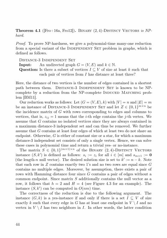
Theorem 4.1 ([Fro+16a, Fro12]). Binary (2, 4)-Distinct Vectors is NP-hard.
Proof. To prove NP-hardness, we give a polynomial-time many-one reductionfrom a special variant of the Independent Set problem in graphs, which isdefined as follows.
Distance-3 Independent SetInput: An undirected graph G = (V,E) and k ∈ N.Question: Is there a subset of vertices I ⊆ V of size at least k such that
each pair of vertices from I has distance at least three?
Here, the distance of two vertices is the number of edges contained in a shortestpath between them. Distance-3 Independent Set is known to be NP-complete by a reduction from the NP-complete Induced Matching prob-lem [BM11].
Our reduction works as follows: Let (G = (V,E), k) with |V | = n and |E| = mbe an instance of Distance-3 Independent Set and let Z ∈ 0, 1m×n bethe incidence matrix of G with rows corresponding to edges and columns tovertices, that is, zij = 1 means that the i-th edge contains the j-th vertex. Weassume that G contains no isolated vertices since they are always contained ina maximum distance-3 independent set and can thus be removed. We furtherassume that G contains at least four edges of which at least two do not share anendpoint. Otherwise, G is either of constant size or a star, for which a maximumdistance-3 independent set consists of only a single vertex. Hence, we can solvethese cases in polynomial time and return a trivial yes- or no-instance.The matrix S ∈ 0, 1(m+1)×n of the Binary (2, 4)-Distinct Vectors
instance (S, k′) is defined as follows: si := zi for all i ∈ [m] and sm+1 := 0(the length-n null vector). The desired solution size is set to k′ := n− k. Notethat each row in Z contains exactly two 1’s and no two rows are equal since Gcontains no multiple edges. Moreover, by assumption, there exists a pair ofrows with Hamming distance four since G contains a pair of edges without acommon endpoint. Since matrix S additionally contains the null vector as arow, it follows that h = 2 and H = 4 (see Figure 4.3 for an example). Theinstance (S, k′) can be computed in O(nm) time.The correctness of the reduction is due to the following argument. The
instance (G, k) is a yes-instance if and only if there is a set I ⊆ V of sizeexactly k such that every edge in G has at least one endpoint in V \ I and novertex in V \ I has two neighbors in I. In other words, the latter condition
44
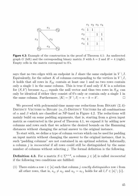
v1 v2
v3 v4
e1
e4 e3
e2
v1 v2 v3 v4
e1
e2
e3
e4
1 11 1
1 11 1
Figure 4.3: Example of the construction in the proof of Theorem 4.1: An undirectedgraph G (left) and the corresponding binary matrix S with h = 2 and H = 4 (right).Empty cells in the matrix correspond to 0’s.
says that no two edges with an endpoint in I share the same endpoint in V \ I.Equivalently, for the subset K of columns corresponding to the vertices in V \ I,it holds that all rows in S|K contain at least one 1 and no two rows containonly a single 1 in the same column. This is true if and only if K is a solutionfor (S, k′) because sm+1 equals the null vector and thus two rows in S|K canonly be identical if either they consist of 0’s only or contain only a single 1 inthe same column. Furthermore, |K| = |V \ I| = n− k = k′.
We proceed with polynomial-time many-one reductions from Binary (2, 4)-Distinct Vectors to Binary (α, β)-Distinct Vectors for all combinationsof α and β which are classified as NP-hard in Figure 4.2. The reductions willmainly build on some padding arguments, that is, starting from a given inputmatrix as constructed in the proof of Theorem 4.1, we expand it by adding newcolumns and rows such that we achieve the desired bounds on the Hammingdistances without changing the actual answer to the original instance.
To start with, we define a type of column vectors which can be used for paddingan input matrix without changing the answer to the original instance, that is,such “padding columns” are not contained in an optimal solution. Informally,a column j is inessential if all rows could still be distinguished by the samenumber of columns without selecting j. The formal definition is the following.
Definition 4.3. For a matrix S ∈ Σn×d, a column j ∈ [d] is called inessentialif the following two conditions are fulfilled:
(1) There exists a row i ∈ [n] such that column j exactly distinguishes row i fromall other rows, that is, sij 6= slj and slj = sl′j holds for all l, l′ ∈ [n] \ i.
45
(2) All rows in S|[d]\j are still distinct.
Note that for binary matrices, Condition (1) of Definition 4.3 can only befulfilled by column vectors that contain either a single 1 or a single 0, that is,the column vectors of weight 1 or n− 1. Next, we show that, for any inessentialcolumn in a given input matrix, we can assume that this column is not containedin a solution for the Distinct Vectors instance.
Lemma 4.2. Let (S ∈ Σn×d, k) be a Distinct Vectors instance withan inessential column j ∈ [d]. Then (S, k) is a yes-instance if and onlyif (S|[d]\j, k) is a yes-instance.
Proof. It is clear that the “if” part of the statement holds; let us consider the“only if” part. To this end, assume that there is a solution set K ⊆ [d] ofcolumns for (S, k) with j ∈ K. Since column j exactly distinguishes row ifrom all other rows and no other pair of rows, it follows that K ′ := K \ jis a solution for (S[[n] \ i, [d] \ j], k − 1). But then, there also exists asolution K ′′ ⊆ [d] \ j for (S[[n], [d] \ j], k). This is true because row iequals at most one other row l in S[[n],K ′] since all rows in S[[n] \ i,K ′] aredistinct. Row i can thus be distinguished from row l by a column j′ ∈ [d] \ jwith sij′ 6= slj′ , which exists because column j is inessential, and thus, bydefinition, all rows in S[[n], [d] \ j] are distinct. Hence, K ′′ := K ′ ∪ j′ is asolution for (S, k).
Note that, due to Lemma 4.2, adding inessential columns to a given inputmatrix yields an equivalent Distinct Vectors instance. Hence, for the binarycase, any construction that only adds column vectors which either contain asingle 1 or a single 0 to the input matrix yields an equivalent instance since thesecolumns are clearly inessential. This allows us to increase the minimum andmaximum pairwise row Hamming distances of a given binary matrix. Followingthis basic idea, we prove the following theorem.
Theorem 4.3. Binary (α, β)-Distinct Vectors is NP-hard for all β ≥ α+2if α is even, and for all β ≥ α+ 3 if α is odd.
Proof. In the following, we give polynomial-time many-one reductions fromBinary (2, 4)-Distinct Vectors. To this end, let (S ∈ 0, 1n×d, k) bethe Binary (2, 4)-Distinct Vectors instance as constructed in the proof ofTheorem 4.1. Recall that this matrix S contains the null row vector, say sn = 0,and all other rows have weight two, w(si) = 2 for all i ∈ [n − 1]. Moreover,
46
1 11 1
1 11 1
1 1 1
1
(a) Case 1: α = 1 and β = 7. By adding b = 3 copies of columnvector 15
1, the maximum Hamming distance is increased to 7.Adding the bottom row and the last column yields a minimumHamming distance of 1.
1 11 1
1 11 1
1 11 1
1 11 1
1111
1 1 1
(b) Case 2: α = 5 and β = 9, that is a = b = 3.
Figure 4.4: Examples of the padding construction. The submatrix framed by thicklines equals the example matrix in Figure 4.3.
there exists a pair of rows with Hamming distance four. Assume, without loss ofgenerality, that the first two rows s1 and s2 have Hamming distance ∆(s1, s2) = 4(Figure 4.3 depicts an example of such a matrix). In the following, we willconstruct an equivalent Binary (α, β)-Distinct Vectors instance (S′, k′) inpolynomial time.
Let Dj ⊆ [n] denote the set of row indices where column vector s∗j equals 1.Further, for i ∈ N and I ⊆ [i], let 1iI ∈ 0, 1i denote the size-i column vectorthat has 1-entries for all indices in I and 0-entries elsewhere.
We prove the theorem in two steps: First, the case α = 1, β = 4 + b forall b ≥ 0, and second, the case α = 2 + a, β = 4 + 2da/2e+ b for all a, b ≥ 0.Note that these two cases together yield the statement of the theorem.
47
Case 1 (α = 1, β = 4 + b, b ≥ 0). We define the instance (S′, k′) as follows:The column vectors of the matrix S′ ∈ 0, 1(n+1)×(d+b+1) are
s′∗j :=
1n+1Dj
, j ∈ 1, . . . , d,1n+11 , j ∈ d+ 1, . . . , d+ b,
1n+1n+1, j = d+ b+ 1.
We set k′ := k + 1. An example of the constructed instance is shown inFigure 4.4a. It is not hard to check that the rows of S′ indeed fulfill theconstraints on the Hamming distances:
h′ := mini 6=j∈[n+1]
∆(si, sj) = ∆(s′n, s′n+1) = 1 and
H ′ := maxi 6=j∈[n+1]
∆(si, sj) = ∆(s′1, s′2) = ∆(s1, s2) + b = 4 + b.
As regards correctness, observe first that every solution contains the columnindex d+ b+ 1 because the row vectors s′n and s′n+1 only differ in this column.Since this column also distinguishes row sn+1 from all other rows and no otherpair of rows in S′, it follows that (S′, k′) is a yes-instance if and only if (S′|[d+b], k)
is a yes-instance. Due to Lemma 4.2, this is the case if and only if (S, k) is ayes-instance.Case 2 (α = 2 + a, β = 4 + 2da/2e + b, a, b ≥ 0). We define the instance
(S′, k′) as follows: Starting with S′ := S, we add da/2e copies of the columnvector 1ni for each i ∈ [n − 1] to S′. Moreover, we add ba/2c copies of thecolumn vector 1n[n−1] to S
′. Finally, we add b copies of the column vector 1n1to S′ and set k′ = k. Figure 4.4b shows an example of the construction. Indeed,we have the following Hamming distances:
∆(s′n, s′1) = 2 + a+ b,
∆(s′n, s′j) = 2 + a,
∆(s′1, s′j) = ∆(s1, sj) + 2da/2e+ b,
∆(s′j , s′j′) = ∆(sj , sj′) + 2da/2e,
for all j, j′ ∈ 2, . . . , n− 1, j 6= j′. Thus, it holds h′ = ∆(s′n, s′2) = 2 + a and
H ′ = ∆(s′1, s′2) = 4 + 2da/2e + b. Since all row vectors in S are distinct and
since we only added columns which distinguish exactly one row from all others,the correctness follows due to Lemma 4.2.
48
Theorem 4.3 implies that for a given instance with fixed minimum pairwiserow Hamming distance α, it is possible to increase the maximum pairwise rowHamming distance β arbitrarily without changing the answer to the instance.On the contrary, however, it is not clear how to construct an equivalent instancewhere only the minimum pairwise row Hamming distance is increased. Indeed, inthe following, we show polynomial-time solvability for the case α ≥ 2bβ/2c − 1.
4.2.2 Polynomial-Time Solvability for Homogeneous DataThe polynomial-time solvability for homogeneous data is based on the observa-tion that, for small differences between maximum and minimum pairwise rowHamming distance, the input matrix is either highly structured or boundedin size by a constant depending only on the maximum pairwise row Hammingdistance. This structure in turn guarantees that the instance is easily solvable.Before proving the theorem, we start with some helpful preliminary results.
First, we show that there is a linear-time preprocessing of a given input matrixsuch that the resulting matrix contains the null vector as a row and no twocolumn vectors are identical.
Lemma 4.4. For a given Distinct Vectors instance I = (S ∈ 0, 1n×d, k)one can compute in O(nd) time an equivalent Distinct Vectors instanceI ′ := (S′ ∈ 0, 1n×d′ , k) such that S′ contains the null vector 0 ∈ 0d′ as arow, the number d′ of columns of S′ is at most d, and no two column vectorsof S′ are identical (implying d′ ≤ 2n).
Proof. From an instance I = (S, k), we compute S′ as follows: First, in orderto have the null vector 0 as a row, we consider an arbitrary row vector, say s1,and iterate over all columns j. If s1j = 1, then we exchange all 1’s and 0’sin column j. Then, we sort the columns of S lexicographically in O(nd) time(using radix sort). We iterate over all columns again and check for any twosuccessive column vectors whether they are identical and, if so, remove oneof them. This ensures that all remaining column vectors are different, whichimplies that there are at most 2n. Thus, in O(nd) time, we end up with amatrix S′ containing at most 2n columns, where s′1 = 0. Clearly, reorderingcolumns, removing identical columns, as well as exchanging 1’s and 0’s in acolumn does not change the answer to the original instance.
We henceforth assume all input instances to be already preprocessed accordingto Lemma 4.4. In fact, we can extend Lemma 4.4 by removing also inessential
49
columns (recall Definition 4.3), that is, we can use the following data reductionrule.
Reduction Rule 4.1. Let (S, k) be a Distinct Vectors instance. If Scontains an inessential column, then delete this column from S.
Lemma 4.5. Reduction Rule 4.1 is correct and can exhaustively be appliedin O(minn, d · nd) time.
Proof. Correctness follows from Lemma 4.2. Exhaustive application of Reduc-tion Rule 4.1 can be done as follows: First, we determine in O(nd) time whichcolumns fulfill Condition (1) of Definition 4.3. Recall that these are exactly theweight-1 and weight-(n− 1) columns of which there can be at most min2n, dafter the preprocessing according to Lemma 4.4. For each of these candidatecolumns j, we check in O(nd) time whether Condition (2) also holds, that is,whether all row vectors are still distinct without column j, by lexicographicallysorting the rows of the matrix without column j. The overall running time isthus in O(minn, d · nd).
We now turn towards proving polynomial-time solvability of Binary (α, β)-Distinct Vectors for α ≥ 2bβ/2c − 1. The proof uses some results fromextremal combinatorics concerning certain set systems. To start with, weintroduce the necessary concepts and notation. Recall Definition 4.1, where wedefined the set Wsi of column indices where row i equals 1. In the following,for a given input matrix S and a given set of row indices I, we will considerthe column system of I, that is, the system containing the sets Wsi of columnindices of all row vectors with indices in I.
Definition 4.4. For a matrix S ∈ 0, 1n×d and a subset I ⊆ [n] of row indices,letW(I) := Wsi | i ∈ I denote the column system of I containing the sets Wsi
of column indices for all rows in I. For ω ∈ [d], let Iω := i ∈ [n] | w(si) = ωbe the set of indices of the weight-ω rows and let Wω :=W(Iω) be the columnsystem of the weight-ω rows.
Figure 4.5 illustrates Definition 4.4. Note that in order to distinguish allrows of weight ω from each other, we only have to consider those columnswhich appear in some of the sets contained in the column system Wω since theweight-ω rows only differ in these columns. Thus, in order to find subsolutionsfor the weight-ω rows, the structure of Wω, especially the pairwise intersectionsof the contained sets, will be very important for us. Therefore, we make use of
50
1 2 3 4 5 6 7
11 1
11
1
1
1
1
1 1
W1 = 3
W2 = 1, 5, 6, 7
W3 = 1, 4, 7, 2, 4, 5
Figure 4.5: An example of a binary matrix (left) containing rows of weight one, two,and three. The corresponding column systems are written on the right.
two general combinatorial concepts of set systems (see [Juk11, Chapter 6] forexample), the first of which defines a system of sets that pairwise intersect inthe same number of elements, whereas the second concept describes the evenstronger condition that all pairwise intersections contain the same elements.
Definition 4.5 (Weak ∆-system). A family F = S1, . . . , Sm of m differentsets is called a weak ∆-system if there is some λ ∈ N such that |Si ∩ Sj | = λ forall i 6= j ∈ [m].
Definition 4.6 (Strong ∆-system). A strong ∆-system (or sunflower) is aweak ∆-system S1, . . . , Sm such that Si ∩Sj = C for all i 6= j ∈ [m] and someset C called the core. The sets Si := Si \ C are called petals.
The following lemma illustrates the merit of the above definitions showingthat any Distinct Vectors instance can easily be solved if the underlyingcolumn system of all non-zero-weight rows forms a sunflower.
Lemma 4.6. Let I := (S ∈ 0, 1n×d, k) be a Distinct Vectors instancesuch that W :=
⋃ω≥1Wω forms a sunflower (note that W0 = ∅ 6∈ W). Then, I
is a yes-instance if and only if k ≥ |W|. Moreover, any solution intersects atleast |W| − 1 of the petals of W.
Proof. Recall that we assume the instance I to be already preprocessed ac-cording to Lemma 4.4. Hence, we can assume without loss of generality thatsn = 0 and that no two column vectors of S are equal. Assume furtherthat W = Ws1 , . . . ,Wsn−1
is a sunflower with core C. An example is depictedin Figure 4.6.
Recall that any solution K fulfills K ∩Dij 6= ∅ for all i 6= j ∈ [n], where Dij
is the set of column indices in which the row vectors si and sj differ. Assume
51

1 2 3 4 5 6 7 8 9 10
1 11 11 11 11 11 1
1
11
1 11
1
11 2
49
7
310
68
5
Figure 4.6: Example of a matrix where the set system W forms a sunflower withcore C = 1, 2 consisting of the first two columns. The six petals from top to bottomare 4, 9, 7, 3, 10, 6, 8, 5 and ∅ (a schematic drawing of W is on the right).Framed by thick lines is a set of columns that distinguish all rows.
towards a contradiction that K ⊆ [d] with |K| < n−1 is a solution. If K∩C = ∅,then K only intersects the petals. Since the petals are pairwise disjoint, itfollows that there exists an i ∈ [n− 1] such that K ∩Wi = K ∩Din = ∅, whichshows that K cannot be solution. If K ∩C 6= ∅, then K intersects at most n− 3of the n − 1 petals in W. Hence, there exist i, j ∈ [n − 1] with i 6= j suchthat K ∩ (Wi ∪ Wj) = K ∩Dij = ∅. Hence, K cannot be a solution. It remainsto show that there is always a solution of size |W| = n− 1. To this end, let Kcontain an arbitrary element from each non-empty petal and, if there is anempty petal, also an arbitrary element from the core C. Clearly, K is a solutionof size n− 1.
According to Lemma 4.6, identifying sunflower structures in a given inputinstance significantly simplifies our problem since they have easy solutions. Tothis end, the following result by Deza [Dez74] will serve as an important toolsince it describes conditions under which a weak ∆-system actually becomes astrong one, that is, a sunflower (see also Jukna [Juk11, Chapter 6, Theorem 6.2]).
Lemma 4.7 (Deza [Dez74, Theorem 2]). Let F be an s-uniform weak ∆-system,that is, each set contains s elements. If |F| ≥ s2 − s+ 2, then F is a sunflower.
The basic scheme for proving polynomial-time solvability of Binary (α, β)-Distinct Vectors for α ≥ 2bβ/2c − 1 is the following: The bounds on the
52
minimum and maximum pairwise row Hamming distances imply that the columnsystemsWx for x = α, . . . , β form x-uniform weak ∆-systems. Using Lemma 4.7,we then conclude that either the size of the instance is upper-bounded by aconstant depending on β only, or that the Wx form sunflowers, which we canhandle according to Lemma 4.6.As a final prerequisite, we prove the following useful lemma concerning the
intersections of a set with sets in a sunflower.
Lemma 4.8. Let λ ∈ N, let F be a sunflower with core C and let X be a setsuch that |X ∩ S| ≥ λ for all S ∈ F . If |F| > |X|, then |X ∩ C| ≥ λ (implyingλ ≤ |C|).
Proof. Assume towards a contradiction that |X ∩ C| < λ. Then X wouldintersect each of the |F| > |X| pairwise disjoint petals of F , which is notpossible.
We are now ready to prove the following theorem.
Theorem 4.9. Binary (α, β)-Distinct Vectors is solvable
1.) in O(minn, d · nd) time if β ≤ α+ 1, and
2.) in O(n3d) time if α is odd and β = α+ 2.
We prove both statements of Theorem 4.9 separately. As mentioned, thebasic structures of both proofs are similar: We first partition the column systeminto uniform weak ∆-systems. Then, we consider for each system the casesof being a sunflower or being of bounded size (due to Lemma 4.7). Then, wemake use of the preprocessing (Lemma 4.4 and Reduction Rule 4.1) and ourknowledge about solutions for sunflowers (Lemma 4.6) to show that only a smallnumber of candidate solutions are to be considered. That is, the instances areessentially solved by the preprocessing routines and we can try out all remainingcandidates to find a solution in polynomial time. Showing that there are onlyfew remaining candidate solutions seems to be more difficult for Statement (2.);thus, the proof of Statement (1.) can be seen as a “warm-up”.
Proof (Theorem 4.9, Statement (1.)) In the following, let I = (S ∈ 0, 1n×d, k)be an instance of Binary (α, β)-Distinct Vectors for α ≤ β ≤ α+ 1. Recallthat we assume I to be already preprocessed according to Lemma 4.4 and Reduc-tion Rule 4.1 in O(minn, d · nd) time, that is, S contains the null row vector,say sn = 0, no two column vectors are equal, which implies d ≤ 2n, and there
53
are no inessential columns. We write Wi := Wsi = j ∈ [d] | sij = 1 for the setof column indices j where row vector si equals 1, and we define Wij := Wi ∩Wj .For ω ∈ [d], let Iω := i ∈ [n] | w(si) = ω denote the set of indices of theweight-ω rows and let nω := |Iω|. For ease of presentation, we sometimes identifycolumns or rows and their corresponding indices.
For all i ∈ [n− 1], we have
∆(si, sn) = ∆(si,0) = w(si) ∈ α, α+ 1.
Since also∆(si, sj) = w(si) + w(sj)− 2|Wij | ∈ α, α+ 1
holds for all i 6= j ∈ [n− 1], the following properties can be derived:
∀i, j ∈ Iα, i 6= j : |Wij | = bα/2c, (4.1)∀i, j ∈ Iα+1, i 6= j : |Wij | = d(α+ 1)/2e, and (4.2)∀i ∈ Iα, j ∈ Iα+1 : |Wij | = b(α+ 1)/2c. (4.3)
For example, let us prove Property (4.1). For i, j ∈ Iα, we have ∆(si, sj) =2α−2|Wij | ∈ α, α+1. Since |Wij | is an integer, 2α−2|Wij | is even. Therefore,if α is even, then 2α− 2|Wij | = α implying |Wij | = α/2 = bα/2c. If α is odd,then 2α− 2|Wij | = α+ 1 and, hence, |Wij | = (α− 1)/2 = bα/2c. This provesProperty (4.1). The proofs for the remaining properties are analogous.
Now, Property (4.1) implies thatWα := Wi | i ∈ Iα is an α-uniform weak ∆-system (every pair of sets intersects in bα/2c elements) and Property (4.2) impliesthat Wα+1 := Wi | i ∈ Iα+1 is an (α+ 1)-uniform weak ∆-system (every pairof sets intersects in d(α+ 1)/2e elements). We define the constant
c := (α+ 1)2 − (α+ 1) + 2
according to the bound in Lemma 4.7. We can assume that maxnα, nα+1 ≥ cbecause otherwise n = nα +nα+1 + 1 ≤ 2c is upper-bounded by a constant, andthus also d ≤ 2n is upper-bounded by a constant (recall that we assume S tobe preprocessed according to Lemma 4.4), which implies that the instance I isconstant-time solvable.If nα+1 ≥ c, then, by Lemma 4.7, it follows that Wα+1 is a sunflower with
a core C of size d(α + 1)/2e and petals Wi, i ∈ Iα+1, of size α + 1 − |C| ≥ 1.For each i ∈ Iα+1 and each j ∈ Iα, Property (4.3) together with nα+1 ≥ c > αimply (due to Lemma 4.8) that |Wj ∩ C| = |Wij |. Thus, we have Wij ⊆ C
54
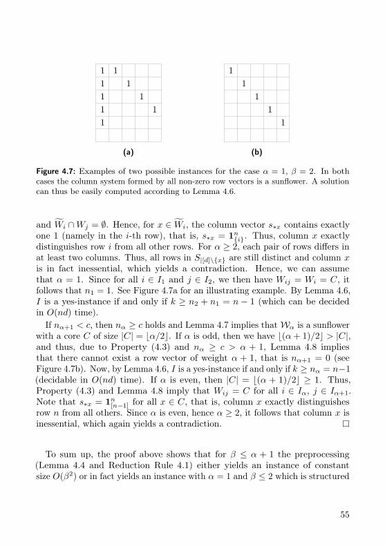
11111
11
11
(a)
11
11
1
(b)
Figure 4.7: Examples of two possible instances for the case α = 1, β = 2. In bothcases the column system formed by all non-zero row vectors is a sunflower. A solutioncan thus be easily computed according to Lemma 4.6.
and Wi ∩Wj = ∅. Hence, for x ∈ Wi, the column vector s∗x contains exactlyone 1 (namely in the i-th row), that is, s∗x = 1ni. Thus, column x exactlydistinguishes row i from all other rows. For α ≥ 2, each pair of rows differs inat least two columns. Thus, all rows in S|[d]\x are still distinct and column xis in fact inessential, which yields a contradiction. Hence, we can assumethat α = 1. Since for all i ∈ I1 and j ∈ I2, we then have Wij = Wi = C, itfollows that n1 = 1. See Figure 4.7a for an illustrating example. By Lemma 4.6,I is a yes-instance if and only if k ≥ n2 + n1 = n − 1 (which can be decidedin O(nd) time).
If nα+1 < c, then nα ≥ c holds and Lemma 4.7 implies that Wα is a sunflowerwith a core C of size |C| = bα/2c. If α is odd, then we have b(α+ 1)/2c > |C|,and thus, due to Property (4.3) and nα ≥ c > α + 1, Lemma 4.8 impliesthat there cannot exist a row vector of weight α + 1, that is nα+1 = 0 (seeFigure 4.7b). Now, by Lemma 4.6, I is a yes-instance if and only if k ≥ nα = n−1(decidable in O(nd) time). If α is even, then |C| = b(α + 1)/2c ≥ 1. Thus,Property (4.3) and Lemma 4.8 imply that Wij = C for all i ∈ Iα, j ∈ Iα+1.Note that s∗x = 1n[n−1] for all x ∈ C, that is, column x exactly distinguishesrow n from all others. Since α is even, hence α ≥ 2, it follows that column x isinessential, which again yields a contradiction.
To sum up, the proof above shows that for β ≤ α + 1 the preprocessing(Lemma 4.4 and Reduction Rule 4.1) either yields an instance of constantsize O(β2) or in fact yields an instance with α = 1 and β ≤ 2 which is structured
55
in such a way that it is easily solvable. Hence, the overall running time for thiscase is determined by the polynomial running time of the preprocessing.Next, we show that Binary (α, α + 2)-Distinct Vectors is solvable
in O(n3d) time if α is odd. We use the same notation as in the proof ofStatement (1.) (also many arguments are completely analogous). Again, weassume the input instance I = (S, k) to be already preprocessed according toLemma 4.4 and Reduction Rule 4.1.
Proof (Theorem 4.9, Statement (2.)) Since
∆(si, sj) = w(si) + w(sj)− 2|Wij | ∈ α, α+ 1, α+ 2
holds for all i 6= j ∈ [n], it follows that
∆(si, sn) = w(si) ∈ α, α+ 1, α+ 2
holds for all i ∈ [n− 1]. By plugging in the respective values for w(si) and w(sj)in the above formula for ∆(si, sj), the following properties can be derived (inan analogous way as for Properties (4.1) to (4.3) in the proof of Statement (1)):
∀i, j ∈ Iα, i 6= j : |Wij | = bα/2c, (4.4)∀i ∈ Iα, j ∈ Iα+1 : |Wij | ∈ bα/2c, dα/2e, (4.5)∀i ∈ Iα, j ∈ Iα+2 : |Wij | = dα/2e, (4.6)∀i, j ∈ Iα+1, i 6= j : |Wij | = dα/2e, (4.7)∀i ∈ Iα+1, j ∈ Iα+2 : |Wij | ∈ dα/2e, dα/2e+ 1, (4.8)∀i, j ∈ Iα+2, i 6= j : |Wij | = dα/2e+ 1. (4.9)
Properties (4.4), (4.7), and (4.9) imply that Wα, Wα+1, and Wα+2 are α-,(α+ 1)-, and (α+ 2)-uniform weak ∆-systems, respectively.
In the following, we denote by Uω :=⋃i∈Iω Wi the index set of the columns
where at least one weight-ω row vector equals 1. Let c := (α+ 2)2 − (α+ 2) + 2.For each x ∈ α, α+ 1, α+ 2, we either have nx < c or nx ≥ c. Overall, thisgives eight possible cases, each of which we now show how to solve:Case 1 (nα < c, nα+1 < c, nα+2 < c). In this case, the number of rows
in S is upper-bounded by a constant depending on α, and thus, I is of overallconstant size.Case 2 (nα ≥ c, nα+1 < c, nα+2 < c). Due to Lemma 4.7, the system Wα
forms a sunflower. Let C with |C| = bα/2c be the core of Wα. For α =
56
1, clearly, any solution K contains all column indices from U1 in order todistinguish the weight-1 rows from the null vector. Since |U2 ∪ U3| ≤ 2n2 + 3n3
is upper-bounded by a constant, the number of possible subsets K ′ ⊆ U2 ∪ U3
is also upper-bounded by a constant. Thus, we only have to check a constantnumber of sets K = U1 ∪ K ′. For α ≥ 3, the size of a petal Wi, i ∈ Iα,is |Wi| = |Wi| − |C| = α − bα/2c = dα/2e ≥ 2. Since the petals are pairwisedisjoint, it follows that, for each petal Wi, there exists a j ∈ Iα+1 ∪ Iα+2 suchthat Wi ∩Wj 6= ∅. Otherwise, the column vectors corresponding to the indicesin petal Wi are all equal to 1ni, that is, at least one of them is inessential,which is a contradiction. Since |Uα+1 ∪ Uα+2| is upper-bounded by a constant(depending on α), also the number nα of petals in Wα is upper-bounded by aconstant, which yields an overall constant size of I.
Case 3 (nα < c, nα+1 ≥ c, nα+2 < c). By Lemma 4.7, Wα+1 forms asunflower with a core C of size |C| = dα/2e. The size of each petal Wi, i ∈ Iα+1,is thus |Wi| = dα/2e. Hence, for α ≥ 3, analogous arguments as in Case 2hold. For α = 1, any solution K can be written as K = C ′ ∪ U1 ∪K2 ∪K3,where C ′ ⊆ C, K2 ⊆ U2 \ C and K3 ⊆ U3. Note that |C| and |U3| are upper-bounded by a constant. Hence, the number of different subsets C ′ and K3 isalso a constant. Since |Wi| = 1 holds for all i ∈ I2, we have |U2 \ C| = n2.From Lemma 4.6, it follows that |K2| ≥ n2 − 1 holds in order to distinguish allweight-2 row vectors and the null vector from each other. Therefore, the overallnumber of possible choices for K2, and thus for K, is in O(n).
Case 4 (nα < c, nα+1 < c, nα+2 ≥ c). By Lemma 4.7, Wα+2 forms asunflower with a core C of size |C| = dα/2e + 1. The size of each petal Wi,i ∈ Iα+2, is thus |Wi| = dα/2e. Hence, for α ≥ 3, analogous arguments as inCase 2 hold. For α = 1, any solution K can be written as K = C ′∪U1∪K2∪K3,where C ′ ⊆ C, K2 ⊆ U2 and K3 ⊆ U3 \ C. Note that |C| and |U2| are upper-bounded by a constant. Hence, the number of different subsets C ′ and K2 isalso a constant. Lemma 4.6 implies that |K3| ≥ n3 − 1. Since |U3 \ C| = n3,this yields an overall number of O(n) possible choices for K.
Case 5 (nα ≥ c, nα+1 ≥ c, nα+2 < c). Due to Lemma 4.7, Wα forms asunflower with a core C of size |C| = bα/2c and Wα+1 forms a sunflower withcore C ′ of size |C ′| = dα/2e. First, note that Property (4.6) implies |Wij | =dα/2e > |C| for all i ∈ Iα, j ∈ Iα+2, which is not possible due to Lemma 4.8.Thus, it follows that nα+2 = 0. Moreover, since Property (4.5) implies |Wij | ≥|C| for all i ∈ Iα and j ∈ Iα+1, Lemma 4.8 yields C ⊆ Wij , and thus C ⊂ C ′.
57
Hence, all column vectors in C equal 1n[n−1], which yields a contradictionfor α ≥ 3 because C then contains an inessential column. For α = 1, anysolution K can be written as K = C ′′ ∪ U1 ∪K2, where C ′′ ⊆ C ′ and K2 ⊆ U2.By Lemma 4.6, we know that |K2| ≥ n2 − 1. Since |C ′| = 1 and |U2 \ C ′| = n2,there are O(n) possible choices for K.Case 6 (nα ≥ c, nα+1 < c, nα+2 ≥ c). This case is not possible since we
showed in Case 5 that nα ≥ c implies nα+2 = 0.Case 7 (nα ≥ c, nα+1 ≥ c, nα+2 ≥ c). This case is again not possible.Case 8 (nα < c, nα+1 ≥ c, nα+2 ≥ c). From Lemma 4.7 it follows that Wα+1
forms a sunflower with a core C of size |C| = dα/2e andWα+2 forms a sunflowerwith core C ′ of size |C ′| = dα/2e + 1. Moreover, analogously to Case 5,Property (4.8) and Lemma 4.8 imply C ⊂ C ′.If α = 1, then any solution can be written as K = U1 ∪ C ′′ ∪ K2 ∪ K3,
where C ′′ ⊆ C ′, K2 ⊆ U2 \ C and K3 ⊆ U3 \ C ′. Since |C ′| = dα/2e + 1,|U2\C| = n2, |U3\C ′| = n3, and, by Lemma 4.6, |K2| ≥ n2−1 and |K3| ≥ n3−1,it follows that there are O(n2) possible choices for K.
For α ≥ 3, we show that the matrix S—recall that it is reduced with respectto Reduction Rule 4.1—has a specific structure, depicted in Figure 4.8. Namely,we claim that(a) if Wij \ C ′ 6= ∅ for i 6= j ∈ [n− 1], then i ∈ Iα+1 and j ∈ Iα ∪ Iα+2, and(b) the one column vector s∗z with z ∈ C \ C ′ equals 1nIα∪Iα+2
.Claim (a) implies that each column in [d]\C ′ contains at most two 1’s (naturally,any column contains at least one 1). We will see that in fact all columns in [d]\C ′contain exactly two 1’s and therefore define the edges of a bipartite graph withvertex sets Iα+1 and Iα ∪ Iα+2. We find a matching that saturates Iα+1 in thisbipartite graph and show that the columns corresponding to the matching edgesalong with column z are an optimal solution.
To show Claim (a), observe that, if i 6= j ∈ Iα+2, then Wij \ C ′ = ∅ as Wα+2
is a sunflower with core C ′. Likewise, if i 6= j ∈ Iα+1, then Wij \ C ′ = ∅because Wα+1 is a sunflower with core C and C ⊂ C ′. It hence suffices toshow that Wij \ C ′ = ∅ in the case that either both i, j ∈ Iα or i ∈ Iαand j ∈ Iα+2. To see the latter, note that Property (4.6) and Lemma 4.8imply |Wi ∩ C ′| = dα/2e = |C ′| − 1, for all i ∈ Iα, that is, we have Wij ⊂ C ′
for all i ∈ Iα, j ∈ Iα+2. Now, it only remains to show Wij ⊆ C ′ for i, j ∈ Iα,i 6= j. We derived above that
|Wi ∩ C ′| = |Wj ∩ C ′| = dα/2e = |C ′| − 1.
58
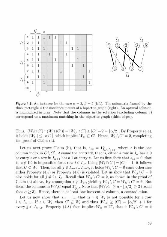
1
2
3
4
5
6
7
8
9
10
1111111
1
11111111
111
11
1 11 1
1 11 1
1 11 1
1 11
1
C ′
C z
I5
I4
I3
1 2 3
I5
8 9
I3
4 5 6 7
I4
Figure 4.8: An instance for the case α = 3, β = 5 (left). The submatrix framed by thethick rectangle is the incidence matrix of a bipartite graph (right). An optimal solutionis highlighted in gray. Note that the columns in the solution (excluding column z)correspond to a maximum matching in the bipartite graph (thick edges).
Thus, |(Wi∩C ′)∩(Wj ∩C ′)| = |Wij ∩C ′| ≥ |C ′|−2 = α/2. By Property (4.4),it holds |Wij | ≤ α/2, which implies Wij ⊆ C ′. Hence, Wij \C ′ = ∅, completingthe proof of Claim (a).
Let us next prove Claim (b), that is, s∗z = 1nIα∪Iα+2
, where z is the onecolumn index in C \C ′. Assume the contrary, that is, either a row in Iα has a 0at entry z or a row in Iα+1 has a 1 at entry z. Let us first show that siz = 0, thatis, z ∈ Wi is impossible for a row i ∈ Iα. Using |Wi ∩ C ′| = |C ′| − 1, it followsthat C ⊂ Wi. Then, for all j ∈ Iα+1∪ Iα+2, it holds Wij \C = ∅ since otherwiseeither Property (4.5) or Property (4.6) is violated. Let us show that Wij \C = ∅also holds for all j = i ∈ Iα. Recall that Wij \ C ′ = ∅, as shown in the proof ofClaim (a) above. By assumption z ∈ Wij , yielding Wij \C = Wij \C ′ = ∅. Butthen, the columns in Wi\C equal 1n
i. Note that |Wi\C| ≥ α−α/2 ≥ 2 (recallthat α ≥ 3). Hence, there is at least one inessential column, a contradiction.Let us now show that siz = 1, that is z ∈ Wi is not possible for a row
i ∈ Iα+1. If z ∈ Wi, then C ′ ⊆ Wi and thus |Wij | ≥ |C ′| = α/2 + 1 forevery j ∈ Iα+2. Property (4.8) then implies Wij = C ′, that is Wij \ C ′ = ∅
59
for every j ∈ Iα+2. Moreover, consider a row j ∈ Iα and note that |Wij ∩C ′| = 1 + |Wj ∩ C| since z ∈ Wj as shown before. By Property (4.5) andLemma 4.8, we have |Wj ∩ C| ≥ bα/2c, which yields |Wij ∩ C ′| ≥ dα/2e. Now,Property (4.5) implies |Wij ∩C ′| = dα/2e = |Wij |, which implies Wij ⊆ C ′, thatis Wij ∩ C ′ = ∅. But then, the columns in Wi \ C ′ are equal to 1ni and thereare at least |Wi \C ′| = α+ 1−dα/2e− 1 = bα/2c ≥ 1 such inessential columns,which yields a contradiction. Hence, for z ∈ C ′ \ C, it holds s∗z = 1nIα∪Iα+2
,proving Claim (b). Note that column z distinguishes all rows in Iα+1 from allrows in Iα ∪ Iα+2.
To finish the proof of Case 8, we need one more observation about the numberof weight-α rows, namely that nα = |C| = dα/2e. Since |Wi∩C ′| = |C ′|−1 = |C|and z ∈Wi holds for all i ∈ Iα, and since also z = C ′ \C, we have |Wi ∩C| =|C| − 1. If nα < |C|, then there exists a column x ∈ C such that x ∈ Wi
for every i ∈ Iα. But then, s∗x = 1n[n−1] is inessential, which is not possible.If nα > |C|, then there exists a pair i 6= j ∈ Iα such that Wi ∩ C = Wj ∩ C.This implies |Wij | ≥ |C| − 1 + 1 = dα/2e, which contradicts Property (4.4).
We now derive a solution from the abovementioned bipartite graph. Considerthe columns in [d] \ C ′. Clearly, if one of these columns contains only one 1,then this column is inessential, which yields a contradiction. Thus, each columncontains at least two 1’s. Using Claim (a), each of the columns also has atmost two 1’s. Also, after preprocessing, no two columns are equal. Thus,the submatrix S[[n − 1], [d] \ C ′] (framed by thick lines in Figure 4.8) is theincidence matrix of a bipartite graph G, where the rows correspond to thevertices (partitioned into Iα+1 and Iα ∪ Iα+2) and the columns define the edges.Moreover, each vertex i ∈ Iα+2 has degree |Wi \ C ′| = dα/2e. Also eachvertex i ∈ Iα+1 has degree |Wi \ C ′| = |Wi \ C| = dα/2e by Claim (b). Eachrow i ∈ Iα has |Wi ∩ C ′| = dα/2e (as shown in the proof of Claim (a)), and,therefore, vertex i has degree |Wi \ C ′| = bα/2c in G. We can now use Hall’stheorem [BG09]2, to show that there exists a matching in G that saturates Iα+1,that is, a subset M ⊆ [d] \ C ′ of nα+1 columns such that |Wi ∩M | = 1 forall i ∈ Iα+1 and |Wi ∩ M | ≤ 1 for all i ∈ Iα ∪ Iα+2. Indeed, taking anysubset T ⊆ Iα+1 of vertices, consider the set NG(T ) ⊆ Iα ∪ Iα+2 of neighborsof T . Since the vertices in NG(T ) have at most the degree of any vertex in T , wehave |NG(T )| ≥ |T |. Hence, the condition of Hall’s theorem is satisfied. Thus,matching M exists as claimed.
2Hall’s theorem states that, for a bipartite graph G = (X ·∪Y,E), there exists an X-saturatingmatching if and only if |T | ≤ |NG(T )| holds for each subset T ⊆ X.
60
We now claim that K := M ∪ z with |K| = nα+1 + 1 is an optimal solution(highlighted in gray in Figure 4.8). First, we show that all rows in S|K arepairwise distinct. Column z distinguishes each row in Iα ∪ Iα+2 from eachrow in Iα+1 ∪ n. Since M saturates Iα+1, all rows in Iα+1 are distinct fromrow n. It remains to show that all pairs of rows in Iα ∪ Iα+2 are distinct. Recallthat Wij \ C ′ = ∅ for all i 6= j ∈ Iα ∪ Iα+2 (by Claim (a)). Thus, every rowi ∈ Iα ∪ Iα+2 with Wi ∩M 6= ∅ is distinct from all other rows in Iα ∪ Iα+2.Hence, since M is a matching, if |M | ≥ nα + nα+2 − 1, then all pairs of rowsin Iα ∪ Iα+2 are distinct. Since G is bipartite, we have
nα+2dα/2e+ nαbα/2c = nα+1dα/2e.
Thus, using nα = dα/2e (as observed above), we have
|M | = nα+1 = nα+2 + bα/2c = nα + nα+2 − 1.
Consequently, all rows in S|K are distinct.Regarding optimality, it remains to show that there is no solution of size nα+1.
This can be seen as follows: Lemma 4.6 implies that any solution K intersectsat least nα+1 − 1 of the petals of Wα+1. If K intersects all nα+1 petals, then,as nα+1 = nα+nα+2−1, there exists a j ∈ Iα∪Iα+2 such thatK∩Wj = ∅, whichis not possible. Otherwise, if K intersects exactly nα+1 − 1 of the petals, thenthere exists an i ∈ Iα+1 and also j 6= j′ ∈ Iα∪ Iα+2 such that K ∩ (Wi \C ′) = ∅,K ∩ (Wj \ C ′) = ∅ and K ∩ (Wj′ \ C ′) = ∅. But it is not possible to pairwisedistinguish all three rows i, j, and j′ from each other with just one column.Hence, any optimal solution contains at least nα+1 + 1 columns and, therefore,I is a yes-instance if and only if k ≥ nα+1 + 1. This finishes Case 8.
As regards the running time, observe that the maximum number of candidatesolutions we have to test in any of the above cases is in O(n2). Checkingwhether a subset of column indices is a solution can be done in O(nd) time vialexicographical sorting of the rows. This yields an overall running time in O(n3d)which also subsumes the O(minn, d · nd) time for the preprocessing.
As a final remark, we mention that polynomial-time solvability actually holdsfor all instances that satisfy the conditions of Theorem 4.9 after the preprocessing(Lemma 4.4 and Reduction Rule 4.1). This yields an even stronger result since inpractice also instances with a larger difference between maximum and minimumpairwise row Hamming distance could be efficiently solvable.
61
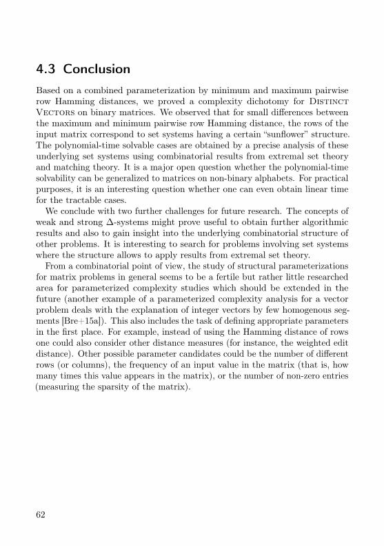
4.3 ConclusionBased on a combined parameterization by minimum and maximum pairwiserow Hamming distances, we proved a complexity dichotomy for DistinctVectors on binary matrices. We observed that for small differences betweenthe maximum and minimum pairwise row Hamming distance, the rows of theinput matrix correspond to set systems having a certain “sunflower” structure.The polynomial-time solvable cases are obtained by a precise analysis of theseunderlying set systems using combinatorial results from extremal set theoryand matching theory. It is a major open question whether the polynomial-timesolvability can be generalized to matrices on non-binary alphabets. For practicalpurposes, it is an interesting question whether one can even obtain linear timefor the tractable cases.
We conclude with two further challenges for future research. The concepts ofweak and strong ∆-systems might prove useful to obtain further algorithmicresults and also to gain insight into the underlying combinatorial structure ofother problems. It is interesting to search for problems involving set systemswhere the structure allows to apply results from extremal set theory.
From a combinatorial point of view, the study of structural parameterizationsfor matrix problems in general seems to be a fertile but rather little researchedarea for parameterized complexity studies which should be extended in thefuture (another example of a parameterized complexity analysis for a vectorproblem deals with the explanation of integer vectors by few homogenous seg-ments [Bre+15a]). This also includes the task of defining appropriate parametersin the first place. For example, instead of using the Hamming distance of rowsone could also consider other distance measures (for instance, the weighted editdistance). Other possible parameter candidates could be the number of differentrows (or columns), the frequency of an input value in the matrix (that is, howmany times this value appears in the matrix), or the number of non-zero entries(measuring the sparsity of the matrix).
62

Chapter 5
Co-Clustering
Co-clustering, that is, partitioning a numerical matrix into “homogeneous”submatrices, has many applications ranging from bioinformatics to electionanalysis. We focus on the basic variant of co-clustering where the homogeneity ofa submatrix is measured in terms of minimizing the maximum distance betweentwo entries. In contrast to Chapter 4, where we combined two parameters,we now conduct a thorough multivariate complexity analysis involving severalcombinations of parameters such as the number of clusters, the number of rows,or the number of different values in the input matrix. As in Chapter 4, we spotseveral NP-hard as well as a number of polynomial-time solvable special cases,thus charting the border of tractability for this challenging data mining problem(however, we do not obtain a complete dichotomy). Moreover, we obtain somefixed-parameter tractability results by developing a reduction to SAT solving.
5.1 Introduction
Co-clustering, also known as biclustering [MO04], performs a simultaneousclustering of the rows and columns of a data matrix (hence, the term “co-clustering”). Roughly speaking, the task is, given a numerical input matrix A,to partition the rows and columns of A into subsets minimizing a given costfunction (measuring “homogeneity”). For a given subset I of rows and a subset Jof columns, the corresponding cluster consists of all entries aij with i ∈ Iand j ∈ J . The cost function usually defines homogeneity in terms of distances(measured by some norm L) between the entries of each cluster. An illustration isgiven in Figure 5.1. Note that the variant where clusters are allowed to “overlap”,meaning that some rows and columns are contained in multiple clusters, hasalso been studied [MO04]. We focus on the non-overlapping variant which canbe stated as follows.
63

0 1 2 2 8 7 8 70 0 1 2 8 8 8 82 2 0 1 4 4 4 43 2 0 1 4 4 4 43 3 0 1 4 4 4 41 1 3 3 6 6 5 52 2 3 2 5 5 5 51 1 3 3 5 5 6 6
Figure 5.1: An example of a co-clustering of an 8× 8 matrix into k = 3 row subsetsand ` = 3 column subsets resulting in 9 clusters (submatrices). Within each clusterthe maximum difference between any two values (this corresponds to the maximumnorm L∞) is at most 1.
Co-ClusteringLInput: A matrix A ∈ Qm×n and two positive integers k, ` ∈ N.Task: Find a partition of A’s rows into k subsets and a partition of A’s
columns into ` subsets such that a given cost function (definedwith respect to some norm L) is minimized for the correspondingclustering.
Co-clustering is a fundamental method for unsupervised data analysis. Itsapplications range from microarrays and bioinformatics over recommendersystems to election analysis [ADK12, Ban+07, MO04, TSS05]. Due to itsenormous practical significance, there is a vast amount of literature discussingvarious variants; however, due to the observed NP-hardness of “almost allinteresting variants” [MO04, Section 2.2], most of the literature deals withheuristic, typically empirically validated algorithms. Indeed, there has beenvery active research on co-clustering in terms of heuristic algorithms while thereis little substantial theoretical work. Motivated by an effort towards a deepertheoretical understanding, we refine the theoretical analysis of the computationalcomplexity of a natural special case of Co-ClusteringL, namely we study thecase of L being the maximum norm L∞, where the problem comes down tominimizing the maximum distance between any two entries of a cluster. This costfunction might be a reasonable choice in practice due to its outlier robustness.Also, by focussing on Co-Clustering∞, we investigate a scenario that iscombinatorially easier to grasp. In particular, our exact and combinatorial
64
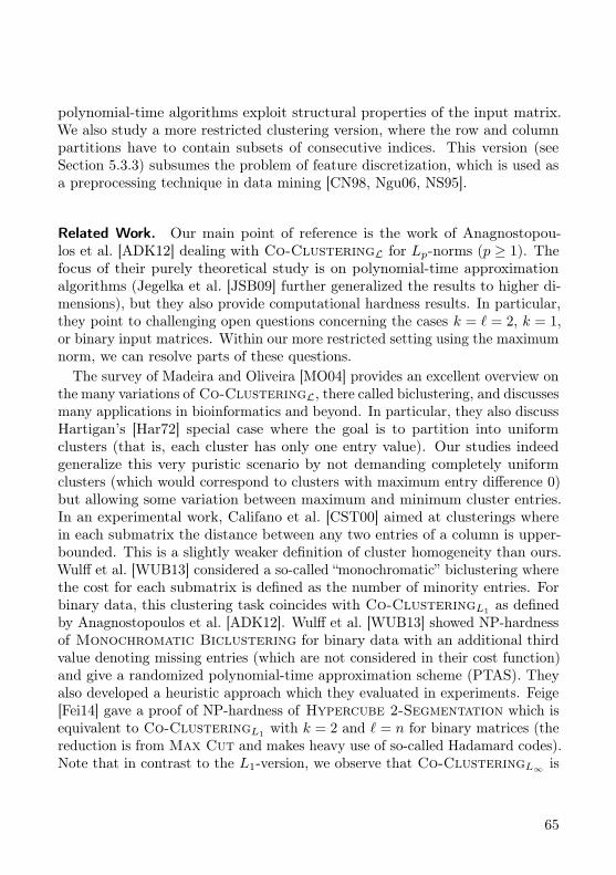
polynomial-time algorithms exploit structural properties of the input matrix.We also study a more restricted clustering version, where the row and columnpartitions have to contain subsets of consecutive indices. This version (seeSection 5.3.3) subsumes the problem of feature discretization, which is used asa preprocessing technique in data mining [CN98, Ngu06, NS95].
Related Work. Our main point of reference is the work of Anagnostopou-los et al. [ADK12] dealing with Co-ClusteringL for Lp-norms (p ≥ 1). Thefocus of their purely theoretical study is on polynomial-time approximationalgorithms (Jegelka et al. [JSB09] further generalized the results to higher di-mensions), but they also provide computational hardness results. In particular,they point to challenging open questions concerning the cases k = ` = 2, k = 1,or binary input matrices. Within our more restricted setting using the maximumnorm, we can resolve parts of these questions.
The survey of Madeira and Oliveira [MO04] provides an excellent overview onthe many variations of Co-ClusteringL, there called biclustering, and discussesmany applications in bioinformatics and beyond. In particular, they also discussHartigan’s [Har72] special case where the goal is to partition into uniformclusters (that is, each cluster has only one entry value). Our studies indeedgeneralize this very puristic scenario by not demanding completely uniformclusters (which would correspond to clusters with maximum entry difference 0)but allowing some variation between maximum and minimum cluster entries.In an experimental work, Califano et al. [CST00] aimed at clusterings wherein each submatrix the distance between any two entries of a column is upper-bounded. This is a slightly weaker definition of cluster homogeneity than ours.Wulff et al. [WUB13] considered a so-called “monochromatic” biclustering wherethe cost for each submatrix is defined as the number of minority entries. Forbinary data, this clustering task coincides with Co-ClusteringL1
as definedby Anagnostopoulos et al. [ADK12]. Wulff et al. [WUB13] showed NP-hardnessof Monochromatic Biclustering for binary data with an additional thirdvalue denoting missing entries (which are not considered in their cost function)and give a randomized polynomial-time approximation scheme (PTAS). Theyalso developed a heuristic approach which they evaluated in experiments. Feige[Fei14] gave a proof of NP-hardness of Hypercube 2-Segmentation which isequivalent to Co-ClusteringL1
with k = 2 and ` = n for binary matrices (thereduction is from Max Cut and makes heavy use of so-called Hadamard codes).Note that in contrast to the L1-version, we observe that Co-ClusteringL∞ is
65
easily solvable on binary matrices. Cheng et al. [Che+16] developed a greedyheuristic for hierarchical co-clustering based on mutual information.
Our Contributions. In terms of defining “cluster homogeneity”, we focus on min-imizing the maximum distance between two entries within a cluster (maximumnorm). Figure 5.2 summarizes our results. Our main conceptual contribution isto provide a seemingly first study on the exact complexity of a natural specialcase of Co-ClusteringL.Our main technical contributions are as follows. We prove several compu-
tational intractability results even for strongly restricted cases (that is, forconstant parameter values). Notably, we reveal non-obvious connections toother fields such as geometric covering and partitioning problems. Moreover, wedemonstrate that the NP-hardness of Co-ClusteringL∞ does not stem fromthe inherent permutation combinatorics (of rows and columns): the problemremains NP-hard when all clusters consist of consecutive rows or columns. Thisis a strong constraint (the search space size is tremendously reduced—basicallyfrom km · `n to
(mk
)·(n`
)) which directly gives a polynomial-time algorithm
if k and ` are constants. Note that in the general case we have NP-hardnessfor k = ` = 3. Concerning the algorithmic results, we develop a novel reduc-tion to SAT solving. This reduction reveals interesting connections betweenco-clustering tasks and SAT solving, which yields polynomial-time algorithmsand fixed-parameter tractability for some special cases.Section 5.2 introduces the formal problem definition and some first obser-
vations. We start with the various NP-hardness results in Section 5.3. InSection 5.4, we describe the SAT solving approach and the obtained algorithmicresults.
5.2 Problem Definition and First ObservationsWe follow the terminology of Anagnostopoulos et al. [ADK12]. For a matrix A ∈Qm×n, a (k, `)-co-clustering is a pair (I,J ) consisting of a k-partition I =I1, . . . , Ik of the row indices [m] of A (that is, Ii ⊆ [m] for all 1 ≤ i ≤ k,Ii ∩ Ij = ∅ for all 1 ≤ i < j ≤ k, and
⋃ki=1 Ii = [m]) and an `-partition J =
J1, . . . , J` of the column indices [n] of A. We call the elements of I row blocksand the elements of J column blocks. Additionally, we require I and J to notcontain empty sets. For (r, s) ∈ [k]×[`], the set Ars := aij ∈ A | (i, j) ∈ Ir×Jsis called a cluster.
66
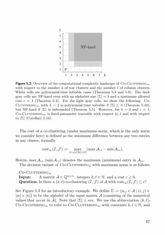
k
1
1
2
2
3
3
4
4
5
5
6
6
7
7
NP-hard
P
Figure 5.2: Overview of the computational complexity landscape of Co-Clustering∞with respect to the number k of row clusters and the number of column clusters.White cells are polynomial-time solvable cases (Theorems 5.8 and 5.9). The darkgray cells are NP-hard even with an alphabet size |Σ| = 3 and a maximum allowedcost c = 1 (Theorem 5.3). For the light gray cells, we show the following: Co-Clustering∞ with k = 2 is polynomial-time solvable if |Σ| ≤ 3 (Theorem 5.10),but NP-hard if |Σ| is unbounded (Theorem 5.5). However, for k = 2 and c = 1,Co-Clustering∞ is fixed-parameter tractable with respect to and with respectto |Σ| (Corollary 5.16).
The cost of a co-clustering (under maximum norm, which is the only normwe consider here) is defined as the maximum difference between any two entriesin any cluster, formally
cost∞(I,J ) := max(r,s)∈[k]×[]
(maxArs −minArs).
Herein, maxArs (minArs) denotes the maximum (minimum) entry in Ars.The decision variant of Co-ClusteringL with maximum norm is as follows.
Co-Clustering∞Input: A matrix A ∈ Qm×n, integers k, ∈ N, and a cost c ≥ 0.Question: Is there a (k, )-co-clustering (I,J ) of A with cost∞(I,J ) ≤ c?
See Figure 5.3 for an introductory example. We define Σ := aij ∈ A | (i, j) ∈[m]× [n] to be the alphabet of the input matrix A (consisting of the numericalvalues that occur in A). Note that |Σ| ≤ mn. We use the abbreviation (k, )-Co-Clustering∞ to refer to Co-Clustering∞ with constants k, ∈ N, and
67
0 4 3 02 2 1 31 3 4 1
A =
0 3 0 42 1 3 21 4 1 3J1 J2
I1
I2
J1 = 1, 3, 4, J2 = 2I1 = 1, I2 = 2, 3
0 0 4 31 1 3 42 3 2 1J1 J2
I1
I2
J1 = 1, 4, J2 = 2, 3I1 = 2, I2 = 1, 3
Figure 5.3: The example shows two (2, 2)-co-clusterings (middle and right) of the samematrix A (left-hand side). It demonstrates that by sorting rows and columns accordingto the co-clustering, the clusters can be illustrated as submatrices of this (permuted)input matrix. The cost of the (2, 2)-co-clustering in the middle is three and the costof the (2, 2)-co-clustering on the right-hand side is one.
by (k, ∗)-Co-Clustering∞ we refer to the case where only k is constant and ` ispart of the input. Clearly, Co-Clustering∞ is symmetric with respect to kand ` in the sense that any (k, `)-co-clustering of a matrix A is equivalent to an(`, k)-co-clustering of the transposed matrix AT . Hence, we always assume thatk ≤ `.
We next collect some simple observations. First, determining whether there isa cost-zero (perfect) co-clustering is easy. Moreover, since, for a binary alphabet,the only interesting case is a perfect co-clustering, we get the following.
Observation 5.1. Co-Clustering∞ is solvable in O(mn) time for cost zeroand also for any size-two alphabet.
Proof. Let (A, k, `, 0) be a Co-Clustering∞ input instance. For a (k, `)-co-clustering with cost 0, it holds that all entries of a cluster are equal. This is onlypossible if there are at most k different rows and at most ` different columnsin A since otherwise there will be a cluster containing two different entries.Thus, the case c = 0 can be solved by lexicographically sorting the rows andcolumns of A in O(mn) time (e.g. using radix sort).
We further observe that the input matrix can, without loss of generality, beassumed to contain only integer values (by some rescaling arguments preservingthe distance relations between elements).
68
Observation 5.2. For any Co-Clustering∞-instance with arbitrary alpha-bet Σ ⊂ Q, one can find in O(|Σ|2) time an equivalent instance with alpha-bet Σ′ ⊂ Z and cost value c′ ∈ N.
Proof. We show that for any instance with arbitrary alphabet Σ ⊂ Q andcost c ≥ 0, there exists an equivalent instance with Σ′ ⊂ Z and c′ ∈ N.Let σi be the i-th element of Σ with respect to any fixed ordering. Theidea is that the cost value c determines which elements of Σ are allowed toappear together in a cluster of a cost-c co-clustering. Namely, in any cost-cco-clustering two elements σi 6= σj can occur in the same cluster if and onlyif |σi − σj | ≤ c. These constraints can be encoded in an undirected graphGc := (Σ, E) with E := σi, σj | σi 6= σj ∈ Σ, |σi − σj | ≤ c, where eachvertex corresponds to an element of Σ, and there is an edge between two verticesif and only if the corresponding elements can occur in the same cluster of acost-c co-clustering.
Now, observe that Gc is a so-called unit interval graph, that is, each vertex σican be represented by the length-c interval [σi, σi+c] such that it holds σi, σj ∈E ⇔ [σi, σi + c] ∩ [σj , σj + c] 6= ∅ (here, we assume all intervals to contain realvalues). Hence, one can find in O(|Σ|2) time [Dur+15] an interval representationof Gc where the vertices σi are represented by length-c′ intervals [σ′i, σ
′i + c′]
of equal integer length c′ ∈ N with integer starting points σ′i ∈ Z such that0 ≤ σ′i ≤ |Σ|2, c′ ≤ |Σ|, and |σ′i − σ′j | ≤ c′ ⇔ |σi − σj | ≤ c. Hence, replacingthe elements σi by σ′i in the input matrix yields a matrix that has a cost-c′co-clustering if and only if the original input matrix has a cost-c co-clustering.Thus, for any instance with alphabet Σ and cost c, there is an equivalent instancewith alphabet Σ′ ⊆ 0, . . . , |Σ|2 and cost c′ ∈ 0, . . . , |Σ|. Consequently, wecan upper-bound the values in Σ′ by |Σ|2 ≤ (mn)2.
Due to Observation 5.2, we henceforth assume for the rest of the chapter thatthe input matrix contains integers, that is, A ∈ Zm×n.
5.3 Hardness Results
In the previous section, we observed that Co-Clustering∞ is easy to solvefor binary input matrices (Observation 5.1). In contrast to this, we show inthis section that its computational complexity significantly changes as soon asthe input matrix contains at least three different values. In fact, even for very
69
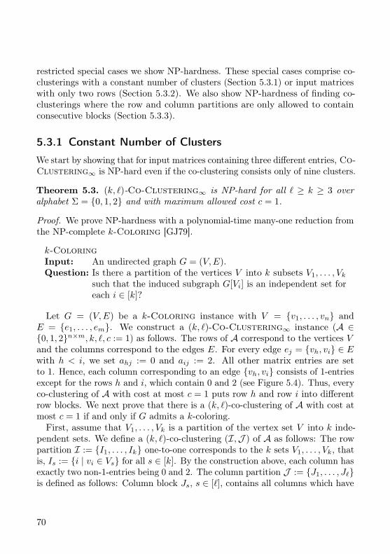
restricted special cases we show NP-hardness. These special cases comprise co-clusterings with a constant number of clusters (Section 5.3.1) or input matriceswith only two rows (Section 5.3.2). We also show NP-hardness of finding co-clusterings where the row and column partitions are only allowed to containconsecutive blocks (Section 5.3.3).
5.3.1 Constant Number of Clusters
We start by showing that for input matrices containing three different entries, Co-Clustering∞ is NP-hard even if the co-clustering consists only of nine clusters.
Theorem 5.3. (k, `)-Co-Clustering∞ is NP-hard for all ` ≥ k ≥ 3 overalphabet Σ = 0, 1, 2 and with maximum allowed cost c = 1.
Proof. We prove NP-hardness with a polynomial-time many-one reduction fromthe NP-complete k-Coloring [GJ79].
k-ColoringInput: An undirected graph G = (V,E).Question: Is there a partition of the vertices V into k subsets V1, . . . , Vk
such that the induced subgraph G[Vi] is an independent set foreach i ∈ [k]?
Let G = (V,E) be a k-Coloring instance with V = v1, . . . , vn andE = e1, . . . , em. We construct a (k, `)-Co-Clustering∞ instance (A ∈0, 1, 2n×m, k, `, c := 1) as follows. The rows of A correspond to the vertices Vand the columns correspond to the edges E. For every edge ej = vh, vi ∈ Ewith h < i, we set ahj := 0 and aij := 2. All other matrix entries are setto 1. Hence, each column corresponding to an edge vh, vi consists of 1-entriesexcept for the rows h and i, which contain 0 and 2 (see Figure 5.4). Thus, everyco-clustering of A with cost at most c = 1 puts row h and row i into differentrow blocks. We next prove that there is a (k, `)-co-clustering of A with cost atmost c = 1 if and only if G admits a k-coloring.First, assume that V1, . . . , Vk is a partition of the vertex set V into k inde-
pendent sets. We define a (k, `)-co-clustering (I,J ) of A as follows: The rowpartition I := I1, . . . , Ik one-to-one corresponds to the k sets V1, . . . , Vk, thatis, Is := i | vi ∈ Vs for all s ∈ [k]. By the construction above, each column hasexactly two non-1-entries being 0 and 2. The column partition J := J1, . . . , J`is defined as follows: Column block Js, s ∈ [`], contains all columns which have
70
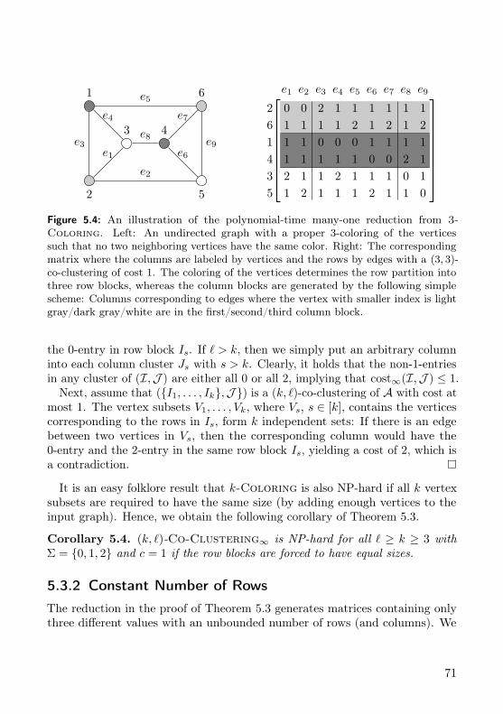
1
2
3 4
5
6
e3e1
e4
e6
e9
e7
e8
e5
e2
1 2 1 1 1 2 1 1 02 1 1 2 1 1 1 0 11 1 1 1 1 0 0 2 11 1 0 0 0 1 1 1 11 1 1 1 2 1 2 1 20 0 2 1 1 1 1 1 12
61435
e1 e2 e3 e4 e5 e6 e7 e8 e9
Figure 5.4: An illustration of the polynomial-time many-one reduction from 3-Coloring. Left: An undirected graph with a proper 3-coloring of the verticessuch that no two neighboring vertices have the same color. Right: The correspondingmatrix where the columns are labeled by vertices and the rows by edges with a (3, 3)-co-clustering of cost 1. The coloring of the vertices determines the row partition intothree row blocks, whereas the column blocks are generated by the following simplescheme: Columns corresponding to edges where the vertex with smaller index is lightgray/dark gray/white are in the first/second/third column block.
the 0-entry in row block Is. If ` > k, then we simply put an arbitrary columninto each column cluster Js with s > k. Clearly, it holds that the non-1-entriesin any cluster of (I,J ) are either all 0 or all 2, implying that cost∞(I,J ) ≤ 1.
Next, assume that (I1, . . . , Ik,J ) is a (k, `)-co-clustering of A with cost atmost 1. The vertex subsets V1, . . . , Vk, where Vs, s ∈ [k], contains the verticescorresponding to the rows in Is, form k independent sets: If there is an edgebetween two vertices in Vs, then the corresponding column would have the0-entry and the 2-entry in the same row block Is, yielding a cost of 2, which isa contradiction.
It is an easy folklore result that k-Coloring is also NP-hard if all k vertexsubsets are required to have the same size (by adding enough vertices to theinput graph). Hence, we obtain the following corollary of Theorem 5.3.
Corollary 5.4. (k, `)-Co-Clustering∞ is NP-hard for all ` ≥ k ≥ 3 withΣ = 0, 1, 2 and c = 1 if the row blocks are forced to have equal sizes.
5.3.2 Constant Number of RowsThe reduction in the proof of Theorem 5.3 generates matrices containing onlythree different values with an unbounded number of rows (and columns). We
71
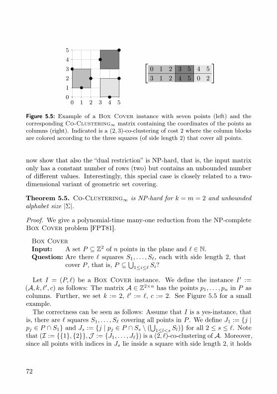
00
1
1
2
2
3
3
4
4
5
5
3 1 2 4 5 0 20 1 2 3 5 4 5
Figure 5.5: Example of a Box Cover instance with seven points (left) and thecorresponding Co-Clustering∞ matrix containing the coordinates of the points ascolumns (right). Indicated is a (2, 3)-co-clustering of cost 2 where the column blocksare colored according to the three squares (of side length 2) that cover all points.
now show that also the “dual restriction” is NP-hard, that is, the input matrixonly has a constant number of rows (two) but contains an unbounded numberof different values. Interestingly, this special case is closely related to a two-dimensional variant of geometric set covering.
Theorem 5.5. Co-Clustering∞ is NP-hard for k = m = 2 and unboundedalphabet size |Σ|.
Proof. We give a polynomial-time many-one reduction from the NP-completeBox Cover problem [FPT81].
Box CoverInput: A set P ⊆ Z2 of n points in the plane and ` ∈ N.Question: Are there ` squares S1, . . . , S`, each with side length 2, that
cover P , that is, P ⊆⋃
1≤i≤` Si?
Let I = (P, `) be a Box Cover instance. We define the instance I ′ :=(A, k, `′, c) as follows: The matrix A ∈ Z2×n has the points p1, . . . , pn in P ascolumns. Further, we set k := 2, `′ := `, c := 2. See Figure 5.5 for a smallexample.
The correctness can be seen as follows: Assume that I is a yes-instance, thatis, there are ` squares S1, . . . , S` covering all points in P . We define J1 := j |pj ∈ P ∩ S1 and Js := j | pj ∈ P ∩ Ss \ (
⋃1≤l<s Sl) for all 2 ≤ s ≤ `. Note
that (I := 1, 2,J := J1, . . . , J`) is a (2, `)-co-clustering of A. Moreover,since all points with indices in Js lie inside a square with side length 2, it holds
72
that each pair of entries in A1s as well as in A2s has distance at most 2,implying cost∞(I,J ) ≤ 2.Conversely, if I ′ is a yes-instance, then let (1, 2,J ) be the (2, `)-
co-clustering of cost at most 2. For any Js ∈ J , it holds that all pointscorresponding to the columns in Js have pairwise distance at most 2 in bothcoordinates. Thus, there exists a square of side length 2 covering all of them.
5.3.3 Clustering into Consecutive Clusters
One is tempted to assume that the hardness of the previous special cases ofCo-Clustering∞ is rooted in the fact that we are allowed to choose arbitrarysubsets for the corresponding row and column partitions since the problemremains hard even for a constant number of clusters even with equal cluster sizes.Hence, in this section, we consider a restricted version of Co-Clustering∞,where the row and the column partition has to consist of consecutive blocks.
Formally, for row indices R = r1, . . . , rk−1 with 1 < r1 < . . . < rk−1 ≤ mand column indices C = c1, . . . , c`−1 with 1 < c1 < . . . < c`−1 ≤ n, thecorresponding consecutive (k, `)-co-clustering (IR,JC) is defined as
IR := 1, . . . , r1 − 1, r1, . . . , r2 − 1, . . . , rk−1, . . . ,m,JC := 1, . . . , c1 − 1, c1, . . . , c2 − 1, . . . , c`−1, . . . , n.
The Consecutive Co-Clustering∞ problem now is to find a consecutive(k, `)-co-clustering of a given input matrix with a given cost.
As it turns out, also this restriction is not sufficient to overcome the inherentintractability of co-clustering, that is, we prove it to be NP-hard. Similarly toSection 5.3.2, we encounter a close relation between consecutive co-clusteringand a geometric problem, namely to find an optimal discretization of the plane;a preprocessing problem with applications in data mining [CN98, Ngu06, NS95].The NP-hard Optimal Discretization problem [CN98] is the following: Givena set of points in the plane, where each point is either colored black or white,the task is to find a consistent set of axis-parallel lines, that is, the vertical andhorizontal lines partition the plane into rectangular regions such that no regioncontains two points of different colors (see Figure 5.6 for an example).
73
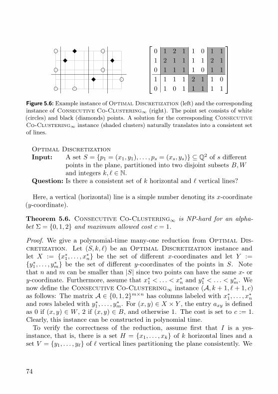
0 1 0 1 1 1 1 11 1 1 1 2 1 1 00 1 1 1 1 0 1 11 2 1 1 1 1 2 10 1 2 1 1 0 1 1
Figure 5.6: Example instance of Optimal Discretization (left) and the correspondinginstance of Consecutive Co-Clustering∞ (right). The point set consists of white(circles) and black (diamonds) points. A solution for the corresponding ConsecutiveCo-Clustering∞ instance (shaded clusters) naturally translates into a consistent setof lines.
Optimal DiscretizationInput: A set S = p1 = (x1, y1), . . . , ps = (xs, ys) ⊆ Q2 of s different
points in the plane, partitioned into two disjoint subsets B,Wand integers k, ∈ N.
Question: Is there a consistent set of k horizontal and vertical lines?
Here, a vertical (horizontal) line is a simple number denoting its x-coordinate(y-coordinate).
Theorem 5.6. Consecutive Co-Clustering∞ is NP-hard for an alpha-bet Σ = 0, 1, 2 and maximum allowed cost c = 1.
Proof. We give a polynomial-time many-one reduction from Optimal Dis-cretization. Let (S, k, ) be an Optimal Discretization instance andlet X := x∗
1, . . . , x∗n be the set of different x-coordinates and let Y :=
y∗1 , . . . , y∗m be the set of different y-coordinates of the points in S. Notethat n and m can be smaller than |S| since two points can have the same x- ory-coordinate. Furthermore, assume that x∗
1 < . . . < x∗n and y∗1 < . . . < y∗m. We
now define the Consecutive Co-Clustering∞ instance (A, k + 1, + 1, c)as follows: The matrix A ∈ 0, 1, 2m×n has columns labeled with x∗
1, . . . , x∗n
and rows labeled with y∗1 , . . . , y∗m. For (x, y) ∈ X × Y , the entry axy is defined
as 0 if (x, y) ∈ W , 2 if (x, y) ∈ B, and otherwise 1. The cost is set to c := 1.Clearly, this instance can be constructed in polynomial time.To verify the correctness of the reduction, assume first that I is a yes-
instance, that is, there is a set H = x1, . . . , xk of k horizontal lines and aset V = y1, . . . , y of vertical lines partitioning the plane consistently. We
74
define row indices R := r1, . . . , rk, ri := maxx∗ ∈ X | x∗ ≤ xi, i = 1, . . . , k,and column indices C := c1, . . . , c`, cj := maxy∗ ∈ Y | y∗ ≤ yj, j = 1, . . . , `.For the corresponding consecutive (k + 1, `+ 1)-co-clustering (IR,JC), it holdsthat no cluster contains both values 0 and 2, since otherwise the correspondingpartition of the plane defined by H and V contains a region with two points ofdifferent colors, which contradicts consistency. Thus, we have cost∞(IR,JC) ≤1, implying that I ′ is a yes-instance.
Conversely, if I ′ is a yes-instance, then there exists a consecutive (k+ 1, `+ 1)-co-clustering (IR,JC) with cost at most 1, that is, no cluster contains bothvalues 0 and 2. Clearly, then the k horizontal lines xi := min Ii+1, i = 1, . . . , k,and the ` vertical lines yj := min Jj+1, j = 1, . . . , `, are consistent. Hence, I isa yes-instance.
Note that even though Consecutive Co-Clustering∞ is NP-hard, therestill is some difference in its computational complexity compared to the generalversion. In contrast to Co-Clustering∞, the consecutive version is polynomial-time solvable for constants k and ` by simply trying out all O(mkn`) consecutivepartitions of the rows and columns (that is, it is contained in XP with respectto (k, `)).
5.4 Tractability Results
In Section 5.3, we showed that Co-Clustering∞ is NP-hard for all con-stants ` ≥ k ≥ 3 and also for k = 2 in case of unbounded ` and |Σ|. In contrastto these hardness results, we now investigate which parameter combinationsyield tractable cases. It turns out that the problem is polynomial-time solvablefor k = ` = 2 and for k = 1 (Section 5.4.2). Moreover, we can solve thecase k = 2 and ` ≥ 3 for |Σ| = 3 in polynomial time by showing that this caseis in fact equivalent to the case k = ` = 2. We further show fixed-parametertractability (for k = 2 and c = 1) for the parameters size |Σ| of the alphabetand the number ` of column blocks (Section 5.4.3).
In Section 5.4.1, we start with a reduction from Co-Clustering∞ to CNF-SAT (the satisfiability problem for Boolean formulas in conjunctive normalform). Later on, it will be used in some special cases (see Theorem 5.9 andTheorem 5.11) because there the corresponding formula—or an equivalentformula—only consists of clauses containing two literals, thus being a polynomial-time solvable 2-SAT instance.
75
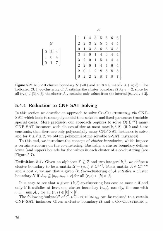
U
0 1 71 0 40 2 4
A
0 2 2 2 8 7 8 72 0 1 2 8 8 8 82 2 0 1 4 4 6 43 2 0 1 5 4 4 43 3 0 1 4 6 4 40 1 3 3 6 6 4 52 2 3 2 5 5 4 51 1 4 3 5 5 6 6
Figure 5.7: A 3 × 3 cluster boundary U (left) and an 8 × 8 matrix A (right). Theindicated (3, 3)-co-clustering of A satisfies the cluster boundary U for c = 2, since forall (r, s) ∈ [3]× [3], the cluster Ars contains only values from the interval [urs, urs + 2].
5.4.1 Reduction to CNF-SAT SolvingIn this section we describe an approach to solve Co-Clustering∞ via CNF-SAT which leads to some polynomial-time solvable and fixed-parameter tractablespecial cases. More precisely, our approach requires to solve O(|Σ|k`) manyCNF-SAT instances with clauses of size at most maxk, `, 2 (if k and ` areconstants, then there are only polynomially many CNF-SAT instances to solve,and for k ≤ ` ≤ 2, we obtain polynomial-time solvable 2-SAT instances).To this end, we introduce the concept of cluster boundaries, which impose
a certain structure on the co-clustering. Basically, a cluster boundary defineslower (and upper) bounds for the values in each cluster of a co-clustering (seeFigure 5.7).
Definition 5.1. Given an alphabet Σ ⊆ Z and two integers k, `, we define acluster boundary to be a matrix U = (urs) ∈ Σk×`. For a matrix A ∈ Σm×n
and a cost c, we say that a given (k, `)-co-clustering of A satisfies a clusterboundary U if Ars ⊆ [urs, urs + c] for all (r, s) ∈ [k]× [`].
It is easy to see that a given (k, `)-co-clustering has cost at most c if andonly if it satisfies at least one cluster boundary (urs), namely, the one withurs = minArs for all (r, s) ∈ [k]× [`].The following “subtask” of Co-Clustering∞ can be reduced to a certain
CNF-SAT instance: Given a cluster boundary U and a Co-Clustering∞
76
instance I, find a co-clustering for I that satisfies U . The polynomial-timereduction provided by the following central lemma can be used to obtain exactCo-Clustering∞ solutions with the help of SAT solvers and we use it in oursubsequent algorithms.
Lemma 5.7. Given a Co-Clustering∞-instance (A, k, `, c) and a clusterboundary U ∈ Σk×`, one can construct in O(mnk`) time a CNF-SAT in-stance φA,U with at most maxk, `, 2 variables per clause such that φA,U issatisfiable if and only if there is a (k, `)-co-clustering of A which satisfies U .
Proof. Given an instance (A, k, `, c) of Co-Clustering∞ and a cluster bound-ary U = (urs) ∈ Σk×`, we define the following Boolean variables: For each(i, r) ∈ [m] × [k], the variable xi,r represents the expression “row i could beput into row block Ir”. Similarly, for each (j, s) ∈ [n] × [`], the variable yj,srepresents that “column j could be put into column block Js”.
We now define a Boolean CNF formula φA,U containing the following clauses:A clause Ri := (xi,1 ∨ xi,2 ∨ . . . ∨ xi,k) for each row i ∈ [m] and a clauseCj := (yj,1 ∨ yj,2 ∨ . . . ∨ yj,`) for each column j ∈ [n]. Additionally, for each(i, j) ∈ [m]× [n] and each (r, s) ∈ [k]× [`] such that element aij does not fit intothe cluster boundary at coordinate (r, s), that is, aij /∈ [urs, urs + c], there is aclause Bijrs := (¬xi,r∨¬yj,s). Note that the clauses Ri and Cj ensure that row iand column j are put into some row and some column block, respectively. Theclause Bijrs expresses that it is impossible to have both row i in block Ir andcolumn j in block Js if aij does not satisfy urs ≤ aij ≤ urs + c. Clearly, φA,U issatisfiable if and only if there exists a (k, `)-co-clustering of A satisfying thecluster boundary U . Note that φA,U consists of km+ `n variables and O(mnk`)clauses and is computable in O(mnkl) time.
Using Lemma 5.7, we can solve Co-Clustering∞ by solving O(|Σ|k`) manyCNF-SAT instances (one for each possible cluster boundary) with km + `nvariables and O(mnk`) clauses of size at most maxk, `, 2.
5.4.2 Polynomial-Time Solvability
We first present a simple and efficient algorithm for (1, ∗)-Co-Clustering∞,that is, the variant where all rows belong to one row block.
Theorem 5.8. (1, ∗)-Co-Clustering∞ is solvable in O(n(m+ log n)) time.
77
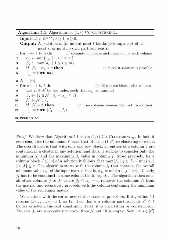
Algorithm 5.1: Algorithm for (1, ∗)-Co-Clustering∞Input: A ∈ Zm×n, ` ≥ 1, c ≥ 0.Output: A partition of [n] into at most ` blocks yielding a cost of at
most c, or no if no such partition exists.1 for j ← 1 to n do // compute minimum and maximum of each column2 αj ← minaij | 1 ≤ i ≤ m3 βj ← maxaij | 1 ≤ i ≤ m4 if βj − αj > c then // check if solution is possible5 return no ;
6 N ← [n]7 for s← 1 to ` do // fill column blocks with columns8 Let js ∈ N be the index such that αjs is minimal9 Js ← j ∈ N | βj − αjs ≤ c
10 N ← N \ Js11 if N = ∅ then // if no columns remain, then return solution12 return (J1, . . . , Js)
13 return no
Proof. We show that Algorithm 5.1 solves (1, ∗)-Co-Clustering∞. In fact, iteven computes the minimum `′ such that A has a (1, `′)-co-clustering of cost c.The overall idea is that with only one row block, all entries of a column j arecontained in a cluster in any solution, and thus, it suffices to consider only theminimum αj and the maximum βj value in column j. More precisely, for acolumn block J ⊆ [n] of a solution it follows that maxβj | j ∈ J −minαj |j ∈ J ≤ c. The algorithm starts with the column j1 that contains the overallminimum value αj1 of the input matrix, that is, αj1 = minαj | j ∈ [n]. Clearly,j1 has to be contained in some column block, say J1. The algorithm then addsall other columns j to J1 where βj ≤ αj1 + c, removes the columns J1 fromthe matrix, and recursively proceeds with the column containing the minimumvalue of the remaining matrix.
We continue with the correctness of the described procedure. If Algorithm 5.1returns (J1, . . . , J`′) at Line 12, then this is a column partition into `′ ≤ `blocks satisfying the cost constraint. First, it is a partition by construction:The sets Js are successively removed from N until it is empty. Now, let s ∈ [`′].
78
Then, for all j ∈ Js, it holds αj ≥ αjs (by definition of js) and βj ≤ αjs + c(by definition of Js). Thus, A1s ⊆ [αjs , αjs + c] holds for all s ∈ [`′], whichyields cost∞([m], J1, . . . , J`′) ≤ c.
Otherwise, if Algorithm 5.1 returns no in Line 5, then it is clearly a no-instancesince the difference between the maximum and the minimum value in a columnis larger than c. If no is returned in Line 13, then the algorithm has computedcolumn indices js and column blocks Js for each s ∈ [`], and there still exists atleast one index j`+1 in N when the algorithm terminates. We claim that thecolumns j1, . . . , j`+1 all have to be in different blocks in any solution. To see this,consider any s, s′ ∈ [` + 1] with s < s′. By construction, js′ /∈ Js. Therefore,βjs′ > αjs +c holds, and columns js and js′ contain elements with distance morethan c. Thus, in any co-clustering with cost at most c, the columns j1, . . . , j`+1
must be in different blocks, which is impossible with only ` blocks. Hence, weindeed have a no-instance.The time complexity is seen as follows. The first loop examines in O(mn)
time all elements of the matrix. The second loop can be performed in O(n) timeif the αj and the βj are sorted beforehand, requiring O(n log n) time. Overall,the running time is in O(n(m+ log n)).
From now on, we focus on the k = 2 case, that is, we need to partition therows into two blocks. We first consider the simplest case, where also ` = 2.
Theorem 5.9. (2, 2)-Co-Clustering∞ is solvable in O(|Σ|2mn) time.
Proof. Let (A ∈ Zm×n, k = 2, ` = 2, c) be a (2, 2)-Co-Clustering∞ instance.We use the reduction to CNF-SAT provided by Lemma 5.7. First, note that acluster boundary U ∈ Σ2×2 can only be satisfied if it contains the elements min Σand mina ∈ Σ | a ≥ max Σ − c. The algorithm enumerates all O(|Σ|2) ofthese cluster boundaries. For a fixed U , we construct the Boolean formula φA,Uin O(mn) time. Observe that this formula is in 2-CNF form: The formulaconsists of k-clauses, `-clauses, and 2-clauses, and we have k = ` = 2. Hence,we can determine whether it is satisfiable in linear time [APT79] (note that thesize of the formula is in O(mn)). Overall, the input is a yes-instance if and onlyif φA,U is satisfiable for some cluster boundary U .
Finally, we show that it is possible to extend the above result to any numberof column blocks for size-three alphabets.
79
Theorem 5.10. (2, ∗)-Co-Clustering∞ is O(mn)-time solvable for |Σ| = 3.
Proof. Let I = (A ∈ α, β, γm×n, k = 2, `, c) be a (2, ∗)-Co-Clustering∞instance. We assume without loss of generality that α < β < γ. The case ` ≤ 2is solvable in O(mn) time by Theorem 5.9. Hence, it remains to consider thecase ` ≥ 3. As |Σ| = 3, there are four potential values for a minimum-cost(2, `)-co-clustering. Namely, cost 0 (all cluster entries are equal), cost β − α,cost γ−β, and cost γ−α. Since any (2, `)-co-clustering is of cost at most γ−αand because it can be checked in O(mn) time whether there is a (2, `)-co-clustering of cost 0 (Observation 5.1), there are only two interesting cases left,that is, c ∈ β − α, γ − β.Avoiding a pair (x, y) ∈ α, β, γ2 means to find a co-clustering without
a cluster containing x and y. If c = maxβ − α, γ − β (Case 1), then theproblem comes down to finding a (2, `)-co-clustering avoiding the pair (α, γ).Otherwise (Case 2), the problem is to find a (2, `)-co-clustering avoiding thepair (α, γ) and, additionally, either (α, β) or (β, γ).Case 1. Finding a (2, `)-co-clustering avoiding (α, γ):
In this case, we substitute α := 0, β := 1, and γ := 2. We describe an algorithmfor finding a (2, `)-co-clustering of cost 1 (avoiding (0, 2)). We assume thatthere is no (2, ` − 1)-co-clustering of cost 1 (iterating over all values from 2to `). Consider a (2, `)-co-clustering (I,J = J1, . . . , J`) of cost 1, that is,for all (r, s) ∈ [2] × [`], it holds Ars ⊆ 0, 1 or Ars ⊆ 1, 2. For s 6= t ∈ [`],let (I,Jst := J \Js, Jt∪Js∪Jt) denote the (2, `−1)-co-clustering where thecolumn blocks Js and Jt are merged. By assumption, for all s 6= t ∈ [`], it holdsthat cost∞(I,Jst) > 1 since otherwise we have found a (2, `− 1)-co-clusteringof cost 1. It follows that 0, 2 ⊆ A1s ∪ A1t or 0, 2 ⊆ A2s ∪ A2t holds forall s 6= t ∈ [`]. This can only be true for ` = 2.This proves that there is a (2, `)-co-clustering of cost 1 if and only if there
is a (2, 2)-co-clustering of cost 1. Hence, Theorem 5.9 shows that this case isO(mn)-time solvable.Case 2. Finding a (2, `)-co-clustering avoiding (α, γ) and (α, β) (or (β, γ)):
In this case, we substitute α := 0, γ := 1, and β := 1 if (α, β) has to be avoided,or β := 0 if (β, γ) has to be avoided. It remains to determine whether thereis a (2, `)-co-clustering with cost 0, which can be done in O(mn) time due toObservation 5.1.
It is open whether polynomial-time solvability of (2, ∗)-Co-Clustering∞ alsoholds for larger (constant-size) alphabets. In the following section, however, we
80

show fixed-parameter tractability with respect to the combined parameter (`, |Σ|)if c = 1.
5.4.3 Fixed-Parameter TractabilityThe hardness results from Section 5.3 show that Co-Clustering∞ is com-putationally hard to solve even from a parameterized view (for each of thefive parameters we considered, NP-hardness holds for a small constant). Thisindicates that fixed-parameter tractability might be a challenging goal to achieve.Based on our reduction to CNF-SAT (Lemma 5.7), however, we show fixed-parameter tractability with respect to some parameter combinations for thespecial case k = 2 and c = 1.We develop an algorithm solving (2, ∗)-Co-Clustering∞ for c = 1. The
main idea is, given matrix A and cluster boundary U , to simplify the Booleanformula φA,U into a 2-CNF formula which can be solved efficiently. This ismade possible by the constraint c = 1, which imposes a very specific structureon the cluster boundary. This approach requires to enumerate all (exponentiallymany) possible cluster boundaries, but yields fixed-parameter tractability forthe combined parameter (`, |Σ|).
Theorem 5.11. (2, ∗)-Co-Clustering∞ is O(|Σ|3`n2m2)-time solvable forc = 1.
In the following, we prove Theorem 5.11 in several steps.A first subresult for the proof of Theorem 5.11 is the following lemma, which
we use to solve the case where the number 2m of possible row partitions is lessthan |Σ|`.
Lemma 5.12. For a fixed row partition I of size k, one can solve (k, ∗)-Co-Clustering∞ in O(|Σ|k`mn`) time. Moreover, Co-Clustering∞ isfixed-parameter tractable with respect to the combined parameter (m, k, `, c).
Proof. Given a fixed size-k row partition I, the algorithm enumerates all |Σ|k`different cluster boundaries U = (urs). We say that a given column j fits incolumn block Js if, for each r ∈ [k] and i ∈ Ir, we have aij ∈ [urs, urs + c] (thiscan be decided in O(m) time for any pair (j, s)). The input is a yes-instanceif and only if for some cluster boundary U , every column fits in at least onecolumn block.
Fixed-parameter tractability with respect to (m, k, `, c) is obtained from twosimple further observations. First, all possible row partitions can be enumerated
81
in O(km) time. Second, since each of the k` clusters contains at most c + 1different values, the alphabet size |Σ| for yes-instances is upper-bounded by (c+1)k`. Together, this yields a running time in O(km((c+ 1)k`)k`mn`).
The following lemma, also used for the proof of Theorem 5.11, yields that forspecially structured cluster boundaries, there is no need to consider more thantwo column clusters to which any column can be assigned.
Lemma 5.13. Let I = (A ∈ Zm×n, k = 2, `, c = 1) be an instance of (2, ∗)-Co-Clustering∞, h1 be an integer with 0 < h1 < m, and U = (urs) ∈ Σ2×` be acluster boundary with pairwise different columns such that |u1s − u2s| = 1 forall s ∈ [`]. Then, in O(n(m + `)) time, one can compute two indices sj ∈ [`]and tj ∈ [`] for each column j ∈ [n], such that the following holds:
If A has a (2, `)-co-clustering (I1, I2, J1, . . . , J`) satisfying U with |I1| =h1, then either j ∈ Jsj or j ∈ Jtj holds.
Proof. To start with, let us define some notation. Given a column j ∈ [n] andany element a ∈ Σ, we write wa(j) for the number of a-entries in column j. Fors ∈ [`], we define U1s := u1s, u1s + 1, U2s := u2s, u2s + 1 and let α be theinteger in U1s\U2s, β be the integer in U1s∩U2s, and γ be the integer in U2s\U1s
(note that all the three sets contain exactly one integer since |u1s − u2s| = 1).We say that a column j ∈ [n] fits boundary column s if the following threeconditions hold:
(i) wx(j) = 0 for any x ∈ Σ \ α, β, γ,
(ii) wα(j) ≤ h1, and
(iii) wγ(j) ≤ h2 := m− h1.
Note that if Condition (i) is violated, then the column contains an element whichis neither in U1s nor in U2s. If Condition (ii) (respectively (iii)) is violated, thenthere are more than h1 (respectively h2) rows that have to be in row block I1(respectively I2). Thus, if j does not fit any boundary column s, then thereis no (2, `)-co-clustering (I1, I2, J1, . . . , J`) satisfying U with |I1| = h1 andj ∈ Js. Hence, in order to find a solution, we need to find out, for each columnin A, to which fitting boundary column in U it should be assigned.
Intuitively, we now prove that in most cases a column has at most two fittingboundary columns, and, in the remaining cases, at most two pairs of “equivalent”boundary columns.
82
Consider a given column j ∈ [n]. Let a := minaij | i ∈ [m] and b :=maxaij | i ∈ [m] (computable in O(m) time). If b ≥ a+ 3, then Condition (i)is always violated, that is, column j does not fit any boundary column, and theinstance is a no-instance.If b = a+ 2, then, again by Condition (i), column j can only fit a boundary
column s where u1s, u2s = a, a+ 1. There are at most two such boundarycolumns in U since all columns in U are distinct. Let sj and tj denote theirindices (computable in O(`) time).
Case b = a is also easy: all values in column j are equal to a. If j fits boundarycolumn s, then, with Conditions (ii) and (iii), a ∈ U1s ∩ U2s, and s is one of atmost two columns in U for which u1s, u2s = a− 1, a. Again, let sj and tjdenote their indices (computable in O(`) time).Finally, if b = a+ 1, then let s ∈ [`] be such that j fits boundary column s.
Hence, by Condition (i), it holds (u1s, u2s) ∈ (a− 1, a), (a, a− 1), (a, b), (b, a).Let s1, . . . , s4 be the four column indices (computable in O(`) time) in U (if theyexist) corresponding to these four cases. We define sj := s1 if j fits boundarycolumn s1 (decidable in O(m) time), and sj := s3 otherwise. Similarly, we definetj := s2 if j fits boundary column s2, and tj := s4 otherwise (O(m) time). Now,consider a (2, `)-co-clustering (I1, I2, J1, . . . , J`) satisfying U with |I1| = h1
such that j ∈ Js∗ for s∗ ∈ s1, s3 with s∗ 6= sj . Since j must fit boundarycolumn s∗, the only possibility is that s∗ = s3 and sj = s1. Thus, j fits bothboundary columns s1 and s3, so Conditions (ii) and (iii) imply wa(j) ≤ h1 andwb(j) ≤ h2. Since wa(j) + wb(j) = m = h1 + h2, we have wa(j) = h1 andwb(j) = h2. Thus, placing j in either of the two column blocks Js1 , Js3 yieldsthe same row partition, namely I1 = i | aij = a and I2 = i | aij = b. Hence,column j can also be added to Js1 instead of Js3 .Similarly with s2 and s4, any solution with j ∈ Js2 or j ∈ Js4 implies that
column j can also be added to Jtj (without any other modification). Thus, sincecolumn j has to be contained in one of the blocks Js1 , . . . , Js4 , we can assumethat it is contained in one of Jsj , Jtj instead.As regards the running time, for each of the n columns we can find the two
indices within at most O(m+ `+m) time. Hence, the overall running time isin O(n(m+ `)).
Having all prerequisites at hand, we now present the proof of Theorem 5.11.
Proof of Theorem 5.11. Let I = (A ∈ Zm×n, k = 2, `, c = 1) be a (2, ∗)-Co-Clustering∞ instance. The proof is by induction on `. For ` = 1, the problem
83
is solvable in O(n(m + log n)) time (Theorem 5.8). We now consider generalvalues of `. Note that if ` is large compared to m (that is, 2m < |Σ|`), thenone can directly guess the row partition and run the algorithm of Lemma 5.12.Thus, we henceforth assume that ` < m.
For a cluster boundary U = (urs) ∈ Σ2×`, let Urs := urs, urs + 1 foreach (r, s) ∈ [2]× [`]. We say that the boundary column s ∈ [`] has
• equal bounds if U1s = U2s (that is, u1s = u2s),
• non-overlapping bounds if U1s ∩ U2s = ∅ (that is |u1s − u2s| > 1),
• properly overlapping bounds otherwise (that is |u1s − u2s| = 1).
We first show that instances having a (2, `)-co-clustering satisfying a clusterboundary that contains at least one column with equal or non-overlappingbounds can be easily solved.
Claim 5.14. If there exists a (2, `)-co-clustering that satisfies a cluster boundarywith equal bounds, then it can be computed in O(|Σ|2`n2m2) time.
Proof. We assume without loss of generality that boundary column ` has equalbounds. We try out all possible values u1` = u2` = u ∈ Σ. Note that columnblock J` imposes no restrictions on the row partition. Hence, any columnof A with all values in u, u + 1 can be put into block J`, and all othercolumns have to end up in the `− 1 other blocks, thus forming an instance of(2, `− 1)-Co-Clustering∞. By induction (the case ` = 1 is easily solvable byTheorem 5.8), each of these cases can be solved in O(|Σ|2(`−1)n2m2) time. Thisprocedure finds a (2, `)-co-clustering with a column block having equal boundsin O(|Σ| · (mn+ |Σ|2(`−1)n2m2)) ⊆ O(|Σ|2`n2m2) time.
Claim 5.15. If there exists a (2, `)-co-clustering that satisfies a cluster boundarywith non-overlapping bounds, then it can be computed in O(|Σ|2`n2m2) time.
Proof. Let s be the index of the boundary column with non-overlapping boundsand assume that, without loss of generality, u1s+1 < u2s. We try out all possiblevalues u2s = u ∈ Σ, and we check for each column j in A, whether j ∈ Js ispossible. In order to have j ∈ Js, it is necessary that all entries in j are containedin u1s, u1s + 1, u, u+ 1 for some u1s < u− 1. Note that if column j fulfills theabove condition, then assuming that j ∈ Js determines the boundary column sand also the entire row partition, that is, if j ∈ Js, then I1 = i | aij < u andI2 = i | aij ≥ u. Using the algorithm described in Lemma 5.12, we can deduce
84
the column partition in O(|Σ|2(`−1)nm`) time (note that there are only |Σ|2(`−1)
possible cluster boundaries to enumerate since column s is already fixed). Theoverall running time is thus in O(|Σ|·n·(m+|Σ|2(`−1)nm`)) ⊆ O(|Σ|2`n2m2).
We now show how to find a (2, `)-co-clustering that satisfies a cluster boundarywith only properly overlapping bounds. We enumerate all such cluster boundariesU = (urs). Note that, for each s ∈ [`], we only need to consider the caseswhere |u1s − u2s| = 1. Also note that we can assume all columns in U to bedistinct since two identical columns could be merged. We then enumerate allpossible values h1 ∈ 1, . . . ,m− 1 (the height of the first row block) and defineh2 := m− h1 > 0. Overall, there are at most (2|Σ|)`m cases to consider.Using Lemma 5.13, we compute in O(mn) time two indices sj , tj for each
column j in A such that for any (2, `)-co-clustering (I1, I2, J1, . . . , J`) satis-fying cluster boundary U with |I1| = h1, either j ∈ Jsj or j ∈ Jtj holds.We now introduce a 2-CNF formula allowing us to simultaneously assign
the rows and columns to the possible blocks (similar to the formula created inLemma 5.7). Let φ′A,U,h1
be a Boolean formula over the same Boolean variablesas in Lemma 5.7 containing the following clauses:
• For each row i ∈ [m], there is a clause R′i := (xi,1 ∨ xi,2).
• For each column j ∈ [n], there is a clause C ′j := (yj,sj ∨ yj,tj ).
• For each (i, j) ∈ [m] × [n] and each (r, s) ∈ [2] × sj , tj such thataij /∈ [urs, urs + 1], there is a clause B′ijrs := (¬xi,r ∨ ¬yj,s).
Note that φ′A,U,h1is a 2-CNF formula with 2m+2n variables and O(mn) clauses.
Clearly, if φ′A,U,h1is satisfiable, then A admits a (2, `)-co-clustering satisfying U .
Conversely, if A admits a (2, `)-co-clustering satisfying U with |I1| = h1, then,by the discussion above, there exists a (2, `)-co-clustering where each column jis in one of the column blocks Jsj or Jtj . For the corresponding Boolean variableassignment, each clause of φ′A,U,h1
is satisfied. Hence, φ′A,U,h1is satisfiable.
Overall, for each cluster boundary U and each h1, we construct and solve theformula φ′A,U,h1
defined above. The matrix A admits a (2, `)-co-clustering ofcost 1 if and only if φ′A,U,h1
is satisfiable for some U and h1. The running timefor constructing and solving the formula φ′A,U,h1
, for fixed U and h1 is in O(mn),which yields a running time in O((2|Σ|)`m · (mn+mn)) ⊆ O((2|Σ|)`nm2) forthis last part.
The final running time is thus in O(2|Σ|2`n2m2+(2|Σ|)`nm2) ⊆ O(|Σ|2`n2m2).
85
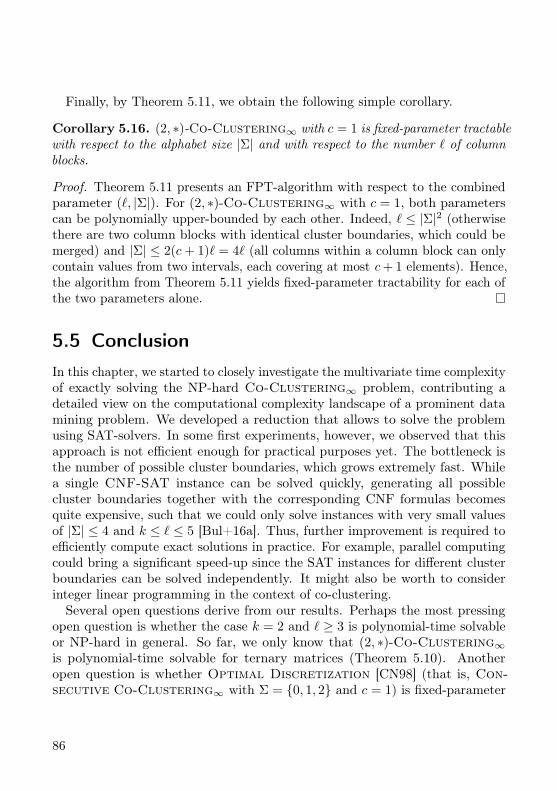
Finally, by Theorem 5.11, we obtain the following simple corollary.
Corollary 5.16. (2, ∗)-Co-Clustering∞ with c = 1 is fixed-parameter tractablewith respect to the alphabet size |Σ| and with respect to the number ` of columnblocks.
Proof. Theorem 5.11 presents an FPT-algorithm with respect to the combinedparameter (`, |Σ|). For (2, ∗)-Co-Clustering∞ with c = 1, both parameterscan be polynomially upper-bounded by each other. Indeed, ` ≤ |Σ|2 (otherwisethere are two column blocks with identical cluster boundaries, which could bemerged) and |Σ| ≤ 2(c+ 1)` = 4` (all columns within a column block can onlycontain values from two intervals, each covering at most c+ 1 elements). Hence,the algorithm from Theorem 5.11 yields fixed-parameter tractability for each ofthe two parameters alone.
5.5 ConclusionIn this chapter, we started to closely investigate the multivariate time complexityof exactly solving the NP-hard Co-Clustering∞ problem, contributing adetailed view on the computational complexity landscape of a prominent datamining problem. We developed a reduction that allows to solve the problemusing SAT-solvers. In some first experiments, however, we observed that thisapproach is not efficient enough for practical purposes yet. The bottleneck isthe number of possible cluster boundaries, which grows extremely fast. Whilea single CNF-SAT instance can be solved quickly, generating all possiblecluster boundaries together with the corresponding CNF formulas becomesquite expensive, such that we could only solve instances with very small valuesof |Σ| ≤ 4 and k ≤ ` ≤ 5 [Bul+16a]. Thus, further improvement is required toefficiently compute exact solutions in practice. For example, parallel computingcould bring a significant speed-up since the SAT instances for different clusterboundaries can be solved independently. It might also be worth to considerinteger linear programming in the context of co-clustering.Several open questions derive from our results. Perhaps the most pressing
open question is whether the case k = 2 and ` ≥ 3 is polynomial-time solvableor NP-hard in general. So far, we only know that (2, ∗)-Co-Clustering∞is polynomial-time solvable for ternary matrices (Theorem 5.10). Anotheropen question is whether Optimal Discretization [CN98] (that is, Con-secutive Co-Clustering∞ with Σ = 0, 1, 2 and c = 1) is fixed-parameter
86
tractable with respect to the combined parameter (k, `). Note that this re-stricted problem is a special case of the Rectangle Stabbing problem whichis known to be W[1]-hard with respect to the number of stabbing lines (thatis, clusters) [DFR12]. Optimal Discretization is also known under thename Red-Blue Separation and was recently shown to be W[1]-hard whenparameterized by the number of separating lines if the lines can be chosenarbitrarily (non-axis parallel) and conjectured to be fixed-parameter tractablefor axis-parallel lines [BGL17]. Last but not least, the computational complexityof higher-dimensional co-clustering versions, e.g. on three-dimensional tensorsas input (the most basic case here corresponds to (2,2,2)-Co-Clustering∞,that is, partitioning each dimension into two subsets) is also open.
We conclude with the following more abstract vision for future research: Notethat for the maximum norm, the cost value c defines a “conflict relation” on thevalues occurring in the input matrix. That is, for any two numbers σ, σ′ ∈ Σwith |σ − σ′| > c, we know that they must end up in different clusters. Theseconflict pairs completely determine all constraints of a solution since all otherpairs can be grouped arbitrarily. This observation can be generalized to a graphmodel. Given a “conflict relation” R ⊆
(Σ2
)determining which pairs are not
allowed to be put together into a cluster, we can define a “conflict graph” (Σ, R).Studying co-clusterings in the context of such conflict graphs and their structuralproperties could be a promising and fruitful direction for future research.
87

Chapter 6
F -Free Editing
In this chapter, we study the parameterized complexity of a general graphmodification problem called F -free Editing: Given a graph G and a naturalnumber k, is it possible to modify at most k edges in G so that the resultinggraph contains no induced subgraph isomorphic to F? This problem comprisessome well-known special cases with applications in machine learning and networkanalysis. For example, the case when F is a path on three vertices is the graphclustering problem Cluster Editing.
In contrast to the previous chapters, where we analyzed problems whosecomplexity has not been studied in detail before, this chapter considers a problemwhose parameterized complexity has already been studied. However, earlierworks on F -free Editing mostly considered the standard parameter, that is,the number k of edge modifications. We consider instead a parameterizationby the number ` of edge modifications above a given lower bound (providedby a packing of induced subgraphs of the input graph), which is a stronger(that is, smaller) parameter. Hence, this parameter allows a sharpening of thecomplexity picture by identifying further tractable cases.
We develop a framework to show fixed-parameter tractability for F -freeEditing with respect to ` by creating a win-win situation where we can eitherapply a polynomial-time data reduction or upper-bound the number k of edgemodifications in `. We show how to apply the framework for three well-knownproblems: Triangle Deletion, Feedback Arc Set in Tournaments, andCluster Editing. Moreover, we explore the limits of this parameterizationapproach by proving NP-hardness for several problem variants (for example, foredge-disjoint subgraph packings or vertex deletions) with constant parametervalue ` = 0.
89
6.1 IntroductionGraph modification problems are a core topic of algorithmic research [Cai96,LY80, Yan81]. Given a graph G, the aim in these problems is to transform Gby a minimum number of modifications (like vertex deletions, edge deletions, oredge insertions) into another graph G′ fulfilling certain properties. Particularlywell-studied are hereditary graph properties, which are closed under vertexdeletions and which are characterized by minimal forbidden induced subgraphs :a graph fulfills a hereditary property Π if and only if it does not contain agraph F from a property-specific family F of graphs as an induced subgraph.All nontrivial vertex deletion problems and many edge modification and deletionproblems for establishing hereditary graph properties are NP-complete [Alo06,ASS16, KM86, LY80, SST04, Yan81]. If the desired graph property has a finiteforbidden induced subgraph characterization, then the corresponding vertexdeletion, edge deletion, and edge modification problems are known to be fixed-parameter tractable with respect to the number k of modifications [Cai96]. Allvertex deletion problems for establishing graph properties characterized by afinite number of forbidden induced subgraphs have a problem kernel of sizepolynomial in the number k of allowed vertex deletions [Kra12]. In contrast,many variants of F -free Editing do not admit a problem kernel whose size ispolynomial in k [CC15, Gui+13, KW13].
Parameterization Above Lower Bounds. When combined with data reduc-tion and pruning rules, search-tree based fixed-parameter algorithms for theparameter k of allowed modifications are competitive in some cases [HH15,MNS12]. Nevertheless, the number k of modifications is often too large andsmaller parameters are desirable.
A natural approach to obtain smaller parameters is “parameterization aboveguaranteed values” [Cyg+13, GP16, Lok+14, MR99]. The idea is to use a lowerbound h on the solution size and to use ` := k − h as parameter instead of k.This idea has been applied successfully to Vertex Cover, that is, K2-FreeVertex Deletion. Since the size of a smallest vertex cover is large in manyinput graphs, parameterizations above the lower bounds “size of a maximummatching M in the input graph” and “optimum value L of the LP relaxation ofthe standard ILP-formulation of Vertex Cover” have been considered. Aftera series of improvements [Cyg+13, GP16, Lok+14, RO09], the currently bestrunning time is 3` · nO(1), where ` := k − (2 · L− |M |) and |M | and L denotethe lower bounds mentioned above [GP16].
90

We extend this approach to edge modification problems, where the number kof modifications tends to be even larger than for vertex deletion problems. Forexample, in the case of Cluster Editing, which asks to destroy inducedpaths on three vertices by edge modifications, the number of modifications isoften larger than the number of vertices in the input graph [Böc+09]. Hence,parameterization above lower bounds seems natural and even more relevantfor edge modification problems. Somewhat surprisingly, this approach has notbeen considered so far. We thus initiate research on parameterization abovelower bounds in this context. As a starting point, we focus on edge modificationproblems for graph properties that are characterized by one forbidden inducedsubgraph F :
F -free EditingInput: A graph G = (V,E) and a natural number k.Question: Is there an F -free editing set S ⊆
(V2
)of size at most k, that is,
an edge modification set such that G4S := (V, (E \S)∪ (S \E))does not contain F as induced subgraph?
In the context of a concrete variant of F -free Editing, we refer to an F -freeediting set as solution and call a solution optimal if it has minimum size.
Lower Bounds from Packings of Induced Subgraphs. Following the approachof parameterizing Vertex Cover above the size of a maximum matching, wecan parameterize F -free Editing above a lower bound obtained from packingsof arbitrary induced non-F -free subgraphs.
Definition 6.1. A vertex-disjoint (or edge-disjoint) packing of induced sub-graphs of a graph G is a set H = H1, . . . ,Hz such that each Hi is an inducedsubgraph of G and such that the vertex sets of the Hi are mutually disjoint (orintersect in at most one vertex).
Though Definition 6.1 does not require H to be maximal (we still call ita packing), it is of course natural in practice to use a maximal packing ofvertex-disjoint subgraphs (for example, computed by some greedy strategy).Also, while it is at first sight natural to consider packings of induced subgraphsthat are isomorphic to F in order to obtain a lower bound on the solutionsize, a packing of other graphs that contain F as induced subgraph might yieldeven better lower bounds and thus a smaller parameter above this lower bound.For example, a K4 contains four K3s and two edge deletions are necessary to
91
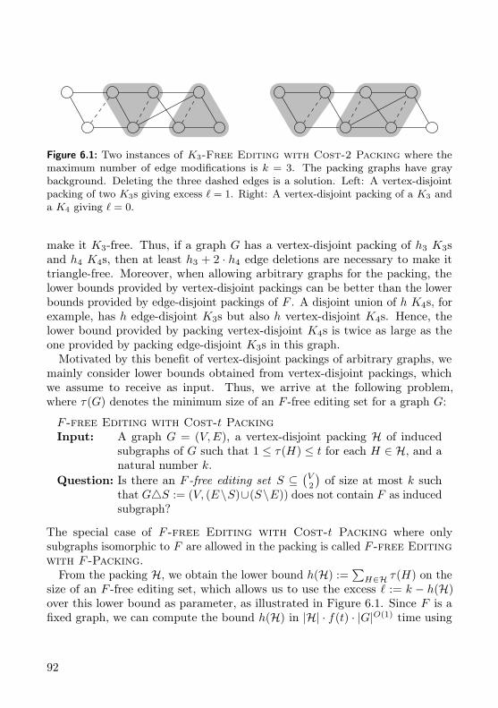
Figure 6.1: Two instances of K3-Free Editing with Cost-2 Packing where themaximum number of edge modifications is k = 3. The packing graphs have graybackground. Deleting the three dashed edges is a solution. Left: A vertex-disjointpacking of two K3s giving excess ` = 1. Right: A vertex-disjoint packing of a K3 anda K4 giving ` = 0.
make it K3-free. Thus, if a graph G has a vertex-disjoint packing of h3 K3sand h4 K4s, then at least h3 + 2 · h4 edge deletions are necessary to make ittriangle-free. Moreover, when allowing arbitrary graphs for the packing, thelower bounds provided by vertex-disjoint packings can be better than the lowerbounds provided by edge-disjoint packings of F . A disjoint union of h K4s, forexample, has h edge-disjoint K3s but also h vertex-disjoint K4s. Hence, thelower bound provided by packing vertex-disjoint K4s is twice as large as theone provided by packing edge-disjoint K3s in this graph.
Motivated by this benefit of vertex-disjoint packings of arbitrary graphs, wemainly consider lower bounds obtained from vertex-disjoint packings, whichwe assume to receive as input. Thus, we arrive at the following problem,where τ(G) denotes the minimum size of an F -free editing set for a graph G:
F -free Editing with Cost-t PackingInput: A graph G = (V,E), a vertex-disjoint packing H of induced
subgraphs of G such that 1 ≤ τ(H) ≤ t for each H ∈ H, and anatural number k.
Question: Is there an F -free editing set S ⊆(V2
)of size at most k such
that G4S := (V, (E\S)∪(S\E)) does not contain F as inducedsubgraph?
The special case of F -free Editing with Cost-t Packing where onlysubgraphs isomorphic to F are allowed in the packing is called F -free Editingwith F -Packing.
From the packing H, we obtain the lower bound h(H) :=∑H∈H τ(H) on the
size of an F -free editing set, which allows us to use the excess ` := k − h(H)over this lower bound as parameter, as illustrated in Figure 6.1. Since F is afixed graph, we can compute the bound h(H) in |H| · f(t) · |G|O(1) time using
92
the generic algorithm [Cai96] mentioned in the introduction for each H ∈ H.In the same time we can also verify whether the cost-t property is fulfilled.
Packings of forbidden induced subgraphs have been used in implementationsof fixed-parameter algorithms to prune the corresponding search trees tremen-dously [HH15]. By showing fixed-parameter algorithms for parameters abovethese lower bounds, we hope to explain the fact that these packings help inobtaining fast algorithms.
Our Contributions. We investigate three variants of F -free Editing withCost-t Packing for small graphs F , that is, on three vertices (the smallestnontrivial number of vertices).In the first (introductory) variant, the graph F is a triangle, that is, a K3
(complete graph on three vertices). This problem is known as TriangleDeletion (note that adding edges is never optimal since it cannot removetriangles) and is related to network cluster analysis.Second, we consider a directed variant in which the input is a tournament
graph and F is a directed cycle on three vertices. This is known as FeedbackArc Set in Tournaments and has applications in rank aggregation.
The third variant is a clustering problem on undirected graphs called ClusterEditing, where F is a P3, that is, a path on three vertices. This problem hasvarious applications in machine learning and bioinformatics.
Our positive results are fixed-parameter algorithms and problem kernels.Using a general approach described in Section 6.2, we obtain fixed-parameteralgorithms for the above variants of F -free Editing with Cost-t Packingparameterized by t and ` (mainly by developing appropriate data reductionrules). This implies fixed-parameter tractability for F -free Editing withF -Packing parameterized by `. Specifically, we obtain the following results(for the kernelization results, we need to assume that t ∈ O(log n) to guaranteepolynomial running time of the data reduction):
• For Triangle Deletion, we show an O((2t+ 3)` · (nm+n ·2.076t))-timealgorithm and an O(t · `)-vertex problem kernel for cost-t packings (Corol-lary 6.6).
• For Feedback Arc Set in Tournaments, we show a 2O(√
(2t+1)`)·
nO(1)-time algorithm and an O(t · `)-vertex problem kernel for cost-tpackings (Corollary 6.11).
93
• For Cluster Editing, we show an O(1.62(2t+1)` + nm+ n · 1.62t)-timealgorithm and an O(t · `)-vertex kernel for cost-t packings (Corollary 6.16),and also give a 4` · nO(1)-time algorithm for P3-packings [BFK18, Theo-rem 6.13].
To the best of our knowledge, the above results are the first fixed-parametertractability results for edge modification problems parameterized above lowerbounds obtained from induced subgraph packings. Moreover, since the parame-ter ` is potentially significantly smaller than the number k of edge modifications,our algorithms might be fast in practice.
On the negative side, we show several NP-hardness results which point out thelimitations of parameterizing graph modification problems above lower boundsobtained from subgraph packings and justify to a certain extent the focus onlower bounds obtained from vertex-disjoint packings. In particular, we showthe following:
• K6-free Deletion with K6-Packing is NP-hard for ` = 0 (Theo-rem 6.18). This implies that a general fixed-parameter tractability resultas it is known for the parameter k [Cai96] cannot be expected.
• If F is a K3 and H is an edge-disjoint packing of h K3s in a graph G, thenit is NP-hard to decide whether G has a K3-free deletion set of size h,that is, ` = 0 (Theorem 6.21). Thus, parameterization by ` is hopeless foredge-disjoint packing lower bounds.
• For all q ≥ 3, Pq-free Vertex Deletion with Pq-Packing is NP-hardeven if ` = 0 (Theorem 6.23).
Organization. In Section 6.2, we present the general approach used in ouralgorithmic results. In Section 6.3, we present the results for Triangle Dele-tion, in Section 6.4 those for Feedback Arc Set in Tournaments, andin Section 6.5 the results for Cluster Editing. Section 6.6 shows edge andvertex deletion problems that remain NP-hard for ` = 0, where ` is the numberof modifications that are allowed in addition to a lower bound based on differenttypes (edge- and vertex-disjoint) of subgraph packings. We conclude with someopen questions in Section 6.7.
94
6.2 General Approach
In this section, we describe the general approach of our fixed-parameter algo-rithms. Recall that τ(H) is the minimum number of edge modifications requiredto transform a graph H into an F -free graph. The idea behind the algorithmsis to arrive at a classic win-win scenario [Fel03, FNN16, Har+15] where we caneither apply polynomial-time data reduction or show that the packing size |H|is upper-bounded in `. This upper bound will allow us to upper-bound k in t · `for yes-instances and, thus, to apply known fixed-parameter algorithms for theparameter k to obtain fixed-parameter tractability results for (t, `).More precisely, we show that, for each induced subgraph H of G in a given
packing H, we face essentially two situations. If there is an optimal solutionfor H that is a subset of an optimal solution for G, then we can apply a datareduction rule. Otherwise, we find a “certificate”, that is, a set of vertex pairswitnessing that either H itself needs to be solved suboptimally or that a vertexpair containing exactly one vertex from H needs to be modified. We use thefollowing terminology for these pairs.
Definition 6.2 (External vertex pairs and edges). A vertex pair u, v is anexternal pair for a packing graph H ∈ H if exactly one of u or v is in V (H). Anedge in G is an external edge for H ∈ H if exactly one of its endpoints is in H.
Observe that every vertex pair (every edge) is an external pair (edge) for atmost two packing graphs since the packing graphs are vertex-disjoint. Conse-quently, the modification of an external vertex pair can destroy at most twocertificates. This is the main fact used in the proof of the following bound on k.
Lemma 6.1. Let (G,H, k) be an instance of F -free Editing with Cost-tPacking and let S be a size-k solution that contains, for each H ∈ H, either
(a) at least τ(H) + 1 vertex pairs from(V (H)
2
), or
(b) at least one external vertex pair v, w for H.
Then, |H| ≤ 2` and thus, k ≤ (2t+ 1)`.
Proof. Denote by Ha ⊆ H the set of all graphs in H that fulfill Property (a)and let pa := |Ha|. Let Hb := H \Ha denote the set containing the remainingpacking graphs (fulfilling Property (b)) and let pb := |Hb|. Thus, |H| = pa + pb.Furthermore, let ha :=
∑H∈Ha τ(H) denote the lower bound obtained from
95
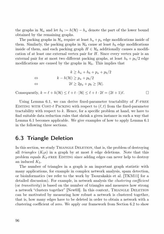
the graphs in Ha and let hb := h(H)− ha denote the part of the lower boundobtained by the remaining graphs.
The packing graphs in Ha require at least ha+pa edge modifications inside ofthem. Similarly, the packing graphs in Hb cause at least hb edge modificationsinside of them, and each packing graph H ∈ Hb additionally causes a modifi-cation of at least one external vertex pair for H. Since every vertex pair is anexternal pair for at most two different packing graphs, at least hb + pb/2 edgemodifications are caused by the graphs in Hb. This implies that
k ≥ ha + hb + pa + pb/2
⇔ k − h(H) ≥ pa + pb/2
⇔ 2` ≥ 2pa + pb ≥ |H|.
Consequently, k = `+ h(H) ≤ `+ t · |H| ≤ `+ t · 2` = (2t+ 1)`.
Using Lemma 6.1, we can derive fixed-parameter tractability of F -freeEditing with Cost-t Packing with respect to (`, t) from the fixed-parametertractability with respect to k. Hence, for a specific problem at hand, we have tofind suitable data reduction rules that shrink a given instance in such a way thatLemma 6.1 becomes applicable. We give examples of how to apply Lemma 6.1in the following three sections.
6.3 Triangle Deletion
In this section, we study Triangle Deletion, that is, the problem of destroyingall triangles (K3s) in a graph by at most k edge deletions. Note that thisproblem equals K3-free Editing since adding edges can never help to destroyan induced K3.The number of triangles in a graph is an important graph statistic with
many applications, for example in complex network analysis, spam detection,or bioinformatics (we refer to the work by Tsourakakis et al. [TKM11] for adetailed discussion). For example, in network analysis the clustering coefficient(or transitivity) is based on the number of triangles and measures how stronga network “clusters together” [New03]. In this context, Triangle Deletioncan be motivated by measuring how robust a network is clustered together,that is, how many edges have to be deleted in order to obtain a network with aclustering coefficient of zero. We apply our framework from Section 6.2 to show
96
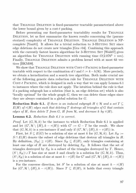
that Triangle Deletion is fixed-parameter tractable parameterized abovethe lower bound given by a cost-t packing.Before presenting our fixed-parameter tractability results for Triangle
Deletion, let us first summarize the known results concerning the (param-eterized) complexity of Triangle Deletion. Triangle Deletion is NP-complete [Yan81]. It allows for a trivial reduction to 3-Hitting Set sinceedge deletions do not create new triangles [Gra+04]. Combining this approachwith the currently fastest known algorithms for 3-Hitting Set [Wah07] givesan algorithm for Triangle Deletion with running time O(2.076k + nm).Finally, Triangle Deletion admits a problem kernel with at most 6k ver-tices [BKM09].
We show that Triangle Deletion with Cost-t Packing is fixed-parametertractable with respect to the combination of t and ` := k−h(H). More precisely,we obtain a kernelization and a search tree algorithm. Both make crucial useof the following generic data reduction rule for Triangle Deletion withCost-t Packing, which is designed in such a way that we can apply Lemma 6.1to instances where the rule does not apply. The intuition behind the rule is thatif a packing subgraph has a solution (that is, an edge deletion set) which is also“locally optimal” for the whole graph G, then we can delete those edges sincethey are always contained in a global solution for G.
Reduction Rule 6.1. If there is an induced subgraph H ∈ H and a set T ⊆E(H) of τ(H) edges such that deleting T destroys all triangles of G that containedges of H, then delete T from G, H from H, and decrease k by τ(H).
Lemma 6.2. Reduction Rule 6.1 is correct.
Proof. Let (G,H, k) be the instance to which Reduction Rule 6.1 is appliedand let (G′,H \ H, k − τ(H)) with G′ := G − T be the result. We showthat (G,H, k) is a yes-instance if and only if (G′,H \ H, k − τ(H)) is.First, let S ⊆ E(G) be a solution of size at most k for (G,H, k). Let SH :=
S ∩ E(H) denote the subset of edge deletions that destroy all triangles in H.By definition, |SH | ≥ τ(H). Since SH ⊆ E(H), only triangles containing atleast one edge of H are destroyed by deleting SH . It follows that the set oftriangles destroyed by SH is a subset of the triangles destroyed by T . Hence,(S \ SH) ∪ T has size at most k and clearly is a solution for (G,H, k). Thus,(S \SH) is a solution of size at most k−τ(H) for G′ and (G′,H\H, k−τ(H))is a yes-instance.For the converse direction, let S′ be a solution of size at most k − τ(H)
for (G′,H \ H, k − τ(H)). Since T ⊆ E(H), it holds that every triangle
97

contained in G that does not contain any edge of H is also a triangle in G′.Thus, S′ is a set of edges whose deletion in G destroys all triangles that do notcontain any edge of H. Since T destroys all triangles containing an edge of H,we have that T ∪ S′ is a solution for G of size at most k.
We now show that if Reduction Rule 6.1 is not applicable to H, then we canfind a certificate for this inapplicability, which will allow us later to branchefficiently on the destruction of triangles:
Definition 6.3 (Certificate). A certificate for inapplicability of ReductionRule 6.1 to an induced subgraph H ∈ H is a set T of triangles in G, eachcontaining exactly one distinct edge of H, such that either
(a) |T | = τ(H) + 1 or
(b) |T | ≤ τ(H) and τ(H ′) > τ(H) − |T |, where H ′ is the subgraph obtainedfrom H by deleting, for each triangle in T , its edge shared with H.
Clearly, if we find a set T of triangles as defined in Definition 6.3, thenReduction Rule 6.1 is not applicable to H since either deleting τ(H) edges in Hleaves a triangle in G with an edge in H (a), or deleting all triangles T and alltriangles in H requires more than τ(H) edge deletions in H (b).
In the following, let Γ(G, k) be the fastest running time to compute a triangle-free deletion set of size at most k in a graph G if it exists. We assume that Γ ismonotonically nondecreasing in the size of G and in k. As mentioned above,currently O(2.076k+ |V (G)| · |E(G)|) is the best known upper bound for Γ(G, k).
Lemma 6.3. We can check for each H ∈ H whether Reduction Rule 6.1applies and output a certificate TH if it does not apply within an overall time ofO(nm+
∑H∈H Γ(H, t)).
Proof. First, in O(nm) time, we compute for all H ∈ H a set TH of trianglesin G that contain exactly one edge e ∈ E(H). These edges are labeled ineach H ∈ H. Then, for each H ∈ H, in Γ(H, t) time we determine the size τ(H)of an optimal triangle-free deletion set for H. Let t′ denote the number oflabeled edges in H.If t′ > τ(H), then we return as certificate τ(H) + 1 triangles of TH , each
containing one distinct edge of τ(H) + 1 arbitrary labeled edges in H.If t′ ≤ τ(H), then let H ′ denote the graph obtained from H by deleting
the labeled edges. Each triangle in G that contains at least one edge of H
98
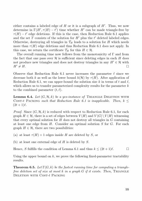
either contains a labeled edge of H or it is a subgraph of H ′. Thus, we nowdetermine in Γ(H ′, τ(H) − t′) time whether H ′ can be made triangle-free byτ(H) − t′ edge deletions. If this is the case, then Reduction Rule 6.1 appliesand the set T consists of the solution for H ′ plus the t′ deleted labeled edges.Otherwise, destroying all triangles in TH leads to a solution for H which needsmore than τ(H) edge deletions and thus Reduction Rule 6.1 does not apply. Inthis case, we return the certificate TH for this H ∈ H.The overall running time now follows from the monotonicity of Γ and from
the fact that one pass over H is sufficient since deleting edges in each H doesnot produce new triangles and does not destroy triangles in any H ′ ∈ H withH ′ 6= H.
Observe that Reduction Rule 6.1 never increases the parameter ` since wedecrease both k as well as the lower bound h(H) by τ(H). After application ofReduction Rule 6.1, we can upper-bound the solution size k in terms of t and `,which allows us to transfer parameterized complexity results for the parameter kto the combined parameter (t, `).
Lemma 6.4. Let (G,H, k) be a yes-instance of Triangle Deletion withCost-t Packing such that Reduction Rule 6.1 is inapplicable. Then, k ≤(2t+ 1)`.
Proof. Since (G,H, k) is reduced with respect to Reduction Rule 6.1, for eachgraph H ∈ H, there is a set of edges between V (H) and V (G)\V (H) witnessingthat every optimal solution for H does not destroy all triangles in G containingat least one edge from H. Consider an optimal solution S for G. For eachgraph H ∈ H, there are two possibilities:
(a) at least τ(H) + 1 edges inside H are deleted by S, or
(b) at least one external edge of H is deleted by S.
Hence, S fulfills the condition of Lemma 6.1 and thus k ≤ (2t+ 1)`.
Using the upper bound on k, we prove the following fixed-parameter tractabilityresults.
Theorem 6.5. Let Γ(G, k) be the fastest running time for computing a triangle-free deletion set of size at most k in a graph G if it exists. Then, TriangleDeletion with Cost-t Packing
99
(i) can be solved in O((2t+ 3)` · (nm+∑H∈H Γ(H, t))) time, and
(ii) admits a problem kernel with at most (12t + 6)` vertices that can becomputed in O(nm+
∑H∈H Γ(H, t)) time.
Proof. We first prove (ii). To this end, let (G = (V,E),H, k) be the inputinstance. First, compute in O(nm +
∑H∈H Γ(H, t)) time an instance that
is reduced with respect to Reduction Rule 6.1 (Lemma 6.3). Afterwards, byLemma 6.4, we can return a trivial constant-size no-instance if k > (2t+ 1)`.Otherwise, we apply the known kernelization algorithm for Triangle Deletionto the instance (G, k) (that is, without H). This kernelization produces inO(m
√m) ⊆ O(nm) time a problem kernel (G′, k′) with at most 6k ≤ (12t+ 6)`
vertices and with k′ ≤ k [BKM09]. Adding an empty packing gives an equivalentinstance (G′, ∅, k′) with parameter `′ = k′ ≤ (2t+ 1)` of Triangle Deletionwith Cost-t Packing.
It remains to prove (i). To this end, we give a search tree algorithm. If ` < 0,then we can clearly reject the instance. Otherwise, apply Reduction Rule 6.1exhaustively in O(nm+
∑H∈H Γ(H, t)) time. Now, consider the following two
cases for the reduced instance.Case 1: H = ∅. If G is triangle-free, then we are done. Otherwise, pick an
arbitrary triangle in G and add it to H.Case 2: H contains a graph H. Since Reduction Rule 6.1 does not apply
to H , there is a certificate T of t′ ≤ τ(H) + 1 triangles, each containing exactlyone distinct edge of H such that deleting the edges of these triangles containedin H produces a subgraph H ′ of H that cannot be made triangle-free by τ(H)−t′edge deletions. Thus, branch into the following (2t′ + 1) ≤ (2t+ 3) cases: First,for each triangle K ∈ T , create two cases, in each deleting a different one of thetwo edges of K that are not in H. In the remaining case, delete the t′ edgesof H and replace H by H ′ in H if τ(H ′) > 0.It remains to show the running time by bounding the search tree size. In
Case 1, no branching is performed and the parameter ` is decreased by one.In Case 2, the parameter ` is decreased by one in each branch: in the first 2t′
cases, an edge that is not contained in any packing graph is deleted (that is,k decreases by one while h(H) remains unchanged). In the final case, thevalue of k decreases by t′. However, τ(H ′) ≥ τ(H)− t′ + 1. Hence, the lowerbound h(H) decreases by τ(H) − τ(H ′) ≤ t′ − 1 and thus the parameter `decreases by at least one. Note that applying Reduction Rule 6.1 never increasesthe parameter. Hence, the depth of the search tree is at most `.
100
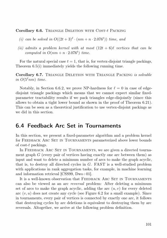
Corollary 6.6. Triangle Deletion with Cost-t Packing
(i) can be solved in O((2t+ 3)` · (nm+ n · 2.076t)) time, and
(ii) admits a problem kernel with at most (12t + 6)` vertices that can becomputed in O(nm+ n · 2.076t) time.
For the natural special case t = 1, that is, for vertex-disjoint triangle packings,Theorem 6.5(i) immediately yields the following running time.
Corollary 6.7. Triangle Deletion with Triangle Packing is solvablein O(5`nm) time.
Notably, in Section 6.6.2, we prove NP-hardness for ` = 0 in case of edge-disjoint triangle packings which means that we cannot expect similar fixed-parameter tractability results if we pack triangles edge-disjointly (since thisallows to obtain a tight lower bound as shown in the proof of Theorem 6.21).This can be seen as a theoretical justification to use vertex-disjoint packings aswe did in this section.
6.4 Feedback Arc Set in Tournaments
In this section, we present a fixed-parameter algorithm and a problem kernelfor Feedback Arc Set in Tournaments parameterized above lower boundsof cost-t packings.
In Feedback Arc Set in Tournaments, we are given a directed tourna-ment graph G (every pair of vertices having exactly one arc between them) asinput and want to delete a minimum number of arcs to make the graph acyclic,that is, to destroy all directed cycles in G. FAST is a well-studied problemwith applications in rank aggregation tasks, for example, in machine learningand information retrieval [CSS99, Dwo+01].
It is a well-known observation that Feedback Arc Set in Tournamentscan also be viewed as an arc reversal problem: After deleting a minimumset of arcs to make the graph acyclic, adding the arc (u, v) for every deletedarc (v, u) does not create any cycle (see Figure 6.2 for a small example). Sincein tournaments, every pair of vertices is connected by exactly one arc, it followsthat destroying cycles by arc deletions is equivalent to destroying them by arcreversals. Altogether, we arrive at the following problem definition.
101
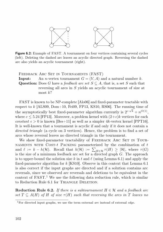
Figure 6.2: Example of FAST. A tournament on four vertices containing several cycles(left). Deleting the dashed arc leaves an acyclic directed graph. Reversing the dashedarc also yields an acyclic tournament (right).
Feedback Arc Set in Tournaments (FAST)Input: An n-vertex tournament G = (V,A) and a natural number k.Question: Does G have a feedback arc set S ⊆ A, that is, a set S such that
reversing all arcs in S yields an acyclic tournament of size atmost k?
FAST is known to be NP-complete [Alo06] and fixed-parameter tractable withrespect to k [ALS09, Dom+10, Fei09, FP13, KS10, RS06]. The running time ofthe asymptotically best fixed-parameter algorithm currently is 2c·
√k + nO(1),
where c ≤ 5.24 [FP13]. Moreover, a problem kernel with (2+ε)k vertices for eachconstant ε > 0 is known [Bes+11] as well as a simpler 4k-vertex kernel [PPT16].It is well-known that a tournament is acyclic if and only if it does not contain adirected triangle (a cycle on 3 vertices). Hence, the problem is to find a set ofarcs whose reversal leaves no directed triangle in the tournament.We show fixed-parameter tractability of Feedback Arc Set in Tour-
naments with Cost-t Packing parameterized by the combination of tand ` := k − h(H). Recall that h(H) :=
∑H∈H τ(H) ≥ |H|, where τ(G)
is the size of a minimum feedback arc set for a directed graph G. The approachis to upper-bound the solution size k in t and ` (using Lemma 6.1) and apply thefixed-parameter algorithm for k [KS10]. Observe in this context that Lemma 6.1is also correct if the input graphs are directed and if a solution contains arcreversals, since we observed arc reversals and deletions to be equivalent in thecontext of FAST.1 We use the following data reduction rule, which is similarto Reduction Rule 6.1 for Triangle Deletion.
Reduction Rule 6.2. If there is a subtournament H ∈ H and a feedback arcset T ⊆ A(H) of H of size τ(H) such that reversing the arcs in T leaves no
1For directed input graphs, we use the term external arc instead of external edge.
102
directed triangles in G containing any arcs of H, then reverse the arcs in T ,remove H from H, and decrease k by τ(H).
Although Reduction Rule 6.2 is strikingly similar to Reduction Rule 6.1 , itscorrectness proof is significantly more involved. In the following, let Γ(G, k) bethe fastest running time for computing a feedback arc set of size at most kfor a given tournament G if it exists. We assume that Γ is monotonicallynondecreasing in both the size of G and in k. As mentioned earlier, 25.24
√k +
|V (G)|O(1) is the currently best known upper bound for Γ(G, k) [FP13].
Lemma 6.8. Reduction Rule 6.2 is correct and, given the tournaments Gand H it can be applied in O
((q2
)(n− q) + Γ(H, t)
)time, where q := |V (H)|.
Proof. We first show correctness. Let I ′ := (G′,H \ H, k − τ(H)) be theinstance created by Reduction Rule 6.2 from I := (G,H, k) by reversing asubset T of arcs of a subtournament H ∈ H of G. If I ′ is a yes-instance, then sois I since G′ is the graph G with the τ(H) arcs in T reversed and, thus, addingthese arcs to a feedback arc set of size k − τ(H) for G′ gives a feedback arcset of size k for G. It remains to prove that if I is a yes-instance, then so is I ′.To this end, we show that there is a minimum-size feedback arc set S for Gwith T ⊆ S.
Let S be a minimum-size feedback arc set for G = (V,A). This implies theexistence of a linear ordering σS = v1, . . . , vn of the vertices V such that thereare |S| backward arcs, that is, arcs (vi, vj) ∈ A such that i > j. Now, let σT =w1, . . . , w|W | be the ordering of the vertices of H = (W,B) corresponding to thelocal solution T for H with τ(H) backward arcs. Let N+(w) := (w, v) ∈ A |v ∈ V \W denote the out-neighbors in V \W of a vertex w ∈W . Analogously,N−(w) := (v, w) ∈ A | v ∈ V \W denotes the set of in-neighbors. By theassumption of Reduction Rule 6.2, for all i < j,
N+(wj) ⊆ N+(wi) and N−(wi) ⊆ N−(wj)
holds since otherwise, after reversing the arcs in T , there exists a directedtriangle containing the arc (wi, wj) of H.If the vertices in W appear in the same relative order in σS as in σT , then
we have T ⊆ S and we are done. Otherwise, we show that we can swap thepositions of vertices of W in σS so that their relative order is the same as in σTwithout increasing the number of backward arcs.
First, note that the number of backward arcs between vertices in V \Wdoes not change when only swapping positions of vertices in W . Also, by
103
assumption, the number of backward arcs between vertices in W in any orderingis at least τ(H), whereas it is exactly τ(H) when ordering them accordingto σT . Thus, it remains to show that the number of backward arcs betweenvertices in W and V \ W is not increased. To this end, consider a seriesof swaps of pairs of vertices wj and wi such that i < j, where wj appearsbefore wi in σS , reordering the vertices in W according to σT . Let Y denotethe set of all vertices that lie between wj and wi in σS (see Figure 6.3 for anexample) and note that swapping wj and wi can only introduce backward arcsbetween wj , wi and vertices in Y . Now, swapping wj and wi removes thebackward arcs from wi to the vertices in N+(wi)∩Y and the backward arcs fromvertices in N−(wj)∩Y to wj , whereas it introduces new backward arcs from wjto (N+(wj) ∩ Y ) ⊆ (N+(wi) ∩ Y ) and from (N−(wi) ∩ Y ) ⊆ (N−(wj) ∩ Y )to wi. It follows that the overall number of backward arcs does not increasein each swap. Hence, the overall number of backward arcs is not increased byrepositioning the vertices in W according to σT . It follows that there is anoptimal solution containing T .It remains to show the running time. First, in Γ(H, t) time, we compute
the size τ(H) of an optimal feedback arc set for H = (W,B). Now, for eacharc (u, v) ∈ B, we check whether there is a vertex w ∈ V \W that forms adirected triangle with u and v. If such a vertex exists, then we reverse thearc (u, v). If this arc reversal introduces a new directed triangle with anothervertex from V \ W , then the rule does not apply. Overall, this procedurerequires O
(|B| · (n− |W |)
)time. Let T ∗ denote the set of arcs that are reversed
in this process. Clearly, if |T ∗| > τ(H), then the rule does not apply. Otherwise,let H ′ denote the graph obtained from H by reversing the arcs in T ∗ andobserve that each remaining directed triangle of G that contains at least onearc of H ′ is contained in H ′. Thus, we now compute whether H ′ has a feedbackarc set T ′ of size τ(H) − |T ∗| in Γ(H ′, τ(H) − |T ∗|) time. If this is the case,then the rule applies and we set T := T ′ ∪ T ∗ (note that T ′ ∩ T ∗ = ∅, sinceotherwise |T | < τ(H), which is not possible by definition of τ(H)). Otherwise,removing all directed triangles in G that contain at least one arc from H requiresmore than τ(H) arc reversals and thus the rule does not apply.
Exhaustive application of Reduction Rule 6.2 allows us to show that k ≤ (2t+1)`holds for any yes-instance.
Lemma 6.9. Let (G,H, k) be a yes-instance of Feedback Arc Set in Tour-naments with Cost-t Packing such that Reduction Rule 6.2 cannot be appliedto any tournament in H. Then, k ≤ (2t+ 1)`.
104
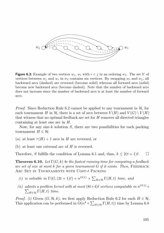
wj wi
Figure 6.3: Example of two vertices wj , wi with i < j in an ordering σS . The set Y ofvertices between wj and wi in σS contains six vertices. By swapping wi and wj , allbackward arcs (dashed) are reversed (become solid) whereas all forward arcs (solid)become new backward arcs (become dashed). Note that the number of backward arcsdoes not increase since the number of backward arcs is at least the number of forwardarcs.
Proof. Since Reduction Rule 6.2 cannot be applied to any tournament in H, foreach tournament H in H, there is a set of arcs between V (H) and V (G) \ V (H)that witness that no optimal feedback arc set for H removes all directed trianglescontaining at least one arc in H.Now, for any size-k solution S, there are two possibilities for each packing
tournament H ∈ H:
(a) at least τ(H) + 1 arcs in H are reversed, or
(b) at least one external arc of H is reversed.
Therefore, S fulfills the condition of Lemma 6.1 and, thus, k ≤ 2(t+ 1)`.
Theorem 6.10. Let Γ(G, k) be the fastest running time for computing a feedbackarc set of size at most k for a given tournament G if it exists. Then, FeedbackArc Set in Tournaments with Cost-t Packing
(i) is solvable in Γ(G, (2t+ 1)`) + nO(1) +∑H∈H Γ(H, t) time, and
(ii) admits a problem kernel with at most (8t+4)` vertices computable in nO(1)+∑H∈H Γ(H, t) time.
Proof. (i) Given (G,H, k), we first apply Reduction Rule 6.2 for each H ∈ H.This application can be performed in O(n4 +
∑H∈H Γ(H, t)) time by Lemma 6.8
105

since |H| ≤ n. One pass of this rule over all H ∈ H is sufficient to obtain aninstance (G′,H′, k′) that is reduced since reversing arcs in some H ∈ H does notremove any directed triangles containing arcs of any other H ′ ∈ H with H ′ 6= H .By Lemma 6.9, we can then reject the instance if k′ > (2t+ 1)`. Otherwise, wecan find a solution in Γ(G′, (2t+ 1)`) time.
(ii) First, we apply Reduction Rule 6.2 once for each H ∈ H in O(n4 +∑H∈H Γ(H, t)) time. After one pass of this rule, the resulting instance (G′,H′, k′)
is reduced since reversing arcs in some H ∈ H does not remove any directedtriangles containing arcs of any other H ′ ∈ H with H ′ 6= H . By Lemma 6.9, wecan reject if k′ > (2t + 1)`. Otherwise, we apply the kernelization algorithmfor FAST by Paul et al. [PPT16] to the instance (G′, k′) to obtain an equiv-alent instance (G′′, k′′) with at most 4k′ ≤ (8t + 4)` vertices and a solutionsize k′′ ≤ k′ in polynomial time. Hence, (G′′, ∅, k′′) is our problem kernel withparameter `′′ = k′′ ≤ (2t+1)` of Feedback Arc Set in Tournaments withCost-t Packing.
Corollary 6.11. Feedback Arc Set in Tournaments with Cost-t Pack-ing
(i) can be solved in 2O(√
(2t+1)`)
+ nO(1) + n2O(√t) time, and
(ii) admits a problem kernel with at most (8t+4)` vertices computable in nO(1)+
n2O(√t) time.
6.5 Cluster EditingWe finally apply our framework from Section 6.2 to Cluster Editing, awell-studied edge modification problem in parameterized complexity [Böc12,CM12, Fom+14, Gra+05, KU12]. The goal is to modify at most k edges in agiven graph such that the resulting graph is a cluster graph, that is, a disjointunion of cliques. For brevity, we refer to the connected components of a clustergraph (which are cliques) and to their vertex sets as clusters. A graph is acluster graph if and only if it is P3-free [SST04]. Thus, Cluster Editing isthe problem P3-free Editing. This graph clustering problem (also known asCorrelation Clustering) has a wide range of applications in the context ofmachine learning and bioinformatics [BB13, BBC04, CDK14, Deh+06, SST04].
The currently fastest algorithm for Cluster Editing parameterized by thesolution size k runs in O(1.62k+n+m) time [Böc12]. Assuming the Exponential
106
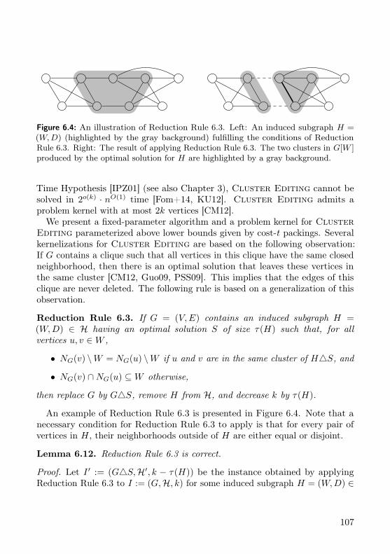
Figure 6.4: An illustration of Reduction Rule 6.3. Left: An induced subgraph H =(W,D) (highlighted by the gray background) fulfilling the conditions of ReductionRule 6.3. Right: The result of applying Reduction Rule 6.3. The two clusters in G[W ]produced by the optimal solution for H are highlighted by a gray background.
Time Hypothesis [IPZ01] (see also Chapter 3), Cluster Editing cannot besolved in 2o(k) · nO(1) time [Fom+14, KU12]. Cluster Editing admits aproblem kernel with at most 2k vertices [CM12].We present a fixed-parameter algorithm and a problem kernel for Cluster
Editing parameterized above lower bounds given by cost-t packings. Severalkernelizations for Cluster Editing are based on the following observation:If G contains a clique such that all vertices in this clique have the same closedneighborhood, then there is an optimal solution that leaves these vertices inthe same cluster [CM12, Guo09, PSS09]. This implies that the edges of thisclique are never deleted. The following rule is based on a generalization of thisobservation.
Reduction Rule 6.3. If G = (V,E) contains an induced subgraph H =(W,D) ∈ H having an optimal solution S of size τ(H) such that, for allvertices u, v ∈W ,
• NG(v) \W = NG(u) \W if u and v are in the same cluster of H4S, and
• NG(v) ∩NG(u) ⊆W otherwise,
then replace G by G4S, remove H from H, and decrease k by τ(H).
An example of Reduction Rule 6.3 is presented in Figure 6.4. Note that anecessary condition for Reduction Rule 6.3 to apply is that for every pair ofvertices in H, their neighborhoods outside of H are either equal or disjoint.
Lemma 6.12. Reduction Rule 6.3 is correct.
Proof. Let I ′ := (G4S,H′, k − τ(H)) be the instance obtained by applyingReduction Rule 6.3 to I := (G,H, k) for some induced subgraph H = (W,D) ∈
107
H of G = (V,E). If I ′ is a yes-instance, then so is I: If there is a solution S′ ofsize at most k − τ(H) for G4S, then S∗ := (S \ S′) ∪ (S′ \ S) is a solution ofsize at most k for G since G4S∗ = (G4S)4S′. It remains to prove that if I isa yes-instance, then so is I ′. To this end, we show that (G,H, k) has an optimalsolution S′ such that S ⊆ S′.Let S∗ be an optimal solution for G, and denote by G∗ := G4S∗ the
cluster graph produced by S∗. We show how to transform S∗ into an optimalsolution S′ containing S. For convenience, let X := V \W and consider thepartition S∗ = S∗X ·∪S∗XW ·∪S∗W , where
• S∗X := u, v ∈ S∗ | u, v ∈ X contains all edge modifications outsideof H,
• S∗XW := u, v ∈ S∗ | u ∈ X ∧ v ∈ W contains the edge modificationsbetween H and the rest of G, and
• S∗W := u, v ∈ S∗ | u, v ∈ W contains the edge modifications insideof H.
The new solution S′ will also contain the edge modifications S∗X . Moreover, theedge modifications S∗W will be replaced by S. It remains to replace S∗XW by asuitable set of edge modifications between H and the rest of G. The idea is totreat all vertices of H with the same neighborhood in X equally.Let Wext be the vertices of W that have at least one neighbor in X and
let Wint := W \ Wext. We define the following equivalence relation ∼ ⊆Wext×Wext: Two vertices u, v ∈Wext are equivalent with respect to ∼ (denotedu ∼ v) if and only if NG(u) ∩X = NG(v) ∩X. For u ∈ Wext, let [u] := v ∈Wext | u ∼ v denote the equivalence class of u with respect to ∼. Fix withineach equivalence class of ∼ an arbitrary vertex that is incident to a minimumnumber of edge modifications in S∗XW and, for each vertex u ∈ Wext, denotethe fixed vertex of [u] by u. Furthermore, for each cluster K of G∗ containingvertices of X and of Wext, fix an arbitrary vertex of K ∩Wext that has in G amaximum number of neighbors in K ∩X; denote this vertex by uK . Finally, calla vertex u ∈ Wext good if there exists a cluster K of G∗ such that [u] = [uK ],that is, uK ∈ [u] (note that if u is good, then all vertices in [u] are good andhave the maximum number of neighbors in K ∩X).
108
Now, consider the edge modification set S′ := S∗X ∪ S ∪ S, where
S :=u, v | u ∈Wext is good and u, v ∈ S∗XW
∪
u, v | u ∈Wext is not good and v ∈ (NG(u) ∩X).
Intuitively, the modifications in S are such that u determines how to treat allvertices in the equivalence class [u]. If u is good, then all vertices in [u] aretreated like u in S∗XW . Otherwise, all edges between vertices in [u] and X in Gare deleted (that is, are contained in S).We first show that S′ is a solution, that is, G′ := G4S′ is a cluster graph.
Clearly, G′[X] = G[X]4S∗X = G∗[X] is a cluster graph and G′[W ] = H4S is acluster graph. It remains to show that every connected component of G′ thatcontains vertices of W and X is a clique. We first show that such a connectedcomponent does not contain any vertex of Wint. To see this, note that thereare no edges between Wint and X in G. Also, no edges between Wint and Xare added by S. By the first condition on S in Reduction Rule 6.3, no clusterof H4S contains vertices from Wint and from Wext. This implies that theconnected component of each vertex u ∈ Wint in G′ is completely containedin Wint. Hence, it remains to consider connected components of G′ containinga vertex u ∈Wext that is connected to some vertices in X. By the conditions ofReduction Rule 6.3, the equivalence class [u] is a cluster in H4S. If u is notgood, then u is not adjacent to any vertex of X in G′. Thus, u is good (that is,all vertices in [u] are good). Then, all vertices of [u] are adjacent to all verticesof exactly one cluster in G′[X] only and not to any other vertex in X. Hence,the connected component of u in G′ is a clique. Altogether this shows that G′is a cluster graph.
It remains to show that |S′| ≤ |S∗|. First, S∗X is a subset of both S∗ and S′.Second, |S| ≤ |S∗W | since S is an optimal solution for H. Thus, it remainsto show |S| ≤ |S∗XW |. Since the vertices of Wint are not incident to any edgemodifications in S, it suffices to prove this inequality by showing, for eachvertex u ∈Wext, that
|e ∈ S | u ∈ e| ≤ |e ∈ S∗XW | u ∈ e|.
If u is good, then the number of edge modifications incident with u in S isthe same as the number of edge modifications incident with u in S∗XW . By thechoice of u, this number is at most the number of edge modifications incidentwith u in S∗XW and the above inequality holds.
109
Otherwise, all edges between u and X are deleted by S, that is, u is incidentto |NG(u)∩X| edge deletions in S. Let K denote the cluster in G∗ containing u.If K contains only vertices in Wext, then u is also incident to |NG(u) ∩X| edgedeletions in S∗XW . Otherwise, since u is not good, there is a vertex w ∈ (K∩Wext)that is not in [u] such that w has at least as many neighbors in K ∩X as u.Since w 6∈ [u] (that is, w 6∼ u), it follows that NG(u)∩X 6= NG(w)∩X. By theconditions of Reduction Rule 6.3, it follows that (NG(u)∩X)∩(NG(w)∩X) = ∅.Since w has at least as many neighbors in K ∩X as u, this means that
|NG(u) ∩K ∩X| ≤ |K ∩X|/2.
Now, observe that S∗XW contains an edge insertion between u and each vertexin (K ∩X) \NG(u). Thus, at least |K ∩X|/2 edges between u and K ∩X areinserted by S∗XW . Moreover, S∗XW contains an edge deletion between u andeach vertex in NG(u) ∩ (X \K). Altogether, this implies
|e ∈ S∗Xw | u ∈ e| ≥ |K ∩X|/2 + |NG(u) ∩ (X \K)|≥ |NG(u) ∩K ∩X|+ |NG(u) ∩ (X \K)|= |NG(u) ∩X| = |e ∈ S | u ∈ e|.
It remains to analyze the running time for applying Reduction Rule 6.3.Let Γ(G, k) be the fastest running time for computing a P3-free editing set ofsize at most k in a graph G if it exists. Here, we assume that Γ is monotonicallynondecreasing in k and polynomial in the size of G. Currently, O(1.62k+|V (G)|+|E(G)|) is the best known upper bound for Γ(G, k) [Böc12, Theorem 2].
Lemma 6.13. In O(m+∑H∈H Γ(H, t)) time, we can apply Reduction Rule 6.3
to all graphs in H.
Proof. We first show that the rule can be applied in O(|W |+∑w∈W degG(w) +
Γ(H, t)) time to an arbitrary graph H = (W,D) ∈ H. For convenience, let X :=V \W .
First, observe that a necessary condition for the rule is that, for each pair ofvertices u and v in H, their neighborhoods in X are the same or disjoint. Thiscan be checked in O(|W |+
∑w∈W degG(w)) time as follows. First, build the
bipartite graph
B := (W ∪ (NG(W ) \W ), u, v ∈ E(G) | u ∈W, v ∈ (NG(W ) \W )).
110
The graph B is a disjoint union of complete bipartite graphs if and onlyif the above necessary condition is fulfilled. Thus, we check in O(|W | +∑w∈W degG(w)) time whether B is a disjoint union of complete bipartite
graphs. If not, then the rule does not apply. Otherwise, we compute inO(|W |+
∑w∈W degG(w)) time the groups of vertices of W whose neighborhood
is the same in B. Afterwards, we can check in O(1) time whether u and vhave the same neighborhood in X in G by checking whether they belong to thesame group. We now compute the set S′ of edge modifications that is alreadydetermined by the conditions of Reduction Rule 6.3: If v and w are nonadjacentand have the same nonempty neighborhood in X, then the edge v, w needsto be inserted and is thus added to S′. Similarly, if v and w are adjacent andhave different neighborhoods in X, then v, w needs to be deleted and is thusadded to S′. Observe that if S′ is a subset of an optimal solution S for H,then |S′| ≤ |D|. Hence, at most |D| edges are added to S′. Since we alreadycomputed the groups of vertices that have the same or disjoint neighborhoods,we can thus compute S′ in O(|W |+ |D|) time.
Let Wext denote the vertices of W that have at least one neighbor in Xand let Wint := W \Wext. Note that after applying the edge modificationsin S′, that is, in H4S′, the induced subgraph (H4S′)[Wext] is a cluster graphand there are no edges between Wext and Wint in H4S′. Thus, to determinewhether S′ can be extended to an optimal solution S for H that fulfills theconditions of Reduction Rule 6.3 we compute an optimal solution of H[Wint]in Γ(H [Wint], τ(H)−|S′|) time. Since |H[Wint]| ≤ |H| and τ(H)−|S′| ≤ t, thiscan be done in Γ(H, t) time. The size of the resulting solution S is compared withthe size of an optimal solution of H , which can also be computed in Γ(H, t) time.It remains to show that Reduction Rule 6.3 can be applied to all packing
subgraphs within the claimed running time. For each graph H = (W,D) ∈ H,we can check in O(|W |+
∑w∈W degG(w) + Γ(H, t)) time whether Reduction
Rule 6.3 applies. If it does, then we can apply the rule in O(|D|) time bymodifying at most |D| edges. Summing up over all graphs in H gives theclaimed running time.
Observe that since k is decreased by τ(H), the parameter ` does not increasewhen Reduction Rule 6.3 is applied. As for the previous problems, applyingthe rule to each H ∈ H is sufficient for upper-bounding k in terms of t and `and thus, for transferring known fixed-parameter tractability results for theparameter k to the combined parameter (t, `).
111
Lemma 6.14. Let (G,H, k) be a yes-instance of Cluster Editing withCost-t Packing such that Reduction Rule 6.3 does not apply to any H ∈ H.Then, k ≤ (2t+ 1)`.
Proof. Since the instance is reduced with respect to Reduction Rule 6.3, foreach H = (W,D) in H and each size-τ(H) solution S for H, either the verticesof some cluster have different neighborhoods in V \W or two vertices of twodistinct clusters have a common neighbor outside of W .Now, fix an arbitrary optimal solution S for G. By the observation above,
there are the following two possibilities for how S modifies each H ∈ H:
(a) more than τ(H) vertex pairs of H are modified by S, or
(b) at least one external vertex pair for H is modified.
Therefore, S fulfills the condition of Lemma 6.1 and thus k ≤ (2t+ 1)`.
Theorem 6.15. Let Γ(G, k) be the fastest running time for computing a P3-freeediting set of size at most k in a graph G if it exists. Then, Cluster Editingwith Cost-t Packing
(i) is solvable in O(Γ(G, (2t+ 1)`) + nm+∑H∈H Γ(H, t)) time and
(ii) admits a problem kernel with at most (4t + 2)` vertices, which can becomputed in O(nm+
∑H∈H Γ(H, t)) time.
Proof. (ii) First, apply Reduction Rule 6.3 exhaustively in O(m+∑H∈H Γ(H, t))
time. Then, by Lemma 6.14, we can either return a trivial constant-size no-instance or have k ≤ (2t + 1)`. In the latter case, we apply a kernelizationalgorithm for Cluster Editing to the instance (G, k) (that is, without H),which produces, in O(nm) time, a problem kernel (G′, k′) with at most 2k ≤(4t + 2)` vertices and with k′ ≤ k [CM12]. Adding an empty packing givesan equivalent instance (G′, ∅, k′) with parameter `′ = k′ of Cluster Editingwith Cost-t Packing.
(i) First, apply the kernelization. Then, by Lemma 6.14, we can either return“no” or have k ≤ (2t + 1)`. We can now apply the algorithm for ClusterEditing that runs in Γ(G, (2t+ 1)`) time.
By plugging in the best known bound for Γ(G, k), we obtain the following.
Corollary 6.16. Cluster Editing with Cost-t Packing
112
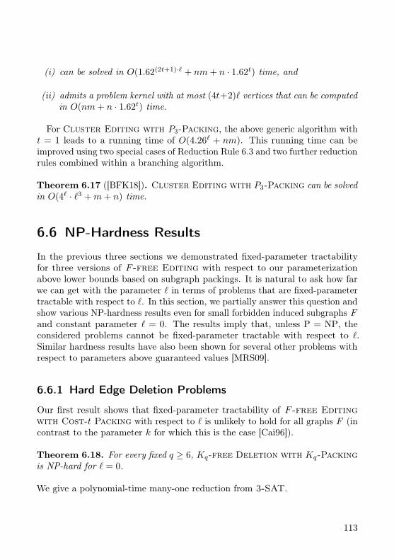
(i) can be solved in O(1.62(2t+1)·` + nm+ n · 1.62t) time, and
(ii) admits a problem kernel with at most (4t+2)` vertices that can be computedin O(nm+ n · 1.62t) time.
For Cluster Editing with P3-Packing, the above generic algorithm witht = 1 leads to a running time of O(4.26` + nm). This running time can beimproved using two special cases of Reduction Rule 6.3 and two further reductionrules combined within a branching algorithm.
Theorem 6.17 ([BFK18]). Cluster Editing with P3-Packing can be solvedin O(4` · `3 +m+ n) time.
6.6 NP-Hardness Results
In the previous three sections we demonstrated fixed-parameter tractabilityfor three versions of F -free Editing with respect to our parameterizationabove lower bounds based on subgraph packings. It is natural to ask how farwe can get with the parameter ` in terms of problems that are fixed-parametertractable with respect to `. In this section, we partially answer this question andshow various NP-hardness results even for small forbidden induced subgraphs Fand constant parameter ` = 0. The results imply that, unless P = NP, theconsidered problems cannot be fixed-parameter tractable with respect to `.Similar hardness results have also been shown for several other problems withrespect to parameters above guaranteed values [MRS09].
6.6.1 Hard Edge Deletion Problems
Our first result shows that fixed-parameter tractability of F -free Editingwith Cost-t Packing with respect to ` is unlikely to hold for all graphs F (incontrast to the parameter k for which this is the case [Cai96]).
Theorem 6.18. For every fixed q ≥ 6, Kq-free Deletion with Kq-Packingis NP-hard for ` = 0.
We give a polynomial-time many-one reduction from 3-SAT.
113
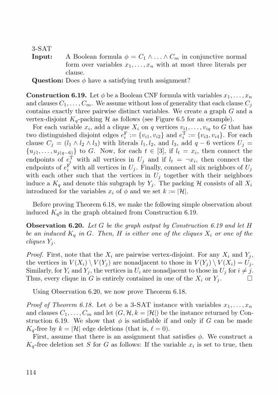
3-SATInput: A Boolean formula φ = C1 ∧ . . . ∧ Cm in conjunctive normal
form over variables x1, . . . , xn with at most three literals perclause.
Question: Does φ have a satisfying truth assignment?
Construction 6.19. Let φ be a Boolean CNF formula with variables x1, . . . , xnand clauses C1, . . . , Cm. We assume without loss of generality that each clause Cjcontains exactly three pairwise distinct variables. We create a graph G and avertex-disjoint Kq-packing H as follows (see Figure 6.5 for an example).
For each variable xi, add a clique Xi on q vertices vi1, . . . , viq to G that hastwo distinguished disjoint edges eFi := vi1, vi2 and eTi := vi3, vi4. For eachclause Cj = (l1 ∧ l2 ∧ l3) with literals l1, l2, and l3, add q − 6 vertices Uj =uj1, . . . , uj(q−6) to G. Now, for each t ∈ [3], if lt = xi, then connect theendpoints of eTi with all vertices in Uj and if lt = ¬xi, then connect theendpoints of eFi with all vertices in Uj . Finally, connect all six neighbors of Ujwith each other such that the vertices in Uj together with their neighborsinduce a Kq and denote this subgraph by Yj . The packing H consists of all Xi
introduced for the variables xi of φ and we set k := |H|.
Before proving Theorem 6.18, we make the following simple observation aboutinduced Kqs in the graph obtained from Construction 6.19.
Observation 6.20. Let G be the graph output by Construction 6.19 and let Hbe an induced Kq in G. Then, H is either one of the cliques Xi or one of thecliques Yj.
Proof. First, note that the Xi are pairwise vertex-disjoint. For any Xi and Yj ,the vertices in V (Xi) \ V (Yj) are nonadjacent to those in V (Yj) \ V (Xi) = Uj .Similarly, for Yi and Yj , the vertices in Ui are nonadjacent to those in Uj for i 6= j.Thus, every clique in G is entirely contained in one of the Xi or Yj .
Using Observation 6.20, we now prove Theorem 6.18.
Proof of Theorem 6.18. Let φ be a 3-SAT instance with variables x1, . . . , xnand clauses C1, . . . , Cm and let (G,H, k = |H|) be the instance returned by Con-struction 6.19. We show that φ is satisfiable if and only if G can be madeKq-free by k = |H| edge deletions (that is, ` = 0).First, assume that there is an assignment that satisfies φ. We construct a
Kq-free deletion set S for G as follows: If the variable xi is set to true, then
114
X1
eF1
eT1 X2
eF2
eT2
X3
eF3 eT3
Figure 6.5: An illustration of Construction 6.19 for q = 6. The gray rectangles depictthe vertex-disjoint packing K6s X1, X2, and X3 (for simplicity only two edges areshown inside each packing K6). The K6 containing the edges eF1 , eF2 , and eT3 isdenoted Yj and encodes the clause Cj = (¬x1 ∨ ¬x2 ∨ x3).
add the edge eTi to S. If the variable xi is set to false, then add eFi to S.Thus, for each Xi, we add exactly one edge to S. Since H consists of the Xi,we have |S| = |H|. Moreover, since each clause Cj contains a true literal, atleast one edge of each Yj is contained in S. Thus, G \ S is Kq-free, since, byObservation 6.20, the only Kqs in G are the Xi and Yj and, for each of them,S contains at least one edge.Now, assume that G can be made Kq-free by deleting a set S of |H| edges.
Then, S deletes exactly one edge of each Xi and at least one edge of each Yj .We can assume without loss of generality that S contains for each Xi either theedge eTi or the edge eFi since deleting one of these edges instead of another edgein Xi always yields a solution by construction. Thus, the edge deletion set Scorresponds to a truth assignment that satisfies φ.
Let us briefly discuss why it is not possible to apply our framework (thatis, use Lemma 6.1 to derive k ≤ (2t+ 1)`) for the case F = K6. In fact, it isindeed possible to formulate a data reduction rule for K6-free Deletion withK6-Packing analogous to Reduction Rule 6.1 for the triangle case. However,
115
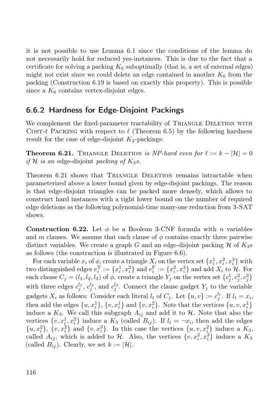
it is not possible to use Lemma 6.1 since the conditions of the lemma donot necessarily hold for reduced yes-instances. This is due to the fact that acertificate for solving a packing K6 suboptimally (that is, a set of external edges)might not exist since we could delete an edge contained in another K6 from thepacking (Construction 6.19 is based on exactly this property). This is possiblesince a K6 contains vertex-disjoint edges.
6.6.2 Hardness for Edge-Disjoint Packings
We complement the fixed-parameter tractability of Triangle Deletion withCost-t Packing with respect to ` (Theorem 6.5) by the following hardnessresult for the case of edge-disjoint K3-packings:
Theorem 6.21. Triangle Deletion is NP-hard even for ` := k − |H| = 0if H is an edge-disjoint packing of K3s.
Theorem 6.21 shows that Triangle Deletion remains intractable whenparameterized above a lower bound given by edge-disjoint packings. The reasonis that edge-disjoint triangles can be packed more densely, which allows toconstruct hard instances with a tight lower bound on the number of requirededge deletions as the following polynomial-time many-one reduction from 3-SATshows.
Construction 6.22. Let φ be a Boolean 3-CNF formula with n variablesand m clauses. We assume that each clause of φ contains exactly three pairwisedistinct variables. We create a graph G and an edge-disjoint packing H of K3sas follows (the construction is illustrated in Figure 6.6).
For each variable xi of φ, create a triangleXi on the vertex set x1i , x
2i , x
3i with
two distinguished edges eTi := x1i , x
2i and eFi := x2
i , x3i and add Xi to H. For
each clause Cj = (l1, l2, l3) of φ, create a triangle Yj on the vertex set c1j , c2j , c3jwith three edges cl1j , c
l2j , and c
l3j . Connect the clause gadget Yj to the variable
gadgets Xi as follows: Consider each literal lt of Cj . Let u, v := cltj . If lt = xi,then add the edges u, x1
i , v, x1i and v, x2
i . Note that the vertices u, v, x1i
induce a K3. We call this subgraph Aij and add it to H. Note that also thevertices v, x1
i , x2i induce a K3 (called Bij). If lt = ¬xi, then add the edges
u, x2i , v, x2
i and v, x3i . In this case the vertices u, v, x2
i induce a K3,called Aij , which is added to H. Also, the vertices v, x2
i , x3i induce a K3
(called Bij). Clearly, we set k := |H|.
116
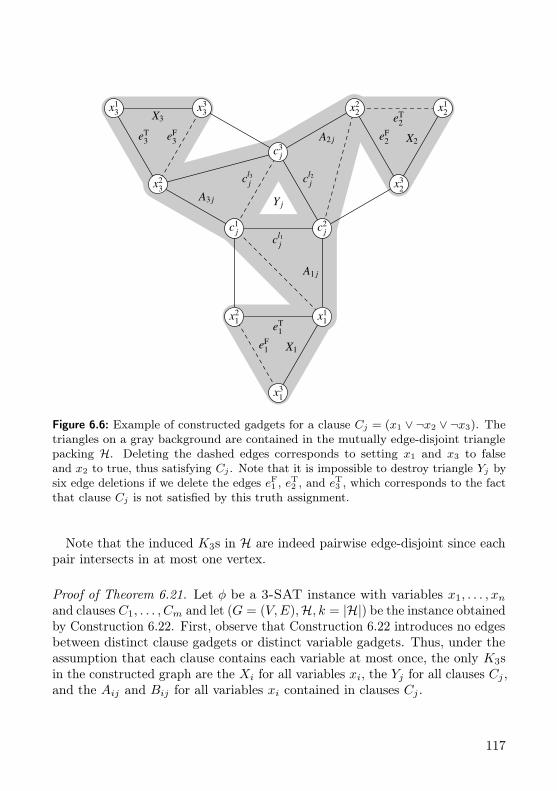
eF1
eT1
eT2
eF2eT
3 eF3
X1
X2
X3
A1 j
A2 j
A3 j
cl1j
cl2jcl3
j
Y j
c1j c2
j
c3j
x11x2
1
x31
x22
x32
x12
x23
x33x1
3
Figure 6.6: Example of constructed gadgets for a clause Cj = (x1 ∨ ¬x2 ∨ ¬x3). Thetriangles on a gray background are contained in the mutually edge-disjoint trianglepacking H. Deleting the dashed edges corresponds to setting x1 and x3 to falseand x2 to true, thus satisfying Cj . Note that it is impossible to destroy triangle Yj bysix edge deletions if we delete the edges eF1 , eT2 , and eT3 , which corresponds to the factthat clause Cj is not satisfied by this truth assignment.
Note that the induced K3s in H are indeed pairwise edge-disjoint since eachpair intersects in at most one vertex.
Proof of Theorem 6.21. Let φ be a 3-SAT instance with variables x1, . . . , xnand clauses C1, . . . , Cm and let (G = (V,E),H, k = |H|) be the instance obtainedby Construction 6.22. First, observe that Construction 6.22 introduces no edgesbetween distinct clause gadgets or distinct variable gadgets. Thus, under theassumption that each clause contains each variable at most once, the only K3sin the constructed graph are the Xi for all variables xi, the Yj for all clauses Cj ,and the Aij and Bij for all variables xi contained in clauses Cj .
117
Now, assume that φ allows for a satisfying truth assignment. We constructa set S of edges of size |H| such that G′ := (V,E \ S) is K3-free. For eachvariable xi that is true, add eTi to S. For each variable xi that is false, addeFi to S. By this choice, each Xi is destroyed in G′. Additionally, for eachclause Cj and its true literals l ∈ xi,¬xi, Bij is destroyed. To destroy Aij ,we add to S the edge of Aij shared with Yj , which also destroys the triangle Yj .For each false literal l ∈ xi,¬xi, we destroy both Bij and Aij by adding to Sthe shared edge of Aij and Bij .
Conversely, assume that there is a set S of size |H| such that G′ = (V,E \ S)is K3-free. We construct a satisfying truth assignment for φ. First, observethat, since the K3s in H are pairwise edge-disjoint, S contains exactly one edgeof each K3 in H. Thus, for each Xi, at most one of the two edges eFi and eTi iscontained in S. The set S contains at least one edge e of each Yj . This edge isshared with an Aij . Since Aij ∈ H and S already contains the edge e of Aij , itfollows that S does not contain the edge shared by Aij and Bij . Since Bij /∈ H,the set S has to contain an edge of Bij shared with another K3 in H. If theclause Cj contains xi, then the only such edge is eTi and we set xi to true. Ifthe clause Cj contains ¬ei, then the only such edge is eFi and we set xi to false.In both cases, clause Cj is satisfied. Since at most one of eTi and eFi is in S, thevalue of each variable xi is well-defined.
6.6.3 Hard Vertex Deletion Problems
In contrast to the previous sections, we consider vertex deletions in this section.We show that the vertex deletion variant (that is, F -Free Vertex Deletion)is an even harder problem than the edge editing variant. Concretely, we proveNP-hardness of the problem of destroying all induced paths Pq on q ≥ 3 verticesby at most |H| vertex deletions if a packing H of vertex-disjoint induced Pqs inthe input graph G is provided as input.
Pq-free Vertex Deletion with Pq-PackingInput: A graph G = (V,E), a vertex-disjoint packing H of induced Pqs,
and a natural number k.Question: Is there a vertex subset S ⊆ V of size at most k such thatG[V \S]
does not contain a Pq as an induced subgraph?
The following theorem implies that P3-Free Vertex Deletion with P3-Packing parameterized by ` := k − |H| is presumably not in XP which is
118
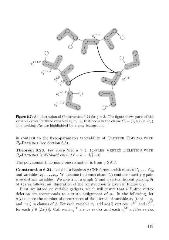
vj−1,Ti
vj−1,Fi
vj,Ti
vj,Fi
vj+1,Ti
vj+1,Fi
vj′,Tr
vj′′,Fs
Figure 6.7: An illustration of Construction 6.24 for q = 3. The figure shows parts of thevariable cycles for three variables xi, xr, xs that occur in the clause Ct = (xi∨xr∨¬xs).The packing P3s are highlighted by a gray background.
in contrast to the fixed-paramater tractability of Cluster Editing withP3-Packing (see Section 6.5).
Theorem 6.23. For every fixed q ≥ 3, Pq-free Vertex Deletion withPq-Packing is NP-hard even if ` = k − |H| = 0.
The polynomial-time many-one reduction is from q-SAT.
Construction 6.24. Let φ be a Boolean q-CNF formula with clauses C1, . . . , Cmand variables x1, . . . , xn. We assume that each clause Cj contains exactly q pair-wise distinct variables. We construct a graph G and a vertex-disjoint packing Hof Pqs as follows; an illustration of the construction is given in Figure 6.7.First, we introduce variable gadgets, which will ensure that a Pq-free vertex
deletion set corresponds to a truth assignment of φ. In the following, letα(i) denote the number of occurrences of the literals of variable xi (that is, xiand ¬xi) in clauses of φ. For each variable xi, add 4α(i) vertices: vj,Ti and vj,Fi ,for each j ∈ [2α(i)]. Call each vj,Ti a true vertex and each vj,Fi a false vertex.
119
Create an induced cycle on the true and false vertices of variable xi by addingthe edge set
Ei :=vj,Ti , vj,Fi | j ∈ [2α(i)]
∪vj,Fi , vj+1,T
i | j ∈ [2α(i)− 1]∪
v2α(i),Fi , v1,T
i .
We call this cycle the variable cycle of xi.Then, for each even j ∈ [2α(i)], attach to vj,Ti and vj,Fi an induced Pq−2 each.
These paths are called the attachment paths of the j-th segment of the variablecycle of xi.Now, for each variable xi, assign to each clause Ct containing xi or ¬xi a
unique number p ∈ [α(i)]. Consider the number j = 2p − 1. We will usevertex vj,Ti or vj,Fi to build the clause gadget for clause Ct. If Ct containsthe literal xi, then attach an induced Pq−2 to vj,Fi . Otherwise, attach aninduced Pq−2 to vj,Ti . As before, call the path the attachment path of the j-thsegment of the cycle. Now, let γti := vj,Ti if Ct contains xi, and let γti := vj,Fiif Ct contains ¬xi. Call these vertices the literal vertices of clause Ct and denotetheir set by Πt. The construction of G is completed as follows. For each Πt,add an arbitrary set of edges to G such that G[Πt] is an induced Pq. The Pq-packing H contains for each variable xi an induced Pq for every segment of thevariable cycle of xi: for each j ∈ [2α(i)], choose an (arbitrary) attachment path(a Pq−2) plus the two segment vertices vj,Fi and vj,Ti . Note that the packing Pqsare clearly vertex-disjoint by construction. We set k := |H|.
Proof of Theorem 6.23. Let φ be a q-SAT instance with variables x1, . . . , xnand clauses C1, . . . , Cm and let (G = (V,E),H, k = |H|) be the instance obtainedby Construction 6.24. We show that φ has a satisfying truth assignment if andonly if G can be made Pq-free by exactly |H| vertex deletions (that is, ` = 0).Assume that φ has a satisfying truth assignment. For each true variable xi
in this assignment, delete all true vertices in its variable gadget, that is, vj,Tifor j ∈ [2α(i)]. For each false variable xi in this assignment, delete all falsevertices in its variable gadget, that is, vj,Fi for j ∈ [2α(i)]. Denote this vertexset by S and observe that |S| = |H|. Moreover, observe that each vertex on thevariable cycle for xi is either deleted or both of its neighbors on the cycle aredeleted. Every induced Pq in G contains at least one vertex from a variable cycleas the attachment paths are too short to induce Pqs. Thus, to show Pq-freeness
120
of G[V \ S] it is sufficient to show that no vertex from a variable cycle is in aninduced Pq.Consider an undeleted vertex in the variable cycle for xi. Assume, without
loss of generality, that this is a true vertex vj,Ti . If j is even, then vj,Ti is not inan induced Pq as its neighbors on the cycle (which are false vertices) are deletedand its only other neighbor is in an attachment path with only q − 2 vertices.If j is odd and the clause Ct corresponding to the j-th segment of the cyclecontains ¬xi, then the only neighbor of vj,Ti in G[V \S] is in an attachment path.It remains to show that vj,Ti is not in an induced Pq if Ct contains xi. The onlyneighbors of vj,Ti in G[V \S] are in Πt. Observe that G[Πt] is an induced Pq andthat, in G[V \ S], every vertex on this path is deleted or its neighbors in V \Πt
are deleted. Hence, the connected component of G[V \ S] containing vj,Ti isan induced subgraph of G[Πt]. Since the assignment is satisfying, at least onevertex of Πt is deleted. Thus, this connected component has at most q − 1vertices and does not contain a Pq.
Conversely, let S ⊆ V be a size-|H| vertex set such that G[V \ S] is Pq-free.First, observe that, without loss of generality, for each variable cycle eitherall true or all false vertices are deleted: No vertex in an attachment path Pis deleted since it is also a solution to delete the vertex in the variable cyclethat has a neighbor in P instead. Hence, at least one vertex of each segmentis deleted since, otherwise, one of the Pqs in H is not destroyed. This alreadyrequires |H| vertex deletions and thus exactly one vertex for each segment of eachvariable cycle is deleted. Finally, by construction, every adjacent pair of verticesin the variable cycle forms a Pq with some attachment path. Consequently, oneof the two vertices is deleted, which implies that either every even or every oddvertex of the cycle is deleted.
Hence, the vertex deletions in the variable cycle define a truth assignmentfor x1, . . . , xn: If all true vertices of the variable cycle of xi are deleted, thenset xi to true; otherwise, set xi to false. This assignment is satisfying: SinceG[V \ S] is Pq-free, for each clause Ct, at least one vertex γti of Πt is deleted.Without loss of generality, let γti = vj,Ti , that is, Ct contains the literal xi. Then,xi is true and clause Ct is satisfied.
121
Theorem 6.23 easily implies an NP-hardness result for the generalization ofVertex Cover to d-uniform hypergraphs:
d-Uniform Hitting Set with PackingInput: A hypergraph H = (V,E) with |e| = d for all e ∈ E, a setH ⊆ E
of pairwise vertex-disjoint hyperedges, and an integer k.Question: Is there a vertex set V ′ ⊆ V of size at most k such that ∀e ∈
E : V ′ ∩ e 6= ∅?
An instance (G,H, k) of Pq-free Vertex Deletion with Pq-Packing caneasily be transformed in polynomial time into an equivalent instance (H,H, k)of q-Uniform Hitting Set with Packing by taking the hypergraph H onthe same vertex set as G having a hyperedge e if and only if G[e] is a Pq. Thepacking H and the integer k remain unchanged, and so does `. Thus, we obtainthe following corollary:
Corollary 6.25. For every d ≥ 3, d-Uniform Hitting Set with Packingis NP-hard even if ` = 0.
Corollary 6.25 shows that the known above-guarantee fixed-parameter algorithmsfor Vertex Cover [Cyg+13, GP16, Lok+14, RO09] do not generalize to d-Uniform Hitting Set.
6.7 Conclusion
In this chapter, we introduced a novel parameterization of F -free Editingabove a given lower bound derived from a packing of subgraphs and developeda framework for showing fixed-parameter tractability. The basic idea is to applypolynomial-time data reduction to the packing subgraphs such that for theresulting instance the number of edge modifications is upper-bounded by theparameter. We showed that the framework can be applied to three data-sciencerelated variants of F -free Editing. Our obtained algorithms are potentiallyfast in practice due to a smaller parameter value than the overall number ofedge modifications. Moreover, since our framework allows to use the fastestknown algorithms with respect to the number of edge modifications, existingimplementations can be used.
There are several open questions to discuss. First of all, the running times ofour algorithms (especially the search tree algorithms for Cluster Editing and
122
Triangle Deletion) could be improved. Maybe more importantly, it is opento determine the complexity of Cluster Editing and Feedback Arc Set inTournaments parameterized above a lower bound of edge-disjoint packings offorbidden induced subgraphs.It is open to extend our framework to further edge modification problems.
The most natural candidates appear to be F -free Editing variants wherethe forbidden induced subgraph F has four vertices. Examples are CographEditing [Liu+12] which is the problem of destroying all induced P4s, K4-freeEditing, Claw-free Editing, and Diamond-free Deletion [Fel+11, SS15].Finding other editing problems on directed graphs for our framework is alsointeresting.
Furthermore, it would be nice to obtain more general theorems separating thetractable from the hard cases of forbidden subgraphs F for this parameterization.For example, the reduction from 3-SAT in Theorem 6.18 essentially relies onthe fact that the graph F contains a matching of size three. Maybe it is possibleto prove a complexity dichotomy based on the matching number of F .On the practical side, our framework offers an interesting tradeoff between
running time and power of generic data reduction rules (this is similar to akernelization scheme by Hüffner et al. [HKN15]). Exploring such tradeoffs (usingthe maximum cost t of the packing subgraphs as adjusting screw) might be arewarding topic for future research. For example, an interesting question toanswer empirically is how much the value of ` can be decreased by increasing tin practice. Our generic data reduction rules are suited for implementation andsubsequent experiments to evaluate their effectiveness. Such a project includesfurther challenges, for example, computing an appropriate packing of inducedsubgraphs efficiently. A concrete subproblem could be formulated as follows:Given t, find an induced subgraph with editing cost t such that a data reductionrule is applicable. The question whether this problem can be solved efficientlyis interesting from a practical as well as from a theoretical perspective.
Finally, parameterizing above a lower bound is a promising approach to obtainefficient algorithms which should also be explored for non-graph problems, forexample, feature selection as studied in Chapter 4.
123

Chapter 7
Dynamic Time Warping
In previous chapters we already studied clustering problems on matrices (Chap-ter 5) and on graphs (Chapter 6). In this chapter, we study a problem fromtime series analysis which is fundamental for clustering time series. In particu-lar, we consider the problem of computing a mean series of a given sample ofseries in dynamic time warping spaces. Dynamic time warping is a distancemeasure between time series and constitutes a major tool for analyzing timeseries. Averaging time series under dynamic warping distance is a challengingcomputational problem, so far solved by several heuristics. Our contributionscomprise a (seemingly first) exact exponential-time algorithm for computinga mean (showing that the problem is in XP with respect to the number ofinput time series, that is, for a constant number of input time series, the prob-lem is polynomial-time solvable). Moreover, we give an exact polynomial-timealgorithm for the special case of (arbitrarily many) binary time series.
7.1 Introduction
The mean of a random variable is a fundamental statistical concept withmany applications in pattern recognition and data mining. The mean is wellunderstood in Euclidean spaces, but can become obscure in non-metric spaces.An important class of non-metric spaces are dynamic time warping spaces. Timeseries such as acoustic signals, electrocardiograms, and internet traffic dataare time-dependent observations that vary in length and temporal dynamics.Given a sample of time series, to filter out such variations, a major directionof time series averaging is based on using dynamic time warping (dtw) asdistance measure between time series. Computing a mean of time series withrespect to the dynamic time warping distance is a fundamental problem arising
125

in the context of nearest neighbor classifiers and centroid-based clusteringalgorithms [HNF08, Mor+18, Pet+16, SDG16].
One way to pose time series averaging as an optimization problem is as follows[CB17, HNF08, PKG11, SDG16, SJ18]: Suppose that X =
(x(1), . . . , x(k)
)is a
sample of k time series (numerical sequences of arbitrary finite lengths). Thena (Fréchet) mean (with respect to dynamic time warping) is any time series zthat minimizes the Fréchet function [Fré48] (of the sample X )
F (z) =1
k
k∑i=1
(dtw
(z, x(i)
))2
,
where dtw(x, y) denotes the dynamic time warping distance between the timeseries x and y. We refer to the problem of minimizing F over the set of all timeseries of finite length as the DTW-Mean problem. Note that if we consideronly time series from the Euclidean space Rn and we replace the dtw-distanceby the Euclidean norm ‖ · ‖2 in the definition of the Fréchet function, then thesolution z simply is the Euclidean mean. For arbitrary time series (of differentlengths), however, one cannot apply the Euclidean distance.Dynamic time warping has been introduced to deal with this scenario (see
Section 7.2 for a formal definition). Intuitively, in order to measure the similaritybetween two time series of different lengths, dynamic time warping allows tostretch the time series non-uniformly such that the resulting “warped” seriesalign well in terms of some cost function. Hence, a mean of a sample of timeseries with respect to dynamic time warping is a time series that can be alignedwell to each sample time series (on average). Figure 7.1 shows an illustratingexample.
Related Work. It is known that solutions for DTW-Mean are guaranteedto exist, but are not unique in general [SJ18]. Polynomial-time algorithms forDTW-Mean are unknown. Until recently [BFN18], it was not known to beNP-hard (though NP-hardness of related problems is mentioned in the litera-ture [HNF08, Pet+16, PG17]). Some exponential-time algorithms have beenproposed to optimally solve DTW-Mean [HNF08, PG12, PKG11], however,without proving their correctness or running times. Several heuristics have beendevised to approximately solve DTW-Mean [CB17, PKG11, SJ18] (withoutany guarantee on the quality of the solution). They are based on prespecifyingthe length of feasible solutions without any knowledge about whether an optimalsolution of this length exists. In summary, both the computational complexity of
126
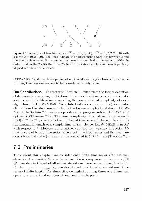
x(1) 0 2 1 1 0
x(2) 0 2 2 2 1 0
z 0 2 1 0
Figure 7.1: A sample of two time series x(1) = (0, 2, 1, 1, 0), x(2) = (0, 2, 2, 2, 1, 0) witha mean z = (0, 2, 1, 0). The lines indicate the corresponding warpings between z andthe sample time series. For example, the mean z is stretched at the second position inorder to align the 2 with the three 2’s in x(2). In this example, the mean is perfectlyaligned with both time series.
DTW-Mean and the development of nontrivial exact algorithms with provablerunning time guarantees are to be considered widely open.
Our Contributions. To start with, Section 7.2 introduces the formal definitionof dynamic time warping. In Section 7.3, we briefly discuss several problematicstatements in the literature concerning the computational complexity of exactalgorithms for DTW-Mean. We refute (with a counterexample) some falseclaims from the literature and clarify the known complexity status of DTW-Mean. In Section 7.4, we develop a dynamic program solving DTW-Meanoptimally (Theorem 7.2). The time complexity of our dynamic program isin O(n2k+1 · k2k), where k is the number of time series in the sample and n isthe maximum length of a sample time series. Hence, DTW-Mean is in XPwith respect to k. Moreover, as a further contribution, we show in Section 7.5that in case of binary time series (where both the input series and the mean areover a binary alphabet) a mean can be computed in O(kn3) time (Theorem 7.3).
7.2 PreliminariesThroughout this chapter, we consider only finite time series with rationalelements. A univariate time series of length n is a sequence x = (x1, . . . , xn) ∈Qn. We denote the set of all univariate rational time series of length n by Tn.Furthermore, T =
⋃n∈N Tn denotes the set of all univariate rational time
series of finite length. For simplicity, we neglect running times of arithmeticaloperations on rational numbers throughout this chapter.
127
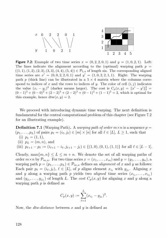
x 0 2 2 0 1
y 1 0 2 11
12
2
3
3
4
4
5
Figure 7.2: Example of two time series x = (0, 2, 2, 0, 1) and y = (1, 0, 2, 1). Left:The lines indicate the alignment according to the (optimal) warping path p =((1, 1), (1, 2), (2, 3), (3, 3), (4, 4), (5, 4)) ∈ P5,4 of length six. The corresponding alignedtime series are x′ = (0, 0, 2, 2, 0, 1) and y′ = (1, 0, 2, 2, 1, 1). Right: The warpingpath p (thick line) can be illustrated in a 5 × 4 matrix where the columns corre-spond to indices of x and the rows to indices of y. The color of cell (i, j) indicatesthe value (xi − yj)
2 (darker means larger). The cost is Cp(x, y) = ‖x′ − y′‖22 =(0− 1)2 + (0− 0)2 + (2− 2)2 + (2− 2)2 + (0− 1)2 + (1− 1)2 = 2, which is optimal forthis example, hence dtw(x, y) = 2.
We proceed with introducing dynamic time warping. The next definition isfundamental for the central computational problem of this chapter (see Figure 7.2for an illustrating example).
Definition 7.1 (Warping Path). A warping path of order m×n is a sequence p =(p1, . . . , pL) of pairs p` = (i`, j`) ∈ [m]× [n] for all ` ∈ [L], L ≥ 1, such that(i) p1 = (1, 1),(ii) pL = (m,n), and(iii) p`+1 − p` := (i`+1 − i`, j`+1 − j`) ∈ (1, 0), (0, 1), (1, 1) for all ` ∈ [L− 1].
Clearly, maxm,n ≤ L ≤ m + n. We denote the set of all warping paths oforderm×n by Pm,n. For two time series x = (x1, . . . , xm) and y = (y1, . . . , yn), awarping path p = (p1, . . . , pL) ∈ Pm,n defines an alignment of x and y as follows:Each pair p` = (i`, j`), ` ∈ [L], of p aligns element xi` with yj` . Aligning xand y along a warping path p yields two aligned time series (xi1 , . . . , xiL)and (yj1 , . . . , yjL) of length L. The cost Cp(x, y) for aligning x and y along awarping path p is defined as
Cp(x, y) :=
L∑`=1
(xi` − yj`)2.
Now, the dtw-distance between x and y is defined as
128
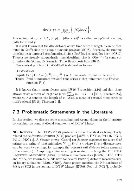
dtw(x, y) := minp∈Pm,n
√Cp(x, y)
.
A warping path p with Cp(x, y) = (dtw(x, y))2 is called an optimal warping
path for x and y.It is well-known that the dtw-distance of two time series of length n can be com-
puted in O(n2) time by a simple dynamic program [SC78]. Recently, the runningtime has been improved to subquadratic time O(n2 log log log n/ log log n) [GS17].There is no strongly subquadratic-time algorithm (that is, O(n2−ε) for some ε >0) unless the Strong Exponential Time Hypothesis fails [BK15].
Our central problem DTW-Mean is defined as follows.
DTW-MeanInput: Sample X =
(x(1), . . . , x(k)
)of k univariate rational time series.
Task: Find a univariate rational time series z that minimizes the Fréchetfunction F (z).
It is known that a mean always exists [JS16, Proposition 2.10] and that therealways exists a mean of length at most
∑ki=1 ni − 2(k − 1) [JS16, Theorem 2.7],
where ni ≥ 2 denotes the length of xi. Also, a mean of rational time series isitself rational [SJ18, Theorem 3.3].
7.3 Problematic Statements in the Literature
In this section, we discuss some misleading and wrong claims in the literatureconcerning the computational complexity of DTW-Mean.
NP-Hardness. The DTW-Mean problem is often described as being closelyrelated to the Steiner String (STS) problem [ASW15, HNF08, Pet+16, PG12,PG17, PKG11]. A Steiner string [Gus97] (or Steiner sequence) for a set S ofstrings is a string s∗ that minimizes
∑s∈S D(s∗, s), where D is a distance mea-
sure between two strings, for example the weighted edit distance (often assumedto be a metric). Computing a Steiner string is related to solving the MultipleSequence Alignment (MSA) problem in bioinformatics [Gus97]. Both, STSand MSA, are known to be NP-hard for several (metric) distance measures evenon binary alphabets [BD01, NR05]. Some papers mention the NP-hardness ofMSA or STS in the context of DTW-Mean [HNF08, Pet+16, PG17], probably
129
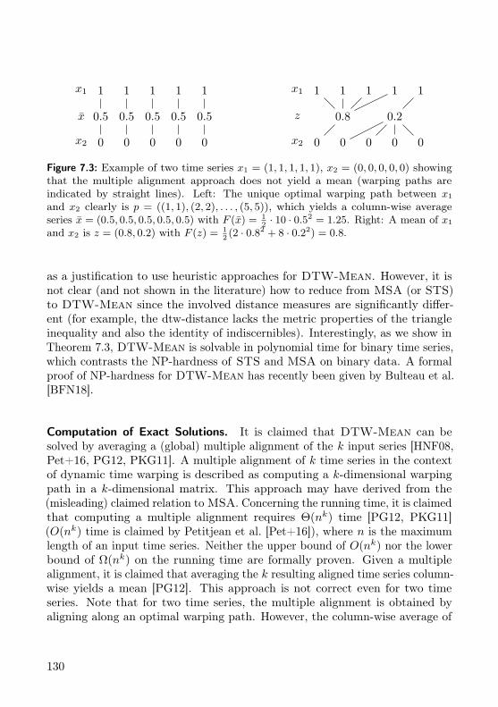
x1 1 1 1 1 1
x2 0 0 0 0 0
x 0.5 0.5 0.5 0.5 0.5
x1 1 1 1 1 1
x2 0 0 0 0 0
z 0.8 0.2
Figure 7.3: Example of two time series x1 = (1, 1, 1, 1, 1), x2 = (0, 0, 0, 0, 0) showingthat the multiple alignment approach does not yield a mean (warping paths areindicated by straight lines). Left: The unique optimal warping path between x1and x2 clearly is p = ((1, 1), (2, 2), . . . , (5, 5)), which yields a column-wise averageseries x = (0.5, 0.5, 0.5, 0.5, 0.5) with F (x) = 1
2· 10 · 0.52 = 1.25. Right: A mean of x1
and x2 is z = (0.8, 0.2) with F (z) = 12(2 · 0.82 + 8 · 0.22) = 0.8.
as a justification to use heuristic approaches for DTW-Mean. However, it isnot clear (and not shown in the literature) how to reduce from MSA (or STS)to DTW-Mean since the involved distance measures are significantly differ-ent (for example, the dtw-distance lacks the metric properties of the triangleinequality and also the identity of indiscernibles). Interestingly, as we show inTheorem 7.3, DTW-Mean is solvable in polynomial time for binary time series,which contrasts the NP-hardness of STS and MSA on binary data. A formalproof of NP-hardness for DTW-Mean has recently been given by Bulteau et al.[BFN18].
Computation of Exact Solutions. It is claimed that DTW-Mean can besolved by averaging a (global) multiple alignment of the k input series [HNF08,Pet+16, PG12, PKG11]. A multiple alignment of k time series in the contextof dynamic time warping is described as computing a k-dimensional warpingpath in a k-dimensional matrix. This approach may have derived from the(misleading) claimed relation to MSA. Concerning the running time, it is claimedthat computing a multiple alignment requires Θ(nk) time [PG12, PKG11](O(nk) time is claimed by Petitjean et al. [Pet+16]), where n is the maximumlength of an input time series. Neither the upper bound of O(nk) nor the lowerbound of Ω(nk) on the running time are formally proven. Given a multiplealignment, it is claimed that averaging the k resulting aligned time series column-wise yields a mean [PG12]. This approach is not correct even for two timeseries. Note that for two time series, the multiple alignment is obtained byaligning along an optimal warping path. However, the column-wise average of
130
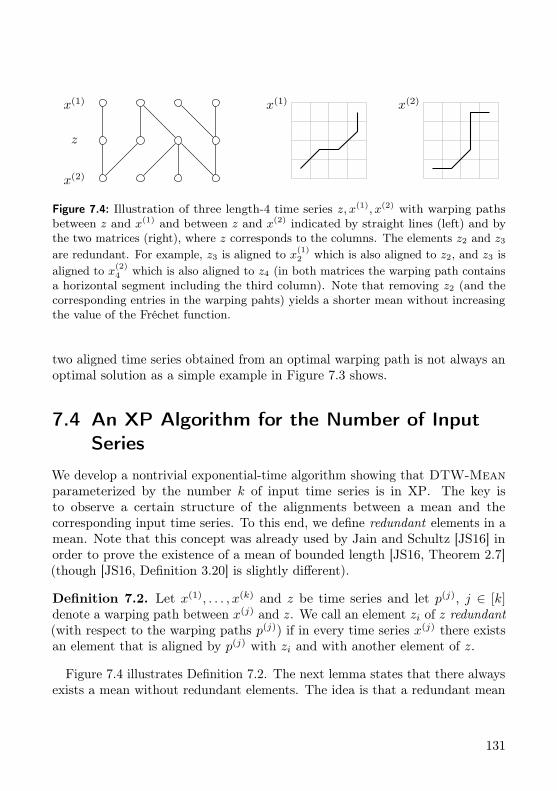
x(1)
z
x(2)
x(1) x(2)
Figure 7.4: Illustration of three length-4 time series z, x(1), x(2) with warping pathsbetween z and x(1) and between z and x(2) indicated by straight lines (left) and bythe two matrices (right), where z corresponds to the columns. The elements z2 and z3are redundant. For example, z3 is aligned to x(1)2 which is also aligned to z2, and z3 isaligned to x(2)4 which is also aligned to z4 (in both matrices the warping path containsa horizontal segment including the third column). Note that removing z2 (and thecorresponding entries in the warping pahts) yields a shorter mean without increasingthe value of the Fréchet function.
two aligned time series obtained from an optimal warping path is not always anoptimal solution as a simple example in Figure 7.3 shows.
7.4 An XP Algorithm for the Number of InputSeries
We develop a nontrivial exponential-time algorithm showing that DTW-Meanparameterized by the number k of input time series is in XP. The key isto observe a certain structure of the alignments between a mean and thecorresponding input time series. To this end, we define redundant elements in amean. Note that this concept was already used by Jain and Schultz [JS16] inorder to prove the existence of a mean of bounded length [JS16, Theorem 2.7](though [JS16, Definition 3.20] is slightly different).
Definition 7.2. Let x(1), . . . , x(k) and z be time series and let p(j), j ∈ [k]denote a warping path between x(j) and z. We call an element zi of z redundant(with respect to the warping paths p(j)) if in every time series x(j) there existsan element that is aligned by p(j) with zi and with another element of z.
Figure 7.4 illustrates Definition 7.2. The next lemma states that there alwaysexists a mean without redundant elements. The idea is that a redundant mean
131
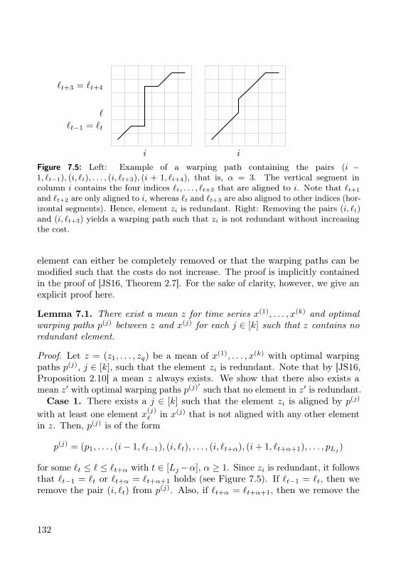
i
`t−1 = `t
`
`t+3 = `t+4
i
Figure 7.5: Left: Example of a warping path containing the pairs (i −1, `t−1), (i, `t), . . . , (i, `t+3), (i + 1, `t+4), that is, α = 3. The vertical segment incolumn i contains the four indices `t, . . . , `t+3 that are aligned to i. Note that `t+1
and `t+2 are only aligned to i, whereas `t and `t+3 are also aligned to other indices (hor-izontal segments). Hence, element zi is redundant. Right: Removing the pairs (i, `t)and (i, `t+3) yields a warping path such that zi is not redundant without increasingthe cost.
element can either be completely removed or that the warping paths can bemodified such that the costs do not increase. The proof is implicitly containedin the proof of [JS16, Theorem 2.7]. For the sake of clarity, however, we give anexplicit proof here.
Lemma 7.1. There exist a mean z for time series x(1), . . . , x(k) and optimalwarping paths p(j) between z and x(j) for each j ∈ [k] such that z contains noredundant element.
Proof. Let z = (z1, . . . , zq) be a mean of x(1), . . . , x(k) with optimal warpingpaths p(j), j ∈ [k], such that the element zi is redundant. Note that by [JS16,Proposition 2.10] a mean z always exists. We show that there also exists amean z′ with optimal warping paths p(j)′ such that no element in z′ is redundant.Case 1. There exists a j ∈ [k] such that the element zi is aligned by p(j)
with at least one element x(j)` in x(j) that is not aligned with any other element
in z. Then, p(j) is of the form
p(j) = (p1, . . . , (i− 1, `t−1), (i, `t), . . . , (i, `t+α), (i+ 1, `t+α+1), . . . , pLj )
for some `t ≤ ` ≤ `t+α with t ∈ [Lj −α], α ≥ 1. Since zi is redundant, it followsthat `t−1 = `t or `t+α = `t+α+1 holds (see Figure 7.5). If `t−1 = `t, then weremove the pair (i, `t) from p(j). Also, if `t+α = `t+α+1, then we remove the
132
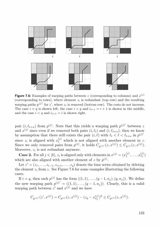
i i i
Figure 7.6: Examples of warping paths between z (corresponding to columns) and x(j)
(corresponding to rows), where element zi is redundant (top row) and the resultingwarping paths p(j)
′for z′, where zi is removed (bottom row). The costs do not increase.
The case i = q is shown left, the case i < q and it+1 = i+ 1 is shown in the middle,and the case i < q and it+1 = i is shown right.
pair (i, `t+α) from p(j). Note that this yields a warping path p(j)′ between zand x(j) since even if we removed both pairs (i, `t) and (i, `t+α), then we knowby assumption that there still exists the pair (i, `) with `t < ` < `t+α in p(j)′
since zi is aligned with x(j)` which is not aligned with another element in z.
Since we only removed pairs from p(j), it holds Cp(j)′ (z, x(j)) ≤ Cp(j)(z, x
(j)).Moreover, zi is not redundant anymore.Case 2. For all j ∈ [k], zi is aligned only with elements in x(j) = (x
(j)1 , . . . , x
(j)nj )
which are also aligned with another element of z by p(j).Let z′ = (z1, . . . , zi−1, zi+1, . . . , zq) denote the time series obtained by deleting
the element zi from z. See Figure 7.6 for some examples illustrating the followingcases.
If i = q, then each p(j) has the form ((1, 1), . . . , (q− 1, nj), (q, nj)). We definethe new warping path p(j)′ = ((1, 1), . . . , (q − 1, nj)). Clearly, this is a validwarping path between z′ and x(j) and we have
Cp(j)′ (z′, x(j)) = Cp(j)(z, x
(j))− (zq − x(j)nj )2 ≤ Cp(j)(z, x(j)).
133
Hence, z′ is a mean with less redundant elements.If i ∈ [q − 1], then consider a warping path p(j) = (p1, . . . , pLj ) and let pt =
(it, `t), t ∈ [Lj − 1] be the first pair such that it = i.If it+1 = i + 1, then `t = `t−1 or `t = `t+1 holds (or both). We define the
new warping path p(j)′ = (p1, . . . , pt−1, (it+1− 1, `t+1), . . . , (iLj − 1, `Lj )). Notethat p(j)′ is a warping path between z′ and x(j) since it+1−1−it−1 = i−(i−1) = 1and `t+1 − `t−1 ≤ 1. The cost is
Cp(j)′ (z′, x(j)) = Cp(j)(z, x
(j))− (zi − x(j)`t
)2 ≤ Cp(j)(z, x(j)).
Hence, z′ is a mean with less redundant elements.If it+1 = i, then it follows 1 < t < Lj − 1 and `t−1 = `t = `t+1 − 1 = `t+2 − 1
and it+2 = i + 1. We define the warping path p(j)′ = (p1, . . . , pt−1, (it+2 −1, `t+2), . . . , (iLj − 1, `Lj )). Clearly, p(j)′ is a warping path between z′ and x(j)
since (it+2 − 1, `t+2)− (it−1, `t−1) = (1, 1). The cost is
Cp(j)′ (z′, x(j)) = Cp(j)(z, x
(j))− (zi − x(j)`t
)2 − (zi − x(j)`t+1
)2 ≤ Cp(j)(z, x(j)),
that is, z′ is a mean with less redundant elements.In both cases above, we reduced the number of redundant elements. In Case 1,
we found another warping path (by removing horizontal segments in the picture)such that zi is not redundant. In Case 2, we removed element zi and constructednew warping paths (by cutting out horizontal segments in the picture). Hence,we can repeat the above arguments until we obtain a mean z′ without redundantelements.
Lemma 7.1 allows us to devise a dynamic program to compute a mean. Thegeneral scheme behind the dynamic program is to test all possibilities to alignthe last mean element to elements from the input time series while recursivelyadding an optimal solution for the remaining non-aligned elements in the inputtime series. The fact that we can assume the last mean element not to beredundant is crucial for this recursive approach, which is described in the proofof the following theorem.
Theorem 7.2. DTW-Mean for k input time series is solvable in O(n2k+12kk)time, where n is the maximum length of all input time series.
Proof. Assume for simplicity that all time series have length n (the general casecan be solved analogously). We find a mean using a dynamic programming
134
approach. Let C be a k-dimensional table, where for all (i1, . . . , ik) ∈ [n]k, wedefine
C[i1, . . . , ik] = minz∈T
1
k
k∑j=1
(dtw(z, (x
(j)1 , . . . , x
(j)ij
)))2
,
that is, C[i1, . . . , ik] is the value F (z) of the Fréchet function of a mean z forthe subseries (x
(1)1 , . . . , x
(1)i1
), . . . , (x(k)1 , . . . , x
(k)ik
). Clearly, C[n, . . . , n] yields theoptimal value F (z) of the input instance.For i1 = i2 = . . . = ik = 1, it is clear that there exists a mean z containing
just one element and each optimal warping path between z and (x(j)1 ) trivially
equals ((1, 1)). Since it can be shown [SJ18, Theorem 3.3] that, given optimalwarping paths, each element of a mean equals the arithmetic mean of all elementsin all time series that are aligned to this element, we initialize
µ = 1/k
k∑j=1
x(j)1 , C[1, . . . , 1] =
1
k
k∑j=1
(x(j)1 − µ)2.
Note that the corresponding mean is z = (µ).For the case that ij > 1 holds for at least one j ∈ [k], we can assume by
Lemma 7.1 that there exist a mean z for (x(1)1 , . . . , x
(1)i1
), . . . , (x(k)1 , . . . , x
(k)ik
) andoptimal warping paths p(j) between z and (x
(j)1 , . . . , x
(j)ij
) such that z contains noredundant elements. Let zq be the last element of z. Then, for each j ∈ [k], zqis aligned by p(j) with some elements x(j)
`j, . . . , x
(j)ij
for `j ∈ [ij ]. Again, zq is thearithmetic mean of all elements in all time series with which it is aligned [SJ18,Theorem 3.3]. Hence, the contribution of zq to F (z) can easily be determined(see the formula for σ(`1, . . . , `k) below).
Now, consider the case that there exists another element zq−1 in z. Clearly,for each j ∈ [k], zq−1 is aligned only to elements with indices at most `jsince otherwise the warping path conditions are violated. Hence, the remain-ing part of F (z) can be obtained recursively from a mean of the time se-ries (x
(1)1 , . . . , x
(1)`1
), . . . , (x(k)1 , . . . , x
(k)`k
). Recall, however, that we assumed znot to contain any redundant element. It follows that zq−1 cannot be alignedwith x(j)
`jfor all j ∈ [k] since zq is already aligned with each x
(j)`j
. Therefore,we add the minimum value C[`′1, . . . , `
′k] over all `′j ∈ max(1, `j − 1), `j such
that `′j = `j − 1 holds for at least one j ∈ [k].
135
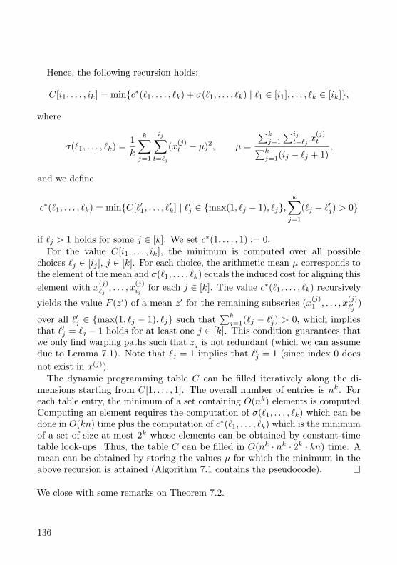
Hence, the following recursion holds:
C[i1, . . . , ik] = minc∗(`1, . . . , `k) + σ(`1, . . . , `k) | `1 ∈ [i1], . . . , `k ∈ [ik],
where
σ(`1, . . . , `k) =1
k
k∑j=1
ij∑t=`j
(x(j)t − µ)2, µ =
∑kj=1
∑ijt=`j
x(j)t∑k
j=1(ij − `j + 1),
and we define
c∗(`1, . . . , `k) = minC[`′1, . . . , `′k] | `′j ∈ max(1, `j − 1), `j,
k∑j=1
(`j − `′j) > 0
if `j > 1 holds for some j ∈ [k]. We set c∗(1, . . . , 1) := 0.For the value C[i1, . . . , ik], the minimum is computed over all possible
choices `j ∈ [ij ], j ∈ [k]. For each choice, the arithmetic mean µ corresponds tothe element of the mean and σ(`1, . . . , `k) equals the induced cost for aligning thiselement with x(j)
`j, . . . , x
(j)ij
for each j ∈ [k]. The value c∗(`1, . . . , `k) recursively
yields the value F (z′) of a mean z′ for the remaining subseries (x(j)1 , . . . , x
(j)`′j
)
over all `′j ∈ max(1, `j − 1), `j such that∑kj=1(`j − `′j) > 0, which implies
that `′j = `j − 1 holds for at least one j ∈ [k]. This condition guarantees thatwe only find warping paths such that zq is not redundant (which we can assumedue to Lemma 7.1). Note that `j = 1 implies that `′j = 1 (since index 0 doesnot exist in x(j)).The dynamic programming table C can be filled iteratively along the di-
mensions starting from C[1, . . . , 1]. The overall number of entries is nk. Foreach table entry, the minimum of a set containing O(nk) elements is computed.Computing an element requires the computation of σ(`1, . . . , `k) which can bedone in O(kn) time plus the computation of c∗(`1, . . . , `k) which is the minimumof a set of size at most 2k whose elements can be obtained by constant-timetable look-ups. Thus, the table C can be filled in O(nk · nk · 2k · kn) time. Amean can be obtained by storing the values µ for which the minimum in theabove recursion is attained (Algorithm 7.1 contains the pseudocode).
We close with some remarks on Theorem 7.2.
136
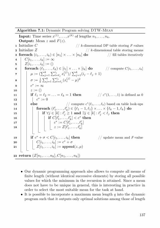
Algorithm 7.1: Dynamic Program solving DTW-Mean
Input: Time series x(1), . . . , x(k) of lengths n1, . . . , nk.Output: Mean z and F (z).
1 Initialize C // k-dimensional DP table storing F -values2 Initialize Z // k-dimensional table storing means3 foreach (i1, . . . , ik) ∈ [n1]× . . .× [nk] do // fill tables iteratively4 C[i1, . . . , ik] :=∞5 Z[i1, . . . , ik] := ()6 foreach (`1, . . . , `k) ∈ [i1]× . . .× [ik] do // compute C[i1, . . . , ik]
7 µ := (∑kj=1
∑ijt=`j
x(j)t )/
∑kj=1(ij − `j + 1)
8 σ := 1k
∑kj=1
∑ijt=`j
(x(j)t − µ)2
9 c∗ :=∞10 z := ()11 if `1 = `2 = . . . = `k = 1 then // c∗(1, . . . , 1) is defined as 012 c∗ := 013 else // compute c∗(`1, . . . , `k) based on table look-ups14 foreach (`′1, . . . , `
′k) ∈ `1 − 1, `1 × . . .× `k − 1, `k do
15 if ∀j ∈ [k] : `′j ≥ 1 and ∃j ∈ [k] : `′j < `j then16 if C[`′1, . . . , `
′k] < c∗ then
17 c∗ := C[`′1, . . . , `′k]
18 z := Z[`′1, . . . , `′k]
19 if c∗ + σ < C[i1, . . . , ik] then // update mean and F -value20 C[i1, . . . , ik] := c∗ + σ21 Z[i1, . . . , ik] := append(z, µ)
22 return (Z[n1, . . . , nk], C[n1, . . . , nk])
• Our dynamic programming approach also allows to compute all means offinite length (without identical successive elements) by storing all possiblevalues for which the minimum in the recursion is attained. Since a meandoes not have to be unique in general, this is interesting in practice inorder to select the most suitable mean for the task at hand.• It is possible to incorporate a maximum mean length q into the dynamic
program such that it outputs only optimal solutions among those of length
137
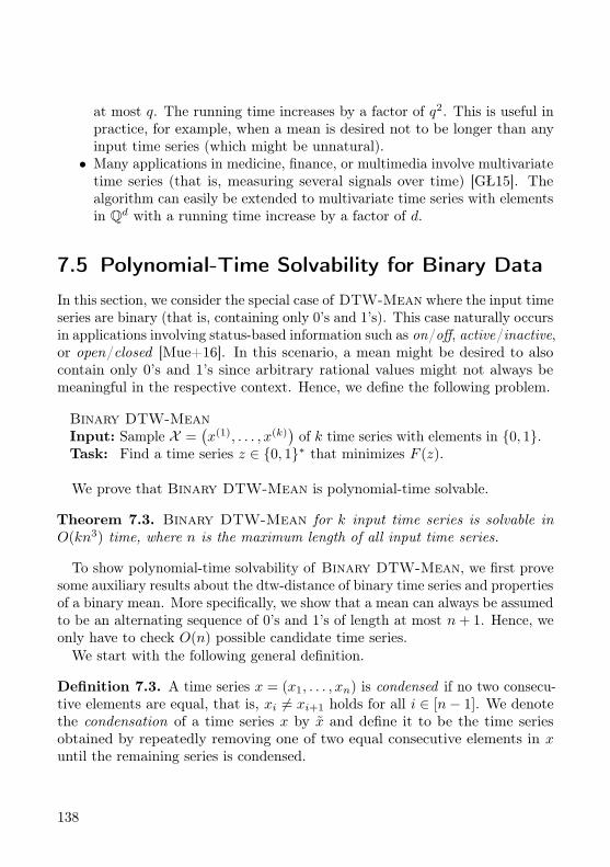
at most q. The running time increases by a factor of q2. This is useful inpractice, for example, when a mean is desired not to be longer than anyinput time series (which might be unnatural).• Many applications in medicine, finance, or multimedia involve multivariatetime series (that is, measuring several signals over time) [GŁ15]. Thealgorithm can easily be extended to multivariate time series with elementsin Qd with a running time increase by a factor of d.
7.5 Polynomial-Time Solvability for Binary Data
In this section, we consider the special case of DTW-Mean where the input timeseries are binary (that is, containing only 0’s and 1’s). This case naturally occursin applications involving status-based information such as on/off, active/inactive,or open/closed [Mue+16]. In this scenario, a mean might be desired to alsocontain only 0’s and 1’s since arbitrary rational values might not always bemeaningful in the respective context. Hence, we define the following problem.
Binary DTW-MeanInput: Sample X =
(x(1), . . . , x(k)
)of k time series with elements in 0, 1.
Task: Find a time series z ∈ 0, 1∗ that minimizes F (z).
We prove that Binary DTW-Mean is polynomial-time solvable.
Theorem 7.3. Binary DTW-Mean for k input time series is solvable inO(kn3) time, where n is the maximum length of all input time series.
To show polynomial-time solvability of Binary DTW-Mean, we first provesome auxiliary results about the dtw-distance of binary time series and propertiesof a binary mean. More specifically, we show that a mean can always be assumedto be an alternating sequence of 0’s and 1’s of length at most n+ 1. Hence, weonly have to check O(n) possible candidate time series.
We start with the following general definition.
Definition 7.3. A time series x = (x1, . . . , xn) is condensed if no two consecu-tive elements are equal, that is, xi 6= xi+1 holds for all i ∈ [n− 1]. We denotethe condensation of a time series x by x and define it to be the time seriesobtained by repeatedly removing one of two equal consecutive elements in xuntil the remaining series is condensed.
138
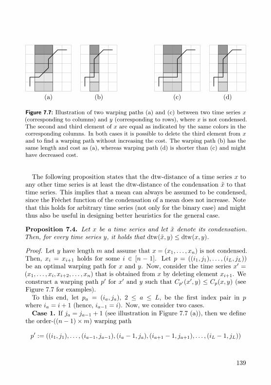
(a) (b) (c) (d)
Figure 7.7: Illustration of two warping paths (a) and (c) between two time series x(corresponding to columns) and y (corresponding to rows), where x is not condensed.The second and third element of x are equal as indicated by the same colors in thecorresponding columns. In both cases it is possible to delete the third element from xand to find a warping path without increasing the cost. The warping path (b) has thesame length and cost as (a), whereas warping path (d) is shorter than (c) and mighthave decreased cost.
The following proposition states that the dtw-distance of a time series x toany other time series is at least the dtw-distance of the condensation x to thattime series. This implies that a mean can always be assumed to be condensed,since the Fréchet function of the condensation of a mean does not increase. Notethat this holds for arbitrary time series (not only for the binary case) and mightthus also be useful in designing better heuristics for the general case.
Proposition 7.4. Let x be a time series and let x denote its condensation.Then, for every time series y, it holds that dtw(x, y) ≤ dtw(x, y).
Proof. Let y have length m and assume that x = (x1, . . . , xn) is not condensed.Then, xi = xi+1 holds for some i ∈ [n − 1]. Let p = ((i1, j1), . . . , (iL, jL))be an optimal warping path for x and y. Now, consider the time series x′ =(x1, . . . , xi, xi+2, . . . , xn) that is obtained from x by deleting element xi+1. Weconstruct a warping path p′ for x′ and y such that Cp′(x′, y) ≤ Cp(x, y) (seeFigure 7.7 for examples).To this end, let pa = (ia, ja), 2 ≤ a ≤ L, be the first index pair in p
where ia = i+ 1 (hence, ia−1 = i). Now, we consider two cases.Case 1. If ja = ja−1 + 1 (see illustration in Figure 7.7 (a)), then we define
the order-((n− 1)×m) warping path
p′ := ((i1, j1), . . . , (ia−1, ja−1), (ia − 1, ja), (ia+1 − 1, ja+1), . . . , (iL − 1, jL))
139
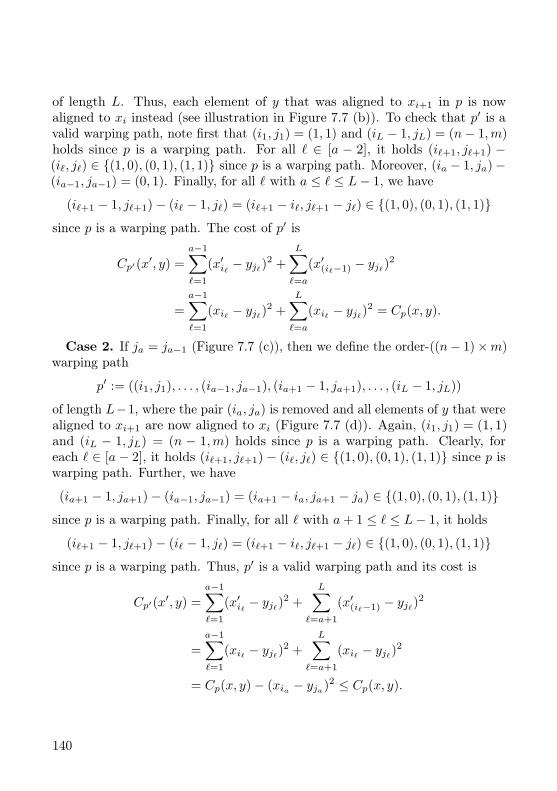
of length L. Thus, each element of y that was aligned to xi+1 in p is nowaligned to xi instead (see illustration in Figure 7.7 (b)). To check that p′ is avalid warping path, note first that (i1, j1) = (1, 1) and (iL − 1, jL) = (n− 1,m)holds since p is a warping path. For all ` ∈ [a − 2], it holds (i`+1, j`+1) −(i`, j`) ∈ (1, 0), (0, 1), (1, 1) since p is a warping path. Moreover, (ia − 1, ja)−(ia−1, ja−1) = (0, 1). Finally, for all ` with a ≤ ` ≤ L− 1, we have
(i`+1 − 1, j`+1)− (i` − 1, j`) = (i`+1 − i`, j`+1 − j`) ∈ (1, 0), (0, 1), (1, 1)
since p is a warping path. The cost of p′ is
Cp′(x′, y) =
a−1∑`=1
(x′i` − yj`)2 +
L∑`=a
(x′(i`−1) − yj`)2
=
a−1∑`=1
(xi` − yj`)2 +
L∑`=a
(xi` − yj`)2 = Cp(x, y).
Case 2. If ja = ja−1 (Figure 7.7 (c)), then we define the order-((n− 1)×m)warping path
p′ := ((i1, j1), . . . , (ia−1, ja−1), (ia+1 − 1, ja+1), . . . , (iL − 1, jL))
of length L−1, where the pair (ia, ja) is removed and all elements of y that werealigned to xi+1 are now aligned to xi (Figure 7.7 (d)). Again, (i1, j1) = (1, 1)and (iL − 1, jL) = (n − 1,m) holds since p is a warping path. Clearly, foreach ` ∈ [a− 2], it holds (i`+1, j`+1)− (i`, j`) ∈ (1, 0), (0, 1), (1, 1) since p iswarping path. Further, we have
(ia+1 − 1, ja+1)− (ia−1, ja−1) = (ia+1 − ia, ja+1 − ja) ∈ (1, 0), (0, 1), (1, 1)
since p is a warping path. Finally, for all ` with a+ 1 ≤ ` ≤ L− 1, it holds
(i`+1 − 1, j`+1)− (i` − 1, j`) = (i`+1 − i`, j`+1 − j`) ∈ (1, 0), (0, 1), (1, 1)
since p is a warping path. Thus, p′ is a valid warping path and its cost is
Cp′(x′, y) =
a−1∑`=1
(x′i` − yj`)2 +
L∑`=a+1
(x′(i`−1) − yj`)2
=
a−1∑`=1
(xi` − yj`)2 +
L∑`=a+1
(xi` − yj`)2
= Cp(x, y)− (xia − yja)2 ≤ Cp(x, y).
140
Figure 7.8: Examples of warping paths having the cost claimed in Lemma 7.5 for thethree cases of binary condensed time series x and y. Gray cells in a matrix indicateindex pairs (i, j) with (xi − yj)2 = 1. The case x1 = y1 is depicted left. The otherexamples depict the case that x1 6= y1. The case that x and y have equal length isshown in the middle. Note that the shown warping paths are optimal since in eachcase every warping path contains at least two gray cells.
Since in both cases above, the cost does not increase, we obtain
dtw(x′, y) ≤ Cp′(x′, y) ≤ Cp(x, y) = dtw(x, y).
Repeating this argument until x′ is condensed finishes the proof.
Proposition 7.4 implies that we can assume a mean to be condensed. Next,we are going to prove an upper bound of n+ 1 on the length of a binary mean.To this end, we analyze the dtw-distances of binary time series. Note that abinary condensed time series is completely determined by its first element andits length. We use this property to give a closed expression for the dtw-distanceof two condensed binary time series.
Lemma 7.5. Let x = (x1, . . . , xn), y = (y1, . . . , ym) ∈ 0, 1∗ be two condensedbinary time series with n ≥ m. Then, it holds that
dtw(x, y)2 =
d(n−m)/2e, x1 = y1
2, x1 6= y1 ∧ n = m
1 + b(n−m)/2c, x1 6= y1 ∧ n > m
.
Proof. We prove the statement by first giving a warping path that has theclaimed cost and second proving that every warping path has at least theclaimed cost.“≤”: We show that there exists a warping path p between x and y that has
the claimed cost (see Figure 7.8 for examples). The warping path p is definedas follows:
141
If x1 = y1, then we have xi = yi for all i ∈ [m] (since x and y are condensedand binary) and we set
p := ((1, 1), (2, 2), . . . , (m,m), (m+ 1,m), . . . , (n,m)).
This warping path has cost Cp(x, y) =∑ni=m+1(xi − ym)2 = d(n−m)/2e.
If x1 6= y1, then we have xi = yi−1 for all 2 ≤ i ≤ m. Thus, for n = m, thewarping path
p := ((1, 1), (2, 1), (3, 2), . . . , (n,m− 1), (n,m))
has cost Cp(x, y) = (x1−y1)2 + (xn−ym)2 = 2, Finally, for n > m, the warpingpath
p := ((1, 1), (2, 1), (3, 2), . . . , (m+ 1,m), (m+ 2,m), . . . , (n,m))
yields cost
Cp(x, y) = (x1 − y1)2 +
m+1∑i=2
(xi − yi−1)2 +
n∑i=m+2
(xi − ym)2
= 1 +
n∑i=m+2
(xi − ym)2 = 1 + d(n−m− 1)/2e = 1 + b(n−m)/2c.
“≥”: We show that every warping path has at least the cost claimed above.Consider an optimal warping path p = (p1, . . . , pL) for x and y and note that,since n ≥ m, there are at least n−m different indices `1, . . . , `n−m with
1 ≤ `1 < . . . < `n−m ≤ L− 1
such that p`t+1 − p`t = (1, 0) for every t ∈ [n −m]. For such an index `t, letp`t+1 = (i, j) and p`t = (i′, j′) with i = i′ + 1 and j = j′. Then, we have
(xi − yj)2 + (xi′ − yj′)2 = (xi − yj)2 + (xi′ − yj)2 = 1
since xi 6= xi′ (recall that x is condensed and binary). Hence, for each t ∈1, . . . , d(n − m)/2e, the index `2t−1 contributes a cost of 1 to the sumof Cp(x, y). Thus, dtw(x, y)2 ≥ d(n−m)/2e.If x1 = y1, then this lower bound matches the claimed cost. If x1 6= y1
and n = m, then also xn 6= ym and hence, every warping path has cost at
142
least 2. Finally, consider the case that x1 6= y1 and n > m. If n − m isodd, then d(n−m)/2e = 1 + b(n−m)/2c and hence, the above lower boundmatches the claimed cost. If n − m is even, then xn 6= ym. Consider theindices `1, . . . , `n−m from above implying the lower bound of d(n − m)/2e.Note that if `1 > 1 or `n−m < L − 1 holds, then Cp(x, y) ≥ d(n −m)/2e + 1holds since (x1 − y1)2 = (xn − ym)2 = 1 (which contributes at least onefurther 1 to the sum Cp(x, y)). This lower bound matches the claimed costs.Otherwise, if 1 = `1 < `2 < . . . < `n−m = L − 1, then each of the indices`1, `3, `5, . . . , `n−m−1, `n−m contributes a cost of 1 to Cp(x, y). Hence, the lowerbound is d(n−m)/2e+ 1 as claimed. This finishes the proof.
Note that according to Lemma 7.5, for a fixed condensed binary time series yof length m, the value dtw(x, y)2 is monotonically increasing in the length of xfor all condensed binary time series x of length n ≥ m+ 1. We use this propertylater in the proof of Lemma 7.7 where we derive an upper bound on the lengthof a binary mean. In order to prove Lemma 7.7, we also need the followinglemma concerning the dtw-distances between condensed and non-condensedtime series.
Lemma 7.6. Let x = (x1, . . . , xn) be a condensed binary time series andlet y = (y1, . . . , ym) ∈ 0, 1∗ with n ≥ m. Then, for the condensation y of y itholds dtw(x, y)2 = dtw(x, y)2.
Proof. Assume that y is not condensed. Then, y consists of ` ∈ [m] blocks,where a block is a maximal subsequence of consecutive 0’s or consecutive 1’s in y.Let m1, . . . ,m` denote the lengths of these blocks where m1 + . . . + m` = m.Note also that y has length ` with ` < m ≤ n. We define a warping path pbetween x and y such that Cp(x, y) = dtw(x, y)2. Note that, by Lemma 7.5, wehave
dtw(x, y)2 =
d(n− `)/2e, x1 = y1
1 + b(n− `)/2c, x1 6= y1
.
The idea is, to extend the optimal warping path between x and y as given inthe proof of Lemma 7.5 (see Figure 7.9).
If x1 = y1, then we set
p := ((1, 1), . . . , (1,m1), (2,m1 + 1), . . . , (2,m1 +m2), . . . ,
(`,m−m` + 1), . . . , (`,m), (`+ 1,m), . . . , (n,m))
and obtain cost Cp(x, y) =∑ni=`+1(xi − ym)2 = d(n− `)/2e.
143
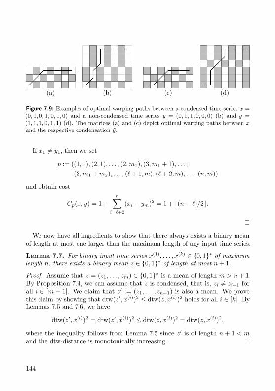
(a) (b) (c) (d)
Figure 7.9: Examples of optimal warping paths between a condensed time series x =(0, 1, 0, 1, 0, 1, 0) and a non-condensed time series y = (0, 1, 1, 0, 0, 0) (b) and y =(1, 1, 1, 0, 1, 1) (d). The matrices (a) and (c) depict optimal warping paths between xand the respective condensation y.
If x1 6= y1, then we set
p := ((1, 1), (2, 1), . . . , (2,m1), (3,m1 + 1), . . . ,
(3,m1 +m2), . . . , (`+ 1,m), (`+ 2,m), . . . , (n,m))
and obtain cost
Cp(x, y) = 1 +
n∑i=`+2
(xi − ym)2 = 1 + b(n− `)/2c.
We now have all ingredients to show that there always exists a binary meanof length at most one larger than the maximum length of any input time series.
Lemma 7.7. For binary input time series x(1), . . . , x(k) ∈ 0, 1∗ of maximumlength n, there exists a binary mean z ∈ 0, 1∗ of length at most n+ 1.
Proof. Assume that z = (z1, . . . , zm) ∈ 0, 1∗ is a mean of length m > n+ 1.By Proposition 7.4, we can assume that z is condensed, that is, zi 6= zi+1 forall i ∈ [m − 1]. We claim that z′ := (z1, . . . , zn+1) is also a mean. We provethis claim by showing that dtw(z′, x(i))2 ≤ dtw(z, x(i))2 holds for all i ∈ [k]. ByLemmas 7.5 and 7.6, we have
dtw(z′, x(i))2 = dtw(z′, x(i))2 ≤ dtw(z, x(i))2 = dtw(z, x(i))2,
where the inequality follows from Lemma 7.5 since z′ is of length n + 1 < mand the dtw-distance is monotonically increasing.
144
Having established that a binary mean is always condensed and of boundedlength, we now show that it can be found in polynomial time.
Proof of Theorem 7.3. By Proposition 7.4 and Lemma 7.7, we can assume thedesired mean z to be a condensed series of length at most n+ 1. Thus, there areat most 2n+ 2 many possible candidates for z. For each candidate z, we cancompute the value F (z) in O(kn2) time and select the one with the smallestvalue. This yields an overall running time in O(kn3).
The proof of Theorem 7.3 relies on the fact that there are only O(n) differentbinary condensed candidate time series of length at most n + 1. Note that,for an alphabet with three elements, the number of condensed time series ofbounded length is already exponential in the length. It is therefore not clearhow to compute a mean over larger alphabets in polynomial time even if weassume an upper bound on its length.
7.6 ConclusionWe studied the complexity of computing an exact mean in dynamic time warpingspaces and developed a first provably correct algorithm (running in exponentialtime). Moreover, we proved that the special case of binary data is polynomial-time solvable. Our results are obtained by analyzing the structure of warpingpaths for optimal solutions. In this chapter we took a first step towards atheoretically profound (parameterized) complexity analysis of a fundamentalproblem in time series analysis; an endeavor which might also prove beneficialin practice at some point. Note that DTW-Mean has recently been shown tobe NP-hard, W[1]-hard with respect to the number k of input time series, andnot solvable in time no(k) · ρ(k) for any computable function ρ (assuming theExponential Time Hypothesis), where n is the maximum length of any inputtime series [BFN18] (it is conjectured that these hardness results even hold forbinary input time series).In preliminary experimental work, we used our exact dynamic program to
evaluate the performance of state-of-the-art heuristics. The results indicate apoor worst-case performance of heuristic approaches with considerable space forimprovements [Bri+18].We conclude with some challenges for future research. From an algorithmic
point of view, improving the exponential running time part (for example,reducing n2k+1 to nk) might be an interesting challenge. Another natural
145
parameter is the maximum length n of the input series. So far, it is evenopen whether DTW-Mean is in XP with respect to n. Concerning otherparameterizations, it might be interesting to search for data-driven parametersthat are motivated by the structure of existing real-world data sets. For instance,such parameters could measure the sparsity of the time series (that is, the numberof non-zero entries) or the maximum Euclidean distance between any two timeseries (in case of equal-length time series).
It is further interesting to investigate whether one can extend the polynomial-time solvability of Binary DTW-Mean to larger alphabet sizes; already thecase of alphabet size three is open. Improving the O(kn3)-time algorithm forBinary DTW-Mean might also be worth in order to conduct experiments.
Finally, we wonder whether there are other (practically relevant) restrictionsof DTW-Mean that make the problem more tractable. For example, one couldrestrict the length or the shape of a warping path, or one could optimize over arestricted set of candidate means. Another idea is to define a maximum numberof elements from each input time series that are allowed to be aligned to a singlemean element in order to avoid degenerate solutions.
146
Chapter 8
Outlook
We shed some light on the border of computational tractability for some prac-tically motivated problems related to data science questions. Most of theinvestigated problems are computationally hard (NP-hard) to solve in general.However, by adopting a parameterized view, we showed that choosing the “right”parameters allows to detect tractable (sometimes polynomial-time solvable andsometimes fixed-parameter tractable) cases for each problem. Our theoreticalresults serve as a first step towards exactly solving problems efficiently in prac-tice and raise some hope not to be forced to always rely on heuristics. Moreover,our results carry the potential to obtain a better understanding of heuristicapproaches (cf. [KNN16]) by determining and explaining the cases in whichthey might not perform well.
We suggested concrete directions for future research specific to each consideredproblem in the conclusion of the corresponding chapter. This chapter concludesthe thesis with some more general ideas for future research directions.
First of all, the presented results are clearly theoretical in nature and constitutesome initial points of reference for further investigations. An obvious questionis how well the developed algorithms perform in practice. Answering thisquestion profoundly1 should be done by an algorithm engineering approachincluding implementation, optimization and thorough experimental evaluationon real-world data (which should easily be available for most of the consideredproblems).A good candidate problem for evaluation certainly is Cluster Editing
which is practically relevant and empirically well-studied. Our fine-tunabledata reduction rules developed in Chapter 6 carry the potential to speed upstate-of-the-art algorithms. It is interesting to investigate to which extent this
1Note that we already conducted some preliminary experiments for Co-Clustering∞ (seeSection 5.5) and DTW-Mean (see Section 7.6).
147
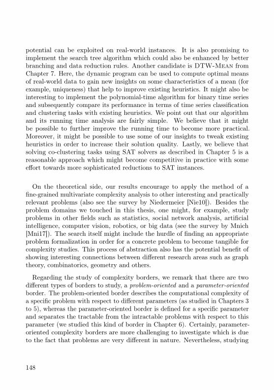
potential can be exploited on real-world instances. It is also promising toimplement the search tree algorithm which could also be enhanced by betterbranching and data reduction rules. Another candidate is DTW-Mean fromChapter 7. Here, the dynamic program can be used to compute optimal meansof real-world data to gain new insights on some characteristics of a mean (forexample, uniqueness) that help to improve existing heuristics. It might also beinteresting to implement the polynomial-time algorithm for binary time seriesand subsequently compare its performance in terms of time series classificationand clustering tasks with existing heuristics. We point out that our algorithmand its running time analysis are fairly simple. We believe that it mightbe possible to further improve the running time to become more practical.Moreover, it might be possible to use some of our insights to tweak existingheuristics in order to increase their solution quality. Lastly, we believe thatsolving co-clustering tasks using SAT solvers as described in Chapter 5 is areasonable approach which might become competitive in practice with someeffort towards more sophisticated reductions to SAT instances.
On the theoretical side, our results encourage to apply the method of afine-grained multivariate complexity analysis to other interesting and practicallyrelevant problems (also see the survey by Niedermeier [Nie10]). Besides theproblem domains we touched in this thesis, one might, for example, studyproblems in other fields such as statistics, social network analysis, artificialintelligence, computer vision, robotics, or big data (see the survey by Mnich[Mni17]). The search itself might include the hurdle of finding an appropriateproblem formalization in order for a concrete problem to become tangible forcomplexity studies. This process of abstraction also has the potential benefit ofshowing interesting connections between different research areas such as graphtheory, combinatorics, geometry and others.
Regarding the study of complexity borders, we remark that there are twodifferent types of borders to study, a problem-oriented and a parameter-orientedborder. The problem-oriented border describes the computational complexity ofa specific problem with respect to different parameters (as studied in Chapters 3to 5), whereas the parameter-oriented border is defined for a specific parameterand separates the tractable from the intractable problems with respect to thisparameter (we studied this kind of border in Chapter 6). Certainly, parameter-oriented complexity borders are more challenging to investigate which is dueto the fact that problems are very different in nature. Nevertheless, studying
148
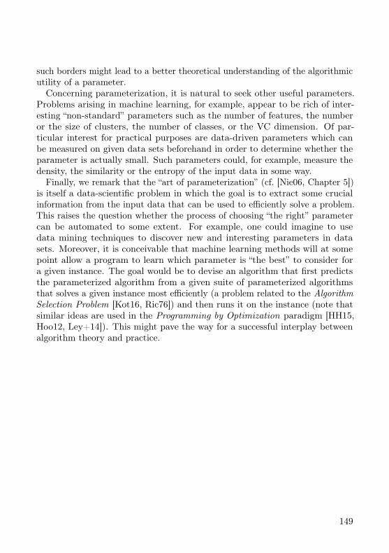
such borders might lead to a better theoretical understanding of the algorithmicutility of a parameter.Concerning parameterization, it is natural to seek other useful parameters.
Problems arising in machine learning, for example, appear to be rich of inter-esting “non-standard” parameters such as the number of features, the numberor the size of clusters, the number of classes, or the VC dimension. Of par-ticular interest for practical purposes are data-driven parameters which canbe measured on given data sets beforehand in order to determine whether theparameter is actually small. Such parameters could, for example, measure thedensity, the similarity or the entropy of the input data in some way.
Finally, we remark that the “art of parameterization” (cf. [Nie06, Chapter 5])is itself a data-scientific problem in which the goal is to extract some crucialinformation from the input data that can be used to efficiently solve a problem.This raises the question whether the process of choosing “the right” parametercan be automated to some extent. For example, one could imagine to usedata mining techniques to discover new and interesting parameters in datasets. Moreover, it is conceivable that machine learning methods will at somepoint allow a program to learn which parameter is “the best” to consider fora given instance. The goal would be to devise an algorithm that first predictsthe parameterized algorithm from a given suite of parameterized algorithmsthat solves a given instance most efficiently (a problem related to the AlgorithmSelection Problem [Kot16, Ric76]) and then runs it on the instance (note thatsimilar ideas are used in the Programming by Optimization paradigm [HH15,Hoo12, Ley+14]). This might pave the way for a successful interplay betweenalgorithm theory and practice.
149

Bibliography
[AB09] S. Arora and B. Barak. Computational Complexity—A Modern Approach.Cambridge University Press, 2009 (cited on p. 7).
[ADK12] A. Anagnostopoulos, A. Dasgupta, and R. Kumar. “A constant-factorapproximation algorithm for co-clustering”. In: Theory of Computing 8(2012), pp. 597–622 (cited on pp. 64–66).
[AK00] P. Alimonti and V. Kann. “Some APX-completeness results for cubic graphs”.In: Theoretical Computer Science 237.1–2 (2000), pp. 123–134 (cited onp. 24).
[Alo06] N. Alon. “Ranking tournaments”. In: SIAM Journal on Discrete Mathematics20.1 (2006), pp. 137–142 (cited on pp. 90, 102).
[ALS09] N. Alon, D. Lokshtanov, and S. Saurabh. “Fast FAST”. In: Proceedings of the36th International Colloquium on Automata, Languages, and Programming(ICALP ’09). Vol. 5555. LNCS. Springer, 2009, pp. 49–58 (cited on p. 102).
[APT79] B. Aspvall, M. F. Plass, and R. E. Tarjan. “A linear-time algorithm fortesting the truth of certain quantified boolean formulas”. In: InformationProcessing Letters 8.3 (1979), pp. 121–123 (cited on p. 79).
[ASS16] N. R. Aravind, R. B. Sandeep, and N. Sivadasan. “Parameterized lowerbounds and dichotomy results for the NP-completeness of H-free edge mod-ification problems”. In: Proceedings of the 12th Latin American Symposiumon Theoretical Informatics, (LATIN ’16). Vol. 9644. 2016, pp. 82–95 (citedon p. 90).
[ASW15] S. Aghabozorgi, A. S. Shirkhorshidi, and T. Y. Wah. “Time-series clustering– A decade review”. In: Information Systems 53 (2015), pp. 16–38 (citedon p. 129).
[Ban+07] A. Banerjee, I. S. Dhillon, J. Ghosh, S. Merugu, and D. S. Modha. “Ageneralized maximum entropy approach to Bregman co-clustering andmatrix approximation”. In: Journal of Machine Learning Research 8 (2007),pp. 1919–1986 (cited on p. 64).
[Bar+17] L. Barba, J. Cardinal, J. Iacono, S. Langerman, A. Ooms, and N. Solomon.“Subquadratic algorithms for algebraic generalizations of 3SUM”. In: Pro-ceedings of the 33rd International Symposium on Computational Geome-
151
try (SoCG ’17). Vol. 77. Leibniz International Proceedings in Informatics(LIPIcs). Schloss Dagstuhl–Leibniz-Zentrum fuer Informatik, 2017, 13:1–13:15 (cited on pp. 13, 16).
[BB13] S. Böcker and J. Baumbach. “Cluster editing”. In: The Nature of Compu-tation. Logic, Algorithms, Applications: Proceedings of the 9th Conferenceon Computability in Europe (CiE ’13). Vol. 7921. LNCS. Springer, 2013,pp. 33–44 (cited on p. 106).
[BBC04] N. Bansal, A. Blum, and S. Chawla. “Correlation clustering”. In: MachineLearning 56.1 (2004), pp. 89–113 (cited on p. 106).
[BD01] P. Bonizzoni and G. Della Vedova. “The complexity of multiple sequencealignment with SP-score that is a metric”. In: Theoretical Computer Science259.1–2 (2001), pp. 63–79 (cited on p. 129).
[Bee+84] C. Beeri, M. Dowd, R. Fagin, and R. Statman. “On the structure of Arm-strong relations for functional dependencies”. In: Journal of the ACM 31.1(1984), pp. 30–46 (cited on p. 41).
[Bes+11] S. Bessy, F. V. Fomin, S. Gaspers, C. Paul, A. Perez, S. Saurabh, andS. Thomassé. “Kernels for feedback arc set in tournaments”. In: Journal ofComputer and System Sciences 77.6 (2011), pp. 1071–1078 (cited on p. 102).
[Bev+15] R. van Bevern, R. Bredereck, J. Chen, V. Froese, R. Niedermeier, andG. J. Woeginger. “Network-based vertex dissolution”. In: SIAM Journal onDiscrete Mathematics 29.2 (2015), pp. 888–914 (cited on p. xi).
[Bev+17] R. van Bevern, R. Bredereck, L. Bulteau, J. Chen, V. Froese, R. Niedermeier,and G. J. Woeginger. “Partitioning perfect graphs into stars”. In: Journalof Graph Theory 85.2 (2017), pp. 297–335 (cited on p. xi).
[Bev14] R. van Bevern. “Towards optimal and expressive kernelization for d-HittingSet”. In: Algorithmica 70.1 (2014), pp. 129–147 (cited on p. 30).
[BFK16] R. van Bevern, V. Froese, and C. Komusiewicz. “Parameterizing edgemodification problems above lower bounds”. In: Proceedings of the 11thInternational Computer Science Symposium in Russia (CSR ’16). Vol. 9691.LNCS. Springer, 2016, pp. 57–72 (cited on p. x).
[BFK18] R. van Bevern, V. Froese, and C. Komusiewicz. “Parameterizing edge modi-fication problems above lower bounds”. In: Theory of Computing Systems62.3 (2018), pp. 739–770 (cited on pp. x, 94, 113).
[BFN18] L. Bulteau, V. Froese, and R. Niedermeier. “Hardness of consensus problemsfor circular strings and time series averaging”. In: CoRR abs/1804.02854(2018). Submitted to FOCS. (cited on pp. 4, 126, 130, 145).
[BFS17] T. Bläsius, T. Friedrich, and M. Schirneck. “The parameterized complex-ity of dependency detection in relational databases”. In: Proceedings of
152
the 11th International Symposium on Parameterized and Exact Computa-tion (IPEC ’16). Vol. 63. LIPIcs. Schloss Dagstuhl–Leibniz-Zentrum fuerInformatik, 2017, 6:1–6:13 (cited on p. 41).
[BFT16] L. Bulteau, V. Froese, and N. Talmon. “Multi-player diffusion games ongraph classes”. In: Internet Mathematics 12.6 (2016), pp. 363–380 (citedon p. xi).
[BG09] J. Bang-Jensen and G. Gutin. Digraphs: Theory, Algorithms and Applica-tions. Springer, 2009 (cited on p. 60).
[BGL17] É. Bonnet, P. Giannopoulos, and M. Lampis. “On the parameterized com-plexity of red-blue points separation”. In: Proceedings of the 12th Interna-tional Symposium on Parameterized and Exact Computation (IPEC ’17).LIPIcs. Schloss Dagstuhl - Leibniz-Zentrum fuer Informatik, 2017, 8:1–8:13(cited on p. 87).
[BJK14] H. L. Bodlaender, B. M. P. Jansen, and S. Kratsch. “Kernelization lowerbounds by cross-composition”. In: SIAM Journal on Discrete Mathematics28.1 (2014), pp. 277–305 (cited on p. 10).
[BK15] K. Bringmann and M. Künnemann. “Quadratic conditional lower boundsfor string problems and dynamic time warping”. In: Proceedings of the 56thAnnual IEEE Symposium on Foundations of Computer Science (FOCS ’15).IEEE, 2015, pp. 79–97 (cited on p. 129).
[BKM09] D. Brügmann, C. Komusiewicz, and H. Moser. “On generating triangle-freegraphs”. In: Proceedings of the DIMAP Workshop on Algorithmic GraphTheory (AGT ’09). Vol. 32. Electronic Notes in Discrete Mathematics.Elsevier, 2009, pp. 51–58 (cited on pp. 97, 100).
[BL97] A. Blum and P. Langley. “Selection of relevant features and examples inmachine learning”. In: Artificial Intelligence 97.1-2 (1997), pp. 245–271(cited on p. 40).
[BM11] A. Brandstädt and R. Mosca. “On distance-3 matchings and induced match-ings”. In: Discrete Applied Mathematics 159.7 (2011), pp. 509–520 (citedon p. 44).
[Böc+09] S. Böcker, S. Briesemeister, Q. B. A. Bui, and A. Truß. “Going weighted:parameterized algorithms for cluster editing”. In: Theoretical ComputerScience 410.52 (2009), pp. 5467–5480 (cited on p. 91).
[Böc12] S. Böcker. “A golden ratio parameterized algorithm for cluster editing”. In:Journal of Discrete Algorithms 16 (2012), pp. 79–89 (cited on pp. 106, 110).
[Bod+09] H. L. Bodlaender, R. G. Downey, M. R. Fellows, and D. Hermelin. “Onproblems without polynomial kernels”. In: Journal of Computer and SystemSciences 75.8 (2009), pp. 423–434 (cited on p. 10).
153

[Boi+17] J.-D. Boissonnat, K. Dutta, A. Ghosh, and S. Kolay. “Kernelization ofthe subset general position problem in geometry”. In: Proceedings of the42nd International Symposium on Mathematical Foundations of ComputerScience (MFCS ’17). LIPIcs. Schloss Dagstuhl–Leibniz-Zentrum fuer Infor-matik, 2017, 25:1–25:13 (cited on pp. 36, 37).
[Bre+15a] R. Bredereck, J. Chen, S. Hartung, C. Komusiewicz, R. Niedermeier, andO. Suchý. “On explaining integer vectors by few homogenous segments”.In: Journal of Computer and System Sciences 81.4 (2015), pp. 766–782(cited on p. 62).
[Bre+15b] R. Bredereck, V. Froese, S. Hartung, A. Nichterlein, R. Niedermeier, andN. Talmon. “The complexity of degree anonymization by vertex addition”.In: Theoretical Computer Science 607.1 (2015), pp. 16–34 (cited on p. xi).
[Bre+18] R. Bredereck, V. Froese, M. Koseler, M. G. Millani, A. Nichterlein, andR. Niedermeier. “A parameterized algorithmics framework for digraphdegree sequence completion problems”. In: Algorithmica (2018). Acceptedfor publication. url: https://arxiv.org/abs/1604.06302 (cited on p. xi).
[Bri+18] M. Brill, T. Fluschnik, V. Froese, B. Jain, R. Niedermeier, and D. Schultz.“Exact mean computation in dynamic time warping spaces”. In: Proceedingsof the SIAM International Conference on Data Mining (SDM ’18). SIAM,2018, pp. 540–548 (cited on pp. xi, 145).
[BTY11] H. L. Bodlaender, S. Thomassé, and A. Yeo. “Kernel bounds for disjointcycles and disjoint paths”. In: Theoretical Computer Science 412.35 (2011),pp. 4570–4578 (cited on p. 10).
[Bul+14] L. Bulteau, V. Froese, S. Hartung, and R. Niedermeier. “Co-clustering underthe maximum norm”. In: Proceedings of the 25th International Symposiumon Algorithms and Computation (ISAAC ’14). LNCS 8889. Springer, 2014,pp. 298–309 (cited on p. x).
[Bul+16a] L. Bulteau, V. Froese, S. Hartung, and R. Niedermeier. “Co-clustering underthe maximum norm”. In: Algorithms 9.1 (2016). Art. No. 17 (cited on pp. x,86).
[Bul+16b] L. Bulteau, V. Froese, K. Kutzkov, and R. Pagh. “Triangle counting indynamic graph streams”. In: Algorithmica 76.1 (2016), pp. 259–278 (citedon p. xi).
[Bul+17] L. Bulteau, S. Fafianie, V. Froese, R. Niedermeier, and N. Talmon. “Thecomplexity of finding effectors”. In: Theory of Computing Systems 60.2(2017), pp. 253–279 (cited on p. xi).
154

[Cai+97] L. Cai, J. Chen, R. G. Downey, and M. R. Fellows. “Advice classes ofparameterized tractability”. In: Annals of Pure and Applied Logic 84.1(1997), pp. 119–138 (cited on p. 9).
[Cai96] L. Cai. “Fixed-parameter tractability of graph modification problems forhereditary properties”. In: Information Processing Letters 58.4 (1996),pp. 171–176 (cited on pp. 90, 93, 94, 113).
[Cao12] C. Cao. “Study on Two Optimization Problems: Line Cover and MaximumGenus Embedding”. MA thesis. Texas A&M University, May 2012 (citedon pp. 15, 24–26, 28).
[CB17] M. Cuturi and M. Blondel. “Soft-DTW: a differentiable loss function fortime-series”. In: Proceedings of the 34th International Conference on MachineLearning (ICML ’17). Vol. 70. Proceedings of Machine Learning Research.PMLR, 2017, pp. 894–903 (cited on p. 126).
[CC15] L. Cai and Y. Cai. “Incompressibility of H-free edge modification problems”.In: Algorithmica 71.3 (2015), pp. 731–757 (cited on p. 90).
[CDK14] F. Chierichetti, N. Dalvi, and R. Kumar. “Correlation clustering in MapRe-duce”. In: Proceedings of the 20th ACM SIGKDD International Conferenceon Knowledge Discovery and Data Mining (KDD ’14). ACM, 2014, pp. 641–650 (cited on p. 106).
[Cha+00] M. Charikar, V. Guruswami, R. Kumar, S. Rajagopalan, and A. Sahai.“Combinatorial feature selection problems”. In: Proceedings of the 41st IEEEAnnual Symposium on Foundations of Computer Science (FOCS ’00). 2000,pp. 631–640 (cited on pp. 39–41).
[Che+16] W. Cheng, X. Zhang, F. Pan, and W. Wang. “HICC: an entropy splitting-based framework for hierarchical co-clustering”. In: Knowledge and Infor-mation Systems 46.2 (2016), pp. 343–367 (cited on p. 66).
[CM03] C. Cotta and P. Moscato. “The k-feature set problem is W[2]-complete”.In: Journal of Computer and System Sciences 67.4 (2003), pp. 686–690(cited on p. 41).
[CM12] J. Chen and J. Meng. “A 2k kernel for the cluster editing problem”. In:Journal of Computer and System Sciences 78.1 (2012), pp. 211–220 (citedon pp. 106, 107, 112).
[CN98] B. S. Chlebus and S. H. Nguyen. “On finding optimal discretizations for twoattributes”. In: Proceedings of the First International Conference on RoughSets and Current Trends in Computing (RSCTC ’98). Vol. 1424. LNCS.Springer, 1998, pp. 537–544 (cited on pp. 65, 73, 86).
155
[Cov65] T. M. Cover. “Geometrical and statistical properties of systems of linearinequalities with applications in pattern recognition”. In: IEEE Transactionson Electronic Computers EC-14.3 (1965), pp. 326–334 (cited on p. 13).
[CS14] G. Chandrashekar and F. Sahin. “A survey on feature selection methods”. In:Computers & Electrical Engineering 40.1 (2014), pp. 16–28 (cited on p. 40).
[CSS99] W. W. Cohen, R. E. Schapire, and Y. Singer. “Learning to order things”.In: Journal of Artificial Intelligence Research 10 (1999), pp. 243–270 (citedon p. 101).
[CST00] A. Califano, G. Stolovitzky, and Y. Tu. “Analysis of gene expression microar-rays for phenotype classification”. In: Proceedings of the Eighth InternationalConference on Intelligent Systems for Molecular Biology (ISMB’00). AAAI,2000, pp. 75–85 (cited on p. 65).
[Cyg+13] M. Cygan, M. Pilipczuk, M. Pilipczuk, and J. O. Wojtaszczyk. “On mul-tiway cut parameterized above lower bounds”. In: ACM Transactions onComputation Theory 5.1 (2013), p. 3 (cited on pp. 90, 122).
[Cyg+15] M. Cygan, F. V. Fomin, Ł. Kowalik, D. Lokshtanov, D. Marx, M. Pilipczuk,M. Pilipczuk, and S. Saurabh. Parameterized Algorithms. Springer, 2015(cited on p. 8).
[Das+07] A. Dasgupta, P. Drineas, B. Harb, V. Josifovski, and M. W. Mahoney.“Feature selection methods for text classification”. In: Proceedings of the13th ACM SIGKDD International Conference on Knowledge Discovery andData Mining (KDD ’07). ACM, 2007, pp. 230–239 (cited on p. 40).
[Dat03] C. J. Date. An Introduction to Database Systems. Pearson, 2003 (citedon p. 40).
[Deh+06] F. Dehne, M. A. Langston, X. Luo, S. Pitre, P. Shaw, and Y. Zhang. “Thecluster editing problem: implementations and experiments”. In: Proceed-ings of the Second International Workshop on Parameterized and ExactComputation (IWPEC ’06). Vol. 4169. LNCS. Springer, 2006, pp. 13–24(cited on p. 106).
[Deı+06] V. G. Deıneko, M. Hoffmann, Y. Okamoto, and G. J. Woeginger. “Thetraveling salesman problem with few inner points”. In: Operations ResearchLetters 34.1 (2006), pp. 106–110 (cited on p. 33).
[Dez74] M. Deza. “Solution d’un problème de Erdős-Lovász”. In: Journal of Combi-natorial Theory, Series B 16.2 (1974), pp. 166–167 (cited on p. 52).
[DF13] R. G. Downey and M. R. Fellows. Fundamentals of Parameterized Com-plexity. Springer, 2013 (cited on pp. 8, 20).
[DF99] R. G. Downey and M. R. Fellows. Parameterized Complexity. Springer, 1999(cited on p. 8).
156
[DFR12] M. Dom, M. R. Fellows, and F. A. Rosamond. “The parameterized com-plexity of stabbing rectangles”. In: Algorithmica 62.1–2 (2012), pp. 564–594(cited on p. 87).
[DK08] A. Das and D. Kempe. “Algorithms for subset selection in linear regres-sion”. In: Proceedings of the 40th Annual ACM Symposium on Theory ofComputing (STOC ’08). ACM, 2008, pp. 45–54 (cited on p. 40).
[DM14] H. Dell and D. van Melkebeek. “Satisfiability allows no nontrivial sparsifi-cation unless the polynomial-time hierarchy collapses”. In: Journal of theACM 61.4 (2014), 23:1–23:27 (cited on pp. 10, 33, 34, 36).
[Dom+10] M. Dom, J. Guo, F. Hüffner, R. Niedermeier, and A. Truß. “Fixed-parametertractability results for feedback set problems in tournaments”. In: Journalof Discrete Algorithms 8.1 (2010), pp. 76–86 (cited on p. 102).
[DR94] S. Davies and S. Russell. “NP-completeness of searches for smallest possiblefeature sets”. In: AAAI Symposium on Intelligent Relevance. 1994, pp. 37–39(cited on p. 41).
[Dru15] A. Drucker. “New limits to classical and quantum instance compression”. In:SIAM Journal on Computing 44.5 (2015), pp. 1443–1479 (cited on p. 10).
[Dur+15] G. Durán, F. F. Slezak, L. Grippo, F. de S. Oliveira, and J. Szwarcfiter. “Onunit interval graphs with integer endpoints”. In: Electronic Notes in DiscreteMathematics 50.Supplement C (2015), pp. 445–450 (cited on p. 69).
[Dwo+01] C. Dwork, R. Kumar, M. Naor, and D. Sivakumar. “Rank aggregationmethods for the web”. In: Proceedings of the 10th International Conferenceon World Wide Webseries (WWW ’01). ACM, 2001, pp. 613–622 (citedon p. 101).
[EOS86] H. Edelsbrunner, J. O’Rourke, and R. Seidel. “Constructing arrangements oflines and hyperplanes with applications”. In: SIAM Journal on Computing15.2 (1986), pp. 341–363 (cited on p. 32).
[Erd86] P. Erdős. “On some metric and combinatorial geometric problems”. In:Discrete Mathematics 60 (1986), pp. 147–153 (cited on p. 15).
[Est+05] V. Estivill-Castro, M. Fellows, M. A. Langston, and F. Rosamond. “FPTis P-time extremal structure I (fixed-parameter tractability is polynomial-time extremal structure theory)”. In: Algorithms and Complexity (Texts inAlgorithmics 4). King’s College Publications, 2005, pp. 1–41 (cited on p. 2).
[Fei09] U. Feige. “Faster FAST (feedback arc set in tournaments)”. In: CoRRabs/0911.5094 (2009). url: http://arxiv.org/abs/0911.5094 (cited onp. 102).
[Fei14] U. Feige. “NP-hardness of hypercube 2-segmentation”. In: CoRR abs/1411.0821(2014). url: https://arxiv.org/abs/1411.0821 (cited on p. 65).
157
[Fel+11] M. R. Fellows, J. Guo, C. Komusiewicz, R. Niedermeier, and J. Uhlmann.“Graph-based data clustering with overlaps”. In: Discrete Optimization 8.1(2011), pp. 2–17 (cited on p. 123).
[Fel03] M. R. Fellows. “Blow-ups, win/win’s, and crown rules: some new directionsin FPT”. In: Proceedings of the 29th International Workshop on Graph-Theoretic Concepts in Computer Science (WG ’03). Vol. 2880. LNCS. 2003,pp. 1–12 (cited on p. 95).
[FG06] J. Flum and M. Grohe. Parameterized Complexity Theory. Springer, 2006(cited on pp. 3, 8, 39).
[FKV14] S. Felsner, M. Kaufmann, and P. Valtr. “Bend-optimal orthogonal graphdrawing in the general position model”. In: Computational Geometry 47.3,Part B (2014), pp. 460–468 (cited on p. 13).
[FNN16] V. Froese, A. Nichterlein, and R. Niedermeier. “Win-win kernelization fordegree sequence completion problems”. In: Journal of Computer and SystemSciences 82.6 (2016), pp. 1100–1111 (cited on pp. xi, 95).
[Fom+14] F. V. Fomin, S. Kratsch, M. Pilipczuk, M. Pilipczuk, and Y. Villanger.“Tight bounds for parameterized complexity of cluster editing with a smallnumber of clusters”. In: Journal of Computer and System Sciences 80.7(2014), pp. 1430–1447 (cited on pp. 106, 107).
[For03] G. Forman. “An extensive empirical study of feature selection metrics fortext classification”. In: Journal of Machine Learning Research 3 (2003),pp. 1289–1305 (cited on p. 40).
[FP13] F. V. Fomin and M. Pilipczuk. “Subexponential parameterized algorithm forcomputing the cutwidth of a semi-complete digraph”. In: Proceedings of the21st Annual European Symposium (ESA ’13). Vol. 8125. LNCS. Springer,2013, pp. 505–516 (cited on pp. 102, 103).
[FPT81] R. J. Fowler, M. S. Paterson, and S. L. Tanimoto. “Optimal packing andcovering in the plane are NP-complete”. In: Information Processing Letters12.3 (1981), pp. 133–137 (cited on p. 72).
[Fré48] M. Fréchet. “Les éléments aléatoires de nature quelconque dans un espacedistancié”. In: Annales de l’institut Henri Poincaré (1948), pp. 215–310(cited on p. 126).
[Fro+13] V. Froese, R. van Bevern, R. Niedermeier, and M. Sorge. “A parameter-ized complexity analysis of combinatorial feature selection problems”. In:Proceedings of the 38th International Symposium on Mathematical Founda-tions of Computer Science (MFCS ’13). Vol. 8087. LNCS. Springer, 2013,pp. 445–456 (cited on p. x).
158

[Fro+16a] V. Froese, R. van Bevern, R. Niedermeier, and M. Sorge. “Exploiting hiddenstructure in selecting dimensions that distinguish vectors”. In: Journal ofComputer and System Sciences 82.3 (2016), pp. 521–535 (cited on pp. x,41, 43, 44).
[Fro+16b] V. Froese, I. Kanj, A. Nichterlein, and R. Niedermeier. “Finding pointsin general position”. In: Proceedings of the 28th Canadian Conference onComputational Geometry (CCCG ’16). 2016, pp. 7–14 (cited on p. ix).
[Fro+17] V. Froese, I. Kanj, A. Nichterlein, and R. Niedermeier. “Finding points ingeneral position”. In: International Journal of Computational Geometry &Applications 27.4 (2017), pp. 277–296 (cited on p. ix).
[Fro12] V. Froese. “Combinatorial Feature Selection: Parameterized Algorithms andComplexity”. MA thesis. TU Berlin, 2012 (cited on pp. ix, 41, 43, 44).
[Für91] Z. Füredi. “Maximal independent subsets in Steiner systems and in planarsets”. In: SIAM Journal on Discrete Mathematics 4.2 (1991), pp. 196–199(cited on p. 29).
[GE03] I. Guyon and A. Elisseeff. “An introduction to variable and feature selection”.In: Journal of Machine Learning Research 3 (2003), pp. 1157–1182 (citedon p. 40).
[GJ79] M. R. Garey and D. S. Johnson. Computers and Intractability: A Guideto the Theory of NP-Completeness. W. H. Freeman and Company, 1979(cited on pp. 7, 24, 70).
[GK68] R. K. Guy and P. A. Kelly. “The no-three-in-line problem”. In: CanadianMathematical Bulletin 11 (1968), pp. 527–531 (cited on p. 14).
[GŁ15] T. Górecki and M. Łuczak. “Multivariate time series classification withparametric derivative dynamic time warping”. In: Expert Systems withApplications 42.5 (2015), pp. 2305–2312 (cited on p. 138).
[GOR96] L. J. Guibas, M. H. Overmars, and J. Robert. “The exact fitting problem inhigher dimensions”. In: Computational Geometry: Theory and Applications6.4 (1996), pp. 215–230 (cited on pp. 26, 28).
[GP16] S. Garg and G. Philip. “Raising the bar for vertex cover: fixed-parametertractability above a higher guarantee”. In: Proceedings of the 27th AnnualACM-SIAM Symposium on Discrete Algorithms (SODA ’16). SIAM, 2016,pp. 1152–1166 (cited on pp. 90, 122).
[GR15] S. K. Ghosh and B. Roy. “Some results on point visibility graphs”. In:Theoretical Computer Science 575 (2015), pp. 17–32 (cited on p. 16).
[Gra+04] J. Gramm, J. Guo, F. Hüffner, and R. Niedermeier. “Automated genera-tion of search tree algorithms for hard graph modification problems”. In:Algorithmica 39.4 (2004), pp. 321–347 (cited on p. 97).
159
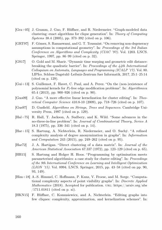
[Gra+05] J. Gramm, J. Guo, F. Hüffner, and R. Niedermeier. “Graph-modeled dataclustering: exact algorithms for clique generation”. In: Theory of ComputingSystems 38.4 (2005), pp. 373–392 (cited on p. 106).
[GRT97] F. Gómez, S. Ramaswami, and G. T. Toussaint. “On removing non-degeneracyassumptions in computational geometry”. In: Proceedings of the 3rd ItalianConference on Algorithms and Complexity (CIAC ’97). Vol. 1203. LNCS.Springer, 1997, pp. 86–99 (cited on p. 32).
[GS17] O. Gold and M. Sharir. “Dynamic time warping and geometric edit distance:breaking the quadratic barrier”. In: Proceedings of the 44th InternationalColloquium on Automata, Languages and Programming (ICALP ’17). Vol. 80.LIPIcs. Schloss Dagstuhl–Leibniz-Zentrum fuer Informatik, 2017, 25:1–25:14(cited on p. 129).
[Gui+13] S. Guillemot, F. Havet, C. Paul, and A. Perez. “On the (non-)existence ofpolynomial kernels for P`-free edge modification problems”. In: Algorithmica65.4 (2013), pp. 900–926 (cited on p. 90).
[Guo09] J. Guo. “A more effective linear kernelization for cluster editing”. In: Theo-retical Computer Science 410.8-10 (2009), pp. 718–726 (cited on p. 107).
[Gus97] D. Gusfield. Algorithms on Strings, Trees and Sequences. Cambridge Uni-versity Press, 1997 (cited on p. 129).
[Hal+75] R. Hall, T. Jackson, A. Sudbery, and K. Wild. “Some advances in theno-three-in-line problem”. In: Journal of Combinatorial Theory, Series A18.3 (1975), pp. 336–341 (cited on p. 14).
[Har+15] S. Hartung, A. Nichterlein, R. Niedermeier, and O. Suchý. “A refinedcomplexity analysis of degree anonymization in graphs”. In: Informationand Computation 243 (2015), pp. 249–262 (cited on p. 95).
[Har72] J. A. Hartigan. “Direct clustering of a data matrix”. In: Journal of theAmerican Statistical Association 67.337 (1972), pp. 123–129 (cited on p. 65).
[HH15] S. Hartung and Holger H. Hoos. “Programming by optimisation meetsparameterised algorithmics: a case study for cluster editing”. In: Proceedingsof the 9th International Conference on Learning and Intelligent Optimization(LION ’15). Vol. 8994. LNCS. Springer, 2015, pp. 43–58 (cited on pp. 90,93, 149).
[Him+18] A.-S. Himmel, C. Hoffmann, P. Kunz, V. Froese, and M. Sorge. “Computa-tional complexity aspects of point visibility graphs”. In: Discrete AppliedMathematics (2018). Accepted for publication. url: https://arxiv.org/abs/1711.01811 (cited on p. xi).
[HKN15] F. Hüffner, C. Komusiewicz, and A. Nichterlein. “Editing graphs intofew cliques: complexity, approximation, and kernelization schemes”. In:
160

Proceedings of the Algorithms and Data Structures Symposium (WADS’15).Vol. 9214. LNCS. Springer, 2015, pp. 410–421 (cited on p. 123).
[HNF08] V. Hautamaki, P. Nykanen, and P. Franti. “Time-series clustering by ap-proximate prototypes”. In: Proceedings of the 19th International Conferenceon Pattern Recognition (ICPR ’08). IEEE, 2008, pp. 1–4 (cited on pp. 126,129, 130).
[HO06] M. Hoffmann and Y. Okamoto. “The minimum weight triangulation problemwith few inner points”. In: Computational Geometry: Theory and Applica-tions 34.3 (2006), pp. 149–158 (cited on p. 33).
[Hoo12] H. H. Hoos. “Programming by optimization”. In: Communications of theACM 55.2 (2012), pp. 70–80 (cited on p. 149).
[IP01] R. Impagliazzo and R. Paturi. “On the complexity of k-SAT”. In: Journalof Computer and System Sciences 62.2 (2001), pp. 367–375 (cited on p. 8).
[IPZ01] R. Impagliazzo, R. Paturi, and F. Zane. “Which problems have stronglyexponential complexity?” In: Journal of Computer and System Sciences63.4 (2001), pp. 512–530 (cited on pp. 23, 24, 107).
[Joh14] H. R. Johnson. “Some new maximum VC classes”. In: Information ProcessingLetters 114.6 (2014), pp. 294–298 (cited on p. 13).
[JS16] B. Jain and D. Schultz. “A reduction theorem for the sample mean indynamic time warping spaces”. In: CoRR abs/1610.04460 (2016) (citedon pp. 129, 131, 132).
[JS99] D. Johnson and M. Szegedy. “What are the least tractable instances of max-imum independent set?” In: Proceedings of the 16th ACM-SIAM Symposiumon Discrete Algorithms (SODA ’99). 1999, pp. 927–928 (cited on p. 24).
[JSB09] S. Jegelka, S. Sra, and A. Banerjee. “Approximation algorithms for ten-sor clustering”. In: Proceedings of the 20th International Conference ofAlgorithmic Learning Theory (ALT’09). Vol. 5809. LNCS. Springer, 2009,pp. 368–383 (cited on p. 65).
[Juk11] S. Jukna. Extremal Combinatorics. Springer, 2011 (cited on pp. 51, 52).[KKW15] C. Knauer, S. König, and D. Werner. “Fixed-parameter complexity and
approximability of norm maximization”. In: Discrete & ComputationalGeometry 53.2 (2015), pp. 276–295 (cited on p. 37).
[KM86] M. Křivánek and J. Morávek. “NP-hard problems in hierarchical-tree clus-tering”. In: Acta Informatica 23.3 (1986), pp. 311–323 (cited on p. 90).
[KNN16] C. Komusiewicz, A. Nichterlein, and R. Niedermeier. “Parameterized algo-rithmics for graph modification problems: on interactions with heuristics”.In: Proceedings of the 41st International Workshop on Graph-Theoretic
161
Concepts in Computer Science (WG ’15). Vol. 9224. LNCS. Springer, 2016,pp. 3–15 (cited on p. 147).
[Kot16] L. Kotthoff. “Algorithm selection for combinatorial search problems: asurvey”. In: Data Mining and Constraint Programming: Foundations of aCross-Disciplinary Approach. Ed. by C. Bessiere, L. De Raedt, L. Kotthoff,S. Nijssen, B. O’Sullivan, and D. Pedreschi. Springer, 2016, pp. 149–190(cited on p. 149).
[KPR16] S. Kratsch, G. Philip, and S. Ray. “Point line cover: the easy kernel isessentially tight”. In: ACM Transactions on Algorithms 12.3 (2016), 40:1–40:16 (cited on pp. 16, 34–36).
[Kra12] S. Kratsch. “Polynomial kernelizations for MIN F+Π1 and MAX NP”. In:Algorithmica 63.1-2 (2012), pp. 532–550 (cited on p. 90).
[KS10] M. Karpinski and W. Schudy. “Faster algorithms for feedback arc settournament, Kemeny rank aggregation and betweenness tournament”. In:Proceedings of the 21st International Symposium on Algorithms and Com-putation (ISAAC ’10). Vol. 6506. LNCS. Springer, 2010, pp. 3–14 (citedon p. 102).
[KS96] D. Koller and M. Sahami. “Towards optimal feature selection”. In: Pro-ceedings of the 13th International Conference on Machine Learning (ICML1996). 1996, pp. 284–292 (cited on p. 39).
[KU12] C. Komusiewicz and J. Uhlmann. “Cluster editing with locally boundedmodifications”. In: Discrete Applied Mathematics 160.15 (2012), pp. 2259–2270 (cited on pp. 106, 107).
[KW13] S. Kratsch and M. Wahlström. “Two edge modification problems withoutpolynomial kernels”. In: Discrete Optimization 10.3 (2013), pp. 193–199(cited on p. 90).
[Ley+14] K. Leyton-Brown, H. H. Hoos, F. Hutter, and L. Xu. “Understanding theempirical hardness of NP-complete problems”. In: Communications of theACM 57.5 (2014), pp. 98–107 (cited on p. 149).
[Liu+12] Y. Liu, J. Wang, J. Guo, and J. Chen. “Complexity and parameterizedalgorithms for Cograph Editing”. In: Theoretical Computer Science 461(2012), pp. 45–54 (cited on p. 123).
[LM05] S. Langerman and P. Morin. “Covering things with things”. In: Discrete &Computational Geometry 33.4 (2005), pp. 717–729 (cited on p. 26).
[Lok+14] D. Lokshtanov, N. S. Narayanaswamy, V. Raman, M. S. Ramanujan, and S.Saurabh. “Faster parameterized algorithms using linear programming”. In:ACM Transactions on Algorithms 11.2 (2014), 15:1–15:31 (cited on pp. 90,122).
162
[LY80] J. M. Lewis and M. Yannakakis. “The node-deletion problem for hereditaryproperties is NP-complete”. In: Journal of Computer and System Sciences20.2 (1980), pp. 219–230 (cited on p. 90).
[Mni17] M. Mnich. “Big data algorithms beyond machine learning”. In: KI - Kün-stliche Intelligenz (2017), pp. 1–9 (cited on p. 148).
[MNS12] H. Moser, R. Niedermeier, and M. Sorge. “Exact combinatorial algorithmsand experiments for finding maximum k-plexes”. In: Journal of Combinato-rial Optimization 24.3 (2012), pp. 347–373 (cited on p. 90).
[MO04] S. C. Madeira and A. L. Oliveira. “Biclustering algorithms for biologicaldata analysis: a survey”. In: IEEE/ACM Transactions on ComputationalBiology and Bioinformatics 1.1 (2004), pp. 24–45 (cited on pp. 63–65).
[Mor+18] M. Morel, C. Achard, R. Kulpa, and S. Dubuisson. “Time-series averag-ing using constrained dynamic time warping with tolerance”. In: PatternRecognition 74 (2018), pp. 77–89 (cited on p. 126).
[MR15] P. Moradi and M. Rostami. “A graph theoretic approach for unsupervisedfeature selection”. In: Engineering Applications of Artificial Intelligence44.Supplement C (2015), pp. 33–45 (cited on p. 40).
[MR99] M. Mahajan and V. Raman. “Parameterizing above guaranteed values:MaxSat and MaxCut”. In: Journal of Algorithms 31.2 (1999), pp. 335–354(cited on p. 90).
[MRS09] M. Mahajan, V. Raman, and S. Sikdar. “Parameterizing above or belowguaranteed values”. In: Journal of Computer and System Sciences 75.2(2009), pp. 137–153 (cited on p. 113).
[Mue+16] A. Mueen, N. Chavoshi, N. Abu-El-Rub, H. Hamooni, and A. Minnich.“AWarp: fast warping distance for sparse time series”. In: Proceedings of the16th IEEE International Conference on Data Mining (ICDM ’16). IEEE,2016, pp. 350–359 (cited on p. 138).
[New03] M. E. J. Newman. “The structure and function of complex networks”. In:SIAM Review 45.2 (2003), pp. 167–256 (cited on p. 96).
[Ngu06] H. S. Nguyen. “Approximate boolean reasoning: foundations and applica-tions in data mining”. In: Transactions on Rough Sets V. Vol. 4100. LNCS.Springer, 2006, pp. 334–506 (cited on pp. 65, 73).
[Nie06] R. Niedermeier. Invitation to Fixed-Parameter Algorithms. Oxford Univer-sity Press, 2006 (cited on pp. 8, 149).
[Nie10] R. Niedermeier. “Reflections on multivariate algorithmics and problemparameterization”. In: Proceedings of the 27th International Symposiumon Theoretical Aspects of Computer Science (STACS ’10). Vol. 5. LIPIcs.
163
Schloss Dagstuhl - Leibniz-Zentrum fuer Informatik, 2010, pp. 17–32 (citedon p. 148).
[NR05] F. Nicolas and E. Rivals. “Hardness results for the center and median stringproblems under the weighted and unweighted edit distances”. In: Journalof Discrete Algorithms 3.2 (2005), pp. 390–415 (cited on p. 129).
[NS95] S. H. Nguyen and A. Skowron. “Quantization of real value attributes -rough set and boolean reasoning approach”. In: Proc. Second Joint AnnualConference on Information Sciences. 1995, pp. 34–37 (cited on pp. 65, 73).
[Pap94] C. H. Papadimitriou. Computational Complexity. Addison Wesley, 1994(cited on p. 7).
[Paw91] Z. Pawlak. Rough Sets: Theoretical Aspects of Reasoning about Data. KluwerAcademic, 1991 (cited on p. 41).
[Pet+16] F. Petitjean, G. Forestier, G. I. Webb, A. E. Nicholson, Y. Chen, and E.Keogh. “Faster and more accurate classification of time series by exploitinga novel dynamic time warping averaging algorithm”. In: Knowledge andInformation Systems 47.1 (2016), pp. 1–26 (cited on pp. 126, 129, 130).
[PG12] F. Petitjean and P. Gançarski. “Summarizing a set of time series by averag-ing: from Steiner sequence to compact multiple alignment”. In: TheoreticalComputer Science 414.1 (2012), pp. 76–91 (cited on pp. 126, 129, 130).
[PG17] J. Paparrizos and L. Gravano. “Fast and accurate time-series clustering”.In: ACM Transactions on Database Systems 42.2 (2017), 8:1–8:49 (citedon pp. 126, 129).
[PKG11] F. Petitjean, A. Ketterlin, and P. Gançarski. “A global averaging methodfor dynamic time warping, with applications to clustering”. In: PatternRecognition 44.3 (2011), pp. 678–693 (cited on pp. 126, 129, 130).
[PPT16] C. Paul, A. Perez, and S. Thomassé. “Linear kernel for rooted tripletinconsistency and other problems based on conflict packing technique”. In:Journal of Computer and System Sciences 82.2 (2016), pp. 366–379 (citedon pp. 102, 106).
[PSS09] F. Protti, M. D. da Silva, and J. L. Szwarcfiter. “Applying modular decompo-sition to parameterized cluster editing problems”. In: Theory of ComputingSystems 44.1 (2009), pp. 91–104 (cited on p. 107).
[Put+15] N. Puthiyedth, C. Riveros, R. Berretta, and P. Moscato. “A new combina-torial optimization approach for integrated feature selection using differentdatasets: a prostate cancer transcriptomic study”. In: PLoS ONE 10.6(2015), e0127702 (cited on p. 40).
164
[PW13] M. S. Payne and D. R. Wood. “On the general position subset selectionproblem”. In: SIAM Journal on Discrete Mathematics 27.4 (2013), pp. 1727–1733 (cited on pp. 15, 26, 27).
[Ric76] J. R. Rice. “The algorithm selection problem”. In: ed. by M. Rubinoff andM. C. Yovits. Vol. 15. Advances in Computers Supplement C. Elsevier,1976, pp. 65–118 (cited on p. 149).
[RO09] I. Razgon and B. O’Sullivan. “Almost 2-SAT is fixed-parameter tractable”.In: Journal of Computer and System Sciences 75.8 (2009), pp. 435–450(cited on pp. 90, 122).
[Rob55] H. Robbins. “A remark on Stirling’s formula”. In: The American Mathemat-ical Monthly 62.1 (1955), pp. 26–29 (cited on p. 28).
[Rot51] K. F. Roth. “On a problem of Heilbronn”. In: Journal of the LondonMathematical Society 1.3 (1951), pp. 198–204 (cited on p. 14).
[RS06] V. Raman and S. Saurabh. “Parameterized algorithms for feedback setproblems and their duals in tournaments”. In: Theoretical Computer Science351.3 (2006), pp. 446–458 (cited on p. 102).
[Rud17] A. G. Rudi. “An improved lower bound for general position subset selection”.In: International Journal of Computing Science and Mathematics 8.6 (2017),pp. 562–569 (cited on p. 15).
[SC78] H. Sakoe and S. Chiba. “Dynamic programming algorithm optimization forspoken word recognition”. In: IEEE Transactions on Acoustics, Speech andSignal Processing 26.1 (1978), pp. 43–49 (cited on p. 129).
[SDG16] S. Soheily-Khah, A. Douzal-Chouakria, and E. Gaussier. “Generalized k-means-based clustering for temporal data under weighted and kernel timewarp”. In: Pattern Recognition Letters 75 (2016), pp. 63–69 (cited on p. 126).
[SJ18] D. Schultz and B. Jain. “Nonsmooth analysis and subgradient methodsfor averaging in dynamic time warping spaces”. In: Pattern Recognition74.Supplement C (2018), pp. 340–358 (cited on pp. 126, 129, 135).
[SR92] A. Skowron and C. Rauszer. “The discernibility matrices and functionsin information systems”. In: Intelligent Decision Support—Handbook ofApplications and Advances of the Rough Sets Theory. Ed. by R. Slowinski.Kluwer Academic, 1992, pp. 331–362 (cited on p. 41).
[SS15] R. B. Sandeep and N. Sivadasan. “Parameterized lower bound and improvedkernel for diamond-free edge deletion”. In: Proceedings of the 10th Interna-tional Symposium on Parameterized and Exact Computation (IPEC ’15).Vol. 43. LIPIcs. Schloss Dagstuhl - Leibniz-Zentrum fuer Informatik, 2015,pp. 365–376 (cited on p. 123).
165
[SST04] R. Shamir, R. Sharan, and D. Tsur. “Cluster graph modification problems”.In: Discrete Applied Mathematics 144.1 (2004), pp. 173–182 (cited on pp. 90,106).
[Tan96] L. Tan. “The group of rational points on the unit circle”. In: MathematicsMagazine 96.3 (1996), pp. 163–171 (cited on p. 18).
[TKM11] C. E. Tsourakakis, M. N. Kolountzakis, and G. L. Miller. “Triangle spar-sifiers”. In: Journal of Graph Algorithms and Applications 15.6 (2011),pp. 703–726 (cited on p. 96).
[TSS05] A. Tanay, R. Sharan, and R. Shamir. “Biclustering algorithms: a survey”.In: Handbook of Computational Molecular Biology. Chapman & Hall/CRC,2005 (cited on p. 64).
[Vaz01] V. V. Vazirani. Approximation Algorithms. Springer, 2001 (cited on p. 11).[Wah07] M. Wahlström. “Algorithms, Measures and Upper Bounds for Satisfiability
and Related Problems”. PhD thesis. Linköping University, Mar. 2007 (citedon pp. 30, 97).
[WS11] D. P. Williamson and D. B. Shmoys. The Design of Approximation Algo-rithms. Cambridge University Press, 2011 (cited on p. 11).
[WUB13] S. Wulff, R. Urner, and S. Ben-David. “Monochromatic bi-clustering”. In:Proceedings of the 30th International Conference on Machine Learning(ICML’13). Vol. 28 (2). JMLR Workshop and Conference Proceedings, 2013,pp. 145–153 (cited on p. 65).
[Yan81] M. Yannakakis. “Edge-deletion problems”. In: SIAM Journal on Computing10.2 (1981), pp. 297–309 (cited on pp. 90, 97).
[Yap83] C. K. Yap. “Some consequences of non-uniform conditions on uniformclasses”. In: Theoretical Computer Science 26.3 (1983), pp. 287–300 (citedon p. 10).
166
Schriftenreihe Foundations of computing Hrsg.: Prof. Dr. Stephan Kreutzer, Prof. Dr. Uwe Nestmann, Prof. Dr. Rolf Niedermeier ISSN 2199-5249 (print) ISSN 2199-5257 (online)
01: Bevern, René van: Fixed-Parameter Linear-Time Algorithms for NP-hard Graph and Hypergraph Problems Arising in Industrial Applications. - 2014. - 225 S. ISBN 978-3-7983-2705-4 (print) EUR 12,00
ISBN 978-3-7983-2706-1 (online)
02: Nichterlein, André: Degree-Constrained Editing of Small-Degree Graphs. - 2015. - xiv, 225 S. ISBN 978-3-7983-2705-4 (print) EUR 12,00 ISBN 978-3-7983-2706-1 (online)
03: Bredereck, Robert: Multivariate Com-
plexity Analysis of Team Management Problems. - 2015. - xix, 228 S. ISBN 978-3-7983-2764-1 (print) EUR 12,00 ISBN 978-3-7983-2765-8 (online)
04: Talmon, Nimrod: Algorithmic Aspects of Manipulation and Anonymization in Social Choice and Social Networks. - 2016. - xiv, 275 S. ISBN 978-3-7983-2804-4 (print) EUR 13,00 ISBN 978-3-7983-2805-1 (online)
05: Siebertz, Sebastian: Nowhere Dense Classes of Graphs. Characterisations and Algorithmic Meta-Theorems. - 2016. - xxii, 149 S. ISBN 978-3-7983-2818-1 (print) EUR 11,00 ISBN 978-3-7983-2819-8 (online)
06: Chen, Jiehua: Exploiting Structure in Computationally Hard Voting Problems. - 2016. - xxi, 255 S. ISBN 978-3-7983-2825-9 (print) EUR 13,00 ISBN 978-3-7983-2826-6 (online)
07: Arbach, Youssef: On the Foundations of dynamic coalitions. Modeling changes and evolution of workflows in healthcare scenarios - 2016. - xv, 171 S. ISBN 978-3-7983-2856-3 (print) EUR 12,00 ISBN 978-3-7983-2857-0 (online)
08: Sorge, Manuel: Be sparse! Be dense! Be robust! Elements of parameterized algorithmics. -
2017. - xvi, 251 S. ISBN 978-3-7983-2885-3 (print) EUR 13,00 ISBN 978-3-7983-2886-0 (online)
09: Dittmann, Christoph: Parity games, separations, and the modal μ-calculus. - 2017. - x, 274 S. ISBN 978-3-7983-2887-7 (print) EUR 13,00 ISBN 978-3-7983-2888-4 (online) 10: noch nicht erschienen 11: noch nicht erschienen

Fine
-Gra
ined
Com
plex
ity A
naly
sis o
f Som
e Co
mbi
nato
rial D
ata
Scie
nce
Prob
lem
s
Universitätsverlag der TU Berlin
Universitätsverlag der TU Berlin
Foundations of computing Volume 12
This thesis is concerned with analyzing the computational complexity of combinatorial problems arising in data science. The considered problems include selecting points in general position, combinatorial feature selection, co-clustering, graph clustering, and time series averaging. Ad-opting a parameterized viewpoint, a multivariate complexity analysis is conducted to chart the border between tractability and intractability for these practically motivated problems.Intractability results include NP- and W-hardness, approximation hardness, as well as kerneliza-tion and running time lower bounds. Tractability is achieved by developing parameterized algo-rithms which solve specific problem instances in polynomial time for constant parameter values.The developed algorithms utilize various parameters such as the number of clusters, the Ham-ming distance of data points, or the solution value above a guarantee. The algorithms involve tools from combinatorics, data reduction, SAT-solving, and dynamic programming. While most of the studied problems turned out to be computationally hard to solve in general, this thesis reveals meaningful tractable special cases for each of the considered problems.
Vi
ncen
t Fro
ese
12
Fine-Grained Complexity Analysis of Some Combinatorial Data Science Problems
http://verlag.tu-berlin.de
ISBN 978-3-7983-3003-0 (print)ISBN 978-3-7983-3004-7 (online)
9 783798 330030I S B N 9 7 8 - 3 - 7 9 8 3 - 3 0 0 3 - 0
Vincent Froese
Fine-Grained Complexity Analysis of Some Combinatorial Data Science Problems