a fine-grained xml structural comparison approach

C. Parent et al. (Eds.): ER 2007, LNCS 4801, pp. 582–598, 2007. © Springer-Verlag Berlin Heidelberg 2007

A Fine-Grained XML Structural Comparison Approach

Joe Tekli, Richard Chbeir, and Kokou Yetongnon

LE2I Laboratory UMR-CNRS, University of Bourgogne 21078 Dijon Cedex France

{joe.tekli,richard.chbeir,kokou.yetongnon}@u-bourgogne.fr

Abstract. As the Web continues to grow and evolve, more and more information is being placed in structurally rich documents, XML documents in particular, so as to improve the efficiency of similarity clustering, information retrieval and data management applications. Various algorithms for comparing hierarchically structured data, e.g., XML documents, have been proposed in the literature. Most of them make use of techniques for finding the edit distance between tree structures, XML documents being modeled as ordered labeled trees. Nevertheless, a thorough investigation of current approaches led us to identify several structural similarity aspects, i.e. sub-tree related similarities, which are not sufficiently addressed while comparing XML documents. In this paper, we provide an improved comparison method to deal with fine-grained sub-trees and leaf node repetitions, without increasing overall complexity with respect to current XML comparison methods. Our approach consists of two main algorithms for discovering the structural commonality between sub-trees and computing tree-based edit operations costs. A prototype has been developed to evaluate the optimality and performance of our method. Experimental results, on both real and synthetic XML data, demonstrate better performance with respect to alternative XML comparison methods.

Keywords: XML, Semi-structured data, Structural similarity, Tree edit distance.

1 Introduction

W3C’s XML (eXtensible Mark-up Language) has recently gained unparalleled importance as a fundamental standard for efficient data management and exchange. Information destined to be broadcasted over the web is henceforth represented using XML, in order to guarantee its interoperability. The use of XML covers data representation and storage (e.g., complex multimedia objects), database information interchange, data filtering, as well as web services interaction. Owing to the unprecedented web exploitation of XML, XML-based comparison, especially for heterogeneous1 documents, becomes a central issue in the information retrieval and database communities. The applications of XML comparison are numerous and range over: version control, change management and data warehousing (finding, scoring and browsing changes between different versions of a document, support of temporal queries and index maintenance) [4, 5, 6], XML retrieval (finding and ranking results 1 We denote by heterogeneous XML document one that does not conform to a given grammar

(DTD/XML Schema), which is the case of a lot of XML documents found on the web [13].

A Fine-Grained XML Structural Comparison Approach 583

according to their similarity in order to retrieve the best results possible) [16, 22] as well as the classification/clustering of XML documents gathered from the web against a set of DTDs declared in an XML database (just as schemas are necessary in traditional DBMS for the provision of efficient storage, retrieval, protection and indexing facilities, the same is true for DTDs and XML repositories) [2, 6, 13].

A range of algorithms for comparing semi-structured data, e.g., XML-based documents, have been proposed in the literature. Most of them make use of techniques for finding the edit distance between tree structures, XML documents being treated as Ordered Labeled Trees (OLT). Nonetheless, a thorough investigation of the most recent and efficient XML structural similarity approaches [4, 6, 13] led us to pinpoint certain cases where the edit distance outcome is inaccurate. These inaccuracies correspond to undetected sub-tree structural resemblances, as we will see in the motivating examples. The goal of our study here is to provide a fine-grained XML comparison method able to efficiently detect XML structural similarity without decreasing system performance. In short, we aim to build on existing approaches, mainly those provided in [4, 13], in order to consider the various sub-tree structural commonalities while comparing XML trees.

The remainder of this paper is organized as follows. Section 2 presents some motivating examples. In Section 3, we review background and related work in XML structural similarity. Section 4 develops our XML structural similarity approach. Section 5 is devoted to present our prototype and experimental tests. Conclusions and ongoing work are covered in Section 6.

2 Motivation

XML documents tend to have many optional and repeated elements. Such elements induce recurring sub-trees of similar or identical structures. As a result, algorithms for comparing XML document trees should be aware of such repetitions/resemblances so as to efficiently assess structural similarity.

2.1 Undetected Sub-tree Similarities

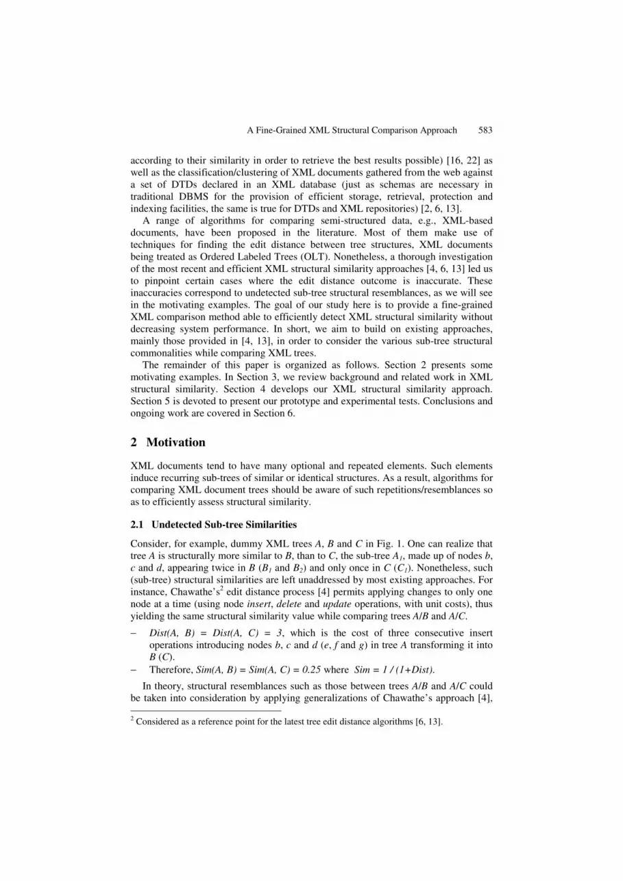
Consider, for example, dummy XML trees A, B and C in Fig. 1. One can realize that tree A is structurally more similar to B, than to C, the sub-tree A1, made up of nodes b, c and d, appearing twice in B (B1 and B2) and only once in C (C1). Nonetheless, such (sub-tree) structural similarities are left unaddressed by most existing approaches. For instance, Chawathe’s2 edit distance process [4] permits applying changes to only one node at a time (using node insert, delete and update operations, with unit costs), thus yielding the same structural similarity value while comparing trees A/B and A/C.

− Dist(A, B) = Dist(A, C) = 3, which is the cost of three consecutive insert operations introducing nodes b, c and d (e, f and g) in tree A transforming it into B (C).

− Therefore, Sim(A, B) = Sim(A, C) = 0.25 where Sim = 1 / (1+Dist).

In theory, structural resemblances such as those between trees A/B and A/C could be taken into consideration by applying generalizations of Chawathe’s approach [4], 2 Considered as a reference point for the latest tree edit distance algorithms [6, 13].

584 J. Tekli, R. Chbeir, and K. Yetongnon

developed by Nierman and Jagadish [13] and Dalamagas et al. [6] (introducing edit operations allowing the insertion and deletion of whole sub-trees). Yet, our examination of the approaches provided in [6, 13] led us to identify certain cases where sub-tree structural similarities are disregarded:

− Similarity between trees A/D (sub-trees A1 and D2) in comparison with A/E. − Similarity between trees F/G (sub-trees F1 and G2) relatively to F/H. − Similarity between trees F/I (sub-tree F1 and tree I) in comparison with F/J.

In essence, the authors in [13] make use of the contained in relation between trees (cf. Definition 2) so as to capture sub-tree similarities. Following [13], a tree A may be inserted in T only if A is already contained in the source tree T. Similarly, a tree A may be deleted only if A is already contained in the destination tree T. Therefore, the approach in [13] captures the sub-tree structural similarities between XML trees A/B in Fig. 1, transforming A to B in a single edit operation: (inserting sub-tree B2 in A, B2

occurring in A as A1), whereas transforming A to C would always need three consecutive insert operations (inserting nodes e, f and g).

Fig. 1. Sample XML trees

Nonetheless, when the containment relation is not fulfilled, certain structural similarities are ignored. Consider, for instance, trees A and D in Fig. 1. Since D2 is not contained in A, it is inserted via four edit operations instead of one (insert tree), while transforming A to D, ignoring the fact that part of D2 (sub-tree of nodes b, c, d) is identical to A1. Therefore, equal distances are obtained when comparing trees A/D and A/E, disregarding A/D’s structural resemblances:

− Dist(A, D) = CostIns(h) + CostIns(b) + CostIns(c) + CostIns(d) + CostIns(h) = 1+4 = 5 − Dist(A, E) = CostIns(h) + CostIns(e) + CostIns(f) + CostIns(g) + CostIns(h) = 1+4 = 5

h

i j

b

c dH1

H2

a

m

g

h i j

G1

G2

a

m

b

c d f

a

b

c d e

Tree F

F1

a

b

c d h

e

f g h

a

b

c d h

b

c d h

Tree D

a

b

c d

e

f g

a

b

d

b

c d c

a

b

c dA1

Tree A Tree C

B1 B2 C1 C2

D2D1 E2 E1

Tree E

Tree B

Tree I Tree G Tree H

Tree J


Likewise for the D to A transformation (tree D2 will not be deleted via a single delete tree operation since it is not contained in the destination tree A), achieving Dist(D, A) = Dist(E, A) = 5. Other types of sub-tree structural similarities that are missed by [13]’s approach (and likewise missed by [4, 6]) can be identified when comparing trees F/G and F/H, as well as F/I and F/J. The F, G, H case is different than its predecessor (the A, D, F case) in that the sub-trees sharing structural similarities (F1 and G2) occur at different depths (whereas with A/D, A1 and D2 are at the same depth). On the other hand, the F, I, J case differs from the previous ones since structural similarities occur, not only among sub-trees, but also at the sub-tree/tree level (e.g., between sub-tree F1 and tree I).

Note that in [6], the authors complement their edit distance algorithm (which can be viewed as a specialized version of [13]’s algorithm) with a repetition/nesting reduction process, summarizing the XML documents prior to the comparison phase. Such a reduction pre-processing transforms, for instance, tree B to A, thus yielding Dist(A, B) = 0 which is not accurate (tree A is obviously different than B). While it might be useful for structural clustering tasks, the reduction process yields inaccurate comparison results in the general case, which is why it is disregarded in our discussion. Therefore, we only consider [6]’s edit distance algorithm in our analysis.

2.2 The Special Case of Single Leaf Node Sub-trees

In addition, none of the approaches mentioned above is able to effectively compare documents made of repeating leaf node sub-trees. For example, following [4, 6, 13], the same structural similarity value is obtained when comparing document K, of Fig. 2, to documents L and M, Sim(K, L) = Sim(K, M) = 0.5, having Dist(K, L) = Dist(K, M) = 1.

− Dist(K, L) = CostIns(b) = 1 − Dist(K, M) = CostIns(c) = 1

However, one can realize that document trees K and L are more similar than K and M, node b of tree K appearing twice in tree L, and only once in XML tree M. Likewise for K/N with respect to K/O and K/P. Identical distances are attained when comparing document trees K/N, K/O and K/P, Dist(K, N)=Dist(K, O)= Dist(K, P)=2, despite the fact that the node b is repeated three times in tree N, twice in tree O and only appears once in P.

− Dist(K, N) = CostIns(b) + CostIns(b) = 2 − Dist(K, O) = CostIns(b) + CostIns(c) = 2 − Dist(K, P) = CostIns(c) + CostIns(d) = 2

\

Fig. 2. XML documents consisting of leaf node sub-trees

b c d

a a

b b c

a

b b b c b

a a

b b

a

b

Tree K Tree L Tree M Tree N Tree O Tree P


In this paper, we explicitly mention the case of leaf node repetitions since:

− Leaf nodes are a special kind of sub-trees: single node sub-trees. Therefore, the study of sub-tree resemblances and repetitions should logically cover leaf nodes, so as to attain a more complete XML similarity approach.

− Leaf node repetitions are usually as frequent as substructure repetitions (i.e. non-leaf node sub-tree repetitions) in XML documents.

− Detecting leaf node repetitions is spontaneous in the XML context, and would help increase the discriminative power of XML comparison methods, as shown in the examples of Fig. 2 (which will be subsequently conferred in detail).

3 Related Work and Background

3.1 XML Data Model

XML documents represent hierarchically structured information and can be modeled as Ordered Labeled Trees (OLTs)3 [20]. Nodes in a traditional DOM (Document Object Model) ordered labeled tree represent XML elements and are labeled with corresponding element tag names. Attributes mark the nodes of their containing elements. However, to incorporate attributes in their similarity computations, some approaches [13, 22] have considered OLTs with distinct attribute nodes, labeled with corresponding attribute names. Attribute nodes appear as children of their encompassing element nodes, sorted by attribute name, and appearing before all sub-element siblings [13]. The authors in [7, 13] agree on disregarding element/attribute values while studying the structural properties of heterogeneous XML documents.

3.2 Sate of the Art

Various methods, for determining structural similarities between hierarchically structured data, particularly XML documents, have been proposed. Most of them derive, in one way or another, the dynamic programming techniques for finding edit distance between strings [11, 18, 19]. In essence, all these approaches aim at finding the cheapest sequence of edit operations that can transform one tree into another. Nevertheless, tree edit distance algorithms can be distinguished by the set of edit operations that are allowed as well as overall complexity and performance levels. Early approaches in [17, 21] allow insertion, deletion and relabeling of nodes anywhere in the tree. Yet, they are relatively complex. For instance, the approach in [17] has a time complexity O(|A||B| depth(A) depth(B)) (where |A| and |B| denote tree cardinalities while depth(A) and depth(B) are the depths of the trees). The authors in [3, 5] restrict insertion and deletion operations to leaf nodes and add a move operator that can relocate a sub-tree, as a single edit operation, from one parent to another. However, corresponding algorithms do not guarantee optimal results. Recent work by Chawathe [4] restricts insertion and deletion operations to leaf nodes, and allows the relabeling of nodes anywhere in the tree, while disregarding the move operation. The overall complexity of [4]’s algorithm is of O(N2). Nierman and Jagadish [13] extend the approach of [4] by adding two new operations: insert tree and delete tree to allow insertion and deletion of whole sub-trees within in an OLT. This approach’s 3 In the following, tree designates ordered labeled tree.


overall complexity simplifies to O(N2) despite being conceptually more complex than its predecessor. A specialized version of [13]’s algorithm is provided in [6]. Following [6], tree insertion/deletion operations costs are computed as the sum of the costs of inserting/deleting all individual nodes in the considered sub-trees, whereas in [13], certain sub-tree similarities are considered (via the containment relation, cf. Definition 2) while assigning operations costs. On the other hand, an original structural similarity approach is presented in [7]. It disregards OLTs and utilizes the Fast Fourier Transform to compute similarity between XML documents. Yet, the authors did not compare their algorithm’s optimality to existing edit distance approaches. Another approach, disregarding edit distance computations was introduced by Sanz et al. in [15]. It utilizes specific indexing structures rather than tree edit distance. Experimental results in [15] confirm that the approach is of linear complexity. Nonetheless, the authors in [15] do not compare their algorithm’s optimality to existing approaches.

4 Proposal

Our XML structural similarity approach consists of two algorithms: i) an algorithm for identifying the Commonality Between two Sub-trees (CBS)4, ii) and an algorithm for computing the Tree edit distance Operations Costs (TOC). The TOC algorithm makes use of CBS, its results being exploited via [13]’s main edit distance algorithm (cf. Appendix), so as to identify the structural similarity between two XML documents (cf. Fig. 3). In the following, we start by presenting some basic definitions required to develop each of our algorithms.

Fig. 3. Simplified activity diagram of our XML structural similarity approach

4.1 Preliminary Definitions

Def. 1 - Ordered Labeled Tree: it is a rooted tree in which the nodes are ordered and labeled. We denote by λ(T) the label of the root node of tree T. In the rest of this paper, the term tree means rooted ordered labeled tree.

Def. 2 - Tree “Contained in” relationship: a tree A is said to be contained in a tree T if all nodes of A occur in T, with the same parent/child edge relationship and node order. Additional nodes may occur in T between nodes in the embedding of A (e.g., tree K in Fig. 2 is contained in tree A of Fig. 1).

Def. 3 - Sub-tree: given two trees T and T’, T’ is a sub-tree of T if all nodes of T’ occur in T, with the same parent/child edge relationship and node order, such as no

4 CBS can be applied to whole trees. However, in our study, its use is coupled with sub-trees.

TOC

CBS

Edit Distance Tree T2

Tree T1


additional nodes occur in the embedding of T’ (e.g., A1 in Fig. 1 is a sub-tree of A, whereas tree K does not qualify as a sub-tree of A since nodes c and d occur in its embedding in A).

Def. 4 - First level sub-tree: given a tree T with root p of degree k, the first level sub-trees, T1, …, Tk of T are the sub-trees rooted at the children nodes of p: p1, …, pk.

Def. 5 - Ld-pair representation of a node: it is defined as the pair (l, d) where l and d are respectively the node’s label and depth in the tree. We use p.l and p.d to refer to the label and the depth of an ld-pair node p respectively.

Def. 6 - Ld-pair representation of a tree: it is the list, in preorder, of the ld-pairs of its nodes (cf. Fig. 4). Given a tree in ld-pair representation T = (t1, t2, …, tn), T[i] refers to the ith node ti of T. Consequently, T[i].l and T[i].d denote, respectively, the label and the depth of the ith node of T, i designating the preorder traversal rank of node T[i] in T.

Def. 7 - Structural commonality between sub-trees: given two sub-trees A = (a1, …, am) and B = (b1, …, bn), the structural commonality between A and B, designated by ComSubTree(A, B), is a set of nodes N = {n1, …, np} such that ∀ ni ∈ N, ni occurs in A and B with the same label, depth and relative node order (in preorder traversal ranking) as in A and B. For 1 ≤ i ≤ p ; 1 ≤ r ≤ m ; 1 ≤ u ≤ n:

(1) ni.l = ar.l = bu.l (2) ni.d = ar.d = bu.d (3) For any nj ∈ N / i ≤ j, ∃ as ∈ A and bv ∈ B such as:

• nj.l = as.l = bv.l • nj.d = as.d = bv.d • r ≤ s, u ≤ v

(4) There is no set of nodes N’ that satisfies conditions 1, 2 and 3 and is of larger cardinality than N.

A1 = ((b, 0), (c, 1), (d, 1)) A11 = (c, 0) A12 = (d, 1)

B1 = ((b, 0), (c, 1), (d, 1)) B11 = (c, 0) B12 = (d, 0)

B2 = ((b, 0), (c, 1), (d, 1)) B21 = (c, 0) B22 = (d, 0)

C1 = ((b, 0), (c, 1), (d, 1)) C11 = (c, 0) C12 = (d, 0)

C2 = ((e, 0), (f, 1), (g, 1)) C21 = (f, 0) C22 = (g, 0)

D1 = ((b, 0), (c, 1), (d, 1), (h, 1)) D11 = (c, 0) D12 = (d, 0) D13 = (h, 0)

D2 = ((b, 0), (c, 1), (d, 1), (h, 1)) D21 = (c, 0) D22 = (d, 0) D23 = (h, 0)

E1 = ((b, 0), (c, 1), (d, 1), (h, 1)) E11 = (c , 0) E12 = (d, 0) E13 = (h, 0)

E2 = ((e, 0), (f, 1), (g, 1), (h, 1)) E21 = (f, 0) E22 = (g, 0) E23 = (h, 0)

F1 = ((b, 0), (c, 1), (d, 1), (e, 1)) F11 = (c, 0) F12 = (d, 0) F13 = (e, 0)

G1 = ((m, 0), (b, 1), (c, 2), (d, 2), (e, 2)) G2 = ((b, 0), (c, 1), (d, 1), (e, 1))

G21 = (c, 0) G22 = (d, 0) G23 = (e, 0)

H1 = ((m, 0), (g, 1), (h, 2), (i, 2), (j, 2)) H2 = ((g, 0), (h, 1), (i, 1), (j, 1))

H21 = (h, 0) H22 = (i, 0) H23 = (j, 0)

I1 = (c, 0) I2 = (d, 0) J1 = (i, 0) J2 = (j, 0)

Fig. 4. Ld-pair representations of all sub-trees in Fig. 1, including single leaf node sub-trees


In other words, ComSubTree(A, B)5 identifies the set of matching nodes between sub-trees A and B, node matching being undertaken with respect to the node label, depth and relative preorder ranking. Please note that in the rest of the paper, the term commonality always designates the structural commonality.

Def. 8 - Insert node: given a node x of degree 0 (leaf node) and a tree T with root node p having first level sub-trees T1, …, Tm, Ins(x, i, p, l) is a node insertion applied to T, inserting x as the ith child of p, thus yielding T’ with first level sub-trees T1, … , Ti-1, x, Ti+1, … , Tm+1, where l is the label of x.

Def. 9 - Delete node: given a leaf node x and a tree T with root node p, x being the ith child of p, Del(x, p) is a node deletion operation applied to T that yields T’ with first level sub-trees T1, … , Ti-1, Ti+1, … , Tm.

Def. 10 - Update node: given a node x in tree T, and a label l, Upd(x, l) is a node update operation applied to x resulting in T’ which is identical to T except that in T’, x bears l as its label. The update operation could be also formulated as follows: Upd(x, y) where y.l denotes the new label to be assumed by x.

Def. 11 - Insert tree: given a tree A and a tree T with root node p having first level sub-trees T1, …, Tm , InsTree(A, i, p) is a tree insertion applied to T, inserting A as the ith sub-tree of p, thus yielding T’ with first level sub-trees T1, …, Ti-1, A, Ti+1, …, Tm+1.

Def. 12 - Delete tree: given a tree A and a tree T with root node p, A being the ith sub-tree of p, DelTree(A, p) is a tree deletion operation applied to T that yields T’ with first level sub-trees T1, … , Ti-1, Ti+1, … , Tm.

4.2 Commonality Between Sub-trees (CBS)

In order to capture the sub-tree structural similarities not well addressed by current approaches, we identify the need to replace the tree contained in relation making up a necessary condition for executing tree insertion and deletion operations in [13], by introducing the notion of commonality between two sub-trees. Following Definition 7, the problem of finding the structural commonality between two sub-trees SbTi and SbTj is equivalent to finding the maximum number of matching nodes in SbTi and SbTj (|ComSubTree(SbTi, SbTj)|). However, the problem of finding the shortest edit distance between SbTi and SbTj comes down to identifying the minimal number of edit operations that can transform SbTi to SbTj. Those are dual problems since identifying the shortest edit distance between two sub-trees (trees) underscores, in a roundabout way, their maximum number of matching nodes.

Therefore, we introduce in Fig. 5 our CBS algorithm, based on the edit distance concept, to identify the structural commonality between sub-trees (similarly to the approach provided in [12] in which Myers develops an edit distance based approach for computing the longest common sub-sequence between two strings). Note that in CBS, sub-trees are treated in their ld-pair representations (cf. Fig. 4). Using the ld-pair tree representations, sub-trees are transformed into modified sequences (ld-pairs), making them suitable for standard edit distance computations. 5 Our sub-tree structural commonality definition can be equally applied to whole trees (a sub-

tree being basically a tree). However, in this study, it is mostly utilized with sub-trees.


Afterward, the maximum number of matching nodes between SbTi and SbTj, |ComSubTree(SbTi, SbTj)|, is identified with respect to the minimum edit distance:

− Total number of deletions - we delete all nodes of SbTi except those having matching nodes in SbTj:

Deletions∑ = |SbTi| - |ComSubTree(SbTi , SbTj)|

− Total number of insertions - we insert into SbTi all nodes of SbTj except those having matching nodes in SbTi:

Insertions∑ = |SbTj| - |ComSubTree(SbTi , SbTj)|

− Following CBS, using constant unit costs (=1) for node insertion and deletion operations, the edit distance between sub-trees SbTi and SbTj becomes as

follows: Dist[|SbTi|][|SbTj|] = Deletions∑ 1 +

Insertions∑ 1 = |SbTi| + |SbTj| - 2

|ComSubTree(SbTi , SbTj)|

− Therefore, | |+| | - [| |][| |]

| ( , )| =2

i j i j

i j

SbT SbT Dist SbT SbTComSubTree SbT SbT

For instance, |ComSubTree(A1,D1)| = 3 (nodes b, c, d), |ComSubTree(E2,G2)|= 1 (node f). Note that applying CBS to leaf node sub-trees comes down to comparing two labels: those of the leaf nodes at hand. For example:

− |ComSubTree(A11, B11)| = 1, A11 and B11 consisting of leaf node c, − |ComSubTree(A11, B12)| = 0, A11 and B12 having different labels (λ(A11) =

A11[0].l = c whereas λ(B12) = B12[0].l = d).

Similarly, when computing the commonality between a leaf node sub-tree (e.g., A11) and a non-leaf node sub-tree (e.g., B1), CBS comes down to comparing the label of the former (e.g., λ(A11)) to the label of the root node of the latter (e.g., λ(B1)). For example, |ComSubTree(A11, B1)| = 0, A11 and the root of B11 having different labels (λ(A11) = A11[0].l = c whereas λ(B1) = B1 [0].l = b).

4.3 Tree Edition Operations Costs (TOC)

Our CBS algorithm, for the identification of the commonality between sub-trees, is to be utilized in TOC: an algorithm dedicated to computing the tree edit distance operations costs (insert tree and delete tree, cf. definitions 11 and 12). Consequently, those costs will be exploited via [13]’s main edit distance approach (cf. Fig. 5) providing an improved and more accurate XML structural similarity measure. TOC is developed in Fig. 5 and consists of three main steps:

− Step 1 (lines 2-15) identifies the structural commonalities between each pair of sub-trees in the source and destination trees respectively (T1 and T2), assigning tree insert/delete operation costs accordingly.

− Step 2 (lines 16-20) identifies the structural commonalities between each sub-tree in the source tree (T1) and the destination tree (T2) as a whole, updating delete tree operation costs correspondingly.

− Step 3 (lines 21-25) identifies the structural commonalities between each sub-tree in the destination tree (T2) and the source tree (T1) as a whole, modifying insert tree operation costs accordingly.


Algorithm CBS()

Input: Sub-trees SbTi and SbTj (in ld-pair) Output: |ComSubTree(SbTi, SbTj)|

Begin 1

Dist [][] = new [0...|SbTi|][0…|SbTj|] Dist[0][0] = 0

For (n = 1 ; n ≤ |SbTi| ; n++) 5 {Dist[n][0] = Dist[n-1][0] + CostDel(SbTi[n])}

For (m = 1 ; m ≤ |SbTj| ; m++) {Dist[0][m] = Dist[0][m-1] + CostIns(SbTj[m])}

For (n = 1 ; n ≤ |SbTi| ; n++) 10 {

For (m = 1 ; m ≤ |SbTj| ; m++) {

Dist[n][m] = min{ If (SbTi[n].d = SbTj[m].d & SbTi[n].l = SbTj[m].l) 15

{ Dist[n-1][m-1] }, Dist[n-1][m] + CostDel(SbTi[n]), Dist[n][m-1] + CostIns(SbTj[m]) }

} } 20

Return | |+| | - [| |][| |]

i j i jSbT SbT Dist SbT SbT

2

End // |CBS(SbTi, SbTj)|

Algorithm TOC()

Input: Trees T1 and T2 Output: Insert tree and delete tree operations costs

Begin 1

For each sub-tree SbTi in T1 //Going through { //all sub-trees in T1

CostDelTree(SbTi) = i

x

x∑Del

All nodes of SbT

Cost ( ) //sub-trees in T1. 5

For each sub-tree SbTj in T2 //Going through { //all sub-trees in T2

CostInsTree(SbTj) = j

x

x∑Ins

All nodes of SbT

Cost ( )

CostDelTree(SbTi) = Min{ CostDelTree(SbTi), 10

i ji

i j

( , )

(| | , | |)

x

x ×∑Del

All nodes of SbT

1Cost ( )

SbT SbT 1 +

Max SbT SbT

CBS }

CostInsTree(SbTj) = Min{ CostInsTree(SbTj),

i jj

i j

( , )

(| | , | |)

x ×∑Ins

All nodes of SbT

1Cost ( )

SbT SbT 1 +

Max SbT SbT

x CBS}

} } 15

For each sub-tree SbTi in T1 // Comparing sub-trees in T1 { // to whole tree T2.

CostDelTree(SbTi) = Min{ CostDelTree(SbTi),

ii

i

( , )

(| | , | |)

x

x ×∑Del

All nodes of SbT 2

2

1Cost ( )

SbT T 1 +

Max SbT T

CBS}

} 20

For each sub-tree SbTj in T2 // Comparing sub-trees in T2 { // to whole tree T1.

CostInsTree(SbTj) = Min{ CostInsTree(SbTj),

jj

j

( , )

(| | , | |)

x

x ×∑Ins

All nodes of SbT 1

1

1Cost ( )

T SbT 1 +

Max T SbT

CBS}

} 25

End

Algorithm EditDistance()

Input: Trees A and B Output: Edit distance between A and B

Begin 1

M = Degree(A) //Number of 1st level sub-trees in A N = Degree(B) //Number of 1st level sub-trees in B

Dist [][] = new [0...M][0…N] 5 Dist[0][0] = CostUpd(λ(A), λ(B))

For (i = 1 ; i ≤ M ; i++) { Dist[i][0] = Dist[i-1][0] + CostDelTree(Ai) }

For (j = 1 ; j ≤ N ; j++) { Dist[0][j] = Dist[0][j-1] + CostInsTree(Bj) } 10

For (i = 1 ; i ≤ M ; i++) {

For (j = 1 ; j ≤ N ; j++) {

Dist[i][j] = min{ 15 Dist[i-1][j-1] + EditDistance(Ai, Bj), Dist[i-1][j] + CostDelTree(Ai), Dist[i][j-1] + CostInsTree(Bj) }

} } 20

Return Dist[M][N]

End

Fig. 5. Our TOC and CBS algorithms, along with [13]’s Edit Distance algorithm

Steps 2 and 3 are introduced to capture, not only the structural similarities between

sub-trees, but also the similarities between the sub-trees and the overall structures of the trees being compared. The relevance of steps 2 and 3 becomes obvious when one of the trees involved in the comparison process shares structural similarities with one


(or more) of the sub-trees encompassed in the other XML document tree (e.g., the F, I, J case in Fig. 1, where tree I is structurally similar to sub-tree F1 of tree F).

Using CBS, TOC identifies the structural commonality between each and every pair of sub-trees (SbTi, SbTj) in the two trees A and B being compared (step 1), as well as their commonalities with the whole trees A and B, respectively (steps 2 and 3). Consequently, those values are normalized via corresponding tree/sub-tree cardinalities Max(|SbTi| , |SbTj|) to be comprised between 0 and 1:

− i j

i j

(SbT , SbT )

Max(|SbT | , |SbT |)

CBS= 0 When there is no structural commonality

between SbTi and SbTj : CBS(SbTi, SbTj) = 0

− i j

i j

(SbT , SbT )

Max(|SbT | , |SbT |)

CBS= 1 When the sub-trees are identical:

CBS(SbTi, SbTj) = |SbTi| = |SbTj|

For instance, 1 1

1 1

(A , D ) 30.75

Max(|A | , |D |) 4

CBS= = , 2 2

2 2

(E , G ) 10.25

Max(|E | , |G |) 4

CBS= = (cf. Fig. 1).

Thus, using the normalized commonality, tree operations costs would vary as follows:

Maximum insert/delete tree cost for sub-tree Sbi: Minimum insert/delete tree cost for sub-tree Sbi:

CostInsTree/DelTree(Sbi) = Ins/DelAll nodes of SbTi

Cost ( ) 1x

x ×∑ CostInsTree/DelTree(Sbi) = Ins/DelAll nodes of SbTi

1

2Cost ( )

x

x ×∑

Lemma 1. Following TOC, the maximal insert/delete tree operation cost for a given sub-tree SbTi (attained when no sub-tree structural similarities with SbTi are identified in the source/destination tree respectively) is the sum of the costs (unit costs, =1)6 of inserting/deleting every individual node of SbTi (the proof is evident).

Lemma 2. Following TOC, the minimal insert/delete tree operation cost for SbTi (attained when a sub-tree structurally identical to SbTi is identified in the source/destination tree respectively) is equal to half its corresponding insert/delete tree maximum cost.

Proof: The smallest sub-tree that can be treated via a tree operation is a sub-tree consisting of two nodes. For such a tree, the minimum insert/delete tree operation cost would be equal to 1 (its maximum cost being equal to 2), equivalent to the cost of inserting/deleting a single node, which is the lowest tree operation cost attainable following TOC.

The minimal tree operation cost is defined in such a way in order to guarantee that the cost of inserting/deleting a non-leaf node sub-tree will never be less than the cost of inserting/deleting a single node (single node operations having unit costs). In fact, TOC is based on the intuition that tree operations are more costly than node

6 An intuitive and natural way has been usually used to assign single node operation costs and

consists of considering identical unit costs for insertion and deletion operations [4, 15].


operations. Consequently, for leaf node sub-trees, the maximum insert/delete tree operation cost is equal to 1, the cost of inserting/deleting the single node at hand:

− CostInsTree/DelTree(SbTi) = CostIns/Del(x) × 1 = 1 , that is when SbTi is made of single node x

Likewise, the minimum cost for inserting/deleting a single node sub-tree is equal to 0.5, half its insert/delete maximum cost:

− CostInsTree/DelTree(SbTi) = CostIns/Del(x) × 1/2 = 0.5 , SbTi consisting of single node x

Note that in our approach, single node insertions/deletions are undertaken via tree insert/delete operations (cf. definitions 11 and 12) applied on leaf node sub-trees. On the other hand, insert/delete node operations (cf. definitions 8 and 9, which are assigned unit costs as with traditional edit distance approaches) are only utilized to compute tree insertion/deletion operations costs (cf. CBS and TOC in Fig. 5). They do not however contribute to the dynamic programming procedure adopted in our edit distance approach (similarly to [6, 13], cf. Edit Distance algorithm in Fig. 5).

Using TOC, we compute the costs of tree insertion and deletion operations based on their corresponding trees’ maximum normalized commonality values (a maximum commonality value inducing a minimum tree operation cost).

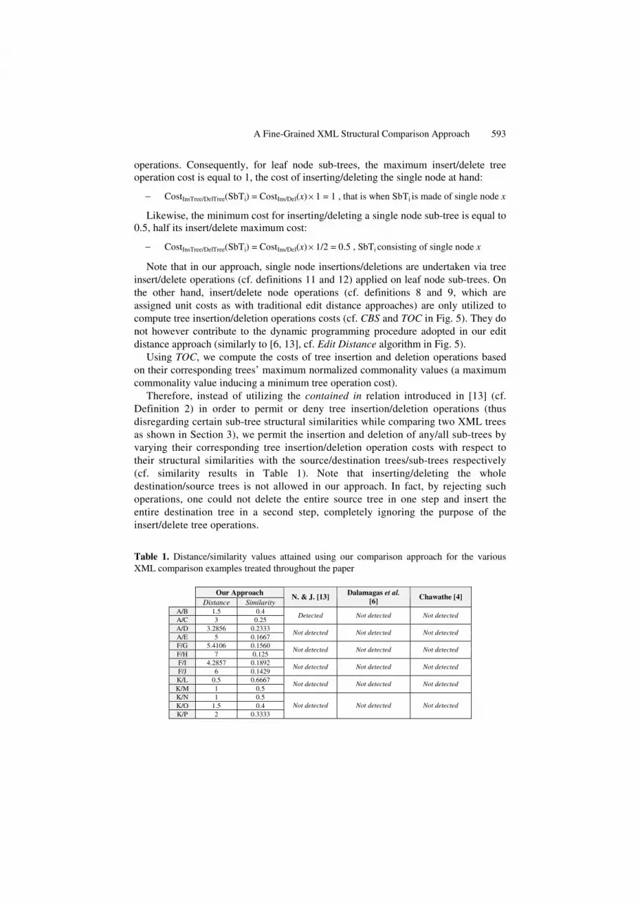
Therefore, instead of utilizing the contained in relation introduced in [13] (cf. Definition 2) in order to permit or deny tree insertion/deletion operations (thus disregarding certain sub-tree structural similarities while comparing two XML trees as shown in Section 3), we permit the insertion and deletion of any/all sub-trees by varying their corresponding tree insertion/deletion operation costs with respect to their structural similarities with the source/destination trees/sub-trees respectively (cf. similarity results in Table 1). Note that inserting/deleting the whole destination/source trees is not allowed in our approach. In fact, by rejecting such operations, one could not delete the entire source tree in one step and insert the entire destination tree in a second step, completely ignoring the purpose of the insert/delete tree operations.

Table 1. Distance/similarity values attained using our comparison approach for the various XML comparison examples treated throughout the paper

Our Approach Distance Similarity

N. & J. [13] Dalamagas et al. [6]

Chawathe [4]

A/B 1.5 0.4 A/C 3 0.25

Detected Not detected Not detected

A/D 3.2856 0.2333 A/E 5 0.1667

Not detected Not detected Not detected

F/G 5.4106 0.1560 F/H 7 0.125


F/I 4.2857 0.1892 F/J 6 0.1429


K/L 0.5 0.6667 K/M 1 0.5


K/N 1 0.5 K/O 1.5 0.4 K/P 2 0.3333



4.4 Efficiency w.r.t. Existing Approaches

In the previous paragraphs, the comparison of our method with existing tree XML structural similarity approaches is done via examples. Here, we formalize the comparison and show that existing methods are lower bounds of our approach.

Theorem. Let T1 and T2 be XML trees, and Sim(T1, T2) = 1 / 1 + Dist(T1, T2), then:

− SimChawathe(T1, T2) ≤ SimOur Approach(T1, T2) − SimDalamagas et al.(T1, T2) ≤ SimOur Approach(T1, T2) − SimN.&J(T1, T2). ≤ SimOur Approach(T1, T2)

Proof:

− Proving that Chawathe’s algorithm [4] is a lower bound of our XML comparison method is straight forward. When computing the distance between two trees using Chawathe’s approach [4], all sub-trees are inserted/deleted via single node insertion/deletion operations regardless of the sub-tree similarities at hand. The costs of these insertions/deletions are equivalent to the maximum tree insertion/deletion operations’ costs following our TOC algorithm (cf. Section 4.3), which yield a maximum edit distance, thus a minimum similarity value between the trees being compared. In other words, Chawathe’s algorithm [4] always yields similarity values lesser or equal to those computed via our approach.

− Proving that Dalamagas et al.’s algorithm [6] is a lower bound of our XML comparison method is also trivial. Indeed, the costs of tree insertion/deletion operations in [6] are computed as the sum of the costs of inserting/deleting all individual nodes in the considered sub-trees. These costs come down to the maximum tree operations costs computed following our method. Consequently, Dalamagas et al.’s algorithm [6] always yields similarity values that are lesser or equal to those computed via our method. Recall that we do not consider [6]’s repetition/nesting reduction process in our analysis (cf. Section 2.1).

− As for Nierman and Jagadish [13], tree insertion/deletion operations costs are affected by the tree containment relation (cf. Definition 2). Maximum costs (i.e. the costs of inserting/deleting all single nodes in the considered sub-trees) are attained when the containment relation is not verified. Otherwise, tree operations costs are minimal (the minimum tree operation cost is not formally defined in [13]. Thus, for a given sub-tree, we consider that it is equal to half its maximum tree operation cost so as to respect the intuition that tree operations costs are always higher or equal than single node operations costs). In other words, Nierman and Jagadish’s algorithm [13] only considers the containment relation between sub-trees while varying tree operations costs. However, our algorithm detects fined-grained structural similarities (i.e. sub-tree commonalities) between sub-trees, among which the containment relation, and varies tree operations accordingly. Thus, our approach is able to detect a wider set or structural similarities and consequently yields higher similarity values. In other words, when comparing two XML trees, Nierman and Jagadish’s algorithm [13] yields similarity values that are lesser or equal to those obtained via our XML structural comparison method.


4.5 Complexity Analysis

The overall complexity of our approach simplifies to O(|T1||T2|), where |T1| and |T2| denote the cardinalities of the compared trees, and is computed as follows:

− CBS algorithm for the identification of the commonality between two sub-trees is of complexity: O(|SbTi||SbTj|) where |SbTi| and |SbTj| denote the cardinalities of the compared sub-trees.

− TOC algorithm for computing the costs of tree insert/delete operations,

which makes use of CBS, is time complexity: 1 2 1| | | | | |

1 1 1

(| | | |) + (| | | |) T T T

i j i 2i j i

O SbT SbT O SbT T

2| |

1

+ (| | | |)T

j 1j

O SbT T.

Lemma 3. Let T1 and T2 be two ordered labeled trees, where 1Tn and

2Tn represent the

number of leafs in T1 and T2, SbTi and SbTj the sub-trees of T1 and T2 respectively.

Then TOC’s complexity:1 2 1 2| | | | | | | |

1 1 1 1

(| | | |) + (| | | |) + (| | | |)T T T T

i j i 2 j 1i j i j

O SbT SbT O SbT T O SbT T= = = =∑ ∑ ∑ ∑ ,

simplifies to O(|T1||T2|).

Proof:

• Step 1 of TOC – Identifying the structural commonalities between each pair of sub-trees in the source and destination trees:

1 2| | | |

1 1

(| | | |) (| || |) T T

i j 1 2i j

(demonstrated in [9])O SbT SbT O T T= =

≤∑ ∑

• Step 2 of TOC – Identifying the structural commonalities between each sub-tree in the source tree (T1) and the whole destination tree (T2):

1 1| | | |

1 1

(| | | |) = | | (| |) < (| || |)T T

i 2 2 i 1 2i i

O SbT T T O SbT O T T= =∑ ∑

• Step 3 of TOC – Identifying the structural commonalities between the source tree as a whole (T1) and each sub-tree in the destination tree (T2):

2 2| | | |

1 1

(| | | |) = | | (| |) < (| || |) T T

j 1 1 j 1 2j j

O SbT T T O SbT O T T= =∑ ∑

Note that the edit distance algorithm adopted from [13], which utilizes the results attained by TOC (tree operations costs), is of complexity O(|T1||T2|).

5 Experimental Evaluation

In order to validate our structural similarity approach and compare its optimality with alternative methods, we make use of structural clustering. In our experiments, we adopt the well known single link hierarchical clustering techniques [8, 10] although any form of clustering could be utilized. In order to evaluate clustering quality, we make use of precision and recall metrics commonly used in information retrieval. Having an a priori knowledge of which documents should be members of the


appropriate cluster (mapping between original DTD clusters and the extracted clusters), Dalamagas et al. [6] define precision PR and recall R as:

1

1 1 +

n

iin n

i ii i

aPR

a b

=

= =

∑=∑ ∑

and 1

1 1 +

n

ii

n n

i ii i

aR

a c

=

= =

∑=∑ ∑

where:

− n is the total number of clusters in the clustering set considered, − ai is the number of XML documents in Ci that indeed correspond to DTDi − bi is the number of documents in Ci that do not correspond to DTDi (mis-

clustered) − ci is the number of XML documents not in Ci, although they correspond to

DTDi (documents that should have been clustered in Ci).

Nonetheless, in addition to comparing one approach’s precision improvement to another’s recall improvement, it is a common practice to compare F-values, F-value = 2 PR R/(PR+R). Therefore, as in traditional information retrieval evaluation, high precision and recall, and thus high F-value (indicating in our case excellent clustering quality) characterize a good similarity method.

5.1 Experimental Results

We conducted a battery of experiments on real and synthetic XML documents. Two sets of 600 documents were generated from 20 real-case7

and synthetic DTDs, using an adaptation of the IBM XML documents generator8

. We varied the MaxRepeats parameter to determine the number of times a node will appear as a child of its parent node. For a real dataset, we considered the online version of the ACM SIGMOD Record9

. Overall precision, recall and F-value results are reported in Table 2.

Table 2. Average PR, R and F-values obtained by varying the clustering level between [0, 1]

SIGMOD Set 1 (MaxRepeats=5) Set 2 (MaxRepeats =10) PR R F-value PR R F-value PR R F-value

Chawathe [4] 0.8782 0.3910 0.6346 0.2502 0.4737 0.3619 0.2602 0.3809 0.3031 DCWS [6] 0.8782 0.3931 0.6356 0.2581 0.4838 0.3709 0.2779 0.3821 0.3061 N & J [13] 0.8637 0.4615 0.6626 0.2334 0.6162 0.4248 0.2234 0.4177 0.3271

Our approach 0.9086 0.4866 0.6706 0.2341 0.6262 0.4302 0.2203 0.4656 0.3458

Results, with respect to all three data sets, indicate that our approach yields

improved clustering quality (i.e. structural comparison quality) vis-à-vis current alternative approaches. Note that the complete precision vs. recall curves, describing the detailed behavior of each comparison method while varying the clustering level (and which clearly reveal that our method achieves better combinations of precision and recall, and thus higher clustering quality) are disregarded due to lack of space.

7 From http://www.xmlfiles.com and http://www.w3schools.com 8 http://www.alphaworks.ibm.com 9 Available at http://www.acm.org/sigmod/xml


5.2 Timing Results

Following the complexity analysis developed in Section 4.4, our XML structural similarity method is linear in the number of nodes of each tree, and polynomial (quadratic) in the size of the two trees being compared: O(|T1||T2|) (which can be simplified to O(N2), N being the maximum number of nodes in trees T1 and T2). This linear dependency on the size of each tree is experimentally verified, timing results being presented in Fig. 6. Timing experiments were carried out on a PC with an Intel Xeon 2.66 GHz processor (1GB RAM), running at 533 MHz. Fig. 6 shows that the time to identify the structural similarity between two XML trees of various sizes grows in an almost perfect linear fashion with tree size. Therefore, despite appearing theoretically more complex, timing results demonstrate that our method’s complexity is the same as the approaches by Nierman & Jagadish [13], Dalamagas et al. [6] as well as Chawathe [4].

0

100

200

300

400

500

600

700

0 100 200 300 400 500 600 700 800 900 1000

Number of nodes in tree T1

Tim

e (i

n se

co

nds

)

1 0 0

2 0 0

3 0 0

4 0 0

5 0 0

6 0 0

7 0 0

8 0 0

9 0 0

1 0 0 0

Fig. 6. Timing results obtained using our comparison method

6 Conclusion

In this paper, we proposed a structure-based similarity approach for comparing XML documents. Based on a tree edit distance technique, our approach captures fine-grained structural similarities while comparing XML documents not fully addressed in current approaches. Our theoretical study as well as our experimental evaluation showed that the proposed method yields improved structural similarity results with respect to existing alternatives, while having the same time complexity (O(N2)).

As continuing work, we are exploring the use of our approach in order to compare, not only the structure of XML documents (element/attribute labels) but also their information content (element/attribute values). In such a framework, XML schemas might have to be integrated in the comparison process, schemas underlining element/attribute data types which are required to compare corresponding element/attribute values. We are also working on extending our approach to encompass semantic similarity assessment between element/attribute node labels while comparing XML documents (taking into account synonyms, antonyms, acronyms, etc. in the edit distance process). In addition, we plan on releasing a public web service version of our prototype.

Number of nodesin tree T2


References

1. Aho, A., Hirschberg, D., Ullman, J.: Bounds on the Complexity of the Longest Common Subsequence Problem. Association for Computing Machinery 23(1), 1–12 (1976)

2. Bertino, E., Guerrini, G., Mesiti, M.: A Matching Algorithm for Measuring the Structural Similarity between an XML Documents and a DTD and its Applications. Elsevier Computer Science 29, 23–46 (2004)

3. Chawathe, S., Rajaraman, A., Garcia-Molina, H., Widom, J.: Change Detection in Hierarchically Structured Information. In: Proc. of the ACM SIGMOD 1996, ACM Press, New York (1996)

4. Chawathe, S.: Comparing Hierarchical Data in External Memory. In: VLDB 1999, pp. 90–101 (1999)

5. Cobéna, G., Abiteboul, S., Marian, A.: Detecting Changes in XML Documents. In: Proc. of the IEEE Int. Conf. on Data Engineering, pp. 41–52. IEEE Computer Society Press, Los Alamitos (2002)

6. Dalamagas, T., Cheng, T., Winkel, K., Sellis, T.: A methodology for clustering XML documents by structure. Information Systems 31(3), 187–228 (2006)

7. Flesca, S., Manco, G., Masciari, E., Pontieri, L., Pugliese, A.: Detecting Structural Similarities Between XML Documents. In: Proc. of 5th SIGMOD Workshop on The Web and Databases (2002)

8. Gower, J.C., Ross, G.J.S.: Minimum Spanning Trees and Single Linkage Cluster Analysis. Applied Statistics 18, 54–64 (1969)

9. Guha, S., Jagadish, H.V., Koudas, N., Srivastava, D., Yu, T.: Approximate XML Joins. In: Proceedings of ACM SIGMOD 2002, pp. 287–298 (2002)

10. Halkidi, M., Batistakis, Y., Vazirgiannis, M.: Clustering Algorithms and Validity Measures. In: SSDBM Conference, Virginia, USA (2001)

11. Levenshtein, V.: Binary Codes Capable of Correcting Deletions, Insertions and Reversals. Sov. Phys. Dokl. 6, 707–710 (1966)

12. Myers, E.: An O(ND) Difference Algorithm and Its Variations. Algorithmica 1, 251–266 (1986)

13. Nierman, A., Jagadish, H.V.: Evaluating structural similarity in XML documents. In: Proceedings of the 5th SIGMOD Workshop on The Web and Databases (2002)

14. van Rijsbergen, C.J.: Information Retrieval. Butterworths, London (1979) 15. Sanz, I., Mesiti, M., Guerrini, G., Berlanga Lavori, R.: Approximate Subtree Identification

in Heterogeneous XML Documents Collections. In: Bressan, S., Ceri, S., Hunt, E., Ives, Z.G., Bellahsène, Z., Rys, M., Unland, R. (eds.) XSym 2005. LNCS, vol. 3671, pp. 192–206. Springer, Heidelberg (2005)

16. Schlieder, T.: Similarity Search in XML Data Using Cost-based Query Transformations. In: Proceedings of 4th SIGMOD Workshop on The Web and Databases (2001)

17. Shasha, D., Zhang, K.: Approximate Tree Pattern Matching. In: Pattern Matching in Strings, Trees and Arrays, ch. 14, Oxford University Press, Oxford (1995)

18. Wagner, J., Fisher, M.: The String-to-String correction problem. ACM J. 21, 168–173 (1974) 19. Wong, C., Chandra, A.: Bounds for the String Editing Problem. ACM J. 23(1), 13–16

(1976) 20. WWW Consortium, The Document Object Model, http://www.w3.org/DOM 21. Zhang, K., Shasha, D.: Simple Fast Algorithms for the Editing Distance Between Trees

and Related Problems. SIAM J. of Computing 18(6), 1245–1262 (1989) 22. Zhang, Z., Li, R., Cao, S., Zhu, Y.: Similarity Metric in XML Documents. In: Knowledge

Management and Experience Management Workshop (2003)