arX

iv:0

705.

4043

v2 [

gr-q

c] 1

5 N

ov 2

007

Field-theoretical formulations of MOND-like gravity

Jean-Philippe Bruneton and Gilles Esposito-Farese

GRεCO, Institut d’Astrophysique de Paris,

UMR 7095-CNRS, Universite Pierre et Marie Curie-Paris6,

98bis boulevard Arago, F-75014 Paris, France

(Dated: May 25, 2007)

AbstractModified Newtonian dynamics (MOND) is a possible way to explain the flat galaxy rotation

curves without invoking the existence of dark matter. It is however quite difficult to predict such a

phenomenology in a consistent field theory, free of instabilities and admitting a well-posed Cauchy

problem. We examine critically various proposals of the literature, and underline their successes and

failures both from the experimental and the field-theoretical viewpoints. We exhibit new difficulties

in both cases, and point out the hidden fine tuning of some models. On the other hand, we show

that several published no-go theorems are based on hypotheses which may be unnecessary, so that

the space of possible models is a priori larger. We examine a new route to reproduce the MOND

physics, in which the field equations are particularly simple outside matter. However, the analysis

of the field equations within matter (a crucial point which is often forgotten in the literature)

exhibits a deadly problem, namely that they do not remain always hyperbolic. Incidentally, we

prove that the same theoretical framework provides a stable and well-posed model able to reproduce

the Pioneer anomaly without spoiling any of the precision tests of general relativity. Our conclusion

is that all MOND-like models proposed in the literature, including the new ones examined in this

paper, present serious difficulties: Not only they are unnaturally fine tuned, but they also fail to

reproduce some experimental facts or are unstable or inconsistent as field theories. However, some

frameworks, notably the tensor-vector-scalar (TeVeS) one of Bekenstein and Sanders, seem more

promising than others, and our discussion underlines in which directions one should try to improve

them.

PACS numbers: 04.50.+h, 95.30.Sf, 95.35.+d

1

I. INTRODUCTION

Although general relativity (GR) passes all precision tests with flying colors [1, 2], thereremain some puzzling experimental issues, notably the fact that the Universe seems to befilled with about 72% of dark energy and 24% of dark matter, only 4% of its energy contentbeing made of ordinary baryonic matter [3, 4]. Dark energy, a fluid whose negative pressure isclose to the opposite of its energy density, would be responsible for the present acceleratedexpansion of the Universe [5, 6, 7, 8]. Dark matter, a pressureless and noninteractingcomponent of matter detected only by its gravitational influence, is suggested by severalexperimental data, notably the flat rotation curves of clusters and galaxies [9]. Anotherexperimental issue is the anomalous extra acceleration δa ≈ 8.5 × 10−10 m.s−2 towards theSun that the two Pioneer spacecrafts exhibited between 30 and 70 AU [10] (see also [11]).

Actually, none of these issues contradicts GR nor Newtonian gravity directly. Indeed,dark energy may be understood as the existence of a tiny cosmological constant Λ ≈ 3 ×10−122 c3/(~G), or as a scalar field (called quintessence) slowly rolling down a potential[12, 13, 14]. Many candidates of dark matter particles have also been predicted by differenttheoretical models (notably the class of neutralinos, either light or more massive, occurringin supersymmetric theories; see e.g. [15]), and numerical simulations of structure formationhave obtained great successes while incorporating such a dark matter (see, e.g., [16]). [Itremains however to explain why Λ is so small but nonzero, and why the dark energy anddark matter densities happen to be today of the same order of magnitude.] The Pioneeranomaly seems more problematic, but the two spacecrafts are identical and were not builtto test gravity, therefore one must keep cautious in interpreting their data. A dedicatedmission would be necessary to confirm the existence of such an anomalous acceleration.

Nevertheless, these various issues, considered simultaneously, give us a hint that Newton’slaw might need to be modified at large distances, instead of invoking the existence of severaldark fluids. To avoid the dark matter hypothesis, Milgrom [17] proposed in 1983 sucha phenomenological modification, which superbly accounts for galaxy rotation curves [18](although galaxy clusters anyway require some amount of dark matter), and automaticallyrecovers the Tully-Fisher law [19] v4

∞ ∝ M (where M denotes the baryonic mass of a galaxy,and v∞ the asymptotic circular velocity of visible matter in its outer region). The norma of a particle’s acceleration is assumed to be given by its Newtonian value aN when it isgreater than a universal constant a0 ≈ 1.2 × 10−10 m.s−2, but to read a =

√aNa0 in the

small-acceleration regime a < a0. In particular, the gravitational acceleration should nowread a =

√GMa0/r at large distances, instead of the usual GM/r2 law.

Various attempts have been made to derive such a modified Newtonian dynamics(MOND) from a consistent relativistic field theory. The main aim of the present paperis to examine them critically, by underlining their generic difficulties and how some modelsmanaged to solve them. Three classes of difficulties may actually be distinguished: (i) theo-retical ones, namely whether the proposed model derives from an action principle, is stableand admits a well-posed Cauchy problem; (ii) experimental ones, in particular whethersolar-system and binary-pulsar tests are passed, and whether the predicted light deflectionby galaxies or haloes is consistent with weak-lensing observations; and (iii) “esthetical” ones,i.e., whether the proposed model is natural enough to be considered as predictive, or so fine-tuned that it almost becomes a fit of experimental data. These different classes of difficultiesare anyway related, because fine-tuning is often necessary to avoid an experimental problem,and because some tunings sometimes hide serious theoretical inconsistencies.

2

We will not address below the problem of dark energy, although it may also be tackledwith a modified-gravity viewpoint. For instance the DGP brane model [20, 21] predicts anaccelerated expansion of the Universe without invoking a cosmological constant [22, 23], andthe k-essence models [24, 25, 26] also reproduce many cosmological features in a somewhatmore natural way than quintessence theories. Some of our theoretical discussions below,notably about stability and causality, are nevertheless directly relevant to such models. In-deed, k-essence theories are characterized by a non-linear function of a scalar field’s kineticterm, precisely in the same way relativistic aquadraric Lagrangians (RAQUAL) were de-vised to reproduce the MOND phenomenology in a consistent field theory [27]. Our aim isnot to discuss the Pioneer anomaly in depth either. Although the numerical value of thesespacecrafts’ extra acceleration δa is of the same order of magnitude as the MOND parametera0, there indeed exist important differences between their behavior and the MOND dynam-ics. However, we will come back to the Pioneer anomaly at the very end of the presentpaper. While analyzing a new class of models a priori devised to reproduce the MONDphenomenology, we will show that it can account for the Pioneer anomaly without spoilingany of the precision tests of general relativity, while being stable and admitting a well-posedCauchy problem.

Our paper is organized as follows. In Sec. II, we examine the various ways one may try tomodify the laws of gravity in a consistent relativistic field theory, and give a critical reviewof several models proposed in the literature. We notably underline that an action should notdepend on the mass of a galaxy, otherwise one is defining a different theory for each galaxy.We also recall why higher-order gravity is generically unstable, contrary to scalar-tensortheories. When the dynamics of the scalar field is defined by an aquadratic kinetic term(RAQUAL or k-essence theories), we discuss the different consistency conditions it mustsatisfy. We point out that such conditions suffice for local causality to be satisfied, althoughsome modes may propagate faster than light or gravitational waves. We finally recall howRef. [27] reproduced the MOND gravitational force thanks to a RAQUAL model, but weexhibit a serious fine-tuning problem which does not seem to have been discussed before —or at least was not pointed out so clearly.

In Sec. III, we recall that many models fail to reproduce the observed light deflection by“dark matter” haloes. We exhibit a counter-example to an erroneous claim in the literature,although this counter-example does not reproduce the correct MOND phenomenology. Wealso recall how a “disformal” (i.e., non-conformal) coupling of the scalar field to matterallowed Refs. [28, 29] to predict the right light deflection, but that this class of models hasbeen discarded too quickly, because of the existence of superluminal gravitons. Actually, theconsistency and causality of such models is clear when analyzed in the Einstein frame. Onthe other hand, we show that the consistency of the field equations within matter impliesnew conditions which must be satisfied by the functions defining the theory. As far as weare aware, these crucial conditions were not derived previously in the literature. We finallydiscuss how the best present model, called TeVeS [30, 31, 32, 33], solved the problem oflight deflection by considering a stratified theory, involving a unit vector field in addition toa metric tensor and one or several scalar fields.

In Sec. IV, we discuss the various difficulties which anyway remain in this TeVeS model,including some which have already been discussed in the literature and that we merelysummarize. Reference [34] proved that the TeVeS Hamiltonian is not bounded by below,and therefore that the model is unstable. We also point out other instabilities in relatedmodels. Many papers underlined that stratified theories define a preferred frame, and that

3

they are a priori inconsistent with solar-system tests of local Lorentz invariance of gravity.However, the vector field is assumed to be dynamical in TeVeS, and it has been argued in[30, 31] that such tests are now passed. Although we do not perform a full analysis ourselves,our discussion suggests that preferred-frame effects are actually expected in TeVeS, andthat they may be avoided only at the expense of an unnatural fine-tuning. The reason whydisformal models were discarded in favor of the stratified TeVeS theory was mainly to avoidsuperluminal gravitons. However, the opposite phenomenon occurs in TeVeS: photons (andhigh-energy matter particles) propagate faster than gravitons. References [35, 36] actuallyproved that the observation of high-energy cosmic rays imposes tight constraints on sucha behavior, because these rays should have lost their energy by Cherenkov radiation ofgravitational waves. After recalling this argument, we conclude that the sign of one of theTeVeS parameters should be flipped, implying that gravitons now propagate faster thanlight, like in the RAQUAL models. We finally discuss briefly binary-pulsar constraints, stillwithout performing a full analysis, but underlining that a large amount of energy shouldbe emitted as dipolar waves of the scalar field. The matter-scalar coupling constant shouldthus be small enough in TeVeS to pass binary-pulsar tests, and this implies an unnaturalfine-tuning of its Lagrangian.

Section V is devoted to new models whose point of view differs significantly from thoseof the literature. They are extremely simple in vacuum, reducing respectively to generalrelativity and to Brans-Dicke theory. The MOND phenomenology is obtained via a non-minimal coupling of matter to the gravitational field(s). However, the first model exhibits asubtle instability, similar to the one occurring in higher-order gravity (although no tachyonnor ghost degree of freedom may be identified in vacuum). The second model avoids thisinstability due to higher derivatives, and reproduces the MOND phenomenology (includinglight deflection) quite simply, as compared to the literature. However, our analysis of thefield equations shows that they do not remain hyperbolic within the dilute gas in outerregions of a galaxy. Therefore, although promising, this model is inconsistent. But the sameframework provides a simple model to reproduce consistently the Pioneer anomaly, withoutspoiling the precision tests of general relativity.

Finally, we present our conclusions in Sec. VI. We notably mention other experimentalconstraints that any complete MOND-like theory of gravity should also satisfy, besides thosewhich are discussed in the present paper.

II. LOOKING FOR MOND-LIKE FIELD THEORIES

A. General relativity

Einstein’s general relativity is based on two independent hypotheses, which are mostconveniently described by decomposing its action as S = Sgravity + Smatter. First, it assumesthat all matter fields, including gauge bosons, are minimally coupled to a single metric tensor,that we will denote gµν throughout the present paper. This metric defines the lengths andtimes measured by laboratory rods and clocks (made of matter), and is thereby called the“physical metric” (the name “Jordan metric” is also often used in the literature). The matteraction may thus be written as Smatter[ψ; gµν ], where ψ denotes globally all matter fields,and where the angular brackets indicate a functional dependence. This so-called “metriccoupling” implies the weak equivalence principle, i.e., the fact that laboratory-size objectsfall with the same acceleration in an external gravitational field, which is experimentally

4

verified to a few parts in 1013 [37, 38]. For instance, the action of a point-particle reads

Spp = −∫

mc√

−gµν(x)vµvν dt, and depends both on the spacetime position xµ of theparticle and its velocity vµ ≡ dxµ/dt. The second building block of GR is the Einstein-Hilbert action

Sgravity =c4

16πG

∫

d4x

c

√−g∗R∗, (2.1)

which defines the dynamics of a spin-2 field g∗µν , called the “Einstein metric”. We use the signconventions of [39], notably the mostly-plus signature, and always indicate with a tilde ora star (either upper or lower) which metric is used to construct the corresponding quantity.For instance, g∗ ≡ det(g∗µν) is the determinant of the Einstein metric and R∗ its scalar

curvature. Similarly, we will denote as ∇µ and ∇∗µ the covariant derivatives corresponding

respectively to the Jordan and Einstein metrics, and as gµν and gµν∗ the inverses of thesetwo metrics. This rather heavy notation will allow us to be always sure of what we aretalking about in the following. Einstein’s second hypothesis is that both metrics coincide:gµν = g∗µν .

Milgrom analyzed in [40, 41] the consequences of modifying the matter action, that hecalled “modified inertia”. He focused on a point particle in an external gravitational field,and assumed that its action could depend also on the acceleration a ≡ dv/dt and its highertime-derivatives. However, he proved that to obtain both the Newtonian and the MONDlimits and satisfy Galileo invariance, the action must depend on all time-derivatives dnv/dtn

to any order, i.e., that the action is necessarily nonlocal. This does not necessarily violatecausality (see the counter-example in [42]), and is actually a good feature for the stabilityof the theory (see Sec. IIC below), but the actual computation of the predictions is quiteinvolved. We refer the reader to the detailed paper [40] for more information about thisinteresting viewpoint, but we focus below on metric field theories, i.e., such that matter isminimally coupled to gµν as in GR, with only first derivatives of the matter fields enteringthe action.

Another way to modify GR is to assume that this physical metric does not propagate as apure spin-2 field, i.e., that its dynamics is no longer described by the Einstein-Hilbert action(2.1), and that gµν is actually a combination of various fields. Since the weak equivalenceprinciple is very well tested experimentally, and implied by a metric coupling, most MOND-like models in the literature focused on such a “modified gravity” viewpoint, and we willexamine them in the present paper. The fact that they involve extra fields, besides the usualgraviton (fluctuation of g∗µν) and the various matter fields entering the Standard Model ofparticle physics, makes the distinction with dark matter models rather subtle. The crucialdifference is that, in the dark-matter paradigm, the amount of dark matter is imposed byinitial conditions, and its clustering generates gravitational wells in which baryonic matterfall to form galaxies and large-scale structures. On the other hand, in the modified-gravityviewpoint, baryonic matter generates itself an effective dark-matter halo Mdark ∝

√

Mbaryon.Such a halo may just be an artifact of the way we interpret the gravitational field of baryonicmatter alone at large distances. But it may also be a real dark-matter halo, made of the extragravitational fields, and generating itself a Newtonian potential. In such a case, the differencewith standard dark-matter models would be that its mass Mdark is imposed as above by thebaryonic one, and modified gravity could thus be considered as a constrained class of dark-matter models. Most of the theories that we will mention in the following predict that theenergy density of the extra gravitational degrees of freedom is negligible with respect tobaryonic matter: |T extra fields

µν | ≪ |Tmatterµν |. Therefore, the effective dark-matter haloes will be

5

most of the time artifacts of our interpretation of observations. However, we will also considerin Sec. III B a model of the “constrained dark matter” type (|T extra fields

µν | ≫ |Tmatterµν |), as a

counter-example to some claims in the literature about light deflection.1

As suggested by Milgrom, one may also consider models modifying both inertia andgravity. Paradoxically, as we will see in Sec. VA below, there also exists a non-trivial (non-GR) possibility in which neither of them is modified in the above sense. Matter will beuniversally coupled to a second-rank symmetric tensor gµν , i.e., still described by an actionSmatter[ψ; gµν ], and the dynamics of gravity will be described by the pure Einstein-Hilbertaction (2.1) in vacuum, but the two metrics gµν and g∗µν will nevertheless differ within matter.

B. Various ideas in the literature

Although interesting from a phenomenological point of view, some models proposed inthe literature write field equations which do not derive from an action, and cannot beobtained within a consistent field theory. For instance, actually not to reproduce a MOND-like behavior but anyway as a model of dark matter, Ref. [45] proposes to couple differentlydark matter and baryonic matter to gravity (an idea explored in the cosmological context byvarious authors, notably [46, 47, 48, 49, 50, 51, 52, 53]). The authors underline themselvesthat it cannot be considered as a fundamental theory (and they actually need some negativeenergy to obtain a repulsive force), but it is also instructive to stress that it cannot derivefrom an action. Indeed, the scalar field entering this model is assumed not to be generatedby baryons, which implies that the scalar-baryon vertex vanishes. On the other hand, theassumed equation of motion for this baryonic matter does depend on the scalar field, therebyimplying that the scalar-baryon vertex does not vanish. In conclusion, although the behaviorof such a model might be mimicked as an effective theory of a more fundamental one, itcannot be described itself as a field theory, and notably does not satisfy conservation laws.In the present paper, our discussion will be restricted to consistent field theories.

Some models in the literature do write actions, but they depend on the (baryonic orluminous) mass M of the galaxy [54, 55]. For instance Ref. [55] proposes a gravitationalaction in which the kinetic term is some power of the Ricci scalar R1−n/2. Since this implies,in general, an asymptotic velocity of the form v2 ∝ nc2 +O(GM/r), Ref. [55] then proposes

to replace n by√

GMa0/c4 in order to recover the Tully-Fisher law. However, without anadditional prescription (which must be non-local in nature) specifying which mass M entersthe action, this theory is ill defined. We will come back to such f(R) theories of gravity inSec. IIC and in Sec. IID. It should be also underlined that a gravitational force ∝ 1/r isnot difficult to obtain by choosing an appropriate scalar field potential, for instance, as wewill illustrate in Sec. IID below. However, the second crucial feature of MOND, which arisesfrom the Tully-Fisher law, is also the factor

√GMa0 ∝

√M multiplying this 1/r. Some

consistent field theories actually obtain a flattening of rotation curves but do not predictthe right amplitude of the asymptotic velocity [56, 57].

In [58, 59], Einstein and Straus studied an extension of general relativity in which the met-ric tensor is nonsymmetric, gµν 6= gνµ. In modern language, this corresponds to considering

1 Let us also mention that the recent reinterpretation of MOND proposed in Refs. [43, 44] is also of the

constrained dark matter type: The MOND force ∝ 1/r is caused by a background of gravitational dipoles

contributing directly to the Newtonian potential.

6

an antisymmetric tensor field B[µν] as a partner to the usual graviton g(µν). Moffat analyzedthe phenomenology of this class of models in many papers (starting with [60]), and it wasshown to define a consistent and stable field theory provided B[µν] is massive [61]. More re-cently, Moffat showed that it may reproduce the flat rotation curves of clusters and galaxies[62, 63, 64, 65, 66, 67], probably even better that the original MOND proposal. However,several assumptions are needed to obtain such a prediction, and it cannot yet be consideredas a predictive field theory, in our opinion. Indeed, the author points out himself that aconstant entering his action must take three different values at the solar system, galaxy, andcluster scales. It must therefore be considered as a running (renormalized) coupling constantinstead of a pure number imposed in the action, and a complete theory should be able topredict the three needed values. A related difficulty is the fact that the force generatedby the antisymmetric tensor field B[µν] is repulsive, whereas galaxy rotation curves need agravitational attraction greater that the Newtonian one. Here again, the author invokesrenormalization of the constants to obtain the right behavior, but does not provide a fullderivation. But the most instructive difficulty of Ref. [63] is that the extra force is predicted

to be ∝ kM2/r instead of the needed ∝√M/r behavior. The author first assumed in [63]

that an unknown mechanism could tune the proportionality constant to be k ∝ M−3/2, sothat the right MOND phenomenology would be recovered. More recently [65], he managedto derive this relation by assuming a particular form of a potential. However, this potentialdoes depend explicitly on the mass M of the galaxy, and the predictivity of the model isthus lost. In conclusion, although the framework of nonsymmetric gravity seems promising,it is not yet formulated as a closed consistent field theory, and it should only be consideredat present as a phenomenological fit of observational data.

In the following, we will focus on field theories whose actions do not depend on the massor scale of the considered objects. They may involve fine-tuned numbers, but they will befixed once for all. This is necessary to define a predictive model, but we will underline thatit does not suffice to prove its consistency. In particular, the stability needs to be analyzedcarefully.

C. Higher-order gravity

One-loop divergences of quantized GR [68] are well known to generate terms proportionalto2 R2, R2

µν and R2µνρσ. It is thus natural to consider extensions of GR already involving

such higher powers of the curvature tensor in the classical action. At quadratic order, it isalways possible to write them as

Sgravity =c4

16πG

∫

d4x

c

√−g

[

R + αC2µνρσ + β R2 + γGB

]

, (2.2)

where Cµνρσ denotes the Weyl (fully traceless) tensor, GB ≡ R2µνρσ − 4R2

µν + R2 is theGauss-Bonnet topological invariant, and α, β, γ are constants having the dimension of alength squared (i.e., (~/mc)2 if m denotes the corresponding mass scale). The topologicalinvariant GB does not contribute to the local field equations and may thus be discarded.In his famous thesis [69], Stelle proved that such an action gives a renormalizable quantum

2 To simplify, we do not write the tildes which should decorate all quantities in this subsection, indicating

that gµν = gµν will be later assumed to be minimally coupled to matter.

7

theory, to all orders, provided both α and β are nonzero. However, he also underlinedthat this cannot be the ultimate answer to quantum gravity because such a theory containsa ghost, i.e., a degree of freedom whose kinetic energy is negative. To understand thisintuitively, it suffices to decompose the schematic propagator in irreducible fractions:

1

p2 + αp4=

1

p2− 1

p2 + 1/α, (2.3)

where the first term, 1/p2, corresponds to the propagator of the usual massless graviton,whereas the second term corresponds to a massive degree of freedom such that m2 = 1/α.The negative sign of this second term indicates that it carries negative energy. Note thatone cannot change its sign by playing with that of α: If α < 0, this extra degree of freedomis even a tachyon (negative mass squared), but it anyway remains a ghost (negative kineticenergy). The problem with such a ghost degree of freedom is that the theory is violentlyunstable. Indeed, the vacuum can disintegrate in an arbitrary amount of positive-energyusual gravitons whose energy is balanced by negative-energy ghosts. Even at the classicallevel, although such an instability is difficult to exhibit explicitly on a toy model, one expectsanyway the perturbations of a given background to generically diverge, by creating growinggravitational waves containing both positive-energy (massless) modes and negative-energy(massive) ones.

The actual calculation, taking into account all contracted indices in the propagators,confirms the above schematic reasoning for the αC2

µνρσ term in action (2.2), and shows thatthe extra massive mode has also a spin 2, like the usual massless graviton. On the otherhand, the β R2 term generates in fact a positive-energy massive scalar degree of freedom. Wewill recall a well-known and simple derivation in Sec. IID below. The intuitive explanationis that the scalar mode corresponds in GR to the negative gravitational binding energy(which is not an actual degree of freedom because it is constrained by the field equations),so that the negative sign entering the right-hand side of Eq. (2.3) in fact multiplies an alreadynegative term. The resulting extra degree of freedom thereby appears as a positive-energyscalar field [70].

More general actions f(R,Rµν , Rµνρσ) have been considered several times in the literature,notably in [71] and [72]. The conclusion is that they generically contain the massive spin-2ghost exhibited above, which ruins the stability of the theory. The only allowed models,within this class, are functions of the scalar curvature alone, f(R), that we will study inSec. IID below.

The fact that such functions of the curvature generically involve a ghost tells us that someparticular models may avoid it. One may for instance consider a Lagrangian of the formR+γGB+α(R2

µνρσ)n, n ≥ 2, whose quadratic term reduces to the Gauss-Bonnet topological

invariant GB ≡ R2µνρσ−4R2

µν+R2. Around a flat Minkowski background, the only quadratic

kinetic term O(gµν − ηµν)2 is thus the one coming from the standard Einstein-Hilbert term

R, so that no propagator can be defined for any ghost degree of freedom. However, Ref. [71]underlined that flat spacetime is generically not a solution of such higher-order gravitytheories. Around a curved background, the second-order expansion of higher-order termslike (R2

µνρσ)n thereby generates a nonzero kinetic term for the spin-2 ghost (see Fig. 6 in

Sec. VA below for a diagrammatic illustration).One may still try to devise higher-order gravity models such that their second-order

expansion around any background never generates a negative-energy kinetic term. Forinstance, Refs. [73, 74, 75] consider Lagrangians of the form R+ f(GB), and show that the

8

two degrees of freedom corresponding to the generic spin-2 ghost are not excited. A similartrick as the one presented in Sec. IID below for f(R) models indeed proves that R+ f(GB)theories only involve a scalar degree of freedom in addition to the usual massless spin-2 graviton. However, the kinetic terms take nonstandard expressions in this framework,and at present there is no proof that the full Hamiltonian is bounded by below. Onecan even show that ghost modes do exist in particular backgrounds (see, e.g., Eq. (22) ofRef. [75]), although this does not prove either that the Hamiltonian is necessarily unboundedby below. In our opinion, the clearest hint that R + f(GB) models are probably unstablecomes from the schematic reasoning of Eq. (2.3) above. In f(R) models, the scalar degree offreedom happened to have positive kinetic energy because it corresponded to a higher-orderexcitation of the negative-energy Newtonian potential (constrained by the field equations).In R + f(GB) models, the scalar degree of freedom a priori corresponds to a higher-orderexcitation of another mode present in GR, generically dynamical and therefore carryingpositive energy. The crucial minus sign entering Eq. (2.3) then shows that the new scalarmode should probably be a ghost.

More generally, deadly instabilities can exist in higher-order field theories even if no ghostdegree of freedom can be identified in a perturbative way. Indeed, as recalled notably in[70], their Hamiltonian is generically unbounded by below because it is linear in at leastone of the canonical momenta. As in [70], let us illustrate this on the simplest example ofa Lagrangian depending on a variable q and its first two time derivatives, say L(q, q, q). Ifq can be eliminated from L by partial integration, we are in the standard case of a theorydepending only on first derivatives, and we know that some models do give a Hamiltonianwhich is bounded by below. This is the case when q appears only linearly in L, evenmultiplied by a function of q and q since

∫

dt qnqmq = −n/(m+1)∫

dt qn−1qm+2+ boundaryterms. Let us thus consider only the case of a “non-degenerate” Lagrangian,3 i.e., such thatthe definition p2 ≡ ∂L/∂q can be inverted to express q as a function of q, q and p2:

q = f(q, q, p2). (2.4)

In such a case, Ostrogradski showed in 1850 [76] that the initial data must be specified bytwo pairs of conjugate momenta, that he defined as

q1 ≡ q , p1 ≡∂L∂q

− d

dt

(

∂L∂q

)

, (2.5a)

q2 ≡ q , p2 ≡∂L∂q

, (2.5b)

and he proved that the following definition of the Hamiltonian

H ≡ p1q1 + p2q2 −L(q, q, q) (2.6)

does generate time translations. Indeed, qi = ∂H/∂pi and pi = −∂H/∂qi reproduce theEuler-Lagrange equations of motion deriving from the original Lagrangian L. However, thisHamiltonian must be expressed in terms of the momenta qi and pi defined in Eqs. (2.5)above. Recalling that Eq. (2.4) allows us to write q = f(q1, q2, p2), one gets

H = p1q2 + p2f(q1, q2, p2) − L (q1, q2, f(q1, q2, p2)) . (2.7)

3 Note that the R + f(GB) models studied in Refs. [73, 74, 75] are degenerate, so that their Hamiltonian

cannot be written in the Ostrogradski form (2.6), but this does not suffice to prove their stability.

9

The crucial problem of this expression is that it is linear in p1, and therefore unbounded bybelow [70]. In other words, the theory is necessarily unstable, even if one does not identifyany explicit contribution −p2

i defining a ghost degree of freedom. If one diagonalizes thekinetic terms in Eq. (2.7) at quadratic order, say in terms of new momenta p′i, then thestandard positive-energy degree of freedom should appear as +p′21 . Since we know that His unbounded by below, the other momentum p′2 must have a negative contribution, but itmay be for instance of the form −p′42 , and therefore absent at quadratic order.

This result can be straightforwardly extended to (non-degenerate) models depending oneven higher time-derivatives of q, say up to dnq/dtn. In that case, Ref. [76] shows thatthe Hamiltonian is linear in n − 1 of the momenta pi, and thereby unbounded by below.On the other hand, Ostrogradski’s construction of the Hamiltonian cannot be used if Ldepends on an infinite number of time derivatives, i.e., if it defines a nonlocal theory. Insuch a case, the theory may actually be stable although its expansion looks pathological [77].This is notably the case in the effective low-energy models defined by string theory, whichdo involve quadratic curvature terms like Eq. (2.2) above, but also any higher derivativeof the curvature tensor (whose phenomenological effects occur at the same order as thequadratic terms). Nonlocal models of MOND have been studied in the literature [42], andthey can be proved to satisfy anyway causality, but they remain difficult to study from aphenomenological point of view. In the following, we will focus on local field theories.

D. Scalar-tensor theories

As mentioned in the previous section, gravity models whose Lagrangians are given byfunctions of the scalar curvature, f(R), do not exhibit any ghost degree of freedom, andavoid the generic “Ostrogradskian” instability of higher-derivative theories [70]. Let usrecall here the simplest way to prove it (see [71, 72, 78, 79, 80, 81, 82, 83, 84], and notethat the following derivation assumes that the scalar curvature R is a function of the metricgµν and its derivatives alone; the derivation and the result differ in the first-order Palatiniformalism, where the scalar field does not acquire any kinetic term [85, 86]). We start froman action

Sgravity =

∫

d4x√

−g f(R), (2.8)

where the global factor c3/16πG is temporarily set to 1, to simplify. We now introduce aLagrange parameter φ to rewrite this action as

Sgravity =

∫

d4x√

−g

f(φ) +(

R − φ)

f ′(φ)

. (2.9)

The field equation for φ reads(

R− φ)

f ′′(φ) = 0, and implies φ = R within each spacetime

domain where f ′′(φ) 6= 0. [If there exist hypersurfaces or more general domains wheref ′′(φ) = 0, then either f is constant and there is no gravitational degree of freedom in suchdomains, or f(R) ∝ R − 2Λ and the theory reduces to GR plus a possible cosmologicalconstant. In both cases, the scalar degree of freedom that we will exhibit below cannotpropagate within such domains. A consistent field theory, without any discontinuity of itsdegrees of freedom, can thus be defined only within the domains, possibly infinite, wheref ′′(R) 6= 0.] The field equations for the metric gµν may now be derived from action (2.9),

and one finds that they reduce to those deriving from action (2.8) when φ is replaced by R.

10

This can also be seen by the a priori illicit use of the field equation φ = R directly withinaction (2.9), which reduces trivially to (2.8). In other words, the theory defined by action(2.8) is equivalent to the scalar-tensor one

Sgravity =

∫

d4x√

−g

f ′(φ)R− 0 (∂µφ)2 − [φf ′(φ) − f(φ)]

, (2.10)

within each spacetime domain where f ′′(R) never vanishes. If one redefines the scalar fieldas Φ ≡ f ′(φ), this action takes the form of the famous (Jordan-Fierz)-Brans-Dicke theory[87, 88, 89] with no explicit kinetic term for Φ, i.e., with a vanishing ωBD parameter, andwith a potential defined by the last term within square brackets. It should be stressedthat solar-system experiments [90] impose the bound ωBD > 4000 when the scalar-fieldpotential vanishes. Therefore, if matter is assumed to be coupled to gµν , the resultingscalar degree of freedom needs to be massive enough to have a negligible effect in the solar-system gravitational physics. The shape of the initial function f(R) is thus constrained byexperiment.

Although action (2.10) does not involve any explicit kinetic term for φ (or the Brans-Dickescalar Φ), this scalar field does propagate. Indeed, the first contribution f ′(φ)R containsterms of the form φ∂2g, i.e., cross terms −∂φ∂g after partial integration. A redefinition ofthe fields then allows us to diagonalize their kinetic terms. This is achieved with the newvariables

g∗µν ≡ f ′(φ)gµν , (2.11a)

ϕ ≡√

3

2ln f ′(φ), (2.11b)

V (ϕ) ≡ φf ′(φ) − f(φ)

4f ′2(φ), (2.11c)

and the full action, Eq. (2.10) plus the matter part Smatter[ψ; gµν ], now reads

S =c4

4πG

∫

d4x

c

√−g∗

R∗

4− 1

2gµν∗ ∂µϕ∂νϕ− V (ϕ)

+ Smatter[ψ; gµν = A2(ϕ)g∗µν ], (2.12)

where we have put back the global factor c3/16πG multiplying the gravitational action,

and where A(ϕ) = eϕ/√

3. This is a particular case of scalar-tensor theory [91], where the

precise matter-scalar coupling function A(ϕ) = eϕ/√

3 comes from our initial hypothesis ofa f(R) theory. More general models may involve an arbitrary nonvanishing function A(ϕ)relating the Einstein metric g∗µν (whose fluctuations define the spin-2 degree of freedom)

to the physical one gµν = A2(ϕ)g∗µν . Action (2.12) clearly shows that the spin-0 degree offreedom ϕ does propagate and carries positive kinetic energy. Of course, this does not sufficeto guarantee the stability of the theory: The potential V (ϕ), Eq. (2.11c), also needs to bebounded by below, and this imposes constraints on the initial function f(R).

Although such tensor-mono-scalar models are perfectly well-defined field theories, theydo not reproduce the MOND phenomenology, at least not in the most natural cases. Indeed,when the potential V (ϕ) has a negligible influence, the scalar-field contribution to the grav-itational interaction is proportional to the Newtonian one, at lowest order, i.e., of the formϕ ∝ GM/rc2 where M is the baryonic mass of the body generating the field. Therefore,it does not give the MOND potential

√GMa0 ln r we are looking for. It has been shown

11

in [92, 93, 94] that Gaussian matter-scalar coupling functions A2(ϕ) = eβ0ϕ2

, with β0 < 0,generate nonperturbative effects such that ϕ is no longer strictly proportional to M , butstill almost so for two different mass ranges. Therefore, the factor

√M we are looking for

cannot be obtained that way either, besides the fact that the radial dependence of the scalarfield is still ∝ 1/r instead of being logarithmic. When the potential V (ϕ) has a minimum,its second derivative defines the mass m of the scalar degree of freedom, and its contri-bution to the gravitational interaction is of the Yukawa type, ϕ ∝ GMe−mr/rc2, still not

of the MONDian form, notably because its global factor is M instead of√M . [Note that

the Yukawa force is proportional to ∂rϕ ∝ GMe−mr(1/r2 + m/r), and therefore includes aMOND-like 1/r contribution. However, it dominates the main 1/r2 term only for mr ≫ 1,i.e., precisely when the exponential e−mr makes the whole force quickly tend towards zero.]A “quintessence”-like potential, whose minimum occurs at ϕ→ ∞, seems better because itallows us to build a logarithmic gravitational potential. Indeed, if V (ϕ) = −2a2e−bϕ, wherea and b are two constants, then ϕ = (2/b) ln(abr) is a solution of the vacuum field equation∆ϕ = V ′(ϕ). However, not only this potential is unbounded by below, thereby spoiling thestability of the model, but ϕ is also multiplied by a constant 2/b (independent of the matter

source) instead of being proportional to√M .

A generalization of f(R) theories has been considered in Refs. [84, 95], where theLagrangian density is given by some function of the scalar curvature and its iteratedd’Alembertian, f(R,R, . . . ,nR). The theory can be shown to be generically equivalentto a tensor-multi-scalar theory [91] involving n+1 scalar fields. The signs of their respectivekinetic terms depends on the numerical constants entering the function f(R,R, . . . ,nR),and there is thus no guarantee that they all carry positive energy in the general case. How-ever, well chosen functions f do define stable tensor-multi-scalar theories.

Although it seems difficult to reproduce MOND dynamics with tensor-mono-scalar mod-els, general tensor-multi-scalar theories might actually succeed. Indeed a particular tensor-bi-scalar model, called “phase coupling gravity” (PCG), has been shown to reproduce theTully-Fisher law in some appropriate regime (there exists a critical mass above which MONDphenomenology arises) [96, 97]. However this model is marginally ruled out experimentally[30], and moreover needs a potential which is unbounded by below, thereby spoiling thestability of the model. This kind of theory has then been promoted to a “tensor-vector-bi-scalar” model [33], that we shall examine in more detail in Sec. IVA.

Among stable scalar-tensor theories, let us finally mention those involving a coupling ofthe scalar field to the Gauss-Bonnet topological invariant, i.e., involving a term of the formf(ϕ) × GB in the gravitational action. [Note that the function of ϕ is a priori free, butthat the Gauss-Bonnet term must appear linearly.] Contrary to the higher-order theoriesdiscussed in Sec. IIC above, such models do not always contain ghost degrees of freedom.They have been studied in various contexts (see e.g. [98, 99, 100, 101, 102]), but not withthe aim of reproducing the MOND phenomenology. Our own investigations showed that itis a priori promising, because the Riemann tensor Rµνρσ generated by a body of baryonicmass M does not vanish outside it, and therefore gives us a local access to M . However, asecond information is also needed to separate M from the radial dependence, and we didnot find any simple way to generate a potential

√GMa0 ln r. [It is actually possible if one

defines a nonstandard kinetic term for the scalar field, as in Sec. II E below, but the scalar-Gauss-Bonnet coupling is not necessary in such a case.] A related but much simpler idea isexplored in Sec. V below.

12

E. K-essence or RAQUAL models

The above scalar-tensor models may involve three functions of the scalar field, namelythe potential V (ϕ), the matter-scalar coupling function A(ϕ), and the possible scalar-Gauss-Bonnet coupling f(ϕ) × GB. Their generalization to n scalar fields ϕa [91] may also in-volve a n× n symmetric matrix γab(ϕ

c) depending on them and defining their kinetic termgµν∗ γab(ϕ

c)∂µϕa∂νϕ

b. Their phenomenology is however similar to the single scalar case, atleast if all of them carry positive energy and their potential is bounded by below, to ensurethe stability of the theory [91]. On the other hand, a significantly different physics arisesif one considers more general kinetic terms of the form f(s, ϕ), where s ≡ gµν∗ ∂µϕ∂νϕ isthe standard one. [Beware that the literature often uses the notation X ≡ s/2, which ac-tually does not change the following discussion.] Such models, without any matter-scalarcoupling, have been studied in the cosmological context under the name of “k-inflation” [24]or “k-essence” [25, 26], the letter k meaning that their dynamics is kinetic dominated, asopposed to quintessence models in which the potential V (ϕ) plays a crucial role. When amatter-scalar coupling A(ϕ) is also assumed, such models have been studied to reproduce theMOND dynamics under the name of “Relativistic AQUAdratic Lagrangians” (RAQUAL)[27]. Their action is thus of the form

S =c4

4πG

∫

d4x

c

√−g∗

R∗

4− 1

2f(s, ϕ) − V (ϕ)

+ Smatter[ψ; gµν = A2(ϕ)g∗µν ], (2.13)

with s ≡ gµν∗ ∂µϕ∂νϕ, and they can be considered as natural generalizations of the simplest

f(R) model, Eq. (2.12). Note that the potential V (ϕ) may be reabsorbed within the generalfunction f(s, ϕ), and that it is therefore unnecessary. However, since one often considersfunctions f(s) of the kinetic term alone, it remains convenient to keep an explicit potentialV (ϕ). Reference [27] proved that an appropriate nonlinear function f(s, ϕ) allows us toreproduce the MOND gravitational potential

√GMa0 ln r, but that some difficulties remain,

as discussed below and in Secs. II F and III.Several conditions must be imposed on this function f(s, ϕ) to guarantee the consistency

of the field theory. For any real value of s ∈ [−∞,+∞], one must have

(a) f ′(s, ϕ) > 0,

(b) 2sf ′′(s, ϕ) + f ′(s, ϕ) > 0,

where a prime denotes derivation with respect to s, i.e., f ′ = ∂f(s, ϕ)/∂s. The conditionf ′(s) ≥ 0, implied by (a), is necessary for the Hamiltonian to be bounded by below. Indeed,up to a global factor c4/8πG that we do not write to simplify the discussion, the contributionof the scalar field to this Hamiltonian reads H = 2(∂0ϕ)2f ′(s) + f(s) in a locally inertialframe. If there existed a value s− such that f ′(s−) < 0, then H could be made arbitrarilylarge and negative by choosing diverging values of (∂0ϕ)2 and (∂iϕ)2 such that −(∂0ϕ)2 +(∂iϕ)2 = s−. On the other hand, conditions (a) and (b) are necessary and sufficient for thefield equation to be always hyperbolic, so that the Cauchy problem is well posed for thescalar field. Indeed, it reads

Gµν∇∗µ∇∗

νϕ =1

2

∂f

∂ϕ− s

∂f ′

∂ϕ+∂V

∂ϕ− 4πG

c3√−g∗

δSmatter

δϕ, (2.14)

13

where Gµν ≡ f ′gµν∗ +2f ′′∇µ∗ϕ∇ν

∗ϕ plays the role of an effective metric in which ϕ propagates.The lowest eigenvalue of Gµν is negative (i.e., defining a consistent time) only if condition(b) is satisfied, and it is easy to check4 that the three others are then positive (definingspatial dimensions) if (a) is also satisfied.5 As a quick check of condition (b), one may forinstance consider the particular case of a homogeneous scalar field (∂iϕ = 0) in a locallyinertial frame (g∗µν = ηµν): The fact that we need G00 = −f ′ + 2f ′′ × (−s) < 0 thenimmediately yields inequality (b). Finally, conditions (a) and (b) together suffice for theHamiltonian to be bounded by below, provided the function f(s, ϕ) is analytic and f(s =0, ϕ) is itself bounded by below for any ϕ. Indeed, still in a locally inertial frame, we knowthat s = −(∂0ϕ)2 + (∂iϕ)2 ≥ −(∂0ϕ)2. Together with condition (a), we can thus concludethat the Hamiltonian H = 2(∂0ϕ)2f ′ + f is greater than −2sf ′ + f , which is known to be adecreasing function of s because of condition (b). Therefore, for any s ≤ 0, the Hamiltonianis necessarily greater than f(s = 0, ϕ). On the other hand, for s ≥ 0, we also know thatH ≥ f ≥ f(s = 0, ϕ), first because (∂0ϕ)2 ≥ 0 and then because condition (a) implies thatf is an increasing function of s. Although we used the hyperbolicity condition (b) to derivethat the Hamiltonian is bounded by below, note that condition (b) is not implied by thisboundedness, on the contrary. Nevertheless, it reappears when considering the propagationvelocity of perturbations around a background [24], c2s = f ′/(2sf ′′ +f ′). Such perturbationsare unstable if c2s < 0, and one may thus think that condition (b) should be implied bythe boundedness by below of the Hamiltonian. However, the energy of the perturbations isonly part of the total Hamiltonian, which also includes the energies of the background andits interactions with the perturbations. A total Hamiltonian bounded by below thereforedoes not suffice to guarantee the stability of perturbations; the hyperbolicity of the fieldequations, condition (b), is also crucial.

In Ref. [103] (see also [104]), a third condition was underlined for such k-essence models,besides (a) and (b) above:

(c) f ′′(s) ≤ 0.

This extra condition is necessary for the causal cone of the scalar field to remain insidethe light cone defined by the spacetime metric g∗µν , i.e., to avoid superluminal propagation.The simplest way to derive this inequality is to consider a null vector kµ with respectto the metric Gµν = (1/f ′)[g∗µν − 2f ′′∂µϕ∂νϕ/(2sf

′′ + f ′)], defined as the inverse of theeffective metric Gµν entering Eq. (2.14) above. [We assume here that f ′ never vanishes.]The equation Gµνk

µkν = 0 then gives g∗µνkµkν = 2f ′′(kµ∂µϕ)2/(2sf ′′ + f ′), and obviously

implies g∗µνkµkν ≤ 0 if conditions (b) and (c) are satisfied. The causal cone of the scalar field

is thus timelike or null with respect to the Einstein metric g∗µν . Such a condition (c) wouldbe extremely constraining, since it would rule out notably any monomial f(s) = sn, whichwould violate either (a) or (c) depending on the parity of n. However, let us underline that

4 The simplest calculation consist in diagonalizing the matrix Gµρg∗ρν , instead of the tensor Gµν , and impose

that its four eigenvalues are positive. This also ensures that there exists a coordinate system in which the

time directions defined by Gµν and g∗µν coincide.5 One could also consider the degenerate case where f ′(s) vanishes on some hypersurfaces. On them, the

effective metric can then be put in the form diag(−1, 0, 0, 0) in some appropriate basis, and thus define

a consistent time, if and only if f ′′(s) < 0. Strictly speaking, the scalar field equation is not hyperbolic

in that case but it has nevertheless a well-posed Cauchy problem. Using condition (b), we can conclude

that f ′(s) may vanish only at negative values of s.

14

Cauchysurface

causal cones

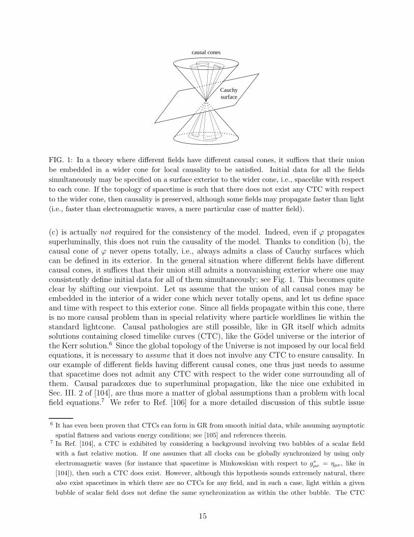
FIG. 1: In a theory where different fields have different causal cones, it suffices that their union

be embedded in a wider cone for local causality to be satisfied. Initial data for all the fields

simultaneously may be specified on a surface exterior to the wider cone, i.e., spacelike with respect

to each cone. If the topology of spacetime is such that there does not exist any CTC with respect

to the wider cone, then causality is preserved, although some fields may propagate faster than light

(i.e., faster than electromagnetic waves, a mere particular case of matter field).

(c) is actually not required for the consistency of the model. Indeed, even if ϕ propagatessuperluminally, this does not ruin the causality of the model. Thanks to condition (b), thecausal cone of ϕ never opens totally, i.e., always admits a class of Cauchy surfaces whichcan be defined in its exterior. In the general situation where different fields have differentcausal cones, it suffices that their union still admits a nonvanishing exterior where one mayconsistently define initial data for all of them simultaneously; see Fig. 1. This becomes quiteclear by shifting our viewpoint. Let us assume that the union of all causal cones may beembedded in the interior of a wider cone which never totally opens, and let us define spaceand time with respect to this exterior cone. Since all fields propagate within this cone, thereis no more causal problem than in special relativity where particle worldlines lie within thestandard lightcone. Causal pathologies are still possible, like in GR itself which admitssolutions containing closed timelike curves (CTC), like the Godel universe or the interior ofthe Kerr solution.6 Since the global topology of the Universe is not imposed by our local fieldequations, it is necessary to assume that it does not involve any CTC to ensure causality. Inour example of different fields having different causal cones, one thus just needs to assumethat spacetime does not admit any CTC with respect to the wider cone surrounding all ofthem. Causal paradoxes due to superluminal propagation, like the nice one exhibited inSec. III. 2 of [104], are thus more a matter of global assumptions than a problem with localfield equations.7 We refer to Ref. [106] for a more detailed discussion of this subtle issue

6 It has even been proven that CTCs can form in GR from smooth initial data, while assuming asymptotic

spatial flatness and various energy conditions; see [105] and references therein.7 In Ref. [104], a CTC is exhibited by considering a background involving two bubbles of a scalar field

with a fast relative motion. If one assumes that all clocks can be globally synchronized by using only

electromagnetic waves (for instance that spacetime is Minkowskian with respect to g∗µν = ηµν , like in

[104]), then such a CTC does exist. However, although this hypothesis sounds extremely natural, there

also exist spacetimes in which there are no CTCs for any field, and in such a case, light within a given

bubble of scalar field does not define the same synchronization as within the other bubble. The CTC

15

(see also Sec. IIIC below and the very recent article [107]). Reference [108] claims thatmicroscopically Lorentz-invariant particles cannot give rise to superluminal signals, but thisconclusion does not take into account their possible self-interactions via their kinetic term,like f(s) in our present case of k-essence models (2.13). As shown above, superluminalsignals do occur when f ′′(s) > 0, although the theory is microscopically Lorentz-invariant— and causal when the hyperbolicity conditions (a) and (b) are satisfied. The causal coneof the scalar field ϕ is either interior or exterior to the light cone defined by g∗µν (dependingon the local value of s), but it always remains a cone thanks to these conditions. At eachspacetime point, any surface exterior to the wider of these two cones may be used as aCauchy surface to impose initial data. Of course, a surface lying between the two conesbehaves as a spacelike one for the thinner cone but as a timelike one for the thicker. Somecausal paradoxes discussed in the literature (including in [103]) are actually based on theimproper use of such intermediate surfaces. They are clearly not consistent Cauchy surfacesfor the fastest field (i.e., the wider cone), so that data are necessarily constrained on them.The conclusion of such paradoxes, namely that initial data are constrained, is thus actuallyhidden in the use of these intermediate surfaces.

F. MOND as a RAQUAL model

As mentioned above, Ref. [27] proved that RAQUAL models (2.13) may reproduce theMOND gravitational potential. Indeed, if f(s) is assumed not to depend explicitly on ϕ, ifthe potential V (ϕ) vanishes, and if one chooses an exponential (Brans-Dicke-like) matter-scalar coupling function A(ϕ) = exp(αϕ), Eq. (2.14) reduces to

∇∗µ [f ′(s)∇µ

∗ϕ] = −4πG

c4α T ∗, (2.15)

where T ∗ ≡ g∗µνTµν∗ denotes the trace of the matter energy-momentum tensor T µν∗ ≡

(2c/√−g∗) δSmatter/δg

∗µν . In order to recover the right Newtonian limit for large accelera-

tions a > a0, one may follow Ref. [27] and impose8 f ′(s) → 1 for large positive values of s. Insuch a case, the scalar field reads ϕ ≈ −αGM/rc2 near a body of mass M , and test particlesfeel an extra potential αϕc2 ≈ −α2GM/r adding up to the standard gravitational potential−GM/r mediated by the spin-2 interaction (i.e., by the Einstein metric g∗µν). The total

potential −G(1+α2)M/r is thus of the Newtonian type, with a renormalized effective grav-itational constant Geff = G(1+α2) (see for instance [91] and line (a) of Fig. 5 in Sec. III be-low). Precision tests in the solar system are however sensitive to post-Newtonian corrections,and they prove that the scalar contribution must be negligible. Indeed, the parametrizedpost-Newtonian (PPN) parameter γPPN assumes the value γPPN = 1 − 2α2/(1 + α2) in thepresent (conformally-coupled) scalar-tensor framework [see Refs. [1, 91] and Eq. (3.4) be-low], and the impressive experimental bound |γPPN − 1| < 2 × 10−5 obtained in [90] from

constructed in [104] would then become an artifact of gluing independent coordinate systems at the edges

of the bubbles.8 Note that imposing f ′(s) → const. is strictly equivalent, since the arbitrary constant can be absorbed in

a redefinition of the matter-scalar coupling constant α. In the following, the experimental constraints on

α that we quote correspond to the choice f ′(s) → 1 in the Newtonian regime.

16

1 2 3 4

0.2

0.4

0.6

0.8

1

f’

s-0

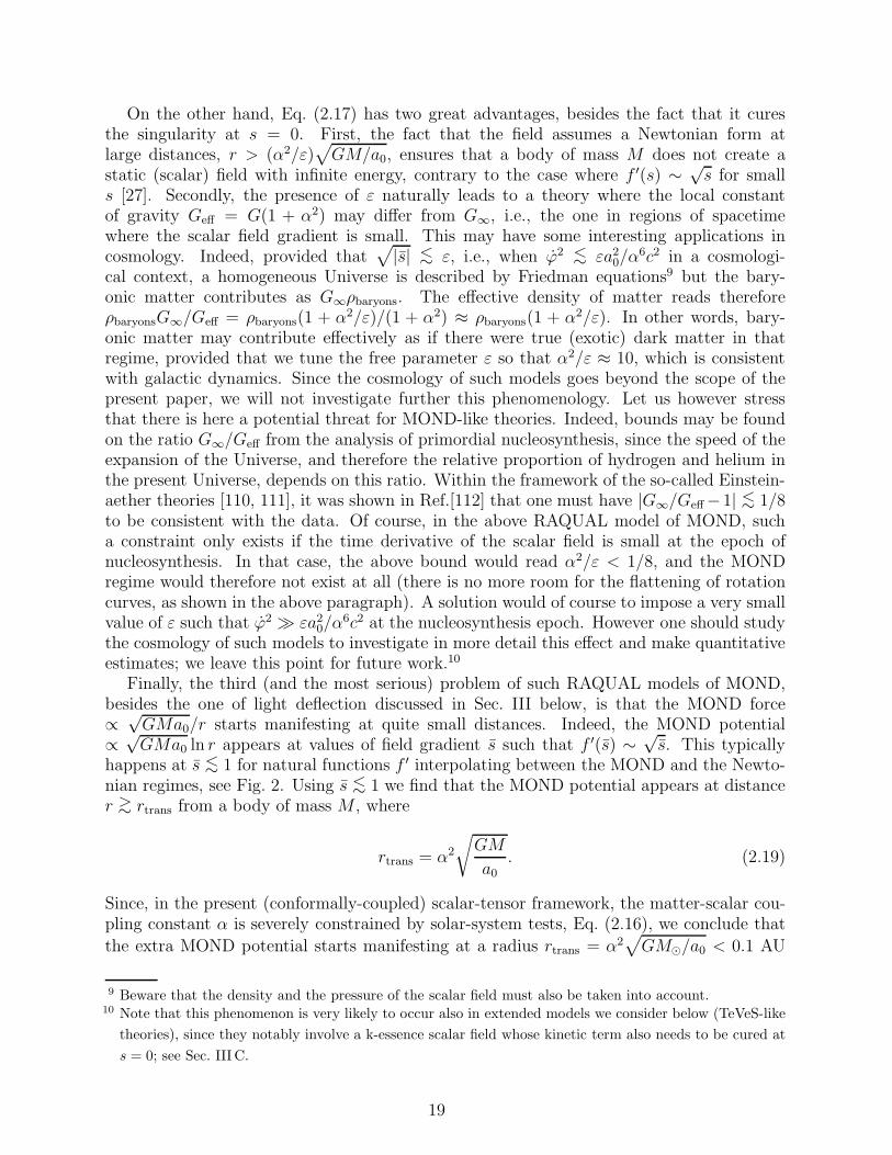
FIG. 2: A simple function f ′(s) reproducing the MOND dynamics for small s (i.e., large distances)

and the Newtonian one for large s (i.e., small distances).

the observation of the Cassini spacecraft implies therefore

α2 < 10−5. (2.16)

Instead of imposing f ′(s) → 1 for large values of s, one may also recover the right Newtonianlimit by choosing a decreasing function f ′(s), such that the scalar contribution is evensmaller. Condition (b) should however still be satisfied, thereby constraining the slope off ′(s).

But the crucial feature of Eq. (2.15) is that it also allows us to reproduce the MONDpotential for small accelerations a < a0. Indeed, if f ′(s) ≈ ℓ0

√s for small and positive

values of s, where ℓ0 is a constant having the dimension of a length, one gets (∂rϕ)2 ≈αGM/ℓ0c

2r2 near a spherical body of mass M . Test particles therefore feel, in addition

to the usual Newtonian potential −GM/r, an extra potential αϕc2 ≈√

α3GMc2/ℓ0 ln rwhich reduces to the MOND one

√GMa0 ln r for ℓ0 = α3c2/a0. A simple way to connect

this MOND limit to the above Newtonian one is to choose for instance f ′(s) =√s/√

1 + s,where s ≡ α6c4s/a2

0 is dimensionless. The shape of this function is illustrated in Fig. 2.By integrating this expression, one can thus conclude that the precise function f(s) =

(a20/α

6c4)[

√

s(1 + s) − sinh−1(√s)]

, or any other one having the same asymptotic behaviors

for large and small positive values of s, allows us to reproduce the MOND dynamics.However, the authors of Ref. [27] noticed that the scalar field propagates superluminally

in the MOND (small positive s) regime, since f ′′(s) ≈ 12ℓ0/

√s > 0 contradicts condition

(c) above. This is the reason why they discarded this model, although we underlined abovethat such a superluminal propagation actually does not threaten causality, provided thehyperbolicity conditions (a) and (b) are satisfied. In fact, the only experimental constraintswe have on the existence of several causal cones is in favor of superluminal fields! As wewill discuss in Sec. IVC, if light (and thus matter) travelled faster than some field to whichit couples, then it would emit Cherenkov radiation of this field. High-energy cosmic rayswould thus be significantly suppressed.

It thus seems that the above RAQUAL model reproducing the MOND dynamics is a

priori consistent. However, it presents several other difficulties. The main one has beenimmediately recognized and addressed in the literature: Because of the specific form of thematter-scalar coupling assumed in action (2.13), this model does not reproduce the observed

17

light deflection by “dark matter”. We will devote Sec. III below to this crucial problem. Letus here mention the other problems that we noticed, and which do not seem to have beendiscussed in the literature.

First of all, the above function f(s) is clearly not defined for negative values of s. Onemay try to replace s by its absolute value |s|, and also multiply globally f(s) by the sign ofs in order to still satisfy conditions (a) and (b). However, this would not cure the serious

problem occurring at s = 0. Indeed, since f(s) → (2α3c2/3a0)s√

|s| for small values ofs, the strict inequality (b) is not satisfied at s = 0. In other words, the scalar field equa-tion (2.14) or (2.15) is no longer hyperbolic on the hypersurfaces where s vanishes, and thescalar degree of freedom cannot cross them. Since s ≈ (∂iϕ)2 ≥ 0 when considering the localphysics of clustered matter, but s ≈ −ϕ2 ≤ 0 when considering the cosmological evolutionof the Universe, there always exist such singular surfaces around clusters. Therefore, thismodel cannot describe consistently both cosmology and galaxies, unless independent solu-tions are glued by hand on the singular hypersurfaces s = 0. However, a simple cure to thisdiscontinuity would be to consider, for small values of s, a function

f ′(s) = ε+√

|s|, (2.17)

where ε is a small dimensionless positive number. Then both conditions (a) and (b) wouldobviously be satisfied even at s = 0. In other words, the RAQUAL model (2.13) withV (ϕ) = 0, A(ϕ) = exp(αϕ) and

f(s) = ε s+a2

0 sgn(s)

α6c4

[

√

|s| (1 + |s|) − sinh−1(

√

|s|)]

, (2.18)

where s ≡ α6c4s/a20, does reproduce the MOND dynamics and is free of mathematical

inconsistencies. Of course, there is no reason why this specific function, for negative valuesof s, should reproduce the right cosmological behavior. One may obviously look for otherfunctions of s < 0 connecting smoothly to (2.18) for small values of |s|, provided conditions(a) and (b) above remain always satisfied. Therefore, Eq. (2.18) should just be consideredas an example of a mathematically consistent RAQUAL model.

A second difficulty is that the above model is rather fine tuned, since it needs the intro-duction of a small dimensionless constant ε besides Milgrom’s MOND acceleration constanta0 ≈ 1.2 × 10−10 m.s−2. Indeed, the presence of ε in Eqs. (2.17),(2.18) notably impliesthat Newtonian gravity is recovered at very large distances, the MOND regime manifestingonly at intermediate ranges [106]. When s → 0, the derivative f ′(s) entering Eq. (2.15)tends to ε, so that the scalar field reads ϕ ≈ −(α/ε)GM/rc2 faraway from a body ofmass M . In this regime, the total gravitational potential felt by a test particle reads−G(1 + α2/ε)M/r, and is therefore of the Newtonian form with a renormalized gravita-tional constant G∞ = G(1 + α2/ε), where the subscript refers to the fact that the aboveform of the potential holds exactly when r → ∞ (remind that, if r → 0, the effective grav-itational constant is given by Geff = G(1 + α2)). Let us compute the range of distancesr for which the MOND force dominates the Newtonian contribution. One needs of coursef ′(s) ∝ √

s and thus ε ≪√s. On the other hand, the MOND force dominates the Newto-

nian one if r ≫√

GM/a0. Using s ≈ (∂rϕ)2 ≈ GMa0/α2c4r2, we thus find that the MOND

force dominates within the following range of distances√

GM/a0 ≪ r ≪ (α2/ε)√

GM/a0.Since solar system tests impose α2 < 10−5, Eq. (2.16), and since rotation curves of galaxies

may be flat up to r ∼ 10√

GM/a0 [109], one needs therefore ε≪ 10−6. This illustrates thefine tuning required to define a consistent RAQUAL model even for s→ 0.

18

On the other hand, Eq. (2.17) has two great advantages, besides the fact that it curesthe singularity at s = 0. First, the fact that the field assumes a Newtonian form atlarge distances, r > (α2/ε)

√

GM/a0, ensures that a body of mass M does not create astatic (scalar) field with infinite energy, contrary to the case where f ′(s) ∼ √

s for smalls [27]. Secondly, the presence of ε naturally leads to a theory where the local constantof gravity Geff = G(1 + α2) may differ from G∞, i.e., the one in regions of spacetimewhere the scalar field gradient is small. This may have some interesting applications incosmology. Indeed, provided that

√

|s| <∼ ε, i.e., when ϕ2 <∼ εa20/α

6c2 in a cosmologi-cal context, a homogeneous Universe is described by Friedman equations9 but the bary-onic matter contributes as G∞ρbaryons. The effective density of matter reads thereforeρbaryonsG∞/Geff = ρbaryons(1 + α2/ε)/(1 + α2) ≈ ρbaryons(1 + α2/ε). In other words, bary-onic matter may contribute effectively as if there were true (exotic) dark matter in thatregime, provided that we tune the free parameter ε so that α2/ε ≈ 10, which is consistentwith galactic dynamics. Since the cosmology of such models goes beyond the scope of thepresent paper, we will not investigate further this phenomenology. Let us however stressthat there is here a potential threat for MOND-like theories. Indeed, bounds may be foundon the ratio G∞/Geff from the analysis of primordial nucleosynthesis, since the speed of theexpansion of the Universe, and therefore the relative proportion of hydrogen and helium inthe present Universe, depends on this ratio. Within the framework of the so-called Einstein-aether theories [110, 111], it was shown in Ref.[112] that one must have |G∞/Geff −1| <∼ 1/8to be consistent with the data. Of course, in the above RAQUAL model of MOND, sucha constraint only exists if the time derivative of the scalar field is small at the epoch ofnucleosynthesis. In that case, the above bound would read α2/ε < 1/8, and the MONDregime would therefore not exist at all (there is no more room for the flattening of rotationcurves, as shown in the above paragraph). A solution would of course to impose a very smallvalue of ε such that ϕ2 ≫ εa2

0/α6c2 at the nucleosynthesis epoch. However one should study

the cosmology of such models to investigate in more detail this effect and make quantitativeestimates; we leave this point for future work.10

Finally, the third (and the most serious) problem of such RAQUAL models of MOND,besides the one of light deflection discussed in Sec. III below, is that the MOND force∝

√GMa0/r starts manifesting at quite small distances. Indeed, the MOND potential

∝√GMa0 ln r appears at values of field gradient s such that f ′(s) ∼

√s. This typically

happens at s <∼ 1 for natural functions f ′ interpolating between the MOND and the Newto-nian regimes, see Fig. 2. Using s <∼ 1 we find that the MOND potential appears at distancer >∼ rtrans from a body of mass M , where

rtrans = α2

√

GM

a0. (2.19)

Since, in the present (conformally-coupled) scalar-tensor framework, the matter-scalar cou-pling constant α is severely constrained by solar-system tests, Eq. (2.16), we conclude that

the extra MOND potential starts manifesting at a radius rtrans = α2√

GM⊙/a0 < 0.1 AU

9 Beware that the density and the pressure of the scalar field must also be taken into account.10 Note that this phenomenon is very likely to occur also in extended models we consider below (TeVeS-like

theories), since they notably involve a k-essence scalar field whose kinetic term also needs to be cured at

s = 0; see Sec. III C.

19

f’

s-

1

10–100

s-r

a

a0

0 30AU 7000AU

α2GMr2

GMa0

r

10–5

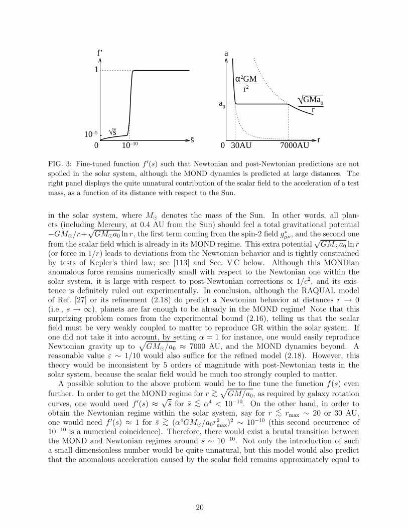
FIG. 3: Fine-tuned function f ′(s) such that Newtonian and post-Newtonian predictions are not

spoiled in the solar system, although the MOND dynamics is predicted at large distances. The

right panel displays the quite unnatural contribution of the scalar field to the acceleration of a test

mass, as a function of its distance with respect to the Sun.

in the solar system, where M⊙ denotes the mass of the Sun. In other words, all plan-ets (including Mercury, at 0.4 AU from the Sun) should feel a total gravitational potential−GM⊙/r+

√GM⊙a0 ln r, the first term coming from the spin-2 field g∗µν , and the second one

from the scalar field which is already in its MOND regime. This extra potential√GM⊙a0 ln r

(or force in 1/r) leads to deviations from the Newtonian behavior and is tightly constrainedby tests of Kepler’s third law; see [113] and Sec. VC below. Although this MONDiananomalous force remains numerically small with respect to the Newtonian one within thesolar system, it is large with respect to post-Newtonian corrections ∝ 1/c2, and its exis-tence is definitely ruled out experimentally. In conclusion, although the RAQUAL modelof Ref. [27] or its refinement (2.18) do predict a Newtonian behavior at distances r → 0(i.e., s → ∞), planets are far enough to be already in the MOND regime! Note that thissurprizing problem comes from the experimental bound (2.16), telling us that the scalarfield must be very weakly coupled to matter to reproduce GR within the solar system. Ifone did not take it into account, by setting α = 1 for instance, one would easily reproduceNewtonian gravity up to

√

GM⊙/a0 ≈ 7000 AU, and the MOND dynamics beyond. Areasonable value ε ∼ 1/10 would also suffice for the refined model (2.18). However, thistheory would be inconsistent by 5 orders of magnitude with post-Newtonian tests in thesolar system, because the scalar field would be much too strongly coupled to matter.

A possible solution to the above problem would be to fine tune the function f(s) even

further. In order to get the MOND regime for r >∼√

GM/a0, as required by galaxy rotation

curves, one would need f ′(s) ≈√s for s <∼ α4 < 10−10. On the other hand, in order to

obtain the Newtonian regime within the solar system, say for r <∼ rmax ∼ 20 or 30 AU,one would need f ′(s) ≈ 1 for s >∼ (α4GM⊙/a0r

2max)

2 ∼ 10−10 (this second occurrence of10−10 is a numerical coincidence). Therefore, there would exist a brutal transition betweenthe MOND and Newtonian regimes around s ∼ 10−10. Not only the introduction of sucha small dimensionless number would be quite unnatural, but this model would also predictthat the anomalous acceleration caused by the scalar field remains approximately equal to

20

1 2 3 4

0.1

0.2

0.3

0.4

0.5

0

f’

s-

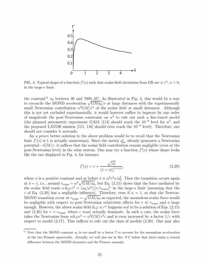
FIG. 4: Typical shape of a function f ′(s) such that scalar-field deviations from GR are ∝ rn, n > 0,

in the large-s limit.

the constant11 a0 between 30 and 7000 AU. As illustrated in Fig. 3, this would be a wayto reconcile the MOND acceleration

√GMa0/r at large distances with the experimentally

small Newtonian contribution α2GM/r2 of the scalar field at small distances. Althoughthis is not yet excluded experimentally, it would however suffice to improve by one orderof magnitude the post-Newtonian constraint on α2 to rule out such a fine-tuned model(the planned astrometric experiment GAIA [114] should reach the 10−6 level for α2, andthe proposed LATOR mission [115, 116] should even reach the 10−8 level). Therefore, oneshould not consider it seriously.

An a priori better solution to the above problem would be to recall that the Newtonianlimit f ′(s) ≈ 1 is actually unnecessary. Since the metric g∗µν already generates a Newtonianpotential −GM/r, it suffices that the scalar field contribution remain negligible (even at thepost-Newtonian level) in the solar system. One may try a function f ′(s) whose shape lookslike the one displayed in Fig. 4, for instance

f ′(s) = ε+

√

|s|(1 + |s|)1+1/n

, (2.20)

where n is a positive constant and as before s ≡ α6c4s/a20. Then the transition occurs again

at s ∼ 1, i.e., around rtrans = α2√

GM/a0, but Eq. (2.15) shows that the force mediated bythe scalar field reads α∂rϕ c

2 = (a0/α2) (r/rtrans)

n in the large-s limit [assuming that theε of Eq. (2.20) has a negligible influence]. Therefore, even if α = 1, so that the Newton-

MOND transition occur at rtrans =√

GM/a0 as expected, the anomalous scalar force wouldbe negligible with respect to post-Newtonian relativistic effects for r ≪ rtrans and n largeenough. However, the above scalar field ∂rϕ ∝ rn happens not to be a solution of Eqs. (2.15)and (2.20) for r < rtrans, where ε must actually dominate. In such a case, the scalar forcetakes the Newtonian form α∂rϕc

2 = α2GM/r2ε and is even increased by a factor 1/ε withrespect to model (2.17). This suffices to rule out the class of models (2.20). One may also

11 Note that the MOND constant a0 is too small by a factor 7 to account for the anomalous acceleration

of the two Pioneer spacecrafts. Actually, we will also see in Sec. VC below that there exists a crucial

difference between the MOND dynamics and the Pioneer anomaly.

21

notice that for ε→ 0, they do not satisfy the hyperbolicity condition (b) in the large-s limitunless n = ∞; but even for this limiting case n = ∞, the scalar force is not negligible atsmall distances.

In conclusion, the above discussion illustrates that RAQUAL models are severely con-strained, although they involve a free function f(s) defining the kinetic term of the scalarfield. Contrary to some fears in the literature, the possible superluminal propagations donot threaten causality, and the two conditions (a) and (b) are the only ones which mustbe imposed to guarantee the field theory’s consistency. For instance, monomials f(s) = sn

are allowed if n is positive and odd [except on the possible hypersurfaces where s vanishes,which would violate the strict inequality (b)]. However, when taking into account simulta-neously these two consistency conditions and experimental constraints, it seems difficult toreproduce the MOND dynamics at large distances without spoiling the Newtonian and post-Newtonian limits in the solar system. It seems necessary to consider unnatural functionsf(s) involving small dimensionless numbers.

In the next section, we will address the problem of light deflection, and recall the solutionwhich has been devised in the literature. This solution will at the same time release theexperimental constraint on the matter-scalar coupling constant α obtained from accuratemeasurement of the post-Newtonian parameter γPPN within the solar system, and thereforecure the above fine-tuning problem. On the other hand, we will show in Sec. IVD thatthe analysis of binary-pulsar data also imposes a bound on α, so that the problem of thefine-tuning of the free function f will anyway remain.

III. THE PROBLEM OF LIGHT DEFLECTION

A. Conformally-coupled scalar field

Both scalar-tensor theories (2.12) and RAQUAL models (2.13) assume a conformal re-lation gµν = A2(ϕ)g∗µν between the physical and Einstein metrics. The inverse metrics are

thus related by gµν = A−2(ϕ)gµν∗ , and their determinants read g = A2d(ϕ)g∗ in d spacetimedimensions. Since all matter fields, including gauge bosons, are assumed to be minimallycoupled to gµν , this leads to a simple prediction for the behavior of light in such models.Indeed, the action of electromagnetism is conformal invariant in d = 4 dimensions:

SEM =

∫

d4x

c

√−g4

gµρgνσFµνFρσ

=

∫

d4x

c

A4(ϕ)√−g∗4

[

A−2(ϕ)gµρ∗] [

A−2(ϕ)gνσ∗]

FµνFρσ

=

∫

d4x

c

√−g∗4

gµρ∗ gνσ∗ FµνFρσ. (3.1)

Therefore, light is only coupled to the spin-2 field g∗µν , but does not feel at all the presenceof the scalar field ϕ. In terms of Feynman diagrams, there exist nonvanishing verticesconnecting one or several gravitons to two photon lines, but the similar vertices connectingphotons to scalar lines all vanish; this is illustrated in line (b) of Fig. 5. It is then obviousthat light behaves strictly as in GR, in a geometry described by the Einstein metric g∗µν . Inparticular, the light deflection angle caused by a spherical body of mass M must be given

22

α0 α0

scalargraviton+

= 0 but ≠ 0

ϕ

ϕϕ

(a)

(b)

(c)

= 0...,,≠ 0 but...,

FIG. 5: Feynman diagrams in scalar-tensor theories, where straight, curly and wavy lines represent

respectively the scalar field, gravitons and photons. Matter sources are represented by blobs.

(a) Diagrammatic interpretation of the effective gravitational constant Geff = G(1+α20), where each

vertex connecting matter to one scalar line involves a factor α0. (b) Photons are directly coupled

to gravitons but not to the scalar field. (c) Photons feel nevertheless the scalar field indirectly, via

its influence on gravitons: The energy-momentum tensor of the scalar field generates a curvature

of the Einstein metric g∗µν in which electromagnetic waves propagate.

by the same expression as in GR (at lowest order)

∆θ =4GM

bc2, (3.2)

where b denotes the impact parameter of the light ray. An even simpler way to prove thatlight propagates in the Einstein metric g∗µν , without feeling the scalar field, is to note thatits geodesic equation reads gµνdx

µdxν = 0 in the eikonal approximation. Dividing by thenonvanishing factor A2(ϕ), this equation implies g∗µνdx

µdxν = 0, giving thus the standardgeodesic equation for null rays in the metric g∗µν . [It is interesting to note that this secondreasoning would remain valid even if the action of electromagnetism were not conformalinvariant, for instance in dimension d 6= 4, or even if one multiplied it by an explicit scalar-photon coupling function B2(ϕ), thereby violating the weak equivalence principle. Then it isstraightforward to prove that the nonvanishing scalar-photon vertices would only affect theamplitude of electromagnetic waves, in the eikonal approximation, but not their polarizationnor their trajectory. One of us (G.E.F.) discussed this result with B. Bertotti several yearsago, but it has been recently rediscovered in [117].]

However, the crucial difference with GR is that massive matter does feel the scalar field,via the matter-scalar coupling function A(ϕ). One may expand this function around thebackground value ϕ0 of the scalar field as

lnA(ϕ) = const. + α0(ϕ− ϕ0) +1

2β0(ϕ− ϕ0)

2 + · · · , (3.3)

where α0, β0, . . . , are dimensionless constants. In usual scalar-tensor theories (2.12), aswell as in the Newtonian regime of RAQUAL models (2.13), the lowest-order contributionof the scalar field to the gravitational potential felt by a test mass reads then −α2

0GM/r[1, 91]. This generalizes the results recalled in Sec. II F above in the particular case of anexponential coupling function A(ϕ) = eαϕ. This spin-0 contribution adds up to the standardNewtonian potential −GM/r caused by the spin-2 interaction (i.e., via the Einstein metric

23

g∗µν), so that the total gravitational potential remains of the Newtonian form but with an

effective gravitational constant Geff = G(1+α20); see line (a) of Fig. 5. In other words, when

one determines the mass of the Sun by analyzing the orbits of the planets, one actuallymeasures GeffM instead of the bare GM . Therefore, if one expresses the light deflectionangle (3.2) in terms of the observable quantity GeffM , one gets

∆θ =4GeffM

(1 + α20)bc

2≤ 4GeffM

bc2. (3.4)

For a given value of the observed constant GeffM , general relativity would have predicted4GeffM/bc2. In conclusion, the light deflection angle is actually smaller in scalar-tensortheories than in GR, although photons are strictly decoupled from the scalar field! Thisparadoxical result is simply due to the fact that we need to compare the measured angle ∆θwith another observable, GeffM , which is influenced by the scalar field.

This reduction of light deflection in scalar-tensor theories has been immediately recog-nized as a serious problem for MOND-like field theories [28, 29]. Indeed, if one interpretsdata within GR, the presence of dark matter suggested by galaxy rotation curves is con-firmed by weak lensing observations [118, 119, 120]. Therefore, in a modified-gravity theoryavoiding the assumption of dark matter, one should predict simultaneously a larger gravita-tional potential and a larger light deflection. However, the interpretation of data is slightlymore subtle than in the solar system, because there exist at least three different notions ofmass which may be defined for a galaxy: (i) its baryonic mass Mb, assumed to be propor-tional to its luminous mass ML; (ii) its total mass (baryonic plus “dark”) evaluated fromits rotation curve, that we will denote M rot

tot ; and (iii) its total mass evaluated from weaklensing, that we will denote M lens

tot . The only conclusion driven from the above result (3.4)is that the deflecting mass is smaller than the gravitational one in scalar-tensor theories:

M lenstot ≤M rot

tot . (3.5)

Note that this conclusion is also valid in the class of RAQUAL models reproducing theMOND dynamics that we discussed in Sec. II F above. Indeed, the MOND force was causedby the exchange of a scalar particle [cf. line (a) of Fig. 5], i.e., by the conformal factor A2(ϕ)relating the physical metric gµν to the Einstein one g∗µν . Since light only feels the latter,the total mass evaluated from weak lensing is obviously smaller that the one evaluated fromrotation curves.

On the other hand, it should be underlined that Eq. (3.4) does not imply M lenstot ≤ Mb,

contrary to some erroneous or imprecise claims in the literature (see, e.g., [29]). Indeed,the stress-energy tensor of the scalar field does contribute to the curvature of the Einsteinmetric g∗µν , so that light deflection may be larger than if only baryonic matter was present.This is illustrated in terms of Feynman diagrams in line (c) of Fig. 5: Although the scalar-photon vertex vanishes, light may nevertheless feel the scalar field indirectly via a gravitonexchange. The reason why this does not appear in Eqs. (3.2) or (3.4) above is because wederived them at lowest order in powers of 1/c2, and in usual scalar-tensor theories or in theNewtonian regime of RAQUAL models. But when considering their MOND regime, onecannot any longer perform a naive post-Newtonian expansion. Indeed, the stress-energy ofthe scalar field may become non-negligible with respect to that of baryonic matter, and evendominate it, although this scalar field has been generated by its coupling to matter. Thismere sentence gives us a hint that such a model may be unstable, but one should note thatM lens

tot ≫Mb is indeed possible in RAQUAL models.

24

We will provide an explicit example in Sec. III B below, although it does not reproducethe right MOND dynamics. Its aim is just to underline that the derivation of the inequalityM lens

tot ≤Mb proposed in Ref. [29] is incorrect. It is instructive to locate where its reasoningfails. It writes the deflection angle in terms of the T rr component of the total stress-energytensor, and decomposes it in two contributions, due to matter and to the scalar field. Ithappens that the latter is negative. However, what was identified as the matter contributionto T rr happens not to vanish outside matter. Therefore, the decomposition was flawed, andpart of the positive contribution of the scalar field to light deflection was actually attributedto matter. The simplest way to understand that a scalar field may indeed increase lightdeflection is to consider it as a dark matter fluid, without any coupling to baryonic matterand assuming GR as the correct theory of gravity. If the scalar field is massive enough, itwill obviously cluster and contribute to the total gravitational potential deflecting light.

Actually, a violation of inequality (3.5) is a priori also possible when the scalar’s stress-energy contributes significantly to the curvature of the Einstein metric g∗µν . Indeed, specificmodels could predict a negligible contribution to the time component g∗00 but a significantone to the spatial components g∗ij. In such a case, test particles would feel the standard

Newtonian potential −12(1 + g∗00)c

2 ≈ −GM/r [and the extra scalar force caused by theconformal factor A2(ϕ), which may be tuned to be negligible], but light bending would bedirectly affected by the scalar-induced corrections entering g∗ij. Therefore, M lens

tot > M rottot

seems possible. However, such models may be difficult to construct if one imposes thepositivity of energy, as in Ref. [29]. We will not attempt to study them here, since there isanyway no experimental evidence for M lens

tot > M rottot . Weak-lensing observations only impose

M lenstot ∼M rot

tot [118, 119, 120].Let us end this section by recalling that the conclusion of Ref. [29] remains correct in a

limiting case which is often implicitly assumed in MOND-like field theories [42, 121]: If thestress-energy of the scalar field is negligible with respect to that of baryonic matter, thenthe curvature of the Einstein metric g∗µν is basically generated by Mb alone. Since light only

feels g∗µν , weak lensing provides a measure of M lenstot ≈ Mb. In other words, light is only

deflected by baryonic matter, whereas experiment tells us that the much greater amountof “dark matter” does deflect it too. We will review in Secs. IIIC and IIID how the sameauthors as Ref. [29] devised a clever way to solve this crucial difficulty of RAQUAL models.

B. A RAQUAL example increasing light deflection

Let us illustrate that RAQUAL models may predict a much larger light deflection thanif there were baryonic matter alone in GR, i.e., that M lens

tot ≫ Mb is possible. We considerthe action

S =c4

16πG

∫

d4x

c

√−g∗

R∗ − ℓ2(n−1)0 sn

+ Smatter

[

ψ; gµν = A2(ϕ)g∗µν]

, (3.6)

where as before s ≡ gµν∗ ∂µϕ∂νϕ, ℓ0 is a length scale (e.g. ℓ0 ∝ c2/a0 in MOND-like models),and n is a positive odd integer. As underlined at the end of Sec. II, such a model satisfiesthe two consistency conditions (a) and (b), except on hypersurfaces where s vanishes. Itsuffices to add a small standard kinetic term −εs (with ε > 0) to the above action to cure thesingularity on such hypersurfaces. However, we will not take into account this refinementbecause the above model will anyway not reproduce the correct MOND dynamics.

25

The field equations deriving from action (3.6) read

R∗µν −

1

2g∗µνR

∗ =8πG

c4(

T ∗matterµν + T ∗ϕ

µν

)

, (3.7a)

n ℓ2(n−1)0 ∇∗

µ

(

sn−1∂µ∗ϕ)

= −8πG

c4d lnA(ϕ)

dϕT ∗

matter, (3.7b)

where the stress-energy tensor of the scalar field is given by

8πG

c4T ∗ϕµν =

(

ℓ20 s)n−1

(

n ∂µϕ∂νϕ− 1

2s g∗µν

)

. (3.8)

Let us choose for instance an exponential (Brans-Dicke-like) matter-scalar coupling functionA(ϕ) = eαϕ, so that d lnA(ϕ)/dϕ = α is constant. The solution of Eq. (3.7b), around aspherical body of mass M , is then easy to write at lowest order (i.e., neglecting the curvatureof spacetime):

ϕ = ϕ0 +2n− 1

2n− 3

(

2αGMℓ0nr2c2

)1/(2n−1)r

ℓ0. (3.9)

The stress-energy tensor of the scalar field reads thus

8πG

c4T ∗ϕµν =

αGM

ℓ0r2c2

(

2αGMℓ0nr2c2

)1/(2n−1) (

2δrµδrν −

1

ng∗µν

)

, (3.10)

and Einstein’s equations (3.7a) can now be solved straightforwardly, still to lowest orderaround a flat Minkowski background. In particular, one may write (8πG/c4)(T ∗ϕ

00 − 12g∗00T

∗ϕ) =

R∗00 ≈ 1

2∆ ln(−g∗00), and this gives immediately

− g∗00 = 1 − 2GM

rc2− (n− 1)(2n− 1)2

n(2n− 3)

αGM

ℓ0c2

(

2αGMℓ0nr2c2

)1/(2n−1)

+ O(

1

c4

)

. (3.11)

The R∗rr component of Einstein’s equations can now be used to solve for g∗rr, but one must

specify the coordinate system to write the solution explicitly. In order to compute easilythe light deflection angle below, it will be convenient to use the so-called “Schwarzschildcoordinates” (which define an “area radius” r), such that the line element takes the form

ds2∗ = −B(r)c2dt2 + A(r)dr2 + r2(dθ2 + sin2 θ dφ2). (3.12)

One then finds straightforwardly

g∗rr = A(r) = 1 +2GM

rc2+αGM

nℓ0c2

(

2αGMℓ0nr2c2

)1/(2n−1)

+ O(

1

c4

)

. (3.13)

The physical metric gµν = e2αϕg∗µν to which matter is coupled can now be deduced fromEqs. (3.9), (3.11) and (3.13). In particular, the gravitational potential felt by test massesreads V = −1

2(1 + g00)c

2, and its radial derivative ∂rV gives their acceleration

a =GM

r2+

(

2αGMℓ0nr2c2

)1/(2n−1) [αc2

ℓ0+

(

1 − 1

n

)(

1 +2

2n− 3

)

αGM

ℓ0r

]

. (3.14)

26

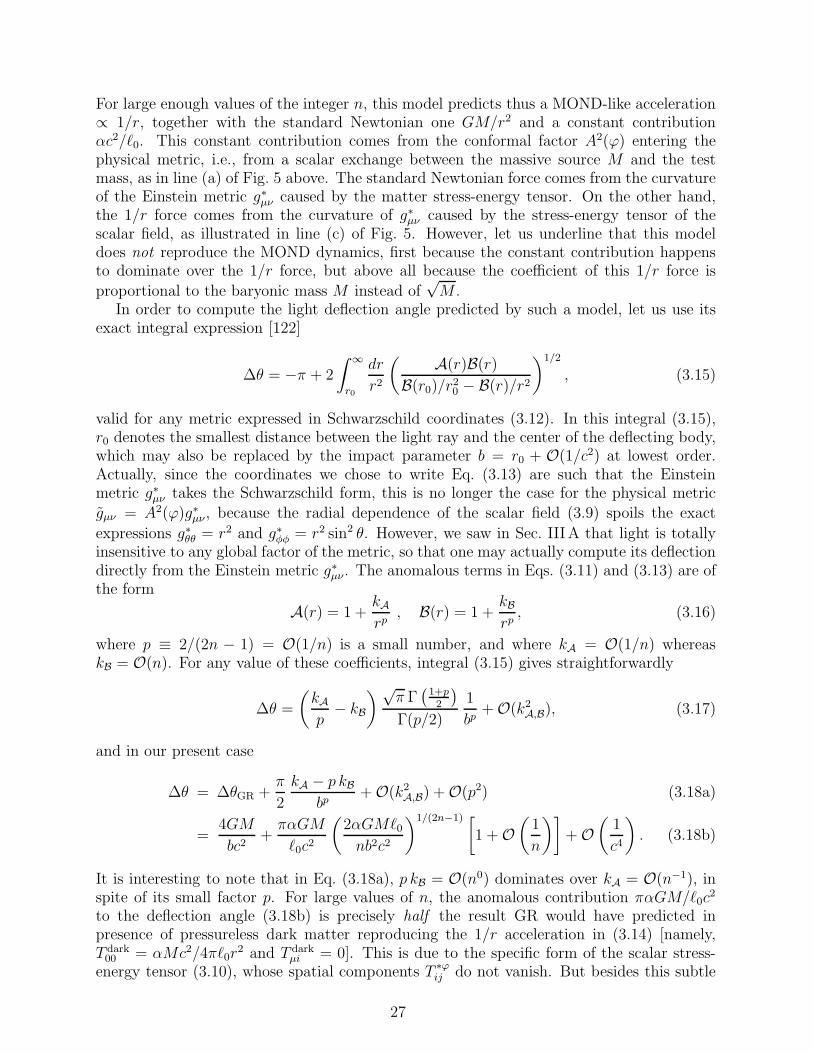
For large enough values of the integer n, this model predicts thus a MOND-like acceleration∝ 1/r, together with the standard Newtonian one GM/r2 and a constant contributionαc2/ℓ0. This constant contribution comes from the conformal factor A2(ϕ) entering thephysical metric, i.e., from a scalar exchange between the massive source M and the testmass, as in line (a) of Fig. 5 above. The standard Newtonian force comes from the curvatureof the Einstein metric g∗µν caused by the matter stress-energy tensor. On the other hand,the 1/r force comes from the curvature of g∗µν caused by the stress-energy tensor of thescalar field, as illustrated in line (c) of Fig. 5. However, let us underline that this modeldoes not reproduce the MOND dynamics, first because the constant contribution happensto dominate over the 1/r force, but above all because the coefficient of this 1/r force is

proportional to the baryonic mass M instead of√M .

In order to compute the light deflection angle predicted by such a model, let us use itsexact integral expression [122]

∆θ = −π + 2

∫ ∞

r0

dr

r2

( A(r)B(r)

B(r0)/r20 − B(r)/r2

)1/2

, (3.15)

valid for any metric expressed in Schwarzschild coordinates (3.12). In this integral (3.15),r0 denotes the smallest distance between the light ray and the center of the deflecting body,which may also be replaced by the impact parameter b = r0 + O(1/c2) at lowest order.Actually, since the coordinates we chose to write Eq. (3.13) are such that the Einsteinmetric g∗µν takes the Schwarzschild form, this is no longer the case for the physical metric

gµν = A2(ϕ)g∗µν , because the radial dependence of the scalar field (3.9) spoils the exact

expressions g∗θθ = r2 and g∗φφ = r2 sin2 θ. However, we saw in Sec. IIIA that light is totallyinsensitive to any global factor of the metric, so that one may actually compute its deflectiondirectly from the Einstein metric g∗µν . The anomalous terms in Eqs. (3.11) and (3.13) are ofthe form

A(r) = 1 +kArp

, B(r) = 1 +kBrp, (3.16)

where p ≡ 2/(2n − 1) = O(1/n) is a small number, and where kA = O(1/n) whereaskB = O(n). For any value of these coefficients, integral (3.15) gives straightforwardly

∆θ =

(

kAp

− kB

)√π Γ(

1+p2

)

Γ(p/2)

1

bp+ O(k2

A,B), (3.17)

and in our present case

∆θ = ∆θGR +π

2

kA − p kBbp

+ O(k2A,B) + O(p2) (3.18a)

=4GM

bc2+παGM

ℓ0c2

(

2αGMℓ0nb2c2

)1/(2n−1) [

1 + O(

1

n

)]

+ O(

1

c4

)

. (3.18b)

It is interesting to note that in Eq. (3.18a), p kB = O(n0) dominates over kA = O(n−1), inspite of its small factor p. For large values of n, the anomalous contribution παGM/ℓ0c

2

to the deflection angle (3.18b) is precisely half the result GR would have predicted inpresence of pressureless dark matter reproducing the 1/r acceleration in (3.14) [namely,T dark

00 = αMc2/4πℓ0r2 and T dark

µi = 0]. This is due to the specific form of the scalar stress-energy tensor (3.10), whose spatial components T ∗ϕ

ij do not vanish. But besides this subtle

27

factor 2 discrepancy with the standard dark matter prediction, let us also recall that light isinsensitive to the conformal factor A2(ϕ), responsible for the dominant anomalous contribu-tion in (3.14), namely the constant one αc2/ℓ0. In conclusion, using the notation introducedin Sec. IIIA, the present model actually predicts M lens

tot ≪ M rottot , which is even worse than

the inequality (3.5) derived in standard scalar-tensor theories. On the other hand, for a largeenough impact parameter b, the light deflection angle (3.18b), ∆θ ≈ παGM/ℓ0c

2 = const, ismuch larger than the one predicted by GR in presence of M alone, namely 4GM/bc2 → 0.Therefore, we have exhibited a RAQUAL model predicting M lens

tot ≫Mb.One might try to refine the model (3.6) by choosing another matter-scalar coupling func-

tion, for instanceA(ϕ) = exp(αϕ−2n), (3.19)

with the same integer n as in the kinetic term of the scalar field. A first useful consequenceof such a choice is that the extra constant acceleration we found in Eq. (3.14) above becomesnow negligible. Indeed, it came from the conformal factor A2(ϕ) relating the physical andEinstein metrics, so that this extra acceleration derives now from αϕ−2nc2 = O(r−2n), andtends quickly towards 0 as r grows. On the other hand, the 1/r acceleration of Eq. (3.14)is still predicted, since it comes from the curvature of the Einstein metric caused by thescalar’s stress-energy tensor ∝ 1/r2. For large enough impact parameters, such a modelpredicts thus

M lenstot ≈ 1

2M rot

tot ≫ Mb, (3.20)

the factor 12

coming from the same calculation as Eq. (3.18) above. The second conse-quence of the choice (3.19) is that Eq. (3.7b) now involves the non-constant coefficientd lnA(ϕ)/dϕ = −2nα/ϕ2n+1. If one naively counts the powers of ∂rϕ and ϕ entering thisEq. (3.7b), one could then deduce that ϕ4n ∝ T ∗

matter ∝M . Using now Eq. (3.8), this would

imply T ∗ϕµν ∝ (∂rϕ)2n ∝

√M , which looks like the dark matter MOND wishes to mimic.

However, this would be the case only if ϕ → 0 as r → 0, within body M . Then one canprove that ϕ ∝ √

r for small radii, and∫

d3xT ∗ϕµν would diverge within the body. Therefore,

such a solution is unphysical. On the other hand, if ϕ→ ϕ0 6= 0 within the body, then onegets back an exterior solution of the form (3.9), where α is replaced here by −2nα/ϕ2n+1

0 , so

that the anomalous force is a priori again proportional to M instead of the looked-for√M .

There could still remain a possibility to recover the MOND force with such a RAQUALmodel, if one could prove that ϕ → ϕ0 ∝ M1/4n within the body. This would be the casefor instance if ϕ → 0 at a given radius, say at the surface of the body. However, thiswould correspond to a diverging matter-scalar coupling strength at this radius (singular andobviously forbidden by solar-system tests), and we anyway do not see how to impose sucha relation, nor the precise value of ϕ0. In standard scalar-tensor theories, the scalar fieldtends towards a constant ϕ0 when r → ∞, this constant being imposed by the cosmologi-cal evolution of the Universe, and being constrained by post-Newtonian tests of gravity inthe solar system. Here, the scalar field ϕ = ϕ0 + const. r1−2/(2n−1) diverges at infinity, assoon as a single particle exists in the Universe. This pathological behavior is linked withthe fact that the solution of Eq. (3.7b) cannot be written unambiguously, the integrationconstant ϕ0 remaining undetermined. In the model (3.9), where A(ϕ) = eαϕ, this constantdid not enter any physical observable, but it does when the matter-scalar coupling functionis no longer a mere exponential, as in our present attempt (3.19). Therefore, although thismatter-scalar coupling function looks promising to reproduce the MOND dynamics from asimple RAQUAL model, it fails to define a fully predictive theory. Its only solid prediction

28

is that light bending would be twice smaller than the prediction of GR in presence of darkmatter, cf. Eq. (3.20). As far as we know, this is still allowed by weak-lensing observations[118, 119, 120].

In conclusion, we have exhibited RAQUAL models predicting a much larger light deflec-tion than GR in presence of baryonic matter alone, but this framework does not seem toreproduce the MOND dynamics consistently. Note that the class of RAQUAL theories ex-amined in the present subsection IIIB are actually models of dark matter. Extra Newtonianforce and light deflection are caused by the stress-energy tensor of the scalar field, whichplays thus the role of dark matter. The only difference with standard dark matter modelsis that its distribution is strictly imposed by the one of baryonic matter, whereas they areusually only related via the dynamical evolution of large-scale structures.

C. Disformal coupling

A nice trick exists to increase light deflection within scalar-tensor theories or RAQUALmodels. It is similar to Ni’s “stratified theory of gravity” [1, 123], and was introduced byBekenstein in [28]; see also [29]. Instead of assuming that matter is coupled to a physicalmetric gµν = A2(ϕ)g∗µν , conformally related to the Einstein metric g∗µν , one may consider a“disformal” relation of the form

gµν = A2(ϕ, s)g∗µν +B(ϕ, s)∂µϕ∂νϕ, (3.21)

where as before s ≡ gµν∗ ∂µϕ∂νϕ. The crucial difference is that the ∂µϕ∂νϕ contribution nowprivileges a particular direction, namely the radial one in spherically symmetrical systems.This extra contribution may remain negligible in the equations of motion of test particles,but now light can be directly sensitive to the presence of the scalar field, contrary to thecase of conformal coupling that we discussed in Sec. IIIA.

Let us emphasize that because of the disformal coupling above, light (or matter) cantravel faster or slower than gravitons depending on the sign of B. In a similar way as inSec. II E, this does not imply a violation of causality, provided that the matter metric is stillof Lorentzian signature. The matter metric Eq. (3.21) is causal if

A2(ϕ, s) > 0 and A2(ϕ, s) + sB(ϕ, s) > 0 (3.22)

for all ϕ and s. Notice that if A does not depend on s, B must depend on s for the latterinequality to hold. Beware that these kind of models used in the literature as realizationsof varying speed of light scenarios [124, 125] do not respect this last inequality. Indeed,whereas A was taken to be 1, B was chosen constant B = −L2 with L being some fixedlength scale. Therefore matter field equations are elliptic at local scales (s > 1/L2), and donot have a well-posed Cauchy problem.

By analogy with the Schwarzschild metric, whose positive contribution in the radialcomponent grr = 1+2GM/rc2 +O(1/c4) contributes positively to light deflection (togetherwith the standard Newtonian potential involved in g00), one understands intuitively thatpositive values of B(s, ϕ) should increase light deflection. To prove it, let us first recallagain that light is insensitive to any global factor of the metric, because of the conformalinvariance of electromagnetism in 4 dimensions, Eq. (3.1). Therefore, instead of the metric(3.21), one may equivalently consider gµν ≡ g∗µν + (B/A2)∂µϕ∂νϕ. Let us then assume thatthe coordinates have been chosen so that the Einstein metric g∗µν takes the Schwarzschild

29

form (3.12). Since, in a static and spherically symmetric situation, the disformal contribution(B/A2)∂µϕ∂νϕ only contributes to the radial component grr, the metric gµν is also of theSchwarzschild form, and one may thus use integral (3.15) to compute the light deflectionangle. The only difference with GR is that the radial metric component now reads A =AGR +(B/A2)(∂rϕ)2. [Beware not to confuse the metric components A ≡ grr and B ≡ −g00

defined in (3.12) with the scalar-field functionals A(s, ϕ) and B(s, ϕ) entering (3.21).] At firstpost-Newtonian order, all contributions coming from g∗µν reproduce the general relativistic

result, and the only extra contribution is thus the one proportional to (B/A2)(∂rϕ)2, assumedto be of order O(1/c2) too:

∆θ = ∆θGR +

∫ ∞

r0

dr/r√

r2/r20 − 1

B (∂rϕ)2

A2+ O

(

1

c4

)

. (3.23)

Even without performing the explicit integration in particular models, it is thus clear thata positive value of B(s, ϕ) always gives a positive contribution to light bending, since theextra term in (3.23) is the integral of a positive function.

For instance, if one tunes the model such that (B/A2)(∂rϕ)2 = 4√GMa0/c

2 is indepen-dent of r (as we will do in Sec. V below), then

∆θ = ∆θGR +2π

√GMa0

c2+ O

(

1

c4

)

, (3.24)

and the second term reproduces exactly the deflection GR would have predicted in pres-ence of dark matter (which is independent of the impact parameter,12 as if there were adeficit angle in a flat conical space). Indeed, it is straightforward to prove that a darkmatter density T00/c

2 =√GMa0/4πGr

2 generates a logarithmic MOND-like potential inthe time component of the metric, −g00 = 1 − 2GM/rc2 + 2

√GMa0 ln r/c2 + O(1/c4), and

that the corresponding radial metric reads grr = 1 + 2GM/rc2 + 2√GMa0/c

2 + O(1/c4)in Schwarzschild coordinates. A similar calculation as above then yields the same lightdeflection angle (3.24) [see Eq. (3.32) below for an explicit derivation]. Note in passingthat grr 6= −1/g00 in such coordinates, contrary to the standard Schwarzschild solutionin vacuum. On the other hand, if one rewrites this same metric in isotropic coordinates,ds2 = −g00c

2dt2 + gρρ(

dρ2 + ρ2dθ2 + ρ2 sin2 θdφ2)

, one indeed recovers the usual relation

gρρ = −1/g00 +O(1/c4) = 1+2GM/ρc2−2√GMa0 ln ρ/c2 +O(1/c4). This remark reminds

us that a metric is coordinate-dependent, and that observable quantities cannot be readnaively in its coefficients. Even the signs of the predicted effects are not obvious. For in-stance, if one had naively tried to impose A2(s, ϕ) = (1+2

√GMa0 ln r/c2) but grr = −1/g00

in Eq. (3.21), then one would have needed a negative B(s, ϕ), and the predicted deflectionangle would have been negative (and diverging), ∆θ = ∆θGR − 2π

√GMa0 ln 2b/c2.

Equation (3.23) proves that a positive value of B(s, ϕ) always increases light deflection.However, light rays satisfy then gµνdx

µdxν = 0 ⇔ g∗µνdxµdxν = −B/A2(∂µϕdx

µ)2 ≤ 0, andphotons are thus timelike with respect to the Einstein metric g∗µν . This has been considered

12 Note that although the deflection angle is constant, the direction of deflection is radial with respect to the

deflecting body, so that distant objects are deformed and weak lensing observations can be performed. A

constant deflection angle in a constant direction would have just shifted globally the image of the distant

objects, without any deformation.

30

as a serious flaw by the authors of Refs. [28, 29]. Indeed, this means that gravitons (i.e.,perturbations of the Einstein metric g∗µν) are superluminal, and it was believed that thisimplied causality violations. Reference [29] even presents the reasoning the other way: Ifone imposes from the beginning that no field (even gravity) can propagate faster than light,then a disformal coupling (3.21) needs B ≤ 0, therefore light deflection is even smaller thatthe one predicted in standard scalar-tensor or RAQUAL models, see Sec. IIIA. This sufficedfor the authors of these references to discard such models. Actually, as already discussed inSec. II E, such a superluminal propagation does not threaten causality. This is even clearerin the present case, since one is used to write the field equations in terms of the Einsteinmetric g∗µν (i.e., in what is usually called the “Einstein frame”), in order to diagonalize thekinetic terms and prove that the Cauchy problem is well posed. To guarantee causality, likein GR, one needs to assume that spacetime does not involve any closed timelike curve withrespect to g∗µν . Since the causal cone of matter, defined by the physical metric gµν , is alwaysinterior to the one defined by g∗µν if B > 0, there cannot exist any CTC for any matter field.In conclusion, the nice trick of disformal coupling, Eq. (3.21), is consistent from the pointof view of causality.

It remains however to study its consistency within matter. Indeed, the physical metricgµν is involved in many places of the matter action, to contract indices, to define covariantderivatives, and in the volume element

√−g d4x. One should thus take into account thematter contribution δSmatter[ψ; gµν ]/δϕ in the Euler-Lagrange equation (2.14) for ϕ, andstudy simultaneously the matter field equations δSmatter[ψ; gµν ]/δψ = 0 (where as before ψdenotes any matter field). One should then identify any second derivative of ϕ which appearsin them, and prove that the full set of field equations, for matter, the scalar field and theEinstein metric g∗µν , has a well-posed Cauchy problem. This is usually done by diagonalizingthe kinetic terms, i.e., by separating all second derivatives in the left-hand side of the fieldequations, and by proving that their differential operator is hyperbolic. In the general caseof a theory involving any kind of matter, this is quite involved and we postpone this crucialstudy to a future work. Indeed, if one considers an action of the form (2.13) with a physicalmetric (3.21), the scalar field equation reads

√−g∗∇∗

µ

[

∂f

∂s∇µ

∗ϕ

]

−4πG

c4∂µ

√

−g[

B T µν + 2∂ lnA

∂sTgµν∗ +

(

∂B

∂s− 2B

∂ lnA

∂s

)

T ρσ∂ρϕ∂σϕgµν∗

]

∂νϕ

=√−g∗

(

1

2

∂f

∂ϕ+∂V

∂ϕ

)

− 4πG

c4

√

−g[

∂ lnA

∂ϕT +

(

1

2

∂B

∂ϕ−B

∂ lnA

∂ϕ

)

T ρσ∂ρϕ∂σϕ

]

,

(3.25)

where T µν ≡(

2c/√−g

)

δSmatter/δgµν is the physical stress-energy tensor, T ≡ T µν gµν , andg = A8(1 + sB/A2)g∗ from definition (3.21). Note that Eq. (3.25) reduces to Eq. (2.15) forA = eαϕ and B = 0. The right hand side of the above equation does not involve any secondderivative and is merely a source term [if ∂A/∂ϕ were vanishing, ∂µϕ = 0 would always bea solution]. The left hand side however contains second derivatives of the scalar field and

of matter fields, through terms like ∂T . The equation is not diagonal and, moreover, theeffective metric multiplying the second derivative of ϕ has a rather complicated expressionthat notably involves terms like T µν , T ρσ∂ρϕ∂σϕ. The Lorentzian signature of the latter istherefore a quite involved question, even if we expect that it may depend on generic energy

31

conditions in the matter sector. Note that the literature on such MOND-like field theoriesdid not discuss the consistency of the field equations within matter. We will not examineeither the fully general case in the present paper, but we wish to underline that this should

be done. We will however analyze below the particular case where matter is described by apressureless and isentropic perfect fluid. Although much simpler than the general case, it isrelevant for most matter in the universe, and exhibits the subtle conditions which must beimposed on the coupling constants A and B for the scalar field equation to remain alwaysconsistent. As far as we are aware, this is the first time such a discussion is presented.

The action defining a pressureless and isentropic perfect fluid reads Smatter =−∫

d4x√−g ρc, where ρ is the conserved matter density as observed in the Jordan frame.

If uλ ≡ dxλ/√

−gµνdxµdxν denotes the matter unit 4-velocity, one has thus ∇λ(ρuλ) = 0,

which can be equivalently written in terms of a partial derivative as ∂λ(√−g ρuλ) = 0.

This equation implies that the matter current density√−g ρuλ is determined everywhere

once initial conditions are given at a point of the flowlines, and it is therefore unchangedif the metric gµν is varied: δ(

√−g ρuλ)/δgµν = 0. In particular, the coordinate-conserveddensity13 ρ ≡ √−g ρu0 is independent of the Jordan metric gµν , and thereby indepen-dent of both the Einstein metric g∗µν and the scalar field ϕ (as well as its derivatives ∂µϕ).

The pressureless perfect fluid action may thus be written as Smatter = −∫

d4x ρc/u0 =

−∫

d3x ρc√

−gµνdxµdxν , which does depend explicitly on the scalar field via the Jordanmetric (3.21), and therefore contributes to the scalar-field dynamics within matter. Intro-ducing the Einstein-frame unit 4-velocity uλ∗ ≡ dxλ/

√

−g∗µνdxµdxν (independent of ϕ andits derivatives), one may thus write the action of the scalar field as

Sϕ = − c4

8πG

∫

d4x

c

√−g∗[

f(s, ϕ) + 2V (ϕ)]

−∫

d4x

c

ρc2

u0∗

√

A2(ϕ, s) − (uµ∗∂µϕ)2B(ϕ, s),

(3.26)where all the scalar-field dependences are now explicitly exhibited (neither

√−g∗ nor ρc2/u0∗

depend on it). In conclusion, the dynamics of the scalar field within matter is described byan action generalizing the RAQUAL form (2.13), in which the function f(ϕ, s) is replacedby

f(ϕ, s, uµ∗∂µϕ) = f(ϕ, s) +8πGρ√−g∗ u0

∗c2A√

1 − (uµ∗∂µϕ)2B/A2, (3.27)

where A(ϕ, s) and B(ϕ, s) are themselves functions of the scalar field and s ≡ gµν∗ ∂µϕ∂νϕ.Since the derivatives of the scalar field do not enter only via s but also via uµ∗∂µϕ, the

conditions that such a function f must satisfy to define a consistent scalar-field equation(hyperbolicity and Hamiltonian bounded by below) are significantly more complicated than(a) and (b) of Sec. II E above [that f itself must still satisfy to define a consistent scalar-fieldequation in vacuum]. Using as before a prime to denote partial derivation with respect to s,

i.e., f ′ ≡ ∂f (ϕ, s, uµ∗∂µϕ)/∂s, and introducing the shorthand notation ρ ≡ 2πGρ/√−g∗ u0

∗c2,

C ≡ B/√

A2 − (uµ∗∂µϕ)2B, and D ≡ C + (uµ∗∂µϕ)2C3/B, the hyperbolicity conditions forthe scalar field equation within matter may be written as

(a1) f ′ > 0,

13 The coordinate-conserved density ρ is often denoted as ρ∗ in the general relativistic literature, but this

star index would be confusing in our present context where Einstein-frame quantities already bear such

an index.

32

(b1) sf ′′ + f ′ + ρD − 4ρ(uµ∗∂µϕ)2C ′

±

(

sf ′′ − ρD)2

− 4ρ (uµ∗∂µϕ)2(

f ′′ + 2ρC ′)

(

2sC ′ +D)

1/2

> 0.

Note that in condition (b1), the inequality must be satisfied for both signs of the squareroot, and it suffices thus to check its lowest value, involving a minus sign. At the lowestpost-Newtonian level, in the limit (uµ∗∂µϕ)2 ≪ |s|, one may simplify these conditions as

(a2) f ′ > 0,

(b2) 2sf ′′ + f ′ > 0,

(c2) f ′ + 2ρC > 0.

If B is chosen positive in Eq. (3.21), in order to increase light deflection in the MONDregime, then ρC > 0 and condition (c2) is implied by (a2). On the other hand, in theultrarelativistic regime, or in the cosmological one where |∂0ϕ| ≫ |∂iϕ|, conditions (a1) and(b1) reduce to

(a3) f ′ > 0,

(b3) 2sf ′′ + f ′ + 2ρ (4sC ′ +D) > 0.

Note however that conditions (a1) and (b1) should in principle be satisfied in any situation(within matter), in order for the model to always remain a well-defined field theory.

In addition to (a1) and (b1), the contribution of the scalar field to the Hamiltonian shouldalso be bounded by below. In the rest frame of the perfect fluid, such that uµ∗ = (1, 0, 0, 0),and simultaneously with coordinates which diagonalize locally the Einstein metric g∗µν =

diag(−1, 1, 1, 1), this contribution is proportional to f + 2(∂0ϕ)2(f ′ + 2ρC). The generalconditions needed to ensure that it is bounded by below are more involved. It suffices tocheck that this is indeed the case for each particular model that one may consider.

Let us finally mention that no extra condition is necessary to ensure that the argumentof the square root is positive in Eqs. (3.26)-(3.27). Indeed, since matter is assumed to bemetrically coupled to the Jordan metric gµν , we know that gµν u

µuν = −1, i.e., that thematter 4-velocity must be timelike with respect to gµν . This implies 1− (uµ∗∂µϕ)2B/A2 > 0,which should be understood as a condition (automatically) satisfied by the Einstein-frame4-velocity uµ∗ , but not as a constraint on the functions A(ϕ, s) and B(ϕ, s).

Besides this important question of the consistency of the scalar field equation withinmatter, it also remains to study the precise predictions of this class of models. Specificexamples have been analyzed in Refs. [28, 29, 124, 125]. We will examine a very differentone in Sec. VB below, but still within this class of disformally coupled scalar-tensor theories.We will notably show that the predicted light deflection can be consistent both with weak-lensing determinations of dark matter and with post-Newtonian tests in the solar system.

D. Stratified theories

Because the above superluminal propagation of gravity was considered as deadly, Sandersproposed in [32, 33] another kind of disformal coupling, where the physical metric to which

33

matter is universally coupled takes the form

gµν = A2(ϕ)g∗µν +B(ϕ)UµUν . (3.28)

This is thus strictly the same form as Eq. (3.21) above, but the gradient ∂µϕ has beenreplaced by a vector field Uµ (not to be confused with the matter unitary velocities uµ anduµ∗ introduced in Sec. IIIC above). Bekenstein’s theory TeVeS [30, 31] also assumes theabove disformal relation. The dynamics of the vector field is defined by a specific kineticterm of the Proca form (∂[µUν])

2, and its norm is imposed to be gµν∗ UµUν = −1 thanks to aLagrange parameter. The reason why it is necessary to fix its norm is because the magnitudeof scalar-field effects would otherwise depend on the background norm of the vector field.Since backgrounds where Uµ = 0 would be possible, one would not predict any extra lightdeflection caused by the scalar field in such situations. Moreover the Lagrange multiplierensures that the vector field equation is consistent with any type of matter one considers.Indeed, without the Lagrange multiplier, the equation of motion reads

∇∗µ(∇[µ

∗ Uν]∗ ) ∝

√−g√−g∗T ρνUρ, (3.29)

where Uν∗ ≡ gµν∗ Uµ, and its divergence imposes that the stress-energy tensor of matter must

satisfy the non-trivial property ∇∗ν(T

ρνUρ√−g/√−g∗) = 0, that may be satisfied only by

very particular type of matter. On the other hand, a term like λ(UµUµ∗ + 1) in the action,

where λ is a Lagrange multiplier, gives rise to a term proportional to λUν∗ in the left hand

side of Eq. (3.29), whose divergence equals the a priori non vanishing divergence of the righthand side, thus giving its value to λ. Note finally that the consistency of the field equationsrequires that the above matter metric (3.28) has a Lorentzian signature. This conditionreads A2 > 0 and A2 > B for all ϕ, where we used UµU

µ∗ = −1.

One could think that the vector field is chosen timelike (negative norm), contrary to thegradient ∂µϕ in the vicinity of clustered matter, in order to preserve isotropy of space whichis very well tested experimentally. However, this is not the case, since a timelike vector doesdefine a preferred frame (i.e., an “ether”), namely the one where it takes the canonical formUµ = (±1, 0, 0, 0). We will briefly discuss the related experimental difficulties in Sec. IVBbelow.

The bonus added by this vector field Uµ, with respect to the purely scalar case (3.21),is threefold: (i) it allows us to increase light deflection without necessitating superluminalpropagation of gravity; (ii) it can also be used to tune a specific kinetic term for the scalarfield, in order to avoid its own superluminal propagation identified in Sec. II F above; (iii) thedynamics of the various fields is easier to analyze even within matter, and there does notseem to exist any generic difficulty with the Cauchy problem. Of course, the third pointis actually the only useful one, since we know that superluminal propagation does notthreaten causality provided there always exists a nonvanishing exterior to the union of allcausal cones, as discussed in Sec. II E above and in Refs. [106, 107]. However, the real reasonwhy this vector was considered in Refs. [30, 31, 32, 33] is indeed to avoid any superluminalpropagation. Point (ii) is easy to understand: If the kinetic term of the scalar field is definedas (gµν∗ −Uµ

∗ Uν∗ )∂µϕ∂νϕ, instead of the standard s = gµν∗ ∂µϕ∂νϕ, then a violation of condition

(c) of Sec. II E only implies that the scalar causal cone is exterior to the one defined by theinverse of gµν∗ − Uµ

∗ Uν∗ , namely g∗µν + 1

2UµUν = diag(−1

2, 1, 1, 1) in the preferred frame and

in locally inertial coordinates. It becomes thus possible to reproduce the MOND dynamics

34

while avoiding a propagation of ϕ outside the causal cone defined by g∗µν = diag(−1, 1, 1, 1).Since point (i) is subtler, we discuss it now in more detail.

It is actually quite simple to understand why a coupling of matter (including electro-magnetism) to the disformal metric (3.28) suffices to increase light deflection. The basicidea is similar to the case of the previous disformal coupling (3.21): Photons are now di-rectly coupled to the scalar field, whereas they do not feel any global factor of the metric.More precisely, in the preferred frame where Uµ = (±1, 0, 0, 0), and in locally inertial co-ordinates such that g∗µν = diag(−1, 1, 1, 1) at a given spacetime point, one notices that−UµUν = diag(−1, 0, 0, 0) behaves like the g∗00 component of the metric, and converselythat g∗µν + UµUν = diag(0, 1, 1, 1) behaves like its spatial components g∗ij. The vector fieldis thus a mere tool to separate by hand the space and time components of a tensor (im-plying obviously a violation of Lorentz invariance, namely the existence of an ether). Itsinterest is that one may now multiply g∗00 and g∗ij by different functions of the scalar field.

Inverse factors e2αϕ and e−2αϕ have been chosen in Refs. [30, 31, 32, 33], in order to mimicGR in isotropic coordinates. One could consider more generally inverse factors A2(ϕ) andA−2(ϕ), but an exponential (Brans-Dicke-like) coupling A(ϕ) = eαϕ suffices to predict theright phenomenology. The physical metric is thus chosen as

g00 = e2αϕg∗00 ; gij = e−2αϕg∗ij. (3.30)

This can be rewritten covariantly thanks to the vector field Uµ defining the preferred frame:

gµν = −e2αϕUµUν + e−2αϕ(g∗µν + UµUν)

= e−2αϕg∗µν − 2UµUν sinh(2αϕ). (3.31)

This matter metric has a Lorentzian signature, as can be easily checked. Beware that ournotation differs slightly from that of Refs. [30, 31]. In these references, the matter-scalar

coupling constant α reads√

k/4π where k is a dimensionless parameter.In order to reproduce the MOND dynamics at large distances, the model must be tuned

so that e2αϕ = 1 + 2√GMa0 ln r/c2 in this regime. Moreover, if one insists on the fact that

photons should propagate faster than gravitons (even if it is actually not necessary), onemust have αϕ ≥ 0 at every spacetime point. The logarithm entering this MOND potentialshould therefore be understood as ln(r/ℓ), where ℓ is a length scale significantly smallerthan the size of the considered galaxy (either imposed dynamically by the model, or simplya universal constant much smaller than the size of any galaxy). Indeed, ds2 = 0 ⇔ ds2

∗ =2e2αϕ sinh(2αϕ)(Uµdx

µ)2 ≥ 0 because αϕ ≥ 0, and the cone defined by gµν is thus widerthan the one defined by g∗µν .

Note that the character spacelike of ∂µϕ or timelike of Uµ does not change the signof the square (∂µϕdx

µ)2 or (Uµdxµ)2. The crucial difference is that we now consider a

negative factor for the term UµUν entering the disformal metric (3.31), whereas we neededa positive value of B(s, ϕ) to increase light bending with metric (3.21). In fact, it mayseem paradoxical to increase light bending with the negative term entering Eq. (3.31), sincephotons now propagate faster than in GR (i.e., faster than gravitons), if αϕ > 0. Intuitively,the trajectories of fast particles are almost straight lines, whereas slower ones are significantlycurved by the Newtonian potential. This reasoning just happens to be erroneous,14 becauselight bending depends very differently on the temporal (g00) and spatial (gij) components of

14 As an illustration of this point, let us recall that the scalar field surrounding a body of mass M is not

35

the metric, as illustrated by Eq. (3.15) in Schwarzschild coordinates. At linear order, Ref. [29]actually proves that this integral involves the radial derivative ∂rg00 of the time component,thanks to a partial integration, whereas the radial component grr enters it without anyderivation.15 In other words, one needs an additional positive term in grr to increase lightbending, as proven in Eq. (3.23) above, but one needs a term whose radial derivative isnegative if it enters g00, as in Eq. (3.31) above. This is the reason why the Newtonian andMOND potentials enter so differently in the metric predicted by GR in presence of darkmatter g00 = −1 + 2GM/rc2 − 2

√GMa0 ln r/c2 and grr = 1 + 2GM/rc2 + 2

√GMa0/c

2 [seebelow Eq. (3.24)]. In spite of their relatives signs, all the above terms contribute positivelyto light bending, because those entering grr are positive, and because the derivatives of thoseentering g00 are negative.

The above discussion illustrates once again that observable quantities, or even their signs,can be subtle to identify in the components of a metric tensor. The only way to be sure of anobservable prediction is to compute it explicitly. We already mentioned, below Eq. (3.24),that the GR metric in presence of dark matter takes precisely the form (3.30) in isotropiccoordinates. Let us however derive now the light deflection angle it predicts. First of all,since light is insensitive to any global factor, let us multiply it by e2αϕ, i.e., consider insteadthe metric g00 ≡ e4αϕg∗00 and gij ≡ g∗ij. If the coordinates have been chosen so that theEinstein metric g∗µν takes the Schwarzschild form (3.12), this is also the case for gµν and onemay thus use the integral expression (3.15). At first post-Newtonian order, all contributionscoming from g∗µν reproduce the general relativistic result,16 and the only extra contribution

is proportional to the scalar field, namely αϕ = αϕ0 +√GMa0 ln r/c2 + O(1/c4) in the

MOND regime. One thus gets straightforwardly

∆θ = ∆θGR + 4α

∫ ∞

r0

ϕ(r) − ϕ(r0)

(1 − r20/r

2)3/2

r0dr

r2+ O

(

1

c4

)

= ∆θGR +4√GMa0

c2

∫ ∞

r0

ln(r/r0)

(1 − r20/r

2)3/2

r0dr

r2+ O

(

1

c4

)

= ∆θGR +4√GMa0

c2

[

arcsin(r0r

)

− (r0/r) ln(r0/r)√

1 − r20/r

2

]∞

r0

+ O(

1

c4

)

= ∆θGR +2π

√GMa0

c2+ O

(

1

c4

)

, (3.32)

which confirms that the light deflection angle is positive although photons are faster thanin GR (with respect to the Einstein metric g∗µν). This angle is exactly the one predicted

only given by ϕlocal = −αGM/rc2 (or√GMa0 ln r/αc2, depending on the regime), but more generally

by ϕ0 + ϕlocal when one takes into account the asymptotic value of the scalar field ϕ0 which evolves with

cosmic time. Since the “speed” of photons (or, more precisely, their character timelike, null or spacelike

with respect to the Einstein metric g∗µν) depends on the sign of ϕ0 + ϕlocal, one may expect that light

bending would be affected by ϕ0. Actually this is not the case, as shown by the first line of Eq. (3.32).15 This also explains why the time component kB enters multiplied by a factor −p in Eq. (3.18a), contrary

to the radial component kA.16 Actually, there is a subtle modification of the Einstein metric g∗µν itself in TeVeS, because of the contri-

bution of the energy-momentum tensor of the unit vector Uµ; see Eq. (58) of [30] and Eq. (6.2) of [31].

However, this correction is chosen to be negligible in TeVeS.

36

by GR, when a spherical halo of dark matter is assumed to generate a Newtonian potential√GMa0 ln r. Moreover, the first line makes it clear that the background value of ϕ does

not contribute to the integral. It must be stressed that the sign of ϕ is not crucial initself; what is important is that its derivative is positive. It is therefore possible to have acosmological background such that αϕ < 0 locally whereas the amount of light deflectionremains the same. This remark will be of great importance in Sec. IVC, since we will showthat an empirical fact strongly supports that gravitons should propagate at a speed greater(or equal) than the speed of photons (i.e., that αϕ should be negative).

Although the above construction seems natural (apart from the existence of a preferredframe), let us however underline that it is actually quite ad hoc. Indeed, the relation (3.30)has been imposed by hand precisely to mimic GR’s metric, but any other relation betweeng∗00 and g∗ij would have predicted another light deflection angle. Even without consideringthe general case (3.28), where A(ϕ) and B(ϕ) are fully independent functions of the scalarfield, it is instructive to analyze a disformal coupling slightly generalizing Eq. (3.31), namely

gµν = −e2αϕUµUν + e−2καϕ(g∗µν + UµUν), (3.33)

where κ and the matter-scalar coupling constant α are dimensionless numbers to be con-strained by experiments. The tightest experimental constraints come from solar-systemtests, i.e., in the Newtonian regime of such theories, where one must have ϕ = ϕ0−αGM/rc2.A nonvanishing background value ϕ0 of the scalar field is necessary to respect the inequal-ity αϕ ≥ 0, imposed in Ref. [30] to avoid superluminal gravitons. Since GM/Rc2 ≤ 1

2

for any body of mass M and radius R, it suffices to impose ϕ0/α ≥ 12. (Let us however

recall that superluminal gravitons are actually not a problem, as discussed in Sec. II Eabove and in Refs. [106, 107].) In this Newtonian regime, metric (3.33) reads thusg00 = exp(2αϕ0) [−1 + 2(1 + α2)GM/rc2] + O(1/c4) and gij = exp(−2καϕ0)δij [1 + 2(1 +κα2)GM/rc2] + O(1/c4), where the constant exponential factors may be eliminated by aredefinition of (physical) time and length units. The Eddington post-Newtonian parameterγPPN is thus given by

γPPN =1 + κα2

1 + α2= 1 +

(κ− 1)α2

1 + α2. (3.34)

The Cassini constraint [90] on this parameter imposes therefore |κ−1|α2/(1+α2) < 2×10−5.In conclusion, experiment forces us to fine tune κ ≈ 1, otherwise the matter-scalar couplingconstant α needs to be small and we get back the serious problem pointed out in Sec. II Fabove: The MOND logarithmic potential starts manifesting at too small distances, and oneneeds unnatural RAQUAL kinetic terms like the one of Fig. 3 to pass solar-system tests.[Note that κ = 1 ± 0.1 suffices for the Newton-MOND transition to be much smootherthat in this Figure, allowing a Newtonian regime up to distances ∼ 100 AU instead of30 AU, but this remains nevertheless a quite fine-tuned behavior.] On the other hand, ifκ = 1 strictly, as chosen in Refs. [30, 31, 32, 33], there is no longer any post-Newtoniansolar-system constraint on the matter-scalar coupling constant α, and one may thus a priori

choose α = 1 and a RAQUAL kinetic term of the natural form of Fig. 2. [The fact thatκ = 1 implies γPPN = 1 has been noticed in Ref. [30]. However, its author did not chooseα = 1 (i.e., k = 4π in the TeVeS notation) but a smaller value α ≈ 5× 10−2 (i.e., k ≈ 0.03).The reason was that he wished to neglect the energy-momentum tensor of the scalar field∝ α2, but it is actually negligible even when α = 1 since it is of second post-Newtonianorder O(1/c4).]

37

This discussion illustrates that several experimental constraints have already been usedto construct the model proposed in Refs. [30, 31, 32, 33]. Moreover, one cannot claim thatit predicts the right light deflection, but rather that it has been tuned in order to do so. Avivid way to illustrate the fine tuning hidden in the choice (3.30)-(3.31) is to exhibit differentmetrics of the form (3.28), reproducing GR’s light deflection in the Newtonian regime of thesolar system but a different one in the MOND regime. For instance, if one writes thisphysical metric as17

gµν = −f0(ϕ)UµUν + fr(ϕ)(g∗µν + UµUν), (3.35)

then the choice f0(ϕ) = e2ϕ and fr(ϕ) = e−2ϕ/(1+εϕ) reproduces the above model whenϕ≪ 1/ε, but predicts a smaller light deflection when ϕ > 1/ε, notably when ϕ ∝ ln r → ∞in the MOND regime. On the contrary, the choice f0(ϕ) = e2ϕ and fr(ϕ) = e−2ϕ(1+εϕ)

would also mimic the above model for ϕ ≪ 1/ε, but predict a much larger light deflectionwhen ϕ > 1/ε, in the MOND regime. Therefore the specific choice (3.30)-(3.31), mimickingGR, may almost be considered as a fit of some experimental data. It is nevertheless rathernatural, and the fact that it allows to reproduce GR’s predictions in presence of dark matteris anyway a great achievement, since light deflection was a crucial difficulty of previousconstructions.

Further analysis of such stratified theories however undermines this conclusion, and wewill see that they cannot survive other phenomenological constraints, unless they are muchmore fine-tuned than they already are.

IV. DIFFICULTIES WITH STRATIFIED THEORIES

A. Stability issues

One of the great advantages of the stratified TeVeS metric (3.28), over the disformallycoupled scalar field (3.21), is the simplicity of the field equations within matter. However,as we have seen, the vector field needs to have a constant norm unless consistency problemsoccur in its field equation, and this has two serious drawbacks. First, this leads to a mixingof the vector and the spin-2 degrees of freedom and thereby to a nondiagonal system ofdifferential equations. This means that the actual degrees of freedom have to be computedcarefully (as done in [111] in the specific case gµν = g∗µν). Second, the fact that the vectorfield must be of constant norm spoils its stability. Indeed, as was shown in Ref. [34], theHamiltonian of the vector field is not bounded by below, and the theory is unstable. Thedynamics of the vector field derives from the action

S =

∫

Ld4x = − Kc3

32πG

∫ √−g∗d4x

[

gµρ∗ gνσ∗ FµνFρσ − 2λ(gµν∗ UµUν + 1)

]

, (4.1)

where the stress Fµν is given by ∂µUν − ∂νUµ, L is the Lagrangian density, and K is apositive dimensionless number. The Hamiltonian can be computed in the standard way,noticing that both λ and U0 must be treated as Lagrange multipliers since the action does

17 To simplify the discussion, we assume here that the asymptotic value ϕ0 vanishes, or, stated differently,

we merely denote here ϕ− ϕ0 as ϕ.

38

not involve their time derivatives. The momenta read then

πi = −Kc3

8πGF 0i∗ , (4.2)

where latin indices run from 1 to 3, and indices are raised using the inverse Einstein metricgµν∗ . In the limit of decoupling gravity (g∗µν → ηµν), the Hamiltonian reads

H =

∫

d3x(

πi∂0Ui − L)

=Kc3

8πG

∫

d3x

(

FµνFµν∗

4− F 0i

∗ ∂0Ui

)

, (4.3)

where we used that UµUµ∗ = −1 which derives from the equation δS/δλ = 0. One then writes

∂0Ui as F0i + ∂iU0 and integrates by parts the last term. The Hamiltonian, as a functionalof the independent field configurations Ui and πi, then reads

H =

∫

d3x

[

4πG

Kc3π

2 +Kc3

4πG(∇ ×U)2 +

√1 + U2 ∇π

]

, (4.4)

where bold-faced symbol denotes three-vectors. The first two terms are just proportional toE2+B2 where E and B are the usual electric and magnetic fields associated to Uµ. Contraryto the Maxwell case where ∇π ∝ ∇E = 0 in vacuum, the last term does not vanish here(even in vacuum), and can take arbitrarily large and negative values. This can be made moreexplicit, for instance, by considering the special case where the vector field derives from astatic potential φ, i.e., Ui = ∂iφ(x); see Ref. [34]. The Hamiltonian is thus unbounded bybelow, and the theory is unstable, at least as it is defined in action (4.1). Note that emptyspace (Ui = 0) is not even a locally stable vacuum, because when Ui = ∂iφ(x) → 0, thedominant term is the last one in Hamiltonian (4.4). Of course, there always remains thepossibility that higher-order terms could stabilize the model (around a different vacuum),but one should exhibit such corrections explicitly to prove the consistency of the model.

We stressed in Sec. IID that a competing model (phase coupling gravity) also reproducesthe MOND dynamics. The theory is however unstable because of the presence of a negativepotential. Recently, an improved version of this theory (called BSTV) was given in Ref. [33].It involves, besides two scalar fields, a dynamical unit vector field in order to reproduce theright amount of light deflection using a disformal metric of type (3.31). This improvedtheory is however still unstable. Three different terms of the full Hamiltonian can take itto arbitrary large and negative values. To begin with, there is the instability driven by thevector field that we described above, if its kinetic term if of the Proca form (like in TeVeS).The dynamics of the two scalar fields q and ϕ derives from the action18

S = −∫ √

−g∗d4x

(

1

2(∂µq)

2 +[

h(q)gµν∗ +(

f(q) − h(q))

Uµ∗ U

ν∗]

∂µϕ∂νϕ+ V (q)

)

. (4.5)

Because the author of Ref. [33] wrote a quadratic potential V (q) = −Aq2 with A > 0, thefield q is tachyonic and thus unstable. Note that this potential is not crucial to obtain the

18 Beware that Ref. [33] uses the opposite (mostly −) signature. We have translated its action in our mostly +

convention.

39

MOND dynamics, but is merely added to produce oscillations of the scalar field that maygenerate the cosmic microwave background (CMB) spectrum predicted in cold dark mattertheories. Curing the instability by changing the sign of A may however spoil this interestingphenomenology. The computation of the full Hamiltonian reveals another instability. Themomenta read pq = ∂0q and pϕ = 2h∂0ϕ − 2(Uµ∂

µϕ)(h − f)U0. This last equality can beinverted to find ∂0ϕ as a function of (notably) pϕ. Since the resulting Hamiltonian has aquite complicated expression, we only report its value on the particular field configurationsuch that Ui = 0. Up to the contribution of the vector field, we have:

H =

∫

d3x

(

p2q + (∂iq)

2

2−Aq2 +

p2ϕ

4[2h(q) − f(q)]+ h(q)(∂iϕ)2

)

. (4.6)

Changing the sign of A would not be sufficient to guarantee the stability of the theory.Indeed, the functions h and f must behave as h(q) = q2 and f(q) = q6 (at least in someregime) in order to obtain MOND dynamics. Therefore the term p2

ϕ/4(2h− f) can be madearbitrarily large and negative.

B. Preferred-frame effects

Ni’s stratified theory [123] is a particular case of disformal coupling (3.31) where theEinstein metric is no longer dynamical, and assumed to be flat: g∗µν = ηµν . Although it

was built to reproduce the Schwarzschild solution at linear order, by imposing e2αϕ = 1 −2GM/rc2, it is nevertheless known to be inconsistent with preferred-frame tests. Indeed, itpredicts a post-Newtonian parameter α1 ≈ −8, whereas the present experimental constraintis |α1| < 10−4 [1, 2]. One may thus wonder if the more general models of Sec. IIID presentthe same difficulty.

Their experimental constraints have been discussed in Ref. [32], as well in Ref. [126] ina more general context. In the case where the preferred frame defined by Uµ is assumedto be the CMB rest frame (as is usually done when analyzing the weak-field predictions ofvector-tensor theories), Ref. [32] has proven that the post-Newtonian parameter α1 ≈ −16α2

(where α without any index denotes as before the matter-scalar coupling constant, relatedto the parameter η of Ref. [32] by η = 4α2). The other PPN parameters characterizingpreferred-frame effects vanish identically, like in general relativity (α2 = α3 = 0). Thepresent experimental bound on α1 would thus impose α2 < 6 × 10−6, even tighter thanthe light-deflection constraint α2 < 10−5 on conformally-coupled scalar-tensor theories. Thefine-tuning problem discussed in Sec. II F above would thus be even more serious in thepresent disformal framework.

However, the vector field Uµ is dynamical, and Refs. [30, 31] claim that its field equationdrives it to be parallel to the matter proper time, i.e., to read Uµ = (±1, 0, 0, 0) in thematter rest frame. In such a case, there would be no preferred-frame effect due to themotion at 370 km.s−1 of the solar-system with respect to the CMB, but there could stillexist observable effects due to the planets’ velocities around the Sun. The Earth’s velocityat about 30 km.s−1 would a priori induce effects constrained by the tracking of artificialsatellites [127], and although the bound on α2 might be increased by a factor 10, the fine-tuning described in Sec. II F would still be necessary. It remains possible that the vectorfield is also driven to be parallel to the Earth’s proper time in its vicinity, but there wouldalways exist a transition region between the barycentric and geocentric frames in which testparticle should undergo observable effects due to the variation of Uµ.

40

Anyway, the derivation proposed in [30, 31] actually only proves that Uµ = (±1, 0, 0, 0)is a solution, but not the solution. In other words, it just tells us that a situation wherematter is at rest with respect to the preferred frame is possible. This obviously does not provethat the model is consistent with high-precision tests of local Lorentz invariance of gravity.There remains to perform a careful analysis of the specific models proposed in [30, 31, 33]in order to draw definite conclusions about this problem of preferred-frame effects. We willnot discuss it any longer in the present paper, because stratified theories anyway presentseveral other serious difficulties.

C. Cherenkov radiation and high-energy cosmic rays

Throughout this paper, we insisted on the fact that superluminal fields do not neces-sarily threaten causality, provided they propagate along cones in spacetime, i.e., if theirequations of motion remain hyperbolic. We even announced in Sec. II F that experimentstrongly suggests that no field should propagate slower than light. Indeed highly relativisticmatter coupled to a subluminal field emits Cherenkov radiation and thereby loses energy.In particular, the various gravitational fields one may consider should not propagate slowerthan light, otherwise ultra high energy cosmic rays would emit “gravi-Cherenkov” radiation(following the term used in [35, 36]), and those that we detect should thus have been pro-duced near the Earth. However, no source has been identified within a range of the order ofthe kiloparsec, and this yields a tight bound on how much photons (and hence relativisticmatter particles) are allowed to travel faster than gravity.

Cherenkov radiation occurs in electrodynamics when charged particles propagate fasterthan light in a medium with refractive index n > 1. The emission of a real photon throughthe vertex of QED is kinematically allowed in that case because electromagnetic waves donot follow the usual dispersion law kµk

µ = 0, but satisfy the law |k| = n|k0| in a refractivemedium and have thus a larger wave vector than angular frequency if n > 1; see [35, 36].

If light propagates faster than gravitational waves, as is the case in the above stratifiedtheory with αϕ > 0, a similar phenomenon occurs: (ultra relativistic) matter particlespropagating faster than gravity emit gravitational waves. The same reasoning as aboveshows that this tree process is kinematically allowed. We may however stress a subtletyhere. Since spacetime is endowed with two different metrics of Lorentzian signature, onecan define two different sets of locally inertial coordinates (for which one of the two metricsg∗µν or gµν , but not both, is written in its canonical form). There exists therefore two(equivalent) formulations of conservation laws. Gravitational waves follow the null geodesicof the gravitational metric19 and satisfy thus the equation gµν∗ kµkν = 0, where kµ denotestheir wave four-vector. Their dispersion relation in the matter (Jordan) frame reads thusgµνkµkν = (Uµ

∗ kµ)2B/[A2(B − A2)], and takes the form

|k| = |k0|√

1 + 2 sinh(2αϕ) (4.7)

in coordinates such that gµν = ηµν and simultaneously Uµ∗ = (±1, 0, 0, 0) locally (which can

always be imposed by a local Lorentz transformation keeping gµν = ηµν). Using αϕ≪ 1, we

19 Beware that the spectrum of gravitational waves may be affected by the presence of the vector field.

However, when the kinetic term of the vector field is of the Proca type, there is no such modification; see

Ref. [128].

41

get |k| = |k0|(1 + 2αϕ). In other words, everything behaves as if gravitons were travellingwithin a refractive medium of index n ≈ 1 + 2αϕ. The emission of real gravitational wavesby ultra relativistic matter particles is thus allowed once αϕ > 0. The authors of Ref. [35]calculated the rate of energy loss by this process and found:

dE

dt≈ Gp4(n− 1)2

~2clight

(4.8)

for a particle of momentum p. Here we approximate pure numbers by 1, which is correct inview of the exact results derived in [35]. [This result is actually obtained for a scalar particleof matter; the case of a proton is more involved but leads to similar formulae; see Ref. [36]].This equation is easily integrated for an ultra-relativistic particle E ≈ pclight. Assumingthat the initial value of the momentum pi is much larger than the final one pf and that n isapproximatively constant along the particle’s path, one finds that it can travel only over adistance of order

Lmax ∼~2c3light

Gp3f(n− 1)2

, (4.9)

whose value reads

Lmax ∼ 2 × 10−11

(n− 1)2m (4.10)

for pf ∼ 1020 eV. Therefore, cosmic rays detected on Earth with such a high momenta as1020 eV cannot have been produced farther than Lmax. Assuming that these cosmic rayshave at least a galactic origin, we find Lmax

>∼ 1021 m and therefore n− 1 <∼ 10−16. Note ofcourse that gravi-Cherenkov radiation can only be emitted by matter particles propagatingat a speed greater than cgravitons = clight/n, where n − 1 <∼ 10−16. Therefore only ultra-

relativistic particles with a Lorentz-Fitzgerald factor of order γ ≥ 1/√

2(n− 1) ∼ 108 canemit gravitational waves in this way. Assuming that the observed high-energy cosmic rayswith momenta p ∼ 1020 eV are protons, we find that their γ reads 1011, so that our analysisis self-consistent.

Since the gravitational field produced by the Milky Way is approximatively MONDianin the vicinity of the Sun, we have n− 1 ≈ 2αϕ ≈ 2

√

GMMilky Waya0 ln(r/ℓ)/c2, where ℓ is a

fixed length scale and where, numerically,√

GMMilky Waya0/c2 ∼ 10−7. If one insists on the

fact that αϕ should be positive (so that gravity propagates slower than photons), the onlyway inequality n − 1 <∼ 10−16 could be satisfied would be to fine tune the length scale ℓ tothe galactocentric distance of the Sun up to nine decimals! In other words, such a theorypredicts that high energy cosmic rays should not be seen unless they are produced very closeto the Earth, or if the Sun were very specifically located within our galaxy. This is clearlyunacceptable, and αϕ would anyway become negative for slightly smaller galactocentricdistances. In other words, gravity must propagate faster than light at least in some regions.

The only reasonable way to avoid the above fine tuning problem is simply to have αϕ < 0.In such a case, light propagates slower than gravitons and there is no gravi-Cherenkovradiation at all.20 Let us emphasize that it is however in great disagreement with the whole

20 Note that one may also consider Cherenkov radiation made of waves of the vector field. Indeed, depending

on the sign of the parameters, such “Einstein-aether” waves [128] may propagate slower than light. In

any case, however, it would be possible to require that αϕ is negative enough so that light (and hence

42

spirit of the TeVeS theory. Indeed the vector field was precisely introduced to produce theright amount of light deflection while avoiding any superluminal field. Actually, the abovediscussion shows that subluminal fields coupled to the matter sector are generically ruled outby the existence of ultra high-energy cosmic rays. Therefore MOND-like stratified theoriesreproducing the right light deflection must either be based on the disformal relation (3.21)(where the vector field assumes the form Uµ = ∂µϕ) with B > 0, or on the disformal metricEq. (3.31) with αϕ < 0. In conclusion, light should in any case travel slower than gravitons.Let us recall that it does not imply a violation of causality, provided all field equationsremain hyperbolic.

D. Binary-pulsar constraints

The fourth and probably most serious difficulty of stratified theories is their consistencywith binary-pulsar observations. Indeed, even if the choice κ = 1, in Eq. (3.34), releasesthe constraint on α arising from precise measurement of the Eddington parameter γPPN

in the solar system, binary-pulsar data a priori impose a tight constraint on it too. Theliterature on binary-pulsar tests has studied wide classes of alternative theories of gravity[1, 91, 93, 94, 129, 130, 131] but not the disformal coupling (3.28). A specific analysis shouldthus be performed, but it goes beyond the scope of the present article. Let us just mentionhere that a strong matter-scalar coupling constant α ≈ 1 means that the spin-2 (g∗µν − ηµν)and spin-0 (ϕ−ϕ0) fields are of the same order of magnitude in the vicinity of massive bodies,i.e., in the Newtonian regime of the model. Near a binary system, these fields cannot be staticbecause they are driven by the orbital motion. This causes the emission of gravitational andscalar waves (and even waves of the vector field Uµ, in the present TeVeS model), whichextract energy from the system and make the orbit shrink. Because of the specific form ofthe kinetic terms (i.e., of the helicities of the degrees of freedom), the energy loss via spin-2waves start at the quadrupolar order O(1/c5), but it is of the much larger order O(1/c3)for the dipolar spin-0 waves [monopolar scalar waves also exist but cause an energy loss oforder O(1/c5) instead of O(1/c) if the two orbiting bodies are at equilibrium]. The orbitshould thus shrink much more quickly in the present model than in GR, and this is known tobe inconsistent with several binary-pulsar observations [91, 93, 94, 129, 130, 131, 132, 133].Since this reasoning only depends on the local dynamics of the scalar field, its subtle MOND-like behavior at larger distances should not change the conclusion. The scalar waves willobviously behave in a non-standard way at distances r >∼

√

GM/a0, but they have anywayextracted too much energy from the binary system in the near zone. Note also that thepeculiar matter-scalar coupling (3.30)-(3.31) should not change either the above conclusion.It tells us that ϕ does not feel the matter current and pressure T ∗matter

ij as in standard scalar-

tensor theories, but the dominant source remains αT ∗matter00 ∝ αMc2 and generates a scalar

field ϕ − ϕ0 = O(αGM/rc2). Therefore, we expect present binary-pulsar data to imposeα2 < 4 × 10−4, as in Brans-Dicke theory [129, 130, 131]. Although this is less constrainingthan the 10−5 bound imposed by solar system [90] on conformally-coupled scalar fields(2.12)-(2.13), this binary-pulsar constraint on the matter-scalar coupling constant is thus a

matter) propagates slowly enough, to ensure that matter particles do not emit such Cherenkov radiation

at all.

43

priori also valid for the disformally coupled ones (3.21)-(3.28).21

Note that this constraint is one order of magnitude smaller than the value α2 ≈ 2× 10−3

chosen in TeVeS [31] (where α2 = k/4π in Bekenstein’s notation). This reference neededto choose α2 > 1.4 × 10−3 in order to predict negligible MONDian effects at distancessmaller than Saturn’s orbit, assuming a natural RAQUAL kinetic term like the one displayedin Fig. 2 above. Since this is inconsistent with binary-pulsar tests, we recover again theproblem discussed in Sec. II F: α needs to be small and we need an unnatural kinetic termf(s). In particular, the acceleration cannot be purely Newtonian beyond r ∼ 150 AU (ifα2 = 4×10−4), and an approximately constant extra contribution a0 must exist between this

distance and√

GM/a0 ≈ 7000 AU, where it becomes of the 1/r MOND form (see Fig. 3).Although this is still allowed experimentally, this behavior seems anyway too fine-tuned.

E. Discussion

As Secs. IIID and IV above underline, the TeVeS model [30, 31, 33] is certainly thebest field theory reproducing the MOND dynamics in the literature, but it has still somedrawbacks. One of them is probably unavoidable: It is fine tuned to obtain the wantedphenomenology. A second one seems generic but hopefully curable in some specific models:It presents some instabilities. Other theoretical problems should be solved, and have alreadyreceived some answers: It involves discontinuities, too many different fields, and the variousarbitrary functions it contains look quite complicated. But the most serious difficulties seemto be experimental, as discussed in the present section. In particular, it very probably doesnot pass binary-pulsar tests in its present form (or needs to be even more fine-tuned in aquite unnatural way). We will also mention in Sec. VI other generic problems that anyMOND-like field theory should address. Therefore, in spite of the great achievements ofRefs. [30, 31, 33], it remains interesting to look for other theoretical frameworks able toreproduce the MOND dynamics in a consistent way. We will examine a rather new onein the following section, although it is still in the class of RAQUAL and disformal models.Its original feature is that the theory will be particularly simple in vacuum (outside mattersources), namely pure general relativity in a first model, and pure Brans-Dicke theory in asecond one. However, we will see that the consistency of the field equations within matterexhibits subtle but crucial difficulties.

V. NONMINIMAL METRIC COUPLINGS

A. Changing the matter–spin 2 coupling

In the present section, we adopt a mixing of the modified-inertia and modified-gravityviewpoints discussed in Sec. IIA above. Like in the modified-inertia framework, the dynam-ics of gravity in vacuum will be defined by the Einstein-Hilbert action (2.1). On the other

21 This discussion is reminiscent of a particular tensor-bi-scalar theory constructed in [91] as a contrasting

alternative to GR. It depends on two free parameters characterizing how the two scalar fields are coupled

to matter. Even for strong couplings, the model was fine tuned to pass anyway solar-system tests. The

combination of various binary-pulsar tests however severely constrains both of the parameters [91, 131].

44

hand, like in modified gravity, the matter action will be assumed to depend only on thematter fields and their first derivatives, or, in the case of test particles, on their positionsand velocities only. Moreover, in order to preserve the weak equivalence principle, we willassume that all matter fields are coupled to a single second rank symmetric tensor gµν . Inother words, the action of the theory reads

S =c4

16πG

∫

d4x

c

√−g∗R∗ + Smatter[ψ; gµν ], (5.1)

where as before ψ denotes globally any matter field. Therefore, we do not seem to havechanged anything with respect to GR, and this looks like a model in which neither inertianor gravity are modified! However, the crucial difference with GR is that we will assumethe physical metric gµν to depend not only on the Einstein (spin-2) metric g∗µν , but alsoon the curvature tensors one may construct from it and their covariant derivatives. Severaldefinitions of gµν yield the right MOND phenomenology at leading order, and differ only atthe post-Newtonian level, i.e., for relativistic corrections of order O(1/c2) with respect tothe Newtonian and MOND accelerations. Let us choose a particular example:

gµν ≡ g∗µν +

√

a0/3

4 c

(∂λGB)2 h(X) g∗µν + 2 ∂µGB ∂νGB

(∗GB/10)7/4, (5.2)

where GB ≡ R∗2µνρσ − 4R∗2

µν + R2∗ is the Gauss-Bonnet topological invariant (which may be

replaced by R∗2µνρσ or the square of the Weyl tensor C∗2

µνρσ without changing the results atfirst order in

√a0), where

∗ denotes the d’Alembertian operator (covariant with respect tothe Einstein metric g∗µν), and where

X ≡ 1

ℓ0

√

30 GB

∗GB. (5.3)

The fixed length scale ℓ0 is introduced to make this quantity dimensionless. The numericalfactors entering Eqs. (5.2)-(5.3) have been chosen to simplify the expression of the functionh(X), which will be specified below. Note that gµν is indeed a second-rank symmetric tensor,since it is constructed only from tensors, their covariant derivatives and their contractions.The matter action Smatter[ψ; gµν ] thereby satisfies exactly Lorentz invariance. Moreover, thisis still a local action since the physical metric (5.2) involves a finite number of derivativesof g∗µν . It should be noted that Eq. (5.2) does not make sense in flat spacetime, because itwould involve ratios of vanishing expressions, but our Universe is never strictly flat sincemassive bodies do exist.

Since in Eq. (5.1), the physical metric gµν only enters the matter action, the curvature ten-sors it involves do not contribute to the dynamics of gravity in vacuum. This implies notablythat the Birkhoff theorem is satisfied, like in GR. The metric generated by a spherically sym-metric distribution of matter is thus of the Schwarzschild type, i.e., reads in Schwarzschildcoordinates

g∗µνdxµdxν = −

(

1 − 2GM

rc2

)

c2dt2 +

(

1 − 2GM

rc2

)−1

dr2 + r2(

dθ2 + sin2 θ dφ2)

, (5.4)

where M is a constant, very close to the one that GR would have defined (but slightlymodified because of the nonminimal coupling of matter to curvature). It is then straightfor-ward to compute the gravitational potential V = −1

2(1 + g00)c

2 felt by a test particle slowly

45

moving in such a spacetime. The Schwarzschild solution (5.4) implies

GB = R∗2µνρσ = C∗2

µνρσ = 48

(

GM

r3c2

)2

, (5.5)

∗GB = 1440

(

GM

r4c2

)2(

1 − 12

5

GM

rc2

)

, (5.6)

so that the time-time component of the physical metric reads

g00 = −1 +2GM

rc2− 2

√GMa0

c2h

(

r

ℓ0

)

+ O(

1

c4

)

. (5.7)

One thus recovers the MOND potential if one chooses h(X) = lnX, and the length scale ℓ0is then arbitrary since it does not enter any observable prediction. However, we know thatthe MOND potential should not be felt at small distances, because it would be inconsistentwith solar-system tests of Kepler’s third law [113]. One should thus choose a more fine-tuned function h(X), such that its derivative gives a 1/r force at large distances r ≫ ℓ0 buta vanishing one when r ≪ ℓ0. One may choose for instance h′(X) = X/(1 +X)2, i.e., afterintegration,

h(X) = (1 +X)−1 + ln(1 +X). (5.8)

Now the constant ℓ0 does enter the physical predictions, and in order to obtain the correctphenomenology, it should be chosen much larger than the solar-system size but small withrespect to the radius of any galaxy. This underlines that the present model is also quite finetuned, in a similar way as the RAQUAL models discussed in Secs. II F and IIID above. Theyneeded specific aquadratic kinetic terms for the scalar field, and the transition between theNewtonian and MOND regimes then occurred at a radius ∼ α2

√

GM/a0, generically muchtoo small to be consistent with solar-system tests. Here the transition scale ℓ0 is fixed byhand in Eq. (5.3), which may be considered as a bonus or a drawback. Note anyway that it

would be easy to impose ℓ0 =√

GM/a0, for instance, merely by using again Eqs. (5.5) and(5.6) to define this quantity and replace it in (5.3). However, the corresponding definitionof X ≈ (∗GB)5/4

√a0GB/(∂λGB)2c would be even more unnatural!

The light deflection can also be derived straightforwardly from the physical metric (5.2)expanded at first order in 1/c2. Since photons do not feel any global factor of the metric, wemay actually discard the term proportional to

√a0 g

∗µν in Eq. (5.2), modulo higher corrections

O(a0/c4). Let us denote as gµν the resulting metric, which suffices to derive the light

path. The only remaining modification with respect to general relativity is the final term ofEq. (5.2), proportional to ∂µGB ∂νGB. In the case of the Schwarzschild solution (5.4), thisterm only contributes to the radial-radial component of the metric

grr = 1 +2GM

rc2+

4√GMa0

c2+ O

(

1

c4

)

. (5.9)

We thus recover the disformal metric constructed in Sec. IIIC above, and the correspondinglight deflection, Eq. (3.24), reproduces exactly (by construction) the result predicted by GRin presence of dark matter. Note that the extra (constant) deflection angle 2π

√GMa0/c

2

is also predicted in the solar system. It would be possible to suppress it by introducinganother fine-tuned function b(X) multiplying the ∂µGB ∂νGB term in Eq. (5.2). However,

46

this is not necessary, since this extra deflection angle is ≈ 2× 10−6 arcsec for M = M⊙, i.e.,negligible with respect to present and foreseen experimental accuracy.

Therefore, the above model reproduces both the MOND dynamics and the correct lightdeflection in a particularly simple way. It does not introduce any superfluous degree offreedom in the vacuum, outside matter sources: It has the same spectrum as GR, namely amassless spin-2 field carrying positive energy, and does not contain any ghost nor tachyon.Moreover, it satisfies general covariance, Lorentz invariance (no preferred frame), locality,and the weak equivalence principle. Binary-pulsar tests are also obviously passed, since themetric g∗µν generated by a binary system takes exactly the same form as in GR. The onlydifference is that the masses slightly differ from those GR would have predicted for a givenamount of matter. However, since these masses are not directly measured, but determinedfrom the combination of various orbital observables, the analysis of binary-pulsar data isactually strictly the same as in GR.

It should also be underlined that nonminimal couplings to curvature, such as those in-troduced in (5.2), do appear in scalar-tensor theories and in GR itself when describing themotion of extended bodies [94, 134, 135]. Indeed, when tidal effects can be neglected (i.e., upto order 1/c9 included, in GR), compact bodies are characterized only by their mass besidestheir position and velocity, and their action can thus be written Spp = −

∫

mc√

−g∗µνdxµdxν .As soon as tidal deformations start influencing their motion (from order 1/c10 in GR), theymust be described by more “form factors” characterizing how they are coupled to derivativesof the metric. Phenomenological couplings to R∗2

µνρσ and higher derivatives are thus expectedto occur even within GR. Therefore, those entering Eq. (5.2) are rather natural, and definea consistent dynamics for massive point particles.

However, the above model also presents several difficulties. First of all, it has been fine-tuned to yield the right phenomenology, but other functions of the curvature tensors wouldobviously give a fully different physics. For instance, it suffices to change the numericalcoefficient of the disformal contribution ∂µGB ∂νGB in Eq. (5.2) to change the predictionfor light bending by any amount. Therefore, this model is unpredictive, and just manages tofit some experimental data. Actually, this is probably one of its main interests: It illustrates,in a very simple framework, all the hypotheses which are also needed in other models ofthe literature. As discussed at the end of Sec. IIID above, the best present MOND-likefield theory [30, 31, 33] could also predict a fully different light bending than GR if one hadchosen different functions of the scalar field in Eq. (3.30).

A related problem is that there exist many different realizations of the physical metricgµν yielding the same phenomenology at lowest order. Indeed, Eq. (5.2) is actually a mererewriting of the needed metric (5.7)-(5.9) in a covariant way. Any other combination ofthe Riemann curvature tensor and its covariant derivatives, reducing to the same metricat order O(1/c2), is thus equally valid. For instance, the crucial factor (2

√GMa0/c

2)g∗µνmay equivalently be written in terms of (∗GB)−3/4R∗

µρστR∗ρστν . Any other nonvanishing

contraction, like (∇∗µR

∗νρστ )

2 or Rµν∗ ρσR

ρσ∗ κλR

κλ∗ µν , may also be used to build the appropriate

MOND potential. [On the other hand, neither the Ricci tensor R∗µν , the scalar curvature

R∗, nor any of their covariant derivatives, can be used to construct the physical metricgµν , since they vanish in vacuum and thereby cannot be felt by a test particle far from thegravitational source.] The physical metric (5.2) that we chose above is convenient to writebecause it involves very few explicit indices, but it has no special property which distinguishesit from other possible choices. This freedom actually teaches us another important lesson:There is no reason, for a model reproducing the right phenomenology at lowest order, to

47

remain valid at higher orders. In the present case, there is an infinity of ways to complete itat higher post-Newtonian orders, by adding arbitrary combinations of the curvature tensorand its covariant derivatives. In the case of the TeVeS model [30, 31, 33], there is no reasoneither to trust its higher post-Newtonian predictions.

Another related problem is that the variableX defined in Eq. (5.3) may become imaginaryin particular backgrounds where

∗GB < 0. One may of course take its absolute value inorder to always define X consistently, but it would anyway diverge on the hypersurfaceswhere

∗GB = 0. The full metric (5.2) is actually ill-defined on such hypersurfaces, sinceour “correcting terms” O(

√a0) may blow up. This illustrates once again that the specific

choice (5.2) is not justified by any symmetry principle nor any fundamental theory. Thisis just a possible phenomenological realization of the MOND dynamics at lowest order, butnot a complete theory remaining consistent in all physical situations. It is always possibleto refine the model to avoid such pathological situations, as we did in Sec. II F to avoidthe singularity of RAQUAL models on the hypersurfaces where s ≡ gµν∗ ∂µϕ∂µϕ vanishes.However, such refinements do not make the models more fundamental, and there is still noreason to believe their predictions in situations very different from clustered matter (i.e.,solar system and galaxies).

But the most serious difficulty of the nonminimally-coupled model (5.1)-(5.2) is its consis-tency within matter. First of all, the physical metric gµν should always remain hyperbolic, inorder to define a well-posed Cauchy problem for matter fields. This is clearly the case if thecorrecting terms O(

√a0) entering (5.2) remain small with respect to the flat background

metric ηµν = diag(−1, 1, 1, 1). In more general situations where they become of order 1,higher-order corrections are anyway expected to grow too, and the above phenomenologicalmodel just stops being predictive. Once again, the lowest-order MOND dynamics does notsuffice to fully specify the physics in all regimes. The deadly problem arises in the fieldequations for gravity within matter. Indeed, since higher derivatives of g∗µν enter the matteraction, the full Hamiltonian is not bounded by below, because of Ostrogradski’s theoremdiscussed in Sec. IIC above. Therefore this model is unstable, in the same way as higher-order gravity. Although one cannot identify any ghost degree of freedom around a flat emptybackground, a Lagrangian of the form R + γGB + α(R2

µνρσ)n (n ≥ 2, and probably even

R+f(GB) as in Refs. [73, 74, 75]) does contain negative-energy modes around curved back-grounds, and the present model (5.1)-(5.2) involves negative-energy modes within matter.This is illustrated in terms of Feynman diagrams in Fig. 6.

As a simple toy model of such unstable theories, one may consider for instance theLagrangian L = −(∂µψ)2 [1 + λ(∂νϕ)2] in flat spacetime, where λ is a nonzero constant.The scalar ψ is an analogue of the matter fields in our present model (5.1)-(5.2), and of theusual massless graviton in Lagrangians of the formR+γGB+α(R2

µνρσ)n. One cannot identify

any kinetic term for the second scalar ϕ around a background ψ = const, but it is obviousthat it defines a ghost degree of freedom in backgrounds where λ(∂µψ)2 < 0. More generally,

one can easily compute the Hamiltonian H =[

ψ2+(∂iψ)2][

1+λ(∂jϕ)2]

+λϕ2[

(∂iψ)2−3ψ2]

,and prove that there always exist initial conditions such that H → −∞. If λ > 0, it sufficesfor instance to choose ∂iψ = ∂iϕ = 0, ϕ2 = 1/λ, ψ2 → ∞, and if λ < 0, to choose ∂iϕ = 0,

ψ = 0, (∂iψ)2ϕ2 → ∞. Both cases can be expressed the same way in terms of the conjugate

momenta πψ ≡ ∂L/∂ψ and πϕ ≡ ∂L/∂ϕ: Whatever the sign of λ 6= 0, one gets H → −∞for ∂iϕ = 0, πψ = 0, ∂iψ → 0 and π2

ϕ → ∞.In the present model (5.1)-(5.2), the simplest way to understand the existence of negative-

energy modes, confined within matter, is to consider a homogeneous density (either fill-

48

(a)

(b)

≠ 0= 0 but

≠ 0= 0 but

ψ

ψ–

FIG. 6: Diagrammatic illustration of the negative-energy modes spoiling the stability of (a) La-

grangians of the form R+γGB+α(R2µνρσ)

n, n ≥ 2, and (b) the present nonminimal metric coupling

(5.1)-(5.2). As before, curly lines represent spin-2 degrees of freedom, namely the usual massless

and positive-energy graviton in plain line, and the massive ghost in dotted lines. Contrary to Fig.5,

straight lines represent here matter fields ψ instead of the scalar field ϕ. In both cases (a) and

(b), no ghost degree of freedom can be identified around a flat or empty background. However,

a ghost mode does exist in curved backgrounds in case (a), and within matter in case (b). They

use the background gravitons or matter fields as “catalyzers” in order to propagate and develop

instabilities.

ing the Universe, as in standard cosmological models, or in the interior of a massivebody). Then the matter action Smatter[ψ; gµν ] actually defines a gravity theory of the formf(R∗

µνρσ, R∗µν ,∇∗

λR∗µνρσ, . . . ), which is known to contain a massive spin-2 ghost degree of

freedom [69, 71, 72], as recalled in Sec. IIC. Of course, one may invoke again higher-ordercorrections to the phenomenological model (5.2), which may be able to stabilize it. However,it remains that it is unstable without considering such higher-order corrections, and there-fore that its lowest-order truncation (5.2) cannot describe consistently massive bodies. Atthe classical level, one should analyze carefully this instability to determine its characteristictimescale. Naively, one could expect it to be related to the MOND acceleration scale a0,i.e., of order c/a0 ≈ 6/H0 ≈ 8 × 1010 yr. Since this is several times larger than the ageof the Universe, this would obviously not be a problem for massive stars. However, otherdimensionful constants do exist in the model. The length scale ℓ0 entering (5.3) does notchange any physical prediction at small enough distances, but within matter, all massesor coupling constants entering the matter action Smatter may contribute to the instabilitytimescale. Therefore, the analysis of this instability is highly nontrivial. It may actuallyhappen that it does not develop at the classical level. Indeed, it is quite difficult to exhibittoy models in which the presence of ghost degrees of freedom (negative kinetic energy) im-ply classical instabilities, whereas they are obvious in presence of tachyons (maximum ofa potential). On the other hand, ghost degrees of freedom are known to be deadly at thequantum level, because the vacuum then disintegrates instantaneously [70].

In conclusion, the nonminimally-coupled model (5.1)-(5.2) has many interesting features,notably the fact that it is rather simple and that its predictions can be easily computedfrom the general relativistic metric. But it is unstable and therefore one cannot trust itspredictions. It may still be useful as a phenomenological framework at lowest order inpowers of

√a0, since it goes beyond the original MOND formulation [17]. For instance,

when a test particle is located between two massive bodies, it may happen that its totalacceleration is smaller than a0 although each individual force happens to be in the standardNewtonian regime (f > ma0). In such a case, one may wonder what MOND should predict,whereas the present nonminimally-coupled model unambiguously defines the dynamics from

49

the local curvature tensor and its covariant derivatives. This model also allows us to computeconsistent MOND effects for non-spherically symmetric sources. But its main interest isto show that the MOND dynamics is consistent with most of GR’s symmetries. It alsoillustrates in a clear way many generic problems of other MOND-like field theories of theliterature, notably their unpredictiveness (because they are just tuned to reproduce theneeded physics) and their almost systematic instability.

B. A nonminimal scalar-tensor model

The most serious problem of the above nonminimally-coupled model is its instability be-cause of the presence of higher derivatives of the metric in the matter action. By introducingback a single scalar field, we will now show that this instability may be avoided (but thata more subtle consistency problem anyway remains, as discussed at the end of the presentsection). It will not even be necessary to give it an aquadratic kinetic term as in Sec. II E.A standard scalar-tensor theory of the form (2.12) will suffice for our purpose, but with amore complex physical metric gµν .

The idea is very similar to the previous section VA. We showed in Eqs. (5.5)-(5.6) that acombination of curvature tensors and their covariant derivatives gave us a local access to thebaryonic mass M and to the distance r, independently from each other. It was thus possibleto construct from them the needed MOND potential

√GMa0 ln r. In standard scalar-tensor

theories, with an exponential matter-scalar coupling function A(ϕ) = eαϕ, we know that thescalar field takes the form ϕ = −αGM/rc2 + O(1/c4) in the vicinity of a spherical body ofmass M , if the background value ϕ0 vanishes. Then it is obvious that combinations of ϕand its derivative ∂rϕ = αGM/r2c2 +O(1/c4) also give us access to M and r independently.One may thus imitate the previous model (5.1)-(5.2) by defining

S =c4

4πG

∫

d4x

c

√−g∗

R∗

4− s

2− 1

2

(mc

~

)2

ϕ2

+ Smatter [ψ; gµν ] , (5.10)

where s ≡ gµν∗ ∂µϕ∂νϕ denotes as before the standard kinetic term of the scalar field, andwhere gµν ≡ A2g∗µν +B∂µϕ∂νϕ takes the disformal form (3.21) with

A(ϕ, s) ≡ eαϕ − ϕX

αh(X), (5.11a)

B(ϕ, s) ≡ −4ϕX

α

1

s, (5.11b)

X ≡√αa0

cs−1/4. (5.11c)

The function h(X) = (1 + X)−1 + ln(1 + X) was chosen in Eq. (5.8) to reproduce theMOND 1/r force at large distances but a negligible one at small distances. The potentialV (ϕ) = 1

2(mc/~)2ϕ2 introduced in Eq. (5.10) has a negligible influence on local physics

(solar system, binary pulsars, galaxies and clusters) if the mass it involves is small enough,say mc2/~ <∼ H where H denotes the Hubble constant. However, it plays a role in thecosmological evolution of the scalar field, driving it to the minimum ϕ0 = 0. This termensures thus that the background value of the scalar field vanishes. Note however that theabove model must be refined to remain consistent in the cosmological regime (s < 0), on thehypersurfaces s = 0 surrounding any galaxy or cluster (see Sec. II F above), and near the

50

center of any massive body where s → 0. It suffices, for instance, to replace s by√s2 + ε2

in Eqs. (5.11), where ε ∼ (mc/~)2 <∼ H2/c2 is small enough to have negligible influenceboth on Newtonian and MONDian physics. As already underlined below Eq. (2.18) and inSec. VA, such a refinement just illustrates how to define a consistent field theory, but thereis no reason to trust its predictions in the cosmological regime s ≤ 0. Indeed, many otherfunctions of s could connect smoothly to those entering (5.11) for small values of s, and theyare not imposed by the MOND phenomenology.

Since the above model defines a standard scalar-tensor theory outside matter (in vacuum),we know that the scalar field takes the form ϕ ∝ −GM/rc2 + O(1/c4) in the vicinity ofa spherical body of mass M . The multiplicative factor is just α in scalar-tensor theories,but it may now be modified by the MOND-like corrections we added in the physical metricgµν . One expects it to remain close to α if the matter sources are compact enough to bein the Newtonian regime of the model. This is not only the case for solar-system bodiesand binary pulsars, but also for almost all the baryonic mass of galaxies and clusters. Wewill thus merely assume that ϕ ≈ −αGM/rc2 in the present discussion. We will come backbelow to the (crucial) problem of the scalar field equation within matter, and thereby to theactual coupling constant α entering this expression. The value ϕ ≈ −αGM/rc2 implies that

X = r/√

GM/a0, which not only gives us a direct access to the radial distance r, but also

involves the MOND characteristic radius ℓ0 =√

GM/a0. This is thus already a bonus withrespect to the purely metric model (5.1)-(5.2), since one needed to impose by hand that thearbitrary scale ℓ0 was much larger than the solar-system size but smaller than the radiusof any galaxy. Here, this is obtained automatically from a rather simple definition of X,Eq. (5.11c). One also finds that ϕX/α = −

√GMa0/c

2, i.e., precisely (by construction) theneeded factor of the MOND logarithmic potential.22 Therefore, the physical metric admitsthe following post-Newtonian expansion:

gµν =

[

1 − 2α2GM

rc2+

2√GMa0

c2h

(

r√

GM/a0

)]

g∗µν +4√GMa0

c2δrµδ

rν + O

(

1

c4

)

. (5.12)

For distances r ≫√

GM/a0, the function h(X) has been chosen to reproduce the MONDlogarithmic potential, and the disformal contribution ∝ δrµδ

rν in (5.12) is precisely the one

needed to reproduce the same light deflection as GR in presence of dark matter, Eq. (3.24),as already noticed below Eq. (5.9) for the previous nonminimal metric model. On the

other hand, for r ≪√

GM/a0, the function h(X) tends to 1 and does not contribute toany physical observable, whereas the disformal contribution ∝ δrµδ

rν still gives the constant

anomalous light deflection (3.24), but too small to be of observational significance in thesolar system. Therefore, this model does reproduce the right phenomenology. Solar-systemtests just impose the tight bound α2 < 10−5, as in standard scalar-tensor theories, becausethe −2α2GM/rc2 term contributes to our interpretation of light deflection, as explained inEq. (3.4) above.

Since this model has been devised to reproduce the standard Brans-Dicke predictionsfor distances r ≪

√

GM/a0, we can also conclude that it passes binary-pulsar tests, whichimpose the constraint α2 < 4 × 10−4 [129, 130, 131], weaker than the above solar-system

22 This negative value ensures that the matter field equations are well posed, since inequalities (3.22) are

satisfied: A2 + sB = A2 + 4√GMa0/c

2 > A2 > 0.

51

one. Contrary to our discussion of the TeVeS model in Sec. IVD, the (spin-2 and spin-0) gravitational waves are now strictly the same as in Brans-Dicke theory, even at largedistances where MOND effects can be observed on material test bodies. Indeed, this modelis a pure scalar-tensor theory in vacuum, so that gravitational waves themselves do notfeel any MONDian effect. This is an interesting feature of this model, and also its maindifference with the previous ones proposed in the literature. In previous models, the helicity-0 (scalar) waves undergo MONDian effects at large distances from massive sources, whereasthey follow the same geodesics (of the Einstein metric g∗µν) as the helicity-2 waves in thepresent model. Unfortunately, this different prediction cannot be used to experimentallydiscriminate between these models, because the solar-system constraint α2 < 10−5 on thematter-scalar coupling constant implies that gravitational-wave detectors (made of matter)are almost insensitive to scalar waves. On the other hand, let us underline that they couldin principle discriminate between such MOND-like field theories and the standard darkmatter hypothesis. Indeed, all RAQUAL and disformal models, including TeVeS and thepresent one, predict that the helicity-2 waves are not directly coupled to the scalar field, andthereby are not deflected by what we usually interpret as dark matter haloes, contrary tolight (coupled to the physical metric gµν describing MONDian effects). Therefore, when theLISA interferometer will detect gravitational waves emitted from optically known sources,their direction should be slightly different from the optical direction if there exists at leastone intermediate gravitational deflector. Unfortunately again, the LISA angular resolutionwill be about the angular size of the Moon (30 arcmin), much too large to measure sucha deflection angle between electromagnetic and gravitational waves. But the time-delay

between gravitational waves and optical or neutrino pulses from supernovae would allow usto discriminate between MOND and the dark matter hypothesis, as recently shown in [136].

The deadly problem of the previous model (5.1)-(5.2) was its Ostrogradskian instabil-ity. One may thus wonder if the present scalar-tensor variant avoids it. Indeed, since thematter action a priori involves covariant derivatives of the matter fields, it depends on thefirst derivatives of the physical metric gµν , and thereby of the second derivatives of ϕ, seeEqs. (5.11). The same instability as before, caused by second and higher derivatives, seemsthus to spoil the present model too. However, let us recall that the standard model ofparticle physics only involves gauge bosons described by 1-forms, and fermions described byDirac spinors. If is well known that all covariant derivatives may be replaced by ordinaryones in forms, because their antisymmetry cancels all the Christoffel symbols Γλµν . There-fore, there is actually no derivative of gµν involved in the action describing the dynamicsof gauge bosons, and only ϕ and its first gradient ∂µϕ enter it. On the other hand, theaction of a spinor in curved spacetime does depend of the first derivative of the metric (viathe derivative of a tetrad, cf. Sec. 12.5 of [122]), but only linearly. Schematically, it readsψgm/∂ψ + ψgn(/∂g)ψ. Therefore, ∇∗

µ∂νϕ enters this action, but if one tries to define a conju-gate momentum p2 ≡ ∂L/∂ϕ, then its expression does not depend on any second derivativeof ϕ. Therefore, one cannot express ϕ as a function of ϕ, ϕ and p2 as in Eq. (2.4), and we arethus precisely in the case of a degenerate Lagrangian for which the Ostrogradskian instabil-ity does not occur. More explicitly, all second time derivatives of the scalar field, ϕ, may beeliminated by partial integration. In conclusion, the action of the standard model of particlephysics actually does not depend on ϕ, and the above model is thus free of Ostrogradskianinstability.

However, this absence of generic instability does not suffice to prove that the model isindeed stable. One must also check that the scalar field equation remains consistent within

52

matter. In the most general case of arbitrary matter fields and arbitrary initial conditions,this problem is quite involved because the matter action depends on the derivative of thescalar field. As discussed in Sec. IIIC, one should write all the field equations, includingfor matter, and prove that the second derivatives of the scalar field define a hyperbolicoperator. The simpler case of a pressureless perfect fluid will however suffice to exhibit thesubtle difficulties appearing in this class of models. The generalized RAQUAL kinetic term

f(ϕ, s, ∂0ϕ) = s+8πGρ

c2A√

1 − (∂0ϕ)2B/A2, (5.13)

written here in the rest frame of the perfect fluid and in coordinates locally diagonalizing theEinstein metric g∗µν = diag(−1, 1, 1, 1), should satisfy inequalities (a1) and (b1) quoted belowEq. (3.27). The contribution of the scalar field to the Hamiltonian should also be boundedby below. Since the model has been constructed to reproduce the MOND dynamics at thelowest (Newtonian) order, without imposing its behavior at higher post-Newtonian orders

nor in the cosmological regime, let us focus on the conditions (a2), (b2) and (c2) that fshould at least satisfy at the Newtonian level. As mentioned in Sec. IIIC, condition (c2) isactually implied by (a2), because we imposed a positive value of the coupling function B inorder to increase light deflection in the MOND regime. Moreover, one can check easily thatthe terms proportional to (∂0ϕ)2 may be neglected in (a2) and (b2). On the other hand,note that A′/c2 and sA′′/c2 are actually of Newtonian order O(1/c0), in spite of the explicitfactor 1/c2. At this Newtonian order, it suffices thus to check conditions

(a2) f ′ > 0,

(b2) 2sf ′′ + f ′ > 0,

where f may be approximated as f ≈ s+(8πGρ/c2)A, as if we were considering a RAQUALmodel in vacuum; see conditions (a) and (b) of Sec. II E. In such a case, these hyperbolicityconditions suffice to ensure that the scalar-field contribution to the Hamiltonian is boundedby below. [The coupling function B plays an even more negligible role in the Hamiltonianthan in the hyperbolicity conditions, namely of order O(1/c4) smaller than the lowest terminvolving the matter density ρ.]

In the Newtonian regime, i.e., when the MONDian correction involving ϕX/α inEqs. (5.11) are negligible, it is obvious that the hyperbolicity conditions (a2) and (b2)are satisfied. The model reduces indeed to the standard Brans-Dicke theory, whose consis-tency is well known. If all matter in the Universe was clustered as compact enough bodies,like stars and planets, then this Newtonian regime of the model would always be reachedwhen considering the scalar field equation within matter, and its Cauchy problem wouldalways be well posed. As mentioned below Eqs. (5.11), there would still remain a difficultynear the center of any body, where the spatial gradient of the scalar field tends to 0, andtherefore where MOND corrections may become large (before they are saturated by our ad

hoc replacement of s by√s2 + ε2). However, it is not even necessary to study such centers

of compact bodies to point out an extremely serious difficulty of this model. Indeed, theredoes exist dilute gas in the outer regions of galaxies where the MOND phenomenology ap-plies. One should therefore check whether conditions (a2) and (b2) hold when the ϕX/αcorrections start dominating even over the Newtonian force. Actually, for the coupling func-tions (5.11), one finds that condition (b2) is easily satisfied, but it happens that (a2) is

not. Indeed, f ′ ≈ 1 + (8πGρ/c2)A′, where A′ = (h + X dh/dX)ϕX/4αs. The coefficient

53

(h+X dh/dX) varies from 1 to 3.3 in the range of distances relevant to the MOND regime,

namely X = r/√

GM/a0 < 10. On the other hand, ϕX/αs = −(√GMa0/c

2)(αGM/r2c2)−2

is a huge negative number, because the kinetic term s of the scalar field appears in its de-nominator. Even multiplied by the small gas density Gρ/c2 existing in the outer regions of

galaxies, this negative contribution to f ′ dominates by several orders of magnitude over the1 coming from the standard kinetic term in vacuum. In other words, f ′ < 0 within such agas, and the scalar perturbations are thus ill defined. In spite of its nice features and itsrelative simplicity, the model (5.11) is thus inconsistent, because the scalar field equation isnot always hyperbolic within matter. Such a difficulty was not discussed in previous workson MOND-like field theories, although it seems generic for disformally-coupled scalar-tensormodels (3.21).

Of course, one may try to tune the coupling function A, Eq. (5.11a), to cure this incon-sistency. For instance, since ϕX/α takes the constant value −

√GMa0/c

2 outside matter,one may add to A any function of ϕX/α without changing its spatial gradient, i.e., the forcefelt by a test mass. However, it is straightforward to show that there is not much freedomfor such a function. In order to ensure condition (a2) without spoiling (b2), it must be closeto k(ϕX/α)−2, where k is a constant. This precise expression has the peculiarity not to con-

tribute to condition (b2), whereas it adds a positive contribution to f ′. The crucial difficultyis that the proportionality constant k must take a fixed value, imposed in the action of themodel, and should not be chosen independently for each galaxy or cluster (cf. our discussionin Sec. II B above). To guarantee condition (a2) in any situation, k should thus be chosenlarge enough, and one finds that k > 2(GMclustera0/c

4)3/2 would suffice, where Mcluster is thelargest cluster mass existing in the Universe. Obviously, this appearance of another dimen-sionful constant in the model underlines that it would be even more fine tuned than before.[One might be tempted to simply set k = 1 to make the model more natural, but the couplingconstant A would then take large values instead of admitting a post-Newtonian expansionA = 1 +O(1/c2), and the predicted MONDian effects would then be reduced by the inverseof this large value.] But it happens that such a tuning of the coupling function A actuallydoes not work. Indeed, although a term k(ϕX/α)−2 would not contribute to the force felt

by a test mass, it does contribute to the scalar field equation 2∇∗µ(f

′∇µ∗ϕ) = ∂f/∂ϕ. In

the MOND regime, it even dominates over the other contributions in both sides of this fieldequation, in spite of its coefficient (8πGρ/c2) involving the small gas density ρ. In a regionwhere ρ is almost constant, one may thus divide each side by it, and one gets a scalar fieldequation fully different from the one satisfied in vacuum,23 although it does not depend anylonger on the precise value of ρ. Its exact solution is difficult to find, but the signs involvedanyway show that ϕ would quickly tend to 0 within matter (in the MOND regime), insteadof keeping the form ϕ ≈ −αGM/rc2 that we assumed from the beginning of this section toconstruct the present model. Even without invoking the signs on the different terms in thisfield equation, it is anyway obvious to check that ϕ ≈ −αGM/rc2 cannot be valid within

23 This problem actually already arises with the initial coupling function A, Eq. (5.11a), whose MONDian

terms dominate within the gas in outer regions of galaxies. However, one can check that the scalar field and

its derivative keep the same orders of magnitude as the vacuum (Brans-Dicke) behavior ϕ ≈ −αGM/rc2

we assumed, so that the phenomenological predictions remain correct up to factors of order unity. On

the other hand, the scalar field behavior is fully changed within this outer gas when the correcting term

k(ϕX/α)−2 is included.

54

the gas in outer regions of a galaxy. In other words, the extra force predicted by such amodel, if any, would not take the MOND form that we wished. In conclusion, a tuningof the coupling function A to ensure the hyperbolicity of the scalar field equation withinmatter suffices to ruin the predictions of the model.

The above hyperbolicity problem underlines again how difficult it is to construct aMOND-like field theory, even fine tuned. In spite of the presence of several free functionsin the model, which could a priori fit any phenomenology one wishes, the consistency ofthe field equations within matter is a strong enough condition to rule it out. One shouldhowever underline that this conclusion cannot be considered as a no-go theorem. The sameframework as Eqs. (5.10)-(5.11) might be able to reproduce consistently the MOND dynam-ics with different coupling functions A and B. If the scalar field does not take the form−αGM/rc2 in the MOND regime, then specific combinations of ϕ and its kinetic term smight be able to give us access independently to the crucial factor

√GMa0/c

2 and to the

radius r/√

GM/a0. The MOND metric (5.12) might thus be obtained again, and our dis-cussion above shows that the Ostrogradskian instability would still be avoided. We expectthe hyperbolicity conditions (a2) and (b2) to still cause serious problems within matterin the MOND regime, but we do not have any proof. Our investigations indicate anywaythat the coupling functions A and B would very probably involve unnaturally complicatedexpressions (like large powers of s or transcendental functions).

C. The Pioneer anomaly

As mentioned in Sec. I, the two Pioneer spacecrafts exhibited an anomalous extra accel-eration δa ≈ 8.5×10−10 m.s−2 towards the Sun, between 30 and 70 AU [10, 137, 138]. Froma theoretical point of view, this anomaly is a priori much easier to explain than dark matterby a fine-tuned model modifying Newtonian gravity. Indeed, it has been observed in oursingle solar system, mainly characterized by the solar mass M⊙, whereas galaxy and clusterrotation curves have confirmed the relation Mdark ∝

√

Mbaryon for many different valuesof the masses. A possible explanation (or, rather, description) of the Pioneer accelerationwould be to couple matter to a scalar field, whose potential is merely fitted to reproduceobserved data. However, in order not to spoil the precision tests of Kepler’s third law in thesolar system, such a potential should not manifest at distances smaller than Saturn’s orbit(≈ 10 AU), and cause an almost constant extra force beyond 30 AU. Besides the fact thatthis would be quite unnatural, one may also wonder if this would correspond to a stabletheory. Indeed, the simplest stable potential for a scalar field is a mass term ∝ ϕ2, andit causes a force which decreases (exponentially) as the distance grows. Even within thea priori simpler case of the Pioneer anomaly, the construction of a stable model does notseem obvious, thus.

A first, important, step has been understood in the series of papers [139, 140, 141]by Jaekel and Reynaud. From a phenomenological viewpoint, it is much more natural todescribe the Pioneer anomaly by a modification of the spatial metric gij rather than theNewtonian potential involved in g00. Indeed, if the metric is written in the Schwarzschildform (3.12), then the geodesics equation for a test mass m0 reads

E2/c2 −(

m20c

2 + J 2u2)

B = J 2AB u′2, (5.14)

where E is the particle conserved energy (including rest mass m0c2), J its angular mo-

mentum, u ≡ 1/r, and a prime denotes here derivation with respect to the angle in polar

55

coordinates. For a circular orbit, u′ = 0 so that the spatial metric component grr = Adoes not enter this equation.24 More generally, its right-hand side is proportional to thesquare of the orbit’s eccentricity, e2. In conclusion, planets on nearly circular orbits arealmost insensitive to a small modification of A, whereas they would feel any extra potentialentering the time component B. On the other hand, hyperbolic trajectories,25 like those oflight rays and the Pioneer spacecrafts, are directly sensitive to a modification of A. This isactually the crucial difference between galaxy rotation curves (which exhibit a discrepancywith Newton’s law for the circular orbits of outer stars) with the Pioneer anomaly (occur-ring for hyperbolic trajectories). While it was necessary to modify the time-time metric g00

to reproduce the MOND phenomenology (together with the spatial one gij to predict thecorrect light deflection), it is possible to account for the Pioneer anomaly by a modificationof grr alone.

However, post-Newtonian tests in the solar system, notably those of light deflection andShapiro time delay, severely constrain the magnitude of the deviations from general relativityin the spatial component A. In particular, it is impossible to account for the Pioneer anomalywithin the parametrized post-Newtonian formalism [1, 142, 143, 144, 145, 146, 147], whichdescribes all metrically-coupled theories of gravity at order O(1/c2) with respect to theNewtonian force, under the hypothesis that the gravitational field does not involve anycharacteristic length scale. This hypothesis implies that all post-Newtonian parameters,including the famous Eddington parameters β and γ, must be independent of the radialdistance r. Within this wide class of theories, the Pioneer anomaly is merely inconsistentwith other precision tests in the solar system.

The lesson of Refs. [139, 140, 141] is that a spatial dependence of the Eddington parameterγ, going thus beyond the PPN formalism, suffices to account for the Pioneer anomaly withoutspoiling the classic tests. This parameter should of course remain very close to the generalrelativistic value γ = 1 at small radii, so that light-deflection and time-delay predictions areconsistent with observation, but it may change at distances >∼ 30 AU to fit Pioneer data. Intheir first analysis, Refs. [139, 140] showed that an expression γ = 1 + κr2 would a priori

suffice, for an appropriate constant κ tuned to reproduce the Pioneer extra acceleration. Inother words, the radial component of the metric should take the form grr = 1+2γGM⊙/rc

2+O(1/c4) = 1 + (2GM⊙/c

2)(1/r + κr) + O(1/c4), in which a small term linear in r correctsthe general relativistic 1/r potential. The refined discussion of Ref. [141] actually leadsto a more complex radial dependence of the parameter γ, cubic in r, but the qualitativeconclusion remains the same.

Let us just summarize here the simpler result of [139, 140]. The extra acceleration δa

24 Beware that in the Schwarzschild coordinates we are using, the post-Newtonian term in the time compo-

nent g00 of the metric is proportional to the combination β − γ of the Eddington parameters, whereas it

is proportional to γ in the radial component. It would thus be misleading to claim that circular orbits are

merely independent of γ. The correct statement should underline that this is only true for a fixed value

of β − γ.25 Recall that the virial theorem implies v2/c2 = O(GM/rc2) for bound orbits, whereas hyperbolic ones

reach a nonzero asymptotic velocity v2/c2 ≫ GM/rc2 for large distances r. As compared to the time-

time contribution g00c2dt2 to the line element ds2, the spatial one gijdx

idxj = gijvivjdt2 is thus of

post-Newtonian order for bound orbits, but much larger for hyperbolic ones (and actually of the same

order as the time-time contribution for light rays, yielding the famous (1+γ) factor of the light deflection

formula).

56

caused by a term knrn added to grr = A is a straightforward consequence of the geodesics

equation (5.14). One finds

δa = −1

2kn n r

n−1 v2 n, (5.15)

where v denotes the particle’s velocity and n ≡ x/r the radial unit vector (pointing awayfrom the Sun). Since the velocities of the Pioneer spacecrafts were almost constant on therange of distances where their anomalous acceleration was observed, one thus needs n = 1and a positive value of k1 to obtain a constant δa directed towards the Sun. Actually, onedoes not directly observe the acceleration of the spacecrafts, but deduce it from Dopplertracking. One should thus also take into account the fact that electromagnetic waves travelin the same metric, and feel the anomalous potential too. References [139, 140] show thatthis leads to a factor 2 difference in the prediction of the recorded anomalous acceleration,i.e., δa = k1 v

2. Numerically, for the Pioneer spacecrafts, v ≈ 1.2 × 104m.s−1 and δa ≈8.5 × 10−10m.s−2, therefore

k1 ≈0.5 m.s−2

c2≈ (106AU)−1. (5.16)

If interpreted as a varying Eddington parameter γ = 1 + κr2, with 2κGM⊙/c2 = k1, this

gives κ ≈ 45 AU−2. The refined analysis of Ref. [141] yields a quadratic extra potential k2r2

with k2 ≈ 8× 10−8 AU−2, i.e., a varying Eddington parameter γ ≈ 1 + 4(r/AU)3. It furthertunes this extra potential in the form k2(r− r⊕)2 + k′2(r− r⊕), where r⊕ is the radius of theEarth’s orbit and k′2 another constant characterizing the anomalous acceleration at r = r⊕.We shall not take into account such refinements in the following, but just mention that theywould not change our conclusion.

The last difficulty is to exhibit a consistent field theory reproducing such a radial depen-dence of γ, both stable and admitting a well-posed Cauchy problem. Because of the genericdifficulties with modified gravity models recalled in Sec. II, and notably the stability issuesof higher-order gravity discussed in Sec. IIC, it is a priori not obvious that such a theoryexists, and Refs. [139, 140] actually write nonlocal field equations without discussing thesecrucial mathematical requirements. But it happens that the scalar-tensor framework ofSec. VB above suffices to reproduce consistently a varying Eddington parameter γ. Indeed,the disformal contribution B∂µϕ∂νϕ to the physical metric (3.21) is precisely what is neededto change only the radial component grr, i.e., what is denoted as A in the geodesics equation(5.14). As in Sec. VB, one may thus consider a scalar field weakly coupled to matter via aBrans-Dicke conformal factor A2(ϕ) = exp(2αϕ), and build the appropriate correction26 tothe radial metric by using ϕ ≈ −αGM⊙/rc

2 and√s = ∂rϕ ≈ αGM⊙/r

2c2. Since we do nothave any experimental evidence that the Pioneer anomalous acceleration is related to thesolar mass (nor its square root nor any function of it), several expressions can actually beused to build an extra gravitational potential linear in r, for instance 1/ϕ or s−1/4, or anyfunction like ϕ−1f(ϕ4/s). The simplest choice would be to impose B = −λ5/ϕ

5, where λ5

is a positive constant, i.e., a physical metric of the form

gµν = e2αϕg∗µν −λ5

ϕ5∂µϕ∂νϕ, (5.17)

26 A correction to the time-time metric g00 would also be easy to define by using ϕ and ∂rϕ. This might be

necessary to avoid too large modifications of the planets’ perihelion shifts, which depend on both of the

PPN parameters β and γ.

57

so that grr = e2αϕg∗rr − (λ5/ϕ)(s/ϕ4) involves a positive correction proportional to r. [Themore complex, quadratic, potential derived in Ref. [141] can be obtained in the same way,by choosing for instance B = µ6/ϕ

6 + µ5/ϕ5 + µ4/ϕ

4, where µ4,5,6 are three constants suchthat B > 0, in order to predict an extra acceleration directed towards the Sun.] Of course,expression (5.17) is valid only in the vicinity of the Sun, where s > 0 and ϕ < 0. It shouldbe refined to remain valid in other regimes, but the Pioneer data do not tell us how. Sincethe condition A2 + sB > 0 must be satisfied to ensure the hyperbolicity of the matter fieldequations, see Eq. (3.22), it might be better to consider coupling functions B = λ9s/|ϕ|9or B = λ1/(|ϕ|s). However, it would also suffice to multiply the above B = −λ5/ϕ

5 bya function h(s), such that h(s) = 0 for s < 0 and h(s) = 1 for s > (αGM⊙/r

2maxc

2)2,where rmax ≈ 70 AU is the largest distance for recorded Pioneer data. The above met-ric (5.17) should also be refined to avoid divergences when ϕ passes through zero with a

nonvanishing derivative. A possible solution would be to replace −ϕ by√

ϕ2 + ε2, whereε ≪ αGM⊙/rmaxc

2 is a tiny dimensionless number, negligible for the Pioneer phenomenol-ogy but eliminating our anomalous potential at larger distances. Numerically, one wouldneed ε ≪ 10−10α < 3 × 10−13, if one takes into account the solar-system constraints on thematter-scalar coupling constant α < 3×10−3. On the other hand, to reproduce the observedPioneer anomaly, the constant λ5 entering Eq. (5.17) should take the numerical value

λ5 ≈ α3(10−4m)2 < (2 × 10−8m)2, (5.18)

the upper limit corresponding to the largest allowed value for α. [The other possible ex-pressions for B quoted above would need factors µ6 ≈ α4(4 × 10−9m)2 < (4 × 10−14m)2,λ9 ≈ α5(0.4 m)4 < (3 × 10−4m)4 and λ1 ≈ 10−14α < 3 × 10−17 respectively.]

Such numerical constants underline that we are merely fine-tuning a model to accountfor experimental data. However, the crucial point that we wish to stress is that the model(5.10) with a physical metric (5.17) is stable and admits a well-posed Cauchy problem. Thehyperbolicity conditions (a1) and (b1) of Sec. IIIC are indeed trivially satisfied, becauseboth coupling functions A = exp(αϕ) and B = −λ5/ϕ

5 are independent of the kinetic terms, and because B > 0 in the regime where this model is defined. Actually, for such a simplecase, one may even check the hyperbolicity of the fully general scalar field equation (3.25)within any kind of matter. The fact that the Hamiltonian is bounded by below is also anobvious consequence of the positivity of B. [Note that all these consistency conditions arealso obvious for the more complex expression B = µ6/ϕ

6 + µ5/ϕ5 + µ4/ϕ

4 mentioned aboveto reproduce the quadratic potential derived in Ref. [141]. On the other hand, they areless trivial for the other possible expressions for B quoted above, such as B = λ9s/|ϕ|9 orB = λ1/(|ϕ|s). However, they may still be easily checked at the lowest post-Newtonian level,where the hyperbolicity conditions reduce to (a2), (b2) and (c2) of Sec. IIIC, and where allterms proportional to uµ∗∂µϕ may be neglected.]

The final consistency check is to show that the scalar field takes indeed the form ϕ ≈−αGM⊙/rc

2 in the solar system, since we assumed this expression to build our anomalous

potential. One just writes the scalar field equation within matter, 2∇∗µ(f

′∇µ∗ϕ) = ∂f/∂ϕ,

where f is defined in Eq. (3.27). If the Sun were an isolated body, the scalar field wouldbe generated by it only, and one would have uµ∗∂µϕ = 0 strictly (up to a negligible timevariation of the scalar field possibly imposed by the cosmological evolution). In such a case,the model reduces to Brans-Dicke theory, and one gets thus obviously ϕ ≈ −αGM⊙/rc

2.When considering other bodies in the solar system, the largest effects due to the disformalcoupling function B occur at large distances from the Sun. One finds that the coupling

58

constant α is then renormalized into α + O(rv2/GM⊙)k1r/α, where k1 ≈ (106AU)−1 isthe coefficient (5.16) of the linear anomalous potential we added to the radial metric. Thecoefficient O(rv2/GM⊙) is of order unity for planets because of the virial theorem, and solar-system tests impose α2 < 10−5. For the largest allowed value of α, we can thus concludethat our anomalous potential does not contribute significantly to the scalar field equationup to r ∼ 10 AU (i.e., Saturn’s orbit). For outer planets, α may be increased by a factor<∼ 4, but since their masses are negligible with respect to that of the Sun, the approximatevalue of the scalar field near the Pioneer spacecrafts remains anyway ϕ ≈ −αGM⊙/rc

2. Thelargest modification of the matter-scalar coupling constant occurs for the Pioneer spacecraftsthemselves (or any object on a hyperbolic orbit at similar distances from the Sun), sincerv2/GM⊙ ≈ 10 for r = 70 AU and the spacecrafts’ velocity v ≈ 1.2 × 104 m.s−1. Thismeans that this coupling constant is increased by a factor ∼ 80 at such distances, explainingincidentally why these spacecrafts are sensitive to the scalar field. But the local perturbationof ϕ they induce does not act on their own trajectory, and it remains negligibly small forother bodies (as if we were considering 80 spacecrafts instead of one, but weakly coupled tothe scalar field as in Brans-Dicke theory).

In conclusion, although the above model (5.10)-(5.17) is not justified by any underlyingsymmetry principle, and should be considered more as a fit of Pioneer data than as apredictive theory, it proves that it is possible to account for this anomalous acceleration in aconsistent field theory, while satisfying all other solar-system data (and binary-pulsar teststoo, since the model reduces to Brans-Dicke theory in vacuum). Let us recall that thereis no reason to trust Eq. (5.17) in a different regime than the one relevant to the Pioneerspacecrafts, and notably in cosmology. Note also that there exist many different ways toreproduce the same phenomenology, as exhibited by various expressions of the disformalcoupling function B above. Our only addition with respect to Refs. [139, 140, 141] is thata varying post-Newtonian parameter γ is indeed possible within a stable model admitting awell-posed Cauchy problem.

VI. CONCLUSIONS

One of the aims of this article was to clarify the mathematical consistency of various fieldtheories proposed in the literature to reproduce the MOND phenomenology. We underlinedthat besides experimental constraints which need to be satisfied, including new ones thatwe discussed (notably binary-pulsar tests), there are also several basic requirements that afield theory needs to meet: stability (i.e., boundedness by below of its Hamiltonian) andwell-posedness of its Cauchy problem (i.e., notably the fact that all field equations must behyperbolic). In our opinion, the TeVeS model [30, 31] is presently the most promising, butit also presents several serious difficulties discussed in Sec. IV, and cannot be consideredyet as a fully consistent theory. We examined another possible route to reproduce theMOND phenomenology, within the class of the already studied RAQUAL models [27], butwith a different spirit. Its originality is that the theory is particularly simple in vacuum(pure general relativity or Brans-Dicke theory). However, the analysis of the field equationswithin matter exhibited a deadly inconsistency. Although this framework did not provideany serious alternative to TeVeS yet, we anyway believe further work along its line might doso. Its interest also lies in its relative simplicity. The model proposed in Sec. VA, assuminga nonminimal coupling of matter to the spacetime curvature, is for instance an excellenttoy model of other MOND-like field theories, as its exhibits their generic difficulties: non-

59

predictiveness, fine-tuning, and above all instability.It should be underlined that other experimental problems also need to be addressed by

any field theory of MOND, although we did not discuss them in the present article. Firstof all, weak lensing observations have already exhibited several evidences of dark matternot located around clusters of baryonic matter, notably the famous bullet cluster27 [150]and the very recent dark matter ring [151]. The basic idea of the MOND dynamics seemstherefore to be contradicted. However, several studies [152, 153, 154, 155] have argued thatsuch observations do not rule out MOND-like field theories, whose predictions can differsignificantly from the original MOND proposal in non-spherical and dynamical situations.Another generic problem of models avoiding the dark matter hypothesis is to predict theright relative heights of the second and third acoustic peaks of the CMB spectrum. Indeed,in absence of collisionless dark matter, their heights should decrease monotonically by Silkdamping, whereas WMAP data [3, 4] confirm that the second and third peaks have similarheights (consistent with the dark matter paradigm). Reference [156] analyzed the CMBspectrum within the TeVeS model, and found that it can fit experimental data providedtheir is a present density Ων ≈ 0.17 of massive neutrinos. This number is not far fromthe needed dark matter density ΩDM ≈ 0.24 in the standard ΛCDM (cosmological constantplus cold dark matter) cosmological model, and illustrates that the existence of dark matter(as massive neutrinos) would anyway be needed in the TeVeS model, although the MONDdynamics was initially devised to avoid the dark matter hypothesis. However, it is alreadyknown that some amount of dark matter is anyway needed to account for the cluster rotationcurves, within the MOND model, and massive neutrinos would be perfect candidates sincethey can cluster on such scales although they are too light to cluster on galaxy scales.Therefore, a MOND-like field theory remains a possibility, provided there is a large enoughdensity of massive neutrinos — or any other dark matter candidate with similar properties.In the model [33], closely related to TeVeS, one of the two scalar degrees of freedom isassumed to play the role of this dark matter. A third difficulty of MOND-like field theoriesis also to explain the numerical coincidence a0 ≈ cH0/6 between the MOND accelerationconstant and the Hubble constant (i.e., the present expansion rate of the Universe) [17].Some very promising ideas have been developed notably in [33], but it cannot be consideredas a prediction. For instance, it may happen that a0 is actually related to the cosmologicalconstant instead of the Hubble expansion rate, via a relation like a0 ≈ (

√Λ)c2/8. In such a

case, it would not vary with time, and one would “only” have to explain why it happens totake this precise value. On the other hand, a constant value of a0 would probably be ruledout by the observed CMB spectrum, although this obviously depends on the precise featuresof the model. A fourth and related difficulty is to explain structure formation without colddark matter, while remaining consistent with the tiny amplitude of CMB fluctuations. Asfar as we are aware, there is at present no obvious solution to this crucial problem, anda larger value of a0 at early cosmological times might be necessary. The modification ofgravity, the possible renormalization of Newton’s constant G at large distances, and thecontribution of the various fields entering the model might also contribute to a solution. Afifth difficulty is more theoretical than experimental. The action-reaction principle impliesthat if a mass m1 feels a force (

√Gm2a0)m1/r caused by a second mass m2, in the MOND

regime, then the latter must feel the opposite force and thereby undergo an acceleration

27 On the other hand, the cluster Abell 520 [148] exhibits a dark core which might be more natural to explain

within MOND than as dark matter [149].

60

(√

Ga0/m2)m1/r. Since this expression diverges asm2 → 0, any light enough particle shouldthus be infinitely accelerated by distant objects feeling its MOND potential. Actually, theself-energy of such particles must be properly renormalized, and it has been proven in [27]that the RAQUAL model does not suffer from any inconsistency due to the action-reactionprinciple. Indeed, the force felt by mass m1 takes the MOND form (

√Gm2a0)m1/r only

when m2 ≫ m1. The exact expression of the forces has been derived in [157], m1a1 = m2a2 =

(2√Ga0/3r)[(m1+m2)

3/2−m3/21 −m3/2

2 ], so that the acceleration a2 =√Gm1a0/r+O(

√m2)

remains finite even when m2 → 0. Although we expect that similar arguments would applyfor any field theory deriving from an action principle, it remains to explicitly prove so fornew models that one may consider, for instance for the class of nonminimally coupled fieldsstudied in Sec. V above.

All these difficulties, in addition to those discussed in the present paper, underline thatthe construction of a consistent field theory reproducing the MOND dynamics and the rightlight deflection is far from being obvious. Although the considered actions depend on severalfree functions allowing us to fit different kinds of data, there are so many theoretical andexperimental constraints that no model passes all of them at present. The conclusion ofour analysis seems thus to be in favor of the dark matter paradigm. On the other hand,the Tully-Fisher law, i.e., the existence of a universal acceleration scale a0, has not yet beenderived in dark matter models. More generally, dark matter profiles seem to be tightlycorrelated to baryonic ones [158] (up to apparent counterexamples such as the bullet cluster[150, 151]), and this lacks any explanation in CDM whereas this is an obvious prediction ofMOND. Therefore, the dark and baryonic matter clustering still needs to be understood inmore detail, and the analysis of modified gravity theories remains an interesting alternativeto the standard ΛCDM paradigm.

Identifying theoretical difficulties and finding ways to solve them often provides newpossible interpretations of experimental data. For instance, we saw in Sec. II F that theRAQUAL kinetic term needed to be slightly modified for vanishingly small accelerations, inorder for the field theory to remain consistent. The resulting model predicts that gravitybecomes Newtonian again at very large distances (after a transition by the MOND regime),but with a much larger gravitational constant. Both the cosmological predictions and ourinterpretation of cosmological data would be fully changed within such a model. This maylead to a new understanding of both the “local” mass discrepancies (within galaxies andclusters) and of the cosmological dark matter. Another bonus of our study was also toprovide an example of a consistent field theory reproducing the Pioneer anomaly withoutspoiling other predictions of general relativity. But although it passes theoretical and ex-perimental constraints, it does not pass “esthetical” ones (as defined in the Introduction),i.e., it is actually tuned to account for Pioneer data. It would remain to find an underlyingsymmetry principle which could predict this phenomenology.

Acknowledgments

We wish to thank many colleagues for discussions about dark matter and MOND, notablyL. Blanchet, T. Damour, C. Deffayet, E. Flanagan, B. Fort, A. Lue, G. Mamon, J. Moffat,

61

Y. Mellier, M. Milgrom, R. Sanders, J.-P. Uzan, K. Van Acoleyen and R. Woodard.

[1] C. M. Will, Theory and experiment in gravitational physics (Cambridge University Press,

Cambridge, 1993).

[2] C. M. Will, Living Rev. Rel. 9, 3 (2006), http://www.livingreviews.org/lrr-2006-3,

gr-qc/0510072.

[3] D. N. Spergel et al. (WMAP), Astrophys. J. Suppl. 148, 175 (2003), astro-ph/0302209.

[4] D. N. Spergel et al. (WMAP), Astrophys. J. Suppl. 170, 377 (2007), astro-ph/0603449.

[5] J. L. Tonry et al. (Supernova Search Team), Astrophys. J. 594, 1 (2003), astro-ph/0305008.

[6] R. A. Knop et al. (Supernova Cosmology Project), Astrophys. J. 598, 102 (2003),

astro-ph/0309368.

[7] A. G. Riess et al. (Supernova Search Team), Astrophys. J. 607, 665 (2004), astro-ph/0402512.

[8] P. Astier et al. (The SNLS), Astron. Astrophys. 447, 31 (2006), astro-ph/0510447.

[9] V. C. Rubin, N. Thonnard, and W. K. Ford Jr., Astrophys. J. 225, L107 (1978).

[10] J. D. Anderson et al., Phys. Rev. D65, 082004 (2002), gr-qc/0104064.

[11] C. Lammerzahl, O. Preuss, and H. Dittus (2006), gr-qc/0604052.

[12] B. Ratra and P. J. E. Peebles, Phys. Rev. D37, 3406 (1988).

[13] R. R. Caldwell, R. Dave, and P. J. Steinhardt, Phys. Rev. Lett. 80, 1582 (1998),

astro-ph/9708069.

[14] I. Zlatev, L.-M. Wang, and P. J. Steinhardt, Phys. Rev. Lett. 82, 896 (1999),

astro-ph/9807002.

[15] C. Boehm, P. Fayet, and J. Silk, Phys. Rev. D69, 101302(R) (2004), hep-ph/0311143.

[16] E. Hayashi et al., Mon. Not. Roy. Astron. Soc. 355, 794 (2004).

[17] M. Milgrom, Astrophys. J. 270, 365 (1983).

[18] R. H. Sanders and S. S. McGaugh, Ann. Rev. Astron. Astrophys. 40, 263 (2002),

astro-ph/0204521.

[19] R. B. Tully and J. R. Fisher, Astron. Astrophys. 54, 661 (1977).

[20] G. R. Dvali, G. Gabadadze, and M. Porrati, Phys. Lett. B485, 208 (2000), hep-th/0005016.

[21] G. R. Dvali and G. Gabadadze, Phys. Rev. D63, 065007 (2001), hep-th/0008054.

[22] C. Deffayet, Phys. Lett. B502, 199 (2001), hep-th/0010186.

[23] C. Deffayet, G. R. Dvali, and G. Gabadadze, Phys. Rev. D65, 044023 (2002),

astro-ph/0105068.

[24] C. Armendariz-Picon, T. Damour, and V. F. Mukhanov, Phys. Lett. B458, 209 (1999),

hep-th/9904075.

[25] T. Chiba, T. Okabe, and M. Yamaguchi, Phys. Rev. D62, 023511 (2000), astro-ph/9912463.

[26] C. Armendariz-Picon, V. F. Mukhanov, and P. J. Steinhardt, Phys. Rev. D63, 103510 (2001),

astro-ph/0006373.

[27] J. Bekenstein and M. Milgrom, Astrophys. J. 286, 7 (1984).

[28] J. D. Bekenstein, Phys. Rev. D48, 3641 (1993), gr-qc/9211017.

[29] J. D. Bekenstein and R. H. Sanders, Astrophys. J. 429, 480 (1994), astro-ph/9311062.

[30] J. D. Bekenstein, Phys. Rev. D70, 083509 (2004), astro-ph/0403694.

[31] J. D. Bekenstein, PoS JHW2004, 012 (2005), astro-ph/0412652.

[32] R. H. Sanders, Astrophys. J. 480, 492 (1997), astro-ph/9612099.

[33] R. H. Sanders, Mon. Not. Roy. Astron. Soc. 363, 459 (2005), astro-ph/0502222.

62

[34] M. A. Clayton (2001), gr-qc/0104103.

[35] G. D. Moore and A. E. Nelson, JHEP 09, 023 (2001), hep-ph/0106220.

[36] J. W. Elliott, G. D. Moore, and H. Stoica, JHEP 08, 066 (2005), hep-ph/0505211.

[37] S. Baessler et al., Phys. Rev. Lett. 83, 003585 (1999).

[38] J. G. Williams, S. G. Turyshev, and D. H. Boggs, Phys. Rev. Lett. 93, 261101 (2004),

gr-qc/0411113.

[39] C. W. Misner, K. S. Thorne, and J. A. Wheeler, Gravitation (Freeman, San Francisco, 1973).

[40] M. Milgrom, Ann. Phys. 229, 384 (1994), astro-ph/9303012.

[41] M. Milgrom, Phys. Lett. A253, 273 (1999), astro-ph/9805346.

[42] M. E. Soussa and R. P. Woodard, Class. Quant. Grav. 20, 2737 (2003), astro-ph/0302030.

[43] L. Blanchet, Class. Quant. Grav. 24, 3529 (2007), astro-ph/0605637.

[44] L. Blanchet, Class. Quant. Grav. 24, 3541 (2007), gr-qc/0609121.

[45] F. Piazza and C. Marinoni, Phys. Rev. Lett. 91, 141301 (2003), hep-ph/0304228.

[46] T. Damour, G. W. Gibbons, and C. Gundlach, Phys. Rev. Lett. 64, 123 (1990).

[47] T. Damour and C. Gundlach, Phys. Rev. D43, 3873 (1991).

[48] J. A. Casas, J. Garcia-Bellido, and M. Quiros, Class. Quant. Grav. 9, 1371 (1992),

hep-ph/9204213.

[49] G. W. Anderson and S. M. Carroll (1997), astro-ph/9711288.

[50] L. Amendola, Phys. Rev. D62, 043511 (2000), astro-ph/9908023.

[51] D. Comelli, M. Pietroni, and A. Riotto, Phys. Lett. B571, 115 (2003), hep-ph/0302080.

[52] G. R. Farrar and P. J. E. Peebles, Astrophys. J. 604, 1 (2004), astro-ph/0307316.

[53] L. Amendola, G. Camargo Campos, and R. Rosenfeld, Phys. Rev. D75, 083506 (2007),

astro-ph/0610806.

[54] M. Cadoni, Gen. Rel. Grav. 36, 2681 (2004), gr-qc/0312054.

[55] Y. Sobouti, Astron. Astrophys. 464, 921 (2007), astro-ph/0603302.

[56] S. Capozziello, V. F. Cardone, and A. Troisi, Mon. Not. Roy. Astron. Soc. 375, 1423 (2007),

astro-ph/0603522.

[57] W. F. Kao (2005), gr-qc/0512062.

[58] A. Einstein, Sitz. Preuss. Akad. Wiss. 22, 414 (1925).

[59] A. Einstein and E. G. Straus, Ann. Math. 47, 731 (1946).

[60] J. W. Moffat, Phys. Rev. D19, 3554 (1979).

[61] T. Damour, S. Deser, and J. G. McCarthy, Phys. Rev. D47, 1541 (1993), gr-qc/9207003.

[62] J. W. Moffat (2004), astro-ph/0403266.

[63] J. W. Moffat (2004), gr-qc/0404076.

[64] J. W. Moffat, JCAP 0505, 003 (2005), astro-ph/0412195.

[65] J. W. Moffat, JCAP 0603, 004 (2006), gr-qc/0506021.

[66] J. R. Brownstein and J. W. Moffat, Astrophys. J. 636, 721 (2006), astro-ph/0506370.

[67] J. R. Brownstein and J. W. Moffat, Mon. Not. Roy. Astron. Soc. 367, 527 (2006),

astro-ph/0507222.

[68] G. ’t Hooft and M. J. G. Veltman, Annales Inst. H. Poincare, Phys. Theor., A20, 69 (1974).

[69] K. S. Stelle, Phys. Rev. D16, 953 (1977).

[70] R. P. Woodard (2006), astro-ph/0601672.

[71] A. Hindawi, B. A. Ovrut, and D. Waldram, Phys. Rev. D53, 5597 (1996), hep-th/9509147.

[72] E. T. Tomboulis, Phys. Lett. B389, 225 (1996), hep-th/9601082.

[73] I. Navarro and K. Van Acoleyen, JCAP 0603, 008 (2006), gr-qc/0511045.

[74] G. Cognola, E. Elizalde, S. Nojiri, S. D. Odintsov, and S. Zerbini, Phys. Rev. D73, 084007

63

(2006), hep-th/0601008.

[75] A. De Felice, M. Hindmarsh, and M. Trodden, JCAP 0608, 005 (2006), astro-ph/0604154.

[76] M. Ostrogradski, Mem. Ac. St. Petersbourg Rev. VI 4, 385 (1850).

[77] J. Z. Simon, Phys. Rev. D41, 3720 (1990).

[78] P. W. Higgs, Nuovo Cimento 11, 816 (1959).

[79] G. Bicknell, J. Phys. A 7, 1061 (1974).

[80] P. Teyssandier and P. Tourrenc, J. Math. Phys. 24, 2793 (1983).

[81] B. Whitt, Phys. Lett. B145, 176 (1984).

[82] L. Bel and H. Sirousse Zia, Phys. Rev. D 32, 3128 (1985).

[83] H.-J. Schmidt, Astron. Nachr. 308, 183 (1987), gr-qc/0106035.

[84] D. Wands, Class. Quant. Grav. 11, 269 (1994), gr-qc/9307034.

[85] E. E. Flanagan, Phys. Rev. Lett. 92, 071101 (2004), astro-ph/0308111.

[86] E. E. Flanagan, Class. Quant. Grav. 21, 417 (2003), gr-qc/0309015.

[87] C. Brans and R. H. Dicke, Phys. Rev. 124, 925 (1961).

[88] P. Jordan, Z. Phys. 157, 112 (1959).

[89] M. Fierz, Helv. Phys. Acta 29, 128 (1956).

[90] B. Bertotti, L. Iess, and P. Tortora, Nature 425, 374 (2003).

[91] T. Damour and G. Esposito-Farese, Class. Quant. Grav. 9, 2093 (1992).

[92] T. Damour and G. Esposito-Farese, Phys. Rev. Lett. 70, 2220 (1993).

[93] T. Damour and G. Esposito-Farese, Phys. Rev. D54, 1474 (1996), gr-qc/9602056.

[94] T. Damour and G. Esposito-Farese, Phys. Rev. D58, 042001 (1998), gr-qc/9803031.

[95] S. Gottlober, H. J. Schmidt, and A. A. Starobinsky, Class. Quant. Grav. 7, 893 (1990).

[96] J. D. Bekenstein, Phys. Lett. B202, 497 (1988).

[97] R. H. Sanders, Mon. Not. Roy. Astron. Soc. 235, 105 (1988).

[98] D. G. Boulware and S. Deser, Phys. Lett. B175, 409 (1986).

[99] G. Esposito-Farese (2003), in Proceedings of the XXXVIIIth Rencontres de Moriond, March

2003, The’ Gioi Publishers (Vietnam), p. 427, gr-qc/0306018; E. Semboloni, Laurea thesis,

Univ. of Pisa (2002), unpublished.

[100] G. Esposito-Farese, AIP Conf. Proc. 736, 35 (2004), gr-qc/0409081.

[101] L. Amendola, C. Charmousis, and S. C. Davis, JCAP 0612, 020 (2006), hep-th/0506137.

[102] L. Amendola, C. Charmousis, and S. C. Davis (2007), arXiv:0704.0175 [astro-ph].

[103] Y. Aharonov, A. Komar, and L. Susskind, Phys. Rev. 182, 1400 (1969).

[104] A. Adams, N. Arkani-Hamed, S. Dubovsky, A. Nicolis, and R. Rattazzi, JHEP 10, 014

(2006), hep-th/0602178.

[105] A. Ori, Phys. Rev. D76, 044002 (2007), gr-qc/0701024.

[106] J.-P. Bruneton, Phys. Rev. D75, 085013 (2007), gr-qc/0607055.

[107] E. Babichev, V. Mukhanov, and A. Vikman (2007), arXiv:0708.0561 [hep-th].

[108] G. Ellis, R. Maartens, and M. A. H. MacCallum, Gen. Rel. Grav. 39, 1651 (2007),

gr-qc/0703121.

[109] G. Gentile, P. Salucci, U. Klein, and G. L. Granato, Mon. Not. Roy. Astron. Soc. 375, 199

(2007), astro-ph/0611355.

[110] T. Jacobson and D. Mattingly, Phys. Rev. D64, 024028 (2001), gr-qc/0007031.

[111] C. Eling, T. Jacobson, and D. Mattingly (2004), gr-qc/0410001.

[112] S. M. Carroll and E. A. Lim, Phys. Rev. D70, 123525 (2004), hep-th/0407149.

[113] C. Talmadge, J. P. Berthias, R. W. Hellings, and E. M. Standish, Phys. Rev. Lett. 61, 1159

(1988).

64

[114] L. Lindegren and M. A. C. Perryman, Astron. Astrophys. Suppl. Ser. 116, 579 (1996), see

also www.rssd.esa.int/gaia/.

[115] S. G. Turyshev, M. Shao, and K. Nordtvedt Jr., Class. Quant. Grav. 21, 2773 (2004),

gr-qc/0311020.

[116] S. G. Turyshev, M. Shao, and K. Nordtvedt Jr., Int. J. Mod. Phys. D13, 2035 (2004),

gr-qc/0410044.

[117] Y. Fujii and M. Sasaki, Phys. Rev. D75, 064028 (2007), astro-ph/0608508.

[118] B. Fort and Y. Mellier, Astron. Astrophys. Rev. 5, 239 (1994).

[119] Y. Mellier, Ann. Rev. Astron. Astrophys. 37, 127 (1999), astro-ph/9812172.

[120] M. Bartelmann and P. Schneider, Phys. Rept. 340, 291 (2001), astro-ph/9912508.

[121] M. E. Soussa and R. P. Woodard, Phys. Lett. B578, 253 (2004), astro-ph/0307358.

[122] S. Weinberg, Gravitation and cosmology (John Wiley and Sons, New-York, 1972).

[123] W.-T. Ni, Phys. Rev. D7, 2880 (1973).

[124] M. A. Clayton and J. W. Moffat, Phys. Lett. B477, 269 (2000), gr-qc/9910112.

[125] B. A. Bassett, S. Liberati, C. Molina-Paris, and M. Visser, Phys. Rev. D62, 103518 (2000),

astro-ph/0001441.

[126] B. Z. Foster and T. Jacobson, Phys. Rev. D73, 064015 (2006), gr-qc/0509083.

[127] T. Damour and G. Esposito-Farese, Phys. Rev. D49, 1693 (1994), gr-qc/9311034.

[128] T. Jacobson and D. Mattingly, Phys. Rev. D70, 024003 (2004), gr-qc/0402005.

[129] G. Esposito-Farese (2005), in Proceedings of the tenth Marcel Grossmann Meeting, July

2003, World Scientific, p. 647, gr-qc/0402007.

[130] T. Damour (2007), arXiv:0704.0749 [gr-qc].

[131] T. Damour and G. Esposito-Farese (2007), in preparation.

[132] D. Eardley, Astrophys. J. 196, L59 (1975).

[133] C. Will and D. Eardley, Astrophys. J. 212, L91 (1977).

[134] K. Nordtvedt, Phys. Rev. D49, 5165 (1994).

[135] W. D. Goldberger and I. Z. Rothstein, Phys. Rev. D73, 104029 (2006), hep-th/0409156.

[136] E. O. Kahya and R. P. Woodard, Phys. Lett. B652, 213 (2007), arXiv:0705.0153 [astro-ph].

[137] M. M. Nieto and S. G. Turyshev, Class. Quant. Grav. 21, 4005 (2004), gr-qc/0308017.

[138] S. G. Turyshev, V. T. Toth, L. R. Kellogg, E. L. Lau, and K. J. Lee, Int. J. Mod. Phys. D15,

1 (2006), gr-qc/0512121.

[139] M.-T. Jaekel and S. Reynaud, Class. Quant. Grav. 22, 2135 (2005), gr-qc/0502007.

[140] M.-T. Jaekel and S. Reynaud, Class. Quant. Grav. 23, 777 (2006), gr-qc/0510068.

[141] M.-T. Jaekel and S. Reynaud, Class. Quant. Grav. 23, 7561 (2006), gr-qc/0610155.

[142] A. Eddington, The Mathematical Theory of Relativity (Cambridge University Press, London,

1923).

[143] L. I. Schiff, Am. J. Phys. 28, 340 (1960).

[144] R. Baierlein, Phys. Rev. 162, 1275 (1967).

[145] K. Nordtvedt, Phys. Rev. 169, 1017 (1968).

[146] C. M. Will, Astrophys. J. 163, 611 (1971).

[147] C. M. Will and K. Nordtvedt, Astrophys. J. 177, 757 (1972).

[148] A. Mahdavi, H. Hoekstra, A. Babul, D. Balam, and P. Capak (2007), arXiv:0706.3048 [astro-

ph].

[149] B. Fort (2007), private communication.

[150] D. Clowe, A. Gonzalez, and M. Markevitch, Astrophys. J. 604, 596 (2004), astro-ph/0312273.

[151] M. J. Jee et al. (2007), arXiv:0705.2171 [astro-ph].

65

[152] G. W. Angus, B. Famaey, and H. Zhao, Mon. Not. Roy. Astron. Soc. 371, 138 (2006),

astro-ph/0606216.

[153] G. W. Angus, H. Shan, H. Zhao, and B. Famaey, Astrophys. J. 654, L13 (2007),

astro-ph/0609125.

[154] J. R. Brownstein and J. W. Moffat (2007), astro-ph/0702146.

[155] G. W. Angus and S. S. McGaugh (2007), arXiv:0704.0381 [astro-ph].

[156] C. Skordis, D. F. Mota, P. G. Ferreira, and C. Boehm, Phys. Rev. Lett. 96, 011301 (2006),

astro-ph/0505519.

[157] M. Milgrom, Phys. Rev. E56, 1148 (1997), gr-qc/9705003.

[158] S. S. McGaugh, Phys. Rev. Lett. 95, 171302 (2005), astro-ph/0509305.

66