Example 1  Determine the absolute extrema for the following function and interval.

                                    

SolutionAll we really need to do here is follow the procedure given above.  So, first notice that this is a polynomial and so in continuous everywhere and in particular is then continuous on the given interval. Now, we need to get the derivative so that we can find the critical points of the function.

                                           

 It looks like we’ll have two critical points,  and

.  Note that we actually want something more than just the critical points.  We only want the critical points of the function that lie in the interval in question.  Both of these do fall in the interval as so we will use both of them.  That may seem like a silly thing to mention at this point, but it is often forgotten, usually when it becomes important, and so we will mention it at every opportunity to make sure it’s not forgotten. Now we evaluate the function at the critical points and the end points of the interval.

                                       

 Absolute extrema are the largest and smallest the function will ever be and these four points represent the only places in the interval where the absolute extrema can occur.  So, from this list we see that the absolute maximum of g(t) is 24 and it occurs at

 (a critical point) and the absolute minimum of g(t) is -28 which occurs at  (an endpoint).

 In this example we saw that absolute extrema can and will occur at both endpoints and

critical points.  One of the biggest mistakes that students make with these problems is to forget to check the endpoints of the interval.

 Example 2  Determine the absolute extrema for the following function and interval.

                                     

SolutionNote that this problem is almost identical to the first problem.  The only difference is the interval that we’re working on.  This small change will completely change our answer however.  With this change we have excluded both of the answers from the first example. The first step is to again find the critical points.  From the first example we know these are

 and ..  At this point it’s important to recall that we only want the critical points that actually fall in the interval in question.  This means that we only want  since  falls outside the interval. Now evaluate the function at the single critical point in the interval and the two endpoints.                            

 From this list of values we see that the absolute maximum is 8 and will occur at

 and the absolute minimum is -3 which occurs at . 

As we saw in this example a simple change in the interval can completely change the answer.  It also has shown us that we do need to be careful to exclude critical points that aren’t in the interval.  Had we forgotten this and included  we

would have gotten the wrong absolute maximum! 

This is the other big mistakes that students make in these problems.  All too often they forget to exclude critical points that aren’t in the interval.  If your instructor is anything like me this

will mean that you will get the wrong answer.  It’s not too hard to make sure that a critical point outside of the interval is larger or smaller than any of the points in the interval.

 Example 3  Suppose that the population (in thousands) of a certain kind of insect after t months is given by the following formula.

                                                   

Determine the minimum and maximum population in the first 4 months. SolutionThe question that we’re really asking is to find the absolute extrema of P(t) on the interval [0,4].  Since this function is continuous everywhere we know we can do this.                                                                                                                   Let’s start with the derivative.

                                                       

 We need the critical points of the function.  The derivative exists everywhere so there are no critical points from that.  So, all we need to do is determine where the derivative is zero.

                                                        

 The solutions to this are,         

 So, these are all the critical points.  We need to determine the ones that fall in the interval [0,4].  There’s nothing to do except plug some n’s into the formulas until we get all of them. 

 :                                       

We’ll need both of these critical points. 

 :                      

We’ll need these. 

 :                      

In this case we only need the first one since the second is out of the interval. There are five critical points that are in the interval.  They are,                                      

 Finally, to determine the absolute minimum and maximum population we only need to plug these values into the function as well as the two end points.  Here are the function evaluations.                        

 From these evaluations it appears that the minimum population is 100,000 (remember that P is in thousands…) which occurs at  and the maximum population is 111,900 which occurs at .

 Make sure that you can correctly solve trig equations.  If we had forgotten the

 we would have missed the last three critical points in the interval and hence gotten the wrong answer since the maximum population was at the final critical point.

 Also, note that we do really need to be very careful with rounding answers here.  If we’d rounded to the nearest integer, for instance, it would appear that the maximum population

would have occurred at two different locations instead of only one. 

Example 4  Suppose that the amount of money in a bank account after t years is given by,

                                                      

Determine the minimum and maximum amount of money in the account during the first 10 years that it is open. SolutionHere we are really asking for the absolute extrema of A(t) on the interval [0,10].  As with the previous examples this function is continuous everywhere and so we know that this can be done. We’ll first need the derivative so we can find the critical points.

                                              

 The derivative exists everywhere and the exponential is never zero.  Therefore the derivative will only be zero where,                             

 We’ve got two critical points, however only  is actually in the interval so that is only critical point that we’ll use.  Let’s now evaluate the function at the lone critical point and the end points of the interval.  Here are those function evaluations.                      

 So, the maximum amount in the account will be $2000 which occurs at  and the minimum amount in the account will be $199.66 which occurs at the 2 year mark.

 In this example there are two important things to note.  First, if we had included the second

critical point we would have gotten an incorrect answer for the maximum amount so it’s important to be careful with which critical points to include and which to exclude.

 All of the problems that we’ve worked to this point had derivatives that existed everywhere and so the only critical points that we looked at were those for which the derivative is zero. 

Do not get too locked into this always happening.  Most of the problems that we run into will be like this, but they won’t all be like this.

 Let’s work another example to make this point.

 Example 5  Determine the absolute extrema for the following function and interval.

                                      

SolutionAgain, as with all the other examples here, this function is continuous on the given interval and so we know that this can be done. First we’ll need the derivative and make sure you can do the simplification that we did here to make the work for finding the critical points easier.

                                          

 So, it looks like we’ve got two critical points.                           

 Both of these are in the interval so let’s evaluate the function at these points and the end points of the interval.                                

 The function has an absolute maximum of zero at  and the function will have an absolute minimum of -15 at . So, if we had ignored or forgotten about the critical point where the derivative doesn’t exist (  ) we would not have gotten the correct answer.

----------------

Absolute and Local Extrema

→

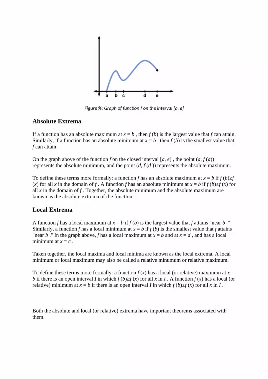
Figure %: Graph of function f on the interval [a, e]

Absolute Extrema

If a function has an absolute maximum at x = b , then f (b) is the largest value that f can attain. Similarly, if a function has an absolute minimum at x = b , then f (b) is the smallest value that f can attain.

On the graph above of the function f on the closed interval [a, e] , the point (a, f (a)) represents the absolute minimum, and the point (d, f (d )) represents the absolute maximum.

To define these terms more formally: a function f has an absolute maximum at x = b if f (b)≥f (x) for all x in the domain of f . A function f has an absolute minimum at x = b if f (b)≤f (x) for all x in the domain of f . Together, the absolute minimum and the absolute maximum are known as the absolute extrema of the function.

Local Extrema

A function f has a local maximum at x = b if f (b) is the largest value that f attains "near b ." Similarly, a function f has a local minimum at x = b if f (b) is the smallest value that f attains "near b ." In the graph above, f has a local maximum at x = b and at x = d , and has a local minimum at x = c .

Taken together, the local maxima and local minima are known as the local extrema. A local minimum or local maximum may also be called a relative minumum or relative maximum.

To define these terms more formally: a function f (x) has a local (or relative) maximum at x = b if there is an open interval I in which f (b)≥f (x) for all x in I . A function f (x) has a local (or relative) minimum at x = b if there is an open interval I in which f (b)≤f (x) for all x in I .

Both the absolute and local (or relative) extrema have important theorems associated with them.

Extreme Value Theorem

The extreme value theorem states the following: if f is a continuous function on the closed interval [a, b] , then f attains both an absolute maximum and an absolute minimum on [a, b] .

For example, it can be seen in the three continuous functions below that f attains both an absolute max and an absolute min on [a, b] :

Figure %: Demonstrating the extreme value theorem on continuous functions

Upon reflection, this theorem should seem intuitively obvious, but it is actually very difficult to prove, so the proof will be omitted here.

Note that the extreme value theorem only applies to continuous functions on a closed interval. If, for example, we had a continuous function on an open interval, the EVT would not apply. Consider the example of the function f (x) = x on the open interval (0, 1) :

Figure %: The EVT does not apply to function defined on an open interval.

Note that f (x) does not attain a minimum value on this open interval, since as x approaches 0, f (x) gets smaller and smaller, but never actually reaches 0. Similarly, there is no absolute max, because as x approaches 1, f (x) gets closer and closer to 1, but never actually reaches it.

Critical Point Theorem

Note that on the graph presented at the start of this section, f had local extrema at x = b , x = c , and x = d .

Figure %: Graph of function f on the interval [a, e]

It seems as though the tangent to the graph at each of these points is horizontal. It is in fact always the case that: if f has a local extrema at b and f'(b) exists, then f'(b) = 0 .

Sometimes, it is also possible for a continuous function to have a local extremum at a point where the derivative does not exist. For example, the function f (x) =|x - b| has a local min at x = b .

Figure %: f (x) =|x - b|

Note that the derivative, f'(b) , does not exist in this case.

We can combine these two observations into a single theorem called the Critical Point Theorem. A critical point of a function f occurs where f'(x) = 0 or f'(x) is undefined. Then the statement of the critical point theorem is that if f has a local extremum at x = b , then (b, f (b)) is a critical point.

Note that the converse of this theorem is not true, i,e, it is not the case that all critical points are local extrema. For example, in the graph below, the point x = b has a horizontal tangent, so f'(b) = 0 , but f does not have a local extremum at b :

Figure %: The converse of the critical point theorem is not necessarily tr

--------------- Problems for "Absolute and Local Extrema"

→

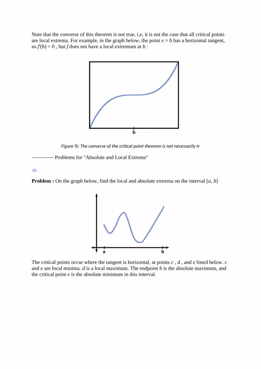
Problem : On the graph below, find the local and absolute extrema on the interval [a, b]

The critical points occur where the tangent is horizontal, at points c , d , and e listed below. c and e are local minima. d is a local maximum. The endpoint b is the absolute maximum, and the critical point e is the absolute minimum in this interval.

Problem : Find the critical points of f (x) = x 3 + x 2

f'(x) = x 2 + 2x f'(x) = 0 at x = 0 and x = - 2

Problem : Does f (x) = x 3 + x 2 have an absolute maximum?

No, it does not, since as x approaches infinity, f (x) approaches infinity, so the function grows without bound and has no maximum.

Problem : The Extreme Value Theorem doesn't apply to continuous functions on open intervals, but could such a function have both an absolute minimum and an absolute maximum on that open interval?

Yes, it certainly could. These extrema could occur at critical point on the interior of the interval:

Problem : Do absolute extrema always count as local extrema?

No. Absolute extrema that occur at the endpoints of an interval are not considered local extrema because the definition of a local extremum requires that there be an open interval I containing the extremum, but if the point is an endpoint, no such open interval exists.

-----------

The Mean Value Theorem

→

Connect any two points, (a, f (a)) and (b, f (b)) , on a differentiable function f to form a line:

Figure %: Connecting two points on a continuous function

Intuitively, it should be clear that we can find a point c between a and b where the tangent line is parallel to the secant drawn between a and b . In other words, it should be possible to find a point such that the slope of the tangent at c is the same as the slope of the secant line drawn from a to b .

Figure %: Demonstration of the Mean Value Theorem

This intuitive idea is stated as the Mean Value Theorem, which states that if f is continuous on [a, b] and differentiable on (a, b) , then there exists a point c on [a, b] for which

f'(c) =

Rolle's Theorem

Rolle's theorem is a special case of the mean value theorem in which f (a) = f (b) . It says: if f is continuous on [a,b] and differentiable on (a,b), and f (a) = f (b) , then there is a c on (a, b) where f'(c) = 0 .

The figure below should make clear that this is just a special case of the mean value theorem:

Figure %: Rolle's theorem as a case of the Mean Value Theorem

Problems for "The Mean Value Theorem" →

In problems 1-3, for each of the following functions f defined on [a, b] find the c on [a, b] such that

f'(c) =    

Problem : 1) f (x) = x 2 - 4x on [2, 4]

f'(c)= = 2  

2c - 4=2  c=3  

Problem : 2) f (x) = sin(x) + cos(x) on [0, 4Π]

   f'(c) = = 0  

   cos(x) - sin(x) = 0  

  x = , , , or  

Problem : 3) f (x) = on [1, 2]

f'(c) =

 

  = -  

-  = -  

c = ±  

Problem : 4) On the interval [-5,5], there is no point at which the derivative of f (x) =|x| is equal to zero, even though f (- 5) = f (5) . Is this a contradiction of Rolle's theorem?

No, it isn't a contradiction, since this function is not differentiable on the entire interval (- 5, 5) .

Problem : Find the number c that satisfies Rolle's theorem for f (x) = sin(x) on the interval [0, Π] .

(sin(x))' = cos(x) cos(x) = 0 at x = ----------

First, let's establish some definitions: f is said to be increasing on an interval I if for all x in I , f (x 1) < f (x 2) whenever x 1 < x 2 . f is said to be decreasing on an interval I if for all x in I , f (x 1) > f (x 2) whenever x 1 < x 2 . A function is monotonic on an interval I if it is only increasing or only decreasing on I .

The derivative can help us determine whether a function is increasing or decreasing on an interval. This knowledge will later allow us to sketch rough graphs of functions.

Let f be continuous on [a, b] and differentiable on (a, b) . If f'(x) > 0 for all x on (a, b) , then f is increasing on [a, b] . If f'(x) < 0 for all x on (a, b) , then f is decreasing on [a, b] .

This should make intuitive sense. In the graph below, wherever the slope of the tangent is positive, the function seems to be increasing. Likewise, wherever the slope of the tangent is negative, the function seems to be decreasing:

Figure %: Increasing and decreasing functions

Example: Find regions where f (x) = x 3 - x 2 - 6x is increasing and decreasing.

Solution:

f'(x) = x 2 - x - 6

f'(x) = (x - 3)(x + 2)

Now we find regions where f'(x) is positive, negative, or zero. f'(x) = 0 at x = 3 and x = - 2 . This can be marked on the number line:

From looking at the factors, it is clear that the derivative is positive on (- ∞, - 2) , and (3,∞) . The derivative is negative on (- 2, 3) .

This means that f is increasing on (- ∞, - 2) , and (3,∞) , and that it is decreasing on (- 2, 3) .

This can be indicated by arrows in the following way:

The points x = - 2 and x = 3 have horizontal tangents, which makes them critical points, but are they local extrema? It might be assumed that because f is increasing to the left of x = - 2 and decreasing to the right of x = - 2 that x = - 2 represents a local maximum. Similarly, it might be assumed that because f is decreasing to the left of x = 3 and increasing to the right of x = 3 that x = 3 represents a local minimum. This is in fact correct. This idea can be generalized in the following way:

The First Derivative Test for Classifying Critical Points

Let c be a critical number (i.e., f'(c) = 0 or f'(c) is undefined) of a continuous function f that is differentiable near x = c except possibly at x = c . Then if f'(x) is negative to the left of c and positive to the right of c , f has a local minimum at c . If f'(x) is positive to the left of c and negative to the right of c , then f has a local maximum at c . If f'(x) does not change sign at c , then (c, f (c)) is neither a local maximum nor a local minimum.

This should be clear from the figures below:

Example

Sketch a rough graph of f (x) = x 3 - x 2 - 6x

Based on previously collected data, f is increasing on (- ∞, - 2) , and (3,∞) f is decreasing on (- 2, 3) f has a local max at x = - 2 and a local min at x = 3

To sketch the graph, we might want to find the exact coordinates of the critical points: f (- 2) = 7 and f (3) = - 13 . Using this information, a rough sketch of f might look like:

Figure %: Rough sketch of f (x) = x 3 - x 2 - 6x based on first- derivative information

-------------

Problems from "Using the First Derivative to Analyze Functions"

→

Problem : f (x) = x 3 -4x 2 - 4 . Show where f (x) is increasing and where it is decreasing.

f'(x) = 3x 2 - 8x ;f'(x) = 0 at x = 0 and x = . The sign of the derivative is reported on the number line below:

So, f is increasing on (- ∞, 0) and ( ,∞) , and it is decreasing on (0, )

Problem : f (x) = sin(x) . Where is f increasing and decreasing on the interval [0, 2Π]?

f'(x) = - cos(x) ;f'(x) = 0 at x = and x = .The sign of the derivative and the behavior of the function is indicated below:

Problem : Classify the critical points of f (x) = x 3 -3x 2 - 9x .

f'(x) = 3x 2 - 6x - 9 The sign of the derivative is shown in the figure below.

Because the derivative is positive to the left of x = - 1 and negative to the right, x = - 1 is a local maximum; x = 3 is a local minimum.

Problem : Below is the graph of the derivative of a function f . Find regions where f is increasing and decreasing, and classify the critical points.

The sign of f'(x) and the behavior of f is depicted below:

While b , d , f , and h are critical points, only d and h are local extrema. d is a local maximum and h is a local minimum. ---------------

Using the Second Derivative to Analyze Functions

→

The first derivative can provide very useful information about the behavior of a graph. This information can be used to draw rough sketches of what a function might look like. The second derivative, f''(x) , can provide even more information about the function to help refine the sketches even further.

Consider the following graph of f on the closed interval [a, c] :

It is clear that f (x) is increasing on [a, c] . However, its behavior prior to point b seems to be somehow different from its behavior after point b .

A section of the graph of f (x) is considered to be concave up if its slope increases as x increases. This is the same as saying that the derivative increases as x increases. A section of the graph of f (x) is considered to be concave down if its slope decreases as x increases. This is the same as saying that the derivative decreases as x increases.

In the graph above, the segment on the interval (a, b) is concave up, while the segment on the interval (b, c) is concave down This can be seen be observing the tangent lines below:

The point b is known as a point of inflection because the concavity of the graph changes there. Any point where the graph goes from concave up to concave down, or concave down to concave up, is an inflection point.

A segment of the graph that is concave up resembles all or part of the following curve:

Figure %: Concave up curve

A segment of the graph that is concave down resembles all or part of the following curve:

Figure %: Concave down curve

To help remember this, a common saying is "concave up makes a cup, while concave down makes a frown."

Note that for concave up curves, the slope must always be increasing, but this does not mean that the function itself must be increasing. This is because a function can be decreasing while its slope is increasing. In the left half of the concave up curve drawn above, the function is decreasing, but the slope is increasing because it is becoming less negative. At the midpoint, it finally becomes zero, and then continues to increase by becoming more positive.

As one might suspect, the second derivative, which is the rate of change of the first derivative, is closely related to concavity:

If f''(x) > 0 for all x on an interval I , then f is concave up on I . If f''(x) < 0 for all x on an interval I , then f is concave down on I .

This should make sense, because f''(x) > 0 means that f'(x) is increasing, and this is the definition of concave up.

Example

Use the first and second derivatives to sketch a rough graph of f (x) = x 3 - x 2 - 6x . In the previous section, based on the first derivative, the following information was already gathered:

f is increasing on (- ∞, - 2) , and (3,∞)

f is decreasing on (- 2, 3) f has a local max at x = - 2 and a local min at x = 3

f (- 2) = 8 and

f (3) = - 13

Except for the values of f , this information can be represented as:

The second derivative can now be used to find the concavity of segments of the graph: f'(x) = x 2 - x - 6 f''(x) = 2x - 1 f''(x) = 0 when x = f''(x) > 0 (concave up) when x > f''(x) < 0 (concave down) when x <

This can be schematized as:

Because the graph changes from concave down to concave up at x = , that point is an inflection point. Now, the information from the first and second derivative can be combined into a single sketch blueprint:

The Second Derivative Test for Classifying Critical Points

The second derivative gives us another way to classify critical points as local maxima or local minima. This method is based on the observation that a point with a horizontal tangent is a

local maximum if it is part of a concave down segment, and a minimum if it is part of a concave up segment.

Let f be continuous on an open interval containing c , and let f'(c) = 0 .

If f''(c) > 0 , f (c) is a local minimum. If f''(c) < 0 , f (c) is a local maximum. If f''(c) = 0 , then the test is inconclusive. f (c) could be a local maximum, local minimum, or

neither.

To see how this works, consider again f (x) = x 3 - x 2 - 6x . f'(- 2) = 0 . To classify f (- 2) , find the second derivative:

f''(x) = 2x - 1 f''(- 2) = - 5 , which is less than zero, so the segment is concave down, and f has a local maximum at x = - 2 , confirming what has already been shown by the first derivative test.

----------------------

Problems for "Using the Second Derivative to Analyze Functions" →

Problem : f (x) = 2x 3 -3x 2 - 4 . Use the second derivative test to classify the critical points.

f'(x) = 6x 2 - 6x ;f'(x) = 0 at x = 0 and x = 1 .f''(x) = 12x - 6 ;f''(0) = - 6 , so there is a local max at x = 0 .f''(1) = 6 , so there is a local min at x = 1 .

Problem : Describe the concavity of f (x) = 2x 3 -3x 2 - 4 and find any inflection points.

f''(x) = 12x - 6 , so f''(x) = 0 when x = . The sign of f''(x) and the concavity of f are depicted below:

f has an inflection point at x = because the concavity of the graph changes there.

Problem : f (x) = sin(x) . Use the second derivative test to classify the critical points on the interval [0, 2Π] .

f'(x) = - cos(x) ;f'(x) = 0 at x = and x = .f''(x) = - sin(x) ;f''( ) = - 1 , so f has a local maximum there.f''( ) = 1 , so f has a local minimum there.

Problem : Describe the concavity of f and find any inflection point for f (x) = sin(x) on the interval [0, 2Π] .

f''(x) = - sin(x) , so f''(x) = 0 at x = 0 , x = Π , and x = 2Π . The sign of f''(x) and the concavity of f are depicted below:

On the interval [0, 2Π] , f only has an inflection point at x = Π . If we were to extend the graph in both directions, x = 0 and x = 2Π would also be points of inflection. --------------Vertical and Horizontal Asymptotes

→

Vertical Asymptotes

A vertical asymptote occurs at x = c when the following are all true

1) f (c) is undefined

2) f (x) = ∞ or - ∞

3) f (x) = ∞ or - ∞

Taken together, #2 and #3 mean that f "grows without bound" as it approaches x = c . This happens most often with a rational function at a value of x that leads to a denominator of

zero. For example, consider f (x) = . f (x) is undefined at x = - 1 .

1) f (x) is undefined at x = - 1

2) = - ∞

3) = + ∞

Thus, x = - 1 is a vertical asymptote of f , graphed below:

Figure %: f (x) = has a vertical asymptote at x = - 1

Horizontal Asymptotes

A horizontal asymptote is a horizontal line that the graph of a function approaches, but never touches as x approaches negative or positive infinity. If f (x) = L or f (x) = L , then the line y = L is a horiztonal asymptote of the function f. For example, consider the

function f (x) = . This function has a horizontal asymptote at y = 2 on both the left and the right ends of the graph:

Figure %: f (x) = . Has a horizontal asymptote at y = 2

Note that a function may cross its horizontal asymptote near the origin, but it cannot cross it as x approaches infinity.

Intuitively, we can see that y = 2 is a horizontal asymptote of f because as x approaches

infinity, f (x) = behaves more and more like f (x) = , which is the same as f (x) = 2 . Although f behaves more and more like this, it never actually becomes this function, so y = 2 is approached but not reached.

Intuition can usually lead to the right answer with these problems, but the following is a more methodical way of calculating limits at infinity.

Evaluating Limits at Infinity

In order to find horizontal asymptotes, we must evaluate limits as x approaches infinity. To evaluate the limits of rational functions at infinity, first divide each of the terms in the numerator and the denominator by the highest. For example, to evaluate

first divide each of the terms in the numerator and denominator by the highest power of x present in the function. In this case, that is x 3 .

then evaluate the individual limits using the following rule: if r is a rational number greater than zero such that x r is defined for all x , then

= 0

Applying this rule in this case leads to the following:

=

--------------Problems for "Vertical and Horizontal Asymptotes" →

Problem : Find any vertical asymptotes for f (x) = .

A candidate for a vertical asymptote is the place where the denominator goes to zero, which in this case is x = 3 . We must take limits to prove that this is an asymptote.

   = - ∞  

   = + ∞  

This means that x = - 3 is a vertical asymptote of f .

Problem : Find any vertical asymptotes for f (x) = .

 =  

  = (x + 2) = 5  

 =  

  = (x + 2) = 5  

This point is not an asymptote, but merely a point of discontinuity in the graph.

Problem : Find any horizontal asymptotes for f (x) = .

To find horizontal asymptotes, we take limits at infinity:

 =

 

  = = 1

 

 =

 

  = = 1

 

So, the line y = 1 is a horizontal asymptote of this function at both positive and negative infinity.

Problem : Find any horizontal asymptotes for f (x) = .

 =

 

  = = + ∞

 

 =

 

  = = - ∞

 

So, f does not have any horizontal asymptotes. ---------Optimization

→

Optimization of One Variable

For what value(s) of x will the function f (x) = x 3 -2x 2 - 5x be largest on the interval [- 10, 10] ?

This problem is asking us to find the absolute maximum on the interval. One way to do this is to graph the function and determine by inspection what the absolute maximum is. However, this is a very time-consuming process. A more streamlined approach is to identify all possible candidates for a local maximum and compare them to each other to see which is the largest.

The possible places for an absolute maximum to occur are at the local maxima or at the endpoints of the interval. The first step is to identify the critical points and classify them as local maxima, local minima, or neither.

f'(x) = x 2 - 4x - 5 = (x - 5)(x + 1),

so f'(x) = 0 at x = 5 and x = - 1 .

Now, to classify these points, the second derivative test can be used.

f''(x) = 2x - 4 ;f''(5) = 6 , which is greater than zero, so f (5) is a local minimum.f''(- 1) = - 6 ,which is less than zero, so f (- 1) is a local maximum.

Finally, the actual values of the local maxima and the endpoints should be compared to each other to see which of these is the absolute maximum.

f (- 10) = - 283 f (- 1) = 2 f (10) = 83

So, the absolute maximum on the interval occurs when x = 10 .

Example: For what value(s) of x will the function f (x) = x 3 -2x 2 - 5x be largest for all x ?

This problem is identical to the one above, except that there are no endpoints to compare to the local maxima.

In this situation, we must check what happens to the function as x approaches positive and negative infinity. By inspection, it becomes clear that as x approaches positive infinity, f also approaches positive infinity. Thus, the function grows without bound, and there is no absolute maximum.

Constrained Optimization

A builder needs to make a box with a square bottom and rectangular sides. The box has no top. If the material for the sides cost $2 per square foot, and the material for the bottom costs $4 per square foot, what is the largest volume box that the builder can make with $20?

This problem is known as a "constrained optimization" problem. The procedure for solving this sort of problem is ultimately similar to the procedure described above for optimizing

functions of one variable. However, some work is required to transform this word problem into a function of one variable. The first three steps below describe this process.

Step One: Identify the objective function and express it in terms of the relevant variables.

The objective function represents the quantity that is ultimately going to be maximized or minimized. In this case, the quantity of interest is the volume of the box, and it needs to be maximized. The relevant variables here are the dimensions of the box. It is often useful to draw a diagram:

Let x be the both the length and width of the square bottom of the box.Let y be the height of the sides of the box.

Expressing the volume in terms of the relevant variables generates the objective function: V = x 2 y . This quantity must be maximized.

Step Two: Identify the constraint.

The constraint is the rule or equation that relates the variables used to generate the objective function. In this case, the way to relate the variables x and y is to use the fact that the total price of the box materials must equal $20. Since the cost of the material is the area of the material multiplied by the cost per square foot, the constraint can be expressed as follows:

(4xy)(2) + (x 2)(4) = 20

Step Three: Use the constraint to express the objective as a function of one variable.

The methods that we have learned to analyze functions only apply to functions of one variable. The constraint can be used to reduce the objective to a function of one variable so that our techniques of finding maxima and minima will apply. This involves using the constraint to solve for one variable in terms of another. In this case, we solve for y , although solving for x will work also:

y = = - <BR>

Now, this can be substituted back into the original objective to yield:

V = x 2 -

Step Four: Now, V is expressed as a function of one variable, x , and procedures explained previously to for optimizing functions of one variable can be used.

The domain of V(x) is (0, + ∞) . This is because x could never be a negative quantity, and could not be zero.

V'(x) = - x 2

V'(x) = 0 whenx = ±

but only x = + is in the domain of V.

Now, to check if this critical point is a local maximum, minimum, or neither, the second derivative test can be used:

V''(x) = - 3x

V'' = - 3 < 0

Because the second derivative is negative, this critical point is a local maximum.

We can also be sure that this is the absolute maximum on the open interval (0, + ∞) . This is because there are there are no more critical points on this interval, so the graph must only be increasing to the left of the critical point, and decreasing to the right. To answer the original problem, the largest possible volume is:

V

= -

=

-

=

= square feet

-----------------------Problems for "Optimization" →

Problem : Find 2 positive numbers whose product is 25 and whose sum is a minimum.

Objective: S = x + y . The goal is to minimize S . Constraint: xy = 25 . Substitute constraint into objective:

S = + x; domain = (0,∞)  

S'(x) = + 1  

  S'(x) = 0 when x = 5  

Use second derivative to classify:

S''(x) =    

S''(5) > 0 , so S has a local min at x = 5 . However, notice that S''(x) is always positive on the interval (0,∞) , so S is always concave up on that interval, which means that the local min is also the absolute min. Therefore, 5 and 5 are the positive numbers with the smallest sum whose product is 25.

Problem : What is the maximum value of f (x) = x 4 -8x 2 - 3 on the interval [- 3, 3] ?

f'(x) = 4x 3 -16x = 4x(x 2 - 4) .This equals zero when x equals 0 or -2 or +2. Making use of the sign of the first derivative yields the following chart for the behavior of f :

Based on this, the only local maximum occurs at x = 0 . Now, to see if this is an absolute maximum on the interval, compare the value of f at x = 0 to the value at the endpoints. f (- 3) = 6 f (0) = - 3 f (3) = 6 While x = 0 is a local maximum, it is not the absolute maximum on this interval. The absolute maximum occurs at both of the endpoints in this case.

Problem : A shepherd wishes to build a rectangular fenced area against the side of a barn. He has 360 feet of fencing material, and only needs to use it on three sides of the enclosure, since the wall of the barn will provide the last side. What dimensions should the shepherd choose to maximize the area of the enclosure?

Below is a sketch of the situation:

Objective: maximize A = xy .Constraint: 2y + x = 360 .Substitution into objective: A = (360 - 2y)(y) A(y) = 360y - 2y 2 A'(y) = 360 - 4y A'(y) = 0 at x = 90 A''(y) = - 4 , so A''(90) < 0 and y = 90 is a local maximum. However, because A''(y) = - 4 for all y , the graph of A(y) is always concave down, so the local maximum is also the absolute maximum. Thus, choosing y = 90 ft and x = 180 ft will generate the largest area.

Problem : Find the point on the graph of y = x 2 that is the smallest distance from the point (0, 6) .

Objective: Let D = the distance between the point (x,y) on the graph of f (x) = x 2 and the point (0, 6) . D = We want to minimize this function. In practice, minimizing the distance is the same as minimizing the square of the distance, and because working with square roots can become complicated, we will choose here to minimize the function D 2 , which is the square of the distance. So, D 2 = (y - 6)2 + x 2 . Constraint: y = x 2 . Substituted objective: D 2 = (x 2 -6)2 + x 2 .

   (D 2)'(x) = 2(x 2 -6)2(2x) + 2x    = 4x 3 - 24x + 2x    = x(4x 2 - 22)  

  (D 2)'(x) = 0 atx = 0 and atx = ±

 

  Now use the second derivative:     (D 2)''(x) = 12x 2 - 22     (D 2)''(0) < 0, so it is a local max.  

  (D 2)''( ) > 0, so it is a local min.

 

  (D 2)''(- ) > 0, so it is a local min also.

 

Note that by symmetry, the points ( , ) and (- , ) on the graph of y = x 2 are both the exact same distance from the point (0, 6) . To see that these local minima are also at the absolute minimum distance, consider the following diagram.

From this information, it should be apparent that this function attains its lowest values at x =

±