Neurocomputing 94 (2012) 68–76

Contents lists available at SciVerse ScienceDirect

Neurocomputing

0925-23

http://d

E-m

w.liu@c

a.krishn

journal homepage: www.elsevier.com/locate/neucom

Face recognition using various scales of discriminant color space transform

Billy Y.L. Li a, Wanquan Liu a, Senjian An a, Aneesh Krishna a, Tianwei Xu b

a Department of Computing, Curtin University GPO Box U1987, Perth, WA 6845, Australiab School of Information, Yunnan Normal University, 650092 Kunming, PR China

a r t i c l e i n f o

Article history:

Received 14 February 2011

Received in revised form

18 April 2012

Accepted 22 April 2012

Communicated by D. Xucoefficients in terms of linear combinations of the R, G and B components (based on a discriminate

Available online 7 June 2012

Keywords:

Color face recognition

Discriminant color space

FERET

FRGC

12/$ - see front matter Crown Copyright & 2

x.doi.org/10.1016/j.neucom.2012.04.005

ail addresses: y.li2@postgrad.curtin.edu.au (B

urtin.edu.au (W. Liu), s.an@curtin.edu.au (S. A

a@curtin.edu.au (A. Krishna).

a b s t r a c t

Research on color face recognition in the existing literature is aimed to establish a color space that can

have the most of the discriminative information from the original data. This mainly includes optimal

combination of different color components from the original color space. Recently proposed discrimi-

nate color space (DCS) is theoretically optimal for classification, in which one seeks a set of optimal

criterion). This work proposes an innovative block-wise DCS (BWDCS) method, which allows each block

of the image to be in a distinct DCS. This is an interesting alternative to the methods relying on

converting whole image to DCS. This idea is evaluated with four appearance-based subspace state-of-

the-art methods on five different publicly available databases including the well-known FERET and

FRGC databases. Experimental results show that the performance of these four gray-scale based

methods can be improved by 17% on average when they are used with the proposed color space.

Crown Copyright & 2012 Published by Elsevier B.V. All rights reserved.

1. Introduction

Though face recognition (FR) has been investigated for morethan twenty years, some recent algorithms showing state of theart performance [1–8] are proposed and only tested on grayimages. On the other hand, color information has been shown tobe effective in improving face recognition performance. Theresearch result in [9] shows that color is important informationfor face recognition and its impact is further investigated in [10].Current research efforts on color face recognition are proven to beempirically superior to the traditional gray-scale based facerecognition [11–15]. Thus, we propose to advance the state ofthe art algorithms by incorporating them [1–8] with discriminatecolor information.

Unlike gray-scale images, color images are represented by a colorspace (like RGB). Many researches on color face recognition havelooked into which color space is more suitable for face recognition[12,16–18]. The most recent and promising one is the discriminatecolor space (DCS) [12]. DCS linearly combines R, G and B componentsof a color image using a set of optimal coefficients based on Fisher’scriterion [19]. This space thus provides a theoretically optimalrepresentation of a color image for recognition purpose, and it hasshown outstanding performance in [12] with only one traditionalclassifier. However, the shortcoming for DCS method is that it

012 Published by Elsevier B.V. All

.Y.L. Li),

n),

converts the entire image from RGB into one DCS. This will notprovide the best discriminate information for some parts of the colorimage since a color image consists of many different colors at variouslocations. For example, different lips may be more recognizable byred component, while different eyes may be more discriminable byblue component, i.e., different blocks or pixels should be treateddifferently instead of as one image in DCS. Taking motivation fromthis idea, the current work proposes two novel color spaces namelythe block-wise DCS (BWDCS), and the pixel-level DCS (PLDCS) inwhich one aims to find optimal discriminate color space for eachblock or each pixel in the images of RGB color model.

In this paper, four appearance-based subspace algorithms[1–4] are considered, and each of them is integrated with theproposed color spaces. Improvement in their performances isnoted on five different benchmarked databases. The most recentpreprocessing pipeline in [5] is also integrated into the proposedsystem to form a complete color face recognition framework.

The rest of this paper is organized as follows. The original DCSmethod is reviewed briefly in Section 2. Section 3 addresses thepixel-level DCS and Section 4 addresses the block-wise DCS.Experiments are provided in Section 5, In Section 6 we shallcompare PLDCS against DCS and Section 7 concludes the paper.

2. Discriminant color space

The DCS was originally proposed in [12] for color facerecognition. This section briefly describes DCS. Let A be a colorimage with a resolution of H�W consisting of three color

rights reserved.

B.Y.L. Li et al. / Neurocomputing 94 (2012) 68–76 69

components R, G and B. Assume they are represented as columnvectors: A¼[R, G, B] A RPx3, where P¼H�W is the number ofpixels. The idea is to convert the image A in RGB space to an imageD in a more discriminable space namely the DCS. Let the imageD be:

D¼ ½D1,D2,D3�ARP�3

ð1Þ

The conversion is done by linearly combining R, G and B usinga set of coefficients defined as

Dk¼ x1kRþx2kGþx3kB¼ AXk ð2Þ

where k¼1, 2, 3 and Xk¼[x1k,x2k,x3k]TA R3�1 is the combinationcoefficients that can be found via maximizing the followingobjective function:

JðXÞ ¼traceðSbÞ

traceðSwÞ¼

XTLbX

XTLwXð3Þ

where X¼[X1,X2,X3]TA R3�3. Sb and Sw are the scatter matrices inthe D-space. Let there be N training images for C classes, Ti be theith class (i¼1, 2y C) and Ni be the number of images in Ti. Thenthe Lb, Lw namely the color space scatter matrices can be derivedas

Lb ¼XC

i ¼ 1

QiðAi�AÞTðAi�AÞ ð4Þ

Lw ¼XC

i ¼ 1

Qi

Qi�1

XAj ATi

ðAj�AiÞTðAj�AiÞ ð5Þ

where j¼1, 2 y N and Qi is the prior probability for Ti

commonly being evaluated as Qi¼Ni/N. Moreover, A and Ai arethe global and the class means respectively, computed as

A¼1

N

XN

j ¼ 1

Aj ð6Þ

and

Ai ¼1

Ni

XAj ATi

Aj ð7Þ

For detailed steps to derive Lb and Lw, we shall refer the readerto [12]. In fact, the optimal X that maximizes (3) is the generalizedeigenvectors corresponding to the largest eigen value l satisfyingthe equation

LbX ¼ lLwX ð8Þ

3. Pixel-level discriminant color space

Unlike DCS which assigns the same coefficients for all pixels,PLDCS assigns different coefficients to different pixels as

DKp ¼ x1kpRpþx2kPGpþx3kpBp ð9Þ

where p¼1, 2 y P. These different coefficients are obtained byoptimizing the objective function locally for each pixel. Then weconvert each image A in RGB space to image E in PLDCS, whichconsists of P different DCS. Image E is denoted as

E¼Dp ¼ ½D1p ,D2

p ,D3p � ð10Þ

The algorithmic procedure to convert a color image from RGBto PLDCS is stated below:

1.

Store each color image using color space rearrangement inwhich R, G and B are three column vectors, i.e. A¼[R, G, B] ARP�3.

2.

Pixel extraction. From p ¼1, extract the first pixel Ap¼[Rp, Gp,Bp] A R1�3.

Compute Ap and Aip using (6) and (7). Then Lbp and Lwp using(4) and (5).

3.

Do eigen value decomposition and obtain the local projectionmatrix Xp by solving (8).

4.

Convert Ap to Ep using (9) and (10). 5. Repeat Step 2 for p¼pþ1, until p¼P.

PLDCS is locally optimal for each pixel, while DCS is onlyholistically optimal, in terms of classification for full image. Byallowing different projections at different locations, we expect thediscrimination power of PLDCS is theoretically stronger than DCS.

4. Block-wise discriminant color space

Since PLDCS repeats calculations for each single pixel, it isexpected to work slower. The main bottleneck is in the P timesDCS calculations. PLDCS may also suffer from over-fittingproblem. Instead of pixel calculation, we propose a method whichcan operate on blocks of an image to overcome the motionedshortcoming.

For an image with resolution H�W, we can divide the imageinto small blocks with size h�w (hoH and woW) and converteach block to DCS. For simplicity, we just reduce the block size tofit for the image edges, but other handling rules may also beapplied. If the block size is defined as one block of H�W, then it isDCS and similarly, if the block size is defined as 1�1, then itis PLDCS.

Now we shall state the algorithmic procedure to convert acolor image from RGB to BWDCS as follows:

1.

Store each color image using image matrices rearrangement inwhich R, G and B are three matrices, i.e. A¼[R, G, B] ARH�W�3.

2.

From the first pixel, extract h rows and w columns as a block(or sub-image), i.e. ~A ¼ ½ ~R, ~G, ~B�ARh�w�3 If h or w exceed A’savailable rows or columns, reduce h or w to fit.

3.

Rearrange ~Ausing color space rearrangement by converting ~R,~G and ~B to three augmented vectors ~A ¼ ½ ~R, ~G, ~B�ARðhnwÞ�3.

4.

Compute ~A and ~Ai using (6) and (7). Then ~Lb and ~Lw using(4) and (5).

5.

Do eigen value decomposition and obtain the sub-imageprojection matrix ~X by solving (8).

6.

DCS transformation. Convert ~A to ~D using (1) and (2). 7. Repeat Step 2 for the next unconverted block, until every block

is converted.

Block-wise DCS has two main advantages. Firstly, it runs fasterwith the increase of block size. In terms of color space conversion,PLDCS has a complexity of OðH �WÞ while the complexity ofblock-wise DCS is O(H�W/h�w). Secondly, each calculation ofblock-wise DCS makes use of information from the adjacent pixelswhich are always correlated. Thus, the classification results areexpected to be more robust potentially.

5. Experiments

In this section, we have tested our proposed color spaces byintegrating them with four subspace methods [1–4]. We have alsocompared the performance against other color spaces as well asgray-scale (as origin of these four methods). This section presents

Fig. 1. Example images from the four databases used in our experiments.

B.Y.L. Li et al. / Neurocomputing 94 (2012) 68–7670

details of the experiments in terms of performance statistic,datasets, integration methods and results.

5.1. Evaluation protocol and performance statistics

Following [20], we divide face recognition problems into twotypes: face identification problem and face verification problem.In our experiments, both problems are evaluated.

The evaluation protocol used in this paper is as follows. Eachdatabase is divided into three mutually exclusive sets: training set,gallery set and probe set. Training is done on the training set whiletesting is done on both gallery and probe set. For identificationproblems, the probe images are matched to all of the gallery imagesto find the match. For verification problems, we consider acceptingor rejecting the probe against the claimed gallery image. For eachtype of problem, the performance is calculated in a different manner.

The performance statistics defined in [20] for each type ofproblem is adopted. For identification problems, we report therank-one identification rate on the Cumulative Match Character-istics (CMC) curve. For the verification problems, we report theface verification rate (FVR) at 0.001 false accept rate (FAR) on theReceiver operating characteristic (ROC) curve.

5.2. Databases and experimental setup

To ensure that our experimental results are unbiased, weextensively evaluate them on five color face databases.

�

The Aberdeen database from Psychological Image Collection atStirling (PICS) [21]. � Georgia Tech face database (GT) [22]. � AR face database (AR) [23]. � The Facial Recognition Technology (FERET) [24]. �

1 One image per subject in fa set.

Face Recognition Grand Challenge version 2 experiment 4(FRGC-204) [25].

Images in PICS [21] are collected for research in Psychology,however, it is also suitable for the face recognition communitygiven its variations in illumination, facial expression and pose. Weselect a subset of the database that consists of 29 people eachhaving 9 images. Since this is a small database, we formulate thetest as face identification problem: 4 images per person arerandomly chosen for training as well as being the gallery imagesand the remaining 5 for probe. To ensure that result is notdepending on specific training/testing samples, the process isrepeated 10 times and the average rank-one identification rate isreported with the standard deviation.

GT [22] is a database often used for face recognition. Forexample it has been used in [6], because of its variations in facialexpression/details and pose. The database consists of 50 peopleeach having 15 images. We test them as a face identificationproblem: i.e., using all images of 25 people randomly chosen fortraining and for the other 25 people, 8 images per person arerandomly chosen as gallery and remaining images for probe, suchthat the subjects for testing are never been seen during training.By repeating 10 times, the average rank-one identification rate isreported with the standard deviation.

AR [23] is a publicly available face database. It is widely usedfor evaluating face identification problems. For instance, in[18,26]. This database contains over 4000 images which iscaptured in two sessions with different facial expressions, illumi-nation conditions and occlusions. We use a subset of all the un-occluded images from the first 50 males and 50 females. As theresult, a total of 1400 images from two sessions (14 images persubject) are involved in our experiment. We formulate a time-delayed face identification problem using images from session

one for training and images from session two for testing. Notethat the size of this database is much larger than PICS and GT.Therefore, this allow us to evaluate on a larger-scale identificationproblem.

For FERET [24], we are using the color version (though someimages still are in the gray-scale) which was released in the year2003. It was the de facto standard dataset to evaluate facerecognition systems at that time because of the strictly controlledparameters and support by the government. The database pro-vides standard subsets namely fa, fb, dup1 and dup2. We selectonly the color images with eyes/lip coordinates provided, result-ing in a total of 2419 images (808þ806þ593þ212), from thefour sets. We then construct the training set by selecting from fathe first 400 images/subjects1 that are not appearing in dup2 andthen combining with the images of the corresponding subjects infb and dup1, resulting in 1013 images (400faþ399fbþ214dup1).The rest of the 408 images from fa served as gallery, the rest of407 images from fb serve as one probe set and all 212 imagesfrom dup2 serve as another probe set. This design allows trainingon images that varies in facial expression and the session time isup to 1.5 years, while testing on facial expression effect (fb) andaging effect of longer than 1.5 years (dup2). Subjects in trainingand testing sets are mutually exclusive. We report face verifica-tion rate on the two tests respectively.

FRGC version 2 [25] having more than 50000 records isconstructed by the same organization as FERET, and is becomingthe next major challenge for face recognition systems. Weconsider only the most challenging experiment 4 ROCIII whichis testing with controlled gallery images and uncontrolled probeimages pairs that is one semester different in collection time. Thislarge-scaled dataset exhibits large intrapersonal variations andsome people look very similar due to strong illumination.

Some example images used in our experiments from eachdatabase are shown in Fig. 1 as ready reference. A summary isshown in Table 1.

Table 1Databases Summary.

Name Problem Training Gallery Probe

PICS Seen identification 116 – 145

GT Unseen identification 375 200 175

AR Large-scale seen identification 700 – 700

FERET Unseen verification 1013 408 407(fb) 212(dup2)

FRGC-204 Large-scale partially-seen verification 12776 16028 8014

Fig. 2. Face recognition system pipeline.

Table 2Method Parameters.

Method Parameter PICS GT AR FERET FRGC(2 0 4)

Gamma Correction g 0.9 0.9 1 0.2 0.5

DoG Filitering s0 0 0 0.4 0.4 0.8

s1 0 0 0 �1 �3

Constrast

Equalization

a 0.1 0.1 0.1 0.1 0.1

t 1 2 10 3 �10

wPCA Features 35 250 550 700 1000

rLDA Regular. l features 0.5 0.5 5e�3 10 5

28 24 99 385 220

sLPP Dist. metric PCA

Dim. w features

cos cos cos cos cos

35 250 550 700 1000

0 0 0 1 100

18 35 200 335 220

IDA Regular. l features 50 100 100 0.1 10

28 24 99 390 221

Feature Vector

Similarity Metric

L2 L2 cos cos cos

Table 3Experiment Results.

PICS

Original [1–4] RGB [11] DCS [12] ProposedwPCA 71.8%71.2 72.9%71.3 83.4%70.8 90.8%70.6 (1)

rLDA 86.7%70.7 88.9%70.5 95.7%70.4 97.4%70.5 (1)

sLPP 77.7%71.1 78.7%71.2 86.9%71.0 93.8%71.0 (1)

IDA 86.3%70.9 87.9%70.5 95.4%70.5 97.0%70.5 (2)

GT

Original [1–4] RGB [11] DCS [12] ProposedwPCA 84.4%71.0 85.2%71.0 90.1%70.6 95.0%70.5 (1)

rLDA 87.5%71.0 90.6%70.8 94.6%70.5 95.7%70.4 (1)

sLPP 89.7%70.8 90.6%70.7 94.5%70.7 96.9%70.6 (2)

IDA 91.6%70.8 92.3%70.7 95.0%70.5 96.1%70.3 (2)

AR

Original [1–4] RGB [11] DCS [12] ProposedwPCA 50.6% 74.0% 74.5% 77.0% (6)

rLDA 80.5% 86.6% 87.6% 90.3% (2)

sLPP 80.3% 90.1% 91.6% 93.0% (1)

IDA 79.0% 80.4% 81.0% 82.0% (6)

FERET fa-fb

Original [1–4] RGB [11] DCS [12] ProposedwPCA 85.1% 88.3% 90.1% 93.1% (4)

rLDA 90.5% 92.0% 93.9% 94.7% (4)

sLPP 85.5% 89.9% 93.7% 95.3% (2)

IDA 88.2% 91.5% 95.7% 96.4% (2)

FERET fa-dup2

Original [1–4] RGB [11] DCS [12] ProposedwPCA 35.2% 39.8% 59.6% 66.2% (2)

rLDA 42.9% 50.5% 71.5% 73.7% (2)

sLPP 37.1% 43.4% 59.8% 66.8% (8)

IDA 34.1% 40.7% 70.6% 71.7% (16)

FRGC-204

Original [1–4] RGB [11] DCS [12] ProposedwPCA 18.2% 20.2% 21.5% 23.3% (6)

B.Y.L. Li et al. / Neurocomputing 94 (2012) 68–76 71

5.3. System pipeline and method integration

The face recognition system pipeline involves image pre-processing, color space conversion, feature extraction and simi-larity score calculation as illustrated in Fig. 2.

Preprocessing is done as following: the face region is croppedout and resized to resolution of 32�32 after eyes and lip alignedto same position. Then we apply the preprocessing chain in [5]2

on each of the color image components (R, G and B) separately, i.e.gamma correction, DoG filtering and contrast equalizationto reduce illumination effect and enhance facial feature. Thepreprocessing parameters are tuned manually to the best forgray-scale images and recorded in Table 2. The default parameters

rLDA 56.5% 75.7% 76.5% 78.2% (16)

sLPP 56.2% 73.0% 74.0% 75.9% (6)

IDA 37.9% 73.5% 74.4% 75.5% (16)2 Code available at http://parnec.nuaa.edu.cn/xtan.

Table 4Various Block Size.

PICS

1�1 2�2 4�4 6�6 8�8 16�16wPCA 90.8%70.6 90.6%70.6 88.1%71.0 86.9%70.8 84.8%70.8 84.8%70.8

rLDA 97.4%70.4 97.4%70.4 97.0%70.5 96.1%70.4 96.4%70.4 95.9%70.4

sLPP 93.8%70.9 92.7%71.0 91.3%70.8 89.7%70.8 89.0%70.8 89.6%71.0

IDA 96.8%70.5 97.0%70.5 96.6%70.5 95.8%70.4 96.3%70.4 95.8%70.5

GT

1�1 2�2 4�4 6�6 8�8 16�16wPCA 95.0%70.5 95.0%70.6 94.7%70.6 93.4%70.6 94.1%70.7 91.4%70.8

rLDA 95.7%70.4 95.5%70.4 95.2%70.5 94.6%70.5 95.6%70.5 94.3%70.6

sLPP 96.6%70.6 96.9%70.4 96.1%70.4 95.5%70.5 96.3%70.4 95.3%70.5

IDA 96.0%70.3 96.1%70.3 95.8%70.4 95.1%70.5 95.8%70.5 94.9%70.5

AR

1�1 2�2 4�4 6�6 8�8 16�16wPCA 76.3% 76.3% 76.3% 77.0% 76.3% 75.7%

rLDA 90.1% 90.3% 90.1% 90.3% 90.1% 89.0%

sLPP 93.0% 92.4% 92.6% 92.3% 92.0% 92.7%

IDA 81.8% 81.4% 81.0% 82.0% 81.4% 80.3%

FERET fa–fb

1�1 2�2 4�4 6�6 8�8 16�16wPCA 92.3% 93.0% 93.1% 92.0% 91.3% 92.5%

rLDA 94.4% 94.6% 94.7% 93.7% 94.1% 94.3%

sLPP 94.6% 95.3% 94.3% 94.9% 94.2% 93.7%

IDA 96.1% 96.4% 96.1% 95.5% 95.8% 95.8%

FERET fa-dup2

1�1 2�2 4�4 6�6 8�8 16�16wPCA 64.2% 66.2% 64.5% 58.5% 60.3% 59.7%

rLDA 72.9% 73.7% 72.5% 70.8% 73.5% 71.3%

sLPP 63.4% 62.2% 62.2% 58.9% 66.8% 60.4%

IDA 69.6% 67.8% 70.2% 66.7% 70.8% 71.7%FRGC-204

1�1 2�2 4�4 6�6 8�8 16�16wPCA 22.5% 22.4% 22.5% 23.3% 22.2% 22.5%

rLDA 77.3% 77.7% 77.7% 77.7% 77.5% 78.2%sLPP 75.7% 75.3% 75.6% 75.9% 75.2% 75.5%

IDA 74.3% 74.0% 74.4% 74.0% 74.6% 75.5%

B.Y.L. Li et al. / Neurocomputing 94 (2012) 68–7672

in [5] is not used since they are optimized for descriptor methodsrather than for subspace methods. Details on each parameters canbe have by referring to [5]. Lastly, each color components arenormalized to zero mean pixel and unit standard deviation.Specifically, letting the three color components are Ci wherei¼1, 2, 3, mi and si be the mean and standard deviation of allpixels in Ci, the normalization is done as follows:

Ci’Ci�mi1P�1

sið11Þ

where P is the number of pixels in Ci, 1p�1 is a vector with allones.

For color spaces, we have compared PLDCS and BWDCS withDCS, RGB as well as gray-scale. After converting to specific colorspace or gray-scale, each color components are normalized onceagain to zero mean pixel and unit standard deviation using (11).

Before extracting features, each of the color components isconcatenated to an augmented vector. The feature extractionmethods we considered are:

�

whitened Principal Component Analysis (wPCA) [1] � regularized Linear Discriminant Analysis (rLDA) [2] � supervised Locality Preserving Projection (sLPP) [3]3

�

intrinsic Discriminant Analysis (IDA) [4].

3 Code available at: http://www.zjucadcg.cn/dengcai/.

The reason of choosing these methods is because we are extend-ing the work in [12] where DCS was tested on an appearance-basedsubspace method, thus we choose to test on the same type ofmethods. Further, we want to test on methods that are stable andwell-developed like PCA [27] and LDA [19], but new enough tocompete with the state of the art. For each method, parameters aretuned manually to the best for gray-scale images and recorded inTable 2. Note that the parameter w of sLPP is a constant numberadded to the weight matrix. The reason is that when we construct theweighted graph for color space that allows negative values such asDCS, PLDCS and BWDCS, some weights become negative. However,constructing this graph using the original RGB image or Euclideandistance decreases the performance. We find that simply adding aconstant number w to the weights increases the performance slightly,thus we introduce this parameter.

Similarity score is calculated either by Euclidean distance orCosine similarity depends on which measurement gives higherperformance on gray-scale image. The score is then normalizedusing z-score [28]. Lastly, the similarity matrix is evaluated usingthe specific performance statistic described in Section 5.1.

5.4. Experimental results

The experimental results are presented in Table 3. For PICS andGT, the average rank one identification rate r is reported alongwith the standard deviation s in the format r7s. For AR, we reportthe rank one identification rate. For FERET and FRGC, the faceverification rates (FVR) at 0.1% false accept rate (FAR) is reported.

B.Y.L. Li et al. / Neurocomputing 94 (2012) 68–76 73

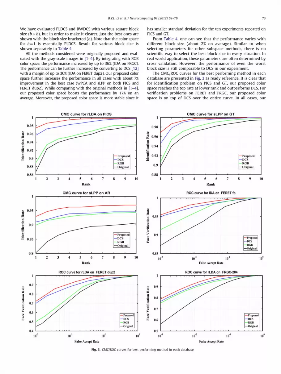
We have evaluated PLDCS and BWDCS with various square blocksize (b� b), but in order to make it clearer, just the best ones areshown with the block size bracketed (b). Note that the color spacefor b¼1 is essentially PLDCS. Result for various block size isshown separately in Table 4.

All the methods considered were originally proposed and eval-uated with the gray-scale images in [1–4]. By integrating with RGBcolor space, the performance increased by up to 36% (IDA on FRGC).The performance can be further increased by converting to DCS [12]with a margin of up to 30% (IDA on FERET dup2). Our proposed colorspace further increases the performance in all cases with about 7%improvement in the best case (wPCA and sLPP on both PICS andFERET dup2). While comparing with the original methods in [1–4],our proposed color space boosts the performance by 17% on anaverage. Moreover, the proposed color space is more stable since it

Fig. 3. CMC/ROC curves for best perfo

has smaller standard deviation for the ten experiments repeated onPICS and GT.

From Table 4, one can see that the performance varies withdifferent block size (about 2% on average). Similar to whenselecting parameters for other subspace methods, there is noscientific way to select the best block size in every situation. Inreal world application, these parameters are often determined bycross validation. However, the performance of even the worstblock size is still comparable to DCS in our experiment.

The CMC/ROC curves for the best performing method in eachdatabase are presented in Fig. 3 as ready reference. It is clear thatfor identification problem on PICS and GT, our proposed colorspace reaches the top rate at lower rank and outperforms DCS. Forverification problems on FERET and FRGC, our proposed colorspace is on top of DCS over the entire curve. In all cases, our

rming method in each database.

B.Y.L. Li et al. / Neurocomputing 94 (2012) 68–7674

proposed color space is superior to gray-scale (these methodsoriginally developed for).

6. An investigation into holistic and local DCS

DCS [12] makes use of holistic information while we general-ize it to use different scales of local information. As a result,optimal projection can be obtained to suit each local area. Inaddition, the correlation between each color components can befurther reduced which is shown to be an important factor forperformance increment [26].

Some color spaces are illustrated in Fig. 4. For DCS, PLDCS andBWDCS, we scale the pixel values of each color component to imagedomain (0, 255). One can see that PLDCS is visually very different toDCS. For example, the mouth area is forced to be in yellow color inDCS, while the fisher optimal color is actually near blue and green(which can be seen from the color image of PLDCS).

The projection vector associated with the largest Eigen valueobtained after training on FERET database is further investigated.

Fig. 4. Illustration of R, G, B color component images and the three DCS

component images generated by the proposed method.

Fig. 5. Angle differences between DCS and PLDCS projection vectors. (Left) Box plot fo

a gray-scale image.

Since, the image resolution is 32�32, there are 1024 PLDCSprojection vectors. Angles between the DCS projection vectorto each of these PLDCS vectors are calculated. The summary ofthese 1024 angle differences are shown using box plot inFig. 5(left). On an average, each PLDCS vectors are different toDCS vectors by 41 %

o.

All 1024 angle differences are then scaled from degree domain (0,90) to image domain (0, 255) and are then shown as a gray-scaleimage in Fig. 5(right). It is important to note that this figure is not atransform of a facial image. Black color (0) means minimum angledifference (0.40%

o) while white color (255) means maximum angle

difference (89.99%o). Each region on a face having similar color is also

having similar projection vector, while the greatest difference is ataround the lip, eyes and edges, thus making the image look likea face.

DCS is based on Fisher Criterion [19] and hence optimal forclassification. However, as illustrated, every pixel has its own optimalprojection vector and most of them are different to the projectionvector obtained by DCS method. The fact that DCS method uses oneDCS projection for every pixel diminishes its performance.

Yang et al.[26] show that color spaces that have Double ZeroSum (DZS) property is better for face recognition. A color space isDZS if two columns of its transformation matrix have zero sums.DZS is important because color spaces that are DZS have lowercorrelation between their color components. The three colorcomponents of RGB is highly correlated therefore is not a goodcolor space for recognition. DCS is a near DZS color space hencehaving low inter-component correlation and higher discrimina-tion power. PLDCS has DZS property for each single pixels, thusfurther reduces the inter-component correlation.

Table 5 shows that average inter-component correlation for thetraining images in FRGC-204 and FERET. Given K color imagesAi ¼ ½A

1i ,A2

i ,A3i � (i¼1yK), where A1A2A3 are three color components.

The correlation matrix is calculated first from each individualimage as:

rx,yi ¼

E½ðAxi�EAx

i ÞðAyi�EAy

i ÞT�

sxi s

yi

r the differences. (Right) Scales the differences to image domain (0,255) forming

Table 5Average Inter-component Correlation.

FRGC-204 FERET

RGB 0.9283 0.9332

DCS 0.2992 0.3795

PLDCS 0.1669 0.0828

B.Y.L. Li et al. / Neurocomputing 94 (2012) 68–76 75

ðx,y¼ 1,2,3, xayÞ ð12Þ

Since rx,yi ¼ r

y,xi and the sign does not affect the correlation

magnitude, the average correlation R is calculated by averagingacross all images and taking absolute value

R¼1

K

Xk

i ¼ 1

r1,2i

������þ r1,3

i

������þ r2,3

i

������

3

0@

1A ð13Þ

R is ranged from zero to one. Zero means no correlation at allwhile one means perfectly correlated. We can see from Table 4that image in PLDCS has much lower correlation.

To conclude, different locations of a face have different optimalcolor space for classification. The improvement achieved byPLDCS or BWDCS is mostly due to the reason that it capturesthe optimal space for each pixel or block. As well as it furtherreduces correlation between color components.

7. Conclusions

This paper proposed new color spaces for face recognition. Wehighlight our contributions as follows. Firstly, we incorporate somepromising subspace algorithms that are originally proposed andevaluated on gray images with our new color spaces. Secondly, aneffective preprocessing pipeline proposed recently is integrated in ourrecognition framework to work along with color images. Thirdly, wedesigned repeatable experimental setups that covered many aspectsof face recognition problems including seen and unseen identificationas well as unseen and partially-seen verification. Fourth, by improv-ing DCS, two new color spaces are proposed for color face recognitionnamely PLDCS and BWDCS.

Experimental results show that, for all subspace methods con-sidered, the performances are improved significantly in the followingorder: gray-scale, RGB, DCS and our proposed PLDCS/BWDCS. Sincemany recently proposed methods are still being developed using thegray-scale images, the state of the art can be advanced by using thecolor spaces proposed in this work.

References

[1] W. Deng, J. Hu, J. Guo, W. Cai, D. Feng, Robust, accurate and efficient facerecognition from a single training image: a uniform pursuit approach, PatternRecognition 43 (2010) 1748–1762.

[2] J. Lu, K.N. Plataniotis, A.N. Venetsanopoulos, Regularization studies on LDAfor face recognition, in: Proceedings of the 2004 International Conference onImage Processing (ICIP) ’04, 2004, vol. 1, pp. 63–66.

[3] Z. Zheng, F. Yang, W. Tan, J. Jia, J. Yang, Gabor feature-based face recognition usingsupervised locality preserving projection, Signal Process. 87 (2007) 2473–2483.

[4] Y. Wang, Y. Wu, Face recognition using intrinsicfaces, Pattern Recognition 43(2010) 3580–3590.

[5] X. Tan, B. Triggs, Enhanced local texture feature sets for face recognitionunder difficult lighting conditions, IEEE Trans. Image Process. 19 (2010)1635–1650.

[6] I. Naseem, R. Togneri, M. Bennamoun, Linear regression for face recognition,pattern analysis and machine intell, IEEE Trans. on Pattern Analy. Mach.Intelligence (2010).

[7] G.F. Lu, Z. Lin, Z. Jin, Face recognition using discriminant locality preservingprojections based on maximum margin criterion, Pattern Recognition 43(2010) 3572–3579.

[8] M. Guillaumin, J. Verbeek, C. Schmid, Is that you? Metric LearningApproaches for Face Identification.,’’ presented at the International Confer-ence on Computer Vision (ICCV), 2009.

[9] L. Torres, J.Y. Reutter, L. Lorente, Importance of the color information in facerecognition, IEEE International Conference on Image Processing, vol. 3, 1999,pp. 627–631.

[10] A. Yip, P. Sinha, Role of color in face recognition, MIT tech report (ai.mit.com)AIM-2001-035 CBCL-212, 2001.

[11] M. Thomas, C. Kambhamettu, S. Kumar, Face recognition using a colorsubspace LDA approach, Proceedings on the International Conference onTools with Artificial Intelligence, ICTAI, vol. 1, 2008, pp. 231–235.

[12] J. Yang and C. Liu, A discriminant color space method for face representa-tion and verification on a large-scale database, 2008 19th InternationalConference on Pattern Recognition, ICPR 2008, 2008.

[13] Z. Liu, C. Liu, Fusion of the complementary discrete cosine features in the YIQcolor space for face recognition, Comput Vision Image Understanding 111(2008) 249–262.

[14] S. Peichung, L. Chengjun, Improving the face recognition grand challengebaseline performance using color configurations across color spaces,’’ in:Proceedings of the 2006 IEEE International Conference on Image Processing,2006, pp. 1001–1004.

[15] P. Shih, C. Liu, Comparative assessment of content-based face image retrieval indifferent color spaces, Int. J. Pattern Recognition Artif. Intell. 19 (2005) 873–893.

[16] C. Liu, J. Yang, ICA color space for pattern recognition, IEEE Trans. NeuralNetworks 20 (2009) 248–257.

[17] J. Yang, C. Liu, Color image discriminant models and algorithms for facerecognition, IEEE Trans. Neural Networks 19 (2008) 2088–2098.

[18] J. Yang, C. Liu, L. Zhang, Color space normalization: Enhancing the discriminatingpower of color spaces for face recognition, Pattern Recognition 43 (2010)1454–1466.

[19] P.N. Belhumeur, J.P. Hespanha, D.J. Kriegman, Eigenfaces vs. fisherfaces:recognition using class specific linear projection, IEEE Trans. Pattern Anal.Mach. Intell. 19 (1997) 711–720.

[20] Biometric Testing and Statistics: National Science and Technology Council(NSTC), 2006.

[21] P. Hancock,The Psychological Image Collection at Stirling (PICS) (n.d., 20 June2009), available from: /http://pics.psych.stir.ac.uk/S.

[22] A.V. Nefian.,Georgia Tech Face Database 1999, available from: /http://www.anefian.com/research/face_reco.htmS.

[23] A.M. Martinez and R. Benavente, The AR face database: CVC Tech. Report #24,1998.

[24] J. Phillips, H. Moon, S. Rizvi, P. Rauss, The FERET evaluation methodology forface-recognition algorithms, IEEE Trans. Pattern Anal. Mach. Intell. 22 (2000)1090–1104.

[25] P.J. Phillips, P.J. Flynn, T. Scruggs, K.W. Bowyer, J. Chang, K. Hoffman,J. Marques, J. Min, W. Worek, Overview of the face recognition grandchallenge, Proc. IEEE Conf. Comput. Vision Pattern Recognition (2005).

[26] J. Yang, C. Liu, J.Y. Yang, What kind of color spaces is suitable for color facerecognition? Neurocomputing 73 (2010) 2140–2146.

[27] M. Turk, A. Pentland, Eigenfaces for recognition, J. Cogn. Neurosci. 3 (1991) 71–86.[28] A. Jain, K. Nandakumar, A. Ross, Score normalization in multimodal biometric

systems, Pattern Recognition 38 (2005) 2270–2285.

Billy Y.L. Li received the Bachelor of Science degreewith first class honors in Computer Science fromCurtin University in 2009 and he is pursuing hisPh. D. degree currently. His research area is patternrecognition and face recognition.

Wanquan Liu received the B. Sc. degree in AppliedMathematics from Qufu Normal University, PR China,in 1985, the M. Sc. degree in Control Theory andOperation Research from Chinese Academy of Sciencein 1988, and the Ph. D. degree in Electrical Engineeringfrom Shanghai Jiaotong University, in 1993. He onceholds the ARC Fellowship and JSPS Fellowship andattracted research funds from different resources. He iscurrently an associate professor in the Department ofComputing at Curtin University. His research interestsinclude large scale pattern recognition, control sys-tems, signal processing, machine learning, and intelli-

gent systems.

Senjian An received the B.S degree from ShandongUniversity, Jinan, China, in 1989, the M.S. degree fromthe Chinese Academy of Sciences, Beijing, in 1992,andthe Ph. D. degree from Peking University, Beijing, in1996. He was with the Institute of Systems Science,Chinese Academy of Sciences, Beijing, where he was apost doctoral Research Fellow from 1996 to 1998. In1998, he joined the Beijing Institute of Technology,Beijing and he was an associate Professor from 1998 to2001. From 2001 to 2004, he was a Research Fellowwith The University of Melbourne, Parkville, Australia.Since 2004, he has been working at Curtin University,

where he is currently a Research Fellow. His research

interests include machine learning, face recognition and object detection.

B.Y.L. Li et al. / Neurocomputing 94 (2012) 68–7676

Aneesh Krishna is currently Senior Lecturer ofSoftware Engineering with the Department of Comput-ing, Curtin University, Australia, since July 2009. Heholds a Ph. D. in Software Engineering from theUniversity of Wollongong, Australia, an M. Sc (Engg.)in Electronics Engineering from Aligarh Muslim Uni-versity, India and a B.E. degree in Electronics Engineer-ing from Bangalore University, India. He was a Lecturerin Software Engineering at the School of ComputerScience and Software Engineering, University ofWollongong, Australia (from February 2006–June2009). His research interests include Software Engi-

neering, Requirements Engineering, Conceptual Mod-

eling, Agent Systems, Formal Methods and Service-Oriented Computing.

Tianwei Xu is currently a Professor in School ofInformation at Yunnan Normal Universityin PRChina. His research areas include face recognitionand information retrieval.