ExPlanes: Exploring Planes in Triplet Data

Bruno Schwenk1, Joachim Selbig2, Yehuda Ben-Zion3, Matthias Holschneider1

1Institut fur Mathematik, Universitat Potsdam, 14476 Potsdam, Germany

2Institut fur Biochemie und Biologie, Universitat Potsdam, 14476 Potsdam, Germany

3USC Earth Sciences, Los Angeles, CA 90089-0740

Summary

Many methods for the analysis of gene expression-, protein- or metabolite-data focus on theinvestigation of binary relationships, while the underlying biological processes creating thisdata may generate relations of higher than bivariate complexity. We give a novel methodExPlanes that helps to explore certain types of ternary relationships in a statistically robust,Bayesian framework. To arrive at an characterization of the data structure contained intriplet data we investigate 2-dimensional planes being the only linear structures that cannotbe inferred from projections of the data. The key part of our methodology is the definitionof a robust, Bayesian plane posterior under the assumption of an invariant prior and aGaussian error model. A numerical representation of the plane posterior can be exploredinteractively. Beyond this purely Bayesian approach we can use the plane posterior toconstruct a family of posterior-based test statistics that allow testing the data for differentplane related hypotheses. To demonstrate practicability we queried triplets of metabolicdata from a plant crossing experiment for the presence of plane-, line- and point-structuresby using posterior-based test statistics and were able to show their distinctiveness.

1 Introduction

Over the last twenty years, significant advances in experimental technologies have providedthe prerequisites for a better understanding of cellular regulatory and metabolic processes, cf.[5, 3, 13].

These data on gene expression, metabolite concentrations, protein abundances, and also fluxesallow the improvement of pathway and network modeling and simulation with the goal of betterunderstanding the dynamics of cellular processes, cf. [6, 8, 16].

A variety of methods to analyze these data is based on the detection of localpair-wise (orbinary) relationships that also can be used to generate networks which represent defined aspectsof structure within the data such that methods from graph theory can be applied to make furtherinferences on the underlying biology. The traditional way of defining local relations that giverise to global graph-like structure consists in considering pair-wise relationships described bylinear or non-linear distance measures such as Pearson correlation or mutual information, cf.[2, 11, 17]. These approaches allow the identification of highly interconnected sets of moleculesthat ostensibly form functional units from dependencies that are defined only between pairs ofvariables.

Journal of Integrative Bioinformatics, 7(3):132, 2010 http://journal.imbio.de

doi:10.2390/biecoll-jib-2010-132 1

While these methods only investigate pair-wise relations it is a fundamental fact that inter-actions between the building blocks of bio systems give rise to relationships of higher thanbivariate complexity. One example is the regulation of enzyme activity that induces dependen-cies not only between product and substrate of an enzyme, but also with possible regulatoryactive compounds, another is the oligomerization of proteins influencing their biologic activity.

Recently the information processing inequality, partial correlation and conditional mutual in-formation are taken into account in order to represent ternary relationships between triplets ofvariables and especially the concept of direct causation, cf. [12, 19, 20].

Here we generalize a method published by Kose e.a. [11] for investigating binary relationshipsand propose an approach, we callExPlanes (Exploring Planes in triplet data), for investi-gating ternary relationships relying on the Bayesian formalism. It differs from the previousapproaches in specific aspects and gives a method to investigate otherwise inaccessible typesof interrelations.

While the method in [11] deals with the investigation of (multiple)1-dimensional linear re-lationships in2-space (geometrically: lines) we investigate2-dimensional linear relationships3-space (geometrically: planes) as the only linear generalization being non trivial in the sensethat it cannot be inferred from the knowledge of2-dimensional projections of the data alone.

The core of our method is the numeric approximation and interactive visualization of theBayesian posterior of the set of2-planes with respect to data in3-space and a robust errormodel.

In contrast to conventional regression methods we explicitly require that the results of ourmethod donot depend on the ordering of the variables a-priori. This refers to a situation inwhich a causal direction between the quantities under investigation is not known a-priori oreven impossible to define on an conceptual level. The a-priori independence on ordering isincorporated by creating a translationally and rotationally invariant Bayesian posterior in thespace of planes, which is subsequently processed and visualized by techniques building onthese properties.

From the method in [11] the characteristics inherited are robustness against outliers in the data,use of estimates for correlated measurement errors, capability of exploring multiple linear rela-tionships by use of test statistics and testing for specific structures in the data.

The generalizations compared to [11] consist in following points: treatment of ternary relation-ships, interactive visualization of the posterior and invariance against rotation and translation.

Our method ExPlanes has two parts: First we compute and interactively visualize the Bayesianposterior in the space of all possible2-planes in3-space (two dimensional linear relations) ina translationally and rotationally invariant way. Since the space on which the plane posterioris defined is itself a3-dimensional manifold it cannot be overseen visually by plotting a singlediagram, as it was possible for the case of binary relationships [11]. The method of visualizationwe propose uses the mathematical structure of this space, which is the Cartesian product of thesurface of the unit sphere and the positive, real numbers to display and explore the posteriorinteractively. Second we use the posterior to detect specific ternary relationships by defining afamily of test statistics as functionals of this posterior distribution.

In contrast to the methods described by [2, 12, 20] that estimate mutual information as differ-

Journal of Integrative Bioinformatics, 7(3):132, 2010 http://journal.imbio.de

doi:10.2390/biecoll-jib-2010-132 2

ence of entropies indirectly calculated from histogram- or kernel-estimates of the probabilitydensity function generating the data, ExPlanes avoids the estimation of entropies. Moreover itincorporates an error model that allows the accommodation of its sensitivity to outliers. Whilethe methods based on (conditional) mutual information do not allow the specification of thetype of relation, ExPlanes allows the testing for specific ternary relationships. Because Ex-Planes is rotationally invariant the results do not depend on the ordering of the variable tripletsand is especially suited in situations, in which no causal ordering can be assumed, in contrastto regression methods.

ExPlanes was applied exemplarily to metabolite profile data generated by microchip-basednanoflow-direct-infusion QTOF mass spectrometry [15]. In addition to the first results derivedby acombination of principal and independent component analysis, we show here that far moredetailed information on the level of triplets of single metabolites, in contrast to the processingof aggregated quantities like PCA and ICA, can be obtained.

2 Method

ExPlanes relates 3-dimensional data~xi ∈ R3 with given error covariancesΣi ∈ R

3×3 that haveto be calculated in advance, e.g. from technical replicates, to the set of all possible 2-planes in 3-space. It does so by calculating, visualizing and processing a robust Bayesian posterior definedin the set of all possible planes. Further details of mathematical derivations and visualizationcan be found in the supplementary material (AppendicesA - E).

2.1 2-Planes in 3-Space

A planeE is defined as the set of points~x ∈ R3 that fulfill the condition:

E ={

~x ∈ R3|(~x · ~n − β) = 0}

(1)

Therein~n is the normal-vector of the plane andβ ∈ R+ its distance to the origin. The set of all

possible 2-planes in 3-space is itself a 3-dimensional manifold. It can be characterized by twoangular coordinatesθ andφ and the distanceβ (AppendixA).

To enable a Bayesian treatment we have to define a probability measure in plane-space thatreflects the invariance structure of the problem [9, 10] (Appendix B). We assume invarianceagainst rotation and translation of the 3-space, in absence of any given data, and calculate theinvariant measure, that results in the space of planes to:

dµ(E) = const· sin[θ] dθ dφ dβ. (2)

It reflects our prior knowledge of the problem, so that with respect to this measure the prior isuniform:

p(E) = const. (3)

Journal of Integrative Bioinformatics, 7(3):132, 2010 http://journal.imbio.de

doi:10.2390/biecoll-jib-2010-132 3

2.2 Error Model

Until now planes are just geometrical entities but not models in the statistical sense. To usethem as a tool for (Bayesian) statistical analysis we augment them by anerror model. Moreprecisely, we have to make an assumption that if a given quantity in reality has the value~y witha given probabilityp(~x|~y, Σ) we observe the value~x instead.

In this paper we use a multivariate Gaussian error model with covariance matrixΣ and zerosystematical error:

p(~x|~y, Σ) ∼ exp[

−1

2(~y − ~x)T

Σ−1(~y − ~x)

]

(4)

The error model gives us the probability that a single data point~x results from a single, truepoint ~y. We now want to compute the probability distributions of a single observation thatcomes from some location on a fixed planeE. For this, we need to specify the distribution ofpoints on the planedp(~y) on the plane. The distribution of a single observation coming fromthe planeE is then computed as:

p(~x|E, Σ) =∫

Ep(~x|~y) dp(~y) (5)

Since we do not have any a priori information about the localization of the points~y on the planewe assume an uniform and hence improper distribution. Thusdp(~y) is simply a Euclideansurface measure. Remembering that the planeE itself is parameterized byE = E(~n, β) wearrive at a result analogous to eqn. (14) in [11] for the Likelihood of planeE = E(~n, β):

p(~x|E, Σ) ∼ exp

[

−1

2

(~x · ~n − β)2

~nTΣ~n

]

(6)

For fixedE as a function of~x, this density is an improper Gaussian distribution with degen-erated covariance matrix. It shows that the probability distribution that a given point~x stemsfrom a certain planeE depends only on its normal distance.

By the theorem of Bayes and the assumption of a uniform prior with respect to the invariantmeasure (2) this is proportional to the posterior of a planeE given a single data point~x:

p(E|~x, Σ) = p(~x)−1 p(~x|E, Σ) p(E) ∼ p(~x|E, Σ) (7)

2.3 Robust Posterior

After obtaining the expression (6) for the probability of a given planeE(~n, β) with respect toa single data point~x we now have to find an expression for the posteriorp(E|{~xi}, Σ, ...) of aplaneE with respect to a set of data points{~xi} wherei ∈ {1, 2, ..., N}.

A principle desideratum in data analysis isrobustness. This means that the conclusions drawnfrom a data set do not change strongly if one or even few of the data points, calledoutliers,result from processes that have nothing to do with the phenomenon generating the variabilityunder investigation. Examples are mistakes in the measurements or sample handling or geneticor environmental deviations concerning single biological organisms in the sample. An exampleof a method of analysis that is not robust in this sense is Pearson’s coefficient of correlation for

Journal of Integrative Bioinformatics, 7(3):132, 2010 http://journal.imbio.de

doi:10.2390/biecoll-jib-2010-132 4

small sample sizes, since a single outlying data point sufficiently distant from the meaningfulrest of the population can twist the result away from the biologically correct number.

To arrive at an intrinsically robust formula for the posterior we follow the concept of [11] andassume implicitly that with a given plausibility any of the values in a set of data points{~xi}may bean outlier. For the posterior densityp(~n, β|{~xi}, Σ, c) [11] arrive at following formula:

ln[ p(~n, β|{~xi}, Σ, c) ] ∼N∑

i=1

ln [p(~n, β|~xi, Σ) + c ] (8)

=N∑

i=1

ln

[

exp

[

−1

2

(~xi · ~n − β)2

~nT Σi~n

]

+ c

]

(9)

Thereinc, called the “decoupling term”, reflects the prior that a given data point is in fact anoutlier. It ensures the robustness of the formula since vanishing of a single termp(~n, β|~xi, Σ)does, for values ofc ≈ 1, not result in infinitely negative value of the logarithm, and so limitsthe maximum influence of a single data point on the sum toln[c]. In our subsequent analyzeswe set the numerical value to unityc = 1, in accordance with [11].

It was shown by [11] that this formulation of the posterior (8) can be utilized to mixtures of dataconsisting of multiple linear relations, given approximate values ofc. In a Bayesian sense thiscan be understood in the following way: The summation of single point posteriorp(~n, β|~xi, Σ)and decoupling termc in (8) describes a situation in which the individual data point can eitherbe attributed to the planeE(~n) or the completely un-informative alternative represented by anconstant, improper likelihood. The possibility of investigating multiple linear relationships nowcorresponds to the assumption, that any of the other possible planes might be “absorbed” in thisisotropic alternative.

For details on numerical discretization see AppendixC.

2.4 Visualization

Mathematically the posteriorp(~n, β|{~xi}, Σ, c) is a probability density over the distanceβ andthe unit vector~n. For visualization of its sphere part, this is the dependence on the unit vector~n given afixedvalue of the radiusβ, in analogy to geographicalmap projectionswe use an(almost) area conserving mapping of the coordinatesθ andφ onto the screen. For simplicityof the formula we used the Kavarayskiy VII projection [18]. The logarithm of the posterior isthen displayed on this map by a color coding.

To inspect the dependence of the posterior on the radius we integrate out the angular depen-dence and obtain themarginal distributionoverβ, the “β-marginal”:

p(β|{~xi}, Σ, c) =∫

2π

0

∫ π

0

p(φ, θ, β|{~xi}, Σ, c) sin[θ]dθ dφ (10)

In our software prototype we realized the simultaneous visualization of sphere part andβ-marginal by arranging the color coded map of the sphere-part for a given value ofβ above awhite bar-chart of the logarithm of theβ-marginal (10). To indicate the actual value ofβ therespective bar in the bar chart is marked in red. We included two forms of interactivity: Firstwe made it possible to explore the values ofβ by by mouse clicking on the respective position

Journal of Integrative Bioinformatics, 7(3):132, 2010 http://journal.imbio.de

doi:10.2390/biecoll-jib-2010-132 5

of theβ-marginal bar. Second we allowed the user to select planes by clicking on the spherepart map. The selected planes are then stored in a list and displayed as blue numbers in thediagram (AppendixD).

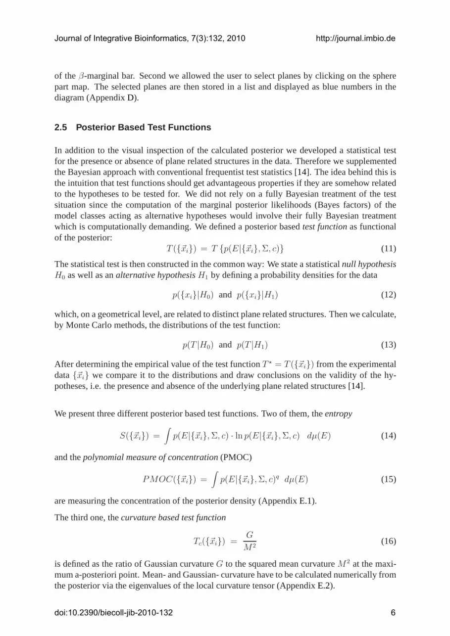
2.5 Posterior Based Test Functions

In addition to the visual inspection of the calculated posterior we developed a statistical testfor the presence or absence of plane related structures in the data. Therefore we supplementedthe Bayesian approach with conventional frequentist test statistics [14]. The idea behind this isthe intuition that test functions should get advantageous properties if they are somehow relatedto the hypotheses to be tested for. We did not rely on a fully Bayesian treatment of the testsituation since the computation of the marginal posterior likelihoods (Bayes factors) of themodel classes acting as alternative hypotheses would involve their fully Bayesian treatmentwhich is computationally demanding. We defined a posterior basedtest functionas functionalof the posterior:

T ({~xi}) = T {p(E|{~xi}, Σ, c)} (11)

The statistical test is then constructed in the common way: We state a statisticalnull hypothesisH0 as well as analternative hypothesisH1 by defining a probability densities for the data

p({xi}|H0) and p({xi}|H1) (12)

which, on a geometrical level, are related to distinct plane related structures. Then we calculate,by Monte Carlo methods, the distributions of the test function:

p(T |H0) and p(T |H1) (13)

After determining the empirical value of the test functionT ⋆ = T ({~xi}) from the experimentaldata{~xi} we compare it to the distributions and draw conclusions on the validity of the hy-potheses, i.e. the presence and absence of the underlying plane related structures [14].

Wepresent three different posterior based test functions. Two of them, theentropy

S({~xi}) =∫

p(E|{~xi}, Σ, c) · ln p(E|{~xi}, Σ, c) dµ(E) (14)

and thepolynomial measure of concentration(PMOC)

PMOC({~xi}) =∫

p(E|{~xi}, Σ, c)q dµ(E) (15)

are measuring the concentration of the posterior density (AppendixE.1).

Thethird one, thecurvature based test function

Tc({~xi}) =G

M2(16)

is defined as the ratio of Gaussian curvatureG to the squared mean curvatureM2 at the maxi-mum a-posteriori point. Mean- and Gaussian- curvature have to be calculated numerically fromthe posterior via the eigenvalues of the local curvature tensor (AppendixE.2).

Journal of Integrative Bioinformatics, 7(3):132, 2010 http://journal.imbio.de

doi:10.2390/biecoll-jib-2010-132 6

3 Plant Metabolite Data

Weapply the method described above to triplets of metabolic data, generated in an experimentpublished earlier in literature [15]. We first describe the experiment and the data, then weapply the methods described in section2.5 to extract the presence of plane-like structures andvisualize them exemplarily.

3.1 Description of Experiment and Data

In the experiment parent plants from the twoArabidopsis thalianainbred linesCol10 andC24 were mated, resulting in four possible combinations of parent genotypes. For each ofthis crossings three F1 hybrids were grown (so calledbiological replicates), after harvestingand preparation for approximately eight samples (technical replicates) the intensities of 736metabolites, identified by the mass to charge ratio (m/z), were measured. Since no identificationof the chemical species was done in the mass-spectrometric data, we identify the metabolitesby arbitrary indices.

Before we start the Bayesian analysis itself, we explore the data by investigating different mea-sures for technical and biological variability:

A quantitative description of the precision of the data is thetechnical variabilitydefined as thestandard deviation of technical replicates made from one biological replicate.

We define theestimated biological valueas the mean value of the technical replicates madefrom one biological replicate, it serves as an estimator for the true value of the metaboliteconcentration in the plant.

For a given set of plants, not necessarily being biological replicates of a single crossing, wedefine thebiological variabilityas the standard deviation of their estimated biological values.

Based on these quantities we chose a sample combined out of the biological replicates of theC24 × Col10 and theC24 × C24 crossings for further investigation, because it showed themost promising ratio of (large) biological to (small) technical variability. With respect to therelatively high technical noise it was necessary to include only the most informative variablesin our analysis.

We sorted the metabolites according to the ratio of biological to technical variability and se-lected the first six metabolites, #278, #322, #523, #380, #290 and #715, from that list. Thosewe combined in all possible, non redundant ways to triplets, which were then the 3-dimensionalinput to Bayesian method described above.

3.2 Testing Plane Related Hypotheses

We used theempirical covariance matrixof the technical replicates asΣ in the Gaussian errormodel (4) for each data point resulting from the underlying biologicalreplicate. In the setunder investigation the 6 independent entries of the symmetric positive definite3×3 covariancematricesΣ had to bes estimated from 8 technical replicates. We controlled the accuracy of thisestimate by using Bayesian estimation, see AppendixF.

Journal of Integrative Bioinformatics, 7(3):132, 2010 http://journal.imbio.de

doi:10.2390/biecoll-jib-2010-132 7

2000 4000 6000 8000

020

0040

0060

00

# 322#

380

−200 0 200 400 600 800

020

040

060

080

0

# 278

# 52

3

Figure 1: Pair plots of metabolite intensities, the axes are labeled with the respective metaboliteindices. Triangles mark data points from theCol10×Col10 crossing, circles from theC24×Col10crossing. The different colors indicate the individual biological replicates, in addition the more“earthly” colors are redundantly attributed to the C24×Col10 crossing. A strong correlation (upto 0.98) can be seen in the technical replicates.

The necessity for using a correlated error model is evident if one looks at thepair plotsof themetabolite intensities as well as the numerical values of the covariances, as exemplified in Fig-ure1 for metabolite pairs#380×#322 and#523×#278. This a very strong correlation in thetechnical replicates (up to0.98). The diagrams also indicate that the technical and biologicalvariabilities arerelated, which can be interpreted in the sense that the same biochemical mecha-nisms acting in the intact plants are responsible for the variability occurring during preparationand measurement.

We defined three test hypotheses, qualitatively related to the geometrical structures point, lineand plane. For each metabolite triplet under investigation the parameters of the probability dis-tribution forming the statistical hypotheses was then set depending on numerical values char-acterizing the data.

The center of the datawas defined as the median of the biological estimated values of thebiological replicates under investigation. Themean technical covariancewas defined as theaverage of the covariance matrices of the technical replicates over the biological replicates.

The hypotheses were defined algorithmically by:

Point Gaussian distribution with mean technical covariance around the center of the data.

Line Draw a line from the origin through the center of the data. Distribute the points onthat line with a Gaussian distribution of zero mean and variance equal to the sum of thesquared biological variability of the metabolites involved. Add centered Gaussian noisewith technical covariance.

Plane Scatter the points on a plane trough the center of the data, employing a radial symmet-rical Gaussian distribution with a variance equal to the mean of the squared biologicalvariability of the metabolites involved. Add centered Gaussian noise with technical co-variance.

From these distributions we drew 30 sample points and calculated entropy (32), polynomialmeasure of concentration (33) and curvature based test statistics (38). In that way we obtainedsmall size samples of these quantities given the test hypotheses that we compared with the datameasured in the experiment.

Journal of Integrative Bioinformatics, 7(3):132, 2010 http://journal.imbio.de

doi:10.2390/biecoll-jib-2010-132 8

5 10 15 20−

9−

8−

7−

6−

5−

4

Entropy

Triplet #

Figure 2: Entropy of the observed data (black spot) and 10 draws from the hypotheses plane(green spots), line (red circles) and point (blue triangles). The different metabolite triplets underinvestigation are indexed on the abscissa.

5 10 15 20

2040

6080

100

120

140

P.M.O.C

Triplet #

Figure 3: Polynomial measure of concentration of the observed data (black spot) and 10 drawsfrom the hypotheses plane (green spots), line (red circles) and point (blue triangles). The differentmetabolite triplets under investigation are indexed on the abscissa.

5 10 15 20

0.0

0.2

0.4

0.6

0.8

1.0

G / M^2

Triplet #

Figure 4: Curvature based Test Statistics of the observed data (black spot) and 10 draws fromthe hypotheses plane (green spots), line (red circles) and point (blue triangles). The differentmetabolite triplets under investigation are indexed on the abscissa.

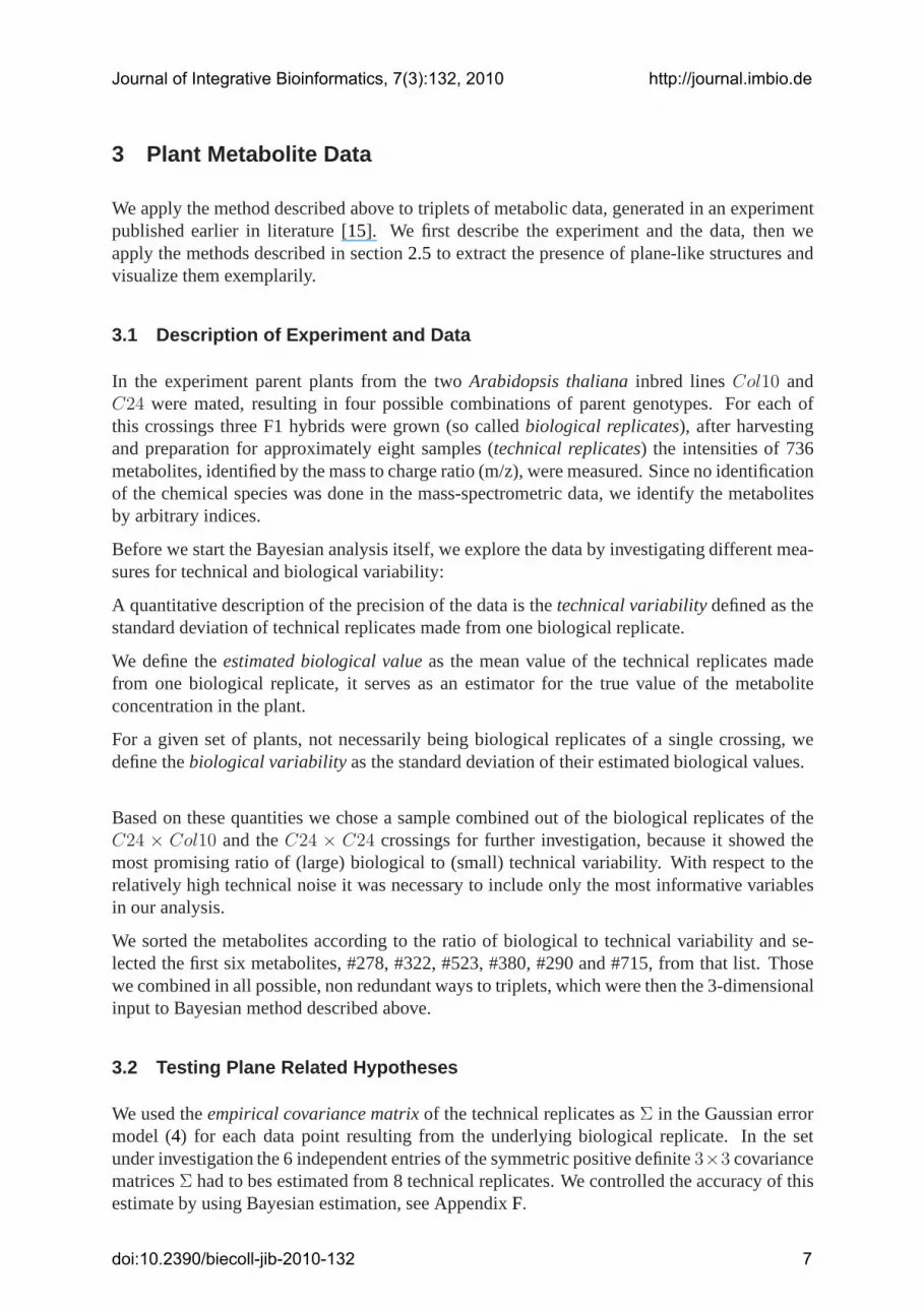
Figure 2 to 4 show this results. On the abscissa the metabolite triplet underconsiderationis indexed, on the ordinate the value of the test statistics is displayed.Green, blue and redpoints mark the values generated by the test hypotheses plane, point and line, while the valueoriginating from the experimental data are indicated inblack. In addition we computed p-valuesusing student’s t-statistics, which were in good accordance with the diagrams of the samples oftest functions Figure5.

For the entropy Figure2 and the polynomial measure of concentration Figure3, we notice thatthey are in principle able to separate the three different hypotheses, in contrast to the curva-

Journal of Integrative Bioinformatics, 7(3):132, 2010 http://journal.imbio.de

doi:10.2390/biecoll-jib-2010-132 9

5 10 15 20

−50

−30

−10

0Entropy

Triplet #

log(

pV)

5 10 15 20

−30

−20

−10

0

P.M.O.C.

Triplet # lo

g(pV

)

5 10 15 20

−10

−6

−4

−2

0

G / M^2.

Triplet #

log(

pV)

Figure 5: Logarithmic p-values as estimated from the distributions of the test functions Entropy,Polynomial Measure of Concentration andC/M2. The 5% confidence interval is marked by ablack, horizontal line. Hypotheses tested for are plane (green spots), line (red circles) and point(blue triangles).

a.) b.)

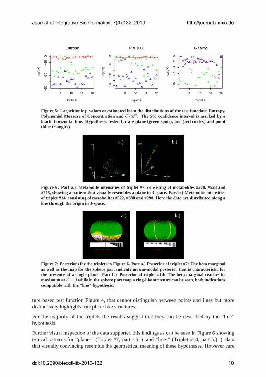
Figure 6: Part a.) Metabolite intensities of triplet #7, consisting of metabolites #278, #523 and#715, showing a pattern that visually resembles a plane in 3-space. Part b.) Metabolite intensitiesof triplet #14, consisting of metabolites #322, #380 and #290. Here the data are distributed along aline through the origin in 3-space.

a.) b.)

Figure 7: Posteriors for the triplets in Figure 6. Part a.) Posterior of triplet #7: The beta marginalas well as the map for the sphere part indicate an uni-modal posterior that is characteristic forthe presence of a single plane. Part b.) Posterior of triplet #14: The beta marginal reaches itsmaximum at β = 0 while in the sphere part map a ring-like structure can be seen, both indicationscompatible with the ”line”-hypothesis.

ture based test function Figure4, that cannot distinguish between points and lines but moredistinctively highlights true plane like structures.

For the majority of the triplets the results suggest that they can be described by the “line”hypothesis.

Further visual inspection of the data supported this findings as can be seen in Figure6 showingtypical patterns for “plane-” (Triplet #7, part a.) ) and “line-” (Triplet #14, part b.) ) datathat visually convincing resemble the geometrical meaning of these hypotheses. However care

Journal of Integrative Bioinformatics, 7(3):132, 2010 http://journal.imbio.de

doi:10.2390/biecoll-jib-2010-132 10

must be taken in comparing the visual appearance of the data to the statistical hypotheses whichare based on the error model and not on the distance in 3-space directly. Therefore we usedour methodology that incorporates this information to visualize the posterior . Figure7 showsscreen shots of the interactive visualization of the posterior at the respective maximal points oftheβ-marginal. In part a.) the posterior for triplet #7 indicates an uni-modal posterior that ischaracteristic for the presence of a single plane. In part b.) the beta marginal for triplet #14reaches its maximum atβ = 0 while in the sphere part a ring like structure can be seen, bothindications compatible with the ”line”-hypothesis; also compare Figures.2, 3 and4.

4 Conclusions

We were able to enrich the toolbox of the biological data analyst with the novel method Ex-Planes for the exploration of ternary relationships in profile data that combines following fea-tures: Invariance against rotations and consequently relabeling of the axes, which makes itespecially suitable in cases where no a-priori ordering of the variables can be assumed. Inthis it differs from usual regression methods. Possibility to accommodate robustness againstoutliers and incorporation of an individual error estimate for each data point. The possibilityof investigating multiple linear relationships. Different test functions enable the detection of avariety of plane related ternary structures, to be defined by appropriate statistical hypotheses.We demonstrated all these aspects on a metabolite data set.

Since ExPlanes combines certain functionalities, there are similarities as well as differences toestablished methods: With PCA it has in common, that it can be used for the detection of lowerdimensional subspaces in the data. However PCA is vulnerable against outliers and does notallow for the investigation of multiple linear relationships. It does not incorporate knowledgeabout measurement errors, which are especially of interest in investigations of metabolic data.Projection Pursuit (PP) is a larger class of algorithms that all have in common that they searchfor a linear projection of the data (which by definition has reduced dimensionality) which max-imizes certain objective functions [7]. PP-methods have in common with ExPlanes, that theycan be used for the detection and exploration of linear relationships, and can be made robustagainst outliers. For the special case of 2-planes in 3-space, which is of interest here, they donot incorporate the invariant prior and the interactive method of visualization.

References

[1] I.N. Bronstein, K.A. Semendjajew, and ea.Taschenbuch der Mathematik. Verlag HarriDeutsch, Thun und Frankfurt am Main, 2001.

[2] A. Butte and I. S. Kohane. Mutual information relevance networks: Functional genomicclustering using pair-wise entropy measurements.Pac. Symp. Biocomput., 5:415–426,2000.

[3] O. Fiehn, J. Kopka, P. Dormann, T. Altmann, R. Trethewey, and L. Willmitzer. Metaboliteprofiling for plant functional genomics.Nat. Biotechnol., 18:1157–1161, 2000.

Journal of Integrative Bioinformatics, 7(3):132, 2010 http://journal.imbio.de

doi:10.2390/biecoll-jib-2010-132 11

[4] W. Freeden, T. Gervens, and M. Schreiner.Constructive Approximation on the Sphere:With Applications to Geomathematics. Claredon Press, Oxford, 1998.

[5] B. Grunenfelder and E.A. Winzeler. Treasures and traps in genome-wide datasets: Caseexamples from yeast.Nat. Rev. Genetics, 3:653–661, 2002.

[6] R. Heinrich and S. Schuster.The Regulation of Cellular Systems. Chapman and Hall,New York, 1996.

[7] P.H. Huber. Projection pursuit.The Annals of Statistics, 13(4):435–475, 1985.

[8] N. Jamshidi and B. Palsson. Formulating genome-scale kinetic models in the post-genomeera.Molecular Systems Biology, 4:171, 2008.

[9] E.T. Jaynes. The well-posed problem.Foundations of Physics, 3(4):477–491, 1973.

[10] E.T. Jaynes and G.L. Bretthorst.Probability Theory. The Logic of Science: Theory andElementary Applications Vol. 1. Cambridge University Press, Cambridge, 2003.

[11] F. Kose, J. Budczies, M. Holschneider, and O. Fiehn. Robust detection and verificationof linear relationships to generate metabolic networks using estimates of technical errors.BMC Bioinformatics, 8:162, 2007.

[12] A. Margolin, K. Basso I. Neemenmann, C. Wiggins, G. Stolovitzky, R. Della Favera, andA. Califano. Arcane: An algorithm for the reconstruction of gene regulatory networks ina mammalina cellular context.BMC Bioinformatics, 7, Suppl.1:S7, 2006.

[13] A. Pandey and M. Mann. Proteomics to study genes and genomes.Nature, 405:837–846,2000.

[14] H. Rinne.Taschenbuch der Statistik 2.uberarbeitete und erweiterte Auflage. Verlag HarriDeutsch, Thun und Frankfurt am Main, 1997.

[15] M. Scholz, S. Gatzek, A. Sterling, O. Fiehn, and J. Selbig. Metabolite fingerprint-ing: detecting biological features by independent component analysis.Bioinformatics,20(15):2447–2454, 2004.

[16] J. Stelling, S. Klamt, K. Bettenbrock, S. Schuster, and E.D. Gilles. Metabolic networkstructure determines key aspects of functionality and regulation.Nature, 420:190–193,2002.

[17] R. Steuer, J. Kurths, C.O. Daub, and J. Selbig. The mutual information: Detecting andevaluating dependencies between variables.Bioinformatics, 18, Suppl 2:231–240, 2002.

[18] Wikipedia. Kavrayskiy vii projection.http//en.wikipedia.org/wiki/Kavrayskiy V II.

[19] Y. Yang, A.P. Tashman, J.Y. Lee, S. Yoon, W. Mao, K. Ahn, W. Kim, N.R. Mendell,D. Gordon, and S.J. Finch. Mixture modelling of microarray gene expression data.BMCProc, 1 Suppl. 1:S 50, 2007.

[20] W. Zhao, E. Serpedin, and E.R. Gougherty. Inferring connectivity of genetic regulatorynetworks using information-theoretic criteria.IEEE/ACM Transactions on ComputationalBiology and Bioinformatics, 5:262–274, 2008.

Journal of Integrative Bioinformatics, 7(3):132, 2010 http://journal.imbio.de

doi:10.2390/biecoll-jib-2010-132 12

nx

����

β

O

E

Figure 8: Definition of a planeE as the set of vectors~x that have the same projected distanceβ indirection of a given unit vector~n.

A The Set of Planes

Consider the3-dimensional Euclidean spaceR3. A 2-plane is a two dimensional affine sub-space. The set of all2-planes is a3 dimensional manifold. Unfortunately, there is no globalparameterization of this space. However, there is a parameterization that is good for all practi-cal purposes. Consider now a unit-vector~n and a real numberβ ≥ 0. The set of points~x thathave in the direction~n the distanceβ is a2 dimensional plane. In formulas we may write (seeFigure8):

E ={

~x ∈ R3|(~x · ~n − β) = 0}

(17)

Vice versa all planes that do not contain the origin can be written uniquely in that way. Theplanes that go through the origin can still be written in that way, however, the representation isnot unique anymore, since~n and−~n give rise to the same plane. Nevertheless we identify

E ↔ (β, ~n).

The unit vector itself may be written in polar coordinates using two anglesθ ∈ [0; π] andφ ∈ [0, 2π). We then may write [1]

~n =

sin[θ] · cos[φ]sin[θ] · sin[φ]

cos[θ]

(18)

where the usual care has to be taken forθ = 0 andθ = π since there the parameterizationdegenerates. In that way we obtain a parameterization

E ↔ (β, θ, φ) ∈ [0,∞) × [0, π] × [0, 2π),

where care has to taken at the pointsθ ∈ {0, π} andβ = 0.

B Invariant Measure

Since it is our aim to perform Bayesian analysis on the set of possible planes, which itself isa 3-dimensional manifold, that can not be continuously to theR

3 itself, we have to determine

Journal of Integrative Bioinformatics, 7(3):132, 2010 http://journal.imbio.de

doi:10.2390/biecoll-jib-2010-132 13

a probability measure on it. We need this measure for integrating over the prior and posterior(if we, for example want to calculate measures of concentration like entropy). Since in theabsence of data it contains all the information at hand the prior density relative to this measureis uniform. The complete absence of information from data should be invariant under thenatural coordinate changes: No information is gained by translating the whole space or rotatingit. Therefore the measure that we are looking for should be invariant under the group generatedby rotations and translations (i.e. the Euclidean group). We denote by

~x′ = R~x with R−1 = R

T (19)

the rotations and by~x′ = ~x + ~a (20)

the translations of points in three dimensional spaceR3.

In our case we can show that there is an up to a multiplicative constant unique measure thatsatisfies these invariance properties. The proof is following the method given in [9, 10]. Inthe parameterization given by (18) this invariant measure in the space of planesdµ(E) can beexpressed as:

dµ(E) = const· sin[θ] dθ dφ dβ. (21)

Note that the points, where the parameterization becomes singular only have measure0. Soour parameterization is fine for any distribution of planes which does not have a point mass attheses singular values.

C Discretization

To represent numerically and visualize the posterior we have to find a discretization of the setof planes under consideration.

For any data set we can, before the computation of the posterior, see that the possible distanceto the origin is limited to some intervalβ ∈ [βmin; βmax]. In this interval we discretizeβ by aset of equidistant values{βmin, ..., βb, ..., βmax}.

The discretization of the sphere part of the posterior, for every of the discretized values ofβb,is taken over from [4].

The polar angleθ is represented by a set ofγ equidistant points{θ0, ..., θi, ...θγ} with θ0 = 0(north pole) andθγ = π (south pole).

The azimuthal angleφ is also discretized by an equidistant lattice{φi,0, ..., φi,j, ..., φi,γi}. Here

the number of points of discretizationγi depends onθi in a way ensuring that the points of

Journal of Integrative Bioinformatics, 7(3):132, 2010 http://journal.imbio.de

doi:10.2390/biecoll-jib-2010-132 14

discretization(θi, φi,j) are uniformly spread over the surface of the sphere [4]:

Θ0 = 0 φ0,1 = 0 north pole (22)

∆Θ =π

γwith γ ∈ N (23)

Θi = i · ∆Θ with i ∈ {1, 2, ..., γ − 1} (24)

γi =

2π

arccos[

(cos[∆Θ] − cos2[Θi])/ sin2[Θi]]

(25)

φi,j =(

j −1

2

)

(

2π

γi

)

with j ∈ {1, 2, ..., γi} (26)

Θγ = π φγ,1 = 0 south pole (27)

The angular resolution depends on the integer parameterγ which gives the number of latticepoints inΘ direction, so before the calculation of the posterior, after specifying the data and theparameters of the error model, we have to find an numerically adequate value for it. To obtaina practical estimate we look again at the posterior of a single data point (6):

p(~n, β|~x, Σ) ∼ exp

[

−1

2

(~x · ~n − β)2

~nT Σ~n

]

We consider the generic case of a data point~x = x · ~nz situated at distance|~x| in “north”direction~nz = ~n(θ = 0, φ = 0). The error model is assumed to be isotropic withΣ = σ2 · I.

Since here the scalar product~n · ~x = |~x| · cos θ does not depend onφ the posterior is a functionof θ and β alone. We use a saddle point approximation around the maximum valueθ⋆ =arccos[β/|~x|], β⋆ = |~x| and find that it is approximately proportional to:

p(θ, φ, β⋆) ∼ exp

[

−1

2

(β⋆)2 sin2 θ⋆ (θ − θ⋆)2

σ2

]

(28)

The standard deviation in angular directionσθ is:

σθ =σ

|~x|·

1√

1 − β/|~x|(29)

It has its minimum atσθ = σ/|~x|, so the angular standard deviation depends on therelativeerror σrel ≡ σ/|~x| of the data.

From identical arguments we see that the standard deviation inβ directionσβ = σ, and hencedepends on theabsolute errorσabs ≡ σ.

We use this insight and to the number of pointsγ in θ direction to

γ = ceiling{

resθ · π

σrel

}

+ 1 (30)

and the spacing of the points inβ direction to:

∆β =σabs

resβ

(31)

Journal of Integrative Bioinformatics, 7(3):132, 2010 http://journal.imbio.de

doi:10.2390/biecoll-jib-2010-132 15

nx

����

β

O

Plane

Figure 9: The set of planes thatexplain a single data point~x, that means which have zero distanceto it. The vector β · ~n, called thedescriptorof a planeE, forms a rectangular triangle with ~x ashypotenuse. This means the descriptors of all planes explaining a data point form a sphere through~x and the origin of the coordinate system (Thales’ theorem), of which here a cut in two dimensionsis shown.

Hereinresθ andresβ are the precision of the discretization. In the actual choice of their valuesa tradeoff between runtime of the calculation and precision has to be kept in mind. Numericalinvestigations showed that all ready a value ofresθ = resβ = 3.6 gave very accurate results.

In dealing with different, anisotropic estimates for the standard deviation of the error we calcu-lated the relative and absolute error in the data for each single point, using the eigenvalues ofthe covariance matrixΣi, and took the maximum of the resolution.

D Visualization Example

D.1 Plane Posterior for a Single Point

To get an intuition how the plane posterior for a single point (7) looks like, we draw a figurethat shows which planes are able to “explain” a given data point perfectly. This means we askfor the subset of planes that have zero distance to the data point. The distance of a point~x to aplaneE(~n, β) computes to|~x ·~n−β|. If we set it to zero we can see that the vectorβ ·~n, calledthe descriptorof the plane, has to form an rectangular triangle with~x as hypotenuse. FromThales’ theorem we see that the set of descriptors belonging to planes that explain a given datapoint is aspherethrough the data point and the origin of the coordinate system. Figure9 showsthis in two dimensions, rotating the drawing around~x gives the sphere.

From this considerations we see that the probability density of a single data point attains aconstant, maximal value on the Thales’ sphere and decreases in accordance to the covarianceparametersΣ of the error model.

D.2 Plane Posterior of a Mixture

In Figure10 as an example we visualize the posterior of the Thales sphere resulting from asingle data point, as discussed in section2.2. In Figure10.a the sphere part of zero radius

Journal of Integrative Bioinformatics, 7(3):132, 2010 http://journal.imbio.de

doi:10.2390/biecoll-jib-2010-132 16

����

n

β

O

Plane

x

a.) b.)

a.) b.)

c.)

c.)

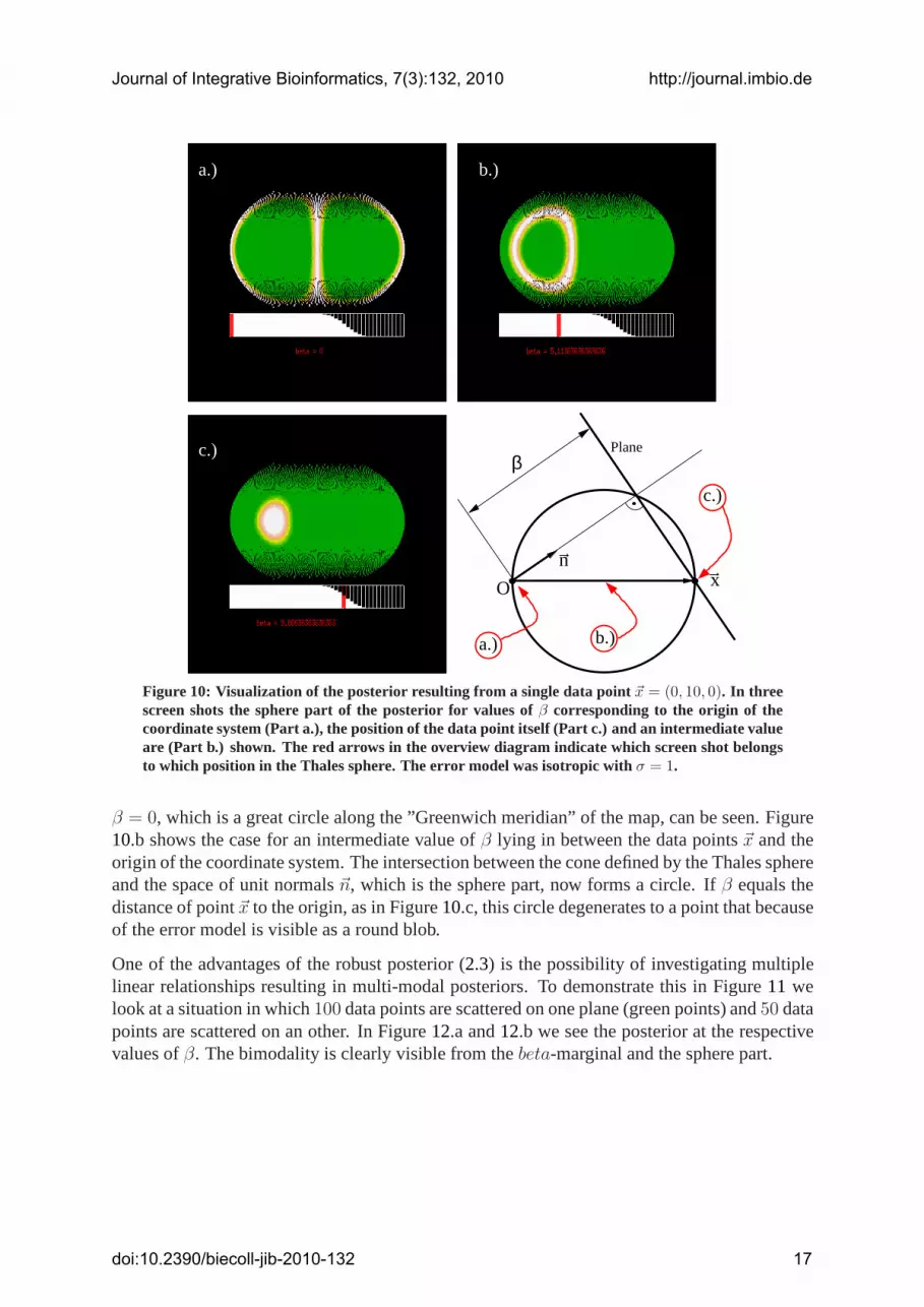
Figure 10: Visualization of the posterior resulting from a single data point~x = (0, 10, 0). In threescreen shots the sphere part of the posterior for values ofβ corresponding to the origin of thecoordinate system (Part a.), the position of the data point itself (Part c.) and an intermediate valueare (Part b.) shown. The red arrows in the overview diagram indicate which screen shot belongsto which position in the Thales sphere. The error model was isotropic withσ = 1.

β = 0, which is a great circle along the ”Greenwich meridian” of the map, can be seen. Figure10.b shows the case for an intermediate value ofβ lying in between the data points~x and theorigin of the coordinate system. The intersection between the cone defined by the Thales sphereand the space of unit normals~n, which is the sphere part, now forms a circle. Ifβ equals thedistance of point~x to the origin, as in Figure10.c, this circle degenerates to a point that becauseof the error model is visible as a round blob.

One of the advantages of the robust posterior (2.3) is the possibility of investigating multiplelinear relationships resulting in multi-modal posteriors. To demonstrate this in Figure11 welook at a situation in which100 data points are scattered on one plane (green points) and50 datapoints are scattered on an other. In Figure12.a and12.b we see the posterior at the respectivevalues ofβ. The bimodality is clearly visible from thebeta-marginal and the sphere part.

Journal of Integrative Bioinformatics, 7(3):132, 2010 http://journal.imbio.de

doi:10.2390/biecoll-jib-2010-132 17

Figure 11: Synthetic data for a mixture of two planes withφ = π4

, θ = π2

, β = 2 (green, 100data points) and φ = π , θ = π

2, β = 5 (red, 50 data points). The data points are normally

scattered on the planes with a standard deviation ofσ = 5, in addition isotropic Gaussian noisewith standard deviation of σ = 1 is added.

a.)

b.)

Figure 12: Posterior for the synthetic data in Figure11. An isotropic error model with standarddeviation of σ = 1 is assumed, the out lier factor isc = 1. Part a.) shows the sphere part forβ = 1.86 and Part b.) for β = 4.95, which are approximately the values of the correspondingplanes, indicated by blue integer numbers in the map. The bi-modality is clearly visible from thesphere part and theβ-marginal.

Journal of Integrative Bioinformatics, 7(3):132, 2010 http://journal.imbio.de

doi:10.2390/biecoll-jib-2010-132 18

−5 −4 −3 −2

010

020

030

040

0

Isotropic

Plane

Entropy

N= 17

Figure 13: Distribution of the entropy (32) under the null hypothesisH0 “data stray around plane”and alternative hypothesisH1 “data are isotropically scattered in space”, see definition (E.1), forN = 17 data points. Histogram sampled over 1200 repetitions.

E Posterior Based Test Functions

E.1 Concentration Based Test Functions

We present two different concentration based test functions. The first one is based on measuresof concentration of the posterior like theentropy

S({~xi}) =∫

p(E|{~xi}, Σ, c) · ln p(E|{~xi}, Σ, c) dµ(E) (32)

or thepolynomial measure of concentration:

PMOC({~xi}) =∫

p(E|{~xi}, Σ, c)q dµ(E) (33)

Hereinq is the exponent of the polynomial, that in our study was constantly set toq = 0.5.

We investigated the capability of these functions to distinguish between certain plane related

structures by defining the two hypotheses:

H0: [Null Hypothesis] Data points arefirst casted isotropicallyon a square plane of size20 × 20and afterwards are subjected do a3-dimensional Gaussian error withstandard deviationσ = 1

H1: [Alternative Hypothesis] Datapoints are scatteredisotropically in a cube of size20 × 20 × 20

Then we repeatedly drew samples ofN data points and, assuming an isotropic error with stan-dard deviationσ = 1, we calculated the test functions, in this way obtaining a sample from thetest distribution (13). As can be seen from Figure13 and Figure14 the entropy as well as thepolynomial measure of concentration were indeed able to separate the two hypotheses underthe given conditions.

Journal of Integrative Bioinformatics, 7(3):132, 2010 http://journal.imbio.de

doi:10.2390/biecoll-jib-2010-132 19

8 10 12 14

050

100

150

200

250

300

IsotropicPlane

P.M.O.CN= 17q= 0.5

Figure 14: Distribution of the polynomial measure of concentration (33) under the null hypothesisH0 “data stray around plane” and alternative hypothesisH1 “data are isotropically scattered inspace”, see definition (E.1), for N = 17 data points and exponentq = 0.5. Histogram sampledover 1200 repetitions.

E.2 Curvature Based Test Function

The second approach for constructing test functions is based on measures of the local curva-ture of the sphere part of the posterior, calculated in the immediate neighborhood of its globalmaximum.

To define the invariant local measures of curvature, themean curvatureM and theGaussiancurvatureG, we use the sphere part of the posterior that remains if one fixesβ to the valueβ⋆

where the posterior attains its global maximum:

p(~n, β⋆|{~xi}, Σ, c) with (~n⋆, β⋆) = arg max~n,β

[p(~n, β|{~xi}, Σ, c)] (34)

After parameterization (18) this is a function of the two anglesθ and φ. We concentrate ourinterest into the immediate neighborhood around the global maximum of the posterior, thatoccurs atθ⋆ andφ⋆. From the values of (34) in this neighborhood we can now compute thelocal values of the main radii of curvatureR1 andR2 at the point(θ⋆, φ⋆, β⋆) [1].

From the main radii of curvature we obtain theinvariantsof the curvature tensor, the meancurvature

M =1

2

(

1

R1

+1

R2

)

(35)

and the Gaussian curvature:

G =1

R1 · R2

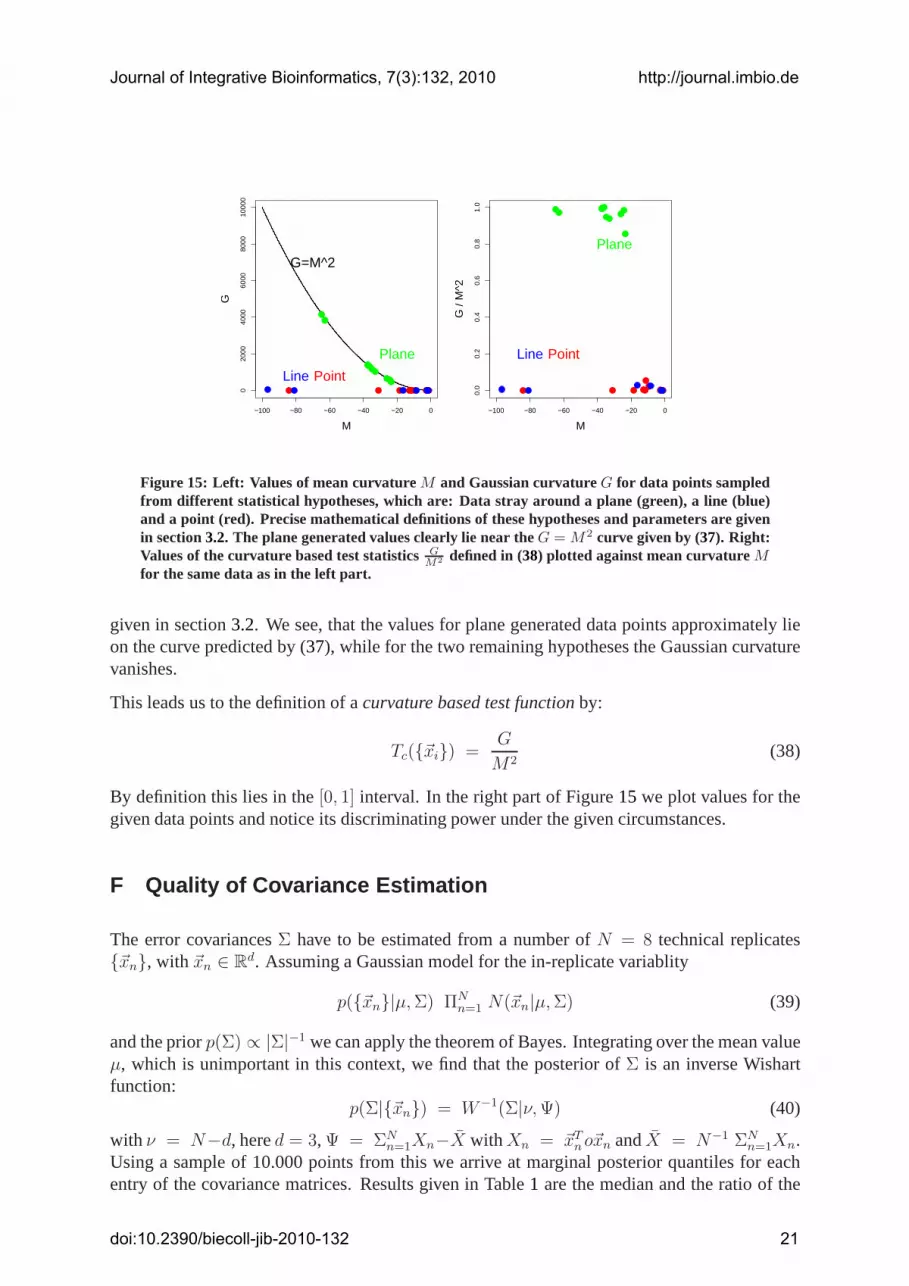
(36)

The definition of the test function itself is based on the observation that, in case the data arein fact straying around a plane, the sphere part (34) forms a circular ”blob” around the globalmaximum. This circular symmetry implies that the main radii of curvature are equalR1 = R2,which leads to following simple relationship between mean and Gaussian curvature:

G = M2 (37)

In the left part of Figure15 we illustrate this by plotting the Gaussian against the mean cur-vature for data points sampled from different, synthetically generated hypotheses, namely datastray around a plane, a line or a point. The exact mathematical definition of the hypotheses is

Journal of Integrative Bioinformatics, 7(3):132, 2010 http://journal.imbio.de

doi:10.2390/biecoll-jib-2010-132 20

−100 −80 −60 −40 −20 0

020

0040

0060

0080

0010

000

M

G

G=M^2

Plane

PointLine

−100 −80 −60 −40 −20 0

0.0

0.2

0.4

0.6

0.8

1.0

M

G /

M^2

Plane

PointLine

Figure 15: Left: Values of mean curvatureM and Gaussian curvatureG for data points sampledfrom different statistical hypotheses, which are: Data stray around a plane (green), a line (blue)and a point (red). Precise mathematical definitions of these hypotheses and parameters are givenin section3.2. The plane generated values clearly lie near theG = M2 curve given by (37). Right:Values of the curvature based test statisticsG

M2 defined in (38) plotted against mean curvatureMfor the same data as in the left part.

given in section3.2. We see, that the values for plane generated data points approximately lieon the curve predicted by (37), while for the two remaining hypotheses the Gaussian curvaturevanishes.

This leads us to the definition of acurvature based test functionby:

Tc({~xi}) =G

M2(38)

By definition this lies in the[0, 1] interval. In the right part of Figure15 we plot values for thegiven data points and notice its discriminating power under the given circumstances.

F Quality of Covariance Estimation

The error covariancesΣ have to be estimated from a number ofN = 8 technical replicates{~xn}, with ~xn ∈ R

d. Assuming a Gaussian model for the in-replicate variablity

p({~xn}|µ, Σ) ΠNn=1 N(~xn|µ, Σ) (39)

and the priorp(Σ) ∝ |Σ|−1 we can apply the theorem of Bayes. Integrating over the mean valueµ, which is unimportant in this context, we find that the posterior ofΣ is an inverse Wishartfunction:

p(Σ|{~xn}) = W−1(Σ|ν, Ψ) (40)

with ν = N−d, hered = 3, Ψ = ΣNn=1Xn−X with Xn = ~xT

no~xn andX = N−1 ΣNn=1Xn.

Using a sample of 10.000 points from this we arrive at marginal posterior quantiles for eachentry of the covariance matrices. Results given in Table1 are the median and the ratio of the

Journal of Integrative Bioinformatics, 7(3):132, 2010 http://journal.imbio.de

doi:10.2390/biecoll-jib-2010-132 21

75% quantile to the 25% quantile of the marginal posteriors forΣ for each triplet. They indicatethat the quality of the estimation, in which the choice of the standard estimator forΣ is founded,is sufficient for practical purposes.

Journal of Integrative Bioinformatics, 7(3):132, 2010 http://journal.imbio.de

doi:10.2390/biecoll-jib-2010-132 22

# Triplet. Σ1,1 Σ2,2 Σ3,3

75% / 25% median 75% / 25% median 75% / 25% median1 1.36 22600 1.36 5630000 1.36 792002 1.36 22500 1.36 5650000 1.36 17000003 1.36 22400 1.36 5660000 1.36 706004 1.36 22500 1.36 5610000 1.35 1850005 1.37 22300 1.36 79100 1.36 16900006 1.36 22500 1.36 79600 1.36 705007 1.37 22500 1.37 79400 1.36 1850008 1.35 22500 1.36 1690000 1.36 705009 1.35 22500 1.36 1690000 1.36 18500010 1.36 22300 1.36 70200 1.36 18500011 1.36 5640000 1.37 79300 1.35 169000012 1.36 5650000 1.36 79100 1.36 7020013 1.36 5660000 1.37 79600 1.36 18400014 1.36 5640000 1.36 1690000 1.36 7040015 1.36 5660000 1.36 1700000 1.37 18500016 1.36 5640000 1.36 70500 1.36 18500017 1.36 79400 1.36 1690000 1.37 7020018 1.35 79700 1.36 1690000 1.36 18500019 1.36 79400 1.35 70200 1.36 18400020 1.36 1700000 1.36 70600 1.37 186000

# Triplet. Σ1,2 Σ2,3 Σ3,1

75% / 25% median 75% / 25% median 75% / 25% median1 1.59 194000 0.683 -467000 0.62 -217002 1.58 194000 1.36 3080000 1.59 1040003 1.58 193000 2.17 187000 1.4 327004 1.56 194000 1.38 946000 1.52 384005 0.618 -21600 0.677 -251000 1.58 1030006 0.615 -21700 0.155 -10700 1.41 326007 0.616 -21600 0.668 -78700 1.53 384008 1.59 104000 2.27 97500 1.4 326009 1.57 104000 1.38 523000 1.52 3840010 1.41 32500 1.9 41000 1.55 3820011 0.687 -469000 0.682 -252000 1.35 307000012 0.686 -469000 0.16 -10800 2.15 18600013 0.686 -468000 0.676 -78500 1.38 94900014 1.36 3070000 2.22 97500 2.13 18700015 1.37 3080000 1.38 524000 1.38 95200016 2.17 186000 1.89 41400 1.38 94700017 0.677 -253000 2.29 96900 0.18 -1090018 0.687 -254000 1.37 524000 0.676 -7880019 0.156 -10900 1.87 41500 0.675 -7860020 2.28 97800 1.92 41600 1.38 526000

Table 1: Estimation of covariances from technical replicates. The median and the the ratio of the75% quantile to the 25% quantile of the marginal covariance posteriors forΣ1,1 ... Σ3,1 .

Journal of Integrative Bioinformatics, 7(3):132, 2010 http://journal.imbio.de

doi:10.2390/biecoll-jib-2010-132 23