modeling film flows down inclined planes
TRANSCRIPT
Eur. Phys. J. B 6, 277–292 (1998) THE EUROPEANPHYSICAL JOURNAL Bc©
EDP SciencesSpringer-Verlag 1998
Modeling film flows down inclined planes
C. Ruyer-Quila and P. Mannevilleb
Laboratoire d’Hydrodynamiquec, Ecole Polytechnique, 91128 Palaiseau, France
Received: 16 April 1998 / Revised: 29 June 1998 / Accepted: 2 July 1998
Abstract. A new model of film flow down an inclined plane is derived by a method combining results ofthe classical long wavelength expansion to a weighted-residuals technique. It can be expressed as a set ofthree coupled evolution equations for three slowly varying fields, the thickness h, the flow-rate q, and a newvariable τ that measures the departure of the wall shear from the shear predicted by a parabolic velocityprofile. Results of a preliminary study are in good agreement with theoretical asymptotic properties closeto the instability threshold, laboratory experiments beyond threshold and numerical simulations of the fullNavier–Stokes equations.
PACS. 47.20M Interfacial instability – 47.20K Nonlinearity
1 Introduction
In addition to being involved in a wide variety of techni-cal applications (chemical reactors, evaporators, etc.), thedynamics of fluid films is an interesting topic in itself. Asa matter of fact, thin films flowing down inclined surfacesexhibit a rich phenomenology [1] and offer a good testingground for the study of the transition to turbulence. Insta-bilities take place at low flow rates, which gives a uniqueopportunity to analyze the development of waves at thesurface of the fluid into large-amplitude strongly nonlin-ear localized structures such as solitary pulses and fur-ther to study their disorganization into developed spatio-temporal chaos via secondary instabilities.
A trivial solution to the flow equations is easily foundin the form of a steady uniform parallel flow with parabolicvelocity profile, often called Nusselt’s solution, where thework done by gravity is exactly consumed by viscousdissipation. Thin films at low flow rate over sufficientlysteep surfaces turn out to be unstable against long wave-length infinitesimal perturbations, i.e. wavelength largewhen compared to the thickness of the flow. This is con-firmed by a general study of the relevant Orr–Sommerfeldequation which shows that short-wavelength shear insta-bilities of the Tollmien–Schlichting type are only relevantfor flows over planes at vanishingly small inclination an-gles and very high flow rates [2].
In the following we will thus be concerned with longwavelength interfacial instability modes, the dynamicsof which is essentially controlled by viscosity and sur-face tension effects. Close to the threshold these waves
a e-mail: [email protected] e-mail: [email protected] CNRS UMR n◦ 7646.
present themselves as stream-wise surface undulationsfree of span-wise modulations (“two-dimensional” waves)emerging from a supercritical (i.e., continuous) bifurca-tion. Farther from threshold, they saturate at finite ampli-tudes and, depending on control parameters, may developsecondary instabilities involving span-wise modulations(“three-dimensional” instabilities) [3] or first evolve intolocalized “solitary” structures that subsequently desta-bilize [4]. For the moment we will focus on the two-dimensional case where the hydrodynamic fields dependonly on the cross-stream and stream-wise coordinates,y and x respectively (see Fig. 1), leaving the three-dimensional problem for future study.
It turns out that, for the regimes we are interestedin, the height of the waves remains small when comparedto their wavelength. This motivates a long standing prac-tice [5,6] of studying them by means of asymptotic ex-pansions in powers of a small parameter ε, usually calledthe film parameter. Starting from this long-wave expan-sion, a certain number of models have then been derivedsince the pioneering work of Kapitza [7], e.g. [8–10] forthe most recent ones, see the review by Demekhin et al.[11] for earlier attempts. The simplest useful result ob-tained in this way is a partial differential equation calledBenney’s equation [12] to be written explicitly later (36).Governing the local thickness of the film h(x, t) in termsof its space-time derivatives, it will be written here simplyas ∂th = G(hn, ∂xmh), where G involves various algebraicpowers and differentiation orders (n,m) of h. Within thisapproach the film evolution is modeled in terms of lubrica-tion theory, which results in the enslaving of flow variablesto the local film height, i.e. a reduction to some effectivedynamics for the interface through the elimination of de-grees of freedom associated to velocity field.
278 The European Physical Journal B
The simplification brought by this reduction hasmainly permitted a first study of the nonlinear develop-ment of waves using the tools of dynamical systems the-ory [13], study that was continued using the celebratedKuramoto–Sivashinsky (KS) equation [14], obtained in thepresent context by taking the limit of small amplitudemodulations [15,16]. By contrast with the KS equation,Benney’s equation can lead to a non-physical evolutionwith the development of finite-time singularities [13,17].Such an evolution strongly limits its use to a narrow neigh-borhood of the threshold where the KS equation —thatdoes not behave so wildly— is expected to give alreadyvaluable results.
Numerical investigation of the full Navier-Stokes (NS)equations, though conceivable, is cumbersome owing tothe presence of a free boundary. Though it can (should)serve as a check point for models in the two-dimensionalcase, the only one to be reliably implemented up tonow [18,19], the numerical approach does not give muchinsight into the mechanisms of chaotic wave motion andpattern formation. An intermediate level of modeling isobtained in terms of so-called boundary layers equations(BL) [20], i.e. reduced NS equations incorporating thecondition that stream-wise gradients are small when com-pared to cross-stream variations. Though one is left with aproblem that has the same dimensionality as the originalone, it is a little simpler and leads to lighter computationsgiving realistic results [21].
A subsequent level of modeling is achieved by assum-ing a specific shape for the velocity profile and averagingthe stream-wise momentum equation in order to relate the
thickness h of the film to the local flow rate q =∫ h
0 u(y) dy.The first such integral boundary layer model was derivedby Shkadov [22]. We will reobtain it below as system (49,50). The assumption about the velocity profile and theaveraging procedure are in fact two specific ingredients ofa more general method for solving the BL equations interms of weighted residuals [23] instead of standard dis-crete methods (e.g., finite differences). The limitations ofShkadov’s model come from the lack of freedom in thedescription of the hydrodynamic fields and the too rus-tic character of the consistency condition expressed viathe averaging. In spite of these limitations, problems thatcould only be approached through black-box numericalcomputations of full or reduced NS equations can now bedealt with a set of partial differential equations with re-duced space dimensionality (1 instead of 2). Accordingly,properties of nonlinear waves can again be studied in theirrest-frame using the tools of dynamical systems theory [24,25]. Better approximations of the flow have to be devel-oped in order to get more realistic results. This requisitehas lead to the derivation of improved models by weightedresidual methods [9,10], by expanding the hydrodynamicfields on a functional basis of the cross-stream variabley, finding relations between the coefficients of the (trun-cated) expansion from the NS or BL equations by somespecific projection rule, and further applying the resultingset of equations to concrete problems such as the structureof solitary waves. In the absence of clear physical meaning
x
y
z
0
β
y
u
x
0
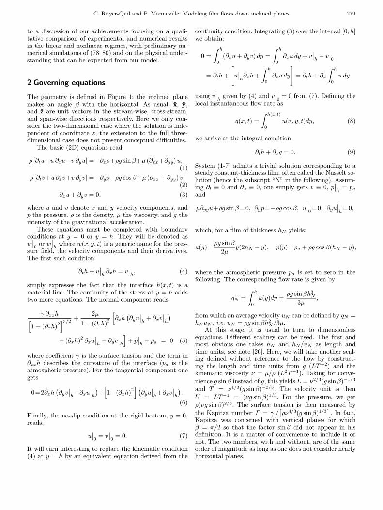
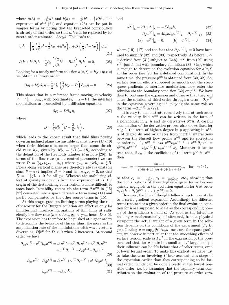
Fig. 1. Fluid film flowing down an inclined plane: definitionof the geometry.
for the coefficients appearing in the expansion, the inter-pretation of such studies is not straightforward and oneis often confined to a comparison of the obtained outputwith that of concurrent models and numerical solutionsof BL or NS equations, or with the results of laboratoryexperiments.
In this paper, after having recalled the governing equa-tions (Sect. 2) of the two-dimensional problem to which wewill restrict, we briefly repeat the first steps of the Ben-ney’s gradient expansion for the dynamics of film flows(Sect. 3) that will be useful to us afterward. We then de-velop our model in two steps, mostly for pedagogical rea-sons (Sects. 4 and 5). We follow the same general strategyas Yu et al. [9] and use BL equations as a starting point,which has the interest of focusing on the appropriate longwavelength properties of the flow right from the begin-ning. We also use polynomials to expand the velocity fieldbut, to stay closer to the physics of the problem, instead ofchoosing some general systematic expressions of increas-ing degree, we prefer to take the specific polynomials thatappear in Benney’s gradient expansion and to introducecombinations of coefficients of the lowest order terms thatmay be given an immediate physical interpretation. Thefirst-order problem (Sect. 4) involves two polynomials, thezeroth-order parabolic profile and a correction issued fromBenney’s expansion. Relevant coefficients involve the flowrate q, and a new field called τ measuring the departure ofthe wall shear from the shear predicted by a parabolic ve-locity profile. At this order, τ is slaved to h and q and canbe eliminated adiabatically, yielding a set of two partialdifferential equations (9, 58) with the same structure asShkadov’s model but different coefficients. With respect tothe latter, the advantage of our first-order model is to givea more accurate description of the vicinity of the instabil-ity threshold, and in particular to predict the critical flowrate exactly. At second order (Sect. 5), τ becomes a degreeof freedom for its own and four well-chosen supplementarypolynomials are introduced, the coefficients of which canbe eliminated to yield a system of three equations (78–80) governing h, q, and τ . Sections 6 and 7 are devoted
C. Ruyer-Quil and P. Manneville: Modeling film flows down inclined planes 279
to a discussion of our achievements focusing on a quali-tative comparison of experimental and numerical resultsin the linear and nonlinear regimes, with preliminary nu-merical simulations of (78–80) and on the physical under-standing that can be expected from our model.
2 Governing equations
The geometry is defined in Figure 1: the inclined planemakes an angle β with the horizontal. As usual, x, y,and z are unit vectors in the stream-wise, cross-stream,and span-wise directions respectively. Here we only con-sider the two-dimensional case where the solution is inde-pendent of coordinate z, the extension to the full three-dimensional case does not present conceptual difficulties.
The basic (2D) equations read
ρ [∂tu+u ∂xu+v ∂yu] =−∂xp+ρg sinβ+µ (∂xx+∂yy)u,(1)
ρ [∂tv+u ∂xv+v ∂yv] =−∂yp−ρg cosβ+µ (∂xx + ∂yy) v,(2)
∂xu+ ∂yv = 0, (3)
where u and v denote x and y velocity components, andp the pressure. ρ is the density, µ the viscosity, and g theintensity of the gravitational acceleration.
These equations must be completed with boundaryconditions at y = 0 or y = h. They will be denoted asw∣∣0
or w∣∣h
where w(x, y, t) is a generic name for the pres-sure field, the velocity components and their derivatives.The first such condition:
∂th+ u∣∣h∂xh = v
∣∣h, (4)
simply expresses the fact that the interface h(x, t) is amaterial line. The continuity of the stress at y = h addstwo more equations. The normal component reads
γ ∂xxh[1 + (∂xh)
2]3/2 +
2µ
1 + (∂xh)2
[∂xh
(∂yu∣∣h
+ ∂xv∣∣h
)− (∂xh)
2∂xu
∣∣h− ∂yv
∣∣h
]+ p∣∣h− pa = 0 (5)
where coefficient γ is the surface tension and the term in∂xxh describes the curvature of the interface (pa is theatmospheric pressure). For the tangential component onegets
0=2∂xh(∂yv∣∣h−∂xu
∣∣h
)+[1−(∂xh)
2] (∂yu∣∣h
+∂xv∣∣h
).
(6)
Finally, the no-slip condition at the rigid bottom, y = 0,reads:
u∣∣0
= v∣∣0
= 0. (7)
It will turn interesting to replace the kinematic condition(4) at y = h by an equivalent equation derived from the
continuity condition. Integrating (3) over the interval [0, h]we obtain:
0 =
∫ h
0
(∂xu+ ∂yv) dy =
∫ h
0
∂xu dy + v∣∣h− v∣∣0
= ∂th+
[u∣∣h∂xh+
∫ h
0
∂xu dy
]= ∂th+ ∂x
∫ h
0
u dy
using v∣∣h
given by (4) and v∣∣0
= 0 from (7). Defining thelocal instantaneous flow rate as
q(x, t) =
∫ h(x,t)
0
u(x, y, t)dy, (8)
we arrive at the integral condition
∂th+ ∂xq = 0. (9)
System (1-7) admits a trivial solution corresponding to asteady constant-thickness film, often called the Nusselt so-lution (hence the subscript “N” in the following). Assum-ing ∂t ≡ 0 and ∂x ≡ 0, one simply gets v ≡ 0, p
∣∣h
= paand
µ∂yyu+ρg sinβ=0, ∂yp=−ρg cosβ, u∣∣0=0, ∂yu
∣∣h
=0,
which, for a film of thickness hN yields:
u(y)=ρg sinβ
2µy(2hN − y), p(y)=pa + ρg cosβ(hN − y),
where the atmospheric pressure pa is set to zero in thefollowing. The corresponding flow rate is given by
qN =
∫ h
0
u(y)dy =ρg sinβh3
N
3µ,
from which an average velocity uN can be defined by qN =hNuN , i.e. uN = ρg sinβh2
N/3µ.At this stage, it is usual to turn to dimensionless
equations. Different scalings can be used. The first andmost obvious one takes hN and hN/uN as length andtime units, see note [26]. Here, we will take another scal-ing defined without reference to the flow by construct-ing the length and time units from g (LT−2) and thekinematic viscosity ν = µ/ρ (L2T−1). Taking for conve-nience g sinβ instead of g, this yields L = ν2/3(g sinβ)−1/3
and T = ν1/3(g sinβ)−2/3. The velocity unit is thenU = LT−1 = (νg sinβ)1/3. For the pressure, we getρ(νg sinβ)2/3. The surface tension is then measured bythe Kapitza number Γ = γ
/[ρν4/3(g sinβ)1/3
]. In fact,
Kapitza was concerned with vertical planes for whichβ = π/2 so that the factor sinβ did not appear in hisdefinition. It is a matter of convenience to include it ornot. The two numbers, with and without, are of the sameorder of magnitude as long as one does not consider nearlyhorizontal planes.
280 The European Physical Journal B
Inserting the corresponding variable changes we obtain
∂tu+u ∂xu+v ∂yu =−∂xp+1+(∂xx+∂yy)u, (10)
∂tv+u ∂xv+v ∂yv =−∂yp−B+(∂xx+∂yy) v, (11)
where B = cotβ and, for the normal-stress boundary con-dition at y = h
Γ ∂xxh[1 + (∂xh)
2]3/2 +
2
1 + (∂xh)2
[∂xh
(∂yu∣∣h
+ ∂xv∣∣h
)− (∂xh)2∂xu
∣∣h− ∂yv
∣∣h
]+ p∣∣h
= 0, (12)
while the continuity condition (3), the kinematic condition(4) at y = h and the remaining boundary conditions (6,7)are left unchanged. In this unit system where g sinβ = ν =ρ = 1, the Nusselt flow rate given by qN = uNhN = 1
3h3N
is numerically equal to the Reynolds number R as definedin note [26].
3 Gradient expansion
Laboratory experiments show that the Nusselt solutionmay not be relevant, being possibly unstable against wavesat the surface of the film. However, as long as the flow rateis not too large, the interface remains smooth at the scaleof the film thickness as measured locally by h(x, t). Thisfeature can be introduced as a supplementary assumptionand solutions to the equations can be searched in the formof a systematic expansion in powers of a formal parame-ter ε expressing the smallness of the stream-wise spacederivative ∂x.
At order zero, the problem simply reads
∂yyu(0) = −1, ∂yp
(0) = −B, ∂yu(0)∣∣h
= 0,
u(0)∣∣0
= 0, p(0)∣∣h
= 0,
so that the Nusselt solution is recovered locally withh(x, t) as reference height:
u(0)(y) =1
2y(2h− y), v(0) ≡ 0, p(0) = B(h− y),
(13)
yielding a local flow rate q(0) = 13h
3. This is an exact solu-tion to the problem, provided that the thickness gradientis strictly zero. When this is no longer the case, correc-tions have to be introduced. Assuming that h ≡ h(x, t)but remains slowly varying, one now looks for a solution“close to” the stationary uniform flow in the form:
u = u(0)(h(x, t), y) + u(1)(x, y, t) + u(2)(x, y, t) + . . . ,
v = v(1)(x, y, t) + v(2)(x, y, t) + . . . ,
p = p(0)(h(x, t), y) + p(1)(x, y, t) + p(2)(x, y, t) + . . . ,
where the corrections are formally of order 1, 2, . . .
When developing the calculation systematically, weshould notice first that the status of the kinematic in-terface condition (4) or its integral version (9) is differentfrom that of the other equations. As a matter of fact, thesought-after solution has to be seen as a functional of hand its successive space-time derivatives, all considered asindependent quantities. Once it is found at a given or-der, the result can be inserted in (9) (or (4)), which thenpresents itself as a constraint relating h and its succes-sive partial derivatives, i.e. an evolution equation for h.Furthermore, it is immediately seen that this equation isformally one order higher than the solution found. So,already at zeroth order we get the following nontrivial re-lation
∂th+ ∂xq(0) ≡ ∂th+ h2∂xh = 0. (14)
However, letting H = h2 leads to ∂tH+H∂xH = 0, i.e. theBurgers equation, an equation known to produce shocksand hence steep gradients incompatible with the slow-variation assumption. Continuing the expansion is there-fore necessary for finding gradient-limiting terms playingthe role of viscous dissipation in the Burgers case. Thoughthe result is not guaranteed to be well-behaved, let us re-view the first steps of the expansion.
At first order we get:
∂yyu(1)−v(1)∂yu
(0) =∂tu(0)+u(0)∂xu
(0)+∂xp(0), (15)
∂yyv(1) − ∂yp
(1) = 0, (16)
∂yv(1) = −∂xu
(0), (17)
to be solved with the appropriate boundary conditions:
p(1)∣∣h− 2∂yv
(1)∣∣h
= 0, (18)
∂yu(1)∣∣h
= 0, (19)
(a) u(1)∣∣0
= 0, (b) v(1)∣∣0
= 0. (20)
(Note that ∂yu(0)∣∣h
= 0 has been taken into account to
simplify the r.h.s. of (18).) Equation (17) yields v(1) =− 1
2y2∂xh when making use of (20b). The stream-wise
correction u(1) is then obtained from (15) together withboundary conditions (19, 20a) and the pressure correctionfrom (16) subject to (18). We obtain
u(1)(x, y, t) =1
2
(1
3y3 − h2y
)∂th+
[1
6
(1
4y4 − h3y
)h
+ B
(1
2y2 − hy
)]∂xh, (21)
p(1)(x, y, t) = −(y + h)∂xh. (22)
To complete the calculation at first order it remains toexpress the kinematic condition in integral form (9). With
u = u(0) +u(1), we obtain for q =∫ h
0 u(y) dy an expression
of the form 13h
3 + a(h)∂th+ b(h)∂xh, hence the evolutionequation for h(x, t):
∂th+ h2∂xh+ ∂x [a(h)∂th+ b(h)∂xh] = 0, (23)
C. Ruyer-Quil and P. Manneville: Modeling film flows down inclined planes 281
where a(h) = − 524h
4 and b(h) = − 340h
6 − 13Bh
3. The
expression of u(1) (21) and equation (23) can be put insimpler forms by noting that the bracketed contributionis already of first order, so that ∂th can be replaced by itszeroth order estimate −h2∂xh. This leads to:
u(1) =
[1
3
(1
8y4−
1
2hy3+h3y
)h+B
(1
2y2−hy
)]∂xh,
(24)
∂th+ h2∂xh+1
3∂x
[(2
5h6 −Bh3
)∂xh
]= 0. (25)
Looking for a nearly uniform solution h(x, t) = hN+η(x, t)we obtain at lowest order:
∂tη + h2N∂xη +
1
3h3N
(2
5h3N −B
)∂xxη = 0. (26)
This shows that in a reference frame moving at velocityV = h2
N = 3uN , with coordinate ξ = x−V t, the interfacemodulations are controlled by a diffusion equation:
∂tη = D∂ξξη, (27)
where
D =1
3h3N
(B −
2
5h3N
), (28)
which leads to the known result that fluid films flowingdown an inclined plane are unstable against waves (D < 0)when their thickness becomes larger than some thresh-old value hNc given by: h3
Nc = 52B (= 3Rc according to
the definition of the Reynolds number R in note [26]). Interms of the flow rate (usual control parameter) we canwrite D = 6
5qN (qNc − qN ) where qNc = 13h
3Nc = 5
6B.Flows along vertical planes are therefore always unstablesince θ = π/2 implies B = 0 and hence qNc = 0, so thatD = − 6
5q2N < 0 for all qN . Whereas the stabilizing ef-
fect of gravity is obvious from the expression of D, theorigin of the destabilizing contribution is more difficult totrace back. Instability comes via the term ∂tu
(0) in (15)[27] converted into a space derivative term using (14) andpartly compensated by the other source terms in (15).
At this stage, gradient-limiting terms playing the roleof viscosity for the Burgers equation are effective only forinfinitesimal interface fluctuations of thin films at suffi-ciently low flow rate (hN < hNc, qN < qNc, hence D > 0).The expansion has therefore to be pushed at higher ordersto determine the behavior of thicker films, the more as theamplification rate of the modulations with wave-vector kdiverge as |D|k2 for D < 0 when k increases. At secondorder we have
∂yyu(2)−v(2)∂yu
(0) = ∂tu(1)+u(0)∂xu
(1)+u(1)∂xu(0)
+v(1)∂yu(1)−∂xp
(1)−∂xxu(0),
(29)
∂yyv(2)−∂yp
(2) = ∂tv(1)+u(0)∂xv
(1)+v(1)∂yv(1),
(30)
∂yv(2) = −∂xu
(1), (31)
and
p(2)∣∣h− 2∂yv
(2)∣∣h
= −Γ∂xxh, (32)
∂yu(2)∣∣h
= 4∂xh∂xu(0)∣∣h− ∂xv
(1)∣∣h, (33)
(a) u(2)∣∣0
= 0, (b) v(2)∣∣0
= 0. (34)
where (19), (17) and the fact that ∂yu(0)∣∣h
= 0 have been
used to simplify (32) and (33), respectively. As before, v(2)
is derived from (31) subject to (34b), u(2) from (29) usingv(2) just found with boundary conditions (33, 34a), whichis enough to determine the evolution equation for h(x, t)at this order (see [28] for a detailed computation). In thesame time, the pressure p(2) is obtained from (30, 32). So,surface tension effects supposed to smooth out the steepspace gradients of interface modulations now enter thesolution via the boundary condition (32) on p(2). We havethus to continue the expansion and observe that they willenter the solution at third order through a term −∂xp(2)
in the equation governing u(3) playing the same role asthe term −∂xp(1) in (29).
It is easy to demonstrate recursively that at each ordern the velocity field u(n) can be written in the form ofa polynomial in y, h and its derivatives ∂mx h. A carefulexamination of the derivation process also shows that, forn ≥ 2, the term of highest degree in y appearing in u(n)
is of degree 4n and originates from inertial interactionsbetween the Nusselt flow profile u(0) and its correctionat order n − 1, u(n−1), via u(0)∂xu
(n−1) + v(n)∂yu(0) =
u(0)∂xu(n−1) − ∂yu(0)
∫ y0 ∂xu
(n−1) dy. Moreover, it can be
seen that, if cn is the coefficient of the term y4n in u(n),then
cn+1 = −4n− 1
2(4n+ 1)(4n+ 3)(4n+ 4)cn for n ≥ 1,
so that c2 = − 14480 , c3 = 1
1520640 etc., showing thatthe contributions of these highest-degree terms becomequickly negligible in the evolution equation for h at ordern, ∂th+ ∂x(q(0) + . . .+ q(n)) = 0.
However, the line of thought followed up to now sticksto a strict gradient expansion. Accordingly the differentterms retained at a given order in the final evolution equa-tion for h are supposed to scale as the corresponding pow-ers of the gradients ∂x and ∂t. As soon as the latter areno longer mathematically infinitesimal, from a physicalviewpoint the actual weight of a given term in the solu-tion depends on the conditions of the experiment (Γ , B,qN ). Letting µ = supx |h
−1∂xh| measure the space gradi-ent, we observe in particular that the smoothing effects ofsurface tension scale as Γµ2 in the expression of the pres-sure and that, for µ finite but small and Γ large enough,their influence can be felt before that of other terms, evenof lower formal order. To make this explicit, we have justto take the term involving Γ into account at a stage ofthe expansion earlier than that corresponding to its for-mal order, which can be done already at the lowest pos-sible order, i.e. by assuming that the capillary term con-tributes to the evaluation of the pressure at order zero.
282 The European Physical Journal B
Boundary condition (12) then reads p∣∣h
= −Γ∂xxh sothat the pressure is no longer given as in (13) but ratherby
p(0) = B(h− y)− Γ∂xxh. (35)
The solution at first order has to be modified accordingly,which yields
∂th+ h2∂xh+1
3∂x
[(2
5h6 −Bh3
)∂xh+ Γh3∂x3h
]= 0.
(36)
instead of (25).Considering infinitesimal modulations, in lieu of (27)
we now get
∂tη = D∂ξξη −K∂ξξξξη, (37)
with K = 13h
3NΓ = qNΓ . As expected from Fourier
analysis with perturbations ∝ exp(ikx), the last term in(37) damps out short-wavelength fluctuations, at a rate−Kk4 that dominates the destabilizing contribution |D|k2
when D is negative. The two terms counterbalance eachother exactly for a certain cut-off wave-vector kc givenby k2
c = |D|/K = 65 (qN − qNc)/Γ . This wave-vector de-
fines a scale for which, in order of magnitude, capillaryeffects enter the problem and work to limit the divergenceof space gradients. A low order truncation of the expan-sion will therefore be acceptable if kc is physically smallenough, which will always be the case close to the insta-bility threshold qNc.
Equation (36), usually called the Benney equation, isthus expected to govern the interface modulations withspace gradients at most of order kc as long as kc � 1, i.e.at flow rates close to the threshold in a range depending onthe value of Γ . The linear argument above using (37) giveshints on the behavior of solutions to (36) only because theinstability turns out to be supercritical, so that a weakly-nonlinear theory accounts for the continuous growth ofthe amplitude of modulations in the neighborhood of thethreshold. In fact, owing to the strong nonlinearities as-sociated with the high powers of h present, this neigh-borhood is quite narrow and typical solutions to (36) dis-play finite-time singularities not so far from the threshold.From the additive nature of the contribution of the Γ -termin (12) leading directly to (35), it is clear that, dependingon the order in ∂x one decides to introduce it, other gra-dient terms in h will appear in (36), which will play aneffective role if kc is too large, i.e. in general K too small,hence Γ too small. Taking these terms into account doesnot solve the problem of finite-time singularities, whoseorigin may be attributed to the strongly nonlinear charac-ter of the evolution equation for h, which involves rapidlyincreasing powers of h as the gradient expansion proceeds.
4 First-order model
In the gradient expansion, the flow variables are sup-posed to be strictly enslaved to the local thickness h which
plays the role of an effective degree of freedom governedby a Benney-like evolution equation. Another approach isthen needed to deal with the dynamics of the film in acontext where this enslaving is partly relaxed and othereffective degrees of freedom are introduced, under the con-straint that these new variables should remain slowly vari-able in x and t and that exact results of the gradientexpansion should be recovered in the appropriate limit.Up to now, the hydrodynamic fields (u, v, p) could be ex-panded on a special set of polynomials in y with slowlyvarying coefficients functions of h(x, t) and its derivatives.If the flow modulations are sufficiently slow, these fieldsshould not be far from their estimates obtained by the gra-dient expansion. In other terms, the residue of a Galerkinexpansion —or of an approximation derived from a moregeneral weighted residual method— based on these poly-nomials should be intrinsically small. The coefficients ofthe expansion would then be considered as the sought-after effective degrees of freedom, and they would be gov-erned by equations generalizing the expressions asymp-totically valid when modulations are infinitely slow. Therequired extension would give some latitude of evolutionto these coefficients around the asymptotic value obtainedfrom the gradient expansion. The model developed belowis an attempt to implement this general idea in the most“economical” way.
Let us begin with the set of equations consistent atfirst order except for surface tension effects that, thoughformally of higher order, are included here owing to theirgradient-limiting role, as discussed above. The problem tobe solved reads:
∂tu+ u∂xu+ v∂yu+ ∂xp− ∂yyu− 1 = 0, (38)
∂yp+B − ∂yyv = 0, (39)
∂xu+ ∂yv = 0, (40)
with boundary conditions
p∣∣h
+ Γ∂xxh− 2∂yv∣∣h
= 0, (41)
∂yu∣∣h
= 0, (42)
u∣∣0
= 0, v∣∣0
= 0, (43)
and of course the kinematic condition at the interfacewhich, in integral form (9), accounts for mass conserva-tion on average over the thickness.
Integrating (39) with the help of boundary conditions(41–42) we get p = B(h − y) + ∂yv + ∂yv
∣∣h− Γ∂xxh and
further eliminate ∂xp from (38). Because ∂yv = −∂xu is afirst order term, its derivative is of second order and canbe dropped of. Therefore, our set of equations read
∂tu+ u∂xu+ v∂yu− ∂yyu = 1−B∂xh+ Γ∂x3h, (44)
∂xu+ ∂yv = 0, (45)
with boundary conditions (42–43). (44–45) is sometimescalled boundary-layer equations (BL).
Let us now consider the averaging of equation (44) thatgives the balance of x-momentum (von Karman’s equation
C. Ruyer-Quil and P. Manneville: Modeling film flows down inclined planes 283
in the context of boundary layers). We obtain:∫ h
0
[∂tu+u∂xu+v∂yu−∂yyu] dy=h+Γh∂x3h−Bh∂xh,
(46)
which can be transformed into
∂t
∫ h
0
u dy+∂x
∫ h
0
u2 dy=h−∂yu∣∣0+Γh∂x3h−Bh∂xh.
(47)
Transformation of the l.h.s. is similar to that leading to(9). The term ∂yu
∣∣0, representing the shear at the wall,
will be denoted τw in the following. On the l.h.s. we rec-
ognize q =∫ h
0 u(y) dy and we can define a new averaged
field r =∫ h
0u2(y) dy. With these notations (47) reads:
∂tq + ∂xr = h (1 + Γ∂x3h−B∂xh)− τw. (48)
Assuming a given velocity profile, one arrives at a set oftwo equations (9) and (48) for two unknowns h and q, sincer can then be computed from q. Simply taking Kapitza’sparabolic profile u(y) ∝ 1
2ζ(2−ζ) where ζ = y/h, we have
r = 65 (q2/h), and τw = 3q/h2. Inserting these estimates
in (48) we obtain Shkadov’s model [22]:
∂th = −∂xq, (49)
∂tq = h−3q
h2−
12
5
q
h∂xq+
(6
5
q2
h2−Bh
)∂xh+Γh∂x3h.
(50)
Now, taking (49, 50) as a set of primitive equations, letus consider slow modulations to the uniform solution thatverifies q = 1
3h3 = q(0). We are now in position to perform
a gradient expansion parallel to the previous one by as-suming q = q(0) +q(1) +q(2) + . . . , where q(1), q(2), etc. areformally of order 1, 2, etc. At lowest order we obtain forthe l.h.s. of (50): ∂tq
(0) = ∂t(13h
3) = h2∂th = −h2∂xq(0) =
−h2(h2∂xh) = −h4∂xh, and for the r.h.s.:
−3q(1)
h2+
[6
5
q(0)2
h2−Bh
]∂xh−
12
5
q(0)
h∂xq
(0)+Γh∂x3h,
where, as before, the surface-tension term has been intro-duced earlier than dictated by its formal order. This leadsto the estimate
q(1) =1
9h6∂xh−
1
3Bh3∂xh+
1
3Γh3∂x3h,
which, when replaced in ∂th + ∂x[q(0) + q(1)
]= 0, gives
the following evolution equation
∂th+ h2∂xh+1
3∂x
[(1
3h6 −Bh3
)∂xh+ Γh3∂x3h
]= 0,
(51)
which differs from equation (36) by the coefficient in frontof h6. This discrepancy leads to an overestimation ofthe critical Reynolds number Rc,IBL = B [29]. Proko-piou et al. [8] and Lee and Mei [10] tried to get rid ofthis discrepancy by starting from systems of equationsmore complete than (44–45), while keeping the zeroth-order parabolic velocity profile. These approaches failedto recover the correct critical Reynolds number predictionRc = 5
6B and led back to Rc,IBL. The cause of this failurethus seems to be the lack of flexibility of the assump-tion about the velocity profile rather than the omission ofterms in the set of primitive equations.
In the spirit of Shkadov’s assumption, a whole familyof models analogous to (49–50), with just different numer-ical constants, would be obtained by using velocity profilesexpressed in terms of a single, possibly better fitted, func-tion of the reduced variable ζ = y/h, u = a(x, t) g(ζ).Such velocity profiles are sometimes called “similar” solu-tions in boundary-layer theory [30]. The defect of such anapproach comes from a somewhat arbitrary freezing of theeffective degrees of freedom involved in the velocity field.Here we want to relax part of this constraint by assumingthat u is a superposition of functions with slow variablecoefficients so that the quantities r and τw are less rigidlyrelated to q and h.
So, keeping in mind the results of the long-wavelengthexpansion, we may reasonably admit that Shkadov’s sim-ple assumption, valid at order zero, can be improved bycorrecting the parabolic profile with the polynomials thatappear in the gradient expansion at higher orders, or moreprecisely, linearly independent combinations of these poly-nomials adequately chosen for better computational ease.So, let us expand u as
u(x, y, t) = b0(x, t)f (0)(y/h) + b1(x, t)f (1)(y/h), (52)
where f (0)(ζ) ≡ − 12ζ
2 + ζ and f (1)(ζ) ≡16
(14ζ
4 − ζ3 + ζ2). Whereas u(0) in (13) is obviously
proportional to f (0), a little algebra is necessary to checkthat u(1) in (24) can indeed be written as some specificcombination of f (0) and f (1) (cf. note [31]).
Apart from the fact that the so-far unknown fields b0and b1 are supposed to be slow functions of x and t, bydefinition of q they must fulfill
q =
∫ h
0
u(y) dy =1
3h
(b0 +
1
15b1
). (53)
At this stage we have three unknowns, h, b0, and b1 butfrom (53) we see that we can pass to a set formed by h, qand b1, with b0 given by b0 = (3q/h)− 1
15b1. Inserting this
in τw ≡ ∂yu∣∣0
= b0/h we get τw = (3q/h2)− (b1/15h). Inthat way, b1 appears as a correction to the shear at theplate that would be created by a parabolic velocity profilecorresponding to a film with thickness h and flow rate q.To make this explicit, let us re-define b1 as b1 = −15hτ sothat
τw =3q
h2+ τ. (54)
284 The European Physical Journal B
What we have just done is to pass from the original alge-braic variables b0 and b1 to the more physically mindedvariables q and τ . Accordingly (52) can be rewritten as
u =
(3q
h+ hτ
)f (0)(y/h)− 15hτf (1)(y/h). (55)
But, h, q, and τ still make a set of three variables forwhich we have only two equations (9, 48). Several strate-gies can be followed to find equations for the unknowns bythe method of weighted residual. One can for example av-erage the governing equations with a series of weights. (Inthe classical Galerkin method the set of weight functionsis simply the set of the basis functions, further assumedto fulfill the boundary conditions.) Here equation (48) isjust the averaged version of (44) with the trivial uniformweight and, as shown previously, (9) is nothing but theaveraged continuity equation (3) simplified by using thekinematic interface evolution equation (4). An alternatemethod consists in imposing conditions at special pointsof the domain (collocation). Here, to obtain complemen-tary equations, we will follow this last method and im-pose the fulfillment of additional conditions at y = 0 andy = h. These relations will be obtained by differentiat-ing the equations of motion with respect to y and furtherevaluating them at the boundaries (see [32]). Conditionsat y = 0 can be interpreted as relations giving the coeffi-cients of a Taylor expansion of the solution as a functionof y.
A condition useful at first order is obtained from (44)differentiated with respect to y:
∂tyu+ u∂xyu+ v∂yyu− ∂y3u = 0,
further evaluated at y = 0, which gives:
∂t(∂yu∣∣0)− ∂y3u
∣∣0
= 0. (56)
Equation (56) tells us that the fluctuations of the shearat the wall are directly linked to the presence of correc-tions to the velocity profile beyond the parabolic shapefor which they cancel identically. From (55) and (54), fur-ther observing that τ is a first-order correction so that theterm ∂tτ is of higher order and can be dropped from (56),we get the required supplementary equation
∂t
(3q
h2
)− 15
τ
h2= 0, (57)
expressing the correction τ in terms of the time derivativeof the other fields. Inserting the resulting evaluation of τwin (48), using (9) to eliminate ∂th and the (here sufficient)zeroth-order estimate r = 6
5 (q2/h), we get
∂tq=5
6h−
5
2
q
h2−
7
3
q
h∂xq+
(q2
h2−
5
6Bh
)∂xh+
5
6Γh∂x3h.
(58)
When added to (9), equation (58) completes the model atfirst order as a system of two partial differential equations
for the two unknowns h and q. Having the same structureas Shkadov’s model but with slightly different coefficients,it will be called “modified Shkadov model”. The correc-tions arise from a better account of the fluctuations ofτw introduced via the third derivative term in (56) bythe ζ3-term in f (1), which can be traced back to the ∂thcontribution of u(1) in (21) already at the origin of theinstability of the plane interface.
Now, let us consider a gradient expansion of (9, 58)similar to the previous ones by assuming q = q(0) + q(1) +q(2) + · · · . We are this time led to
q(1) =2
15h6∂xh−
1
3Bh3∂xh+
1
3Γh3∂x3h,
which, when replaced in ∂th+∂x[q(0) + q(1)
]= 0, gives us
back the Benney equation (36). So, by construction, thenear-critical behavior is correctly predicted by our mod-ified Shkadov model, which no longer overestimates thevalue of the stability threshold.
Though predictions in the asymptotic domain far be-yond the near-critical region are not improved by the cor-rection, a step has clearly been made in the right direction.In particular, the derivation implies that the shear at thewall is a slowly varying quantity. At order zero, q is slavedto h (or the reverse) and τw does not fluctuate (inject-ing a parabolic profile for u in (56) gives ∂t(∂yu
∣∣0) = 0).
At order one, q and h are two independent slowly vary-ing effective degrees of freedom while τw remains rigidlylinked to q and h through (57). Let us now proceed tothe next step. Anticipating the result, we will introducefour additional fields b2, . . . , b5 associated with the ve-locity corrections introduced by the gradient expansionat second order. Supplementary conditions at boundariesanalogous to (56) will be derived which, when imposed tothe solution will allow us to eliminate these supplemen-tary fields so that we will be left with three equations forthree unknowns, h, q and τ , that will play the role of anadditional independent effective degree of freedom. Thederivation detailed in the next section can be skipped bythose only interested in the result, equations (78–80).
5 Second-order model
Let us first write down the set of equations consistent atsecond order. Clearly all terms in (10), rewritten here forconvenience as
∂tu+ u∂xu+ v∂yu+ ∂xp− (∂xx + ∂yy)u− 1 = 0, (59)
are relevant. Such is not the case for (11) which can besimplified as
∂yp− ∂yyv +B = 0. (60)
It can indeed be seen that the contribution of the terms∂tv + u∂xv + v∂yv is in fact of higher order, owing to thedifferentiation of p with respect to x in (59) as seen fromthe calculation leading to (63) below. Of course u and vremain linked by the continuity equation (3).
C. Ruyer-Quil and P. Manneville: Modeling film flows down inclined planes 285
For the boundary conditions we have
p∣∣h
+ Γ∂xxh− 2∂yv∣∣h
= 0, (61)
−4∂xh∂xu∣∣h
+ ∂yu∣∣h
+ ∂xv∣∣h
= 0, (62)
to which we add (43) and of course (9).Let us transform (59). Integrating (60) with respect to
y we get p(y) = −By+∂yv+K. The integration constantK, in fact a function of x and t, is obtained from (61)which gives K = Bh + ∂yv
∣∣h− Γ∂xxh, hence p = B(h −
y) + ∂yv + ∂yv∣∣h− Γ∂xxh. Inserting this expression into
(59) we get:
∂tu+ u∂xu+ v∂yu = 1 + ∂yyu− 2∂xyv + ∂x
[∂xu
∣∣h
]−B∂xh+ Γ∂x3h, (63)
where the continuity equation has been used to transform∂xxu into −∂xyv and −∂yv
∣∣h
into ∂xu∣∣h
(notice that thislast term is a function of x and t through h and is differ-entiated with respect to x as such). Averaging (63) overthe thickness h as before we obtain
∂tq + ∂xr = h[1 + Γ∂x3h−B∂xh+ ∂x
(∂xu
∣∣h
) ]−τw + ∂yu
∣∣h− 2∂xv
∣∣h,
where q, r, and τw are defined as before. (The secondboundary term ∂xv
∣∣0
resulting from the explicit integra-tion of ∂xyv has been dropped since it cancels automat-ically by virtue of v
∣∣0≡ 0.) Making use of (62) we can
simplify this equation: explicitly, we have h∂x(∂xu
∣∣h
)+
∂yu∣∣h− 2∂xv
∣∣h
= h∂x(∂xu
∣∣h
)+[4∂xh∂xu
∣∣h− ∂xv
∣∣h
]−
2∂xv∣∣h
=[h∂x
(∂xu
∣∣h
)+ ∂xh∂xu
∣∣h
]+ 3∂xh∂xu
∣∣h−
3∂xv∣∣h
= ∂x[h∂xu
∣∣h
]− 3∂xh∂yv
∣∣h− 3∂xv
∣∣h
=
∂x[h∂xu
∣∣h
]− 3∂x
(v∣∣h
)= ∂x
[h∂xu
∣∣h− 3v
∣∣h
]. Finally we
arrive at
∂tq+∂xr=h[1+Γ∂x3h−B∂xh
]−τw+∂x
[h∂xu
∣∣h−3v
∣∣h
],
(64)
to be compared with its first order counter-part (48).The two first polynomials to be used in addition to
f (0) and f (1) are f (2) = 12ζ
2 and f (3) = 112
(− 1
2ζ4 + ζ2
).
The set{f (0), f (1), f (2), f (3)
}is easily seen to form a basis
of the space of polynomials of degree ≤ 4 that cancel aty = 0. The two last polynomials f (4) = 1
120
(− 1
6ζ6 + ζ5
)and f (5) = 1
240
(156ζ
8 − 17ζ
7 + 13ζ
6)
have been chosen soas to permit the reconstruction of all the polynomialsentering the gradient expansion at second order. Theirseemingly exotic coefficients have been fixed by the ad-ditional constraints: d5f (4)/dζ5|0 = 1, d6f (5)/dζ6|0 = 1,that slightly simplify the forthcoming computations. Thevelocity component u is expanded as
u(x, y, t) =5∑k=0
bk(x, t)f (k)(y/h),
so that, by definition of q, we have
q = h
(1
3b0 +
1
45b1 +
1
6b2 +
7
360b3 +
1
840b4 +
1
7560b5
).
(65)
These new polynomials do not contribute to the evaluationof τw which is therefore still given by τw = b0/h.
Sticking to the approach followed for the derivationof the first order model, we keep q and τ as primitivevariables in addition to h. In particular τ remains definedfrom τw = (3q/h2) + τ , which implies b0 = (3q/h) + hτ .Inserting this in (65) we obtain b1 = −(15hτ + 15
2 b2 −78b3 + 3
56b4 + 1168b5), so that the expression of u extending
(55) to second order reads:
u =
(3q
h+hτ
)f (0)−
(15hτ+
15
2b2+
7
8b3+
3
56b4+
1
168b5
)× f (1) +
5∑k=2
bkf(k), (66)
from which v = −∫ y
0 ∂xu dy can be derived. To deal withthe seven unknowns h, q, τ , bk, k = 2, . . . , 5, assumed tobe slow functions of x and t, we need seven independentequations. In addition to the kinematic condition at theinterface (9) and the average x-momentum equation (64)derived earlier, we have the boundary condition (62) onthe tangential stress at y = h, here used for the first time.To get the remaining four equations we follow the samescheme as for the first-order model and look for collocationat the boundaries.
The equation extending (56) at second order is ob-tained by differentiating (59) with respect to y, whichyields:
∂tyu+ u∂xyu+ v∂y2u− ∂y3u− 2∂x2yu = 0, (67)
where we have used (60) differentiated with respect to xand the continuity equation (3) to eliminate ∂xyp. Furtherevaluating (67) at y = 0 gives us
∂t(∂yu∣∣0)− ∂y3u
∣∣0− 2∂x2yu
∣∣0
= 0. (68)
The evaluation of (67) at y = h leads to an independentequation. The raw condition:
∂tyu∣∣h
+ u∣∣h∂xyu
∣∣h
+ v∣∣h∂y2u
∣∣h− ∂y3u
∣∣h− 2∂x2yu
∣∣h
= 0
can be simplified by noting that ∂tyu∣∣h
= ∂t(∂yu∣∣h
)−
∂yyu∣∣h∂th and ∂xyu
∣∣h
= ∂x(∂yu
∣∣h
)− ∂yyu
∣∣h∂xh. It is
easily checked that the kinematic condition v∣∣h
= ∂th +
u∣∣h∂xh at the interface leads to a canceling of terms in
∂yyu∣∣h. Furthermore (62) shows that ∂yu
∣∣h
is already ofsecond-order so that its x and t derivatives can be ne-glected. Accordingly, equation (67) evaluated at y = hsimply reads
∂y3u∣∣h
+ 2∂x2yu∣∣h
= 0. (69)
286 The European Physical Journal B
To obtain simple conditions involving more specifically thevariables associated to the high-degree polynomials f (k),k = 4, 5, we will add conditions obtained in the same wayas (68) but with higher derivatives. The second derivativeof (59) brings no new condition on the coefficients of thesepolynomials since d4f (4)/dζ4 and d4f (5)/dζ4 cancel whenevaluated at ζ = 0. Thus taking the third derivative of(59), we obtain
∂t(∂y3u∣∣0) + 2∂yu
∣∣0∂xy2u
∣∣0− ∂y5u
∣∣0− 2∂x2y3u
∣∣0
= 0,
(70)
and next for the fourth derivative:
∂t(∂y4u∣∣0) + 3∂yu
∣∣0∂xy3u
∣∣0
+ 2∂y2u∣∣0∂xy2u
∣∣0
− 2∂xyu∣∣0∂y3u
∣∣0− ∂y6u
∣∣0− 2∂x2y4u
∣∣0
= 0. (71)
The model at second order is obtained by inserting theansatz (66) into equations (9,64,62,68–71). In the deriva-tion of the first-order model, the time derivative of τ couldbe neglected since it was of higher order. This allowedus to eliminate it from the equations to get a system oftwo equations for the two unknowns h and q. Here thisderivative is no longer negligible and τ is a genuine dy-namical variable. By contrast, the additional fields aresecond-order corrections so that their t- or x-derivatives,of still higher order, can be dropped without damage. Thederivation, straightforward but (really) tedious, has beenperformed using mathematica. Let us consider first theequations accounting for the enslaving of b2, ..., b5 to h, q,and τ , namely (62) and (69–71) taken in that order. Weobtain
b2
h+b4
30h+
b5
210h+
3q(∂xh)2
h2−
3∂xh ∂xq
h
+3q ∂xxh
2h−∂xxq=0, (72)
−b3+b4
3+b5
15−
36q(∂xh)2
h+12∂xh ∂xq+6q ∂xxh=0,
(73)
54q2 ∂xh
h6−
18q ∂xq
h5−b4
h5+15∂t
[ τh2
]+
54q τ ∂xh
h4
−6τ∂xq
h3−
36q∂xτ
h3= 0, (74)
9∂x
[q2
h6
]+b4 − b5h6
− 15∂t
[ τh3
]−
234q τ ∂xh
h5
+ 919q ∂xτ − 6τ ∂xq
h4= 0. (75)
As already mentioned, partial derivatives of the bk do notenter these equations so that they can be obtained imme-diately as functions of h, q, and τ . Indeed b4 is directlyextracted from (74), next b5 from (75), and finally b2 and
b3 from (72) and (73), respectively. In fact, the somehowweird definitions of polynomials f (2) to f (5) were intendedto make this final evaluation simpler: instead of having thebk given by the most general (4× 4) linear system, we getthem by elementary substitution owing to the fact thatspecific coefficients in this linear system cancel automati-cally when the corresponding combinations of derivativesare evaluated at y = 0 or y = h.
To terminate the derivation of the second-order model,it remains to substitute the expressions of the bk in thedynamical equations for h, q and τ , that is to say thekinematic condition at the interface (9), the average x-momentum balance equation (64) that now reads
∂tq+∂x
[6q2
5h−
2
35hqτ
]=−
3q
h2−τ+h+∂x
[9∂xq
2−
6q∂xh
h
]−Bh∂xh+ Γh∂x3h, (76)
and the stress balance at y = 0:
−15τ
h2+ ∂t
[3q
h2
]+ ∂tτ − ∂xx
[6q
h2
]−
1
h3
[15
2b2 +
7
8b3
+3
56b4 +
1
168b5
]= 0. (77)
At last we obtain
∂th = −∂xq, (78)
∂tq=h−3q
h2−τ+∂x
[2
35hτq−
6q2
5h−
6q∂xh
h+
9∂xq
2
]−Bh∂xh+ Γh∂x3h, (79)
∂tτ =7
h−
21q
h4−
42τ
h2−
18q2∂xh
5h4+
6q∂xq
5h3+
2qτ∂xh
5h2
+τ∂xq
15h−
3q∂xτ
5h+
84q(∂xh)2
h4−
63∂xq∂xh
h3
−7B∂xh
h+
7Γ∂x3h
h· (80)
A gradient expansion up to second order assuming q =q(0) + q(1) + q(2) and τ = τ (1) + τ (2) leads to
q(2) =
(7
3h3 −
8
15B h6 +
127
315h9
)(∂xh)2
+
(h4 −
10
63B h7 +
4
63h10
)∂x2h,
τ (2) =
(2h−
4
15B h4 +
13
63h7
)(∂xh)2
+
(1
2h2 −
8
105B h5 +
2
63h8
)∂x2h,
yielding the exact second-order evolution equation [6] asexpected.
At this stage, one can notice that the second-orderformulation includes the effects of the stream-wise dissi-pation, while they are absent from the first-order model,
C. Ruyer-Quil and P. Manneville: Modeling film flows down inclined planes 287
and more generally from any expansion based on the first-order BL equations (44, 45). As a matter of fact, perform-ing the same derivation at second order with this system,one obtains
∂th = −∂xq, (81)
∂tq = h−3q
h2− τ + ∂x
[2
35hτq −
6q2
5h
]−Bh∂xh+ Γh∂x3h, (82)
∂tτ =7
h−
21q
h4−
42τ
h2−
18q2∂xh
5h4+
6q∂xq
5h3+
2qτ∂xh
5h2
+τ∂xq
15h−
3q∂xτ
5h−
7B∂xh
h+
7Γ∂x3h
h, (83)
where it can be seen that terms of the form ∂xx() or∂x()∂x(), are absent. By difference with (78–80), suchterms have thus to be attributed to the effects of stream-wise viscous dissipation.
6 Linear stability analysis
Before presenting our preliminary numerical results withthe model equations developed in Sections 4 and 5, letus compare their linear stability properties with the datacollected by Liu et al. [33]. Setting w = wN + w exp[i(kx−ωt)] where w and wN refer to h and q and their values forthe reference Nusselt flow solution, linearizing (9, 58), weobtain
ω h = k q,
(5
2+ i
(1
9h4N −
5
6BhN
)k −i
5
6ΓhN k
3
)h =(
5
6+ i
7
27h4N k − i
1
3h2N ω
)q.
Compatibility of this system yields the dispersion rela-tion. For easier comparison with experimental results, itis preferable to turn to a scaling where hN is the lengthscale. This leads to change k into k/hN , ω into ωhN , andto introduce the Reynolds and Weber numbers, R = 1
3h3N
and W = Γ/h2N respectively.
k + i
(2
15R−
1
3B
)k2 − i
1
3Wk4 +
(−1− i
14
15Rk
)ω
+ i6
5Rω2 = 0. (84)
Separating real and imaginary parts for real k and ω weget
ω = k, (85)
6
5R−B = Wk2. (86)
Equation (86) defines the neutral stability curve of themodified Shkadov model in the plane (R, k) while (85)
implies that the phase speed c = ω/k is constant and equalto unity at marginality. As expected, equations (85–86)characterize the marginal waves of Benney’s equation (36)[13] (For comparison, linear stability analysis of Shkadov’smodel (49–50) would lead to R−B = Wk2.).
Following Yih [34], let us consider the temporal stabil-ity problem in terms of an asymptotic expansion of fre-quency ω in powers of a real wave-number k in the limitk� 1. We get
ω = k + i k2
(2
5R−
1
3B
)+ k3
(22
45BR −
44
75R2
)+ i k4
(−
2
15B2R+
28
27BR2 −
1184
1125R3 −
1
3W
)+O(k5),
(87)
to be compared with the exact asymptotic expansion ofOrr–Sommerfeld equation,
ω = k + i k2
(2
5R−
1
3B
)+ k3
(−1 +
10
21BR −
4
7R2
)+i k4
(3
5B −
471
224R−
2
15B2R+
17363
17325BR2
−75872
75075R3 −
1
3W
)+O(k5). (88)
Although equation (87) is close to (88), three terms aremissing in (87). A careful examination of the calculusshows that these terms mostly originate from second-orderviscous terms omitted in the derivation of (9–58).
A parallel stability analysis of the second-order model(78–80) leads to the dispersion relation
A(k) + B(k)ω + C(k)ω2 + D(k)ω3 = 0, (89)
with
A(k) =k+i
(1
5R−
1
3B
)k2+
(4
5−
2
1225R2+
1
105BR
)k3
+ i
(2
175R−
1
3W
)k4 +
1
315Wk5,
B(k) = −1− i38
35Rk +
(−
9
5+
6
245R2 −
1
35BR
)k2
− i29
350Rk3 −
3
105WRk4,
C(k) = i9
7R−
3
35R2k + i
9
70Rk2,D(k) =
3
35R2.
The asymptotic expansion of (89) in the temporal domain(k ∈ R) gives
ω = k + i k2
(2
5R−
1
3B
)+ k3
(−1 +
10
21BR −
4
7R2
)+i k4
(3
5B −
376
175R−
2
15B2R+
3683
3675BR2
−1238
1225R3 −
1
3W
)+O(k5), (90)
288 The European Physical Journal B
8 9 10 11 12 13 14 150
2
4
6
8
10
12
Reynolds number
freq
uenc
y (H
z)
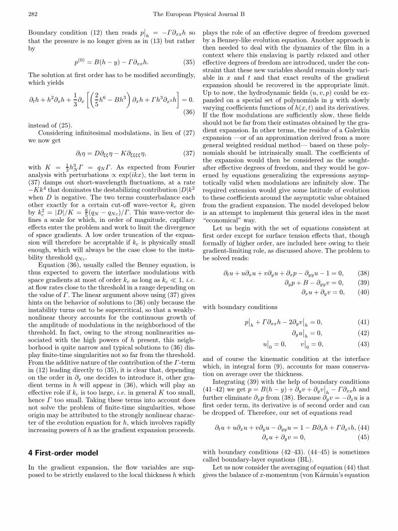
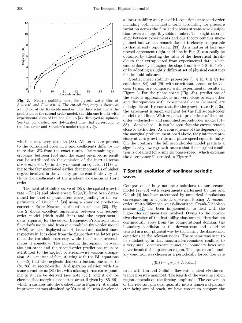
Fig. 2. Neutral stability curve for glycerin-water films atβ = 5.6◦ and Γ = 700.15. The cut-off frequency is shown asa function of the Reynolds number. The thick solid line is theprediction of the second-order model, the thin one is a fit withexperimental data of Liu and Gollub [33] displayed as squares.See text for dashed and dot-dashed lines that correspond tothe first-order and Shkadov’s model respectively.
which is now very close to (88). All terms are presentto the considered order in k and coefficients differ by nomore than 3% from the exact result. The remaining dis-crepancy between (90) and the exact asymptotic resultcan be attributed to the omission of the inertial terms∂tv + u∂xv + v∂yv in the y-momentum equation (11) ow-ing to the fact mentioned earlier that monomials of higherdegree involved in the velocity profile contribute very lit-tle to the coefficients of the gradient expansion at thirdorder.
The neutral stability curve of (89), the spatial growthrate −Im(k) and phase speed Re(ω/k) have been deter-mined for a set of parameters corresponding to the ex-periments of Liu et al. [33] using a standard predictor-corrector Euler–Newton continuation scheme [35]. Fig-ure 2 shows excellent agreement between our second-order model (thick solid line) and the experimentaldata (squares) for the cut-off frequency. Predictions fromShkadov’s model and from our modified first-order model(9–58) are also displayed as dot-dashed and dashed lines,respectively. It is clear from the figure that the latter pre-dicts the threshold correctly, while the former overesti-mates it somehow. The increasing discrepancy betweenthe first-order and the second-order predictions must beattributed to the neglect of stream-wise viscous dissipa-tion. As a matter of fact, starting with the BL equations(44–45) that also neglects this contribution, one is led to(81–83) at second-order. A dispersion relation with thesame structure as (89) but with missing terms correspond-ing to it can be derived (see note [36]), and it can bechecked that marginal properties are still given by (85–86),which translates into the dashed line in Figure 2. A similarimprovement was obtained by Yu et al. [9] who developed
a linear stability analysis of BL equations at second-orderincluding both a heuristic term accounting for pressurevariation across the film and viscous stream-wise dissipa-tion, even at large Reynolds number. The slight discrep-ancy between experiments and our theory remains unex-plained but we can remark that it is closely comparableto that already reported in [33]. As a matter of fact, im-proved agreement (light solid line in Fig. 2) can easily beobtained by adjusting the value of the theoretical thresh-old to that extrapolated from experimental data, whichcan be done by changing the slope from β = 5.6◦ to 5.85◦,or by adopting a slightly different set of physical constantsfor the fluid mixture.
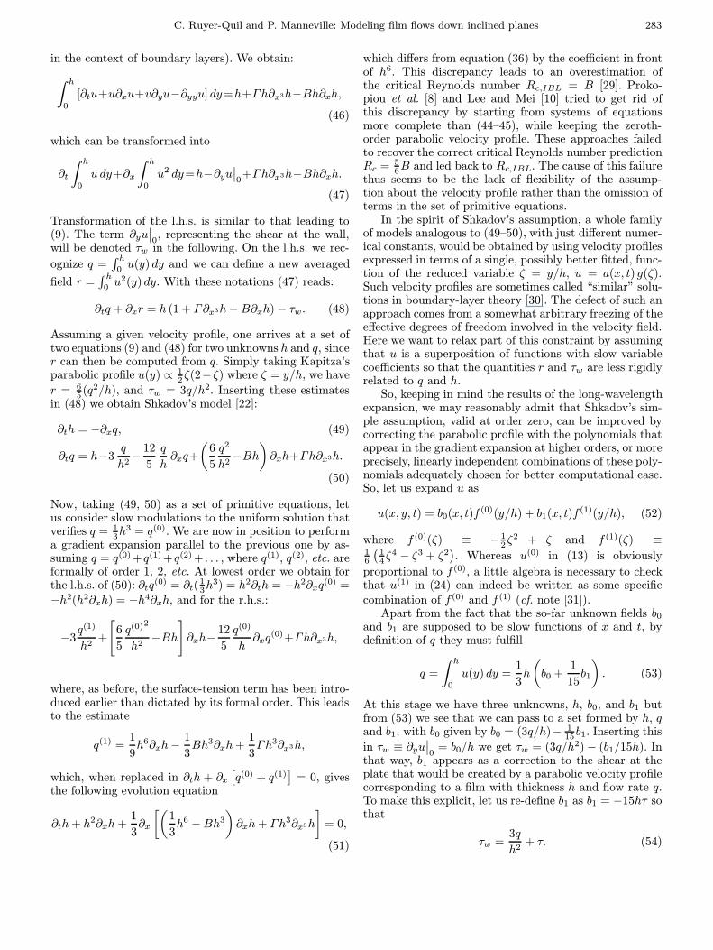
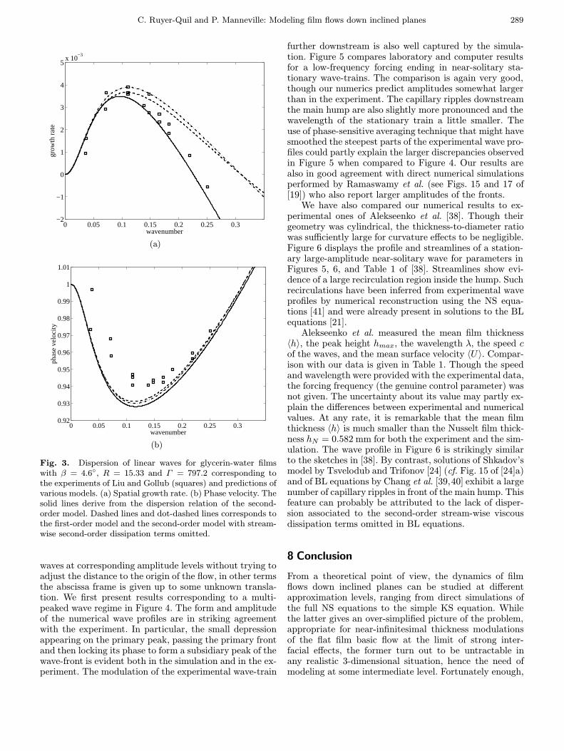
Spatial linear stability properties (ω ∈ R, k ∈ C) forequations (84) and (89) with or without second-order vis-cous terms, are compared with experimental results inFigure 3. For the phase speed (Fig. 3b), predictions ofthe various approximations are very close to each otherand discrepancies with experimental data (squares) arenot significant. By contrast, for the growth-rate (Fig. 3a)the agreement is again excellent for the full second-ordermodel (solid line). With respect to predictions of the first-order —dashed— and simplified second-order model (81–83) —dot-dashed— it can be seen that the curves remainclose to each other. As a consequence of the degeneracy ofthe marginal problem mentioned above, they intersect pre-cisely at zero growth-rate and phase-speed equal to unity.On the contrary, the full second-order model predicts asignificantly lower growth-rate so that the marginal condi-tion is obtained for a smaller phase-speed, which explainsthe discrepancy illustrated in Figure 2.
7 Spatial evolution of nonlinear periodicwaves
Comparison of fully nonlinear solutions to our second-model (78–80) with experiments performed by Liu andGollub [4] has been attempted by numerical simulationscorresponding to a periodic upstream forcing. A second-order finite-difference quasi-linearized Crank-Nicholsonscheme [37] has been implemented to deal with thehigh-order nonlinearities involved. Owing to the convec-tive character of the instability that sweeps disturbancescontinuously away from the computational domain, theboundary condition at the downstream end could betreated in a non-physical way by truncating the discretizedequations at the relevant nodes. The scheme was seen tobe satisfactory in that inaccuracies remained confined toa very small downstream numerical boundary layer andnever invaded the upstream region. The upstream bound-ary condition was chosen as a periodically forced flow rate
q(0, t) = qN (1 +A cosωt)
to fit with Liu and Gollub’s flow-rate control via the en-trance pressure manifold. The length of the wave inceptionregion depends on the forcing amplitude. The conversionof the relevant physical quantity into a numerical param-eter being out of reach, we have chosen to compare the
C. Ruyer-Quil and P. Manneville: Modeling film flows down inclined planes 289
0 0.05 0.1 0.15 0.2 0.25 0.3−2
−1
0
1
2
3
4
5x 10
−3
wavenumber
grow
th r
ate
(a)
0 0.05 0.1 0.15 0.2 0.25 0.30.92
0.93
0.94
0.95
0.96
0.97
0.98
0.99
1
1.01
wavenumber
phas
e ve
loci
ty
(b)
Fig. 3. Dispersion of linear waves for glycerin-water filmswith β = 4.6◦, R = 15.33 and Γ = 797.2 corresponding tothe experiments of Liu and Gollub (squares) and predictions ofvarious models. (a) Spatial growth rate. (b) Phase velocity. Thesolid lines derive from the dispersion relation of the second-order model. Dashed lines and dot-dashed lines corresponds tothe first-order model and the second-order model with stream-wise second-order dissipation terms omitted.
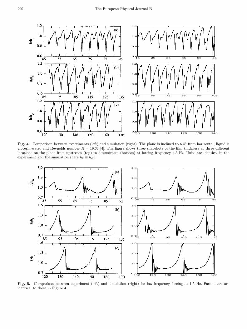
waves at corresponding amplitude levels without trying toadjust the distance to the origin of the flow, in other termsthe abscissa frame is given up to some unknown transla-tion. We first present results corresponding to a multi-peaked wave regime in Figure 4. The form and amplitudeof the numerical wave profiles are in striking agreementwith the experiment. In particular, the small depressionappearing on the primary peak, passing the primary frontand then locking its phase to form a subsidiary peak of thewave-front is evident both in the simulation and in the ex-periment. The modulation of the experimental wave-train
further downstream is also well captured by the simula-tion. Figure 5 compares laboratory and computer resultsfor a low-frequency forcing ending in near-solitary sta-tionary wave-trains. The comparison is again very good,though our numerics predict amplitudes somewhat largerthan in the experiment. The capillary ripples downstreamthe main hump are also slightly more pronounced and thewavelength of the stationary train a little smaller. Theuse of phase-sensitive averaging technique that might havesmoothed the steepest parts of the experimental wave pro-files could partly explain the larger discrepancies observedin Figure 5 when compared to Figure 4. Our results arealso in good agreement with direct numerical simulationsperformed by Ramaswamy et al. (see Figs. 15 and 17 of[19]) who also report larger amplitudes of the fronts.
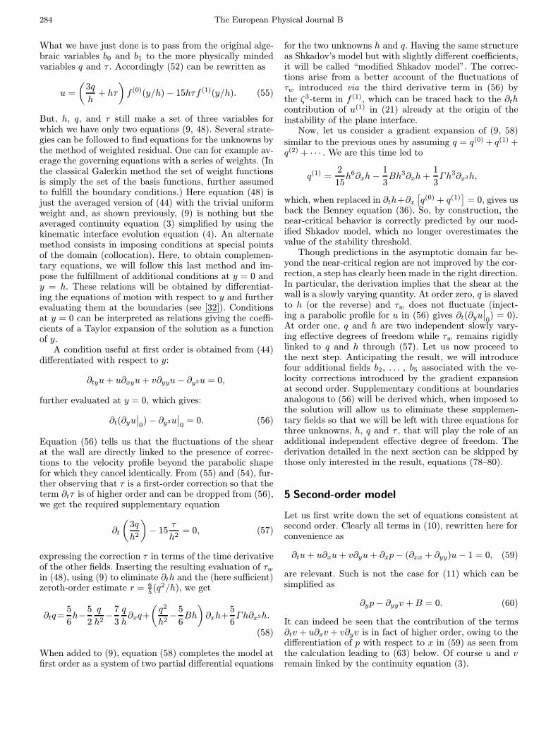
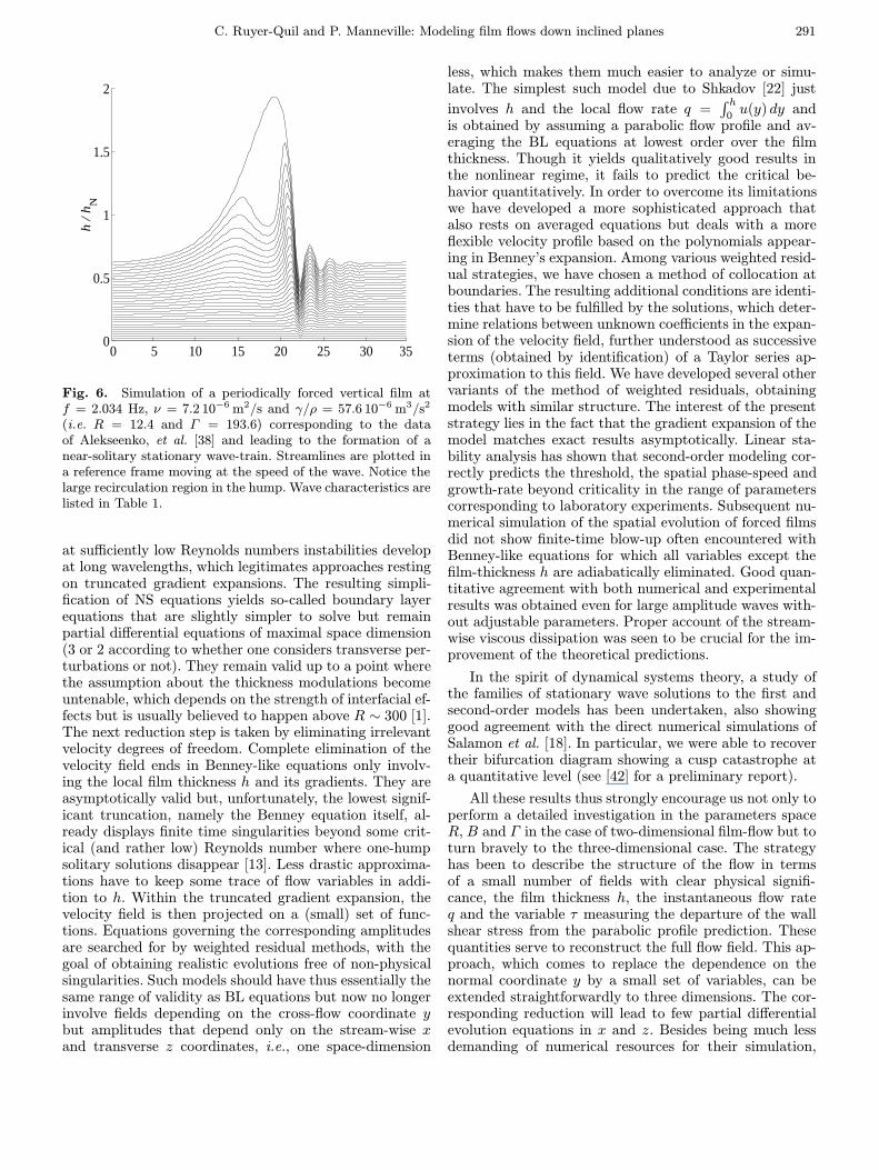
We have also compared our numerical results to ex-perimental ones of Alekseenko et al. [38]. Though theirgeometry was cylindrical, the thickness-to-diameter ratiowas sufficiently large for curvature effects to be negligible.Figure 6 displays the profile and streamlines of a station-ary large-amplitude near-solitary wave for parameters inFigures 5, 6, and Table 1 of [38]. Streamlines show evi-dence of a large recirculation region inside the hump. Suchrecirculations have been inferred from experimental waveprofiles by numerical reconstruction using the NS equa-tions [41] and were already present in solutions to the BLequations [21].
Alekseenko et al. measured the mean film thickness〈h〉, the peak height hmax, the wavelength λ, the speed cof the waves, and the mean surface velocity 〈U〉. Compar-ison with our data is given in Table 1. Though the speedand wavelength were provided with the experimental data,the forcing frequency (the genuine control parameter) wasnot given. The uncertainty about its value may partly ex-plain the differences between experimental and numericalvalues. At any rate, it is remarkable that the mean filmthickness 〈h〉 is much smaller than the Nusselt film thick-ness hN = 0.582 mm for both the experiment and the sim-ulation. The wave profile in Figure 6 is strikingly similarto the sketches in [38]. By contrast, solutions of Shkadov’smodel by Tsvelodub and Trifonov [24] (cf. Fig. 15 of [24]a)and of BL equations by Chang et al. [39,40] exhibit a largenumber of capillary ripples in front of the main hump. Thisfeature can probably be attributed to the lack of disper-sion associated to the second-order stream-wise viscousdissipation terms omitted in BL equations.
8 Conclusion
From a theoretical point of view, the dynamics of filmflows down inclined planes can be studied at differentapproximation levels, ranging from direct simulations ofthe full NS equations to the simple KS equation. Whilethe latter gives an over-simplified picture of the problem,appropriate for near-infinitesimal thickness modulationsof the flat film basic flow at the limit of strong inter-facial effects, the former turn out to be untractable inany realistic 3-dimensional situation, hence the need ofmodeling at some intermediate level. Fortunately enough,
290 The European Physical Journal B
90 100 110 120 130 1400.6
0.8
1.0
1.2
55 65 75 85 95 1050.6
0.8
1.0
1.2
15 25 35 45 55 650.6
0.8
1.0
1.2
Fig. 4. Comparison between experiments (left) and simulation (right). The plane is inclined to 6.4◦ from horizontal, liquid isglycerin-water and Reynolds number R = 19.33 [4]. The figure shows three snapshots of the film thickness at three differentlocations on the plane from upstream (top) to downstream (bottom) at forcing frequency 4.5 Hz. Units are identical in theexperiment and the simulation (here h0 ≡ hN ).
110 120 130 140 150 1600.7
1.0
1.3
1.6
75 85 95 105 115 1250.7
1.0
1.3
1.6
35 45 55 65 75 850.7
1.0
1.3
1.6
Fig. 5. Comparison between experiment (left) and simulation (right) for low-frequency forcing at 1.5 Hz. Parameters areidentical to those in Figure 4.
C. Ruyer-Quil and P. Manneville: Modeling film flows down inclined planes 291
0 5 10 15 20 25 30 35 0
0.5
1
1.5
2h
/ h
N
Fig. 6. Simulation of a periodically forced vertical film atf = 2.034 Hz, ν = 7.2 10−6 m2/s and γ/ρ = 57.6 10−6 m3/s2
(i.e. R = 12.4 and Γ = 193.6) corresponding to the dataof Alekseenko, et al. [38] and leading to the formation of anear-solitary stationary wave-train. Streamlines are plotted ina reference frame moving at the speed of the wave. Notice thelarge recirculation region in the hump. Wave characteristics arelisted in Table 1.
at sufficiently low Reynolds numbers instabilities developat long wavelengths, which legitimates approaches restingon truncated gradient expansions. The resulting simpli-fication of NS equations yields so-called boundary layerequations that are slightly simpler to solve but remainpartial differential equations of maximal space dimension(3 or 2 according to whether one considers transverse per-turbations or not). They remain valid up to a point wherethe assumption about the thickness modulations becomeuntenable, which depends on the strength of interfacial ef-fects but is usually believed to happen above R ∼ 300 [1].The next reduction step is taken by eliminating irrelevantvelocity degrees of freedom. Complete elimination of thevelocity field ends in Benney-like equations only involv-ing the local film thickness h and its gradients. They areasymptotically valid but, unfortunately, the lowest signif-icant truncation, namely the Benney equation itself, al-ready displays finite time singularities beyond some crit-ical (and rather low) Reynolds number where one-humpsolitary solutions disappear [13]. Less drastic approxima-tions have to keep some trace of flow variables in addi-tion to h. Within the truncated gradient expansion, thevelocity field is then projected on a (small) set of func-tions. Equations governing the corresponding amplitudesare searched for by weighted residual methods, with thegoal of obtaining realistic evolutions free of non-physicalsingularities. Such models should have thus essentially thesame range of validity as BL equations but now no longerinvolve fields depending on the cross-flow coordinate ybut amplitudes that depend only on the stream-wise xand transverse z coordinates, i.e., one space-dimension
less, which makes them much easier to analyze or simu-late. The simplest such model due to Shkadov [22] just
involves h and the local flow rate q =∫ h
0u(y) dy and
is obtained by assuming a parabolic flow profile and av-eraging the BL equations at lowest order over the filmthickness. Though it yields qualitatively good results inthe nonlinear regime, it fails to predict the critical be-havior quantitatively. In order to overcome its limitationswe have developed a more sophisticated approach thatalso rests on averaged equations but deals with a moreflexible velocity profile based on the polynomials appear-ing in Benney’s expansion. Among various weighted resid-ual strategies, we have chosen a method of collocation atboundaries. The resulting additional conditions are identi-ties that have to be fulfilled by the solutions, which deter-mine relations between unknown coefficients in the expan-sion of the velocity field, further understood as successiveterms (obtained by identification) of a Taylor series ap-proximation to this field. We have developed several othervariants of the method of weighted residuals, obtainingmodels with similar structure. The interest of the presentstrategy lies in the fact that the gradient expansion of themodel matches exact results asymptotically. Linear sta-bility analysis has shown that second-order modeling cor-rectly predicts the threshold, the spatial phase-speed andgrowth-rate beyond criticality in the range of parameterscorresponding to laboratory experiments. Subsequent nu-merical simulation of the spatial evolution of forced filmsdid not show finite-time blow-up often encountered withBenney-like equations for which all variables except thefilm-thickness h are adiabatically eliminated. Good quan-titative agreement with both numerical and experimentalresults was obtained even for large amplitude waves with-out adjustable parameters. Proper account of the stream-wise viscous dissipation was seen to be crucial for the im-provement of the theoretical predictions.
In the spirit of dynamical systems theory, a study ofthe families of stationary wave solutions to the first andsecond-order models has been undertaken, also showinggood agreement with the direct numerical simulations ofSalamon et al. [18]. In particular, we were able to recovertheir bifurcation diagram showing a cusp catastrophe ata quantitative level (see [42] for a preliminary report).
All these results thus strongly encourage us not only toperform a detailed investigation in the parameters spaceR, B and Γ in the case of two-dimensional film-flow but toturn bravely to the three-dimensional case. The strategyhas been to describe the structure of the flow in termsof a small number of fields with clear physical signifi-cance, the film thickness h, the instantaneous flow rateq and the variable τ measuring the departure of the wallshear stress from the parabolic profile prediction. Thesequantities serve to reconstruct the full flow field. This ap-proach, which comes to replace the dependence on thenormal coordinate y by a small set of variables, can beextended straightforwardly to three dimensions. The cor-responding reduction will lead to few partial differentialevolution equations in x and z. Besides being much lessdemanding of numerical resources for their simulation,
292 The European Physical Journal B
Table 1. Wave characteristics corresponding to Figure 6.Top line: Experimental observations. Bottom line: Numericalresults.
〈h〉 hmax λ c c 〈U〉mm mm mm mm/s qN/〈h〉 qN/〈h〉
0.545 1.12 36 460 2.83 1.270.514 1.13 34 434 3.20 1.30
the study of these equations should give clearer insight inthe physical mechanisms at the origin of secondary three-dimensional instabilities observed in experiments [3].
The modeling of film flows over inclined planes thus of-fers to us a unique opportunity of understanding the tran-sition to turbulence via spatio-temporal chaos in open-flow configurations, hinting at other hydrodynamic prob-lems such as boundary-layer stability.
This work was supported by a grant from the Delegation Ge-nerale a l’Armement (DGA) of the French Ministry of Defense.The authors would like to thank J.M. Chomaz, B.S. Tilley andI. Delbende for stimulating discussions. Thanks are warmlyextended to T. Lescuyer, J. Webert and C. Cossu for theirkind and helpful assistance.
References
1. H.C. Chang, Annu. Rev. Fluid Mech. 26, 103–136 (1994).2. J.M. Floryan, S.H. Davis, R.E. Kelly, Phys. Fluids 30, 983–
989 (1987).3. J. Liu, B. Schneider, J.P. Gollub, Phys. Fluids 7, 55–67
(1995).4. J. Liu, J.P. Gollub, Phys. Fluids 6, 1702–1712 (1994).5. J. Benney, J. Math. Phys. 45, 150–155 (1966).6. S.P. Lin, J. Fluid Mech. 63, 417–429 (1974).7. P.L. Kapitza, S.P. Kapitza, Zh. Ekper. Teor. Fiz. 19, 105
(1949); Also in Collected papers of P.L. Kapitza, edited byD. Ter Haar, pp. 690–709.
8. T. Prokopiou, M. Cheng, H.C. Chang, J. Fluid Mech. 222,665–691 (1991).
9. L.-Q. Yu, F.K. Wasden, A.E. Dukler, V. Balakotaiah,Phys. Fluids 7, 1886–1902 (1995).
10. J.-J. Lee, C.C. Mei, J. Fluid Mech. 307, 191–229 (1996).11. E.A. Demekhin, M.A. Kaplan, V.Y. Shkadov, Izv. Ak.
Nauk SSSR, Mekh. Zhi. Gaza 6, 73–81 (1987).12. Actually, considering only small surface tension effects,
Benney never expressed any truncation of his expansionin the form (36). To our knowledge, the first occurrence of(36) is in: B. Gjevik, Phys. Fluids 13, 1918–25 (1970).
13. A. Pumir, P. Manneville, Y. Pomeau, J. Fluid Mech. 135,27–50 (1983).
14. Y. Kuramoto, T. Tsuzuki, Prog. Theor. Phys. 55, 536(1976); G.I. Sivashinsky, Acta Astronautica 4, 356 (1977);Y. Kuramoto, Prog. Theor. Phys. Suppl. 64, 1177 (1978).
15. O.Y. Tsvelodub, Izv. Ak. Nauk SSR, Mekh. Zh. Gaza 4,142–146 (1980).
16. H.C. Chang, Phys. Fluids 29, 3142–3147 (1986).
17. S.W. Joo, S.H. Davis, S.G. Bankoff, Phys. Fluids. A 3,231–232 (1991).
18. T.R. Salamon, R.C. Armstrong, R.A. Brown, Phys. Fluids6, 2202–2220 (1994).
19. B. Ramaswamy, S. Chippada, S.W. Joo, J. Fluid Mech.325, 163–194 (1996).
20. E.A. Demekhin, I.A. Demekhin, V.Y. Shkadov, Izv. Ak.Nauk SSSR, Mekh. Zhi. Gaza 4, 9–16 (1983).
21. H.C. Chang, E.A. Demekhin, D.I. Kopelevitch, J. FluidMech. 250, 433–480 (1993).
22. V.Y. Shkadov, Izv. Ak. Nauk SSSR, Mekh. Zhi. Gaza 2,43–51 (1967).
23. B.A. Finlayson, The method of weighted residuals and vari-ational principles, with application in fluid mechanics, heatand mass transfer (Academic Press, 1972).
24. (a) Y.Y. Trifonov, O.Y. Tsvelodub, J. Fluid Mech. 229,531–554 (1991); (b) O.Y. Tsvelodub, Y.Y. Trifonov, J.Fluid Mech. 244, 149–169 (1992).
25. H.C. Chang, E.A. Demekhin, D.I. Kopelevitch, Physica D63, 299–320 (1993).
26. The relative importance of inertia and viscous effectsis then characterized by the Reynolds number R =ρuNhN/µ, whereas surface tension γ is measured by theWeber number W = γ/(ρg sin βh2
N ) via the stream-wisecomponent of the gravitational acceleration g sin β.
27. M.K. Smith, J. Fluid Mech. 217, 469–485 (1990).28. C. Nakaya, Phys. Fluids 18, 1407–1412 (1975).29. M. Cheng, H.C. Chang, Phys. Fluids 7, 34–54 (1995).30. H. Schlichting, Boundary-layer theory (McGraw-Hill,
1955).31. Polynomial f (1) is chosen such that df (1)/dζ|0 = 0,
d3f (1)/dζ3|0 = −1. This choice is in line with those madefor the higher degree polynomials used later, which are inturn justified by the fact that we use collocation residualsat the boundary points ζ = 0 and ζ = 1.
32. J. Villadsen, M.L. Michelsen, Solution of differential equa-tion models by polynomial approximation (Prentice-Hall,1978).
33. J. Liu, J.D. Paul, J.P. Gollub, J. Fluid Mech. 250, 69–101(1993).
34. C.S Yih, Phys. Fluids 6, 321–334 (1963).35. E.L. Allgower, K. Georg, Numerical continuation methods
(Springer-Verlag, 1990).36. Namely, 4
5k3 + i 2
175Rk4 in A(k), − 9
5k2 − i 29
350Rk3 in B(k),
and i 970Rk2 in C(k).
37. R.D. Richtmeyer, K.W. Morton, Difference methods forinitial value problems (Interscience, 1967).
38. S.V Alekseenko, V.Y. Nakoryakov, B.G. Pokusaev, AIChEJ. 31, 1446–1460 (1985).
39. H.C. Chang, E.A. Demekhin, E. Kalaidin, J. Fluid Mech.294, 123–154 (1995); AIChE J. 42, 1553–1568 (1996).
40. Demekhin et al. have shown that the set of control param-eters can be reduced to a single reduced Reynolds numberδ for the BL equations and a vertical plane [20]. The soli-tary wave in Figure 6 corresponds to δ = 0.056 and speedc = 7.33 uN , to be compared with results in [39].
41. F.K. Wasden, A.E. Duckler, AIChE J. 35, 187–195 (1989).42. C. Ruyer-Quil, P. Manneville, Transition to turbulence of
fluid flowing down an inclined plane: Modeling and sim-ulation, Proceedings of the 7th European Turbulence Con-ference, Saint Jean Cap Ferrat, June 30-July 3, 1998, inAdvances in Turbulence VII , edited by U. Frisch, (Kluwer,1998), pp. 93-96.