evaluation and optimization of seismic networks and algorithms for earthquake early warning – the...

Evaluation and optimization of seismic networks and algorithmsfor earthquake early warning – the case of Istanbul (Turkey)

Adrien Oth,1 Maren Böse,2 Friedemann Wenzel,3 Nina Köhler,3,5 and Mustafa Erdik4

Received 4 February 2010; revised 1 June 2010; accepted 2 July 2010; published 28 October 2010.

[1] Earthquake early warning (EEW) systems should provide reliable warnings as quicklyas possible with a minimum number of false and missed alarms. Using the example of themegacity Istanbul and based on a set of simulated scenario earthquakes, we present anovel approach for evaluating and optimizing seismic networks for EEW, in particular inregions with a scarce number of instrumentally recorded earthquakes. We show that, whilethe current station locations of the existing Istanbul EEW system are well chosen, itsperformance can be enhanced by modifying the parameters governing the declaration ofwarnings. Furthermore, unless using ocean bottom seismometers or modifying the currentEEW algorithm, additional stations might not lead to any significant performance increase.

Citation: Oth, A., M. Böse, F. Wenzel, N. Köhler, and M. Erdik (2010), Evaluation and optimization of seismic networks andalgorithms for earthquake early warning – the case of Istanbul (Turkey), J. Geophys. Res., 115, B10311,doi:10.1029/2010JB007447.

1. Introduction

[2] Earthquake early warning (EEW) represents animportant tool for seismic risk mitigation, since it fills the gapbetween long‐term hazard assessment [e.g., Petersen et al.,2008] and postevent rapid response tools [Wald et al., 2003],allowing for preventive action such as defining appropriatebuilding codes, and facilitating efficient search and rescueoperations, respectively. In between these, EEW systemsoperate during the co‐seismic stage of an earthquake byproviding short‐term (in the order of a few to several tens ofseconds) warnings of impending strong ground shaking at agiven user site, for instance a heavily populated metropolitanarea.[3] The usefulness of EEW systems, however, strongly

depends on their ability to provide both fast and reliablewarnings. As a general rule, there is a trade‐off between thesetwo requirements [Böse et al., 2008]. Providing warningsmore quickly leads to a loss of accuracy due to the smalleramount of seismological information available, whereas, forthe same reason, a higher degree of reliability involves a lossof warning time.[4] Several algorithms for tackling the EEW problem

exist [Kanamori, 2005; Allen et al., 2009b]. The types of

information they provide can differ: while the EEW systemsoperational in, e.g., Mexico [Espinosa‐Aranda et al., 1995]and Istanbul [Erdik et al., 2003] provide rather qualitativewarnings (basically stating whether strong ground motion isexpected or not), others like the one recently implementedby the Japan Meteorological Agency [Kamigaichi et al.,2009] or those currently undergoing real‐time testing inCalifornia [Allen et al., 2009a; Böse et al., 2009; Cua et al.,2009] provide quantitative regional ground motion estimates(for instance of peak ground velocity), resulting in so‐calledalert maps. No matter which methodology is chosen, theimplementation of an EEW system requires either theexistence of a seismic network not specifically designed forEEW (which may, therefore, be supplemented by a givennumber of sensors) or the design of an entirely new network.Furthermore, each EEW methodology involves automatedrules to decide if a warning shall be issued or not. Theserules need a certain number of system parameters that haveto be set appropriately.[5] Efficient EEW aiming at both fast and accurate

warnings thus requires an optimally designed seismic net-work (or supplementation of an existing one) and the bestset of algorithm parameters. Optimum network design is notstraightforward, since it strongly depends on the seismo-tectonic setting of the region of interest, funding availability(which directly translates into sensor and infrastructureavailability), and other constraints. These requirements mightalso differ for different EEW algorithms.[6] Designing EEW systems thus requires systematic

evaluation and optimization. While significant advanceshave been made in understanding the general feasibilityand limitations of EEW algorithms [Allen et al., 2009b, andreferences therein] and communication technology [Böseet al., 2009], little attention has been paid to optimizationso far. In order to contribute to this need, we developed a

1European Center for Geodynamics and Seismology, Walferdange,Grand‐Duchy of Luxembourg.

2Seismological Laboratory, California Institute of Technology,Pasadena, California, USA.

3Geophysical Institute, Karlsruhe Institute of Technology (KIT),Karlsruhe, Germany.

4Kandilli Observatory and Earthquake Research Institute, Departmentof Earthquake Engineering, Bogazici University, Istanbul, Turkey.

5Now at Swiss Re Europe S.A., Niederlassung Deutschland,Unterföhring, Germany.

Copyright 2010 by the American Geophysical Union.0148‐0227/10/2010JB007447

JOURNAL OF GEOPHYSICAL RESEARCH, VOL. 115, B10311, doi:10.1029/2010JB007447, 2010

B10311 1 of 22

http://dx.doi.org/10.1029/2010JB007447

systematic optimization technique for EEW systems, and wedemonstrate this approach on the example of the IstanbulEEW system. Starting with the evaluation of the currentIstanbul EEW system, we then investigate the effect ofchanges in the algorithm parameters currently used in thesystem and finalize our discussion by optimizing the seismicnetwork design using a microgenetic algorithm and a costfunction designed to compare the performance of differentEEW system variants.

2. The Current Istanbul Earthquake EarlyWarning System (IEEWS)

[7] The seismic risk in Istanbul is considerable [Hubert‐Ferrari et al., 2000] caused by its proximity to the NorthAnatolian fault below the Sea of Marmara [Armijo et al.,2002; Le Pichon et al., 2002] and its dense population.The probability for an earthquake of magnitude 7 or largerbeneath the Sea of Marmara in the time span 2004–2034 hasbeen calculated to be 35%–70% [Parsons, 2004]. Inresponse to this threat, the Istanbul EEW system (IEEWS)was installed in 2002 [Erdik et al., 2003]. The IEEWScomprises ten real‐time 3‐component accelerometric sen-sors distributed along the shoreline of the Sea of Marmara(Figure 1). The current system is based on three trigger

thresholds that need to be exceeded at three or more sensorswithin 5 seconds before a warning is declared. The currentthresholds are 0.02, 0.05, and 0.1 g, corresponding towarning classes I, II, and III, respectively [Erdik et al.,2003]. The trigger thresholds need to be large enough toavoid false alarms caused by small earthquakes and smallenough to provide reliable warnings for moderate to largeevents with strong shaking, without missing importantalarms. The current values have been chosen based onexpert judgment, without a clear quantitative relationship tothe expected ground motions in Istanbul.

3. Finite Fault Stochastic Seismogram Simulation

[8] Our optimization approach requires recordings ofearthquakes that are representative for the seismic activity inthe given region, including both small and large magnitudeearthquakes on all potentially active faults. Alike in mostregions in the world, respective data in the Marmara region isvery sparse, and therefore the simulation of synthetic seis-mograms from sets of scenario earthquakes is unavoidable.[9] In order to assess the performance of the IEEWS, we

therefore constructed a massive database of 36,000 syntheticseismograms from 150 scenario earthquakes (Figures 1and 2) along five fault segments beneath the Sea of

Figure 1. Epicenters of the 180 simulated scenario earthquakes in the Marmara region around Istanbul.150 events are simulated along five fault segments in the Sea of Marmara (see Figure 3a) and 30 arerandomly distributed around the city. This set of scenario earthquakes covers a wide range of potentialseismic events in the Sea of Marmara region and is used to evaluate the performance of different EEWsystems. The ten stations of the current Istanbul EEW system (IEEWS) are shown as yellow triangles(three of them located on the Prince’s Islands southeast of Istanbul), and the user site for warnings,downtown Istanbul, is marked with a red square.

OTH ET AL.: OPTIMIZING SEISMIC NETWORKS FOR EEW B10311B10311

2 of 22

Marmara (Figure 3a) [Böse et al., 2008] with momentmagnitudes ranging from 4.5 to 7.5 using the extendedfinite‐fault stochastic simulation technique (FFSST) forseismicP‐ and S‐wavemotion [Beresnev and Atkinson, 1997;Böse, 2006; Böse et al., 2008]. Additionally, 30 randomlydistributed events with magnitudes between 4.5 and 5.0were considered. Seismograms were calculated on a grid ofpotential station locations with 0.1° grid spacing in latitudeand longitude surrounding Istanbul (128 onshore and112 offshore sites; Figure 3a), as well as at the selected usersite for warnings, downtown Istanbul. The 112 offshorelocations within the Sea of Marmara were considered aspotential sites of ocean bottom seismometers (OBS).[10] The FFSST divides the fault plane of an earthquake

into a number of subfaults, each of which is assumed to

Figure 2. Example for a simulated acceleration time his-tory in Istanbul from a magnitude 6.9 earthquake with anepicentral distance of 33 km. Shown are the typical featuresof interest in EEW, the P‐ and S‐wave onsets, as well as thepeak ground motion.

Figure 3. (a) Comparison of sensor locations of the current Istanbul EEW system (IEEWS) and opti-mized system with ten sensors. The grey open triangles represent the grid of potential onshore stationlocations at which synthetic seismograms are generated from all scenario earthquakes. Three grid pointswere included on the Prince’s Islands southeast of Istanbul, exactly co‐located with the current stations.The five segments on which the set of scenario earthquakes were simulated are shown as black lines.Segment 4 represents joint ruptures of segment 1, 2, and 3. (b) Classification errors for the currentIEEWS. Each bar shows the percentage of events of the respective class (0‐III) in the simulated set ofearthquakes. The different gray scales indicate how many of the events within a given class have beencorrectly classified (darkest), or have been under‐estimated or overestimated by one, two or three levels,respectively. Note the large amount of misclassified events of class I (especially those misclassified bytwo levels) and II. These events are overestimated to be class III, i.e., highly damaging, earthquakes.(c) Same as (b) for the optimized system of ten stations. Note the strong increase of correctly classifiedearthquakes.


3 of 22

behave as a point source radiating seismic waves. For eachof these subfaults, the ground motion at the observation siteis calculated using appropriate models for the velocity struc-ture, source spectral shape, and geometrical and anelasticattenuation [Böse, 2006; Böse et al., 2008]. Site amplifica-tion effects were estimated from the topographic slope thatcan be considered as a rough proxy for the shear wavevelocity of the uppermost 30 m, VS30 [Wald and Allen,2007]. The corresponding data were downloaded from theglobal VS30 map server provided by the United States Geo-logical Survey at 30 arc‐sec resolution (http://earthquake.usgs.gov/vs30/). From the VS30 estimates, each potentialstation location was assigned to one of the National Earth-quake Hazard Reduction Program (NEHRP) site classes andan average site amplification function (considering linearsoil behavior) for the respective class was used [Boore andJoyner, 1997]. Even though this approach provides firstorder estimates of site amplification only and considerabledeviations might exist from this average amplification at agiven site, it is at present the best approach to include asystematic estimate of site effects in ground motion simu-lations at a large number of sites. Of course, if empirical siteresponse studies or borehole data were available, they couldalso be used to characterize site response at these locations.Most grid points were associated with NEHRP C siteresponse class, only few of them as NEHRP B or D. For thegrid of potential OBS locations beneath the Sea of Marmara,the topography‐based approach cannot be used and weconsidered these grid points as NEHRP C sites.[11] The final seismogram from a given earthquake at a

given site is obtained by a summation of the contribu-tions from the different subfaults with appropriate timelags to account for the rupture propagation and differentlengths of subfault‐receiver paths, and appropriate weightscorresponding to the (variable) radiation strength of eachsubfault, accounting for the typically observed slip hetero-geneity [Somerville et al., 1999]. Amplitude levels as wellas frequency content and duration of ground motion werecalibrated with observations from the Izmit and Düczeearthquakes and from a small event (M 4.3) which occurredin the Sea of Marmara, as well as to agree with typicalground motion attenuation relationships [Böse, 2006]. Theslip distributions on the fault were randomly generated. Boththe random phase of the stochastic procedure and the slipdistribution have significant impact on the generated timehistories. Therefore, we obtain somewhat different warningtimes for different realizations. Considering in this study alarge dataset of different scenario events, we assume to givea reasonable reflection of the aleatory variability of any(large) set of recorded ground motions.[12] The synthetic seismograms were not perturbed

through adding noise to the traces. Visual inspection ofaccelerometric data recorded by the surface sensor of theAtaköy vertical array located in the western part of Istanbul[Parolai et al., 2009] not very far away from one of thecurrent IEEWS stations show for instance a time domainnoise level of the order of 0.1 mg, which is two orders ofmagnitude lower than the lowest trigger threshold we areconsidering (0.01 g). Therefore, seismic noise should nothave a serious impact on the discrimination between smalland large events based on time domain trigger thresholdexceedance.

[13] As a representation of the current IEEWS, the gridnodes closest to the current sensor locations were picked.Since in the current IEEWS methodology, time domainamplitude information of the entire seismograms, ratherthan phase information of the early P‐wave signals is beingused, stochastically simulated ground motions calibrated torealistic amplitude levels are suitable synthetic data in thiscase.

4. Optimization Approach

[14] With the database described above, we have now athand a set of scenario earthquakes for which an EEW sys-tem for Istanbul should show the best possible performance.As mentioned at the beginning of the previous section, it isof highest relevance that these scenario earthquakes coverall faults around Istanbul that might be capable of generatingearthquakes posing a hazard to the city. If this were not thecase, the optimally designed EEW system would not be ableto appropriately deal with events occurring in these uncon-sidered source regions, which in turn could lead to missingimportant alarms. In the case of Istanbul, the seismic hazardis practically entirely determined by the branches of theNorth Anatolian fault beneath the Sea of Marmara, whichare, according to current knowledge, the only structures inthe immediate vicinity of Istanbul that can support suchlarge earthquakes. Therefore, by defining a set of scenarioevents providing a detailed coverage of these potential sourceregions throughout the entirety of the Sea of Marmara, weare confident not to have forgotten any relevant source zonefor the Istanbul EEW system. The 30 randomly distributedsmaller scenario events account for the possibility that asmaller earthquake might also occur off the North Anatolianfault as well.[15] The optimization results presented in this article

depend of course on the dataset of simulated seismogramsused for this purpose. Due to the large number of parametersinvolved in the calculation of the latter and limited com-putational resources, it is impossible to provide a detailedanalysis of the impact of each of these parameters on thefinal optimization results. However, tests using subsetsof the database led to stable results very similar to thoseobtained using the full dataset, which are described below.[16] Once this set of representative scenario earthquakes is

defined, there are three cases that should be considered.

4.1. Performance Evaluation of An ExistingEEW System

[17] If sensors are in place and the algorithm and itsparameters specified, then the system performance of anEEW system can be evaluated for a set of scenario events.First attempts of such a performance evaluation haverecently been made in southern Italy [Zollo et al., 2009],with a particular interest in finite‐fault effects.[18] For a proper evaluation of the IEEWS, it is necessary

to provide a quantitative relationship between groundmotion in Istanbul (user site for warnings) and each warningclass. Therefore, we considered earthquakes causing peakground acceleration (PGA) in Istanbul of 0.02 g ≤ PGA <0.07 g as class I events (i.e., for these events, a class Iwarning should be declared), with 0.07 g ≤ PGA < 0.12 g asclass II, and with PGA ≥ 0.12 g as class III events. For this


4 of 22

classification, we followed the rule of thumb that groundmotions with PGA > ∼0.1 g are considered as potentiallyseriously damaging [Anderson, 2003], and with our choice,class I and II each cover a range of 0.05 g. Earthquakes withPGA < 0.02 g are considered as class 0 events, i.e., nowarning should be declared. Note that these class definitionthresholds simply determine what warning class should bedeclared by the EEW system for a given event in the optimalcase, and they are different from the trigger thresholds of theEEW system (which determine what warning class is reallydeclared by the considered system). The choice of theseclass definition thresholds is to some degree arbitrary andshould be adapted to the desired system sensitivity or users’needs if known. Note that for an event of warning class III,class I and II alarms will be declared first.[19] For each simulated scenario earthquake, the available

warning time for a given class is calculated as the differencebetween the time when the class definition threshold inIstanbul is first exceeded (e.g., for class II when the groundmotion in Istanbul first exceeds 0.07 g) and the time whenthe trigger threshold of that class has been exceeded at threesensors within 5 seconds (e.g., for the current IEEWS,0.05 g for class II).[20] The evaluation of the performance of the current

system can then be done by considering the availablewarning times for all scenario earthquakes as well as thenumber of correctly and incorrectly classified events.Whether or not the performance of the system is consideredacceptable depends on the criteria set by the user of thesystem. Concerning the current IEEWS, as mentioned ear-lier, the current trigger thresholds are set to 0.02, 0.05, and0.1 g, corresponding to warning classes I, II, and III,respectively [Erdik et al., 2003], and these are smaller thanthe chosen class definition thresholds in Istanbul in our case.Hence, as the sensors of the current system are of coursecloser to the fault segments beneath the Sea of Marmarathan downtown Istanbul and since obviously ground motionamplitudes decrease with increasing distance, it can beexpected that with these class definition thresholds inIstanbul, the current system might provide a relatively largenumber of false alarms, as we show later. Therefore, weexpect that the trigger thresholds would need to be increasedfor the current system in order to increase its performancewith the used definition of warning classes.

4.2. Evaluation and Optimization of EEW AlgorithmParameters (Here: Trigger Thresholds)

[21] The parameters of an EEW algorithm can be evalu-ated and optimized by applying the algorithm to the set ofscenario events under the variation of the parameters. Whatmakes this step nontrivial is the fact that, as soon as differentvariants of the EEW system are compared with each other,it is necessary to define an appropriate cost function (orobjective function), whose value for a given EEW systemvariant depends both on the available warning times andclassification performance (taking into account also theeffects of false and missed alarms) for all scenario events.[22] Using the cost function described in the following

section, we performed a systematic search over differenttrigger threshold combinations while keeping the sensorlocations of the current IEEWS fixed in order to find thelowest cost combination of the trigger thresholds.

4.3. Evaluation and Optimization of a Seismic Network

[23] The evaluation and optimization of a new seismicnetwork is the most challenging task and involves eithersupplementing an existing network with additional sensorsor designing a completely new network. It requires thedetermination of both optimal locations for the (additional)sensors and the best system parameters at the same time.Depending on their number, the parameters may be opti-mized by simple search over different combinations ofthem; however, this becomes difficult (if not impossible) ifsensor locations have to be also optimized at the same time,because for the latter usually a large number of possiblesolutions exist. For this reason and because this problemcannot be formulated as a simple linear inverse problem,nonlinear optimization techniques such as simulated anneal-ing or genetic algorithms come into play.

5. Cost Function and Microgenetic Algorithm

5.1. The Cost Function

[24] In every optimization problem, the choice of the costfunction is most essential for evaluating the quality of agiven set of model parameters. A model performing bestconsidering one cost function may not remain to be the bestwhen considering another one. The definition of an appro-priate cost function is not straightforward in this casebecause we are not fitting synthetic data calculated with aset of model parameters to observations in the classicalsense [Tarantola, 2005]. Instead, we need a cost functionthat is able to find the EEW system configuration withlargest warning times at the highest level of reliability (i.e.,best classification performance). Since there is usually atrade‐off between these two requirements [Böse et al.,2008], the cost function has to find the best compromisebetween them.[25] Furthermore, a class II event, e.g., should be char-

acterized by two warning times, one for class I and one forclass II, because the exceedance of the higher triggerthreshold requires also the exceedance of the threshold ofthe lower class. In the case of erroneous classification asclass I event, no warning time of class II is available thatcould be evaluated. Instead, the effect of the missed alarm ofclass II has to be accounted for in the cost function. Asimilar problem arises in the case of false alarms, i.e., if thewarning class declared is too high.[26] We have developed a cost function to cope with these

problems:

cost ¼XNevt

i¼1

Wi L � ð1� KÞ � sigmoidðtwarn;i; tcenter; SÞ þ K� � ð1Þ

with

sigmoidðtwarn;i; tcenter; SÞ ¼ 1� 1

1þ exp �Sðtwarn;i � tcenterÞ� � :

ð2Þ

twarn,i represents the available warning time for the ith event,and tcenter is a fixed center time of the sigmoid function, i.e.,the time where the sigmoid function takes the value 1/2.The sigmoid in (2) equals one for twarn � tcenter (small,


5 of 22

respectively, insufficient warning time), 1/2 for twarn =tcenter, and zero for twarn � tcenter (large warning time)(Figure 4). K is either zero if the estimated class is equal tothe expected class (i.e., correct classification) or one other-wise; L is a constant of value one for expected class I, II, orIII events and zero for expected class 0 events. Finally, S isthe spread parameter of the sigmoid function that governshow strongly it spreads over time and Wi is the weightassociated with event i. By minimizing the cost function inequation (1), we maximize at the same time both the numberof correct classifications and the available warning times.The final cost for the EEW system is thus given by theweighted sum (normalized to unity) of these individualearthquake costs, with weights chosen such that theexpected warning classes are equally weighted rather thanthe individual events.[27] The cost of each earthquake in the dataset is set to

the maximum value of one if it is not correctly classified(K = 1). Warning times are evaluated only for correctlyclassified events (K = 0). Correct classification is consideredas a fundamental precondition before warning times areevaluated because large numbers of false and missed alarmsare socioeconomically unacceptable even if the warningtimes for the remaining correctly classified events areexcellent.[28] For class II and class III events, only the warning

times of class II, respectively, class III are considered (andnot the warning times of the lower classes that are auto-matically declared as well) since the warning time that reallymatters is the one for the final class. The parameter L (L = 0for class 0 events, L = 1 otherwise) is needed to deal withthe events of class 0, where no warning by the systemshould be declared. If such an event is correctly classified,there is no warning time to be evaluated, and the individualcost for this specific event will be zero because K = 0. If aclass 0 event is overestimated and leads to a false alarm, the(nonweighted) individual cost for that event will be one,since K = 1 and L = 0 and the available warning time will

not be evaluated since no warning is desired for such anevent.[29] The weighting of events in equation (1) is necessary

because the number of class 0 events is much larger than thenumber of class I, II, or III events. This is also to beexpected in reality since small events that should not triggerthe system are more abundant than large ones that should doso. If all earthquakes would be equally weighted, the class0 events would clearly dominate the evaluation scheme.Therefore, we chose to assign equal weights to the fourclasses of expected ground motion in Istanbul rather than toall events:

Wi ¼ 1

4� 1

NclassðiÞ; ð3Þ

where Nclass(i) is the total number of earthquakes falling intothe warning class of event i (N0 = 79, NI = 46, NII = 28 andNIII = 27 for classes 0, I, II, and III, respectively). The sumof the weights for all events equals one.[30] Instead of using a sigmoid function in equation (1),

the warning times could also be evaluated with a linearfunction, which might appear more logical at first glance.However, for a given EEW application, the usefulness of thewarning time is not necessarily steadily increasing withincreasing warning time. For instance, if a warning time of5 seconds is enough to cut the flow of a gas pipeline, theavailability of 15 seconds does not provide an enormousadditional gain for this specific application. In such a case, itis preferable to design an EEW system that provides overallsomewhat shorter warning times (as long as they are largerthan 5 seconds in that case), but is highly robust, rather thana system providing very large warning times for a subset ofevents, but with lower overall reliability. For this reason, wedecided to use a sigmoid function in order to evaluate thewarning times. The center time tcenter of the sigmoid inequation (1) can be chosen based on the application in mindand the spread of the function based on the tolerance ofwarning times lower than tcenter.[31] For the demonstration of our approach on the

example of Istanbul, we chose tcenter based on considerationof the local seismotectonic setting. For each event, weassumed that at every onshore grid point a hypotheticalseismic station were available. For a given trigger threshold,we determined the time when this trigger threshold was firstexceeded at three hypothetical stations and considered thistime as the earliest theoretically possible time when awarning can be declared. This gave us the largest theoreti-cally possible warning times for all events and warningclasses in the database.[32] For trigger thresholds in the range of 0.01–0.15 g, the

largest theoretically possible warning times range between 0and 20 seconds with a median of about 7–8 seconds for allclasses (Figures 5a–5c). A further increase of the triggerthreshold to, for instance, 0.2 g leads to a decrease of themedian to about 5 seconds for class III events (Figure 5d).Since we cannot exclude that the optimal trigger thresholdfor class III might be located in the upper part of the con-sidered range (0.01–0.32 g) and these largest theoreticallypossible warning times cannot be reached with a realisticnetwork of a much smaller number of sensors, we decided touse tcenter = 6 seconds for class I and II warning times and

Figure 4. Sigmoid function as defined in equation (2)for the evaluation of class I and II events (black line, withtcenter = 6 seconds) and class III (gray line with tcenter =4 seconds).


6 of 22

tcenter = 4 seconds for the evaluation of class III warningtimes. The spread parameters S of the sigmoid function wasset such that the function in equation (2) reached the plateauvalue of one (maximum nonweighted individual cost) forany warning time lower than 0 seconds. With these defini-tions, a warning time of class I and II is assigned zero cost ifit is larger than about 12 sec (since then there is no costreduction anymore), and one of class III is regarded asoptimal if it is larger than 8 sec. We also investigated theinfluence of choosing larger tcenter values (for instancetcenter = 8 seconds for class I and II and tcenter = 6 secondsfor class III).

5.2. The Microgenetic Algorithm (MGA) OptimizationProcedure

[33] For the optimization of sensor locations and triggerthresholds (i.e., finding sensor locations and trigger thresh-olds providing minimum cost as defined above), we used a

microgenetic algorithm (MGA) [Krishnakumar, 1989].MGAs belong to the general class of genetic algorithms(GAs) [Goldberg, 1989], which are guided search techniquesbased on evolutionary principles (survival of the fittestindividuals, genetic recombination of these, and mutation) tofind models that minimize a given cost function.[34] Typically, a GA starts with a random population of

test models, called chromosomes, which can for instanceconsist of binary representations of the different modelparameters (in that case, each bit is usually termed as agene). Each chromosome is evaluated and associated with acost. The fittest chromosomes (i.e., those with lowest cost)are allowed to mate and exchange genetic information via acrossover operator, which leads to a given number of off-spring. These offspring are then subjected to a mutationoperator and finally form the new generation, and the pro-cess restarts (for further details on genetic operators, see,e.g., Haupt and Haupt [1998]). Over many generations, the

Figure 5. Distribution of the largest theoretically possible warning times considering a hypothetical net-work with stations at all onshore grid points, thus covering the entire region of interest, for four differenttrigger thresholds ((a) 0.05 g, (b) 0.10 g, (c) 0.15 g, (d) 0.20 g). For each of these trigger thresholds, theselargest theoretically possible warning times have been computed for all three warning classes and themedian of each distribution is indicated with a dashed line.


7 of 22

population will lose diversity and converge to a state ofminimum cost, in our case corresponding to optimum sensorlocations and trigger thresholds. However, no guarantee canbe given that the global minimum will be found, so that acareful analysis of the variability of solutions obtained fromseveral independent runs of the code is indispensable.[35] As a general rule, the population size of a genetic

algorithm should scale exponentially with the number ofgenes within each chromosome in order to maintain a rea-sonable degree of genetic diversity over many generations,so that the algorithm does not prematurely converge into alocal minimum [Goldberg, 1989]. If the number of modelparameters and hence the length of the chromosomesincreases above a certain level, this may lead to populationsizes which are computationally unacceptable since theconvergence of very large populations may need a verylarge number of cost function evaluations and a lot ofmemory.[36] A MGA is a variant of a GA which avoids these

problems and has been proven to perform equally well oreven better than classic GAs for a range of optimizationproblems [e.g., Krishnakumar, 1989; Carroll, 1996; Abu‐Lebdeh and Benekohal, 1999; Alvarez, 2002]. An MGAworks very similarly to a classic GA, except for the fact thatit uses very small population sizes. Such small populationsare not able to maintain genetic diversity for very long andgenerally converge within few generations. When thealgorithm has converged, the population is reinitialized to arandom state except for the fittest chromosome, whichpasses unchanged. Hence, the missing genetic diversity iscompensated by many restarts of the algorithm. A MGAusually converges with fewer cost function evaluations thana classic GA does.[37] In our case, the chromosomes consist of the sensor

locations for an EEW system with a given number of stationsand the set of three trigger thresholds. For the sensor loca-tions, we searched the 128 grid points for potential onshorestations and, if OBS were considered, the 112 offshore gridpoints within the Sea of Marmara for the location of thesesensors. The search range for the three trigger thresholdswas 0.01–0.32 g, with intervals of 0.01 g.[38] We used a MGA with binary encoding, a population

size of fifteen chromosomes, uniform crossover with aprobability Pcross = 0.95 and no mutation. The algorithmwas defined to have converged when less than 5% of thegenes differed from one chromosome to another within onegeneration and in that case, the population was reinitialized.[39] The algorithm was run ten times for each investigated

case with different random seed for 5,000 generations. Forthe first time after 1,000 generations and then every 500, wechecked whether the fittest chromosome had improved bymore than 1%. If this was not the case, the algorithm wascompletely reinitialized, including the fittest chromosome.With this procedure, we assess in each case a total of morethan 700,000 EEW system configurations and put a strongemphasis in sampling the search space in order to obtain aset of best solutions rather than one single optimum oneonly. In each case, the 1,000 best solutions were analyzed toassess the stability of the minimum cost EEW system con-figuration, both in terms of station distribution and triggerthresholds.

[40] We finally note that our current scheme for evalua-tion and optimization assumes a fully functional EEWsystem. Failures of individual stations are significantlycomplicating the situation and a full treatment of this prob-lem would need to take into account random station failuresduring the simulated scenario earthquakes. One solution todeal with this problem would be calculating, for each stationconfiguration, the cost for the system when a given numberof stations (e.g., two) fail, repeat this calculation for thefailure of all possible subsets of that number of the network,and use, for instance, the cost of the worst case or themedian value as final estimate for the cost of this particularsystem configuration. However, this procedure would involvea strong increase in computation time, since the evaluationof one EEW system configuration would need several oreven many cost function evaluations, increasing severelywith increasing number of stations and potential stationfailures.

6. Results and Discussion

6.1. Performance Evaluation of the Current IEEWS

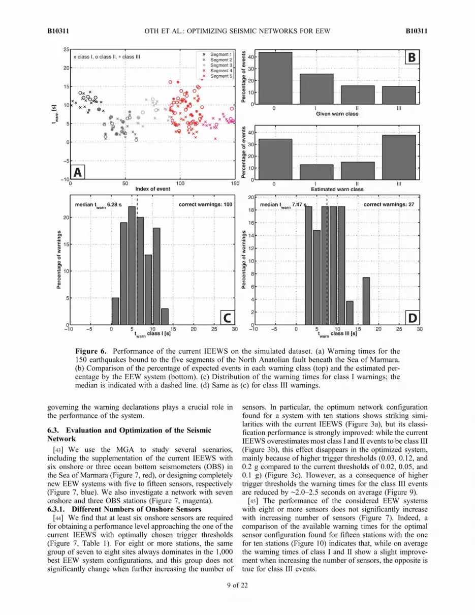
[41] Using the simulated ground motion time series, wefind that the available warning times for the current IEEWSrange from 0 to 17 seconds (Figure 6a). On average,∼7.5 seconds warning time are available of events in class III(i.e., most severe ground shaking in Istanbul). However, aserious drawback of the current IEEWS is that it tends toproduce a large number of false class III alarms (∼2.5 timesmore class III warnings than expected), and thus stronglyoverpredicts the ground motion level in Istanbul (Figure 6).In terms of the previously defined classification of severityof shaking in Istanbul, only ∼54% of all events are correctlyclassified by the IEEWS (Figure 7, Table 1). Note that thisresult depends on the previously discussed choice of classdefinition thresholds for the ground motions in Istanbulassigning each event to class 0, I, II, or III (i.e., on thechoice of what level of ground motion is considered assevere). Thus the current IEEWS is highly sensitive to smalland moderate ground shaking, declaring alarms of thehighest category also for many events with PGA in Istanbulwell below 0.1g.

6.2. Evaluation and Optimization of TriggerThresholds

[42] From a systematic search over different triggerthreshold combinations while keeping the sensor locationsof the current IEEWS fixed, we find that the performance isbest if the trigger thresholds are set to 0.03, 0.12, and 0.16 g(compared with 0.02, 0.05, and 0.1 g of the current IEEWS).We searched the trigger threshold range 0.01–0.32 g withincrements of 0.01 g and under the constraint that the classII and III thresholds are larger than the class I and II ones,respectively. These new thresholds lead to an overall costreduction of ∼23% as compared with the current IEEWS(Figure 7, Table 1). Though the warning times are somewhatdecreased due to the higher trigger thresholds for classes IIand III (Figure 8), more than 80% of all events are nowcorrectly classified (Figure 7). This outcome clearly showsthat, for a given EEW system with given seismic networklayout, the appropriate choice of the system parameters


8 of 22

governing the warning declarations plays a crucial role inthe performance of the system.

6.3. Evaluation and Optimization of the SeismicNetwork

[43] We use the MGA to study several scenarios,including the supplementation of the current IEEWS withsix onshore or three ocean bottom seismometers (OBS) inthe Sea of Marmara (Figure 7, red), or designing completelynew EEW systems with five to fifteen sensors, respectively(Figure 7, blue). We also investigate a network with sevenonshore and three OBS stations (Figure 7, magenta).6.3.1. Different Numbers of Onshore Sensors[44] We find that at least six onshore sensors are required

for obtaining a performance level approaching the one of thecurrent IEEWS with optimally chosen trigger thresholds(Figure 7, Table 1). For eight or more stations, the samegroup of seven to eight sites always dominates in the 1,000best EEW system configurations, and this group does notsignificantly change when further increasing the number of

sensors. In particular, the optimum network configurationfound for a system with ten stations shows striking simi-larities with the current IEEWS (Figure 3a), but its classi-fication performance is strongly improved: while the currentIEEWS overestimates most class I and II events to be class III(Figure 3b), this effect disappears in the optimized system,mainly because of higher trigger thresholds (0.03, 0.12, and0.2 g compared to the current thresholds of 0.02, 0.05, and0.1 g) (Figure 3c). However, as a consequence of highertrigger thresholds the warning times for the class III eventsare reduced by ∼2.0–2.5 seconds on average (Figure 9).[45] The performance of the considered EEW systems

with eight or more sensors does not significantly increasewith increasing number of sensors (Figure 7). Indeed, acomparison of the available warning times for the optimalsensor configuration found for fifteen stations with the onefor ten stations (Figure 10) indicates that, while on averagethe warning times of class I and II show a slight improve-ment when increasing the number of sensors, the opposite istrue for class III events.

Figure 6. Performance of the current IEEWS on the simulated dataset. (a) Warning times for the150 earthquakes bound to the five segments of the North Anatolian fault beneath the Sea of Marmara.(b) Comparison of the percentage of expected events in each warning class (top) and the estimated per-centage by the EEW system (bottom). (c) Distribution of the warning times for class I warnings; themedian is indicated with a dashed line. (d) Same as (c) for class III warnings.


9 of 22

[46] When more sensors are available, each fault segmentcan be more densely instrumented, whereby moderateevents further away from Istanbul, causing only moderateground motions in the city for which class I or II warnings

are expected, can be detected more timely. However, suchevents can cause large ground motions close to the source,and setting up a denser network therefore leads to thenecessity of increasing the class III trigger threshold (as

Figure 7. Costs (i.e., quantitative measure of performance) of the best EEW system configurationsfound by the optimization approach. Black square: cost of the current IEEWS. Blue squares: costs ofthe best EEW system configuration for fully optimized systems with different numbers of stations (bestsolution found in ten MGA runs, trigger thresholds are also optimized). Magenta square: cost of best con-figuration for a system of seven onshore stations and three OBS. Red squares: costs of EEW system con-figurations including the current ten sensors. For each case, the thin black line indicates the cost range ofthe 1,000 best solutions found in the MGA runs (except for the current system with optimized thresholds,since in that case no MGA optimization, but a systematic search over a fixed number of trigger thresholdcombinations, was performed). Inset: Percentage of correctly classified scenario events for the differentlowest cost EEW system configurations.

Table 1. Results from the Evaluation and Optimization of EEW Systems with Different Numbers of Onshore Sensors and UnderConsideration of OBSa

Configuration Costmin

Cost range1,000 best models(in % of Costmin) A1 (g) A2 (g) A3 (g) factOBS

% Eventscorrectlyclassified

Current 0.574 / 0.02 0.05 0.10 / 53.9Current optimal thresholds 0.439 / 0.03 0.12 0.16 / 80.65 onshore stations 0.536 5 0.03 0.07 0.19 / 84.46 onshore stations 0.472 12 0.02 0.10 0.17 / 85.08 onshore stations 0.413 10 0.03 0.10 0.17 / 87.810 onshore stations 0.397 9 0.03 0.12 0.20 / 86.712 onshore stations 0.379 10 0.04 0.12 0.21 / 87.215 onshore stations 0.379 7 0.04 0.13 0.24 / 87.810 existing stations + 6 onshore stations 0.420 2 0.04 0.12 0.17 / 81.110 existing stations + 3 OBS 0.355 5 0.03 0.12 0.26 1.0 82.27 onshore stations + 3 OBS 0.325 11 0.03 0.08 0.20 1.4 86.710 onshore stations with tcenter = [8 8 6] s 0.530 5 0.04 0.16 0.31 / 75.07 onshore stations + 3 OBS with tcenter = [8 8 6] s 0.458 8 0.03 0.13 0.20 1.3 83.3

aShown is the minimum cost in case of optimization runs the cost range of the 1,000 best solutions and the three trigger thresholds of the optimal systemconfiguration (A1, A2, A3). When also considering OBS, the scaling factor factOBS between trigger thresholds onshore and for OBS is also shown.


10 of 22

observed in the optimization runs with increasing number ofstations, Table 1) in order to avoid false alarms for Istanbul,as there may be three or more sensors located near theepicenter. In return, an increase of the class III triggerthreshold leads to the observed decrease of the averageavailable warning time for class III events.[47] No matter what the tested number of sensors is, the

overall classification performance is always better than 80%if the trigger thresholds are appropriately chosen, eventhough generally slightly more events are correctly classi-fied when designing a completely new system rather thaninvolving the sensor locations of the current IEEWS(Figure 7).6.3.2. Variability Analysis of the Solutions[48] For each investigated EEW system variant, we obtain

from the MGA runs an optimal system configuration withlowest cost. This optimal solution, however, may not be theonly good solution, as it is a common situation that the costfunction shows several distinct (or even numerous) localminima. For this reason, we performed ten independent runsof the MGA as described above and investigated the vari-ability of the 1,000 best solutions.

[49] For this purpose, we determined the relative fre-quency of each potential station location on the grid in the1,000 best EEW system configurations. For differentnumbers of sensors, we generally found a consistent patternin the grid points dominantly contributing to the 1,000 bestsolutions (Figure 11), and this pattern also clearly appears inthe corresponding minimum cost solution (Figure 12). Foronly five sensors, there is basically no choice where todeploy them, and the variability in the 1,000 best solutionsis very small. For six sensors, there is considerably morevariability, which, however, decreases again when movingon to a system of eight sensors. From eight to fifteen sen-sors, there is a consistent pattern of about eight sites thatdominate in the set of 1,000 best solutions: a cluster of threestations southwest of Istanbul, another cluster on or aroundthe Prince’s Islands southeast of Istanbul, and one totwo sites on the Yalova peninsula (opposite to Istanbul,Figure 1) (Figure 11). This clustering into groups of at leastthree stations is not very surprising, since our EEW algo-rithm requires three sensors to exceed the trigger thresholdwithin 5 seconds before declaring an alarm. Therefore, setsof three stations have to be close enough to each other to

Figure 8. Same as Figure 6, performance of the IEEWS with optimized thresholds.


11 of 22

satisfy this condition. This result and the fact that there is nosignificant decrease in the cost for a number of sensorsexceeding eight to ten stations (Figure 7, Table 1) suggeststhat no significant performance improvement can be expectedusing this EEW algorithm with a larger number of sensors.[50] The stability analysis of the trigger thresholds found

in the 1,000 best solutions (Figure 13) shows strong simi-larities with the stability analysis of the sensor locations(Figure 11): the variability increases when increasing thenumber of sensors from five to six, but decreases againwhen considering eight or ten sensors. In general, the triggerthreshold for class I is the most stable, indicating that thediscrimination between class 0 (no warning) and class Ievents works very well.6.3.3. Supplementing the Current Seismic Network[51] We find that supplementing the current IEEWS

network for instance with six additional sensors hardlyachieves any enhancements compared to the current systemwith optimized trigger thresholds. When considering thecase of supplementing the current IEEWS network with sixsensors, four of these are consistently placed on the Yalovapeninsula (Figure 14a), and the 1,000 best configurations

show very little variability both in station distribution(Figure 14b) and trigger thresholds (Figure 14c). However,compared to the current IEEWS with optimized triggerthresholds, there is only a negligible performance increase(less than 5% of reduction in cost, Figure 7), and the triggerthresholds are practically identical (Table 1). This resultclearly suggests that no significant performance increasecan be expected when supplementing the existing networkof ten sensors with additional stations.6.3.4. The Usage of Three Ocean Bottom Seismometers[52] We tested two supposed cases: first, we considered

adding three OBS to the current IEEWS network and sear-ched for their optimal positions within the Sea of Marmaraand the optimal trigger thresholds. Second, we optimized acompletely new system consisting of seven onshore stationsand three OBS.[53] When considering the usage of OBS, we introduced a

further variable into the optimization, namely a scalingfactor between the trigger thresholds for onshore stationsand the OBS, factOBS, since the OBS will be located muchcloser to the fault and therefore, higher trigger thresholdshave to be expected for these stations. We allowed this

Figure 9. Same as Figure 6, performance of the optimized EEW system consisting of ten stations.


12 of 22

factor to range between one (equal trigger thresholds) andtwo (double trigger thresholds for OBS).[54] Supplementing the current system with three OBS

leads to a considerable decrease in cost of close to 20% ascompared with only optimizing the trigger thresholds of thesystem (Table 1). The variability in the locations and triggerthresholds is again very small (Figures 15b and 15c), and thescaling factor factOBS ranges between 1 and 1.5 (Figure 15c).The median of the warning times shows an increase of about1.3 seconds as compared with the current IEEWS networkconfiguration and optimal thresholds.[55] The lowest cost of all considered cases is obtained

when optimizing a system of seven onshore sensors andthree OBS (Figure 16, Table 1). Almost 87% of all eventscan be correctly classified with such a system, only someevents of class I have been overestimated to be class II(Figure 16d). Again, the obtained station distributions andtrigger thresholds for the 1,000 best models are rather stable,even though there is slightly more variability than for asystem consisting of onshore stations only (Figures 16band 16c). The median warning time for class III earthquakesranges around 7.3 seconds. Compared with the optimumten sensor system with only onshore stations, the warningtime for class III events increases thus by ∼2.4 seconds onaverage.

[56] However, the practical problems in using OBS areconsiderable (e.g., costs for data transmission or the fact thatsteep slopes in the bathymetry in some areas of the Sea ofMarmara may prohibit the successful deployment of anOBS) which were not considered in our studies. Moreover,other factors such as the appropriateness of the average siteresponse function are difficult to assess in the case of OBSand the ones used for the simulation of the ground motiontime histories beneath the Sea of Marmara (NEHRP C)might be problematic as well. Nevertheless, while keepingthese drawbacks in mind, our results suggest that the usageof OBS in the Istanbul case might be promising.6.3.5. The Effect of Claiming Larger Warning Times[57] All results discussed so far were obtained using tcenter =

6 seconds for class I and II events and tcenter = 4 seconds forclass III events in the cost function defined in equation (1),which were chosen based on theoretical considerations for ahypothetical network having stations at all grid points.[58] In order to test the effect of claiming larger warning

times, we ran the optimization procedure for an EEW sys-tem of ten onshore stations as well as for one of sevenonshore and three OBS stations using tcenter = 8 seconds forclass I and II and tcenter = 6 seconds for class III, thusclaiming 2 seconds more of warning time for an event to beassociated with the same cost as before.

Figure 10. Comparison of the performance in terms of warning times between the best system config-uration found with fifteen sensors and the best with ten sensors. Shown is the difference in warning time,Dtwarn = twarn,15 − twarn,10, for each correctly classified event (given by the index of the event from 1 to150, with 30 events on each of the five segments. The three lines (see legend) show the mean Dtwarn forthe three different classes. These indicate that the mean warning times for class I and II are slightly betterfor the system of fifteen sensors, while the mean warning times for class III are better for a system of tensensors.


13 of 22

[59] The results reveal a strongly modified sensor con-figuration in the case of ten onshore stations (Figure 17a),with the general effect that the sensors move further awayfrom the user site, downtown Istanbul. Moreover, thePrince’s Islands southeast of Istanbul do not show anyimportance anymore in the results, as can be seen from theoptimum sensor configuration (Figure 17a) and the vari-ability analysis for the station configuration in the 1,000 bestsolutions (Figure 17b). The station distribution as well as thetrigger thresholds show stable characteristics (Figures 17band 17c), the latter being larger for class II and III thanpreviously. However, the most interesting aspect is the factthat the class III events are almost all incorrectly classified(Figure 17d), and that the warning times for the few correctclass III events are extraordinarily poor (Figure 17f). Thisobservation can be explained by the fact that most of the

class III earthquakes originate on segment 2 very close toIstanbul or on segment 4, which is intended to simulate jointruptures of segments 1, 2, and 3. These segments are soclose to Istanbul that it is impossible to fulfill the require-ment of obtaining these longer warning times while keepingthe class III trigger threshold at a high enough level so thatit does not cause a significant number of class III falsealarms. The cost function in equation (1) associates an insuf-ficient warning time with the same cost as a missed alarm(which is effectively the case if the warning comes too late)and the optimization procedure simply ignores these seg-ments, as there is no chance to obtain acceptable warningtimes following the above definition. Instead, sensors aremoved to areas where there is a chance to fulfill the require-ments on warning time, which are further away from the cityof Istanbul.

Figure 11. Analysis and comparison of variability in terms of station configuration in the 1,000 bestEEW system configurations found in ten independent runs of the MGA for different numbers of stations.Each grid point appearing in more than 10% of the 1,000 best configurations is depicted with a coloredtriangle, the color and the size of the latter indicating its relevance in the 1,000 best solutions.


14 of 22

[60] In contrast, the results for the case of seven onshoreand three OBS sensors (Figure 18) look quite similar tothe ones for the same system with smaller tcenter values(Figure 16), however, with lower influence of the Prince’sIslands than before, which is again due to the proximity ofthese to the city of Istanbul. The trigger thresholds are quitesimilar too (Table 1). The main difference is that the warningtimes, especially for class II, show a slight improvement(Figures 18e and 18f), however, at the price of a slightdecrease in the overall classification performance (Table 1,Figure 18d). In this case, the optimization with the largertcenter values still provides reasonable results because, asdiscussed earlier, the usage of three OBS has the potential toincrease the warning times on average by 2 seconds ascompared with a system of only onshore stations.[61] This example shows that there is indeed a trade‐off

between warning time and system robustness: if, for a givenseismotectonic setting, the requested warning times are too

large, then the faults for which this problem applies aresimply ignored.

7. Conclusions

[62] Our results suggest that the current network layout ofthe IEEWS is not far from optimal. Furthermore, the currentIEEWS is highly sensitive to rather small ground motionamplitudes, declaring warnings of the highest category forevents with PGA in Istanbul well below 0.1 g. Therefore, anappropriate increase of the class II and III trigger thresholdstogether with a potential slight rearrangement of the existingnetwork are likely to have a much stronger impact onincreasing the system performance than adding supple-mentary sensors. Our results also indicate that the usage ofthree OBS in the Sea of Marmara could improve the systemperformance (Figure 7) and might increase the availablewarning times by 2 to 3 seconds.

Figure 12. Comparison of the station configuration of the best EEW system found in ten independentruns of the MGA for different numbers of stations.


15 of 22

Figure 13. Analysis and comparison of variability in terms of trigger thresholds in the 1,000 best EEWsystem configurations found in ten independent runs of the MGA for different numbers of stations. Shownare histograms in percent indicating the relevance of each threshold.


16 of 22

Figure 14. Results of optimization and performance when adding six stations to the current IEEWSsensor configuration and looking for optimal trigger thresholds. (a) Best station distribution found.(b) Variability in sensor configuration in 1,000 best configurations. (c) Variability in trigger thresholdsin 1,000 best configurations. (d) Classification errors produced by the best system (see also Figures 3band 3c for explanation). (d) Distribution of the warning times for class I warnings; the median is indi-cated with a dashed line. (f) Same as (e) for class III warnings.


17 of 22

Figure 15. Same as Figure 14, results of optimization and performance when adding three OBS to thecurrent IEEWS and looking for optimal trigger thresholds.


18 of 22

Figure 16. Same as Figure 14, results of optimization and performance of the EEW system whenoptimizing a system of seven onshore stations and three OBS.


19 of 22

Figure 17. Same as Figure 14, results of optimization and performance of the EEW system whenoptimizing a system of ten onshore stations with tcenter = 8 seconds for class I and II and tcenter = 6 secondsfor class III in the cost function.


20 of 22

[63] The proposed methodology enabled us to systemati-cally look into the performance and optimization potentialof the IEEWS. The technique can also be applied to otherEEW systems by adapting the cost function to the respectiveEEW algorithm and the output it provides. The optimizationcan also be performed with specific applications in mind.For instance, if a certain automated application, such ascutting pipeline flow, needs a minimum time to be executed,the cost function can be designed to find the optimal systemconfiguration fulfilling these constraints. Moreover, the

classification scheme for ground shaking severity does notnecessarily have to be based on PGA, as PGA alone iscertainly not the best proxy for expected damage potential.[64] However, a clear requirement of our approach is that

the database of synthetic seismograms is appropriate for thecorresponding EEW algorithm. For instance, with stochas-tically simulated time histories as used in this study, a per-formance evaluation of an EEW system based on magnitudeestimation from the predominant period of the early P‐wavesignals [e.g., Nakamura, 1988; Allen and Kanamori, 2003]

Figure 18. Same as Figure 14, results of optimization and performance of the EEW system whenoptimizing a system of seven onshore stations and three OBS with tcenter = 8 seconds for class I and II andtcenter = 6 seconds for class III in the cost function.


21 of 22

does not make sense, but would require synthetic wave-forms with deterministic signals at low frequencies [Olsonand Allen, 2005]. In such a case, more physics‐basedground motion simulations are required.

[65] Acknowledgments. The work presented in this article has beencarried out within the framework of the EU FP6 project SAFER (SeimiceArly warning For EuRope). The authors wish to thank Stefano Parolaiand Dino Bindi for valuable comments that helped to improve an earlierversion of this manuscript. Matteo Picozzi checked the seismic noise levelon the Ataköy array data in Istanbul for us. Thanks are also due to the asso-ciate editor and two anonymous reviewers for constructive comments andsuggestions. This publication was supported by the National ResearchFund, Luxembourg (FNR/10/AM4/22).

ReferencesAbu‐Lebdeh, G., and R. F. Benekohal (1999), Convergence variability andpopulation sizing in micro‐genetic algorithms, Comput. ‐Aided Civ. andInfrastruct. Eng., 14, 321–334.

Allen, R. M., and H. Kanamori (2003), The potential for earthquake earlywarning in southern California, Science, 300, 786–789.

Allen, R. M., H. Brown, M. Hellweg, O. Khainovski, P. Lombard, andD. Neuhauser (2009a), Real‐time earthquake detection and hazardassessment by ElarmS across California, Geophys. Res. Lett., 36,L00B08, doi:10.1029/2008GL036766.

Allen, R. M., P. Gasparini, O. Kamigaichi, and M. Böse (2009b), Thestatus of earthquake early warning around the world: an introductoryoverview, Seismol. Res. Lett., 80, 682–693.

Alvarez, G. (2002), Can we make genetic algorithms work in high‐dimensionality problems?, Stanford Explor. Proj. SEP Rep. 112.

Anderson, J. (2003), Strong motion seismology, in International Handbookof Earthquake Engineering and Seismology, edited by W. H. K. Lee,H. Kanamori, P. C. Jennings, and C. Kisslinger, Part B, Chap. 57,pp. 937–966, Academic, San Diego, California.

Armijo, R., B. Meyer, S. Navarro, G. King, and A. Barka (2002), Asym-metric slip partitioning in the Sea of Marmara pull‐apart: A clue to prop-agation processes of the North Anatolian fault?, Terra Nova, 14, 80–86.

Beresnev, I. A., and G. M. Atkinson (1997), Modeling finite‐fault radiationfrom the wn spectrum, Bull. Seismol. Soc. Am., 87, 67–84.

Boore, D. M., and W.B. Joyner (1997), Site amplifications for generic rockstudies, Bull. Seismol. Soc. Am., 87, 327–341.

Böse, M. (2006), Earthquake early warning for Istanbul using artificialneural networks, Ph.D. thesis, 181 pp., Karlsruhe University, Karlsruhe,Germany.

Böse, M., E. Hauksson, K. Solanki, H. Kanamori, and T. H. Heaton (2009),Real‐time testing of the on‐site warning algorithm in southern Californiaand its performance during the July 29, 2008 Mw 5.4 Chino Hills earth-quake, Geophys. Res. Lett., 36, L00B03, doi:10.1029/2008GL036366.

Böse,M., F.Wenzel, andM. Erdik (2008), PreSEIS: A neural network‐basedapproach to earthquake early warning for finite faults, Bull Seismol. Soc.Am., 98, 366–382, doi:10.1785/0120070002.

Carroll, D. L. (1996), Genetic algorithms and optimizing chemical oxygen‐iodine lasers, in Developments in Theoretical and Applied Mechanics,Vol. XVIII, edited by H. B. Wilson et al., School of Engineering, TheUniversity of Alabama, pp. 411–424.

Cua, G., M. Fischer, T. Heaton, and S. Wiemer (2009), Real‐time perfor-mance of the Virtual Seismologist earthquake early warning algorithm inSouthern California, Seismol. Res. Lett., 80(5), pp. 740–747.

Erdik, M., Y. Fahjan, O. Ozel, H. Alcik, A. Mert, and M. Gul (2003),Istanbul earthquake rapid response and early warning system, BullEarthq. Eng., 1, 157–163.

Espinosa‐Aranda, J. M., A. Jimenez, G. Ibarrola, F. Alcantar, A. Aguilar,M. Inostroza, and S. Maldonado (1995), Mexico City seismic alertsystem, Seismol. Res. Lett., 66, 42–53.

Goldberg, D. (1989), Genetic algorithms in search for optimization andmachine learning, Addison‐Wesley, New York.

Haupt, R. L., and S. E. Haupt (1998), Practical Genetic Algorithms, Wiley‐Interscience, New York.

Hubert‐Ferrari, A., A. Barka, E. Jacques, S. S. Nalbant, B.Meyer, R. Armijo,P. Tapponnier, and G. C. P. King (2000), Seismic hazard in the Sea ofMarmara following the Izmit earthquake, Nature, 404, 269–272.

Kamigaichi, O., M. Saito, K. Doi, T. Matsumori, S. Tsukada, K. Takeda,T. Shimoyama, K. Nakamura, M. Kiyomoto, and Y. Watanbe (2009),Earthquake early warning in Japan: Warning the general public andfuture prospects, Seismol. Res. Lett., 80, 717–726.

Kanamori, H. (2005), Real‐time seismology and earthquake damage mitiga-tion, Annu. Rev. Earth Planet. Sci., 33, 195–124, doi:10.1146/annurev.earth.33.092203.122626.

Krishnakumar, K. (1989), Micro‐Genetic Algorithms for stationary andnon‐stationary function optimization, in Proceedings of SPIE: IntelligentControl and Adaptive Systems, Vol. 1196, Philadelphia, PA, pp. 289–296.

Le Pichon, X., N. Chamot‐Rooke, C. Rangin, and A. M. C. Sengor (2002),The North Anatolian fault in the Sea of Marmara, J. Geophys. Res.,108(B4), 2179, doi:10.1029/2002JB001862.

Nakamura, Y. (1988), On the urgent earthquake detection and alarm sys-tem (UrEDAS), in Proc. of the 9th World Conference on EarthquakeEngineering VII, 673–678.

Olson, E., and R. M. Allen (2005), The deterministic nature of earthquakerupture, Nature, 438, 212–215.

Parolai, S., A. Ansal, A. Kurtulus, A. Strollo, R. Wang, and J. Zschau(2009), The Ataköy vertical array (Turkey): Insights into seismic wavepropagation in the shallow‐most crustal layers by waveform deconvolu-tion, Geophys. J. Int., 178, 1649–1662, doi:10.1111/j.1365-246X.2009.04257.x.

Parsons, T. (2004), Recalculated probability of M ≥ 7 earthquakes beneaththe Sea of Marmara, Turkey, J. Geophys. Res., 109 , B05304,doi:10.1029/2003JB002667.

Petersen, M. D., A. D. Frankel, S. C. Harmsen, C. S. Mueller, K. M. Haller,R. L. Wheeler, R. L. Wesson, Y. Zeng, O. S. Boyd, D. M. Perkins,N. Luco, E. H. Field, C. J. Wills, and K. S. Rukstales (2008), Documenta-tion for the 2008 update of the United States national seismic hazardmaps, U. S. Geological Survey Open File Rep. 2008–1128, 61 pp.

Somerville, P., K. Irikura, R. Graves, S. Sawada, D. Wald, N. Abrahamson,Y. Iwasaki, T. Kagawa, N. Smith, and A. Kowada (1999), Characterizingcrustal earthquake slip models for the prediction of strong groundmotion, Seismol. Res. Lett., 70, 59–80.

Tarantola, A. (2005), Inverse problem theory and methods for modelparameter estimation, SIAM: Soc. Indust. Appl. Math, 352 pp.

Wald, D. J., and T. I. Allen (2007), Topographic slope as a proxy for seismicsite conditions and amplification, Bull. Seismol. Soc. Am., 97, 1379–1395.

Wald, D. J., L. Wald, B. Worden, and J. Goltz (2003), ShakeMap: A toolfor earthquake response, U. S. Geological Survey Fact Sheet 087‐03.

Zollo, A., G. Iannacone, M. Lancieri, L. Cantore, V. Convertito, A. Emolo,G. Festa, F. Gallovic, M. Vassallo, C. Martino, C. Satriano, andP. Gasparini (2009), Earthquake early warning system in southern Italy:Methodologies and performance evaluation, Geophys. Res. Lett., 36,L00B07, doi:10.1029/2008GL036689.

M. Böse, Seismological Laboratory, California Institute of Technology,1200 East California Boulevard, Pasadena, CA 91125, USA.M. Erdik, Kandilli Observatory and Earthquake Research Institute,

Department of Earthquake Engineering, Bogazici University, 81220Cengelköy, Istanbul, Turkey.N. Köhler, Swiss Re Europe S.A., Niederlassung Deutschland,

Dieselstr. 11, 85774 Unterföhring, Germany.A. Oth, European Center for Geodynamics and Seismology, 19 rue Josy

Welter, L‐7256 Walferdange, Grand‐Duchy of Luxembourg. ([email protected])F. Wenzel, Geophysical Institute, Karlsruhe Institute of Technology

(KIT), Hertzstr. 16, 76187 Karlsruhe, Germany.


22 of 22

evaluation and optimization of seismic networks and algorithms for earthquake early warning – the...

Documents