estimating recurrence times and seismic hazard of large

Geophys. J. Int. (2007) 170, 1300–1310 doi: 10.1111/j.1365-246X.2007.03480.xG

JISei

smol

ogy

Estimating recurrence times and seismic hazard of large earthquakeson an individual fault

G. Zoller,1,3 Y. Ben-Zion,2 M. Holschneider3 and S. Hainzl41Institute of Physics, University of Potsdam, Potsdam, Germany. E-mail: [email protected] of Earth Sciences, University of Southern California, Los Angeles, USA3Institute of Mathematics, University of Potsdam, Potsdam, Germany4GeoForschungsZentrum Potsdam, Potsdam, Germany

Accepted 2007 April 30. Received 2007 March 14; in original form 2006 August 18

S U M M A R YWe present a strategy for estimating the recurrence times between large earthquakes and as-sociated seismic hazard on a given fault section. The goal of the analysis is to address twofundamental problems. (1) The lack of sufficient direct earthquake data and (2) the existence of‘subgrid’ processes that can not be accounted for in any model. We deal with the first problemby using long simulations (some 10 000 yr) of a physically motivated ‘coarsegrain’ model thatreproduces the main statistical properties of seismicity on individual faults. We address thesecond problem by adding stochasticity to the macroscopic model parameters. A small numberN of observational earthquake times (2 ≤ N ≤ 10) can be used to determine the values of modelparameters which are most representative for the fault. As an application of the method, weconsider a model set-up that produces the characteristic earthquake distribution, and where thestress drops are associated with some uncertainty. Using several model realizations with differ-ent values of stress drops, we generate a set of corresponding synthetic earthquake catalogues.The recurrence time distributions in the simulated catalogues are fitted approximately by agamma distribution. A superposition of appropriately scaled gamma distributions is then usedto construct a distribution of recurrence intervals that incorporates the assumed uncertainty ofthe stress drops. Combining such synthetic data with observed recurrence times between theobservational ∼M6 earthquakes on the Parkfield segment of the San Andreas fault, allows us toconstrain the distribution of recurrence intervals and to estimate the average stress drop of theevents. Based on this procedure, we calculate for the Parkfield region the expected recurrencetime distribution, the hazard function, and the mean waiting time to the next ∼M6 earthquake.Using five observational recurrence times from 1857 to 1966, the recurrence time distributionhas a maximum at 22.2 yr and decays rapidly for higher intervals. The probability for the post1966 large event to occur on or before 2004 September 28 is 94 per cent. The average stressdrop of ∼M6 Parkfield earthquakes is in the range �τ = (3.04 ± 0.27) MPa.

Key words: dynamics, earthquakes, fault model, rates, seismic-event, seismicity.

1 I N T RO D U C T I O N

The distribution of recurrence times of large earthquakes is cru-cial for the calculation of seismic hazard. Due to a lack of obser-vational data, this distribution is unknown for real fault systems.Commonly used distributions are based on extreme value statisticsand on models for catastrophic failure. These include the lognormaldistribution (Patel et al. 1976), the Brownian passage time distribu-tion (Matthews et al. 2002), and the Gumbel distribution (Gumbel1960). All distributions are characterized by a maximum for a cer-tain recurrence time followed by an asymptotic decay. The Brownianpassage time distribution and the lognormal distribution have beenused by the Working Group on California Earthquake Probabilities

(WGCEP 2003), for example, for calculating earthquake probabil-ities in the San Francisco Bay area. Yakovlev et al. (2006) calcu-lated recurrence time distributions from simulated data based on the‘Virtual California’ model (Rundle et al. 2006), which consists ofabout 650 fault sections in various places in California. They con-cluded that the Weibull distribution (Weibull 1951) provides a betterfit to the data than either the lognormal or the Brownian passage timedistribution.

In many cases there is a practical need to estimate the distributionof recurrence intervals of earthquakes in a specific region (e.g. witha nuclear power plants or other critical structure), where the seismichazard is dominated by a single large fault section. In these cases, itis important to estimate the recurrence intervals of large earthquakes

1300 C© 2007 The Authors

Journal compilation C© 2007 RAS

Dow

nloaded from https://academ

ic.oup.com/gji/article/170/3/1300/635850 by guest on 28 M

arch 2022

Estimating recurrence times of large earthquakes 1301

on the dominant fault, in a way that assimilates available informationon properties of the fault and associated earthquakes. In this work,we discuss a strategy for obtaining such estimates by combininglong synthetic earthquake records from a model of a heterogeneousstrike-slip fault in a 3-D elastic half-space with observational datafrom a natural fault section. First, a simulated catalogue that in-cludes a very large number of strong earthquakes is analysed toprovide a recurrence time distribution for fixed choices of modelparameters. Then, one or more parameters are varied in order toestimate their influence on the recurrence time distribution. Thisallows us to calculate the expected distribution of recurrence timeswhich assimilates information on uncertainties of model parame-ters. Second, if a few observational recurrence times are available,Bayes’ theorem (Bernardo & Smith 1994) can be used to incorporatethis additional observational information into the estimation of themodel parameters, the recurrence time distribution, and the hazardfunction.

In this paper, we restrict ourselves to variations of a single pa-rameter, namely the mean stress drop �τ of the large events (M ≥M cut), and we use a parameter range where the synthetic cataloguesshow clear characteristic earthquake statistics. This latter choice hastwo reasons. (1) The definition of a large earthquake (as an eventwithin the characteristic earthquake peak in the frequency-size dis-tribution) is straightforward. (2) It allows us to apply the method tothe Parkfield seismicity, which is a known example for characteris-tic earthquake behaviour with seven ∼M6 events. A generalizationof the method to multiple parameters and assimilation of additionaldata is straightforward and is left for future studies.

The reminder of the paper is organized as follows. In the nextsection we give a brief summary of the employed fault model andthe synthetic data. In Section 3 the recurrence time distributions arecalculated. In Section 4 we derive the Bayesian approach and weapply it in Section 5 to the sequence of ∼M6 Parkfield events. Theresults are summarized and discussed in Section 6.

2 M E T H O D O L O G Y

In this section we give a description of the methodology includingthe employed earthquake model (Section 2.1), the synthetic data(Section 2.2) and Bayesian analysis (Section 2.3).

2.1 Model

The presentation of the model is divided into three parts: the geom-etry of the fault, the tectonic loading (interseismic processes), andthe evolution of stress and strength during an earthquake (coseismicprocesses).

2.1.1 Model geometry

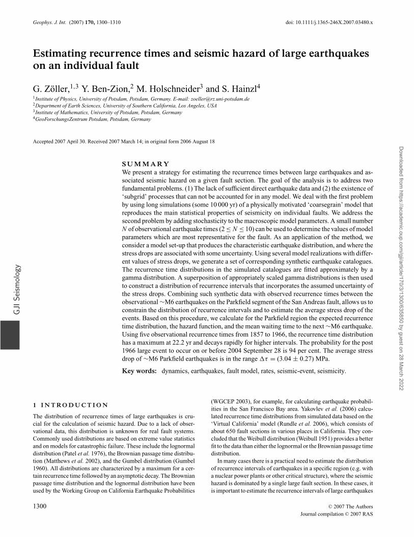
The model consists of a strike-slip fault section, covered by a com-putational grid of length Lx and depth Dz, where deformational pro-cesses are calculated (Fig. 1). As discussed by Zoller et al. (2005a),the planar grid can be considered as an approximation of differentfault segments with similar orientation. In this view, earthquakeson different but nearby fault segments are mapped on a plane. Theexamined fault section is part of an infinite half-plane. The modelprovides a computational framework, compatible overall with theelastic rebound theory of Reid (1910), for spatiotemporal patternsof earthquakes on a discrete heterogeneous fault in an elastic half-space (Ben-Zion & Rice 1993).

v = 35 mm/yearpl

North

Depth

segmented fault

35 km

8.75 km

Figure 1. Sketch of the fault model.

2.1.2 Plate motion

Tectonic loading is imposed by a motion with constant velocity vpl

of the regions around the computational grid. The space-dependentloading rate provides realistic boundary conditions. Using the staticstress transfer function for slip in elastic solid, the continuous tec-tonic loading for each cell with coordinates x (distance along strike)and z (depth) on the computational grid is a linear function of timet:

τload(x, z; t) = γ (x, z) · t. (1)

The loading rate is

γ (x, z) = vpl ·∑

(x ′,z′)∈grid

K (x, z; x ′, z′), (2)

where K(x, z; x′, z′) is the 3-D solution of Chinnery (1963) for staticdislocations on rectangular patches in an elastic Poisson solid withrigidity µ. We note that the loading rates are space-dependent, buttime-independent. In particular, cells at the boundaries of the gridhave higher loading rates than cells in the centre.

2.1.3 Earthquake initiation and coseismic stress transfer

The evolution of earthquakes is controlled by threshold dynamicsassociated with frictional strength and shear stress, which have thesame physical dimension. The frictional strength, serving as thethreshold, is constant in the interseismic period but may changeduring rupture.

An earthquake is initiated at time t, if the local stress τ (x, z; t)exceeds the static strength τ s(x, z). Then the stress in cell (x, z) dropsinstantaneously to the arrest stress τ a(x, z) leading to slip

δu(x, z; t) = τ (x, z; t) − τa(x, z)

K (x, z; x, z), (3)

where K(x, z; x, z) is the self-stiffness of cell (x, z).The strength drops to a dynamic friction value τ d(x, z) for the

reminder of the event. The brittle failure envelope τ f (x, z, t) duringan earthquake is thus given by

τ f (x, z; t) ={

τs(x, z) : cell (x, z) did not fail.

τd (x, z) : cell (x, z) already failed.(4)

At the end of the earthquake, the strength recovers everywhere backto the static level. The dynamic friction is calculated from the static

C© 2007 The Authors, GJI, 170, 1300–1310


Dow



arch 2022

1302 G. Zoller et al.

and arrest stress levels in relation to a dynamic overshoot coefficientD:

τd = τs − τs − τa

D. (5)

If cell (x′, z′) slips at time t (according to eq. 3), the stress in cell(x, z) will increase at time t + δt . Imposing a constant shear wavevelocity v s leads to δt = r/v s, where r is the spatial distance betweencells (x, z) and (x′, z′). The change of stress in cell (x, z) at time t canthus be calculated by summing up the stress contributions from allslip events in the past:

δτ (x, z; t) =∑

(x ′,z′)∈grid

K (x, z; x ′, z′)δu(x ′, z′; t − r/vs). (6)

The value of v s defines the event time scale and has no influenceon the earthquake catalogues. A finite value of v s corresponds tothe quasi-dynamic approximation of Zoller et al. (2004), whereasv s → ∞ reduces to the quasi-static procedure of Ben-Zion & Rice(1993). The calculations below are done for a finite value of v s, butthe statistical aspects of the results remain the same for the quasi-static case.

2.1.4 Simulation algorithm

The simulation starts at t = 0 with random stress values below thestatic strength,

τ (x, z; t) < τs(x, z) (7)

for all cells (x, z).The tectonic loading (Section 2.1.2) produces an increase of stress

on the fault, as long as eq. (7) holds. During this period the fault islocked and no slip occurs: δu(x , z; t) = 0 for all cells (x, z). If thelocal stress τ (x, z; t) exceeds the static strength τ s(x, z) at time tE,an earthquake is initiated in cell (x, z), the hypocentre. The stressand the strength (see eq. 4) drop in this cell,

τ (x, z; t) → τa(x, z), (8)

τ f (x, z; t) → τd (x, z), (9)

and cell (x, z) accumulates corresponding incremental slip accord-ing to eq. (3). Following eq. (6), stress is redistributed in spaceand time to the other cells. If eq. (7) is valid again for all cells be-tween tE and the maximum propagation time t max = r max/v s (withrmax = √

L2x + D2

z ; see Section 2.1.1), the earthquake is termi-nated. Otherwise, eq. (7) is violated for N space–time-points (x 1,z1; t 1), . . . , (x N , z N ; t N ). If (xi, zi; ti) denotes the space–time-pointwith the smallest time ti, slip will be initiated in cell (xi, zi) at timeti and eqs (8) and (9) are applied to this cell. Again, stress is re-distributed according to eq. (6), and the stability condition (eq. 7)is checked. This procedure is repeated until eq. (7) is satisfied forall cells. Then the earthquake is terminated and all strength valuesrecover back to the static level τ f (x, z; t) → τs(x, z). The tectonicloading sets in again (Section 2.1.2) and increases the stress, untilthe next earthquake is initiated.

2.1.5 Parameters of the model

The dimensions of the employed computational grid are L x =35 km length and Dz = 8.75 km depth. The grid is divided into128 × 32 uniform cells of 0.23 km length and width. The values forplate velocity and rigidity are vpl = 35 mm yr−1 and µ = 30 GPa

(Ben-Zion & Rice 1993), the dynamic overshoot coefficient is D =1.25 (Madariaga 1976).

Ben-Zion (1996) and Zoller et al. (2005b) have shown that thedistribution of brittle properties τ s , τ a , or τ d and the degree ofquenched spatial disorder can tune the statistics and dynamics ofthe simulated data between two end-member cases: (1) Gutenberg–Richter statistics over a broad range of magnitudes and irregularoccurrence of large earthquakes, and (2) characteristic earthquakestatistics with overall regular (quasi-periodic) occurring large earth-quakes. In this work, we use parameters leading to the second case.In particular, we assume a high value of dynamic weakening (τ s −τ d)/τ s and a fault without strong spatial heterogeneities. The staticstrength τ s is constant for all computational cells, τ s(x , z) ≡20 MPa, and the arrest stress is chosen randomly from the inter-val τ a(x , z) ∈ [τ s − �τ s − 0.5 MPa ; τ s − �τ s + 0.5 MPa] with�τ s = 9 MPa, 10 MPa, . . . , 16 MPa. We point out that �τ s (stressdrop for a single slipping cell) is different from �τ , which denotesthe average stress drop over the failure area during an earthquake.

2.2 Earthquake catalogues

For each distribution of �τ s, we generate a catalogue with 5 × 105

earthquakes. Each earthquake is characterized by the occurrencetime, the hypocentre coordinates and the magnitude. The magni-tudes are calculated from the simulated potency values, with potencybeing the integral of slip on the failure area,

P =∫

gridδu(x, z) d A, (10)

where δ u (x, z) denotes the total slip of cell (x, z) during the earth-quake. The potency values are converted to earthquake magnitudeswith the empirical potency–magnitude scaling relation of Ben-Zion& Zhu (2002):

M = 2

3log10 (P) + 3.6. (11)

The minimum magnitude M min is determined by the minimumstress drop and the dimension of a computational cell; the maximummagnitude M max increases with the total number of cells and thuswith the size of the computational grid.

In earlier work (Zoller et al. 2006), we have studied the interevent-time distribution of our model for the whole range of magnitudes[M min, M max] and found that it is in good agreement with therecently proposed universal scaling law for natural seismicity ofCorral (2004). Weatherley & Abe (2004) found that this distri-bution is also applicable to results generated by block-spring anddiscrete-lattice models of seismicity. This study, however, focuseson recurrence times of the large earthquakes, because these eventshave the largest impact on the seismic hazard. Although we do notanalyse statistical properties of the small and intermediate events,it is crucial to use a model that generates such events because theycontribute to the self-organization of the stress-field, and hence candelay, advance or trigger the large events. This requires very longsimulations, because large events occur relatively infrequent.

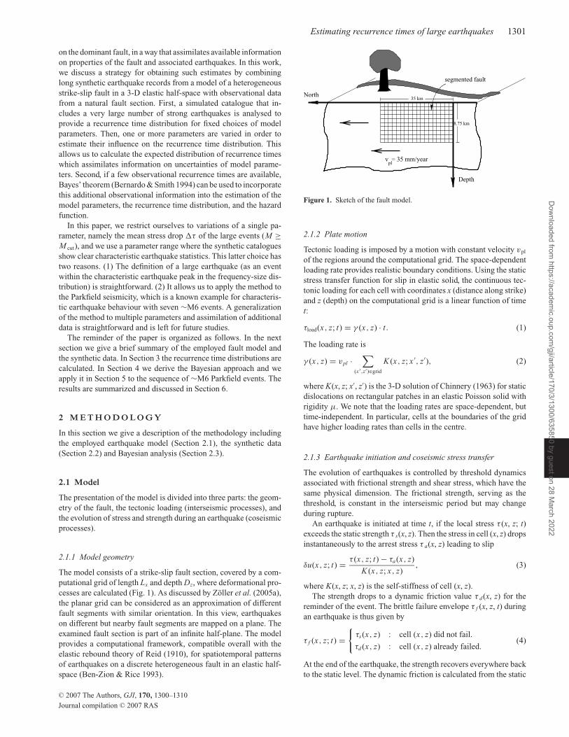
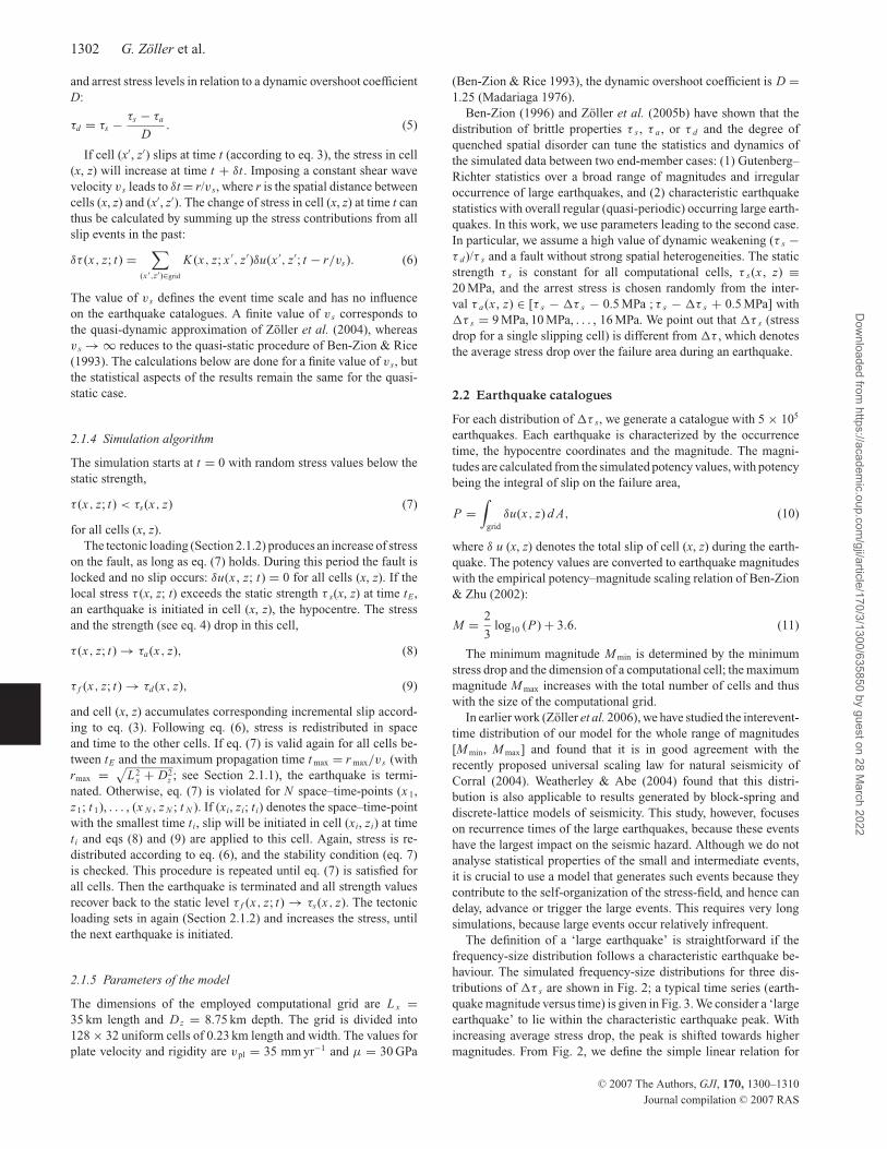
The definition of a ‘large earthquake’ is straightforward if thefrequency-size distribution follows a characteristic earthquake be-haviour. The simulated frequency-size distributions for three dis-tributions of �τ s are shown in Fig. 2; a typical time series (earth-quake magnitude versus time) is given in Fig. 3. We consider a ‘largeearthquake’ to lie within the characteristic earthquake peak. Withincreasing average stress drop, the peak is shifted towards highermagnitudes. From Fig. 2, we define the simple linear relation for

C© 2007 The Authors, GJI, 170, 1300–1310


Dow



arch 2022


1e-05

1e-04

0.001

0.01

0.1

1

4 4.5 5 5.5 6 6.5 7

nr o

f EQ

s/yr

magnitude

10 MPa13 MPa16 MPa

Figure 2. Frequency-size distribution for three realizations of the modelcorresponding to three values of the single cell stress drops: �τ s =10 MPa, 13 MPa, 16 MPa.

4

5

6

0 50 100 150 200 250 300

mag

nitu

de

time (yrs)

Figure 3. Example of a time-series of magnitude versus time.

the magnitude cut-off M cut = 6.2 + 0.03 × (�τ s − 9.0) with �τ s

in MPa. This condition results in an approximate number of 1200large earthquakes for a catalogue, which is sufficient to calculate re-currence time distributions. The mean stress drop for a mainshock�τ is calculated by summing the differences between the initial andfinal stresses over the failure area and by averaging this value overall earthquakes with M ≥ M cut.

2.3 Bayesian analysis

The Bayesian approach (Bernardo & Smith 1994) provides a mathe-matical tool for the treatment of uncertainties in modelling and dataanalysis. In the Bayesian view, probability is associated with a lackof knowledge and considered to measure the degree of belief thatan event will occur (Sornette 2000).

In the context of earthquake recurrences, Bayes’ theorem (eq. 12)can be used to deal with uncertainties of model parameters andprobabilistic uncertainty in the occurrence of earthquakes. It canbe used to update current probabilities, for example, associatedwith seismic hazard, if new information (in terms of an eventE) becomes available. An important feature of Bayes’ probabil-ity theory is the ability to combine statistical information on seis-micity with non-statistical data coming from geology or historicseismicity.

Bayes’ theorem in a discrete representation can be formulated asfollows:

P(Hi | E) = P(E | Hi )P(Hi )∑j P(E | Hj )P(Hj )

, (12)

where the H i denote all mutually exclusive hypotheses, P(E | H i)is the likelihood function, P(H i) is the a priori probability of thehypothesis H i before the new information (event E) is available, andP(H i | E) is the corresponding a posteriori probability including thenew information.

Campbell (1982) has derived a probabilistic hazard model basedon exponentially distributed earthquake magnitudes and a Poissonprocess for the temporal earthquake occurrence. In that application,eq. (12) is used to account for uncertainties of the mean earthquakerate in the Poisson distribution and the b value in the magnitudedistribution. This model has been applied to calculate the seismichazard in the San Jacinto fault zone in California (Campbell 1983).Ferraes (1992) imposes a lognormal distribution for the recurrenceof characteristic earthquakes in order to study the Ometepec seg-ment of Mexican subduction zone. Parvez (2006) uses Campbell’s(1982) model to calculate probabilities for earthquake occurrencein the North East Indian peninsula. Further applications of Bayes’probability theory to the problem of earthquake recurrence are re-viewed in Parvez (2006).

3 R E C U R R E N C E T I M ED I S T R I B U T I O N S

In this section, we calculate probability density functions of re-currence times for eight realizations corresponding to eight dis-tributions of the single cell stress drops introduced at the end ofSection 2.1. The recurrence time t is defined as the waiting timebetween two subsequent earthquakes with M ≥ M cut. The pdf f (t)of the recurrence times is approximated by

f (t) = 1

Ntot

�N (t)

�t, (13)

where N tot is the total number of recurrence times, and �N(t) is thenumber of recurrence times in the interval [t ; t + �t]. The pdf isnormalized satisfying∫ ∞

0f (t) dt = 1. (14)

The cumulative distribution (cdf) is defined by

C(t) =∫ t

0f (t ′) dt ′. (15)

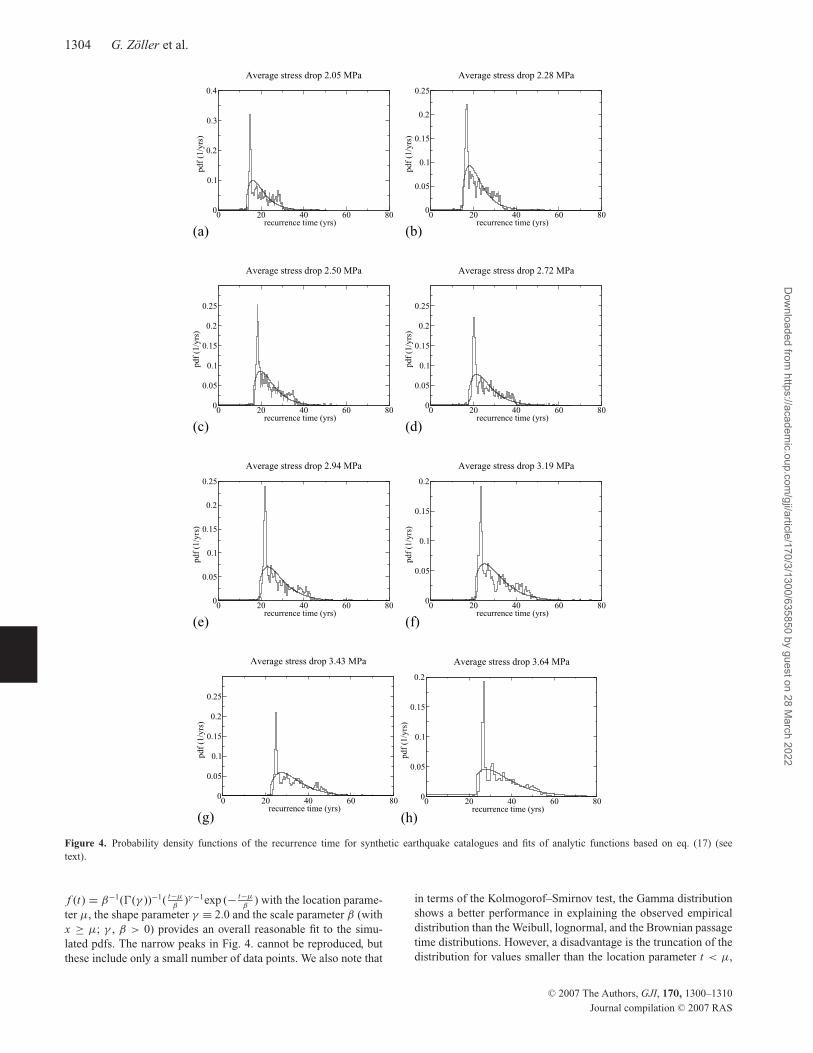
The panels in Fig. 4 show the recurrence time pdfs for the simu-lations. A common feature of the pdfs is the rapid increase arounda certain time t∗(�τ ) and the gradual decay for higher values of t.With growing average stress drops, the pdf becomes broader. Table 1summarizes the relevant parameters of the recurrence time distri-butions: the imposed values of τ s − τ a, the magnitude thresholdM cut, the average stress drop �τ of earthquakes with M ≥ M cut,the mean µt and the standard deviation σ t of the recurrence timedistribution.

Fig. 5 gives fits and empirical relations between µt and σ t of apdf and the average stress drop �τ of large events. While the meanvalue of the recurrence time pdf grows linearly with the stress drops,the standard deviation is characterized by a quadratic increase:

µt (�τ ) = 9.7 · �τ

σt (�τ ) = 1.8 · �τ 2 − 6.8 · �τ + 11.7 (16)

with µt, σ t in years and �τ in MPa.In the next step, it is desirable to get pdfs also for similar model

realizations that have other values of �τ . Toward this end, wefit the simulated pdfs by an analytical function which conservesthe mean value µt and the standard deviation σ t. If a relation-ship between (µt, σ t) and the stress drop �τ can be establishedby interpolation, it may be used to estimate the recurrence timepdfs for other values of �τ . We find that the Gamma distribution

C© 2007 The Authors, GJI, 170, 1300–1310


Dow



arch 2022


0 20 40 60 80recurrence time (yrs)

0

0.1

0.2

0.3

0.4

pdf

(1/y

rs)

Average stress drop 2.05 MPa

(a)0 20 40 60 80

recurrence time (yrs)

0

0.05

0.1

0.15

0.2

0.25

pdf

(1/y

rs)


(b)


0

0.05

0.1

0.15

0.2

0.25

pdf

(1/y

rs)


(c)0 20 40 60 80


0

0.05

0.1

0.15

0.2

0.25

pdf

(1/y

rs)


(d)


0

0.05

0.1

0.15

0.2

0.25

pdf

(1/y

rs)


(e)0 20 40 60 80


0

0.05

0.1

0.15

0.2

pdf

(1/y

rs)


(f)


0

0.05

0.1

0.15

0.2

0.25

pdf

(1/y

rs)


(g)0 20 40 60 80


0

0.05

0.1

0.15

0.2

pdf

(1/y

rs)


(h)

Figure 4. Probability density functions of the recurrence time for synthetic earthquake catalogues and fits of analytic functions based on eq. (17) (seetext).

f (t) = β−1(�(γ ))−1( t−µ

β)γ−1exp (− t−µ

β) with the location parame-

ter µ, the shape parameter γ ≡ 2.0 and the scale parameter β (withx ≥ µ; γ , β > 0) provides an overall reasonable fit to the simu-lated pdfs. The narrow peaks in Fig. 4. cannot be reproduced, butthese include only a small number of data points. We also note that

in terms of the Kolmogorof–Smirnov test, the Gamma distributionshows a better performance in explaining the observed empiricaldistribution than the Weibull, lognormal, and the Brownian passagetime distributions. However, a disadvantage is the truncation of thedistribution for values smaller than the location parameter t < µ,

C© 2007 The Authors, GJI, 170, 1300–1310


Dow



arch 2022


Table 1. Parameters of simulated earthquake catalogues and corre-sponding recurrence time distributions.

τ s − τ a (MPa) M cut �τ (MPa) µt (yr) σ t (yr)

9.0 6.20 2.05 19.84 5.2210.0 6.23 2.28 22.03 5.6211.0 6.26 2.50 24.06 6.0812.0 6.29 2.72 26.14 6.6613.0 6.32 2.94 28.31 7.3514.0 6.35 3.19 31.06 8.4615.0 6.38 3.43 33.61 8.8216.0 6.41 3.64 35.98 11.32

20

25

30

35

2 2.2 2.4 2.6 2.8 3 3.2 3.4 3.6 3.8

mea

n re

curr

ence

tim

e (y

rs)

stress drop (MPa) (a)

5

6

7

8

9

10

11

12

2 2.2 2.4 2.6 2.8 3 3.2 3.4 3.6 3.8

std

of r

ecur

renc

e tim

es (

yrs)

stress drop (MPa) (b)

Figure 5. Relation of (a) the mean value µt and (b) the standard deviationσ t of a pdf of recurrence intervals and the average stress drop �τ . The solidlines are least square fits to the data points (see eq. 16).

which excludes small recurrence times, for example, arising fromlarge aftershocks. Therefore, we set f (t) to be constant, f (t) ≡ h,for 0 ≤ t ≤ t∗(�τ ),

f (t) ={

h for t ≤ t∗

( t−µβ )exp (− t−µ

β )

β�(2) for t > t∗,(17)

where the offset value t∗ is empirically determined from Fig. 4 byt∗ = 6.5 · �τ , with t∗(�τ ) given in years and �τ in MPa. Thevalue h is determined by the normalization condition eq. (14). Weemphasize that we aim to reproduce the overall shape of a single pdfrather than the details. Small fluctuations and higher-order peakswill be suppressed in the next analysis step, when many pdfs areintegrated. The location parameter µ and the scale parameter β aredetermined analytically (Papoulis 1984) from the mean value µt andthe standard deviation σ t of the data (neglecting the constant part)by

µ = µt − σt · √2

β = σt/√

2. (18)

The fits to the eight pdfs from the simulated earthquake cataloguesare shown as smooth lines in Fig. 4.

4 A C C O U N T I N G F O R U N C E RTA I N T I E S

In order to account for the limited knowledge of model parameters,like the stress drop �τ , we use two approaches: in the first ‘basic’approach, no information except upper and lower bounds of thestress drop�τ are given. In the second approach, we will incorporatea small number of observational recurrence times T 1, . . . , T N froma certain region, into the a posteriori pdf of recurrence times andaverage stress drop.

0

0.01

0.02

0.03

0.04

0.05

0.06

0 10 20 30 40 50 60 70 80

pdf (

1/yr

s)


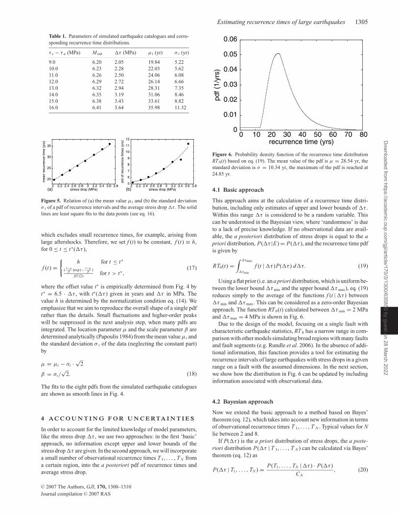
Figure 6. Probability density function of the recurrence time distributionRT 0(t) based on eq. (19). The mean value of the pdf is µ = 28.54 yr, thestandard deviation is σ = 10.34 yr, the maximum of the pdf is reached at24.85 yr.

4.1 Basic approach

This approach aims at the calculation of a recurrence time distri-bution, including only estimates of upper and lower bounds of �τ .Within this range �τ is considered to be a random variable. Thiscan be understood in the Bayesian view, where ‘randomness’ is dueto a lack of precise knowledge. If no observational data are avail-able, the a posteriori distribution of stress drops is equal to the apriori distribution, P(�τ |E) = P(�τ ), and the recurrence time pdfis given by

RT0(t) =∫ �τmax

�τmin

f (t | �τ )P(�τ ) d�τ. (19)

Using a flat prior (i.e. an a priori distribution, which is uniform be-tween the lower bound �τ min and the upper bound �τ max), eq. (19)reduces simply to the average of the functions f (t | �τ ) between�τ min and �τ max. This can be considered as a zero-order Bayesianapproach. The function RT 0(t) calculated between �τ min = 2 MPaand �τ max = 4 MPa is shown in Fig. 6.

Due to the design of the model, focusing on a single fault withcharacteristic earthquake statistics, RT 0 has a narrow range in com-parison with other models simulating broad regions with many faultsand fault segments (e.g. Rundle et al. 2006). In the absence of addi-tional information, this function provides a tool for estimating therecurrence intervals of large earthquakes with stress drops in a givenrange on a fault with the assumed dimensions. In the next section,we show how the distribution in Fig. 6 can be updated by includinginformation associated with observational data.

4.2 Bayesian approach

Now we extend the basic approach to a method based on Bayes’theorem (eq. 12), which takes into account new information in termsof observational recurrence times T 1, . . . , T N . Typical values for Nlie between 2 and 8.

If P(�τ ) is the a priori distribution of stress drops, the a poste-riori distribution P(�τ | T 1, . . . , T N ) can be calculated via Bayes’theorem (eq. 12) as

P(�τ | T1, . . . , TN ) = P(T1, . . . , TN | �τ ) · P(�τ )

CN, (20)

C© 2007 The Authors, GJI, 170, 1300–1310


Dow



arch 2022


Table 2. Comparison of the mean stress dropsfrom synthetic catalogues 〈�τ true〉 with stress drops�τ max calculated from six ‘observational’ recurrencetimes (maximum of the pdf in eq. 20), respectively.Each line corresponds to one model realization. Thevalues in bracket are the mean values of the a poste-riori stress drop distributions. The errors denote onestandard deviation.

〈�τ true〉 (MPa) �τ max [〈�τ 〉] (MPa)

1.93 ± 0.17 1.98[1.95] ± 0.162.26 ± 0.20 2.34[2.27] ± 0.172.55 ± 0.31 2.52[2.52] ± 0.372.59 ± 0.28 2.70[2.71] ± 0.223.00 ± 0.30 3.18[3.12] ± 0.263.00 ± 0.20 3.06[3.04] ± 0.263.56 ± 0.38 3.60[3.58] ± 0.353.49 ± 0.45 3.42[3.44] ± 0.33

with the likelihood function

P(T1, . . . , TN | �τ ) =N∏

i=1

f (Ti | �τ ) (21)

and the normalization factor

CN =∫ �τmax

�τmin

P(T1, . . . , TN | �τ ) · P(�τ ) d�τ. (22)

Here we have used our assumption that the large events follow arenewal process with stationary pdf f (T i | �τ ) depending only onthe stress drop �τ (i.e. the recurrence times are independent andidentically distributed random variables with common distributionf ).

If no detailed seismological information are available, it will bereasonable to use again a flat prior, that is, a uniform a priori dis-tribution of stress drops, P(�τ ) ≡ 1/(�τ max − �τ min) between twoboundary values �τ min and �τ max.

A local maximum of P(�τ | T 1, . . . , T N ) with respect to �τ in-dicates the most likely stress drop �τ , from which the observationalrecurrence times have been drawn.

The capability of the Bayesian approach to estimate stress dropscan be tested by applying it to a synthetic catalogue with known stressdrops. To perform such a test, we generate short catalogues with thesame parameters as in Section 2.2, using different realizations forthe stress field. From each catalogue we select randomly a periodthat includes seven large earthquakes (six recurrence times) andcalculate the mean and the standard deviation of the stress drops.Then the average stress drop is estimated by means of the Bayesianapproach (eq. 20) from the six ‘observed’ recurrence times. Theresults for eight scenarios are provides in Table 2. The comparison ofthe actual used (true) and calculated stress drops shows a reasonableagreement.

Based on the a posteriori distribution P(�τ | T 1, . . . , T N ), otherfunctions related to seismic hazard can be calculated. We consider(1) the recurrence time distribution RT(t), (2) the cumulative re-currence time distribution C(t), (3) the hazard function H and (4)the waiting time to the next large earthquake �tw(t | H) for a givenhazard level. These functions are defined as follows:

(1) The recurrence time pdf is calculated via

RT (t) =∫ �τmax

�τmin

f (t | �τ )P(�τ | T1, . . . , TN ) d�τ. (23)

(2) The corresponding cumulative recurrence time distributionis

C(t) =∫ t

0RT (t ′) dt ′. (24)

(3) The hazard function is

Ht0 (�t) = C(t0 + �t) − C(t0)

1 − C(t0). (25)

The function H is the probability that the next large earthquakeoccurs in the interval [t 0; t 0 + �t] given the time t0 since the lastlarge event.

(4) Finally, solving eq. (25) for the waiting time �t after t0,yields the function �tw(t0 | H). It is the value of the waiting time�t for a given hazard H . In particular, the time to a hazard of 0.5,�tw(t0 | 0.5), is called the mean waiting time to the next large earth-quake.

5 A P P L I C AT I O N T O PA R K F I E L DS E I S M I C I T Y

The Parkfield segment of the San Andreas fault in California is oneof the best monitored seismic regions in the world. Over a periodof about 100 yr beginning in 1857, earthquakes with magnitudeM ≈ 6 occurred quasi-periodically with a period of about 24.5 yr. Anexception is the 1934 event, which followed 12 yr after the previousmain shock. The last event fitting this estimate was observed in 1966leading to a simple forecast for a subsequent earthquake in 1988.More realistic estimates accounting for lengthening of recurrenceintervals due to viscoelastic relaxation following the 1857 event ledto a forecast of 1995 ± 11 yr (Ben-Zion et al. 1993). The occurrenceof the 1983 Coalinga earthquake may have produced perturbationsthat delayed further the expected Parkfield event (Miller 1996). Inorder to detect possible precursors to the forecasted event, the so-called Parkfield experiment, including ground motion instruments,strain-metres and GPS stations, has been running since around 1985.The next ∼M6 earthquake occurred on 2004 September 28 withoutany clear precursory phenomenon (Lindh 2005; Langbein et al.2005).

In the following we use the sequence of recurrence times between1857 and 2004: T1 = 24.1 yr, T2 = 20.1 yr, T3 = 21.0 yr, T4 =12.2 yr, T5 = 32.0 yr and T6 = 38.2 yr. More details on the Park-field sequence are available at http://quake.wr.usgs.gov/research/parkfield/hist.html. We first exclude the 2004 event (T 6) in orderto perform a retrospective hazard assessment.

For this application, it is essential that our simulated large eventsresemble the Parkfield seismicity with respect to the characteristicearthquake statistics and quasi-periodic occurrence of large events.As shown in Figs 2 and 3, these features are generated by our model.Other aspects of natural seismicity, like the spatial distribution ofhypocentres and aftershock activity, are missing from our simulatedresults. Also the magnitude values exceed somewhat those of theobserved Parkfield events, because we consider a purely brittle faultsegment, whereas the Parkfield section contains a mixture of brittleand creeping regions. We emphasize that our present goal is to finda minimal model focusing on particular statistical features whichis, the distribution of large earthquake recurrence times. The abovementioned features can be incorporated by using the model versionsof Ben-Zion (1996) and Zoller et al. (2005a). For this study, however,the basic model described in Section 2 is sufficient.

We assume a uniform a priori distribution of stress drops between�τ min = 2 MPa and �τ max = 4 MPa and the recurrence times T i (i =

C© 2007 The Authors, GJI, 170, 1300–1310


Dow



arch 2022


0

0.5

1

1.5

2

2.5

2 2.2 2.4 2.6 2.8 3 3.2 3.4 3.6 3.8 4

pdf (

1/M

Pa)

stress drop (MPa)

1857-19661857-2004

Figure 7. A posteriori distribution P(�τ | T 1, . . . , T N ) of stress drop �τ

defined in eq. (20); the likelihood function in eq. (21) for different valuesof �τ has been calculated using eq. (16). The solid line is based on fiveobservational recurrence times (1857–1966), while the calculation leadingto the dashed line includes also the 2004 event.

1, . . . , 5) from Parkfield, and calculate the a posteriori distributionP(�τ | T 1, . . . , T N ) according to eq. (20). The result for the averagestress drop of an ∼ M6 earthquake given in Fig. 7, leads to anexpectation value of �τ = (2.94 ± 0.33) MPa (maximum of thepdf in eq. (20)). This indicates the most representative value of thestress drop during a large earthquake; the error corresponds to onestandard deviation. If the 2004 Parkfield event is also taken intoaccount, this value changes to �τ = (3.04 ± 0.27) MPa (dashedline in Fig. 7).

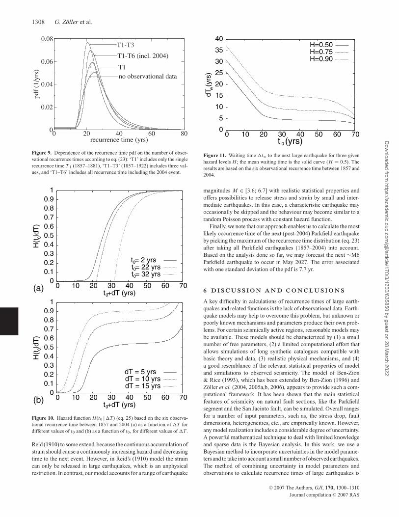
The pdf and cdf of the recurrence time distribution in terms ofeq. (23) are shown in Fig. 8. This distribution, derived from theGamma distribution as a basis function, is similar to recurrencetime distributions from other models, for example, the Virtual Cali-fornia model. A main difference, however, is the behaviour for smallrecurrence times. Additionally, Fig. 8(a) shows a significant modifi-cation of the recurrence time pdf arising from the observational data:the width of the distribution becomes narrow and the position of themaximum is shifted from 25.3 to 21.4 yr. The dependence of the pdfon the number of observational recurrence times is illustrated moreclearly in Fig. 9. It is seen that even a single observational valueleads to a major correction of the distribution. This result is particu-larly encouraging for the analysis of other seismically active regions,where only two or three large earthquakes were observed. Fig. 8(b)provides the corresponding cumulative distributions (eq. 24) for thebasic approach (without observational data) and two realizations ofthe Bayesian approach. The figure also provides the cdf of the sixParkfield recurrence times, which is similar in shape but slightlyshifted towards smaller recurrence times. This is related to the lackof small recurrence times in the model.

Based on the two curves in Fig. 8(a), we estimate the probabilitythat a large earthquakes takes place before 38.2 yr after the lastevent, which corresponds to the time difference between the 1966and the 2004 earthquake. The basic approach (without observationaldata) based on eq. (19) leads to a probability of 85 per cent, whilethe Bayesian approach with the five observational values (1857 to1966) results in 94 per cent probability. On the other hand, if thelargest recurrence time �T max is defined on a 95 per cent level ofthe hazard, the basic approach leads to �Tmax = 48.2 yr, while�Tmax = 39.4 yr for the Bayesian approach.

0

0.01

0.02

0.03

0.04

0.05

0.06

0.07

0.08

0 10 20 30 40 50 60 70 80

pdf (

1/yr

s)


Parkfield data 1857-1966

(a)

no data

0

0.2

0.4

0.6

0.8

1

0 10 20 30 40 50 60 70 80

cdf

recurrence time (yrs)(b)

no data1857-19221857-2004

Parkfield data

Figure 8. (a) Solid line: recurrence time distribution RT(t) (eq. 23); the meanvalue is µ = 28.1 yr, the standard deviation is σ = 9.9 yr, the maximumof the pdf is reached at 22.4 yr. The dashed line is identical to Fig. 6; (b)cumulative recurrence time distribution C(t) (eq. (24)) for (1) the basicapproach (Section 4.1): solid line; (2) the Bayesian approach (Section 4.1)with three data points: long-dashed line and (3) the Bayesian approach withsix data points: short-dashed line. The step function denotes the cdf of thesix Parkfield recurrence times.

Fig. 10 shows the hazard function H(t0 | �t) for fixed t0 andvarying �t (Fig. 10a) and for fixed �t and varying t0 (Fig. 10b). Thiscalculation is based on the six observational recurrence times from1857 to 2004. Consequently, the solid curve in Fig. 10a representsthe actual hazard given that no ∼M6 earthquake occurred on theParkfield segment since 2006 September 28. We restrict ourselvesto the range of recurrence times where data from the simulations areavailable (see Fig. 4) and do not extrapolate the distributions towardsvery large recurrence times. The correct asymptotic behaviour ofthe recurrence time pdf is unknown, even for model simulations,because of the relative small number of events. We suggest thatthe Gamma distribution is a suitable choice for most values of therecurrence times of large earthquakes on a single fault section. Theplots show a continuous increase of the hazard, followed by a periodof approximately constant hazard (t0 ≥ 30 yr in Fig. 10(b)). Inthis state, the fault has almost lost his memory corresponding to aPoisson process.

Fig. 11 shows the estimated waiting time �tw as a function oft0 for a given hazard level H . In the range where synthetic data aregiven, the waiting time decreases and becomes almost constant aftert0 ≈ 30 yr. This seems to contradict the elastic rebound model of

C© 2007 The Authors, GJI, 170, 1300–1310


Dow



arch 2022



0

0.02

0.04

0.06

0.08pd

f (1

/yrs

)

no observational dataT1

T1-T6 (incl. 2004)

T1-T3

Figure 9. Dependence of the recurrence time pdf on the number of obser-vational recurrence times according to eq. (23): ‘T1’ includes only the singlerecurrence time T 1 (1857–1881), ‘T1–T3’ (1857–1922) includes three val-ues, and ‘T1–T6’ includes all recurrence time including the 2004 event.

0 0.1 0.2 0.3 0.4 0.5 0.6 0.7 0.8 0.9

1

0 10 20 30 40 50 60 70

H(t

|dT

) 0

(a)t +dT (yrs) 0

t = 2 yrs 0 t = 22 yrs 0 t = 32 yrs 0

0 0.1 0.2 0.3 0.4 0.5 0.6 0.7 0.8 0.9

1

0 10 20 30 40 50 60 70

H(t

|dT

) 0

(b)t +dT (yrs) 0

dT = 5 yrsdT = 10 yrsdT = 15 yrs

Figure 10. Hazard function H(t0 | �T) (eq. 25) based on the six observa-tional recurrence time between 1857 and 2004 (a) as a function of �T fordifferent values of t0 and (b) as a function of t0, for different values of �T .

Reid (1910) to some extend, because the continuous accumulation ofstrain should cause a continuously increasing hazard and decreasingtime to the next event. However, in Reid’s (1910) model the straincan only be released in large earthquakes, which is an unphysicalrestriction. In contrast, our model accounts for a range of earthquake

0

5

10

15

20

25

30

35

40

0 10 20 30 40 50 60 70

dT (

yrs)

w

t (yrs) 0

H=0.50H=0.75H=0.90

Figure 11. Waiting time �tw to the next large earthquake for three givenhazard levels H ; the mean waiting time is the solid curve (H = 0.5). Theresults are based on the six observational recurrence time between 1857 and2004.

magnitudes M ∈ [3.6; 6.7] with realistic statistical properties andoffers possibilities to release stress and strain by small and inter-mediate earthquakes. In this case, a characteristic earthquake mayoccasionally be skipped and the behaviour may become similar to arandom Poisson process with constant hazard function.

Finally, we note that our approach enables us to calculate the mostlikely occurrence time of the next (post-2004) Parkfield earthquakeby picking the maximum of the recurrence time distribution (eq. 23)after taking all Parkfield earthquakes (1857–2004) into account.Based on the analysis done so far, we may forecast the next ∼M6Parkfield earthquake to occur in May 2027. The error associatedwith one standard deviation of the pdf is 7.7 yr.

6 D I S C U S S I O N A N D C O N C L U S I O N S

A key difficulty in calculations of recurrence times of large earth-quakes and related functions is the lack of observational data. Earth-quake models may help to overcome this problem, but unknown orpoorly known mechanisms and parameters produce their own prob-lems. For certain seismically active regions, reasonable models maybe available. These models should be characterized by (1) a smallnumber of free parameters, (2) a limited computational effort thatallows simulations of long synthetic catalogues compatible withbasic theory and data, (3) realistic physical mechanisms, and (4)a good resemblance of the relevant statistical properties of modeland simulations to observed seismicity. The model of Ben-Zion& Rice (1993), which has been extended by Ben-Zion (1996) andZoller et al. (2004, 2005a,b, 2006), appears to provide such a com-putational framework. It has been shown that the main statisticalfeatures of seismicity on natural fault sections, like the Parkfieldsegment and the San Jacinto fault, can be simulated. Overall rangesfor a number of input parameters, such as, the stress drop, faultdimensions, heterogeneities, etc., are empirically known. However,any model realization includes a considerable degree of uncertainty.A powerful mathematical technique to deal with limited knowledgeand sparse data is the Bayesian analysis. In this work, we use aBayesian method to incorporate uncertainties in the model parame-ters and to take into account a small number of observed earthquakes.The method of combining uncertainty in model parameters andobservations to calculate recurrence times of large earthquakes is

C© 2007 The Authors, GJI, 170, 1300–1310


Dow



arch 2022


demonstrated for a poorly known stress drop of large earthquakesin the Parkfield section of the San Andreas fault.

A generalization to other parameters and regions is straightfor-ward. The recurrence time pdfs for the synthetic earthquake cata-logues are generally similar in shape to those from other models.Because our model consists of a single fault, the data do not mixevents occurring on different faults and the range of recurrence timesis relatively narrow. A Gamma distribution with a shape parameterγ = 2 augmented by a constant part for small values gives an overallgood performance of the pdfs. Taking into account six observationalrecurrence times (from 1857 to 2004), we predict a mean stress drop�τ = (3.04 ± 0.27) MPa for ∼ M6 Parkfield earthquakes, whichis in reasonable agreement with the findings of Bakun et al. (2005).By means of synthetic tests, we find that the Bayesian method ispowerful for estimating model parameters which are representativefor an active fault zone, even if only a small number of observationaldata are available.

The results based on model data and Parkfield seismicity indicatethat the hazard first increases after a large earthquake continuously,followed by a period where it is almost constant. In other words, if acharacteristic earthquake is missing or delayed due to stress releasein small and intermediate earthquakes, the statistics approach thatof a random Poisson process with constant hazard. Using refinedmodels and accounting for uncertainties in several parameters, forexample, fault dimensions and heterogeneities, will improve theaccuracy of the predicted recurrence time distributions.

The type of basis distributions which are fitted to the synthetic datacan affect the results. In this study, the Gamma distribution appearsto work well, especially since we do not use in applications singledistributions, but combined distributions in which small details areaveraged out. However, the Gamma distribution has shortcomingsfor small recurrence times (truncation) and for large recurrencetimes (asymptotic behaviour). One focus of our future work willbe an effort to find distributions with better performance over theentire range of values.

The methodology presented in this paper can be extended to in-corporate additional observational results and their uncertainties, aswell as additional model ingredients. We note that in many situationsno information other than a priori estimates of certain parametersare available. In such cases, the discussed method provides a rationalway for combining the a priori information with simulations froma single fault model in order to calculate the seismic hazard. Ourapproach avoids the high degree of complexity and the mixing ofdifferent event populations of models having large number of faultsand parameters. In applications dominated by the largest nearbyfault, our approach may provide useful quantitative estimates of theseismic hazard.

A C K N O W L E D G M E N T S

We are grateful to Donald Turcotte for stimulating discussions.GZ acknowledges support from the German Research Soci-ety (SFB555). YBZ acknowledges support from the SouthernCalifornia Earthquake Center (based on NSF cooperative agreementEAR-8920136 and United States Geological Survey cooperativeagreement 14-08-0001-A0899). GZ and YBZ thank the Kavli Insti-tute for Theoretical Physics, UC Santa Barbara, for hospitality dur-ing a 2005 program on Friction, Fracture and Earthquake Physics,and partial support based on NSF grant PHY99-0794. Commentsfrom Jeremy Zechar, Editor Cindy Ebinger and two anonymous re-viewers helped to improve the manuscript.

R E F E R E N C E S

Ben-Zion, Y., 1996. Stress, slip, and earthquakes in models of complexsingle-fault systems incorporating brittle and creep deformations, J. geo-phys. Res., 101, 5677–5706.

Ben-Zion, Y. & Rice, J.R., 1993. Earthquake failure sequences along a cel-lular fault zone in a three-dimensional elastic solid containing asperityand nonasperity regions, J. geophys. Res., 98, 14 109–14 131.

Ben-Zion, Y. & Zhu, L., 2002. Potency-magnitude scaling relations for south-ern California earthquakes with 1.0 ≤ M L≤ 7.0, Geophys. J. Int., 148,F1–F5.

Ben-Zion, Y., Dmowska, R. & Rice, J.R., 1993. Interaction of theSan-Andreas fault creeping section with adjacent great rupture zonesand earthquake recurrence at Parkfield, J. geophys. Res., 98, 2135–2144.

Bakun, W.H. et al., 2005. Implications for prediction and haz-ard assessment from the 2004 Parkfield earthquake, Nature, 437,doi:10.1038/nature04067.

Bernardo, J.M. & Smith, A.F.M., 1994. Bayesian Theory, Wiley, Chichester.Campbell, K.W., 1982. Bayesian analysis of extreme earthquake occur-

rences. Part I. Probabilistic hazard model, Bull. seism. Soc. Am., 72, 1689–1705.

Campbell, K.W., 1983. Application to the San Jacinto fault zone of southernCalifornia, Bull. seism. Soc. Am., 73, 1099–1115.

Chinnery, M., 1963. The stress changes that accompany strike-slip faulting.Bull. seism. Soc. Am., 53, 921–932.

Coleman, B.D., 1958. Statistics and time dependence of mechanical break-down in fibers, J. Appl. Phys., 29, 968–983.

Corral, A., 2004. Long-term clustering, scaling, and universality in thetemporal occurrence of earthquakes. Phys. Rev. Lett. 92, 108 501,doi:10.1103/PhysRevLett.92.108501.

Gumbel, E.J., 1960. Multivariate Extremal Distributions, Bull. Inst. Internat.de Statistique, 37, 471–475.

Langbein, J. et al., 2005. Preliminary Report on the 28 September 2004, M6.0 Parkfield, California Earthquake, Seism. Res. Lett., 76, 1–17.

Ferraes, S.G., 1992. The Bayesian probabilistic prediction of the next earth-quake in the Ometepec segment of the Mexican subduction zone, PureAppl. Geophys. 139, 309–329.

Lindh, A.G., 2005. Opinion: Success and failure at Parkfield, Seism. Res.Lett., 76, 3–6.

Madariaga, R., 1976, Dynamics of an expanding circular fault, Bull. seism.Soc. Am., 66, 639–666.

Matthews, M.V., Ellsworth, W.L. & Reasenberg, P.A., 2002. A Brown-ian model for recurrent earthquakes, Bull. seism. Soc. Am., 92, 2233–2250.

Miller, S.A., 1996. Fluid-mediated influence of adjacent thrusting on theseismic cycle at Parkfield, Nature, 382, 799–802.

Papoulis, A., 1984. Probability, Random Variables, and Stochastic Pro-cesses, pp. 103–104, 2nd edn McGraw-Hill, New York.

Parvez, I.A., 2006. On the Bayesian analysis of the earthquake hazardin the North-East Indian peninsula, Nat. Hazards, 40, 397–412, doi10.1007/s11069-006-9002-4.

Patel, J.K., Kapadia, C.H. & Owen, D.B., 1976. Handbook of StatisticalDistributions, Marcel Dekker, New York.

Reid, H.F., 1910. The Mechanics of the Earthquake, The California Earth-quake of April 18, 1906, Report of the State Investigation Commission,Vol. 2, Carnegie Institution of Washington, Washington, DC.

Rundle, J.B., Rundle, P.B., Donnellan, A., Li, P., Klein, W., Morein, G.,Turcotte, D.L. & Grant, L., 2006. Stress transfer in earthquakes, hazardestimation and ensemble forecasting: inferences from numerical simula-tions, Tectonophysics, 413, 109–125.

Sornette, D., 2000. Critical Phenomena in Natural Sciences, Springer,Berlin, Heidelberg, New York.

Weatherley, D. & Abe, S., 2004. Earthquake statistics in a block slidermodel and a fully dynamic fault model, Nonlin. Proc. Geophys., 11, 503–560.

Weibull, W., 1951. A statistical distribution of wide applicability, J. Appl.Mech., 18, 293–297.

C© 2007 The Authors, GJI, 170, 1300–1310


Dow



arch 2022


Working Group on California Earthquake Probabilities, 2003. Earthquakeprobabilities in the San Francisco Bay region, US Geol. Survey Open FileReport 03-214, US Geological Survey, 2003.

Yakovlev, G., Turcotte, D.L., Rundle, J.B. & Rundle, P.B., 2006. Sim-ulation based distributions of earthquake recurrence times on theSan Andreas fault system, Bull. seism. Soc. Am., 96, 1995–2007,doi:10.1785/0120050183.

Zoller, G., Holschneider, M. & Ben-Zion, Y., 2004. Quasi-static and quasi-dynamic modeling of earthquake failure at intermediate scales, Pure. appl.Geophys. 161, 2103–2118, doi 10.1007/s00024-004-2551-0.

Zoller, G., Hainzl, S., Holschneider, M. & Ben-Zion, Y., 2005a. Aftershocksresulting from creeping sections in a heterogeneous fault, Geophys. Res.Lett., 32, L03 308, doi: 10.1029/2004GL021871.

Zoller, G., Holschneider, M. & Ben-Zion, Y., 2005b. The role of hetero-geneities as a tuning parameter of earthquake dynamics. Pure. Appl. Geo-phys. 162, 1027–1049, doi:10.1007/s00024-004-2660-9.

Zoller, G., Hainzl, S., Ben-Zion, Y. & Holschneider, M., 2006. Earth-quake activity related to seismic cycles in a model for a heteroge-neous strike-slip fault, Tectonophysics, 423, 137–145, doi:10.1016/j.tecto.2006.03.007.

C© 2007 The Authors, GJI, 170, 1300–1310


Dow



arch 2022

estimating recurrence times and seismic hazard of large

Documents