eScholarship provides open access, scholarly publishingservices to the University of California and delivers a dynamicresearch platform to scholars worldwide.

Lawrence Berkeley National Laboratory

Peer Reviewed

Title:Estimating maximum sustainable injection pressure during geological sequestration of CO2 usingcoupled fluid flow and geomechanical fault-slip analysis

Author:Rutqvist, J.Birkholzer, J.Cappa, F.Tsang, C.-F.

Publication Date:10-17-2006

Publication Info:Lawrence Berkeley National Laboratory

Permalink:http://escholarship.org/uc/item/6q00q3bb

Abstract:This paper demonstrates the use of coupled fluid flow and geomechanical fault slip (faultreactivation) analysis to estimate the maximum sustainable injection pressure during geologicalsequestration of CO2. Two numerical modeling approaches for analyzing faultslip are applied,one using continuum stress-strain analysis and the other using discrete fault analysis. Theresults of these two approaches to numerical fault-slip analyses are compared to the resultsof a more conventional analytical fault-slip analysis that assumes simplified reservoir geometry.It is shown that the simplified analytical fault-slip analysis may lead to either overestimationor underestimation of the maximum sustainable injection pressure because it cannot resolveimportant geometrical factors associated with the injection induced spatial evolution of fluidpressure and stress. We conclude that a fully coupled numerical analysis can more accuratelyaccount for the spatial evolution of both in situ stresses and fluid pressure, and therefore resultsin a more accurate estimation of the maximum sustainable CO2 injection pressure.

1

Estimating Maximum Sustainable Injection Pressure during GeologicalSequestration of CO2 using Coupled Fluid Flow and Geomechanical

Fault-slip Analysis

J. Rutqvist*, J. Birkholzer, F. Cappa, C.-F. Tsang

Lawrence Berkeley National Laboratory, Earth Sciences Division, Berkeley, CA 94 720, USA

* Corresponding author. Tel.: +1-510-486-5432, fax.: +1-510-486-5432 E-mail address: Jrutqvist@lb.gov (J. Rutqvist)

ABSTRACT

This paper demonstrates the use of coupled fluid flow and geomechanical fault slip (fault

reactivation) analysis to estimate the maximum sustainable injection pressure during

geological sequestration of CO2. Two numerical modeling approaches for analyzing fault-

slip are applied, one using continuum stress-strain analysis and the other using discrete fault

analysis. The results of these two approaches to numerical fault-slip analyses are compared

to the results of a more conventional analytical fault-slip analysis that assumes simplified

reservoir geometry. It is shown that the simplified analytical fault-slip analysis may lead to

either overestimation or underestimation of the maximum sustainable injection pressure

because it cannot resolve important geometrical factors associated with the injection

induced spatial evolution of fluid pressure and stress. We conclude that a fully coupled

numerical analysis can more accurately account for the spatial evolution of both in situ

stresses and fluid pressure, and therefore results in a more accurate estimation of the

maximum sustainable CO2 injection pressure.

2

1. Introduction

Geological sequestration of CO2 involves injection of supercritical CO2 into deep-seated

reservoirs overlaid by low-permeability capping formations. At an industrial CO2 injection

site, the injection rate and pressure need to be sufficiently high to inject a desired yearly

mass of CO2. The degree of overpressure (over initial reservoir pressure) that the storage

reservoir can withstand is determined by the ability of its caprock to contain the injected

CO2 as a barrier of high capillarity and low permeability. The ability to contain CO2 by

capillary forces can be expressed in terms of the pressure required to displace the native

caprock water, the so-called threshold pressure, which is also an important limiting factor

in natural gas storage [1]. However, during CO2 injection increasing reservoir fluid pressure

will induce mechanical stresses and deformations in and around the injection formation. If

the reservoir pressure becomes too large, the induced stresses may even cause irreversible

mechanical changes, creating new fractures or reactivating existing faults. Such fracturing

or fault reactivation could open new flow paths through otherwise high-capillarity and low-

permeability capping formations and thereby substantially reduce sequestration

effectiveness. The “maximum sustainable injection pressure,” is the maximum pressure that

will not lead to such unwanted and potentially damaging effects.

In evaluating the maximum sustainable CO2 injection pressure, much can be learned from

studies related to naturally overpressured sediments and gas reservoirs [2, 3]. In such

formations, initiation and reactivation of brittle faults and fractures within low-permeability

cap rock limit the degree of overpressure. Sibson [3] concludes that reshear of existing

cohesionless faults that are favorably oriented for frictional reactivation provides the lower

3

limiting bound to overpressures, whereas drainage of conduits by hydraulic extension

fracturing is important only in the case of intact cap rock under low differential stress. In

fractured rocks, it has also been observed that fractures favorably oriented for slip, so-

called critically stressed fractures, tend to be active ground water flow paths (e.g., Barton et

al., [4]). If shear slip occurs on a critically stressed fracture, it can raise the permeability of

the fracture through several mechanisms, including brecciation, surface roughness, and

breakdown of seals [4]. Given the role of fault-reactivation and fracturing in naturally

overpressured reservoirs and other types of fractured rock, the potential for fault

reactivation must be seen as a key issue in the design and performance assessment of

industrial CO2 sequestration sites.

In this paper, we describe and demonstrate the application of coupled fluid flow and

geomechanical fault-slip (fault-reactivation) analysis for estimating maximum sustainable

injection pressure at a CO2 sequestration site. In Section 2, we first describe “conventional”

analytic fault-reactivation-analysis techniques, and then in Section 3, we describe our

numerical modeling approach. In Section 4, the maximum sustainable injection pressure is

studied for two modeling approaches, one involving continuum stress-strain analysis and

the other using discrete fault analysis. The results of maximum sustainable pressure for the

two modeling approaches are also compared to that of simplified analytical estimates.

Finally, we provide a discussion and concluding remarks related to determination of

maximum sustainable injection pressure for geological CO2 storage operations.

4

2. Analytical Shear-Slip Analysis

Analytical techniques for studying shear slip along faults (fault reactivation) were

originally developed and applied to study earthquakes and effects of fault reactivation on

hydrocarbon accumulations. Recently, these techniques have also been applied to the study

of fault stability associated with CO2 sequestration (e.g., [5]). Analytical shear-slip analysis

is conducted using principal stress magnitudes and orientations with respect to pre-existing

fault planes and fluid pressure within the fault plane [5, 6] (Figure 1a). The most

fundamental criterion for fault (shear) slip is derived from the effective stress law and the

Coulomb criterion, rewritten as:

( )pC n −+= σµτ (1)

where τ is shear stress, C is cohesion, µ is coefficient of friction, σn is normal stress, and p

is fluid pressure [7]. The shear and normal stress across the plane can be calculated from

the two-dimensional normal and shear stresses as (Figure 1a):

( ) θτθσστ 2cos2sin21

xzxz +−= (2)

θτθσθσσ 2cos2sincos 22xzzxn ++= (3)

Equation (1) indicates that increasing fluid pressure during an underground injection (for

example) may induce shear slip (Figure 2a).

Analytical shear-slip analysis usually aims at determining where and when (at what fluid

pressure) fault reactivation may occur, and what mode of reactivation (e.g., reverse, normal,

or strike-slip fault reactivation) is most likely. The results may be presented in three-

5

dimensional contour plots and stereographic projection plots, indicating locations and

orientations of faults that are most prone to slip—e.g., [5, 8].

Fault stability is frequently evaluated in terms of the ratio of shear stress to effective normal

stress (τ/σ′n) acting on the fault plane [5, 9]. This ratio is sometimes called the “slip

tendency” or “ambient stress ratio”[9]. According to Equation (1), for a cohesionless fault

(C = 0), slip will be induced once the ambient stress ratio exceeds the coefficient of static

friction, i.e.,

µσ

τ≥

− pn

(4)

where σn – p is the effective normal stress, σ′n, within the fault, i.e., σ′n = σn – P.

The potential for fault slip may also be expressed in terms of the fluid pressure required to

induce slip. The maximum sustainable injection pressure, or the critical pressure Pc, can be

calculated from Equation (1) as:

µτ

σ −= ncP (5)

Comparing this Pc with a reference in situ pore pressure (Pp), the critical perturbation

pressure (Pcp) can be obtained [10]. Pcp indicates how close a particular section of a fault is

to slipping, given the reference Pp.

The coefficient of static friction, µ, is a key parameter in estimating the potential for fault

slip. Field observations have shown that µ ranges approximately from 0.6 to 0.85 (e.g., [5]).

6

Moreover, a frictional coefficient of µ = 0.6 is a lower-limit value observed for the most

hydraulically active fractures in fractured rock masses (e.g., [4]). Thus, using µ = 0.6 in

Equation (4) would most likely give a conservative estimate of the maximum sustainable

fluid pressure during a CO2 injection, although faults containing clay minerals may have a

friction coefficient less than µ = 0.6 [11].

Analytical shear-slip analysis is usually based on pre-injection principal stress magnitudes

and orientations corresponding to the remote stress field (Figure 1a). However, numerical

modeling, as well as observations at depleted hydrocarbon reservoirs, indicate that the in

situ stress field may not remain constant during fluid injection, but may rather evolve in

time and space, controlled by the evolutions of fluid pressure and temperature, and by site-

specific structural geometry [12, 13, 14]. The stress field changes because of injection-

induced poro-elastic stressing when the pressurized reservoir is prevented from expanding

by the rigidity of the surrounding rock mass. As a result, the stress field acting on the fault

plane changes (Figure 1b). Such changes may in some cases lead to increased normal stress

across the fault and thereby tend to prevent shear-slip. In other cases, poro-elastic stressing

may change the in situ stress field in such a way that shear stress acting on the fault will

increase and failure could be induced (Figure 2b).

Analytical techniques may also be used to estimate the magnitude of poro-elastic stressing,

albeit under simplifying geometrical assumptions. For assumed uniaxial strain conditions,

7

representing an idealized thin, laterally extensive reservoir, under constant vertical stress,

injection-induced horizontal stress may be estimated as

νν

ασ−−

∆=∆1

21Px (6)

where α is Biot’s coefficient, and ν is Poisson’s ratio [13, 14]. Substituting values for

Biot’s coefficient (α ~ 1) and Poisson’s ratio (ν = 0.2 to 0.3), Equation (6) indicates that

∆σx would be approximately 0.5 to 0.6 of ∆P. This theoretical value compares reasonably

well with analyses of horizontal stress measurements in depleted hydrocarbon reservoirs

[13]. The vertical stress is assumed constant and equal to the weight of the overlying rock

mass because injection-induced changes in vertical stress may be small, due to the free-

moving ground surface.

3. Shear-Slip Analysis in TOUGH-FLAC

In this section, we describe an approach to shear-slip analysis based on the coupled

multiphase fluid flow and geomechanical simulator TOUGH-FLAC. The TOUGH-FLAC

simulator, described in detail by Rutqvist et al., [15] and Rutqvist and Tsang [16], is based

on the linking of the multiphase fluid flow simulator TOUGH2 [17] and the geomechanical

code FLAC3D [18]. In a coupled simulation using TOUGH-FLAC, shear-slip analysis can

either be carried out as a continuum analysis or discrete fault analysis. In a continuum

analysis the potential for shear slip can be evaluated by studying the time evolution of the

in situ stresses and assessing the potential for shear slip using a failure criterion. In the case

of discrete fault analysis, both extent and magnitude of shear slip can be calculated using

FLAC3D special fault mechanical elements.

8

3.1 Continuum Shear-Slip Analysis

A continuum shear-slip analysis may be conducted using the linear elastic option of

FLAC3D [18]. In such a case, the coupled TOUGH-FLAC simulation calculates changes in

the stress field caused by changes in pressure and temperature. The evolution of the stress

field can then be compared to a failure criterion to evaluate whether shear slip is likely or

not. For example, the evolution of stresses at a point may be compared to critical stresses

obtained from the Coulomb criterion in Equation (1). To evaluate the τ and σn needed for

Equation (1), the orientation of the fault relative to the principal stresses must be known.

However, the location and orientation of fractures in the field may not be well known. It

might therefore be useful, as a precaution, to assume that a fault (or pre-exiting fracture)

could exist at any point with an arbitrary orientation. In such a case, the potential for shear

slip can be evaluated with a Coulomb failure criterion in the following form [19]:

( ) ϕϕστ cossin 022 SPscmm +−= (7)

where τm2 and σm2 are the two-dimensional maximum shear stress and mean stress in the

principal stress plane (σ1, σ3), defined as:

( )312 21

σστ −=m(8)

( )312 21

σσσ +=m(9)

where S0 and ϕ are the coefficient of internal cohesion and angle of internal friction of the

fault, respectively.

9

This can also be expressed in terms of effective principal stresses as:

301 σσ ′+=′ qC (10)

where C0 is the uniaxial compressive strength and q is the slope of the σ′1 versus σ′3 line,

which is related to µ according to:

( )2

21

2 1

++= µµq (11)

The criterion in Equation (10) will be used below, in Section 4.1 of this paper, to follow the

simulated time-evolution of the principal (σ′1, σ′3) stress path in relation to the principal

stresses required for failure.

Note that the equations presented in this section can also be used for analytical estimates of

the maximum sustainable fluid pressure. The difference in the numerical approach is that

we are calculating the spatial evolution of effective stresses including site-specific

geometry, whereas with the analytical techniques, we have to assume simplified geometry

with uniform fluid pressure and stress distribution.

3.2 Shear-Slip Analysis Along Discrete Faults

In general, the mechanical behavior of faults and fault zones can be represented in FLAC3D

by special mechanical interfaces (Figure 3a), by an equivalent continuum representation

using solid elements (Figure 3b), or by a combination of mechanical interfaces and solid

elements. Multiple element representation might be necessary to represent complex,

10

heterogeneous permeability structures in major fault zones. Such a representation might

include a low-permeability fault core and adjacent damaged rock zones.

Figure 3a shows a fault represented by the FLAC3D mechanical interface. An interface can

be used to model the mechanical behavior of faults characterized by Coulomb sliding

and/or separation. Interfaces have the properties of friction, cohesion, dilation, normal and

shear stiffness, and tensile strength. An interface element representation is perhaps the most

appropriate if the thickness of the fault is negligible compared to the size of the problem.

This may include major fault zones in a regional-scale model (on the order of kilometers),

or in the case of minor, single-shear fractures at a smaller scale. To simulate permeability

enhancement along the interface, or sealing effects across the interface, TOUGH2 hydraulic

elements must be added along the interface. The TOUGH2 hydraulic element is necessary

to provide fluid pressure that will act within the fault, affecting the effective normal stress,

which in turn affects the shear strength through the Coulomb criterion.

An alternative approach to the interface element is to represent the fault as an equivalent

continuum using FLAC3D standard solid elements (Figure 3b). In an equivalent continuum

model representation of a fault structure, the fault mechanical properties can be represented

by constitutive models of various sophistication, from the simplest isotropic linear elastic to

more complex elasto-plastic or visco-plastic (creep) models. One particularly useful

approach, available in FLAC3D, is to represent the mechanical behavior of the fault as a

ubiquitously fractured media. Such a model can be used to represent strongly anisotropic

mechanical behavior, including anisotropic plasticity. With anisotropic plasticity in the

11

constitutive mechanical model, a Mohr-Coulomb shear slip behavior can be simulated,

including friction, cohesion, and shear-dilation. Therefore, the mechanical behavior of the

anisotropic solid element representation can be made equivalent to that of the interface

element.

The use of interface elements for fault representation in TOUGH-FLAC was demonstrated

by Rutqvist and Tsang [12]. However, it is generally more difficult to generate the required

gridding in FLAC3D and TOUGH2, and the hydromechanical coupling of FLAC3D interface

behavior to TOUGH2 is more complicated. Therefore, if fault mechanical behavior can be

appropriately represented with solid elements, the hydromechanical coupling between

FLAC3D and TOUGH2 is more straightforward to implement.

4. Numerical Analysis of Maximum Sustainable CO2 Pressure

In the next two subsections, we demonstrate the use of TOUGH-FLAC for evaluation of

maximum sustainable injection pressure, using continuum shear-slip analysis and shear-slip

analysis with discrete fault representation. The results of the two numerical approaches are

also compared to simplified analytical estimates of maximum sustainable injection

pressure. The fluid properties are calculated using the ECO2N property module in

TOUGH2, which contains a comprehensive description of the thermodynamic and

thermophysical properties of water-NaCl-CO2 mixtures needed for the multiphase fluid

flow analysis of CO2 sequestration in brine water formations. The two analysis examples

apply to a reservoir that has not been previously depleted and where plastic yielding does

not occur.

12

4.1 Continuum Shear-Slip Analysis

In this simulation example, compressed CO2 is injected at 1,500 m depth into a permeable

formation overlain by low-permeability caprock (Figure 4). Material properties and input

data are given in Table 1. Some material properties, such as porosity and permeability, are

actually stress-dependent according to details given in [12]. However, the stress-dependent

effects are not relevant for the analysis presented in this paper, where we focus on the

potential for fault reactivation.

In this analysis, the potential for shear slip is estimated by substituting zero cohesion (S0 =

0 ⇒ C0 = 0) and a friction angle of 30° into Equation (10), leading to the following

criterion for shear slip:

31 3σσ ′=′ (12)

where 3σ′3 is equal to the critical maximum principal effective stress σ′1c. Thus, shear slip

would be induced whenever the maximum principal effective stress exceeds three times the

minimum compressive effective stress.

Zero cohesion and a friction angle of 30° correspond to a static coefficient of friction µs =

tan30° ≈ 0.6, which is, as mentioned in Section 2, a lower-limit value frequently observed

in studies of the correlation between hydraulic conducting fractures and maximum shear

stress in fractured rock masses [4]. We simulate a constant-rate CO2 injection, evaluating

the maximum sustainable injection pressure for two different stress regimes: (1) a

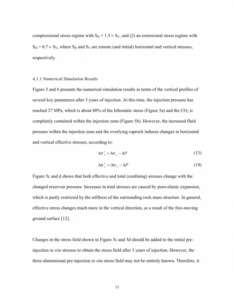
13

compressional stress regime with SH = 1.5 × SV, and (2) an extensional stress regime with

SH = 0.7 × SV, where SH and SV are remote (and initial) horizontal and vertical stresses,

respectively.

4.1.1 Numerical Simulation Results

Figure 5 and 6 presents the numerical simulation results in terms of the vertical profiles of

several key parameters after 3 years of injection. At this time, the injection pressure has

reached 27 MPa, which is about 80% of the lithostatic stress (Figure 5a) and the CO2 is

completely contained within the injection zone (Figure 5b). However, the increased fluid

pressure within the injection zone and the overlying caprock induces changes in horizontal

and vertical effective stresses, according to:

Pxx ∆−∆=′∆ σσ (13)

Pzz ∆−∆=′∆ σσ (14)

Figure 5c and d shows that both effective and total (confining) stresses change with the

changed reservoir pressure. Increases in total stresses are caused by poro-elastic expansion,

which is partly restricted by the stiffness of the surrounding rock-mass structure. In general,

effective stress changes much more in the vertical direction, as a result of the free-moving

ground surface [12].

Changes in the stress field shown in Figure 5c and 5d should be added to the initial pre-

injection in situ stresses to obtain the stress field after 3 years of injection. However, the

three-dimensional pre-injection in situ stress field may not be entirely known. Therefore, it

14

is useful to evaluate the maximum sustainable injection pressure for various in situ stress

regimes, including compressional pressure regime (for which SH > SV) and extensional

regime (for which SH < SV).

Figure 6a and b present vertical profiles for evaluation of shear-slip potential for the two

different stress regimes. In the case of a compressional stress regime (Figure 6a), shear slip

is most likely in the lower part of the cap, at the interface with the injection zone, and at the

lower part of the injection zone. However, the shear slip would probably not propagate

through the upper part of the cap, which would thus remain intact. In the case of an

extensional stress regime (Figure 6b), shear slip might first be induced near the ground

surface and in the overburden rock above the zone of pressure increase. Thereafter, shear

slip might also be induced in the caprock, just above the injection zone.

In Figure 7, the path of the principal effective stresses, σ′1 and σ′3, in the lower part of the

caprock (near its interface with the injection zone) is plotted and compared to the failure

criterion in Equation (12). For a compressional stress field, the principal stresses would

move into a region of likely shear slip after just over one year of injection at an injection

pressure of about 24 MPa. In an extensional stress regime, shear slip could occur just after

three years of injection at an injection pressure of about 28 MPa.

15

4.1.2 Comparison to Simplified Analytical Estimates

The maximum sustainable injection pressure may be estimated analytically using Equation

(12) for lithostatic vertical stress, SV = 33.2 MPa, at 1,500 m, and with different horizontal

stress, SH = 1.5SV or SH = 0.7SV, depending on the assumed stress regime. The critical

pressure Pc for inducing shear slip on an arbitrarily oriented fault can be derived from

Equation (12) by considering that shear slip occurs when P = Pc, that is we insert σ′1 = σ1

– Pc and σ′3 = σ3 – Pc into Equation (12)

23 13 σσ −

=cP (15)

First, estimating the maximum sustainable injection pressure from the initial (pre-injection)

stress field, we assume that the local stresses are equal to the remote stresses, i.e. σy = SV

and σx = SH (Figure 1a). For a compressional stress regime, σ1 = σx = SH = 1.5SV = 49.8

MPa and σ3 = σy = SV = 33.2 MPa, whereas for an extensional stress regime, σ1 = σy = SV =

33.2 MPa and σ3 = σx = SH = 0.7SV = 23.2 MPa. By substituting these numbers into

Equation (15), the simplified analytical estimate of the maximum sustainable injection

pressure is 25 MPa for a compressional stress regime and 18 MPa for an extensional stress

regime. These numbers indicate that the simplified analytical estimate excluding poro-

elastic stress is similar to that of the numerical analysis for a compressional stress regime,

whereas the simplified estimate for an extensional stress regime is overly conservative—

that is, the maximum sustainable injection pressure is underestimated (see Table 2). For the

extensional stress regime, the maximum sustainable injection pressure is underestimated by

16

Equation (15) because it neglects injection-induced poro-elastic stressing that tends to

increase the minimum principal stress, which in this case is horizontal.

If we consider the poro-elastic stressing analytically, using Equation (6) and a Poisson’s

ratio of 0.25 (Table 1), we find that ∆σx = 2∆P/3 ≈ 0.67∆P. In this case the local horizontal

stresses should be calculated as σx = SH + ∆σx = SH + 2∆P/3 (see also Figure 1b). Thus, for

a compressional stress regime, σ1 = σx = SH + 2∆P/3 = 1.5SV + 2∆P/3 and σ3 = σy = SV. For

the extensional stress regime, σ1 = σy = Sv and σ3 = σx = SH + 2∆P/3 = 0.7SV + 2∆P/3, if ∆P

< 15 MPa (if ∆P exceeds 15 MPa, the maximum principal compressive stress becomes

horizontal). By substituting these parameters into Equation (15), we determined a critical

pressure Pc = 27.2 MPa for a compressional stress regime. For an extensional stress regime,

the solution with the above parameters indicates that a critical pressure will never be

reached, but the estimated poro-elastic stress becomes very high and shifts the maximum

principal stress from vertical to horizontal, resulting in a very high critical pressure (Pc ≈ 63

MPa). Thus, for an extensional stress regime, the simplified analytical estimate including

poro-elastic stress grossly overestimates the maximum sustainable injection pressure (Table

2).

4.2 Shear-Slip Analysis with a Discrete Fault

In this simulation example, a shear-slip analysis is conducted using a discrete fault

representation in TOUGH-FLAC. As in the previous example, compressed CO2 is injected

at 1,500 m depth into a permeable formation overlain by a low-permeability caprock.

17

However, in this case, the injection zone is effectively bounded by an offset fault (Figure

8). In this example, an extensional stress regime with SH = 0.7×SV is assumed, and the fault

is considered cohesionless, with a friction angle of 25°.

4.2.1 Numerical Simulation Results

In the TOUGH-FLAC simulation, the fault is discretized into solid elements with

anisotropy of mechanical (elasto-plastic) and hydrologic properties. In this model, fault

permeability changes with shear such that for a fully reactivated fault (maximum shear

strain), permeability increases by two orders of magnitude. This is simulated by relating the

permeability changes, k/k0, to maximum shear strain, εsh, according to:

shkk

εβ ∆⋅+= 10

(16)

where β is set to 1×10-4 to obtain a two-order-of-magnitude permeability increase for a

fully reactivated fault. Other material properties and input data are similar to that of the

above continuum shear-slip analysis (Table 1).

Figure 9 shows the evolution of injection pressure during the constant-rate CO2 injection,

whereas Figure 10 and 11 shows contour plots that can help to explain the pressure

responses in Figure 9. In Figure 9, the fully coupled hydromechanical simulation (solid line

in Figure 9) is compared to an uncoupled simulation with no fault reactivation (dashed line

in Figure 9). If no fault reactivation is considered, fluid pressure would quickly rise above

lithostatic stress. On the other hand, if fault reactivation and shear-induced permeability

changes are considered, the injection pressure does not rise as high, but peaks at a

18

magnitude well below lithostatic stress. Figure 10 shows that after 6 months, the zone of

shear slip, observed as a zone of localized substantial shear strain, extends all the way

through the upper cap. Thus, a new flow path has opened up across the upper cap. As a

result, reservoir pressure can be released through the fault once it has opened all the way.

Moreover, after about 1 year and 4 months, the injected CO2-rich fluid reaches and

migrates up along the fault (see spread of CO2 at 1 and 3 years Figure 11).

From Figure 9, the maximum sustainable injection pressure might be estimated to be in the

range of 19 to 25 MPa. The first sign of shear-induced permeability change occurs after

about 1.5 months at an injection pressure of about 19 MPa. This finding indicates some

shear slip and permeability change, but shear slip does not propagate across the upper cap

until the injection pressure reaches about 25 MPa, which occurs after about 6 months of

injection. Actually, at 19 MPa, the injection pressure is affected by leakage into the

underlying formation. Upward leakage to overlying formations does not occur until the

fault slip has propagated through the upper cap, which occurs after 6 months at an injection

pressure of about 25 MPa. Therefore, the maximum sustainable injection pressure

estimated to be 25 MPa.

4.2.2 Comparison to Simplified Analytical Estimates

In this case we can also estimate the maximum sustainable injection pressure using

Equation (1), for the undisturbed initial stress field. At the depth of injection, the initial

stresses are SV = 33 MPa, and SH = 0.7×SV = 23 MPa. Using Equation (1) and considering

19

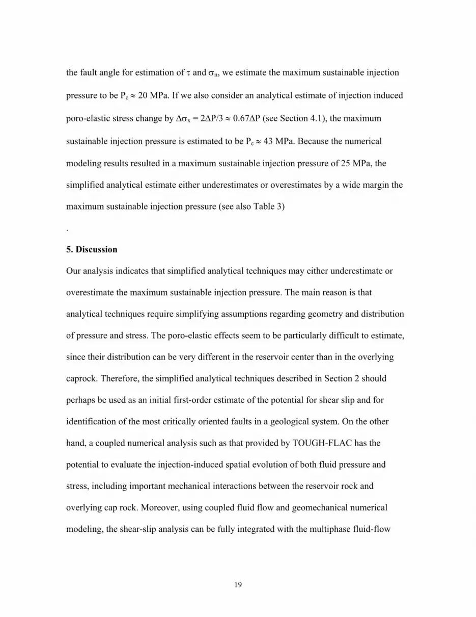
the fault angle for estimation of τ and σn, we estimate the maximum sustainable injection

pressure to be Pc ≈ 20 MPa. If we also consider an analytical estimate of injection induced

poro-elastic stress change by ∆σx = 2∆P/3 ≈ 0.67∆P (see Section 4.1), the maximum

sustainable injection pressure is estimated to be Pc ≈ 43 MPa. Because the numerical

modeling results resulted in a maximum sustainable injection pressure of 25 MPa, the

simplified analytical estimate either underestimates or overestimates by a wide margin the

maximum sustainable injection pressure (see also Table 3)

.

5. Discussion

Our analysis indicates that simplified analytical techniques may either underestimate or

overestimate the maximum sustainable injection pressure. The main reason is that

analytical techniques require simplifying assumptions regarding geometry and distribution

of pressure and stress. The poro-elastic effects seem to be particularly difficult to estimate,

since their distribution can be very different in the reservoir center than in the overlying

caprock. Therefore, the simplified analytical techniques described in Section 2 should

perhaps be used as an initial first-order estimate of the potential for shear slip and for

identification of the most critically oriented faults in a geological system. On the other

hand, a coupled numerical analysis such as that provided by TOUGH-FLAC has the

potential to evaluate the injection-induced spatial evolution of both fluid pressure and

stress, including important mechanical interactions between the reservoir rock and

overlying cap rock. Moreover, using coupled fluid flow and geomechanical numerical

modeling, the shear-slip analysis can be fully integrated with the multiphase fluid-flow

20

reservoir analysis of a site and can therefore be used for design and optimization of

injection/withdrawal operations. Such optimization could include maximizing injected CO2

mass while minimizing the risk for leakage.

6. Concluding Remarks

In this paper, we describe and demonstrate the use of coupled multiphase fluid flow and

geomechanical fault-slip analysis for estimation of maximum sustainable injection pressure

during geological sequestration of CO2. Comparison of numerical results to that of

analytical estimates using simplifying geometrical assumptions showed that the simplified

analytical estimates might either overestimate or underestimate the maximum sustainable

injection pressure. When conventional analytical techniques are used without accounting

for poro-elastic stresses, the analytical estimates are in most cases going to be conservative.

If poro-elastic stressing is considered in the analytical estimates using the assumption of

uniaxial strain conditions, the maximum sustainable injection pressure might be grossly

overestimated. The main advantage of the numerical approach presented in this paper

(compared to more conventional simplified analytical methods) is that the coupled

numerical analysis more accurately takes into account structural geometry and its effect on

the injection-induced spatial evolution of fluid pressure and in situ stress. Therefore, the

numerical analysis results in a more accurate estimation of the maximum sustainable CO2

injection pressure.

21

Acknowledgments

The work presented in this paper was financed by contributions from the Ministry of

Economy, Trade and Industry Ministry (METI) of Japan, and the U.S. Environmental

Protection Agency, Office of Water and Office of Air and Radiation, under an Interagency

Agreement with the U.S. Department of Energy at the Lawrence Berkeley National

Laboratory, No. DE-AC02-05CH11231.

References

[1] Thomas L.K., Katz D.L., Tek M.R. Threshold pressure phenomena in porous media.Society of Petroleum Engineers Journal, June 1968:174–184.

[2] Poston SW, Berg RR. Overpressured gas reservoirs. Society of Petroleum Engineers,Richardson, Texas, 1997. p. 138.

[3] Sibson RH. Brittle-failure controls on maximum sustainable overpressure in differenttectonic stress regimes. Bull Am Assoc Petrol Geol 2003;87:901–908.

[4] Barton CA, Zoback MD, Moos D. Fluid flow along potentially active faults incrystalline rock. Geology 1995;23:683-686.

[5] Streit JE, Hillis RR. Estimating fault stability and sustainable fluid pressures forunderground storage of CO2 in porous rock. Energy 2004;29:1445–1456.

[6] Wiprut D, Zoback MD. Fault reactivation and fluid flow along a previously dormantnormal fault in the northern North Sea. Geology 2000;28:595-598.

[7] Scholz CH, The Mechanics of Earthquakes and Faulting. Cambridge University Press,New York., 1990.

[8] van Ruth PJ, Nelson E, Hillis RR. Fault reactivation potential during CO2 injection inthe Gippsland Basin, Australia. Exploration Geophysics 2006;37:50–56.

[9] Morris A, Ferril DA, Henderson DB. Slip tendency analysis and fault reactivation.Geology 1996;24:275–278.

22

[10]Chiaramonte L, Zoback M, Friedmann J, Stamp V. CO2 sequestration, fault stabilityand seal integrity at Teapot Dome, Wyoming. 8th International Conference onGreenhouse Gas Control Technologies, Trondheim, Norway, June 19-22, 2006.

[11] Byerlee J. Friction of rocks. Pure and Applied Geophysics 1978:116;615–626.

[12]Rutqvist J, Tsang C-F. Coupled hydromechanical effects of CO2 injection. In: TsangC.F., Apps J.A., editors. Underground Injection Science and Technology. Elsevier,2005. p. 649–679.

[13]Hawkes CD, McLellan PJ, Zimmer U and Bachu S. Geomechanical Factors AffectingGeological Storage of CO2 in Depleted Oil and Gas Reservoirs: Risks andMechanisms, Proceedings of Gulf Rocks 2004, the 6th North America RockMechanics Symposium (NARMS): Rock Mechanics Across Borders and Disciplines,Houston, Texas, June 5-9, 2004.

[14] Hillis RR. Coupled changes in pore pressure and stress in oil fields and sedimentarybasins. Petroleum Geoscience 2001:7;419–425.

[15]Rutqvist J, Wu YS, Tsang C-F, Bodvarsson G. A Modeling Approach for Analysis of

Coupled Multiphase Fluid Flow, Heat Transfer, and Deformation in Fractured PorousRock Int J Rock mech Min Sc 2002;39:429-442.

[16]Rutqvist J, Tsang C-F. TOUGH-FLAC: A numerical simulator for analysis of coupledthremal-hydrologic-mechanical processes in fractured and porous geological mediaunder multi-phase flow conditions. Proceedings of the TOUGH symposium 2003,Lawrence Berkeley National Laboratory, Berkeley, May 12–14, 2003.

[17]Pruess K., Oldenburg C, and Moridis G. TOUGH2 User’s Guide, Version 2.0, ReportLBNL-43134, Lawrence Berkeley National Laboratory, Berkeley, Calif., 1999.

[18] Itasca Consulting Group, FLAC 3D, Fast Lagrangian Analysis of Continua in 3Dimensions. Version 2.0. Five volumes. Minneapolis, Minnesota, Itasca ConsultingGroup, 1997.

[19]Jaeger JC, Cook NGW. Fundamentals of Rock Mechanics. Chapman and Hall, London1979, p. 593.

[20]Corey AT. The interrelation between oil and gas relative permeabilities. ProducersMonthly November 1954: p. 38-41.

[21]van Genuchten MT. A closed-form equation for predicting the hydraulic conductivityof unsaturated soils. Soil Sci Soc Am J 1980;44:892-898.

23

Figure captions

Figure 1. Schematic of in situ stresses and fluid pressure considered in fault reactivationanalysis. (a) simplifying assumption in which local stresses are equal to pre-injection andremote stresses and (b) local stresses are the sum of remote and injection induced poro-elastic stress. SH and SV are remote (and initial) horizontal and vertical stresses,respectively.

Figure 2. Shear slip along a pre-existing fault (or fracture) as a result of (a) increased fluidpressure and (b) thermal- or poro-elastic stressing.

Figure 3. Fault plane representation in coupled TOUGH2 and FLAC3D analysis using (a)FLAC3D mechanical interface, or (b) multiple solid elements with anisotropic properties.

Figure 4. Schematic of model geometry for modeling of CO2 injection and continuumshear-slip.

Figure 5. Vertical profiles of (a) fluid pressure, (b) CO2 saturation, (c) change in horizontaleffective and total stress, and (d) change in vertical effective and total stress.

Figure 6. Vertical profiles of σ′1 - σ′1c = σ′1 - 3σ′3 for (a) compressional and (b) extensionalstress regimes.

Figure 7. Principal (effective) stress path at the bottom of the caprock for compressionaland extensional stress regimes.

Figure 8. Schematic for TOUGH-FLAC modeling of discrete fault hydromechanicalbehavior during CO2 injection.

Figure 9. Simulated evolution of injection pressure with and without consideration of shear-slip-induced fault permeability changes.

Figure 10. Contour of maximum shear strain after 6 months of injection.

Figure 11. Simulated evolution of CO2-rich phase. The contours indicates how far the CO2-rich fluid have spread as a separate phase after 1 month, 3 months, 6 months, 1 year and 3years of injection.

24

σz = SV

PσxSH SH

Sv

σx = SH

Remotestress

Local stressacross fault

σz = SV + ∆σV

PσxSH SH

SV

σx = SH + ∆σH

Poro-elastic stressing

Figure 1(a) Figure 1(b)

25

Shear Stress

Intact Rock Failure

Fault Slip

Effective Normal Stress σ ́ 3 σ ́ 1

Change in Fluid Pressure

Figure 2(a)

ShearStress

Intact RockFailure

Fault SlipThermal- or poro-elastic stressing

Effective Normal Stressσ́3 σ́ 1

Figure 2(b)

26

FLAC3D MechanicalInterface

Added TOUGH2Fault HydraulicElements

Figure 3(a)

FLAC3D MechanicalMultiple Solid ElementRepresentation

TOUGH2 MultipleHydraulic ElementRepresentation

Figure 3(b)

27

CO2

Large Lateral Extension

1.5 km

Injection zone(100 m thick)

Cap Rock(50 m thick)

Base Vertical profile

Figure 4

28

FLUID PRESSURE (MPa)

Z(m)

0 10 20 30 40

0

500

1000

1500

2000

2500

3000Lithostatic Stress

Hydrostatic

Pressure

Well pressureabout 80% oflithostatic stress

Cap

Inj. zoneBase

∆P

CO2 GAS SATURATION

Z(m)

0 0.5 1

0

500

1000

1500

2000

2500

3000

Injected CO2 iscontained within theinjection zone

Figure 5(a) Figure 5(b)

29

STRESS (MPa)

Z(m)

-10 0 10

0

500

1000

1500

2000

2500

3000

CapInj. zoneBase

Poroelastic stressingincreases totalhorizontal stressin injection zone

∆σx∆'σx

∆P

STRESS (MPa)

Z(m)

-10 0 10

0

500

1000

1500

2000

2500

3000

Cap

Base

∆σz∆'σz

∆P

Strong reductionin vertical effectivestress

Figure 5(c) Figure 5(d)

30

σ'1-σ'1c (MPa)

Z(m)

-10 0 10 20 30

0

500

1000

1500

2000

2500

3000

CapInj. zoneBase

Locations of highpotential forshear slip

Failure No failure

σ'1-σ'1c (MPa)

Z(m)

-10 0 10 20 30

0

500

1000

1500

2000

2500

3000

CapInj. zoneBase

Location of highestpotential for shearslip

No failureFailure

Figure 6(a) Figure 6(b)

31

σ'3 (MPa)

σ '1(MPa)

0 5 10 15 200

5

10

15

20

25

30

σ'3 (MPa)

σ '1(MPa)

0 5 10 15 200

5

10

15

20

25

30

σ'1 > 3σ'3(Shear slip)

σ'1 < 3σ'3(No slip)

t = 01 Yr

3 Yr

1 Yr

3 Yr

Compressionalstress regime(σH = 1.5σV)

Extensionalstress regime(σH = 0.7σV)

t = 0

Figure 7

32

Figure 8

33

TIME (Years)

PRESSURE(MPa)

0 1 215

20

25

30

35LithostaticStress 33 MPa

CO2 breaksthrough faultFault fully reactivatedacross cap

Fault reactivation (shear slip)begins near injection zone

Simulation with nofault reactivation

Figure 9

34

Figure 10

35

Figure 11

36

Table 1. Material properties used in TOUGH-FLAC simulations. Property Upper Cap Aquifer Basement

Young’s modulus, E (GPa) 5 5 5 5

Poisson’s ratio, ν (-) 0.25 0.25 0.25 0.25

Biot’s parameter, α (-) 1 1 1 1

Saturated rock density, ρs (kg/m3) 2260 2260 2260 2260

Porosity, φ (-) 0.1 0.01 0.1 0.01

Permeability, k, (m2) 1×10-15 1×10-17 1×10-13 1×10-17

Corey [20] irreducible gas saturation, Srg (-) 0.05 0.05 0.05 0.05

Corey [20] irreducible liquid saturation, Srl 0.3 0.3 0.3 0.3

van Genuchten [21] capillary strengthparameter P, (kPa)

196 3100 19.6 3100

van Genuchten [21] exponent, m 0.457 0.457 0.457 0.457

37

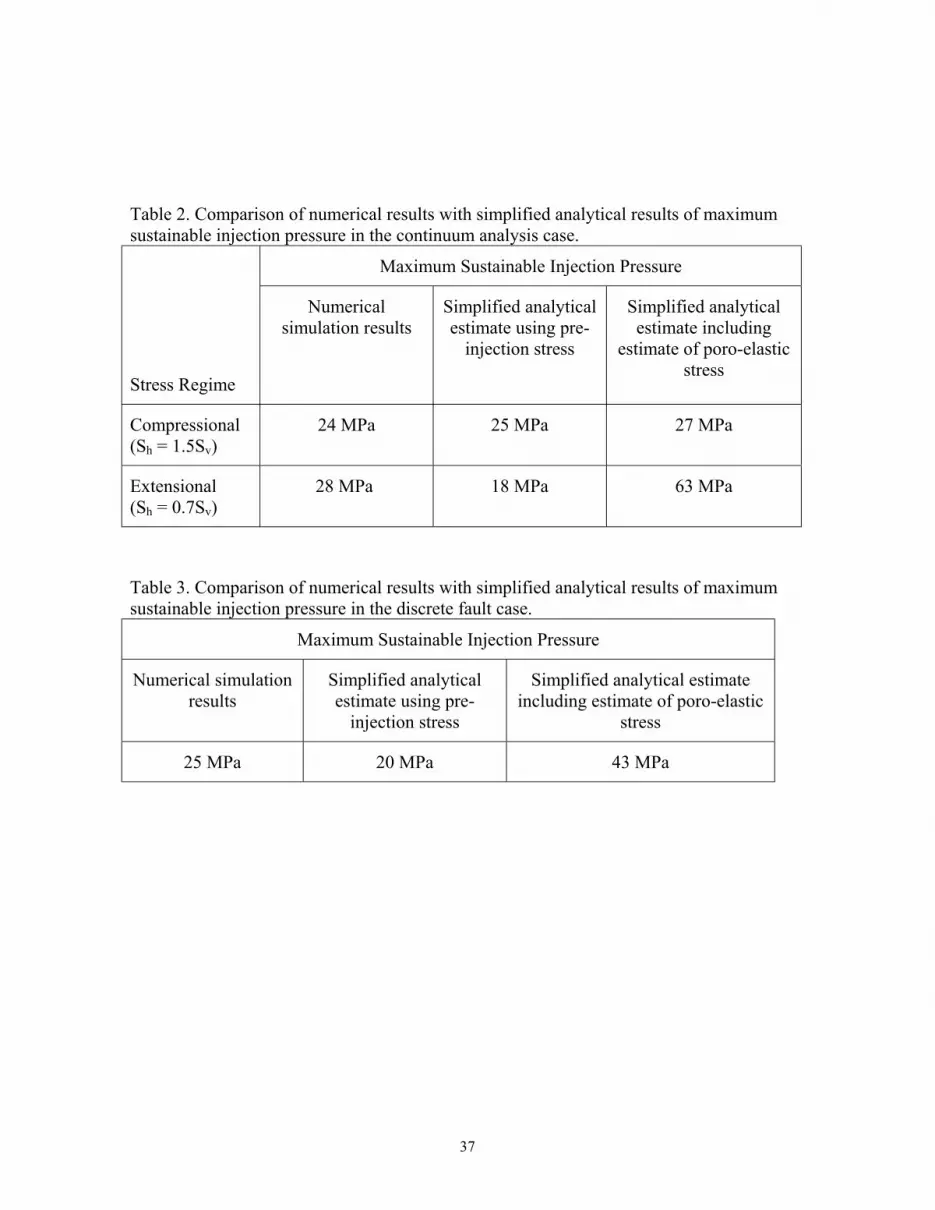
Table 2. Comparison of numerical results with simplified analytical results of maximumsustainable injection pressure in the continuum analysis case.

Maximum Sustainable Injection Pressure

Stress Regime

Numericalsimulation results

Simplified analyticalestimate using pre-

injection stress

Simplified analyticalestimate including

estimate of poro-elasticstress

Compressional(Sh = 1.5Sv)

24 MPa 25 MPa 27 MPa

Extensional(Sh = 0.7Sv)

28 MPa 18 MPa 63 MPa

Table 3. Comparison of numerical results with simplified analytical results of maximumsustainable injection pressure in the discrete fault case.

Maximum Sustainable Injection Pressure

Numerical simulationresults

Simplified analyticalestimate using pre-

injection stress

Simplified analytical estimateincluding estimate of poro-elastic

stress

25 MPa 20 MPa 43 MPa