environmental geology of the avon-heathcote estuary
TRANSCRIPT

ENVIRON:MENTAL GEOLOGY OF THE AVON-HEATHCOTE ESTUARY
J.M. Macpherson
A thesis submitted for the degree of Doctor of Philosophy
UniveTsity of Canterbury, Christchurch, New Zealand
February 1978.
2

c " . I,
"
(
i
ABSTRACT
The Avon-Heathcote is a small, microtidal, predominantly
intertidal, weather-dominated estuary. It has experienced large
alterations to its physical environment as a result of the establishment
and growth of the adjacent Christchurch City, on what was previously a
swampy, dune-bordered coastal plain. During the period 1850-1920 the
tidal compartment decreased by 30%, then returned rapidly to its original
volume. It has since increased to about 30% more than its pre-European
volume. The inlet area progressively changed its configuration to
accommodate these alterations in volume.
An analysis of the energetics of waves and tidal currents shows
that wave-induced shear stresses predominate in this estuary, particularly
above the MTL, and are only exceeded by tidal current stresses in and
adj acent to subtidal channels, where tidal velocities exceed 60 cm/s.
Because of depth limitations the largest waves in this estuary normally
have periods of 1.4 s, amplitudes of 30 cm and lengths of 3.5 m.
Wave energy gradients are due to downfetch variations in wave frequency,
not variations in wave size.
The muddiest sediment occurs close to the entrances of the Avon
and Heathcote rivers, and patterns of mud deposition are regulated
both by rates of sediment supply and by wave energy. The sand fraction
of active surface sediment can be divided into two groups - one
consisting of a single population deposited solely from saltation, the
other consisting of a mixture of this saltation population, and material
deposited from suspension. Sand is only deposited from suspension near
the two river entrances, or on intertidal flats below the MTL, where
wave shear stresses are less than 2 dynes/cm 2•
Shallow cores reveal that a record of the history of this estuary
is preserved in its subsurface sediment. An abiologic, pre-estuarine/
estuarine pre-European/estuarine post-European sequence is recognised
beneath a 15-20 cm deep bioturbation interface. Above this interface
benthic animals have produced a homogeneous mixed layer, depleted of
suspendible fines, which is overlain by a thin and commonly quite
different active layer. The active layer exists independently of trends
in net erosion or deposition of sediment.

ACKNOHLEDGEMENTS
The \vriter wishes to thank the following per~ons and
organisations: Dr D.W. Lewis, who suggested the topic,
supervised the research, and revie\>Jed a first draft of the text.
Dr J.A. Robb, and the Christchurch Drainage Board, who supplied
the 1;>Jrit er with historical maps, charts and literature, and whose
survey data have been fundamentally influential. Dr A.J. Pearce
critically reviewed a near-final draft of the text. Lee Leonard
assisted with the drawing of some of the figures, Frank McGregor
supplied an excellent and very useful series of low level
air photographs, and Albert Downing photographed and printed the
figures and maps. The writer was supported during 1975 by a
University of Canterbury Teaching Fellowship, which is gratefully
acknowledged.
Special thanl~ to Susan Macpherson for support and
continuous encouragement.
Personal communications acknowledged in the text
were from the following people: G. Coates, Department
of Geology, University of Canterbury; D. McConochie,
M.Sc. student, Department of Geology, University of
Canterbury; P.J. McWilliam, Chief Engineer, CDB;
D. Retter, M.A. student, Department of Geography,
University of Canterbury; J.A. Robb, Biologist, CDB;
and D.D. Wilson, Christchurch Office; NZ Geological Survey.
ii

CONTENTS
ABSTRACT
ACKNOWLEDGEMENTS
GLOSSARY
LIST OF FIGURES
LIST OF MAPS
INTRODUCTION
Previous work
1. Definition of an es
2. Classification of es tuaries
3. Discussion
4. The influence of tidal range
5. Previous \vork in the Avon-Heathcote Estuary
PART ONE
HISTORY OF TIlE AVON-HEATHCOTE ESTUARY
Quaterny history of the Christchurch area
Post-European history of the Avon--Heathcote Estuary
1. Introduction
2. Urbanisation and drainage modifications in the Christchurch area
3. Changes in the tidal compartment of the Avon~Heathcote Estuary
4. Discussion and conclusions
5. Changes at the inlet to the es
PART THO
, 1850-1975
ENERGETICS - WAVES AND THE TIDE
Introduction
Waves and "Vlave hindcasting
1. Wind characteristics
2. De lin a fetch
3. Sr.ffi i>lave predictions
iii
Page
i
ii
vii
viii
xii
1
1
1
3
3
4
4
5
7
7
8
8
9
12
16
16
16
24
24

4. Limitations on wave dimensions
5. Wind event frequencies
6 . Discuss ion
Near bottom velocities and shear stresses
Threshold of sediment motion under waves
Wave refraction
1. Introduction
2. Discussion
3. Results
Wave-generated bedforms
Tides
1. Introduction
2. Ripple orientations and dimensions
1. .Introduction
2. Previous vlOrk
3. Shear- stress
4. Sediment entrainment
5. Entrainment into suspension
6, Current-generated bedforms
Wind-driven currents
Introduction
PART THREE
BA THY NET RY
Descriptions and ations
1. Eastern high tide slopes
2. Eastern mid tide shelf and low tide flats
3. Western and flats
4. The Heathcote Basin
5. Central mounds
6. Throughgoing subtidal channels
Discussion
Patterns of erosion and deposition
An energy-bathymetry model for the Avon-Heathcote Estuary
iv
Page
24
27
27
29
31
31
31
32
32
34
34
38
39
39
39
42
43
44
44
46
50
50
50
56
57
63
63
63
65
66
68.

PART FOUR
SURFACE SEDI~lliNT
Introduction
Mud
Sand
1. Observations and interpretations
2. Discussion
l.
2.
3.
4.
5.
6.
7 •
Introductory discussion
Numerical procedures
Cluster is results and interpretations
Height above datum preferences of groups A to E
Regional distribution patterns
Interpretations
Graphic statistics
PART FIVE
SUBSURFACE SEDIMENT
Tn;Tnrillrtinn
I:v1ethods
Results and interpretations
Sediment from beneath the bioturbation interface
1. Unit (a)
2. Unit (b)
3. Unit (c)
Biology and physical characteristics of from above the bioturbation interface
1. Biology
2. Sedir!lCn t analyses
3. Conclusions and discussion
Clay mineralogy
1. Methods
2. Results
3. Conclusions
Sand fraction mineralogy
Microfauna
1. Results
2. Conclusi.ons
v
70
70
70
75
76
76
79
80
88
90
92
94
103
103
104
10/{
lOLl
111
119
123
124
129
136
140
140
141
141
143
144
1LI4 1 1'-LLfO

PART SIX
SUMMARY AND SYNTHESIS
Summary history of the Avon-Heathcote Estuary
Energetics
1. Wind and waves
2. Tidal currents
3. Wind-driven currents
Bathymetry
Surface sediment
1. Mud
2. Sand
Subsurface sediment
1. Stratigraphy
2. Near-surface bioturbate sediment
3. Predictions
REFERENCES
APPENDICES
Appendix 1. Historical estimates of the tidal compartment of the Avon-Heathcote Estuary
1. Predicted volumes
2. Direct estimates
3. Methods used to calculate volumetric changes
4. Results
Appendix 2. Bathymorphic profiles surveyed in 1920, 1962 and 1975/77
Appendix 3. Surface and subsurface sediment analyses. Methods and procedures
1. Sampling design
2. Sampling methods
3. Sand vs mud
vi
Page
147
149
149
150
151
151
152
152
153
155
156
156
158
159
173
173
173
177
177
179
186
186
186
188
4. Sand fraction analyses by sedimentation 188
5, Reproducibility and reliability 192
Appendix 4. Detailed descriptive and graphic logs, subsurface sediment cores from the Avon-Heathcote Estuary 199

Abs
p. 1
p. 3
p. 4
p. 7
p. 9
p. 13
p. 18
p. 23
p. 30
p. 31
p. 42
p. 43
p. 48
p. 52
p. 56
p. 65
p. 66
p. 74
p. 75
p. 77
p. 78
p. 80
p.l04
p.ll?
p.ll8
p.128
p.129
p.154
p.175
p.194
There
par. 1
par. 1
par. 1
par. 2
par. 2
par. 1
. 5
Fig. 6
Environmental Geology of the Avon-Heathcote Estuary
Corrections and Amendments
line 2 Rivers.
6 km 2•
basin.
mesotidal.
Martins 196~, Heinemann. 106m 3.
"B" missing, LH side, centre panel.
RH column consists of values> 20 knots.
vii
Fig. 10 directional arrows misidentified - solid arrows indicate the mean SW wind; sharp open arrows, the NW; and squat open arrows, the E wind.
par. 3 p ~ fluid density.
par, 2 orbital velocities should be in cm/s. par, 3 omit "geometrical optics and ". -
par. 4 final sentence should continue " ... expediency, in spite of the further limitation that in the present case, velocities have not been measured 100 cm above the bed."
tables should have U, not uIOO ' in LH columns.
par. 1 sentence 2. location 3 Figure 17, not Figure 20.
Fig. 22 Sandy Point.
par. 4 sentence 1. Omit words in parentheses.
sentence I, above ~WOST; sentence 4, Heathcote.
par. 4 and onwards, Maps i and !, not 2 and 3.
Fig. 35 A is upper plot, B is lower. Sorted in caption.
line 4 magnitude_.
2nd to last line, lo~.
par. 2 modal.
psi ~ -lo92x.
(and onwards), s = standard deviation, N = number of samples.
Fig. 60. Caption should continue " ... subsurface sediment. Arrows show mean HAD values of each group. JI
Fig. 61. Caption should continue n ••• sediment. Numbered asterisks are group means, with b ' mean unnumbered; dashed lines are linear regressions fitted to all group bl-b4 samples (short dashes) and to group means only (long dashes) .
line 5 pre~umably.
par. 3 on not of.
par. 2 sentence 6 should read " •.. suspended sand (and mud) ... "
par. 3 1.65 1.51 x 10⁶ml.
par. 3 Fig. 84 should be Fig. 85. In Fig. 83 data are from Fig. 82, not 33; and in Figure 85 data are from Fig. 84, not 35.
are no Figures 75 and 76.

AHE =
CDB =
HAD
HWOST
HWONT
MHW =
MTL
MLW
LWONT
LWOST
yBP
CERC
GLOSSARY OF FREQUENTLY USED ABBREVIATIONS
Avon-Heathcote Estuary
Christchurch Drainage Board
Height above (Christchurch Drainage Board) datum
High water, ordinary spring tide
High water, ordinary neap tide
Mean high water
Mean tide level (equivalent to mean sea level)
Mean low water
Low water, ordinary neap tide
Low water, ordinary spring tide
Years before present
Coastal Engineering Research Centre
(at the us Army Corps of Engineers)
vii

FIGURE
1
2
3
4
5
6
7
8
9
10
11
12
13
14
15
16
LIST OF FIGURES
Location maps
Geology of the Christchurch area
Christchurch and suburbs. Population. miles of stormwater and sewage pipes, volumes of effluent released into the estuary from CDB treatment works, and changes in the volume of the tidal compartment of theMIE for the period from 1850 to 1975.
Diagrammatic representation of exponential changes in the volume of the tidal compartment of the Avon-Heathcote Estuary, for the period 1850-1980
Synoptic maps of changes in the inlet area of the Avon-Heathcote Estuary for the period 1850 to 1975
Wind event frequency table
Derivation of wind stress (E ) and w
effective wind stress (Ewf
)
Frequency distributions of wind stress, effective wind stress, per cent total wind events, and per cent total wind events greater than or equal to 19 knots (5 m/s)
Directional distribution of effective wind stress (Ewf)
Effective fetch map of the Avon-Heathcote Estuary
Wave prediction curves
Diagrarrunatic illustration of the relationships between wave generation and water depth in the Avon-Heathcote Estuary
Southwest wind (217 0) and east "lind (075 0 ) 1;.lave
refraction diagram
Wave formed ripples of the Avon-Heathcote Estuary
Distribution and orientations of wave-formed ripples on September 4 1976 (\Vest side) and September 8 1976 (east side)
Ripple crest spacing vs water depth (as height above datum), western slopes, tember 4 1976
17 Intertidal and subtidal current velocities in the
18
19
20
Avon·-Heathcote Estuary
Current-formed ripples in the Avon-Heathcote Estuary
The intertidal configuration of the ebb-tide delta of the Avon-Heathcote Estuary
Possible \vind-driven advective circulation of the Avon-Heathcote Estuary
viii
Page
2
6
11
13
18
19
21
2.2
23
25
28
33
35
36
37
45
49

FIGURE
21
22
23
24
25
26
27
28
29
30
31
32
Intertidal bathyforms of the Avon-Heathcote Estuary
Shorelines of the Avon-Heathcote Estuary
Bathymorphic profiles. Eastern high tide slopes, lines 2-10.
Bathymorphic profiles. Eastern high tide slopes, lines 11-15.
Bathymorphic response to wave energy
Summary bathymetry and wave energy distribution of the eastern side of the Avon-Heathcote Estuary
Bathymorphic profiles. Eastern midtide shelf, lines 7 and 8. Eastern low tide flats, lines 5-8.
Bathymorphic profiles. Western slopes and flats, lines 2-8.
Bathymorphic profiles. Western slopes, lines 9-15.
Bathymorphic response to wave energy
Bathymorphic profiles. Central sand mounds, lines 8, 11-13.
Bathymetry/Energy model of the intertidal slopes and flats of the Avon-Heathcote Estuary
33 Huddiness of surface sediment of the
34
35
36
37
38
39
40
41
42
43
Avon-Heathcote Estuary
Sediment muddiness vs water depth
Sediment muddiness vs ,"vater depth
Dendogram resulting from cluster analysis of 102 representative samples of surface sediment from the Avon-Henthcote Estuary
Representative cumulative probability curves of samples from cluster groups A, Band C
Representative cumulative probability curves of samples from cluster groups D, E and F
Cumulative curve envelopes (from Figures 41 and 42) of cluster groups A-C and plotted on conunon axes
Scatter plot of mean size VB graphic standard deviation (sorting) of 480 samples from cluster groups A-F
Scatter plot of 5th percentiles (psi 5) vs 95th percentiles (psi 95) of 480 samples from the cluster groups A-F
Histograms of sample frequency vs sample HAD for cluster groups A-E
Diagrammatic distribution patterns of sediment cluster groups
44 Surface sediment of the Avon-Heathcote Estuary. Sand fraction graphic standard delfiation (sorting), contoured at 0,2 psi; 0,3 psi and 0,4
ix
Page
51
52
53
54
55
58
59
60
61
62
64
69
72
73
74
81
82
83
84
86
87
89
91
95

FIGURE
45 Surface sediment of the Avon-Heathcote Estuary. Sand fraction at 2.0 psi, 2.5
mean diameter, contoured and 3.0 psi
,1!6 A - Constant-scale bathymorphic profiles, lines 2-ll
47
48
49
50
51
52
53
54
55
56
57
58
59
60
61
61
63
from the western s and flats. Horizontal reference marks are at 9.0 m HAD. B - trends in sand fraction mean diameter plotted at the same constant scale
A - Constant-scale bathymorphic profiles, lines 2, 5, 6-8 from the eastern lmv tide flats. B - Trends in sand fraction graphic mean size
A - Constant-scale bathymorphic profiles across 9.0 m HAD flats and shelves, plotted on common axes
Graphic mean size/bathymetry model of the surface sediment of the Avon-Heathcote Estuary
Stratigraphic sections and summary graphic logs
Summary s
Summary stratigraphy
Summary s
Representative cumulative probability curves, graphic statislics and percentile input data, unit (a) subsurface sediment
Scatter plots of graphic mean diameter vs graphic standard deviation, and graphic mean diameter vs HAD, unit (a) subsurface sediment
Contoured upper contact of subsurface sediment unit ( ,in metres ~AD
Sand fraction graphic statistics, data, and dendrogram resulting from cluster of data, unit (b) subsurface sediment
input analysis
sentative CUIllulative probability curves from groups 101-64 and 6', unit (b) subsurface sediment. Follows page no.
Scat ter plot of graphic mean diameter vs graphic standard deviation for samples from unit (b), subsurface sediment
frequency vs HAD for the groups b 1-b4 and b I, unit (b) subsurface sediment
Scatter plots. A -- Nean diameter vs HAD. B Per cent mud vs HAD. Sample from cluster group (b), subsurface sediment
Surface occurrences of pas mud -- subsurface stratigraphic Avon-Heathcote Estuary
anthropogenic unit (c) - in the
entative cumulative ty curves, graphic statistics and percentile input ,data, unit (c) subsurface sediment
x
96
97
99
101
102
105
106
107
108
109
llO
ll2
ll4
ll4
116
117
ll8
120
121

FIGURE
64
65
66
67
68
69
70
71
72
73
74
...,., I I
78
79
80
81
82
83
84
Scatter plots. A - Hean diameter vs graphic standard deviation. B - Hean diameter vs HAD, unit (c) subsurface sediment
Surface evidence of sediment-modifying biological activity in the Avon-Heathcote Estuary
Surface evidence of sediment-modifying biological activity in the Avon-Heathcote Estuary
Scatter plot showing 17 pairs of surface sediment samples and adjacent uppermost core samples from the Avon-Heathcote EStuary
The western end of line 12
Sand fraction cumulative probability curves of surface and 5 cm core samples. Follows page no.
Plots of sediment muddiness and graphic mean diameter of surface and 5 cm core sample pairs from line 12
Scatter plots, surface sample and 5 cm core sample pairs, from line 12
Shallow cores 2-9 from line 12 in the Heathcote Basin
Cumulative probability curves of samples from cores 2, 4 and 5-6
Cumulative probability curves of samples from cores 7, 8 and 9 .4 1 , Q 1:.,. 1. ..9 ~. I • ~ ., 1 '1 ! ._ fi - 1.4,1;. pedK. lle..L)SllLo VO 1ft pedK. lleJ. Lo \J.ll llLLL.L.LIlIC
from X-ray analyses of subsurface sediment samples from the Avon-Heathcote Estuary, B loR peak heights vs 7R peak heights from the same analyses
Relative abundances and stratigraphic distribution of Ostracoda in four core samples from the Avon-Heathcote Estuary
Cross-sectional area of the tidal entrance at mid tide and the tidal compartment at ordinary spring tide, Avon-Heathcote Estuary, 185l,-1975
Comparison of cumulative probability curves of four representative sand fractions of samples from the Avon-Heathcote Estuary
Scatter plots of sieve vs RSA size analyses
Replication exercise. Results of analyses of 31 subsamples of 539
Replication exercise. Sequential variations in mean diameter, graphic standard deviation (sorting), skewness and kurtosis of 31 subsamples of sample 539, run in the sequence 1-31. Data from Figure 33,
Replication exercise~ Results of analyses of 25 consecutive 1m x Scm surface sediment samples from the eastern end of line 9.
xi
Page
122
125
126
130
132
132
133
134
135
137
l38
142
145
17l~
190
191
193
195
196

xii
FIGURE Page
85 Replication exercise. Sequential variation in granulometric ies of 25 consecutive 1m x 5cm surface sediment s Data from ~igure 35 197
LIST OF MAPS
Follows MAP Page
1 Intertidal bathymetry of the Avon-Heathcote Estuary [.9
2 Dis of samples belonging to cluster groups A to F 90
3 Sediment , 1920 to 1962 177
4 Sedimen t budget, 1962 to 1975/77 177

INTRODUCTION
This study consists of a detailed examination of the
Avon-Heathcote Estuary (AHE) , a small (area = 6 km) shallow (mean
1
depth at HWOST == 140 cm) largely intertidal (15% subtidal) estuary
surrounded by the eastern suburbs of Christchurch City on the east
coast of the South Island, Ne~", Zealand (Figure 1). The ABE is a
particularly suitable research area because it is a convenient size, it
is readily accessible, and because its biology is fairly well known.
Purpose
The primary objective has been to investigate physical changes
that have occurred in the AHE as a result of man's activities. This
objective has been realised' by making a relatively long term
(130 year) retrospective assessment of the impact of a1ristchurch City
on the estuary. Contemporary physical processes and the properties of
active surface sediment >"ere examined to the major sources of
physical energy in the estuary, and to show how these affect the
t:nmsport <md deposition of sediment. Subsurface sediment was
examined to test the possibility that it contains a record of past
environmental conditions.
Previous ,,,,ork
The literature on estuaries is vast, diverse, and difficult to
summarise. Good general reviews include the landmark publication
edited by Lauff (Estuaries, 1967), physical oceanography texts by
Ippen (1966), Dyer (1973) and Officer (1976b), collections of papers
edited by Nelson (1973) and Cronin (1975), and numerous papers in
scores of international journals. Volume 19 (5) of Oceanus is a good
review of many aspects of es tuarine geology, oceanography and eco
The innovative manual of simple oceanographic techniques by Wright
(1974) is also useful.
1. Defin-it-ion of an estuary. The most commonly accepted
definition is that of Pritchard (1967: "An estuary is a semi-enclosed
coastal body of water >"hieh has a free connection with the sea and
within which sea water is measureably diluted with fresh water derived
from land drainage."

c
A
/ I
I I
/ /
/ /
/
B ,--________ ... __ ~.
/ ~------~----~_hf--f-----7
Figure 1. ],ocation map". A - New Zealand. B - l'er,asus Buy (1), mouth of the \';aimalcariri River (2), the Avon-Hee,thcote Estuary (3). llarLics Peninsula, with Lyttel ton Harbour (4) and Alearoa Harbour (5), and Lake Ellepmere (6). C - Detni 1 of oouthe rn Pe(!,a13U[1 Day (1) and the Chrbtchurch areu, shov/ing the Avon-Heathcote Eatuary (2), Brighton Spit (3) awl the urban area (4).
2

3
2. CZassification of es-{;ual'ies. Various classification schemes
for estuaries have been proposed in the past, and these can be grouped
into two principal types:
(i) Those based on the mode of f01:-mation of the basis. Thus
Pritchard (1967) recognised four varieties: drowned river
valleys (also known as coastal plain estuaries), fj ords,
bar-built estuaries, and those produced by tectonic processes
(or all those not fitting the first three classes).
(ii) Those based on different degrees of mixing of fresh and salt
water: circulation patterns, the intensity of vertical density
stratification, and the extent of lateral homogeneity are the
major variables in these classifications (Schubel, 1972; Dyer,
1973; Officer, 1976b). End members are salt-wedge estuaries,
where the interface between salt and fresh ';vater is steep and
abrupt, and well mixed estuaries, where the water mass may be
horizontally as well as vertically homogeneous.
3. Discussion. Host of the material published on estuaries
is concerned with large, mesotidal, predominantly subtidal coastal
plain (river valley) estuaries, where the tidal range may be
consicierably less than hal f the mean depth, and where water tlO\ving
into the estuary is usually in residence for many tidal cycles.
Such estuaries are commonly either partially mixed or highly
stratified (Officer, 1976b). Examples are Chesapeake Bay and the
New England estuaries of the U.S. Atlantic Coast, the Thames, Tay
and Severn estuaries of the U.K., and the Gironde of France.
Research in estuaries of this sort has tended to concentrate
on the nature of tidal averaged (mean) flow, the location and dynamics
of shoaling areas, the properties and transportation of suspended
particulate matter, both organic and inorganic, and the nature and
significance of poorly understood phenomena such as occurrences of
ephemeral fluid mud - heavy-metal rich, anaerobic material ,,7hich may
significantly alter the environmental quality of many large estuaries
(for example see Officer, 1976a). The turbidity maxima which exist
near the landward ends of many large estuaries, various shipping
oriented engineering problems, . and environmental problems involving
waste disposal are also features which have received considerable
attention (for example see Cronin, 1975). Huch of this material is
irrelevant to the present study, because the ABE is very small,

microtidal, has an almost complete tidal exchange, and is usually
well mixed (for example see Knox and Kilner, 1973).
4. The influence of tidal range. Hayes (1975) has proposed
useful subclassification of coastal plain and bar-built estuaries
which is based in tidal range, and three classes are recognised:
(i) Microtidal where the tidal range is 0-2 m
(ii) Mestodial - where the tidal range is 2-4 m
(iii) Macrotidal where the tidal range is > 4 m
Microtidal estuaries are characterised by storm-surge
and wave-built featU1~es, and may have small flood-tide deltas.
Dominant processes are wind and wave induced; currents generated
by the astronomical tide are important transporters of sediment
only at the mouth.
The channel and shoal morphologies of tidal del tas in
mesotidal estuaries are remarkably similar from place to place,
a
and conform to basic models, regardless of varying local hydrodynamic
conditions (Coastal Research Group, 1969; Hayes, 1975; Reinson, 1977).
A major feature is the horizontal separation of flood and ebb currents
in the channels of Lne Licial cieltas due to the time-velocity
4
asymmetry of tidal currents (Postma, 1967; Hayes, 1975). Macrotidal
estuaries are dominated by tidal currents and are usually broad-mouthed
and funnel shaped. Sand bodies are centrally located, linear, and
aligned parallel to the long axis of the estuary. Marginal muddy tidal
flats are cornmon.
5. Previous work in the Avon-Heathcote Estuary. The i111.published
compilation by Knox and Kilner (The ecology of the Avon-Heathcote
Estuary, 1973), prepared for the Christchurch Drainage Board (CDB) ,
contains a comprehensive summary of scientific work done in and near
the AHE prior to 1972. This work was mostly biological, much of it
dire cted towards an evaluation of the role of the CDB in the pollution
of the estuary. Several of the individual projects reported in this
compilation briefly examined aspects of the physical environment.
An at tempt to summarise this early vlOrk would unnecessarily duplicate
Knox and Kilner's excellent review - relevant aspects of it will be
referred to \vhere appropriate in the following report.

PART ONE
HISTORY OF TIIE AVON-HEATHCOTE ESTUARY
the Chris area
Metropoli tan Christchurch and the AHE are situated on a coastal
plain composed of Late Quaternary terrestrial gravels, marine and dune
sands, and estuarine peats and clays (Suggate, 1958, 1968;
Brown, 1975, in press; Wilson, in press). To the south-east, the
metropoli tan area spreads on to the lower and \Vestern flanks of
Banks Peninsula, which is composed of andesitic and basaltic-andesitic
flows and red-weathering rates of the telton Volcanics
(Figure 2). Yellmv loess, dominantly of coarse silt, mantles the
lower flanks of the volcanic cone.
During the last 5 000 years the Bay coastline has
migrated eastwards (D. D. Hilson, pers. comm.), leaving behind a
sequence of surface sediments which progresses from inland
and swamp renmants ~ alluvial silt and fluvi at i le gravels, through
sand and fixed and semi-fixed dunes, to the modern beach
(Figure 2). Biggs (1947) recognised three separate dune belts
within the coastal part of this sequence (shown undifferentiated in
Figure 2); Blake (1964) dated the oldest (inland) belt at about
4 000 to 5 SOD yBP, the central belt at 1 000 to 2 000 yBP, and the
youngest belt, landward of the active dunes of the modern beach, at
400 to 1000 yBP. Dune renmants of the second belt occur west of
the AHE, \vhile sand of the younger belt occurs to the north-east -
indicat tha t the es probably first appeared between 1 000
and 2 000 years ago. The western edge of the modern estuary is
inferred to be the approximate position of the coast at the time
of formation of the second dune belt, and Sandy Point (Map 1) is
interpreted as an abandoned spit hook, analogous to the present one
several thousand metres to the east.
5

Km
F gure 2. Geology of the Christchurch area. After Drown (1975. in press). F' xed and semj.-fixed duneD and inland !:land deposita are stippled. Other f 0.tures inclUde active' dunes and th(.l modorn beach {l}, 'drained lH::J.t swamps ( ), alluvial silt dvpol:\i ts (J), fluviatile gravel of the rive r flood plaine (4), loess areao (5) and volcanic rock of the 'l'ertiary Lyttelton Vol canoe (6). Numbered localities include the Avon-Heathcote Estuary (7), Colombo Street (8), 1'apanui Road (9). b;oorhoune Avenue (10), Linwood Avonue (11), the .Avon River (12) and the Heathcote River (13).
6

is to
1. Introduction and discussion. The common fate of estuaries
with seJiment (Roberts and Pierce, 1974)", and some have
done so in historical times for example the River Dee in England
e, 1973). Estuaries are infilled with sediment because they
are very efficient sediment sinks, accumulating almost all material
en tering them from both land and offshore sources (Meade, 1974).
Many estuaries have filled with sediment since the beginning
7
of the 20th Century because of landuse changes in their catchment areas
(Roberts and Pierce, 1974). A major cause of accelerated infilling is
the conversion of large proportions of estuarine catchments from
rural to urban uses.
The effects of urbanisation on adjacent waterways are well
. known (Savani and Kamerer, 1961; Lindh, 1972; Guy and Jones, 1973;
Heinmann and Piest, 1973). During the early urban - when
vegetation cover is removed, some houses are built, wells are drilled
and sanitary drains dug there is an increase in stormHater flow, an
increase in soil moist:ure, a rise in the Hater table, and some
waterlogging of land. As a result sediment yields increase, and
sediment accumulates rapidly in nearby streams. In later stages
the combination of increasing impervious cover and roads) and
more efficient results in increas volumes of storm runoff
and a reduction in the runoff lag time - the time betHeen the centre
of mass of a rainstorm and the centre of mass of the resulting runoff
(1<Jartins, 1968; Leopold, 1968; Detwyler, 1971).
During post-urban basin stabilisation (Guy and Jones, 1972,
p.2109) sediment deposited in streams and other \.rater bodies during
early urbanisation is re-eroded, as the rate of sediment supply
decreases, but runoff volumes and flood flow"s continue to increase.
As further stabilisation occurs Hatercourses are stripped of
sediment deposited
beyond their
Sediment moving
early developIT~nt > and often increase
dimensions to accommodate the increasing flow.
and beyond these enlarging channels will
usually be considerably coarser than
con s t ruct ion.
t yielded during

8
2. Urbawisation dT'ainage modifications in the Christchurch
area. The first European settlers arrived in the Christchurch area in
1850, and by 1875 the population had risen to more than 10 600 (Retter,
pers. comm.). Early maps of the area (lmown as Black Maps and held by
the Lands and Survey Department, Christchurch - see Scott (1963) for
a redrafted version) indicate that in about 1850 the area which is now
Christchurch City was predominantly wet marshy land, with shallow ponds
and shaking bogs, vegetated ,.,rith rushes, flax and ferns. To the east
the older parts of the dune complex were covered with grasses and
Manuka, while the youngest, easternmost dunes were unvegetated.
Areas of open grassland were interspersed between the swamps and
sandhills.
In the earliest days of settlement surface water in the area
was clear and pure in appearance, and quite suitable for drinking
(Scott, 1963, p.68). However, as the population grew, the quality
of the surface ",ater declined, and after rain the area was often a
" ... pestilential swamp" (Hercus, 1942). Although early drainage
works were undertaken by the Canterbury Provincial Council, a lack of
unanimity and purpose meant that it ,-laS 1878 before the ne,.,rly formed
Christchurch Drainage Board (CDB) could an underground sewage
.... -.-.....:3 ..,+- ........... Y'r<'r ... ,....,-.f- ............. --."'+- .................... 1 .. 1 on 1 L.t..!.l..U !.J \,.. V J..l.ltllY Ut...'-.l.. LJ.'-t.. \-""V.L L'I,.« .L ...J V ...L ,
3.2 X 10 6 gallons of effluent flm.,red daily to a sewage farm near the
present day oxidation ponds (immediately to the west of the estuary).
As a result the quality of surface water in the area improved, and in
1890 the Colonial analyst reported that water entering the estuary
after passing through the new sewage farm ,.,ras " ... deprived of any
harmfull constituents" (Hercus, 19 l f2, p.57).
Although it was never intended to, the sewage system altered
surface runoff characteristics. By 1930, a minimum of 600 gallons/
acre/day of groundwater entered the sewers from the City area
(Scott, 1963), reducing surface runoff from unpaved areas as a result.
The significance of this effec.t is illustrated by the observation that
in 1930, 30% of the freshl:.,rater catchment of the AIlE (whic.h covers an
area of 73 miles 2 and contains 75 miles of natural watercourses) was
serviced by sewers, with a total length of 152 miles (Scott, 1963).
3. Changes in the tidal compartment of the Avon-Heathcote
Estuary: I t is reasonable to expect that radical alterations to the
hydraulics and hydrology of the freshwater catchment of the AHE, an

9
inevitable result of the growth of Christchurch City" would cause an
accelerated rate of infilling, and a sympathetic decrease in the volume
of the tidal compartment (defined as the volume of water in the estuary
at high tide, minus the amount that remains at low ,.tide). It has been
possible to make a total of 10 estimates of historical volumes of
the tidal compartment of this estuary, using the methods outlined in
Appendix 1. 3 shows the resulting trend, and also ShovlS changes
in population numbers, in the length of the sewage-stormwater system,
and in the amount of effluent released into the estuary from CDB
treatment works. The results summarised in Figure 3 are interpreted to
mean that the tidal compartment decreased in volume from 1850 onwards,
reaching a value of 4.8 to 5.0 x 10 6 m sometime between 1875 and 1900.
This was a decrease of about 30% from the pre-European value of
7. 7 X 10 6 m The volume subsequently increased, quite rapidly from
about 1900 to 1920, less rapidly thereafter, to' reach a value of about
10.9 X 10 6 m in 1975 (30% more than in 1850).
Figure 3 reveals that the decreasing tidal compartment trend
,vas reversed at about the time that the CDB began to rationalise the
City drainage system (in about 1880). The subsequent rapid increase
in volume was paralleled by increases in the length of the City t S
drainage system, suggesting that there may be a fundamental link
bet'veen changes in the tidal compartment and the rate of modification
of the freshwater catchment of the estuary.
4. Discussion and conclusions. Human activities which alter
geomorphic systems often do so by disrupting natural steady-state or
quasi-equilibrium conditions (for example, see Graf, 1977). Because
fluvial systems are particularly sensitive to changes in landuse,
they are especially susceptible to disruption. After the initial
disturbance, they begin to change quickly, and approach new equilibria
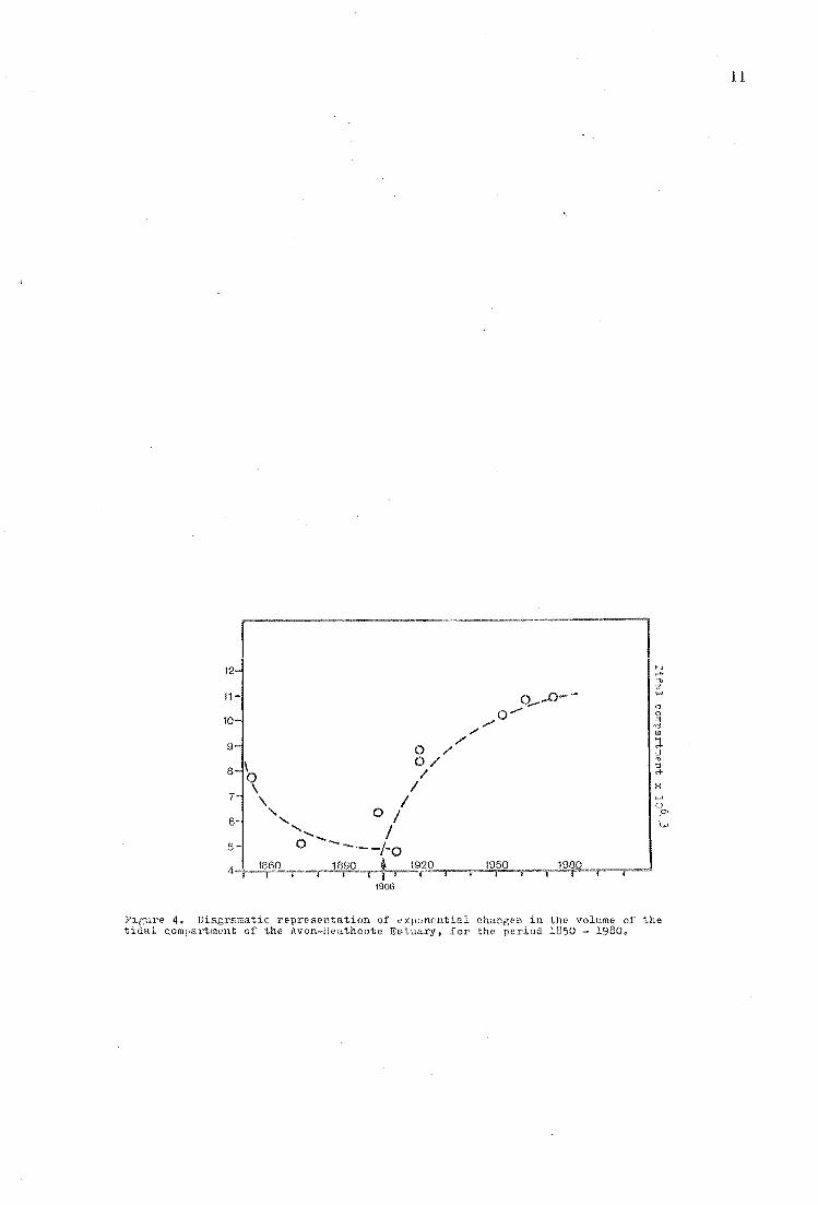
at exponen dally deereasing rates. In Figure 4, t1;vo diagrammatic
exponential functions are fitted to data from Appendix 1, and these
show that changes in the tidal compartment of the ARE may be
quali tati vely modelled as two exponential functions, suggesting tha t
the estuary has responded to two separate geomorphic disruptions.
Tbe first was due to the rapid early settlement of the area, when
drainage work lagged behind urban growth, and \vhen the volume of
sediment supplied to the Avon and Heathcote Rivers probably increased
steeply. This sediment 'vas presumably deposited in the (:~stuary,
causing the decrease tn the tidal compartmen t sho~"m in Figure 4.

10
on
s o
f efrlu
en
t/day
X
l06
mile
s o
f se
wers
Fig
ure].
Ch
ristc
hu
rch
an
d
sub
urb
s. l'o
pu
latio
n,
milt's
of
Elto
rmw
ater and
Ele\~age
pip
e",
vo
lum
es o
f efo
flu€
'ut
rele
ased
in
to th
e
men
t V
lork
". u
nd
in
th
e
vo
lum
e o
f th
e
tidal
of
th"
AB
E fo
r th
e
perio
d
from
to
1
97
5.
Circ
les (O
) sh
ow
each
o
f th
o
10
eatim
ate
s
of
the
vo
lum
e o
f th
e
co
mp
artm
en
t fro
m
Fig
ure
79
. T
he
heaVY
lin
e is
fi t te
d
to
meau
valu
es
for
ab
ou
t 1
90
8
and
fo
r 1
92
0.
'fho
lo
w
valu
e at
19
64
is
p
red
icte
d
from
th
e
Fu
rlwrt-H
eath
re
latio
ntlh
ill. !H
'£!
Ap
pen
dix
1.
12
Fir:ure 4. Diagrnmatic representation of exponential changes in the volume of the tidal compartment of the Avon-Heathcote Bstuary. for the period 1850 - 1980,
11

The second disruption. whi~h reversed (or overwhelmed) the first,
was probably a combined effect of reduced sediment supply due to
drainage basin stabilisation, and of changes in both the storm
and low-flow runoff response of the area. The second curve now
appears to be asymptotically approaching a new, post-urban
equilibrium state.
12
5. Changes at the inlet to the estuary~ .1850-.1975. As well as
internal volumetric changes, the estuary has experienced major changes
in the configuration of its inlet area since 1850. The early maps of
HMS PaJ'l.dora (1854), Elliot (1874), ~Iclntyre-Lewis (1904), of the
Lyttelton Harbour Board survey (1920), of HMNZS Lachlan (1950) and of
the 1970 Wallingford Report' (all supplied to the writer by the CDB),
provide valuable documentation of these changes. Figure 5 is a series
of maps which summarise maj or changes that have occurred in the inlet
area during the period 1854~1975. Many of these changes have been
reported previously (by Pearce, 1951; Scott, 1955; Hutchinson, 1972;
Knox and Kilner, 1973; and Millward, 1975), and have been interpreted
as respon ses to inexplicable variations in onshore ':lave energy,
longshore sediment supply, river flmv, or all three,
The changes shown in 5 occurred in three phases: the
first, from 1850 to about 1928, smv the outlet change little, except
that during the early years the arcuate southern channel carried most
of the flmv through Moncks Bay, and by 1928 the northern, dia,gonal
channel carried most of the flow. The second phase, from about the
mid 1920' s to the mid 1950' s, saw a maj or reorganisation occur, with
most changes happening during ~vinter storms (Pearce, 1950; Hutchinson,
1972). The principal subtidal channel migrated south into Moncks Bay,
the spit grew south and west, sand was deposited on Clifton Beach
(previously a rocky shore), and the ebb delta migrated north about
500 m. As the ebb delta migrated north, the wave climate of Sumner
Beach changed, because the delta had previously sheltered Sumner from
large waves from the eas t and north-east. Severe erosion of the beach
threatened seaside real estate, and expensive coast protection work
was necessary (Scott, 1955; l"ktcpherson, 19 ). During the third phase,
from 1955 to the present, the rate of change slowed, and the result is
the configuration shown in Figure 5D.
Significant changes did not occur at the outlet until the late
1920' s, when the tidal compartment of the estuary first exceeded the

A
About 1935 to about 1';46 c
~~~~~~."'-~~
o
'rhi' confirurntion in 1975. Not" the landward migrf~tion of the 2 metre depth contour (from 9 to 10), the northwards roiF-ration of the ebb delta (11 to 12), southl',ards mi{;ration of the principal subtidal chanpel (13), the disappearance of :';umner beach (14) and the "roY/th of a large new beach ut Clifton (15). Note also the prPIJence of a well developed ebb spit and flood ramp (16)/ and a flood tide channe 1 (17).
Configuration of the principal subtidal channel and aSBociat~d sand bodies between 1854 and 1928. Thlo' numb~red localities are Beachville Road (Bhowin~ the position of the preoent-day seaYlall( 1». 1Il0ncks Duy (2), Shag Ro"k (3). Cavo Rock (Cave leland on early charts)(4). and Sumner Beach (5). Note location of the hieh water mark (6), the low water mark (7) the 2 metres depth contour ( ..... ~, the ebb tide dol ta (8), the principal subtidal channel ( _)! and the flood tide flow patter-A VV)'
1~46 to about 1955
••••• ./12 ..... '
Figure 5. Synoptic maps of changes in tht' inlet area of thE' Avon-HeathcotE' E~tuary for the period IB50 to 1975.
13

pre-European volume of about 8 x 10 6 m3 • Most of the changes occurred
relatively quickly between 1930 and 1960, when the tidal compartment
increased rapidly from 8 to 10 X 10 6 m3• The writer's interpretation
is that the changes shovm in Figure 5 were an ordeI'ly, progressive
response to accommodate the increasing volumes of water flowing
through the inlet. The tidal compartment curve in Figure Lf appears
to be asymptotic approaching a value of about 11 x 10 6 m3, and the
14
inlet has changed little in recent years. The 1975 configuration shown
in Figure 5D has a more efficient, symetrical appearance than
configurations preceding it, and appears similar in shape to high
energy, mesotidal inlets associated with bar-built estuaries,
such as those on parts of the U.S. Atlantic Coast (for example, see
Lynch-Blosse and Kumar, 1976).
The cross-sectional area of a stable tidal inlet (with a supply
of sediment) is coupled to the flow of water through the inlet by a
critical stress relationship, in which the maximum current speed
is 1.14 mls (Heath, 1975; Bruun and Gerritson, 1960). This is the
theoretical basis of the Furkert-Heath relationship, and it means that
all other things b equal, changes in the tidal compartment will
cause an inlet to erode or deposit sediment to maintain a maximum
~hroughgoing curren~ of 1. 14 mi s. The broad nature of this
relationship is clearly illustrated in Heath I s data, ~vhere 16
different New Zealand tidal inlets conform to the Furkert-Heath
relationship, in spite of ,vide variations in offshore bathyme"try,
onshore wave energy, ffild rate of sediment supply (Heath, 1975,
pp.453-454). Walton (1977) has recorded that in some mobile U.S.
tidal inlets, there is a linear relationship between the volume of
sand stored in the ebb delta (the "outer bar" of Walton), and the
cross-sectional area of the adjacent inlet. This relationship is
functionally analogous to the Furkert-Heath relationship, and it is
interesting to note that the 1975 ebb delta in Figure 5D is
than the ebb delta in 5A (at least, the 2 m depth contour is displaced
further sem.;rard in 1975), which probably means that it contains more
sand and is acting as a depository of sanel removed from the inlet as
thetidal compartment increased. This interpretation lends qualitative
support to the conclusion that. the configuration, as w"ell as the
cross-sectional area of the inle t system has histor ically been
re ated by the amount of ,qater flowing through it.

15
It has been assumed in the past that man-induced changes in the
AHE are a 20th Century event. For example, Knox and Kilner (1973)
considered the first biological survey of the estuary (by Thompson,
in 1929) to be a useful baseline, against which subsequen t changes
may be evaluated. The information in Figures 3 and 4 suggests that
Thompson saw the estuary in a substantially altered state, and that
the use of his observations to assay present-day features may be
seriously misleading. It has also long be,en assumed that the estuary
is filling "lith sediment (Knox and Kilner, 1973; J.A. Robb, pers.
comm.). That the opposite is true is a surpris discovery,
particularly in view of the reasonable expectation that this estuary
would react to post-European changes by accumulating sediment. The
discovery that both of assumption are incorrect will
fundamen tally influence the following sections of this report.

16
PART TI<10
, ENERGETICS - WAVES AND THE TIDE
From Part One it is clear that the growth of Christchurch City
has had a maj or impact on the Avon-Heathcote Estuary. Since the ABE
is predominantly intertidal, intertidal processes have probably
figured largely in this impact. According to Hayes (1975), microtidal
estuaries are dominated by wave generated processes, and an analysis
of wave energy is an appropriate place to begin the description of
physical intertidal processes.
Haves
Gathering statistically meaningful field data on waves is an
expensive and technically difficult process, especially in shallow
"later, where waves may be influenced by local bathymetry (U.S. Army,
Corps of Engineers, 1962). A more efficient method is to predict
wave dimensions from a knowledge of the wind energy available to build
waves. This process is known as wave hindcasting (predict waves
from past meteorological records), and the techniques, limitations and
shortcomings of the methods involved are quite well known. The
principal reference is the U. S. Army Coastal Engineering Research
Cen tre, Shore Protection Nanual (CERC, 1973; and subsequent updates)
1. Wind characteristics. The first step in wave hindcasting
is to estimate surface wind speeds and directions. The CDB operates
a recording anemometer at Bromley, about 5 km west of the estuary.
Daily records are -routinely analysed by the Ne1;v Zealand Neteorological
Service, and a 5 year run of such analyses "laS made available by the
CDB. The 5 year record (from April 1st 1967 to JYfarch 31st 1972)
consisted of wind speeds and directions at exact hours 0100 to 2400,
NZ Standard Time, with speed in knots (where 1 knot = approximately
0.5 m/s) and directions in 100
arcs.
Since waves only occur when the tide is in, it is sufficient to
cons ider wind which blows for some arbitrary period corresponding to
high tide - in this study high tide ± 2 hours ,vas chosen.

17
tide times for the pe :ciod covered by the wind record were obtained , ,
from the NZ Nautical Almanack (1967-1972), 1;.,rith tide times for the
estuary assumed to be the times predicted for Lyttelton, plus 1 hour
(Consultants Report, 1973).
A list of high tide times (rounded to the nearer:: t half hour)
was prepared for the 5 year period (a total of 3 586 tides). Wind
speeds and directions at each hour for 2 hours either side of high tide
were also listed, giving either 4 or 5 wind vectors, depending on
\vhether high tide occurred closest to a whole or half hour. Mean wind
speeds and directions \Vere calculated for each h tide, and
variations in both speed and direction were also recorded. These pairs
of mean values are termed wind events. If the wind was calm for three
or more of the readings involved in each event, the high tide was
recorded as a calm. High tides where no data was recorded (mainly
because of instrument malfunctions) were also noted. The wind was
'calm, or not recorded" for a total of 1 364 tides during the 5 year
d (38% of all events). About 10% of all events Here 'no data'
events.
A wind event frequency table was constructed (Figure 6), from
which it is clear that Hind events in the AIlE are directionally
anisotropic, clustering about 0900 (easterlies) and 2600 (south
westerlies). The purpose of a wind analysis is to determine the amount
of ene rgy available to make waves. Thus estimates of ;vind stress are
also necessary, ~Vind stress (Ew) is defined as force/unit ar~a acting
on the water surface, \vhere E increases with increasing wind speed (u) w
'dl than U2
b 1 'dl h U3
h more rapl y , ut ess rapl y t an ,so t at
(Honk, 1955).
If E is assumed to increase in proportion to U2
( for example, see w
Bokuniewicz and others, 1975), then the results ~vill be conservative
estimates of wind stress.
Multiplying U2
by frequency for the wind speed classes in
Figure 6 dimensionless parameters of wind stress, which for
convenience may be recalculated as percentages (Figure 7). Low speed
wind events are more variable in both speed and direction than faster
events, and are relatively insignificant producers of \Vaves, so wind
events with mean speeds of less than 10 knots (5 m/s) are disregarded.
The resulting distribution of effective ,vind stress (E f) forms the w
basis of subsequent analyses.

MEAN DIRECTION MEAN SPEED (KNOTS) 2 3 4 5 6 7 8 9 10 11 12 13 14 15 16 17 18 19 20
010 0 2 3 2 1 2 1 1 3 2 1 1 1 2 0 1 020 0 2 1 1 1 0 1 0 2 1 2 2 1 030 0 1 2 4 3 4 2 3 2 3 2 0 0 2 040 1 2 7 5 3 5 4 4 3 3 1 0 2 0 1 0 0 0 0 1 050 3 1 6 6 8 5 6 3 7 5 2 3 2 1 060 6 13 7 17 10 13 4 9 6 8 6 4 1 2 070 10 12 14 20 26 29 21 14 19 9 8 5 2 1 1 1 080 18 15 14 26 30 34 24 22 22 14 8 3 5 2 2 0 0 0 0 1 090 14 21 15 23 18 25 24 25 24 13 12 6 4 4 1 1 100 13 11 12 20 21 23 30 31 17 15 9 4 5 7 1 110 6 15 17 9 7 11 9 9 11 4 6 7 1 3 1 120 2 4 3 2 3 7 1 1 2 3 1 0 0 0 1 130 2 0 0 2 1 1 1 2 1 0 0 0 0 0 0 0 0 0 0 1 140 2 1 0 0 0 3 0 .1 0 0 0 1 150 1 0 1 1 1 ]60 0 170 0 1 2 0 0 3 1 0 1 180 0 1 1 0 2 3 2 1 1 3 190 1 2 2 1 0 0 1 2 5 5 0 0 1 200 2 0 1 4 6 7 4 3 9 2 3 3 5 2 0 0 1 1 210 2 4 4 6 6 1 7 3 4 4 3 3 3 0 2 2 0 0 0 2 220 3 4 2 5 5 12 3 4 6 5 4 6 3 2 1 3 1 0 1 3 230 7 3 2 4 4 6 9 4 9 1 11 3 2 1 1 240 9 11 7 3 6 12 4 9 8 4 0 2 0 2 0 0 0 1 250 15 12 18 13 7 9 6 6 5 4 0 1 0 0 0 0 ].
260 9 18 12 16 23 8 4 4 2 1 2 0 0 0 0 0 0 0 1 1 270 14 12 14 1, 12 6 'i 4 3 () () 1 1 280 8 6 18 3 8 4 2 0 0 2 290 10 4 9 7 2 2 2 0 0 0 0 0 1 3 0 0 1 0 1 300 5 5 0 3 0 1 1 1 2 0 0 3 1 3 1 0 1 1 0 1 310 1 3 1 0 1 1 2 2 1 4 1 1 2 0 1 2 1 0 0 1 320 1 4 1 1 0 1 2 2 2 0 1 1 0 0 0 1 2 0 1 330 1 4 2 0 0 2 4 1 2 0 1 2 0 2 0 1 0 0 0 1 340 1 0 0 1 3 1 1 2 2 1 1 1 1 0 0 1 1 350 0 0 2 0 1 1 2 2 5 0 3 1 1 2 0 0 0 1 360 2 2 3 2 1 1 2 0 0 0 3 4 3 1
TOTAL 177196203220219243192175186116 91 68 48 42 14 13 9 4 4 12 c 2232 EVEIiTS -l ?" 'f' \D 'f' I-' ?" ;l ?" ;.n ;- w '" ;' 0 ? 0 0 ? ? PERCENT of . ? . . . . '" 99.10% \D -l 0 co-co 0'> co W '" 0 0 I-' co 0'> V1 -1>0 t-' I-' V1
TOTAL EVENTS w co \D 0'> I-' en 0 -1>0 W 0 co V1 V1 0 W co 0 co co '" \D
Figuro 6. Wind event frequency table. Mean wind speed and direction for each of 2 232 high tides for the period 04 1967 to 03 1972.
18

19
~
til til .... 8 til 8 Z8 til
0 j!:
~ I"'I~ !~g ~~ til
1"'1 :~ I'il 0 ~~ 1><0
::.- n ""'~ ""' r'l On Z A\ ZO 1'il..:J
~ 0": I"'In ril
~~ <.>
NUJ,;BER PERCENT OF PERCENT OF A 'H ~N DIRECTION 01' EVENTS TOTAL EVENTS E TOTAL E ~
Pi l-f j!: ... ~ W 1"'1 w
010 23 1.04 1. 44 11 1.81 1790 1.87 020 14 0.63 0.86 8 1,31 1143 1.20 030 28 1.27 1. 42 9 1.48 1301 1. 36 040 41 1.86 2.05 11 1.81 1896 1.99 050 55 2.50 2.75 20 3. 2717 2.85 060 100 4.54 4.28 27 3754 3.93 070 182 8.26 7.83 46 6148 6.44 080 222 10.08 15009 9.92 57 7891 8.27 090 216 9.81 15438 10,21 65 8944 C;.37 100 206 9.35 13655 9.03 58 8298 8.69 110 158 7.17 7510 4.96 33 4758 4.98 120 30 1. 36 1701 1.12 7 963 1.01 130 11 0.50 910 0.60 2 541 0.57 140 8 0.36 414 0.27 ~ 169 0.18 150 4 0.18 8~ 0.05 0 160 0 0 170 8 0.36 352 0.23 1 0.16 100 0.10 180 14 0.63 916 0.60 4 0.66 436 0.46 190 20 0.91 1606 1.06 11 1.81 1301 1.36 200 53 2.41 5378 3.55 26 4.28 4196 4.40 210 56 2.54 5732 3.79 23 3.79 4518 4.73 220 73 3.31 8762 5.79 35 5.77 7273 7.62
(..7 3."~ 5510 3 .. 6~ 2f A (..1 3985 ~.l? 76 3.54 4544 3.00 17 2:80 2433 2.55 97 4.40 )821 2.53 11 1.81 1477 1. 55
101 4.58 438) 2.89 7 1.15 1793 1.88 270 85 3.86 2748 1.81 5 0.82 665 0.70 280 51 2.31 1303 0.86 2 0.33 242 0.25 290 42 1.91 2288 1.51 6 0.99 1595 1.67 300 29 1.31 3294 2.17 2.14 2960 3.,10 310 25 1.13 3310 2.18 2.30 2888 3.02 320 20 0.91 2266 1.50 1.31 1850 1.94 330 23 1.04 2457 1,62 9 1.48 1950 2.04 340 17 0.77 1855 1.22 8 1.31 1443 1.51 350 21 0.95 2515 0.66 2.14 2108 2.21 360 24 1.09 2258 1.49 1.81 1921 2.0~
Figure 7. Derivation of wind stress (Ew) and e:ffective wind stress (Bw:f) •

20
Figure 8 shows the directional properties of the four
distributions generated above, and from Figure 8 it is clear that
three preferred directions are ficant in the ,vind energy field
of the ARE: 48% of all E f occurs between 0300 and' 110°, 30% between \-1
190° and 270°, and 20% between 290° and 010°,
To simp analyses based on the wind stress values produced
above, mean values for each of the preferred directions shown in
Figure 8 were calculated, using a graphic~l technique analogous to
that used for calculating the properties of grain size distributions.
Percentages of Ewf for each of the three wind directions were
recalculated to 100 (Figure 9), and plotted on probability paper as
cumulative curves, The appropriate percentiles were then read from
the curves, and graphic mean values calculated.
Figure 6 shows that high speed winds are unequally distributed -
. south-westerlies tend to be higher velocity events than north·-wester1ies,
which tend to be higher velocity events than easterlies. If all wind
events less than 15 knots (7.5 m/s) are omitted from the calculation,
ea3terlies produce only 28 per cent of all E f' south-'wester1ies w
36 per cent, and north-westerlies 34 per cent. Compare this to
calculations based on all data in Figure 6, ,-lhich indicate that
westerlies produce about 70 per cent of total Ewf
' This means that
although east winds are more persistent, they may not contribute as
much energy as either of the west '''inds.
The CERC wave prediction method assumes that deviations from
mean wind directions do not exceed 45 0, and that wind speeds do not
vary more than 5 knots (2.5 m/s) from mean values (CERC Manual,
pp. 3-'-2 7) . Confidence in predicted results deteriorates significantly
when deviatiDns exceed these limits. In many hindcasting predictions,
wind duration is also significant. but in small enclosed bodies of
water it is unlikely to impose limits on wave estimates (Sutherland,
1977) .
Inspection of instrlLTnent traces from the Bromley anemometer
indicates that these constraints on speed and direction variability
are probably only exceeded in one of every 12 or 15 events, and the
effect of limited duration (when the wind blows for less than half
the 4 hour high tide period, for example) is on significant in
perhaps one event in every 30. Since the simplified hindcasting method
employed in this project will be accurate within 20% for only about
two th:i rds of thf~ ti nlR (CERe N;:1nw'll, liP ,3-33), :1 t has hRRn RRR11meo thAt

+'
$.; g
g 0
~
{')
'H
~ 'd
. '0
(!)
.. +
' 0
+'
ii .<l
g V
l 0
'M
{')
$.; V
l {')
0 +
' !:l
0 V
l 0
aj
'M
'M
'0
+'
<Il ~
0 0
'M
. '" rl~
00
H
<'i
d c.
1~
0 'rl
+' +
' 0
r-l '0
r-'-
'
0>
: '"
0 ll~
~.
+,o
, r-l
'" 6 ~
+'
j>
:> o
c'
';;l m
'"
+=' ~~
g N
e
c<'
';: 1/\ N
'H
. '"
0 ",0
.,
'" 0
H
."ll.. H
t-
.<l ~t
.<l N
+
' g
N
+'
t .
0 "
\D
;:; 0
' .<l
N
J\
'rl r-l
+'
0 10 N
'.-, 0
" "
t') N
0 N
0 (J) ~
g 0 'f2 0 ~
0 ::: 0 (J)
0 r-.
-g 0 t')
0
Fig
ure
8.
Fro
qu
ency
d
istrib
utio
ns
of
win
d stre
ss,
effe
ctiv
e
win
d stre
ss,
perc
en
t to
tal
win
d
()ven
ts, an
d
perc€
'nt
tota
l w
ind
,",v
ents
gro
ate
r th
an
o
r eq
ual
to
10
k
no
ts (5
m/s
) •
21
~
Ol
0 H
IV
0 Q
rl
j:j 0 -rI +
' <>
'" H 'M
R

E-< Z «l 0 P:l «l P. .... ~
r>-l
030 2.846 040 4.148 050 5.944 060 8.213 070 13.453 080 17.264 090 19.568 100 18.154 110 10.409
CUMULATIVE PERCENT CUHVES FOR THE THREE PREFERRED DIRECTIONS
+------r----~------~H_--_199~
r-----~----_+------r_~~~----_49~
~------.~------~r_----_4------_4------_10.1%
030 040 050 060 070 080 090 100 110 EAST-!lOaTH~AST ·.:IUD
lQO 200 210 220 2,0 240 2<;0 :>60 270 ::.iOU'rH'; EST \;IND
290 300 310 320 330 340 350 360 010 HORTHI","]?ST '.".'IND
E-< ~ ~ E-< Z
~ ~ Z 0 HE-< HE-< «l HE-< P:l E-<Z E-<Z 0 E-<Z «l <~ <r>-1 p:: <14 P. o-'lO .-10 ~ o-'lU P. p:: . 8P:l P. 8(~ .... S~ ""r.4 ....
B~ ~ ::>il. ~ 14 U 0 14
2.846 190 4.88 4.88 290 8.62 8.62 8.994 200 15.75 20.63 300 15.99 24.61
14.938 210 16.95 37.58 310 15.60 40.21 23.151 220 27.29 64.87 320 9.99 50.20 36.604 230 11.20 76.07 330 10.54 60.74 53.688 240 9.13 85.20 340 7.80 68.54 73.436 250 5.54 90.74 350 11.39 79.93 91.590 260 6.73 97.47 360 10.38 90.31
101.999 270 2.49 99.96 010 9.67 99.98
Mean direction 075 0 Iv,ean direction 217 0 Mean direction 3230
East-northwest wind Southwest wind Northweflt wind
Figure 9. Directional distribution of effective wind stress (Ewf ) •
22

Figure 10. Effective fetch map of 'the Avon--!ioathcote Eatuary.
Con'Gours of equal. effeotive fetch (in thousands of feet). Calculated accordill(! to tho method of the US Anny Shore I'rote etion r,!anual, pp 329-332. Solid l.ino ~ south west wind at a lDaan directton of 217 deBrtll!B (squat open an'owa), line with one dot = north w(>st wind at 323 dgrees (~'hnrp open 8.r1'o'o'o) and liuo with two do'l;o '" eas't wind at 075 degrees (solid arrovlEl). Circles aro data points.
23

incorporating the few events with high variability into the analysis
will not materially alter the reliability of the results.
2. Delineating a fetch. The second step in the hindcasting
procedure is to choose a fetch over ~vhich wind is reasonably constant
in speed and direction, and to measure its length. The three mean
directions from Figure 9 delineate appropriate fetch directions.
Fetch width may be significant in enclosed bodies of water,
placing a restriction on fetch dis tances, in such a vlay that the less
the \vidth/length ratio, the shorter will be the effective fetch.
24
The CERC procedure (pp.3-30 to 3-33) was used in this study, and
effective fetch values for the relevant wind directions were calculated
for about 110 stations in the AIlE.
Figure 10 shmvs contours of effective fetch for the three mean
wind directions; in the AHE, few areas have fetches exceeding 1 800
metres (6000· feet), and long fetch winds are distributed quite
uniformly around the east, south, and south-west shores. Areas in
the north-west experience only short fetch east winds. The pattern
of fetch contours is most complex in the sout!l-<Hest, Hhere fetch width
is more limiting than elsewhere in the estuary.
3. SftID wave predictions. Once mean wind speeds and directions
have been established, and effective fetches calculated, wave parameters
may be read directly from prediction graphs. The CERC graphs are based
on procedures developed by Sverdrup and Munk (1947), with revisions by
Bretschneider (1958) and subsequent modifications, and the prediction
scheme is 10l0wn as the Sverdrup-Hunk-Bretschneider (SHE) technique.
Replotted versions of 5MB curves from the CERC Manual are presented
as Figure 11. With these graphs, wave heights and wave periods may be
estimated for winds of 10, 15 and 20 knots, for given fetches from 1000
to 8 000 feet (300 to 2 400 metres). The curves in Figures llA and 11B
are for wave generation in water 5 feet (1.5 metres) deep (Figure 3-21,
CERe Manual, pp. 3- if 7) .
4. Limitations on wave dimensions. Water depth affects wave
genera tion. In water 1;.]here the relative dep th d/L is greater than 1/2
(d = depth below still water level, L = wave length), wave
characteris tics are virtually independen t of water depth, and waves
are unaffected by the bottom.

, 25
-
--..
I
~ ~
/ V
/' V
V //
/ -
/ 'fh,.vp p(·riod (s!'conde) o
Qm~i!!-
~ of '<;5 ~ -r;:
,;.- ,...
i I
\ I
l. I
\ ~.i 1\ 0
\ \~ \ \
\ \ \ \ "
5 ---.
\ a ,..
1\ 1\
1\ ~ ~ \ .~
1\ r
t: Yo II) ..
f\ \
~~ \ \ \ :\ 1\ 1\ 1\ ~ \ \ ~
.;;, rl\
\
'" '" 0
~'\ cl !ell
"I
,,~
'" :? (() <9 r:- -iD If) '1 c:' ;;1 ,:. ~ -, , .:: ~ !1: Wave 11eicht (feet) wav. period (seconds)
Figuro 11. Wuve prediction curve.s for wuter 5 faet doep (1.5m) for winda of 10, 15 and 20 knots (5m/e, 7.5m/a, lOm/s). A - Itave height curves, B Wave period curves, C - Height ubove datum of half deepwater wave length (he) 'i wave poriod, for the Avon-Heathcote Estuary.
.p
'" '" 't-,
o o
IS) 0
x

26
As ~vaves propagate into shaTiow water, or grow downfetch in water of
constant depth, they begin to feel the bottom and bottom sediment starts
to feel the waves, as oscillatory water motions associated with the
w'aves exert a shear stress on the bottom.
~'lhere d /1. is less than 1/25, waves are in shallow water, and
depths from 1/2 to 1/25 are defined as transitional (Madsen, 1976;
CERC Manual, 1973). Significant alterations to wave properties begin
when waves propagate into water shallower than d/I. = 1/2 (a water depth
referred to as h ). Since ~vavelength varies with decreasing depth in c
shallow water, h is calculated from wave period (T), which remains c
constant according to
h c
For example, a 1.2 second wave has an h value of about 1 metre, and c
interacts with the bottom in water shallower than 1 metre.
Inspection of Figure lIB shows that for winds from 10 to 20
knots, and for fetch distances from 1000 to 6 000 feet, wave periods
in the ABE will vary froin about 1 s to 1.9 s. However, if h values c
are recalculated as height above datum values (by subtracting hc from
a still ,vater level of 10.22 m, which is m.,rOST) it is found that when
wave per:tocts reach about 1.35 s to L 4 s, they have h va.Lues ot about c
8.7 m HAD (Figure lIC). This means that in water deeper than 8.7 m
HAD, l.4 s waves will be interacting with the bottom. Hap 1 shows
that only small areas of the ARE are deeper than 8.7 m HAD; thus waves
with periods greater than 1.4s will be rare in this estuary. This
conclusion is supported by two observations:
(i) When ripples form on the higher intertidal flats they are of
uniform size and spacing .- regardless of the mean wind speed,
direction or fetch distance during the preceding tide -
ffild so were presumably made by waves of similar uniform sizes.
(ii) On days when the mean ,vind speed exceeds about 10 knots, high
tide wave trains contain a high proportion of spilling waves
(Cokelet, 1977) that is, many waves in the train have reac.hed
a limiting steepness (a maximum size) and have begun to break.
Yachtsmen also record that waves larger than about 1 foot (30 em)
are rarely en countered in the ABE, regardless of wind strength
or fetch distance (G. Coates, pel's. conun.).

5. Wind event frequencies. The preceding analysis has shown
that regardless of fetch dis tance or wind velocity, the waves which
form at about high tide in the ARE rarely have periods which exceed
1.4 s. This means that the best method of assessing the relative
wave-making importance of the three mean winds is to calculate wind
event frequencies, not total effective wind stress. From Figure 7
the appropriate frequencies are:
Direction
075 217 323
Number of events
327 166
94
Percentage of total events
56 28 16
These data indicate that the east wind is the dominant wave producer,
as east winds are twice as frequent as south-west winds, and four
. times as frequent as north-w~st winds.
6. Discussion. TIle particular significance of sections 4
and 5, above, is demonstrated in Figure 12. Have-generated shear
stress exerted on the bottom of the estuary increases down fetch
because with increasing fetch, a greater number of wind events are
capaule vf uuihilllg wave::; wllldl [eel LIle uuLLuHI. ,. r"1 ("'. 1~
Ll. UUWill.eLCU
energy gradients occur, they are a product of a greater number of
wave events, each of 1;V'hich builds waves of a similar size, not a
result of increasing wave size. A further conclusion is that if
much of the wind blowing down a particular fetch occurs as high
velocity events, most waves will bot tom near the proximal end of the
fetch, and wave energy will tend to be distributed uniformly down
fetch. If much of the wind blows as low velocity events, at or near
10 knots, then the bottoming zone is spread down the fetch, and
there is more likely to be a downfetch energy gradient. Obstructions
such as :3hoa1s or sand moundB which are significantly shallower than
water on their upfetch side will cause equilibrium waves to break,
and if the breaking zone is shallow enough to cause the complete
breakdown of approaching waves, it "Till act as the origin of a
second fetch, further homogenising downfetch energy distribution.
27

[0 "" ::s,.-p..~ ::; '1 III " <+ <Of-' '1'" p..
'" 'OtJ <+ ..... ::rill
[}q .... '1 ::s [D
a <+[0 ::rd"',.-
" :>-<; .... 01-' ~ i.....J I ~
:0::", a><+ III '1 <+[0 0<+ 0"<+0 '" :; t:Jo ClH, d~<+ [D;:T ~~ • '1
to I-' [D <+ .... o ::s Cl ::r ,.-'0 Cl
c'
'" c> ::;
'" '" t:l1
~ < o
~ <> ::s '" '1 ;:> d,... o :s
800 a I I
metres m:osrejD>"',;,--------------------------------------------1
=====----------------~~~~~~~~~~I . m ¢I 'aves break on central shoals, 0 10 Om
ill D ill:::l~~ i . trail' loS e;enerated / . .. , Ir'" ".w r . / I I h 10 knot wind / I
knot ",nd XI ' V / ,/ / Centr81 s2.nd mound /" /
/ ... </}::;;:! --- /
hc 15
/' 10 knot v.ind 'I1l.. ~ hc ~
hc 15 knot
Explanation
1. A 15 knot east wind begins ':0 eenerate waves at m; as the wave train progresses downfetch, wavelencth increase:, until n, where water depth is equivalent to half the waveleneth, and waves effect i v,?ly enter sha110w water.
2. A 10 knot east wind beeins ';0 eenerate waves at 0; which reach a vlater depth equivalent to half their wave :Leneth at p, ancl effectively enter shallow water.
3. As waves approach shallow cl'ntral sandy mounds, increasing steepness causes breaking by spilling, and the wave train may break down. New ge.neration begins at x, and half wavelength depths follow paths x - y, x - z.
h c= half wavelength depth, bel,)w still water line (where SWL HlfOST)
¢ East v.ind
N 0::

bottom velocities and - stresses
As waves enter water shallower than d/L = 0.5 they begin to
exert shear stresses on the bottom. To the first approximation
29
the motion involved is pUtely oscillatory - there is no net transport
(Madsen, 1976). From Airey wave theory (see the CERC Manual for an
excellent discussion of wave theory) it is possible to calculate wave
properties associated \'lith this oscillatory motion, including horizontal
near bottom velocities, amplitudes of near bottom wave orbits, and the
maximum near bottom shear stresses. Madsen (1976) has presented a
useful summary of these applications, and the following analyses are
substantially derived from that summary.
Maximum horizontal near-bottom velocity (~): For waves with T o
1. 4 s,
height, L
H = 14 cm, and L = 3.56 m (\'lhere T = \'lave period, H = wave o 0
wave length, and the subscript 0 indicates deep water
conditions) , the following values are calculated:
h h/L ub 0
0.5 m o . ILl 22.12 cmls
1.0 m 0.28 14.38 cmls
1.5 m 0.42 9.95 emls
These values demonstrate the large increases in near bottom velocity
that occur as waves propagate into shallow water, producing steep energy
gradients along the bottom in the transition zone between deep an<d
shallow water.
Orbital amplitudes: As waves shoal, the originally circular
orbits become elliptical, and the amplitude of motion near the bottom
(~) increases according to ~ = ubh'l; \'lhere w = radian frequency,
2pi/T. The following values are calculated from the above figures:
Ub
22.12 cmls
14.38 cmls
9.95 cmls
Wave Reynolds Number (RE) , "\
~)
4.93 cm
3.21 cm
2.92 cm
relative roughness (d ) and the s
friction factor (f ): The maximum near bottom shear stress is related w
to the square of velocity by a wave friction factor, f . w

30
For turbulent flow the wave friction factor is a function of relative
bottom roughness and the wave Reynolds number, ubJ\/v; where v is the
kinematic viscosity of the fluid (10- 1 cm 2/s). Where bottom roughness
is contributed by ripples, the equivalent sand roughness (d ) may be s
quite high (0.5 to 1.5 cm). Where the bottom is smooth, d may be as s
low as 1.5 x 10- 3 em (fine sand sized), or even as low as 1.5 x 10⁻⁴ em
(silt sized). Thus relative roughness values (J\/ds ) may vary from
about 10 to about 3200 for h = 0.5 m, and from 2 to about 2 000 for
h = 1.5 m.
The wave friction factor is a function of both relative roughness
and RE, and may be obtained from a friction factor diagram (Madsen,
1976, Figure 8; after Jonsson, 1965). The following values have been
calculated:
Water depth d Ab/ds f s w
0.5 m 0.5 em 10 7 x 10- 2
0.5 m 0.015 cm 330 0.15 x 10- 2
LOrn 0.015 cm 214 0.02
L5m 0.5 cm 6 0.1
1.5m 0.015 em 195 0.015
HaxiUlum near bottom shear stress (tb
): Knowledge of f ,max w
permits evaluation of the maximum bottom shear stress, which is
proportional to the product of the friction factor and the square of
the bottom velocity.
t b,max
For water depth of 0.5 m, with roughness contributed by ripples 0.5 em
high,
t b,max
If roughness is fine sand sized,
t b,max
17.13 dynes/cm 2•
3.67 dynes/cm 2•
For water which is 1.0m deep, with 0.015 cm bottom roughness,
t = b,max
2 2.07 dynes/em.
For water which is 1.5 m deep, with 0.5 cm bottom roughness,
t b,max
2 4.95 dynes/cm ,
and if bottom roughness is fine sand sized,
t b,max
2 0.5 dynes/cm .
31
These figures emphasise that waves exert very much more stress on a
rippled bottom in water 0.5 m deep, than on a smooth fine sandy bottom
in 1.5 m deep water - the difference is about 1. 5 orders of magnitude.
Threshold motion under
Komar and Miller (1975) present a set of curves relating bottom
orbital velocities to grain diameters for varying wave periods for the
threshold of sediment motion, and from this figure the values below
were obt ained.
wave period 1. 4 seconds,
water depth orbital velocity approximate maximum grain diameter potentially entrained by waves
0.5 m 22 m/sec 0.5 mm (1.0 phi)
l.Om 14 m! sec 0.25 mm (2.0 phi)
1.5m 10 m/sec 0.15 mm (about 3 phi).
Considering that there haV8 been relatively few studies of sediment
movement under >;.Javes, and that more data may er the empirical
relationships which form the basis of the equations governing Komar
and Miller's (1975) threshold diagram, better approximations than these
are not possible at present.
Wave refraction
1. Introduction. Many waves in the ARE feel the bottom along
much of their traverse across the estuary, and it is reasonable to
assume that their passage is significantly altered by the configuration
of the bottom. One result of this feedback is that waves are refracted,
tending to approach the shore normal to the bottom contours. Refraction
may be analysed graphically, with the theoretical basis developed from
geometrical Dptics and Snell's Law (CERC Manual, pp.2-65), by tracing the

passage of wave rays (orthogonals to crests) across a. sloping bottom
as a sequence of straight line increments. This method is labour
intensive, and numerical IT£thods have been developed as a more
efficient alternative (Wilson, 1966). A version of. Wilson's computer
program has been adapted for the University of Canterbury Burroughs
B7600 computer by A.J. Sutherland (Department of Civil Engineering),
32
and this program was used to obtain the data summarised in Figure 13,
which shows the results of a number of computer runs for mean south-west
and east winds.
The method involves drawing an arbitrary grid over the estuary,
and reading off water ths at d intersections (where depth is
assumed to be depth below HWOST). The resulting lists, combined with
wave period and deepwater crest orientations form the input data for
the program. Results are plotted as wave rays, which may be
replotted on to the original bathymetric base.
2. Discussion. Refraction analyses are usually undertaken for
oceanographic or engineering purposes, or as a method of evaluating
longshore differences in wave energy, '(vhere variations in bel3.ch
alignment, or of offshore bathymetry, may variously modify deep1;vater
waves as approach the shore. In such studies it is usually
assumed that waves entering the coastal zone have travelled from a
generating area some distance away, and that the only modifications
that occur as waves run in tmvards the coast are those produced by the
shoaling trans formation. Little work appears to have been done in
shallow enclosed basins where deepwater conditions may only apply for
short sections of the total fetch, and where there is a continuing
interaction bet'(veen the forcing '(vind and the restraining limitation of
shallow water. It may \vell be that the assumptions built into the
numerical method do not apply in such circumstances (CERC Manual,
pp.2-65); in particular the assumptions that waves are long-crested,
cons tant period, small amplitude, and monochromatic. For this reason
the information in Figure 13 probably only has qualitative
applications - attempts have not been made to calculate the effects
of the shoaling transformation on wave properties.
3. ResuZts. Figure 13 indicates that east wind '(vaves are little
modified by the bottom north of line 12 (Map 1), until running into
water shallower than mid tide levels (9.0 m HAD - water shallower than
1 ,20 ill) ,

33
Figure ~J. Southwost wind (217°) and east wi11t1 (075°) \"lave refractiOll diagralll. Wave period 1.4 Beconds. Arrows ahow directions of wave propagation ill deop water, assumed parallel to the wJ.nd direc'tio):},tl, Linea aro wava ra;ya (orthogonala to cNatE) •

34
Cen tral bathymetric highs and shallow marginal areas. act as lenses,
converging wave rays (as in the south Heathcote Basin) or causing rays
to diverge (as in north Heathcote Basin). Where rays converge, waves
will become steeper, and if the train is close to a. limiting steepness,
breaking will occur, probably as slightly more vigorous spilling.
Where rays diverge, energy is spread along greater crest lengths,
and wave heights should decrease. The overall effect is probably that
refraction acts as a further homogeniser of wave properties in
converging areas, producing uniform wave fields where many individual
waves are close to a maximum steepness. In diverging areas, maximum
wave sizes may be less than the IIBan equilibrium size.
The refraction pattern for the mean south-~vest wind indicates
that Sandy Point tends to shade the upfetch western shore from waves,
while the central highs tend to homogenise wave properties, and produce
a uniform wave climate along the eastern shore the estuary. A few trial
runs for the inean north-west 'wind showed an analogous pattern,
indicating that north-west wave energy is spread uniformly along the
south and south-east shores.
Wave-generated bedforms
1. Introduction. When the wind during a preceding high tide
exceeds about 10 knots, intertidal flats uncovered at low tide show
widespread trains of strikingly parallel straight transverse
asymmetrical ripples (Figure 14). Such ripples have been widely
reported on tidal flats (i.e. Allen, 1968; Reineck and Singh, 1974;
Tanner, 1967) and are thought to be produced by shoaling waves that
generate an asymmetrical oscillatory motion at the bed. In the
Avon-Heathcote Estuary these ripples rarely occur below the mean tide
level (9.0 m HAD), and are usually only found in clean sand. They
often form lanes several metres wide (Allen, 1968, p.92) and may occur
in isolated patches surrounded by smooth sand. In very shallow water
(less than about 20 cm) around the edges of the estuary, very
a~,ymlTle trical lingoid or barchan-shaped ripples may occur, merging
offshore in to straight ripple trains, or occasionally oc curring as
isolated ripple patches. If succeeding high tides are calm, newly
formed ripple trains are destroyed by rounding of the crests and by
bioturbation of the soft sediment surface (especially by the abundant
mudflat snail Amphibola - Figure 14F). so that after about 4 to 6 calm

I ' i',
c o
F
t'Lr,ure 14 . av(' formed rip.,les of th Avon- Heathcote f<'tuo.ry. A - L.rallel Imo ... t ,'tr'lir.ht noymmet rical ripllel' t.v i r'1. of ('uutt>rn high tl.de ( '~ . 5m) ::tlopes •
• e .. l(' l. 0 l:>cm , arrow 8hol'ls uirE'otion of v.av e propar,at lon, \\h ieh \',0.9 to the north e ",t . Vic-v. i3 tc:o the north. B - Detal. 1 of ripples in A, "cale is lOem , ,rrow ~10 3 ~Dve direction. C - lAo1ated p tch of a lmo.t nt raicht rr~ymmptrl.ca1 l'LpplelO ne'lr thE H'" ma r k a t :,andy loint (bono tip l.n bac X:!'round) . A1'ro\·. "hO\'.a
ve di r pctl.on. D - Deteul of part of an iaolated r 1(, 'Oeit ch on the e~stcrn l. h tide slope . lote a brupt trans 1. tion from smooth to rippled • an d . H', mark is
to .h(' left , v iew l. 9 sou th , ('call' l.S l Oem . r: - Barchan- shaped very asymmetrical !'LPI'les ut the tn , mark (landward of D, ubvvlI). ,1"'0 )11," •• ,, ' v, in etion ,
C", 1f' io IDem . }' - vet'iil 0: rim'leo ourfaee al'ter on( efW,m I. i"h tine , "ho'''i!lf' tfH '''loothifl#' ' letivitieo of Amphibol'l eren'.ta , bur O· ... J.ur int~ the uri·tee at ( 1) 'Utd (2) , 'wtJ p'.ck',ril1l: ::turf~.ce t'leoim.mt into I'eeo.l "trinr:s ( . ) . dote th eh' r etex·1.·tl.e bJ.ro3-i'oot. tlhnped f~l·dJ.nf" tr"ee of thE' biv"lve 1ili"-I"I<' (4) . ;cult' io lJcrn . l~ 0 !"lee Pif.Ure~ lI5 nn u6 . -

o L---<-.. __ ,_ ..... _---'--km
orien';e.tio:::l.S of wuvo-f'oJ'!l)e4 r1"P'P1Q6 on. SO"Pt(1lQbOl" 4 1976 8 1976 (,last "ido).. .\.:-1"0111"8 to,b,ow meo.n ",1n.d diroctioM during
numbenl $.X'liI ri'Pple cnuta/c. tlli<:llc lino4 ollow crest etrikll
w Cl'

5 (") 11 0> ro <+ '1l '{j
'" 0
~.
0 i3 ~
-4
water depth (m HAD) 9.0mHAD '" Midtide level
l>'igure 16. Ripple crest spacing VB water depth (as heigh-t above datum), wefltarn slopes, September 4 1976.
37

38
high tides the flats are quite smooth.
2. Ripple orientations and dimensions. Ripples were measured
at low tide on opposite sides of the estuary on September 4th and
September 8th 1976. Winds of 12 knots (6 m/sec) fr~m 070 degrees,
and 14 knots (7 m/sec) from 252 degrees, respectively, blew during high
tides which preceded the t~"o visits, and the state of preservation of
both ripple sets indicated that they formed during the preceding high
tide.
In both areas (Figure 15) crest spacing was quite uniform on
the higher flats (at about 20/m, measured normal to crests), regardless
of fetch. Ripples formed in deeper water tended to be smaller,
especially on the western side of the estuary, vlhere up to 30 crests
per metre were occasionally measured (Figure 16). Mean values were:
. Angle between Mean Mean preceding mean ~"ind Number crest crest and mean ripple Standard of
spacing strike crest strike deviation measurement --~ ---
4.53 cm 0.72 cm 15 East - - - - - 0280
-- - - - - - - - - - - - - - - - - - - -
side 15
! 550
7.500 I
West 4.58 cm 0.20 em 6
- - - - - - - - - - - - - - - - - - f- - - - - - - - - -side 285 0
9
420
250
-------
In small bodies of waterl\ripple wavelength is usually about 4/5ths of
the amplitude of the waves (Inman, 1957; Komar, 197 1f, quoted in
-
Komar, 1976). If this relationship holds in the ARE, the waves which
formed the ripples in Figure 15 had near-bot tom amplitudes ranging from
4.16 cm to 6.82 em (from 30/m to 18/m). In section 7 above, predicted
amplitudes for water of 1.0 m deep and 1.5 m deep were 3.21 em and
4.93 cm. The predicted values are about 30% too small, whieh seems to
indicate that the relationship between wave size and ripple amplitude
is not generally applicable. Hmvever, fe" of the data used to establish
the relationship were from natural conditions, and those which were
scattered widely about mean values (Inman, 1957).
I

39
Tides
1. Introduction. In an intertidal estuary, the semi-diurnal
tide contains considerably more kinetic energy than the waves which
develop on windy days (Bukuniewicz and others, 1975), yet in typical
microtidal estuaries tidal currents are only important transporters of
sediment near the inlet, where tidal velocities are highest (Hayes,
1975). Wind-induced processes (\Vaves and \vind tides) predominate
throughout the remainder of typical microtidal estuaries.
Although wave motion may be the principal initiator of sediment
movement (on the Continental Shelf), net sediment transport is usually
accomplished by a superimposed current (Madsen, 1976). Carter and Heath
(1975) have demonstrated the importance of superimposed currents on the
New Zealand Shelf, as have Channon and Hamilton (1976) for part of the
Shelf off Southwest Britain.
In developing an. understanding of the intertidal sedimentation
of the ARE, the present analysis began by considering wave energy; the
observations above suggest that the next step is to assess tidal current
energy.
2. Previous work. Linzey (1944) described the general
characteristics of tidal movements in the ARE, and collected some
current-velocity data. Bruce (1953) and Webb (1972) added to this
early work (see the summary in Knox and Kilner, 1973). Mmvson (1972)
has calculated river and other non-tidal flows for various discharge
conditions and tidal ranges, and has usefully summarised the hydrological
properties of the estuary and its freshwater catchment.
The Wallingford Report (1970) contains data on tide levels and
current velocities at the inlet to the estuary (at Shag Rock and at the
Sumner Lifeboat Station), at Ferrymeade Bridge, and at Bridge Street
Bridge. These data \Vere supplied to the ~vallingford investigators by
consultants to the CDB, to be used for the scaling and evaluation of a
large (30m x 30m) physical model of the estuary. Accordinr; to the
Wallingford report, maximum tidal velocities in the principal subtidal
channel at Shag Rock reach 1.52m/s during flood tides and 1.83m/s
during the ebb (ill both cases measurements were made 1 metre below the
surface). These velocities are. almost t\vice those measured by Bruce
(1953), who reported a maximum ebb velocity of 1.10 m/s at Shag Rock.
Notes on the HM8 Pandora chart (185 Lf) indicate that maximum currents
were about 2 knots (1.0 m/s) in the vicinity of Shag Hock.
40
Heath (1975) has shown that ~maximum tidal velocities in mobile inlets
in theory should be about 1. It. m/s.
Linzey (1944) measured a flood tide maximum of 0 .L16 mls at
Ferrymeade Bridge, and an ebb maximum of 0.3 m/s. The Wallingford
Report indicates that the CDB consultants recorded 0.6 mls in both
cases. At Bridge Street Bridge Linzey recorded 0.3 mls maxima for
both the ebb and flood tides, while the consultants recorded 0.6 mls
and 0.8 mls respectively. It appears that the consultants obtained
values about twice those reported from other sources. TIlis may have
been a result of misreading the current meters used to obtain the data,
or perhaps a drafting error if the consultants supplied the Wallingford
investigators with graphed rather than tabulated results. Certainly
at least one Figure in the Wallingford Report is plotted upside down
(part of Figure 6, Part I), so the second option is quite plausible.
Yet it is difficult to believe that the Wallingford investigators would
acc a mistake of that order, and the build it into their model!
The only available information on current velocities from
intertidal areas is that supplied by Knox and Kilner (1973) and
summarised in Figure 17. Current velocities deduced from dye tracers
(or from drogues, or any other free subme or send-submerged objects)
as in Figure 17, are known as Lagrangian velocities (\vhere .in effect.
a parcel of water is tracked along a stream-line for a measured time
and an average velocity is calculated). Lagrangian velocities are not
necessarily comparable to Eulerian velocities (measured as the rate of
flow past a fixed point) because the two techniques resolve turbulence
in moving \vater in differen t ,,,ays - the meters used to obtain Eulerian
veloci ties introduce significant flm" disturbances, and they are
insensitive to higher frequency fluctuations (Byrne and Boon, 1973).
The Lagrangian velocities shown in Figure 17 are likely to be
conservative, and perhaps less than equivalent Eulerian measurements,
because the method of estimating distances assumes that dye slugs
travelled linearly from point to point within the estuary - which may
not be the case. Figure 17 indicates that Lagrangian velocities in the
subtidal channel several hundred metres downstream from Bridge Street
Bridge are about 15 cnl/s shortly after high tide, and reach 62 cmls in
the principal subtidal channel 3.5 hours after high tide. Lagrangian
veloci ties of 83 cmls were recorded in Figure 17 in the subtidal channel
off Beachville Road. TI1ese are similar to the values of Linzey (1944)
and Bruce (1953), but cons iderably less than the Eulerian velocities
reported by the consultants to the CVB.

l'"xperiment 1. December 6, 1972. l·'lat calm con~itions, Rhodamine dye. Dy~ released at position 1 above; locations at 30 minutes (2), 43 r<linutes, 61 minutes (3), 105, 124 and 163 minutes (4) and at 17[; minutes (5), are shown by the series of large sCjuat a1'ro\\s above ( V ).
Calculated velocities for the leading edGe of the dye slug are; 0-30 minutes, O. 05m/sec i 0-43 minutes. 0.15m/sec; 0-61 minutes, 0.34m/sec; 61-105 minu-tes, 0.23m/sec; 105-163 minutes, 0.24m/sec; and 164-178 minut<:s, 0.75m/sec.
Experiment 2(A). Pt'bruary 1973. ilorth east wind at 5-10 kr'ots, light Ylater chop, Rhodamine dye. lJ,ye released at 6; locations at 40 minutes (7), 65 minutes (t'), 105 minut!ls (9), 135 minutes (10), 230 minutes (11), 250 minutes (12) and 265 minutes (13), are shown by smaller black arrows above.
Calculated velocitie8 for th" leading edr.e of the dye slug are; 0-40 minutes, 0.05m/sec; O-lIS minutes, 0.12m/secl 0-105 minutes, 0.15m/sec; 0-135 minutes, 0.15m/sec; 135-230 minuteB, 0.18m/sec; 230-250 minutes, 0.62m/sec; 250-256 minutes, O. nm/8(,c.
Bxp<'rimpnt 2(n). AB for 2(A), except dye (PluoreBCE'ine) was relE'ascd directl.y into the ,won sudtida]_ channel at 14. Locations at 20 minutes (15), 70 minutes (16), 130 minutes (17), 170 minutes,(190 minutes, and 210 minutes (18), are shown by open an'ovls above (~).
Calculated velocities forth€' leading edge of this dye 81ug are; 0-20 minutes, 0.15m/sec; 0-70 minutes, 0.13m/sec; 0-1 0 minutes, O.lOm/sec; 0-17) minutes, 0.18m/sec; 0-190 minutes, 0.21m/sE'cj 190-210 minutes, 0.62m/eec.
FigurG 17. Intertidal and subtidal cnrrent velocities in tho Avon-Heathcote Estuary. l'rom dye -tracking oxperimenta reported by Knox and Kil1wr (1973).
41

42
In vie,v of the above Ciiscussion, the Wallingford Report data is
discounted, and the values below have been adopted as probable maximum
values, based on Figure 17, and both Linzey (1944) and Bruce (1953).
Maximum-velocity
Higher intertidal flats
Intermediate intertidal flats
Lower intertidal flats
Intertidal channels
Sub tidal channels
Principal subtidal channel
5 cmls
20 cm/s
35 cmls
60 cmls
90 cmls
114 cmls
3. Shear stress. The movement of sediment under unidirectional
currents has received considerable attention - much of it to do with the
transport of sediment in rivers and artificial channels, but an
appreciable amount involving the transport of sandy sediment on the I
Continental Shelf and in nearshore waters (see Sternberg, 1968, 1972;
Ludwick, 1975).
Komar (1976 a, b) has presented a particularly useful summary of
the properties of boundary layers of natural unidirectional currents,
and of the derivation of the quadratic stress law,
t
"vhere t boundary shear stress, cIaO = drag coefficient from
measurements made 100 ern above the bottom, p fluid dens ity,
mean veloci ty 100 cm above the bottom. The quadratic stre.ss law
establishes a proportionality bet,·]een the boundary stress exerted by a
fluid flow and the square of the mean velocity of the flow, so that by
assuming or establishing cIaO' only u100
need be known to evaluate t.
Sternberg's (1968, 1972) measurements of cIaO in Puget Sound,
U.S.A., indicate that clOO
3x10⁻³ This result has been supported
by Channon (again for Shelf conditions, in Channon and Hamilton, 1971)
and McCave (in Komar, 1976b). Thus
t -3 - 2. .
3 x 10 p(u100
) .
There are limitations on the use of this average value of c (Komar, loa
1976b, pp .100-102; Ludwick, 1975), but considering the levels of
approximation involved in the estimates of tidal velocities, the
Rfl8111nption of Stp.rnherz! R v,q 1 He is probably a reasonable expediency.
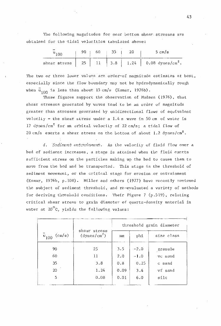
The following magnituQBs for near bottom shear. stresses are
obtained for the tidal velocities tabulated above:
u100 ~r_6°_-I1_3_5_1 __ 2_0 __ ~_5_cm_I_S __ _
shear stress I 25 11 3,8 1.24 0.08 dynes/cm 2,
43
The two or three lower values are order-of magnitude estimates at best,
especially since the flmv boundary may not be hydrodynamically rough
when u100
is less than about 15 cm/s (Komar, 1976b).
These figures support the observation of Madsen (1976), that
shear stresses generated by waves tend to be an order of magnitude
greater than stresses generated by unidirectional flows of equivalent
velocity - the shear stress under a 1.4 s wave in 50 cm of water is
17 dynes/cm2 for an orbital velocity of 22 cm/s; a tidal flow of
20 cm/s exerts a shear stress on the bottom of about 1.2 dynes/cm2•
4. Sediment entrainment. As the velocity of fluid flow over a
bed of sediment increases, a stage is attained when the fluid exerts
sufficient stress on the particles making up the bed to cause them to
move from the bed and be transported. This stage is the threshold of
sediment movement, or the critical stage for erosion or entrainment
(Komar, 1976b, p.108). Miller and others (1977) have recently reviewed
the subject of sediment threshold, and re-evaluated a variety of methods
for deriving threshold conditions. Their Figure 7 (p .519), relating
critical shear stress to grain diameter of quartz-density material in
water at 20o
C, yields the following values:
threshold shear stress
u100 (cml s) (dynes/cm 2) mm phi
90 25 3.5 -2.0 granule
60 11 2.0 -1.0 vc sand
35 3.8 0.8 0.25 c sand
20 1. 24 0.09 3.4 vf sand
5 0.08 0.01 6.0 silt

44
5. Entrainment into suspension. Bagnold (1966) has shmm that
sediment is entrained directly into suspension if upward-directed
turbulence in the boundary layer contains velocity fluctuations which
'exceed the settling velocity of sediment grains. B'agnold's (1966)
suspension criterion indicates that sediment finer than 0.17 mm
(2.5 phi) will be entrained directly into suspension immediately after
threshold conditions are exceeded. McCave Komar, 1976b) considered
that sediment finer than 0.23 mm (2.0 phi) would be entrainE?d directly
into suspension.
6. Current-generated bedforms. If threshold conditions are
exceeded by a gradual increase in current velocity, the first evidence
of sediment movement is the construction of. bedforms, which progress
through a hierarchical sequence as shear stress increases. The
literature on current=formed bedforms is very large (see Simons and
others, 1965; Guy and others,' 1966; Allen, 1968, 1970; Boothroyd and
Hubbard, 1974, 1975; and the useful summary and review of Reineck and
Singh, 1975). The proper ties of bedforms are one of the two key
responses used to infer sediment transport patterns in many marine
studies (Swift and Ludwick, 1976), because bedforms often indicate a
sense of transport as well as a transport mode (the other response is
the sediment 2e frequency distribution).
Current-formed ripples are absent from the intermediate and
higher intertidal flats of the AHE - here tidal currents reach maximum
velocities of 20 cm/s, and are only capable of entraining silt and
very fine sand. On lower intertidal flats, where current velocities
may reach 35 cm/s, isolated lingoid ripples and small patches of
strongly undulatory straight ripples (sinuous ripples of Allen, 1968)
do occur, but are restricted to channel edges (Figure 18A). Lingoid
ripples occur on the floors of intertidal channels and on point bars
adjacent to subtidal channels (Figure 18B) and are widespread on the
flood delta and superimposed on larger bedforms in the inlet area
(Figure 18C,D).
\iJeakly undulatory and almost straight-crested ripples occur
sporadically on lower intertidal flats, and may occur on the eastern
slopes of the eastern central sand mound, \vhere they display a
flood-oriented asymmetry. TIley may also occur on the higher intertidal
slopes of the eastern flats, south of line 15, where they are ebb
oriented. Some occurrences of almost straight-crested ripples in the

;. rr nt - fo ('u ripnle::1 in ~ht' ilvon- l enthcotC' stu ·,ry . ;.. - l ne l tor:\, rro, 'hows (ebb) flol. direction, subtid'll chR.nnE'l erirE' , no ·th~rn 01' r' lor:
,thf'rn :'Ilone:- (I'i(:ure 2(1) . ;c"le it; in ern . B - Lingoid rinrlc::1 from the 1 d~lt (louth of line lb • • I'ro~ UhOWD (ebb) floft ulrtction. Jc~lc b in em . ~i ly unJuL~tory ana nlmo~t ~truirht ebb- ori entE'd r i nple!'l ::louth of line Ib,
• 1 th .1 lncipient lunute mE'raripnlp i n t hp l·orE'rrou.n d . . ;pac(' ic; 1m hi~h , HrrOI',,1 ,01' (obb) flo'. dirt'ction . D - .eakly undul[1tory riPl'lE''l OPT,oGitc 11(",ch\'ill(' " ri (b'·ekrround) 'l(l in C , above . JC[1ir i n em . F - Alma t 'ltr~,ir:ht-er('''tE'
fl ' ore - nol"'TT\nl cur ent rinpl es .... i th auperimlloE'E'd nhore- purcillel ,,' ave ripples , EIOutt. p' ,'t.ern hirh tide ~ Olll1S , nouth of line 15 . c.:urrent from left to ri{llt , · ... ind ·1l1.cll fon~ed the ,·.ave ripnl1) 9 blel. towordo til£' oboerve r . ... c··le i n em .
F - lrrer;ul '~ r m('tr(' - scale no"wible inCipient OlE'r,aripple s .l.n ch"'1nel off the ":aU"E"luy , t'outh of the lI"uthcot" subt i dal ch nnel. Vip\"; is no r th C?ust , flood tlde ilo~ d1.rection 10 to the left , ~cale io in em . Ripnle8 con!'l i nt of fluidBl mud nd ublndant cockl es .

46
last two locations have the appearance of wave ripples; they are
dis tinguished from wave ripples by their size (they are usually about
t';vice as large, with crest spacings of 8 to 10 cm), and by their
orientation, which is shore-norma1.(at right an1ges to the shore
parallel tidal currents) rather than shore-parallel. They often show
superimposed \vave ripples \vith a different orientation (Figure 18E).
Visible megaripples, with crest spacings of 60 cm to 6 m, and
sand waves, 'ivith crest spacings greater than 6 m (scheme of Boothroyd
and Hubbard, 1974) only occur on the sides of the inlet channel south
of line 15 (Map 1); where they are particularly well developed on the
ebb spit and flood ramp in MOncks Bay (Figure 19). Some larger
intertidal channels contain ebb-oriented slightly asymmetrical mounds
of coarse shelly debris (Figure 18F) which may be 15 to 20 cm high,
and vary from a few centimetres apart to more than 10 metres apart.
The ARE is predominantly intertidal, and the bathymet ry is
dominated by intertidal flats which are shallower than the midtide level
(which is 9.0 m HAD in Map 1; also see Part 3). The above discussion
illustrates that tidal currents do not entrain sediment on flats
shallower than the midtide level, and only sporadically entrain sediment
on the lower intertidal flats, in areas adjacent to the intertidal or
subtidal channels. Larger bedforms are res~ricLed LO ~he inleL ar~a
south of line 15, where current velocities probably exceed 60 cm/s .
Wind-driven currents
On shallow continental shelves, prevailing winds may increase
(or decrease) the velocity of tidal currents by a factor equivalent
to 1.5% or 2% of the wind speed (Caston, 1976). Some data from the
North Sea indicate that above a threshold wind velocity, variously
estimated at from 10 knots (5 m/sec) to 25 knots (12.5 m/sec ), near
surface currents may respond to wind by as much as 4 per cent of the
wind speed (Caston, 1976). Hellstrom (1940), Norrman(1964) and
Kjerfve (1975), among others, have shmm that in shallmv, enclosed
basins, 'ivind stress on the surface tends to pile water against the
downwind shore (\vind setup) with the result that ,vater levels fall
at the upwind shore (wind setdmvn). The phenomenon is known as a
wind tide, and it may gene.rate ·quite strong currents as water flows
away from the setup end.

,~ urI' 1" . "he int rtid 1 confll!.Urqtion of th .. ebb-t~ e delta of the ... '1onHl" thcotc stuary (in r oncks .Jay) in mid ~975 (top) and mld ~977 (be101 ) • .. otl.CP tne :::eTleration of ebb (1) and flood (2) chartl'e1n in 1975 , f100c orl~nted mer' r~p,,~e(l (3) , Ilnd sandwav s ( 4) , and bb- oriented sand v.ave", on the floou r amtJ (5) (see Hayes , 1975 ; Coa"'ta~ HeGcarch r.roup , 19b9 ; dnd ... llen , 1':/08 for termino1o(.Y) . By mid 1977 the ebb opi t ha.d prown ellst toward", the entranc 'It :;hnr, loc k « (,) and beE'n brE'ached by the e bb flo\': (7 ). I oticE' the ebb- orHnted umd waves ( , 9 ), e b b-oriented megari pples (10) , ~ nd f l oodoriented "l i ghtly undulatory sand I',aves ( 11) . loth pho t ograph s by Frank /.l cGreror

48
Knox and Kilner (1973jhave described the pattern of water
movements on the eastern side of the estuary on both vlindy and calm
days (their observations are summarised in Figure 17), and the writer
made similar observations - on days ,·;chen a moderate to strong easterly
blows, turbid water entering the estuary from the CDB outfalls near the
western end of line 6 (Map 1) flows south along the western shore of
the estuary on the ebbing tide, and enters the Heathcote channel in the
eastern Heathcote Basin. On calm days the turbid plume flows obliquely
offshore, entering the Avon channel at location 3, Figure 20. This is
interpreted as evidence that the east wind influences the circulation
of water across the western flats, and generates a long-shore current
which flows dmm the western shore of the estuary.
A predictable result of increasing depths of water over the
intertidal zone of the ARE is that maximum wave sizes will increase,
more stress will be exerted on the water mass by winds, and setups
will be more likely to occur. There is some evidence that a coincidence
of spring high tides and strong south-west winds may cause more than
normal supratidal flooding in the north-east corner of the estuary
and upstream in the Avon River (P.J. McWilliam, pers. cornrn.), probably
as a result of wind set up.
It is cCnlC:.luJeJ [LUlU LIle Ciuuve oDt:iervations Lhat: bot:n east and
south-west winds influence the circulation of water on an estuary-wide
scale during the period around high tide, and the speculative model
presented as Figure 20 is an attempt to predict the effects of these
influences. The overall results are that Avon River water will tend to
flow more across the western than the eastern intertidal flats in the
north; Heathcote River water will tend to be ponded in the Heathcote
Basin, and flow slmvly semvards, and sediment suspended from the eastern
and central flats will tend to be transported west across the estuary by
advection (in sllspension in a moving water mass) .
Apart from the brief qualitative observations outlined above,
these possible effects are unexplored in the MIE; yet they may be quite
significant - a 20 knot wind which produced a current equivalent to 5%
of wind speed would be generating a 50 cm/s current. Added to an
ebbing tide, such a current could more than double normal tidal
velocities, and so significantly alter the ability of tidal currents
to entrain sediment.

49
Figure 20. Possible wind-driven advective circulation of the Avon-Heathcote Estuary.
On when the oast wind exceeds about 10 knota (5m/a) effluent discharged from CDB at (1) shortly after high tide, flows as a plumB down the west sidE' of tho estuary (Figure 18)(2) to enter tho Heathcote Channel at (3) after about 170 minut99", By 300 minuteD the leading edgoo:f thB plumB may be at BeB.chvtlle Road (4). \'later entering tho estuary from the Avon River may be directed westwards (5) as water entrained by the elwt wind flowsdownwind across tho central flats. Water on the eaatern flats will tend to flow north an<l west for some timE) after high tide (6). producing a flood-oriented floVi Bssymetry ovsr the eastern flats.
\Iater entering from the Heathcote River may be ponded in tho Heathcote Basin (7) and flow slowly eastwal'ds against the east wind setup,8
When southwest winds bloW (9) water may be forced northwards along the eaotern ohore to contribute to 8 setup in the northern end of the 8atuar'J (10), Water may flow westward away from tho setup surgo (11), diverting Avon Rival' water W6!rt acrODS tho western alopos and flats (12), as on ensterly days.
Hoathcote Riv!'r water may flow northwards away from tho southwest aitdown at (;1.3) and be ponded in the Heathcote Basin, as on easterly days,

IIlIp 1
INTERTIDlL BATHYMETRY of the AVON-HEATHCOTE ESTUARY _ Contou~ are height above Christchurch Drainage Board datum in Metres (1), based on surveying done in late 1975, 1976 and early 1977. Contour interval is 10cm. ~ap is not planimetriclllly correct - contouring is based on interpolation between surveyed lines, guided by uncontrolled vertical air photor,raphs_ Subtidal channels are not contoured - see Appendix 2 for details.
Tidal levela ·;.ater depth wi th reference to CDB datum "i th reference to CDB datum
Highest high tide (HHT) 10.79m HAD Depth below HAD High water ordilla!7 spring tide 10.21 HI';OST Ibean high tide (r.:HT) 9.87 0 Hich water ordilla!7 neap tide 9.54 20 Xean tide level (MTL) 8.99 ~g Low water ordinary neap tide 8.20 100 .. ean lOti tide (MLT) 8.12 120 Low water ordinary spring tide 8.05m HAD 140
180 em
10.20 10.00 9.8 9.4 9.2 9.0 B.8 8.6 m HAD
Land margins are classified as seawall (2), rip-rap shore protection (3), sandy beach at HI-,OST level (4), man-made earth works- (5), or cliffed and eroding salt marsh (6). Numbered circles (7) indicate permanent (usually concrete) markers at the ends of surveyed linea 2-16. Surveyi~ controlled by Tom Cleary (CDB), map drafted by J. ~. ~acpherson, drawn by Lee Leonard in December 1977.
1E¥-1 21 3~··1
51 61 0ii ..
4E=i
7~1
Field drain
SANDY
o 1000 , , Melree
N ..
SOUTHSHORE
~'" 1)111111 ~/ / \ llJll f t(14
I I _____ L ___________ _

50
PART THREE
BATHYMETRY
Introduction
An examination of the profiles in Appendix 2 indicates that the
intertidal zone of the ARE can be separated into a small number of
bathyforms - intertidal landforms - which are characterised by
consistent heights above datum, shape and orientation; and which show
uniform and predictable patterns of erosion and deposition of sediment
over the period 1962-1975/77. A scheme ~.;rhich subdivides the ARE into
12 such bathyforms is presented in Figure 21.
Des tations
1. Eastern high tide slopes.
(i) 1ne eastern high tide slopes (bathyform 1 in Figure 21)
extend from the high water mark to the first intertidal or subtidal
channel, and occur along the complete length of the eastern side of
the estuary. The shoreline along this eastern side may consist of a
sandy beach, a cliff eroded into salt marsh deposits, a seawall, or
riprap shore protection (Figure 22). Offshore, these eastern slopes
are usually low angle convex upvlards features, commonly with a break
in slope at about 9.5 to 9.6 m HAD - for example see profiles 5, 6, 8,
9 and 10, Figure 23. Occasionally there is an upper slope, above 9.5 m,
\-lhich is steeper and concave offshore, as in profile 10, Figure 23.
(ii) Wave-induced, near-bottom shear stresses are highest in
water which is shallower than 0.5 m in the ARE, and we have seen
(in Part 2), that ~.;rave formed ripples often occur on intertidal flats
and slopes above 9.0 ITt HAD. If wave energy has any influence on the
bathymetry of this estuary, it should be easiest to identify this
influence in the area of the eastern high tide slopes, where maximum
shear stresses occur.
Figure 25 shm.;rs a plot of steepness (defined as the horizont al
distance from the high water mark to the 9.6 TIl contour, measured along
bathyme tric profiles 2 - 15) vs south-west wind fetch distance.

2 3
Figuro 21. Intertidal bathyforffis of the Avon-Heathcote Estuary.
1. - Eastern high tide slopes. 2. - Eastern mid tide shelf. 3. - ~:ast0rn low tide flats. 4. - Plood tide delta. 5 to 7. - Central mounds. 8. - V,estern Glopes and flats. 9. - Hoathcot.e Basin. 10, - Centra:l low tide flats. 11. - Southern mid tide flata, 12, _ Southern slopes and i'lats, McCor-macks Bay channols. Shading indicate" zones between 9.2 and 9.4m HAD (I), betw!3on 8.8 !l.ud 9.Om (2), and below 8.6m (3). Thi", figure is !:Iummarised from Map 1.
51

F'
1' 1. TI <2 . ,jhorelines of the von- Hf?uthcot c Es tua ry. A, B - Janoy ana shelly m~rl{ be a ches . lotE.' sWlloh mark (\'la t e r leve l marks) (1 un d 4), and thE.' l i ne
o. ebri::; 'loflf' thE.' Jj"O:3'l' mark ( 2 and 3) . A i", near east end of l ineJb , Lap I , J 1.S ~outh side of ::;not rO l.nt. ~pade (1 me trE.' high, * ) and ~DB S UrY Y crew (<; ) (' i Vf Gca l s . ~ - Eroding s a l t marsh , ,'outh Ilt'a!>ant Point a rea , n e a r the e n t t'nd of l ine 6 , I.,ap 1. lot e ff:.OST le vel ( b ) a nd boulder s i zed mud particles ( 7)erodE.'d fr om cliffed mar ",h depos its. Spade for a cal e , v i ",' i s east south :J.st , locatl.on ( 8 ) i s s i mi l a r t o lo c~tion ( 10 ) below . D - Coar se r i p r ap shore prote'e tion, i mmed i a t e l y west of C, above . t;pade f or scale (-J(- ) . E - SeuI' ,' 1 at N£st end of l i ne s 6 a n d 7 , I,lap 1. ';pade ,for Bcal e ( * ) . F - Pi n e r j prap sho r e protecti on (11), South hare a rea , near the east end of i na 1 3 , Map 1. lIo te shallow pond (12 ) in front of a vert ic 1 c oncrete b l ock aeawall (1 3 ) , prob ably due to reflecti on of waves at hl.gh tide.

looki"". --0 north
Heavy lines ~ 11ghter li- ~re profil e nes are 9a BUrv = eroai profiles eyed in d _ don, n - survey
_ eposi tion C = no cha ad Vertical • !)ga, 1n soo.10 -metres w 18 heigh Refer t • here lo.21m
t above da"tllill
for loc~t ~ppendix 2 HAD = HI-,OST 10n details ~nd 1lap 1 •
Figure 23. Dllthymorphic profiles,
I
and 1976 ('62). ('75),
Ea.stern high tido elopes ,
53
3 10-0
linea 2-10.

looking north
l I o m 50
'62
X -----I»
o
9·0
Figuro 24. Bathymorphic profiles, EaEltern high tide slopea, linea 11-15. L('gend as in l!'igure 23. .
54

" ~
If,
'" H 100 +'
'" a '-'
H g .p >'1 ',-80 0 0
A ;j a II>
,;. 00 0 +'
'" J..l 0
.Q 40 111
E! 0 H 'H .. 0
§ 20 +' <I, 'r! A
'~I
0 rl
X
+'
'" 'H
,; ::l 0
1: 0 0
E 0;>
0;; Q)
.Q +'
+' al
.Q 0 +' Q)
'H
'" ? .r! .> 0
'" 'H 'H
"
B
6
5
3
2
55
Numbers identify bathymorphio profiles from the eastern side of· the estuary
o 2
?ffective fetch at the shore, feet x 103
Numbers identify bathymorphic profiles
Heathcote 3ttsin, 0.98
100 200
. 14~ I ~ . I"~
o
Lines 2 - 10, lforthwest slopes,
3
Pigur" Bathymorphic reBponso to wave energy. A - D~atance from high water mark to the HAD contour '/6 effe.ctive southwest fetch, crOf.lB1inoa 2-15, eustern high tid" 13 - Steepness of the western high tide slope (defined ns tho ohore-normal between the 9.5m and 8.8m !lAD contours) va effectiv~ enat fetch, linea 12-15, Heathcote Baain, and 1ill!HJ 2-10, northwest high tido ll10pea.

56
The good linear fit between -steepness and· fetch distance (and thus
wave energy) indicates that the configuration of these upper eastern
slopes is significantly influenced by wave energy.
(iii) Bet\veen lines 10 and 16 the eastern slopes are separated
from a flight of offshore mounds by three deeply incised arcuate
intertidal channels. In this area north-west winds have maximum fetch
distances, and the offshore mounds and channels appear to be aligned
normal to the direction of the mean north-west wind. In the north,
from lines 5 to 9, the bathymetry appears to be aligned normal to the
south-\vest wind. Figure 26 indicates that these effects are probably
responses to a vector product of the two west winds, and that the
eastern high tide slope is responding to wave energy by orienting itself
normal to the dominant wave approach direction. Rosin (1975) has
demonstrated an analogous (but more striking) response in a microtidal
estuary in the U.S .A. (Nantucket Harbour) \vhere shoreline features
display a long-term equilibrium configuration governed largely by the
direction of wave approach.
The patterns of erosion and deposition shmvn in Figures 23 and
24 indicate that where profiles have changed over the period 1962-75,
the general shape has been conserved, and the trend is to\vards a uniform
in the lee of bathymetric highs (lines 6, 10, 11, 12 and 13). Slopes
with no upwind bathymetric high have almost all experienced some erosion.
Thus the intertidal channels south of line 9 are migrating land\vards, as
they line up across the mean incoming wave train (see line 14
especially) . Note that the higher ends of lines 6, 7 and 8 changed
little over the 12 year period, indicating that here, where wave energy
is highest, the bathymetry has achieved a quasi-stable form. The higher
ends of lines 12, 13 and 14 show similar stability, presumably for the
same reason, but with respect to the north-west wind.
2. Eas-tel'n mid tide shelf C01d lOLJ tide flats. 'Between the foot
of the high tide slope and the Avon channel, the eastern intertidal
flats are separable into a midtide bathyform (number 2 in Figure 27),
and a low tide bathyform (number 3 in Figure 27), with mean heights
above datum of about 9.0 m and 8.75 m respectively.
(i) Figure 27 shows that in bathyforms 2 and 3, westward facing
slopes were usually eroded between 1962 and 1975, whereas east facing
slopes usually accumulated sediment.

57
West slopes in the lee of bathymetric highs showed little change,
and intertidal channels have maintained their positions.
(ii) The stability over the 12 year period of steep
, particularly at the landward edges of these bathyforms,
indicates that unlike the high tide slope, these flats are not
attempting to orient themselves with respect to prevailing or vector
wave approaches. The analysis in Part 2 has shown that in \i1ater 1.5 m
deep, over a smooth bottom, the orbital motion of 1.4 s waves exerts
only 0.5 dynes / cm2 on the bottom, and the above observations indicate
that this is not sufficient to significantly influence the configuration
of the intertidal zone at ths below the midti.de (below 9.0 m) .
3. Western slopes and flats. Figures 28 and 29 show the east
bathymorphic profiles of the western intertidal zone. This side
of the estuary is influenced predominantly by east wind waves
(Figure 10) and effec ti ve fetch increases progres from north to
south. There is a corresponding decrease in the s
intertidal zone (Figure 25B» indicating that the
side of the es tuary are also responding to wave energy.
of the
flats on this
(i) Downfetch (higher wave energy) west side profiles resemble
those from the higher energy sector of the opposite shore (compare the
western and eastern ends of profile 10, Appendix 2); this is interpreted
to mean that the trend visible in Figures 28 and 29 is towards a
universal form, stable at the energy levels associated with fetch
distances of about 6 000 feet (1 800 m). In this estuary, vlave energy
gradients are a result of increasing shear stress frequencies, not
increasing wave size - since maximum waves are of uniform size
throughout the estuary. Thus the equilibrium bathymetry demonstrated
above is a response to more frequent stress, not to changes in absolute
levels of stress. As effective fetch distances increase from north to
south, the total amount of sediment involved in erosion and deposition
over the period 1962-1975/77 decreases. This may mean that the rate
of response to wave energy is also related to shear stress frequency,
and that given sufficient time, the north-west slopes may also adopt a
stable configuration similar to that in the south-west. This conclusion
has significant cations, especially where shore\i1ard erosion of
salt marsh may soon threaten stopbanks on the eastern edges of CDB
oxidation ponds.

Figure 26. Summar.Y bathYlUf'try and wave energy distribution of the eastern "dde of the ABE. Contours are 9.0m and 9.2m BAD, and effective fetch (- -). Straight line B indicate mean south west and north west (323 0 ) wind dirE'c'tions ( _E~ ) from Figure 10. Notice normal to lOl1.gest-fl"tch south west winds at 1 and 2. and IH! normal to a probable vector product of the two winds, at 3. Notice also an increasing tflndancy for the 9.0 to 9.2m bathymetry to align itself normal to tho north west wind where effective fetch distances u'(Jproach 5 000 feot, from 4to 6. ,
58

Lines 7 and 8 J'uotern mid tide (1helf' loolcing north
~'5.
7 g·O
~g.o
S<5J
g.OL I ,--\,,---
8 5 ~---·4 ,,_~ ~~ I ~~ nc d -Y n~~ 8
Figure 27. Bathymorphic profiles, Eastern mid tide shelf, lines 7 and 8, Eastern low tide flats, lines 5-8. Legend as in Figure 23.
59

5
2
4
~ ~ CO'---;;,. \, '- '- "---------1\ '" '1':::-\ "' __ '-_1 \ " ~-- " "---~ ........ ,-- 1"--e , ___ ~~ \~"" \ '- -, :::\- CO"" '" '" / -"--:~:"-:::'~l--""""'~ \~.\ I :.:y; "-
0
Figure 28.
\ '-..""'-:75, '\ '62-
m 100
6~, 95 ~-9-5
1 0"80 !lnd tern s t' 'lea .. \Ies . h -c profl. Bathymorp 1. flats, 1inl!I'1 d as in 23. 2-8. Legen
60
9-5
9-0
85

Figure 29. . rofiles. ilathyrnorphl.C p r.'e"tern "lope".
1 0,.,,, north 100 n.-o
On Figure 23. d a'1 1. 15 L£'cen , liner. 9- •
61

9.0
8.9
8.8
2 7 r .. 0.49
100m
0.77
200m I
Off8horf distance (from the HliOST mark) along cross line
A. LiDE'2.r rE'gre8:cions fitted to height above datum vs 6i<,tance of1'8h01'0 for survey lines 4 through 10, I',est sida. Hieher coefficients of dftennination indicate straighter survey lines.
M o rl
x 1-7 +'
'" .;': 1-6
.S I- 5
7 o
OJ "
4" ,,0 0.6 I
0 8 ..
5 .. 6
0 0
0.7 I
Coeffioient of detormination
)0 .. 0 .. 0
9
0.8 0.9 I I
B. Profile straightness (from A) V8 effective fetch at the 8.8m HAD contour, for survey lines 4·through 10, west side.
Figure 30. llathymorphic response to wave ('nergy. A - Profile strai.gtnesB. II _ Profile straighnes8 vs effective f"tch. Lines 2-10, westox'u slopos,
62

63
(ii) The steepness trend demonstrated in Figure 25B is
accompanied by a parallel trend towards profile straightness - line 11,
for example, is quite straight. This straightness trend can be
illustrated by plotting distance offshore (from the 9.5 m contour to
the 8.8 m contour) against HAD, for survey stations along each of the
western profiles. The regression lines and their coefficients of
determination are plotted in Figure 30A, and in 30B, coefficients of
determination are plotted against effective fetch, showing clearly that
apart from profile 7, coefficients are higher (lines are straighter) as
fetch increaes.
4. The Heathcote Basin. Because fetch width has a relatively
large influence on effective fetch values in the narrow Heathcote Basin,
patterns of increasing wave energy (with respect to the east wind) are
difficult to predict. Notice however that profiles 12, 13, 14 and 15
(Figure 29), all of which end at the Humphreys Drive seawall, are quite
uniform in appearance, steepening slightly to the north. Figure 25B
indicates that this is probably a response to increasing fetch, and
that these four profiles are
energy profile.
ight variations on a straight, high
;:,. cent:Y'a i mounds. 1)a thytorms ::>, 6 and I ( j 1); rounded,
regularly shaped mounds in the centre of the estuary, show pat terns of
erosion and deposition which are dominated by the lateral migration of
major intertidal and subtidal channels. For example, between 1920 and
1962 a subtidal channel around the northern edge of bathyform 6 was
abandoned (see line 10, Appendix 2), and the channel between bathyforms
5 and 6 eroded laterally about 50-60 m over the period 1962-1975/77 -
from location 1 to 2 in 31. Away from the major channels
relatively little erosion mld deposition occurred between 1962 and
1975/77.
6. ThY'oughgoing subtidal channels. For convenience, only
the Avon and Heathcote throughgoing channels are termed subtidal.
Minor contributory-distributary channels may be at least partly
subtidal, or subtidal only during neap tides; since they always
originate on, or flow across, the intertidal flats, they are termed
intertidal. Where the two subtidal channels meet - off Beachville Road,
Figure 5 - they become the principal subtidal channel, which flows out
to sea.

64
looking north
Fic;ure 31. llathymorphic profiles, Central sand mounds, lines 8, 11-13. Legend ao 23.

65
Both intertidal and subtidal channels are steep sided features
(Appendix 2), with a break in s at the edge of the intertidal flats
at about 8.5 to 8.6 ill HAD (50-60 cm above HHOST, 30-40 em above HWONT).
Thus flow is wholly within the channels for about 2-Lf hours around low
tide, and they become extensions of their respective rivers until some
time after the tide turns. lit tIe standing or slow-moving water
remains on the intertidal flats once they are uncovered on the ebb tide.
The Avon and Heatchote channels are quite shallow where they enter the
estuary (at Bridge Street and Ferrymeade Bridge) averaging about
l.Om to 1.5m below U~OST. -.;.;rith deeper pools down to 2.5m below LWOST.
As they approach their confluence, and the start of the common channel,
they deepen to about 2.5 m to. 3.0 m below LWOST, and from the
of the common channel, water depth increases rapidly, to a maximum of
about a metre above datum (7 or 8 metres deep), just upstream from
Shag Rock (Royds cUld Sutherland, 1962).
The in Appendix 2 reveal that few major changes have
occurred in the positions or depths of the subtidal channels since 1920.
TIley do tend to be sl ly deeper and straighter than in 1920, and some
lateral adjustments have occurred. For example, see lines 2 and 6,
Appendix 2, where the Avon has abandoned the channel it erred in
1920 and eroded a new one, resulting in a straighter configuration.
Historical evidence for changes over the period 1850-1920 is sparse,
although there is agreement that both the Avon and Heathcote channels
\.,idened c1ncl their courses over that period (Hutchinson,
1972; Knox and Kilner, 1973). Knox and Kilner record that the Avon
channel would not have been navigable by a boat with a 2 foot draft
at low water in 1858.
These widening and straightening trends are ted to be an
adjustment to the increasing tidal compartment, and to be analogous to
changes in the configuration of the principal subtidal channel, which
has also
(Part One).
Dis c llS s ion
usted to changes in the volume of the tidal compartment
(i) No attempt has been made to describe the sedimentology or
bathymetry of the inlet area (the ebb and flood deltas south of line 16)
for two reasons: because it was recognised in the project that
intertidal processes within the body of the estuary were probably more

66
important in its post-European evolution~ and because. tidal deltas have
been quite well documented in the literature, and delta processes are
well D10wn (for example see Coastal Research Group, 1969: Klein, 1970:
Boothroyd and Hubbard, 1974; Hayes, 1975; Allen and Friend, 1976).
(ii) Resio and others (1977) have analysed the bathymetry of
the shallow continental shelf off the Atlantic and Culf Coasts of the
U.S.A. They found that offshore profiles could be divided into two
segments; a curvilinear, concave upwards, nearshore segment, and
a linear (straight) offshore segment. They interpreted this
configuration to be predominantly wave influenced.
The striking similarity between higher energy profiles from
the AHE and typical shelf profiles figured by Resio and others (1977,
Figure 1) is intriguing, and suggests that some sections of the AHE
may resemble, on a smaller scale, the North American east coast shelf.
Perhaps the 'universal' equilibrium configuration of some of the higher
intertidal flats of the AHE is a feature of all weather-dominated
shelf-like sea floors.
Patterns of erosion and
The 1975/77 resurvey of the AHE was intended to quantify changes
which might have occurred since 1962, and the 1920 data was assessed for
similar reasons (J.A. Robb, pers. corom.) , The aim was to detect
patterns of erosion and deposition, and in particular to provide
evidence concerning the role of effluent discharged by the CDB in both
local and estuary-wide deposition. Maps 2 and 3 in Appendix 1 are
the first attempts to synthesise data from the three surveys.
JvIap 2 shows areas of net erosion and deposition for the period
1920-1962 for the area north of line 10 (data were sparse south of line
10, and direct comparison with the 1962 survey was not possible).
Landward erosion of supratidal salt marsh has occurred along most of
the north-west shore of the estuary (also see Harrison, 1967). This
erosion is continuing, and Millward (1975) considered that tens of
metres may have been removed from much of the north-west shore over the
past twenty or so years. Sediment has accumulated on the intertidal
flats adjacent to the salt marsh in the north--west corner of the estuary
and also in a broad intertidal' zone which beco~s an intertidal channel
(north of area 2) to the south. Sediment also accumulated where
subtidal channels were abandoned between 1920 and 1962 (areas 3 and 4,

67
Map 2; possibly also area 2)~. In general, erosion of sediment from
the intertidal flats was widespread, with almost a metre of material
removed in some areas (Appendix 1).
Nap 3 shows eL1S of erosion and deposition for the whole
estuary over the period 1962-1975. Inspection of Map 3 and the profiles
in Appendix 1 indicates that much smaller volumes of sediment were
involved in net movements during this period. Sediment accumulated at
all of the major entrances to the estuary: at the Ferrymead Bridge;
south of the Jetty in the far north-east; on the flats in the inlet
area opposite Beachville Road; and off the outfalls along the western
flats north of Sandy Point (see ~~p 1 for location details). All of
these locations are point SO'Jrces of inflmving water) and it is a
reasonable conclusion that sediment deposited adjacent to each, was
from external sources. In icular the accumulation of about 60000 m3
of sediment in areas 2 and 3, downstream from the CDB outfalls, may
indicate that they have .been responsible for the deposition of large
volumes of sediment.
Figures 28 and 29 show that this material accumulated either
in shallow water for example at about 9.0 m HAD on line 6, and between
9.0 and 9.5 m HAD on lines 9 and 11 - or in deeper water, usually on lee
RlopeR, at the offRhore enri,q of 1 ineR 7 - 11. 'l'hl1R Rome of thiR mRt.eri.<11
accumulated in areas sheltered from wave activity, but quite significant
amounts accumulated on otherwise stable slopes subj ected to high levels
of wave activity.
There is no evidence of ial deposition close to the
outfalls - in deeper water the thickness of accumulated sediment seems
to be related more to the extent of shelter from east wind waves than
to distance from the outfalls (see profile 7, Figure 27). Apart from
their proximity to the outfalls, there is no bathymetric evidence that
the accumulations of sediment on lines 6 - 11 are related to the release
of effluent from the oxidation ponds.
Some sediment deposi ted near the >vestern end of line 6 has been
supplied by the erosion of plunge pools and channels near the outfall
pipes, but this redeposition has involved 100s rather than 1000s of
cubic metres of sediment, and is probably insignificant in the overall
sediment budget.

68
An energy-bathymetry model for the Avo.n-Heathcote Estuary
Figure 32 is a generalised semi-quantitative model of the
bathymetric distribution of wave- and tidal current-induced near bottom
shear stress in the ARE. The model is based on the simplifying
assumption that the bottom may be classified into three depth zones;
9.5 m slopes, flats, and mounds; 9.0 m flats; and 8.75 m flats.
Intertidal areas consisting of more or less straight slopes which deepen
offshore at constant rates are for convenience considered to be special
cases, where the straight horizontal lines in Figures 32B ffild 32C may
be replaced with sloping or curved lines, while the essential
relationships remain unchanged.
The modelled energy distribution in Figure 32 is from data in
Part 2; for wave energy the simplifying assumption is that shear stress
values are 17 dynes/cm on 9.5m slopes, 2 dynes/cm2 on 9.0m flats and
mounds, and less than 0.5 dynes/ on 8. 75 m flats. For tidal current
energy the corresponding figures are; less than 0.1 dynes/cm 2,
1.2 dynes/cm2 , and 4 dynes/cm 2• In the intertidal channels shear stress
values of 12 dynes/ cm2 are assumed.
Figure 32 illustrates three features which are particularly
important in the energetics of this estuary:
(i) Areas characterised by high wave energy and high tidal
current energy tend to be mutually exclusive.
(ii) At HHOST, wave stresses are an order of magnitude higher
in ,vater which is 0.5 m (on 9.5 m flats and slopes), than in \Vater
which is 1. 0 m deep (on 9.0 m flats). The figures are 17 dynes/ cm2
vs about 2 dynes/cm2 •
(iii) Tidal shear stresses are greater than wave-induced shear
stresses on the deeper intertidal flats, and reach maximum values in
intertidal and subtidal channels.

a 10 ¢A
~ +' oj 'tj
Q)
:-9 0
.n oj
+' .Q t;/) .,.. '" ,r:
sL
T S. I a, ~ ;i
I '"
I 'J> '-. 0
I a",
L_ b
T I I I I I I
20 I
N I a I ()
'-. I III I '" I s:: S I
10
o -
Figure 32. Bathymetry/Energy mode:' of the intertidal elopes and flats of the Avon-Heathcote Estuary, A - Bathy"td,l"Y model, conaioting of 9.5m slopes, 9.0m llhelves, and a.75m HAD low tide flats, with intermediate intertidal channels, B _ ~iodelhd distribution of tide induced (a) and "iave··induce'::' (b) near bottom "'hear stress. C _ Combinod wave and ti.dal current shear stress, produced by summing (a) and (b) from B.
69

70
PART FOUR
SURFACE SEDIMENT
Introduction
Much of the research effort in this study concentrated on surface
sediment, because this material potorrtially bears the imprint of its
depositional environment. It may exhibit process-specific properties
imprinted on it during transport or deposition, as well as trends which
develop in response to local or regional energy gradients.
The theoretical approach to sampling and analysing surface
sedimen t, and the sampling design, sampling me thodology and analytical
procedures adopted for this study are detailed in Appendix 3. In brief,
the need for a reliable, representative and environmentally meaningful
sample suite was satisfied by sampling only active, uppermost surface
sediment, by performing size analyses only on the sand fractions of
surface samples and by using a sedimentation instrument -- a Woods Hole
type Rapid Sediment Analyser (RSA) to determine these size distributions.
to the
preparation of a short paper (Macpherson and LeHis, in prep.) and the
arguments presented in that paper are given in an expanded form in
Appendix 3. Also included in Appendix 3 are the results of a comparison
of size analyses performed by both sieving and sedimentation, and
results of tests to examine the reliability of the methods used to
measure sediment muddiness, and those used to measure sand fraction
granulometrics by sedimentation. An evaluation of the variability
likely to be present at or near sampling sites is also presented in
Appendix 3.
Mud
Sand and mud sized sedimentary particles are transported and
deposited according to different physical laws (see Appendix 3), and
their properties and distributions should be considered separately.
1. Observations and interpre tations. The muddies t sediment in
the ARE occurs in the Heathcote Basin, where an area of about 600000 m2
(defined by the 40% mud contour, Figure 33) has a mean muddiness of 60%

71
(s = 16%, N 37), and maximum values up to 90%. Sediment with more
than llO% mud also occurs along the western intertidal flat, and in the
north-wes t corner of the esttk'1ry, where an area of 240 000 m2 has a mean
muddiness of 50% (s 11%, N =: 31). Two shallow subtidal ponds on the
eastern low tide flats are the only other areas with more than 40% mud.
The t~vo largest muddy areas will be referred to as the Heathcote and
Avon Mud Depositories.
Figure 33 shows that the Heathcote Depository occurs on the
lower flats adjacent to the Heathcote River entrance, and that the
Avon Depository similarly occurs adjacent to the Avon River entrance.
On the central western flats muddy sediment occurs as an elongate zone
which becomes narrower and less muddy with increasing distance from
the river entrance.
In 1965, automatic turbidity meters were installed in the Avon
River (near Gloucester Street) and the Heathcote River (near Buxton
Terrace) by the consultants to the CDB (the Hallingford Report, 1970).
Both ran for about 12 months, and the results llldicate that during 1965,
900 tons (dry ,veight) of suspended solids ~vas transported down the Avon
River (2.5 tpd) and 11 000 tons down the Heathcote (30 tpd). Records
for a period of high river flow in April 1968 indicate that values for
suspended solids in the Heathcote River were 10 times higher than in the
Avon (1 275 ppm vs 135 ppm), and Heathcote flood flmvs may normally carry
an order of magni tude more suspended solids than the Avon.
In Figure 34, all samples from Lines 2 to 11 (Map 1) on the
western slopes are grouped into areas of approximately equal size.
Regressions of sediment muddiness on to HAD for all samples from each
area show that there is an offshore trend towards muddier sediment in
deeper water in each of the four areas, that the trends steepen offshore
from north to south, and that sediment at equivalent depths tends to be
less muddy in the south.
Tidal current velocities and shear stresses increase as water
depth increases towards subtidal channels in this estuary (Part Two),
so it is unlikely that the patterns of sediment muddiness shown in
Figure 33 are significantly influenced by tidal currents - if they were,'
sediment muddiness would decrease \vith increasing depth, \vhich is
clearly not the case. It is probable that these patterns are influenced
both by variations in wave energy, which increases from north to south
as east wind fetch distances increase, and by preferential deposition,
with the muddiest sediment deposited closest to the source of supp

o 200 400 600 800 l~ __ ~! ___ ~
m
Figure 33 Muddiness of surfaco sediment of the Avoll-Heathcote Estuary. Contourod at 5fo. 2{l",.-, 40'10. 60% and 8070. Closed contours I'lith outer hachures contain higher values within, inner hachursB indicate lower values within.
72
t N

A
90
-80
70
60 '0 ;::! G
+' 50 d
'" Cl H
"' ,".ll 40
-30
20
lU
8.5
80
-70
'd 60 ;'
" ,~
~ 50
v c, w
40
30
20
10
LWOST
9.0
o
Lines 2, 3
4, 5, 6
7 & 8
9, 10, 11
0
-..,0 0.16
... ...
......... : ..... /
Lines 2 & 3 0 4 & 5 f:::. 6,7 &80HTS
(iMTS
i}LTF
Height above datum
0 16
0 21
l::.. 14
fiZj 20
HWOST
F'igure 34. Sediment muddiness vs watC'r depth (fiS HAD). A - tlamples from the \I~!.'stern "lopes and flats of bathyform 8, lines 2-11. lJ - "amples from the east~rn elopes and flats of bathyforms 1, 2 [lnd J, lines 2-8. Empty symbols represent high tido "lope (HT:';) samples, half blacked symbols repr('sent mid tide shelf (MT3) samples, and fully black<:d symbola rC'presont loYi tide flat (LTl") BumpleB.
73

90
80
70
60
'd g 50
~ <> ()
H C> 40
"" -30
-20
10
0
9Q
80
70
60
'tl ;:l
50 S
+' ~
'" () 40
'" '" ""' 30
20
10
'I LWOST
0
@O~ A
0 O egA 0
00
0 !J. 0 f::. f::.
If 0
b:./J.
o 0 e <J 1 a o ,C
~;ii! 0
~ 0 ~ 0
e 0
0 0
8.5 9,0 Height
.t-
0
0
0
9.5 above datum
0
o CSM
HITS
Ilil. EHTSilc
>6000 ~
5 - 6000 0
<5000 ~
HWOST
Figure 35. ;jerliment muddiness vs wuter dopth (as HAD). A - Sampll's from central mounds (CS1.1), eastern high tide slopes (EHTS) and intertidal chunnels wi thin and adjacent to the eastern high tide SlOp08 (itc). B -. Samples from the Heathcote Basill, bathyfor\11s 8(lines 11 and south), 9 and 10. Samples are sotred into three effectiv~ fetch clauses.

75
the Avon River.
On the north-eastern flats, at equivalent distances from the
river entrance and at equivalent water depths, sediment is about an
order of magnitudes less muddy than on the western slopes (Figure 35B).
There is a ,veakly developed longshore trend visible in the data from
these eastern slopes, but south of Line 3 (Map 1), sediment above the
HTL is uniformly mud free. There is also a poorly developed tendency
for sediment muddiness to increase with increasing depth below the
MTL, and the 10wtide flats (at about 8.5 to 8.8m HAD) are clearly
muddiest at equivalent depths in the north (lines 2 and 3). The
significantly 1Nler muddiness of these eastern flats may be due to
higher wave energy, or to the frequent westward diversion of muddy
Avon River water by a wind induced circulation (Figure 20). That muddy
sediment does not occur above the MTL in areas exposed to longfetch
waves is interpreted to result from higher levels of shear stress,
which increases steeply above . the HTL.
Figure 35B shmvs per cent mud plotted against ""vater depth (as
HAD) for the northern and western flats of the Heathcote Basin, \vith
samples grouped into three fetch classes. Figure 35B indicates that
in the Heathcote Basin, sediment muddiness is partly independent of
influence on the distribution of mud in this area, and that processes
related to preferential deposition (close to the Heathcote River
point-source) dominate.
2. Discussion. The evidence for nearly complete retention of
fluvial sediment in many estuaries is incontestable (Schubel, 1971;
Heade, 1974; Drake, 1976). If it is assumed that a minimum of 80% of
the 12 000 tons/year supplied to the ARE is permanently deposited in
the two muddiest areas, this would represent an accumulation of
o .01 tons /m2 /year of sediment, or about 1 em/year (assuming 1 ton = 1 m 3) •
However the data and discussions presented in Part One indicate that the
ARE has been a net exporter of sedin~nt since about the turn of the
century. This apparent paradox will be returned to, and examined in
more detail, in Part Five.
The pattern of sediment muddiness shown in Figure 33 is not
similar to the patterns of erosl0n and deposition shown in Map 4,
indicating that deposition and erosion of sediment, and sediment
muddiness, are independent and that much of the mud in this es tuary is

76
deposited in areas undergoing net erosion. This indicates that very
little mud is permanently deposited, and it is probable that the
residence time is short for mud particles entering this estuary.
Since mud sized particles are important in the fluxes of many agents of
pollution through estuaries, this is a conclusion vnth broad
environmental ficance (see Goldberg, 1976).
A reasonable extension of the conclusions arrived at above
is that any external source of fine sediment will have a mud depository
at its entrance to the estuary. The CDn has been concerned that the
release of treated effluent at the point sourceS shown in Hap 1 may be
contributing to the deposition of organic-rich fine sediment in the
north end of the estuary (J.A. Robb, pers. corum.), Knox and Kilner
(1973) record an extensive area of fine sediment" ... in front of the
sev7age oxidation ponds" (p .64), and by implication the release of
effluent here was considered to be the source of this sediment. The
present study indicates that in 1975/77 this zone of fine sediment did
not exist, and that the distribution of mud on the north-west intertidal
flats can be adequately related to an Avon River source. Thus there is
no evidence that the release of effluent contributes to the deposition
of mud in this area.
Sand
Of the two response characteristics used to infer patterns of
sediment transport - sediment textures and substrate bedforms- the
former has greater potential in the present study, because bedforms are
absent or ephemeral in most intertidal areas in this estuary (see Part
Three) .
1. Lntx'oductox'y discussion. Numerous attempts to identify and
model environrr,ent-specific sediment textures have been reported in the
literature. Historically two lines of investigation have been followed.
The first utilises various hivariate combinations of grain-size
parameters, in the hope of arriving at genetic textural classifications
(Folk and Ward, 1957; Mason and Folk, 1958; Stel'lart, 1958; Sahu, 1964;
Friedman, 1976; Hoiola and Wieser, 1968; Hails and Hoyt, 1969).
Passega (1957) introduced the CH diagram (first percentile vs median)
in an attempt to refine the bivariate method, and to relate textures
direct to sedimentary processes. Subsequent work by Passega (1964),

77
Rizzini (1968) and Passega and Byramjee (1969) led to 'the use of other
plots (F/H, L/M, A/M; where F, L and A are weight percentages finer than
125, 31 and 4 microns respectively). There is little to be gained from
this bivariate approach in the present study. While it is convenient to
illustrate sediment properties with bivariate plots, and to characterise
sediments in terms of summary statistics (Folk and Hard, 1957), it is
naive to expect such characterisations to lead to universally applicable
genetic classifications of sediment textures. Bivariate plots are
frequently subjective and ambiguous oversimplifications of the real
world, and they often produce contradictory results (in particular
see the recent work of Siemers, 1976; and Amaral and Pryor, 1977).
The second line of investigation is based on the physics of
sedimentation, and offers much more promise- it follows from early
work by Udden (1914), Doeglass (1946) and Inman (1949). Here the
organising principle is that the size-frequency distributions of sand
samples tend to be log-normal (Krumbein, 1934). It is now part of the
conventional ~.,isdom that log--normal distributions, defined by their
means and standard deviations, are signatures of depositional events
(Swift and Ludwick, 1976), and that deviations from log-normality
reflect both the provenance and subsequent hydraulic history of a
sediment.
Hhen plotted on a probability scale, log-normal size
distributions appear as straight lines. However, most natural
distributions are s-shaped and may be resolved into three straight-line
segments. each of which represents subpopulations 'within distributions.
Different interpretations of the significance of these subpopulations
have led to the development of two schools of thought:
(i) Straight line segments may be the result of mixing of two or more
overlapping log-normal subpopulations (Tanner, 1959, 1964; Spenser,
1963). The processes involved may be simply mixing (adding together
of two or more basic components), or may be more complex, due to the
censoring, filtering or truncation of components, or a combilllition of
these (Tanner, 1964). It is mathematically and physically feasible to
derive any given log-probability curve from mixtures of a variety of
other curves, so this first interpretation is quite valid (Tanner, 1964;
Reed and others, 1975; Sagoe arid Visher, 1977), but if correct, it
severely limits the interpretive power of lob-probability grain size
analysis, because the processes involved cannot be retrieved from the

resulting distribution, and -the meaning of the curve remains a
mystery.
78
(ii) The second school bases its interpretation of size distributions
on the work of Moss (1962, 1963, 1972), even though some writers appear
to be reluctant to acknowledge this debt (see Tanner, 1964; Middleton,
1976). Moss recognised that many s-shaped cumulative curves are due
to the presence of three subpopulations of grains. A framework
subpopulation makes up the bulk of most sediments, with a model diameter
\v-hich is related to the hydraulics of the flow. A finer interstitial
subpopulation consists of grains fine enough to filter into the gaps
between the framework grains. Moss recognised a ationship between
grain subpopulations and transport mechanisms (surface creep or traction,
saltation and suspension) and showed that the most exactingly selected
particles, the frame~vork population, are deposited from a carpet of
saltating grains. Coarse gra~ns are transported by sliding or rolling
along the depositional surface, and so must be transported over a bed
of relatively low grain roughness, and are always coarser than the
grains deposited from saltation. Fine grains of the interstitial
subpopulation are deposited from suspension.
A contemporary application of Hoss I s concepts is tha t of Visher
(1969, 1972). Here the basic assumption is that any s-shaped cumulative
curve can be subdivided into straight-line segments, each of which
represents a truncated normal subpopulation, deposited from a particular
transport process, and that the breaks (inflections and truncated
segmen ts) are environmentally diagnostic. According to this approach
a coarse subpopulation (coarser than 0.0 to -1.0 phi) usually consists
of grains transported by traction, a predominant central subpopulation
consists of grains deposited from saltation, and a fine subpopulation
(usually finer than 2.0 to 3.0 phi) consists of grains deposited from
suspension. Visher further proposed that within broad limits,
cumulative curve shapes are diagnostic of their depositional environment,
with different curve shapes a product of different combinations of
sorting and mixing of subpopulations.
A major problem with the Visher approach is that it lacks
experimental respectability - very little evidence is available to prove
or disprove the basic assumptions (Middleton, 1976; Sagoe and Visher,
1977). It remains attractive mainly because it is potentially the most
useful tool in the area of research which aims to extract information

79
on depositional sedimentary -processes from textural responses.
Reed and others (1975) have evaluated some of the assumptions
contained in the Hoss-Visher approach to grain-size analysis. They
found that by generating hypothetical grain-size dis tributions and
mixing them in different proportions, they could produce realistic
looking probability plots consisting of straight-line segments
intersecting at oblique angles. They also found that by dissecting
representative curves from the literature, they could identify
distributions which were also mixtures of normal, untruncated
distributions, some which were combinations of truncated distributions,
and some which were apparently not combinations of normal curves, either
mixed or truncated. They concluded that sieved grain-size distributions
may well be mixtures of log-normal distributions, but they may equally
well be truncated mixtures, or other unidentifiable functions. Thus
the conclusions of the first school, above, are quite justified.
Reed and others then investigated the significance of settling
velocity distributions, and discovered that this technique, in
combination with multivariate statistics, provided a reliable method
for discriminating between depositional environments. They decided
that sands are truly composed of log-normal subpopulations, probably
at t ributable to the traction, saltation and suspension modes of gr.-ain
movemen t, but that it is set t velocities not sieved grain sizes,
that are log-normally distributed.
Three maj or conclusions which result from the above discussion
are: (i) Separate straight-line segments in settling velocity
distributions of sand probably represent log-·normal subpopulations.
(ii) Segments coarser than 0.0 phi represent material transported by
traction, those finer than 3.0 phi represent material transported in
suspension, and predominant central segments represent material
transported by saltation. And (iii), while sieved size distributions
mayor may not be signatures of particular depositional events, the
evidence of Reed and others (1975) suggests that settling velocity
distributions are usually process-specific signatures, and usually do
consist of mixtures of log-normal subpopulations.
2. Nwner'ical procedures. A major requirement of an analysis of
large numbers of experimental results is a simplification which reduces
the data to a manageable form, yet obscures as little useful information
as possible. In the present project this requirement has been

80
accomplished by ordering the samples into like groups with a Q-mode
cluster analysis (program on tape supplied by M. McClennan, New Zealand
Forest Research Institute, Christchurch). Q-mode cluster analysis is
a technique which groups samples which are most similar (which have a
high coefficient of similarity - in this case a modified Sorensons
coefficient), and then orders them at successively lower levels
with other groups (see Davis, 1973, pp. 456-472). The result is a
hierarchical classification that is both objective and unambiguous.
The sorting process had to be conducted at two levels, since
about 480 samples were involved. Initial clustering runs were conducted
using all of the samples from each of the bathyforms identified in
Figure 20, so that these first runs involved between 50 and 150 samples.
Input data were the seven percentiles coded from the Rapid Sediment
* Analyser (RSA) cumulative curves (see Appendix 3). From the resulting
dendrograms, groups of samples vlith coefficients of similarity greater
than 0.99,. and with both mean diameter and sorting standard deviations
less than 0.05, were identified. These groups were then represented by
the individual sample with sorting and mean diameter values closest to
the group mean. Representative samples were then run again, and the
resulting dendrogram is presented as Figure 36.
3. Cluster analysis results and interpretations. Inspection
of Figure 36 shows that the dendrogram may be subdivided into equivalent
groups at various levels of similarity. For example a subdivision at a
similari ty of about 0.96 to 0.97 results in the six groups labelled A to
F in Figure 36. TI1is classification proved to be a good compromise
between simplification and a minimum loss of information, and has been
adopted for further analysis. Sample lists and the input data which
form the basis of this classification are included in supplementary
material filed in the University of Canterbury Department of Geology
Library. Representative cumulative curves for each cluster group are
plotted in Figures 37 and 38, and these are replotted on common axes
as curve envelopes in Figure 39.
Figures 40 and 41 illustrate some of the summary properties of
the 480 samples involved in the classification .
.,~
In this report psi'" 10g2x, where x ::: the sedimentation diameter, defined in Appendix 3. This transformation is analogous to the size-scale phi transform of Krumbein (1934); after Middleton (1967), as used by Reed and others (1975).

-,,---- I
2 3 4 5 6 t
A 8 9 10 11 12 13
A 14 15 16 17 18 19
B 20 21 22 23 24 25 26 27 28 29 30 31 32 33 34 35 36 37
C 38 39 40 41 42 43 44 45 48 47 48 49 50
51 52 53 5<1 55 56 57 58 59 CO 61 62 63 64
0 65 66 61 68 69 70 71 72 73 74 75
V 76 17 --r- 78 79 80 81 82 83 84 85
E 86 87 88 89 90 91 92
J_~ 93
A 94 95 96 97
F 98 99
100 101 102
~
100 .98 .96 .94 .92 .90
PigurE' )6 Dendrogram resulting from cluster analysis of 102 representative samples of flurface sediment from the Avon-Hoathcote Estuary. Jimilarity scale is a modifiod 8orronsons Coofficiont • Groups A-I" repressnt a 6-fo1d grouping of the 102 oarn]Jloo.
81

37. RapI~sen B and C. A,
cumuJ.ative tative bnbility pro ~ curves 0 f sample
82
luster f:corn C.

LL
a
83
' .. -
-----* r
-J(.
til::!
~ '" ~ ~
---------------~N
Figure )8. Representative cumulative probability curvoa of samples from cluster groupo D. E ond F.
N .'"

84
----~~~----------+-----------------------------~----------------~~
'--''-'--'--0)
I w
~- .. ~~~ ... ---------------------j-.---.----------~~
Figuro 39. Cumulative curvo Bl1velOlleB (from Figures 41 and 42) of eluato!' groupo A-C and D-F, plotted on common axos.

In Figure 40 the most commonly used Folk and Hard (1957) graphic
statistics (mean size and sorting) are plotted together, and in
85
Figure 41 the 5th and 95th percentiles, from the Folk and Hard input
data, are plotted. In both Figures 40 and 41 s8.mple groups overlap,
and samples tend to be uniformly distributed within their sectors of
the plots. This is interpreted to mean that the six groups in
Figure 36 are subdivisions of a continuous spectrum of size
distributions, and that the cluster grouping is an arbitrary subdivision
of this spectrum (an artificial ordering of the input data into like
groups), not a recognition of six discrete natural clusters.
A convenient standard scheme for describing cumulative curve
shapes has been adopted, and three basic shapes are recognised:
(1) Straight or monolinear. (ii) Bilinear or trilinear (with 2 or 3
straight-line segments), And (iii) Curvlinear (with no break in slope).
Groups A to C contain size distributions which are characteristically
bilinear or s-shaped curvilinear, with a marked inflection (break in
slope) at about 3.0 psi/50%. The two linear segments in these curves
are interpreted as two log-normal subpopulations; it may be that samples
with curvilinear size distributions contain untruncated mixtures of
these same t\.;ro populations, and sharp inflections represent truncated
mixtures. However there is no way ot testing this possibill.ty (Keed
and others, 1975; Clark, 1976).
Follmving the introductory discussion, above, the tvlO straight
line subpopulations are interpreted to represent material deposited from
saltation (the coarse population) and from suspension (the fine tail).
Notice that the coarse halves of these size distributions are uniformly
steep, and cover similar size ranges, indicating that sorting within
the coarse saltation population is similar, and that differences between
saltation populations are due largely to variations in popUlation mean
size. However the suspension populations become both finer and poorer
sorted from A to C, suggesting that the saltation and suspension
populations have granulometric properties that are at least partly
independent; for example in Figure lfl there is a slight tendency for
coarser psi 5 values to correspond to coarser psi 95 values (where psi 5
and psi 95 are assumed to be representative of the saltation and
suspension populations respectively), but the two are largely
independent.
Groups D to F consist of samples which are generally better
sorted and coarser than A to C, and \vhich are characterised by straight

-3.6
o
f-3.4
f-3.2
f-3.0
1-2.2
o 1--2.0
o
o
o o
00 0 o 8 §
o
<>
0.3 0 I
o
o 0 8 00 0
o 00 o
<>
0.4 I
Sortine
o
o
o
86
o
OA
~B
OC 60 ~E
OF
Figuro 40. Scatter plot of moan Bize VB graphic standard doviation (Borting) of 480 samploB fromcluster groups A-F.

'" 0' .. '" p
3.5
3,0
2.5
I I ."
.( : , , , \
+ ~ "\--
\ E \ , ,
D
, I' , 'I' , ' I' tJ'" '.Y
0
o~~ 0'0
0 0
<>
p815
87
Al 0
A2 0
b ®
c 0 D 6
E II
F <)
2 3
I,'ig1lro 41. :.;catter plot o:f 5th percentiles (poiS) ,VB 95th percontilea (poi95) of 480 oumploa :from the cluster groups A-P.

88
or slightly curvilinear cumulative curves (Figure 39)', Except for some
samples in Group D, fine subpopu1ation material is apparently absent
from these samples - they are interpreted to consist of a single
log-normal population, probably deposited from saltation.
There is a slight tendency for sorting to worsen from D to F,
with a marked coarsening trend,and in general terms it is reasonable
to interpret all Group D-F samples as similarly sorted, with most of
the difference between them due to variations in mean grain size.
An examination of Figure 39 indicates that Group D-F sediment may be
physically identical to the saltation populations of Group A to C
samples.
General conclusions which result from these data and analyses
are that the sand fractions of surface sediment in the ARE consist of
material deposited solely from saltation, or of a mixture of material
deposited from both saltation and suspension. The uniformly well sorted
saltation population has granu10metric properties that are largely
independent of those of the suspension population. Most of the variation
between samples is due to the presence or absence of the suspension
subpopulation (which if present makes up about 50% of the san~le), and
to variations in the mean size (but not the sorting) of the saltation
popu1a tion,
4. Heig.ht above datum preferences of groups A to E. Histograms
of HAD vs frequency for samples from each of the cluster Groups A to E
are presented in Figure 42. Tl:vo observations are particularly
significant:
(i) The two Groups A to C and D to E have distinctly different HAD
preferences. About 75-80% of all Group A to C samples were from below
the MTL (below 9.0m HAD), only 0.5% were from above 9.5m HAD, and
there ,vere none above 10.0 m. Groups D and E prefer shallow water -
about 60% of all Group D samples were from above the MTL, and 80% of
Group E samples were from above the MTL. Hmvever, the depth
distributions of D and E are bimodal; there is a small peak in the
histograms between 8.5m and 8.75m, and a much larger peak between
9.0 m and 9.25 m. Thus sediment belonging to Groups D and E is found
in two environments - on the deepest intertidal flats (flats deeper
than 8.5 m HAD are uncommon), and on intertidal flats above the MTL.
(ii) The three Groups A, Band C show markedly similar depth
preferences.

0.4
0.3
0.2
'T
~ ~ ..... f ••••
~I --'----'--'J.--!:-I --L..........l-J---.-i..,-L--1-.L-,.!\ 8 9 10 11
m HAD
.. ~ " .. .... f •• •
f' .... ~ , .. . .... ......
.....
• 1' •••••••• . ....... . ............ .. .. ¥ .. J .. ~ .. .. .. ~ ............. ..
~ ...... " ....... -......... ......... , . ....... "' .. .......... ................. .................... ........ ............... .............. ..................... .............. " ... ..................... 10 ., .................... .
. .. .. .. .. .. ~ .... ~ ..... " .. 11 ................ ~ ..... ..
~ .................. ~ ..... .. , ~ .................... .. ............ " .. . .. • 4 •• ~ ............. .. ............... ................ . ........... .... ........ .. ••• to ••••••••• ................. ...... ", ..... . .. ...... .......... .......... .. .............. ...............
~lJ:::t:t::II:::::tt:: > ::::::::::::::::::::::::::::::
__ ... '.~ .. .".':~ .. \ .. ::."'.".l-_~ ...
89
~ :~::::::::::::::::::::::::::::::::::::;:;:::;:&:~
I 8
m HAD
l'igur" 42. Hiatograms of Dumple frequoncy VD Dumplo,HAD for c1.ustor groupe A-E.

90
General conclusions ~;;r1iich result from these observations are
that sediment is only commonly deposited from suspension be1mv the HTL,
in water deeper than about 1.2 m below HWOST. Hmvever the absence of
a Susp£Qsion subpopu1ation is not depth-diagnostic, because sediments
without the population also occur on the deeper intertidal flats, below
the HTL. Processes which are responsible for the differences between
Groups A, Band C are independent of depth, since the three groups have
almost identical depth preferences.
5. RegionaZ distribution patterns. Hap 2 shows the regional
distributions of the six cluster Groups A to F. The following featuret\
are visible in this map:
(i) In the Heathcote Basin the largest area of Group C sediment in
the estuary occurs close to the river entrance, and there appears to
be a progression from Group C to B to A ~vith increasing distance from
the entrance. This progression is shown in a simplified diagrammatic
form in Figure 43. In the sequence C-B there is a slight coarsening
of the saltation population, and in C-B-A there is a clear trend towards
a coarser, better sorted suspension population.
(ii) Large areas of the higher intertidal flats around the edges of
the ARE consist of Groups D and E sediment. Group E is distributed
along the entire length of the eastern high tide slopes, and in an
intermittent strip down the western high tide slopes, becoming more
abundant south of line 6 (Hap 1). In general there is also an offshore
trend across the higher intertidal slopes and flats, from F to E to D.
These patterns are also shown diagrammatically in Figure 43.
(iii) An assemblage of Groups D and A occurs on midtide (9.0 m) slopes
and flats in the centre of the estuary, and along the eastern flats.
On the eastern midtide flats Group Al sediment occurs only in the
intertidal channels.
(iv) The north end of the western slopes and the low tide flat
east of the Avon channel are characterised by a mixed assemblage,
where sediment of Groups A to C occurs in an apparently disorganised
pattern, with poorly developed depth preferences. In this north-western
corner of the estuary sediment. of groups D to F is restricted to narrow
irregular zones along the upper and lower margins of the intertidal
flats.

Map 2. Distribution of samples belonging to cluster groups A to F. Contours are 8.6m, 8.8m and 9.0nI. from I.lap 1.. :;hading and hatching indicate the distributions of the groups and assemblages identified below.
Illiili~1 Predolllinantl1 group A
IiiI Predominantly group B
l1li Pr9dominantly group C
B m ~
bd o
0,
As.emblage or groups D+A
Fredominantl1 group B
Disordered assemblage of A+B+C
Asselllblage or D+B:!:,E
Subgroup A1. samp1.es
o , ,
~
C1.uater grou}.
A 0
8 •
C 0 D A E • F <>
• • m '100

B
o 800 L-....L........L_I---l
m
PigUTIii 43. Dillgraml1latic dilJtrU),\l<~ion patternB of ElGdimelat oluotel' groupo. A - Dadilllcnt muddinEHJD from Figure 37. for compari tive purposes. B - Gonax:al190d pattor.\ of distribution of samploD from groups A, Band C in the Hoathcote Baoin. C - OCCUl"'l"GnC0 or ll!3flOmblago A+!l+C tn the nort.h Vlest of the ostuary. 8.8m HAD contoul' shown for referenco. D - Distribution of group E sedimont on higher weotarn olop,~o. E - Diatributtoll. of group E sediment and tho !laoemblage D+A, on tho (lmai;-'lrn high tide 1310pol1l. 9.Om HAD contours shown for referonco. Soo Map 4 for the oriiilinal 'jl8:1:t~rna.
91
92
6. Interpretations.--
(i) The pattern of mud deposition in the Heathcote Basin (shown in
summary form in Figure 43A) is the result of a compromise between
processes which supply m~d to the ARE, and those which influence its
deposition. Similarly, the distribution of sand of Groups A to C
sediment in this basin is a compromise between the two sets of
processes. Close to the river entrance, only Group C sediment is
deposited, regardless of water depth (Figure 43B). With increasing
distance from the river entrance, Groups B and A occur.
The major differences between A, Band C are in the mean size
and sorting of the suspension subpopulation, which becomes coarser an~
better sorted with increasing distance from the river entrance. The . sequence C-B-A is interpreted to be a preferential deposition feature,
perhaps related to suspended sediment concentrations - which must be
highest in fresh river water, and which decrease as river water is
mixed into cleaner, more saline estuary water.
One result of this pattern of deposition is a negative selective
sorting effect, where the suspended sediment subpopulation is finest
and poorest sorted close to the source, the mean size of the
sUbpopulation increases with increasing distance f dOvffistream', and
whole sample sorting val ues worsen rather than improve 1;ilith increasing
distance from the source.
(ii) Above the 9.0 m HAD contour (in water shallower than 1.2 m below
HWOST), the distribution of sediment consisting of a single saltation
population (Groups D, E and F) is influenced by both water depth and
fetch distance. For example in Figure 43D, Group E sediment occurs
in progressively deeper water as east 1;ilind fetch distances increase
from north to south. Since downfetch energy gradients are due to higher
frequencies of similar sized "l"aves in this area (see Part Two), this
pattern is interpreted to be a result of increasing shear stress
frequency, rather than increasing absolute levels of shear stress,
However the observation that Group E sediloont is found in progressively
deeper water from north to south, while mean size and sorting values
remain constant, is interpreted to mean that the granulometric
properties characteristic of Group E sediment are a response to constant
absolute levels of shear stress, and are independent of shear stress
frequency. As fetch distances increase, shear stress frequencies
necessary for the formation of Group E sediment occur in progressively
93
deeper "!'vater, and as maximum values of about 1800 m are approached,
the Group E zone approaches depths of about 1.2 m below HWOST (9.0 m
HAD) •
The wave climate of the eastern side of the ARE is more
homogeneous than the climate of the western side, and as a result
Group E sediment occurs along almost the full length of the eastern
high tide slope (Figure 43E).
(iii) The widespread group D ± A assemblage - commonest on 9.0 m flats -
is interpreted to form in areas of relatively low near bottom shear
stress, relatively far from the two river entrances.
(iv) The northern zone of mixed A to C sediment, shown
diagrammatically in Figure 43C, is interpreted to be an area ·where
no single environmental factor is sufficiently dominant to exert an
organis influence on the active layer. Fine sediment is supplied
to these western slopes by the Avon River in relatively small amounts,
so there is not a clearly visible distribution pattern, as there is in
the Heathcote Basin. East wind fetch distances are short, the area is
protected from long-fetch southerlies, and as a result it is only in
the shallowest water that shear stress frequencies are high enough to
cpr1-i mPnt- TYt .. nntl"'t"t-; AC! ;n ~ "nn a; c:'r~nr m~nnpr. ----~-----~- c--c------ ~-- -- -~--------~~ .. ~--~-----.
(v) In this estuary, active sediment cumulative curve
recognised and sorted into like groups by the clustering operation,
are not process-specific. The energy/bathymetry model proposed in
Figure 32 indicates that wave stress is energetically dominant in
shallow water, while tidal currents dominate in deeper water, yet
Group E sediment occurs in both environments. It appears that curve
shapes may be shear stress-specific, regardless of how the stress is
applied.
(vi) The presence of large areas of active sediment with remarkably
uniform properties is interpreted to mean that most of the surface
sediment in this estuary is in equilibrium ~"ith the physical environment.
The gradient from C to A in the Heathcote Basin presumably also
represents a dynamic equilibrium, between processes which supply the
sediment and those which distribute it.
(vii) A comparison of Map 2 and J:.faps 3 and 4 indicates that there is no
apparent relationship between the cluster group pattern and patterns of
erosion and deposition.

94
7. Graphic statistics. It is instructive to compare Map 2 with
traditional granu10metric maps (Figures 44 and 45) which show patterns
of mean size and sorting in the AHE. Predictably there are
similarities, since all three maps are based on the same size
distributions. Notice however that there is considerably less
information in the two graphic statistics maps, partly because the
sediment in this estuary show's little size or sorting variation, and
partly because graphic statistics are insensitive to minor variations
in size distributions. In effect, the cluster map combines the four
graphic statistics of mean size, sorting, ske~mess and kurtosis in one
variable.
Figures 44 and 45 emphasise that mean size variation is greater
than sorting variation in the ARE. Mean size values range from coarser
than 2.0 psi (0.25 mm, medium sand) to finer than 3.0 psi (0.125 mm,
very fine sand), with minimum recorded values of about 3.5 psi (about
0.09mm). However sand from this estuary is either well sorted or very
well sorted, with values ranging from 0.14 psi to 0.50 psi. Natural
sediments may be as poorly sorted as 8 or 10 phi (Folk, 1968), w'hich
emphasises the uniformly good sorting in this environment.
Earlier work (see Figure 32) has shown that it is possible to
realistically model the bathymetry and the distrlbution of energy ln the
ARE in relatively simple terms. It is clear from the results above
that surface sediment granulometrics are poorly related to this process
model in some areas, and below the MTL, sediment properties are a
compromise between the rate of supply of sediment, and the ability of
physical processes to sort it into depth-specific assemblages.
In an attempt to test the systematics of the relationship bet~veen
bathymetry and sediment granu10metrics a number of representative
bathymorphic profiles were plotted at a constant horizontal scale, and
sediment samples collected along each profile were also plotted at the
same scale. The advantages of a constant scale approach are that it is
easier to compare trends along sample lines within bathyforms, and to
compare different bathyfonns of various sizes.
The results are shotm in Figures 46 to 48, and summarised in
model form in Figure 49. TI1ese diagrams show that on the western
slopes, from Lines 2 to 11 (Map, 1), bo th longshore and offshore trends
occur. The bathymetric analysis in Part Three has shown that these
western slopes become progressively less steep and straighter with
increasing wave energy, and the constant scale diagram in Figure ll6A

o 200 400 600 800 L---L--~I __ ~I __ ~!
111
Figure 44. !:lurface sediment of the Avon-Heathcote Efltuary. Sand fraction graphic standard d<'viation (florting), contoured a"t O.2psi, O.3psi and O.4psi. Small circles enclose samples not wi thin the indicated sorting classes. Closed contourEi with outer hachures contain higher values, inner hachures indicate lower valuea within.
95
t N

b / /::.
o..r:.·: ,', . ~'. :::::::: . ............ ............. ...............
:::::::~.:::::: . ............. ............. ........... ::::::::~.: ' ........ .,
\::. . a. ::.::::::::::::::: '>~ J::::. ::::::::::::--
~ <\:~::~(::':-:-:':-:-:-:-:'::::::::::J -; ~ o~ '(~Z:\:::::::::::7 ~A
.. - c:..:o:,;,,'';;'; /' ~ U
3{)
o 200 400 600 800 I I l.~
m
}'igure 45. Surface sediment of the Avon-Heathcote Estuary. Sand fraction graphic mean ctiame'ter. contoured at 2. Opoi. 2. 5psi and 3. Opsi. Sediment with mean sizes coarser than 2.0psi occurs only at (a) and (b). Small circles enclose samples not within the indicated oizo class.
96
t N

'--___ ... 1 '-___ ---'
'" 0 N M o M
o
0
!'?
o
o
'"
97
\
e 0 'H ".,
..<I +' aI P Ql U) 0 H 0 aI
'" D
~ +' Ql .... 'Cl
'H 0
'd '" 0 H <D p.,
l"igure 46. A - C on"tant-Bcnle bathymorphic profil€'B. linc!:I 2-11 from th~ western (dope", and flat!:l. Horizontal reference marh' are at 9.0m IIAD. D - Trends in !:land fraction I'.raphic m('an diameter p'lotted at the same constant Bcale. Cluster group 8.ymbolu at' in previous figures" 'Profilet'l are plotted on seperate vertical axes in four groups (2-5 .• 0+7, 8+9. 10+.1.1) for easier comparisons.

98
emphasises these progressive-changes. The profiles plotted on separate
vertical axes in Figure 46A fall into four groups: 2 to 5, 6 and 7,
8 and 9, and 10 and 11. The northernmost profiles are distinctly
curvilinear, while the southern profiles are dis tinc tly straight.
The mean sedimentation diameter trends in Figure 46B also show
progressive changes. Profiles 2 to 5 have broadly similar character
istics, with Group D, E or F sediment at the landward edge, a central
zone consisting predominantly of A to C sediment, and a channel margin
zone of D and E (± B) sediment. Profiles 6 and 7 are similar, with a
broad central zone of finer sediment and coarser sediment of cluster
Groups D and E at the landward and channel margins. Profiles 8 to 11
end offshore in shallow intertidal channels - where tidal velocities are
lower - and here there is a simple fining offshore trend, with coarsest
sediment at the landward edge, and with relatively little sediment of
Groups A to C.
The close parallels between bathymetry and sand fraction trends
in Figure 46 indicates that wave energy is the primary control on sand
fraction properties. However the trends along profiles 2 to 5 are clear
evidence that in deeper water, adjacent to subtidal channels, tidal
currents may exert the primary influence on sand fraction properties.
with increasing feLch dis Lances the relaLionships between
bathymetry and sediment granulometrics become simpler and easier to
predict (compare Line 11 in Figures 46A and 46B). In general sorting
improves, skewness values approach zero (indicating perfectly
symmetrical size distributions) and kurtosis values approach 1
(indicating perfect Gaussian size distributions) as mean diameters
approach values of about 2.5 psi.
Figure 46 demonstrates the relationships between bathymetry and
mean size on representative low tide (8.75 m) flats. The profiles in
46A change progressively through the sequence 6-7-8-5-2, and the
corresponding mean size trends do likewise (46B). However the grain size
response is not related only to \Vater depth) and trends along individual
profiles appear to be a compromise between tidal energy, ·wave energy,
and the rate of sediment supply.
:Figure Lf 7 8ho;'7S cons tant scale bathymetric and mean grain size
trends across representative 9.0 III flats and mounds, and representative
eastern 9.5m slopes. Both the bathymetry and grain size profiles are
uiarkedly uniform, with as much grain size variation between profiles as
along profiles, and no visible relationships between profile
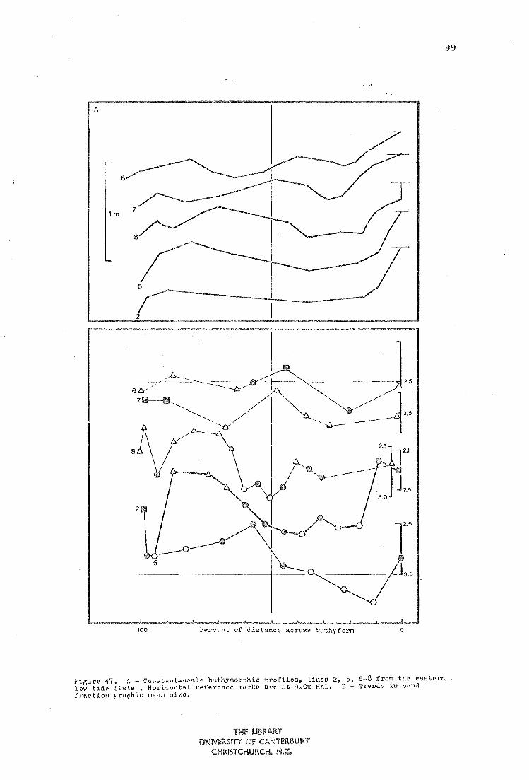
A
1m
2
100
I
5~ I
_._"],. ~j"
1 2.5
1 ~l 2.1
" fJ,., 3.0
r l'€'rcent of distance across bathyform o
Figure 47. A _ Constant-ElCale bathymorphic profiles, lino£) 2, 5. 6·.8 from the eastern loVi tid£' flats • Horizontal r .. ference marks are at 9.0rn HAD. B - Trends in Eland fraction craphic mean aizo.
THE LIBRARY ONIVE~SlTY OF CANTERBURY
CHRISTCHURCH, N.Z,
99

configurations and the corresponding grain size trends.
Figure 49 demonstrates that above the MTL, sediment properties
are uniform and independent of HAD, with coarsest sediment at the
landward margins of bathyforms. Finest sediment occurs in deeper
water adjacent to the intertidal channels, and there is a slight
mean grain size difference between 9.0 m and 9.5 m bathyforms,
shown diagrammatically in Figure 49.
100

'" '" o
'" ."
'"
o
o ~ __ J-.,_..,.,J0
o
o o ~
101
Figure 48, A - Constant-ucale bathymorphic profiles across 9.0m HAD flatu and shelves, plotted on common axes, Ilnd with trenus in sand fraction p,ra"phic mean diameter shown below. l'rofiles viewed looking north or east. D Constant Bcale bathymor"phic "profiles aCrOB8 n'"presentative eastern high tide slo"pGs, plotted on common axes. and Vii th sand fraction trends as in A.

2
102
looking south
§~----------------------~~---------------.~~-J <!) /
s /'
30
3
25
looking north .----------------.:.~ --- I' -------'30 ........... - .. - ......... _ .... _ ..
...... '"
'"
\ \ \ \
'.
.. - .. - _ ......... -
.;:; P=-~~---_..::: ----------------------~25 ~'l
looki!1f'; north L--______ ~__.:. _______________ _J30
5
Figure 49. Graphic mean size/ bathym .. try model of the surfacE" sediment of the Avon-Heathcote EDtuary. j"ean ci iamp.ter tr .. nds are from Figures 45 to 47. 1 _ Shore-normal trend where the bottom elopeo regularly offshoro (as on the westE'I'I1 slopes and flats, ohowing a generalised trend (a) and a long .. fetch, straight-profile trend similar to thoso on lines 10 and 11 (b). 2 and 3 -.~hore-normal trends aeroso mid tide shelves and high tide slopes.
4 Bathymorphic model (from Figuro 32). 5 - Trend across low tide flata.

103
PART FIVE
SUBSURFACE SEDIMENT
Introduction
An analysis of subsurface sediment from the ARE was undertaken
to evaluate a number of outstanding problems. In particular the active
layer assumption, which formed the basis of the sampling method used to
collect surface sediment, required testing. The nature and significance
of processes which maintain equilibrium distribution patterns in the
face of continuing erosion need to be evaluated, and the probability
that there may be a stratigraphic record of the response to early
urbanisation outlined in Part One, also requires evaluation.
Nethods
To obtain the maximum information from subsurface sediment it is
necessary to collect undisturbed stratigraphic sequences. Two methods
were adopted in this study:
(i) Short lengths of thin-walled plastic drain pipe (internal diameter
60 mm, outer diameter 64 mm) were pushed by hand into the sediment, then
lifted or dug out. Tubes 1;vere sealed with plastic bags, returned
immediately to the laboratory and opened with a sharp knife.
(ii) Longer cores v7ere collected with thicker-walled tubing (internal
diameter 53 mm, outer diameter 60 nun) cut into 1.5 m and 2 m lengths.
The tubes were hammered into the sediment with the flat back of a spade.
Before use the top end was squared off to avoid splitting, and a shallow
cutting face was bevelled on to the leading edge, The tubes could often
be driven 1.5 m to 1.8 m into the sediment, and were then dug out.
Recovery problems were only encountered where sediment in the tube was
predominantly mud free; in most cases muddy layers near the tops of
filled tubes acted as natural plugs, preventing the loss of sediment
from the bottom end of the core. These thicker tubes were opened in the
laboratory by cutting a slice of plastic from opposite sides 1;'7i th an
elec trical band saw> leavin g a thin layer which tvas subsequently cut
through wi th a knife,

In both methods, once the tubes were cut open, the top half was
lifted off, exposing an almost undisturbed sequence of sediment for
description and analysis. A total of 47 cores were recovered using the
two methods. All were logged immediately after opening - while still
wet, and before oxidation destroyed layering and mottling due to the
presence of chemical layering (Hayes, 196 1f). Samples were analysed
exactly as were surface sediment samples.
Results and interpretations
Detailed core logs are presented in Appendix 4. An examination
of these logs reveals that four distinctly different stratigraphic units
are present in the subsurface sediment of the ARE. There is an upper
zone of dark grey and black mottled, bioturbate sediment, inhabited by
a number of burrowing animals, and separated from underlying sediment
by a bioturbation interface. Beneath this surface there are three
units: a basal massive sand unit - unit (a); an intermediate layered
muddy unit - (b); and an uppermost, thin, massive, muddy unit - (c).
The stratigraphic relationship of these units are summarised in
Figures 50 to 53.
Sediment from bene~th the bioturbation ~~~~-------------~---
~ ...... -I-,...-+=-- ............. _LLL '-'-..L.L UL.\""
1. Unit (aJ. Several of the deeper cores finished in massive,
dark grey, friable, clean, coaser fine sand (,-lith mean diameters from
2.0 to 2.5 psi) or medium sand, with rare wood fragments, and sparse
coarse shelly debris. Unit (a) sediment was uniformly low in mud (mean
muddiness was 3.47%, s '" 1.66%, N= 8). Sand fraction graphic
statistics, input data, and probability cumulative curves are shown in
Figures 54 and 55, Vlhere it can be seen that apart from two unusual
samples from core 42 (830 and 831), unit (a) sand is uniformly well
sorted, although spanning a wide size range. Cumulative curves of
unit (a) sand are either almost straight, or slightly curvilinear, and
are interpreted to represent a single saltation population, similar to
Groups D to F in the surface sediment scheme. Figure 5SB indicates that
there is no relationship between grain size and HAD in this unit. If
the tidal range has remained unchanged since the deposition of unit (a)
sand, then Figure 55B indicates some of it was probably deposited in
subtidal conditions, and all of it was deposited below the MTL.

A
B 'fil
Figure 50. stratigraphic sections and summary graphic ~ogs. A - Core locations. B - Simplified descriptive sedimentology of cores, 1 - Bioturbate (mottled) sediment. 2 - Olive grey plastic mud. 3 - Friable massive dark grey fine sand. 4 - MasE'ive dark grey and grey-black muddy fine sand and very fine sand. 5 - Weakly laminated very fine sand and muddy very fine sand. 6 - Well laminated very fine sand, very fine sandy mud and mud.
105

Fig
ure
5
1.
Sum
mary
[ltratig
ra'P
hy
b
asa
d
on
deta
i1()d
lo
gs in
Ap
pen
dix
4.
Seo
b'igur~ 5
0 fo
r lo
catio
ns
of
co
res
an
d
Ilod
imen
t d
escrip
tion
s.
Lette
rs
(8.).
(b)
and
(c
) ro
for
to o
tratig
rav
hic
u
nits
d
OB
orib
ed in
tex
t.
106

"':: t"',
~ 'i
'" V1 I\)
'" x " I-'
'" 15 <+ ,..., o ;:<
ll' (!)
H, o 'i
10
datum (m)
9.5
":l 9 ,.... ~ 'i
'" ,,~
I-'
8.5
8
1.5
100
200
42
""" o -.J

10
8
. .0
Fig
ure 5J.
Ex
pla
natio
n as
for F
igu
ro
51
.

I I I I.
9
I l I l
I ill 1/' ;/ ~,,1''1
0 ,.: : II /11
, I '/
... iV IJ //' II :'/ I ! ,: .'I
.... ,z 1/ - 'I' '/
I~ b /' /, : /0 ./
f I, II ,I . j ': /f f fA if , I,
Ph' jI / l /'
I . ~ I: , 829,
// / /1
50
10
/ii"( PI -J' I j810 r
834 " f' c,;,;'OO
b-b_lL" 2 3 4
'j,!;IPLE" '10, GR.liEt,'l ST. OSV. S;~W'I£SS KURI0S1 S f>IItS PH!I& P)lIl$ P"IHSO PHt75 PH1Ur.. PH19$ .. _- .. - -~ ............... '3) 2,35 0,23 0.25 0.97 2,111 2,(,;) 1,6S La) 3.04 l,IS l,)9
a'Jo 2.66 O,2S 0.30 1.22 2,35 2~1o} 2.53 2,&r. 2.a! 2.:)4 J.lt
0'0 2' • l~ Il 0.2:9 0,25 1.05 2.C9 2.21. 2 .. 28 2.4f.l 2.6S 1.77 3.04
e,) 2.12 O.}O O,l) 1.0'7 1.9) 2~06 2 .. 10 2.26 2.50 2.63 2.97
RZ? 2.64 0.2S 0.4) I. J6 2,35 2+44 2.1,o;t Lsa 2.79 2.;11 J.20
SJC J. J& 0.51 0,08 0.79 2.)0 ','S 2.7.9: J.lO J,&I J,n 3,90
Ol' 3.17 0·51 0,10 O.n :l.lil 1,M 1#71J J. to J,(,1 J.71o J.:H
SJ4 1.15 0.25 0.07 1..09 1.8\ 2.02 2.09 2.23 2.41 2.50 2.6&
S4G 2.1 •• 0,25 0.011 1.19 \ ~95 2. t9 2.25 2.110 2,56 2,GS 2.llS
OS> 1.06 0.14 0.29 1.07 I.S' 1,&5 t.70 1.01 1,01 2.12 2~ 15
Figure 54. Hepresentative cumulativeprQbability curves, graphic statiotic6 nnd percGntil~ input data, unit (8) subsurface sediment.
109
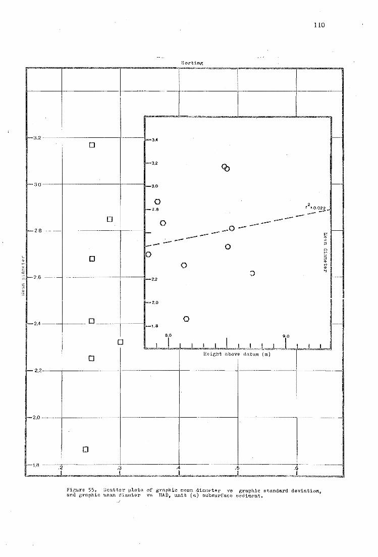
1-3.2
-3.0
-2.8
j
: 1-2.6
"
1-2.4
>-2.2
!
-2.0
1-1.8
",
110
Sorting
-1-3.4
0
1-3.2
CO
1-3.0
0 2 1-2.8 r '0.O2~. --0 --0 -_0 ---I- - ~"! .-- '" - - '" 1--- °
l:l P-
O ,....
0 '" a '" 0 <+
'" :) '1
.. -1-2.2
1- 2.0
0 1-1.8
8.0
1 Y I 1 I I I I I I I I I
0 Height above datum {ml
'f . i ·1 Figure 55. Scatt~r plots of graphic moan diameter VEl graphic standard deviatioll, and graphic mean diamter vs HAD, unit (a) sub8urfllce sediment.
f--
f--.
I--
i--
\---.-

111
Figure 56 shows contol.lrs drawn on top of unit.(a). The data
used to construct Figure 56 were derived by calculating the HAD of the
upper contact of unit (a) for all core locations where unit (a) sand
was recovered. If the assumption that the upper contact of unit (a)
sediment represents a synchronous surface is justified, then Figure 56
may indicate that immediately before deposition of overlying sediment
the unit (a) surface consisted of a western mid to low tide slope,
separated from an eastern low tide flat by a broad subtidal channel.
Drillers logs, supplied to the writer by the CDB, and information
from D.D. Wilson (pers. comm., 1977), indicate that typical sequences of
sediment encountered during subsurface investigations near the ARE pass
through an upper layer of fine muddy material, from 1 to 2 m thick, and
then through at least tens of metres of monotonous, massive, dark grey
sand. Cores figured by Brown (1975, in press), indicate that this
sand - the C'hristchurch Formation of Suggate (1958) - is up to 50 m
thick beneath·the estuary. Unit (a) is interpreted to represent the
uppermost few decimetres of this sand, and to be uppermost Christchurch
Formation sediment.
Unit (a) is interpreted to be pre-estuarine, open ocean sediment
for two reasons. Firstly because of the similarity between unit (a)
sedi~ent and monotcncuG, Guppc3cdly murine __ 1 J ... _ .• Ot:.::U...l..1Ut:!1IL
(Suggate, 1968). Secondly, because of the textural evidence in
Figure 54 - present day sand with nearly straight cumulative curves
and unifo"l.'111ly excellent sorting only occurs in shallow water (above
9.0 m HAD) w'here wave energy is relatively high. The presence of
similar sand in deeper water (dmvn to 8.0 m, Figure SSB) may indicate
a regime of larger waves - and perhaps' oceanic conditions.
2. Unit (b). In almost all cores, massive clean friable unit
(a) sand is overlain by muddy, stratified sediment. The contact is
invariably sharp and abrupt, and represented by a significant textural
discontinuity. This stratified sediment is commonly plane-laminated
muddy very fine sand, often with centimetre or decimetre scale interbeds
of massive muddy fine sand and muddy very fine sand. Where relatively
thick (as in core 41), this sequence may contain one or more decimetre
scale fining upwards sequences, with individual units typically
beginning at an erosional and textural discontinuity as clean fine sand,
grading up into weakly laminated finer fine sand (2.5 to 3.0 psi), muddy
laminated very fine sand, and massive very fine sandy mud or mud (more

112
,; >i E ; ~
.! .. § :; ; i . " ~ " Jl ~
J " Q
.. "
" ':'
• .. <
0
n
" 0
0 " ~ ,.. It '" ~ \t II Q
0
:J1,
I! 1:, ... ..
+
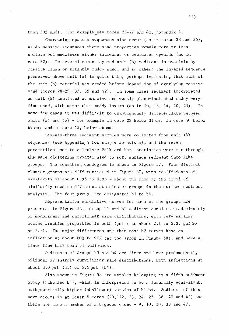
113
than 50% mud). For example __ see cores 26-27 and 42 ,Appendix 4.
Coarsening upwards sequences also occur (as in 38 and 35),
.as do massive sequences where sand properties remain more or less
uniform but muddiness either increases or decreases upwards (as in
core 32). In several cores layered unit (b) sediment is overlain by
massive clean or slightly muddy sand, and in others the layered sequence
preserved above unit (a) is quite thin, perhaps indicating that much of
the unit (b) material was eroded before deposition of overlying massive
sand (cores 28-29, 35, 35 and 42). In some cases sediment interpreted
as unit (b) consisted of massive and weakly plane-laminated muddy very
fine sand, with minor thin muddy layers (as in 10, 13, 14, 20, 23). In
some few' cases it was difficult to unambiguously differentiate between
units (a) and (b) - for example in core 23 below 31 cm; in core 40 below
69 cm; and in core 42, below 56 cm.
Seventy-three sediment samples were collected from unit (b)
sequences Appendix 4 for. sample locations), and the seven
percentiles used to calculate Folk and lV"ard statistics were run through
the same clustering program used to sort surface sediment into like
groups. The resulting dendogram is shown in Figure 57. Four distinct
cluster groups are differentiated in Figure 57, with coefficients of
similarity used to differentiate cluster groups in the surface sediment
analysis. The four groups are designated b1 to b4.
Representative cumulative curves for each of the groups are
presented in Figure 58. Group b1 and b2 sediment consists predominantly
of monolinear and curvilinear size distributions, with very similar
coarse fraction properties in both (psi 5 at about 2.1 to 2.2, psi 50
at 2.5). The major differences are that most b2 curves have an
inflection at about 80% to 90% (at the arrow in Figure 58), and have a
finer fine tail than b1 sediments.
Sediments of Groups b3 and b4 are finer and have predominantly
bilinear or sharply curvilinear size distributions, with inflections at
about 3.0 psi (b3) or 2.5 psi (b4).
Also shown in Figure 58 are samples belonging to a fifth sediment
group (labelled b l), which is interpreted to be a laterally equivalent,
bathymetrically higher (shallower) version of b1-b4. Sediment of this
sort occurs in at least 8 cores (20,' 22, 23, 2LI, 25, 38, 40 and 42) and
there are also a numb er of ambiguous cases - 9, 10, 30, 39 and 47.

t
I t
j t
j t
I
2.1t)
2.)9
2.111
2. ]f.
2.71
2.75
2.BB
2.92
2.8f!
2.61t
2.70
?.AS
2.81
:7:.87
2:.78
Jolt.
3.J6
.l,JIt
J.J2
3.37
).JO
J .le
3.)0
).26
J.27
).20
).ltlt
2.99
J.12
).11
J.1l
1.10
).12
3.18
J.02
l.Ot.
3,00
2.91t
O.lI
O,lI
0.28
0.)2
0,29
0,27
0.2)
O.llt
0,22
0,25
O,21t
0,23
0.20
0.26
0.2A
0.2)
0.)9
0.12
0.))
0.32
O.J7
0.29
0,29
0.17
0.)6
0.)]
0.]]
0.)2
O,ltl
0,'+2
0.55
O,lt9
0.(,2
0.)5
0.)5
(\.ll
0.)6
0.35
a,llt
0.)6
0.J5
0,15
0.)6
0.32
O.llt
0.)9
a,lto
O,1t2
0.]2
0.35
O,llt
0.)2
0,36
0.)7
O.llt
0.))
0.)8
O,llt
0.37
0.1t2
O,ld
0.)9
0,1t9
O,it(l
O,1t7
0.56
0,52
0.50
0.1t)
0,29
0.25
0.21
0.11
0.06
0,08
O.llt
O,lS
0.21t
0.20
0,12
0,18
0.09
0.26
0,06
0.18
0.1)
0,22
0.1t8
0.1t7
0.2)
0.22
0.))
O,llt
0.)1
0.2B
0.37
0,32
0,12
0.1t7
0,)2
0.27
0,11
O.H
0,12
0.10
0,08
0,10
0,07
0,05
0,29
U.IO
0.15
0.1)
O,llt
0,11
0.15
O,21t
-0,01
0,27
·0,01
-0.05
-0.01
0.1t)
0,)8
O,It)
0.)6
0.29
0.19
0.1t)
0.20
0.25
a.!!)
0.20
0.11
0.111
0.06
0.06
0.)9
1.21
1.20
1.08
0.92
I.ClI:I
0.96
I,OIt .
1.00
1.11t
1,2)
1,07
1.26
1.18
1.15
1.17
1.00
1,16
I.tlt
1.16
0.96
0,87
1.10
0.90
1.28
1,61
0.9)
0.9i1
0.73
0.91
0.71t
0,70
0.78
0.76
0.78
0.75
C.77
0.75
0.78
O,7J
0.73
0,89
0.72
0.73
0.77
0.82
0.69
0.77
0.82
0,87
0.9J
0.99
0,87
0,87
1.05
0,92
0.90
0.92
0,80
0.71t
0081!
0,73
0.82
0.60
0.73
0.97
2.2) 2,)2 2.)6 2.50 2.72 2.0U ).12
2.15 2.)2 2.n 2,5) 2.71t 2.0S 1.)5
1,2) 2.)5 2.1t2 2.56 2.72 2.05 ).2)
2.00 2.26 2.)1t 2,50 2.70 2.U6 ),17
2,OU 2,)0 2.)11 2.51t 2,19 _ 2,02 ),15
2.1l 2.n 2,lt9 2.56 2.7 1• 2.01! ).0)
2.16 2.)] 2.)9 2.56 2.72 2.7') 2,99
2.0'1 2.20 2.26 2.1t2 2.67 2.0) ),26
2.)0 2.50 2.51t 2,6) 2.60 2.90 ),15
2.27 2,lt0 2.1!6 2.59 2,75 1,09 ).12
2.17 2.)0 1.lS 2.1t9 2.66 2.76 2.99
2.17 2.26 2,)) 2.1t8 2.66 2.71t 2.91
2.23 2.)1t 2.)9 2.50 2.61t 2.n 2.89
2.16 2.28 2.)) 2.1t5 2.6) 2,70 2.86
2.12 2.25 2.)1 2.1t1t 2.59 2,(,6 2,8)
2,05 2.22 2.25 2.1t0 2.62 2,n 2.95
1.90
2,00
1.8)
2.60
2.)5
2.25 2.1t) 2.61
2.26 2.)] 2.56
2.15 2.)8 2.65
2.6') 2.75 2.82
2,lt9 2,62 2.89
2.1t9 2.66 2,89
2.1t9 2.65 2,9)
2.1t0 2.61t 2,88
2,70 1,98
2,60 2.90
2.00 ).11t
2,00 ).00
).00 ).50
).05 ).1t0
).15 ).60
).00 ).21t
2,)2 2,51 2.56 2.72 2.92 ).05 ).)It
2.1t8 2.55 2.60 2.75 2.9) ),08 ),ItO
2031 2.51 2.57 2,7) ).00 ).21 J.5)
2,)8 2.51t 2.62 2.60 ).11t ).)0 ).60
2,ilO 2,56 2.65 2081t ),19 ).)5 ).55
2.'19 2,60 2.66 2.81 J.06 ).21t ).56
2.CI] 2.21t 2.)1 2.52 2.89 ).10 J.)5
2.10 2.26 2.)0 2.57 2,86 ).07 J.60
1.22 2.)] 2.1t1t 2.60 2,86 ).1) ).87
2,12 2.)1t 2.1t5 2.72 ).20 ) ,il9 J,8)
2,11 2.JS 2.1t~. 2.71 ).15 -).)6 ).70
2,02 2.26 2.n 2,70 ).1t0 ).65 ),B5
2.01 2.27 2.n 2.61 ),20 1.'15 ),66
2,09 2.97 .1.0) ),J2 ).60 ).ll J.,)2
2.90 2.98 ).05 ).JI! ),61! ).75 ),91
2.60 2.96 J.05 ).J2 ).61t 1.75 ).92
2.01t 2.91t ).02 ).)0 J.59 J.72 ).90
2.88 J.OO J.IO ),J6 J.66 ).76 ),91t
2.90 J.OI J.IO J.J7 ).65 J.75 ).91
2,62 ),05 J,IO 1.28 ).70 ).00 J.95,
2,tl5 2,91 ),00 J.29 ),56 lob9 J.B7
2080 2.9J 2.9') J,25 J.55 ).68 J.87
2.80 2,88 2,95 ),21t ),51t ~.6U J.85
2,06 2.95 J.OI 3;26 ).51t loGS ),81
2,87 2.9J ).10 ).29 ).56 J,69 J,87
2,70 2.0J 2.9) ).2) lo57 ).72 3.90
2.70 2.02 2,00 LIS J.51t J,69 ),S8
2,55 2. BJ 2.9J ) .25 J,6J J. 72 ) ,86
2,8J 2,89 2,91t ).16 ).ltl! J.56
2.95 J.05 J. IS JoltS J.75 J.OJ
2.91 J.OIt J.17 J.1t1t J.7I J,OO
2.95 ),12 )020 )01t6 J.70 J,OO
2,6) 2.73 2.70 2,95 J.J2 J.1t9
2 0 60 2.71t 2.80 2.97 J.J2 J,lt9
2,61t 2.71t 2.78 2.91t ).21t lold
2.69 2.19 2,Olt )'01 J.JIt J.'18
J.8J
).96
J.92
).95
).77
J.70
).75
J.75
2,52 2.75 2.80 J.OO J.)] J.52 J.n 2.57 2,75 2.8J J.02 J.27 J,ltl J.70
2.57 2.67 2.71 2,89 J.21t ),111 J.76
2.1t9 2,72 2001 ).05 J.1t2 ),59 J 0 8J
2,5J 2,73 2.80 J,OIt J.ItO ),57 J.87
2,65 2,7'1 2.82 J,IO ),ItJ ).56 J,81t
2.112 2.60 2.60 J.02 J.50 ),67 J.90
2.JS 2,65 2075 J.07 J.50 ),65 J.08
2,51 2,69 2.70 J.12 J.56 ),72 J.90
2.15 2,ltJ 2.60 2,98 J.1t5 ),61t ).05
2.25 2.51t 2.65 2.91t J.1t7 J.GIt J.86
2.21t 2,ltO 2.59 2.97 Joltlt ),55 ).75
2.25 2.52 2.60 2.79 J.20 ),50 J.86
710
8))
739
729
717
728
75'
7))
850
797
732
790
826
807
656
660
7" 658
662
6"
8)2A
009 ~ 793
a28
." 7.' 7f)6
670
800
027
8" 659
.'7 705
6G7
·'5 661
657
99 98
114
97 96 95 94 93 92
Modified So!'rensons Coefficient
Pigure 57. ~and fraction graphic statistics, percentile input data, and dendrogram resulting from cluster analysis of input data, unit (bl subsurface sediment.
91 00

I
.- . -~
7~ 8<17 : - - -. 1-- 1---- - ... I "792 .6&4: r . i 715 71<1 f ! 82 I, I /1-8$0
b, ,/1 78<1' I ~: " 'I b:2 fI~ I b
3 Ji 78<1 b, f'l' 842 fl'· " 'H i . - --. I IJ I I 785 ::; l
901 I I I I I I -r---II---+--I--+-+-+-+-+ /. I fJ I / I II.~f J I I I I I
o / ,/ . ~1,'Hli i/ . JAI.l i: 'II * 1/ * . I: * I I I I
3~i If
II , !
! I 101 I I I I
)
I 7 /
, 1 I I I I ,795 I I I I I I I '
~t
I 1 2 3 2 3 1
Figure 58. aepreeentetive cumulative probability curves from groupe bl-b4 &ad be, unit (b) subsurface aedi.eat.
2
8281 f 809
I 3 , 2 3 1 2 3 ..

115
Group b ' consists of massive well sorted fine sand, physically very
similar to unit (a) sediment, except slightly muddier. Group b ' sediment sometimes directly overlies unit (b), as in cores 42 and 43,
but more commonly occurs as a laterally equivalent, bathymetrica11y
higher correlative of (b), as in the core series 38-23-24 (Figure 52).
Mean size vs sort of all unit (b) samples is plotted in
Figure 59, at the same scale as Figure 40 (for surface sediment).
A comparison of Figures 40 and 59 indicates that sediment of units bl
and b ' is analogous to Group D surface sediment, b2 is analogous to B,
and b4 to C. Sediment similar to subsurface unit b3 has not been
recorded at the surface. The distribution of samples in Figure 59 shows
that the cluster groups bl to b4 occupy separate sections of the
diagram, and are evenly distributed within their individual fields,
indicating that here also, the clus
classification of convenience.
operation has made a
Figure 60 shows the depth preferences of the five groups.
Groups bl and b2 have similar depth distributions, with identical means
and ranges. Group b3 sediment occurs preferentially in deeper water,
never above the MTL (9.0m), with a mean depth of 8.45m HAD. Group n4
samples tend to occur bet\veen 8.0 m and 8.25 m, or between 8.75 m and
of 8.56 m; .9.nd b I S 8 tend to occur
preferentially above the MrL. ,vi th a mean HAD of 9.30 m.
Groups bl and b2 have depth distributions similar to those of
the series A-B-C (Figure 43) for surface sediment, b ' is similar to
group F, but b3 and b4 do not have surface equivalents.
Figures 6lA and 6lB are plots of mean size vs HAD and per cent
mud vs HAD for all unit (b) sediment These figures show that
there is a general trend towards coarser, cleaner sediment in shallow
water, and regression lines fitted to group average values (for bl-b4
only) show high coefficients of determination, indicating that the
average trend is valid.
Unit (b) sediment is commonly plane-laminated and muddy, and
granulometric and HAD-preference studies show that it is similar to
modern, active sediment in the AHE, but quite dissimilar to unit (a)
sediment beneath.
Unit (b) sand consists of single log-normal size distributions
interpreted to have been deposited from saltation, or of simple mixtures
of this saltation population with material interpreted to have been
deposited from suspension.

3-2
2-8
-2-4
2-2
2·0
o 0 0
o 0
~ DOmn
0
~ ~rP ~
~ ~
()
Q>
Q>
@ Q>
Ql(8
o o
o
-0
o
0 0 0
o
tlorting
ObI
() b2
o b3
(;l1 b4
~ b'
Figur~ 59. tlcatLer plot of c:raphic meun diameter vo p;raphic otllndurd doviation for oalllnl"", from unit (b). (lubourfllco (If'uimf'nt.
116

117
bl
b3
b4
~--~ .. b'
m HAD
Figuro 60. Sample frequency vs HAD for the groups bl-b4 and b', unit (b) subsurface flPdimont.

20
8.5
~U3 40 0
30
, ,
9.0
G!;l 0
He.if,ht above datum
95
10 2@ 30 4 ~
b' 6
l"igure 61. Scatter plots. A - 1,lean diameter VB HAD. n - l'erecont mud VB HAD. :.;ample from cluoter group (b), subBurface sediment.
118

119
Differences between samples are a result of various mixtures of the two
basic populations, and this simple two-component model is analogous to
that derived for surface sediment. However, unlike surface samples
groups b3 and b4 contain more than 50% of the suspension population,
and Figure 58 indicates that some b3 samples contain as much as 80%.
Unit (b) is interpreted to have been deposited after the ARE
was separated from open ocean conditions, and to represent material
deposited under conditions essentially similar to those which apply
at present.
3. unit (0), In many cores, unit (b) sediment is overlain by a
thin layer of massive olive grey plastic (buttery) mud, or very fine
sandy mud - unit (c). This olive plastic mud is commonly massive and
monotonous in appearance, but it may show laminations (for example,
core 13), and it may be rich in coarse, leafy organic debris (probably
Zostera leaves), The contact betvleen units (b) and (c) is commonly
sharp and abrupt, \-lith a major textural discontinuity; in some cores
the contact is gradational, with interbedded sand and mud grading up
through sandy plastic mud to plastic mud (cores 37 and 41 for example).
Cores with olive plastic mud occur throughout the estuary, with
the thickest sequences recorded from the north-west corner (Figure 53).
There \Vas no apparent relationship betvleen occurrences of plastic mud
and HAD, and the unit was apparently deposited throughout the estuary.
Because of its cohesiveness unit (c) is more resistant to erosion
than most other sediment in the ARE, and is exposed at the surface in
many locations in the estuary (Figure 62). When exposed on the higher
intertidal flats unit (c) tends to be rich in coarse organic debris
(leafy material, twigs and shell fragments), and as a result has a
fibrous, crumbly texture.
Unit (c) has a mean mud content of 80% (s = 17%, N = 15), a sand
fraction mean diameter of 3.08 psi (s = 0.16 psi, N = 10), and a mean
sorting of 0.47 (s = 0.04, N 10). The mean thickness of the unit,
from four apparently complete sections (with gradational or planar
contacts - cores 17, 22, 39 and 46) is 25 cm, and the average HAD of the
top of the unit is 8.96 m.
"t-lhile unit (c) sediment is different in appearance from both
overlying and underlying sediment, it has a markedly uniform appearance
from core to core, and very similar physical propert ies. Figures 63 and
64 show cumulative curves and summary granulometric properties of
unit (c) sand, and a comparison with 58 shows that it is

," .... . - .• ' "1'_~
])
F ir:ur ~ 6 2 . J urfu c o ec " rr e ne E'8 of ]l03 t -"urOll~an >J. n t hropoge nie mu d - 8ubsu r fac "'t ra t ~ /; r"nhi e u ni t (e) - ill the Avon- !i e a thco t R!:' tu . ry . A, Il - ll n~t (e) Jll .s t i c ',ud expo('~d i n the "1.oe'" of a "ha l l ow int e r i d 1 I ll ey n e a r t he ~nd of' line 1 6 , " ,'l ~'t ern h i e..h t ~ d c 8 10pe s ( 1 ) . Vi ",·,' i s e a s t no r th e as t, ebb flo'l, i " t o t he ri Gh t (~) . ~ pBdp f or sca l e (*) . Not e coa r s e r, a ct i v e cl e a n Ra nd ( )) , w ~ t h l i ne Rt ~ o n9 p ~ ra l e l t o th e ebb fl ow d irec tion ( s r r ow ed) , a n d bu r r ows in th e l u mpy, cQ h e ~ ~ve e ro~i D n- re ~ i ute nt p la~ t ic mud ( 4 ) . ~ h i t Rr r OW i n A i s 20 e m long . C - Unit (e) f~brou ", o r r:an ic- r ieh l a st ic mu d e xp ose o i r1med i n te ly s ou t h of :.i =dy }'o int. V 1P,VY i ,' \',c t- t i nto t he 1I 0 r t h He>a th c ot c- Bas i n ( I"ap I ) , 'r om C eary ( ClJB t.u rv By or) f o r ~ u' le. ~J ot c ge a rp 01' e r od ing mud ( 5 ), o;o h own i n d e t a i l in E , be> l ol'/ (l oo k i ng . " s t), a nd pos t ( 6 ) f or l ocati on. Uni t (c) mu() i ,' intc'm:e l y b o red, a nd ri ip" offD ho r e (t o t h e r i gh t in E ) at g sl i ghtly l owe r a nc le t ha n the pr s ent - da y 8 cl i m ~ nt Durfae ~ . D - Un i t ( c ) " a ndy mud (7), expoz ed n C'!l. r t he e astc' r n e n d of l ~ n e 1 0 , ~ap 1 . Vi e w is t o t h e no r th . F - o l ive pl a utic mud of u n it (c) dug f r om be ne ath cle a n fr i abl~ sand (8 ) on line 1 0 , near t h e l oca ti on of core 36 , <'iRU r e 50 (sa p a et a l le d log of co re 36 in Anne n d ix 4 ) . G - :Jhel l ,V I orp;an ic -ri ch u n i t (e) mu d ( 9 ) C'x:pOc' e d a t the !!", ma r k ( 1 0 ) neUl ' the eaC' t end of l ine 3, /""p 1. liule i,' 2 5cm l onr:.
iLO
, 6

psi diameter
90 -I---+-+--+-+--l--i--f---I--
2 3 4
~:''':'L£ r,c. GP. r~(fI'i ST. 'JE'I. SKElfllt:SS KunHISI $ 1"!!15 ('Hili) flHllS PUIS!) PHJ75 PH{r14 PIH95
719 ).10 0,/;10 0.21 0,81 2.49 2,66 2.15 J .0) 3.43 3.61 ).84
720 3.14 0,'14 0.25 O,B3 2 ~ 54 2,72 '2,30 3.06 1.47 1.6; 3.90
)21 3.10 0,42 0.\4 O,B4 2+56 2.7S 2,ns J .Il J.4e 3.65 l,B5
72' ).10 0,112 0.22 0.70 '2,60 2.75 2.90 3.)0 1.S1 J.6S 3.85
721 J.11 0.49 0.07 0.71 2.Jj~ 2.58 2.67 1.08 J. $0 1.67 J.84
)14 3.11 0.50 0.17 0,80 2.J6 2.61 2.72 3,03 J.50 1.70 3,88
ns 3.23 0,1,2 -,').0$ 0.80 2.58 2.77 :2 .06 3,25 1.S4 1.6. 1.90
7)4 J .14:' 0,50 0,0$ 0.76 2.39 2~6J '2.74 1.1l 1.5S J.72 3.90
71' J ~ 16. 0.50 0.05 0.76 2.39 2..1 L14 loll J ~55 J.n 3,90
742: '2.!l4 0.52 0.47 o,ns 2.22 2..37 2.45 2,66 ),24 J ,48 J,6S
749 L75 0.51 0.46 1.10 2.16 2.30 2.16 2.59 2.95 J.n 1.74
I,'igure 63. [{epreeentative cumulative probability curves, graphic statistics and percentile input data, unit (c) subsurface sediment.
121

Sort i l14J: .2 .3 .4 5
I I -,
!-- 8.4 I
i-- 3.2 --+----···-······--+------------+---li:f--
o £?
i--3,O ~ __ . __ --t--_--l---_O_x~_\\ 1--.. \
o f-2.8 ---t--------+--------..... --+--------l--
o
122
6
11--_11--3.4 1!--+--~ ........ ----_+_----_lI
-2,8
Il----JI"- 2.6
I
I
o
I I I I
Figure 64. ::)catter plota. A Mean diameter vs graphic standard deviation, B - Mean diameter V8 HAD, unit (c) subsurface sediment.

uniformly finer and poorer sorted than any of the subgroups of (b).
Figure 64 shmvs that there is no relationship between the sand
properties of unit (c) and water depth.
123
Unit (c) sediment is different from all other material
in the ARE, both ancient and modern; it was deposited as a thin blanket
throughout the estuary - in many places where fine sediment had not
previously been deposited, and where it has not been deposited since.
The unit was most probably deposited during a period of very much
higher than usual suspended sediment concentrations, and was deposited
relatively rapidly and at uniform rates (hence the massive appearance,
and the independence of sand fraction properties, muddiness, and HAD).
The event most likely to be responsible for flood the estuary with
high concentrations of mud, for periods sufficiently long to allow an
accumulation of tens of centimetres of sediment, is the urbanisation
of the catchment area of the estuary during the second half of the
19th Century. Thus unit (c) sediment is interpreted to represent
mat erial depos ited during urbanisation of the Christchurch area,
when the tidal compartment decreased by about 30%. If this
int ation is correct it means that the (b)-(c) contact can be
dated at about 1850, and the upper contact of (c) at about 1900.
If unit: (c) was sieed wieh an average thickness of 50 cm
throughout the estuary, this would represent an accumulation rate of
2 em/year for the 25 year period 1850-1900, and a total of 3.0 X 10⁶ rna
of sediment, which corresponds to the f predicted in Part One
(and in detail in Appendix 1) for the decrease in the tidal compartment
during this period.
Biology and physical characteristics of sediment from above
ion in t erf ace
In many cores, cohesive muddy unit (b) or (c) sediment has an
intensely burrowed upper contact, and where thin unit (c) horizons are
exposed at the surface, they are intens burrowed (Figure 62). The
overlying sediment is massive sand, and it commonly contains abundant
articulated (living) or coarsely fragmented bivalves. Locally there
are pebbles and blebs of soft plast ic mud in this upper sandy zone
(see cores 37 and 41 in Appendix 4) . If muddy horizons occur within
this upper zone, are intensely disturbed, and consist of a few
streaky remnants of mud surrounded by sand (as in cores 26-27, 32 and
!}3) •

124
Mottling and visible burrowing in subsurface sediment in marine
environments is due to the myriad activities of organisms living on
or in the bottom sediment, which eat, burrow through, spray out, or
otherwise disturb and mix near-surface sediment (Schink and Guinasso,
1977; Rhoads, 1967). Benthic animals physically alter the sediment in
which they live in a variety of ways Myers, 1977, for a brief,
recent review of this subject). Biologically mediated sediment-water
interactions involve the movement of organic matter, nutrients, and
pollutants, and are significant in both the benthic and pelagic food
chains (Myers, 1977; Goreau, 1977).
1. Biology. A wide variety of different animals are involved
in the bioturbation of near surface and subsurface sediment in the ARE;
four groups warrant detailed discussion:
(i) Polychaete worms are the most abundant animals in the ARE
in both variety and numbers (Voller, 1973; Knox and Kilner, 1973).
Estcourt (1967) found a total of 21 species, and one of these (Aonides
trifidus) was found in concentrations of up to 6 OOO/m 2 • Some are quite
large, Glycera americana may reach 27 cm in length, and some are deep
burrowers - the widespread detritus-feeding worm Nicon aesturiensis may
be found in permanent burrows as as 40 cm below the surface in the
ARE. Some are carnivores (G. conericana) , some are surface detritus and
deposit feeders tN. aesturie ) and some are suspension feeders
(Scolecolepids henhami). As well as species which live in permanent
burrows, there are free-living burrowing species (Anglaophamus macroura)
and tube-building species (especially Boccardia lynrar~hia and
AxiotheUa quadrimacuZata, see Figure 65). The lugworm Aharenicola
affinis constructs large and conspicuous
sandy midtidal flats (Figure 66A, 66B).
n mounds on many clean
Rhoads has shown that the North American polychaete Clymenella
torquata is capable of producing vertical grain size ients in near
surface sediment, and of reworking all sediment to a depth of 20 cm in
1.4 to 2.4 years. Other polychaetes are also capable of reworking large
volumes of sediment, and of producing subsurface biogenic layering.
On the North Sea intertidal flats off Holland and Germany, the
polychaete AY8nicola (an animal which is similar to the Aharenicola spp.
found in the ARE) produces a distinctive 20-30 cm deep concentration of
gastropod shells in a manner similar to that described for C. torquata
(Reineck and Singh, 1975, p. 135).

;\ 1-\
rur' L';. . .Jr. CEI PVl enol' ':Ii .8 iment-moo~j"y1.np, bl.oloricnl ctivi t.V 1n the vo: - thcot~ otu r:f . A - Holell ~nd !'urf:lc() mr.rK111("S (1) 1n cJ.()tln frl. ·blp lwl{'u .. nd ne 1'" tte C',wtl'rn lnd of line if) ) I,.ap 1 . ,.n1m,.t,. not 1. (m.i·ipG ,
r 10cm 1011<' . II - Circu1:1r trUCE'll (2 , 3 1n ::>lonull ".uo /'lpc:r thE' \'.r>. tr-l 'n • t,j of line " . p 1 , nrob:'bly ouC' to 0. nolych",tl' wonn . ~,izo 8 ( .. l) boot.
_n 1 ~ Iormpu in eli ntly muolfY very f l.n( "nnd occupi"" by (\('n: !.' Jf1ul' tion ">1' tht> t.tI e - buil"in{' nolych:.lete "xiothC'll'l 'lu,.ari.,·,cul"t· •
'r'b bur 01. (4) .TId 1 .. Ter· f'Xc'!v"tl.on " pron (oul:ll.n d by "'oU tr 'crro;'n) , (' • tr'_l ("lthcct( .J·S1.n 1o .. tid!.' (b . lIJm II"I) r ;.to . Ld'''C C' P uiamr t('r 5c"1 .
r' b miT 0· ... (5) ~XC'lvut l.on pron (L» , ,1m hibo1n trail (7) . no f' rt1y a 'i, d .mphl bola (t. , l.n rl.pp1eu c1 an « ·-.no n",.r th!.' H. mark t tile \. "tf'rTI eno
f l1ne 11, ... . '1' 1 . Jar i::J lJcrn 1011(" . ~. - Cr·].u burlo"I::> .n.) nnron" (" , 10 , 11) ~lrl cr m·lTlu.n{'r a1 an un1 C'ntiJ'ied · ... orm ( ~ , 1 .) , nenr tht' r' t c:>nd of line
1. Har 1 " llJcm lOll{ .
125

('
c
II
of tP _1l1!'nt-m llfYlne. bio ,.<' Ll. c i\'l.ty in the {' ~ t1.an C t "~th, lUI' ,~rm ,,0 r~n1.c"l· .f in1."
(1) mel f( dinr tr'c('t1 oj tilf' eiv' lvI" ',comon" hticrui ( ), outh<'I'n flllt[l .., a th£' cau"I'I','Y . ,.ci.ll' i,' L 'cr. . IJ - ['floti,,., c' itS () , A) or
rl'f1l.co1· . 'in~ , ... comona r tdint trace s , l.ir-l t1Llt' 11 tG npn r -h f·:;"t (nu ')f Llnp " "an 1 • .jc ·~le l." lOcm. C - Gull" f~l'dinc; tl(".r the \\c-st no of lint' ' ,
[l 1. Gulls r..1 it o.te t1 rf~c" :1(>()impnt (5) by briskly r ' .. s inv [lU lo\·~rl.nr tht1 r
e t - (' tirlf' "oft-bouied unl.mals broufht to th(' ourt'tcE', 'lna m Lkinr .. tl.nct iv(' natterinl" oound . ::ot ce the l u rf< ar 'is of rl'fl!' tiv!' <ltG-nair1#'
',', ter , ano the abundant Amnhibola . D - Gh[. r act('r1.st i c birdt1- f'o ot t1hupe-Q feeLl 1llg r'l.c e of acomona (b). E - 110110w" made by a t:ul l from th(' rrOUll 1n C, " ove
(7 ind i c tes rir-ht foot m,' rk, the bl.rd faceD away from the- obaerver). "a te lighter c oloured mud on "the floor of the de-prl's: ' i on , the area of coars r :.gi tilted seo im('nt in fr ont (8) . ',md pol.vchacte tubes cX)'losed l.n the sides of the hoUo',' B ( :J) . F - Larger area of r:u11- '-'&i tElted sed imen t , "howine fluia-mud fill ec, d t·pr as i ans (10 ), a nd an Am-phibola tri,~l (11) . ,en(Oe can diam~te r ~cm .
- Dc nB~ populat i on of Amphibolu on high tide slopes ( 1.) to lU . Om HAD) near the east pnci o~ line 10 . H - I tensely bioturbnte d seoiment just off the east end of thc Causeway . iote Mac omons traces (12) , abundant trails of the topshe11 Zed ilonlU. Gu brostrllta (13 ) and l'p;estion casts of an unidentl.fied .;orm (14).
126

127
Estimates of rates bioturbation by polychaetes are not
available for the ARE, but considering the high population densities
present here, the turnover time for surface sediment may be
significan less than the 1.4 years discovered by Rhvads in
Barnstable Harbour, Mass., U.S.A.
The bivalve Chione stuchyburyi - the coclue - is easily the most
conspicuous member of the macrofauna of the ABE (Voller, 1973; Knox
and Kilner, 1973), with recorded densities as high as 2500/m 2 on some
lower intertidal flats. C. stuchyburyi is a filter feeder, capable of
filtering water at rates of 0.5 L/h for 12 h/day, and one individual
may fix up to 44 g of suspended matter (dry weight) in one year (Knox
and Kilner, 1973, p. 188). Cockles burrow to depths of 2-4 cm, and
when present in high concentrations, may constitute from 30-40% by
volume of the upper few centimetres of sediment (Figure 18). The major
significance of cockles in sedimentary terms is their filter
activity, since they package suspended material into aggregate
grains, which may be transported as sand sized material, or be buried
beneath the sediment surface (Haven and Morales Alamo, 1966; Myers,
1977) .
The wedge shell Macomona Liliana is common on clean sandy midtide
flat c ~.,., .... "h-t~ nC\i~l1"3""~T T,T'horA ............. '-'''" ......... - - ........................ J, •• "' .. - ..... -
25 cm beneath the sediment surface. It feeds through an inhalant siphon
which it extends to the surface and uses to suck sediment from an area
of about 10 cm2, leaving a dist inctive, radiating, birds-foot like
feeding trace (Figure 66A, B and H).
Other bivalves are relatively rare; the green mussel Perna
canaliculus occurs in an area of about 50 x 200 m on the north side of
the principal subtidal channel opposite Beachville Road, and the pipi
Amphidesma australe austra is also found in small numbers (Knox and
Kilner, 1973).
Six groups of gastropods occur in the AHE (Voller, 1973), but
only two appear to be significant sediment modifiers. The large mudflat
snail Amphibola crenata is widespread (Figure 66G, for example).
Amphibola feed when the tide is out by passing material from a
centimetre-wide, less than millimetre-deep strip of the surface through
its gut, and extruding it as a continuous fecal string (see Figures 65
and 66). The long fecal strings are readily broken into shorter lengths,
and the resulting millimetre-scale equant aggregate grains accumulate in
shallow depressions and bettveen ripples on the intertidal flats.

128
This writer has observed that where A. crenata is present in large
numbers, up to 80% of the sediment surface may be ingested and packaged
into fecal strings over a period of 3 to 4 low tides. On windy days
waves sweep accumulated fecal particles from the intertidal flats, and
they are preumably lost from the estuary. Thus although A. crenata
reworks sediment by stion and surface displacement, its principal
role in the sedimentology of the ARE is as a packager of surface
sediment into readily transported, coarse aggregate grains.
The small topshe11 Zediloma subrostrata is less widely
dist ribut ed than A. crenata, but appears to modify sediment in a
similar way (Figure 66H). Other species, including the scavaging
carnivore ComiYIBlla glandiforrnis (often seen converging in scores on
dead animals) are apparently insignificant bioturbators.
(iii) Crabs are ubiquitous in the ARE. There are four major
species: the small fleet-footed Helice crassa, the lower mudflat crab
Macrophthalmus hirtipes~ Hemigrapsus crenulatus (which Jones, 1976,
found to be most abundant overall), and Cyclograpsus lavauxi. The two
burr,?wers, H. crassa and M. hirtipes, are maj or bioturbators throughout
the estuary. They both occupy permanent burrmvs, which may be 10-15 em
deep and up to 5 cm in diame ter . During the exc avation and maint enance
of burrows, an apron of sediment is usually built up around the entrance
(Figure 65D, E and F). \.Jhere burrows are abundant (some H. crassa
'colonies' contain 4-5 burrmvs/m 2) up to 20% of the surface sediment
may consist of excavation aprons, \"hich in some cases may contain as
much as 250 cm 3 of unconsolidated sediment.
(iv) A burrowing Amphipod (ParacorophiwnJ 'vas found by Voller
(1973) in large numbers in the north of the estuary, and a burrmving
anemone (Edwardsia leucome los) is common on the lower flat s and slopes
near the estuary inlet (Knox and Kilner, 1973). Both of these animals
seem to be relatively insignificant bioturbators.
Gulls are capable of modifying large areas of surface sediment
during feeding activities (Figure 66C, E and F), groups of several dozen
birds are usually involved, and the result is the production of large
areas of slightly hUllUllocky agitated sediment, with feet-shaped
centimetre-deep depressions or parallel tracks, floored with a layer
of fluid mud. The gulls choose clean sand, in areas where a few
mil1imetres of water remains Et low tide, and in such areas surface
sediment is extensively reworked to a depth of 0,5 to 1.5 cm.

These features are similar to the resting traces rec~rded by
Hertweck (1970).
129
Only three plant species occur in icant numbers in the ARE.
A dense zone of the eelgrass Zostera nana occurs in the centre of the
estuary Knox and lalner, 1973, p. 24; and vertical air photographs
in supplementary material filed in the Department of Geology library,
University of Canterbury). Zostera mats tend to accumulate fine
sediment, and may raise the sediment level up to 10 cm above the
surrounding bottom. Zostera was widespread prior to 1930 in the ARE,
but almost completely disappeared in the 1930's (J.A. Robb, pers. comm.).
Historical fluctuations in the amount of Zostera covering the bottom of
this estuary are likely to have influenced the long-term trend discussed
in Part One (and summarised in Figure 4), but the significance of this
influence cannot be evaluated.
Two s of sea lettuce (Ulva lactuca and Enteromorpha) are
common in the ~stuary, but have a negligible effect of sedimentation.
The introduced cordgrass Spartina x townserdii (Knox and Kilner, 1973,
p. 177) also occurs. Spartina grows as stout, erect clumps which spread
laterally from horizontal rhizomes, and may cause vertical accretion of
sediment at rates of up to 3.0 em/year (Knox and Kilner, 1973, p. 179).
prevented from spreading beyond a few small colonies.
2. Sediment analyses. Work on bioturbation in shallow marine
environments has tended to concentrate on the activities of particular
animals or groups of animals, on the structures and traces left by
animals, or on the vertical and horizontal distribution of animals and
animal assemblages (for examples see Rhoads, 1967; Hertweck, 1970;
Howard and Frey, 1972; and especially Myers, 1977). In this project
it was felt that there was more to be gained by concentrating on an
understanding of the physical results of bioturbation. In particular,
attention was concentrated on relationships between the bioturbate zone
and the uppermost active layer, and the role of bioturbation in the
transportation of sediment into and out of the subsurface zone.
As a preliminary experiment, some of the granulometric properties
of sand from near surface and surface (active layer) samples \Vere
compared. Figure 67 shows a plot of mean size vs sorting for 16 such
pairs. In most cases core samples are of the uppermost 5 to 10 cm of
sediment, although some included the upper 20-25 cm {for example;

h
"' +'
'"
---+-----------+-~---- ---j-------3.2
r-------t-------------+---------~~+_--------~~+)~~-----3.0
28
8 ~.... ------l--------------i----------.f-~- .~--_F~----------~--------------." I 2.8 u
1--~--------L~~~7L---~···········-+_-------------4--------------~-----------2.4
.2 .3 .5
Gorting
Figure 67 "catter lllot showing 17 11llirs of surface sodiment (active layor) samples (O) und adjacent uppermost core samples (*) from the Avon-Heathcote EstuaI"J. Adjacent lluirs are linked.
130

131
core 18 in Appendix 4). It --is clear from Figure 67 that there are
significant differences between active layer and subsurface sand
properties, and that these differences are apparently not systematic.
This is an important discovery, because it justifies the sampling
approach adopted for this project - surface sediment is more likely to
reflect contemporary environmental conditions than is subsurface
sediment.
To examine relationships between surface and near surface
sediment, a series of samples was collected in the Heathcote Basin.
The s run began at the permanent concrete marker about 80 m east
of the riprap seawall at the western end of line 12, and a surface
sample (usually of the upper 1-2 rom of sediment, collected as outlined
in Appendix 4) and a 5 cm-deep core were collected at CDB pegs at 100 m
intervals for 1 000 m east line 12. Deeper cores were also
collected at several of these sites (core series 2-9; cores 32 and 43).
Figure 68 shows the bathymetry of the western end of line 12, and the
locations of all core and surface samples. All of the samples were
analysed using the standard techniques previously described.
Figures 69, 70 and 71 show some of the properties of the surface
and 5 cm core sample pairs. Examination of these figures reveals that
some sample pairs have very s~milar cumu~at~ve probabi~ity curves (for
e 649 and 650 in 69), while others are quite dissimilar
(631 and 632). In some s the surface are uniformly coarser
(647-648), or uniformly finer (645-646). Other pairs have similar
coarse tails, but dissimilar fine tails (629-630, 631-632). Notice that
there is a fine-coarse-fine trend from left to right in 69, which
is apparently related to HAD. The relationships shown in 69
support the conclusions drawn from Figure 67 - that surface and
subsurface sediment properties are not ematically related in this
Figures 70 and 71 show some of the summary properties of the
sample pairs, plotted against sample HAD. Figure 70A shows that mean
grain size is uniform and independent of depth above 9.0 m, and becomes
finer ~vith increas depth below 9.0 m. This figure emphasises the
broadly similar nature of the sand fraction properties of the sample
pairs, shown by the left to right trend in Figure 69. This trend is
clearly related to water depth, and is probably a T.vave energy response,
as demonstrated in Part Four. However 70B shows that the mud
cont ent of the two sample types is dissimilar. Above 9.0 m sediment

a « :r: E
'" ai
• 647 648
650
E 0 0
'"
E 0
~
o
~'igure b8. 'fhe VI('(1tern <?nd of line 12 in the Heathcote Erwin, nhowine the bathymetry in 1962 (thin line) and 1976 (thicker ), \',ith th~ ':I.Om HAD level (dn£1hed line) and the sect ion above ':I. Om (b-c) 8hown for r<:fe renee. i'lotted on this profile are the permanent concrete- mnrl(cr u"t the end o:f line 12 (a), SUrl~t.lCl' (ouu numue.n.1) ttHo. llubnurface (t'vt'tl numlJE'r(l) '.Jom deep core ""u inwnt namplec'. the locations of Bhnllow corell ?-'J (thich d":Jhrd lin",,) ''',,] ;J deeper coren (thin d[lshf'd lines).
132

I
9&
\.
2 I I 1 3 I I 1 4 I I
I , i I. I I-I-tl pt..ll
I I
1147
1/ 8 ..
8
/ 90 I I I I I I I -/ I I I I I
/ I
/ /
/ J
'I I 150 I ~ .1 I I II.... I I I I I I I I
II> .. ... :
1 L.. ~ 1/ Y I ., 1+1-+1 -+-1 --111--+1-+1---+1 --+-1 -1-1 -II
· " ! M.t 1 I " I I I I I I I I I 2. 3.. 2. I a ..
-a.. I I I I I , It' psi I I t PSi I I ,
~LJL ~; t I I I t I I 4 I I I I I I I ~ I I; u ,~ 690 S.ad traotion cumulative ~robability curves ot aurface and 5e. corw .ampl •• c011ected at stations shown in Pigure 66. Each pair is ~lott.d 08 c~o. ax •• , ahown by reterenc. to the point 3.0psi/5~.

A
2.9
2.8
H .. 2.7 +-'
'" @ .... 2.6 .., ~ '" ;>l
2.5
2.4
2.3
-- ! .B
40
'ti 30 11
+-' s:1 .. 0 N
'" ;l., 0
8.7
,,~~!
o
8.8 8.9
o o O.-..::J:.-.----I
~-O---go.
o / o
9.0 9.1
0.03
ocmO 5cmO
9.2 HAD
Figure 70. Plots of sediment muddiness and graphic mean diameter of surface and 50m oore samplE' pairs from lino 12. A - Mean diameter vs height above datum, with regression linos fitted to surfaoe sample da'ta (thick lines) and oore sample data (thin linea), from above and below 9.0m HAD. Numbers adjaoent to lines are ooefficients of determJ.uation. B - Similal' plot for percent mud vs HAD.
133

A
40
30
Oem
20
10 /r: 10
B 2,4
,~ "'"'j'
.35
Oem
.3 t.JJ P
'M .p H 0
UJ 25
0
.25
Sorting
Percent mud
0 Q)/
9 CD 'U
+ '" Ii () <I>
0 ~
~ P.
t 9
20 30 40
Lean diameter 2.6 2.8 3.0
o
2.4
,3 .35 .4
5cm
Figure 71 Scatter plots, t;urface sample and 5ClU core sample pairs, from line 12. Il }'ercent mud vo p~roent mud, with samples groul1ed into those from abov€' 9.0m (0), and thosE' from below (0). B I,lean diameter vs mean diameter (6) and gra-phic Cltandard deviation vs 'standard deviation (0) plots. Bladl symbols indicate samples from above 9.0m HAD.
134

co \ <»
'" 10,
N
0 '<
D
... <D
10 <D
1',--
<')
~l---"""'"
\
'<t
, , III <D o
j)
9
, , , , I , , ~
<')
OJ
OJ
'" I----i~
\ \ \ \ \ \
I I
135
j~ ~D
I I <»
a)
I ....
:e ~
.... ....
.... III
'"
<D CD
I '"
<D <D
<D~I
l~ n .... ~
~I-.
~
N ~ _
__
__
__
__
__
__
__
_ __
_
::x: E
~
Fig
ure
7
2.
:Jhallo
w
nare
s 2
-9
from
line
12
in
the
Heath
cote B
asin
(see
Fig
ure
66 fo
r lo
catio
ns).
sho
win
g th
e b
iotu
rbatio
n in
terfa
ce
( ....... ) an
d b
iotu
rbu
te
Bed
imo
nt
(1).
and
m
assive
sand
an
d
muddy
sand
(2
), V
lell la
min
ate
d
sand
an
d
mud
(3)
and
mo
dera
tely
to
wea~ly
lam
inate
d
sand
and
mud
(4)
of
Bu
bB
tlrface.un
it (b
). V
ertic
al
bars
rep
rese
nt
samp
le lo
natio
ns.
I,eft
vertic
al
scale
is
HAD. 'of ·th
o
sedim
ent
surfa
ce,
righ
t sc
alo
re
fors
to
corOB
.

136
from core samples is an order" of magnitude muddier than surface
sediment, and muddiness values fluctuate much more in subsurface than
in surface samples. Belm·] the MTL, there is effectively no relationship
between water depth and muddiness of 5 cm core samples, but surface
samples do show a tendency to be muddier in deeper water.
Illustrated in Figure 72 are a series of deeper cores from
line 12 (see Figure 68 for locations) with a simplified sediment
classification modified from logs in Appendix 4. In each of the cores
in Figure 72 the base of the bioturbate zone (the bioturbation
interface) was clearly recognisable, usually about 15 cm below the
surface, and beneath the interface, plane laminated and massive unit (b)
sediment occurred.
Figures 73 and 74 illustrate cumulative curves of sand from the
samples shmm in Figure 72, with samples from below the bioturbation
interface shaded for easy identification. These two figures show that
sediment from below the interface is consistently finer than sedime"nt
from above (for example see core 2). Cumulative curves from below the
interface are commonly bilinear or multilinear, with a major inflection
at about 3.0 psi. However, curves of samples from above the interface
are commonly almost straight, and do not contain as much very fine sand.
SnmR C'"llrVRS AflflR::lr t:n he i nt"Rrmp.rii ate between snh1 nterfAce and near
surface curves (for example 665 in core 7, 674 in core 4), indicating
that some bioturbate sediment has properties that are intermediate
between those of the parent material - the undisturbed sediment from
below the interface - and active or subactive surface sediment.
3. Conclusions and discussion. In the ARE an active layer
occurs as a thin skin on top of a subsurface bioturbate zone. This
active layer has physical properties that reflect contemporary physical
processes, and which may be significantly different from the properties
of immediately underlying bioturbate sediment, and markedly different
from the undisturbed ancient sediment below the bioturbation interface.
Predictable gradients in sediment properties Here not observed
,vithin the bioturbate zone beneath the active layer. Sediment from
above the bioturbation interface consists of a homogeneous mixture of
constituents re,vorked from below, and constituents supplied from above
by contemporary physical and biological processes. The mixed,
bioturbat e zone is depleted of suspendible fines (very fine sand and
mud), and enriched in a coarse lag of polygenetic sand with

, >,; I
.... ~ "I d>
-l :-'
Q
§i ~ f-' P <+
90 .... < '" '" "I 0 cr p cr 1-" f-' ..... ... '< ()
~ 50 '1 < .. Q
0 ...., , '" i II>
~ f-' ro
'" .... 10 '1 0 a / ()
0 '"l ., '" ""
/ / ..
/ "
/1 ,/ I ,,' / ....
~
~ '"
/651/,
I 678/ 652
'-" I 0'\ .
L L-lJ 2
2
I
;
! IJ
I~/~ : / ' :'/
,~
J /
/. {
I -l
I,l,v //, -I-
675 676 677
f
3 4 2 3
4
4
m 15&6
641 /,,642
/644 11'/ .... 643 +.. I I
" I I I I I j Yr I X-/1, VII Ii // 1/ ~ I. . I: ~ ~ ~I/ /f / .. ;1 l /1 /~ 660// (/
7 yl'" f !~I j I I I I
,/.1
1// I il;
/ 'If: I I I I rl·
':
2
670' 671
3 4 ...... W --..I

138
~'igure 74. Cumulnti ve probahili ty curves of' samplos from cores 7, 8 and 9.

granulometric properties unrelated to anyone set of physical
sedimentary processes.
139
The AHE is experiencing
water interface is continually
net erosion, and the sediment
As a result the inhabitants
of the bioturbate zone are effectively "eating" their way downwards
into progressively older sediment, which is mixed into the bioturbate
zone (and the fine suspendible fractio.n is added to the water column)
at a rate equivalent to the rate of lowering of the sediment-water
interface. The rate at which a net loss of sediment occurs at a
particular location will be influenced both by the rate of reworking
(\vhich will be related to the population densities and the species of
animals involved in bioturbation) and by the muddiness of both the
bioturbate zone and the older, undisturbed sediment beneath. If
subsurface sediment is very muddy, then a large proportion of the
material reworked on to the surface may be permanently removed. For
example the removal of all the mud from a 15 cm thick zone of 50% mud
may result in about 7-8 cm of lowering of the sediment-water interface,
all other being equal.
It was demonstrated in Part Four that both surface mud
depositories and active surface sand have properties which are
apparent paradox is resolved if burrowing crabs, assisted by
polychaetes, bivalves and gulls, are the principal agents of sediment
erosion. If crabs excavate muddy sediment on to an equilibrium sandy
surface, then mud and sand finer than the equilibrium sjze will be
read removed by tidal currents or \Vave activity, and over a period
of time the result \vi11 be a net loss, effectively by removing sediment
from below the surface, rather than eroding it from the top. If sandy
sediment is excavated on to a muddy surface, there will be a similar
net loss, as fines are winnowed from the hydrodynamically rough deposit.
Surface sediment \vi11 be enriched in the coarser material \vhich remains.
As Figures 65 and 66 demonstrate, both of these processes do occur, and
one result is that a net removal of sediment without
significantly altering those surface properties that are in short-term
equilibrium with surface processes.
A repercussion of the processes outlined above is that where
subsurface sediment is very fine grained, as in the AHE (where units (b)
or (c) are usually \vithin 15 cm of the surface), crab burrowing may be a
major supplier of mud to the modern environment. In this estuary,

140
subsurface mud is predomina?~ly either pre-European or immediately
post..:..European in origin; thus it is essentially pre-industrial 'virgin I
mud, and it may be quite different from mud supplied present day,
which may have properties that reflect an industrial environment.
If a large amount of the mud supplied to the estuary at present is
contributed by crab burrowing, it may significantly dilute modem
material from external sources.
Clay mineralogy
Many estuaries show regional variations in the clay mineralogy
of both suspended and deposited sediment. This may be because clay
properties change as the salinity of estuarine water increases seaward,
it may be because of differential deposition (through physico-chemical
flocculation) as salinity increases, it may be because of a size
segregation analogous to selective sorting (finer grains travel further),
or it may be because seaward 'clays have a different (usually offshore)
source than land derived, upper estuary clays (for examples see Edzvald
and O'Melia, 1975; Gibbs, 1977; Meza and Paola, 1977; and Meade, 1972).
As an exploratory test to determine whether clay mineralogy'
showed systematic variations in either stratigraphy or location within
t-he AlfR: 80me 80 ('.ore Ramp 1 e8 ~ pIllS a few Rurface samples ~ were analysed
for clay mineralogy.
1. Methods. Samples to be analysed were rout inely wet sieved
and the mud fraction made up to lL. After removal of a 20 mt aliquot
to determine per cent mud, the 1L suspensions were re-stirred and
allowed to stand for 2 h, when a further 50 rut aliquot was taken from
a depth of 10 cm, providing a sample of the finer than 8 phi size class
(finer than about 4 microns). This aliquot was oven dried at 60-700 C,
powdered, made into a with distilled water, spread thinly on a
slide, and allowed to dry at room temperature. were
X-rayed from 4 to 160 28 with CuK a radiation, some were reX-rayed
after addition of a drops of a mixture of 9 parts ethyl alcohol
and 1 part glycerol a technique equivalent to glycolatlon, but more
efficient (D .• HcConchie, pers. comm.). A few samples were o subsequently baked at 550 C for 1 h and reX-rayed, and some glyceroled
(unbaked) samples were scanned- slowly (at 0.250 28/minute) with narrow
beam radiation over the 3.5 to 3.6R kaolinite/chlorite doublet.

2. Results.
(i) All non-glyceroled samples produced strong, sharp X-ray
diffraction maxima (peaks) at 14~, 10~ and 7Cfi..
(ii) A few glyceroled samples produced small, broad peaks at
about 17~, otherwise glyceroled and unglyceroled traces
were identical.
(iii) The 7~ peak completely disappeared from all samples
treated by baking.
141
(iv) Slow scanning across the 3.5 to 3.6~ area of a number of traces
indicated that only one peak was present - at about 3.54~.
These results are interpreted tomeail that all analysed samples
contained the non-expanding clays chlorite (~vith an (001) peak at llf~,
an (002) peak at 7~, and an ,(004) peak at 3.5~) and 10~ illite.
Some samples contained traces of an expanding clay, probably
montmorillonite, which produced the peak at 17~ (Grim, 1953; Johns
and others, 1954; Martin and others, 1961; Biscaye, 1964, 1965).
The absence of kaolinite was confirmed by the destruction of the
7~ kaolinite/chlorite peak on heating, the lack of a kaolinite peak
in the 3 .5~ area, ~vhere slow scanning will differentiate between
kaolinite at 3.58Cfi. and chlorite at 3.54~ (Biscaye, 1964), and the
constant ratio between the 7R and 14Cfi. peak heights (Figure 77).
All samples contained clay sized quartz and feldspar particles.
Following the methods outlined by Griffin (in Carver, 1971,
pp. 541-571), semi-quantitative estimates of clay contents of samples
were made by multiplying peak heights by Biscaye's (1964) weighting
factors, such that
17Cfi. glyceroled peak height montmorillonite %
4 x height of 10Cfi. peak illite %
2 x height of 7~ peak chlorite %
Figure 77B indicates that 10~ illite and 7Cfi. chlorite were present
in constant proportions in almost all samples, and from the weighting
factors above, the proportions are 60% illite, 40% chlorite, ± a trace
of montmorillonite.
:3. Conclusions. Figure 77 shows that the clay mineralogy
of all analysed samples was remarkably uniform - consisting of a

40
30
14 A
20
10
70
60
50
-10
lOA
30
20
10
A
I::;
NaB9
r2 ,. 81
~ '-"'_~_-J __ mk ~_~_--'! __ ".j.,._--.! __ '"
50
7A
60 70
N ,,72
r2" 0.96
oomm
~'iguro 77. A _ l4R peak heights vs 7f? peak heights (in llLil1i!1lterea) from Xray analyses of Bubl'lLtrf!l;co aodiment aampl'lfl from the Avon-Heathco·to Es1;uary. B - l.OR p<'ale heights VS 7X -peak heigh-ts from tho same analysea.
142

143
simple illite-chlorite ± montmorillonite assemblage, with no detected
stratigraphic or locational preferences. Samples were representative
of all stratigraphic units, and included uppermost bioturbate zone
samples from all major bathyforms. From these observations it is
concluded that clay mineralogy is of no interpretive stratigraphic or
sedimentological value in this estuary, and cannot be used to identify
sources of fine material, or to classify synchronous stratigraphic
events.
Presumably this result reflects the geology of the Christchurch
area, which consists predominant of sands and silts deposited in
post-glacial time under shallow marine conditions. Non-marine material
(from Banks Peninsula volcanics and loess) is presumably a minor
constituent in the , or perhaps only contributes small amounts
of clay minerals - loess from the northern flanks of Banks Peninsula
usually has less than 10% sized material, of which less than 50%
is clay minerals (Me Conchi,e , . comm. , 1977), and thus has little
influence on the mineralogy of the estuary.
Sand
Reed (1951) and Harrison (1976) have both examined sandy sediment
from the ARE. Reed I s samples were collected during the illiNZS Lachlan
survey in 1950 (see Part One and Appendix 1 of this report), from the
entrance area of the estuary (Reed, 1951, p. 130). Harrison's samples
were from subsurface cores collected along the western and north-eastern
edges of the
The analysed by Reed (1951) contained predominantly
subangular sand-sized grains of quartz, feldspar and rock fragments.
Most monocrystalline grains showed undulatory extinction, and some clear
quartz were polycrystalline with sutured boundaries. The
feldspars - acidic plagioclase and orthoclase - were commonly clouded by
alteration products such as sericite, epidote and chlorite. The
composite (rock) fragments ';V-ere of sandstone (grey\vacke) and siltstone.
Plates of green chlorite and biotite were recorded in minor amounts by
Reed.
and
minerals - including biotite, chlorite, magnetite, ziron
- comprised less than 0.01% of the finer than 2.0phi
fractions of seven of his samples.
Harrison (1976) recorded that sand in his samples were
mainly subangular, with occasional well rounded Samples

consisted mostly of quartz, --feldspar and rock fragments, in the
approximate proportions 50%, 20% and 30%. The samples were classified
as feldspathic litharenites by Harrison. The present writer has
observed that many sand samples from the ARE contain 2 to 3% well
rounded, dark green glauconitic grains, and up to 5% of the coarser
sand grains in many samples are polished, highly rounded, clear quartz
grains.
Reed (1951) considered that the great majority of the sedimentary
material he examined was derived from the foothills of the Southern
Alps, and had been transported to the Pegasus Bay coastline by the
Waimakariri River. The presence of rounded glauconite and
polished, anomalously well rounded quartz grains, suggests that this
Waimakariri material is diluted with small amounts of sediment from
other sources - perhaps by onshore transport of sediment from the
Canterbury Continental Shelf (see the next section, on microfauna).
Microfauna
D.G. Jenkins and K. Swanson, both of the Department of Geology,
University of Canterbury, examined samples representative of all
stratigraphic units for both foraminifera and ostracoda respectively.
Figure 78 is from Swanson (in press, in preparation). Subsamples
analysed by Swanson were 100 g splits of large samples from cores
25(773),39(860,40-50 em), and l~0(859, equivalent to 850; and 858,
from 100 to 120 em). Samples were sieved into four size fractions -
coarser than 80 microns, 80-120, 120-200, finer than 200 - and all
ostracods and forams were hand picked from each fraction.
1. Results. A large and diverse ostracod assemblage was
identified from samples representing each of three stratigraphic
units (a) to (c) and from a sample of the bioturbate zone. Samples
contained previously recorded from the New Zealand Continental
Shelf (by Swanson, in press) and all contained species known to live in
estuarine conditions. In addition, sample 858 contained which
live in flowing fresh water, and sample 773 contained one specimen
(Darwinula sp.) known to live in marsh and S1;vamp conditions. Unit (c),
represented by sample 860, contained only Callistocythere neoplana,
which was present in large numbers (102 specimens were picked from 860).
D.G, Jenkins recorded a sparse foram assemblage, including benthic and
planktonic species, some of which were of Tertiary age.

strntigraphic units
Cytherella sp. Loxocythere crassa
L. kingi Callistocythere obtusa
Callistocythere neoplana
11tmseyelln minuta M. tumida
Kotoracythere formosa Hemicythere sp. a
H. ap. b \'iaiparac.ythereis joanae ~uadracythere truncula
Trachyleberis ap.
Copytus nouaezealundiae Sahl1ia sp.
Fontocythere hedleyi ?
Oculocyth('ropte:::'on confusu,a ?
O. dividentum O. mosaica
Semicytherura sericava Loxoconcha punctata
Loxoconchinid sp. :k----------~i~~~~ ::; c.Le rocnu.us sp. Xestoleberis sp.
Semixestoleberis taiaroaensis Argilloecia sp.
Polycope sp. Unknown sp. a
Unknovm sp. b Unknown ap. c Darvlinula sp',
Cypridinid ap. "'> ----...; Ilyocypris sp. "">----....;
~ rteworked - shelf and offshoro species
'* S'Pecies known to live in <,stua'rine COT'ditiol1s
""> Species known to live in flowing fresh wator
~----
~ Species known to live in marsh and swrunp conditions
~',m]Jl(' preperation, identifications, environmental pr€'ferences u.PO original sketch all by K. Swanson (1977 in press, in prep.)
145
Figure 78. Relative abundances and stratigraphic distribution of ostracoda in fo~r core samplos from the Avon-Heathcote Estuary.

146
2. ConcZusions.
(i) Microfauna preserved in historic and prehistoric sediments of
the AHE are derived from freshwater, estuarine and oceanic environments;
both ancient and modern.
(ii) Some specimens are of Tertiary age, and may be derived from
submarine erosion of Tertiary strata exposed on the sea floor of
Pegasus Bay (perhaps from Pegasus Canyon, at the outer edge of the
Shelf) .
(iii) It is reasonable to infer that some sand present in the ARE has
been transported onshore from Shelf sources, although it is not possible
to judge whether this reflects contemporary processes, or whether
onshore sand and microfossil transport accompanied the post-glacial
transgression.
It may be that sand deposited during westward transgression of
the coastline contained material from offshore sources, and that this
material is currently being reworked in the modern estuary. Present day
landward transportation of sand is well documented elsewhere (for
example Meade, 1972). A continuous net loss of sediment from this
estuary does not preclude the contemporaneous addition of sand - Boggs
and Jones (lYJ6) have recorded up-estuary sand transport distances of
800 m in one flood tide in a small Oregon estuary, and Schiedegger and
Phipps (1976) record that in the Greys Harbour Estuary (Washington,
U.S.A.) sand sized marine sediment is transported up to 11 km into the
estuary.
(i v) If sample 860 is representative of all olive plastic mud, then
Figure 78 indicates that the deposition of this material as a result of
post-European flooding of the estuary with mud caused the death of all
ostracod groups inhabiting the estuary, except C. neopZana, which
thrived under those conditions. During the period of time represented
by sample 860, ostracod tests from external sources were not deposited
in the estuary.
It may not be unreasonable to infer that widespread mass
mortality of the benthic community occurred during deposition of
unit (c), probably during the years 1850-1880, and that the present
community is a recolonisation assemblage.

147
PART SIX
SUMMARY AND SYNTHESIS
Summary history of the Avon-HE!<:3._J:~s:-ote estuary
~llie AHE is on a coastal plain which consists of Late Quaternary
terrestrial and estuarine , sands, peats and mud (Part One;
Figure 1). The estuary probably formed between 1 000 and 2000 yBP.
When the first settlers arrived, in 1850, the area which is now
Christchurch City was predominantly swamp and marsh, separated from the
sea by a belt of dunes. Early urbanisation probably led to a
increase in the supply of fine sediment to the estuary,
during the period 1850-1875, when little effective work ,vas
undertaken but the population' grew from a few hundred to more than
10 600 people. The establishment of the Christchurch Board
anri a subsequent burst of drainlaying activity meant that by 1900
5Lt km of sewage and s tormwater pipes were laid, and the quality of
surface water ·'(and public health) improved as a result.
impervious cover (mainly roofs and roads) and more efficient drainage
resulted in increas volumes of storm runoff, and a reduction in the
runoff lag time. In combination with a decreasing availability of
erodible material, these effects caused a steep decline in the supply
of sediment to the estuary.
Urbanisation and drainage modifications in the catchment of the
AHE resulted in an accumulation of sediment, and a decrease in the tidal
compartment. Estimates of post-European changes in the volume of the
tidal show that during the first 50 years it decreased by
about 30% (Part One; Figure 3). However. shortly after the CDB was
established, this trend slowed, then reversed, and the tidal compartment
has since increased to about 30% more than its 1850 volume. The two
trends were probably exponential (Figure 4). The first was due to early
urbanisation and increased sediment yields; the second was probably due
to a reduced sediment supply and radical to the hydraulics of
the freshwater catchment of the estuary.
A reconstruction of historical changes that have occurred around
the inlet of the estuary since 1850, based on a series of maps made at
20-30 year intervals (Figure 5), shows that these changes occurred in

148
three phases; from 1850 to about 1925 there was little change; from
1925 to 1955 winter storms precipitated episodic changes which resulted
in a 500 m northwards migration of the semvard section of the principal
subtidal channel, CI. south,vards migration of the landwards section into
Moncks Bay, sympathetic adjustments of the end of Brighton Spit, erosion
of sand from Sumner Beach, and deposition of sand to form a new beach at
Clifton. From 1955 to the present the new configuration has changed
little.
The changes which occurred after 1925 ,vere in-phase with changes
in the tidal compartment, and significant changes only occurred when
the tidal compartment increased above the 1850 (pre-European) volume.
Changes at the outlet and to the volume of the tidal compartment have
since occurred at rates. The inlet has adjusted to the
volumes of water flowing through it, and has adopted a different
configuration as a direct result of the exponential response of the
tidal compartment of the estuary to changes in sediment yields and
runoff caused by the development of Christchurch City.
The belief that the AHE has been changed by man's activities is
fully justified. lbe changes which have occurred have had an
exaggerated effect in this estuary because it is small ffi1d microtidal,
and because the treshwater catchment ot the estuary is so thoroughly
dominated by the Christchurch urban area. It is clear from Part One
that physical pollution of the sort that has occurred in this estuary
is not irreversible. Generalis from the results summarised above,
the indication is that estuaries are 2apable of adjusting and
readjus quickly to changes in local sediment and water budgets.
Altered runoff characteristics may be the major agents of physical
pollution in urban watercourses, and in nearby water bodies.
There have been some highly visible and costly consequences of
the impact of Christchurch City on the AIlE - for example the alterations
to the inlet area, and the resulting shore protection work at Sumner and
in Moncks Bay (Scott,. 1955). Inevitably, other changes must also have
occurred, especi.ally as a result of large variations in the volume of
the tidal compartment - changes in mean salinity, mean water temperature,
suspended sediment concentrations, wave characteristics, bottom sediment
properties, tidal current velocities, and so on.
A process-response link between changes in the tidal compartment
of an estuary and progressive, systematic changes in the configuration
of the inlet to the estuary has not been previously reported in the

149
literature. The discovery ~of such a link may have significant planning
and engineering repercussions in areas where inlet changes threaten
seaside real estate (as has happened in the Christchurch area - Part
One, and as is currently happening in several other coastal areas in
New Zealand). If a history of catchment landuse alterations can be
reconstructed for an estuary, and especially if historical charts of
the inlet are available, reasonably confident predictions of future
patterns and rates of change may be possible. For another recent
discussion of this subject see Reinson (1977).
Ene
1. Wind and waves. Major conclusions reached after an analysis
of the wind climate of the ARE are that effective wind stress is
directionally anisotropic, that the east wind is twice as frequent as
the south-west wind and four. times as frequent as the north-west wind.
Maximum effective fetch distances of about 1800 m are uniformly
distributed along the eastern and southern shores of the estuary, and
fetch distances increase from north to south along the north-western
shore. Width limitations significantly mod the distribution of
effecti'.'e fetch in the Heathcote Be.sin (Figl!~es I) to if))
Because the estuary is shallow, maximum "laves have periods of
1. 4 s, amplitudes of 30 cm and lengths of 3.5 m. Waves reach this
maximum size quickly and relatively close to the start of each fetch,
so that downfetch gradients in wave energy are due to increasing wave
frequencies. With increasing fetch distances, more low velocity wind
events generate waves large enough to interact with the bottom. Because
west winds tend to be higher velocity events, downfetch energy gradients
are less well developed in areas subject to 10ngfetch westerlies. East
,·linds tend to be lower velocity events, and are more likely to generate
downfetchenergy gradients.
The application of small amplitude (Airey) Have theory (Part
THo) has shown that maximum near bottom orbital velocities under waves
in the ARE vary from 10 emls in water 1.5 m deep, to 22 cmls in Hater
0.5 m The amplitudes of orbital motions increase from 3 to 5 cm
during the translation from 1.5 m deep water to 0.5 TIl deep Hater. Since
near bottom shear stress is a function of both water depth and bottom
roughness, and the presence of ripples significantly increases relative
roughness values, there are very large differences between shear

150
stresses exerted on the bottom in water 1.5 m deep, where roughness
may be very fine sand sized) and in water 0.5 m deep, whe re ripple sized
roughness may occur. Shear stress values increase from 0.5 dynes/cm2
to 2.0 dynes/cm 2 to 17 dynes/cm 2 as water in the ARE sp.oals from 1.5m
to 1.0 m to 0.5 m below HWOST, and the large increase from 1.0 m to
0.5 m (almost an order of magnitude) is particularly important.
A refraction analysis (Figure 13) indicates that wave directions
are only significantly altered in water shallower than 1.2 m below HWOST
in this estuary (where the bottom is above 9.0 m HAD), and that
refraction acts to homogenise wave properties. However, in the north
and west, and in the Heathcote Basin, the transformation
reduces wave sizes, and effectively produces wave shadows.
2. Tidal currents. A review of current velocities measured in
the ARE indicates that probable maximum values for different water
depths range from 5 to more than 100 cm/s. Near bottom shear stresses,
calculated from the quadratic stress law with an assumed drag
c~efficient (clOO) of 3 x 10⁻³ , vary from less than 0.01 dynes/cm 2 in
water shallower than 0.5 m to more than 25 dynes/cm 2 in the deeper
intertidal and subtidal channels. Even though these are probably no
better than order-ot-magnitude estimates, they e!the surprising
discovery that tidal current shear stress values exceed wave induced
shear stresses only on thelowest intertidal flats and in the subtidal
channels of this estuary. This is true in spite of the large amounts
of kinetic energy contained in the ebbing and tide. These
estimates also emphasise that in this estuary, tidal and wind induced
shear stress maxima are mutually exclusive and that the area of lowest
com~ined shear stress occurs at intermediate depths, midway between the
high water mark and the subtidal channels (Figure 32).
Current generated bedforms, predominantly lingoid and undulatory
straight s, are only found on lower intertidal flats, in the
subtidal channels, and on the flood delta in the AHE. Here tidal
velocities reach maximum values of about 60 cm/s. bedforms -
megaripples and sand waves only occur in the inlet area adjacent to
the principal subtidal channel, where velocities exceed 80-90 cmls on
both the ebbing and flooding tides (Figure 19).
Threshold criteria indicate that tidal currents which exceed
60 cmls are capable of entraining very coarse sand and small s' , typical lmver intertidal currents of 35 cmls are capable of entra:l.ning

151
very fine sand and silt sized particles.
3. Wind-driven currents. The influence of Hind entrainment on
large scale, cross-estuary, advectioI'l! of "later and suspended solids, and
on tidal current velocities, is an unexplored effect in this estuary.
Qualitative observations of wind-driven longshore currents and of
flooding due to wind setup indicate that wind forcing almost certainly
significantly modifies net circulation patterns, and influences the
transport routes of inflowing turbid water (Figure 20). If wind setup
significantly deepens water in some areas at high tide, then
contemporaneous waves will also be larger, and near bottom shear stresses
will increase. It is probable that setups and wind driven surges are
more common now than in the past, since the mean depth of the estuary
has increased over at least the past 50 years. Maximum wave sizes will
also have increased as a result of this deepening, and more stress will
be transferred from wind to the Hater mass during storms. Thus
supratidal flooding may be an increasingly common engineering problem
in the Imv-lying areas adjacent to the estuary, some of ~vhich have only
recently been built on,
13~thymetry
The ABE can be subdivided into a small number of distinctly
different and internally consistent bathyforms (Figure 21). Eastern
high tide slopes are usually lo~v angle convex upwards features which
demonstrat e clear responses to wave energy (Figures 23 and 2Lf). Inter
tidal channels and offshore mounds associated with the eastern high tide
slopes in the south-eastern and central eastern parts of the estuary
tend to align themselves normal to the dominant west wind and to migrate
down-wind in a shore~vards direction (Figure 26). Erosion and deposition
of sediment on the eastern slopes tends to conserve their shapes, and
contributes to the trend towards a wave-normal alignment of the
bathymetry. Areas exposed to longest fetch waves exhibit quasi-stable
forms in equilibrium with wave energy, reflecting the pervasive,
macrobathymetric influence of waves in this estuary (Figure 30).
Deeper eastern flats are less Hell organised by waves, and
their bathymetry is a compromise betHeen wave and tidal current energy.
\~estern slopes and flats also show an orderly response to wave energy,
trending from relatively high angle concave upwards curvilinear profiles
in the north, towards low angle concave upwards or nearly straight

152
configurations in the south, cas downfetch wave energy (wave frequency)
increases. Although it is likely that sediment accumulations on these
western slopes are a consequence of the large volumes of effluent
released from CDB outfalls, there is no conclusive bathymetric
evidence to prove or disprove the possibility (Figures 28 and 29).
Tidal currents, rather than wave energy, control the
configurations of the central mounds, larger intertidal channels,
and subtidal channels of this estuary.
A comparison of bathymetric data from surveys completed in 1920,
1962, and 1975/77 shows that the intertidal zone of the northern half
of the ARE (and probably of the "Thole estuary) lost up to 1 m of
sediment between 1920 and 1962, and that the intertidal flats continued
to lose sediment bet'veen 1962 and 1975/77, but at slower rates.
Since 1962 sediment has accumulated adjacent to the two river entrances,
and off the oxidation pond outfalls, but most erosion and deposition
was due to slight tments' in subtidal channel alignments (see
Maps 3 and 4, Appendix 1).
Surface s
The surface sediment analysed in this study was collected from
an uppermost , which is actively responding to the present energy
regime and is thus a sedimentation unit (Appendix 3). Samples were
separated into sand and mud (at 0.0625 rom), and sand fraction size
analyses were performed '\vi th a Woods Hole-type Rapid Sediment Analyser.
A brief of sieve and RSA analyses of representative surface
sediment from the AHE indicates that there \Vere maj or
differences between the results obtained by each method, and it is
probable that if sieve analyses had been used exclusively in this
project the final conclusions would have been quite different
(Figures 79 and 80).
1. Mud. The muddiest sediment in the AHE occurs at the mouths
of the Avon and Heathcote Rivers, where areas of 240000m 2 and 600000m 2
are muddier than 40%, and reach maximum values of almost
90% 33), Trends in sediment muddiness which
bathymetric contours, and the absence of mud above the MTL in
most areas exposed to relatively long fetch waves, indicate that wave
energy exerts the principal control on mud deposition in this estuary.
However, close to the tv70 river mouths, mud deposition erns appear

153
to be a compromise between the rate of supply, the distance from a
source, and wave energy. The re pattenls may be qui te coherent,
but it has not been possible to evaluate the relative importance of
each process.
That the Heathcote depository is 2.5 times larger than the Avon,
and 10% muddier, is int to be the result of order of magnitude
differences in the rates of supply of sediment, and an indication that
the mean muddiness of these depositories is influenced significantly by
preferential deposition close to an essentially point source.
The evidence of erosion - when a brief literature
survey suggests that estuaries are often almost perfect retainers of
.s~diment - and the presence of coherent patterns of mud in
areas undergoing active erosion, are both apparently
observations. The discovery of a sensible explanation of these features
is a major result of the analysis of subsurface sediment in Part Five.
Since much of mud 'supplied to the ARE is ed in areas
undergoing net erosion, it is probable that this mud is only in
residence for a short time. As a result it is predicted that pollutants
adsorbed on to mud icles ,,7ill tend to have short residence times,
and bottom sediment will not be enriched in mud-borne pollutants.
Finally, there is no physical, depositional evidence that the
release of effluent into the estuary from CDB oxidation ponds affects
the deposition of mud in any way.
2. Sand. A review of the literature on methods of identifying
environment-specific sediment textures leads up to the conclusion that
bivariate size plots are of no value to study, and that there
is lit tIe to be gained from this approach. Methods which follow from
the work of Moss (1962, 1963) and Visher (1969) are potentially useful
analytical tools, and they provide plausible explanations of sand
fraction size distributions of surface s from the ARE.
A cluster analysis was used to sort all surface samples (about
480) into like groups. Six groups were identified, and these \\Tere
interpreted to be arbitrary subdivisions of a continuous spectrum of
grain-size distributions, and not six discrete and natural clusters
(Figures 40 and 41). Two basic grain-size distributions were
recognised; the first was characterised by sharply curvilinear or
bilinear cumulati.ve curves, interpreted to represent two log-normal
subpopulations, one deposited from saltation and one from suspension

154
(Figures 37 and 38). 1be second basic distribution was characterised
by straight or slightly curvilinear (rarely bilinear) curves,
interpreted to represent a single log-normal population deposited from
saltation. Within the first basic group (cluster Groups A to C) the
two subpopulations appear to have largely independent properties - the
saltation population is uniformly well sorted, whereas both the sort'ing
and mean size of the suspension population varies from Group A to C.
Within the second group (Groups D to F) sorting values are consistently
excellent, but mean sizes increase from D to F.
Histograms of sample height above datum vs sample frequency for
each of the cluster Groups A to E (Figure 42) show that in the series
A-B-C samples occur preferentially below the MTL, and only 0.5%
from above the HWONT line (about 9.5 m HAD). There were no differences
in the depth preferences of the three Groups A, Band C. Groups D and E
occur preferentially in shallow 'vater, but the HAD histograms of these
two groups are bimodal, indic'ating that a significant percentage of these
samples occur on the deepest intertidal flats - adjacent to the through
going subtidal channels,' These results mean that sediment is only
conunonly deposited from suspension belmv the MTL, in 'vater deeper than
about 1.2 m below HvlOST. Analyses presented in Part 'Tr.vo indicate that
below the 1vilL, near Dor-com shear srresses decrease rapidly with
increasing depth. The threshold for the deposition of suspended
sediment (and mud) is probably about 2 dynes/cm 2 - below this value,
sediment is deposited from suspension; above it, sediment is not.
A map shmving the cluster group identity of all surface samples
from the AIlE (Map 2) indicates that the distribution of sediment
deposited from suspension in this estuary is a cOl~romise between
processes which supply sediment, and those which influence its
deposition and transportation 'vithin the estuary. The sequence C-B-:-A,
which occurs with increasing distance from the river entrance in the
Heathcote Basin, is interpreted to be a preferential depositional
feature. In areas above the ~fi'L (away from the river entrances), the
properties of surface sediment are governed by both water depth and
fetch distances, so that with increasing effective fetch distances,
and thus increasing shear stress frequencies, sediment of Group E occurs
in progressively deeper water. The granulometric properties of Group E
sediment remain constant downfetch, indicating that sediment granulo
metrics are independent of shear stress frequency, but depaldent on
absolute levels of shear stress.

155
Cumulative curve shapes are not process-specific in this estuary,
and the available evidence indicates that they are probably shear
stress-specific. This result has significant repercussions for the
Visher approach to cumulative curve analysis, since it indicates that
a fundamental assumption of this approach - that breaks or inflections
in log-probability grain size distributions are environmentally
diagnostic (Visher, 1969, 1977) - may be invalid. The results of this
study indicate that shear stress levels, and the properties of material
supplied to a particular environment, are the main determinants of
log-probability curve shapes - the processes which exert the stress are
not recoverable from the resulting size distributions.
The presence of large areas of active sediment with remarkably
uniform properties indicates that much of the active sediment in this
estuary is in equilibrium with the physical environment, lild that
relict material supplied by the continuing net erosion demonstrated in
Part One is not a significant modifier of surface sediment properties.
A comparison of the cluster group map and maps of net erosion and
deposition (Maps 2, 3 and 4) indicates that this is a valid conclusion,
since the t,vo pat terns are clearly independent.
An analysis of the granulometrics of individual bathyforms
indicates that where longshore energy gradients occur (as along the
western slopes), longshore sediment gradients also occur. However,
shore-normal trends are usually dominant, in response to the dominant
shore-normal trends in water depth, wave energy and tidal current
energy. Where energy is uniformly distributed longshore (as along the
eastern slopes and flats), and where the bathymetry is characterised by
large areas with consistent heights above datum (as on the eastern 9.0m
and 9.5 m bathyforms), sediment properties are also uniform, and exhibit
an approximat ely shore--par allel, cons tant depth zonation.
Sub
Detailed logging of 47 cores of subsurface sediment from the ARE
revealed the presence of a stratigraphy consisting of pre-estuarine
sand, overlain by a layered estuarine sequence, which in turn is
overlain by post-European (anthropogenic) mud. The uppermost 25 cm 30 em
of most cores consists of intensely bioturbate mottled sediment (which
may be considered as a fourth stratigraphic unit) overlain by a thin,
active layer.

156
1. Stratigraphy. Pre-estuarine sand - unit (a) ~ is uniformly
low in mud and uniformly very well sorted, although mean grain size
values vary from about 1.9 to 3.2 psi. Unit (a) sediment is interpreted
to been deposited only from saltation. It belongs to the
Christchurch Formation (of , 1958), and represents the top of a
50 m thick, massive sequence of shallow marine sediment deposited during
post-glacial transgression of the Canterbury coastline. Contours drawn
on top of this unit indicate that the two major throughgoing subtidal
channels have probably occupied their present positions since the
estuary was first enclosed from the sea (Figure 56).
The estuarine sequence - unit (b) - consists of plane-laminated
sand, muddy sand and sandy mud (rarely mud), and exhibits both fining
upwards and coarsening upwards sedimentation sequences. A cluster
analysis of all unit (b) s.and samples (with the same program previously
used to cluster surface sediment samples) produced four cluster groups
(Figure 57). Representative cumulative curves and summary bivariate
plots (Figures 58 and 59) indicate that as with surface sediment,
unit (b) sand fractions are separated by the clus operation into
groups of convenience, and that there is a continuous spectrum of
log-normal distributions, between end members characterised by straight
curves, and by sharply curvilinear or bilinear curves. A fifth sample
group (b') consists of a laterally equivalent, shallow water version of
bl to b4.
Massive olive grey plastic (buttery) mud of unit (c) overlies
unit (b) sediment in many cores, and was probably deposited as a blanket
throughout the Mud of this unit is interpreted to be post-
European in origin, and to represent material supplied to the estuary
during the early urbanisation phase of the growth of Christchurch City.
Thus the lower contact cif this unit may be dated at about 1850 (when
settlement by European migrants first began), and the upper contact
(where preserved) at about 1900. A mean accumulation of 50 cm of unit
(c) sediment throughout the estuary would have been sufficient to cause
the 30% decrease in the tidal compartment that probably occurred over
the period 1850-1900.
2. Near-surface bioturbate sediment. A variety of infaunal
and epifaunal animals in the ARE modify surface and near-surface
sediment. In particular the mudflat snail AmphiboZa crenata browses
across the sediment surface, converting the most recently deposited

157
material into readily transpGrted fecal aggregates, and effectively
speeding the removal of fine sediment from the estuary. The bivalve
Macomona liliana alters the physical properties of surface and
subsurface sediment by burrowing to depths of about 25 cm, then
ting surface sediment and egesting it to form mounds on the
surface. Blrrowing crabs excavate sediment from depths of up to 15 cm
below' the sediment surface, dumping it as mounds adjacent to their
burrows. Polychaete worms may be present in high densities, and clearly
alter the surface roughness and compactness of the bottom of the estuary,
exerting an influence which although virtually unevaluated, must be of
maj or significance. Burrmvs, tubes, and excavation and defecation mounds
and hollows of the sort illustrated in Figures 65 and 66 create a
biogenic microbathymetry (Heezen and Hollister, 1971; Myers, 1977) which
may significantly alter near bottom shear stress values, and assist in
the removal of recently deposited (and biodeposited, or reworked),
friable sediment.
The bioturbate zone which results from the net effects of all
this biological activity is probably turned over to a depth of 10-25cm
on a time scale of tens of days to tens of months. A thin skin of
active sediment covers the upper surface of this bioturbate zone, and
sediment below this aC1:ive layer is muddier than tht! a~tivt!
shallow water (above the MTL) , but less muddy than the active layer in
deeper water. "(mile active layer muddiness is related to HAD, the
muddiness of the upper 5 cm 0 f bioturbate sediment is not. There are
no systematic relationships betvleen active layer sand properties and
sand properties of samples from the bioturbate zone beneath, although
the summary gr~nulometrics of both sample types are broadly dependent on
HAD. These results indicate that if the present project had been based
on a different sampling method - perhaps 5 cm deep cores, or samples
more casual dimensions, the information detailed in Part Four would not
have been obtained.
Recognition of the role of burrowing animals in the long- and
short-term dynamics of this estuary has provided answers to several
apparently paradoxical observations. Animals \vhich excavate or defecate'
subsurface material on to the sediment surface assist in net erosion,
and the removal of fine suspendible sediment, and generate patterns of
net erosion and deposition vlhich are unrelated to variations in wave
or tide energy, and which are independent of present day rates of
sediment supply. Thus there may be coherent sediment muddiness

158
patterns, due to the of mud on the sediment surface, in areas
which are experiencing a net removal of sediment.
3. Predictions. It is probable that a net loss of sediment is
occurring in this estuary because fine sediment is being exported
seawards at a greater rate than it is being renewed. Thus, as long as
muddy sediment is available to be mined by burrowers, a net loss will
continue, the tidal compartment will continue to increase, erosion of
the edges of the estuary will continue, and shore protection costs may
rise, particularly where the estuary margins consist of erodible salt
marsh or swamp deposits, or dune sand. Eventually a layer of uniformly
clean sand will blanket much of the ~stuary - as is now the case in
several areas, for see cores 23, 25, 37 and 39. This layer of
clean sand will act as a buffer between the ancient muddy sediment
that remains, and the modern environment .
When the reservoir of biologically available virgin mud is worked
out to a uniform depth - when all unit (b) and (c) sediment is buffered
by a clean sandy surface layer - mud from external sources, probably
reflecting a more polluted industrial source, may begin to predominate
in the flux of fine sediment through the ARE. There is likely to be a
All remaining ancient, pre-industrial mud may be buffered by a sand layer
within 25 years. The biological implications of this in fine
sediment sources may be far-reaching. Filter feeders and surface
detritus~feeding animals which extract much of their food from finer
particles, may decline in numbers as the reservoir of mud is mined out,
and as suspended sediment concentrations decrease. adjustments
to the remainder of the benthic community may result in significant
long-term
Estuary.
in the biological character of the Avon-Heathcote

159
REFERENCES
Allen, J.R.L., 1968. Current Ripples. North Holland Publishing Co.,
Amsterdam. 432 pp.
Allen, J .R.L., and P.F. Friend, 1976. Changes in intertidal dunes
during two spring-neap intertidal cycles, Lifeboat Station Bank,
Wells-Next-the-Sea, Norfolk (England). Sedimentology, 23:
329-346.
Apfel, E.T., 1938. Phase sampling of sediments. J. Sedim. petrol.,
8: 67-68.
Amaral, E.J., and W.A. Pryor, 1977. Depositional environment of the
St. Peter sandstone deduced by textural analysis. J. Sedim.
petrol., 47(1): 32-52.
Bagnold, R.A., 1966. An approach to the sediment transport problem from
general physics. U.S. Geol. Surv. Prof. Paper 422-I: 37 pp.
Bascomb, C.L., 1968.
dis tribution.
Biggs, L.R., 1947.
A new apparatus for recording particle size
J. Sedim. petrol., 38: 878-884.
The formation, control and utilization of the
coastal sand dunes between the Waimakariri River and the Sumner
Estuary. Unpub. M.A. thesis in Geog., Univ. of Canterbury.
Biscaye, P.E., 1964. Distinction between kaolinite and chlorite in
Recent sediments by X-ray diffraction. Am. Miner., 49:
1281-1289.
Biscaye, P.E., 1965. llineralogy and sedimentation of Recent deep-sea
clay in the Atlantic Ocean and adjacent seas and oceans.
Geol. Soc. Arner. Bull., 76: 803-832.
Blake, G.J., 1964. Coastal progradation in Pegasus Bay. Unpub. M.Sc.
thesis in Geog., Univ. of Canterbury.
Bokuniewicz, H.J., R.B. Gordon, and C.C. Pilbeam, 1975. Stress on the
bottom of an estuary. Nature, 257: 575-577.
Boggs, S., and C.A. Jones, 1976. Seasonal reversal of flood-tide
dominant sediment transport in a small Oregon estuary. Geol.
Soc. Amer. Bull., 87: 419-426.

160
Boothroyd, J.C., and D.K. Hubbard, 1971f. Bedform development and
distribution tern, Parker and Essex Estuaries, Massachusetts.
U.S. Army Corps of Engineers, Coastal Engineering Research
Center, Fort Belvoir, Va., U.S.A.
Bretschneider, C.L., 1958. Revisions in wave forecasting; deep and
shallow water. Proc. 6th Conf. Coastal Engineering; Amer. Soc.
Civil Engineers, Council on wave research.
Brown, L.J., 1975. Water well data. Sheet 576/7-8, Belfast-Styx.
N.Z. Geol. Surv., Report 72.
Brown, L.J., in press. Water well data. Sheet 584/1-2, Christchurch
Sumner. N.Z. Geol. Surv. Report.
Bruce, A., 1953. Report on a biological and chemical inves tigation
of the waters in the Estuary of the Avon and Heathcote Rivers,
Christchurch Drainage Board Report, Christchurch, New Zealand.
58 pp.
Bruun, P., and F. Gerritson, 1960. Stability of coastal inlets.
North Holland, Amsterdam. 123 pp.
Byrne, R.J., and J.D. Boon, 1973. An inexpensive, fast response
Carter, L., and R.A. Heath, 1975. Role of mean circulation, tides and
waves in the transport of bottom sediment on the New Zealand
Continental Shelf. N.Z. JI Mar. Freshwater Res., 9: 423-448.
Carver, R.E., 1971. Procedures in Sedimentary Petrology. Wiley
Interscience, New York. 653 pp.
Caston, V.N .D., 1976. A ,,,ind-driven near-bottom current in the
Southern North Sea. Est. Coastal Mar. Sci., 4: 23-32.
Channon, R.D., 1971. The Bristol Fall Column for coarse sediment
grading. J. Sedim. petrol., 41: 867-870.
Channon, R.D., and D. Hamilton, 1976. Wave and tidal current sorting
of shelf sediments southwest of England. Sedimentology,
23: 17-42.
Clark, M.W., 1976. Some methods for statistical analysis of multimodal
distributions and their application to grain-size data.
Mathematical Geology, 8(3): 267-282.

Coastal Research Group, 196 9-~ Coastal environments, N. E. Mass. and
New Hampshire, Field trip, Eastern Section Society of Econ.
Paleont. and Min., Univ. of Mass.
Cochran, W.G., F. Hosteller, and J.W. Tukey, 1954. Principles of
sampling. Jour. Amer. Stat. Assoc., 49: 13-25.
Cokelet, E.D., 1977. Breaking waves. Nature, 267: 769-774.
Consultants to the Christchurch Drainage Board, 1973. Report on
Christchurch Drainage Investigation by Royds Sutherland and
HcLeay, Powell Fenwick and Partners, Consulting Engineers.
Unpub. report held by the CDB, Christchurch, New Zealand.
161
Cronin, L.E. (Ed.), 1975. Estuarine research, Volume II, Geology and
Engineering. Academic Press, Inc., New York. 590 pp.
Davis, J.C., 1973. Statistics and data analysis in geology.
John Wiley and Sons, N~w York. 550 pp.
Det,vyler, T.R., 1971. Man's impact on environment. HcGraw Hill,
New York. 731 pp.
Doeglas, D,J., 1946. Interpretation of results of mechanical analyses.
J. Sedim. petrol., 16: ·19-40.
Drake, D.E., 1976. Suspended sediment transport and mud deposition on
Continental Shelves. In: Stanley, D.J., and D.J.P. S,.;rift (Eds),
Marine sediment transport and environmental management.
John \Uley and Sons, New York: 593 pp.
Dyer, K.R., 1973. Estuaries: A physical introduction. John Wiley and
Sons, New York. 140 pp.
Edzwald, J.K., and C.R. O'Helia, 1975. Clay distributions in Recent
estuarine sediments. Clays and Clay Mins., 23: 39-44.
Emery, K.O. 1938. Rapid method of mechanical analysis of sands.
J. Sedim. petrol., 8: 105-111.
Erlich, R., 196£1. The role of the homogeneous unit in sampling plans
for sediments. J. Sedim. petrol., 34: 43 39.
Estcourt, I.N., 1962. An ecological survey of the burrowing polychaetes
of the Avon-Heathco te Estuary. Unpub. H. Sc. thesis in Zool.,
Univ. of Canterbury.

162
»
Felix, D.W., 1969. An inexpensive recording settling tube for analysis
of sands.J. Sedim. petrol., 39: 777-780.
Folk, R.L., Student operator error in determination of roundness,
sphericity and grain size. J. Sedim. petrol., 25: 297-301.
Folk, R. L., 1968. Petrology of sedimentary rocks. Hemphills, Austin,
Texas. 159 pp.
Eolk, R.L., and w.e. Ward, 1957. Brazos River Bar: A study in the
ficance of grain-size parameters. J. Sedim. petrol.,
27: 3-26.
Friedman, C.M., 1961. Distinctions between dune beach, and river sands
from their textural characteristics. J. Sedim. petrol., 31:
514-529.
Furkert, F.W., 1947. Tidal compartments, their influence on dimensions
of harbour entrance channels. N.Z. Inst. . Proc., 33:
11.
Galehouse, J. S., 1971. Sedimentation" analysis. In: Carver, 1971.
pp. 69-94.
Goldberg~ E.D .. 1976. Pollution history of estuarine sediments.
Oceanus, 19 (5) : 18- 26.
Goldberg, E.D., E. Gamble, J.J. Griffin, and Minoru Koide, 1977.
Pollution history of Narragansett Bay as recorded in its
sediments. Est. Coast. Mar. Sci., 5: 549-561.
Goreau, T.J., 1977. Quantitative effects of sediment mixing on
stratigraphy and biogeochemistry: a s theory approach.
Nature, 265: 525-526.
Gibbs, R.J., 1977. Clay mineral segregation in the marine environment.
J. Sedim. petrol., 47(1): 237-243.
Gibbs, R.J., M.D. Mathews, and D.A. Link, 1971. The relationship
between sphere size and settling velocity. J. Sedim. petrol.,
41: 7-18.
Graf, W .L., 1977. The rate law in fluvial geomorpholgy.
Am. J. Sci., 271: 17 8- 191.
Griffin, G.M., 1971. Interpretation of
In: Carver, 1971. pp. 541-570.
diffraction data.

Griffiths, J.C., 1967. Scientific method in analysis. of sediments.
McGraw Hill Book Co., New York. 508 pp.
Grim, R.E., 1968. Clay Mineralogy, 2nd Ed., McGraw-Hill, New York.
596 pp.
163
Guy, H.P., D.B. Simons, and E.V. Richardson, 1966. Summary of alluvial
channel data from flame experiments 1956-1961. U.S. Geol. Surv.
Prof. Paper 462-J. 96 pp.
Guy, H.P., and D.E. Jones, 1972. Urban sedimentation - In perspective.
Jl. Hydraulics Div., Proc. Amer. Soc. Civil Eng., 98 (HY12):
2099-2116.
Hails, J. R., and J. H. Hoyt, 1969. The significance and limi ta tions of
statistical parameters for distinguishing ancient and modem
sedimentary environments of the lower Georgia coastal plain.
J. Sedim. petrol., 39: 559-580.
Harrison, S.P.A., 1976. Holocene stratigraphy of the Avon-Heathcote
Estuary. Undergraduate project report, Department of Geology,
University of Canterbury, 52 pp.
Haven, D.S., and R. Morales-Alamo, 1966. Aspects of biodeposition by
Oceanogr., 11: 487-498.
Haven, D.S., and R. Morales-Alamo, 1972. Biodepo~ition as a factor in
sedimentation of fine suspended solids in estuaries. In:
B.W. Nelson (Ed.), Environmental framework of coastal plain
estuaries. Geol. Soc. Am. Mem., 133. pp.121-130.
Hayes, F. R., 1964. The mud-water interface, Oceanogr. mar. bioI.
Ann. Rev., 2: 121-145.
Hayes, M.D., 1975. MOrphology of sand accumulation in estuaries:
An introduction to the symposium. In: Gronin, L.E. (Ed.),
Estuarine research, Volume II, Geology and Engineering.
Academic Press, Inc., New York, 590 pp.
Heath, R,A., 1975. Stability of some New Zealand coastal inlets.
N.Z. Jll>'1ar. Freshwater Res., 9: l.49-456.
Heezen, B.C., and C. Hollister, 1964. Deep-sea current evidence from
abyssal sediments. Marine Geol., 1: 141-174.
Heinemann, H.G. and R.F. Pie-st, 1973. Soil erosion-sediment yield.
Research in progress. EOS: 149-159.
Hellstrom, B., 1970. Wind effect on lakes and rivers. Esselte An,
Stockholm, Sweden.
Hercus, A.I., 1948. A city built on a swamp - The story of the
drainage of Christchurch, 1850-1903. Unpub. M.A. thesis in
history, Univ. of Canterbury, Christchurch.
Hertweck, G., 1970. Das watt. Waldemar kramer,
Frankfurt. 110 pp.
Howard, J.D. and R.W. Frey, 1975. Estuaries of the Georgia coast,
U.S.A.: Sedimentology and Biology: 1. Introduction.
Senckenbergiana marit., 7: 1-31.
164
Hutchinson, A.H., 1972. Resource management in the estuarine
environment. Acase study, the Avon-Heathcote Estuary,
Christchurch. Unpub. M.Sc. thesis in geog., Univ. of Canterbury.
Hydraulics Research Station, Wallingford, England, 1970. Christchurch,
New Zealand. Model studies of flood alleviation. Report EXS09.
Inman, D.I., 1949. Sorting of sediments in the light of fluid
mechanics. J. Sedim. petrol., 19: 51-70.
Inman, D.L., ·1957. Wave generated ripples in nearshore sands. Beach
Erosion Board Tech. Memo., 100, 42 pp.
Ippen, A.T. (Ed.), 1966. Estuary and coastline hydrodynamics.
McGraw Hill Book Co., New York. 744 pp.
Johns, W.D., R.E. Grim, and W.F. Bradley, 1954.
of clay minerals by diffraction methods.
24: 242-251.
Quantitative estimates
J. Sedim. petrol .•
Jones, M.B., 1976, Limiting factors in the distribution of intertidal
crabs in the Avon-Heathcote Estuary, Christchurch. N.Z. Jl
Mar. Freshwater Res., 10(4): 577-587.
Jopling, A. S., 1961,. Interpreting the concept of the sedimentation
uni t. J. Sedim. petrol., 3H 1) : 165-172.
Kjerfve, B., 1975. Tide and fair-weather effects in a bar-built
Louisiana estuary. In: Cronin, i..E. (Ed.), Estuarine research,
Volume II, Ge.ology and Engineering. Academic Press, Inc.,
New York. 590 pp.

165
Klein, G.D.V., 1970. Depositional and dispersal dynamics of intertidal
sand bars. J. Sedim. petrol., 40: 1095-1127.
Knox, G.A., and A.R. Kilner, 1973. The ecology of the Avon-Heathcote
Estuary. Unpub. report to the CDB.
358 pp.
Komar, P.D., 1974. Oscillatory ripple marks and the evaluation of
ancient wave conditions and environments. J. Sedim. petrol.,
44: 169-180.
Komar, P.D., and M.C. Miller, 1975. On the comparison of the threshold
of sediment motion under waves and unidirectional currents,
with a discussion of the practical evaluation of the threshold.
J. Sedim. petrol., 45: 362-36.
Komar, P.D., 1976a. Boundary layer flow water steady unidirectional
currents. In: Stanle~, D.J.,and D.J.P. Swift (Eds.), Marine
sediment transport and environmental management. John Wiley
and Sons, NeH York. 593 pp. , Komar, P.D. 1976b. The transport of cohesionless sediments on
continental shelves. In: Stanley, D.J., and D.J.P. Swift (Eds.),
~IDrine sediment transport and environmental management.
John Wiley and Sons, New York. 593 pp.
Kranek, K., 1975. Sediment depositon from flocculated suspensions.
Sedimentology, 22: 111-123.
Krumbein, W.C., 1934. Size-frequency distributions of sediments.
J. Sedim. petrol., 4: 65-77.
Lee, L.P., 1953, Mean sea level and mean high water mark. N.Z. Survey
Draughtsmen's Jl., 1: 325-343.
Legget, R.F., 1973. Cities and Geology. McGraw Hill, New York,
624 pp.
Leopold, L.B., 1968. Hydrology for urban land planning - A debook
on the hydrologic effects of urban landuse. U.S. Geol. Surv.
Circular 554. 18 pp.
Lindh, G., 1972. Urbanisation:, A hydrological headache. Ambio,
1(6): 185-201.

166
Linzey, J. T., 1944. A short-study of the hydrography of the Avon and
Heathcote Rivers. Trans. Proc. Roy. Soc. N.Z., 73: 365-376.
Ludwick, J.C., 1975. Tidal currents, sediment ort and sand banks
in Chesapeake Bay entrance, Virginia. In: Hayes, M.O. (Ed.),
Second International Estuarine Conf. Proc. Myrtle Beach,
South Carolina.
Lynch-Blosse, M.A., and N. Kumar, 1976. Evolution of dovmdrift-offset
tidal effects: a model based on the Brigantine inlet system of
New Jersey. Jl. Geol., 84: 165-178.
Macpherson, J.M., 1976. Aspects of the environmental impact of
Christchurch City. N.Z. Geol. Soc. Newsletter, 16: 18-20.
Macpherson, J.M., and D.W. Lewis, in prep. What are you sampling?
Madsen, O.S., 1976. Wave climate of the continental margin: elements of
its mathematical ion. In: Stanley, D.J., and
D.J.P. Swift (Eds.), Marine sediment transport and environmental
m~nagement. John \Viley and Sons, New York. 593 pp.
Mqrtens, L.A., 1966. Flood inundation and effects of urbanisation in
metropolitan Charlotte (North Carolina). U.S. Geol. Surv.
open file rept., 54 pp.
Mason, C.C., and R.L. Folk, 1958. Differentiation of beach, dune,
and eolian flat environments by size analysis, Mustant Island,
Texas. J; Sedim. petrol., 28: 211-226.
Mawson, A.H., 1972. Notes on the hydrology of the Avon and Heathcote
Estuary. Unpub. paper presented to an Ecology Action seminar
at the Univ. of Canterbury, 4 Aug. 1972.
McCave, I.N .• 1969. Deposition of fine-grained sediment from tidal
currents. Nature 224: 1288-1289.
Meade, R.H., 1972. Transport and deposition of sediment in estuaries.
In: Nelson, B . \oJ. (Ed.), Environmental framework of coastal
plain estuaries. Geol. Soc. America Memoir 133.
Meza, M.P., and C.R. Paola, 1977. Evidence for onshore deposition of
Pleistocene Continental Shelf clays. Mar. Geol., 23: M27-M36.
Miller, M.C., I.N. McCave, and P.D. Komar, 1977. Threshold of sediment
motion under unidirectional currents. Sedimentology, 24:
507-527.

167
Millward, W.A.M., 1975. Physical characteristics of an estuarine
environment. M.A. thesis, Dept. of Geog., Dniv. of Canterbury.
Middleton, C.V., 1967. s on density and turbidity currents,
3. The deposition of sediment. Canadian Jour. Earth Sci.,
4: 475-505.
Middleton, G.V., 1976.
distributions.
interpretation of sand size
of Geol., 84: 405-426.
Moiola, R.J., and D. '<leiser, 1968. Textural parameters: An evaluation.
J. Sedim. ., 38(1): lIS-53.
Moss, A.J., 1962. The physical nature of common sandy and pebbly
deposits (Part 1). Am. J. Sci., 260: 337-373.
MOss, A.J., 1963. The physical nature of common sandy and pebbly
deposits (Part 2). Am. J. Sci., 261: 297-343.
MOss, A.J., 1972. Bedload sediments. Sedimentology, 18: 159-219.
Munk, W.H., 1955. Stress on water: A hypothesis. Quart. J. Roy.
Meteor. Soc., 81: 320-332.
Myers, A.C., 1977. Sediment processing in a marine subtidal sandy
bottom community: 1. Physical aspects. J. Mar. Res.! 35(3):
609-632.
Nelson, B.W., (Ed.), 1972. Environmental framework of coastal
estuaries. Geol. Soc. America, Memoir 133.
Nelson, T.A., 1976. An automated rapid sediment analyses (ARSA).
Sedimentology, 23: 867-872.
Norrman, J.~., 1964.
morphology.
Lake Vattern. Investigations on shore and bottom
Geog. Annaler XLVI. 238 pp.
Officer, C.B., 1976a. Physical oceanography of estuaries. Oceanus,
19(3): 3-9.
Officer, C.B., 1976b. Physical oceanography of estuaries (and
associated coastal waters). John Wiley and Sons, New York.
465 pp.
Otto, G.H., 1938. The sedimentation unit and its use in field sampling.
J. Ceol., 46: 569-582.
, R., 1957. Textural characteristics of clastic deposition.
Bull. Am. Assoc. Petrol. Geologists, 41: 1952-1984.

Passega, R., 1964. Grain-size representation by CM patterns as a
geological tool. J. Sedim. petrol., 34: 830-847.
Passega, R., and R. Byramjee, 1969. Grain-size image of clastic
deposits. Sedimentology, 13~ 233-252.
168
Pearce, B.R., 1950. Recent changes in the Sumner Foreshore and Estuary.
Unpub. M.A. thesis in geog., Univ. of Canterbury, New Zealand.
Poole, D.M., 1957. Size analysis of sand by a sedimentation technique.
J. Sedim. petrol., 27: 460-468.
Postma, H., 1967. Sediment transport and sedimentation in the estuarine
environment. In: Lauf, G.H. (Ed.), Est uaries, Publ. No. 83:
158-179. Amer. Assoc. Adv. Sci., Washington, D.C.
Pri tchard, D. W., 1956. The dynamic structure of a coastal plain estuary.
J. Mar. Research, 15: 33-42.
Pritchard, D.W. 1967. ObserVations of circulation in coastal plain
estuaries. In: Lauff, G.H. (Ed.), Estuaries, Publ. No. 83:
37-44. Amer. Assoc. Adv. Sci., Washington, D.C.
Reed, J.J., 1951. Marine sediments near Sumner, Canterbury, New Zealand.
N.Z. Jl. Sci. Tech., Section B, 33(2): 129-137.
Reed, W.E., R. LeFever, and G.J. Moir, 1975. Depositional environment
interpretation from settling-velocity (Psi) distributions.
Geol. Soc. Amer. Bull., 86: 1321-1328.
Reins on , G.E. 1977. Tide--current control of submarine morphology at
the mouth of submarine morphology at the mouth of the Miramichi
Estuary, New Brunswick. Can. J. Earth Sci., 14: 2524-2532.
Reineck, H.E., and I.B. Singh, 1975. Depositional sedimentary environ
ments. Springer Verlag, Berlin. 439 pp.
Resio, D.T., R. Dolan, B.P. Hayden, and C.L. Vincent, 1977. Systematic
variations in offshore bathymetry. Journ. Geol., 85: 105-113.
Rhoads, D.C., 1963. Rates of sediment reworking by Yoldia limatula in
Buzzards Bay, Massachusetts, and Long Island Sound. J. Sedim.
petrol., 33: 723-727.
Rhoads, D.C., 1967. Biogenic reworking of intertidal and subtidal
sediments in Barnstable Harbour and Buzzards Bay, Mass. J.
Geol., 75: 461-476.
169
Rizzini, A., 1968. Sedimentolo representation of grain sizes.
Mem. Soc. Geol. Italia, 7: 65-89.
Roberts, W.P., and J.W. Pierce, 1974. Sediment yield in the Patuxent
River (Md.) undergoing urbanisatin, 1968-1969. Sediment. Geol.,
12: 179-197.
Rogers, J.J.\v., 1965. Reproduceability and significance of
measurements of sedimentary size distributions.
J. Sedim. petrol., 35:722-732.
Rosin, P.S., 1975. and processes of cuspate spit shorelines.
In: Cronin, L.E. (Ed.), Estuarine research, Volume II,
Geology and Academic Press, Inc., New York.
590 pp.
Sagoe, K-M.O., and G.S. Visher, 1977. Population breaks in
distributions of sand - a theoretical model. J. Sedim.
47(1): 10.
Sahu, B.K., 1964. Depositional mechanisms from the size
clastic sediments. J. Sedim. petrol., 34: 73-83.
Sandford, R.B., and D.J.P. Swift, 1971. Comparison of s
of
set techniques for size analysis, using a Benthos rapid
sediment analyzer. Sedimentology, 17: 257-264.
Savani, I. and J.C. Kamerer, 1961. Urban growth and the water regimen.
U.S. Geol. Surv. Water Supply paper 1591A.
Sche , K.F., and J.B. Phipps, 1976. patterns of sand in
's Harbour Estuary, l..Jashington, J. Sedim. petrol., 46(1):
163-166.
Schink, D.R.,and N.L. Guinassa Jr., 1977. Effects of bioturbation on
sediment - seawater interaction. Marine Geology, 23: 133-154.
Schlee, J., 1966. A modified Woods Hole rapid sedin~nt analyzer.
J. Sedim. petrol., 36: 403-413.
Schubel, J.R., 1971. Estuarine circulation and sedimentation. In:
Schubel, J.R. (Ed.), The Estuarine Environment: Estuaries and
Estuarine Sedimentation. Am. Geol. Inst. Short Course Lecture
Notes. Am. Geol. Inst., Washington, D.C. pp.VI-117.

Scott, E.F., 1963. Christchurch data. Notes and comments on the
Christchurch drainage and sewerage systems. Unpublished
report held by the CDB, Christchurch, New Zealand.
Scott, W. H., 1955. Sea erosion and coast protection at Sumner.
N.Z. Engineer 10: 438-447.
Sengupta, S., and H.J. Veenstra, 1968. On sieving and settling
techniques for sand analysis. Sedimentology, 11: 83-98.
170
Siemers, C.T., 1976. Sedimentology of the rocktown channel sandstone,
upper part of the Dakota Formation (Cretaceous), Central Kansas.
J. Sedim. petrol., 46(1): 97-123.
Simons, D.B., E.V. Richardson, and M.L. Albertson, 1961. Flume studies
using medium sand (0.45mm). U.S. Geol. Surv. Water Supply
Paper 1498-A. 76 pp.
Spenser, D.W. 1963. The interpretation of grain-size distribution
curves of elastic sediments. J. Sedim. petrol., 33: 180-190.
Sternberg, R.W., 1968. Friction factos in tidal channels with differing
bed roughness. Mar. Geol., 6: 243-261.
Sternberg, R.W., 1972. Predicting initial motion and bedload transport
of sediment particles in the shallow marine environment.
In: Swift, D.J.P., D.B. Duane, and O.H. Piley (Eds.),
Shelf sediment rransport. Dowden Hutchinson and Ross,
Stroudsberg, Pa., U.S.A. pp. 61-82.
Stewart, H.B., Jr., 1958. Sedimentary reflections of depositional
environments in San Miguel Lagoon, Baja California, Mexico.
Am. Assoc. Petrol. Geol. Bull., 42: 2567-2618.
Suggate, R.P., 1958. Late Quaternary deposits of the Christchurch
metropolitan area. N.Z. J1. Geol. Geophys., 1(1): 103-122.
Suggate, R.P. 1968. Post-glacial sea level rise in the Christchurch
metropolitan area, New Zealand. Geo1. en Hijnbouw, 47(4):
291-297.
Sutherland, A.J., 1977. Wave generation and forecasting. Notes for
a seminar on Coastal Engineering, Univ. of Canterbury.
Swanson, K., s. The ostracod fauna of the Otago Shelf, New ---"--_._-Zealand. N.Z. Oceanographic lnst. Memoir.

171
Swift, J.P., and J.C. 1udwic-k, 1976. Substrate response to hydraulic
process: Grain-size frequency distributions and bedforms.
In: Stanley, D.J., and D.J.P. Swift (Eds.), Marine sediment
transport and environmental management. Wiley-Interscience.
New York. pp. 159-196.
Sverdrup, H.U., and W.H. Munk, 1947. Wind, sea and swell: Theory
of relations for forecasting. Publication No. 601, U.S. Navy
Hydrographic Office, Washington, D.C. , Tanner, W. F. 1959.
differences.
Sample components obtained by the method of
J. Sedim. petrol., 29: 408-411.
Tanner, W. F. 1967. Ripple mark indices and their use.
Sedimentology, 9: 89-104.
Thompson, E.F., 1929. An introduction to the natural history of the
Heathcote Estuary and ,Brighton Beach, Canterbury, New Zealand.
A study in littoral ecology. Unpub. M. Sc. thesis in bioI.,
Canterbury University College, Christchurch.
Udden, J.A., 1914. Mechanical composition of clastic sediments.
Geol. Soc. Amer. Bull., 25: 655-744.
U.S. Army Coastal Engineering Research Centre, 1973. Shore protection
manual. U.S. Government Printing Office, ~.Jashington, D.C.
U.S. Army, Corps of Engineers, 1962. Waves on inland reservoirs.
TM-132, Beach Erosion Board, Washington, D.C.
Visher, G.S., 1969. Grain size distribution and depositional processes.
J. Sedim. petrol., 39: 1074-1106.
Walton, T.1., Jr., 1977. A relationship between inlet cross-section
and outer bar storage. Shore and Beach, April 1977: 9-13.
Webb, B.F., 1967. A study in the biology of the fish population of the
Avon-Heathcote Estuary. Unpub. M.Sc. thesis in Zool., University
of Canterbury, Christchurch.
Wigram, Sir H.F., 1916. The story of Christchurch, New Zealand.
1yttelton Times, Christchurch. 269 pp.
~Hlson, D.D., in press. Hydrogeology of Metropolitan Christchurch.
J1. Hydrol. N.Z.

172
Wilson, W.S., 1966. A metho-d for calculating and plotting surface wave
rays. U.S. Army CorpS of Engineers Tech. Memo. No. 17,
Coastal Engineering Research Center,· Hashington, D.C.
Wright, F.F., 1974. Estuarine Oceanography. AGI/McGraw-Hill.
Zeigler, J .M., G.G. Whitney, and C.R. Hayes, 1960. Hoods Hole rapid
sediment analyzer. J. Sedim. petrol., 30: 490-495.

173
APPENDIX 1
Historical estimates ()f the tidal compartment of the ARE
1. Predicted volumes. The entrance of the NIE has been surveyed
a number of times since 1848 (see Scott, 1955, for a comprehensive list),
and these surveys provide a method of estimating the tidal compartment.
The method relies on work by Heath (1975) and earlier observations by
Furkert (1947), Wh9 have shown that there is a linear relationship
(here called the Furkert-Heath relationship) between the cross-sectional
area of the entrance to a tidal inlet, and the tidal compartment of the
inlet - in other words, that the amount of water flowing through an
inlet regulates its size. By making the assumptions explained in
e 79, it had been possible to estimate inlet cross-sectional areas
from charts made in 1854, 187'4 and 1904, and then to predict the
corresponding tidal compartments from the Furkert-Heath relationship.
The results are listed in Figure 79, and they indicate that in 1854
the tidal compartment of this estuary was probably about 7.7 X lOG m3;
by 1874 it had decreased to 5.1 x 10 6 m3, and by 1904 it had increased
- ,.. ~ -.:. ')
agaln, to about b x lU- m-.
2. Direct estimates.
(i) A value of 4.85 x 10 6 m 3 for 1911 (from Little, 1911, Mawson,
1962) is based on a direct estimate of the volume of water leaving the
estuary on an ordinary tide, and is of doubtful reliability, mainly
because Little apparently reported a figure of 9.5 x 10⁶ tons of water
(9.652 x 10 6 m3) as a daily outflow. Daily may mean for one tidal cycle
(about 12.5 h) or two tidal cycles (25 h), and so the appropriate figure
for the tidal compartment may be 9.652 or 4.826 X 10 6 m3• Since the
latter is closer to independent estimates for 1904 and 1920 (Figure 79),
it is accepted as most likely to be correct. Other workers (Bruce,
1953; Mawson, 1962) have chosen the higher value.
(ii) Another doubtful direct estimate was made by Bruce in 1953, who
used figures for depth, width and current speed at the inlet (presumably
at or near Shag Rock Figure 79), to calculate the amount of water
leaving the estuary during one tidal cycle (otherwise unspecified),
Bruce arrived at a figure of 360 x 10 6 cubic feet (10.19 x 10 6 m3).

Souroe and date of data
lThlS Pandora 1854
I'lha tely Elliot 1874
'McInty re-Lewis 1904
Joshua Little 1911
LHE/CDD Survey 1920
.. Druce 1953
,Royds and Sutherland
1964 Aa abovo
CDE 1975
Maximum at Shag
9.14m
5.98m
!i.98m
8.84m
8.53m
dopth !!Iidtide width Rockl at Shag Rock:!
91.4m
70.lm
118.87m
100.58m
U8.87m
Adjusted
460m2
305m2
378m2
araB3 Tidal
compartment
1. Shag Rock is used becauae it is easily locnted on old charta, and because
N a N
0 rl
X
al .. f.; oj
a 0
'.-I +' () ¢l Ol I
'" '" 0 f.; 0
the principal subtidal channel has :flowed 'adjacen't to Shag Rock continuously since ltl54 - hence data for midtida width and maximum depth can be extracted from old charts with, most confidence froJ'!l this locality. 2. ilidth across the principal subtidal channel, from midtide mark to midtida mark. 3. Depth soundings plotted on many old charts are not located aocurately enough to allow the construction of detailed cross-sections, so an estimnte of crosssectional area is made by assuming a rectangular shape, Buch that midtide width ,multiplied by maximum depth equals cross-'sec-tional area. However the survey by Boyds and Sutherland (1964) did include a detailed section at Shag Rock, and the cross-sectional area calculated from that 8~"tion is 55% less than the equivalent rectangular section. By assuming this relationship has held during the period 1854-1975, adjusted areas can be calculated, at 55% of the rectangular aect1~ 4. Tidal compartment predicted from the Furkert-Heath relationship (below). 5. Tid::::.l ~c::p;;.:::--t~::-;."t cul~ ...... 1;:;.t2~ !'l~vru ~,tu.A.-ivl.lg iLl\.1iJ."'t;\.::-~ WtHt.bU.J:t;:tutHl~tt, .i.t.luluuiD8 detailed surveying of the bathymet~ of the estuary (Royde and Sutherland 1964, Christchurch Drainage Board 1975-76) and measurementa of velocities and crosssectional areas at Shag Rook (Bruce 1953, Little, 1911).
50
2
10
5
4 3
2
50
The Purker't-Heath Relationehill (from Heath, 1975). Figures shown are the cl'oss-sectionaJ. areas an.d
~tidal compartmenta tabulated above.
20 15
,,;'" ~. 'b
1- Y h" 1-'0' ,,0
<i ~ ", h *' 1- Ie? 0 t.le° 1- ",'Y
f\'O 1-"> o<i
"j
5 2
Figure 79. Cross-sectional area of the tidal entranoe at mid tide and the tidal compartment at ordinary spring tide, Avon-Heathoote Estuary, 1854 - 1975.
174

Since she did not specify her methods, this volume has an unknown
reliability.
175
(iii) The three most reliable estimates in Figure 79 are based on a
survey carried out in 1967 by consultants to the CDB. This survey was
part of a comprehensive data gathering exercise (the Wallingford Report,
1970) set up to provide prototype data for a flood protection study of
the AHE by the British Ministry of Transport Hydraulics Research
Station. The consultants (Royds and Sutherland, now Royds Sutherland
Evans and McLeay) established a series of fixed, permanent stations
around the perimeter of the estuary, defining the end points of
eas t-west surveyed lines which formed the basis of a 200 x 20 link grid
covering the whole estuary.
Data collected from this survey was used by CDB engineers to
estimate the volume of the tidal compartment of the estuary; and the
resultant figure of 10.80 x 10 6 m3 (Mawson, 1972, p. 2) for the volume
of water leaving the estuary during an ordinary spring tide is accepted
as a reliable value for the 1962 tidal compartment. The consultants
data may also be used to check the Furkert-Heath predictions for earlier
tidal compartments, since a cross-section surveyed across the principal
subtidal channel from Shag Rock to the Spit gives a 1962 cross-sectional
area of 557 m2, or a predicted tidal compartment of 9.15 x 10⁶ m3
•
Compared to the calculated figure of 10.80 x 10 6 m3 there is a
difference of 1.51 x 10⁶ m3, which indicates the magnitude of error
likely to be contained in the values listed in Figure 79.
The consultants' survey design has been retained in a subsequent
resurvey of the estuary by CDB surveyors (frequently assisted by the
writer) which attempted to exactly reoccupy the 1962 grid. Data from
this 1975/77 resurvey is used here to produce a bathymetric map of the
estuary (Map 1), on which east-west lines 2 to 16 are the original 1962
lines reoccupied by the CDB team.
In 1920 the Lyttelton Harbour Board (LHB) and the CDB completed
a bathymetric survey of the estuary, and although this work was
concentrated around the inlet, some reasonably detailed data for the
northern half of the estuary was also collected (supplied to the writer
by J .A. Robb, CDB). This survey \Vas done by boat at high tide, with
levels measured by sounding and corrected to a tide curve. The results
are less accurate and less precise than those of the 1962 and 1975/77
surveys (J .A. Robb, pers. comm.). The LHB crews collected their data
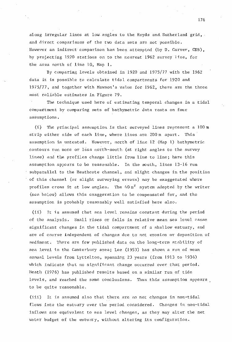
176
along irregular lines at low angles to the Royds and Sutherland grid,
and direct comparisons of the two data sets are not possible.
However an indirect comparison has been attempted (by D. Carver, CDB),
by projecting 1920 stations on to the nearest 1962 survey line, for
the area north of line 10, Map 1.
By comparing levels obtained in 1920 and 1975/77 with the 1962
data it is possible to calculate tidal compartments for 1920 and
1975/77, and together with Mawson's value for 1962, there are the three
most reliable estimates in Figure 79.
The technique used here of estimating temporal changes in a tidal
compartment by comparing sets of bathymetric data rests on four
assumptions.
(i) The principal assumption is that surveyed lines represent a 100m
strip either side of each line, where lines are 200 m apart. This
assumption is untested. However, north of line 12 (Map 1) bathymetric
contours run more or less north-south (at right angles to the survey
lines) and the profiles change little from line to line; here this
assumption appears to be reasonable. In the south, lines 13-16 run
subparallel to the Heathcote channel, and slight changes in the position
of this channel (or slight surveying errors) may be exaggerated where
profiles cross it at low angles. The 40 m2 em adopted by the writer
(see below) allows this exaggeration to be compensated for, and the
assumption is probably reasonably well satisfied here also.
(ii) It is assumed that sea level remains constant during the period
of the analysis. Small rises or falls in relative mean sea level cause
significant changes in the tidal compartment of a shallow estuary, and
are of course independent of changes due to net erosion or deposition of
sediment. There are few published data on the long-term stability of
sea level in the Canterbury area; Lee (1953) has shown a run of mean
annual levels from Lyttelton, spanning 23 years (from 1913 to 1936)
which indicate that no significant change occurred over that period.
Heath (1976) has published results based on a similar run of tide
levels, and reached the same conclusions. TIluS this assumption appears
to be quite reasonable.
(iii) It is assumed also that there are no net changes in non-tidal
flows into the estuary over the period considered. Changes in non-tidal
inflows are equivalent to sea level changes, as they may alter the net
water budget of the estuary, without altering its configuration.

177
Although some data on non-tidal flows into the estuary are available,
no attempts have been made to estimate long-term net changes (Scott,
1963; Mawson, 1972). An assessment of the contribution that changes
in non-tidal flows may have made to the post-European budget of the ARE
is provided by historic data on inflows from the CDB sewage treatment
plant (from Scott, 1963; Knox and Kilner, 1973). In 1929, 8 x 10 6
gallons/day of treated effluent was discharged (about 0.3% of the tidal
compartment, then about 8.8 x10 6 m3 ), by 1975 this had increased to
30 x 10 6 gallons/day (or about 0.8% of the 1975 tidal compartment).
Changes of this magnitude are probably not significant, and this third
assumption appears to be reasonable.
(iv) Finally it is also assumed that no errors in surveying enter
the calculations. The possibility that benchmarks may have moved
between the 1962 and 1975/77 surveys, introducing widespread constant
errors, appears to be slight (J.A. Robb, pers. comm., 1977).
3. Methods used to calculate volumetric changes. Data from
the three most reliable surveys were plotted with large vertical
exaggeration, the resulting bathymetric profiles (Appendix 2) were
subdivided into 40 m sections. The vertical differences between the
1920, 1962 ~~~ 1975/77 prGfilc3 ~crc ~c~su~~d at the illirlpuiut cf each
40 m section. Volumetric changes were calculated by multiplying these
vertical differences by 40 2 - the resulting values effectively represent
net changes in a series of 40 m2 cells along each profile. To calculate
net losses and gains for the whole estuary, the proportions of cells
showing positive, negative or no change were calculated for each survey
line, and a strip 100 m wide on either side of each line was subdivided
into similar proportions of positive, negative and no change cells, by
interpolating blocks of similar cells from line to line (Maps 3 and 4).
The values for each 200 m strip were then summed to arrive at the final
figures shot-1n in Maps 3 and 4.
4. Results. If the four assumptions are valid, the volumetric
changes shown in Maps 3 and 4 are equivalent to changes in the tidal
compartment of the ARE. The total figure shown in Map 3, subtracted
from the 1962 compartment (Mawson, 1972) gives a 1920 volume of
8.78 X 10⁶ mS. This represents a mean annual rate of increase of
7 x 10 Q mS for the 42 year period 1920-62. There is a difference of
0.6 x 10 6 mS between this value and the pred icted value for 1920

.ap 3. S.diment 'buqet, 1920 to 1962. L1us 2 to 10 oDl,y'.
$I! Are .. ot •• dt.ent acoUlllllaUOIl ~ 1, 2
A~.. ot s.diment accumulation - a subtidal channel.'infill.d betwe.n 1920 aDd 1962 3. 4
'W(d..~ ~......,.;,.,;;l.t':f A~a8 ot •• diment .resieD-- raprasent1rl.g erosion
ot high-water salt marsh, causir~ losse. ot 800m to 1050lIl ot s.diment (verticall;r J a a narrow strip alone the lIW shon ot the .stua17.
Unmarked squa~d are.. - sediment .rosion Blank (unsquarad) ara .. - subtidal. chB!lJ'lels
Intertidal volumes ot s.diment accumulation 1 52 664a3
2 75 2lu3
l Ei7 200II3
4 14 84Qa3
Total 209 920m3
Int.rtidal. volumes ot sediment .rosion 1 113 )2la3
N.tt loss trom the atertidal. zone
Subtidal volum.s - .rosion d.position
N.tt loss trom the subtidal zone
OVerall nett los. (Between lines 2 and 10 onl7)
903 401m3
16) 410m3
55 047.3
108 363m3
1 011 764m3
Predicted overall loss, based on the assumption that the area trolD lines 2 to 10 is representative ot the whole estuar.y, and consists of 5~ ot the whol ••••
2 023 528m3
QI IIII1
c::>~~ I I
" ,Q,...111111 IIIIII1111111 II 1II1I
Grid is arbitrarily located and a~~d ,np~~.~tA. aDd covers the same area - at the sam, ,ca1e - ..... p 1. Open arrows show ends of surveyed ba~metric·protil ••• pmall solid arl'OWS and as"ociat.d th1c1ce~ black la •• phow locations and low tide drainage directions ot inb_ tidal channels. See profiles in Appendix 2 tor vertical amounts of erosion and d.position along individual protiles.
¢:::J
I I I I I I I I I I I I ! t J t I I I I I I I r I ,¢:::J , ""IIIIIFI,,<::::J
IIIIII Till r'1¢::!

.a, 4. S.diment bud •• t, 1962 to 1975/17.
Art.. of •• dia.nt accumulation 1, 2, 3, •• J 8
UJUIIlZ'Qd 'qv.a,red area, - ,ediment ero,ion Blank (UNIqv.a'red) are .. - INbt14al ch_1a
IDtartidal volum., - ,ediment accumulation Area 1 6612m)
2 17 400113
3 41 270.3
4 99 680.) , 28 2)6.) 6 21 79,J.) 7 6 iJ4a3
8 1706.3
,lue ,catt.red minor accumulation 5 179m3
total 228 010.3
Intertidal volum. - aed1ment"eroaion 286178m)
.aU loa, - intertidal zone
Subtidal volume, - .rosion - deposit1on
.ett 1088 - subtidal zone
oY.rall nett 10as
)28 040.3
215 872m3
112 168~)
170 336m3
~IIIII <:=J
QI I I I I I I I I
~IIIIIIIIIII
, I , I , I I I I I I I I ,<:=J
I t-=t I I I I I I I 1" I I <:=J
"I" f"1 II¢::!

(Figure 79), tY'hich is approximately equivalent to the mean annual
change for the 42 year period.
178
Similarly, addition of the net result of the calculations
summarised in Map t .. to Mawson's 1962 volume gives a 1975/77 value of
10.93 x 10 6 m ; indicating a mean annual increase in the tidal
compartment from 1962 to 1977 of about 9 x 10 3 m3• For the 55 year
period 1920-1975/77, the mean annual increase in the tidal compartment
of the ARE was 18.5 x 10 3 m3, or 0.34%.
CDB engineers have calculated a net loss of 1.08 x 10⁶ m3 for
the area between lines 2 and 10 (Map 3) for the period 1920-1962
(J.A. Robb, pers. comm.). This is about 6% more than the writer's
calculation of 1.01 x 10⁶ m3• The CDB method was based on a computer
technique which integrated the vertical differences between the 1920
and 1962 surveys, and calculated a net change on the unqualified
assumption that each line was representative of the 100m strip either
side of it.
Although the CDB method is more precise than the writer's, it
is likely to be less accurate, since it fails to account for the
exaggerations caused when survey lines cross steep-sided subtidal
channels at loYl angles (see profiles 14 and 15 in Appendix 2).

2
3
4
5
A:P'P ... ndix 2. Bathymorphic 'Profiles aurvE'~ed in 1920, 1962, Ilnd 1975/77. Annotutioll!.1 ",how \,rofile numbers (2 to 15), profilp oriBina ( W) and l?rofile pnds ( E ). Arrows show profilE's complpted on a following -page ( ~~). or continuod froma previous page ( ~). Crosses are at 9.6m IMD, and arE' spaced 100m apart. Vertical scale ~8 indicated along the right margin, in metres-HAD.
E
-+-
E
+100 -+-
75 62
E
-+-
E
75
-+- + 100+ -+-
179
10
9
8
7
9
8
7 10
9
8
7
9
8
7

180
6
-I-
7
-I- 9
8
7
8
\---------------------------~--~-------------------------~7 9 W
-I-

181
E
-+ -+ -+ 9
s
7
10
-+ -+ -+ -+ -+
8
8
7
w
7

182
E
-I- 9
8
~-----------1/·--------------------------------------------------------~.7
12
62 -I- -I- -I- -I-
w
8
~----------------------------------------------------------------------i7
-I- -9
62
-8
7

183
13 W
+- +- +- +- 9
8
~-------------------------------------------------------------------17
E
+- +- +- +- +- 9
8

14
10
+ + + + + + + + + + ~ 9
75
8
++++++ 9
8
I ~\J~7
-t- + + 9
8
184

185
8
62
. . 15
7

186
APPENDIX 3
Surface and subsurface sediment analyses, Methods and procedures.
1. SampZing design. A problem often experienced in exploratory
field studies is the difficulty of estimat an optimum sampling
design - one which yields maximum information for minimum effort.
Since trends in sediment properties in the ARE were originally unknown,
an extensive and dense sample collection was attempted.
A separate problem involves the statistical validity of sampling
plans. In this study no attempt has been made to randomise the sampling
design, for two reasons:
(i) The number of random samples needed to adequately represent all
bathymetric subenvironments would have been prohibitively large, and
the sampling design would have been unwieldy.
(ii) The CDB survey network ,vas partly completed, and marked at
convenient intervals with semi-permanent markers. before sampling began.
The benefits of using these fixed sites, which could be resampled or
revisited for other purposes, outweighed the theoretical benefits of a
random design (Cockran and others, 1954). Unwitt bias was eliminated
as much as possible by sampling only at peg locations, or at multiples
of 20 m between pegs.
2. SampZing methods. If substrate properties are to be used as
environmental monitors, then sample collection techniques are critically
important. That no amount of analytical effort will extract meaningful
results from meaningless samples is a truism apparently ignored by many
recent workers (Macpherson and Lewis, in prep., 1978).
Early observations indicated that the upper few centimetres of
sediment on the intertidal flats of the ARE was highly variable -
sometimes massive, sometimes stratified - and almost always inhabited
by a variety of benthic animals. Recognition of widespread erosion also
lead to the possibility that surface sediment properties might be
inherited from older sediment. and not be related to modern processes.
Methods which ignored the potentially complex and polygenetic nature of
this sediment would be unlikely to provide environmentally meaningful
information - worse, they might be seriously misleading.

187
The sampling problem~~as tackled by assuming that there was an
uppermost layer of sediment, perhaps a few grain diameters to a few
centimetres thick, which was available to be modified by contemporary
processes, and which owed its characteristics to those processes - in
other words, that there might be an uppermost layer with the properties
of a sedimentation unit (Otto, 1938; Jopling, 1964). This assumption
is examined and justified in Part Five.
This uppermost layer, appropriately termed the active layer -
was sampled with a soft flexible spatula (various plastic kitchen tools
are suitable) by carefully scraping off the soft, unconsolidated surface
sediment at each site. This method was used consistently throughout.
Usually a sample of about 10 x 10 cm x 1-2 mm was collected, and stored in
a plastic bag until analysed in the laboratory.
Samples stored in plastic bags were usually analysed within
48 hours of arriving in the laboratory. About 30 g - 50 g of each sample
was wet sieved through +0 .5 phi (0.7 mm) and -4.0 phi (0.0625 mm)
screens, and the fraction coarser than +0.5 phi (living animals, whole
shells, coarse shelly and other organic debris) was discarded.
All material passing through the 4.0 phi sieve was collected,
made up to lL, stirred vigorously, and a 20 mt aliquot was taken
immediat: and pipet: t:ed int:o a preweigned 50 mi beaker. Aft:er oven
drying and cooling to room temperature, this weight of material (x 50)
~vas accepted as the weight of mud in the original sample. Included in
this figure was any salt or other dissolved solids in the sample, as
well as organic material, dissolved organic material, and so on.
The sand fraction (all the material caught on the 4.0 phi sieve)
was washed into preweighed 200 mt beakers, oven dried at 35-450
C,
allowed to cool to room temperature and weighed. Sand and mud weights
were combined to produce a total sediment weight, and per cent mud was
calculated.
The dry sand was thoroughly mixed, and about 2 g extracted with a
small spoon and poured into a screw-top plastic container, to make up a
subs ample with a weight of 2.0 ± 0.1 g.
subsequent RSA analysis.
This subsample was used for
lhe RSA used for this project has a perspex settling tube with
a fall distance of 1 m, and an internal diameter of 12.7 em (5 inches).
Recorder output consisted of a cumulative differential pressure
vs time curve, traced on to squared paper as the sand grains set
a transducer port, 1 m below the top of the tube.

188
From the instrument curve, elapsed times corresponding to the
95th, 84th, 75th, 50th, 25th, 16th and 5th percentiles were read off
(the input percentiles for Folk and Ward graphic statistics),
recalculated as settling velocities, and converted to sedimentation
diameters using the data of Gibbs and others (1971).
Finally the percentile data were coded on to punched cards,
and graphic statistics were calculated by the University of Canterbury
Burroughs B6700 computer.
3. sand vs MUd. The widely held belief that the best sediment
samples are those collected from single, homogeneous sedimentation units
is well supported by theoretical and experimental evidence (Otto, 1938;
Apfel, 1938; Griffiths, 1962; Erlich, 1964; Jopling, 1964). Samples
which amalgamate more than one such unit may contain material deposited
under different physical conditions, and yield results not amenable to
sensible interpretation. Yet it is still apparently common to assume
that useful data can be obtained from sediment size analyses which
amalgamate results of separate mud and sand size analyses - in spite of
the common awareness that sand and mud are transported and deposited in
different ways, and according DO different physical laws.
The principal reason for considering the sand and mud frac.tions
of a sediment as separate sedimentation units is the common observation
that fine particles are almost always aggregated into larger, composite
particles in nature (Kranck, 1975; Drake, 1975). Aggregate grains do
not fulfil the requirements of Stokes' Law - the theoretical basis of
most laboratory procedures for the size analysis of fine sediment -
because they are frequently not rigid, smooth, spherical, or inelastic
(Galehouse, 1971). On deposition individual aggregates will probably
lose their identity; ~oJhen sampled and subjected to normal laboratory
procedures they almost certainly will (Kranck, 1975). And finally - as
Folk (1968) has pointed out - measurements of size distributions of fine
sediment may only be an indication of the efficiency of a particular
dispersal technique.
In the present project 'size' analyses of surface mud were not
attempted - only the total amount of mud (as defined above) was
routinely determined.
4. Sand fraction anaZyses by sedimentation. Two methods are
available for the size analyses of sandy sediment; sieving, and

189
sedimentation. Sieving separates grains according to their least
cross-sectional area (Galehouse, 1971), however the behaviour of sand,
grains in water is a function of their volume, density, roundness and
spericity. Sedimentation analyses are the only 3izing techniques which
take all four of these factors into account. Considering the
intentions of the present study, a sedimentation method was chosen, and
a Woods Hole-type Rapid Sediment Analyser (RSA) manufactured by Pelagic
Instruments Inc., and owned by the Department of Geography, University
of Canterbury, was used for all routine size analyses.
The particular advantages of an RSA as an analytical tool are
that it is rapid, seldom requiring more than 10 minutes/sample, it is
precise and accurate - replicates exhibit high reproduceability; and
it provides a continuous record of size distributions, allowing fine
subdivisions. Disadvantages include difficulties associated with
converting settling velocities to equivalent diameters, comparing
settling and sieved analyses, the under-representation of the tails of
size distributions by sedimentation methods, and technical problems
involving the introduction of srunplesinto the water column. For
examples see Emery (1938), Doeglas (1946), Poole (1957), Zeigler and
others (1960), Schlee (1966), Bascomb (1968), Felix (1969), Nelson
(1976) and Channon (19 ). Emery (1938), Schlee (1966), Sengupta and
Veenstra (1968), Sandford and Swift (1971) and Reed and others (1975)
have compared sieving and settling techniques using a variety of
settling devices. Reed and others in particular found systematic and
sometimes spectacular differences in grain size distributions derived
from the two different methods. They attributed these to " ..• subtle
variations in sorting with grain size, the result of an interplay
between mineralogic composition and size ... ".
In the present study a small number of samples were both sieved
and analysed with the RSA, and representative cumulative curves are
sho,\Ill in Figure 80. Here it can be seen that the two methods do give
quite different results. In Figure 81, equivalent properties are
plotted against one another, and the results mean that sieving will
indicate sediment from the AHE is finer, better sorted if well sorted,
poorer sorted if poorly sorted, more negatively skewed, and more
leptokurtic than RSA analysis would indicate. Notice also that it is
at the fine end of the curves (near 95%) that most differences occur.
There are three approaches to the problem of converting settling
velocities to equivalent diameters. The first is 'to estabish an

190
f-- -q-,.... 0
«
~ if) cc: 'in
~ a.
I !--- (') I-
0)
-~ I"-(j)
.
_NI.- I I
I I I
~~ 0-- -(')-
~, -0-.... --
~ ---
I--- -q-,...
<U >
f--- ,!!! (/)
i--- (') ~-~ =E - ---
I ---,.--- N I-
~ l"-e ~
I 1 ' - .~ '" a.
l-I
e to
CW;llll'.cti'll' l'ercpnt
I"ie,uro 80. Comparioon of cumulative probability curve::1 of snnd fractiono of oampleo from tho Avon-Heathcot<:l Estuary. O.;'5phi data pointo .from oievo analyses, emaIl circles are from HiiA !lnul.)1 $ e 8.
I
to ....
four ropr<:lsontativa l,argo circlos are
a.lpsi data'points
I-
I-
1-
- (\1'&-
-I-
(j)
- ~-
-I
-
I-• 1-
- (\I'~ -
----
--I-

RSA
4
3
2 •
2
+
'4 Ski
• , -2 -., 0
.~~ I
- ·4 ·2 0
5 percentile
3
2 A&G V
Q
2
0
·3
·2
3 4 ·2 ·3
KG
.e • 1-2
~ ! I -2 -4 + 0'6
4 95 percentile
3
Sieve
F'igure 81. 0catter plots of sieve va RSA aize analyses.
«)
" •
·4
e
~
0·8 1-0
• •
·5
••
1·2
4
·6
"
191
/ ./

192
apparatus-specific relationship by calibrating an instrument against
particles of known sizes (Gibbs and others, 1971; Nelson, 1976).
The second approach is to convert measured fall velocities to
equivalent diameters using standard relationships. Gibbs and others
(1971) have published a standard settling velocity equation, derived
from exhaustive experimental work, and tables of data from Gibbs and
others were used in the present project to construct a standard
calibration curve relating fall velocity to sedimentation diameter.
Sedimentation diameter is defined as the diameter of a glass sphere
having the same settling velocity as a natural particle. The standard
curve used in the present project is filed with other supplementary
material in the Department of Geology library.
A third approach is simply to express results as fall
velocities. This idea is intuitively attractive, but suffers from
the major disadvantage that geologists are accustomed to describing
sediments in terms of grain size, not cm/second.
5. Reproducibility and reliability. The reproduceability
of the analytical method for sediment muddiness was checked by taking
24 x 20 m2 aliquots from a 1L cylinder and treating each as a normal
21.13% and a standard deviation of 0.16%. This indicates that
differences greater than 0.64% mud (± 2 standard deviations) have
a probability of at least 95% of not being due to experimental error.
Although other workers have claimed that settling tubes
are capable of giving results of reasonably high reliability,
for example Schlee and others (1965), a simple reproduceability test
was completed to ensure that the instrument used in the present study
was behaving adequately. The sand fraction of sample 539 was split
into 31 x 2.0± 0.1 g subsamples, and these were run in sequence
through the RSA. Figure 82 shows means and standard deviations
calculated for percentile input data, and graphic statistics calculated
from analyses of each of the 31 subsamples. The variability in the data
of Figure 82 is an indication of the amount of experimental error likely
to be introduced in the laboratory in the present study. Within the
input data, extreme values (psi 5 and psi 95) have highest variability
(largest standard deviations); within the graphic statistics sorting is
least variable, kurtosis is most variable.

5)? 1 F I.8t 2.U
$)' 2 J '.11 2.28
5U ) R .~,. 2.)1
539 I. S 1.71 :Z.)O
5l?5-Tl,91 1.21
51? 6 1 ,,~.~ 2.21
5)9 7 C 1571 2a25
$)9 8 I,) 1.69 2.2'
5]9 !l l 1~10 2.2"
5H lOU t ~61 2.2S
53? 1H1 1.16 2.27
53!> 1211 •• 61 2.:lI.
53?!) '.66 2~21t
539 14P 1.66 2.22
5H '5'S 1 5 72 2.25
S)~ 161 '551 2.2)
51' 11 1.$1 2.21
5)9 180 1.611 2.28
53? J'311 t.6i, 2.2)
SH 20C t .. 12 2~Z6
S~!:J 21 '~12 2.?1l
SH 22 I.U 2.26
.539 2l t.!'Q 2.2:6·
539 24 t.SS 2,26
5::1 2S 1.10 2.U
53,?6 t.S2 2.21
5H 27 '_12 2.,,11
5J'J 2il 1.60 2.tS
531 29 1.66 2.25
5)90){l 1.61 2.21
~l'l II t.11 2.21,
HI
? o ....., 'd IJ> .... .
O.2A
O.U·
0.27
0~28
0.21
0.21
0,23
0,)2
0.29
0.21
0.1)
0.31
0.16
0.2?
0.27
(/j
n o . o
,I\)
'd (0
I"" .
HI
o . o \J1 .
HI
I-' . o ....., ~
o . o 0\
t.:U 2.06 2.12 2.2' 2.5t 2.U 2~OO
1.91 1.01 2.07 2,2" 2.'*6 2.5!.! 2.74
1.86 1.01 :Z.iO 1.2? 2.50 2.62 1.11,)
1.:'11 2.01 2.11 2.27 2.50 2.$1 2.80
t.,) 2.0" 2 .. 11 2.21 2.41t 1~51 2.10
lAfl:6 2.0) 2.0, 1.U t.toJ 2.55 ~.1-"
I.M I.?' 2.0' 1.12 l.ltl 2.5" 20.1'
•• 87 1.0) 2.0, 2.i6 Z.~6 2.59 2.71
1.134 2.00 2.06 2.U 2,40 I.'" 2.61
1.81 2.03 2.IQ 2~21 ~.46 1.S5 2.12
1.81 2.0) 2.10 2.26 1.'+) 1.$2 1.'9
t.i;U t.~l 2,015 l~U 2,40 1.51 2.7"
!.Sll '.91 2.0) 2.11 2.'" 2.5ft 2.7\
1.77 t.'" 2.0J l.20 2.H 1.51 2.11
1.86 1.,7 2.0$ 2.'2 1.4J 2.S6 2.1tt
1.77 1~96 2~04 2.19 2,40 2tS) 2.1'*
' .. 71 1,9~ 2 6 0 .. 2.Ia 2.)8 2.to9 2.10
I,SS 2.01 2.07 2.26 2.43 2,58 2.18
,.32 1.:18 Z.05 2.22 2 .. 42 2.49 2.76
I.Sl 2.00 2.01 2.ll 2 .. 42 1.SS 2.15
1.Jll 2.01 2.09 2,210 2.ltlt 2.S? 2.76
t.n 1.94 2'.07 2,:'5 2~46 2.se 2.9ft
,.01 1.99 2,01 2.2ft 1,45 2.55 2.71
'~81 2.00 2.01 2.24 2;44 l.SS 1.11
1.95 :?Ot) 2,01 2.23 21lS 2.',5 2'#6.
1.11 1.92 L,01 2.,e 2.'d 2.5) ~.16
1.81 2.01 2 .. 10 2.26 2.42 2.55 2.11
1,1!) 1.')7 2.062.21 2.11:2 z.5\ 2.7"
t.a4 2.00 2.0'; 2.ll 2.41 2~5) .1:.76
I.S(I 1~90 1~05 ::.l~ 1.3!l 2.t..0 2.61
1.85 I.$I~ 2~05 1~11 Z.41t Z.5) 1.7'
~I
I-' . (» ..,. '.II
II
? o \J1
", . o ~
<l) .... '" \J1 ~
or' '" .... \J1 o
MI
o . o ./>.
XI
o . o ./>.
~I
'])
o . o \J1
Figure 82. Replication exercise. Rosults of analyses of 31 subsam~lea of 539.
193

194
These results mean that differences in mean diameter greater
than 0.12 psi (± 2 s) have a probability of at least 95% of not being
due to experimental error. For sorting the figure is 0.08 psi, for
skewness it is 0.20, and for kurtosis 0.24. These results are v]ithin
the limits accepted as reasonable in experimental analyses of sediment
(Folk, 1955; Rogers, 1965).
It is also instructive to examine the nature of variability at
the sample site. Since exact replication of samples is not possible,
the next best option is to collect a number of closely spaced samples,
and test them for variability. This was done at the east end of line 9
(Hap 1), where 25 samples were collected, beginning at a peg of 9.70 m
HAD and progressing west. Samples were 1 m x 5 cm x 1-2 nUll in size, so
that a 25 m strip of the estuary bot tom was continuously sampled
(samples 688-712). Results are shown in Figures 83 and 84.
Figure 84 is a stack of histograms, where percentiles at 0.1 psi
intervals are plotted from sample midpoint to midpoint. For example
the top line in Figure 84 shows the percentage value of the 1.8 psi
percentile from each analysis. A surprising result is the uniformity
of the extreme values in the 25 samples, and the variability of midrange
values. From sample to sample the coarse tail in particular is
" ; rCillarkatly Li(lifuLUl (auuul. 1-2/~ ur :::;eu11UeUl. 1:::; l:uu:::;l:::;LeuLly l:var:::;ec Lllan
1. 8 psi). Compare this to the amount of material coarser than 2.40 psi,
which varies from about 40% to about 70%. Slight variations in skewness
(displacement of the mode from the mean) produce this pattern, and the
effect is exaggerated because these samples are so well sorted - there
is a particularly close grouping around central values.
Figure 84 also reveals that there may be two separate sand
populations present in the 25 m run, represented by samples 688-700 vs
701-713. This possibility provided an opportunity to test the levels of
significance established above. Mean values and standard deviations
for each sample group are shown in Figure 84B, where histograms of
sample graphic statistics also indicate the possible presence of the
two sand populations.
The difference between the two mean diameters is 0.07 psi, and
from above, this is clearly not significant. Similarly for sorting,
the difference is 0.04 psi, and this is not significant. Notice that
the variations in graphic values in Figure 84 are less than the
variations in Figure 82. In other words the variation along this 25m
run was less than the variation expected from experimental error, and a

~
0 (1)
(I) N
CO N
,... N
ID N
Il) N
." C\I
(1) N
N N
N 0 N
Ol ~
$!
,...
<0 ~
Il)
;!
(1)
N ~
:::
;?
Ol
ro
,...
ID
Il)
'<t
(1)
N
(J) (1)
Q III N
'"
~ .. +' ., & .,.. .,; III .,.. ~ III
0 ., ~ ::iii
NT", t L" ;t \II ~
\I)
'" ~ ~ ;;0 Nix N ~ <:> 1>< 0 IX .. - IX -..
Figure 8). Re~lication exerciee. sequential variations in mean diameter, gra~hio standard deviation (sorting), skewness and lrurtosis of 31 subsam~les of sample 539. run in the sequence 1-31. Data from Figure 33.
195
'" 6
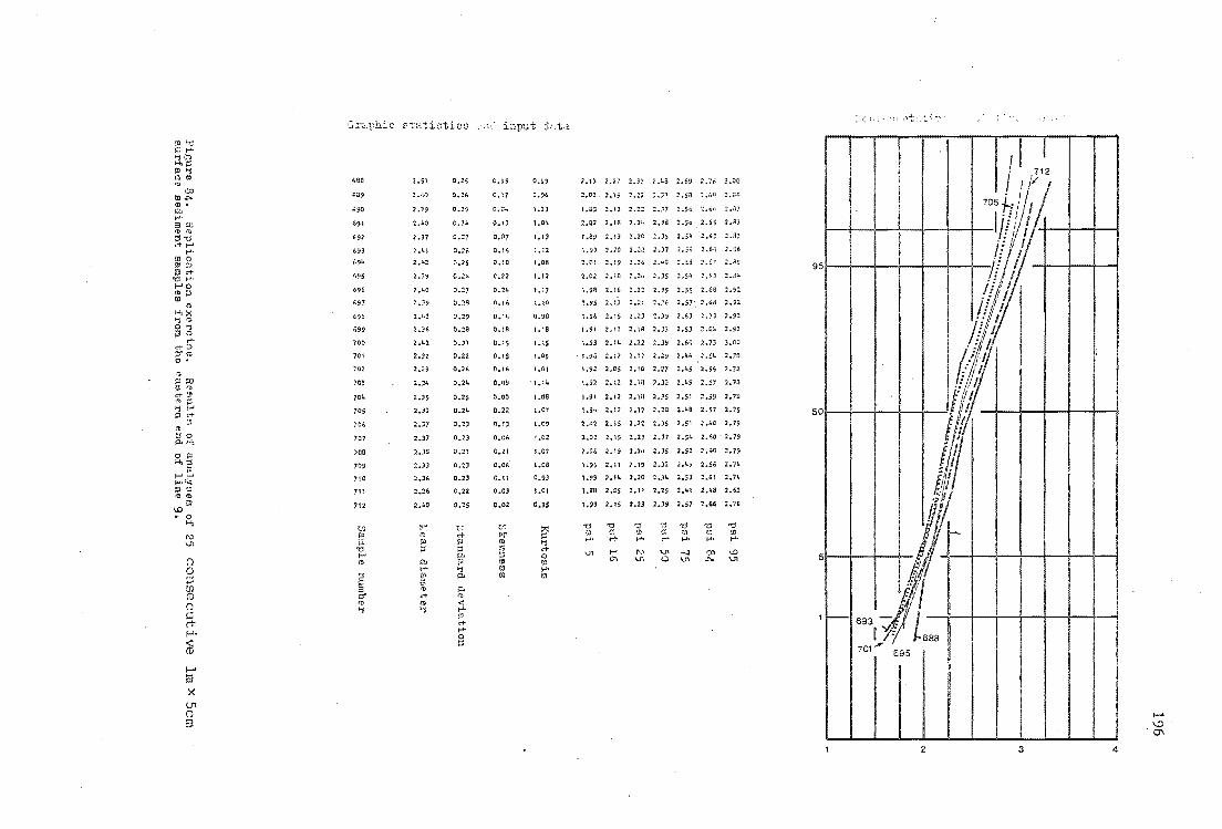
:ni-::J ~ .... 'i0'0 ,..,,: \l) 'i nO) '"
'" ""X 'i '" O'i 51 n .... <+tll ;:rm '" . '" l"::tJ W'1:> <i-'Jl .,,~
~~ 'Jl
'" ;Jo "",.., o III H,;l
III f-'f-' .... '< ::; '" "'<r>
!l) \!) • 0 ,..,
'" VI
(l o ::i til rD (l
8-f-J.
~
~ X (jl
o !J
Graphic stt'.tistics input cl:lt i
<as
'0' t.90
691
." b~)
69"
095
696
697
69'
699
700
701
702
10)
70k
705
70.
707
70n
70s
710
m 7\2
w jlJ ;:; 'd f-'
'" ~ cf
'" .,
2.51
z ~j.l)
2..-:9
2~40
2.37
7.,4}
2 .. 1_'1
2.39
" .. 4n 2 .. 39
2.1.2
:2 ~;6
2.t.2.
2:.)2
2.29
2.31.
2.:5-
2.32
2.37
l.37
2.38
'.ll 2 .. 34
2 .. 26
2,,40
r ." ~ ;J
"" ... ~ ." <t (!)
'i
O.2t;
0.21.
0 .. 29
0.210
0.27
0.2:;
-'.25
O.;H.
0.2:,-
0;211
O.::!9
C.16
0.)1
0.22
O .. U.
0.24
0.2$
0 .. 21 ..
0.23
0 .. 23
0 .. 21
c .23
O.l)
0.22
0.25
t: <i[' ;:s p. III 'i
"" "'" '" <: ... p <i.... o l:l
0.19
0.17
ri.e4
0 .. 13
0.07
0 .. \")
o. :0
C.22
0 .. 24
O.H.
O.,ll
0.18
0 .. 1 S
0.15
O.H'
O.O!i
0.00
0.22
0 .. 13
0 .. 0(,
0 .. 21
0 .. 0';
0 .. 11
0.0)
0.02
(0
~r
'" ~ '" CD
'"
0.99
0.96
L.23
1.01.
1.0
1.12
1.011
, .12
1 .. 17
1 .. 10
0.90
1.18
1 .. 15
1,,05
1.t'l1
'1.14
1 .. 08-
1 .. 07
1 .. 09
i.02
1.07
I ~oa
0 .. 93
1.0t
0.95
2 >-j d o !Jl ... '"
2.U 2.27 2 •. ;;1 ;1.43 2.H< 2.7'ci .:~vo
2.02. 2 .. 15 2.::!2 -:.:P L~a :'L,6~! Z:.E£
I.GS 2.1) 2.22 2.),7 2.55 ::.(,(, 2.t17
1 .. 02 2.1f1 2 .. 24 2.,36. 2.50 2:.65 2.83
1.8~ 2~13 2.20 1.35 2.$4 2.6; :!~A:
1.:;3 2.]0 2.~:; :'1,.)7 2.56 2.6<; 2.1::6
2.0! :!.19 2.26 L4C :.;'3 :'.6'1 :!.i15
2.02 ::.lR 2.2h ~.35 2.S4 2.6~ 2.d';'
1 .. !:If) 2.16 2.22 2.3$ 2.5S 1.613 2.:>2
l.!'5 l.U 2.:::1 Z.:?f: 2.57' ~.t<S 2.n
1.96 2 .. 15 2.:!] : • .39 2 .. 63 2.':1'3 2.92
1.91 L 12 2. HI 2.33 2.53 2.6:" 2.92
\ .. 93 2.14 2.22 2.3:,J 2.M 2 .. 73 3.00
t .. 96 ::.11 2.17 2.29 2./;& 2.$4 2.7;')
1.92 2.0$ 2.10 2.'n 2.45 2.5t;, 7.73
\.92 2 .. 12 2.111 '.32 2.49 2.57 2.73
1.9\ 2.12 2 .. '8 LJS 2.S1 2.59 2~7S
1.94 2 .. 12 2.17 2,,:W 2.48 2.57 2.7$
2.-02 2,.i$ 2.22 2 .. 35 2.51 2.60 2.79
2.02 2.15 2.23 2.)1 2.S4 2.~0 2.79
2.06 2 .. Hi 2.24 2.35 2.52 2.&1J 2.79
1.'> :: .. il 1.19 ';~J2 2 .. 4;;' 2.,SG 2.74
1.99 1,,1&' 2.20 2.31.. 2 .. 53 2.61 2 .. 74
1.SR 2"OS 2.11 2.25 2~I..l 2.43 2_62
1.99 2.15 2.23 2.3g 2 .. 57 2 .. 66 2 .. 78
'0 'd 1]) '7.l ........... Vl f-'
0\
":1 '1l ... to Ul
~ 'd m m ... .... '-, ...] o Ul
"" oj '.Jl !Jl 1--1" t--I •
0> \.0 .".. U1
'~I "t ~~ "
I Ii! ..,..I--+-~
,,' I I , I I I I I
501 I I I
51-I -f-I:---+-
I-- 693 _,'I.' I ;: ., I
701 695
688
2 3 4
..... \.0 C)"\

197 A
1-6
Hl 2-0
2·1
2·2
2':) --2·4
~~// 2·5
/'-....'-.... /'/ /'V --2-1,
_//-_/~~--/ 2-7
2·8
2·9
~ 3·2
3'2 3-3
B
-20
-25r-------i--t-----r~--+_------------~-+--+=~~==~--------
-30
·35
701-712 ~ - 2.34, 6 = 0.04
701.-712 x:; 0.23. 8
Figure 85. Replication exercise. Sequential variation in granulometric properties of 25 con~ecutivo 1m x 5cm surface sediment samples. Data from Figure 35. A _ Sequential changes in cumUlative perecentagea of O.lpai intervals, from 1.8pai to 3.}psi. B - Sequential changes in graphic statistics.
0
- 10
25
" ~ ~ .:: ..... I' <+ 1511 ..... <: .,
'1\ +: (') ,~
;S <+
75
90
100
2-0

normal 10 em x 10 em sample from anywhere along the run would have
adequately represented it.
198

Graphic log
199
App<'ndix 4. Detailed descriptive and graphio logs, subsurface sediment coroEl from th<, Avon-Heathcote Estuary. A - Graphic log layout. B - Sediment key. Individual logs follow on subsE'quE'nt pages.
Sampl", looation
Sample numl: '(' L.
5~ I: I I
~ I
,.'-
Medium Eland (Mz " 2.0 pa1)
Coarser fin& aand (lUz -2.0-2.5 pai)
Finer fine sand (Mz 2.5-3.0 (Psl)
Very fine sand (iYlz < 3.0 pei)
Sandy mud (:> 50';' mud)
Bioturbate sediment (mottled texture)
clive plastic mud and sandy mud
Regularly, sparaely laminatoa sand and sandy mud.
strongly laminated sand and s:o.ndy mud
/ I I
'" I SaDd fraction graphic t-Il.i;;tl.u-ia.l.·u llt;'viai..lou
Moderately lar.linated sand and sanely m,," Tln...- ....... hal nVJ
~;rf;':c~ (cm) -
I :Jand fraction mE'an grain size
Percent mud
/ /
/ /
'fieakl,Y laminated sano and muddy sand
BrO\'m organic hash
Disarticulated bivalves
ArticulatE'd and living bivalves
Mud blebs comprise l-l0,~ of sediment
I/ood fragme.nt
Dored contact, burrol'ls stuffed with overlying sediment
Allgular or irregular bedt. iog surface

CORE 2 651 I
om I __ ~_~~~ r=H
652 I J
[l 679
10
lJ 678
~ ~
677 I I
20 I 676 ~ I
675
30
11 I -I Percent ·mud 0 10 20 30 40 50 60 70
~and fraction oeun oiza 2·0 2<2 2'4 2·6 2'8 3·0 3'2 3'4
3a.~d. fraction sorting ()'2 Q.3 0·4 0·5
CORE 4 645 I
om t- ---.=PI,
10
2011
30
PerCf.'nt mud Sand Iraotion Dean size
Sand fraotion Borting
j
11 0
2'0
646
674
673
672
671
10
2·2
()'2
I L, I I
I tD
20 30 40 50 60 70
2'4 2·6 2'8 3·0 3'2 3'4
0'3 0'4 0·5
200
CORE
om
20.
670
669
30
11 0 10 20 30 40 50 60 70
2-0 2·2 2'4 2-6 2'8 3·0 3'2 3'4
()'2 Q.3 0·4 0·5
Text follows ~
CORE 6 641
om 1-~42-~n
668
10
20
667
11 I - I 0 10 20 30 40 50 60 70
2·0 2·2 2'4 2·6 2'8 3·0 3'2 3'4
()'2 0·3 0·4 0·5

CORE 7 639
cm
10
20
. ~. 640 I 1 _____ _
663
1 I I I
I !---l-I ~! ---,J---I--l Percent mud 0 10 20 30 40 50 60 70
Sa~d fraction oean size
;'.;ar;d fraction SOr1;illi~
CORE 8
2-0 2-2 2·4 2-6 2-8 3-0 3-2 3-4
1>2 0·3 0·4 0·5
637
cm III~-10
'20
30
662
661
660 I I
65. -=r--L.!_----I
II L-......L.. ---L--.l-.-L-~ Percent mud 0 10 20 30 40 50 60 70
Sand fraction mean size 2·0 2'2 2'4 2·6 2·8 3·0 3'2 3'4
SaI1.d fraction sorting 1>2 0'3 0·4 0'5
cm
10
'20
em
10
'20
30
40
201
CORE 9· .mp;-m635
CORE 10
655
656
657
658
713
714.
715
716
--, I I ,
r I I
Text follows t
718
11L.........-...!~-.I.---..!1 o 10 20 30 40 50 60 70
2.0 2-2 2'4 2-6 2·8 .3·0 3'2 3'4
1>2 0·3 0·4 0·5
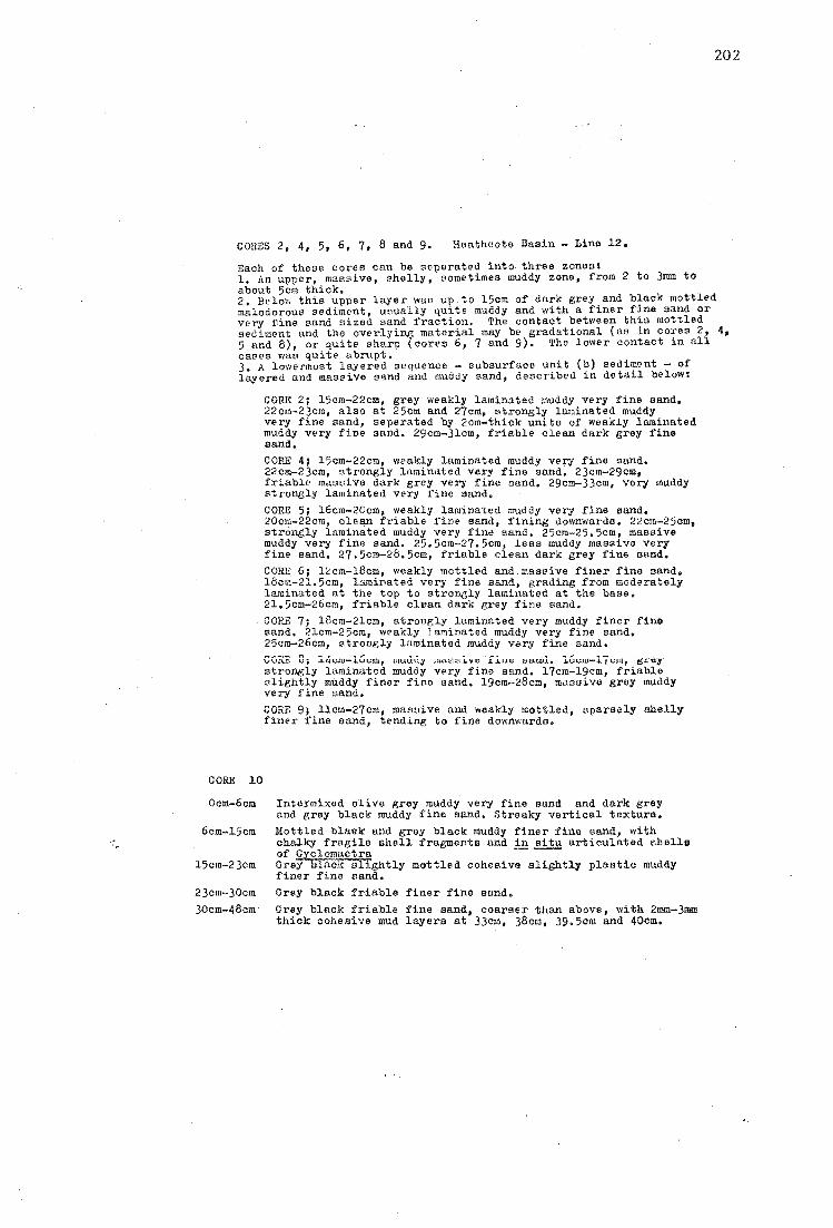
202
CORES 2, 4, 5. 6, 7. 8 and 9. Heathcote Basin - Line 12.
Each of these cores can be separated into three zones; 1. An upper, massive, shelly, sometimes muddy zone, from 2 to 3mm to about 50m thiok. 2. Below this upper layer was up to 15cm of dark grey. and b~aok mottled malodorous sediment, usually quite muddy and wl.th a fl.ner f~ne sand or very :t1ine sand sized sand fraotion. The contaot between thl.s mottled sediment and the overlyi~ material may be g.radational (as in co:es 2, 4, 5 and 8), or quite sharp (oores 6, 7 and 9). The lower contaot l.n all oases was quit., abrupt. 3. A lowermost layered sequence - subsurfaco u~it (?) sedi'!lent - 0: layered and massive sand and muddy sand, descr'l.bed l.n datal.l below.
CORE 10
Ocm-6om
6om-150m
15cm-23cm
23cm-30cm 30cm-48om
CORE 2; 15cm-22om, grey weakly laminated muddy very fine oand. 22om-23cm, also at 25cm and 270m, strongly laminated muddy very fine aand, seperated by 20m-thick units of weakly laminated muddy very fine sand. 29cm-31om, friable olean dark grey fine sand •. CORE 4; 150m-22cm, weakly laminated muddy ve.ry fine sand. 22cm-23cm, strongly laminated very fine sand. 23cm-29cm, friable massive dark grey very fine sand. 29cm-33cm, very muddy stronely laminated very fine sand, CORE 5; 16om-20cm, weakly laminated muddy very fine sand. 20cm-22om, cle~ friable fine sand, fini!~ downwardo. 22cm-250m. strongly laminated muddy very fine sand. 250m-25.5cm, massive muddy very fine sand. 25. 50m-27. 50m, less muddy massive very fine sand. 27. 5cm-2B. 50m, friable clean dark grey fine oand. CORE 6; 1~cm-1Bom, weakly mottled andmas~ive finer fino sand, IBom-21.5cm, 1umirlated very fine aand, grading from moderately laminated at the top to strongly laminated at the baae. 21.5cm-26cm, friable clran dark grey fina sand. CORE 7; 18cm-21cm, strongly laminated very muddy finer fine sand. 21om-25cm, weakly ) aminated muddy very fine sand. 250m-260m, fltrong~y laminated muddy ve,ry fine sand. "" ... -.~ n ......, ..... .,.... , .. "O, ..... vv.t\...C.· U; .L l !t.J-tU-.1.U\,;J..U, UH.4UU.,Y UId.!;lt;jJ.,Vt: LJ.l,lt: t;t:t.JJ.U. J..UUJ.U-.1.fC1U, f:5,J.'ul strongly laminated muddy very fine sand. 17om-19cm, friable slightly muddy finer fins sand. 190m-2Bcm, massive grey muddy very fine sand. CORE 9, 110m-270m, massive and weakly mottled, sparsely shelly finer fine sand, tending to fine downwards.
Intermixed olive grey muddy very fine sand and dark grey and grey black muddy fino aand. Streaky vertical texture. Mottled blank and grey black muddy finer fine sand, with chalky fragile shell. fragments and in situ articulated she11a of ClETomactra -- ----Grey aOlrBITghtly mottled cohesive s~ightJ.y plastic muddy finer fine sand. Grey bl.flCk friable finer fine sand. Grey blaole friable fine sand, ooarser than above, with 2mm-3mm thick oohesive mud layers at 33cm, 38cm, 39.5cm and 40cm.

CORE 11
om
50
60
70
719
80
7<::'0
90
721
100
722
110
I~ Fercent mud 0 10 20
Sa::1d =raction mean size 2-0 2-2 2-4
~ar.d fraction sorting ()'2
I 30 40 50
2-6 2-8 3-0
0·3 0-4
I I I I I I
~
I I I J r I f ,.----....
I
I J I I I I I
60
3-2
70
3-4
0·5
CORE 12
em
10
20
30
40
723
724
725
to 202
20
2'4
I 30
2-6
203
I I I I I I I I I I I
~ I I I I I I I I I 1 I I , , I I
40 50 60 70
2'8 3·0 3-2 3-4
50 ()'2 0·3 0·4 0-5
CORE 12 + ~imi1ar to oore 11, sandier at the top, othE'rYlise monotonous, malodorous olive grey mud.
.......... CORE 11
750m of sticky plastic m€'dium dark grey and olive grey mud. Slight fining upwards tr€'nd (from 3.18 to 3.10 psi me>an grain size over the interval sampled) and slight trend in colour, from dark grey at the base, to olive grey near the top.

204
CORE 13
cm 93~ud
726
I I
10 727 I I I I
: I I
20 I I I
728 I I I I
30 I I I I
I I I
40 729 I I I I
L I I I
Percent mud 0 10 20 30 40 50 60
Sand ~raction Dean siza 2-0 2·2 2'4 2-6 2'8 3·0 3-2
Sand fraction sorting 0-2 1).3 0·4
Ocm-?5cm rJalodorous
7.5cm-1,5cm 15cm-35cm dark er~y
Oliv~ grey weakly laminated plastic t mud. Abrupt lower contact. Lassive friable grey sand. l"ottled dark grey and medium
Duddy very fine sand and rine sand
35cm-45cm \"a88i ve friable grey fine sand.
70
3-4
0-5
-
40
CORE 14 0-17cm Mottled medium grey and dark grey muddy sand, apparently fining upwards.
17om-21cm Clean friable massive dark grey sand.
21cm-37cm r,:assi ve or weakly mottled very weakly laminated and planebedded medium dark grey muddy sand. 37cm-44cm Clean mas8ive monotonous friablo dark grey sand.
733
11 I Percent mud 0 10 20 30 40 50 60
Sand fraction mean size 2·0 2·2 2'4 2>6 2'8 3-0 3-2
Sand fraction sorting 0-2 0·3 . 0·4
70
3-4
0·5

205
CORE 15
em ...........
734
10
735
86% mut! .--
93%mud
CORE 15
0-25cm l.i~ditun dark grey and olive grey plastic ,nalodorous mud. V. lamin-ated at the top, grading dovm sandy mud and wl.'ukly laminated mUdd.y !;land.
25cm-45cm Dark grey weakly laminated very fine sand and fine sand. I,iottled in part.
20 _
-I
30 I I I
736 1 I I
40 I
P6rcc-nt l;.ud Sc .. l'1d fraction wean siz.'3 2·0
::arJd f'raction sorting
CORE 16
0-8em Sandy mud and muddy ve17 fine sand mottled sediment. 8cm-30cm Olive and m~dium dark grey massive monotonous malodorous mUd. Sandy layers at 30em and 32cm, sharp lower contact. 30cm-40cID+ Mottled muddy finer fine sand and very fine sand.
CORE 16
em
10
0·5
738 96;';mud
20
30
40 I~ II
Percent laud 0 10 20 30 40 50 60 70
Sand traction mean size 2-0 2·2 2-4 2-6 2'8 3·0 3'2 3'4
Sand fraction aorting (}2 0'3 0-4 0·5

COllE 17
em 740 I :
10
741
20
742
30
~ 40
II Percent l1111d 0 10 20 30
SE..'1d ~raction mean size 2·0 2-2 2-4 2-6
, '----
~
743
40 50 60 70
'2'8 3-0 3'2 3-4
206
........ COllE 17 0-5em Dlaek and dark grey mottled
muddy fine aand. 5em-24cm Medium dark grey ano dark grey
Qottled muddy fine sand. 24cm-28em Olive grey mud and medium dark
grey muddy fine aandl interbedded clean sandy zone.
28em-40em Dark grey clean friable massive fine sand.
CORE 18
em
10 744
;;a."10 fraction s'orti!1,; ()'2 0-3 0·4 0-5
CORE 18 ~ 0-22om Mottled blaek, dark grey and
olive grey muddy finer fine sand.
22cm-37em !.iassive dark grey friable slightly mudd~ fine sand, organic-rich at the top.
37cm-42em Laminated dark grey sand and olive-grey muddy very fine sand.
42cm-45cm Massive friable clean fine aand,
20
30
40
Percent mud Sand fraction mean size
Sand fraction aorting
II 0
2·0
745
746
10 20 30 40 50 60
2-2 2-4 2-6 2·8 3-0 3-2
()'2 0-3 0'.4
70
3-4
0-6

om
10
20
30
40
CORE 19
749
O-lom 10m-110m
110m-310m
310m-330m
330m-350m 350m-370m 37om-44om
Dark grey friable massive sand. Mottled olive grey mud and dark grey muddy sand. Massive dark grey sandI friable and with little mud. Weakly laminated muddy very fine sand and finer fine sand. Mottled olive grey mud and fine sand. Massive friable olean very fine sand. Idottled olive grey mud and dark grey very fine and finer fine sand.
CORE 20
om
l~--
.~---IU------'
\ 1L..--L---1--L--J...---L---I.---l 10 I
I
Percent mud 0 10 20 30 40 50 60 70 ~ ~!'.:1d fraotion mean siz~ 2-0 2·2 2'4 2·6 2'8 3-0 3-2 3'4
C>2 0-3 0·5
CORE 20 ~ 0-3cm Grey friable olean massive aand.
30m-8cm Massive black and weakly mottled black and dark grey sand.
20
8cm-9.50m Cohesive muddy black fine sand. 9.5-130m Weakly laminated and spars£'ly
mottled blaok and grey sand. 30 130m-330m Weakly laminated dark grey fine
sand; with a Imm-2mm thick medium sand lamina at 13cm, intense mottling from 16om-21cm, and fining upwards from ooarser fine sand at the base.
33cm-44cm Massive blaok sand, with light grey lamina at 36, 38 and 40cm. Weakly laminated from 42cm-44cm.
Percent mud Sand fraction mean size
Sand fraction sorting
\ I 0
2·0
10 20
2·2 2-4
C>2
I I I . I
~ I I I I I I I
~ I I I I I
L. 30
2-6
0'3
I 40
2-13
207
750
751
752
753
754
755
756
757
I 50 60 70
3·0 3'2 '3'4
0·4 0'5

208
CORE 22 CORE n
cm cm I 775 r 681
I I I 776 I I
10 10 I I
I
682 I I
777 I I
20 20 I .1
683 I
, I 684 778 I
30 I I 30
I I 779 I 685 I I I
40
686 J 0 10 20 30 40 50 60 70
2·2 2'4 2·6 2-8 3-0 3-2 3'4
A 0.2 0·3 0·4 0·5
'j 50 I I
t CORE 21 I 687 masElive I 0-2.5cm Friable grey clean sand.
I 2.5cm-240m Grey and black bioturbate
I sand and muddy sand; layer of coarse
~ shE'll debris at 9cm; grading down through
60 a bored cont~ot zone to structure less,
I textureleas, monotonous, malodorous,
I plastic Olive-grey mud.
I I
758 ~ I I CORE 22 I rredominantly friable grey sand. Becomes I muddier towards the base, with muddy
70 I zones at 24cm-290m (20.29%), 390m-490m I (27.8.2%) and particularly at 830m-840m I (vo l1ample) where plastic grey mud over-t lies a thick (1.5cm) brown orgenic hash
I layer.
I 759
I I
80 I I
760

COIlE 2)
! , 761
I·p r- ,- ~ I I
lOcm '.762 I
I:F ~ I I I I
20 76) I I I I I I I
30 I I
I 764 I I I I I I 76 I 5
I 40cm I
l
I I :Percent mud 0 10 20 3:)
Sand fraction ~ean size 2·0 2·2 2'4 2>6
SaLd fraction sorting 0.2 0.3
CORE 24
40
2'6
209
Ocm-Scm Grey friable mas8ive coarser fine sand.
Scm-13cm \leakly mottled dark grey and grey coarser fine sand, with mud blebs causing slight increase in muddiness towards the base.
13cm-27cm Massive dark grey salld with eparse fine· (,hell d",bris (hash) at the top, grading to accasional disarticulated whole valves and coarse shelly debris at the base.
27cm-31cm Laminated olive-grey mud and muddy sal}d •. Abrupt upper contact, abundant fine brown organic hash, especially at the base
COllE 24
r
I I 766
I- r I I
10cm I ,
76 I 7
I to I- \
I I I
50 60 70 I 3·0 3'2 3'4
0·4 0'5
I 7 I I
68
I I I
All massi va grey friable sand. Slightly darker ". ~-at Scm-15cm, otherwise quite monotonous throughout. I
I I I I I I
40cm I 769 I I I I I
1 I :Percent mud 0 to 20 30 40 50
Sand fraction mean size 2·0 2·2 2'4 2·6 2·8 3·0
Sand fraction aorting ()O2 0'3 0·4
60 70
3'2 3-4
0·5

210
CORE 26/27
em
10
20
30
40
60
70
80.
Percent mud
Sand fraction mean size Sand fraction Borting
11
780 If i
90
10011 I i I
Oem-140m Bioturbate zone; Oem-6cm, mottled blaxk muddy very fine sand, grading into a zone of contorted, intensely burrowed muddy layers, over 6em-llem, which becomelese disturbed towards the base. where weakly bioturbate muddy laminae alternate with
sand layers. Coarse brown hash layer at 14cm.
14cm-20cm Very muddy regularly lam-inated fine sand with abundant brown grading dOVin into a pair of mud flasers(?); seperated by clean friablf! ve'ry fine aand. 20cm-25cm I.jassi ve very fine sand with sparse coarse org',nic haah.
5cm !,iassive and weakly lamvery ftne sand. Layer of brown
organic haah at 34.5cm. 38.5cm-45cm l:.assive v~ry fine sand,
ing up to weakly laminated muddvery fine sand.
4~cm-50om Massive very fine sand, with abundant (c. 10% by volume) fine brown hash; ab~'ut lcm of muddier very fine Band at the base.
: I I
787
0 10 20
2·0 2·2 2'4
Q.2
130
140
50cm-56cm \'Ieakly laminated slightly muddy very fine sand, 56cm-58cm Massine olive grey v~ry fine sandy mud.
30 40
2-6 2·8
0·3
I I
50
3·0
0·4
58cm-95cm Very weakly lamivated muddy very fine sandI bc>tter laminated, with regular. brown hash-rich muddy 18minae over the interval 80cm-90cm, and only sparsel,y laminated from 90cm-95cm. 95cm-96cm ',iassive oll,ve grey Vf!ry fine sandy mud.
60
3'2
96cm-l04cm Massive olivf! grey very fine sandy mud, overlain by massive muddy very fine sand, grading up into weakly laminated, then mode/lerately well laminated muddy very fine sand. 104cm-lllcm Regularly laminated muddy very fine sand, grading up into massive very fine sandy mud. lllcm-145cm Clean friable grey massive finer fine sand, grading down into coarser fine sand.
I 0 10 20 30 40 50 60 70
2·0 2'2 2'4 2·6 2'8 3·0 3-2 3'4
02 0·3 0·4 0·5
70
3'4
0·5

CORE 28/29
em
10
20
30
40
50
60
70
28/29 Ctd.
- --
788 I I
80
Ocm-16cm Grey friable muddy finer fine sand at the top, grading at 5cm-6cm into black and dark grey mottled muddy finer fine nand and very fine sand.
16cm-64cm L!ottled and patchy grey and black muddy very fine eand, muddy finer fine Band and coarser fine Band, with a layer of coarser fine sand over the interval 51cm-55cm. 64cm-68cm Massive. muddy coarser fine sand. 6ecm-70cm Clean friable dark grey 'coarser fine sand. 70cm-71cm_ !.iuddy massive very fine sand overlying 0.25cm of massive olive grey mud. 71cm-74cm Basal massive mud layer overlain by weakly laminated muddy finer fine sand. 74cm-·C;)cul 14ottl.ed mud and fine sand.
Ocm-18.5cm Mottled muddy finer fine sand and very fine sand, shelly at about 10cm. 18 • .5cm-40cm Laaaive malodorous olive grey plastic mud. 40cm-50.5cm Abrupt basal contact, Grading ur. through slightly muddy weakly laminated finer fine Band and very fine Band, to 2cm of massive muddy very fine sand, at the top. 50.Scm-S9cm Massive shelly dark grey friable clean coarser fine sand.
789
50
CORE 46
11 ! Percent mud 0 10 20 30 40 50 60 70
Sand fraction mean size 2'0 2·2 2·4 2·6 2·8 3·0 3'2 3·4
Sand fraction sorting 02 ()O3 0·4 0·5
211
cm
10
20
30
40

CORE 30
CJRE 33
CORE 33 GORE 34A COllE 34B
cmlll
20.
301 30
4°1 4 40
GO{<I-::'::; ... ;JU L"i,i,l,,<i uetr", grey and black muaay very 1'1.n(.' sand and finer fine sand. 15cm-19cm I.!as~i ve clean grey friable finer fine sand.
19cm-23cm J"aSSi"le clean sliehtly coarser fine sand.
23cm-25cm ',.eakly laminated slightly muddy very fine sand.
25cm-2S>cm ;:asclive .clean grey finer fille sand as above.
2~cm-30cm Regularly laminated muddy very fine sand. 30cm-36cm I"as('i ve sand as above. 36cm-40cm Clean grey friable fine sand with 2%-5~ millimetre-size very fine sundy mud blebs.
40cm- I"asi:'i ve monotonous clean sand as above.
Ocm-2cm llriable grey fine sand.
212
2cm-llcm L.a.fwive black and v,('ukly mottled black and grey-black slightly muddy fine sand. llcm-23cm Grey mud and muddy very fine sand mottled with dark grey and bla.ck fine sand. 23cm-34cm ' eakly laminated muddy very fine sand and very fine sand, eradinc up\,,'ards into mas!:'ive m<.'oium grey muddy very finE' sand.
34cm-37crnCIE'an to slic:htly muddy coarser fine sand, with sparse millimetre-size mud blebs.
37cm- ',,'ea:dy lalllinated slightly muddy finer fine sand and very fine sand.
CORE;;; 34A and 34D Doth cores consist predominantly of dark grey massive, clean, friable coarser fine sand. In both there> is a dark~r grey and grey-black mottled zone from 2cm to about 15cm. In 34A an abrupt, irrec,ular contact at 10cm may be an erosional contuct bellcen two generations of mottled sediment. At 16cm in 34A there is abundant contorted slabs, 20m to 30m thick, of olive grey plastic mud, in u matrix of clean friable sand. Below this, to depths of 25cm-30cm, the sand contains blebs of millimetresize grey plastic m\ld. At 25cm in 34B there is a 2nun-3mm thick light c,rey muddy very fine sandy layer.

em
10
20
40
50
60
CORE 32
1_791. --,,-----,-,I I
~T 1 794
795
II I I I
I I I I
70-1· ... , ... , ........... ,'O'C1 I '-- r
796
I.·;· ... r.j.r •••• ··~ I 80~!
I I
797 J
1 I
Ii I I I
I I I
.J
llL--L-.L..-~~. Percent Inud 0 10 20 30 40 50 60 70
Sand fraction mean size 2·0 2·2 2'4 2·6 2·8 3·0 3'2 3'4
Sand fraction sorting 02 0·3 0·4 0·5
798
799
: ..
I I I I 1 I 800
213
I 100 -[ii'f:iiI" rid I
1:;:;:;:;:::;:;:;:::;:;:;:;:;1 1----,,----,----,1
" "
" "
: "
140
Ocm-13cm Black and dark grey mottled muddy very fine sand. 13cm-29cm Contorted strongly mottled (intensely bored) layered mud6y very fine sand and very fine sand, at the top, grading down through muddy mottled weakly laminated very fine sand to massive slightly muddy very fine sand (21-25cm) then massive clean friable medium grey very fine sand. Thi3 UT.Li t fineD upwurdo from 29 cm, 29cm-46cm Massive clean f!iable very fine sand at the base (4~cm-~6cm), overlain by weakly laminaoea si1gntiy muddy very fine sand rich in Imm-2mm-thick brown hash layers (40cm-4~cm) which is overlain by weakly laminated slightly muddy very fine sand, grading up into mud ,1 ior weakly laminated very fine sand (33cm-40cm) and then massive olive grey mud and strongly. regularly, finely laminated very mudoy very fine sand, rich in organic brown hash.
46cm-63cm laminated muddy very fine sand, stronger, more regular lamination towrds the top, also less muddy and richer in brown organic hash towards the top. Abrupt upper and lower contacts •
63cm-69cm Olive grey massive mud grading up into regularly laminated very muddy very fine sand. 69cm-76cm Nassive dark grey friable finer fine sand. 76cm-85.5cm Olive grey sandy mud gnadingup into laminated slightly muddy very fine sand.
85.5cm-140cm l,iassi ve medium-dark grey, clean friable fine sfu,d.

CORE 35
11 Percent mud 0
Sand fraction mean size 2·0
Sand fraction sorting
801
B02
Ocm-3cm r:;assive muddy fria.ble finer fine sand. 3cm-15cm Mottled and intermixed dark grey sand and plastic olive grey mud, intensely bioturbated and rich in brown organic'hash and coarse shelJy debris. Gradatimnal into: 15cm-35cm Olive grey plastic mud, VlE'akly laminated in part. 35cm-45cm Intermixed olive grey plas1 plastic mud and muddy very fine sand. 0.25cm-l.5cm-Jong stabs of plastic mud in a chaotic sandy matrix. 45cm-53cm j,!asElive muc.dy finer f'ine sand, with 2-3mm-thick layers of course friable brown hash at 45cm and a;ti 53cm.
803
804
805
B07
BOB
10 20 30
2-2 2-4 2·6
M 0·3
m II:
B06
I I I I
40
2-8
50
3-0
0·4
60 70
3'2 3-4
0·5
214
809 I I
II] BIO
1 I I --L.-J 0 10 20 30 40 50 60
2·0 2-2 2'4 2-6 2'8 3·0 3-2
0-2 0-3 ().4
1.10
53cm-70cm Abrupt angular(?erosiona.l) basal contact, 0.5cm of olive grey very fine Elandy mud at the base, grading up into weakly laminated muddy very fine sand, then into massive dark grey finer fine sand, with sparse blebs of olive grey plastic mud at 55cm-57cm. 70cm-73cm Friable massive coarser fine sand. 73cm-80cm Sequence similar to interval from 53cm to 70cm; lcm of maSBi ve olive grey mud at the base, grading up into weakly laminated very muddy very fine sand, then up into medium dark grey massive very fine sand.
70
3-4
0·5
BOcm-85cm Medium grey muddy very fine sand. Abrupt, angular basal contact. B5cm-133cm I,jassi ve clean dark grey friable coarser fine sand.

CORE 36·'
10
20
30
Ocm-3cm 1!asli'ive friable 'oedium dark grey fine sand with abundam; disarticulated li'he 1 lli' , 3cm-bcm Black and dark grey mottled muddy fine sand, 6cm-15cm Laminated olive grey plastic mud. 15cm-26cm Clean friable E'li;'.htl.v muddy very fill€' sand. with slabs and large (pebble-sized) blebs of olive grey plastic mud. Layer of sandy brol'ln organic hash at 20cm. 26cm-40cm lflaasive dark grey friable coarser fine sand, with blebs of grey plastic mud from 26cm-30cm.
50
Ocm-15cm Black and dark grey muddy fine sand and very fin!.' sahd, abUl'1d~nt livin~ bivalves at the top; a layer of coarse (pebble-sized) plastic mud slabs at 3cm-4cIDj and abundant disarticulated shells at 5cm-7cm. 15cm-65cm [,ias8ive olive grey pla8tic mud, bored at the top, interlaminated with sand and coarse organic hash at thE' base. 65cm-70cm l>luddy very fine sand.
215
CORE 37
60
70

CORE 38
cm
10
20
30
40
50
Ocm-l.5cm Grey friable coarser fine sand,
1.5cm-15cm !Aottled coarse 5cm-8cm.
and black slightly muddy sand. Abundant debris and disarticulated valves at
T I 1
l5cm-21cm Olive-grey mas~ive plastic malodorous mud. Bored upper contact is sharp and abrupt, lower contact is gradational into strogly laminated mud and muddy very fine sand.
21cm-30mn Abrupt lower contact, grading from massive mudd.y very fine sand, to muddier very fine sand, to laminated mud and sand at the top. Fining upwards,
30cm-51cm Jllassive friable clean dark grey finer fiue sand; abrupt irregular contact at the base; fining upwards to very fine sand over the upper 4cm.
51cm-71cm Series of 4 fining downwards units (51-58, 58-60, 60-64, 64-71cm). Each with an irraEular abrupt (erosional?) lower contact, 0.5-l.0cm of massive grey mud at the base, grading up into laminated muddy very fine sand, massive muddy finer fine sand, then massive clean finer fine sand. Abundant fine brown organic debris and t>.ash layers, especially at 69cm.
I P&rcent mud 0 10 20 30 40
Sand 'rnotion .,= ,b, l,.n 2·2 2'4 2·6 2·8
Sand fraction sorting (}2 ().3
814 T-- 817
1
216
50 60 70
3·0 3'2 3-4
0·4 0·5
II I I
I ] g I I
IJJJ 815
818
60
70
80
Pllrcent mud Sand fraction mean 8iz~
Sand fraction sorting
71cm-78cm Massive slightly muddy· very fine sand.
78cm-86cm Strongly laminated very fine santly mud, grading up into weakly laminated and massive very fine sand and finer fine sand.
1 I 0 10 20 30 40 50 60 70
2-0 2-2 2'4 2-6 2·8 3·0 ·3'2 3-4
(}2 0·3 0-4 0·5
100
86cm-130cm Massi va friable clean dark grey coarser fine sand.

CORE 39
70
80
Percent mud Sal'ld fraction mean size
Sand fraction sorting
839 not analysed
Ocm-lcm Slightly muddY.tine sand, \\ith abundant living bivalves. lorn-150m Black and dark grey mottled, malodorous, muddy very fine sand; blebs of ·)liv6 grey plastic mud and abundant coarse shelly debris at 5cm-7cm. I,ayer of disarticulated whole shells at 14cm.
14cm-18cm Gradation from mottled sand above, through medium grey slightly muddy very fine sand, into: 18cm-65cm Olive grey massive plastic malodorous very fine sandy mud and mud 18cm-65cm Olive grey ~assive plastic malodorous very fine sandy mud and mud. '
65cm-l04cm l:as(1i va and very weakly laminated muddy very fine sand and very fine sandy mud, fining upwards from finer fine sand at the base, to very fi;~c [,.....r;,~ o.~ the tep. Rich in bro\\n organic hash (c. 2-5;); by volume in Viet sediment) towards the top. 104cm-140cm hlassive dark grey monotonous friable clean, coarser fine s~ sana.
840
841
842
1 I 0 10 20 30
2-0 2-2 2-4 2-6
C>2 0-3
40 50 60
2-6 3-0 3-2
0-4
I I I I I I I ,I I I I I I I
70
3-4
0-5
84%mud
217
843
844
845
110
120
846
11 0 10 20 30 40 SO 60 '70
2-0 2·2 2-4 2'6 2'8 3-0 3-2 3-4
C>2 0·3 0·4 0-5

CORE 40
cm
10
30
Perce!1t !r.ud
Sand fraction mean sizo S~~d fraction sorting
11 0
Ocm-2cm Medium grey friable massive cl~an coarser fine sand. 2crn-4lcm Mottled black and dark grey clean and slightly muddy friabl~ fine sand, Sparsely sh~lly.
41cm-47cm lJuddy finer fine sand, organic rich at the top, weakly laminated throughout, and slightly sandier at the base. 47cm-54 • .5cm Oli ve gr~y malodorous massive plastiC mud.
54.5cm-69cm 3helly muddy very fin~ sand and fine sand, sparse mil,imetre-size blebs of plastic mud, otherwise massiv~. v9cm-9licm ~\assi ve dark grey fri;:-.ble 1fl(·dium sand, with sparse blebs ~stic mud and abundant coarse shelly debris. 96cm-140cm !.,asr'i ve dark grey clean friable ~ sand.
10 20 30 40 50 60 70
2·0 2·2 2'4 2·6 2'8 3·0 3'2 3'4
0.2 0'3- 0·4 0·5
218
ITI 852
-no
-120
- 130

CORE 4J.
40
50
60
80
Ocm-2cm Grey friable fine sand.
2cm-35cm Olive-grey plastic massive, malodorous sparsely shelly mud, Bored upper cont<lct with burrows atuffed with overlying fine annd.
35cm-48cm Firting-upwarda sequence, quite sandy at the base, grading up through weakly laminated very fine sand and muddy very fine sand, to y;eakly laminated very fine sandy plastic mud.
.dPf':m_l')lnm Mll,1{;V T'inp~ f'inp R~nn
\\ith millimetre:thick grey mud ?flasers,
51cm-68cm Slightly muddy finer fine sand and vert fine sand with blebs and stringers of plastic grey mud, shelly towards the base,
68cm-116cm Massive clean friable grey-and medium-dark grey fine sand; sparse muddy horizons.
CORE 47
219
o
Ocm-lcm Clean friable fine sand.
lcm-4cm Slightly muddy fine sand.
4cm-18cm Mottled dark grey and bl~ck slightly muddy finer fine sand and very fine sand, Abrupt lower contact.
20
18cm-33cm Mas8ive grey muddy fine sand and very fine sandl shelly and leas muddy at the base fining upwards} anil in stuffed burrows in underlying sediment.
33cm-43cm Olive-grey plastic mud as in CORE 41.
40cm
43cm-45crn Maasive clean friable grey coaraer fine sand •
8e
100
COilE 41 continued ( eOcm-1l6cm)
J.l6cm

CORE 42
em
10
I I
1 I I
IT 4
20
I JO ~
I I
40 826
50
60
70
80
IL Percent mud 0 10 20
Sand fraction mean aize 2'0 2·2 2'4
Sand fraction Borting ()'2
819
820
821
822
823
824
825
II!
II
30 40 50 60
2·6 2-8 3·0 3'2
0·3 0·4
220
I 0 10 20 30 40 50 60 70
2'0 2'2 2-4 2·6 2-8 3·0 3'2 3'4
()'2 0'3 0·4 0·5
0-5cm Grey friable massive coarser fine sand. 5cm-35em !.iedium-dark grey and black sparsely mottled friable coarser fine sand, grading from 200m downwards into black masE'ive coarser fine ,sand, and fining downwards to an abrupt lower aontact. <<;"m_AfI"m l.;pnillm "rev R.nd dark Il.rev muddy finer fine sand. Abundant dissrticulated sh~lla. and'w~ak sparse laminations at the top. Abrupt lower cont[lCt.
48cm-56cm Light olive grey massive mudoy very fine sand. 56cm-105cm I.IssfO,ive clean medium· grey friable fine sand, with lamin8.ted very fine sand and very fine sandy mud at 59cm-61cm, 62cm-65cm, 88cm-9lcm,
70
3·4
0·5

CORE 43 em
).0
30
40
50 -
60
70 -
80
Percent loud Sand ~raetion mean size
~ar.d fraction sorting
2cm-5cm Intensely bored s'treak,y remnant of olive grey plastio mud. Overlain by 2cm of friable clean sand, and underlain by about 10clll:'of massive black sliglltly muddy, weakly mottled, sand.
221
l5cm-4lcm Slightly muddy and muddy finer fine sand. strongly laminatod at the top, where black send, rich in fine organio haEili, is, stuffed into burrows and fillo depressions in the bored upper contact. Leas muddy and quite weakly laminated towards the base.
4lcm-130cm Massive friable medium grey coarser fine sand. Quite monotonous in appearanoe.
832b
80
[]~31
lID 834
II] 836
I I 835 I I
130
11 0 10 20 30 40 50 60 70
2'0 2'2 2'4 2·6 2'8 3·0 3'2 3·4
()'2 0·3 0·4 0·5 wtrasot

CORE 44
20
30.==
40
50
Ocm-22cm ',;ottled black and durk {';!'ey sliehtly muddy fine sand, shelly at the base, and at 10cm.
22cm-33cm li.udcly very fine sand and fine [!ind with 0.75-1.25 cm ?flasers of massive olive grey mud, rich in brown organic hash.
33cm-69cm Clean dark gey massive friable coarser fil')e sand and ?medium sand.
Ocm-5cm Grey friable massive finer fine, "'lIDO.
5cm-18cm i.,as::'i ve black and dark {j!'ey friable sand, shelly at the baE's. 1[\:.:tu-31clU i.:tt:.:'\: ive ~n<.i weakly f:lottled black Band with blebs of olive gre¥ clastic mud (about 51> by volume). 3lcm-43cm Friable finer fine srwdj with a layer of voarl?e broVin and black r1ant debris. small but abundant disarticulated bivalves, and small g~stropods. 43cm-80cm Olive grey malodoroul' masl!ive pla8tic mud.
CORE 25
80
Percent mud Sand fraction mean size
Sand fraction sorting
t I 0
2-0
770
I I J J
771 I I I I I
774a
L, I J J I
772 I I I I I , I I I I
773 I I I
222
774b ~I 774b is 98.1%mud •
I I
10 20 30 40 50 60 70
2·2 2'4 2-6 2'8 3·0 3-2 3-4
(}2 0·3 0·4 O-S