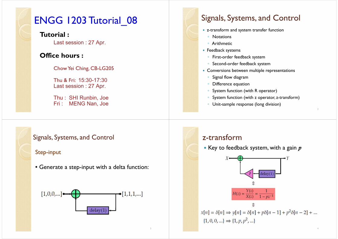
Tutorial :Last session : 27 Apr.

Office hours :

Chow Yei Ching, CB-LG205

Thu & Fri: 15:30-17:30Last session : 27 Apr.

Thu : SHI Runbin, JoeFri : MENG Nan, Joe

ENGG 1203 Tutorial_08 Signals, Systems, and Control z-transform and system transfer function◦ Notations◦ Arithmetic

Feedback systems◦ First-order feedback system◦ Second-order feedback system

Conversions between multiple representations◦ Signal flow diagram ◦ Difference equation◦ System function (with R operator)◦ System function (with z operator, z-transform)◦ Unit-sample response (long division)

2

Signals, Systems, and Control

3

Step-input

• Generate a step-input with a delta function:

z-transform Key to feedback system, with a gain p

4

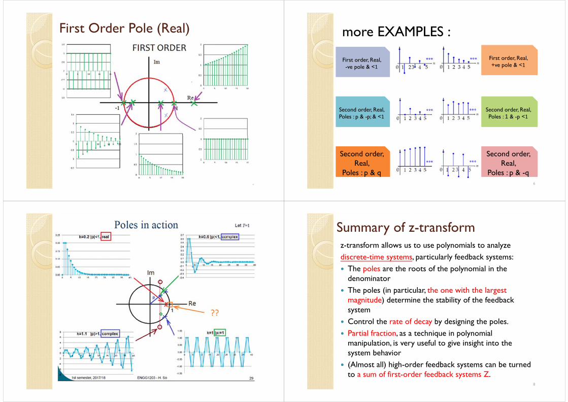
First Order Pole (Real)

5 6

First order, Real, -ve pole & <1

Second order, Real,

Poles : p & q

First order, Real, +ve pole & <1

Second order, Real, Poles : p & -p; & <1

Second order, Real, Poles : 1 & -p <1

Second order, Real,

Poles : p & -q

more EXAMPLES :

7

Summary of z-transformz-transform allows us to use polynomials to analyzediscrete-time systems, particularly feedback systems: The poles are the roots of the polynomial in the

denominator The poles (in particular, the one with the largest

magnitude) determine the stability of the feedback system

Control the rate of decay by designing the poles. Partial fraction, as a technique in polynomial

manipulation, is very useful to give insight into the system behavior

(Almost all) high-order feedback systems can be turned to a sum of first-order feedback systems Z.

8

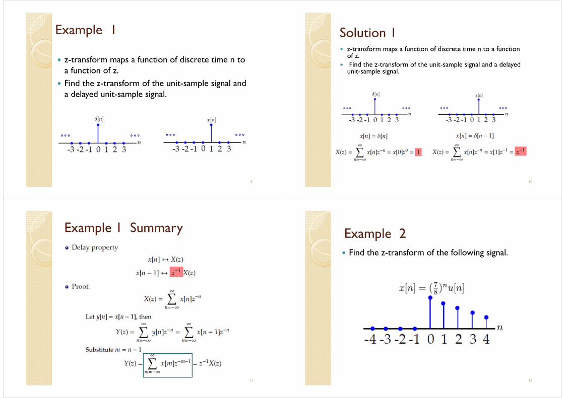
Example 1

z-transform maps a function of discrete time n to a function of z.

Find the z-transform of the unit-sample signal and a delayed unit-sample signal.

9

Solution 1 z-transform maps a function of discrete time n to a function

of z. Find the z-transform of the unit-sample signal and a delayed

unit-sample signal.

10

Example 1 Summary

11

Example 2 Find the z-transform of the following signal.

12

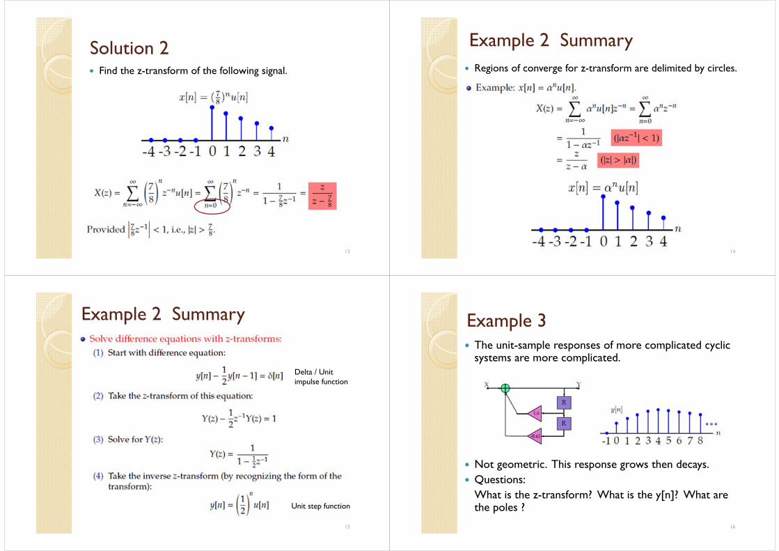
Solution 2 Find the z-transform of the following signal.

13

Example 2 Summary Regions of converge for z-transform are delimited by circles.

14

Example 2 Summary

15

Delta / Unit impulse function

Unit step function

Example 3 The unit-sample responses of more complicated cyclic

systems are more complicated.

Not geometric. This response grows then decays. Questions:

What is the z-transform? What is the y[n]? What are the poles ?

16

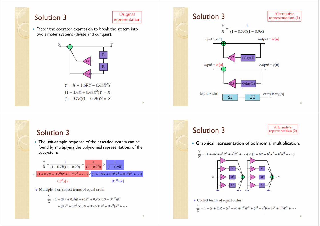
Solution 3 Factor the operator expression to break the system into

two simpler systems (divide and conquer).

17

Solution 3

18

Solution 3 The unit-sample response of the cascaded system can be

found by multiplying the polynomial representations of the subsystems.

19

Solution 3 Graphical representation of polynomial multiplication.

20

Solution 3

Tabular representation of polynomial multiplication.

Group same powers of R by following reverse diagonals:

21

Solution 3 Use partial fractions to rewrite as a sum of simpler

parts.

22

( By Partial fraction )

Solution 3 The sum of simpler parts suggests a parallel

implementation.

23

Solution 3 Graphical representation of the sum of geometric

sequences.

24

Solution 3 Partial fractions provide a remarkable equivalence.

follows from thinking about system as polynomial (factoring).

25

Solution 3 The key to simplifying a higher-order system is

identifying its poles. Poles are the roots of the denominator of the

system function when R 1/z Start with the system transfer function:

26

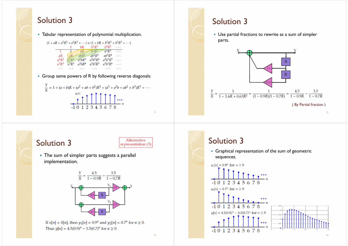
Example 4 Consider the flow graph below, where k1 = 1.6

and k2 = -0.63.

27

Solution 4

28

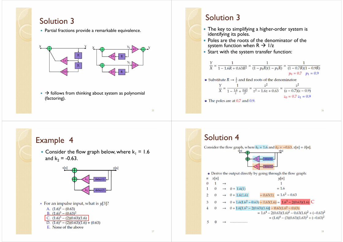
Question 5 A discrete-time system is represented by

What is the transfer function given by H(z) = Y(z)/X(z) ?

29

Ans : B

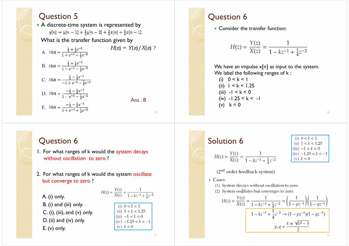
Question 6 Consider the transfer function:

We have an impulse x[n] as input to the system.We label the following ranges of k :

(i) 0 < k < 1(ii) 1 < k < 1.25(iii) -1 < k < 0(iv) -1.25 < k < -1(v) k = 0

30

Question 61. For what ranges of k would the system decays

without oscillation to zero ?

2. For what ranges of k would the system oscillate but converge to zero ?

A. (i) only.B. (i) and (iii) only.C. (i), (iii), and (v) only.D. (ii) and (iv) only.E. (v) only.

31

Solution 6

32

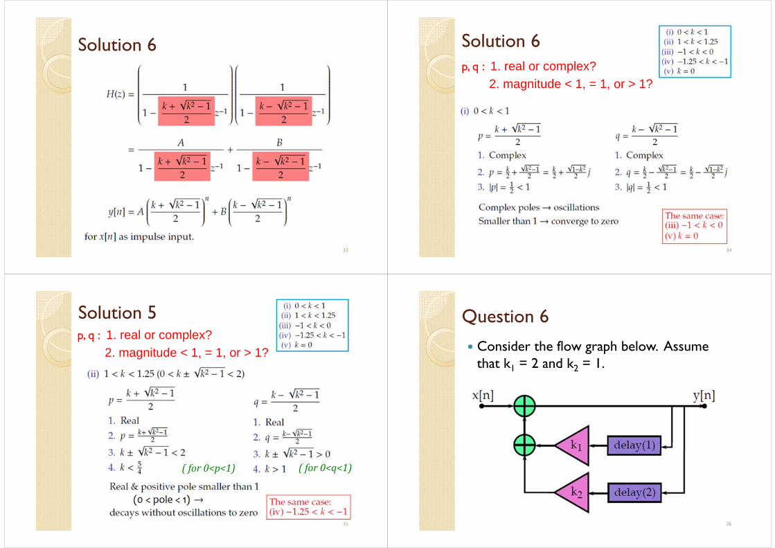
Solution 6

33

Solution 6p, q : 1. real or complex?

2. magnitude < 1, = 1, or > 1?

34

Solution 5

35

p, q : 1. real or complex?2. magnitude < 1, = 1, or > 1?

(for0<p<1) (for0<q<1)

Question 6 Consider the flow graph below. Assume

that k1 = 2 and k2 = 1.

36

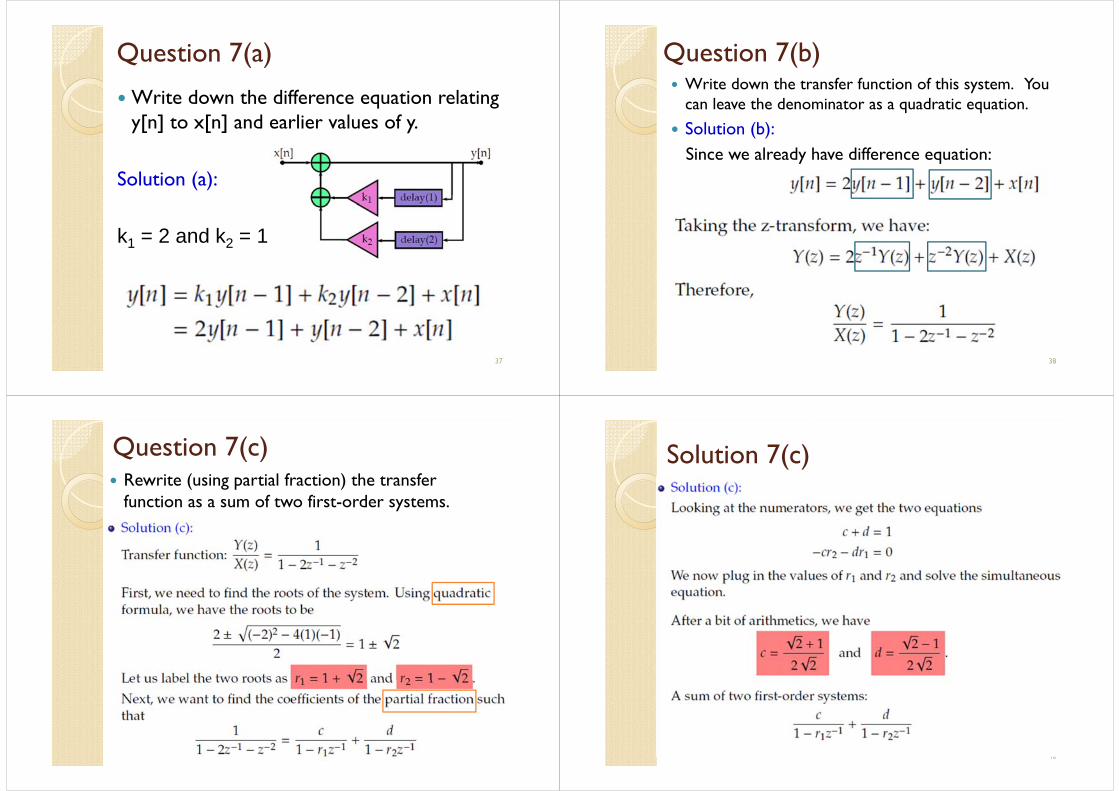
Question 7(a)

Write down the difference equation relating y[n] to x[n] and earlier values of y.

Solution (a):

k1 = 2 and k2 = 1

37

Question 7(b) Write down the transfer function of this system. You

can leave the denominator as a quadratic equation.

Solution (b):Since we already have difference equation:

38

Question 7(c) Rewrite (using partial fraction) the transfer

function as a sum of two first-order systems.

39

Solution 7(c)

40

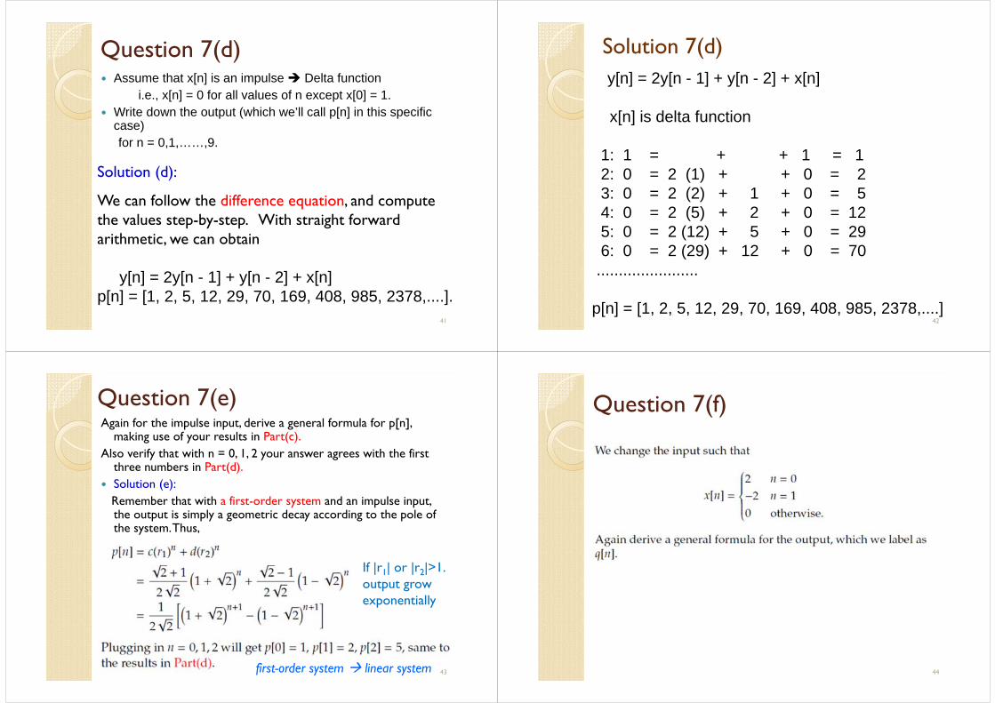
Question 7(d) Assume that x[n] is an impulse Delta function

i.e., x[n] = 0 for all values of n except x[0] = 1. Write down the output (which we’ll call p[n] in this specific

case)for n = 0,1,……,9.

41

Solution (d):

We can follow the difference equation, and compute the values step-by-step. With straight forward arithmetic, we can obtain

y[n] = 2y[n - 1] + y[n - 2] + x[n]p[n] = [1, 2, 5, 12, 29, 70, 169, 408, 985, 2378,....].

42

y[n] = 2y[n - 1] + y[n - 2] + x[n]

x[n] is delta function

1: 1 = + + 1 = 12: 0 = 2 (1) + + 0 = 2 3: 0 = 2 (2) + 1 + 0 = 54: 0 = 2 (5) + 2 + 0 = 125: 0 = 2 (12) + 5 + 0 = 296: 0 = 2 (29) + 12 + 0 = 70

.......................

p[n] = [1, 2, 5, 12, 29, 70, 169, 408, 985, 2378,....]

Solution 7(d)

Question 7(e)Again for the impulse input, derive a general formula for p[n],

making use of your results in Part(c).Also verify that with n = 0, 1, 2 your answer agrees with the first

three numbers in Part(d). Solution (e):

Remember that with a first-order system and an impulse input, the output is simply a geometric decay according to the pole of the system. Thus,

43

If |r1| or |r2|>1. output grow exponentially

first-order system linear system

Question 7(f)

44

Solution 7(f)

45

x[n]=2; n = 0 x[n] =-2; n = 1

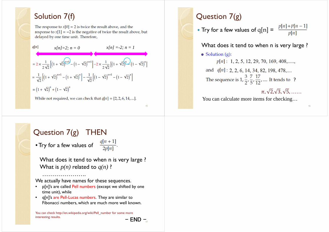
Question 7(g)

Try for a few values of q[n] =

What does it tend to when n is very large ?

You can calculate more items for checking…46

, , , , ……

THEN

47

We actually have names for these sequences. • p[n]’s are called Pell numbers (except we shifted by one

time unit), while • q[n]’s are Pell-Lucas numbers. They are similar to

Fibonacci numbers, which are much more well known.

You can check http://en.wikipedia.org/wiki/Pell_number for some more interesting results.

• Try for a few values of

What does it tend to when n is very large ?What is p(n) related to q(n) ?………………….

Question 7(g)

- END -