empirical comparison of inflation models' forecast accuracy

Empirical comparison of inflation models’forecast accuracy

Øyvind Eitrheim, Tore Anders Husebø and Ragnar Nymoen∗

2nd July 2000

Abstract

Forecasting inflation is important in practical monetary policy, and in-creasingly so in countries who have adopted inflation targeting as their oper-ative monetary policy regime. Inflation models are however contested. Rivalmodels are shown to have different forecasting properties over a period thatcovers a change in regime in the Norwegian economy—from high to low infla-tion. There is no ground for choosing a policy model on the basis of forecastperformance alone, but different models can be useful for different purposes.For example, we find that simple forecasting rules based on differencing arerelatively robust to structural breaks. Thus they contain information thatcan be used to intercept-correct a larger model that contains policy relevantcausal information.

∗The first author is head of research and the second is staff economist in Norges Bank (TheCentral Bank of Norway). The third author is professor of economics at the University of Oslo andspecial consultant in Norges Bank. The views expressed in this paper are solely the responsibilityof the authors and should not be interpreted as reflecting those of Norges Bank. We would like tothank Michael P. Clements for advise and suggestions. Please address correspondence to the thirdauthor: Ragnar Nymoen, University of Oslo, Department of Economics. P.O. Box 1095 Blindern.N-0317 Oslo, Norway. Internet: [email protected].

1

1 Introduction

Producers and consumers of empirical models take a shared interest in comparisonof model forecasts. As pointed out by Granger (1990), consumers of models careabout out-of-sample model properties and consequently put weight on comparisonsof model forecasts. Since producers of models in turn wish to influence the beliefsof model consumers, comparison of model forecasts provides an important interfacebetween producers and consumers of empirical models.

A comparison of forecast from empirical models can be based on “raw” modelforecasts (e.g. provided by the producers) or on the published forecasts that includethe effects of judgmental corrections (intercept corrections). In this paper the aimis to focus on the mapping from model specification to forecast properties, so weconsider the raw model forecast, without the intervening corrections made by fore-casters. Another issue is that any comparison will inevitably consider only a sub-setof macro economic variables, and the choice of variables will influence the outcomeof the comparison. This problem extends to whether it is levels variables that areforecasted or their growth rates, since the ranking of forecast accuracy may dependon which linear transformation one uses, see Clements and Hendry (1993),Clementsand Hendry (1998, Chapter 3).

In the following, these issues are pushed somewhat in the background by focus-ing on inflation forecasting. The vector of variables that enter the comparison is the“typical” list of variables that are forecasted in the central banks’ economic bulletinsand outlooks. The typical list include a limited number of annual growth rates : In-flation (in Norway, this is CPI inflation), wage growth, import price growth, GDPgrowth, growth in consumer expenditure, housing price growth (asset inflation), butalso at least one levels variable, namely the rate of unemployment.

In the 1990s, inflation targeting has emerged as a candidate intermediate tar-get for monetary policy. An explicit inflation target for monetary policy means aquantified inflation target, e.g. 2 per cent per year, and a tolerance interval around itof (for example) ±1 percentage point, and that the central bank is given full controlof monetary instruments. New Zealand and Canada are the pioneering countries.Sweden moved to inflation targeting in 1993, and since 1997 an inflation target hasrepresented the nominal anchor of the UK economy.

As emphasized in Svensson (1997b), an explicit inflation target implies that thecentral bank’s conditional forecasts 1-2 years ahead become the intermediate targetof monetary policy. If the inflation forecast is sufficiently close to the target, thepolicy instruments (a short-term interest rate) is left unaltered. If the forecasted rateof inflation is higher (lower) than the target, monetary instruments are changed untilthe revised forecast is close to the inflation target. In such instances the propertiesof the forecasting model (the dynamic multipliers) can have a large influence on howmuch the interest rate is changed.

It is seen that with the conditional inflation forecasts as the operational targetof monetary policy, there is an unusually strong linkage between forecasting andpolicy analysis. Decisions are more explicitly forward looking than in other instancesof macroeconomic policy making, where the assessment of the current economicsituation plays a prominent role. That said, inflation forecasts are also importantelements in policy discussions also under exchange rate “regimes” other than explicitinflation targeting. Thus, Svensson (1997a) notes that inflation forecasts preparedby Norges Bank are “more explicit and detailed than Sveriges Riksbank’s forecast”,

2

even though Norway has no formal inflation target.In this chapter we compare forecasts that made for policy purposes. Section 2

gives the economic background and discusses the relationship between model spec-ification and inflation forecasting and section 3 provides an empirical investigationexample of how the models perform econometrically and in forecasting inflation. Insection 4 we outline four different forecasting models for the Norwegian economy.First, we present two large scale macroeconometric models which contain monetarypolicy channels (transmission mechanisms) linking monetary policy instruments likeshort run money market interest rates and exchange rates to other economic vari-ables (e.g., those listed above), through causal mechanisms which allow for monetarypolicy analysis. Second, we also look at two simple non-causal forecasting modelsin differences. Section 5 discuss the forecasting properties of the four models usingstochastic simulation.

2 Model specification and inflation forecasting

One of the inflation models with the longest track record is the Phillips curve. It wasintegrated into macroeconometric models in the 1970s. In the mid 1980s, however,the Phillips curve approach has been challenged by a model consisting of a negativerelationship between the level of the real wage and the rate of unemployment, dubbedthe wage curve by Blanchflower and Oswald (1994), together with firms’ price settingschedule.1 The wage curve is consistent with a wide range of economic theories, seeBlanchard and Katz (1997), but its original impact among European economists wasdue the explicit treatment of union behaviour and imperfectly competitive productmarkets, see Layard and Nickell (1986), Rowlatt (1987), Hoel and Nymoen (1988).Because the modern theory of wage and price setting recognizes the importance ofimperfect competition on both product and labour markets, we refer to this class ofmodels as the Imperfect Competition Model—ICM hereafter.

In equation (2.1) pct denotes the log of the consumer price index in period t.∆ is the first difference operator, so ∆pct is CPI-inflation:

∆pct = γ1(ut−1 − un) + γ ′3(L)∆zt − αi

n∑i=1

ECi,t−1 +εt (2.1)

The first term on the right hand is the (log of) the rate of unemployment (ut−1)minus its (unconditional) mean un, hence E[ut−1 − un] = 0. It represents “excessdemand” in the labour market and how wage increases are transmitted on to CPI-inflation. Empirical equations often include a product market output-gap variablealongside the unemployment term. However, this variable is not needed in order todiscriminate between theories, and is omitted from (2.1)

The term zt is a vector of variables that enter in differenced form and γ ′2(L)

is the corresponding vector polynomial with coefficients. Typical elements in thispart of the model are the lagged rate of inflation, i.e., ∆pct−1, the rate of change inimport prices and changes in indirect tax-rates.

The case where the remaining coefficients in the equation are zero, i.e. α1 =... = αn = 0, corresponds to the Phillips-curve model. The Phillips-curve is an

1Wallis (1993) gives an excellent exposition, emphasizing the impact on macroeconometricmodelling and policy analysis.

3

important model in current macroeconomics, for example in the theory of monetarypolicy as laid out in Clarida and Gertler (1999), and it dominates the theoreticalliterature on inflation targeting, see Svensson (2000). The Bank of England (1999)includes Phillips-curve models in their suite of models for monetary policy. MervynKing, the Deputy Governor of the Bank of England puts it quite explicitly: ‘..theconcept of a natural rate of unemployment, and the existence of a vertical long-runPhillips curve, are crucial to the framework of monetary policy.’2

The empirical literature shows that the Phillips curve holds its ground whentested on US data—see Fuhrer (1995), Gordon (1997), Gali and Gertler (1999), andBlanchard and Katz (1999). Studies from Europe usually conclude differently: Thepreferred models tend to imply a negative relationship between the real wage leveland the rate of unemployment, see e.g. Dreze and Bean (1990, Table 1.4), OECD(1997, Table 1.A.1), Wallis (1993) and Rødseth and Nymoen (1999). These findingsare consistent with the seminal paper of Sargan (1964), and the later theoreticaldevelopments leading to the ICM class of wage and price setting equations.

The negative relationship between the real wage level and the rate of unemploy-ment, which is also referred to in the literature as the wage-curve, see Blanchflowerand Oswald (1994), can be incorporated in (2.1) in the following way: Let wt denotethe log of the nominal wage rate in period t, so wt − pct is the real-wage, then theequilibrium correction term EC1,t can be specified as

EC1,t = wt − pct + β11ut − µ1, with α1 ≥ 0 and β11 ≥ 0. (2.2)

Thus, the future rate of inflation is influenced by a situation “today” in which thereal-wage is high relative to the “equilibrium” real-wage β11uT +µ1. The parameterµ1 denotes the (long run) mean of the relationship, i.e. E[EC1,t] = 0. Disequilibriain firms’ price setting have similar implications, and the inflation equation there-fore contains a second term EC2,t that relates the price level in period T to theequilibrium price level. Hence, in a simple specification,

EC2,t = (pct − wt)− β12(pit − pct) + µ2 with α2 ≥ 0 and β21 ≥ 0, (2.3)

where pit is the log of the import price index.It is seen that both the Phillips-curve and the ICM theories focus on the labour

and product markets. Although, in theory disequilibria in other markets, such asthe money market and the market for foreign exchange might have predictive powerfor inflation, we only consider the case of n = 2 in equation (2.1). Thus, the Phillips-curve equation takes the simple form

∆pct = γ1(ut−1 − un) + γ ′3(L)∆zt + εphil,t, (2.4)

while an inflation equation consistent with the ICM is given by

∆pct = γ ′2(L)∆zt + α1EC1,t−1 + α2EC2,t−1 + εICM,t. (2.5)

In (2.5) the unemployment term (ut−1−un) is omitted because, according to theory,unemployment creates inflation via wage-setting. Thus, if the wage-curve implicitin (2.2) is correctly modelled, there is no additional predictive power arising froman inclusion of (ut−1 − un) in the equation, see Kolsrud and Nymoen (1998) for adiscussion.

2King (1998, p.12)

4

The two models take different views on the causal mechanisms in the infla-tion process, and as a result, they can lead to conflicting policy recommendations.Consider for example a situation where both models forecast a rise in inflation,e.g. because of a sudden rise in domestic spending. Based on the Phillips-curve,one might recommend a rise in the Bank’s interest rate, since otherwise it wouldtake several periods before unemployment rises enough to curb inflation. Moreover,since any departure of unemployment from its natural-rate is temporary, one mightas well provoke a temporary rise in ut, “today”, in order to cut-off inflation pressuredirectly. The ICM model points to other mechanism than unemployment that canstabilize inflation. For example, in an open economy, a rise in inflation leads to afall in profits, and wage claims will be reduced as a result even at the going rate ofunemployment. According, to the ICM it is also possible that a rise in the inter-est rate has lasting effects on the rate of unemployment, i.e., the natural-rate maynot be invariant to policy changes, see Kolsrud and Nymoen (1998), Bardsen et al.(2000). Thus, the recommendation could be a more moderate rise in the interestrate.

However, equation (2.4) and (2.5) have in common that they include causalinformation about the effects of other variables on inflation. In this respect theystand apart from univariate time series models which only include causal informationin the form of lagged values of inflation itself. A simple example is given by

∆pct = γ0 + γ3p∆pct−1 + εAR,t, (2.6)

which is a 1thorder autoregressive model of inflation. Finally, we consider forecastingmodels of the random-walk type, i.e.,

∆∆pct = εdAR,t. (2.7)

We use the acronym dAR for the disturbance in (2.7), since an interpretation of(2.7) is that it is an autoregression in differences, obtained by setting γ3p = 1 in(2.6).

A common tread in many published evaluations of forecasts is the use of time-series models as a benchmark for comparison with forecasts derived from large-scale econometric systems of equations, see Granger and Newbold (1986, Chapter9.4) for a survey. The finding that the benchmark-models often outperformed theeconometric models represents an important puzzle that has not been fully resolveduntil recently, by the work of Michael Clements and David Hendry. In short, thesolution lies in the insight that e.g., the random-walk model is not the “naive”forecasting tool that it appears at first sight. Instead, its’ forecasts are relativelyrobust to some types of structural changes that occurs frequently in practice, andthat are damaging to forecasts derived from econometric models.

Equations (2.4)-(2.7) are special cases of the general equation (2.1). Assumenow that the disturbances ε1,ε2, ...εT in (2.1) represent an innovation process relativeto the information available at time T , denoted IT . A strategy of choosing a fore-casting model for period T +1 is to first estimate (2.1) on the sample (t = 1, 2, ...T )and then test the validity of the restrictions of the different models. Only the modelwhich is valid reductions of (2.1) will have disturbance that are innovations relativeto the information set IT . The conditional mean of that congruent model the pre-dictor of inflation in period T + 1 that has minimum mean-squared forecast error(MMSFE), see e.g. Clements and Hendry (1998, Chapter 2.7).

5

However, this result implicitly assumes that the process that we forecast isstable over the forecast horizon. But experience tells us that parameters frequentlychange. Suppose for example that a “regime shift” occurs in period T + 1. Thecongruent model then no longer reflects the true process in the forecast period,and thus we cannot use the above theorem to show that its conditional mean isthe MMSFE forecast. Conversely, simple univariate models like (??) and (2.7) areunlikely to be congruent representations. Despite this, they offer some degree ofprotection against damage caused by non-stationarities.

Clements and Hendry (1998), (1999) have developed the theory of forecastingeconomic time series to account for instability and non-stationarity in the processes.One important results is that there is no way of knowing a priori which model willhave the best forecast properties, an econometric model that include relevant causalinformation or a simple random walk model like (2.7), see e.g., Clements and Hendry(1998, Chapter 2.9). In our case, the econometric ICM may be the encompassingmodel, but if the parameters of the inflation process alters in the forecast period,its forecasts may still compare unfavourably with the forecasts of simple time seriesmodels.

As an example, suppose that possibility that the parameters of the wage curveµ1 changes in period T + 1, i.e., there is a shock to wage-setting. The ICM-forecastE[∆pcT+2 | IT+1] then becomes biased. Moreover, in the case that µ1 changeswithin sample (in period T say), and that change is undetected by the forecaster,the ICM model will produce a biased forecast for period T + 1, while the random-walk forecast from (2.7) may be unbiased. Thus the better model in terms of causalinformation actually loses in a comparison to the random walk on this measureof forecast accuracy. Moreover, it is also possible that the Phillips-curve modeloutperforms the ICM. The reason is that the Phillips-curve shares the 1-step forecastproperties of the random walk in this case, since it omits the EC11,t−1 term that isaffected by the structural break.

So far we have only considered 1-step forecasts, but it is clear that the sameissues arise for dynamic multi-step forecasts. For example, in the Phillips-curve andin the ICM model, uT+1 has to be forecasted in order to calculate E[∆pcT+2 | IT ].Hence a larger econometric model is needed for forecasting, and if a structural breakoccurs in those parts of the economy that determine uT+1, the inflation forecastis damaged. Conversely, simple univariate forecasting tools are by constructioninsulated from structural changes elsewhere in the system. Also, in that sense theyproduce robust forecasts.

Systems of equation that are developed with econometric methods are referredto as equilibrium-correcting models, EqCMs. The generalization of the simple au-toregressive inflation models in (2.6) and (2.7) are system of equation that only usedifferences of the data, without equilibrium correction terms, i.e., VARs in differ-ences (DVs, Clements and Hendry (1999, Chapter 5)) and double-differences (DDVs).The Phillips-curve and the ICM are examples of EqCMs. At first sight it may seemthat this tag only applies to the ICM, since the terms EC1,t−1 and EC2,t−1 are omit-ted from the Phillips-curve. However, the Phillips-curve conveys the alternative viewthat inflation is stabilized by ut − un → 0 in steady-state. Thus the equilibratingterm is the rate of unemployment itself, rather than EC1,t−1 and EC2,t−1.

In the following, these issues are investigated by comparison of the forecasts ofthe different model specifications: ICM, Phillips-curve, univariate autoregression indifferences and double differencing forecasting rules. In the next section we compare

6

small scale models of inflation are evaluated econometrically priori to forecast com-parison. In section 4 we investigate different version of the macroeconomic modelsused by the Central Bank of Norway.

3 Two inflation models3

I this section we compare forecast of the two contending inflation quarterly modelsover the period 1995.1-1998.4. The estimation sample is 1968.1-1994.4. The sample-split coincides with an important change in the Norwegian economy: The movefrom a high-inflation regime to a new regime with low and stable inflation. Themeans of the annual CPI growth rate of are 6.7% (estimation sample) and 2.1%(forecast period). The corresponding standard deviations are 3% and 0.6%. Thusthe experiment is relevant for elucidating how well the different models forecast thenew regime, conditional on the old regime.A VAR for the five endogenous variables ∆wt, ∆pct, ∆pt, ∆yt and ∆ut was estimatedwith data 1995.1-1998.4 (N = 108). The definitions of the variables are:

• wt = log of nominal wage cost per man hour in Norwegian manufacturing

• yt = log of manufacturing value-added (fixed prices) per man hour.

• pt = log of the manufacturing value-added deflator.

• ut = log of the rate of unemployment.

• pc = log of the consumer price index.

The equilibrium correction mechanism in equations (3.1) and (3.2) were taken asknown, thus.

wt = pt + yt − 0.08ut + EC1,t, (3.1)

pct = 0.6(w − y)t + 0.4pit + τ 3t + EC2,t. (3.2)

pi is log of the import price index of manufactures, and τ 3t is an indirect tax-rate.These two equations are the empirical counterparts to (2.2) and (2.3). The estimatesare taken from Bjørnstad and Nymoen (1999), and are also consistent with thefindings for annual data in Johansen (1995). Equation (3.2) is from Bardsen et al.(1998).4

The unrestricted system is large (43 coefficients in each equation), due to 4.order dynamics and the inclusion of 18 non-modelled variables, e.g., current andlagged import price growth ∆pit, the change in normal working hours in manufac-turing (∆ht), a variable that captures the coverage of labour markets programmes(progt), and changes in the payroll and indirect tax-rates (∆τ 1,t and ∆τ 3t). The de-terministic terms include intercepts, three centered seasonal dummies, incomes pol-icy dummies for 1979 and 1988, and a VAT dummy for the 1970q1. Finally,dummiesthat capture both deterministic shifts in the mean of the rate of unemployment aswell as a changing seasonal pattern, see Akram (1999).

3All results in this section were obtained by GiveWin 1.20 and PcFIML 9.20, see Doornik andHendry (1996a) and Doornik and Hendry (1996b).

4However, this relationship was obtained for total economy wages and productivity, and there-fore cointegration may be weaker for our manufacturing wage cost data.

7

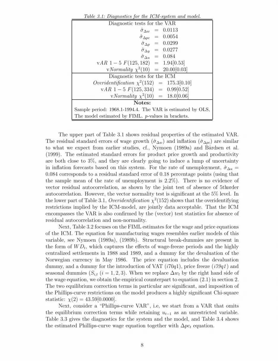
Table 3.1: Diagnostics for the ICM-system and model.Diagnostic tests for the VAR

σ∆w = 0.0113σ∆pc = 0.0054σ∆p = 0.0299σ∆y = 0.0277σ∆u = 0.084

vAR 1− 5 F (125, 182) = 1.94[0.53]vNormality χ2(10) = 20.00[0.03]Diagnostic tests for the ICM

Overidentification χ2(152) = 175.3[0.10]vAR 1− 5 F (125, 334) = 0.99[0.52]

vNormality χ2(10) = 18.0[0.06]Notes:

Sample period: 1968.1-1994.4. The VAR is estimated by OLS,The model estimated by FIML. p-values in brackets.

The upper part of Table 3.1 shows residual properties of the estimated VAR.The residual standard errors of wage growth (σ∆w) and inflation (σ∆pc) are similarto what we expect from earlier studies, cf., Nymoen (1989a) and Bardsen et al.(1999). The estimated standard errors for product price growth and productivityare both close to 3%, and they are clearly going to induce a lump of uncertaintyin inflation forecasts based on this system. For the rate of unemployment, σ∆u =0.084 corresponds to a residual standard error of 0.18 percentage points (using thatthe sample mean of the rate of unemployment is 2.2%). There is no evidence ofvector residual autocorrelation, as shown by the joint test of absence of 5thorderautocorrelation. However, the vector normality test is significant at the 5% level. Inthe lower part of Table 3.1, Overidentification χ2(152) shows that the overidentifyingrestrictions implied by the ICM-model, are jointly data acceptable. That the ICMencompasses the VAR is also confirmed by the (vector) test statistics for absence ofresidual autocorrelation and non-normality.

Next, Table 3.2 focuses on the FIML estimates for the wage and price equationsof the ICM. The equation for manufacturing wages resembles earlier models of thisvariable, see Nymoen (1989a), (1989b). Structural break-dummies are present inthe form of WDt, which captures the effects of wage-freeze periods and the highlycentralized settlements in 1988 and 1989, and a dummy for the devaluation of theNorwegian currency in May 1986. The price equation includes the devaluationdummy, and a dummy for the introduction of VAT (i70q1), price freeze (i79q1 ) andseasonal dummies (Si,t (i = 1, 2, 3). When we replace ∆wt by the right hand side ofthe wage equation, we obtain the empirical counterpart to equation (2.1) in section 2.The two equilibrium correction terms in particular are significant, and imposition ofthe Phillips-curve restrictions on the model produces a highly significant Chi-squarestatistic: χ(2) = 43.59[0.0000].

Next, consider a “Phillips-curve VAR”, i.e, we start from a VAR that omitsthe equilibrium correction terms while retaining ut−1 as an unrestricted variable.Table 3.3 gives the diagnostics for the system and the model, and Table 3.4 showsthe estimated Phillips-curve wage equation together with ∆pct equation.

8

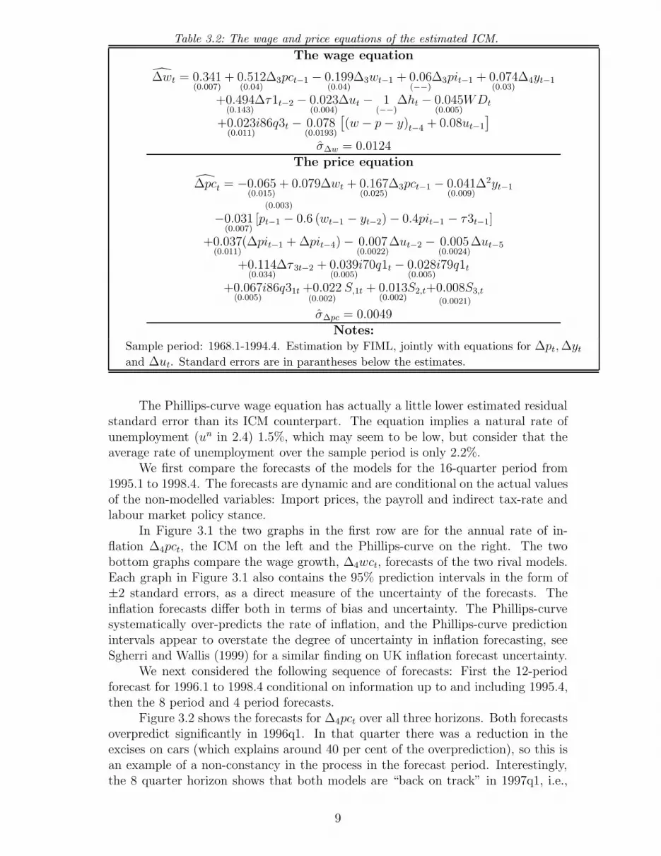
Table 3.2: The wage and price equations of the estimated ICM.The wage equation

∆wt = 0.341(0.007)

+ 0.512(0.04)

∆3pct−1 − 0.199(0.04)

∆3wt−1 + 0.06(−−)

∆3pit−1 + 0.074(0.03)

∆4yt−1

+0.494(0.143)

∆τ1t−2 − 0.023(0.004)

∆ut − 1(−−)

∆ht − 0.045(0.005)

WDt

+0.023(0.011)

i86q3t − 0.078(0.0193)

[(w − p− y)t−4 + 0.08ut−1

]σ∆w = 0.0124

The price equation

∆pct = −0.065(0.015)

+ 0.079

(0.003)

∆wt + 0.167(0.025)

∆3pct−1 − 0.041(0.009)

∆2yt−1

−0.031(0.007)

[pt−1 − 0.6 (wt−1 − yt−2)− 0.4pit−1 − τ3t−1]

+0.037(0.011)

(∆pit−1 + ∆pit−4)− 0.007(0.0022)

∆ut−2 − 0.005(0.0024)

∆ut−5

+0.114(0.034)

∆τ 3t−2 + 0.039(0.005)

i70q1t − 0.028(0.005)

i79q1t

+0.067(0.005)

i86q31t +0.022(0.002)

S,1t + 0.013(0.002)

S2,t+0.008S3,t(0.0021)

σ∆pc = 0.0049Notes:

Sample period: 1968.1-1994.4. Estimation by FIML, jointly with equations for ∆pt,∆yt

and ∆ut. Standard errors are in parantheses below the estimates.

The Phillips-curve wage equation has actually a little lower estimated residualstandard error than its ICM counterpart. The equation implies a natural rate ofunemployment (un in 2.4) 1.5%, which may seem to be low, but consider that theaverage rate of unemployment over the sample period is only 2.2%.

We first compare the forecasts of the models for the 16-quarter period from1995.1 to 1998.4. The forecasts are dynamic and are conditional on the actual valuesof the non-modelled variables: Import prices, the payroll and indirect tax-rate andlabour market policy stance.

In Figure 3.1 the two graphs in the first row are for the annual rate of in-flation ∆4pct, the ICM on the left and the Phillips-curve on the right. The twobottom graphs compare the wage growth, ∆4wct, forecasts of the two rival models.Each graph in Figure 3.1 also contains the 95% prediction intervals in the form of±2 standard errors, as a direct measure of the uncertainty of the forecasts. Theinflation forecasts differ both in terms of bias and uncertainty. The Phillips-curvesystematically over-predicts the rate of inflation, and the Phillips-curve predictionintervals appear to overstate the degree of uncertainty in inflation forecasting, seeSgherri and Wallis (1999) for a similar finding on UK inflation forecast uncertainty.

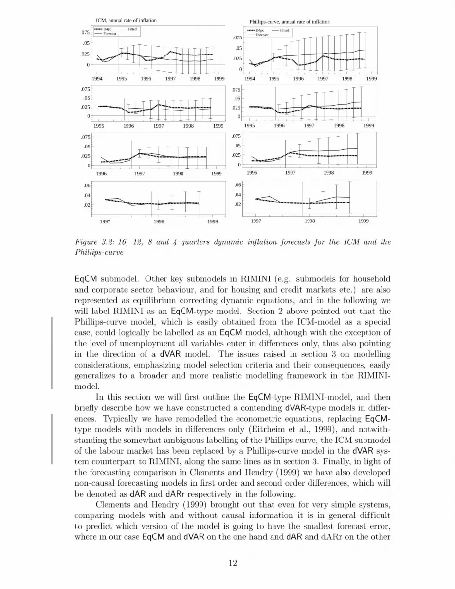
We next considered the following sequence of forecasts: First the 12-periodforecast for 1996.1 to 1998.4 conditional on information up to and including 1995.4,then the 8 period and 4 period forecasts.

Figure 3.2 shows the forecasts for ∆4pct over all three horizons. Both forecastsoverpredict significantly in 1996q1. In that quarter there was a reduction in theexcises on cars (which explains around 40 per cent of the overprediction), so this isan example of a non-constancy in the process in the forecast period. Interestingly,the 8 quarter horizon shows that both models are “back on track” in 1997q1, i.e.,

9

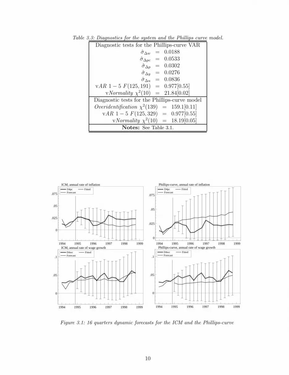
Table 3.3: Diagnostics for the system and the Phillips curve model.Diagnostic tests for the Phillips-curve VAR

σ∆w = 0.0188σ∆pc = 0.0533σ∆p = 0.0302σ∆y = 0.0276σ∆u = 0.0836

vAR 1− 5 F (125, 191) = 0.977[0.55]vNormality χ2(10) = 21.84[0.02]

Diagnostic tests for the Phillips-curve modelOveridentification χ2(139) = 159.1[0.11]

vAR 1− 5 F (125, 329) = 0.977[0.55]vNormality χ2(10) = 18.19[0.05]

Notes: See Table 3.1.

1994 1995 1996 1997 1998 1999

0

.025

.05

.075

ICM, annual rate of inflationD4pc FittedForecast

1994 1995 1996 1997 1998 1999

0

.05

.1

ICM, annual rate of wage growthD4wc FittedForecast

1994 1995 1996 1997 1998 1999

0

.025

.05

.075

Phillips-curve, annual rate of inflationD4pc FittedForecast

1994 1995 1996 1997 1998 1999

0

.05

.1

Phillips-curve, annual rate of wage growthD4wc FittedForecast

Figure 3.1: 16 quarters dynamic forecasts for the ICM and the Phillips-curve

10

Table 3.4: The wage and inflation equations of the estimated Phillips-curve.The wage Phillips-curve

∆wt = 0.0094(0.0019)

+ 0.503(0.07)

∆2pct−1 − 0.195(0.06)

∆wt−1 + 0.06(−−)

∆3pit−1

+0.395(0.14)

∆τ1t−2 − 0.013(0.006)

∆ut − 0.0067(0.0016)

ut−1 − 1(−−)

∆ht

−0.046(0.006)

WDt + 0.027(0.011)

i86q3−0.005(0.003)

S1t −0.001S2t(0.004)

−0.001S3t(0.004)

σ∆w = 0.0122The price equation

∆pct = −0.065(0.016)

+ 0.108(0.037)

∆wtt−1 + 0.216(0.025)

∆3pct−1 + 0.039(0.013)

(∆pit−1 + ∆pit−4)

−0.029(0.0095)

∆2yt−1 − 0.007(0.0025)

∆ut−2 + 0.129(0.0342)

∆τ 3t−2

+0.038(0.0056)

i70q1t − 0.025(0.0055)

i79q11t + 0.013(0.0055)

i86q31t

−0.021(0.0024)

S1,t −0.012S2,t(0.0027)

−0.010S3,t(0.0022)

σ∆pc = 0.0055Notes: See Table 3.2

when the excise reduction is in the conditioning information set. However, thePhillips-curve continues to overpredict, also for the 8 and 4 quarter horizons. Infact, it is also evident from the graphs that on a comparison of biases, the Phillips-curve model would be beaten by a no-change rule, i.e., a double difference “model”∆∆4pct = 0.

In sum, although the both the ICM and the Phillips-curve appear to be congru-ent models within sample, their forecast properties are indeed significantly differentfrom a user’s point of view. In this one-off “test”, the Phillips-curve is poor on fore-casting the mean of inflation in the new low-inflation regime, and it overstates theuncertainty in inflation forecasting. Causal information does not necessarily lead tosuccessful forecasts, i.e., the finding that the Phillips-curve loses to a random-walkmodel of inflation over the latter part of the sample. In the next two sections theempirical analysis of these issues are carried one step further when we compare fore-casts derived from large-scale systems of the Norwegian economy, using stochasticsimulation techniques.

4 Large scale macroeconomic models of the Nor-

wegian economy

RIMINI5 is the Norges Bank macroeconometric model, which is routinely used forpractical forecasting and policy analysis. RIMINI is a large scale model whichlinks together several important submodels of the Norwegian economy. One of thesubmodels is an ICM-type wage/price submodel of the labour market similar to themodel discussed in section 3, hence we adopt the same labels and denote this as an

5RIMINI was originally an acronym for a model for the Real economy and Income accounts -a MINI-version. The model version used in this paper has 205 endogenous variables, although alarge fraction of these are accounting identities or technical relationships creating links betweenvariables, see Eitrheim and Nymoen (1991) for a brief documentation of a predecessor of the model.

11

1994 1995 1996 1997 1998 1999

0

.025

.05

.075

ICM, annual rate of inflation

D4pc FittedForecast

1994 1995 1996 1997 1998 1999

0

.025

.05

.075

Phillips-curve, annual rate of inflation

D4pc FittedForecast

1995 1996 1997 1998 1999

0

.025

.05

.075

1995 1996 1997 1998 1999

0

.025

.05

.075

1996 1997 1998 1999

0

.025

.05

.075

1996 1997 1998 1999

0

.025

.05

.075

1997 1998 1999

.02

.04

.06

1997 1998 1999

.02

.04

.06

Figure 3.2: 16, 12, 8 and 4 quarters dynamic inflation forecasts for the ICM and thePhillips-curve

EqCM submodel. Other key submodels in RIMINI (e.g. submodels for householdand corporate sector behaviour, and for housing and credit markets etc.) are alsorepresented as equilibrium correcting dynamic equations, and in the following wewill label RIMINI as an EqCM-type model. Section 2 above pointed out that thePhillips-curve model, which is easily obtained from the ICM-model as a specialcase, could logically be labelled as an EqCM model, although with the exception ofthe level of unemployment all variables enter in differences only, thus also pointingin the direction of a dVAR model. The issues raised in section 3 on modellingconsiderations, emphasizing model selection criteria and their consequences, easilygeneralizes to a broader and more realistic modelling framework in the RIMINI-model.

In this section we will first outline the EqCM-type RIMINI-model, and thenbriefly describe how we have constructed a contending dVAR-type models in differ-ences. Typically we have remodelled the econometric equations, replacing EqCM-type models with models in differences only (Eitrheim et al., 1999), and notwith-standing the somewhat ambiguous labelling of the Phillips curve, the ICM submodelof the labour market has been replaced by a Phillips-curve model in the dVAR sys-tem counterpart to RIMINI, along the same lines as in section 3. Finally, in light ofthe forecasting comparison in Clements and Hendry (1999) we have also developednon-causal forecasting models in first order and second order differences, which willbe denoted as dAR and dARr respectively in the following.

Clements and Hendry (1999) brought out that even for very simple systems,comparing models with and without causal information it is in general difficultto predict which version of the model is going to have the smallest forecast error,where in our case EqCM and dVAR on the one hand and dAR and dARr on the other

12

represent models with and without causal information respectively.In section 5 below, we generate multi-period forecasts from the econometric

model RIMINI used by Norges Bank, and compare these to the forecasts from modelsbased on differenced data, focusing on both forecast error biases and uncertaintyusing stochastic simulation. The latter extends the analysis in Eitrheim et al. (1999),and we have also extended the maximum forecasting horizon from 12 to 28 quarters.As a background for the simulations, the rest of this section describes the mainfeatures of the incumbent EqCM and how we have designed the three rival dVARforecasting systems.

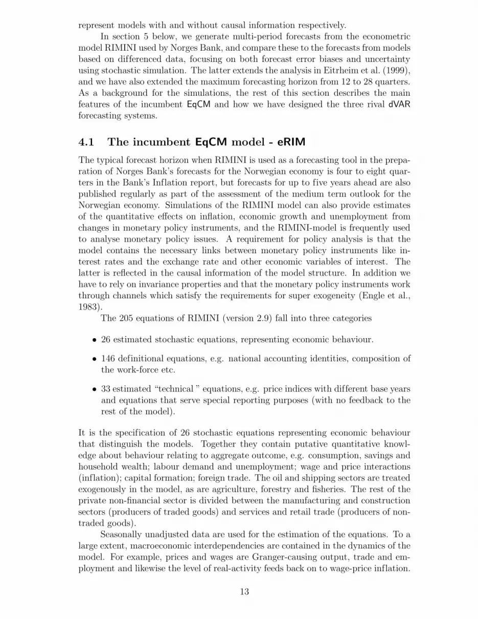
4.1 The incumbent EqCM model - eRIM

The typical forecast horizon when RIMINI is used as a forecasting tool in the prepa-ration of Norges Bank’s forecasts for the Norwegian economy is four to eight quar-ters in the Bank’s Inflation report, but forecasts for up to five years ahead are alsopublished regularly as part of the assessment of the medium term outlook for theNorwegian economy. Simulations of the RIMINI model can also provide estimatesof the quantitative effects on inflation, economic growth and unemployment fromchanges in monetary policy instruments, and the RIMINI-model is frequently usedto analyse monetary policy issues. A requirement for policy analysis is that themodel contains the necessary links between monetary policy instruments like in-terest rates and the exchange rate and other economic variables of interest. Thelatter is reflected in the causal information of the model structure. In addition wehave to rely on invariance properties and that the monetary policy instruments workthrough channels which satisfy the requirements for super exogeneity (Engle et al.,1983).

The 205 equations of RIMINI (version 2.9) fall into three categories

• 26 estimated stochastic equations, representing economic behaviour.

• 146 definitional equations, e.g. national accounting identities, composition ofthe work-force etc.

• 33 estimated “technical ” equations, e.g. price indices with different base yearsand equations that serve special reporting purposes (with no feedback to therest of the model).

It is the specification of 26 stochastic equations representing economic behaviourthat distinguish the models. Together they contain putative quantitative knowl-edge about behaviour relating to aggregate outcome, e.g. consumption, savings andhousehold wealth; labour demand and unemployment; wage and price interactions(inflation); capital formation; foreign trade. The oil and shipping sectors are treatedexogenously in the model, as are agriculture, forestry and fisheries. The rest of theprivate non-financial sector is divided between the manufacturing and constructionsectors (producers of traded goods) and services and retail trade (producers of non-traded goods).

Seasonally unadjusted data are used for the estimation of the equations. To alarge extent, macroeconomic interdependencies are contained in the dynamics of themodel. For example, prices and wages are Granger-causing output, trade and em-ployment and likewise the level of real-activity feeds back on to wage-price inflation.

13

The model is an open system: Examples of important non-modelled variables are thelevel of economic activity by trading partners, as well as inflation and wage-costs inthose countries. Indicators of economic policy (the level of government expenditure,the short-term interest rate and the exchange rate), are also non-modelled and theforecasts are therefore conditional on a particular scenario for these variables. TheEqCM model RIMINI will be labeled eRIM in the following.

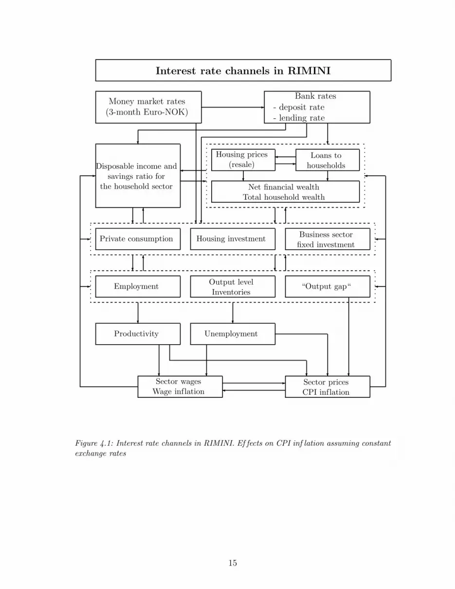
To provide some insights in the type of causal information which is reflected inthe behavioural relationships in eRIM (and dVARc below), consider the link betweeninterest rates and other economic variables in Figure 4.1. The main links betweenshort-term interest rates and aggregated variables like output, employment and CPIinflation in RIMINI, is often denoted as the “interest rate channel” of monetarypolicy.

14

Interest rate channels in RIMINI

Money market rates(3-month Euro-NOK)

Bank rates

- deposit rate- lending rate

✲

Disposable income andsavings ratio for

the household sector

Housing prices(resale)

Loans tohouseholds✲

✛

❄

Net financial wealthTotal household wealth

❄ ❄

❄✻

✲✛

❄✻

Private consumption Housing investment Business sectorfixed investment

❄❄

❄

❄✻

❄✻

Employment Output levelInventories

“Output gap“

❄ ❄

❄

Productivity Unemployment

❄ ❄ ❄❄Sector wagesWage inflation

Sector pricesCPI inflation

✲✛

✛

✛

✛

✲

✲

✲

Figure 4.1: Interest rate channels in RIMINI. Ef fects on CPI inf lation assuming constantexchange rates

15

The main mechanisms of the interest rate channel in RIMINI are: A partialrise in the short-term money market interest rate (typically 3-month NOK rates)assuming fixed exchange rates, leads to an increase in banks’ borrowing and lendinginterest rates with a lag. Aggregate demand is influenced by the interest rate shiftthrough several mechanisms, such as a negative effect on housing prices which (fora given stock of housing capital) causes real household wealth to decline and sup-presses total consumer expenditure. Likewise, there are negative direct and indirecteffects on real investments in sectors producing traded and non-traded goods andon housing investments. The housing and credit markets in RIMINI are interrelatedthrough the housing price and household loans equations which a.o. reflects thathousing capital is collateralized against household loans (mainly in private and stateowned banks) and noting that the ownership rate among Norwegian households ex-ceeds 80%. CPI inflation is reduced after a lag, mainly as a result of the effects ofchanges in aggregate demand on aggregate output and employment (productivity),but also as a result of changes in unit labour costs.

4.2 A full scale dVAR model - dRIMc

Because all the stochastic equations in RIMINI are in equilibrium correction form,a simple dVAR version of the model, can be obtained by omitting the equilibriumcorrecting terms from the equation and re-specifying all the affected equations interms of differences alone. In our earlier paper however, we found that this left uswith seriously misspecified equations a.o. due to the autocorrelation in the omittedequilibrium correcting term. This model was denoted dRIM in Eitrheim et al. (1999)and we have discarded this model in the present analysis.

The previous paper also showed that a more interesting rival was a re-modelledversion of dRIM (a similar procedure was applied in section 3). In order to makethe residuals of the dVAR-equations empirically white-noise, additional terms indifferences often had to be added to remove autocorrelation from the model residuals.The corrected dVAR version of RIMINI is denoted dRIMc, and, bearing in mind thepotential bias in the estimation of the drift term in small samples, we have madesimulations with a version of dRIMc where we systematically excluded the constantterm from typical no-drift variables like unemployment rates and interest rates, seeEitrheim et al. (1999) for discussion.

Hence, the two complete system forecasting models, eRIM and the no-driftversion of dRIMc, both broadly satisfy the same set of single equation model designcriteria and show model residuals which are close to empirical white noise, zero meaninnovations.

4.3 Difference and double difference models - dAR and dARr

Both models considered so far are “system of equations” forecasting models. Forcomparison, we have also prepared single equation forecasts for each variable, i.e.in line with equations (2.6) and (2.7) in section 2 (see also Clements and Hendry(1999, Chapter 5)) but allowing for higher order dynamics and seasonality. Thefirst set of single equation forecasts is dubbed dAR, and is based on unrestrictedestimation of AR(4) models, including a constant term and three seasonal dummies.Finally, we generate forecasts from ∆4∆ lnXt = 0, for each variable Xt in theset of endogenous variables. This set of forecasts is called dARr, where the r is a

16

reminder that the forecasts are based on completely restricted AR(4) processes. Theunivariate dARr“models” are specified without drift terms, hence their forecasts areprotected against trend-misrepresentation.

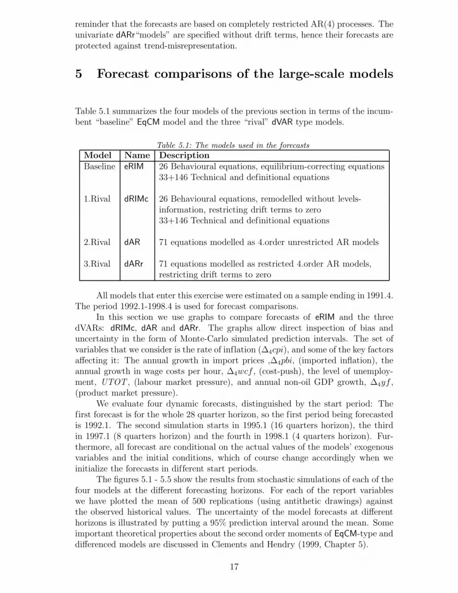
5 Forecast comparisons of the large-scale models

Table 5.1 summarizes the four models of the previous section in terms of the incum-bent “baseline” EqCM model and the three “rival” dVAR type models.

Table 5.1: The models used in the forecastsModel Name DescriptionBaseline eRIM 26 Behavioural equations, equilibrium-correcting equations

33+146 Technical and definitional equations

1.Rival dRIMc 26 Behavioural equations, remodelled without levels-information, restricting drift terms to zero33+146 Technical and definitional equations

2.Rival dAR 71 equations modelled as 4.order unrestricted AR models

3.Rival dARr 71 equations modelled as restricted 4.order AR models,restricting drift terms to zero

All models that enter this exercise were estimated on a sample ending in 1991.4.The period 1992.1-1998.4 is used for forecast comparisons.

In this section we use graphs to compare forecasts of eRIM and the threedVARs: dRIMc, dAR and dARr. The graphs allow direct inspection of bias anduncertainty in the form of Monte-Carlo simulated prediction intervals. The set ofvariables that we consider is the rate of inflation (∆4cpi), and some of the key factorsaffecting it: The annual growth in import prices ,∆4pbi, (imported inflation), theannual growth in wage costs per hour, ∆4wcf , (cost-push), the level of unemploy-ment, UTOT , (labour market pressure), and annual non-oil GDP growth, ∆4yf ,(product market pressure).

We evaluate four dynamic forecasts, distinguished by the start period: Thefirst forecast is for the whole 28 quarter horizon, so the first period being forecastedis 1992.1. The second simulation starts in 1995.1 (16 quarters horizon), the thirdin 1997.1 (8 quarters horizon) and the fourth in 1998.1 (4 quarters horizon). Fur-thermore, all forecast are conditional on the actual values of the models’ exogenousvariables and the initial conditions, which of course change accordingly when weinitialize the forecasts in different start periods.

The figures 5.1 - 5.5 show the results from stochastic simulations of each of thefour models at the different forecasting horizons. For each of the report variableswe have plotted the mean of 500 replications (using antithetic drawings) againstthe observed historical values. The uncertainty of the model forecasts at differenthorizons is illustrated by putting a 95% prediction interval around the mean. Someimportant theoretical properties about the second order moments of EqCM-type anddifferenced models are discussed in Clements and Hendry (1999, Chapter 5).

17

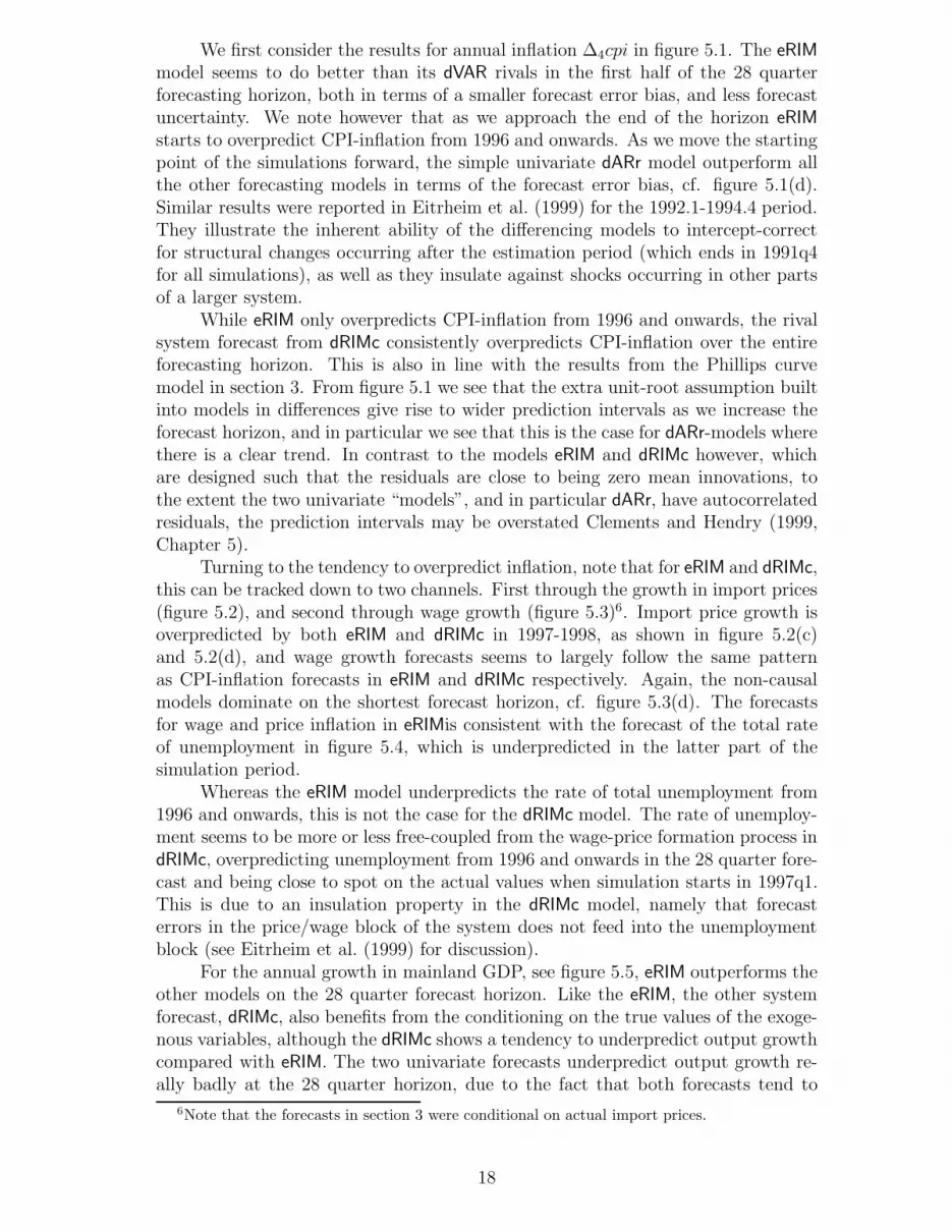
We first consider the results for annual inflation ∆4cpi in figure 5.1. The eRIMmodel seems to do better than its dVAR rivals in the first half of the 28 quarterforecasting horizon, both in terms of a smaller forecast error bias, and less forecastuncertainty. We note however that as we approach the end of the horizon eRIMstarts to overpredict CPI-inflation from 1996 and onwards. As we move the startingpoint of the simulations forward, the simple univariate dARr model outperform allthe other forecasting models in terms of the forecast error bias, cf. figure 5.1(d).Similar results were reported in Eitrheim et al. (1999) for the 1992.1-1994.4 period.They illustrate the inherent ability of the differencing models to intercept-correctfor structural changes occurring after the estimation period (which ends in 1991q4for all simulations), as well as they insulate against shocks occurring in other partsof a larger system.

While eRIM only overpredicts CPI-inflation from 1996 and onwards, the rivalsystem forecast from dRIMc consistently overpredicts CPI-inflation over the entireforecasting horizon. This is also in line with the results from the Phillips curvemodel in section 3. From figure 5.1 we see that the extra unit-root assumption builtinto models in differences give rise to wider prediction intervals as we increase theforecast horizon, and in particular we see that this is the case for dARr-models wherethere is a clear trend. In contrast to the models eRIM and dRIMc however, whichare designed such that the residuals are close to being zero mean innovations, tothe extent the two univariate “models”, and in particular dARr, have autocorrelatedresiduals, the prediction intervals may be overstated Clements and Hendry (1999,Chapter 5).

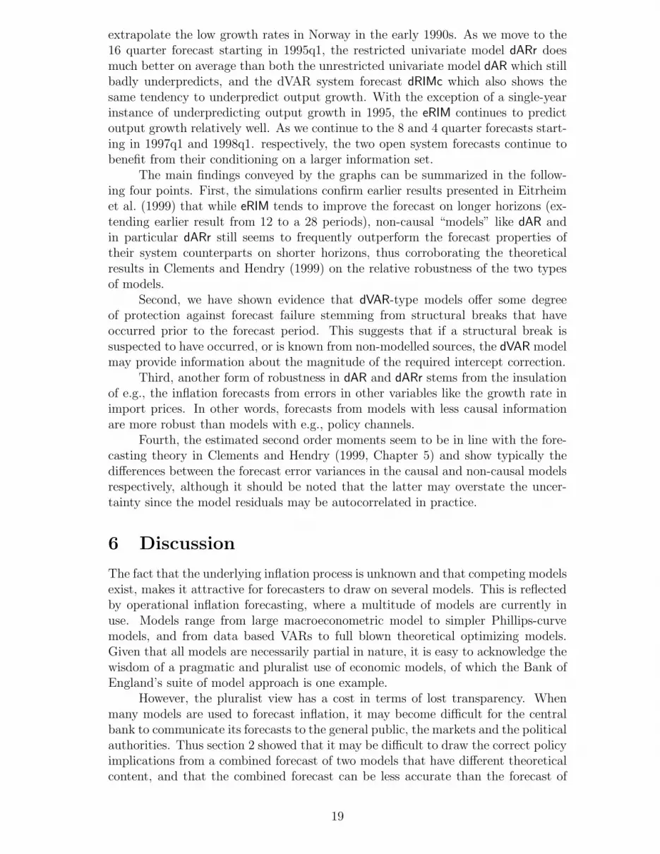
Turning to the tendency to overpredict inflation, note that for eRIM and dRIMc,this can be tracked down to two channels. First through the growth in import prices(figure 5.2), and second through wage growth (figure 5.3)6. Import price growth isoverpredicted by both eRIM and dRIMc in 1997-1998, as shown in figure 5.2(c)and 5.2(d), and wage growth forecasts seems to largely follow the same patternas CPI-inflation forecasts in eRIM and dRIMc respectively. Again, the non-causalmodels dominate on the shortest forecast horizon, cf. figure 5.3(d). The forecastsfor wage and price inflation in eRIMis consistent with the forecast of the total rateof unemployment in figure 5.4, which is underpredicted in the latter part of thesimulation period.

Whereas the eRIM model underpredicts the rate of total unemployment from1996 and onwards, this is not the case for the dRIMc model. The rate of unemploy-ment seems to be more or less free-coupled from the wage-price formation process indRIMc, overpredicting unemployment from 1996 and onwards in the 28 quarter fore-cast and being close to spot on the actual values when simulation starts in 1997q1.This is due to an insulation property in the dRIMc model, namely that forecasterrors in the price/wage block of the system does not feed into the unemploymentblock (see Eitrheim et al. (1999) for discussion).

For the annual growth in mainland GDP, see figure 5.5, eRIM outperforms theother models on the 28 quarter forecast horizon. Like the eRIM, the other systemforecast, dRIMc, also benefits from the conditioning on the true values of the exoge-nous variables, although the dRIMc shows a tendency to underpredict output growthcompared with eRIM. The two univariate forecasts underpredict output growth re-ally badly at the 28 quarter horizon, due to the fact that both forecasts tend to

6Note that the forecasts in section 3 were conditional on actual import prices.

18

extrapolate the low growth rates in Norway in the early 1990s. As we move to the16 quarter forecast starting in 1995q1, the restricted univariate model dARr doesmuch better on average than both the unrestricted univariate model dAR which stillbadly underpredicts, and the dVAR system forecast dRIMc which also shows thesame tendency to underpredict output growth. With the exception of a single-yearinstance of underpredicting output growth in 1995, the eRIM continues to predictoutput growth relatively well. As we continue to the 8 and 4 quarter forecasts start-ing in 1997q1 and 1998q1. respectively, the two open system forecasts continue tobenefit from their conditioning on a larger information set.

The main findings conveyed by the graphs can be summarized in the follow-ing four points. First, the simulations confirm earlier results presented in Eitrheimet al. (1999) that while eRIM tends to improve the forecast on longer horizons (ex-tending earlier result from 12 to a 28 periods), non-causal “models” like dAR andin particular dARr still seems to frequently outperform the forecast properties oftheir system counterparts on shorter horizons, thus corroborating the theoreticalresults in Clements and Hendry (1999) on the relative robustness of the two typesof models.

Second, we have shown evidence that dVAR-type models offer some degreeof protection against forecast failure stemming from structural breaks that haveoccurred prior to the forecast period. This suggests that if a structural break issuspected to have occurred, or is known from non-modelled sources, the dVAR modelmay provide information about the magnitude of the required intercept correction.

Third, another form of robustness in dAR and dARr stems from the insulationof e.g., the inflation forecasts from errors in other variables like the growth rate inimport prices. In other words, forecasts from models with less causal informationare more robust than models with e.g., policy channels.

Fourth, the estimated second order moments seem to be in line with the fore-casting theory in Clements and Hendry (1999, Chapter 5) and show typically thedifferences between the forecast error variances in the causal and non-causal modelsrespectively, although it should be noted that the latter may overstate the uncer-tainty since the model residuals may be autocorrelated in practice.

6 Discussion

The fact that the underlying inflation process is unknown and that competing modelsexist, makes it attractive for forecasters to draw on several models. This is reflectedby operational inflation forecasting, where a multitude of models are currently inuse. Models range from large macroeconometric model to simpler Phillips-curvemodels, and from data based VARs to full blown theoretical optimizing models.Given that all models are necessarily partial in nature, it is easy to acknowledge thewisdom of a pragmatic and pluralist use of economic models, of which the Bank ofEngland’s suite of model approach is one example.

However, the pluralist view has a cost in terms of lost transparency. Whenmany models are used to forecast inflation, it may become difficult for the centralbank to communicate its forecasts to the general public, the markets and the politicalauthorities. Thus section 2 showed that it may be difficult to draw the correct policyimplications from a combined forecast of two models that have different theoreticalcontent, and that the combined forecast can be less accurate than the forecast of

19

Figure 5.1: Forecast comparisons over different horizons based on stochastic simulation.Annual consumer price inflation ∆4cpi

1992 1993 1994 1995 1996 1997 1998-0.02

0.00

0.02

0.04

0.06

0.08

eRIM

1992 1993 1994 1995 1996 1997 19980.00

0.02

0.04

0.06

0.08

0.10

0.12

0.14

dRIMc (no drift)

1992 1993 1994 1995 1996 1997 1998-0.02

0.00

0.02

0.04

0.06

0.08

0.10

0.12

dAR

1992 1993 1994 1995 1996 1997 1998-0.04

-0.02

0.00

0.02

0.04

0.06

0.08

0.10

dARr

(a) 28 quarter forecast horizon, 1992.1 - 1998.4

1995 1996 1997 1998-0.02

0.00

0.02

0.04

0.06

0.08

eRIM

1995 1996 1997 19980.00

0.02

0.04

0.06

0.08

0.10

0.12

0.14

dRIMc (no drift)

1995 1996 1997 1998-0.02

0.00

0.02

0.04

0.06

0.08

0.10

0.12

dAR

1995 1996 1997 1998-0.04

-0.02

0.00

0.02

0.04

0.06

dARr

(b) 16 quarter forecast horizon, 1995.1 - 1998.4

1997 19980.02

0.03

0.04

0.05

0.06

0.07

0.08

0.09

eRIM

1997 19980.00

0.02

0.04

0.06

0.08

0.10

0.12

0.14

dRIMc (no drift)

1997 1998-0.02

0.00

0.02

0.04

0.06

0.08

0.10

0.12

dAR

1997 1998-0.02

-0.01

0.00

0.01

0.02

0.03

0.04

0.05

dARr

(c) 8 quarter forecast horizon, 1997.1 - 1998.4

Q1 Q2 Q3 Q41998

0.00

0.01

0.02

0.03

0.04

0.05

0.06

0.07

0.08

eRIM

Q1 Q2 Q3 Q41998

0.00

0.02

0.04

0.06

0.08

0.10

dRIMc (no drift)

Q1 Q2 Q3 Q41998

-0.02

0.00

0.02

0.04

0.06

0.08

0.10

dAR

Q1 Q2 Q3 Q41998

0.00

0.01

0.02

0.03

0.04

0.05

dARr

(d) 4 quarter forecast horizon, 1998.1 - 1998.420

Figure 5.2: Forecast comparisons over different horizons based on stochastic simulation.Annual import price growth ∆4pbi

1992 1993 1994 1995 1996 1997 1998-0.10

-0.05

0.00

0.05

0.10

0.15

eRIM

1992 1993 1994 1995 1996 1997 1998-0.15

-0.10

-0.05

0.00

0.05

0.10

0.15

0.20

dRIMc (no drift)

1992 1993 1994 1995 1996 1997 1998-0.10

-0.05

0.00

0.05

0.10

0.15

dAR

1992 1993 1994 1995 1996 1997 1998-0.4

-0.3

-0.2

-0.1

0.0

0.1

0.2

0.3

0.4

dARr


1995 1996 1997 1998-0.10

-0.05

0.00

0.05

0.10

0.15

eRIM

1995 1996 1997 1998-0.15

-0.10

-0.05

0.00

0.05

0.10

0.15

0.20

dRIMc (no drift)

1995 1996 1997 1998-0.10

-0.05

0.00

0.05

0.10

0.15

0.20

dAR

1995 1996 1997 1998-0.3

-0.2

-0.1

0.0

0.1

0.2

0.3

dARr


1997 1998-0.05

0.00

0.05

0.10

0.15

0.20

eRIM

1997 1998-0.10

-0.05

0.00

0.05

0.10

0.15

0.20

dRIMc (no drift)

1997 1998-0.10

-0.05

0.00

0.05

0.10

0.15

dAR

1997 1998-0.20

-0.15

-0.10

-0.05

0.00

0.05

0.10

0.15

0.20

dARr


Q1 Q2 Q3 Q41998

-0.05

0.00

0.05

0.10

0.15

0.20

eRIM

Q1 Q2 Q3 Q41998

-0.10

-0.05

0.00

0.05

0.10

0.15

dRIMc (no drift)

Q1 Q2 Q3 Q41998

-0.10

-0.05

0.00

0.05

0.10

0.15

dAR

Q1 Q2 Q3 Q41998

-0.15

-0.10

-0.05

0.00

0.05

0.10

0.15

dARr


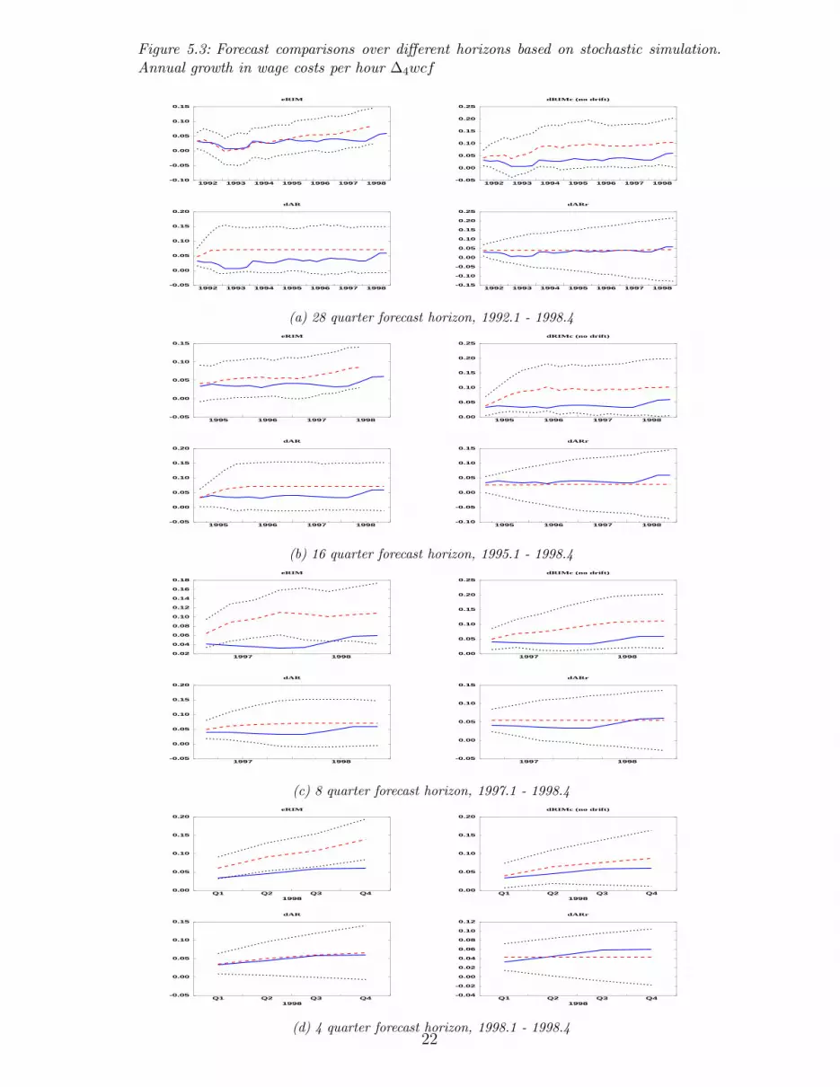
Figure 5.3: Forecast comparisons over different horizons based on stochastic simulation.Annual growth in wage costs per hour ∆4wcf

1992 1993 1994 1995 1996 1997 1998-0.10

-0.05

0.00

0.05

0.10

0.15

eRIM

1992 1993 1994 1995 1996 1997 1998-0.05

0.00

0.05

0.10

0.15

0.20

0.25

dRIMc (no drift)

1992 1993 1994 1995 1996 1997 1998-0.05

0.00

0.05

0.10

0.15

0.20

dAR

1992 1993 1994 1995 1996 1997 1998-0.15

-0.10

-0.05

0.00

0.05

0.10

0.15

0.20

0.25

dARr


1995 1996 1997 1998-0.05

0.00

0.05

0.10

0.15

eRIM

1995 1996 1997 19980.00

0.05

0.10

0.15

0.20

0.25

dRIMc (no drift)

1995 1996 1997 1998-0.05

0.00

0.05

0.10

0.15

0.20

dAR

1995 1996 1997 1998-0.10

-0.05

0.00

0.05

0.10

0.15

dARr


1997 19980.02

0.04

0.06

0.08

0.10

0.12

0.14

0.16

0.18

eRIM

1997 19980.00

0.05

0.10

0.15

0.20

0.25

dRIMc (no drift)

1997 1998-0.05

0.00

0.05

0.10

0.15

0.20

dAR

1997 1998-0.05

0.00

0.05

0.10

0.15

dARr


Q1 Q2 Q3 Q41998

0.00

0.05

0.10

0.15

0.20

eRIM

Q1 Q2 Q3 Q41998

0.00

0.05

0.10

0.15

0.20

dRIMc (no drift)

Q1 Q2 Q3 Q41998

-0.05

0.00

0.05

0.10

0.15

dAR

Q1 Q2 Q3 Q41998

-0.04

-0.02

0.00

0.02

0.04

0.06

0.08

0.10

0.12

dARr


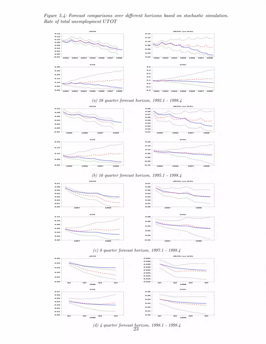
Figure 5.4: Forecast comparisons over different horizons based on stochastic simulation.Rate of total unemployment UTOT

1992 1993 1994 1995 1996 1997 1998-0.02

0.00

0.02

0.04

0.06

0.08

0.10

0.12

0.14

eRIM

1992 1993 1994 1995 1996 1997 19980.02

0.04

0.06

0.08

0.10

0.12

0.14

dRIMc (no drift)

1992 1993 1994 1995 1996 1997 19980.00

0.05

0.10

0.15

0.20

0.25

0.30

dAR

1992 1993 1994 1995 1996 1997 1998-0.2

-0.1

0.0

0.1

0.2

0.3

0.4

0.5

dARr


1995 1996 1997 1998-0.02

0.00

0.02

0.04

0.06

0.08

0.10

eRIM

1995 1996 1997 19980.01

0.02

0.03

0.04

0.05

0.06

0.07

0.08

0.09

dRIMc (no drift)

1995 1996 1997 19980.00

0.05

0.10

0.15

0.20

dAR

1995 1996 1997 1998-0.10

-0.05

0.00

0.05

0.10

0.15

0.20

dARr


1997 19980.00

0.01

0.02

0.03

0.04

0.05

0.06

0.07

eRIM

1997 19980.00

0.01

0.02

0.03

0.04

0.05

0.06

0.07

dRIMc (no drift)

1997 19980.00

0.02

0.04

0.06

0.08

0.10

0.12

dAR

1997 1998-0.02

0.00

0.02

0.04

0.06

0.08

dARr


Q1 Q2 Q3 Q41998

0.00

0.01

0.02

0.03

0.04

0.05

eRIM

Q1 Q2 Q3 Q41998

0.010

0.015

0.020

0.025

0.030

0.035

0.040

0.045

0.050

dRIMc (no drift)

Q1 Q2 Q3 Q41998

0.00

0.01

0.02

0.03

0.04

0.05

0.06

0.07

dAR

Q1 Q2 Q3 Q41998

0.00

0.01

0.02

0.03

0.04

0.05

0.06

dARr


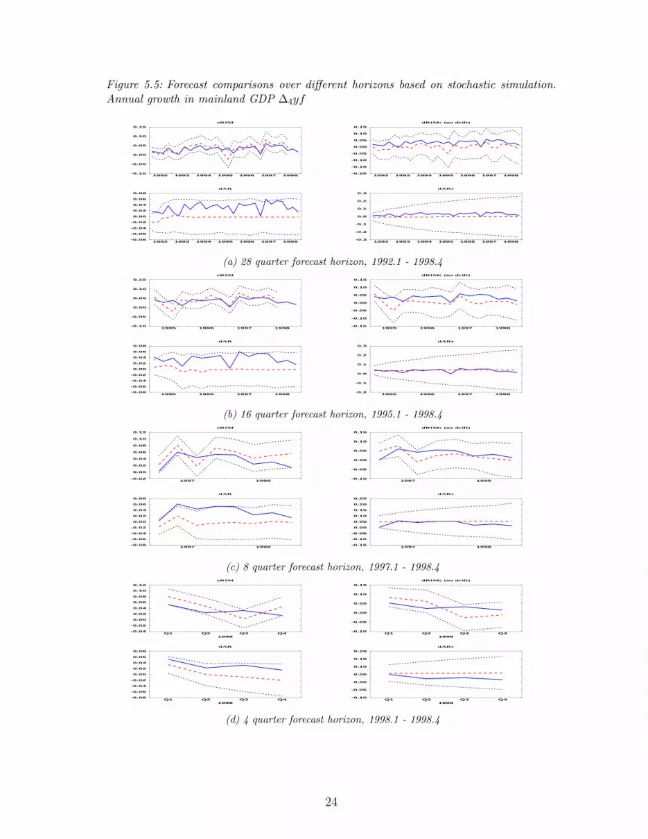
Figure 5.5: Forecast comparisons over different horizons based on stochastic simulation.Annual growth in mainland GDP ∆4yf

1992 1993 1994 1995 1996 1997 1998-0.10

-0.05

0.00

0.05

0.10

0.15

eRIM

1992 1993 1994 1995 1996 1997 1998-0.20

-0.15

-0.10

-0.05

0.00

0.05

0.10

0.15

dRIMc (no drift)

1992 1993 1994 1995 1996 1997 1998-0.08

-0.06

-0.04

-0.02

0.00

0.02

0.04

0.06

0.08

dAR

1992 1993 1994 1995 1996 1997 1998-0.3

-0.2

-0.1

0.0

0.1

0.2

0.3

dARr


1995 1996 1997 1998-0.10

-0.05

0.00

0.05

0.10

0.15

eRIM

1995 1996 1997 1998-0.15

-0.10

-0.05

0.00

0.05

0.10

0.15

dRIMc (no drift)

1995 1996 1997 1998-0.08

-0.06

-0.04

-0.02

0.00

0.02

0.04

0.06

0.08

dAR

1995 1996 1997 1998-0.2

-0.1

0.0

0.1

0.2

0.3

dARr


1997 1998-0.02

0.00

0.02

0.04

0.06

0.08

0.10

0.12

eRIM

1997 1998-0.10

-0.05

0.00

0.05

0.10

0.15

dRIMc (no drift)

1997 1998-0.08

-0.06

-0.04

-0.02

0.00

0.02

0.04

0.06

0.08

dAR

1997 1998-0.15

-0.10

-0.05

0.00

0.05

0.10

0.15

0.20

0.25

dARr


Q1 Q2 Q3 Q41998

-0.04

-0.02

0.00

0.02

0.04

0.06

0.08

0.10

0.12

eRIM

Q1 Q2 Q3 Q41998

-0.10

-0.05

0.00

0.05

0.10

0.15

dRIMc (no drift)

Q1 Q2 Q3 Q41998

-0.08

-0.06

-0.04

-0.02

0.00

0.02

0.04

0.06

0.08

dAR

Q1 Q2 Q3 Q41998

-0.10

-0.05

0.00

0.05

0.10

0.15

0.20

dARr


24

the model with best econometric properties. Hence, model pluralism can be carriedtoo far. An alternative is represented by the encompassing principle and progressiveresearch strategies. In practice this entails a strategy where one tests competingmodels as thoroughly as practically feasible, and keep only the encompassing modelin the suite of models. Our example in section 2 focused on competing models ofthe supply side, the ICM and the Phillips-curve. But several other issues in themodelling of inflation can in principle be tackled along the same line, for examplethe role of rational expectations, and forward looking optimizing behaviour, see e.g.Hendry (1995, chapter 14).

A more specific argument for pluralism stems from the insight that an EqCMis incapable of correcting forecasts sufficiently for the impact of parameter changesthat occur prior to the start of the forecast period. In contrast, a univariate dVARforecast moves back on track once it is conditional on the period when the parameterchange took place. Section 5 of this chapter provided several empirical examples.This supports the view that an EqCM and simple dVARs could constitute a suiteof models for forecasting, where the role of the dVAR is primarily to help interceptcorrect the policy model.

References

Akram, Q. F. (1999). Multiple Unemployment Equilibria—Do Transitory ShocksHave Permanent Effects? Working paper 1999/6, Oslo: Norges Bank.

Bank of England (1999). Economic Models at the Bank of England . Bank of England.

Bardsen, G., and R. Nymoen (2000). Testing steady-state implications of theNAIRU. Unpublished paper, Norges Bank.

Bardsen, G., P. G. Fisher and R. Nymoen (1998). Business Cycles: Real Facts orFallacies? In Strøm, S. (ed.), Econometrics and Economic Theory in the 20th Cen-tury: The Ragnar Frisch Centennial Symposium, no. 32 in Econometric SocietyMonograph Series, chap. 16, 499–527. Cambridge University Press, Cambridge.

Bardsen, G., E. S. Jansen and R. Nymoen (1999). Econometric Inflation Targeting.Working paper 1999/5, Oslo: Norges Bank.

Bjørnstad, R. and R. Nymoen (1999). Wages and Profitability: Norwegian Manu-facturing 1967q1- 1998q2. Working paper 1999/7, Oslo: Norges Bank.

Blanchard, O. J. and L. Katz (1997). What Do We Know and Do Not Know Aboutthe Natural Rate of Unemployment. Journal of Economic Perspectives, 11 , 51–72.

Blanchard, O. J. and L. Katz (1999). Wage Dynamics: Reconciling Theory andEvidence. NBER Working Paper Series 6924, National Bureau of Economic Re-search.

Blanchflower, D. G. and A. J. Oswald (1994). The Wage Curve. The MIT Press,Cambridge, Massachusetts.

Clarida, J. G., Richard and M. Gertler (1999). The Science of Monetary Policy: ANew Keynesian Perspective. Journal of Economic Literature, 37 (4), 1661–1707.

25

Clements, M. P. and D. F. Hendry (1993). On the Limitations of Comparing MeanSquared Forecasts Errors. Journal of Forecasting , 12 , 669–676. (With discussion).

Clements, M. P. and D. F. Hendry (1998). Forecasting Economic Time Series.Cambridge University Press, Cambridge.

Clements, M. P. and D. F. Hendry (1999). Forecasting Non-stationary EconomicTime Series. The MIT Press, Cambridge, MA.

Doornik, J. A. and D. F. Hendry (1996a). GiveWin. An Interface to EmpiricalModelling . International Thomson Publishing, London.

Doornik, J. A. and D. F. Hendry (1996b). Modelling Dynamic Systems Using PcFiml9.0 for Windows. International Thomson Publishing, London.

Dreze, J. and C. R. Bean (1990). Europe’s Unemployment Problem; Introductionand Synthesis. In Dreze, J. and C. R. Bean (eds.), Europe’s Unemployment Prob-lem, chap. 1. MIT Press, Cambridge.

Eitrheim, Ø., T. A. Husebø and R. Nymoen (1999). Error-correction versusdifferencing in macroeconometric forecasting. Economic Modelling , 16 , 515–544.

Eitrheim, Ø. and R. Nymoen (1991). Real wages in a multisectoral model of theNorwegian economy. Economic Modelling , 8 (1), 63–82.

Engle, R. F., D. F. Hendry and J.-F. Richard (1983). Exogeneity. Econometrica,51 , 277–304.

Fuhrer, J. C. (1995). The Phillips Curve is Alive and Well. New England EconomicReview , 41–56.

Gali, J. and M. Gertler (1999). Inflation Dynamics: A Structural EconometricAnalysis. Journal of Monetary Economics, 44 (2), 233–258.

Gordon, R. J. (1997). The Time-Varying NAIRU and its Implications for EconomicPolicy. Journal of Economic Perspectives, 11 (1), 11–32.

Granger, C. W. J. (1990). General Introduction: Where are the Controversies inEconometric Methodology? In Granger, C. W. J. (ed.), Modelling Economic Se-ries. Readings in Econometric Methodology , 1–23. Oxford University Press, Ox-ford.

Granger, C. W. J. and P. Newbold (1986). Forecasting Economic Time Series.Academic Press, San Diego.

Hendry, D. F. (1995). Dynamic Econometrics. Oxford University Press, Oxford.

Hoel, M. and R. Nymoen (1988). Wage Formation in Norwegian Manufacturing. AnEmpirical Application of a Theoretical Bargaining Model. European EconomicReview , 32 , 977–997.

Johansen, K. (1995). Norwegian Wage Curves. Oxford Bulletin of Economics andStatistics, 57 , 229—247.

26

King, M. (1998). Mr King Explores Lessons from the UK Labour Market. BISReview , (103).

Kolsrud, D. and R. Nymoen (1998). Unemployment and the Open Economy Wage-Price Spiral. Journal of Economic Studies, 25 , 450–467.

Layard, R. and S. Nickell (1986). Unemployment in Britain. Economica, 53 , 121–166. Special issue.

Nymoen, R. (1989a). Modelling Wages in the Small Open Economy: An Error-Correction Model of Norwegian Manufacturing Wages. Oxford Bulletin of Eco-nomics and Statistics , 51 , 239–258.

Nymoen, R. (1989b). Wages and the Length of the Working Day. An EmpiricalTest Based on Norwegian Quarterly Manufacturing Data. Scandinavian Journalof Economics , 91 , 599–612.

OECD (1997). Employment Outlook . No. July 1997. OECD.

Rødseth, A. and R. Nymoen (1999). Nordic Wage Formation and UnemploymentSeven Years Later. Memorandum 10/99, Department of Economics, University ofOslo.

Rowlatt, P. A. (1987). A model of wage bargaining. Oxford Bulletin of Economicsand Statistics , 49 , 347–372.

Sargan, J. D. (1964). Wages and Prices in the United Kingdom: A Study of Econo-metric Methodology. In Hart, P. E., G. Mills and J. K. Whitaker (eds.), Economet-ric Analysis for National Economic Planning , 25–63. Butterworth Co., London.

Sgherri, S. and K. F. Wallis (1999). Inflation Targetry and the Modelling of Wagesand Prices. Mimo ESRC Macroeconomic Modelling Bureau, University of War-wick.

Svensson, L. E. O. (1997a). Exchange Rate Target or Inflation Target for Norway?In Christiansen, A. B. and J. F. Qvigstad (eds.), Choosing a Monetary PolicyTarget , chap. 7, 121–138. Scandinavian University Press, Oslo.

Svensson, L. E. O. (1997b). Inflation Forecast Targeting: Implementing and Moni-toring Inflation Targets. European Economic Review , 41 , 1111–1146.

Svensson, L. E. O. (2000). Open Economy Inflation Targeting. Journal of Interna-tional Economics , 50 , 155–183.

Wallis, K. F. (1993). On Macroeconomic Policy and Macroeconomic Models. TheEconomic Record , 69 , 113–130.

27

empirical comparison of inflation models' forecast accuracy

Documents