robust inflation-forecast-based rules to shield against indeterminacy

Robust Inflation-Forecast-Based Rules to Shield

against Indeterminacy∗

Nicoletta Batini

International Monetary Fund

Alejandro Justiniano

International Monetary Fund

Paul Levine

University of Surrey

Joseph Pearlman

London Metropolitan University

June 24, 2004

Abstract

We estimate several variants of a linearized form of a New Keynesian model using

quarterly US data. Using these rival models and the estimated posterior probabilities

we then design rules that are robust in two senses: ‘weakly robust’ rules are guaranteed

to be stable and determinate in all the possible variants of the model, whereas ‘strongly

robust’ rules, in addition, use the probabilities to minimize an expected loss function

of the central bank subject to this model uncertainty. We find three main results.

First, in our two model variants with the highest posterior model probabilities there

are substantial stabilization gains from commitment. Second, an optimized inflation

targeting rule feeding back on current inflation will result in a unique stable equilibrium

and realize at least three-quarters of these potential gains, even if it is used in a variant

of the model that is not the one for which it was designed. Third, the performance

of optimimized inflation targeting rules perform increasing less well as the forward

horizon increases from j = 0 to j = 1, 2 quarters. For j=2, only a rule designed for

our most indeterminacy-prone model is weakly robust and yields determinacy across

all models. A strongly robust rule can be designed that sacrifices performance in the

least probable models for better performance in the most probable models.

JEL Classification: E52, E37, E58

Keywords: robustness, Taylor rules, inflation-forecast-based rules, indeterminacy

∗This paper is preliminary and should not be quoted without the permission of the authors. Views

expressed in this paper do not reflect those of the IMF.

Contents

1 Introduction 1

2 Recent Related Literature 3

3 The Model 3

3.1 Households . . . . . . . . . . . . . . . . . . . . . . . . . . . . . . . . . . . . 4

3.2 Firms . . . . . . . . . . . . . . . . . . . . . . . . . . . . . . . . . . . . . . . 5

3.3 Equilibrium . . . . . . . . . . . . . . . . . . . . . . . . . . . . . . . . . . . . 6

3.4 Linearization and State Space Representation . . . . . . . . . . . . . . . . . 7

3.5 Estimation . . . . . . . . . . . . . . . . . . . . . . . . . . . . . . . . . . . . 8

3.5.1 Overview . . . . . . . . . . . . . . . . . . . . . . . . . . . . . . . . . 8

3.5.2 Methodology . . . . . . . . . . . . . . . . . . . . . . . . . . . . . . . 9

3.5.3 Data and Priors . . . . . . . . . . . . . . . . . . . . . . . . . . . . . 10

3.5.4 Estimation Results . . . . . . . . . . . . . . . . . . . . . . . . . . . . 12

3.5.5 Model Comparison . . . . . . . . . . . . . . . . . . . . . . . . . . . 14

4 The Stability and Determinacy of IFB Rules 15

4.1 Theory . . . . . . . . . . . . . . . . . . . . . . . . . . . . . . . . . . . . . . . 15

4.2 The Likelihood of Indeterminacy . . . . . . . . . . . . . . . . . . . . . . . . 25

5 Optimal Policy and Optimized IFB Rules without Model Uncertainty 25

5.1 Optimal Policy with and without Commitment . . . . . . . . . . . . . . . . 27

5.2 Optimized IFB Rules . . . . . . . . . . . . . . . . . . . . . . . . . . . . . . . 28

6 Robust Rules with Model Uncertainty 35

6.1 Theory . . . . . . . . . . . . . . . . . . . . . . . . . . . . . . . . . . . . . . . 35

6.2 Robust Rules Across Three Rival Models . . . . . . . . . . . . . . . . . . . 37

7 Conclusions 38

A Computation of Policy Rules 43

A.1 The Optimal Policy with Commitment . . . . . . . . . . . . . . . . . . . . . 43

A.2 The Dynamic Programming Discretionary Policy . . . . . . . . . . . . . . . 45

A.3 Optimized Simple Rules . . . . . . . . . . . . . . . . . . . . . . . . . . . . . 46

A.4 The Stochastic Case . . . . . . . . . . . . . . . . . . . . . . . . . . . . . . . 47

B Estimation Results 48

1 Introduction

”Uncertainty is not just an important feature of the monetary policy landscape; it is the

defining characteristic of that landscape.” Alan Greenspan1

This paper adopts a consistently Bayesian approach to the measurement of uncertainty

and the design of robust rules for the conduct of monetary policy. Employing a New Key-

nesian model, the source of uncertainty in our paper concerns the structural parameters

and the volatility of the white noise disturbances. We estimate several variants of a lin-

earized form of the model using quarterly US data. From these competing specifications

we obtain estimates for posterior model probabilities. Using these rival models and the

estimated probabilities we then design rules that are robust in two senses: ‘weakly ro-

bust’ rules are guaranteed to be stable and determinate in all the possible variants of the

model whereas ‘strongly robust’ rules, also guarantee stable and unique equilibria and, in

addition, use the probabilities to minimize an expected loss function of the central bank

subject to this model uncertainty.

Our approach thus differs from existing work on the design of robust policy rules in

two important respects. First, existing work typically posits uncertainty by arbitrarily

calibrating the relative probability of alternative models being true representations of the

economy (see for example Angeloni et al. (2003); Coenen (2003)). This paper provides a

first attempt to quantify and at the same time utilize estimated measures of uncertainty

for the design of robust rules. Second we examine robust policy in a unified framework

that compares different simple rules with each other, and with their optimal counterparts.

Throughout we focus on Taylor-type rules, and in particular on inflation-forecast-based

(IFB) rules. These are ‘simple’ rules as in Taylor (1993), but where the policy instrument

responds to deviations of expected, rather than current inflation from target. In most

applications, the inflation forecasts underlying IFB rules are taken to be the endogenous

rational-expectations forecasts conditional on an intertemporal equilibrium of the model.

These rules are of specific interest because similar reaction functions are used in the

Quarterly Projection Model of the Bank of Canada (see Coletti et al. (1996)), and in

the Forecasting and Policy System of the Reserve Bank of New Zealand (see Black et al.

(1997)) – two prominent inflation targeting central banks. As shown in Clarida et al.

1Federal Reserve Bank of Kansas (2003), Opening Remarks.

1

(2000) and Castelnuovo (2003), estimates of IFB-type rules appear to be a good fit to

the actual monetary policy in the US and Europe of recent years.) However, with IFB

rules indeterminacy can be particularly severe and can take two forms: if the response of

interest rates to a rise in expected inflation is insufficient, then real interest rates fall thus

raising demand and confirming any exogenous expected inflation. But indeterminacy is

also possible if the rule is overly aggressive (Bernanke and Woodford (1997); Batini and

Pearlman (2002); Giannoni and Woodford (2002); Batini et al. (2004), BLP hereafter).

We find three main results. First, in our two model variants with the highest posterior

model probabilities there are substantial stabilization gains from commitment. This is

measured for each model by comparing the expected loss from the optimal policies with

and without commitment. We assess this gain to be between a 3.6% to 9.4% equivalent

permanent increase in output. Second, an optimized inflation targeting rule feeding back

on current inflation will result in a unique stable equilibrium and realize at least three-

quarters of these potential gains even if the implemented rule is designed for the wrong

model. Current inflation rules, in other words, are robust in both the weak and strong

sense. Third, the optimized inflation targeting rules perform increasing less well as the

forward horizon increases from j = 0 (the current inflation rule) to j = 1, 2 quarters.

Denoting such a rule by IFBj, we find a qualitative difference between IFB1 and IFB2

rules. For IFB1 optimal rules, a rule designed for the wrong model is still weakly robust,

but for IFB2 optimal rules this is no longer the case. Then only a rule designed for

our most indeterminacy-prone model is weakly robust and yields determinacy across all

models. In both cases a strongly robust rule can be designed that sacrifices performance

in the least probable models for better performance in the most probable models.

The rest of the paper is organized as follows. Section 2 sets out a New Keynesian

model which, in its most general form, exhibits persistence in both inflation and output.

Sections 4 examines the indeterminacy problem of IFB rules using the root locus method

employed by Batini and Pearlman (2002) and BLP. This analysis indicates which features

of the model make it indeterminacy-prone. Section 5 first focuses on IFB and optimal

rules without uncertainty before we turn to the robust policy problem in section 6. A final

section 7 provides conclusions. The general solution solution procedures for computing

the optimal rules are set out in an Appendix.

2

2 Recent Related Literature

Not surprisingly other approaches to policy design with uncertainty are found in a rapidly

growing literature. Hansen and Sargent (2002) (henceforth H&S) adopt a minmax frame-

work with three key ingredients that distinguishes it from alternatives. First, it conducts

‘local analysis’ in the sense that it assumes that the true model is known only up to some

local neighborhood of models that surround the ‘approximating’ or ‘core’ model. Second,

it uses a minmax criterion without priors in model space. Third, the type of uncertainty is

both unstructured and additive being reflected in additive shock processes that are ‘chosen’

by malevolent nature to feed back on state variables so has to maximize the loss function

the policy-maker is trying to minimize. Another strand retains the minmax framework

but assumes bounded uncertainty about the values of certain parameters in the model

(Giannoni (2002), Gaspar and Smets (2002), Angeloni et al. (2003)). Tetlow and von zur

Muehlen (2002) provides a comparison of the H&S unstructured model uncertainty and

the latter structured approaches. Walsh (2003) provides a useful overview of the literature

and and carries out a number of policy exercises using a similar New Keynesian model

to that in our paper. First, he assesses Taylor rules and first difference rules when target

variables in these rules can only be measured imperfectly. Second, he examines ‘robust,

optimal, explicit instrument rules’ proposed by Giannoni and Woodford (2002) and Svens-

son and Woodford (1999) that are robust in the sense of being independent of both the

variance-covariance structure of the white-noise disturbances and the serial correlation of

the disturbances. Third, he implements the H&S robust control procedure. The conclu-

sions most relevant to our paper are that uncertainty about the output gap suggests using

a first difference rule, and that parameter uncertainty has no general implications for the

size of the feedback coefficients in the optimized simple rules.

3 The Model

Our model is the closed economy version of BLP. There is one traded risk-free nominal

bond. A final homogeneous good is produced competitively using a CES technology con-

sisting of a continuum of differentiated non-traded goods. Intermediate goods producers

and household suppliers of labor have monopolistic power. Nominal prices of intermediate

3

goods, are sticky. We incorporate a bias for consumption of home-produced goods, habit

formation in consumption, and Calvo price setting with indexing of prices for those firms

who, in a particular period, do not re-optimize their prices. The latter two aspects of the

model follow Christiano et al. (2001) and, as with these authors, our motivation is an em-

pirical one: to generate sufficient inertia in the model so as to enable it, in calibrated form,

to reproduce commonly observed output, inflation and nominal interest rate responses to

exogenous shocks.

Our model is stochastic with two exogenous AR(1) stochastic processes for total factor

productivity in the intermediate goods sector and government spending.

3.1 Households

A representative household r maximizes

E0

∞∑

t=0

βt

(Ct(r) − Ht)1−σ

1 − σ+ χ

(

Mt(r)Pt

)1−ϕ

1 − ϕ− κ

Nt(r)1+φ

1 + φ+ u(Gt)

(1)

where Et is the expectations operator indicating expectations formed at time t, Ct(r) is

an index of consumption, Nt(r) are hours worked, Ht represents the habit, or desire not

to differ too much from other consumers, and we choose it as Ht = hCt−1, where Ct is

the average consumption index and h ∈ [0, 1). When h = 0, σ > 1 is the risk aversion

parameter (or the inverse of the intertemporal elasticity of substitution)2. Mt(r) are end-

of-period nominal money balances and u(Gt) is the utility from exogenous real government

spending Gt.

The representative household r must obey a budget constraint:

PtCt(r) + Dt(r) + Mt(r) = Wt(r)Nt(r) + (1 + it−1)Dt−1(r) + Mt−1(r) + Γt(r) − Ptτt (2)

where Pt is a price index, Dt(r) are end-of-period holdings of riskless nominal bonds with

nominal interest rate it over the interval [t, t + 1]. Wt(r) is the wage, Γt(r) are dividends

from ownership of firms and τt are lump-sum real taxes. In addition, if we assume that

households’ labour supply is differentiated with elasticity of supply η, then (as we shall

see below) the demand for each consumer’s labor is given by

Nt(r) =

(

Wt(r)

Wt

)

−η

Nt (3)

2When h 6= 0, σ is merely an index of the curvature of the utility function.

4

where Wt =[

∫ 10 Wt(r)

1−ηdr] 1

1−ηis an average wage index and Nt =

∫ 10 Nt(r)dr is aggre-

gate employment.

Maximizing (1) subject to (2) and (3) and imposing symmetry on households (so that

Ct(r) = Ct, etc) yields standard results:

1 = β(1 + it)Et

[

(

Ct+1 − Ht+1

Ct − Ht

)

−σ Pt

Pt+1

]

(4)

(

Mt

Pt

)

−ϕ

=(Ct − Ht)

−σ

χPt

[

it1 + it

]

(5)

Wt

Pt=

κ

(1 − 1η )

Nφt (Ct − Ht)

σ (6)

(4) is the familiar Keynes-Ramsey rule adapted to take into account of the consumption

habit. In (5), the demand for money balances depends positively on consumption relative

to habit and negatively on the nominal interest rate. Given the central bank’s setting of

the latter, (5) is completely recursive to the rest of the system describing our macro-model

and will be ignored in the rest of the paper. (6) reflects the market power of households

arising from their monopolistic supply of a differentiated factor input with elasticity η.

3.2 Firms

Competitive final goods firms use a continuum of non-traded intermediate goods according

to a constant returns CES technology to produce aggregate output

Yt =

(∫ 1

0Yt(m)(ζ−1)/ζdm

)ζ/(ζ−1)

(7)

where ζ is the elasticity of substitution. This implies a set of demand equations for each

intermediate good m with price Pt(m) of the form

Yt(m) =

(

Pt(m)

Pt

)

−ζ

Yt (8)

where Pt =[

∫ 10 Pt(m)1−ζdm

] 11−ζ

. Pt is an aggregate intermediate price index, but since

final goods firms are competitive and the only inputs are intermediate goods, it is also the

domestic price level.

In the intermediate goods sector each good m is produced by a single firm m using

only differentiated labour with another constant returns CES technology:

Yt(m) = At

(∫ 1

0Ntm(r)(η−1)/ηdr

)η/(η−1)

(9)

5

where Ntm(r) is the labour input of type r by firm m and At is an exogenous shock

capturing shifts to trend total factor productivity (TFP) in this sector. Minimizing costs∫ 10 Wt(r)Ntm(r)dr and aggregating over firms leads to the demand for labor as shown in

(3). In a equilibrium of equal households and firms, all wages adjust to the same level Wt

and it follows that Yt = AtNt.

For later analysis it is useful to define the real marginal cost as the wage relative to

domestic producer price. Using (6) and Yt = AtNt this can be written as

MCt ≡Wt

AtPt=

κ

(1 − 1η )At

(

Yt

At

)φ

(Ct − Ht)σ (10)

Now we assume that there is a probability of 1 − ξ at each period that the price of

each intermediate good m is set optimally to P 0t (m). If the price is not re-optimized,

then it is indexed to last period’s aggregate producer price inflation.3 With indexation

parameter γ ≥ 0, this implies that successive prices with no reoptimization are given

by P 0t (m), P 0

t (m)(

Pt

Pt−1

)γ, P 0

t (m)(

Pt+1

Pt−1

)γ, ... . For each intermediate producer m the

objective is at time t to choose Pt(m) to maximize discounted profits

Et

∞∑

k=0

(

ξ

1 + it

)k

Yt+k(m)

[

P 0t (m)

(

Pt+k−1

Pt−1

)γ

− Wt+k

At

]

(11)

given it (since firms are atomistic), subject to (8). The solution to this is

Et

∞∑

k=0

(

ξ

1 + it

)k

Yt+k(m)

[

P 0t (m)

(

Pt+k−1

Pt−1

)γ

− 1

(1 − 1/ζ)

Wt+k

At

]

= 0 (12)

and by the law of large numbers the evolution of the price index is given by

P 1−ζt+1 = ξ

(

Pt

(

Pt

Pt−1

)γ)1−ζ

+ (1 − ξ)(P 0t+1)

1−ζ (13)

3.3 Equilibrium

In equilibrium, goods markets, money markets and the bond market all clear. Equating

the supply and demand of the consumer good we obtain

Yt = ANt = Ct + Gt (14)

3Thus we can interpret 11−ξ

as the average duration for which prices are left unchanged.

6

A balanced budget government budget constraint

Gt = τt +Mt − Mt−1

Pt(15)

completes the model. Given interest rates i (expressed later in terms of an optimal or IFB

rule) the money supply is fixed by the central banks to accommodate money demand. By

Walras’ Law we can dispense with the bond market equilibrium condition and therefore

the government budget constraint that determines taxes τt. Then the equilibrium defined

at t = 0 as stochastic processes Ct, Dt, Pt, Mt, Wt, Yt, Nt, given past price indices and

exogenous TFP and government spending processes.

3.4 Linearization and State Space Representation

We now linearize about the deterministic zero-inflation steady state. Output is then at its

sticky-price, imperfectly competitive natural rate and from the Keynes-Ramsey condition

(4) the nominal rate of interest is given by ı = 1β − 1. Now define all lower case variables

as proportional deviations from this baseline steady state.4

Then the linearization takes the form:

πt =β

1 + βγEtπt+1 +

γ

1 + βγπt−1 +

(1 − βξ)(1 − ξ)

(1 + βγ)ξmct (16)

mct = −(1 + φ)at +σ

1 − h(ct − hct−1) + φyt (17)

ct =h

1 + hct−1 +

1

1 + hEtct+1 −

1 − h

(1 + h)σ(it − Etπt+1) (18)

yt =C

Yct +

G

Ygt (19)

gt = ρggt−1 + ǫgt (20)

at = ρaat−1 + ǫat (21)

Variables yt, ct, mct, at, gt are proportional deviations about the steady state. πt and it

are absolute deviations about the steady state.5 For later use we require the output gap

the difference between output for the sticky price model obtained above and output when

4That is, for a typical variable Xt, xt = Xt−X

X≃ log

(

Xt

X

)

where X is the baseline steady state. The

interest rate however is now expressed as an absolute deviation about i.5Note that (20) and (18) imply an IS curve given by yt −

h1+h

yt−1 − 11+h

Etyt+1 − sg(gt −h

1+hgt−1 −

11+h

Etgt+1) +(1−h)(1−sg)

(1+h)σ(it − Etπt+1) = 0 where sg = G

Y.

7

prices are flexible, ynt say. The latter, obtained by putting ξ = 0 into (16) to (19), is in

deviation form given by6:

σ

1 − h(cnt − hcn,t−1) + φynt = (1 + φ)at (22)

ynt =C

Ycnt +

G

Ygt (23)

We can write this system in state space form as

zt+1

Etxt+1

= A

zt

xt

+ Bit + C

ǫgt+1

ǫat+1

(24)

yt

ynt

= E

zt

xt

(25)

where zt = [at, gt, ct−1, cn,t−1, πt−1] is a vector of predetermined variables at time t and

xt = [ct, πt] are non-predetermined variables. Rational expectations are formed assuming

an information set zs, xs, s ≤ t, the model and the monetary rule.

3.5 Estimation

3.5.1 Overview

In this section we estimate four main variants of model (16)-(21) using Bayesian methods.

In particular, we estimate: the most general specification of the model with both inflation

and habit persistence(we label this variant ’Z’); a version of the model without inflation

persistence but with persistence in habits (γ = 0, we label this variant ’G’); a version

without habit persistence but with persistence in inflation (h = 0, we label this variant

’H’); and finally a version with neither inflation nor habit persistence (γ = h = 0, we label

this variant ’GH’). We close the model with a 1-quarter ahead IFB rule of the form (29)

that is the subject of the next section.

Bayesian estimation of the model has the specific advantage that it provides a posterior

distribution of the parameter values that allows us to make probabilistic statements about

the functionals of the model(s)’ parameters. Furthermore, it provides us with the odds

on models that allow us to quantify how likely itis the data would have come from a

model with both habit and inflation persistence as opposed to a framework with just one

6Note that the zero-inflation steady states of the sticky and flexi-price steady states are the same.

8

of these mechanisms or neither. In this sense the estimation method per se supplies us

with a consistent measure of both parameter (posterior distribution of the parameters)

and model (posterior odds) uncertainty.7

The idea here is to utilize both measures of uncertainty in the construction of a policy

rule that, in the presence of such uncertainty, is robust in both the weak and strong

senses.8 The derivation of robust rules using consistent measures of parameter and model

uncertainty directly from estimation of the model thus advances upon existing studies

on the design of robust rules that instead ’calibrated’ uncertainty in an ad hoc fashion

(see, for example, Levin et al. (2001); Rudebusch (2002); Angeloni et al. (2003); Coenen

(2003).

The sub-sections below offer: a brief sketch of the methods used in estimation (Subsec-

tion 3.5.2); a discussion of the specification of the prior distributions (Sub-section 3.5.3);

the results from the estimation of our four model specifications (Sub-section 3.5.4); and

a formal comparison of models (Sub-section 3.5.5). This sub-section shows how we ob-

tain the posterior model probabilities that we use as weights for the competing model

specifications in the analysis of robust IFB rules under uncertainty.

3.5.2 Methodology

Each model indexed by k and denoted mk, has an associated set of unknown parameters

ωk ∈ Ωk. Following a Bayesian approach, our aim is to characterize the posterior distri-

bution of the models’ parameters, p(

ωk|Y T , mk

)

,where Y T stands for the full sample of

observed data (T denotes the number of observations). Having specified a (perhaps model

specific) prior density, p(ωk|mk), the posterior of the parameters is given by

p(

ωk|Y T , mk

)

=L

(

ωk|Y T , mk

)

p(ωk|mk)∫

L (ωk|Y T , mk) p(ωk|mk)dωk(26)

where L(

ωk|Y T , mk

)

is the likelihood obtained under the assumption of normally dis-

tributed disturbances from the state-space representation implied by the solution of the

7Justiniano and Preston (2004) discuss the many additional advantages of using Bayesian methods to

estimate dynamic stochastic general equilibrium models. These include overcoming convergence problems

with numerical routines to maximize the likelihood as well as providing measures of uncertainty that need

not assume a symmetric distribution.8This paper for now only provides results for robustness with respect to model uncertainty. Current

research is investigating robustness with respect to parameter uncertainty.

9

linear rational expectations model. The denominator in equation (26) corresponds to the

marginal likelihood (also known as the ‘marginal data density’) and, as explained later,

plays a key role in model comparisons.

The solution of the model is a non-linear function of the parameters which does not

allow for any closed-form expression for the posterior density. Furthermore, the high-

dimensionality of the parameters space renders numerical integration inefficient. Markov

Chain Monte Carlo (MCMC) methods, however, provide a feasible and accurate approxi-

mation to this density.

Following Schorfheide (2000) the estimation follows a two step approach. In the first

step, a numerical algorithm is used to approximate the posterior mode by combining the

likelihood L(Y T |ωk, mk) with the prior. In the second step, the obtained posterior mode is

then used as starting value (ω0k) for a Random Walk Metropolis algorithm that generates

draws from the posterior p(ωk|Y T , mk). At each step i of the Markov Chain, the proposal

density used to draw a new candidate parameter ω∗

k is a normal centered at the current

state of the chain, N(ωik, cΣk). A new draw is then accepted with probability

α = min(1,L(Y T |ω∗

k, mk)p(ω∗

k|mk)

L(Y T |ωik, mk)p(ωi

k|mk))

If accepted, ωi+1k = ω∗

k; otherwise, ωi+1k = ωı

k. We generate chains of 130,000 draws in

this manner discarding the first 30,000 iterations.9

Point estimates of the parameters ωk can be obtained from the generated values by

using various location measures, such as mean or, as in this paper, medians. Similarly,

measures of uncertainty follow from computing the percentiles of the draws.

3.5.3 Data and Priors

We estimate the model(s) using quarterly US data on real GDP (detrended–as standard

in the literature we detrend this using a Hodrick-Prescott filter, see Lubik and Schorfheide

(2003), Juillard et al. (2004)), the Federal Funds rate (annualized, in percentage points),

and the annualized log difference of the consumer price index (CPI) for the sample 1984:I-

9This initial burn-in phase is intended to remove any dependence of the chain from its starting values.

10

2003:IV.10 All series were obtained from DataStream International.

Following Lubik and Schorfheide (2004) rather than de-meaning the series, we estimate

the mean of inflation and the (unobservable) real interest rate, π∗ and r∗ respectively,

together with the model(s) parameters. In turn, this gives the following mapping between

observables (superscript obs) and the variables following the solution of the model.

πobst

yobst

iobst

=

π∗

0

π∗ + r∗

+

4 0 0

0 1 0

0 0 4

πt

yt

it

In addition, the mean of the real rate gives us an estimate of the discount factor

β = 1/ 0.25

√

1 + r∗

100 .

To proceed with the Bayesian estimation we need a prior distribution for the param-

eters. Details on our priors are presented in Table 1 in Appendix B reporting the type

of density, mean and standard deviation for each coefficient.11 The last two columns also

provide the 1% and 99% percentiles of the prior ordinates. In choosing these densities we

considered the entire spectrum of prior existing empirical estimates or calibrations. As a

result, some of our priors are more widely dispersed, and therefore less tight than those

chosen by other authors. 12

The degree of habit formation (h), price indexation (γ) and interest smoothing in the

IFB-type rule (ρ), as well as the autoregressive coefficients of the shocks (ρg and ρa) are all

constrained to the unit interval, motivating our choice of Beta densities for these priors.

The priors for h and γ are centered at 0.7, on the assumption that output and inflation

are considerably inertial, in line with findings by Fuhrer and Moore (1995), Fuhrer (2000),

Banerjee and Batini (2003, 2004) and Smets and Wouters (2004)(SW, 2004), among others.

Likewise, our prior for the mean of ρ is rather high and close to the estimates from Clarida

et al. (2000) (CGG,2000).

10Eight observations, corresponding to the perior 1982:I - 1983:IV are used to intialize

the Kalman filter.11In principle, is would be possible to specify flat or non-informative priors for estimating θk. However,

in addition to being able to choose priors based on coefficients values available in the literature, flat priors

are not well suited for model comparisons.12Throughout the estimation of different models, the share of government expenditures in output is

calibrated at 0.22,which represents the sample average of this coefficient for our sample.

11

Priors for σ and φ are shaped in the form of a Gamma density and are chosen to be

fairly flat, reflecting the wide dispersion of existing empirical estimates and calibrations

of these parameters in the literature. (see Nelson and Nikolov (2002)).

The slope of the Phillips’ curve, λ = (1−βξ)(1−ξ)(1+βγ)ξ is a function of the degree of price

stickiness in the economy, ξ, and the discount factor. So we selected the prior for λ in

line with the assumption that the quarterly discount factor is equal to 0.99 and prices are

sticky for three quarters, as suggested by survey evidence on the average duration of US

price contracts (see, for example, Blinder et al. (1998).13

Finally, the prior for θ accounts for the breadth of the spectrum of estimated responses

to expected inflation by the US Federal Reserve. More specifically, our specification con-

tains the 90% posterior intervals of Lubik and Schorfheide (2004)14 and it is fairly looser

than the prior specified by SW for the same parameter.15

3.5.4 Estimation Results

Table 2, Appendix B, summarizes the results of estimating the four model variants

(G,H,GH and Z). The three columns for each specification report the median, 1st and

9th decile of the 100,000 draws generated using the Random Walk-Metropolis algorithm

used to approximate the posterior densities.

A few important things emerge from the table. First, estimates of the policy coefficients

are fairly robust across specifications. Posterior estimates of ρ are tightly concentrated

on values that suggest a substantial degree of interest smoothing, in accordance with

results reported by CGG amongst other authors. Meanwhile, the posterior density for

θ is remarkably similar (that is both in medians and percentiles) across the first three

specifications, implying a very aggressive response by the US Federal Reserve to expected

13It is worth noting that the results of the estimation from assuming a prior directly on the Calvo

coefficient ξ are somewhat different. This may be because with a prior on lambda, as we have used now,

the link between ξ and the discount factor in determining the slope of the PC is not imposed. We plan to

re-run the estimation with this alternative prior as a robustness check.14Note that in contrast to these authors however we constrain the estimation to the region of determinacy

and therefore truncate the prior for θ. The results of their paper suggest, however, that at least for a Taylor

rule on current inflation, indeterminacy has not been an issue for our sample. In light of the results in

BLP, exploring whether their results extend to the estimation of IFB is left for a future project.15 In their paper, however, SW include the output gap in the Taylor rule.

12

inflation, in line with findings by CGG for a similar rule and sample.

The median estimates for r∗ translate into a median value of 0.995 for the stochastic

discount factor which, in turn, implies plausible estimates for the degree of price stickiness

based on the inferred values for λ. The implied point estimates of ξ range from 0.36 up

to 0.67, decreasing, as expected, depending on whether or not price indexation is allowed

for.16 These higher values are in accordance with Blinder et al. (1998) and Rotemberg and

Woodford (1998), but contrast the high degree of price rigidity estimated by SW (2004).

Our estimates of σ are rather large. With no habits, these estimates map directly with

the intertemporal elasticity of substitution and suggest that this may be quite small.17 A

common theme in papers estimating DSGE models is the difficulty in pinning down φ.

Therefore, it is not surprising that, inference on the inverse Frisch elasticity of labor supply

is susceptible to the specification of the model, and exhibits wide posterior probability

intervals.

Turning to the coefficient governing habit formation, h is tightly estimated and suggests

rather inertial consumption and output processes. Reported posterior intervals for h are

almost identical to the ones obtained by Juillard et al. (2004) and higher than the estimates

by SW. By contrast, the posterior density of γ lies to the left of our chosen prior, suggesting,

in contrast to studies mentioned earlier, that inflation is intrinsically not very persistent

– a result that accords with findings in Erceg and Levin (2001), Taylor (2000) and Cogley

and Sargent (2001).

Estimates of the shock processes reveal that both the technology and the government

expenditure shock are highly persistent, and this holds true regardless of the exact model

specification. Posterior estimates clearly attribute greater volatilty of shocks to the gov-

ernment expenditure component rather than to disturbances in technology.18

16Using λ ≡ (1−βξ)(1−ξ)(1+βγ)ξ

we obtain ξ = 0.67, 0.36, 0, 60, 0.53 corresponding to contract lengths, 11−ξ

, of

3.06, 1.57, 2.50 and 2.13 quarters for models G, H, GH and Z respectively.17This result is attributable to a prior density centered on high values for σ. Redoing the estimation

using the SW priors leads to point estimates far closer to one, clearly revealing that inference on this

parameters is sensitive to the choice of priors.18 Indeed, the 1st posterior decile of the former exceeds the 9th decile of the latter, for all models,

despite similar prior densities for the innovation standard deviations. As usual, exogenous disturbances to

the monetary policy equation appear much less important than technology and government expenditure

shocks in driving inflation, consumption and output processes.19

13

3.5.5 Model Comparison

Since the goal of this paper is to characterize the design of robust rules under uncertainty,

it is important to investigate which specification seems to be best supported by the data.

In doing so we do not intend to select any particular model as being the ‘true’ one but

rather wish to compute posterior probabilities to place odds on the different models.

Bayesian methods for model comparisons allows us to obtain these posterior model

probabilities in order to discriminate or aggregate across competing specifications, there-

after providing coefficient estimates that explicitly account for model uncertainty. Let

us define mk to be one possible element from the (discrete) set of competing models

µ = G, H, GH, Z. The posterior model probability for p(mk|Y T ) summarizes the evi-

dence provided by the data in favor of mk and is then given by

p(mk|Y T ) = f(Y T |mk)p(mk)/f(Y T ) (27)

where p(mk) stands for the prior probability assigned to model k, that in our case equals 14

since we treat each model as equiprobable a-priori. The first expression in the numerator is

known as the marginal likelihood (or marginal data density) and was previously presented

as the denominator in equation (26)

f(Y T |mk) =

∫

L(

ωk|Y T , mk

)

p(ωk|mk)dωk (28)

Equation (27) can be conveniently re-written as

p(mk|Y T ) =f(Y T |mk)p(mk)

∑

i∈µ f(Y T |mi)p(mi)

which emphasizes the key role the marginal likelihood plays in constructing odds on mod-

els.20 Computing the marginal likelihood usually requires simulation methods and a num-

ber of proposals in this vein are now available from the statistics literature.21

In this paper, instead we estimate the model probabilities by relying on the Reversible

Jump MCMC algorithm (RJMCMC) of Dellaportas et al. (2002)). This method belongs

20Notice that posterior model probabilities lead directly to the posterior odds that can be used to

compare two models, say mk and mh by updating the prior odds with the Bayes Factor.21 Chib (2000) provides an excellent survey of simulation methods in general and discusses methods for

model comparison

14

to the popular class of product space search algorithms, widely used in the statistic liter-

ature,22 that allow for the joint estimation of the model indicator, mk and parameters ωk

and which do not requiring therefor evaluating the marginal likelihood.23

Estimates of p(mk|Y T ) obtained with the RJMCMC for our four model variants are

presented in Table 3, Appendix B. In line with results discussed above, the specification

with habit persistence and no price indexation (G) attains highest posterior probability.

Model Z that allows for both of these intrinsic mechanisms follows in probability ranking.

In contrast, a model with no habit persistence is 9 times less likely than those specifications

(Z and G) with endogenous persistence in consumption. Finally, the most restrictive

model., GH attains the lowest posterior model probability further providing evidence of

the need to incorporate at least one of the two intrinsic mechanisms imparting greater

inertia to the model. Therefore, these results can be interpreted as suggesting that

the addition of endogenous mechanisms of persistence, particularly habit in consumption,

improve the fit of the model. These posterior odds will be used to weight the models for

our analysis of uncertainty on the robustness of policy rules.

4 The Stability and Determinacy of IFB Rules

4.1 Theory

This section studies an IFB rule of the form

it = ρit−1 + θ(1 − ρ)Etπt+j (29)

22The interest reader is referred to Carlin and Han (2001) for an overview of these methods.23The RJMCMC requires a set of preliminary runs in order to generate a proposal density, V (ωk|mk)

for each model’s parameters To this end we use the 100,000 draws generated for the estimation of the

parameters discussed above and choose V (ωk|mk) to be a normal density, centered at the mean of those

draws and with fatter tails than the posterior. The algorithm then operates over the product space

µ×Πk=1Ωk by drawing , at each step, a candidate model m∗

k from a proposal density J -which in our case

assigns equals probability to all models- drawing ωk from V (ωk|mk) and then accepting or not the jump

to m∗

k with a Metropolis type probability. We generated 200,000 draws in this manner, discard the first

20,000 and then compute the proportion of draws the sampler spent in each model to directly obtain the

model probabilities.

15

where j ≥ 0 is the forecast horizon, which is a feedback on single-period inflation over the

period [t + j − 1, t + j].24

With rule (29), policymakers set the nominal interest rate so as to respond to deviations

of the inflation term from target. In addition, policymakers smooth rates, in line with the

idea that central banks adjust the short-term nominal interest rate only partially towards

the long-run inflation target, which is set to zero for simplicity in our set-up.25 The

parameter ρ ∈ [0, 1) measures the degree of interest rate smoothing. j is the feedback

horizon of the central bank. When j = 0, the central bank feeds back from current

dated variables only. When j > 0, the central bank feeds back instead from deviations

of forecasts of variables from target. Finally, θ > 0 is the feedback parameter: the larger

is θ, the faster is the pace at which the central bank acts to eliminate the gap between

expected inflation and its target value. We now show that, for given degrees of interest rate

smoothing ρ, the stabilizing characteristics of these rules depend both on the magnitude

of θ and the length of the feedback horizon j.

To understand better how the precise combination of the pair (j, θ), IFB rules can lead

the economy into instability or indeterminacy consider the deterministic model economy

(24) and (25) with interest rate rules of the form (29). gt and at are exogenous stable

processes and play no part in the stability analysis. For convenience, we therefore set

them to zero.

Let z be the forward operator. Taking z -transforms of (16), (17), (18) and (29), the

characteristic equation for the system is given by:

(z − ρ)[(z − 1)(z − h)(βz − 1)(z − γ) − λ

µz2(φz + µ(z − h))]

+λθ

µ(1 − ρ)(φz + µ(z − h))zj+2 = 0 (30)

where we have defined λ ≡ (1−βξ)(1−ξ)ξ , φ ≡ C

Yφ and µ ≡ σ

1−h . Equation (30) shows that

the minimal state-space form of the system has dimension max (5, j + 3). Since there are

24To set the model up with this rule in state-space form for j ≤ 1 we simply need to augment the state

vector with a lagged term it−1. For j = 2 replace t with t + 1 in (16)-(17) and take expectations at time

t. Then the state-space presentations remains of the same dimension. For j > 2 replace t with t + j − 1

in (16)-(17) and take expectations at time t. The state vector must then be augmented with Etπt+1 · · ·

Etπt+j−2.25For instance (29) can be written as ∆it = 1−ρ

ρ[θEtπt+j − it] which is a partial adjustment to a static

IFB rule it = θEtπt+j .

16

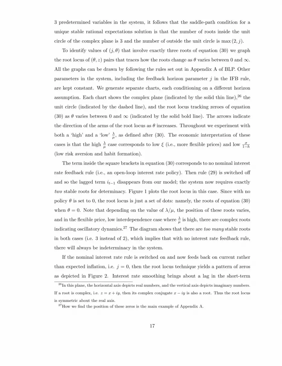
3 predetermined variables in the system, it follows that the saddle-path condition for a

unique stable rational expectations solution is that the number of roots inside the unit

circle of the complex plane is 3 and the number of outside the unit circle is max (2, j).

To identify values of (j, θ) that involve exactly three roots of equation (30) we graph

the root locus of (θ, z) pairs that traces how the roots change as θ varies between 0 and ∞.

All the graphs can be drawn by following the rules set out in Appendix A of BLP. Other

parameters in the system, including the feedback horizon parameter j in the IFB rule,

are kept constant. We generate separate charts, each conditioning on a different horizon

assumption. Each chart shows the complex plane (indicated by the solid thin line),26 the

unit circle (indicated by the dashed line), and the root locus tracking zeroes of equation

(30) as θ varies between 0 and ∞ (indicated by the solid bold line). The arrows indicate

the direction of the arms of the root locus as θ increases. Throughout we experiment with

both a ‘high’ and a ‘low’ λµ , as defined after (30). The economic interpretation of these

cases is that the high λµ case corresponds to low ξ (i.e., more flexible prices) and low σ

1−h

(low risk aversion and habit formation).

The term inside the square brackets in equation (30) corresponds to no nominal interest

rate feedback rule (i.e., an open-loop interest rate policy). Then rule (29) is switched off

and so the lagged term it−1 disappears from our model; the system now requires exactly

two stable roots for determinacy. Figure 1 plots the root locus in this case. Since with no

policy θ is set to 0, the root locus is just a set of dots: namely, the roots of equation (30)

when θ = 0. Note that depending on the value of λ/µ, the position of these roots varies,

and in the flexible price, low interdependence case where λµ is high, there are complex roots

indicating oscillatory dynamics.27 The diagram shows that there are too many stable roots

in both cases (i.e. 3 instead of 2), which implies that with no interest rate feedback rule,

there will always be indeterminacy in the system.

If the nominal interest rate rule is switched on and now feeds back on current rather

than expected inflation, i.e. j = 0, then the root locus technique yields a pattern of zeros

as depicted in Figure 2. Interest rate smoothing brings about a lag in the short-term

26In this plane, the horizontal axis depicts real numbers, and the vertical axis depicts imaginary numbers.

If a root is complex, i.e. z = x + iy, then its complex conjugate x − iy is also a root. Thus the root locus

is symmetric about the real axis.27How we find the position of these zeros is the main example of Appendix A.

17

1−1 1−1

(i) low λ/µ (ii) high λ/µ

Figure 1: Possible position of zeroes when θ = 0

1−1 1−1


ρ ρ

Figure 2: Position of zeroes as θ changes using current inflation

nominal interest rate and the system is now stable if it has exactly three stable roots (as

we now have three predetermined variables in the system). The figure demonstrates that

if θ is sufficiently large, one arm of the root locus starting originally at ρ exits the unit

circle, turning one root from stable to unstable so that there are now three – as required

– instead of four stable roots and the system has a determinate equilibrium. As θ → ∞,

there are roots at ±i∞, two roots at 0, and one at µh/(φ + µ), the latter shown as a

square.

Note that when θ = z = 1, the characteristic equation has the value 0, confirming that

the branch of the root locus moving away from z = ρ crosses the unit circle at a value

θ = 1. Thus we conclude that for a rule feeding back on current inflation, the system

exhibits determinacy if and only if θ > 1. For higher values of j ≥ 1 we can draw the se-

quence of root locus diagrams shown in Figures 3-6, and so confirm the well-known ‘Taylor

18

1−1 1−1


ρ ρ

Figure 3: Position of zeroes as θ changes: 1-period ahead expected inflation

1−1 1−1


ρ ρ

Figure 4: Position of zeroes as θ changes: 2-period ahead expected inflation

Principle’ that interest rates need to react to inflation with a feedback greater than unity.

However for j ≥ 1 our diagrams show that an arm of the root locus re-enters the unit

circle for some high θ > 1 and indeterminacy re-emerges. Therefore θ > 1 is necessary but

not sufficient for stability and determinacy. Our results up to this point are summarized

in proposition 1:

Proposition 1 : For a rule feeding back on current inflation (j = 0), θ > 1 is

a necessary and sufficient condition for stability and determinacy. For higher

feedback horizons (j ≥ 1), θ > 1 is a necessary but not sufficient condition for

stability and determinacy.

Now let θ(j) be the upper critical value of θ for the system for a feedback horizon j.

Figure 3 shows that for the case j = 1, i.e. one-quarter ahead forecasts which corresponds

19

to a case studied by CGG (2000), indeterminacy occurs when this portion of the root

locus enters the unit circle at z = −1.28 The critical upper value for θ = θ(1) when this

occurs is obtained by substituting z = −1 and j = 1 into the characteristic equation (30)

to obtain:

θ(1) =1 + ρ

1 − ρ

[

1 +2(1 + h)(1 + β)(1 + γ)µ

λ(φ + µ(1 + h))

]

(31)

One important thing to note looking at this expression for a 1-period ahead IFB rule

is that the greater is the degree of smoothing captured by the parameter ρ in the interest

rate rule, the larger the maximum permissible value of θ before indeterminacy sets in. In

this sense indeterminacy is less of a potential problem for high ρ. Similarly from (31) the

problem of indeterminacy lessens for high h, γ and σ, and low λ and φ. Notice from the

definition of λ after (30) that low λ is associated with a high degree of price stickiness.

With this is mind we can summarize these results as:

Proposition 2: For a 1-period ahead IFB rule, indeterminacy is less of a prob-

lem if there is a high degree of interest rate smoothing, habit persistence, price

indexing, price stickiness and household risk aversion, and a low elasticity of

disutility with respect to hours worked.

Proceeding on to j-period ahead IFB rules for j ≥ 2 the analysis is more difficult. For

j = 2, Figures 4 shows that indeterminacy occurs when the root locus enters the unit

circle at z = cos(ψ) + isin(ψ) for some ψ ∈ (0, π2 ). All our results up to this point are

analytical using topological reasoning, but now the threshold θ(j) for j ≥ 2 must be found

numerically. Given j, write the characteristic equation as

max(5,j+3)∑

k=1

ak(θ)zk = 0 (32)

noting that some of the ak are dependent on θ. The root locus meets the unit circle at

z = cos(ψ) + isin(ψ). Using De Moivre’s theorem zk = cos(kψ) + isin(kψ) and equating

real and imaginary parts we arrive at two equations which can be solved numerically for

θ and ψ.

As well as locating an upper threshold θ(j), an even more significant result concerning

indeterminacy emerges from Figure 4. This have been drawn in for values of ρ such that

28Thus Figure 3 portrays diagrammatically the result shown analytically by Woodford (2003), chapter

4, that there is a value of θ = θS say, beyond which there is indeterminacy.

20

the two rightmost poles of the root locus are joined by straight lines that meet outside the

unit circle. The implication is that for some values of θ > 1, these yield unstable roots of

the system, and therefore the system will have exactly three stable roots which is what

is required for determinacy. (Note that if the arms of the root locus from ∞ cross the

unit circle before these latter meet, then there may anyway be too many stable roots).

However, for a lower value of ρ it could happen that rather than meeting to the right of

z = 1, the two arms instead meet to the left of z = 1, that is inside the unit circle and

then remain within it, as in figure 5. This would imply that for all θ there are always

more than three stable roots, which would entail, in turn, indeterminacy for all values of

θ. We therefore conclude that there is determinacy for θ slightly greater than 1 if the root

locus passes through z = 1 from the left, as in figures 3 and 4. Conversely, Figure 5 for

the left and middle examples show indeterminacy for all θ if the root locus passes through

z = 1 from the right. However, to be certain that this result is true for all θ, we need to

be able to show that once this arm of the root locus enters the unit circle it never leaves

it, as is the case in the right hand example of Figure 5. The simplest case for which this

‘pathological’ behaviour cannot happen is when h = γ = 0. We can now show:

Proposition 3 : For the general model there is always some lead JS such that

for

j > JS =1

1 − ρ+

(1 − β)(1 − γ)σ

λ(φ + σ)(33)

there is indeterminacy for all values of θ, provided that that the arm of the

root locus from the right is ‘non-pathological’ in the sense that it enters the

unit circle only once. If h = γ = 0 this is true if β > ρ >√

2 − 1 and λ(φ+σ)σ >

(1−β)(1+ρ)(1−ρ)2

ρ2+2ρ−1.

Proof : See BLP, Appendix B.

For h, γ > 0 the derivation of sufficient conditions that rule out pathological behaviour

has proved elusive. However for small values of h, γ, the root locus diagrams correspond

to the ‘low λ/µ’ ones of Figures 2-4, with the inner arms that lie off the real axis becoming

vanishingly small as h, γ tend to 0. By a continuity argument therefore, it follows that the

sufficient conditions of Proposition 3 apply in this case as well for small h, γ. Numerical

experiments indicate that pathological behaviour does not occur for all realistic values of

the parameters. Indeed it is extremely difficult to numerically produce diagrams such as

21

1−1 1−1

(i) low λ (ii) high λ

ρ ρ 1−1

(iii) very low λ

ρ

Figure 5: Position of zeros as θ changes: 3-period ahead expected inflation, and

low ρ

that on the right-hand-side of figure 5. For example with other parameters set at central

values the parameter ξ must exceed 0.9, corresponding the price contracts of 10 quarters

to generate such an example. In addition our calibrated values indicate that the sufficient

conditions in proposition 3 are easily satisfied.

Propositions 1 and 3 confirm, in a rigorous setting, the possibility of real indeterminacy

for any IFB rule with lead j ≥ 1 when the feedback inflation is below unity (the Taylor

principle) and above a threshold θ(j). The root locus diagrams in figures 3 and 4 show

that ¯θ(1) > ¯θ(2), so that indeterminacy becomes more of a problem as j increases from

j = 1 to j = 2. Tables 1a-1f below shows that this deterioration continues for higher j and

eventually, from proposition 2, for high j no IFB rule of the form (29) results in a unique

stable equilibrium. The value of ρ is crucial in determining the critical value of the lead

j beyond which indeterminacy sets in. The lower ρ, the lower the maximum-permitted

inflation horizon the central bank can respond to, and hence, the larger the region of

indeterminacy under IFB rules. Thus the absence of interest rate smoothing has the same

indeterminacy-inducing effect as high j.

In tables 1a parameter values are set as for model G (apart from θ which is calculated

to be the threshold value). Then the numerical calculations for alternative values of

parameters h, γ, λ, σ and φ are repeated in tables 1b-1f. The results show that proposition

2 which applies to 1-period ahead IFB rules only may well carry over to j-period ahead

22

rules as well for changes to h, λ and γ, but not to σ and φ.

j j=1 j=2 j=3 j=4 j ≥ 5

θ(j) 222 23.4 5.2 1.74 indeterminacy

Table 1a. Critical upper bounds for θ(j) for Model G. Parameter values:

h = 0.85, γ = 0, λ = 0.16, σ = 3.29, φ = 1.46.

j j=1 j=2 j=3 j=4 j ≥ 5


Table 1b. Critical upper bounds for θ(j) for Model G but with h = 0.

j j=1 j=2 j=3 j=4 j ≥ 4


Table 1c. Critical upper bounds for θ(j) for Model G but with γ = 0.5.

j j=1 j=2 j=3 j=4 j ≥ 5


Table 1d. Critical upper bounds for θ(j) for Model G but with λ = 1.

j j=1 j=2 j=3 j=4 j ≥ 5


Table 1e. Critical upper bounds for θ(j) for Model G but with σ = 1.

j j=1 j=2 j=3 j=4 j ≥ 4


Table 1c. Critical upper bounds for θ(j) for Model G but with φ = 3.

23

0.2 0.3 0.4 0.5 0.6 0.7 0.8 0.9 10

10

20

30

40

50

60

70

80

90

100

ρ

θ

Regions of Indeterminacy

1 period ahead

2 Periods ahead

3 periods ahead

4 periods ahead

Figure 6: Regions of Indeterminacy for single period inflation rate targets.

0.2 0.3 0.4 0.5 0.6 0.7 0.8 0.9 10

10

20

30

40

50

60

70

80

90

100

ρ

θ

1 period ahead

2 period ahead average



Regions of Indeterminacy

Figure 7: Regions of Indeterminacy for average inflation rate targets.

24

4.2 The Likelihood of Indeterminacy

Figures 6 and 7 show the indeterminacy for parameters ρ and θ based on model G. These

figures are based on 1000 draws of parameter combinations using the estimated parameter

distributions of section 2.5. Regions to the south-west of each contour then represent 100%

confidence regions of determinacy. Figure 6 is drawn for single period IFB rules as in (29)

for j = 1, 2, 3, 4. In figure 7, this is compared with an average IFB rule of the form

it = ρit−1 + θ(1 − ρ)Et

j∑

r=0

πt+r (34)

For both single-period ahead and average period rules, regions of determinacy indicate

combinations of ρ and θ that are weakly robust for all possible non-policy parameter com-

binations in model G. The declining size of this region as the forward horizon j increases

confirms the earlier theoretical results that show that IFB rules with unique and stable

equilibria are increasingly constrained in the choice of (ρ, θ) with a qualitative change

taking place between j = 1 and j = 2.29

5 Optimal Policy and Optimized IFB Rules without Model

Uncertainty

Without model uncertainty, the policy problem of the central bank at time t = 1 is to

choose in each period t = 1, 2, 3, · · · an interest rate it so as to minimize a loss function

that depends on the variation of the output relative to an an output target ot = ynt + k,

inflation and the change in the nominal interest rate30:

Ω0 = E0

[

1

2

∞∑

t=0

βtc

[

(yt − ot)2 + bπ2

t + c(it − it−1)2]

]

(35)

where βc is the discount factor of the central bank. The term k is ambitious target for

output that exceeds the natural level of output. It arises because natural level of output

is not efficient (owing to mark-up pricing in a monopolistically competitive intermediate

29Ideally we would like to locate the 100%, 95% etc confidence regions of weak robustness across all

possible non-policy parameter combinations across all model variants. This will feature in a future version

of this paper.30Notice this is a central bankers’ loss function, not a welfare function. It describes the actual policy

objectives banks have (or are instructed to have) rather than what they should have.

25

goods, market power in the labour market and habit persistence). This inefficiency can

be seen from the model set out in BLP. Consider the steady state where Ct = Ct−1 = C

and Y = C + G. The utility of the representative household is found by choosing Y to

maximize

U =[(1 − h)(Y − G)]1−σ

1 − σ− κ

1 + φ

(

Y

A

)1+φ

(36)

After some rearrangement the first order condition for the efficient level of output, Y = Y ∗,

is

(Y ∗)φ(Y ∗ − G)σ =(1 − h)1−σA1+φ

κ(37)

From BLP in the sticky-price model, the real marginal cost is given by

MC =κ

(1 − 1η )A

(

Y

A

)φ

(C(1 − h))σ = 1 − 1

ζ(38)

where η and ζ are the elasticities for demand for differentiated labour and the differentiated

intermediate good respectively. Rearranging this gives the following expression for the

natural level of output Y n

(Y n)φ(Y n − G)σ =

(

1 − 1ζ

) (

1 − 1η

)

A1+φ

κ(1 − h)σ(39)

It follows that Y n < Y ∗ iff(

1 − 1

ζ

) (

1 − 1

η

)

< 1 − h (40)

In the absence of habit persistence (h = 0) this will also hold, but with habit persistence

it is possible that the steady state natural rate of output is too large, not too small. The

intuition here is that with habit persistence each household derive utility from consumption

at time t relative to hCt−1 where Ct is aggregate consumption considered exogenous by

each household. In equilibrium other households behave similarly and the consumption-

leisure choice of each household is distorted in favour of too much consumption and too

little leisure (therefore too much labour supply and output) compared with to the efficient

choice of the central planner. Thus for high h and high values of elasticities ζ and η (which

reduce the efficiency in the output and labour markets) it is possible that k < 0 which will

lead to a negative inflation bias! However for elasticities sufficiently close to unity (which

is consistent with empirical estimates) (40) will hold and k > 0. In fact in our simulations

we will set k = Y ∗−Y n

Y n > 0 thus implying combinations of these elasticities consistent with

this chosen value.

26

5.1 Optimal Policy with and without Commitment

Before turning to IFB rules, we compute the optimal policies where the policy maker can

commit, and the optimal discretionary policy where no commitment mechanism is in place.

We compare the performance of these policies with that of an estimated one-period-ahead

IFB rule. All parameter values apart from those defining the central bank’s loss function

are based on model G as reported in section 2.5.31

In our linear-quadratic framework optimal policies (including those for optimal IFB

rules) conveniently decompose into deterministic and stochastic components. Let target

variables in (35) be written as sums of a deterministic stochastic components such as

yt = yt + yt where all variables are expressed in deviation form about the baseline zero-

inflation deterministic steady state of the model. Then the loss function decomposes as

Ω0 =1

2

∞∑

t=0

βtc

[

(yt − ot)2 + bπ2

t + c(it − it−1)2 + E0

[

(yt − ot)2 + bπ2

t + c(it − it−1)2]]

= Ω0 + Ω0 (41)

say. The policymaker can then design an optimal policy consisting of an open-loop tra-

jectory that minimizes Ω0 subject to the deterministic model plus a feedback rule that

minimizes Ω0 subject to a stochastic model expressing stochastic deviations about the

open-loop trajectory. By the property of certainty equivalence for full optimal policies,

but not optimized simple rules, the feedback rule is independent of both the initial val-

ues of the predetermined variables and the variance-covariance matrix of the white-noise

disturbances.

Figures 8-11 show the deterministic component of inflation and the output gap under

optimal policies compared with the trajectories under the estimated one-period ahead IFB

rule. The optimal policy under commitment provides a benchmark with which to compare

the loss in other policy rules. Comparing the optimal discretionary policy with the latter

gives an empirical assessment of the potential gains from commitment. In these simulations

we have set c = 1 in (35), k = 5% and calibrated b to result in an annual inflationary bias

(the long-run inflation rate) under discretion of 5%. This gave b = 2.5, 1.5, 0.85 for models

G, GH and Z respectively. The discount factor of the central bank was set at βc = 0.988

which corresponds to an annual discount rate of 5%.

31Details of solution procedures are provide in the Appendix.

27

In figures 8 and 9 the central bank responds only to an ambitious output target k = 5%

with all predetermined variables at the beginning of period 1 at the baseline steady. In

figure 6 with commitment the central bank engages in a bout of inflation engineered by a

drop in the interest rate, but this quickly falls to close to zero. Under discretion however we

have the familiar inflationary bias of 1.3% per quarter used to calibrate b. Corresponding

to these inflation rates the output gap yt − ynt in figure 7 rises by 0.22% moving a little

way towards its target of k = 5%, and then falls towards zero. Under discretion there is

a smaller rise in the output gap and in the long-run there is a permanent increase arising

from the small output-inflation trade-off in the model.

In figures 10 and 11 we suppress the ambitious output target by putting k = 0 and allow

the policymaker to engage in a deterministic stabilization exercise in response to a shock

to TFP of 1% at the beginning of period t = 1. We can now compare the stabilization

performance of the optimal rules with the estimated IFB rule. In figures 10 and 11 we

can see that the commitment policy stabilizes inflation and the output gap somewhat

better than the discretionary policy and that both optimal policies are far superior in this

respect to the estimated actual rule. In figures 12 and 13 we repeat this exercise for a

shock to government spending. From figure 12, this increases inflation and the central

bank responds by raising the real interest rate and moderating the increase in demand.

The flexible price level of output rate ynt rises with government spending because the latter

crowds out consumption and households respond by supplying more labour. Aggregate

demand then rises, but by less than ynt and the net effect of these changes in figure 11 is

to see the output gap initially fall before gradually returning to its steady state. In figure

13 changes in the natural level of output, ynt dominate the output gap yt − ynt, so there

are imperceptible differences between the policy rules.

5.2 Optimized IFB Rules

We now turn to optimized IFB rules and optimal Taylor-type rules feeding back on either

current inflation alone or on inflation and the output gap. The latter is expressed as

it = ρit−1 + (1 − ρ)[θπt + θy(yt − ynt )] (42)

Starting at the steady state rules of the form (29) or (42) are stabilization rules re-

sponding only to displacements of at and gt. In all the results from this point onwards

28

0 5 10 15 20 25 30−0.2

0

0.2

0.4

0.6

0.8

1

1.2

1.4

1.6

1.8

INF

LAT

ION

RA

TE

TIME IN QUARTERS

Optimal Discretionary Policy

Optimal Policy with Commitment

Figure 8: Quarterly Inflation Rate (%) for Deterministic Optimal Policy. k =

5%, a(0) = g(0) = 0.

0 5 10 15 20 25 300

0.05

0.1

0.15

0.2

0.25

OU

TP

UT

GA

P

TIME IN QUARTERS



Figure 9: Output Gap (% deviation from baseline) for Deterministic Optimal

Policy. k = 5%, a(0) = g(0) = 0.

29

0 5 10 15 20 25 30−0.4

−0.35

−0.3

−0.25

−0.2

−0.15

−0.1

−0.05

0

0.05

INF

LAT

ION

RA

TE

TIME IN QUARTERS


Estimated IFB Rule


Figure 10: Quarterly Inflation Rate (%) for Stabilization Policy: Supply Shock,

k = 0%, a(0) = 1; g(0) = 0.

0 5 10 15 20 25 30−0.045

−0.04

−0.035

−0.03

−0.025

−0.02

−0.015

−0.01

−0.005

0

0.005

OU

TP

UT

GA

P

TIME IN QUARTERS



Estimated IFB Rule

Figure 11: Output Gap (% deviation from baseline)for Stabilization Policy:

Supply Shock, k = 0%, a(0) = 1; g(0) = 0.

30

0 5 10 15 20 25 30−0.05

0

0.05

0.1

0.15

0.2

0.25

0.3

TIME IN QUARTERS

INF

LAT

ION

RA

TE



Estimated IFB Rule

Figure 12: Quarterly Inflation Rate (%) for Stabilization Policy: Demand Shock,

k = 0%, a(0) = 0; g(0) = 1.

0 5 10 15 20 25 30−1.1

−1

−0.9

−0.8

−0.7

−0.6

−0.5

−0.4

−0.3

−0.2

−0.1

TIME IN QUARTERS

OU

TP

UT

GA

P

Estimated IFB Rule



Figure 13: Output Gap (% deviation from baseline)for Stabilization Policy:

Demand Shock, k = 0%, a(0) = 0; g(0) = 1.

31

we focus exclusively on stabilization policy by putting a0 = g0 = k = 0 so there is no

deterministic component of policy in response to an ambitious output target.32 Given the

estimated variance-covariance matrix of the white noise disturbances, an optimal combi-

nation (θ, ρ) can be found for each rule defined by the time horizon j ≥ 0, and for the

Taylor rule, and optimal combination (θ, θy, ρ). The results are shown in tables 2 to 5 for

the estimated models G, GH, H and Z of section 2.5.

Rule ρ θ θy Loss Function % Output Equivalent

Estimated 1-period ahead IFB 0.80 2.56 0 2711 1.27

Feedback on πt 0.94 5.00 0 2696 0.90

Taylor Rule 0.97 4.03 0.09 2686 0.66

1-period ahead IFB 0.83 4.66 0 2708 1.20

2-period ahead IFB 0.58 2.65 0 2749 2.20

Optimal Commitment n.a. n.a. n.a 2659 0

Optimal Discretion n.a. n.a. n.a 3045 9.42

Table 2. Model G: Optimal Rules, Optimized Simple rules and the Estimated

1-period ahead IFB Rule Compared.33

32Since the IFB rule assumes a commitment mechanism, the policymaker in principle should be able to

implement a policy it = it plus a feedback component such as (29) or (42) relative to it, where the latter

is the optimal deterministic trajectory found in the previous section.33Let Ω=loss from rule, ΩOPT =loss from optimal rule with commitment. A 1% permanent fall in the

output gap leads to a reduction in the loss function of 12(1−βCB)

= 41 in our calibration. The % output

equivalent loss is then a measure of the degree of sub-optimality of the IFB or Taylor Rule and is defined

as Ω−ΩOP T

41× 100 where ΩOPT = 125. In each model the weight b on inflation in (35) was chosen to give

an annual inflationary bias of 5%. Denoting this coefficient by bs, s = G, GH, H, Z this gave calibrated

values bG = 2.5, bGH = 1.5, bH = 2.5 and bZ = 0.85. The central banker’s quarterly discount factor was

set at βc = 0.988 corresponding to an annual discount rate of 5%. Optimized simple rules were restricted

to the ranges ρ ∈ [0, 1] and θ ∈ [1, 5].

32


Estimated 1-period ahead IFB 0.72 2.64 0 58.4 1.38

Feedback on πt 0.67 5.00 0 5.14 0.12

Taylor Rule 0.74 5.00 1.0 4.75 0.11

1-period ahead IFB 0.60 2.09 0 56.5 1.37

2-period ahead IFB 0.57 2.20 0 198 4.82

Optimal Commitment n.a. n.a. n.a 0.31 0

Optimal Discretion n.a. n.a. n.a 4.58 0.10

Table 3. Model GH: As for table 2.



Feedback on πt 0.68 4.98 0 8.14 0.19

Taylor Rule 0.76 5 0.55 7.92 0.19

1-period ahead IFB 0.61 1.55 0 232 5.65

2-period ahead IFB 0.67 3.65 0 3421 83

Optimal Commitment n.a. n.a. n.a 0.19 0

Optimal Discretion n.a. n.a. n.a 7.93 0.19

Table 4. Model H: As for table 2.



Feedback on πt 0.92 4.64 0 3380 0.24

Taylor Rule 0.95 3.37 0.035 3380 0.20

1-period ahead IFB 0.83 2.82 0 3416 1.12

2-period ahead IFB 0.49 1.93 0 3708 8.2

Optimal Commitment n.a. n.a. n.a 3370 0

Optimal Discretion n.a. n.a. n.a 3519 3.63

Table 5. Model Z: As for table 2.

33

A number of interesting observations emerge from table 2. First, for the most probable

model G, comparing the optimal policies with commitment and with discretion in table

2, the stabilization gain from commitment is equivalent to a 9.42% permanent increase in

output as seen by the last column. If the policymaker can commit using a simple rule,

the best one in this respect is a Taylor rule, and this realizes a large part of the potential

stabilization gains from commitment. Second, the estimated 1-period ahead IFB rule is

sub-optimal in its class by an output equivalent of only 0.07% increase in output. Third,

the determinacy conditions on ρ and θ severely constrain the range of possible stabilizing

rules and as a result compared with the Taylor rule, IFB rules perform very badly, especially

as j increases. This is what one would expect from proposition 2.

Comparing results across models, models GH and H where there is no habit persistence

exhibit quite different results from models G and Z with habit persistence. First habit

persistence considerably increases the potential stabilization gains from commitment. In

its absence these gains drop to only 0.1% and 0.19% in models GH and H respectively. In

such a world there is less of a rationale for simple rules as commitment mechanisms and

indeed they fail to perform better than optimal discretion in terms of the policymaker’s

loss function. If there is a rationale it lies with possibility that the optimal discretionary

policy set out in Appendix A.2 gives indeterminacy when implemented as a rule. Although

the procedure set out computes a unique time consistent solution and policy rule of the

form it = Dzt, we find for all models that if we plug the rule into the model we get do

indeterminacy. This raises a problem of how such a the rule can be implemented and leaves

us with a role for simple rules. Second, the poor performance of IFB rules carries over for

remaining models, especially for model H which combines an absence of habit persistence

with the indexing of Calvo contracts. Now a 2-period IFB rule results in an output

equivalent loss of 83%. The reason for this can be seen from proposition 2. Model H, as

well as exhibiting no habit persistence has a high degree of price flexibility, a low degree of

household risk aversion and a high elasticity of disutility of work, all factors that encourage

indeterminacy according to proposition 2 and the numerical simulations in tables 1a-1f.

Since in a quarterly model, a 2-period is well within the practices of inflation-targeting

34

central banks, we regard model H as implausible.34 We therefore confine ourselves to only

three models, G, GH and Z in what follows.

6 Robust Rules with Model Uncertainty

6.1 Theory

In this section we consider model uncertainty in the form of uncertain estimates of the

non-policy parameters of the model, Θ = (β, γ, ξ, φ, σ, h, ρa, ρb, ζ, η, κ, σ2at, σ

2gt). Suppose

the state of the world s is described by a model with Θ = Θs expressed in state-space

form as

zst+1

Etxst+1

= As

zst

xst

+ Bsist + Cs

ǫgt+1

ǫat+1

(43)

osi = Es

zst

xst

(44)

where zst−1 = [as

t , gst , c

st−1, c

sn,t−1, π

st−1] is a vector of predetermined variables at time t and

xt = [cst , π

st ] are non-predetermined variables in state s of the world. In (43) and (44) it is

important to stress that variables are in deviation form about a zero-inflation steady state

of the model in state s. For example output in deviation form is given by yst =

Y st −Y s

Yswhere

Y s is the steady state of the model in state s defined by parameters Θs and ist = it − is

where the natural rate of interest in model s, is = 1βs − 1.

Our approach to robust policy design is to set up a composite model of outputs from

each of the states s = 1, 2, · · ·, n and to minimize the expected loss across these states using

the posterior probabilities obtained in section 2.5. To do so we must set up the model in

state s in terms of the actual interest rate, not the deviation about the steady state. Then

augmenting the state vector to become zst = [1, as

t , gst , c

st−1, c

sn,t−1, π

st−1] we can rewrite (43)

as

zst+1

Etxst+1

= As

zst

xst

+ Bsit + Cs

ǫgt+1

ǫat+1

; s = 1, 2, · · ·, n (45)

34This is also borne out by an alternative Modified Harmonic Mean estimator proposed by Geweke

(1999) which also found that the H-model posterior probability was very low, but not that of the GH

model.

35

Ω0 =1

2

∞∑

t=0

βtc

n∑

s=1

ps

[

(yst − os

t )2 + b(πs

t )2 + c(it − it−1)

2

+ E0

[

(yst − os

t )2 + b(πs

t )2 + c(it − it−1)

2]

]

(46)

In (46) the output target in state s of the world is given by ost = ynt + ks where the

ambitious output target ks = (Y ∗)s−Y s

n

Y sn

depends on s. In fact we will continue to assume

that the central bank has no ambitious output targets and set ks = 0 in its loss function.

However with model uncertainty there is still a deterministic component of policy arising

from differences in the natural rate of interest compatible with zero inflation in the steady

state, is = 1βs − 1.35 A rule specifying it = is in the long-run will only result in zero

inflation in model s. From the consumers’ Euler equation (4) in model r with βr > βs,

implementing the rule designed for model s gives a steady state inflation rate πr given by

βr(1 + is)

(1 + πr)=

βr

βs(1 + πr)= 1 i.e., πr =

βr

βs− 1 > 0 (47)

Our robust rule designed for any model specifies a natural zero inflation rate of interest iR,

corresponding to a discount factor βR = 11+iR

to result in an expected long-run inflation

rate across models of zero. This implies βR is determined by

n∑

s=1

ps

[

βs

βR− 1

]

⇒ βR =n

∑

s=1

psβs (48)

That is, βR is the expected value of βs across the model variants.

There is one final consideration first raised by Levine (1986) that is usually ignored

in the literature. Up to now we have assumed that private sector expectations Etxst+1

are state s model-consistent expectations. In other worlds in each state of the world the

private sector knows the state and faces no model uncertainty. In a more general formula-

tion of the problem we can relax this assumption and assume that both the policymaker

and the private sector faces model uncertainty. Suppose that in state s of the world the

latter believes model s′ with probability qss′ . Then Etxst+1 must be replaced by the com-

posite expectation∑n

s′=1 qss′Etxs′t+1 and the model no longer decomposes into independent

systems. In the results that follow we bypass this complication and confine ourselves to

model-consistent expectations in each state of the world.

35In fact estimated differences in βs between models are not great, so the point we make here is only

potentially important.

36

6.2 Robust Rules Across Three Rival Models

We now report results for IFB rules with horizon j = 0, 1, 2 for three rival models G, GH

and Z. The diagonal elements of table 6 gives the policymaker’s losses obtained previously

in tables 2 to 5 when the optimal rule designed for model s=G, GH, Z is implemented

in that model. Figures in brackets refer to output equivalent % losses. We refer to these

rules as IFBj(s) for horizon j = 0, 1, 2. The off-diagonal entries show the loss outcome

when the rule designed for model s is implemented on model r 6= s. A striking pattern

emerges from this table: whereas the current inflation rules IFB0 are remarkably robust

across models, this is no longer true for IFB1 and IFB2 rules. An IFB1 rule designed

for the wrong model perform particularly badly in model GH with losses increasing to an

equivalent of a permanent decrease in output of around 10%. Matters become worse for

the IFB2 rule. Optimal rules designed for models G and H give indeterminacy in model

GH.

Rule Model G Model GH Model Z

IFB0(G) 2696 (0.90) 7.48 (0.18) 3380 (0.24)

IFB0(GH) 2698 (0.95) 5.14 (0.12) 3381 (0.27)

IFB0(Z) 2698 (0.95) 6.90 (0.16) 3380 (0.20)

IFB1(G) 2708 (1.20) 397 (9.67) 3429 (1.44)

IFB1(GH) 2716 (1.39) 56.5 (1.39) 3430 (1.46)

IFB1(Z) 2712 (1.29) 441 (10.8) 3416 (1.12)

IFB1(Robust) 2709 (1.22) 64.1 (1.56) 3418 (1.17)

IFB2(G) 2749 (2.20) indeterminacy 3745 (9.2)

IFB2(GH) 2752 (2.27) 198 (4.82) 3732 (8.83)

IFB2(Z) 2759 (2.44) indeterminacy 3708 (8.2)

IFB2(Robust) 2751 (2.24) 189.4 (4.83) 3734 (8.88)

Table 6. Value of Loss Function for Different Rules with Model Uncertainty36

36Current Inflation (s) denotes the optimal rule feeding back on πt designed for model s = G, GH, Z.

Similarly IFBj(s) denotes the outcome from the j-horizon IFB rule designed for model s. Each row then

gives the value of the loss function for models s = G, GH, Z. The % output equivalent losses are in

brackets. Diagonal elements correspond to losses in tables 2 to 5.

37

A simple solution to the lack of robustness of rules IFB1 and IFB2 is to design them on

the assumption that the world is characterized by zero habit persistence and price indexing,

i.e., by model GH. However by using the procedure set out in the previous subsection we

can do better and design a robust rules that shields against indeterminacy in all states and

performs better on average across models. Using the probabilities pG = 0.56, pGH = 0.12

and pZ = 0.32 for models G, GH and Z respectively, table 7 reports the optimal robust

rule. The relevant rows of table 6 show that, compared with the rule designed for model

GH, our robust rule sacrifices performance in model GH (which only occurs with low

probability) for better performance in the more probable states G and H.

Robust Rule ρ θ

1-period ahead IFB 0.830 3.442

2-period ahead IFB 0.574 2.261

Table 7. Robust IFB Rules.

7 Conclusions

Both our theoretical results on IFB rules in section 3 and our numerical results of that and

later sections indicate that they become increasing prone to the problem of indeterminacy

as the forward horizon increases from j = 0 to j = 2. As a consequence optimized rules

of this type perform increasing worse too. For j = 2 we found that the strongly robust

rule offers little improvement over the weakly robust rule that only shielded the economy

against indeterminacy.

In view of this result the question arises of why do central banks pursue forward-looking

targeting rules in the first place? Two main reasons for favouring such rules are commonly

cited. First, the delayed response of inflation to interest rate changes obliges monetary

authorities to react in a pre-emptive fashion to expected inflation in the future. Second,

by targeting inflation in the future in a simple and accountable fashion, the central bank

can respond to shocks whilst at the same time providing the private sector with assurances

that inflation will eventually return to its long-run target of zero inflation, in our set-up.

Of these two reasons only the second is compatible with our analysis. Central banks can

only target forecasts of future inflation and these can only be conditional on information

38

available at the time the interest rate is set, i.e., the state vector at time t in (24). By

committing to a rule that feeds back on inflation j ≥ 1 periods ahead, since this forecast

can be expressed as a linear combination of these state variables, the authority is severely

constraining how the interest rate should in effect respond to this information, and it is

this constraint that lies at the heart of the poor performance of these rules. It may well

be the case that a long forward horizon is necessary to establish the commitment to a low

inflation target, but this credibility argument needs to be formalized.

References

Angeloni, I., Coenen, G., and Smets, F. (2003). Persistence, the transmission mechanism

and robust monetary policy. Working Paper Series no. 250, European Central Bank.

Banerjee, R. and Batini, N. (2003). UK consumers’ habits. Bank of England External

MPC Discussion Paper Series 13.

Banerjee, R. and Batini, N. (2004). Inflation dynamics in seven industrialised open

economies. Unpublished manuscript, Bank of England.

Batini, N. and Pearlman, J. (2002). Too Much Too Soon: Instability and Indeterminacy

With Forward-Looking Rules. Bank of England External MPC Discussion Paper No. 8.

Batini, N., Levine, P., and Pearlman, J. (2004). Indeterminancy with Inflation-Forecast-

Based Rules in a Two-Bloc Model. ECB Discussion Paper no 340 and FRB Discussion

Paper no 797, presented at the International Research Forum on Monetary Policy in

Washington, DC, November 14-15, 2003.

Bernanke, B. and Woodford, M. (1997). Inflation Forecasts and Monetary Policy. Journal

of Money Credit and Banking, 24, 653–684.

Black, R., Cassino, V., Aaron, D., Hansen, E., Hunt, B., Rose, D., and Scott, A. (1997).

The Forecasting and policy System: The Core Model. Research Paper No. 43, Reserve

Bank of New Zealand, Wellington.

Blinder, A., Canetti, E., Lebow, D., and Rudd, J. (1998). Asking About Prices: A New

Approach to Understanding Price Stickiness. Russell Sage Foundation Publications.

39

Carlin, B. and Han, C. (2001). Mcmc methods for computing Bayes factors: A comparative

review. Unpublished manuscript, University of Minnesota.

Castelnuovo, E. (2003). Taylor Rules and Interest Rate Smoothing in the US and EMU.

Mimeo, Bocconi University.

Chib, S. (2000). Markov Chain Monte Carlo Methods: Computation and Inference. In

J. Heckman and E. Leamer, editors, Handbook of Econometrics: Volume 5, pages 3569–

3649. Amsterdam: North Holland.

Christiano, L. J., Eichenbaum, M., and Evans, C. (2001). Nominal Rigidities and the

Dynamic Effects of a Shock to Monetary Policy. NBER Working Paper, no. 8403.

Clarida, R., Galı, J., and Gertler, M. (2000). Monetary Policy Rules and Macroeconomic

Stability: Evidence and Some Theory. Quarterly Journal of Economics, 115(1), 147–80.

Coenen, G. (2003). Inflation persistence and robust monetary policy design. Working

Paper Series no. 290, European Central Bank.

Cogley, T. and Sargent, T. (2001). Evolving post-World War II dynamics. NBER Macroe-

conoics Annual 16.

Coletti, D., Hunt, B., Rose, D., and Tetlow, R. (1996). Bank of Canada’s New Quarterly

Projection Model. Part 3, The Dynamic Model: QPM. Technical Report No. 75, Bank

of Canada, Ottawa.

Currie, D. and Levine, P. (1993). Rules, Reputation and Macroeconomic Policy Coordi-

nation. CUP.

Dellaportas, P., Forster, J., and Ntzoufras, I. (2002). Bayesian model and variable selection

using mcmc. Statistics and Computing, 12, 27–36.

Erceg, C. and Levin, A. (2001). Imperfect credibility and inflation persistence. Finance

and Economics Discussion Paper 2001-45, Federal Reserve Board.

Federal Reserve Bank of Kansas (2003). Monetary Policy and Uncertainty: Adapting to

a Changing Economy. Kansas City: Federal Reserve Bank of Kansas City.

40

Fuhrer, J. C. (2000). An optimization-based model for monetary policy analysis: can habit

formation help? American Economic Review, pages 367–390.

Fuhrer, J. C. and Moore, G. R. (1995). Inflation Persistence. Quarterly Journal of Eco-

nomics, 110, 127–59.

Gaspar, V. and Smets, P. (2002). Monetary policy, price stability and output gap stabili-

sation. Mimeo, European Central Bank.

Geweke, J. (1999). Using simulation methods for Bayesian econometric models: Infer-

ence, development and communication. Staff Report 249, Federal Reserve Bank of

Minnneapolis.

Giannoni, M. and Woodford, M. (2002). Optimal Interest-Rate Rules: I. General Theory.

NBER Working Paper no. 9419.

Giannoni, M. P. (2002). Does model uncertainty justify caution? Robust optimal monetary

policy in a forward-lookink model. Macroeconomic Dynamics, 6, 111–144.

Hansen, L. and Sargent, T. J. (2002). Robust Control and Model Uncertainty in Macroe-

conomics. Mimeo,University of Chicago, Stanford University and Hoover Institute.

Juillard, M., Karam, P., Laxton, D., and Pesenti, P. (2004). Welfare-based monetary

policy rules in an estimated DSGE model in the US economy. unpublished manuscript,

Federal Reserve Bank of New York.

Justiniano, A. and Preston, B. (2004). New open economy and exchange rate pass through:

an empirical investigation. Unpublished manuscript, Columbia University.

Levin, A., Wieland, V., and C., W. J. (2001). The performance of inflation forecast-based

rules under model uncertainty. Federal Reserve Board International Finance Discussion

Paper No.

Levine, P. (1986). The formulation of robust policies for rival rational expectations models

of the economy. Journal of Economic Dynamics and Control, 10, 93–97.

Lubik, T. and Schorfheide, F. (2003). Testing for Indeterminacy: An Application to U.S.

Monetary Policy. Mimeo, John Hopkins University.

41

Lubik, T. and Schorfheide, F. (2004). Testing for indeterminacy: An application to US

monetary policy. American Economic Review, 94, 190–217.

Nelson, E. and Nikolov, K. (2002). Monetary policy and stagflation in the UK. Bank of

England Working Paper 155.

Rotemberg, J. J. and Woodford, M. (1998). An optimization-based econometric framework

for the evaluation of monetary policy. Technical Working Paper 233, NBER.

Schorfheide, F. (2000). Loss function-based evaluation of dsge models. Journal of Applied

Econometrics, 15(6), 645–670.

Smets, F. and Wouters, R. (2004). Shocks and frictions in US business cycles: A Bayesian

DSGE approach. Unpublished manuscript, European Central Bank.

Svensson, L. E. O. and Woodford, M. (1999). Implementing Optimal Policy through

Inflation-Forecast Targeting. Mimeo, Princeton University.

Taylor, J. B. (1993). Discretion versus policy rules in practice. Carnegie-Rochester Con-

ference Series on Public Policy, 39, 195–214.

Taylor, J. B. (2000). Low inflation pass-through and the pricing power of firms. European

Economic Review, 44, 1389–408.

Tetlow, R. J. and von zur Muehlen, P. (2002). Robust monetary policy with misspecified

models: control: Does model uncertainty always call for attenuated policy? Mimeo,

Federal Reserve Board.

Walsh, C. (2003). Implications of a changing Economic Structure for the Strategy of

Monetary Policy. In F. R. B. of Kansas City, editor, Monetary Policy and Uncertainty:

Adapting to a Changing Economy. Kansas City: Federal Reserve Bank of Kansas City.

Woodford, M. (2003). Foundations of a Theory of Monetary Policy. Princeton University

Press.

42

A Computation of Policy Rules

The general model in deterministic form takes the form

[

zt+1

xet+1,t

]

= A

[

zt

xt

]

+ Bwt (A.1)

where zt is an (n − m) × 1 vector of predetermined variables including non-stationary

processed, z0 is given, wt is a vector of policy variables, xt is an m × 1 vector of non-

predetermined variables and xet+1,t denotes rational (model consistent) expectations of

xt+1 formed at time t. Then xet+1,t = xt+1 and letting yT

t =[

zTt xT

t

]

(A.1) becomes

yt+1 = Ayt + Bwt (A.2)

Define target variables st by

st = Myt + Hwt (A.3)

and the policy-maker’s loss function at time t by

Ωt =1

2

∞∑

i=0

λt[sTt+iQ1st+i + wT

t+iQ2wt+i] (A.4)

which we rewrite as

Ωt =1

2

∞∑

i=0

λt[yTt+iQyt+iQyt+i + 2yT

t+iUwt+i + wTt+iRwt+i] (A.5)

where Q = MT Q1M , U = MT Q1H, R = Q2 + HT Q1H, Q1 and Q2 are symmetric

and non-negative definite R is required to be positive definite and λ ∈ (0, 1) is discount

factor. The procedures for evaluating the three policy rules are outlined in the rest of this

appendix (or Currie and Levine (1993) for a more detailed treatment).

A.1 The Optimal Policy with Commitment

Consider the policy-maker’s ex-ante optimal policy at t = 0. This is found by minimizing

Ω0 given by (A.5) subject to (A.2) and (A.3) and given z0. We proceed by defining the

Hamiltonian

Ht(yt, yt+1, µt+1) =1

2λt(yT

t Qyt + 2yTt Uwt + wT

t Rwt) + µt+1(Ayt + Bwt − yt+1) (A.6)

where µt is a row vector of costate variables. By standard Lagrange multiplier theory we

minimize

L0(y0, y1, . . . , w0, w1, . . . , µ1, µ2, . . .) =∞

∑

t=0

Ht (A.7)

43

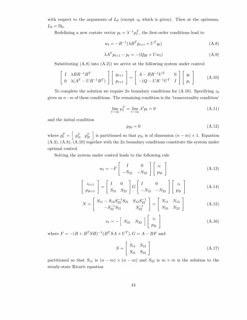
with respect to the arguments of L0 (except z0 which is given). Then at the optimum,

L0 = Ω0.

Redefining a new costate vector pt = λ−1µTt , the first-order conditions lead to

wt = −R−1(λBT pt+1 + UT yt) (A.8)

λAT pt+1 − pt = −(Qyt + Uwt) (A.9)

Substituting (A.8) into (A.2)) we arrive at the following system under control

[

I λBR−1BT

0 λ(AT − UR−1BT )

] [

yt+1

pt+1

]

=

[

A − BR−1UT 0

−(Q − UR−1UT I

] [

yt

pt

]

(A.10)

To complete the solution we require 2n boundary conditions for (A.10). Specifying z0

gives us n−m of these conditions. The remaining condition is the ’transversality condition’

limt→∞

µTt = lim

t→∞

λtpt = 0 (A.11)

and the initial condition

p20 = 0 (A.12)

where pTt =

[

pT1t pT

2t

]

is partitioned so that p1t is of dimension (n − m) × 1. Equation

(A.3), (A.8), (A.10) together with the 2n boundary conditions constitute the system under

optimal control.

Solving the system under control leads to the following rule

wt = −F

[

I 0

−N21 −N22

] [

zt

p2t

]

(A.13)

[

zt+1

p2t+1

]

=

[

I 0

S21 S22

]

G

[

I 0

−N21 −N22

] [

zt

p2t

]

(A.14)

N =

[

S11 − S12S−122 S21 S12S

−122

−S−122 S21 S−1

22

]

=

[

N11 N12

N21 N22

]

(A.15)

xt = −[

N21 N22

]

[

zt

p2t

]

(A.16)

where F = −(R + BT SB)−1(BT SA + UT ), G = A − BF and

S =

[

S11 S12

S21 S22

]

(A.17)

partitioned so that S11 is (n − m) × (n − m) and S22 is m × m is the solution to the

steady-state Ricatti equation

44

S = Q − UF − F T UT + F T RF + λ(A − BF )T S(A − BF ) (A.18)

The cost-to-go for the optimal policy (OP) at time t is

ΩOPt = −1

2(tr(N11Zt) + tr(N22p2tp

T2t)) (A.19)

where Zt = ztzTt . To achieve optimality the policy-maker sets p20 = 0 at time t = 0. At

time t > 0 there exists a gain from reneging by resetting p2t = 0. It can be shown that

N22 < 0, so the incentive to renege exists at all points along the trajectory of the optimal

policy. This is the time-inconsistency problem.

A.2 The Dynamic Programming Discretionary Policy

The evaluate the discretionary (time-consistent) policy we rewrite the cost-to-go Ωt given

by (A.5) as

Ωt =1

2[yT

t Qyt + 2yTt Uwt + wT

t Rwt + λΩt+1] (A.20)

The dynamic programming solution then seeks a stationary solution of the form wt =

−Fzt in which Ωt is minimized at time t subject to (1) in the knowledge that a similar

procedure will be used to minimize Ωt+1 at time t + 1.

Suppose that the policy-maker at time t expects a private-sector response from t + 1

onwards, determined by subsequent reoptimisation, of the form

xt+τ = −Nt+1zt+τ , τ ≥ 1 (A.21)

The loss at time t for the ex ante optimal policy was from (A.8) found to be a quadratic

function of xt and p2t. We have seen that the inclusion of p2t was the source of the time

inconsistency in that case. We therefore seek a lower-order controller wt = −Fzt with

the cost-to-go quadratic in zt only. We then write Ωt+1 = 12ZT

t+1St+1Zt+1 in (A.20). This

leads to the following iterative process for Ft

wt = −Ftzt (A.22)

where

Ft = (Rt + λBTt St+1Bt)

−1(UTt + λB

Tt St+1At)

Rt = R + KTt Q22Kt + U2T Kt + KT

t U2

Kt = −(A22 + Nt+1A12)−1(Nt+1B

1 + B2)

Bt = B1 + A12Kt

U t = U1 + Q12Kt + JTt U2 + JT

t Q22Jt

J t = −(A22 + Nt+1A12)−1(Nt+1A11 + A12)

45

At = A11 + A12Jt

St = Qt − U tFt − F Tt U

T+ F

Tt RtFt + λ(At − BtFt)

T St+1(At − BtF t)

Qt = Q11 + JTt Q21 + Q12Jt + JT

t Q22Jt

Nt = −Jt + KtFt

where B =

[

B1

B2

]

, U =

[

U1

U2

]

, A =

[

A11 A12

A21 A22

]

, and Q similarly are partitioned

conformably with the predetermined and non-predetermined components of the state vec-

tor.

The sequence above describes an iterative process for Ft, Nt, and St starting with some

initial values for Nt and St. If the process converges to stationary values, F, N and S say,

then the time-consistent feedback rule is wt = −Fzt with loss at time t given by

ΩTCt =

1

2zTt Szt =

1

2tr(SZt) (A.23)

A.3 Optimized Simple Rules

We now consider simple sub-optimal rules of the form

wt = Dyt = D

[

zt

xt

]

(A.24)

where D is constrained to be sparse in some specified way. Rule can be quite general. By

augmenting the state vector in an appropriate way it can represent a PID (proportional-

integral-derivative)controller (though the paper is restricted to a simple proportional con-

troller only).

Substituting (A.3) into (A.5) gives

Ωt =1

2

∞∑

i=0

λtyTt+iPt+iyt+i (A.25)

where P = Q+UD +DT UT +DT RD. The system under control (A.1), with wt given by

(A.3), has a rational expectations solution with xt = −Nzt where N = N(D). Hence

yTt Pyt = zT

t Tzt (A.26)

where T = P11 − NT P21 − P12N + NT P22N , P is partitioned as for S in (A.17) onwards

and

zt+1 = (G11 − G12N)zt (A.27)

where G = A + BD is partitioned as for P . Solving (A.27) we have

zt = (G11 − G12N)tz0 (A.28)

46

Hence from (A.29), (A.26) and (A.28) we may write at time t

ΩSIMt =

1

2zTt V zt =

1

2tr(V Zt) (A.29)

where Zt = ztzTt and V satisfies the Lyapunov equation

V = T + HT V H (A.30)

where H = G11 − G12N . At time t = 0 the optimized simple rule is then found by

minimizing Ω0 given by (A.29) with respect to the non-zero elements of D given z0 using

a standard numerical technique. An important feature of the result is that unlike the

previous solution the optimal value of D, D∗ say, is not independent of z0. That is to say

D∗ = D∗(z0)

A.4 The Stochastic Case

Consider the stochastic generalization of (A.1)[

zt+1

xet+1,t

]

= A

[

zt

xt

]

+ Bwt +

[

ut

0

]

(A.31)

where ut is an n × 1 vector of white noise disturbances independently distributed with

cov(ut) = Σ. Then, it can be shown that certainty equivalence applies to all the policy

rules apart from the simple rules (see Currie and Levine (1993)). The expected loss at

time t is as before with quadratic terms of the form zTt Xzt = tr(Xzt, Z

Tt ) replaced with

Et

(

tr

[

X

(

ztzTt +

∞∑

i=1

λtut+iuTt+i

)])

= tr

[

X

(

zTt zt +

λ

1 − λΣ

)]

(A.32)

where Et is the expectations operator with expectations formed at time t.

Thus for the optimal policy with commitment (A.19) becomes in the stochastic case

ΩOPt = −1

2tr

(

N11

(

Zt +λ

1 − λΣ

)

+ N22p2tpT2t

)

(A.33)

For the time-consistent policy (A.23) becomes

ΩTCt = −1

2tr

(

S

(

Zt +λ

1 − λΣ

))

(A.34)

and for the simple rule, generalizing (A.29)

ΩSIMt = −1

2tr

(

V

(

Zt +λ

1 − λΣ

))

(A.35)

The optimimized simple rule is found at time t = 0 by minimizing ΩSIM0 given by

(A.35). Now we find that

D∗ = D∗

(

z0 +λ

1 − λΣ

)

(A.36)

or, in other words, the optimimized rule depends both on the initial displacement z0 and

on the covariance matrix of disturbances Σ.

47

1% 99%

ρi B 0.75 0.15 0.538 0.981

θ G 1.7 0.5 1.099 3.074

λ G 0.15 0.1 0.044 0.473

φ G 1.75 0.5 1.148 3.118

σ G 1.5 0.8 0.609 3.952

γ B 0.7 0.1 0.566 0.897

h B 0.7 0.1 0.566 0.897

ρa B 0.7 0.15 0.492 0.959

ρg B 0.7 0.15 0.492 0.959

π* G 4 2 1.745 10.045

r* G 2 1 0.872 5.023

sdg IG1 1.7 inf 0.635 9.260

sde IG1 1 inf 0.372 5.699

sda IG1 1.7 inf 0.635 9.260

For all models, g is calibrated to 0.22. Distributions: G (Gamma), B (Beta), and ), IG1 ( Inverse Gamma-1). ρ corresponds to the autoregressive coefficient of an AR(1) process. sd stands for the standard deviation of the shocks. .Last two columns, report the inverse cumulative distribution function of each prior ordinate for thepercentiles 0.01 and 0.99.

Table1 : Priors for Baseline model

Percentiles Distribution Mean

Standard Deviation

APPENDIX B: ESTIMATION RESULTS

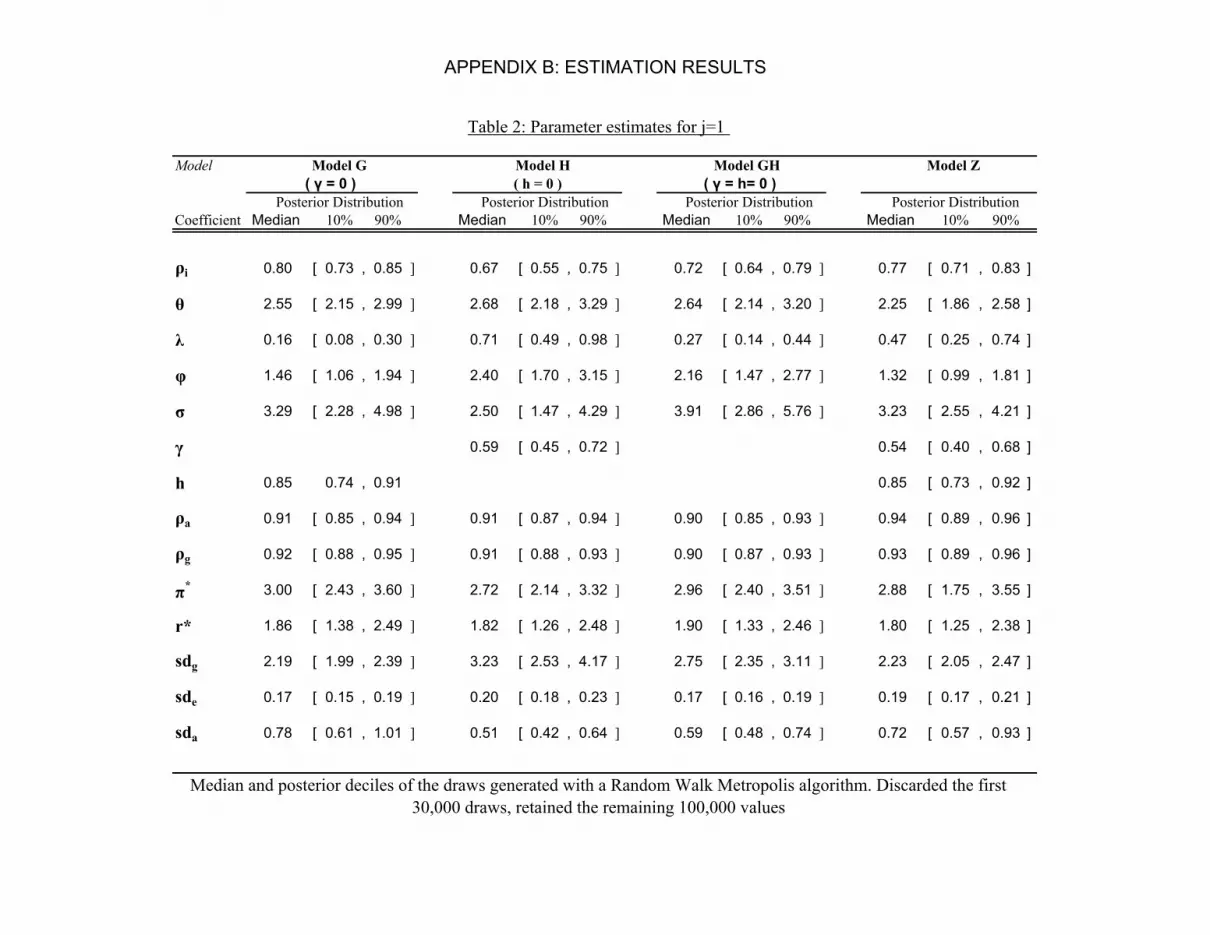
Model Model G Model H Model GH Model Z

Posterior Distribution Posterior Distribution Posterior Distribution Posterior DistributionCoefficient Median 10% 90% Median 10% 90% Median 10% 90% Median 10% 90%

ρi 0.80 [ 0.73 , 0.85 ] 0.67 [ 0.55 , 0.75 ] 0.72 [ 0.64 , 0.79 ] 0.77 [ 0.71 , 0.83 ]

θ 2.55 [ 2.15 , 2.99 ] 2.68 [ 2.18 , 3.29 ] 2.64 [ 2.14 , 3.20 ] 2.25 [ 1.86 , 2.58 ]

λ 0.16 [ 0.08 , 0.30 ] 0.71 [ 0.49 , 0.98 ] 0.27 [ 0.14 , 0.44 ] 0.47 [ 0.25 , 0.74 ]

φ 1.46 [ 1.06 , 1.94 ] 2.40 [ 1.70 , 3.15 ] 2.16 [ 1.47 , 2.77 ] 1.32 [ 0.99 , 1.81 ]

σ 3.29 [ 2.28 , 4.98 ] 2.50 [ 1.47 , 4.29 ] 3.91 [ 2.86 , 5.76 ] 3.23 [ 2.55 , 4.21 ]

γ 0.59 [ 0.45 , 0.72 ] 0.54 [ 0.40 , 0.68 ]

h 0.85 0.74 , 0.91 0.85 [ 0.73 , 0.92 ]

ρa 0.91 [ 0.85 , 0.94 ] 0.91 [ 0.87 , 0.94 ] 0.90 [ 0.85 , 0.93 ] 0.94 [ 0.89 , 0.96 ]

ρg 0.92 [ 0.88 , 0.95 ] 0.91 [ 0.88 , 0.93 ] 0.90 [ 0.87 , 0.93 ] 0.93 [ 0.89 , 0.96 ]

π* 3.00 [ 2.43 , 3.60 ] 2.72 [ 2.14 , 3.32 ] 2.96 [ 2.40 , 3.51 ] 2.88 [ 1.75 , 3.55 ]

r* 1.86 [ 1.38 , 2.49 ] 1.82 [ 1.26 , 2.48 ] 1.90 [ 1.33 , 2.46 ] 1.80 [ 1.25 , 2.38 ]

sdg 2.19 [ 1.99 , 2.39 ] 3.23 [ 2.53 , 4.17 ] 2.75 [ 2.35 , 3.11 ] 2.23 [ 2.05 , 2.47 ]

sde 0.17 [ 0.15 , 0.19 ] 0.20 [ 0.18 , 0.23 ] 0.17 [ 0.16 , 0.19 ] 0.19 [ 0.17 , 0.21 ]

sda 0.78 [ 0.61 , 1.01 ] 0.51 [ 0.42 , 0.64 ] 0.59 [ 0.48 , 0.74 ] 0.72 [ 0.57 , 0.93 ]

Table 2: Parameter estimates for j=1

Median and posterior deciles of the draws generated with a Random Walk Metropolis algorithm. Discarded the first 30,000 draws, retained the remaining 100,000 values

( h = 0 )( γ = 0 ) ( γ = h= 0 )


Model

G ( γ = 0 )

H ( h= 0)

GH ( γ =h= 0 )

Z

Table 3: Model Comparisons

Reversible MCMC of Dellaportas et al. (2002). 100,000 draws to obtain the proposal densities. For the Metropolis step, Discarded the first 20,000 values and retained the remaining 180,000. Posterior odds P(m|data) based on assigning each model equal prior probability. Model proposal density assigns equal probability to the jump to any of four possible models, regardless of the current model in the chain.

Posterior Odds, P( m | data )

0.56

0.32

0.09

Reversible Jump MCMC

0.03


robust inflation-forecast-based rules to shield against indeterminacy

Documents